Computer Simulation
of Liquids
M. P. ALLEN
H. H. Wills Physics Laboratory
University of Bristol
and
D. J. TILDESLEY
Department of Chemistry
The University, Southampton
CLARENDON PRESS OXFORD

Oxford University Press, Walton Street, Oxford OX2 6DP
Oxford New York Toronto
Delhi Bombay Calcutta Madras Karachi
PetalingJaya Singapore Hong Kong Tokyo
Nairobi Dar es Salaam Cape Town
Melbourne Auckland
and associated companies in
Berlin Ibadan
Oxford is a trade mark of Oxford University Press
Published in the United States
by Oxford University Press, New York
© M. P. Allen and D. J. Tildesley, 1987
First published 1987
First published in paperback (with corrections) 1989
Reprinted 1990 (twice), 1991
All rights reserved. No part of this publication may be reproduced,
stored in a retrieval system, or transmitted, in any form or by any means,
electronic, mechanical, photocopying, recording, or otherwise, without
the prior permission of Oxford University Press
This book is sold subject to the condition that it shall not, by way
of trade or otherwise, be lent, re-sold, hired out or otherwise circulated
without the publisher's prior consent in any form of binding or cover
other than that in which it is published and without a similar condition
including this condition being imposed on the subsequent purchaser
British Library Cataloguing in Publication Data
Allen, M. P.
Computer simulation of liquids.
1. Liquids—Simulation methods
2. Digital computer simulation
I. Title II. Tildesley, D. J.
530.4'2'0724 QC145.2
ISBN 0-19-855375-7
ISBN 0-19-855645^t (pbk)
Library of Congress Cataloging in Publication Data
Allen, M. P.
Computer simulation of liquids.
1. Liquids—Mathematical models.
2. Liquids—Data processing.
3. Molecular dynamics.
4. Monte Carlo method.
I. Tildesley, D. J.
II. Title.
QC145.2.A43 1987 532'.00724 87-1555
ISBN 0-19-855375-7
ISBN 0-19-855645^t (pbk)
Printed in Great Britain by
The Ipswich Book Co Ltd,
Ipswich, Suffolk

To
Diane and Pauline

PREFACE
This is a 'how-to-do-it' book for people who want to use computers to
simulate the behaviour of atomic and molecular liquids. We hope that it toll
be useful to first-year graduate students, research workers in industry and
academia, and to teachers and lecturers who want to use the computer to
illustrate the way liquids behave.
Getting started is the main barrier to writing a simulation program. Few
people begin their research into liquids by sitting down and composing a
program from scratch. Yet these programs are not inherently complicated:
there are just a few pitfalls to be avoided. In the past, many simulation
programs have been handed down from one research group to another and
from one generation of students to the next. Indeed, with a trained eye, it is
possible to trace many programs back to one of the handful of groups working
in the field 20 years ago. Technical details such as methods for improving the
speed of the program or for avoiding common mistakes are often buried in the
appendices of publications or passed on by word of mouth. In the first six
chapters of this book, we have tried to gather together these details and to
present a clear account of the techniques, namely Monte Carlo and molecular
dynamics. The hope is that a graduate student could use these chapters to
write his own program.
The field of computer simulation has enjoyed rapid advances in the last five
years. Smart Monte Carlo sampling techniques have been introduced and
tested, and the molecular dynamics method has been extended to simulate
various ensembles. The techniques have been merged into a new field of
stochastic simulations and extended to cover quantum-mechanical as well as
classical systems. A book on simulation would be incomplete without some
mention of these advances and we have tackled them in Chapters 7 to 10.
Chapter 11 contains a brief account of some interesting problems to which the
methods have been applied. Our choices in this chapter are subjective and our
coverage far from exhaustive. The aim is to give the reader a taste rather than a
feast. Finally we have included examples of computer code to illustrate points
made in the text, and have provided a wide selection of useful routines which
are available on-line from two sources. We have not attempted to tackle the
important areas of solid state simulation and protein molecular mechanics.
The techniques discussed in this book are useful in these fields, but
additionally much weight is given to energy minimization rather than the
simulation of systems at non-zero temperatures. The vast field of lattice
dynamics is discussed in many other texts.
Both of us were fortunate in that we had expert guidance when starting
work in the field, and we would like to take this opportunity to thank
P. Schofield (Harwell) and W. B. Streett (Cornell), who set us on the right

viii PREFACE
road some years ago. This book was largely written and created at the Physical
Chemistry Laboratory, Oxford, where both of us have spent a large part of
our research careers. We owe a great debt of gratitude to the head of
department, J. S. Rowlinson, who has provided us with continuous en-
encouragement and support in this venture, as well as a meticulous criticism of
early versions of the manuscript. We would also like to thank our friends and
colleagues in the Physics department at Bristol and the Chemistry depart-
department at Southampton for their help and encouragement, and we are indebted
to many colleagues, who in discussions at conferences and workshops,
particularly those organized by CCP5 and CECAM, have helped to form our
ideas. We cannot mention all by name, but should say that conversations with
D. Frenkel and P. A. Madden have been especially helpful. We would also like
to thank M. Gillan and J. P. Ryckaert, who made useful comments on certain
chapters, and I. R. McDonald who read and commented on the completed
manuscript. We are grateful for the assistance of Mrs L. Hayes, at Oxford
University Computing Service, where the original Microfiche was produced.
Lastly, we thank Taylor and Francis for allowing us to reproduce diagrams
from Molecular Physics and Advances in Physics, and ICL and Cray Research
(UK) for the photographs in Fig. 1.1. Detailed acknowledgements appear in
the text.
Books are not written without a lot of family support. One of us (DJT)
wants to thank the Oaks and the Sibleys of Bicester for their hospitality during
many weekends in the last three years. Our wives, Diane and Pauline, have
suffered in silence during our frequent disappearances, and given us their
unflagging support during the whole project. We owe them a great deal.
Bristol M. P. A.
Southampton D. J. T.
May 1986

CONTENTS
LIST OF SYMBOLS xv
1 INTRODUCTION 1
1.1 A short history of computer simulation 1
1.2 Computer simulation: motivation and applications 4
1.3 Model systems and interaction potentials 6
1.3.1 Introduction 6
1.3.2 Atomic systems 7
1.3.3 Molecular systems 12
1.3.4 Lattice systems 16
1.3.5 Calculating the potential 18
1.4 Constructing an intermolecular potential 20
1.4.1 Introduction 20
1.4.2 Building the model potential 20
1.4.3 Adjusting the model potential 22
1.5 Studying small systems 23
1.5.1 Introduction 23
1.5.2 Periodic boundary conditions 24
1.5.3 Potential truncation 27
1.5.4 Computer code for periodic boundaries 29
1.5.5 Spherical boundary conditions 32
2 STATISTICAL MECHANICS 33
2.1 Sampling from ensembles 33
2.2 Common statistical ensembles 39
2.3 Transforming between ensembles 43
2.4 Simple thermodynamic averages 46
2.5 Fluctuations 51
2.6 Structural quantities 54
2.7 Time correlation functions and transport coefficients 58
2.8 Long-range corrections 64
2.9 Quantum corrections 65
2.10 Constraints 68
3 MOLECULAR DYNAMICS 71
3.1 Equations of motion for atomic systems 71
3.2 Finite difference methods 73
3.2.1 The Verlet algorithm 78
3.2.2 The Gear predictor-corrector 82
3.2.3 Other methods 84
3.3 Molecular dynamics of rigid non-spherical bodies 84
3.3.1 Non-linear molecules 85
3.3.2 Linear molecules 90

x CONTENTS
3.4 Constraint dynamics
3.5 Checks on accuracy
3.6 Molecular dynamics of hard systems
3.6.1 Hard spheres
3.6.2 Hard non-spherical bodies
4 MONTE CARLO METHODS
4.1 Introduction
4.2 Monte Carlo integration
4.2.1 Hit and miss
4.2.2 Sample mean integration
4.3 Importance sampling
4.4 The Metropolis method
4.5 Isothermal-isobaric Monte Carlo
4.6 Grand canonical Monte Carlo
4.7 Molecular liquids
4.7.1 Rigid molecules
4.7.2 Non-rigid molecules
5 SOME TRICKS OF THE TRADE
5.1 Introduction
5.2 The heart of the matter
5.2.1 Efficient calculation of forces, energies, and pressures
5.2.2 Avoiding the square root
5.2.3 Table look-up and spline-fit potentials
5.2.4 Shifted and shifted-force potentials
5.3 Neighbour lists
5.3.1 The Verlet neighbour list
5.3.2 Cell structures and linked lists
5.4 Multiple time step methods 152
5.5 How to handle long-range forces 155
5.5.1 Introduction 155
5.5.2 The Ewald sum 156
5.5.3 The reaction field method 162
5.5.4 Other methods 164
5.5.5 Summary 164
5.6 When the dust has settled 166
5.7 Starting up 168
5.7.1 The initial configuration 168
5.7.2 The initial velocities 170
5.7.3 Equilibration 171
5.8 Organization of the simulation 173
5.8.1 Input/output and file handling 174
5.8.2 Program structure 175
5.8.3 The scheme in action 180
6 HOW TO ANALYSE THE RESULTS 182
6.1 Introduction 182
6.2 Liquid structure 183

CONTENTS xi
6.3 Time correlation functions 185
6.3.1 The direct approach 185
6.3.2 The fast Fourier transform method 188
6.4 Estimating errors 191
6.4.1 Errors in equilibrium averages 192
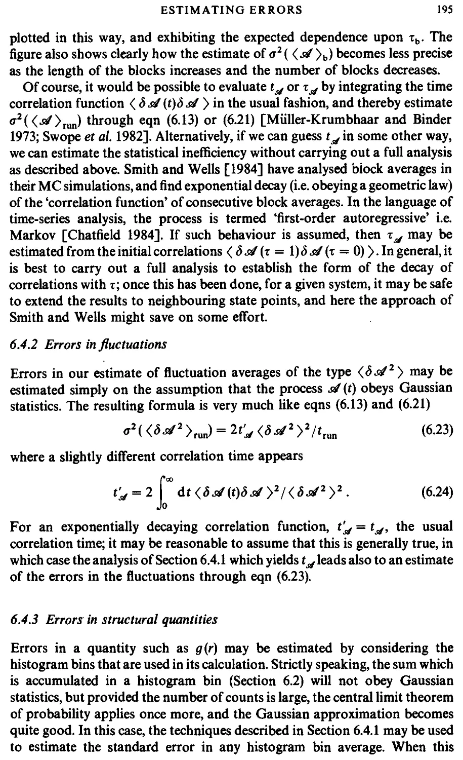
6.4.2 Errors in fluctuations 195
6.4.3 Errors in structural quantities 195
6.4.4 Errors in time correlation functions 196
6.5 Correcting the results 198
6.5.1 Correcting thermodynamic averages 199
6.5.2 Extending g(r) to large r 199
6.5.3 Extrapolating g(r) to contact 201
6.5.4 Smoothing g(r) 203
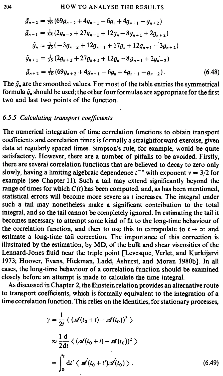
6.5.5 Calculating transport coefficients 204
6.5.6 Smoothing a spectrum 208
7 ADVANCED SIMULATION TECHNIQUES 212
7.1 Introduction 212
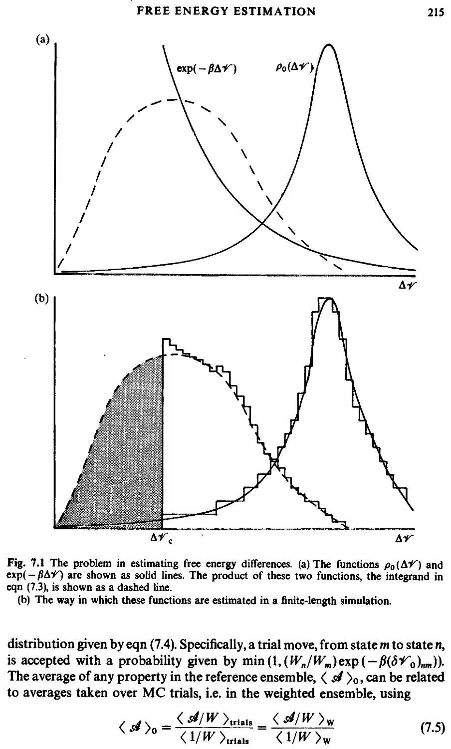
7.2 Free energy estimation 213
7.2.1 Introduction 213
7.2.2 Non-Boltzmann sampling 213
7.2.3 Acceptance ratio method 218
7.2.4 Summary 219
7.3 Smarter Monte Carlo 220
7.3.1 Preferential sampling 220
7.3.2 Force-bias Monte Carlo 224
7.3.3 Smart Monte Carlo 225
7.3.4 Virial-bias Monte Carlo 226
7.4 Constant-temperature molecular dynamics 227
7.4.1 Stochastic methods 227
7.4.2 Extended system methods 228
7.4.3 Constraint methods 230
7.4.4 Other methods 231
7.5 Constant-pressure molecular dynamics 232
7.5.1 Extended system methods 232
7.5.2 Constraint methods 234
7.5.3 Other methods 236
7.5.4 Changing box shape 236
7.6 Practical points 238
7.7 The Gibbs Monte Carlo method 239
8 NON-EQUILIBRIUM MOLECULAR DYNAMICS 240
8.1 Introduction 240
8.2 Shear flow 242
8.3 Expansion and contraction 249
8.4 Heat flow 250
8.5 Diffusion 251
8.6 Other perturbations 253
8.7 Practical points 253

Xll
CONTENTS
9 BROWNIAN DYNAMICS
9.1 Introduction
9.2 Projection operators
9.3 Brownian dynamics
9.4 Hydrodynamic and memory effects
10 QUANTUM SIMULATIONS
10.1 Introduction
10.2 Semiclassical path-integral simulations
10.3 Semiclassical Gaussian wavepackets
10.4 Quantum random walk simulations
11 SOME APPLICATIONS
11.1 Introduction
11.2 The liquid drop
11.3 Melting
11.4 Molten salts
11.5 Liquid crystals
11.6 Rotational dynamics
11.7 Long-time tails
11.8 Interfaces
257
257
257
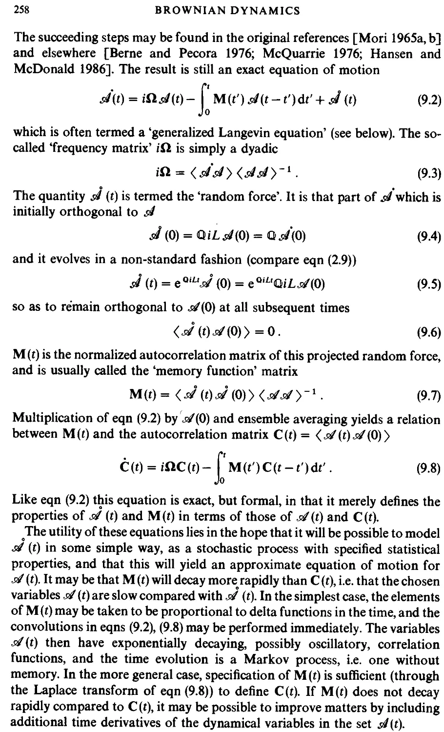
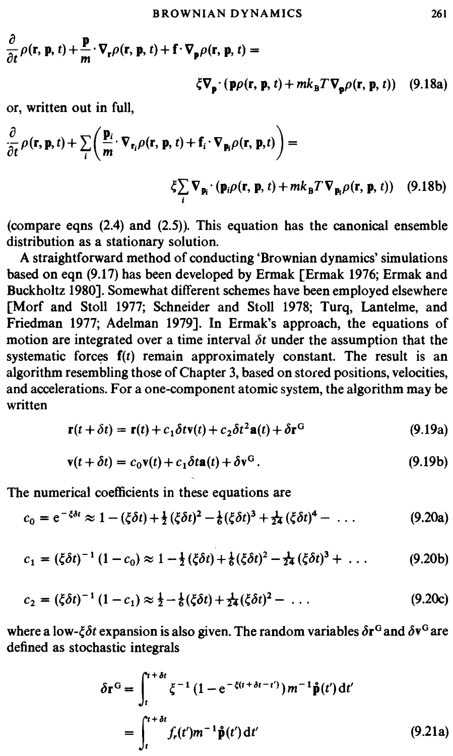
259
264
270
270
272
279
282
286
286
286
292
298
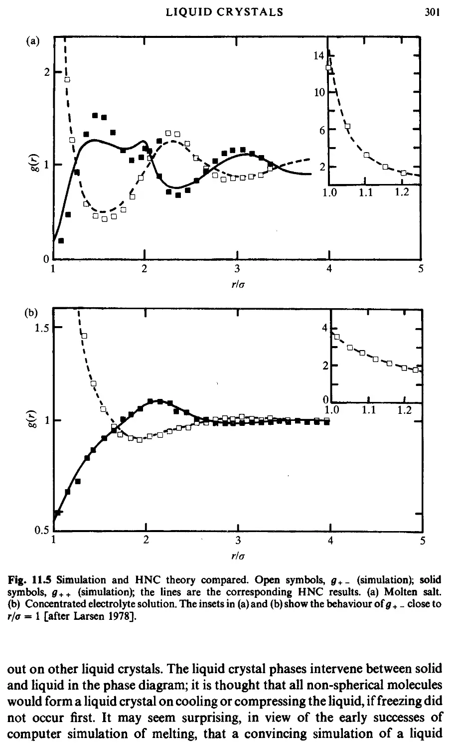
300
306
310
312
APPENDIX A
APPENDIX В
APPENDIX С
COMPUTERS AND COMPUTER
SIMULATION
A. 1 Computer hardware
A.2 Programming languages
A.3 Efficient programming in FORTRAN-77
REDUCED UNITS
B. 1 Reduced units
320
320
322
324
327
327
CALCULATION OF FORCES AND TORQUES 329
С1 Introduction 329
C.2 The polymer chain 329
C.3 The molecular fluid with multipoles 332
C.4 The triple-dipole potential 334
APPENDIX D
FOURIER TRANSFORMS 336
D. 1 The Fourier transform 336
D.2 The discrete Fourier transform 337
D.3 Numerical Fourier transforms 338
APPENDIX E THE GEAR PREDICTOR-CORRECTOR 340
E. 1 The Gear predictor-corrector 340
APPENDIX F PROGRAM AVAILABILITY 343

CONTENTS
APPENDIX G
REFERENCES
INDEX
RANDOM NUMBERS 345
G. 1 Random number generators 345
Random numbers uniform on @,1) 345
Generating non-uniform distributions 347
Random vectors on the surface of a sphere 349
G.2
G.3
G.4
G.5
Choosing randomly and uniformly from complicated
regions 349
G.6 Sampling from an arbitrary distribution 351
352
383

LIST OF SYMBOLS
Latin Alphabet
a
а
A
s/
A
b
b
В
я
c(r)
Cp
Cy
d
dab
e,™
e
s
i
&
g(r)
яки
9ab(
9ltm
9l
g
G
G(r,
h =
h(r)
H
Ж
i
1
atom index
molecular acceleration
Helmholtz free energy
general dynamic variable
rotation matrix
set of dynamic variables
atom index
time derivative of acceleration
second virial coefficient
general dynamic variable
f(t) normalized time correlation function
direct pair correlation function
g(t) un-normalized time correlation function
constant-pressure heat capacity
constant-volume heat capacity
spatial dimensionality
intramolecular bond length
atom position relative to molecular centre of mass
diffusion coefficient
pair diffusion matrix
n, Wigner rotation matrix
molecular axis unit vector
total internal energy
electric field
force on molecule
force on molecule i due to j
Fermi function
applied field
pair distribution function.
;, ?lt, ?lj) molecular pair distribution function
r^) site-site distribution function
(r) spherical harmonic coefficients of pair distribution function
angular correlation parameter
constraint force
Gibbs free energy
t) van Hove function
/|/2я Planck's constant
total pair correlation function
enthalpy
Hamiltonian
molecule index
molecular moment of inertia
/vv, /,, principal components of inertia tensor
A.3.3)
C.2)
B.2)
B.1)
C.3.1)
(8.1)
A.3.3)
C.2)
A.4.3)
B.3)
B.7)
F.5.2)
B.7)
B.5)
B.5)
E.5)
E-5.2)
C.3)
B.7)
(9.4)
B.6)
A.3.3)
B.2)
E.5.3)
B.4)
B.4)
G.2.3)
(8.1)
B.6)
B.6)
B.6)
B.6)
B.6)
C.4)
B.2)
B.7)
B.2)
F.5.2)
B.2)
A.3.1)
A.3.1)
B.9)
B.9)

LIST OF SYMBOLS
/(*, t)
j
i
j?
j
к
к
Ж
I
L
L
L
se
m
m
M
n
N
0
P
P
Pi
P
&
P
q
Q
Q
Q
Q
r
г
ГУ
&t
5
5
S
S
S(k)
S(k, a>)
S
t
T
intermediate scattering function
molecule index
particle current
energy current
total angular momentum
generalized coordinate or molecule index
Boltzmann's constant
wave vector
kinetic energy
cell length
box length
Liouville operator (always found as iL)
angular momentum
Lagrangian
molecular mass
possible outcome or state label
memory function matrix
possible outcome or state label
number of molecules
octopole moment
molecular momentum
pressure
Legendre polynomial
total linear momentum
instantaneous pressure
instantaneous pressure tensor
projection operator
generalized coordinates
quadrupole moment
partition function
quaternion
projection operator
molecular separation
molecular position
position of molecule i relative to j (rf — Tj)
site-site vector (short for ria— r^)
region of space
statistical inefficiency
scaled time variable
scaled molecular position
entropy
structure factor
dynamic structure factor
total intrinsic angular momentum (spin)
action integral
time
correlation or relaxation time
temperature
B.7)
A.3.2)
(8.2)
B.7)
C.6.1)
A.3.2)
A.2)
A.5.2)
A.3.1)
E.3.2)
A.5.2)
B.1)
C.1)
C.1)
A.3.1)
D.3)
(9.2)
D.3)
A.3.1)
A.3.3)
A.3.1)
B.4)
B.6)
B.2)
B.4)
B.7)
(9,2)
A.3.1)
A.3.3)
B.1)
C.3.1)
(9.2)
A.3.2)
A.3.1)
A-3.2)
B.4)
D.4)
F.4.1)
G.4.2)
D.5)
B.2)
B.6)
B.7)
C.6.1)
A0.2)
B.1)
B.7)
A.2)

LIST OF SYMBOLS xvii
У instantaneous kinetic temperature B.4)
u(r) pseudo-potential A0.4)
v(r) pair potential A.3.2)
v molecular velocity B.7)
у у velocity of molecule i relative to j (Vj — Vj) C.6.1)
V volume A.2)
¦V total potential energy A.3.1)
w(r) pair virial function B.4)
W weighting function G.2.2)
IT total virial function B.4)
x Cartesian coordinate A.3.1)
x(r) pair hypervirial function B.5)
Ж total hypervirial function B.5)
у Cartesian coordinate A.3.1)
Yim spherical harmonic function B.6)
z Cartesian coordinate A-3.1)
z charge A.3.2)
z activity D.6)
Z configuration integral B.2)
Greek alphabet
a Cartesian component (x, y, z) A.3.1)
ctp thermal expansion coefficient B.5)
a underlying stochastic transition matrix D.3)
fS Cartesian component (x, y, z) A-3.1)
0 inverse temperature (l/kBT) B.3)
fSs adiabatic compressibility B.5)
/?r isothermal compressibility B.5)
у a general transport coefficient B.7)
ys surface tension A1-2)
yv thermal pressure coefficient B.5)
Уц _ angle between molecular axis vectors B.6)
Г point in phase space B.1)
<5(...) Dirac delta function B.2)
St time step C.2)
8s/ deviation of s/ from ensemble average B.3)
e energy parameter in pair potentials A-3-2)
6,- energy per molecule B.7)
6 relative permittivity (dielectric constant) E.5.2)
60 permittivity of free space A.3.2)
С random number < , (G.3)
ц shear viscosity B.7)
ц у bulk viscosity , B.7)
в Euler angle C.3.1)
в bond bending angle A.3.3)
6(x) unit step function F.5.3)
к inertia parameter C.6.1)

xviii LIST OF SYMBOLS
к: inverse of charge screening length E.5.2)
X Lagrange undetermined multiplier C.4)
kT thermal conductivity B.7)
Л thermal de Broglie wavelength B.2)
(i chemical potential B.2)
/i molecular dipole moment E.5.2)
v exponent in soft-sphere potential A.3.2)
v discrete frequency index F.3.2)
? random number in range @,1) (G.2)
i friction coefficient (9.3)
<!;(r, p) dynamical friction coefficient G.4.3)
я stochastic transition matrix D.3)
p number density B.1)
p(k) spatial Fourier transform of number density B.6)
p(T) phase space distribution function B.1)
p(...) general probability distribution function D.2.2)
p . set of all possible probabilities D.3)
a length parameter in pair potentials A-3.2)
ff(s/) RMS fluctuation for dynamical variable s/ B.3)
т discrete time or trial index B.1)
tv discrete correlation 'time' F.4.1)
т torque acting on a molecule C.3)
ф Euler angle C.3.1)
ф bond torsional angle A.3.3)
X constraint condition C.4)
Z(r, p) dynamic scaling factor in constant-pressure simulations G.5.2)
ф Euler angle C.3.1)
ф(г, t) wavepacket A0.3)
4* thermodynamic potential B.1)
*F(r, t) many-body wavefunction A0.1)
(o frequency (D.I)
to molecular angular velocity B.7)
Si molecular orientation A.3.1)
SI frequency matrix (always found as iSl) (9.2)
Subscripts and superscripts
r/a denotes position of atom a in molecule i A.3.3)
ria denotes a component ( = x, y, z) of position vector A.3.1)
|| denotes parallel or longitudinal component B.7)
l denotes perpendicular or transverse component B.7)
* denotes reduced variables or complex conjugate (B.I)
id denotes ideal gas part B.2)
ex denotes excess part B.2)
cl denotes classical variable B.9)
qu denotes quantum variable B.9)
p denotes predicted values C.2)
с denotes corrected values C.2)

LIST OF SYMBOLS xix
T denotes matrix transpose G.5.4)
b denotes body-fixed variable C.3.1)
s denotes space-fixed variable C.3.1)
Special conventions
Vr gradient with respect to molecular positions B.1)
V gradient with respect to molecular momenta B.1)
d/dt total derivative with respect to time B.1)
д/dt partial derivative with respect to time B.1)
f, г etc. single and double time derivatives B.1)
<• •-Xriais MC trial or step-by-step average D.2.2)
<. ..>,lme time average B.1)
<• • Xns general ensemble average B.1)
<.. .>ne non-equilibrium ensemble average (8.1)
<.. .>w weighted average G.2.2)

1
INTRODUCTION
1.1 A short history of computer simulation
What is a liquid? As you read this book, you may be mixing up, drinking down,
sailing on, or sinking in, a liquid. Liquids flow, although they may be very
viscous. They may be transparent, or they may scatter light strongly. Liquids
may be found in bulk, or in the form of tiny droplets. They may be vaporized or
frozen. Life as we know it probably evolved in the liquid phase, and our bodies
are kept alive by chemical reactions occurring in liquids. There are many
fascinating details of liquid-like behaviour, covering thermodynamics, struc-
structure, and motion. Why do liquids behave like this?
The study of the liquid state of matter has a long and rich history, from both
the theoretical and experimental standpoints. From early observations of
Brownian motion to recent neutron scattering experiments, experimentalists
have worked to improve the understanding of the structure and particle
dynamics that characterize liquids. At the same time, theoreticians have tried
to construct simple models which explain how liquids behave. In this book, we
concentrate exclusively on molecular models of liquids, and their analysis by
computer simulation. For excellent accounts of the current status of liquid
science, the reader should consult the standard references [Barker and
Henderson 1976; Rowlinson and Swinton 1982; Hansen and McDonald
1986].
Early models of liquids [Morrell and Hildebrand 1936] involved the
physical manipulation and analysis of the packing of a large number of
gelatine balls, representing the molecules; this resulted in a surprisingly good
three-dimensional picture of the structure of a liquid, or perhaps a random
glass, and later applications of the technique have been described [Bernal and
King 1968]. Even today, there is some interest in the study of assemblies of
metal ball bearings, kept in motion by mechanical vibration [Pierariski,
Malecki, Kuczynski, and Wojciechowski 19781 However, the use of large
numbers of physical objects to represent molecules can be very time-
consuming, there are obvious limitations on the types of interactions between
them, and the effects of gravity can never be eliminated. The natural extension
of this approach is to use a mathematical, rather than a physical, model, and to
perform the analysis by computer.
It is now over 30 years since the first computer simulation of a liquid was
carried out at the Los Alamos National Laboratories in the United States
[Metropolis, Rosenbluth, Rosenbluth, Teller, and Teller 1953]. The Los
Alamos computer, called MANIAC, was at that time one of the most powerful
available; it is a measure of the recent rapid advance in computer technology
that microcomputers of comparable power are now available to the general

2 INTRODUCTION
public at modest cost. Modern computers range from the relatively cheap, but
powerful, single-user workstation to the extremely fast and expensive
mainframe, as exemplified in Fig. 1.1. Rapid development of computer
hardware is currently under way, with the introduction of specialized features,
such as pipeline and array processors, and totally new architectures, such as the
dataflow approach. Computer simulation is possible on most machines, and
we provide an overview of some widely available computers, and computing
languages, as they relate to simulation, in Appendix A.
The very earliest work [Metropolis et al. 1953] laid the foundations of
modern 'Monte Carlo' simulation (so-called because of the role that random
numbers play in the method). The precise technique employed in this study is
still widely used, and is referred to simply as 'Metropolis Monte Carlo'; we will
use the abbreviation 'MC. The original models were highly idealized
representations of molecules, such as hard spheres and disks, but, within a few
years MC simulations were carried out on the Lennard-Jones interaction
potential [Wood and Parker 1957] (see Section 1.3). This made it possible to
compare data obtained from experiments on, for example, liquid argon, with
the computer-generated thermodynamic data derived from a model.
A different technique is required to obtain the dynamic properties of many-
particle systems. Molecular dynamics (MD) is the term used to describe the
solution of the classical equations of motion (Newton's equations) for a set of
molecules. This was first accomplished, for a system of hard spheres, by Alder
and Wainwright [1957, 1959]. In this case, the particles move at constant
velocity between perfectly elastic collisions, and it is possible to solve the
dynamic problem without making any approximations, within the limits
imposed by machine accuracy. It was several years before a successful attempt
was made to solve the equations of motion for a set of Lennard-Jones particles
[Rahman 1964]. Here, an approximate, step-by-step procedure is needed,
since the forces change continuously as the particles move. Since that time, the
properties of the Lennard-Jones model have been thoroughly investigated
[Verlet 1967, 1968; Nicolas, Gubbins, Streett, and Tildesley 1979].
After this initial groundwork on atomic systems, computer simulation
developed rapidly. An early attempt to model a diatomic molecular liquid
[Harp and Berne 1968; Berne and Harp 1970] using molecular dynamics was
quickly followed by two ambitious attempts to model liquid water, first by MC
[Barker and Watts 1969], and then by MD [Rahman and Stillinger 1971].
Water remains one of the most interesting and difficult liquids to study
[Stillinger 1975, 1980; Wood 1979; Morse and Rice 1982]. Small rigid
molecules [Barojas, Levesque, and Quentrec 1973], flexible hydrocarbons
[Ryckaert and Bellemans 1975] and even large molecules such as proteins
[McCammon, Gelin, and Karplus 1977] have all been objects of study in
recent years. Computer simulation has been used to improve our understand-
understanding of phase transitions and behaviour at interfaces [Lee, Barker, and Pound
1974; Chapela, Saville, Thompson, and Rowlinson 1977; Frenkel and
McTague 1980]. We shall be looking in detail at these developments in the last

Fig. I.I Two modern computers, (a) The PHRQ computer, marketed in the UK by ICL: a
single-user graphics workstation capable of fast numerical calculations. 'b| llic CRAY 1-S
computer: a supercomputer which uses pipeline processing to perform outstandingly fast
numerical calculations.

4 INTRODUCTION
chapter of this book. The techniques of computer simulation have also
advanced, with the introduction of 'non-equilibrium' methods of measuring
transport coefficients [Lees and Edwards 1972; Hoover and Ashurst 1975;
Ciccotti, Jacucci, and McDonald 1979], the development of 'stochastic
dynamics' methods [Turq, Lantelme, and Friedman 1977], and the incorpor-
incorporation of quantum mechanical effects [Corbin and Singer 1982; Ceperley and
Kalos 1986]. Again, these will be dealt with in the later chapters. First, we turn
to the questions: What is computer simulation? How does it work? What can it
tell us?
1.2 Computer simulation: motivation and applications
Some problems in statistical mechanics are exactly soluble. By this, we mean
that a complete specification of the microscopic properties of a system (such as
the Hamiltonian of an idealized model like the perfect gas or the Einstein
crystal) leads directly, and perhaps easily, to a set of interesting results or
macroscopic properties (such as an equation of state like PV = NkBT). There
are only a handful of non-trivial, exactly soluble problems in statistical
mechanics [Baxter 1982]; the two-dimensional Ising model is a famous
example.
Some problems in statistical mechanics, while not being exactly soluble,
succumb readily to analysis based on a straightforward approximation
scheme. Computers may have an incidental, calculational, part to play in such
work, for example in the evaluation of cluster integrals in the virial expansion
for dilute, imperfect gases. The problem is that, like the virial expansion, many
'straightforward' approximation schemes simply do not work when applied to
liquids. For some liquid properties, it may not even be clear how to begin
constructing an approximate theory in a reasonable way. The more difficult
and interesting the problem, the more desirable it becomes to have exact
results available, both to test existing approximation methods and to point the
way towards new approaches. It is also important to be able to do this without
necessarily introducing the additional question of how closely a particular
model (which may be very idealized) mimics a real liquid, although this may
also be a matter of interest.
Computer simulations have a valuable role to play in providing essentially
exact results for problems in statistical mechanics which would otherwise only
be soluble by approximate methods, or might be quite intractable. In this
sense, computer simulation is a test of theories and, historically, simulations
have indeed discriminated between well-founded approaches (such as integral
equation theories [Hansen and McDonald 1986]) and ideas that are plausible
but, in the event, less successful (such as the old cell theories of liquids
[Lennard-Jones and Devonshire 1939a, 1939b]). The results of computer
simulations may also be compared with those of real experiments. In the first
place, this is a test of the underlying model used in a computer simulation.

COMPUTER SIMULATION: MOTIVATION AND APPLICATIONS 5
Eventually, if the model is a good one, the simulator hopes to offer insights to
the experimentalist, and assist in the interpretation of new results. This dual
role of simulation, as a bridge between models and theoretical predictions on
the one hand, and between models and experimental results on the other, is
illustrated in Fig. 1.2. Because of this connecting role, and the way in which
simulations are conducted and analysed, these techniques are often termed
'computer experiments'.
PERFORM
EXPERIMENTS
CARRY OUT
COMPUTER
SIMULATIONS
CONSTRUCT
APPROXIMATE
THEORIES
/EXPERIMEI
\. RESULTS
EXACT
RESULTS FO
MODEL
THEORETICAL^
PREDICTIONS/
TESTS OF
THEORIES
Fig. 1.2 The connection between experiment, theory, and computer simulation.
/TESTS 0F\
^MODELSJ
Computer simulation provides a direct route from the microscopic details of
a system (the masses of the atoms, the interactions between them, molecular
geometry etc.) to macroscopic properties of experimental interest (the
equation of state, transport coefficients, structural order parameters, and so
on). As well as being of academic interest, this type of information is
technologically useful. It may be difficult or impossible to carry out
experiments under extremes of temperature and pressure, while a computer

6 INTRODUCTION
simulation of the material in, say, a shock wave, a high-temperature plasma, a
nuclear reactor, or a planetary core, would be perfectly feasible. Quite subtle
details of molecular motion and structure, for example in heterogeneous
catalysis, fast ion conduction, or enzyme action, are difficult to probe
experimentally, but can be extracted readily from a computer simulation.
Finally, while the speed of molecular events is itself an experimental difficulty,
it presents no hindrance to the simulator. A wide range of physical phenomena,
from the molecular scale to the galactic [Hockney and Eastwood 1981], may
be studied using some form of computer simulation.
In most of this book, we will be concerned with the details of carrying out
simulations (the central box in Fig. 1.2). In the rest of this chapter, however, we
deal with the general question of how to put information in (i.e. how to define a
model of a liquid) while in Chapter 2 we examine how to get information out
(using statistical mechanics).
1.3 Model systems and interaction potentials
1.3.1 Introduction
In most of this book, the microscopic state of a system may be specified in
terms of the positions and momenta of a constituent set of particles: the atoms
and molecules. Within the Born-Oppenheimer approximation, it is possible to
express the Hamiltonian of a system as a function of the nuclear variables, the
(rapid) motion of the electrons having been averaged out. Making the
additional approximation that a classical description is adequate, we may write
the Hamiltonian Ж of a system of N molecules as a sum of kinetic and
potential energy functions of the set of coordinates q, and momenta p, of each
molecule i. Adopting a condensed notation
q = (qi,q2,---,qN) (i-ia)
P = (Pi, P2,. .., Pn) (lib)
we have
Jf(q,p)=jr(p) + f(q).. A.2)
The generalized coordinates q may simply be the set of Cartesian coordinates r,
of each atom (or nucleus) in the system, but, as we shall see, it is sometimes
useful to treat molecules as rigid bodies, in which case q will consist of the
Cartesian coordinates of each molecular centre of mass together with a set of
variables ft, that specify molecular orientation. In any case, p stands for the
appropriate set of conjugate momenta. Usually, the kinetic energy Ж takes the
form
A.3)

MODEL SYSTEMS AND INTERACTION POTENTIALS 7
where m, is the molecular mass, and the index a runs over the different (x, y, z)
components of the momentum of molecule i. The potential energy ~f~ contains
the interesting information regarding intermolecular interactions: assuming
that У is fairly sensibly behaved, it will be possible to construct, from Ж, an
equation of motion (in Hamiltonian, Lagrangian, or Newtonian form) which
governs the entire time-evolution of the system and all its mechanical
properties [Goldstein 1980]. Solution of this equatiqn will generally involve
calculating, from V, the forces ff, and torques т„ acting on the molecules (see
Chapter 3). The Hamiltonian also dictates the equilibrium distribution
function for molecular positions and momenta (see Chapter 2). Thus,
generally, it is Ж (or V) which is the basic input to a computer simulation
program. The approach used almost universally in computer simulation is to
break up the potential energy into terms involving pairs, triplets, etc. of
molecules. In the following sections we shall consider this in detail.
Before leaving this section, we should mention briefly somewhat different
approaches to the calculation of У. In these developments, the distribution of
electrons in the system is not modelled by an effective potential У (q), but is
treated by a form of density functional theory. In one approach, the electron
density is represented by an extension of the electron gas theory [LeSar and
Gordon 1982,1983; LeSar 1984]. In another, electronic degrees of freedom are
explicitly included in the description, and the electrons are allowed to relax
during the course of the simulation by a process known as 'simulated
annealing' [Car and Parrinello 1985]. Both these methods avoid the division
of if into pairwise and higher terms. They seem promising for future
simulations of solids and liquids.
1.3.2 Atomic systems
Consider first the simple case of a system containing N atoms. The potential
energy may be divided into terms depending on the coordinates of individual
atoms, pairs, triplets etc.:
X % v3(ifoij,ik)+ ... A.4)
i i j>i i j>ik>j>i
The Yj ? notation indicates a summation over all distinct pairs i and; without
counting any pair twice (i.e. as ij and;i); the same care must be taken for triplets
etc. The first term in eqn A.4), vi (г,), represents the effect of an external field
(including, for example, the container walls) on the system. The remaining
terms represent particle interactions. The second term, v2, the pair potential, is
the most important. The pair potential depends only on the magnitude of the
pair separation г1} = |r, - г,|, so it may be written v2(rij). Figure 1.3 shows one
of the more recent estimates for the pair potential between two argon atoms, as

INTRODUCTION
-150u
Fig. 1.3 Argon pair potentials. We illustrate the BBMS pair potential for argon (solid line)
[Maitland and Smith 1971]. The BFW potential [Barker et al. 1971] is numerically very similar.
Also shown is the Lennard-Jones 12-6 effective pair potential (dashed line) used in computer
simulations of liquid argon.
a function of separation [Bobetic and Barker 1970; Barker, Fisher, and Watts
1971; Maitland and Smith 1971]. This 'BBMS' potential was derived by
considering a large quantity of experimental data, including molecular beam
scattering, spectroscopy of the argon dimer, inversion of the temperature-
dependence of the second virial coefficient, and solid-state properties, together
with theoretical calculations of the long-range contributions [Maitland,
Rigby, Smith, and Wakeham 1981]. The potential is also consistent with
current estimates of transport coefficients in the gas phase.
The DBMS potential shows the typical features of intermolecular interac-
interactions. There is an attractive tail at large separations, essentially due to
correlation between the electron clouds surrounding the atoms ('van der
Waals' or 'London' dispersion). In addition, for charged species, Coulombic
terms would be present. There is a negative well, responsible for cohesion in
condensed phases. Finally, there is a steeply rising repulsive wall at short
distances, due to non-bonded overlap between the electron clouds.
The v3 term in eqn A.4), involving triplets of molecules, is undoubtedly
significant at liquid densities. Estimates of the magnitudes of the leading,
triple-dipole, three-body contribution [Axilrod and Teller 1943] have been
made for inert gases in their solid-state f.c.c. lattices [Doran and Zucker 1971;
Barker 1976]. It is found that up to 10 per cent of the lattice energy of argon

MODEL SYSTEMS AND INTERACTION POTENTIALS 9
(and more in the case of more polarizable species) may be due to these non-
additive terms in the potential; we may expect the same order of magnitude to
hold in the liquid phase. Four-body (and higher) terms in eqn A.4) are expected
to be small in comparison with v2 and v3.
Despite the size of three-body terms in the potential, they are only rarely
included in computer simulations [Barker et al. 1971; Monson, Rigby, and
Steele 1983]. This is because, as we shall see shortly, the calculation of any
quantity involving a sum over triplets of molecules will be very time-
consuming on a computer. Fortunately, the pairwise approximation gives a
remarkably good description of liquid properties because the average three-
body effects can be partially included by defining an 'effective' pair potential.
To do this, we rewrite eqn A.4) in the form
Г(ги). A.5)
i i j > i
The pair potentials appearing in computer simulations are generally to be
regarded as effective pair potentials of this kind, representing all the many-
body effects; for simplicity, we will just use the notation v(ru) or v(r). A
consequence of this approximation is that the effective pair potential needed to
reproduce experimental data may turn out to depend on the density,
temperature etc., while the true two-body potential v2 (ги) of course does not.
Now we turn to the simpler, more idealized, pair potentials commonly used
in computer simulations. These reflect the salient features of real interactions
in a general, often empirical, way. Illustrated with the BBMS argon potential in
Fig. 1.3 is a simple Lennard-Jones 12-6 potential
t>u(r) = 4?(((j/rI2-(c7/rN) A.6)
which provides a reasonable description of the properties of argon, via
computer simulation, if the parameters ? and a are chosen appropriately. The
potential has a long-range attractive tail of the form — 1/r6, a negative well of
depth ?, and a steeply rising repulsive wall at distances less than r ~ a. The
well-depth is often quoted in units of temperature as e/kB, where fcB is
Boltzmann's constant; values of e/kB « 120 К and а к 0.34 nm provide
reasonable agreement with the experimental properties of liquid argon. Once
again, we must emphasize that these are not the values which would apply to an
isolated pair of argon atoms, as is clear from Fig. 1.3
For the purposes of investigating general properties of liquids, and for
comparison with theory, highly idealized pair potentials may be of value. In
Fig. 1.4, we illustrate three forms which, although unrealistic, are very simple
and convenient to use in computer simulation and in liquid-state theory. These
are: the hard-sphere potential

10
(a)
v(r)
INTRODUCTION
(b)
v(r)
U-
(c)
(r)
Fig. 1.4 Idealized pair potentials, (a) The hard-sphere potential; (b) The square-well
potential; (c) The soft-sphere potential with repulsion parameter v = 1; (d) The soft-sphere
potential with repulsion parameter v = 12.
the square-well potential
i>sw(r) =
oo
-e
0
(r<'
@-2
and the soft-sphere potential
vss(r) = Ф/гУ = ar'
A.8)
A.9)
where v is a parameter, often chosen to be an integer. The soft-sphere potential
becomes progressively 'harder' as v is increased. Soft-sphere potentials contain
no attractive part.
It is often useful to divide more realistic potentials into separate attractive
and repulsive components, and the separation proposed by Weeks, Chandler,
and Andersen [1971] involves splitting the potential at the minimum. For the
Lennard-Jones potential, the repulsive and attractive parts are thus

MODEL SYSTEMS AND INTERACTION POTENTIALS
11
t>RU(r) =
t,ALJ(r) =
A.10a)
A.10b)
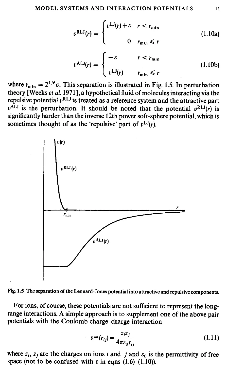
where rmln = 21/6ст. This separation is illustrated in Fig. 1.5. In perturbation
theory [Weeks et al. 1971], a hypothetical fluid of molecules interacting via the
repulsive potential i>RLJ is treated as a reference system and the attractive part
vAU is the perturbation. It should be noted that the potential vRL3(r) is
significantly harder than the inverse 12th power soft-sphere potential, which is
sometimes thought of as the 'repulsive' part of vLi(r).
„RU(r)
Fig. 1.5 The separation of the Lennard-Jones potential into attractive and repulsive components.
For ions, of course, these potentials are not sufficient to represent the long-
range interactions. A simple approach is to supplement one of the above pair
potentials with the Coulomb charge-charge interaction
where z,, Zj are the charges on ions i and j and ?0 is the permittivity of free
space (not to be confused with ? in eqns A.6)—A.10)).

12 INTRODUCTION
For ionic systems, induction interactions are important: the ionic charge
induces a dipole on a neighbouring ion. This term is not pairwise additive and
hence is difficult to include in a simulation. The shell model is a crude attempt
to take this ion polarizability into account [Dixon and Sangster 1976]. Each
ion is represented as a core surrounded by a shell. Part of the ionic charge is
located on the shell and the rest in the core. This division is always arranged so
that the shell charge is negative (it represents the electronic cloud). The
interactions between ions are just sums of the Coulombic shell-shell,
core-core, and shell-core contributions. The shell and core of a given ion are
coupled by a harmonic spring potential. The shells are taken to have zero mass.
During a simulation, their positions are adjusted iteratively to zero the net
force acting on each shell: this process makes the simulations very expensive.
When a potential depends upon just a few parameters, such as ? and a above,
it may be possible to choose an appropriate set of units in which these
parameters take values of unity. This results in a simpler description of the
properties of the model, and there may also be technical advantages within a
simulation program. For Coulomb systems, the factor Ane^ in eqn A.11) is
often omitted, and this corresponds to choosing a non-standard unit of charge.
We discuss such reduced units in Appendix B. Reduced densities, temperatures
etc. are denoted by an asterisk, i.e. p*, T* etc.
1.3.3 Molecular systems
In principle there is no reason to abandon the atomic approach when dealing
with molecular systems: chemical bonds are simply interatomic potential
energy terms [Chandler 1982]. Ideally, we would like to treat all aspects of
chemical bonding, including the reactions which form and break bonds, in a
proper quantum mechanical fashion. This difficult task has not yet been
accomplished. On the other hand, the classical approximation is likely to be
seriously in error for intramolecular bonds. The most common solution to
these problems is to treat the molecule as a rigid or semi-rigid, unit, with fixed
bond lengths and, sometimes, fixed bond angles and torsion angles. The
rationale here is that bond vibrations are of very high frequency (and hence
difficult to handle, certainly in a classical simulation) but of low amplitude
(therefore being unimportant for many liquid properties). Thus, a diatomic
molecule with a strongly binding interatomic potential energy surface might
be replaced by a dumb-bell with a rigid interatomic bond.
The interaction between the nuclei and electronic charge clouds of a pair of
molecules i and; is clearly a complicated function of relative positions г„ г, and
orientations Slh Slj [Gray and Gubbins 1984]. One way of modelling a
molecule is to concentrate on the positions and sizes of the constituent atoms
[Eyring 1932]. The much simplified 'atom-atom' or 'site-site' approximation
for diatomic molecules is illustrated in Fig. 1.6. The total interaction is a sum of

MODEL SYSTEMS AND INTERACTION POTENTIALS
13
Fig. 1.6 An atom-atom model of a diatomic molecule.
pairwise contributions from distinct sites a in molecule i, at position ria, and b
in molecule j, at position ijb
A.12)
Here a, b take the values 1,2, vab is the pair potential acting between sites a and
b, and rab is shorthand for the inter-site separation rab = |ria — гД
The interaction sites are usually centred, more or less, on the positions of the
nuclei in the real molecule, so as to represent the basic effects of molecular
'shape'. A very simple extension of the hard-sphere model is to consider a
diatomic composed of two hard spheres fused together [Streett and Tildesley
1976], but more realistic models involve continuous potentials. Thus,
nitrogen, fluorine, chlorine etc. have been depicted as two 'Lennard-Jones
atoms' separated by a fixed bond length [Barojas et al. 1973; Cheung and
Powles 1975; Singer, Taylor, and Singer 1977]. Similar approaches apply to
polyatomic molecules.
The description of the molecular charge distribution may be improved
somewhat by incorporating point multipole moments at the centre of charge
[Streett and Tildesley 1977]. These multipoles may be equal to the known
(isolated molecule) values, or may be 'effective' values chosen simply to yield a
better description of the liquid structure and thermodynamic properties. It is
now generally accepted that such a multipole expansion is not rapidly
convergent. A promising alternative approach for ionic and polar systems, is to
use a set of fictitious 'partial charges' distributed 'in a physically reasonable
way' around the molecule so as to reproduce the known multipole moments
[Murthy, O'Shea, and McDonald 1983], and a further refinement is to

14
INTRODUCTION
distribute fictitious multipoles in a similar way [Price, Stone, and Alderton
1984]. For example, the electrostatic part of the interaction between nitrogen
molecules may be modelled using five partial charges placed along the axis,
while, for methane, a tetrahedral arrangement of partial charges is appropri-
appropriate. These are illustrated in Fig. 1.7. For the case of N2, the quadrupole
moment Q is given by [Gray and Gubbins 1984]
G= I za<i A.13)
z' z
-2B+2')
z z'
(a)
I— 0.0549 nm«-|
-0.0653nm-*-|
Fig. 1.7 Partial charge models, (a) A five-charge model for N2. There is one charge at the bond
centre, two at the positions of the nuclei, and two more displaced beyond the nuclei. Typical values
are (in units of the magnitude of the electronic charge) z = + 5.2366, z' = - 4.0469, giving
Q = - 4.67 x 10 ' *° С m2 [Murthy et al. 1983]. (b) A five-charge model for CH4. There is one
charge at the centre, and four others at the positions of the hydrogen nuclei. A typical value is
z = 0.143 giving О = 5.77 x 100 Cm3 [Righini, Maki, and Klein 1981].

MODEL SYSTEMS AND INTERACTION POTENTIALS 15
with similar expressions for the higher multipoles (all the odd ones vanish for
N2). The first non-vanishing moment for methane is the octopole
0 = ^ ? 2araxrayraz A.14)
in the coordinate system of Fig. 1.7. The aim of all these approaches is to
approximate the complete charge distribution in the molecule. In a calculation
of the potential energy, the interaction between partial charges on different
molecules would be summed in the same way as the other site-site interactions.
For large rigid models, a substantial number of sites would be required to
model the repulsive core. For example, a crude model of the nematogen
quinquaphenyl, which represented each of the five benzene rings as a single
Lennard-Jones site, would necessitate 25 site-site interactions between each
pair of molecules; sites based on each carbon atom would be more realistic but
extremely expensive. An alternative type of intermolecular potential, intro-
introduced by Corner [1948], involves a single site-site interaction between a pair
of molecules, characterized by energy and length parameters that depend on
the relative orientation of the molecules. A version of this family of molecular
potentials that has been used in computer simulation studies is the Gaussian
overlap model generalized to a Lennard-Jones form [Berne and Pechukas
1972]. The basic potential acting between two linear molecules is the Lennard-
Jones interaction, eqn A.6), with the angular dependence of e and a determined
by considering the overlap of two ellipsoidal Gaussian functions (representing
the electron clouds of the molecules). The energy parameter is written
г(€1ьЩ = ^ь{\-хЧ^^?Ги2 A.15)
where e,ph is a constant and ef, e, are unit vectors describing the orientation of
the molecules i and,/. я is an anisotropy parameter determined by the length of
the major and minor axes of the electron cloud ellipsoid
The length parameter is given by
r?(l-ze1..eJ.)
(U7)
where <xSPh is a constant. In certain respects, this form of the overlap potential is
unrealistic, and it has been extended to make e also dependent upon ry [Gay
and Berne 1981]. The extended potential can be parameterized to mimic a
linear site-site potential, and should be particularly useful in the simulation of
nematic liquid crystals.

16 INTRODUCTION
For larger molecules it may not be reasonable to 'fix' all the internal degrees
of freedom. In particular, torsional motion about bonds, which gives rise to
conformational interconversion in, for example, alkanes, cannot in general be
neglected (since these motions involve energy changes comparable with
normal thermal energies). An early simulation of n-butane, CH3CH2CH2CH3
[Ryckaert and Bellemans 1975; Marechal and Ryckaert 1983], provides a good
example of the way in which these features are incorporated in a simple model.
Butane can be represented as a four-centre molecule, with fixed bond lengths
and bond bending angles, derived from known experimental (structural) data
(see Fig. 1.8). A very common simplifying feature is built into this model: whole
groups of atoms, such as CH3 and CH2, are condensed into spherically
symmetric effective 'united atoms'. In fact, for butane, the interactions between
such groups may be represented quite well by the ubiquitous Lennard-Jones
potential, with empirically chosen parameters. In a simulation, the Ci-Сг,
C2-C3 and C3-C4 bond lengths are held fixed by a method of constraints
which will be described in detail in Chapter 3. The angles в and в' may be fixed
by additionally constraining the Q-C3 and C2-C4 distances, i.e. by introduc-
introducing 'phantom bonds'. If this is done, just one internal degree of freedom,
namely the rotation about the C2-C3 bond, measured by the angle Ф, is left
unconstrained; for each molecule, an extra term in the potential energy,
^torsion ^ periodic in ф, appears in the hamiltonian. This potential would have
a minimum at a value of ф corresponding to the trans conformer of butane,
and secondary minima at the gauche conformations. It is easy to see how this
approach may be extended to much larger flexible molecules. The con-
consequences of constraining bond lengths and angles will be treated in more
detail in Chapters 2-4.
As the molecular model becomes more complicated, so too do the
expressions for the potential energy, forces, and torques, due to molecular
interactions. In Appendix C, we give some examples of these formulae, for
rigid and flexible molecules, interacting via site-site pairwise potentials,
including multipolar terms. We also show how to derive the forces from a
simple three-body potential.
1.3.4 Lattice systems
We may also consider the consequences of removing rather than adding
degrees of freedom to the molecular model. In a crystal, molecular translation
is severely restricted, while rotational motion (in plastic crystals for instance)
may still occur. A simplified model of this situation may be devised, in which
the molecular centres of mass are fixed at their equilibrium crystal lattice sites,
and the potential energy is written solely as a function of molecular
orientations. Such models are frequently of theoretical, rather than practical,
interest, and accordingly the interactions are often of a very idealized form: the
molecules may be represented as point multipoles for example, and interac-

MODEL SYSTEMS AND INTERACTION POTENTIALS
(a)
17
Fig. 1.8 (a) A model of butane [Ryckaert and Bellemans 1975].
[Marechal and Ryckaert 1983].
(b) The torsional potential
tions may even be restricted to nearest neighbours only [O'Shea 1978; Nose,
Kataoka, Okada, and Yamamoto 1981]. Ultimately, this leads us to the spin
models of theoretical physics, as typified by the Heisenberg, Ising, and Potts
models. These models are really attempts to deal with a simple quantum

18 INTRODUCTION
mechanical Hamiltonian for a solid-state lattice system, rather than the
classical equations of motion for a liquid. However, because of its correspon-
correspondence with the lattice gas model, the Ising model is still of some interest in
classical liquid state theory. There has been a substantial amount of work
involving Monte Carlo simulation of such spin systems, which we must
regrettably omit from a book of this size. The importance of these idealized
models in statistical mechanics is illustrated elsewhere [see e.g. Binder 1984,
1986; Toda, Kubo, and Saito 1983]. Lattice model simulations, however, have
been useful in the study of polymer chains, and we discuss this briefly in
Chapter 4. Paradoxically, lattice models have also been useful in the study of
liquid crystals, which we mention in Chapter 11.
7.3.5 Calculating the potential
This is an appropriate point to introduce our first piece of computer code,
which illustrates the calculation of the potential energy in a system of
Lennard-Jones atoms. Converting the algebraic equations of this chapter into
a form suitable for the computer is a straightforward exercise in FORmula
TRANslation, for which the FORTRAN programming language has histori-
historically been regarded as most suitable (see Appendix A). We suppose that the
coordinate vectors of our atoms are stored in three FORTRAN arrays RX (I),
RY (I) and RZ (I), with the particle index I varying from 1 to N (the number of
particles). For the Lennard-Jones potential it is useful to have precomputed
the value of a2, which is stored in the variable SIGSQ. The potential energy
will be stored in a variable V, which is zeroed initially, and is then accumulated
in a double loop over all distinct pairs of atoms, taking care to count each pair
only once. v = 00
DO 100 I » 1, N - 1
RXI » RX(I)
RYI - RY(I)
RZI - RZ(I)
DO 99 J = I + 1, N
RXIJ - RXI - RX(J)
RYIJ - RYI - RY(J)
RZIJ - RZI - RZ(J)
RIJSQ
SR2
SR6
SR12
V
99 CONTINUE
100 CONTINUE
V - 4.0 * EPSLON * V
RXIJ ** 2 + RYIJ ** 2 + RZIJ ** 2
SIGSQ / RIJSQ
SR2 * SR2 * SR2
SR6 ** 2
V + SR12 - SR6

MODEL SYSTEMS AND INTERACTION POTENTIALS 19
Some measures have been taken here to avoid unnecessary use of computer
time. The factor 4e D.0 *EPSLON in FORTRAN), which appears in every
pair potential term, is multiplied in once, at the very end, rather than many
times within the crucial 'inner loop' over index J. We have used temporary
variables RXI, RYI, and RZI so that we do not have to make a large number of
array references in this inner loop. Other, more subtle points (such as whether
it may be faster to compute the square of a number by using the exponen-
exponentiation operation ** or by multiplying the number by itself) are discussed in
Appendix A. The more general questions of time-saving tricks in this part of
the program are addressed in Chapter 5. The extension of this type of double
loop to deal with other forms of the pair potential, and to compute forces in
addition to potential terms, is straightforward, and examples will be given in
later chapters. For molecular systems, the same general principles apply, but
additional loops over the different sites or atoms in a molecule may be needed.
For example, consider the site-site diatomic model of eqn A.12) and Fig. 1.6. If
the coordinates of site a in molecule i are stored in array elements RX (I, A),
RY (I, A), RZ (I, A), then the intermolecular interactions might be computed as
follows:
97
98
99
100
DO 100 A
DO 99
DO
- 1, 2
В - 1, 2
98 I » 1,
DO 97 J -
RXAB -
RYAB -
RZAB -
N - 1
I + 1,
RX(I,A)
RY(I.A)
RZ(I,A)
... calculate
CONTINUE
CONTINUE
CONTINUE
CONTINUE
N
- RX(J,B)
- RY(J,B)
- RZ(J,B)
ia-jb interaction ...
This use of doubly dimensioned arrays may not be efficient on some
machines, but is quite convenient. Note that, apart from the dependence of the
loop over J on the index I, the order of nesting is a matter of choice. Here, we
have placed a loop over molecular indices innermost; assuming that N is
relatively large, the vectorization of this loop on a pipeline machine will result
in a great increase in speed of execution. Simulations of molecular systems may
also involve the calculation of intramolecular energies, which, for site-site
potentials, will necessitate a triple summation (over I, A, and B).

20 INTRODUCTION
The above examples are essentially summations over pairs of interaction
sites in the system. Any calculation of three-body interactions will, of course,
entail triple summations of the kind
98
99
100
DO 100 I - 1, N - 2
D0 99J=I+l,N-
DO 98 К - J + 1,
... calculate
CONTINUE
CONTINUE
CONTINUE
1
N
i-j-k interaction
Because all distinct triplets are examined, this will be much more
time consuming than the summations described above. Even for pairwise-
additive potentials, the energy or force calculation is the most expensive part of
a computer simulation. We will return to this crucial section of the program in
Chapter 5.
1.4 Constructing an intermolecular potential
1.4.1 Introduction
There are essentially two stages in setting up a realistic simulation of a given
system. The first is 'getting started' by constructing a first guess at a potential
model. This should be a reasonable model of the system, and allow some
preliminary simulations to be carried out. The second is to use the simulation
results to refine the potential model in a systematic way, repeating the process
several times if necessary. We consider the two phases in turn.
1.4.2 Building the model potential
To illustrate the process of building up an intermolecular potential, we begin
by considering a small molecule, such as N2, OCS, or CH4, which can be
modelled using the interaction site potentials discussed in Section 1.3. The
essential features of this model will be an anisotropic repulsive core, to
represent the shape, an anisotropic dispersion interaction, and some partial
charges to model the permanent electrostatic effects. This crude effective pair
potential can then be refined by using it to calculate properties of the gas,
liquid, and solid, and comparing with experiment.
Each short-range site-site interaction can be modelled using a
Lennard-Jones potential. Suitable energy and length parameters for interac-

CONSTRUCTING AN INTERMOLECULAR POTENTIAL 21
tions between pairs of identical atoms in different molecules are available from
a number of simulation studies. Some of these are given in Table 1.1.
Table 1.1. Atom-atom interaction parameters
Atom
H
He
С
N
О
F
Ne
S
Cl
Ar
Br
Kr
Source
[Murad and Gubbins 1978]
[Maitland et al. 1981]
[Tildesley and Madden 1981]
[Cheung and Powles 1975]
[English and Venables 1974]
[Singer et al. 1977]
[Maitland et al. 1981]
[Tildesley and Madden, 1981]
[Singer et al. 1977]
[Maitland et al. 1981]
[Singer et al. 1977]
[Maitland et al. 1981]
e/kB(K)
8.6
10.2
51.2
37.3
61.6
52.8
47.0
183.0
173.5
119.8
257.2
164.0
ff(nm)
0.281
0.228
0.335
0.331
0.295
0.283
0.272
0.352
0.335
0.341
0.354
0.383
The energy parameter ? increases with atomic number as the polarizability
goes up; a also increases down a group of the periodic table, but decreases from
left to right across a period with the increasing nuclear charge. For elements
which do not appear in Table 1.1, a guide to ? and a might be provided by the
polarizability and van der Waals radius respectively. These values are only
intended as a reasonable first guess: they take no regard of chemical
environment and are not designed to be transferable. For example, the carbon
atom parameters in CS2 given in the table are quite different from the values
appropriate to a carbon atom in graphite [Crowell 1958]. Interactions
between unlike atoms in different molecules can be approximated using the
venerable Lorentz-Berthelot mixing rules. For example, in CS2 the cross terms
are given by
] A-18)
and
In tackling larger molecules, it may be necessary to model several atoms as a
unified site. We have seen this for butane in Section 1.3, and a similar approach
has been used in a model of benzene [Evans and Watts 1976]. There are also
complete sets of transferable potential parameters available for aromatic and
aliphatic hydrocarbons [Williams 1965, 1967], and for hydrogen-bonded
liquids [Jorgensen 1981], which use the site-site approach. In the case of the
Williams potentials, an exponential repulsion rather than Lennard-Jones
power law is used. The specification of an interaction site model is made

22 INTRODUCTION
complete by defining the positions of the sites within the molecule. Normally,
these are located at the positions of the nuclei, with the bond lengths obtained
from a standard source [CRC 1984].
The site-site Lennard-Jones potentials include an anisotropic dispersion
which has the correct г ~ б radial dependence at long range. However, this is not
the exact result for the anisotropic dispersion from second order perturbation
theory. The correct formula, in an appropriate functional form for use in a
simulation, is given by Burgos, Murthy, and Righini [1982]. Its implemen-
implementation requires an estimate of the polarizability and polarizability anisotropy
of the molecule.
The most convenient way of representing electrostatic interactions is
through partial charges as discussed in Section 1.3. To minimize the
calculation of site-site distances, they can be made to coincide with the
Lennard-Jones sites, but this is not always desirable or possible; the only
physical constraint on partial charge positions is that they should not lie
outside the repulsive core region, since the potential might then diverge if
molecules came too close. The magnitudes of the charges can be chosen to
duplicate the known gas phase electrostatic moments [Gray and Gubbins
1984, Appendix D]. Alternatively, the moments may be taken as adjustable
parameters. For example, in a simple three-site model of N2 representing only
the quadrupole-quadrupole interaction, the best agreement with condensed
phase properties is obtained with charges giving a quadrupole 10-15 per cent
lower than the gas phase value [Murthy, Singer, Klein, and McDonald 1980].
However, a sensible strategy is to begin with the gas phase values, and alter the
repulsive core parameters ? and a before changing the partial charges.
1.4.3 Adjusting the model potential
The first-guess potential can be used to calculate a number of properties in the
gas, liquid, and solid phases; comparison of these results with experiment may
be used to refine the potential, and the cycle can be repeated if necessary. The
second virial coefficient is given by
B(T) = ~SF I r'*dr°|dftf\diij exp (~
A.20)
where Q = An for a linear molecule and п = 8тг2 for a non-linear one. This
multidimensional integral (four-dimensional for a linear molecule and six-
dimensional for a non-linear one) is easily calculated using a non-product
algorithm [Murad 1978]. Experimental values of B(T) have been compiled by
Dymond and Smith [1980]. Trial and error adjustment of the Lennard-Jones
? and a parameters should be carried out, with any bond lengths and partial
charges held fixed, so as to produce the closest match with the experimental

STUDYING SMALL SYSTEMS 23
B(T). This will produce an improved potential, but still one that is based on
pair properties.
The next step is to carry out a series of computer simulations of the liquid
state, as described in Chapters 3 and 4. The densities and temperatures of the
simulations should be chosen to be close to the orthobaric curve of the real
system, i.e. the liquid-vapour coexistence line. The output from these
simulations, particularly the total internal energy and the pressure, may be
compared with the experimental values. The coexisting pressures are readily
available [Rowlinson and Swinton 1982], and the internal energy can be
obtained approximately from the known latent heat of evaporation. The
energy parameters ? are adjusted to give a good fit to the internal energies
along the orthobaric curve, and the length parameters a altered to fit the
pressures. If no satisfactory fit is obtained at this stage, the partial charges may
be adjusted.
Although the solid state is not the province of this book, it offers a sensitive
test of any potential model. Using the experimentally observed crystal
structure, and the refined potential model, the lattice energy at zero
temperature can be compared with the experimental value (remembering to
add a correction for quantum zero-point motion). In addition, the lattice
parameters corresponding to the minimum energy for the model solid can be
compared with the values obtained by diffraction, and also lattice dynamics
calculations [Neto, Righini, Califano, and Walmsley 1978] used to obtain
phonons, librational modes, and dispersion curves of the model solid. Finally,
we can ask if the experimental crystal structure is indeed the minimum energy
structure for our potential. These constitute severe tests of our model-building
skills.
1.5 Studying small systems
1.5.1 Introduction
Computer simulations are usually performed on a small number of molecules,
10 < N < 10000. The size of the system is limited by the available storage on
the host computer, and, more crucially, by the speed of execution of the
program. The time taken for a double loop used to evaluate the forces or
potential energy is proportional to N2. Special techniques (see Chapter 5) may
reduce this dependence to @(N), for very large systems, but the force/energy
loop almost inevitably dictates the overall speed, and, clearly, smaller systems
will always be less expensive. If we are interested in the properties of a very
small liquid drop, or a microcrystal, then the simulation will be straight-
straightforward. The cohesive forces between molecules may be sufficient to hold the
system together unaided during the course of a simulation; otherwise our set of
N molecules may be confined by a potential representing a container, which
prevents them from drifting apart (see Chapter 11). These arrangements,

24
INTRODUCTION
however, are not satisfactory for the simulation of bulk liquids. A major
obstacle to such a simulation is the large fraction of molecules which lie on the
surface of any small sample; for 1000 molecules arranged in a 10 x 10 x 10
cube, no less than 488 molecules appear on the cube faces. Whether or not the
cube is surrounded by a containing wall, molecules on the surface will
experience quite different forces from molecules in the bulk.
1.5.2 Periodic boundary conditions
The problem of surface effects can be overcome by implementing periodic
boundary conditions [Born and von Karman 1912]. The cubic box is
replicated throughout space to form an infinite lattice. In the course of the
simulation, as a molecule moves in the original box, its periodic image in each
of the neighbouring boxes moves in exactly the same way. Thus, as a molecule
leaves the central box, one of its images will enter through the opposite face.
There are no walls at the boundary of the central box, and no surface
molecules. This box simply forms a convenient axis system for measuring the
coordinates of the N molecules. A two-dimensional version of such a periodic
system is shown in Fig. 1.9. The duplicate boxes are labelled А, В, С, etc., in an
Fig. 1.9 A two-dimensional periodic system. Molecules can enter and leave each box across each
of the four edges. In a three-dimensional example, molecules would be free to cross any of the six
cube faces.

STUDYING SMALL SYSTEMS 25
arbitrary fashion. As particle 1 moves through a boundary, its images, 1A, 1B,
etc. (where the subscript specifies in which box the image lies) move across their
corresponding boundaries. The number density in the central box (and hence
in the entire system) is conserved. It is not necessary to store the coordinates of
all the images in a simulation (an infinite number!), just the molecules in the
central box. When a molecule leaves the box by crossing a boundary, attention
may be switched to the image just entering. It is sometimes useful to picture the
basic simulation box (in our two-dimensional example) as being rolled up to
form the surface of a three-dimensional torus or doughnut, when there is no
need to consider an infinite number of replicas of the system, nor any image
particles. This correctly represents the topology of the system, if not the
geometry. A similar analogy exists for a three-dimensional periodic system, but
this is more difficult to visualize!
It is important to ask if the properties of a small, infinitely periodic, system,
and the macroscopic system which it represents, are the same. This will depend
both on the range of the intermolecular potential and the phenomenon under
investigation. For a fluid of Lennard-Jones atoms, it should be possible to
perform a simulation in a cubic box of side L « 6a, without a particle being
able to 'sense' the symmetry of the periodic lattice. If the potential is long
ranged (i.e. v(r) ~ r~v where v is less than the dimensionality of the system)
there will be a substantial interaction between a particle and its own images in
neighbouring boxes, and consequently the symmetry of the cell structure is
imposed on a fluid which is in reality isotropic. The methods used to cope with
long-range potentials, for example in the simulation of charged ions (v{r)
~ r~ l) and dipolar molecules (v(r) ~ r~3), are discussed in Chapter 5. Recent
work has shown that, even in the case of short-range potentials, the periodic
boundary conditions can induce anisotropies in the fluid structure [Mandell
1976; Impey, Madden, and Tildesley 1981]. These effects are pronounced for
small system sizes (N « 100) and for properties such as the g2 light scattering
factor (see Chapter 2), which has a substantial long-range contribution. Pratt
and Haan [1981] have developed theoretical methods for investigating the
effects of boundary conditions on equilibrium properties.
The use of periodic boundary conditions inhibits the occurrence of long-
wavelength fluctuations. For a cube of side L, the periodicity will suppress any
density waves with a wavelength greater than L. Thus, it would not be possible
to simulate a liquid close to the gas-liquid critical point, where the range of
critical fluctuations is macroscopic. Furthermore, transitions which are known
to be first order often exhibit the characteristics of higher order transitions
when modelled in a small box because of the suppression of fluctuations.
Examples are the nematic to isotropic transition in liquid crystals [Luckhurst
and Simpson 1982] and the solid to plastic crystal transition for N2 adsorbed
on graphite [Mouritsen and Berlinsky 1982]. The same limitations apply to
the simulation of long-wavelength phonons in model solids, where, in addition,
the cell periodicity picks out a discrete set of available wave-vectors (i.e.

26
INTRODUCTION
к = (kx, ky, кгJл/Ь, where kx, ky, кг are integers) in the first Brillouin zone
[Klein and Weis 1977]. Periodic boundary conditions have also been shown to
affect the rate at which a simulated liquid nucleates and forms a solid or glass
when it is rapidly cooled [Honeycutt and Andersen 1984].
Despite the above remarks, the common experience in simulation work is
that periodic boundary conditions have little effect on the equilibrium
thermodynamic properties and structures of fluids away from phase tran-
transitions and where the interactions are short-ranged. It is always sensible to
check that this is true for each model studied. If the resources are available, it
should be standard practice to increase the number of molecules (and the box
size, so as to maintain constant density) and rerun the simulations.
The cubic box has been used almost exclusively in computer simulation
studies because of its geometrical simplicity. Of the four remaining semi-
regular space-filling polyhedra, the rhombic dodecahedron [Wang and
Krumhansl 1972] and the truncated octahedron [Adams 1979,1980] have also
been studied. These boxes are illustrated in Fig. 1.10. They are more nearly
spherical than the cube, which may be useful for simulating liquids, whose
structure is spatially isotropic. In addition, for a given number density, the
distance between periodic images is larger than in the cube. This property is
useful in calculating distribution functions and structure factors (see Chapters
2 and 6).
(a)
Fig. 1.10 Non-cubic simulation boxes, (a) The truncated octahedron and its containing
cube; (b) the rhombic dodecahedron and its containing cube. The axes are those used in
microfiche F.I.
So far, we have tacitly assumed that there is no external potential, i.e. no t>,
term in eqns A.4), A.5). If such a potential is present, then either it must have
the same periodicity as the simulation box, or the periodic boundaries must be
abandoned. In some cases, it is not appropriate to employ periodic boundary
conditions in each of the three coordinate directions. In the simulation of CH4
on graphite [Severin and Tildesley 1980] the simulation box, shown in Fig. 1.11,
is periodic in the plane of the surface. In the z-direction, the graphite surface

STUDYING SMALL SYSTEMS
27
(b)
Fig. 1.11 Periodic boundaries used in the simulation of adsorption [Severin and Tildesley
1980]. (a) A side view of the box. There-is a reflecting boundary at a height L,- (b) A top view,
showing the rhombic shape (i.e. the same geometry as the underlying graphite lattice).
forms the lower boundary of the box, and the bulk of the adsorbate is in the
region just above the graphite. Any molecule in the gas above the surface is
confined by reversing its velocity should it cross a plane at a height Lz above
the surface. If Lz is sufficiently large, this reflecting boundary will not influence
the behaviour of the adsorbed monolayer. In the plane of the surface, the shape
of the periodic box is a rhombus of side L. This conforms to the symmetry of
the underlying graphite. Similar boxes have been used in the simulation of the
electrical double layer [Torrie and Valleau 1979], of the liquid-vapour surface
[Chapela et al. 1977], and of fluids in small pores [Subramanian and Davis
1979].
7.5.5 Potential truncation
Now we must turn to the question of calculating properties of systems subject
to periodic boundary conditions. The heart of the MC and MD programs
involves the calculation of the potential energy of a particular configuration,

28
INTRODUCTION
and, in the case of MD, the forces acting on all molecules. Consider how we
would calculate the force on molecule 1, or those contributions to the potential
energy involving molecule 1, assuming pairwise additivity. We must include
interactions between molecule 1 and every other molecule i in the simulation
box. There are N — 1 terms in this sum. However, in principle, we must also
include all interactions between molecule 1 and images iA, iB, etc. lying in the
surrounding boxes. This is an infinite number of terms, and of course is
impossible to calculate in practice. For a short-range potential energy
function, we may restrict this summation by making an approximation.
Consider molecule 1 to rest at the centre of a region which has the same size
and shape as the basic simulation box (see Fig. 1.12). Molecule 1 interacts with
all the molecules whose centres lie within this region, that is with the closest
periodic images of the other N -1 molecules. This is called the 'minimum
image convention': for example, in Fig. 1.12 molecule 1 interacts with
molecules 2,3E, 4E and 5C. This technique, which is a natural consequence of
the periodic boundary conditions, was first used in simulation by Metropolis
et al. [1953].
In the minimum image convention, then, the calculation of the potential
energy due to pairwise-additive interactions involves $N(N -1) terms. This
Fig. 1.12 The minimum image convention in a two-dimensional system. The central box contains
five molecules. The 'box' constructed with molecule 1 at its centre also contains five molecules. The
dashed circle represents a potential cutoff.

STUDYING SMALL SYSTEMS 29
may still be a very substantial calculation for a system of (say) 1000 particles. A
further approximation significantly improves this situation. The largest
contribution to the potential and forces comes from neighbours close to the
molecule of interest, and for short-range forces we normally apply a spherical
cutoff. This means setting the pair potential v(r) to zero for r > rc, where rc is
the cutoff distance. The dashed circle in Fig. 1.12 represents a cutoff, and in this
case molecules 2 and 4E contribute to the force on 1, since their centres lie
inside the cutoff, whereas molecules 3E and 5C do not contribute. In a cubic
simulation box of side L, the number of neighbours explicitly considered is
reduced by a factor of approximately Anrl /3L3, and this may be a substantial
saving. The introduction of a spherical cutoff should be a small perturbation,
and the cutoff distance should be sufficiently large to ensure this. As an
example, in the simulation of Lennard-Jones atoms, the value of the pair
potential at the boundary of a cutoff sphere of typical radius re = 2.5a is just
1.6 per cent of the well depth. Of course, the penalty of applying a spherical
cutoff is that the thermodynamic (and other) properties of the model fluid will
no longer be exactly the same as for (say) the non-truncated, Lennard-Jones
fluid. As we shall see in Chapter 2, it is possible to apply long-range corrections
to such results, so as to recover, approximately, the desired information.
The cutoff distance must be no greater than ^L for consistency with the
minimum image convention. In the non-cubic simulation boxes of Fig. 1.10,
for a given density and number of particles, rc may take somewhat larger values
than in the cubic case. Looked at another way, an advantage of non-cubic
boundary conditions is that they permit simulations with a given cutoff
distance and density to be conducted using fewer particles. As an example, a
simulation in a cubic box, with rc set equal to ? L, might involve N = 256
molecules; taking the same density, the same cutoff could be used in a
simulation of N = 197 molecules in a truncated octahedron, or just N = 181
molecules in a rhombic dodecahedron.
1.5.4 Computer code for periodic boundaries
How do we handle periodic boundaries and the minimum image convention,
in a simulation program? Let us assume that, initially, the N molecules in the
simulation lie within a cubic box of side L, with the origin at its centre, i.e. all
coordinates lie in the range ( — %L,%L). As the simulation proceeds, these
molecules move about the infinite periodic system. When a molecule leaves the
box by crossing one of the boundaries, it is usual to switch attention to the
image molecule entering the box, by simply adding L to, or subtracting L from,
the appropriate coordinate. One simple way to do this uses a FORTRAN IF
statement to test the positions immediately after the molecules have been
moved (whether by MC or MD):
IF ( RX(I) .GT. B0XL2 ) RX(I) - RX(I) - BOXL
IF ( RX(I) .LT. -B0XL2 ) RX(I) - RX(I) + BOXL

30 INTRODUCTION
Here, BOXL is a variable containing the box length L, and BOXL2 is just
half the box length. Similar statements are applied to the у and z coordinates.
An alternative to the IF statement is to use FORTRAN arithmetic functions to
calculate the correct number of box lengths to be added or subtracted:
RX(I) - RX(I) - BOXL * ANINT ( RX(I) / BOXL )
The function ANINT(X) returns the nearest integer to X, converting the
result back to type REAL; thus ANINT (-0.49) has the value 0.0, whereas
ANINT (— 0.51) is —1.0. By using these methods, we always have available the
coordinates of the N molecules that currently lie in the 'central' box. It is not
strictly necessary to do this; we could, instead, use uncorrected coordinates,
and follow the motion of the N molecules that were in the central box at the
start of the simulation. Indeed, as we shall see in Chapters 2 and 6, for
calculation of transport coefficients it may be most desirable to have a set of
uncorrected positions on hand. If it is decided to do this, however, care must be
taken that the minimum image convention is correctly applied, so as to work
out the vector between the two closest images of a pair of molecules, no matter
how many 'boxes' apart they may be.
The minimum image convention may be coded in the same way as the
periodic boundary adjustments. Of the two methods mentioned above, the
arithmetic formula is usually preferable, being simpler; the use of IF
statements inside the inner loop, particularly on pipeline machines, is to be
avoided (see Appendix A). Immediately after calculating a pair separation
vector, the following statements should be applied:
RXIJ - RXIJ - BOXL * ANINT ( RXIJ / BOXL )
RYIJ - RYIJ - BOXL * ANINT ( RYIJ / BOXL )
RZIJ - RZIJ - BOXL * ANINT ( RZIJ / BOXL )
The above code is guaranteed to yield the minimum image vector, no matter
how many 'box lengths' apart the original images may be.
The calculation of minimum image distances is simplified by the use of
reduced units: the length of the box is taken to define the fundamental unit of
length in the simulation. Some workers define L = 1, others prefer to take
L = 2. By setting 1 = 1, with particle coordinates nominally in the range
(-2, +4), the minimum image correction above becomes
RXIJ - RXIJ - ANINT ( RXIJ )
RYIJ = RYIJ - ANINT ( RYIJ )
RZIJ = RZIJ - ANINT ( RZIJ )
which is simpler, and faster, than the code for a general box length. This
approach is an alternative to the use of the pair potential to define reduced
units as discussed in Appendix B, and is more generally applicable. For this
reason a simulation box of unit length is adopted in some of the examples given
in this book and on the attached microfiche.

STUDYING SMALL SYSTEMS 31
There are several alternative ways of coding the minimum image correc-
corrections, some of which rely on the images being in the same, central box (i.e. on
the periodic boundary correction being applied whenever the molecules move.)
Some of these methods, for cubic boxes, are discussed in Appendix A. We have
also mentioned the possibility of conducting simulations in non-cubic periodic
boundary conditions. The FORTRAN code for implementing the minimum
image correction in the cases of the truncated octahedron and the rhombic
dodecahedron are given in program F.I [see also Adams, 1983a; Smith
1983]. The code for the rhombic dodecahedron is a little more complicated
than the code for the truncated octahedron, and the gain small, so that the
truncated octahedron is preferable. We also give on the microfiche the code for
computirig minimum image corrections in the two-dimensional rhombic box
often used in surface simulations.
Now we turn to the implementation of a spherical cutoff, i.e. we wish to set
the pair potential (and all forces) to zero if the pair separation lies outside some
distance rc. It is easy to compute the square of the particle separation r0 and,
rather than waste time taking the square root of this quantity, it is fastest to
compare this with the square of rc, which might be computed earlier and
stored in a FORTRAN variable RCUTSQ. After computing the minimum
image intermolecular vector, the following statements would be employed:
RIJSQ - RXIJ ** 2 + RYU ** 2 + RZIJ ** 2
IF ( RIJSQ .LT. RCUTSQ ) THEN
... compute i-j interaction ...
... accumulate energy and forces ...
ENDIF
In a large system, it may be worthwhile to apply separate tests for the x, y,
and z directions or some similar scheme.
IF ( ABS ( RXIJ ) .LT. RCUT ) THEN
IF ( ABS ( RYIJ ) .LT. RCUT ) THEN
IF ( ABS ( RZIJ ) .LT. RCUT ) THEN
RIJSQ = RXIJ ** 2 + RYIJ ** 2 + RZIJ ** 2
IF ( RIJSQ .LT. RCUTSQ ) THEN
... compute i-j interaction ...
... accumulate energy and forces ...
ENDIF
ENDIF
ENDIF
ENDIF

32 INTRODUCTION
The time saved in dropping out of this part of the program at any early stage
must be weighed against the overheads of extra calculation and testing. A
different approach is needed on a pipeline machine, since the IF statements
may prevent vectorization of the inner loop. In this situation, it is generally
simplest to compute all the minimum image interactions, and then set to zero
the potential energy (and forces) arising from pairs separated by distances
greater than rc. The extra work involved here is more than offset by the speed
increase on vectorization. Within the inner loop, this is simply achieved by
setting the inverse squared separation 1/r? to zero, where appropriate, before
calculating energies, forces etc. as functions of this quantity. The following
code performs this task on the CRAY 1-S fFincham and Ralston 1981]
RIJSQ - RXIJ ** 2 + RYIJ ** 2 + RZIJ ** 2
RIJSQI - 1.0 / RIJSQ
RIJSQI = CVMGP ( RIJSQI, 0.0, RCUTSQ - RIJSQ )
... compute i-j interaction ...
... as functions of RIJSQI ...
The function CVMGP(A, В, С) is a vector merge statement which returns
the value A if С is non-negative and the value В otherwise. Note that no time is
saved by using a spherical cutoff in this way on a pipeline machine. The only
reason for implementing the spherical cutoff in this case is so that the usual
long-range corrections may be applied to the simulation results (see Chapter
2). In Chapter S we discuss the more complicated time-saving tricks used in the
simulations of large systems.
1.5.5 Spherical boundary conditions
Before leaving this section, we should mention an alternative to the standard
periodic boundary conditions for simulating bulk liquids. A two-dimensional
system may be embedded in the surface of a sphere without introducing any
physical boundaries [Hansen, Levesque, and Weis 1979] and the idea may be
extended to consider a three-dimensional system as being the surface of a
hypersphere [Kratky 1980; Kratky and Schreiner 1982]. The spherical or
hyperspherical system is finite: it cannot be considered as part of an infinitely
repeating periodic system. In this case, non-Euclidean geometry is an
unavoidable complication, and distances between particles are typically
measured along the great circle geodesies joining them. However, the effects of
the curved geometry will decrease as the system size increases, and such
'spherical boundary conditions' are expected to be a valid method of
simulating bulk liquids. Interesting differences from the standard periodic
boundary conditions, particularly close to any solid-liquid phase transition,
will result from the different topology. Periodic boundaries will be biased in
favour of the formation of a solid with a lattice structure which matches the
simulation box; in general, a periodic lattice is not consistent with spherical
boundaries, and so the liquid state will be favoured in most simulations using
this technique.

2
STATISTICAL MECHANICS
2.1 Sampling from ensembles
Computer simulation generates information at the microscopic level (atomic
and molecular positions, velocities etc.) and the conversion of this very detailed
information into macroscopic terms (pressure, internal energy etc.) is the
province of statistical mechanics. It is not our aim to provide a text in this field,
since many excellent sources are available [Hill 1956; McQuarrie 1976;
Landau and Lifshitz 1980; Friedman 1985; Hansen and McDonald 1986;
Chandler, 1987]. In this chapter, our aim is to summarize those aspects of the
subject which are of most interest to the computer simulator.
Let us consider, for simplicity, a one-component macroscopic system;
extension to a multicomponent system is straightforward. The thermo-
dynamic state of such a system is usually defined by a small set of parameters
(such as the number of particles JV, the temperature T, and the pressure P).
Other thermodynamic properties (density p, chemical potential ц, heat
capacity Cv etc.) may be derived through knowledge of the equations of state
and the fundamental equations of thermodynamics. Even quantities such as
the diffusion coefficient D, the shear viscosity ц, and the structure factor S(k)
are state functions: although they clearly say something about the microscopic
structure and dynamics of the system, their values are completely dictated by
the few variables (e.g. NPT) characterizing the thermodynamic state, not by
the very many atomic positions and momenta that define the instantaneous
mechanical state. These positions and momenta can be thought of as
coordinates in a multidimensional space: phase space. For a system of N
atoms, this space has 6N dimensions. Let us use the abbreviation Г for a
particular point in phase space, and suppose that we can write the instan-
instantaneous value of some property $t (it might be the potential energy) as a
function si (Г). The system evolves in time, so that Г, and hence srf(T) will
change. It is reasonable to assume that the experimentally observable
'macroscopic' property j/obs is really the time average of s/(T) taken over a
long time interval:
e= Шп -^- [^s/(T{t))dt . B.1)
'obs"*00 obs Jo
The equations governing this time evolution, Newton's equations of motion in
a simple classical system, are of course well known. They are just a system of
ordinary differential equations: solving them on a computer, to a desired
accuracy, is a practical proposition for, say, 1000 particles, although not for a
truly macroscopic number (e.g. 1023). So far as the calculation of time averages

34 STATISTICAL MECHANICS
is concerned, we clearly cannot hope to extend the integration of eqn B.1) to
infinite time, but might be satisfied to average over a long finite time tobs. This is
exactly what we do in a molecular dynamics simulation. In fact, the equations
of motion are usually solved on a step-by-step basis, i.e. a large finite number
robs of time steps, of length 8t = tobs/Tobs are taken. In this case, we may
rewrite eqn B.1) in the form
_ . ..)• B-2)
Tobs t = 1
In the summation, т simply stands for an index running over the succession of
time steps. This analogy between the discrete т and the continuous t is useful,
even when, as we shall see in other examples, т does not correspond to the
passage of time in any physical sense.
The practical questions regarding the method are whether or not a sufficient
region of phase space is explored by the system trajectory to yield satisfactory
time averages within a feasible amount of computer time, and whether
thermodynamic consistency can be attained between simulations with ident-
identical macroscopic parameters (density, energy etc.) but different initial con-
conditions (atomic positions and velocities). The answers to these questions are
that such simulation runs are indeed within the power of modern computers,
and that thermodynamically consistent results for liquid state properties can
indeed be obtained, provided that attention is paid to the selection of initial
conditions. We will turn to the technical details of the method in Chapter 3.
The calculation of time averages by MD is not the approach to
thermodynamic properties implicit in conventional statistical mechanics.
Because of the complexity of the time evolution of j/(r(t)) for large numbers
of molecules, Gibbs suggested replacing the time average by the ensemble
average. Here, we regard an ensemble as a collection of points Г in phase space.
The points are distributed according to a probability density р(Г). This
function is determined by the chosen fixed macroscopic parameters
(NPT, N VTetc), so we use the notation pNPT, pNyT, or, in general, pens. Each
point represents a typical system at any particular instant of time. Each system
evolves in time, according to the usual mechanical equations of motion, quite
independently of the other systems. Consequently, in general, the phase space
density РепДГ) will change with time. However, no systems are destroyed or
created during this evolution, and Liouville's theorem, which is essentially a
conservation law for probability density, states that dp/dt = 0 where d/dt
denotes the total derivative with respect to time (following a state Г as it
moves). As an example, consider a set of N atoms with Cartesian coordinates rf
and momenta p,, in the classical approximation. The total time derivative is
B-3.)

SAMPLING FROM ENSEMBLES 35
= |- + f-Vr+p-Vp. B.3b)
In eqn B.3a), д/dt represents differentiation, with respect to time, of a function,
V,( and Vpi are derivatives with respect to atomip position and momentum
respectively, and rh p, signify the time derivatives of the position and
momentum. Equation B.3b) is the same equation written in a more compact
way, and the equation may be further condensed by defining the Liouville
operator L
= (r-Vr + p-VD) B.4)
i
so that d/dt = д/dt + iL and, using Liouville's theorem, we may write
д„ tr л
= -iLp(T,t). B.5)
dt
This equation tells us that the rate of change of pensat a particular fixed point in
phase space is related to the flows into and out of that point. This equation has
a formal solution
реш(Г, t) = exp( - iLt) pms(T, 0) B.6)
where the exponential of an operator really means a series expansion
exp(-jLt)= l-iLt-$L2t2 + B.7)
The equation of motion of a function like <я/(Г), which does not depend
explicitly on time, takes a conjugate form [McQuarrie 1976]:
j/(T@) = iLj/(T(t)) B.8)
or
B.9)
To be quite clear: in eqns B.5) and B.6) we consider the time-dependence of
Pgjjj at a fixed point Г in phase space; in eqns B.8) and B.9), j/(F) is time-
dependent because we are following the time evolution Г (t) along a trajectory.
This relationship is analogous to that between the Schrodinger and
Heisenberg pictures in quantum mechanics.
If реП5(Г) represents an equilibrium ensemble, then its time-dependence
completely vanishes, dptBJdt = 0. The system evolution then becomes quite
special. As each system leaves a particular state Г(т) and moves on to the next,
Г(т +1), another system arrives from state Г (т -1) to replace it. The motion
resembles a long and convoluted conga line at a crowded party (see Fig. 2.1).
There might be several such processions, each passing through different
regions of phase space. However, if there is just one trajectory that passes
through all the points in phase space for which рт$ is non-zero (i.e. the

36 STATISTICAL MECHANICS
Fig. 2.1 A schematic representation of phase space. The hexagonal cells represent state points
(q, p). In an ergodic system, all the trajectories here would be different sections of a single long
trajectory. A substantial region of cyclical trajectories, and a barrier region leading to bottlenecks,
are shaded.
procession forms a single, very long, closed circuit) then each system will
eventually visit all the state points. Such a system is termed 'ergodic' and the
time taken to complete a cycle (the Poincare recurrence time) is immeasurably
long for a many-particle system (and for many parties as well it seems).
Nevertheless, in principle, the fact that individual systems are moving around
the circuit becomes unimportant: the average properties of our partygoers, for
example, could be deduced from a snapshot of the event, rather than by
following the complete experiences of one individual through the entire
proceedings. This corresponds to replacing the time average in eqn B.1) by an
average taken over all the members of the ensemble, 'frozen' at a particular
time:
¦^obs = <^>ens = <^IPens> = I ^(Г)реп8(Г) . B.10)
Г
The < si \p > notation reminds us of the dependence of the average on both si
and p: this is important when taking a thermodynamic derivative of s/obs (we
must differentiate both parts) or when considering time-dependent properties
(when the Schrodinger/Heisenberg analogy may be exploited). Actually, we
will be concerned with the practical question of efficient and thorough
sampling of phase space, which is not quite the same as the rigorous definition
of ergodicity [for a fuller discussion, see Tolman 1938]. In terms of our
analogy of conga lines, there should not be a preponderance of independent

SAMPLING FROM ENSEMBLES 37
closed circuits ('cliques') in which individuals can become trapped and fail fully
to sample the available space (this is important in parties as well as in
simulations). An MD simulation which started in the shaded cyclic region of
Fig. 2.1, for example, would be disastrous. On the other hand, small non-
ergodic regions are less likely to be dangerous and more likely to be recognized
if they are unfortunately selected as starting points for a simulation. In a
similar way, regions of phase space which act as barriers and cause bottlenecks
through which only a few trajectories pass (see Fig. 2.1) can result in poor
sampling by the relatively short simulation runs carried out in practice, even if
the system is technically ergodic.
It is sometimes convenient to use, in place of реП8(Г), a 'weight' function
wens(r), which satisfies the following equations:
Реп8(Г) = е;п>епз(Г) B-11)
ееп8=Е^е„з(Г) B-12)
Г
<•* >ens= Z ">еп8(Г)^(Г)/? ^(Г) . B.13)
Г Г
The weight function is essentially a non-normalized form of реп8(Г), with the
partition function Qeos (also called the sum over states) acting as the
normalizing factor. Both и>еш(Г) and Qenscan contain an arbitrary multiplicat-
multiplicative constant, whose choice corresponds to the definition of a zero of entropy.
Qens is simply a function of the macroscopic properties defining the ensemble,
and connection with classical thermodynamics is made by defining a
thermodynamic potential *Pens [see e.g. McQuarrie 1976]
*«--ln e«- B.i4)
This is the function.that has a minimum value at thermodynamic equilibrium
(e.g. the negative of the entropy S for a system at constant N VE, the Gibbs
function G for a constant-NPr system).
Throughout the above discussion, although we have occasionally used the
language of classical mechanics, we have assumed that the states Гаге discrete
(e.g. a set of quantum numbers) and that we may sum over them. If the system
were enclosed in a container, there would be a countably infinite set of
quantum states. In the classical approximation, Г represents the set of
(continuously variable) particle positions and momenta, and we should replace
the summation by a classical phase space integral, w^and Qensare then usually
defined with appropriate factors included to make them dimensionless, and to
match up with the usual semiclassical 'coarse-grained' phase space volume
elements. On a computer, of course, all numbers are held to a finite precision
and so, technically, positions and momenta are represented by discrete, not
continuous, variables; we now have a countable and finite set of states. We

38 STATISTICAL MECHANICS
assume that the distinction between this case and the classical limit is of no
practical importance, and will use whichever representation is most
convenient.
One conceivable approach to the computation of thermodynamic
quantities, therefore, would be a direct evaluation of Qms, for a particular
ensemble, using eqn B.12). This summation, over all possible states, is not
feasible for many-particle systems: there are too many states, most of which
have a very low weight due to non-physical overlaps between the repulsive
cores of the molecules, rendering them unimportant. We would like to conduct
the summation so as to exclude this large number of irrelevant states, and
include only those with a high probability. Unfortunately, it is generally not
possible to estimate QeBS directly in this way. However, the underlying idea,
that of generating (somehow) a set of states in phase space that are sampled
from the complete set in accordance with the probability density реш(Г), is
central to the Monte Carlo technique.
We proceed by analogy with molecular dynamics in the sense that the
ensemble average of eqn B.13) is replaced by a trajectory average like eqn B.2).
Newton's equations generate a succession of states in accordance with the
distribution function pNVE for the constant-N VE or microcanonical en-
ensemble. Suppose we wish to investigate other ensembles; experiments in the
laboratory, for example, are frequently performed under conditions of
constant temperature and pressure, while it is often very convenient to
consider inhomogeneous systems at constant chemical potential. For each
such case, let us invent a kind of equation of motion, i.e. a means of generating,
from one state point Г(т), a succeeding state point Г(т +1). This recipe need
have no physical interpretation, and it could be entirely deterministic or could
involve a stochastic, random, element. It might be derived by modifying the
true equations of motion in some way, or it may have no relation whatever
with normal dynamics.
To be useful, this prescription should satisfy some sensible conditions:
(a) the probability density реп8(Г) for the ensemble of interest should not
change as the system evolves;
(b) any 'reasonable' starting distribution p (Г) should tend to this stationary
solution as the simulation proceeds;
(c) we should be able to argue that ergodicity holds, even though we cannot
hope to prove this for realistic systems.
If these conditions are satisfied, then we should be able to generate, from an
initial state, a succession of state points which, in the long term, are sampled in
accordance with the desired probability density реп8(Г). In these circum-
circumstances, the ensemble average will be equal to a kind of 'time average':
J robs
<bs = <* >ens = — I ^(T(T)) • B.15)
Tobs t = 1

COMMON STATISTICAL ENSEMBLES 39
Here т is an index running over the succession of robs states or trials generated
by our prescription; in a practical simulation, zobs would be a large finite
number. This is exactly what we do in Monte Carlo simulations. The trick, of
course, lies in the generation of the trajectory through phase space, and the
different recipes for different ensembles will be discussed in Chapter 4. In
general, because only a finite number of states can be generated in any one
simulation, Monte Carlo results are subject to the same questions of initial
condition effects and satisfactory phase space exploration as are molecular
dynamics results.
2.2 Common statistical ensembles
Let us consider four ensembles in common use: the microcanonical, or
constant-N VE, ensemble just mentioned, the canonical, or constant-N VT,
ensemble, the isothermal-isobaric constant-NPT ensemble, and the grand
canonical constant-^ VT ensemble. For each ensemble, the aforementioned
thermodynamic variables are specified, i.e. fixed. Other thermodynamic
quantities must be determined by ensemble averaging and, for any particular
state point, the instantaneous values of the appropriate phase function will
deviate from this average value, i.e. fluctuations occur.
The probability density for the microcanonical ensemble is proportional to
S(Jf(T)-E)
where Г represents the set of particle positions and momenta (or quantum
numbers), and Ж (Г) is the Hamiltonian. The delta function selects out those
states of an N-particle system in a container of volume V that have the desired
energy E. When the set of states is discrete, 8 is just the Kronecker delta, taking
values of 0 or 1; when the states are continuous, S is the Dirac delta function.
The microcanonical partition function may be written:
6аги? = 1«(-*(Г)-?) B-16)
г
where the summation takes due note of indistinguishability of particles. In the
quasi-classical expression for QNVE, for an atomic system, the indistinguish-
indistinguishability is handled using a factor of 1/N!
lp(f(,p)) B.17)
ЛП hiN J
Here, J drdp stands for integration over all 6N phase space coordinates. The
appropriate thermodynamic potential is the negative of the entropy
-S/kB=-In QNyE. B.18)
The factor involving Planck's constant h in eqn B.17) corresponds to the usual
zero of entropy for the ideal gas (the Sackur-Tetrode equation).

40 STATISTICAL MECHANICS
For a classical system, Newton's equations of motion conserve energy and
so provide a suitable method (but not the only method [Severin, Freasier,
Hamer, Jolly, and Nordholm 1978; Creutz 1983]) for generating a succession
of state points sampled from this ensemble, as discussed in the previous
section. In fact, for a system not subjected to external forces, these equations
also conserve total linear momentum P, and so molecular dynamics probes a
subset of the microcanonical ensemble, namely the constant-N VEP ensemble
(for technical reasons, as we shall see in Chapter 3, total angular momentum is
not conserved in most MD simulations). Since it is easy to transform into the
centre-of-mass frame, the choice of P is not crucial, and zero momentum is
usually chosen for convenience. Differences between the constant-N VE and
constant-N VEP ensembles are minor: for the latter, an additional three
constraints exist in that only (N — 1) particle momenta are actually in-
independent of each other.
The density for the canonical ensemble is proportional to
and the partition function is
I B.19)
г
or, in quasi-classical form, for an atomic system
Qnvt = y^n fdrdp exp(" *(r'
The appropriate thermodynamic function is the Helmholtz free energy A
A/kBT= -In QNVr B.21)
In the canonical ensemble, all values of the energy are allowed, and energy
fluctuations are non-zero. Thus, although pNV1{Y) is indeed a stationary
solution of the Liouville equation, the corresponding mechanical equations of
motion are not a satisfactory method of sampling states in this ensemble, since
they conserve energy: normal time evolution occurs on a set of independent
constant-energy surfaces, each of which should be appropriately weighted, by
the factor exp (— Ж (Г)/квТ). Our prescription for generating a succession of
states must make provision for transitions between the energy surfaces, so that
a single trajectory can probe all the accessible phase space, and yield the correct
relative weighting. We shall encounter several ways of doing this in the later
chapters.
Because the energy is always expressible as a sum of kinetic (p-dependent)
and potential (q-dependent) contributions, the partition function factorizes
into a product of kinetic (ideal gas) and potential (excess) parts.
fdq

COMMON STATISTICAL ENSEMBLES 41
Again, for an atomic system, we see (by taking У =j 0) that
Q'nvt~ алл3" B-23)
Л being the thermal de Broglie wavelength
Л = (h2/2nmkBTI12 . B.24)
The excess part is
Qnvt= V-Njdrexp(-r(r)/kbT). B.25)
Instead of Q^VT, we often use the configuration integral
ZNI/r=jdrexp(-Tr(r)ABr). B.26)
Some workers include a factor N\ in the definition of ZNVT. Although Q§УТ
and Qyi^are dimensionless, the configuration integral has dimensions of VN.
As a consequence of the separation ofQNVT, all the thermody namic properties
derived from A can be expressed as a sum of ideal gas and configurational
parts. In statistical mechanics, it is easy to evaluate ideal gas properties
[Rowlinson 1963], and we may expect most attention to focus on the
configurational functions. In fact, it proves possible to probe just the
configurational part of phase space according to the canonical distribution,
using standard Monte Carlo methods. The corresponding trajectory through
phase space has essentially independent projections on the coordinate and
momentum sub-spaces. The ideal gas properties are added onto the results of
configuration-space Monte Carlo simulations afterwards.
The probability density for the isothermal-isobaric ensemble is propor-
proportional to
Note that the quantity appearing in the exponent, when averaged, gives the
thermodynamic enthalpy H = <^f> + P<F>. Now the volume V has joined
the list of microscopic quantities (r and p) comprising the state point Г. The
appropriate partition function is
'-NVT-
TV V
B.27)
The summation over possible volumes may also be written as an integral, in
which case some basic unit of volume Vo must be chosen to render QNPT
dimensionless. This choice is not fundamentally important [Wood 1968a]. In
quasi-classical form, for an atomic system, we write:
==_L_Li_ !d
B.28)

42 STATISTICAL MECHANICS
The corresponding thermodynamic function is the Gibbs free energy G
G/kbT= -In QNPT. B.29)
The prescription for generating state points in the constant-NPr ensemble
must clearly provide for changes in the sample volume as well as energy. Once
more, it is possible to separate configurational properties from kinetic ones,
and to devise a Monte Carlo procedure to probe configuration space only. The
configuration integral in this ensemble is
ZNPT= $dVcxp(-PV/kBT) Jdrexp(-Tr(r)/fcBr). B.30)
Again, some definitions include ЛП and Vo as normalizing factors.
The density function for the grand canonical ensemble is proportional to
where ц is the specified chemical potential. Now the number of particles N is a
variable, along with the coordinates and momenta of those particles. The
grand canonical partition function is
Q,vt =11 exP( - (•*¦ - ЦК)/къТ) = ? Mp((iN/kBT) QNVT. B.31)
T N N
In quasi-classical form, for an atomic system,
Qhvt = I ]Jj -^ ехр(дЛГ/*вЛ Jdrdp exp( - Ж/kBT). B.32)
Although it is occasionally useful to pretend that N is a continuous variable,
for most purposes we sum, rather than integrate, in eqns B.31) and B.32). The
appropriate thermodynamic function is just — PV/kBT:
-PV/kBT= -In Q^. B.33)
Whatever scheme we employ to generate states in the grand ensemble, clearly it
must allow for addition and removal of particles. Once more, it is possible to
invent a Monte Carlo method to do this, and, moreover, to probe just the
configurational part of phase space; however, it turns out to be necessary to
include the form of the kinetic partition function in the prescription used.
It is possible to construct many more ensembles, some of which are of
interest in computer simulation. When comparing molecular dynamics with
Monte Carlo, it may be convenient to add the constraint of constant (zero)
total momentum, i.e. fixed centre of mass, to the constant-N VT ensemble. It is
also permissible to constrain certain degrees of freedom (for example, the total
kinetic energy [Hoover 1983a, 1983b], or the energy in a particular chemical
bond [Freasier, Jolly, Hamer, and Nordholm 1979]) while allowing others to
fluctuate. Also, non-equilibrium ensembles may be set up (see Chapter 8). The
possibilities are endless, the general requirements being that a phase-space

TRANSFORMING BETWEEN ENSEMBLES 43
density Реп^Г) can be written down, and that a corresponding prescription for
generating state points can be devised. The remaining questions are ones of
practicality.
Not all ensembles are of interest to the computer simulator. The properties
of generalized ensembles, such as the constant-цРГ ensemble, have been
discussed [Hill 1956]. Here, only intensive parameters are specified: the
corresponding extensive quantities show unbounded fluctuations, i.e. the
system size can grow without limit. Also, ц, Р, and Гаге related by an equation
of state, so, although this equation may be unknown, they are not in-
independently variable. For these reasons, the simulation of the constant-^РГ
ensemble and related pathological examples is not a practical proposition. In
all the ensembles dealt with in this book, at least one extensive parameter
(usually N or V) is fixed to act as a limit on the system size.
Finally, it is by no means guaranteed that a chosen prescription for
generating phase space trajectories will correspond to any ensemble at all. It is
easy to think of extreme examples of modified equations of motion for which
no possible function рт${Г) is a stationary solution. In principle, some care
should be taken to establish which ensemble, if any, is probed by any novel
simulation technique.
2.3 Transforming between ensembles
Since the ensembles are essentially artificial constructs, it would be reassuring
to know that they produce average properties which are consistent with one
another. In the thermodynamic limit (for an infinite system size) and as long as
we avoid the neighbourhood of phase transitions, this is believed to be true for
the commonly used statistical ensembles [Fisher 1964]. Since we will be
dealing with systems containing a finite number of particles, it is of some
interest to see, in a general way, how this result comes about. The method of
transformation between ensembles is standard [Hill 1956; Lebowitz, Percus,
and Verlet 1967; Munster 1969; Landau and Lifshitz 1980] and we merely
outline the procedure here. Nonetheless, the development is rather formal, and
this section could be skipped on a first reading.
We shall be interested in transforming from an ensemble in which an
extensive thermodynamic variable F is fixed to one in which the intensive
conjugate variable / is constant. Typical conjugate pairs are (/?, E), (f}P, V),
(—Pn,N), where /? = l/kBT. If the old partition function and characteristic
thermodynamic potential are QF and Чр respectively, then the new quantities
are given by:
Q/ = jdFexp(-F/)Qf, B.34)
«p/ = <Pf+F/. B.35)
Equations B.19)-B.33) provide specific examples of these relations. Equation

44 STATISTICAL MECHANICS
B.35) corresponds to the Legendre transformation of classical thermo-
thermodynamics. For example, when moving from a system at constant energy to one
at constant temperature (i.e. constant /?), the characteristic thermodynamic
potential changes from —S/kB to —S/kB+[IE — PA. Similarly, on going to
constant temperature and pressure, the thermodynamic potential becomes
The average <<я/>/ calculated in the constant-/ensemble is related to the
average <j/>f calculated at constant-/" by [Lebowitz et al. 1967]
<.(/>/ = exp(^/)JdF'exp(-4'r-F7)<^>f,. B.36)
The equivalence of ensembles relies on the behaviour of the integrand of this
equation for a large system: it becomes very sharply peaked around the mean
value F = <F>/. In the thermodynamic limit of infinite system size, we
obtain simply
B.37)
where it is understood that F = < F }f. Thus, the averages of any quantity
calculated in, say, the constant-N VE ensemble and the constant-N VT
ensemble, will be equal in the thermodynamic limit, as long as we choose E and
Г consistently so that E = <? }NyT. In fact, there are some restrictions on the
kinds of functions si for which eqn B.37) holds. si should be, essentially, a
sum of single-particle functions,
si = JTsi, B.38)
or, at least, a sum of independent contributions from different parts of the
fluid, which may be added up in a similar way. All of the thermodynamic
functions are of this short-ranged nature, insofar as they are limited by the
range of intermolecular interactions. For long-ranged (e.g. dielectric) pro-
properties and long-ranged (e.g. Coulombic) forces, this becomes a more subtle
point.
The situation for a finite number of particles is treated by expanding
the integrand of eqn B.36) about the mean value <F>/. If we write F' =
', then we obtain [Lebowitz et al. 1967]:
The correction term, which is proportional to the mean square fluctuations
< SF2 > of the quantity F in the constant-/ensemble, is expected to be relatively
small since, as mentioned above, the distribution of F values should be very
sharply peaked for a many-particle system. This fluctuation term may be
expressed as a straightforward thermodynamic derivative. Since F and /are
conjugate variables, we have

TRANSFORMING BETWEEN ENSEMBLES 45
<F>f=-Wf/df B.40)
<<5F2 >, = d'Vj/dj* = -d <F>,/df. B.41)
We may write this simply as -(dF/df). Equation B.39) is most usefully
rearranged by taking the last term across to the other side, and treating it as a
function of/through the relation F = (Fyf. Thus
idF d2
2TfW
1 д д
{2Л2)
Bearing in mind that F is extensive and / intensive, the small relative
magnitude of the correction term can be seen explicitly: it decreases as 0 (N ~1).
Although the fluctuations are small, they are nonetheless measurable in
computer simulations. They are of interest because they are related to
thermodynamic derivatives (like the specific heat or the isothermal compress-
compressibility) by equations such as eqn B.41). In general, we define the RMS deviation
by the equation
c2(s/) = <«5^2>ens = <.^2>ens- <stym B.43)
where
aj/ = j/-<j/>e,. B.44)
It is quite important to realize that, despite the (8s/2 > notation, we are not
dealing here with the average of a mechanical quantity like st; the best we can
do is to write а2 (s/) as a difference of two terms, as in eqn B.43). Thus, the
previous observations on equivalence of ensembles do not apply: fluctuations
in different ensembles are not the same. As an obvious example, energy
fluctuations in the constant-N VE ensemble are (by definition) zero, whereas in
the constant-N VT ensemble, they are not. The transformation technique may
be applied to obtain an equation analogous to eqn B.42) [Lebowitz et al.
1967]. In the general case of the covariance of two variables si and Si the result
is
(^^^y B.45)
Now the correction term is of the same order as the fluctuations themselves.
Consider, once more, energy fluctuations in the microcanonical and canonical
ensembles, i.e. let s/ = Я = F = E and/= /? = l/kBT. Then on the left of eqn

46 STATISTICAL MECHANICS
B.45) we have zero, and on the right we have a2(E) at constant-JV VT and a
combination of thermodynamic derivatives which turn out to equal (dE/dfi)
— -kBT2Cy, where Cv is the constant-volume heat capacity.
2.4 Simple thermodynamic averages
A consequence of the equivalence of ensembles is that, provided a suitable
phase function can be identified in each case, the basic thermodynamic
properties of a model system may be calculated as averages in any convenient
ensemble. Accordingly, we give in this section expressions for common
thermodynamic quantities, omitting the subscripts which identify particular
ensembles. These functions are usually derivatives of one of the characteristic
thermodynamic. functions *Pens. Examples are P = — (дА/д V )Nr and
The kinetic, potential, and total internal energies may be calculated using the
phase functions of eqns A.1)—A.3):
?= <jf> = (jfy + ^ry. B.46)
The kinetic energy is a sum of contributions from individual particle momenta,
while evaluation of the potential contribution involves summing over all pairs,
triplets etc. of molecules, depending upon the complexity of the function as
discussed in Chapter 1.
The temperature and pressure may be calculated using the virial theorem,
which we write in the form of 'generalized equipartition' [Miinster 1969]:
B.47a)
B.47b)
for any generalized coordinate qk or momentum pk. These equations are
examples of the general form <s/дЖ/dqk > = kBT(ds4'/dqk > which may be
easily derived in the canonical ensemble. They are valid (to fffJV)) in any
ensemble.
Equation B.47a) is particularly simple when the momenta appear as squared
terms in the Hamiltonian. For example, in the atomic case, we may sum up 3N
terms of the form p2jmh to obtain
< E IP,- I'M > = 2 <Ж У = 3NkBT. B.48)
i = 1
This is the familiar equipartition principle: an average energy of kBT/2 per
degree of freedom. It is convenient to define an instantaneous 'kinetic
temperature' function
•5Г = 2jf/3NkB = -1- ? |p,[>, B.49)

SIMPLE THERMODYNAMIC AVERAGES 47
whose average is equal to T. Obviously, this is not a unique definition. For a
system of rigid molecules, described in terms of centre-of-mass positions and
velocities together with orientational variables, the angular velocities may also
appear in the definition of ^". Alternatively, it may be useful to define separate
'translational' and 'rotational' temperatures each of which, when averaged,
gives T. In eqn B.47a) it is assumed that the independent degrees of freedom
have been identified and assigned generalized coordinates qk and momenta pk.
For a system of JV atoms, subject to internal molecular constraints, the number
of degrees of freedom will be 3N — Nc where JVC is the total number of
independent internal constraints (fixed bond lengths and angles) defined in the
molecular model. Then, we must replace eqn B.49) by
ыа^У1*- A50)
We must also include in JVC any additional global constraints on the ensemble.
For example, in the 'molecular dynamics' constant-JV VEP ensemble, we must
include the three extra constraints on centre of mass motion.
The pressure may be calculated via eqn B.47b). If we choose Cartesian
coordinates, and use Hamilton's equations of motion (see Chapter 3), it is easy
to see that each coordinate derivative in eqn B.47b) is the negative of a
component of the force ff on some molecule i, and we may write, summing over
JV molecules,
-i< E «WriiO=!< E rrf?ot>= -NkBT. B.51)
i=l i =1
We have used the symbol f;tot because this represents the sum of inter-
molecular forces and external forces. The latter are related to the external
pressure, as can be seen by considering the effect of the container walls on the
system:
i< E r,-fIext>=-P^. B.52)
i= 1
If we define the 'internal virial' "W
-i?r,-V,^-iIr,-li = *r B.53)
i = 1 i=l
where now we restrict attention to intermolecular forces, then
PV = NkBT+Afy. B.54)
This suggests that we define an instantaneous 'pressure' function [Cheung
1977]
^ + ^" B.55)

48 STATISTICAL MECHANICS
whose average is simply P. Again, this definition is not unique; apart from the
different ways of defining "W, which we shall see below, it may be most
convenient (say in a constant temperature ensemble) to use
<?' = pkbT+iT/V = < &« > + <?« B.56)
instead. Both & and &' give P when averaged, but their fluctuations in any
ensemble will, in general, be different. It should be noted that the above
derivation is not really valid for the infinite periodic systems used in computer
simulations: there are no container walls and no external forces. Nonetheless,
the result is the same [Erpenbeck and Wood 1977].
For pairwise interactions, T^"is more conveniently expressed in a form which
is explicitly independent of the origin of coordinates. This is done by writing f,
as the sum of forces fy on atom i due to atom j
?rrii = I Z r,-fy = il Z r.-fo + r.-f,,. B.57)
' < i+i ' i+i
The second equality follows because the indices i and j are equivalent.
Newton's third law f,, = - f,7 is then used to switch the force indices
yfy = 5;5>yfu B.58)
i }>t
where г,, = r, — r,, and the final form of the summation is usually more
convenient. It is essential to use the ry- fy form in a simulation that employs
periodic boundary conditions. So we have at last
E w(ry) B.59)
where the intermolecular pair virial function w(r) is
B.60)
Like "У, Ti^is limited by the range of the interactions, and hence <т^> should
be a well-behaved, ensemble-independent function in most cases.
For molecular fluids we may write
Z ry«y- -41 Z 'о-(^/)ед
i j>i i j>i
= -41 Z w(ry) B.61)
where ry is the vector between the molecular centres. Here we have made it

SIMPLE THERMODYNAMIC AVERAGES 49
clear that the pair virial is defined as a position derivative at constant
orientation of the molecules
. B.62)
aa.
The pressure function 9 is defined through eqn B.55) as before. For
interaction site models, we may treat the system as a set of atoms, and use eqns
B.59), B.60), with the summations taken over distinct pairs of sites ia and jb
(compare eqn A.12)). When doing this, however, it is important to include all
intramolecular contributions (forces along the bonds for example) in the sum.
Alternatively, the molecular definition, eqns B.61), B.62) is still valid. In this
case, for computational purposes, eqn B.62) may be rewritten in the form
) B.63)
rab
where rei, = rfo - rjb is the vector between the sites and wab(rab) is the site-site
pair virial function. This is equivalent to expressing ii} in eqn B.61) as the sum
of all the site-site forces acting between the molecules. Whether the atomic or
molecular definition of the virial is adopted, the ensemble average <т^"> and
hence <^> = P should be unaffected.
Quantities such as <JV > and < K> are easily evaluated in the simulation of
ensembles in which these quantities vary, and derived functions such as the
enthalpy are easily calculated from the above.
Now we turn to the question of evaluating entropy-related ('statistical')
quantities such as the Gibbs and Helmholtz functions, the chemical potential
ц, and the entropy itself. A direct approach is to conduct a simulation of the
grand canonical ensemble, in which ц, or a related quantity, is specified. It must
be said at the outset that there are some technical difficulties associated with
grand canonical ensemble simulations, and we return to this in Chapter 4.
There are also difficulties in obtaining these functions in the other common
ensembles, since they are related directly to the partition function Q, not to its
derivatives. To calculate Q would mean summing over all the states of the
system. It might seem that we could use the formula
exp (А«/къТ) = Qf? = <exp (Г/квТ) >NVT B.64)
to estimate the excess statistical properties, but, in practice, the distribution
pNyTmll be very sharply peaked around the largest values of exp (— У /къТ),
i.e. where exp (t~/kBT) is comparatively small. Consequently, any simulation
technique that samples according to the equilibrium distribution will be bound
to give a poor estimate of A by this route. Special sampling techniques have
been developed to evaluate averages of this type [Valleau and Torrie 1977] and
we return to this in Chapter 7. It is comparatively easy to obtain free energy
differences for a given system at two different temperatures by integrating the
internal energy along a line of constant density:

50 STATISTICAL MECHANICS
(_?_)г(_?_) = J^_A_)| = _ ?(~)f • B-65)
Alternatively, integration of the pressure along an isotherm may be used:
P Jk, l^W Г '
To use these expressions, it is necessary to calculate ensemble averages at state
points along a reversible thermodynamic path. To calculate absolute free
energies and entropies, it is necessary to extend the thermodynamic integration
far enough to reach a state point whose properties can be calculated essentially
exactly. In general, these calculations may be expensive, since accurate
thermodynamic information is required for many closely spaced state points.
One fairly direct, and widely applicable, method for calculating ц is based on
the thermodynamic identities
cxpi-p/kf) = QN+l/QN = QnIQn-x B.67)
valid at large JV for both the constant-N VT and constant-NPr ensembles.
From these equations, we can obtain expressions for the chemical potential in
terms of a kind of ensemble average [Widom 1963, 1982]. If we define the
excess chemical potential цех = ц — цы then we can write
/Iе* = - *B7Tn < exp (- Г1Ы/квТ) > B.68)
where T^"test is the potential energy change which would result from the
addition of a particle (at random) to the system. This is the 'test particle
insertion' method of estimating ц. Eqn 2.68 also applies in the constant-/! VT
ensemble [Henderson 1983]. A slightly different formula applies for constant
NVE because of the kinetic temperature fluctuations [Frenkel 1986]
B.69a)
where F is the instantaneous kinetic temperature. Similarly for the constant-
NPT ensemble, it is necessary to include the fluctuations in the volume V
[Shing and Chung 1987]
B.69b)
In all these cases the 'test particle', the (JV + l)th, is not actually inserted: it is a
'ghost', i.e. the N real particles are not affected by its presence. There is an
alternative formula which applies to the removal of a test particle (selected
at random) from the system [Powles, Evans, and Quirke 1982]. This 'test
particle' is not actually removed: it is a real particle and continues to interact
normally with its neighbours. In practice, this technique does not give an
accurate estimate of /iex, and for hard spheres (for example) it is completely
unworkable [Rowlinson and Widom 1982]. We defer a detailed discussion of
the applicability of these methods and more advanced techniques until
Chapter 7.

FLUCTUATIONS 51
2.5 Fluctuations
We now discuss the information that can be obtained from RMS fluctuations,
calculated as indicated in eqn B.43). The quantities of most interest are the
constant-volume specific heat capacity Cv= (dE/dT)v or its constant-
pressure counterpart Cp= (дН/дТ)р, the thermal expansion coefficient ap
= V~l (d V/dT)p, the isothermal compressibility pT= - V~l{dVldP)v\hQ
thermal pressure coefficient yv = (дР/дТ)у, and the adiabatic (constant-S)
analogues of these last three. The relation xp = pTy v means that only two of
these quantities are needed to define the third. In part, formulae for these
quantities can be obtained from the standard theory of fluctuations [Landau
and Lifshitz 1980], but in computer simulations we must be earful to
distinguish between properly defined mechanical quantities such as the energy,
or Hamiltonian, Ж, the kinetic temperature У or the instantaneous pressure
9, and thermodynamic concepts such as Г and P, which we can only describe
as ensemble averages or as parameters defining an ensemble. Thus, a standard
formula such as a2 (E) = <<5?2 > = kBT2Cvcan actually be used to calculate
the specific heat in the canonical ensemble (provided we recognize that E really
means Ж), whereas the analogous simple formula o2(P) = <<5P2>
= fcB7yF/9rwill not be so useful (since P is not the same as &\
Fluctuations are readily computed in the canonical ensemble, and accord-
accordingly we start with this case. As just mentioned, the specific heat is given by
fluctuations in the total energy
. B.70)
This can be divided into kinetic and potential contributions which are
uncorrelated (i.e. (ЬХЫУтт= О):
{6Ж2 }NVT= FГ2 yNyT+ FЖ2 }NVT. B.71)
The kinetic part can be calculated easily, for example in the case of a system of
JV atoms:
3/V
FЖ2 }NyT= -Y(kBTJ = 3N/2p2 B.72)
yielding the ideal gas part of the specific heat, Cl$ = (i/2)Nk9 For this case,
then, potential energy fluctuations are simply
Fr2yNyT=kBT2(Cy-$NkB)- B.73)
Consideration of the cross-correlation of potential energy and virial fluctu-
fluctuations yields an expression for the thermal pressure coefficient у v [Rowlinson
1969]:
-NkB) B.74)

52 STATISTICAL MECHANICS
where -W is defined in eqns B.59)-B.63). In terms of the pressure function
defined in eqn B.SS) this becomes
<6Г6&У„УТ=квТ2(уу-ркв) B.75)
once more valid for a system of JV atoms. Equation B.75) also applies if & is
replaced by 9' or by ^ex (eqn B.56)), which is more likely to be available in a
(configuration-space) constant-JVVr Monte Carlo calculation. Similar for-
formulae may be derived for molecular systems. When we come to consider
fluctuations of the virial itself, we must define a further 'hypervirial' function
x = *E IE E ('«• Ч)(ги • vjr B-76)
i j>i к l>k
which becomes, for a pairwise additive potential,
where
x(r) = r^ B.78)
w(r) being the intermolecular virial defined in eqn B.60). It is then easy to show
that
~=kBT(NkBT+
or
B-80)
The average < Ж > is a non-thermodynamic quantity. Nonetheless, it can be
calculated in a computer simulation, and so eqns B.79) and B.80) provide a
route to the isothermal compressibility /?r Note that Cheung [1977] uses a
different definition of the hypervirial function. In terms of the fluctuations of
9', the analogous formula is
B.81)
and this would be the formula used in most constant-JV VT simulations.
The desired fluctuation expressions for the microcanonical ensemble may
best be derived from the above equations, by applying the transformation
formula, eqn B.45) [Lebowitz et al. 1967; Cheung, 1977] or directly [Ray and
Graben 1981]. The equivalence of ensembles guarantees that the values of
simple averages (such as < Ж > above) are unchanged by this transformation.
In the microcanonical ensemble, the energy (of course) is fixed, but the specific

FLUCTUATIONS 53
heat may be obtained by examining fluctuations in the separate potential and
kinetic components [Lebowitz et al. 1967]. For JV atoms,
<^2 W= <^2>NH? = f^B^(l-^)- B-82)
Cross-correlations of the pressure function and (say) the kinetic energy may be
used to obtain the thermal pressure coefficient:
NkT ( IFv \
J^l^j B.83)
Finally, the expression for fluctuations of 9 in the microcanonical ensemble
yield the isothermal compressibility, but the formula is made slightly more
compact by introducing the adiabatic compressibility /?s, and using
^1
. B-84)
In eqns B.82)-B.84) T is short for (&")NVE- All the above expressions are
easily derived using the transformation technique outlined earlier, and they are
all valid for systems of JV atoms. The same expressions (to leading order in JV)
hold in the constant-JV VEP ensemble probed by molecular dynamics.
Analogous formulae for molecular systems may be derived in a similar way.
Conversion from the canonical to the isothermal-isobaric ensemble is easily
achieved. Most of the formulae of interest are very simple since they involve
well-defined mechanical quantities. At constant T and P, both volume and
energy fluctuations may occur. The volume fluctuations are related to the
isothermal compressibility
(SV2yNPT=VkBTpT. B.85)
The simplest specific heat formula may be obtained by calculating the
'instantaneous' enthalpy Ж + P V, when we see
B.86)
This equation can be split into the separate terms involving (SMf2 >, <E V2 >
and (дЖд Vy. Finally, the thermal expansion coefficient may be calculated
from the cross-correlations of 'enthalpy' and volume:
(ЗУд(Ж + PV)yNPT=kBT2V<xp. B.87)
Other quantities may be obtained by standard thermodynamic manipulations.
Finally, to reiterate, although P is fixed in the above expressions, the functions
& and 9' defined in eqns B.55)-B.56) will fluctuate around the average
value P.

54 STATISTICAL MECHANICS
In the grand canonical ensemble, energy, pressure and number fluctuations
occur. The number fluctuations yield the isothermal compressibility
<SN2 >MKr= kBT(dN/dfi)VT= ^-kBTpr. B.88)
Expressions for the other thermodynamic derivatives are a little more
complicated [Adams 1975]. The simplest formula for a specific heat is
obtained by considering (by analogy with the enthalpy) a function Ж — fiN:
B-89)
and the usual specific heat Cv (i.e. CNy) is obtained by thermodynamic
manipulations:
The thermal expansion coefficient may be derived in the same way:
_ppr
p~ T NkBT2 + N2kBT2
Finally, the thermal pressure coefficient is given by
NkB XSrSN^yrf N
Except within brackets <...>, JV in the above equations is understood to
mean <N>M(T) an<^ similarly P means (^У^ут. As emphasized by Adams
[1975], when these formulae are used in a computer simulation, it is advisable
to cross-check them with the thermodynamic identity <xp= ftTyy.
2.6 Structural quantities
The structure of simple monatomic fluids is characterized by a set of
distribution functions for the atomic positions, the simplest of which is the pair
distribution function д2(г:, г,), or дг(гц) or simply g(r). This function gives the
probability of finding a pair of atoms a distance r apart, relative to the
probability expected for a completely random distribution at the same density.
To define g(r), we integrate the configurational distribution function over the
positions of all atoms except two, incorporating the appropriate normaliz-
normalization factors [McQuarrie 1976; Hansen and McDonald 1986]. In the
canonical ensemble
N?7~l) |dr3dr4...drNexp(-^(r,,r2,...rN)). B.93)
P ^NVT J

STRUCTURAL QUANTITIES
55
Obviously the choice i = \,j = 2 is arbitrary in a system of identical atoms.
An equivalent definition takes an ensemble average over pairs
g(r) = ,
. B.94)
i J + i
This last form may be used in the evaluation of g(r) by computer simulation; in
practice, the delta function is replaced by a function which is non-zero in a
small range of separations, and a histogram is compiled of all pair separations
falling within each such range (see Chapter 6). Figure 2.2 shows a typical pair
distribution function for the Lennard-Jones liquid close to its triple point.
Fig. 2.2 Pair distribution function for the Lennard-Jones fluid close to the triple point
(Г* = 0.71, p* = 0.844).
The pair distribution function is useful, not only because it provides insight
into the liquid structure, but also because the ensemble average of any pair
function may be expressed in the form
1 Г
<a(r,-,r,)> =— dr,drj^(ri, rj)a(r,-, Tj). B.95a)
or
<-яО = <ЕЕа(гц)> =iNp Г a(r)g(rLnr2dr B.95b)
( j>t JO
For example, we may write the energy (assuming pair additivity)
Г r2v(r)g(r)dr B.96)
Jo

56 STATISTICAL MECHANICS
or the pressure
л»
PV = NkBT-B/3)nNp r2w(r)g(r)dr B.97)
Jo
although in practice a direct evaluation of these quantities, as discussed in
Section 2.4, will usually be more accurate. Even the chemical potential may be
related to g(r)
ц = kBTln(pA3) + 4np f d? Г r2v(r)g(r;Z)dr B.98)
J J
with Л given by eqn B.24). As usual with the chemical potential, there is a twist:
the formula involves a pair distribution function g(r;i) which depends upon a
parameter coupling the two atoms, and it is necessary to integrate over this
parameter [McQuarrie 1976].
The definition of the pair distribution function may be extended to the
molecular case when the function g(rfJ, ft,-, ft,) depends upon the separation
between, and orientations of the molecules. This may be evaluated in a
simulation by compiling histograms, as in the atomic case, but of course there
is now the problem that more variables are involved, and a very large,
multidimensional table will be needed. A number of different approaches
which give partial descriptions of orientational ordering have been developed
[Gray and Gubbins 1984]:
(a) sections through g (ry, ft,, ft,) are calculated as a function of rtJ for fixed
relative orientations [Haile and Gray 1980];
(b) g(rtj, ft,, ftj) can be represented as a spherical harmonic expansion,
where the coefficients are functions of rtj [Streett and Tildesley 1976;
Haile and Gray 1980];
(c) a set of site-site distribution functions gab(rab), can be calculated in the
same way as the atomic g(r) for each type of site.
The first method proceeds by compiling histograms, just as for g(r), but
restricting the accumulation of data to pairs of molecules which are close to a
few specific relative orientations. Thus, for pairs of linear molecules, parallel
configurations and T-shapes might be of interest.
The spherical harmonic expansion for a pair of linear molecules would take
the form
0(r№ ft, ft,) = 4я ? ? ? gWm (ry) Ylm (ft,) Yre (ft,) B.99)
I = о V - О m
where the functions Yim(ft) are spherical harmonics and fn= —m. The range
of the sum over m values is either (- /, /) or (- /', /'), whichever is the smaller.
Note that the orientations are measured relative to the vector tki in each case.
In a simulation, the coefficients gllm would be evaluated by averaging a product
of spherical harmonics over a spherical shell around each molecule, as

STRUCTURAL QUANTITIES 57
described in Chapter 6. The function gOoo(r) is the isotropic component, i.e.
the pair distribution function for molecular centres averaged over all
orientations. This approach is readily extended to non-linear molecules. The
expansion can be carried out in a molecule-fixed frame [Streett and Tildesley
1976] or in a space-fixed frame [Haile and Gray 1980]. The coefficients can be
recombined to give the total distribution function, but this is not profitable for
elongated molecules, since many terms are required for the series to converge.
Certain observable properties are related to limited numbers of the harmonic
coefficients. The angular correlation parameter of rank /, gb may be expressed
in the molecule-fixed frame
4jto m=+i f0
M+ I m=-i Jo
^> B.100b)
where P,(cosy) is a Legendre polynomial and yi7 is the angle between the axis
vectors of molecules i and j. g^ is related to the dielectric properties of polar
molecules, while g2 may be investigated by depolarized light scattering.
Formulae analogous to eqns B.99) and B.100) may be written for non-linear
molecules. These would involve the Wigner rotation matrices 3ilmm. (ftf)
instead of the spherical harmonics [Gray and Gubbins 1984, Appendix 7].
As an alternative, a site-site description may be more appropriate. Pair
distribution functions gab(rab) are defined for each pair of sites on different
molecules, using the same definition as in the atomic case. The number of
independent </a(,(ra(,) functions will depend on the complexity of the molecule.
For example in a three-site model of OCS, the isotropic liquid is described by
six independent gab functions, (for OO, ОС, OS, CC, CS, and SS distances)
whereas for a five-site model of CH4, the liquid is described by three functions
(CC, CH, HH). While less information is contained in these distribution
functions than in the components of д(гц, ft(, ft,), they have the advantage of
being directly related to the structure factor of the molecular fluid [Lowden
and Chandler 1974] and hence to experimentally observable properties (for
example neutron and X-ray scattering). We return to the calculation of these
quantities in Chapter 6.
Finally, we turn to the definitions of quantities that depend upon
wavevector rather than on position. In a simulation with periodic boundaries,
we are restricted to wavevectors that are commensurate with the periodicity of
the system, i.e. with the simulation box. Specifically, in a cubic box, we may
examine fluctuations for which к = Bn/L)(kx,ky,kt) where L is the box
length and к„ ку, кг are integers. This is a severe restriction, particularly at low
k. One quantity of interest is the spatial Fourier transform of the number
density n
(fc)= ?exP(Jk-rf). B.101)

58 STATISTICAL MECHANICS
Fluctuations in p(k) are related to the structure factor S(k)
B.102)
which may be measured by neutron or X-ray scattering experiments. Thus,
S(k) describes the Fourier components of density fluctuations in the liquid. It
is related, through a three-dimensional Fourier transform (see Appendix D) to
the pair distribution function
S(k) = 1 +pd(k) = 1 +pg(k) = 1 +4яр Г r2 S-^g(r)dr B.103)
Jo *r
where we have introduced the Fourier transform of the total correlation
function h(r) = g(r) — 1, and have ignored a delta function contribution at
к = 0. In a similar way, /c-dependent orientational functions may be calculated
and measured routinely in computer simulations.
2.7 Time correlation functions and transport coefficients
Correlations between two different quantities jj/ and 0S are measured in the
usual statistical sense, via the correlation coefficient c^a
с*я= <дя?6®}/а(.я?)о(@) B.104)
with <t(jj/) and a {01) given by eqn B.43). Schwartz inequalities guarantee that
the absolute value of c^lies between 0 and 1, with values close to 1 indicating
a high degree of correlation. The idea of the correlation coefficient may be
extended in a very useful way, by considering jj/ and & to be evaluated at two
different times. The resulting quantity is a function of the time difference t: it is
a 'time correlation function' c^M(t). For identical phase functions, c^^(t) is
called an autocorrelation function and its time integral (from t = 0 to t = oo)
is a correlation time t^. These functions are of great interest in computer
simulation because:
(a) they give a clear picture of the dynamics in a fluid;
(b) their time integrals t^ may often be related directly to macroscopic
transport coefficients;
(c) their Fourier transforms c^^(co) may often be related to experimental
spectra.
Good discussions of time correlation functions may be found in the
standard references [Steele 1969, 1980; Berne and Harp 1970; McQuarrie
1976; Hansen and McDonald 1986]. A few comments may be relevant here.
The non-normalized correlation function is defined
s еп8 B.105)
so that
B.106a)

TIME CORRELATION FUNCTIONS 59
or
^ ^ ^J^JO). B.106b)
Just like Eя/5@ >, C^^(t) is different for different ensembles, and eqn B.45)
may be used to transform from one ensemble to another. The computation of
C^git) may be thought of as a two-stage process. First, we must select initial
state points Г@), according to the desired distribution реп8(Г), over which we
will subsequently average. This may be done using any of the prescriptions
mentioned in Section 2.1. Second, we must evaluate F(t). This means solving
the true (Newtonian) equations of motion. By this means, time-dependent
properties may be calculated in any ensemble. In practice, the mechanical
equations of motion are almost always used for both purposes, i.e. we use
molecular dynamics to calculate time correlation functions in the micro-
canonical ensemble.
Some attention must be paid to the question of ensemble equivalence,
however, since the link between correlation functions and transport coef-
coefficients is made through linear response theory, which can be carried out in
virtually any ensemble. This actually caused some confusion in the original
derivations of expressions for transport coefficients [Zwanzig 1965]. Below,
we make some general observations, and refer the reader elsewhere
[McQuarrie 1976] for a fuller discussion.
Transport coefficients are defined in terms of the response of a system to a
perturbation. For example, the diffusion coefficient relates the particle flux to a
concentration gradient, while the shear viscosity is a measure of the shear stress
induced by an applied velocity gradient. By introducing such perturbations
into the Hamiltonian, or directly into the equations of motion, their effect on
the distribution function pens may be calculated. Generally, a time-dependent,
non-equilibrium distribution p(t) = pens + Sp(t) is produced. Hence, any non-
equilibrium ensemble average (in particular, the desired response) may be
calculated. By retaining the linear terms in the perturbation, and comparing
the equation for the response with a macroscopic transport equation, we may
identify the transport coefficient. This is usually the infinite time integral of an
equilibrium time correlation function of the form
= Г dt
Jo
B.107)
where у is the transport coefficient, and s/ is a variable appearing in the
perturbation term in the Hamiltonian. Associated with any expression of this
kind, there is also an 'Einstein relation'
2ty=<(j*4t)-^@)J> B.108)
which holds at large t (compared with the correlation time of s/). The
connection between eqns B.107) and B.108) may easily be established by
integration by parts. Note that only a few genuine transport coefficients exist,

60 STATISTICAL MECHANICS
i.e. for only a few 'hydrodynamic' variables si do eqns B.107) and B.108) give a
non-zero у [McQuarrie 1976].
In computer simulations, transport coefficients may be calculated from
equilibrium correlation functions, using eqn B.107), by observing Einstein
relations, eqn B.108), or indeed by going back to first principles and
conducting a suitable non-equilibrium simulation. The details of calculation
via eqns B.107), B.108) will be given in Chapter 6, and we examine non-
equilibrium methods in Chapter 8. For use in equilibrium molecular dynamics,
we give here the equations for calculating thermal transportcoefficients in the
microcanonical ensemble, for a fluid composed of JV identical molecules.
The diffusion coefficient D is given (in three dimensions) by
= 4 f"
Jo
dt <?,(«)• ?,@)> B.109)
where vf (t) is the centre-of-mass velocity of a single molecule. The correspond-
corresponding Einstein relation, valid at long times, is
2t?> = i<|r,(t)-ri@)|2> B.110)
where r,(t) is the molecule position. In practice, these averages would be
computed for each of the N particles in the simulation, the results added
together, and divided by JV, to improve statistical accuracy. Note that in the
computation of the right of eqn B.110), it is important not to switch attention
from one periodic image to another, which is why it is sometimes useful to have
available a set of particle coordinates which have not been subjected to
periodic boundary corrections during the simulation (see Section 1.5 and
Chapter 6).
The shear viscosity rj is given by
Г^ Г dt
liBI JO
or
2ft» = -?- < (^ (t) - &„ (О)J > . B.112)
Kb-*
Here ч
[ > B-113)
+ ? r,.ft,)
or
^ = p (l PbPitlm +1 E 'у/уд ) B-114)
is an off-diagonal (а Ф ft) element of the pressure tensor (compare the virial
expression for the pressure function eqns B.55) and B.59)) and

TIME CORRELATION FUNCTIONS 61
The negative of 0*^ is often called the stress tensor. These quantities are multi-
particle properties, properties of the system as a whole, and so no additional
averaging over the JV particles is possible. Consequently r\ is subject to much
greater statistical imprecision than D. Some improvement is possible by
averaging over different components, a/? = xy, yz, zx, of &ар.
The bulk viscosity is given by a similar expression:
JO
\ At
Jo
60@)) B.116a)
where we sum over ct,f} = x,y,z and note that & — |Tr & =
Rotational invariance leads to the equivalent expression
V Г00
кв* Jo
B.116b)
Here the diagonal stresses must be evaluated with care, since a non-
vanishing equilibrium average must be subtracted:
-P B.117a)
B.117b)
with ^*ra given by an expression like eqn B.114). The corresponding Einstein
relation is [Alder, Gass, and Wainwright 1970]
2t(r)v + U)=jff<(^(t)-XA0)-PtJy. B.118)
The thermal conductivity Arcan be written [Hansen and McDonald 1986]
кт = ГТ2 Г dt <J' WJ.1 @)> B.119)
kby Jo
or
^ • B.120)
Here, jj is a component of the energy current, i.e. the time derivative of
B-121)
i
The term ? ria <e, > makes no contribution if ? rte = 0, as is the case in a
i i
normal one-component MD simulation. In calculating the energy per
molecule s,, the potential energy of two molecules (assuming pairwise

62 STATISTICAL MECHANICS
potentials) is taken to be divided equally between them:
e,. = p?/2m,. + i ]>>(,-). B.122)
These expressions for ^and kT are ensemble-dependent and the above
equations hold for the microcanonical case only. A fuller discussion may be
found in the references [McQuarrie 1976; Zwanzig 1965].
Transport coefficients are related to the long-time behaviour of correlation
functions. Short-time correlations, on the other hand, may be linked with static
equilibrium ensemble averages, by expanding in a Taylor series. For example,
the velocity of particle i may be written
v, (t) = ?, @) + ?, @) t + i V, @) t2 + . . . . B.123)
Multiplying by y, @) and ensemble averaging yields
= <»i2>-i<tf>t2+-... B-124)
The vanishing of the term linear in t, and the last step, where we set < v, • v, > =
— <v, • v,>, follow from time reversal symmetry and stationarity [McQuarrie
1976]. Thus, the short-time velocity autocorrelation function is related to the
mean square acceleration, i.e. to the mean square force. This behaviour may be
used to define the Einstein frequency coE
<v,- (t) • v,. @) >-<»?> A - i co2Et2 +...). B.125)
The analogy with the Einstein model, of an atom vibrating in the mean force
field of its neighbours, with frequency шЕ in the harmonic approximation,
becomes clear when we replace the mean square force by the average potential
curvature using
% >=-квт (dfjerix >
?х> B.126)
(another application of (j/djf/dqky = kBT(d^/dqk}). The result is
This may be easily evaluated for, say, a pairwise additive potential. Short-time
expansions of other time correlation functions may be obtained using similar
techniques. The temporal Fourier transform (see Appendix D) of the velocity
autocorrelation function is proportional to the density of normal modes in a
purely harmonic system, and is often loosely referred to as the 'density of
states' in solids and liquids. The velocity autocorrelation function and its
Fourier transform for the Lennard-Jones liquid near the triple point are
illustrated in Fig. 2.3.

TIME CORRELATION FUNCTIONS
63
(a)
1.0-
0.0
0.5 1.0 1.5
'(PS)
0.0
Fig. 2.3 (a) The velocity autocorrelation function and
Lennard-Jones liquid near the triple point (p* = 0.85, T*
(b) its Fourier transform, for the
0.76).
We can only mention briefly some other correlation functions of interest in
computer simulations. The generalization of eqn B.102) to the time domain
yields the intermediate scattering function I(k, t)
I{k,t) = N~1 (p(k,t)p(-k,O)} B.128)
with p (k, t) defined by eqn B.101). The temporal Fourier transform of this, the
dynamic structure factor S (к, со), in principle, may be measured by inelastic
neutron scattering. Spatially Fourier-transforming I(k, t) yields the van Hove
function G(r, t), a generalization of g(r) which measures the probability of
finding a particle at position r at time t, given that a particle was at the origin of
coordinates at time 0. All of these functions may be divided into parts due to

64 STATISTICAL MECHANICS
'self (i.e. single-particle) motion and due to 'distinct' (i.e. collective) effects.
Other /c-dependent variables may be defined, and their time correlation
functions are of great interest [Hansen and McDonald 1986]. For example,
longitudinal and transverse momentum components may be defined
РНК t) = p IP,x(t) exp (ikrix(t)) B.129)
Pi (k>f) = \} ? Piy® exP (*»-uW) B.130a)
P2 % t) = | ?ph(t) exp (jfcrtx(r)) B.130b)
where for convenience we take к = (к, 0,0) in the x direction. These quantities
are useful in discussing hydrodynamic modes in liquids. These functions may
all be computed routinely in simulations, although, as always, the allowed k-
values are restricted by small system sizes and periodic boundary conditions.
For systems of rigid molecules, the angular velocity eu, plays a role in
reorientational dynamics analogous to that of v, in translation (see Chapter 3).
The angular velocity correlation function <to,(f). соД0)> may be used to
describe rotation. Time-dependent orientational correlations may be defined
[Gordon 1968; Steele 1969, 1980] as straightforward generalizations of the
quantities seen earlier. For a linear molecule, the time correlation function of
rank-/ spherical harmonics is
= <P;(cos<5y(t))> B.131)
where Sy (t) is the magnitude of the angle turned through in time t. Note that
there are 2/ + 1 rank-/ functions, all identical in form, corresponding to the
different values of m. Analogous formulae for non-linear molecules involve the
Wigner rotation matrices
clmm(t) = B/+ 1) <0L(ni(
B-132)
These quantities are experimentally accessible and the relationships between
them are of great theoretical interest (see Chapter 11). For example, first-rank
autocorrelation functions may be related to infra-red absorption, and second-
rank functions to light scattering. Functions of all ranks contribute to inelastic
neutron scattering spectra from molecular liquids.
2.8 Long-range corrections
As explained in Section 1.5, computer simulations frequently use a pair
potential with a spherical cutoff at a distance rc. It becomes useful to correct

QUANTUM CORRECTIONS 65
the results of simulations to compensate for the missing long-range part of the
potential. Contributions to the energy, pressure etc. for r>rc are frequently
estimated by assuming that g (r) « 1 in this region, and using eqns B.96)-B.98)
?full « Ec + ?LRC = ?c + 2nNp Г r2 v(r) dr B.133)
с= {PV)c-B/3)nNp Г r2w(r)dr B.134)
Г
r)dr B.135)
where ?full, {РУ)(ии> Htun are the desired values for a liquid with the full
potential, and Ec, (PV)C, цс are the values actually determined from a
simulation using a potential with a cutoff. For the Lennard-Jones potential,
eqn A.6), these equations become
4*c = (8/9OtJVp* r*-9-(8/3OtJVp* r* B.136)
= C2/9)n p*2rr9-(i6/3)nP*2r*-3 B.137)
= A6/9)*p* r*~9-A6/3O1 p* r* B.138)
where we use Lennard-Jones reduced units (see Appendix B). In the case of the
constant-JV VE and constant-JV VT ensembles, these corrections can be applied
to the results after a simulation has run. However, if the volume or the number
of particles is allowed to fluctuate (for example, in a constant-JVPJ or
constant-/* VT simulation) it is important to apply the corrections to the
calculated instantaneous energies, pressures etc. during the course of a
simulation, since they will change as the density fluctuates: it is far more tricky
to attempt to do this when the simulation is over.
2.9 Quantum corrections
Most of this book will deal with the computer simulation of systems within the
classical approximation, although we turn in Chapter 10 to the attempts which
have been made to incorporate quantum effects in simulations. Quantum
effects in thermodynamics may be measured experimentally via the isotope
separation factor, while tunnelling, superfluidity etc. are clear manifestations
of quantum mechanics.
Even within the limitations of a classical simulation, it is still possible to
estimate quantum corrections of thermodynamic functions. This is achieved
by expanding the partition function in powers of Planck's constant, h = h/ln
[Wigner 1932; Kirkwood 1933]. For a system of JV atoms we have
) BЛ39)

66 STATISTICAL MECHANICS
where Л is defined in eqn B.24). The expansion accounts for the leading
quantum-mechanical diffraction effects; other effects, such as exchange, are
small for most cases of interest. Additional details may be found elsewhere
[Landau and Lifshitz 1980; McQuarrie 1976]. This leads to the following
correction (quantum-classical) to the Helmholtz free energy, ДЛ = A1" — Acl
АЛГй2)?2 </?>/m. B.140)
Here, as in Section 2.7, </2 > is the mean square force on one atom in the
simulation. Obviously, better statistics are obtained by averaging over all JV
atoms. An equivalent expression is
i - na2p Г
trans 48tc J
drg(>
NA2p
assuming pairwise interactions. Additional corrections of order h* can be
estimated if the three-body distribution function g3 can be calculated in a
simulation [Hansen and Weis 1969]. Note that for hard systems, the leading
quantum correction is of order h: for hard spheres it amounts to replacing the
hard sphere diameter a by <т + Л/,/8 [Hemmer 1968; Jancovici 1969]. By
differentiating the above equations, quantum corrections to the energy,
pressure, etc. can easily be obtained.
Equation B.140) is also the translational correction for a system of JV
molecules, where it is understood that m now stands for the molecular mass
and </2 > is the mean square force acting on the molecular centre of mass.
Additional corrections must be applied for a molecular system, to take account
of rotational motion [St Pierre and Steele 1969; Powles and Rickayzen 1979].
For linear molecules, with moment of inertia /, the additional term is [Gray
and Gubbins 1984]
<rf)/I-Nh2/6I B.142)
where <rf > is the mean square torque acting on a molecule. The correction for
the general asymmetric top, with three different moments of inertia Ixx, Iyy,
and /„, is rather more complicated:
ot = liV^(M> + <^> + <^>)
? f -Г7-]
cyclic lxx 'jy'iij
where the sum is over the three cyclic permutations of x, y, and z. These results
are independent of ensemble, and from them the quantum corrections to any

QUANTUM CORRECTIONS 67
other thermodynamic quantity can easily be calculated. Moreover, it is easy to
compute the mean square force and mean square torque in a simulation.
Recently, another, possibly more accurate, way of estimating quantum
corrections has been proposed [Berens, Mackay, White, and Wilson 1983]. In
this approach, the velocity autocorrelation function is calculated and is
Fourier transformed, to obtain a spectrum, or density of states,
dtexp(i<at) <v,(r)-
Л0
=
J-
m Г»
dt exp(icot) <v,(t)• v,@)> . B.144)
Then, quantum corrections are applied to any thermodynamic quantities of
interest, using the approximation that the system behaves as a set of harmonic
oscillators, whose frequency distribution is dictated by the measured velocity
spectrum. For each thermodynamic function a correction function which
would apply to a harmonic oscillator of frequency со, may be defined. The total
correction is then obtained by integrating over all frequencies. For the
Helmholtz free energy, the correction is given by
ал in,, т['*<кал , ч, /exp(ift<a/fcBr)-CTp(-ito>/fcBr) )
AA = 3JV/cB T — cm(ca) In —- I B.145)
J-X2n \ hco/kBT /
which agrees with eqn B.140) to &{h2). The rationale here is that the harmonic
approximation is most accurate for the high-frequency motions that con-
contribute the largest quantum corrections, whereas the anharmonic motions are
mainly of low frequency, and thus their quantum corrections are less
important. It is not clear whether this is the case for most liquids.
Quantum corrections may also be applied to structural quantities such as
g(r). The formulae are rather complex, and will not be given here, but they are
based on the same formula eqn B.139) for the partition function [Gibson
1974]. Again, the result is different for hard systems [Gibson 1975a, b].
When it comes to time-dependent properties, there is one quantum
correction which is essential to bring the results of classical simulations into
line with experiment. Quantum-mechanical autocorrelation functions obey
the detailed balance condition
C*Jo>) = exp (phco) C^J - со) B.146)
whereas of course classical autocorrelation functions are even in frequency
[Berne and Harp 1970]. The effects of detailed balance are clearly visible in
experimental spectra, for example in inelastic neutron scattering, which probes
S(k,co); in fact experimental results are often converted to the symmetrized
form exp(?ftj?to)S(/c,to) for comparison with classical theories. Simple
empirical measures have been advocated to convert classical time correlation

68 STATISTICAL MECHANICS
functions into approximate quantum-mechanical ones. Both the 'complex-
time' substitutions
C^W-C^t-fcW) B147)
[Schofield 1960] and
[Egelstaff 1961] result in functions which satisfy detailed balance. The former
is somewhat easier to apply, since it equates the symmetrized experimental
spectrum with the classical simulated one, while the latter satisfies some
additional frequency integral relations.
2.10 Constraints
In modelling large molecules such as proteins it may be necessary to include
constraints in the potential model, as discussed in Section 1.3.3. This
introduces some subtleties into the statistical mechanical description. The
system of constrained molecules moves on a well-defined hypersurface in
phase space. The generalized coordinates corresponding to the constraints and
their conjugate momenta are removed from the Hamiltonian. The system is not
equivalent to a fluid where the constrained degrees of freedom are replaced by
harmonic springs, even in the limit of infinitely strong force constants [Fixman
1974; Pear and Weiner 1979; Chandler and Berne 1979].
To explore this difference more formally we consider a set of JV atoms
grouped into molecules in some arbitrary way by harmonic springs. The
Cartesian coordinates of the atoms are the 3JV values (r = ria, i = 1,2,. . . JV,
a = x, y, z). The system can be described by 3JV generalized coordinates q (i.e.
the positions of the centre of mass of each molecule, their orientations, and
vibrational coordinates). The potential energy of the system can be separated
into a part, "У%, associated with the 'soft' coordinates (the translations,
rotations and internal conversions) and a part -Th associated with the 'hard'
coordinates (bond stretching and possibly bond angle vibrations)
ir(q) = ^s(qs)+^h(qh)- B.149)
If the force constants of the hard modes are independent of qs, then the
canonical ensemble average of some configurational property s/(<?) is
[Berendsen and van Gunsteren 1984]
where |G| is the determinant of the mass-weighted metric tensor G, which is
associated with the transformation from Cartesian to generalized coordinates.

CONSTRAINTS 69
G involves all the generalized coordinates and is a 3 JV x 3 JV matrix. If the hard
variables are actually constrained they are removed from the matrix G.
where
Gs is a sub-matrix of G and has the dimension of the number of soft degrees of
freedom. The simulation of a constrained system does not yield the same
average as the simulation of the unconstrained system unless |G|/|GS| is
independent of the soft modes. In the simulation of large flexible molecules, it
may be necessary to constrain some of the internal degrees of freedom, and in
this case we would probably require an estimate of (s#yNVT rather than
n vr Fixman [ 1974] has suggested a solution to the problem of obtaining
^in a simulation employing constrained variables. A term,
| B.154)
is added to the potential Ул. |H| is given by
. B.155)
Substituting t^s + t^c as the potential in eqn B.152) we recover the un-
unconstrained average of eqn B.150). The separate calculation of G and Gs to
obtain their determinants is difficult. However, |H|, is the determinant of a
simpler matrix
i = 1 x oria oria
which has the dimensions of the number of constrained (hard) degrees of
freedom.
As a simple example of the use of eqn B.156) consider the case of a butane
molecule (see Fig. 1.8). In our simplified butane, the four united atoms have the
same mass m, the bond angles and torsional angle are free to change but the
three bond lengths, Q-C2, C2-C3, and C3-C4 are fixed. The 3x3 matrix H is
/ 2m —mcosO 0 \
[ — mcos0 2m —mcosd' I
\ 0 -mcos0' 2m J
and
. B.157)
Since 9 and в' can change, H should be included through eqn B.154). However,
it is possible to use a harmonic bond-angle potential, which keeps the bond-

70 STATISTICAL MECHANICS
angles very close to their equilibrium values. In this case H is approximately
constant and might be neglected without seriously affecting (,s/yNVT- If we
had also constrained the bond angles in our model of butane, then | H | would
have been a function of the torsional angle ф as well as the 9 angles. Thus H can
change significantly when the molecules convert from the trans to the gauche
state and Y\. must be included in the potential [van Gunsteren 1980]. In the
case of a completely rigid molecule, |H| is a constant and need not be included.
We shall discuss the consequences of constraining degrees of freedom at the
appropriate points in Chapters 3 and 4.

3
MOLECULAR DYNAMICS
3.1 Equations of motion for atomic systems
In this chapter, we deal with the techniques used to solve the classical equations
of motion for a system of JV molecules interacting via a potential ¦f as in eqn
A.4). These equations may be written down in various ways [Goldstein 1980].
Perhaps the most fundamental form is the Lagrangian equation of motion
(d?/dqk)(d?/dqk) = O C.1)
where the Lagrangian function ?? (q, q) is defined in terms of kinetic and
potential energies
<?=Ж-Г C.2)
and is considered to be a function of the generalized coordinates qk and their
time derivatives qk. If we consider a system of atoms, with Cartesian
coordinates r{ and the usual definitions of Ж and Y~ (eqns A.3) and A.4)) then
eqn C.1) becomes
m'i, -1 C-3)
where m, is the mass of atom i and
ff = Vr.^ = -\tr C.4)
is the force on that atom. These equations also apply to the centre of mass
motion of a molecule, with f( representing the total force on molecule i; the
equations for rotational motion may also be expressed in the form of eqn C.1),
and will be dealt with in Sections 3.3 and 3.4.
The generalized momentum pk conjugate to qk is defined as
C.5)
The momenta feature in the Hamiltonian form of the equations of motion
C.6a)
C.6b)
The Hamiltonian is strictly defined by the equation
к
where it is assumed that we can write qk on the right as some function of the
momenta p. For our immediate purposes (involving a potential "V which is

72 MOLECULAR DYNAMICS
independent of velocities and time) this reduces to eqn A.2), and Ж is
automatically equal to the energy [Goldstein 1980, chapter 8]. For Cartesian
coordinates, Hamilton's equations become
r,- = fi/щ C.8a)
P>-Vrssef'- C.8b)
Computing centre of mass trajectories, then, involves solving either a system of
3JV second-order differential equations, eqn C.3), or an equivalent set of 6JV
first-order differential equations, eqns C.8a), C.8b). Before considering how to
do this, we can make some very general remarks regarding the equations
themselves.
A consequence of eqn C.6b), or equivalently eqns C.5) and C.1), is that in
certain circumstances a particular generalized momentum pk may be con-
conserved, i.e. pk — 0. The requirement is that if, and hence Ж in this case, shall be
independent of the corresponding generalized coordinate qk. For any set of
particles, it is possible to choose six generalized coordinates, changes in which
correspond to translations of the centre of mass, and rotations about the centre
of mass, for the system as a whole (changes in the remaining 3JV —6
coordinates involving motion of the particles relative to one another). If the
potential function "V depends only on the magnitudes of particle separations
(as is usual) and there is no external field applied (i.e. the term t^ in eqn A.4) is
absent) then У, Ж*, and if are manifestly independent of these six generalized
coordinates. The corresponding conjugate momenta, in Cartesian coordi-
coordinates, are the total linear momentum
P = I P. . C.9)
i
and the total angular momentum
L = Z rf x P' = Z mi*i x *¦ C-Ю)
i i
where we take the origin at the centre of mass of the system. Thus, these are
conserved quantities for a completely isolated set of interacting molecules. In
practice, we rarely consider completely isolated systems. A more general
criterion for the existence of these conservation laws is provided by symmetry
considerations [Goldstein 1980, Chapter 8]. If the system (i.e Ж) is invariant
to translation in a particular direction, then the corresponding momentum
component is conserved. If the system is invariant to rotation about an axis,
then the corresponding angular momentum component is conserved. Thus, we
occasionally encounter systems enclosed in a spherical box, and so a
spherically symmetrical vt term appears in eqn A.4); all three components of
total angular momentum about the centre of symmetry will be conserved, but
total translational momentum will not be. If the surrounding walls formed a

FINITE DIFFERENCE METHODS 73
cubical box, none of these quantities would be conserved. In the case of the
periodic boundary conditions described in Chapter 1, it is easy to see that
translational invariance is preserved, and hence total linear momentum is
conserved. Several different box geometries were considered in Chapter 1, but
none of them were spherically symmetrical; in fact it is impossible (in
Euclidean space) to construct a spherically symmetric periodic system. Hence,
despite the fact that there may be no vx term in eqn A.4), total angular
momentum is not conserved in most molecular dynamics simulations. In the
case of the spherical boundary conditions discussed in Section 1.5.5, a kind of
angular momentum conservation law does apply. When we embed a two-
dimensional system in the surface of a sphere the three-dimensional spherical
symmetry is preserved. Similarly, for a three-dimensional system, there should
be a four-dimensional conserved 'hyper-angular momentum'.
We have left until last the most important conservation law. It is easy to
show, assuming У and Ж do not depend explicitly on time (so that дЖ /dt
= 0), that the form of the equations of motion guarantees that the total
derivative Ж = &Ж/dt is zero, i.e. the Hamiltonian is a constant of the
motion. This energy conservation law applies whether or not an external
potential exists: the essential condition is that no explicitly time-dependent (or
velocity-dependent) forces shall act on the system.
The second point concerning the equations of motion is that they are
reversible in time. By changing the signs of all the velocities or momenta, we
will cause the molecules to retrace their trajectories. If the equations of motion
are solved correctly, the computer-generated trajectories will also have this
property.
Our final observation concerning eqns C.3), C.4), and C.6) is that the spatial
derivative of the potential appears. This leads to a qualitative difference in the
form of the motion, and the way in which the equations are solved, depending
upon whether or not У is a continuous function of particle positions. To use
the finite time-step method of solution to be described in the next section, it is
essential that the particle positions vary smoothly with time: a Taylor
expansion of r(t) about time t may be necessary, for example. Whenever the
potential varies sharply (as in the hard sphere and square well cases) impulsive
'collisions' between particles occur at which the velocities (typically) change
discontinuously. The particle dynamics at the moment of each collision must
be treated explicitly, and separately from the smooth inter-collisional motion.
The identification of successive collisions is the key feature of a molecular
dynamics program for such systems, and we shall discuss this in Section 3.6.
3.2 Finite difference methods
A standard method for solution of ordinary differential equations such as eqns
C.3) and C.8) is the finite difference approach. The general idea is as follows.
Given the molecular positions, velocities, and other dynamic information at

74 MOLECULAR DYNAMICS
time t, we attempt to obtain the positions, velocities etc. at a later time t + St, to
a sufficient degree of accuracy. The equations are solved on a step-by-step
basis; the choice of the time interval 81 will depend somewhat on the method of
solution, but St will be significantly smaller than the typical time taken for a
molecule to travel its own length. Many different algorithms fall into the
general finite difference pattern, and several have been reviewed [Gear 1966,
1971; van Gunsteren and Berendsen 1977; Berendsen and van Gunsteren
1986]. To illustrate the principles of the method, we will choose one (a
predictor-corrector algorithm) and then proceed to discuss the technical
details which affect the choice in practice.
If the classical trajectory is continuous, then an estimate of the positions,
velocities etc. at time t + St may be obtained by Taylor expansion about time t:
... C.11)
The superscript marks these as 'predicted' values: we shall be 'correcting' them
shortly. Just as r and v stand for the complete set of positions and velocities, so
a is short for all the accelerations, and b denotes all the third time derivatives of
r. If we truncate the expansion, retaining (for example) just the terms given
explicitly in eqn C.11), then we seem to have achieved our aim of (ap-
(approximately) advancing the values of the stored coordinates and derivatives
from one time step to the next. In this example, we would store four 'vectors' r,
v, a, and b. Equivalent alternatives would be to base the prediction on r, v and
'old' values of the velocities v(t — St), \(t — 2St), or on r, v, a and 'old'
accelerations a(t — St), using slightly different predictor equations. However,
there is a snag. An equation like eqn C.11) will not generate correct trajectories
as time advances, because we have not introduced the equations of motion.
These enter through the correction step. We may calculate, from the new
positions rp, the forces at time t + St, and hence the correct accelerations
ac(t + 8t). These can be compared with the predicted accelerations from eqn
C.11), to estimate the size of the error in the prediction step:
Au{t + St)=*uc(t + St)-*>(t + St). C.12)
This error, and the results of the predictor step, are fed into the corrector step,
which reads, typically,
ac(t + St) = »"(t + St) + c2 A»(t + St)
C.13)

FINITE DIFFERENCE METHODS 75
The idea is that rc(t + St) etc. are now better approximations to the true
positions, velocities etc. Gear [1966,1971] has discussed the 'best' choice for
the coefficients со,с1,сг,сг . . . (i.e. the choice leading to optimum stability
and accuracy of the trajectories). Different values of the coefficients are
required if we include more (or fewer) position derivatives in our scheme, and
the coefficients also depend upon the order of the differential equation being
solved (here it is second order, since the double time derivative of position is
being compared with the accelerations computed from r). Tables of the
coefficients proposed by Gear [1966, 1971] are given in Appendix E, and the
way in which eqns C.11)—C.13) are used in a program is illustrated in
F.2.
The corrector step may be iterated: new 'correct' accelerations are calculated
from the positions rc and compared with the current values of ac, so as to
further refine the positions, velocities etc. through an equation like eqn C.13).
In many applications this iteration is the key to obtaining an accurate solution.
The predictor provides an initial guess at the solution, which in principle does
not have to be a very good one, since the successive corrector iterations should
then converge rapidly onto the correct answer. In molecular dynamics,
however, the evaluation of accelerations (i.e. forces) from particle positions is
the most time-consuming part of a simulation, and since this is implicit in each
corrector step, a large number of corrector iterations would be very expensive.
Normally, just one (occasionally two) corrector steps are carried out, and so an
accurate predictor stage (such as the Taylor series of eqn C.11)) is essential.
The general scheme of a stepwise MD simulation, based on a
predictor-corrector algorithm, may be summarized as follows:
(a) predict the positions, velocities, accelerations etc., at a time t + St, using
the current values of these quantities;
(b) evaluate the forces, and hence accelerations a, = ff/nij, from the new
positions;
(c) correct the predicted positions, velocities, accelerations etc., using the
new accelerations;
(d) calculate any variables of interest, such as the energy, virial, order
parameters, ready for the accumulation of time averages, before
returning to (a) for the next step.
The simple predictor-corrector algorithm just described is only one of many
possibilities. Which is the best algorithm to use in MD? The choice is not so
wide as it may seem at first. Firstly, a large class of algorithms may be
interconverted by simple matrix transformation [Gear 1966, 1971; van
Gunsteren and Berendsen 1977; Berendsen and van Gunsteren 1986] and
hence are essentially equivalent, although there may be small differences due to
round-off errors. Secondly, we have a choice in that we may treat the equations
of motion as first-order differential equations, or we may integrate them
directly in the form r = f/m. It is usually possible to relate algorithms
expressed in these two different ways.

76 MOLECULAR DYNAMICS
A shortlist of desirable qualities for a successful simulation algorithm might
be as follows.
(a) It should be fast, and require little memory.
(b) It should permit the use of a long time step St.
(c) It should duplicate the classical trajectory as closely as possible.
(d) It should satisfy the known conservation laws for energy and momen-
momentum, and be time-reversible.
(e) It should be simple in form and easy to program.
For molecular dynamics, not all of the above points are very important.
Compared with the time-consuming force calculation, which is carried out at
every time step, the raw speed of the integration algorithm is not crucial. It is
far more important to be able to employ a long time step St: in this way, a given
period of 'simulation' time can be covered in a modest number of integration
steps, i.e. in an acceptable amount of computer time. Clearly, the larger St, the
less accurately will our solution follow the correct classical trajectory. How
important are points (c) and (d) above?
The accuracy and stability of a simulation algorithm are measured by its
local and global truncation errors, and algorithms may be tested on a simple
model, such as the harmonic oscillator [Gear 1966, 1971; Hockney and
Eastwood 1981]. The algorithms to be discussed below have been chosen with
these criteria in mind, but it is unreasonable to expect that any approximate
method of solution will dutifully follow the exact classical trajectory
indefinitely. Any two classical trajectories which are initially very close will
eventually diverge from one another exponentially with time. In the same way,
any small perturbation, even the tiny error associated with finite precision
arithmetic, will tend to cause a computer-generated trajectory to diverge from
the true classical trajectory with which it is initially coincident. We illustrate
the effect in Fig. 3.1: using one simulation as a reference, we show that a small
perturbation applied at time t = 0 causes the trajectories in the perturbed
simulation to diverge from the reference trajectories, and become statistically
uncorrelated, within a few hundred time steps [see also Stoddard and Ford
1973, and Erpenbeck and Wood 1977]. In this example, we show the growing
average'distance in configuration space', defined as | Ar | where |Ar|2 = A/JV)
? I r. @ — r ? (t) 12, r° @ being the position of molecule i at time t in a reference
simulation, and rf(t) being the position of the same molecule at the same time
in the perturbed simulation. In the three cases illustrated here, all the molecules
in the perturbed runs are initially displaced in random directions from their
reference positions at t = 0, by 10 ~3 a, 10 ~6 a, and 10 "9 a, respectively, where
a is the molecular diameter. In all other respects, the runs are identical; in
particular, each corresponds to essentially the same total energy. As the runs
proceed, however, other mechanical quantities eventually become statistically
uncorrelated. In Fig. 3.1, we show the percentage difference in kinetic energies
between perturbed and reference simulations. On the scale of the figure, the

FINITE DIFFERENCE METHODS
77
(b)
io-3
time steps
< 1_
Лт Ю-
Fig. 3.1 The divergence of trajectories in molecular dynamics. Atoms interacting through the
potential uRU (r), eqn A.10a), were used, and a dense fluid state was simulated (p* = 0.6,
T* = 1.05, St* = 0.005). The curves are labelled with the initial displacement in units of а. (а) Лг
is the phase space separation between perturbed and reference trajectories, (b) AjT/jT is the
percentage difference in kinetic energies.
kinetic energies remain very close for a period whose length depends on the
size of the initial perturbation; after this point the differences become
noticeable very rapidly. Presumably, both the reference trajectory and the
perturbed trajectory are diverging from the true solution of Newton's
equations.
Clearly, no integration algorithm will provide an essentially exact solution
for a very long time. Fortunately, we do not need to do this. Remember that
molecular dynamics serves two roles. Firstly, we need essentially exact
solutions of the equations of motion for times comparable with the correlation
times of interest, so that we may accurately calculate time correlation
functions. Secondly, we use the method to generate states sampled from the
microcanonical ensemble. We do not need exact classical trajectories to do this,
but must lay great emphasis on energy conservation as being of primary
importance for this reason. Momentum conservation is also important, but
this can usually be easily arranged. The point is that the particle trajectories
must stay on the appropriate constant-energy hypersurface in phase space,
otherwise correct ensemble averages will not be generated. Energy conser-
conservation is degraded as the time step is increased, and so all simulations involve a
trade-off between economy and accuracy: a good algorithm permits a large
time step to be used while preserving acceptable energy conservation. Other

78 MOLECULAR DYNAMICS
factors dictating the energy-conserving properties are the shape of the
potential energy curves and the typical particle velocities. Thus, shorter time
steps are used at high temperatures, for light molecules, and for rapidly varying
potential functions.
The final quality an integration algorithm should possess is simplicity. A
simple algorithm will involve the storage of only a few coordinates, velocities
etc., and will be easy to program. Bearing in mind that solution of ordinary
differential equations is a fairly routine task, there is little point in wasting
valuable man-hours on programming a very complicated algorithm, when the
time might be better spent checking and optimizing the calculation of forces
(see Chapter 5). Little computer time is to be gained by increases in algorithm
speed, and the consequences of making a mistake in coding a complicated
scheme might be significant. We now turn to specific examples of algorithms in
common use.
3.2.1 The Verlet algorithm
Perhaps the most widely used method of integrating the equations of motion is
that initially adopted by Verlet [1967] and attributed to Stormer [Gear 1971].
This method is a direct solution of the second-order equations C.3). The
method is based on positions r (t), accelerations a (t), and the positions r (t — S t)
from the previous step. The equation for advancing the positions reads as
follows:
r(t + St) = 2r(t)-r(t-St) + St2»(t). C.14)
There are several points to note about eqn C.14). It will be seen that the
velocities do not appear at all. They have been eliminated by addition of the
equations obtained by Taylor expansion about r(t):
2 a(t)+ ...
(t)- .... C.15)
The velocities are not needed to compute the trajectories, but they are useful
for estimating the kinetic energy (and hence the total energy). They may be
obtained from the formula
Whereas eqn C.14) is correct except for errors of order 5t* (the local error) the
velocities from eqn C.16) are subject to errors of order St2. More accurate
estimates of v (t) can be made, if more variables are stored, but this adds to the
inconvenience already implicit in eqn C.16), namely that v(t) can only be
computed once r(t + dt) is known. A second observation regarding the Verlet
algorithm is that it is properly centred (i.e. r(t-5t) and r(t + 5t) play

FINITE DIFFERENCE METHODS
79
symmetrical roles in eqn C.14)), making it time-reversible. Thirdly, the
advancement of positions takes place all in one go, rather than in two stages as
in the predictor-corrector example. This means that the algorithm is coded
differently from the standard predictor-corrector (given on microfiche F.2).
Assume that we have available the current and old positions. The current
accelerations are evaluated in the force loop as usual. Then, the coordinates
are advanced in the following way.
SUMVSQ =0.0
SUMVX = 0.0
SUMVY - 0.0
SUMVZ » 0.0
DO 100 I = 1, N
100
RXNEWI
RYNEWI
RZNEWI
VXI
VYI
VZI
SUMVSQ
SUMVX
SUMVY
SUMVZ
RXOLD(I)
RYOLD(I)
RZOLD(I)
RX(I)
RYU)
RZ(I)
CONTINUE
2.0 * RX(I) - RXOLD(I) + DTSQ * AX(I)
2.0 * RY(I) - RYOLD(I) + DTSQ * AY(I)
2.0 * RZ(I) - RZOLD(I) + DTSQ * AZ(I)
( RXNEWI - RXOLD(I) ) / DT2
( RYNEWI - RYOLD(I) ) / DT2
( RZNEWI - RZOLD(I) ) / DT2
SUMVSQ + VXI ** 2 + VYI ** 2 + VZI ** 2
SUMVX + VXI
SUMVY + VYI
SUMVZ + VZI
RX(D
RY(I)
RZ(I)
RXNEWI
RYNEWI
RZNEWI
The variables DTSQ and DT2 store, respectively, St2 and 2dt. Note the use
of temporary variables RXNEWI, RYNEWI and RZNEWI to store the new
positions within the loop. This is necessary because the current values must be
transferred over to the 'old' position variables before being overwritten with
the new values. This shuffling operation takes place in the last six statements
within the loop. Note also that the calculation of kinetic energy (from
SUMVSQ) and total linear momentum (from SUMVX, SUMVY and
SUMVZ), is included in the loop, since this is the only moment at which both
r(t + 6t) and r(t — dt) are available to compute velocities. Following the
particle move, we are ready to evaluate the forces for the next step. The overall
scheme is illustrated in Fig. 3.2.
As we can see, the Verlet method requires essentially 9N words of storage,
making it very compact, and it is simple to program. The algorithm is exactly
reversible in time and, given conservative forces, is guaranteed to conserve
linear momentum. The method has been shown to have excellent energy-
conserving properties even with long time steps. As an example, for
simulations of liquid argon near the triple point, RMS energy fluctuations of
the order 0.01 per cent of the potential well depth are observed using

80
MOLECULAR DYNAMICS
(a) t-St t t+St
t-St t t+St
T
V
a
t
(b)
г
V
1
¦о .а
(с)
г
V
а
—
/
|
1
1
¦i и ' —^
1
1 1
t-St
t
t+St
^±хЛ
LJ
ГП
а
1
Fig. 3.2 Various forms of the Verlet algorithm, (a) Verlet's original method, (b) The leap-
leapfrog form, (c) The velocity form. We show successive steps in the implementation of each
algorithm. In each case, the stored variables are in grey boxes.
bt « 10 14 s, and these increase to 0.2 per cent for 8t « 4 x 10 14 s [Verlet
1967; Fincham and Heyes 1982; Heyes and Singer 1982]. Against the Verlet
algorithm, we must say that the handling of velocities is rather awkward, and
that the form of the algorithm may needlessly introduce some numerical
imprecision [Dahlquist and Bjork 1974]. This arises because, in eqn C.14), a
small term (d (8t2)) is added to a difference of large terms @ (81°)), in order to
generate the trajectory.
Modifications to the basic Verlet scheme have been proposed to tackle these
deficiencies. One of these is a so-called half-step 'leap-frog' scheme [Hockney
1970; Potter 1972, Chapter 5]. The origin of the name becomes apparent when
we write the algorithm down:
C.17a)
C.17b)
The stored quantities are the current positions r(t) and accelerations a(t)
together with the mid-step velocities v(t — l/2<5f)- The velocity equation
C.17b) is implemented first, and the velocities leap over the coordinates to give
the next mid-step values v(t + l/2<5t)- During this step, the current velocities
may be calculated
v(t) = %(v(t + $8t) + y(t-$8t)). C.18)
This is necessary so that the energy (Ж = Ж + "У) at time t can be calculated,
as well as any other quantities that require positions and velocities at the same
instant. Following this, eqn C.17a) is used to propel the positions once more
ahead of the velocities. After this, the new accelerations may be evaluated ready

FINITE DIFFERENCE METHODS 81
for the next step. This is illustrated in Fig. 3.2. Elimination of the velocities
from these equations shows that the method is algebraically equivalent to
Verlet's algorithm. There are some advantages in programming eqns
C.17)—C.18), however, since the velocities (admittedly not at time t) appear
explicitly [Fincham and Heyes 1982]; for example, adjusting the simulation
energy is usually achieved by appropriately scaling the velocities. Numerical
benefits derive from the fact that at no stage do we take the difference of two
large quantities to obtain a small one; this minimizes loss of precision on a
computer. If there is a desperate need to conserve storage space, the
accelerations may be directly accumulated onto the velocities, thus making the
overall requirements of order 6JV words [Fincham and Heyes 1982]. The cost
is that eqn C.18) may no longer be used, and it becomes necessary to estimate
the kinetic energy at time tfrom the known mid-step values. An example of the
leap-frog technique in use in a low-storage program coded in FORTRAN and
in BASIC (for a microcomputer) is given in F.3. Finally, we note that the leap-
leapfrog approach may be applied to other algorithms as well as Verlet's [Fincham
and Heyes 1982].
As eqn C.18) shows, leap-frog methods still do not handle the velocities in a
completely satisfactory manner. A Verlet-equivalent algorithm which does
store positions, velocities, and accelerations all at the same time t, and which
minimizes round-off error, has recently been proposed [Swope, Andersen,
Berens, and Wilson 1982]. This 'velocity Verlet' algorithm takes the form
C.19a)
C.19b)
Again, the Verlet algorithm may be recovered by eliminating the velocities. In
this form, the method resembles a three-value predictor-corrector algorithm
(see Appendix E), where the position corrector coefficient is zero [van
Gunsteren and Berendsen 1977]. The algorithm only requires storage of r, v,
and a. Although it is not implemented in exactly the form of a Gear
predictor-corrector, it does involve two stages, with a force evaluation in
between. Firstly, the new positions at time t + St are calculated using eqn
C.19a), and the velocities at mid-step are computed using
v(t + iEO = v(t) + i<5ta(t). C.20)
The forces and accelerations at time t + dt are then computed, and the velocity
move completed
C.21)
At this point, the kinetic energy at time t + St is available. The potential energy
at this time will have been evaluated in the force loop. The whole process is
shown in Fig. 3.2. The method once more uses 9JV words of storage, and its

82 MOLECULAR DYNAMICS
numerical stability, convenience, and simplicity make it perhaps the most
attractive proposed to date. The code for the velocity version of Verlet's
method is a straightforward transcription of eqns C.19)—C.21) (see program
F.4).
Before we leave Verlet, we should mention the investigation by Beeman
[1976] of several algorithms, one of which reduces to eqn C.14) when the
velocities are eliminated [Sangster and Dixon 1976; Hockney and Eastwood
1981]. The algorithm is
6t2»{t)-};St2»{t-St) C.22a)
8t). C.22b)
The method stores r(t), v(f), a(«), and »(t-8t). Offsetting the complexity of
these formulae, and the need to store the 'old' accelerations, is a more accurate
equation for the velocities than eqn C.16), and consequently an apparent
improvement in energy conservation. However, once again, all the methods
described in this section are essentially equivalent in that they have identical
global errors and in fact generate identical position trajectories.
3.2.2 The Gear predictor-correctoi
We have already discussed the basic predictor-corrector algorithm with Gear's
set of corrector coefficients. How does it compare with the various forms of the
Verlet algorithm? In the form described here, a four-value Gear algorithm (as
described earlier) requires 15JV words of storage (r, v, a, b, and the new
accelerations/forces); a more accurate five-value method would need 18 N
words. This is a large requirement compared with Verlet, and this may be an
important factor. Unfortunately, increasing the order of a Gear method does
not result in a great improvement in accuracy for molecular dynamics. It is
instructive to consider the reasons for this. In a liquid, the forces on a molecule,
and hence its motion during a time step, are dictated by the motion of its
neighbours, particularly the close neighbours, which move into and out of a
small region of strong interaction with the molecule. This makes any Taylor
series predictor, which takes no account of the motion of the neighbours,
unreliable, and a high-order predictor is no significant improvement over a
low-order one. Since the success of the predictor-corrector method relies on
the accuracy of the predictor, especially if we perform only one corrector
iteration, the higher-order Gear algorithms have little to offer over the simpler
low-order Verlet type methods. If we measure performance by calculating the
root-mean-square energy fluctuations FЖ2 >1/2 for a short run using a
particular time step 8t, then the results typically take the form of Fig. 3.3 [see
also van Gunsteren and Berendsen 1977; Fincham and Heyes 1982; Berendsen
and van Gunsteren 1986J. At short St, the higher-order Gear methods are

FINITE DIFFERENCE METHODS
dt
83
10
1(T2
10'1
ю-5
10
10
Fig. 3.3 Energy conservation of various algorithms. The system studied is as for Fig. 3.1. We
calculate RMS energy fluctuations (dJf2}112 for various runs starting from the same initial
conditions, and proceeding for the same total simulation time trun, but using different time steps dt
and corresponding numbers of steps т^ = \mJ5t. The plot uses log-log scales. The curves
correspond to velocity Verlet (circles), Gear fourth-order (squares), Gear fifth-order (triangles),
and Gear sixth-order (diamonds) algorithms.
КГ
,-2
10
lO
rv-4 ^
more accurate, but in most simulations we are interested in making St as high
as possible. With a longer time step, the Verlet algorithm is more attractive. In
fact, (дЖ2I/2 is closely proportional to dt2 for Verlet-equivalent
algorithms, while energy conservation for the higher-order methods worsens
much more rapidly with increasing S t. However, in many of the applications to
be described in later chapters, it is very convenient to use a standard Gear
method, which may be easily adapted to handle modified first- and second-
order equations of motion. For an extensive discussion of the merits of various
MD algorithms see Berendsen and van Gunsteren [1986].

84 MOLECULAR DYNAMICS
3.2.3 Other methods
The earliest molecular dynamics simulations of systems with continuous
potentials [Rahman 1964] utilized a predictor-corrector algorithm of the
form D(t + St) (tSt) + 25tv(t) C.23a)
(t)'\ C.23b)
t)]- C.23c)
Equation C.23a) is used to provide an initial guess at the new positions, from
which the accelerations &(t + dt) may be calculated. The new velocities, and
then the new positions proper, follow from eqns C.23b), C.23c); the
accelerations may then be recalculated, and these last two equations iterated,
to refine the position and velocity estimates. The method provides accurate
solutions of the equations of motion, but only if two or three passes through
eqns C.23b), C.23c), complete with expensive force evaluation, are carried out.
For this reason, the use of the above equations is rare. For the same reason,
standard packaged routines such as the Runge-Kutta-Gill method, are only
occasionally used [Berne and Harp 1970, Appendix A].
The final algorithm we shall mention is one proposed by Toxvaerd [1982]
and examined in detail by Heyes and Singer [1982]. This method has been
developed specifically with the aim of yielding very accurate trajectories at
some cost in execution speed, by attempting to take the motion of neighbour-
neighbouring molecules directly into account. The method requires two passes through
the expensive force loop to accomplish this; typically, energy conservation
(which is two to three orders of magnitude better than that of the Verlet
algorithm) is achieved, in a program that runs three times more slowly. It is not
clear whether other approaches (for example, successive corrector iterations or
simply a reduced time step) would be equally effective in generating more
accurate trajectories.
3.3 Molecular dynamics of rigid non-spherical bodies
Molecular systems, of course, are not rigid bodies in any sense: they consist of
fundamental particles interacting via intra- and intermolecular forces. In
principle, we should not distinguish between these forces, but as a practical
definition we take the forces acting within molecules to be at least an order of
magnitude greater than those acting between molecules. If treated classically,
as in the earliest molecular simulations [Harp and Berne 1968,1970; Berne and
Harp 1970] molecular bond vibrations would occur so rapidly that an
extremely short time step would be required to solve the equations of motion.
In any case, the classical approach is highly questionable for bond vibrations.
A common solution to these problems is to take the intramolecular bonds to
be of fixed length. This is not an inconsequential step, but seems reasonable if,

MOLECULAR DYNAMICS OF RIGID NON-SPHERICAL BODIES 85
as is commonly true at normal temperatures, the amplitude of vibration
(classical or quantum) is small compared with molecular dimensions. For
polyatomic molecules, we must also consider whether all bond angles should
be assumed to be fixed. This is less reasonable in molecules with low-frequency
torsional degrees of freedom, or indeed where conformer interconversion is of
interest. In this section, we consider the molecular dynamics of molecules in
which all bond lengths and internal angles are taken to be constant, i.e. in
which the molecule is a single rigid unit. In Section 3.4 we discuss the
simulation of flexible polyatomic molecules.
In classical mechanics, it is natural to divide molecular motion into
translation of the centre of mass and rotation about the centre of mass
[Goldstein 1980]. The former motion is handled by the methods of the
previous sections: we simply interpret the force f; in the equation mr] = f, as
being the vector sum of all the forces acting on molecule i at the centre of mass
r,. The rotational motion is governed by the torque т, about the centre of mass.
When the interactions have the form of forces fia acting on sites ria in the
molecule, the torque is simply defined
ti = i:(ria-rj)xf>.a = Xdiaxf1.a. C.24)
a a
The positions of atoms relative to the molecular centre of mass are written dia
here. When multipolar terms appear in the potential, the expression for the
torque is more complicated [Price et al. 1984], but it may still be calculated
from the molecular positions and orientations (see Appendix C). The torque
enters the rotational equations of motion in the same way that the force enters
the translational equations; the nature of orientation space, however, guaran-
guarantees that the equations of reorientational motion will not be as simple as the
translational equations. In this section, we consider the motion of a non-linear
molecule under the influence of external forces, taking our origin of
coordinates to lie at the centre of mass. We then consider the special case of
linear diatomic and polyatomic molecules. To simplify the notation, we drop
the suffix i in this section, understanding da and fa etc. to refer to the atoms in a
single molecule.
3.3.1 Non-linear molecules
The orientation of a rigid body specifies the relation between an axis system
fixed in space and one fixed with respect to the body, usually the 'principal'
body-fixed system in which the inertia tensor is diagonal. Any unit vector e
may be expressed in terms of components in the body-fixed or space-fixed
frames: we use the notation eb and e*, respectively. These components are
related by the rotation matrix A
C.25)

86
MOLECULAR DYNAMICS
The nine components of the rotation matrix are the direction cosines of the
body-fixed axis vectors in the space-fixed frame, and they completely define the
molecular orientation. In fact there is substantial redundancy in this formula:
only three independent quantities (generalized coordinates) are needed to
define A. These are generally taken to be the Euler angles фвф in a suitable
convention (see Fig. 3.4 and Goldstein [1980]).
Fig. 3.4 Definition of Euler angles.
sin <? sin 0
— cos<?sin0
A =
sin0sint/r \
sin0cosi/r 1
cos0. /
C.26)
Clearly, if e is a vector fixed in the molecular frame (e.g. a bond vector) then eb
will not change with time. In space-fixed coordinates, though, the components
of es will vary. This is a specific case of the general equation linking time
derivatives in the two systems
es = eb + o>s x es = o>s x es. C.27)
The time derivative of the angular velocity vector a» is dictated by the torque т
acting on the molecule. Although the torque is most easily evaluated in space-
fixed axes, it is most convenient to make the connection with o>, via the angular
momentum 1, in the body-fixed principal axis system where the inertia tensor I
is diagonal. Thus we may write
H = ts C.28a)
jb+O)bX Ib= Tb.
C.28b)

MOLECULAR DYNAMICS OF RIGID NON-SPHERICAL BODIES 87
Note that we have taken the components of ш x 1 in the body-fixed frame, since
lb and tb are expressed in that frame. The resulting equations for the
components of <o in the body-fixed frame are
-rb
ть П -I \
а>ъ = -^ + 1 — — I @*0)* C.29b)
wb = j- + (^рЦ OX C-29c)
where Ixx, Iyy, and /„ are the three principal moments of inertia. Conversion
from space-fixed to body-fixed systems and back is handled by the analogues
of eqn C.25), i.e.
tb=A-ts C.30)
os= Aob= Атшь C.31)
since the inverse of A is its transpose. To complete the picture, we need an
equation of motion for the molecular orientation itself, i.e. for A. This may
take the form of three equations like eqn C.27) for the basic vectors of the
molecular frame, or we may write down the equations of motion of the Euler
angles themselves
sin<icos0 cos<icos0
Ф = - to| ^ n + cot—~— + <°l
sm0 y —°
в = c|? 0
ф^со^-со^. C.32)
r sin0 *sin0 l '
Once more, we emphasize that these equations would apply to each molecule
separately. In principle, eqns C.26) with C.29)-C.32), may be solved in a step-
by-step fashion, just as we deal with the translational equations of motion.
However, they suffer from a serious drawback. The presence of the sin0 terms
in eqn C.32) means that a divergence occurs whenever 0 approaches 0 or n. The
molecular motion is unaffected when this occurs (of course!) but, because of
our choice of axes, the angles ф and ф become degenerate (see Fig. 3.4). Thus,
the equations of motion are unsatisfactory when written in this form. One way
to cope with this would be to reduce the time step, so as to deal with the more
rapidly varying quantities, whenever any molecule approached the critical
values в x 0 or n. This would be very expensive and awkward, and a slightly
more satisfactory solution was employed by Barojas, Levesque, and Quentrec
[1973]: two alternative sets of space-fixed axes for each molecule were used,

MOLECULAR DYNAMICS
and whenever the angle в in one system approached 0 or я, a switchover to the
other set was made.
In recent years, a much more elegant and straightforward solution to the
problem of divergence in the orientational equations of motion has been
proposed. Recognizing that singularity-free equations could not be obtained
in terms of three independent variables, Evans [1977] suggested the use of four
quaternion parameters as generalized coordinates. Quaternions fulfil the
requirements of having well-behaved equations of motion. The four quater-
quaternions are linked by one algebraic equation, so there is just one 'redundant'
variable. The basic simulation algorithm has been described by Evans and
Murad [1977].
A quaternion Q is a set of four scalar quantities
Q = (*?o> 9i> 9г> 9з) C.33)
and it is often useful to think of the last three elements (<h>92, 9з) as
constituting a vector. The quaternions of interest here satisfy the constraint
9o + 9i + 9г + 9з = 1 C.34)
and the way in which such a quaternion may represent the orientation of a
rigid body is discussed by Goldstein [1980]. In the Euler angle convention of
Fig. 3.4 and eqn C.26), it is most convenient to define
q0 = cos jO cos
q2 = sin j0 sin
q3 = cos y0 sin
when the rotation matrix becomes
/ql+ql-ql-ql
> — ф)
— ф)
-d
C.35)
. C.36)
ql-q\-ql
The quaternions for each molecule satisfy the equations of motion
C.37)
The equations of motion, eqn C.37) with C.29), using the matrix of eqn C.36)
to transform between space-fixed and body-fixed coordinates, contain no

MOLECULAR DYNAMICS OF RIGID NON-SPHERICAL BODIES 89
unpleasant singularities. They are a system of first-order differential equations
which may be solved by the Gear predictor-corrector method, with appropri-
appropriate values for the corrector coefficients as described in Appendix E. The
scheme involves storing all four quaternions, together with their first four (say)
time derivatives, and also the angular velocities and four time derivatives, for
each molecule. The general scheme of Section 3.2 is followed, with the slight
complication that prediction and correction are applied to the angular
velocities (based on eqn C.29)) and then to the quaternions (eqn C.37)). This
is illustrated in program F.5.
It is possible to go further, and eliminate the angular velocities from the
equations of motion altogether, obtaining second-order differential equations
for the quaternions [Powles, Evans, McGrath, Gubbins, and Murad 1979;
Allen 1984a]. An advantage of this approach is that, for multipolar potentials,
the torques may be expressed very easily as derivatives of the potential with
respect to the quaternions themselves, thus simplifying the algebra.
As in the translational case, an alternative to the Gear predictor-corrector
algorithm seems preferable. A leap-frog formulation for quaternions has been
proposed [Fincham 1981]. The simple leap-frog described in section 3.2.1
cannot be used directly, because the quaternion derivatives Q appearing in eqn
C.37) depend not only upon the angular velocity but also on Q itself. However,
a modified leap-frog [Potter 1972] may be applied in this case. The method is
based on stored values of Is (t — %dt), Q(t) and the torques ts(t) just computed
from positions and orientations at time t. The first step is to bring all the
angular momenta up to date
ls(t) = \s(t-$dt) + ±dtx*(t). C.38)
These quantities are used to form the body-fixed angular velocity at time t,
which in turn gives the time derivative of the quaternions Q(t) through eqn
C.37). Then, a guess at Q(t + %dt) is made
Q(t + #t) = Q{t) + i6tQ(t). C.39)
None of these values need to be stored away permanently; the sole aim of the
auxiliary equations C.38) and C.39) is to obtain an estimate of Q(t + %dt) so
that transformations from space-fixed to body-fixed angular momentum, and
the calculation of Q, can be implemented at the half-step time. The main
algorithm equations are
\*(t + tft) = \s(t - Щ + dtxs(t) C.40a)
and
Q(t + dt) = Q(t) + dtQ (t + %dt) C.40b)
where eqn C.40b) is implemented after we have converted \s(t + jdt) into
Q(t + $dt) using the results of the auxiliary equations. The torques and forces
may now be evaluated (assuming that the centre of mass cordimates have also

90 MOLECULAR DYNAMICS
been advanced to time t + St) and the whole process repeated. The algorithm
seems to be stable and accurate with a moderately large time step [Fincham
1981] and the associated code appears on microfiche F.6.
Whichever method is used to integrate forward the quaternion equations of
motion, in principle the constraint ql + q\ + q\ + q\ = 1 should be preserved:
it is easy to show that, according to eqn C.37), the time derivative of the sum of
squares is zero. In practice, of course, the fact that the equations are only being
solved approximately means that small errors may build up over a period of
time. To avoid this, it is common practice to 'renormalize' the quaternions, so
as to guarantee that the sum of squares for each molecule is unity, at frequent
intervals (e.g. every time step).
3.3.2 Linear molecules
For a linear molecule, one of the principal moments of inertia vanishes, and the
other two inertia components become equal. It is possible to treat the motion
of linear molecules by adaptations of the algorithms discussed in the previous
section. For example, a quaternion parameter algorithm can be used, where
one of the body-fixed angular velocity components (corresponding to rotation
about the axis) is always kept at a zero value. This approach however is a little
clumsy, and contains much redundant information: to specify the orientation
of a linear molecule, we only need to know the components of a unit vector
pointing along the axis. A simulation algorithm which takes advantage of the
special properties of linear molecules, and uses a Gear predictor-corrector
technique, was proposed by Cheung and Powles [1975]. The way in which the
predictor-corrector method is used is very much like the quaternion
parameter approach described in the last section: the equations for the angular
velocity (plus derivatives) and for the bond vector (plus derivatives) are treated
successively. The approach we shall describe here, however, uses the leap-frog
method.
For a linear molecule, the angular velocity and the torque must be
perpendicular to the molecular axis at all times. If es is the unit vector along the
axis, this means that the torque on a molecule can always be written as
xs = e x gs C.41)
where gs can be determined from the intermolecular forces. In the particular
case of an interaction site model, the position of each site relative to the centre
of mass may be written
das = 4,es C.42)
so we may then write
gs = I4fas C.43)

MOLECULAR DYNAMICS OF RIGID NON-SPHERICAL BODIES 91
(compare eqn C.24)). The vector gs can always be replaced by its component
perpendicular to the molecular axis without affecting eqn C.41), i.e. we may
write
ts = es x g1 C.44)
with
C.45)
The vector gx has the useful property that | gx |2 = |ts |2, so that it can be used
to calculate the mean squared torque on a given molecule.
The equations of rotational motion can now be written as two first-order
differential equations [Singer et al. 1977]
У = us C.46a)
as = g1// + Aes C.46b)
where / is the moment of inertia. The first equation simply defines us as the time
derivative of es. The second equation looks unusual, but, on time-
differentiating the relation es x us = <os (see eqn 3.27), eqn C.46b) reduces to
the more familiar eqn C.28a) with is = I(b*. Physically, the two terms in eqn
C.46b) correspond to the force gx responsible for rotation of the molecule, and
the force les along the bond which constrains the bond length to be a constant
of the motion. The quantity A can be thought of as a Lagrange multiplier, and
we shall meet further examples of this approach to bond constraints in the next
section. Fincham [1984] has proposed a solution to eqn C.46) using a leap-
leapfrog algorithm. An expression for A is obtained by considering the advance-
advancement of coordinates over half a time step
= us(t -i&) + №[SL(t)/I + A(t)es(t)] . C.47)
Taking the scalar product of both sides with the vector es(t), and using
e»(t)-u'@ = 0 and es(t)gx(O = 0 gives
X(t}St = - 2us(t -Ш-*№ C.48)
and so
Etus(t) = dtg\t)/I - 2[u8(t -ic5t)-es(t)M0 • C-49)
This equation is used to advance a full step in the integration algorithm
us (t + i«5t) = us (r - |Et) + Etus (t). C.50)
The step is completed using
es(t + et) = es(t) + «5t us(t + Ш. C.51)
The above equations are applied to each molecule. This algorithm seems to
produce stable and accurate trajectories, requires the storage of es(t),
us(t-i<k) and gx(t), and is simple to program (see program F.6).

92 MOLECULAR DYNAMICS
3.4 Constraint dynamics
In polyatomic systems, it becomes necessary to consider not only the
stretching of interatomic bonds, but also bending motions, which change the
angle between bonds, and twisting motions, which alter torsional angles (see
Fig. 1.8). These torsional motions are, typically, of much lower frequency than
bond vibrations, and are very important in long-chain organic molecules: they
lead to conformational interconversion and have a direct influence on polymer
dynamics. Clearly, these effects must be treated properly in molecular
dynamics, within the classical approximation. It would be quite unrealistic to
assume total rigidity of such a molecule, although bond lengths can be thought
of as fixed and a case might be made out for a similar approximation in the case
of bond bending angles.
Of course, for any system with such holonomic constraints applied (i.e. a set
of algebraic equations connecting the coordinates) it is possible to construct a
set of generalized coordinates obeying constraint-free equations of motion (i.e.
ones in which the constraints appear implicitly). For any molecule of moderate
complexity, such an approach would be very complicated, although it was used
in the first simulations of butane [Ryckaert and Bellemans 1975]. The
equations of motion in such a case are derived from first principles, starting
with the Lagrangian (eqns C.1) and C.2)).
A special technique has been developed to handle the dynamics of a
molecular system in which certain arbitrarily selected degrees of freedom (such
as bond lengths) are constrained, while others remain free to evolve under the
influence of intermolecular and intramolecular forces. This constraint dy-
dynamics approach [Ryckaert, Ciccotti, and Berendsen 1977] in effect uses a set
of undetermined multipliers to represent the magnitudes of forces directed
along the bonds, which are required to keep the bond lengths constant. The
technique is to solve the equations of motion for one time step in the absence of
the constraint forces, and subsequently determine their magnitudes and
correct the atomic positions. The method can be applied equally well to totally
rigid and non-rigid molecules. Its great appeal is that it reduces even a complex
polyatomic liquid simulation to the level of difficulty of an atomic calculation
plus a constraint package based on molecular geometry. The method is
described in detail by Ryckaert et al. [1977], but we will illustrate its
application with a simple example. In this section, as in the last one, r0 will
represent the position of atom a in a specific molecule.
Consider a bent triatomic molecule such as water, in which we wish to
constrain two of the bonds to be of fixed length, but allow the remaining bond,
and hence the inter-bond angle, to vary under the influence of the intra-
intramolecular potential. Numbering the central (oxygen) atom 2, and the two
outer (hydrogen) atoms 1 and 3, we write the equations of motion in the form
= fx + gt C.52a)

CONSTRAINT DYNAMICS 93
m2r2 = f2 + g2 C.52b)
m3r3 = f3 + g3 C.52c)
Here fb f2, and f3 are the forces due to intermolecular interactions and to those
intramolecular effects that are explicitly included in the potential. The
remaining terms gx etc. are the constraint forces: their role is solely to keep the
desired bond lengths constant, that is to ensure that the equations
Xi2 = rj2(t)-dj2=0 C.53a)
Xi3 = r22At)-dh = 0 C.53b)
(where dx 2 and d23 are the bond lengths, and rl2 = \r1—r2 |etc.) are satisfied at
all times. The Lagrangian equations of motion are derived from these
constraints [Bradbury 1968, Chapter 11]; they are eqns C.52) with
&. = ^12^X12+^23^X23 C.54)
and A12 and A23 are undetermined (Lagrangian) multipliers. The factors of
A/2) are introduced so that this definition of the multipliers agrees with later
equations. So far, we have made no approximations, and, in principle, could
solve for the constraint forces [Orban and Ryckaert 1974]. However, because
we are bound to solve the equations of motion approximately, using finite
difference methods, in practice this will lead to bond lengths that steadily
diverge from the desired values.
Instead, Ryckaert et al. [1977] suggested an approach in which the
constraint forces are calculated so as to guarantee that the constraints are
satisfied at each time step; by implication, the constraint forces themselves are
only correct to the same order of accuracy as the integration algorithm. Thus,
we write
C.55)
where gir> is an approximation (the form of which will be given below) to the
true forces of constraint, g0 acting on each atom a. By considering the way in
which these forces enter into the Verlet algorithm, eqn C.14), we can write
ra(t + dt) = r'a(t + et)+(et2/ma)^(t) C.56)
where x'a(t + dt) is the position which would have been reached in the absence
of any constraints. Returning to our example of water, and recognizing that the
constraint forces must be directed along the bonds and must conform to
Newton's third law, we see that
gir) = A12r12 C.57a)
g2r) = >-23r23-*l2rl2 C.57b)
g<;>=-A23r23 C.57c)

94 MOLECULAR DYNAMICS
where Xx 2 and AM are the undetermined multipliers. These may be calculated if
we write out eqn C.56) explicitly:
r, (t + dt) = r', (t + dt) + (St2/mi )Al2rl2(t) C.58a)
r'2(t + dt) + (St2/m2)X23r23(t)
-(St2/m2)Xi2rl2(t) C.58b)
r'3(t + dt)-(dt2/m3)A23r23(t). C.58c)
Thus
-6t2m2lA23r23(t) C.59a)
+ dt2(m2i+m3-1)/.23r23(t). C.59b)
Now we can take the square modulus of both sides, and apply our desired
constraints: |r12(t + <5OI2 = l<"i2@l2 — d?2 and similarly for r23. The result is
a pair of quadratic equations in A12 and k23, the coefficients in which are all
known (given that we already have the 'unconstrained' positions r'a) and which
can be solved for the undetermined multipliers. In practice, since terms linear
in Я12Д23 are proportional to dt2, while the second order terms are
proportional to dt*, these equations are solved in an iterative fashion. The
quadratic terms are dropped and the remaining linear equations solved for Я, 2
and A23; these values are substituted into the quadratic terms to give new linear
equations, which yield improved estimates of Xl2 and X23, and so on. Finally,
these values are used in eqn C.58). The way in which the above equations
translate into code is shown in program F.7.
We have examined this case in some detail so as to bring out the important
features in a more general scheme. Bond angle (as opposed to bond length)
constraints present no fundamental difficulty, and may be handled by
introducing additional length constraints. For example, the H-O-H bond
angle in water may be fixed by constraining the H-H distance, in addition to
the O-H bond lengths. Instead of eqn C.58) we would then have
t2/m1)X12r12(t)-(dt2/m1)X31r3l(t) C.60a)
r2(t + dt) = r'2(t + dt) + (dt2/m2)A23r23(t)-(dt2/m2)X12r12(t) C.60b)
T3(t + dt) = r'3(t + dt) + (dt2/m3)A31r3l(t)-(St2/m3)X23r23(t) C.60c)
and eqn C.59) would be replaced by
C.61a)

CONSTRAINT DYNAMICS 95
C.61b)
0- C.61c)
This process of 'triangulating' the molecule by introducing fictitious bonds is
straightforwardly applied to more complex systems. Figure 1.8 shows bond
length constraints applied to the carbon units in a recent model of butane,
which leaves just one internal parameter (the torsion angle ф) free to evolve
under the influence of the potential. The extension to n-alkanes is discussed by
Ryckaert et al. [1977] and an application to the case of n-decane has been
described [Ryckaert and Bellemans 1978].
For very small molecules, as in the example above, the (linearized) constraint
equations may be solved by straightforward algebra. For a larger polyatomic
molecule, with nc constraints, the solution of these equations essentially
requires inversion of an nc x nc matrix at each time step. This could become
time-consuming for very large molecules, such as proteins. Assuming,
however, that only near-neighbour atoms and bonds are related by constraint
equations, the constraint matrix will be sparse, and special inversion tech-
techniques might be applicable. An alternative procedure is to go through the
constraints one by one, cyclically, adjusting the coordinates so as to satisfy
each in turn. The procedure may be iterated until all the constraints are
satisfied to within a given tolerance. This approach has been called SHAKE
[Ryckaert et al. 1977] and is most useful when large molecules are involved. An
example of the SHAKE algorithm for a chain molecule is given in program
F.8.
Problems may arise in the construction of a constraint scheme for certain
molecules. Consider the linear molecule CS2: it has three atoms and five
degrees of freedom (two rotational and three translational) so we require
nc = 3x3 — 5 = 4 constraints. This is impossible with only three bond lengths
available to be specified. A more subtle example is that of benzene, modelled as
six united CH atoms in a hexagon. For six degrees of freedom (three rotational
and three translational) we require nc = 3x6 — 6 = 12 constraints, and this
number may indeed be accommodated. However, the constraint matrix is then
found to be singular, i.e. its determinant vanishes. Physically, the problem is
that all the constraints act in the plane of the molecule, and none of them act to
preserve planarity. The solution to both these problems is to choose a subset of
atoms sufficient to define the molecular geometry, apply constraints to those
atoms, and express the coordinates of the remaining atoms as linear
combinations of those of the primary 'core' [Ciccotti, Ferrario, and Ryckaert
1982]. In computing the dynamics of the core, there is a simple prescription for
transferring the forces acting on the 'secondary' atoms to the core atoms, so as
to generate the correct linear and angular accelerations. Recently, the SHAKE

96 MOLECULAR DYNAMICS
method has been extended to handle more general geometrical constraints
[Ryckaert 1985] needed to specify (for example) the arrangement of side-
chains or substituent atoms in flexible hydrocarbons. A review of these
techniques has recently appeared [Ciccotti and Ryckaert 1986].
SHAKE is most easily applied to the Verlet algorithm, in which only
positions and accelerations appear, although van Gunsteren and Berendsen
[1977] have described how SHAKE could be fitted into a higher order
predictor-corrector method. The aim of such a constraint package in an
algorithm which includes velocities (and higher derivatives of position) is to
ensure that not only do we satisfy the constraint equations but also we satisfy
the derivatives of those equations: if г2аЬ = rab • rah = constant, then we should
ensure that d(r^)/dt = 2таЬ ¦ rab = 0. Recently, a modification of the method of
constraints, built around the velocity version of Verlet's algorithm
(Section 3.2.1) has been proposed [Andersen 1983]. Again, approximations to
the true constraint forces are needed in the equations of motion to guarantee
that the constraints are satisfied at all time steps. The velocity Verlet algorithm
is a two-stage process, with each stage involving the forces, including the forces
of constraint. Accordingly, at each stage an approximation to g is made, so as
to ensure that the constraints are satisfied. Referring to eqns C.19)—C.21), we
see that the constraint forces enter into the algorithm as follows. In the first
stage we have
)gt:)(t) C.62)
and
jgi^t). C.63)
The constraint forces, gj,r), for this stage are directed along the bond vectors
rah(t). They are determined by solving eqn C.62) by matrix inversion or
iteratively as in SHAKE. At the same time, the velocities \'a at time t + ^St,
obtained using eqn C.20), are adjusted according to eqn C.63). The second part
of the algorithm follows evaluation of the non-constraint forces fa(t + dt),
which are used in eqn C.21) to give v'a(t + 5t). The second stage is:
va(t + <5t) = v;(t + «5f) + i(«5f/mu)g:;)(f + <5t). C.64)
These constraint forces ffc'^t + dt), are directed along the bonds rah(t + 3t),
and are chosen so that the velocities satisfy the constraints exactly at time
t + St. Note that, in the next integration step, a different approximation to
these same constraint forces, namely gj,r)( t + St), will be used. This step follows
immediately. By analogy with SHAKE, Andersen has termed the iterative
solution of these equations 'RATTLE'. Code for the RATTLE algorithm in a
simulation of a chain molecule is given in program F.9 (compare with
SHAKE in F.8).
This is a good point at which to reflect on the relative merits of the constraint
methods and quaternion parameter methods for the solution of rigid body
equations of motion. Constraint dynamics provides a neat and simple

CONSTRAINT DYNAMICS 97
approach, readily adapted to different molecular geometries. Quaternions are
an equally elegant and general solution. At first sight, it would seem that for
large 'rigid' structures (such as benzene and adamantane) the number of
constraints required would be excessive for an essentially simple problem in
rigid body motion, and that quaternions would have a clear advantage.
However, Ciccotti et al. [1982] have substantially rationalized this situation,
reducing the constraint equations to dealing with a rigid 'core' of atoms (two
for a linear molecule, three for a planar molecule, and four for a non-planar
one) for any rigid molecule geometry. Comparison with the quaternion
predictor-corrector method used in simulations of liquid CS2 [Tildesley and
Madden 1981] suggests that constraint dynamics permits a much longer time
step, while being, in other respects, of comparable efficiency [Ciccotti et al.
1982]. However, it is now clear [Fincham 1981] that low order quaternion
algorithms, such as the modified leap-frog discussed in Section 3.3.1, are
superior to the predictor-corrector approach, and are at least as accurate at
long time steps as the method of constraints. Possibly the only case where
constraint dynamics is simpler, as far as rigid bodies are concerned, is that of
the diatomic or other linear molecules, in which special techniques, as
discussed in Section 3.3.2, can be used.
On the other hand, as soon as any non-rigidity is introduced into the
molecular model, constraint dynamics as typified by SHAKE and RATTLE
provide the only realistic option, with outstanding advantages of generality
and convenience over the alternative methods based on generalized coordi-
coordinates. For flexible molecules, we have ample choice as to where to apply
constraints, and it is generally believed that, while constraining bond lengths is
worthwhile, it is best to leave bond angles (and certainly torsion angles) free to
evolve under the influence of appropriate terms in the potential energy. This is
partly on the grounds of program efficiency: the SHAKE algorithm iterations
converge very slowly when rigid 'triangulated' molecular units are involved,
often necessitating a reduced time step, which might as well be used in a proper
integration of the bond 'wagging' motions instead [van Gunsteren and
Berendsen 1977; van Gunsteren 1980]. The other reason is that the relatively
low frequencies of these motions makes the constraint approximation less
valid. As discussed in Section 2.10, a model with a strong harmonic potential is
different from one in which the potential is replaced by a rigid constraint. This
point has been recognized for some time in the field of polymer dynamics, and
has been tested by computer simulation [Fixman 1974, 1978a, b; Go and
Scheraga 1976; Helfand 1979; Pear and Weiner 1979]. In practical terms, for a
model of a protein molecule, van Gunsteren and Karplus [1982] have shown
that the introduction of bond length constraints into a model based otherwise
on realistic intramolecular potential functions has little effect on the structure
and dynamics, but the further introduction of constraints on bond angles
seriously affects the torsion angle distributions and the all-important confor-
mational interconversion rates. This effect can be countered by adding the

98 MOLECULAR DYNAMICS
additional constraint potential of eqn B.154), which involves the calculation of
the metric determinant |H|. This is time-consuming and algebraically
complicated for all but the simplest flexible molecules, and the lesson seems to
be that, for realistic molecular dynamics simulations, bond length constraints
are permissible, but bond angle constraints should not be introduced without
examining their effects.
Two final points should be made, in relation to the calculation of
thermodynamic properties of model systems incorporating constraints. The
calculation of the total kinetic energy of such a system is a simple matter of
summing the individual atomic contributions in the usual way. When using
this quantity to estimate the temperature, according to eqn B.50), we must
divide by the number of degrees of freedom. It should be clear from the
specification of the molecular model how many independent constraints have
been applied, and hence what the number of degrees of freedom is. Secondly, in
molecular systems quantities such as the pressure may be calculated in several
ways, the two most important of which focus on the component atoms, and on
the molecular centres of mass, respectively. Consider the evaluation of the
virial function (eqn B.59)) interpreting the sum as being taken over all
atom-atom separations rab and forces tab. In this case, all intramolecular
contributions to "W including the constraint forces should be taken into
account. Now consider the alternative interpretation of eqn B.61), in which we
take the fy to represent the sum of all the forces acting on a molecule i, due to
its interactions with molecule j, and take each such force to act at the centre of
mass. In this case, all the intramolecular forces, including the constraint forces,
cancel out and can be omitted from the sum. It is easy to show that, at
equilibrium, the average pressure computed by either route is the same.
3.5 Checks on accuracy
Is it working properly? This is the first question that must be asked when a
simulation is run for the first time, and the answer is frequently in the negative.
Here, we discuss the tell-tale signs of a non-functioning MD program.
The first check must be that the conservation laws are properly obeyed, and
in particular that the energy should be 'constant'. In fact small changes in the
energy will occur (see Fig. 3.3). For a simple Lennard-Jones system, fluctu-
fluctuations of order 1 part in 104 are generally considered to be acceptable,
although some workers are less demanding, and some more so. No systematic
investigation of this point has been carried out [Fincham 1985]. Energy
fluctuations may be reduced by decreasing the time step. If one of the Verlet
algorithms is being used, then a suggestion due to Andersen [see Berens et al.
1983] may be useful. Several short runs should be undertaken, each starting
from the same initial configuration and covering the same total time trun: each
run should employ a different time step dt, and hence consist of a different
number of steps trun = trun/dt. The RMS energy fluctuations for each run

CHECKS ON ACCURACY 99
should be calculated. If the program is functioning correctly, and other sources
of energy fluctuations (such as potential truncation) have been eliminated, then
the Verlet algorithm should give RMS energy fluctuations which are
accurately proportional to St2 (see Fig. 3.3). A good initial estimate of dt is that
it should be roughly an order of magnitude less than the Einstein period
tE = 2n/(oE, where the Einstein frequency a>E is given by eqn. B.127). If a
typical liquid starting configuration is available, then coE may be obtained by
averaging over all the molecules in the system. Otherwise, a guess may be made
by considering a hypothetical solid phase of the same density as the system of
interest.
A slow upward drift of energy may also be due to a time step that is too long,
to potential truncation effects (see Section 5.2.4), or might indicate a program
error. Effects with a 'physical' origin and those due to time step problems can
be distinguished by the procedure outlined above, i.e. duplicating a short run
but using a larger number of smaller time steps. If the drift as a function of
simulation time is unchanged, then it is presumably connected with the system
under study, whereas if it is substantially reduced, the method used to solve the
equations of motion (possibly the size of the time step) is responsible. In the
category of program error, we should mention the possibility that the wrong
quantity is being calculated. If the total energy varies significantly but the
simulation is 'stable' in the sense that no inexorable climb in energy occurs,
then the way in which the energy is calculated should be examined. Are
potential and kinetic contributions added together correctly? Is the pairwise
force (appearing in the double loop) in fact correctly derived from the
potential? This last possibility may be tested by including statements that
calculate the force on a given particle numerically, from the potential energy,
by displacing it slightly in each of the three coordinate directions. The result
may be compared with the analytical formula encoded in the program. As
emphasized earlier, although small fluctuations are permissible, it is essential
to eliminate any traces of a drift in the total energy over periods of thousands
of time steps, if the simulation is to probe the microcanonical ensemble
correctly.
Rather than a slow drift, a very rapid, even catastrophic, increase in energy
may occur within the first few time steps. There are two possibilities here:
either a starting configuration with particle overlaps has been chosen (so that
the intermolecular forces are unusually large) or there is a serious program
error. The starting configuration may be tested simply by printing out the
initial coordinates and inspecting the numbers. Alternatively, particularly
when the number of particles is large, statements may temporarily be
incorporated into the force loop so as to test each of the pair separations and
print out particle coordinates and identifiers whenever a very close pair is
detected.
Tracking down a serious program error may be a difficult task. It is a
favourite mistake, particularly when reading in the potential parameters in real

100 MOLECULAR DYNAMICS
(e.g. SI) units to make a small, but disastrous, error in unit conversion. There is
much to be said for testing out a program on a small number of particles before
tackling the full-size system, but beware! Is the potential cutoff distance still
smaller than half of the box length? Frequent program errors involve
mismatching of number, length or type of variables passed between routines in
COMMON blocks or in argument lists. Simple typographical errors, while
hard to spot, may have far-reaching effects. It is hard to overemphasize how
useful modern software development tools can be in locating and eliminating
mistakes of this kind. A good editor may be used to check the source code
much more efficiently than simple visual inspection. Many FORTRAN
compilers produce compilation listings which include a summary of the types
and lengths of all variables used in each routine. Examining these listings is a
good way to spot misspelt variables. On modern computers, excellent
interactive FORTRAN debugging facilities exist, which allow the program to
be run under user control, with constant monitoring of the program flow and
the values of variables of interest. Needless to say, a program written in a
simple, logical, and modular fashion will be easier to debug (and will contain
fewer errors!) than one which has not been planned in this way [Balfour and
Marwick 1979; Ledgard and Chmura 1978]. Some programming consider-
considerations appear in Appendix A.
For molecular simulations, errors may creep into the program more easily
than in the simple atomic case. Energy should be conserved just as for atomic
simulations, although, for small molecules, a rather short time step may be
needed to achieve this, since rotational motion occurs so rapidly. If non-
conservation is a problem, several points may need checking. Incorrectly
differentiating the potential on the way to the torques may be a source of error:
this is more complicated for potentials incorporating multipolar terms [see
Appendix C]. Again, this may be tested numerically, by subjecting selected
molecules to small rotations, and observing the change in potential energy. If
the angular part of the motion is suspect, the rest of the program may be tested
by 'freezing out' the rotation. This is accomplished by disengaging the
rotational algorithm; physically this corresponds to giving the molecules an
infinite moment of inertia and zero angular velocity. Energy should still be
conserved under these conditions. Conversely, the angular motion may be
tested out by omitting, temporarily, the translational algorithm, thus fixing the
molecular centres at their initial positions.
Two final points should be made. When the program appears to be running
correctly, the user should check that the monitored quantities are in fact
evolving in time. Even conserved variables will fluctuate a little if only due to
round-off errors, and any quantity that appears to be constant to 10 significant
figures should be regarded with suspicion: it is probably not being updated at
all. Excellent conservation, but no science, will result from a program that does
not, in fact, move the particles (due to some error associated with the predictor
and corrector routines, for example). A time step that is too small (or that has

MOLECULAR DYNAMICS OF HARD SYSTEMS 101
been accidentally set to zero) will be very wasteful of computer time, and the
extent to which St can be increased without prejudicing the stability of the
simulation should be investigated. Finally, the problems discussed above are
all 'mechanical' rather than 'thermodynamic', i.e. they are associated with the
correct solution of the equations of motion. The quite separate question of
attaining thermodynamic equilibrium will be discussed in Chapter 5. If a well-
known system is being simulated (e.g. Lennard-Jones, soft-sphere potentials
etc.) then it is obviously sensible to compare the simulation output, when
equilibrium has been attained, with the known thermodynamic properties.
3.6 Molecular dynamics of hard systems
The molecular dynamics of molecules interacting via hard potentials (i.e.
discontinuous functions of distance) must be solved in a way which is
qualitatively different from the molecular dynamics of soft bodies. Whenever
the distance between two particles becomes equal to a point of discontinuity in
the potential, then a 'collision' (in a broad sense) occurs: the particle velocities
will change suddenly, in a specified manner, depending upon the particular
model under study. Thus, the primary aim of a simulation program here is to
locate the time, collision partners, and all impact parameters, for every
collision occurring in the system, in chronological order. Instead of a regular,
step-by-step, approach, as for soft potentials, hard potential programs evolve
on a collision-by-collision basis, computing the collision dynamics and then
searching for the next collision. The general scheme may be summarized as
follows:
(a) locate next collision;
(b) move all particles forward until collision occurs;
(c) implement collision dynamics for the colliding pair;
(d) calculate any properties of interest, ready for averaging, before
returning to (a).
Because of the need to locate accurately future collision times, simulations
have been restricted in the main to systems in which force-free motion occurs
between collisions, and in which the molecular geometry is spherical. In these
simple cases, which include hard spheres [Alder and Wainwright 1959,1960],
rough, and otherwise-modified, hard spheres [O'Dell and Berne 1975; Berne
1977], and square-well molecules [Alder and Wainwright 1959], location of the
time of collision between any two particles requires the solution of a quadratic
equation. We examine this in detail in the next section. The computational
problems become quite daunting when we consider solving the highly non-
nonlinear equations that result from models in which the hard cores are
supplemented with long-range soft potentials. An example is the primitive
model of electrolytes, consisting of hard spheres plus Coulomb interactions.
By contrast, such systems may be handled easily using Monte Carlo simulation

102 MOLECULAR DYNAMICS
(see Chapter 4). Recent developments suggest that it may be possible to treat
these 'hybrid' hard + soft systems by returning to an approximate 'step-by-
step' approach [Stratt, Holmgren, and Chandler 1981; McNeill and Madden
1982]. We consider this briefly in Section 3.6.2.
3.6.1 Hard spheres
A program to solve hard-sphere molecular dynamics has two functions to
perform: the calculation of collision times and the implementation of collision
dynamics. The collision time calculation is the expensive part of the program,
since, in principle, all possible collisions between distinct pairs must be
considered.
Consider two spheres, i and./, of diameter a, whose positions at time t are r,-
and r,, and whose velocities are v, and v,-. If these particles are to collide at time
t + ttj then the following equation will be satisfied:
|r«(« + «y)l - I'u + VyI = a C-65)
where ry = r, - г,- and vy = vf - v7. If we define btj = ry • vy, then this equation
becomes
vfjtj; + 26Wtw + rfj - a2 = 0. C.66)
This is a quadratic equation in ty. If fey > 0, then the molecules are going away
from each other and they will not collide. If fcy < 0, it may still be true that
b% — vfj {rfj - a2) < 0, in which case eqn C.66) has complex roots and again no
collision occurs. Otherwise (assuming that the spheres are not already
overlapping) two positive roots arise, the smaller of which corresponds to
impact
A simple piece of code to locate the next possible collision for each particle is
given below. As will become clear, it is useful to store away all the collision
times (in an array COLTIM) and the collision partners (PARTNR) as we find
them. Also, in the following, TIMBIG just stores a long time (i.e. a large
number, say 1010) and SIGSQ is the square of the particle diameter SIGMA.
Finally, in applying the minimum image convention for periodic boundaries
(taking the unit cube as the simulation box) we are assuming that we only need
to examine the nearest images of any two particles in order to pick out the
collision between them. Relaxing this assumption makes the simulation
program a little more complicated; it should only break down at very low
densities.

MOLECULAR DYNAMICS OF HARD SYSTEMS 103
DO 100 I = 1, N
COLTIM(I) - TIMBIG
100 CONTINUE
00 200 I - 1, N-l
DO 199 J - I + 1, N
RXIJ
RYIJ
RZIJ
RXIJ
RYIJ
RZIJ
VXIJ
VYIJ
VZIJ
BIJ
RX(I) - RX(J)
RY(I) - RY(J)
RZ(I) - RZ(J)
RXIJ - ANINT ( RXIJ )
RYIJ - ANINT ( RYIJ )
RZIJ - ANINT ( RZIJ )
VX(I) - VX(J)
VY(I) - VY(J)
VZ(I) - VZ(J)
RXIJ * VXIJ + RYIJ * VYIJ + RZIJ * VZIJ
IF ( BIJ .LT. 0.0 ) THEN
RIJSQ » RXIJ .** 2 + RYIJ ** 2 + RZIJ ** 2
VIJSQ - VXIJ ** 2 + VYIJ ** 2 + VZIJ ** 2
DISCR » BIJ ** 2 - VIJSQ * ( RIJSQ - SIGSQ )
IF ( DISCR .GT. 0.0 ) THEN
TIJ - ( - BIJ - SQRT ( DISCR ) ) / VIJSQ
IF ( TIJ .LT. COLTIM(I) ) THEN
COLTIM(I) - TIJ
PARTNR(I) - J
ENDIF
IF ( TIJ .LT. COLTIM(J) ) THEN
199
200
COLTIM(J)
PARTNR(J)
ENDIF
ENDIF
ENDIF
CONTINUE
CONTINUE
- TIJ
- I
In the interests of clarity, we have not optimized this code; a more efficient
version appears on microfiche F.10. Notice how the collision times are initially
all set to be very large, and are only reduced to reasonable values when all the
requirements for a collision are met. The next stage of the program is to locate
the earliest collision and the colliding pair i and j.

104 MOLECULAR DYNAMICS
TIJ =¦ TIMBIG
DO 300 К - 1, N
IF ( COLTIM(K) .LT. TIJ ) THEN
TIJ - COLTIM(K)
I « К
ENDIF
300 CONTINUE
J - PARTNR(I)
All molecules are moved forward by the time ttj, the periodic boundary
conditions are applied, and the table of future collision times is adjusted
accordingly:
DO 400 К - 1, N
COLTIM(K) - TIJ
RX(K) + VX(K) * TIJ
RY(K) + VY(K) * TIJ
RZ(K) + VZ(K) * TIJ
RX(K) - ANINT ( RX(K) )
RY(K) - ANINT ( RY(K) )
RZ(K) - ANINT ( ( )
COLTIM(K)
RX(K)
RY(K)
RZ(K)
RX(K)
RY(K)
RZ(K)
400 CONTINUE
Now we are ready to carry through the second part of the calculation,
namely the collision dynamics themselves. The changes in velocities of the
colliding pair are completely dictated by the requirements that energy and
linear momentum be conserved and (for smooth hard spheres) that the impulse
acts along the line of centres, as shown in Fig. 3.5.
Using conservation of total linear momentum and (kinetic) energy, and
assuming equal masses, the velocity change c5v,, such that
v, (after) = v, (before) + cSv, C.68a)
^ (after) = yj (before) - dyt C.68b)
is given by
Syt = - (bij/a2)^ = - Tyl C.69)
with bij = Tu • у(/ evaluated now at the moment of impact (it is still a negative
number). Thus, Sv] is simply the negative of the projection of vy along the rl7
direction, which we denote vy' (see Fig. 3.5). The code for the collision
dynamics is simply a transcription of eqn C.69) followed by eqns C.68a) and
C.68b).
Now we could return to the initial loop and recalculate all collision times
afresh. In fact, there is no need to carry out this calculation in entirety, since

MOLECULAR DYNAMICS OF HARD SYSTEMS 105
many of the details in COLTIM and PARTNR will have been unaffected by
the collision between i and/ Obviously, we must look for the next collision
partners of i and j; also, we have to discover the fate of any other molecules
which were due to collide with i and j, had these two not met each other first.
Apart from these, the information in our collision lists is still quite valid. The
'update' procedure can take the following form:
ii = i
jj = j
DO 500 I = 1, N
IF ( ( I .EQ. II ) .OR. ( PARTNR(I) .EQ. II ) .OR.
: ( I .EQ. JJ ) .OR. ( PARTNR(I) .EQ. JJ ) ) THEN
COLTIM(I) = TIMBIG
DO 499 J = 1, N
IF ( J .NE. I ) THEN
... usual calculation for IJ collision ...
IF ( TIJ .LT. COLTIM(I) ) THEN
COLTIM(I) = TIJ
PARTNR(I) = J
ENDIF
IF ( TIJ .LT. COLTIM(J) ) THEN
COLTIM(J) = TIJ
PARTNR(J) = I
ENDIF
ENDIF
499 CONTINUE
ENDIF
500 CONTINUE
Following this, the smallest time in COLTIM is located, the particles are
rqoved on, and the whole procedure is repeated. A complete (and fairly
efficient) hard-sphere program is given in F.10.
The generalization of this program to the case of the square-well potential is
straightforward. Now, for each pair, there are two distances at which
'collisions' occur, so the algorithm for determining collision times is slightly
more involved. Collisions at the inner sphere obey normal hard-sphere
dynamics; at the outer boundary, the change in momentum is determined by
the usual conservation laws. For molecules approaching each other, the

106
MOLECULAR DYNAMICS
<5v,
<5v,
Vy(after)
v,(after)
Fig. 3.5 A smooth hard-sphere collision. The vector construction gives the change in velocities for
each particle. For illustrative purposes, we have taken all the vectors to be coplanar in this example.
potential energy drops on crossing the boundary, and so the kinetic energy
shows a corresponding increase. If the molecules are separating, two possi-
possibilities arise. If the total kinetic energy is sufficient, the molecules cross the
boundary with a loss in Ж to compensate the rise in У. Alternatively, if X is
insufficient, reflection at the outer boundary occurs and the particles remain
'bound'.
More complicated potentials involving several 'steps' can be treated in the
same way; a quite realistic potential can be constructed from a large number of
vertical and horizontal segments, but of course the simulation becomes more
expensive as more 'collisions' have to be dealt with per unit time [Chapela,
Martinez-Casas, and Alejandre 1984].
The other main modification to the hard-sphere model which preserves
spherical symmetry is the introduction of roughness. Rough spheres
[Subramanian and Davis 1975; O'Dell and Berne 1975], differ from simple
hard spheres only in their collision dynamics: the free flight dynamics between
collisions, and hence the techniques used to locate future collisions, are
identical. Rough spheres are characterized by a diameter a, a mass m, and a
moment of inertia / or, alternatively, a parameter к = 41/ma2. They have
translational velocities v and angular or 'spin' velocities со. Rough sphere
collision dynamics are subject to the usual conservation laws: a collision
between two molecules will preserve total energy (rotational plus trans-
translational) total linear momentum, and total angular momentum defined by
L + S = ? mr, x v,• + ?
i i
C.70)

MOLECULAR DYNAMICS OF HARD SYSTEMS
107
The difference between rough and smooth hard spheres may be viewed in the
following way (see Fig. 3,6). Consider the two points on the sphere surfaces
that come together at the moment of impact. The relative velocity vector of
these points is
xr0. C.71)
™p=
Fig. 3.6 A rough hard-sphere collision. We show the reversal of the relative velocity vector of the
impact points. For illustrative purposes, all vectors are taken to be coplanar, except for the angular
velocity vectors which point upwards, normal to the plane.
We may resolve this vector into components parallel to the line of the centres
of the colliding pair, and perpendicular to this line
vimp=vimp|| + vim
C.72)
Because the spheres are hard, the parallel component of vj]"p is reversed on
impact. For smooth hard spheres, the perpendicular part is not altered, and so
there is no change in the angular velocities: these become redundant. For
rough hard spheres, both parts of the relative velocity vector v|j"pare reversed
on impact. Hence
C.73)
C.74)
(after) - v/]"p (before) = - 2vjfP (before).
Then the conservation laws lead to an expression for the impulse
in terms of which the changes in velocities and angular velocities become

108 MOLECULAR DYNAMICS
m\i (after) = mv( (before) + 5pf
mVj (after) = m\j (before) — 5p(
Ia>i (after) = /e>, (before)—jt^ x Spt
I(Oj (after) = Icoj (before)—?гу х 5p,. C.75)
The computer code for the above equations is quite straightforward. The
rough sphere system provides a nice illustration of the fact that, although
J = L + S is indeed conserved in molecular encounters, the intrinsic or 'spin'
angular momentum S is not. In this case, each collision creates (or destroys)
spin, and the change is divided equally between the partners. Consequently, L
is also not separately conserved. For quite different reasons, having nothing to
do with the dynamics of individual collisions, periodic boundary conditions
will destroy the conservation law for J (see Chapter 1). Attempts have been
made to introduce 'partial roughness' into the basic hard-sphere model [Berne
1977; Lyklema 1979a, b] but we shall not discuss them here.
Apart from verifying the conservation laws at each collision, a simple test for
the proper working of a hard-sphere program is to examine configurations at
intervals during the simulation to check for overlaps. The properties of the
hard sphere system are well-established, of course, and could be compared
with the output from a new program to check the basic method.
3.6.2 Hard non-spherical bodies
For any non-spherical rigid body model, calculating the collision point for two
molecules, even in the case of free flight between collisions, becomes a taxing
numerical problem. In general, a highly non-linear equation for the time at
which the contact condition is met must be solved. This has only been
attempted for systems of hard spherocylinders [Rebertus and Sando 1977], for
fused dumb-bell diatomics [Bellemans, Orban, and van Belle 1980; Allen and
Imbierski, 1987], and for hard lines and related models [Frenkel and Maguire
1983; Allen and Cunningham 1986]. Since the collision equation must be
solved for each possible colliding pair, any technique that speeds up the
numerical solution is of great benefit.
Such a method might simply be a way of rapidly establishing upper and
lower bounds on the possible roots. In some circumstances, all we need to
know is whether or not a root exists within a finite time interval, i.e. a time step.
For many hard systems, the result of not detecting a collision between two
molecules will be that overlap occurs. By checking the overlap condition at
regular intervals St, we can detect collisions and locate the collision time within
that interval. The only errors involved here will be if two particles enter and
then leave the overlap region within the course of one time step, i.e. if multiple
roots of the collision equation exist in that interval. This error can be
minimized if St is chosen to be sufficiently small. Within a very small distance

MOLECULAR DYNAMICS OF HARD SYSTEMS 109
of a known root, solution of the collision equation becomes a straightforward
procedure.
The above method was essentially that employed by Rebertus and Sando
[1977] in their simulations of hard spherocylinders. The way in which we can
deal 'retrospectively' with the collisions occurring in a time step has been
investigated in some detail by Stratt et al. [1981]. A bonus associated with the
return to a step-by-step approach is that we are no longer restricted to free
flight between collisions: it is just as easy to use any of the algorithms described
earlier in this chapter to integrate the equations of motion forward in time.
Thus, it is now possible to treat 'hybrid' systems of hard cores plus soft
attractive (or repulsive) potentials [McNeill and Madden 1982].
As an example of a rigid body model that cannot be treated in the above
fashion, we should mention the study by Frenkel and Maguire [1983] of a
system of infinitely thin hard lines of finite length. In a system of this kind, in
three dimensions, overlaps can never Occur, so it is less easy to detect collisions
retrospectively. In this situation, a brute force solution of the collision
equations is unavoidable, although it is possible to optimize the root-searching
procedure. These comments apply equally to more complicated molecular
models based on the hard line unit [Allen and Cunningham 1986].
The extension of the step-by-step algorithm to the case of flexible
polyatomic molecules with hard and soft potentials should present no
additional problems (a simple example is the use of rigid, angle-constraining
'windows' in a simulation of a butane-like model [Stratt et al. 1981]). We
should mention one elegant approach to the model of a flexible chain of hard
spheres [Rapaport 1978,1979; Bellemans et al. 1980] which once more reduces
the complexity of a polyatomic simulation to the level of a simple atomic
simulation. In the Rapaport model, the length of the bond between two
adjacent atoms in the chain is not fixed, but is constrained to lie between two
values a and a + da. Interactions between non-bonded atoms, and between
atoms on different polymer molecules, are of the usual hard sphere form. The
spherical atoms undergo free flight between collisions that are of the usual
kind: in fact the 'bonds' are no more than extreme examples of the square-well
potential (with infinite walls on both sides of the well). By choosing da to be
small, the bond lengths may be constrained as closely as desired, at the expense
(of course) of there being more 'bond collisions' per unit time. The model can
be extended so that we can construct nearly-rigid, as well as more complicated
flexible, molecules from the basic building blocks [Chapela et al. 1984].
Checks on the working of a program which simulates hard molecular
systems must include tests of the basic conservation laws on collision, and
periodic examination of the configuration for unphysical overlaps. It is also
sensible to conduct preliminary runs for any special cases of the molecular
model (for example, hard spheres or lines) whose properties are well-known.

4
MONTE CARLO METHODS
4.1 Introduction
The Monte Carlo method was developed by von Neumann, Ulam, and
Metropolis at the end of the Second World War to study the diffusion of
neutrons in fissionable material. The name 'Monte Carlo', chosen because of
the extensive use of random numbers in the calculation, was coined by
Metropolis in 1947 and used in the title of a paper describing the early work at
Los Alamos [Metropolis and Ulam 1949].
Statisticians had used model sampling experiments to investigate problems
long before this time. The English statistician W. S. Gossett ('Student') [1908]
estimated the correlation coefficients in his 't' distribution with the help of a
sampling experiment, and Lord Kelvin's assistant generated 5000 random
trajectories to study the elastic collisions of particles with shaped walls [Kelvin
1901]. The novel contribution of von Neumann and Ulam [1945] was to
realize that determinate mathematical problems could be treated by finding
a probabilistic analogue which is then solved by a stochastic sampling
experiment.
These sampling experiments involve the generation of random numbers
followed by a limited number of arithmetic and logical operations, which are
often the same at each step. These are tasks that are well suited to a computer
and the growth in the importance of the method can be linked to the rapid
development of these machines. The arrival of the MANIAC computer at Los
Alamos in 1952 prompted the study of the many-body problem by Metropolis
et al. [1953] and the development of the Metropolis Monte Carlo method
[Wood 1986], which is the subject of this chapter.
As always, there are those who cannot wait for technology. Buffon, the
eminent eighteenth-century French naturalist, discovered a beautiful theorem
in geometrical probability. If a needle of length / is thrown at random onto a set
of equally spaced parallel lines, d apart (where d > I), the probability of the
needle crossing a line is 2l/nd. In 1901, the Italian mathematician Lazzerini
performed a simulation by spinning round and dropping a needle 3407 times.
He estimated я to be 3.1415929 [Pedoe 1958]. We shall use this as an example
of a simple Monte Carlo integration in the next section. From this exhausting
beginning the method has grown to the point where it is, arguably, 'the most
powerful and commonly used technique for analysing complex problems'
[Rubinstein 1981].
As outlined in Chapter 2, the Metropolis Monte Carlo method aims to
generate a trajectory in phase space which samples from a chosen statistical
ensemble. There are several difficulties involved in devising such a prescription
and making it work for a system of molecules in a liquid. So we take care to

MONTE CARLO INTEGRATION
111
introduce the Monte Carlo method through some simple examples in the
following sections.
4.2 Monte Carlo integration
4.2.1 Hit and miss
We can illustrate the use of the MC technique as a method of integration by
returning to the evaluation of я. This can be done by finding the area of a circle
of unit radius. The circle, centred at the origin and inscribed in a square, is
shown in Fig. 4.1.
I
У
с
¦
\
/
R
X
A
Fig. 4.1 The geometry for the hit and miss integration to find the area of the circle.
A number of trial shots are generated in the square OABC. At each trial two
independent random numbers are chosen from a uniform distribution on
@,1). These numbers are used as the coordinates of a point, (examples are
marked as crosses in the figure). The distance from the random point to the
origin is calculated. If this distance is less than or equal to one, the shot has
landed in the shaded region and a hit is scored. If a total of Tshot shots are fired
and Thl, hits scored then
я да ¦
4 x Area under the curve CA 4th
Area of the square OABC Tsh<
D.1)
The key to this method is the generation of 2т811О, random numbers from a
uniform distribution. Random number generators are simple programs and
their construction and performance are discussed in Appendix G.
The estimate of this area will depend on the numbers of trials; in fact the
error in the estimate is 0(т^,/2). The results from a hit and miss experiment are

112
MONTE CARLO METHODS
shown in Fig. 4.2; the correct value for the area of the circle is, of course, я and
after 107 shots the MC estimate is 3.14173 correct to four figures. To calculate
another decimal place would require an order of magnitude increase in the
number of shots. It is straightforward to devise a similar hit-and-miss
experiment to simulate Buffon's needle. In Fig. 4.2 an estimate of я obtained in
this way has been included. After 107 shots the result is 3.140472 (only accurate
to three figures), confirming that Lazzerini had a lucky afternoon.
:>.J>K>
3.145
3.144
3.143
3.142
л
3.141
3.140
3.139
3.138
И
. в
? 0
'_ eJ3
А Д
¦ 1 1
О
АДА Q
¦ 1 . .
И
shots
iii
5xl06
107
Fig. 4.2 The cumulative estimate of л as a function of the number of MC shots by hit-and-miss
area of a circle (triangles) and the Buflfon needle experiment (squares).
4.2.2 Sample mean integration
Hit and miss integration is conceptually easy to understand but the sample
mean method is more generally applicable and offers a more accurate estimate
for most integrals [Hammersley and Handscomb 1964; Rubinstein 1981]. In
this case the integral of interest
F
-Г
dxf(x)
is rewritten as
D.2)
D.3)
where p(x) is an arbitrary probability density function. Consider performing a
number of trials т, each consisting of choosing a random number C, from the
distribution p(x)in the range (xb x2). Then
,_
D.4)

MONTE CARLO INTEGRATION 113
where the brackets represent an average over all trials. A simple application
would be to choose p(x) to be uniform, i.e.
P(x) = — x, < x ^ x2 D.5)
(X2—X1)
and then the integral F can be estimated as
Fa,(*2-*i) ^'/(Ct) D.6)
^max t = 1
To apply this approach to the estimation of я we consider the equation for the
circle in the first quadrant,/(x) = A -x2)'2, with x between x, = 0 and
x2 = 1. In a typical experiment the estimate of я after 107 trials using eqn D.6)
is 3.14169.
For the simple one-dimensional integration, eqn D.2), the MC technique is
not competitive with straightforward numerical methods such as Simpson's
rule (the Simpson's rule estimate of я with only 10* function evaluations is
3.141593). However, for the multidimensional integrals of statistical mechan-
mechanics, the sample mean method, with a suitable choice of p(x), is the only sensible
solution. To understand this, we consider the evaluation of the configurational
integral ZNVT= Jdrexp(-/?iT), (eqn B.26)), for a system of, say, N = 100
molecules in a cube of side L. Even a crude Simpson's rule integration might
require 10 function evaluations for each of the 300 coordinates, so as to span
the range (—\L, \L). This total of 10300 function evaluations is quite
infeasible. Moreover, the overwhelming proportion of these would give a zero
result since the Boltzmann factor is extremely small (zero for hard spheres)
whenever molecules overlap significantly. The sample mean approach to this
integral, using a uniform distribution, might proceed as follows. A trial т is
carried out:
(a) pick a point at random in the 300-dimensional configuration space, by
generating 300 random numbers, on {—\L,\L), which, taken in
triplets, specify the coordinates of each molecule;
(b) calculate the potential energy, тГ (т), and hence the Boltzmann factor
for this configuration.
This procedure is repeated for many trials and the configurational integral is
estimated using
ZNVT* ? ехр(-/?тГ(т)). D.7)
Tmax t = l
In principle, the number of trials т max may be increased until ZNVTis estimated
to the desired accuracy. We would not expect to have to conduct 10300
function evaluations, as for Simpson's rule, but again a large number of the
trials would give a very small contribution to the average. An accurate
estimation of ZN|/rfor a dense liquid using a uniform sample mean method is

114 MONTE CARLO METHODS
beyond the capabilities of current computers, although methods of this type
have been used to examine the structural properties of the hard sphere fluid at
low densities [Alder, Frankel, and Lewinson 1955]. The difficulties in the
calculation of ZNVT apply equally to the calculation of ensemble averages
such as
if we attempt to estimate the numerator and denominator separately by using
the uniform sample mean method. However, at realistic liquid densities the
problem can be solved using a sample mean integration where the random
coordinates are chosen from a non-uniform distribution. This method of
'importance sampling' is discussed in the next section.
4.3 Importance sampling
Importance sampling techniques choose random numbers from a distribution
p(x), which allows the function evaluation to be concentrated in the regions of
space that make important contributions to the integral. Consider the
canonical ensemble. In this case the desired integral is
<*>nvt= №Гр NyT(T)s/(T)
i.e. the integrand is/= pNyrtf. By sampling configurations at random, from a
chosen distribution p we can estimate the integral as
triih- D-9)
For most functions s^(T), the integrand will be significant where pNvris
significant. In these cases choosing p = pN ^should give a good estimate of the
integral. In this case
trials-
(This is not always true and sometimes we choose alternative distributions
р(Г) (see Section 7.2.2).)
Such a method, with p = pNyT, was originally developed by Metropolis
et al. [1953]. The problem is not solved, simply rephrased. The difficult job is
finding a method of generating a sequence of random states so that by the end
of the simulation each state has occurred with the appropriate probability. It
turns out that it is possible to do this without ever calculating the normalizing
factor for pNVT, i.e. the partition function (see eqns B.11)—B.13)).
The solution is to set up a Markov chain of states of the liquid, which is
constructed so that it has a limiting distribution of pNVT. A Markov chain is a
sequence of trials that satisfies two conditions:

IMPORTANCE SAMPLING 115
(a) The outcome of each trial belongs to a finite set of outcomes,
{ГЬГ2, • • • Гт)Г„,... }, called the state space.
(b) The outcome of each trial depends only on the outcome of the trial that
immediately precedes it.
Two states Гт and Г„ are linked by a transition probability nmn, which is the
probability of going from state m to state n. The properties of a Markov chain
are best illustrated with a simple example. Suppose the reliability of your
mainframe computer follows a certain pattern. If it is up and running on one
day it has a 60 per cent chance of running correctly on the next. If, however, it is
down, it has a 70 per cent chance of also being down the next day. The state
space has two components, up (|) and down (\), and the transition matrix has
the form .
f /0.6 0.4 \
"=1@.3 0.7 У DЛ1)
If the computer is equally likely to be up or down to begin with, then the initial
probability can be represented as a vector, which has the dimensions of the
state space
pA) = @.5 0.5). D.12)
The probability that the computer is up on the second day is given by the
matrix equation
pB) = p(i)n = @.45, 0.55) D.13)
i.e. there is a 45 per cent chance of running a program. The next day would give
pC) = рB)я = pll)nn = рA)я2 = @435i Q565)) D 14)
and a 43.5 per cent chance of success. If you are anxious to calculate your
chances in the long run, then the limiting distribution is given by
p= lim рA)я*. D.15)
t -* oo
A few applications of eqn D.15) show that the result converges to p = @.4286,
0.5714). It is clear from eqn D.15) that the limiting distribution, p, must satisfy
the eigenvalue equation
pn = p D.16a)
1ртятя = р„ D.16b)
m
with eigenvalue unity, я is termed a stochastic matrix since its rows add to one
1ятп = 1. D.17)

116 MONTE CARLO METHODS
It is the transition matrix for an irreducible Markov chain. (An irreducible or
ergodic chain is one where every state can eventually be reached from another
state.) More formally, we note that the Perron-Frobenius theorem [Chung
1960; Feller 1957] states that an irreducible stochastic matrix has one left
eigenvalue which equals unity, and the corresponding eigenvector is the
limiting distribution of the chain. The other eigenvalues are less than unity and
they govern the rate of convergence of the Markov chain. The limiting
distribution, p implied by the chain is quite independent of the initial condition
pA) (so don't worry if your machine is likely to be down today).
In the case of a liquid, we must construct a much larger transition matrix,
which is stochastic and ergodic (see Chapter 2). In contrast to the previous
problem, the elements of the transition matrix are unknown, but the limiting
distribution of the chain is the vector with elements pm = pNVT(Ym) for each
point Гт in phase space. It is possible to determine elements of я which satisfy
eqns D.16) and D.17) and thereby generate a phase space trajectory in the
canonical ensemble. We have considerable freedom in finding an appropriate
transition matrix, with the crucial constraint that the elements of the matrix
should be independent of QNVT A useful trick in searching for a solution of
eqn D.16) is to replace it by the unnecessarily strong condition of'microscopic
reversibility':
pmnmn = р„ппт. D.18)
Summing over all states m and making use of eqn D.17) we regain eqn D.16)
lnm =рп^пт = Рп- D-19)
m
A suitable scheme for constructing a phase space trajectory in the canonical
ensemble involves choosing a transition matrix which satisfies eqns D.17) and
D.18). The first such scheme was suggested by Metropolis et al. [1953] and is
often known as the asymmetrical solution. If the states m and n are distinct, this
solution considers two cases
ят„ = ат„ pn> Pm тфп D.20a)
nmn = a.mn(pjpm) pn<Pm тфп. D.20b)
It is also important to allow for the possibility that the liquid remains in the
same state,
nmm = 1 - I nmn. D.20c)
n фт
In this solution a is a symmetrical stochastic matrix, (<xmn = a.nm), often called
the underlying matrix of the Markov chain. The symmetric properties of a can
be used to show that for the three cases (pm = pm pm < pn, and pm> pn) the
transition matrix defined in eqn D.20) satisfies eqns D.17) and D.18). It is worth

IMPORTANCE SAMPLING 117
stressing that it is the symmetric property of a that is essential in satisfying
microscopic reversibility in this case. Non-symmetrical a matrices which
satisfy microscopic reversibility or just the weaker condition, eqn D.16), can be
constructed but these are not part of the basic Metropolis recipe [Owicki and
Scheraga 1977a]. Finally, this solution only involves the ratio pjpm and is
therefore independent of QNyr
There are other solutions to eqns D.17) and D.18). The symmetrical solution
[Wood and Jacobson 1959; Flinn and McManus 1961; Barker 1965], is often
referred to as Barker sampling:
ятл = ат„Р„/(р„ + Рт) тфп D.21а)
D.21b)
Z nmn
пфт
Equation D.21) also satisfies the condition of microscopic reversibility.
If states of the fluid are generated using transition matrices such as eqns
D.20) and D.21), then a particular property, <-^/>run, obtained by averaging
over the trun trials in the Markov chain is related to the average in the canonical
ensemble [Chung 1960, p. 99; Wood 1968a]
nvt = <^ >run + «'(С2) D-22)
As mentioned in Chapter 2, we usually restrict simulations to the configur-
configurational part of phase space, calculate average configurational properties of the
fluid, and add the ideal gas parts after the simulation.
Since there are a number of suitable transition matrices, it is useful to choose
a particular solution which minimizes the variance in the estimate of <-^/>run.
Suitable prescriptions for defining the variance in the mean, <x2( (s/}rM), are
discussed in Chapter 7. In particular the 'statistical inefficiency's (Section 6.4.1)
s= lim w^K-aOnJ/*2^) D.23)
tton-»oo
measures how slowly a run converges to its limiting value. Peskun [1973] has
shown that it is reasonable to order two transition matrices,
Щ^п2 D.24)
if each off-diagonal element of ях is less than the corresponding element in n2.
If this is the case, then
5(<-^>,я1)>5(<^>,я2) D.25)
for any property j/. If the off-diagonal elements of я are large then the
probability of remaining in the same state is small and the sampling of phase
space will be improved. With the restriction that pm and р„ are positive, eqns
D.20) and D.21) show that the Metropolis solution leads to a lower statistical
inefficiency of the mean than the Barker solution.

118 MONTE CARLO METHODS
Valleau and Whittington [1977a] stress that a low statistical inefficiency is
not the only criterion for choosing a particular я. Since the simulations are of
finite length, it is essential that the Markov chain samples a representative
portion of phase space in a reasonable number of moves. All the results derived
in this section depend on the ergodicity of the chain (i.e. that there is some non-
nonzero multi-step transition probability of moving between any two allowed
states of the fluid). If these allowed states are not connected the MC run may
produce a low s but in addition a poor estimate of the canonical average. When
the path between two allowed regions of phase space is difficult to find, the
situation is described as a bottleneck (see Fig. 2.1). These bottlenecks are
always a worry in MC simulations but are particularly troublesome in the
simulation of two-phase coexistence [Lee et al. 1974], in the simulation of
phase transitions [Evans, Tildesley, and Sluckin 1984], and in simulations of
ordinary liquids at unusually high density.
Where a comparison has been made between the two common solutions to
the transition matrix, eqns D.20) and D.21), the Metropolis solution appears to
lead to a faster convergence of the chain [Valleau and Whittington 1977b].
The Metropolis method becomes more favourable as the number of available
states at a given step increases and as the energy difference between the states
increases. (For two-state problems such as the Ising model the symmetric
algorithm may be favourable [Cunningham and Meijer 1976]). In the next
section we describe the implementation of the asymmetric solution.
4.4 The Metropolis method
To implement the Metropolis solution to the transition matrix, it is necessary
to specify the underlying stochastic matrix a. This matrix is designed to take
the system from state m into any one of its neighbouring states n with equal
probability. There is considerable freedom in choosing a and the only
constraint is that amn = anm. A useful but arbitrary definition of a neighbouring
state is illustrated in Fig. 4.3. This diagram shows six atoms in a state m; to
construct a neighbouring state n one atom (i) is chosen at random and
displaced from its position rj" with equal probability to any point r" inside the
square 0t. This square is of side 2Srmax and is centred at rf. In a three-
dimensional example, 8t would be a small cube. On the computer there are a
large but finite number of new positions, N^, for the atom i and in this case oemn
can be simply defined as
D.26)
With this choice of a, eqn D.20) is readily implemented. At the beginning of
an MC move an atom is picked at random and given a uniform random
displacement along each of the coordinate directions. The maximum displace-

THE METROPOLIS METHOD
119
Fig. 4.3 State л is obtained from state m by moving atom /' with a uniform probability to any point
in the shaded region Я.
ment, Ermax, is an adjustable parameter that governs the size of the region &
and controls the convergence of the Markov chain. The new position is
obtained with the following code. RANF(DUMMY) is a library function for
generating a uniform random number on @,1); a dummy argument is required
by FORTRAN-77 syntax. DRMAX is the maximum displacement 5гтлх.
RXINEW » RX(I)
RYINEW - RY(I)
RZINEW » RZ(I)
+ ( 2.0 * RANF ( DUMMY ) - 1.0 ) *
+ ( 2.0 * RANF ( DUMMY ) - 1.0 ) *
+ ( 2.0 * RANF ( DUMMY ) - 1.0 ) *
DRMAX
DRMAX
DRMAX
The appropriate element of the transition matrix depends on the relative
probabilities of the initial state m and the final state n. There are two cases to
consider. If д-Г„т = "Vn - Ym < 0 then pn > pm and eqn D.20a) applies. If
ЬУ„т > 0 then р„ < pm and eqn D.20b) applies. (The symbol ¦Vm is used as a
shorthand for "V (Гт).) The next step in an MC move is to determine Ы^пт. The
determination of &Vnm does not require a complete recalculation of the
configurational energy of the mth state, just the changes associated with the
moving atom. For example (see Fig. 4.4) the change in potential energy is
calculated by computing the energy of atom i with all the other atoms before
and after the move
f=l
J=l
D.27)
where the sum over the atoms excludes atom i. In calculating the change of
energy, the explicit interaction of atom i with all its neighbours out to a cutoff
distance rc is considered. The contribution from atoms beyond the cutoff could
be estimated using a mean field correction (see Section 2.8), but in fact the
correction for atom i in the old and new positions is exactly the same and does
not need to be included explicitly in the calculation of &Упт.

120
MONTE CARLO METHODS
OOP
Fig. 4.4 State л is generated from state m by displacing atom i from rf to r J1.
If the move is downhill in energy {Ы^пт s% 0), then the probability of state n
is greater than state m and the new configuration is accepted. The method of
choosing trial moves ensures that the transition probability nmn = amn, the
value required by eqn D.20a).
If the move is uphill in energy {Ь^пт > 0), then the move is accepted with a
probability pjpm according to eqn D.20b). Again the factor a.mn is automati-
automatically included in making the move. This ratio can be readily expressed as the
Boltzmann factor of the energy difference:
ехр(-/?тГ„)
D.28)
То accept a move with a probability of ехр( — /?EтГ„т), a random number I; is
generated uniformly on @,1). The random number is compared with
exp( - fiSi^nn). If it is less than exp( - /iSi^) the move is accepted. This procedure
is illustrated in Fig. 4.5. During the run, suppose that a particular uphill move,
о ьгж sr
Fig. 4.5 Accepting uphill moves in the MC simulation.

THE METROPOLIS METHOD 121
bVnm, is attempted. If at that point a random number ?t is chosen (see Fig. 4.5),
the move is accepted. If ?2 is chosen the move is rejected. Over the course of the
run the net result is that energy changes such as ЬУпт are accepted with a
probability exp (— ^5Упт). If the uphill move is rejected, the system remains in
state m in accord with the finite probability nmm of eqn D.20c). In this case, the
atom is retained at its old position and the old configuration is recounted as a
new state in the chain. This procedure can be summarized by noting that we
accept any move (uphill or downhill) with probability min A, exp (- рб^„т)),
where min has the same meaning as the FORTRAN MIN function.
A complete MC program for a fluid of Lennard-Jones atoms is given
in F.ll. Here, we show the typical code for the heart of the program,
the acceptance and rejection of moves. In this code, DELTV is the energy
difference St~nm between the states. One point to note is that we must guard
against a trial move which results in significant molecular overlap, since a very
large value of ЬУ„т might cause underflow problems in the computation of
exp (- P3^m). We do this by testing /?<5т^„т (DELTVB below). If it is too large
(say > 75) then the move is immediately rejected. This also results in a saving
of time, since exponentiation is usually an expensive operation.
DELTV - VNEW - VOLD
DELTVB - BETA * DELTV
IF ( DELTVB .LT. 75.0 ) THEN
IF ( DELTVB .LE. 0.0 ) THEN
V
RX(I)
RY(I)
RZ(I)
NACCPT
V + DELTV
RXINEW
RYINEW
RZINEW
NACCPT + 1
ELSEIF ( EXP ( - DELTVB ) .GT. RANF ( DUMMY ) ) THEN
V
RX(I)
RY(I)
RZ(I)
NACCPT
V + DELTV
RXINEW
RYINEW
RZINEW
NACCPT + 1
ENDIF
ENDIF
NTRIAL - NTRIAL + 1
... accumulate averages ...
So far we have said little about the maximum allowed displacement of the
atom, Srmax, which governs the size of the trial move. If this parameter is too
small then a large fraction of moves are accepted but the phase space of the
liquid is explored slowly, i.e. consecutive states are highly correlated. If Srmax is

122 MONTE CARLO METHODS
too large then nearly all the trial moves are rejected and again there is little
movement through phase space. In fact 5rmax is often adjusted during the
simulation so that about half the trial moves are rejected. This adjustment can
be handled automatically using the following code, which adjusts the
maximum displacement every NADJST trial moves.
IF ( MOD ( NTRIAL, NADJST ) .EQ. 0 ) THEN
RATIO - REAL ( NACCPT ) / REAL ( NADJST )
IF ( RATIO .GT. 0.5 ) THEN
DRMAX = DRMAX * 1.05
ELSE
DRMAX - DRMAX * 0.95
ENDIF
NACCPT - 0
ENDIF
It is not clear that an acceptance ratio of 0.5 is optimum. A reported study of
the parameter SrmM [Wood and Jacobson 1959] suggests that an acceptance
ratio of only 0.1 maximizes the root mean square displacement of atoms as a
function of computer time. The root mean square displacement is one possible
measure of the movement through phase space and the work suggests that a
small number of large moves is most cost effective. Few simulators would have
the courage to reject nine out of ten moves on this limited evidence and an
acceptance ratio of 0.5 is still common. This issue highlights a difficulty in
assessing particular simulation methods. The work of Wood and Jacobson
was performed on 32 hard spheres, at a particular packing fraction, on a first
generation computer. There is no reason to believe that their results would be
the same for a different potential, at a different state point on a different
machine. The MC technique is time-consuming and since most researchers are
more interested in new results rather than methodology there has been little
work on the optimization of parameters such as Srmm and the choice of
transition matrix.
In the original Metropolis method one randomly chosen atom is moved to
generate a new state. The underlying stochastic matrix can be changed so that
several or all of the atoms are moved simultaneously [Ree 1970; Ceperley,
Chester, and Kalos 1977]. с5тГЯ1Я is calculated using a straightforward
extension of eqn D.27) and the move is accepted or rejected using the normal
criteria. Chapman and Quirke [1985] have performed a simulation of 32
Lennard-Jones atoms at a typical liquid density and temperature. In this study,
all 32 atoms were moved simultaneously, and an acceptance ratio of « 30 p'er
cent was obtained using Srmax к 03a. Chapman and Quirke found that

ISOTHERMAL-ISOBARIC MONTE CARLO 123
equilibration (see Chapter 5) was achieved more rapidly by employing multi-
particle moves rather than single-particle moves. The relative efficiency of
multi-particle and single-particle moves, as measured by their ability to sample
phase space in a given amount of computer time, has not been subjected to
systematic study.
A common practice in MC simulation is to select the atoms to move
sequentially (i.e. in order of atom index) rather than randomly. This cuts down
on the amount of random number generation and is an equally valid method
of generating the correctly weighted states [Hastings 1970]. The length of a
MC simulation is conveniently measured in 'cycles', i.e. N trial moves whether
selected sequentially or randomly. The computer time involved in a MC cycle
is comparable (although obviously not equivalent) to that in a MD time step.
The simulation of hard spheres is particularly easy using the MC
method. The same Metropolis procedure is used, except that, in this case, the
overlap of two spheres results in an infinite positive energy change and
exp (— рдУм,) = О- All trial moves involving an overlap are immediately
rejected since exp( — fibV^ would be smaller than any random number
generated on @,1). Equally all moves that do not involve overlap are
immediately accepted. As before in the case of a rejection the old configuration
is recounted in the average.
The importance sampling technique only generates states that make a
substantial contribution to ensemble averages such as the energy. In practice
we cannot sum over all the possible states of the fluid and so cannot calculate
ZN VT. Consequently, this is not a direct route to the 'statistical' properties of the
fluid such as A, S, and ц. In the canonical ensemble there are a number of ways
around this problem, such as thermodynamic integration and the particle
insertion methods (see Section 2.4). It is also possible to use umbrella sampling
to calculate free energy differences (see Chapter 7). Alternatively the problem
can be tackled at root by conducting simulations in the grand canonical
ensemble (Section 4.6).
4.5 IsothermaMsobaric Monte Carlo
An advantage of the MC method is that it can be readily adapted to the
calculation of averages in any ensemble. Wood [1968a, b; 1970] first showed
that the method could be extended to the isothermal-isobaric ensemble. This
ensemble was introduced in Section 2.2, and in designing a simulation method
we should recall that the number of molecules, the temperature, and the
pressure are fixed while the volume of the simulation box is allowed to
fluctuate. The original constant-NPJ simulations were performed on hard
spheres and disks, but McDonald [1969,1972] extended the technique to
cover continuous potentials in his study of Lennard-Jones mixtures. This
ensemble was thought to be particularly appropriate for simulating mixtures
since experimental measurements of excess properties are recorded at constant

124 MONTE CARLO METHODS
pressure and theories of mixing are often formulated with this assumption.
The method has also been used in the simulation of single-component fluids
[Vorontstov-Vel'yaminov, ЕГу-Ashevich, Morgenshtern, and Chakovskikh
1970] and in the study of phase transitions [Abraham 1982]. It is worth
recalling that at constant N, P, T we should not see two phases coexisting in
the same simulation cell, a problem which bedevils the simulation of phase
transitions in the canonical ensemble.
In the constant-NPr ensemble the configurational average of a property si
is given by
dVexp(-pPV)VN\
I ds si
. D.29)
Z NPT
In eqn D.29), Zwris the appropriate configurational integral eqn. B.30) and V
is the volume of the fluid. Note that in this equation we use a set of scaled
coordinates s = (sb s2, . . .,sN) where
s = L~1r. D.30)
In this case the configurational integral in eqn D.29) is over the unit cube and
the additional factor of K^comes from the volume element dr. (In this section
the simulation box is assumed to be a cube of side L- Vх /3; the arguments can
be easily extended to non-cubic boxes.)
The Metropolis scheme is implemented by generating a Markov chain of
states which has a limiting distribution proportional to
exp(-/?(PK + TT(s)) + Nln V)
and the method used is a direct extension of the ideas discussed in Section 4.4.
A new state is generated by displacing a molecule randomly and/or making a
random volume change from Vm to Vn
xBf-l). D.31)
Here, as usual, ? is a random number generated uniformly on @,1), while ? is a
vector whose components are also uniform random numbers on @,1) and 1 is
the vector A,1,1). Ssmax and SVmax govern the maximum changes in the
scaled coordinates of the particles, and in the volume of the simulation
box, respectively. Their precise values will depend on the state point studied
and they are chosen to produce an acceptance ratio of 35-50 per cent
[McDonald 1972]. These values are initial guesses and can be*automatically
adjusted by the program, although in this case there are two independent
maximum displacements and many different combinations will produce a
given acceptance ratio.
Once the new state n has been produced the quantity SH is calculated,
SHnm = Wm + P(V.-VJ-Np-1HVe/VJ. D.32)

ISOTHERMAL-ISOBARIC MONTE CARLO 125
8Hnm is closely related to the enthalpy change in moving from state m to state n.
Moves are accepted with a probability equal to min A, exp (- /iSHnm)) using
the techniques discussed in Section 4.4. A move may proceed with a change in
particle position or a change in volume or a combination of both.
Eppenga and Frenkel [1984] have pointed out that it may be more
convenient to make random changes in In V rather than in V itself. A random
number S(\n V) is chosen uniformly in some range (—<5(ln V)max, <5(ln F)max),
the volume multiplied by exp F(In V)) and the molecular positions scaled
accordingly. The only change to the acceptance/rejection procedure is that the
factor N in eqn D.32) is replaced by N + 1.
One important difference between this ensemble and the canonical en-
ensemble is that when a move involves a change in volume the density of the
liquid changes. In this case the long-range corrections to the energy in states m
and n are different and must be included directly in the calculation of bVnm (see
Section 2.8).
In the general case, changing the volume is computationally more expensive
than displacing a molecule. For a molecule displacement there are at most
2{N -1) calculations of the pair potential in calculating Ы^пт. In general, a
volume change in a pair-additive fluid requires the recalculation of all the
$N(N — 1) interactions. Fortunately, for the simplest potentials, the change in
ir with volume can be calculated by scaling. As an example, consider the
configurational energy of a Lennard-Jones fluid in state m:
\ i y
and
D.33)
Here we have divided up the potential into its separate twelfth-power and
sixth-power components. If the only change between the states m and n is the
length of the box then the energy of the new state is
L V2 (L \6
— \ y/-F> / m
L
D34)
This calculation is extremely rapid and only requires that the two components
of the potential energy, тГ<12) and тГF), be stored separately. If the potential
cutoff is taken to scale with the box length (i.e. rc = scL with sc constant) then
the separate terms ^„^and ^{ЦС scale just like тГA2) and тГF) respectively.
If in addition to a box-length change a molecule is simultaneously displaced,
then there are two contributions
D.35)

126 MONTE CARLO METHODS
where bi^lt is given by eqn D.34) and
6Г%=Гн(Ьп)-Гт(Ьп). D.36)
Thus the energy change on displacement is obtained using the new box-length
Ln (think of scaling the box, followed by moving the molecule).
This simple prescription for the calculation of bYnm relies on there being
just one characteristic length in the potential function. This may not be the case
for some complicated pair potentials, and it is also not true for most molecular
models, where intramolecular bond lengths as well as site-site potentials
appear. For an interaction site model, simple scaling would imply a non-
physical change in the molecular shape. For these cases the calculation of
if,vj| is expensive and so volume changes must be carried out much less
frequently than the displacement of a particle [Owicki and Scheraga 1977b].
In a constant-ЛГРГ simulation of 125 H2O molecules, Jorgensen [1982]
attempted to change the volume of the box once every sixth cycle. The range
for a possible volume move was ~ ± 50 A3. The code for a constant-NPr
simulation is given in program F.12.
By averaging over the states in the Markov chain it is possible to calculate
mechanical properties such as the volume and the enthalpy, and various
properties related to their fluctuations. In common with the constant-N VT
simulation, this method only samples important regions of phase space and it
is not possible to calculate the 'statistical' properties such as the Gibbs free
energy. During the course of a particular run the virial can be calculated in the
usual manner to produce an estimate of the pressure. This calculated pressure
(including the long-range correction) should be equal to the input pressure, P,
used in eqn D.32) to generate the Markov chain. This test is a useful check of a
properly coded constant-NPr program.
From the limited evidence available, it appears that the fluctuations of
averages calculated in a constant-NPr MC simulation are greater than those
associated with the averages in a constant-N VT simulation. However, the error
involved in calculating excess properties of mixtures in the two ensembles is
comparable, since they can be arrived at more directly in a constant-iVP7
calculation [McDonald 1972].
Finally, constant-pressure simulations of hard disks and spheres, [Wood
1968b, 1970], can be readily performed using the methods described in this
section. Wood [1968b] has also developed an elegant method for hard-core
systems where the integral over exp ( — fiPV) in eqn D.29) is used to define a
Laplace transform. The simulation is performed by generating a Markov chain
in the transform space using a suitably defined pseudo-potential. This method
avoids direct scaling of the box; details can be found in the original paper.
4.6 Grand canonical Monte Carlo
In grand canonical ensemble MC (GCMC) the chemical potential is fixed
while the number of molecules fluctuates. The simulations are carried out at

GRAND CANONICAL MONTE CARLO 127
constant ц, V, and T, and the average of some property sf is given by
jv=o . _____^ D37)
Si/iVT
where z = exp(/?/*)/A3 is the activity, Л is defined in eqn B.24) and Q^in eqn
B.32). Again it is convenient to use a set of scaled coordinates s = (sb s2,..., Sjy)
defined as in eqn D.30) for each particular value of N. In common with the
other ensembles discussed in this chapter only the configurational properties
are calculated during the simulation and the ideal gas contributions are added
at the end. A minor complication is that these contributions will depend on
<N> VT, which must be calculated during the run. N is not a continuous
variable (the minimum change in N is one), and the sum in eqn D.37) will not be
replaced by an integral.
In GCMC the Markov chain is constructed so that the limiting distribution
is proportional to
ехр(-0AГ(8)-Л^)-1пЛП-ЗЛПпЛ + ЛПп V). D.38)
A number of methods of generating this chain have been proposed. A
method applied in early studies of lattice systems [Salsburg, Jacobson, Fickett,
and Wood 1959; Chesnut 1963], uses a set of variables (cu c2 . ¦ •), each taking
the value 0 (unoccupied) or 1 (occupied), to define a configuration. In the
simplest approach a trial move attempts to turn either a 'ghost' site (ct = 0)
into a real site (c, = 1) or vice versa.
This method has been extended to continuous fluids by Rowley, Nicholson,
and Parsonage [1975] and used more recently by Yao, Greenkorn, and Chao
[1982]. In this application real and ghost molecules are moved throughout the
system using the normal Metropolis method for displacement. This means
that 'ghost' moves are always accepted because no interactions are involved. In
addition there are frequent conversion attempts between 'ghost' and real
molecules. Unfortunately a 'ghost' molecule tends to remain close to the
position at which its real precursor was destroyed, and is likely to re-
materialize, at some later step in the simulation, in this same 'hole' in the liquid.
This memory effect does not lead to incorrect results [Barker and Henderson
1976], but may result in a slow convergence of the chain. The total number of
real and ghost molecules, M, must be chosen so that if all the molecules became
real Y would be very high for all possible configurations. In this case the sum
in eqn D.37) can be truncated at M. This analysis makes it clear that, in GCMC
simulations, we are essentially transferring molecules between our system of
interest and an ideal gas system, each of which is limited to a maximum of M
molecules. Thus the system properties are measured relative to those of this
restricted ideal gas; if M is sufficiently large this should not matter.
Most workers now adopt the original method of Norman and Filinov
[1969]. In this technique there are three different types of move:

128 MONTE CARLO METHODS
(a) a molecule is displaced;
(b) a molecule is destroyed (no record of its position is kept);
(c) a molecule is created at a random position in the fluid.
Displacement is handled using the normal Metropolis method. If a molecule is
destroyed the ratio of the probabilities of the two states is (JV is the number of
molecules initially in state m)
^ ^ D.39)
which in terms of the activity is
^ = exp( - рдГпт + ln(N/z V)) = exp( - /Ш)лт). D.40)
Pm
Here we have defined the 'destruction function' SDnm. A destruction move is
accepted with probability min(l, exp( — /?<5Dnm)) using the methods of
Section 4.4. Finally, in a creation step, similar arguments give
^ = exp( - р5Гпт + ln(z V/N + 1)) = exp( - p5Cnm) D.41)
Pm
(defining the 'creation function' 5Cnm) and the move is accepted or rejected
using the same criteria.
In this scheme there is the danger of using an underlying stochastic matrix
which is unsymmetric with respect to creation/destruction. The condition of
microscopic reversibility can be satisfied by making the probability of an
attempted creation, ac, equal to the probability of an attempted destruction, ad
[Nicholson and Parsonage 1982, p. 154]. The method outlined allows for the
destruction or creation of only one molecule at a time. Except at low densities,
moves which involve the addition or removal of more than one molecule
would be highly improbable and such changes are not cost effective [Norman
and Filinov 1969].
Although ad must equal <xc there is some freedom in chosing between
creation/destruction and a simple displacement, am. Again Norman and
Filinov [1969] varied <xm and found that <xm = ad = ac = 1/3 gave the fastest
convergence of the chain, and these are the values commonly employed. Thus
moves, destructions, and creations are selected at random, with equal
probability.
Typically, the configurational energy, pressure, and density are calculated as
ensemble averages during the course of the GCMC simulations. The beauty of
this type of simulation is that the free energy can be calculated directly,
A/N = n-<&}/iyTV/<N>liyT D.42)
and using eqn D.42) it is possible to determine all the 'statistical' properties of
the liquid.

GRAND CANONICAL MONTE CARLO 129
Variations on the method described in this section have been employed by a
number of workers. The Metropolis method for creation and destruction can
be replaced by a symmetrical algorithm. In this case the decisions for creation
and destruction are respectively
create if ( 1 + —^— exp (р8"Гт)
and
destroy if I 1+^-ехр(/?<5тГят)'
with ? generated uniformly on @, 1).
Adams [1974, 1975] has also suggested an alternative formulation which
splits the chemical potential into the ideal gas and excess parts:
fi = fi" + jUid
kT\n(A3/V). D.43)
Adams performed the MC simulation at constant B, V, and T, where В is
defined by eqn D.43). ц can be obtained by calculating < N > „^during the run
and using it in eqn D.43). The technique is completely equivalent to the normal
method at constant z, V, and T.
There are a number of technical points to be considered in performing
GCMC. In common with the constant-NPr ensemble, the density is not
constant during the run. In these cases the long-range corrections must be
included directly in the calculation of bVnm. The corrections should also be
applied during the run to other configurational properties such as the virial. If
this is not done, difficulties may arise in correcting the pressure at the end of the
simulation: this can affect the calculation of the free energy through eqn D.42)
[Barker and Henderson 1976; Rowley, Nicholson, and Parsonage 1978].
A problem which is peculiar to GCMC is that, when molecules are created
or destroyed, the array indices which identify the molecule need to be
reordered. This problem can be handled neatly using the following technique
[Nicholson 1984]. In this simple illustration, we consider a simulation which
begins with six molecules and where we expect a maximum of ten. An array
LOCATE is the key to which molecules are 'alive' at the current step of the
simulation. At the first step LOCATE looks like
I
LOCATE(I)
1
1
2
2
3
3
4
4
5
5
6
6
7
0
8
0
9
0
10
0
s.t

130 MONTE CARLO METHODS
If molecule 3 is destroyed the array is updated and 3 is moved to the 'dead' area
of the array.
I 123456789 10
LOCATE(I) 1245630000
N = 5 (b)
If a new molecule is created it is given the index LOCATE(N + 1) i.e. the array
would remain unchanged but N would be increased by one.
I 123456789 10
LOCATE(I) 1245630000
N = 6 (C)
Suppose a second new molecule is created. In this case LOCATE(N + 1) = 0
so the new molecule index is set to N + 1 and N is then increased by one.
I 123456789 10
LOCATE(I) 1245637000
iy = j (d)
At any stage in the program it is easy to search over all the molecules actually
present by running over a loop with upper index N as follows:
DO 10 I = 1, N
IATOM = LOCATE(I)
RXI = RX(IATOM)
RYI - RY(IATOM)
RZI - RZ(IATOM)
... calculate energy etc. ...
10 CONTINUE
In the Norman and Filinov method, the new molecule 3, which is in
LOCATEF) at the end of step (c), has coordinates RXC), RYC), RZC), which
are chosen at random and which are not related to the original coordinates of
molecule 3 at step (a). The code for creation and destruction attempts in
GCMC is given in program F.13 and the code for updating and tidying the
array LOCATE is given in program F.14.

MOLECULAR LIQUIDS 131
Grand canonical simulations are more complicated to program than those
in the canonical ensemble. The advantage of the method is that it provides a
direct route to the 'statistical' properties of the fluid. For example, by
determining the free energy of two different solid structures in two in-
independent GCMC simulations we can say which of the two structures is
thermodynamically stable at a particular ju and T. GCMC is particularly useful
for studying inhomogeneous systems such as monolayer and multilayer
adsorption near a surface [Whitehouse, Nicholson, and Parsonage 1983] or
the electrical double-layer [Carnie and Torrie 1984; Guldbrand, JSnsson,
Wennerstrom, and Linse 1984]. In these systems the surface often attracts the
molecules strongly so that when a molecule diffuses into the vicinity of the
surface it may tend to remain there throughout the simulation. GCMC
additionally destroys particles in the dense region near the surface and creates
them in the dilute region away from the surface. In this way it should
encourage efficient sampling of some less likely but allowed regions of phase
space as well as helping to break up metastable structures near the surface.
GCMC simulations of fluids have not been used widely. The problem is that
as the density of the fluid is increased the probability of successful creation or
destruction steps becomes small. Creation attempts fail because of the high
risk of overlap. Destruction attempts fail because the removal of a particle
without the subsequent relaxation of the liquid structure results in the loss of
attractive interactions. Clearly this means that destructions in the vicinity of a
surface may be infrequent and this somewhat offsets the advantage of GCMC
in the simulation of adsorption [Nicholson 1984]. To address these problems,
Mezei [1980] has extended the basic method to search for cavities in the fluid
which are of an appropriate size to support a creation. Once these cavities are
located, creation attempts are made more frequently in the region of the cavity.
In the Lennard-Jones fluid at T* = 2.0, the highest density at which the
system could be successfully studied was increased from p* = 0.65 (conven-
(conventional GCMC) to p* - 0.85 (extended GCMC). The techniques for preferen-
preferential sampling close to a molecule or a cavity are discussed in Section 7.3.
4.7 Molecular liquids
4.7.1 Rigid molecules
In the MC simulation of a molecular liquid the underlying matrix of the
Markov chain is altered to allow moves which usually consist of a combined
translation and rotation of one molecule. Chains involving a number of purely
translational and purely rotational steps are perfectly proper but are not
usually exploited in the simulation of molecular liquids. (There have been a
number of simulations of idealized models of liquid crystals and plastic
crystals where the centres of the molecules are fixed to a three-dimensional

132 MONTE CARLO METHODS
lattice. These simulations consist of purely rotational moves [see e.g.
Luckhurst and Simpson 1982; O'Shea 1978].)
The translational part of the move is carried out by randomly displacing the
centre of mass of a molecule along each of the space-fixed axes. As before the
maximum displacement is governed by the adjustable parameter Srmax. The
orientation of a molecule is often described in terms of the Euler angles defined
in Section 3.3.1. A change in orientation can be achieved by taking small
random displacements in each of the Euler angles of molecule i.
D.44a)
D.44b)
х D.44с)
where 8фтах, S6max, and Зфтях are the maximum displacements in the Euler
angles.
In an MC step the ratio of the probabilities of the two states is given by
pn
Pm exp(-/?^Jdrmdftm (- >
The appropriate volume elements have been included to convert the
probability densities into probabilities. dftm = Y\ dft™ and dftj" =
i= 1
sin в"<1в"йф"йфГ/а for molecule i in state т. П is a constant which is 8 n2
for non-linear molecules. In the case of linear molecules, the angle ф is not
required to define the orientation, and П = 4 я. The volume elements for states
m and и have not previously been included in the ratio pjpm (see eqn D.28)), for
the simple reason that they are the same in both states for a translational move,
and cancel. For a move which only involves one molecule i
The ratio of the sines must appear in the transition matrix nmn either in the
acceptance/rejection criterion or in the underlying matrix element <xmn. This
last approach is most convenient. It amounts to choosing random displace-
displacements in cosd, rather than in 6{.
cosfll" = cosflr + B?2 - l)<5(cos 6»)^ D.47)
and adopting the usual Metropolis recipe of accepting or rejecting with a
probability of min A, exp( — /3(>Vnm)). Including the sin0 factor in the
underlying chain avoids difficulties with 0 ¦" = 0 analogous to the problems
mentioned in Section 3.3.1. Equations D.44a), D.44c), and D.47) move a
molecule from one orientational state into any one of its neighbouring
orientational states with equal probability and fulfil the condition of
microscopic reversibility.

MOLECULAR LIQUIDS 133
It is useful to keep the angles which describe the orientation of a particular
molecule in the appropriate range (— n, n) for ф and ф, and @, n) for в. This is
not essential, but avoids unnecessary work and possible overflow in the
subsequent evaluation of any trigonometric functions. This can be done by a
piece of code which is rather like that used to implement periodic boundary
conditions. If DPHIMX is the maximum change in ф, and TWOPI stores the
value 2n,
PHINEW = PHIOLD + ( 2.0 * RANF ( DUMMY ) - 1.0 ) * DPHIMX
PHINEW = PHINEW - ANINT ( PHINEW / TWOPI ) * TWOPI
with similar code for ф. In the case of eqn D.47), it is necessary to keep cos в in
the range (- 1,1):
COSNEW = COSOLD + ( 2.0 * RANF ( DUMMY ) - 1.0 ) * DCOSMX
COSNEW - COSNEW - ANINT ( COSNEW / 2.0 ) * 2.0
Note that when the ANINT function is not zero the molecule is rotated by n.
An alternative method for rotating the molecules was originally proposed
by Barker and Watts [1969] in their MC simulation of water. It involves
selecting a molecule and rotating it by a random amount dy (selected uniformly
in the usual way) about one of the three space-fixed axes chosen at random. For
example we consider a fluid of linear molecules (these ideas can be readily
extended to non-linear molecules). In this case it is more convenient to
represent the molecular orientation by a unit vector e fixed in the molecule.
The orientation of molecule i is represented by a vector with components
eiy=i
е1г —cosOi. D.48)
A new configuration is generated using
e? = Axe7" D.49)
where
Ax = ( 0 cosEy sinEy ) D.50)
cosEy
and the equation corresponds to a rotation of Sy about the space-fixed x axis.
There are similar equations for rotations about the у and z axes,
cosdy 0 — siaSy
0 1 0
siady 0 cos<5y
A,= | 0 1 0 I D.51)

134 MONTE CARLO METHODS
and
/ cos<5}> sin<5;> 0 \
Аг = l-sin<5y cos<5}> 0 1 D.52)
\ 0 0 1/
The advantage of this method is that the orientation of the molecule can be
stored as one or more vectors. For interaction site model fluids, this means that
the expensive evaluation of trigonometric functions can be avoided com-
completely. This is not the case with methods that involve changes in the Euler
angles. Similar formulae apply when quaternions are used to represent
molecular orientations [Vesely 1982].
A third method for changing the orientation of a molecule has been
suggested by Jansoone [1974]. The new trial orientation, e", is chosen
randomly and uniformly on a region of the surface of a sphere with the
constraint that
l-e?-e?<d< 1. D.53)
d controls the size of the maximum displacement and a sensible first guess for
this parameter is 0.2. There are a number of methods for generating a random
vector on the surface of a sphere (see Appendix G.3). These can be easily
combined with the method for generating randomly and uniformly in a
restricted region (see Appendix G.4) to produce a simple algorithm which will
generate orientations with the constraint eqn D.53). Examples of code for
these three methods of generating a new orientation are given in program
F.15.
One difficulty with MC methods for molecular fluids is that there are usually
a number of parameters governing the maximum translational and orien-
tational displacement of a molecule during a move. As usual these parameters
can be adjusted automatically to give an acceptance rate of « 0.5, but there is
not a unique set of maximum displacement parameters which will achieve this.
A sensible set of values is best obtained by trial and error for the particular
simulation in hand.
The MC method is particularly useful for simulating hard-core molecules.
The complicated MD schemes mentioned in Section 3.6.2 can be avoided and
the program consists simply of choosing one of the above schemes for moving
a molecule and an algorithm for checking for overlap. The heart of a simple
MC program for hard dumb-bells is given in F.I6.
The MC method has been used successfully in the canonical ensemble for
simulating hard-core molecules [Streett and Tildesley 1978; Wojcik and
Gubbins 1983] and more realistic linear and non-linear molecules [Barker and
Watts 1969; Romano and Singer 1979]. Simulations of molecular fluids have
also been attempted in the isothermal-isobaric ensemble [Owicki and
Scheraga 1977b; Eppenga and Frenkel 1984]. To our knowledge there have
been no simulations of molecular liquids in the grand canonical ensemble.

MOLECULAR LIQUIDS 135
4.7.2 Non-rigid molecules
Non-rigidity introduces new difficulties into the MC technique. The problem
in this case is to find a suitable set of generalized coordinates to describe the
positions and momenta of the molecules. Once the generalized momentum
coordinates have been established, the integrations over the momenta can be
performed analytically which will leave just the configurational part of the
ensemble average. However, the integration over momenta will produce
complicated Jacobians in the configurational integral, one for each molecule
(see Section 2.10). The Jacobian will be some function of the generalized
orientational variables, в, ф which describe the overall orientation of the
molecule and the bond bending and torsion angles which describe the internal
configuration. A simple example of this type of term is the sin 0f in the
configurational integral for rigid molecules, which comes from the integration
over the momenta {рф\. As we have already seen in Section 4.7.1, these
Jacobians are important in calculating the ratio pjpm used in generating the
Markov chain in the Metropolis method or, correspondingly, in designing the
correct underlying stochastic matrix. For non-rigid molecules, correctly
handling the Jacobian terms is more difficult.
This problem can be solved satisfactorily for the class of non-rigid molecules
where the overall moment of inertia is independent of the coordinates of
internal rotation (e.g. iso-butane, acetone) [Pitzer and Gwinn 1942].
Generalized coordinates have also been developed for a non-rigid model of
butane, which does not fall into this simple class [Ryckaert and Bellemans
1975; Pear and Weiner 1979], but the expressions are complicated and become
increasingly so for longer molecules.
One way of working with generalized coordinates is as follows. In butane
(see Section 1.3), it is possible to constrain bond lengths and bond bending
angles, while allowing the torsional angle to change according to its potential
function. The movement of the molecule in the simulation is achieved by
random movements of randomly chosen atoms subject to the required
constraints [Curro 1974]. An example of such a technique is shown for butane
in Fig. 4.6.
A typical MC sequence might be (assuming that each move is accepted):
(a) atom 1 is moved by rotating around the 2-3 bond;
(b) atoms 1 and 2 are moved simultaneously by rotating around the 3-4
bond;
(c) atom 4 is moved by rotating around the 2-3 bond.
Moves (a) and (c) involve a random displacement of the torsional angle ф, in
the range (— л, л). The entire molecule is translated and rotated through space
by making random rotations of atoms around randomly chosen bonds. We
can also include an explicit translation of the whole molecule, and an overall
rotation about one of the space-fixed axes. The disadvantage of this simple

136 MONTE CARLO METHODS
Fig. 4.6 A possible method for moving a chain molecule (butane), subject to bond length and
angle constraints, in an MC simulation.
approach at high density is that a small rotation around the 1-2 bond can cause
a substantial movement of atom 4, which is likely to result in overlap and a
high rejection rate for new configurations.
If we consider the case of the simplified butane molecule introduced in
Sections 1.3.3 and 2.10, then a trial MC move might consist of a translation and
rotation of the whole molecule and a change in the internal configuration
made by choosing a random increment in d(cos0), d(cos0')> and йф (see Fig.
1.8). To avoid the artefacts associated with the constraint approximation, the
Markov chain should be generated with a limiting distribution proportional to
exp( - Р(-Г + Гс)) = exp( - /J(f + ?fcBrin[2 + sin20 + sin20'])) •
D.54)
If в and в' stay close to their equilibrium values throughout, it might be
possible to introduce only a small error by neglecting the constraint potential
Yc in eqn D.54). The constraint term becomes more complicated and
important in the case of bond-angle constraints. For this reason there have
been few Metropolis MC simulations of long-chain flexible molecules. The
technique of choice is constraint dynamics, using quadratic bond-angle
potentials to avoid the metric term in the potential (see Section 3.4).
There have been a considerable number of studies of polymer systems using
the MC method [Binder 1984]. Single chains can be simulated using crude MC
methods. In this technique a polymer chain of specified length is built up
randomly in space [Lai and Spencer 1971] or on a lattice [Suzuki and Nakata
1970]. A chain is abandoned if a substantial overlap is introduced during its
construction. When a large number N of chains of the required length have
been produced, the average of a property (such as the end-to-end distance) is
calculated from

MOLECULAR LIQUIDS
137
D.55)
where the sums range over all the N polymer chains. The approach is
inapplicable for a dense fluid of chains. A more conventional MC method,
which avoids this problem, was suggested by Wall and Mandel [1975]. In a
real fluid a chain is likely to move in a slithering fashion: the head of the chain
moves to a new position and the rest of the chain follows like a snake or lizard.
This type of motion is termed 'reptation' [de Gennes 1971]. A successful MC
algorithm would mimic this motion. The 'slithering snake' model was
originally applied to a polymer on a two-dimensional lattice and a simple
example is shown in Fig. 4.7.
H
p
R
b
n
)
T
(a)
\
H
ii
R
T
(b)
T,
1
в
' i
T.
n
i
H
(d)
(c)
Fig. 4.7 The slithering snake polymer on a two-dimentional lattice. The configurations are
generated in order (a), (b), (c), and (d).
A polymer of eight segments is simulated. One end of the molecule is chosen
at random to be the head (H) while the other is the tail (T). The head is moved
to a new position on the lattice, all the other atoms move one site along the
chain and the tail position becomes vacant. In Fig. 4.7(b) the proposed head
move is rejected, since the chains are not allowed to overlap. The resulting

138 MONTE CARLO METHODS
configuration, which is identical to the previous one, is included in the
averaging, and the simulation proceeds. We can see that random selection of
the head and tail is important, since otherwise the system might become locked
with the head unable to move. In Fig. 4.7 (c), head and tail have been
interchanged, and the proposed move is accepted, since the tail position of the
chain will be empty when the move is complete. Although this example
illustrates the method for a single polymer chain, it is easily extended to a dense
fluid of chains, since only one atom moves in generating each new
configuration.
Such 'reptation MC algorithms have been applied to chains on a three-
dimensional lattice [Wall, Chin, and Mandel 1977] and to continuum fluids
[Brender and Lax 1983]. Bishop, Ceperley, Frisch, and Kalos [1980] have
developed a reptation algorithm which is suitable for a chain with arbitrary
intermolecular and intramolecular potentials in a continuum fluid. The
method exploits the Metropolis solution to the transition matrix to asymptoti-
asymptotically sample the Boltzmann distribution. In the case studied by Bishop and co-
workers, the model consists of N chains each containing na atoms. All the
atoms in the fluid interact through the repulsive part of the Lennard-Jones
potential, vRU(r), eqn A.10a); this interaction controls the excluded volume of
the chains. In addition, adjacent atoms in the same chain interact through a
modified harmonic potential,
w " J l D.56)
00 Г > ffj
where, typically, ox = 1.95 a and /c = 20. Each chain is considered in turn and
one end is chosen randomly as the head. The initial coordinates of the atoms in
the ith chain are (rfl, rf2,. . . , tin). A new position is selected for the head, atom
«a,
в D.57)
The direction of <5r is chosen at random on the surface of a sphere, and the
magnitude 5r is chosen according to the probability distribution
exp( - fivH(r)) using a rejection technique (see Appendix G). Thus, the
intramolecular bonding potential is used in selecting the trial move (other
examples of introducing bias in this way will be seen in Chapter 7). The chain
has a new, trial configuration (rl2, rl3,. . . , г,„о, г'). The change in non-bonded
interactions in creating a new configuration is calculated by summing over all
the atoms
- ra
+ ? I fRU(|r;a - I'D - v*U(\tj. - ra I). D.58)

MOLECULAR LIQUIDS 139
Non-bonded interactions from chain i and from all other chains j are included
here. b*Vnm is used to decide whether the move should be accepted or rejected
according to the Metropolis criteria. As usual, rejected moves are recounted.
The approach works well; there are no geometrical constraints to take into
account in this example, all the atoms being free to move under the influence of
the potentials.

5
SOME TRICKS OF THE TRADE
5.1 Introduction
The purpose of this chapter is to put flesh on the bones of the techniques that
have been outlined in Chapters 3 and 4. There is a considerable gulf between
understanding the ideas behind the MC and MD methods, and writing and
running efficient programs. In this chapter, we describe some of the
programming techniques commonly used in the simulation of fluids. There are
a number of similarities in the structure of MC and MD programs. They
involve a start-up from an initial configuration of molecules, the generation of
new configurations in a particular ensemble, and the calculation of observable
properties by averaging over a finite number of configurations. Because of the
similarities, most of the ideas developed in this chapter are applicable to both
techniques, and we shall proceed with this in mind, pointing out any specific
exceptions. The first part of this chapter describes the methods used to speed
up the evaluation of the interactions between molecules, which are at the heart
of a simulation program. The second part describes the overall structure of a
typical program and gives details of running a simulation.
5.2 The heart of the matter
In Chapter 1, we gave an example of the calculation of the potential energy for
a system of particles interacting via the pairwise Lennard-Jones potential. At
that point, we paid little attention to the efficiency of that calculation, although
we have mentioned points such as the need to avoid the square root function,
and the relative speeds of arithmetic operations (see Chapter 1 and Appendix
A). The calculation of the potential energy of a particular configuration (and,
in the case, of MD, the forces acting on all molecules), is the heart of a
simulation program, and is executed many millions of times. Great care must
be taken to make this particular section of code as efficient as possible. In this
section we return to the force/energy routine with the following questions in
mind. Is it possible to avoid expensive function evaluations when we calculate
the forces on a molecule? What happens when the form of the potential makes
taking a square root inevitable? What can we do with much more complicated
forms of pair potential?
5.2.1 Efficient calculation of forces, energies, and pressures
Consider, initially, an atomic system with pairwise potentials. Assume that we
have identified a pair of atoms i and/ Using the minimum image separations,

THE HEART OF THE MATTER 141
the squared interatomic distance is readily calculated. The force on atom i due
to j is
fy=-V(ry)=-Vrui;(ru). E-1)
This force is directed along the interatomic vector rl7 = г, - г, (see Fig. 5.1) and
it is easy to show that
Fig. 5.1 The separation vector and force between two molecules.
This equation makes it clear that if и(г,7) is an even function of r(j, then the
force vector can be calculated without ever working out the absolute
magnitude of ry: ry will do. The function w(rjj) is the pair virial function
introduced in eqns B.59)-B.63). If v(ru) is even in ry, then so is \»(ги). Taking
the Lennard-Jones potential, eqn A.6), as our example, we have
24f
fy = — [2(<7/ryI2 - (<7/riyN] ry. E.3)
In an MD simulation, и(гу), w(ry), and fy are calculated within a double loop
over all pairs i and j as outlined in Chapter 1. The force on particle; is
calculated from the force on i by exploiting Newton's third law. There are one
or two elementary steps that can be taken to make this calculation efficient, and
these appear in program F.17. In a MC calculation, t>(ry) and vv(ry) will
typically be calculated in a loop over j, with i (the particle being given a trial
move) specified. This is illustrated in program F.ll.

142 SOME TRICKS OF THE TRADE
The calculation of the configurational energy and the force can be readily
extended to molecular fluids in the interaction site formalism. In this case the
potential energy is given by eqn A.12) and the virial by (for example) eqn B.63).
If required, the forces are calculated in a straightforward way. In this case, it
may be simplest to calculate the virial by using the definitions (compare eqns
B.59), B.61))
w(ra6)= -rab.fab E.4)
summed over all distinct site-site separations rab and forces fab (including
intramolecular ones) or
w(ru)=-ry.fy E.5)
summed over distinct pairs of molecules, where f0 is the sum of site-site
interactions fab acting between each pair. These equations translate easily into
code. For more complicated intermolecular potentials, for example involving
multipoles, the expressions given in Appendix С may be used.
There are some special considerations which apply to MC simulations, and
which may improve the efficiency of the program. When a molecule i is
subjected to a trial move, the new interactions with its neighbours j are
calculated. It is possible to keep a watch for substantial overlap energies during
this calculation: if one is detected, the remainder of the loop over j is
immediately skipped and the move rejected. The method is particularly
effective in the simulation of hard-core molecules, when a single overlap is
sufficient to guarantee rejection. Note that it only makes sense to test the trial
configuration in this way, since the current configuration is presumably free of
substantial overlaps. For soft-core potentials care should be taken not to set
the overlap criterion at too low an energy: occasional significant overlaps may
make an important contribution to some ensemble averages.
If no big overlaps are found, the result of the loops over j is a change in
potential energy which is used in the MC acceptance/rejection test. If the move
is accepted, this number can be used to update the current potential energy (as
seen in Section 4.4): there is no need to recalculate the energy from scratch. It
may be worth considering a similar approach when calculating the virial, i.e.
compute the change in this function which accompanies each trial move, and
update if if it is accepted. Whether this is cost-effective compared with a less
frequent complete recalculation of "W depends on the acceptance ratio: it
would not be worthwhile if a large fraction of moves were rejected. In any case,
a complete recalculation of the energy and the virial should be carried out at
the end of the simulation as a check that all is well.
The calculation of the pressure in systems of hard molecules (whether in MC
or in MD) is carried out in a slightly different fashion, not generally within the
innermost loop of the program, and we return to this in Section 5.6.

THE HEART OF THE MATTER 143
5.2.2 Avoiding the square root
When the potential has an odd power of ги (ion-ion, dipole-dipole for
example), there is no method of calculating the potential function without
evaluating the square root of the intermolecular separation. To avoid the use
of the SQRT function, Singer [1983] suggests the following algorithm for the
case where r2 lies between 0.1 and 1.0. This should be true in most cases if we
elect to use the (-1, + 1) or ( — j, +$) simulation box (Chapter 1) so long as
the number of molecules is not too large (when scaled intermolecular distances
might fall below the lower limit). The square root is expanded as a least-
squares polynomial. Let s = r?. The equation
ry = s1'2 E.6a)
is replaced by
rtj Kco + cis + c2s2 + c3s3 E.6b)
where the coefficients are [Powles 1984a] c0 = 0.188030699, c^ = 1.48359853,
c2 = -1.0979059, and c3 = 0.430357353. Refinement cycles are used to make
improvements on the first guess:
у E.7)
where 8s = s — r?. Three refinement steps gives an accuracy of six figures. This
algorithm is approximately 20 times faster than the intrinsic SQRT function
on the CDC 7600, when efficiently programmed: see F.I8. However, this
performance varies dramatically from machine to machine, and there may be
no improvement at all on some computers.
5.2.3 Table look-up and spline fit potentials
As the potentials used in simulations become more complicated, a direct
evaluation of the potential and forces can be avoided by using a prepared table.
This technique has been used in the simulation of the Barker-Fisher-Watts
potential for argon [Barker et al. 1971], which contains 11 adjustable
parameters and an exponential. The table is constructed once, at the beginning
of the simulation program, and the potential and force are calculated as
functions of s = rfj. In the following code, as an example, we set up a table to
calculate the exponential-6 potential,
t>E6(r) = -A/r6 + Bexp(-Cr) E.8)
where A, B, and С are parameters. The table interval 8s is stored in DS, and
KMAX is the number of table entries. A variable RLOW is used to prevent
arithmetic overflow resulting from attempting to calculate the potential at very
short distances; typically RLOW would be set to one-quarter of the potential
minimum distance.

144
SOME TRICKS OF THE TRADE
100
DO 100 К = 1, KMAX
S = REAL ( К ) * OS
RIJ = SQRT ( S )
IF ( RIJ .GT. RLOW ) THEN
VTAB(K) - - A / ( RIJ ** 6 ) + В * EXP ( - С * RIJ )
ENDIF
CONTINUE
During the course of the run, values of s = r? are calculated for a particular
pair of molecules, and the potential is interpolated from the table. There are a
variety of interpolation algorithms, and as an example we use the
Newton-Gregory forward difference method [Booth 1972]. Suppose we have
tabulated a function d(s), i.e. we have a set of values t>! = t>(si),i>2 = v{s2),etc.at
equal intervals 5s. Define the first differences 5vk = vk+l — vk and the second
differences 52vk = 5vk+1 — 5vk. If we have a value s lying between the table
values sk and sk+1, then v(s) may be interpolated from the values vk, 5vk, and
S2vk (see Fig. 5.2). Setting ? = (s - sk)/Ss, we have
^-\N2vk. E.9)
Sk + 2
Fig. 5.2 The Newton-Gregory forward difference interpolation.
This interpolation can be programmed efficiently using the following code.
Assume that r ? has been calculated in the usual way, and stored in the variable
RIJSQ. SDS is rfj/5rfj, i.e. s/5s.
SDS
К
XI
VK
VK1
VK2
Tl
T2
VIJ
RIJSQ / DS
INT ( SDS )
SDS - REAL ( К
VTAB(K)
VTAB(K+1)
VTAB(K+2)
VK + ( VK1
- VK )
XI
VK1 + ( VK2 - VK1 ) * ( XI - 1.0 )
Tl + ( T2 - Tl ) * XI * 0.5

THE HEART OF THE MATTER 145
In a molecular dynamics simulation, of course, we also need to evaluate the
forces. We may compute these by constructing a separate table of values of the
function w(rij)/r?j, which enters into the force calculation through eqn E.2). It
is simpler, however, to note that this function is given by
w(rfj) _w(s) _2dv
~^~-~-"dT E10)
and obtain it by differentiation of eqn E.9). The success of the interpolation
method depends on the careful choice of the table-spacing. Typically, we find
that Ss = 5rfj = O.Olr2, where rm is the position of the potential minimum,
produces a sufficiently fine grid for use in MD and MC simulations.
An improvement to this method has been suggested [Andrea, Swope, and
Andersen 1983] which cuts down the storage requirements for the tables. This
is particularly important if the fluid is characterized by many different site-site
potentials. The function v(s) (where s = r,2) is again divided into a number of
regions by grid points or knots sk. In each interval (sk, sk+1) the function is
approximated by a fifth-order polynomial
v(s) « c0 + ct Ss + c28s2 + c3Ss3 + cA5sA + cs5s5 E.11)
where now Ss = s — sk. The coefficients c0 ... c5 are uniquely determined by
the exact values of v(s), dt>(s)/ds, and d2 v(s)/ds2 at the two ends of the interval
[Andrea et al. 1983, Appendix]. Thus, we need to store the grid points sk
(which need not be evenly spaced) and six coefficients for each interval. In their
simulation of water, Andrea et al. represented the O-O, O-H, and H-H
potentials using 14, 16, and 26 intervals respectively. For MD, the forces are
easily obtained by differentiating eqn E.11) and using eqn E.10), as before.
5.2.4 Shifted and shifted-force potentials
The truncation of the intermodular potential at a cutoff introduces some
difficulties in denning a consistent potential and force for use in the MD
method. The function 1>(гу) used in a simulation contains a discontinuity at
r0 = rc: whenever a pair of molecules crosses this boundary, the total energy
will not be conserved. We can avoid this by shifting the potential function by
an amount t>c = v(re), i.e. using instead the function
The small additional term is constant for any pair interaction, and does not
affect the forces, and hence the equations of motion of the system. However, its
contribution to the total energy varies from time step to time step, since the
total number of pairs within cutoff range varies. This term should certainly be
included in the calculation of the total energy, so as to check the conservation

146
SOME TRICKS OF THE TRADE
law. However, there is a further problem. The force between a pair of
molecules is still discontinuous at r(J- = rc. For example, in the Lennard-Jones
case, the force is given by eqn E.3) for rl7 s$ r^ but is zero for r0 > rv The
magnitude of the discontinuity is 0.0396a for rc = 2.5<r. It can cause
instability in the numerical solution of the differential equations. To avoid this
difficulty, a number of workers have used a 'shifted-force potential' [Stoddard
and Ford 1973; Streett, Tildesley, and Saville 1978a; Nicolas et al. 1979;
Powles et al. 1982]. A small linear term is added to the potential, so that its
derivative is zero at the cutoff distance
E.13)
The discontinuity now appears in the gradient of the force, not in the force
itself. The shifted-force potential for the Lennard-Jones case is shown in Fig.
5.3. The force goes smoothly to zero at the cutoff rc, removing problems in
energy conservation and any numerical instability in the equations of motion.
Making the additional term quadratic [Stoddard and Ford 1973] avoids
taking a square root. Of course, the difference between the shifted-force
potential and the original potential means that the simulation no longer
corresponds to the desired model liquid. However, the thermodynamic
properties of a fluid of particles interacting with the unshifted potential can be
recovered from the shifted-force potential simulation results, using a simple
perturbation scheme [Nicolas et al. 1979; Powles 1984b].
(b)
Fig. 5.3 Magnitude of the pair potential (solid line) and force (dashed line) for (a) theLennard-
Jones potential and (b) its shifted-force modification.
5.3 Neighbour lists
In the inner loops of the MD and MC programs, we consider a molecule i and
loop over all molecules j to calculate the minimum image separations. If

NEIGHBOUR LISTS 147
molecules are separated by distances greater than the potential cutoff, the
program skips to the end of the inner loop, avoiding expensive calculations,
and considers the next neighbour. In this method, the time to examine all pair
separations is proportional to N2. Verlet [1967] suggested a technique for
improving the speed of a program by maintaining a list of the neighbours of a
particular molecule, which is updated at intervals. Between updates of the
neighbour list, the program does not check through all they molecules, but just
those appearing on the list. The number of pair separations explicitly
considered is reduced. This saves time in looping through;, minimum imaging,
calculating rfj, and checking against the cutoff, for all those particles not on the
list. Obviously, there is no change in the time actually spent calculating the
energy and forces arising from neighbours within the potential cutoff. In this
section, we describe some useful time-saving neighbour list methods. These
methods are equally applicable to MC and MD simulations, and for
convenience we use the MD method to illustrate them. There are differences
concerning the relative sizes of the neighbour lists required in MC and MD
and we return to this point at the end of the next section. Related techniques
may be used to speed up MD of hard systems [Erpenbeck and Wood 1977]. In
this case, the aim is to construct and maintain, as efficiently as possible, a table
of future collisions between pairs of molecules. The entire question of the
scheduling of molecular collisions has been discussed by Rapaport [1980].
5.3.1 The Verlet neighbour list
In the original Verlet method, the potential cutoff sphere, of radius rc, around a
particular molecule is surrounded by a 'skin', to give a larger sphere of radius
rh as shown in Fig. 5.4. At the first step in a simulation, a list is constructed of
all the neighbours of each molecule, for which the pair separation is within r,.
These neighbours are stored in a large array, called, shall we say, LIST. LIST is
quite large, of dimension roughly AnrfpN/6. At the same time a second
indexing array, POINT, of size N, is constructed. POINT(I) points to the
position in the array LIST where the first neighbour of molecule I can be
found. Since POINT(I +1) points to the first neighbour of molecule I + 1,
then POINT(I + 1) — 1 points to the last neighbour of molecule I. Thus, using
POINT, we can readily identify the part of the large LIST array which
contains neighbours of I. The code for setting up the arrays LIST and POINT
is given in program F.19.
Over the next few time steps, the list is used in the force/energy evaluation
routine. For each molecule I, the program identifies the neighbours J, by
running over LIST from POINT(I) to POINT(I + 1)-1. It is essential to
check that POINT(I + 1) is actually greater than POINT(I): if this is not the
case, then molecule I has no neighbours, and can be skipped. This is certainly
possible in dilute systems. A sample force routine using the Verlet list is given
in program F.19. From time to time, the neighbour list is reconstructed, and

148
SOME TRICKS OF THE TRADE
Fig. 5.4 The cutoff sphere, and its skin, around a molecule 1. Molecules 2,3,4, S, and 6 are on the
list of molecule 1; molecule 7 is not. Only molecules 2,3, and 4 are within the range of the potential
at the time the list is constructed.
the cycle is repeated. The algorithm is successful because the skin around rc is
chosen to be thick enough so that between reconstructions a molecule, such as
7 in Fig. 5.4, which is not on the list of molecule 1, cannot penetrate through the
skin into the important rc sphere. Molecules such as 3 and 4 can move in and
out of this sphere, but since they are on the list of molecule 1, they are always
considered regardless, until the list is next updated.
The interval between updates of the table is often fixed at the beginning of
the program, and intervals of 10-20 steps are quite common. An important
refinement allows the program to update the neighbour list automatically.
When the list is constructed, a vector for each molecule is set to zero. At
subsequent steps, the vector is incremented with the displacement of each
molecule. Thus it stores the total displacement for each molecule since the last
update. When the sum of the magnitudes of the two largest displacements
exceeds r, -rc, the neighbour list should be updated again [Fincham and
Ralston 1981; Thompson 1983]. The code for automatic updating of the
neighbour list is given on microfiche F.19.
The list sphere radius, r,, is a parameter that we are free to choose. As r, is
increased, the frequency of updates of the neighbour list will decrease.
However, with a large list, the efficiency of the non-update steps will decrease.
This balance has been examined by Thompson [1983] for MD simulations of
256 and 500 Lennard-Jones atoms. Simulations at p* = 0.8, T* = 0.76, were
run for 1000 time steps; rc was fixed at 2.5<r, and r, varied. The results are given
in Table 5.1. A list cutoff of about 2.7<r would provide substantial speed

NEIGHBOUR LISTS 149
Table 5.1 Time saving using a Verlet neighbour list
[Thompson 1983].
List
Radius
no list
2.60
2.70
2.90
3.10
3.43
3.50
Update"
interval
5.78
12.50
26.32
43.48
83.33
100.00
Time»
N = 256 1
3.33
2.24
2.17
2.28
2.47
2.89
—
V = 500
10.00
4.93
4.55
4.51
4.79
• —
5.86
'Update interval is the average number of steps between updates.
It is essentially independent of system size.
Time is CPU time per step, in seconds. The runs were
performed on a PDP 11/70.
increases for both systems, but for systems of size N « 500 and larger, the
improvement is dramatic. As the size of the system becomes larger, the size of
the LIST array grows, approximately oc N. If storage is a priority, then a
binary representation of the list can be employed [O'Shea 1983]. Each bit in a
two-dimensional array represents a pair of molecules i and j. This bit is set to 1
if the molecules are neighbours, and zero otherwise. The array is used to check
for neighbours at subsequent steps, and is revised at suitable intervals. For a
system of 256 molecules, a conventional neighbour list would require
approximately 64 x 256 words; on a 16-bit machine, the binary array reduces
this to 8 x 256 words.
In the MC method, the array POINT has a size N +1 rather than N, since
the index I runs over all N atoms rather than N - 1 as in MD. In addition, the
array LIST is roughly twice as large in MC as in a corresponding MD
program. In the MD technique, the list for a particular molecule i contains
only the molecules/ with an index greater than i, since in this method we use
Newton's third law to calculate the force on j from i at the same time as the
force on i from/ In the MC method particles i and у are moved independently
and the list must contain separately the information that i is a neighbour of/
and j a neighbour of i. In this case the binary representation discussed by
O'Shea [1983] is particularly useful.
5.3.2 Cell structures and linked lists
As the size of the system increases towards 1000 molecules, the conventional
neighbour list becomes too large to store easily, and the logical testing of every

150
SOME TRICKS OF THE TRADE
pair in the system is inefficient. An alternative method of keeping track of
neighbours for large systems is the cell index method [Quentrec and Brot
1975; Hockney and Eastwood 1981]. The cubic simulation box (extension to
non-cubic cases is possible) is divided into a regular lattice of M x M x M cells.
A two-dimensional representation of this is shown in Fig. 5.5. These cells are
chosen so that the side of the cell / = L/M is greater than the cutoff distance for
the forces, rc. For the two-dimensional example of Fig. 5.5, the neighbours of
any molecule in cell 13 are to be found in the cells 7,8,9,12,13,14,17,18,19. If
there is a separate list of molecules in each of those cells, then searching
through the neighbours is a rapid process. For the two-dimensional system
illustrated, there are approximately Nc = N/M2 molecules in each cell; the
analogous result in three dimensions would be Nc = N/M3. Using the cell
(a)
21
16
11
6
1
22
17
12
7
2
23
18
13
8
3
24
19
14
9
4
25
20
15
10
5
Fig. 5.5 The cell method in two dimensions, (a) The central box is divided into M x M cells
(M = 5). (b) A close-up of cells 1 and 2, showing the molecules and the link-list structure.

NEIGHBOUR LISTS 151
structure in two dimensions we need only examine 9NiVe pairs (or just 4.5NNC
if we take advantage of the third law in the MD method). This contrasts with
N2 (or $N(N -1)) for the brute force approach. When the cell structure is used
in three dimensions, then we compute 27NNC interactions A3.5NNC for MD)
as compared with N2 (or |]V(jV - 1)).
The cell structure may be set up and used by the method of linked lists
[Knuth 1973, Chapter 2; Hockney and Eastwood 1981, Chapter 8]. The first
part of the method involves sorting all the molecules into their appropriate
cells. This sorting is rapid, and may be performed every step. Two arrays are
created during the sorting process. The 'head-of-chain' array (HEAD) has one
element for each cell. This element contains the identification number of one of
the molecules sorted into that cell. This number is used to address the element
of a linked-list array (LIST), which contains the number of the next molecule in
that cell. In turn, the LIST array element for that molecule is the index of the
next molecule in the cell, and so on. If we follow the trail of link-list references,
we will eventually reach an element of LIST which is zero. This indicates that
there are no more molecules in that cell, and we move on to the head-of-chain
molecule for the next cell. To illustrate this, imagine a simulation of particles in
two cells: 1,2,5,7, and 8 in cell one and 3,4,6,9, and 10 in cell two (see Fig. 5.5).
The HEAD and LIST arrays are
position: 123456789 10
HEAD: 8 10
LIST: 0 1
For cell two, HEADB) = 10, and the route through the linked list is
arrowed. The construction of HEAD and LIST is straightforward. We take the
usual unit cube simulation box, in which case the cell length is just l/M. The
inverse of this quantity is stored in CELLI.
DO 100 ICELL = 1, NCELL
HEAD(ICELL) = 0
100 CONTINUE
CELLI - REAL ( M )
DO 200 I - 1, N
ICELL - 1 + INT ( ( RX(I) + 0.5 ) * CELLI )
: + INT ( ( RY(I) + 0.5 ) * CELLI ) * M
: + INT ( ( RZ(I) + 0.5 ) * CELLI ) * M * M
LIST(I) - HEAD(ICELL)
HEAD(ICELL) - I
200 CONTINUE

152 SOME TRICKS OF THE TRADE
In MD, the calculation of the forces is performed by looping over all cells.
For a given cell, the program sorts through the linked list. A particular
molecule on the list may interact with all molecules in the same cell that are
further down the list. This avoids counting the ij interaction twice. A particular
molecule also may interact with the molecules in the neighbouring cells. To
avoid double counting of these forces, only a limited number of the
neighbouring cells are considered. This idea is most easily explained with
reference to our two-dimensional example shown in Fig. 5.5. A molecule in cell
13 interacts with eight neighbouring cells, but the program only checks the
chains in cells 9,14,18, and 19. Interactions between cells Band 12are checked
when cell 12 is the focus of attention, and so on. In this way, we can make full
use of Newton's third law in calculating the forces. We note that, for a cell at
the edge of the basic simulation box, A5 for example in Fig. 5.5) it is necess-
necessary to consider the periodic cells F, 11, and 16). An example of the code
for constructing and searching through cells is given in F.20. The cell
structure may be used somewhat more efficiently if the molecules in each cell
are sorted into order of increasing (say) x-coordinate [Hockney and Eastwood
1981].
The linked-list method can also be used with the MC technique. In this case,
a molecule move involves checking molecules in the same cell, and in all the
neighbouring cells. The linked-list method has been used with considerable
success in simulation of systems such as plasmas, galaxies, and ionic crystals,
which require a large number of particles [Hockney and Eastwood 1981]. In
both the linked-list methods and the Verlet neighbour list, the computing time
required to run a simulation tends to increase linearly with the number of
particles N rather than quadratically. This rule of thumb does not take into
account the extra time required to set up and manipulate the lists. For small
systems (N x 100) the overheads involved make the use of lists unprofitable.
A modification of the cell structure employs cells that are sufficiently small
that at most one particle can occupy each cell. In this case, a linked-list
structure as described above is not required: the program simply loops over all
cells, and conducts an inner loop over the cells that are within a distance rc of
the cell of interest. Advantages of this method are that the list of cells 'within
range' of each given cell may be computed at the start of the program,
remaining unaltered throughout, and that a simple decision (is the cell
occupied or not?) is required at each stage.
5.4 Multiple time step methods
In a typical MD simulation, as much as 95 per cent of the computing time is
spent in examining the complete set of j N (N — 1) pairs, identifying those pairs
separated by less than the cutoff distance rc, and computing the forces for this
subset. The remaining pair interactions do not influence the dynamics of the
system. For each molecule, the set of neighbours within the cutoff changes with

MULTIPLE TIME STEP METHODS
153
time; the task of identifying and rejecting the others is time-consuming, but the
book-keeping methods discussed in the previous sections reduce this time
considerably. Any further increase in speed can only be achieved by cutting
down the time spent actually evaluating forces between pairs within cutoff
range.
The multiple time-step method [Streett, Tildesley, and Saville 1978a, b] is
designed to do this. Figure 5.6 shows the close neighbours of an atom i, which
are split into two groups: 'primary' neighbours, which lie within a distance rpof
atom i, and 'secondary' neighbours, which are at a distance between rp and rc
from i. In this way, the total force f, on i is separated into a primary component
f pdue to the close neighbours, and a secondary component f f from the more
remote neighbours. Typically, for a Lennard-Jones fluid, rp would be chosen to
lie between a and 1.5<r. The motion of atom i is dominated by a rapidly
changing primary force resulting from collisions with the nearest neighbour
'cage'. The secondary force is smaller, and changes more slowly with time. The
multiple time step method takes advantage of this separation, and aims to
calculate the secondary pair interactions less frequently than the more
important primary ones. The method is most conveniently used in conjunction
with the Gear predictor-corrector algorithm (Section 3.2 and Appendix E).
Fig. 5.6 The close neighbours of a molecule. These molecules are divided into primary and
secondary neighbours.

154 SOME TRICKS OF THE TRADE
At time t the primary and secondary forces on each atom i are calculated in
the usual way. At the same time, the time derivatives of the secondary forces,
ff(t), ff (t)..., up to order m say, are calculated, and a list of primary
neighbours is compiled. At each of the next Tmts— 1 steps, the primary force is
computed explicitly using the list. The secondary force is estimated using a
Taylor series of order m:
t!(t + xSt) « f?(t) + (T&)f?@ + i(^tJ«H- • • • E.14)
Following these tmts steps (one involving a full calculation of forces and the
secondary time derivatives, and Tmts— 1 using eqn E.14) for the secondary
forces) the entire process is repeated, starting with a recalculation of the
primary list. Thus, the method effectively uses two time steps: St for the
primary interactions and tmtsSt for the secondary ones.
Convenient expressions for the force derivatives can be readily obtained in
terms of the time derivatives of particle positions and spatial derivatives of the
potential. For example,
1?-1АуГц + Вц(гугц)гу E.15)
j
and
ff = Z [By (ry • hi + hj ¦ hi) + Cy (ry • ry f ]ry
i
+ 2B0 (ry • ro)ry + Ay Yy E.16)
where Ац = -(l/ry)(d»y/dry), By = (l/rlV)(dAu/drjJ), and
Cy = (l/ry)(dBy/dry), and the summations range over all secondary neigh-
neighbours/ These calculations take place in the force loop; time derivatives such as
r'y = r, -Vj are readily calculated from the time derivatives of atomic positions
available from the predictor stage of the Gear algorithm (Section 3.2). An
example of a program using this method is given in F.21.
In the study of Streett et al. [1978a] a third-order Taylor series, with
rmts= 10, rc= 2.5<r and r = 1.1 <r was used. In the simulation of a Lennard-
Jones fluid at a reduced density p*=0.8, the average numbers of primary and
secondary neighbours were found to be 1.4 and 24, respectively. The multiple
time-step method in this case resulted in a speed improvement of a factor of
7-10 over a conventional MD program with no neighbour lists, and a factor of
3-5 over a program using a Verlet neighbour list. These relative timings will
depend upon precise details of operations carried out in the force loop, and
may be machine dependent.
The method has been successfully applied to molecular fluids [Streett, et al.
1978b] and to chain molecules [Swindoll and Haile 1984]. It has been
extended to the case when there are three regions inside the rc sphere, each with
a different time step [Nicolas et al. 1979]. One interesting application of the
method is in the simulation of fluids with three-body forces [Haile 1978]. For

HOW TO HANDLE LONG-RANGE FORCES 155
the Axilrod-Teller potential (see Appendix С and Maitland et al. [1981]), the
three-body contribution to the force varies slowly with time, and it is possible
to treat the entire three-body component as a secondary interaction. In this
way, the prohibitively expensive summation over triplets may be avoided for
most of the steps in the simulation.
There are still some difficulties with the method. Firstly, there is a
considerable programming effort required to incorporate the relevant code
into a conventional program. Secondly, the method has only been used with a
time step St rather smaller than that used in conventional simulations (e.g.
5 x 10S s [Streett et al. 1978a], as opposed to the more usual 104 [Verlet
1967]). It is found that the use of a larger time step requires an increase in rp
and a decrease in the update interval Tm(s, thus offsetting some of the
advantages gained by using multiple time steps. The efficiency of the method is
clearly very sensitive to the choice of rp; perhaps the best way to test this
method is to fix the desired time step, decide upon a satisfactory level of energy
conservation, and adjust rp and the update interval tmts, to maximize the
efficiency of the simulation subject to these constraints. For molecular fluids,
where a shorter time step is often required in any case, these difficulties are less
evident.
5.5 How to handle long-range forces
5.5.1 Introduction
In the previous sections, we have discussed the core of the program when the
forces are short ranged. In this section, we turn our attention to the handling of
long-range forces in simulations.
A long-range force is often defined as one in which the spatial interaction
falls off no faster than r~d where d is the dimensionality of the system. In this
category are the charge-charge interaction between ions (v "(r) ~ r'1) and the
dipole-dipole interaction between molecules (v^ir) ~ r~3). These forces are a
serious problem for the computer simulator, since their range is greater than
half the box length for a typical simulation of « 500 molecules. The brute
force solution to this problem would be to increase the size of the central box L
to hundreds of nanometres so that the screening by neighbours would
diminish the effective range of the potentials. Even with modern computers,
this solution is impracticable, since the time required to run such a simulation
is approximately proportional to N2, i.e. L6.
How can such potentials be handled? The problem is particularly acute for
v"(r). Straightforward spherical truncation of the potential can be ruled out.
The resulting sphere around a given ion could be charged, since the number of
anions and cations need not balance at any instant. The tendency of ions to
migrate back and forth across the spherical surface would create artificial
effects at r = rc. This can be countered by distributing a new charge over the

156 SOME TRICKS OF THE TRADE
surface of the sphere, equal in magnitude and opposite in sign to the net charge
of the sphere, so as to guarantee local electroneutrality. This is rather like
shifting the potential as described in Section 5.2.4. Adams [1983b] shows that
the results from this approach are system size-dependent but that for a system
of 512 ions, they compare well with those obtained from the Ewald sum (see
the next section). However, some undesirable structural effects are inevitable.
In contrast, the basic minimum image method corresponds to cutting off the
potential at the surface of a cube surrounding the ion in question (see Fig.
1.12). This cube will be electrically neutral. However, the drawback is that
similarly charged ions will tend to occupy positions in opposite corners of the
cube: the periodic image structure will be imposed directly on what should be
an isotropic liquid, and this results in a distortion of the liquid structure. This
effect might be reduced in the non-cubic boxes of Fig. 1.10 [Adams 1980].
Similar, if less dramatic, effects would be seen by applying spherical cutoff or
minimum image to a polar system (идд(г)).
In Sections 5.5.2 and 5.5.3, we concentrate on two methods which can be
used to tackle the problem of long-range forces. The lattice methods, such as
the Ewald sum, include the interaction of an ion or molecule with all its
periodic images. These methods will tend to overemphasize the periodic nature
of the model fluid. The reaction field methods assume that the interaction from
molecules beyond a cutoff distance can be handled in an average way, using
macroscopic electrostatics. These methods will tend to overemphasize the
continuum nature of a polar fluid and require an a priori estimate of the
relative permittivity. Both methods use well-known ideas from the theory of
electrostatics [see e.g. Frohlich 1949]. In particular, a charge distribution
within a spherical cavity polarizes the surrounding medium. This polarization,
which depends upon the relative permittivity of the medium, has an effect on
the charge distribution in the cavity.
5.5.2 The Ewald sum
The Ewald sum is a technique for efficiently summing the interaction between
an ion and all its periodic images. It was originally developed in the study of
ionic crystals [Ewald 1921; Madelung 1918]. In Fig. 1.9, ion 1 interacts with
ions 2,2A, 2B, and all the other images of 2. The potential energy can be written
as
I ^ц E.17)
i = 1 j
where zu Zj, are the charges. Remember that, for simplicity of notation, we are
omitting all factors of 4ns0: this corresponds to adopting a non-SI unit of
charge (see Appendix B). The sum over n is the sum over all simple cubic lattice
points, n = (nxL, nyL, nzL) with nx, ny, nz integers. This vector reflects the
shape of the basic box. The prime indicates that we omit i = j for n = 0. For

HOW TO HANDLE LONG-RANGE FORCES
157
long-range potentials, this sum is conditionally convergent, i.e. the result
depends on the order in which we add up the terms. A natural choice is to take
boxes in order of their proximity to the central box. The unit cells are added in
sequence: the first term has |n| = 0, i.e. n = @,0,0); the second term, |n| = L,
comprises the six boxes centred at n = (± L, 0,0), @, ± L, 0), @,0, ± L); etc. As
we add further terms to the sum, we are building up our infinite system in
roughly spherical layers (see Fig. 5.7). When we adopt this approach, we
must specify the nature of the medium surrounding the sphere, in particular its
relative permittivity (dielectric constant) ?s. The results for a sphere sur-
surrounded by a good conductor such as a metal (ss = oo) and for a sphere
surrounded by vacuum (e, = 1) are different [de Leeuw, Perram, and Smith
1980].
E.18)
Fig. 5.7 Building up the sphere of simulation boxes. We illustrate a very small system of two ion
pairs for simplicity. The shaded region represents the external dielectric continuum of relative
permittivity ey
This equation applies in the limit of a very large sphere of boxes. In the
vacuum, the sphere has a dipolar layer on its surface: the last term in eqn E.18)
cancels this. For the sphere in a conductor there is no such layer. The Ewald
method isa way of efficiently calculating i^"(es = oo). Equation E.18) enables
us to use the Ewald sum in a simulation where the large sphere is in a vacuum, if
this is more convenient. The mathematical details of the method are given by
de Leeuw et al. [1980] and Heyes [1981]. Here we concentrate on the physical

158
SOME TRICKS OF THE TRADE
ideas. At any point during the simulation, the distribution of charges in the
central cell constitutes the unit cell for a neutral lattice which extends
throughout space. In the Ewald method, each point charge is surrounded by a
charge distribution of equal magnitude and opposite sign, which spreads out
radially from the charge. This distribution is conveniently taken to be
Gaussian
pf (r) = z./c3 ехр(-к2г2)/я3/2
E.19)
where the arbitrary parameter к determines the width of the distribution, and r
is the position relative to the centre of the distribution. This extra distribution
acts like an ionic atmosphere, to screen the interaction between neighbouring
charges. The screened interactions are now short-ranged, and the total
screened potential is calculated by summing over all the molecules in the
central cube and all their images in the real space lattice of image boxes. This is
illustrated in Fig. 5.8(a).
(a)
(b)
рг(г)
P'(r)
Fig. 5.8 Charge distribution in the Ewald sum.
distribution, (b) Cancelling distribution.
(a) Original point charges plus screening
A charge distribution pf the same sign as the original charge, and the same
shape as the distribution pf (r) is also added (see Fig. 5.8(b)). This cancelling
distribution reduces the overall potential to that due to the original set of
charges. The cancelling distribution is summed in reciprocal space. In other

HOW TO HANDLE LONG-RANGE FORCES 159
words, the Fourier transforms of the cancelling distributions (one for each
original charge) are added, and the total transformed back into real space.
(Fourier transforms are discussed in Appendix D.) There is an important
correction: the recipe includes the interaction of the cancelling distribution
centred at r, with itself, and this self term must be subtracted from the total.
Thus, the final potential energy will contain a real space sum plus a reciprocal
space sum minus a self-term plus the surface term already discussed. The final
result is
N
(ф112) t zf + B*/3L3)
i= X
E.20)
Here erfc (x) is the complementary error function (erfc (x) = B/я1/2)х
j^°exp( — t2)dt) which falls to zero with increasing x. Thus, if к is chosen to be
large enough, the only term which contributes to the sum in real space is that
with n = 0, and so the first term reduces to the normal minimum image
convention. The second term is a sum over reciprocal vectors к = 2nn/L2. A
large value of к corresponds to a sharp distribution of charge, so that we need
to include many terms in the /c-space summation to model it. In a simulation,
the aim is to choose a value of к and a sufficient number of /c-vectors, so that
eqn E.20) (with the real space sum truncated at n = 0) and eqn E.18) give the
same energy for typical liquid configurations. In practice, к is typically set to
5/L and 100-200 wave vectors are used in the /c-space sum [Woodcock and
Singer 1971]. We stress that checks should be carried out on the reliability of
eqn E.20) for each individual system which is simulated before beginning the
run.
The modified charge-charge interaction is calculated in the normal way in
the main loop of the simulation program; erfc (x) is available as an intrinsic
function in many extensions of FORTRAN-77, and in some mathematical
function libraries. The sum over k vectors is normally carried out in a separate
subroutine; using complex arithmetic, it is possible to replace the triple sum
over | к |, i, and j, by a double sum over | к | and i. A version of this subroutine is
given in program F.22. This part of the program can be quite expensive on
conventional computers, but it may be efficiently vectorized, and so is well-
suited for pipeline processing. Before leaving the Ewald sum, we note that
there is nothing unique about the Gaussian form of the charge distribution.
This general method is due to Berthaut [1952], and Heyes [1981] has given the
appropriate functional forms for nine different charge distributions.

160 SOME TRICKS OF THE TRADE
The original method of Ewald can be readily extended to dipolar systems. In
the derivation of eqn E.20), z( is simply replaced by /i,. V,(, where Mi is the
molecular dipole. The resulting expression is [Kornfeld 1924; Adams and
McDonald 1976; de Leeuw et al. 198Q]
(=1 j=l \|n| = 0
^ E.21)
i = 1 i = 1 j = 1
where again factors of 4я?0 are omitted. In this equation, the sums over i and у
are for dipoles in the central box and
B(r) = erfc (кг)/г3 + (Ik/п1 /2)exp( - к2 r2)/r2 E.22)
C(r) = 3erfc (кг)/г5 + Bк/я1/2)Bк2 + 3/г2)ехр(-к2г2)/г2. E.23)
This expression can be used in the same way as the Ewald sum, with the real
space sum truncated at |n| = 0 and a separate subroutine to calculate the k-
vector sum. Smith [1982a] has given an elegant formulation of the extension of
the Ewald method to dipoles and quadrupoles; his article contains explicit
expressions for forces and torques which will be of use in MD simulations.
A conceptually simple method for modelling dipoles and higher moments is
to represent them as partial charges within the core of a molecule. In this case,
the Ewald method may be applied directly to each partial charge at a particular
site. The only complication in this case is in the self term. In a normal ionic
simulation, we subtract the spurious term in the fc-space summation that arises
from the interaction of a charge at rf with the distributed charge also centred at
r,. In the simulation of partial charges within a molecule, it is necessary to
subtract the terms that arise from the interaction of the charge at ria with the
distributed charges centred at all the other sites within the same molecule (rj0,
rIb, etc.) [Heyes 1983a]. This gives rise to a self-energy of
zJlKzJn^ + ? ziberf(Kdab)/dab)
i a=l \ Ьфа /
f I KzZ/nll2 + t I Z ziazibcr{(Kdab)/dab) E.24)
i\a=l a =1 Ьфа )
where there are ns sites on molecule i and the intramolecular separation of sites

HOW TO HANDLE LONG-RANGE FORCES 161
a and b is dab. This term must be subtracted from the potential energy.
Detailed theoretical studies [de Leeuw et al., 1980; Felderhof, 1980;
Neumann and Steinhauser, 1983a, b; Neumann, Steinhauser and Pawley,
1984] have revealed the precise nature of the simulation when we employ a
lattice sum. In this short section we present a simplified picture. For a review of
the underlying ideas in dielectric theory, the reader is referred to Madden and
Kivelson [1984] and for a more detailed account of their implementation in
computer simulations to McDonald [1986].
The simulations which use the potential energy of eqn E.20) are for a very
large sphere of periodic replications of the central box in vacuo. As ?s, the
relative permittivity of the surroundings is changed, the potential energy
function is altered. For a dipolar system, de Leeuw et al. [1980] have shown
Г-W - *-»<*, - .) - >$,?=S> t t й-ft E.25,
where у = 4прц2/9квТ. If, instead of vacuum, the sphere is considered to be
surrounded by metal (?s -> oo), the last term in this equation exactly cancels the
surface term in eqn E.21). The potential functions of eqns E.21) and E.20) are
often used without the final surface terms [Woodcock and Singer 1971; Adams
and McDonald 1976] corresponding to a sphere surrounded by a metal. That
the sum of the first three terms in these equations corresponds to the case
?s = oo can be traced to the neglect of the term к — 0 in the reciprocal space
summations.
The relative permittivity ? of the system of interest is, in general, not the same
as that of the surrounding medium. The appropriate formula for calculating ?
in a particular simulation does, however, depend on ?s in the following way
L iL E26)
?-1 з^од Be,+i)
where g is related to the fluctuation in the total dipole moment of the central
simulation box
<
N
Z л
> - <
N
>
E7)
Note that the calculated value of g depends upon es through the simulation
Hamiltonian. For ?s = 1, eqn E.26) reduces to the Clausius-Mosotti result
and for ?. -> oo
s
E.29)

162
SOME TRICKS OF THE TRADE
A sensible way of calculating ? is to run the simulation using the potential
energy of eqn E.21) without the surface term, and to substitute the calculated
value of g into eqn E.29). The error magnification in using eqn E.28) is
substantial, and this route to ? should be avoided. In summary, the
thermodynamic properties (E and P) and the permittivity are independent of
?s, whereas the appropriate Hamiltonian and 0-factor are not. There may also
be a small effect on the structure. The best choice for es would be e, in which
case eqn E.26) reduces to the Kirkwood formula (Frohlich 1949]
B?+l)(?-l)
?e -и(«).
However, of course, we do not know ? in advance.
E.30)
5.5.3 The reaction field method
In the reaction field method, the field on a dipole in the simulation consists of
two parts: the first is a short-range contribution from molecules situated
within a cutoff sphere or 'cavity'^?, and the second arises from molecules
outside Я which are considered to form a dielectric continuum (?s) producing a
reaction field within the cavity [Onsager 1936] (see Fig. 5.9). The size of the
reaction field acting on molecule i is proportional to the moment of the cavity
surrounding i,
Fig. 5.9 A cavity and reaction field. Molecules 2, 3, and 4 interact directly with molecule 1. The
continuum polarized by the molecules in the cavity produces a reaction field at 1 (shaded).

HOW TO HANDLE LONG-RANGE FORCES 163
where the summation extends over the molecules in the cavity, including i, and
rc is the radius of the cavity. The contribution to the energy from the reaction
field is -%Mi'&i- The torque on molecule i from the reaction field is /<, x <?,.
Barker and Watts [1973] first used the reaction field in a simulation of water,
and there are useful discussions by Friedman [1975] and Barker [1980].
Whenever a molecule enters or leaves the cavity surrounding another, a
discontinuous jump occurs in the energy due to direct interactions within the
cavity and in the reaction field contribution. These changes do not exactly
cancel, and the result is poor energy conservation in MD. In addition, spurious
features appear in the radial distribution function at r = rc. These problems
may be avoided by tapering the interactions at the cavity surface [Adams,
Adams, and Hills 1979]: the explicit interactions between molecules i and j are
weighted by a factor/(r0), which approaches zero continuously at ry = rc. For
example, linear tapering may be used:
/Ы =
1.0 ru < г,
(гв-гц)/(гв-г,) rt^riJ^rc E.32)
0.0 rc < ru
where an appropriate value of rt is rt = 0.95 rc. The contribution of the
molecular dipoles to the cavity dipole, and hence the reaction field, are
correspondingly weighted. Recent investigations of tapering methods [Adams
et al. 1979; Andrea et al. 1983; Berens et al. 1983] have suggested that it may be
rewarding to adopt more sophisticated formulae than the linear one given
above. When partial charges (or multipoles) are used to represent a molecular
system, it is also best to define the cavity M using the centre of a molecule as the
origin for the cutoff rc, rather than attempting to apply it site-by-site.
Neumann and Steinhauser [1980], and Neumann [1983] have considered
the nature of the simulations when a reaction field is applied. The appropriate
formula for calculating the dielectric constant is eqn E.26) where g(es) is
calculated from the fluctuation in the total moment of the complete central
simulation box [Patey, Levesque, and Weiss 1982] as in eqn E.27).
The static reaction field is straightforward to calculate in a conventional
MD or MC simulation, and it involves only a modest increase in execution
time. A potential difficulty with the reaction field method is the need for an a
priori knowledge of the external dielectric constant (?s). Fortunately, the
thermodynamic properties of a dipolar fluid are reasonably insensitive to the
choice of ?5, and the dielectric constant can be calculated using eqn E.26).
A possible modification is to take account of the finite time required for the
reaction field to respond to changes in the cavity dipole. This 'delayed reaction
field' method has been employed in simulations of water [van Gunsteren,
Berendsen, and Rullmann 1978]. A disadvantage of this method is that the
reaction field does work on the cavity dipole, and so energy is not conserved in
a constant-JV VE MD simulation.

164 SOME TRICKS OF THE TRADE
5.5.4 Other methods
Our survey of the inclusion of long-range forces in fluid simulation has been
necessarily brief. There are two other important techniques, which we can only
outline.
The first is the particle-particle and particle-mesh (PPPM) algorithm for
ionic systems [Eastwood, Hockney, and Lawrence 1980]. In common with the
Ewald method, this algorithm separates the total force on ion i into a long-
range and short-range part. The short-range part of the potential is handled
normally (see Sections 5.2 and 5.3). The total long-range part of the force on i is
calculated using the particle-mesh technique. There are three distinct steps.
(a) The charge density in the fluid is approximated by assigning charges to a
finely-spaced mesh in the simulation box.
(b) The fast Fourier transform technique is used to solve Poisson's equation
for the electrostatic potential due to the charge distribution on the mesh.
This gives the potential at each mesh point.
(c) The field at each mesh point is calculated by numerically differentiating
the potential, and then the force on a particular particle i is calculated
from the mesh field by interpolation.
This method has been employed in the simulation of the melting of ionic
crystals and is described fully by Hockney and Eastwood [1981]. It has the
ail ^ntage over the Ewald method of taking a time <P(N) at large N rather than
С'(N2), which is particularly useful in the study of large systems.
The second method is a technique due to Ladd [1977, 1978] for studying
dipolar sys^ms. The interaction of a dipole р{ with all its minimum image
neighbours is considered explicitly. As usual, the minimum image 'box'
surrounding the particle of interest is considered at the centre of a periodic
array of its own replicas. Ladd expands the electric field due to the particles in
each of the neighbouring boxes in a multipole expansion around the centre of
the simulation box. The energy of a molecular dipole at r; is a sum of the
interactions with these neighbouring box multipoles plus the explicit mini-
minimum image neighbour interaction.
5.5.5 Summary
Finally, we address the question of when we need to use these complicated
schemes for handling the long-range forces. In the case of an ionic liquid,
where we use the unscreened Coulomb potential, there is no real choice but to
implement the Ewald method, or the particle-mesh method, for accurate
calculations of thermodynamic and structural properties. Valleau [1980] and
Valleau and Whittington [1977a] have criticized the use of the Ewald sum,
because of the unrealistic way an instantaneous dipolar fluctuation of charge
in the simulation box is duplicated (rather than being damped out) in the

HOW TO HANDLE LONG-RANGE FORCES 165
infinite replica system. This objection may be particularly important when
behaviour near an electrode is being simulated (see Chapter 11). The evidence
so far indicates that structure in a homogeneous fluid, simulated with the
Ewald method, is remarkably isotropic, as long as a sufficient number of k-
vectors are used [Adams 1983b].
In the case of the dipole-dipole interaction, the problem becomes less clear
cut. Table 5.2 contains the simple thermodynamic properties for a Lennard-
Jones fluid, where the atoms have additional point dipoles at the centre (the
Stockmayer potential) [Adams et al. 1979]. The long-range forces are handled
in a variety of different ways. Apart from the minimum image method, all the
techniques give essentially the same result for E and P, considering the slight
differences in temperature.
Table 5.2 Thermodynamic properties of a dipolar fluid
\_after Adams et al. 1979]. p* = 0.80, and ц*2 = 1.0.
Method -V* P* T*
Minimum image 5.98
Spherical truncation 6.18
Ewald-Kornfeld 6.22
Reaction field 6.17
Tapered spherical truncation 6.19
Tapered reaction field 6.20 1.64 1.243
Energy, pressure and temperature are measured in
Lennard-Jones reduced units (Appendix B). For the reaction
field methods, e.s = 7.0.
It appears that the long-range forces are not important for simple
thermodynamic properties of dipolar fluids. This is also true for the single-
particle time correlation functions.
For accurate calculation of dielectric properties, collective correlation
functions, and spherical harmonic coefficients of the angular pair distribution
function, it is essential to deal with the long-range forces properly. An example
is the calculation of the relative permittivity for the Stockmayer fluid
[Neumann et al. 1984]. Table 5.3 contains ? calculated in four simulations of
the same fluid at the same state point. Two of the simulations use the reaction
field method with different values of the relative permittivity of the surround-
surrounding medium (?s). The other two simulations use the lattice sum method due to
Ladd (see Section 5.5.4). In this case the sphere of periodic replications is
surrounded by a material of relative permittivity ?s.
There is good agreement between the results obtained using the reaction
field and the lattice sum, and the results for different values of es are also
1.66
1.61
1.52
1.69
1.59
1.235
1.242
1.228
1.266
1.236

166 SOME TRICKS OF THE TRADE
Table 5.3 The relative permittivity (г) of the Stockmayer fluid, p* = 0.822,
fi*2 = 3.0 andy = 2.994 [after Neumann et al. 1984].
Method e, N T* e MD time steps
Reaction field
Reaction field
Lattice sum
Lattice sum
70
00
70
00
512
512
512
256
1.149
1.150
1.152
1.149
66.6
66.1
66.5
67.2
100000
150000
100000
100000
consistent. Recent studies indicate that it is possible to make an accurate
estimate of e for a model polar fluid using either the reaction field or the lattice
sum with a system of 256 molecules.
5.6 When the dust has settled
At the end of the central loop of the program, a new configuration of molecules
is created, and there are a number of important configurational properties that
can be calculated. At this point in the program, the potential energy and the
forces on particular molecules are available. The square of the configurational
energy, У2, is calculated so that, at the end of the simulation,
(< "^ 2 > - < "V >2) can be used in eqns B.73) or B.82) to calculate the specific
heat in the canonical or microcanonical ensemble.
Although the average force and torque on a molecule in a fluid are zero, the
mean-square values of these properties can be used to calculate the quantum
corrections to the free energy given by eqns B.140)-B.143). In a MD
simulation, the force f, on molecule i from its neighbours is calculated to move
the molecules. The forces are not required in the implementation of the
Metropolis MC method, so that they must be evaluated in addition to the
potential energy if the quantum corrections are to be evaluated. The
alternative of calculating the corrections via g(r) (eqn B.141)) is less accurate.
This is the point in the simulation at which a direct calculation of the
chemical potential can be carried out. A test particle, which is identical to the
other molecules in the simulation, is inserted into the fluid at random [Widom
1963]. The particle does not disturb the phase trajectory of the fluid, but the
energy of interaction with the other molecules, T^test, is calculated. This
operation is repeated many times, and the quantity exp (-/finest) 's usec* 'n
eqn B.68) to compute the chemical potential.
Another simple way of implementing the method is as follows [Powles
et al. 1982]. A lattice of points (typically 7 x 7 x 7) is set up in the basic simu-
simulation box, and a fictitious particle is placed at each of the lattice points. The
grid is inserted at regular intervals (say every 20 time steps or cycles) and
exp( - /Ji^test) evaluated for each particle. In the MD method, the total kinetic

WHEN THE DUST HAS SETTLED 167
temperature, 9~, fluctuates and it is essential to use eqn B.68b). The insertion
subroutine increases the running time by approximately 20 per cent.
The difficulty with this method is that a large number of substantial overlaps
occur when particles are inserted. The exponential is then negligible, and we do
not improve the statistics in the estimation of /i. Special techniques may be
needed in such cases and we address these in Chapter 7. This is not a severe
problem for the Lennard-Jones fluid, where Powles et al. [1982] have
calculated ц close to the triple point with runs of less than 8000 time steps. For
molecular fluids, Romano and Singer [1979] calculated fi for a model of liquid
chlorine up to a reduced density of pa3 = 0.4 (the triple point density is
« 0.52); Fincham, Quirke, and Tildesley [1986] obtained an accurate estimate
of ц by direct insertion at pa3 = 0.45 for the same model. Finally, in the case of
mixtures, the chemical potential of each species can be determined by inserting
a grid containing only molecules of that species. A full discussion of the particle
insertion method is given by Powles et al. [1982] and Frenkel [1986].
For systems of hard molecules, the pressure is generally not calculated in the
expensive inner loop region of the program (whether MC or MD). In fact, in
Monte Carlo simulations of hard systems, the usual virial expression for P
cannot be used. Eppenga and Frenkel [1984] have reported a trick for
estimating P which is rather like the test particle determination of ц. As
described by them, the method is restricted to convex hard molecules, and
involves calculating the probability of acceptance of a trial box size contrac-
contraction, just as is used in constant-NPTMC simulations. In this case, the move is a
fake: it does not actually take place. For molecules that are not convex,
acceptance of a fake box expansion would also need to be considered. Of
course, in genuine constant-NPr MC, the pressure is a parameter of the
simulation, so these problems need not arise. In molecular dynamics of hard
molecules, the virial expression can be recast into a form involving an average
over collisions
J V<5P, E-33)
J Z V<5P,
•"obs colls
where i and; represent a colliding pair, ti} is the vector between the molecular
centres at the time of collision, and dp, = -dp, is the collisional impulse, i.e.
the change in momentum. The sum is over all collisions occurring in time ?obs.
This expression may also be written in terms of the collision rate and the
average of r,7 • <5p, per collision. Further details, including a discussion of the
system-size dependence of these formulae may be found elsewhere [Alder and
Wainwright 1960; Hoover and Alder 1967; Erpenbeck and Wood 1977].
In this book, we have assumed that calculation of most other properties of
interest will be carried out after the simulation, by analysis of an output tape or
disk file. This analysis will be the subject of Chapter 6. In some cases, however,
it may be preferable to calculate properties such as time correlation functions
and structural distributions during the simulation itself. Against this, it must be

168 SOME TRICKS OF THE TRADE
said that the simulation program may become overcomplicated if too much
calculation is included in it. For example, the pair distribution function g(r)
involves a sum over pairs of molecules, and this is sometimes included in the
inner loop of an MD program. However, g(r) is generally of interest for
separations r much greater than the potential cutoff rc, and so we need to
examine many more pairs than would be required to calculate the energy and
forces. It is sensible to carry out this expensive summation less frequently than
once per time step. This means that a logical switch must be included in the
inner loop, to indicate when the g{f) calculation is to be switched on, or
alternatively a completely separate routine for calculating g(r) should be
written, and called (say) every 10 steps or MC cycles. Since a logical switch may
inhibit vectorization of the inner loop on some pipeline machines, the latter
course of action seems preferable, and the g(r) routine will turn out to be very
similar to that used in tape analysis, as described in Chapter 6. In a similar way,
time correlation functions may be calculated during an MD simulation, by
methods very similar to some of those described in Chapter 6. However, this
will require extra storage in the simulation program, and will make the
program itself more complicated.
5.7 Starting up
In the remainder of this chapter, we consider the overall structure of the
simulation programs. It is usual to carry out sequences of runs at different state
points, each run following on from the previous one. In both MD and MC
techniques, it is necessary to design a starting configuration for the first
simulation. For MC, the molecular positions and orientations are specified,
and for MD, in addition, the initial velocities and angular velocities must be
chosen. For the first run in a series it is important to choose a configuration
that can relax quickly to the structure and velocity distribution appropriate to
a fluid. This period of equilibration must be monitored carefully, since the
disappearance of the initial structure may be quite slow. As a series of runs
progresses, the coordinates and velocities from the last configuration of the
previous run can be scaled (giving a new density, energy etc.) to form the initial
configuration for the next run. Again, with each change in state point, a period
of equilibration must be set aside before attempting to compute proper
simulation averages.
5.7.1 The initial configuration
The simplest method of constructing a liquid structure is to place molecules at
random inside the simulation box (see Appendix G). The difficulty with this
technique is that the configuration so constructed may contain substantial
overlaps. This would be totally unphysical for a hard-core system. For soft
potentials, the energy for most random configurations, although high, can be

STARTING UP
169
calculated (provided no two molecules are centred at exactly the same point),
so this type of configuration can be used to start Monte Carlo simulations,
provided that the system is allowed to relax. In molecular dynamics, on the
other hand, the large intermolecular potentials and the correspondingly large
forces can cause difficulties in the solution of the stiff differential equations of
motion.
It is more usual to start from a lattice. Almost any lattice is suitable, but
historically the face-centred cubic structure, with its 4M3 (M = 2, 3,4, 5 . . .)
lattice points has been the starting configuration for many simulations. This
lattice is shown in Fig. 5.10. The lattice spacing is chosen so that the
appropriate liquid state density is obtained. During the course of the
simulation the lattice structure will disappear, to be replaced by a typical liquid
structure. This process of'melting' can be enhanced by giving each molecule a
small random displacement from its initial lattice point along each of the
space-fixed axes [Schofield 1973].
Fig. 5.10 Unit cell of the f.c.c. structure for linear molecules. The centre-of-mass positions are
as in the argon lattice. The orientations are in four sublattices: (a) A,1.1); (b) A, -1,
-1); (c) (-1,1, -1); (d) (-1, -1,1).
In the case of a molecular fluid, it is also necessary to assign the initial
orientations of the molecules. A model commonly used for linear molecules is
the a-f.c.c. lattice, which is the solid structure of CO2 and one of the phases of
N2 (see Fig. 5.10). In this structure, there are four sublattices of molecules
oriented along the four diagonals of the unit cell. A code for generating the
a-f.cc. lattice is given in program F.23. For non-linear molecules, any
suitable known crystal structure could be used. Small random displacements
can also be applied to the lattice orientations so as to speed up melting. Some
workers prefer to choose the orientations completely randomly given a centre

170 SOME TRICKS OF THE TRADE
of mass structure, although at high densities, with elongated molecules,
random assignment of the directions can result in non-physical overlaps.
5.7.2 The initial velocities
For a molecular dynamics simulation, the initial velocities of all the molecules
must be specified. It is usual to choose random velocities, with magnitudes
conforming to the required temperature, corrected so that there is no overall
momentum
P= I m,v, = 0. E.34)
i = i
The velocities may be chosen randomly from a Gaussian distribution (see
Appendix G). For example, in an atomic system
p(vix) = (m,./2rc/cBn1/2exp(-!m,.t?//cB7') E.35)
where p(vix) is the probability density for velocity component vix, and similar
equations apply for the у and z components. The same equations apply to the
centre-of-mass velocities in a molecular system. As a simple alternative, each
velocity component may be chosen to be uniformly distributed in a range
(-^max- + l'max); 4^е Maxwell-Boltzmann distribution is rapidly established
by molecular collisions within (typically) 100 time steps.
For a molecular fluid, the angular velocity in the body-fixed frame is also
chosen to be consistent with the required temperature
E.36)
Here, I is the moment of inertia tensor and / the number of degrees of
rotational freedom (two for a linear molecule, three for a nonlinear one).
Because the total angular momentum is not conserved, it is not essential to set
the initial value of this quantity to zero, but it is sensible to ensure that the
molecular angular momenta roughly cancel each other. For linear molecules,
each angular velocity o, must be chosen perpendicular to the molecular axis
(see Appendix G). An example of this technique is given in program F.24.
One method for initializing the angular velocity for a lattice configuration
involves choosing pairs of molecules with identical orientations and assigning
them equal and opposite angular velocities chosen at random. An alternative
method is to set the angular velocity of every molecule to zero at the start of the
run, and to choose the translational kinetic temperature to be greater than
required. The normal process of equilibration will then redistribute the energy
amongst the different degrees of freedom. Precise adjustments to the kinetic
temperature are made by scaling velocities during equilibration.

STARTING UP 171
5.7.3 Equilibration
If a simulation is started from a lattice, or from a disordered configuration at a
different density and temperature, it is necessary to run for a period so that the
system can come to equilibrium at the new state point. At the end of this
equilibration period, all memory of the initial configuration should have been
lost. A simple way to monitor system equilibration is to record the
instantaneous values of the potential energy and pressure during this period.
In the case of a lattice start, the potential energy rises from a large negative
value to a value typical of a dense liquid, as shown in Fig. 5.11 (a). The
behaviour of the instantaneous pressure is also shown in Fig. 5.1 l(b). The
equilibration period should be extended at least until these quantities have
ceased to show a systematic drift and have started to oscillate about steady
mean values.
Equilibration is especially important when the initial configuration is a
lattice, and the state point of interest is in the liquid region of the phase
diagram. There are a number of parameters that can be monitored to track the
'melting' of the lattice, and subsequent progress to equilibrium. The degree of
translational order in the centres of mass is tested by evaluating the
translational order parameter
/>(*)-4 I cos(k-r() E.37)
where r( is the position vector of the centre of mass of the ith molecule
and к is a reciprocal lattice vector of the initial lattice. For example, к = Bл//)
(-1,1, -1) = (BЛ01/3 n/L)( - 1,1, -1) for f.cc. where / is the unit cell size,
which may be set equal to L/iN/4I /3 in a cubic simulation box. It is, of course,
possible to monitor several such components. For a solid, p(k) is of order
unity, whereas for a liquid it oscillates, with amplitude 0(N~112) about zero
[Verlet 1967]. The translational order parameter for a simulation starting in
the f.cc. lattice is shown in Fig. 5.11 (c). It is clear that, in this instance, p{k) is a
much more sensitive indicator of the persistence of a lattice structure, and of
the need to extend the equilibration period, than the 'thermodynamic'
quantities shown in Fig. 5.11 (a) and (b).
The rotational order parameter, as introduced by Vieillard-Baron [1972] is
given, for linear molecules by
p,4ipi (c°s *)=41 c°s yi <5-38)
•" i = 1 •" i
where yt is the angle between the molecular axis of molecule i and the original
axis direction in the perfect crystal. Several other parameters of this type (for
example, higher-order Legendre polynomials) can be monitored. Pt is 1 for the
initial configuration and fluctuates around zero with amplitude <9(N~112)
when the fluid is rotationally disordered. For non-linear molecules, several

SOME TRICKS OF THE TRADE
(a)
1
1
(b)
(с)
0
-2
-4
-6
1
0
-1
-2
:-3
-4
-5
1
(d)
Ь- о
1 H 1 V —H 1 1-
0 10 20 30 40
50 100 200 300 400 500
Steps
Fig. 5.11 The equilibration phase of a MD simulation. The first 50 steps are shown in detail. The
system consists of 108 atoms interacting via the Lennard-Jones pair potential, starting from an
f.c.c. lattice with Maxwell-Boltzman velocity distribution. The system is near the triple point
(p* = 0.8442, T* = 0.722, St* = 0.005, r* = 2.5, no long-range corrections applied), (a) Potential,
kinetic, and total energies; (b) instantaneous pressure; (c) translational order parameter;
(d) root-mean-square displacement.
similar order parameters, based on different molecular axes, may be examined;
they should all vanish simultaneously on 'melting'. An example of an order
parameter evaluation subroutine is given in F.25.
An additional strategy involves monitoring the mean squared displacements
of molecules from their initial lattice positions. This function increases during
the course of a liquid simulation (see eqn B.110)) but oscillates around a mean
value in a solid. A useful rule of thumb is that when the root-mean-squared
displacement per particle exceeds 0.5a and is clearly increasing, then the system

ORGANIZATION OF THE SIMULATION 173
has 'melted' and the equilibration can be terminated. Care should be taken to
exclude periodic boundary corrections in the computation of this quantity.
This technique is useful for monitoring equilibration not only from a lattice
but also from a disordered starting configuration, particularly when there is a
danger that the system may become trapped in a glassy state rather than
forming a liquid: eqn E.37) would not be appropriate for these cases.
An additional danger during the equilibration period is that the system may
enter a region of gas-liquid coexistence. If a study of a homogeneous fluid is
attempted in the two-phase region, large, slow density fluctuations occur in the
central simulation box. This is most clearly manifest in the radial distribution
function [Jacucci and Quirke 1980a]. In the two-phase region, g(r) has an
unusually large first peak (g{r) x 5), it exhibits long-ranged, slow, oscillations,
and does not decay to its correct long-range value of 1. The structure factor
S(k) diverges as к -> 0, indicating long-wavelength fluctuations. Monitoring
these structural quantities may give a warning that the system has entered a
two-phase region, in which case extremely long equilibration times will be
required.
One useful trick that may be used to increase the rate of equilibration from a
lattice, is to raise the kinetic temperature to a high value (e.g. T* = 5 for
Lennard-Jones atoms) for the initial 500 steps (for example, by scaling all the
velocities). The temperature is reset to the desired value during the second part
of the equilibration period. It is sometimes convenient to continually adjust
the kinetic temperature of an MD simulation throughout the equilibration
phase, using one of the methods described in Chapter 7.
It is difficult to say how long a run is needed to guarantee equilibration, but
periods of 500-1000 time steps or MC cycles are typical (remember (Section 4.4)
that for an N-atom system, one MC cycle is N attempted moves). More time
should be set aside for equilibration from an initial lattice, or whenever it is
suspected that a phase transition is close; somewhat less time is required for
high-temperature fluids. The golden rule is to examine carefully the par-
parameters mentioned above, as the simulation proceeds. At the end of equili-
equilibration, they should have clearly reached the expected limiting behaviour. In an
MD simulation, it is also worthwhile to check the proper partitioning of
kinetic temperature for a molecular system (i.e. ^"ro, * ^"trans) although it
should be remembered that these instantaneous values are subject to
significant fluctuations. At the end of the equilibration period, the accumu-
accumulators for the ensemble averages are reset to zero, and the production phase of
the simulation begins.
5.8 Organization of the simulation
Computer simulations are programs that require a substantial amount of
CPU time. A typical MD or MC simulation of a fluid will take over an hour of
time on a CDC 7600. Simulations that are run on a minicomputer may take

174 SOME TRICKS OF THE TRADE
many days or weeks of dedicated computing. For this reason, simulations
should be designed so that they can be restarted with the minimum difficulty.
The restart facility enables the total simulation to be broken up into
manageable chunks of computing time. In the event of an unexpected machine
failure, the program can be started again with a minimum loss of computing
resources. It may even be possible to make the simulation self-starting, so that
it can be run as a series of small jobs without human intervention. The details
of job organization clearly depend on the particular computer being used; in
this section, we try to illustrate one scheme which, we hope, will be fairly
generally applicable and easily adapted.
5.8.1 Input/output and file handling
Ideally, manipulation of files by the user should be kept to a minimum. Only a
handful of parameters define the important features of a simulation: the run
length, step size, desired temperature etc. These numbers can be stored in a
small input file, which can easily be accessed and altered by the user.
Accordingly, they should be read in by the program as formatted records—
preferably free format should be used, and it seems sensible to associate this file
with the FORTRAN-77 default input channel. Consequently, the basic
parameters are read in by a READ( *, *) statement. Equally, the user should be
able to read the essential output from the simulation: the instantaneous values
of energy, pressure etc. will be needed at frequent intervals, and at the end of
the run, the simulation averages of a number of quantities will be of immediate
interest. This information can be directed to the FORTRAN-77 default output
channel, using WRITE(*, /) statements, where / represents a format
statement number or specifier. This channel is also the destination of any run
time error messages generated by the program. Instead of files on disk, of
course, the default input and output channels could be associated with a card
reader and line printer, or with a terminal keyboard and screen, respectively.
The remaining information required by the program need only be in
machine-readable form, i.e. for reasons of economy of storage space can be
accessed using unformatted READ and WRITE statements. Typically, the
molecular positions, velocities, accelerations etc. (the starting configuration)
can be stored in a file of this kind. It is useful to update this information, and
store the current configuration together with average accumulators at regular
intervals during the run. By over-writing this file frequently (perhaps every
100-500 steps or cycles) we make it easy to restart the simulation in the event of
program (or machine) failure; consequently, the file is best placed on disk. We
shall refer to this file as the configuration file; it is written out for the last time at
the end of the simulation, and is saved for future use (i.e. as the starting point
for a new run). Finally, we come to the very large file that stores molecular
positions, velocities, and accelerations, taken at frequent intervals (typically 10
steps) during the run, for future analysis. Eventually, this vast amount of

ORGANIZATION OF THE SIMULATION
175
information must be stored on magnetic tape, although on some computers it
may be possible to use an intermediate, temporary disk file during the
simulation, copying the results to tape afterwards; this avoids dedicating a tape
deck to the program for the entire period of the run. Since these configurations
are not required for restarting the simulation, it may be possible to condense
the information (e.g. using reduced precision variables) before writing it out
(unformatted) so as to save space. We shall refer to this file as the tape file, or
simply as the tape.
5.8.2 Program structure
In the following, we will assume that all manipulation of the configuration file
is performed in separate utility programs. This includes the initial generation
of a configuration at the start of a series of simulations (for more details, see
Section 5.7), the scaling of coordinates or velocities to generate a different state
point from a previous final configuration, and the setting to zero of the
ancillary information (step number, average accumulators etc.), which should
be carried out at the start of a simulation at a new state point. In short, the
utility programs produce a configuration file which is 'ready to go'. By
separating these activities from the main simulation program, the latter is kept
simple in structure: it accepts an initial configuration and, during the course of
the run, maintains it in a state suitable for continuing the run. The
'configuration handling' utility programs may be run interactively or as batch
jobs in between runs of the main program.
In our scheme, then, the main program begins by reading in the run
parameters, with statements like the following.
READ (*,*)
READ (*,*)
READ (*,*)
READ (*,*)
READ (*,*)
WRITE (*,'
WRITE (*,'
WRITE (*,'
WRITE (*,'
WRITE (*,'
WRITE (*,'
WRITE (*,'
WRITE (*,'
WRITE (*,'
WRITE (*,'
WRITE (*,'
TITLE
CNFILE
TPFILE
NSTEP, ISAVE, IPRINT, ITAPE
DT, DENS, TEMP
(IX,
(IX,
(IX,
(IX,
(IX,
(IX,
(IX,
(IX,
(IX,
(IX,
(IX,
'SIMULATION RUN ",
'CONFIGURATION FILE '',
•TAPE FILE ",
•NUMBER OF STEPS ' ',
'SAVE INTERVAL ",
'PRINT INTERVAL '',
•TAPE WRITE INTERVAL",
'EQUILIBRATION FLAG ",
'TIME STEP ' ',
"DENSITY ",
•TEMPERATURE ",
, EQLBRT
IX,A
IX,A
IX,A
IX,110
IX,110
IX,110
IX,110
IX,110
1X.F15
1X.F15
1X.F15
)')
)')
)')
)')
)')
)')
)')
)')
8)')
8)')
8)')
TITLE
CNFILE
TPFILE
NSTEP
ISAVE
IPRINT
ITAPE
EQLBRT
DT
DENS
TEMP
In the first three statements, we read in a run title, and the names of the
configuration and tape files, to character variables, which will have been
declared in a statement of the kind
CHARACTER TITLE*50, CNFILE*30, TPFILE*30

176 SOME TRICKS OF THE TRADE
at the start of the program. For list-directed input, as here, the data items will
take the form of character constants
'Descriptive run title'
'Filename 1'
'Filename^
whereas the apostrophes may be omitted if a statement with format control
such as READ (*, '(A)') CNFILE is used instead. It is very useful to identify
each run using a suitably descriptive title, if only to allow easy recognition of
the output at a later date. If date and time routines are available, then again it is
convenient to write these out at the start of the run, for easy reference. In the
same way, it is most advisable to write out the basic run parameters, exactly as
they are read in, at the start of the output file, thus avoiding any ambiguity
about the nature of the simulation, when the results are studied later. Here, we
are reading in the number of steps in the entire run, and the intervals (in steps)
between successive print-outs of thermodynamic information, between suc-
successive writes to the tape file, and between successive updates of the
configuration file. We also read a flag or switch controlling (as an example)
which of two algorithms to use for moving the molecules: these might be a
standard molecular dynamics algorithm (EQLBRT=0) and a special equilib-
equilibration algorithm (EQLBRT=1), which continually rescales the molecular
velocities so as to maintain a desired temperature. Information defining the
state point (for example temperature and density) and parameters such as the
time step (or in Monte Carlo, the maximum size of moves) are also read in.
Unless we are dealing with a very simple pair potential, we would want to
include potential parameters, the length of potential cutoffs, and perhaps the
relative molecular masses in this list of input parameters. Where appropriate, it
will be necessary to read in parameters governing the size and precision of any
potential lookup tables, and also the size of any neighbour list structures to be
used in the program.
Following the initial input of parameters, it will be necessary to define
subsidiary quantities. For example, we might require the value of a for a pair
potential, in units of the box length, and this must be computed from the
density and the number of molecules in the simulation. Other parameters,
which may be most conveniently input in reduced units based on the potential,
or even in SI units, will have to be converted into the units appropriate to the
simulation program. This may be conveniently done in a separate routine,
called by a statement of the form
CALL SETUP ( N, DENS, ... SIGMA,
If we are using potential tables and neighbour lists, we will also have to
initialize them. Generally, it is advisable to delegate each separate task of this
kind to a separate subroutine, so as to maintain a simple and clear, modular,

ORGANIZATION OF THE SIMULATION 177
program structure. The next stage of the program is to open the configuration
file and read it in. Typically, the code might look like this:
OPEN ( UNIT - CONFIG, FILE = CNFILE,
: STATUS = 'UNKNOWN', FORM = 'UNFORMATTED' )
READ ( CONFIG ) RX, RY, RZ, VX, VY, VZ
READ ( CONFIG ) STEP, ACE, ACES, ACV, ACVS
CLOSE ( UNIT = CONFIG )
Here, CONFIG is the unit number, an INTEGER variable, perhaps
specified in a PARAMETER statement at the start of the program. The
STATUS = 'OLD' option should ensure that an error will be generated, and
the program will crash, if the configuration file does not exist. If a 'softer'
failure option is required, perhaps with an explanatory error message, the ERR
= parameter in the OPEN statement may be used. The first record of the file,
we have assumed, contains molecular positions, velocities etc., while the
second contains the INTEGER variable STEP, which indicates how many
steps had been completed when these variables were written out, and the
various accumulators (for energy, squared energy, potential energy, squared
potential energy etc.) which are incremented as the program proceeds. At the
start of the run, these quantities will usually have been initialized with zero
values by the configuration handling program. They will be non-zero if it has
been decided to extend a previous run to a larger number of steps (when we
simply change the value of NSTEP in the input file and let the run pick up
where it left off) or when we are restarting a crashed simulation with the same
input file and the configuration file, which will have been updated by the
program some time before the crash. The configuration file is closed in the
statements above, but it will be reopened, overwritten, and closed again many
times during the simulation, for this purpose.
Next, if desired, the large tape file should be opened ready for output. Let us
assume that a value of ITAPE=0 indicates that no tape output is required. In
that case,
IF ( ITAPE .GT. 0 ) THEN
OPEN ( UNIT = TAPE, FILE = TPFILE,
: STATUS » 'UNKNOWN', FORM = 'UNFORMATTED' )
ENDIF
Here, the STATUS = 'UNKNOWN' option should simply open the file if it
exists already, but should create a new file otherwise. This is important, since a
new file will normally be required at the start of a new run, but the existing
information will be needed in the case of a restart. This information may be
preserved by reading through the appropriate number of records in the tape
file, and appending records as the simulation proceeds afterwards. It is easiest
to do this if each tape file record includes the time step at which it was written

178 SOME TRICKS OF THE TRADE
out (TSTEP) and if we may assume that the interval between updates of the
configuration file (ISAVE) is longer than the interval between writes to the
tape file (ITAPE). In that case, if STEP is non-zero, we can be sure that it will
be necessary to read in at least one record from the tape file, and we can use the
following simple code, which compares the time-step for each tape record with
the time step of the configuration file from which we are starting, or restarting,
the run. The code would probably be more elegant if we could use the DO
WHILE . . . ENDDO construction available in many extended FORTRAN-
77 compilers, but unfortunately this is not part of the standard language.
IF ( ( STEP .GT. 0 ) .AND. ( ITAPE .NE. 0 ) ) THEN
10 READ ( TAPE ) TSTEP, ... and information for this step ...
IF ( ( TSTEP + ITAPE ) .LE. STEP ) GOTO 10
ENDIF
This positions the tape file at exactly the right point for future output. Note
that this may not be the end of the tape file: if tape output is more frequent than
the updating of the configuration file, then all the records between the time of
this last update and the (presumed) crash of the previous program are not
wanted, but will be reproduced in the current simulation. This code will need
modification if, for example, we ever wish to extend a run but prefer to create a
new tape file rather than append to an existing one.
We are almost ready to deal with the body of the simulation. Before doing
so, for a molecular dynamics simulation, we may have to call some routine to
compute the initial forces on the molecules, if these were not included in the
configuration file. For Monte Carlo, there will be an initial calculation of the
total energy, and perhaps other properties, of the system. Thus, we should
CALL FORCE or CALL ENERGY as appropriate. Finally, if any of the
'interval' parameters ISAVE, IPRINT, ITAPE etc., have been given zero
values (to indicate that no output is required) then these values should be reset
so that they can be used in the FORTRAN MOD (...) function without
causing an overflow.
IF ( ISAVE .EQ. 0 ) ISAVE = NSTEP + 1
IF ( IPRINT .EQ. 0 ) IPRINT - NSTEP + 1
IF ( ITAPE .EQ. 0 ) ITAPE » NSTEP + 1
These new values will fulfil the required function, as will be seen below. The
main program loop may be written in the following way; note that, again, we
are essentially programming a construct of the form DO WHILE (STEP .LT.
NSTEP). . . ENDDO.

ORGANIZATION OF THE SIMULATION 179
100 IF ( STEP .LT. NSTEP ) THEN
CALL MOVE ( N, DT, RX, RY, RZ, VX, VY, VZ,
: AX, AY, AZ, V, K, W, ... )
CALL CALC ( ... any other quantities for this step ... )
STEP - STEP + 1
ACE » ACE + E
ACES = ACES + E ** 2
... other accumulators treated similarly ...
IF ( MOD ( STEP, IPRINT ) .EQ. 0 ) THEN
AVE - ACE / REAL ( STEP }
... calculate other running averages similarly ...
... write out information to output channel
ENDIF
IF ( MOD ( STEP, ITAPE ) .EQ. 0 ) THEN
... compute data needed for tape file ...
WRITE ( TAPE J STEP, ... and desired information ...
ENDIF
IF ( MOD ( STEP, ISAVE ) .EQ. 0 ) THEN
OPEN ( UNIT - CONFIG, FILE = CNFILE,
: STATUS = 'OLD', FORM - 'UNFORMATTED' )
WRITE ( CONFIG ) RX, RY, RZ, VX, VY, VZ
WRITE ( CONFIG ) STEP, ACE, ACES, ...
CLOSE ( UNIT - CONFIG )
ENDIF
GOTO 100
ENDIF
IF ( ITAPE .LE. NSTEP ) CLOSE ( UNIT = TAPE )
STOP
The MOVE subroutine is really shorthand for any of the MD or MC
algorithms mentioned in the earlier chapters, complete with any force or
energy evaluation routines that may be necessary. In the course of this, the
current values of the potential and kinetic energies, virial function etc. will
probably be calculated. Any other instantaneous values of interest, such as
order parameters and distribution function histograms, should be computed
in subroutines immediately following the MOVE routine (indicated schemati-
schematically above by CALL CALC). The step counter, and the various accumulators,

180 SOME TRICKS OF THE TRADE
are then incremented as shown. Following these calculations, at the appropri-
appropriate intervals, information on the progress of the run is sent to the default
output channel, data (possibly in condensed form) is output to the tape file,
and, lastly (for reasons of safety), the current coordinates, momenta, and
running totals are output to the configuration file, which will be used for a
restart if need be. The whole loop is repeated until the desired number of steps
have been executed.
The above scheme will only allow restarts, of course, if files (specifically the
tape file) that were open at the time of a program crash remain un-corrupted
and accessible afterwards. If this is not the case, then more complicated steps
must be taken to maximize the safety of the information generated by the
program. This may involve opening, appending to, and then closing the tape
file at frequent intervals (perhaps every record).
5.8.3 The scheme in action
The scheme outlined above would typically be run as a series of simulations
alternating with configuration-modifying programs. Typically, the configur-
configuration handler would be used to generate the initial configuration, either from
scratch (see Section 5.7) or by modifying the final configuration from an old
run. This would be followed by an equilibration run, with the flag EQLBRT set
to 1, to select the appropriate algorithm, and probably without any output to
the tape file (so ITAPE would be zero and TPFILE would be ignored by the
program). The output configuration file from the equilibration run would then
be used by the configuration utility routine to generate an initial configuration
for the production phase. This might involve simply setting the step counter
and all the accumulators to zero. The production run would then be carried
out. At any stage, should a crash occur, the program could be resubmitted with
an identical set of input data, and would carry on from the last update of the
configuration file. All this assumes that, after each run, the user will examine
the output before setting the subsequent run in motion. This is usually to be
recommended: it is always desirable to check that, for example, equilibration
has proceeded satisfactorily, or that any crash that may have occurred is due to
a machine failure rather than a program fault or the filling of the available file
store. However, it would also be quite possible to set up a sequence of jobs to
run consecutively, without intervention. It is even possible to allow for
automatic recovery from program failure, by submitting several identical runs
in succession. A crash of program 1 would then be picked up by program 2, and
so on. Should program 1 finish normally, then, as can be seen above, the
subsequent programs will simply open, read, and close the tape and
configuration files, and then stop. Clearly, it is possible to concoct much more
sophisticated schemes to control the running of simulations. If it is possible to
set flags to indicate successful (or otherwise) completion of a program, and
then to use these in a control language which can take decisions governing the

ORGANIZATION OF THE SIMULATION 181
submission of subsequent jobs, then the whole process can be made automatic.
It is still worth emphasizing, however, the importance of looking at the raw
results as soon as possible after the jobs have run.
Once a simulation is completed, the line printer output should be carefully
filed. Simulations tend to produce a wealth of information, and a large
quantity of output. In our experience, unless this output is processed and filed
immediately, it will be difficult to retrace the work at a later date. The most
valuable information from the simulation may be the configurations stored on
tape (the 'tape file'). These may well be analysed and re-examined for many
years and form a useful database for future work. Magnetic tapes are
notoriously unreliable, and a back-up copy should be made as soon as possible.

6
HOW TO ANALYSE THE RESULTS
6.1 Introduction
It is probably true that the moment the simulation run is finished, you will
remember something important that you have forgotten to calculate.
Certainly, as a series of simulation runs unfolds and new phenomena become
apparent, you may wish to reanalyse the configurations to calculate appropri-
appropriate averages and correlation functions. To this end, configurations generated
in the run are often stored on a magnetic tape or disk, which is then used for all
subsequent analysis (see Section 5.8).
In a MC simulation it would be inappropriate to store every configuration
since neighbouring configurations are identical or highly correlated. Typically,
the configuration at the end of every 5th or 10th cycle is stored (one cycle = N
attempted moves). Each stored configuration will contain the vectors describ-
describing the positions of the atoms, and in the case of a molecular fluid, each
orientation. It is also convenient to store the instantaneous values of the
energy, virial, and any other property of interest. Although these properties
can be reconstructed from the positions of the particles this is often an
expensive calculation.
Equally, in a MD simulation, successive time steps are correlated and do not
contain significantly new information. In this case it is sufficient to store every
5th or 10th time step on the tape for subsequent analysis. An MD simulation
produces a substantial amount of useful information, and it is normal to store
vectors of the positions (orientations), velocities (angular velocities), and forces
(torques) for each molecule, as well as the instantaneous values of all the
calculated properties. The information stored in an MD simulation is time-
ordered and can be used to calculate the time correlation functions discussed in
Chapter 2. The molecular positions that are stored from the MD simulation
may be for particles in the central box which have been subjected to the
periodic boundary conditions. It is also useful to store trajectories which have
not been adjusted in this way, but which represent the actual movement of a
molecule in space. These trajectories are particularly useful in calculating the
self diffusion coefficient. It is possible to convert from one representation to
the other, on the assumption that molecules do not naturally move distances of
the order of half a box length in the interval between stored time steps.
Programs for doing this are given in F.26.
In this chapter, we discuss how to analyse a tape or disk file so as to produce
structural distribution functions and time correlation functions. We then
proceed to the important question of assessing the statistical errors in the
simulation results. Finally, we outline some techniques used to correct, extend,
or smooth the raw data.

LIQUID STRUCTURE 183
6.2 Liquid structure
We have assumed that the analysis of liquid structure will take place after a
simulation is completed. As mentioned in Chapter 5, it is possible to do this
during the simulation run itself, using methods very similar to those described
here.
The pair distribution function g(r) is formally defined by eqn B.94), but is
most simply thought of as the number of atoms a distance r from a given atom
compared with the number at the same distance in an ideal gas at the same
density.
We calculate g(r) as follows. Configurations are read from the tape in turn
and the minimum image separations ry of all the pairs of atoms are calculated.
These separations are sorted into a histogram (HIST) where each bin has a
width Sr (DELR) and extends from r to r + Sr. A typical piece of FORTRAN
code for the sorting of the N atoms is
DO 100 I - 1, N - 1
DO 99 J - I + 1, N
... calculate minimum image distances ...
RIJSQ - RXIJ * RXIJ + RYU * RYIJ + RZIJ * RZIJ
RIJ » SQRT ( RIJSQ )
BIN - INT ( RIJ / DELR ) + 1
99
100
IF ( BIN .LE.
HIST(BIN)
ENDIF
CONTINUE
CONTINUE
MAXBIN ) THEN
- HIST(BIN) + 2
In this code, BIN is an INTEGER variable, and MAXBIN is the size of the
HIST array. The ij and ji separations are sorted simultaneously, and the IF
statement is used to limit the calculation of g (r) to distances less than some
maximum, say half the box-length.
When all the configurations have been processed, the histogram HIST must
be normalized to calculate g(r). Suppose there are тГAП steps on the tape, and a
particular bin b of the histogram, corresponding to the interval (r, r + Sr),
contains n,,,, (b) pairs. Then the average number of atoms whose distance from
a given atom in the fluid lies in this interval, is
«(*>) = nhis(b)/(tfxTrun). F.1)
The average number of atoms in the same interval in an ideal gas at the same
density p is

184 HOW TO ANALYSE THE RESULTS
nu(b) = ^p[(r + «5rK-r3]. F.2)
By definition, the radial distribution function is
(b) F.3)
and the code for normalizing HIST is
CONST = 4.0 * PI * RHO / 3.0
DO 10 BIN = 1, MAXBIN
RLOWER = REAL ( BIN - 1 ) * DELR
RUPPER = RLOWER + DELR
NIDEAL = CONST * ( RUPPER ** 3 - RLOWER ** 3 )
GR(BIN) = REAL(HIST(BIN)) / REAL(NSTEP) / REAL(N) / NIDEAL
10 CONTINUE
Note that NIDEAL is REAL! The appropriate distance for a particular
element of our g (r) histogram is at the centre of the interval (r, r + 5r), i.e. at
RLOWER + DELR/2 in the above example.
The double loop code for sorting separations is quite expensive, but cannot
be vectorized because the array HIST is not accessed sequentially. Fincham
[1983] has discussed a method of calculating g{r) by sorting over the
histogram bins rather than the molecules, which is suitable for use on pipeline
and parallel processors. Our code involves taking a square-root for each pair in
every configuration. This aspect of the calculation can be speeded up using the
technique for calculating square roots discussed in Section 5.2.2. It is also
possible to sort the squared distances directly into a histogram and to calculate
g(r2). A disadvantage of this is that the resulting g(r) is obtained at uneven
intervals in r with a larger spacing at small r, which is just the region in which
the function is required with the highest precision. Extrapolation and
interpolation is difficult at small r because the function is rapidly varying (see
Section 6.5.3).
An identical sorting technique can be applied to the site-site pair
distribution functions mentioned in Section 2.6, and to the spherical harmonic
coefficients defined in eqn B.99). In the latter case, we average in a shell as
follows [Streett and Tildesley 1976; Gray and Gubbins 1984]
QlVm Ы = 4*0000(Гу) < Ytn (««) 17* №j) >shell F4>
where m = - m. In this equation, < . .. >shellhas the following interpretation.
For each pair ij, a particular bin of the g000 (ry) histogram, corresponding to a
molecular centre-centre separation ry, is incremented by two, just as in the
atomic case. At the same time, the corresponding bin of each gu>m histogram
should have Yfi, (ft|) Yfe (Л,) + Y& (uj) Y*m (Q,) added to it. At the end of
the calculation, each gn>m histogram bin is divided by the corresponding

TIME CORRELATION FUNCTIONS 185
element of the g000 histogram. The result is the shell average in eqn F.4). The
function 0OOO (r) is then calculated from its histogram in the usual way, and
used in eqn F.4) to give the other gu>m functions.
6.3 Time correlation functions
In this section, we consider the calculation of time correlation functions from
the tape file that contains positions, velocities, and accelerations stored at
regular intervals during a molecular dynamics simulation. Bearing in mind
that a wide variety of correlation functions may be of interest, analysis of a tape
is logistically simpler than the alternative of calculating the correlation
functions during the simulation run itself. However, it is possible to do some
analysis of this kind during a simulation, and we shall return to this briefly
below.
6.3.1 The direct approach
The direct approach to the calculation of time correlation functions is based on
the definition eqn B.105). Suppose that we are interested in a mechanical
property, s/ (t), which may be expressed as a function of particle positions and
velocities. s4 (t) might be a component of the velocity of a particle, or of the
microscopic pressure tensor, or a spatial Fourier component of the particle
density, for example. From the data in the tape file, s4 (t) will be available at
equal intervals of time 8t; typically 8t will be a small multiple of the time step
used in the simulation. We use x to label successive steps on tape, i.e. t — xdt.
The definition of time-average, in a discretized form, allows us to write the
non-normalized autocorrelation function of sf (t) as
< * (*)•<* @) > - — i J*(t0) J* (t0 +1). F.5)
In words, we average over ттаж time origins the product of s4 at a time xo8t and
s/ at a time xdt later. For each value of x, the value of т0 + т must never exceed
the number of values of s/, xrm, stored on the tape. Thus the short-time
correlations, with x small, may be determined with slightly greater statistical
precision because the number of terms in the average, ттах, may be larger. We
return to this in Section 6.4. Again, as written, eqn F.5) assumes that each
successive data point is used as a time origin. This is not necessary, and indeed
may be inefficient, since successive origins will be highly correlated. A faster
calculation will result from summation over every fifth or tenth point as time
origin (with a corresponding change in the normalizing factor 1 / tmax) and with
little degradation of the statistics.
The calculation may be repeated for different values oft, and the result will
be a correlation function evaluated at equally spaced intervals of time dt apart,
from zero to as high a value as required. In principle, xdt could extend to the

186 HOW TO ANALYSE THE RESULTS
entire time spanned by the data, but the statistics for this longest time would be
poor, there being just one term in the summation for eqn F.5) (the product of
the first and last values o(s/). In practice, C^(t) should decay to zero in a time
which is short compared with the complete run time, and it may be that only a
few hundred values of т are of interest.
A simple subroutine to calculate an autocorrelation function might take the
following form.
SUBROUTINE CORFUN ( TRUN, TCOR, A, ACF, NORM )
INTEGER TRUN, TCOR
REAL A(TRUN), ACF@:TCOR), NORM@:TCOR)
INTEGER T, TO, TTO, TTOMAX
REAL АО
DO 100 T = 0, TCOR
ACF(.T) - 0.0
NORM(T) =0.0
100 CONTINUE
DO 200 TO = 1, TRUN
A0 - A(T0)
TTOMAX - MIN ( TRUN, TO + TCOR.)
DO 199 TTO - TO, TTOMAX
T » TTO - TO
ACF(T) - ACF(T) + A0 * A(TT0)
NORM(T) - NORM(T) +1.0
199 CONTINUE
200
300
CONTINUE
DO 300 T -
ACF(T)
CONTINUE
RETURN
END
0, TCOR
- ACF(T) / NORM(T)
The central loop of this routine is slightly more efficient than the more
obvious alternative.

TIME CORRELATION FUNCTIONS 187
DO 200 T= 0, TCOR
TMAX = TRUN - T
ATAO = 0.0
DO 199 TO = 1, TMAX
ATAO - ATAO + A(T0) * A(T0 + T)
199 CONTINUE
ACF(T),= ATAO / REAL ( TMAX )
200 CONTINUE
Because inverting the order of the loops makes the correct normalizing
factor less obvious, we have included the foolproof counter NORM (T) in our
example. In fact, NORM(T) should be equal to REAL(TRUN-T) in this case.
To select origins less frequently, the outer DO LOOP in our example should
be replaced by
DO 200 TO - 1, TRUN, TGAP
with TGAP equal to 5 or 10 for example. The modification of the
subroutine to deal with cross-correlations (s/(t)&@) > is straightforward.
In the previous example we have assumed for simplicity that all the values of
s/ (t) can be stored in memory at once. On modern machines, memory is quite
cheap, and so this is commonly true. Some mainframes have extensive
'secondary' storage for large arrays, to improve the efficiency of handling them.
On virtual machines, even if such a large amount of data cannot all be held in
memory at once, the transfers to and from the disk are handled efficiently and
transparently, so that our sample subroutine should still work.
If memory limitations are severe, the next best alternative is to calculate the
values of л/ (т) and store them in a disk file, where they can be manipulated by
FORTRAN direct access I/O statements. In this case, the central part of our
correlation function routine might have the form
DO 200 TO = 1, TRUN
READ ( DISK, REC = TO ) A0
ТТ0МАХ = MIN ( TRUN, TO + TCOR )
DO 199 ТТ0 = ТО, ТТ0МАХ
T « ТТ0 - TO
READ ( DISK, REC = ТТ0 ) AT
ACF(T) - ACF(T) + A0 * AT
NORM(T) - NORM(T) + 1
199 CONTINUE
200 CONTINUE

188 HOW TO ANALYSE THE RESULTS
Here DISK is the FORTRAN INTEGER variable representing the
appropriate logical unit. Note that, most of the time, we are reading data
sequentially from the disk, so it would only take a few modifications to replace
the direct access statements above with sequential I/O statements, with
REWIND and BACKSPACE statements in the appropriate places. On some
systems, tape manipulation occurs by reading the entire tape onto a large disk,
and conducting all subsequent manipulations by disk access, making frequent
REWINDS fairly cheap and harmless.
In the worst case, it may be necessary to analyse the data by reading directly
from a magnetic tape, when the priority must be to avoid repetitive physical
rewinding of the tape itself. Assuming that enough memory is available to store
all the desired elements of the autocorrelation function (rather than the data),
it is possible to carry out the calculation with a single sweep through the data
on a tape or disk. In this method, тсог time steps are read into memory, where
(Tcor — l)<5t is the maximum time for which the correlation function is required.
As each step is read from tape, the correlations with all previous steps are
computed. In the example of Fig. 6.1 (a), step 4 is correlated with the first three
steps. When тсог steps have been read (Fig. 6.1 (b)), the information in step 1 is
no longer needed, and step тсог + 1 is read into this location. This is correlated
with all the other steps (Fig. 6.1(c)). The next step is read into location 2, and
the correlation proceeds (Fig. 6.1(d)). There is no need to rewind the tape, but
storage requirements once again become high as soon as several correlation
functions are required (for example, all the single-particle velocity autocorre-
autocorrelations). A sample program is given in F.21. Essentially this same method can
be used to calculate correlation functions while the run is in progress, avoiding
all use of tape or disk storage.
6.3.2 The fast Fourier transform method
It is possible to improve the speed of calculating time correlation functions
by taking advantage of the very rapid algorithms available for computing
discrete Fourier transforms. This particular application of the fast Fourier
transform (FFT) was proposed by Futrelle and McGinty [1971] and some
details are given by Kestemont and van Craen [1976] and by Smith [1982b,
c]. The method is an application of the convolution/correlation theorem
given in Appendix D. Apart from the normalizing factor ттах (which may be
incorporated later) the discrete correlation function, eqn F.5), may be written
as
1 0^т<2тгцп. F.6a)
The prime reminds us of the dropped normalization. The sum runs over twice
the actual number of data points: in this equation it is assumed that we have

TIME CORRELATION FUNCTIONS
(a) QJ
ACF
11 I 21 ЗИИ I I I 1 1 I A
(b) I ? I 8 1 7 I 6 I 5 I 4 I 3 I 2 I 1 FT! ACF
I 1 I 2 I 3 I 4 I 5 I 6 I7T8 1
T M [ ( ( I I
ГПТ1 ACF
I 3 1 4 1 5 I 6 I 7 I 8 I 9 110 I A
171615141
] ACF
1111121 314I5I6I7I8I 9 1101 A
к
Fig. 6.1 Calculating time correlation functions in a single sweep. In this example !„, = 10. The
data A is correlated with itself to give the correlation function ACF. The latest data item to be read
in is shaded.
appended a set of rrun zeroes to the end of our MD data. This allows us to treat
the data as being cyclic in time, i.e. s/ Btrun + 1) = s/ A), without introducing
any spurious correlation. Physically we are only interested in т = 0,. ,.
Trun ~ 1- This is the easiest way of avoiding the spurious correlations that
would otherwise arise in the FFT method [Futrelle and McGinty 1971;
Kestemont and van Craen 1976]. It is convenient for this purpose to renumber
the time origins starting from 0 instead of 1

190 HOW TO ANALYSE THE RESULTS
Equation F.6b) is exactly equivalent to eqn F.5) with the normalization
omitted, and the upper limit тт„ given by trun - t. The equations in Appendix
D give
&*№ = ^* M A*) - I Av)\2, v = 0, 1,. . ., 2тив - 1 F.7)
where v is the discrete frequency index, and С'^(т) may be recovered from
5
T |2 ехрBя1Ут/2тшп). F.8)
^run v = О
The steps involved in calculating the correlation function are:
(a) double the amount of data to be treated by adding trun zeroes to the end
of it, storing the data in COMPLEX variables;
(b) transform the data s/(x) -* s/(v) using an FFT routine;
(c) calculate the square modulus Ij/ifv)!2 = C'^(v);
(d) inverse transform the results C'^^(v) -* С'^(т) using an inverse FFT
routine;
(e) apply the normalization (тгип — т) needed to convert С'^(т)
This seems a roundabout route to С rf^(t), but each stage of the process may be
carried out very speedily on a computer. For large values of trun, the FTT takes
a time proportional to *runlog2Trun, while direct evaluation of the full
correlation function takes a time proportional to т2цп.
It is worth emphasizing that the above equations are exact, and may be
verified using the expressions given in Appendix D. Therefore correlation
functions calculated directly and via the FFT should be identical, subject to the
limitations imposed by numerical imprecision. It should be noted that the
correlation function obtained is real given that the initial data is real;
the imaginary part of С^^(т) is wasted. The way in which two correlation
functions can be calculated at once, using both the real and imaginary values,
has been discussed by Kestemont and van Craen [1976].
When should we use direct calculation and when FFT? The FFT method
requires that the entire set of data s/ (т) and an equal number of zeroes be
stored in COMPLEX variables, all at once, which may cause a storage
problem. Secondly, it produces the 'complete' correlation function over times
up to the entire simulation run time. As mentioned earlier, such long-time
information is usually not required, and is statistically not significant because
of the poor averaging; when comparing speeds it should be remembered that
the conventional method gains by not computing this unwanted information,
taking a time proportional to trun (not т2цп) at large тгцп. Thirdly, as pointed
out by Smith [1982c], the direct method may gain from vectorization on a
pipeline machine when many correlation functions are required at once; the
FFT method must simply compute them one at a time. Having said this, in
situations where a large amount of data must be processed, if it can all be

ESTIMATING ERRORS 191
stored in memory at once, the raw speed of the FFT method should make it the
preferred choice.
6.4 Estimating errors
Computer simulation is an experimental science in so far as the results may be
subject to systematic and statistical errors. Sources of systematic error include
size-dependence, the possible effects of random number generators, poor
equilibration, etc. These should, of course, be estimated and eliminated where
possible. It is also essential to obtain an estimate of the statistical significance
of the results. Simulation averages are taken over runs of finite length, and this
is the main cause of statistical imprecision in the mean values so obtained.
It is often possible to analyse statistical errors in quantities such as <j/>,
< 6 л/ 2 У, by assuming that s/ (t) is a Gaussian process. This means that all the
moments of s/ are determined by the first two, the mean and the variance.
Specifically,
> = 0 (nodd)
= ? < S st (t,)S s/ (tj) >< S rf (tk) S s* fo) > . .. . (и even) F.9)
pairs
where the sum extends over all distinct pairings of the times tt etc. at which the
function is evaluated. The same kind of formula applies to a discrete (rather
than continuous-time) process, and so much the same analysis will hold in MC
and MD simulations. For Gaussian processes, our estimates of errors in < s/ >,
Cs/2 } etc. will all be traced back to the variance, or in general to the function
< Jj/(t)J.</@)>, through eqn F.9).
The Gaussian assumption is reasonable if the quantity of interest is
essentially the sum of a large number of 'random' quantities (statistically
independent or not). This is the central limit theorem of probability. Thus, a
simulation run average may be thought of as being sampled from some
limiting Gaussian distribution about the true mean because it is a sum over
many steps. We would like to know the variance of this distribution. The same
applies to an average taken over, for example, one-tenth of a run: a so-called
block average. Instantaneous values in a simulation, or averages taken over
very short intervals, are less likely to obey Gaussian statistics. Even here,
however, the Gaussian assumption may not be far wrong. Any property, such
as the energy, the virial etc., is a sum of contributions from different parts of the
fluid. This at least is true when the potential is not long-ranged. We expect such
a quantity to obey statistics that are approximately Gaussian. Of course, in the
case of single-particle velocities and angular velocities taken at equal times, the
distribution is exactly Gaussian.
Our problem, then, is to estimate the variance in a long (but finite)
simulation run average. We consider this for simple averages, including

192 HOW TO ANALYSE THE RESULTS
structural distribution functions, for fluctuations, and for time-dependent
correlation functions in the following sections.
6.4.1 Errors in equilibrium averages
Suppose that we are analysing a tape of simulation results that contains a total
of trun time steps, or configurations. The run average of some property s/ is
Trun t = 1
If we were to assume that each quantity s/ (т) were statistically independent of
the others, then the variance in the mean would simply be given by
^2(<^>run) = ^(^)Arun F.11)
where
a1 (s/) = < bd1 >run = *?
= — ? (j/(т)- <^>runJ F.12)
^run t =1
(see eqn B.43)). The estimated error in the mean is given by a( <J^>run). Of
course, the data points are usually not independent: we normally store
configurations sufficiently frequently that they are highly correlated with each
other. The number of steps for which these correlations persist must be built
into eqn F.11). For example, suppose that our irun configurations actually
consist of blocks, each containing 2т ^ identical configurations. For large t^,
this corresponds to a correlation 'time' x^. Then,
^(<^>,и„) = 2т^2(^)/тшп. F.13)
This analysis is due to Jacucci and Rahman [1984]; note that these authors
define a correlation time to be twice as long as ours. In general, the correlation
'time' x^ will be unknown before we start analysing the results.
To handle this problem the sequence of steps on the tape is broken up into
blocks each of length т„. Let there be и„ blocks, so that и„т„ = тгцп. The mean
value of s/ is calculated for each block
I /() F.14)
where the sum runs over configurations in block b only. The mean values for all
the blocks of this kind may then be used to estimate the variance
<72(<.яОь) = --I (<-яОъ-<-«Оги„J- F-15)
«b b=l
We expect this quantity to be inversely proportional to т„ at large tb, as the
blocks become large enough to be statistically uncorrelated. Our aim is to
discover the constant of proportionality, which will allow us to estimate

ESTIMATING ERRORS
193
a2 ( < s/ >b) for the single large block that constitutes the entire run. Following
Friedberg and Cameron [1970], we define the statistical inefficiency, s, as
s = lim
F.16)
It is the limiting ratio of the observed variance of an average to the limit
expected on the assumption of uncorrelated Gaussian statistics. Figure 6.2(a)
shows a plot of ть<т2{(я/уь)/о2(л/) against т?/2 for the pressure in a
simulation of a molecular liquid [Fincham et al. 1986] (tb/2 is simply a
convenient variable for the plot). A plateau value of s = 22 is obtained. This
means that only about one configuration in every 22 stored on tape contributes
completely new information to the average. The RMS pressure fluctuation in
therunis<7(^) = 10.9 MPa. The run was of total length 30 000 time steps and
so
<r(<^>ruJ = B2/30000I/2 x 10.9 = 0.3 MPa. F.17)
This is typical of the accuracy obtainable in computer simulations.
s 10
Fig. 6.2 The calculation of the statistical inefficiency s. (a) The approach to the
plateau, (b) The inverse-ib plot.
Any technique that reduces s will help us to calculate more accurate
simulation averages. As an example, we consider the calculation of the
chemical potential in a molecular liquid, by Fincham et al. [1986]. These

194 HOW TO ANALYSE THE RESULTS
authors estimated ц with a statistical inefficiency s « 20 by inserting a test-
particle lattice where the orientations of the molecules were fixed throughout
the simulation. By randomizing the orientations of the test molecules on the
lattice at each insertion, s was reduced to s « 10. Both methods are valid, but
randomizing the orientations on the test lattice allows insertion every tenth
step to gain significantly new information. Inserting every tenth step in the case
of fixed lattice orientations is not a significant improvement over inserting
every twentieth: twice as long a run is still required to calculate /i to a given
accuracy. In a similar way it is s which has been used to compare the efficiency
of different MC algorithms (see Section 4.3).
The above method of analysis applies to any simulation results stored on
tape, but it is instructive to consider the particular case of time averages as
estimated by MD. For an average
-\i
sf(t')d? F.18)
the standard result for the variance is related to the correlation function of s/
[Papoulis 1965, Chapter 9]
F.19)
Averaging over times much shorter than the correlation time t^ of s/ gives
F.20)
Note that this is independent oft: the variance of short time averages (e.g. a few
time steps) is essentially the same as that of the instantaneously sampled values.
Averaging over times much longer than t^ gives
<r2((s/yt>t ) =- (djrf(t')8s/ >dt'--j- t'(8s/(t')ds/ydt'
-7 I <*j/(t')*j/>dt'-4- \* t'
-^ Г t'
(ds/(t')ds/}dt'. F.21)
The leading term dominates as t -* oo and we may write
2t^= lim to2((s/yt)/o2(s/). F.22)
Comparing this with eqn F.16) (and also eqn F.13)) we see that the statistical
inefficiency is just twice the correlation time t^ divided by the time interval
between configurations on tape. Equation F.21) also shows that the next highest
term is proportional to l/t2 at long time. This suggests that it is most sensible
to plot to2((s/\)/o2(s/) against l/t, or in general хьо2((л/}ь)/<т2(л/)
against 1/ть, when a linear form at low values will be obtained [Jacucci and
Rahman 1984]. Figure 6.2(b) shows the pressure data of Fincham et al. [1986]

ESTIMATING ERRORS 195
plotted in this way, and exhibiting the expected dependence upon ть. The
figure also shows clearly how the estimate of a2 ( <s/ >b) becomes less precise
as the length of the blocks increases and the number of blocks decreases.
Of course, it would be possible to evaluate t^ or т^ by integrating the time
correlation function < 5s/(t)8s/ > in the usual fashion, and thereby estimate
<72(<jj/>run) through eqn F.13) or F.21) [Miiller-Krumbhaar and Binder
1973; Swope et al. 1982]. Alternatively, if we can guess t^ in some other way,
we can estimate the statistical inefficiency without carrying out a full analysis
as described above. Smith and Wells [1984] have analysed biock averages in
their MC simulations, and find exponential decay (i.e. obeying a geometric law)
of the 'correlation function' of consecutive block averages. In the language of
time-series analysis, the process is termed 'first-order autoregressive' i.e.
Markov [Chatfield 1984]. If such behaviour is assumed, then x^ may be
estimated from the initial correlations < b л/ (т = 1) 5 л/ (т = 0) >. In general, it
is best to carry out a full analysis to establish the form of the decay of
correlations with т; once this has been done, for a given system, it may be safe
to extend the results to neighbouring state points, and here the approach of
Smith and Wells might save on some effort.
6.4.2 Errors in fluctuations
Errors in our estimate of fluctuation averages of the type <<5^2> may be
estimated simply on the assumption that the process s/ (t) obeys Gaussian
statistics. The resulting formula is very much like eqns F.13) and F.21)
>2/trun F.23)
where a slightly different correlation time appears
f°°
O = 2 dtFs/{t)ds/y2/<i6s/2y2. F.24)
Jo
For an exponentially decaying correlation function, t'^ = t^, the usual
correlation time; it may be reasonable to assume that this is generally true, in
which case the analysis of Section 6.4.1 which yields td leads also to an estimate
of the errors in the fluctuations through eqn F.23).
6.4.3 Errors in structural quantities
Errors in a quantity such as g(r) may be estimated by considering the
histogram bins that are used in its calculation. Strictly speaking, the sum which
is accumulated in a histogram bin (Section 6.2) will not obey Gaussian
statistics, but provided the number of counts is large, the central limit theorem
of probability applies once more, and the Gaussian approximation becomes
quite good. In this case, the techniques described in Section 6.4.1 may be used
to estimate the standard error in any histogram bin average. When this

196 HOW TO ANALYSE THE RESULTS
quantity is normalized to give a particular value of g(r), the standard error is
divided by exactly the same normalizing factor. Carrying out a full block-
average analysis for each point in g(r) would be very time-consuming, and not
essential. It would be sufficient in most cases to select a few points, near the first
and second peaks and in the intervening minimum for example, and estimate
the statistics there. A further estimate should be made at large distances:
remember that statistics should be much improved as r increases, due to the
increasing volume of spherical shells.
6.4.4 Errors in time correlation functions
The time correlation functions calculated in MD simulations are subject to the
same kind of random errors as described for static quantities and fluctuations
in the previous sections. We denote the run average by
'run Jo
F.25)
where we have assumed for simplicity that < s/ > vanishes. The error we wish
to estimate is that in
1 f«~
= — dt'
frun JO
F.26)
where < . . . > denotes the true, infinite time or ensemble average. The mean
value < dC(t) > should vanish of course, but the variance of the mean is given
by [Zwanzig and Ailawadi 1969; Frenkel 1980]
a2( <^(t)st >run) = ~ Г"" Г'"" dt'dt"
'run Jo Jo
' + t)s/(t")s/(t" +1) > - <s/(t)s/@) >2). F.27)
The four-variable correlation function in this equation may be simplified if we
make the assumption that s/ (t) obeys Gaussian statistics, using eqn F.9). After
some straightforward manipulations described in detail by Frenkel [1980] the
variance reduces to
ff2«j/(t).i/>n») * 2t'^C^@J/trun F.28)
where t'^ is the correlation time defined by eqn F.24). The standard error in the
normalized correlation function is thus independent of time and is given by
« Bt'JttunI'2 F.29)
which has the usual appearance. As an example, for td of the order often time

ESTIMATING ERRORS 197
steps, it would be necessary to conduct a run of 10s steps in order to obtain a
relative precision of ~ 1 per cent in C^^(t). If we use the simulation average
C?"s/ @) = < -s^2 )run instead of the exact ensemble average in eqn F.29), then
the error at short times is reduced due to cancellation in the random
fluctuations [Zwanzig and Ailawadi 1969]
<7«^(t)^>run)/<^2>run * Bt'JttUBI'2 (l-Cj/j/(t)) F.30)
where c^ (t) = (s/(t)s/@)y/^s/2y. Thus the error is zero at t = 0, but it
tends to Bt'^/tTUBI12 at long times.
This looks rather depressing, but the gloom is lightened when we turn to the
calculation of single-particle correlation functions, such as the velocity
autocorrelation function. The final result is then an average over N separate
functions for each axis direction
с„Д0 = ^ I <»i«@»i«@)> F.31)
(and in this case a further average over the equivalent axes could be carried
out). The analysis of this situation follows the above pattern, and the estimated
error is eventually found to be « Bt^/JVtrunI/2 at long times. The extra
factor of N112 in the denominator suggests that 1 per cent accuracy in the
velocity autocorrelation function might be achieved with 104 time steps for a
100-particle system. This argument is simplistic, since the velocities of
neighbouring particles at different times are not statistically independent, but
single-particle correlation functions are still generally found to be less noisy
than their collective counterparts. The precision with which a time correlation
function may be estimated depends upon the spatial range of correlations in
the fluid; the size of statistically independent regions may depend upon the
range of the potential and on the state point. Some of these ideas are discussed
further by Frenkel [1980].
In principle, a block analysis of time correlation functions could be carried
out in much the same way as that applied to static averages. However, the
block lengths would have to be substantial to make a reasonably accurate
estimate of the errors, and this type of analysis may be impractical.
We have not included in the above analysis the point raised in Section 6.3,
namely that the number of time origins available for the averaging of long-time
correlations may be significantly less than the number of origins for short-time
correlations. This limitation is imposed by the finite run length, and it means
that trun in the previous discussion should be replaced by ttUB — t for
correlations (s/(t)s/}. Thus, an additional time-dependence, leading to
slightly poorer statistics for longer times, enters into the formulae.
One possible source of systematic error in time correlation functions should
be mentioned. The usual periodic boundary conditions mean that any
disturbance, such as a sound wave, may propagate through the box, leaving
through one side and re-entering through the other, so as to arrive back at its

198 HOW TO ANALYSE THE RESULTS
starting point. This would happen in a time of order L/vt where L is the box
length and t>s the speed of sound. With typical values of L = 2 nm and t>s
= 1000 ms, this 'recurrence time' is about 2ps, which is certainly well
within the range of correlation times of interest. It is sensible, and has become
the recommended practice, to inspect time correlation functions for signs of
anomalous behaviour, possibly increased noise levels, at times greater than
this. It is doubtful that a periodic system would correctly reproduce the
correlations arising in a macroscopic liquid sample at such long times. The
phenomenon was originally reported by Alder and Wainwright [1970] and
more recently by Schoen, Vogelsang, and Hoheisel [1984]. The latter workers
found it hard to reproduce their results for the Lennard-Jones liquid. We
would expect to see much more significant effects in solids, where sound waves
are well-developed, whereas phonons are much more strongly damped in
liquids. Nonetheless, it is obviously a good idea to keep the possibility of
correlation recurrence effects in mind, particularly if'long-time tail' behaviour
(see Chapter 11) is under study.
6.5 Correcting the results
When the results of a simulation have been calculated, and the errors
estimated, they may still not be in the form most suitable for interpretation.
The run averages may not correspond to exactly the desired state point, the
structural or time-dependent properties may require extrapolation or
smoothing, and it may be necessary to do some time integration or Fourier
transformation to obtain the desired quantities. In this section, we discuss all
these points.
6.5.1 Correcting thermodynamic averages
In constant-N VE molecular dynamics, the kinetic temperature fluctuates
around its mean value. It is difficult to preset a desired value of Г in a
simulation and this is inconvenient for comparison of results with other
simulations, real experiments, and theory. The determination of isotherms is
useful, for example, in the calculation of a coexistence curve. Powles et al.
[1982] have suggested a useful method for the correction of thermodynamic
results to the desired temperature. For a particular property d, obtained in a
simulation at a mean temperature Ttm — < 9~ >run, the results can be corrected
to the desired temperature T using
) + (Т- Гшп) (j^j +.... F.32)
If the temperature difference is small, the Taylor series can be truncated at the
first term. For the energy E, the appropriate thermodynamic derivative is of

CORRECTING THE RESULTS 199
course С v. In the case of the chemical potential and the pressure, convenient
expressions for the derivatives are
СГ))/
where E/N is the total energy per molecule, which is known exactly in the
simulation. A series of simulation runs is carried out by varying the density,
while the mean temperature of each run is kept as close to the desired value Г as
possible. This is achieved by using one of the methods described in Chapter 7
during the equilibration period. E/N is almost a linear function of p, and the
derivative d(E/N)/dp is easily calculated from this series of runs. Strictly
speaking we require the derivative at fixed T (the desired temperature). In
practice, the errors in the derivative arising from the small temperature
differences between runs are small and can be ignored. Thus, by using eqn
F.32), values of E, P, and ц along an isotherm may be calculated. The technique
is easily extended to other thermodynamic quantities.
6.5.2 Extending g(r) to large r
The range of g(r) that can be calculated in the simulation is limited by the
length L of the simulation box, which for a given number of molecules is
determined by the liquid density. g(r) can only be calculated for r < L/2 to be
consistent with the minimum image convention. This truncation of g(r) at such
a small value of r may prevent its accurate Fourier transformation to the
structure factor S(k) defined in eqn B.103).
In principle, the long-range behaviour of g(r) may be deduced from its
behaviour at short distances. This idea is embodied in the Ornstein-Zernike
equation [Hansen and McDonald 1986]
A(r) = c(r) + pJdr'A(|r-r'|)c(|r'|). F.35)
Eqn F.35) just defines the direct correlation function c(r) in terms of the total
correlation functions h(r) = g(r) — 1. While h(r) is long-range in normal liquids,
c(r) has approximately the same range as the potential, and is expected to be
small after « 2<7 in many cases. Verlet [1968] exploited this property in using
the Percus-Yevick approximation [Hansen and McDonald 1986]
c(r) = (Л(г) + 1) A - exp (fiv(r))) F.36)
to extend g(r) beyond r = L/2. Subsequent workers have attempted to
improve on Verlet's method. If c(r) is zero beyond a certain cutoff distance r0
then Baxter [1970] employs a Weiner-Hopf factorization to obtain a pair of
equations:

200 HOW TO ANALYSE THE RESULTS
fr0
> dr'e'(r')
r c{r) = - Q'(r) + 2np dr'Q'(r')Q(r' -r) 0 < r < r0
= 0 ' r^r0 F.37)
and
rhir) = -Q'(r) + 2np fr°dr'(r-r')A(|r-r'|)e(r'). F.38)
where the function Q(r) is zero for r > r0 and continuous at r0, and
Q'(r) = dQ(r)/dr. r0 is not the potential cutoff (rc), but rather the distance
beyond which c(r) = 0 (most likely r0 > rc). The continuity of Q(r) means that
= - r°dr'e'(r')-
Q(r)=-\ dr'Q'(r'). F.39)
The remarkable property of this factorization is that if we know h(r) on the
range 0 < r < r0, then eqn F.37) can be solved to produce c(r) over its
complete range, and hence h(r) over its complete range through eqn F.35). The
structure factor can be obtained directly from the relationship
S(k) = 1 + ph(k) = A - Ре(к)У1 F.40)
(see eqn B.103)).
Jolly, Freasier, and Bearman [1976] have proposed a method to extend g(r)
based on Baxter's factorization. Suppose h(r) = g(r) — 1 has been calculated
during the simulation out to some distance rh ^ L/2. Initially, h(r) for
rh < r < r0 is set to zero; h(r) for r < rh, as calculated in the simulation, remains
fixed throughout the procedure. Jolly et al. [1976] actually choose r0 = 4a,
and rh = 2.5<7. Initially, Q(r) and Q'(r) are set to zero for 0 < r < ro.c(r) is
estimated over its whole range using the Percus-Yevick approximation, (eqn
F.36)). The following iterative procedure is proposed:
(a) calculate Q'(r), r < rh, from eqn F.38);
(b) calculate Q'(r), rh<r <r0, from eqn F.37);
(c) calculate Q(r), 0 < r < r0, from eqn F.39);
(d) calculate h(r), rh < r, from eqn F.38);
(e) estimate c(r), rh<r <r0, using the Percus-Yevick eqn F.36);
(f) return to step (a), repeating until convergence is achieved.
The number of iterations required is typically between 50 and 100.
Convergence can be speeded up by mixing the old and new iterations in steps
(a) and (b), i.e.
e«w (r) - m Q'oul (r) + A - m)e'ln (r) F.41)
with m = 1.25 being typical. The method requires simple one-dimensional
numerical integration and no Fourier transforms.
Dixon and Hutchinson [1977] describe an alternative use of Baxter's
factorization to extend g(r). They make r0 < rh, and choose a value that

CORRECTING THE RESULTS
201
minimizes any discontinuity in h(r) at r = r0. They assume that c(r) — 0 for
r>r0, but avoid any explicit use of a model such as the Percus-Yevick
approximation. The reader is referred to the original paper for the compu-
computational details, but the general scheme is very similar to that used by Jolly et al.
Figure 6.3 shows the direct correlation function calculated from a simulated
g(r) for the Lennard-Jones fluid at state point p* = 0.88, T* = 1.1 [Verlet
1968]. The method of Dixon and Hutchinson was used, with a value of
r0 = 2.6<7. This technique reveals a minimum in c(r) in the same region as the
minimum in the potential, and also shows how quickly c(r) decays with
distance.
10
-10
-20
-30
-40
0.5
0
-0.5
rla
Fig. 6.3 The direct correlation function for the Lennard-Jones fluid calculated using the
factorization method of Dixon and Hutchinson [1977] (solid line). The region around the
potential minimum (dashed line) is shown on an expanded scale.
6.5.3 Extrapolating g (r) to contact
For a fluid with smooth repulsive interactions (such as the Lennard-Jones
fluid), g(r) has a maximum which corresponds to the minimum in the potential.
At lower values of r, g(r) falls rapidly to zero. For a hard-core fluid (such as a
fluid of hard spheres or hard dumb-bells), g(r), or more generally gab (r), is
discontinuous at r = aab, and is zero inside the core. The value of gab at contact,
9аь(ааь\ is directly related to the pressure and the other thermodynamic
properties of the hard-core fluid.
For a site-site hard-core fluid the potential between two molecules i and j
can be written in terms of the unit step function, в(х).

202 HOW TO ANALYSE THE RESULTS
ехр(-0»(гу,П„П,)) = П exp(-j8t>ai(rfli)) = П e(rttb-aab). F.42)
a, b a,b
The product is over the independent site-site distances rab between the pair of
molecules. Differentiating eqn F.42) gives the virial for the fluid,
W(ripHi,ilJ)=-p-1 4? ? exp(pvab(rab))d(rab-aab)№±)
F.43)
This virial can be used in eqns B.54), B.61) to obtain the pressure [Nezbeda
1977; Aviram, Tildesley, and Streett 1977]
гг =: +^r ?? **<*i)*iff*(*i) (б-44)
where
te*(refc) = < {rab ¦ ry)/reb >shell F.45)
and the average is for a shell centred at rab. For a hard-sphere fluid rab(rab)
= rab and there is only one term in the sum in eqn F.44),
(ff+). F.46)
Рквт з •"" '•
The product т:аЬ(гаЬ)даЬ(гаЬ) for refc = <га+ь cannot be calculated directly in a
standard constant-JV КГ МС simulation, and has to be extrapolated from
values close to contact. This extrapolation requires some care since gab (rab) can
rise or fall rapidly close to contact.
As an example of the extrapolation we consider a fluid of homonuclear
diatomic molecules with bond length d/o — 0.6 at a reduced density p* = pa3
= 0.446 [Tildesley and Streett 1980]. In this fluid, the four site-site
distribution functions are equivalent and eqn F.44) reduces to
pkBT 3 r_ff+
= 1+ lim/(r) F.47)
where т* = т/<7 and we have defined the function/(r). This function is shown
in Fig. 6.4. This calculation was performed for shells of thickness dr centred at
a + nbr, where n is a positive integer. There is an additional half-shell of
thickness dr/2 centred at o + dr/4. The contact value is shown to be
independent of the shell thickness dr for the two values used in this study
(dr = 0.025<7 and Sr — O.Olff). The care needed in performing extrapolations of
this kind is highlighted by the initial disagreement between two sets of
simulations of the hard dumb-bell fluid [Aviram et al. 1977; Freasier, Jolly, and
Bearman 1976] which now seems to have been resolved [Tildesley and Streett
1980; Freasier 1980].

CORRECTING THE RESULTS
203
1.00
1.05
rlo
Fig. 6.4 Extrapolating f(r) to contact. Shells of thickness 0.025<r (circles) and 0.01 a (squares) were
used. The triangle with the error bar indicates the extrapolated value.
A trick, which is sometimes useful in calculating the contact value, is to
extrapolate (rab/oaby f(rab), where v is an integer, to rab = aab. This extra-
extrapolation produces f(oab) regardless of the value of v. If the function is steeply
varying, an appropriate choice of v can facilitate the extrapolation.
Freasier [1980] has reported a suggestion due to D. J. Evans, that such an
extrapolation procedure be employed during the simulation run itself. The
problems involved in estimating the pressure, particularly for hard molecular
systems, lead to a general preference for constant-JVPr MC simulation or
to molecular dynamics where possible, when obtaining the pressure is
straightforward (see Section 5.6).
6.5.4 Smoothing g (r)
The radial distribution function and any of the angular correlation functions,
such as the spherical harmonic coefficients, are subject to statistical noise. For
the purposes of comparing with theoretical approximations or in order to
calculate accurate Fourier transforms (see Appendix D), it is sometimes useful
to smooth this data. Smoothing can be achieved by fitting a least-squares
polynomial in r. However, it is difficult to find appropriate functional forms to
fit a variety of correlation functions, over a wide range of temperature and
density. A useful compromise is to use a smoothing formula to replace each
tabulated value by a least-squares polynomial which fits a sub-range of points
[Stark 1970]. The appropriate formula for a third-degree, five-point smooth-
smoothing is,

204 HOW TO ANALYSE THE RESULTS
Ян = A(-3gB-2 + 12ft,-i + 170, + 12gn+l-3gn+2)
1-0„_2). F.48)
The д„ are the smoothed values. For most of the table entries the symmetrical
formula д„ should be used; the other four formulae are appropriate for the first
two and last two points of the function.
6.5.5 Calculating transport coefficients
The numerical integration of time correlation functions to obtain transport
coefficients and correlation times is formally a straightforward exercise, given
data at regularly spaced times. Simpson's rule, for example, would be quite
satisfactory. However, there are a number of pitfalls to be avoided. Firstly,
there are several correlation functions that are believed to decay to zero only
slowly, having a limiting algebraic dependence t~v with exponent v = 3/2 for
example (see Chapter 11). Such a tail may extend significantly beyond the
range of times for which C(t) has been computed, and, as has been mentioned,
statistical errors will become more severe as t increases. The integral under
such a tail may nonetheless make a significant contribution to the total
integral, and so the tail cannot be completely ignored. In estimating the tail it
becomes necessary to attempt some kind of fit to the long-time behaviour of
the correlation function, and then to use this to extrapolate to t -* oo and
estimate a long-time tail correction. The importance of this correction is
illustrated by the estimation, by MD, of the bulk and shear viscosities of the
Lennard-Jones fluid near the triple point [Levesque, Verlet, and Kurkijarvi
1973; Hoover, Evans, Hickman, Ladd, Ashurst, and Moran 1980b]. In all
cases, the long-time behaviour of a correlation function should be examined
closely before an attempt is made to calculate the time integral.
As discussed in Chapter 2, the Einstein relation provides an alternative route
to transport coefficients, which is formally equivalent to the integration of a
time correlation function. This relies on the identities, for stationary processes,
~
Jo
F.49)

CORRECTING THE RESULTS 205
The approximate equality becomes exact at long times. Here the average
is taken over time origins t0. Thus, the diffusion coefficient may be esti-
estimated by observing the mean-squared displacement < |r,(r) — r,@)|2 ) as a
function of time. Alder, Gass, and Wainwright [1970] have pointed out that
the transport coefficients may be more readily calculated from the gradient
id/dt < (s/(t)-s/@)J > than from the expression l/2t < (j/(t)-j/@)J#>.
For variables with an exponentially decaying correlation function, < s/(t)s/ >
= < s/2 > exp (- t/tj) we have
^@)J > = Г df < J(t')J
°^2
^t/tJ) F.50)
but
jt < (sf(t) - .^@)J > = (J2 > tj/ A - tjt + (tjt) exp (- t/tj). F.51)
In the first case, the correct result < -я/2 > t^ is approached exponentially
quickly as t increases, but the second equation has a slower mverse-t
dependence. From the above equations it should be obvious that the
correlation function at any time t may be recovered from < (stf{t) — j/@)J >
by numerical differentiation.
This leads us to ask when the route via the Einstein relation might be
preferred to the calculation of a correlation function. The latter method is by
far the most common, possibly because of the interest in the correlation
functions themselves. However, there is much to be said for the Einstein
relation route. In integrating the equations of motion, we use (at least) the
known first and second derivatives of molecular positions and orientations:
this order of numerical accuracy is 'built in' to computed mean-square
displacements and the like. When we numerically integrate a correlation
function using, say, Simpson's rule, especially if we have only stored data every
5 or 10 time steps, we are introducing additional sources of inaccuracy. In
addition, there is the tendency to stop calculating and integrating time
correlation functions when the signal seems to have disappeared in the noise.
This is dangerous because of the possibility of missing contributions from the
small, but systematic, long-time correlations.
A graphic illustration of this is shown in Fig. 6.5. The diffusion coefficient of
CS2 may be estimated [Tildesley and Madden 1983] by computing mean-
squared displacements for each molecule, in a direction parallel to the
molecular axis at time t = 0 and in two directions perpendicular to the axis.
The axis system does not move or rotate with the molecule, and at long times
the Einstein plots (Fig. 6.5(a)) show identical limiting behaviour. Thus, as
expected, the diffusion coefficient turns out the same in each direction. The
velocity autocorrelation functions may also be resolved into components
along each of the three directions, and these are shown in Fig. 6.5b. Two

206
HOW TO ANALYSE THE RESULTS
(a) 0.075
0.050-
f
0.025
15
(b) 1.0
0.5
0.0
-0.5
0.5
r(ps)
1.0
Fig. 6.5 Calculating the diffusion coefficient in CS2. (a) Mean square displacements at
T = 192 K, 244 K, 294 K. (b) Velocity autocorrelation functions at T = 192 K. In each case we
show components parallel and perpendicular to the molecular axis system at < = 0 [Tildesley and
Madden 1983]
different kinds of behaviour (along and perpendicular to the axis) are seen: this
is to be expected. More seriously, the correlation functions seem to have
decayed to zero at t « 1.8 ps, and integration up to this point gives different
results for the longitudinal and transverse cases. These estimates of D are
wrong. Despite appearances, there is still some residual structure in the

CORRECTING THE RESULTS 207
velocity autocorrelation functions, which persists until molecular reorien-
tations have completely relaxed. This effect can be seen on the Einstein plot,
which has been extended to long enough times. In principle, if the velocity
autocorrelation function were computed sufficiently accurately at long times,
the same effect would be seen, and the diffusion coefficient would be correctly
determined.
Alder et al. [1970] have described in some detail one situation in which the
Einstein expression is more convenient even when the correlation function
itself is of direct interest, namely the molecular dynamics of hard systems. For
some dynamic quantities there will be a 'potential' contribution involving
intermolecular forces, which, for hard systems act instantaneously only at
collisions. Thus such contributions will be entirely absent from data stored on
a tape at regular intervals for correlation function analysis. The problem is
exactly analogous to that of estimating the pressure in a hard system (see
Section 5.6), and occurs when we wish to calculate shear or bulk viscosities
from stress (pressure) tensor correlations, and thermal conductivities from
local energy fluctuations. The collisional contributions to these dynamical
quantities must be taken into account during the simulation run itself.
Moreover, because the forces act impulsively, the appropriate dynamical
quantities s/{t) will contain delta functions, which would make the usual
correlation function analysis rather awkward.
The Einstein relation variables s/(t) are easier to handle: they merely change
discontinuously at collisions. Following Alder et al. [1970] we take as our
example the calculation of the shear viscosity ц via off-diagonal elements of the
pressure tensor. The dynamical variable is (assuming equal masses)
^ = ^Еад,. F.52)
For systems undergoing free flight between collisions (say at times ty and t2),
the change in SLxy is just
Г]2-'1). F.53)
After a collision the term in square brackets changes, but this change is easy to
compute, involving just the velocities of the colliding molecules. At a collision
there is also a change in lxy\
lxy(t+)-lxy(r) = ^mrijxSriy F.54)
where i and j are the colliding pair, riJx = rix — rjx, and Sfiy is the collisional
change in the velocity of i (= —Srjy). Thus the total change in SLxy over any
period of time is obtained by summing all the terms of the type shown in eqn
F.53), for all the inter-collisional intervals in that period (including the times

208 HOW TO ANALYSE THE RESULTS
before the first and after the last collision) and adding in all the terms of the
type shown in eqn F.54) for the collisions occurring in that interval. These
values of &xy (t) - 3.xy @) may then be used in the Einstein expressions. Finally,
the correlation function is recovered by numerical differentiation.
It should be noted that purely 'kinetic' correlation functions, such as the
velocity autocorrelation function, and correlation functions involving molecu-
molecular positions and orientations, not 'potential' terms, can be calculated in the
normal way even for hard systems, and this is the preferred method where
possible.
6.5.6 Smoothing a spectrum
Often we wish to transform a time correlation function into the frequency
domain. There are several methods of doing this, two of which are discussed in
Appendix D. Just as in the case of spatial correlations, the truncation of C(t)
after a finite time, and the presence of random statistical errors, make the
evaluation of the Fourier transform difficult. Spurious features in Ctun((o),
which is obtained by transforming a truncated Crun (t), can obscure features
present in the complete spectrum, С (со). In particular, the truncation causes
spectral leakage, which often results in rapidly varying side lobes around a
peak, and loss of resolution.
Windowing functions are weighting functions applied to the raw Crun (t) to
reduce the order of the discontinuity at the truncation point (tmax). Harris
[1978] presents a thorough discussion of over thirty windowing functions and
we illustrate their properties by considering the Blackman window. Suppose
we have calculated the correlation function at regular intervals Crun (т) with т
= 0,1, . . . , ттах. Then, each value of Crun(t) is multiplied by the windowing
function
W (t) = 0.42 - 0.5 cos (— ) + 0.08 cos ( — ). F.55)
VTm.x/ V*max/
The result is then ready for Fourier transformation. Alternatively, the Fourier
transform of the windowing function, W{ca), is convoluted with ?tun((o) to
produce the windowed spectrum, С w{(o):
{w-(o'). F.56)
The coefficients in the windowing function are chosen so that W is sharply
peaked, which leads to a good resolution in the windowed spectrum. The
window function of eqn F.55) reduces the side lobes by a factor of 58 dB from
those of a rectangular window (which is equivalent to a cutoff at tmax). An
example of a windowed spectrum is shown in Fig. 6.6. We consider Fourier
transforming the model correlation function
C(t) = exp(- 0.01 t) cos (t) t = 0,1, ...34. F.57)

CORRECTING THE RESULTS
209
0.5
1.0
1.5
03
2.0
2.5
Fig. 6.6 The spectrum of the model correlation function given in eqn F.57): truncated data (solid
line), Blackman window (dashed line), and maximum entropy method (dotted line).
This truncated function gives side lobes in the Fourier transform. These are
removed on application of the Blackman window which gives a smooth curve
with a maximum at the correct frequency but a lower intensity than б (со) from
the truncated data. This is a serious consideration if band areas or peak heights
are of interest. Berens and Wilson QJ 981] use a four-term Blackman-Harris
window in computing the rotational spectrum of liquid CO in a CO/Ar
mixture by simulation. They note that multiplying С w((o) by the inverse sum of
the squares of the windowing function makes it possible to correct the spectral
band areas for the scaling effects of the windowing function.
The maximum entropy method is a technique for computing the most
uniform spectrum consistent with a set of data [Guiasu and Shenitzer 1985].
To visualize this method, we imagine a team of monkeys producing an
enormous number of random spectra. Without being biased, the monkeys are
likely to produce more spectra of certain forms (e.g. flat, featureless ones) than
others (containing specific sharp peaks). The spectra are transformed and
passed to a dedicated theoretician for sorting. If a particular transform is
inconsistent with the given correlation function Crun (t) then it is discarded. If
the transform is consistent with Crun (t), (i.e. it agrees to within the estimated
error) it is sorted into an appropriate pile: different piles for different spectra.
After a very large number of compatible spectra have been sorted in this way,
the piles are examined. The maximum entropy, or most likely, form of
spectrum is represented by the largest pile.
In practice, the method works as follows. We make the assumption that
every discrete point Crun (т) in the correlation function has a Gaussian error

210
HOW TO ANALYSE THE RESULTS
associated with it which is described by a variance a2 (Crun (t)), or for short
<t2(t). The quantity that we shall be varying is a trial fit spectrum Cfli(v)
evaluated at a large number of discrete frequencies v. We can easily transform
?f a (v)to obtain the trial correlation function Cf „ (t) (see Appendix D), and the
measure of a good fit is the quantity
F.58)
In fact, a reasonable fit (one within the statistical errors) would have x2 — *ma%>
and the technique will aim to fix x2 at this value [Gull and Daniell 1978]. The
most probable fit subject to this constraint is obtained by maximizing
Fig. 6.7 The spectrum of the angular velocity autocorrelation function of a nitrite ion in a
simulation of solid NaNO2. (a) Fourier transform of truncated data, (b) Maximum entropy
spectrum. (This diagram was supplied by Dr R. M. Lynden-Bell, Cambridge, who performed the
maximum entropy transform using a package due to J. Skilling.)

CORRECTING THE RESULTS 211
F.59)
A is a Lagrange multiplier which constrains x2 to be a constant. The first term in
eqn F.59) is the information-theoretical entropy of the spectrum. On
differentiating we obtain
{- 1 + l(±-1
exP{ A j
F.60)
which can be solved iteratively. For a particular A, we begin with a uniform
6fit(v) to produce by transformation Cflt(t). This is used in eqn F.60) to
recalculate 6fi,(v), and the process repeated to convergence. This whole
procedure is carried out for a number of A values until we obtain a consistent
6fi,(v) which has x2 — ^max. In practice the solution is unchanged for a large
range of A. Note that the method completely avoids transforming the data, but
it does rely on having reliable estimates of the statistical errors <г2(т) for each
point in the correlation function. A package for performing the maximum
entropy transform has been developed by J. Skilling.
The maximum entropy transform of eqn F.57) is shown in Fig. 6.6: the
method does an excellent job of smoothing the transform of the truncated data
while maintaining the peak height. An example of the maximum entropy
method on real data is shown in Fig. 6.7. Here, the aim is to Fourier transform
one of the independent components of the angular velocity autocorrelation
function for a model of the nitrite ion in a simulation of crystalline NaNO2
(see Section 11.6) [Klein and McDonald 1982]. Figure 6.7 shows the spectrum
°f c<ojo, @ where the y-axis of the ion bisects the ONO bond. The improvement
is expected to be somewhat less pronounced for a liquid.

7
ADVANCED SIMULATION TECHNIQUES
7.1 Introduction
The MD and MC methods described in Chapters 3 and 4 may not be the most
efficient ways of estimating certain statistical averages. The Metropolis
prescription, eqn D.20), for example, generates simulation trajectories that are
naturally weighted to favour thermally populated states of the system, i.e. with
Boltzmann-like weights. There are a number of important properties, such as
free energies, that are difficult to calculate using this approach (see Sections 2.4,
5.6); direct calculation of the free energy really requires more substantial
sampling over higher-energy configurations. In such non-Boltzmann sam-
sampling, pjpm is no longer simply exp (- РдУпт) but the two states n and m are
additionally weighted by a suitable function. This weighting function is
designed to encourage the system to explore regions of phase space not
frequently sampled by the Metropolis method. The weighted averages may be
estimated more accurately than in conventional Monte Carlo, and are then
corrected, giving the desired ensemble averages, at the end of the simulation.
We describe this technique in Section 7.2.
A second extension involves changing the underlying stochastic matrix a to
make Monte Carlo 'smarter' at choosing its trial moves. In the conventional
method, a is symmetric and trial moves are selected randomly according to eqn
D.26). However, it is possible to choose an a that is unsymmetric and that
still satisfies the condition of microscopic reversibility. This may be used in the
Monte Carlo method to sample preferentially in the vicinity of a solute
molecule or a cavity in the fluid. Another application is to move particles
preferentially in the direction of the forces acting on them. We describe these
techniques in Section 7.3.
Why should these methods be more efficient? In essence, they introduce
some of the character of MD into MC simulations. MD is totally de-
deterministic, and intrinsically many-body in nature. By contrast, Metropolis
MC is entirely stochastic and usually entails single-particle moves.
Unfavourable energy configurations are avoided simply by rejecting them and
standing still. It would be more satisfying, and perhaps more efficient, to guide
the system in its search for favourable configurations, particularly if collective
motions are important in avoiding 'barriers' in phase space. This is the role of
the forces in MD: to lead downhill, with the kinetic terms being a
counterbalancing effect. That this might be more efficient than simple MC is
suggested by the analogy of Brownian motion: the diffusion coefficient is
inversely proportional to the friction coefficient, which measures the strength
of the random forces (see Chapter 9).
These considerations are also a motivation for adapting the constant-N VE

FREE ENERGY ESTIMATION 213
MD method so as to probe constant-temperature and constant-pressure
ensembles. The analogous generalizations of MC were described in Chapter 4.
Apart from possibly improving the efficiency with which we sample different
ensembles, such simulations might represent more faithfully than the conven-
conventional MD method the behaviour of a fluid element, whose volume and energy
would fluctuate. We describe these methods in Sections 7.4 and 7.5.
We must be careful before completely dismissing conventional MC in
favour of modified MD, however. MD may be strikingly 'non-ergodic' in some
circumstances. Energy transfer between nearly harmonic oscillators is very
inefficient, for example. At low temperatures, the harmonic approximation
holds quite well, and the system may easily become 'mode-locked' in a few
quasi-harmonic oscillations [M. L. Klein, private communication]. This
behaviour may persist on heating up an initially crystalline or glassy
configuration, for example by scaling the velocities, and the introduction of
some 'randomness' into the MD equations may assist equilibration in these
circumstances [H. С Andersen, private communication]. Some of the
methods to be described in Sections 7.4 and 7.5 include stochastic elements,
and some do not. The choice of the best technique, possibly intermediate
between MD and MC, may vary dramatically from one system to another.
7.2 Free energy estimation
7.2.7 Introduction
In this section we discuss the ways in which conventional simulations can be
extended to facilitate the calculation of free energies. The methods of
thermodynamic integration and direct particle insertion have been introduced
in Section 2.4, and some technical details of the particle insertion method are
given in Section 5.6. Grand canonical MC, which is another direct method for
calculating the free energy, is discussed in Section 4.6. Now we take the
opportunity to go further into the free-energy problem. We present a summary
of the available methods and comment on their usefulness in Section 7.2.4.
7.2.2 Non-Boltzmann sampling
Considerable effort has been expended on developing novel MC methods
which allow determination of the 'statistical' properties (e.g. A and S) of fluids.
Such properties can be calculated from the configurational partition function
Q%VT defined in eqn B.25), which may also be written as a configurational
average
Q?,Vr=l/<exp(/?*OW. G.1)
In principle, the denominator in eqn G.1) can be calculated in a conventional
simulation. Unfortunately, Metropolis Monte Carlo is designed to sample

214 ADVANCED SIMULATION TECHNIQUES
regions in which the potential energy is negative, or small and positive. These
regions make little contribution to the average in eqn G.1), and this route to A
is impractical. In this section, we discuss a more general method: umbrella
sampling.
Let us begin with a less taxing problem than that of estimating eqn G.1),
specifically the calculation of a free energy difference. Consider two fluids
characterized by potentials У (r) and Vo (r). If the free energy of the reference
fluid, Ao, is known, then the free energy of the fluid of interest, A, can be
determined from
where ДУ (r) = У (r) — Vo (r) and the ensemble average < . .. >0 is taken in
the reference system Уй. Unless the two fluids are very similar, and $АУ is
small for all the important configurations in this ensemble, the average in eqn
G.2) is difficult to calculate accurately. The reason for this becomes clear if we
rewrite the configurational density function p0 (r) as a function, p0 (AV), of the
energy difference. Then
*р(-рАГ)ро(АГ). G.3)
po (АУ) is the density (per unit AV) of configurations г in the reference
ensemble which satisfy f (r) = Уо (г) + A"V for the specified A~V. p0 contains
the Boltzmann factor exp( — РУО) and a factor associated with the change
from 3N variables (r) to one (АУ). Fig. 7.1 (a) shows the density ро{АУ) and
exp(-/?AiH at a particular temperature. The density ро(АУ) decreases
rapidly away from the mean value. In a simulation run of finite length, very low
values of АУ are not sampled accurately. Indeed, in a histogram recording the
potential energies which arise in such a simulation, there will be no entries at all
for AV less than some value AVC (see Fig. 7.1 (b)). The true distribution (i.e.
that obtained from an infinite run) would be small but non-zero below AVC.
For estimating most properties, this would not matter. However, when
multiplied by the rapidly growing value of exp (— fiAV), these low energy
points should make a substantial contribution to the integral in eqn G.3). This
contribution is the shaded area in Fig. 7.1(b), which in the finite-length
simulation is incorrectly reckoned to be zero.
The solution to this problem is to sample on a non-Boltzmann distribution
which favours configurations with large negative values of АУ. This bias must
be introduced so that it can subsequently be removed. Torrie and Valleau
[1974, 1977a] sample from a general density function
p w(r) = W(t) exp (- /?tK0 (r))/ J dr Щг) exp (- рГ0 (г)). G.4)
Here W(t) = W(AV{t)) is a positive-valued weighting function which is
specified at the beginning of a simulation run. The method described in
Chapter 4 is used to produce a Markov chain of states with a limiting

FREE ENERGY ESTIMATION
215
Fig. 7.1 The problem in estimating free energy differences, (a) The functions po{^"^) and
ехр(-^Дт^) are shown as solid lines. The product of these two functions, the integrand in
eqn G.3), is shown as a dashed line,
(b) The way in which these functions are estimated in a finite-length simulation.
distribution given by eqn G.4). Specifically, a trial move, from state m to state n,
is accepted with a probability given by min(l,(W/B/W/m)exp(—Р(8^0)Пт))-
The average of any property in the reference ensemble, < st >0, can be related
to averages taken over MC trials, i.e. in the weighted ensemble, using
G.5)

216 ADVANCED SIMULATION TECHNIQUES
where the notation < .. . >wremindsusof the weighting. This means that the
ratio s4(t)l W{t) is calculated for each step of the simulation, and averaged over
the run; the average of 1/W(r) is also required in order to obtain the final result.
The densities po(A*O and pw(AiT) are related by
G-6)
Thus, the density function p0 itself may be calculated by building up a
histogram during the simulation. An appropriate choice of 1?(АУ) with an
accurate estimate of the denominator in eqn G.6) gives p0 over a much wider
range of АУ than is possible in a conventional simulation. The improved p0
can be used in eqn G.3) to calculate the required free energy difference.
Equivalently, eqn G.5) can be used with si = exp (-/?ДтГ).
One of the difficulties with this method is that there is no a priori recipe for
1?(АУ). It is often adjusted by trial and error until pwis as wide and uniform
as possible, forming an 'umbrella' over the two systems У and Vo. A useful
rule of thumb is that it should extend the range of energies sampled in a
conventional MC simulation by a factor of three or more, allowing accurate
calculation of much smaller p0 values [Torrie and Valleau 1977a]. A limitation
of the method is that, in practice, unlike particle insertion or grand canonical
MC, it only gives free energy differences between quite similar systems. The
calculation of absolute free energies requires an accurate knowledge of the
reference system value. Umbrella sampling is generally performed on small
systems, typically 32 particles. This is necessary because the larger the system,
the smaller the relative fluctuations, and the more sharply varying the density
functions. Fortunately, the N-dependence of relative free energies is thought
to be small, and the simulations are economical.
If the two systems У and Vo are very different from one another, it may be
necessary to introduce an intermediate stage, or many intermediate stages. In
this case, eqn G.2) can be generalized to
exp (-p(A - Ao)) = < exp (-р(Г - Гп)) >„ x
о G.7)
where systems f^i ¦. ¦ У„ have been introduced with properties intermediate
between those of У and Уй. This multistage sampling [Valleau and Card
1972] has been employed directly to calculate the free-energy difference
between hard spheres and Coulombic hard spheres. Each of the separate
averages in eqn G.7) can be evaluated with the help of umbrella sampling,
which reduces the number of intermediate stages [Torrie and Valleau 1977a].
As an illustration of the umbrella sampling technique, Torrie and Valleau
[1977a] have related the free energy of the Lennard-Jones fluid to that of the
inverse 12th power fluid, and these same authors also found it useful in the

FREE ENERGY ESTIMATION 217
study of liquid mixtures [Torrie and Valleau 1977b]. Umbrella sampling has
also been used to calculate the surface tension (i.e. excess surface free energy) of
a model of water [Lee and Scott 1980]. These authors suggest
W (Af) = exp (- 0А-Г/2) G.8)
as an appropriate choice for the weighting function.
Shing and Gubbins [1981, 1982] used umbrella sampling in conjunction
with test particle insertion to calculate the chemical potential. We describe the
second of their two methods, which is the more generally applicable. A single
test particle is inserted in the fluid, at intervals during the normal simulation. It
moves through the fluid using a non-Boltzmann sampling algorithm which
favours configurations of high exp(-/?ytest) (see Section 2.4, eqn B.68)).
Each configuration is weighted by a factor W (i^"tcst). One particularly simple
form for W is
= 0 rusi > rmix. G.9)
In the simulation of a Lennard-Jones fluid, Утлх was taken to be 200e, and the
weighting function rejected all moves which led to a significant overlap. The
test particle has no real interaction with the atoms in the fluid, and, in general, a
test particle move from position r^t to r"est is accepted if
where i is a random number in the range @,1). During the run the distribution
of test particle energies, pw0^,est) is calculated. The distribution is propor-
proportional to the unweighted distribution, PoO^ust) f°r ^te»t < ^max (see eqn
G.6)). The constant of proportionality is most easily obtained in this case by
performing a parallel set of unweighted test-particle insertions, and comparing
the two distributions in the region where they are both well-known. Once
Po (^test) is known accurately over its complete range, then the chemical
potential can be calculated from
)GЛ1)
The usual problem with the insertion method, namely the high probability of
finding overlaps at high densities, is controlled by the weighted sampling.
Shing and Gubbins [1982] have also proposed a method which concentrates
the sampling on the configurations that exhibit suitable 'holes' for the
insertion. A recent modification of the particle insertion method has been to
'turn on' the test particle interaction gradually [Mon and Griffiths 1985]. The
idea of using a variable coupling parameter has been used to estimate
solubilities [Swope and Andersen 1984].

218 ADVANCED SIMULATION TECHNIQUES
7.2.3 Acceptance ratio method
An interesting extension of the ideas introduced in the previous section is the
work of Bennett [1976]. In the canonical ensemble, the ratio of the partition
functions of two fluids is given in terms of an arbitrary weighting function
Qx =Q1jdrW(r)exp(-p(rl+r0)) = <Уехр(-^1)>0
Go eJdrHr)exp(«^ + n)) <^«ф@П)> '
The choice W = exp (Р"Г0) or W - exp (/h^) leads to eqn G.2), but, as we
have seen, this is likely to be impractical. Bennett shows that a particular choice
of W will minimize the variance in the estimation of Qt /Qo. The best choice is
GЛЗ)
where (to/so) and (tj/si) are the number of statistically independent
configurations generated in each of the two Markov chains (see eqn F.16)).
Substitution of eqn G.13) into eqn G.12) gives
GЛ4)
where С = ln(Q1Six0/Qos0zl), Ы = (Vx -тГ0) and .^" is the Fermi
function
G.15)
Writing eqn G.14) in terms of energy distributions, we obtain
exp (C) • GЛ6)
The constant С acts as a shift in potential, so as to bring the two systems into as
close a correspondence as possible. The method works as follows. A simulation
of each fluid is performed, and the density functions py and p0 calculated by
constructing histograms as functions of АУ. A value of С is guessed, and the
ratio QilQo calculated from eqn G.16). С is recalculated from
C*ln(Gi/Go)- G-17)
In eqn G.17) we have assumed that ^/«i « to/so. This can be checked by
direct calculation using the methods described in Section 6.4. An iterative
solution of eqns G.16) and G.17) gives a value for С and Qi/Q0. Bennett [1976]
presents an alternative graphical solution. The method works well if there is
any overlap between the functions px and p0. The overlap can b|e improved
using umbrella or multi-stage sampling. Equation G.16) has been used to
calculate the free energy of a model of liquid nitrogen from that of the hard
dumb-bell fluid [Jacucci and Quirke 1980b].

FREE ENERGY ESTIMATION 219
A slightly modified form of eqn G.14) is applicable in the constant-
ensemble [Frenkel 1986]
^o + C]>o
Qo < -^[ - (A^ - A?)Ab-^i " C] >
exp(C) G.18)
where С = ln(Q1s1To/QosoT1), Q means QNyE, and AE = Et—E0 is the
difference between the total energies in the two simulations. 9~й and 3~x
are the instantaneous values of the temperature and eqn G.18) assumes that
<^"i > = <^ >• The microcanonical partition function can be related to the
entropy through eqn B.18). In the MD simulations the two density functions
р1((ДтГ-Д?)//св.Г1) and po((A^-АЕ)/квУ0) are calculated and eqn
G.18) is solved iteratively for C.
7.2.4 Summary
Statistical properties can be calculated directly by simulating in the grand
canonical ensemble. Grand canonical simulations have not yet been performed
using the MD method and a purpose-built MC program is required. Even with
this effort, GCMC simulations are not useful at high density without some
biased sampling trick.
The umbrella sampling method does give a useful route to free energy
differences. However, it cannot give absolute free energies, and there is always
a subjective element in choosing the appropriate weighting function. Two
systems that are quite different can only be linked by performing several
intermediate simulations, even with the use of umbrella sampling at each stage.
If there is any overlap between the distributions of configurational energy in the
two systems, then Bennett's method is a useful route to the free energy
differences. It can be easily enhanced by the use of umbrella sampling.
Perhaps the most direct attack is to calculate the chemical potential by the
particle insertion method in the canonical or microcanonical ensemble (using
the appropriate formula). This method is easy to program and fits neatly into
an existing code. The additional time required for the calculation is ap-
approximately 20 per cent of the normal run time. This method may also fail at
densities close to the triple point, although there is some disagreement about
its precise range of validity. A useful check is to calculate the distribution of test
particle energies and real molecule energies during a run. When the logarithm
of the ratio of these distributions is plotted against /?^,est it should be a
straight line of slope one, and the intercept should be — Pfi'* [Powles et al.
1982]. If this method gives a different result from the straightforward average
of the Boltzmann factor of the test particle energy, then there is a problem with
convergence. In this case the particle insertion should be enhanced by umbrella
sampling [Shing and Gubbins 1982].
The internal energy can be accurately calculated by simulation in the
canonical ensemble, and the temperature can be accurately calculated in the

220 ADVANCED SIMULATION TECHNIQUES
microcanonical ensemble. This makes the thermodynamic integration of eqn
B.65) an accurate route to free energy differences. One possible disadvantage is
that a large number of simulations may be required to span the integration
range. This is not a problem if the aim of the simulation is an extensive
exploration of the phase diagram, and one short cut is to plan simulations at
appropriate temperatures along the integration range to enable you to
perform a Gauss-Legendre quadrature of eqn B.65) without the need for
interpolation [Frenkel 1986]. One other possible difficulty is the requirement
of finding a reversible path between the state of interest and some reference
state. Ingenious attempts have been made to integrate along a thermodynamic
path linking the liquid with the ideal gas [Hansen and Verlet 1969] or with the
harmonic lattice [Hoover and Ree 1968] without encountering the irreversi-
bility associated with the intervening phase transitions. In the solid state, it
may be necessary to apply an external field to reach the Einstein crystal
[Frenkel and Ladd 1984] and a similar technique may be used to calculate the
free energy of a liquid crystal [Frenkel, Mulder, and McTague 1985] (see
Chapter 11).
7.3 Smarter Monte Carlo
In the conventional MC method, all the molecules are moved with equal
probability, in directions chosen at random. This may not be the most efficient
way to proceed: we might wish to attempt moves for some molecules more
often than others, or to bias the moves in preferred directions.
This preferential sampling can be accomplished using an extension of the
Metropolis solution (eqn D.20)) of the following form:
Птп = «ш anmPn > amnPm тфп
= «т„ ( Т5^1 ) «шлРп < *т«Рт
\атПРт/
U=l-Iv G-19)
пфт
We recall that nmn is the one-step transition probability of going from state m
to state n. In this case it is easy to show that microscopic reversibility is
satisfied, even if amn Ф a.nm. The Markov chain can be easily generated by
making random trial moves from state m to state n according to a.mn. The trial
move is accepted with a probability given by min A, a.nmpnla.mnpm). The details
of this type of procedure are given in Section 4.4. We make use of the above
prescription in the following.
7.3.1 Preferential sampling
In a dilute solution of an ion in water, for example, the most important
interactions are often those between solute and solvent, and between solvent

SMARTER MONTE CARLO 221
molecules in the primary solvation shell. The solvent molecules further from
the ion do not play such an important role. It is sensible to move the molecules
in the first solvation shell more frequently than the more remote molecules. Let
us define a region ^sol around the solute molecule, solvent molecules within
the region being designated 'in', and the remainder being 'out'. A parameter p
defines how often we wish to move the 'out' molecules relative to the 'in' ones: p
lies between 0 and 1, values close to 0 corresponding to much more frequent
moves of the 'in' molecules. A move consists of the following steps [Owicki and
Scheraga 1977a]:
(a) Choose a molecule at random.
(b) If it is 'in', make a trial move.
(c) If it is 'out', generate a random number uniformly on @,1). If p is greater
than the random number then make a trial move. If not, then return to
step (a).
In step (c), if it is decided not to make a trial move, we return to step (a)
immediately, and select a new molecule, without accumulating any averages
etc. This procedure will attempt 'out' molecule moves with probability p
relative to 'in' molecule moves. Trial moves are accepted with a probability
min(l,amipn/amnpm) and the problem is to calculate the ratio am,/a.mn for this
scheme. Consider a configuration m with Nln 'in' molecules and Noul 'out'
molecules. The chance of selecting an 'in' molecule is
where N' = pN + A -p)Nin. Note how, in eqn G.20) we count all the times
that we look at 'out' molecules, decide not to try moving them, and return to
step (a), eventually selecting an 'in' molecule.
Once we have decided to attempt a move, there are four distinct cases,
corresponding to the moving molecule in states m and n being 'in' or 'out'
respectively. Let us consider the case in which we attempt to move a molecule
which was initially 'in' the region St^ to a position outside that region (see
Fig. 7.2). Suppose that trial moves may occur to any of N' а positions within a
cube Й? centred on the initial position of the molecule. Then <xmn is the
probability of choosing a specific 'in' molecule, and attempting to move it to
one of these sites as shown in Fig. 7.2:
_J_^nJ___L_
тп~М1пМ'Мя~М'Мя-
The chance of attempting the reverse move, from a state containing
Nout+1 = N — Nin+1 'out' molecules and Nin— 1 'in' molecules, is

222
ADVANCED SIMULATION TECHNIQUES
Fig. 7.2 (a) Attempting to move a solvent molecule out of the region around the solute
(shaded), (b) Attempting the reverse move.
1 ( ^п-1 \ l
a"m== N-Nin + 1 \ ~pN + (l-p)(Nin-l)JjV^
G.22)
and the desired ratio can be obtained. Summarizing for all four cases we have
anm/amn =
a /a =
p(l-(l-p)/
1
ЛГ) (in-»
(out-*
«)
out)
out)
G.23a)
G.23b)
(in -¦ in)
(out -»in).
G.23c)
G.23d)
where N' is calculated for Nin molecules in state m. In the simulation, p is
chosen so that the initial probability of attempting an 'in' molecule move is
typically 1/2. In an unweighted simulation, the probability of moving 'in'
molecules obviously depends on the system size, but would be much lower, say
10-20 per cent.
Owicki [1978] has suggested an alternative method for preferential
sampling which has been used in the simulation of aqueous solutions
[Mehrotra, Mezei, and Beveridge 1983]. In this method, the probability of
choosing a solvent molecule decays monotonically with its distance from the
solute. We define a weighting function, which typically takes the form
W(rm) = ru* G.24)
where v is an integer. Here ri0 is the distance of molecule i from the solute,

SMARTER MONTE CARLO 223
which we label 0. At any instant, a properly normalized weight may be formed
"M G.25)
and used to define a probability distribution for the current configuration. A
molecule i is chosen from this distribution using a rejection technique as
described in Appendix G. An attempted move is then made to any of the Nя
neighbouring positions. Denoting W (rj0) in the initial and final states simply
by Wm and Wn respectively, the required ratio of underlying transition matrix
elements is
«nJocmi,= WJWm. G.26)
In the above, we have tacitly assumed that the solute molecule is fixed. This is
permissible, but relaxation of the first neighbour shell will be enhanced if the
solute is allowed to move as well. This will, of course, change all the
interactions with solvent molecules. In the scheme described above, the solute
may be moved as often as desired, with ocnm/amn = 1, without any additional
modifications.
A useful example of preferential sampling is the cavity-biased GCMC
method [Mezei 1980]. GCMC becomes less useful at high densities because of
the difficulty of making successful creation and destruction attempts. In the
cavity-biased method insertion is only allowed at points where a cavity of a
suitable radius, rc, exists. The probabilities of accepting a creation or
destruction attempt (eqns D.40) and D.41)) are modified by an additional
factor pN, the probability of finding a cavity of radius rc, or larger, in a fluid of
N molecules. A creation attempt is accepted with a probability given by
G.27a)
and a destruction attempt is accepted with a probability given by
min A, exp [ - psrm + In (N/zFPjv_,)]). G.27b)
The simulation is realized by distributing a number of test sites uniformly
throughout the fluid. During the run each site is tested to see whether it is at the
centre of a suitable cavity or not. In this way pN is calculated with a steadily
improving reliability and at the same time it is possible to locate points in the
fluid suitable for an attempted creation. In the event that no cavity is available,
we can continue with the next move or use a scheme which mixes the cavity
sampling with the more conventional GCMC method. Details of the mixed
scheme, which requires complicated book-keeping to ensure microscopic
reversibility, are given in the original paper. Mezei reports an eightfold
increase in the efficiency of creation/destruction attempts in a simulation of a
supercritical Lennard-Jones fluid.

224 ADVANCED SIMULATION TECHNIQUES
7.3.2 Force-bias Monte Carlo
In real liquids, the movement of a molecule is biased in the direction of the
forces acting on it. It is possible to build this bias into the underlying stochastic
matrix a of the Markov chain. The reason for adopting a force-bias scheme is
to improve convergence to the limiting distribution, and steer the system more
efficiently around the bottlenecks of phase space (see Section 4.3 and Fig. 2.1).
Pangali, Rao, and Berne [1978] adopt the following prescription for the
underlying Markov chain:
amn = exp( + l/?(fr^rr))/C(fr,A,^max) ne®
amn = 0 пф®. G.28)
Here we have assumed that just one atom i is to be moved, f •" is the force on this
atom in state m, 5f-m = r" — rf is the displacement vector in a trial move to
state n, к is a constant and С is a normalizing factor. Typically, A lies between 0
and 1. When Л = 0, eqn G.28) reduces to eqn D.26) for the conventional
transition probability. As usual, 0t is a cube of side 2drmSLX centred on the initial
position rf (see Fig. 4.3). A little manipulation shows that
rrf- us i - 8sinh(^rmax/?)sinh (A/Mr^/^sinh (A/?<5rmax/?)
Mi>> ™x> W3f?J?yf?.
G.29)
It is clear from eqn G.28) that this prescription biases dr"m in the direction of
the force on the atom.
The FB method is implemented as follows. An atom i is chosen at random
and given a trial random displacement 5r"m selected using a rejection technique
(see Appendix G) from the probability distribution determined by eqn G.28).
The trial move is accepted with a probability given by min A, х„тр„/ат„рт).
The ratio appearing here is given by
р(/(лт p( f?) + 5W™)) G.30)
amnPm
where
(§gHA|^) G.31)
can be calculated using eqn G.29). For small values of Ermax
61У™*и2рбг2тлх(FГП2 + 2д{Г-т G.32)
where ^f?m = f J1 - f *. The two parameters in the method, X and <5rmax, can be
adjusted to maximize the root-mean-square displacement of the system
through phase space (a simple, though not unique, measure of efficiency) [Rao
and Berne 1979; D'Evelyn and Rice 1981].

SMARTER MONTE CARLO 225
The FB method is particularly powerful when dealing with hydrogen-
bonded liquids such as water, which are susceptible to bottlenecks in phase
space. Molecular translation is handled as described above, and the extension
to include torque-biased rotational moves is straightforward. The analogous
equation to eqn G.28) is
G.33)
where tf is the torque on molecule i in state m, and дф"т is the trial angular
displacement, i.e. 5ф1т — 5ф"те where e is the axis of rotation. A study of a
model of water using the force-bias method [Rao, Pangali, and Berne 1979]
demonstrated clear advantages over conventional MC methods, and better
agreement with MD results for this system. A further study [Mehrotra et al.
1983] showed an improvement in convergence by a factor 2-3 over conven-
conventional MC.
7.3.3 Smart Monte Carlo
Force-bias Monte Carlo involves a combination of stochastic and systematic
effects on the choice of trial moves. A similar situation applies to the motion of
a Brownian molecule in a fluid: it moves around under the influence of random
forces (from surrounding solvent molecules) and systematic forces (from other
nearby Brownian molecules). We will turn to the simulation of Brownian
motion in detail in Chapter 9, and simply give here the application of this
method to the 'Smart Monte Carlo' (SMC) scheme devised by Rossky, Doll,
and Friedman [1978]. The trial displacement of a molecule i from state m to
state n may be written
5r1m = PAi? + 5T?. G.34)
<5rp is a random displacement whose components are chosen from a Gaussian
distribution with zero mean and variance <(<5rgJ> = <(<5rgJ>
= <(&"gJ > = 2A. The quantity A is an adjustable parameter (equal to the
diffusion coefficient multiplied by the time step in Brownian dynamics
simulation). The underlying stochastic matrix for this procedure is
<xmn = DAn)~3/2 exp (- (SiT ~ PA ff J/4A). G.35)
In practice a trial move consists of selecting a random vector Srp from a
Gaussian distribution as described in Appendix G, and using it to displace a
molecule chosen at random according to eqn G.34). The move is accepted with
probability min(l, anmpn/amr,pm) (see eqn G.19)) and the required ratio is
G.36)
«mnPm
where
о л
G.37)

226 ADVANCED SIMULATION TECHNIQUES
and the notation is the same as for eqn G.32). Rossky et al. [1978] tested the
method by simulating ion clusters, and Northrup and McCammon [1980]
have used Smart Monte Carlo to study protein structure fluctuations.
There are clear similarities, and slight differences, between the FB and SMC
methods. One difference is that eqn G.3S) puts no upper limit on the
displacement that a given molecule may suffer at any step, using a Gaussian
probability distribution instead of a cubic trial displacement region. However,
if we write eqn G.35) in the form
атп = DАпГ312ехр(-Р2АГГ2/4-дгГ2/4А)ехр( + №Т-дгГ) G.38)
and compare with eqn G.28), we note that the distributions are particularly
similar for X = \. For this choice, the two ratios governing acceptance of a
move are identical if [Rao and Berne 1979]
G.39)
and for small step sizes, this holds for
A-Sr^/6. G.40)
Comparisons between the two techniqu/s are probably quite system-
dependent. Both offer a substantial improvement over conventional MC on a
step-by-step basis in many cases, but they are comparable with molecular
dynamics in complexity and expense since they involve calculation of forces
and torques. Both methods improve the acceptance rate of moves. The most
efficient method, in this sense, would make anm /<xmn = pm/pn, when every move
would be accepted, but of course pn is not known before a move is tried. SMC,
and FB with A = 1/2, both approach 100 per cent acceptance rates quadrati-
cally as the step size is reduced. This makes multi-molecule moves more
feasible. In fact, Smart Monte Carlo simulations with JV-molecule moves and
small step sizes are almost identical with the Brownian dynamics
(Schmoluchowski equation) simulations of Chapter 9. The extra flexibility of
SMC and FB methods lies in the possibility of using larger steps (and rejecting
some moves) and also in being able to move any number of molecules from
1 toN.
7.3.4 Virial-bias Monte Carlo
FB and SMC simulations are not limited to the canonical ensemble. Mezei
[1983] has used a similar technique in the constant-NPr ensemble. For a
volume perturbation the analogue of the force is (see Section 4.5)
=P-&' G.41)

CONSTANT-TEMPERATURE MOLECULAR DYNAMICS 227
(see eqn B.56)). A virial-biased volume move is attempted using an underlying
stochastic matrix given by
amn = exp (+ A/S(ПдVnm)/C(fv, A, 5VmJ. пеЯу
= 0 пф?у G.42)
where the new volume after the attempted move, Vn, is in a region 8t v defined
by Vm ± д Kmax, and С is a normalizing constant. A trial move is accepted with a
probability given by min A, anm pn /amn pm). This algorithm is analogous to the
FB method. There is a similar technique based on the SMC method [Mezei
1983]. Both techniques appear to give a significant improvement in the
sampling of the constant-JV РГ ensemble.
7.4 Constant-temperature molecular dynamics
The FB and SMC techniques may be viewed as attempts to introduce some
dynamic features into constant-N VT Monte Carlo. Now we approach the
problem from the other direction, and seek to adapt MD so as to sample a
constant-temperature ensemble. Several different methods of prescribing the
temperature in a molecular dynamics simulation exist. A recent review
[Andersen, Allen, Bellemans, Board, Clarke, Ferrario, Haile, Nose,
Opheusden, and Ryckaert 1984] has attempted to summarize these methods
and highlight their advantages and disadvantages. Here we outline the ones in
common use, and discuss practical points in their implementation.
7.4.1 Stochastic methods
A physical picture of a system corresponding to the canonical ensemble
involves weak 'stray interactions' between the molecules of the system and the
particles of a heat bath at a specified temperature [Tolman 1938]. This leads to
a straightforward adaptation of the MD method [Andersen 1980]. At
intervals, the velocity of a randomly selected molecule is chosen afresh from
the Maxwell-Boltzmann distribution (see Appendix G). This corresponds to a
collision with an imaginary heat-bath particle. The system moves through
phase space on a constant-energy surface, until the velocity of one molecule is
changed; the system then jumps onto a different energy surface and the
hamiltonian motion proceeds. In this way, the system samples all of the
important regions of phase space, generating an irreducible Markov chain.
The limiting probability density of the chain can be shown to be the canonical
one of Section 2.2 [Andersen 1980].
In the original description of the method, times between collisions with the
bath are chosen from a Poisson distribution, with a specified mean collision
time, but this choice does not affect the final phase-space distribution. If the
collisions take place infrequently, energy fluctuations will occur slowly, but

228 ADVANCED SIMULATION TECHNIQUES
kinetic energy (temperature) fluctuations will occur much as in conventional
MD. If the collisions occur very frequently, then kinetic temperature
fluctuations are dominated by them, rather than by the systematic dynamics.
Too high a collision rate will slow down the speed at which the molecules in the
system explore configuration space, whereas too low a rate means that the
canonical distribution of energies will only be sampled slowly. If it is intended
that the system mimic a volume element in a real liquid, in thermal contact with
its surroundings, then Andersen [1980] suggests a collision rate given by
rate per particle ос 1/3^г7з G-43)
where Aris the thermal conductivity. Note that this decreases as the system size
goes up. In suitable circumstances, the collisions have only a small effect on
single-particle time correlation functions [Haile and Gupta 1983], but too
high a collision rate will lead to exponentially decaying correlation functions
[Evans and Morriss 1984a].
An alternative to altering the velocity of one particle at a time is to reselect
the velocities of all particles at once, rather less frequently, at equally spaced
intervals of time [Andrea et a\. 1983]. In between these 'massive stochastic
collisions', time correlation functions may be calculated in the usual way. This
allows us to obtain correlation functions with Newtonian dynamics, but
averaged over an initial canonical distribution.
Heyes [1983b] has suggested a method in which an attempt is made to scale
all the velocities systematically up or down and the attempt accepted or
rejected using a MC technique. Every (say) tenth step in an MD simulation, a
random number ?is chosen uniformly in a small range, e.g. [ — 0.05,0.05]. The
new trial velocities are given by
G.44)
and the ratio of the probabilities of the new and old states in momentum space
is
PJpm = exp(-A) G.45)
where
A = im/S? |fm|2((l + 02- 1)-ЗЛПп A+0- G.46)
i
The second term is associated with the change in the velocity volume element.
The trial move is accepted with a probability given by min A, exp (- A)). This
method also samples the canonical ensemble.
7.4.2 Extended system methods
A second way to treat the dynamics of a system in contact with a thermal
reservoir is to include a degree of freedom which represents that reservoir, and

CONSTANT-TEMPERATURE MOLECULAR DYNAMICS 229
carry out a simulation of this 'extended system'. Energy is allowed to flow
dynamically from the reservoir to the system and back; the reservoir has a
certain 'thermal inertia' associated with it, and the whole technique is rather
like controlling the volume of a sample by using a piston (see Section 7.5). Nose
[1984] has described the implementation of this method. The extra degree of
freedom is denoted s, and it has a conjugate momentum ps. The real particle
velocities are related to the time-derivatives of position by
v = si = p/ms. G.47)
An extra potential energy term is associated with s:
G.48)
where/is the number of degrees of freedom CN — 3 if the total momentum is
fixed) and T is the specified temperature. There is also a kinetic energy term
G.49)
where Q is the thermal inertia parameter with dimension (energy) (timeJ
which controls the rate of temperature fluctuations.
The Lagrangian of the system is
--rs G.50)
where Ж = ? \ m,-f f and ~V is evaluated as a function of г in the usual way. The
1
equations of motion can be readily derived
г = f/ms2 - 2si/s G.51a)
' Y?kBT/s. G.51b)
The extended system Hamiltonian Жs = Ж + Ж5 + -V + ys is conserved, and
the extended system density function is microcanonical
^)- G-52)
Manipulation of the delta functions and an integration over the variables s and
ps gives a canonical distribution of the variables г and p/s. Nose [1984] shows
how this result depends upon the logarithmic dependence of Ys on s. The
equations of motion are solved using standard predictor-corrector methods
(see Appendix E) and the conservation of Ж3 acts as a useful check on the
programming. A sample program is given in F.28.
Nose [1984] discusses the choice of the adjustable parameter Q. Too high a
value of Q results in slow energy flow between the system and reservoir, and in
the limit Q -* oo we Tegain conventional MD. On the other hand, if Q is too
low, long-lived, weakly damped oscillations of the energy occur, resulting in

230 ADVANCED SIMULATION TECHNIQUES
poor equilibration. It may be necessary to choose Q by trial and error, so as to
achieve satisfactory damping of these correlations.
7.4.3 Constraint methods
A simple method of fixing the kinetic temperature of a system in MD is to
rescale the velocities at each time step by a factor of (Т/?ГУt2 where 9~ is the
current kinetic temperature and Г is the desired thermodynamic temperature.
This method has been used extensively in the equilibration phase of MD
simulation (see Chapter 5) and has also been suggested as a means of
performing 'isothermal molecular dynamics' [Woodcock 1971]. Velocity
reseating turns out [Andersen et al. 1984] to be a crude method of solving a set
of equations of motion that differ from the Newtonian ones. Newtonian
mechanics implies that the energy and momentum are the conserved variables
of the motion. Constant kinetic temperature dynamics is generated by the
equations of motion [Hoover, Ladd, and Moran 1982; Evans 1983a]
f = p/m G.53a)
p = f-?(r,p)p. G.53b)
The quantity ?(¦*, p) is a kind of 'friction coefficient' which varies so as to
constrain 9~ to a constant value, i.e. to guarantee that (in an atomic system)
P, = 0. G.54)
The constraint is chosen so as to perturb as little as possible the classical
equations of motion, by making ? a Lagrange multiplier which minimizes the
difference (in a least-squares sense) between the constrained and Newtonian
trajectories. This principle of least constraint is due to Gauss [Hoover 1983a;
Evans and Morriss 1984a]. The resulting expression is
G.55)
These equations generate a path which samples the constant-JV V9~ ensemble
[Evans and Morriss 1983a] with a density function pNVS- proportional to
Here Pis the total linear momentum, which is usually set to zero. &~ is obtained
from the kinetic energy using the correct number of degrees of freedom, which
is 3N — 4 in a fluid of N atoms, given that the kinetic energy and three
momentum components are fixed. The delta functions do not depend on
conngurational coordinates, and so this method generates conngurational

CONSTANT-TEMPERATURE MOLECULAR DYNAMICS 231
properties in the canonical ensemble. The momentum distribution is not
canonical, but the equivalence of ensembles guarantees that the differences in
most simple averages will be of order (P(l/N). Usually, configurational
properties are calculated during a simulation, and the exactly known kinetic
properties are added in separately, as in constant-N VT Monte Carlo.
Equations G.53a, b) can be solved using the Gear predictor-corrector
method discussed in Chapter 3 and Appendix E. Alternatively, a variant of the
leap-frog scheme (Section 3.2.1) has been proposed [Brown and Clarke 1984].
This takes the form of a modified velocity equation
G.56)
and it is implemented as follows.
(a) Make an unconstrained half step
F(t) = r(t-iat) + if(t)fc/m G.57)
(b) Calculate x = (T/&~I12 where T is the desired temperature and 9~ is
calculated from these unconstrained velocities f'(t). x'1 is equal to
(c) Complete the full step using
' г (t + Ш = BX - 1) r(r - *&) + tf(tMt/m. G.58)
A copy of a program to implement this method is given in F.29. In molecular
fluids, the rotational and translational kinetic energies can be constrained
separately using this technique [Fincham et al. 1986].
7.4.4 Other methods
There are several additional techniques for performing constant temperature
molecular dynamics. A number of these use Brownian dynamics algorithms to
solve the many-particle Langevin equation [Ermak and Yeh 1974; Schneider
and Stoll 1978] and some of these will be discussed in Chapter 9. Instead of
reselecting Maxwellian velocities at random, it is possible to do so when
particles cross a 'thermal wall' [Ciccotti and Tenenbaum 1980]. A further
refinement of the velocity rescaling approach has been proposed [Berendsen,
Postma, van Gunsteren, DiNola, and Haak 1984]. At each time step, velocities
are scaled by a factor
where 2Г is the current kinetic temperature and tris a preset time constant.
This method forces the system towards the desired temperature at a rate
determined by tT, while only slightly perturbing the forces on each molecule.
In a simulation of water, Berendsen et al. [1984] found a relaxation time of

232 ADVANCED SIMULATION TECHNIQUES
fr= 0.4 ps to be appropriate. This method does not generate states in the
canonical ensemble, but seems to be very useful for purposes of changing state
and equilibrating a system at the new temperature.
Hoover [1985] has extended the analysis of Nose (see Section 7.4.2). He
derives a slightly different set of equations which dispense with the time-
scaling parameter s.
r = p/m
p = f-?p. G.60)
In this case the friction coefficient ? is given by the first-order differential
equation
i = -(kBy~-kBT) G.61)
Q
where Q is the thermal inertia parameter and / the number of degrees of
freedom. These equations do generate states in the canonical ensemble and eqn
G.61) is unique in this respect [Hoover 1985]. The method of Berendsen et al.
[1984] can be cast in a similar form but in this case
G.62)
Note that it is ? and not \ that is constrained here. Equation G.61) steers the
temperature towards the required value in a much gentler way than eqn G.62).
They are both in sharp contrast to eqn G.55) which constrains the kinetic
energy to a constant value.
7.5 Constant-pressure molecular dynamics
The various schemes for prescribing the pressure of a molecular dynamics
simulation have also been reviewed in the recent CECAM report [Andersen
et al. 1984]. Once more, we summarize the popular methods and discuss
practical points. In all of these approaches it is inevitable that the system box
must change its volume (as it does in constant-pressure MC simulations). No
stochastic methods for constant-pressure MD seem to have been developed,
although it would probably be feasible to incorporate MC-like box-size
'moves' at intervals in a conventional MD simulation. Analogues of the
extended system and constraint methods of temperature control do, however,
exist.
7.5.1 Extended system methods
Andersen [1980] originally proposed a method for constant pressure MD,
which involves coupling the system to an external variable V, the volume of the
simulation box. This coupling mimics the action of a piston on a real system.

CONSTANT-PRESSURE MOLECULAR DYNAMICS 233
The piston has a 'mass' Q (which actually has the units of (mass) (length)'4)
and is associated with a kinetic energy
. G.63)
The potential energy associated with the additional variable is
rv=?V G.64)
where P is the specified pressure. The potential and kinetic energies associated
with the molecules are written with r and v given in terms of scaled variables
r=F1/3s G.65a)
v=F1/3s G.65b)
so that -Г = Г (V 1/3s) and Jf = i m 2 vf = i m V2'3 2 if. The equations of
motion can be readily obtained from the Lagrangian
&У = Ж+Жу-Г-Гу G.66)
and are
s = f/ (m V'/3) - B/3) s VIV G.67a)
G.67b)
where the forces f and the pressure function 9 (eqn B.55)) are calculated using
normal, unsealed, coordinates and momenta. The Hamiltonian of this system
Jfy = X'+Jfy+ir + i/'y is conserved, being equal to the enthalpy of the
fluid plus an additional factor of i kB Tassociated with the kinetic energy of the
volume fluctuation. The conservation law is a useful check of a properly
functioning program. These equations of motion generate trajectories which
sample the isobaric-isoenthalpic ensemble. This is not one of the common
ensembles discussed in Chapter 2, but its properties have been described [Ray,
Graben, and Haile 1981].
Haile and Graben [1980] describe a method of implementing this type of
MD simulation. This essentially solves the equations of motion in terms of the
scaled positions and momenta in a box of unit length. The equations are
typically solved using a Gear predictor-corrector with coefficients given in
Appendix E (as appropriate for a second-order differential equation with the
first derivatives appearing on the right). The differential equation for the
volume of the box is coupled to the equations of motion for the molecules,
since the forces and pressure are evaluated using unsealed coordinates. When
comparing the instantaneous pressure & to the desired pressure P, it is
essential to add the long-range correction (eqn B.134)) at each time step as the
simulation proceeds, since the density is continually changing. Unsealed
trajectories can be obtained from eqn G.65a) and the unsealed velocities
obtained by differentiation
f = F1/3s + $F-2/3Fs. G.68)

234 ADVANCED SIMULATION TECHNIQUES
The method does not fit easily into the leap-frog scheme since s is not available
at each time step t. A modified form of leap-frog has been described [Brown
and Clarke 1984] which avoids this problem, and which is constructed in terms
of unsealed positions and velocities. A modification of the velocity Verlet
scheme has also been described [Fox and Andersen 1984]. An example of a
constant-JVPH MD program is given in F.30.
The parameter Q, the 'piston mass', is an adjustable parameter in Andersen's
method. A low 'mass' will result in rapid box size oscillations, which are not
damped very efficiently by the random motions of the molecules. A large 'mass'
will give rise to slow exploration of volume-space, and an infinite mass restores
normal MD. To mimic events in a small volume element of a liquid, Andersen
[1980] recommends that the time scale for box-volume fluctuations should be
roughly the same as those for a sound wave to cross the simulation box. Brown
and Clarke [1984] suggest a value of QoA/m = 0.0027 in their simulations of
256 Lennard-Jones atoms, and Fox and Andersen [1984] use a similar value.
Interesting though the isobaric-isoenthalpic ensemble may be, it is unusual.
Quite commonly, the constant pressure method of this section is combined
with one of the constant temperature methods described in Section 7.4 (see
[Andersen 1980]) so as to simulate the constant-JVPr ensemble. If the
stochastic approach is used, the distribution from which the scaled velocities
are chosen is proportional to exp( — mV2l3s?/2kBT). Fox and Andersen
[1984] recommend also making stochastic impacts on the piston, and describe
a method of doing this.
7.5.2 Constraint methods
In the same way as seen in Section 7.4.3, equations of motion may be devised
which make the instantaneous pressure 0> (as defined by eqn B.55)) a constant
of the motion. By using a Lagrange multiplier, and applying Gauss's principle,
this can be done in such a way as to minimize the change in dynamics [Evans
and Morriss 1983b, 1984a]
p)r G.69a)
p = f-X(r,p)p G.69b)
К=ЗК*(г,р). G.69с)
Here x (r, p) is the Lagrange multiplier, which can also be thought of as the rate
of dilation of the system. An expression for x can be obtained by differentiating
eqn B.55) which defines &:
Ъ& V + Ъ& V = ? B/m)p, ¦ p, + r, • f, + f, • r,. G.70)
j
If the instantaneous value of the pressure is constant then we can set 9 = P
and Ф = 0. Then eqns G.69) and 7.70) give

CONSTANT-PRESSURE MOLECULAR DYNAMICS 235
X = '- ^ G.71)
where py = p, — py and the function x(ry) is defined in eqn B.78). In calculating
the denominator of eqn G.71), we must include long-range corrections for the
x(ry) term
Г x(ry)r5dry G.72)
LRC Jrc
and a similar long-range correction (eqn B.134)) for the PFterm. As in the last
section, this is because the density of the system varies during the simulation.
The equations of motion are solved, as written above, by a standard
predictor-corrector technique. Some care must be taken whenever a particle
crosses a periodic boundary, since all the derivatives of position change
discontinuously when the position is shifted (see eqn G.69a)). For example,
if = p + xr + XT. G.73)
To calculate these, we need the derivatives of x which are obtained by repeated
differentiation of eqn G.69c)
G.74)
and so on.
The ensemble generated by these equations has constant mechanical
pressure and enthalpy functions, and so is not one of the usual ones. It is
perhaps more useful to simulate the 'isothermal-isobaric' ensemble, by which
we mean constant-N0>$~. To do this, eqn G.69b) is modified to include an
additional Lagrange multiplier, as in Section 7.4.3 [Evans and Morriss 1983b]
p = f-X(r,p)p-?(r,p)p. G.75)
In this case, the expression for x is
Ц (rypy)x(ry)/ry
X = - '-^ G.76)
and {x + 0 is given by the expression on the right of eqn G.55). The equations
of motion are solved as before. The phase space density function for the
ensemble is now proportional to [Evans and Morriss 1983a]
-T) b{0> - P)exp(- pf +
(compare the constant-JVP!Tcase discussed in Section 2.2). A sample program
appears in F.31.

236 ADVANCED SIMULATION TECHNIQUES
7.5.3 Other methods
Berendsen et al. [1984] have described a particularly simple technique for
coupling to a 'pressure bath'. An extra term is added to the equations of motion
to produce a pressure change. The system is made to obey the equation
d^/dt = (P - »)\tr G.77)
where P is the desired pressure and tp is a time constant. At each step, the
volume of the box is scaled by a factor #, and the molecular centre-of-mass
coordinates by a factor x113
r' = x1/3r G.78)
where
X = l-f}T^(P-0>). G.79)
Here, /?ris the isothermal compressibility and 3t the simulation time step. An
exact knowledge of /?ris not necessary, since this factor can be included in the
time constant tp. In simulations of water, values of tp = 0.01ps and
tp = 0.1 ps were found suitable [Berendsen et al. 1984]. The method does not
drastically alter the dynamic trajectories and is easy to program, but the
appropriate ensemble has not been identified. Hoover [1985] has given a set of
equations that probe the constant-JVPrensemble in the spirit of Andersen and
Nose. His equations are
s=p/mF
i = @>-P)V/tpkBT G.80)
where tp is a relaxation time for the pressure fluctuations.
7.5.4 Changing box-shape
The constant-pressure method of Andersen [1980] allows for isotropic
changes in the volume of the simulation box. Parrinello and Rahman [1980,
1981,1982] have extended this method to allow the simulation box to change
shape as well as size. This is not of great use in liquid-state simulations, since
the box may become quite elongated in the absence of elastic restoring forces,
but we describe it briefly here for completeness. The technique is particularly
helpful in the study of solids, since it allows for phase changes in the simtilation

CONSTANT-PRESSURE MOLECULAR DYNAMICS
237
which may involve changes in the unit cell dimensions and angles. The scaled
coordinates are now introduced through the equation
r = Hs
G.81)
where H = (hx, h2, h3) is a transformation matrix whose columns are the three
vectors Ь„ representing the sides of the box. V, the volume of the box, is given
by
F=|H| = h1-h2xh3. G.82)
The changing box-shape is represented in Fig. 7.3.
Fig. 7.3 Changing box-shape.
The 'potential energy' associated with the box is once more
and the extra 'kinetic energy' term is
G.83)
G.84)
« 0
where Q is the box 'mass'. The equations of motion are obtained in the usual
way from the Lagrangian & =Ж+ХУ-Г-Уу&пй they are
mi = H l f-mG~1 Gs G.85a)
1)T G.85b)
where G = HTH is a metric tensor and T stands for transpose. Here the
pressure tensor & (see eqn B.114)) plays the same role as did 0> in the
Andersen method. In scaled variables it is

238 ADVANCED SIMULATION TECHNIQUES
) G.86)
where f,7 is the force on i due to j in unsealed form. A simple expression for
H ~l can be obtained from the reciprocal lattice vectors of the MD box. Once
more the extended system Hamiltonian is conserved and the equations can be
solved using a predictor-corrector technique. The method has been extended
to molecular systems by Nose and Klein [1983], who discuss many interesting
technical aspects including the question of the overall rotation of the box. The
method has also been applied in connection with constraint dynamics
[Ferrario and Ryckaert 1985].
7.6 Practical points
Many of the technical details of constant-pressure and constant-temperature
MD algorithms have been discussed above. We have left some questions
unanswered however. Which method to use? What are the advantages and
drawbacks?
If the aim is to achieve a prescribed temperature during the equilibration
phase of a simulation, then simple velocity reseating (Section 7.4.3) is certainly
quick and easy to implement, and requires no random number generator.
However, it is crude, and plenty of simulation time should be allowed for the
system to 'settle down' to its new temperature. If there are any worries about
equilibration, then Andersen's stochastic approach is probably safer, and the
progress of the system towards equilibrium should be monitored carefully.
There are situations in which a smooth control of temperature is preferable:
for example, in Chapter 8 we shall meet non-equilibrium methods which
would otherwise cause the system to heat up. Here, the more sophisticated
constraint method [Hoover et al. 1982; Evans 1983a] is the easiest to employ,
and has no adjustable parameters. For the generation of true canonical
ensemble averages, the method of Nose is an interesting possibility, but
Hoover's version [1985] and the stochastic approach [Andersen 1980] are
easier to use: both require a sensible selection of parameters.
To equilibrate a system at a new pressure, the method of Berendsen et al.
[1984] has much to recommend it on the grounds of simplicity. The method of
Hoover [1985] looks like the best candidate for conducting equilibrium
constant-pressure simulations. It combines naturally with the constant
temperature algorithm given in the same paper for simulating the constant-
NPT ensemble. The extended system methods of Section 7.5.1 are slightly
more complicated to program.
It should be noted that the constraint methods, eqns G.53) and G.69), are
only designed to conserve 3~ and & respectively, not to fix these quantities at a
prescribed value. The desired values T and P do not, in fact, appear in the
algorithms. This means that, due to accumulation of algorithm error, 3~ and 3P

PRACTICAL POINTS 239
will tend to drift from their initial values, and it is necessary to make small
corrections, say every time step. It also means that special measures must be
taken whenever it is required to change temperature or pressure. This is an easy
matter in the former case, since the kinetic temperature can be changed by
simple velocity scaling, but the adjustment of pressure to a prescribed value is a
little awkward [Evans and Morriss 1983b]. For this reason, other methods
may be preferable.
7.7 The Gibbs Monte Carlo method
Recently, Panagiotopoulos [1987 a] has devised a new simulation technique,
the Gibbs Monte Carlo method, for the direct simulation of fluid phase
equilibria. The method uses two basic simulation boxes which are located
within the two coexisting phases. The boxes are surrounded by the normal
periodic images and there is no attempt to simulate the interface between the
phases. The Monte Carlo technique uses three types of move. There are
independent particle displacements in each box which are made using the
normal Metropolis algorithm. There is a combined attempted volume-move in
which the volume of one box changes by A V while the volume of the other box
changes by — A V. The pressure in the two boxes is equal, but its precise value is
not required in the algorithm. Finally there is a combined attempted
creation/destruction-move in which a randomly chosen particle is extracted
from one box and placed at random in the other box. The chemical potential in
the two boxes is equal, but its precise value is not required. The simulation is
started from a temperature and an overall density, for both boxes, which is in
the mechanically unstable two-phase region. The volume and number of
particles in each box changes rapidly from the arbitrary starting configuration
to values characteristic of the two coexisting phases. Details of the technique
can be found in the original paper. The method has been extended to mixture
and membrane equilibria [Panagiotopoulos, Quirke, Stapleton, and Tildesley,
1988] and to inhomogeneous systems [Panagiotopoulos 1987/»]. The method
has significant advantages in speed over conventional free energy calculations
of phase boundaries, but in its present form it will not simulate equilibria
involving solid phases.

8
NON-EQUILIBRIUM MOLECULAR DYNAMICS
8.1 Introduction
So far in this book, we have considered the computer simulation of systems at
equilibrium. Even the introduction, into the molecular dynamics equations, of
terms representing the coupling to external systems (constant-temperature
reservoirs, pistons etc.) have preserved equilibrium: the changes do not induce
any thermodynamic fluxes. In this chapter, we examine adaptations of MD
that sample non-equilibrium ensembles. One motivation for this is to improve
the efficiency with which transport coefficients are calculated, the route via
linear response theory and time correlation functions (eqns B.109)-B.122))
being subject to significant statistical error. This has been discussed in part in
Chapter 6. Another is to examine directly the response of a system to a large
perturbation lying outside the regime of linear response theory.
One problem with time correlation functions is that they represent the
average response to the naturally occurring (and hence fairly small) fluctu-
fluctuations in the system properties. The signal-to-noise ratio is particularly
unfavourable at long times, where there may be a significant contribution to
the integral defining a transport coefficient. Moreover, the finite system size
imposes a limit on the maximum time for which reliable correlations can be
calculated. The idea behind non-equilibrium methods is that a much larger
fluctuation may be induced artificially, and the signal-to-noise level of the
measured response improved dramatically. By measuring the steady state
response to such a perturbation, problems with long-time.behaviour of
correlation functions are avoided. NEMD measurements are made in much
the same way as that used to estimate simple equilibrium averages such as the
pressure and temperature. These methods correspond much more closely to
the procedure adopted in experiments: shear and bulk viscosities, and thermal
conductivities, are measured by creating a flow (of momentum, energy etc.) in
the material under study.
Early attempts to induce momentum or energy flow in a molecular
dynamics simulation have been reviewed by Hoover and Ashurst [1975]. One
possibility is to introduce boundaries, or boundary regions, where particles are
made to interact with external momentum or energy reservoirs [Ashurst and
Hoover 1972, 1973, 1975; Hoover and Ashurst 1975; Tenenbaum, Ciccotti,
and Gallico 1982]. These methods have the disadvantage of being incom-
incompatible with periodic boundary conditions, and so they introduce surface
effects into the simulation. The approaches we shall describe avoid this, by
being designed for consistency with the usual periodic boundaries, or by
modifying these boundaries in a homogeneous way, preserving translational
invariance and periodicity. Non-equilibrium molecular dynamics simulations

INTRODUCTION 241
have grown in popularity over the last few years, and several excellent reviews
[Ciccotti, Jacucci, and McDonald 1979; Hoover 1983a, 1983b; Evans and
Morriss 1984a] may be consulted for further details.
The methods we are about to describe all involve perturbing the usual
equations of motion in some way. Such a perturbation may be switched on at
time t = 0, remaining constant thereafter, in which case the measured
responses will be proportional to time-integrated correlation functions. The
long-time steady-state responses (the infinite time integrals) may then yield
transport coefficients. Alternatively, the perturbation may be applied as a delta
function pulse at time t = 0 with subsequent time evolution occurring
normally. In this case, the responses are typically proportional to the
correlation functions themselves: they must be measured at each time step
following the perturbation, and integrated numerically to give transport
coefficients. Finally, a sinusoidally oscillating perturbation may be applied.
After an initial transient period, the measured responses will be proportional
to the real and imaginary parts of the Fourier-Laplace transformed corre-
correlation functions, at the applied frequency. To obtain transport coefficients,
several experiments at different frequencies must be carried out, and the results
extrapolated to zero frequency. The advantages and disadvantages of these
different techniques will be discussed following a description of some of the
perturbations applied.
The perturbations appear in the equations of motion as follows [Evans and
Morriss 1984a]
(8.1a)
4 (8.1b)
The condensed notation disguises the complexity of these equations in general.
Here, ^{t) is a 3Af-component vector representing a time-dependent applied
field. It can be thought of as applying to each molecule, in each coordinate
direction, separately. The quantities s4p(q, p) and ^/q(q, p) are functions of
particle positions and momenta. They describe the way in which the field
couples to the molecules, perhaps through a term in the system Hamiltonian.
Each can be a 3JV x 3N matrix in the general case, but usually many of the
components vanish. The perturbation can often be thought of as coupling
separately to some property of each molecule (for example, its momentum), in
which case ,$/pand d4 become very simple indeed. However, some properties
(e.g. the energy density, the pressure tensor), while being formally broken
down into molecule-by-molecule contributions, actually depend on inter-
molecular interactions, and so s4f and s44 must be functions of all particle
positions and momenta in the general case.
In standard linear response theory, the perturbation is represented as an
additonal term in the system Hamiltonian

242 NON-EQUILIBRIUM MOLECULAR DYNAMICS
(8.2)
i
in which case we simply have
dp = Vpd (8.3a)
s*4 = \qd. (8.3b)
The average value < dt >ne of any phase function & (q, p) in the non-equilibrium
ensemble generated by the perturbation is given by
(8.4)
assuming that the equilibrium ensemble average < Я > vanishes and that the
perturbation is switched on at time t = 0. However, it has long been recognized
that the perturbation need not be derived from a Hamiltonian [Jackson and
Mazur 1964]. Provided that
V,-4 + Vp-p-(V,-rfp-Vp-rf,)-^(t)-0 (8.5)
the incompressibility of phase space still holds, and eqn (8.4) may still be
derived. In this case, however, d cannot be regarded as the time derivative of a
variable d. Rather, it is simply a function of q and p, denned by the rate of
change of internal energy
X - - ((p/m)- dq + f df) ¦ .<F(t) = - J- JF(t). (8.6)
Thus si .and si pare sufficient to define d in eqn (8.4). These equations have
been developed and extended by Evans and co-workers [Evans and Morriss
1984a].
When a perturbation is applied in molecular dynamics, typically the system
heats up. This heating may be controlled by techniques analogous to those
employed in constant-temperature MD, as discussed in Chapter 7. In the
following sections, we shall omit the extra terms in the equations of motion
which serve this purpose. This choice corresponds to a perturbation which is
applied adiabatically, i.e. the work done on the system exactly matches the
increase in the internal energy. We shall return to this in Section 8.7. Moreover,
in Sections 8.2-8.5, the perturbations are assumed to apply to an atomic system,
or to the centres of mass of a system of molecules. Accordingly, we shall revert
to the notation r, p rather than q, p.
8.2 Shear flow
Some of the earliest non-equilibrium simulations attempted to measure the
shear viscosity of an atomic Lennard-Jones fluid. One technique, which
maintains conventional cubic periodic boundary conditions, is to use a

SHEAR FLOW
243
spatially periodic perturbation to generate an oscillatory velocity profile
[Gosling, McDonald, and Singer 1973; Ciccotti, Jacucci, and McDonald 1975,
1979]. At each time step in an otherwise conventional MD simulation, an
external force in the jc-direction is applied to each molecule. The magnitude of
the force depends upon the molecule's ^-coordinate as follows:
/g* = У cos Bnnriy/L) = F cos kriy (8.7)
where & is a constant and the wavevector к = @,/с,0) = (Q,2nn/L,Q), with и
an integer, is commensurate with the side L of the simulation box. This force
field is illustrated in Fig. 8.1 for the lowest wavelength case, и = 1. On applying
this perturbation and waiting, a spatially periodic velocity profile develops.
Specifically, at a given ^-coordinate ry, the mean x-velocity of a molecule
should be
< »* (»"») > ne * (P/k* f) & COS kr
y ¦
(8.8)
fax
'ix
Fig. 8.1 Spatially oscillating shear flow perturbation.
By fitting their results to this equation, Gosling et al. [1973] were able to
estimate the shear viscosity ц with significantly less computational effort than
that required using equilibrium methods.

244 NON-EQUILIBRIUM MOLECULAR DYNAMICS
It is worth examining carefully the origins of eqn (8.8). The perturbation of
eqn (8.7) is a non-Hamiltonian one, but falls into the general scheme of the last
section. Writing in a slightly more general form
ff«(t) = !F(t)exp(-ikriy) (8.9)
we can show that the response in any fc-dependent quantity 01 (k) is related to a
correlation function involving the transverse current jx(k, t) or the transverse
momentum px (k, t):
Jx(k,t) = - ? vix(t)exp(ikriy(t)) (8.10a)
Px (*, t) = p ? plx(t)exp (ifcr,,(t)). (8.10b)
These equations are analogous to eqn B.130), except that we take the k-vector
in the у direction and make the x-component of the velocity explicit.
Specifically, the perturbation of eqn (8.9) appears in eqn (8.1) in the following
way. For all i, we have s/qix = — exp (— ikriy), while all the remaining .srfq
and .srfp terms vanish. We therefore have (eqn (8.6)) si = ? (Pix/m)s/qix =
-Vji(-k). Thus
<^(M)>ne = r^; ['dt' <!9(k,t-t')ti{-k,0)>&(t') (8.11)
kbj Jo
and for the response in the current itself
i^(t'). (8.12)
kbj
{'dt\ji(k,t-t')ji(-k,
Jo
The equilibrium time correlation function is real, and is linked to the shear
viscosity through the Fourier-Laplace transform, valid at low к, (о [Hansen
and McDonald 1986]:
<ji(k,a>)ti(k)> * ¦ \Л
kBT m + k2ti(k,co
This equation may be used to define a k, ш-dependent shear viscosity rj(k,co),
which goes over to the transport coefficient ц on taking the limit co-*O
followed by the limit к -* 0. Taking the zero-frequency limit here means time-
integrating from t = 0 to t = oo, so
If the perturbation remains constant, ^(t) = J5" from t — 0 onwards, this is
essentially the quantity appearing on the right of eqn (8.12) as the integration

SHEAR FLOW 245
limit goes to infinity and the steady state is obtained. Thus
(8.15)
Apart from a factor of p linking the current and velocity profile, and the
explicit appearance of the cos kry term reflecting the fact that a real
perturbation (the real part of eqn (8.9)) yields a real, in-phase response, this is
eqn (8.8). Note how the method relies on a fc-dependent viscosity going
smoothly to r\ as к -* 0. This means that in a real application, several different
/c-vectors should be chosen, all orthogonal to the x-direction, and an
extrapolation to zero к should be undertaken [Ciccotti et al. 1975].
The pitfalls inherent in using finite-/c perturbations are well illustrated by
another attempt to measure r\ via coupling to the transverse momentum
density [Ciccotti et al 1979]. In this case, the perturbation is of Hamiltonian
form, eqn (8.2), with
(8.16)
and к = @, к, 0) as before. The responses in this case are given by
(8.17)
kbj Jo
where
&yx(k, t) = - ? mt^exp (ikriy)
is defined so that pi~(k,t) = ik0>yx(k,t) (compare eqn B.114)). Specifically
. (8.19)
Now the infinite time integral of (&yx{k,t)&yx( — k)y can be calculated by
applying a steady perturbation and measuring the long-time response of the
out-of-phase component of &yx (k) (i.e. the sin kry component if a real cos kry
field is applied, because of the ik factor in eqn (8.19)). Unfortunately, this
quantity vanishes identically for finite k. This is because in the equation
t, = lim lim ~ [°°dte"'« <&yx(k,t) 0>yx(-k)) (8.20)
ш-«0 /fc-«0 /CBJf Jo
the k -* 0 limit must be taken first (yielding eqn B.111)). It is not possible to
define a quantity ц (k, со) which has sensible behaviour at low со simply by
omitting the limiting operations in eqn (8.20). Of course the same difficulty

246
NON-EQUILIBRIUM MOLECULAR DYNAMICS
applies in any attempt to measure r\ via an equilibrium MD calculation of
eqn (8.20). A way around this problem has been given by Evans [1981a], but in
either case (equilibrium or non-equilibrium calculations) the wavevector and
frequency-dependent correlation function in eqn (8.20) is required before the
extrapolation to give ц can be undertaken.
If a zero-wavevector transport coefficient is required, then a zero-
wavevector technique is preferred, and this involves a modification of the
periodic boundary conditions. Such a modification was proposed by Lees and
Edwards [1972] and is illustrated in Fig. 8.2. In essence, the infinite periodic
system is subjected to a uniform shear in the xy plane. The simulation box and
its images centred at (x, y) = (± L, 0), (± 2L, 0), etc. (for example, A and E in
Fig. 8.2.) are taken to be stationary. Boxes in the layer above, (x, y) = @, L),
(±L,L), (±2L,L), etc. (e.g. B,C,D) are moving at a speed (dvjdry)L in the
positive x direction (dvx/dry is the shear rate). Boxes in the layer below, (x, y)
= @,-L), (±L,-L), (+2L, -L), etc. (e.g. F,G,H) move at a speed
(dvx/dry) L in the negative x direction. In the more remote layers, boxes are
moving proportionally faster relative to the central one. Box B, for example,
starts off adjacent to A but, if (dvx/dry) is a constant, it will move away in the
positive x-direction throughout the simulation, possibly ending up hundreds
of box lengths away. This is a transformation of the same kind as seen in the
Parrinello-Rahman method described in Section 7.5.4, but corresponding to a
simple shear in one direction only (see Fig. 8.2). It is most convenient to
Fig. 8.2 Homogeneous shear boundary conditions.

SHEAR FLOW 247
represent this using shifted cubic boxes, rather than by deforming the box,
since a steady shear can then be maintained without the box angles becoming
extremely acute (compare Fig. 7.3). Of course it is also possible to make
(dvx/dry) vary sinusoidally in time, in which case the box В will oscillate about
its initial position.
The periodic minimum image convention must be modified in this case.
Suppose the upper layer (BCD in Fig. 8.2) is displaced relative to the central
box by an amount 6rx.
CORY = ANINT ( RYU / YBOX )
RXIJ =• RXIJ - CORY * DELRX
RXIJ = RXIJ - ANINT ( RXIJ / XBOX ) * XBOX
RYU = RYU - CORY * YBOX
RZIJ = RZU - ANINT ( RZU / ZBOX ) * ZBOX
where DELRX stores the displacement 5rx. Thus, an extra correction is
applied to the x component, which depends upon the number of boxes
separating the two molecules in the у direction. Note that adding or
subtracting whole box lengths to or from Srx makes no difference to this
correction and it is convenient to take — L/2 < Srx < L/2. It is advisable to
keep replacing molecules in the central box as they cross the boundaries,
especially if a steady-state shear is imposed, to prevent the build-up of
substantial differences in the x coordinates. When this is done, the x velocity of
a molecule must be changed as it crosses the box boundary in the ^-direction,
for consistency with the applied velocity gradient. Let the variable DELVX
store the value of the difference in box velocities between adjacent layers, i.e.
(dvx/dry) L. Then periodic boundary crossing is handled as follows.
CORY
RX(I)
RX(I)
RY(I)
RZU)
VX(I)
ANINT ( RY(I) / YBOX )
RX(I) - CORY * DELRX
RX(I) - ANINT ( RX(I) / XBOX ) * XBOX
RY(I) - CORY * YBOX
RZ(I) - ANINT ( RZ(I) / ZBOX ) * ZBOX
VX(I) - CORY * DELVX
For large simulations, it may be desirable to speed up the calculation by
using a neighbour list. If so, it makes more sense to use a link-list cell method
rather than the simple Verlet approach, because of the steadily changing box
geometry [Evans and Morriss 1984a]. There is a subtlety here, since the
shifting layers of boxes may necessitate searching more cells than is the case in
a conventional simulation. The way this is done is shown in program F.32.
The Lees-Edwards boundary conditions alone can be used to set up and
maintain a steady linear velocity profile, with gradient di'x/drr The shear
viscosity is then estimated from the steady-state non-equilibrium average of
t?yx(k = 0)
< 9yx (t -> oo) >ne = - r, (dvjdr,). (8.21)
This technique was used by Naitoh and Ono [1976, 1979], Evans [1979a,b],

248 NON-EQUILIBRIUM MOLECULAR DYNAMICS
and by many others subsequently. It is a satisfactory way to mimic steady
Couette flow occurring in real systems [Schlichting 1979]. However, the
modified boundaries alone are not sufficient to drive the most general time-
dependent perturbations.
Now we wish to apply a shear perturbation to each molecule, instead of just
relying on the modified boundaries. Suitable equations of motion which
generate a time-dependent shear were proposed by Hoover, Evans, and co-
workers [Hoover et al. 1980b]. The extra perturbation term is of hamiltonian
form, eqn (8.2), with
() (8.22)
& is the instantaneous rate of strain, i.e. & = (dvx/dry). This gives equations
of motion of the form (eqns (8.1), (8.3))
riy =
riz = Piz/m (8.23a)
Pix = fix
P,z=fiz. (8.23b)
These equations are implemented in conjunction with the periodic boundary
conditions of Lees and Edwards (consider replacing riy with riy±L in
eqn (8.23a)). We will show that they are a consistent low-fc limit of eqns (8.16),
(8.17). If the perturbation in eqn (8.16) is divided by — ik to give instead
= Vpt (- M) .<F(t)/( - ik) = ? pix exp (- ikriy) &(t)/( - ik) (8.24)
the exponential may be expanded and the first term dropped because of
momentum conservation. Taking the limit к ~* 0 then gives eqn (8.22). ^(t) is
the instantaneous rate of strain. The analogue of eqn (8.17) is then
f^ \ (8.25)
KB7 JO
and eqn (8.19) becomes
f^ f - П &yx > *(?) (8.26)
-V С'
"в1 Jo
where zero-fc values are implied throughout.
In fact, a slight modification of eqns (8.23) is now preferred [Evans and
Morriss 1984a, 1984b; Ladd 1984]:

EXPANSION AND CONTRACTION 249
riy = Pty/m
K = PiJm (8.27a)
Piy=fiy
A,=/h- (8.27b)
These equations are non-Hamiltonian, but generate the same linear responses
as eqns (8.23)-(8.26). They are preferred because they are believed to give
correct non-linear properties [Evans and Morriss 1984b] and the correct
distribution in the dilute gas [Ladd 1984] where eqn (8.23) fails. They also
generate trajectories identical to the straightforward Lees-Edwards boundary
conditions when ^(t) is a constant. This follows from an elimination of
momenta
ru=fjm. (8.28)
If a step function perturbation is applied, i.e. &{t) = constant for t > 0,
eqns (8.28) are integrated over an infinitesimal time interval at t = 0 (this sets
up the correct initial velocity gradient) and evolution thereafter occurs with
normal Newtonian mechanics (.#" = 0) plus the modified boundaries. For the
more general case (e.g. !F(t) oscillating in time) step-by-step integration of
eqns (8.27) or (8.28) is needed.
Couette flow, as simulated through the preceding equations, contains some
rotational character: the equations are not symmetrical in the x and у
coordinates. A symmetrized set of equations may be devised by combining the
perturbations for dvx/dry and dvy/drx and applying the shear in both
directions simultaneously. This generates irrotational flow. Alternatively, the
shear viscosity may be investigated by combining a compression in the x-
direction with an expansion in the y-direction (thus maintaining rectangular
symmetry), and measuring &xx — &yy [K. Singer, unpublished, acting on a
suggestion of W. Hoover; Heyes 1983c]. Unfortunately, in neither case is it
possible to apply these perturbations continuously and indefinitely in time,
because the simulation box becomes extremely elongated.
8.3 Expansion and contraction
Ciccotti et al. [1979] have outlined schemes to compute, by non-equilibrium
methods analogous to those of the previous section, the longitudinal current
correlation function and the autocorrelation of diagonal elements of the

250 NON-EQUILIBRIUM MOLECULAR DYNAMICS
pressure tensor, at finite k. Because of the hydrodynamic coupling between
the particle density, the longitudinal current, and the energy density,
the expressions linking these with the bulk viscosity also involve the thermal
conductivity and the compressibility [Hansen and McDonald 1986].
Consequently, to estimate the bulk viscosity, we must turn to the zero-fc
expression, eqn B.116), and use a homogeneous NEMD technique for
simplicity. Such a technique, very closely related to those used for shear
viscosity, has been developed by Hoover and co-workers [Hoover, Ladd,
Hickman, and Holian 1980a; Hoover et al. 1980b]. The modified equations of
motion are
(8.29a)
(8.29b)
and they correspond to a homogeneous dilation or contraction of the system.
They are combined with uniformly expanding or contracting periodic
boundary conditions, of the kind described for Andersen's method [Andersen
1980] of constant-pressure dynamics (Section 7.5.1). In fact, there is a close
connection between the two methods, the difference lying in the quantities held
fixed and those allowed to vary.
8.4 Heat flow
The development of a non-equilibrium method of determining the thermal
conductivity has been a non-trivial exercise. At finite k, it is straightforward to
introduce a Hamiltonian perturbation along the lines previously described,
which couples to the energy density and which can yield the energy current
autocorrelation function [Ciccotti, Jacucci, and McDonald 1978, 1979]. The
link with the transport coefficient, however, suffers from the same drawback as
in most of the previous cases: the limit к -* 0 must be taken before со ~* 0 (i.e.
before a steady-state time integration) or the function vanishes. Essentially
identical homogeneous algorithms which avoid this problem, and which are
still compatible with periodic boundaries, were developed independently by
Evans [Evans 1982a; Evans and Morriss 1984a] and by Gillan and Dixon
[1983]. The modified equations are
r, = p,/w (8.30a)
Pi = f S
ZJV j к
Here, ,<F(i) is a three-component vector chosen to lie (say) in the x-direction:
^"=(,^¦,0,0). The term <5?j = 8j-<?1> is the deviation of the 'single-particle

DIFFUSION 251
energy' from its average value (see eqn B.121)). The last term in eqn (8.30b)
ensures that momentum is conserved (it redistributes non-conservative terms,
with a negative sign, equally amongst all the particles). These equations are
non-Hamiltonian, but satisfy the condition laid down in eqn (8.5), and so allow
linear response theory to be applied in the usual way. The responses are related
to correlations with the zero-fc energy fluxjj:
' (8-31)
where
Л = T>I % деМ* + E I (V fy) r№ I. (8.32)
In particular,
v Л
(8.33)
so (compare with eqn B.119)) the thermal conductivity is given by a steady-
state experiment, with &(t') = У after t = 0,
1TT = <№-+со» J P.. (8.34)
The method induces an energy flux, without requiring a temperature gradient
which would not be compatible with periodic boundaries. Note that in
mixtures, the formulae are more complicated, and involve the heat flux rather
than the energy flux (these two are identical if all the molecules have the same
mass [Hansen and McDonald 1986]).
8.5 Diffusion
Non-equilibrium methods to measure the diffusion coefficient or mobility are
most closely connected with the original linear-response theory derivations
[Kubo 1957, 1966; Luttinger 1964; Zwanzig 1965]. The mobility of a single
molecule in a simulation may be measured by applying an additional force to
that molecule and measuring its drift velocity at steady state [Ciccotti and
Jacucci 1975]. This is a useful approach when a single solute molecule is
present in a solvent. The generalization of this approach to measure mutual
diffusion in a binary mixture was considered by Ciccotti et al. [1979], and it is
simplest to consider in the context of measuring the electrical conductivity in a
binary electrolyte. A Hamiltonian perturbation (eqn (8.2)) is applied with
(8.35)

252 NON-EQUILIBRIUM MOLECULAR DYNAMICS
so the equations of motion are conventional except for
ft, =/i,+ *!*¦(«)• (8-36)
Here, z( = ± 1 (say) is the charge on each ion. Responses are then related to
correlations with the charge current
ЛЮ-pIW) (8-37)
and in particular
<Jl(t) >ne = ^ Г df <Я(* - О Л > ^(O • (8-38)
KB1 JO
Applying a steady-state field for t > 0, and measuring the steady-state induced
current, gives the electrical conductivity. Ciccotti et al. [1979] made it clear,
however, that it is not necessary for the particles to be charged; the quantities z,
simply label different species. In the case of a neutral 1:1 binary mixture, the
steady-state response in j J is simply related to the mutual diffusion coefficient
Dm [Jacucci and McDonald 1975]:
D.-Ц'
P Jo
¦<ЯМЛ(О)> (8.39)
where р is the total number density. Hence
А, = ^<Я (*-«>)>„ (8-40)
if we apply & at t = 0.
Recently, this approach has been taken to its natural conclusion, when the
two components become identical [Evans, Hoover, Failor, Moran, and Ladd
1983; Evans and Morriss 1984a]. Now the zt are simply labels without physical
meaning, in a one-component system: half the particles are labelled +1 and
half labelled — 1 at random. When the perturbation of eqn (8.35) is applied,
eqn (8.40) yields the self-diffusion coefficient. Evans et al. [1983] compare the
Hamiltonian algorithm described here with one derived from Gauss's prin-
principle of least constraint, and find the latter to be more efficient in establishing
the desired steady state. For a one-component fluid, of course, there is less
motivation to develop non-equilibrium methods of measuring the diffusion
coefficient, since equilibrium simulations give this quantity with reasonable
accuracy compared with the other transport coefficients.
Before leaving this section, we should mention that fc-dependent pertur-
perturbations which induce charge currents may also be applied, much as for the
other cases considered previously [Ciccotti et al. 1979]. We should also
mention an elegant technique due to Holian [Hoover and Ashurst 1975;
Erpenbeck and Wood 1977] which measures the diffusion coefficient by
'colouring' particles in a conventional MD simulation.

OTHER PERTURBATIONS 253
8.6 Other perturbations
There is plenty of scope to extend NEMD methods to study quantities other
than the transport coefficients of hydrodynamics and their associated
correlation functions. In an atomic fluid, an example is the direct measurement
of the dynamic structure factor S(k,co) [W.A.B. Evans, unpublished]. Here, a
spatially periodic perturbation is applied which couples to the number density.
The method yields a response function that may be converted directly to
S(k,(o) in a manner preserving the quantum mechanical detailed balance
condition, eqn B.146), whereas conventional methods of obtaining S(k, со)
(through eqn B.128)) yield the symmetrical, classical function.
When it comes to molecular fluids, many more quantities are of interest. All
the methods described previously can be applied, but there is the choice of
applying the perturbations to the centres of mass of the molecules, or to other
positions such as the atomic sites (if any) [Allen 1984b; Ladd 1984; Allen and
Marechal 1986]. This choice does not affect the values of hydrodynamic
transport coefficients, but differences can be seen at finite wavevector and
frequency. Shear-brientational coupling can be measured like this [Evans
1981b; Allen and Kivelson 1981] as can the way in which internal motions of
chain molecules respond to flows [Brown and Clarke 1983].
In addition, totally new NEMD techniques may be applied to molecular
fluids. Evans and Powles [1982] have investigated the dielectric properties of
polar liquids by applying a suitable electric field and observing the response in
the dipole moment. Normal periodic boundaries are employed in this case.
Evans [1979c] has described a method of coupling to the antisymmetric modes
of a molecular liquid via an imposed 'sprain rate'. No modification of periodic
boundaries is necessary, merely the uniform adjustment of molecular angular
velocities. The transport coefficient measured in this way is the vortex viscosity:
its measurement by equilibrium simulations is fraught with danger [Evans and
Streett 1978; Evans and Hanley 1982]. Evans and Gaylor [1983] have
proposed a method for coupling to second-rank molecular orientation
variables. This is useful for determining transport coefficients which appear in
the theory of Rayleigh light scattering and flow birefringence experiments.
Indeed, predicted Rayleigh and Raman spectra may be generated directly by
this method.
8.7 Practical points
Now we turn to the practical implementation of NEMD simulations. Much
discussion of the methods has appeared in a recent conference report [Hanley
1983] and in the review articles mentioned earlier.
In the previous sections, we have given the modified equations of motion
which generate the desired response. These equations may be solved by
standard methods as discussed in Chapter 3. It is possible to adapt one of the

254 NON-EQUILIBRIUM MOLECULAR DYNAMICS
Verlet methods for this purpose, but, since most of the perturbations involve
the equivalent of velocity-dependent forces, it is probably more convenient to
use one of the general purpose Gear algorithms [Gear 1966, 1971] (see
Appendix E).
There are three common ways in which the applied perturbation may vary in
time: as a delta function at time t = 0, as a step function, switched on at time
t = 0, or as a sinusoidally varying function, beginning at time t = 0. The most
straightforward way of measuring a transport coefficient is to apply a step-
function perturbation, since the desired quantity is usually the t -* oo limiting
steady-state response. In'a few cases, notably bulk viscosity and the sym-
symmetrized shear viscosity calculations, the modified periodic boundary con-
conditions do not allow a steady perturbation to be applied for a long time,
because the cell dimensions would become extreme. In these cases, a delta-
function or a frequency-dependent perturbation may be of use; the frequency-
dependence of correlation functions may, in any case, be of interest.
The co-dependent calculations can be extremely lengthy, since an extrapol-
extrapolation to zero frequency is entailed [Hoover et al. 1980a, b]. Following a few
cycles which are discarded to remove any transient effects of switching on the
perturbation at t = 0, several hundred cycles of oscillation may be required at
each frequency. Most of the work should be concentrated at the lowest
frequencies, where the response is weakest. The total may amount to a million
integration steps or more, which makes small system sizes obligatory. The
extrapolation process is made more difficult by the interesting low-frequency
cusp-like behaviour which seems to be exhibited by many correlation
functions. Typically, responses proportional to a>112, apparently resulting
from long-time t~312 tails, are observed. We return to this in Chapter 11.
In straightforward applications, large perturbations, much larger than those
employed in real experiments on molecular systems, are needed to achieve a
reasonable signal-to-noise ratio. This leads to measurably non-linear re-
responses, which may themselves be of interest, but which necessitate an
extrapolation to zero applied field if a transport coefficient is to be measured.
Once again, a square-root dependence of response upon field seems to be
suggested by NEMD [Naitoh and Ono 1976; Evans 1979b] although this has
been questioned [Erpenbeck 1983]. Needless to say, the functional form
assumed at low applied field significantly affects the extrapolated value. If
linear response theory applied throughout, it would be possible to apply
several perturbations simultaneously (e.g. at different frequencies or wave-
wavelengths) without the responses interfering with each other. In practice, non-
nonlinear effects act to mix up the responses, making it inadvisable to attempt such
multiple experiments in general.
When a large perturbation is applied to a system, there are three common
ways of allowing the system to respond: adiabatically, isoenergetically, or
isothermally.
In an adiabatic experiment, all the work done by the external forces appears

PRACTICAL POINTS 255
as a change in the internal energy of the system, which will therefore 'heat up'.
This heating was allowed to proceed in early work [Gosling et al. 1973], but
carries with it the annoyance that the state point under study is steadily
changing. More recently, adiabatic evolution has been allowed to occur during
the course of cycles of an oscillatory perturbation [Hoover et al. 1980a, b], with
the state point being reset (by velocity scaling) before the start of each new
cycle. In this work, the strain amplitudes were kept sufficiently small E-20 per
cent) to avoid excessive heating during the course of a cycle.
More usually, the state point is controlled at each step of the simulation.
This used to be done by velocity rescaling to maintain constant kinetic
temperature [Evans 1979a, b] but now, more sophisticated modifications to
the equations of motion, as described in Chapter 7, may be used to guarantee
isothermal (i.e. constant-^") or isoenergetic (constant-Jf) evolution. To be
specific, a term — {(r, p) p is added to the momentum equations given in the
previous sections, with S, chosen by a Lagrange multiplier technique so as to
constrain 3~ or Ж to the desired value.
To avoid all the problems associated with system heating and non-linearity,
Ciccotti et al. [1979] have suggested the use of a 'subtraction technique'.
Perturbed and unperturbed trajectories are run simultaneously, from the same
initial configuration. The desired response is computed, not merely as a value
in the perturbed ensemble, but as the difference between perturbed and
unperturbed values. In the thermodynamic limit, given that the equilibrium
ensemble average of the property of interest vanishes, this makes no difference,
but in practical terms this procedure cuts out most of the non-systematic
'statistical' noise, at least in the short-time response. In turn, this means that
small perturbations, as used in real experiments, may be employed. The
drawback, of course, is that trajectories evolving according to slightly different
equations of motion will diverge exponentially from one another, and become
statistically uncorrelated, in a way similar to that shown in Fig. 3.1. Only in the
initial portion of the trajectory is a linear, systematic response difference seen;
at long times, noise dominates. Thus, there is no point in attempting to
establish a long-term, 'steady-state', response, or a long-term response to an
oscillatory perturbation. The only way of measuring a transport coefficient is
to apply a delta function (or step function) perturbation at time t = 0, and
hope that the correlation function of interest has decayed to zero (or its time
integral has reached a plateau value) before the noise sets in. To achieve
acceptable statistical averaging over the initial conditions, the procedure is
repeated several E0-200) times and the results accumulated. Generally, this is
done by running the unperturbed simulation continuously, and starting
perturbed segments from time to time in the manner shown in Fig. 8.3.
The subtraction technique may be combined with single-particle [Ciccotti
and Jacucci 1975], fc-dependent [Ciccotti et al. 1979], and spatially homo-
homogeneous [Singer, Singer, and Fincham 1980; Evans and Powles 1982]
perturbations. It is unfortunate that, in general, just as the response seems to be

256
NON-EQUILIBRIUM MOLECULAR DYNAMICS
As/ ^- As/ ^ <As/>
Fig. 8.3 Schematic view of the subtraction technique. The solid line is the unperturbed run, and
the dashed lines the perturbed segments. The accumulation of several differential responses is
illustrated schematically.
approaching its limiting value, it becomes overwhelmed in noise. An approach
similar to that used in Chapter 6 to estimate statistical errors in correlation
functions may be applied to this question, and it may be shown that indeed the
noise level will begin to dominate after one or two correlation times
[G. Ciccotti, unpublished].
, Why should we use non-equilibrium methods? It is still an open question as
to whether or not they are more efficient at estimating transport coefficients
than equilibrium simulations. It should be remembered that the techniques
described in Sections 6.3 and 6.5.5 can produce an entire range of correlation
functions and transport coefficients from the output of a single equilibrium
run. Non-equilibrium simulations are normally able to provide only one
fundamental transport coefficient, plus the coefficients describing cross-
coupling with the applied perturbation, at once. If the basic simulation is
expensive (e.g. for a complicated molecular model) compared with the
correlation function analysis, then equilibrium methods should be used. On
the other hand, NEMD is claimed to be much more efficient when the
comparison is made for individual transport coefficients. By applying a steady-
state perturbation, the problem of integrating a correlation function which has
a long-time tail (or similarly examining an Einstein plot) is avoided, but it is
replaced with the need to extrapolate, in a possibly ill-defined manner, to zero
applied perturbation. It is believed that there is much less N-dependence in
some transport coefficients determined by NEMD methods than in those
obtained by equilibrium simulations [Ashurst and Hoover 1977; Evans 1979b;
Hoover et al. 1980b; Holian and Evans 1983]. Arguments for and against non-
equilibrium simulations continue in the literature [Hanley 1983].

9
BROWNIAN DYNAMICS
9.1 Introduction
The simulation techniques we shall describe in this chapter are not motivated
in quite the same way as those treated in previous chapters. The problem we
wish to address is timescale separation, which occurs when one form of motion
in the system is much faster than another. This can be a serious problem in
MD, and similar difficulties arise in MC simulations. The short time-steps
needed to handle the fast motion and the very long runs needed to allow
evolution of the slower modes make the simulations very expensive. This is
especially irritating if the fast motions are not of great interest in themselves. In
some cases (Sections 3.4, 4.7) it is possible to replace such fast degrees of
freedom by rigid constraints, but this is not always feasible. Consider the
simulation of a large molecule (e.g. a protein) or a collection of heavy ions in a
solvent. Even though the motion of the solvent molecules is of little interest,
they will be present in large numbers, and they will make a full MD simulation
very expensive. In such a case, an approximate approach may be adopted. The
solvent particles are omitted from the simulation, and their effects upon the
solute represented by a combination of random forces and frictional terms.
Newton's equations of motion are thus replaced by some kind of Langevin
equation.
9.2 Projection operators
The theoretical basis for simplifying the equations of motion, and removing
rapidly varying degrees of freedom, is given by Zwanzig [1960,1961a, b] and
by Mori [1965a, b]. These authors introduced 'projection operators' into the
equations of motion to obtain a 'reduced description'. Mori's derivation begins
with the dynamical variables of interest, -s^t, each of which evolves according
to eqn B.8). Consider a set of dynamical variables d = ($4х,.$4г, . . . .я/„)
which is a subset of the complete set of all such functions. For example, d may
consist of the phase space coordinates of the molecules of interest, the solvent
particles being omitted. The aim is an equation of motion involving just the set
d, not the other variables. To this end, Mori introduces operators P and Q
with P + Q = 1, defined to project out from any dynamical variable those parts
which, respectively, lie within, and are orthogonal to, the state space defined by
d. In this context, two variables s/t and &6{ are orthogonal if the equilibrium
average < л/{Я{ > vanishes. The exact evolution equation for si is then divided
up as follows:
d\t) = iLd(t) = PiLd{i) + QiLd{t). (9.1)

258 BROWNIAN DYNAMICS
The succeeding steps may be found in the original references [Mori 1965a, b]
and elsewhere [Berne and Pecora 1976; McQuarrie 1976; Hansen and
McDonald 1986]. The result is still an exact equation of motion
J(t) = itls4(t)- Г M(t') j4{t-t')dt' + J (t)
Jo
(9.2)
which is often termed a 'generalized Langevin equation' (see below). The so-
called 'frequency matrix' iSl is simply a dyadic
l. (9.3)
The quantity rf (t) is termed the 'random force'. It is that part of si which is
initially orthogonal to d
J @) = Q iL si(Q) = Q J@) (9.4)
and it evolves in a non-standard fashion (compare eqn B.9))
J (t) = e QiLlJ @) = e QiLlQiLjtf@) (9.5)
so as to remain orthogonal to s/@) at all subsequent times
V (9.6)
M (t) is the normalized autocorrelation matrix of this projected random force,
and is usually called the 'memory function' matrix
M(t)= (J (t)J@)~y(.stf.s#yx . (9.7)
Multiplication of eqn (9.2) by s/@) and ensemble averaging yields a relation
between M(t) and the autocorrelation matrix C(t) =
)-\M(t')C(t-t')dt'. (9.8)
Like eqn (9.2) this equation is exact, but formal, in that it merely defines the
properties of s/ (t) and M(t) in terms of those of s/(t) and C{t).
The utility of these equations lies in the hope that it will be possible to model
s/ (t) in some simple way, as a stochastic process with specified statistical
properties, and that this will yield an approximate equation of motion for
л/ (t). It may be that M (t) will decay more^rapidly than С (t), i.e. that the chosen
variables stf (t) are slow compared with J (t). In the simplest case, the elements
of M(() may be taken to be proportional to delta functions in the time, and the
convolutions in eqns (9.2), (9.8) may be performed immediately. The variables
j^(t) then have exponentially decaying, possibly oscillatory, correlation
functions, and the time evolution is a Markov process, i.e. one without
memory. In the more general case, specification of M(t) is sufficient (through
the Laplace transform of eqn (9.8)) to define C(t). If M(t) does not decay
rapidly compared to C(?), it may be possible to improve matters by including
additional time derivatives of the dynamical variables in the set

BROWNIAN DYNAMICS 259
Zwanzig [1960, 1961a, b] originally presented an analogous derivation in
which projection operators are introduced into the equation of motion, eqn
B.5), for the phase space distribution function р(Г, t), rather than into the
dynamic variable equations. This yields a generalized Fokker-Planck equa-
equation for the reduced distribution function. The approach is in all respects
equivalent to that of Mori, the relationship between the two being akin to that
between the Heisenberg and Schrodinger pictures in quantum mechanics. An
elegant unified treatment has been presented by Nordholm and Zwanzig
[1975].
9.3 Brownian dynamics
The classical application of projection operators, and the one of interest to us,
is when si consists of a single component pix(t) of the momentum of a single
molecule. In Cartesian coordinates, for simplicity, the projected equations of
motion take the form
pia(t) = - Г M(f)pdt - П df + pM ¦ (9.9b)
Jo
In the delta function approximation we have
<P«@p.«@) > = M(t) <p? > = 4 (Pi > S(t) = 2mkBnS(t) (9.10)
where {is the friction constant. Integration over the delta function from time
t = 0 in eqn (9.9b) gives a factor \ and leads to the classical Langevin equation
(9.И)
and exponential decay of the momentum autocorrelation function
?-«'. (9.12)
The first term on the right of eqn (9.11) is a frictional force. It is the role of pia(t)
in eqn (9.11) which has led to the designation 'random force' for s/, in the more
general case eqn (9.2). Equation (9.11) generates classical Brownian motion as
expected for a particle under the influence of rapid, random, buffeting from its
neighbours in a liquid [Chandrasekhar 1943]. The short-time dynamics is
unphysical: the momentum autocorrelation function does not decay exponen-
exponentially in a real fluid (see Fig. 2.3), and a realistic memory function is not even
particularly short-lived in time by comparison [Hansen and McDonald 1986].
Nonetheless, at long times, molecular displacements generated by eqns
(9.9)-(9.12) conform to Einstein's relation, eqn B.110), with <J related to the
diffusion coefficient D by
i = kBT/mD (9.13)
as can be seen by integrating eqn (9.12) and using eqn B.109).

260 BROWNIAN DYNAMICS
In order to realize eqn (9.11) in a simulation, the statistical properties of
pia(t) must be completely specified. Almost invariably, pia(t) is assumed to be a
Gaussian random process (see Section 6.4) whose moments are defined by
< PiAt)PiM > [Wang and Uhlenbeck 1945]. The linear form of eqn (9.9) then
leads directly to a Maxwellian velocity distribution. The presence of the delta
function in eqn (9.10) makes it awkward to consider the explicit form of these
moments. There are some hidden subtleties in the Langevin equation [Doob
1942] which may be circumvented by always considering time integrals of pia
rather than the random force itself. For a Gaussian random process of the type
described above, and for any function f(t), the variable
=
f(t')pici(t')dt' (9.14)
is a random variable with a Gaussian distribution
1
apBnI
with zero mean, and variance given by
exP {-i(^Pg/^J} (9-15)
(9.16)
[Chandrasekhar 1943]. As we shall see shortly, these results allow the
construction of a simulation algorithm, based on the integration of eqn (9.11)
over a succession of time steps St, in the usual MD fashion.
For a system of independent particles, the above equations would apply to
each momentum component separately. To be useful, they must be generalized
to the case of interacting particles. This introduces some subtleties, to which we
shall return below. The simplest approach is to add the forces of interaction
directly into eqn (9.11), which we now write as a 3JV-dimensional vector
equation
(9.17)
where f is derived from a potential in the usual way. The friction coefficient
may be different for different types of molecule (we shall confine ourselves to a
single component for simplicity) but it is assumed to be independent of particle
positions and momenta. Frictional effects are taken to be isotropic, so ^ is a
scalar. The random forces p(t) on different molecules are taken to be
independent of each other, with each vectorial component satisfying eqns
(9.10), (9.14)-(9.16). It should be emphasized that the projection operator
approach does not lead directly to eqn (9.17): the full effects of solvent-
mediated interparticle interactions are neglected in the above ad hoc treatment.
Equation (9.17), together with г = p/m, is equivalent to a Fokker-Planck
equation for the phase space density function [see e.g. Stratonovich 1963,
1967; Haken 1975, Sections 11C and 12B]

BROWNIAN DYNAMICS 261
д р
-p(r, p, t) + - • Vrp(r, p, t) + f • V pit, p, t) =
Of Ш r
?Vp- (pp(r, p, t) + mkBTVpP(r, p, 0) (9.18a)
or, written out in full,
~p(r,p, t) + ?№• ?rjp(r, p, t) + fr ?„.р(г, p,t) J =
«E V (piP(r, p, О + ^вГ^^р^, р, 0) (9.18b)
(compare eqns B.4) and B.5)). This equation has the canonical ensemble
distribution as a stationary solution.
A straightforward method of conducting 'Brownian dynamics' simulations
based on eqn (9.17) has been developed by Ermak [Ermak 1976; Ermak and
Buckholtz 1980]. Somewhat different schemes have been employed elsewhere
[Morf and Stoll 1977; Schneider and Stoll 1978; Turq, Lantelme, and
Friedman 1977; Adelman 1979]. In Ermak's approach, the equations of
motion are integrated over a time interval dt under the assumption that the
systematic forces f(t) remain approximately constant. The result is an
algorithm resembling those of Chapter 3, based on stored positions, velocities,
and accelerations. For a one-component atomic system, the algorithm may be
written
t(t + dt) = r(t) + clEtv(t) + c2dt2a(t) + dr° (9.19a)
v(t + dt) = cov(t) + c^tait) + 5v°. (9.19b)
The numerical coefficients in these equations are
c0 -e-«*« l-CtfO + iK*J-*«&)*+*«&)*- ¦ ¦ • (9.20a)
Cl - tf &Г»A - Co) * 1 - i (&t) + i({&J - -k (iStf + ¦¦¦ (9.20b)
^-««О-'О-Сх)**-^**)+ *«&)*- ... (9.20c)
where a lov/-l;St expansion is also given. The random variables St° and Sva are
defined as stochastic integrals
n+st
<5г° =
fr(t')m~l${t')dt' (9.21a)

262 BROWNIAN DYNAMICS
rt
=
+ SI
(9.21b)
and we have defined the functions fr{?) and /,.(*')• Equations (9.19a) and
(9.19b) are stochastic, in the sense that they equate the statistical properties of
<5rG and <5vG with those of the other terms in the equations. Thus, unlike
conventional dynamics, there is no 'unique' trajectory: we can only generate a
representative trajectory, i.e. produce a realization of the stochastic process. In
a simulation, each pair of vectorial components of Sra, S\a, i.e. Sr°, Sv?, is
sampled from a bivariate Gaussian distribution defined by equations similar to
eqns (9.14H9.16) [Chandrasekhar 1943]
/>(&•?
with zero mean values, variances given by
к T f'+*' k T f'
of = < (Sr% J > = It, -5- fj(t') dt' = It, -5- JJ (t") At"
M Jt m Jo
— M2 —2— (Fbi\~1 f? — Г^ЛЛ^ — 4p~**' 4-p~2^'11 fQ^o)
m
к Т PH
A е~2«л) (9.23b)
jo '"
and a correlation coefficient crv determined by
crvarav=(dr%5vgy
g > - U -2- MnfAOif
m J(
(l-e-'s*J. (9.23c)
The way in which this sampling is carried out is outlined in Appendix G.
Following the selection of values of <5r°and 5va, i(t + dt) and v(t + 5t) are made
to satisfy eqns (9.19a, b) and the algorithm proceeds step-by-step in the usual

BROWNIAN DYNAMICS 263
way. At each stage it is essential that correlated values Srfc, 5v% are sampled as
described above, since they are integrals involving the same random process
pja(t) over the same time interval (eqns (9.21a), (9.21b)); different particles, and
different vectorial components, are sampled independently.
Ermak's algorithm is an attempt to treat properly both the systematic
dynamic and stochastic elements of the Langevin equation. At low values of
the friction coefficient ?, the dynamical aspects dominate, and Newtonian
mechanics is recovered as ^ -+ 0. Equations (9.19) and (9.20) then become a
simple Taylor series predictor algorithm. As discussed in Chapter 3, this is not
a particularly accurate method of conducting MD simulations, and the same is
true of Brownian dynamics at low friction: what is needed here is a stochastic
generalization, with friction, of a predictor-corrector or Verlet-like algorithm.
A simple algorithm of this type, which reduces to the velocity Verlet algorithm
of Section C.2.1), is obtained if, on integrating the velocity equation, the
systematic force is assumed to vary linearly with time:
t(t + dt) = r(t) + c^tvit) + c2<5t2a(t) + c5rG (9.24a)
y(t + 5t) = co\(t) + (ct - c2Mt*(t) + c2St*(t + dt) + c5vG. (9.24b)
After the selection of the random components 5r°and <5v° for a given step, the
algorithm is implemented in the usual way. Other Verlet-like algorithms have
been proposed [Allen 1980, 1982; van Gunsteren and Berendsen 1982] and,
although there is no unique way of generalizing the method, these are all
closely related to each other and provide a similar measure of improvement
over the simple predictor of Ermak, at low friction. At high values of & the
dynamical aspects become less important, and there is little to choose between
the different methods.
If long-time configurational dynamics are of interest, then the momentum
variables may be dropped from the equations of motion, in the spirit of time-
scale separation implicit in the projection-operator method. The 'position
Langevin equation' is a simplified version of equations given by Lax [1966]
and by Zwanzig [1969]:
W = r^f@ + Ht) = W/mt + Ht) ¦ (9.25)
Here, D is the diffusion coefficient and f the instantaneous systematic force, as
usual. The quantity f (t) is a 'random velocity process' which may be taken to
have a delta function correlation for each molecule
<M0WO)>«2DS(t)««A,. (9.26)
The associated equation of motion for the configurational distribution
function is the well-known Schmoluchowski equation
| ^t-(fy(t, t)) = DV2iP(t, t) (9.27a)

264 BROWNIAN DYNAMICS
or
3D *-,
— p(r, t) + t-=.Z v'i' (f^(r>')) = DZ V'iP(r> *)• (9.27b)
At long times, these equations lead to Einstein's diffusion law and a steady-
state canonical distribution for the positions. An algorithm based on eqn (9.25)
[Ermak and Yeh 1974; Ermak 1975] is
D
= r(t) + 8tf(t)/m^ + 8rG (9.28)
where each component Srf* is chosen independently from a Gaussian
distribution with zero mean and variance < (8rf? J > = 2D8t (compare eqn
(9.23a) for large ?8t). As usual, these equations apply to each component of r.
The short-time dynamics generated by these equations are even more
unrealistic than those resulting from the Langevin equation. In fact, the
method is very much more closely related to the force-bias and smart MC
methods of Section G.3) than to MD. However, some realism in the long-time
dynamics may be restored by the inclusion of hydrodynamic effects.
In the above, we have concentrated on atomic systems. The formalism may
be generalized to include rigid and non-rigid molecules, and the incorporation
of constraints into Brownian dynamics is straightforward [van Gunsteren and
Berendsen 1982] although the usual care should be taken in their application
[van Gunsteren 1980; van Gunsteren and Karplus 1982].
9.4 Hydrodynamic and memory effects
The projection operator approach has been the basis of the dynamic
techniques discussed in the previous section, but the extension to interacting
many-body systems has involved additional assumptions. In particular, the
only coupling between molecules in eqns (9.17), (9.25), is that due to direct
intermolecular forces derived from a potential. The effect of one molecule on
another through the flow of solvent molecules around them is completely
neglected, as is any modification of the interaction between them due to
solvent structure. The inclusion of such effects makes Brownian dynamics
more realistic and self-consistent, as indeed does the incorporation of memory
effects into the time evolution. We discuss these extensions in this section.
In principle, the inclusion of a specified memory function of finite duration
in the Brownian dynamics algorithm is straightforward. The method is based
on the integration of eqns (9.9a, b) over a time step 8t, with the convolution
term being evaluated by quadrature. Of course, it is necessary to store the
values of the momenta at previous time steps in order to evaluate the
convolution integral. The longer the 'memory' of the system, the more of each

HYDRODYNAMIC AND MEMORY EFFECTS 265
molecule's prior history must be stored, and this makes the method difficult
and expensive to implement in practice [Ciccotti, Orban, and Ryckaert 1976;
Doll and Dion 1976]. Alternative approaches are possible when the memory
function can be approximated by a simple exponential decay in time [Ermak
and Buckholtz 1980] or indeed as a sum of a finite number of exponentials
[Ciccotti and Ryckaert 1980]. The simplest way of treating this is true to the
spirit of the projection operator formalism, adding more time derivatives to
the set of dynamic variables under consideration, in order to improve the
description, particularly at short times. The equations of motion may be
written (compare eqns (9.9a, b) and (9.11))
•
p =
р<1> =
p<*>=
f/m
PA)
PB>
p«3)
i(n-l) _ _(n)
p<"> = - ?<»уи> + ?<»> (9.29)
where the set of equations is truncated at the nth level. This corresponds to
Mori's 'continued fraction' representation [Mori 1965b], so-called because of
the form of the equation linking the Laplace-transformed momentum
autocorrelation function and the friction coefficient ((n). This last quantity is
the only dynamical parameter of the method, and it may be linked to the value
of the diffusion coefficient through eqn (9.29). By a procedure of this kind
[Ciccotti and Ryckaert 1980; Adelman 1979] Brownian dynamics of a single
molecule may be carried out in a manner exactly analogous to the simulations
discussed in the previous section, so as to give a momentum autocorrelation
function which is a sum of n exponentials in the time; the only difference is that
a vector Markov process, rather than a scalar one, is being realized. The
method generalizes in the usual way to the many-body case.
Now we turn to the effects of molecular interactions on the stochastic
equations of motion. It should be realized at the outset that a formal
projection operator derivation of the generalized Langevin equation for
interacting molecules [Ciccotti and Ryckaert 1981] introduces some un-
unavoidable difficulties. The random force term is no longer orthogonal to the
initial momentum, and the time-scale separation arguments leading to the
adoption of a delta-function memory are no longer plausible, when
the systematic forces depend non-linearly on the molecular positions. The
equation linking the magnitude of the random forces with the temperature
(e.g. eqn (9.10)) may also be altered [Bossis, Quentrec, and Boon 1982].
If an equation such as eqn (9.17) is to apply to a system of interacting
molecules, then the friction coefficient { must depend upon all the molecular

266 BROWNIAN DYNAMICS
positions and momenta. The physical reason for this is that solvent flow,
induced by one molecule, must have an effect through the frictional forces on
other molecules. In fact, the problem is only tractable if we drop all
dependence of the friction coefficient on momenta, and concentrate on
configuration-dependent effects. This means that the incorporation of hydro-
dynamic flow into Brownian dynamics is done at the position-
Langevin/Schmoluchowski level of description, rather than at the momentum-
Langevin/Fokker-Planck level. The Schmoluchowski equation for interacting
molecules is [Murphy and Aguirre 1972; Wilemski 1976]
= Vr-D(t)-Vrp(r,r) (9.30a)
or, in full,
Du(t)-\,p(r,t). (9.30b)
The associated Langevin-type of equation depends upon the convention
adopted for stochastic differentials. In the Stratonovich interpretation it is
[Lax 1966; Hess and Klein 1978]
f @ = ~ • W + (V,- a(t)) ¦ a(t) + i (t) (9.31a)
KB1
or
^ (9.31b)
J KBJ j к
while in the Ito calculus it is [Tough, Pusey, Lekkerkerker, and van den Broek,
1986]
?^ (9.32a)
or
MO = E?44« + Vr/Dy(t) + Mt). (9.32b)
These equations have been seen in skeletal form as eqn (9.25), but the full forms
are much more complicated. Here the diffusion 'constant' D is in fact a
ЗЛГ x 3N tensor or matrix, whose components depend upon the molecular
positions. It can be regarded as a set of 3 x 3 matrices T>u for each pair of
molecules. The a matrix is the 'square root' of D, i.e. D = a2. Both D and a are
symmetric. The formal differences between eqns (9.31) and (9.32) and the link
with Zwanzig's equation [Zwanzig 1969] have been discussed by Tough et al.
[1986]. Any ambiguity disappears when a finite time step is considered. An
integration algorithm based on these equations may be written in much the
same way as eqn (9.28) [Ermak and McCammon 1978]

HYDRODYNAMIC AND MEMORY EFFECTS 267
r,(t + St) = r,(f) + ?^~ • tj№ + Vr/ Du№ + <5rf (9.33)
where the components of <5rp are random variables selected from the 3N-
variate Gaussian distribution with zero means, and covariance matrix
<<5rp<5if> = 2D0<5t. (9.34)
Note that the components of dtp for different molecules are no longer
statistically independent. In the techniques discussed so far, generating the
random numbers is almost always less time-consuming than evaluating the
systematic forces, but the reverse may well be true in this case. Sampling the 3iV
correlated values of <5rpis discussed in Appendix G, but we note here that this
will involve some expensive manipulations of the ЗЛГ х ЗЛГ matrix D at each
time step. The way in which the diffusion tensor depends upon molecular
positions is not known exactly, but is clearly important. On commonly
adopted form, suggested by macroscopic hydrodynamics, is the Oseen tensor,
defined by the following 3x3 matrix for each pair of molecules i and ;:
8да/гц
ИФЛ (9-35)
where ц is the viscosity and r0 an estimate of the molecular radius. This tensor
has the property that Vr- D = 0 so this term may be dropped from eqn (9.33).
Ermak and McCammon [1978] give a detailed description of the application
of these techniques. A sample program is given in F.33.
We should make a few comments regarding Dfj. Firstly, we should
emphasize that this is part of the input to a simulation, not the output. It
represents diffusive or frictional effects in the dilute system, not the measured
diffusion coefficients in the more concentrated systems, which may be studied
by Brownian dynamics. The term 'mobility tensor' is sometimes used for
T>ij/kBT, and this may be less confusing. Secondly, eqn (9.35) is only the first
term in an expansion of the pair diffusion coefficient for an incompressible
fluid in inverse powers of r,7; higher-order terms have been given [Felderhof
1977; Schmitz and Felderhof 1982] and these could be incorporated in a
Brownian dynamics simulation. The leading term, eqn (9.35), is very long-
ranged, and it may be possible to handle this, in a periodic system, by Ewald
summation [Beenakker 1986]. However, it is not clear that periodic boundary
conditions (included, for example, in program F.33) are consistent with the
use of equations such as eqn (9.35) and its extensions, with or without an
Ewald-like summation [Smith 1987]. Thirdly, the use of a pairwise expression
for diffusive effects is itself an approximation. Expressions which include
three- and four-body effects have been published [Mazur 1982; Mazur and van

268
BROWNIAN DYNAMICS
(a)
1.2
-1.2
2
r/o-
Fig. 9.1 (a) The Lennard-Jones potential (dashed line) and the potential of mean force (solid
line) T* = 0.76, p* = 0.85). (b) The Lennard-Jones potential (dashed line) and the DLVO
potential between two colloidal particles (solid line).

HYDRODYNAMIC AND MEMORY EFFECTS 269
Saarloos 1982; van Saarloos and Mazur 1983] but to implement these in a
simulation would be considerably more expensive than the already costly
pairwise form for D. In an attempt to incorporate many-body effects, Snook,
van Megen, and Tough [1983] have used effective screened pair diffusion
tensors.
One final modification to the basic Brownian dynamics method may be
made, in order to represent more faithfully the effect of the solvent. The bare
interaction between molecules should be replaced by a solvent-averaged
effective potential (sometimes loosely called a 'potential of mean force'). This
makes sure that the effect of solvent structure is included in the simulation. The
simplest possible form, which caters for pairwise effects, would be
v<tf(r)x-kBT\ng(r) (9.36)
where g(r) is an estimate of the pair distribution function for the two molecules
in the fluid of interest (eqns B.93) and B.94)). The theoretical foundation for
this modification lies in the work of Chandler and Pratt [1976]; the required
distribution functions may be calculated theoretically, or could be obtained
from a preliminary MD simulation incorporating the solvent molecules
explicitly. In most cases, a simple functional form for the effective pair
potential will not be available, so a tabulated potential (Section 5.2.3) will have
to be used in the Brownian dynamics simulation. We illustrate in Fig. 9.1 the
potential of mean force expected for a pair of atoms in a Lennard-Jones fluid
close to the triple point. Also shown is the so-called DLVO potential [Verwey
and Overbeek 1948], which plays the same role as an effective interaction
between two charged species in a colloidal suspension. Of course, if the aim is
not to mimic the motion of solute molecules in a solvent, but just their
thermodynamic and structural properties, then solvent-averaged effective
potentials can be used in conventional MD and MC simulations.

10
QUANTUM SIMULATIONS
10.1 Introduction
In Section 2.9 we described the way in which first-order quantum corrections
may be applied to classical simulations, once the results are available. The
corrections to the thermodynamic properties arise from the
Wigner-Kirkwood expansion of the phase-space distribution function [Green
1951; Oppenheim and Ross 1957] which may in turn be treated as an extra
term in the Hamiltonian [Singer and Singer 1984]
24m|_ m\ i J , ,
A0.1)
Of course, as an alternative, the quantum potential can be obtained by
integrating over the momenta
{ Y (Ю.2)
24/n
This potential may be used in a conventional Monte Carlo simulation to
generate quantum-corrected configurational properties. It is the treatment of
this additional term by thermodynamic perturbation theory that gives rise to
the quantum corrections mentioned in Section 2.9. A molecular dynamics
simulation of a model of neon, based on the Hamiltonian of eqn A0.1), and
using normal Hamiltonian mechanics, has been reported [Singer and Singer
1984]. Apart from measures to cope with numerical instabilities resulting from
derivatives of the repulsive part of the potential, the technique is quite
standard.
In this chapter, we consider techniques not based on an expansion in h2 such
as that of eqn A0.1). We start with the non-normalized quantum-mechanical
density operator
^ .. A0.3)
which satisfies the Bloch equation
dp/dp = -Жр. A0.4)
In the coordinate representation of quantum mechanics, we may define the
density matrix as

INTRODUCTION 271
where n is a quantum state of the system. The time-dependent Schrodinger
equation is
A0.6)
which means that the quantum-mechanical propagator from time 0 to time t
has the formal solution
A0.7)
This propagator converts 4*@) to 4*(t). Thus we see an analogy between the
propagator of eqn A0.7) and the definition of p, eqn A0.3), or similarly
between eqn A0.6) and the Bloch equation A0.4). This isomorphism is
achieved by P*->it/ti. Some of the techniques discussed in this chapter use
high-temperature or short-time approximations to the quantum-mech-
quantum-mechanical density matrix or propagator. Nonetheless, these techniques are often
useful in low temperature simulations where the u2-expansions might
fail.
By taking the trace of p(r, i; /?), i.e. by setting г = г' and then integrating
over r, we obtain the quantum partition function.
= Jdrp(r, г; Д) = fdr ? ЧЧ(г)рЧп(г). A0.8)
As usual г represents the position of all the molecules. Using this relationship,
thermodynamic, static structural properties, and dynamic properties may, in
some circumstances, be estimated by the temperature-time analogy already
discussed.
As an alternative to the simple expansion in powers of h2 the path integral
formulation of quantum mechanics [Feynman and Hibbs 1965] has been a
fruitful source of theoretical approaches and simulation techniques. In
Section 10.2 we describe a simulation algorithm which has arisen directly out
of this formalism, and in Section 10.3 we turn to an attempt to solve the time-
dependent Schrodinger equation approximately, using Gaussian wavepackets.
All these approaches are semiclassical finite-temperature techniques, which
may provide a measure of improvement over quantum-corrected classical
results (e.g. liquid neon), but which are not applicable in the strongly quantum-
mechanical low-temperature limit (e.g. liquid helium). For the latter case,
special techniques have been developed, and as an example we consider a
random walk estimation of the ground state in Section 10.4.
This chapter is not an extensive review of all the quantum-mechanical
simulation techniques that have been employed. For example, Green's
function Monte Carlo is beyond the scope of this book. Excellent reviews of
the simulation of liquids of bosons and fermions are available [Ceperley and
Kalos 1979; Schmidt and Kalos 1984; Kalos 1984].

272 QUANTUM SIMULATIONS
10.2 Semiclassical path-integral simulations
One of the most straightforward of the semiclassical simulation techniques is
that based on a discretization of the path-integral form of the density matrix
[Feynman and Hibbs 1965], because the method essentially reduces to
performing a classical simulation. Since the early simulation work [Fosdick
and Jordan 1966; Jordan and Fosdick 1968] and the work of Barker [1979],
the technique has become popular, in part because the full implications of the
quantum-classical isomorphism have become clear [Chandler and Wolynes
1981; Schweizer, Stratt, Chandler, and Wolynes 1981].
The development proceeds as follows, considering initially a single mol-
molecule. Starting with eqn A0.5) and eqn A0.8) we divide the exponential into P
equal parts
^ A0.9)
and inserting unity in the form
l = Jdr|r><r| A0.10)
between each exponential gives
гя> <г,|е-'ог">|г1 > . A0.11a)
= J dr,dr2dr,p(ri, r2; fi/P)p(r2, r3; p/P)
A0.11b)
We seem to have complicated the problem; instead of one integral over
diagonal elements of p, we now have many integrals involving offdiagonal
elements. However, each term p(ra, rb; P/P) involves, effectively, a higher
temperature (or a weaker Hamiltonian) than the original. At sufficiently large
values of P, the following approximation becomes applicable:
р(гв,г„;Р/Р)к
P freeze' rb'P/~) CXp \ — \plLr)\_y \fa) ' ' \*b)j) \i\J.lZ)
where i^d(ra) is the classical potential energy as a function of the configur-
ational coordinates, and where the free-particle density matrix is known
exactly. For a single molecule it is
/ Pm V12 f Pm

SEMICLASSICAL PATH INTEGRAL SIMULATIONS 273
Now the expression for Q is
„. / Pm V>2
2 Г
drx . . . drf
A0.14)
The above formulae are almost unchanged when we generalize to a many
molecule system. For N atoms,
Pm YNP/2
)
A0.15)
We must consider carefully what eqn A0.15) represents. Each vector ru
represents a complete set of ЗЛГ coordinates, defining a system like our iV-atom
quantum system of interest. The function У(гя) is the potential energy
function for each one of these systems, calculated in the usual way. Imagine a
total of P such systems, which are more or less superimposed on each other.
Each atom in system a is quite close to (but not exactly on top of) the
corresponding atom in systems b,c, . . . etc. Each contributes a term ¦f с|(г„) to
the Boltzmann factors in eqn A0.15), but the total is divided by P to obtain, in a
sense, an averaged potential. The systems interact with each other through the
first exponential term in the integrand of eqn A0.15). Each vector гаЬ(г12, г23
etc.) represents the complete set of N separations between corresponding
atoms of the two separate systems a and b. Specifically the squared terms
appearing in eqn A0.15) are
r2b= I \ria-rib\2 (Ю.16)
i= 1
where ria is the position of atom i in system a. These interactions are of a
harmonic form, i.e. the systems are coupled by springs.
There is an alternative and very fruitful way of picturing our system of NP
atoms [Chandler and Wolynes 1981]. It can be regarded as set of N molecules,
each consisting of P atoms which are joined together to form a classical ring
polymer. This is illustrated in Fig. 10.1. We write the integral in eqn A0.15) in
the form of a classical configurational integral
ZNVT= Jexp(-/S^/"(r))dr11 . . . dria . . . drNP A0.17)

274
QUANTUM SIMULATIONS
1
Fig. 10.1 Two ring-polymer 'molecules' (P = 5) representing the interaction between two atoms
in a path-integral simulation. The straight lines are the intermolecular potential interactions, the
wavy lines represent the intramolecular spring potentials.
with the configurational energy consisting of two parts
The classical part is
A0.18)
4 f i>cK-r
r a=li<j
if i>cl(r,*,v,).
(Ю.19)
We have assumed pairwise additivity here and in Fig. 10.1 for simplicity,
although this is not essential. The quantum part of the potential is

SEMICLASSICAL PATH INTEGRAL SIMULATIONS 275
J A0.20)
where we take a + 1 to equal 1 when a = P. Note how the interactions between
molecules only involve correspondingly numbered atoms a (i.e. atom 1 on
molecule i only sees atom 1 on molecule./, k, etc.), while the interactions within
molecules just involve atoms with adjacent labels. The system is formally a set
of polymer molecules, but an unusual one: the molecules cannot become
entangled, because of the form of eqn A0.19), and the equilibrium atom-atom
bond lengths in each molecule, according to eqn A0.20), are zero.
The term outside the integral of eqn A0.15) may be regarded as the kinetic
contribution to the partition function, if the mass of the atoms in our system is
chosen appropriately. Actually, this choice is not critical, since it is the
configurational averaging which is the key problem to solve. Nonetheless it
proves convenient (see below) to use an MD-based simulation method, and De
Raedt, Sprik, and Klein [1984] recommend making each atom of mass
Pm = M. Then the kinetic energy of the system becomes
¦*" = \Z (Pm)\via\2 = W \9ia\2/(Pm) = W IPJVM • A0.21)
and the integration over momenta, in the usual quasi-classical way, yields
1 / M \iNp/2
\) ]***{№*+'")}'• (Ю.22)
Apart from the indistinguishability factors, which may be ignored as far as the
calculation of averages is concerned, this is the approximate quantum partition
function eqn A0.15) for our ЛГ-particle system. (Note that, although we are
free to choose M, the m appearing in тГчи eqn A0.20) is not adjustable.)
Thus a Monte Carlo simulation of the classical ring polymer system with
potential energy "V" given by eqn A0.18), or a molecular dynamics simulation
with Hamiltonian Ж + У specified by eqns A0.18) and A0.21), may be used to
generate averages in an ensemble whose configurational distribution function
approximates that of a quantum system. The simulation of isolated quantum
atoms in a classical solvent bath is straightforward: the classical atoms behave
like polymers contracted to a point.
As the number of particles P in our ring polymer grows we obtain a better
approximation to the quantum partition function; these equations become
formally exact as P -> oo, going over to the Feynman path-integral

276
QUANTUM SIMULATIONS
representation [Feynman and Hibbs 1965]. How well do we expect to do at
finite P? Some idea of what we may expect can be obtained by studying the
quantum harmonic oscillator for which exact solutions are available in the
classical P = 1 case, in the quantum-mechanical P -> oo limit, and for all
intermediate P [Schweizer et al. 1981]. The computed average energy is
plotted in Fig. 10.2. It can be seen that the finite-P energy curves deviate from
the true result as the temperature decreases, leaving the zero-point level (jhco)
and dropping to the classical value at T — 0, < E > = 0. The region of
agreement may be extended to lower temperatures by increasing P.
1.0-
0.0
Fig. 10.2 The average energy of the path-integral approximation to the quantum harmonic
oscillator of frequency to as a function of temperature. We give the results for various values of P,
the number of'atoms' in the ring polymer. P = 1 is the classical result, and P -> oo is the quantum
mechanical limit.
Now to the practical matters. The classical polymer model is easily
simulated by standard techniques, such as constant-ЛГ VT MC or MD. There
are, however, some technical problems to be expected as P increases.
According to eqn A0.20) the internal spring constant increases with P as well as
with temperature, while the external forces felt by each individual atom
decrease as P increases. In an MC simulation this might mean that separate
attention would have to be given to moves which altered intramolecular
distances and those involving the molecule as a whole. In some cases, a normal
mode analysis of the polymer may help in choosing MC step sizes [Herman,
Bruskin, and Berne 1982]. More directly, one can abandon intramolecular
Metropolis moves and build the polymer from scratch, by sampling from the

SEMICLASSICAL PATH INTEGRAL SIMULATIONS 277
internal, free-molecule, distribution [Jacucci and Omerti 1983]. An important
development is to construct the molecule in stages [Sprik, Klein, and Chandler
1985]. In MD simulations there is the corresponding danger that the time-
scale separation of the internal and external motions may become well
separated at high P and this will necessitate a shorter time step. A sensible
choice of the dynamic mass M helps to overcome this problem: with the choice
of eqn A0.21) the stiffest internal modes of the polymer will be characterized
by a frequency kBT/h; alternative choices of M may be made so as to match the
internal frequencies with the external time scales [De Raedt et al. 1984].
Nonetheless, the danger of slow energy exchange between internal and
external modes, leading to non-ergodic behaviour, is a serious concern. The
'randomness' of the simulation may be increased by adopting one of the
stochastic constant-ЛГ VT MD algorithms described in Section 7.4, and this is
the recommended method.
There are some subtleties in the way a semiclassical path integral simulation
is used to estimate ensemble averages. The most obvious concerns the energy.
This is obtained in the usual way by forming - Q^v-j{dQNVTldP); however, the
'quantum spring' potential is temperature-dependent, and the result is
>. A0.23)
Note the sign of the < iTqu > term. This might cause some confusion in an MD
simulation, where the total energy У"х + i^qu + Ж is the conserved variable
(between stochastic collisions if these are applied). This quantity is not the
desired estimator for the quantum energy. There is yet a further wrinkle. The
'quantum kinetic energy' part of eqn A0.23) is the difference between two
quantities, \NPkbT and < ///~qu >, both of which increase with P. This gives rise
to loss of statistical precision: in fact the relative variance in this quantity
increases linearly with P, making the estimate worse as the simulation becomes
more accurate [Herman et al. 1982]. The solution to this is to use the virial
theorem for the harmonic potentials to replace eqn A0.23) by the following
a i<i a i<j
A0.24)
Actually, it is not clear that this will give a significant improvement. Jacucci
[1984] has pointed out that the statistical inefficiency (see Section 6.4.1) may
be worse for the quantity in eqn A0.24) than for that in eqn A0.23), due to the
persistence of correlations, thus wiping out the advantage. Other configur-
ational properties are estimated in a straightforward way. For example, the

278 QUANTUM SIMULATIONS
pressure may be obtained from the volume derivative of Q. The pair
distribution function, which is a partially integrated form of p(r, r; /?), becomes
essentially a site-site g(r) for atoms with the same atom label [Chandler and
Wolynes 1981]. It is accumulated in the normal way. The 'size' of each
quantum molecule is also of interest [De Raedt et al. 1984; Parrinello and
Rahman 1984]. This may be measured by the radius of gyration Л,
t
0=1
Я?=4 t Iгш-r,I2 A0.25)
where г, = A/P) ]Г ritt is the centre of mass.
Time-dependent properties are a different matter. Even if the Hamiltonian
yd _j_ ^-qu + jf js use(j jn an md simulation, the resulting dynamics do not
have any physical meaning. An indirect approach, based on the time-
temperature analogy, has been advanced [Thirumalai and Berne, 1983,1984].
This involves measuring the internal 'spatial' correlation functions of the
polymer chain.
The extension of the path integral method to molecular systems is possible
and desirable when, in a case such as water, translational motion may be
regarded as classical while rotation is quantum-mechanical [Kuharski and
Rossky 1984]. There are additional complications in the case of asymmetric
tops.
The path integral method described in this section is often termed the
'primitive algorithm'; it uses the most crude approximation to the density
matrix. Other improved approximations have been advocated [Schweizer et al.
1981] with the aim of reducing the number of polymer units required and
possibly improving the convergence. At least one straightforward improve-
improvement, namely
Ж, г,,;
PtJr., ГЫ Р/Р) exp | - Щ {Г(х.) + Г(хь)) + ~ V]r (r.))J A0.26)
has been tried using the MC method [Thirumalai and Berne 1983].
Stratt and Miller [1977] have suggested an interesting extension of the path
integral techniques discussed in this section. They write the quantum density
matrix, semiclassically, in terms of an action integral У
Г
Jo
dt' jSf(f) A0.27)
where -Sf (() = J5f (r(t), p(?)) is the Lagrangian, but, in this case, in imaginary
time. Adopting a short-time (high-temperature) approximation for the action
would lead to the type of expressions seen earlier in this section. Rather than
do this, Stratt and Miller suggest estimating the density matrix by following
the classical path along a trajectory for an imaginary time hfi/2i. The

SEMICLASSICAL GAUSSIAN WAVEPACK.ETS 279
imaginary-time equations of motion are of Hamiltonian form, but involve
an imaginary momentum, and a potential that is the negative of the real one.
These equations are solved using standard MD techniques. The average of the
Hamiltonian along the trajectory can be used, for example, in the Boltzmann
weighting factor of a Monte Carlo simulation.
10.3 Semiclassical Gaussian wavepackets
Interest in dynamic properties has lead to attempts to solve the time-
dependent Schrodinger equation, eqn A0.6), for many-particle systems, by
computer simulation. A direct, full, treatment of this problem is well beyond
current capabilities, but useful approximate treatments exist. Using the work
of Heller [1975,1976] as a basis, Singer and co-workers [Corbin and Singer
1982; Singer and Smith 1986] have suggested MD methods using Gaussian
wavepackets. The total wavefunction is taken to be a simple product, (i.e. one
without the correct quantum symmetry)
4(r,t)= П ^fo.O A0.28)
where each single-particle wavefunction takes the form of a generalized
complex Gaussian
ф,(г„ t) = exp(i (в,@|г,-r,(f)|2 + Pi(t)- fc -г,@) + МО)} (Ю.29)
specified by the parameters r, (t), p, (t), a, (t), and bt (t). We distinguish г, (t) from
the argument r, of the wavefunction, by retaining the explicit time dependence
throughout, r< (t) is a real vector representing the centre of the wavepacket. It
satisfies the equation
r.@= <^,(r,.,0|r1.|<Ai(r?,0> (Ю.30)
where the brackets represent the quantum mechanical expectation value, (i.e.
integrating over all r,). In the same way p, is a real vector which measures the
expectation value of the momentum
O"/, 0>
= <*«('«, 01 у Vn№((r,,t)>.
The quantities a^t) and b,(t) are complex. a,(t) essentially determines the
'width' of the wavepacket. As defined by eqn A0.29), ^(r,-, t) is spherically
symmetrical; non-spherical wavepackets may be treated by making dj(t) a
matrix, but this is not thought to be advantageous [Singer and Smith, 1986].
The phase and normalization of the wavepacket are determined by b, (t). If real
and imaginary parts are defined by

280 QUANTUM SIMULATIONS
A0.32a)
A0.32b)
then the imaginary components are related by
<!Мг„ t)l!Mr,, t)> = 1 = (i)) exp(-2bj(t)/ft). A0.33)
The time evolution of the system, i.e. that of the parameters rf(t)> p,(t), a,(f),
bj(t), is determined by the time-dependent Schrodinger equation, and by the
ansatz that the wavepackets retain the Gaussian form at all times. The
Gaussian form is indeed preserved for a wavepacket in an isotropic harmonic
potential, and Heller's first suggestion [Heller 1975] is to make a locally
quadratic approximation in the region of each wavepacket. This leads to
classical motion of the wavepacket centre, i.e. r,(t) and p,(t), with the
parameters at(t), b,{t) obeying a subsidiary set of differential equations. The
method seems to fail for liquids where anharmonic terms in the potential are
important [Corbin and Singer 1982]. The second suggestion of Heller [1976]
is that the parameters defining the wavepacket evolve so as to minimize the
difference between the left and right sides of the time-dependent Schrodinger
equation, eqn A0.6), in a least-squares sense. This is an analogous procedure to
that used to modify the classical equations of motion, via Gauss's principle, as
described in Section 7.4.3.
The development proceeds as follows [Corbin and Singer 1982; Singer and
Smith 1986]. Assuming that the potential takes a pairwise-additive form, we
may define an effective one-body potential for each molecule at each instant
»«fo, 0 = Z ШЪ, t)\v(r,-rjMj(rJt t)> • (Ю.34)
j
This quantity is pre-averaged over the neighbouring wavepackets. Because of
the simple form of eqn A0.28), each wavepacket should obey the equation of
motion
= Jtr^i(r,,t). A0:35)
The variational principle which has to be satisfied is that [McLachlan 1964]
A0.36)
shall be minimized with respect to the variation in XV, i.e. with respect to the
time derivatives of the parameters in each ф^ With eqn A0.28) we obtain for
each molecule i, the following expression involving at (t)
dr, -z—r-r
J \aa,(t)

SEMICLASSICAL GAUSSIAN WAVEPACK.ETS 281
and similar equations for the other parameters fcf@, rf(t), pf@. From eqn
A0.29) it can be seen that the parameter derivatives are proportional to
ff(rh t), or to W(r,, t)(r,- - r,@). or to M(rh t)l r, - r,@l2 so eqn A0.37) and
its analogues lead directly to
? = 0 A0.38a)
drf 1ift -p - jfiil/i I (r,- - r,@)iA? = 0 A0.38b)
fdr/i^-Jf^W-r^OlV? = 0. A0.38c)
Knowing the forms of all the quantities appearing in these equations, it is easy
to obtain equations of motion for the parameters. After some manipulation
these become
r,@= Pi(t)/m A0.39a)
Ш = - <<Mr«, 01 V'(r'> Ol^Oi, 0> A0.39b)
a,@= -2ai(tJ/m-^(\l/i(ri,t)\^2tivi(ri,t)\il/i(ri, t)} A0.39c)
bi(t) = 31"йл,@/»я + |pj(t)|2/2m- (ф(гь t)\Vi(rh t)\i//(rh 0>
" 01 v^f(rb 01«А,(гь o> • (io.39d)
These equations have a simple form. They involve the interaction potential, its
gradient and its Laplacian, averaged over the wavepacket centred on r, (having
already been averaged over all the neighbouring wavepackets). Heller's locally
quadratic approximation evaluates these terms as if the wavepacket around i
had no extent; thus <Vt)j> simply becomes (Vi>,)r( = r((() and the first two
equations generate classical motion. The last term in eqn A0.39d), which is
actually proportional to < |r, - r,(t)|2 >, also vanishes in this limit. In practice,
it seems that the full eqns A0.39) are preferable. The solution of these
equations in an MD simulation is almost a standard exercise. To avoid
instabilities in eqns A0.39c,d), a, and b, may be replaced by two new
parameters [Corbin and Singer 1982; Reimers, Wilson, and Heller 1983], z,
and pZ(. These are defined by
a,(t) = Ph(t)/2z,(t) A0.40a)
and
A0.40b)
and the first-order differential equations solved by, for example, a Gear
method (Appendix E). An equation for b^t) could also be obtained in terms of

282 QUANTUM SIMULATIONS
these parameters. In practice, the phase information that appears in the real
part of bt (t) is not required, while the imaginary part may be determined by eqn
A0.33), so bt(t) may be dropped from the algorithm altogether. Because of the
form of the integrals < ф{ | vt | ф( > etc., and the use of Gaussian wavepackets, it is
necessary to use an approximate form of the pair potential that avoids a
divergence at г,- = rt(t). The Lennard-Jones potential can be approximated
quite well by a sum of two Gaussian functions [Corbin and Singer 1982], with
the additional advantage that the Gaussian integrals have simple functional
forms.
10.4 Quantum random walk simulations
The semiclassical methods discussed in the previous sections are suitable for
the simulation of liquid neon, where the quantum effects are significant but not
dominant. For liquids whose behaviour is essentially quantum mechanical,
such as liquid helium, a number of MC methods have been developed, and in
this section we discuss solving the many-body Schrodinger equation by
generating a random walk in imaginary time.
The adoption of an imaginary time evolution converts the Schrodinger
equation into one of a diffusional kind.
^ ;f(r)-?rmr,s) A0.41)
where s = it/h, "V" is the potential, and ET is an arbitrary zero of the energy
which is useful in this problem. The 'diffusion coefficient' is defined to be
D = h2/2m. A0.42)
The simulation of this equation to solve the quantum many-body problem is a
very old idea, possibly dating back to Fermi [Metropolis and Ulam 1949], but
it is the modern implementation of Anderson [1975, 1976] that interests us
here.
The diffusive part of eqn A0.41) can clearly be simulated by a 'position-
Langevin' equation approach, as discussed in Section 9.3; if we interpret *P(r, s)
(note: not l^l2!) as a probability density, it is essentially the Schmoluchowski
equation, eqn (9.27) without the systematic forces. The additional compli-
complication is that the (f(r) —?rL* term acts as a birth and death process (or a
chemical reaction) which changes the weighting (probability) of configurations
with time. To incorporate this in a Langevin simulation means allowing the
creation and destruction of whole systems of molecules. Simulations of many
individual systems are run in parallel with one another. Although this sounds
cumbersome, in practice it is a feasible route to the properties of the quantum
liquid. That such a simulation may yield a ground-state stationary solution of
the Schrodinger equation may be seen by the following argument. Any time-

QUANTUM RANDOM WALK SIMULATIONS 283
dependent wavefunction can be expanded as a set of stationary states, Ч*я,
when the time evolution becomes
4(r, t) = ?
?(г, s) - ? с exp (- s(?B - ? r))«P. (r) A0.43)
л
where the cn are the initial condition coefficients. In the imaginary time
formalism, the state with the lowest energy Eo becomes the dominant term at
long times. If we have chosen ET< Eo, then the ground-state exponential
decays the least rapidly with time, while if ET> Eo the ground-state function
grows faster than any other. If we are lucky enough to choose ?r= Eo, then
the function Ч*(г, s) tends to Ч*0(г) at l°ng times while the other state
contributions decay away. For Ч*(г, s) to be properly treated as a probability
density, it must be everywhere positive (or negative) and this will be true for the
ground state of a liquid of bosons.
The reaction part of the 'reaction-diffusion' equation is treated as usual, by
integrating over a short time step 5s. Formally
?(s + 5s) = ?(s) exp (- (-T(r) - ETMs). A0.44)
This enters into the simplest quantum Monte Carlo algorithm as follows.
Begin with a large number A00-1000) of replicas of the ЛГ-body system of
interest.
(a) Perform a Brownian dynamics step for the Schmoluchowski equation,
with D given by eqn A0.42), on each system. (Note that the temperature
does not enter into the random walk algorithm since there are no
systematic forces.)
(b) For each system, evaluate У (recompute exp (-(V (t)-ET)) = K,and
replace the system by К identical copies of itself (see below).
(c) Return to step (a).
Step (b) requires a little more explanation, since in general К will be a real
number between 0 and oo. If К > 1, say equal to int (K) + K' then the system is
replaced by int (K) replicas of itself, and a further copy is added with a
probability K' (using a random number generated uniformly on the range
@,1)). If К < 1, then the current system is deleted from the simulation with
probability A — K) (again using a random number).
The above scheme is fairly crude. Clearly, depending on ET, the number of
systems still under consideration may grow or fall dramatically, and the value
of this parameter is continually adjusted during the simulation to keep the
current number approximately constant [Anderson 1975]. Hopefully in the
course of a run conducted in this way ET-> Eo. The fluctuation in the number
of systems is substantial and this makes the estimate of ET subject to a large
statistical error. A number of ways around this difficulty have been proposed

284 QUANTUM SIMULATIONS
[Anderson 1980; Mentch and Anderson, 1981] and we shall concentrate on
one approach [Kalos, Levesque, and Verlet 1974; Reynolds, Ceperley, Alder,
and Lester 1982] which uses importance sampling. Suppose we multiply
4*(r, s) by a specified trial wavefunction 4*r(r, s) and use the result
Г,5) A0.45)
in the Schrodinger equation. Then we obtain
= -DV2t<b + {ET(T)-ET)<b + DSt{<b!F) A0.46)
where the local energy is defined by
Ет{т) = Ч^ЖЧт, A0.47)
and should not be confused with ET. We have also defined the quantum force
.Ф, which is derived from the pseudo-potential u(rtJ) if *Pr is given (as is
common) by
4V(r) = exp {-iX E «Ы} = П «Ф {-i «Ы) • (Ю.48)
< ]>i i<j
Compare these equations with eqn (9.27). Note that we formally set kBT = 1
throughout. All the techniques described in this section are now applied to the
function Ф rather than to 4*. The procedure for duplicating or deleting systems
now depends on (ET(r) — ET), where ET(r) is evaluated for each system. This
process is controlled more easily by a sensible choice of Ч*г(г) as discussed by
Reynolds et al. [1982]. The quantum force appears in these simulations just as
the classical force appears in the smart MC method described in Chapter 7, or
the Brownian dynamics of Chapter 9. This force guides the system in its search
for low 'energy' i.e. high Ч**. If 4*r is a good approximation to the ground state
4*o. then the energy ET(r) tends to Eo independently of r, and so <?r(r)> is
subject to little uncertainty. If ET is adjusted so as to maintain the steady-state
population of systems, then this will also tend to Eo. As Reynolds et al. [1982]
point out, the average <Er(r)> obtained without any system
creation/destruction attempts would correspond to a variational estimate
based on 4>T. Identical variational estimates can also be calculated using the
Monte Carlo method [McMillan 1965; Schmidt and Kalos 1984]. In the
random walk techniques the MC simulation is replaced by a Brownian
dynamics technique. The inclusion of destruction and creation allows *F(r) to
differ from 4*r and the simulation probes the improved 4*(r). Of course making
4*r more complicated and hence more complete, adds to the computational
expense.
The particular problems of fermion systems are discussed by Reynolds et al.
[1982]. The essential point is that the ground-state fermion wavefunction

QUANTUM RANDOM WALK SIMULATIONS 285
must contain multidimensional nodal surfaces. Each region of configuration
space bounded by these 'hypersurfaces', in which Ч*гтау be taken to have one
sign throughout, may be treated separately by the random walk technique. The
nodal positions themselves are essentially fixed by the predetermined form of
Ч^г). This introduces a further variational element into the calculation. The
fixed-node approximation, and alternative approaches for fermion systems are
described in detail by Reynolds et al. [1982].

11
SOME APPLICATIONS
11.1 Introduction
In this chapter, we shall present several examples illustrating the application of
the simulation techniques described earlier. It is not our intention to give a
complete survey of each field. Rather, we have chosen a few case studies which
emphasize the role of computer simulation as depicted in Fig. 1.2, namely to
test theories and explain experimental results by providing a microscopic view
of liquids not obtainable by any other means. This is a personal selection of
topics which interest us, and which illustrate specific points; more detail, which
we cannot include for reasons of space, will be found in the references.
11.2 The liquid drop
The statistical mechanics of inhomogeneous systems, such as the gas-liquid
interface, is an active area of current research [Rowlinson and Widom 1982].
There are many properties of small liquid drops, such as the radial dependence
of the pressure and the size-dependence of the surface tension, which are of
fundamental interest and which are not readily available from experiment. A
small drop, in equilibrium with its vapour, is an obvious candidate for
computer simulation. This section discusses new technical problems as-
associated with the preparation and equilibration of stable systems in the two-
phase region, and highlights some of the important results that have emerged
from the recent studies.
The main thrust of this work has been to explore fundamental properties of
drops rather than to make a connection with the scant experimental results.
For this reason, this simulations employ simple models such as the truncated
Lennard-Jones potential, or the Stockmayer potential. The three major studies
of the Lennard-Jones drop [Rusanov and Brodskaya, 1977; Powles, Fowler,
and Evans 1983a; Thompson, Gubbins, Walton, Chantry, and Rowlinson
1984] use the molecular dynamics method. Unbiased MC methods can lead to
bottlenecks, which have caused artificial structure in the density profile of a
planar interface [Lee et al. 1974].
Large system sizes and long runs are required to obtain useful results for
drops. The largest systems studied contained 2048 atoms [Thompson et al.
1984]. In the same study a drop and vapour containing 138 atoms was
simulated for 350 x 103 time steps. Powles et al. [1983a] studied 1300 atoms
for 15 x 103 time steps. Their simulations employed an unusually large
potential cutoff of 10<r which made long-range corrections unnecessary, but
which increased the computing time significantly. The earlier simulations of

THE LIQUID DROP 287
Rusanov and Brodskaya [1977] were only 5000 time steps, which is probably
too short to produce accurate results for the pressure tensor P or for the
surface tension ys, although their results are in qualitative agreement with the
recent studies.
The simulation of the drop begins by performing a normal bulk simulation
of the Lennard-Jones fluid using periodic boundary conditions. The drop is
excised from the bulk and placed either at the centre of a new periodic system
with a larger central box [Powles et al. 1983] or in a spherical container
[Rusanov and Brodskaya 1977; Thompson et al. 1984]. The size of the central
box or the spherical container must be large enough so that two periodic
images of the drop, or the drop and the wall of the container, do not interfere
with one another. On the other hand, if the system size is chosen to be too large,
the liquid drop will evaporate to produce a uniform gas. The difficulty of
choosing a suitable starting density can only be resolved by trial and error. In
practice the distance between the outside of the two periodic images of the
drop should be at least a drop diameter. In the case of a container, its radius
should be two to three times larger than the radius of the drop.
The spherical container is best thought of as a static external field which
confines the molecules to a constant volume. Thompson et al. [1984] use the
repulsive Lennard-Jones potential t>RU(d) (eqn. A.10a)) to model this wall; d is
the distance along a radius from the molecule to the wall. Solving Newton's
equations for this system will conserve energy and angular momentum. The
drop moves around inside the spherical container as atoms evaporate from the
surface of the liquid and subsequently rejoin the drop. In another variant of
this technique the external field moves so that it is always centred on the centre
of mass of the system. Solution of Newton's equations in a time-dependent
external field does not conserve energy; in this particular instance [Thompson
et al. 1984] the simulation was also performed at constant temperature using
momentum scaling (see Section 7.4.3) and the equilibrium results were shown
to be equivalent to those obtained in the more conventional microcanonical
ensemble.
Figure 11.1 shows a snapshot of part of a drop after equilibration. At any
instant the drop is non-spherical, but on average the structure is spherical and
the drop is surrounded by a uniform vapour. The radius of the drop, defined
shortly in eqn A1.4), changes by less than 1 per cent during the production
phase of the run. The temperature profile through the drop is constant.
The principal structural property of the drop is the density profile, p(r). It is
defined as the average number of atoms per unit volume a distance r from the
centre of the drop. Since the drop moves during the run, it is necessary to
recalculate its centre of mass as an origin for p(r) at each step. This is defined,
assuming equal mass atoms, by
("-I)

288
SOME APPLICATIONS
9o°
W
Fig. 11.1 A snapshot of one octant of a drop with its centre at the origin. We also show the density
profile and the Gibbs dividing surface, which defines the radius rc [after Thompson et al. 1984].
where N' is the number of atoms in the drop at time t. This has to be defined in
some way. Powles, Fowler, and Evans [1983b] have implemented the nearest-
neighbour distance criterion of Stoddard [1978] for identifying atoms in the
drop. The method makes use of a clustering algorithm. This begins by picking
an atom i. All atoms j that satisfy
rij<rd A1.2)
where rcl is a critical atom separation, are defined to be in the same cluster as i.
Each such atom; is added to the cluster, and is subsequently used in the same
way as i, to identify further members. When this first cluster is complete, an
atom outside the cluster is picked, and the process repeated to generate a
second cluster, and so on. The whole procedure partitions the complete set of
atoms into mutually exclusive clusters. In the case of the liquid drop system,
the largest cluster is the drop itself and the algorithm works most efficiently if
the first atom i is near the centre of the drop. The atoms not in the drop cluster
are defined to be in the vapour. Fowler [1984] has described in detail the
implementation of the method. An efficient clustering algorithm is given in

THE LIQUID DROP 289
F.34. rcl has to be chosen sensibly. Studying the dependence of N' upon rc,
provides guidance in the choice of this parameter. Powles et al. [1983b]
recommend a value of rd = 1.9<r; Thompson et al. [1984] suggest a range of
1.3-1.8G.
The simulated p(r) can be fitted using a hyperbolic tangent functional form
P(r) = 1(P, + P9) -±(Д - P.) tanh B(r - ro)/ds) A1.3)
where p, and pg are the density of the liquid well inside the drop and the density
of the vapour, respectively. ds is a measure of the thickness of the interface and
r0 is an estimate of the drop radius. It is likely to be quite close to the radius of
the equimolar dividing surface (Gibbs surface)
re3 = —^— Г ^P-r3dr. A1.4)
Pg-Pl Jo dr
re is defined so that if the limiting densities of the two phases were constant up
to r = re and changed discontinuously at r = re(ds -> 0 in eqn A1.3)), the
system would contain the same number of molecules. This is illustrated in
Fig. 11.1.
Both simulation studies show that the width of the surface increases rapidly
with temperature, and that drops disintegrate at temperatures below the
normal critical temperature. At T* = 0.71 the surface thickness is almost
independent of the drop size, but at T* = 0.80, ds increases for smaller drop
size. The liquid density of the drop increases above the planar limit as the drop
size decreases. This is predicted by the Laplace equation, where the pressure
difference, AP = Pt — Pg, is inversely proportional to the radius of the surface
of tension, rs
AP = 2yJrs. A1.5)
ys is the surface tension, which is defined to act at the surface r = rs. Hence, for
a moderately small drop, we see a large pressure difference and a high pt. For
very small drops, eqn A1.5) does not apply; the opposite trend is observed and
Pi decreases with drop size as the attractive cohesive forces decrease.
Powles et al. [1983b] show that the capillary wave contribution to the
surface thickness can be estimated using linearized hydrodynamics. If this
broadening due to capillary waves is added to the intrinsic profiles calculated
from integral equation theories, the results agree well with the simulated
widths at all but the highest temperatures.
The pressure tensor in a spherical drop can be written in terms of two
independent components; the normal, PN(r), and the transverse, PT(r). The
condition for mechanical equilibrium, V • P = 0, relates these components
through a differential equation.

290 SOME APPLICATIONS
This is in contrast to the planar interface where the components must be
calculated separately. For the drop, the calculation of P N(r) is sufficient to
describe P, and to calculate ys through a thermodynamic or a mechanical
route.
The pressure tensor has the following form (compare eqns B.113), B.114))
f dr^(r-
iI ? </y, f dr^(r-
r') > A1.7)
where Cu is any contour joining atom i toy [Schofield and Henderson 1982].
The simplest choice of contour, due to Irving and Kirk wood (IK), is to use the
straight line between the two atoms. There are an infinite number of other
choices, and this results from the lack of uniqueness in the definition of the
microscopic stress tensor. It should be stressed that P, and Pg, the pressure well
inside the drop and in the vapour respectively, are independent of the choice of
contour. The IK normal component of the pressure tensor calculated in the
simulation can be described by a tanh formula similar to eqn A1.3). The
corresponding Pr, calculated from eqn A1.6), generally displays a large
negative region. For all but the smallest drops, PT(r) < PN(r), indicating that
the surface is under tension. Thompson et al. [1984] have compared the IK
pressure tensor results with an alternative choice due to Harasima, but find
that the latter is subject to greater statistical fluctuations.
There are a number of possible routes to the surface tension. The Laplace
equation, eqn A1.5), can be combined with the Tolman equation for the
variation of ys with drop size
у x is the surface tension of the fluid in the planar limit. A rearrangement of
eqns A1.5) and A1.8) gives
P,-P.
and the thermodynamic expression for ys
( '[
Pt,Pg, and re are unambiguously determined in the simulation and ys can be
calculated in terms of yx. A mechanical route to ys gives
y3s= -ift-Pf^r'^^dr. A1.11)
This requires PN(r) over its whole range, which is not uniquely determined.

THE LIQUID DROP 291
The thermodynamic formula (eqn A1.10)) for ys gives slightly larger values
than eqn A1.11) using the IK value of PN(r). Despite the uncertainties in у „ for
the model, the agreement is good. The simulations show that ys decreases with
increasing curvature and that re exceeds rs by ~ 0.4-0.6<r. The fall in ys with
temperature is greater than in the case of the planar interface.
Powles et al. [1983a] suggest the Kelvin equation as a route to the surface
tension:
H" (iu2)
where Pg{rs) is the vapour pressure around a particular drop and Pg(oo) is the
vapour pressure above the planar interface at the same temperature. Powles et
al. [1983a] have used this equation to estimate the surface tension ]>x,. For a
large drop, the Kelvin equation can be written in its limiting form
(IU3)
If the density of the drop, the vapour pressures, and the equimolar radius can
be measured for a large enough drop, then eqn A1.13) gives a route to yx,
which is independent of the liquid pressure. It should be stressed that eqn
A1.12) and eqn A1.13) assume a drop of incompressible fluid surrounded by
an ideal vapour, which is a useful approximation close to the triple point.
Equation A1.12) does not constitute an independent route to у s since there is
no straightforward way to obtain rs from re without knowing the liquid
pressure. Powles et al. [ 1983a] estimate Pg for their drops by calculating pg and
assuming that the vapour is ideal. The largest drop studied gave a value of
V* = 1.55 + 0.20 compared with an estimate from the planar simulation of
у * = 1.31 ± 0.02. Interestingly, the pressure of the vapour can also be obtained
by the normal virial calculation, eqn B.55), in the case of a drop simulated
using periodic boundary conditions. The only requirement is that the surface
of the central box is always in the vapour part of the system. The virial
equation, using the mean density of the sample, simply gives the average of the
normal pressure over the surface of the box. This result is not true for
simulations using a spherical external field. In the case of a hard-wall spherical
container, the conventional virial calculation, using the mean density, yields
only the local kinetic contribution to the pressure at the wall of the container
[Powles, Rickayzen, and Williams 1985]. Thompson et al. [1984] demonstrate
the large uncertainties in the calculation of the vapour pressure in their
simulations (which are for large system sizes and very long runs). They
maintain that this makes the Kelvin route to the surface tension a much less
viable proposition than eqns A1.9) and A1.10).
Recently, simulations have been extended to drops of Stockmayer molecules
(Lennard-Jones atoms plus point dipoles) [Powles, Fowler, and Evans 1984].

292 SOME APPLICATIONS
This may be a route to the macroscopic dielectric constant that avoids the
technical problems of periodic boundary conditions for systems with long-
range forces (see Section 5.5).
11.3 Melting
The computer simulation method produced some of its most interesting
results within a few years of its inception. The first hard disk MC simulations
were reported in 1953 [Metropolis et al. 1953], hard spheres were under
investigation the following year [Rosenbluth and Rosenbluth 1954], and by
1957 both MD and MC simulations indicated that hard spheres could form
two distinct phases [Wood and Jacobson 1957; Alder and Wainwright 1957].
Considerable care was exercised in comparing and cross-checking these results
[Wood 1986] and there was a good deal of caution in interpreting them. Later,
a first-order melting transition for hard spheres was demonstrated convinc-
convincingly, and the terms 'solid' and 'fluid' were used.
What did these early workers see? The hard-disk system was seen to exhibit a
doubly branched equation of state, i.e. for a given p, it seemed to be possible for
the system to be in equilibrium at either of two pressures P. On the high-
pressure branch, the system appeared disordered and molecular diffusion
could occur, while on the low-pressure branch, an ordered system with little
molecular motion was seen. In a sufficiently long run, with p fixed at « 2/3 of
the close-packed density, the system would occasionally switch back and forth
between the two branches.
Flipping between two branches of an equation of state is behaviour typical
of a small system (N = 32 —108) in which the free energy penalty for forming
an interface prevents two-phase coexistence. For somewhat larger systems,
and in two rather than three dimensions, coexistence is more easily achieved. A
memorable 'time-lapse photograph' of the hard-disk system [Alder and
Wainwright 1962] shows clearly distinguishable fluid-like and solid-like
phases. For coexisting phases, the interface free energy produces a smooth
'small-system' loop (sometimes called, rather misleadingly, a 'van der Waals'
loop) in the phase diagram. This curve connects the fluid and solid branches
[Alder and Wainwright 1962; Mayer and Wood 1965] and a schematic
illustration appears in Fig. 11.2 (a). For larger systems, the relative contri-
contribution of the interface to the free energy diminishes, and the loop becomes
flatter. In the thermodynamic limit, it reduces to a horizontal straight line. In a
constant-pressure simulation [see for example Wood 1968a] coexisting phases
should not be seen. Close to the phase transition, the overall density will
fluctuate, taking the system from the low-density branch to the high-density
branch and back. For a small system, the distribution of densities is rather
broad and featureless, but as N increases the density distribution develops a
double-peaked structure. Eventually, for large N, the system density remains
very close to one value or the other, flipping occasionally between the two

MELTING
293
(a)
P
(с)
P
\solid
\
\solid
4
4
VIN
VIN
\
liquidX
\
liquid \
\
(b)
P
(d)
A/N
\solid
\
\!
\solid
\
VIN
VIN
'K
\
\
liquidX
4 liquid
iV
Fig. 11.2 Thermodynamic properties near melting.
(a) The equation of state. We show the loop which appears for a small system (dots), for a larger
system (dashes), and the thermodynamic limit (solid line).
(b) Metastability and hysteresis in simulations. The dotted lines represent transitions from
metastable states as seen in a constant-pressure or constant-volume simulation.
(c) The Maxwell construction. The indicated areas are equal.
(d) The double tangent construction. Dotted lines indicate the metastable regions.
branches, and spending a proportion of time in each state, depending on the
value of the pressure.
For fairly large systems, the dynamics close to a phase transition become
quite sluggish, and the above pattern is not followed: poor equilibration results
in hysteresis effects. A metastable solid will be produced by heating or
expanding past the thermodynamic coexistence point (see Fig. U.2(b)). Usually

294 SOME APPLICATIONS
this will suddenly melt to a liquid at a more or less well-defined point of
mechanical instability. In the reverse direction, it is easy to produce a
metastable liquid by cooling or compressing past coexistence. Crystallization
to the perfect solid will almost never take place; depending upon the rate of
change of state point from one run to the next, nucleation will occur to
produce either a defective solid composed of several crystallites, or a random
glassy state. Figure 11.2(b) shows the transitions (dotted) from the metastable
states. Horizontal jumps are seen in a constant pressure simulation while
vertical jumps occur at constant volume: the grey area represents a (possibly
poorly equilibrated) region of two-phase coexistence.
If the simulation runs yield a genuine small-system loop without hysteresis
[Alder and Wainwright 1962], then the Maxwell equal-area construction may
be used to locate the thermodynamic coexistence points (Fig. 11.2(c)). In the
more usual case, data within the metastable region is unreliable, and the free
energy must be calculated approaching the transition along each branch (for
example by thermodynamic integration as discussed in Chapter 2) and the
thermodynamic coexistence conditions (equal T, P, and \i in both phases)
solved. These simultaneous equations may be solved numerically, or a
graphical method may be employed. One such approach is the double-tangent
construction (Fig. 11.2(d)). Suppose a series of runs at constant temperature
has been carried out. A graph of Helmholtz free energy per molecule, A/N, is
drawn as a function of volume per molecule, V/N, for each branch, and the
common tangent obtained. This touches the two branches at the coexisting
inverse densities and its gradient is the negative of the transition pressure Pr
The equivalence of the method to the equal-area construction is easily
demonstrated [Thompson 1972, Section 4-4; Mohling 1982, Section 39]. In
practice, it is more accurate to plot A/N + Po V/N against V/N where Po is a
constant close to P, [Broughton, Gilmer, and Weeks 1982]. This removes most
of the leading PV term, making the curvature of each branch more
pronounced and the tangent easier to draw. The construction is otherwise the
same, with the gradient being — (P, — Po).
It is not our intention to survey the study of melting by computer
simulation. Some studies have been particularly instructive, however. Hoover
and Ree [1968] determined the hard sphere melting parameters, using an
interesting single-occupancy cell method to evaluate the entropy in the solid
phase. As well as a series of conventional simulations, Hoover and Ree
conducted simulations of a system in which each particle was restricted to lie
within its own Wigner-Seitz lattice cell in configuration space. In the dense
solid, this restriction has no effect on the system properties. As the density is
reduced, the single-occupancy system does not melt in the conventional sense,
but goes over to a type of lattice gas, whose properties can be calculated
exactly. The method was devised to enable thermodynamic integration to be
carried out along a reversible path linking the solid with a gaseous phase. In
fact, a weak phase transition does seem to occur for the single-occupancy

MELTING 295
system, and this necessitates very careful thermodynamic integration in the
transition region. The study of Hoover and Ree was noteworthy in that it
clarified many ideas concerning 'communal entropy', and in particular showed
that this quantity does not suddenly change on melting, but varies smoothly as
the density is changed. Hoover, Gray, and Johnson [1971] conducted a survey
of several soft-sphere systems, determining equations of state and melting
properties. Their work demonstrates the more straightforward thermody-
thermodynamic integration route to A, along a path to the ideal, low-temperature,
harmonic lattice limit, whose properties can be calculated exactly. Note that
this option does not exist for hard spheres, since the harmonic approximation
is never valid for the hard-sphere crystal. Melting in the Lennard-Jones system
has been studied conventionally by Hansen and Verlet [1969], and also by
Ladd and Woodcock [1977,1978]. In this latter study, a large system was set
up with all three phases in coexistence, and the properties of interest measured
directly, by looking at regions located well within each phase. The sluggish
equilibration time-scales in such a large inhomogeneous system were a serious
problem in this work.
Computer simulation has also contributed to our understanding of the
mechanism of melting, with interest in the two-dimensional case being
particularly stimulated by a theory due to Halperin and Nelson [1978] and
Young [1979]. In this theory, the unbinding of pairs of dislocation defects was
supposed to cause the solid to melt by a continuous (not first-order) transition.
The resulting two-dimensional fluid was termed the 'hexatic phase', and was
predicted to be translationally disordered but exhibit long-range orientational
ordering (that is, ordering of the directions of vectors between neighbouring
atoms). In this context, 'long-range' correlations decay algebraically as r~v
with separation, while 'short-range' correlations vanish exponentially as
exp( —r/rc). A second continuous transition was required to convert this
hexatic phase into a normal, isotropic fluid, with short-range orientational
ordering. Some universal predictions regarding the elastic behaviour of the
solid and the form of spatial correlation functions in the fluid were made. Most
of these predictions were amenable to testing by computer simulation. Many
simulations of different systems by MD and MC were carried out, with some
workers claiming support for the theory and others favouring a conventional
first-order mechanism with no intermediate phase [see e.g. Frenkel and
McTague 1979; Tobochnik and Chester 1980, 1982; Barker, Henderson, and
Abraham 1981; Broughton, Gilmer, and Weeks 1981, 1982; Allen, Frenkel,
Gignac, and McTague 1983]. The general results seem to be that the
thermodynamic properties (determined by methods such as those described
above) are consistent with first-order melting, and that there is no convincing
evidence of a hexatic phase. This last point is not surprising, since the hexatic
phase is predicted to be 'critical', i.e. one with long-range, slow, correlations,
and dynamics [Zippelius, Halperin, and Nelson 1980] which would be difficult
to simulate properly. However, the elastic constant behaviour seems generally

296 SOME APPLICATIONS
to conform to the Halperin-Nelson-Young picture, and 'orientational'
correlations seem to grow as the transition is approached from the fluid phase,
which would not be expected if a simple first-order mechanism operated [Allen
et al. 1983].
Two aspects of these studies are of particular interest. Firstly, a method was
developed to allow the identification of point defects in the two-dimensional
system [McTague, Frenkel, and Allen 1980; Stillinger and Weber 1981], and
thereby test the underlying assumptions of the melting theory. The method
involves specifying the nearest neighbours of each atom by a geometrical
construction called a Voronoi polygon, so unambiguously assigning each
atom a coordination number. In two-dimensional periodic boundaries the
average coordination number is exactly six. In a perfect lattice, each atom has
six neighbours. In an imperfect system, the atoms with coordination numbers
other than six are the defects. Each seven- or five-coordinate atom is a
disclination: a defect which disrupts the 'orientational' ordering in the lattice
(see Fig. 11.3(a)). The second transition is associated with formation of
isolated disclinations by dissociation of bound pairs. A 7-5 pair of atoms is an
isolated dislocation, which disrupts positional ordering (see Fig. 11.3(b)). The
first transition is associated with unbinding of dislocation pairs; bound
dislocation pairs appear as 7-5-7-5 quartets. Typical defect structures above
and below melting in a soft-disk system [Allen et al. 1983] are shown in
Fig. 11.3(c, d). Identification of the defects in this way gives a nice example of
how computer simulation can provide geometrical and topological informa-
information, as well as simple thermodynamics and structures. In this case, very
complex defect structures (ndt just isolated dislocations and disclinations)
were seen close to melting. Incidentally, in three dimensions, the Voronoi
construction is also useful in discussing freezing and nucleation phenomena
[Tanemura, Hiwatari, Matsuda, Ogawa, Ogita, and Ueda 1977,1978; Hsu and
Rahman 1979]. Routines for carrying out the Voronoi construction in two and
three dimensions are given in F.35. The second interesting develop-
development is a study by Saito [1982, 1983], which dispenses with the molecules
altogether. Saito conducts a grand canonical ensemble simulation of a system
of dislocation defects on a lattice, interacting through a hamiltonian derived
from continuum elasticity theory, thus testing part of the melting theory
directly. He finds that first-order melting or continuous melting can be
generated, depending upon the value of the dislocation core energy.
Fig. 11.3 (a, b) Two-dimensional melting defect structure. Seven-coordinate atoms are denoted
by +, five-coordinate atoms by —. Lattice circuits start at the black atoms and move anticlockwise
as indicated by the solid black lines, (a) Definition of a disclination. The 'compass needle'
remains fixed in a local coordinate system. After a lattice circuit, it is rotated by
я/3. (b) Definition of a dislocation. A lattice circuit fails to close: it would close in the absence of
the dislocation.
(c, d) Defect structure in the soft-disc fluid [after Allen et al, 1983]. Five-coordinate atoms are
labelled with —, seven-coordinate atoms with +, and eight-coordinate atoms with #. Six-
coordinate atoms are omitted for clarity, (c) Solid near melting, (d) Fluid near melting.

MOLTEN SALTS

298 SOME APPLICATIONS
Further discussions of melting in two dimensions may be found in the
review of Abraham [1982], while Frenkel and McTague [1980] have surveyed
the whole field of melting and supercooled liquids. An excellent overview of the
use of computer simulations in the study of phase transitions has been
published by Mouritsen [1984]. It should be clear from the above that
although simulation has helped establish the order and thermodynamic
characteristics of the melting transition in many cases, there is still much work
to be done on understanding the microscopic details of the melting
mechanism.
11.4 Molten salts
The simplest molten salts are two-component mixtures of atomic anions and
cations which interact through spherically symmetrical potentials (e.g. KC1,
LiF). The unusual features of these fluids are the range of the potential
interactions, which causes long-range structural correlations, and the strength
of the attractive cation-anion interaction, which causes sharp peaks in the
corresponding radial distribution function g+_(r) (i.e. long-lived cage struc-
structures around each ion). The long-range forces must be handled properly in the
simulation using one of the methods described in Section 5.5.
The simplest model for a molten salt is the 'restricted primitive model', in
which ions are modelled by hard spheres, all with the same diameter, and with
unit positive or negative point charges z, at the centre of each sphere:
v RPM(ru) = ^J- + t>HS(ry) • A1.14)
The first term is the Coulomb potential, eqn A.11), in units where 4яе0 = 1 (see
Appendix B). The second term is the hard-sphere potential, eqn A.7). The
'restriction' to equal sizes can be relaxed of course. A more realistic potential is
the Born-Mayer-Huggins or Tosi-Fumi potential [Fumi and Tosi 1964]
»1ТЫ-^ + >4««р(-ВуГц)-%-^. A1.15)
rU rij rij
Here, AtJ etc. are parameters discussed by Sangstcr and Dixon [1976] for
seventeen binary salts. The first term is the electrostatic interaction, the
repulsive exponential core prevents ions from overlapping, and the remaining
terms represent dispersion interactions. These should be thought of as
'effective' pair potentials, as is the Lennard-Jones potential for uncharged
fluids, since dispersion and overlap effects are not truly pairwise additive.
Induction interactions may be important for ionic systems, and can be handled
in a crude way by the shell model discussed in Section 1.3.2.
More sophisticated ion potentials can be calculated from first principles. An
example is the self-consistent-field calculation of the potential between Na+
and NO^" ions used in a simulation of molten NaNO2 [Goddard, Klein, and

MOLTEN SALTS
299
Ozaki 1983]. In this study, good agreement between the simulated structure
and that obtained from X-ray diffraction was observed. Ab initio calculations
are more successful for potentials with large well-depths because the inherent
errors (particularly basis-set superposition) are relatively less important in
these cases. These methods are expected to find greater application in the study
of molten salts and polar liquids than in the case of non-polar systems.
An example of an extensive study of the non-polarizable rigid ion model is
the simulation of molten NaCl using the potential v^ir) [Lewis and Singer
1975]. This simulation accurately reproduces the internal energy and specific
heat of the molten salt. As usual in simulation, this simple potential gives less
satisfactory agreement with experimental pressures. The partial radial distri-
distributions g + + (r), g _ _ (r), and g + _ (r), which describe structure in the melt, can be
calculated by simulation and compared with the results of neutron diffraction
from isotopically enriched NaCl samples [Edwards, Enderby, Howe, and Page
1975; Enderby and Neilson 1980]. Figure 11.4 compares such neutron
scattering results for g + _ (r) with the simulations of Lewis and Singer, and also
with a shell model calculation [Dixon and Sangster 1976]. The two
r(nm)
Fig. 11.4 Comparison of experimental g+- (r) (line) with simulations using rigid ions (solid
symbols) and shell model ions (open symbols) [after Sangster and Dixon 1976].

300 SOME APPLICATIONS
simulations are in excellent agreement with each other, but the small feature in
the experimental g+ _(r) at 0.45 nm is not reproduced and the simulated first
peak is too sharp. The agreement between simulation and experiment for
g--(r) and g + + (r) is slightly better, particularly in the case of the shell model
(the rigid ion model fails to distinguish sufficiently between the two functions).
Although we can see that there is still room for improvement, in general
potentials of the kind v^ir) reproduce experimental peak positions and the
general shapes of distribution functions for ionic melts quite well [Enderby
and Neilson 1980]. More realistic potentials, rather than improved ways of
handling long-range forces, will probably lead to the next significant advances.
Apart from a direct comparison with experiment, the simulation can be used
to test theories of ionic liquids. A strong candidate here is the hypernetted
chain (HNC) equation which closes the Ornstein-Zernike formula (eqn F.35)).
The HNC approximation is
c(r) = h(r)-Pv(r)- In g(r) A1.16)
and it is expected to be more accurate for ionic fluids than the Percus-Yevick
approximation, eqn F.36) [Hansen and McDonald 1986]. Larsen [1978] has
performed an MC simulation using the simple potential uRPM(r), eqn A1.14),
for which g++ = g~- by symmetry. Figure 11.5 shows a comparison of the
radial distribution functions with the HNC theory at a charge and density
appropriate to a molten salt.
Note that the peculiar shape of the g+ + (r) curve at r = 2a is due to
correlations between two like charges on opposite sides of a differently
charged ion. HNC theory reproduces this effect quite well. The theory also
works well at close range, right up to the contact value (g+ + (<т) к 13). There is
a discrepancy in the region of the first peak of g+ +(r), with HNC theory being
flatter than the simulation results. At lower densities corresponding to a
concentrated aqueous electrolyte, the simulation and HNC results are
essentially identical. Both simulation and theory show the build up of
significant charge ordering even at these densities. HNC theory has been
successful in predicting the structure of more realistic models of ionic melts,
using the Tosi-Fumi potential [Enderby and Neilson, 1980].
11.5 Liquid crystals
A liquid crystalline phase is one in which long-range orientational order
persists but molecular centres of mass are (to some extent) disordered and
translationally mobile. The simplest liquid crystal is the nematic. In a nematic
phase, the molecular axes in any substantial region of the fluid are distributed
about a preferred direction in space (the director) while the molecular centres
are completely translationally disordered. Most of this section will be
concerned with nematics, although a little simulation work has been carried

LIQUID CRYSTALS
301
(a)
¦
1
-1
D
1
1
\
\
D
I
4
7
/
/¦
¦
¦
f
i
i
\
A
ч _
DD
1
¦
¦ "!
1
^ ?
1
DD
I / 4\
f t3w -
V ^
¦¦¦
1
,1 ¦ я
ntPDO-CT
1
14
10
6
—
<1 2
1
-
L
\
-\
\
- \
-
-
.0
1
;
\
1
1.1
1
-
—
-
•-
¦
1.2
(b)
1.5 -
0.5
3
rla
1
1
" h
\
\
\
\
4
\
1 1
4
2
0
-
1
¦
l.l
-
-
i
1.2
-
3
rla
Fig. 11.5 Simulation and HNC theory compared. Open symbols, g+- (simulation); solid
symbols, g++ (simulation); the lines are the corresponding HNC results, (a) Molten salt,
(b) Concentrated electrolyte solution. The insets in (a) and (b) show the behaviour of g + _ close to
r/a = 1 [after Larsen 1978].
out on other liquid crystals. The liquid crystal phases intervene between solid
and liquid in the phase diagram; it is thought that all non-spherical molecules
would form a liquid crystal on cooling or compressing the liquid, if freezing did
not occur first. It may seem surprising, in view of the early successes of
computer simulation of melting, that a convincing simulation of a liquid

302 SOME APPLICATIONS
crystal has only recently been carried out. It is instructive to consider the
reasons for this.
Molecules forming liquid crystals are generally quite anisometric. Most of
the early simulation work on liquids concentrated on atoms and diatomic
molecules, using site-site potentials, for reasons of simplicity and limited
computational resources. As discussed in Section 1.3, a substantial number of
site-site potentials would be required to model elongated molecules (and
indeed flat, plate-like, ones). For example, a simple nematogen such as
quinquaphenyl would require five touching spheres to give the correct
length-to-width ratio. Accordingly, specific orientation-dependent interac-
interactions have been devised. The prototype, a generalization of hard spheres, is the
hard ellipsoid of revolution with one unique axis of length 2a and two equal
perpendicular axes of length 2b (further generalization to spheroids with three
different axes is possible of course). Unfortunately, the mathematical condition
for overlap between two ellipsoids [Vieillard-Baron 1974] is computationally
quite expensive, and this affects the speed of a Monte Carlo simulation. A
cheaper model is the hard spherocylinder (a cylinder with hemispherical caps
at the ends) [Vieillard-Baron 1974]. For soft potentials, an 'ellipsoidal'
generalization of the Lennard-Jones potential was mentioned in Chapter 1,
eqns A.15H1.17) [Berne and Pechukas 1972; Gay and Berne 1981].
These simple potentials allow the simulator to explore two of the possible
factors influencing nematic formation, namely the presence of anisotropic
repulsive interactions and anisotropic attractive dispersion forces. The relative
importance of these two factors has been the subject of much discussion
[Luckhurst and Gray 1979]. Other possible factors favouring nematic
formation are the presence of flexible tails and large electrostatic multipoles.
Since a realistic simulation of large samples of molecules such as quin-
quinquaphenyl is beyond current capabilities, simple potentials such as those
mentioned above are of great practical value in understanding the essential
physics underlying the nematic phase.
The early attempts to simulate a liquid crystal [Vieillard-Baron 1972,1974;
Kushick and Berne 1976] whether using hard or soft potentials, had some
discouraging features in common. It proved to be easy to generate an
orientationally ordered liquid by melting a crystal, or by imposing an external
field. The orientation would persist on equilibrating in the absence of the fields
for long times, but eventually, in almost every case, orientational order would
disappear. Sometimes this would occur suddenly, as a jump from one 'plateau'
value to another, raising the spectre of 'bottlenecks' in phase space (see Fig.
2.1). In no case, in this early work, was spontaneous ordering observed on
cooling or compressing the isotropic liquid. In Monte Carlo studies of hard
systems, an additional impediment to the gathering of thermodynamic
evidence for any phase transition was the difficulty of measuring the pressure
(see Section 5.6). Almost the only encouraging fact to come out of this early
work was that (as expected) it is easier to generate a nematic phase in a two-

LIQUID CRYSTALS 303
dimensional system than in a three-dimensional one. Suitably elongated hard
ellipses will form a liquid crystal in between the normal liquid and solid phases
in two dimensions [Vieillard-Baron 1972]. A particularly easy case to program
is the extreme one of infinitesimally thin, finite-length line segments or needles
(which cannot form a solid at all). An MC program for this system is given in
F.36.
Accordingly, simulations of orientationally ordered phases have been
mainly restricted to lattice systems, with the molecular centres of mass being
perfectly ordered. Useful information regarding liquid crystals can be obtained
from these simulations despite the lattice restriction. This is because the details
of the most interesting aspect of these liquid crystals, namely the
nematic-isotropic transition itself, may be independent of the translational
degrees of freedom. Typically, these simulations involve nearest-neighbour
interactions using the Lebwohl-Lasher potential [Luckhurst and Simpson
1982; Zannoni 1979]
v(rtJ,at,aJ) = AP2(eosylj) A1.17)
where ytJ is the angle between molecules i and j as defined in Appendix C.3, A
is a negative constant, and P2 a Legendre polynomial. This system shows an
orientational phase transition. Early studies of system-size dependence
indicated a first-order transition, with a much larger entropy change than
observed in real liquid crystals. The orientational order parameter (see below)
which should be infinite in the nematic phase, did not diverge sufficiently
quickly in the simulation on approaching the transition from the disordered
phase. Very recently, Fabbri and Zannoni A986) have shown that these details
are crucially dependent on the system size. Studying a system of
27000 molecules, they obtained results in much closer agreement with
experiment.
Recently, the lattice restriction has been removed. Using a constant-NPr
Monte Carlo method, Luckhurst and Romano [1980] simulated a system of
Lennard-Jones atoms with an orientational potential of the form of eqn A1.17)
multiplied by a distance-dependent term. In this simulation, the angle-
dependent potential was introduced into a ready-equilibrated Lennard-Jones
liquid system, and an orientational order-disorder transition was observed.
How can we be sure that we are really simulating a nematic-isotropic
transition? To be as convincing as the simulation of melting, it would be
necessary to determine the free energies of isotropic and nematic phases close
to the transition, and to locate the liquid crystal transition in relation to the
normal melting point, so as to ensure against simulating a metastable state of
some kind. In other words we would need to map out the complete phase
diagram of the system. Ideally, spontaneous ordering from isotropic to
nematic phases should be seen. In addition, it might be possible to observe a
specific heat anomaly consistent with the predictions of finite size scaling for
first order transitions [Mouritsen 1984].

304 SOME APPLICATIONS
Recently, a complete phase diagram has been determined for a hard core
system. This was partly motivated by Onsager's prediction [Onsager 1949]
that a liquid of very long, thin, molecules would form a nematic phase. Monte
Carlo studies of extremely oblate ellipsoids (hard platelets) [Frenkel and
Eppenga 1982; Eppenga and Frenkel 1984] were followed by a general survey
of the phase diagram for ellipsoids of various length-to-width ratios [Frenkel,
Mulder, and McTague 1984, 1985; Frenkel and Mulder, 1985; Perram,
Wertheim, Lebowitz, and Williams 1984]. These simulations differed from the
earlier work of Vieillard-Baron in only a few details, but the improvements
turned out to be crucial. Firstly, the difficulty with pressure evaluation in a
constant-volume system was avoided by conducting constant-pressure MC
runs (Section 4.5) and by developing a new method for estimating the pressure
in constant-volume simulations (Section 5.6) [Eppenga and Frenkel 1984].
Secondly, the coexistence points were established by computing free energies in
a variety of ways, including biased-orientation test-particle insertion [Eppenga
and Frenkel 1984] and thermodynamic integration along paths involving the
application of external fields [Frenkel and Mulder 1985]. Thirdly, an
alternative way of rejecting configurations of overlapping ellipsoids was
introduced [Perram et al. 1984]. Using the improved methods, and a relatively
small system (N « 100) it proved possible to generate a nematic liquid crystal.
Indeed, spontaneous nucleation from the isotropic liquid was observed.
Relaxation 'times' in and around the nematic phase were quite long, but
hysteresis effects near the transition were not so severe as in the solid-liquid
case. The transition was identified as being first order, with a very small change
in density (~ 1 per cent) and hence a small transition entropy, as observed in
real systems. The phase diagram for hard ellipsoids is illustrated in Fig. 11.6.
The system shows normal and plastic solid phases as well as nematic and
isotropic liquids. The shapes of the liquid-solid coexistence lines reflect the
different entropies, i.e. different degrees of ordering, in the various phases. The
diagram is approximately symmetrical about the a/b = 1 hard sphere line. This
a/b <-> b/a symmetry also appears in the thermodynamic properties. This is
partly fortuitous, in that the second virial coefficient В is the same for a/b as it
is for b/a, but higher coefficients are not.
How can we identify a liquid crystal phase in a simulation? In the real
nematic, the director changes slowly with time and from place to place in the
liquid. The length scale of director fluctuations will be large compared to a
typical simulation box size, so a single director will apply to the whole sample
at any instant. Slow fluctuations in 'time', however, may well occur in MD and,
particularly, MC simulations, so identifying the director is a first step in
calculating the nematic order parameter. This is the ensemble (or simulation)
average of
p2 W = 7? I p2 (cos в\ (t)) = ^P2 (e? • n) A1.18)

LIQUID CRYSTALS
305
1 -
/
/
I
1
s
i
1
i
/
¦
¦
s
ft
9
a
Г
0
e
I
i
\
\
\
\
\
0
*
s
i
%
$r
9
\
\
i
4
\n
\
\
\
- 1
0 \ i 1 2 4 oo
u/fe
Fig. 11.6 The phase diagram for hard ellipsoids of revolution. Note that the horizontal axis
measures the length-to-width ratio a/b on a non-linear scale, and that the density is in reduced
units p* = pab1. Circles are the MC results [Frenkel and Mulder 1985]. Shading denotes
coexisting phases. I is the isotropic liquid, N the nematic liquid crystal, S the normal solid, and P
the plastic solid. The limiting behaviour of the nematic-solid coexistence lines is not known.
where в\ is the angle between the molecular axis ef and the director n. The
unknown director may be determined by maximizing P2 with respect to
rotations of n. Writing P2 = n • Q ¦ n where the ordering matrix Q is
Qx/) = — X 3efa e\f - дяР A1-19)
reduces the problem to diagonalizing Q. Suppose the eigenvalues of this
matrix are l+,k0, and A_ in order of decreasing size. The largest positive
eigenvalue A+ may be taken to be P2(t) and the corresponding eigenvector is
the director [Zannoni 1979]. The other eigenvalues are Ao « A_ x — \P2{t)-
In principle, we should diagonalize Q whenever we wish to calculate the order
parameter. In practice, since director fluctuations are slow, the matrix elements
may be block-averaged over a number of MC cycles or MD steps, before
diagonalizing to obtain the director; this director may be used for several
subsequent steps or cycles to calculate P2(t) through eqn A1.18). A difficulty
arises when the three eigenvalues are comparable in magnitude, for example
just on the isotropic side of the isotropic-nematic transition. A+ will then be
positive, &(N~112). Eppenga and Frenkel [1984] consider order parameter
fluctuations in some detail, and recommend taking — 2A0 as the order
parameter rather than A+. In the nematic phase this choice makes little

306 SOME APPLICATIONS
difference; in the isotropic phase, however, Ao will be much closer to zero than
the other two, and this will make it easier to distinguish the two phases.
However, care should be taken that switching from Л+ to Ao close to the
transition does not prejudice conclusions regarding the order of the transition.
An alternative approach is to look at pair correlations of orientation, as
measured by
The average in eqn A1.20) is calculated by considering molecule i at the origin
and calculating the average of P2 (cos у1}) over all molecules j in a spherical
shell of width Sr a distance r from molecule j. In the nematic phase, at large
distances (but below the range of spatial director fluctuations) g2(r) will
approach a constant value equal to <P2>2- Thus, measuring g2(r) and
observing a plateau for r < L/2 is a route to <P2 > [Frenkel et al. 1984,1985;
Frenkel and Mulder 1985]. In the isotropic phase, g2 (r) should tend to zero at
large r, but is subject to the same sorts of fluctuation as discussed above for
The use of constant-pressure Monte Carlo in these cases leads one to
speculate that constant-volume simulations might have led to more problems
with bottlenecks in the earlier work. In any case, the successful simulation of a
nematic phase will no doubt encourage further work, to establish the possible
roles of attractive interactions and flexibility for instance, and to calculate the
elastic constants and transport properties. We may also see simulations of
more complex liquid crystals (biaxials, smectics, cholesterics, for instance), and
the examination of surface-induced ordering, all of which are of great practical
interest.
11.6 Rotational dynamics
The reorientational correlation function of a single rigid molecule, clmm> (t)
(eqn B.132)) is a measure of the degree of correlation between the orientation
of a molecule at time t and the same molecule at time 0. It answers the question
about how well a molecule in a condensed phase remembers where it was
pointing a time t earlier. In principle, these correlation functions can be
obtained experimentally from the Fourier transform of the infra-red spectrum
(/ = 1) and the Raman spectrum (/ = 2), although there are considerable
experimental and theoretical difficulties in making this connection [Yarwood
1984]. However, the comparison of the simulated correlation times with those
measured experimentally, by optical spectroscopy or magnetic resonance, is a
useful check on how well a particular intermolecular potential models the
liquid dynamics. Apart from the comparison with experimental measure-
measurements, simulated correlation functions can be used to evaluate the numerous
phenomenologicai theories of molecular reorientation in liquids. In addition
the simulation provides a route to more fundamental correlation functions

ROTATIONAL DYNAMICS
307
such as those of angular velocity c^it), and torque ctr(t), which are not
available experimentally. This section begins with a description of clmm> (t) and
сшш(() and the connection between them for various model liquids. A number
of simple models are examined in the light of the MD results. The techniques
for calculating a correlation function are described in detail in Chapter 6.
Consider the angular velocity of a single molecule (of(t) measured in the
space-fixed frame. We are interested in the autocorrelation function
In addition, for symmetric and asymmetric top molecules (such as CH3CN
and H2O respectively) it is also useful to decompose o>f(t) into components
directed along the principal axes efa{t) of the molecule at time t:
<a)ta@)a),.(t)et@)-ei(t)>/<a)?>.
(t)
A1.22)
0.0
(
¦
0.5
0.0
) 1
\
2
(b)
0.25
0.5 1.0
'(ps)
Fig. 11.7 Rotational correlation functions.
(a) c^t) for model liquid CX4, Г= 312 К.
(b) c^Jf) for liquid CS2, Г = 244 К.
(c) cv (t) for H2O, T = 286 K.
(d) (e)fand (f) are the orientational correlation functions, corresponding to (a), (b) and (c)
respectively. We plot (/(/+1)) In c, (t) vs t for various / values.

308 SOME APPLICATIONS
For spherical tops (e.g. CH4) and linear molecules (e.g. N2) сюа (t) and c^^(t)
are identical. Typical shapes for these correlation functions in the liquid phase
are shown in Fig. 11.7.
For a typical tetrahedral molecule CX4, resembling CBr4 [Lynden-Bell and
McDonald 1981], at a high temperature and a low density, Fig. 11.7(a), the
influence of the neighbouring molecules decorrelates the angular velocity
slowly, on a time scale of ta x 0.418 ps. The behaviour in Fig. 11.7(a) is quite
different from the ideal gas where caai{t) would remain constant at a value of
unity. The observed behaviour is typical of molecules whose forward
rotational motion is, on average, weakly damped (i.e. a low-torque fluid). In
this case the initial decay of the correlation function must be quadratic, but at
longer times it is well represented by an exponential (and so t ~x « slope).
Fig. 11.7(b) is for liquid CS2 on the orthobaric curve [Tildesley and Madden
1983]. CS2 is a highly elongated linear triatomic molecule which experiences
substantial torques in the liquid phase. This tends to reverse the direction of
rotation of the molecules, i.e. changes the sign of e>,. On average, this
behaviour gives сши)(г) a characteristic negative region, which in this case has a
minimum at a value of ~ —0.15. The correlation time tm « 0.06 ps, which is
significantly shorter than for CBr4 and close to the experimental estimate of
the spin rotation time obtained by NMR @.076 ps at T = 249 K).
Fig. 11.7(c) is for a model of water [Impey, Madden, and McDonald 1982].
In this fluid the molecule is reorienting as part of a local hydrogen-bond
network, and its motion is more librational than that of CS2. In a solid, cwu> (t)
oscillates about zero, with a damped harmonic functional form. In H2O this
oscillation is heavily damped but there are still three clearly visible minima in
сюю@- *<¦> is much smaller than in the previous cases, indicating a more
complete cancellation of the positive and negative lobes, and in water the first
minimum is caa>(t) « —0.5.
These three types of cmm (t) cover the range of behaviour found in the liquid-
state simulations and provide an understanding of the underlying dynamics of
the reorientation, which should help to explain the shapes of clmm< (t). In many
cases, in isotropic liquids, the different m components of clmm- (t) are equivalent.
In any case, the c,mm< (t) may be averaged to give one ct(t), which is often the
quantity of experimental interest. The c, (t) corresponding to the three сшш (t) of
Fig. 11.7(a-c) are shown in Fig. 11.7(d-e). An elegant connection between the
two functions can be made in terms of the so-called cumulant expansion
[Lynden-Bell 1984]. For spherical tops or linear molecules, the leading term in
the expansion is
{
(t-t')cajt')dt' A1.23)
where <a>* > = kBT/I, I being the moment of inertia. Higher-order terms
(sometimes called non-Gaussian terms) in the cumulant expansion contain

ROTATIONAL DYNAMICS 309
functions of four and six angular velocities and the reader is referred to
Lynden-Bell [1984] for more details.
Equation A1.23) can be used to obtain the limiting behaviour of In c,(t). At
long times, when the decay of c^t) is complete, then
In c,(t) x -1A+ 1 )< (o2x > (tj + constant) A1.24)
and a plot of (/(/+ I)) In c,(t) against t should be linear in time. This linear
portion is present in Fig. 11.7(d-f). It is the part of c, (t) most readily available
from experiment, and it gives no information about the short-time or
collisional dynamics of the molecules. At short times, сюю (t) « 1 and
In c,(t) a -l(l+l)((o2x)t2/2 A1.25)
i.e. the function is quadratic in t. The nature of the change from quadratic to
linear behaviour depends on the precise form of сша (t). We can understand this
by differentiating In ct(t):
^lnc,(t)« -I(l+D<o2x)cajt). A1.26)
If cmm(f) is always positive, then the first and second derivatives are always
negative. Whenever cmm@ changes sign, then there is a corresponding point of
inflexion in In c,(t). Finally if the area of сшш(Г) below the axis at any time t
exceeds the area above the axis, the slope of In Cj (t) will be positive. Examples of
these three kinds of behaviour can be seen in Fig. 11.7 (d-f). Interestingly, if the
cumulant expansion had converged at its leading term, eqn A1.23), the curves
for the various / values shown in Fig. 11.7 would be coincident. The effect of the
higher-order cumulants is clear. Curves with higher / values lie above those
with / = 1, and this fanning out is a general phenomenon.
Correlation times measured from the half widths of the infra-red and
Raman spectra should be associated with the limiting slope of In c,(t).
Correlation times measured by NMR and other relaxation techniques give an
estimate of the integral of c,(t). For an exponential reorientational correlation
function, Ci(t) = exp ( — t/t,), these two methods give an identical tt. In a low-
torque liquid, In c,(t) approaches its limiting slope from below and
t( (slope) > ti (integral). For a high-torque liquid, In ct (t) approaches its limiting
slope from above and tt (slope) < tt (integral). This difference in correlation
times, due to the different definitions, has been seen for / = 1 and / = 2 in the
simulations of CH3CN and CS2, and in the corresponding experiments.

310 SOME APPLICATIONS
11.7 Long-time tails
The hard-sphere molecular dynamics simulations of Alder and Wainwright
[1969, 1970] provided one of the most interesting insights into liquid state
dynamics. This was the revelation that the velocity autocorrelation function
does not decay exponentially at long times, but instead exhibits the much
slower dependence cvv(i) ~ t~d/2, where d is the spatial dimensionality of the
system. This algebraic long-time tail makes a substantial contribution to the
diffusion coefficient in three dimensions, through eqn B.107). In two
dimensions, the integral of cvv(t) diverges, and so the diffusion law is not
obeyed. The slow decay of the velocity correlations may be explained by
kinetic [Dorfman and Cohen 1970, 1972, 1975] and mode coupling [Ernst,
Hauge, and van Leeuwen 1970,1971,1976a, b] theories, but there is a simple
underlying hydrodynamic picture [Alder and Wainwright 1970; Alder, 1986].
A moving atom compresses the liquid in front of it, rarefies the liquid behind it,
and causes a vortex; flow to circulate around it. The vortex creates a long-time
'push' from behind. The vortex velocity field can be thought of as occupying a
volume of the fluid whose linear dimensions grow diffusively
( ~ t112) and whose volume increases ~ tdl2. Momentum conservation in this
region leads to the magnitude of the push felt by the central atom decreasing as
~ t~dl2. Alder and Wainwright painstakingly calculated this velocity field in
the two-dimensional case. Their results [Alder and Wainwright 1970],
illustrated schematically in Fig. 11.8, agree very well with the predictions of
continuum hydrodynamics for times longer than 10 collisions.
Hydrodynamic theories predict correctly the magnitude of the tail in cvv(t)
which, as can be seen from the above argument, is positive. In dense fluids of
course, cvv{t) shows a negative 'back-scattering' effect at moderately short
times (see Fig. 2.3), but the asymptotic long-time behaviour is still as described
above. The long-time tail is an example of a cooperative effect influencing
single-particle motion, and breaking down the assumption of molecular chaos
that underlies the simplest kinetic theory calculations. Its discovery by
computer simulation is also an example of a result that would have been very
difficult to obtain in any other way.
The long-time behaviour of other correlation functions, such as the off-
diagonal pressure or stress autocorrelation function which determines the
viscosity, has been the subject of much discussion in recent years. The stress
can be divided into a kinetic or ideal part and a potential or excess contribution
<*„-<?3 + <*3 A1.27)
and so its autocorrelation function can be broken down into three
components: <^$(t)^@)>, <^g(t)^3@)>, and < &§ (t) P% @) > =
(&%№ ^"$@)>. An early study of the two-dimensional hard-disk fluid
[Wainwright et al. 1971] suggested the existence of a long-time tail in the
kinetic part as predicted by theory [Ernst et al. 1976a], but seemed also to

LONG-TIME TAILS 311
•
1
1
I
\
/
/
1
\
\
s
4
' S
/ •
\ N
\ V
^ >.
— ^
fa)
v*v
ч
^ \
\
1
^ 1
1
*\
\
\
ч I
f /
/
/ s
/ ' /
l ч ч
\
t
1
\ f t
\ * ^
ч ^
ч X
t
\
4
"""
4
^ ^. "ч. X
, - - v
ч * ' '
^::
¦*" ~ **¦ ч
4 -• -*¦ л
\
. \ \
\
\
« \
\
t j
1
- {
\
\
¦ j
Fig. 11.8 The velocity field surrounding a central atom in a two-dimensional fluid. The central
atom has a velocity i> at time t = 0. (a) Velocity field a short time later, (b) Velocity field a long
time later.
show long-time tails in the other components, which are not in agreement with
theoretical predictions. This study was not conclusive, but more extensive
equilibrium simulations of the hard-sphere fluid [Erpenbeck and Wood 1981],
and especially the non-equilibrium oscillatory shear simulations of the
Lennard-Jones fluid [Evans, 1980,1981c, 1983b; Hoover et al. 1980b] seem to
show a long-time tail with contributions from all three components, the
potential term outweighing the others, and the overall magnitude being many
times the theoretical prediction. In the NEMD simulations (see Section 8.7) a
t~312 long-time tail appears as a limiting square-root dependence, <u1/2, in the
frequency-dependent shear viscosity.
Reservations have been expressed regarding these results [see for example
Alder 1983,1986]. It had been known for a long time that stress relaxation in
dense liquids is sluggish [Alder et al. 1970; Levesque et al. 1973]. This has led to
the term 'molasses tail' for the slow decay of the stress correlation function.
There is no way to guarantee that the correlations have been followed for long
enough in an MD simulation for the asymptotic behaviour to set in. In
equilibrium simulations the 'sound wave' problem is a limiting factor (see
Section 6.4.4), while in the fitting of NEMD data, much weight is inevitably
given to the high-frequency results which are cheaper to obtain and hence
usually of greater statistical precision.
The long-time tail question for < ^@^@) > also seems to be linked to
the shear-rate dependence of r\ as observed in NEMD. Once again, theory
predicts a square-root dependence of r\ on the rate of strain [Kawasaki and

312 SOME APPLICATIONS
Gunton 1973; Yamada and Kawasaki 1975; Ernst, Cichocki, Dorfman,
Sharma, and van Beijeren 1978] while some NEMD simulations show such a
dependence but with a much larger numerical coefficient [Naitoh and Ono
1976, 1978, 1979; Evans 1979b, 1981c]. Other work [Erpenbeck, 1983, 1984]
shows no square-root dependence at low strain rate. This point deserves
further investigation, particularly since there may be a theoretical connection
between the coefficients pf the square-root terms for frequency and shear-rate
dependence [Zwanzig 1981].
Some of the most interesting information to come out of the NEMD
simulations, which may have a bearing on the long-time tails, concerns the
structural changes which occur on shearing a liquid [Heyes, Kim, Montrose
and Litovitz 1980; Heyes, Montrose and Litovitz 1983; Evans 1983b]. This
may even lead to phase transitions [Erpenbeck 1984; Heyes, 1986] in
which ordered chains of atoms appear in the liquid; however, recent work
[Evans and Morriss 1986] suggests that this may be an artefact produced by
the method of temperature control. Shear-induced melting has also been
observed [Evans 1982b]. These observations may be compared with exper-
experiment [Beysens, Gbadamassi 1979; Clark and Ackerson 1980; Ackerson and
Clark 1983].
Long-time tails may also exist in other correlation functions. Hoover and
co-workers [Hoover et al. 1980a, b] have carried out NEMD studies of the
autocorrelation function of diagonal elements of the pressure tensor, finding
the familiar square-root frequency-dependence at low frequency. They point
out that for soft spheres interacting through potentials of the form of eqn A.9),
a simple proportionality exists between the kinetic, potential, and cross-
contributions to the frequency-dependent bulk viscosity. Thus, if one
component has a long-time tail, all components must do so; moreover the
potential contributions will dominate in all cases of interest. The resolution of
the apparent differences between simulation and theory in these cases is a
problem of great current interest.
11.8 Interfaces
The computer simulation of interfaces has been thoroughly surveyed by
Nicholson and Parsonage [1982]. In this section, we consider a number of
studies that illustrate the different techniques used in this area.
We begin by considering the solid-liquid interface. In the simplest model,
the solid surface may be represented as a structureless, smooth, rigid, hard
wall; in fact, a fixed external potential acting on the fluid molecules. As we shall
see, more sophistication is needed to represent a real solid surface, but rigid
walls are a useful starting point for comparisons with experiment and tests of
theory.
Out of the large number of simulations of this kind, we shall pick a series of
studies by Henderson and van Swol [Henderson and van Swol 1984,1985; van

INTERFACES 313
Swol and Henderson 1986], using hard sphere and square-well potentials. In
this work, periodic boundaries in one direction (z, say) are replaced by a pair of
rigid confining walls, while periodicity in the other two 'transverse' directions
is preserved. As well as the infinitely repulsive contributions to the potentials,
either or both of the molecule-molecule and molecule-wall interactions may
have an attractive square-well contribution (eqn A.8)).
The most basic quantity of interest is the fluid density profile near a wall, and
a technical question arises immediately: where is the wall? Henderson and van
Swol [1984] point out that it is correctly defined as the plane beyond which
molecular centres cannot penetrate, i.e. it lies half a diameter in from the
intuitive position of contact with the hard-sphere surfaces. In their simulations
of hard spheres near freezing between two hard walls, Henderson and van
Swol show that the density profile rises as the distance (from the true wall) is
decreased from « \a to zero. Further from the wall, the profile typically
oscillates with distance, indicating a layered structure. The transverse pressure
components, defined in one of the ways mentioned in Section 11.1, oscillate in
a similar way, while the normal pressure component is independent of
position. Henderson and van Swol also measured pair correlations near the
wall, i.e. д(зф riz, rjz) where s? = rfjx + rfJy. They found that the function at
contact with the wall, g{si}, 0+, 0+), is very similar to the bulk g{r), having
somewhat more pronounced oscillations with longer wavelength.
The situation becomes much more interesting when attractive interactions
are present: 'wetting' phenomena can occur. Consider a solid in contact with
vapour as one approaches the bulk liquid-vapour coexistence curve. Liquid
may be adsorbed at the solid surface: either partial wetting to give surface
droplets or complete wetting to give a film covering the whole surface may
occur. In the latter case, the degree of adsorption diverges as one approaches
bulk coexistence. As one moves along the coexistence curve away from the
bulk critical point, one expects a changeover from complete to partial wetting
at some temperature Tv. This wetting transition may be first order (the
divergence in the adsorption disappears abruptly) or continuous. We can
reverse the roles of liquid and vapour here and consider instead wetting by the
vapour, or 'drying'.
Henderson and van Swol have simulated the square-well fluid against hard
walls [Henderson and van Swol 1985] and against square-well walls [van Swol
and Henderson 1986]. For hard walls, complete wetting by vapour occurs
along the entire bulk liquid-vapour coexistence curve and no wetting
transition is seen. The system allows a detailed study of the approach to
complete wetting, starting in the bulk liquid region and reducing the density by
moving the walls apart. As the bulk coexistence curve is approached, with the
bulk density varying smoothly, the density profile near the walls drops
dramatically, indicating complete wetting by vapour: a vapour film develops
between solid and liquid. It was shown that this is associated with capillary
wave fluctuations in the liquid-vapour interface, and a diverging correlation

314 SOME APPLICATIONS
length, parallel to the wall. In the subsequent study incorporating attractive
molecule-wall contributions, the wetting transition was observed. A square-
well fluid was confined between one square-well wall and one hard wall. This
arrangement made it possible to maintain liquid-vapour coexistence, by
having a free interface in the system, with the vapour phase being next to the
hard wall. This interface was sufficiently far from the square-well wall not to
interfere with the wetting behaviour of interest. Instead of moving along the
bulk coexistence curve by varying the temperature, van Swol and Henderson
chose a fixed point on the curve and varied the magnitude of the wall-molecule
attraction, thus moving the wetting temperature Г„. Strong evidence in favour
of a first order change from partial wetting to complete wetting by vapour was
obtained.
These simulations went hand-in-hand with a detailed theoretical analysis,
and there were also some interesting technical features. Standard Metropolis
Monte Carlo was used for preliminary simulations and equilibration, but the
production runs employed the molecular dynamics method. This was partly
because evidence emerged of bottleneck problems with MC, and partly
because it is more straightforward to obtain the pressure in a dynamic
simulation. In fact, a check that the normal component PN was constant
throughout the system was an essential indicator of equilibration. This
quantity was determined via the usual virial expression and compared with the
value at the walls given by the average momentum transferred in wall collisions
and also by extrapolating the density profile to contact. To maintain the
desired temperature, velocity rescaling was used at each square-well collision,
thus simulating the constant-JV V9~ ensemble (Section 7.4.3). Finally, grand
canonical Monte Carlo was not used. This would correspond to simulation of
an open capillary, in which case the wetting transition would most likely be
pre-empted by capillary condensation (or in this case, evaporation). In other
words, if the total number of molecules is allowed to vary, the simulation box
will tend to completely fill up (or in this case completely empty) rather than
show the desired surface adsorption. As is common in surface work, large
simulation boxes were required here, both in the longitudinal direction (to
minimize interference between the walls and allow several interfaces to exist)
and transverse (to allow structural correlations to develop). With system sizes
varying up to 8192 atoms, the link-list method (Section 5.3.2) was essential in
speeding up the program.
More exotic liquids can be studied in the presence of hard, structureless
walls. Heyes and Clarke [1981] have studied a Tosi-Fumi potential model of
molten K.C1 near a charged hard wall, representing an electrode surface.
Valleau, Torrie and co-workers [Torrie and Valleau 1980, 1982; Torrie,
Valleau, and Patey 1982; Valleau and Torrie, 1984; Carnie and Torrie, 1984]
have examined the behaviour of the primitive model under similar conditions.
In the study of KC1, using the MD method, the imposition of a realistic electric
field A09 Vm~l) between the walls polarizes the sample, with К + ions migrating

INTERFACES 315
to the negative electrode. However, this effect is not dramatic, and does not
establish alternating planes of opposite charge near the electrode. The single-
ion density function p(z) is determined primarily by packing against the wall,
and is highly structured because of this. It is also clear from this study that,
even for a reasonably large sample size N = 504, making the walls typically
5 nm apart, the strength and range of Coulombic interactions causes
interference between the structures at the two walls. The variation in ion
densities across the simulation box partly motivated the choice of grand
canonical Monte Carlo for the primitive model simulations. With a strongly
varying single-particle density, we can no longer be certain of the density of the
bulk fluid with which the system is in equilibrium. Specifying the chemical
potential, rather than the number of particles, means that the state point of the
system is no longer in doubt. In all this work, the shortcomings of the Ewald
method, particularly its overemphasis of fluctuating dipole correlations, have
been re-examined (see Section 5.5.5). Valleau and co-workers [Valleau and
Whittington 1977a; Valleau 1980] use an image charge method, which is
described in detail in the original publications. Heyes [1983d] has suggested a
somewhat different formulation of the lattice sum for this application. A
primary result of these studies is that the simplest theory of ionic liquids at a
charged electrode, namely the modified Gouy-Chapman theory, is surpris-
surprisingly successful at describing the single-particle distributions, for singly
charged ions in a solvent of moderate relative permittivity ?. As the charges go
up, or ? goes down, more sophisticated theories are required. Clearly these
simulations, with the need for large systems and the handling of long-range
forces, are at the limits of available computing resources at present.
Real surfaces are not structureless. Consider an adatom at position r, near to
a graphite surface in the x-y plane. The external potential 1>5(г() acting on the
adatom should depend on all components of r(, not just riz. One possibility is
to write the potential as a sum of interactions with carbon atoms at positions rc
within the graphite
This is an extension of the site-site model discussed in Chapter 1; vic(r) might
typically be a Lennard-Jones potential. To obtain an accurate representation
of t)s(r,) we might need to include hundreds of surface atoms. A useful
simplification [Steele 1974] is to expand in the reciprocal lattice vectors of the
surface
vs(rf) = vo(riz) + 5>»(г(ж)/»(rto r,,). A1.29)
к
The coefficients vk depend only on the height of the adatom, and the basis set
fk(rix, riy) depends on the symmetry of the surface. The sum is over wave
numbers к corresponding to /c-vectors in the surface. For graphite, the

316 SOME APPLICATIONS
expansion is rapidly convergent and inclusion of к = 0 and к = 1 reproduces
t>s(r,) to better than 1 per cent. If t>fc(r) is a Lennard-Jones potential, then a
closed form can be obtained for the coefficients. vo(riz) still involves a sum over
graphite planes, but this can be accurately approximated using an
Euler-Maclaurin expansion. In calculating vt (rtl), it is usual to consider just
the first plane of graphite atoms. For the hexagonally symmetrical basal planes
of graphite,
3(rto--^ A1.30)
+ COS-
where a is the magnitude of the graphite lattice vector. Further details of
model are given elsewhere [Joshi and Tildesley 1985]. The details of
expansion for a variety of different surface symmetries are also availab
[Steele 1974].
In MD simulations with a static external field, energy is conserved but
momentum is not. The periodic boundary conditions must match the
symmetry of the external field. This is not a problem when the adsorbed phase
is essentially fluid-like, or when it is a solid in registry with the substrate, but
clearly a conflict arises when a solid phase forms with a different periodicity
from the underlying lattice (an incommensurate solid). In addition, simulation
techniques involving a continuously changing box-shape or size cannot be
conducted with a static external field of this kind, and so as yet we have no
method of simulating at constant spreading pressure for these models.
As an example of the use of this technique, we show in Fig. 11.9 a snapshot
from a simulation of N2 on graphite [Talbot, Tildesley, and Steele 1985]. The
molecules form a monolayer which behaves like a two-dimensional liquid. At
this relatively high density, many molecules are forced to tilt out of the surface.
At lower densities, molecules are found preferentially parallel to the surface.
In some simulations, we must allow the surface atoms complete freedom of
movement. A typical example is the study of surface melting of a Lennard-
Jones f.c.c. crystal in a vacuum [Broughton and Woodcock 1978]. The aim is
to model a semi-infinite f.c.c. lattice, with a vacuum surface in the
z-directiort and periodic boundary conditions in the x- and y-directions. The
four uppermost layers, comprising 1024 atoms, are free to move. The lower
layers, which are not expected to be involved in the surface melting, are
represented by a static external field. This model goes some of the way towards
a completely realistic simulation, although the presence of the static field and
the periodic boundaries both act to artificially stabilize the crystal.
A plot of internal energy as a function of temperature showed three clear
discontinuities corresponding to the distinct melting of each of the first three

INTERFACES
317
С
Fig. 11.9 A snapshot from a simulation of N2 adsorbed on graphite, showing the projection of the
molecules on the surface. The coverage is 5.45 nm and the temperature is approximately 80 K.
(This diagram was supplied by J. Talbot, Southampton).
layers. An interesting change in the density profile was observed on melting.
The peaks corresponding to the four layers were broadened, and the average
lattice spacing in the z-direction increased, with temperature. This change was
marked for the top two layers. Striking time-dependent properties were also
seen at a temperature just above melting of the top layer.
The mean-squared displacements for atoms in this layer increased linearly
with time as in a liquid (see Fig. 6.5(a)). At the same time, in the second layer, a
plateau value characteristic of the solid was quickly achieved. The overall
conclusion was that the surface melted in a stepwise succession of intralayer
transitions. The mechanism for each melting transition involved the pro-
promotion of atoms to the fluid layer above and an increased mobility in the
depleted layer.
In some studies of surfaces, the use of any static external field is
inappropriate. An important example is the scattering of atoms from surfaces.
This process will involve a possible rearrangement of the surface atoms at the
point of collision, surface diffusion of the adatom, and energy exchange

318 SOME APPLICATIONS
between it and the underlying solid. In simulating this process, we wish to
avoid explicit consideration of the large number of surface and bulk atoms
which play no part in the collision, while at the same time incorporating the
thermal motion of the solid and allowing for energy exchange.
Tully, Gilmer, and Shugard A979) have developed a hybrid MD and
Brownian dynamics technique to attack this problem. They consider the
explicit dynamics of the mobile surface atoms at the point of adatom impact.
Typically, this would be the hundred or so closest atoms. The remainder of the
surface and bulk atoms are modelled by a set of 'ghost' particles.
Each mobile atom is associated with a ghost particle. The x- and
y-coordinates of the ghost are the same as those of the real atom, while the
z-coordinate obeys a Langevin-type equation. The real atoms obey Newton's
equations, but they are coupled through the surface potential to the ghosts.
The various parameters in the Langevin equation are determined from the
atomic masses, the temperature, and the phonon spectrum of the solid
(measured or modelled). It is as if each real atom is carrying around a
Brownian oscillator which simulates energy exchange with the surface.
The method has been used to study surface diffusion and the dissociation of
adsorbed clusters. Tully A980) has described how the full three-dimensional
motion of the bulk solid can be coupled to an adatom using a similar Langevin
model. In more recent work, the adatom interacts explicitly with a very small
portion of the surface (say ~ 12 atoms) which is coupled stochastically to the
bulk. This 'hemisphere' of primary atoms moves around with the adatom as it
skates and hops across the surface [Tully, 1981; Lucchese and Tully 1984].

APPENDICES

APPENDIX A
COMPUTERS AND COMPUTER SIMULATION
A.I Computer hardware
In this appendix, we attempt to describe the 'tools' of a computer simulator's trade: the
experimental apparatus; the computer and its software and programming languages.
Computer simulations require large quantities of computer time, but this does not
mean that they are restricted to the most expensive and powerful machines. The ability
to conduct uninterrupted runs for hours, perhaps days, on a dedicated small machine
may make this a very attractive alternative.
Such is the speed of development of computer hardware that almost any statement
made regarding current capabilities is liable to be out of date very rapidly. Nonetheless,
we think it useful to give a summary of the types of machines that may be used for
computer simulation. We discuss the hardware broadly in order of increasing power
and expense.
Firstly, we have the smallest microcomputers, produced by a wide range of
manufacturers, which are creating such an impact on the domestic and business fronts.
These machines are, typically, based on a single microprocessor chip, usually an 8-bit or
16-bit processor; however, the 32-bit chips used in much larger machines are now
beginning to make an appearance in micros. Microcomputers suffer from the
disadvantages of slow speed, low memory (sc 128 kbyte) and, in the main, the
restriction to simple interpretive languages, such as BASIC, or assembler code.
Advantages are low cost, making the machines very accessible, and the great emphasis
on interactive graphics. For serious computer simulation, the current generation of
microcomputers are of limited power, although they clearly have a future in
educational applications. These micros can also serve a purpose as 'intelligent
terminals', allowing local program editing and graphics while acting as a means of
communicating with a much larger machine. Here they begin to merge with the more
powerful single-user workstation (exemplified by the Three Rivers/ICL PERQ of Fig.
1.1). These differ from the microcomputer in that they are faster, have more memory,
support high level language compilers (such as FORTRAN, C, PASCAL), and provide
more sophisticated software development tools (editors). With a continuing emphasis
on graphics, these machines are ideal for the 'molecular mechanics' applications of
computer simulation (user-controlled enzyme docking manoeuvres for example). As
dedicated machines, they can also be useful for simple liquid state simulations, with the
advantages of sophisticated graphical output of results.
The workstations are essentially single-user machines. Here they differ from the mini-
and midi- ranges (typified by the PDP-11 and VAX-11 series from DEC), which are
multi-user computers allowing interactive use simultaneously with background
('batch') jobs. These machines are characterized by memory in the Mbyte range; in the
more modern computers, however, there is almost no memory limitation, due to the
introduction of the virtual machine approach: rapid transfers to and from disk drives
allow a trade-off of speed against memory requirements, which is almost transparent to
the user. Computers in this range are ideal for computer simulation, and provide
excellent interactive facilities for program development together with a choice of

COMPUTER HARDWARE
321
languages and standard packages and substantial computing power at modest cost.
Moreover, a range of add-on processors (of the pipeline type, see below) has appeared
(the Floating Point Systems array processors are examples), which greatly increase the
power and make large-scale simulations possible.
For large-scale computations, a mainframe computer may be needed. Here, the
manufacturers (IBM and CDC are well known) provide a powerful 'number cruncher'
with a very wide range of languages, libraries, and packages. Although these machines
are not always the most suitable for developing programs, they have been the mainstay
of research in computer simulation for years. Their only real disadvantage is cost:
mainframes are usually found only in the larger universities or at regional computing
centres. Even more expensive are the latest supercomputers. The machines discussed
above are serial machines, i.e. one instruction is carried out after another in the central
processor. Ultimately, there are limits on the speed of such machines, imposed firstly by
the amount of heat which must be dissipated in a rapidly operating unit, and secondly
by the finite speed of light, which restricts the speed at which information can be passed
around the system. Supercomputers use changes in the architecture to improve
throughput. Pipeline machines or vector processors (such as the CRAY-1 and the
CYBER-205) attempt to optimize the speed with which a sequence of elementary
operations is carried out on a large set of data. Suppose that each item of data 1, 2,
3 ... is to be subjected to the same set of operations A -> В -> С -> D. A might be
fetching a number from store, В taking its modulus, С taking its square root, and D
replacing it in store. Then overall throughput is maximized by feeding the data
consecutively into an operation 'pipe'. Schematically:
STEP 1
STEP 2
STEP 3
STEP 4
STEP 5
STEP б
INPUT STREAM
5,
6,
7.
8,
9,
10,
4,
5,
6,
7,
8,
9,
3.
4,
5,
6,
7,
8,
STEP 104 108, 107, 106, 105
OPERATION PIPE
A-> В -+C-+ D
104 103 102 101
OUTPUT STREAM
1
2 ,1
100, 99, 98 ... 3, 2,
To process 100 numbers requires (here) 104 steps, the time taken being dictated by
the slowest of the operations А, В, С, D. On a serial machine, 400 steps would be needed.
These vector operations are treated very efficiently on a pipeline machine. There are
some restrictions on the possible tasks that can be performed this way: for example, no
decisions based on the values of the data can be taken within the pipeline operation (i.e.
no IF statements). We return to this shortly; suffice it to say here that most molecular
dynamics programs can be 'vectorized', whereas most Monte Carlo algorithms cannot.
The second class of supercomputer currently available is the genuine array processor
(typified by the ICL DAP). This is simply a set of processors working in parallel; the

322 COMPUTERS AND COMPUTER SIMULATION
processors each operate on their own set of data, although there may be inter-processor
connections to allow more complex operations. Also, logical masks may be used to
switch some of the processors off. This approach is simple and very powerful, although
it does require a new approach to many programming problems. The DAP, for
instance, uses a parallel language adaptation of FORTRAN. Molecular dynamics may
be approached in this way, but Monte Carlo is not intrinsically a 'parallel' technique, so
only limited applications in this area exist.
Finally, we turn to machines constructed especially for the purpose of computer
simulation. Monte Carlo simulations of Ising-type models are obvious candidates for
purpose-built computers [Pearson, Richardson, and Toussaint 1983; Hoogland, Spaa,
Selman, and Compagner 1983] but one molecular dynamics machine, for a general
atomic system with a tabulated potential, has been described [Bakker, Bruin, van
Dieren, and Hilhorst 1982]. Although these machines are outstandingly fast, they are of
course restricted in application and required substantial input of effort and expertise to
construct. Recently, this situation has changed. Developments in integrated circuit
technology mean that a complicated parallel processor can be contained on one chip.
An example of this technology is the INMOS transputer. Each transputer contains a
32-bit processor, its own memory and some fast communications links. Using a large
number of transputers in parallel, it may be possible to construct a machine comparable
to a supercomputer at a fraction of the cost. Although transputers work in parallel,
different processors can perform different instructions on different sets of data at the
same time. This multiple instruction, multiple data architecture makes the transputer
array more versatile than the DAP. In the future, computer simulations may well be
performed on microcomputers with transputer boards owned by individual research
groups. Current developments in computer architecture have recently been surveyed
from the viewpoint of computer simulation [Berendsen 1984; Abraham 1985].
A.2 Programming languages
Historically, FORTRAN (FORmula TRANslation) has been the most common
programming language for computer simulation, in view of its suitability for scientific
applications, with a variety of mathematical functions, and the availability of
FORTRAN compilers producing efficient code. The importance of extracting the most
from the computer in the early days of simulation is emphasized by the use of assembler
coding, instead of FORTRAN, for the most time-consuming program sections (the
'inner loop'). With some exceptions, the situation has changed somewhat since the early
days. Now, computer time is more plentiful, and the gaps in speed between assembler
and compiled FORTRAN, and between FORTRAN compilers and other languages,
have narrowed. Rather more significant now is the programmer effort required to
translate an idea into a working program. A scientist's time is valuable, and more
structured programming languages (C, PASCAL, ALGOL-68) may be preferable to
FORTRAN (at least to the older FORTRAN-66 or FORTRAN-IV dialects) in this
respect. Having said this, the FORTRAN-77 standard incorporates many of the
elements of these languages, notably the IF THEN . .. ELSE ... ENDIF construct,
which greatly simplify the writing, and final appearance, of programs. There are still
some drawbacks to FORTRAN-77 (restriction to six-character variable names,
absence of DO WHILE ... ENDDO and CASE statements, and recursion, although
these may appear in extended versions of the language on many machines) but the

PROGRAMMING LANGUAGES 323
widespread implementation of FORTRAN-77, the features built into it, and its
historical position, still make it the natural choice for the examples in this book.
We have attempted to adopt certain features of FORTRAN-77 consistently
throughout. We use block-IF constructions instead of jumps to labelled statements,
and avoid GOTO statements, because this clarifies the program structure. We make
little use of COMMON blocks, preferring to pass information via subprogram
argument lists, again for clarity, although the storage of the major arrays in a program
(the positions, velocities, forces etc.) in COMMON may be the most efficient. In
general, we have tried to follow consistent rules of style, indenting DO-loops and IF-
blocks etc., to make the program easier to follow, in accord with recommended practice
[Balfour and Marwick 1979; Ledgard and Chmura 1978].
Some features of FORTRAN-77 have been deliberately avoided. We have made no
use of the FORTRAN initial letter convention (according to which, variables beginning
with the letters I, J, K, L, M, N are assumed to be of INTEGER type, and all others are
assumed to be REAL, unless otherwise stated). This allows us to adopt more mnemonic
names for variables, and it is in any case recommended practice to declare all variables
at the start of a program segment. In our examples, we either declare the type of each
variable, or assume it to be obvious from the context. In the same way, we do not use the
IMPLICIT statement to set our own initial letter convention. We should mention one
non-FORTRAN-77 feature which is implemented on some compilers, namely the
IMPLICIT NONE statement: this forces the user to declare all variables (flagging
those which are not explicitly declared) and is extremely useful in program develop-
development, for catching misspelt variables and possible clashes of variable use. The
FORTRAN-77 statement IMPLICIT CHARACTER* 99 (A-Z) can be used to have
almost the same effect: any variables not explicitly declared are almost certain to show
up sooner rather than later!
In our program examples, we have used REAL variables for floating-point
operations. On some machines (e.g. the CDC 7600) REAL variables consist of 60 bits,
and are therefore quite accurate enough for most computer simulation work. On 32-bit
machines, however, it is more common to use DOUBLE PRECISION variables for
accuracy, at least in molecular dynamics. There is not the same need for numerical
precision in Monte Carlo. It is not even clear that DOUBLE PRECISION is necessary
for MD simulations; very similar transport coefficients result from simulations
conducted with both 32-bit and 64-bit variables, although there may be more doubt
about the accuracy of time correlation functions computed from single-precision MD
trajectories. DOUBLE PRECISION calculations are, of course, slower than REAL
ones, so some experimentation in this field may be worthwhile.
The exceptions to the use of FORTRAN mentioned above relate to the non-standard
programming required on vector (pipeline) and array processors. Perhaps the most
obvious feature of these machines is that functions are provided that refer to entire
vectors or matrices at once. In DAP-FORTRAN, for example, MATRIX variables
consisting, typically, of 64 x 64 = 4096 elements may be defined, and 4096 additions or
multiplications carried out simultaneously by a simple statement like A = В + С; а
serial machine would use a lengthy DO-loop. Many pipeline machines have functions
for manipulating vectors of any length in a convenient and efficient fashion. In terms of
program structure, pipeline and array machines tend to require the replacement of IF
statements by logical masks. For example, to implement a spherical cutoff, DAP-
FORTRAN might use the following statements:

324 COMPUTERS AND COMPUTER SIMULATION
TOO_FAR_APART = ( RIJSQ .GT. RCUTSQ )
VIJ ( TOO_FAR_APART ) = 0.0
WIJ ( TOO FAR APART ) = 0.0
Here, RCUTSQ contains the squared potential cutoff distance, RIJSQ is a MATRIX
variable containing all the squared pair separations, and VIJ, WIJ similarly contain all
the pair potential and pair virial terms. The LOGICAL MATRIX TOO_FAR_APART
(note that DAP-FORTRAN allows very descriptive variable names!) picks out all those
pairs which are out of range, and is used as a mask in two statements which set the
relevant potential and virial elements to zero. Note that, on a parallel machine, there is
nothing to be gained by avoiding the calculation of some of the pair interactions, if we
approach the problem this way. In the same way, we see in Section 1.5 a function which
performs the same task of spherical cutoff on the CRAY-IS. Operations of the kind
described above are almost certain to be incorporated into the next internationally
agreed FORTRAN standard.
Finally, although some low-cost add-on vector processors will compile high-level
'vectorized' languages, for some applications on some machines it becomes essential to
program in the low-level assembler code unique to the machine. Typically, this involves
considering a step-by-step implementation of various machine functions, integer
additions, floating-point multiplies, memory fetches etc., which can be carried out
simultaneously. If these operations take different amounts of time (for example, two
machine cycles for an integer addition, three cycles for a floating-point multiply, one
cycle for a memory fetch) then the whole process becomes very much like the
composition of a musical 'round', with the different operations taking the parts of
different voices.
A.3 Efficient programming in FORTRAN-77
We considered some possible general ways of improving the efficiency of computer
simulation programs in Chapter 5; here, we draw the reader's attention to some
machine-dependent points which may have a bearing on execution speed.
In the text, we have assumed that exponentiation (**) is the slowest FORTRAN
arithmetic operation, followed by division (/), multiplication (*), and finally addition
and subtraction (+, —). Operations on integers may be slower than floating-point
operations; operations on double-precision numbers are always slower. Much
depends on whether all or some of the operations are performed by hardware or by
(slower) software. On most machines, which are designed to manipulate 4-byte, 32-bit
numbers, it is not usually the case that INTEGER*2 or LOGICAL* 1 operations are
significantly faster than INTEGER*4 or LOGICAL*4. FORTRAN mathematical
functions, such as SQRT, EXP, and SIN, are almost invariably slower than any of the
arithmetic operations.
These factors have dictated the form of some of the statements in the text and on
microfiche. If several divisions by the same number are to be performed, we frequently
compute the inverse number first and carry out several multiplications by the inverse
instead. Also, we take care to avoid square roots if possible. There are some points to

EFFICIENT PROGRAMMING IN FORTRAN-77 325
watch out for. It may be quicker to compute X + X than to calculate 2.0 *X. On the
other hand, if X is an INTEGER variable, the compiler may recognize 2 *X and X/2 as
simple bit-shifting operations, which can be performed very rapidly. In the same way,
X *X may be faster than X**2, and X * X * X may be faster than X **3. This will be true if
exponentiation is performed, in effect, by taking logs. On the other hand, the compiler
may recognize squaring, cubing etc. as operations that may be optimized, so X**2
might be faster. The rule, as always, is to try it on your machine and see.
In rare instances, the above hierarchy is completely changed. The DAP, for instance,
is built around bitwise processors. For these, operations on short variables
(INTEGER*1, REAL*3) are faster than operations on standard length ones, while
LOGICAL operations (on one bit) are exceptionally fast. All floating-point operations
are performed by software, and so are comparatively slow. Functions such as SQRT
and EXP are no longer to be avoided at all costs.
The second main point concerns the use of arrays. Array references are time
consuming, hence the use of statements such as RXI = RX(I) for frequently used
variables that appear inside an inner loop. Often, references to multi-dimensional
arrays are especially slow. In the text, therefore, we have used three separate arrays,
RX(N), RY(N), RZ(N), rather than a single array RC, N), for position vectors. For the
same reason, some workers prefer to use a large, one-dimensional array R of length 3N,
with successive elements storing (x, y, z) values. When we come to molecular systems,
particularly non-rigid ones, when we may wish to store several site positions for each
molecule, then the alternative to the use of arrays such as RX(I, A), RY(I, A), RZ(I, A)
for ria becomes rather complicated, and we have stuck to this usage for simplicity. When
multi-dimensional arrays are used, some attention should be paid to the order in which
the elements are referenced: the default order of storage in FORTRAN has the first
index varying most rapidly and the last index most slowly, and this may affect the speed
of access. It is frequently recommended that constructions such as
DO 100 I - 1, IMAX
DO 90 J - 1, JMAX
... refer to ARRAY(I.J) ...
90 CONTINUE
100 CONTINUE
should be avoided; the alternative
DO 100 J - 1, JMAX
DO 90 I - 1, IMAX
... refer to ARRAY(I.J) ...
90 CONTINUE
100 CONTINUE
is often much faster.

326 COMPUTERS AND COMPUTER SIMULATION
Our final point concerns the use of FORTRAN functions such as ANINT in the
implementation of the minimum image convention and periodic boundary correction.
There are many ways of coding the minimum image calculation, some involving
functions, some involving tests. On pipeline machines we should avoid IF statements,
but on serial machines they are worth considering. Suppose we have calculated the
vector between two particles i and j by statements such as
RXIJ - RX(I) - RX(J)
and similar statements in the у and z directions. Then the statement
RXIJ » RXIJ - BOXL * ANINT ( RXIJ / BOXL )
or
RXIJ - RXIJ - BOXL * ANINT ( RXIJ * BOXI )
where BOXL is the box length, and BOXI its inverse, with corresponding statements
for у and z, will carry out minimum imaging in a cubic box for any initial pair of images
of particles i and j. These statements become more efficient when working in a box of
unit length:
RXIJ - RXIJ - ANINT ( RXIJ )
Curiously, on some vector processors, the ANINT function may inhibit vectorization.
Some workers have used the AINT function instead
RXIJ - RXIJ - BOX * AINT ( RXIJ / B0XL2 )
where BOXL2 is half the box length. Here it is easiest to use a box length of two, but this
method requires that i and j be in the same box. With the same proviso, the following
statements will also perform the minimum image correction
, IF ( RXIJ .GT. B0XL2 ) THEN
RXIJ - RXIJ - BOXL
ELSEIF ( RXIJ .LT. -B0XL2 ) THEN
RXIJ - RXIJ + BOXL
ENDIF
Two tests may be avoided if we put
IF ( ABS ( RXIJ ) .GT. B0XL2 ) THEN
RXIJ - RXIJ - SIGN ( BOXL, RXIJ )
ENDIF
In the case that we only wish to find the distance between i and j, not the components of
the separation vector, as in a Monte Carlo simulation or in a calculation of the tables for
g{r), then we may use
DXIJ - ABS ( RX(I) - RX(J) )
IF ( DXIJ .GT. B0XL2 ) DXIJ = BOXL - DXIJ
together with similar statements for у and z, to compute r?>.

APPENDIX В
REDUCED UNITS
B.1 Reduced units
For systems consisting of just one type of molecule, it is sensible to use the mass of the
molecule as a fundamental unit, i.e. set m, = 1. As a consequence, the particle momenta
p, and velocities vf become numerically identical, as do the forces t, and acceleraions a,.
This approach can be extended further. If the molecules interact by pair potentials of a
simple form, i.e. like the Lennard-Jones potential (eqn A.6)) they are completely
specified by a few parameters such as e and a, then further fundamental units of energy,
length etc. may be defined. From these definitions, units of other quantities (pressure,
time, momentum etc.) follow directly. Static and dynamic properties of the Lennard-
Jones system are invariably quoted in reduced units
(B.1)
(B.2)
(B.3)
(B.4)
(B.5)
(B.6)
(B.7)
(B.8)
and so on. The reduced thermodynamic variables determine the state point or, to be
precise, a set of corresponding states with closely related properties. Quite generally, if
the potential takes the form v(r) = ef(r/a), there is a principle of corresponding states
which applies to thermodynamic, structural, and dynamic properties [Helfand and
Rice 1960]. Thus, the Lennard-Jones potential may be used to fit the equation of state
for a large number of systems [Rahman 1964; McDonald and Singer 1972]. For
the even simpler soft-sphere potential of eqn A.9), a single reduced variable
(pa3) (в//свГK/у defines the excess (i.e. non-ideal) properties [see e.g. Hoover, Ross,
Johnson, Henderson, Barker, and Brown 1970; Hoover et al. 1971]. In the limit of the
hard sphere potential (formally corresponding to v -+ oo) the temperature becomes a
totally redundant variable so far as static quantities are concerned, and enters the
dynamic properties only through the definition of a reduced time
t* = (kBT/ma2I/2t. (B.9)
The use of reduced units avoids the possible embarrassment of conducting essentially
duplicate simulations. There are also technical advantages in the use of reduced units. If
parameters such as 6 and a have been given a value of unity, they need not appear in a
computer simulation program at all; consequently some time will be saved in the
calculation of potential energies, forces etc. Of course, the program then becomes
unique to the particular functional form of the chosen potential. For complicated
density
temperature
energy
pressure
time
force
torque
surface tension
p*=pa>
T* = kBT/e
E* = E/e
P* = Po3/e
t* = (e/mo2)i/2t
f * = fff/e
t* = t/e
y* = yo2/e

328 REDUCED UNITS
potentials, with many adjustable parameters, or in the case of mixtures of species, there
is only a slight technical advantage to be gained by choosing one particular energy
parameter, one characteristic length, and one molecular mass, to be unity.
In SI units Coulomb's law is
where z,- and z7 are charges in Coulombs, and rtJ is their separation in metres.
e0 = 8.8542 x 10 ~12 C2N~lm~2 is the permittivity of free space. In reduced units
based on the Lennard-Jones energy and length parameters, the charge, dipole, and
quadrupole are
2* = z/DnB0OBI12
Q* = е/DЯЕ0(Т5ЕI'2. (B.11)
Many older papers give the moments in electrostatic units. Useful conversion factors
are
Charge: 1 С = 2.9979 x 109 e.s.u.
Dipole: 1 Cm = 2.9979 x 1011 e.s.u. cm
Quadrupole: 1 Cm2 = 2.9979 x 10u e.s.u. cm2 . (B.12)
It is convenient to use an alternative definition of the unit of charge, whether or not
other reduced units are employed. In most of this book eqn (B.10) is used without the
factor 4яе0. In this case the charge z, is divided by DяеоI/2 and has units of m N1'2.

APPENDIX С
CALCULATION OF FORCES AND TORQUES
C.I Introduction
The correct calculation of the forces and torques resulting from a given potential model
is essential in the construction of a properly functioning molecular dynamics program.
In this appendix, we consider forces, and, where appropriate, torques, arising from
three complicated potential models:
(a) a polymer chain with constrained bond lengths, but realistic bond angle bending
and torsional potentials;
(b) a molecular fluid of linear molecules, where the permanent electrostatic
interactions are handled using a multipole expansion;
(c) a fluid of atoms with three-body interactions modelled using the Axilrod-Teller
triple-dipole potential.
The formulae given here will be useful to anyone constructing simulation programs
containing these potential models. In addition, the methods of derivation may assist the
reader in handling a range of more complicated potentials.
C.2 The polymer chain
The model of a polymer consists of na atoms linked by rigid bonds. The angle between
successive bonds, 9a, and the torsional angle фа defined by three successive bond
vectors, are both allowed to vary. The way in which the atoms and angles are labelled is
shown in Fig. C.I. If the bond vector between atoms a-1 and a is do = ta - ra_ u then 0„
may be calculated from
cos0a= ,.daM^. (C.I)
Fig. C.I A polymer chain. The bending angle в„ is the angle between the bond vectors d, and
da -,. The torsional angle фа is the angle between the plane defined by d, and da -, and that defined
by 4-i anddo_2-

330 CALCULATION OF FORCES AND TORQUES
and фа may be obtained from
Associated with each 0e will be a bond bending potential term, which might take the
quadratic form
Щ{ва) = \кв(ва-ву (С.З)
where в° is the equilibrium value. Associated with the torsional angles will be potential
terms of the form exemplified in Fig. 1.8, i.e. a sum of trigonometric functions such as
MW=2>»cos4, (C.4)
к
where the coefficients ck define the potential and the summation is truncated at (say)
к = 6. The precise forms of eqns (C.3) and (C.4) are not necessary for the following
discussion, however. We assume that the dynamics of this model will be solved by a
constraint algorithm such as SHAKE or RATTLE (see Chapter 3), which is based on
atomic motion. The key quantities to be calculated, then, are the forces on each atom
due to intermolecular potentials (typically straightforward atom-atom) and due to
potentials such as those of eqns (С.З), (С.4). Following the general approach of Pear
and Weiner [1979], it is possible to obtain expressions for these forces. The position
coordinate of atom a will appear in the potential energy expressions for bending ve(9a),
»a@a+i)> and ve(ea+2), and also in the potential energies for torsion, v^X ^ф(фа+1),
Яф(Фа-и\ and v^a+3). Hence there will be contributions to the force on atom a from
all these sources. These contributions are evaluated by simple differentiation:
We assume that the derivatives of the potentials with respect to cos фа and cos 9a may be
readily calculated. The evaluation of the gradients of the cosine functions is more
complicated. The formulae are simplified if we define
СяЬ = Qa = d, d6 (C.6)
and
Dttb = Dba = CaaCbb-C1ab. (C.7)
These quantities are easily evaluated during a simulation, and the cosines may be
expressed in terms of them:
совв.-С-_1(С-С.-1._1Г1'2 (С.8)
cos<?o = -(С-_1С._1._2-Си_2С.-1._1)(Ди-11>._1._2)-1'2. (С.9)
There are a simple set of rules governing the vector differentiation of the С and D
functions with respect to the position of atom a:

THE POLYMER CHAIN 331
VraQa+i = da+i — d0
VtCab= d> F^a,a+l)
VraC,,+u>=-d» (Ь^а, a+1)
(CIO)
and
a —2Caoda+1 — 2C
e Аь (Ьфа,а+\)
VtDa+ lb = - 2С„^0+, + 2Са+1ь&„ (Ь±а,а+1)
VrjD6c = 0 (ft,c^e,a+l). (СП)
These relations are derived with the help of the identity
V(A-B)= (B-V)A+(A-V)B + Bx(Vx A) + Ax(VxB) (C.12)
in which the two terms involving V x vanish for the vectors involved here. The
expressions required in eqn (C.5) are then
Vrocos0a+1 = (C.+1.+ 1CJ-1/2((C-I+,/C.+ 1. + 1W.+ , -{Caa+JCJia
+ da+1-do)
Vrecos0a+2 = (C.+a.+aC.+1.+ I)-1'2((C.+a.+ i/C.+ u+1W.+, -йа+г) (С13)
and
— CaiIdo+1 -C
<,+ia)"l/2(-C<I1,+1dA+2 + C<I+lll+2d
Q+le+1 ^a + 2 + 2Ca<r+2d11+j
e + 2Qa+l ~Qa+2Q+la+l)
—Caada+1 — Cao+1da+1 +Caa+1da)

332
CALCULATION OF FORCES AND TORQUES
In this way the force on each atom a may be calculated. We note that some of the terms
in these equations will vanish if a is close to the end of the polymer chain.
C.3 The molecular fluid with multipoles
The methods for calculating the force and torque in an interaction site model fluid are
described in Chapters 1 and S. Here, we discuss the forces and torques which arise from
the permanent electrostatic interactions within the framework of the multipole
expansion. For simplicity, we take the example of linear molecules. The configuration
of a pair of linear molecules is shown in Fig. C.2.
Fig. C.2 The relative orientation of two linear molecules.
The centres of the molecules are separated by a vector rl7. 0f and 9j are the angles
between r0 and the unit vectors directed along the molecular axes, e, and e,-. фи is the
angle between the plane containing e, and r,7 and that containing e,- and r,7. It is
convenient to define an angle yu such that
(C15)

THE MOLECULAR FLUID WITH MULTIPOLES 333
If molecules i and j each have a dipole moment of size \t and a quadrupole moment of
size Q, then the electrostatic interaction energies are:
(a) dipole-dipole
f&" = (f/rb) (cos yy - 3cos 0fcos 9j); (C.16)
(b) dipole-quadrupole + quadrupole-dipole
vfjQ = CixQ/2rfj) (cos 0, -cos 0y) A + 5cos 0fcos 0, -2cos ytJ); (С.17)
(c) quadrupole-quadrupole
vff* = CG2/4r5) A - 5cos2 0, - 5cos2 0,
- 15cos2 0(со820у + 2(со8уо-5сО8 0fcos 9jJ). (С.18)
The force on molecule i due to j is
f.;=-ViJ (C19)
where the arguments (r0, cos 0,, cos 6j, cos y,7) are understood. Using the chain rule,
\ Vr cos 0J - (F^- Vr ,cos Ум •
The angle y0 is independent of ry> so the last term vanishes. Using cos 0f = (e( • Гц)/гу,
we obtain
Vri;cos 0! = -cos 0,гц/г5 + е,/гц (С.21)
and a similar result for Vr.cos 0^. Combining these results gives
f = -(rJl
\(\(r
rj\drj \Гц Tii rfj ){dcos9j
Now we turn to the evaluation of the torque on molecule i due to molecule ;', which is
defined by
to= -t,xVtv,j. (C.23)
We should only consider the component of the gradient tangential to the vector е(, but
in fact any non-physical radial component will disappear on taking the vector product,
and so we can ignore this complication. Again applying the chain rule,

334 CALCULATION OF FORCES AND TORQUES
The first and third terms vanish, and we obtain finally
I (С.25)
Note that the force and torque on molecule j due to i can be obtained by
interchanging the labels and changing the signs of cos 0, and cos вг From eqns (C.22)
and (C.25) we see that fy = - f,, but that ty ^ -t,-,. As an example of the use of these
equations, the force and torque between a pair of dipoles are
Ъи2 f \
fy= -fj.=-4r (со&уц-Ьсо%в,со%в})(х^г1}) + со&в^,+со^в^} I
(C.26a)
u2
xu = —з («'x eJ ~ 3cos eJ <e'x ru)Ay) (C26b)
"ij
U2
XJ'= -3(ejxef-3cos0.-(ejxr«)Mj)- (C26c)
The development in this section is based on a paper by Cheung [1976]. Price, Stone,
and Alderton [1984] have given a more formal and thorough development which
includes the electrostatic interactions for non-linear molecules. In both these papers,
the convention employed is ry = г, - r,, which is opposite to that adopted in this book.
C.4 The triple-dipole potential
In this section, we consider the interaction between triplets of atoms through a
potential of the Axilrod-Teller form
v(l + 3cos в, cos 0, cos 9k)
t>AT(r,, , tt)
rijrjkrik
-l(Tik-Tjk) (ra-r,j)
'ij'jk'ik
where v is a constant, and the geometry is defined in Fig. C.3.
For acute-angled triangles this energy term is positive, but if one of the angles is
obtuse it can become negative: thus near-linear configurations are slightly favoured.
The net contribution in a liquid, however, is positive, and may amount to ap-
approximately 10-15 per cent of the total energy in, for example, argon.
The forces are readily calculated by straightforward differentiation.
fi= -VriPAT(r,-, tt,th)
= "и5г*5г]~к515(г%г%г?к-3 (rik-rJk) (ivгу) (гутд)) {г^
+ 3 ((ry • rjk) (rik • ttJ) + (rik ¦ ry) (rlk • rJk)) rjk
(С.28)

THE TRIPLE DIPOLE POTENTIAL
335
Fig. C.3. A triplet of atoms. The internal angles of the triangle are used in calculating the triple-
dipole potential.
-VtjvAJ(r,,rj,rk)
vrJsr;V?5[5(rJ.r?r?t-3(rrt-rj7k) (r№-ry) (Гу-гд)
+ 3 ( (Гц • Гд ) (ГЛ • Гу) - (ГЛ • Гд ) (Гу • Гд ))г№
+ 3 ( (Гй • Гд) (Г1к ¦ Гу)) (Гу - Гд )
-rj2r(j)
(С.29)
-3(Г^Тд) (Г,»-Гу) (ГуТд)) (-
-3((гйТд) (Г«ТЦ)+ (ГлТд) (ГуТд))Гу
-3((rtt-ry) (ry-гд)) (Гд + Гц)
г№)] (С.30)
The expressions for the potential and force both contain odd powers of the
intermolecular separations, and an evaluation of these distances in the triplet will
inevitably involve taking square roots (see Chapter 5). The forces will be evaluated in a
triple loop as described in Chapter 1.

APPENDIX D
FOURIER TRANSFORMS
D.I The Fourier transform
The structural and dynamic results of computer simulations must often be transformed
between time and frequency domains or between normal space and reciprocal space. To
be compared with experiment, a time correlation function C(t) is usually transformed
to produce a spectrum б (со)
J-
dtC(r)exp(-»cor). (D.I)
If C(t) is an even function of time (e.g. a classical autocorrelation function) this may be
written
/*+ oo /*oo
t (со) = d tC (t)cos cot = 2 d t С (t)cos cot, (D.2)
and the inverse transform is
|*oo jj^y I Лоо
C(t)= — C(co)exp(icot) = - d<»C(co)coscot. (D.3)
J-oo 2Я Я Jo
It should be noted that true (i.e. quantum-mechanical) autocorrelation functions are
not even in time, obeying instead the detailed balance condition (see Section 2.9). The
time-reversal symmetry of classical cross-correlation functions is discussed in many
places [e.g. Berne and Harp 1970].
A variety of combinations of numerical prefactors may appear in the above
definitions. Also, it is sometimes convenient to use, instead of со, the variable v = w/2n,
when the definitions become symmetrical. We shall stick to со, reserving v for use as a
discrete frequency index in the following section.
In practice, the time correlation function is known to some finite maximum time,
(шах> which is determined by the method of analysis and the simulation run time. This
value of t max replaces the upper limit in eqn (D.2). Useful formulae may be derived from
the orthogonality relations
Г00 dco
f
exp(icor)exp( - icot') = 6(t -1') (D.4a)
dcocoscotcoscot' = -nS(t-t') (D.4b)
The convolution/correlation theorem states that if
C(t)=| dt'A(t')B(t-t') (D.5)
J-oo
then
б ё (D.6)

THE DISCRETE FOURIER TRANSFORM 337
while if
f"
C(t)= dt'A(t')B(t + t') (D.I)
J-oo
then
where* denotes the complex conjugate, and we take A and В to be real.
Structural quantities such as g(r) may be related to quantities observed in (say)
scattering experiments by a three-dimensional Fourier transform, such as
S (k) — 1 = f d r exp (i к • t)pg (r). (D.9)
These may be treated in a manner analogous to the one-dimensional case. In practice,
when the functions depend only upon the magnitude of their arguments, it is sensible to
integrate over the angular variables to obtain an equation such as
with the inverse transform being
* 1 f °° sin kr
D.2 The discrete Fourier transform
A discrete Fourier transform pair is defined ,
?(v)= ? С(т)ехр(-2я«ут/и) v = 0, 1,. . ., n- 1, (D.12a)
1 ""'
C(x) = - ? 6{v)e\pBnivx/n) t = 0, 1,. . . , n- 1. (D.12b)
n» = o
This is a relationship between a function С (t) of time tabulated at n points, 8t apart, so
that C(t) = C(tdt), and a function С (ш) of frequency w, also tabulated at n points, 6m
apart, so that C(v) = C(vdco). The intervals in time and frequency are related by
nStSco = In. (D.13)
The orthogonality relation is
1 "^
The analogy between these equations and eqns (D.1)-(D.4) is obvious. There are,
however, some subtleties involved in the use of the discrete Fourier transforms
[Brigham 1974; Smith 1982b, 1982c]. In particular, when we use eqns (D.12), (D.14), we
must understand С (t) to be periodic in time with period nSt, and C(co) to be periodic in
frequency with period nSco. Note that the indices above run from 0 to n — 1, rather than
taking positive and negative values (contrast eqns (D.12) with (D.1)-(D.3)). This is not

338 FOURIER TRANSFORMS
serious, since a shift of time origin simply implies multiplication of the transform by a
complex number. These transforms may be calculated very rapidly on a digital
computer [Cooley and Tukey 1965].
The discrete convolution/correlation theorem is that if
A(x')B(x-x')
0
then
while if
l А(т')В(т + т'
i'-0
then
These equations are used in the computation of correlation functions by the FFT
method (Section 6.3). In this application, the тгап data items generated in a run are
supplemented by тгоп zeroes, so that n = 2тгип in this case. This avoids the introduction
of spurious correlations due to the implied periodicity of the functions mentioned
above.
D.3 Numerical Fourier transforms
Most functions have to be Fourier transformed numerically. For large values of the
frequency, со, the integrand in the transform oscillates rapidly and methods such as
Simpson's rule are inadequate. An accurate method due to Filon [1928] fits a quadratic
polynomial between discrete function points and evaluates the resulting integral
analytically. For an integral of the form
dtC(t)coscot, (D.19)
Jo
6((o) = 2
Jo
the range is divided into In equal intervals, so that
tmlx = 2nSt. (D.20)
If we define
6 = o)St, (D.21)
then
С (со) = 2Et(aC(tinax)sincotmax +/?Ce + yCo), (D.22)
where
a = A/03) @2 + 0sin 0 cos в - 2sin2 0)
/? = B/03) @A +cos2 0)-2sin 0cos 0)
у = D/03) (sin 0 - 0cos 0). (D.23)

NUMERICAL FOURIER TRANSFORMS 339
Ce is the sum of all the even ordinates of the curve, C(t) cos tot, less one-half of the first
and last ones. Co is the sum of all the odd ordinates. This algorithm, though accurate,
does not preserve the orthogonality of the transform: transformation from t-space to
co-space and back again will not, in general, regenerate the initial correlation function
exactly. Lado [1971] has suggested a simple algorithm which preserves the orthogo-
orthogonality of the transform and can be used with the fast Fourier method of Cooley and
Tukey [1965]. The integral is replaced by a discrete sum
t i)(v-i)*/(B-i)). (D.24)
The back transform is
C(r-i)-— ? ?(v-i)coe((r-i)(v-i)*/Oi-i)). (D.25)
n v = i
The upper limit n of the summations can be replaced by n — 1, since the last term
vanishes in each case. The points at which the function is evaluated are fixed in this
method. C(r-i) means С((т-|)&) where St = tmiX/(n-i) and C(v-$) means
C((v—iN(o) with Sa> = n/tm!a. These 'half-integer' values would usually be calculated by
interpolation from the simulation data. Apart from the trivial 'half-integer' phase shifts,
these are straightforward discrete Fourier transforms, and they may be computed by
the efficient FFT method. This method is less accurate than that of Filon, being
essentially a trapezoidal rule, but it can be made more accurate by decreasing 5t (i.e.
calculating the correlation function at finer intervals). A program to calculate the one-
dimensional transform using Lado's method and Filon's method is given in F.37. Sine
transforms are tackled in a way analogous to cosine transforms as shown in the
microfiche.
The one-dimensional transform of eqn (D.10) may be calculated by Filon's method, if
an extra factor of r is incorporated into the function being transformed. Lado [1971]
also discusses in detail the calculation of two- and three-dimensional Fourier
transforms.

APPENDIX E
THE GEAR PREDICTOR-CORRECTOR
E.I The Gear predictor-corrector
Both translational and rotational equations of motion have been numerically solved by
applying the predictor-corrector method. If a predictor-corrector is used, the most
common form has been that in which the molecular position (or orientation) and
several time derivatives, all evaluated at the same time, are stored. This is the so-called
Nordsieck representation. Alternatives would involve storing 'old' velocities, acceler-
accelerations, etc. The corrector coefficients for various predictor-corrector methods have
been discussed by Gear [1966, 1971]. It is most convenient to discuss the
Nordsieck-Gear predictor-corrector in terms of time step scaled velocities, acceler-
accelerations etc. Quite generally, suppose that r0 represents a set of particle positions, or
perhaps quaternion parameters specifying the orientations. Let us define the successive
scaled time derivatives of r0 to be r, = 8i(dro/dt), t2 = iSt2(d2r0/dt2),
r3 = ?c5t3(d3r0/dr3), etc. Taking, as an example, the four-value Gear algorithm, the
Taylor series predictor becomes, in matrix form,
( ' '
The matrix is the Pascal triangle matrix. The form of the matrix makes the predictor
easy to apply; if desired, the predictor can be coded so as to involve additions of the
variables, not multiplications, and there may be some numerical advantages in this. This
form of the predictor is easily extended to different orders of algorithm. The corrector
coefficients due to Gear [1966,1971] are always quoted on the assumption that time
step scaled variables are being used; note that the time step factors make these
coefficients different from the ones introduced in Section 3.2. The corrector takes the
form
1
0
0
0
1
1
0
0
1
2
1
0
l\
з
з
l/
/roW
/ r,(t)
I r2(t)
\Гз@
1 =
J
The values of the corrector coefficients depend upon the order of the differential
equation being solved. For a first-order equation of motion of the form
r = /(r) (E.3)
we have Дг = r, — rj where rj is the predicted first derivative according to eqn (E.I), and
r° is the corrected first derivative obtained by substituting r% into the equation of
motion. The Gear corrector coefficients for a first-order equation are given in Table E. 1.

THE GEAR PREDICTOR-CORRECTOR 341
Table E.I Gear corrector coefficients for a first-order equation
Values c0 c, c2 c3 c4 c5
3
4
5
5/12
3/8
251/720
1 1/2
1 3/4
1 11/12
1/6
1/3
1/24
95/288 1 25/24 35/72 5/48 1/120
Table E.2 Gear corrector coefficients for a second-order equation
Values
3
4
5
6
Co
0
1/6
19/120
3/20
С
1 1
5/6 1
3/4 1
251/360 1
Сз
1/3
1/2
11/18
с*
1/12
1/6
1/60
For a second-order equation
r=/(r) (E.4)
we have Дг = t\— r? where r? is the predicted value and r^is obtained by substituting rg
into the equation of motion. The coefficients for a second-order equation are given in
Table E.2.
For second-order equations of the form
r-/(r,f) (E.5)
in which the first derivatives also appear on the right, the coefficients c0 should be
replaced by 19/90 in the five-value method and by 3/16 in the six-value method,
respectively. The coefficients given above for the second-order three-value method are
actually those corresponding to the velocity Verlet algorithm discussed in Section 3.3.1,
which we have formally fitted into the Gear scheme.
In Chapter 3 we have argued that the Verlet methods are generally simpler and
exhibit better energy conservation than the Gear algorithms, for straightforward MD
simulation of atomic systems. The situation is slightly different when rotational motion
is involved, or when some of the special techniques described in Chapters 7-9 are used.
In these cases, the velocities often appear on the right of the equations of motion. It is
frequently possible to adapt one of the Verlet/leap-frog methods to solve these
differential equations (and some examples appear in the text) but it is probably more
convenient to use one of the general-purpose Gear algorithms. A first-order Gear
method based on all six vectors (positions and momenta) may be used. In this case, time
derivatives of all these quantities should be stored. Alternatively, the momenta may be

342 THE GEAR PREDICTOR-CORRECTOR
eliminated from the equations of motion. It is then possible to apply the Gear method
for a second-order differential equation based on r and its derivatives. If the values of r
appear on the right, the alternative coefficients mentioned above (e.g. 3/16 not 3/20,
19/90 not 19/120) should be used. If the momenta are required (they may not be
equivalent to the velocities in some of the techniques described in Chapters 7 and 8) they
may be obtained from г, г etc.

APPENDIX F
PROGRAM AVAILABILITY
The programs referred to in the text are available, on-line, from two sources.
In the UK, the programs have been deposited with the Science and Engineering
Research Council Collaborative Computational Project on the computer simulation of
condensed phases, CCPS. Information on how to access those programs and other
interesting simulation codes can be obtained by writing to the CCP5 Secretary, Theory
and Computational Science Division, SERC, Daresbury Laboratory, Daresbury
Warrington WA4 4AD.
In the USA, the programs are available from the statmech group FTP facility at
Cornell. The VAX has a hostname cheme.tn.cornell.edu (internet address 128.84.253.7)
and users can log in to the account 'statmech' with password 'statmech'. The programs
are in sub-directory [.ALLEN.TILDESLEY]. For example
%ftp cheme.tn.cornell. edu
username: statmech
password: statmech
ftp > cd alien-tildesley
ftp> mget *
ftp> bye
Readers are welcome to use this facility directly.
Although a few complete programs are provided, our aim has been to offer building
blocks rather than black boxes. As far as we are aware, the programs work correctly, but
we can accept no responsibility for the consequences of any errors, and would be
grateful to hear from you if you find any. You should always check out a routine for
your particular application. The programs contain some explanatory comments, and
are written, in the main, in FORTRAN-77. One or two routines are written in BASIC,
for use on microcomputers. In the absence of any universally agreed standard for
BASIC, we have chosen a very rudimentary dialect. These programs have been run on
an Acorn model В computer. Hopefully, the translation of these programs into more
sophisticated languages such as PASCAL or С should not be difficult.
A package of simulation programs built around the SHAKE algorithm, is available
from the authors, W. F. van Gunsteren and H. J. С Berendsen, at the University of
Groningen. Note that, in this case, copyright resides with the original authors, who
should be consulted regarding any possible commercial applications.
List of programs
F.I Periodic boundary conditions in various geometries.
F.2 5-Value Gear predictor-corrector algorithm.
F.3 Low-storage MD programs using leap-frog Verlet algorithm.
F.4 Velocity version of Verlet algorithm.
F.5 Quaternion parameter predictor-corrector algorithm.
F.6 Leap-frog algorithms for rotational motion.
F.7 Constraint dynamics for a non-linear triatomic molecule.
F.8 SHAKE algorithm for constraint dynamics of a chain molecule.

PROGRAMS ON MICROFICHE
RATTLE algorithm for constraint dynamics of a chain molecule.
Hard sphere molecular dynamics program.
Constant-N VT Monte Carlo for Lennard-Jones atoms.
Constant-NP7" Monte Carlo algorithm.
The heart of a constant-// VT Monte Carlo program.
Algorithm to handle indices in constant-// VT Monte Carlo.
Routines to randomly rotate molecules.
Hard dumb-bell Monte Carlo program.
A simple Lennard-Jones force routine.
Algorithm for avoiding the square root operation.
The Verlet neighbour list.
Routines to construct and use cell linked-list method
Multiple time-step molecular dynamics.
Routines to perform the Ewald sum.
Routine to set up a-f.c.c. lattice of linear molecules.
Initial velocity distribution.
Routine to calculate translational order parameter.
Routines to fold/unfold trajectories in periodic boundaries.
Program to compute time correlation functions.
Constant-N VT molecular dynamics (extended system method).
Constant-N VT molecular dynamics (constraint method).
Constant-NPH molecular dynamics (extended system method).
Constant-NP7" molecular dynamics (constraint method).
Cell linked lists in sheared boundaries.
Brownian dynamics for a Lennard-Jones fliuid.
An efficient clustering routine.
The Voronoi construction in 2D and 3D.
Monte Carlo simulation of hard lines in 2D.
Routines to calculate Fourier transforms.

APPENDIX G
RANDOM NUMBERS
G.I Random number generators
Before the development of computers, random sequences of numbers had to be
generated by physical methods such as rolling dice, tossing coins, picking numbers
from an urn, or analysing noise generated in an electronic valve. These processes are
slow, sometimes unreliable, and generate sequences which cannot be easily reproduced.
To assist workers in this field, large tables of pre-calculated random sequences were
published [Rand Corporation, 1955]. Many applications, including Monte Carlo and
stochastic dynamics simulation, require random sequences of millions of numbers, for
which the above approaches are inadequate. A solution is to generate numbers with the
desired properties purely by arithmetic manipulation on a computer. For example, an
early suggestion of von Neumann [1951] was to start with a four-digit number (e.g.
9876), square it (to give 97535376), and extract the middle four digits E353). This
process is repeated, to generate a sequence of four digit numbers (9876, 5353, 6546,
8501, 2670,...). Methods of this type are repeatable and, of course, completely
deterministic, so the numbers cannot be called 'random'; the terms 'pseudo-random' or
'quasi-random' are used instead. This leads us to consider carefully what properties of
'randomness' are required in any particular application. In fact, the 'mid-square'
method described above performs rather poorly by most criteria: it tends to produce
cyclical sequences of numbers and it terminates whenever a zero is generated. The trick
of pseudo-random number generation is to produce a repeatable sequence that passes a
wide range of statistical tests for independence, and that is sampled from the desired
distribution.
G.2 Random numbers uniform on @,1)
Most random number generators have at their heart a means of generating numbers
that are uniformly distributed in the range @,1). This is commonly done via a sequence
of large positive integers Xt, each generated from the previous one by some operation
(e.g. multiplication) conducted in finite modulus arithmetic. A typical multiplicative
generator is of the form
A-j+1=aA-,mod(M) (G.I)
where a and M are both large positive integers. The modulo operation simply means (as
for the MOD function in FORTRAN)
X mod (M) = X - M int (X/M) (G.2)
where int (...) stands for 'integer part of...'. Thus each integer in the sequence lies in
the range @, M -1) and the desired random numbers ? are
ii-XJht. (G.3)
In this book, ? will denote a random number chosen in this way, uniformly on the range
@,1). Since Xt can never exceed M -1 the sequence must repeat after M — 1 integers

346 RANDOM NUMBERS
have been generated, and it may cycle round more often. Knuth [1973, Chapter 3] has
outlined a number of principles for generating uniform random variates. For
generators such as eqn (G.I) the important rules are:
(a) Choose a large value of M to maximize the period of the generator. In many
generators M is the largest integer that will fit into the machine, i.e. 2' where / is
the computer's word-length.
(b) If M is a power of 2, then choose a so that a mod (8) = 5 or 3.
(c) The right-hand bits of X{ may not be very random. This problem can be avoided
by always basing decisions on the normalized random number, &, in which the
non-random bits must be insignificant, rather than on Xt itself.
(d) The seed Xo should be relatively prime to M.
If M is equal to 2', then the maximum period of a simple multiplicative generator is
M/4; if M is chosen to be prime the maximum possible period is M — 1 (X = 0 should
never be generated for obvious reasons). The actual period may depend critically on the
value of the initial seed Xo.
The generator (M, a) = B31 -1, 75) is used in the assembly language programs
GGL1 and GGL2, and in the FORTRAN routine GGL, on the IBM 360 mainframe.
The value of M is the largest prime that can be represented in a 32-bit word with one bit
reserved for the sign. In the NAG library routine G05CAF [NAG 1984] the generator
(M,a) = B59,1313) is used. This generator can be coded efficiently on a machine with a
60-bit word length (e.g. the CDC 7600), but is also available as a slower multiprecision
assembler routine on other machines. However, in computer simulations the raw speed
of a random number generator is seldom important, since most of the computing time
is spent elsewhere (for example in computing energies and forces). The generation of a
sequence with good statistical properties and a long period is more important than the
timing of the routine. A random number generator should allow the user to initialize
the seed repeatably (good for program testing) or non-repeatably (essential for
independent production runs).
Random number sequences should be thoroughly tested. Rubinstein [1981, Chapter
2] describes seven important statistical tests which can be applied to a sequence of
random numbers. To illustrate the idea we mention the serial test. If the random
numbers are taken successively in (x, y) pairs, they should describe points which are
randomly distributed in the unit square; taken in (x, y, z) triplets, they should be
randomly distributed in the unit cube etc. The once popular generators (M, a) = B35,
218 + 3) and (M, a) = B32, 216 + 3) fail the pair and triplet tests respectively
[Greenberger 1965]. By contrast, the NAG random number generator mentioned
above satisfies the serial test for hypercubes of dimension eight and lower. In addition
to a serial test a spectral analysis of the output sequence can be a discriminating tool in
testing and designing new generators [Conveyou and MacPherson 1967].
Purpose-built random number generators are available on mainframe and minicom-
minicomputers as part of the manufacturers' software or in the common applications libraries.
They are best written in assembler by an expert and it is probably not advisable to write
one for your own MC program. A serious user should check with the author of the
routine about the estimated period of the generator and the statistical tests to which it
has been subjected. Generating long random number sequences on microcomputers
(word-length 16 or less), is currently an area of active research.

GENERATING NON-UNIFORM DISTRIBUTIONS 347
G.3 Generating non-uniform distributions
Using the random number ?, generated uniformly on @,1) it is possible to construct
random numbers taken from a variety of distributions. There are many distributions
which are of interest to statisticians but only a limited number which are required in
liquid-state simulation. In this section we discuss generating random variables on the
normal (Gaussian), and exponential distributions. The interested reader is referred to
Rubinstein [1981] for a comprehensive discussion of other distributions, and proof of
the results quoted in this section.
The normal distribution, with mean <x>, and variance a2 is defined as
A random number f generated from this distribution is related to a number ? generated
from the normal distribution with zero mean and unit variance by
C=<x>+<rC. (G.5)
The problem is reduced to sampling from a normal distribution with zero mean and
unit variance, and we have chosen two methods from the many possibilities. The first
method involves two steps and the generation of two uniform random variates [Box
and Muller 1958]:
(a) generate uniform random variates ^ and i2 on @,1);
(b) calculated = (-21n?,I/2cos27r?2 and ?2 = (-21а{1I12иш2п{2.
The numbers d and B are the desired (independent) normally distributed random
numbers. The second method also involves two steps and the generation of 12 uniform
random variates:
(a) generate 12 uniform random variates, {t .. . ?12 in the range @,1);
12
(b) calculate^ ? ?-6.
i = l
This second method yields numbers ? which are sampled from an approximately
normal distribution (by virtue of the central limit theorem of probability). Clearly,
random variates outside the range (— 6,6) will never be generated using this method,
but it is adequate for most purposes, and is quite fast. The speed relative to the
Box-Muller technique will depend on the precise timings of the FORTRAN functions
ALOG, SQRT, COS, SIN, and the random number generator itself. A slight
improvement [Knuth 1973] is to calculate
and then form the polynomial
2 2 (G.7)

348 RANDOM NUMBERS
where the coefficients are
a, = 3.949846138
a3 = 0.252408784
a5 = 0.076542912
a7 = 0.008355968
a9 = 0.029899776 (G.8)
In some applications (e.g. Brownian dynamics, Chapter 9) we need to generate
correlated pairs of numbers that are normally distributed. Given two independent
normal random deviates Ci and ?2> with zero means and unit variances, obtained by the
methods outlined above, the variables
Ci = ffiCi
C2=ff2(Cl2Cl + (l-C?2I/2C2) (G.9)
are sampled from the bivariate Gaussian distribution with zero means, variances a\ and
a\, and correlation coefficient cl2.
In the Brownian dynamics simulations described in Section 9.4, we need to sample a
large number of correlated random numbers from a multivariate Gaussian distri-
distribution. Suppose we require n correlated normal random deviates d with zero mean and
specified covariance matrix C,y = <?!?} >. The distribution is
Some numerical packages include routines for sampling from this distribution (e.g.
GGNRM in the IMSL library, GO5EAF/GO5EZF in the NAG library), and it is also
possible to write your own. Suppose that n independent Gaussian random numbers (,¦
are generated, using the methods described above, with zero means and unit variances.
The method relies on the existence of a lower triangular matrix L which satisfies LL'
= C. The elements of this matrix are determined by [Ermak and McCammon 1978]
n
(G.I la)
¦Cn/Ln (G.llb)
La = \Cu- У Li]* i>l (G.llc)
(G.I Id)
f-i -|j
t = i j
U, = Гс„-Vul^Ilu i>j>i
and the desired random variables are just
C- Z
i- 1
Note the limits of summation in eqns (G.llc,d). These make it possible to evaluate
the first row of L, (i.e. just Ln), followed by the second row (L21, L22), and so on.
Note also that eqn (G.9) is a special case of this result, for two variables with
Co = ff.ffjCy, ij = 1,2. In Brownian dynamics n = 3N and С = <<5r<5r> = 2D<5t.
The exponential distribution is
p(x)=<x>exp(-x/<x» 0<x<oo
= 0 otherwise (G.13)

RANDOM VECTORS ON THE SURFACE OF A SPHERE 349
where <x> is a positive parameter. A method of generating a random variate ? on this
distribution is
(a) Generate a uniform random variate, <!;, on @,1);
(b) Calculated -<x>ln?.
An example of the use of such a distribution is in the selection of random angular
velocities <o for a set of linear molecules. This may be accomplished by choosing
the direction of a» randomly in the plane perpendicular to the molecular axis
(see next section), and then selecting the value of to2 from the distribution
I/2kBTexp(-Iw2/2kBT), i.e. from the exponential distribution with <x> = 2kBT/I.
G.4 Random vectors on the surface of a sphere
There are a number of suitable methods for generating a vector on the surface of a unit
sphere. The simplest of these uses the acceptance-rejection technique of von Neumann
[1951]. The procedure is iterative:
(a) Generate three uniform random variates, {,, ^2, and ?3, on @,1);
(b) Calculate (, = 1 - 2^ for i = 1,3 so that the vector С = ((,, ?2, ?3) is distributed
uniformly in a cube of side 2, centred at the origin;
(c) Form the sum C2 = ?2 + Cl + ?;
(d) For C2 < 1 (ie. inside the inscribed sphere) take { = (C1/CC2/CC3/C) as the
vector;
(e) For С > 1 reject the vector and return to step (a).
The efficiency of this method tends to я/6 so that the algorithm requires 5.73 uniform
variates on average.
Marsaglia [1972] has suggested an interesting improvement:
(a) Generate two uniform.random variates, ii,ii on @,1);
(b) Calculate {, = 1 -2{, for i = 1,2;
(c) Form the sum C2 = C» + Ci;
(d) For C2<1 take the vector, С = Bd A-C2I/2, 2BA -?2I/2, l-2?2);
(e) For C2 > 1, reject and return to step (a).
This method requires on average 2.55 uniform variates and a square root. The method
can be readily extended to choosing points on a four-sphere and Marsaglia gives an
appropriate algorithm. To obtain random vectors in a plane normal to a given unit
vector e, simply subtract that part of (parallel to e i.e. form \ — (?• e)e and renormalize.
G.5 Choosing randomly and uniformly from complicated regions
von Neumann [1951] suggested the following algorithm for generating from an
arbitrary distribution p(x). The distribution function is split in the following way
p(x) = Ca(x)b(x) (G.14)
where a(x) is a simpler distribution function, from which it is easy to generate a random
variate, b(x) is a function which lies between zero and one and С ( > 1) is a constant. The
following steps generate a random number on p(x):

350 RANDOM NUMBERS
(a) generate a uniform random variate, {, on @,1);
(b) generate ? randomly on the distribution a(x);
(c) if t, < b(Q then ( is random on p(x);
(d) if not, go to step (a).
A trivial example illustrates this technique. The probem is to generate a number
uniformly on (x1,x2) assuming we can generate randomly on the range (x1;x3)
t t t
Xj X2 X3
We require to sample from the distribution,
p(x) = X! < x < x2 . (G.15)
x2 — xt
The distribution p(x) is split up as follows:
a(x) =
Хг-Xi
and b(x) is the unit step function 6(x2 — x). This separation is easily checked by
substituting a(x), b(x), and С into eqn (G.14). A little reflection shows that in this case
the von Neumann algorithm simplifies considerably:
(a) generate ? uniformly on (х^Хз)
(b) if С < x2 then take С as the random number on p(x);
(c) if not, go to (a).
This simple one-dimensional example can be readily extended to higher dimensions
and more complicated shapes. It will be noticed that the basic Monte Carlo sampling
method is based on this approach.
To generate a vector which lies uniformly on the surface of a sphere but within a solid
angle 8SI of a given direction (see Fig. G.I):
sa.
Fig. G.I Choosing a random vector on the surface of a sphere, with its end inside the shaded
region SCI.

SAMPLING FROM AN ARBITRARY DISTRIBUTION 351
(a) generate С uniformly on the sphere;
(b) if {e<5Q, then accept {;
(c) if not go to (a).
This method is the basis of choosing 'random' rotations restricted in magnitude, as used
in Monte Carlo simulations of molecules. Clearly the secret of success in this method, in
general, is to choose a(x) so that it is convenient for calculating random variates, (a
hy persphere, hy perellipsoid etc.), but which approximately covers the same range as the
required region <5Sl. The closer the region <5Sl to the region covered by a(x), the fewer
random variates are required.
G.6 Sampling from an arbitrary distribution
In a number of applications it is necessary to sample from an arbitrary distribution, p(x)
which is bounded and of finite range, x, < x < x2. Von Neumann's algorithm can be
used by writing
= Ар(х)в(хих,х1IА (G.13)
Where A > 1 is a normalizing constant which ensures that A ' 1p(x) is always < 1 and
0(xi,x,x2) =1 for Xi < x < x2 and zero otherwise. To generate randomly on p(x)
[Rubinstein 1981, p. 45]:
(a) generate two uniform random variates ^ and ?2;
(b) if ii < A~1p(x1 + (xx-Xx)^), then xt + (x2-xx)^2 is random on p(x);
(c) if not, go to (a).

REFERENCES
As well as primary literature references, we have included work reported in the
'Rapport d'activite scientifique du CECAM' (CECAM Workshop reports) and the
'Daresbury Laboratory Information Quarterly for MD and MC simulations', which
we abbreviate 'CCP5 Quarterly'. It should be noted that these are unrefereed journals,
which are used as an informal, but very useful, medium of information exchange. Some
of the papers listed below are included in a reprint collection Simulation of liquids and
solids. Molecular dynamics and Monte Carlo methods in statistical mechanics (eds. G.
Ciccotti, D. Frenkel, and I. R. McDonald). North Holland (in press).
The number in square brackets following each entry gives the section number in
which the reference is made.
Abraham, F. F. A982). Statistical surface physics: a perspective via computer simu-
simulation of microclusters, interfaces and simple films. Rep. Prog. Phys. 45,
1113-61. [4.5,11.3]
Abraham, F. F. A985). Computational statistical mechanics. Methodology, appli-
applications and supercomputing. Adv. Phys. 35, 1-111 [A.I]
Ackerson, B. J. and Clark, N. A. A983). Sheared colloidal suspensions. Physica 118A,
221-49. [11.7]
Adams, D. J. A974). Chemical potential of hard sphere fluids by Monte Carlo methods.
Mol. Phys. 28, 1241-52. [4.6]
Adams, D. J. A975). Grand canonical ensemble Monte Carlo for a Lennard-Jones fluid.
Mol. Phys. 29, 307-11. [2.5,4.6]
Adams, D. J. A979). Computer simulation of ionic systems: the distorting effects of the
boundary conditions. Chem. Phys. Lett. 62, 329-32. [1.5.2]
Adams, D. J. A980). Periodic truncated octahedral boundary conditions. The problem
of long-range forces in the computer simulation of condensed media (ed. D. Ceperley).
NRCC Workshop Proceedings Vol. 9, p. 13. [1.5.2]
Adams, D. J. A983a). Alternatives to the periodic cube in computer simulation. CCP5
Quarterly 10, 30-6. [1.5.4]
Adams, D. J. A983b). On the use of the Ewald summation in computer simulation. J.
chem. Phys. 78, 2585-90. [5.5.1, 5.5.5]
Adams, D. J. and McDonald, I. R. A976). Thermodynamic and dielectric properties of
polar lattices. Mol. Phys. 32, 931-47. [5.5.2, 5.5.3]
Adams, D. J., Adams, E. H., and Hills, G. J. A979). The computer simulation of polar
liquids. Mol. Phys. 38, 387-400. [5.5.3, 5.5.5]
Adelman, S. A. A979). Generalized Langevin theory for many-body problems in
chemical dynamics: general formulation and the equivalent harmonic chain rep-
representation. J. chem. Phys. 71, 4471-86. [9.3,9.4]
Alder, B. J. A983). Comments on nonequilibrium molecular dynamics. Physica 118A,
413-18. [11.7]
Alder, B. J. A986) Molecular dynamics simulations. Molecular dynamics simulation of
statistical mechanical systems. Proceedings of the Enrico Fermi Summer School,
Varenna, 1985, pp 66-80. Soc. Italiana di Fisica, Bologna. [11.7]
Alder, B. J. and Wainwright, Т. Е. A957). Phase transition for a hard sphere system. J.
chem. Phys. 27, 1208-9. [1.1, 11.3]
Alder, B. J. and Wainwright, Т. Е. A959). Studies in molecular dynamics. I. General

REFERENCES 353
method. J. chem. Phys. 31, 459-66. [1.1,3.6]
Alder, B. J. and Wainwright, Т. Е. A960). Studies in molecular dynamics. II. Behaviour
of a small number of elastic spheres. J. chem. Phys. 33, 1439-51. [3.6, 5.6].
Alder, B. J. and Wainwright, Т. Е. A962). Phase transition in elastic disks. Phys. Rev.
127,359-61. [11.3]
Alder, B. J. and Wainwright, Т. Е. A969). Enhancement of diffusion by vortex-like
motion of classical hard particles. Proceedings of the International Conference on
Statistical Mechanics, Kyoto, 1968. J. phys. Soc. Japan Suppl. 26, 267-9, [11.7]
Alder, B. J. and Wainwright, Т. Е. A970). Decay of the velocity autocorrelation
function, Phys. Rev. Al, 18-21. [6.4.4, 11.7]
Alder, B. J., Frankel, S. P., and Lewinson, V. A. A955). Radial distribution function
calculated by the Monte Carlo method for a hard sphere fluid. J. chem. Phys. 23,
417-19. [4.2.2]
Alder, B. J., Gass, D. M., and Wainwright, Т. Е. A970). Studies in molecular dynamics.
VIII. The transport coefficients for a hard sphere fluid. J. chem. Phys. 53,
3813-26. [6.5.5, 11.7]
Allen, M. P. A980). Brownian dynamics simulation of a chemical reaction in solution.
Mol. Phys. 40, 1073-87. [9.3]
Allen, M. P. A982). Algorithms for Brownian dynamics. Mol. Phys. 47,599-601. [9.3]
Allen, M. P. A984a). A molecular dynamics simulation study of octopoles in the field of
a planar surface. Mol. Phys. 52, 717-32. [3.3.1]
Allen, M. P. A984b). Atomic and molecular representations of molecular hydro-
dynamic variables. Mol. Phys. 52, 705-16. [8.6]
Allen, M. P. and Cunningham, I. С. Н. A986). A computer simulation study of idealized
model tetrahedral molecules. Mol. Phys. 58, 615-25. [3.6.2]
Allen, M. P. and Imbierski, A. A. A987). A molecular dynamics study of the hard dumb-
dumbbell system. Mol. Phys. 60, 453-73. [3.6.2]
Allen, M. P. and Kivelson, D. A981). Non-equilibrium molecular dynamics simulation
and generalized hydrodynamics of transverse modes in molecular fluids. Mol. Phys,
44, 945-65. [8.6]
Allen, M. P. and Marechal, G. A986). Nonequilibrium molecular dynamics simulation
of a molecular fluid subjected to an oscillatory shear perturbation. Mol. Phys. 57,
7-19. [8.6]
Allen, M. P., Frenkel, D., Gignac, W., and McTague, J. P. A983). A Monte Carlo
simulation study of the two-dimensional melting mechanism. J. chem. Phys. 78,
4206-22. [11.3]
Andersen, H. С A980). Molecular dynamics simulations at constant pressure and/or
temperature. J. chem. Phys. 72, 2384-93. [7.4.1, 7.5.1, 7.5.4, 7.6, 8.3]
Andersen, H. C. A983). Rattle: a 'velocity' version of the shake algorithm for molecular
dynamics calculations, J. comput. Phys. 52, 24-34. [3.4]
Andersen, H. C, Allen, M. P., Bellemans, A., Board, J., Clarke, J. H. R., Ferrario, M.,
Haile, J. M., Nose, S., Opheusden, J. V., and Ryckaert, J. P. A984). New molecular
dynamics methods for various ensembles, Rapport d'activite scientifique du
CECAM, pp. 82-115. [7.4,7.4.3]
Anderson, J. B. A975). A random walk simulation of the Schrodinger equation: H^. J.
chem. Phys. 63, 1499-1503. [10.4]
Anderson, J. B. A976). Quantum chemistry by random walk. H2P, H^D^'A,,
H23Z+ H4lZ+, Be'S. J. chem. Phys. 65, 4121-27. [10.4]
Anderson, J. B. A980). Quantum chemistry by random walk: higher accuracy. J. chem.
Phys. 73, 3897-9. [10.4]

354 REFERENCES
Andrea, Т. A., Swope, W. C, and Andersen, H. С A983). The role of long ranged forces
in determining the structure and properties of liquid water. J. chem. Phys. 79,
4576-84. [5.2.3, 5.5.3, 7.4.1]
Ashurst, W. T. and Hoover, W. G. A972). Nonequilibrium molecular dynamics: shear
viscosity and thermal conductivity. Bull. Am. phys. Soc. 17, 1196. [8.1]
Ashurst, W. T. and Hoover, W. G. A973). Argon shear viscosity via a Lennard-Jones
potential with equilibrium and nonequilibrium molecular dynamics. Phys. Rev. Lett.
31, 206-8. [8.1]
Ashurst, W. T. and Hoover, W. G. A975). Dense fluid shear viscosity via non-
equilibrium molecular dynamics. Phys. Rev. All, 658-78. [8.1]
Ashurst, W. T. and Hoover, W. G. A977). Shear viscosity via periodic nonequilibrium
molecular dynamics. Phys. Lett. 61 A, 175-7. [8.7]
Aviram, I., Tildesley, D. J., and Streett, W. B. A977). The virial pressure in a fluid of hard
polyatomic molecules, Mol. Phys. 34, 881-5. [6.5.3]
Axilrod, В. М. and Teller, E. A943). Interaction of the van der Waals' type between
three atoms. J. chem. Phys. 11, 299-300. [1.3.2]
Bakker, A. F., Bruin, C, van Dieren, F., and Hilhorst, H. J. A982). Molecular dynamics
of 16000 Lennard-Jones particles. Phys. Lett. 93A, 67-9. [A.I]
Balfour, A. and Marwick, D. H. A979). Programming in standard FORTRAN-11.
Heinemann, London. [3.5, A.2]
Barker, A. A. A965). Monte Carlo calculations of the radial distribution functions for a
proton-electron plasma. Aust. J. Phys. 18, 119-33. [4.3]
Barker, J. A. A976). Interatomic potentials for inert gases from experimental data. In
Rare gas solids (eds. M. L. Klein and J. A. Venables) Vol. I, pp. 212-64. Academic
Press, London. [1.3.2]
Barker, J. A. A979). A quantum statistical Monte Carlo method; path integrals with
boundary conditions. J. chem. Phys. 70, 2914-18. [10.2]
Barker, J. A. A980). Reaction field method for polar fluids. The problem of long-range
forces in the computer simulation of condensed matter (ed. D. Ceperley). NRCC
Workshop Proceedings Vol. 9, pp. 45-6. [5.5.3]
Barker, J. A. and Henderson, D. A976). What is 'liquid'? Understanding the states of
matter. Rev. Mod. Phys. 48, 587-671. [1.1,4.6]
Barker, J. A. and Watts, R. O. A969). Structure of water: a Monte Carlo calculation.
Chem. Phys. Lett. 3, 144-145. [1.1,4.7.1]
Barker, J. A. and Watts, R. O. A973). Monte Carlo studies of the dielectric properties of
water-like models. Mol. Phys. 26, 789-92. [5.5.3]
Barker, J. A., Fisher, R. A., and Watts, R. O. A971). Liquid argon: Monte Carlo and
molecular dynamics calculations. Mol. Phys. 21, 657-73. [1.3.2, 5.2.3]
Barker, J. A., Henderson, D., and Abraham, F. F. A981). Phase diagram of the two-
dimensional Lennard-Jones system: evidence for first order transitions. Physica
A106, 226-38. [11.3]
Barojas, J., Levesque, D., and Quentrec, B. A973). Simulation of diatomic homonuclear
liquids. Phys. Rev. A7, 1092-105. [1.1,1.3.3, 3.3]
Baxter, R. J. A970). Ornstein-Zernike relation and Percus-Yevick approximation for
fluid mixtures. J. chem. Phys. 52, 4559-62. [6.5.2]
Baxter, R. J. A982). Exactly solved models in statistical mechanics. Academic Press,
London. [1.2]

REFERENCES 355
Beeman, D. A976). Some multistep methods for use in molecular dynamics calcu-
calculations. J. comput. Phys. 20, 130-9. [3.2.1]
Beenakker, С W. J. A986). Ewald sum of the Rotne-Prager tensor. J. chetn. Phys. 85,
1581-2. [9,4]
Bellemans, A., Orban, J., and van Belle, D. A980). Molecular dynamics of rigid and non-
rigid necklaces of hard discs. Mol. Phys. 39, 781-82. [3.6.2]
Bennett, С. Н. A976). Efficient estimation of free energy differences from Monte Carlo
data. J. comput. Phys. 22, 245-68. [7.2.2]
Berendsen, H. J. C. A984). Special purpose computational machines. Rapport d'activite
scientifique du CECAM, pp. 166-75. [A.I]
Berendsen, H. J. С and Van Gunsteren, W. F. A984). Molecular dynamics simulations:
techniques and approaches. In Molecular liquids, dynamics and interaction (eds. A. J.
Barnes, W. J. Orville-Thomas, and J. Yarwood). NATO ASI series C135, pp.
475-500, Reidel, New York. [2.10]
Berendsen, H. J. C. and Van Gunsteren, W. F. A986). Practical algorithms for dynamic
simulations. Molecular dynamics simulation of statistical mechanical systems.
Proceedings of the Enrico Fermi Summer School. Varenna, 1985 pp 43-65. Soc.
Italiana di Fisica, Bologna. [3.2, 3.2.2]
Berendsen, H. J. C, Postma, J. P. M., Van Gunsteren, W. F., Di Nola, A., and Haak, J. R.
A984). Molecular dynamics with coupling to an external bath. J. chem. Phys. 81,
3684-90. [7.4.4, 7.5.3, 7.6]
Berens, P. H. and Wilson, K. R. A981). Molecular dynamics and spectra. I. Diatomic
rotation and vibration. J. chem. Phys. 74, 4872-82. [6.5.6]
Berens, P. H., Mackay, D. H. J., White, G. M., and Wilson, K. R. A983).
Thermodynamics and quantum corrections from molecular dynamics for liquid
water. J. chem. Phys. 79, 2375-89. [2.9, 3.5, 5.5.3]
Bernal, J. D. and King, S. V. A968). Experimental studies of a simple liquid model. In
Physics of simple liquids, (eds. H. N. V. Temperley, J. S. Rowlinson, and G. S.
Rushbrooke) pp. 231-52. North-Holland, Amsterdam. [1.1]
Berne, B. J. A977). Molecular dynamics of the rough sphere fluid. II. Kinetic models of
partially sticky spheres, structured spheres, and rough screwballs. J. chem. Phys. 66,
2821-30. [3.6, 3.6.1]
Berne, B. J. and Harp, G. D. A970). On the calculation of time correlation functions.
Adv. Chem. Phys. 17, 63-227. [1.1, 2.7, 2.9, 3.2.3, 3.3, 11.6, D.I]
Berne, B. J. and Pechukas, P. A972). Gaussian model potentials for molecular
interactions. J. chem. Phys. 56, 4213-16. [1.3.3, 11.5]
Berne, B. J. and Pecora, R. A976). Dynamic light scattering. Wiley, New York. [9.2]
Berthaut, F. A952). L'energie electrostatique de reseaux ioniques. J. Phys. Radium 13,
499-505. [5.5.2]
Beysens, D. and Gbadamassi, M. A979). Shear-induced transition to mean-field critical
behaviour. J. Phy. Lett. 40, L565-7. [11.7]
Binder, K. A984). Applications of the Monte Carlo method in statistical physics. Topics
in current Physics Vol. 36, Springer, Berlin. [1.3.4, 4.7.2]
Binder, K. A986). Monte Carlo methods in statistical physics Bnd edn). Topics in
Current Physics Vol. 7. Springer, Berlin. [1.3.4]
Bishop, M., Ceperley, D., Frisch, H. L., and Kalos, M. H. A980). Investigations of static
properties of model bulk polymer fluids. J. chem. Phys. 72, 3228-35. [4.7.2]

356 REFERENCES
Bobetic, M. V. and Barker, J. A. A970). Lattice dynamics with three-body forces: argon.
Phys. Rev. B2, 4169-75. [1.3.2]
Booth, A. D. A972). Numerical methods Crd edn). Butterworth, London
[5.2.3]
Born, M. and Von Karman, Th. A912). Uber Schwingungen in Raumgittern. Physik. Z.
13, 297-309. [1.5.2]
Bossis, G., Quentrec, В., and Boon, J. P. A982). Brownian dynamics and the
fluctuation-dissipation theorem. Mol. Phys. 45, 191-6. [9.4]
Box, G. E. P. and Muller, M. E. A958). A note on the generation of random normal
deviates. Ann. math. Stat. 29, 610-11. [G.3]
Bradbury, Т. С A968). Theoretical mechanics. Wiley, New York. [3.4]
Brender, С and Lax, M. A977). A Monte Carlo off-lattice method: the slithering snake
in a continuum. J. chem. Phys. 79, 2423-5. [4.7.2]
Brigham, E. O. A974). The fast Fourier transform. Prentice-Hall, Englewood Cliffs,
NJ. [D.2]
Broughton, J. Q. and Woodcock, L. V. A978). A molecular dynamics study of surface
melting. J. Phys. СИ, 2743-62. [11.8]
Broughton, J. Q., Gilmer, G. H., and Weeks, J. D. A981). Constant-pressure molecular
dynamics simulations of the 2D r~12 system: comparison with isochores and
isotherms. J. chem. Phys. 75, 5128-32. [11.3]
Broughton, J. Q., Gilmer, G. H., and Weeks, J. D. A982). Molecular dynamics study of
melting in two dimensions. Inverse twelfth-power interaction. Phys. Rev. B25,
4651-69. [11.3]
Brown, D. and Clarke, J. H. R. A983). The rheological properties of model liquid n-
hexane determined by nonequilibrium molecular dynamics. Chem. Phys. Lett. 98,
579-83. [8.6]
Brown, D. and Clarke, J. H. R. A984). A comparison of constant energy, constant
temperature, and constant pressure ensembles in molecular dynamics simulations of
atomic liquids. Mol. Phys. 51, 1243-52. [7.4.3, 7.5.1]
Burgos, E., Murthy, С S.,and Righini, R. A982). Crystal structure and lattice dynamics
of chlorine. The role of electrostatic and anisotropic atom-atom potentials. Mol.
Phys. 47, 1391-1403. [1.4.2]
С R. С A984). CRC handbook of chemistry and physics. Chemical Rubber Company,
Florida. [1.4.2]
Car, R. and Parrinello, M. A985). Unified approach for molecular dynamics and
density functional theory. Phys. Rev. Lett. 55, 2471-4. [1.3.1]
Carnie, S. L. and Torrie, G. M. A984). The statistical mechanics of the electrical double
layer. Adv. Chem. Phys. 56, 141-253. [4.6, 11.8]
Ceperley, D. M. and Kalos, M. H. A986). Quantum many-body problems. In Monte
Carlo methods in statistical physics Bnd edn) A986) (ed. K. Binder). Topics in Current
Physics Vol. 7, pp. 145-94. Springer, Berlin. [1.1]
Ceperley, D. M., Chester, G. V., and Kalos, M. H. A977). Monte Carlo simulation of a
many-fermion study. Phys. Rev. B16, 3081-99. [4.4]
Chandler, D. A982). Equilibrium theory of polyatomic fluids. In The liquid state of
matter: fluids simple and complex (eds. E. W. Montroll and J. L. Lebowitz). Studies in
Statistical Mechanics Vol. VIII, 275-340. North Holland, Amsterdam. [1.3.3]
Chandler, D. A987). Introduction to modern statistical mechanics. Oxford University
Press, New York. [2.1]

REFERENCES 357
Chandler, D. and Berne, B. J. A979). Comment on the role of constraints on the
structure of n-butane in liquid solvents. J. chem. Phys. 71, 5386-7. [2.10]
Chandler, D. and Pratt, L. R. A976). Statistical mechanics of chemical equilibria and
intramolecular structures of nonrigid molecules in condensed phases. J. chem. Phys.
65,2925-40. [9.4]
Chandler, D. and Wolynes, P. G. A981). Exploiting the isomorphism between quantum
theory and classical statistical mechanics of polyatomic fluids. J. chem. Phys. 74,
4078-95. [10.2]
Chandrasekhar, S. A943). Stochastic problems in physics and astronomy. Rev. Mod.
Phys. 15,1-89. Also in Selected papers on noise and stochastic processes (ed. N. Wax).
Dover, New York, 1954. [9.3]
Chapela, G. A., Martinez-Casas, S. E., and Alejandre, J. A984). Molecular dynamics for
discontinuous potentials. I. General method and simulation of hard polyatomic
molecules. Mol. Phys. 53, 139-59. [3.6.1, 3.6.2]
Chapela, G. A., Saville, G., Thompson, S. M., and Rowlinson, J. S. A977). Computer
simulation of a gas-liquid surface. Part 1. J. chem. Soc. Faraday II 73,
1133-44. [1.1, 1.5.2]
Chapman, W. and Quirke, N. A985). Metropolis Monte Carlo simulation of fluids with
multiparticle moves. Proceedings of the NATO Workshop on the Simulation of
Condensed Matter, 1984. Physica B131, 34-40. [4.4]
Chatfield, С A984). The analysis of time series. An introduction Crd edn). Chapman
and Hall. [6.4.1]
Chesnut, D. A. A963). Monte Carlo calculations for the two-dimensional triangular
lattice gas: supercritical region. J. chem. Phys. 39, 2081-84. [4.6]
Cheung, P. S. Y. A976). On the efficient evaluation of torques and forces for anisotropic
potentials in computer simulation of liquids composed of linear molecules. Chem.
Phys. Lett. 40, 19-22. [C. 3]
Cheung, P. S. Y. A977). On the calculation of specific heats, thermal pressure
coefficients, and compressibilities in molecular dynamics simulations. Mol. Phys. 33,
519-26. [2.4,2.5]
Cheung, P. S. Y. and Powles, J. G. A975). The properties of liquid nitrogen. IV. A
computer simulation. Mol. Phys. 30, 921-49. [1.3.3, 1.4.2, 3.3.2]
Chung, K. L. A960). Markov chains with stationary state probabilities Vol. 1. Springer,
Heidelberg. [4.3]
Ciccotti, G. and Jacucci, G. A975). Direct computation of dynamical response by
molecular dynamics: the mobility of a charged Lennard-Jones particle. Phys. Rev.
Lett. 35, 789-92. [8.5, 8.7]
Ciccotti, G. and Ryckaert, J. P. A980). Computer simulation of the generalized
Brownian motion. I. The scalar case. Mol. Phys. 40, 141-59. [9.4]
Ciccotti, G. and Ryckaert, J. P. A981). On the derivation of the generalized Langevin
equation for interacting Brownian particles. J. stat. Phys. 26, 73-82. [9.4]
Ciccotti, G. and Ryckaert, J. P. A986). Molecular dynamics simulation of rigid
molecules. Comput. Phys. Rep. 4, 345-92 [3.4]
Ciccotti, G. and Tenenbaum, A. A980). Canonical ensemble and nonequilibrium states
by molecular dynamics. J. stat. Phys. 23, 767-72. [7.4.4]
Ciccotti, G., Ferrario, M., and Ryckaert, J. P. A982). Molecular dynamics of rigid
systems in cartesian coordinates. A general formulation, Mol. Phys. 47,
1253-64. [3.4]

358 REFERENCES
Ciccotti, G., Jacucci, G., and McDonald, I. R. A975). Transport properties of molten
alkali halides. Phys. Rev. A13, 426-36. [8.2]
Ciccotti, G., Jacucci, G., and McDonald, I. R. A978). Thermal response to a weak
external field. J. Phys. СИ, L509-13. [8.4]
Ciccotti, G., Jacucci, G., and McDonald, I. R. A979). 'Thought experiments'
by molecular dynamics. J. stat. Phys. 21, 1-22. [1.1, 8.1, 8.2, 8.3, 8.4, 8.5,
8.7]
Ciccotti, G., Orban, J., and Ryckaert, J. P. A976). Stochastic approach to the dynamics
of large molecules in a solvent. Rapport d'activite scientifique du CECAM, 'Models
for protein dynamics'. [9.4]
Clark, N. A. and Ackerson, B. J. A980). Observation of the coupling of concentration
fluctuations to steady-state shear flow. Phys. Rev. Lett. 44, 1005-8. [11.7]
Conveyou, R. R. and Macpherson, R. D. A967). Fourier analysis of uniform random
number generators. J. Ass. Comput. Mach. 14, 100-19. [G.2]
Cooley, J. N. and Tukey, J. W. A965). An algorithm for the machine calculation of
complex Fourier series. Math. Comput. 19, 297-301. [D.2, D.3]
Corbin, N. and Singer, K. A982). Semiclassical molecular dynamics of wave packets.
Mol. Phys. 46, 671-7. [1.1, 10.3]
Corner, J. A948). The second virial coefficient of a gas of nonspherical molecules. Proc.
R. Soc. Lond. A192, 275-92. [1.3.3]
Creutz, M. A983). Microcanonical Monte Carlo simulation. Phys. Rev. Lett. 50,
1411-14. [2.2]
Crowell, A. D. A958). Potential energy functions for graphite. J. chem. Phys. 29,
446-7. [1.4.2]
Cunningham, G. W. and Meijer, P. H. E. A976). A comparison of two Monte Carlo
methods for computations in statistical mechanics. J. comput. Phys. 20,
50-63. [4.3]
Curro, J. A974). Computer simulation of multiple chain systems: the effect of density
on the average chain dimensions. J. chem. Phys. 61, 1203-7. [4.7.2]
Dahlquist, G. and Bjork, A. A974). Numerical methods. Prentice-Hall. Englewood
Cliffs, NJ [3.2.1]
Debye, P. A929). Polar molecules. Dover Press, New York. [116]
De Gennes, P. A971). Reptation of a polymer chain in the presence of fixed obstacles. J.
chem. Phys. 55, 572-9. [4.7.2]
De Leeuw, S. W., Perram, J. W., and Smith, E. R. A980). Simulation of electrostatic
systems in periodic boundary conditions. I. Lattice sums and dielectric constant.
Proc. R. Soc. Lond. A373, 27-56. [5.5.2]
De Raedt, В., Sprik, M., and Klein, M. L. A984). Computer simulation of muonium in
water. J. chem. Phys. 80, 5719-24. [10.2]
D'Evelyn, M. P. and Rice, S. A. A981). Configuration space diffusion criterion for
optimization of the force-bias Monte Carlo method. Comments. Chem. Phys. Lett.
77,630-3. [7.3.2]
Dixon, M. and Hutchinson, P. A977). A method for the extrapolation of pair
distribution functions. Mol. Phys. 33, 1663-70. [6.5.2]
Dixon, M. and Sangster, M. J. L. A976). The structure of molten NaCl from a
simulation model which allows for the polarization of both ions. J. Phys. C9,
L5-9. [1.3.2,11.4]
Doll, J. D. and Dion, D. R. A976). Generalized Langevin equation approach for

REFERENCES 359
atom/solid surface scattering: numerical techniques for Gaussian generalized
Langevin dynamics. J. chem. Phys. 65, 3762-6. [9.4]
Doob, J. L. A942). The Brownian movement and stochastic equations. Ann. Math. 43,
351-69. Also in Selected papers on noise and stochastic processes (ed. N. Wax). Dover,
New York, 1954. [9.3]
Doran, M. B. and Zucker, I. J. A971). Higher order multipole three-body Van der
Waals' interactions and stability of rare gas solids. J. Phys. C4, 307-12. [1.3.2]
Dorfman, J. R. and Cohen, E. G. D. A970). Velocity correlation functions in two and
three dimensions. Phys. Rev. Lett. 25, 1257-60. [11.7]
Dorfman, J. R. and Cohen, E. G. D. A972). Velocity correlation functions in two and
three dimensions: low density. Phys. Rev. A6, 776-90. [11.7]
Dorfman, J. R. and Cohen, E. G. D. A975). Velocity correlation functions in two and
three dimensions. II. Higher density. Phys. Rev. A12, 292-316. [11.7]
Dymond, J. H. and Smith, E. B. A980). The virial coefficients of pure gases and mixtures.
A critical compilation. Oxford Science Research Paper Series. Oxford University
Press, Oxford. [1.4.3]
Eastwood, J. W., Hockney, R. W., and Lawrence, D. A980). P3M3DP—the three
dimensional periodic particle-particle/particle-mesh program. Comput. Phys.
- Commun. 19, 215-61. [5.5.4]
Edwards, F. G., Enderby, J. E., Howe, R. A., and Page, D. I. A975). The structure of
molten sodium chloride. J. Phys. C8, 3483-90. [11.4]
Egelstaff, P. A. A961). The theory of the thermal neutron scattering law. In Inelastic
scattering of neutrons in solids and liquids, pp. 25-38. IAEA, Vienna. [2.9]
Enderby, J. E. and Neilson, G. W. A980). Structural properties of ionic liquids. Adv.
Phys. 29, 323-65. [11.4]
English, С A. and Venables, J. A. A974). The structure of diatomic molecular solids.
Proc. R. Soc. Lord. A340, 57-80. [1.4.2]
Eppenga, R. and Frenkel, D. A984). Monte Carlo study of the isotropic and nematic
phases of infinitely thin hard platelets. Mol. Phys. 52,1303-34. [4.5,4.7.1,5.6,11.5]
Ermak, D. L. A975). A computer simulation of charged particles in solution. I.
Technique and equilibrium properties. J. chem. Phys. 62, 4189-96. [9.3]
Ermak, D. L. A976). Brownian dynamics techniques and their application to dilute
solutions. Rapport d'activite scientifique du CECAM, pp. 66-81. [9.3]
Ermak, D. L. and Buckholtz, H. A980). Numerical integration of the Langevin
equation: Monte Carlo simulation. J. comput. Phys. 35, 169-82. [9.3, 9.4]
Ermak, D. L. and McCammon, J. A. A978). Brownian dynamics with hydrodynamic
interactions. J. chem. Phys. 69, 1352-60. [9.4, G.3]
Ermak, D. L. and Yeh, Y. A974). Equilibrium electrostatic effects on behaviour of
polyions in solution: polyion-mobile ion interaction. Chem. Phys. Lett. 24,
243-8. [7.4.4,9.3]
Ernst, M. H., Hauge, E. H., and Van Leeuwen, J. M. J. A970). Asymptotic time
behaviour of correlation functions. Phys. Rev. Lett. 25, 1254-6. [11.7]
Ernst, M. H., Hauge, E. H., and Van Leeuwen, J. M. J. A971). Asymptotic time
behaviour of correlation functions. I. Kinetic terms. Phys. Rev. A4,2055-65. [11.7]
Ernst, M. H., Hauge, E. H., and Van Leeuwen, J. M. J. A976a). Asymptotic time
behaviour of correlation functions. II. Kinetic and potential terms. J. stat. Phys. 15,
7-22. [11.7]
Ernst, M. H., Hauge, E. H., and Van Leeuwen, J. M. J. A976b). Asymptotic time

360 REFERENCES
behaviour of correlation functions. III. Local equilibrium and mode-coupling
theory, J. stat. Phys. 15, 23-58. [11.7]
Ernst, M. H., Cichocki, В., Dorfman, J. R., Sharma, J., and Van Beijeren, H. A978).
Kinetic theory of nonlinear viscous flow in two and three dimensions. J. stat. Phys.
18,237-70. [11.7]
Erpenbeck, J. J. A983). Nonequilibrium molecular dynamics calculations of the shear
viscosity of hard spheres. Physica 118A, 144-56. [8.7, 11.7]
Erpenbeck, J. J. A984). Shear viscosity of the hard sphere fluid via nonequilibrium
molecular dynamics. Phys. Rev. Lett. 52, 1333-5. [11.7]
Erpenbeck, J. J.and Wood,W. W. A977). Molecular dynamics techniques for hard core
systems. In Statistical mechanics B. Modern theoretical chemistry (ed. B. J. Berne) Vol.
6, pp. 1-40. Plenum, New York. [2.4, 3.2, 5.3, 5.6, 8.5]
Erpenbeck, J. J. and Wood, W. W. A981). Molecular dynamics calculations of shear
viscosity time correlation functions for hard spheres. J. stat. Phys. 24,
455-68. [11.7]
Evans, D. J. A977). On the representation of orientation space. Mol. Phys. 34,
317-25. [3.3.1]
Evans, D. J. A979a). The frequency dependent shear viscosity of methane. Mol. Phys.
37, 1745-54. [8.2, 8.7]
Evans, D. J. A979b). Nonlinear viscous flow in the Lennard-Jones fluid. Phys. Lett.
74A, 229-32. [8.2,8.7,11.7]
Evans, D. J. A979c). The nonsymmetric pressure tensor in polyatomic fluids. J. stat.
Phys. 20, 547-55. [8.6]
Evans, D. J. A980). Enhanced t~312 long-time tail for the stress-stress time correlation
function. J. stat. Phys. 22, 81-90. [11.7]
Evans, D. J. A981a). Equilibrium fluctuation expressions for the wavevector- and
frequency-dependent shear viscosity. Phys. Rev. A23, 2622-6. [8.2]
Evans, D. J. A981b). Nonequilibrium molecular dynamics study of the rheological
properties of diatomic liquids. Mol. Phys, 42, 1355-65. [8.6]
Evans, D. J. A981c). Rheological properties of simple fluids by computer simulation.
Phys. Rev. A23, 1988-97. [11.7]
Evans, D. J. A982a). Homogeneous NEMD algorithm for thermal conductivity:
application of non-canonical linear response theory. Phys. Lett. 91 A, 457-60. [8.4]
Evans, D. J. A982b). Shear-induced melting of soft sphere crystals. Phys. Rev. A25,
2788-92. [11.7]
Evans, D. J. A983a). Computer experiment for nonlinear thermodynamics of Couette
flow. J. chem. Phys. 78, 3297-302. [7.4.3, 7.6]
Evans, D. J. A983b). Molecular dynamics simulations of the rheological properties of
simple fluids. Physica 118A, 51-68. [11.7]
Evans, D. J. and Gaylor, K. A983). NEMD algorithm for calculating the Raman
spectra of dense fluids. Mol. Phys. 49, 963-72. [8.6]
Evans, D. J. and Hanley, H. J. M. A982). Fluctuation expressions for fast thermal
transport processes: vortex viscosity. Phys. Rev. A25, 1771-4. [8.6]
Evans, D. J. and Morriss, G. P. A983a). The isothermal isobaric molecular dynamics
ensemble. Phys. Lett. 98A, 433-6. [7.4.3, 7.5.2]
Evans, D. J. and Morriss, G. P. A983b). Isothermal isobaric molecular dynamics. Chem.
Phys. 77, 63-6. [7.5.2, 7.6]

REFERENCES 361
Evans, D. J.and Morriss, G. P. A984a). Non-Newtonian molecular dynamics. Comput.
Phys. Rep. 1, 297-344. [7.4.1, 7.4.3, 7.5.2, 8.1, 8.2, 8.4, 8.5]
Evans, D. J. and Morriss, G. P. A984b). Nonlinear response theory for steady planar
Couette flow. Phys. Rev. A30, 1528-30. [8.2]
Evans D. J. and Morriss G. P. A986). Shear thickening and turbulence in simple fluids.
Phys. Rev. Lett. 56, 2172-5 [11.7]
Evans, D. J. and Murad, S. A977). Singularity-free algorithm for molecular dynamics
simulation of rigid polyatomics. Mol. Phys. 34, 327-31. [3.3.1]
Evans, D. J. and Streett, W. B. A978). Transport properties of homonuclear diatomics.
II. Dense fluids. Mol. Phys. 36, 161-76. [8.6]
Evans, D. J. and Watts, R. O. A976). On the structure of liquid benzene. Mol. Phys. 32,
93-100. [1.4.2]
Evans, D. J., Hoover, W. G., Failor, B. H., Moran, В., and Ladd, A. J. С A983).
Nonequilibrium molecular dynamics via Gauss's principle of least constraint. Phys.
Rev. A28, 1016-21. [8.5]
Evans, H., Tildesley, D. J., and Sluckin, T. A984). Boundary effects in the orientational
ordering of adsorbed nitrogen. J. Phys. C17, 4907-26. [4.3]
Evans, W. A. B. and Powles, J. G. A982). The computer simulation of the dielectric
properties of polar liquids. The dielectric constant and relaxation of liquid hydrogen
chloride. Mol Phys. 45, 695-707. [8.6, 8.7]
Ewald, P. A921). Die Berechnung optischer und elektrostatischer Gitterpotentiale.
Ann. Phys. 64, 253-87. [5.5.2]
Eyring, H. A932). Steric hindrance and collision diameters. J. Am. chem. Soc. 54,
3191-203. [1.3.3]
Fabbri, U. and Zannoni, C. A986). A Monte Carlo investigation of the
Lebwohl-Lasher lattice model in the vicinity of the orientational phase transition.
Mol. Phys. 58, 763-88. [11.5]
Felderhof, B. U. A977). Hydrodynamic interaction between two spheres. Physica A89,
373-84. [9.4]
Felderhof, B. U. A980). Fluctuation theorems for dielectrics with periodic boundary
conditions. Physica 101A, 275-82. [5.5.3]
Feller, W. A957). An introduction to probability theory and its applications Bnd edn).
Wiley, New York. [4.3]
Ferrario, M. and Ryckaert, J. P. A985). Constant-pressure, constant-temperature
molecular dynamics for rigid and partially rigid molecular systems. Mol. Phys. 54,
587-604. [7.5.4]
Feynman, R. P. and Hibbs, A. R. A965). Quantum mechanics and path integrals.
McGraw-Hill, New York. [10.1, 10.2]
Filon, L. N. G. A928). On a quadrature formula for trigonometric integrals. Proc. R.
Soc. Edinburgh A49, 38-47. [D.3]
Fincham, D. A981). An algorithm for the rotational motion of rigid molecules. CCP5
Quarterly 2, 6-10. [3.3.1, 3.4]
Fincham, D. A983). RDF on the DAP: easier than you think. CCP5 Quarterly 8,
45-6. [6.2]
Fincham, D. A984). More on rotational motion of linear molecules. CCP5 Quarterly
12,47-8. [3.3.2]
Fincham, D. A985). How big is a timestep? CCP5 Quarterly 17, 43-50. [3.5]

362 REFERENCES
Fincham, D. and Heyes, D. M. A982). Integration algorithms in molecular dynamics.
CCP5 Quarterly 6, 4-10. [3.2.1, 3.2.2]
Fincham, D. and Ralston, B. J. A981). Molecular dynamics simulation using the
CRAY-1 vector processing computer. Comput. Phys. Commun. 23, 127-34. [1.5.4,
5.3.1]
Fincham, D., Quirke, N.,and Tildesley, D. J. A986). Computer simulation of molecular
liquid mixtures. I. A diatomic Lennard-Jones model mixture for CO2/C2H6. J.
chem. Phys. 84, 4535-46 [5.6, 6.4.1, 7.4.3]
Fisher, M. E. A964). The free energy of a macroscopic system. Arch. Rat. Mech. Anal.
17,377-410. [2.3]
Fixman, M. A974). Classical statistical mechanics of constraints: a theorem and
application to polymers. Proc. nat. Acad. Sri. 71, 3050-3. [2.10, 3.4]
Fixman, M. A978a). Simulation of polymer dynamics. I. General theory. J. chem. Phys.
69, 1527-37. [3.4]
Fixman, M. A978b). Simulation of polymer dynamics. II. Relaxation rates and dynamic
viscosity. J. chem. Phys. 69, 1538-45. [3.4]
Flinn, P. A. and McManus, G. M. A961). Monte Carlo calculation of the
order-disorder transformation in the body-centred cubic lattice. Phys. Rev. 124,
54-9. [4.3]
Fosdick, L. D. and Jordan, H. F. A966). Path integral calculation of the two particle
Slater sum for He4. Phys. Rev. 143, 58-66. [10.2]
Fowler, R. F. A984). The identification of a droplet in equilibrium with its vapour.
CCP5 Quarterly 13, 58-62. [11.2]
Fox, J. R. and Andersen, H. С A984). Molecular dynamics simulations of a super-
supercooled monatomic liquid and glass. J. phys. Chem. 88, 4019-27. [7.5.1]
Freasier, В. С A980). Equation of state of fused hard spheres revisited. Mol. Phys. 39,
1273-80. [6.5.3]
Freasier, B. C, Jolly, D., and Bearman, R. J. A976). Hard dumbells: Monte Carlo
pressures and virial coefficients. Mol. Phys. 31, 255-63. [6.5.3]
Freasier, B. C, Jolly, D. L., Hamer, N. D., and Nordholm, S. A979). Effective
vibrational potentials of bromine in argon. Monte Carlo simulation in a mixed
ensemble. Chem. Phys. 38, 293-300. [2.2]
Frenkel, D. A980). Intermolecular spectroscopy and computer simulations.
Intermolecular spectroscopy and dynamical properties of dense systems. Proceedings
of the Enrico Fermi Summer School, Vol. 75, pp. 156-201. Soc. Italiana di Fisica,
Bologna. [6.4.1]
Frenkel, D. A986). Free energy computation and first order phase transitions,
Molecular dynamics simulation of statistical mechanical systems. Proceedings of the
Enrico Fermi Summer School, Varenna 1985, pp 151-88. [2.4, 5.6, 7.2.3, 7.2.4]
Frenkel, D. and Eppenga, R. A982). Monte Carlo study of the isotropic-nematic
transition in a fluid of thin hard disks. Phys. Rev. Lett. 49, 1089-92. [115]
Frenkel, D. and Ladd, A. J. С A984). New Monte Carlo method to compute the free
energy of arbitrary solids. Application to the f.c.c. and h.c.p. phases of hard spheres. J.
chem. Phys. 81, 3188-93. [7.2.4]
Frenkel, D. and Maguire, J. F. A983). Molecular dynamics study of the dynamical
properties of an assembly of infinitely thin hard rods. Mol. Phys. 49,503-41. [3.6.2]
Frenkel, D. and McTague, J. P. A979). Evidence for an orientationally ordered two
dimensional fluid phase from molecular dynamics calculations. Phys. Rev. Lett. 42,
1632-5. [11.3]

REFERENCES 363
Frenkel, D. and McTague, J. P. A980). Computer simulations of freezing and
supercooled liquids. A. Rev. Phys. Chem. 31, 491-521. [1.1, 11.3]
Frenkel, D. and Mulder, В. М. A985). The hard ellipsoid-of-revolution fluid. I. Monte
Carlo simulations, Mol. Phys. 55, 1171-92. [11.5]
Frenkel, D., Mulder, B. M., and McTague, J. P. A984). Phase diagram of a system of
hard ellipsoids. Phys. Rev. Lett. 52, 287-90. [11.5]
Frenkel, D., Mulder, В. М. and McTague, J. P. A985). Phase diagram of hard ellipsoids
of revolution. Mol. Cryst. Liq. Cryst. 123, 119-28. [7.2.4, 11.5]
Friedberg, R. and Cameron, J. E. A970). Test of the Monte Carlo method: fast
simulation of a small Ising lattice. J. chem. Phys. 52, 6049-58. [6.4.1]
Friedman, H. L. A975). Image approximation to the reaction field. Mol. Phys. 29,
1533^*3. [5.5.3]
Friedman, H. L. A985). A course in statistical mechanics. Prentice-Hall, Englewood
Cliffs, NJ. [2.1]
Frohlich, H. A949). Theory of dielectrics; dielectric constant and dielectric loss. Oxford
University Press, Oxford. [5.5.1, 5.5.3]
Fumi, F. G. and Tosi, M. P. A964). Ionic sizes and Born repulsive parameters in the
NaCl-type alkali halides. I. The Huggins-Mayer and Pauling forms. J. Phys. Chem.
Solids 25, 31-43. [11.4]
Futrelle, R. P. and McGinty, D. J. A971). Calculation of spectra and correlation
functions from molecular dynamics data using the fast Fourier transform. Chem.
Phys. Lett. 12, 285-7. [6.3.2]
Gay, J. G. and Berne, B. J. A981). Modification of the overlap potential to mimic a
linear site-site potential. J. chem. Phys. 74, 3316-19. [1.3.3, 11.5]
Gear, С W. A966). The numerical integration of ordinary differential equations of
various orders. Report ANL 7126, Argonne National Laboratory. [3.2, 8.7, E.I]
Gear, С W. A971). Numerical initial value problems in ordinary differential equations.
Prentice-Hall, Englewood Cliffs, NJ. [3.2, 3.2.1, 8.7, E.I]
Gibson, W. G. A974). Quantum corrections to the radial distribution function of a
fluid. Mol. Phys. 28, 793-800. [2.9]
Gibson, W. G. A975a). Quantum corrections to the properties of a dense fluid with
nonanalytic intermolecular potential function. I. The general case. Mol. Phys. 30,
1-11. [2.9]
Gibson, W. G. A975b). Quantum corrections to the properties of a dense fluid with
nonanalytic intermolecular potential function. II. Hard spheres. Mol. Phys. 30,
13-30. [2.9]
Gillan, M. J. and Dixon, M. A983). The calculation of thermal conductivities by
perturbed molecular dynamics simulation. J. Phys. С16, 869-78. [8.4]
Go, N. and Scheraga, H. A. A976). On the use of classical statistical mechanics in the
treatment of polymer chain conformation. Macromolecules 9, 535-42. [3.4]
Goddard, J. D., Klein, M. L, and Ozaki, Y. A983). Ab initio potential curves for sodium
nitrite and the simulation of the molten salt. J. Phys. Soc. Japan 52, 1168-72.
[11.4]
Goldstein, H. A980). Classical mechanics Bnd edn). Addison-Wesley, Reading,
MA. [1.3.1, 3.1, 3.3, 3.3.1]
Gordon, R. A968). Correlation functions for molecular motion. Adv. Magn. Reson. 3,
1^2. [2.7]
Gosling, E. M., McDonald, I. R., and Singer, K. A973). On the calculation by molecular
dynamics of the shear viscosity of a simple fluid. Mol. Phys. 26,1475-84. [8.2,8.7]

364 REFERENCES
Gray, С. G. and Gubbins, К. Е. A984). The theory of molecular fluids. I. Fundamentals.
Clarendon Press, Oxford. [1.4.2, 2.6, 6.2]
Green, H. S. A951). The quantum mechanics of assemblies of interacting particles. J.
chem. Phys. 19, 955-62. [10.1]
Greenberger, M. A965). Method in randomness. Commun. Ass. Comput. Mach. 8,
177-9. [G.2]
Guiasu, S. and Shenitzer, A. A985). The principle of maximum entropy. Math. Intell. 7,
42-8. [6.5.6]
Guldbrand, L., Jonsson, В., Wennerstrom, H., and Linse, P. A984). Electrical double
layer forces. A Monte Carlo study. J. chem. Phys. 80, 2221-8. [4.6]
Gull, S. F. and Daniell, G. J. A978). Image reconstruction from incomplete and noisy
data. Nature 272, 686-90. [6.5.6]
Haile, J. M. A978). Molecular dynamics simulation of simple fluids with three-body
interactions included. In Computer modelling of matter (ed. P. Lykos). ACS
Symposium series Vol. 86, pp. 172-90. Washington. [5.4]
Haile, J. M. and Graben, H. W. A980). Molecular dynamics simulations extended to
various ensembles. I. Equilibrium properties in the isoenthalpic-isobaric ensemble.
J. chem. Phys. 73, 2412-9 [7.5.1]
Haile, J. M. and Gray, C. G. A980). Spherical harmonic expansions of the angular pair
correlation function in molecular fluids. Chem. Phys. Lett. 76, 583-8. [2.6]
Haile, J. M. and Gupta, S. A983). Extensions of molecular dynamics simulation
method. II. Isothermal systems. J. chem. Phys. 79, 3067-76. [7.4.1]
Haken, H. A975). Cooperative phenomena in systems far from thermal equilibrium
and in non-physical systems. Rev. Mod. Phys. 47, 67-121. [9.3]
Halperin, B. I. and Nelson, D. R. A978). Theory of two-dimensional melting. Phys. Rev.
Lett. 41, 121-4, 519(E). [11.3]
Hammersley, J. M. and Handscomb, D. C. A964). Monte Carlo methods. Wiley, New
York. [4.2.2]
Hanley, H. J. M. A983). Nonlinear fluid behaviour. Proceedings of a Conference in
Boulder, Colorado. Physica 118A, 1-454. [8.7]
Hansen, J. P. and McDonald, I. R. A986). Theory of simple liquids. Bnd ed.). Academic
Press, New York. [1.1, 1.2, 2.1, 2.6, 2.7, 6.5.2, 8.2, 8.3, 8.4, 9.2, 9.3, 11.4]
Hansen, J. P. and Verlet, L. A969). Phase transitions of the Lennard-Jones system.
Phys. Rev. 184, 151-61. [7.2.4, 11.3]
Hansen, J. P. and Weis, J. J. A969). Quantum corrections to the coexistence curve of
neon near the triple point. Phys. Rev. 188, 314-18. [2.9]
Hansen, J. P., Levesque, D., and Weis, J. J. A979). Self diffusion in the two-dimensional
classical electron gas. Phys. Rev. Lett. 43, 979-82. [1.5.5]
Harp, G. D. and Berne, B. J. A968). Linear and angular momentum autocorrelation
functions in diatomic liquids. J. chem. Phys. 49, 1249-54. [1.1, 3.3]
Harp, G. D. and Berne, B. J. A970). Time correlation functions, memory functions, and
molecular dynamics. Phys. Rev. A2, 975-96. [3.3]
Harris, F. J. A978). On the use of windows for harmonic analysis with discrete Fourier
transforms. Proc. IEEE 66, 51-83. [6.5.6]
Hastings, W. K. A970). Monte Carlo sampling methods using Markov chains, and their
applications. Biometrika 57, 97-109. [4.4]
Helfand, E. A979). Flexible vs rigid constraints in statistical mechanics. J. chem. Phys.
71,5000-7. [3.4]

REFERENCES 365
Helfand, E. and Rice, S. A. A960). Principle of corresponding states for transport
properties. J. chem. Phys. 32, 1642-4. [B.I]
Heller, E. J. A975). Time-dependent approach to semiclassical dynamics. J. chem. Phys.
62, 1544-55. [10.3]
Heller, E. J. A976). Time-dependent variational approach to semiclassical dynamics. J.
chem. Phys. 64, 63-73. [10.3]
Hemmer, P. C. A968). The hard core quantum gas at high temperatures. Phys. Lett.
A27, 377-8. [2.9]
Henderson, J. R. A983). Statistical mechanics of fluids at spherical structureless walls.
Mol. Phys. 50, 741-61. [2.4]
Henderson, J. R. and Van Swol, F. A984). On the interface between a fluid and a planar
wall. Theory and simulations of a hard sphere fluid at a hard wall. Mol. Phys. 51,
991-1010. [11.8]
Henderson, J. R. and Van Swol, F. A985). On the approach to complete wetting by gas
at a liquid-wall interface. Exact sum rules, fluctuation theory and the verification by
computer simulation of the presence of long-range pair correlations at the wall. Mol.
Phys. 56, 1313-56. [11.8]
Herman, M. F., Bruskin, E. J., and Berne, B. J. A982). On path integral Monte Carlo
simulations. J. chem. Phys. 76, 5150-5. [10.2]
Hess, W. and Klein, R. A978). Dynamical properties of colloidal systems. I. Derivation
of stochastic transport equations. Physica 94A, 71-90. [9.4]
Heyes, D. M. A981). Electrostatic potentials and fields in infinite point charge lattices.
J. chem. Phys. 74, 1924-9. [5.5.2]
Heyes, D. M. A983a). MD incorporating Ewald summations on partial charge
polyatomic systems. CCP5 Quarterly 8, 29-36. [5.5.2]
Heyes, D. M. A983b). Molecular dynamics at constant pressure and temperature.
Chem. Phys. 82, 285-301. [7.4.1]
Heyes, D. M. A983c). Self-diffusion and shear viscosity of simple fluids. A molecular
dynamics study. J. chem. Soc. Faraday II, 79, 1741-58. [8.2]
Heyes, D. M. A983d). A new method of performing MD and MC on point charge
systems. I. The lamina. CCP5 Quarterly 9, 20-7. [11.8]
Heyes, D. M. A986). Shear thinning and thickening of the Lennard-Jones fluid. A
molecular dynamics study. J. chem. Soc. Faraday II, 82, 1365-83. [11.7]
Heyes, D. M. and Clarke, J. H. R. A981). Computer simulation of molten salt
interphases. Effect of a rigid boundary and an applied electric field. J. chem. Soc.
Faraday II 77, 1089-100. [11.8]
Heyes, D. M. and Singer, K. A982). A very accurate molecular dynamics algorithm.
CCP5 Quarterly 6, 11-23. [3.2.1, 3.2.3]
Heyes, D. M., Montrose, С J., and Litovitz, T. A. A983). Viscoelastic shear thinning of
liquids: a molecular dynamics study. J. chem. Soc. Faraday II 79, 611-35. [11.7]
Heyes, D. M., Kim, J. J., Montrose, C. J., and Litovitz, T. A. A980). Time dependent
nonlinear shear stress effects in simple liquids: a molecular dynamics study. J. chem.
Phys. 73, 3987-96. [11.7]
Hill, T. L. A956). Statistical mechanics. McGraw-Hill, New York.. [2.1, 2.2, 2.3]
Hockney, R. W. A970). The potential calculation and some applications. Methods
comput.Phys. 9, 136-211. [3.2.1]
Hockney, R. W. and Eastwood, J. W. A981). Computer simulation using particles.
McGraw-Hill, New York. [1.2, 3.2, 3.2.1, 5.3.2, 5.5.4]

366 REFERENCES
Holian, В. L. and Evans, D. J. A983). Shear viscosities away from the melting line: a
comparison of equilibrium and nonequilibrium molecular dynamics. J. chem. Phys.
78,5147-50. [8.7]
Honeycutt, J. P. and Andersen, H. С A984). The effect of periodic boundary
conditions on homogeneous nucleation observed in computer simulations. Chem.
Phys. Lett. 108, 535-8. [1.5.2]
Hoogland, A., Spaa, J., Selman, В., and Compagner, A. A983). A special-purpose
processor for the Monte Carlo simulation of Ising spin systems. J. comput. Phys. 51,
250-60. [A.1]
Hoover, W. G. A983a). Nonequilibrium molecular dynamics. A. Rev. phys. Chem. 34,
103-27. [2.2, 7.4.3, 8.1]
Hoover, W. G. A983b). Atomistic nonequilibrium computer simulations. Physica
118A, 111-22. [2.2,8.1]
Hoover, W. G. A985). Canonical dynamics: equilibrium phase-space distributions.
Phys. Rev. A31, 1695-7. [7.4.4, 7.5.3, 7.6]
Hoover, W. G. and Alder, B. J. A967). Studies in molecular dynamics. IV. The pressure,
collision rate, and their number dependence for hard disks. J. chem. Phys. 46,
686-91. [5.6]
Hoover, W. G. and Ashurst, W. T. A975). Nonequilibrium molecular dynamics. In
Theoretical chemistry: Advances and perspectives (ed. H. Eyring and D. Henderson).
Vol. 1, pp.1-51. Academic Press, New York. [1.1, 8.1, 8.5]
Hoover, W. G. and Ree, F. H. A968). Melting transition and communal entropy for
hard spheres. J. chem. Phys. 49, 3609-17. [7.2.4, 11.3]
Hoover, W. G., Gray, S. G., and Johnson, K. W. A971). Thermodynamic properties of
the fluid and solid phases for inverse power potentials. J. chem. Phys. 55, 1128-36.
[11.3, B.I]
Hoover, W. G., Ladd, A. J. C, and Moran, B. A982). High strain rate plastic flow
studied via nonequilibrium molecular dynamics. Phys. Rev. Lett. 48,
1818-20. [7.4.3, 7.6]
Hoover, W. G., Ladd, A. J. C, Hickman, R. В., and Holian, B. L. A980a). Bulk viscosity
via nonequilibrium and equilibrium molecular dynamics. Phys. Rev. A21,
1756-60. [8.3,8.7,11.7]
Hoover, W. G., Evans, D. J., Hickman, R. В., Ladd, A. J. C, Ashurst, W. Т., and Moran,
B. A980b). Lennard-Jones triple-point bulk and shear viscosities. Green-Kubo
theory, Hamiltonian mechanics, and non-equilibrium molecular dynamics. Phys.
Rev. A22, 1690-7. [6.5.5, 8.2, 8.3, 8.7, 11.7]
Hoover, W. G., Ross, M., Johnson, K. W., Henderson, D., Barker, J. A., and Brown,
В. С A970). Soft sphere equation of state. J. chem. Phys. 52, 4931-41. [B.I]
Hsu, С S. and Rahman, A., A979). Crystal nucleation and growth in liquid rubidium. J.
chem. Phys. 70, 5234-40. [11.3]
Impey, R. W., Madden, P. A., and McDonald, I. R. A982). Spectroscopic and transport
properties of water. Model calculations and the interpretation of experimental
results. Mol. Phys. 46, 513-39. [11.6]
Impey, R. W., Madden, P. A., and Tildesley, D. J. A981). On the calculation of the
orientational correlation parameter gz. Mol. Phys. 44, 1319-34. [1.5.2]
Jackson, J. L. and Mazur, P. A964). On the statistical mechanical derivation of the
correlation formula for the viscosity. Physica 30, 2295-304. [8.1]
Jacucci, G. A984). Path integral Monte Carlo. In Monte Carlo methods in quantum

REFERENCES 367
problems (ed. M. H. Kalos). NATO ASI Series Vol. C125, pp. 117-44. Reidel, New
York. [10.2]
Jacucci, G. and McDonald, I. R. A97S). Structure and diffusion in mixtures of rare gas
liquids. Physica 80A, 607-25. [8.5]
Jacucci, G. and Omerti, E. A983). Monte Carlo calculation of the radial distribution
function of quantum hard spheres at finite temperatures using path integrals with
boundary conditions. J. chem. Phys. 79, 3051-4. [10.2]
Jacucci, G. and Quirke, N. A980a). Structural correlation functions in the coexistence
region .from molecular dynamics. Nuovo Cimento 58B, 317-22. [5.7.3]
Jacucci, G. and Quirke, N. A980b). Monte Carlo calculation of the free energy
differences between hard- and soft-core fluids. Mol. Phys. 40, 1005-9. [7.2.2]
Jacucci, G. and Rahman, A. A984). Comparing the efficiency of Metropolis Monte
Carlo and molecular dynamics methods for configuration space sampling. Nuovo
Cimento D4, 341-56. [6.4.1]
Jancovici, B. A969). Quantum mechanical equation of state ofa hard sphere gas at high
temperature. Phys. Rev. 178, 295-7. [2.9]
Jansoone, V. M. A974). Dielectric properties ofa model fluid with the Monte Carlo
method. Chem. Phys. 3, 78-86. [4.7.1]
Jolly, D. L., Freasier, B. G, and Bearman, R. J. A976). The extension of simulation
radial distribution functions to an arbitrary range by Baxter's factorization
technique. Chem. Phys. 15, 237-42. [6.5.2]
Jordan, H. F. and Fosdick, L. D. A968). Three-particle effects in the pair distribution
function for He4 gas. Phys. Rev. 171, 128-49. [10.2]
Jorgensen, W. L. A981). Transferable intermolecular potential functions for water,
alcohols, and esters. Application to liquid water. J. Am. chem. Soc. 103,
335-40. [1.4.2]
Jorgensen, W. L. A982). Revised TIPS model for simulations of liquid water and
aqueous solutions. J. chem. Phys. 77, 4156-63. [4.5]
Joshi, Y. P. and Tildesley, D. J. A985). A simulation study of the melting of patches of
N2 adsorbed on graphite. Mol. Phys. 55, 999-1016. [11.8]
Kalos, M. H. A984). Monte Carlo methods in quantum problems. NATO Advanced
Science Institute Series, Vol. C125, Reidel, New York. [10.1]
Kalos, M. H., Levesque, D., and Verlet, L. A974). Helium at zero temperature with hard
sphere and other forces. Phys. Rev. A9, 2178-95. [10.4]
Kawasaki, K. and Gunton, J. D. A973). Theory of nonlinear transport processes:
nonlinear shear viscosity and norml stress effects. Phys. Rev. A8, 2048-64. [11.7]
Kelvin (Lord) A901). Nineteenth century clouds over the dynamical theory of heat and
light. Phil. Mag. 2, 1-40. [4.1]
Kestemont, E. and Van Craen, J. A976). On the computation of correlation functions in
molecular dynamics experiments. J. comput. Phys. 22, 451-8. [6.3.2]
Kirkwood, J. A933). Quantum statistics of almost classical assemblies. Phys. Rev. 44,
31-7. [2.9]
Klein, M. L. and McDonald, I. R. A982). Properties of the paraelectric-solid and
molten phases of sodium nitrite. Proc. R. Soc. Lond. A382, 471-82. [6.5.6]
Klein, M. L. and Weis, J. J. A977). The dynamical structure factor S(Q,co) of solid /?-N2.
J. chem. Phys. 67, 217-224. [1.5.2]
Knuth, D. A973). The art of computer programming. Bnd edn). Addison-Wesley,
Reading, MA. [5.3.2, G.2]

368 REFERENCES
Kornfeld, H. A924). Die Berechnung elektrostatischer Potentiate und der Energie von
Dipol- und Quadrupolgittern. Z. Phys. 22, 27-43. [5.5.2]
Kratky, K. W. A980). New boundary condition for computer experiments of
thermodynamic systems. J. comput. Phys. 37, 205-17. [1.5.5]
Kratky, K. W. and Schreiner, W. A982). Computational techniques for spherical
boundary conditions. J. comput. Phys. 47, 313-320. [1.5.5]
Kubo, R. A957). Statistical mechanical theory of irreversible processes. I. General
theory and simple applications to magnetic and conduction problems. J. phys. Soc.
Japan 12, 570-86. [8.5]
Kubo, R. A966). The fluctuation dissipation theorem. Rep. Prog. Phys. 29,
255-284. [8.5]
Kuharski, R. A. and Rossky, P. J. A984). Quantum mechanical contributions to the
structure of liquid water. Chem. Phys. Lett. 103, 357-62. [10.2]
Kushick, J. and Berne, B. J. A976). Computer simulation of anisotropic molecular
fluids. J. chem. Phys. 64, 1362-7. [11.5]
Ladd, A. J. С A977). Monte Carlo simulation of water. Mol. Phys. 33,
1039-50. [5.5.4]
Ladd, A. J. С A978). Long-range dipolar interactions in computer simulations of polar
liquids. Mol. Phys. 36, 463-74. [5.5.4]
Ladd, A. J. С A984). Equations of motion for nonequilibrium molecular dynamics
simulations of viscous flow in molecular liquids. Mol. Phys. 53,459-63. [8.2, 8.6]
Ladd, A. J. С and Woodcock, L. V. A977) Triple-point coexistence properties of the
Lennard-Jones system. Chem. Phys. Lett. 51, 155-9. [113]
Ladd, A. J. С and Woodcock, L. V. A978). Interfacial and coexistence properties of the
Lennard-Jones system at the triple point. Mol. Phys. 36, 611-619. [11.3]
Lado, F. A971). Numerical Fourier transforms in one, two, and three dimensions for
liquid state calculations. J. comput. Phys. 8, 417-33. [D.3]
Lai, M. and Spencer, D. A971). Monte Carlo computer simulation of chain molecules.
HI. Simulation of n-alkane molecules. Mol. Phys. 22, 649-59. [4.7.2]
Landau, L. D. and Lifshitz, E. M. A980). Statistical physics (Course of Theoretical
Physics, 5) Crd edn, revised E. M. Lifshitz and L. P. Pitaevskii). Pergamon Press,
Oxford. [2.1, 2.3, 2.5, 2.9]
Larsen, B. A978). Studies in statistical mechanics of coulombic systems. III. Numerical
solution of the HNC and RHNC equations for the restricted primitive model. J.
chem. Phys. 68, 4511-23. [11.4]
Lax, M. A966). Classical noise. IV. Langevin methods. Rev. Mod. Phys. 38,
541-66. [9.3,9.4]
Lebowitz, J. L., Percus, J. K., and Verlet, L. A967). Ensemble dependence of
fluctuations with application to machine computations. Phys. Rev. 153,
25(M. [2.3,2.5]
Ledgard, H. F. and Chmura, L. J. A978). FORTRAN with style. Programming proverbs.
Hayden New Jersey. [3.5, A.2]
Lee, С Y. and Scott, H. L. A980). The surface tension of water: a Monte Carlo
calculation using an umbrella sampling algorithm. J. chem. Phys. 73,
4591-6. [7.2.1]
Lee, J. K., Barker, J. A., and Pound, G. M. A974). Surface structure and surface tension:
perturbation theory and Monte Carlo calculation. J. chem. Phys. 60,1976-80. [1.1,
4.3, 11.2]

REFERENCES 369
Lees, A. W. and Edwards, S. F. A972). The computer study of transport processes
under extreme conditions. J. Phys. C5, 1921-9. [1.1, 8.2]
Lennard-Jones, J. E. and Devonshire, A. F. A939a). Critical and cooperative
phenomena. III. A theory of melting and the structure of liquids. Proc. R. Soc. Lond.
A169, 317-38. [1.2]
Lennard-Jones, J. E. and Devonshire, A. F. A939b). Critical and cooperative
phenomena. IV. A theory of disorder in solids and liquids and the process of melting.
Proc. R. Soc. Lond. A170, 464-84. [1.2]
LeSar, R. A984). Improved electron-gas model calculations of solid N2 to 10 GPa. J.
chem. Phys. 81, 5104-08. [1.3.1]
LeSar, R. and Gordon, R. G. A982). Density functional theory for the solid alkali
cyanides. J. chem. Phys. 77, 3682-92. [1.3.1]
LeSar, R. and Gordon, R. G. A983). Density functional theory for solid nitrogen and
carbon dioxide at high pressure. J. chem. Phys. 78, 4991-6. [1-3.1]
Levesque, D., Verlet, L., and Kurkijarvi, J. A973). Computer experiments on classical
fluids. IV. Transport properties and time correlation functions of the Lennard-Jones
liquid near its triple point. Phys. Rev. A7, 1690-700. [6.5.5, 11.7]
Lewis, J. W. E. and Singer, K. A975). Thermodynamic properties and self-diffusion of
molten sodium chloride. J. chem. Soc. Faraday II 71, 41-53. [11.4]
Lowden, L. J. and Chandler, D. A974). Theory of intermolecular pair correlations for
molecular liquids. Applications to liquid carbon disulfide, carbon diselenide and
benzene. J. chem. Phys. 61, 5228-^1. [2.6]
Lucchese, R. R. and Tully, J. С A984). Trajectory studies of rainbow scattering from
the reconstructed SiA00) surface., Surf. Sci. 137, 570-98. [11.8]
Luckhurst, G. R. and Gray, G. W. A979). The molecular physics of liquid crystals.
Academic Press, New York. [11-5]
Luckhurst, G. R. and Romano S. A980). Computer simulation of anisotropic systems.
IV. The effect of translational freedom. Proc. R. Soc. Lond. A373, 111-30. [11.5]
Luckhurst, G. R. and Simpson, P. A982). Computer simulation studies of anisotropic
systems.VIII. The Lebwohl-Lasher model of nematogens revisited. Mol. Phys. 47,
251-65. [1.5.2,4.7.1,11.5]
Luttinger, J. M. A964). Theory of thermal transport coefficients. Phys. Rev. 135A
1505-14. [8.5]
Lyklema, J. W. A979a). Computer simulation of a rough sphere fluid. I. Physica A96,
573-93. [3.6.1]
Lyklema, J. W. A979b). Computer simulation of a rough sphere fluid. II. Comparison
with stochastic models. Physica A96, 594-605. [3.6.1]
Lynden-Bell, R. M. A984). Comparison of the results from simulations with the
predictions of models for molecular reorientation. In Molecular liquids, dynamics and
interactions, (eds A. J. Barnes, W. J. Orville-Thomas, and J. Yarwood) NATO ASI
Series Vol. 135, pp. 501-518, Reidel, New York. [11.6]
Lynden-Bell, R. M. and McDonald, I. R. A981). Reorientational correlation functions
for computer simulated liquids of tetrahedral molecules. Mol. Phys. 43,
1429-40. [11.6]
McCammon, J. A., Gelin, B. R., and Karplus, M. A977). Dynamics of folded proteins.
Nature 267, 585-90. [1.1]
McDonald, I. R. A969). Monte Carlo calculations for one- and two-component fluids
in the isothermal-isobaric ensemble. Chem. Phys. Lett. 3, 241-3. [4.5]

370 REFERENCES
McDonald, I. R. A972). ЛГрГ-ensemble Monte Carlo calculations for binary liquid
mixtures. Mol. Phys. 23, 41-58. [4.5]
McDonald, I. R. A986). Molecular liquids: orientational order and dielectric pro-
properties. Molecular dynamics simulation of statistical mechanical systems. Proceedings
of the Enrico Fermi Summer School, Varenna, 1985, pp 341-70. Soc. Italiana di
Fisica, Bologna. [5.5.2]
McDonald, I. R. and Singer, K. A972). An equation of state for simple liquids. Mol.
Phys. 23, 29-40. [B.I]
McLachlan, A. D. A964). A variational solution of the time-dependent Schrodinger
equation. Mol. Phys. 8, 39-44. [10.3]
McMillan, W. L. A965) Ground state of liquid He4. Phys. Rev. A138,442-51. [10.4]
McNeill, W. J. and Madden, W. G. A982). A new method for the molecular dynamics
simulation of hard core molecules. J. chem. Phys. 76, 6221-6. [3.6, 3.6.2]
McQuarrie, D. A. A976). Statistical mechanics. Harper and Row, New York. [2.1,2.6,
2.7, 2.9, 9.2]
McTague, J. P., Frenkel, D., and Allen, M. P. A980). Simulation studies of the 2-D
melting mechanism. In Ordering in two dimensions, (ed. S. K. Sinha). pp. 147-53.
North Holland, Amsterdam. [11.3]
Madden, P. A. and Kivelson, D. A984). A consistent molecular treatment of dielectric
phenomena. Adv. Chem. Phys. 56, 467-566. [5.5.2]
Madelung, E. A918). Das elektrische Feld in Systemen von regelmassig angeordneten
Punktladungen. Phys. Z. 19, 524-32. [5.5.2]
Maitland, G. С and Smith, E. B. A971). The intermolecular pair potential of argon.
Mol. Phys. 22, 861-8. [1.3.2]
Maitland, G. C, Rigby, M., Smith, E. В., and Wakeham, W. A. A981). Intermolecular
forces: their origin and determination. Clarendon Press, Oxford. [1.3.2, 1.4.2, 5.4]
Mandell, M. J. A976). On the properties of a periodic fluid. J. stat. Phys. 15,
299-305. [1.5.2]
Marechal, G. and Ryckaert, J. P. A983). Atomic vs molecular description of transport
properties in polyatomic fluids: n-butane as an example. Chem. Phys. Lett. 101,
548-54. [1.3.3]
Marsaglia, G. A972). Choosing a point from the surface of a sphere. Ann. math. Stat. 43,
645-6. [G.4]
Mayer, J. E. and Wood, W. W. A965). Interfacial tension effects in finite periodic two-
dimensional systems. J. chem. Phys. 42, 4268-74. [11.3]
Mazur, P. A982). On the motion and Brownian motion of n spheres in a viscous fluid.
Physica A110, 128-46. [9.4]
Mazur, P. and Van Saarloos, W. A982). Many-sphere hydrodynamic interactions and
mobilities in a suspension. Physica A115, 21-57. [9.4]
Mehrotra, P. K., Mezei, M., and Beveridge, D. L. A983). Convergence acceleration in
Monte Carlo simulation on water and aqueous solutions. J. chem. Phys. 78,
3156-66. [7.3,1, 7.3.2]
Mentch, F. and Anderson, J. B. A981). Quantum chemistry by random walk:
importance sampling for H^. J. chem. Phys. 74, 6307-11. [10.4]
Metropolis, N. and Ulam, S. (i949). The Monte Carlo method. J. Am. stat. Ass. 44,
335-41. [4.1, 10.4]
Metropolis, N., Rosenbluth, A. W., Rosenbiuth, M. N., Teller, A. H., and Teller, E.
A953). Equation of state calculations by fast computing machines. J. chem. Phys. 21,
1087-92. [1.1,1.5.3,4.1,4.3,11.3]

REFERENCES 371
Mezei, M. A980). A cavity-biased (ТУц) Monte Carlo method for the computer
simulation of fluids. Mol. Phys. 40, 901-6. [4.6, 7.3.1]
Mezei, M. A983). Virial bias Monte Carlo methods: efficient sampling in the (Г, Р, N)
ensemble. Mol. Phys. 48, 1075-82. [7.3.4]
Mohling, F. A982). Statistical mechanics. Methods and applications. Halsted, New
York. [11.3]
Mon, K. K. and Griffiths, R. B. A98S). Chemical potential by gradual insertion of a
particle in Monte Carlo simulation. Phys. Rev. A31, 956-9. [7.2.1]
Moason, P. A., Rigby, M., and Steele, W. A. A983). Non-additive energy effects in
molecular liquids. Mol. Phys. 49, 893-8. [1.3.2]
Morf, R. and Stoll, E. A977). Numerical methods for the calculation of molecular
dynamics. International Series of Numerical Mathematics (eds. J. Descloux and
J. Marti) Vol. 37, pp. 139-52. Proceedings of the Colloquium on Numerical Analysis.
Birkhauser, Basel. [9.3]
Mori, H. A965a). Transport, collective motion and Brownian motion. Prog, theor.
Phys. 33, 423-55. [9.2]
Mori, H. A965b). A continued fraction representation of the time correlation functions.
Prog, theor. Phys. 34, 399-416. [9.2]
Morrell, W. E. and Hildebrand, J. H. A936). The distribution of molecules in a model
liquid. J. chem. Phys. 4, 224-27. [1.1]
Morse, M. D. and Rice, S. A. A982). Tests of effective pair potentials for water:
predicted ice structures. J. chem. Phys. 76, 650-60. [1.1]
Mouritsen, O. G. A984). Computer studies of phase transitions and critical phenomena.
Springer Series in Computational Physics. Springer, Berlin. [11.3, 11.5]
Mouritsen, O. G. and Berlinsky, A. J. A982). Fluctuation-induced first order phase
transition in an anisotropic planar model of N2 on graphite. Phys. Rev. Lett. 48,
181-4. [1.5.2]
Miiller-Krumbhaar, H. and Binder, K. A973). Dynamic properties of the Monte Carlo
method in statistical mechanics. J. stat. Phys. 8, 1-24. [6.4.1]
Miinster, A. A969). Statistical thermodynamics. Springer/Academic Press, Berlin/New
York. [2.3,2.4]
Murad, S. A978). LINEAR and NONLINEAR. Quantum chemistry program
exchange. QCPE 12, 357. (Indiana University). [1.4.3]
Murad, S. and Gubbins, К. Е. A978). Molecular dynamics simulation of methane using
a singularity free algorithm. In Computer modelling of matter (ed. P. Lykos). ACS
Symposium Series Vol. 86, pp. 62-71. American Chemical Society, Washington.
[1.4.2]
Murphy, T. J. and Aguirre, J. L. A972). Brownian motion of N interacting particles. I.
Extension of the Einstein diffusion relation to the N-particle case. J. chem. Phys. 57,
2098-104. [9.4]
Murthy, С S., O'Shea, S. F., and McDonald, I. R. A983). Electrostatic interactions in
molecular crystals. Lattice dynamics of solid nitrogen and carbon dioxide. Mol. Phys.
50,531-41. [1.3.3]
Murthy, С S., Singer, K., Klein, M. L., and McDonald, I. R. A980). Pairwise effective
potentials for nitrogen. Mol. Phys. 41, 1387-99. [1.4.2]
NAG A984). Routine G05CAF. NAG FORTRAN Library Manual Vol. 4, mark
9. [G.2]
Naitoh, T. and Ono, S. A976). The shear viscosity of hard sphere fluid via
nonequilibrium molecular dynamics. Phys. Lett. 57A, 448-50. [8.2, 8.7, 11.7]

372 REFERENCES
Naitoh, Т. and Ono, S. A978). The shear viscosity of 500 hard spheres via
nonequilibrium molecular dynamics. Phys. Lett. 69A, 125-6. [П-7]
Naitoh, T. and Ono, S. A979). The shear viscosity of a hard sphere fluid via
nonequilibrium molecular dynamics. J. chem. Phys. 70, 4515-23. [8.2, 11.7]
Neto, N.. Righini, R., Califano, S., and Walmsley, S. H. A978). Lattice dynamics of
molecular crystals using atom-atom and multipole-multipole potentials. Chem.
Phys. 29, 167-79. [1.4.3]
Neumann, M. A983). Dipole moment fluctuation formulas in computer simulations of
polar systems. Mol. Phys. 50, 841-58. [5.5.3]
Neumann, M. and Steinhauser, O. A980). The influence of boundary conditions used in
machine simulations on the structure of polar systems. Mol. Phys. 39,
437-54. [5.5.3]
Neumann, M. and Steinhauser. O. A983a). On the calculation of the dielectric constant
using the Ewald-Kornfeld tensor. Chem. Phys. Lett. 95, 417-22. [5.5.2]
Neumann, M. and Steinhauser, O. A983b). On the calculation of the frequency-
dependent dielectric constant in computer simulations. Chem. Phys. Lett. 102,
508-513. [5.5.2]
Neumann, M., Steinhauser, O., and Pawley, G. S. A984). Consistent calculation of the
static and frequency-dependent dielectric constant in computer simulations. Mol.
Phys. 52, 97-113. [5.5.2,5.5.5]
Nezbeda, I. A977). Statistical thermodynamics of interaction site molecules. The theory
of hard dumb-bells. Mol. Phys. 33, 1287-99. [6.5.3]
Nicholson, D. A984). Grand ensemble Monte Carlo. CCP5 Quarterly 11, 19-24.
[4.6]
Nicholson, D. and Parsonage, N. A982). Computer simulation and the statistical
mechanics of adsorption. Academic Press, New York. [4.6]
Nicolas, J. J., Gubbins, K. E., Streett, W. В., and Tildesley, D. J. A979) Equation of
state for the Lennard-Jones fluid. Mol. Phys. 37, 1429-54. [1.1, 5.2.4, 5.4]
Nordholm, S. and Zwanzig, R. A975). A systematic derivation of exact generalized
Brownian motion theory. J. stat. Phys. 13, 347-71. [9.2]
Norman, G. E. and Filinov, V. S. A969). Investigations of phase transitions by a Monte
Carlo method. High Temp. (USSR) 7, 216-22. [4.6]
Northrup, S. H. and McCammon, J. A. A980). Simulation methods for protein
structure fluctuations. Biopolymers 19, 1001-16. [7.3.3]
Nose, S. A984). A molecular dynamics method for simulations in the canonical
ensemble. Mol. Phys. 52, 255-68. [7.4.2]
Nose, S. and Klein, M. L. A983). Constant pressure dynamics for molecular systems.
Mol. Phys. 50, 1055-76. [7.5.4]
Nose, S., Kataoka, Y., Okada, K., and Yamamoto, T. A981). A Monte Carlo study of
phase transitions in a f.c.c. octopolar array. J. chem. Phys. 75, 985-92. [1.3.4]
O'Dell, J. and Berne, B. J. A975). Molecular dynamics of the rough sphere fluid. I.
Rotational relaxation. J. chem. Phys. 63, 2376-94. [3.6, 3.6.1]
Onsager, L. A936). Electric moments of molecules in liquids. J. Am. chem. Soc. 58,
1486-93. [5.5.3]
Onsager, L. A949). The effect of shape on the interaction of colloidal particles. Ann. NY
Acad. Sci. 51, 627-59. [11.5]
Oppenheim, I. and Ross, J. A957). Temperature dependence of distribution functions
in quantum statistical mechanics. Phys. Rev. 107, 28-32. [10.1]

REFERENCES 373
Orban, J. and Ryckaert, J. P. A974). Methods in molecular dynamics. Rapport
d'activite scientifique du CECAM. [3.4]
O'Shea, S. F. A978). A Monte Carlo study of theclassical octopolar solid, J. chem. Phys.
68, 5435-41. [1.3.4, 4.7.1]
O'Shea, S. F. A983). Neighbour lists again. CCP5 Quarterly 9, 41-6. [5.3.1]
Owicki, J. С A978). Optimization of sampling algorithms in Monte Carlo calculations
on fluids. In Computer modelling of matter (ed. P. Lykos). ACS Symposium series Vol.
86, pp. 159-71. American Chemical Society, Washington. [7.3.1]
Owicki, J. С and Scheraga, H. A. A977a). Preferential sampling near solutes in Monte
Carlo calculations on dilute solutions. Chem. Phys. Lett. 47, 600-2. [4.3, 7.3.1]
Owicki, J. С and Scheraga, H. A. A977b). Monte Carlo calculations in the
isothermal-isobaric ensemble. 2. Dilute aqueous solutions of methane. J. Am. chem.
Soc. 99, 7413-18. [4.5,4.7.1]
Panagiotopoulos, A. Z. A987a). Direct determination of phase coexistence properties
of fluids by Monte Carlo simulation in a new ensemble. Mol. Phys. 61, 813-26.
[7.7]
Panagiotopoulos, A. Z. A987b). Adsorption and capillary condensation of fluids in
cylindrical pores by Monte Carlo simulation in the Gibbs ensemble. Mol. Phys. 62,
701-20. [7.7].
Panagiotopoulos, A. Z., Quirke, N., Stapleton, M., and Tildesley, D. J. A988). Phase
equilibria by simulation in the Gibbs ensemble. Alternative derivation, generaliz-
generalization and application to mixture and membrane equilibria. Mol. Phys. 63, 527-46.
[7.7].
Pangali, G, Rao, M., and Berne, B. J. A978). On a novel Monte Carlo scheme for
simulating water and aqueous solutions. Chem. Phys. Lett. 55, 413-17. [7.3.2]
Papoulis, A. A965). Probability, random variables, and stochastic processes. McGraw-
Hill, New York. [6.4.1]
Parrinello, M. and Rahman, A. A980). Crystal structure and pair potentials: a
molecular dynamics study. Phys. Rev. Lett. 45, 1196-99. [7.5.4]
Parrinello, M. and Rahman, A. A981). Polymorphic transitions in single crystals: a new
molecular dynamics method. J. appl. Phys. 52, 7182-90. [7.5.4]
Parrinello, M. and Rahman, A. A982). Strain fluctuations and elastic constants.
J. chem. Phys. 76, 2662-6. [7.5.4]
Parrinello, M. and Rahman, A. A984). Study of an F center in molten KC1. J. chem.
Phys. 80, 860-7. [10.2]
Patey, G. N., Levesque, D., and Weis, J. J. A982). On the theory and computer
simulation of dipolar fluids. Mol. Phys. 45, 733-46. [5.5.3]
Pear, M. R. and Weiner, J. H. A979). Brownian dynamics study of a polymer chain of
linked rigid bodies. J. chem. Phys. 71, 212-24. [2.10, 3.4, 4.7.2, C.2]
Pearson, R. В., Richardson, J. L., and Toussaint, D. A983). A fast processor for Monte
Carlo simulation. J. comput. Phys. 51, 241-9. [A.I]
Pedoe, D. S. A958). The gentle art of mathematics. Penguin, Harmondsworth. [4.1]
Perram, J. W. Wertheim, M. S., Lebowitz, J. L., and Williams, G. O. A984). Monte
Carlo simulation of hard spheroids. Chem. Phys. Lett. 105, 277-80. [115]
Peskun, P. H. A973). Optimum Monte Carlo sampling using» Markov chains.
Biometrika 60, 607-12. [4.3]
Pieranski, P., Malecki, J., Kuczynski, W., and Wojciechowski, K. A978). A hard disc
system, an experimental model. Phil. Mag. A37, 107-15. [1.1]

374 REFERENCES
Pitzer, К. S. and Gwinn, W. D. A942). Energy levels and thermodynamic functions for
molecules with internal rotation. I. Rigid frame with attached tops. J. chem. Phys. 10,
428^10. [4.7.2]
Potter, D. A972). Computational physics. Wiley, New York. [3.2.1, 3.3.1]
Powles, J. G. A984a). Singer on the root. CCP5 Quarterly 11, 39-41. [5.2.2]
Powles, J. G. A984b). The liquid-vapour coexistence line for Lennard-Jones-type
fluids. Physica A126, 289-99. [5.2.4]
Powles, J. G. and Rickayzen, G. A979). Quantum corrections and the computer
simulation of molecular fluids. Mol. Phys. 38, 1875-92. [2.9]
Powles, J. G., Evans, W. А. В., and Quirke, N. A982). Non-destructive molecular
dynamics simulation of the chemical potential of a fluid. Mol. Phys. 46,
1347-70. [2.4, 5.2.4, 5.6, 6.5.1]
Powles, J. G., Fowler, R. F., and Evans, W. A. B. A983a). A new method for computing
surface tension using a drop of liquid. Chem. Phys. Lett. 96, 289-92. [11.2]
Powles, J. G., Fowler, R. F., and Evans, W. A. B. A983b). The surface thickness of
simulated microscopic liquid drops. Phys. Lett. 98A, 421-5. [11.2]
Powles, J. G., Fowler, R. F., and Evans, W. A. B. A984). The dielectric constant of a
polar liquid by the simulation of microscopic drops. Chem. Phys. Lett. 107,
280-3. [11.2]
Powles, J. G., Rickayzen, G., and Williams, M. L. A985). A curious result concerning
the Clausius virial. J. chem. Phys. 83, 293-6. [11.2]
Powles, J. G., Evans, W. A. B, McGrath, E., Gubbins, К. Е., and Murad, S. A979). A
computer simulation for a simple model of liquid hydrogen chloride. Mol. Phys. 38,
893-908. [3.3.1]
Pratt, L. R. and Haan, S. W. A981). Effects of periodic boundary conditions on
equilibrium properties of computer simulated fluids. I. Theory. J. chem. Phys. 74,
1864-72. [1.5.2]
Price, S. L., Stone, A. J., and Alderton, M. A984). Explicit formulae for the electrostatic
energy, forces and torques between a pair of molecules of arbitrary symmetry. Mol.
Phys. 52, 987-1001. [1.3.3, 3.3, C.3]
Quentrec, B. and Brot, С A975). New method for searching for neighbors in molecular
dynamics computations. J. comput. Phys. 13, 430-2. [5.3.2]
Rahman, A. A964). Correlations in the motion of atoms in liquid argon. Phys. Rev.
136A, 405-11. [1.1, 3.2.3, B.I]
Rahman, A. and Stillinger. F. H. A971). Molecular dynamics study of liquid water.
J. chem. Phys., 55, 3336-59. [1.1]
Rand Corporation A955). A million random digits with 100000 normal deviates. The
Free Press, Glencoe, 111. [G.I]
Rao, M. and Berne, B. J. A979). On the force-bias Monte Carlo simulation' of simple
liquids. J. chem. Phys. 71, 129-32. [7.3.2, 7.3.3]
Rao, M. Pangali, C.,and Berne, B. J. A979). On the force-bias Monte Carlo simulation
of water: methodology, optimization and comparison with molecular dynamics.
Mol. Phys. 37, 1773-98. [7.3.2]
Rapaport, D. С A978). Molecular dynamics simulation of polymer chains with
excluded volume. J. Phys. All, L213-17. [3.6.2]
Rapaport, D. С A979). Molecular dynamics study of a polymer chain in solution.
J. chem. Phys. 71, 3299-303. [3.6.2]
Rapaport, D. С A980). The event scheduling problem in molecular dynamics
simulation. J. comput. Phys. 34, 184-201. [5.3]

REFERENCES 375
Ray, J. R. and Graben, H. W. A981). Direct calculation of fluctuation formulae in the
microcanonical ensemble. Mol. Phys. 43, 1293-7. [2.5]
Ray, J. R., Graben, H. W., and Haile, J. M. A981). Statistical mechanics of the
isoenthalpic-isobaric ensemble. Nuovo Cimento 64B, 191-206. [7.5.1]
Rebertus, D. W. and Sando, К. М. A977). Molecular dynamics simulation of a fluid of
hard spherocylinders. J. chem. Phys. 67, 2585-90. [3.6.2]
Ree, F. H. A970). Statistical mechanics of single-occupancy systems of spheres, disks
and rods. J. chem. Phys. 53, 920-31. [4.4]
Reimers, J. R., Wilson, K. R., and Heller, E. J. A983). Complex time dependent wave
packet technique for thermal equilibrium systems: electronic spectra. J. chem. Phys.
79,4749-57. [10.3]
Reynolds, P. J., Ceperley, D. M., Alder, B. J., and Lester, W. A. A982). Fixed-node
Monte Carlo for molecules. J. chem. Phys. 77, 5593-603. [10.4]
Righini, R., Maki, K.,and Klein, M. L. A981). An intermolecular potential for methane.
Chem. Phys. Lett. 80, 301-5. [1.3.3]
Romano, S. and Singer, K. A979). Calculation of the entropy of liquid chlorine and
bromine by computer simulation. Mol. Phys. 37, 1765-72. [4.7.1, 5.6]
Rosenbluth, M. N. and Rosenbluth, A. W. A954). Further results on Monte Carlo
equations of state, J. chem. Phys. 22, 881-4. [11.3]
Rossky, P. J., Doll, J. D., and Friedman, H. L. A978). Brownian dynamics as smart
Monte Carlo simulation, J. chem. Phys. 69, 4628-33. [7.3.3]
Rowley, L. A., Nicholson, D., and Parsonage, N. G. A975). Monte Carlo grand
canonical ensemble calculation in a gas-liquid transition region for 12-6 argon.
J. comput. Phys. 17, 401-14. [4.6]
Rowley, L. A., Nicholson, D., and Parsonage, N. G. A978). Long range corrections to
grand canonical ensemble Monte Carlo calculations for adsorption systems.
J. comput. Phys. 26, 66-79. [4.6]
Rowlinson, J. S. A963). The perfect gas. Pergamon Press, Oxford. [2.2]
Rowlinson, J. S. A969). Liquids and liquid mixtures. Bnd edn). Butterworth,
London. [2.5]
Rowlinson, J. S. and Swinton, F. L. A982). Liquids and liquid mixtures Crd edn).
Butterworth, London. [1.1, 1.4.3]
Rowlinson, J. S. and Widom, B. A982). Molecular theory of capillarity. Clarendon
Press, Oxford. [11.2]
Rubinstein, R. Y. A981). Simulation and Monte Carlo methods. Wiley, New
York. [4.1, 4.2.2, 4.3, G.2, G.3, G.6]
Rusanov, A. I. and Brodskaya, E. N. A977). A molecular dynamics simulation of a
small drop. J. Colloid Interface Sci. 62, 542-55. [11.2]
Ryckaert, J. P. A985). Special geometrical constraints in the molecular dynamics of
chain molecules. Mol. Phys. 55, 549-56. [3.4]
Ryckaert, J. P. and Bellemans, A. A975). Molecular dynamics of liquid n-butane near
its boiling point. Chem. Phys. Lett. 30, 123-5. [1.1, 1.3.3, 3.4, 4.7.2]
Ryckaert, J. P. and Bellemans, A. A978). Molecular dynamics of liquid alkanes. Chem.
Soc. Faraday Discuss. 66, 95-106. [3.4]
Ryckaert, J. P., Ciccotti, G., and Berendsen, H. J. С A977). Numerical integration of
the cartesian equations of motion of a system with constraints: molecular dynamics
of n-alkanes. J. comput. Phys. 23, 327-41. [3.4]
St. Pierre, A. G. and Steele, W. A. A969). The rotational Wigner function. Ann. Phys.

376 REFERENCES
Saito, Y. A982). Melting of dislocation vector systems in two dimensions. Phys. Rev.
Lett. 48, 1114-17. [11.3]
Saito, Y. A983). Two-dimensional melting of dislocation vector systems. Surf. Sci. 125,
285-90. [11.3]
Salsburg, Z. W., Jacobson, J. D., Fickett, W., and Wood, W. W. A959). Application of
the Monte Carlo method to the lattice gas model. I. Two dimensional triangular
lattice. J. chem. Phys. 30, 65-72. [4.6]
Sangster, M. J. L. and Dixon, M. A976). Interionic potentials in alkali
halides and their use in simulation of molten salts. Adv. Phys. 25, 247-342.
[11.4]
Schlichting, H. A979). Boundary layer theory Gth edn). McGraw-Hill, New
York. [8.2]
Schmidt, K. E. and Kalos, M. H. A984). Few- and many-fermion problems. In
Applications of the Monte Carlo method in statistical physics (ed. K. Binder). Topics in
Current Physics Vol. 36, pp. 125-43. Springer, Berlin. [10.1, 10.4]
Schmitz, R. and Felderhof, B. U. A982). Mobility matrix for two spherical particles
with hydrodynamic interactions. Physica A116, 163-77. [9.4].
Schneider, T. and Stoll, E. A978). Molecular dynamics study of a three-dimensional
one-component model for distortive phase transitions. Phys. Rev. В17,
1302-22. [7.4.4,9.3]
Schoen, M., Vogelsang, R., and Hoheisel, С A984). The recurrence time in molecular
dynamics ensembles. CCP5 Quarterly 13, 27-37. [6.4.4]
Schofield, P. A960). Space-time correlation function formalism for slow neutron
scattering. Phys. Rev. Lett. 4, 239-40. [2.9]
Schofield, P. A973). Computer simulation studies of the liquid state. Comput. Phys.
Commun. 5, 17-23. [5.7.1]
Schofield, P. and Henderson, J. R. A982). Statistical mechanics of inhomogeneous
fluids. Proc. R. Soc. Lond. A379, 231—46. [11.2]
Schweizer, K. S., Stratt, R. M., Chandler, D., and Wolynes, P. G. A981). Convenient
and accurate discretized path integral methods for equilibrium quantum mechanical
calculations. J. chem. Phys. 75, 1347-64. [10.2]
Severin, E. S. and Tildesley, D. J. A980). A methane molecule adsorbed on a graphite
surface. Mol. Phys. 41, 1401-18. [1.5.2]
Severin, E. S., Freasier, B. C, Hamer, N. D., Jolly, D. L., and Nordholm, S. A978). An
efficient microcanonical sampling method. Chem. Phys. Lett. 57, 117-20. [2.2]
Shing, K. S. and Chung, S. T. A987). Computer simulation methods for the calculation
of solubility in supercritical extraction systems. J. Phys. Chem. 91, 1674-81. [2.4]
Shing, K. S. and Gubbins, К. Е. A981). The chemical potential from computer
simulation. Test particle method with umbrella sampling. Mol. Phys. 43,
717-21. [7.2.1].
Shing, K. S. and Gubbins, K. E. A982). The chemical potential in dense fluids and fluid
mixtures via computer simulation. Mol. Phys. 46, 1109-28. [7.2.1]
Singer, J. V. L. and Singer, K. A984). Molecular dynamics based on the first order
correction in the Wigner-Kirkwood expansion. CCP5 Quarterly 14, 24-6. [10.1]
Singer, K. A983). A fast method for the evaluation of square roots in computer
simulation. CCP5 Quarterly 8, 47-8. [5.2.2]
Singer, K. and Smith, W. A986). Semiclassical many-particle dynamics with Gaussian
wave packets. Mol. Phys. 57, 761-75. [10.3]
Singer, K., Singer, J. V. L., and Fincham, D. A980). Determination of the shear viscosity

REFERENCES 377
of atomic liquids by nonequilibrium molecular dynamics. Mol. Phys. 40,
515-19. [8.7]
Singer, K., Taylor, A., and Singer, J. V. L. A977). Thermodynamic and structural
properties of liquids modelled by 'two-Lennard-Jones centres' pair potentials. Mol.
Phys. 33, 1757-95. [1.3.3, 1.4.2, 3.3.2]
Smith, E. B. and Wells, В. Н. A984). Estimating errors in molecular simulation
calculations. Mol. Phys. 52, 701-4. [6.4.1]
Smith, E. R. A987). Boundary conditions on hydrodynamics in simulations of dense
suspensions. Chem. Soc. Faraday Discuss. 83, to appear. [9.4]
Smith, W. A982a). Point multipoles in the Ewald summation. CCP5 Quarterly 4,
13-25. [5.5.2]
Smith, W. A982b). An introduction to the discrete Fourier transform. CCP5 Quarterly
5, 34-41. [6.3.2, D.2]
Smith, W. A982c). Correlation functions and the fast Fourier transform. CCPS
Quarterly 7, 12-24. [6.3.2, D.2]
Smith, W. A983). The periodic boundary condition in non-cubic MD cells.
Wigner-Seitz cells with reflection symmetry. CCPS Quarterly 10, 37-42. [1.5.4]
Snook, I., Van Megen, W., and Tough, R. J. A. A983). Diffusion in concentrated hard
sphere dispersions: effective two-particle mobility tensors. J. chem. Phys. 78,
5825-36. [9.4]
Sprik, M., Klein, M. L., and Chandler, D. A985). Staging: a sampling technique for the
Monte Carlo evaluation of path integrals. Phys. Rev. B31, 4234-44 [10.2]
Stark, P. A. A970). Introduction to numerical methods. Macmillan, Toronto. [6.5.4]
Steele, W. A. A969). Time correlation functions. In Transport phenomena in fluids (ed.
H. J. M. Hanley) pp. 209-312. Dekker, New York. [2.7]
Steele, W. A. A974). Interaction of gases with solid surfaces. Pergamon Press,
Oxford. [11.8]
Steele, W. A. A980). Molecular reorientation in dense systems. Intermodular spectro-
scopy and the dynamical properties of dense systems. Proceedings of the Enrico Fermi
Summer School Vol. 75, pp. 325-374. Soc. Italiana di Fisica, Bologna. [2.7,11.6]
Stillinger, F. H. A975). Theory and molecular models for water. Adv. Chem. Phys. 31,
1-101. [1.1]
Stillinger, F. H. A980). Water revisited. Science 209, 451-7. [1.1]
Stillinger, F. H. and Weber, T. A. A981). Gaussian core model in two dimensions. II.
Solid and fluid phase topological distribution functions. J. chem. Phys. 74,
4020-8. [11.3]
Stoddard, S. D. A978).'Identifying clusters in computer experiments on systems of
particles. J. comput. Phys. 11, 291-3. [11.2]
Stoddard, S. D. and Ford, J. A973). Numerical experiments on the stochastic behavior
of a Lennard-Jones gas system. Phys. Rev. A8, 1504-12. [3.2,5.2.4]
Stratonovich, R. L. A963). Topics in the theory of random noise I. Gordon and Breach,
New York. [9.3]
Stratonovich, R. L. A967). Topics in the theory of random noise II. Gordon and Breach,
New York. [9.3]
Stratt, R. M. and Miller, W. H. A977). A phase space sampling approach to equilibrium
semiclassical statistical mechanics. J. chem. Phys. 67, 5894-903. [10.2]
Stratt, R. M., Holmgren, S. L., and Chandler, D. A981). Constrained impulsive
molecular dynamics. Mol. Phys. 42, 1233-43. [3.6, 3.6.2]
Streett, W. B. and Tildesley, D. J. A976). Computer simulations of polyatomic

378 REFERENCES
molecules. I. Monte Carlo studies of hard diatomics. Proc. R. Soc. Lond. A348,
485-510. [1.3.3, 2.6, 6.2]
Streett, W. B. and Tildesley, D. J. A977). Computer simulations of polyatomic
molecules. II. Molecular dynamics studies of diatomic liquids with atom-atom and
quadrupole-quadrupole potentials. Proc. R. Soc. Lond. A355, 239-66. [1.3.3]
Streett, W. B. and Tildesley, D. J. A978). Computer simulations of polyatomic
molecules. III. Monte Carlo simulation studies of heteronuclear and homonuclear
hard diatomics. J. chem. Phys. 68, 1275-84. [4.7.1]
Streett, W. В., Tildesley, D. J., and Saville, G. A978a). Multiple time step methods and
an improved potential function for molecular dynamics simulations of molecular
liquids. In Computer modelling of matter, (ed. P. Lykos). ACS Symposium Series Vol.
86, pp. 144-58. American Chemical Society, Washington. [5.2.4, 5.4]
Streett, W. В., Tildesley, D. J., and Saville, G. A978b), Multiple time step methods in
molecular dynamics. Mol. Phys. 35, 639-48. [5.4]
Student (nom de plume) A908). The probable error of a correlation coefficient.
Biometrika 6, 302-10. [4.1]
Subramanian, G. and Davis, H. T. A975). Molecular dynamical studies of rough sphere
fluids. Phys. Rev. All, 1430-9. [3.6.1]
Subramanian, G. and Davis, H. T. A979). Molecular dynamics of a hard sphere fluid in
small pores. Mol. Phys. 38, 1061-66. [1.5.2]
Suzuki, K. and Nakata, Y. A970). The three-dimensional structure of macromolecules.
I. The conformation of ethylene polymers by the Monte Carlo method. Bull. chem.
Soc. Japan 43, 1006-10. [4.7.2]
Swindoll, R. D. and Haile, J. M. A984). A multiple time step method for molecular
dynamics simulations of fluids of chain molecules. J. comput. Phys. 53,
289-98. [5.4]
Swope, W. С and Andersen, H. С A984). A molecular dynamics method for calculating
the solubility of gases in liquids and the hydrophobic hydration of inert gas atoms in
aqueous solution. J. phys. Chem. 88, 6548-56. [7.2.1]
Swope, W. C, Andersen, H. C, Berens, P. H., and Wilson, K. R. A982). A computer
simulation method for the calculation of equilibrium constants for the formation of
physical clusters of molecules: application to small water clusters. J. chem. Phys. 76,
637-49. [3.2.1,6.4.1]
Talbot, J., Tildesley, D. J., and Steele, W. A. A985). Molecular dynamics simulation
of fluid N2 adsorbed on a graphite surface. Faraday Discuss. Chem. Soc. 80,
91-105. [11.8]
Tanemura, M., Hiwatari, Y., Matsuda, H., Ogawa, Т., Ogita, N., and Ueda, A. A977).
Geometrical analysis of crystallization of the soft-core model. Prog, theor. Phys. 58,
1079-95. [11.3]
Tanemura, M., Hiwatari, Y., Matsuda, H., Ogawa, Т., Ogita, N., and Ueda, A. A978).
Geometrical analysis of crystallization of the soft-core model in an FCC crystal
formation. Prog, theor. Phys. 59, 323-4. [11.3]
Tenenbaum, A., Ciccotti, G., and Gallico, R. A982). Stationary non-equilibrium states
by molecular dynamics. Fourier's law. Phys. Rev. A25, 2778-87. [8.1]
Thirumalai, D. and Berne, B. J. A983). On the calculation of time correlation functions
in quantum systems: path integral techniques. J. chem. Phys. 79, 5029-33. [10.2]
Thirumalai, D. and Berne, B. J. A984). Time correlation functions in quantum systems.
J. chem. Phys. 81, 2512-13. [10.2]

REFERENCES 379
Thompson, С. J. A972). Mathematical statistical mechanics. Macmillan,
London. [11.3]
Thompson, S. M. A983). Use of neighbour lists in molecular dynamics. CCP5 Quarterly
8, 20-8. [5.3.1]
Thompson, S. M., Gubbins, K. E., Walton, J. P. R. В., Chantry, R. A. R.,and Rowlinson,
J. S. A984). A molecular dynamics study of liquid drops. J. chem. Phys. 81,
53CM2. [11.2]
Tildesley, D. J. and Madden, P. A. A981). An effective pair potential for liquid carbon
disulphide. Mol. Phys. 42, 1137-56. [1.4.2, 3.4]
Tildesley, D. J. and Madden, P. A. A983). Time correlation functions for a model of
liquid carbon disulphide. Mol. Phys. 48, 129-52. [6.5.5,11.6]
Tildesley, D. J. and Streett, W. B. A980). An equation of state for hard-dumb-bell fluids.
Mol. Phys. 41, 85-94. [6.5.3]
Tobochnik, J. and Chester, G. V. A980). The melting of two-dimensional solids. In
Ordering in two dimensions (ed. S. K. Sinha). pp. 339-40. North Holland,
Amsterdam. [11.3]
Tobochnik, J. and Chester, G. V. A982). Monte Carlo study of melting in two
dimensions. Phys. Rev. B25, 6778-98. [11.3]
Toda, M., Kubo, R., and Saito, N. A983). Statistical physics 1: Equilibrium statistical
mechanics. Springer, Berlin. [1.3.4]
Tolman, R. С A938). The principles of statistical mechanics. Clarendon Press,
Oxford. [2.1,7.4.1]
Torrie, G. M. and Valleau, J. P. A974). Monte Carlo free energy estimates using non-
Boltzmann sampling: application to the sub-critical Lennard-Jones fluid. Chem.
Phys. Lett. 28, 578-81. [7.2.1]
Torrie, G. M. and Valleau, J. P. A977a). Nonphysical sampling distributions in Monte
Carlo free energy estimation': umbrella sampling. J. comput. Phys. 23,
187-99. [7.2.1]
Torrie, G. M. and Valleau, J. P. A977b). Monte Carlo study of a phase separating liquid
mixture by umbrella sampling. J. chem. Phys. 66, 1402-8. [7.2.1]
Torrie, G. M. and Valleau, J. P. A979). A Monte Carlo study of an electrical double
layer. Chem. Phys. Lett. 65, 343-6. [1.5.2]
Torrie, G. M. and Valleau, J. P. A980). Electrical double layers. I. Monte Carlo study of
a uniformly charged surface. J. chem. Phys. 73, 5807-16. [11.8]
Torrie, G. M. and Valleau, J. P. A982). Electrical double layers. IV. Limitations of the
Gouy-Chapman theory. J. phys. Chem. 86, 3251-7. [11.8]
Torrie, G. M., Valleau, J. P., and Patey, G. N. A982). Electrical double layers. II. Monte
Carlo and HNC studies of image effects. J. chem. Phys. 76, 4615-22. [11.8]
Tough, R. J. A., Pusey, P. N.. Lekkerkerker, H. N. W., and Van den Broeck, С A986).
Stochastic descriptions of the dynamics of interacting Brownian particles. Mol. Phys.
59, 595-619. [9.4]
Toxvaerd, S. A982). A new algorithm for molecular dynamics calculations. J. comput.
Phys. 47, 444-51. [3.2.3]
Tully, J. С A980). Dynamics of gas surface interactions: 3D generalized Langevin
model applied to f.c.c. and b.c.c. surfaces. J. chem. Phys. 74, 1975-85. [11.8]
Tully, J. С A981). Dynamics of gas surface interactions: thermal desorption of Ar and
Xe from platinum. Surf. Sci. Ill, 461-78. [11.8]
Tully, J. C, Gilmer, G. H., and Shugard, M. A979). Molecular dynamics of surface

380 REFERENCES
diffusion. I. The motion of adatoms and clusters. J. chem. Phys. 71,1630-42. [11.8]
Turq, P., Lantelme, F., and Friedman, H. L. A977). Brownian dynamics: its application
to ionic solutions. J. chem. Phys. 66, 3039-44. [1.1, 9.3]
Valleau, J. P. A980). The problem of coulombic forces in computer simulation. The
problem of long-range forces in the computer simulation of condensed media (ed. D.
Ceperley). NRCC Workshop Proceedings Vol. 9, pp. 3-8. [5.5.5,11.8]
Valleau, J. P. and Card, D. N. A972). Monte Carlo estimation of the free energy by
multistage sampling. J. chem. Phys. 57, 5457-62. [7.2.1]
Valleau, J. P. and Torrie, G. M. A977). A guide to Monte Carlo for statistical
mechanics. 2. Byways. In Statistical mechanics A. Modern theoretical chemistry (ed.
B. J. Berne). Vol. 5, pp. 169-94. Plenum Press, New York. [2.4]
Valleau, J. P. and Torrie, G. M. A984). Electrical double layers. V. Asymmetric ion-wall
interactions. J. chem. Phys. 81, 6291-5. [11.8]
Valleau, J. P. and Whittington, S. G. A977a). A guide to Monte Carlo for statistical
mechanics. 1. Highways. In Statistical mechanics A. Modern theoretical chemistry
(ed. B. J. Berne). Vol. 5, pp. 137-168. Plenum Press, New York. [4.3, 5.5.5, 11.8]
Valleau, J. P. and Whittington, S. G. A977b). Monte Carlo in statistical mechanics:
choosing between alternative transition matrices. J. comput. Phys. 24,150-7. [4.3]
Van Gunsteren, W. F. A980). Constrained dynamics of flexible molecules. Mol. Phys.
40,1015-19. [2.10,3.4,9.3]
Van Gunsteren, W. F. and Berendsen, H. J. С A977). Algorithms for macromolecular
dynamics and constraint dynamics. Mol. Phys. 34, 1311-27. [3.2, 3.2.1, 3.2.2, 3.4]
Van Gunsteren, W. F. and Berendsen, H. J. С A982). Algorithms for Brownian
dynamics. Mol. Phys. 45, 637-47. [9.3]
Van Gunsteren, W. F. and Karplus, M. A982). Effect of constraints on the dynamics of
macromolecules. Macromolecules 15, 1528-44. [3.4,9.3]
Van Gunsteren, W. F., Berendsen, H. J. C, and Rullmann, J. A. C. A978). Inclusion of
reaction fields in molecular dynamics: application to liquid water. Faraday
Discuss Chem. Soc. 66, 58-70. [5.5.3]
Van Saarloos, W. and Mazur, P. A983). Many-sphere hydrodynamic interactions. II.
Mobilities at finite frequencies. Physica A120, 77-102. [9.4]
Van Swol, F. and Henderson, J. R. A986). Wetting at a fluid-wall interface. Computer
simulation and exact statistical sum rules. J. chem Soc. Faraday II, 82,
1685-99. [11.8]
Verlet, L. A967). Computer 'experiments' on classical fluids. I. Thermodynamical
properties of Lennard-Jones molecules. Phys. Rev. 159,98-103. [1.1,3.2.1,5.3,5.4,
5.7.3]
Verlet, L. A968). Computer 'experiments' on classical fluids. II. Equilibrium correlation
functions. Phys. Rev. 165, 201-14. [1.1, 6.5.2]
Verwey, E. J. W. and Overbeek, J. Th. G. A948). Theory of the stability oflyophobic
colloids. Elsevier, Amsterdam. [9.4]
Vesely, F. J. A982). Angular Monte Carlo integration using quaternion parameters: a
spherical reference potential for carbon tetrachloride. J. comput. Phys. 47, 291-6.
[4.7.1].
Vieillard-Baron, J. E. A972). Phase transitions of the classical hard ellipse system. J.
chem. Phys. 56, 4729-44. [5.7.3,11.5]
Vieillard-Baron, J. E. A974). The equation of state of a system of hard spherocylinders.
Mol. Phys. 28, 809-18. [11.5]

REFERENCES 381
Von Neumann, J. A951). Various techniques used in connection with random digits.
US Nat. Bur. stand, appl. Math. Ser. 12, 36-8. [G.I, G.4, G.5]
Von Neumann, J. and Ulam, S. A945). Random ergodic theorems. Bull. Am. math. Soc.
51, (9), 660 (No. 165). [4.1]
Voronstov-Vel'Yaminov, P. N., ЕГу-Ashevich, A. M., Morgenshtern, L. A., and
Chakovskikh, V. P. A970). Investigations of phase transitions in argon and coulomb
gas by the Monte Carlo method using an isothermically isobaric ensemble. High
Temp. (USSR) 8, 261-8. [4.5]
Wainwright, T. E., Alder, B. J., and Gass, D. M. A971). Decay of time correlations in
two dimensions. Phys. Rev. A4, 233-7. [11.7]
Wall, F. T. and Mandel, F. A975). Macromolecular dimensions obtained by an efficient
Monte Carlo method without sample attrition. J. chem. Phys. 63, 4592-5. [4.7.2]
Wall, F. Т., Chin, J. C, and Mandel, F. A977). Configurations of macromolecular
chains confined to strips or tubes. J. chem. Phys. 66, 3066-9. [4.7.2]
Wang, M. С and Uhlenbeck, G. E. A945). On the theory of Brownian motion. II. Rev.
Mod. Phys. 17,323-342. Also in Selected papers on noise and stochastic processes (ed.
N. Wax). Dover, New York, 1954. [9.3]
Wang, S. S. and Krumhansl, J. A. A972). Superposition approximation. II. High density
fluid argon. J. chem. Phys. 56, 4287-90. [1.5.2]
Weeks, J. D., Chandler, D. and Andersen, H. С A971). Role of repulsive forces in
determining the equilibrium structure of simple liquids. J. chem. Phys. 54,
5237-47. [1.3.2]
Whitehouse, J. S., Nicholson, D., and Parsonage, N. G. A983). A grand ensemble
Monte Carlo study of krypton adsorbed on graphite. Mol. Phys. 49,829-47. [4.6]
Widom, B. A963). Some topics in the theory of fluids. J. chem. Phys. 39,
2808-12. [2.4,5.6]
Widom, B. A982). Potential distribution theory and the statistical mechanics of fluids.
J. phys. Chem. 86, 869-872. [2.4]
Wigner, E. A932). On the quantum correction for thermodynamic equilibrium. Phys.
Rev. 40, 749-59. [2.9]
Wilemski, G. A976). On the derivation of Schmoluchowski equations with corrections
in the classical theory of Brownian motion. J. stat. Phys. 14, 153-69. [9.4]
Williams, D. E. A965). Non-bonded potential parameters derived from aromatic
hydrocarbons. J. chem. Phys. 45, 3770-8. [1.4.2]
Williams, D. E. A967). Non-bonded potential parameters derived from crystalline
hydrocarbons. J. chem. Phys. 47, 4680-4. [1.4.2]
Wojick, M. and Gubbins, К. Е. A983). Thermodynamics of hard dumbell mixtures.
Mol. Phys. 49, 1401-15. [4.7.1]
Wood, D. W. A979). Computer simulation of water and aqueous solutions. In Water: a
comprehensive treatise (ed. F. Franks). Vol. 6, pp. 279-409. Plenum Press, New
York. [1.1]
Wood, W. W. A968a). Monte Carlo studies of simple liquid models. In Physics of simple
liquids, (ed. H. N. V. Temperley, J. S. Rowlinson, and G. S. Rushbrooke),
pp. 115-230. North Holland, Amsterdam. [4.3, 4.5, 11.3]
Wood, W. W. A968b). Monte Carlo calculations for hard disks in the isothermal-
isobaric ensemble. J. chem. Phys. 48, 415-34. [4.5]
Wood, W. W. A970). Npr-ensemble Monte Carlo calculations for the hard disk fluid. J.
chem. Phys. 52, 729-41. [4.5]

382 REFERENCES
Wood, W. W. A986). Early history of computer simulations in statistical mechanics.
Molecular dynamics simulation of statistical mechanical systems. Proceedings of the
Enrico Fermi Summer School, Varenna 1985, pp 3-14. [4.1, 11.3]
Wood, W. W. and Jacobson, J. D. A957). Preliminary results from a recalculation of the
Monte Carlo equation of state of hard spheres. J. chem. Phys. 27, 1207-8. [11-3]
Wood, W. W. and Jacobson, J. D. A959). Monte Carlo calculations in statistical
mechanics. Proceedings of the Western Joint Computer Conference, (San
Francisco), pp. 261-9. [4.3,4.4]
Wood, W. W. and Parker, F. R. A957). Monte Carlo equation of state of molecules
interacting with the Lennard-Jones potential. I. A supercritical isotherm at about
twice the critical temperature. J. chem. Phys. 27, 720-33. [1.1]
Woodcock, L. V. A971). Isothermal molecular dynamics calculations for liquid salts.
Chem. Phys. Lett. 10, 257-61. [7.4.3]
Woodcock, L. V. and Singer, K. A971). Thermodynamic and structural properties of
liquid ionic salts obtained by Monte Carlo computation. Trans. Faraday Soc. 67,
12-30. [5.5.2]
Yamada, T. and Kawasaki, K. A975). Applications of mode-coupling theory to the
nonlinear stress tensor in fluids. Prog, theor. Phys. 53, 111-24. [11.7]
Yao, J. Greenkorn, R. A., and Chao, К. С A982), Monte Carlo simulation of the grand
canonical ensemble. Mol. Phys. 46, 587-94. [4.6]
Yarwood, J. A984). Experimental determination of correlation functions from infra-
infrared and Raman spectra. In Molecular liquids, dynamics and interactions, (eds. A. J.
Barnes, W. J. Orville-Thomas, and J. Yarwood) NATO ASI series Vol. 135,
pp. 357-82. Reidel, New York. [11.6].
Young, A. P. A979). Melting and the vector coulomb gas in two dimensions. Phys. Rev.
B19, 1855-66. [11.3]
Zannoni, С A979). Computer simulation. In The molecular physics of liquid crystals.
(eds. G. R. Luckhurst and G. W. Gray) Chapter 9, pp. 191-220. Academic Press,
London. [11.5]
Zippelius, A., Halperin, B. I., and Nelson, D. R. A980). Dynamics of two dimensional
melting. Phys. Rev. B22, 2514-41. [11.3]
Zwanzig, R. A960). Ensemble method in the theory of irreversibility. J. chem. Phys. 33,
1338-41. [9.2]
Zwanzig, R. A961a). Statistical mechanics of irreversibility. Lectures in theoretical
physics (eds. W. E. Brittin, B. W. Downs, and J. Downs). Vol. 3. pp. 106-41.
Interscience, New York. [9.2]
Zwanzig, R. A961b). Memory effects in irreversible thermodynamics. Phys. Rev. 124,
983-92. [9.2]
Zwanzig, R. A965). Time correlation functions and transport coefficients in statistical
mechanics. Ann. Rev. phys. Chem. 16, 67-102. [2.7, 8.5]
Zwanzig, R. A969). Langevin theory of polymer dynamics in dilute solution. Adv.
Chem. Phys. 15, 325-31. [9.3, 9.4]
Zwanzig, R. A981). Nonlinear shear viscosity and long time tails. Proc. nat. Acad. Sci.
78,3296-7. [11.7]
Zwanzig, R. and Ailawadi, N. K. A969). Statistical error due to finite time averaging in
computer experiments. Phys. Rev. 182, 280-3. [6.4.1]

INDEX
acceptance ratio 121-3
averages 33
calculation of 46
correction of 198
errors in 192
nonequilibrium 242
quantum 277-8
boundary conditions 24
periodic, see periodic boundary conditions
spherical 32
using walls 27, 72-3, 287, 312ff
Brownian dynamics 257ff, 283, 318
with hydrodynamic effects 266
with memory 264
in quantum simulations 282-5
bulk viscosity 61
calculation of 2O4ff, 250
chemical potential 42; see also free energy
calculation of 49-50, 166, 217, 219
cluster identification 288
computer hardware 320-2
conservation 72
of angular momentum 72, 108
of energy 73, 98-9
of linear momentum 72
constraints 16, 47, 68-70, 92ff
SHAKE method 95
RATTLE method 96
density profile 287, 313
dielectric constant, see relative permittivity
diffusion coefficient 60
calculation of 2O4ff, 251
direct correlation function 199-201
distribution functions 54ff, 299, 337
calculation of 168, 183-5
errors in 195
extending 199-203
smoothing 203
spherical harmonic expansion 56
dynamic structure factor 63
Einstein frequency 62
Einstein relation 59-61, 204-8
ensembles 33ff; see also molecular dynamics
and Monte Carlo
constant-/* VT or grand-canonical 42
constant-N/'Я or isobaric
isoenthalpic 233
constant-Wr or isothermal-isobaric 41-2
constant-Л/ VE or microcanonical 39-40
constant-Л/ VT or canonical 40-1
nonequilibrium 242
transforming between 43ff
equations of motion
Hamiltonian form 71
Lagrangian form 71
rotational 86-7, 91
quaternion 88-90
for hard systems 102, 108
non-equilibrium 241, 248ff
equilibration 168, 171-3
error estimation 191ff
Euler angles 86-8
Euler's equations 86-7
Ewald sum 156ff, 164, 315
finite-difference methods 73ff
fluctuations 45, 51
errors in 195
force 71, 140ff, 329ff; see also potential
mean squared 62, 66
FORTRAN 18, 322ff, 343
Fourier transform 336ff
calculation of 338
discrete 337
spatial 58, 63
temporal 63, 67, 188-91, 208-11
free energy 40; see also chemical potential
calculation of 49-50, 128, 213ff, 295
friction coefficient 259
dynamical 230
02 57, 306
Gear algorithm, see predictor-corrector
Gibbs Monte Carlo method 239
Hamiltonian 6, 71, 229, 233, 270
non-equilibrium 242
heat capacity 51ff
importance sampling, see Monte Carlo
initial configuration 168-70
initial velocities 170
input/output 174
interfaces 26-7, 286-91, 312-18
intermediate scattering function 63
intermolecular potential, see potential
isothermal compressibility 5Iff
Kirk wood g-factor 57, 161-2

384
INDEX
Ladd's method 164
Lagrangian 71, 229, 233, 237
Langevin equation 259, 318
lattice sum, see Ewald sum
leap-frog algorithm 80, 231, 234
for quaternions 89
for vectors 91
Liouville equation 35, 257-9
liquid crystals 300ff
liquid drops 286ff
lists, see neighbour lists
long-range corrections 64-5, 125
long-range forces, see potential
long-time tails 204-5, 310ff
Lorentz-Berthelot rules 21
Markov chain 114
maximum entropy method 209-11
melting 292ff
memory function 258
Metropolis method, see Monte Carlo
microscopic reversibility 116
minimum image convention 28-9
model, see potential
molecular dynamics 7Iff; see also ensembles
accuracy 76-8, 98-101
of atoms 7 Iff
with changing box 232
constant-JVPH 232ff
constant-JVPr 232ff
constant-NKr 227-32
debugging programs 98-101
of hard molecules lOlff, 167
multiple time-step method 152-5
non-equilibrium 240ff, 312
of non-rigid molecules 92ff
of rigid linear molecules 90ff
of rigid non-linear molecules 85ff
path integral methods 275ff
with pressure constraint 234
with stochastic collisions 227
with temperature constraint 230
with thermal reservoir 228
with three-body forces 154
with wavepackets 279ff
Monte Carlo 1 lOff; see also ensembles
acceptance ratio 121-3
asymmetrical solution 116
Barker method 117
cavity-bias 223
constant-fiVT 126ff
constant-NPr 123ff
constant-N VT 118ff
force-bias 224-5
Gibbs method 239
importance sampling 114
many-atom moves 122
Metropolis method 116, 118ff
non-Boltzmann sampling 2131T
of hard molecules 123, 126, 134, 167
of non-rigid molecules 135
of rigid molecules 131
on lattices 16-18, 131-2, 137-8, 303
path integral methods 275ff
preferential sampling 220
quantum random walk method 282
sample mean method 112
simple integration 111
smart method 225-6
symmetrical solution 117
umbrella sampling 2 Off
virial-bias 226
multiple time-step method 152-5
multipoles 13
neighbour lists 146ff
linked 149-52, 247, 314
Verlet 147-9
order parameter
rotational 171, 304-6
translational 171
pair distribution functions, see distribution
functions
pair potential, see potential
particle insertion 50, 166-7, 217
particle-particle particle-mesh (PPPM)
algorithm 164
partition function 37ff
path integral 272
periodic boundary conditions 24ff, 326
cubic 25-32
non-cubic 26-7
sheared 246
phase transistions 25-6, 239, 292-6,
300-6, 316-7
polymers 137-9
potential 7
argon 7
atom-atcm 12, 20-1, 126
atom-surface 315
bond-bending 330
calculation 18ff
construction 20ff
effective 9
electron gas 7
electrostatic
ionic 11-13, 155, 164,297, 315
dipole-dipole 155, 165, 333
multipolar 332
flexible molecules 16, 97-8, 135-9, 330-2
Gaussian overlap 15, 302

INDEX
385
hard ellipsoid 302, 304
hard-sphere 9, 102, 310, 313
hard spherocylinder 302
Lebwohl-Lasher 303
Lennard-Jones 9, 11
long-range 155fT; see also electrostatic
quantum 270
repulsive Lennard-Jones 11, 287
restricted primitive model 298, 314
rough sphere 106
shell model 12
shifted 145-6
site-site 12, 20-1, 126
soft-sphere 10
spherical cutoff 29
square-well 10, 313
tabulated 143-5
tapered 163
three-body 8, 334-5
torsion 16, 330
Tosi-Fumi 298, 314
truncation 27-9, 145-6
predictor-corrector method 74
Gear version 82, 340-2
pressure 47-9, 56
calculation of 167, 201-3
tensor 290, 312
quantum corrections 65-8, 166
quantum potential 270
quantum simulations 27Off
quaternions 88, 134
radial distribution function, see distribution
functions
random force 258
random variables 345ff
exponential 348-9
Gaussian 191, 225-6, 260-9, 347-8
uniform 119, 124, 129, 345-6
von Neumann method 349
random vectors 133-4, 349
RATTLE algorithm 96
reaction field method 162ff
recurrence effect 197-8
reduced units 327-8
relative permittivity 157, 162
calculation of 161-3, 165, 253
rotation matrix 85-8
SHAKE algorithm 95
shear viscosity 60
calculation of 2O4ff, 243, 247
specific heat, see heat capacity
spectra 336
smoothing of 208
spherical cutoff, see potential
statistical inefficiency 117, 193
structure factor 58, 337; see also distribution
functions
dynamic 63
surface tension 289
calculations of 290-1
temperature 46
thermal conductivity 61
calculation of 204ff, 250
thermal expansion coefficient 5Iff
thermal pressure coefficient 51ff
thermodynamic properties, see averages
and fluctuations
thermodynamic integration 50, 219-20
time correlation functions 58ff, 167
angular velocity 307
calculation of 185-91
errors in 196-8
Fourier transforms of 188-90, 336
linear velocity 60, 62
long-time tails 204-5, 310ff
orientational 64, 3O6ff
time reversibility 73
torque 85, 329, 333-4
mean squared 66
transition probability 115, 220ff
transport coefficients 58ff
calculation of 204ff, 240ff
umbrella sampling, see Monte Carlo
underlying matrix 116, 118, 128, 220ff
Verlet algorithm 78ff
leapfrog version 80, 231, 234
velocity version 81
virial coefficient 22-3
virial function 47-9
virial theorem 46
viscosity, see bulk viscosity and shear
viscosity
wetting 314
windowing functions 208-9