Handbook of Complex Variables

Steven G. Krantz
Handbook of
Complex Variables
With 102 Figures
Springer Science+Business Media, LLC

Steven G. Krantz
Department of Mathematics
Washington University in St. Louis
St. Louis, MO 63130
USA
Library of Congress Cataloging-in-Publkation Data
Krantz, Steven G. (Steven George), 1951-
Handbook of complex variables / Steven G. Krantz.
p. cm.
Includes bibliographical references and index.
ISBN 978-1-4612-7206-9 ISBN 978-1-4612-1588-2 (eBook)
DOI 10.1007/978-1-4612-1588-2
1. Functions of complex variables. 2. Mathematical analysis.
I. Title.
QA331.7.K744 1999
515'.9—dc21 99.20156
CIP
AMS Subject Classifications: 30-00, 32-00, 33-00
Printed on acid-free paper.
© 1999 Springer Science+Business Media New York
Originally published by Birkhauser Boston in 1999
Softcover reprint of the hardcover 1st edition 1999
All rights reserved. This work may not be translated or copied in whole or in part without the
written permission of the publisher (Springer Science+Business Media, LLC ), except for brief
excerpts in connection with reviews or scholarly analysis. Use in connection with any form of
information storage and retrieval, electronic adaptation, computer software, or by similar or
dissimilar methodology now known or hereafter developed is forbidden.
The use of general descriptive names, trade names, trademarks, etc., in this publication, even if the
former are not especially identified, is not to be taken as a sign that such names, as understood by
the Trade Marks and Merchandise Marks Act, may accordingly be used freely by anyone.
ISBN 978-1-4612-7206-9
SPIN 19954551
Typeset by the author in MjjX.
987654321

To the memory of Lars Valerian Ahlfors, 1907-1996.

Contents
Preface xix
List of Figures xxi
1 The Complex Plane 1
1.1 Complex Arithmetic 1
1.1.1 The Real Numbers 1
1.1.2 The Complex Numbers 1
1.1.3 Complex Conjugate 2
1.1.4 Modulus of a Complex Number 2
1.1.5 The Topology of the Complex Plane 3
1.1.6 The Complex Numbers as a Field 6
1.1.7 The Fundamental Theorem of Algebra 7
1.2 The Exponential and Applications 7
1.2.1 The Exponential Function 7
1.2.2 The Exponential Using Power Series 8
1.2.3 Laws of Exponentiation 8
1.2.4 Polar Form of a Complex Number 8
1.2.5 Roots of Complex Numbers 10
1.2.6 The Argument of a Complex Number 11
1.2.7 Fundamental Inequalities 12
1.3 Holomorphic Functions 12
1.3.1 Continuously Differentiable and Ck Functions . . 12
1.3.2 The Cauchy-Riemann Equations 13
1.3.3 Derivatives 13
1.3.4 Definition of Holomorphic Function 14
1.3.5 The Complex Derivative 15
VII

viii
1.3.6 Alternative Terminology for
Holomorphic Functions 16
1.4 The Relationship of Holomorphic and
Harmonic Functions 16
1.4.1 Harmonic Functions 16
1.4.2 Holomorphic and Harmonic Functions 17
2 Complex Line Integrals 19
2.1 Real and Complex Line Integrals 19
2.1.1 Curves 19
2.1.2 Closed Curves 19
2.1.3 DifFerentiable and Ck Curves 21
2.1.4 Integrals on Curves 21
2.1.5 The Fundamental Theorem of Calculus
along Curves 22
2.1.6 The Complex Line Integral 22
2.1.7 Properties of Integrals 22
2.2 Complex DiflFerentiability and Conformality 23
2.2.1 Limits 23
2.2.2 Continuity 24
2.2.3 The Complex Derivative 24
2.2.4 Holomorphicity and the Complex Derivative ... 24
2.2.5 Conformality 25
2.3 The Cauchy Integral Theorem and Formula 26
2.3.1 The Cauchy Integral Formula 26
2.3.2 The Cauchy Integral Theorem, Basic Form .... 26
2.3.3 More General Forms of the Cauchy Theorems . . 26
2.3.4 Deformability of Curves 28
2.4 A Coda on the Limitations of the Cauchy
Integral Formula 28
3 Applications of the Cauchy Theory 31
3.1 The Derivatives of a Holomorphic Function 31
3.1.1 A Formula for the Derivative 31
3.1.2 The Cauchy Estimates 31
3.1.3 Entire Functions and Liouville's Theorem 31
3.1.4 The Fundamental Theorem of Algebra 32
3.1.5 Sequences of Holomorphic Functions and
their Derivatives 33
3.1.6 The Power Series Representation of a
Holomorphic Function 34
3.1.7 Table of Elementary Power Series 35
3.2 The Zeros of a Holomorphic Function 36
3.2.1 The Zero Set of a Holomorphic Function 36

Contents ix
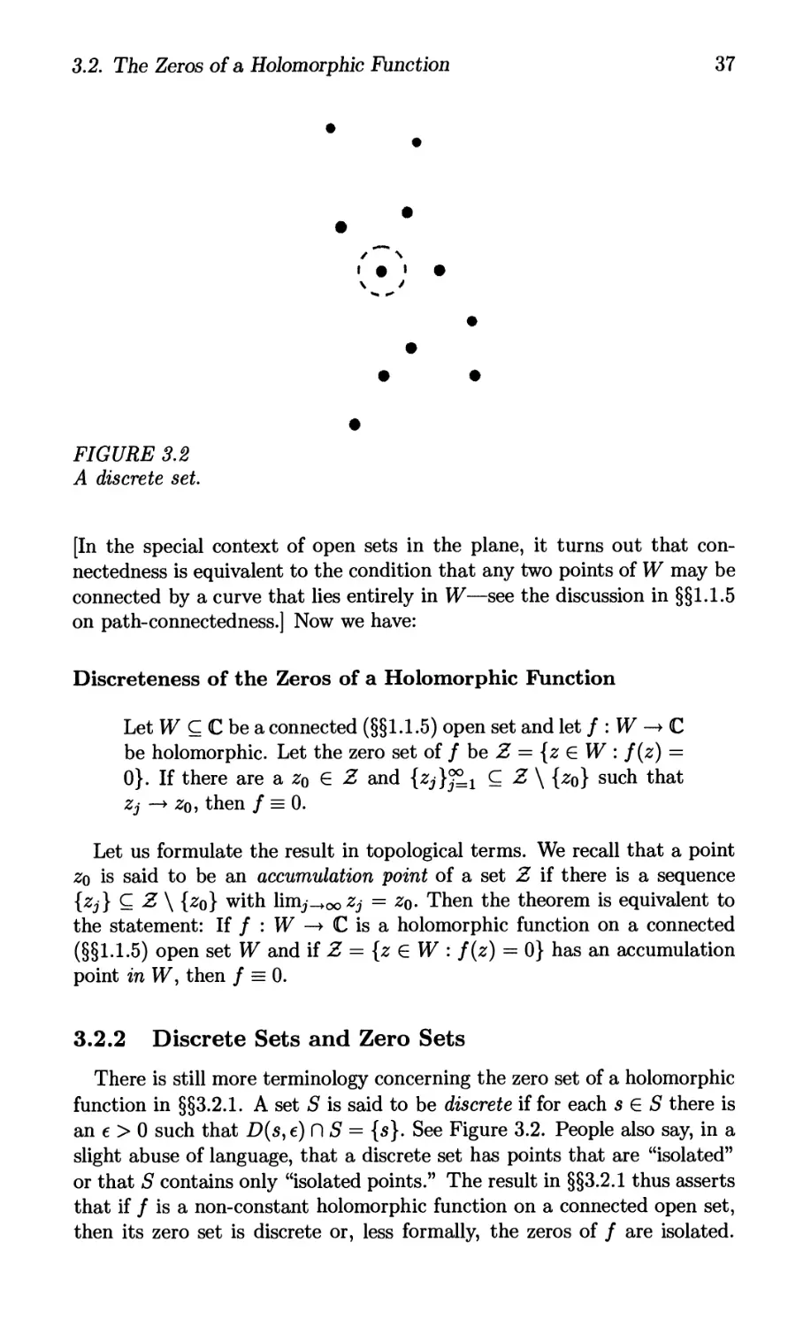
3.2.2 Discrete Sets and Zero Sets 37
3.2.3 Uniqueness of Analytic Continuation 38
4 Isolated Singularities and Laurent Series 41
4.1 The Behavior of a Hoiomorphic Function near an
Isolated Singularity 41
4.1.1 Isolated Singularities 41
4.1.2 A Hoiomorphic Function on a
Punctured Domain 41
4.1.3 Classification of Singularities 41
4.1.4 Removable Singularities, Poles, and
Essential Singularities 42
4.1.5 The Riemann Removable
Singularities Theorem 42
4.1.6 The Casorati-Weierstrass Theorem 43
4.2 Expansion around Singular Points 43
4.2.1 Laurent Series 43
4.2.2 Convergence of a Doubly Infinite Series 43
4.2.3 Annulus of Convergence 44
4.2.4 Uniqueness of the Laurent Expansion 44
4.2.5 The Cauchy Integral Formula for an Annulus ... 45
4.2.6 Existence of Laurent Expansions 45
4.2.7 Hoiomorphic Functions with Isolated
Singularities 45
4.2.8 Classification of Singularities in Terms of
Laurent Series 46
4.3 Examples of Laurent Expansions 46
4.3.1 Principal Part of a Function 46
4.3.2 Algorithm for Calculating the Coefficients of the
Laurent Expansion 48
4.4 The Calculus of Residues 48
4.4.1 Functions with Multiple Singularities 48
4.4.2 The Residue Theorem 48
4.4.3 Residues 49
4.4.4 The Index or Winding Number of a Curve
about a Point 49
4.4.5 Restatement of the Residue Theorem 50
4.4.6 Method for Calculating Residues 50
4.4.7 Summary Charts of Laurent Series and Residues . 51
4.5 Applications to the Calculation of Definite
Integrals and Sums 51
4.5.1 The Evaluation of Definite Integrals 51
4.5.2 A Basic Example 52
4.5.3 Complexification of the Integrand 54

4.5.4 An Example with a More Subtle Choice
of Contour 56
4.5.5 Making the Spurious Part of the
Integral Disappear 58
4.5.6 The Use of the Logarithm 60
4.5.7 Summing a Series Using Residues 62
4.5.8 Summary Chart of Some
Integration Techniques 63
4.6 Meromorphic Functions and Singularities at
Infinity 63
4.6.1 Meromorphic Functions 63
4.6.2 Discrete Sets and Isolated Points 63
4.6.3 Definition of Meromorphic Function 64
4.6.4 Examples of Meromorphic Functions 64
4.6.5 Meromorphic Functions with Infinitely
Many Poles 66
4.6.6 Singularities at Infinity 66
4.6.7 The Laurent Expansion at Infinity 67
4.6.8 Meromorphic at Infinity 67
4.6.9 Meromorphic Functions in the
Extended Plane 67
The Argument Principle 69
5.1 Counting Zeros and Poles 69
5.1.1 Local Geometric Behavior of a
Holomorphic Function 69
5.1.2 Locating the Zeros of a Holomorphic Function . . 69
5.1.3 Zero of Order n 70
5.1.4 Counting the Zeros of a Holomorphic Function . . 70
5.1.5 The Argument Principle 71
5.1.6 Location of Poles 72
5.1.7 The Argument Principle for
Meromorphic Functions 72
5.2 The Local Geometry of Holomorphic Functions 73
5.2.1 The Open Mapping Theorem 73
5.3 Further Results on the Zeros of Holomorphic Functions . . 74
5.3.1 Rouche's Theorem 74
5.3.2 Typical Application of Rouche's Theorem .... 74
5.3.3 Rouche's Theorem and the Fundamental
Theorem of Algebra 75
5.3.4 Hurwitz's Theorem 76
5.4 The Maximum Principle 76
5.4.1 The Maximum Modulus Principle 76
5.4.2 Boundary Maximum Modulus Theorem 76

Contents xi
5.4.3 The Minimum Principle 77
5.4.4 The Maximum Principle on an
Unbounded Domain 77
5.5 The Schwarz Lemma 77
5.5.1 Schwarz's Lemma 78
5.5.2 The Schwarz-Pick Lemma 78
6 The Geometric Theory of Holomorphic Functions 79
6.1 The Idea of a Conformal Mapping 79
6.1.1 Conformal Mappings 79
6.1.2 Conformal Self-Maps of the Plane 79
6.2 Conformal Mappings of the Unit Disc 80
6.2.1 Conformal Self-Maps of the Disc 80
6.2.2 Mobius Transformations 81
6.2.3 Self-Maps of the Disc 81
6.3 Linear Fractional Transformations 81
6.3.1 Linear Fractional Mappings 81
6.3.2 The Topology of the Extended Plane 83
6.3.3 The Riemann Sphere 83
6.3.4 Conformal Self-Maps of the Riemann Sphere ... 84
6.3.5 The Cayley Transform 85
6.3.6 Generalized Circles and Lines 85
6.3.7 The Cayley Transform Revisited 85
6.3.8 Summary Chart of Linear
Fractional Transformations 85
6.4 The Riemann Mapping Theorem 86
6.4.1 The Concept of Homeomorphism 86
6.4.2 The Riemann Mapping Theorem 86
6.4.3 The Riemann Mapping Theorem:
Second Formulation 87
6.5 Conformal Mappings of Annuli 87
6.5.1 A Riemann Mapping Theorem for Annuli 87
6.5.2 Conformal Equivalence of Annuli 87
6.5.3 Classification of Planar Domains 88
7 Harmonic Functions 89
7.1 Basic Properties of Harmonic Functions 89
7.1.1 The Laplace Equation 89
7.1.2 Definition of Harmonic Function 89
7.1.3 Real- and Complex-Valued
Harmonic Functions 89
7.1.4 Harmonic Functions as the Real Parts of
Holomorphic Functions 90
7.1.5 Smoothness of Harmonic Functions 90

7.2 The Maximum Principle and the Mean Value
Property 91
7.2.1 The Maximum Principle for
Harmonic Functions 91
7.2.2 The Minimum Principle for
Harmonic Functions 91
7.2.3 The Boundary Maximum and
Minimum Principles 91
7.2.4 The Mean Value Property 92
7.2.5 Boundary Uniqueness for Harmonic Functions . . 92
7.3 The Poisson Integral Formula 92
7.3.1 The Poisson Integral 92
7.3.2 The Poisson Kernel 93
7.3.3 The Dirichlet Problem 93
7.3.4 The Solution of the Dirichlet Problem
on the Disc 93
7.3.5 The Dirichlet Problem on a General Disc 94
7.4 Regularity of Harmonic Functions 94
7.4.1 The Mean Value Property on Circles 94
7.4.2 The Limit of a Sequence of Harmonic Functions . 95
7.5 The Schwarz Reflection Principle 95
7.5.1 Reflection of Harmonic Functions 95
7.5.2 Schwarz Reflection Principle for
Harmonic Functions 95
7.5.3 The Schwarz Reflection Principle for
Holomorphic Functions 96
7.5.4 More General Versions of the Schwarz
Reflection Principle 96
7.6 Harnack's Principle 97
7.6.1 The Harnack Inequality 97
7.6.2 Harnack's Principle 97
7.7 The Dirichlet Problem and Subharmonic
Functions 97
7.7.1 The Dirichlet Problem 97
7.7.2 Conditions for Solving the Dirichlet Problem ... 98
7.7.3 Motivation for Subharmonic Functions 98
7.7.4 Definition of Subharmonic Function 99
7.7.5 Other Characterizations of
Subharmonic Functions 99
7.7.6 The Maximum Principle 100
7.7.7 Lack of A Minimum Principle 100
7.7.8 Basic Properties of Subharmonic Functions .... 100
7.7.9 The Concept of a Barrier 100
7.8 The General Solution of the Dirichlet Problem 101

Contents xiii
7.8.1 Enunciation of the Solution of the
Dirichlet Problem 101
8 Infinite Series and Products 103
8.1 Basic Concepts Concerning Infinite Sums and
Products 103
8.1.1 Uniform Convergence of a Sequence 103
8.1.2 The Cauchy Condition for a Sequence
of Functions 103
8.1.3 Normal Convergence of a Sequence 103
8.1.4 Normal Convergence of a Series 104
8.1.5 The Cauchy Condition for a Series 104
8.1.6 The Concept of an Infinite Product 104
8.1.7 Infinite Products of Scalars 105
8.1.8 Partial Products 105
8.1.9 Convergence of an Infinite Product 105
8.1.10 The Value of an Infinite Product 106
8.1.11 Products That Are Disallowed 106
8.1.12 Condition for Convergence of an
Infinite Product 106
8.1.13 Infinite Products of Holomorphic Functions .... 107
8.1.14 Vanishing of an Infinite Product 108
8.1.15 Uniform Convergence of an Infinite Product
of Functions 108
8.1.16 Condition for the Uniform Convergence of an
Infinite Product of Functions 108
8.2 The Weierstrass Factorization Theorem 109
8.2.1 Prologue 109
8.2.2 Weierstrass Factors 109
8.2.3 Convergence of the Weierstrass Product 110
8.2.4 Existence of an Entire Function with
Prescribed Zeros 110
8.2.5 The Weierstrass Factorization Theorem 110
8.3 The Theorems of Weierstrass and
Mittag-Leffler 110
8.3.1 The Concept of Weierstrass's Theorem 110
8.3.2 Weierstrass's Theorem Ill
8.3.3 Construction of a Discrete Set Ill
8.3.4 Domains of Existence for
Holomorphic Functions 112
8.3.5 The Field Generated by the Ring of
Holomorphic Functions 112
8.3.6 The Mittag-Leffler Theorem 112
8.3.7 Prescribing Principal Parts 113

xiv
8.4 Normal Families 113
8.4.1 Normal Convergence 113
8.4.2 Normal Families 114
8.4.3 Montel's Theorem, First Version 114
8.4.4 Montel's Theorem, Second Version 114
8.4.5 Examples of Normal Families 114
9 Applications of Infinite Sums and Products 117
9.1 Jensen's Formula and an Introduction to
Blaschke Products 117
9.1.1 Blashke Factors 117
9.1.2 Jensen's Formula 117
9.1.3 Jensen's Inequality 118
9.1.4 Zeros of a Bounded Holomorphic Function .... 118
9.1.5 The Blaschke Condition 118
9.1.6 Blaschke Products 119
9.1.7 Blaschke Factorization 119
9.2 The Hadamard Gap Theorem 119
9.2.1 The Technique of Ostrowski 119
9.2.2 The Ostrowski-Hadamard Gap Theorem 119
9.3 Entire Functions of Finite Order 120
9.3.1 Rate of Growth and Zero Set 120
9.3.2 Finite Order 121
9.3.3 Finite Order and the Exponential Term
of Weierstrass 121
9.3.4 Weierstrass Canonical Products 121
9.3.5 The Hadamard Factorization Theorem 121
9.3.6 Value Distribution Theory 122
10 Analytic Continuation 123
10.1 Definition of an Analytic Function Element 123
10.1.1 Continuation of Holomorphic Functions 123
10.1.2 Examples of Analytic Continuation 123
10.1.3 Function Elements 128
10.1.4 Direct Analytic Continuation 128
10.1.5 Analytic Continuation of a Function 128
10.1.6 Global Analytic Functions 129
10.1.7 An Example of Analytic Continuation 130
10.2 Analytic Continuation along a Curve 130
10.2.1 Continuation on a Curve 130
10.2.2 Uniqueness of Continuation along a Curve .... 131
10.3 The Monodromy Theorem 131
10.3.1 Unambiguity of Analytic Continuation 132
10.3.2 The Concept of Homotopy 132

Contents xv
10.3.3 Fixed Endpoint Homotopy 133
10.3.4 Unrestricted Continuation 134
10.3.5 The Monodromy Theorem 134
10.3.6 Monodromy and Globally Defined
Analytic Functions 134
10.4 The Idea of a Riemann Surface 135
10.4.1 What is a Riemann Surface? 135
10.4.2 Examples of Riemann Surfaces 135
10.4.3 The Riemann Surface for the Square
Root Function 137
10.4.4 Holomorphic Functions on a Riemann Surface . . 137
10.4.5 The Riemann Surface for the Logarithm 138
10.4.6 Riemann Surfaces in General 139
10.5 Picard's Theorems 140
10.5.1 Value Distribution for Entire Functions 140
10.5.2 Picard's Little Theorem 140
10.5.3 Picard's Great Theorem 140
10.5.4 The Little Theorem, the Great Theorem, and
the Casorati-Weierstrass Theorem 140
11 Rational Approximation Theory 143
11.1 Runge's Theorem 143
11.1.1 Approximation by Rational Functions 143
11.1.2 Runge's Theorem 143
11.1.3 Approximation by Polynomials 144
11.1.4 Applications of Runge's Theorem 144
11.2 Mergelyan's Theorem 146
11.2.1 An Improvement of Runge's Theorem 146
11.2.2 A Special Case of Mergelyan's Theorem 146
11.2.3 Generalized Mergelyan Theorem 147
12 Special Classes of Holomorphic Functions 149
12.1 Schlicht Functions and the Bieberbach
Conjecture 149
12.1.1 Schlicht Functions 149
12.1.2 The Bieberbach Conjecture 149
12.1.3 The Lusin Area Integral 150
12.1.4 The Area Principle 150
12.1.5 The Kobe 1/4 Theorem 150
12.2 Extension to the Boundary of Conformal
Mappings 151
12.2.1 Boundary Continuation 151
12.2.2 Some Examples Concerning
Boundary Continuation 151

12.3 Hardy Spaces 152
12.3.1 The Definition of Hardy Spaces 152
12.3.2 The Blaschke Factorization for H°° 153
12.3.3 Monotonicity of the Hardy Space Norm 153
12.3.4 Containment Relations among
Hardy Spaces 153
12.3.5 The Zeros of Hardy Functions 153
12.3.6 The Blaschke Factorization for Hp Functions . . . 154
13 Special Functions 155
13.0 Introduction 155
13.1 The Gamma and Beta Functions 155
13.1.1 Definition of the Gamma Function 155
13.1.2 Recursive Identity for the Gamma Function .... 156
13.1.3 Holomorphicity of the Gamma Function 156
13.1.4 Analytic Continuation of the Gamma Function . . 156
13.1.5 Product Formula for the Gamma Function .... 156
13.1.6 Non-Vanishing of the Gamma Function 156
13.1.7 The Euler-Mascheroni Constant 156
13.1.8 Formula for the Reciprocal of the
Gamma Function 157
13.1.9 Convexity of the Gamma Function 157
13.1.10 The Bohr-Mollerup Theorem 157
13.1.11 The Beta Function 157
13.1.12 Symmetry of the Beta Function 158
13.1.13 Relation of the Beta Function to the
Gamma Function 158
13.1.14 Integral Representation of the Beta Function ... 158
13.2 Riemann's Zeta Function 158
13.2.1 Definition of the Zeta Function 158
13.2.2 The Euler Product Formula 158
13.2.3 Relation of the Zeta Function to the
Gamma Function 159
13.2.4 The Hankel Contour and Hankel Functions .... 159
13.2.5 Expression of the Zeta Function as a
Hankel Integral 160
13.2.6 Location of the Pole of the Zeta Function 160
13.2.7 The Functional Equation 160
13.2.8 Zeros of the Zeta Function 161
13.2.9 The Riemann Hypothesis 161
13.2.10 The Lambda Function 161
13.2.11 Relation of the Zeta Function to the
Lambda Function 161
13.2.12 More on the Zeros of the Zeta Function 162

Contents
xvn
13.2.13 Zeros of the Zeta Function and the Boundary
of the Critical Strip 162
13.3 Some Counting Functions and a Few Technical Lemmas . . 162
13.3.1 The Counting Functions of Classical
Number Theory 162
13.3.2 The Function 7T 162
13.3.3 The Prime Number Theorem 162
14 Applications that Depend on Conformal Mapping 163
14.1 Conformal Mapping 163
14.1.1 A List of Useful Conformal Mappings 163
14.2 Application of Conformal Mapping to the
Dirichlet Problem 164
14.2.1 The Dirichlet Problem 164
14.2.2 Physical Motivation for the Dirichlet Problem . . 164
14.3 Physical Examples Solved by Means of
Conformal Mapping 168
14.3.1 Steady State Heat Distribution on a
Lens-Shaped Region 169
14.3.2 Electrostatics on a Disc 170
14.3.3 Incompressible Fluid Flow around a Post 172
14.4 Numerical Techniques of Conformal Mapping 175
14.4.1 Numerical Approximation of the
Schwarz-ChristofFel Mapping 175
14.4.2 Numerical Approximation to a Mapping onto a
Smooth Domain 179
Appendix to Chapter 14: A Pictorial Catalog
of Conformal Maps 181
15 Transform Theory 195
15.0 Introductory Remarks 195
15.1 Fourier Series 195
15.1.1 Basic Definitions 195
15.1.2 A Remark on Intervals of Arbitrary Length .... 196
15.1.3 Calculating Fourier Coefficients 197
15.1.4 Calculating Fourier Coefficients Using
Complex Analysis 198
15.1.5 Steady State Heat Distribution 199
15.1.6 The Derivative and Fourier Series 201
15.2 The Fourier Transform 202
15.2.1 Basic Definitions 202
15.2.2 Some Fourier Transform Examples that Use
Complex Variables 203

xviii Contents
15.2.3 Solving a Differential Equation Using the
Fourier Transform 210
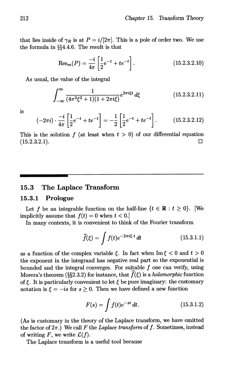
15.3 The Laplace Transform 212
15.3.1 Prologue 212
15.3.2 Solving a Differential Equation Using the
Laplace Transform 213
15.4 The ^-Transform 214
15.4.1 Basic Definitions 214
15.4.2 Population Growth by Means of the
^-Transform 215
16 Computer Packages for Studying Complex Variables 219
16.0 Introductory Remarks 219
16.1 The Software Packages 219
16.1.1 The Software /(*)® 219
16.1.2 Mathematical 221
16.1.3 Maple® 227
16.1.4 MatLab® 229
16.1.5 Ricci® 229
Glossary of Terms from Complex Variable Theory
and Analysis 231
List of Notation 269
Table of Laplace Transforms 273
A Guide to the Literature 275
References 279
Index 283

Preface
This book is written to be a convenient reference for the working scientist,
student, or engineer who needs to know and use basic concepts in complex
analysis. It is not a book of mathematical theory. It is instead a book of
mathematical practice.
All the basic ideas of complex analysis, as well as many typical
applications, are treated. Since we are not developing theory and proofs, we have
not been obliged to conform to a strict logical ordering of topics. Instead,
topics have been organized for ease of reference, so that cognate topics
appear in one place.
Required background for reading the text is minimal: a good
grounding in (real variable) calculus will suffice. However, the reader who gets
maximum utility from the book will be that reader who has had a course
in complex analysis at some time in his life. This book is a handy
compendium of all basic facts about complex variable theory. But it is not a
textbook, and a person would be hard put to endeavor to learn the subject
by reading this book.
Understanding that many readers are not primary users of mathematics,
we have included an extensive glossary and table of notation. The glossary
contains not only all the major terminology of complex variable theory but
also background terminology such as "uniform convergence," "equivalence
class," "compact set," and "accumulation point." We have also included a
complete List of Notation, a Table of Laplace Transforms, and a Guide to
the Literature. The latter is a list of some of the major works in complex
analysis, grouped by type. The book concludes with a References section
and a rather thorough Index.
We have made every effort to give thorough references for all topics.
These references provide further reading, theory, proofs, and exercises.
The notation used in this book is quite standard in the mathematical
world. But the reader should be aware that certain specialized fields have
their own particular notation. For example, electrical engineering uses the
letter j to denote the square root of —1, whereas mathematicians use the
letter i for this purpose. We leave it to the reader to make whatever small
adaptations are necessary to render the contents of this book consistent
with his particular field; we would be doing the reader a disservice to
introduce all possible notational variants.
In order to make the book as easy to use and as self-contained as
possible, we have occasionally repeated topics or formulas. Surely it is more
convenient for readers to have the necessary formula right on the page they
xzx

XX
Preface
are reading than to be flipping back and forth among several disparate
pages. Readers will also find the extensive cross-referencing to be useful.
Because we view the typical reader of this book as one who is interested in
applications of complex functions, we have made a special eflFort to include
material on areas of engineering and physics in which complex variable
theory is applied. This discussion is gathered at the end of the book, in
Chapters 14 and 15.
The book concludes (Chapter 16) with a brief discussion of software that
is useful for understanding concepts from complex variable theory.
We hope that this book will be a valuable tool for the mathematical
scientist.
It is a pleasure to thank the many friends and colleagues who made this
book possible. Ken Rosen first piqued my interest in writing a handbook.
My editor, Wayne Yuhasz, guided me through every step of the process
of writing the book and provided technical support when necessary. Sean
Davey and Clovis Tondo contributed their T^jXpertise. Lynn Apfel gave
me some useful ideas about charts and tables.
Special thanks go to Kitty Laird, who put in untold hours rendering
figures with Corel Draw. I am grateful to George Kamberov and to Stanley
Sawyer, who patiently taught me how to incorporate graphics into a T£}X
document. Finally, I thank Louise Farkas for her splendid copyediting.
Without all these good people, this book could never have been completed
in its present form.
Responsibility for all extant shortcomings in the text is mine alone.
Suggestions for improvement, or identification of errata, are always
appreciated.
St. Louis, Missouri
Steven G. Krantz

List of Figures
1.1 A point in the plane. 2
1.2 Distance to the origin or modulus. 3
1.3 An open disc and a closed disc. 4
1.4 An open set. 4
1.5 An open set and a non-open set. 5
1.6 A set that is neither open nor closed. 5
1.7 A connected set and a disconnected set. 6
1.8 An open set is connected if and only if it is
path-connected. 7
1.9 Polar coordinates of a point in the plane. 9
1.10 The point may approach P arbitrarily. 15
2.1 Two curves in the plane, one closed. 20
2.2 A simple, closed curve. 20
2.3 A curve on which the Cauchy integral theorem is valid. 27
2.4 The Cauchy integral formula. 28
2.5 Deformability of curves. 29
3.1 A compact set is closed and bounded. 34
3.2 A discrete set. 37
3.3 A zero set with a boundary accumulation point. 38
3.4 The principle of persistence of functional relations. 39
4.1 A punctured domain. 42
4.2 A pole at P. 47
4.3 Examples of the index of a curve. 50
4.4 The curve ^r in Subsection 4.5.2. 53
4.5 The curve ^r in Subsection 4.5.3. 55
4.6 The curve ^r in Subsection 4.5.4. 56
4.7 The curve fiR in Subsection 4.5.4. 57
4.8 The curve jj,r in Subsection 4.5.5. 59
4.9 The curve t)r in Subsection 4.5.6. 61
4.10 The curve Tn in Subsection 4.5.7. 63
xxz

XXII
List of Figures
5.1 Locating the zeros of a holomorphic function. 71
5.2 The argument principle: counting the zeros. 72
5.3 The open mapping principle. 73
5.4 Rouche's theorem. 75
6.1 Stereographic projection. 84
7.1 Schwarz reflection. 96
7.2 A convex function. 99
7.3 Smooth boundary means a barrier at each point
of the boundary. 101
8.1 A discrete set A inside U. Ill
9.1 The point P is regular for /. 120
10.1 Analytic continuation to a second disc. 126
10.2 Analytic continuation to a third disc. 126
10.3 Defining the square root function at —1. 127
10.4 Analytic continuation in the other direction. 127
10.5 The function element (#, V) is a direct analytic
continuation of (/, U). 128
10.6 The function element (/&, Uk) is an analytic
continuation of (/i, U\). 129
10.7 Analytic continuation along a curve. 131
10.8 Details of analytic continuation along a curve. 132
10.9 The concept of homotopy. 133
10.10 The monodromy theorem. 134
10.11 The Riemann surface for the square root of z. 137
10.12 The joins in the Riemann surface for the square root
of z. 137
10.13 The Riemann surface for the nth root of z. 138
10.14 The Riemann surface for log z. 139
11.1 The region Kk in Example 11.1.4.1. 144
11.2 The region Kk in Example 11.1.4.2. 146
13.1 The Hankel contour. 159
13.2 The region bounded by Cei, Ce2 contains no poles of u. 160
14.1 Heat distribution on the edge of a metal plate. 165
14.2 Electrostatic potential illustrated with a split cylinder. 165
14.3 The cylindrical halves separated with
insulating material. 166
14.4 Distribution of the electrostatic potential. 166
14.5 A lens-shaped piece of heat-conducting metal. 169
14.6 The angular region in the w-plane that is the image of the
lens-shaped region in the z-plane. 170
14.7 Conformal map of the disc to the upper half-plane. 171
14.8 Incompressible fluid flow with a circular obstacle. 173
14.9 Restriction of attention to the flow in the
upper half-plane. 174
14.10 Conformal map of the region of the flow to the upper
half-plane. 174

List of Figures
xxiii
14.11 An airfoil. 176
14.12 Mapping the upper half-plane to a polygonal region. 177
14.13 Vertices, pre-vertices, and right-turn angles. 177
14.14 (top) Map of the disc to its complement; (middle) Map of the
disc to the disc; (bottom) Map of the upper half-disc to the
first quadrant. 182
14.15 (top) The Cayley transform: A map of the disc to the
upper half-plane; (middle) Map of a cone to a half-strip;
(bottom) Map of a cone to the upper half plane. 183
14.16 (top) Map of a strip to the disc; (middle) Map of a half-strip
to the disc; (bottom) Map of a half-strip to the upper
half-plane. 184
14.17 (a) Map of the disc to a strip; (b) Map of an annular
sector to the interior of a rectangle; (c) Map of a
half-annulus to the interior of a half-ellipse. 185
14.18 (top) Map of the upper half-plane to a 3/4-plane; (middle)
Map of a strip to an annulus; (bottom) Map of a strip
to the upper half-plane. 186
14.19 (top) Map of a disc to a quadrant; (middle) Map of the
complement of two discs to an annulus; (bottom) Map
of the interior of a rectangle to a half-annulus. 187
14.20 (top) Map of a half-disc to a strip; (middle) Map of a disc to a
strip; (bottom) Map of the inside of a parabola to a disc. 188
14.21 (top) Map of a half-disc to a disc; (middle) Map of the slotted
upper half-plane to upper half-plane; (bottom) Map of the
double-sliced plane to the upper half-plane. 189
14.22 (top) Map of a strip to the double-sliced plane; (middle) Map
of the disc to a cone; (bottom) Map of a disc to the
complement of a disc. 190
14.23 (top) Map of a half-strip to a half-quadrant; (middle) Map
of the upper half-plane to a right-angle region; (bottom)
Map of the upper half-plane to the plane less a half-strip. 191
14.24 (top) Map of a disc to the complement of an ellipse;
(middle) Map of a disc to the interior of a cardioid;
(bottom) Map of a disc to the region outside a parabola. 192
14.25 (top) Map of the disc to the slotted plane; (middle) Map of the
upper half-plane to the interior of a triangle; (bottom) Map
of the upper half-plane to the interior of a rectangle. 193
14.26 The Schwarz-Christoffel formula. 194
15.1 Identification of the interval with the circle. 196
15.2 Mathematical model of the disc. 199
15.3 A positively oriented semicircle ^r in the lower
half-plane. 204
15.4 A positively oriented semicircle in the upper half-plane. 205
15.5 The curve 7^. 208

xxiv
List of Figures
15.6 The curve ^R. 209
15.7 The contour used to analyze the integral in (15.2.3.2.8). 211
16.1 The image in the plane of circular level curves under ez. 221
16.2 The image in the Riemann sphere of circular level
curves under ez. 222
16.3 The graph in 3-space of circular level curves acted on
by ez. 222
16.4 The image in the plane of circular level curves under z2. 223
16.5 The image in the Riemann sphere of circular level
curves under z2. 223
16.6 The graph in 4-space of circular level curves
acted on by z2. 224
16.7 The image in the plane of a rectangular grid under ez. 224
16.8 The image in the Riemann sphere of a rectangular
grid under z2. 225
16.9 The graph in 4-space of a rectangular grid acted
on by zs - 3z2 4- z - 2. 225
16.10 The image in the plane of a rectangular grid under log z. 226
16.11 The image in the Riemann sphere of a rectangular
grid under log z. 226
16.12 The graph in 4-space of a rectangular grid acted
on by log z. 227

Chapter 1
The Complex Plane
1.1 Complex Arithmetic
1.1.1 The Real Numbers
The real number system consists of both the rational numbers (numbers
with terminating or repeating decimal expansions) and the irrational
numbers (numbers with infinite, non-repeating decimal expansions). The real
numbers are denoted by the symbol R. We let R2 = {(x, y) : x G R , y G R}
(Figure 1.1).
1.1.2 The Complex Numbers
The complex numbers C consist of K2 equipped with some special
algebraic operations. One defines
(z, y) + (x\ yf) = (x + x\ y + yf),
(x, y) • (x\ y') = (xx' - yy\ xy' + yx').
These operations of + and • are commutative and associative.
We denote (1,0) by 1 and (0,1) by i. If a G M, then we identify a with
the complex number (a, 0). Using this notation, we see that
a • (z, y) = (a, 0) • (z, y) = (ax, ay). (1.1.2.1)
Thus every complex number (#, y) can be written in one and only one
fashion in the form x-l+y-i with #, y G R. We usually write the number
even more succinctly as x + iy. The laws of addition and multiplication
become
(x + iy) + {x' + iy') = (x + x') + i(y + y'),
(x + iy) • (x' + iy') = (xx' - yy') + i(xy' + yx').
1

Chapter 1. The Complex Plane
i
(x,y)
•
FIGURE LI
A point in the plane.
Observe that i • i = —1. Finally, the multiplication law is consistent with
the scalar multiplication introduced in line (1.1.2.1).
The symbols z, w, £ are frequently used to denote complex numbers. We
usually take z — x -\- iy ^ w — u + iv , C = £ + ^7- The real number x
is called the real part of z and is written x = Rez. The real number y is
called the imaginary part of z and is written y = Im z.
The complex number x — iy is by definition the complex conjugate of the
complex number x -\-iy. If z = x + iy, then we denote the conjugate of z
with the symbol ~z\ thus ~z = x — iy.
1.1.3 Complex Conjugate
Note that z + z = 2#, z — ~z — 2iy. Also
Y^Tw = z + w, (1.1.3.1)
T^w = z-w. (1.1.3.2)
A complex number is real (has no imaginary part) if and only if z = H. It
is imaginary (has no real part) if and only if z = —z.
1.1.4 Modulus of a Complex Number
The ordinary Euclidean distance of (z, y) to (0,0) is y/x2 + y2 (Figure
1.2). We also call this number the modulus of the complex number z = x+iy
and we write \z\ = y/x2 + y2. Note that
z-z = x2 + y2 = \z\2.
The distance from z to w is \z—w\. We also have the formulas \z-w\ = \z\-\w\
and |Rez| < \z\ and |Im^| < \z\.

1.1. Complex Arithmetic
3
fry) '
2 + y2 \
k
w
FIGURE 1.2
Distance to the origin or modulus.
1.1.5 The Topology of the Complex Plane
If P is a complex number and r > 0, then we set
D(P, r) = {z G C : \z - P\ < r} (1.1.5.1)
and
D(P,r) = {zeC:\z-P\<r}. (1.1.5.2)
The first of these is the open disc with center P and radius r; the second
is the closed disc with center P and radius r (Figure 1.3). We often use
the simpler symbols D and D to denote, respectively, the discs D(0,1) and
£(o,i).
We say that a set U C C is open if, for each P G C, there is an r > 0
such that D(P, r) C U. Thus an open set is one with the property that
each point P of the set is surrounded by neighboring points that are still
in the set (that is, the points of distance less than r from P)—see Figure
1.4. Of course the number r will depend on P. As examples, U = {z eC:
Rez > 1} is open, but F = {z G C : Re 2 < 1} is not (Figure 1.5).
A set E C C is said to be closed if C \ E = {z G C : z £ E} (the
complement of E in C) is open. The set F in the last paragraph is closed.
It is not the case that any given set is either open or closed. For example,
the set W = {z G C : 1 < Rez < 2} is neither open nor closed (Figure
1.6).
We say that a set E C C is connected if there do not exist non-empty
disjoint open sets U and V such that E = (U D E) U (V D E). Refer to
Figure 1.7 for these ideas. It is a useful fact that if E is an open set, then
E is connected if and only if it is path-connected; this means that any two
points of E can be connected by a continuous path or curve. See Figure
1.8.

4
Chapter 1. The Complex Plane
P ; D(P,r)
FIGURE 1.3
An open disc and a closed disc.
D(Rr)
■* u
\ IXRr) \
P /
FIGURE 1.4
An open set.

1.1. Complex Arithmetic
5
f — I z:Re z <
FIGURE 1.5
An open set and a non-open set.
FIGURE 1.6
A set that is neither open nor closed.

6
Chapter 1. The Complex Plane
E; y
FIGURE 1.7
A connected set and a disconnected set.
1.1.6 The Complex Numbers as a Field
Let 0 denote the number 0 + iO. If z G C, then z + 0 = z. Also, letting
—z = — x — iy, we have z + (—z) = 0. So every complex number has an
additive inverse, and that inverse is unique.
Since 1 = 1 +i0, it follows that 1 • z = z • 1 = z for every complex number
z. If z 7^0, then \z\2 ^ 0 and
1. (1.1.6.1)
So every non-zero complex number has a multiplicative inverse, and that
inverse is unique. It is natural to define \/z to be the multiplicative inverse
z/|z|2 of z and, more generally, to define
1=Z.L= ^L forw^O. (1.1.6.2)
w w \w\2
We also have z/w = ~zjw.
Multiplication and addition satisfy the usual distributive, associative,
and commutative laws. Therefore C is a field (see [HER]). The field C
contains a copy of the real numbers in an obvious way:
RBx^x + iOeC.
(1.1.6.3)

1.2. The Exponential and Applications
7
A
X
FIGURE 1.8
An open set is connected if and only if it is path-connected.
This identification respects addition and multiplication. So we can think
of C as a field extension of R: it is a larger field which contains the field JR.
1.1.7 The Fundamental Theorem of Algebra
It is not true that every non-constant polynomial with real coefficients
has a real root. For instance, p(x) = x2 + 1 has no real roots. The
Fundamental Theorem of Algebra states that every polynomial with complex
coefficients has a complex root (see the treatment in §§3.1.4 below). The
complex field C is the smallest field that contains R and has this so-called
algebraic closure property.
1.2 The Exponential and Applications
1.2.1 The Exponential Function
We define the complex exponential as follows:
(1.2.1.1) If z = x is real, then
OO A
as in calculus. Here ! denotes "factorial": j\ = j • (j — 1) • (j — 2) • • • 3 •
2-1.

8 Chapter 1. The Complex Plane
(1.2.1.2) If z = iy is pure imaginary, then
ez = ety = cos y + i sin y.
(1.2.1.3) If z = x + iy, then
ez = ex+iy = ex • ei2/ = ex • (cos y + isiny).
Part and parcel of the last definition of the exponential is the following
complex-analytic definition of the sine and cosine functions:
cosz = —±- , (1.2.1.4)
eiz — e~iz
sinz = . (1.2.1.5)
Note that when z = x + iO is real this new definition coincides with the
familiar Euler formula from calculus:
etx = cosx + isinx. (1.2.1.6)
1.2.2 The Exponential Using Power Series
It is also possible to define the exponential using power series:
OO A
V—N ZJ
e
= Zzii- (i-2-2-1)
7
Either definition (that in §§1.2.1 or in §§1.2.2) is correct for any z, and they
are logically equivalent.
1.2.3 Laws of Exponentiation
The complex exponential satisfies familiar rules of exponentiation:
ez+w = ez-ew and (ez)w = ezw. (1.2.3.1)
Also
(e*)n = e*..-e* = enz. (1.2.3.2)
n times
1.2.4 Polar Form of a Complex Number
A consequence of our first definition of the complex exponential —see
(1.2.1.2)—is that if £ E C, \C\ = 1, then there is a unique number 0,

1.2. The Exponential and Applications
FIGURE 1.9
Polar coordinates of a point in the plane.
0 < 6 < 27T, such that £ = e10 (see Figure 1.9). Here 6 is the (signed) angle
between the positive x axis and the ray 0£.
Now if z is any non-zero complex number, then
•(a)-
*!•<
(1.2.4.1)
where £ = z/\z\ has modulus 1. Again letting 9 be the angle between the
real axis and 0£, we see that
z=\z\-{
= \z\ei0
re
%e
(1.2.4.2)
where r = \z\. This form is called the polar representation for the
complex number z. (Note that some classical books write the expression
z = re10 = r(cos# + isin#) as z = rcis#. The reader should be aware of
this notation, though we shall not use it in this book.)
EXAMPLE 1.2.4.1 Let z = 1 + V^. Then \z\ = y/l2 + (>/3)2 = 2.
Hence
(!*'*)
z = 2>\- +i^z-
The number in parenthesis subtends an angle of 7r/3 with the positive x-
axis. Therefore
1 + y/Zi = z = 2 • e™/z. D

10
Chapter 1. The Complex Plane
It is often convenient to allow angles that are greater than or equal to
2n in the polar representation; when we do so, the polar representation is
no longer unique. For if k is an integer, then
eie = cos 9 + i sin 0 = cos(0 + 2kn) + i sin(0 + 2kir)
= ei(0+2k*)t (1.2.4.3)
1.2.5 Roots of Complex Numbers
The properties of the exponential operation can be used to find the nth
roots of a complex number.
EXAMPLE 1.2.5.1 To find all sixth roots of 2, we let reie be an
arbitrary sixth root of 2 and solve for r and 6. If
(reie)6 = 2 = 2-ei0 (1.2.5.1.1)
or
r6em = 2 • ei0 , (1.2.5.1.2)
then it follows that r = 21/6 G M and 0 = 0 solve this equation. So the
real number 21/6 • ei0 = 21/6 is a sixth root of two. This is not terribly
surprising, but we are not finished.
We may also solve
r6em = 2 = 2 • e27ri. (1.2.5.1.3)
Hence
r = 21/6 , 6 = 2tt/6 = tt/3. (1.2.5.1.4)
This gives us the number
2i/6eW3 = 21/6(cos7r/3 + isin7r/3) = 21'6 (± + i^\ (1.2.5.1.5)
as a sixth root of two. Similarly, we can solve
r6em = 2 • e4™
rV6* = 2 • e6™
ree«w = 2 . esm
to obtain the other four sixth roots of 2:
2V6 (J2+if) (L2-5L6)

1.2. The Exponential and Applications
11
(1.2.5.1.7)
(1.2.5.1.8)
(1.2.5.1.9)
These are in fact all the sixth roots of 2. □
EXAMPLE 1.2.5.2 Let us find all third roots of i. We begin by
writing i as
i = ei7r/2. (1.2.5.2.1)
Solving the equation
(reief = i = e™?2 (1.2.5.2.2)
then yields r = 1 and 0 = 7r/6.
Next, we write i = e2W2 and solve
(reie)3 = ei5n'2 (1.2.5.2.3)
to obtain that r = 1 and 0 = 57r/6.
Lastly, we write i = el97r/2 and solve
(reie)3 = e*9*/2 (1.2.5.2.4)
to obtain that r = 1 and 6 = 97r/6 = 37r/2.
In summary, the three cube roots of i are
(1.2.5.2.5)
(1.2.5.2.6)
(1.2.5.2.7)
1.2.6 The Argument of a Complex Number
The (non-unique) angle 0 associated to a complex number z ^ 0 is called
its argument, and is written arg2. For instance, arg(l + i) = 7r/4. But it
is also correct to write arg(l + i) = 97r/4,177r/4, —77r/4, etc. We generally
choose the argument 0 to satisfy 0 < 0 < 2ir. This is the principal branch
of the argument—see §§10.1.2, §§10.4.2.
Under multiplication of complex numbers, arguments are additive and
moduli multiply. That is, if z = re%e and w — se1^ then
z-w = reid • se^ = (rs) • e^e^\ (1.2.6.1)
ei7r/6 =
piSn/G
*3tt/2 __
2
2
—i.
.1
.i

12
Chapter 1. The Complex Plane
1.2.7 Fundamental Inequalities
We next record a few inequalities.
The Triangle Inequality: If z,w E C, then
\z + w\ < \z\ + \w\.
More generally,
(1.2.7.1)
(1.2.7.2)
<X>|-
3=1 | 3 = 1
The Cauchy-Schwarz Inequality: If z\,..., zn and w\,..., wn are
complex numbers, then
n
J2Z3W3
j=l
'2
<
n
EN2
J=1
n
Ek-i2
_j=l J
(1.2.7.3)
1.3 Holomorphic Functions
1.3.1 Continuously Differentiable and Ck Functions
In this book we will frequently refer to a domain or a region U C C.
Usually this will mean that U is an open set and that U is connected (see
§1.1.5).
Holomorphic functions are a generalization of complex polynomials. But
they are more flexible objects than polynomials. The collection of all
polynomials is closed under addition and multiplication. However, the collection
of all holomorphic functions is closed under reciprocals, inverses,
exponentiation, logarithms, square roots, and many other operations as well.
There are several different ways to introduce the concept of
holomorphic function. They can be defined by way of power series, or using the
complex derivative, or using partial differential equations. We shall touch
on all these approaches; but our initial definition will be by way of partial
differential equations.
If U C R2 is open and / : U —> R is a continuous function, then / is
called C1 (or continuously differentiable) on U if df/dx and df/dy exist
and are continuous on U. We write / E Cl(U) for short.
More generally, if A: E {0,1,2,...}, then a real-valued function / on U is
called Ck (k times continuously differentiable) if all partial derivatives of /
up to and including order k exist and are continuous on U. We write in this
case / E Ck(U). In particular, a C° function is just a continuous function.

1.3. Holomorphic Functions
13
A function / = u + iv :U —> Cis called Ck if both u and v are Cfe.
1.3.2 The Cauchy-Riemann Equations
If / is any complex-valued function, then we may write / = u + iv, where
u and v are real-valued functions.
EXAMPLE 1.3.2.1 Consider
f(z) = z2 = (x2-y2)+i(2xy);
in this example u — x2 — y2 and v = 2xy. We refer to u as the real part
of / and denote it by Re/; we refer to v as the imaginary part of / and
denote it by Im /. □
Now we formulate the notion of "holomorphic function" in terms of the
real and imaginary parts of / :
Let U C C be an open set and / : U —> C a C1 function. Write
f{z) = u(x,y) + iv(x,y),
with z = x + iy and u and v real-valued functions. If u and v satisfy the
equations
du = dv^ du = _dv^ (13 2 2)
dx dy dy dx
at every point of t/, then the function / is holomorphic (see §§1.3.4, where
a formal definition of "holomorphic" is provided). The first order, linear
partial differential equations in (1.3.2.2) are called the Cauchy-Riemann
equations. A practical method for checking whether a given function is
holomorphic is to check whether it satisfies the Cauchy-Riemann equations.
Another practical method is to check that the function can be expressed
in terms of z alone, with no ^'s present (see §§1.3.3).
1.3.3 Derivatives
We define, for / = u + iv : U —» C a C1 function,
dzf~2\ dx ldy)f ~ 2 \ dx+ dy)
and
df-1( 9 -9\f l( 9u 9v\,
dzf~2\ dx dy) * ~ 2 \ dx dy)
i (dv du\
2\dx~"b~y)
(1.3.3.1)
i f dv du\
2\dx + dy)'
(1.3.3.2)

14
Chapter 1. The Complex Plane
If z = x + iy, z = x — iy, then one can check directly that
9 d_ „
(1.3.3.3)
dz"~"' &z"' = ^
d d
—z = 0, ^-z = l.
If a C1 function / satisfies df/dz = 0 on an open set [/, then / does not
depend on z (but it does depend on ~z). If instead / satisfies df/dz = 0
on an open set [/, then / does not depend on ~z (but it does depend on
z). The condition df/dz = 0 is a reformulation of the Cauchy-Riemann
equations—see §§1.3.4.
1.3.4 Definition of Holomorphic Function
Functions / that satisfy (d/9z)f = 0 are the main concern of complex
analysis. A continuously differentiate (C1) function / : U —> C defined on
an open subset U of C is said to be holomorphic if
| = 0 (1.3.4.1)
at every point of U. Note that this last equation is just a reformulation of
the Cauchy-Riemann equations (§§1.3.2). To see this, we calculate:
"Ke +«£)m*)+*<*)]
a;-^J +'k+^J- (L3-42)
Of course the far right-hand side cannot be identically zero unless each of
its real and imaginary parts is identically zero. It follows that
du dv _
dx dy
and
du dv __
dy dx
These are the Cauchy-Riemann equations (1.3.2.2).

1.3. Holomorphic Functions
15
Z
FIGURE 1.10
The point may approach P arbitrarily.
1.3.5 The Complex Derivative
Let U C C be open, P G U, and g : U\ {P} ->Ca function. We say
that
lim g(z) = i , feC, (1.3.5.1)
z—*P
if for any e > 0 there is a 6 > 0 such that when z G 17 and 0 < |2 — P| < 6
then |#(;z) - £\ < e.
We say that / possesses the complex derivative at P if
lira /M-/P> (,3.5.2)
^">P ^-P V ^
exists. In that case we denote the limit by /;(P) or sometimes by
fz(P) or |(P). (1.3.5.3)
This notation is consistent with that introduced in §§1.3.3: for a
holomorphic function, the complex derivative calculated according to formula
(1.3.5.2) or according to formula (1.3.3.1) is just the same. We shall say
more about the complex derivative in §2.2.3 and §2.2.4.
It should be noted that, in calculating the limit in (1.3.5.2), z must
be allowed to approach P from any direction (see Figure 1.10). As an
example, the function g(x, y) = x — iy—equivalently, g(z) = z—does not
possess the complex derivative at 0. To see this, calculate the limit
z->P Z-P
with z approaching P = 0 through values z = x + iO. The answer is
lim = 1.
x-»o x — 0
If instead z is allowed to approach P = 0 through values z = iy, then the
value is
lim =iizl = _L
2/-»o iy — 0

16
Chapter 1. The Complex Plane
Observe that the two answers do not agree. In order for the complex
derivative to exist, the limit must exist and assume only one value no matter how
z approaches P. Therefore, this example g does not possess the complex
derivative at P = 0. In fact a similar calculation shows that this function
g does not possess the complex derivative at any point.
If a function f possesses the complex derivative at every point of its
open domain U, then f is holomorphic. This definition is equivalent to
definitions given in §§1.3.2, §§1.3.4. We repeat some of these ideas in §2.2.
1.3.6 Alternative Terminology for Holomorphic Functions
Some books use the word "analytic" instead of "holomorphic." Still
others say "differentiable" or "complex differentiable" instead of
"holomorphic." The use of the term "analytic" derives from the fact that a
holomorphic function has a local power series expansion about each point
of its domain (see §§3.1.6). In fact this power series property is a complete
characterization of holomorphic functions; we shall discuss it in detail
below. The use of "differentiable" derives from properties related to the
complex derivative. These pieces of terminology and their significance will
all be sorted out as the book develops. Somewhat archaic terminology for
holomorphic functions, which may be found in older texts, are "regular"
and "monogenic."
Another piece of terminology that is applied to holomorphic functions is
"conformal" or "conformal mapping." "Conformality" is an important
geometric property of holomorphic functions that make these functions useful
for modeling incompressible fluid flow (§§14.2.2) and other physical
phenomena. We shall discuss conformality in §§2.2.5. We shall treat physical
applications of conformality in Chapter 14.
1.4 The Relationship of Holomorphic and Harmonic
Functions
1.4.1 Harmonic Functions
A C2 function u is said to be harmonic if it satisfies the equation
(J?+!?)»=o- <iaii»
This equation is called Laplace's equation, and is frequently abbreviated as
Au = 0. (1.4.1.2)

1.4. Holomorphic and Harmonic Functions
17
1.4.2 Holomorphic and Harmonic Functions
If / is a holomorphic function and / = u + iv is the expression of / in
terms of its real and imaginary parts, then both u and v are harmonic. A
converse is true provided the functions involved are defined on a domain
with no holes:
If TZ is an open rectangle (or open disc) and if u is a real-
valued harmonic function on 7£, then there is a holomorphic
function F on 11 such that ReF = u. In other words, for
such a function u there exists a harmonic function v defined on
TZ such that / = u + iv is holomorphic on TZ. Any two such
functions v must differ by a real constant.
More generally, if U is a region with no holes (a simply
connected region—see §§2.3.3), and if u is harmonic on £/, then
there is a holomorphic function F on U with Re F = u. In other
words, for such a function u there exists a harmonic function v
defined on U such that / = u + iv is holomorphic on U. Any
two such functions v must differ by a constant. We call the
function v a harmonic conjugate for u.
The displayed statement is false on a domain with a hole, such as an
annulus. For example, the harmonic function u = log(x2 + ?/2), defined on
the annulus U = {z : I < \z\ <2}, has no harmonic conjugate on U. See
also §§7.1.4.

Chapter 2
Complex Line Integrals
2.1 Real and Complex Line Integrals
In this section we shall recast the line integral from calculus in complex
notation. The result will be the complex line integral.
2.1.1 Curves
It is convenient to think of a curve as a (continuous) function 7 from
a closed interval [a, b] C R into R2 « C. In practice it is useful not to
distinguish between the function 7 and the image (or set of points that
make up the curve) given by {jit) : t G [a,b]}. Refer to Figure 2.1.
It is often convenient to write
7(0 = (7iW.72(*)) or 7(t) =7i(0+ *»(*)• (2.1.L1)
For example, 7(f) = (cos £, sin t) = cos£ + isin£, t G [0,27r], describes the
unit circle in the plane. The circle is traversed in a counterclockwise manner
as t increases from 0 to 27T. See Figure 2.1.
2.1.2 Closed Curves
The curve 7 : [a, 6] —> C is called c/osed if 7(a) = 7(6). It is called
simple, closed (or Jordan) if the restriction of 7 to the interval [a, b) (which
is commonly written 7L ») is one-to-one and 7(a) = 7(6) (Figures 2.1,
2.2). Intuitively, a simple, closed curve is a curve with no self-intersections,
except of course for the closing up at t = a, b.
In order to work effectively with 7 we need to impose on it some
differentiability properties.
19

20
Chapter 2. Complex Line Integrals
b
Y(b)
the curve Y
2rt
Y(t)=cost + isint
4
o
FIGURE 2.1
Two curves in the plane, one closed.
unit circle
YGO =Y(b)
FIGURE 2.2
A simple, closed curve.

2.1. Real and Complex Line Integrals
21
2.1.3 Differentiable and Ck Curves
A function tp : [a, 6] —> K is called continuously differentiable (or C1),
and we write <p £ Cl{[a,b]), if
(2.1.3.1) (p is continuous on [a, 6];
(2.1.3.2) <// exists on (a, 6);
(2.1.3.3) cp' has a continuous extension to [a, 6].
In other words, we require that
lim ip'(t) and lim <//(£)
both exist.
Note that
<p(b) - p(a) = / (p'(t)dt, (2.1.3.4)
./a
so that the Fundamental Theorem of Calculus holds for (p eCl([a,b]).
A curve 7 : [a, 6] —> C, with 7(2) = 71 (£) + «72(*) is said to be continuous
on [a, 6] if both 71 and 72 are. The curve is continuously differentiable (or
Cl) on [a, 6], and we write
76C1([a,6]), (2.1.3.5)
if 71,72 are continuously diflFerentiable on [a, b]. Under these circumstances
we will write
dj djx . dj2
Tt=it+iii- p-1-3-6*
We also write y(t) for d^/dt.
2.1.4 Integrals on Curves
Let ip : [a, 6] —> C be continuous on [a, 6]. Write ^(£) = ^i(t) + i^2{t)-
Then we define
/ i/>(t)dt= J ipi(t)dt + i J ik(t)dt. (2.1.4.1)
We summarize the ideas presented thus far by noting that if 7 E Cl([a, b])
is complex-valued, then
7(6)-7(a) = f Y(t)dt. (2.1.4.2)
Ja

22
Chapter 2. Complex Line Integrals
2.1.5 The Fundamental Theorem of Calculus along Curves
Now we state the Fundamental Theorem of Calculus (see [THO]) along
curves.
Let U C C be a domain and let 7 : [a, b] —> U be a C1 curve. If
fe&iU), then
/WW - /(7(a)) = / (| WD) • "J + I WO) ■ £) * (2.1.5.1)
2.1.6 The Complex Line Integral
When / is holomorphic, then formula (2.1.5.1) may be rewritten (using
the Cauchy-Riemann equations) as
(«)) = f
Ja
/(7(6))~/(7(o))= r^(7(*))-^(*)*, (2-1.6.1)
where, as earlier, we have taken dj/dt to be dji/dt + id^/dt.
This latter result plays much the same role for holomorphic functions as
does the Fundamental Theorem of Calculus for functions from R to R. The
expression on the right of (2.1.6.1) is called the complex line integral and
is denoted
f^(z)dz. (2.1.6.2)
More generally, if g is any continuous function whose domain contains the
curve 7, then the complex line integral of g along 7 is defined to be
j g(z) dz = J g(j(t)) ■ ^(t) dt. (2.1.6.3)
The whole concept of complex line integral is central to our further
considerations in later sections. We shall use integrals like the one on the right
of (2.1.6.1) even when / is not holomorphic; but we can be sure that the
equality (2.1.6.1) holds only when / is holomorphic.
2.1.7 Properties of Integrals
We conclude this section with some easy but useful fax;ts about integrals.
(2.1.7.1) If ip : [a, b] —> C is continuous, then
/ <p(t)dt\ < I \<p(t)\dt. (2.1.7.1.1)
Ja Ja

2.2. Complex Differentiability
23
(2.1.7.2) If 7 : [a, b] —» C is a C1 curve and <p is a continuous function on
the curve 7, then
where
is the length of 7.
*¥>(*)<** < max |fp(*)|
\J1 I Lt€[a'6]
e(>y)= [b\<p'(t)\dt
Ja
■*(i),
(2.1.7.3) The calculation of a complex line integral is independent of the
way in which we parametrize the path:
Let U C C be an open set and F : U —> C a continuous
function. Let 7 : [a, b] —» £/ be a C1 curve. Suppose that
<£ : [c, d\ —> [a, 6] is a one-to-one, onto, increasing C1 function
with a C1 inverse. Let 7 = 70^. Then
ifdz= j>
/d^. (2.1.7.3.1)
This last statement implies that one can use the idea of
the integral of a function / along a curve 7 when the curve 7
is described geometrically but without reference to a specific
parametrization. For instance, "the integral of ~z
counterclockwise around the unit circle {z € C : \z\ = 1}" is now a phrase
that makes sense, even though we have not indicated a specific
parametrization of the unit circle. Note, however, that the
direction counts: The integral of ~z counterclockwise around the
unit circle is 27ri. If the direction is reversed, then the integral
changes sign: The integral of ~z clockwise around the unit circle
is -2iri.
2.2 Complex Differentiability and Conformality
2.2.1 Limits
Until now we have developed a complex differential and integral calculus.
We now unify the notions of partial derivative and total derivative in the
complex context. For convenience, we shall repeat some ideas from §1.3.

24
Chapter 2. Complex Line Integrals
First we need a suitable notion of limit. The definition is in complete
analogy with the usual definition in calculus:
Let U C C be open, P G U, and g : U \ {P} ->Ca function. We say
that
lim g(z) =e, <EC, (2.2.1.1)
z-*P
if for any e > 0 there is a 6 > 0 such that when z eU and 0 < \z - P\ < <5,
then \g(z) - £\ < e.
2.2.2 Continuity
In a similar fashion, if / is a complex-valued function on an open set U
and P G £/, then we say that / is continuous at P if lim^p /(z) = /(P).
2.2.3 The Complex Derivative
Now let / be a function on the open set U in C and consider, in analogy
with one variable calculus, the difference quotient
M^n ,2.2.3,,
for P ^ z G U. In case
lim m-m (2.2.3.2)
z-»P Z - P '
exists (§§1.3.5), then we say that / possesses a complex derivative at P.
We denote the complex derivative by f'(P).
The classical method of studying complex function theory is by means
of the complex derivative. We take this opportunity to tie up the (well-
motivated) classical viewpoint with our present one.
2.2.4 Holomorphicity and the Complex Derivative
Let U C C be an open set and let / be holomorphic on U. Then /' exists
at each point of U and
f'(z) = g (2.2.4.1)
for all z G U (where df/dz is defined as in §§1.3.3).
Note that, as a consequence, we can (and often will) write /' for df/dz
when / is holomorphic. The following result is a converse:
If / G C1 (U) and / has a complex derivative /' at eax:h point of £/, then /
is holomorphic on U. In particular, if a continuous, complex-valued function
/ on U has a complex derivative at eax;h point and if /' is continuous on £/,
then / is holomorphic on U. Such a function satisfies the Cauchy-Riemann
equations (1.3.2.2).

2.2. Complex Differentiability
25
It is perfectly logical to consider an / that possesses a complex derivative
at each point of U without the additional assumption that / G Cl(U). It
turns out that under these circumstances u and v still satisfy the Cauchy-
Riemann equations. It is a deeper result, due to Goursat, that if / has
a complex derivative at each point of £/, then / G Cl(U) and hence / is
holomorphic. See [GK], especially the Appendix on Goursat's theorem, for
details.
2.2.5 Confer mality
Now we make some remarks about "conformality." Stated loosely, a
function is conformal at a point P G C if the function "preserves angles"
at P and "stretches equally in all directions" at P. Holomorphic functions
enjoy both properties:
Let / be holomorphic in a neighborhood of P G C. Let W\, w^ be complex
numbers of unit modulus. Consider the directional derivatives
»,/Wii>J(,^-f|f) ("-5.1)
and
D„ms^ni±^m. (2.2.5.2)
Then
(2.2.5.3) \DWlf(P)\ = \DW2f(P)\.
(2.2.5.4) If \f'(P)\ ^ 0, then the directed angle from w\ to W2 equals
the directed angle from DWlf(P) to DW2f(P).
In fact the last statement has an important converse: If (2.2.5.4) holds
at P, then / has a complex derivative at P. If (2.2.5.3) holds at P,
then either / or / has a complex derivative at P. Thus a function that is
conformal (in either sense) at all points of an open set U must possess the
complex derivative at each point of U. By the discussion in §§2.2.4, / is
therefore holomorphic if it is C1. Or, by Goursat's theorem, it would then
follow that the function is holomorphic on £/, with the C1 condition being
automatic.

26
Chapter 2. Complex Line Integrals
2.3 The Cauchy Integral Theorem and Formula
2.3.1 The Cauchy Integral Formula
Suppose that U is an open set in C and that / is a holomorphic function
on U. Let z0<EU and let r > 0 be such that D(P, r) C U. Let 7 : [0,1] -+ C
be the C1 curve j(t) = P + rcos(27r£) + irsin(27r£). Then, for each z G
D(P,r),
2.3.2 The Cauchy Integral Theorem, Basic Form
If / is a holomorphic function on an open disc U in the complex plane,
and if 7 : [a, b] —> U is a C1 curve in £/ with 7(a) = 7(6), then
i
/(*)d* = 0. (2.3.2.1)
An important converse of Cauchy's theorem is called Morera 's theorem:
Let / be a continuous function on a connected open set C/CC.
If
I f(z)dz = 0 (2.3.2.2)
for every simple, closed curve 7 in [/, then / is holomorphic on
U.
In the statement of Morera's theorem, the phrase "every simple, closed
curve" may be replaced by "every triangle" or "every square" or "every
circle."
2.3.3 More General Forms of the Cauchy Theorems
Now we present the very useful general statements of the Cauchy integral
theorem and formula. First we need a piece of terminology. A curve 7 :
[a, b] —> C is said to be piecewise Ck if
[a, b] = [ao,ai]U[ai,a2]U---U[am_i,am] (2.3.3.1)
with a = ao < a\ < • • • am = b and 7L , is Ck for 1 < j < m. In other
1 [a j -1 ,a j j
words, 7 is piecewise Ck if it consists finitely many Ck curves chained end
to end.

2.3. The Cauchy Integral Theorem
U : f~' y
FIGURE 2.3
A curve on which the Cauchy integral theorem is valid.
Cauchy Integral Theorem: Let /:[/—> C be holomorphic with U C C
an open set. Then
I f(z)dz = 0 (2.3.3.2)
for each piecewise C1 closed curve 7 in U that can be deformed in U through
closed curves to a point in U—see Figure 2.3.
Cauchy Integral Formula: Suppose that D(z,r) C U. Then
^jf >&«_„,) (2.3.3.3)
for any piecewise C1 closed curve 7 in U \ {z} that can be continuously
deformed in U\{z} to dD(z, r) equipped with counterclockwise orientation.
Refer to Figure 2.4.
A topological notion that is special to complex analysis is simple
connectivity. We say that a domain U C C is simply connected if any closed curve
in U can be continuously deformed to a point. Simple connectivity is a
mathematically rigorous condition that corresponds to the intuitive notion
that the region U has no holes. If U is simply connected, and 7 is a closed
curve in [/, then it follows that 7 can be continuously deformed to lie inside
a disc in U. It follows that Cauchy's theorem applies to 7. To summarize:
on a simply connected region, Cauchy's theorem applies (without any
further hypotheses) to any closed curve in 7. Likewise, in a simply connected
C/, Cauchy's integral formula applied to any simple, closed curve that is
oriented counterclockwise and to any point z that is inside that curve.

28
Chapter 2. Complex Line Integrals
FIGURE 2.4
The Cauchy integral formula.
2.3.4 Deformability of Curves
A central fact about the complex line integral is the deformability of
curves. Let 7 : [a, b] —> U be a piecewise C1 curve in a region U of the
complex plane. Let / be a holomorphic function on U. The value of the
complex line integral
f f(z)dz (2.3.4.1)
J>y
does not change if the curve 7 is smoothly deformed within the region U.
Note that, in order for this statement to be valid, the curve 7 must remain
inside the region of holomorphicity U of f while it is being deformed, and
it must remain a closed curve while it is being deformed. Figure 2.5 shows
curves 71,72 that can be deformed to one another, and a curve 73 that can
be deformed to neither of the first two (because of the hole inside 73).
2.4 A Coda on the Limitations of The Cauchy Integral
Formula
If / is any continuous function on the boundary of the unit disc D =
D(0,1), then the Cauchy integral
/(C)
±1 m
2™ JdD C -
d(
defines a holomorphic function F(z) on D (use Morera's theorem, for
example, to confirm this assertion). What does the new function F have to

2.4. A Coda on the Limitations of The Cauchy Integral Formula 29
FIGURE 2.5
Deformability of curves.
do with the original function /? In general, not much.
For example, if /(£) = £, then F(z) = 0 (exercise). In no sense is the
original function / any kind of "boundary limit" of the new function F.
The question of which functions / are "natural boundary functions" for
holomorphic functions F (in the sense that F is a continuous extension
of F to the closed disc) is rather subtle. Its answer is well understood,
but is best formulated in terms of Fourier series and the so-called Hilbert
transform. The complete story is given in [KRA4].
Contrast this situation for holomorphic function with the much more
succinct and clean situation for harmonic functions (§7.3).

Chapter 3
Applications of the Cauchy Theory
3.1 The Derivatives of a Holomorphic Function
3.1.1 A Formula for the Derivative
Let U C C be an open set and let / be holomorphic on U. Then / G
C°°(U). Moreover, if D(P,r) C U and z G D(P,r), then
\dz) f{z) 2nifK_Pl=r
■^■-dC, k = 0,1,2,.... (3.1.1.1)
(C - ^)&+1
3.1.2 The Cauchy Estimates
If / is a holomorphic on a region containing the closed disc D(P,r) and
if | /| < M on 2?(P,r), then
Qk
< M£. (3,.2,)
3.1.3 Entire Functions and Liouville's Theorem
A function / is said to be entire if it is defined and holomorphic on
all of C, i.e., / : C —► C is holomorphic. For instance, any holomorphic
polynomial is entire, ez is entire, and sin z, cos z are entire. The function
f(z) — 1/z is not entire because it is undefined at z — 0. [In a sense that we
shall make precise later (§4.1, ff.), this last function has a "singularity" at 0.]
The question we wish to consider is: "Which entire functions are bounded?"
This question has a very elegant and complete answer as follows:
Liouville's Theorem A bounded entire function is constant.
The reason that Liouville's theorem is true is so compelling that we include
it.
31

32
Chapter 3. Applications of the Cauchy Theory
Proof: Let / be entire and assume that \f(z)\ < M for all z G C. Fix a
P G C and let r > 0. We apply the Cauchy estimate (3.1.2.1) for k = 1 on
D(P,r). So
< IL». (3.1.3.1)
r
>>
Since this inequality is true for every r > 0, we conclude that
Since P was arbitrary, we conclude that
dz
Therefore / is constant.
The reasoning that establishes Liouville's theorem can also be used to
prove this more general fact: If / : C —> C is an entire function and if for
some real number C and some positive integer A;, it holds that
\f(z)\<C.(l + \z\)k
for all 2, then / is a polynomial in z of degree at most k.
3.1.4 The Fundamental Theorem of Algebra
One of the most elegant applications of Liouville's Theorem is a proof of
what is known as the Fundamental Theorem of Algebra (see also §§1.1.7):
The Fundamental Theorem of Algebra: Let p(z) be a non-
constant (holomorphic) polynomial. Then p has a root. That
is, there exists an a G C such that p(a) = 0.
Proof: Suppose not. Then g(z) = l/p(z) is entire. Also when \z\ —» oo,
then \p(z)\ —► +oo. Thus l/|p(z)| —► 0 as \z\ —> oo; hence g is bounded.
By Liouville's Theorem, g is constant, hence p is constant. Contradiction.
□
If, in the theorem, p has degree k > 1, then let a\ denote the root
provided by the Fundamental Theorem. By the Euclidean algorithm (see
[HUN]), we may divide z — ot\ into p with no remainder to obtain
p(z) = (z-a1)-p1(z). (3.1.4.1)

3.1. The Derivatives of a Holomorphic Function
33
Here p\ is a polynomial of degree k — l.Iffc — 1 > 1, then, by the theorem,
pi has a root a2 . Thus p\ is divisible by (z — a2) and we have
p(z) = (z-oti)-(z-a2)- P2{z) (3.1.4.2)
for some polynomial p2{z) of degree k — 2. This process can be continued
until we arrive at a polynomial p& of degree 0; that is, pk is constant.
We have derived the following fact: If p(z) is a holomorphic polynomial
of degree fc, then there are k complex numbers ai,... a^ (not necessarily
distinct) and a non-zero constant C such that
p(z)=C-(z-cn)..-{z-ak). (3.1.4.3)
If some of the roots of p coincide, then we say that p has multiple roots.
To be specific, if m of the values otjx,..., ajm are equal to some complex
number a, then we say that p has a root of order m at a (or that p has a
root of multiplicity m at a). An example will make the idea clear: Let
p(z) = {z- 5)3 • (* + 2)8 • (z - 1) • (z + 6).
Then we say that p has a root of order 3 at 5, a root of order 8 at —2, and
it has roots of order 1 at 1 and at —6. We also say that p has simple roots
at 1 arid —6.
3.1.5 Sequences of Holomorphic Functions and
their Derivatives
A sequence of functions Qj defined on a common domain E is said to
converge uniformly to a limit function g if, for each e > 0, there is a
number N > 0 such that for all j > N it holds that \gj(x) — g(x)\ < e for
every x G E. The key point is that the degree of closeness of gj(x) to g(x)
is independent of x G E.
Let fj : U —» C, j = 1,2,3..., be a sequence of holomorphic functions
on an open set U in C. Suppose that there is a function / : U —> C
such that, for each compact subset E (a compact set is one that is closed
and bounded—see Figure 3.1) of £/, the restricted sequence /j\e converges
uniformly to /|#. Then / is holomorphic on U. [In particular, / G C°°(U).]
If/j, /, U are as in the preceding paragraph, then, for any k G {0,1,2,...},
we have
uniformly on compact sets.

34
Chapter 3. Applications of the Cauchy Theory
FIGURE 3.1
A compact set is closed and bounded.
3.1.6 The Power Series Representation of a Holomorphic
Function
The ideas being considered in this section can be used to develop our
understanding of power series. A power series
oo
Y,aj(z-Py (3.1.6.1)
j=o
is defined to be the limit of its partial sums
N
SN(z) = Y,aj(z-p)J- (3.1.6.2)
3=0
We say that the partial sums converge to the sum of the entire series.
Any given power series has a disc of convergence. More precisely, let
1 \nm- (3-1-6-3)
limsupj.^
The power series (3.1.6.2) will then certainly converge on the disc D(P,r);
the convergence will be absolute and uniform on any disc D(P,r') with
r' < r.
For clarity, we should point out that in many examples the sequence
\aj\l/i actually converges as j —> oo. Then we may take r to be equal to
l/limj-^oo la?!1/-7. The reader should be aware, however, that in case the
sequence {Ifljl1^'} does not converge, then one must use the more formal
definition (3.1.6.3) of r. See [KRA2], [RUD1].

3.1. The Derivatives of a Holomorphic Function 35
Of course the partial sums, being polynomials, are holomorphic on any
disc D(P,r). If the disc of convergence of the power series is D(P,r), then
let / denote the function to which the power series converges. Then for
any 0 < r' < r we have that
SN(z) -> f(z),
uniformly on D(P, r'). We can conclude immediately that f(z) is
holomorphic on D(P)r). Moreover, we know that
(!)'*« ~(s)'/w- <31fU>
This shows that a differentiated power series has a disc of convergence at
least as large as the disc of convergence (with the same center) of the
original series, and that the differentiated power series converges on that disc
to the derivative of the sum of the original series. In fact, the differentiated
series has exactly the same radius of convergence as the original.
The most important fact about power series for complex function theory
is this: If / is a holomorphic function on a domain U C C, if P G f/, and
if the disc D(P,r) lies in [/, then / may be represented as a convergent
power series on D(P)r). Explicitly, we have
oo
f(z) = Y,aj(z-Py) (3.1.6.5)
where
«i = ^jf1- (3.1-6.6)
[Here the exponent ^ on / denotes the jth derivative.] Thus we have an
explicit way of calculating the power series expansion of any holomorphic
function / about a point P of its domain, and we have an a priori knowledge
of the disc on which the power series representation will converge.
3.1.7 Table of Elementary Power Series
The table on the following page presents a summary of elementary power
series expansions.

36
Chapter 3. Applications of the Cauchy Theory
3.2 The Zeros of a Holomorphic Function
3.2.1 The Zero Set of a Holomorphic Function
Let / be a holomorphic function. If / is not identically zero, then it
turns out that / cannot vanish at too many points. This once again bears
out the dictum that holomorphic functions are a lot like polynomials. To
give this notion a precise formulation, we need to recall the topological
notion of connectedness (§1.1.5). An open set W C C is connected if it is
not possible to find two disjoint, non-empty open sets [/, V in C such that
w = (unw)u(vnw).
(3.2.1.1)
Table of Elementary Power Series
Power Series abt. 0
Disc of Convergence
Function
1-z
1
(I-*)2
cosz
smz
log(z +1)
(z + If
n=0
oo
Y^nz71-1
n=l
^ Z2n
^(~1)n(2^)T
n=0
E(-!)n
-,2n+l
n=0
(2n + l)!
Ezn
n=0
E00 (~1)n^n+l
n=0
50
{z:\z\<l}
{z : \z\ < 1}
all z
all Z
all z
{z : \z\ < 1}
{z : \z\ < 1}

3.2. The Zeros of a Holomorphic Function
37
•
FIGURE 3.2
A discrete set.
[In the special context of open sets in the plane, it turns out that
connectedness is equivalent to the condition that any two points of W may be
connected by a curve that lies entirely in W—see the discussion in §§1.1.5
on path-connectedness.] Now we have:
Discreteness of the Zeros of a Holomorphic Function
Let W C C be a connected (§§1.1.5) open set and let / : W —> C
be holomorphic. Let the zero set of / be Z = {z G W : f(z) =
0}. If there are a z0 € Z and {zj}^ C Z \ {zo} such that
Zj —► zo, then / = 0.
Let us formulate the result in topological terms. We recall that a point
Zo is said to be an accumulation point of a set Z if there is a sequence
{zj} C Z\{zo} with linxj.+oo Zj = Zq. Then the theorem is equivalent to
the statement: If / : W —> C is a holomorphic function on a connected
(§§1.1.5) open set W and if Z = {z eW : f(z) = 0} has an accumulation
point in W, then / = 0.
3.2.2 Discrete Sets and Zero Sets
There is still more terminology concerning the zero set of a holomorphic
function in §§3.2.1. A set S is said to be discrete if for each 5GS there is
an e > 0 such that D(s,e) fl S = {s}. See Figure 3.2. People also say, in a
slight abuse of language, that a discrete set has points that are "isolated"
or that S contains only "isolated points." The result in §§3.2.1 thus asserts
that if / is a non-constant holomorphic function on a connected open set,
then its zero set is discrete or, less formally, the zeros of / are isolated.

38
Chapter 3. Applications of the Cauchy Theory
FIGURE 3.3
A zero set with a boundary accumulation point.
It is important to realize that the result in §§3.2.1 does not rule out the
possibility that the zero set of / can have accumulation points in C \ U\
in particular, a non-constant holomorphic function on an open set U can
indeed have zeros accumulating at a point of dU. Consider, for instance,
the function f(z) = sin(l/[l - z]) on the unit disc. The zeros of this /
include {1 — l/[J7r]}, and these accumulate at the boundary point 1. See
Figure 3.3.
3.2.3 Uniqueness of Analytic Continuation
A consequence of the preceding basic fact (3.2.1) about the zeros of a
holomorphic function is this: Let U C C be a connected open set and
D(P, r) CJJ.lif is holomorphic on U and f\D,Pr) = 0, then / = 0 on U.
Here are some further corollaries:
(3.2.3.1) Let U C C be a connected open set. Let f,g be holomorphic on
U. If {z G U : f(z) = g(z)} has an accumulation point in £/, then / = g.
(3.2.3.2) Let U C C be a connected open set and let f,g be holomorphic
on U. If / • g = 0 on 17, then either / = 0 on U or g = 0 on U.
(3.2.3.3) Let U C C be connected and open and let / be holomorphic on
U. If there is a P G U such that
(^)'/(P) = 0 (3.2.3.3.1)
for every j £ {0,1,2,...}, then / = 0.

3.2. The Zeros of a Holomorphic Function 39
c
cc )iTiplex vaiu
ti ie varidb1^
FIGURE 34
The principle of persistence of functional relations.
(3.2.3.4) If / and g are entire holomorphic functions and if f(x) = g(x)
for all x G M C C, then f = g.lt also holds that functional identities that
are true for all real values of the variable are also true for complex values
of the variable (Figure 3.4). For instance,
sin2 z + cos2 z = 1 for all zeC (3.2.3.4.1)
because the identity is true for all z = x G R. This is an instance of the
"principle of persistence of functional relations"—see [GK].

Chapter 4
Isolated Singularities and Laurent
Series
4.1 The Behavior of a Holomorphic Function near an
Isolated Singularity
4.1.1 Isolated Singularities
It is often important to consider a function that is holomorphic on a
punctured open set U \ {P} C C. Refer to Figure 4.1.
In this chapter we shall obtain a new kind of infinite series expansion
which generalizes the idea of the power series expansion of a holomorphic
function about a (nonsingular) point—see §§3.1.6. We shall in the process
completely classify the behavior of holomorphic functions near an isolated
singular point (§§4.1.3).
4.1.2 A Holomorphic Function on a Punctured Domain
Let U C C be an open set and P G t/. Suppose that / : U \ {P} —> C is
holomorphic. In this situation we say that / has an isolated singular point
(or isolated singularity) at P. The implication of the phrase is usually just
that / is defined and holomorphic on some such "deleted neighborhood"
of P. The specification of the set U is of secondary interest; we wish to
consider the behavior of / "near P."
4.1.3 Classification of Singularities
There are three possibilities for the behavior of / near P that are worth
distinguishing:
41

42
Chapter 4. Isolated Singularities
FIGURE 4.1
A punctured domain.
(4.1.3.1) \f(z)\ is bounded on D(P,r)\{P} for somer > 0 with D(P,r) C
U\ i.e., there is some r > 0 and some M > 0 such that \f(z)\ < M
for *ft z eU CiD{P,r)\{P}.
(4.1.3.2) lim2_P |/(*)| = +00.
(4.1.3.3) Neither (i) nor (ii).
4.1.4 Removable Singularities, Poles, and Essential
Singularities
We shall see momentarily that, if case (4.1.3.1) holds, then / has a limit
at P that extends / so that it is holomorphic on all of U. It is commonly
said in this circumstance that / has a removable singularity at P. In case
(4.1.3.2), we will say that / has a pole at P. In case (4.1.3.3), / will be
said to have an essential singularity at P. Our goal in this and the next
subsection is to understand (4.1.3.1)-(4.1.3.2) in some further detail.
4.1.5 The Riemann Removable Singularities Theorem
Let / : D(P,r) \ {P} —> C be holomorphic and bounded. Then
(4.1.5.1) lim2_+p f(z) exists.

4.2. Expansion around Singular Points
43
(4.1.5.2) The function / : D(P,r) -* C denned by
f(z) if z^P
is holomorphic.
IS
Urn/(C) if z = P
4.1.6 The Casorati-Weierstrass Theorem
If / : £>(P, ro) \ {P} —> C is holomorphic and P is an essential
singularity of /, then f(D(P,r) \ {P}) is dense in C for any
0 < r < r0.
Now we have seen that, at a removable singularity P, a holomorphic
function / on £>(P, ro) \ {P} can be continued to be holomorphic on all of
Z)(P,ro). And, near an essential singularity at P, a holomorphic function
g on Z}(P,ro) \ {P} has image that is dense in C. The third possibility,
that h has a pole at P, has yet to be described. This case will be examined
further in the next section.
We next develop a new type of doubly infinite series that will serve as a
tool for understanding isolated singularities—especially poles.
4.2 Expansion around Singular Points
4.2.1 Laurent Series
A Laurent series on D(P, r) is a (formal) expression of the form
+oo
£ aj(z-Py. (4.2.1.1)
j=-oo
Note that the individual terms are each defined for all z G D(P, r) \ {P}.
4.2.2 Convergence of a Doubly Infinite Series
To discuss convergence of Laurent series, we must first make a general
agreement as to the meaning of the convergence of a "doubly infinite" series
Z)T~oo a3 - We say that such a series converges if X)j=^o aj an<^ Z)Ji a-j =
S7=-oo a3 converge in the usual sense. In this case, we set
+oo /+oo \ /+oo \
U=0 I \j=l

44
Chapter 4. Isolated Singularities
We can now present the analogues for Laurent series of our basic results
for power series.
4.2.3 Annulus of Convergence
The set of convergence of a Laurent series is either an open set of the
form {z : 0 < n < \z - P\ < r2}, together with perhaps some or all of the
boundary points of the set, or a set of the form {z : 0 < r\ < \z — P\ <
+oo}, together with perhaps some or all of the boundary points of the set.
Such an open set is called an annulus centered at P. We shall let
£>(P, +oo) = {z : \z-P\< +00} = C, (4.2.3.1)
D(P, 0) = {z : \z - P\ < 0} = 0, (4.2.3.2)
and
D(P,0) = {P}. (4.2.3.3)
As a result, all (open) annuli (plural of "annulus") can be written in the
form
D(P, r2) \ D(P, n), 0 < n < r2 < +oo. (4.2.3.4)
In precise terms, the "domain of convergence" of a Laurent series is given
as follows:
Let
+oo
be a doubly infinite series. There are unique nonnegative extended real
numbers (4.2.3.4) r\ and r2 (r\ or r2 may be +oo) such that the series
converges absolutely for all z with n < \z — P\ < r2 and diverges for
z with \z - P\ < r\ or \z - P\ > r2. Also, if r\ < S\ < s2 < r2, then
Ylj^-oo \aj(z ~ Py\ converges uniformly on {z : s\ <\z — P\ < s2} and,
consequently, Ylj^-oo aj(z~Py converges absolutely and uniformly there.
4.2.4 Uniqueness of the Laurent Expansion
Let 0 < ri < r2 < oo. If the Laurent series Ylj™-oo aj(z ~ ^ converges
on D(P, r2)\D(P, r\) to a function /, then, for any r satisfying r\ < r < r2,
and each j G Z,
27rifK_Pl=r(C-P)j+1
2ttz ^c_
dC (4.2.4.1)
In particular, the a/s are uniquely determined by /.
We turn now to establishing that convergent Laurent expansions of
functions holomorphic on an annulus do in fact exist.

4.2. Expansion around Singular Points
45
4.2.5 The Cauchy Integral Formula for an Annulus
Suppose that 0<r1<r2< +oo and that / : D(P, r2) \ I>(P, n) -+ C is
holomorphic. Then, for each si,$2 such that r\ < si < s2 < t2 and each
z e D{P, s2) \ D(P, si), it holds that
*™ J\<:-p\=s2 C - z *™ J\c-p\=3l C - z
4.2.6 Existence of Laurent Expansions
Now we have our main result:
If 0 < r\ < r2 < oo and / : D(P, r2) \ D(P, r{) —> C is holomorphic, then
there exist complex numbers a,j such that
+oo
£ ai(z-Py (4.2.6.1)
j = — OO
converges on D(P, r2) \ D(P, r{) to /. If r\ < S\ < s2 < r2) then the series
converges absolutely and uniformly on £>(P, $2) \ D(P, s\).
The series expansion is independent of Si and s2. In fact, for each fixed
j = 0, ±1, ±2,..., the value of
is independent of r provided that r\ <r <r2.
4.2.7 Holomorphic Functions with Isolated Singularities
Now let us specialize what we have learned about Laurent series
expansions to the case of / : D(P,r) \ {P} —> C holomorphic, that is, to a
holomorphic function with an isolated singularity:
If / : D(P,r) \ {P} —> C is holomorphic, then / has a unique Laurent
series expansion
00
/(*)= £ ^(z-Py (4.2.7.1)
that converges absolutely for z G D(P, r)\{P}. The convergence is uniform
on compact subsets of D(P) r) \ {P}. The coefficients are given by
a> = ir>Lr,)W^d<-m:'0<s<r- (4'2X2)

46
Chapter 4. Isolated Singularities
4.2.8 Classification of Singularities in Terms of Laurent
Series
There are three mutually exclusive possibilities for the Laurent series
CO
E aj(z-p)j
j=-oo
about an isolated singularity P:
(4.2.8.1) cij =0 for all j < 0.
(4.2.8.2) For some k > 1, a,ji = 0 for all — oo < j < — fc, but a& ^ 0.
(4.2.8.3) Neither (i) nor (ii) applies.
These three cases correspond exactly to the three types of isolated
singularities that we discussed in §4.1.3: case (4.2.8.1) occurs if and only if
P is a removable singularity; case (4.2.8.2) occurs if and only if P is a
pole (of order A:); and case (4.2.8.3) occurs if and only if P is an essential
singularity.
To put this matter in other words: In case (4.2.8.1), we have a power
series that converges, of course, to a holomorphic function. In case (4.2.8.2),
our Laurent series has the form
CO CO CO
£ aj(z-py = (z-p)~k J2 aj(z-py+k = (z-p)-kY,*i-k(z-py.
j=-k j=-k j=0
Since a-k ^ 0, we see that, for z near P, the function defined by the series
behaves like a-k -(z — P)~k. In short, the function (in absolute value) blows
up like \z — P\~k as z —> P. A graph in (|z|, |/(z)|)-space would exhibit
a "pole"-like singularity. This is the source of the terminology "pole."
See Figure 4.2. Case (4.2.8.3), corresponding to an essential singularity,
is much more complicated; in this case there are infinitely many negative
terms in the Laurent expansion and, by Casorati-Weierstrass (§§4.1.6), they
interact in a complicated fashion.
Picard's Great Theorem (§§10.5.3) will tell us more about the behavior
of a holomorphic function near an essential singularity.
4.3 Examples of Laurent Expansions
4.3.1 Principal Part of a Function
When / has a pole at P, it is customary to call the negative power
part of the Laurent expansion of / around P the principal part of / at

4.3. Examples of Laurent Expansions
47
t Jfc>l
pole at P
FIGURE 12
A pole at P.
P. (Occasionally we shall also use the terminology "Laurent polynomial.")
That is, if
oo
f(z)= ^^(z-Py (4.3.1.1)
j=-k
for z near P, then the principal part of / at P is
(4.3.1.2)
As an example, the Laurent expansion about 0 of the function f(z) =
(z2 + l)/sin(z3) is
f(z) = (z2 + l)
= (z2 + l)
1
sin(z3)
1
z3 1 - z6/3! + •
= —z H (- (a holomorphic function).
z z
The principal part of / is 1/z3 + l/z.
For a second example, consider the function f(z) = (z2+2z+2) sin(l/(z+
1)). Its Laurent expansion about the point —1 is
/(z) = ((z + l)2 + l)-
1
1
+
5040(z +1)
z + 1 6(z + l)3 120(z + l)5
+ -•

48
Chapter 4. Isolated Singularities
5 1 19 1 41 1
~{Z+ ) + 6(z + l) 120 (z + l)3 +5040 (z+1)5 +'
The principal part of / at the point —1 is
5 1 19 1 41 1
+ _,„, , ,XK -+•••■
6(z + l) 120 (z + 1)3 5040 (z + 1)5
4.3.2 Algorithm for Calculating the Coefflcients of the
Laurent Expansion
Let / be holomorphic on D(P, r) \ {P} and suppose that / has a pole of
order k at P. Then the Laurent series coefficients Oj of / expanded about
the point P, for j = — k, — k + 1, — k + 2,..., are given by the formula
{k +
b (If «*-"'"
(4.3.2.1)
Z=P
4.4 The Calculus of Residues
4.4.1 Functions with Multiple Singularities
It turns out to be useful, especially in evaluating various types of
integrals, to consider functions that have more than one "singularity." We
want to consider the following general question:
Suppose that / : U \ {Pi, P2, • • •, Pn) —► C is a holomorphic
function on an open set U C C with finitely many distinct
points Pi, P2, • • •, Pn removed. Suppose further that
7:[0,l]^C/\{Pi,P2,...,Pn} (4.4.1.1)
is a piecewise C1 closed curve (§2.3.3) that (typically)
"surrounds" some of the points Pi,..., Pn. Then how is § f related
to the behavior of / near the points Pi, P2,..., Pn?
The first step is to restrict our attention to open sets U for which § f
is necessarily 0 if Pi, P2,..., Pn are removable singularities of /. See the
next subsection.
4.4.2 The Residue Theorem
Suppose that U C C is a simply connected open set in C, and that
Pi,..., Pn are distinct points of U. Suppose that f :U\{Pi,..., Pn} —> C

4.4. The Calculus of Residues
49
is a holomorphic function and 7 is a piecewise C1 curve in U\{P\,..., Pn}.
Set
Rj = the coefficient of (z - Pj)~l
in the Laurent expansion of / about Pj. (4.4.2.1)
Then
4.4.3 Residues
The result just stated is used so often that some special terminology is
commonly used to simplify its statement. First, the number Rj is usually
called the residue of / at Pj , written Res/(Pj). Note that this terminology
of considering the number Rj attached to the point Pj makes sense because
Res/(Pj) is completely determined by knowing / in a small neighborhood
of Pj. In particular, the value of the residue does not depend on what the
other points P&, k^ j, might be, or on how / behaves near those points.
4.4.4 The Index or Winding Number of a Curve about a
Point
The second piece of terminology associated to our result deals with the
integrals that appear on the right-hand side of equation (4.4.2.2).
If 7 : [a, b] —> C is a piecewise C1 closed curve and if P 0 7 = 7([a, &]),
then the index of 7 with respect to P, written Ind7(P), is defined to be the
number
5s/7rb«- (4A4-1}
The index is also sometimes called the "winding number of the curve 7
about the point P." It is a fa£t that Ind7(P) is always an integer. Figure
4.3 illustrates the index of various curves 7 with respect to different points
P. Intuitively, the index measures the number of times the curve wraps
around P, with counterclockwise being the positive direction of wrapping
and clockwise being the negative.
The fa£t that the index is an integer-valued function suggests that the
index counts the topological winding of the curve 7. Note in particular that
a curve that traces a circle about the origin k times in a counterclockwise
direction has index k with respect to the origin; a curve that traces a circle
about the origin k times in a clockwise direction has index —k with respect
to the origin.

50
Chapter 4. Isolated Singularities
lndy(P)= 1
lndy(P) = -3
FIGURE 4.3
Examples of the index of a curve.
lndy(P) = 2
lndY(P) = -l
4.4.5 Restatement of the Residue Theorem
Using the notation of residue and index, the Residue Theorem's formula
becomes
f f = 2m • J2 Rffl/W)' Ind^P,). (4.4.5.1)
Ji j=i
People sometimes state this formula informally as "the integral of / around
7 equals 2m times the sum of the residues counted according to the index
of 7 about the singularities."
4.4.6 Method for Calculating Residues
We need a method for calculating residues.
Let / be a function with a pole of order A: at P. Then
fc-i
This is just a special case of the formula (4.3.2.1).
(4.4.6.1)
Z=P

4.5. Applications to the Calculation of Integrals
51
Poles and Laurent Coefficients
Item
Formula
j Laurent coefficient of /
with pole of order k at P
residue of / with a pole
of order k at P
order of pole of / at P
order of pole of / at P
1 dk+i
(k + j)\dzk+i
l(z-P)k-f]
jrhjis^K-^-i
Z=P
Z=P
least integer k > 0 such that
(z - P)k • / is bounded near P
lim
2->P
log l/WI
log \z - P\
4.4.7 Summary Charts of Laurent Series and Residues
We provide two charts, the first of which summarizes key ideas about
Laurent coefficients and the second of which contains key ideas about
residues.
4.5 Applications to the Calculation of Definite
Integrals and Sums
4.5.1 The Evaluation of Definite Integrals
One of the most classical and fascinating applications of the calculus of
residues is the calculation of definite (usually improper) real integrals. It
is an over-simplification to call these calculations, taken together, a
"technique": it is more like a collection of techniques. We present several
instances of the method.

52
Chapter 4. Isolated Singularities
Techniques for Finding the Residue at P
Calculation
Function
Type of Pole
/(*)
/(*)
771(2)
n(z)
771(2)
n(z)
m(z)
n(z)
simple
pole of order k
k is the least integer such
that limz-+p /J,(z) exists,
where fi(z) = (z - P)kf{z)
m(P) ^ 0, n(z) = 0, n'{P) + 0
m has zero of order k at P
n has zero of order (A: + 1) at P
m has zero of order r at P
n has zero of order (A: + r) at P
limz-+p(z - P) • f(z)
hm — -Vr
z-*p (fc-1)!
m(P)
n'(P)
(* + !)■
m
(fc)(P)
n(fc+1)(P)
lim
"-Xp (k - 1)! '
li{z) = {z-P) ""
*'"*(*)
«(*)
4.5.2 A Basic Example
To evaluate
/
J— t
r«tc,
(4.5.2.1)
-ool + x4
we "complexify" the integrand to f(z) = l/(l+z4) and consider the integral
1
i
l + z*
rdx.
See Figure 4.4.
Now part of the game here is to choose the right piecewise C1 curve or
"contour" jr. The appropriateness of our choice is justified (after the fact)
by the calculation that we are about to do. Assume that R > 1. Define
jxR(t) = t + iO if -R<t<R,
-y%(t) = Reit if 0 < t < tt.

4.5. Applications to the Calculation of Integrals
53
curv(
-R
1 R
W
W^
y 2
*■> V
R
FIGURE 44
The curve ir in Subsection 4-5.2.
X
Call these two curves, taken.together, 7 or 7^.
Now we set U = C, Pi = 1/V§ + t/V§, P2 = -1/V§ + t/V§, P3 =
-l/v/2 - i/>/2, P4 = l/>/2 - i/>/2; the points Pi, P2, P3,P4 are the poles
of 1/[1 + *4]. Thus /(*) = 1/(1 + z4) is holomorphic on U \ {Pi,..., P4}
and the Residue Theorem applies.
On the one hand,
/ —^ dz = 2m £ Ind7(P,) • Res/(Pi),
•'T + j=l,2
where we sum only over the poles of / that lie inside 7. These are Pi and
Pi. An easy calculation shows that
Res/(P1)
i(l/V2 + i/V2)3
- i\V2+iV2j
ana
ReS'(P2) = 4{-l/J+i/V2)* = "I {~T2+i^) ■
Of course the index at each point is 1. So
7T
On the other hand,
<p t dz = <p - r dz+ <p j dz.
(4.5.2.2)

54
Chapter 4. Isolated Singularities
Trivially,
/ z 1 dz= I —!—r • 1 • dt — / r^—rdt (4.5.2.3)
as R —> +oo. That is good, because this last is the integral that we wish
to evaluate. Better still,
4i+*4
dx
< {length^)} • max
7|
1
1+Z4
<nR-
1
B*-l'
[Here we use the inequality |1 + z4\ > |z|4 — 1, as well as (2.1.7.2).] Thus
1
4i+*4
dz
0
as
R—> oo.
(4.5.2.4)
Finally, (4.5.2.2)-(4.5.2.4) taken together yield
—= = lim <p - j cte
V2 tf-oojT I + 24
= lim A 7 dz + lim <b 7 dz
i?-»oo J^ 1 + Z4 i?-»oo /72 1 + 24
r<ft + 0.
/
1r
OO j
1 + t4
This solves the problem: the value of the integral is 7r/\/2.
In other problems, it will not be so easy to pick the contour so that the
superfluous parts (in the above example, this would be the integral over
7^) tend to zero, nor is it always so easy to prove that they do tend to
zero. Sometimes, it is not even obvious how to complexify the integrand.
4.5.3 Complexification of the Integrand
We evaluate
cos a;
1 + z2
dx
(4.5.3.1)
by using the contour jr as in Figure 4.5 (which is the same as Figure 4.4
from the previous example). The obvious choice for the complexification
of the integrand is
/(*) =
cosz _ [eiz + e~iz}/2 _ [efae-» + e-fae»]/2
1 + z2
1 + z2
1+Z2
(4.5.3.2)

4.5. Applications to the Calculation of Integrals
55
Curve Y,
FIGURE 4.5
The curve jr in Subsection 4.5.3.
X
Now |eixe-2/| = \e~y\ < 1 on Jr but |e~"*are2/| = \ey\ becomes quite large
on 7i? when R is large and positive. There is no evident way to alter the
contour so that good estimates result. Instead, we alter the function! Let
g{z) = ei*/{l + z2).
On the one hand (for R > 1),
f g(z) = 2ni • Resg(i) • Ind7fi(i)
\2eiJ e
On the other hand, with 7^) =t)-R<t<R, and j%(t) = Reu,0 < t <
7r, we have
<p g(z) dz = (p g(z) dz + (p g(z) dz.
Jnm JyR JyR
f f°° eix
f g(z)dz-+ TT^dx M R
J^\, J-00 L •" x
Of course
And
i> g(z)dz
< length(7^) • max \g\ < irR
1
y%
R?-\
00.
0 as R —> 00.
Here we have again used (2.1.7.2).
Thus
f°° c°s* _, t, f°° eix , r, (*\ *
/ ~dx = Re / zdx = Re - ) = —.

56
Chapter 4. Isolated Singularities
R
* w
-R
Y2
r
Y1
_1 >_
p»
^-
R
FIGURE 4.6
The curve 7# in Subsection 4-5.4-
X
4.5.4 An Example with a More Subtle Choice of Contour
Let us evaluate
j—(
sin a;
dx.
(4.5.4.1)
Before we begin, we remark that sinz/z is bounded near zero; also, the
integral converges at oo (as an improper Riemann integral) by integration
by parts. So the problem makes sense. Using the lesson learned from the
last example, we consider the function g(z) = elz/z. However, the pole of
etz/z is at z = 0 and that lies on the contour in Figure 4.6. Thus that
contour may not be used. We instead use the contour \i = \jlr that is
depicted in Figure 4.7.
Define
^R{t) =t, -R<t<-\/R,
^(t) = eif/R, 7T < t < 2tt,
fi3R(t) =t, l/R<t< R,
H%(t) = Reu, 0<t<n.
Clearly
i g(z) dz = Y^f. 9{z) dz.
h j=i h°R
On the one hand, for R > 0,
<b g(z) dz = 2iriResg(0) • IndM(0) = 2iri • 1 • 1 = 2m.
Ju
On the other hand,
<p g(z)dz+(p g(z)dz-+ I —dx as R
Jul Jul J-oc x
(4.5.4.2)
oo. (4.5.4.3)

4.5. Applications to the Calculation of Integrals
57
curve M-
FIGURE 4.7
The curve hr in Subsection 4-5-4-
<p 9{z) dz
<
<b g(z) dz
»R
Im y < VR
+
\f 9{z)
dz
>*R
Im y > V~R
= A + B.
Now
A < length^ n {z : Im z < VR}) • max{|#(;z)| : z e /J>%, ?/ < >/#}
<WS-(-)-+0 as #-+oo.
Also
B < length^ n{z:Imz> VR}) • max{\g(z)\ :zefi4R)y> VR}
<tlR-
R
0 as R —> oo.
So
f 9(z)
J»R
dz
Finally,
0 as R —> 00.
(4.5.4.4)
/• /^ ct(c"/«) /i .A
eft

58
Chapter 4. Isolated Singularities
R^
00
this tends to
= iJ
Jit
/•27T
«/7T
ldt
~m as R —> oo.
"/*)*.
(4.5.4.5)
In summary, (4.5.4.2) — (4.5.4.5) yield
2m = A g(z) dz = ^J $ 9(z) dz
/oo eix
—dx + ni as i? —> oo.
-00 *
Taking imaginary parts yields
Z00 sinz ,
7r = / ax.
J-oo *
4.5.5 Making the Spurious Part of the Integral Disappear
Consider the integral
/
Jo
oo ^1/3
We complexify the integrand by setting f(z) = zl/3/(l + z2). Note that,
on the simply connected set U = C\ {iy : y < 0}, the expression 21/3 is
unambiguously defined as a holomorphic function by setting 21/3 = r1/3e^/3
when z = re10, —tt/2 < 6 < 3ir/2. We use the contour displayed in Figure
4.8.
We must do this since z1/3 is not a well-defined holomorphic function in
any neighborhood of 0. Let us use the notation from the figure. We refer
to the preceding examples for some of the parametrizations that we now
use.
Clearly
Of course that is good, but what will become of the integral over /z}j? We
have
i/fl ,1/3
dt
r _ r1,K _>

4.5. Applications to the Calculation of Integrals
59
FIGURE 4.8
The curve /xr in Subsection 4-5.5.
R (_ty/s
f t
Jl/R 1
1/R L + t2
R giTr/3^1/3
tn e^'H1'
~ Jl/R l+t2
dt
dt.
(by our definition of 21/3 !). Thus
hMd*hn,i>*'~(i+[*+:T'))£'£**" r
■ 00.
On the other hand,
dz
< nR * T?5 7 ""* 0 as R —> °°
it'2 — 1
and
L'^-L'i
** (p^/pW3
{elt/Ry
+ e2it/R?
(i)eu/Rdt
/-2ir e*4t/3
sttt^ <ft -► 0 as R -* 00.
+ e2iVi?2
So
tl/3
2 2 yy0 1+i2
di as jR —► 00.
(4.5.5.2)

60
Chapter 4. Isolated Singularities
The calculus of residues tells us that, for R > 1,
(p f(z) dz = 2iriResf(i) • IndMfi(i)
/ 27T/6\
(4.5.5.3)
Finally, (4.5.5.2) and (4.5.5.3) taken together yield
/
JO
dt = ^.
o l+t2 V3
4.5.6 The Use of the Logarithm
While the integral
/
Jo
dx
can be calculated using methods of calculus, it is enlightening to perform
the integration by complex variable methods. Note that if we endeavor
to use the integrand f(z) = l/(z2 + 6z + 8) together with the idea of the
last example, then there is no "auxiliary radius" that helps. More precisely,
((reie)2+6reie+8) is a constant multiple of r2+6r+8 only if 6 is an integer
multiple of 2ir. The following non-obvious device is often of great utility in
problems of this kind. Define log 2 on U = C \ {x : x > 0} by log(re^) =
(logr) + iO when 0 < 0 < 27r,r > 0. Here logr is understood to be the
standard real logarithm. Then, on [/, log is a well-defined holomorphic
function. [Observe here that there are infinitely many ways to define the
logarithm function on U. One could set log(re^) = (logr) + i(0 + 2kir)
for any integer choice of A:. What we have done here is called "choosing a
branch" of the logarithm.]
We use the contour tjr displayed in Figure 4.9 and integrate the function
g(z) = log z/(z2 +6z + 8). Let
tj^t) = t + i/V2R, 1/V2R <t<R,
r}2R(t) = Reit) 0o<*<27r-0o,
where 0O(#) = tan-1(l/(i?v/2^))
7]%(t) = R-t- i/V2R, 0<t<R- 1/V2R,
r/^t) = e'^/VR, tt/4 < t < 7tt/4.

4.5. Applications to the Calculation of Integrals
Curve r\
FIGURE 4.9
The curve tjr in Subsection 4-5.6.
Now
g(z) dz = 27ri(Resl?/l(-2) • 1 + Res^(-4) • 1)
<
log 2 + iri log 4 + 7ri>
2m I "° 2 "' +
= —7rilog2.
-2
Also, it is straightforward to check that
* 9(z)
dz
•o,
g(z) dz
•0,
as R —> 00. The device that makes this technique work is that, as
log(x + i/y/2R) - log(z - i/V2R) -+ -2™.

62
Chapter 4. Isolated Singularities
So
r t r°° dt
1 - ' ' - • ~ • ' M (4.5.6.4)
** t f y\'
Jo
(4.5.6.2)-(4.5.6.4) taken together yield
/•OO
Jo
dt 1
t2 + 6i + 8 2
<2+6t + 8'
log 2.
4.5.7 Summing a Series Using Residues
We sum the series
oo
X
using contour integration. Define cot z = cos zj sin z. For n = 1,2,... let
Tn be the contour (shown in Figure 4.10) consisting of the counterclockwise
oriented square with corners {(±1 ±i) • (n + |) • 7r}. For 2 fixed and n > \z\
we calculate using residues that
1 f cot C , > _ v^ 1 v^ 1
2™ Jr» C(C - ^) ~ ~ Mi*" - ^) ~ ^O'tt + 2;)
cot z 1
When n > |^|, it is easy to estimate the left-hand side in modulus by
(±-\ • [4(2n + 1)tt] • (—^-—] - 0
as n —> 00.
Thus we see that
00 1 00 -
^--\ l ^n 1
~ 77r(.77r -z) ^ jirijir -
^jn(j7r-z) ^jnijn + z) z
We conclude that
cot z 1
+
z2'
or
^ 2 cot z
3=1 J
oo 1
v^ z 1
Z^^2~~2 2 = ~nCotz
3=1 J
1
Zz
1
+ 2?
This is the desired result .

4.6. Meromorphic Functions
63
'
A
inni |rn
Y
n it 1
A
FIGURE 4.10
The curve Fn in Subsection 4-5.7.
4.5.8 Summary Chart of Some Integration Techniques
On the next page we present, in chart form, just a few of the key methods
of using residues to evaluate definite integrals.
4.6 Meromorphic Functions and Singularities at
Infinity
4.6.1 Meromorphic Functions
We have considered carefully those functions that are holomorphic on sets
of the form D(P,r) \ {P} or, more generally, of the form U \ {P}, where
U is an open set in C and P G U. As we have seen in our discussion of the
calculus of residues, sometimes it is important to consider the possibility
that a function could be "singular" at more than just one point. The
appropriate precise definition requires a little preliminary consideration of
what kinds of sets might be appropriate as "sets of singularities."
4.6.2 Discrete Sets and Isolated Points
A set S in C is discrete if and only if for each z € S there is a positive
number r (depending on z) such that
SnD(*,r) = {*}.
(4.6.2.1)
We also say in this circumstance that S consists of isolated points. This
latter terminology is something of an abuse of language since being discrete

64
Chapter 4. Isolated Singularities
is a property of the set 5, not of the individual points in S.
4.6.3 Definition of Meromorphic Function
Now fix an open set U\ we next define the central concept of meromorphic
function on U.
A meromorphic function f on U with singular set S is a function / :
U\S-*C such that
(4.6.3.1) S is discrete;
(4.6.3.2) / is holomorphic on U \ S (note that U \ S is necessarily open
inC);
(4.6.3.3) for each P G S and r > 0 such that D(P,r) C U and S H
D(P,r) = {P}, the function /|£)(pr)\/p\ nas a (finite order) pole at
P.
For convenience, one often suppresses explicit consideration of the set S
and just says that / is a meromorphic function on U. Sometimes we say,
informally, that a meromorphic function on U is a function on U that is
holomorphic "except for poles." Implicit in this description is the idea that
a pole is an "isolated singularity." In other words, a point P is a pole of /
if and only if there is a disc D(P) r) around P such that / is holomorphic
on D(P, r) \ {P} and has a pole at P. Back on the level of precise language,
we see that our definition of a meromorphic function on U implies that, for
each P G [/, either there is a disc D(P,r) C JJ such that / is holomorphic
on D(P,r) or there is a disc D(P,r) C U such that / is holomorphic on
£>(P, r) \ {P} and has a pole at P.
4.6.4 Examples of Meromorphic Functions
Meromorphic functions are very natural objects to consider, primarily
because they result from considering the (algebraic) reciprocals of
holomorphic functions:
If U is a connected open set in C and if /:[/—> C is a holomorphic
function with / ^ 0, then the function
F:U\{z: f{z) = 0} ^ C (4.6.4.1)
defined by F(z) = l/f{z) is a meromorphic function on U with singular
set (or pole set) equal to {z € U : f(z) = 0}. In a sense that can be
made precise, all meromorphic functions arise as quotients of holomorphic
functions.

4.6. Meromorphic Functions
65
Use of Residues to Evaluate Integrals
Integral
J =
1 f(x) dx
J—oo
1 =
/•OO
/ f(x) dx
J—oo
1 =
J-oo ?(*)
/ =
J-oo ?W
Properties of
No poles of f(z)
on real axis.
Finite number of
poles of f(z)
in plane.
I/(*)I < w
for z large.
f(z) may have
simple poles on
real axis. Finite
number of poles of
f(z) in plane.
I/(*)I * w
for ^ large.
p, ^ polynomials.
[degp]+2 <deg<?.
q has no real zeros.
p, ^ polynomials.
[degp] +2 <deg<?.
p(^)/^(^) may
have simple poles
on real axis.
Value of Integral
I = 2iri x
/ sum of residues \
1 of / in upper J
\ half plane /
I = 2iri x
/ sum of residues \
1 of / in upper J
\ half plane /
+ 7ri x
/ sum of residues \
of/(z)
\on real axis /
I = 2iri x
/ sum of residues \
of p(z)/q(z)
1 in upper half J
\ plane /
I = 2ni x
/ sum of residues \
of p(z)/q(z)
1 in upper half J
\ plane /
+ iri x
/ sum of residues \
of p(z)/q(z)
\ on real axis /

66 Chapter 4. Isolated Singularities
Use of Residues to Evaluate Integrals, Continued
Integral
1 =
1 / eiax-f(x)dx
J—oo
' 1 =
/ eiax-f(x)dx
J—oo
Properties of
a > 0, z large
No poles of /
on real axis.
a > 0, z large
i/(*)i * ft
f(z) may have
simple poles on
real axis
Value of Integral
J = 2m x
/ sum of residues \
1 of eiazf(z) I
1 in upper half J
\ plane /
I = 2iri x
/ sum of residues \
[ of eiazf(z) J
1 in upper half J
\ plane /
+ ni x
/ sum of residues \
\ of eiazf(z)
Von real axis /
4.6.5 Meromorphic Functions with Infinitely Many Poles
It is quite possible for a meromorphic function on an open set U to have
infinitely many poles in U. The function l/sin(l/z) is an obvious example
onU = D\ {0}.
4.6.6 Singularities at Infinity
Our discussion so far of singularities of holomorphic functions can be
generalized to include the limit behavior of holomorphic functions as \z\ —>
+oo. This is a powerful method with many important consequences.
Suppose for example that / : C —> C is an entire function. We can associate to
/ a new function G : C \ {0} -+ C by setting G(z) = f{l/z). The behavior
of the function G near 0 reflects, in an obvious sense, the behavior of / as
|z| —> -f-oo. For instance
lim |/(2)| = +oo (4.6.6.1)
|z|-++oo
if and only if G has a pole at 0.
Suppose that /:[/—> C is a holomorphic function on an open set U C C
and that, for some R > 0,[/ 2 {z : \z\ > R}. Define G : {z : 0 < \z\ <

4.6. Meromorphic Functions
67
1/R} -+ C by G(z) = f(l/z). Then we say that
(4.6.6.2) / has a removable singularity at oo if G has a removable
singularity at 0.
(4.6.6.3) / has a pole at oo if G has a pole at 0.
(4.6.6.4) / has an essential singularity at oo if G has an essential
singularity at 0.
4.6.7 The Laurent Expansion at Infinity
The Laurent expansion of G around 0, G(z) = £+~ anzn, yields
immediately a series expansion for / which converges for \z\ > R, namely,
+00 +00
f{z) = G(l/z) = £ anz-n = £ a„nzn. (4.6.7.1)
— OO —OO
The series Yl-^>a-nZn is called the Laurent expansion of f around oo.
It follows from our definitions and from our earlier discussions that / has
a removable singularity at oo if and only if the Laurent series of / at oo
has no positive powers of z with non-zero coefficients. Also / has a pole at
00 if and only if the series has only a finite number of positive powers of
z with non-zero coefficients. Finally, / has an essential singularity at oo if
and only if the series has infinitely many positive powers.
4.6.8 Meromorphic at Infinity
Suppose that / : C —> C is an entire function. Then lim|2|_>+00 \f(z)\ =
+00 if and only if / is a nonconstant polynomial. In other words, an
entire function that is not a polynomial will have an essential singularity
at infinity.
The entire function / has a removable singularity at oo if and only if /
is a constant.
Suppose that / is a meromorphic function defined on an open set U C C
such that, for some R > 0, we have U 2 {z : \z\ > R}. We say that / is
meromorphic at oo if the function G(z) = f(l/z) is meromorphic in the
usual sense on {z : \z\ < 1/R}.
4.6.9 Meromorphic Functions in the Extended
Plane
The definition of "meromorphic at oo" as given is equivalent to requiring
that, for some R! > R, f has no poles in {z G C : Rf < \z\ < oo} and that
/ has a pole at oo.

68
Chapter 4. Isolated Singularities
A meromorphic function / on C which is also meromorphic at oo must
be a rational function (that is, a quotient of polynomials in z). Conversely,
every rational function is meromorphic on C and at oo.
Remark: It is conventional to rephrase the ideas just presented by saying
that the only functions that are meromorphic in the "extended plane" are
rational functions. We will say more about the extended plane in §§6.3.1-
6.3.3.

Chapter 5
The Argument Principle
5.1 Counting Zeros and Poles
5.1.1 Local Geometric Behavior of a Holomorphic
Function
In this chapter, we shall be concerned with questions that have a
geometric, qualitative nature rather than an analytical, quantitative one. These
questions center around the issue of the local geometric behavior of a
holomorphic function.
5.1.2 Locating the Zeros of a Holomorphic Function
Suppose that /:[/—> C is a holomorphic function on a connected,
open set U C C and that D(P, r) C U. We know from the Cauchy integral
formula that the values of / on D(P, r) are completely determined by the
values of / on dD(P)r). In particular, the number and even the location
of the zeros of / in D(P, r) are determined in principle by / on dD(P, r).
But it is nonetheless a pleasant surprise that there is a simple formula for
the number of zeros of / in D(P,r) in terms of / (and /') on dD(P,r).
In order to obtain a precise formula, we shall have to agree to count zeros
according to multiplicity (see §§3.1.4). We now explain the precise idea.
Let / : U —> C be holomorphic as before, and assume that / has some
zeros in U but that / is not identically zero. Fix Zo £ U such that f(z0) = 0.
Since the zeros of / are isolated, there is an r > 0 such that D(zo,r) C U
and such that / does not vanish on D(zo,r) \ {zo}.
Now the power series expansion of / about z$ has a first non-zero term
determined by the least positive integer n such that f<Jl\zo) ^ 0. (Note
that n > 1 since f(zo) = 0 by hypothesis.) Thus the power series expansion
69

70
Chapter 5. The Argument Principle
of / about zo begins with the nth term:
. 1 d>f
j\ dzi
/(*) = £^(*>)(*-*>)*• (5-1-2-1)
3=n '
Under these circumstances we say that / has a zero of order n (or
multiplicity n) at Zq. When n = 1, then we also say that Zq is a simple zero of
5.1.3 Zero of Order n
The concept of zero of "order n," or "multiplicity n," for a function /
is so important that a variety of terminology has grown up around it (see
also §§3.1.4). It has already been noted that when the multiplicity n = 1,
then the zero is sometimes called simple. For arbitrary n, we sometimes
say that "n is the order of Zq as a zero of /." More generally if f(z0) = /3
so that, for some n > 1, the function /(•) — /? has a zero of order n at
Zo, then we say either that "/ assumes the value /3 at Zq to order n" or
that "the order of the value /3 at zq is n." When n > 1, then we call z0 a
multiple point of the function /.
The next result provides a method for computing the multiplicity n of
the zero at zq from the values of /, /' on the boundary of a disc centered
at Zo>
5.1.4 Counting the Zeros of a Holomorphic Function
If / is holomorphic on a neighborhood of a disc D(P,r) and has a zero
of order n at P and no other zeros in the closed disc, then
2™ JdD(P,r) /(C)
More generally, we consider the case that / has several zeros—with
different locations and different multiplicities—inside a disc: Suppose that
/:[/—> C is holomorphic on an open set U C C and that D(P, r) C U.
Suppose that / is non-vanishing on dD(P, r) and that Z\, z<i,..., z^ are the
zeros of / in the interior of the disc. Let ri£ be the order of the zero of /
at zi, £= 1,. ..,fc. Then
H-J-m^t"'- (5X4'2)
Refer to Figure 5.1 for illustrations of both these situations.

5.1. Counting Zeros and Poles
71
zero of
order n
FIGURE 5.1
Locating the zeros of a holomorphic function.
5.1.5 The Argument Principle
This last formula, which is often called the argument principle, is both
useful and important. For one thing, there is no obvious reason why the
integral in the formula should be an integer, much less the crucial integer
that it is. Since it is an integer, it is a counting function; and we need to
learn more about it.
The integral
lT-i QS-dC (5.1.5.1)
can be reinterpreted as follows: Consider the C1 closed curve
7(t)=/(P + rett), *£[0,2tt]. (5.1.5.2)
Then
>/ £$«»/" 21*. (5.1.5.3)
27T1 7|C_P|=r /(C) 27TZ J0 7(0 ^ '
as you can check by direct calculation. The expression on the right is just
the index of the curve 7 with respect to 0 (with the notion of index that
we defined earlier—§§4.4.4). See Figure 5.2. Thus the number of zeros of
/ (counting multiplicity) inside the circle {( : \( — P\ = r} is equal to the
index of 7 with respect to the origin. This, intuitively speaking, is equal to
the number of times that the /-image of the boundary circle winds around
OinC.

72 Chapter 5. The Argument Principle
lndy(0) = i
FIGURE 5.2
The argument principle: counting the zeros.
The argument principle can be extended to yield information about
meromorphic functions, too. We can see that there is hope for this
notion by investigating the analog of the argument principle for a pole.
5.1.6 Location of Poles
If / : U \ {Q} —> C is a nowhere-zero holomorphic function on U \ {Q}
with a pole of order n at Q and if D(Q, r) C [/, then
^-J 7^TdC = -n. (5.1.6.1)
2™ JdD(Q,r) /(C)
5.1.7 The Argument Principle for Meromorphic Functions
Just as with the argument principle for holomorphic functions, this new
argument principle gives a counting principle for zeros and poles of
meromorphic functions:
Suppose that / is a meromorphic function on an open set U C C, that
D(P,r) C [/, and that / has neither poles nor zeros on dD(P,r). Then
2™ TdD{P,r) /(C) j^[ £-[
where n\, ri2,..., nv are the multiplicities of the zeros Z\, ^2,..., zv of / in
D(P, r) and mi, 7712,..., mq are the orders of the poles W\, ^2,..., wq of /
in D(P,r).

5.2. The Local Geometry of Holomorphic Functions
\ s S
s
\ \
* 1
' 1
/ •
/
""" — -. '
U is an
open set
FIGURE 5.3
The open mapping principle.
f
/—i
/ i
' /
' /
' V
v \
)
1 o*
* - - - ' ' "
f(U)isan
open set
5.2 The Local Geometry of Holomorphic Functions
5.2.1 The Open Mapping Theorem
The argument principle for holomorphic functions has a consequence that
is one of the most important facts about holomorphic functions considered
as geometric mappings:
If / : U —> C is a non-constant holomorphic function on a
connected open set [/, then f(U) is an open set in C.
(5.2.1.1)
See Figure 5.3. The result says, in particular, that if U C C is connected
and open and if /:[/—> C is holomorphic, then either f(U) is a connected
open set (the non-constant case) or f(U) is a single point.
In the subject of topology, a function / is defined to be continuous if the
inverse image of any open set under / is also open. In contexts where the e—
6 definition makes sense, the e — 6 definition (§§2.2.1, 2.2.2) is equivalent to
the inverse-image-of-open-sets definition. By contrast, functions for which
the direct image of any open set is open are called "open mappings."
Here is a quantitative, or counting, statement that comes from the proof
of the open mapping principle: Suppose that /:[/—> C is a non-constant
holomorphic function on a connected open set U such that P G U and
f(P) = Q with order k. Then there are numbers 5, e > 0 such that each

74
Chapter 5. The Argument Principle
q G D(Q, e) \ {Q} has exactly k distinct pre-images in D(P, 6) and each
pre-image is a simple point of /.
The considerations that establish the open mapping principle can also
be used to establish the fact that if / : U —► V is a one-to-one and onto
holomorphic function, then f~l : V —> U is also holomorphic.
5.3 Further Results on the Zeros of Holomorphic
Functions
5.3.1 Rouche's Theorem
Now we consider global aspects of the argument principle.
Suppose that /, g : U —► C are holomorphic functions on an open set
U C C. Suppose also that ~D{P,r) C U and that, for each £ € dD(P,r),
1/(0-ff(OI< 1/(01+ lff(OI- (5-3.1.1)
Then
_L/ f-^d< = ±I ^<. (5.3.1.2)
2™ /aD(P,r) /(C) 2m JmP,r) g{0
That is, the number of zeros of / in D{P, r) counting multiplicities equals
the number of zeros of g in D(P, r) counting multiplicities.
Remark: Rouche's theorem is often stated with the stronger hypothesis
that
1/(0- 9(0\ <\9«)\ (5-3.1.3)
for £ € dD(P,r). Rewriting this hypothesis as
1/(0
9(0
-1
< 1, (5.3.1.4)
we see that it says that the image 7 under f/g of the circle dD(P, r) lies in
the disc D(l, 1). See Figure 5.4. Our weaker hypothesis that |/(C)-^(0I <
1/(01 + l#(0l nas ^ne geometric interpretation that /(0/#(0 ^ m ^ne
set C \ {x + iO : x < 0}. Either hypothesis implies that the image of the
circle dD(P, r) under / has the same "winding number" around 0 as does
the image under g of that circle.
5.3.2 Typical Application of Rouche's Theorem
EXAMPLE 5.3.2.1 Let us determine the number of roots of the
polynomial f(z) = z7 + 5z3 - z - 2 in the unit disc. We do so by comparing

5.3. Further Results on Zeros
image of 9 D(pA
under f/g
FIGURE 54
Rouche's theorem.
the function / to the holomorphic function g(z) = 5^3 on the unit circle.
For \z\ = 1 we have
\f(z) - s(*)| = |z7 - z - 2| < 4 < |0(0| < |/(C)| + |fl(C)l-
By Rouche's theorem, / and g have the same number of zeros, counting
multiplicity, in the unit disc. Since g has three zeros, so does /. □
5.3.3 Rouche's Theorem and the Fundamental Theorem
of Algebra
Rouche's theorem provides a useful way to locate approximately the
zeros of a holomorphic function that is too complicated for the zeros to
be obtained explicitly. As an illustration, we analyze the zeros of a non-
constant polynomial
P(z) = zn + an_xzn-Y + an-2zn~2 + ... + axz + a0.
(5.3.3.1)
If R is sufficiently large (say R > max{l, n-maxo<./<n-i \o>j |}) and |*| =R,
then
\zn\
<1.
Thus Rouche's theorem applies on D(0, R) with f(z) = zn and g(z) = P(z).
We conclude that the number of zeros of P(z) inside D(0, i?), counting
multiplicities, is the same as the number of zeros of zn inside D(0, /?), counting
multiplicities—namely n. Thus we recover the Fundamental Theorem of
Algebra. Incidentally, this example underlines the importance of counting
zeros with multiplicities: the function zn has only one root in the naive

76
Chapter 5. The Argument Principle
sense of counting the number of points where it is zero; but it has n roots
when they are counted with multiplicity.
5.3.4 Hurwitz's Theorem
A second useful consequence of the argument principle is the following
result about the limit of a sequence of zero-free holomorphic functions:
Hurwitz's theorem Suppose that U C C is a connected open
set and that {fj} is a sequence of nowhere-vanishing
holomorphic functions on U. If the sequence {fj} converges uniformly
on compact subsets of U to a (necessarily holomorphic) limit
function /o, then either /o is nowhere-vanishing or /o = 0.
5.4 The Maximum Principle
5.4.1 The Maximum Modulus Principle
A domain in C is a connected open set (§§1.3.1). A bounded domain is
a connected open set U such that there is an R > 0 with \z\ < R for all
zeU—otUCD(0,R).
The Maximum Modulus Principle
Let U C C be a domain. Let / be a holomorphic function on
U. If there is a point P € U such that \f(P)\ > \f(z)\ for all
z 6 17, then / is constant.
Here is a sharper variant of the theorem:
Let U C C be a domain and let / be a holomorphic function on
U. If there is a point P € U at which |/| has a /oca/ maximum,
then / is constant.
5.4.2 Boundary Maximum Modulus Theorem
The following version of the maximum principle is intuitively appealing,
and is frequently useful.
Let U C C be a bounded domain. Let / be a continuous
function on U that is holomorphic on U. Then the maximum value
of |/| on U (which must occur, since U is closed and bounded—
see [RUD1], [KRA2]) must in fact occur on dU.

5.5. The Schwarz Lemma
77
In other words,
max l/l = max|/|.
5.4.3 The Minimum Principle
Holomorphic functions (or, more precisely, their moduli) can have
interior minima. The function f(z) = z2 on D(0,1) has the property that
z = 0 is a global minimum for |/|. However, it is not accidental that this
minimum value is 0:
Let / be holomorphic on a domain U C C. Assume that / never
vanishes. If there is a point P eU such that |/(P)| < \f{z)\ for
all z eU, then / is constant. This result is proved by applying
the maximum principle to the function 1//.
There is also a boundary minimum principle:
Let U C C be a bounded domain. Let / be a continuous
function on U that is holomorphic on U. Assume that / never
vanishes on U. Then the minimum value of |/| on U (which must
occur, since U is closed and bounded—see [RUD1], [KRA2])
must occur on dU.
In other words,
min|/| — min|/|.
U dU ' '
5.4.4 The Maximum Principle on an Unbounded Domain
It should be noted that the maximum modulus theorem is not always
true on an unbounded domain. The standard example is the function
f(z) = exp(exp(^)) on the domain U = {z = x + iy : -7r/2 < y < 7r/2}.
Check for yourself that |/| = 1 on the boundary of U. But the restriction
of / to the real number line is unbounded at infinity. The theorem does,
however, remain true with some additional restrictions. The result known
as the Phragmen-Lindelof theorem is one method of treating maximum
modulus theorems on unbounded domains (see [RUD2]).
5.5 The Schwarz Lemma
This section treats certain estimates that bounded holomorphic
functions on the unit disc necessarily satisfy. We present the classical, analytic
viewpoint in the subject (instead of the geometric viewpoint—see [KRAI]).

78
Chapter 5. The Argument Principle
5.5.1 Schwarz's Lemma
Let / be holomorphic on the unit disc. Assume that
(5.5.1.1) |/(;z)| < 1 for all z.
(5.5.1.2) /(0)=0.
Then \f(z)\ < \z\ and |/'(0)| < 1.
If either \f(z)\ = \z\ for some z ^ 0 or if |/'(0)| = 1, then /
is a rotation: f(z) = az for some complex constant a of unit
modulus.
Schwarz's lemma enables one to classify the invertible holomorphic self-
maps of the unit disc (see [GK]). (Here a self-map of a domain U is a
mapping F :U —> U of the domain to itself.) These are commonly referred
to as the "conformal self-maps" of the disc. The classification is as follows:
If 0 < 6 < 27r, then define the rotation through angle 9 to be the function
pe(z) = el6z; if a is a complex number of modulus less than one, then define
the associated Mobius transformation to be ipa{z) = [z — o]/[l — az]. Any
conformal self-map of the disc is the composition of some rotation p$ with
some Mobius transformation ipa. This topic is treated in detail in §6.2.
We conclude this section by presenting a generalization of the Schwarz
lemma, in which we consider holomorphic mappings / : D —> D, but we
discard the hypothesis that /(0) = 0. This result is known as the Schwarz-
Pick lemma.
5.5.2 The Schwarz-Pick Lemma
Let / be holomorphic on the unit disc. Assume that
(5.5.2.1) |/(2)| < 1 for all z.
(5.5.2.2) f(a) = b for some a, 6 € D(0,1).
Then
lf (a)l - TW
Moreover, if f(a\) = b\ and /(a2) = &2, then
62 ~b\
1 - 6162
<
Cii — a\
1 — a\(i2
(5.5.2.3)
(5.5.2.4)
There is a "uniqueness" result in the Schwarz-Pick Lemma. If either
irwi-i^ o,
bo - 61
0,2 — CL\
1 — <2i<22
with a\ 7^ 0,2 ,
II-6162 I
(5.5.2.5)
then the function / is a conformal self-mapping (one-to-one, onto
holomorphic function) of D(0,1) to itself.

Chapter 6
The Geometric Theory of
Holomorphic Functions
6.1 The Idea of a Conformal Mapping
6.1.1 Conformal Mappings
The main objects of study in this chapter are holomorphic functions
h : U —> V, with U and V open in C, that are one-to-one and onto. Such
a holomorphic function is called a conformal (or biholomorphic) mapping.
The fact that h is supposed to be one-to-one implies that h! is nowhere zero
on U [remember that if h! vanishes to order k > 0 at a point P € t/, then
h is (A: + l)-to-l in a small neighborhood of P—see §§5.2.1]. As a result,
h~l : V —> [/ is also holomorphic—as we discussed in §§5.2.1. A conformal
map h : U —> V from one open set to another can be used to transfer
holomorphic functions on U to V and vice versa: that is, / : V —> C is
holomorphic if and only if / o h is holomorphic on f/; and g : U —> C is
holomorphic if and only if # o /i-1 is holomorphic on V.
Thus, if there is a conformal mapping from U to V, then U and V are
essentially indistinguishable from the viewpoint of complex function theory.
On a practical level, one can often study holomorphic functions on a rather
complicated open set by first mapping that open set to some simpler open
set, then transferring the holomorphic functions as indicated.
6.1.2 Conformal Self-Maps of the Plane
The simplest open subset of C is C itself. Thus it is natural to begin our
study of conformal mappings by considering the conformal mappings of C
to itself. In fact the conformal mappings from C to C can be explicitly
described as follows:
79

80 Chapter 6. Geometric Theory of Holomorphic Functions
A function / : C —* C is a conformal mapping if and only if
there are complex numbers a, b with a^O such that
f(z) = az + b , zeC. (6.1.2.1)
One aspect of the result is fairly obvious: If a, b € C and o^O, then the
map z h-> az + b is certainly a conformal mapping of C to C. In fact one
checks easily that z h-> (z — b)/a is the inverse mapping. The interesting
part of the assertion is that these are in fact the only conformal maps of C
toC.
A generalization of this result about conformal maps of the plane is the
following (consult §§4.6.8 as well as the detailed explanation in [GK]):
If h : C —> C is a holomorphic function such that
lim \h(z)\ = +oo,
|z|-H-oo
then h is a polynomial.
6.2 Conformal Mappings of the Unit Disc
6.2.1 Conformal Self-Maps of the Disc
In this section we describe the set of all conformal maps of the unit disc
to itself. Our first step is to determine those conformal maps of the disc to
the disc that fix the origin. Let D denote the unit disc.
Let us begin by examining a conformal mapping / : D —* D of the unit
disc to itself and such that /(0) = 0. We are assuming that / is one-to-one
and onto. Then, by Schwarz's lemma (§§5.5.1), \f'(0)\ < 1. This reasoning
applies to f'1 as well, so that K/"1)'^)! < 1 or |/'(0)| > 1. We conclude
that |/'(0)| = 1. By the uniqueness part of the Schwarz lemma, / must be
a rotation. So there is a complex number u with \u\ = 1 such that
f(z)=uz VzeD. (6.2.1.1)
It is often convenient to write a rotation as
pe(z) = eiez,
where we have set u = el° with 0 < 0 < 2ir.
We will next generalize this result to conformal self-maps of the disc that
do not necessarily fix the origin.

6.3. Linear Fractional Transformations
81
6.2.2 Mobius Transformations
Construction of Mobius Transformations For a € C, \a\ < 1, we define
z — a
Va(z) =
1 — az
(6.2.2.1)
Then each (pa is a conformal self-map of the unit disc.
To see this assertion, note that if \z\ = 1, then
\Va{z)\ =
z — a
1 — az
=
z(z — a)
1 — az
=
1 — az
1 — az
1.
(6.2.2.2)
Thus (pa takes the boundary of the unit disc to itself. Since (fa{0) = — a €
D, we conclude that (pa maps the unit disc to itself. The same reasoning
applies to (<£a)-1 = <P-ai hence ipa is a one-to-one conformal map of the
disc to the disc.
The biholomorphic self-mappings of D can now be completely
characterized.
6.2.3 Self-Maps of the Disc
Let / : D —> D be a holomorphic function. Then / is a conformal self-
map of D if and only if there are complex numbers a, u with |a;| = 1, \a\ < 1
such that
f(z) = u>.(pa(z) VzeD. (6.2.3.1)
In other words, any conformal self-map of the unit disc to itself is the
composition of a Mobius transformation with a rotation.
It can also be shown that any conformal self-map / of the unit disc can
be written in the form
f(z) = Mv-z),
for some Mobius transformation ^ and some complex number rj with \rj\ =
1.
6.3 Linear Fractional Transformations
6.3.1 Linear Fractional Mappings
The automorphisms (that is, conformal self-mappings) of the unit disc
D are special cases of functions of the form
az + b
cz + d
a, 6, c, d € C.
(6.3.1.1)

82 Chapter 6. Geometric Theory of Holomorphic Functions
It is worthwhile to consider functions of this form in generality. One
restriction on this generality needs to be imposed, however; if ad — bc = 0, then
the numerator is a constant multiple of the denominator provided that the
denominator is not identically zero. So if ad — be = 0, then the function
is either constant or has zero denominator and is nowhere defined. Thus
only the case ad — be ^ 0 is worth considering in detail.
A function of the form
«£+& ad-bc^Q, (6.3.1.2)
cz + d ^ v ;
is called a linear fractional transformation.
Note that (az + b)/(cz + d) is not necessarily defined for all z E C.
Specifically, if c / 0, then it is undefined at z = —d/c. In case c ^ 0,
lim
z—>—d/c
This observation suggests that one might well, for linguistic convenience,
adjoin formally a "point at cxd" to C and consider the value of (az+b)/(cz+
d) to be cxd when z = —d/c (c ^ 0). Thus we will think of both the domain
and the range of our linear fractional transformation to be C U {cxd} (we
sometimes also use the notation C instead of C U {cxd}). Specifically, we
are led to the following alternative method for describing a linear fractional
transformation.
A function / : CU {cxd} —> CU {cxd} is a linear fractional transformation
if there exists a, b,c,d€ C, ad — bc^ 0, such that either
(6.3.1.4) c = 0,d ^ 0,/(oo) = oo, and f(z) = (a/d)z + (b/d) for all z E C;
or
(6.3.1.5) c ^ 0, /(oo) = a/c, /(-d/c) = oo, and f(z) = (az + b)/(cz + d)
for all z E C, z ^ -d/c.
It is important to realize that, as before, the status of the point oo is
entirely formal: we are just using it as a linguistic convenience, to keep
track of the behavior of f(z) both where it is not defined as a map on C
and to keep track of its behavior when \z\-+ +oo. The justification for the
particular devices used is the fact that
(6.3.1.6) lim|z|_,+00/(*) = /(oo) [c = 0; case (6.3.1.4) of the
definition]
(6.3.1.7) lim2_,_d/c|/(*)| = +oo [c ^ 0; case (6.3.1.5) of the
definition].
az + b
cz + d
— +oo.
(6.3.1.3)

6.3. Linear Fractional Transformations
83
6.3.2 The Topology of the Extended Plane
The limit properties of / that we described in §§6.3.1 can be considered as
continuity properties of / from CU {cxd} to CU {cxd} using the definition of
continuity that comes from the topology on CU{cxd}. It is easy to formulate
that topology in terms of open sets. But it is also convenient to formulate
that same topological structure in terms of convergence of sequences:
A sequence {p*} in C U {cxd} converges to p0 G C U {cxd} (notation
lim^oop* = p0) if either
(6.3.2.1) p0 = oo and lim^+oo \pi\ = +cxd where the limit is taken for all
i such that pi G C;
or
(6.3.2.2) po £ C, all but a finite number of the pi are in C and lim^—>oo Pi —
Po in the usual sense of convergence in C
6.3.3 The Riemann Sphere
Stereographic projection puts C = CU {cxd} into one-to-one
correspondence with the two-dimensional sphere S in R3,S = {(#,?/, z) G K3 :
x2 + y2 + z2 = 1} in such a way that topology is preserved in both
directions of the correspondence.
In detail, begin by imagining the unit sphere bisected by the complex
plane with the center of the sphere (0,0,0) coinciding with the origin in the
plane—see Figure 6.1. We define the stereographic projection as follows:
If P = (:r, y) € C, then connect P to the "north pole" N of the sphere
with a line segment. The point n(P) of intersection of this segment with
the sphere is called the stereographic projection of P. Note that, under
stereographic projection, the "point at infinity" in the plane corresponds
to the north pole N of the sphere. For this reason, C U {cxd} is often
thought of as "being" a sphere, and is then called, for historical reasons,
the Riemann sphere.
The construction we have just described is another way to think about
the "extended complex plane"—see §§6.3.2. In these terms, linear fractional
transformations become homeomorphisms of CU{oo} to itself. (Recall that
a homeomorphism is, by definition, a one-to-one, onto, continuous mapping
with a continuous inverse.)
If / : C U {oo} —> C U {cxd} is a linear fractional
transformation, then / is a one-to-one, onto, continuous function. Also,
f~l : CU{oo} —> CU{oo} is a linear fractional transformation,
and is thus a one-to-one, onto, continuous function.

84 Chapter 6. Geometric Theory of Holomorphic Functions
FIGURE 6.1
Stereographic projection.
If g : C U {cxd} —> C U {cxd} is also a linear fractional
transformation, then / o g is a linear fractional transformation.
The simplicity of language obtained by adjoining cxd to C (so that the
composition and inverse properties of linear fractional transformations
obviously hold) is well worth the trouble. Certainly one does not wish to
consider the multiplicity of special possibilities when composing (Az +
B)/(Cz + D) with (az + b)/(cz + d) (namely c = 0,c ^ 0,aC + cD ^
0, aC + cD = 0, etc.) that arise every time composition is considered.
In fact, it is worth summarizing what we have learned in a theorem (see
§§6.3.4). First note that it makes sense now to talk about a homeomorphism
from C U {cxd} to C U {cxd} being conformal: this just means that it (and
hence its inverse) are holomorphic in our extended sense. If if is a conformal
map of C U {co} to itself, then, after composing with a linear fractional
transformation, we may suppose that if maps cxd to itself. Thus <£, after
composition with a linear fraction transformation, is linear. It follows that
(p itself is linear fractional. The following result summarizes the situation:
6.3.4 Conformal Self-Maps of the Riemann Sphere
A function if is a conformal self-mapping of C = C U {cxd} to
itself if and only if (p is linear fractional.
We turn now to the actual utility of linear fractional transformations
(beyond their having been the form of automorphisms of D—see §§6.2.1-
6.2.3—and the form of all conformal self maps of C U {oo} to itself in the
present section). One of the most frequently occurring uses is the following:

6.3. Linear Fractional Transformations
85
6.3.5 The Cayley Transform
The Cayley Transform The linear fractional transformation z h-> (i —
z)/(i + z) maps the upper half plane {z : Imz > 0} conformally onto the
unit disc D = {z : \z\ < 1}.
6.3.6 Generalized Circles and Lines
Calculations of the type that we have been discussing are straightforward
but tedious. It is thus worthwhile to seek a simpler way to understand what
the image under a linear fractional transformation of a given region is. For
regions bounded by line segments and arcs of circles the following result
gives a method for addressing this issue:
Let C be the set of subsets of C U {cxd} consisting of (i) circles and (ii)
sets of the form L U {cxd} where L is a line in C We call the elements of C
"generalized circles." Then every linear fractional transformation if takes
elements of C to elements of C. One verifies this last assertion by noting
that any linear fractional transformation is the composition of dilations,
translations, and the inversion map z h-> \jz\ and ea£h of these component
maps clearly sends generalized circles to generalized circles.
6.3.7 The Cayley Transform Revisited
To illustrate the utility of this last result, we return to the Cayley
transformation
*H->^—-. (6.3.7.1)
V I Z
Under this mapping the point cxd is sent to —1, the point 1 is sent to
(i - l)/(i + 1) = z, and the point -1 is sent to (i - (-l))/(i + (-1)) = —i.
Thus the image under the Cayley transform (a linear fractional
transformation) of three points on MU{cxd} contains three points on the unit circle.
Since three points determine a (generalized) circle, and since linear
fractional transformations send generalized circles to generalized circles, we
may conclude that the Cayley transform sends the real line to the unit
circle. Now the Cayley transform is one-to-one and onto from C U {cxd} to
C U {cxd}. By continuity, it either sends the upper half plane to the (open)
unit disc or to the complement of the closed unit disc. The image of i is 0,
so in fact the Cayley transform sends the upper half plane to the unit disc.
6.3.8 Summary Chart of Linear Fractional
Transformations
The next chart summarizes the properties of some important linear
fractional transformations. Note that U = {z G C : Imz > 0} is the upper

86
Chapter 6. Geometric Theory of Holomorphic Functions
half-plane and D = {z G C : \z\ < 1} is the unit disc; the domain variable
is z and the range variable is w.
Linear Fractional Transformations
Domain
zeC
zeD
zeu
zeD
Image
w eU
w e D
w e D
C
Conditions
L(zx) = wx
L{z2) = w2
L(z3) = w3
Formula
w
az+b
cz+d
w = i-\vz
W
% — z
2+Z
W =
\-az '
a\ <1
L(z) = S~1oT
T(z)
Z-Z3
Z2—Z3
Z2—Z1
S(m) = m~wl . ^2-wa
>> ' 7YI — WZ W2—W1
6.4 The Riemann Mapping Theorem
6.4.1 The Concept of Homeomorphism
Two open sets U and V in C are homeomorphic if there is a one-to-one,
onto, continuous function / : U —> V with f~l : V —> U also continuous.
Such a function / is called a homeomorphism from 17 to V (see also §§6.3.3).
6.4.2 The Riemann Mapping Theorem
The Riemann mapping theorem, sometimes called the greatest theorem
of the nineteenth century, asserts in effect that any planar domain that
has the topology of the unit disc also has the conformal structure of the
unit disc. Even though this theorem has been subsumed by the great uni-
formization theorem of Kobe (see [FAK]), it is still striking in its elegance
and simplicity:
If U is an open subset of C, U ^ C, and if U is homeomorphic
to D, then U is conformally equivalent to D. That is, there is a
holomorphic mapping r/?: U —> D which is one-to-one and onto.

6.5. Conformal Mappings ofAnnuli
87
6.4.3 The Riemann Mapping Theorem: Second
Formulation
An alternative formulation of this theorem uses the concept of "simply
connected" (see also §§2.3.3.). We say that a connected open set U in
the complex plane is simply connected if any closed curve in U can be
continuously deformed to a point. (This is just a precise way of saying
that U has no holes. Yet another formulation of the notion is that the
complement of U has only one connected component.) See §§10.3.2 for a
detailed treatment of homotopy (which is the rigorous notion of "continuous
deformation").
Theorem: If U is an open subset of C, U ^ C, and if U is
simply connected, then U is conformally equivalent to D.
6.5 Conformal Mappings of Annuli
6.5.1 A Riemann Mapping Theorem for Annuli
The Riemann mapping theorem tells us that, from the point of view of
complex analysis, there are only two simply connected planar domains: the
disc and the plane. Any other simply connected region is biholomorphic to
one of these. It is natural then to ask about domains with holes. Take, for
example, a domain U with precisely one hole. Is it conformally equivalent
to an annulus?
Note that if c > 0 is a constant, then for any R\ < R2 the annuli
Ax = {z : R,! < \z\ < R2} and A2 = {z: cRx < \z\ < cR2} (6.5.1.1)
are biholomorphically equivalent under the mapping z h-> cz. The surprising
fact that we shall learn is that these are the only circumstances under which
two annuli are equivalent:
6.5.2 Conformal Equivalence of Annuli
Let
A1 = {zeC:K\z\< i?i} (6.5.2.1)
and
A2 = {zeC:K\z\< R2}. (6.5.2.2)
Then A\ is conformally equivalent to A2 if and only if R\ = R2.
A perhaps more striking result, and more difficult to prove, is this:

88
Chapter 6. Geometric Theory of Holomorphic Functions
Let U C C be any bounded domain with one hole—this means
that the complement of U has two connected components, one
bounded and one not. Then U is conformally equivalent to
some annulus.
See [AHL] for a discursive discussion of this result.
6.5.3 Classification of Planar Domains
The classification of planar domains up to biholomorphic equivalence is
a part of the theory of Riemann surfaces (see §10.4). For now, we comment
that one of the startling classification theorems (a generalization of the
Riemann mapping theorem) is that any bounded planar domain with finitely
many "holes" is conformally equivalent to the unit disc with finitely many
closed circular arcs, coming from circles centered at the origin, removed.
(Here a "hole" in the present context means a bounded, connected
component of the complement of the domain in C, a concept which coincides
with the intuitive idea of a hole.) An alternative equivalent statement is
that any bounded planar domain with finitely many holes is conformally
equivalent to the plane with finitely many vertical slits (see [AHL]). The
analogous result for domains with infinitely many holes is known to be true
when the number of holes is countable.

Chapter 7
Harmonic Functions
7.1 Basic Properties of Harmonic Functions
7.1.1 The Laplace Equation
Let F be a holomorphic function on an open set f/CC. Write F = u+iv,
where u and v are real-valued. The real part u satisfies a certain partial
differential equation known as Laplace's equation:
( d2 d2 \
(Of course the imaginary part v satisfies the same equation.) In this chapter
we shall study systematically those C2 functions that satisfy this equation.
They are called harmonic functions. (Note that we encountered some of
these ideas already in §1.4.)
7.1.2 Definition of Harmonic Function
Recall the precise definition of harmonic function:
A real-valued function u : U —> R on an open set U C C is harmonic if
it is C2 on U and
AweeO, (7.1.2.1)
where the Laplacian Au is defined by
82 d2
Au
-(!(+£)•• <«•">
7.1.3 Real- and Complex-Valued Harmonic Functions
The definition of harmonic function just given applies as well to complex-
valued functions. A complex-valued function is harmonic if and only if its
real and imaginary parts are each harmonic.
89

90
Chapter 7. Harmonic Functions
The first thing that we need to check is that real-valued harmonic
functions are just those functions that arise as the real parts of holomorphic
functions—at least locally.
7.1.4 Harmonic Functions as the Real Parts of
Holomorphic Functions
If u : D(P, r) —> R is a harmonic function on a disc D(P, r), then there
is a holomorphic function F : D(P, r) —> C such that ReF = u on D(P, r).
Note that v is uniquely determined by u except for an additive constant:
the Cauchy-Riemann equations determine the partial derivatives of v and
hence determine v up to an additive constant. One can also think of the
determination, up to a constant, of v by u in another way: If v is another
function such that u + iv is holomorphic, then H = i(v — v) = (u + iv) —
(u+iv) is a holomorphic function with zero real part; hence its image is not
open. Thus H must be a constant, and v and v differ by a constant. Any
(harmonic) function v such that u + iv is holomorphic is called a harmonic
conjugate of u (again see §§1.4.2).
Theorem: If U is a simply connected open set (see §§6.4.3)
and if u : U —> M is a harmonic function, then there is a C2
(indeed a C°°) harmonic function v such that u + iv : U —> C
is holomorphic.
Another important relationship between harmonic and holomorphic
functions is this:
If u : U —> R is harmonic and if # : V —> 17 is holomorphic,
then u o H is harmonic on V.
7.1.5 Smoothness of Harmonic Functions
If u : 17 —> M is a harmonic function on an open set 17 C C, then w G C°°.
In fact a harmonic function is always real analytic (has a local power series
expansion in powers of x and y). This follows, for instance, because a
harmonic function is locally the real part of a holomorphic function (see
§§1.4.2, §§7.1.4).

7.2. The Maximum Principle
91
7.2 The Maximum Principle and the Mean Value
Property
7.2.1 The Maximum Principle for Harmonic Functions
If u : U —> M is harmonic on a connected open set U and if there is
a point Po G U with the property that u(Po) = maxz£u u(z), then u is
constant on U. Compare the maximum modulus principle for holomorphic
functions in §§5.4.1.
7.2.2 The Minimum Principle for Harmonic Functions
If u : U —> R is a harmonic function on a connected open
set U C C and if there is a point P0 G 17 such that w(Po) =
mingle/^(Q), then u is constant on 17. Compare the minimum
principle for holomorphic functions in §§5.4.3.
The reader may note that the minimum principle for holomorphic
functions requires an extra hypothesis (i.e., non-vanishing of the function) while
that for harmonic functions does not. The difference may be explained by
noting that with harmonic functions we are considering the real-valued
function u, while with holomorphic functions we must restrict attention to
the modulus function |/|.
7.2.3 The Boundary Maximum and Minimum Principles
An important and intuitively appealing consequence of the maximum
principle is the following result (which is sometimes called the "boundary
maximum principle"). Recall that a continuous function on a compact set
assumes a maximum value. When the function is harmonic, the maximum
occurs at the boundary in the following precise sense:
Let U C C be a bounded domain. Let wbea continuous, real-
valued function on the closure U of U that is harmonic on U.
Then
maxw = maxw. (7.2.3.1)
u du
The analogous result for the minimum is:
Let U C C be a domain and let u be a continuous function on
the closure U of U that is harmonic on U. Then
min u = min u. (7.2.3.2)
u au
Compare the analogous results for holomorphic functions in §§5.4.2, 5.4.3.

92
Chapter 7. Harmonic Functions
7.2.4 The Mean Value Property
Suppose that u : U —» R is a harmonic function on an open set U C C
and that Z)(P, r) C [/ for some r > 0. Then
1 /"27r
u(P) = — / u(P + re*) d$. (7.2.4.1)
2tt y0
We will see in §§7.4.1 that the mean value property characterizes harmonic
functions.
We conclude this subsection with two alternative formulations of the
mean value property (MVP). In both, u, U, P, r are as above.
First Alternative Formulation of MVP
u(P) = —2 // u(x,y)dxdy.
D(P,r)
Second Alternative Formulation of MVP
*nr JdD(P,r)
fdD(P,r)
where dcr is arc-length measure on dD(P,r).
7.2.5 Boundary Uniqueness for Harmonic Functions
If u\ : D(0,1) —» R and u<i : D(0,1) —> R are two continuous functions,
each of which is harmonic on D(0,1) and if u\ = u<i on 9D(0,1) = {z :
\z\ = 1}, then u\ =U2. This assertion follows from the boundary maximum
principle (§§7.2.3.1) applied to u\ —U2. Thus, in effect, a harmonic function
w on Z)(0,1) that extends continuously to D(0,1) is completely determined
by its values on I)(0,1) \ D(0,1) = &D(0,1).
7.3 The Poisson Integral Formula
7.3.1 The Poisson Integral
The next result shows how to calculate a harmonic function on the disc
from its "boundary values," i.e., its values on the circle that bounds the
disc.

7.3. The Poisson Integral Formula
93
Let u : U —» R be a harmonic function on a neighborhood of D(0,1).
Then, for any point a G D(0,1),
t.(«) = SFjf «(«*)• j^iip^. (7.3.1.1)
7.3.2 The Poisson Kernel
The expression
27r|o-e«*|a (7#d J
is called the Poisson kernel for the unit disc. It is often convenient to
rewrite the formula we have just enunciated by setting a = \a\el6 = re%e.
Then the result says that
1 P2n 1 — r2
u(reie) = — / u(e^)-— -— =■ drj). (7.3.2.2)
v J 2ir J0 v ;l-2rcos(0-^)+r2 y v ;
In other words
u(reie) = / u(eie)Pr(6 - $) #, (7.3.2.3)
Jo
where
7.3.3 The Dirichlet Problem
The Poisson integral formula both reproduces and creates harmonic
functions. But, in contrast to the holomorphic case (§2.4), there is a simple
connection between a continuous function / on dD(0,1) and the created
harmonic function u on D. The following theorem states this connection
precisely. The theorem is usually called "the solution of the Dirichlet
problem on the disc":
7.3.4 The Solution of the Dirichlet Problem on the Disc
Let / be a continuous function on 9D(0,1). Define
{1 f2rc 1 - M2
7T / /(e#) * 1 %o dip if Z£ £>(0, 1)
27r7o \z-e**\* * K ) (7.3.4.1)
S(z) if zedD(0,l).
Then u is continuous on D(0,1) and harmonic on D(0,1).

94
Chapter 7. Harmonic Functions
Closely related to this result is the reproducing property of the Poisson
kernel:
Let u be harmonic on a neighborhood of D(0,1). Then, for z G D(0,1),
1 t 1 — M
w 2TrJ0 K ' |z-e"/f
See (7.3.1.1).
7.3.5 The Dirichlet Problem on a General Disc
A change of variables shows that the results of §§7.3.4 remain true on a
general disc. To wit, let / be a continuous function on dD(P,r). Define
{^- / ' /(e**) • ,,""",1* ~r|2,,, # if * e D(0,1)
2Wo |(z-P)-i?e^|2 v x '
f(z) if z € dD(0,1).
_ (7.3.5.1)
Then tt is continuous on £>(0,1) and harmonic on £>(0,1).
If instead u is harmonic on a neighborhood of D(P,R), then, for 2 G
W,fl),
1 /•2"' R2 - l^ - PI2
7.4 Regularity of Harmonic Functions
7.4.1 The Mean Value Property on Circles
A continuous function h : U —» R on an open set [7 C C has the ep-
mean va/^/e property if, for each point P G [/, there is an ep > 0 such that
D(P, ep) C U and, for every 0 < e < ep,
i /»2tt
fe(P) = tt- / fe(P + eeie)d6. (7.4.1.1)
27T J0
The ep-mean value property allows the size of ep to vary arbitrarily with
P.
If h : U —> M is a continuous function on an open set (7 with
the ep-mean value property, then h is harmonic.

7.5. The Schwarz Reflection Principle
95
7.4.2 The Limit of a Sequence of Harmonic Functions
If {hj} is a sequence of real-valued harmonic functions that converges
uniformly on compact subsets of U to a function h : U —> R, then h is
harmonic on U.
7.5 The Schwarz Reflection Principle
7.5.1 Reflection of Harmonic Functions
We present in this section an application of what we have learned so far to
a question of extension of a harmonic function to a larger domain. This will
already illustrate the importance and power of harmonic function theory
and will provide us with a striking result about holomorphic functions as
well.
7.5.2 Schwarz Reflection Principle for Harmonic Functions
Let V be a connected open set in C. Suppose that
V fl (real axis) = {x G R : a < x < b}.
Set U = {z G V : Imz > 0}. Assume that v : U -> R is
harmonic and that, for each £ G V fl (real axis),
lim v(z) = 0. (7.5.2.1)
Set U = {z : z G U}. Define
(v(z)
v(z) = < 0 ifzGFD (real axis) (7.5.2.2)
{v(s) ifzeU
o ifzevm
-v(Z) if z G C/.
Then t; is harmonic on U* = U U U U {x G R : a < x < b}.
This result provides a way of extending a harmonic function from a
given open set to a larger open set. The method is known as the Schwarz
Reflection Principle. One can think of U as the reflection of U in the real
axis, and the definition of v on U as the correspondingly appropriate idea
of reflecting the function v. See Figure 7.1.

96
Chapter 7. Harmonic Functions
b
FIGURE 7J
Schwarz reflection.
7.5.3 The Schwarz Reflection Principle for Holomorphic
Functions
Let V be a connected open set in C such that Vn (the real axis) =
{x G R : a < x < b} for some a,b €R. Set U = {z €V :Imz >
0}. Suppose that F : U —» C is holomorphic and that
lim ImF(z)
UBz->x
(7.5.3.1)
for each (eVn (real axis). Define U = {zeCiz eU}. Then
there is a holomorphic function G on l/Ul7U{a; G R : a < # < 6}
such that G^ = F. In fact (p(() = \imU3z^ReF(z) exists for
each ( €V H (real axis) and
(F(z) if zeU
q(z\ _ J (p(z) + zO if z G V n (real axis)
F(f) if^Gf/.
(7.5.3.2)
7.5.4 More General Versions of the Schwarz Reflection
Principle
We take this opportunity to note that Schwarz reflection is not simply a
fact about reflection in lines. Since lines are conformally equivalent (by way
of linear fractional transformations) to circles, it is also possible to perform
Schwarz reflection in a circle (with suitably modified hypotheses). More is
true: in fact one can conformally map a neighborhood of any real analytic
curve to a line segment; so, with some extra effort, Schwarz reflection may
be performed in any real analytic arc.

7.6. Harnack's Principle
97
7.6 Harnack's Principle
7.6.1 The Harnack Inequality
Let wbea non-negative, harmonic function on D(0, R). Then,
for any z e D(0,R),
§^[ • u(0) < u(z) < §±M • u(0). (7.6.1.1)
XL T" \Z\ -tt — \Z\
More generally:
Let wbea non-negative, harmonic function on D(P,R). Then,
for any zeD(P,R),
7.6.2 Harnack's Principle
Let ^i < u<i < ... be harmonic functions on a connected open
set U C C. Then either Uj —> oo uniformly on compact sets or
there is a (finite-valued) harmonic function u on U such that
Uj —> u uniformly on compact sets.
7.7 The Dirichlet Problem and Sub harmonic
Functions
7.7.1 The Dirichlet Problem
Let U C C be an open set, U ^ C. Let / be a given continuous function
on dU. Does there exist a continuous function u on U such that u\du = f
and u is harmonic on [7? If u exists, is it unique? These two questions
taken together are called the Dirichlet problem for the domain U. [Note that
we have already solved the Dirichlet problem when U is the unit disc—see
§§7.3.1, §§7.3.4.] It has many motivations from physics (see [COH], [LOG]).
For instance, suppose that a flat, thin film of heat-conducting material is
in thermal equilibrium. That is, the temperature at each point of the film
is constant with passing time (§§14.2.2). Then its temperature at various
points is a harmonic function (see [KRA4]). Physical intuition suggests
that if the boundary dU of the film has a given temperature distribution / :

98
Chapter 7. Harmonic Functions
dU —» R, then the temperatures at interior points are uniquely determined.
Historically, physicists have found this intuition strongly compelling.
From the viewpoint of mathematical proof, as opposed to physical
intuition, the situation is more complicated. The result of §§7.3.4 asserts in
effect that the Dirichlet problem on the unit disc always has a solution.
And, on any bounded domain [/, it has only one solution corresponding
to any given boundary function /, because of the (boundary) maximum
principle: If u\ and u<i are both solutions, then u\ — u<i is harmonic and is
zero on the boundary, so that u\ — u<i = 0, hence u\ =u<i. While this
reasoning demonstrates that the Dirichlet problem on a bounded open set U
can have at most one solution, it is also the case that on more complicated
domains the Dirichlet problem may not have any solution.
7.7.2 Conditions for Solving the Dirichlet Problem
The Dirichlet problem is not always solvable on the domain U = D(0,1)\
{0}; in fact the data f(z) = 1 when \z\ = 1 and f(z) = 0 when z = 0 have
no solution—see [GK, p. 229]. Thus some conditions on dU are necessary in
order that the Dirichlet problem be solvable for U. It will turn out that if dU
consists of "smooth" curves, then the Dirichlet problem is always solvable.
The best possible general result is that if each connected component of the
boundary of U contains more than one point, then the Dirichlet problem
can always be solved. Later, we shall enunciate a classical condition for
solvability of the Dirichlet formulated in the language of barriers.
7.7.3 Motivation for Subharmonic Functions
We first consider the concept of subharmonicity. This is a complex-
analytic analogue of the notion of convexity that we motivate by considering
convexity on the real line. For the moment, fix attention on functions
F : R -> R.
On the real line, the analogue of the Laplacian is the operator d2/dx2.
The analogue of real-valued harmonic functions (that is, the functions u
with Au = 0) are therefore the functions h(x) such that [d2/dx2][h(x)] = 0;
these are the linear ones. Let S be the set of continuous functions / : R —> R
such that whenever J = [a, b] C R and h is a real-valued harmonic function
on R with f(a) < h(a) and f(b) < h(b), then f(x) < h(x) for all xel. (Put
simply, if a harmonic function h is at least as large as / at the endpoints of
an interval, then it is at least as large as / on the entire interval.) Which
functions are in «S? The answer is the collection of all convex functions
(in the usual sense). Refer to Figure 7.2. [Recall here that a function
/ : [a,b] —> R is said to be convex if, whenever c,dG [a,b] and 0 < A < 1
then /((l - X)c + Ad) < (1 - A)/(c) + Xf(d).] These considerations give
us a geometric way to think about convex functions (without resorting to

7.7. The Dirichlet Problem
99
3, fCa^^
a
y = h(x) /y =
— ^^(bi f(b))
b
FIGURE 7.2
A convex function.
differentiation). See [HOR] for more on this view of subharmonic functions.
7.7.4 Definition of Subharmonic Function
Our definition of subharmonic function on a domain in C (or R2) is
motivated by the discussion of convexity in the preceding subsection.
Let U C C be an open set and / a real-valued, continuous
function on U. Suppose that for each D(P, r) C U and every
real-valued harmonic function h defined on a neighborhood of
D(P,r) which satisfies / < h on dD(P,r), it holds that f < h
on D(P,r). Then / is said to be subharmonic on U.
7.7.5 Other Characterizations of Subharmonic
Functions
A function / : U —» R that is C2 is subharmonic if and only if A/ > 0
everywhere. This is analogous to the fact that a C2 function on (an open
set in) R is convex if and only if it has non-negative second derivative
everywhere. The next result will allow us to identify many subharmonic
functions which are only continuous, not C2, so that the A/ > 0 criterion
is not applicable.
Let / : U —» R be continuous. Suppose that, for each D(P,r) C [/,
1 f2*
/(P)-2W f(P + rei6)d0 (7.7.5.1)
(this is called the sub-mean value property). Then / is subharmonic.

100
Chapter 7. Harmonic Functions
Conversely, if / : U —» R is a continuous, subharmonic function and if
~D(P,r) C U, then the inequality (7.7.5.1) holds.
7.7.6 The Maximum Principle
A consequence of the sub-mean value property (7.7.5.1) is the maximum
principle for subharmonic functions:
If / is subharmonic on U and if there is a P G U such that
f(P) > f(z) for all z G C/, then / is constant.
It may be noted that if / is holomorphic then |/| is subharmonic; this
explains why a holomorphic function satisfies the maximum principle.
7.7.7 Lack of A Minimum Principle
We note in passing that there is no "minimum principle" for subharmonic
functions. Subharmonicity is a "one-sided" property.
7.7.8 Basic Properties of Subharmonic Functions
Here are some properties of subharmonic functions that are worth noting.
The third of these explains why subharmonic functions are a much more
flexible tool than holomorphic or even harmonic functions.
1. If /i, /2 are subharmonic functions on [/, then so is fi+f2-
2. If /i is subharmonic on U and a > 0 is a constant, then otf\ is
subharmonic on U.
3. If /i, J2 are subharmonic on U then g(z) = max{fi(z), /2(^)} is also
subharmonic on U.
7.7.9 The Concept of a Barrier
The next notion that we need to introduce is that of a barrier. Namely,
we want to put a geometric-analytic condition on the boundary of a domain
that will rule out examples like the punctured disc in §§7.7.2 (in which the
Dirichlet problem could not be solved). The definition of a barrier at a
point P G dU is a bit technical, but the existence of a barrier will turn out
to be exactly the hypothesis needed for the construction of the solution of
the Dirichlet problem.
Let U C C be an open set and P G dU. We call a function
b : U -> R a barrier for U at P if

7.8. The General Solution
101
FIGURE 7.3
Smooth boundary means a barrier at each point of the boundary.
(7.7.9.1) b is continuous;
(7.7.9.2) b is subharmonic on [/;
(7.7.9.3) b\du < 0;
(7.7.9.4) {zedU: b(z) = 0} = {P}.
Thus the barrier b singles out P in a special function-theoretic fashion.
If U is bounded by a C1 smooth curve (no corners present), then every
point of dU has a barrier. See Figure 7.3.
7.8 The General Solution of the Dirichlet Problem
7.8.1 Enunciation of the Solution of the Dirichlet Problem
Let U be a bounded, connected open subset of C such that U has a
barrier bp for each P G dU. Then the Dirichlet problem can always be
solved on U. That is, if / is a continuous function on dU, then there is
a function u continuous on [/, harmonic on [/, such that u\du = f. The
function u is uniquely determined by these conditions.
The result in the preceding paragraph is the standard textbook result
about regularity for the Dirichlet problem. More advanced techniques
establish that if each connected component of dU has at least two points
then the Dirichlet problem is solvable on U.

Chapter 8
Infinite Series and Products
8.1 Basic Concepts Concerning Infinite Sums and
Products
8.1.1 Uniform Convergence of a Sequence
Let U C C be an open set and Qj: : U —► C functions. Recall (§3.1.5) that
the sequence {gj} is said to converge uniformly on compact subsets ofU
to a function g if the following condition holds: For each compact K CU
(see §§3.1.5) and each e > 0 there is an N > 0 such that if j > N, then
\g(z) — gj(z)\ < e for all z G K. It should be noted that, in general, the
choice of N depends on e and on K, but not on the particular point z G K.
8.1.2 The Cauchy Condition for a Sequence of Functions
Because of the completeness (see [RUD1], [KRA2]) of the complex
numbers, a sequence is uniformly convergent on compact sets if and only if it
is (what is called) uniformly Cauchy on compact sets. Here a sequence of
functions is said to be uniformly Cauchy on compact sets if, for each K
compact in U and each e > 0, there is an N > 0 such that: for all j,k > N
and all z G K we have \gj(z) — gk(z)\ < e. The Cauchy condition is useful
because it does not make explicit reference to the limit function g. One
can thereby verify uniform convergence to some limit without previously
determining the limit function explicitly.
8.1.3 Normal Convergence of a Sequence
For the purposes of complex analysis, the basic fact about uniform
convergence on compact sets is our result which states that if {gj} are holomor-
phic functions on U and if the gj converge uniformly on compact subsets of
U to a function g, then g is holomorphic (§§3.1.5). In these circumstances
we will say that {gj} converges normally to g.
103

104
Chapter 8. Infinite Series and Products
8.1.4 Normal Convergence of a Series
If /i,/2,-«- are functions on [/, then we may study the convergence
properties of
oo
X> (8-1-4.1)
The series converges normally if its sequence of partial sums
N
SN(z) = J2fj(z)> # = 1,2,... (8.1.4.2)
converges normally in U. The function
oo
will then be holomorphic because it is the normal limit of the partial sums
Sn {each of which is holomorphic).
8.1.5 The Cauchy Condition for a Series
There is a Cauchy condition for normal convergence of a series: the series
oo
£/i(*) (8.1.5.1)
is said to be uniformly Cauchy on compact sets if, for each compact K C U
and each e > 0, there is an N > 0 such that for all M > L > N it holds
that
I M I
< e. (8.1.5.2)
[Note that this is just a reformulation of the Cauchy condition for the
sequence of partial sums Sn(z).] It is easy to see that a series that is
uniformly Cauchy converges normally to its limit function.
8.1.6 The Concept of an Infinite Product
Now we turn to products. One of the principal activities in complex
analysis is to construct holomorphic or meromorphic functions with certain
prescribed behavior. For some problems of this type, it frequently turns
out that infinite products are more useful than infinite sums. The reason is
that, for instance, if we want to construct a function that will vanish on a

8.1. Basic Concepts
105
certain infinite set {aj}, then we could hope to find individual functions fj
that vanish at aj and then multiply the /j's together. This process requires
that we make sense of the notion of "infinite product."
8.1.7 Infinite Products of Scalars
We begin with infinite products of complex numbers, and then adapt
the ideas to infinite products of functions. For reasons that will become
apparent momentarily, it is convenient to write products in the form
oo
JJ(1 + ^), (8.1.7.1)
where aj G C. The symbol n stands for multiplication. We want to define
what it means for a product such as (8.1.7.1) to converge.
8.1.8 Partial Products
First define the partial products Pn of (8.1.7.1) to be
N
Pn = l[(l + aj) = (1 + ai) • (1 + a2) • • • (1 + aN). (8.1.8.1)
i=i
We might be tempted to say that the infinite product
oo
Hil + aj) (8.1.8.2)
converges if the sequence of partial products {Pn} converges. But, for
technical reasons, a different definition is more useful.
8.1.9 Convergence of an Infinite Product
An infinite product
oo
H(l+aj) (8.1.9.1)
3=1
is said to converge if
(8.1.8.2) Only a finite number a^,..., ajk of the a j's are equal to —1.
(8.1.9.3) If N0 > 0 is so large that aj ^ -1 for j > iV0, then
Ntim J] (1 + aj) (8.1.9.3.1)
"* °°j=JVo+l

106
Chapter 8. Infinite Series and Products
exists and is non-zero.
8.1.10 The Value of an Infinite Product
If rijLiU + aj) converges, then we define its value to be (with N0 as in
(8.1.9.3))
JV0
Il(1+a;)
N
iim n(i+a;)-
JV0+1
(8.1.10.1)
8.1.11 Products That Are Disallowed
As the exposition develops, it will become clear why we wish to disallow
products with
N
lim TT (l+aJ-) = 0.
(8.1.11.1)
8.1.12 Condition for Convergence of an Infinite Product
If
oo
^2\aj\ <oo, (8.1.12.1)
then
oo
nU + hl) (8.1.12.2)
3=1
converges. [See (8.1.12.6), (8.1.12.7) for part of the mathematical reason
as to why these assertions are true.]
If
oo
nU + N) (8.1.12.3)
i=i
converges, then
oo
2>;l (8.1.12.4)
converges.
Let aj G C. Set
N
N
(8.1.12.5)
Then

8.1. Basic Concepts
107
(8.1.12.6) PN <exp(|ai| + --- + |aiv|).
(8.1.12.7) |P/v-l| <PN-1-
If the infinite product
converges, then so does
If
then
n<i+M)
oo
Jlil + aj).
3=1
oo
^2\aj\<oo,
3=1
(8.1.12.8)
(8.1.12.9)
(8.1.12.10)
J](l + %) (8.1.12.11)
j=i
converges.
This last is our most useful convergence result for infinite products. It is
so important that it is worth restating in a standard alternative form: If
oo
J^ll-fljl <oo, (8.1.12.12)
3=1
then
oo
Y[aj (8.1.12.13)
3=1
converges. The proof is just a change of notation.
8.1.13 Infinite Products of Holomorphic Functions
We now apply these considerations to infinite products of holomorphic
functions.
Let U C C be open. Suppose that fj : U —> C are holomorphic and that
converges
products
oo
uniformly on compact subsets of U. Then the
N
FN(z)
3=1
(8.1.13.1)
sequence of partial
(8.1.13.2)

108
Chapter 8. Infinite Series and Products
converges uniformly on compact subsets of U. In particular, the limit of
these partial products defines a holomorphic function on U.
8.1.14 Vanishing of an Infinite Product
The function / defined on a domain U by the product
oo
f(z) = Jl(l + fj(z)) (8.1.14.1)
j=i
vanishes at a point z0 G U if and only if fj(zo) = — 1 for some j. The
multiplicity of the zero at zq is the sum of the multiplicities of the zeros of
the functions 1 + fj at z$.
8.1.15 Uniform Convergence of an Infinite Product
of Functions
Remark: For convenience, one says that the product n^U + fj(z)) con~
verges uniformly on a set E if
(8.1.15.1) it converges for each z in E
and
(8.1.15.2) the sequence {Y[x (1 + fj(z))} converges uniformly on E to
lira+/*(*)).
Then our main convergence result can be summarized as follows:
8.1.16 Condition for the Uniform Convergence of an
Infinite Product of Functions
Theorem: If X^Li |/j| converges uniformly on compact sets,
then the product ri-TU + fj(z)) converges uniformly on
compact sets.
It should be noted that the convergence conditions in §§8.1.9 are satisfied
automatically in the situation of this last theorem.

8.2. The Weierstrass Factorization Theorem
109
8.2 The Weierstrass Factorization Theorem
8.2.1 Prologue
One of the most significant facts about a polynomial function p(z) of
z G C is that it can be factored (see §§3.1.4):
k
p(z) = c-l[(z-aj). (8.2.1.1)
i=i
Among other things, such a factorization facilitates the study of the zeros
of p. In this section we shall show that in fact any entire function can be
factored in such a way that each multiplicative factor possesses precisely
one zero (of first order). Since a function holomorphic on all of C (called an
entire function) can have infinitely many zeros, the factorization must be
an infinite product in at least some cases. We consider such a factorization
in this section.
8.2.2 Weierstrass Factors
To obtain the Weierstrass factors, we define
E0(z) = l-z (8.2.2.1)
and for 1 < p G Z we let
/ z2 zp\
Ep(z) = (1 - z) exp Iz + — + • • • + — J . (8.2.2.2)
Of course each Ep is holomorphic on all of C. The factorization theory
hinges on a technical calculation that says that, in some sense, Ep is close
to 1 if \z\ is small. This assertion is not surprising since
/ z2 zp\
(x + T + - + 7) (8-2'2-3)
is the initial part of the power series of — log(l - z). Thus
( z2 zp\
(1 - z) exp f z + — + • • • + — J (8.2.2.4)
might be expected to be close to 1 for z small (and p large).

110
Chapter 8. Infinite Series and Products
8.2.3 Convergence of the Weierstrass Product
Let {an}<^L1 be a sequence of non-zero complex numbers with no
accumulation point in the complex plane (note, however, that the an's need not
be distinct). If {pn} are positive integers that satisfy
Efrr)
Pn + 1
< oo (8.2.3.1)
for every r > 0, then the infinite product
8*(£)
(8.2.3.2)
(called a Weierstrass product) converges uniformly on compact subsets of
C to an entire function F. The zeros of F are precisely the points {an},
counted with multiplicity.
8.2.4 Existence of an Entire Function with Prescribed
Zeros
Let {an}(^==1 be any sequence in the plane with no finite accumulation
point. Then there exists an entire function / with zero set precisely equal to
{an}^=1 (counting multiplicities). The function / is given by a Weierstrass
product.
8.2.5 The Weierstrass Factorization Theorem
Let / be an entire function. Suppose that / vanishes to order
m at 0, m > 0. Let {an} be the other zeros of /, listed with
multiplicities. Then there is an entire function g such that
f(z) = zm ■ e»<*> TT En-i (—) . (8.2.5.1)
■"n*-.®
8.3 The Theorems of Weierstrass and
Mittag-Leffler
8.3.1 The Concept of Weierstrass's Theorem
Let U C C be a domain. The only necessary condition that we know for
a set {a,j } C U to be the zero set of a function / holomorphic on U is that

8.3. Weierstrass and Mittag-LefRer Theorems
111
FIGURE 8.1
A discrete set A inside U.
{aj} have no accumulation point in U. It is remarkable that this condition
is also sufficient: that is the content of Weierstrass's theorem.
8.3.2 Weierstrass's Theorem
Let U C C be any open set. Let a\, a<i,... be a finite or infinite
sequence in U (possibly with repetitions) that has no
accumulation point in U. Then there exists a holomorphic function /
on U whose zero set is precisely {aj}. (The function / is
constructed by taking an infinite product.)
We next want to formulate a result about maximal domains of existence
(or domains of definition) of holomorphic functions. But first we need a
geometric fact about open subsets of the plane.
8.3.3 Construction of a Discrete Set
Let U C C be any open set. Then there exists a countably infinite set
ACU such that
(8.3.3.1) A has no accumulation point in U.
(8.3.3.2) Every P G dU is an accumulation point of A.
See Figure 8.1. Details of this construction appear in [GK, p. 268].

112
Chapter 8. Infinite Series and Products
8.3.4 Domains of Existence for Holomorphic Functions
Let U C C be any proper, connected, open subset. There is a
function / holomorphic on U such that / cannot be analytically
continued past any P G dU (see also §§9.2.2 on the concept of
"regular boundary point").
The verification of this last result is just to apply Weierstrass's theorem
to the discrete set described in §§8.3.3. This yields a non-constant
holomorphic function f on U whose zero set accumulates at every boundary
point of U. If / were to analytically continue to any strictly larger open
set [/, then U would contain a point of dU, hence would have an interior
accumulation point of the zeros of /. Thus / would be identically zero,
and that would be a contradiction.
8.3.5 The Field Generated by the Ring of Holomorphic
Functions
Another important corollary of Weierstrass's theorem is that, for any
open [/, the field generated by the ring of holomorphic functions on U is
the field of all meromorphic functions on U. In simpler language:
Let U C C be open. Let m be meromorphic on U. Then there
are holomorphic functions /, g on U such that
m(z) = 44- (8.3.5.1)
8.3.6 The Mittag-Leffler Theorem
Since it is possible to prescribe zeros of a holomorphic function on any
open [/, then of course we can (in principle) prescribe poles—since 1// has
poles exactly where / has zeros. But we can do better: with a little extra
work we can prescribe the negative power portion of the Laurent series on
any discrete subset of U.
We now formulate the basic result on prescribing pole behavior, known
as the Mittag-Leffler theorem, in two different (but equivalent) ways: one
qualitative and the other quantitative.
Mittag-Leffler Theorem: First Version
Let U C C be any open set. Let ai, ol<i, • • • be a finite or count-
ably infinite set of distinct elements ofU with no accumulation

8.4. Normal Families
113
point in U. Suppose, for each j, that Uj is a neighborhood of otj.
Further assume, for each j, that mj is a meromorphic function
defined on Uj with a pole at otj and no other poles. Then there
exists a meromorphic m on U such that m — rrij is holomorphic
on Uj for every j.
The Mittag-Leffler Theorem: Alternative Formulation
Let U C C be any open set. Let ai, c*2,... be a finite or count-
ably infinite set of distinct elements of [/, having no
accumulation point in U. Let Sj be a sequence of Laurent polynomials
(or "principal parts"),
-l
**(*)= E «€•(*-«*)' (s-3-6-1)
(see §§4.3.1). Then there is a meromorphic function on U whose
principal part at each otj is Sj.
8.3.7 Prescribing Principal Parts
The theorems of Weierstrass and Mittag-Leffler can be combined to allow
specification of a finite part of the Laurent series at a discrete set of points:
Let U C C be an open set and let ai,a2,... be a finite or
countably infinite set of distinct points of U having no interior
accumulation point in U. For each j let there be given an
expression
N(j)
e=-M(j)
with M(j),N(j) > 0. Then there is a meromorphic function m
on [/, holomorphic on U \ {oij}, such that: if —M(j) < t <
N(j), then the £th Laurent coefficient of m at otj is ofj.
8.4 Normal Families
8.4.1 Normal Convergence
A sequence of functions fj on an open set U C C is said to converge
normally to a limit function /0 on U (see §§8.1.3) if {fj} converges to /o

114
Chapter 8. Infinite Series and Products
uniformly on compact subsets of U. That is, the convergence is normal if,
for each compact set K C U and each e > 0, there is an N > 0 (depending
on K and e) such that when j > N and z G K, then \fj(z) — fo(z)\ < e
(see §§8.1.3, 3.1.5).
The functions fj(z) = z^ converge normally on the unit disc D to the
function fo(z) = 0. The sequence does not converge uniformly on all of D
to /o, but does converge uniformly on each compact subset of D.
8.4.2 Normal Families
Let J7 be a family of (holomorphic) functions with common domain U.
We say that J7 is a normal family if every sequence in T has a subsequence
that converges uniformly on compact subsets of [/, i.e., converges normally
onU.
Let J7 be a family of functions on an open set U C C. We say that T is
bounded if there is a constant N > 0 such that \f(z)\ < N for all z G U and
all / G T. We say that T is bounded on compact sets if for each compact
set K C U there is a constant M = Mk such that for all / G J7 and all
z G if we have
|/(2)| < M. (8.4.2.1)
8.4.3 MontePs Theorem, First Version
Let T = {fa}a€A be a bounded family of holomorphic functions
on an open set U C C. Then there is a sequence {fj} C J7
such that /j converges normally on U to a limit (holomorphic)
function /0.
Thus a bounded family of holomorphic functions is normal.
8.4.4 MontePs Theorem, Second Version
MontePs Theorem, Second Version Let U C C be an open
set and let J7 be a family of holomorphic functions on U that is
bounded on compact sets. Then there is a sequence {fj} C T
that converges normally on U to a limit (necessarily
holomorphic) function /o.
Thus a family of holomorphic functions that is bounded on compact sets
is normal.
8.4.5 Examples of Normal Families
(8.4.5.1) Consider the family T = -{V}^ of holomorphic functions. If
we take U to be any subset of the unit disc, then T is bounded (by

8.4. Normal Families
115
1) so MontePs theorem (first version) guarantees that there is a
subsequence that converges uniformly on compact subsets. Of course in
this case it is plain by inspection that any subsequence will converge
uniformly on compact sets to the identically zero function.
The family T fails to be bounded on compact sets for any U that
contains points of modulus greater than one. Thus neither version of
MontePs theorem would apply on such a U. And there is no convergent
sequence in T for such a U.
(8.4.5.2) Let T = {z/j}^ on C. Then there is no bound M such that
\z/j\ < M for all j and all z G C. But for each fixed compact
subset K C C there is a constant Mk such that \z/j\ < Mk for all
j and all z € K. (For instance, Mk = max{|^| : z G K} would
do.) Therefore the second version of MontePs theorem applies. And
indeed the sequence {^/j}£i converges normally to 0 on C.

Chapter 9
Applications of Infinite Sums and
Products
9.1 Jensen's Formula and an Introduction to Blaschke
Products
9.1.1 Blashke Factors
First we need means for manipulating the zeros of a holomorphic function
on the disc. What we want is an analogue for the disc of the factors (z — a)
that are used when we study polynomials on C. The necessary device is
what are called the Blaschke factors:
If a G -0(0,1), then we define the Blaschke factor
Ba(z) = f=^. (9.1.1.1)
1 — az
Observe that we have seen these functions before in the guise of Mobius
transformations (§§5.5.1, §§6.2.2).
The function Ba is holomorphic on a neighborhood of D(0,1). It has a
simple zero at a and no others. It has a pole at 1/a. It also satisfies the
property that |Ba(^)| = 1 if z G dD.
The result of §§9.1.2 derives from dividing out the zeros of / using
Blaschke factors:
9.1.2 Jensen's Formula
Let / be holomorphic on a neighborhood of D(0, r) and
suppose that /(0) ^ 0. Let ai,..., a* be the zeros of / in D(0, r),
counted according to their multiplicities. Assume that / does
not vanish on &D(0,r). Then
117

118
Chapter 9. Applications of Sums and Products
k I r I 1 r27r
log |/(0)|+ 5^1og - =— / log\f{re»)\M. (9.1.2.1)
9.1.3 Jensen's Inequality
Jensen's Inequality Let / as in §§9.1.2. Observing that
\r/a,j\ > 1 hence log \r/a,j\ > 0, we conclude that
1 F27r
log |/(0)| < — jf log \f(reie)\ dO. (9.1.3.1)
9.1.4 Zeros of a Bounded Holomorphic Function
We now turn to what is a recurring theme in complex function theory:
that the growth rate of a holomorphic (or meromorphic) function gives
information on the distribution of its zeros. For the unit disc, the result
will be a consequence of Jensen's formula.
If / is a non-constant bounded holomorphic function on D(0,1) and
ai,a2,... are the zeros of / (counted according to their multiplicities),
then
oo
J](l-|ai|)<oo. (9.1.4.1)
It is remarkable that the converse of the preceding result holds (one
might have expected that there would be additional restrictions that need
to be imposed on the dj):
9.1.5 The Blaschke Condition
If {dj} Q -D(0,1) (with possible repetitions) satisfies
oo
5^(1-1^1) <oo (9.1.5.1)
j=i
and no cij = 0, then there is a bounded holomorphic function on D(0,1)
which has zero set consisting precisely of the a/s, counted according to
their multiplicities. Specifically, the infinite product
oo _
—a
n^w <•■"*>
3=1

9.2. The Hadamard Gap Theorem
119
converges uniformly on compact subsets of D(0,1) to a bounded holomor-
phic function B(z). The zeros of B are precisely the a/s, counted according
to their multiplicities.
9.1.6 Blaschke Products
Remark: A Blaschke product is an expression of the form
oo
B(z)=zm-H^Bai{z), (9.1.6.1)
where m is a non-negative integer. When J^(l — \a,j\) < oo, the result of
§§9.1.5 guarantees that the product converges.
9.1.7 Blaschke Factorization
Suppose that / is a bounded holomorphic function on D(0,1) vanishing
to order m > 0 at 0 and that {cij} are its other zeros listed with
multiplicities. Then
M = zm | ft -£-&{*) \ ■ F(z) (9.1.7.1)
where F is a bounded holomorphic function on D(0,1), F is zero-free, and
sup |/(2)|= sup |F(*)|. (9.1.7.2)
z£D(0,l) zGD(0,l)
In other words, / is the product of (i) a factor of the form 2m, (ii) a
Blaschke product, and (iii) a non-vanishing function.
9.2 The Hadamard Gap Theorem
9.2.1 The Technique of Ostrowski
In this brief section we present a technique of Ostrowski for producing
series that exhibit a phenomenon called "over-convergence" (to be defined
below).
9.2.2 The Ostrowski-Hadamard Gap Theorem
Let / be holomorphic on a domain U. A point P of dU is called regular
if / extends to be a holomorphic function on an open set containing U and
also the point P (Figure 9.1).

120
Chapter 9. Applications of Sums and Products
FIGURE 9.1
The point P is regular for f.
Ostrowski-Hadamard Let 0 < p\ < P2 < * * • be integers and
suppose that there is a A > 1 such that
^±i>A for j = 1,2, (9.2.2.1)
Pj
Suppose that, for some sequence of complex numbers {%}, the
power series
oo
/(*)=5>i*Pi (9.2.2.2)
3=1
has radius of convergence 1. Then no point of dD is regular for
/•
The meaning of this theorem is that a function / constructed according
to the series expansion (9.2.2.2) will have the disc as its natural domain
of definition: such an / cannot be holomorphically extended to any larger
open set. See also Chapter 10 on analytic continuation.
9.3 Entire Functions of Finite Order
9.3.1 Rate of Growth and Zero Set
This section contains the version for entire functions of a basic idea that
we alluded to earlier: that the rate of growth of a function controls the
distribution of its zeros.

9.3. Entire Functions of Finite Order
121
9.3.2 Finite Order
An entire function / is said to be of finite order if there exist numbers
a, r > 0 such that
|/(;z)| < exp(|^|a) for all \z\ > r. (9.3.2.1)
The infimum of all numbers a for which such an inequality holds is called
the order of / and is denoted by A = A(/).
Let / be an entire function of finite order A and satisfying /(0) = 1 (this
last is a harmless normalization). If oi, a<i,... are the zeros of / listed with
multiplicities and if |ai| < \a<i\ < ..., then
oo
J2K\~X-l<oo. (9.3.2.2)
n=l
In §§8.2.3 and what followed we showed how to write a factorization of an
entire function in a fashion that made its zeros explicit (the "Weierstrass
factorization"). Recall that the convergence of the Weierstrass product
relied on a condition such as the convergence of the series discussed in
§§8.2.3. The discussion below shows how §§8.2.3 links up with (9.3.2.2).
9.3.3 Finite Order and the Exponential Term of
Weierstrass
Now that we have examined what A(/) says about the zeros of / we
will turn to the other part of the Weierstrass Factorization: the function
g. Some technical preliminaries are needed for this purpose.
Let / be a non-constant entire function of finite order A and suppose
that /(0) = 1. Let {ai,a2, • • •} be the zeros of / listed with multiplicities.
Suppose that |oi| < |a2| < • • •. Hp > A — 1 is an integer, then
9.3.4 Weierstrass Canonical Products
If/ is an entire function of finite order A and /(0) = 1, then the canonical
Weierstrass product
f(z) = e9iz)P(z) (9.3.4.1)
has the property that g is a polynomial of degree less than or equal to A.
9.3.5 The Hadamard Factorization Theorem
If / is an entire function of finite order and {a,j} the zeros of /, listed
with multiplicity, then we define the rank p of / to be the least positive
dP_
dzP
/'(*)
L/C*)

122
Chapter 9. Applications of Sums and Products
integer such that
^K|-^1)<oo. (9.3.5.1)
Observe that the result of §§9.3.2 guarantees that such a p exists. Now
Weierstrass's theorem (§§9.3.4) tells us that the function g in the
exponential is a polynomial of degree q with q < A. We define the genus /i of / to
be the maximum of p and q.
An entire function of finite order A is also of finite genus /i and
/i < A. (9.3.5.2)
9.3.6 Value Distribution Theory
Let / be an entire function of finite order A ^ Z. If c lies in the image of
/, then there are infinitely many distinct Zj G C such that f(zj) = c.
Let / be a non-constant entire function of finite order. Then the image
of / contains all complex numbers except possibly one (this is Picard's
little theorem, §§10.5.2). If, in addition, / has non-integral order, then /
assumes each of these values infinitely many times.

Chapter 10
Analytic Continuation
10.1 Definition of an Analytic Function Element
10.1.1 Continuation of Holomorphic Functions
Suppose that V is a connected, open subset of C and that f\ : V —> C
and /2 : V —» C are holomorphic functions. If there is an open, non-empty
subset U of V such that f\ = ji on [/, then f\ = fa on all of V (see
§§3.2.3). Put another way, if we are given an / holomorphic on [/, then
there is at most one way to extend / to V so that the extended function is
holomorphic. [Of course there might not even be one such extension: if V is
the unit disc and U the disc D(3/4,1/4), then the function f(z) = l/z does
not extend. Or if U is the plane with the non-positive real axis removed,
V = C, and f(reie) = r1/2e^/2, — n < 9 < 7r, then again no extension from
U to V is possible.]
This chapter deals with the question of when this extension process can
be carried out, and in particular what precise meaning can be given to
extending / from U to as large a set V as possible.
10.1.2 Examples of Analytic Continuation
We introduce the basic issues of "analytic continuation" by way of three
examples:
EXAMPLE 10.1.2.1 Define
oo
/(*) = X>*- (10.1.2.1.1)
This series converges normally on the disc D = {^GC:|^|<l}.It diverges
for \z\ > 1. Is it safe to say that D is the natural domain of definition for
123

124
Chapter 10. Analytic Continuation
f (refer to §§8.3.2, §§8.3.4 for this terminology)? Or can we "continue" /
to a larger open set?
We cannot discern easily the answer to this question simply by examining
the power series. Instead, we should sum the series and observe that
/(*) = T~- (10.1.2.1.2)
1 — z
This formula for / agrees with the original definition of / as a series;
however, the formula makes sense for all z G C\{1}. In our new terminology,
to be made more precise later, / has an analytic continuation to C \ {1}.
Thus we see that the natural domain of definition for / is the rather
large set C \ {1}. However, the original definition, by way of a series, gave
little hint of this fact. □
EXAMPLE 10.1.2.2 Consider the function
t*-1e-*eft. (10.1.2.2.1)
T(z) = /
Jo
This function is known as the gamma function of Euler; it is discussed in
detail in §§13.1.1. Let us make the following quick observations:
(10.1.2.2.2) The term tz~l has size I*25"1! = t**z~l. Thus the singularity
at the origin will be integrable when Rez > 0.
(10.1.2.2.3) Because of the presence of the exponential factor, the
integrand will certainly be integrable at infinity.
(10.1.2.2.4) The function T is holomorphic on the domain Uq = {z :
Rez > 0}: the functions
/ ^-Vdt, (10.1.2.2.5)
Ja
with a > 0, are holomorphic by differentiation under the integral sign
(or use Morera's theorem—§§2.3.2), and T(z) is the normal limit of
these integrals as a —» 0+.
The given definition (10.1.2.2.1) of T(z) makes no sense when Re^ < 0
because the improper integral diverges at 0. Can we conclude from this
observation that the natural domain of definition of T is t/o?
Let us examine this question by integrating by parts:
T(z
poo i I 1 r00
)=/ f-1e-tdt=-fe-t\ +-/ t*e-*dt.
Jo z lo z Jo
(10.1.2.2.6)

10.1. Analytic Function Element
125
An elementary analysis shows that, as long as Re z ^ 0, the boundary
terms vanish (in the limit). Thus we see that
1 f°
tze~%dt. (10.1.2.2.7)
Now, whereas the original definition (10.1.2.2.1) of the gamma function
made sense on Uo, this new formula (which agrees with the old one on Uq)
actually makes sense on U\ = {z : Rez > -1} \ {0}. No difficulty about
the convergence of the integral as the lower limit tends to 0+ occurs if
z€{z: Rez > -1}.
We can integrate by parts once again, and find that
This last formula makes sense on U<i = {z : Rez > —2} \ {0, —1}.
Continuing this process, we may verify that the gamma function,
originally defined only on Uo, can be "analytically continued" to U = {z G C :
2^0,-1,-2,...}. □
In the first two examples, the functions are given by a formula that only
makes sense on a certain open set; yet there is in each case a device for
extending the function to a larger open set. Recall that, by our uniqueness
results for analytic functions, there can be at most one way to effect this
"analytic continuation" process to a fixed, larger (connected) open set. In
the next example, we learn about possible ambiguities in the process when
one attempts continuation along two different paths.
EXAMPLE 10.1.2.3 Consider the function f(z), initially defined on
the disc D((l + iO), 1/2) by /(re*) = r^V*/2. Here it is understood
that —7r/4 < 6 < 7r/4. This function is well-defined and holomorphic; in
fact it is the function usually called the principal branch of yfz. Note that
[f(z)]* = z.
Imagine analytically continuing / to a second disc, as shown in Figure
10.1. This is easily done, using the same definition f(reie) = rl/2ei6/2. If
we continue to a third disc (Figure 10.2), and so on, we end up defining
the square root function at z = — 1. See Figure 10.3. Indeed, we find that
/(—1) has the value i.
However, we might have begun our analytic continuation process as
shown in Figure 10.4. We begin at 1, and iterate the continuation
process in a clockwise direction so that process ends at z = — 1. Doing so, we
would have found that /(-l) = — i.

126
Chapter 10. Analytic Continuation
FIGURE 10.1
Analytic continuation to a second disc.
FIGURE 10.2
Analytic continuation to a third disc.

10.1. Analytic Function Element
127
FIGURE 10.3
Defining the square root function at —1.
FIGURE 10.4
Analytic continuation in the other direction.

128
Chapter 10. Analytic Continuation
f defined here
S defined here
FIGURE 10.5
The function element (g,V) is a direct analytic continuation of (f,U).
Thus we see that the process of analytic continuation can be ambiguous.
In the present example, the ambiguity is connected to the fact that a
holomorphic square root function cannot be defined in any neighborhood of the
origin; yet our two paths of analytic continuation encircle the origin. □
It is because of the phenomena illustrated in these three examples—and
many others like them—that we must take a detailed and technical
approach to the process of analytic continuation. Even making the questions
themselves precise takes some thought.
10.1.3 Function Elements
A function element is an ordered pair (/, [/), where U is a disc D(P,r)
and / is a holomorphic function defined on U. If W is an open set, then a
function element in W is a pair (/, U) such that U C W.
10.1.4 Direct Analytic Continuation
Let (/, U) and (#, V) be function elements. We say that (#, V) is a direct
analytic continuation of (/, U) if UnV ^ 0 and / and g are equal on UnV
(Figure 10.5). Obviously (g,V) is a direct analytic continuation of (/,[/)
if and only if (/, U) is a direct analytic continuation of (#, V).
10.1.5 Analytic Continuation of a Function
If (/i,l/i),...,(/fc,l7fc) are function elements and if each (fj,Uj) is a
direct analytic continuation of (/j-i, t/j-i), j = 2,..., fc, then we say that
(/fc> Uk) is an analytic continuation of (/i, U\) (Figure 10.6).
Clearly (fk,Uk) is an analytic continuation of (/i,J7i) if and only if

10.1. Analytic Function Element
t defined here
f2 defined here
f3 defined here
f, defined here
4
f5 defined here
f6 defined here
f, defined here
k
FIGURE 10.6
The function element (fk,Uk) is an analytic continuation of(f\)U\).
(/i, C/i) is an analytic continuation of (/&, £/&). Also if (/&, Uk) is an analytic
continuation of (/i, U\) via a chain (/i,C/i), • • •, (/fc, Uk) and if (/*+*, Uk+e)
is an analytic continuation of (/&, Uk) via a chain (/&, Uk), (A+i, ^fc+i), • • •
(/*+*> #*+*)> then stringing the two chains together into (/i, U\),..., (/*+*,
f/jfe-f^) exhibits (fk+e,Uk+e) as an analytic continuation of (f\}U\).
Obviously any function element (/, U) is an analytic continuation of itself.
10.1.6 Global Analytic Functions
Thus we have an equivalence relation (see [KRA3, p. 52] or the Glossary
for this terminology) by way of analytic continuation on the set of function
elements: namely, two function elements are equivalent if one is the analytic
continuation of the other. The equivalence classes ([KRA3, p. 53]) induced
by this relation are called (global) analytic functions. However, a caution
is in order: global analytic functions are not yet functions in the usual
sense, and they are not analytic in any sense that we have defined as yet.
Justification for the terminology will appear in due course.
Note that the initial element (/,£/) = (fi,U\) uniquely determines the
global analytic function, or equivalence class, that contains it. But a global
analytic function may include more than one function element of the form
(/, U) for a fixed disc U (see Example 10.1.2.3). Indeed, a global analytic

130
Chapter 10. Analytic Continuation
function / may have in effect more than one value at a point: two function
elements (/i, 17) and (/2,U) can be equivalent even though f\(P) ^ /2(F),
where P is the center of the disc [/. If f denotes the global analytic function
corresponding to (/, [/), then we call (/, U) a branch of f.
10.1.7 An Example of Analytic Continuation
EXAMPLE 10.1.7.1 Let U = D(l + i0,1/2) and let / be the holomor-
phic function log z. Here log z is understood to be defined to be log \z\ +
iargz, and —7r/4 < argz < 7r/4. As in Example 10.1.2.3, the function
element (/, U) can be analytically continued to the point —1 + iO in (at
least) two different ways, depending on whether the continuation is along
a curve proceeding clockwise about the origin or counterclockwise about
the origin.
In fact, all the "branches" of log z can be obtained by analytic
continuation of the log \z\ + iargz branch on D(l + 0z,l/2) (by continuing
several times around, either clockwise or counterclockwise). Thus the idea
of "branches" of log z (§§4.5.6, §§10.1.2) is consistent with the general
analytic continuation terminology just introduced. □
In some situations, it is convenient to think of a function element as a
convergent power series. Then the role of the open disc U is played by the
domain of convergence of the power series. This is a useful heuristic idea
for the reader to bear in mind. Prom this viewpoint, two function elements
(/1, U) and (/2, V) at a point P (such that U and V are discs centered at
the same point P) should be regarded as equal if f\ = $2 on U fl V.
10.2 Analytic Continuation along a Curve
10.2.1 Continuation on a Curve
Let 7 : [0,1] —> C be a curve and let (/, U) be a function element with
7(0) the center of the disc U (Figure 10.7). An analytic continuation of
(/,[/) along the curve 7 is a collection of function elements (/t,(7t), t G
[0,1], such that
(10.2.1.1) (/0,C/o) = {f,U).
(10.2.1.2) For each t € [0,1], the center of the disc Ut is 7(f), 0 < t < 1.
(10.2.1.3) For each t € [0,1], there is an e > 0 such that, for each t' G [0,1]
with |^ -t\<e, it holds that

10.3. The Monodromy Theorem
131
t7(l)
FIGURE 10.7
Analytic continuation along a curve.
(a) 7(*') e Ut and hence Uv fl Ut ^ 0;
(b) /* = /t/ on Ut> H £/* (so that (/*, L^) is a direct analytic
continuation of (ft',Ut>))> Refer to Figure 10.8.
Let (/, U) be a function element with U a disc having center P. Let 7
be a curve such that 7(0) = P. Any two analytic continuations of (/, U)
along 7 agree in the following sense: if (/1, J7i) is the terminal element of
one analytic continuation (ft, Ut) and if (/1, U\) is the terminal element of
another analytic continuation (ft) [/*), then f\ and /1 are equal on UidUi.
10.2.2 Uniqueness of Continuation along a Curve
Thus we see that the analytic continuation of a given function element
along a given curve is essentially unique, if it exists. From here on, to
avoid being pedantic, we shall regard two analytic continuations (ft,Ut)
and (/t, Ut) as "equal," or equivalent, if ft = ft on Ut d Ut for all t. With
this terminological convention (which will cause no trouble), the result of
§10.2.1 says exactly that analytic continuation of a given function element
along a curve is unique.
10.3 The Monodromy Theorem
The fundamental issue to be addressed in the present section is this:

132
Chapter 10. Analytic Continuation
FIGURE 10.8
Details of analytic continuation along a curve.
10.3.1 Unambiguity of Analytic Continuation
Let P and Q be points in the complex plane. Let (/, U) be a
function element such that U is a disc centered at P. If 71,72
are two curves that begin at P and terminate at Q then does the
terminal element of the analytic continuation of (/, U) along 71
equal the terminal element of the analytic continuation of (/, U)
along 72 (on their common domain of definition)?
We shall begin to answer this question in §§10.3.2. The culmination of
our discussion will be the monodromy theorem in §§10.3.5.
10.3.2 The Concept of Homotopy
Let Ifbea domain in C. Let 70 : [0,1] -+ W and 71 : [0,1] -+ W be
curves. Assume that 70(0) = 71 (0) = P and that 70(1) = 71 (1) = Q. We
say that 70 and 71 are homotopic in W (with fixed endpoints) if there is a
continuous function
H: [0,1] x[0,l] —W (10.3.2.1)
such that
(10.3.2.2) ff (0, t) = 7o(0 for all t G [0,1];
(10.3.2.3) H(l,t) =7i(0 for all t G [0,1];

10.3. The Monodromy Theorem
133
\i is homotopic to r
7 is homotopic to f?
7 is not homotopic to either r or y
»7 is riot homotopic to either r or M
FIGURE 10.9
The concept of homotopy.
(10.3.2.4) H(s, 0) = P for all s <E [0,1];
(10.3.2.5) H(s, l) = Q for all s <E [0,1].
Then H is called a homotopy (with fixed endpoints) of the curve 70 to the
curve 71. Refer to Figure 10.9 to view two curves that are homotopic and
two that are not.
10.3.3 Fixed Endpoint Homotopy
Note: Since we are only interested in homotopies with fixed endpoints,
we shall omit the phrase "with fixed endpoints" in the remainder of our
discussion.
Intuitively, we think of a homotopy H as follows. Let Hs(t) — ff(s,£).
Then condition (10.3.2.2) says that H0 is the curve 70. Condition (10.3.2.3)
says that H\ is the curve 71. Condition (10.3.2.4) says that all the curves
Hs begin at P. Condition (10.3.2.5) says that all the curves H8 terminate
at Q. The homotopy amounts to a continuous deformation of 70 to 71 with
all curves in the process restricted to lie in W.
We introduce one last piece of terminology:

134
Chapter 10. Analytic Continuation
FIGURE 10.10
The monodromy theorem.
10.3.4 Unrestricted Continuation
Let W be a domain and let (/, U) be a function element in W. We
say (/> U) admits unrestricted continuation in W if there is an analytic
continuation (ft, Ut) of (/, U) along every curve 7 that begins at P and lies
in W.
10.3.5 The Monodromy Theorem
One situation, in practice the primary situation, in which the question
raised in §§10.3.1 always has an affirmative answer is given by the following
theorem:
The Monodromy Theorem: Let W C C be a connected
open set. Let (/, U) be a function element with U C W. Let
P denote the center of the disc U. Assume that (/, U) admits
unrestricted continuation in W. If 70,71 are each curves that
begin at P, terminate at some point Q, and are homotopic
in W, then the analytic continuation of (/, U) to Q along 70
equals the analytic continuation of (/, U) to Q along 71. Refer
to Figure 10.10.
10.3.6 Monodromy and Globally Defined Analytic
Functions
Let W C C be a connected open set. Assume further that W is topolog-
ically simply connected, in the sense that any two curves that begin at the
same point and end at the same point (possibly different from the initial

10.4. The Idea of a Riemann Surface
135
point) are homotopic—see the related discussion of simple connectivity in
§§2.3.3. Assume that (/, U) admits unrestricted continuation in W. Then
there is a globally defined holomorphic function F onW that equals / on
U.
In view of the monodromy theorem, we now can understand specifically
how it can be that the function \fz, and more generally the function log z,
cannot be analytically continued in a well-defined fashion to all of C \ {0}.
The difficulty is with the two curves specified in Example 10.1.2.3, or in
Example of 10.1.7.1: they are not homotopic in the region C \ {0} (which
is the region of definition of the analytic function being considered).
10.4 The Idea of a Riemann Surface
10.4.1 What is a Riemann Surface?
In this section we give an intuitive description of the concept of what is
called a Riemann surface.
The idea of a Riemann surface is that one can visualize geometrically
the behavior of function elements and their analytic continuations. At the
moment, a global analytic function is an analytic object. A global analytic
function is the set of all function elements obtained by analytic continuation
along curves (from a base point P G C) of a function element (/, U) at P.
Such a set, which amounts to a collection of convergent power series at
different points of the plane C, does not seem very geometric in any sense.
But in fact it can be given the structure of a surface, in the intuitive sense
of that word, quite easily. (The precise definition and detailed definition
of what a "surface" is would take us too far afield: we shall be content
here with the informal idea that a surface is a two-dimensional object that
locally "looks like" an open set in the plane. A more precise definition
would be that a surface is a topological space that is locally homeomorphic
to C. See [LST], [ONE] for a more detailed discussion of surfaces.)
10.4.2 Examples of Riemann Surfaces
The idea that we need is most easily appreciated by first working with
a few examples. Consider the function element (/,£/) defined on U =
£>(l + 0z,l/2)by
z = rei6 h-> rl'2eiel\ (10.4.2.1)
where r > 0 and —7r/4 < 6 < n/A makes the re10 representation of z G
-D(l, 1) unique. This function element is the "principal branch of \fz " at
z = 1 that we have already discussed in Example 10.1.2.3. The functional

136
Chapter 10. Analytic Continuation
element (/, U) can be analytically continued along every curve 7 emanating
from 1 and lying in C\{0}. Let us denote by K (for "Riemann surface") the
totality of all function elements obtained by such analytic continuations.
Of course, in set-theoretic terms, % is just the global analytic function y/z,
just as we defined this concept earlier in §§10.1.6. All we are trying to do
now is to "visualize" % in some sense.
Note that every point of K "lies over" a unique point of C \ {0}. A
function element (/, U) G 11 is associated to the center of 17, that is to
sav> (/> U) is a function element at a point of C \ {0}. So we can define a
"projection" n : 11 -+ C \ {0} by
7r((/, U)) = the center of the disc U. (10.4.2.2)
This is just new terminology for a situation that we have already discussed.
The projection n of 1Z is two-to-one onto C \ {0}. In a neighborhood of
a given 2 G C \ {0}, there are exactly two holomorphic branches of y/z. [If
one of these is (/, 17), then the other is (—/,[/). But there is no way to
decide which of (/, U) and (—/, U) is the square root in any sense that can
be made to vary continuously over all of C \ {0}.] We can think of K as a
"surface" in the following manner:
Let us define neighborhoods of "points" (/, 17) in % by declaring a
neighborhood of (/, 17) to be
{(/p» Up) :peU and (/p, Up) is a direct
analytic continuation of (/, 17) to p). (10.4.2.3)
This new definition may seem formalistic and awkward. But it has the
attractive property that it makes n : 1Z —> C \ {0} locally one-to-one.
Every (/, 17) has a neighborhood that maps, under 7r, one-to-one onto an
open subset of C \ {0}. This gives a way to think of % as being locally like
an open set in the plane.
Let us try to visualize K still further. Let W = C \ {z = x + iO : x < 0}.
Then n~1(W) decomposes naturally into two components, each of which is
an open set in K. (Since we have defined neighborhoods of points in 7£, we
naturally have a concept of open set in % as well.) These two components
are "glued together" in K itself: K is connected, while n~1(W) is not. Note
that, on each of the connected components of tt~1(W)) the projection n is
one-to-one. All of this language is just a formalization of the fact that, on
W, there are two holomorphic branches of y/z—namely re16 h-» r1/2e2^/2
and re* h-> -rll2eie/2, -n < 6 < n.
Each of the components of n~1(W) can be thought of as a "copy" of
W, since n maps a given component one-to-one onto W. See Figure 10.11.
How are these "copies," say Q\ and Q2, glued together to form TV. We join
the second quadrant edge of Q\ to the third quadrant edge of Q2 and the
second quadrant edge of Q2 to the third quadrant edge of Q\. Of course

10.4. The Idea of a Riemann Surface
137
FIGURE 10.11
The Riemann surface for the square root of z.
FIGURE 10.12
The joins in the Riemann surface for the square root of z.
these joins cannot be simultaneously performed in three-dimensional space.
So our picture is idealized. See Figure 10.12. Tacitly, in our construction
of 7£, we have restored the negative real axis.
10.4.3 The Riemann Surface for the Square Root Function
We have now constructed a surface, known as the "Riemann surface for
the function ^/i." This surface that we have obtained by gluing together the
two copies of W is in fact homeomorphic to the topological space that we
made from TZ (the set of function elements) when we defined neighborhoods
in %. So we can regard our geometric surface, built from gluing the two
copies of W together, and the function element space 7£, as being the same
thing, that is the same surface.
10.4.4 Holomorphic Functions on a Riemann Surface
Since ir: % —> C \ {0} is locally one-to-one, we can even use this
projection to describe what it means for a function F : 71 —> C to be holomorphic.
Namely, F is holomorphic if F o n~l : 7r ([/)—> C is holomorphic for each
open set U in % with n one-to-one on U. With this definition in mind,
f(z) = y/z becomes a well-defined, "single-valued" holomorphic function

138
Chapter 10. Analytic Continuation
FIGURE 10.13
The Riemann surface for the nth root of z.
on %. To wit, if (/, U) is a function element in 7£, located at P G C \ {0},
i.e., with 7r(/, U) = P, then we set
F((f,U)) = f(P). (10.4.4.1)
In this setup, P2((/, f/)) = tt(/2, f/) = P [since f2(z) = z\. Therefore F is
the square root function, in the sense described.
There are similar pictures for tfz—see Figure 10.13. Note that the
Riemann surface for yfz has n sheets, joined together in sequence.
10.4.5 The Riemann Surface for the Logarithm
It requires some time, and some practice, to become familiar with the
construction of a Riemann surface from a given function. To get
accustomed to it further, let us now discuss briefly the Riemann surface for
"log zn (see also Example 10.1.7.1). More precisely, we begin with the
"principal branch" re7,6 h-> logr + i0 defined on D(l +0i, 1/2) by requiring
that —7r/4 < 6 < 7r/4 and we consider all its analytic continuations along
curves emanating from 1. We can visualize the "branches" here by noting
that, again with W = C \ ({0} U the negative real axis), tt~1(W) has
infinitely many components—each a copy of W—on which tt maps one-to-one
onto W. Namely, these components are the "branches" of log z on W:
rei6 ^logr + i9 + 2mk, k G Z, (10.4.5.1)
where — n < 6 < n. Picture each of these (infinitely many) images stacked
one above the other (Figure 10.14). We join them in an infinite spiral,
or screw, with the upper edge of the fcth surface being joined to the lower
edge of the (k — l)st surface. Observe that going around the origin (counted

10.4. The Idea of a Riemann Surface
139
FIGURE 10.14
The Riemann surface for log z.
clockwise in C \ {0}) corresponds to going around and up one level on the
spiral surface. This is the geometric representation of the fact that, when
we analytically continue a branch of logr-\-i0 + 2irik once around the origin
counterclockwise then k increases by 1. This time there is no joining of the
first and last "sheets." The spiral goes on without limit in both direction.
10.4.6 Riemann Surfaces in General
The idea that we have been discussing, of building surfaces from function
elements, can be carried out in complete generality: Consider the set of all
analytic function elements that can be obtained by analytic continuation
(along some curve in C) of a given function element (/,£/)• This is what
we called earlier a global analytic function. Then this set of function
elements can actually (and always) be regarded as a connected surface: There
is a projection onto an open set in C obtained by sending each function
element to the point of C at which it is located. This projection is a local
identification of the set of function elements with part of C, and so it in
effect exhibits the set of function elements as being two-dimensional, i.e.,
a surface; after this observation, everything proceeds as in the examples.
The reader is invited to experiment with these new ideas—see particularly
the discussion and exercises in [GK].

140
Chapter 10. Analytic Continuation
10.5 Picard's Theorems
10.5.1 Value Distribution for Entire Functions
The image, or set of values, of an entire function must be quite large. This
statement is true in a variety of technical senses, and Nevanlinna theory
gives a detailed development of the concept. Here we simply enunciate
the theorems of Picard which give some sense of the robustness of entire
functions.
10.5.2 Picard's Little Theorem
Theorem: If the range of a holomorphic function / : C —> C
omits two points of C, then / is constant.
The entire function f(z) = ez shows that an entire function can omit
one value (in this case, the value 0). But the theorem says that the only
way that it can omit two values is if the function in question is constant.
10.5.3 Picard's Great Theorem
The following theorem, known as the great theorem of Picard,
strengthens the Little Theorem (see §§10.5.4 for the explication of this connection).
Theorem: Let U be a region in the plane, P G £/, and suppose
that / is holomorphic on U\{P} and has an essential singularity
at P. If e > 0, then the restriction of / to U fl [D(P,e) \ {P}}
assumes all complex values except possibly one.
10.5.4 The Little Theorem, the Great Theorem, and the
Casorati-Weierstrass Theorem
Compare Picard's great theorem with the Casorati/Weierstrass theorem
(§§4.1.6). The Casorati/Weierstrass theorem says that, in a deleted
neighborhood of an essential singularity, a holomorphic function assumes a dense
set of values. Picard's theorem refines this to "all values except possibly
one."
What is the connection between the great theorem and the little
theorem? And how do these two theorems relate to the results about entire
functions that we have already seen?
A non-constant entire function cannot be bounded near infinity, or else
it would be bounded on C and hence (by Liouville's theorem—§§3.1.3) be
constant. So it has either a pole or an essential singularity at infinity. In

10.5. Picard's Theorems
141
the first instance, the function is a polynomial (see §§4.6.6). But then
the Fundamental Theorem of Algebra (§§1.1.7) tells us that the function
assumes all complex values. In the second instance, the great theorem
applies at the point oo and implies the little theorem.
Nevanlinna theory is an analytic refinement of the ideas we have been
discussing here. There is a delicate interplay between the rate of growth
(at oo) of an entire function and the distribution of its zeros. Section 9.3
explores some of these connections.

Chapter 11
Rational Approximation Theory
11.1 Runge's Theorem
11.1.1 Approximation by Rational Functions
A rational function is, by definition, a quotient of polynomials.
Let K C C be compact and let / : K —> C be a given function on K.
Under what conditions is / the uniform limit of rational functions with
poles in C \ K (see §§6.3.1-§§6.3.3 for this notation)? There are some
obvious necessary conditions:
(11.1.1.1) / must be continuous on K\
o
(11.1.1.2) / must be holomorphic on K, the interior of K.
It is a striking result of Mergelyan that, in case C \ K has finitely many
connected components, then these conditions are also sufficient. In the
present section we shall begin by discussing a weaker result—known as
Runge's theorem—that is considerably easier to establish.
11.1.2 Runge's Theorem
Let if C C be compact. Let / be holomorphic on a
neighborhood of K. Let V CC\K contain at least one point from each
connected component of C \ K. Then for any e > 0 there is a
rational function r(z) with poles in V such that
max |/(2)-r(2)| < e. (11.1.2.1)
143

144
Chapter 11. Rational Approximation Theory
FIGURE 11.1
The region Kk in Example 11.1.4-1.
11.1.3 Approximation by Polynomials
Let K C C be compact and assume that C \ K is connected.
Let / be holomorphic on a neighborhood of K. Then for any
e > 0 there is a holomorphic polynomial p(z) such that
max\p(z) - f(z)\ <e
K
This result follows from Runge's theorem by taking V = {oo}.
(11.1.3.1)
11.1.4 Applications of Runge's Theorem
EXAMPLE 11.1.4.1 There is a sequence of holomorphic polynomials
Pj such that pj —> 1 normally in the upper half plane, pj; —> — 1 normally
in the lower half plane, and pj —> 0 normally on the real axis. To see this,
let
Kh
U{z <E C : Imz = 0, |Re*| < A:}.
\z eC: T < \lmz\ < kARez
k
See Figure 11.1.
Let
1 if Im z > ^
fk(z)={0 if\Imz\<i-k
-1 if Imz < ^.
(11.1.4.1.1)
(11.1.4.1.2)
Then fk is holomorphic on a neighborhood of Kk- And C\Kk is connected.
So the result in §§11.1.3 applies and there is a holomorphic polynomial pk

11.1. Runge's Theorem
145
such that
max \Pk(z) - fk(z)\ < 2~k. (11.1.4.1.3)
Kk
The sequence {pk} has the desired properties. □
EXAMPLE 11.1.4.2 There is a sequence of holomorphic polynomials
Pk such that Pk(0) = 1 for all k and pk —> 0 pointwise on (indeed uniformly
on compact subsets of) C \ {0}.
Indeed, for k = 2,3,..., let
Lfc = Z5(0,A;)\ 2?f0,-]u|^GC:0<Im^< —,Re^ > oi
(11.1.4.2.1)
and
Kk = Lk U {0}. (11.1.4.2.2)
See Figure 11.2. Define
f 1 if Ul ^ _
4fc
Wl*l>d
/*W=Sn:,LLi (11.1.4.2.3)
Then /& is holomorphic on a neighborhood of iffc, C\Kk is connected, and
the result of §§11.1.3 applies. So there is a polynomial qk such that
max \qk(z) - fk(z)\ < 2~k. (11.1.4.2.4)
zeKk
Define
Pk(z) = qk(z) + (1 - flb(O)). (11.1.4.2.5)
Then pfc(0) = land
max\pk(z) - fk(z)\ < max\pk{z) - qk(z)\ + \qk{z) - fk(z)\
Kfc Kk
= \l-qk(0)\+max\qk(z)-fk(z)\
Kk
= |/*(0) - ft(0)| + max \qk(z) - fk(z)\
^k
<2-fc + 2-&
= 2~k+\
Thus the sequence {pk} has all the required properties. □

146
Chapter 11. Rational Approximation Theory
FIGURE 11.2
The region Kk in Example 11.1.4-2.
11.2 Mergelyan's Theorem
11.2.1 An Improvement of Runge's Theorem
Runge's theorem leaves open the question whether conditions (11.1.1.1)
and (11.1.1.2) are sufficient for rational approximation on K. When C \
K has finitely many components, the conditions are sufficient: this is
the content of Mergelyan's theorem which we treat in this section. It is
startling that a period of sixty-seven years elapsed between the appearance
of Runge's theorem (1885) and that of Mergelyan's theorem (1952), for
Mergelyan's proof involves no fundamentally new ideas. The proof even
uses Runge's theorem.
11.2.2 A Special Case of Mergelyan's Theorem
Let iTCCbea compact set. We let C(K) denote the space of continuous
functions having domain K.
Let K C C be compact and assume that C \ K is connected.
o
Let / € C(K) be holomorphic on K . Then for any e > 0 there
is a holomorphic polynomial p(z) such that
rmx\p(z)-f(z)\<e. (11.2.2.1)

11.2. Mergelyan's Theorem
147
11.2.3 Generalized Mergelyan Theorem
^^
Let K C C be compact and suppose that C\K has only finitely
many connected components. If / € C(K) is holomorphic on
o
K and if e > 0, then there is a rational function r(z) with poles
in C \ K such that
max|/(*)-r(*)| < c. (11.2.3.1)

Chapter 12
Special Classes of Holomorphic
Functions
12.1 Schlicht Functions and the Bieberbach
Conjecture
12.1.1 Schlicht Functions
A holomorphic function / on the unit disc D is called schlicht if
(12.1.1.1) / is one-to-one,
(12.1.1.2) /(0) = 0,
(12.1.1.3) /'(()) = 1.
In this circumstance we write / € S. Such a function has a power series
expansion of the form
oo
/(*) = * + $>*•**■ (12.1.1.4)
If 0 < 0 < 27r, then the Kobe function
Mz) s ark? (m-L5)
is a schlicht function that satisfies \a,j\ = j for all j.
12.1.2 The Bieberbach Conjecture
It was a problem of long standing to show that the Kobe functions are
the only schlicht functions whose coefficients have this property. It was
149

150
Chapter 12. Classes of Holomorphic Functions
further conjectured that for any schlicht / it holds that \a,j\ < j. This
last was known as the Bieberbach conjecture. Both of these problems were
solved in the affirmative by Louis De Branges [DBR] in 1984.
In this section we list briefly some of the ingredients that have been used
historically to understand the Bieberbach conjecture.
12.1.3 The Lusin Area Integral
Let Q, C C be a domain and (p : Q, —> C a one-to-one holomorphic
function. Then (f(Q,) is a domain and
area(^(Jl)) = / \(p'(z)\2 dxdy. (12.1.3.1)
Jn
12.1 A The Area Principle
The Area Principle If / is schlicht and if
1 1 °°
then
oo
12.1.5 The Kobe 1/4 Theorem
If / is schlicht, then
/(D(0,l))DL>(0,l/4). (12.1.5.1)
Remark: Note that if / € 5, then /(0) = 0 and /'(()) = 1^0, hence, by
the Inverse Function Theorem (see [RUDl]), the image of / will contain an
open neighborhood of the origin. A similar conclusion may be derived from
the open mapping principle of complex variable theory. Kobe's theorem
estimates the size of that neighborhood.
Remark: Historically, (12.1.4.2) and (12.1.5.1) were of interest in schlicht
function theory because they were used to estimate the size of |a2|. By
separate, and increasingly difficult, arguments the estimates \as\ < 3, |a4| <
4, |a5| < 5, |ae| < 6, and so on up to |a8| were successfully proved. Some
of the history is as follows:
(12.1.4.1)
(12.1.4.2)

12.2. Extension to the Boundary
151
1916 Bieberbach |a2| < 2
1923 Loewner |a3| < 3
1955 Garabedian &, SchifFer |a4| < 4
1968 Ozawa & Pederson |a6| < 6
1972 Pederson and SchifFer |a5| < 5
The full Bieberbach conjecture was proved in 1984. The complete history
prior to 1984 is given in the book [DUR].
12.2 Extension to the Boundary of Confermal
Mappings
12.2.1 Boundary Continuation
Let fii,^2 be domains in C and let if : £l\ —> 0,2 be a conformal (one-
to-one, onto, holomorphic) mapping. It is of both aesthetic and practical
interest to consider whether if extends continuously to d£l\ (and, likewise,
(p~l to dQ.2)' One might expect that, the nicer the boundaries of Q.\ and
0,2, the more likely the existence of a continuous extension.
It turns out that a continuous extension to the boundary exists virtually
all the time, and the extension is more regular when the boundary is more
regular. Here are two extreme examples:
12.2.2 Some Examples Concerning Boundary
Continuation
EXAMPLE 12.2.2.1 The conformal mapping
(p : £>(0,1) -> {z € .D(0,1) : Im z > 0} (12.2.2.1.1)
given by
1+e^>(|1-g]/[1 + ^
l_ez(7r/4)([l_^]/[l+^])3/2
extends continuously but not diflFerentiably to ±1. Of course the boundary
of {z € D(0,1) : Im2 > 0} is only piecewise diflFerentiable: it has corners
at ±1. □
EXAMPLE 12.2.2.2 Any conformal map of the disc to the disc has the

152
Chapter 12. Classes of Holomorphic Functions
form
z^ei6»-^—^-, (12.2.2.2.1)
1 - az
some #o € [0,27r) and a € D (see §§6.2.3). Such a map continues holomor-
phically past every point of 3D. Note that 3D is real analytic. □
These two examples are indicative of some general phenomena that occur.
We will now describe three of the most basic results. Let fii, ^2 be bounded
domains and if : Q\ —> 0,2 be a conformal mapping.
(12.2.2.3) Caratheodory's theorem: If dQ.\,dQ,2 are Jordan curves
(simple, closed curves), then if (resp. ip~l) extends one-to-one and
continuously to d£l\ (resp. cft^)-
(12.2.2.4) If 9^1,9^2 are C°°, then <p (resp. <£-1) extends one-to-one to
dQ\ (resp. 9^2) in such a fashion that the extension is C°° on Qi
(resp. ^2)-
(12.2.2.5) If 9fii, 80,2 are real analytic, then ip (resp. <£-1) continues holo-
morphically past Dili (resp. df^)-
It should be noted that these results do not hold as stated if one of
the domains is unbounded. Consider, for instance, the Cayley transform
ip : D —» {z : Imz > 0} given by ip(z) = i(l — z)/(l + z).
12.3 Hardy Spaces
12.3.1 The Definition of Hardy Spaces
If 0 < p < 00, then we define HP(D) to be the class of those functions
holomorphic on the disc and satisfying the growth condition
sup
0<r<
/ 1 r27V \1/p
1V2W0 l/(rC*)|,WJ <0°- (12*3-L1)
In this circumstance we write / € HP(D). It is convenient to use the
notation ||/||jjp to denote the quantity displayed in (12.3.1.1).
We also let H°°(D) denote the class of bounded holomorphic functions
on D, and we let ||/||jj<~ denote the supremum of / on D. (The notation
originates from the use of L°° for bounded functions, with the essential
supremum norm, in real analysis—see [RUD2], [FOL].)

12.3. Hardy Spaces
153
12.3.2 The Blaschke Factorization for H°°
In §9.1 we studied the H°° functions and characterized their zero sets.
We also discovered (see §§9.1.7) that every H°° function / has a
factorization
f(z) = F(z)-B(z) (12.3.2.1)
where B(z) is a Blaschke product having the same zeros (counting
multiplicities) as / and F is a non-vanishing holomorphic function such that
||F||hoo = ||/||hoo.
It is clear that for any p we have HP(D) D H°°(D). G. H. Hardy, M.
Riesz, and others, in a series of papers published in the 1920s, discovered
that HP(D) functions share many of the properties of H°°(D) functions.
In particular, it turns out that the zero sets of HP(D) functions are just
the same as those for H°°(D) functions, and that a factorization such as
(12.3.2.1) is valid. We shall investigate these matters in the present section.
First we state a convenient result which tells us, in effect, that ||/||jjp is
attained as r —> 1".
12.3.3 Monotonicity of the Hardy Space Norm
Let / be holomorphic on D. If 0 < r\ < r<i < 1, then
/•27T /»27T
/ \f(nei9)\i>d9< \f(r2eie)\Pde. (12.3.3.1)
Jo Jo
12.3.4 Containment Relations among
Hardy Spaces
If 0 < p\ < P2 < oo, then
HP2(D)cHPl(D). (12.3.4.1)
EXAMPLE 12.3.4.2 Let m = \px + p2]/2. The function f(z) =
(1 — z)~xlm lies in HPl but not in HP2. These assertions can be
verified with elementary integrations. □
12.3.5 The Zeros of Hardy Functions
If / € Hp, 0 < p < oo, and if ai, a2,... are the zeros of / (listed
with multiplicities), then ^2Al — \o>j\) < oo.
These facts lead to a factorization result for Hp functions:

154
Chapter 12. Classes of Holomorphic Functions
12.3.6 The Blaschke Factorization for H» Functions
Let 0 < p < oo. If / € HP(D) and if / vanishes to order m at 0, then
there is a convergent Blaschke product B and a non-vanishing holomorphic
F on D such that
f(z) = zm ■ F(z) • B(z). (12.3.6.1)
Furthermore, \\F\\„P = \\f\\HP.

Chapter 13
Special Functions
13.0 Introduction
While the spirit of modern analysis is to study classes or types of
functions, there are some particular functions that arise so frequently that they
have intrinsic interest. These functions are usually termed special
functions. In this chapter we shall treat three of these which arise naturally
in complex analysis: the gamma function of Euler, the beta function of
Legendre, and the £ (or zeta) function of Riemann.
13.1 The Gamma and Beta Functions
13.1.1 Definition of the Gamma Function
If Re z > 0, then define
roo
T(z)= / t^e-'dt (13.1.1.1)
Jo
We have already seen this function in §§10.1.2.
Note that
l^-V'l^*1162-1, (13.1.1.2)
so that the integral converges at t = 0. Likewise, for t large,
l^-V'l = ^"V < e*/V* = e"</2 , (13.1.1.3)
so that the integral converges at oo. Thus T is a well-defined function for z
in the right half plane. The following subsections present formally a set of
ideas that we developed briefly in Example 10.1.2.2 to illustrate the notion
of analytic continuation.
155

156
Chapter 13. Special Functions
13.1.2 Recursive Identity for the Gamma Function
A simple calculation shows that T(l) = 1. If Rez > 0, then
T(z + l) = z-T(z). (13.1.2.1)
For n = 1,2,...,
r(n) = (n-l)! (13.1.2.2)
13.1.3 Holomorphicity of the Gamma Function
We can use Morera's theorem (§§2.3.2) to see that the function F(z) is
holomorphic on the right half plane.
13.1.4 Analytic Continuation of the Gamma Function
The function T continues as a meromorphic function to all of C. The
only poles are simple poles at 0, —1, —2, The residue at —A; is (—l)k/k\.
Note that, by the uniqueness of analytic continuation, the functional
equation T(z + 1) = z • T{z) now holds for all z 0 {0, -1, -2,...}. Thus
the T function provides a natural meromorphic continuation to C of the
factorial function on the positive integers.
13.1.5 Product Formula for the Gamma Function
If 2 £{0,-1,-2,...}, then
™-mK)'H)'
\r)z
n\n
lim —— -. (13.1.5.1)
13.1.6 Non-Vanishing of the Gamma Function
The T function never vanishes.
13.1.7 The Euler-Mascheroni Constant
The limit
n^{(1 + 5 + l + -+i)-,0gn} (13171)
exists. The limit is a positive constant denoted by 7 and called the Euler-
Mascheroni constant.

13.1. The Gamma and Beta Functions
157
Calculations show that
7 = 0.57721566... (13.1.7.2)
to an accuracy of eight decimal places. It is unknown whether 7 is rational
or irrational.
13.1.8 Formula for the Reciprocal of the Gamma Function
For any z e C,
OO r / v
n(H)
e-*/j
(13.1.8.1)
T(z)
Weierstrass gave (13.1.8.1) as the definition of the gamma function.
13.1.9 Convexity of the Gamma Function
For x > 0, logT(x) is a convex function.
13.1.10 The Bohr-Mollerup Theorem
Suppose that if : (0,00) —» (0,00) satisfies
(13.1.10.1) log ip(x) is convex;
(13.1.10.2) <p(x + l)=x-<p(x), all x>0;
(13.1.10.3) (p(l) = 1.
Then (p(x) = T(x). Thus (by analytic continuation) T is the only
meromorphic function on C satisfying the functional equation
zT(z) = r(;z + l),r(l) = 1, and which is logarithmically convex
on the positive real axis.
13.1.11 The Beta Function
An auxiliary special function that is closely related to the gamma
function is the beta function
B(z,w)= f tz-\\-t)w~ldt, (13.1.11.1)
which is defined by this formula for Re z > 0, Re w > 0.

158
Chapter 13. Special Functions
13.1.12 Symmetry of the Beta Function
For any z, w with positive real parts,
B(z,w) = B(w,z). (13.1.12.1)
13.1.13 Relation of the Beta Function to the Gamma
Function
For Rez > 0 and Rew > 0,
Note that this last identity provides an analytic continuation of B to all
z, w such that z,w $ {0, —1, —2,...}.
13.1.14 Integral Representation of the Beta Function
For z,w<? {0,-1,-2,...},
B(z,w) = 2 / (an0)22-1(co8 0)2w-1£». (13.1.14.1)
Jo
13.2 Riemann's Zeta Function
13.2.1 Definition of the Zeta Function
For Re 2 > 1, define
oo 1 oo
<(2) = £^ = £e"*logn- (13-2-L1)
n=l n=l
Clearly the series converges absolutely and uniformly on compact subsets
of {z : Re z > 1}, since \nz\ = nRez. So £ is a holomorphic function on
{z :Rez > 1}. Our primary task in this section is to learn how to continue
the zeta function analytically to be a meromorphic function on C\ {1} and
to learn something about the location of its zeros.
13.2.2 The Euler Product Formula
For motivational purposes, let us immediately establish the connection
between £ and the collection of prime numbers.

23.2. Niemann's Zeta Function
159
Radius e
9.8
FIGURE 13.1
The Hankel contour.
c
*>'
Let V = {2,3,5,7,11,...} — {pi,P2, • • •} be the set of positive primes.
For Re2 > 1, the infinite product npgp(l ~" Vpz) converges and
cw ju1 w'
(13.2.2.1)
13.2.3 Relation of the Zeta Function to the Gamma
Function
For Re z > 1,
1 /-°°t'-ie-«
c(*)=fwy. r^
dt.
(13.2.3.1)
13.2.4 The Hankel Contour and Hankel Functions
For z GC fixed, define the auxiliary function
(-W)
u : w i
z-le-w
1-e-
(13.2.4.1)
On the region C \ {w : Rew > 0}, this function is well-defined if we take
—7r < arg(—w) < ir. Also define, for 0 < e ^ 2fc7r, what are called the
Hankel functions
H€(z) = f u
Jce
(w) dw,
(13.2.4.2)
where Ce = Ce(6) is the "Hankel contour" shown in Figure 13.1. Note that
the contour is given the usual positive orientation. The linear portions of
the contour are understood to lie just above and just below the real axis
(at distance 6 > 0 as shown). The circular portion is understood to have
radius e.
Note that, for 0 < ei < €2 < 2ir, i7€l (z) = Ht2 (z) since the region (see
Figure 13.2) bounded by C€l,C€2 contains no poles of u.

160
Chapter 13. Special Functions
FIGURE 13.2
The region bounded by C€l,Ce2 contains no poles ofu.
13.2.5 Expression of the Zeta Function as a Hankel
Integral
For 0 < e < 2tt and Re z > 1 we have
-Hf(z)
<(*) = ^
2i sin(7r^)r(^)'
As a result, £ continues analytically to C \ {1}.
(13.2.5.1)
13.2.6 Location of the Pole of the Zeta Function
The zeta function has a simple pole at z = 1 with residue 1. It has no
other pole.
13.2.7 The Functional Equation
The following fact (the functional equation) provides more explicit
information about the continuation of C to C \ {1}.
For all zeC,
ai-z) = 2az)T(z)cos(^z)-(27rrz.
(13.2.7.1)
Observe that the functional equation gives us an explicit way to extend
the definition of the zeta function to all of C \ {1}, whereas before we only
knew (§§13.2.5) that such a continuation existed. The functional equation
is a sort of reflection formula, giving the values to the left of Re z = 1 in
terms of those to the right.

13.2. Riemann's Zeta Function
161
13.2.8 Zeros of the Zeta Function
The Euler product formula tells us that, for Rez > l,((z) does not
vanish. Since T never vanishes, the functional equation thus says that
£(1 — z) can vanish for Rez > 1 only at the zeros of cos((7r/2)z), that is
only at z = 3,5,... Thus we can establish the following.
The only zeros of £ not in the set {z : 0 < Re z < 1} are at —2, —4, —6, —
13.2.9 The Riemann Hypothesis
Since all the zeros of £ except those at —2, —4, —6,... are in the strip
{z : 0 < Rez < 1}, questions about the zeros of £ focus attention on this
strip. People have consequently, over the years, taken to calling this the
critical strip.
It is known that the zeta function does not vanish on {z : Re z = 1} nor
on {z : Re z = 0} and that it has infinitely many zeros in the interior of the
critical strip (this last is a theorem of Hardy). The celebrated Riemann
Hypothesis is the conjecture that all the zeros of £ in the critical strip
actually lie on the line {z : Rez = 1/2}. The interested reader can refer to
[EDW] for further information about this important unsolved problem. In
this section we shall only discuss the non-vanishing of £ on the boundary of
the strip. In order to achieve this goal, we must bring the prime numbers
V into play.
13.2.10 The Lambda Function
Define the function
A : {n <E Z : n > 0} — R (13.2.10.1)
by the condition
A(m) = {l°*P '^^Csl €P'°<keZ (13.2.10.2)
13.2.11 Relation of the Zeta Function to the Lambda
Function
For Re^ > 1,
Y A(n)e-*logn = ^^. (13.2.11.1)
Equation (13.2.11.1) tells us about the behavior of £ to the right of {z :
Rez = 1} while we actually need information on the line {z : Rez — 1}.
The next result, in contrapositive form, is our device for obtaining this
information.

162
Chapter 13. Special Functions
13.2.12 More on the Zeros of the Zeta Function
If (p is holomorphic in a neighborhood of P G M, if ip not identically zero,
and if ^p(P) = 0, then
Re*-ff >0 (13.2.12.1)
for z G K near P and to the right of P. This information is important when
the location of the zeros of £ is being studied.
13.2.13 Zeros of the Zeta Function and the Boundary of
the Critical Strip
The Riemann zeta function has no zero on the boundary of the critical
strip.
13.3 Some Counting Functions and a Few Technical
Lemmas
13.3.1 The Counting Functions of Classical Number
Theory
In this section we define one of the counting functions of classical number
theory. Traditionally, it is studied by way of Riemann's zeta function.
13.3.2 The Function n
If x > 0, we let
ir(x) = the number of prime numbers not exceeding x. (13.3.2.1)
The prime number theorem is a statement about the growth of ir(x) as
x —> oo.
13.3.3 The Prime Number Theorem
The prime number theorem states that
lim , *)*' x = 1. (13.3.3.1)
x—oo (a;/log re)

Chapter 14
Applications that Depend on
Conformal Mapping
14.1 Conformal Mapping
14.1.1 A List of Useful Conformal Mappings
Part of the utility of conformal mappings is that they can be used to
transform a problem on a given domain V to another domain U (see also
§§6.1.1). Often we take U to be a standard domain such as the disc
D = {zeC:\z\<l} (14.1.1.1)
or the upper half plane
U = {z£C:Imz>0}. (14.1.1.2)
Particularly in the study of partial differential equations, it is important
to have an explicit conformal mapping between the two domains. In the
Appendix to this chapter we give a compendium of conformal mappings of
some of the most frequently encountered planar regions.
The reader will find that, even in cases where the precise mapping that he
seeks has not been listed, he can (much as with a table of integrals) combine
several of the given mappings to produce the results that he seeks. It is also
the case that the techniques presented can be modified to suit a variety of
different situations.
The references [KOB] and [CCP] give more comprehensive lists of
conformal mappings.
163

164
Chapter 14. Applications and Conformal Mapping
14.2 Application of Conformal Mapping to the
Dirichlet Problem
14.2.1 The Dirichlet Problem
Let fi C C be a domain whose boundary consists of finitely many smooth
curves. The Dirichlet problem (see §7.3, §7.7, §7.8), which is a mathematical
problem of interest in its own right, is the boundary value problem
Au = 0 on Q
u = f on dti. (14.2.1.1)
The way to think about this problem is as follows: a data function / on
the boundary of the domain is given. To solve the corresponding Dirichlet
problem, one seeks a harmonic function u on the closure of U (i.e., the union
of U and its boundary) such that u agrees with / on the boundary. We shall
now describe three distinct physical situations that are mathematically
modeled by the Dirichlet problem.
14.2.2 Physical Motivation for the Dirichlet Problem
I. Heat Diffusion: Imagine that Q is a thin plate of heat-conducting
metal. The shape of fJ is arbitrary (not necessarily a rectangle). See
Figure 14.1. A function u(x,y) describes the temperature at each point
(x,y) in Q. It is a standard situation in engineering or physics to consider
idealized heat sources or sinks that maintain specified (fixed) values of u
on certain parts of the boundary; other parts of the boundary are to be
thermally insulated. One wants to find the steady state heat distribution
on Q that is determined by the given boundary conditions. If we let /
denote the temperature specified on the boundary, then it turns out the
solution of the Dirichlet problem (14.2.1.1) is the function that describes
the heat distribution (see [COH], [KRA4], [BCH, p.300] and references
therein for a derivation of this mathematical model for heat distribution).
We will present below some specific examples of heat diffusion problems
that illustrate the mathematical model that we have discussed here, and
we will show how conformal mapping can be used in aid of the solutions of
the problems.
II. Electrostatic Potential: Now we describe a situation in electrostatics
that is modeled by the boundary value problem (14.2.1.1).
Imagine a long, hollow cylinder made of a thin sheet of some conducting
material, such as copper. Split the cylinder lengthwise into two equal pieces
(Figure 14.2). Separate the two pieces with strips of insulating material

14.2 The Dirichlet Problem
165
FIGURE 14.1
Heat distribution on the edge of a metal plate.
FIGURE 14.2
Electrostatic potential illustrated with a split cylinder.
(Figure 14.3). Now ground the upper of the two semi-cylindrical pieces
to potential zero, and keep the lower piece at some non-zero fixed
potential. For simplicity in the present discussion, let us say that this last fixed
potential is 1.
Note that, in the figures, the axis of the cylinder is the z-axis. Consider
a slice of this cylindrical picture which is taken by setting z equal to a small
constant (we want to stay away from the ends of the cylinder, where the
analysis will be a bit different).
Once we have fixed a value of z, then we may study the electrostatic
potential V(x,y), x2 -\-y2 < 1, at a point inside the cylinder. Observe that
V = 0 on the "upper" half of the circle (y > 0) and V = 1 on the "lower"
half of the circle (y < 0)—see Figure 14.4. Physical analysis (see [BCH,

166
Chapter 14. Applications and Conformal Mapping
FIGURE U.S
The cylindrical halves separated with insulating material.
i
r
V
1 •
X
FIGURE 14.4
Distribution of the electrostatic potential
p. 310]) shows that this is another Dirichlet problem, as in (14.2.1.1). We
wish to find a harmonic function V on the disc {(#, y) : x2 + y2 < 1} which
agrees with the given potentials on the boundary.
Conformal mapping can be used as an aid in solving the problem posed
here, and we shall discuss its solution below.
III. Incompressible Fluid Flow: For the mathematical model
considered here, we consider a two-dimensional flow of a fluid that is
• incompressible
• irrotational
• free from viscosity

14.2 The Dirichlet Problem
167
The first of these stipulations means that the fluid is of constant density,
the second means that the curl is zero, and the third means that the fluid
flows freely.
Identifying a point (a, b) in the x - y plane with the complex number
a + ib as usual, we let
V(x, y) = p{x, y) + iq(x, y) (14.2.2.1)
represent the velocity vector of our fluid flow at a point (x,y). We assume
that the fluid flow has no sources or sinks; and we hypothesize that p and
q are C1, or once continuously differentiate (see §§1.3.1).
The circulation of the fluid along any curve 7 is the line integral
[vT(x,y)da. (14.2.2.2)
Here Vt represents the tangential component of the velocity along the
curve 7 and a denotes arc length. We know from advanced calculus that
the circulation can be written
/ p(x, y)dx+ f q(x, y) dy. (14.2.2.3)
J~/ J7
We assume here that 7 is a positively (counterclockwise) oriented simple,
closed curve that lies in a simply connected region D of the flow.
Now Green's theorem allows us to rewrite this last expression for the
circulation as
JJ[qx(x)y)-py(x,y)}dA. (14.2.2.4)
R
Here the subscripts x and y represent partial derivatives, R is the region
surrounded by 7, and dA is the element of area. In summary
f VT{x,y) da = JJ[qx(x,y) - py{x,y)] dA. (14.2.2.5)
7 R
Let us specialize to the case that 7 is a circle of radius r with center
Po = (#o>2/o)- Then the mean angular speed of the flow along 7 is
~^H\[qx{X) V) " Py{X) V)] dA' (14.2.2.6)
R
This expression also happens to represent the average of the function
ufay) = -j[<lx{x,y)-Py{x,y)] (14.2.2.7)

168
Chapter 14. Applications and Conformal Mapping
over R. Since u is continuous, the limit as r —► 0 of (14.2.2.6) is just u;(po)-
It is appropriate to call u the rotation of the fluid, since it is the limit at
the point po of the angular speed of a circular element of the fluid at the
point po- Since our fluid is irrotational, we set uj = 0. Thus we know that
py = qx (14.2.2.8)
in the region D where the flow takes place. Multi-dimensional calculus
then tells us that the flow is path-independent: If X = (x,y) is any point
in the region and 7 is any path joining p0 to X, then the integral
J p(s, t) ds + J q(s, t) dt (14.2.2.9)
is independent of the choice of 7. As a result, the function
V{x,y)= I P&tfds + qisitfdt (14.2.2.10)
is well-defined on D. Differentiating the equation that defines </?, we find
that
—cp(x, y) = p(x, y) and -Q-Vfa 2/) = ^ 2/)- (14.2.2.11)
We call ip a potential function for the flow. To summarize, we know that
V<£ = (p,<?).
The natural physical requirement that the incompressible fluid enter or
leave an element of volume only by flowing through the boundary of that
element (no sources or sinks) entails the mathematical condition that ip be
harmonic. Thus
<Pxx + <Pyy = 0 (14.2.2.12)
on D. In conclusion, studying a fluid flow with specified boundary data
will entail solving the boundary value problem (14.2.1.1).
14.3 Physical Examples Solved by Means of
Conformal Mapping
In this section we give a concrete illustration of the solution of each of
the physical problems described in the last section.

14.3. Physical Examples
169
- 1 t /
-¥ ;
A -7
".* -4~- ^
"\ \
/
9 i
- plane
FIGURE 14.5
A lens-shaped piece of heat-conducting metal.
14.3.1 Steady State Heat Distribution on a Lens-Shaped
Region
EXAMPLE 14.3.1.1 Imagine a lens-shaped piece of heat-conducting
metal as in Figure 14.5. Suppose that the initial distribution of heat is
specified to be 1 on the lower boundary of the lens and 0 on the upper
boundary of the lens (as illustrated in the figure). Determine the steady
state heat distribution.
Solution: Our strategy is to use a conformal mapping to transfer the
problem to a new domain on which it is easier to work. We let z = x + iy
denote the variable in the lens-shaped region and w = u + iv denote the
variable in the new region (which will be an angular region).
In fact let us construct the conformal mapping with our bare hands. If
we arrange for the mapping to be linear fractional and to send the origin
to the origin and the point — 1 + i to infinity, then (since linear fractional
transformations send lines and circles to lines and circles), the images of
the two circular arcs will both be lines. Let us in fact examine the mapping
(The minus sign in the numerator is introduced for convenience.)
We see that /(0) = 0, f(2i) = -1 - i, and /(-2) = -1 + i. Using
conformality (preservation of right angles), we conclude that the image
of the lens-shaped region in the 2-plane is the angular region in the w-
plane depicted in Figure 14.6. The figure also shows on which part of the
boundary the function we seek is to have value 0 and on which part it is
to have value 1. It is easy to write down a harmonic function of the w

170 Chapter 14. Applications and Conformal Mapping
w - plane
t
(9.1)
FIGURE 14.6
The angular region in the w-plane that is the image of the lens-shaped region
in the z-plane.
variable that satisfies the required boundary conditions:
<p(w) = - fargti; + ?) (14.3.1.1.2)
TT V 4/
will certainly do the job if we demand that — tt < argw < tt. But then the
function
u(z) = ipof(z) (14.3.1.1.3)
is a harmonic function on the lens-shaped dbmain in the z-plane that has
the requisite boundary values (we use of course the fact that the
composition of a harmonic function with a holomorphic function is still harmonic).
In other words, the solution to the problem originally posed on the lens-
shaped domain in the z-plane is
-W";-««(rTT+ij) + i- (1"'u'4)
This can also be written as
-y-x
u(z) = — • tan
TT
[-x(x + l)-y(y-l)\
+ 1 (14.3.1.1.5)
2
□
14.3.2 Electrostatics on a Disc
EXAMPLE 14.3.2.1 We now analyze the problem that was set up in
part II of §§14.2.2. We do so by conformally mapping the unit disc (in the

14.3. Physical Examples
f
FIGURE 14.7
Conformal map of the disc to the upper half-plane.
z plane) to the upper half plane (in the w plane) by way of the mapping
1-2
W
f(z)
1 + z
(14.3.2.1.1)
See Figure 14.7. Observe that this conformal mapping takes the upper half
of the unit circle to the positive real axis, the lower half of the unit circle
to the negative real axis, and the point 1 to the origin.
Thus we are led to consider the following boundary value problem on
the upper half plane in the w variable: we seek a harmonic function on
the upper half plane with boundary value 0 on the positive real axis and
boundary value 1 on the negative real axis. Certainly the function
<p(w)
1
-argw
(14.3.2.1.2)
does the job, if we assume that 0 < arg w < 2ir. We pull this solution back
to the disc by way of the mapping /:
u — <P ° /•
(14.3.2.1.3)
This function u is harmonic on the unit disc, has boundary value 0 on the
upper half of the circle, and boundary value 1 on the lower half of the circle.
Our solution may be written more explicitly as
u(z) = - arg
7T
1
I '
l+Z
or as
u(z) = — tan
7T
- x2 - y2
2y
(14.3.2.1.4)
(14.3.2.1.5)

172
Chapter 14. Applications and Conformal Mapping
Of course for this last form of the solution to make sense, we must take
0 < arctan t < ir and we must note that
lim arctan t = 0 and lim arctan t = n. (14.3.2.1.6)
t—0 t—0 v '
t>0 t<0
□
14.3.3 Incompressible Fluid Flow around a Post
EXAMPLE 14.3.3.1 We study the classic problem of the flow of an
incompressible fluid around a cylindrical post.
Recall the potential function if from the end of the discussion in III of
§§14.2.2. If
V=p + iq (14.3.3.1.1)
is the^velocity vector, then we may write
V = (px + i<py = grad<£. (14.3.3.1.2)
Since if is harmonic, we may select a conjugate harmonic function tj) (see
§§1.4.2) for if. Because of the Cauchy-Riemann equations, the velocity
vector will be tangent to any curve ip(x, y) = constant. The function tj) is
called the stream function for the flow. The curves ip(x,y) — constant are
called streamlines of the fluid flow. We call the holomorphic function
H(x + iy) = (p{x, y) + t^(ar, y) (14.3.3.1.3)
the complex potential of the fluid flow.
Using the Cauchy-Riemann equations twice, we can write H'(z) as
H\z) = <px(x,y) + i^x(x,y) (14.3.3.1.4)
or
H'{z) = <px(x,y) - i(py{x,y). (14.3.3.1.5)
Thus formula (14.3.3.1.2) for the velocity becomes
V = H'{z). (14.3.3.1.6)
As a result,
speed = \V\ - 1^(^)1 - \H'(z)\. (14.3.3.1.7)
The analysis we have just described means that, in order to solve an
incompressible fluid flow problem, we need to find the complex potential function
H.

14.3. Physical Examples
173
FIGURE 14.8
Incompressible fluid flow with a circular obstacle.
Now consider an incompressible fluid flow with a circular obstacle as
depicted in Figure 14.8. The flow is from left to right. Far away from the
obstacle, the flow is very nearly along horizontal lines parallel to the x-axis.
But near to the obstacle the flow will be diverted. Our job is to determine
analytically just how that diversion takes place.
We consider the circular obstacle to be given by the equation x2 +y2 = 1.
Elementary symmetry considerations allow us to restrict attention to the
flow in the upper half-plane. See Figure 14.9.
The boundary of the region W of the flow (Figure 14.9) is mapped to
the boundary of the upper half plane U in the w variable (this boundary
is just the w-axis) by the conformal mapping
w = f(z) = z +
(14.3.3.1.8)
And the region itself (shaded in Figure 14.10) is mapped to the upper half
plane in the w variable. The complex potential for a uniform flow in the
upper half plane of the w variable is
G(w) = Aw,
(14.3.3.1.9)
where A is a positive constant. Composing this potential with the mapping
/, we find that the corresponding potential on W is
(14.3.3.1.10)
H(z)=Gof(z)=A- (*+^V
The velocity [referring to equation (14.3.3.1.6)] is then
V = W{z) = A (l - ^ J . (14.3.3.1.11)

174
Chapter 14. Applications and Conformal Mapping
FIGURE 14.9
Restriction of attention to the flow in the upper half-plane.
FIGURE 14.10
Conformal map of the region of the flow to the upper half-plane.

14.4. Numerical Techniques
175
Note that V approaches A as \z\ increases monotonically to infinity. We
conclude that the flow is almost uniform, and parallel to the x-axis, at
points that are far from the circular obstacle. Finally observe that V(~z) =
V(z), so that, by symmetry, formula (14.3.3.11) also represents the velocity
of the flow in the lower half-plane.
According to equation (14.3.3.1.3), the stream function for our problem,
written in polar coordinates, is just the imaginary part of H, or
ij = A(r--} sin0. (14.3.3.1.12)
The streamlines
A(r--j sin0 = C (14.3.3.1.13)
are symmetric to the y-axis and have asymptotes parallel to the x-axis.
When C = 0, then the streamline consists of the circle r = 1 and the parts
of the x axis that lie outside the unit circle. □
14.4 Numerical Techniques of Conformal Mapping
In practical applications, computer techniques for calculating conformal
mappings have proved to be decisive. For instance, it is a standard
technique to conformally map the complement of an airfoil (Figure 14.11) to
the complement of a circle in order to study a boundary value problem on
the complement. Of course the boundary of the airfoil is not given by any
standard geometric curve (circle, parabola, ellipse, etc.), and the only hope
of getting accurate information about the conformal mapping is by means
of numerical analysis.
The literature on numerical techniques of conformal mapping is
extensive. The reference [KYT] is a gateway to some of the standard references.
Here we present only a brief sketch of some of the ideas.
14.4.1 Numerical Approximation of the
Schwarz-Christoffel Mapping
Let P be a polygon in the complex plane with vertices tui,... ,wn. We
wish to conformally map, by way of a mapping g, the upper half plane U
to the interior of P—see Figure 14.12. The vertices iui,... ,iun_i in the
boundary P will have pre-images x\,...,xn-\ under g in dU. These latter
points are called pre-vertices. It is standard to take ±oo G dU to be the

176
Chapter 14. Applications and Conformal Mapping
FIGURE i4.ll
An airfoil.
pre-images of the last vertex wn. Recall that, associated to each corner Wj1
we have a "right-turn angle" Oj. See Figure 14.13.
A conformal self-map of the unit disc is completely determined once
the images of three boundary points are known. Since the disc and the
upper half plane are conformally equivalent by way of the Cayley transform
(§§6.3.5, 6.3.7, 12.2.2), it follows that, in specifying the Schwarz-Christoffel
map, we may select three of the x^s arbitrarily.
We will take x\ = —1,£2 = 0, and xn = +00. It remains to determine
the other n — 3 vertices (which may not be freely chosen). The Schwarz-
ChristofFel map has the form
IdC + B (14.4.1.1)
A i d£ + B
(see Figure 14.26). The choice of A will determine the size of the image
and the choice of B will determine the position. Thus we need to choose
#3,... ,xn-i so that the image mapping has the right shape.
Specifying that the image of the Schwarz-Christoffel map g has the pre-
specified shape (that is, the shape of P) is equivalent to demanding that
\g{x2) -g(xi) I K-wil v ;
The theory of Schwarz-Christoffel guarantees that the angles in the image
will be correct, and the n — 3 equations (14.4.1.2) force n — 2 of the side
lengths to have the correct proportions. With a little planar geometry, one
sees that this information in turn completely determines the shape of the
image of the mapping g.
Finding the correct pre-vertices for a Schwarz-Christoffel mapping
problem is called the Schwarz-Christoffel parameter problem. The problem is

14.4. Numerical Techniques
3
FIGURE 14.12
Mapping the upper half-plane to a polygonal region.
'N.
X
X
vv
FIGURE 14.13
Vertices, pre-vertices, and right-turn angles.

178
Chapter 14. Applications and Conformal Mapping
resolved by solving the constrained system (14.4.1.2) of n — 3 nonlinear
equations. The constraint is that 0 < xs < £4 < • • • < xn-\ < 00.
Unfortunately, standard numerical solution techniques (such as Newton's
method and its variants) do not allow for constraints such as these. We
can eliminate the constraint with a change of variable: Set
Xj =log(Xj -Xj-x) , j = 3,4,...,n-l. (14.4.1.3)
The x 4 s are arbitrary real numbers, with no constraints. The new
system, expressed in terms of the variables £3, £4,... , £n-ij can be solved
using a suitable version of Newton's method. The necessary algorithm is
available as part of MATLAB, Mathematica, and also on most large
scientific computer installations.
Once we have solved the Schwarz-Christoffel parameter problem, then
we wish to calculate the actual conformal map. This entails calculating
the Schwarz-Christoffel integral
fit - a:i)tfl/*(C - X2)6*'* • • • (C - xn-j)"-1^ dC (14.4.1.4)
Even when P is a very simple polygon such as a triangle, we cannot expect
to evaluate the integral (14.4.1.4) by hand. There are well-known
numerical techniques for evaluating an integral Ja if(t) dt. Let us describe three
of them: Fix a partition a = to < t\ < • • • < tk = b of the interval of
integration, which is such that each interval in the partition has the same
length. Let At = (b — a)/k denote that common length.
I. The Midpoint Rule Set Pj=a + (j - 1/2)At, j = 1,..., k. Then
rb k
Ja j=i
,¥>fo)At. (14.4.1.5)
If (p is smooth, then the error in this calculation is of size k~2.
II. The Trapezoid Rule In this methodology we take the points pj at
which if is evaluated to be the interval endpoints. We have
fb At
/ <p{t) dt*Y ^(*°)+ 2^tl) + 2(^ +'" + 2^fc-^ + vttk)} •
(14.4.1.6)
If if is smooth, then the error in this calculation is of size fc~~3.

14.4. Numerical Techniques
179
III. Simpson's Rule In this methodology we use both the interval
endpoints and the midpoints. We have
rb fa (
J (p(t)dt& yj^o) + ^Jb) + 2[^i) + -^fc-i)]
^[v(^)+-«- + v(?t^)]}. (14A3.7)
If (p is smooth, then the error in this calculation is of size A;-4.
More sophisticated techniques, such as the Newton-Cotes formulas and
Gaussian quadrature give even more accurate approximations.
Unfortunately, the integrand in the Schwarz-Christoffel integral has
singularities at the pre-vertices Xj. Thus we must use a variant of the above-
described numerical integration techniques with the partition points and
with weights chosen so as to compensate for the singularities. These ideas
are encapsulated in the method of Gauss- Jacobi quadrature.
Finally, it is often the case that the pre-vertices are very close together.
This extreme proximity can work against the compensating properties of
Gauss-Jacobi quadrature. The method of compound Gauss-Jacobi
quadrature mandates that difficult intervals be heavily subdivided near the end-
points. This method results in a successful calculation of the Schwarz-
Christoffel mapping.
14.4.2 Numerical Approximation to a Mapping onto a
Smooth Domain
One can construct a numerical approximation to a conformal mapping of
the upper half-plane U onto a smoothly bounded domain ft with boundary
curve C by thinking of C as a polygon with infinitely many corners Wj,
each with infinitesimal turning angle Oj.
From the Schwarz-Christoffel formula for the mapping g that we
discussed in §§14.4.1, we know that
g'(z) = A(z - Xl)e^(z - x2)e^{z - Zn-i)"-1^
"ln_1 I
-Yle3lo&(z~xM
Aexp
j=i
(14.4.2.1)
As n —► +oo, it is natural to think of the sum as converging to an integral.
So we have derived the formula
Mr00
g(z) = Aexp - I 6(x) log(z - x) dx
L71" J-oo
(14.4.2.2)

180
Chapter 14. Applications and Conformal Mapping
Here 6 is a function that describes the turning of the curve C per unit
length along the x-axis. Integrating, we find that
fz [1 f°°
g(z) = A / exp - / 6(x) log(z — x) dx
Jo L^ ./-oo
+ £•
(14.4.2.3)
Of course the discussion here has only been a sketch of some of the key
ideas associated with numerical conformal mapping. The reference [SASN,
pp. 430-443] gives a more discursive discussion, with detailed examples.
The reference [SASN] also offers a further guide to the literature.

14.4. Numerical Techniques
181
Appendix to Chapter 14
A Pictorial Catalog
of Conformal Maps
Here we present a graphical compendium of commonly used conformal
mappings. Most of the mappings that we present here are given by explicit
formulas, and are also represented in figures. Wherever possible, we also
provide the inverse of the mapping.
In each case, the domain of the mapping is the z-plane, with x + iy =
z € C. And the range of the mapping is the w-plane, with u + iv = w € C.
In some examples, it is appropriate to label special points a, 6, c,... in the
domain of the mapping and then to specify their image points A, B, C,...
in the range. In other words, if the mapping is called /, then /(a) = A,
/(&) = B, f(c) = C, etc.
All of the mappings presented here map the shaded region in the z-plane
onto the shaded region in the w-plane. Most of the mappings are one-to-
one (i.e., they do not map two distinct points in the domain of the mapping
to the same point in the range of the mapping). In a few cases the mapping
is not one-to-one; these few examples will be clear from context.
In the majority of these examples, the mapping is given by an explicit
formula. In a few cases, such as the Schwarz-Christoffel mapping, the
mapping is given by a semi-explicit integral. In one example (Figure 14.25), the
mapping is given by an elliptic integral. Such integrals cannot be evaluated
in closed form. But they can be calculated to any degree of accuracy
using methods of numerical integration. Section 14.4 will also provide some
information about numerical techniques of conformal mapping. The book
[KOB] gives an extensive listing of explicit conformal mappings; see also
[CCP]. The book [NEH] is a classic treatise on the theory of conformal
mappings.

182
Chapter 14. Applications and Conformal Mapping
w - plane
1 - az
1 - aw
FIGURE 14.14
(top) Map of the disc to its complement; (middle) Map of the disc to the
disc; (bottom) Map of the upper half-disc to the first quadrant

14.4. Numerical Techniques
183
z - plane
w - plane
2 =
1 - 2
i - z The Cayley
transform
ie'-'zi
FIGURE 14.15
(top) The Cayley transform: A map of the disc to the upper half-plane;
(middle) Map of a cone to a half-strip; (bottom) Map of a cone to the
upper half-plane.

184
Chapter 14. Applications and Conformal Mapping
z - Diane
w - plane
tan hi 2..
z = 2 tanh "{
i = Sin 2
z - sin "w
FIGURE 14.16
Ttop) Map of a strip to the disc; (middle) Map of a half-strip to the disc;
(bottom) Map of a half-strip to the upper half-plane.

14.4. Numerical Techniques
185
FIGURE 14.17
(top) Map of the disc to a strip; (middle) Map of an annular sector to
the interior of a rectangle; (bottom) Map of a half-annulus to the interior
of a half-ellipse.

186
Chapter 14. Applications and Conformal Mapping
w = exp z
z = loa w
FIGURE 14.18
(top) Map of the upper half-plane to a Z/A-plane; (middle) Map of a strip
to an annulus; (bottom) Map of a strip to the upper half-plane.

14.4. Numerical Techniques
187
z - plane
w - plane
AW- 1
:.;2~-1)id^1i
1 < c < d
FIGURE 14.19
(top) Map of a disc to a quadrant; (middle) Map of the complement of
two discs to an annulus; (bottom) Map of the interior of a rectangle to a
half-annulus.

188
Chapter 14. Applications and Conformal Mapping
plane
x,
U9 I H
64 v = n2
te*x
z = •' tsn ~' \v
FIGURE 14.20
(top) Map of a half-disc to a strip; (middle) Map of a disc to a strip;
(bottom) Map of the inside of a parabola to a disc.

189
w - plane
FIGURE 14,21
(top) Map of a half-disc to a disc; (middle) Map of the slotted upper
half-plane to upper half-plane; (bottom) Map of the double-sliced plane to
the upper half-plane.
14,4, Numerical Techniques
2 - plana

190 Chapter 14. Applications and Conformal Mapping
■:/2
•' 1 * z '•■
, f - z '
w = a -
aria - rz)
a(r-az)
arw
ar^ iai^w - a;a *-
FIGURE 14.22
(top) Map of a strip to the double-sliced plane; (middle) Map of the disc
to a cone; (bottom) Map of a disc to the complement of a disc.

14.4. Numerical Techniques
w - plane
w = \ sin z
z = sin~*(w2
: z + 1
log
" (sirv^z + z \ 1 - z2)
FIGURE 14.23
(top) Map 0/ a half-strip to a half-quadrant; (middle) Map of the upper
half-plane to a right-angle region; (bottom) Map of the upper half-plane
to the plane less a half-strip.

192 Chapter 14. Applications and Conformal Mapping
FIGURE 14.24
(top) Map of a disc to the complement of an ellipse; (middle) Map of a
disc to the interior of a cardioid; (bottom) Map of a disc to the region
outside a parabola.

14.4. Numerical Techniques
193
FIGURE 14.25
(top) Map of the disc to the slotted plane; (middle) Map of the upper half-
plane to the interior of a triangle; (bottom) Map of the upper half-plane
to the interior of a rectangle.

194
Chapter 14. Applications and Conformal Mapping
z - plane
Only three of these points can
be chosen at random. The rest
are determined by the "geometry
of R"
w = f(z) = A[V-x//7C.(C-x2)^...(C-xn_1)^-l/;rdC+B
f(x1) = w1,f(x2) = w2, ...,f(xn) = wn
FIGURE 14.26
The Schwarz-Christoffel formula.

Chapter 15
Transform Theory
15.0 Introductory Remarks
This chapter will sketch some connections of Fourier series, the Fourier
transform, and the Laplace transform with the theory of complex variables.
This will not be a tutorial in any of these three techniques. The reader who
desires background should consult the delightful texts [DYM] or [KAT].
The idea of Fourier series or Fourier transforms is to take a function /
that one wishes to analyze and to assign to / a new function / that contains
information about the frequencies that are built into the function /. As
such, the Fourier theory is a real variable theory. But complex variables
can come to our aid in the calculation of, and also in the analysis of, /. It
is that circle of ideas that will be explained in the present chapter.
15.1 Fourier Series
15.1.1 Basic Definitions
Fourier series takes place on the interval [0,2n). We think of the end-
points of this interval as being identified, so that geometrically our analysis
is taking place on a circle (Figure 15.1). If / is an integrable function on
[0,27r), then we define
1 f2n
f{n) = 2^i /Wc"mt*- (15-L1-1)
The Fourier series of / is the formal expression
oo
Sf(t)~ £ f(n)eint. (15.1.1.2)
n=—oo
195

196
Chapter 15. Transform Theory
0 2
FIGURE 15.1
Identification of the interval with the circle.
We call this a "formal expression" because we do not know a priori whether
this series converges in any sense, and if it does converge, whether its limit
is the original function /.
There is a highly developed theory of the convergence of Fourier series,
but this is not the proper context in which to describe those results. Let
us simply formulate one of the most transparent and useful theorems.
The partial sums of the Fourier series Sf are defined to be
N
SNf(t) = ]T f(n)eint. (15.1.1.3)
n=-N
We say that the Fourier series converges to the function / at the point t if
Jim SNf(t) = f(t). (15.1.1.4)
Theorem: Let / be an integrable function on [0,2n). If to
is a point of differentiability of /, then the Fourier series Sf
converges to / at to-
Many functions that we encounter in practice are piecewise differentiate,
so this is a theorem that is straightforward to apply. In fact, if / is
continuously differentiate on a compact interval J, then the Fourier series
converges absolutely and uniformly to the original function /. In this
respect Fourier series are much more attractive than Taylor series; for the
Taylor series of even a C°° function / typically does not converge, and even
when it does converge, it typically does not converge to /.
15.1.2 A Remark on Intervals of Arbitrary Length
It is sometimes convenient to let the interval [—7r, n] be the setting for
our study of Fourier series. Since we think of the function / as being
27r-periodic, this results in no change in the notation or in the theory.

15.1. Fourier Series
197
In applications, one often wants to do Fourier series analysis on an
interval [—L/2,L/2]. In this setting the notation is adjusted as follows: For
a function / that is integrable on [—L/2,L/2], we define
1 rL/2
f(n) = T f(t)e-in27r/Ldt (15.1.2.1)
L J-L/2
and set the Fourier series of / equal to
oo
S/(*)~ £ f(n)ein2irt/L. (15.1.2.2)
n=—oo
We shall say no more about Fourier analysis on [—L/2,L/2] at this time.
15.1.3 Calculating Fourier Coefficients
The key to using complex analysis for the purpose of computing Fourier
series is to note that, when n > 0, the function (fn(t) = eint is the
"boundary function" of the holomorphic function zn. What does this mean?
We identify the interval [0,27r) with the unit circle S in the complex
plane by way of the map
M: [0,2tt) —> S
ty-+eint. (15.1.3.1)
Of course, the circle S is the boundary of the unit disc D. If we let z
be a complex variable, then, when \z\ = 1, we know that z has the form
z = e%t for some real number t between 0 and 2n. Thus the holomorphic
(analytic) function zn, n > 0, takes the value (elt)n = eint on the circle.
By the same token, when n < 0, then the meromorphic function zn takes
the value (ett)n = emt on the circle. In this way we associate, in a formal
fashion, the meromorphic function
oo
F(z)= £ f(n)zn (15.1.3.2)
n=—oo
with the Fourier series
oo
s/w~ E /(n)eint- (15-L3-3)
n=—oo
This association is computationally useful, as the next example shows.

198
Chapter 15. Transform Theory
15.1.4 Calculating Fourier Coefficients Using
Complex Analysis
Let us calculate the Fourier coefficients of the function f(t) = e2lsmt
using complex variable theory. We first recall that
tint = ^-\j* - e'*] .
2% L J
(15.1.4.1)
Thus, using the ideas from §§15.1.3, we associate to 2ismt the analytic
function
1
z .
z
As a result, we associate to / the analytic function
F(z) = e?-l/z=ez-e-*~\
But the function on the right is easy to expand in a series:
F(z) =ez -e~2_1
(-l)V-*!
(15.1.4.2)
(15.1.4.3)
ZK
lk=0
U=0
(15.1.4.4)
By the theory of the Cauchy product of series (see [KRA2]), two convergent
power series may be multiplied together in just the same way as two
polynomials: we multiply term by term and then gather together the resulting
terms with the same power of z. We therefore find that
F(z) = £ z»
1 (-1)»
(15.1.4.5)
" ml (m — n)\
In conclusion, we see that the Fourier series of our original function / is
OO
S/(x)~£/(n)einx (15.1.4.6)
— OO
with
Tin) = £
1 (-1)"
m! (m — n)\
(15.1.4.7)
□

15.1. Fourier Series
199
\
FIGURE 15.2
Mathematical model of the disc.
15.1.5 Steady State Heat Distribution
The next example will harken back to our discussion of heat diffusion
in §§14.2.2. But we will now use some ideas from Fourier series and from
Laurent series.
EXAMPLE 15.1.5.1 Suppose that a thin metal heat-conducting plate
is in the shape of a round disc and has radius 1. Imagine that the upper
half of the circular boundary of the plate is held at constant temperature
10° and the lower half of the circular boundary is held at constant
temperature 0°. Describe the steady state heat distribution on the entire plate.
Solution: Model the disc with the interior of the unit circle in the complex
plane (Figure 15.2). Identifying [0,27r) with the unit circle as in §§15.1.3,
we are led to consider the function
/(*) =
f 10if0<*<7r
[0 if 7T < ^ < 2tt.
Then
\ r if
and, for n ^ 0,
1 /»7T -l p2lT
10dt + — / 0dt = 5
o
fr'-sjf
(15.1.5.1.1)
(15.1.5.1.2)
10 • e~mt dt +
2w Jv 2ir m L
(15.1.5.1.3)

200
Chapter 15. Transform Theory
As a result,
1 1 ID J2* 1 If)
int
Sf~5 + Y-^.™h- e-™} eM + T ^ • - [1 - c-*1*] e
^^ 2ir in L J *-; 2ir in L J
—oo n=l
00 i in °° i in
= 5 + r_L.ilL[l_ «,<»*! e~int + y _L . i" N _ c-«niri c,
^-J 27r -zn L J ^-j 27r zn L J
n=l n=l
= 5 + 2Re [ Y ±- ■ ^ [1 - e~in,r]) eint (15.1.5.1.4)
Ktl2* m )
Of course the expression in brackets is 0 when n is even. So we can rewrite
our formula for the Fourier series as
a/., + 5a.(j£_L.^. (15,.5,.6)
This series is associated, just as we discussed in §§15.1.3, with the
analytic function
JP(,)., + 2R.(if_L_4W«.). (15.1.5.1.6)
To sum the series
«.o2t+1
we write it as
oo -2 rz f oo
2fc
dC, (15.1.5.1.8)
where we have used the fact that integrals and convergent power series
commute. But
—— = 1 + a + a2 + • • • (15.1.5.1.9)
1 — a
is a familiar power series expansion. Using this series with a = z2 we find
that
Putting this information into (15.1.5.1.6) yields
™=">[MrH)]
= 5 + -arg(i^V (15.1.5.1.11)
7T \1 — Z J

15.1. Fourier Series
201
This function F(z) = F{re%e) is the harmonic function on the disc with
boundary function /. It is therefore the solution to our heat diffusion
problem. □
15.1.6 The Derivative and Fourier Series
Now we show how complex variables can be used to discover important
formulas about Fourier coefficients. In this subsection we concentrate on
the derivative.
Let / be a C1 function on [0,2ir). Assume that /(0) = limt_>27r- f(t)
and that /'(()) = limt_>27i— /'(£)> so ^na^ ^ne values of / and its derivative
match up at the endpoints. We want to consider how the Fourier series of
/ relates to the Fourier series of /'. We proceed formally.
We write
oo
/(*)~ e ftnynt (15.1.6.1)
n=—oo
and hence
oo
F(z)= E f(n)zn. (15.1.6.2)
n=—oo
A convergent power series may be differentiated termwise, so we have
dF °°
F'(z) = -j-iz) = ]T nf{n)zn-\ (15.1.6.3)
But, with z = elt, we have
dz d it -it
-d-t=Jte =te =tz>
so the chain rule tells us that
dF
dt
_ dF
dz
oo
- E
dz
~dl
n/(n)zn-x
n=—oo
oo
- E
inf{ri)zn
n=—oo
oo
- E
inf(nynt.
■(iz)

202 Chapter 15. Transform Theory
We conclude that the Fourier series for f'{t) is
oo
Y, inf(n)eint, (15.1.6.4)
n=—oo
and that the Fourier coefficients for f'(t) are
[f'f= inf(n). (15.1.6.5)
□
15.2 The Fourier Transform
The Fourier transform is the analogue on the real line of Fourier series
coefficients for a function on [0,2n). For deep reasons (which are explained
in [FOL]), the Fourier series on the bounded interval [0,27r) must be
replaced by the continuous analogue of a sum, which is an integral. In this
section we will learn what the Fourier transform is, and what the basic
convergence question about the Fourier transform is. Then we will see
how complex variable techniques may be used in the study of the Fourier
transform.
15.2.1 Basic Definitions
The Fourier transform takes place on the real line R. If / is an integrable
function on R, then we define
7(0 = j' f{x)e-2^<dt. (15.2.1.1)
The variable t is called the "space variable" and the variable £ is. called the
"Fourier transform variable" (or sometimes the "phase variable"). There
are many variants of this definition. Some tracts replace — 2irit • £ in the
exponential with 2nit • £. Others omit the factor of 27T. We have chosen
this particular definition because it simplifies certain basic formulas in the
subject. The reader who wants to learn the full story of the theory of the
Fourier transform should consult [FOL] or [STW].
The^Fourier transform / of an integrable function / enjoys the property
that / is continuous and vanishes at infinity. However / need not be
integrable. In fact / can die arbitrarily slowly at infinity. This fact of life

15.2. The Fourier Transform
203
necessitates extra care in formulating results about the Fourier transform
and its inverse.
Recall that we recover a function on [0,2ir) from its sequence of Fourier
coefficients by calculating a sum. In the theory of the Fourier transform, we
recover / from / by calculating an integral. Namely, if g is any integrable
function on the real line R, then we define
9V(t) = Jg(0e2**tdt. (15.2.1.2)
The operation v is called the inverse Fourier transform.
It turns out that, whenever the integrals in question make sense, the
operations v and ^ are inverse to each other. More precisely, if / is a
function on the real line such that
• / is integrable,
• / is integrable,
then
[7] v = /• (15.2.1.3)
An easily verified hypothesis that will guarantee that both / and / are
integrable is that / G C2 and /, /', /" be integrable.
15.2.2 Some Fourier Transform Examples that Use
Complex Variables
EXAMPLE 15.2.2.1 Let us calculate the Fourier transform of the
function
/(*) = rh- (15.2.2.1.1)
Solution: The Fourier integral is
/OO -I
^-^e-^Ut. (15.2.2.1.2)
We will evaluate the integral using the calculus of residues.
For fixed £ in R, we thus consider the meromorphic function
m(z) = —-—, (15.2.2.1.3)
1 + z*
which has poles at ±i.
For the case £ > 0 it is convenient to use as contour of integration the
positively oriented semicircle jr of radius R > 1 in the lower half-plane

204
Chapter 15. Transform Theory
FIGURE 15.3
A positively oriented semicircle jr in the lower half-plane.
that is shown in Figure 15.3. Of course this contour only contains the pole
at — i. We find that
27riResm(—i) = I m(z)dz
= / m(z)dz+ / m(z)dz. (15.2.2.1.4)
R 'R
The integral over 71 vanishes as R —> +00 and the integral over j2 tends
to
/oo 1
^-^e-^^dt. (15.2.2.1.5)
It is straightforward to calculate that
Resm(-i) = lim (z - (-i))
z—*—i
p-2iri£z
e-2iri^z
Z2 + l
Z — I ,
\z=—t
e-27Tt£(-t)
^2i
-2t
Thus
27riResm(-i) = -7re~27r^.
We conclude that
^ r°° 1
(15.2.2.1.6)
(15.2.2.1.7)
(15.2.2.1.8)

15.2. The Fourier Transform
205
FIGURE 154
A positively oriented semicircle in the upper half-plane.
A similar calculation, using the contour /i shown in Figure 15.4, shows
that, when £ < 0, then
/(0 = Tre2^. (15.2.2.1.9)
In summary, for any ^GK,
/(0 = «-^i.
(15.2.2.1.10)
We can now check our^work using the inverse Fourier transform: We
observe that both / and / are integrable, so we calculate that
/c
-<
/e2**-*^
JO J-oo
-f
Jo
ire
-27r£ 2iri£t
d£ +
f
Jo
Tre-^e-^dt
= 2Re [/°°7re-2^e2^^
= 2Re \ [°° 7reX-WV d£
= Re
= Re
2tt
-27r + 2nit
1
pe(-27r+27rit)
l£=oo
-U=0
-1 + it
(0-1)
l+t2'
(15.2.2.1.11)
Observe that our calculations confirm the correctness of our Fourier
transform determination. In addition, they demonstrate the validity of

206
Chapter 15. Transform Theory
the Fourier inversion formula in a particular instance.
EXAMPLE 15.2.2.2 Physicists call a function of the form
/(*)
■{
cos27rt if -7/4<t<7/4
0
if t < -7/4 or t > 7/4
(15.2.2.2.1)
a finite wave train. Let us calculate the Fourier transform of this function.
Solution: The Fourier integral is
/oo
We-2*** dt
-oo
= / (cos27r*)e-2^* dt
J-7/4
1 r />7/47r r7/4ir
= £ / e2Kite-2K*t df+ e-2nite-2^t dt
2 [7-7/4tt J-7/4ir
-i r /»7/47r /«7/47r
= i / e^i-^H)tdt+ / gC-lhri-lhriC)*^
2 [7-7/47T J-7/4K
2 VL27™-27™
-|*=7/4 \
J t=-7/J
2iti£
l_
-27T2 - 27T2^V
D(-27ri-27riO*
2\27ri(l-
■0
+
1
27T*(-1 - 0
2isin
e2xi(l-«)[7/4] _ e2iri(l-«)[-7/4]
e-2irt(l+«)[7/4] _ e-2,r«(l+0[-7/4]
]}
2tt(1-0
. 77T 77T 77T . 77T 1
sin — cos —t - cos — sin —t
2 2s 2 2s
1 r . 77T 77T ^ 77T . 77T ^1
-27FW) hTcosT* + cosTsinT*]
1 / 7n\ 1 / 7ttA

15.2. The Fourier Transform
207
1 7tt / -1 1 \
In summary,
= -Hcos^)r^r (152-22-2)
~ 1 (l-K \ 1
/(0 = __ cos ^J __. (15.2.2.2.3)
We may now perform a calculation to confirm the Fourier inversion
formula in this example. The calculus of residues will prove to be a useful
tool in the process.
Now
= __L f° _L_ [c(*r/2)€« + e-(7./2)«ij e2^t^
-_J_ /°° * i£K77T/2)+27rtl dt
-oo
roo
= 1 + 11. (15.2.2.2.4)
First we analyze expression J. For t > —7/4 fixed, the expression
(77r/2) + 2irt is non-negative. Thus the exponential expression will be
bounded (i.e., the real part of the exponent will be non-positive), if we
integrate the meromorphic function
.cte[(7ir/2)+2irt] (15.2.2.2.5)
1
on the curve 7r>jR exhibited in Figure 15.5. It is easy to see that the integral
over 7*E tends to zero as R —> +oo. And the integrals over 7£jj>7r,jj>7r,fl
tend to the integral that is J as r —> 0. It remains to evaluate the integrals
over 7^ and 7^. We do the first and leave the second for the reader.
Now'
±1 -1
2tt JL3 1 - ;
'r,R
_eiz[(77r/2)+2Trt] dz
_J_ [° ^1 ei(-^re-)l(7,/2H2,t]ireiede
2-k J„ l-(-l+re^)2
- --/
0 on~„iO
ire i(-l+rc")[(7ir/2)+2irtl *j
2reie - r2e2ie

Chapter 15. Transform Theory
y4 1\ y6
'r,R \ rr,F
FIGURE 15.5
The curve ^r,R-
= __L / 1 ci(-l+reie)\(7ir/2)+2^] ^
2i: J„ 2-reie
(r_»0) _J_ I"0 1 <[(7lr/2)+2irt] jj
2* A 2
-27Tit
A similar calculation shows that
_e22[(77T/2)+27Tt] ^
In sum,
2n J7a r 1 -
2tt JLs 2tt JLb 2
'r,R >r,R
Jl-nit
COS 27Tt.
(15.2.2.2.6)
(15.2.2.2.7)
(15.2.2.2.8)
To analyze the integral 77, we begin by fixing t > 7/4. Then we will
have (—77r/2) + 2irt > 0. If we again use the contour in Figure 15.5, then
the exponential in the meromorphic function
1
1-z2
iz[(-77r/2)+27rt]
(15.2.2.2.9)
will be bounded on the curve 7*^. Of course the integral over 7^ R tends
to zero as R —> +00. The integrals over 7J? #,7* #>7r # m sum tend to the

15.2. The Fourier Transform
209
FIGURE 15.6
The curve ji^r.
integral that defines 77. Finally, a calculation that is nearly identical to
the one that we just performed for J shows that
--!- / -J_c«[<-7ir/2)+2irt] dz = 1-2^ (15.2.2.2.10)
Similarly,
2tt JL5 1 - ;
_e22[(-77r/2)+27rt] ^ = ie-2wttB
(15.2.2.2.11)
Therefore
// = -cos27r£.
2
(15.2.2.2.12)
In summary, we see that on the common domain t > 7/4 we have
(15.2.2.2.13)
1 1
/ + // = -- cos2tt£ + - cos2tt£ = 0.
Zi Zi
This value agrees with f(t) when t > 7/4.
Similar calculations for t < —7/4 (but using the contour shown in Figure
15.6) show that
[/]v(t)=0. (15.2.2.2.14)
The remaining, and most interesting, calculation is for —7/4 < t < 7/4.
We have already calculated J for that range of t. To calculate 77, we use
the contour in Figure 15.6. The result is that
77 = — -cos27r£.
2
(15.2.2.2.15)

210
Chapter 15. Transform Theory
Therefore
[/] v(i) = -(/ + //) = icos27T< + icos27rt = cos27rf. (15.2.2.2.16)
Zi Zi
This confirms Fourier inversion for the finite wave train. □
15.2.3 Solving a Differential Equation Using the Fourier
Transform
A simple integration by parts confirms that if / G C1(1R) and if both /
and /' are integrable, then
/'(0 = 27ritf (0- (15.2.3.1.1)
This formula is elementary but important. It is analogous to formula
(15.1.6.5) for Fourier series coefficients. We can use it to solve a
diflFerential equation:
EXAMPLE 15.2.3.2 Use the Fourier transform to solve the diflFerential
equation
f"{t)-f{t) = (p{t), (15.2.3.2.1)
where
*<*> = { f J !<S. <15-2-3-2-2)
Solution: We begin by applying the Fourier transform to both sides of
equation (15.2.3.2.1). The result is
-4ttW(0 - /(0 = (p. (15.2.3.2.3)
An easy calculation shows that
«0"i+W (15'2'3'2'4)
Thus, under the Fourier transform, our ordinary diflFerential equation has
become
-4*W(fl - /(0 = ~Y^ii (15.2.3.2.5)
or
fo-(*y + ixi+M0- <15-2-3-2-6)
Of course the expression on the right-hand side of (15.2.3.2.6) has no
singularities on the real line (thanks to complex variables) and is integrable.

15.2. The Fourier Transform
211
FIGURE 15.7
The contour used to analyze the integral in (15.2.3.2.8).
So we may apply the Fourier inversion formula (§15.2.1) to both sides of
(15.2.3.2.6) to obtain
/(*)=[/T(*)
(47T2£2 + 1)(1+27T20
(15.2.3.2.7)
We can find the function / if we can evaluate the expression on the right-
hand side of (15.2.3.2.7). This amounts to calculating the integral
/
p27Tt#
-oo(47r2£2 + l)(l + 27r^)
<e
(15.2.3.2.8)
We will do so for t > 0 (the most interesting set of values for £, given the
data function if in the differential equation) and let the reader worry about
t <0.
It is helpful to use the calculus of residues to evaluate the integral in
(15.2.3.2.8). We use the contour in Figure 15.7, chosen (with R > > 1) so
that the exponential in the integrand will be bounded when the variable is
on the curve and t > 0. The pole of
m(z) =
1
(A7r2z2 + l)(l+2mz)
2irizt _
1
02irizt
(l-2niz){l+2mz)2
(15.2.3.2.9)

212
Chapter 15. Transform Theory
that lies inside of ^r is at P = i/[2ir]. This is a pole of order two. We use
the formula in §§4.4.6. The result is that
Resm(P) =
47T
-e~l +te~
As usual, the value of the integral
1
/
(47r2£2 + l)(l+27ri£)
02mit
<%
IS
(-2«).g[ie-+te-
te-'+te-*
(15.2.3.2.10)
(15.2.3.2.11)
(15.2.3.2.12)
This is the solution / (at least when t > 0) of our differential equation
(15.2.3.2.1). □
15.3 The Laplace Transform
15.3.1 Prologue
Let / be an integrable function on the half-line {t G R : t > 0}. [We
implicitly assume that f(t) = 0 when t < 0.]
In many contexts, it is convenient to think of the Fourier transform
/«)
jm
c-2**'<ft
(15.3.1.1)
as a function of the complex variable £. In fact when Im £ < 0 and t > 0
the exponent in the integrand has negative real part so the exponential is
bounded and the integral converges. For suitable / one can verify, using
Morera's theorem (§§2.3.2) for instance, that /(£) is a holomorphic function
of £. It is particularly convenient to let £ be pure imaginary: the customary
notation is £ = —is for s > 0. Then we have defined a new function
F(s) = Jf(t)e
-St
dt.
(15.3.1.2)
(As is customary in the theory of the Laplace transform, we have omitted
the factor of 2tt.) We call F the Laplace transform of /. Sometimes, instead
of writing F, we write £(/).
The Laplace transform is a useful tool because

15.3. The Laplace Transform 213
• It has formal similarities to the Fourier transform.
• It can be applied to a larger class of functions than the Fourier
transform (since the fact e~3t decays rapidly at infinity).
• It is often straightforward to compute.
The lesson here is that it is sometimes useful to modify a familiar
mathematical operation (in this case the Fourier transform) by letting the variable
be complex (in this case producing the Laplace transform).
We now provide just one example to illustrate the utility of the Laplace
transform.
15.3.2 Solving a Differential Equation Using the Laplace
Transform
EXAMPLE 15.3.2.1 Use the Laplace transform to solve the ordinary
differential equation
/"(*) + 3/'(t) + 2f(t) = sin* (15.3.2.1.1)
subject to the initial conditions /(0) = 1, /;(0) = 0.
Solution: Working by analogy with Example 15.2.3.2, we calculate the
Laplace transform of both sides of the equation. Integrating by parts (as
we did when studying the Fourier transform—§§15.2.3), we can see that
C{f')(s) = s-£f(s)-l (15.3.2.1.2)
and
C(f")(s) = s2Cf(s)-s. (15.3.2.1.3)
(These formulas are correct when all the relevant integrals converge. See
also the Table of Laplace Transforms on page 271.)
Thus equation (15.3.1.1) is transformed to
[s2Cf{s) -s}+ 3[s • Cf{s) - 1] + 2Cf(s) = (£[sin*])(s). (15.3.2.1.4)
A straightforward calculation (using either integration by parts or complex
variable methods) shows that
£[ant](a) = -J—. (15.3.2.1.5)
s ~t~ i
So equation (15.3.2.1.4) becomes
[s2Cf(s) -s}+ 3[* • Cf{s) - 1] + 2Cf(s) = -J—. (15.3.2.1.6)
S i J.

214
Chapter 15. Transform Theory
Just as with the Fourier transform, the Laplace transform has
transformed the differential equation to an algebraic equation. We find that
CM =
s1 + 3s + 2
s2 + l
+ s + 3
(15.3.2.1.7)
We use the method of partial fractions to break up the right-hand side
into simpler components. The result is
*/(•) = rr^r + Tri + XV (15-3.2.1.8)
5/2 -6/5 -3s/10 +1/10
s + 1 + s + 2 + s2 +1
Now our job is to find the inverse Laplace transform of each expression on
the right. One way to do this is by using the Laplace inversion formula
/oo
F{s)e3tds. (15.3.2.1.9)
-200
However, the most common method is to use a Table of Laplace
Transforms, as in [SASN, p. 402] or [CRC, pp. 559-564] or the Table of Laplace
transforms on page 273 of this book. From such a table, we find that
/(*) = §e"* - ^e~2t - 1 cost + 1 sini. (15.3.2.1.10)
The reader may check that this is indeed a solution to the differential
equation (15.3.2.1.1) . □
15.4 The 2-Transform
The ^-transform, under that particular name, is more familiar in the
engineering community than in the mathematics community.
Mathematicians group this circle of ideas with the notion of generating function and
with allied ideas from finite and combinatorial mathematics (see, for
instance [STA]). Here we give a quick introduction to the ^-transform and
its uses.
15.4.1 Basic Definitions
Let {%}t^.oo be a doubly infinite sequence. The ^-transform of this
sequence is defined to be the series
oo
A(z)= Y, aJz~J- (15.4.1.1)

15.4. The z- Transform
215
If this series converges on some annulus centered at the origin, then of
course it defines a holomorphic function. Often the properties of the
original sequence {dj}^^.^ can be studied by way of the holomorphic function
A.
The reference [CRC, pp. 231, 543] explains the relationship between the
^-transform and other transforms that we have discussed. The reference
[HEN, v. 2, pp. 322, 327, 332, 334, 335, 336, 350] gives further instances of
the technique of the ^-transform.
15.4.2 Population Growth by Means of the
^-Transform
We present a typical example of the use of z-series.
EXAMPLE 15.4.2.1 During a period of growth, a population of salmon
has the following two properties:
(15.4.2.1.1) The population, on average, reproduces at the rate of 3% per
month.
(15.4.2.1.2) One hundred new salmon swim upstream and join the
population each month.
If a(n) is the population in month n, then find a formula for a(n).
Solution: Let P denote the initial population. Then we may describe the
sequence in this recursive manner:
a(0) = P
a(l) = a(0) • (1 + .03) + 100
a(2) = a(l)-(l + .03) + 100
etc. (15.4.2.1.3)
Because we are going to use the theory of the ^-transform, it is convenient
to postulate that a(n) = 0 for n < 0.
Let us assume that {a(n)} has a ^-transform A(z)—at least when z is
sufficiently large. It is also convenient to think of each part of the recursion
as depending on n. So let us set
p^={llTA <15-4-2-L4)
and
, x fl00ifn>0 „..,..>
•<n> = \0 ifn<0. (15.4.2.1.5)

216
Chapter 15. Transform Theory
Then our recursion can be expressed as
a(n + 1) = 1.03a(n) + P(n) + s(n). (15.4.2.1.6)
We multiply both sides of this equation by z~n and sum over n to obtain
]T a{n + l)z~n = 1.0353 a(n)z~n + S p(n)^~n + 5Z 5(n)^~n
n n n n
(15.4.2.1.7)
lOOz
or
z • 4(z) = imA(z) + Pz +
z-\
(15.4.2.1.8)
Here, for the last term, we have used the elementary fact that
00 00 ,
valid for \z\ > 1.
Rearranging equation (15.4.2.1.8), we find that
Pz2 + (100 -P)z _ Pz + (100 -P)
W~ (*-!)(*-1.03) ~~ *'(*-!)(*-1.03
(15.4.2.1.9)
(15.4.2.1.10)
valid for \z\ sufficiently large.
Of course we may decompose this last expression for A(z) into a partial
fractions decomposition:
A(z) = z •
P + 100/.03 100/.03
(15.4.2.1.11)
z - 1.03 z - 1
We rewrite the terms in preparation of making a Laurent expansion:
*>-('+£)-Me
100
.03/zJ .03 1-1/z'
For \z\ > 1.03, we may use the standard expansion
(15.4.2.1.12)
1 °°
n=0
<1
(15.4.2.1.13)
to obtain
A(z) = (p + ^) E(1.03)"z-" - H f; *-». (15.4.2.1.14)
^ * ' n=0 * n=0

15.4. The z-Transform
217
Note that we have obtained the expansion of A(z) as a ^-series! Its
coefficients must therefore be the a(n). We conclude that
a{n) = | J 03 y v if n < 0. (15.4.2.1.15)
It is easy to see that this problem could have been solved without the
aid of the ^-transform. But the ^-transform was a useful device for keeping
track of information. □

Chapter 16
Computer Packages for Studying
Complex Variables
16.0 Introductory Remarks
In the past decade or so, there has been a wide proliferation of high
speed digital computing equipment. Concomitant with that growth has
been the development of ever more sophisticated analytic tools for doing
mathematics. Gone are the days of using the computer simply as a "number
cruncher." Now there are sophisticated computer algebra software and
two- and three-dimensional graphing software. In the present chapter we
shall give brief descriptions of the major packages that are useful in doing
complex analysis.
We note that the producers of computer algebra systems in general have
been slow to respond to the need for complex-analytic computing
capabilities. It is only the latest releases of Mathematica and Maple that have
serious power in complex arithmetic. The specialized software f (z) does
only complex analysis, but its capabilities are very particular.
16.1 The Software Packages
16.1.1 The Software f (z)®
The software f (z)®, available for both the PC and Macintosh platforms,
was one of the first to accept complex-analytic input and to be able to
produce graphs of holomorphic functions. The most recent release for the
Windows95 platform, available on CD-ROM, is particularly attractive.
The primary purpose of f (z)® is to graph holomorphic functions. Of
219

220
Chapter 16. Computer Packages
course the graph actually lives in C x C, which is 4-dimensional Euclidean
space. The software f (z)® oflFers the user the option of viewing the graph
in a great variety of configurations. Among these are
(16.1.1.1) As a collection of images (in the plane) of circular level curves.
(16.1.1.2) As a collection of images (in the plane) of rectilinear level
curves.
(16.1.1.3) Either (16.1.1.1) or (16.1.1.2) with the images lying in the
Riemann sphere.
(16.1.1.4) As a graph in three dimensions (where attention is restricted
to either the real part or the imaginary part of the image).
(16.1.1.5) As a graph in 4-dimensional space.
Of course (16.1.1.5) can only be suggested through a variety of
graphical tricks. In particular, animations are used in a compelling manner to
suggest how various three-dimensional cross-sections fit together to
compose the four-dimensional "graph." The commands in f (z)® enable easy
redefinition of the function, zooming, repositioning, and rotation.
Functions may be defined by direct entry of the function name or by
composition or by iteration. It is possible to draw Julia sets, fractals,
Mandelbrot sets, and the various states generated by the complex Newton's
method.
Beautiful line printouts are straightforward to produce; resolution,
colors, and other attributes may be adjusted to suit. The software is
transparent to use; resort to the documentation is rarely necessary.
Although the strength of this software has traditionally been graphics,
the newest Windows95 release also features numerical computation of
complex line integrals. One can calculate winding numbers and verify the
Cauchy integral formula and theorem in particular instances.
Figures 16.1-16.12 exhibit some representative f (z)® output. They
depict the following:
[The function f(z) = ez] Figure 16.1 shows the image in the plane of
circular level curves under ez\ Figure 16.2 shows the image in the
Riemann sphere of circular level curves under ez\ Figure 16.3 shows
the graph in 3-space of circular level curves under ez.
[The function f(z) = z2] Figure 16.4 shows the image in the plane of
circular level curves under z2\ Figure 16.5 shows the image in the
Riemann sphere of circular level curves under z2\ Figure 16.6 shows
the graph in 4-space of circular level curves acted on by z1.

16.1. The Software Packages
221
FIGURE 16.1
The image in the plane of circular level curves under ez.
[Image of a rectangular grid] Figure 16.7 shows the image in the plane
of a rectangular grid under ez\ Figure 16.8 shows the image in the
Riemann sphere of a rectangular grid under z2\ Figure 16.9 the graph
in 4-space of a rectangular grid under z3 — 3z2 + z — 2.
[The image of a rectangular grid under f(z) = log 2] Figure 16.10
shows the image in the plane of a rectangular grid under log z\ Figure
16.11 shows the image in the Riemann sphere of a rectangular grid
under log z\ Figure 16.12 shows the graph in 4-space of a rectangular
grid under log z.
16.1.2 Mathematica®
Mathematica® is a powerful all-around mathematics utility. It can
perform computer algebra operations and numerical calculations, and has
stunning graphing utilities. Version 3 is particularly well-equipped with
complex analysis capabilities. See [WOL] for details of the Mathematica®
syntax.
A complex number is denoted a + bl. Mathematica® can convert such
a complex number to polar form, expressed either with trigonometric
functions or in exponential notation. All complex arithmetic operations are
performed with straightforward commands. For example, the input
(4 + 3I)/(2 - I) (16.1.2.1)
yields the output 1 + 21. The commands Re [z], Im[z], Conjugate[z],
Abs[z] , Arg[z] compute real part, imaginary part, conjugate, modulus,
and argument, respectively. (Continued on page 227.)

222
Chapter 16. Computer Packages
FIGURE 16.2
The image in the Riemann sphere of circular level curves under ez
FIGURE 16.3
The graph in 3-space of circular level curves acted on

16.1. The Software Packages
223
FIGURE 16.4
The image in the plane of circular level curves under z2.
FIGURE 16.5
The image in the Riemann sphere of circular level curves under z2.

224 Chapter 16. Computer Packages
FIGURE 16.6
The graph in 4-space of circular level curves acted on by z2.
FIGURE 16.7
The image in the plane of a rectangular grid under ez.

16.1. The Software Packages
225
FIGURE 16.8
The image in the Riemann sphere of a rectangular grid under z2.
FIGURE 16.9
The graph in 4-space of a rectangular grid acted on by z3 — 3z2 + z — 2.

226
Chapter 16. Computer Packages
FIGURE 16.10
The image in the plane of a rectangular grid under log z.
FIGURE 16.11
The image in the Riemann sphere of a rectangular grid under logz.

16.1. The Software Packages 227
FIGURE 16.12
The graph in 4-space of a rectangular grid acted on by logz.
Mathematica® can factor a polynomial over the Gaussian integers: for
example, the command
Factor [1 + x2, Gaussianlntegers -> True] (16.1.2.2)
yields the output (-1 + x) (I + x).
Mathematica® can calculate residues. The input
Residue[1/x, {x,0}] (16.1.2.3)
yields the output 1, while the input
Residue [1/x2, {x,0}] (16.1.2.4)
yields the output 0.
Mathematica® has a number of specialized commands for converting
a (complex) mathematical expression from one scientific form to another.
Some examples are in the Table of Mathematica® commands.
16.1.3 Maple®
Maple® is another all-around mathematics utility. Like Mathematica®,
it can perform computer algebra operations and run numerical analysis
routines; it also has powerful graphics capabilities.
In general, Maple®'s capabilities are similar to those of Mathematica.®
Of course the syntax is different. Details of Maple® syntax may be found
in [CHA].
Maple® has a command evalc that "oversees" a number of basic
complex arithmetic operations. The Table of Maple® commands exhibits some
uses of evalc and the corresponding output:

228
Chapter 16. Computer Packages
Examples of Mathematica® Commands
input
Exp[2 + 91]//N
ComplexExpand[Sin[x + Iy]]
TrigToExp[Tan[x]]
ExpToTrig[Exp[x] - Exp[-x]]
N[Sqrt[-2I]]
output
-6.73239 + 3.04517 I
Cosh[y] Sin [x] + I Cos[x] Sinn [y]
[I(E~Ix - EIx)]/[E~Ix + EIx]
2 Sinh[x]
1. - 1.1
Examples of Maple® Commands
input
evalc((3 + 5*1)*(7 + 4*1));
evalc(Re((l + 2*I)*(3 - 4*1)));
evalc((-5 + 7*I)/(2 + 3*1));
evalc(sin(I));
evalc (exp(D);
evalc(conjugate(exp(2*1)));
evalc(polar(r,theta));
output
1 + 47 I
11
1 + 2*1
sinh(l) I
cos(l) + sin(l) I
cos(2) - sin(2) I
r cos(theta) + r sin(theta) I
A feature of many of the most popular computer algebra systems is that
the user must tell the software when complex arithmetic is desired. The
command evalc is an illustration of that concept.
Maple® can convert a complex number from Cartesian form to polar
form, expressed either with exponentials or with trigonometric functions.

16.1. The Software Packages
229
Using the command f solve with the complex option, Maple® can find
all the roots of any polynomial with complex coefficients; the roots are
expressed as floating point complex numbers.
Maple® can compute the signum of a complex number where sgn z is
defined to be z/\z\ when z ^ 0. The command is signum z.
Maple® also has advanced capabilities, such as being able to handle the
syntax of the Newman-Penrose conjugation operator. It can treat Hermi-
tian tensors and spinors.
16.1.4 MatLab®
The package MatLab® has the Maple® kernel imbedded in it. But it has
MatLab® 's powerful front end. Therefore, with MatLab,® one can perform
any complex arithmetic operation that can be performed in Maple.® See
[HAL], [MAT], [MOC] for details of the MatLab® syntax.
An attractive feature of MatLab® is that complex numbers do not
require special treatment. They can be entered (using either i or j for \/—l)
just as one would enter a real number.
16.1.5 Ricci®
Ricci® is a Mathematica® package created by John M. Lee. It is
available, together with descriptive material, add-ons, and documentation,
from the Web site
\tt http://www.math.Washington.edu/~lee/Ricci/
Ricci® is designed to do tensor calculations in differential geometry.
As such, it is tangential to the main thrust of the present book. For those
who know the formalism of differential geometry, it may be of interest
to know that Ricci® can calculate covariant derivatives, exterior
derivatives, Riemannian metrics and curvatures, can manipulate vector bundles,
can handle complex bundles and tensors, and conforms to the Einstein
summation convention.
When performed by hand, the calculations described in the preceding
paragraph are massive—and easily prone to error. Ricci® is a powerful
device for accuracy checking and for performing "what if" experiments in
differential geometry. We note that it is not a commercial product.

Glossary of Terms
from Complex Variable Theory
and Analysis
accumulation point Let ai,a2,... be points in the complex plane. A
point b is an accumulation point of the sequence {a^} if the a,j get
arbitrarily close to b. More formally, we require that for each e > 0 there exists an
N > 0 such that when j > N, then \aj -b\<e. §§3.2.1.
analytic continuation The procedure for enlarging the domain of a holo-
morphic function. §§10.1.1, §§10.1.2.
analytic continuation of a function If (/i, U\),..., (/fc, Uk) are function
elements and if each (/j, Uj) is a direct analytic continuation of (/j_i, t^-i),
j = 2,...,A:, then we say that (fk,Uk) is an analytic continuation of
(/i.tfi). §§10.1.5.
analytic continuation of a function element along a curve An
analytic continuation of (/, 17) along the curve 7 is a collection of function
elements {ft,Ut),te [0,1], such that
l)(f0,U0) = (f,U).
2) For each t G [0,1], the center of the disc Ut is 7(£), 0 < t < 1.
3) For each t G [0,1], there is an e > 0 such that, for each t' G [0,1]
with \tf — t\ < e, it holds that
(a) 7(f) G Ut and hence U? H C/t ^ 0;
(b) /* = ftf on [7^/ fl £/* [so that (/t, (7^) is a direct analytic
continuation of (/*/, */*/)]. §§10.2.1.
annulus A set of one of the forms {z G C : 0 < \z\ < R} or {z G C : r <
\z\ < R} or {z G C : r < \z\ < 00}. §§4.2.3.
231

232
Glossary
area principle If / is schlicht and if
fc<*) = 7^ = 7 + 5>
j
then
m-*1U
£ji&/<i. §§12-L4
argument If 2 = re%$ is a complex number written in polar form, then 0
is the argument of z. §§1.2.6.
argument principle Let / be a function that is holomorphic on a domain
that contains the closed disc D(P)r). Assume that no zeros of / lie on
dD(P,r). Then, counting the zeros of / according to multiplicity,
±1 fiO
2™ JdD(P,r) /(C)
d( = # zeros of / inside D(P)r). §§5.1.5
argument principle for meromorphic functions Let / be a
holomorphic function on a domain U CC. Assume that D(P, r) C £7, and that /
has neither zeros nor poles on dD(P)r). Then
2™ jdD(Pir) /(C) p[ £j
where ni, 712,..., np are the multiplicities of the zeros zi, z<i,..., zp of / in
D(P, r) and mi, 7712,..., mq are the orders of the poles w\, ^2,..., wq of /
in L>(P,r). §§5.1.7.
associative law If a, 6, c are complex numbers, then
(a + b) +c = a + (b + c) (Associativity of Addition)
and
(a-b) -c = a- (b-c). (Associativity of Multiplication)
§§1.1.2, 1.1.6.
assumes the value (3 to order n A holomorphic function assumes the
value /? to order n at the point P if the function f(z)— (3 vanishes to order
n at P. §§5.1.3.

Glossary
233
barrier Let U C C be an open set and P G dU. We call a function
6:[/^Ra barrier for [/ at P if
1. 6 is continuous;
2. 6 is subharmonic on XJ\
3. b\QU < 0;
4. {zedU: b{z) = 0} = {P}.
1 v ; / i / §§7.7.9.
beta function If Re 2 > 0, Rett; > 0, then the beta function of z and w is
B(z,w)= I tz~\l-t)w-ldt.
Jo
§§13.1.11.
Bieberbach conjecture This is the problem of showing that each
coefficient aj of the power series expansion of a schlicht function satisfies \a,j\ < j.
In addition, the Kobe functions are the only ones for which equality holds.
§§12.1.2.
biholomorphic mapping See conformal mapping.
Blaschke condition A sequence of complex numbers {aj} C D(0,1)
satisfying
oo
2(1- hi) < oo
is said to satisfy the Blaschke condition. §§9.1.5.
Blaschke factor This is a function of the form
z — a
Ba(z) =
1 - az
for some complex constant a of modulus less than one. See also Mobius
transformation. §§9.1.1.
Blaschke factorization If / is a bounded holomorphic function or, more
generally, a Hardy space function on the unit disc, then we may write

234
Glossary
Here m is the order of the zero of / at z = 0, the points aj are the other
zeros of
/ (counting multiplicities), the Ba are Blaschke factors, and F is a non-
vanishing Hardy space function. §§9.1.7, §§12.3.7.
Blaschke product If {aj} satisfies the Blaschke condition, then the
infinite product
oo _
nsK<*>
converges uniformly on compact subsets of the unit disc to define a holomor-
phic function B on D(0,1). The function B is called a Blaschke product.
§§9.1.6.
Bohr-Mollerup theorem Suppose that tp : (0, oo) —» (0, oo) satisfies
1. logip(x) is convex;
2. ip(x + 1) = x • (f(x), all x > 0;
3. ¥>(!) = I-
Then ip(x) = T(x), where T is the gamma function of Euler. Thus T
is the only meromorphic function on C satisfying the functional equation
zT(z) = Y(z + 1),T(1) = 1, and which is logarithmically convex on the
positive real axis. §§13.1.10.
boundary maximum principle for harmonic functions Let U C C
be a bounded domain. Let u be a continuous function on U that is
harmonic on U. Then the maximum value of u on U (which must occur, since
U is closed and bounded—see [RUD1], [KRA2]) must occur on dU. §§7.2.3.
boundary maximum principle for holomorphic functions Let U C C
be a bounded domain. Let / be a continuous function on U that is
holomorphic on U. Then the maximum value of |/| on U (which must occur, since
U is closed and bounded—see [RUD1], [KRA2]) must occur on dU. §§5.4.2.
boundary minimum principle for harmonic functions Let U C C
be a bounded domain. Let u be a continuous function on U that is
harmonic on U. Then the minimum value of u on U (which must occur, since
U is closed and bounded—see [RUD1], [KRA2]) must occur on dU. §§7.2.3.

Glossary
235
boundary minimum principle for holomorphic functions Let U C C
be a bounded domain. Let / be a continuous function on U that is
holomorphic on U. Assume that / is non-vanishing. Then the minimum value
of / on U (which must occur, since U is closed and bounded—see [RUD1],
[KRA2]) must occur on dU. §§5.4.2.
boundary uniqueness for harmonic functions Let U C C be a bounded
domain. Let U\ and u<i be continuous functions on U that are harmonic on
U. If u\ = U2 on dU then U\ = u<i on all of U. §§7.2.5.
bounded on compact sets Let J7 be a family of functions on an open
set U C C. We say that T is bounded on compact sets if for each compact
set K C [7, there is a constant M — Mk such that for all / G T and all
z € K we have
\f(z)\<M. §§8.4.3.
bounded holomorphic function A holomorphic function / on a domain
U is said to be bounded if there is a positive constant M such that
\m\<M
for all z <E U. §§9.1.4.
Caratheodory's theorem Let if : Hi —» ^2 be a conformal mapping.
If 9^1,9^2 are Jordan curves (simple, closed curves), then if (resp. ip~l)
extends one-to-one and continuously to d£l\ (resp. 9^2). §§12.2.2.
Casorati-Weierstrass theorem Let / be holomorphic on a deleted
neighborhood of P and supposed that / has an essential singularity at P. Then
the set of values of / is dense in the complex plane. §§4.1.6.
Cauchy estimates If / is holomorphic on a region containing the disc
D(P,r) and if |/| < M on D(P,r), then
Qk
<^. rn-ii.
Cauchy integral formula Let / be holomorphic on an open set U that
contains the closed disc D(P,r). Let ^(i) = P + relt. Then, for each
zeD{P,r),
^ia*

236
Glossary
See §§2.3.1. The formula is also true for certain more general curves
(§§2.3.3).
Cauchy integral formula for an annulus Let / be holomorphic on an
annulus {z e C_: r < \z - P\ < R}. Let r < s < S < R. Then for each
z G D(P, S) \ D(P, s) we have
JK ' 27riJf[c_p|=sC--P 2m rK_Pl=s <; - P
§§4.2.5.
Cauchy integral theorem If / is holomorphic on a disc U and if 7 :
[a, b] —> U is a closed curve, then
i
f(z)dz = 0.
§§2.3.2.
The formula is also true for certain more general curves (§§2.3.3).
Cauchy-Riemann equations If u and v are real-valued, continuously
diflFerentiable functions on the domain [/, then u and v are said to satisfy
the Cauchy-Riemann equations on U if
du _ dv dv _ du
dx dy dx dy'
§§1.3.2.
Cauchy-Schwarz Inequality The statement that if z\,... zn and W\,...,
wn are complex numbers, then
|2
<En2Ei
iy9-
§§1.2.7.
Cayley transform This is the function
/(*) = 7
2 — Z
i + z
that conformally maps the upper half plane to the unit disc. §§6.3.5.
classification of singularities in terms of Laurent series Let the
holomorphic function / have an isolated singularity at P, and let
oo
j=-oo

Glossary
237
be its Laurent expansion. Then
• If cij = 0 for all j < 0, then / has a removable singularity at P.
• If, for some k < 0, a,ji = 0 for j < k and a^ ^ 0, then / has a pole of
order k at P.
• If there are infinitely many non-zero a,j with negative index jf, then
/ has an essential singularity at P.
§§4.2.8.
clockwise The direction of traversal of a curve 7 such that the region
interior to the curve is always on the right. §§2.1.7.
closed curve A curve 7 : [a, b] —> C such that 7(a) = 7(6). §§2.1.2.
closed disc of radius r and center P A disc in the plane having radius
r and center P and including the boundary of the disc. §§1.1.5.
closed set A set E in the plane with the property that the complement of
E is open. §§1.1.5.
commutative law If a, 6, c are complex numbers, then
a + b = b + a (Commutativity of Addition)
and
a-b = b- a. (Commutativity of Multiplication)
§§1.1.6.
compact set A set K C C is compact if it is both closed and bounded.
§§3.1.5.
complex derivative If / is a function on a domain 17, then the complex
derivative of / at a point P in U is the limit
complex difFerentiable A function / is differentiate on a domain U if
it possesses the complex derivative at each point of U. §§1.3.6.

238
Glossary
complex line integral Let U be a domain, g a continuous function on [/,
and 7 : [a, b] —> [/ a curve. The complex line integral of g along 7 is
j> g(z) dz = J 5(7(*)) • ^(t)dt. §§2.1.6.
complex numbers Any number of the form x + iy with £ and y real.
§§1.1.2.
condition for the uniform convergence of an infinite product of
functions Let [/ C C be a domain and let fj be holomorphic functions on
U. Assume that
00
converges uniformly on compact subsets of U. Then the sequence of partial
products
N
FN{z) = H(l+fj(z))
converges uniformly on compact sets to a holomorphic limit F(z). We write
00
F(z) = I](l + />(*))• §§8-1-12, §§8.1.15.
3=1
condition for the convergence of an infinite product of numbers
If
OO
X^N<00'
then both
00
n(i+N)
and
00
n(i+a;)
converge. §§8.1.11.

Glossary
239
conformal A function / on a domain U is conformal if it preserves angles
and dilates equally in all directions. A holomorphic function is conformal,
and conversely. §§1.3.6, §§2.2.5.
conformal mapping Let [/, V be domains in C. A function / : U —> V
that is holomorphic, one-to-one, and onto is called a conformal mapping or
conformal map. §§6.1.1.
conformal self-map Let U C C be a domain. A function f :U —>U that
is holomorphic, one-to-one, and onto is called a conformal (or biholomor-
phic) self-map of U. §§5.5.1.
conjugate If z = x + iy is a complex number, then ~z = x — iy is its
(complex) conjugate. §§1.1.2.
connected A set E in the plane is connected if there do not exist disjoint
and non-empty open sets U and V such that E = (UnE)U(VnE). §§1.3.1.
continuing a function element Finding additional function elements
that are analytic continuations of the given function element. §§10.1.2,
§§10.1.3, §§10.1.4.
continuous A function / with domain S is continuous at a point P in S
if the limit of f(x) as x approaches P is f(P). An equivalent definition,
coming from topology, is that / is continuous provided that, whenever V
is an open set in the range of /, then f~l(V) is open in the domain of /.
§§1.3.1, §§5.2.1.
continuously differentiable A function / with domain (the open set)
S is continuously differentiable if the first derivative(s) of / exist at every
point of S and if each of those first derivative functions is continuous on S.
§§1.3.1, §§2.1.3.
continuously differentiable, k times A function / with domain S such
that all derivatives of / up to and including order k exist and each of those
derivative functions is continuous on S. §§1.3.1.
convergence of a Laurent series The Laurent series
oo
j=-oo

240
Glossary
is said to converge if each of the power series
0 oo
£ aj(z-Py and J2a^z~py
j=-oo 1
converges. §§4.2.2.
convergence of an infinite product An infinite product
oo
n(i+^)
is said to converge if
1. Only a finite number a^,..., a,jk of the a/s are equal to —1.
2. If No > 0 is so large that a,j ^ —1 for j > JVo, then
N
lim J] (1+a,)
TV—>+oo ■■■■*■
exists and is non-zero.
§§8.1.9.
convergence of a power series The power series
oo
5>(*-P)'
is said to converge at z if the partial sums Sn(z) converge as a sequence
of numbers. §§3.1.6.
converges uniformly See uniform convergence.
countable set A set S is countable if there is a one-to-one, onto function
/ : S -+ N. §§6.5.3
countably infinite set See countable set.
counterclockwise The direction of traversal of a curve 7 such that the
region interior to the curve is always on the left. §§2.1.7.

Glossary
241
counting function This is a function from classical number theory that
aids in counting the prime numbers. §§13.3.1.
curve A continuous function 7 : [a, b] —> C. §§2.1.1.
deformability Let U be a domain. Let 7 : [a, b] —> U and \x : [a, b] —> [/ be
curves in [/. We say that 7 is deformable to /i in U if there is a continuous
function ff(s,£), 0 < s,t < 1 such that H(0,£) = 7(4), ff(M) = /i(£), and
ff(M) G U for all (s,*)- §§2.3.4, §§10.3.2.
deleted neighborhood Let P e C. A set of the form L>(P,r) \ {P} is
called a deleted neighborhood of P. §§4.1.2.
denumerable set A set that is either finite or countably infinite.
derivative with respect to z If / is a continuously differentiate function
on a domain [/, then the derivative of / with respect to z on U is
derivative with respect to ~z If / is a continuously differentiable function
on a domain [/, then the derivative of / with respect to ~z on U is
fH(£+'£)'-
differentiable See complex differentiable.
direct analytic continuation Let (/, U) and (#, V) be function elements.
We say that (p, V) is a direct analytic continuation of (/,[/) if U fl V 7^ 0
and/ = 0on[/nV: §§10.1.4.
Dirichlet problem on the disc Given a continuous function / on the
boundary of the unit disc dD(0,1), find a continuous function u on Z)(0,1)
whose restriction to 9D(0,1) equals /. §§7.3.4.
Dirichlet problem on a general domain Let U C C be a domain. Let
/ be a continuous function on dU. Find a continuous function uonU such
that u agrees with / on dU. §§7.7.1, §§7.8.1, §§14.2.1.

242
Glossary
disc of convergence A power series
oo
converges on a disc D(P,r), where
1
y —
limsup^oJajlVr
The disc D(P,r) is the disc of convergence of the power series. §§3.1.6.
discrete set A set S C C is discrete if for each sGS there is an 6 > 0
such that D(s,6) n S = {s}. See also isolated point. §§3.2.2.
distributive law If a, 6, c are complex numbers, then the distributive laws
are
a- (b + c) = ab + ac
and
(b + c) - a = ba + ca.
§§1.1.6.
domain A set U in the plane that is both open and connected. §§1.3.1.
domain of a function The domain of a function / is the set of numbers
or points to which / can be applied.
entire function A holomorphic function whose domain is all of C. §§3.1.3.
equivalence class If 11 is an equivalence relation on a set 5, then the sets
E3 = {s' e S : (5,5') G TZ} are called equivalence classes. See [KRA3] for
more on equivalence classes and equivalence relations. §§10.1.6.
equivalence relation Let TZ be a relation on a set S. We call TZ an
equivalence relation if TZ is
• reflexive: For each 5 € 5, (5,5) € TZ.
• symmetric: If s,s' G S and (5,5') G TZ, then (s',s) G TZ.
• transitive: If (5, s') G ft and (s', s") G ft, then (5, s") G ft.

Glossary
243
An equivalence relation results in the set S being partitioned into
equivalence classes. §§10.1.6
essential singularity If the point P is a singularity of the holomorphic
function /, and if P is neither a removable singularity nor a pole, then P
is called an essential singularity. §§4.1.4, §§4.1.6, §§4.2.8.
Euclidean algorithm The algorithm for long division in the theory of
arithmetic. §§3.1.4.
Euler-Mascheroni constant The limit
^{{1 + l + l + - + l)-^n}
exists. The limit is a positive constant denoted by 7 and is called the
Euler-Mascheroni constant. §§13.1.7.
Euler product formula For Re^ > 1, the infinite product YlpeP{l — l/pz)
converges and
?ra-n (■-£)• «*"
Here V = {2,3,5,7,11,...} is the set of prime numbers.
exponential, complex The function ez. §§1.2.1.
extended line The real line (lying in the complex plane) with the point
at infinity adjoined. §§6.3.7.
extended plane The complex plane with the point at infinity adjoined.
See stereographic projection. §§6.3.2.
extended real numbers The real numbers with the points +00 and —00
adjoined. §§4.2.3.
field A number system that is closed under addition, multiplication, and
division by non-zero numbers and in which these operations are
commutative and associative. §§1.1.6.
finite set A set S is finite if it can be put in one-to-one correspondence
with a set of the form {1,2,..., N}. §§4.4.1, §§4.6.7.

244
Glossary
formula for the derivative Let U C C be an open set and let / be
holomorphic on U. Then / is infinitely differentiable on U. Moreover, if
~D(P,r) C U and z e D{P,r)y then
(s)'««>-sjU<** >=*'•'
§§3.1.1.
functional equation for the zeta function This is the relation
C(l-^) = 2CWr^)cos(^).(27r)-,
which holds for all z G C. §§13.2.7.
function element An ordered pair (/, 17) where U is an open disc and /
is a holomorphic function defined on U. §§10.1.3.
Fundamental Theorem of Algebra The statement that every non-
constant polynomial has a root. §§1.1.7, §§3.1.4.
Fundamental Theorem of Calculus along Curves Let U C C be a
domain and 7 = (71,72) : [a, 6] —> [/ a C1 curve. If / € Cl(U), then
/W»))-/(7(.»-jf(gw«))-fe + gw«))-fe)«.
§§2.1.5.
gamma function If Re z > 0, then define
noo
T(z)= / tz-xt-ldt. §§13.1.1
generalized circles and lines In the extended plane C = CU {00}, a
generalized line (generalized circle) is an ordinary line union the point at
infinity. Topologically, an extended line is a circle. §§6.3.6.
genus of an entire function The maximum of the rank of / and of the
degree of the polynomial g in the exponential in the Weierstrass factoriza^
tion. §§9.3.5.

Glossary
245
global analytic function We have an equivalence relation by way of
analytic continuation on the set of function elements. The equivalence classes
([KRA3, p. 53]) induced by this relation are called global analytic
functions. §§10.1.6, §§10.3.6.
greatest lower bound See infimum.
Hankel contour The contour of integration Ce used in the definition of
the Hankel function. §§13.2.4.
Hankel function The function
i(w) dw,
where Ce = Ce(6) is the Hankel contour. §§13.2.4.
He(z) = f u(
Hardy space If 0 < p < oo, then we define HP(D) to be the class of those
functions holomorphic on the disc and satisfying the growth condition
sup -/ \f(re»)\*M) < oo.
0<r<l V^TT J0 J
In this circumstance we write / € HP(D). It is convenient to use the
notation \\/\\hp to denote the displayed quantity.
We also let H°°(D) denote the class of bounded holomorphic functions
on D, and we let ||/||#°o denote the supremum of / on D. §§12.3.1.
harmonic A function u on a domain U is said to be harmonic of Au = 0
on [/, that is, if u satisfies the Laplace equation. §§1.4.1.
harmonic conjugate If u is a real-valued harmonic function on a domain
[/, then a real-valued harmonic function v on U is said to be conjugate to
u if h = u + iv is holomorphic. §§1.4.2.
Harnack inequality Let u be a non-negative, harmonic function D(0, R).
Then, for any z£D(0,R),
^-.(o)<„(z,<|±M.„(o).
Let u be a non-negative, harmonic function on D(P, R). Then, for any
ZGD{P,R),

246
Glossary
Harnack principle Let u\ < u<i < ... be harmonic functions on a
connected open set U C C. Then either Uj —> oo uniformly on compact sets
or there is a harmonic function u on U such that Uj —> u uniformly on
compact sets. §§7.6.2.
holomorphic A continuously differentiate function on a domain U is
holomorphic if it satisfies the Cauchy-Riemann equations on U or (equiva-
lently) if df/dz = 0 on [/. §§1.1.2, §§1.3.4, §§1.3.5.
holomorphic function on a Riemann surface A function F is
holomorphic on the Riemann surface 71 if F o n"1 : tt(U) —> C is holomorphic
for each open set U in 11 with 7r one-to-one on U. Here n is a coordinate
(chart) map on K. §§10.4.4.
homeomorphic Two open sets U and V in C are homeomorphic if there
is a one-to-one, onto, continuous function /:[/—> V with /-1 : V —> £/
also continuous. §§6.4.1.
homeomorphism A homeomorphism of two sets A, B C C is a one-to-one,
onto continuous mapping F : A —> B with a continuous inverse. §§6.4.1.
homotopic See deformability, homotopy. §§10.3.2.
homotopy Let W^bea domain in C. Let 70 : [0,1] —> W and 71 : [0,1] —>
W be curves. Assume that 7o(0) = 7i(0) = P and that 7o(l) = 7i(l) = Q>
We say that 70 and 71 are homotopic in W (with fixed endpoints) if there
is a continuous function
H : [0,1] x [0, l\-*W
such that
1) JJ((M) = 7o(0 for all* €[0,1];
2)ff(M) = 7i(t) for all* € [0,1];
3)ff(s,0) = P for all s € [0,1];
4)H(8,1) = Q for all 5 € [0,1].
Then H is called a homotopy (with fixed endpoints) of the curve 70 to the
curve 71. The two curves 70,71 are said to be homotopic. §§10.3.2.

Glossary
247
Hurwitz's theorem Suppose that U C C is a domain and that {fj} is a
sequence of nowhere-vanishing holomorphic functions on U. If the sequence
{fj} converges uniformly on compact subsets of U to a (necessarily
holomorphic) limit function /o, then either /o is nowhere-vanishing or /o = 0.
§§5.3.4.
image of a function The set of values taken by the function.
imaginary part If z = x + iy is a complex number, then its imaginary
part is y. §§1.1.2.
imaginary part of a function / If / = u + iv is a complex-valued
function, with u and v real-valued functions, then v is its imaginary part.
§§1.3.2.
index Let U be a domain and 7 : [0,1] —> U a piecewise C1 curve in U.
Let P € £/ be a point that does not lie on 7. Then the index of 7 with
respect to P is defined to be
The index is always an integer. §§4.4.4.
infimum Let S C K be a set of numbers. We say that a number m is an
infimum for S if m < s for all s € £ and there is no number greater than
m that has the same property. Every set of real numbers that is bounded
below has an infimum. The term "greatest lower bound" has the same
meaning.
infinite product An expression of the form IIjliU + aj)- §§8.1.6.
integer A whole number, or one of ... — 3, —2, —1,0,1,2,3,....
integral representation of the beta function, alternate form For
z,w# {0,-1,-2,...},
B{z,w) = 2 {siii0)2z-\cos0)2w-ld6.
Jo
§§13.1.14.

248
Glossary
irrational numbers Those real numbers that have non-terminating,
nonrepeating decimal expansions. §§1.1.1.
isolated point A point s of a set S C C is said to be isolated if there is
an 6 > 0 such that D(s,6) nS = {s}. §§3.2.2.
isolated singularity See singularity.
isolated singular point See singularity.
Jensen's formula Let / be holomorphic on a neighborhood of D(0, r)
and suppose that /(0) ^ 0. Let ai,...,afc be the zeros of / in D(0,r),
counted according to their multiplicities. Assume that / does not vanish
on&D(0,r). Then
k \ r \ 1 f27r
log|/(0)| +£log - = — / ]og|/(re*)|(0.
t£ \a}\ 2*Jo
§§9.1.2.
Jensen's inequality Let / as in Jensen's formula. Then
1 f™
log|/(0)|<-yo log\f(reie)\d6.
§§9.1.3.
Jordan curve See simple, closed curve.
Kobe function Let 0 < 0 < 2n. The Kobe function
fe^z) ~ (1+e**)2
is a schlicht function that satisfies \a,j\ = j for all j. §§12.1.1.
Kobe 1/4 theorem If / is schlicht, then
/(D(0,l))D])(0,l/4). §§12.1.5
k times continuously differentiate function A function / with
domain S such that all derivatives of / up to and including order k exist and

Glossary
249
each of those derivatives is continuous on S. §§1.3.1.
Lambda function Define the function
A:{n€Z:n>0}->R
by the condition
AC ) - [ logP if m=Pk'PZV', 0 < A; <E Z
^ \ 0 otherwise.
(Here V is the collection of prime numbers.) §§13.2.10.
Laplace equation The partial differential equation
Au = 0. §§7.1.1
Laplace operator or Laplacian This is the partial differential operator
d2 d2
A = ^ + ^- §§7-L2
Laurent series A series of the form
oo
j=-oo
See also power series. §§4.2.1.
Laurent series expansion about oo Fix a positive number R. Let / be
holomorphic on a set of the form {z € C : \z\ > R}. Define G(z) = f(l/z)
for \z\ < 1/R. If the Laurent series expansion of G about 0 is
oo
j=-oo
then the Laurent series expansion of / about oo is
oo
E °Jz~j- §§4-6-7
J=—oo
least upper bound See supremum.

250
Glossary
limit of the function / at the point P Let / be a function on a domain
U. The complex number £ is the limit of the / at P if for each e > 0 there is
a 6 > 0 such that, whenever z eU and 0 < \z - P\ < 6, then \f(z) - P\ < e.
§§1.3.5.
linear fractional transformation A function of the form
az + b
for a, 6, c, d complex constants with ac — bd^ 0. §§6.3.1.
LiouviUe's theorem If / is an entire function that is bounded, then / is
constant. §§3.1.3.
locally A property is true locally if it is true on compact sets.
Lusin area integral Let fi C C be a domain and ^:(l->Ca one-to-one
holomorphic function. Then y(Q,) is a domain and
area(</?(ft)) = / \(p'(z)\2 dxdy. §§12.1.3
maximum principle for harmonic functions If u is a harmonic
function on a domain U and if P in U is a local maximum for u, then u is
identically constant. §§7.2.1.
maximum principle for holomorphic functions If / is a holomorphic
function on a domain U and if P in U is a local maximum for |/|, then /
is identically constant. §§5.4.1.
maximum principle for subharmonic functions If u is subharmonic
on U and if some point P € U is a local maximum for u, then u is
identically constant. §§7.7.6.
mean value property for harmonic functions Let u be harmonic on
an open set containing the closed disc D(P,r). Then
1 /*27r
u(P) = ^- u(P + reie) M. §§7.2.4
2?r Jo
This identity also holds for holomorphic functions.

Glossary
251
Mergelyan's theorem Let ifCCbe compact and suppose that C \ K
has only finitely many connected components. If / G C(K) is holomorphic
o ^
on K and if e > 0, then there is a rational function r(z) with poles in C\K
such that
max\f(z)-r(z)\<e. §§11.2.3
zGK
Mergelyan's theorem for polynomials Let K C C be compact and
^ o
assume that C \ K is connected. Let / G C(K) be holomorphic on X-
Then for any e > 0 there is a holomorphic polynomial p(z) such that
max\p(z)-f(z)\<e. §§11.2.2
meromorphic at oo Fix a positive number R. Let / be holomorphic on
a set of the form {z G C : \z\ > R}. Define G(z) = f(l/z) for |*| < 1/R.
We say that / is meromorphic at oo provided that G is meromorphic in
the usual sense on{^C: \z\ < 1/R}. §§4.6.8.
meromorphic function Let U be a domain and {Pj} a discrete set in U.
If / is holomorphic on U \ {Pj} and / has a pole at eadi of the {Pj}, then
/ is said to be meromorphic on U. §§4.6.1.
minimum principle for harmonic functions If u is a harmonic
function on a domain U and if P in U is a local minimum for u, then u is
identically constant. §§7.2.2.
minimum principle for holomorphic functions If / is a holomorphic
function on a domain U, if / does not vanish on £/, and if P in U is a local
minimum for |/|, then / is identically constant. §§5.4.3.
Mittag-Leffler theorem Let U C C be any open set. Let ai,Q2,... be
a finite or countably infinite set of distinct elements of U with no
accumulation point in U. Suppose, for eax:h j, that Uj is a neighborhood of olj.
Further assume, for each j, that nij is a meromorphic function defined on
Uj with a pole at a^ and no other poles. Then there exists a meromorphic
m onU such that m — nij is holomorphic on £/j for every j. §§8.3.6.
Mittag-Leffler theorem, alternative formulation Let f/CCbe any
open set. Let ai,a2,... be a finite or countably infinite set of distinct

252
Glossary
elements of U, having no accumulation point in U. Let Sj be a sequence
of Laurent polynomials (or "principal parts"),
-l
Then there is a meromorphic function on U whose principal part at each
otj is Sj. §§8.3.6.
Mobius transformation This is a function of the form
z-a
for a fixed complex constant a with modulus less than 1. Such a function
(fa is a conformal self-map of the unit disc. §§5.5.1.
modulus If z = x + iy is a complex number, then \z\ = \Jx2 + y2 is its
modulus. §§1.1.4.
monodromy theorem Let W C C be a domain. Let (/, U) be a function
element, with U CW. Let P denote the center of the disc U. Assume that
(/, U) admits unrestricted continuation in W. If 70,71 are each curves that
begin at P, terminate at some point Q, and are homotopic in W, then the
analytic continuation of (/, U) to Q along 70 equals the analytic
continuation of (/, U) to Q along 71. §§10.3.5.
monogenic See holomorphic.
monotonocity of the Hardy space norm Let / be holomorphic on D.
If 0 <n <r2 < 1, then
/•27T r2ir
/ \f(rieie)\^de< \f(r2eie)\p<te.
Jo Jo
§§12.3.4.
Montel's theorem Let T = {fa}aeA be a family of holomorphic functions
on an open set U C C. If there is a constant M > 0 such that
|/(*)| < M , for all z e U , / G J\
then there is a sequence {fj} C J7 such that /^ converges normally on [/
to a limit (holomorphic) function /q. §§8.4.2.

Glossary
253
Montel's theorem, second version Let U C C be an open set and let
T be a family of holomorphic functions on U that is bounded on compact
sets. Then there is a sequence {fj} C T that converges normally on U to
a limit (necessarily holomorphic) function /0. §§8.4.4.
Morera's theorem Let / be a continuous function on a connected open
set U C C. If
fl /(*) dz = 0
for every simple, closed curve 7 in [/, then / is holomorphic on U. The
result is true if it is only assumed that the integral is zero when 7 is a
rectangle, or when 7 is a triangle. §§2.3.2.
multiple root Let / be either a polynomial or a holomorphic function on
an open set U. Let A: be a positive integer. If P G U and f(P) = 0, f(P) =
0,..., /(fe-1)(P) = 0, then / is said to have a multiple root at P. The root
is said to be of order k. See vanishes to order k. §§3.1.4.
multiple singularities Let U C C be a domain and Pi, P2,... be a
discrete set in U. If / is holomorphic on U \ {Pj} and has a singularity at
each Pj, then / is said to have multiple singularities in U. §§4.4.1.
multiplicity of a zero or root The number k in the definition of multiple
root §§5.1.2.
neighborhood of a point in a Riemann surface We define
neighborhoods of a "point" (/, U) in K by
{(/*» Up) :p eU and (/p, Up) is a direct
analytic continuation of (/, 17) to p}.
§§10.4.2.
normal convergence of a sequence A sequence of functions gj on a
domain U is said to converge normally to a limit function g if the fj converge
uniformly on compact subsets of U to g. §§8.1.3.
normal convergence of a series A series of functions YfjLi 93 on a
domain U is said to converge normally to a limit function g if the partial sums
Sn = Ylj=i 9j converge uniformly on compact subsets of U to g. §§8.1.4

254
Glossary
normal family Let J7 be a family of (holomorphic) functions with
common domain U. We say that J7 is a normal family if every sequence in T
has a subsequence that converges uniformly on compact subsets of £/, i.e.,
converges normally on U. See MonteVs theorem. §§8.4.3.
one-to-one A function / : S —> T is said to be one-to-one if whenever
ai#«2,then/(ai)#/(32). §§5.2.1.
onto A function / : S —► T is said to be onto if whenever £ G T, then there
is an s G 5 such that f(s) = t. §§5.2.1.
open disc of radius r and center P A disc D(P)r) in the complex
plane having radius r and center P and not including the boundary of the
disc. §§1.1.5.
open mapping A function / : S —> T is said to be open if whenever U C S
is open, then f(U) C T is open. §§5.2.1.
open mapping theorem If f : U —> C is a holomorphic function on a
domain £/, then /([/) will also be open. §§5.2.1.
open set A set U in the plane with the property that each point P G U
has a disc £>(P,r) such that D(P,r) C [/. §§1.1.5.
order of an entire function An entire function / is said to be of finite
order if there exist numbers a, r > 0 such that
|/(;z)| <exp(|^|a) for all \z\ > r.
The infimum of all numbers a for which such an inequality holds is called
the order of / and is denoted by A = A(/). §§9.3.2
order of a pole See pole.
order of a root See multiplicity of a root and vanishes to order k.
Ostrowski-Hadamard gap theorem Let 0 < p\ < p<i < • • • be integers
and suppose that there is a A > 1 such that
^±i>A for j = l,2,.... (9.2.1.1)
Pj

Glossary
255
Suppose that, for some sequence of complex numbers {flj}, the power series
oo
/(*) = 5>i*W (9-2.1.2)
3=1
has radius of convergence 1. Then no point of 3D is regular for /. §§9.2.2
partial fractions A method for decomposing a rational function into a
sum of simpler rational components. Useful in integration theory, as well
as in various algebraic contexts. See [THO] for details. §§15.3.2.
partial product For an infinite product rKLiU +aj)> the partial product
is
N
^v = II(1+^)- §§8'1'8
partial sums of a power series If
oo
3=0
is a power series, then its partial sums are the finite sums
N
sN(z)^aj(z-py
3=0
for N = 0,1,2,.... §§3.1.6.
path See curve. §§2.1.1.
path-connected Let E C C be a set. If, for any two points A and B in
E there is a curve 7 : [0,1] —> E such that 7(0) = A and 7(1) = B, then
we say that E is path-connected. §§1.1.5.
Picard's Great Theorem Let U be a region in the plane, P G £/, and
suppose that / is holomorphic on U \ {P} and has an essential singularity
at P. If e > 0, then the restriction of / to U fl [D(P, e) \ {P}] assumes all
complex values except possibly one. §§10.5.3
Picard's Little Theorem If the range of an entire function / omits two
points of C, then / is constant. In other words, an entire function assumes

256
Glossary
all complex values except possibly one. §§10.5.2.
piecewise Ck A curve 7 : [a, b] —> C is said to be piecewise Ck if
[a, 6] = [a0,ai] U [aua2] U • • • U [am_i,am]
with a = a0 < ai < • • • am = b and 7L , is Ck for 1 < j < m. §§2.3.3.
'laj-i>ajj
7r function For x > 0, this is the function
7r(a;) = the number of prime numbers not exceeding x.
§§13.3.2.
point at 00 A point which is adjoined to the complex plane to make it
topologically a sphere. §§6.3.1, §§6.3.3.
Poisson integral formula Let u : U —> R be a harmonic function on a
neighborhood of D(0,1). Then, for any point a G D(0,1),
u(a) = -l ^).]_ilF#. §87.3.1
Poisson kernel for the unit disc This is the function
1 1 - \a\2
2tt \a-e^\2
that occurs in the Poisson integral formula. §§7.3.2.
polar form of a complex number A complex number z written in the
form z = re%e with r > 0 and 0 E K. The number r is the modulus of z
and 6 is its argument. §§1.2.4.
polar representation of a complex number See polar form. §§1.2.4.
pole Let P be an isolated singularity of the holomorphic function /. If
P is not a removable singularity for / but there exists a k > 0 such that
(z — P)k • / is a removable singularity, then P is called a pole of /. The
least k for which this condition holds is called the order of the pole. §§4.1.4,
§§4.2.8.

Glossary
257
polynomial A polynomial is a function p(z) [resp. p(x)] of the form
p(z) = a0 + a\Z H afc_i^fc-1 + afc2fc,
[resp. p(x) = ao + ai# H afc-ia^-1 + afc£&] where ao,..., a& are complex
constants. §§1.1.7.
power series A series of the form
oo
j=0
More generally, the series can have any limits on the indices:
oo n
^ajiz-Py or £0j(*-P)'. §§3.1.6
pre-vertices The inverse images of the corners of the polygon under study
with the Schwarz-Christoffel mapping. §§14.4.1.
prime number This is an integer (whole number) that has no integer
divisors except 1 and itself. The first few positive prime numbers are
2,3,5,7,11,13,17,19,23. By convention, 1 is not prime. §13.3.
prime number theorem This is the statement that
hm = 1.
x-»oo (x/logx)
Here ir(x) is the "prime number counting function." §§13.3.3
principal branch Usually that branch of a holomorphic function that
focuses on values of the argument 0 < 6 < 2tt. The precise definition
of "principal branch" depends on the particular function being studied.
§§10.1.2, §§10.1.6.
principle of persistence of functional relations If two holomorphic
functions defined in a domain containing the real axis agree for real values
of the argument, then they agree at all points. §§3.2.3.
principal part Let / have a pole of order k at P. The negative power
part
-l
Y,aj(z-py

258
Glossary
of the Laurent series of / about P is called the principal part of / at P.
§§4.3.1.
range of a function Any set containing the image of the function.
rank of an entire function If / is an entire function and {a,j} its zeros
counting multiplicity, then the rank of / is the least positive integer p such
that
£ ki-^1) < oo.
On^O
We denote the rank of / by p = p(f). §§9.3.5.
rational function A rational function is a quotient of polynomials. §§11.1.1.
rational number system Those numbers that are quotients of integers
or whole numbers. A rational number has either terminating or repeating
decimal expansions. §§1.1.1.
real analytic A function / of one or several real variables is called real
analytic if it can locally be expressed as a convergent power series.
real number system Those numbers consisting of either terminating or
non-terminating decimal expansions. §§1.1.1.
real part If z = x+iy is a complex number, then its real part is x. §§1.1.2.
real part of a function / If / = u + iv is a complex-valued function,
with u, v real-valued functions, then u is its real part. §§1.3.2.
recursive identity for the gamma function If Re z > 0, then
T(z + l) = Z'T(z). §§13.1.2
region See domain. §§1.3.1.
regular See holomorphic.
regular boundary point Let / be holomorphic on a domain U. A point
P of dU is called regular if / extends to be a holomorphic function on an

Glossary
259
open set containing U and also the point P. §§9.2.2.
relation Let S be a set. A relation on S is a collection of some (but not
necessarily all) of the ordered pairs (s, s') of elements of S. See also
equivalence relation. §§10.1.6
removable singularity Let P be an isolated singularity of the
holomorphic function /. If / can be defined at P so as to be holomorphic in a
neighborhood of P, then P is called a removable singularity for / . §§4.1.4,
§§4.2.8.
residue If / has Laurent series
oo
j=~oo
about P, then the number a_i is called the residue of / at P. We denote
the residue by Res/(P). §§4.4.3.
residue, formula for Let / have a pole of order k at P. Then the residue
of / at P is given by
■*'<'•>-crhji (£)*"'«-f,Vw>
§§4.4.6
Z=P
residue theorem Let U be a domain and let the holomorphic function
/ have isolated singularities at Pi, P2,..., Pm G U. Let Res/(Pj) be the
residue of / at Pj. Also let 7 : [0,1] —> U \ {Pi, P2,..., Pm} be a piecewise
C1 curve. Let Ind7(Pj) be the winding number of 7 about Pj. Then
J<y
f(z)dz = 2m ^Res/(P7) • Ind7(P7). §§4.4.2
Riemann hypothesis The celebrated Riemann Hypothesis is the
conjecture that all the zeros of the zeta function £ in the critical strip {z G
C : 0 < Re 2 < 1} actually lie on the critical line {z:Rez= 1/2}. §§13.2.9.
Riemann mapping theorem Let U C C be a simply connected
domain, and assume that U ^ C. Then there is a conformal mapping
ip:U-*D(0,l). §§6.4.3.

260
Glossary
Riemann removable singularities theorem If P is an isolated
singularity of the holomorphic function / and if / is bounded in a deleted
neighborhood of P, then / has a removable singularity at P. §§4.1.5.
Riemann sphere See extended plane.
Riemann surface The idea of a Riemann surface is that one can
visualize geometrically the behavior of function elements and their analytic
continuations. A global analytic function is the set of all function elements
obtained by analytic continuation along curves (from a base point P G C)
of a function element (/, U) at P. Such a set, which amounts to a collection
of convergent power series at diflFerent points of the plane C, can be given
the structure of a surface, in the intuitive sense of that word. §§10.4.1.
right turn angle The oriented angle of turning when traversing the
boundary of a polygon that is under study with the Schwarz-Christoffel mapping.
§§14.4.1
ring A number system that is closed under addition and multiplication.
See also field. §§8.3.5.
root of a function or polynomial A value in the domain at which the
function or polynomial vanishes. See also zero. §§1.1.7.
rotation A function z h-> eiaz for some fixed real number a. We sometimes
say that the function represents "rotation through an angle a." §§6.2.1.
Rouche's theorem Let /, g be holomorphic functions on a domain U C C
Suppose that D(P,r) C U and that, for each £ G dD(P,r),
1/(0 -g(Q\< 1/(01 + b(OI- (*)
Then the number of zeros of / inside D(P, r) equals the number of zeros
of g inside D(P,r). The hypothesis (*) is sometimes replaced in practice
with
1/(0 -g(0\< KOI
for £edD{P,r). §§5.3.1.
Runge's theorem Let K C C be compact. Let / be holomorphic on a
neighborhood of K. Let S CC\K contain one point from each connected

Glossary
261
component of C \ K. Then, for any e > 0, there is a rational function r(z)
with poles in S such that
max\f(z)-r(z)\<e. §§11.1.2
Runge's theorem, corollary for polynomials Let K C C be compact
and assume that C \ K is connected. Let / be holomorphic on a
neighborhood of K. Then for any e > 0 there is a holomorphic polynomial p(z)
such that
max|p(z)-/(z)|<e. §§11.1.3
schlicht function A holomorphic function / on the unit disc D is called
schlicht if
1. / is one-to-one.
2. /(0) = 0.
3. /'(()) = 1.
In this circumstance we write / G S. §§12.1.1.
Schwarz-ChristofFel mapping A conformal mapping from the upper half
plane to a polygon. §§14.4.1
Schwarz-ChristofFel parameter problem The problem of determining
the pre-vertices of a Schwarz-ChristofFel mapping. §§14.4.1.
Schwarz lemma Let / be holomorphic on the unit disc. Assume that
1. |/(;z)| < 1 for all z.
2. /(0)=0.
Then |/(*)| < |*| and |/'(0)| < 1.
If either |/(^)| = \z\ for some z ^ 0 or if |/'(0)| — 1, then / is a rotation:
f(z) = otz for some complex constant a of unit modulus. §§5.5.1.
Schwarz-Pick lemma Let / be holomorphic on the unit disc. Assume
that
1. |/(2)| <1 for all z.

262
Glossary
2. /(a) = b for some a, b G £>(0,1).
Then
Moreover, if f{a{) = b\ and f(a2) = b2, then
b2 -bx
bxb2
<
a2 — a\
1 — CL\(L2
There is a "uniqueness" result in the Schwarz-Pick Lemma. If either
!/'(«)!
i - H2
1 - |ols
or
I-6162
=
a2 _ 0i
1 — aia2
then the function / is a conformal self-mapping (one-to-one, onto holomor-
phic function) of £>(0,1) to itself. §§5.5.2.
Schwarz reflection principle for harmonic functions Let V be a
connected open set in C. Suppose that V fl (real axis) = {x €R: a <x <
b}. Set U — {z G V : Imz > 0}. Assume that v : U —> R is harmonic and
that, for each £ G V fl (real axis),
lim v(;z) = 0.
Set {7 = {2 : z G 17}. Define
v(*) =
(v(z) if
i 0 if
*Gt/
2 G V n (real axis)
zSU.
Then 1; is harmonic on U* = UUU U {x <ER: a < x <b}. §§7.5.2.
Schwarz reflection principle for holomorphic functions Let V be a
connected open set in C such that Vn(the real axis) = {x €R: a < x <b}
for some a, b G R. Set U = {z G V : Im z > 0}. Suppose that F : 17 -* C is
holomorphic and that
lim ImF(*) = 0
UBz^x
for each x G R with a < # < 6. Define U = {z G C : z G 17}. Then there is
a holomorphic function G on U* = U UUU {x eR: a < x <b} such that
G
(a, 6) and
^ = F. In fact <£(#) = Umu3z-+x ReF(z) exists for each x = x + iO G
F(*) if 2 G £/
G(*) = ^ ^(x) + iO if 2 G {x G R : a < x < b}
F(f) if z G [/.
§§7.5.2

Glossary
263
simple, closed curve A curve 7 : [a, b] —> C such that 7(a) = 7(6) but
the curve crosses itself nowhere else. §§2.1.2.1
simple root Let / be either a polynomial or a holomorphic function on
an open set U. If f(P) = 0 but f'(P) ^ 0, then / is said to have a simple
root at P. See also multiple root. §§3.1.4.
simply connected A domain U in the plane is simply connected if one
of the following three equivalent conditions holds: it has no holes, or if its
complement has only one connected component, or if each closed curve in
U is homotopic to a point. §§1.4.2.
singularity Let / be a holomorphic function on D(P, r) \ {P} (that is, on
the disc minus its center). Then the point P is said to be a singularity of
/. §§4.1.4.
singularity at 00 Fix a positive number R. Let / be holomorphic on the
set {z G C : \z\ > R}. Define G(z) = f(l/z) for \z\ < \/R. Then
• If G has a removable singularity at 0, then we say that / has a
removable singularity at 00.
• If G has a pole at 0, then we say that / has a pole at 00.
• If G has an essential singularity at 0, then we say that / has an
essential singularity at 00.
§§4.6.6.
small circle mean value property A continuous function /iona domain
U C C is said to have this property if, for each point P G C/, there is a
number ep > 0 such that D(P, ep) C U and, for every 0 < e < ep,
1 f27r
k{P) = 2^L /l(P + eei<')^
A function with the small circle mean value property on U must be
harmonic on U. §§7.4.1.
smooth curve A curve 7 : [a, b] —> C is smooth if 7 is a Ck function
(where k suits the problem at hand, and may be 00) and 7' never vanishes.
§§7.7.2.

264
Glossary
smooth deformability Deformability in which the function H(s,t) is
smooth. See deformability.
solution of the Dirichlet problem on the disc Let / be a continuous
function on 9D(0,1). Define
( 1 f2* 1 - \z\2
(f(z) XzedD(0,l).
Then u is continuous on D(0,1) and harmonic on D(0,1). §§7.3.4.
special function These are particular functions that arise in
theoretical physics, partial differential equations, and mathematical analysis. See
gamma function, beta function. §§13.0.1.
stereographic projection A geometric method for mapping the plane to
a sphere. §§6.3.3.
subharmonic Let U C C be an open set and / a real-valued continuous
function on U. Suppose that for each D(P, r) C U and every real-valued
harmonic function h defined on a neighborhood of D(P, r) that satisfies
/ < h on dD(P,r), it holds that / < h on D(P,r). Then / is said to be
subharmonic on U. §§7.7.4.
sub-mean value property Let /:[/—> R be continuous. Then / satisfies
the sub-mean value property if, for each D(P,r) C [/,
mihL
2tt
f(P + reie)d0. §§7.7.5
supremum Let S C R be a set of numbers. We say that a number M
is a supremum for S if s < M for all s G S and there is no number less
than M that has the same property. Every set of real numbers that is
bounded above has a supremum. The term "least upper bound" has the
same meaning.
topology A mathematical structure specifying open and closed sets and a
notion of convergence. §§1.1.5.

Glossary
265
triangle inequality The statement that if 2, w are complex numbers then
uniform convergence for a sequence Let fj be a sequence of functions
on a set S C C. The fj are said to converge uniformly to a function g
on S if for each e > 0 there is a number N > 0 such that if j > iV, then
\fj(s) — g(s)\ < e for all s G S. In other words, /j(s) converges to #(s) at
the same rate at each point of S. §§3.1.5.
uniform convergence for a series The series
00
£/*(*)
on a set S C C is said to converge uniformly to a limit function F(z) if its
sequence of partial sums converges uniformly to F. Equivalently, the series
converges uniformly to F if for each e > 0 there is a number N > 0 such
that if J > JV, then
I J I
lj=l I
for all z G 5.
uniform convergence on compact subsets for a sequence Let fj be
a sequence of functions on a set 5 C C. The fj are said to converge
uniformly on compact subsets of S to a function g on S if, for each compact
K C S and for each e > 0, there is a N > 0 such that if j > JV, then
\fj(k) — g(k)\ < e for all k G if. In other words, /j(fc) converges to g(k) at
the same rate at each point of K. §§8.1.1.
uniform convergence on compact subsets for a series The series
00
on a set S C C is said to be uniformly convergent on compact sets to a
limit function F(z) if, for each e > 0 and each compact K C 5, there is an
JV > 0 such that if J > iV, then
N
< e

266
Glossary
for every z E K. In other words, the series converges at the same rate at
each point of K. §§8.1.4, §§8.1.5.
uniformly Cauchy for a sequence Let gj be a sequence of functions on a
set SCC. The sequence is uniformly Cauchy if, for each e > 0, there is an
N > 0 such that for all j,k > N and all z E S we have \gj(z) — Qk{z)\ < e.
§§8.1.2.
uniformly Cauchy for a series Let Y1T=\ 9j ^e a series of functions on
a set S C C. The series is uniformly Cauchy if, for each e > 0, there
is an N > 0 such that: for all M > L > N and all z E S we have
IE^^)l<e. §§8.1.5.
uniformly Cauchy on compact subsets for a sequence Let gj be a
sequence of functions on a set S C C. The sequence is uniformly Cauchy on
compact subsets of S if, for each K compact in S and each e > 0, there is an
N > 0 such that for all £,m> N and all k E K we have \ge{k) — gm(k)\ < e.
§§8.1.2.
uniformly Cauchy on compact subsets for a series Let Y^jLi 9j be
a series of functions on a set S C C. The series is uniformly Cauchy on
compact subsets if, for each compact set K in S and each e > 0, there
is an N > 0 such that for all M > L > N and all k E K we have
IE^z,^WI<e. §§8.1.5.
uniqueness of analytic continuation Let / and g be holomorphic
functions on a domain U. If there is a disc D(P,r) C U such that / and g
agree on D(P, r), then / and g agree on all of U. More generally, if / and
g agree on a set with an accumulation point in [/, then they agree at all
points of U. §§3.2.3.
unrestricted continuation Let W be a domain and let (/, U) be a
function element in W. We say (/, U) admits unrestricted continuation in W if
there is an analytic continuation (/*, Ut) of (/, U) along every curve 7 that
begins at P and lies in W. §§10.3.4.
value of an infinite product If IIjliU + aj) converges, then we define
its value to be
in(i+^)|
N
lim TT(1+aj)-
JVo+l
See convergence of an infinite product. §§8.1.10.

Glossary
267
vanishes to order k A holomorphic function on a domain U vanishes to
order k > 1 at P e U if /(0)(P) = 0,..., f(k~l)(P) = 0, but /<*>(P) ^ 0.
vanishing of an infinite product of functions The function / defined
on a domain U by the infinite product
oo
/(*) = 1ft1+ /*<*))
j=i
vanishes at a point 2o £ 17 if and only if fj(z0) = —1 for some j. The
multiplicity of the zero at zq is the sum of the multiplicities of the zeros of
the functions 1 + fj at zq. §§8.1.13.
Weierstrass factor These are the functions
Eo(z) = l-z
and, for 1 < p G Z,
/ z2 zp\
Ep(z) = (1 - z) exp f z + y + • • • + — J •
Weierstrass factors are used in the factorization of entire functions. See
Weierstrass factorization theorem. §§8.2.2
Weierstrass factorization theorem Let / be an entire function.
Suppose that / vanishes to order m at 0, m > 0. Let {an} be the other zeros
of /, listed with multiplicities. Then there is an entire function g such that
OO • v
f(z) = ^-ef^T[En.1( — )
n=l V«n7
Here, for each j, Ej is a Weierstrass factor. §§8.2.4
Weierstrass (canonical) product Let {dj}JLl be a sequence of non-zero
complex numbers with no accumulation point in the complex plane (note,
however, that the a/s need not be distinct). If {pn} are positive integers
that satisfy
< OO
Svw)
for every r > 0, then the infinite product
OO
UMi)

268
Glossary
(called a Weierstrass product) converges uniformly on compact subsets of
C to an entire function F. The zeros of F are precisely the points {an},
counted with multiplicity. §§8.2.2.
Weierstrass theorem Let U C C be any open set. Let a\,a<i,... be a
finite or infinite sequence in U (possibly with repetitions) that has no
accumulation point in U. Then there exists a holomorphic function f on U
whose zero set is precisely {a^}. §§8.3.2.
whole number See integer.
winding number See index.
zero If / is a polynomial or a holomorphic function on an open set U, then
P G U is a zero of / if f(P) = 0. See root of a function or polynomial.
§§3.2.1.
zero set If / is a polynomial or a holomorphic function on an open set 17,
then the zero set of / is Z = {z G U : f(z) = 0}. §§3.2.1.
zeta function For Rez > 1, define
OO -J OO
^) = E^ = Ee"2logre- §§13-2-1
n=l n=l

List of Notation
Notation
R
R2
C
z,wX
z = x + iy
w = u + iv
C = Z + iri
Rez
Imz
~z
\A
D(P,r)
D(P,r)
D
D
A\B
ez
!
cos z
sin 2
argz
Ck
f = u + iv
Re/
Im/
df/Dz
Meaning
real number system
Cartesian plane
complex number system
complex numbers
complex numbers
complex numbers
complex numbers
real part of z
imaginary part of z
conjugate of z
modulus of z
open disc
closed disc
open unit disc
closed unit disc
complement of
Bin A
complex exponential
factorial
eix+e-ix
2
eiz-e~iz
1i
argument of z
k times continuously
differentiate
real and imaginary
parts of /
real part of the
function /
imaginary part of the
function /
derivative with
respect to z
Subsection
1.1.1
1.1.1
1.1.2
1.1.2
1.1.2
1.1.2
1.1.2
1.1.2
1.1.2
1.1.2
1.1.4
1.1.5
1.1.5
1.1.5
1.1.5
1.1.5
1.2.1
1.2.1
1.2.1
1.2.1
1.2.6
1.3.1
2.1.3
1.3.2
1.3.2
1.3.2
1.3.3
269

270
List of Notation
List of Notation, Continued
Notation
df/dz
lim^p f(z)
df/dz
/'(*)
A
7
7\[c,d\
^9(*)dz
Sn(z)
Resf(P)
Ind7(P)
c
CU{oo}
LU{oo}
R U {00}
n£i(i+*i)
PN = n?=1(l+aj)
E0(z)
EP(z)
Ba(z)
B(z)
A(/)
P(f)
tif)
H:[0,l]x[0,i\-*W
Meaning Subsection
derivative with
respect to ~z
limit of / at the point P
complex derivative
complex derivative
the Laplace operator
or Laplacian
a curve
restriction of 7 to [c, d\
complex line integral
of g along 7
partial sum of a
power series
residue of / at P
index of 7 with
respect to P
the extended
complex plane
the extended
complex plane
generalized circle
extended real line
infinite product
partial product
Weierstrass factor
Weierstrass factor
Blaschke factor
Blaschke product
order of /
rank of /
genus of /
a homotopy in W
1.3.3
1.3.5
1.3.5
1.3.5
1.4.1
2.1.1
2.1.2
2.1.6
3.1.6
4.4.3
4.4.4
6.3.1
6.3.1
6.3.6
6.3.7
8.11.6
8.1.8
8.2.1
8.2.1
9.1.1
9.1.6
9.3.2.
9.3.5
9.3.5
10.3.2

List of Notation
271
List of Notation, Continued
Notation
C{K)
S
Hp(D)
II llifp
T(z)
7
B(z,w)
<(*)
V
7r(x)
h
/(»)
Sf(t)
sNf(t)
/(0
9V
F(s)
A/)
A(z)
Meaning
the continuous
functions on K
the class
of Schlicht functions
Hardy space
Hardy space norm
the Gamma function
Euler-Mascheroni
constant
the beta function
the zeta function
the set of
prime numbers
the number of
primes < X
right-turn angle
Fourier coefficient of /
Fourier series of /
partial sum of
Fourier series of /
Fourier transform of /
inverse Fourier
transform of g
Laplace transform of /
Laplace transform of /
z-transform of {dj}
Subsection
11.2.2
12.1.1
12.3.1
12.3.1
13.1.1
13.1.7
13.1.11
13.2.1
13.2.2
13.3.2
14.4.1
15.1.1
15.1.1
15.1.1
15.2.1
15.2.1
15.3
15.3
15.4

Table of Laplace Transforms
Function Laplace Transform Domain of Convergence
eat
1
cosut
smut
coshcctf
sinh ut
e~Xt cosut
e~Xtsmujt
tneat
tn
t cos ut
t sin ut
/'(«)
/"(<)
tm
eatf(t)
1
s—a
s
s2+u;2
a;
s2+w2
s
s2-u;2
a;
s2 — a;2
S+A
(s+A)2+u;2
u>
(s+A)2+u;2
n!
(s-a)^1
n!
2 2
s —a;
(s2+u;2)2
2a;s
(s2+u;2)2
s£/(s)-/(0)
82Cf(s)-sf (0)-f(0)
-(/:/)'«
£/(s - a)
{s : Res > Re a}
{s : Re s > 0}
w real, {s : Res > 0}
w real, {s : Res > 0}
w real, {s : Res > |o;|}
u; real, {s : Res > \u\}
u, A real, {s : Re s > —A}
cj, A real, {s : Re s > —A}
{s : Res > Re a}
{s : Re s > 0}
u real, {s : Res > 0}
u real, {s : Res > 0}
{s :Res > 0}
{s : Re s > 0}
{s :Res > 0}
{s : Re s > 0}
273

A Guide to the Literature
Complex analysis is an old subject, and the associated literature is large.
Here we give the reader a representative sampling of some of the resources
that are available. Of course no list of this kind can be complete.
Traditional Texts
L. V. Ahlfors, Complex Analysis, 2nd ed., McGraw-Hill, New York,
1966.
L. V. Ahlfors, Conformal Invariants, McGraw-Hill, 1973.
C. Caratheodory, Theory of Functions of a Complex Variable, Chelsea,
New York, 1954.
H. P. Cartan, Elementary Theory of Analytic Functions of One and
Several Complex Variables, Addison-Wesley, Reading, 1963.
E. T. Copson, An Introduction to the Theory of Functions of One
Complex Variable, The Clarendon Press, Oxford, 1972.
R. Courant, The Theory of Functions of a Complex Variable, New
York University, New York, 1948.
P. Franklin, Functions of Complex Variables, Prentice-Hall, Engle-
wood Cliffs, 1958.
W. H. J. Fuchs, Topics in the Theory of Functions of One Complex
Variable, Van Nostrand, Princeton, 1967.
B. A. Fuks, Functions of a Complex Variable and Some of Their
Applications, Addison-Wesley, Reading, 1961.
G. M. Goluzin, Geometric Theory of Functions of a Complex
Variable, American Mathematical Society, Providence, 1969.
K. Knopp, Theory of Functions, Dover, New York, 1945-1947.
Z. Nehari, Introduction to Complex Analysis, Allyn & Bacon, Boston,
1961.
R. Nevanlinna, Introduction to Complex Analysis, Chelsea, New York,
1982.
275

276
Guide to the Literature
• W. F. Osgood, Functions of a Complex Variable, G. E. Stechert, New
York, 1942.
• G. Polya and G. Latta, Complex Variables, John Wiley & Sons, New
York, 1974.
• J. Pierpont, Functions of a Complex Variable, Ginn & Co., Boston,
1914.
• S. Saks and A. Zygmund, Analytic Functions, Nakl. Polskiego Tow.
Matematycznego, Warsaw, 1952.
• G. Sansone, Lectures on the Theory of Functions of a Complex
Variable, P. Noordhoff, Groningen, 1960.
• V. I. Smirnov and N. A. Lebedev, Functions of a Complex Variable;
Constructive Theory, MIT Press, Cambridge, 1968.
Modern Texts
• A. Beardon, Complex Analysis: The Argument Principle in Analysis
and Topology, John Wiley & Sons, New York, 1979.
• C. Berenstein and R. Gay, Complex Variables: An Introduction, Springer-
Verlag, New York, 1991.
• R. P. Boas, An Invitation to Complex Analysis, Random House, New
York, 1987.
• R. Burckel, Introduction to Classical Complex Analysis, Academic
Press, New York, 1979.
• J. B. Conway, Functions of One Complex Variable, 2nd ed., Springer-
Verlag, New York, 1978.
• J. Duncan, The Elements of Complex Analysis, John Wiley & Sons,
New York, 1968.
• S. D. Fisher, Complex Variables, 2nd ed., Brooks/Cole, Pacific Grove,
1990.
• A. R. Forsyth, Theory of Functions of a Complex Variable, 3rd ed.,
Dover, New York, 1965.
• A. O. GePfond, Residues and their Applications, Mir Publishers,
Moscow, 1971.
• R. E. Greene and S. G. Krantz, Function Theory of One Complex
Variable, John Wiley and Sons, New York, 1997.

Guide to the Literature 277
• M. Heins, Complex Function Theory, Academic Press, New York,
1968.
• E. Hille, Analytic Function Theory, 2nd ed., Chelsea, New York, 1973.
• W. Kaplan, A First Course in Functions of a Complex Variable,
Addison-Wesley, Cambridge, 1953.
• S. G. Krantz, Complex Analysis: The Geometric Viewpoint,
Mathematical Association of America, Washington, D.C., 1990-
• S. Lang, Complex Analysis, 3rd ed., Springer-Verlag, New York, 1993.
• N. Levinson and R. M. RedheflFer, Complex Variables, Sblden-Day,
San Francisco, 1970.
• A. I. Markushevich, Theory of Functions of a Complex Variable,
Prentice-Hall, Englewood ClifTs, 1965.
• Jerrold Marsden, Basic Complex Analysis, Freeman, San Francisco,
1973.
• G. Mikhailovich, Geometric Theory of Functions of a Complex
Variable, American Mathematical Society, Providence, 1969.
• R. Narasimhan, Complex Analysis in One Variable, Birkhauser,
Boston, 1985.
• T. Needham, Visual Complex Analysis, Oxford University Press, New
York, 1997.
• J. Noguchi, Introduction to Complex Analysis, American
Mathematical Society, Providence, 1998.
• B. Palka, An Introduction to Complex Function Theory, Springer,
New York, 1991.
• R. Remmert, Theory of Complex Functions, Springer-Verlag, New
York, 1991.
• W. Rudin, Real and Complex Analysis, McGraw-Hill, New York,
1966.
• B. V. Shabat, Introduction to Complex Analysis, American
Mathematical Society, Providence, 1992.
• M. R. Spiegel, Schaum7s Outline of the Theory and Problems of
Complex Variables, McGraw-Hill, New York, 1964.

278
Guide to the Literature
Applied Texts
• M. Abramowitz and I. A. Segun, Handbook of Mathematical
Functions, Dover, New York, 1965.
• J. W. Brown and R. V. Churchill, Complex Variables and
Applications, 6th ed., McGraw-Hill, New York, 1996.
• G. F. Carrier, M. Crook, and C. E. Pearson, Functions of a Complex
Variable: Theory and Technique, McGraw-Hill, New York, 1966.
• W. Derrick, Complex Analysis and Applications, 2nd ed., Wadsworth,
Belmont, 1984.
• A. Erdelyi, The Bateman Manuscript Project, McGraw-Hill, New
York, 1954.
• P. Henrici, Applied and Computational Complex Analysis, John Wiley
k Sons, New York, 1974-1986.
• A. Kyrala, Applied Functions of a Complex Variable, John Wiley and
Sons, 1972.
• W. R. Le Page, Complex Variables and the Laplace Transform for
Engineers, McGraw-Hill, New York, 1961.
• E. B. SafF and E. D. Snider, Fundamentals of Complex Analysis for
Mathematics, Science, and Engineering, 2nd ed., Prentice-Hall, En-
glewood Cliffs, 1993.
• D. Zwillinger, et al, CRC Standard Mathematical Tables and
Formulas, CRC Press, Boca Raton, 1996.

References
[AHL] Ahlfors, L., Complex Analysis, 3rd ed., McGraw-Hill, New York,
1979.
[BCH] Brown, J. and Churchill, R., Complex Variables and
Applications, 6th ed., McGraw-Hill, New York, 1996.
[CCP] Carrier, G., Crook, M., and Pearson, C, Functions of a Complex
Variable: Theory and Technique, McGraw-Hill, New York, 1966.
[CHA] Char, B., et al, Maple V: Library Reference Manual, Springer-
Verlag, New York, 1991.
[COH] Courant, R. and Hilbert, D., Methods of Mathematical Physics,
Wiley-Interscience, New York, 1953.
[CRC] Zwillinger, D., et al, CRC Standard Mathematical Tables and
Formulae, 30th ed., CRC Press, Boca Raton, 1996.
[DBR] De Branges, L., A Proof of the Bieberbach conjecture, Acta
Math. 154(1985), 137-152.
[DUR] Duren, P., Univalent Functions, Springer Verlag, New York,
1983.
[DYM] Dym, H. and McKean, H., Fourier Series and Integrals,
Academic Press, New York, 1972.
[EDW] Edwards, H., Riemann's Zeta Function, John Wiley and Sons,
New York, 1974.
[FAK] Farkas, H. and Kra, I., Riemann Surfaces, 2nd ed., Springer,
New York and Berlin, 1992.
[FOL] Folland, G. B., Real Analysis: Modern Techniques and their
Applications, John Wiley and Sons, New York, 1984.
279

280
References
Greene, R. E. and Krantz, S. G., Function Theory of One
Complex Variable, John Wiley and Sons, New York, 1997.
Hanselman, D. and Littlefield, B., The Student Edition of MAT-
LAB, Prentice-Hall, Upper Saddle River, 1997.
Henrici, P., Applied and Computational Complex Analysis, Vol.
I and II, John Wiley and Sons, New York, 1974, 1977.
Herstein, I., Topics in Algebra, Blaisdell, New York, 1964.
Hormander, L., Notions of Convexity, Birkhauser, Boston, 1994.
T. W. Hungerford, Algebra, Springer-Verlag, New York, 1980.
Katznelson, Y., An Introduction to Harmonic Analysis, John
Wiley and Sons, New York, 1968.
Kober, H., Dictionary of Conformal Representations, 2nd ed.,
Dover Publications, New York, 1957.
Krantz, S., Complex Analysis: The Geometric Viewpoint,
Mathematical Association of America, Washington, D.C., 1990.
Krantz, S., Real Analysis and Foundations, CRC Press, Boca
Raton, 1992.
Krantz, S., The Elements of Advanced Mathematics, CRC Press,
Boca Raton, 1995.
Krantz, S., A Panorama of Harmonic Analysis, Mathematical
Association of America, Washington, D.C., 1999.
Kythe, P., Computational Conformal Mapping, Birkhauser,
Boston, 1998.
Logan, J. D., Applied Mathematics, 2nd ed., John Wiley and
Sons, New York, 1997.
Loomis, L. and S. Sternberg, Advanced Calculus, Addison-
Wesley, Reading, 1968.
The Math Works, MATLAB: The Language of Technical
Computing, The Math Works, Natick, Mass., 1997.
Moler, C. and Costa, P., MATLAB Symbolic Math Toolbox, The
Math Works, Inc., Natick, Mass., 1997.
Nehari, Z., Conformal Mapping, Dover Publications, New York,
1952.
B. O'Neill, Elementary Differential Geometry, 2nd ed.,
Academic Press, San Diego, 1997.

References
281
[RUDl] Rudin, W., Principles of Mathematical Analysis, McGraw-Hill,
New York, 1953.
[RUD2] Rudin, W., Real and Complex Analysis, McGraw-Hill, New
York, 1966.
[SASN] SafF, E. and Snider, A., Fundamentals of Complex Analysis for
Mathematics, Science, and Engineering, 2nd ed., Prentice-Hall,
New York, 1993.
[STA] Stanley, R. P., Combinatorics and Commutative Algebra,
Birkhauser Publishing, Boston, 1983.
[STW] Stein, E. M. and Weiss, G., Introduction to Fourier Analysis on
Euclidean Spaces, Princeton University Press, Princeton, 1971.
[THO] Thomas, E. and Finney, R., Calculus and Analytic Geometry,
6th ed., Addison-Wesley, Reading, MA, 1984.
[WOL] Wolfram, S., The Mathematica Book, 3rd ed., Cambridge
University Press, Cambridge, 1996.

Index
accumulation point 37
analytic continuation
along a curve 130
equivalence of two 131
examples of 123, 130
fundamental issue 132
of a function element 128
unambiguity of 132
angles in complex analysis 10
annuli
conformal equivalence of 87
conformal mapping of 87
annulus of convergence of a
Laurent series 44
area principle 150
argument
of a complex number 11
argument principle 71, 72
for meromorphic functions 72
arguments and multiplication 11
associative law 6
associativity
of addition 1
of multiplication 1
barrier 100
and the Dirichlet problem 100
behavior near an isolated
singularity 41
beta function 157
connection with gamma
function 158
integral representation of 158
symmetry of 158
Bieberbach conjecture 150
biholomorphic mappings 79
of annuli 87
of the disc 81
of the extended plane 83
of the plane 80
Blaschke
condition 118
factor 117
factorization 119, 154
factorization, for Hardy spaces
153
product 119, 153
Bohr-Mollerup theorem 157
boundary continuation
of conformal mappings,
examples of 151
of conformal mappings of
domains with real analytic
boundaries 152
of conformal mappings of smoothly
bounded domains 152
boundary
maximum and minimum
principles for harmonic
functions 91
maximum modulus theorem
76
283

284
Index
uniqueness for harmonic
functions 92
bounded on compact sets 114
branch
of a holomorphic function 130
of log z 138
canonical factorization 154
Caratheodory's theorem 152
Casorati-Weierstrass theorem 43
Cauchy condition
for a sequence 103
for a series 104
uniform 103
Cauchy estimates 31
Cauchy integral formula 26
for an annulus 45
general form 26
Cauchy integral theorem 26
general form 26
Cauchy-Riemann equations 13,14
Cauchy-Schwarz inequality 12
Cayley transform 85
circulation of a fluid flow 167
cis notation 9
Ck function 12
closed set 3
coefficients of a Laurent
expansion, calculating 48
commutative law 6
commutativity
of addition 1
of multiplication 1
compact set 33
complex derivative 15, 24
complex differentiability 25
complex line integral 22
complex number(s)
addition 1
additive inverse for 6
algebraic operations 1
argument 11
as a field 6
conjugate 2
imaginary part 2
modulus 2
multiplication 1
multiplicative inverse 6
notation for 2
polar representation 9
real part 2
roots of 10
system 1
standard form 1
topology of 3
compound Gauss-Jacobi quadrar
ture 179
computer algebra systems 219
conformal 16, 25, 79
conformal mapping 16, 79
continuation to the boundary
152
determination of by
boundary points 176
list of 163
numerical techniques 175
of annuli 87
of the disc 80, 81
of the extended plane 83
of the plane 79, 80
conformality 25
characterization of holomor-
phicity in terms of 25
connected set 37
continuation
of a holomorphic function 123
unrestricted 134
continuity, definitions of 73
continuous function 24
continuously differentiable function
12,21
convergence of a power series 34
convexity 98
cosine function 8
counterclockwise 19
counting functions of number
theory 162
critical strip 161
curve 19

Index
285
closed 19
deformability of 28
simple, closed 19
deleted neighborhood 41
differential equations
and the Fourier transform 210
and the Laplace transform 213
direct analytic continuation 128
Dirichlet problem 93
and conformal mapping 164
conditions on the boundary
for solving 98
on a general disc, solution of
94
on a general domain 97
on the disc 93
physical motivation for 164
solution of for a general
domain 101
uniqueness of the solution 98
disc
biholomorphic self-mappings
of 81
closed 3
of convergence of a power
series 34, 35
open 3
discrete set 37, 63
construction of 111
distribution of zeros of an entire
function of finite order
121
distributive law 6
domain 12, 76
indistinguishable from the point
of view of complex
analysis 79
of convergence of a Laurent
series 44
of existence for holomorphic
function 112
with one hole 87, 88
doubly infinite series, convergence
of 43
electrostatic potential and the
Dirichlet problem 164
electrostatics and conformal
mapping 170
entire function 31
of finite order 121
with a removable singularity
at infinity 67
with prescribed zeros 110
ep-mean value property 94
equivalence classes of function
elements 129
essential singularity 42, 67
at infinity 67
in terms of Laurent series 46
Euclidean algorithm 32
Euler formula 8
Euler-Mascheroni constant 156
exponential
function 8
using power series 8
exponentiation, laws of 8
extended complex plane 83
field 6
generated by the ring of
holomorphic functions 112
finite
order 121
wave train 206
wave train, Fourier analysis
of 206
Fourier coefficient
calculation of 197
calculation of using complex
variables 198
Fourier inversion formula 203
Fourier series 195, 196
and steady state heat
distribution 199
and the derivative of a
function 201
on intervals of arbitrary length
196
partial sums 196

286
Index
point wise convergence of 196
Fourier transform 202
and complex variables 203
definition of 202
variable 202
function element 128
functions with multiple
singularities 48
fundamental theorem of algebra
7, 32, 75
fundamental theorem of calculus
21
along curves 22
f(z)® 219
gamma function 155
analytic continuation of 156
convexity of 157
formula for reciprocal of 157
holomorphicity of 156
non-vanishing of 156
product formula for 156
recursive identity for 156
Gauss-Jacobi quadrature 179
Gaussian quadrature 179
generalized circles 85
genus of an entire function 122
global analytic function 129
globally defined analytic functions
129, 134
Goursat's theorem 25
Green's theorem 167
Hadamard factorization theorem
121
Hankel
contour 159
functions 159
representation of zeta
function 159, 160
Hardy class function, Blaschke
factorization for 154
Hardy space 152
containment relations among
153
norm 152
harmonic conjugate 17, 90
harmonic function 16, 89
as the real part of a holomor-
phic function 90
limit of a sequence of 95
real- and complex- valued 89
reflection of 95
smoothness of 90
Harnack's
inequality 97
principle 97
heat
diffusion and the Dirichlet
problem 164
distribution and conformal
mapping 169
holomorphic function 13, 14, 15
alternative terminology for 16
and polynomials 12
and the complex derivative
16
by way of partial differential
equations 12
definition of 14
derivatives of 31
in terms of derivatives 13
on a punctured domain 41
pre-images of 73
with isolated singularities 45
holomorphicity and the complex
derivative 24
homeomorphism 83, 86
homotopic 132
homotopy 132, 133
concept of 132
fixed endpoint 133
Hurwitz's theorem 76
z, definition of 1
imaginary part of a complex-valued
function 13
incompressible fluid flow
and conformal mapping 172
and the Dirichlet problem 166

Index
287
with a circular obstacle 173
independence of parametrization
23
index 49
as an integer-valued function
49
notation for 49
of a curve with respect to a
point 49
inequalities, fundamental 12
infinite product 105
convergence of 105, 106
disallowed 106
multiplicity of zeros of 108
of holomorphic functions 107
of scalars 105
uniform convergence of 108
value of 106
vanishing of 108
integrals on curves 21
integral
calculation of using residues
51
properties of 22
inverse Fourier transform
operator 203
isolated
point 63
singularities 41
singular point 41
Jensen's
formula 117
inequality 118
Kobe
function 149
1/4 theorem 150
Lambda function 161
Laplace
equation 16, 89
operator 16
transform 212
transform, definition of 212
transform, key properties of
212
Laplacian 16, 89
Laurent expansion
about oo 67
existence of 44, 45
uniqueness of 44
Laurent series 43
convergence of 43
limit 24
of a sequence of holomorphic
functions 33
linear fractional transformation 81,
82,84
and the point at infinity 82
lines as generalized circles 85
Liouville's theorem 31
generalization of 32
location of
poles 72
zeros 70
Lusin area integral 150
Maple® 227
Mathematica® 221
MatLab® 229
maximum modulus principle 76
maximum principle
for harmonic functions 91
for subharmonic functions 100
on an unbounded domain 77
mean value property for harmonic
functions 92
Mergelyan's theorem 146
for polynomials 146
general version 147
meromorphic at infinity 67
meromorphic function 63, 64
as quotients of holomorphic
functions 64, 112
examples of 64
in the extended plane 67
with infinitely many poles 66
midpoint rule for numerical
integration 178
minimum principle 77

288
Index
for harmonic functions 91
lack of for subharmonic
functions 100
Mittag-Leffler theorem 112
alternative version 113
monodromy theorem 134
monotonicity of the Hardy space
norm 153
MontePs theorem 114
first version 114
second version 114
Morera's theorem 26
multiple singularities 63
multiplicative identity 1
multiplicity of a root 33
Mobius transformation 78, 81
Newton-Cotes formula 179
normal convergence 103, 113
of a sequence 103
of series 104
normal family 114
examples of 115
north pole 83
numerical approximation of a con-
formal mapping onto a
smoothly bounded domain
179 ft
numerical integration techniques
178 ft
open mapping 73
theorem 73
open set 3
order of an entire function 121
Ostrowski-Hadamard gap theorem
120
Ostrowski's technique 119
over-convergence 119
partial product 105
path independence 168
phase variable 202
Phragmen-Lindelof theorem 77
7r function 162
Picard's
Great Theorem 46, 140
Little Theorem 140
planar domain classification of 88
point at infinity 84
Poisson
integral formula 93
kernel 93
polar form of a complex number
8
pole 42, 67
at infinity 67
of order k 50
in terms of Laurent series 46
location of 72
polynomial
characterization of 80
factorization of 33
population growth and the ^-transform
215
potential function 168
power series 16, 34
and holomorphic functions 35
differentiation of 35
partial sums of 35
representation of a
holomorphic function 34
pre-vertices 175
prescribing principal parts 113
prime number theorem 162
principal
branch of a holomorphic
function 125, 135
part of a function 46
part, prescribing 113
principle of persistence of
functional relations 39
radius of convergence of a power
series 34
rank of an entire function 121
rational function 143
approximation by 143
characterization of 68
rational number system 1
real number system 1

Index
289
real part of a complex-valued
function 13
real numbers as a subfield of the
complex numbers 7
removable singularity 46
in terms of Laurent series 46
at infinity 66
residue
calculus of 48
method for calculating 50
notation for 49
theorem 49, 50
Ricci® 229
Riemann
hypothesis 161, 259
mapping theorem 86, 87
removable singularities
theorem 42
sphere 83
sphere, conformal self-mappings
of 84
surface, examples of 135
surface for log z 138
surface for y/z 137
surface for y/z 138
surface, holomorphic functions
on 137
surface, idea of 135
surface, projection in the
definition of 136
surface, topology of 135, 136
surfaces and branches of a
holomorphic function 136
surfaces in a general context
139
ring 112
rotations 80, 81
Rouche's theorem 74
and the Fundamental
Theorem of Algebra 75
and the winding number 74
applications of 74
Runge's theorem 143
applications of 144 ff.
for polynomials 144
scalar multiplication 2
schlicht functions 149
the class of 149
Schwarz lemma 78
uniqueness in 78
Schwarz reflection principle 96
for harmonic functions 95
for holomorphic functions 96
general versions of 96
Schwarz-Christoffel
mapping 176
parameter problem 176
Schwarz-Pick lemma 78
uniqueness in 78
self-maps of the disc 78
simple root 33
simply connected 27, 87
Simpson's rule for numerical
integration 179
sine function 8
singular set 64
singularities
at infinity 66
classification of 41
classification of in terms of
Laurent series 46
sources and sinks for a fluid flow
168
space variable 202
special functions 155
stereographic projection 83
stream function 172
streamlines of a fluid flow 172
sub-mean value property 99
subharmonic function 99
characterizations of 99
definition of 99
motivation for 98
properties of 100
surface gluing of 136, 137
symbol manipulation software 219
transform theory 195

290
Index
trapezoid rule for numerical
integration 178
triangle inequality 12
uniform
approximation by
polynomials 144
Cauchy condition for a series
104
convergence on compact
subsets 103
unique continuation for holomor-
phic functions 37
uniqueness of analytic
continuation 38
along a curve 131
unrestricted continuation 134
value 0 to order n 70
value distribution theory 122,140
Weierstrass
canonical product 121
factorization, motivation for
109
factorization theorem 110
factors 109
product 110
product, convergence of 110
theorem 111
theorem, concept of 110
winding number 49
zero
location of 69
multiplicity of 70
of a bounded holomorphic
function 118
of a holomorphic function 37
of a holomorphic function,
counting multiplicities 70
of a holomorphic function,
locating 69
of Hardy class functions 153
of order n 70
order of 70
set of a holomorphic function
36,37
simple 70
zeta function 158
definition of 158
Euler product formula 158
pole at 1 160
relation to gamma function
159
relation to Lambda function
161
the functional equation 160
zeros of 161, 162
zeros on the boundary of the
critical strip 162
2-transform 214
definition of 215