Jean-Louis Basdevant Jean Dalibard
The Quantum
Mechanics Solver
How to Apply Quantum Theory
to Modern Physics
With 56 Figures, Numerous Problems and Solutions
Springer

Professor Jean-Louis Basdevant
Ecole Polytechnique
Departement de Physique
91128 Palaiseau Cedex, France
Email: basdevan@poly.polytechnique. fr
Professor Jean Dalibard
Ecole Normale Superieure
Departement de Physique
Laboratoire Kastler Brossel
24, rue Lhomond
75231 Paris Cedex 05, France
Email: jeaa.dalibardSlkb.ens.fr
Library of Congress Cataloging-in-Publication Data
Basdevant, J. L. (Jean-Louis)
The quantum mechanics solver: how to apply quantum theory to modern physics /
Jean-Louis Basdevant, Jean Dalibard.
p. cm. - (Advanced texts in physics, ISSN 1439-2674)
Includes bibliographical references and index.
ISBN 3540634096 (alk. paper)
1. Quantum theory—Problems, exercises, etc. I. Dalibard, J. II. Title. III. Series.
QC174.15.B37 2000
530.12'076-dc21
99-058086
ISSN 1439-2674
ISBN 3-540-63409-6 Springer-Verlag Berlin Heidelberg New York
This work is subject to copyright. All rights are reserved, whether the whole or part of the material
is concerned, specifically the rights of translation, reprinting, reuse of illustrations, recitation, broad-
broadcasting, reproduction on microfilm or in any other way, and storage in data banks. Duplication of
this publication or parts thereof is permitted only under the provisions of the German Copyright Law
of September 9, 1965, in its current version, and permission for use must always be obtained from
Springer-Verlag. Violations are liable for prosecution under the German Copyright Law.
Springer-Verlag is a company in the BertelsmannSpringer publishing group
© Springer-Verlag Berlin Heidelberg 2000
Printed in Germany
The use of general descriptive names, registered names, trademarks, etc. in this publication does not
imply, even in the absence of a specific statement, that such names are exempt from the relevant pro-
protective laws and regulations and therefore free for general use.
Typesetting: Data conversion by EDV-Beratung F. Herweg, Hirschberg
Cover design: design & production GmbH, Heidelberg
Printed on acid-free paper SPIN 10569975 56/3144/di 543210

Preface
Quantum mechanics is an endless source of new questions and fascinating
observations. Examples can be found in fundamental physics and in applied
physics, in mathematical questions as well as in the currently popular debates
on the interpretation of quantum mechanics and its philosophical implica-
implications.
Teaching quantum mechanics relies mostly on theoretical courses, which
are illustrated by simple exercises often of a mathematical character. Reduc-
Reducing quantum physics to this type of problem is somewhat frustrating since
very few, if any, experimental quantities are available to compare the results
with. For a long time, however, from the 1950s to the 1970s, the only alterna-
alternative to these basic exercises seemed to be restricted to questions originating
from atomic and nuclear physics, which were transformed into exactly soluble
problems and related to known higher transcendental functions.
In the past ten or twenty years, things have changed radically. The devel-
development of high technologies is a good example. The one-dimensional square-
well potential used to be a rather academic exercise for beginners. The emer-
emergence of quantum dots and quantum wells in semiconductor technologies has
changed things radically. Optronics and the associated developments in infra-
infrared semiconductor and laser technologies have considerably elevated the social
rank of the square-well model. As a consequence, more and more emphasis
is given to the physical aspects of the phenomena rather than to analytical
or computational considerations.
Many fundamental questions raised since the very beginnings of quantum
theory have received experimental answers in recent years. A celebrated ex-
example is the verification of Bell's inequalities, which has been confirmed in
decisive experiments since the late 1970s. Another is the neutron interfer-
interference experiments of the 1980s, which gave experimental answers to 50 year
old questions related to the measurability of the phase of the wave function.
More recently, the experiments carried out to quantitatively verify decoher-
ence effects and "Schrodinger-cat" situations have raised considerable interest
with respect to the foundations and the interpretation of quantum mechanics.
This book consists of a series of problems concerning present-day experi-
experimental or theoretical questions on quantum mechanics. All of these problems
are based on actual physical examples, even if sometimes the mathemati-

VI Preface
cal structure of the models under consideration is simplified intentionally in
order to get hold of the physics more rapidly. The problems have all been
given to our students in the Ecole Polytechnique and in the Ecole Normale
Superieure in the past 15 years or so.
A special feature of the Ecole Polytechnique comes from a tradition which
has been kept for more than two centuries, and which explains why it is neces-
necessary to devise original problems each year. The exams have a double purpose.
On one hand, they are a means to test the knowledge and ability of the stu-
students. On the other hand, however, they are also taken into account as part of
the entrance examinations to public office jobs in engineering, administrative
and military careers. Therefore, the traditional character of stiff competitive
examinations and strict meritocracy forbids us to make use of problems which
can be found in the existing literature. We must therefore seek them among
the forefront of present research. Most of these problems have been set after a
one-semester course on quantum mechanics at the senior undergraduate level,
which gives you an idea of the type of problems involved. They were given in
written examinations which lasted for four hours. Statistically, most students
would cover 75% of the content of each problem, and between 5 and 10% of
the students gave a more or less complete and correct answer. The three last
problems of this book have been designed for the graduate studies program
at the Ecole normale superieure and Universite Pierre et Marie Curie. Their
solution requires a somewhat deeper knowledge of quantum mechanics, such
as second quantization.
We are indebted to many colleagues who either gave us driving ideas,
or wrote first drafts of some of the problems presented here. We are par-
particularly grateful to Yves Quere for "Colored centers in ionic crystals",
Gilbert Grynberg for "Unstable diatomic molecule", "The hydrogen atom
in crossed fields", "Hidden variables and Bell's inequalities", "Spectroscopic
measurement on a neutron beam" and "Molecular lasers", Frangois Jacquet
for "Neutrino oscillations", Philippe Grangier for "Schrodinger's cat", Jean-
Noel Chazalviel for "Hyperfine structure in electron spin resonance", Thierry
Jolicoeur for "Magnetic excitons", Bernard Equer for "Probing matter with
positive muons", Vincent Gillet for "Energy loss of ions in matter", and Yvan
Castin, Jean-Michel Courty and Dominique Delande for "Quantum reflection
of atoms on a surface" and "Quantum motion in a periodic potential".
Palaiseau, January 2000 Jean-Louis Basdevant
Jean Dalibard

Contents
1. Colored Centers in Ionic Crystals 1
1.1 The Mollwo-Ivey Law 2
1.2 The Jahn-Teller Effect 3
1.3 The Stokes Shift 4
1.4 Solutions 5
Further Comments on F-Centers 10
2. Unstable Diatomic Molecule 11
2.1 Preliminaries 11
2.2 A Molecule Which Is Only Stable in Its Excited State 12
2.3 Solutions 13
3. Neutrino Oscillations 17
3.1 Neutrino Masses and the Associated Oscillations 17
3.2 Solutions 18
4. Colored Molecular Ions 21
4.1 Carbohydrate Ions 21
4.2 Nitrogenous Ions 22
4.3 Solutions 23
5. Schrodinger's Cat 27
5.1 The Quasi-Classical States of a Harmonic Oscillator 27
5.2 Construction of a Schrodinger-Cat State 28
5.3 Quantum Superposition Versus Statistical Mixture 29
5.4 The Fragility of a Quantum Superposition 30
5.5 Solutions 32
Conclusion 37
6. Direct Observation of Field Quantization 39
6.1 Quantization of a Mode of the Electromagnetic Field 39
6.2 The Coupling of the Field with an Atom 41
6.3 Interaction of the Atom and an "Empty" Cavity 42

VIII Contents
6.4 Interaction of an Atom with a Quasi-Classical State 43
6.5 Large Numbers of Photons: Damping and Revivals 44
6.6 Solutions 45
Reference 52
7. Decay of a Tritium Atom 53
7.1 The Energy Balance in Tritium Decay 53
7.2 Solutions 54
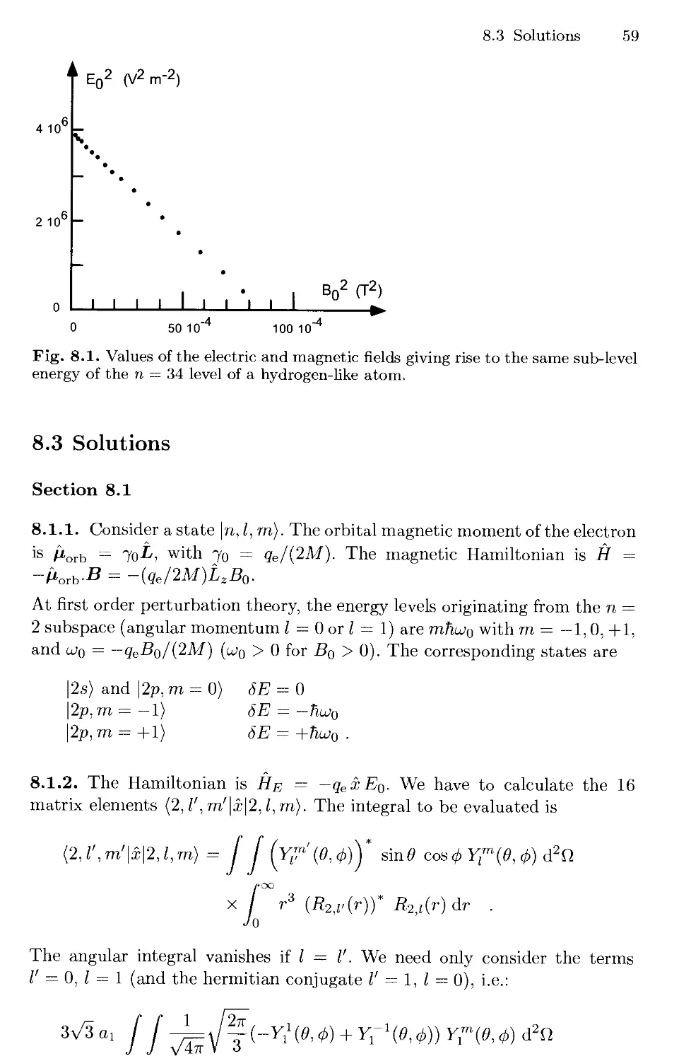
8. The Hydrogen Atom in Crossed Fields 57
8.1 The Hydrogen Atom in Crossed Electric
and Magnetic Fields 57
8.2 Pauli's Result 58
8.3 Solutions 59
9. Exact Results for the Three-Body Problem 61
9.1 The Two-Body Problem 61
9.2 The Variational Method 61
9.3 Relating the Three-Body and Two-Body Sectors 62
9.4 The Three-Body Harmonic Oscillator 63
9.5 From Mesons to Baryons in the Quark Model 63
9.6 Solutions 64
References 68
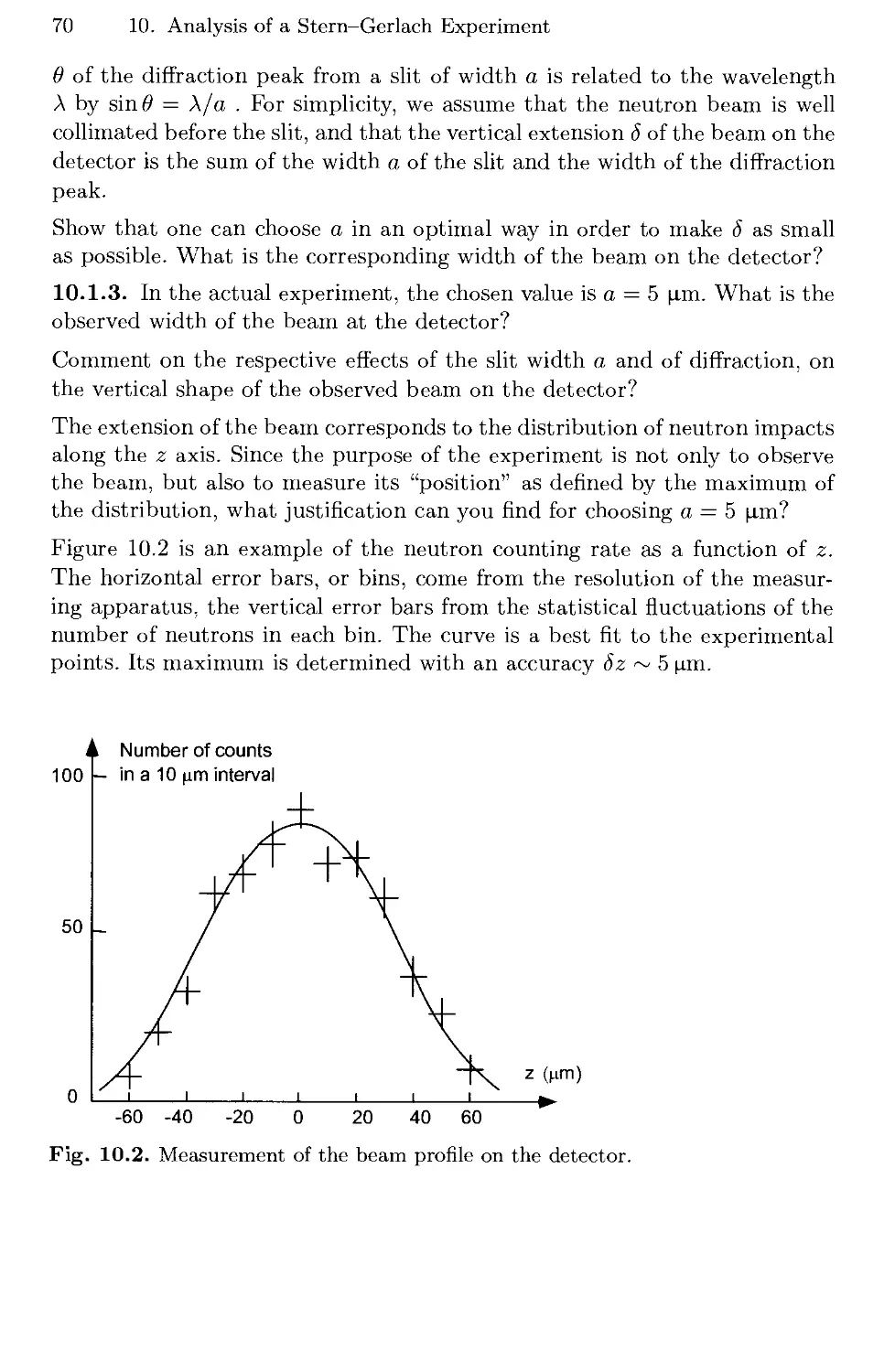
10. Analysis of a Stern-Gerlach Experiment 69
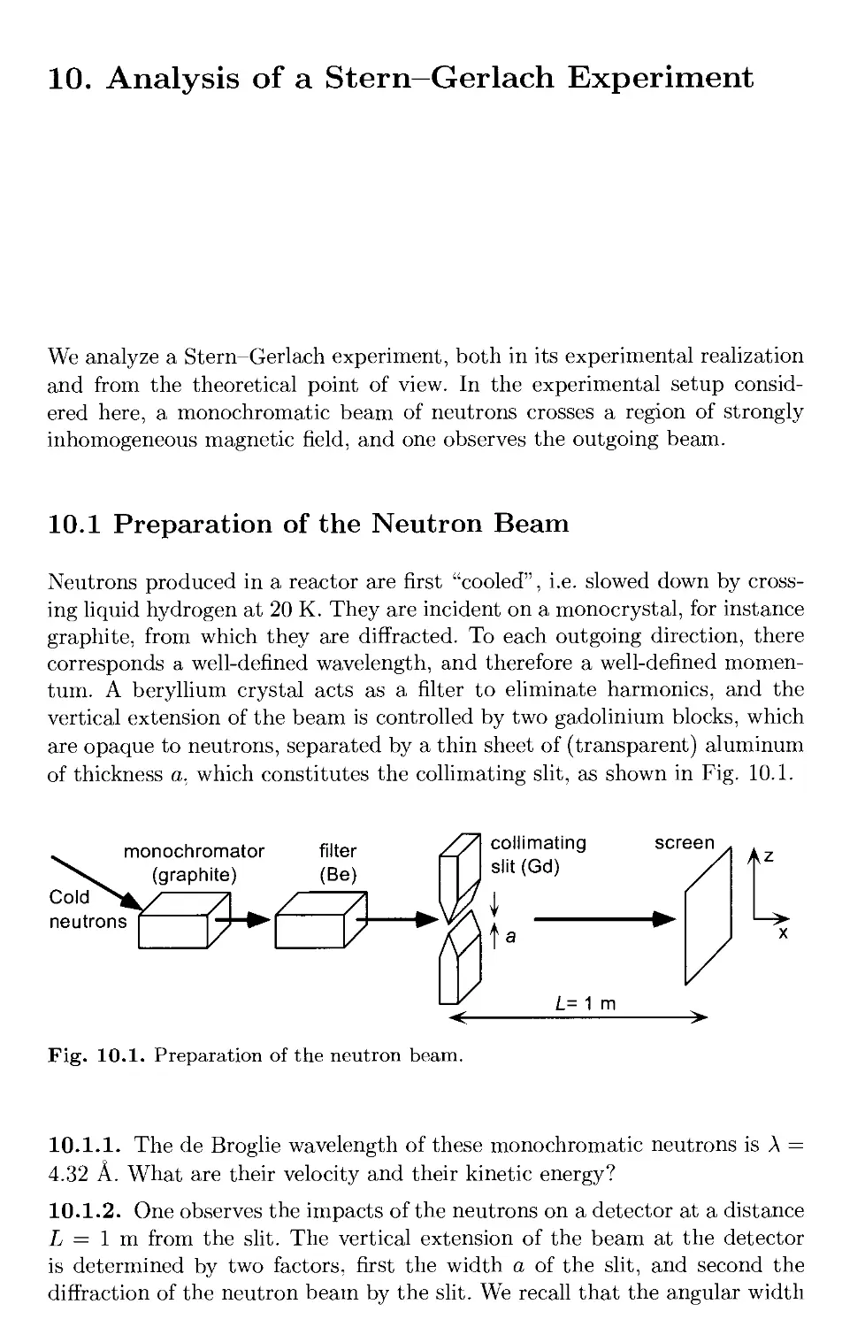
10.1 Preparation of the Neutron Beam 69
10.2 Spin State of the Neutrons 71
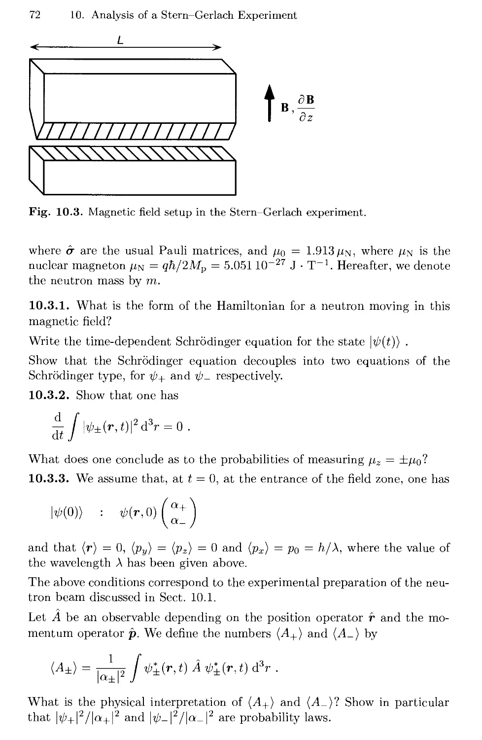
10.3 The Stern-Gerlach Experiment 71
10.4 Solutions 73
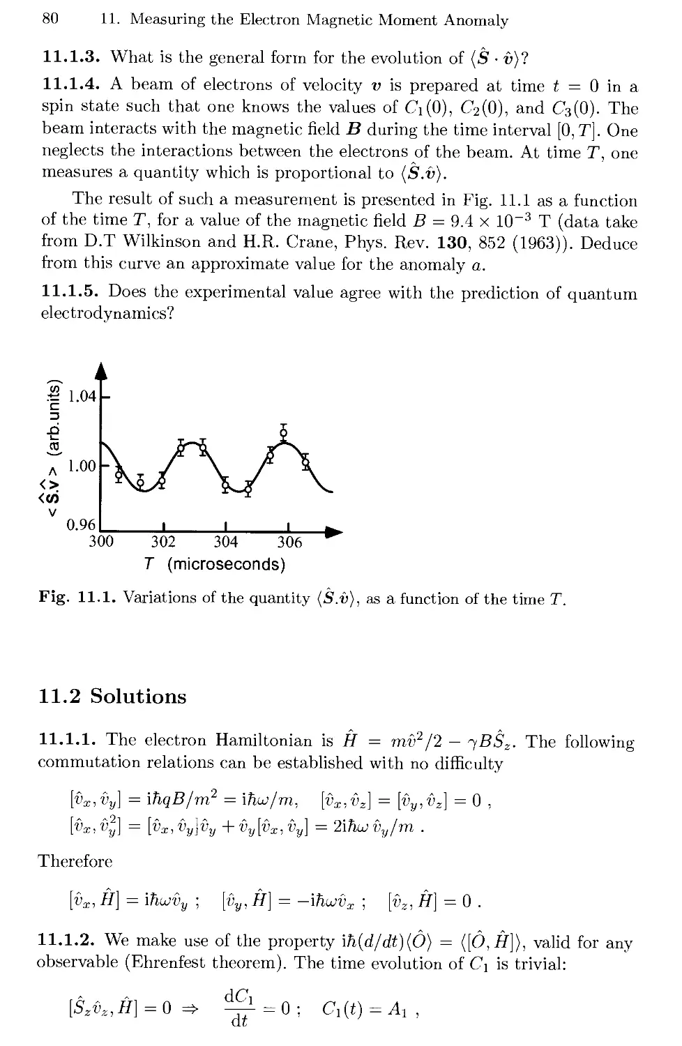
11. Measuring the Electron Magnetic Moment Anomaly 79
11.1 Spin and Momentum Precession of an Electron
in a Magnetic Field 79
11.2 Solutions 80
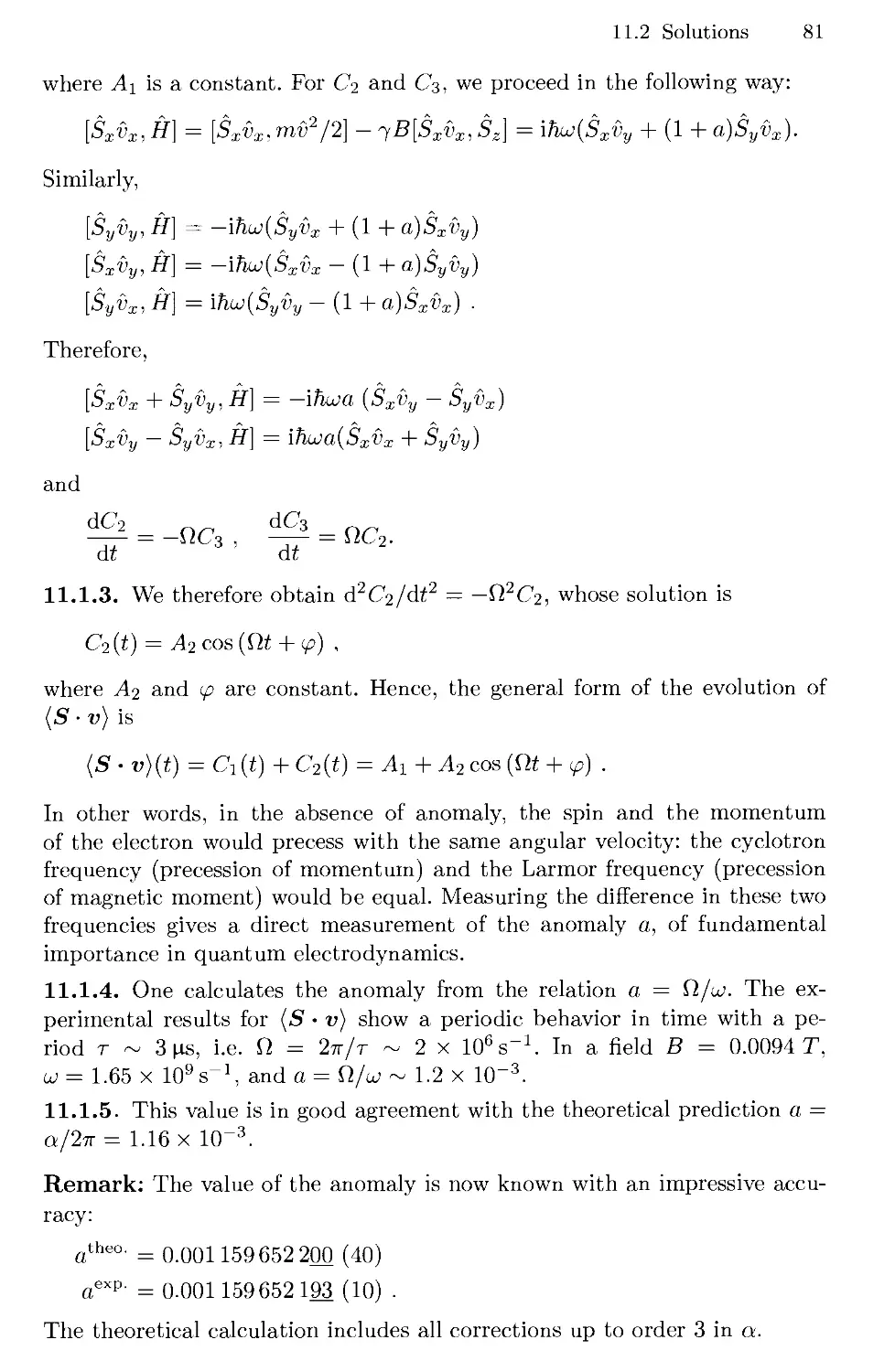
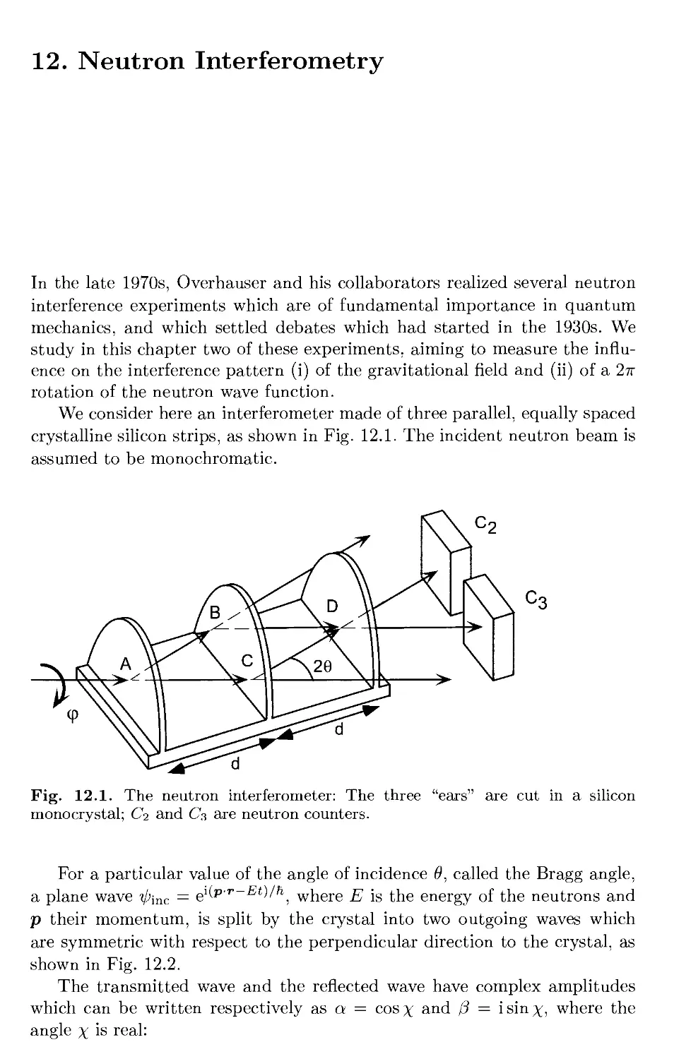
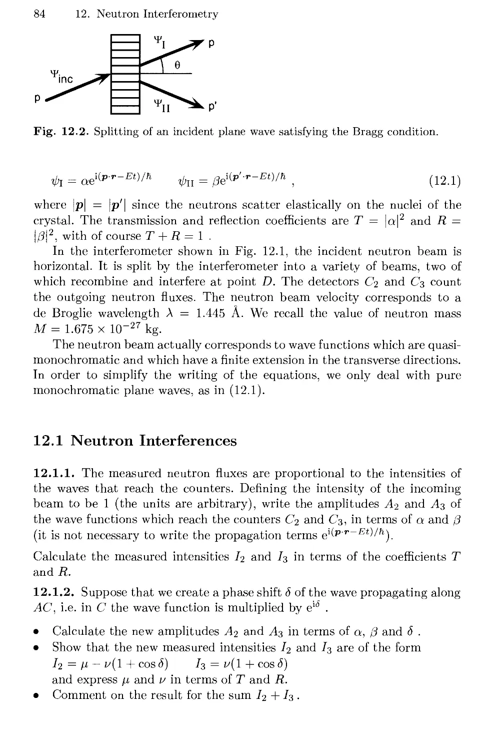
12. Neutron Interferometry 83
12.1 Neutron Interferences 84
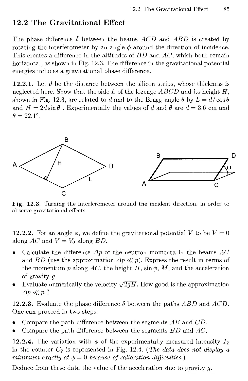
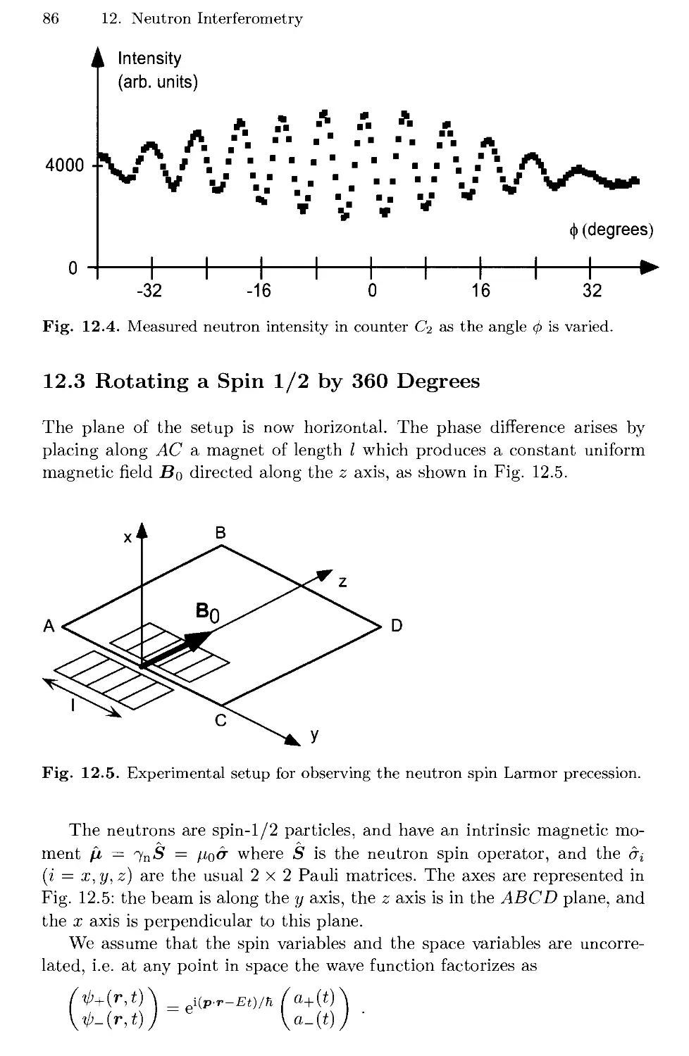
12.2 The Gravitational Effect 85
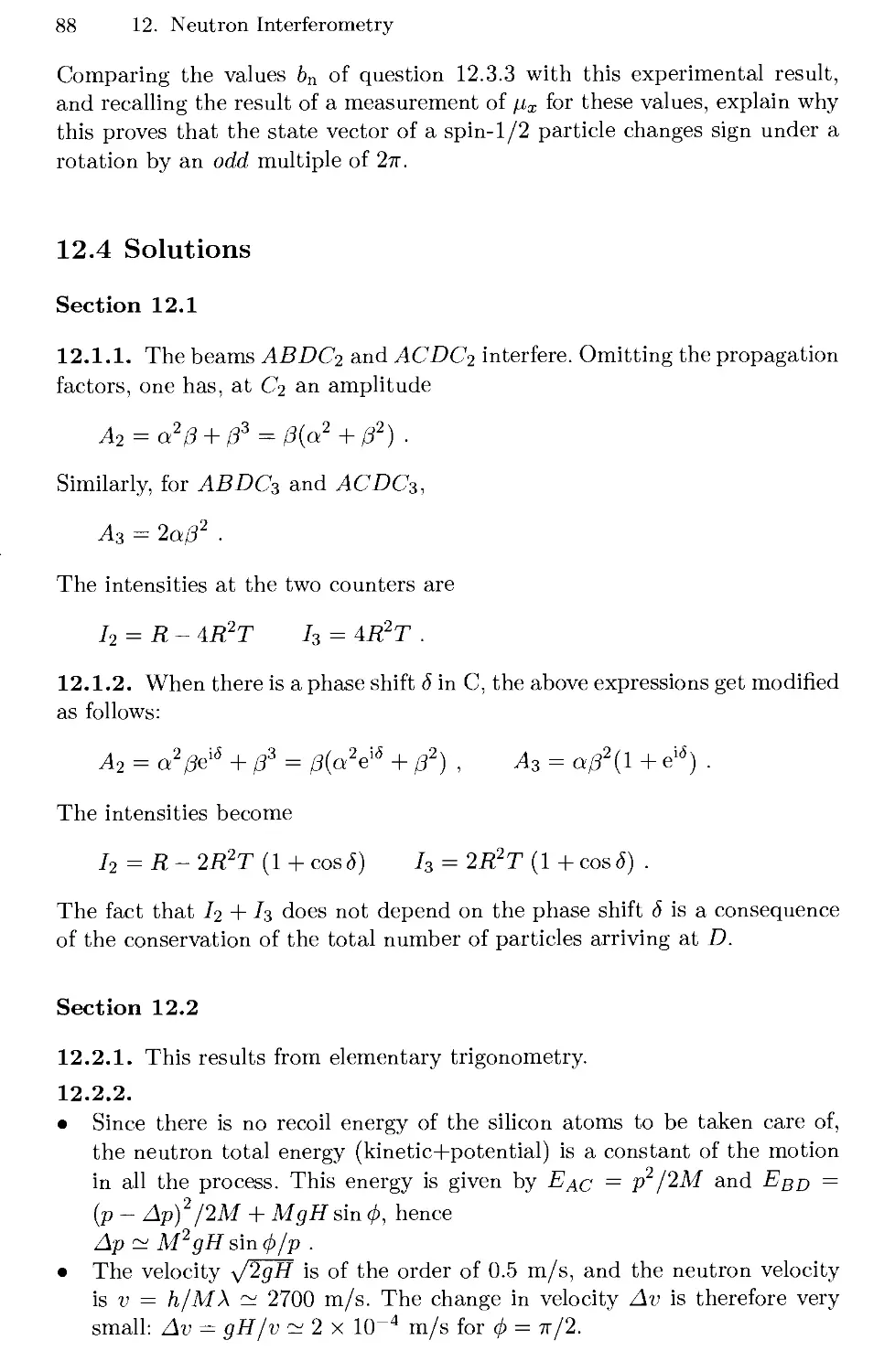
12.3 Rotating a Spin 1/2 by 360 Degrees 86
12.4 Solutions 88
References 91

Contents IX
13. The Penning Trap 93
13.1 Motion of an Electron in a Penning Trap 93
13.2 The Transverse Motion 94
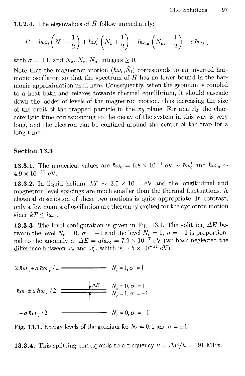
13.3 Measurement of the Electron Anomalous Magnetic Moment. . 95
13.4 Solutions 95
Reference 98
14. Quantum Cryptography 99
14.1 Preliminaries 99
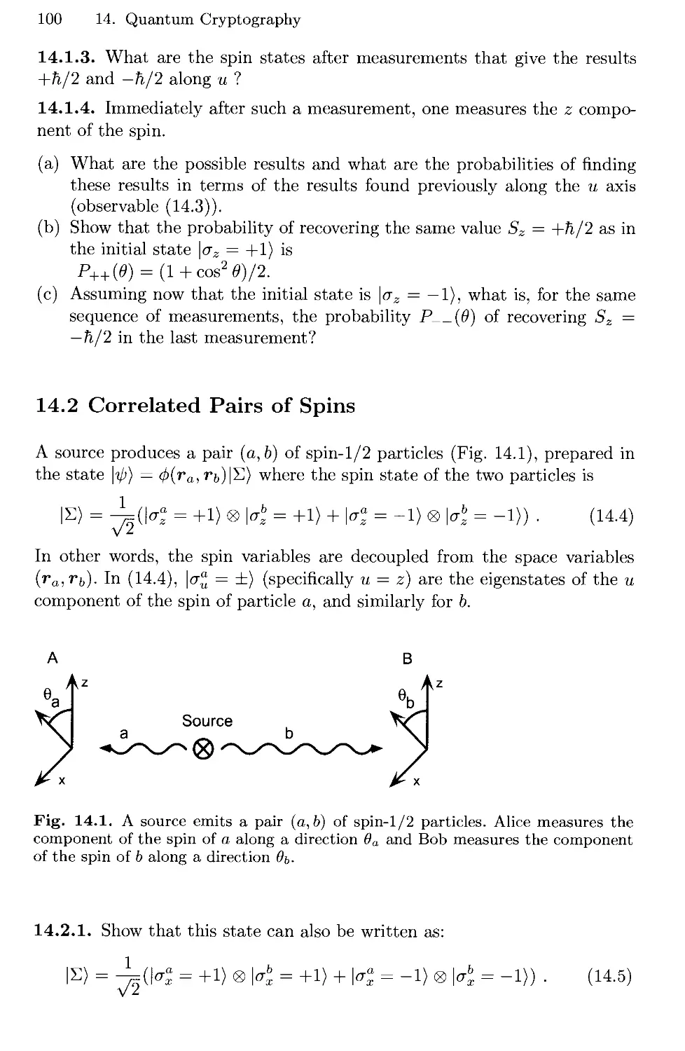
14.2 Correlated Pairs of Spins 100
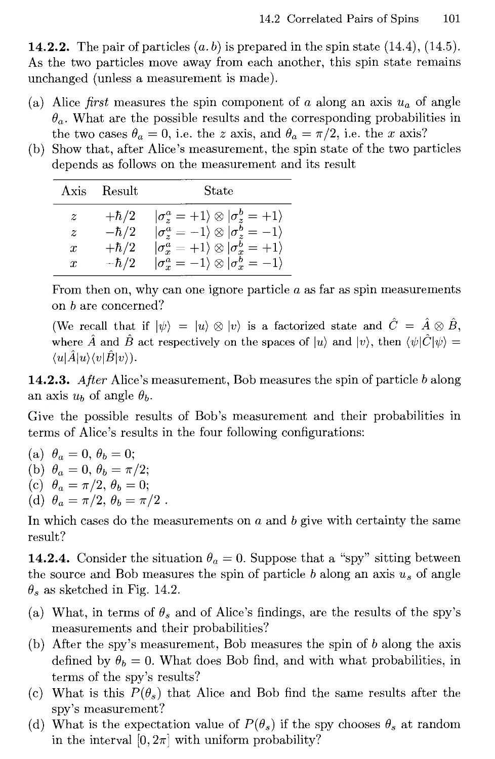
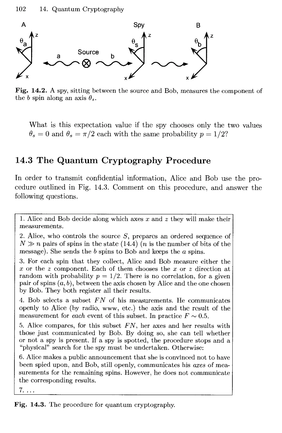
14.3 The Quantum Cryptography Procedure 102
14.4 Solutions 104
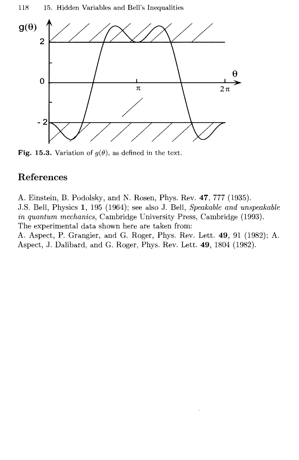
15. Hidden Variables and Bell's Inequalities 109
15.1 The Electron Spin 109
15.2 Correlations Between the Two Spins 109
15.3 Correlations in the Singlet State 110
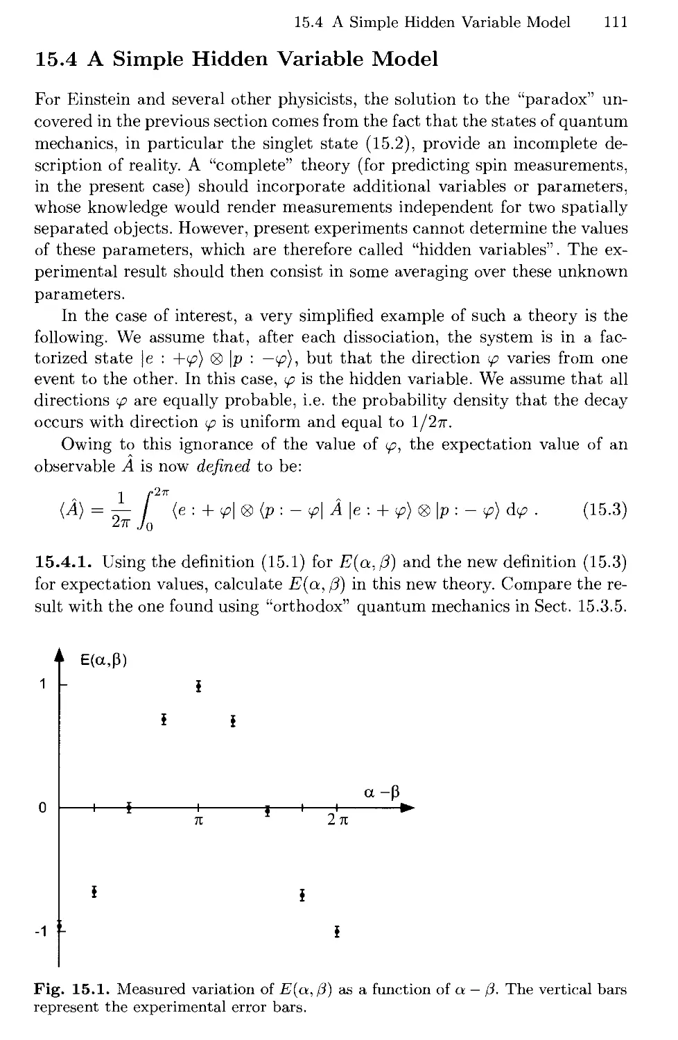
15.4 A Simple Hidden Variable Model Ill
15.5 Bell's Theorem and Experimental Results 112
15.6 Solutions 113
References 118
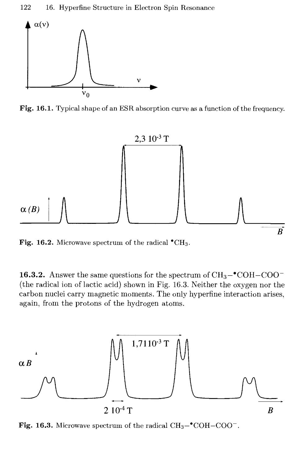
16. Hyperflne Structure in Electron Spin Resonance 119
16.1 Hyperfine Interaction with One Nucleus 120
16.2 Hyperfine Structure with Several Nuclei 120
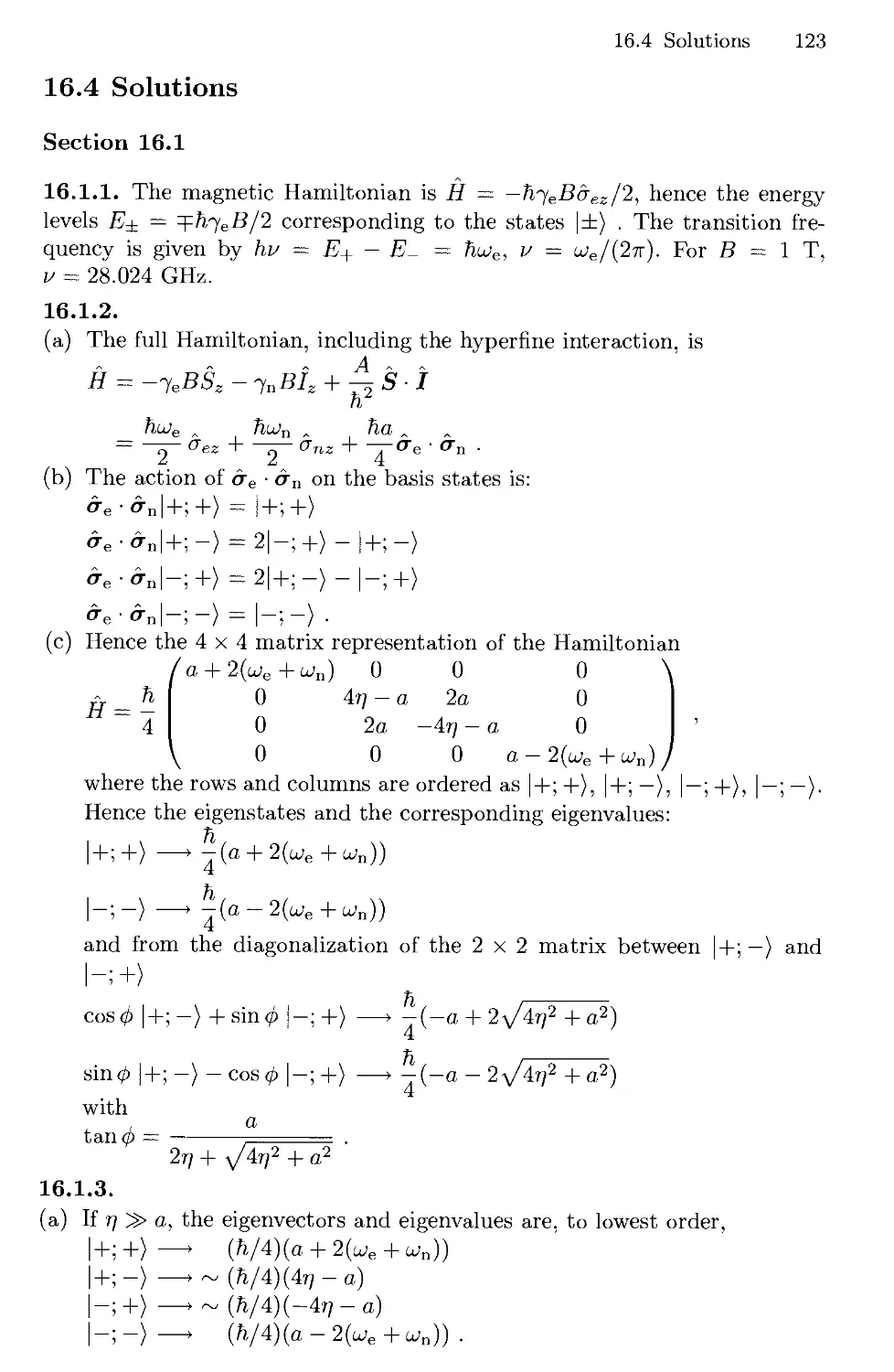
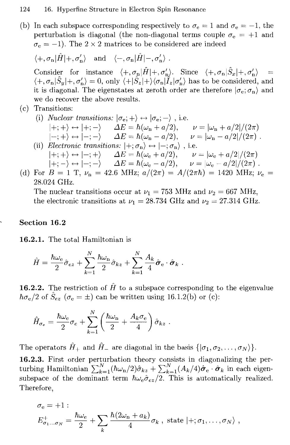
16.3 Experimental Results 121
16.4 Solutions 123
17. The Spectrum of Positronium 127
17.1 Positronium Orbital States 127
17.2 Hyperfine Splitting 127
17.3 Zeeman Effect in the Ground State 128
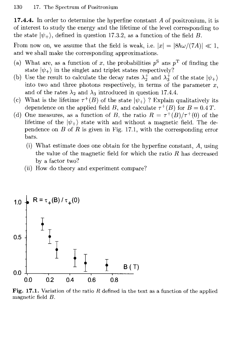
17.4 Decay of Positronium 129
17.5 Solutions 131
References 134
18. Magnetic Excitons 135
18.1 The Molecule CsFeBr3 135
18.2 Spin-Spin Interactions in a Chain of Molecules 136
18.3 Energy Levels of the Chain 136
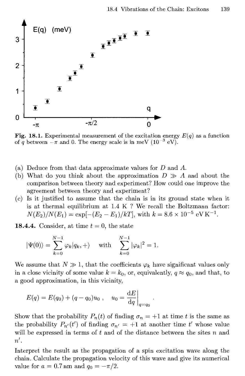
18.4 Vibrations of the Chain: Excitons 138
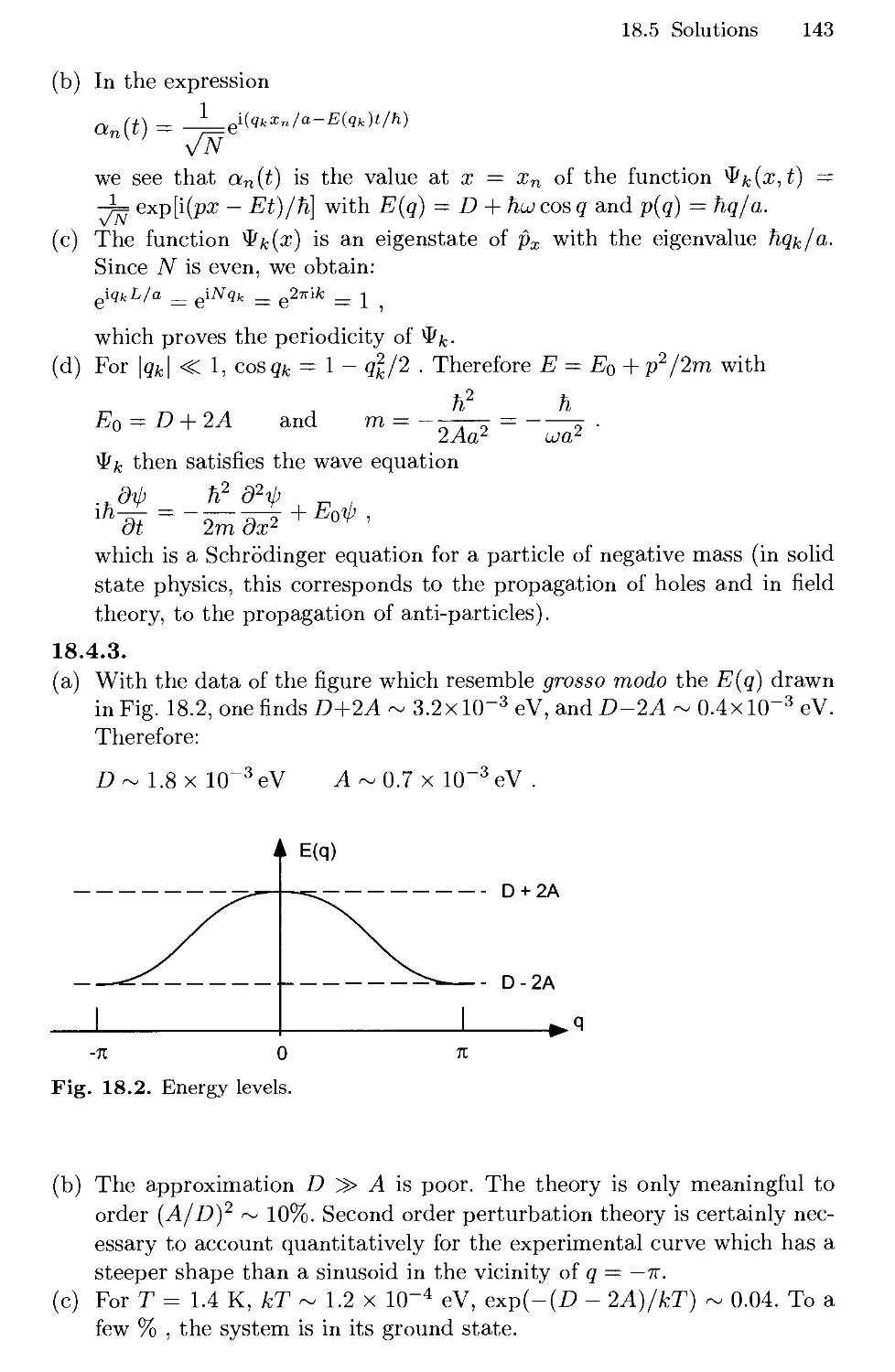
18.5 Solutions 140
Reference 145

X Contents
19. Probing Matter with Positive Muons 147
19.1 Muonium in Vacuum 148
19.2 Muonium in Silicon 149
19.3 Solutions 151
20. Spectroscopic Measurement on a Neutron Beam 157
20.1 Ramsey Fringes 157
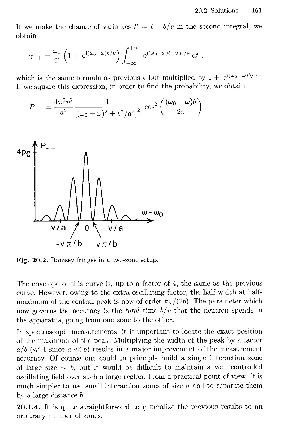
20.2 Solutions 159
Reference 163
21. The Quantum Eraser 165
21.1 Magnetic Resonance 165
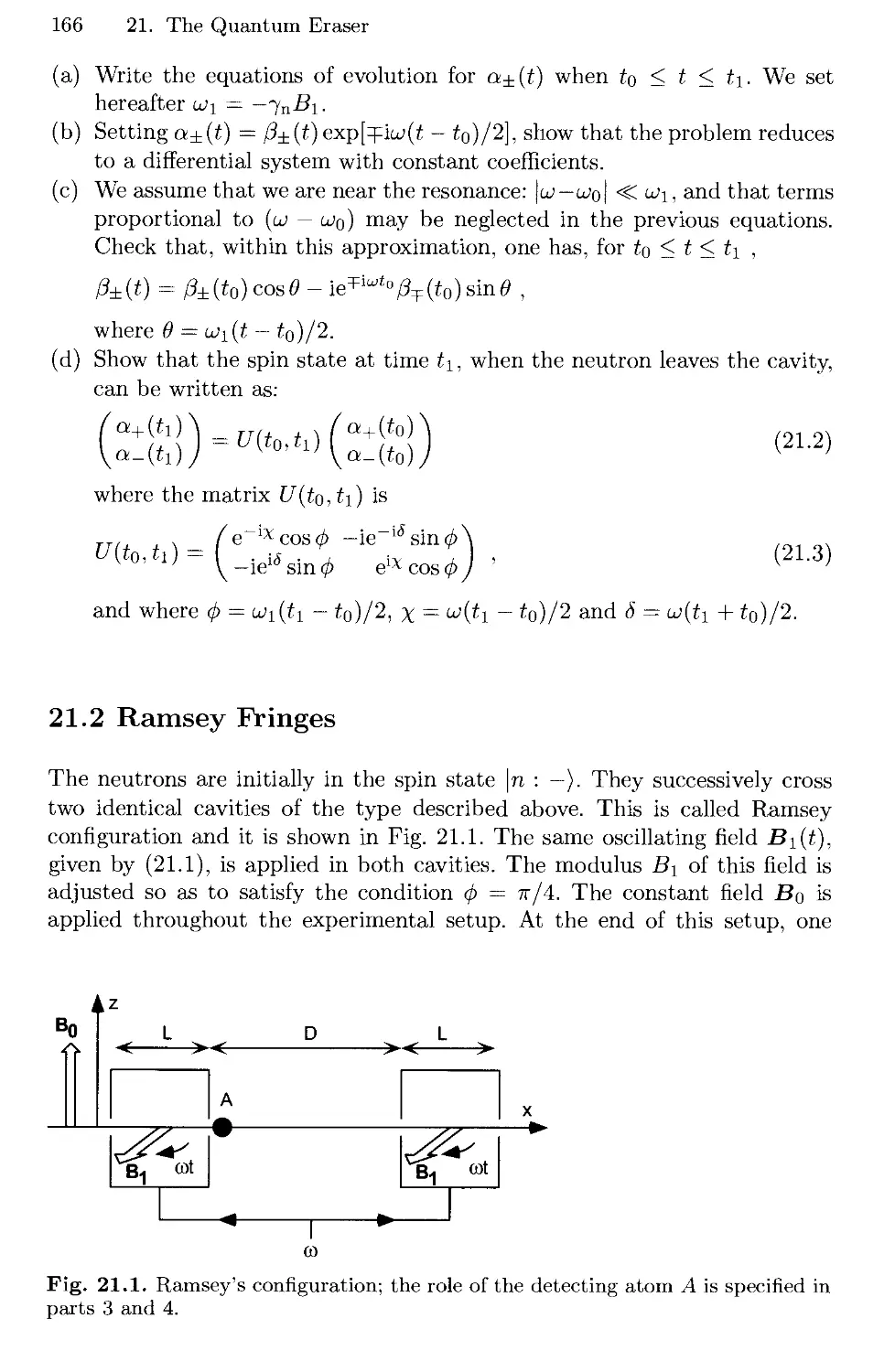
21.2 Ramsey Fringes 166
21.3 Detection of the Neutron Spin State 168
21.4 A Quantum Eraser 169
21.5 Solutions 170
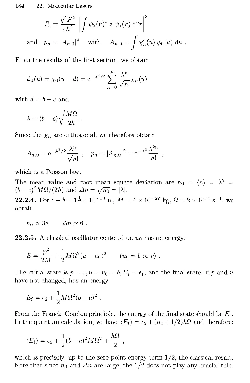
22. Molecular Lasers 179
22.1 Preliminaries 179
22.2 Molecular Lasers 180
22.3 Solutions 182
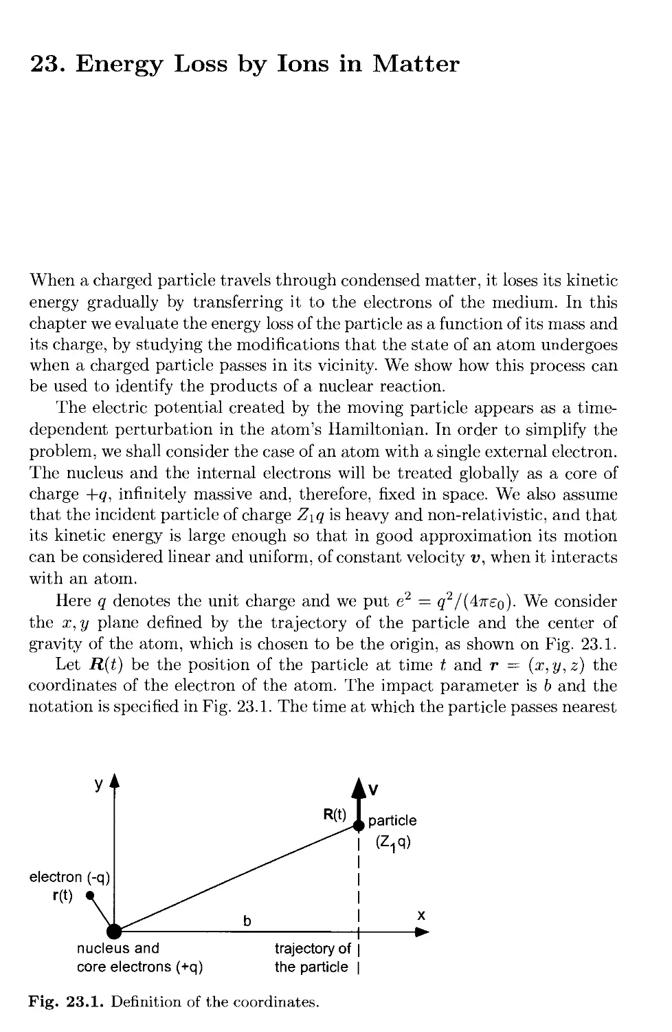
23. Energy Loss by Ions in Matter 187
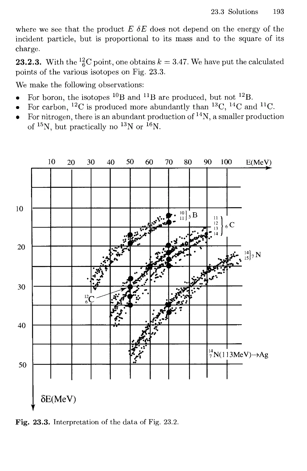
23.1 Energy Absorbed by One Atom 188
23.2 Energy Loss in Matter 188
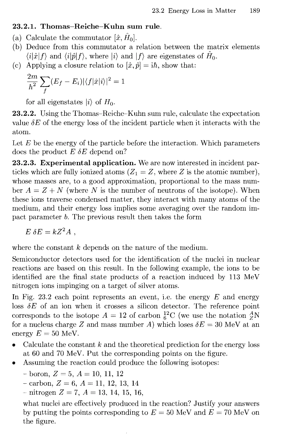
23.3 Solutions 190
24. Properties of a Bose—Einstein Condensate 195
24.1 Particle in a Harmonic Trap 195
24.2 Interactions Between Two Confined Particles 196
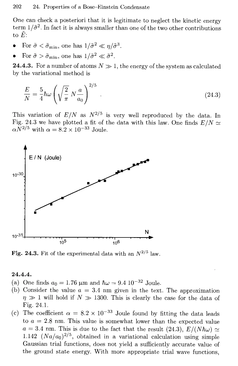
24.3 Energy of a Bose-Einstein Condensate 197
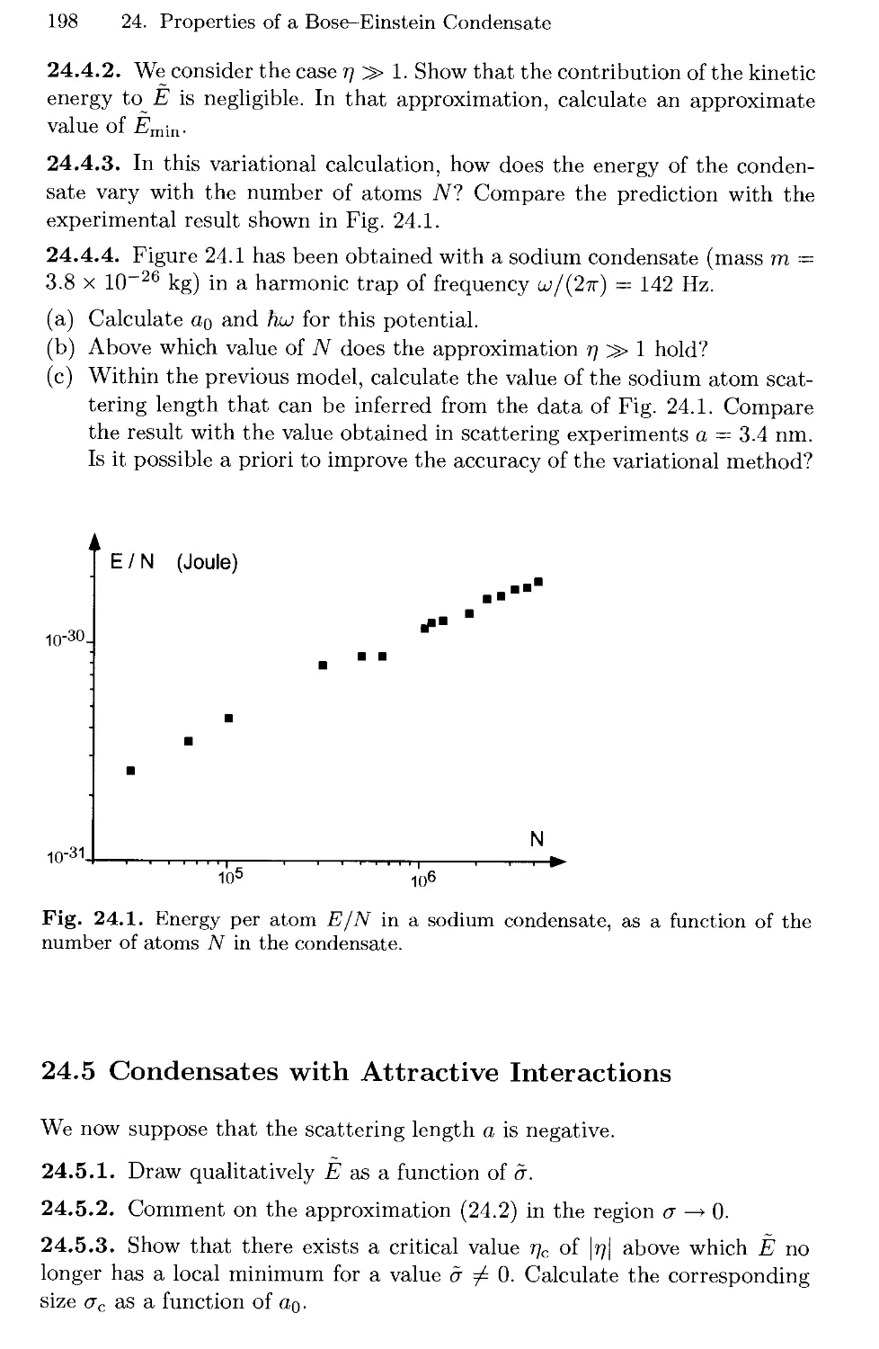
24.4 Condensates with Repulsive Interactions 197
24.5 Condensates with Attractive Interactions 198
24.6 Solutions 199
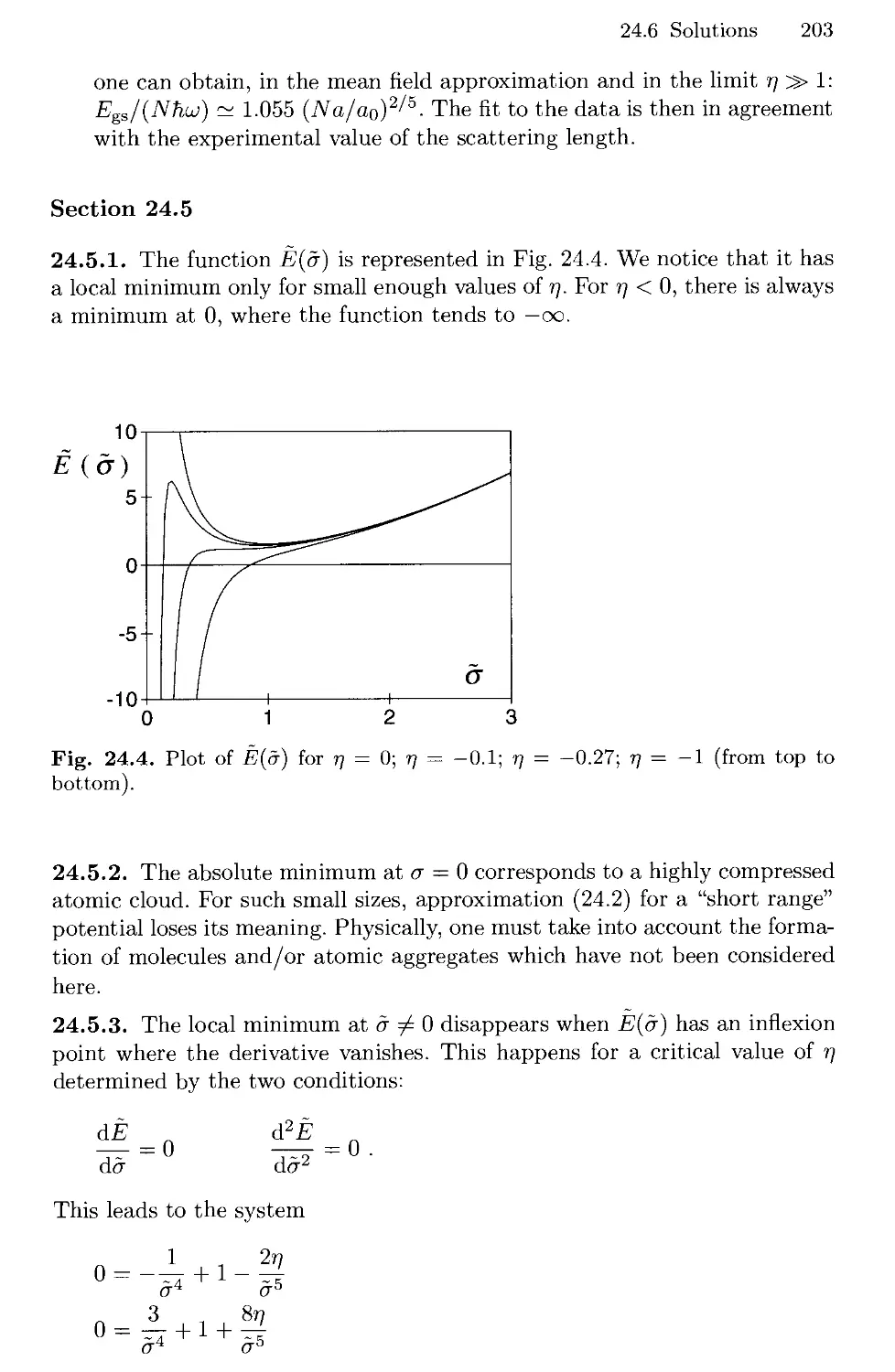
Further Comments 204
25. Quantum Reflection of Atoms from a Surface 205
25.1 The Hydrogen Atom-Liquid Helium Interaction 205
25.2 Excitations on the Surface of Liquid Helium 207
25.3 Quantum Interaction Between H and Liquid He 208
25.4 The Sticking Probability 208
25.5 Solutions 209
References 215

Contents XI
26. Laser Cooling and Trapping 217
26.1 Optical Bloch Equations for an Atom at Rest 217
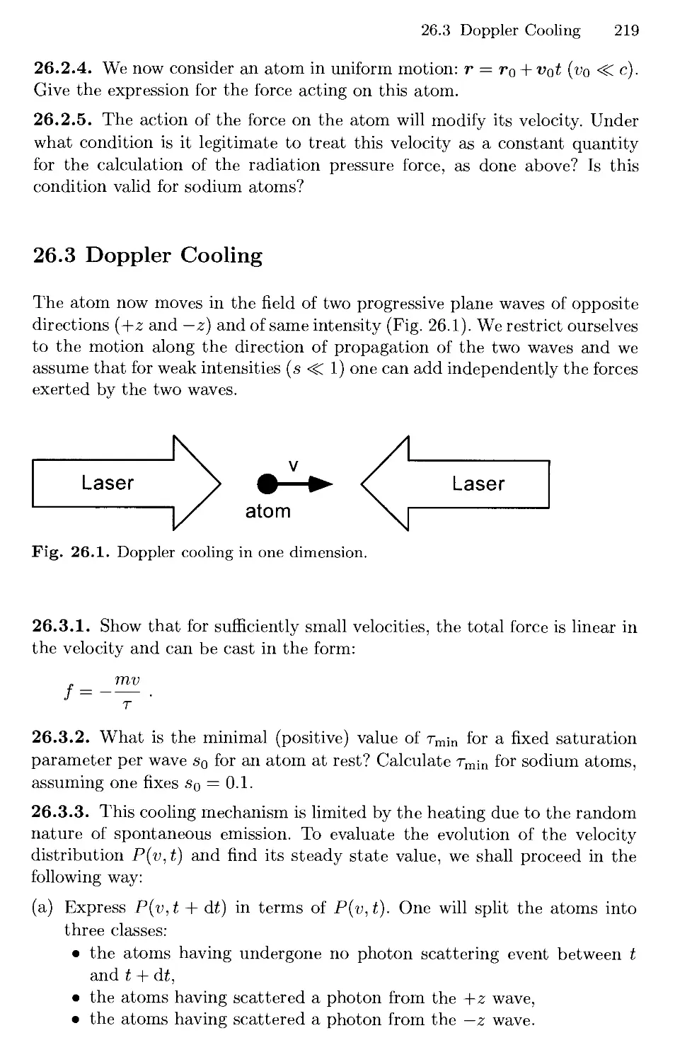
26.2 The Radiation Pressure Force 218
26.3 Doppler Cooling 219
26.4 The Dipole Force 220
26.5 Solutions 220
27. Quantum Motion in a Periodic Potential 227
27.1 Band Structure in a Periodic Potential 227
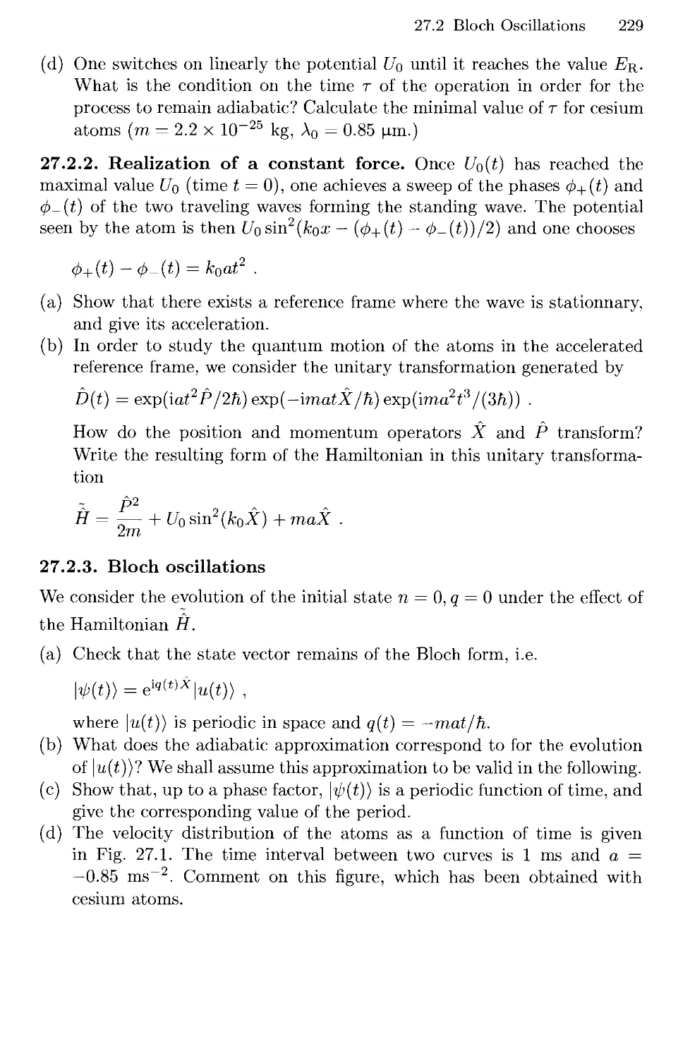
27.2 Bloch Oscillations 228
27.3 Solutions 230
Author Index 239
Subject Index 241

1. Colored Centers in Ionic Crystals
When a vacancy is created in a crystal, an electron may be trapped at this
location. This bound electron can absorb light at well denned frequencies,
thus changing the color of the crystal.
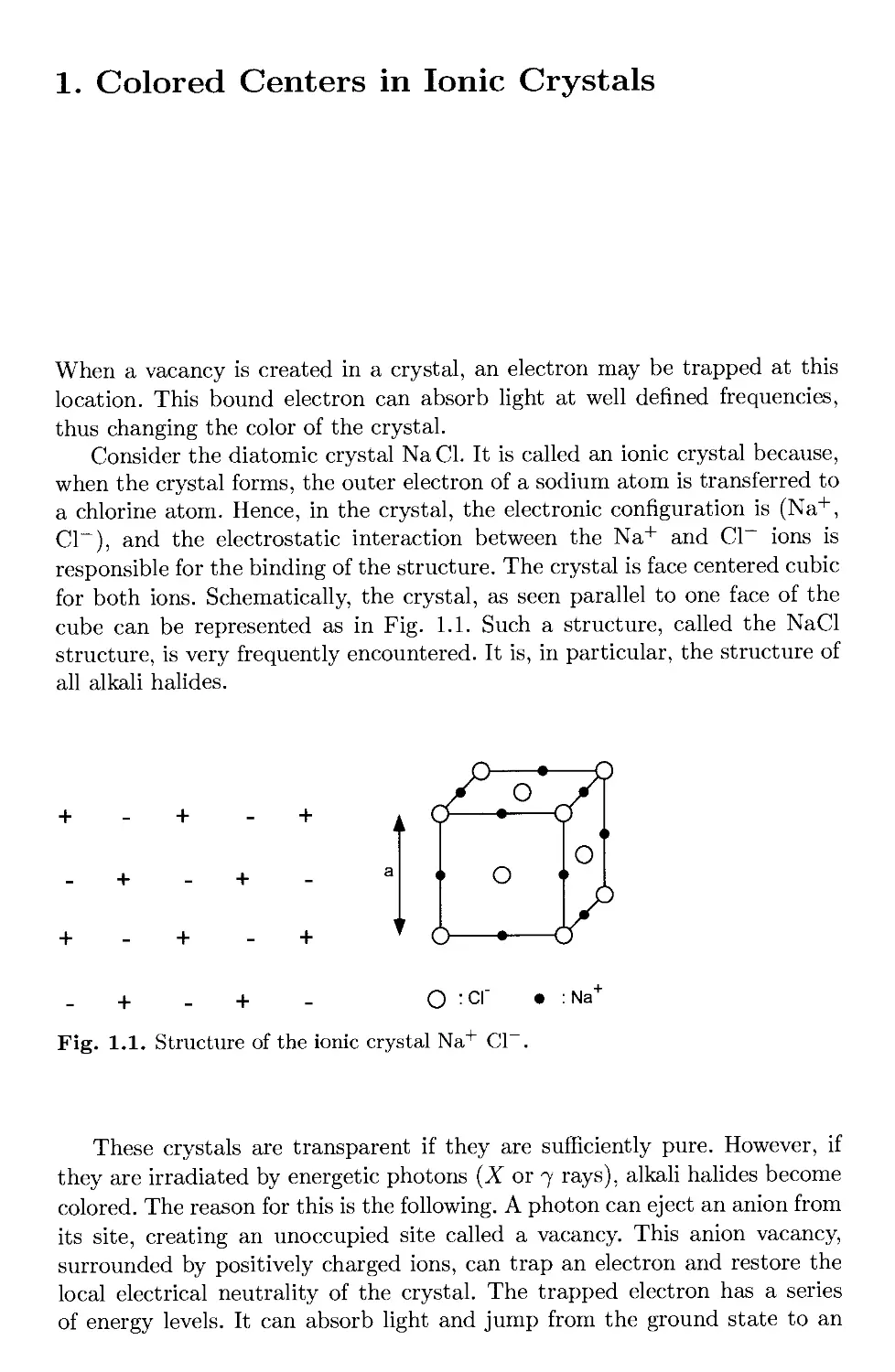
Consider the diatomic crystal NaCl. It is called an ionic crystal because,
when the crystal forms, the outer electron of a sodium atom is transferred to
a chlorine atom. Hence, in the crystal, the electronic configuration is (Na+,
Cl~), and the electrostatic interaction between the Na+ and Cl~ ions is
responsible for the binding of the structure. The crystal is face centered cubic
for both ions. Schematically, the crystal, as seen parallel to one face of the
cube can be represented as in Fig. 1.1. Such a structure, called the NaCl
structure, is very frequently encountered. It is, in particular, the structure of
all alkali halides.
+ - + - О :СГ
Fig. 1.1. Structure of the ionic crystal Na+ СГ
:Na+
These crystals are transparent if they are sufficiently pure. However, if
they are irradiated by energetic photons (X or 7 rays), alkali halides become
colored. The reason for this is the following. A photon can eject an anion from
its site, creating an unoccupied site called a vacancy. This anion vacancy,
surrounded by positively charged ions, can trap an electron and restore the
local electrical neutrality of the crystal. The trapped electron has a series
of energy levels. It can absorb light and jump from the ground state to an

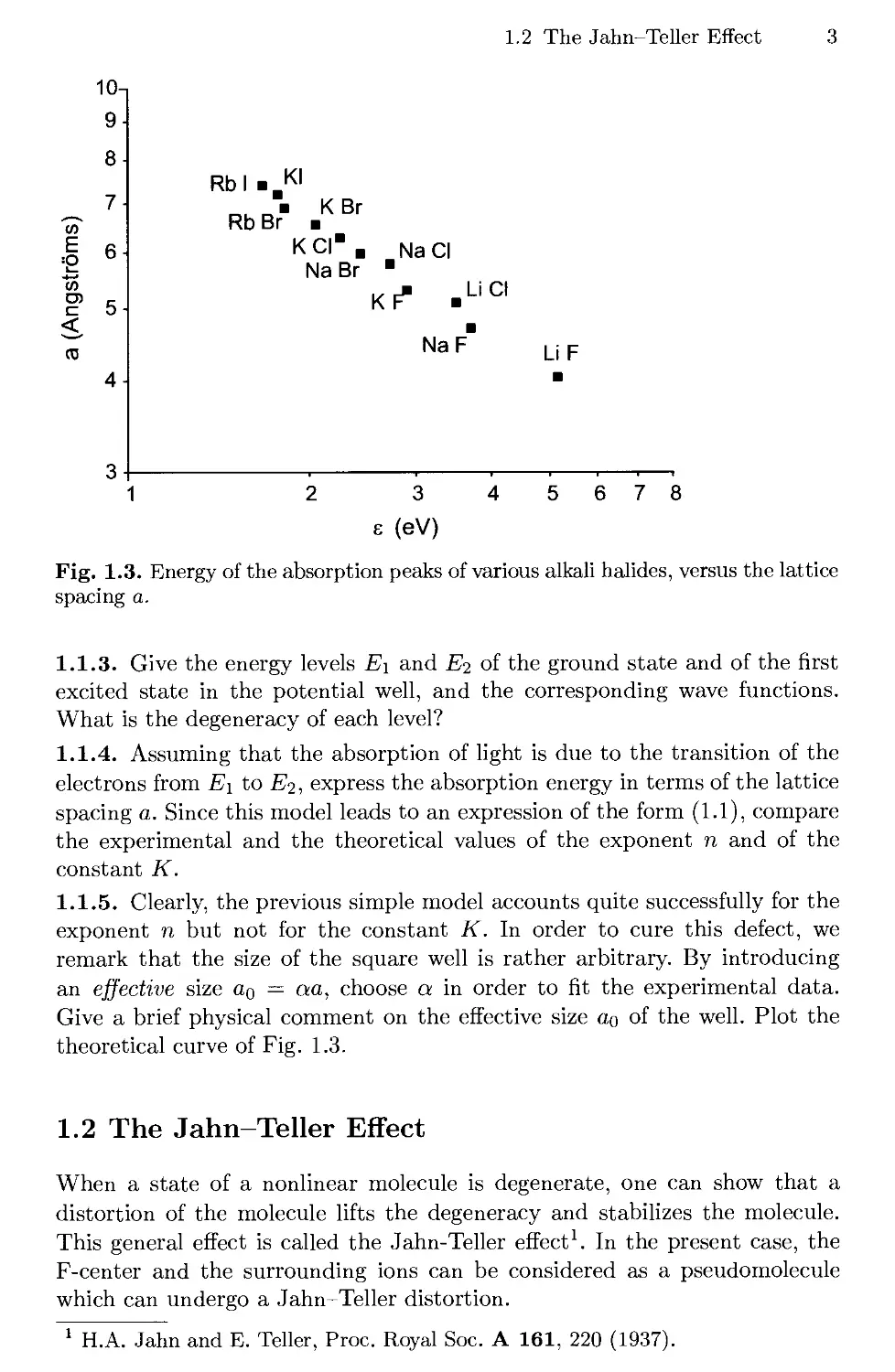
2 1. Colored Centers in Ionic Crystals
Fig. 1.2. Structure of an F-center in a NaCl crystal.
excited state. This process is responsible for the color of the crystal. The elec-
electron trapped in the vacancy is called a colored centre, or F-center (from the
German Farbenzentrum). The structure of an F-center is shown on Fig. 1.2.
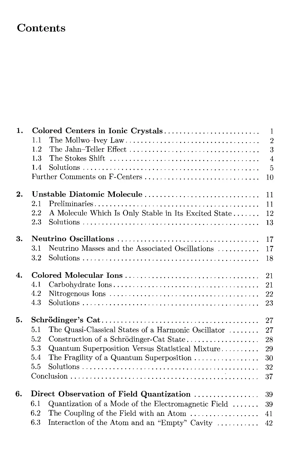
1.1 The Mollwo-Ivey Law
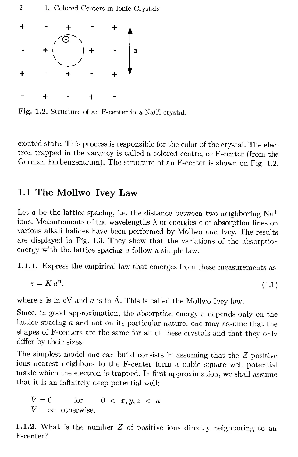
Let a be the lattice spacing, i.e. the distance between two neighboring Na+
ions. Measurements of the wavelengths Л or energies e of absorption lines on
various alkali halides have been performed by Mollwo and Ivey. The results
are displayed in Fig. 1.3. They show that the variations of the absorption
energy with the lattice spacing a follow a simple law.
1.1.1. Express the empirical law that emerges from these measurements as
e = Kan, A.1)
where e is in eV and a is in A. This is called the Mollwo-Ivey law.
Since, in good approximation, the absorption energy e depends only on the
lattice spacing a and not on its particular nature, one may assume that the
shapes of F-centers are the same for all of these crystals and that they only
differ by their sizes.
The simplest model one can build consists in assuming that the Z positive
ions nearest neighbors to the F-center form a cubic square well potential
inside which the electron is trapped. In first approximation, we shall assume
that it is an infinitely deep potential well:
V = 0 for 0 < x,y, z < a
V = oo otherwise.
1.1.2. What is the number Z of positive ions directly neighboring to an
F-center?

1.2 The Jahn-Teller Effect
to
E
ю-,
9
8
7
6
to
с 5
RbBr
KBr
KCI1. NaCI
NaBr ¦
LiCI
NaF LiF
2 3 4 5 6 7 8
8 (eV)
Fig. 1.3. Energy of the absorption peaks of various alkali halides, versus the lattice
spacing a.
1.1.3. Give the energy levels E\ and Ei of the ground state and of the first
excited state in the potential well, and the corresponding wave functions.
What is the degeneracy of each level?
1.1.4. Assuming that the absorption of light is due to the transition of the
electrons from E\ to E2, express the absorption energy in terms of the lattice
spacing a. Since this model leads to an expression of the form A.1), compare
the experimental and the theoretical values of the exponent n and of the
constant K.
1.1.5. Clearly, the previous simple model accounts quite successfully for the
exponent n but not for the constant K. In order to cure this defect, we
remark that the size of the square well is rather arbitrary. By introducing
an effective size a0 = aa, choose a in order to fit the experimental data.
Give a brief physical comment on the effective size ao of the well. Plot the
theoretical curve of Fig. 1.3.
1.2 The Jahn-Teller Effect
When a state of a nonlinear molecule is degenerate, one can show that a
distortion of the molecule lifts the degeneracy and stabilizes the molecule.
This general effect is called the Jahn-Teller effect1. In the present case, the
F-center and the surrounding ions can be considered as a pseudomolecule
which can undergo a Jahn-Teller distortion.
1 H.A. Jahn and E. Teller, Proc. Royal Soc. A 161, 220 A937).

4 1. Colored Centers in Ionic Crystals
Z'
/
/
aO
0
z.
/
/
b
Л
ao
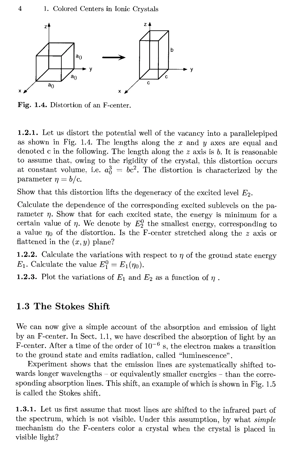
Fig. 1.4. Distortion of an F-center.
1.2.1. Let us distort the potential well of the vacancy into a parallelepiped
as shown in Fig. 1.4. The lengths along the x and у axes are equal and
denoted с in the following. The length along the z axis is b. It is reasonable
to assume that, owing to the rigidity of the crystal, this distortion occurs
at constant volume, i.e. а$ = 6c2. The distortion is characterized by the
parameter r\ = b/c.
Show that this distortion lifts the degeneracy of the excited level E<i-
Calculate the dependence of the corresponding excited sublevels on the pa-
parameter r\. Show that for each excited state, the energy is minimum for a
certain value of r\. We denote by E§ the smallest energy, corresponding to
a value щ of the distortion. Is the F-center stretched along the z axis or
flattened in the (x, y) plane?
1.2.2. Calculate the variations with respect to r\ of the ground state energy
Ei. Calculate the value E\ = ?1G70).
1.2.3. Plot the variations of E\ and E2 as a function of r\ .
1.3 The Stokes Shift
We can now give a simple account of the absorption and emission of light
by an F-center. In Sect. 1.1, we have described the absorption of light by an
F-center. After a time of the order of 10~6 s, the electron makes a transition
to the ground state and emits radiation, called "luminescence".
Experiment shows that the emission lines are systematically shifted to-
towards longer wavelengths - or equivalently smaller energies - than the corre-
corresponding absorption lines. This shift, an example of which is shown in Fig. 1.5
is called the Stokes shift.
1.3.1. Let us first assume that most lines are shifted to the infrared part of
the spectrum, which is not visible. Under this assumption, by what simple
mechanism do the F-centers color a crystal when the crystal is placed in
visible light?

1.4 Solutions
—
_
" J
0,0 0,5
\
emission
Л . /
\
absorption
К Вг B0 К)
\ I I
1,0 1,5 2,0 2,5 3,0
Energy (eV
10 i-
8
6
4
2
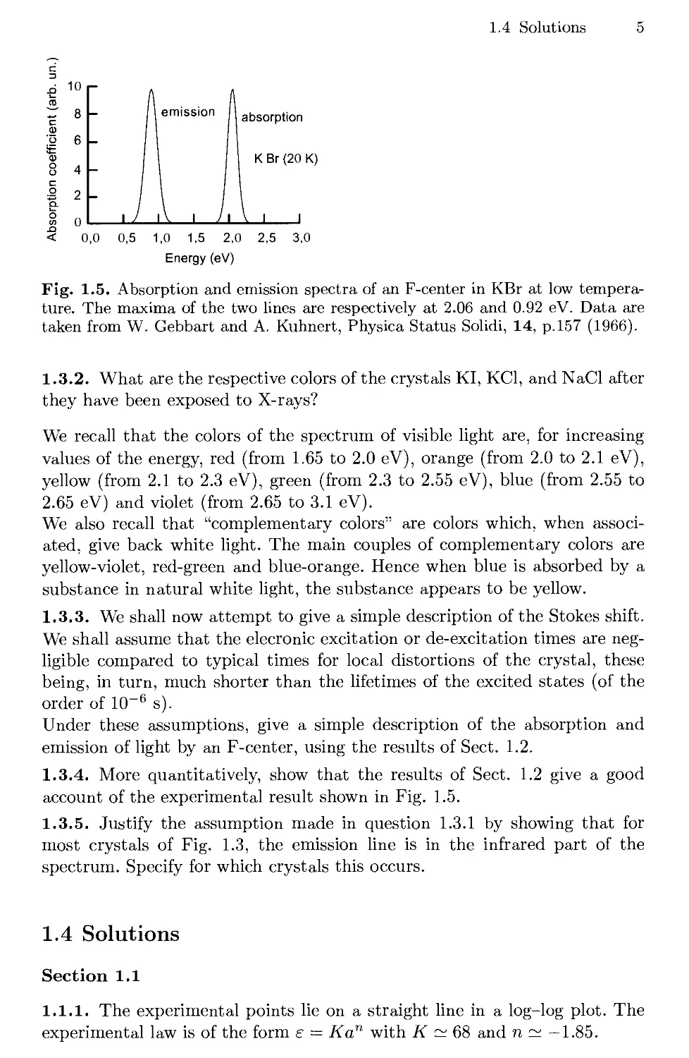
Fig. 1.5. Absorption and emission spectra of an F-center in KBr at low tempera-
temperature. The maxima of the two lines are respectively at 2.06 and 0.92 eV. Data are
taken from W. Gebbart and A. Kuhnert, Physica Status Solidi, 14, p.157 A966).
1.3.2. What are the respective colors of the crystals KI, KC1, and NaCl after
they have been exposed to X-rays?
We recall that the colors of the spectrum of visible light are, for increasing
values of the energy, red (from 1.65 to 2.0 eV), orange (from 2.0 to 2.1 eV),
yellow (from 2.1 to 2.3 eV), green (from 2.3 to 2.55 eV), blue (from 2.55 to
2.65 eV) and violet (from 2.65 to 3.1 eV).
We also recall that "complementary colors" are colors which, when associ-
associated, give back white light. The main couples of complementary colors are
yellow-violet, red-green and blue-orange. Hence when blue is absorbed by a
substance in natural white light, the substance appears to be yellow.
1.3.3. We shall now attempt to give a simple description of the Stokes shift.
We shall assume that the elecronic excitation or de-excitation times are neg-
negligible compared to typical times for local distortions of the crystal, these
being, in turn, much shorter than the lifetimes of the excited states (of the
order of 10 s).
Under these assumptions, give a simple description of the absorption and
emission of light by an F-center, using the results of Sect. 1.2.
1.3.4. More quantitatively, show that the results of Sect. 1.2 give a good
account of the experimental result shown in Fig. 1.5.
1.3.5. Justify the assumption made in question 1.3.1 by showing that for
most crystals of Fig. 1.3, the emission line is in the infrared part of the
spectrum. Specify for which crystals this occurs.
1.4 Solutions
Section 1.1
1.1.1. The experimental points lie on a straight line in a log-log plot. The
experimental law is of the form e = Kan with К ~ 68 and n ~ -1.85.

6 1. Colored Centers in Ionic Crystals
1.1.2. There are Z = 6 positive ions at a distance a/2 of the F-center.
1.1.3. Choosing the origin at a vertex of the cube,
(a) the ground state, with energy E\ = Ш тг2/Bта2), is not degenerate; its
wave function is:
ip(x,y,z) = B/a) sm(irx/a)sin(iry/a)sm(irz/a) ;
(b) the first excited state has a three-fold degeneracy tp2x, fay, Tp2z with for
instance:
tp2z(x,y,z) = B/aK'2 sin(nx/a) sin(ny/a) sinBnz/a)
corresponding to an energy Ei — 6ft тг2/Bта2) .
1.1.4. The transition E\ —> E<i corresponds to the absorption of an energy
e = E2 — E\ = Ш2тг2/Bта2) where a is the lattice spacing. This expression
is of the type A.1) with К = 112 and n = —2. The value of n is close
to what is experimentally observed (—1.85). The constant К is significantly
overestimated.
1.1.5. If the effective extension of the potential is ao = Ota, the theoretical
formula becomes e = Ш2тг2/Bта2а2). Using the value a = 1.13 correspond-
corresponding to К = 87 (and n= —2), one obtains a good fit to the data as shown in
Fig. 1.6.
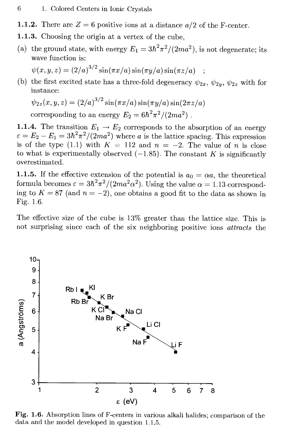
The effective size of the cube is 13% greater than the lattice size. This is
not surprising since each of the six neighboring positive ions attracts the
10-
9
8
to
to
C 5 ¦
4-
3
6 (eV)
6 7 8
Fig. 1.6. Absorption lines of F-centers in various alkali halides; comparison of the
data and the model developed in question 1.1.5.

1.4 Solutions 7
electron of the F-center. In a more realistic potential model of the F-center,
the probability for the electron to be outside the vacancy should be non-zero.
Section 1.2
1.2.1. Consider the state
ip2z(x,y,z) = B/a0f/2 sin(Trx/ao)sin(Try/ao)sinBTrz/ao) .
Under the distortion, it becomes:
¦ф'2г(х,у,г) = B/c)B/bf12 sm(irx/с) sm(iry/c)smB-Kz/b) ,
and the corresponding energy Ei = 6ir2h /Bm<2g) becomes
_h\* B 4
b2z~ 2m U2 b2
Setting 77 = b/c, and imposing that the distortion occurs at constant volume,
<2g = c2b, one has с = аоГ]~1^3 and b = адГ]2^3, hence
Similarly, one finds that
Clearly, E'2x = E'2y on one hand, and E2z on the other are different from E2,
and different from one another. The distortion partially lifts the degeneracy.
If we study the variation of E'2z and E'2x with respect to 77, we find that both
energies have minimum values:
• Е'2г is minimum for r\ = 2, where it reaches the value
E'2x is minimum for r\ = у 2/5 ~ 0.63, where it reaches the value
= 5.52-
Both values are smaller than E2. The first is the absolute minimum. Hence the
energy of the first excited state has the minimum value E2 = 4.76 h тг2/Bтад),
for a value r\ = 2 of the distortion parameter. Since r\ > 1 this corresponds
to an F-center stretched along the z axis.

8 1. Colored Centers in Ionic Crystals
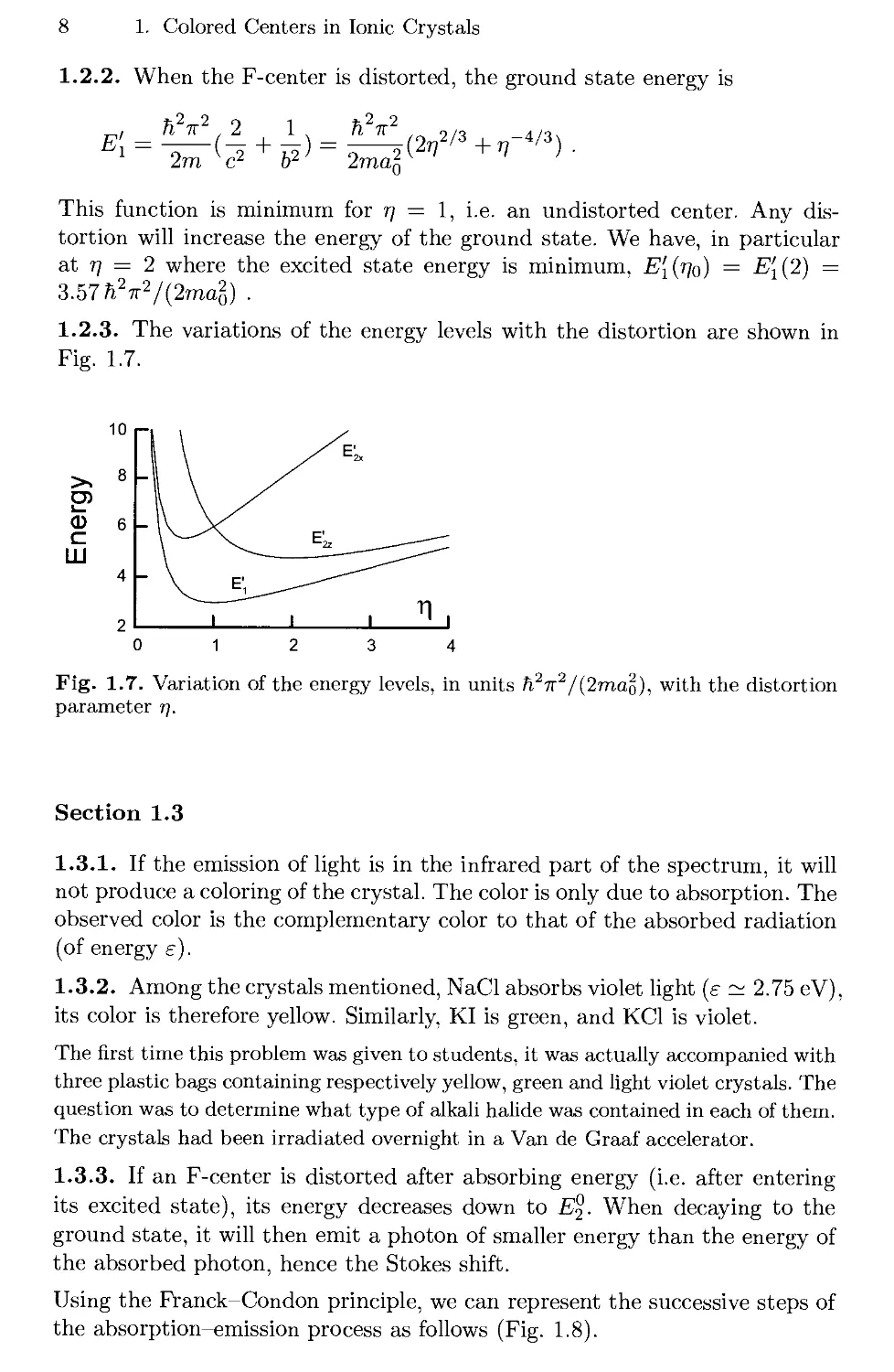
1.2.2. When the F-center is distorted, the ground state energy is
""" """ -Or,2/3 J- r,-4/3i
This function is minimum for r\ = 1, i.e. an undistorted center. Any dis-
distortion will increase the energy of the ground state. We have, in particular
at r\ = 2 where the excited state energy is minimum, Е[(щ) = E[B) =
22§
1.2.3. The variations of the energy levels with the distortion are shown in
Fig. 1.7.
>
В
<D
С
Ш
Fig. 1.7. Variation of the energy levels, in units h2ir2/Bmao), with the distortion
parameter r\.
Section 1.3
1.3.1. If the emission of light is in the infrared part of the spectrum, it will
not produce a coloring of the crystal. The color is only due to absorption. The
observed color is the complementary color to that of the absorbed radiation
(of energy e).
1.3.2. Among the crystals mentioned, NaCl absorbs violet light (e ~ 2.75 eV),
its color is therefore yellow. Similarly, KI is green, and KC1 is violet.
The first time this problem was given to students, it was actually accompanied with
three plastic bags containing respectively yellow, green and light violet crystals. The
question was to determine what type of alkali halide was contained in each of them.
The crystals had been irradiated overnight in a Van de Graaf accelerator.
1.3.3. If an F-center is distorted after absorbing energy (i.e. after entering
its excited state), its energy decreases down to E%- When decaying to the
ground state, it will then emit a photon of smaller energy than the energy of
the absorbed photon, hence the Stokes shift.
Using the Franck-Condon principle, we can represent the successive steps of
the absorption-emission process as follows (Fig. 1.8).

1.4 Solutions
ш
time
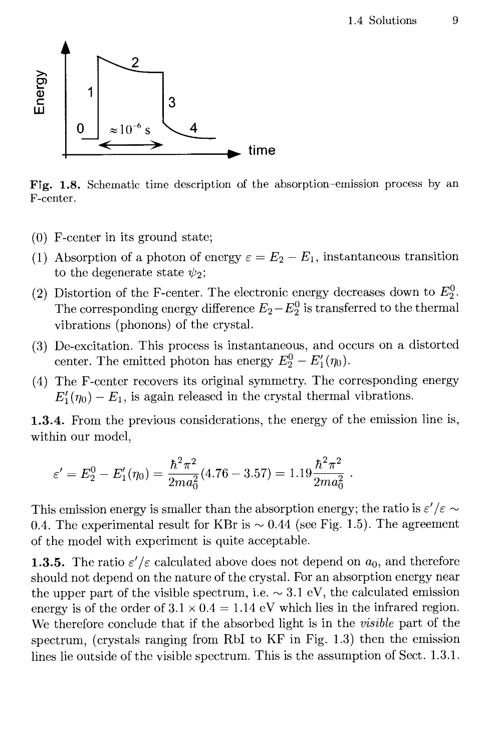
Fig. 1.8. Schematic time description of the absorption-emission process by an
F-center.
@) F-center in its ground state;
A) Absorption of a photon of energy e = E2 — E\, instantaneous transition
to the degenerate state Ф2;
B) Distortion of the F-center. The electronic energy decreases down to E®¦
The corresponding energy difference E2 — E2 is transferred to the thermal
vibrations (phonons) of the crystal.
C) De-excitation. This process is instantaneous, and occurs on a distorted
center. The emitted photon has energy E^ — Е[{щ).
D) The F-center recovers its original symmetry. The corresponding energy
Е[(щ) — Ei, is again released in the crystal thermal vibrations.
1.3.4. From the previous considerations, the energy of the emission line is,
within our model,
»2 2 *2 9
e1 = E% - Е[{щ) = 2D.76-3.57) = 1.19
2mal '
This emission energy is smaller than the absorption energy; the ratio is e'/s ~
0.4. The experimental result for KBr is ~ 0.44 (see Fig. 1.5). The agreement
of the model with experiment is quite acceptable.
1.3.5. The ratio e'/e calculated above does not depend on a0, and therefore
should not depend on the nature of the crystal. For an absorption energy near
the upper part of the visible spectrum, i.e. ~ 3.1 eV, the calculated emission
energy is of the order of 3.1 x 0.4 = 1.14 eV which lies in the infrared region.
We therefore conclude that if the absorbed light is in the visible part of the
spectrum, (crystals ranging from Rbl to KF in Fig. 1.3) then the emission
lines lie outside of the visible spectrum. This is the assumption of Sect. 1.3.1.

10 1. Colored Centers in Ionic Crystals
Further Comments on F-Centers
1. The mechanism by which the F-centers form is still unclear. There are
several proposals (the most plausible being due to Pooley) which are based
on the assumption that the X-ray photons can ionize the anions once
{A~ —> A) or twice [A —> A+). The resulting species, either electrically
neutral or positively charged, is then in a very unstable situation in the
middle of all the positive ions. It is then ejected from its site, leaving
behind a vacancy (F-center) and reaching an interstitial position.
The color can also be obtained by adding impurities (such as a few
Ca++ ions in NaCl) to the crystal. This the reason why many minerals
with a marked ionic character are found colored in nature, while they are
transparent if they are pure (like quartz) . They were contaminated by
other ions when they crystallized.
2. The model of Sect. 1.1 accounts for the Mollwo-Ivey law quite reasonably.
It is, of course, very simplistic. The actual potential is by no means in-
infinitely deep. By electron spin resonance experiments, one can show that
the wave function extends up to the eighth ionic shell surrounding the
F-center, i.e. much further than ao/2.
3. The F-centers can move around. A nearby anion can jump into the F-
center, which therefore moves in the reverse direction. This process in-
involves the crossing of a potential barrier, and is favored by an increase in
temperature. The mobility of an F-center increases with the temperature.
Owing to this mobility, the F-centers tend to disappear, for instance
when they reach the surface of the crystal. One can see the color disappear
if the crystals are heated.
The color can also disappear progressively if the crystals are exposed
to natural light. In fact, the F-centers can then be ionized by ultraviolet
photons, which can eject the electron from its vacancy.

2. Unstable Diatomic Molecule
In a diatomic molecule, the interaction between the atoms depends on their
electronic configuration. It is conceivable that a molecule is stable if one of
the atoms is electronically excited, and unstable if both atoms are in their
ground state. We study here such a scheme, and we focus in particular on
the dissociation of the molecule when the initially excited atom decays to its
ground state.
2.1 Preliminaries
2.1.1. Consider a particle of mass M moving along the x axis and placed in
the potential V\(x):
V\{x) = +oo for x < xo
= 0 for x > Xo.
Let ifk(x) be a stationary solution of the Schrodinger equation with energy
E. It can be written, for x > xo, as
(a) Express к in terms of E .
(b) What is the value of (pk(x) f°r x < xq!
(c) What is the value of Bl
(d) Write the general solution of the Schrodinger equation in terms of the
functions v'fc(x) .
2.1.2. We now consider a particle of mass M moving along the x axis and
placed in the potential Уг(х):
Vi(x) = +°° f°r x < xo
= V0 + MujIx2/2 for x > x0.
where Vo is a constant .
(a) What is the wave function for x < x^l
(b) Express the eigenfunctions Xn(x) of the Hamiltonian in terms of the
normalized Hermite functions Ф„(у) = cney ^2j~^e~v ¦
(c) What are the corresponding energy levels?

12
2. Unstable Diatomic Molecule
2.2 A Molecule Which Is Only Stable
in Its Excited States
Consider a diatomic molecule XY. Let x be the distance between the nuclei
(or between the centers of gravity) of the two atoms X and Y.
The potential energy between the two atoms depends on the excitation
state of the electrons. Let V(x) be this potential energy (for a given electronic
state). Then the (lowest) energy levels of the relative motion of the two atoms
are obtained by solving the one-dimensional Schrodinger equation
~2Mdx^lfi^X'+ (x>^x>~ ^{х), (¦)
where M is the reduced mass M = Mx MY/(MX + MY) ¦
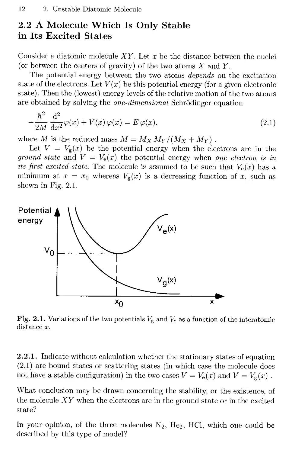
Let V = Vg(x) be the potential energy when the electrons are in the
ground state and V = Ve(x) the potential energy when one electron is in
its first excited state. The molecule is assumed to be such that Ve(x) has a
minimum at x = Xq whereas Vg(x) is a decreasing function of x, such as
shown in Fig. 2.1.
Potential
energy
Fig. 2.1. Variations of the two potentials Vg and Ve as a function of the interatomic
distance x.
2.2.1. Indicate without calculation whether the stationary states of equation
B.1) are bound states or scattering states (in which case the molecule does
not have a stable configuration) in the two cases V = Ve(x) and V = Vg(x) .
What conclusion may be drawn concerning the stability, or the existence, of
the molecule XY when the electrons are in the ground state or in the excited
state?
In your opinion, of the three molecules N2,
described by this type of model?
НС1, which one could be

2.3 Solutions 13
2.2.2. One can build a simple model for this problem by using
Vs(x) = Vi(x) (question 2.1.1) and Ve(x) = V2(x) (question 2.1.2).
Let the stationary solutions be (pk(x) in the first case and Xn(x) m the second
case. Show that the wave function
X) — О yX — •?()/ с ЮГ х .> xq
= 0 for x < 0,
where a = Мц/Й, and С is a normalization constant, is a stationary solution
in the second case V = V2.
What is the corresponding energy El
Do solutions with energies less than E exist? Explain why.
2.2.3. In the initial state, the molecule is assumed to be in the excited elec-
electronic state, and its wave function is xi {%)¦ It can fall back into the electronic
ground state by radiating the excitation energy E. One can show that the
probability of finding the atoms in the final state <fk(x) is proportional to
Calculate this quantity. We recall that
a
2.2.4. The molecule is assumed to be initially at rest. One measures the
velocity v of the atom X, of mass Mx, in the final state of the de-excitation
process. Let P(v) be the probability distribution for finding the velocity v.
How does P(v) vary with v (one can set Vq = MhuH/Mx). For which value
vm of v is P(v) maximum? Calculate vm for Mx = My = 6 x 10~27 kg, and
uj0 = 3 x 1014 s?
2.3 Solutions
Section 2.1
2.1.1. One has the usual relations
^ П2к2 ,
Е к

14 2. Unstable Diatomic Molecule
For x < xo, <fik(x) = 0; hence, by writing the continuity equations at x = xq,
l + ? = 0, i.e. В = -l, and
(fik(x) = 2isin/c(x — x0)
for x > xo ¦
The general solution is a wave packet formed with these stationary solutions,
ip(x, t) = 0 for x < x0, and, for x > x0,
/>OO
Jo
a(k) sin k(x - x0) e"№/c2 t/BM) djfc,
where a(k) is arbitrary (provided that the expression is square integrable).
2.1.2. We set z = x~xo- For z > 0 the potential is harmonic. The condition
V = oo for z < 0 implies that the wave functions should vanish at the origin.
The stationary solutions are therefore, for z > 0, the eigenfunctions of a
harmonic oscillator in z which vanish at z = 0, i.e. the Hermite functions of
odd indices, the variable being гл/а, with a = Mu>o/Ti:
Xn(x) ос Ф2„-1 {{х - хо)л/а) for x > x0
= 0 for x < xq
{{ )/)
= 0 for x < xq ,
and En = V0 + Bn - ±)hoj0, n= 1, 2,....
The ground state is E\ = Vo + C/2)hu)o and the corresponding wave function
is xi(z) oc (x - xo)e-a(x
'''/2
Section 2.2
2.2.1. In case 1 (V = Vg), the system is unbound; one has only scattering
states.
In case 2 (V — Ve), there are some eigenstates of the Hamiltonian corre-
corresponding to bound states, at least if the well depth in ro is deep enough.
The potentials of Fig. 2.1 describe a molecule which is unstable when the elec-
electrons are in the ground state (the potential Vg(x) is repulsive and the molecule
dissociates spontaneously into two atoms). Among the three molecules under
consideration, only Нег could be described by this model, since both N2 and
HC1 are known to be very stable in their ground electronic state. Actually
the molecule Нег can also be formed in its electronic ground state since the
potential Vg has in reality a very shallow minimum. There is a single bound
state in this potential well, with a binding energy t ~ —10~7 eV (average in-
ternuclear distance of 50 A), which was observed only recently.1 In contrast,
it is quite easy to form and detect Нег molecules in an excited electronic
state, for instance in discharges in a cell filled with atomic helium.
1 See, e.g., W. Schollkopf and J. P. Toennies, Science 266, 1345 A994).

2.3 Solutions
15
2.2.2. The first antisymmetric Hermite function (in x — xq) is X\{x)i which
satisfies all criteria. The corresponding eigenvalue is E\ = Vb + C/2Oiu>o
which is the lowest energy value for which the wave function vanishes at
the origin. There are no states with energies lower than E\ for the potential
Ve(x) .
2.2.3. Using the results of question 2.1.1 one obtains, setting у = x — Xq
hk =
X
dx
=4C2
/
JO
у e
~ay I2
sinky dy
We have Jq00 e ay I2 coskydy= у/тг/Bа) е к /Bq). If we take the derivative
with respect to k, we obtain:
f
Jo
and therefore
2тгС2
hk =
2 e'k
2.2.4. The above formula gives, up to a normalisation factor, the probability
density of the relative momentum of the two atoms in the final state p =
hk = Mvr, where vr is the relative velocity of the two particles
P(p) ~ p2e-P2^ah^ .
Since the molecule is at rest in the initial state, the total momentum is zero
and the atoms have momenta p and —p. The probability P(v) is, up to a
multiplicative factor,
P(v) ~ «2e-">oa
with Uq = ah2/Mx = MhuH/Mx. The probability density P(v) peaks at the
value v = Vq. Using the numerical values given in the text, and taking into
account that M = Mx/2 for Mx = MY, one finds v0 ъ 1600 ms.

3. Neutrino Oscillations
At present, most experimental limits on the neutrino masses are consistent
with zero.1 Nevertheless several theoretical and cosmological arguments indi-
indicate that these masses should be finite. The purpose of the following chapter
is to give an example of how one can measure the neutrino mass differences
using a quantum oscillation effect. The underlying theory is based on the
idea that the two neutrinos ve and v^ are actually two different states of the
same physical entity which we will call a "neutrino".
3.1 Neutrino Masses and the Associated Oscillations
In normal /3 decay, and more generally in weak interactions, the electron is
associated with a neutral particle, the neutrino ue. There exists in Nature
a particle, called the [i lepton, whose physical properties appear to be com-
completely similar to those of the electron except for its mass: raM ~ 200 rae. The
ц lepton, or muon, has weak interactions identical to those of the electron,
but it is associated with a different type of neutrino, the muon neutrino v^.
For instance, a neutrino beam produced in an accelerator can interact
with a neutron n inside a nucleus to produce a proton via the reactions:
ue + n^p+e ,3 1-
Vfj, + П —> p + fl,
whereas the reactions ve+ п^р + /л or v^ + n^p+e are never observed.
This is how neutrinos can be detected and identified.
Similarly, the decay of а тг~ meson can proceed via the two modes:
тг~ —> [i + Vn (dominant mode), and тг~ —> e + i/e, C-2)
whereas тг~ —> ц + ve or тг~ —> e + v^ are never observed. The reactions
C.2) are used to produce neutrinos abundantly in accelerators.
In these accelerators, one produces neutrinos with a well defined momen-
momentum p. In all of the following, we shall assume that if m is the mass of the
neutrino under consideration, and E its energy, the mass is so small that
1 See however the recent experimental results reported by Fukuda et al., Phys.
Rev. Lett. 81, 1562 A998).

18 3. Neutrino Oscillations
in the experimental conditions one has E 2> гас2. Therefore the energy, the
momentum and the mass are related by:
E = yp2c2 + ra2c4 ~ pc
ra2c4
and, in very good approximation, the neutrinos travel at the speed of light с
Let H be the Hamiltonian of a free neutrino of momentum p, and \v\)
and \v2) the eigenstates of H:
Н\щ)=Е1\щ), H\v2)=E2\v2)
where
El =
ra?c4
2pc ' -' "~ • 2pc
Here rai and m2 are the masses of the two states \v{) and \u2), and we assume
that rai ф m2, rai > m2 .
Suppose the physical states, corresponding to the particles produced in
reaction C.2), or to the particles detected via reaction C.1), are not \ui) and
\v2) but rather linear combinations of these states:
= \vi)cos9+\v2)sin9
l j
where в is some mixing angle.
3.1.1. At time t — 0, one produces a neutrino of momentum p in the state
v^. Calculate \v(t)) in terms of \v\) and \v2) .
3.1.2. What is the probability of detecting this neutrino in the state \ue) at
a later time t? Express the result in terms of в, с, p, t, and Z\ra2 = ra2 — ra2,.
3.1.3. The detection is done in a target located at a distance I from the
production point. Express the above probability in terms of I.
3.1.4. Assume that the mixing in C.3) is maximum, i.e. в = тг/4. What
is the distance I where the number of detected ue is maximum, assuming
that Лга2с4 = 1 (eVJ and that pc = 10 GeV = 1010 eV? Check that the
numerical results make sense considering that present day accelerators are
several kilometers long.
3.1.5. In practice, the neutrinos are detected at 1 km from the production
point. Knowing that the detector is sensitive to a decrease of 10% in the
number of u^, what limit on Лга2с4 can one reach by this method?
3.2 Solutions
3.1.1. Initially, the neutrino state is |^@)) = \v^) = — |^i)sin#+ \и2)сояв.
Therefore we have at time t:
v(t)) = -\vi) sin в e-iE^lh + \U2) cos9e-'lE2t/h.

3.2 Solutions 19
3.1.2. The probability amplitude for finding this neutrino in the state
at time t is
a = (pe
p(t)) = -sin6» costf e~iE't/h + sme costf e-'lE2t/h.
Hence the probability of detecting a ue at time t is
P = \a\2 = sin2 26» sin2 [ЛЕ t/Bh)},
where
AF F F
ЛЬ = Li ~ L2 =
Zpc Zpc
3.1.3. The time delay is t = l/c and the probability is therefore
pc
3.1.4. In that case, one should have
4ra2c4 I _ 7Г
Ahc pc 2'
which yields numerically I ~ 12 km.
3.1.5. For a probability P = 0.1, we must have Am2cil/(Ahpc2) ~ 0.32, and
therefore
4ra2c4 ~ 2.6 (eVJ.
In 1998, the first evidence for a neutrino oscillation v^ <-» vT was re-
reported (F. Fukuda et al, Phys. Rev. Lett. 81, 1562 A998)). The analysis of
atmospheric neutrino data resulting from a 535-day exposure of the Super-
Kamiokande detector leads to:
5 x 10~4 eV2 < 4m2c4 < 6 x 10 eV2.

4. Colored Molecular Ions
Some pigments are made of linear molecular ions, along which electrons move
freely. We derive here the energy levels of such an electronic system and we
show how this energy scheme explains the observed color of the pigments.
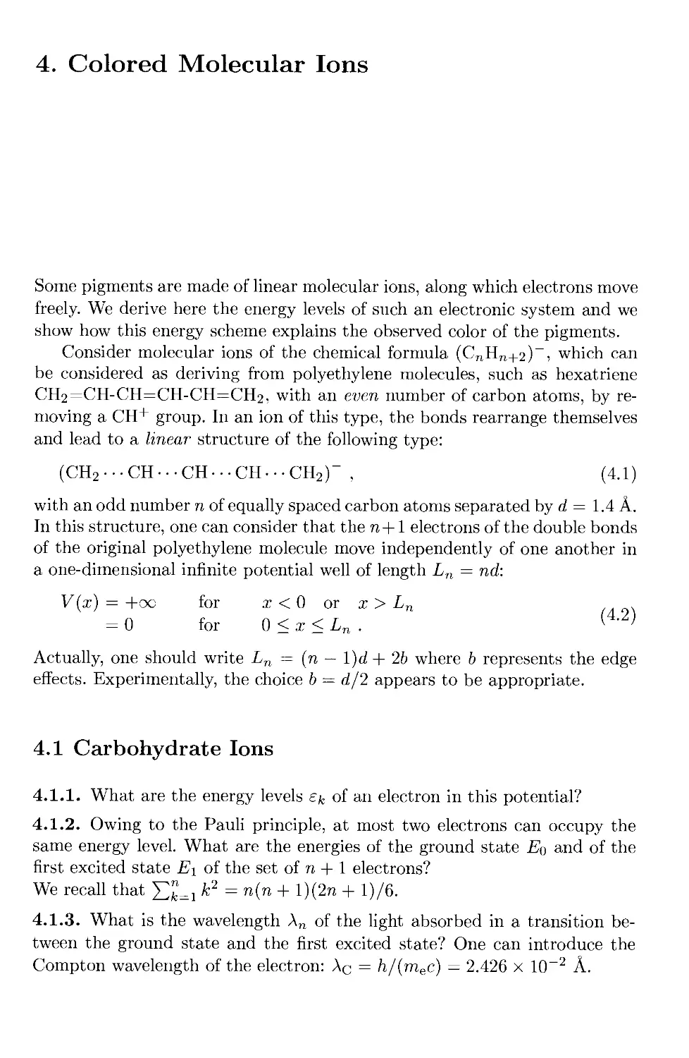
Consider molecular ions of the chemical formula (CnHn+2)~, which can
be considered as deriving from polyethylene molecules, such as hexatriene
CH2=CH-CH=CH-CH=CH2, with an even number of carbon atoms, by re-
removing a CH+ group. In an ion of this type, the bonds rearrange themselves
and lead to a linear structure of the following type:
(CH2 • • • CH • • • CH • • • CH • • • CH2)" , D.1)
with an odd number n of equally spaced carbon atoms separated by d = 1.4 A.
In this structure, one can consider that the n+1 electrons of the double bonds
of the original polyethylene molecule move independently of one another in
a one-dimensional infinite potential well of length Ln = nd:
V(x) = +oc for x < 0 or x > Ln
= 0 for 0 < x < Ln . ( >
Actually, one should write Ln = (n — \)d + 26 where b represents the edge
effects. Experimentally, the choice b = d/2 appears to be appropriate.
4.1 Carbohydrate Ions
4.1.1. What are the energy levels Ek of an electron in this potential?
4.1.2. Owing to the Pauli principle, at most two electrons can occupy the
same energy level. What are the energies of the ground state Eo and of the
first excited state E\ of the set of n + 1 electrons?
We recall that ?Li к2 = n(n + l)Bn + l)/6.
4.1.3. What is the wavelength А„ of the light absorbed in a transition be-
between the ground state and the first excited state? One can introduce the
Compton wavelength of the electron: Ac = h/(mec) — 2.426 x 10~2 A.

22 4. Colored Molecular Ions
4.1.4. Experimentally, one observes that the ions n = 9, n = 11 and n = 13
absorb blue light (A9 ~ 4700 A), yellow light (Au ~ 6000 A) and red light
(A13 ~ 7300 A), respectively. Is the previous model in agreement with this
observation? Are the ions n < 7 от п > 15 colored?
4.2 Nitrogenous Ions
One can replace the central CH group by a nitrogen atom, in order to form
ions of the type:
(CH2 • • • CH • • • N • • • CH • • • СН2Г- D.3)
The presence of the nitrogen atom does not change the distances between
atoms but it changes the above square well potential. The modification con-
consists in adding a small perturbation SV(x), attractive and localized around
the nitrogen atom:
SV(x) = 0 for \x-k*\>a/2
= -Vo for \x-kf-\<a/2 ,
where a/d <c 1 and Vo > 0.
4.2.1. Using first order perturbation theory, give the variations 5ek of the
energy level e^ of an electron in the well. For convenience, give the result to
leading order in a/d.
4.2.2. Experimentally, one observes that, for the same value of n, the spec-
spectrum of the nitrogenous ions D.3) is similar to that of the ions D.1) but that
the wavelengths \^ are systematically shorter (blue-shifted) if n = Ap + 1,
and systematically longer (red-shifted) if n = Ap + 3, than those A° of the
corresponding carbohydrates D.1). Explain this phenomenon and show that
A^ and A° are related by:
where 7 is a parameter to be determined.
4.2.3. The nitrogenous ion n = 11 absorbs red light (A^ ~ 6700 A). Check
that the ion n = 9 absorbs violet light (AjJ1 ~ 4300 A). What is the color of
the nitrogenous ion n = 13 ?
4.2.4. For sufficiently large n, if the nitrogen atom is placed not in the central
site but on either of the two sites adjacent to the center of the chain, one
observes the reverse effect, as compared to question 4.2.2 . There is a red
shift for n = Ap + 1 and a blue shift for n = Ap + 3. Can you give a simple
explanation for this effect?

4.3 Solutions 23
4.3 Solutions
Section 4.1
4.1.1. The energy levels are
к - 1 2
4.1.2. The ground state energy of the n + 1 electrons is
2*2
The energy of the first excited state is
4.1.3. One has hv = Ex - Eo = тг2П2(п + 2)/BmL2n). Since A = c/v, we
obtain an absorption wavelength
А„ = '
8 d2 n-
Ac (n + 2) '
4.1.4. Prom the general form А„ = 646.33 n2/(n + 2), we obtain A9 = 4760 A,
Ац = 6020 A, A13 = 7280 A, in good agreement with experiment.
For smaller n, the wavelengths A7 = 3520 A and A5 = 2310 A are in the
ultraviolet part of the spectrum. The ions n < 7 do not absorb visible light
and are thus not colored.
For n > 15, the wavelengths A15 = 8550 A and A17 = 9830 A are in the
infrared region. These ions do not absorb visible light in transitions from the
ground state to the first excited state. They are nevertheless colored because
of transitions to higher excited states.
Section 4.2
4.2.1. The normalized wave functions are ipk(x) = ^2/Ln sm(kirx/Ln) .
One has
5ek = fsV(x) |Vfc(x)|2 dx = ~V0 [ " |^(x)|2 dx .
J JLn~a/2
Setting у = x — Ln/2, one obtains
2V0 f+a/2 . 2fkn ктгу\
fefc = —j— / sin2 - + — dy .
Ln J-o.li \ 2 nd J
There are two cases:

24 4. Colored Molecular Ions
• к even:
«/2
i.e.
n J-a/2 \nd J
The perturbation is negligible.
• к odd:
/2
2V0 f+
^ /
2
cos2
To first order in a/d, we have 5ek — —IV^ajnd < 0.
The exact formulas are:
6ek = -— a-(-l) rsm —-
The (single particle) energy levels corresponding to even values of к are prac-
practically unaffected by the perturbation; only those with к odd are shifted. This
is simple to understand. For к even, the center of the chain is a node of the
wave function, and the integral defining 6ек is negligible. For к odd, on the
contrary, the center is an antinode, we integrate over a maximum of the wave
function, and the perturbation is maximum.
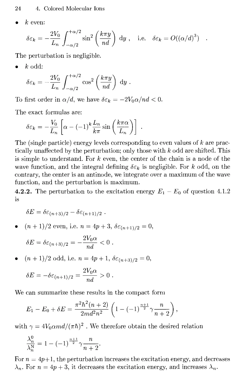
4.2.2. The perturbation to the excitation energy Ei - Eo of question 4.1.2
is
5E = fe(n+3)/2 - <fe(n+l)/2 •
• (n + l)/2 even, i.e. n = Ap + 3, 5s(n+i)/2 = 0,
5E = fe(n+3)/2 = ——{- <0.
• (ra + l)/2 odd, i.e. n = Ap + 1, fe(n+3)/2 = 0,
6E = -5e(n+l)/2 = -^- > 0 .
We can summarize these results in the compact form
4 ' n + 2,
with 7 = 4Voamd/(irhJ . We therefore obtain the desired relation
For ra = 4p+l, the perturbation increases the excitation energy, and decreases
An. For n = 4p + 3, it decreases the excitation energy, and increases An.

4.3 Solutions 25
4.2.3. For the ion n = 11 one obtains the relation A - П7/1З) = 6000/6700,
therefore 7 ~ 0.12 and X^ = 4330 A, in good agreement with experiment.
One also obtains A^3 = 6600 A, which absorbs red light and gives a green
color to the corresponding pigment. Note that the presence of the nitrogen
atom yields A^3 < Afx whereas А°3 > A^.
4.2.4. The distance between a node and an antinode of Vfc(^) is Sx =
nd/Bk).
For к = (n + l)/2 and к = (n + 3)/2 which are the states of interest, we
will have respectively Sx = nd/(n + 1) and Sx = nd/(n + 3), i.e. Sx ~ d
if n is large. Consequently, if a wave function has a node at the center, it
has an antinode in the vicinity of the two adjacent sites, and vice versa.
The reasoning is therefore similar to the answer to questions 4.2.1 and 4.2.2,
with the reverse effect. The lines are red-shifted if n = 4p + 1 and they are
blue-shifted if n = 4p + 3.

5. Schrodinger's Cat
The superposition principle states that if \фа) and \фь) are two possible states
of a quantum system, the quantum superposition (\фа) + \фь))/у/2 is also
an allowed state for this system. This principle is essential in explaining
interference phenomena. However, when it is applied to "large" objects, it
leads to paradoxical situations where a system can be in a superposition of
states which is classically self-contradictory (antinomic).
The most famous example is Schrodinger's "cat paradox" where the cat
is in a superposition of the "dead" and "alive" states. The purpose of this
chapter is to show that such superpositions of macroscopic states are not
detectable in practice. They are extremely fragile, and a very weak coupling
to the environment suffices to destroy the quantum superposition of the two
states \фа) and \фь)-
5.1 The Quasi-Classical States of a Harmonic Oscillator
In this problem, we shall consider high energy excitations of a one-dimensional
harmonic oscillator, of mass ra and frequency uj. The Hamiltonian is written
2ra 2
We denote the eigenstates of H by {\n)}. The energy of the state
En = (n + l/2)huj.
n) is
5.1.1. Preliminaries. We introduce the operators X = xy/mui/h, P =
p/vrnkuj and the annihilation and creation operators
a = 4= (x + \P) a* = -^ (x - \P) N = a^a .
We recall the commutators: [X,P] = i, [a,a^] = 1, and the relations: H =
%uj{N + 1/2) and N\n) = n\n).
(a) Check that if one works with functions of the dimensionless variables X
and P, one has

28 5. Schrodinger's Cat
(b) Evaluate the commutator [TV, a], and prove that
a\n) = y/n\n - I) E.1)
to within a phase factor which we set equal to 1 in what follows.
(c) Using E.1) for n — 0 and expressing a in terms of X and P, calculate
the wave function of the ground state фо(Х) and its Fourier transform
ipo(P). It is not necessary to normalize the result.
5.1.2. The quasi-classical states. The eigenstates of the operator a are
called quasi-classical states, for reasons which we now examine.
Consider an arbitrary complex number a . Show that the following state
a^ E.2)
is a normalized eigenstate of a with eigenvalue a-: a\a) = a\a).
5.1.3. Calculate the expectation value of the energy in a quasi-classical state
|a). Calculate also the expectation values (x) and (p) and the root mean
square deviations Ax and Ap for this state. Show that one has Ax Ap = h/2.
5.1.4. Following a similar procedure as in question 5.1.1(c) above, determine
the wave function ipa(X) of the quasi-classical state |a), and its Fourier
transform <pa(P)- Again, it is not necessary to normalize the result.
5.1.5. Suppose that at time t = 0, the oscillator is in a quasi-classical state
|«o) with a0 = pe1^ where p is a real positive number.
(a) Show that at any later time t the oscillator is also in a quasi-classical
state which can be written as e~lujt/2\a(t)). Determine the value of a(t)
in terms of p, ф, со and t.
(b) Evaluate (x)t and (p)t- Taking into account the result of question 5.1.3,
and assuming that |a| 3> 1, justify briefly why these states are called
"quasi-classical".
5.1.6. Numerical example. Consider a simple pendulum of length 1 meter
and of mass 1 gram. Assume the state of this pendulum can be described by
a quasi-classical state. At time t = 0 the pendulum is at (x0) = 1 micrometer
from its classical equilibrium position, with zero mean velocity.
(a) What is the corresponding value of a@)?
(b) What is the relative uncertainty on its position Ax/xo7
(c) What is the value of a(t) after 1/4 period of oscillation?
5.2 Construction of a Schrodinger-Cat State
During the time interval [0,T], one adds to the harmonic potential, the cou-
coupling
W = hg (a)aJ .

5.3 Quantum Superposition Versus Statistical Mixture
29
We assume that g is much larger than u> and that loT <C 1. Hence, we can
make the approximation that, during the interval [0, T], the Hamiltonian of
the system is simply W. At time t = 0, the system is in a quasi-classical state
= И-
5.2.1. Show that the states \n) are eigenstates of W, and write the expansion
of the state \ф(Т)) at time T on the basis {|ra)}.
5.2.2. How does \ф{Т)) simplify in the particular cases T = 2тг/# and T =
5.2.3. One now chooses T = тг/2д. Show that this gives
E.3)
5.2.4. Suppose a is pure imaginary: a = \p.
(a) Discuss qualitatively the physical properties of the state E.3).
(b) Consider a value of |a| of the same order of magnitude as in question
5.1.6. In what sense can this state be considered a concrete realization
of the "Schrodinger cat" type of state mentioned in the introduction?
5.3 Quantum Superposition Versus Statistical Mixture
We now study the properties of the state E.3) in a "macroscopic" situation
a\ 3> 1. We choose a pure imaginary, a — \p, and we set po — p\j2mhu>.
5.3.1. Consider a quantum system in the state E.3). Write the (non-normal-
(non-normalized) probability distributions for the position and for the momentum of the
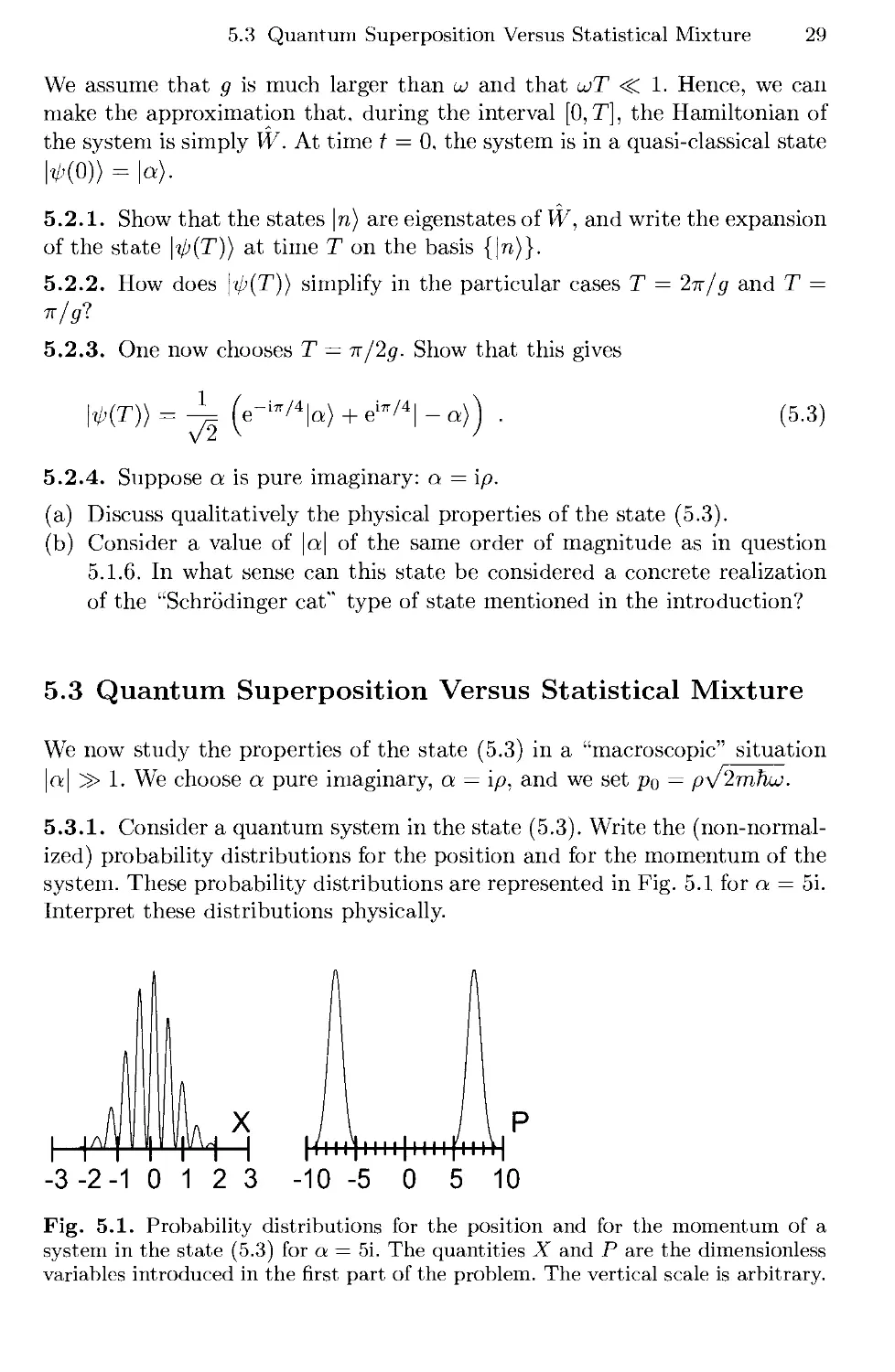
system. These probability distributions are represented in Fig. 5.1 for a = 5i.
Interpret these distributions physically.
-3 -2 -1
-10 -5 0 5 10
Fig. 5.1. Probability distributions for the position and for the momentum of a
system in the state E.3) for a = 5i. The quantities X and P are the dimensionless
variables introduced in the first part of the problem. The vertical scale is arbitrary.

30 5. Schrodinger's Cat
5.3.2. A physicist (Alice) prepares TV independent systems all in the state
E.3) and measures the momentum of each of these systems. The measuring
apparatus has a resolution 5p such that:
For TV 3> 1, draw qualitatively the histogram of the results of the TV mea-
measurements.
5.3.3. The state E.3) represents the quantum superposition of two states
which are macroscopically different, and therefore leads to the paradoxical
situations mentioned in the introduction. Another physicist (Bob) claims that
the measurements done by Alice have not been performed on TV quantum
sysytems in the state E.3), but that Alice is actually dealing with a non-
paradoxical "statistical mixture", that is to say that half of the TV systems
are in the state \a) and the other half in the state \ — a). Assuming this is
true, does one obtain the same probability distribution as for the previous
question for the TV momentum measurements?
5.3.4. In order to settle the matter, Alice now measures the position of each
of TV independent systems, all prepared in the state E.3). Draw the shape
of the resulting distribution of events, assuming that the resolution 5x of the
measuring apparatus is such that:
1 Hh
5x « —
a
mui
5.3.5. Can Bob obtain the same result concerning the TV position measure-
measurements assuming he is dealing with a statistical mixture?
5.3.6. Considering the numerical value obtained in the case of a simple pen-
pendulum in question 5.1.6, evaluate the resolution 5x which is necessary in order
to tell the difference between a set of TV systems in the quantum superposi-
superposition E.3), and a statistical mixture consisting in TV/2 pendulums in the state
\a) and TV/2 pendulums in the state | — a).
5.4 The Fragility of a Quantum Superposition
In a realistic physical situation, one must take into account the coupling
of the oscillator with its environment, in order to estimate how long one
can discriminate between the quantum superposition E.3) (that is to say the
"Schrodinger cat" which is "alive and dead") and a simple statistical mixture
(i.e. a set of cats (systems), half of which are alive, the other half being dead;
each cat being either alive or dead.)
If the oscillator is initially in the quasi-classical state |a0) and if the
environment is in a state |xe@)), the wave function of the total system is the

5.4 The Fragility of a Quantum Superposition 31
product of the individual wave functions, and the state vector of the total
system can be written as the (tensor) product of the state vectors of the two
subsystems:
|Ф@)> = Ы1Хе@)> .
The coupling is responsible for the damping of the oscillator's amplitude. At
a later time t, the state vector of the total system becomes:
with a\ = a(t)e 7*; the number a(t) corresponds to the quasi-classical state
one would find in the absence of damping (question 5.1.5(a)) and 7 is a real
positive number.
5.4.1. Using the result 5.1.3, give the expectation value of the energy of
the oscillator at time t, and the energy acquired by the environment when
2-yt <c 1.
5.4.2. For initial states of the " Schrodinger cat" type for the oscillator, the
state vector of the total system is, at t = 0,
\[2 V /
and, at a later time t,
still with a\ — a(?)e~7*. We choose t such that a\ is pure imaginary, with
\ot\ 3> 1. \xe (t)) and \xi @) are tw0 normalized states of the environment
that are a priori different (but not orthogonal).
The probability distribution of the oscillator's position, measured indepen-
independently of the state of the environment, is then
Setting ц = {xe (t)\xe @) with 0 < rj < 1 (rj is supposed to be real) and
using the results of Sect. 5.3, describe without any calculation, the result of:
(a) N independent position measurements,
(b) N independent momentum measurements.
Which condition on rj allows one to distinguish between a quantum superpo-
superposition and a statistical mixture?

32 5. Schrodinger's Cat
5.4.3. In a very simple model, the environment is represented by a second
oscillator, of same mass and frequency as the first one. We assume that this
second oscillator is initially in its ground state jXe(O)) = |0). If the coupling
between the two oscillators is quadratic, we will take for granted that
• the states \\e (i)) are quasi-classical states: \xi @) = I i/^)i
• and that, for short times (-yt <S 1): |/3|2 = 2ryt\ao\2.
(a) From the expansion E.2), show that r\ — (/3\ — /3) = exp(—2|/3|2).
(b) Using the expression found in question 5.4.1 for the energy of the first
oscillator, determine the typical energy transfer between the two oscilla-
oscillators, above which the difference between a quantum superposition and a
statistical mixture becomes unobservable.
5.4.4. Consider again the simple pendulum described above. Assume the
damping time is one year (a pendulum in vacuum with reduced friction).
Using the result of the previous question, evaluate the time during which a
"Schrodinger cat" state can be observed. Comment and conclude.
5.5 Solutions
Section 5.1
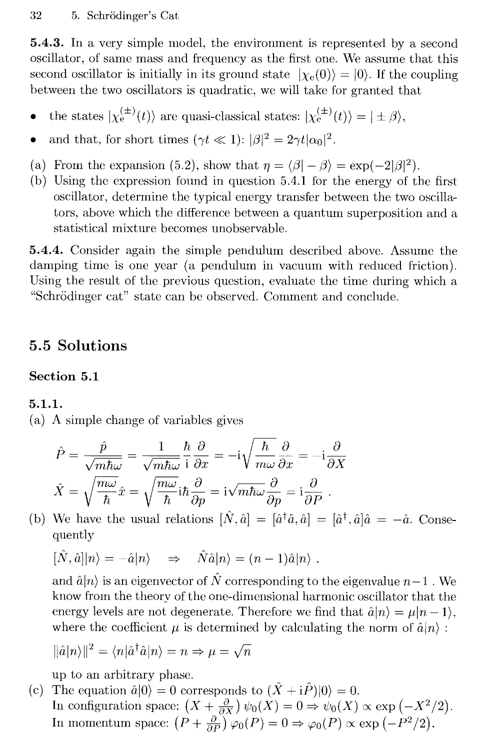
5.1.1.
(a) A simple change of variables gives
P- P - 1 %d - и
Vmnuj Vmnuj i ox V
Imuj „ Irrvjj.. д . ,—
X — \ -^—x = \ -^—m-r- = lvm
V h \ h dp
(b) We have the usual relations [N.a] = [aJa,a] = [aKa]a = —a. Conse-
Consequently
[N, a]\n) = -a\n) => Na\n) = {n - l)a\n) .
and a\n) is an eigenvector of N corresponding to the eigenvalue n—l. We
know from the theory of the one-dimensional harmonic oscillator that the
energy levels are not degenerate. Therefore we find that a\n) = ц\п— 1),
where the coefficient /x is determined by calculating the norm of a\n) :
ja|n)||2 — (nja'ajn) = n => /i = \fn
up to an arbitrary phase.
(c) The equation a\0) = 0 corresponds to (X + iP)|0) = 0.
In configuration space: [X + ^) фо(Х) = 0 =Ф- Фо(Х) ос ехр (—Х2/2).
In momentum space: (P + ^) <po(P) = 0 => <fio(P) oc exp (-P2/2).
й д
-a _
dp
1
. a
^p
ал"

5.5 Solutions 33
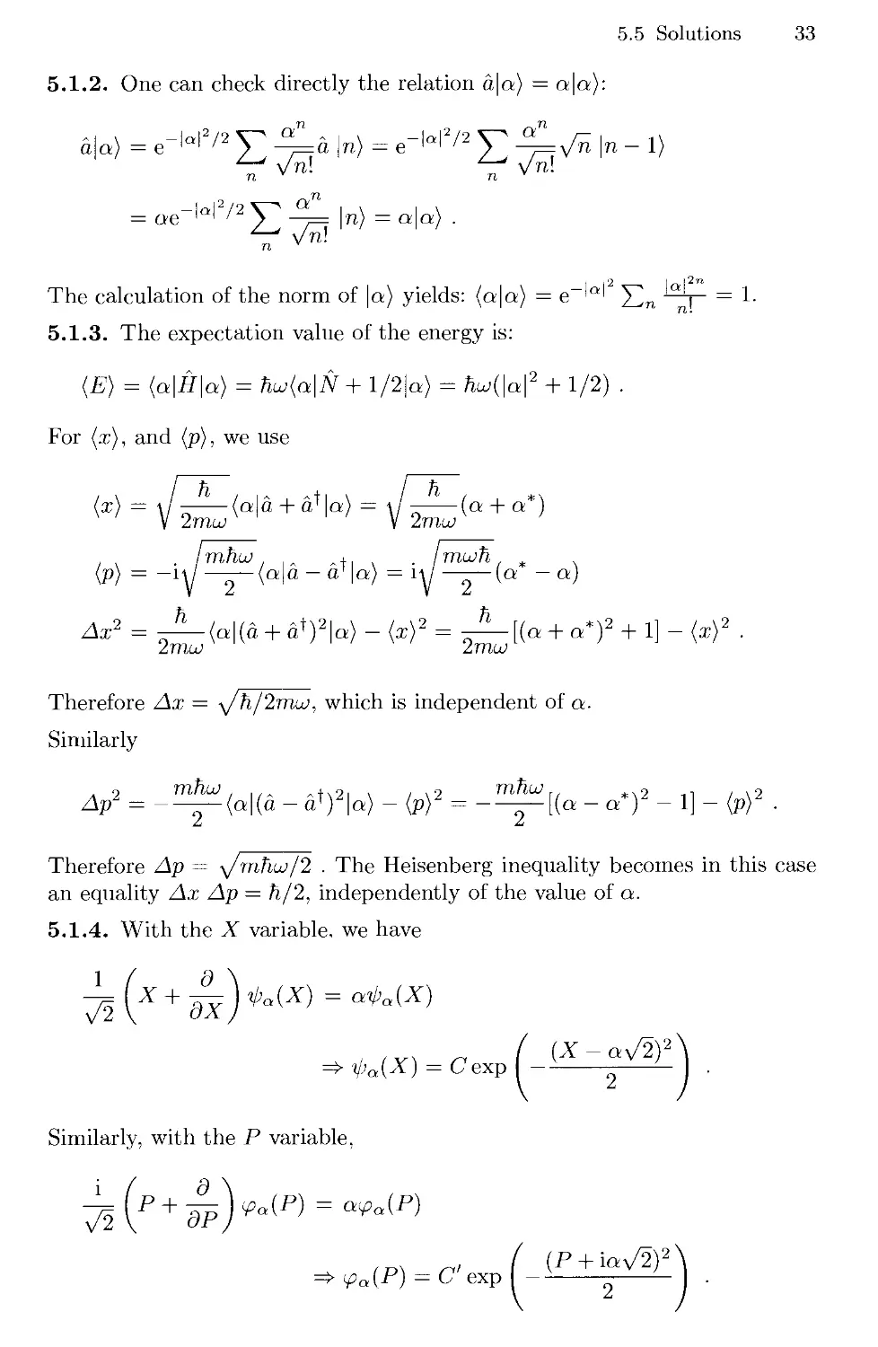
5.1.2. One can check directly the relation a\a) = a\a):
a
a) = e
an) = e
= oe
n) = a\a) .
The calculation of the norm of \a) yields: (a\a) = e 'Q' J2n I =
5.1.3. The expectation value of the energy is:
(E) = (a\H\a) = htu(a\N+ 1/2|q) = Нси(\а\2 + 1/2) .
For (x), and (p), we use
(a + a*)
<P> = "i
mhuj
2 Ma-a'\a) = i\j^-{a -a)
*J
Therefore Лх = \jTi/2mui, which is independent of a.
Similarly
Therefore Ap — yJmhu)/2 . The Heisenberg inequality becomes in this case
an equality Ax Ap = h/2, independently of the value of a.
5.1.4. With the X variable, we have
д
Similarly, with the P variable,

34 5. Schrodinger's Cat
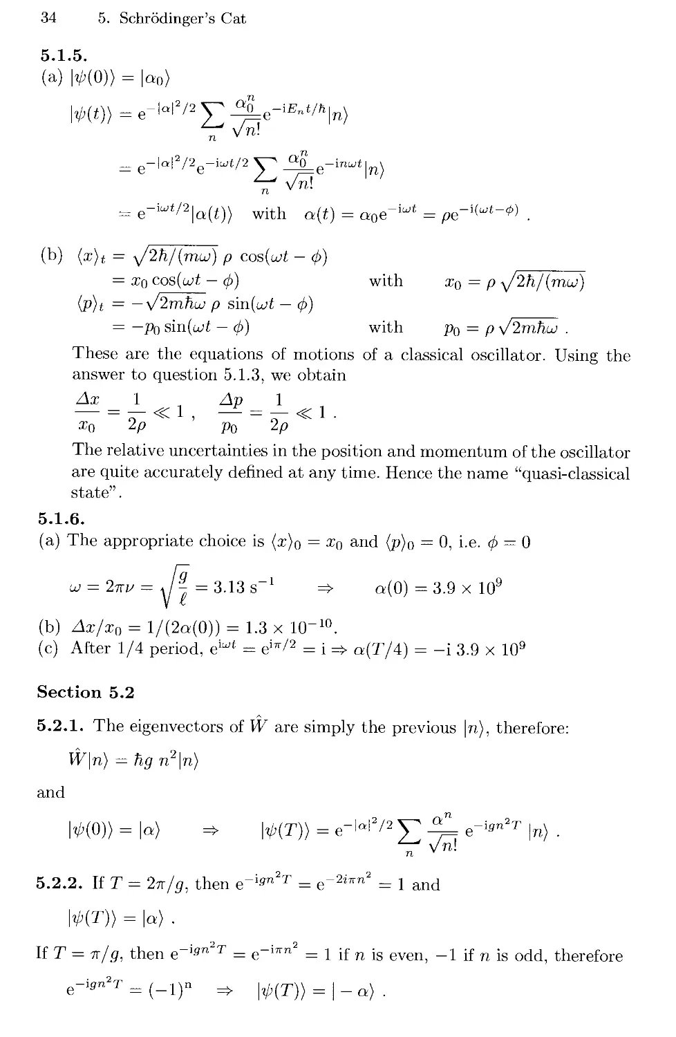
5.1.5.
(a) |V@)> = |«o)
-ы^\п)
= e-'luJt/2\a(t)) with a(t) = аое~1ш* =
with
xq = p \j2Ti/(
mu))
(b) (x)t = \j2h/{muf) p cos(u)t — ф)
= xq cos{uit — ф)
(p)t = —\//2mhuj p s'm(ujt — ф)
= — Pq sm(ujt — ф)
with pQ = p \j2mhio .
These are the equations of motions of a classical oscillator. Using the
answer to question 5.1.3, we obtain
Ax 1 Ap 1
xQ 2p p0 2p
The relative uncertainties in the position and momentum of the oscillator
are quite accurately defined at any time. Hence the name "quasi-classical
state".
5.1.6.
(a) The appropriate choice is (x)q = xq and (p)o = 0, i.e. ф = 0
uj = 2тш= W^ = 3.13 s"
a@) = 3.9 x 109
(b) Ax/xQ = l/Ba@))_ = 1.3 x 100.
(c) After 1/4 period, eiuJt = ei7r/2 = i => a(T/4) = -i 3.9 x 109
Section 5.2
5.2.1. The eigenvectors of W are simply the previous \n), therefore:
W\n) = hg
and
= \a)
ЩТ)) = e
-p-|a|2/2'
П) .
5.2.2. If T = 2тг/5, then e"^" T = e-2i7rn =
\ф(Т)) = \a) .
If T = n/g, then e~lgn T = e~17r™ = 1 if n is even, —1 if n is odd, therefore
¦,-ign'T

5.5 Solutions 35
5.2.3. If T = тт/2д, then e-ign2T = e?™2 = 1 for n even, and e^™^ = -i
if n is odd.
We can rewrite this relation as
or, equivalently,
5.2.4.
(a) For a — ip, in the state \a), the oscillator has a zero mean position
and a positive velocity. In the state | — a), the oscillator also has a zero
mean position, but a negative velocity. The state E.3) is a quantum
superposition of these two situations.
(b) If |a| 3> 1, the states |a) and | — a) are macroscopically different (anti-
(antinomic). The state E.3) is a quantum superposition of such states. It
therefore constitutes a (harmless) version of Schrodinger's cat, where we
represent "dead" or "alive" cats by simple vectors of Hilbert space.
Section 5.3
5.3.1. The probability distributions for the position and momentum are
V(X) oc
ос
V{P) ос
~ exp[-(P - pV2J} + exp[-(P
In the latter equation, we have used the fact that, for /)> 1, the two Gaus-
sians centered at p\[2 and —p\[2 have a negligible overlap.
5.3.2. Alice will find two peaks, each of which contains roughly half of the
events, centered respectively at p$ and — p$.
5.3.3. The statistical mixture of Bob leads to the same momentum distribu-
distribution as that measured by Alice: the N/2 oscillators in the state |a) all lead to
a mean momentum +po, and the N/2 oscillators in the state |a) to —po- Up
to this point, there is therefore no difference, and no paradoxical behavior
related to the quantum superposition E.3).

36 5. Schrodinger's Cat
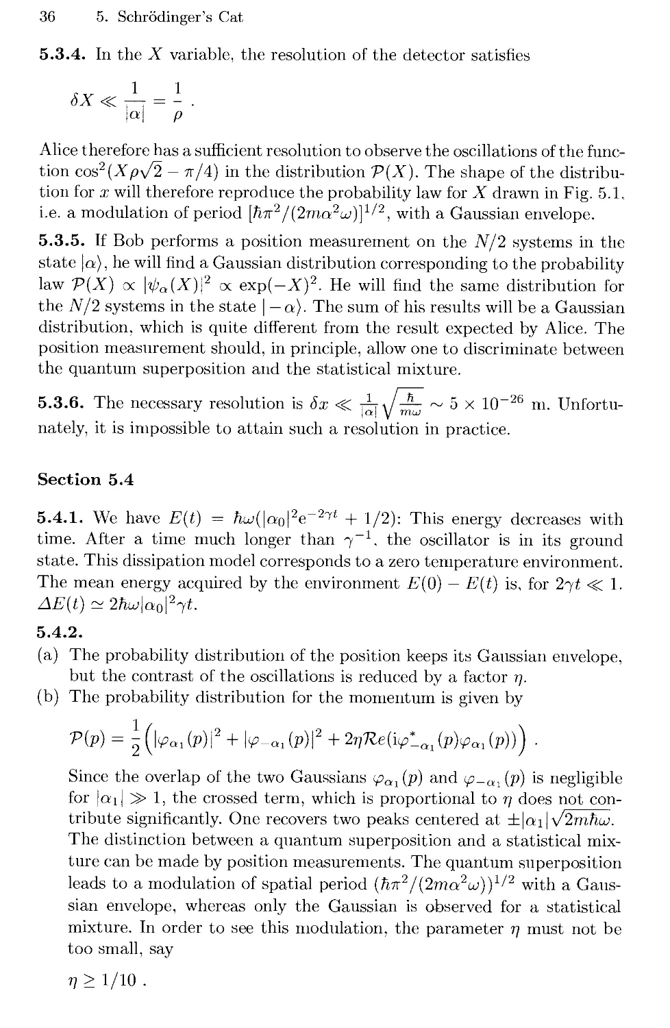
5.3.4. In the X variable, the resolution of the detector satisfies
a
Alice therefore has a sufficient resolution to observe the oscillations of the func-
function cos2'(Xp\/2 — it/4) in the distribution V(X). The shape of the distribu-
distribution for x will therefore reproduce the probability law for X drawn in Fig. 5.1,
i.e. a modulation of period [Tnt2 / Bma2u>)}1/2, with a Gaussian envelope.
5.3.5. If Bob performs a position measurement on the N/2 systems in the
state |a), he will find a Gaussian distribution corresponding to the probability
law V(X) ос \фа{Х)\2 ос ехр(—XJ. He will find the same distribution for
the N/2 systems in the state | — a). The sum of his results will be a Gaussian
distribution, which is quite different from the result expected by Alice. The
position measurement should, in principle, allow one to discriminate between
the quantum superposition and the statistical mixture.
5.3.6. The necessary resolution is Sx <S AJ^ ~ 5 x 10~26 m. Unfortu-
Unfortunately, it is impossible to attain such a resolution in practice.
Section 5.4
5.4.1. We have E(t) = ftw(|ao|2e~27* + 1/2): This energy decreases with
time. After a time much longer than 7. the oscillator is in its ground
state. This dissipation model corresponds to a zero temperature environment.
The mean energy acquired by the environment ?"@) — E(t) is, for 2-yt <C 1.
AE(t) ~ 2huj\aQ\2'yt.
5.4.2.
(a) The probability distribution of the position keeps its Gaussian envelope,
but the contrast of the oscillations is reduced by a factor r\.
(b) The probability distribution for the momentum is given by
Пр)= \(\vai(p)\2 + \v-ai(p)\2 +Ше(^-а1ШаЛр))) ¦
Since the overlap of the two Gaussians ipai (p) and tp-ai (p) is negligible
for |ai| ^> 1, the crossed term, which is proportional to r/ does not con-
contribute significantly. One recovers two peaks centered at ±\ai\y/2mhuj.
The distinction between a quantum superposition and a statistical mix-
mixture can be made by position measurements. The quantum superposition
leads to a modulation of spatial period {Tm2/{2ma2ui)I /2 with a Gaus-
Gaussian envelope, whereas only the Gaussian is observed for a statistical
mixture. In order to see this modulation, the parameter r\ must not be
too small, say

Conclusion 37
5.4.3.
(a) A simple calculation gives
@
(b) From the previous considerations, we must have e~2'^' > 1/10. i.e.
\e\<\.
For times shorter than -} :, the energy of the first oscillator is
E(t) = E@) - 2<yt\ao\2huj .
The energy of the second oscillator is
E'(t) = huj(\P(t)\2 + 1/2) = huj/2 + 2^\аа\2Тии .
The total energy is conserved; the energy tranferred during time t is
AE(t) = 2ryt\ao\2huj = Tiuj\f3\2. In order to distinguish between a quan-
quantum superposition and a statistical mixture, we must have ЛЕ < hui .
In other words, if a single energy quantum fiw is transferred, it becomes
problematic to tell the difference.
5.4.4. With I/27 = 1 year = 3 x 107 seconds, the time it takes to reach
Щ = 1 is B7Ja0j2) ^ 2 x 102 seconds!
Conclusion
Even for a system as well protected from the environment as we have as-
assumed for the pendulum, the quantum superpositions of macroscopic states
are miobservable. After a very short time, all measurements one can make
on a system initially prepared in such a state coincide with those made on
a statistical mixture. It is therefore not possible, at present, to observe the
effects related to the paradoxical character of a macroscopic quantum su-
superposition. However, it is quite possible to observe "mesoscopic" kittens,
for systems which have a limited number of degrees of freedom and are well
isolated. The first attempts concerned SQUIDS (Josephson junctions in su-
superconducting rings), but the results were not conclusive. The idea developed
here is oriented towards quantum optics, and has been proposed by Bernard
Yurke and David Stoler. Phys. Rev. Lett. 57, p. 13 A986). The most conclu-
conclusive results have been obtained at the Ecole Normale Superieure in Paris, on
microwave photons E0 GHz) stored in a superconducting cavity (M. Brune,
E. Hagley, J. Dreyer, X. Maitre. A. Maali, С Wunderlich. J.-M. Raimond.
and S. Haroche. Phys. Rev. Lett. 77. 4887 A996)). The field stored in the
cavity is a quasi-perfect harmonic oscillator. The preparation of the kitten
(Sect. 5.2) is accomplished by sending atoms through the cavity. Dissipation
(Sect. 5.4) corresponds to the very weak residual absorption by the walls of
the superconducting cavity. One can realize "kittens" made of 5 or 10 pho-
photons (i.e. \a\2 = 5 or 10) and one can check the theory precisely, including
the decoherence due to dissipation effects.

6. Direct Observation of Field Quantization
We consider here a two-level atom interacting with a single mode of the elec-
electromagnetic field. When this mode is treated quantum mechanically, specific
features occur in the atomic dynamics, such as damping and revivals of the
Rabi oscillations.
6.1 Quantization of a Mode of the Electromagnetic Field
We recall that in classical mechanics, a harmonic oscillator of mass m and
frequency uj/2tc obeys the equations of motion dx/dt = p/m and dp/dt =
—тю^х where x is the position and p the momentum of the oscillator. Defin-
Defining the reduced variables X(t) = x(t) л/muJJh and P(t) = p(t)/Vhmuj. the
equations of motion of the oscillator are
dt dt
and the total energy U(t) is given by
2
6.1.1. Consider a cavity for electromagnetic waves, of volume V. Throughout
this chapter, we consider a single mode of the electromagnetic field, of the
form
E(r, t) = ux e(t) sin kz B{r, t) = uy b(t) cos kz ,
where ux, uy and uz are an orthonormal basis. We recall Maxwell's equations
in vacuum:
V ¦ E(r,t) = 0 V/\E(r,;
V -B(r,t) = 0 VAB(r,t) =
dt
dE(r,t)
c2 Ot
and the total energy U{t) of the field in the cavity:
U(t)= [ (%E?(r,t)-

40 6. Direct Observation of Field Quantization
(a) Express de/dt and db/dt in terms of к, с, e(t), b(t).
(b) Express U(t) in terms of V, e(t), b(t), eo, /j.q. One can take
sin2 kz d3r = / cos2 kz d3r = — .
v Jv 2
(c) Setting ш = ck and introducing the reduced variables
X(t) = \[^e(t)
show that the equations for dx/dt, dH/dt and U(t) in terms of х,П and
lo are formally identical to equations F.1) and F.2).
6.1.2. The quantization of the mode of the electromagnetic field under con-
consideration is performed in the same way as that of an ordinary harmonic
oscillator. One associates to the physical quantities x and П, Hermitian op-
operators x an<i П which satisfy the commutation relation
The Hamiltonian of the field in the cavity is
The energy of the field is quantized: En = (n+ 1/2) Hlu (n is a non-negative
integer); one denotes by \n) the eigenstate of He with eigenvalue En.
The quantum states of the field in the cavity are linear combinations of the
set {jn)}. The state |0), of energy Eq = hu>/2, is called the "vacuum", and
the state jn) of energy En = Eq + tiHlu is called the "n photon state". A
"photon" corresponds to an elementary excitation of the field, of energy Hlu.
One introduces the "creation" and "annihilation" operators of a photon as
а+ = (x — ift)/\/2 and a = (x + ift)/\/2 respectively. These operators satisfy
the usual relations:
аЦп) = а/пН-Т|п+ 1)
a\n) = \/n\n - 1) if пф Q and a|0) = 0 .
(a) Express He in terms of a* and a. The observable N = a*a is called the
"number of photons".
The observables corresponding to the electric and magnetic fields at a
point r are defined as:
E(r) =
B(r) = iuy \ [a' -a) cos kz .
The interpretation of the theory in terms of states and observables is the
same as in ordinary quantum mechanics.

6.2 The Coupling of the Field with an Atom 41
(b) Calculate the expectation values (E(r)) , (B(r)) , and (n\Hc\n) in an
n-photon state.
6.1.3. The following superposition:
^ а-
а) = е
n) , F.4)
where a is any complex number, is called a "quasi-classical" state of the field.
(a) Show that \a) is a normalized eigenvector of the annihilation operator a
and give the corresponding eigenvalue. Calculate the expectation value
(n) of the number of photons in that state.
(b) Show that if, at time t = 0, the state of the field is |^@)) = |a), then,
at time t, Щг)) = e-ibjt/2\(ae~iuJt)).
(c) Calculate the expectation values {E(r))t and {B(r))t at time t in a
quasi-classical state for which a is real.
(d) Check that {E(r))t and (B(r))t satisfy Maxwell's equations.
(e) Calculate the energy of a classical field such that Ec[(r,t) = (E(r))t
and Bci(r.t) = (B(r))t. Compare the result with the expectation value
of Hq in the same quasi-classical state.
(f) Why do these results justify the name "quasi-classical" state for |a) if
a
> 1?
6.2 The Coupling of the Field with an Atom
Consider an atom at point Tq in the cavity. The motion of the center of mass of
the atom in space is treated classically. Hereafter we restrict ourselves to the
two-dimensional subspace of internal atomic states generated by the ground
state |/) and an excited state |e). The origin of atomic energies is chosen
in such a way that the energies of [/) and |e) are respectively —Tilo^/2 and
(u>a > 0). In the basis {[/), je)} , one can introduce the operators:
1 0\ „ /00\ . /0
that is to say <J+\f) = je) and <r_|e) = |/), and the atomic Hainiltonian can
be written as: Яд = %^о •
The set of orthonormal states {\f,n),\e,n),n > 0} where \f,n) =
|/) !g) \n) and \e.n) = |e) ® \n) forms a basis of the Hilbert space of the
{atom+photons} states.
6.2.1. Check that it is an eigenbasis of Ho = Да + Не, and give the corre-
corresponding eigenvalues.

42 6. Direct Observation of Field Quantization
6.2.2. In the remaining parts of the problem we assume that the frequency
of the cavity is exactly tuned to the Bohr frequency of the atom, i.e. u> = top^.
Draw schematically the positions of the first 5 energy levels of Hq. Show that,
except for the ground state, the eigenstates of Ho are grouped in degenerate
pairs.
6.2.3. The Haniiltonian of the electric dipole coupling between the atom and
the field can be written as:
W = 7 (aa+ + а}&_) ,
where 7 = —d^/fuo/eoVsinfczo, and where the electric dipole moment d is
determined experimentally.
(a) Write the action of W on the states |/, n) and |e, n).
(b) To which physical processes do aa+ and fit<7_ correspond?
6.2.4. Determine the eigenstates of H = Hq + W and the corresponding
energies. Show that the problem reduces to the diagonalization of a set of
2x2 matrices. One hereafter sets:
= 7 = —d\ —— sinfczo Г2П = Г20л/п + 1 .
2
The energies corresponding to the eigenstates \ф^) are denoted E^.
6.3 Interaction of the Atom and an "Empty" Cavity
In the following, one assumes that the atom crosses the cavity along a line
where sinfczo = 1.
An atom in the excited state je) is sent into the cavity prepared in the
vacuum state JO). At time t = 0 , when the atom enters the cavity, the state
of the system is |e, n = 0).
6.3.1. What is the state of the system at a later time t?
6.3.2. What is the probability Pf(T) of finding the atom in the state / at
time T when the atom leaves the cavity? Show that Pf(T) is a periodic
function of T (T is varied by changing the velocity of the atom).
6.3.3. The experiment has been performed on rubidium atoms for a couple
of states (/, e) such that d = 1.1 x 1(T26 Cm and lo/2-k = 5.0 x 1010 Hz. The
volume of the cavity is 1.87 x 10~6 m3 (we recall that e0 = 1/C6тгЮ9) S.I.).
The curve Pj(T), together with the real part of its Fourier transform
J{v) = /0°° cos BтшТ) Pf{T) dT, are shown in Fig. 6.1. One observes a

6.4 Interaction of an Atom with a Quasi-Classical State
43
0,04-,
I J(v) |
(b)
v (kHz)
80 100
0 20 40 60 80 100 120 140
Fig. 6.1. (a) Probability P;(T) of detecting the atom in the ground state after it
crosses a cavity containing zero photons; (b) Fourier transform of this probability,
as defined in the text.
damped oscillation, the damping being due to imperfections in the exper-
experimental setup.
How do theory and experiment compare?
(We recall that the Fourier transform of a damped sinusoid in time exhibits a peak
at the frequency of this sinusoid, whose width is proportional to the inverse of the
characteristic damping time.)
6.4 Interaction of an Atom with a Quasi-Classical State
The atom, initially in the state je), is now sent into a cavity where a quasi-
classical state |a) of the field has been prepared. At time t = 0 the atom
enters the cavity and the state of the system is |e) <g> \a).
6.4.1. Calculate the probability Pf(T,n) of finding, at time T, the atom
in the state |/) and the field in the state \n + 1), for n > 0. What is the
probability of finding the atom in the state |/) and the field in the state |0)?
6.4.2. Write the probability Pf{T) of finding the atom in the state |/), inde-
independently of the state of the field, as an infinite sum of oscillating functions.
6.4.3. On Fig. 6.2 are plotted an experimental measurement of Pf(T) and
the real part of its Fourier transform J{v)- The cavity used for this mea-
measurement is the same as in Fig. 6.1, but the field has been prepared in a
quasi-classical state before the atom is sent in.
(a) Determine the three frequencies vq , v\, v^ which contribute most strongly
to Pf(T).
(b) Do the ratios vi/щ and щ/щ have the expected values?
(c) From the values J{vq) and J{vi), determine an approximate value for
the mean number of photons \a\2 in the cavity.

44
1,0-,
0,8-
0,6
0,4-
0,2-
0,0
6. Direct Observation of Field Quantization
t(ns)
20 40 60 80 100
0,012-
0,008
0,004
0,000
U(v)|
(b)
v (kHz)
0 20 40 60 80 100 120 140
Fig. 6.2. (a) Probability P;{T) of measuring the atom in the ground state af-
after the atom has passed through a cavity containing a quasi-classical state of the
electromagnetic field; (b) Fourier transform of this probability.
6.5 Large Numbers of Photons: Damping and Revivals
Consider a quasi-classical state \a) of the field corresponding to a large mean
number of photons: \a\2 ~ no > 1, where n0 is an integer. In this case, the
probability тг(п) of finding n photons can be cast, in good approximation, in
the form:
7r(n) = e
2n
n\
л/2-ktiq
exp
,-n0)
This Gaussian limit of the Poisson distribution can be obtained by using the
Stirling formula n\ ~ ппе~п-\/2тгп and expanding 1птг(н) in the vicinity of
n = n0.
6.5.1. Show that this probability takes significant values only if n is in a
neighborhood Sn of Hq. Give the relative value Sii/tiq.
6.5.2. For such a quasi-classical state, one tries to evaluate the probability
P/(T) of detecting the atom in the state / after its interaction with the field.
In order to do this,
• one linearizes the dependence of Qn on n in the vicinity of щ:
n-n0
Sln — Slno
F.5)
• one replaces the discrete summation in Pf(T) by an integral.
(a) Show that, under these approximations, Pf(T) is an oscillating function
of T for short times, but that this oscillation is damped away after a
characteristic time Xb. Give the value of Tr>
We recall that
{•ОС -,
^(х-х0) /2a
cos(aa;) da. = e-
(b) Does this damping time depend on the mean value of the number of
photons no?
(c) Give a qualitative explanation for this damping.

6.6 Solutions 45
6.5.3. If one keeps the expression of Pj(T) as a discrete sum, an exact nu-
numerical calculation shows that one expects a revival of the oscillations of
Pf(T) for certain times Tr large compared to To, as shown in Fig. 6.3.
This phenomenon is called quantum revival and it is currently being studied
experimentally.
Keeping the discrete sum but using the approximation F.5), can you explain
the revival qualitatively? How does the time of the first revival depend on
n0?
Pf(t)
0.5-
0
0 50 100 150
Fig. 6.3. Exact theoretical calculation of Pf(T) for (n) ~ 25 photons.
6.6 Solutions
Section 6.1
6.1.1.
(a) The pair of Maxwell equations V • E = 0 and V ¦ В = 0 are satisfied
whatever the values of the functions e(t) and b(t). The equations Va? =
-(дВ/dt) and c2V Л В = -(дЕ/dt) require that:
(b) The electromagnetic energy can be written as:
U(t)= f (^e2(t) sin2 kz + ^-b2(t) cos2 kz)d3r
J \ 2 2/x /
4 2/j.q
(c) Under the change of functions suggested in the text, we obtain:
These two equations are formally identical to the equations of motion of
a particle in a harmonic oscillator potential.

46 6. Direct Observation of Field Quantization
6.1.2.
(a) From [x, П] = i, we deduce that:
1
In addition, x = (a + d+)/\/2 and П = i(at _ й)/\Д), i.e.:
Hc = — (aa) + й+й) = ftij I a)a + - j ,
(b) For an n photon state, we find (n|d|n) = (n\a}\n) = 0, which results in
<ВД>=0 (S(r)>=0.
The state \n) is an eigenstate of He with eigenvahie (n + l/2)hut, i.e.
Г
6.1.3.
(a) The action of a on \a) gives
n|n — 1)
oo „_i
— 1) =
The vector |a) is normalized:
и=0
The expectation value of the number of photons in that state is:
(n) = (a\N\a) = (a\a4\a) = \\a\a)\\2 = \a\2 .
(b) The time evolution of \ift(t)) is given by
oo „
1#)> = е-|а|/2У
= еШ1/'е
-\a\2/2
00 /^о-^Л™
n=0

6.6 Solutions 47
(с) The expectation values of the electric and magnetic fields are
(E(r))t = 2acosut sinfcz W—— ux
(B(r))t = — 2asinut cos kz ..
V v
(d) These fields are of the same type as the classical fields considered at the
beginning of the problem, with
e(t) = 2a W— cosut b(t) = -2a
V e0V
Given the relation еоцос2 — 1, we verify that e(t) = c2kb(t) and b =
—ke(t). Therefore the expectation values of the field operators satisfy
Maxwell's equations.
(e) The energy of the classical field can be calculated using the result of
question 6.1.1b. Since cos2 tot + sin2 cot = 1, we find U(t) = hcoa2. This
"classical" energy is therefore time-independent. The expectation value
of Hc is:
(#c) = {hco(N + 1/2)) = Hio(a2 + 1/2) .
It is also time independent (Ehrenfest's theorem).
(f) For |a| much larger than 1, the ratio U(t)/(Hc) is close to 1. More
generally, the expectation value of a physical quantity as calculated for
a quantum field in the state \a), will be close to the value calculated for
a classical field such that Ec\(r,t) = (E(r))t and Bc\(r,t) = (B(r))t.
Section 6.2
6.2.1. One checks that
6.2.2. For a cavity which resonates at the atom's frequency, i.e. if u> = u>a,
the couple of states |/, n+1), |e, n) are degenerate. The first five levels of Ho
are shown in Fig. 6.4a. Only the ground state |/, 0) of the atom+field system
is non-degenerate.
6.2.3.
(a) The action of W on the basis vectors of Ho is given by:
W\f,n) = y/n~/\e,n-l) if n>l
= 0 if n = 0
W\e,n) =¦

48 6. Direct Observation of Field Quantization
(a)
I/.2) I'M)
- E
- E
- F
= 2ha>
= tico
-0
/
Ф1)
Ф1)
(b)
|ш0
Fig. 6.4. (a) Positions of the five first energy levels of Ho. (b) Positions of the five
first energy levels of H = Ho + W.
The coupling under consideration corresponds to an electric dipole inter-
interaction of the form — D ¦ E(r), where D is the observable electric dipole
moment of the atom.
(b) W couples the two states of each degenerate pair. The term aa+ cor-
corresponds to the absorption of a photon by the atom, which undergoes
a transition from the ground state to the excited state. The term a)&-
corresponds to the emission of a photon by the atom, which undergoes
a transition from the excited state to the ground state.
6.2.4. The operator W is block-diagonal in the eigenbasis of Ho {|/, n), \e, n)}.
Therefore:
• The state |/, 0) is an eigenstate of Ho + W with the eigenvalue 0.
• In each eigen-subspace of Ho generated by {|/, n + 1), |e, n)} with n > 0,
one must diagonalize the 2x2 matrix:
(п+1)Псо Ш„/2
hfin/2 (n + i)hi
whose eigenvectors and corresponding eigenvalues arc (n > 0):
\Фп) corresponding to E? = (n + l)hu> -\ —-
Zi
\ф~) corresponding to E~ = (n + l)hu —- .
The first five energy levels of Ho + W are shown in Fig. 6.4b.
Section 6.3
6.3.1. We expand the initial state on on the eigenbasis of H:

6.6 Solutions 49
The time evolution of the state vector is therefore given by:
6.3.2. In general, the probability of detecting the atom in the state /, inde-
independently of the field state, is given by:
n = 0
In the particular case of an initially empty cavity, only the term n = 1
contributes to the sum. Using |/. 1) = (\ф^) + \Фо)) /у/2, we find
2
It is indeed a periodic function of T, with angular frequency fl0.
6.3.3. Experimentally, one measures an oscillation of frequency щ = 47kHz.
This result corresponds to the expected value:
1 2d I Hlo
Section 6.4
6.4.1. Again, we expand the initial state on the eigenbasis of Ho + W
oo n
\e,n)
At time t the state vector is
lEnt/H\<t>n) -'
„=o Vn! V2
We therefore observe that:

50 6. Direct Observation of Field Quantization
• the probability of finding the atom in the state |/) and the field in the
state |0) vanishes for all values of T,
• the probability Pf{T, n) can be obtained from the scalar product of \tp(t))
/
Pf(T,n) = -
4 n\
U|2n
\2n , 2
J_ e-iEit/h _ e-\E-t/h
UnT
2n
!
(l-cosunT) .
6.4.2. The probability Pf(T) is simply the sum of all probabilities Pf(T,n):
a cos VLnT .
'2 2 ^ n!
n=0 n=0
6.4.3.
(a) The three most prominent peaks of J{y) occur at the frequencies i/0 =
47kHz (already found for an empty cavity), v\ = 65kHz and v<i =
81kHz.
(b) The ratios of the measured frequencies are very close to the theoretical
predictions: v\/vq = \[2 and v^Jvq = \fb.
(c) The ratio J(v\)/ J(vq) is of the order of 0.9. Assuming the peaks have the
same widths, and that these widths are small compared to the splitting
— vq-, this ratio correponds to the average number of photons
in
the cavity.
Actually, the peaks overlap, which makes this determination somewhat
inaccurate. If one performs a more sophisticated analysis, taking into
account the widths of the peaks, one obtains |a|2 = 0.85 ± 0.04 (see
reference at end of this chapter).
Comment: One can also determine |a|2 from the ratio J{уъ)IJ(y\)
which should be equal to \a\2/2. However, the inaccuracy due to the
overlap of the peaks is greater than for J(vi)/J(vq), owing to the small-
ness of J{y2).
Section 6.5
6.5.1. The probability тг(п) takes significant values only if (n — noJ/Bno)
is not much larger than 1, i.e. for integer values of n in a neighborhood of
n0 of relative extension of the order of 1/y/no. For n0 3> 1, the distribution
7r(n) is therefore peaked around 77,0•
6.5.2.
(a) Consider the result of question 6.4.2, where we replace fln by its approx-
approximation F.5):
\ ~ \
$>(n)cos|(^0 + tto;^=^)T| F.6)
n=0

6.6 Solutions 51
We now replace the discrete sum by an integral:
e~
/•oo -u2/Bn0)
¦ COS П„„ + пп -—, T du .
We have extended the lower integration bound from —no down to —oo,
using the fact that the width of the gaussian is у/по <С no- We now
develop the expression to be integrated upon:
cos mno+fic
= cos (QnoT) cos
— sin (flnaT) sin ( -
V
The sine term does not contribute to the integral (odd function) and we
find:
For no > 1, the argument of the exponential simplifies, and we obtain:
Pf(T) = \ - \ cos (finoT) exp (-
with TD =
(b) In this approximation, the oscillations are damped out in a time Td
which is independent of the number of photons no. For a given atomic
transition (for fixed values of d and ui), this time Td increases like the
square root of the volume of the cavity. In the limit of an infinite cavity,
i.e. an atom in empty space, this damping time becomes infinite: we
recover the usual Rabi oscillation. For a cavity of finite size, the number
of visible oscillations of Pf(T) is roughly z/noTrj ~ у/щ,.
(c) The function Pf (T) is made up of a large number of oscillating functions
with similar frequencies. Initially, these different functions are in phase,
and their sum Pf(T) exhibits marked oscillations. After a time Тц, the
various oscillations are no longer in phase with one another and the
resulting oscillation of Pf(T) is damped. One can find the damping time
by simply estimating the time for which the two frequencies at half width
on either side of the maximum of тг(гг) are out of phase by ?r:
+ 7Г and \/пп ± у/пп ~ у/гцл ± -

52 6. Direct Observation of Field Quantization
6.5.3. Within the approximation F.5) suggested in the text, equation F.6)
above corresponds to a periodic evolution of period
Indeed
Tr = 4тг (no + 1) + 2тг(п — no)
We therefore expect that all the oscillating functions which contribute to
Pf(T) will reset in phase at times TR, 2TR,... The time of the first revival,
measured in Fig. 6.3, is Q.qT ~ 64, in excellent agreement with this prediction.
Notice that TR ~ 4 л/щ Ty> , which means that the revival time is always large
compared to the damping time.
Actually, one can see from the result of Fig. 6.3 that the functions are only
partly in phase. This comes from the fact that the numerical calculation
has been done with the exact expression of fln. In this case, the difference
between two consecutive frequencies f2n+i — f2n is not exactly a constant,
contrary to what happens in approximation F.5); the function Pf(T) is not
really periodic. After a few revivals, one obtains a complicated behavior of
Pf(T), which can be analysed with the techniques developed for the study
of chaos.
Comments: The damping phenomenon which we have obtained above is
"classical": one would obtain it within a classical description of the interaction
of the field and the atom, by considering a field whose intensity is not well
defined (this would be the analog of a distribution тг(п) of the number of
photons). On the other hand, the revival conies from the fact that the set of
frequencies f2ra is discrete. It is a direct consequence of the quantization of
the electromagnetic field, in the same way as the occurrence of frequencies
v0V2, щ\Д,. ¦. in the evolution of Pf(T) (Sect. 6.4).
The experiments described in this problem have been performed in Paris,
at the Laboratoire Kastler Brossel. The pair of levels (/, e) correspond to
very excited levels of rubidium, which explains the large value of the electric
dipole moment d. The field is confined in a superconducting niobium cavity
(Q-factor of ~ 108), cooled down to 0.8 К in order to avoid perturbations to
the experiment due to the thermal black body radiation.
Reference
M. Brune, F. Schmidt-Kaler, A. Maali, J. Dreyer, E. Hagley, J.-M. Raimond,
and S. Haroche, Phys. Rev. Lett. 76, 1800 A996).

7. Decay of a Tritium Atom
The nucleus of the tritium atom is the isotope 3H, of charge Z = 1. This
nucleus is radioactive and transforms into a 3He nucleus by /3 decay. The
purpose of this chapter is to study the electronic state of the 3He+ ion formed
after the decay.
We consider nuclei as infinitely massive compared to the electron, of mass
m. We write a,\ = h2/(me2) for the Bohr radius and E\ = mc2a2/2 ~ 13.6 eV
for the ionization energy of the hydrogen atom, where a is the fine structure
constant [e2 = д2/Dтгео), where q is the electron charge].
In the ground state |V>o) °f the tritium atom, the wave function of the
electron (n = 1,1 = 0, m = 0) is the same as in the normal hydrogen atom:
G.1)
The /3 decay of the tritium nucleus leads to:
3H^3He + e~ + P G.2)
(p is an antineutrino), where the emitted electron has an energy of the order
of 15 keV and the helium nucleus 3He has charge Z = 2. The decay is an
instantaneous process; the /3 electron is emitted with a large velocity and
leaves the atomic system very rapidly. Consequently, an ionized 3He+ atom
is formed, for which, at the time tg °f the decay, the wave function of the
electron is practically the same as in tritium, and we shall assume it is still
given by G.2). We denote by \n,l,m) the states of the ionized helium atom
which is a hydrogen-like system, i.e. one electron placed in the Coulomb field
of a nucleus of charge 2.
7.1 The Energy Balance in Tritium Decay
7.1.1. Write the Hamiltonian H1 of the atomic electron before the decay and
the Hamiltonian Hi of this electron after the decay (when the potential term
has suddenly changed).
7.1.2. What are, in terms of E\, the energy levels of the 3He+ atom? Give
its Bohr radius and its ground state wave function

54 7. Decay of a Tritium Atom
7.1.3. Calculate the expectation value (E) of the energy of the electron after
the decay. One can for instance make use of the fact that:
1 1 e2
(V>ol ~ IV'o) = — and H2 = H1 .
Г di Г
Give the value of (E) in eV.
7.1.4. Express in terms of |V>o) and \n,l,m) the probability amplitude
c(n,l,m) and the probability p(n,l,m) of finding the electron in the state
n,l,m) of 3He+ after the decay. Show that only the probabilities pn =
p (n, 0, 0) do not vanish.
7.1.5. Calculate the probability p\ of finding the electron in the ground state
of 3He+. What is the corresponding contribution to (E)?
7.1.6. A numerical calculation gives the following values:
p2 = - , Ур„ = 0.02137, V ^ = 0.00177.
Calculate the probability 5Z^Li Pn °f finding the atomic electron in a bound
state of 3He+ and the corresponding contribution to (E). Comment on the
result.
7.1.7. Experimentally, in the /3 decay of the tritium atom, one observes that,
in about 3% of the events, there are two outgoing electrons, one with a mean
kinetic energy (E^) ~ 15 keV, the other with (Ek) ~ 34.3 eV, thus leaving
a completely ionized 3He2+ nucleus, as if the /3 decay electron had "ejected"
the atomic electron. Explain this phenomenon.
7.2 Solutions
7.1.1. The two Hamiltonians are
н = $—-е- й2 = — ~2—
2m r 2m r
7.1.2. The energy levels corresponding to the bound states of a hydrogen-
like atom of nuclear charge Z are En = —Z2Ei/n2. In the present case,
En = —4Ei/n2. The new Bohr radius is a2 = a,\/2, and the wave function
is
/тгай

7.2 Solutions 55
7.1.3. The expectation value of the electron energy in the new nuclear con-
configuration is
(E) = (фо\Н2\Фо) = (Фо\Нг\фо) - (Фо
which amounts to
(E) = -Ei - — = -3Et ~ -40.8 eV .
7.1.4. By definition, the probability amplitude is c(n,l,m) = (п,1,т\фо) ,
and the probability p(n, I, m) = \(n, I, ttt.|^o)|2 • The analytic form is
c(n
:,l,m) = J' Rni(r) (?Г(в,ф)Т фо(г) d3r ,
where Rni(r) are the radial wave functions of the 3He+ hydrogen-like atom.
Since ip0 is of the form Vo(r) = Х(г)?$(в,ф), the orthogonality of spherical
harmonics implies p(n, I, rri) = 0 if (I, m) ф @,0).
7.1.5. The probability amplitude in the lowest energy state is
Г а-г/а2 -г
-r dr =
27
Hence the probability pi = 0.70233 and the contribution to the energy
PlEr = -38.2 eV.
7.1.6. With the numerical values given in the text, one has P2E2 = —Ei/A =
-3.4 eV, and p = J2T P™ = 0.9737 . The contribution to (E) is (EB) =
T,TPnEn = -3.0664 Ei = -41.7 eV.
The total probability is smaller than 1; there exists a non-zero probability
A — p) = 0.026 that the atomic electron is not bound in the final state.
The contribution of bound states (Ев) = -41.7 eV is smaller than the total
expectation value of the energy (E) by 0.9 eV. The probability A — p) corre-
corresponds therefore to a positive electron energy, i.e. an ionization of 3He+ into
3He2+ with emission of the atomic electron.
7.1.7. There is necessarily a probability 1 —p = 0.026 for the atomic electron
not to be bound around the helium nucleus, therefore that the helium atom
be completely ionized in the decay. If the mean kinetic energy of the expelled
electron is E^ ~ 34.3 eV, this represents a contribution of the order of A —
р)Е^ ~ +0.89 eV to the mean energy which compensates the apparent energy
deficit noted above.

56 7. Decay of a Tritium Atom
Comment: This type of reaction is currently being intensively studied in
order to determine the neutrino mass. If Mi and M2 are the masses of the
two nuclei, Ep the energy of the /3 electron, E the energy of the atomic
electron, and Е„ the neutrino energy, energy conservation gives for each event:
MiC2 — E\ = M2C2 + Ер + Е„ + Е. For a given value of E, the determination
of the maximum energy of the /3 electron (which covers all the spectrum
up to 19 keV in the tritium atom case) provides a method for determining
the minimum value mpc2 of E& through this energy balance. An important
theoretical problem is that current experiments are performed on molecular
tritium (HT or TT molecules) and that molecular wave functions are not
known explicitly, contrary to the atomic case considered here.

8. The Hydrogen Atom in Crossed Fields
We study using perturbation theory the modification of the energy spectrum
of a hydrogen atom placed in crossed static electric and magnetic fields. We
thus recover (in the perturbative regime) a result first derived by Pauli.
In his famous 1925 paper on the hydrogen atom, W. Pauli made use of the
particular symmetry of the Coulomb problem. In addition to the hydrogen
spectrum, he was able to calculate the splitting of the levels in an electric
field (Stark effect) or in a magnetic field (Zeeman effect). Pauli also noticed
that he could obtain a simple and compact formula for the level splitting in
a superposition of a magnetic field Bq and an electric field Eq both static
and uniform, and perpendicular to each other. In this case, he found that a
level with principal quantum number n is split into 2n — 1 sublevels
En + 6E^k) with
6E^=hk(co20+u,2ey/2 , (8.1)
where к is an integer ranging from — (n —1) to n —1, loq and uje are respectively
proportional to Bq and Eq, and toe can be written as
Ые=^/(П) With Пе
where M and qe are the mass and charge of the electron, and where f(n)
depends on n only.
It is only in 1983 that Pauli's result was verified experimentally. Our
purpose, here, is to prove equation (8.1) in the special case n = 2, to calculate
luq and cue in that case, and, by examining the experimental result for n = 34,
to guess what was the very simple formula found by Pauli for f(n).
8.1 The Hydrogen Atom in Crossed Electric
and Magnetic Fields
We consider the n = 2 level of the hydrogen atom. We neglect all spin effects.
We assume that Bo is along the z axis and Eq along the x axis. We use first
order perturbation theory.

58 8. The Hydrogen Atom in Crossed Fields
8.1.1. What are the energy levels and the corresponding eigenstates in the
presence of -Bo only? Check that (8.1) is valid in this case and give the value
8.1.2. In the presence of Eq only, the perturbing Hamiltonian is the electric
dipole term He = —D.Eq = —qer.Eo. Write the matrix representing He in
the n = 2 subspace under consideration.
We recall that:
(a) Jo°° r3R2S(r) R2P(r)dr = 3\/3ai where i?2s and R.2P are the radial wave
functions for the level n = 2,1 = 0 and n = 2,1 = 1 respectively, and
where a! = Ti2/(Me2) is the Bohr radius (e2 = q^/Ane0).
(b) In spherical coordinates (9 polar angle and ф azimuthal angle), the I = 0
and I = 1 spherical harmonics are
8.1.3. Calculate the energies of the levels originating from the n = 2 level in
the presence of the crossed fields Eq and Bq. Show that one recovers (8.1)
with u>e = C/2)/B)fie, and give the value of /B).
8.2 Pauli's Result
The first experimental verification of Pauli's result was achieved in 1983.: In
Fig. 8.1, the points correspond to a sub-level with a given value of к arising
from the n = 34 level of an hydrogen-like atom. All points correspond to the
same energy of this level, but to different values of the static fields Eq and
Bo-
Knowing that we is a function of the principal quantum number n of the
form: cue = C/2)/(n)fie, and that cu0 and пе are the constants introduced
above, answer the following questions:
8.2.1. Does the experimental data agree with equation (8.1)?
8.2.2. Write the quantity uj^ + ui2 in the form Л (jBq + /2(п)Е^), give the
value of the constant 7, and calculate /C4).
8.2.3. Guess Pauli's result concerning f(n).
1 Figure 8.1 was obtained by F. Biraben, D. Delande, J.-C. Gay, and F. Penent,
with rubidium atoms prepared in a Rydberg state, i.e. with an electron placed
in a strongly excited level (see J.-C. Gay, in Atoms in unusual situations, J.-P.
Briand ed., p. 107, Plenum, New York, 1986).

4 106
2 10
8.3 Solutions 59
E02 (V2m-2)
I I I I I I I I
B02
50 10 100 10
Fig. 8.1. Values of the electric and magnetic fields giving rise to the same sub-level
energy of the n = 34 level of a hydrogen-like atom.
8.3 Solutions
Section 8.1
8.1.1. Consider a state \n, I, m). The orbital magnetic moment of the electron
is /логЪ = 7oi, with 7o = qe/BM). The magnetic Hamiltonian is H =
-AOTb.B = ~(qe/2M)LzB0.
At first order perturbation theory, the energy levels originating from the n =
2 subspace (angular momentum I = 0 or I — 1) are mhojQ with m = —1,0, +1,
and luo = —qeBo/BM) (uiq > 0 for Bq > 0). The corresponding states are
\2s) and \2p, m = 0) SE = 0
|2jJ, 771 = —1) E^ = —flOJo
\2p, m = +1) SE = +Tiujq .
8.1.2. The Hamiltonian is He = —qexEo. We have to calculate the 16
matrix elements B,1', m'\x\2, l,m). The integral to be evaluated is
B,l',m'\x\2,l,m) = f f {y^'(9,ф)Х sin в совф УгтF», ф) d2u
x f r3 (R2,v(r))* R2,i(r)dr .
Jo
The angular integral vanishes if Z = I'. We need only consider the terms
I' = 0, I = 1 (and the hermitian conjugate I' = 1, I = 0), i.e.:
Ol 11 J^yiz^-y^, ф) + Yl-\e,

60 8. The Hydrogen Atom in Crossed Fields
where we have incorporated the radial integral given in the text. One therefore
obtains 3ai (8m,-i — <Sm,i)/"\/2- The only non-vanishing matrix elements are
Bs\H\2p,m = ±1) and their hermitian conjugates.
Setting fle = 4neohEo/(Mqe) = qeEoa,i/h, we obtain the matrix
'00 0 1\
00 0 0
V2 | 00 0-1
10-1 0/
where the rows (columns) are ordered as 2p, m = 1, 0, —1; 2s.
8.1.3. We want to find the eigenvalues of the matrix
0
0
0
0
0
0
0
—u
0
3ue/
0
There is an obvious eigenvalue Л = 0 since the \2p,m = 0) and \2s) states
do not mix in the presence the electric field. The three other eigenvalues are
easily obtained as the solutions of:
i.e. A = 0 and A = ±Пл/и[+~Щ.
The shifts of the energy levels are therefore: 6E = 0 twice degenerate, and
SE = ±H^uJq + 9Щ. If we adopt the prescription given in the text, we obtain
tue = 3Oe =>¦ /B) = 2 .
Section 8.2
8.2.1. We remark that the experimental points are aligned on a straight line
uBq + bE2, = constant which is in agreement with (8.1), i.e. a constant value
of Wg + uj2 corresponds to a constant value of each energy level.
8.2.2. Given the definitions of ojq and fle , one has
2 2 ^ /4тгеой\ \(ас
where a is the fine structure constant and с the velocity of light. The exper-
experimental line
(ac/3JB2 + /2C4)?2
goes through the points El = 0, B% ~ 87 x 10~4 T2 and B2 = 0, E% ~
4 x 106 V2m-2. This gives /C4) = 34.
8.2.3. Indeed, the very simple result found by Pauli was f(n) = n.

9. Exact Results for the Three-Body Problem
The three-body problem is a famous question of mechanics. Newton actually
quit physics because he found it too difficult. Henri Poincare was the first
to prove exact properties, and this contributed to his celebrity. The purpose
of this chapter is to derive some rigorous results for the three-body problem
in quantum mechanics. Here we are interested in obtaining rigorous lower
bounds on three-body ground state energies. Upper bounds are easier to ob-
obtain by va iational calculations. We will see that our lower bounds are actually
quite close to the exact answers, to which they provide useful approximations.
9.1 The Two-Body Problem
Consider a system of two particles with equal masses m and momenta p\ and
p2, interacting via a potential V{r\2) where r\2 = \r\ — r2 .
9.1.1. Write the Hamiltonian H of the system. Let P = Pi + p2 and p =
(Pi ~ P2)/2 be the total and relative momentum.
Separate the center of mass Hcm and the relative H\2 Hamiltonians by writing
tf as:
-2 „2
H = Hcm + H12, #cm = — , H12 = ?- + V(r12) , (9.1)
where M = 2m is the total mass of the system. Give the value of the reduced
mass ц in terms of m.
9.1.2. We denote by E^2\ii) the ground state energy of H\2. Give the ex-
expression for E^(fi) in the two cases V(r) = ~b2/r and V(r) = кг2/2.
9.2 The Variational Method
Let {\n)} be the orthonormal eigenstates of a Hamiltonian H and {En} the
ordered sequence of its corresponding eigenvalues: Eq < E\ < E2 < ¦ ¦ ¦ ¦
9.2.1. Show that (n\H\n) = En.

62 9. Exact Results for the Three-Body Problem
9.2.2. Consider an arbitrary vector \ф) of the Hilbert space of the system.
By expanding \ip) on the basis {|n)}, demonstrate the inequality
W>, (ф\Н\ф)>Е0(ф\ф). (9.2)
9.2.3. Show that the previous result remains valid if H is the Hamiltonian
of a two-body subsystem and \ф) a three-body state. In order to do so, one
can denote by #12 the Hamiltonian of the A, 2) subsystem in the three-body
system of wave function ф(т\, r2, т*з)- One can first consider a given value of
Г3, and then integrate the result over this variable.
9.3 Relating the Three-Body and Two-Body Sectors
Consider a system of three-particles of equal masses m with pairwise inter-
interactions:
V = V(r12) + V(r13) + V(r23) .
9.3.1. Check the identity
3(p? + p\ + Рз) = (Pi + P2 + РзJ + (Pi ~ P2J + (P2 - РзJ + (Рз - PiJ
and show that the three-body Hamiltonian #C' can be written as
Л(з) ?т 1 Л(з) ?т P
6m
where P = i>i + i>2 + i>3 is the total three-body momentum, and where the
relative Hamiltonian #rel is a sum of two-particle Hamiltonians of the type
defined in (9.1),
#rel = #12 + #23 + #31
with a new value // of the reduced mass. Express // in terms of m.
9.3.2. Do the two-body Hamiltonians #,j commute in general? What would
be the result if they did?
9.3.3. We note the normalized ground state of #rel by |f2) and the cor-
corresponding energy by E^. Show that the three-body ground state energy
is related to the ground state energy of each two-body subsystem by the
inequality:
?C) > 3^B)^'). (9.3)
9.3.4. Which lower bounds on the three-body ground-state energy E^ does
one obtain in the two cases V(r) = —b2/r and V(r) = кг2/21
In the first case, the exact result, which can be obtained numerically, is
~ -1.067 mb4/h2. How does this compare with the bound (9.3)?

9.5 From Mesons to Baryons in the Quark Model 63
9.4 The Three-Body Harmonic Oscillator
The three-body problem can be solved exactly in the case of harmonic inter-
interactions V(r) = кг2/2. In order to do this, we introduce the Jacobi variables:
#i = (fi - f2)/V2, #2 = Bf3 - fi - r2)/VE, R3 = (fi + f2 + f3)/V3
Qi = (Pi - P2)/V2, Q2 = Bp3 - Pl - p2)/V6, Q3 = (Pl +p2+ P3)/V3.
9.4.1. What are the commutation relations between the components Щ and
Ql of #* andQf, (a= 1,2,3, and/3 = 1,2,3)?
9.4.2. Check that one has Q\ + Q\ + Q\ = p? + p2, + ^ , and:
3(Д? + Д|) = (ri - r2J + (r2 - r3J + (r3 - r-iJ .
9.4.3. Rewrite the three-body Hamiltonian in terms of these variables for a
harmonic two-body interaction V(r) = кг2/2. Derive the three-body ground
state energy from the result. Show that the inequality (9.3) is saturated, i.e.
the bound (9.3) coincides with the exact result in that case.
Do you think that the bound (9.3), which is valid for any potential, can be
improved without further specifying the potential?
9.5 From Mesons to Baryons in the Quark Model
In elementary particle physics, the previous results are of particular interest
since mesons are bound states of two quarks, whereas baryons, such as the
proton, are bound states of three quarks. Furthermore, it is an empirical ob-
observation that the spectroscopy of mesons and baryons is very well accounted
for by non-relativistic potential models for systems of quarks.
The ф meson, for instance, is a bound state of a strange quark s and
its antiquark s, both of same mass ms. The mass гпф is given by тф =
2ms + ?"B)(/л)/с2 where /i = ms/2, с is the speed of light, and E^ is the
ground state energy of the ss system which is bound by a potential Vqq(r).
The fi~ baryon is made of three strange quarks. Its mass is given by Mq =
3ms + E^ (fi)Ic2, where E^ is the ground state energy of the three s quarks,
which interact pairwise through a two-body potential Vqq(r).
These potentials are related very simply to each other by
Vqq(r) = 2Vqq(r) ¦
It is a remarkable property, called flavor independence, that these potentials
are the Same for all types of quarks.
9.5.1. Following a procedure similar to that of Sect. 9.3, show that
); express // in terms of fi = ms/2.

64 9. Exact Results for the Three-Body Problem
9.5.2. Consider the potential Vqq(r) = g ln(r/r0), and the two-body Hamilto-
nians H^(fi) and H^(jl) corresponding to the same potential but different
reduced masses fi and Д. By rescaling r, transform H^(jl) into H^^fi) + C,
where С is a constant.
Calculate the value of С and show that the eigenvalues E^ '(/i) of
and En\fi) of Я^2)(Д) are related by the simple formula
9.5.3. A striking characteristic of the level spacings in quark-antiquark sys-
systems is that these spacings are approximately independent of the nature of
the quarks under consideration, therefore independent of the quark masses.
Why does this justify the form of the above potential Vqqif) = g\n(r/ro)l
9.5.4. Show that the following relation holds between the Q,~ and ф masses
Mq and т,ф :
3
Ma. > -тф + а
and express the constant a in terms of the coupling constant g.
9.5.5. The observed masses are тф = 1019 MeV/c2 and Mq. = 1672 MeV/c2.
The coupling constant is g = 650 MeV. Test the inequality with these data.
9.6 Solutions
Section 9.1
9.1.1. The two-body Hamiltonian is
The center of mass motion can be separated as usual:
» 2
where M = 2m and fi = m/2 are respectively the total mass and the reduced
mass of the system.
9.1.2. For a Coulomb-type interaction V{r) = —b2/r, we get
Е^Цп) = -f^-
' 2h2 '
For a harmonic interaction V(r) = кг2/2, we get

9.6 Solutions 65
Section 9.2
9.2.1. By definition, (п\Й\п) = En(n\n) = En.
9.2.2. Since {\n)} is a basis of the Hilbert space, \ф) can be expanded as
\ф) = ^cn|n), and the square of its norm is (ф\ф) = ^ lcn|2- We therefore
^ 2
If we simply write
(ф\Н\ф) - Е0(ф\ф) = ]
we obtain, since En > Eo and |cn|2 > 0:
(ф\Н\ф) > Е0(ф\ф) .
9.2.3. If H = H12, for fixed Г3, ip(ri, Г2, r3) can be considered as a non-
normalized two-body wave function. Therefore
/ Ф*(г1,г2,г3) Н12 ф(г1,г2,г3) d3ri d3r2
>E0 f \ф(гъг2,г3)\2 d3nd3r2 .
By integrating this inequality over r3, one obtains the desired result.
Section 9.3
9.3.1. The identity is obvious, since the crossed terms vanish on the right-
hand side. Therefore Я = p2/Fm) + Я12 + Я23 + Я31, with
H,, +v(nj)+v(ru) m
with a reduced mass [>! = Зт/А.
9.3.2. Obviously, Я12 and H23 do not commute; for instance pi — p2 does
not commute with V(r23). If they did, the three-body energies would just be
the sum of two-body energies as calculated with a reduced mass // = 3m/4,
and the solution of the three-body problem would be simple.
9.3.3. By definition, E{3~> = (Г>|Яг(^|Г>) = ?(fi|i^2)|fi). However, owing to
the results of questions 9.2.2 and 9.2.3, we have (ЩЙ^^П) > E^di'), so
that
E{3) > 3?B)(//) with A*'

66 9. Exact Results for the Three-Body Problem
9.3.4. For a Coulomb-type potential, we obtain
V64 9 mb4
2 h2 ~ 8 h2 '
which deviates by only 6% from the exact answer —1.067 mbA /Ti2.
In the harmonic case, we obtain:
Section 9.4
9.4.1. One easily verifies that Jacobi variables satisfy canonical commutation
relations:
[R?,Q%\=ih6jk6a0.
9.4.2. These relations are a simple algebraic exercise.
9.4.3. We find
2m 2 г 2т 2 2m
where Hcm = Q2/Bm) = P2 /Fm) is the center of mass Hamiltonian. The
three Hamiltonians Hi, Hi, and Hcm commute. The ground state energy
(with the center of mass at rest) is therefore
m \ m
which coincides with the lower bound obtained in question 9.3.4. The bound
is therefore saturated if the interaction is harmonic.
In order to improve the bound, one must further specify the interaction.
Actually, the bound is saturated if and only if the interaction potential is
harmonic. Indeed the variational inequality we use becomes an equality if
and only if the wave function coincides with the exact ground state wave
function. Owing to the particular symmetry of quadratic forms, the Jacobi
variables guarantee that this happens in the harmonic case. The property
ceases to be true for any other potential.

9.6 Solutions 67
Section 9.5
9.5.1. The ss relative Hamiltonian is
#B) _ f_ , у _(r\
The sss relative Hamiltonian is (cf. Sect. 9.3):
i ~ PjJ | ly ,
r>C) _
6TOs
Therefore,
? 0 with ЯИ = ((ft"^)/2) +
with /Li' = 3ms/8 = 3/^/4. From this relation we deduce the inequality:
2?C> >3?B)(//) with ц' = Зц/4.
9.5.2. With the rescaling r —> ar, one obtains:
The choice a = л/fi/p, leads to H^(p) = H^(fi) + g\na so that
9.5.3. In a logarithmic potential, the level spacing is independent of the
mass. This is a remarkable feature of the observed spectra, at least for heavy
quarks, and justifies the investigation of the logarithmic potential. Amazingly
enough, this empirical prescription works quite well for light quarks, although
one might expect that a relativistic treatment is necessary.
9.5.4. The binding energies satisfy
with
?C) E{2)
= 3ms H — тф = 2ms H —
cz cz
We therefore obtain

68 9. Exact Results for the Three-Body Problem
9.5.5. For g = 650 MeV and a = 140 MeV/c2, we obtain
Afac2 = 1672 MeV > 1669 MeV ,
which is remarkably accurate.
Actually, the quark-quark potential is only logarithmic at distances smaller
than 1 fin, which corresponds to the ф mean square radius. At larger dis-
distances, it grows more rapidly (linearly). Such inequalities are quite useful in
practice for deciding what choice to make for the potential and for its do-
domain of validity. The generalization of such inequalities can be found in the
literature quoted below. They are useful in a variety of physical problems.
References
J.-L. Basdevant, J.-M. Richard, and A. Martin, Nuclear Physics B343, 60.
69 A990).
J-L. Basdevant, J.-M. Richard, A. Martin, and Tai Tsun Wu, Nuclear Physics
B393, 111 A993).

10. Analysis of a Stern—Gerlach Experiment
We analyze a Stern-Gerlach experiment, both in its experimental realization
and from the theoretical point of view. In the experimental setup consid-
considered here, a monochromatic beam of neutrons crosses a region of strongly
inhomogeneous magnetic field, and one observes the outgoing beam.
10.1 Preparation of the Neutron Beam
Neutrons produced in a reactor are first "cooled", i.e. slowed down by cross-
crossing liquid hydrogen at 20 К. They are incident on a monocrystal, for instance
graphite, from which they are diffracted. To each outgoing direction, there
corresponds a well-defined wavelength, and therefore a well-defined momen-
momentum. A beryllium crystal acts as a filter to eliminate harmonics, and the
vertical extension of the beam is controlled by two gadolinium blocks, which
are opaque to neutrons, separated by a thin sheet of (transparent) aluminum
of thickness a. which constitutes the collimating slit, as shown in Fig. 10.1.
monochromator
(graphite)
collimating
slit (Gd)
screen
Cold
neutrons
L= 1 m
Fig. 10.1. Preparation of the neutron beam.
10.1.1. The de Broglie wavelength of these monochromatic neutrons is Л =
4.32 A. What are their velocity and their kinetic energy?
10.1.2. One observes the impacts of the neutrons on a detector at a distance
L = 1 m from the slit. The vertical extension of the beam at the detector
is determined by two factors, first the width a of the slit, and second the
diffraction of the neutron beam by the slit. We recall that the angular width

70 10. Analysis of a Stern-Gerlach Experiment
9 of the diffraction peak from a slit of width a is related to the wavelength
Л by sin# = A/a . For simplicity, we assume that the neutron beam is well
collimated before the slit, and that the vertical extension 5 of the beam on the
detector is the sum of the width a of the slit and the width of the diffraction
peak.
Show that one can choose a in an optimal way in order to make 5 as small
as possible. What is the corresponding width of the beam on the detector?
10.1.3. In the actual experiment, the chosen value is a = 5 |im. What is the
observed width of the beam at the detector?
Comment on the respective effects of the slit width a and of diffraction, on
the vertical shape of the observed beam on the detector?
The extension of the beam corresponds to the distribution of neutron impacts
along the z axis. Since the purpose of the experiment is not only to observe
the beam, but also to measure its "position" as defined by the maximum of
the distribution, what justification can you find for choosing a = 5 fim?
Figure 10.2 is an example of the neutron counting rate as a function of z.
The horizontal error bars, or bins, come from the resolution of the measur-
measuring apparatus, the vertical error bars from the statistical fluctuations of the
number of neutrons in each bin. The curve is a best fit to the experimental
points. Its maximum is determined with an accuracy Sz ~ 5 щп.
100
50
Number of counts
- in a 10 цт interval
z (цт)
0
-60 -40 -20 0 20 40 60
Fig. 10.2. Measurement of the beam profile on the detector.

10.3 The Stern-Gerlach Experiment 71
10.2 Spin State of the Neutrons
In order to completely describe the state of a neutron, i.e. both its spin state
and its spatial state, we consider the eigenbasis of the spin projection along
the z axis, Sz, and we represent the neutron state as
where the respective probabilities of finding the neutron in the vicinity of
point r with its spin component Sz = ±h/2 are
d3P(r,Sz = ±h/2,t) = 2 3
10.2.1. What are the probabilities P±{t) of finding, at time t, the values
±h/2 when measuring Sz irrespective of the position r?
10.2.2. What is, in terms of ф+ and ф-, the expectation value of the x
component of the neutron spin (Sx) in the state \фA))?
10.2.3. What are the expectation values of the neutron's position (r) and
momentum (p) in the state \ф(?)I
10.2.4. We assume that the state of the neutron can be written:
where the two complex numbers a± are such that \a+\2 + |a_|2 = 1 . How
do the results of questions 10.2.2 and 10.2.3 simplify in that case?
10.3 The Stern-Gerlach Experiment
Between the slit, whose center is located at the origin of coordinates (x =
у = z = 0) , and the detector, located in the plane x = L, we place a magnet
of length L whose field В is directed along the z axis. The magnetic field
varies strongly with z; see Fig. 10.3.
We assume that the components of the magnetic field are
Bx = By = 0 BZ=BO + b'z .
In what follows we choose1 Bo = 1 T and b' = 100 T/m.
The magnetic moment of the neutron fi in the matrix representation that
we have chosen for \ф) is
A = Mo o- ,
1 This form violates Maxwell's equation V • В = 0, but it simplifies the following
calculation. With a little modification (e.g. Bx = 0, By = —b'y and Bv <S. Bz
over the region of space crossed by the neutron beam), one can settle this matter,
and arrive at the same conclusions.

72 10. Analysis of a Stern-Gerlach Experiment
L
\
TTTI111 111111111
t
в,
ав
Fig. 10.3. Magnetic field setup in the Stern-Gerlach experiment.
where cr are the usual Pauli matrices, and /xo = 1.913 /xn, where /xn is the
nuclear magneton /xN = qh/2Mp = 5.05110~27 J • T. Hereafter, we denote
the neutron mass by m.
10.3.1. What is the form of the Hamiltonian for a neutron moving in this
magnetic field?
Write the time-dependent Schrodinger equation for the state \4>(t)) .
Show that the Schrodinger equation decouples into two equations of the
Schrodinger type, for ф+ and ф_ respectively.
10.3.2. Show that one has
d f 2 3
What does one conclude as to the probabilities of measuring [iz = ±/xo?
10.3.3. We assume that, at t = 0, at the entrance of the field zone, one has
and that (r) = 0, (py) = (pz) = 0 and (px) = po = h/X, where the value of
the wavelength A has been given above.
The above conditions correspond to the experimental preparation of the neu-
neutron beam discussed in Sect. 10.1.
Let A be an observable depending on the position operator f and the mo-
momentum operator p. We define the numbers (A+) and (Л_) by
(A,
= -^2 JФ±(г,
d3r .
What is the physical interpretation of (A+) and (Л_)? Show in particular
that |^+|2/|a+|2 and |^-|2/|«-|2 are probability laws.

10.4 Solutions 73
10.3.4. Apply Ehrenfest's theorem to calculate the following quantities:
d7(r±)' dt{p±) ¦
Solve the resulting equations and give the time evolution of (r±) and (p±).
Give the physical interpretation of the result, and explain why one observes
a splitting of the initial beam into two beams of relative intensities \a+ 2 and
\a-\2 .
10.3.5. Calculate the splitting between the two beams when they leave the
magnet. Express the result in terms of the kinetic energy of the incident
neutrons (we recall that t = lm and b' = 100 T/m).
Given the experimental error Sz in the measurement of the position of the
maximum intensity of a beam, i.e. Sz = 5 x 10~6 m as discussed in question
10.1.3, what is the accuracy on the measurement of the neutron magnetic
moment in such an experiment, assuming that the determination of the mag-
magnetic field and the neutron energy is not a limitation? Compare with the
result of magnetic resonance experiments:
Mo = (-1.91304184 ± 8.8 x 10) /xN .
10.3.6. In the same experimental setup, what would be the splitting of a
beam of silver atoms (in the original experiment of Stern and Gerlach, the
atomic beam came from an oven at 1000 K) of energy E ~ 1.38 x 10~20 J.
The magnetic moment of a silver atom is the same as that of the valence
electron |/xe| = qh/2me ~ 9.3 x 104 J.T .
10.3.7. Show that, quite generally, in order to be able to separate the two
outgoing beams, the condition to be satisfied is of the form
E± t > Ti/2 ,
where E± is the transverse kinetic energy acquired by the neutrons in the
process, and t is the time they spend in the magnetic field. Comment and
conclude.
10.4 Solutions
Section 10.1
10.1.1. We have v = h/(Xm) and E = mv2/2, which yields v = 916 ms
and E = 0.438 x 10 eV.
10.1.2. The contribution of diffraction to the beam width is Ediff = L tan# ~
LX/а . With the simple additive prescription (which can be improved, but
this would not yield very different results), we obtain S = a + LX/a which is

74 10. Analysis of a Stern-Gerlach Experiment
minimal for a = \/LA ~ 21 |xm. The spreading of the beam on the detector
is then equal to the Heisenberg minimum S = 2\[L\ = 42 |xm.
The uncertainty relations forbid 5 to be less than some lower limit. In other
words, the spreading of the wave packet, which increases as a decreases com-
competes with the spatial definition of the incoming beam.
10.1.3. For a = 5 |xm, we have 5 = 91.5 |xm.
In that case, the effect of diffraction is predominant. The reason for making
this choice is that the shape of the diffraction peak is known and can be fitted
quite nicely. Therefore, this is an advantage in determining the position of
the maximum. However, one cannot choose a to be too small, otherwise the
neutron flux becomes too small, and the number of events is insufficient.
Section 10.2
10.2.1. P±(t) = f№±{r,t)\2 d3r
N.B. The normalization condition (total probability equal to 1) is
t)\2 + \ф-(г,г)\2) d3r = 1 .
The quantity \ф+(г^)\2 + \ф-(г^)\2 is the probability density of finding the
neutron at point r .
10.2.2. By definition, the expectation value of Sx is (Sx) = ф/2)(ф\ах\ф)
therefore
10.2.3. Similarly
r (\ф+(г,г)\2 + \ф-(г,1)\2) d3r,
= J
y(^;(*)Vtf(*)+C(*)Vtf(*)) d3r.
10.2.4. If the variables are factorized, we have the simple results:
and
(r) = I r \ф{г,г)\2а3г , (p) = - I ф*{г,г) Чф(г,1) d3r .

10.4 Solutions 75
Section 10.3
10.3.1. The matrix form of the Hamiltonian is
-2
The Schrodinger equation is
at
If we write it in terms of the coordinates ф± we obtain the uncoupled set
\h — ip+(r,t) = - — Аф+-цо{Во+Ь'г)ф+
at 2m
\П — ф-{г,г) = - — Аф-+цо{Во+Ь'г)ф_
or, equivalently 11г^.\ф±) = Н±\ф±) , with
h2
H±=- — A т Vo(Bo-b'z) .
In other words, we are dealing with two uncoupled Schrodinger equations,
where the potentials have the opposite values. This is basically what causes
the Stern-Gerlach splitting.
10.3.2. Since both ф+ and ф- satisfy Schrodinger equations, and since H±
are both hermitian, we have the usual properties of Hamiltonian evolution
for ф+ and ф- separately, in particular the conservation of the norm. The
probability of finding fiz = ±/xoi and the expectation value of /xz are both
time independent.
10.3.3. By definition, we have
where |a±|2 is time independent. The quantities \ф+(г, t)\2/\a+\2 and
\ф-(г,t)\2/\ot- 2 are the probability densities for finding a neutron at po-
position r with, respectively, Sz = +h/2 and Sz = —h/2.
The quantities (A+) and (A_) are the expectation values of the physical
quantity A, for neutrons which have, respectively, Sz = +h/2 and Sz — —h/2.
10.3.4. Applying Ehrenfest's theorem, one has for any observable
* (f i\ \ A fj , 1 «h , I f i\ A^r

76 10. Analysis of a Stern-Gerlach Experiment
Therefore
d
— (r±) = (p±)/m
and
The solution of these equations is straightforward:
(Px±) = Po , (py±) = 0 , (pz±) = ±Hob't
Consequently, the expectation values of the vertical positions of the neutrons
which have \xz = +/xo and fj,z = — /iq diverge as time progresses: there is a
separation in space of the support of the two wave functions ф+ and ф_. The
intensities of the two outgoing beams are proportional to \a+\2 and |«-|2.
10.3.5. As the neutrons leave the magnet, one has (x) = L, therefore t = L/v
and Az = \nob'\L2/mv2 = \/iob'\L2/2E where E is the energy of the incident
neutrons.
This provides a splitting of Az = 0.69 mm. The error on the position of each
beam is Sz = 5 |xm, that is to say a relative error on the splitting of the
beams, or equivalently, on the measurement of цо
1.5% .
—
Mo Az
which is far from the accuracy of magnetic resonance measurements.
10.3.6. For silver atoms, one has l/xol/2-E1 = 3.4 x 1(Г4 Т. Hence, in the
same configuration, one would obtain, for the same value of the field gradient
and the same length L = 1 m, a separation Az = 3.4 cm, much larger than
for neutrons. Actually, Stern and Gerlach, in their first experiment, had a
much weaker field gradient and their magnet was 20 cm long.
10.3.7. The condition to be satisfied in order to resolve the two outgoing
beams is that the distance Az between the peaks should be larger than
the full width of each peak (this is a common criterion in optics; by an
appropriate inspection of the line shape, one may lower this limit). We have
seen in Sect. 10.1 that the absolute minimum for the total beam extension
on the detector is 2\/LA, which amounts to a full width at half-maximum
\/LA . In other words, we must have:
Az2 > L\ .

10.4 Solutions 77
In the previous section, we have obtained the value of Az, and, by squaring,
we obtain Az2 = {цф1) t4/m2. where t is the time spent traversing the
magnet.
On the other hand, the transverse kinetic energy of an outgoing neutron is
E± = P2z±/{2m) = ^ob'ft2/Bm) .
Putting the two previous relations together, we obtain Az2 = 2E±t2/m;
inserting this result in the first inequality, we obtain
E±_ t>h/2,
where we have used L = vt and A = h/mv. This is nothing but one of the
many forms of the time-energy uncertainty relation. The right-hand side is
not the standard h/2 because we have considered a rectangular shape of the
incident beam (and not a Gaussian). This brings in an extra factor of 2тг.
Physically, this result is interesting in many respects.
• First, it shows that the effort that counts in making the experiment feasi-
feasible is not to improve individually the magnitude of the field gradient, or
the length of the apparatus, etc., but the particular combination of the
product of the energy transferred to the system and the interaction time
of the system with the measuring apparatus.
• Secondly, this is a particular example of the fundamental fact stressed by
many authors2 that a measurement is never point-like. It has always a
finite extension both in space and in time. The Stern-Gerlach experiment
is actually a very good example of a measuring apparatus in quantum
mechanics since it transfers quantum information - here the spin state of
the neutron - into space-time accessible quantities - here the splitting of
the outgoing beams.
• This time-energy uncertainty relation is encountered in most, if not all
quantum measurements. Here it emerges as a consequence of the spread-
spreading of the wave packet. It is a simple and fruitful exercise to demonstrate
rigorously the above property by calculating directly the time evolution
of the following expectation values:
(z±>, Az2 = D) - (z±J , №r>=(|g). (z±P±+P±z±).
2 See, for instance. L.D. Landau and E.M. Lifshitz, Quantum Mechanics, Perga-
mon Press, Oxford, 1965.

11. Measuring
the Electron Magnetic Moment Anomaly
In the framework of the Dirac equation, the gyromagnetic factor g of the
electron is equal to 2. In other words the ratio between the magnetic moment
and the spin of the electron is gq/Bm) = q/m, where q and m are the charge
and the mass of the particle. When one takes into account the interaction
of the electron with the quantized electromagnetic field, one predicts a value
of g slightly different from 2. The purpose of this chapter is to study the
measurement of the quantity g — 2.
11.1 Spin and Momentum Precession of an Electron
in a Magnetic Field
Consider an electron, of mass m and charge q (q < 0), placed in a uniform
and static magnetic field В directed along the z axis. The Hamiltonian of
the electron is
where A is the vector potential A = В x f/2 and ft is the intrinsic magnetic
moment operator of the electron. This magnetic moment is related to the
spin operator S by fi = ^/S, with 7 = A + a)q/m. The quantity a is called
the magnetic moment "anomaly". In the framework of the Dirac equation,
a = 0. Using quantum electrodynamics, one predicts at first order in the fine
structure constant a — а/Bтг).
The velocity operator is v = (p — qA)/m, and we set u) = qB/m.
11.1.1. Verify the following commutation relations:
[vx, H] = ihu vy ; [vy, H] = -ikuj vx ; [vz, H] = 0 .
11.1.2. Consider the three quantities
Ci(t) = {Szvz) , C2(t) = (Sxvx + Syi,y) , C3(t) = (Sxvy - Syvx) .
Write the time evolution equations for СьС^Сз- Show that these three
equations form a linear differential system with constant coefficients. One
will make use of the quantity fl = auj.

80
11. Measuring the Electron Magnetic Moment Anomaly
11.1.3. What is the general form for the evolution of (S ¦ v)?
11.1.4. A beam of electrons of velocity v is prepared at time t = 0 in a
spin state Such that one knows the values of Ci@), Сг@), and Сз@). The
beam interacts with the magnetic field В during the time interval [0, T]. One
neglects the interactions between the electrons of the beam. At time T, one
measures a quantity which is proportional to (S.v).
The result of such a measurement is presented in Fig. 11.1 as a function
of the time T, for a value of the magnetic field В = 9.4 x 10~3 T (data take
from D.T Wilkinson and H.R. Crane, Phys. Rev. 130, 852 A963)). Deduce
from this curve an approximate value for the anomaly a.
11.1.5. Does the experimental value agree with the prediction of quantum
electrodynamics?
| 1.04
.Q
CO
1.00
0.96
300 302 304 306
T (microseconds)
Fig. 11.1. Variations of the quantity (S.v), as a function of the time T.
11.2 Solutions
11.1.1. The electron Hamiltonian is H = mv2/2 — ^BSZ. The following
commutation relations can be established with no difficulty
[vx,Vy\ = \hqB/m2 = ifkj/m, [vx,vz] = [vy,vz] = 0 ,
[vx,vl\ - [vx,Vy]vy +Vy[vx,vy] = 2ihujvy/m .
Therefore
[vx, H] = ihujVy ; [vy, H] = —\hujvx ; [vz, H] = 0 .
11.1.2. We make use of the property ih(d/dt)(O) = ([?,#]), valid for any
observable (Ehrenfest theorem). The time evolution of C\ is trivial:
[Szvz,E] = 0 => ^=°; Cl{t) = A1 ,

11.2 Solutions 81
where A\ is a constant. For C2 and C3, we proceed in the following way:
[Sxvx, H] = [Sxvx, mv2/2] - -yB[Sxvx, Sz] = ihu(Sxvy + A + a)Svvx).
Similarly,
[Syvy, H] = -ihuj{Syvx + A + a)Sxvy)
[Sxvy, H] = -ihuj{Sxvx - A + a)SyVy)
[Syvx, H) = \huj{SyVy — A + a)Sxvx) .
Therefore,
[Sxvx + SvVy, H] = -ihuja (Sxvy - Syvx)
[Sxvy - Syvx, H] = ihuja(Sxvx + Svvy)
and
d°2 or d°3
11.1.3. We therefore obtain d2C2/dt2 = -U2C2, whose solution is
C2{t) = A2 cos (ut + <p) ,
where A2 and tp are constant. Hence, the general form of the evolution of
(S-v) is
(S-v)(t) = d{t) + C2{t) = Ai+A2 cos (Qt + ip) .
In other words, in the absence of anomaly, the spin and the momentum
of the electron would precess with the same angular velocity: the cyclotron
frequency (precession of momentum) and the Larmor frequency (precession
of magnetic moment) would be equal. Measuring the difference in these two
frequencies gives a direct measurement of the anomaly a, of fundamental
importance in quantum electrodynamics.
11.1.4. One calculates the anomaly from the relation a = Q/uj. The ex-
experimental results for (S • v) show a periodic behavior in time with a pe-
period т ~ 3^s, i.e. п = 2тг/т ~2x lOS. In a field В = 0.0094 T,
uj= 1.65 x lO5^-1, anda = Q/w~ 1.2 x 10.
11.1.5. This value is in good agreement with the theoretical prediction a =
а/2тг = 1.16 x 10~3.
Remark: The value of the anomaly is now known with an impressive accu-
accuracy:
atheo. = 0 001159652 200 D0)
aexP. = a0Q1159652 193 A0) .
The theoretical calculation includes all corrections up to order 3 in a.

12. Neutron Interferometry
In the late 1970s, Overhauser and his collaborators realized several neutron
interference experiments which are of fundamental importance in quantum
mechanics, and which settled debates which had started in the 1930s. We
study in this chapter two of these experiments, aiming to measure the influ-
influence on the interference pattern (i) of the gravitational field and (ii) of а 2тг
rotation of the neutron wave function.
We consider here an interferometer made of three parallel, equally spaced
crystalline silicon strips, as shown in Fig. 12.1. The incident neutron beam is
assumed to be monochromatic.
C2
Fig. 12.1. The neutron interferometer: The three
monocrystal; Ci and Ca are neutron counters.
:'ears" are cut in a silicon
For a particular value of the angle of incidence в, called the Bragg angle,
a plane wave ф-тс = e1(Pr~Bt)/?l, where E is the energy of the neutrons and
p their momentum, is split by the crystal into two outgoing waves which
are symmetric with respect to the perpendicular direction to the crystal, as
shown in Fig. 12.2.
The transmitted wave and the reflected wave have complex amplitudes
which can be written respectively as a = cos \ and /3 = i sin x, where the
angle x is real;

84 12. Neutron Interferometry
P
Fig. 12.2. Splitting of an incident plane wave satisfying the Bragg condition.
A2.1)
where \p\ = \p'\ since the neutrons scatter elastically on the nuclei of the
crystal. The transmission and reflection coefficients are T = a and R =
|/3|2, with of course T + R = 1 .
In the interferometer shown in Fig. 12.1, the incident neutron beam is
horizontal. It is split by the interferometer into a variety of beams, two of
which recombine and interfere at point D. The detectors C*2 and C3 count
the outgoing neutron fluxes. The neutron beam velocity corresponds to a
de Broglie wavelength A = 1.445 A. We recall the value of neutron mass
M = 1.675 x НГ27 kg.
The neutron beam actually corresponds to wave functions which are quasi-
monochromatic and which have a finite extension in the transverse directions.
In order to simplify the writing of the equations, we only deal with pure
monochromatic plane waves, as in A2.1).
12.1 Neutron Interferences
12.1.1. The measured neutron fluxes are proportional to the intensities of
the waves that reach the counters. Defining the intensity of the incoming
beam to be 1 (the units are arbitrary), write the amplitudes Ai and A3 of
the wave functions which reach the counters C2 and C3, in terms of a and j3
(it is not necessary to write the propagation terms el(p-r-Et)lhy
Calculate the measured intensities I2 and /3 in terms of the coefficients T
and R.
12.1.2. Suppose that we create a phase shift 5 of the wave propagating along
AC, i.e. in С the wave function is multiplied by e .
• Calculate the new amplitudes A2 and A3 in terms of a, /3 and S .
• Show that the new measured intensities I2 and /3 are of the form
I2 = Ц — v(l + cos 5) I3 = i/(l + cos 5)
and express [i and v in terms of T and R.
• Comment on the result for the sum I2 + /3 .

12.2 The Gravitational Effect 85
12.2 The Gravitational Effect
The phase difference 5 between the beams ACD and ABD is created by
rotating the interferometer by an angle ф around the direction of incidence.
This creates a difference in the altitudes of BD and AC, which both remain
horizontal, as shown in Fig. 12.3. The difference in the gravitational potential
energies induces a gravitational phase difference.
12.2.1. Let d be the distance between the silicon strips, whose thickness is
neglected here. Show that the side L of the lozenge ABCD and its height ff,
shown in Fig. 12.3, are related to d and to the Bragg angle в by L = d/cosd
and H = 2dsin6 . Experimentally the values of d and в are d = 3.6 cm and
(9 = 22.1°.
Fig. 12.3. Turning the interferometer around the incident direction, in order to
observe gravitational effects.
12.2.2. For an angle ф, we define the gravitational potential V to be V = 0
along AC and V = Vo along BD.
• Calculate the difference Ap of the neutron momenta in the beams AC
and BD (use the approximation Ap <C p). Express the result in terms of
the momentum p along AC, the height H, втф, М, and the acceleration
of gravity g .
• Evaluate numerically the velocity \/2gH. How good is the approximation
4p«p?
12.2.3. Evaluate the phase difference 5 between the paths ABD and ACD.
One can proceed in two steps:
• Compare the path difference between the segments AB and CD.
• Compare the path difference between the segments BD and AC.
12.2.4. The variation with ф of the experimentally measured intensity li
in the counter C2 is represented in Fig. 12.4. (The data does not display a
minimum exactly at ф = 0 because of calibration difficulties.)
Deduce from these data the value of the acceleration due to gravity g.

86
12. Neutron Interferometry
i
4000 ¦
0 -
i Intensity
(arb. units)
^ V V/ :: :¦
ф (degrees)
1 ^
-32 -16 0 16 32
Fig. 12.4. Measured neutron intensity in counter C-2 as the angle ф is varied.
12.3 Rotating a Spin 1/2 by 360 Degrees
The plane of the setup is now horizontal. The phase difference arises by
placing along AC a magnet of length I which produces a constant uniform
magnetic field Bq directed along the z axis, as shown in Fig. 12.5.
Fig. 12.5. Experimental setup for observing the neutron spin Larmor precession.
The neutrons are spin-1/2 particles, and have an intrinsic magnetic mo-
moment p, = "fnS = /ло& where S is the neutron spin operator, and the <Tj
(г = x, у, z) are the usual 2x2 Pauli matrices. The axes are represented in
Fig. 12.5: the beam is along the у axis, the z axis is in the ABCD plane, and
the x axis is perpendicular to this plane.
We assume that the spin variables and the space variables are uncorre-
lated, i.e. at any point in space the wave function factorizes as
^+{r,t)\ =ei(p.r-Et)/h

12.3 Rotating a Spin 1/2 by 360 Degrees 87
We neglect any transient effect due to the entrance and the exit of the field
zone.
The incident neutrons are prepared in the spin state
1
which is the eigenstate of jlx with eigenvalue +/^o- The spin state is not
modified when the neutrons cross the crystal strips.
12.3.1.
(a) Write the magnetic interaction Hamiltonian of the spin with the magnetic
field.
(b) What is the time evolution of the spin state of a neutron in the magnet?
(c) Setting и) = — 2/xo B0/h, calculate the three components of the expecta-
expectation value {p) in this state, and describe the time evolution of (p) in the
magnet.
12.3.2. When the neutron leaves the magnet, what is the probability Px{+fM>)
of finding /лх = +/xo when measuring the x component of the neutron mag-
magnetic moment? For simplicity, one can set T = MlX/Bnh) and express the
result in terms of the angle 6 = ljT/2.
12.3.3. For which values bn = nb\ (n integer) of the field Bo is this proba-
probability equal to 1? To what motion of the average magnetic moment do these
values bn correspond?
Calculate bl with /x0 = -9.65 x 1(Г27 JT, I = 2.8 cm, A = 1.445 A.
12.3.4. Write the state of the neutrons when they arrive on C*2 and C3 (note
P2 and рз the respective momenta).
12.3.5. The counters Ci and C3 measure the neutron fluxes h and /3. They
are not sensitive to spin variables. Express the difference of intensities I2 —13
in terms of S and of the coefficients T and R.
12.3.6. The experimental measurement of I2 —/3 as a function of the applied
field Bo is given in Fig. 12.6. A numerical fit of the curve shows that the
distance between two maxima is ЛВ = F4 ± 2) x 10~4 T.
(Л
E
.a
ro
¦
i
3300
2900
2500
• •
л # / • y\
ч Г i t.
B0 (mT)
0 6 12
Fig. 12.6. Difference of counting rates (I2 — h) as a function of the applied field.

88 12. Neutron Interferometry
Comparing the values bn of question 12.3.3 with this experimental result,
and recalling the result of a measurement of \xx for these values, explain why
this proves that the state vector of a spin-1/2 particle changes sign under a
rotation by an odd multiple of 2ir.
12.4 Solutions
Section 12.1
12.1.1. The beams ABDC2 and ACDC2 interfere. Omitting the propagation
factors, one has, at C2 an amplitude
A2 = a20 + 03 =/3(a2 +/32) .
Similarly, for ABDC3 and ACDC3,
A3 = 2a/?2 .
The intensities at the two counters are
I2 = R- Ш2Т h = 4R2T .
12.1.2. When there is a phase shift S in C, the above expressions get modified
as follows:
A2 = a2/3eiS +03 = /?(a2ei<5 + 02) , A3 = a/?2(l + ei<5) .
The intensities become
h = R-2R2T A + cosS) h = 2R2T(l+cos6) .
The fact that I2 +13 does not depend on the phase shift S is a consequence
of the conservation of the total number of particles arriving at D.
Section 12.2
12.2.1. This results from elementary trigonometry.
12.2.2.
• Since there is no recoil energy of the silicon atoms to be taken care of,
the neutron total energy (kinetic+potential) is a constant of the motion
in all the process. This energy is given by -Еде = p2/2M and Eqd =
(p - Apf /2M + MgH sin ф, hence
Ар ~ M2gH sin ф/р .
• The velocity \/2gH is of the order of 0.5 m/s, and the neutron velocity
is v = h/MX ~ 2700 m/s. The change in velocity Av is therefore very
small: Av = gH/v ~2x 10~4 m/s for ф = тт/2.

12.4 Solutions 89
12.2.3.
• The gravitational potential varies in exactly the same way along AB and
CD. The neutron state in both cases is a plane wave with momentum
p = h/X just before A or C. The same Schrodinger equation is used to
determine the wave function at the end of the segments. This implies that
the phases accumulated along the two segments AB and CD are equal.
• When comparing the segments AC and BD, the previous reasoning does
not apply, since the initial state of the neutron is not the same for the two
segments. The initial state is exp(ipz / h) for AC, and exp[i(p — Ap)z/h] for
BD. After travelling over a distance L — AC = BD, the phase difference
between the two paths is
r ApL M2gXd2 n . 1
о — = к— tan в sin ф .
n wh
12.2.4. From the previous result, one has 62 ~ <$i = A g (sin Ф2 — sin^i),
where A = M2Xd2 tan в/(тгП2). Therefore,
_ S2 - Si
A (sin Ф2 ~ sin^i)
There are 9 oscillations, i.e. F2 — Si) = 18тг, between Ф1 = —32° and Ф2 —
+24°, which gives g ^ 9.8 ms~2. The relative precision of the experiment
was actually of the order of 10~3 .
Section 12.3
12.3.1. Since В is along the z axis, the magnetic Hamiltonian is:
1
HB0
At time t, the spin state is
By a direct calculation of (//) or by using Ehrenfest theorem
±), we obtain:
-0.
Initially (fj,x) = Ho and (fj,y) = (fj,z) = 0; therefore,
(//) ~ /xo {cosujt ux + sinujt uy) .

90 12. Neutron Interferometry
12.3.2. When the neutrons leave the field zone, the probability of finding
is
with T = l/v = IMX/h.
12.3.3. The above probability is equal to 1 if S = nir (wT = 2птг), or Bo =
nbi with
9 й
bl = ^- = 34.5 x Ю-4 Т .
MIX
For 6 = П7Г the magnetic moment has rotated by 2ri7r around the z axis by
Larmor precession.
12.3.4. The formulas are similar to those found in question 12.1.2. The phase
of the upper component of the spinor written in the {|+)г,|~)г} basis, is
shifted by +6, that of the lower component by —6:
P ( C2+ a2eiS
Amplitude at the counter C2 : eKp2-r-Et)/h
Amplitude at the counter C3 : eKP3-r-Et)/h
V2
12.3.5. Since the measuring apparatus is insensitive to spin variables, we
must add the probabilities corresponding to Sz = ±1, each of which is the
modulus squared of a sum of amplitudes. Altogether, we obtain the following
intensities of the total neutron flux in the two counters:
h = R- 2R2T A + cos6) , h = 2R2TA + cos6)
and
h-h = R~ 4Д2ТA + cos5) .
12.3.6. There will be a minimum of/2-/3 each time cos S = +1, i.e. S = 2ri7r.
This corresponds to a constructive interference in channel 3. On the other
hand, there appears a maximum if cos E = —1, i.e. S = Bn + 1)тг, and this
corresponds to a destructive interference in channel 3 (/3 = 0).
If 6 — nir, whatever the integer n, one is sure to find the neutrons in the same
spin state as in the initial beam. However, the interference pattern depends
on the parity of n.
The experimental result ЛВ = F4 ±2) x 1СГ4 T confirms that if the spin has
rotated by 4ri7r, one recovers a constructive interference in channel 3 as in the
absence of rotation, while if it has rotated by Dn + 2Or, the interference in
C3 is destructive. The probability amplitude for the path ACD has changed
sign in this latter case, although a spin measurement in this path after the
magnet will give exactly the same result as on the incoming beam.

References 91
References
A.W. Overhauser, A.R. Collela, and S.A. Werner, Phys. Rev. Lett., 33, 1237
A974); 34, 1472 A975); 35, 1053 A975).
See also D. Greenberger and A.W. Overhauser, Scientific American, May
1980.

13. The Penning Trap
One can make artificial atoms by trapping elementary particles such as elec-
electrons, positrons, protons, or antiprotons, in electric and magnetic fields pro-
produced in laboratories. We study here such a device using static electric and
magnetic fields. We then investigate how this trap can provide a very precise
method of measuring masses and magnetic moments of particles.
A Penning trap consists in the superposition of a uniform magnetic field
В directed along the z axis and a quadrupole electric field which derives from
an electrostatic potential of the form Ф = A{2z2 — x2 — y2), where Л is a
positive constant.
An electron of charge — q (q > 0) and mass m is placed in such a device.
We denote its spin operator by S and its momentum by p. The Hamiltonian
of the electron in the above superposition of fields is
H = — (p + qA(r)J + V(r) + (l+a) — S-B,
2mK K " y ' y 'm
where V(r) = mu)lBz2 -x2 -y2)/A is the electrostatic potential energy, and
Air) = В x r/2 is the vector potential. The constant a ~ 1.16 x 10~3 is the
gyromagnetic anomaly of the electron's magnetic moment.
13.1 Motion of an Electron in a Penning Trap
We set u)c = qB/m, where В is the modulus of the magnetic field, and we
assume that the cyclotron frequency u)c is much larger than loq.
13.1.1. Show that the Hamiltonian can be split into three terms:
H = HZ + Ht+Hs
with
#t = Щ^- + \тп2{х2 + y2) + \uclz A3.2)
Hs = A+a) ljcSz , A3.3)

94 13. The Penning Trap
where L is the orbital angular momentum of the electron. Express Q in terms
of ljc and u)q .
13.1.2. What are the eigenvalues and eigenstates of Hs ? We set u>s = A +
a)u)c/2 and note |<r), a = ±1, the eigenvectors of Sz.
13.1.3. Explain why Hz, Ht) and Hs commute. Give the structure of their
common eigenfunctions and give the eigenvalues of H in terms of the eigen-
eigenvalues of Hz, Ht and Hs.
13.1.4. In order to calculate the motion along the z axis, we introduce the
creation and annihilation operators a\ and az:
1 / . i \ „ 1 / . i
al = —=. az —pz , az = —^ az Л zPz
z V? \ ah1 J V2\ ahF*
where a = ^mu>o/h .
(a) Show that the commutation relation [az, az] = 1 holds for all a.
(b) Show that Hz = hto0(Nz + \) where Nz = a\az.
(c) Give the eigenvalues of Nz and those of Hz.
13.2 The Transverse Motion
We are now interested in the transverse motion, i.e. the motion in the (x, y)
plane.
13.2.1. We define the right and left circular creation and annihilation oper-
operators by
fir = \ U{x - \y) + -^ (px -ipyfj A3.4)
+ iy) + ~^(Px + ipy)\ , A3.5)
where /3 is a real constant. Show that for all /3
[ar,al] = 1 , [ai,a\] = 1 , [ar,ai] =0 , [ат,а\} =0 .
13.2.2. We put 7Vr = a\ar and N\ = a\ax. Show that Lz = h(Nr - Щ) for
all/?.
13.2.3. By choosing /3 in an appropriate way, show that Ht takes the form
Ht = hu'c (nt + ^\- hum (йг +
Express u)'c and u>m in terms of ljc and ujq ¦

13.4 Solutions 95
13.2.4. From the previous considerations, show that the eigenvalues of H
are of the form:
E = Пи0 (Nz + - J + hu'c Ыс + - J - hu)m (Nm + - J + crhujs ,
with a = ±1, and Nz, Nc, Nm integers.
13.3 Measurement
of the Electron Anomalous Magnetic Moment
The electric quadrupole field is such that hu!0 = 2.58xlO~7eV. The magnetic
field is В = 5.87 Т. The system is placed in liquid helium at a temperature
of 4.2 K.
13.3.1. Calculate Juvc, Jiuj'c, and Ьит. We recall that qh/2m = 5.79 x
10~5 eVT.
13.3.2. Is a quantum description necessary for the longitudinal (Nz) and
magnetron (iVm) degrees of freedom?
13.3.3. Knowing that the electron anomaly is a ~ 0.00116, draw schemati-
schematically the relative positions of the four levels
Nz = 0 ; 7Vm = 0 ; 7VC = 0 and 1 ; a = ±1 .
How does the splitting of the states Nc = 0 , a = +1 and iVc = 1 , a = — 1,
vary with the anomaly a ?
13.3.4. The measurement of the anomaly a is performed by a magnetic
resonance experiment involving the transition between the two levels 7VC =
0 , a = +1, and Nc = 1 , <r = — 1. What is the corresponding value of the
radiofrequency?
13.4 Solutions
Section 13.1
13.1.1. We note that p • A = A • p = L • B/2 = LzB/2, and that A
B2(S;2 + y2)/4. We then obtain immediately A3.1)-A3.3) with
4\ с —и/ — о о
2 2и>с
13.1.2. The eigenstates of Hs are |±), with the energy ±A + a)hujc/2

96 13. The Penning Trap
13.1.3. Hz, Ht and Hs act on different variables and therefore commute. An
eigenbasis of H can be obtained using the eigenstates 4>(z), ф(х,у), and \o)
of Hz, Ht, and Hs, respectively. The corresponding eigenvalues are the sum
of the individual eigenvalues.
13.1.4. The equality [az,a|] = 1 for all a is straightforward. We recover
the quantization of the harmonic oscillator by Dirac's method. Therefore
Hz = hu)o(Nz + \), the eigenvalues of Nz are the non-negative integers, those
of Hz are Tujo{Nz + \) , Nz = 0,1,... .
Section 13.2
13.2.1. The algebra leading to the four commutation relations is straight-
straightforward. For exemple we obtain
, i i
[ar,al\ = — ([x - iy,-(px +ipy)\ + \px - ipy,x + iy\) = ¦— (
An 4л
13.2.2. From the relations
\ (C2B + 2) + ^(р2+р2
\ (C(x + у2) + ^-2(р2х+р2у)-2-
we obtain
Lz = h(Nr -Ni),NT+Ni = \ (C2(x2 + У2) + ^
13.2.3. We set /32 = mQ/h. From the two relations found above, we now
find
or in other words:
Ht = hu>' I Nr -\—
c\r2
with
LO> = ^ + П = \

13.4 Solutions 97
13.2.4. The eigenvalues of H follow immediately:
E =
with a = ±1, and Nz, Nc, Nm integers > 0.
Note that the magnetron motion (hu>mNi) corresponds to an inverted har-
harmonic oscillator, so that the spectrum of H has no lower bound in the har-
harmonic approximation used here. Consequently, when the geonium is coupled
to a heat bath and relaxes towards thermal equilibrium, it should cascade
down the ladder of levels of the magnetron motion, thus increasing the size
of the orbit of the trapped particle in the xy plane. Fortunately the char-
characteristic time corresponding to the decay of the system in this way is very
long, and the electron can be confined around the center of the trap for a
long time.
Section 13.3
13.3.1. The numerical values are hujc = 6.8 x 10~4 eV ~ hu'c and hujm ~
4.9 x ИГ11 eV.
13.3.2. In liquid helium, kT ~ 3.5 x 10~4 eV and the longitudinal and
magnetron level spacings are much smaller than the thermal fluctuations. A
classical description of these two motions is quite appropriate. In contrast,
only a few quanta of oscillation are thermally excited for the cyclotron motion
since kT < hujc.
13.3.3. The level configuration is given in Fig. 13.1. The splitting AE be-
between the level Nc = 0, a = +1 and the level Nc = 1, a = — 1 is proportion-
nal to the anomaly a: AE = abuc = 7.9 x 10~7 eV (we have neglected the
difference between loc and uj'c, which is ~ 5 x 101 eV).
2hwc+ahwc/2 Nc = \,g =1
|A? TV. = 0, a =1
hco +aho),. /2
-I Nc = \,a =-1
-ahcojl 7Vc=0,cr=-l
Fig. 13.1. Energy levels of the geonium for Nc = 0,1 and a = ±1.
13.3.4. This splitting corresponds to a frequency v — AE/h = 191 MHz.

98 13. The Penning Trap
Reference
L.S. Brown and G. Gabrielse, Geonium theory: Physics of a single electron
or ion in a Penning trap, Rev. Mod. Phys. 58, 223 A986).

14. Quantum Cryptography
Cryptography consists in sending a message to a correspondent and in min-
minimizing the risk of this message being intercepted by an unwanted outsider.
The present problem shows how quantum mechanics can provide a procedure
to achieve this goal. We assume here that Alice (A) wants to send Bob (B)
some information which may be coded in the binary system, for instance
+ + + + -••• A4.1)
We denote the number of bits of this message by n. Alice wants to send this
message to Bob only if she has made sure that no "spy" is listening to the
communication.
14.1 Preliminaries
Consider a spin 1/2 particle. The spin operator is S = (h/2) a where the set
<7j, г = x,y,z are the Pauli matrices. We write \az = +1) and \az = -1) for
the eigenstates of Sz with respective eigenvalues +7i/2 and —h/2.
Consider a particle in the state \az = +1). One measures the component
of the spin along an axis и in the (x, z) plane, defined by the unit vector
eu — cosO ez +sin# ex , A4.2)
where ez and ex are the unit vectors along the z and x axes respectively. We
recall that the corresponding operator is
S-eu = -(cosd&z +sin0<7x) . A4.3)
14.1.1. Show that the possible results of the measurement are +h/2 and
-h/2 .
14.1.2. Show that the eigenstates of the observable A4.3) are (to within a
multiplicative constant):
= +1) = COS(
(Tz = +1)
Oz = +1) ¦
= -1)
(Jz = -J
and express ф in terms of в. Write the probabilities p^ of finding +h/2 and
—h/2 when measuring the projection of the spin along the и axis.

100 14. Quantum Cryptography
14.1.3. What are the spin states after measurements that give the results
+H/2 and —h/2 along и ?
14.1.4. Immediately after such a measurement, one measures the z compo-
component of the spin.
(a) What are the possible results and what are the probabilities of finding
these results in terms of the results found previously along the и axis
(observable A4.3)).
(b) Show that the probability of recovering the same value Sz = +h/2 as in
the initial state \az = +1) is
P++@) = (l+cos20)/2.
(c) Assuming now that the initial state is \az = —1), what is, for the same
sequence of measurements, the probability P @) of recovering Sz =
—h/2 in the last measurement?
14.2 Correlated Pairs of Spins
A source produces a pair (a, b) of spin-1/2 particles (Fig. 14.1), prepared in
the state \ф) — ф(га, Гь)|Е) where the spin state of the two particles is
|E) = ±={\oaz = +1) ® \a\ = +1) + К = -1) ® \°l = -1)) • A4.4)
In other words, the spin variables are decoupled from the space variables
(**aj **!>)• In A4.4), |<7° = ±) (specifically и = z) are the eigenstates of the и
component of the spin of particle a, and similarly for b.
Fig. 14.1. A source emits a pair (a, b) of spin-1/2 particles. Alice measures the
component of the spin of a along a direction ва and Bob measures the component
of the spin of b along a direction вь.
14.2.1. Show that this state can also be written as:
|E) = -^(|< = +1) ® \аъх = +1) + К = -1) ® \abx = -1)) . A4.5)

14.2 Correlated Pairs of Spins 101
14.2.2. The pair of particles (a.b) is prepared in the spin state A4.4), A4.5).
As the two particles move away from each another, this spin state remains
unchanged (unless a measurement is made).
(a) Alice first measures the spin component of a along an axis ua of angle
9a. What are the possible results and the corresponding probabilities in
the two cases 9a = 0, i.e. the z axis, and 9a = тг/2, i.e. the x axis?
(b) Show that, after Alice's measurement, the spin state of the two particles
depends as follows on the measurement and its result
Axis Result State
z
z
X
X
+П/2
-h/2
+h/2
-h/2
<
<
<
= +1)®
= -1)®
= +1) <8>
= -1)®
a\ = +1)
°\ = "I)
a\ = +1)
o\ = -1)
From then on, why can one ignore particle a as far as spin measurements
on b are concerned?
(We recall that if \ф) = \u) ® \v) is a factorized state and С = A (g) B,
where A and В act respectively on the spaces of \u) and \v), then (ip\C\ip) =
(u\A\u)(v\B\v)).
14.2.3. After Alice's measurement, Bob measures the spin of particle b along
an axis щ of angle въ-
Give the possible results of Bob's measurement and their probabilities in
terms of Alice's results in the four following configurations:
(a) 9a = 0,9b = 0;
(b) 9a = 0,9ь = тг/2;
(c) 9а = тт/2, 9b = 0;
(d) 9a = тг/2, 9b = тг/2 .
In which cases do the measurements on a and b give with Certainty the same
result?
14.2.4. Consider the situation 9a = 0. Suppose that a "spy" sitting between
the source and Bob measures the spin of particle b along an axis us of angle
9S as sketched in Fig. 14.2.
(a) What, in terms of 9S and of Alice's findings, are the results of the spy's
measurements and their probabilities?
(b) After the spy's measurement, Bob measures the spin of b along the axis
defined by 9f, = 0. What does Bob find, and with what probabilities, in
terms of the spy's results?
(c) What is this P(9S) that Alice and Bob find the same results after the
spy's measurement?
(d) What is the expectation value of P(9S) if the spy chooses 9S at random
in the interval [0, 2тг] with uniform probability?

14. Quantum Cryptography
Fig. 14.2. A spy, sitting between the source and Bob, measures the component of
the b spin along an axis 8S.
What is this expectation value if the spy chooses only the two values
6S = 0 and 6S = тг/2 each with the same probability p = 1/2?
14.3 The Quantum Cryptography Procedure
In order to transmit confidential information, Alice and Bob use the pro-
procedure outlined in Fig. 14.3. Comment on this procedure, and answer the
following questions.
1. Alice and Bob decide along which axes x and z they will make their
measurements.
2. Alice, who controls the source 5, prepares an ordered sequence of
N 2> n pairs of spins in the state A4.4) (n is the number of bits of the
message). She sends the b spins to Bob and keeps the a spins.
3. For each spin that they collect, Alice and Bob measure either the
x or the z component. Each of them chooses the x or z direction at
random with probability p = 1/2. There is no correlation, for a given
pair of spins (a, 6), between the axis chosen by Alice and the one chosen
by Bob. They both register all their results.
4. Bob selects a subset FN of his measurements. He communicates
openly to Alice (by radio, www, etc.) the axis and the result of the
measurement for each event of this subset. In practice F ~ 0.5.
5. Alice compares, for this subset FN, her axes and her results with
those just communicated by Bob. By doing so, she can tell whether
or not a spy is present. If a spy is spotted, the procedure stops and a
"physical" search for the spy must be undertaken. Otherwise:
6. Alice makes a public announcement that she is convinced not to have
been spied upon, and Bob, still openly, communicates his axes of mea-
measurements for the remaining spins. However, he does not communicate
the corresponding results.
7. ...
Fig. 14.3. The procedure for quantum cryptography.

14.3 The Quantum Cryptography Procedure 103
14.3.1. How can Alice be sure that a spy is present?
14.3.2. What is the probability that an operating spy will escape being
detected? Calculate this probability for FN = 200.
14.3.3. Does the spy become more "invisible" if he/she knows the system of
axes (x, z) chosen by Alice and Bob to perform their measurements?
14.3.4. Comment on the two "experiments" whose results are given in Tables
14.1 and 14.2. Show that a spy has certainly listened to communication 2.
What is the probability that a spy listened to communication 1, but remained
undetected?
14.3.5. Complete the missing item (number 7 in the above procedure), and
indicate how Alice can send her message A4.1) to Bob without using any
other spin pairs than the TV pairs which Bob and she have already analyzed.
Using Table 14.3, tell how, in experiment 1, Alice can send to Bob the message
Table 14.1. Experiment 1, realized with 12 pairs of spins. Top: set of axes and re-
results obtained by Alice. Bottom: choices of axes and results publicly communicated
by Bob.
A
A
A
В
В
В
Spin#
Axis
Result
Spin#
Axis
Result
1
X
+
1
X
+
2
X
—
2
3
z
+
3
X
—
4
X
+
4
z
—
5
z
-
5
6
z
-
6
7
X
+
7
X
+
8
z
+
8
9
z
+
9
10
z
-
10
X
+
11
X
+
11
X
+
12
X
—
12
Table 14.2. Experiment 2, realized with 12 pairs of spins. Top: set of axes and re-
results obtained by Alice. Bottom: choices of axes and results publicly communicated
by Bob.
A
A
A
В
В
В
Spin #
Axis
Result
Spin#
Axis
Result
1
X
+
1
2
z
+
2
X
+
3
z
-
3
4
z
+
4
5
X
+
5
X
+
6
X
-
6
7
z
+
7
8
X
+
8
X
-
9
X
-
9
z
+
10
z
-
10
11
X
+
11
z
+
12
z
+
12
z
-
Table 14.3. Choice of axes publicly communicated by Bob in the framework of
experiment 1, after Alice has said she is convinced that she is not being spied upon.
Spin
Axis
#
2
X
5
X
6
X
8
z
9
X
12
X

104 14. Quantum Cryptography
14.4 Solutions
Section 14.1
14.1.1. The spin observable along the и axis is
о - _ ^ [cos 9 sm9\
u~ 2 \smO -cosOJ ¦
The possible results of the measurement are the eigenvalues of S ¦ eu, i.e.
±h/2.
14.1.2. The corresponding eigenvectors are
\au = +1) = cos(e/2)\az = +1) + sinF»/2)|<72 = -1)
\au = -1) = -sm(e/2)\az = +1) + cos(9/2)\(Xz = -1) ,
therefore ф = в/2. The probabilities follow directly:
pt = \((TU = ±l\az = +1)|2 , p+ = cos2(9/2) , p- = sin2(9/2) .
14.1.3. The state after a measurement with the result +H/2 (or —h/2) is
ou = +1) (or \au = -1)).
14.1.4.
(a) If the measurement along и has given +H/2, then the probabilities for
the second measurement are:
Pz(±h/2) = \(<jz = ±i\au = +i}\2
with
pj(+h/2) = cos2F»/2) , p+(-ft/2) = sin2F»/2) .
If the measurement along и has given —h/2, then
pz(-h/2) = cos2(9/2) , p;(+h/2) = Sm2(9/2) .
(b) One recovers Sz = +h/2 with probabilities:
(i) p+.p+(+h/2) — cos4(9/2) if the measurement along и has given
+h/2,
(ii) p~.p~(+h/2) = sin4F'/2) if the measurement along и has given
-h/2 .
Altogether, one has
P++ = cos4 - + sin4 - = i(l + cos2 в) .
(c) The intermediate results are reversed, but the final probability is the
same
P__ = cos4 в- + sin4 в- = 1A + cos2 в) .

14.4 Solutions 105
Section 14.2
14.2.1. The z and x eigenstates are related by \<yx = ±1) = (|<тг = +1) ±
If we make the substitution in expression A4.4), we obtain
~ ( (K = +1) + К = -1)) ® № = +1) + \o»z = -1))
+ (K = +1) - \aaz = -1)) ® (|a2 = +1) - \abz = -1))) ,
where the crossed terms disappear. More generally, the state under consid-
consideration is actually invariant under rotations around the у axis. In an actual
experiment, it would be simpler to work with the singlet state
(\<т = +1) ® \a\ = -1) - |< = -1) ® \ab
|0,0) = ±(\<таг = +1) ® \a\ = -1) - |< = -1) ® \ab =
where Alice and Bob would simply find results of opposite signs by measuring
along the same axis.
14.2.2.
(a) Alice finds ±h/2 with p = 1/2 in each case. This result is obtained by
noticing that the projector on the eigenstate |<r™ = +1) is P+ = |<r™ =
+l){aaz = +1| ®Ib and that p(+h/2) = (Z\P+\Z) = 1/2, (and similarly
forp(-n/2)).
(b) This array of results is a consequence of the reduction of the wave packet.
If Alice measures along the z axis, we use A4.4); the normalized projec-
projections on the eigenstates of Sz are \aaz = +1) <8> \az = +1) (Alice's result:
+H/2) and \aaz = -1) ® \a\ = -1) (Alice's result: -h/2). A similar for-
formula holds for a measurement along the x axis, because of the invariance
property, and its consequence, equation A4.5).
Any measurement on b (a probability, an expectation value) will imply
expectation values of operators of the type Ia®Bb where Bb is a projector
or a spin operator. Since the states under consideration are factorized,
the corresponding expressions for spin measurements on b will be of the
type
{{aaz = +1| ® (crb = +l\)Ia ® Bb{\aaz = +1) ® \abz = +1)) .
This reduces to
(<r« = +l\aaz = +l).{abz = +l\Bb\abz = +1) = (<rbz = +l\Bb\abz = +1)
where the spin state of a is irrelevant.
14.2.3. For the first and second configurations, we can summarize the results
as follows:

106 14. Quantum Cryptography
ва 0ъ Alice Bob Probability
0 0 +h/2 +П/2 p = 1
0 0 -h/2 -h/2 p = 1
0 тг/2 +h/2 ±h/2 p± = 1/2
0 тг/2 -h/2 ±h/2 p± = 1/2
The results for ва = тг/2, вь = 0 are identical to those of ва = 0, вь = тг/2;
similarly, the case ва = тг/2, вь = тг/2 is identical to ва = 0, въ = 0 (one
actually recovers the same result for any ва = вь).
In the two cases (a) and (d), where ва = вь, i.e. when they measure along
the same axis, Alice and Bob are sure to find the same result.
14.2.4.
(a) Concerning the findings of Alice and of the spy, we have:
Alice Spy Probability
+h/2 +h/2 cos2F»s/2)
+h/2 -h/2 sin2F»s/2)
-h/2 +h/2 sin2Fls/2)
-h/2 -h/2 cos2F»s/2)
(b) Concerning the findings of Bob and of the spy:
Spy Bob Probability
+h/2 +h/2 cos2F»s/2)
+h/2 -h/2 sin2F»s/2)
-h/2 +h/2 sin2F»s/2)
-h/2 -h/2 cos2F»s/2)
(c) The probability that Alice and Bob find the same result has actually
been calculated in questions 14.1.4(b,c), we simply have
(d) Amazingly enough, the two expectation values are the same. On one
hand, one has /Q27r Р(ве)<1ве/Bп) = 3/4. On the other, since P@) = 1
and P(n/2) = 1/2, on the average p = 3/4 if the values 6S = 0 and
в8 — n/2 are chosen with equal probabilities.
Section 14.3
14.3.1. Necessarily, if ва = вь, the results of Alice and Bob must be the same.
If a single measurement done along the same axis ва = вь gives different
results for Alice and Bob, a spy is certainly operating (at least in an ideal

14.4 Solutions 107
experiment). If ва ф вь, on the average half of the results are the same, half
have opposite signs.
14.3.2. The only chance for the spy to remain invisible is that Alice and Bob
always find the same results when they choose the same axis. For each pair
of spins, there is a probability 1/2 that they choose the same axis, and there
is in this case a probability 1/4 that they do not find the same result if a spy
is operating (question 14.2.4(d)). Therefore, for each pair of spins, there is a
probability 1/8 that the spy is detected, and a probability 7/8 that the spy
remains invisible.
This may seem a quite inefficient detection method. However, for a large
number of events, the probability G/8) that the spy remains undetected
is very small. For FN = 200 one has G/8J00 w 2.5 x 102.
14.3.3. Quite surprisingly, as mentioned above, the spy does not gain any-
anything in finding out which x and z axes Alice and Bob have agreed on in step
1 of the procedure.
14.3.4. Experiment number 2. Measurements 8 and 12, where the axes are
the same, give opposite results: rush upon the spy!
In experiment number 1, however, measurements 1, 7 and 11 along the x axis
do give the same results and are consistent with the assumption that there
is no spy around. However, the number TV = 3 is quite small in the present
case. If a spy is operating, the probability that he/she remains undetected is
w 40%.
14.3.5. Among the A — F)N remaining measurements, Alice selects a se-
sequence of events where the axes are the same and which reproduces her
message. She communicates openly to Bob the labels of these events, and
Bob can (at last !) read the message on his own set of data.
In the present case, Alice tells Bob to look at the results # 8 and #12, where
Bob can read (+, —).
Comment: This procedure is presently being developed in several indus-
industrial research laboratories. In practice, one uses photon pairs with correlated
polarizations rather than spin 1/2 particles.
See, for instance C. Bennett, G. Brassard, and A. Ekert, Quantum Cryp-
Cryptography, Scientific American, Vol. 267, p. 26 (October 1992).

15. Hidden Variables and Bell's Inequalities
When a quantum system possesses more than one degree of freedom, the
associated Hilbert space is a tensor product of the spaces associated to each
degree of freedom. This structure leads to specific properties of quantum
mechanics, whose paradoxical character has been pointed out by Einstein,
Podolsky and Rosen. Here we study an example of such a situation, by con-
considering entangled states for the spins of two particles.
The system under consideration is a hydrogen atom which is dissociated
into an electron and a proton. We consider the spin states of these two parti-
particles when they have left the dissociation region and are located in geometri-
geometrically distinct regions, e.g. a few meters from one another. They are then free
particles whose spin states do not evolve.
15.1 The Electron Spin
Consider a unit vector uv in the (z,x) plane: uv = cos <puz + s\mpux, where
uz and ux are unit vectors along the z and x axes. We note Seip = S^.u^
the component of the electron spin along the uv axis .
15.1.1. What are the eigenvalues of Seip?
15.1.2. We denote the eigenvectors of Seip by |e : + ip) and \e : — ф) which,
in the limit ip = 0, reduce respectively to the eigenvectors |e : +) and |e : —)
of Sez. Express \e : + ip) and \e : — <p) in terms of |e : +) and |e : —).
15.1.3. Assume the electron is emitted in the state |e : + ip). One measures
the component Sea of the spin along the direction ua = cos a uz + sin a ux.
What is the probability P+(a) of finding the electron in the state |e : + a)?
What is the expectation value (Sea) in the spin state \e : + tp)?
15.2 Correlations Between the Two Spins
We assume that, after the dissociation, the electron-proton system is in the
factorized spin state |e : + <p) <S> \p : — ip).

110 15. Hidden Variables and Bell's Inequalities
We recall that if |ui) and \u2) G E, |ui) and \v2) G F, [u] ®\v) eG = E®F,
and if A and В act respectively in E and F, С = A ® В acting in G, one has:
Ы ® {v2\ С |ui> (8) |vi) - (u2|i|ui> (v2\B\vi) .
15.2.1. What is the probability P+(a) of finding +h/2 when measuring the
component Sea of the electron spin in this state?
Having found this value, what is the state of the system after the measure-
measurement?
Is the proton spin state affected by the measurement of the electron spin?
15.2.2. Calculate the expectation values (Sea) and (Spp) of the components
of the electron and the proton spins along axes defined respectively by ua
and up = cos /3 uz + sin /3 ux.
15-2.3. The correlation coefficient between the two spins E(a,E) is defined
as
Calculate E{a,j3) in the state under consideration.
15.3 Correlations in the Singlet State
One now assumes that, after the dissociation, the two particles are in the
singlet spin state:
) A5.2)
15.3.1. One measures the component Sea of the electron spin along the
direction ua. Give the possible results and their probabilities.
15.3.2. Suppose the result of this measurement is +H/2. Later on, one mea-
measures the component Spp of the proton spin along the direction up. Here
again give the possible results and their probabilities.
15.3.3. Would one have the same probabilities if the proton spin had been
measured before the electron spin?
Why was this result shocking for Einstein who claimed that "the real states
of two spatially separated objects must be independent of one another"?
15.3.4. Calculate the expectation values (Sea) and (Spp) of the electron and
the proton spin components if the system is in the singlet state A5.2).
15.3.5. Calculate E{a,j3) in the singlet state.

15.4 A Simple Hidden Variable Model 111
15.4 A Simple Hidden Variable Model
For Einstein and several other physicists, the solution to the "paradox" un-
uncovered in the previous section comes from the fact that the states of quantum
mechanics, in particular the singlet state A5.2), provide an incomplete de-
description of reality. A "complete" theory (for predicting spin measurements,
in the present case) should incorporate additional variables or parameters,
whose knowledge would render measurements independent for two spatially
separated objects. However, present experiments cannot determine the values
of these parameters, which are therefore called "hidden variables". The ex-
experimental result should then consist in some averaging over these unknown
parameters.
In the case of interest, a very simplified example of such a theory is the
following. We assume that, after each dissociation, the system is in a fac-
torized state |e : +ip) <g) \p : —<p), but that the direction ip varies from one
event to the other. In this case, tp is the hidden variable. We assume that all
directions ip are equally probable, i.e. the probability density that the decay
occurs with direction tp is uniform and equal to 1/2тг.
Owing to this ignorance of the value of tp, the expectation value of an
observable A is now defined to be:
1 [2t:
{A) = — / (e : + y>| ® <p : - <p\ A \e : + ip) ® \p : - p) dy> . A5.3)
15.4.1. Using the definition A5.1) for E(a,C) and the new definition A5.3)
for expectation values, calculate E(a, C) in this new theory. Compare the re-
result with the one found using "orthodox" quantum mechanics in Sect. 15.3.5.
iv E(oc,P)
cc-p
2тг
-1
Fig. 15.1. Measured variation of E(a, /3) as a function of a — /3. The vertical bars
represent the experimental error bars.

112 15. Hidden Variables and Bell's Inequalities
15.4.2. The first precise experimental tests of hidden variable descriptions
vs. quantum mechanics have been performed on correlated pairs of photons
emitted in an atomic cascade.1 Although one is not dealing with spin-1/2
particles in this case, the physical content is basically the same as here. As
an example, Fig. 15.1 presents experimental results obtained by A. Aspect
and his collaborators in 1982. It gives the variation of E(a,C) as a function
of the difference a - C, which is found to be the only experimentally relevant
quantity.
Which theory, quantum mechanics or the simple hidden variable model de-
developed above, gives a good account of the experimental data?
15.5 Bell's Theorem and Experimental Results
As proved by Bell in 1965, the disagreement between the predictions of quan-
quantum mechanics and those of hidden variable theories is actually very general
when one considers correlation measurements on entangled states. We now
show that the correlation results for hidden variable theories are constrained
by what is known as Bell's inequality, which, however, may be violated by
quantum mechanics.
Consider a hidden variable theory, whose result consists in two functions
A(X,ua) and B(X,u0) giving respectively the results of the electron and
proton spin measurements. Each of these two functions takes only the two
values h/2 and —Ti/2. It depends on the value of the hidden variable A for the
considered electron-proton pair. The nature of this hidden variable need not
be further specified for the proof of Bell's theorem. The result A of course
depends on the axis ua chosen for the measurement of the electron spin, but
it does not depend on the axis u0. Similarly В does not depend on ua. This
locality hypothesis is essential for the following discussion.
15.5.1. Give the correlation coefficient E(a,f3) for a hidden variable theory
in terms of the functions A and В and the (unknown) distribution law P(X)
for the hidden variable A.
15.5.2. Show that for any set ua, u'a, u0, u'0, one has
A{X, ua) B(X, up) + A(X, ua) B(X, u'p)
+ A(X,ula)B(X,u'0)-A(X,u'a)B(X,u0) = ±^- . A5.4)
15.5.3. We define the quantity S as
S = E(a, C) + E(a, /31) + E(a', 0) - E(a', /3) .
1 The precision has now been greatly improved with the use of photon pairs
produced by nonlinear splitting of ultraviolet photons (for a review, see e.g.
A. Aspect, Nature, vol. 398, p. 189 A8 March 1999)).

15.6 Solutions 113
Derive Bell's inequality
15.5.4. Consider the particular case a — /3 — C1 — a = a' — 0 = тг/4, and
compare the predictions of quantum mechanics with the constraint imposed
by Bell's inequality.
15.5.5. The experimental results obtained by. Aspect et al. are E(a,/3) =
-0.66 (±0.04) for a-/3 = it/A and E(a, C) = +0.68 (±0.03) for a-/3 = Зтг/4.
Is a description of these experimental results by a local hidden variable theory
possible?
Are these results compatible with quantum mechanics?
15.6 Solutions
Section 15.1
15.1.1. In the eigenbasis |e : ±) of Sez, the matrix of Seip is
h /cosy siny>\
2 у sin if — cos tp J
The eigenvalues of this operator are +h/2 and —h/2 .
15.1.2. The corresponding eigenvectors are
\e : + if) = cos — |e : +) + sin — |e : —)
Z Z
if 02
|e : - if) = - sin — |e : +) + cos —
Zj Zj
e :
15.1.3. The probability amplitude is (e : + a\e : + <p) = cos((y - a)/2) and
the probability P+ (a) = cos2((y - a)/2). Similarly P_(a) = sin2((v5 - a)/2),
and the expectation value is, finally,
(Sea) = ^ COS (if-a) .
Section 15.2
15.2.1. The projector on the eigenstate |e : + a), corresponding to the
measured value, is |e : + a) (e : + a\ <g) /p, where Ip is the identity operator
on the proton states. Therefore
and the state after measurement is |e : + a) <g) |p : — ip). The proton spin is
not affected, because the initial state is factorized (all probability laws are
factorized).

114 15. Hidden Variables and Bell's Inequalities
15.2.2. One has (Sea) = ~ cos {ip - a) and (Sp0) = -§ cos (ip - /3).
15.2.3. By definition, one has:
h2 h2
S2a = -Ie and S2p0 = -Ip
and
(Sea <8) Sp0) = (e : + p\Sea\e : + p) (p : - f\Sp0\p : - if)
Ь2
= — —- cos(y - a) cos(y - C) .
Therefore E{a, C) = 0 . This just reflects the fact that in a factorized state,
the two spin variables are independent.
Section 15.3
15.3.1. There are two possible values:
fi/2, corresponding to the projector |e : + a) (e : + a\ <g) Ip, and
—h/2, corresponding to the projector \e : — a) (e : — a\ <g) Ip.
Therefore, the probabilities are
P+(a) = \ (|(e : + a\e : +)|2 + |(e : + a\e : -)|2) = 1/2
and similarly P-{a) = 1/2. This result is a consequence of the rotational
invariance of the singlet state.
15.3.2. The state after the measurement of the electron spin, yielding the
result +h/2, is
a
cos —
a
e : + a) <g) \p : -) - sin — \e : + a) <g) \p : +) = \e : + a) <g> \p : - a).
This simple result is also a consequence of the rotational invariance of the
singlet state, which can be written as
|Ф8) = -7= (|e : + a) <g) \p : - a) - |e : - a) <g) |p : + a)) .
Now the two possible results for the measurement of the proton spin ±%/2
have probabilities

15.6 Solutions 115
15.3.3. If one had measured Sp0 first, one would have found P+(fl) =
P-iP) = 1/2-
The fact that a measurement on the electron affects the probabilities for
the results of a measurement on the proton, although the two particles are
spatially separated, is in contradiction with Einstein's assertion, or belief.
This is the starting point of the Einstein-Podolsky-Rosen paradox. Quantum
mechanics is not a local theory as far as measurement is concerned.
Note, however, that this non-locality does not allow the instantaneous trans-
transmission of information. From a measurement of the proton spin, one can not
determine whether the electron spin has been previously measured. It is only
when, for a series of experiments, the results of the measurements on the
electron and the proton are later compared, that one can find this non-local
character of quantum mechanics.
15.3.4. Individually, the expectation values vanish, since one does not worry
about the other variable:
(Sea) = {SP0) = 0 .
15.3.5. However, the spins are correlated and we have
/А с \_^2f-2a~0 2 a — 0
[beat ® <Jp/3/ = ~7~ I Sin — — COS —
4 V 2 2
and therefore E(a, /3) = — cos(a — /3).
Section 15.4
15.4.1. Using the results of Sect. 15.2, we have:
and similarly {Sp0) = 0. We also obtain
{Sea ® Sp0) = -— I cos(y - a) cos(<p - C) —
h2
Therefore, in this simple hidden variable model,
E(a,p) = ~cos(a-p).
In such a model, one finds a non-vanishing correlation coefficient, which is
an interesting observation. Even more interesting is that this correlation is
smaller than the prediction of quantum mechanics by a factor 2.

116 15. Hidden Variables and Bell's Inequalities
15.4.2. The experimental points agree with the predictions of quantum me-
mechanics, and undoubtedly disagree with the results of the particular hidden
variable model we have considered. We must however point out that the data
given in the text is not the actual measured data. The "true" results are shown
in Fig. 15.2, where the error bars correspond only to statistical errors. The
difference from theory (i.e. quantum mechanics) is due to systematic errors,
mainly the acceptance of the detectors.
E(cc,P)
-1
cc-p
2тг
Fig. 15.2. Actual experimental variation of E(a,f3) as a function of a — E.
Section 15.5
15.5.1. In the framework of a hidden variable theory, the correlation coeffi-
coefficient is
E{a, C) = ^ J P(X) A(X, ua) B(X, u0) dA ,
where P(X) is the (unknown) distribution law for the variable A, with
P(X) > 0 VA and Г P(X) dA = 1 .
Note that we assume here that the hidden variable theory reproduces the
one-operator averages found for the singlet state:
(Sea) = J P(X) A(X, ua) dA = 0 (Sp0) = J P(X) B(X, u0) dA = 0.

15.6 Solutions 117
If this was not the case, such a hidden variable theory should clearly be
rejected since it would not reproduce a well established experimental result.
15.5.2. The quantity of interest can be written:
A{X,ua) (B{X,u0)+B{X,u'0))+A{X,u'a) (В(Х,и'0)-В(Х,и0)) .
The two quantities B(X, u0) and -B(A, u'0) can take only the two values ±h/2.
Therefore one has either
B(X, up) + B(X, и'р) = ±П B(X, up) - B(X, u'p) = 0
or
B(X, u0) + B(X, u'0) = 0 B(X, u0) - B(X, u'0) = ±h ,
hence the result, since |Л(А, uQ)| = \A(\, u'0)\ = h/2.
15.5.3. We multiply the result A5.4) by P(X) and integrate over A. Bell's
inequality follows immediately.
15.5.4. The quantum mechanical result for S is
SQ = - cos(a - C) - cos(a - /3') - cos(a' - 0) + cos(a' - 0) .
In general, if we set 6i = a — C, 62 = C' — a, 63 = a' — 0', we can look for
the extrema of
/@1, 02, #3) =COS@1 + 02 + 0з) - (COS 6i + COS 6»2 + COS 6»3) .
The extrema correspond to 61=62 = 0з and sin 6\ = sin 3#i, whose solutions
between 0 and тг are 6\ = 0, тг/4, Зтг/4, тг . Defining the function gF\) =
-3cos6»i +cos36»i we have: g@) = -2, д(тг/4) = -2^2, з(Зтг/4) = 2^/2,
д(ж) = 2.
We have represented the variation of g{6) in Fig. 15.3. The shaded areas
correspond to results which cannot be explained by hidden variable theories.
In particular, for a - C = C1 — a = a' - C' = тг/4, we get Sq = —2\/2, which
clearly violates Bell's inequality.
This system constitutes therefore a test of the predictions of quantum me-
mechanics vs. any local hidden variable theory.
15.5.5. The numbers given in the text lead to |3?(тг/4) - ?(Зтг/4)| =
2.66 (±0.15) in excellent agreement with quantum mechanics B\/2) but in-
incompatible with hidden variable theories.
As in the previous question, the actual measurements were in fact Е(тг/4) =
-0.62 (±0.04), ?(Зтг/4) = 0.60 (±0.03), therefore |3?(тг/4) - ?(Зтг/4)| =
2.46 (±0.15) which violates unquestionably Bell's inequality, and is consistent
with the quantum mechanical prediction.
It is therefore not possible to find a local hidden variable theory which gives
a good account of experiment.

118 15. Hidden Variables and Bell's Inequalities
д(в)
Fig. 15.3. Variation of g{9), as defined in the text.
References
A. Einstein, B. Podolsky, and N. Rosen, Phys. Rev. 47, 777 A935).
J.S. Bell, Physics 1, 195 A964); see also J. Bell, Speakable and unspeakable
in quantum mechanics, Cambridge University Press, Cambridge A993).
The experimental data shown here are taken from:
A. Aspect, P. Grangier, and G. Roger, Phys. Rev. Lett. 49, 91 A982); A.
Aspect, J. Dalibard, and G. Roger, Phys. Rev. Lett. 49, 1804 A982).

16. Hyperfine Structure
in Electron Spin Resonance
Many molecular species, such as free radicals, possess an unpaired electron.
The magnetic spin resonance of this electron, called electron spin resonance
(ESR) as opposed to nuclear magnetic resonance, provides useful information
about the electronic structure of the molecule, as we shall see in this chapter.
We assume here the following:
1. Spin variables and space variables are independent, both for electrons and
for nuclei; we are only interested in the former.
2. The spatial ground state of the unpaired electron is non-degenerate, and
one can neglect the effect of a magnetic field on its wave function.
3. We only take into account the following magnetic spin interactions: (a)
the Zeeman interaction of spin magnetic moments with an external field
B, and (b) the hyperfine interaction between the outer electron and the
nuclei.
4. For a given nucleus in the molecule, the hyperfine interaction has the form
Huf = (A/h ) S ¦ I = (A/4)ae • <тп where S = hae/2 is the electron spin
and I = han/2 is the nuclear spin; <re and &n are the Pauli matrices
which act respectively in the Hilbert spaces of the electron and of the
nucleus. The constant A is given by
2
A = --/иО7е7п?
where /Uo = l/eoc2 is the magnetic susceptibility of vacuum, 7e and 7n
are the gyromagnetic factors of the electron and of the nucleus under
consideration, and ф(гп) is the value of the electron wave function at the
position rn of this nucleus.
5. In all the problems, the system is considered to be in a constant uniform
magnetic field В directed along the z axis. For simplicity, we set A = ha,
ue = -jeB, wn = -JnB and rj — (u/e - un)/2.
The numerical values of gyromagnetic ratios are
electron: 7е/Bтг) = -28.024 GHzT ,
proton: 7р/Bтг) = +42.574 MHzT .

120 16. Hyperfine Structure in Electron Spin Resonance
16.1 Hyperfine Interaction with One Nucleus
16.1.1. We first consider a species where the nuclei do not possess a magnetic
moment, so that there is no hyperfine interaction.
Write the Zeeman interaction Hamiltonian of the electron with the magnetic
field B.
What are the energy levels of the system?
What is the value of the frequency that can excite the system? Give its
numerical value for a magnetic field of 1 Tesla.
16.1.2. We now assume that the molecule has one spin-1/2 nucleus. We
denote the (factorized) eigenbasis common to Sz and Iz by {|<те;<тп)} with
cre = ±1 and crn = ±1.
(a) Write the complete spin Hamiltonian.
(b) Calculate the action of ae ¦ crn on the vectors of the basis {\ae;an)}.
(c) Write the matrix form of the Hamiltonian in this basis, and calculate its
eigenvalues.
16.1.3. From now on, we assume that the magnetic field В is strong, in the
sense that \uie\ 3> \a\.
(a) Give the approximate form of the eigenvalues to first order in ajr\.
(b) Recover these results by first diagonalizing the electron Zeeman Hamil-
Hamiltonian, and by treating the other terms, i.e. the nuclear Zeeman Hamil-
Hamiltonian and the hyperfine interaction, in first order perturbation theory.
What are the corresponding eigenstates (to zeroth order in а/т;)?
(c) One can show that the transitions an electromagnetic field can induce
occur only between states which differ by the value of a single spin (for
instance, the transitions |+;—) —> | —;+) are forbidden). Under these
conditions, what are the observable transition frequencies, knowing that
all transitions which are not forbidden actually occur? Classify these
transitions in two sets corresponding respectively to nuclear and to elec-
electronic spin transitions.
(d) Calculate these frequencies numerically for the hydrogen atom in a field
В = 1 Т. We recall that, in this case, А/BтгП) ~ 1.420 GHz.
16.2 Hyperfine Structure with Several Nuclei
We now assume that the molecule has -/V protons in hydrogen atoms located
in on sites t*i, ..., гдг, whose spins are denoted I\,..., /дг •
The Hilbert space of spin degrees of freedom is of dimension 2N+1. It is
spanned by the set:
{\ae;ai,a2,---,crN)} = {\ae) <g) |cti) <g) \a2) ® • • • ® \<tn)}

16.3 Experimental Results 121
with <7e = ±1 and Ok = ±1, к = 1,...,N. This set is an orthonormal
eigenbasis common to the z projection of the spin observables Sz and Ikz, к =
1,..., N, of the TV + 1 particles.
16.2.1. Let Ak = hak be the hyperfine constant of proton k. Write the
expression for the spin Hamiltonian of the system (we recall that the magnetic
nucleus-nucleus interaction is neglected).
16.2.2. Show that the restriction of this Hamiltonian to each eigen-subspace
of Sz is diagonal.
16.2.3. Assuming, as in 16.1.3, that the field is strong, calculate the eigen-
eigenvalues in first order perturbation theory, and the corresponding eigenstates.
16.2.4. What are the observable electron spin transition frequencies? How
many lines corresponding to these frequencies should the spectrum display
in principle?
16.2.5. What is the number of lines and the multiplicity of each of them
(i.e. the number of transitions at the same frequency) if all the protons are
equivalent, i.e. if all the \ф(гь)\2, and therefore the coefficients a^, are equal?
16.2.6. What is the number of lines and their multiplicities, if there exist two
sets of equivalent protons, one with p protons corresponding to the constant
ap, the other with q = N — p protons, corresponding to the constant aq ?
16.3 Experimental Results
Experimentally, one measures the positions and the intensities of the absorp-
absorption lines in the microwave region. An absorption line appears as a peak in
the absorbed intensity a(i>) as a function of the frequency, whose qualitative
shape is shown in Fig. 16.1.
It can be shown that the intensity of an absorption peak at a given fre-
frequency is proportional to the number of transitions (multiplicity of the line)
which occur at that frequency. For experimental convenience, one fixes the
frequency of the microwave at a given value, and one varies the magnetic
field В . This results in an absorption curve a(B).
16.3.1. Figure 16.2 shows the spectrum of the free radical *СНз (methyl)
(J.N. Chazalviel, private communication). The carbon nucleus does not pos-
possess any magnetic moment; only the protons of the hydrogen atoms give rise
to hyperfine interactions.
(a) Interpret this spectrum qualitatively. Explain the number of lines and
their relative intensities. How many different coefficients ak are there?
(b) Give the value of ak/Bir). Calculate the value of \ф(гк)\2 for the unpaired
electron in this molecule. It is convenient to express the result in terms
°f iV'WlHydrogen = VGrai) where a\ is the Bohr radius of hydrogen.

122 16. Hyperfine Structure in Electron Spin Resonance
a(v)
Fig. 16.1. Typical shape of an ESR absorption curve as a function of the frequency.
2,3 lO T
a(B)
В
Fig. 16.2. Microwave spectrum of the radical *СНз
16.3.2. Answer the same questions for the spectrum of CH3—*COH—COO
(the radical ion of lactic acid) shown in Fig. 16.3. Neither the oxygen nor the
carbon nuclei carry magnetic moments. The only hyperfine interaction arises,
again, from the protons of the hydrogen atoms.
aB
l,7110T
j V
2 10T
Fig. 16.3. Microwave spectrum of the radical СН3-*СОН-СОСГ

16.4 Solutions
123
16.4 Solutions
Section 16.1
16.1.1. The magnetic Hamiltonian is H = —h-yeBaez/2, hence the energy
levels E± = =F^7e^/2 corresponding to the states |±) . The transition fre-
frequency is given by hv = E+ — E- = hoje, v = LOe/{2ir). For В = 1 T,
v = 28.024 GHz.
16.1.2.
(a) The full Hamiltonian, including the hyperfme interaction, is
H = -leBSz - lnBIz + ^S-I
Tiu)n
ha
(b) The action of <re ¦ <Tn on the basis states is:
<те • <rr
(c) Hence the 4x4 matrix representation of the Hamiltonian
(а + 2{ие+ип) 0 0 0 \
0 4f)-e 2a 0
0 2a -4rj-a 0
0 0 0 a - 2(ue + un) j
where the rows and columns are ordered as |+; +), |+; —), | —; +), | —; —).
Hence the eigenstates and the corresponding eigenvalues:
h
4
and from the diagonalization of the 2x2 matrix between |+;—) and
соъф |+;-) +sin<
h.
-(-a +
+ a2
; -) - cosi
a
with
Ьапф =
2r\ + \J^r\2 + a2
16.1.3.
(a) If r\ ^> a, the eigenvectors and eigenvalues are, to lowest order,

124 16. Hyperfine Structure in Electron Spin Resonance
(b) In each subspace corresponding respectively to ae = 1 and ae = —1, the
perturbation is diagonal (the non-diagonal terms couple ae = +1 and
cre = —1). The 2x2 matrices to be considered are indeed
(+,an\H\+,a'n) and (-, an|tf|-, a'n) .
Consider for instance (+,an\H\+,a'n). Since {+,an\Sx\+,a'n) =
{+,an\Sy\+,a'n) = 0, only (+|5'г|+)(<тп|/г|<Тп) has to be considered, and
it is diagonal. The eigenstates at zeroth order are therefore \ae;an) and
we do recover the above results.
(c) Transitions:
(i) Nuclear transitions: \ae;+) <-> |cre; —) , i.e.
= Цшп+а/2), v--
' = h(ujn-a/2), v = \ип - а/2|/Bтг) .
(ii) Electronic transitions: \+;an) <-> \—;an) , i.e.
!+;+)<->-;+) АЕ = Цие+а/2), v = \ue + а/2\/Bтг)
+;-)*->-;-) АЕ = П(ие-а/2), v = \ue - а/2|/Bтг) .
(d) For В = 1 T, i/n = 42.6 MHz; а/Bтг) = А/BтгП) = 1420 MHz; i/e =
28.024 GHz.
The nuclear transitions occur at v\ = 753 MHz and V2 = 667 MHz,
the electronic transitions at v\ = 28.734 GHz and v-i — 27.314 GHz.
Section 16.2
16.2.1. The total Hamiltonian is
H = —aez + ^ -7T°
fc=l
N
k -
fe=l
16.2.2. The restriction of H to a subspace corresponding to the eigenvalue
hae/2 of Sez (ae = ±) can be written using 16.1.2(b) or (c):
hu/e
Akae
The operators H+ and _H"_ are diagonal in the basis {\<j\,O2,---, cn)}-
16.2.3. First order perturbation theory consists in diagonalizing the per-
perturbing Hamiltonian ][^=1(fr<^n/2)<7fcz + /Lfc=i(^W4)<re • <Tfc in each eigen-
subspace of the dominant term hujeaez/2. This is automatically realized.
Therefore,
ae = +1 :

16.4 Solutions
125
Up = — 1 :
E-
E
к
hBcjn - ak)
, state |—;<
16.2.4. There are 2N transitions |+;<ti, ... ,pn)
sponding to the 2N possible choices for the set
frequencies are
\~;ci,... ,&n) corre-
corre}- The corresponding
Av,
G\ ...СГдг
1
E
к
16.2.5. If all ak are equal to a, we have
LJP
= — \u;e + Ma/2\
2тг
with M = Y, а к = N, N - 2,..., -N + 2, -N, i.e. N + 1 absorption lines.
There are CN transitions which have the same frequency and con-
contribute to each line. The relative intensities of the lines will therefore be
proportional to the binomial coefficients Cj^~ ' . The splitting between
two adjacent lines is a.
16.2.6. If p equivalent protons correspond to the coupling constant Ap, and
q = N — p correspond to Aq , then
Av =
2тг
a.
v
IS'
a
я
3 = 1
1
2тг
There are p + 1 values of Mp: p,p — 2,..., —p, and q+1 values of Mq: Mq =
q, q—2,..., —q. The total number of lines is (p+1) (q+1), and the multiplicity
ol a line corresponding to a given couple (Mp,Mq) is Cp
Cq
Section 16.3
16.3.1. The experimental results confirm the above analysis.
(a) For *СНз there are 4 equally spaced lines of relative intensities 1,3,3,1.
This is in perfect agreement with the fact that the three protons of *CH3
are obviously equivalent. All the Ak coefficients are equal.
(b) For a fixed lj, one gets by considering two consecutive lines, for instance
the center lines: a/2 — ~yeBi = —a/2 — 7^2 so that a = ")e(Bi — .82)-
We deduce v = \a\/2ir = 65 MHz = \Ак\/2пП, and жа\\ф(гк)\2 =
|V(rfc)|7|V@)|^ydrogen = 65/1420 ~ 0.045. In the radical «СН3, the
probability that the outer electron is on top of a proton is smaller by a
factor 3 x 0.045 = 0.135 than in the hydrogen atom.

126 16. Hyperfine Structure in Electron Spin Resonance
16.3.2. In the case of CH3-*COH-COO~, there are four dominant lines,
each of which is split into two. This agrees perfectly with the fact that, in
CH3-*COH—COO~, the 3 protons of the CH3 group are equivalent and have
the same hyperfine constant a\ whereas the proton of the *COH group has
a different constant п2 which is noticeably smaller than a\.
A calculation similar to the previous one gives |V)(^fc)|2/IV'@)lHydrogen ~ 0.034
for the protons of the CH3 group, and Мг*:I2/М0Iнуаго8еп ~ °-004 for the
proton of #COH.

17. The Spectrum of Positronium
The positron e+ is the antiparticle of the electron. It is a spin-1/2 particle,
which has the same mass m as the electron, but an electric charge of opposite
sign. In this chapter we consider the system called positronium which is an
atom consisting of an e+e~ pair.
17.1 Positronium Orbital States
We first consider only the spatial properties of the system, neglecting all spin
effects. We only retain the Coulomb interaction between the two particles. No
proof is required, an appropriate transcription of the hydrogen atom results
suffices.
17.1.1. Express the reduced mass of the system /л, in terms of the electron
mass m.
17.1.2. Write the Hamiltonian of the relative motion of the two particles in
terms of their separation r and their relative momentum p.
17.1.3. What are the energy levels of the system, and their degeneracies?
How do they compare with those of hydrogen?
17.1.4. What is the Bohr radius a$ of the system? How do the sizes of
hydrogen and positronium compare?
17.1.5. Give the expression for the normalized ground state wave function
^ioo(r). Express |V'ioo@)|2 in terms of the fundamental constants: m, c, fi,
and the fine structure constant a.
17.2 Hyperfine Splitting
We now study the hyperfine splitting of the ground state.
17.2.1. What is the degeneracy of the orbital ground state if one takes into
account spin variables (in the absence of a spin-spin interaction)?
17.2.2. Explain why the (spin) gyromagnetic ratios of the positron and of
the electron have opposite signs: 71 = —72 = 7. Express 7 in terms of q and
m.

128 17. The Spectrum of Positronium
17.2.3. One assumes that, as in hydrogen, the spin-spin Hamiltonian in the
orbital ground state is:
tfss = ^S1-S2, A7.1)
where the constant A has the dimension of an energy.
Recall the eigenstates and eigenvalues of Hss in the spin basis ЦстьОг)},
where o\ = ±1, 02 = ±1.
17.2.4. As in hydrogen, the constant A originates from a contact term:
A = ~l ^ 71 72 ft2 |Vioo@)|2. A7-2)
3 eo<r
(a) The observed hyperfine line of positronium has a frequency v ~ 200 GHz,
compared to v ~ 1.4 GHz for hydrogen. Justify this difference of two
orders of magnitude.
(b) Express the constant A in terms of the fine structure constant and the
energy me2. Give the numerical value of A in eV.
(c) What frequency of the hyperfine transition corresponds to this calculated
value of A!
17.2.5. Actually, the possibility that the electron and the positron can anni-
annihilate, leads to an additional contribution H^ in the hyperfine Hamiltonian.
One can show that HA does not affect states of total spin equal to zero
(S = 0), and that it increases systematically the energies of S = 1 states by
the amount:
tfA: 5Е3=1 = Ц- FEs=° = 0), A7.3)
where A is the same constant as in A7.2).
(a) What are the energies of the S = 1 and S = 0 states, if one takes into
account the above annihilation term?
(b) Calculate the frequency of the corresponding hyperfine transition.
17.3 Zeeman Effect in the Ground State
The system is placed in a constant uniform magnetic field В directed along
the z axis. The additional Zeeman Hamiltonian has the form
+ LO2S2Z ,
where u\ = -j\B and u2 = -72-8-
17.3.1.
(a) Taking into account the result of question 17.2.2 and setting и = —7-B,
write the action of Hz on the basis states {|cri, cr2)}.

17.4 Decay of Positronium 129
(b) Write in terms of A and hui the matrix representation of
H = HSS+HA+ Hz A7.4)
in the basis {\S, m)} of the total spin of the two particles.
(c) Give the numerical value of Tkj in eV for a field В = 1 Т. Is it easy
experimentally to be in a strong field regime, i.e. tkj ^> A 1
17.3.2. Calculate the energy eigenvalues in the presence of the field B; ex-
express the corresponding eigenstates in the basis {\S,m)} of the total spin.
The largest eigenvalue will be written E+ and the corresponding eigenstate
\ф+). For convenience, one can introduce the quantity x = 8fiuj/GA), and
the angle в defined by sin2# = x/y/l +x2, cos2# = l/\/l + x2.
17.3.3. Draw qualitatively the variations of the energy levels in terms of B.
Are there any remaining degeneracies?
17.4 Decay of Positronium
We recall that when a system A is unstable and decays: A —> В + ¦ ¦ •, the
probability for this system to decay during the interval [t, t + dt] if it is
prepared at t = 0, is dp = Xe~xtdt, where the decay rate A is related to the
lifetime r of the system by r = I/A. If the decay can proceed via different
channels, e.g. A —> В + ¦ ¦ ¦ and A —> С + ¦ ¦ •, with respective decay rates Ai
and A2, the total decay rate is the sum of the partial rates, and the lifetime
of A 1st = l/(Ai +A2).
In all what follows, we place ourselves in the rest frame of the positronium.
17.4.1. In a two-photon decay, or annihilation, of positronium, what are the
energies of the two outgoing photons, and what are their relative directions?
17.4.2. One can show that the annihilation rate of positronium into photons
in an orbital state \n, I, m) is proportional to the probability for the electron
and positron to be at the same point, i.e. to IV'nJm(O)!2- In what orbital states
is the annihilation possible?
17.4.3. In quantum field theory, one can show that, owing to charge conju-
conjugation invariance,
• a singlet state, S — 0, can only decay into an even number of photons:
• a triplet state, S = 1, can only decay into an odd number of photons:
3,5,- •
In the orbital ground state V'loo, split by spin-spin interactions as calculated
in Sect. 17.2, the lifetime of the singlet state is r2 ~ 1.25 x 10~10 s, and the
lifetime of either of the three triplet states is r3 ~ 1.4 x 10~7 s. Quantum
field theory predicts:
A2 = — = 4тга2 с (—) |^юо(О)|2, А3 = — = -—(тг2 - 9) a A2 .
т2 \mcj r3 9ttv
Compare theory and experiment.

130 17. The Spectrum of Positronium
17.4.4. In order to determine the hyperfine constant A of positronium, it is
of interest to study the energy and the lifetime of the level corresponding to
the state \ф+), defined in question 17.3.2, as a function of the field B.
From now on, we assume that the field is weak, i.e. \x\ = \8huj/GA)\ <c 1,
and we shall make the corresponding approximations.
(a) What are, as a function of x, the probabilities ps ans pT of finding the
state \ф+) in the singlet and triplet states respectively?
(b) Use the result to calculate the decay rates Aj and Aj of the state \ф+)
into two and three photons respectively, in terms of the parameter x,
and of the rates A2 and A3 introduced in question 17.4.4.
(c) What is the lifetime т+(В) of the state \ф+) ? Explain qualitatively its
dependence on the applied field B, and calculate т+(В) for В = 0.4 Т.
(d) One measures, as a function of B, the ratio R = r+(_B)/r+@) of the
lifetime of the \ф+) state with and without a magnetic field. The de-
dependence on В of R is given in Fig. 17.1, with the corresponding error
bars.
(i) What estimate does one obtain for the hyperfine constant, A, using
the value of the magnetic field for which the ratio R has decreased
by a factor two?
(ii) How do theory and experiment compare?
1.0
0.5 -
R = x+(B)/x+@)
>I
B(T)
0.0 V •
0.0 0.2 0.4 0.6 0.8
Fig. 17.1. Variation of the ratio R defined in the text as a function of the applied
magnetic field B.

17.5 Solutions 131
17.5 Solutions
Section 17.1
In positronium, we have, by scaling:
17.1.1. A reduced mass ц = m/2.
17.1.2. A center of mass Hamiltonian H = p /2fi — q2/4тгеог.
17.1.3. The energy levels En = -A/2)цс2а2/п2 = -(l/4)mc2a2/n2. The
degeneracy is n2 for each level, as in the hydrogen atom; the bound state
energies are half of those of hydrogen.
17.1.4. The Bohr radius is a0 = Н/(цса) = 2h/(mca) = 2a$ ~ 1.06 A. The
diameter of positronium is (r) = 3ao/2 = 3a^, and, since the proton is fixed,
the diameter of the hydrogen is 2(г)н = 3a$. Therefore the two systems have
the same size.
17.1.5. The ground state wave function is ipwo(r) = e~r/°°/у/тга^, and we
have |^100@)|2 = (тса/BП)K/тг.
Section 17.2
17.2.1. In the orbital ground state, the degeneracy is 4, corresponding to
the number of independent spin states.
17.2.2. Since the masses are equal, but the charges are opposite, we have
7i = q/m, 72 = -q/m, 7 = q/m.
17.2.3. As usual, we can express the spin-spin operator in terms of the total
spin S as Si ¦ S2 = [S2 — S2 — S|]/2. Hence, the orbital ground state is split
into:
• the triplet states: | + +), (| -\—) + | —h))/\/2, | ), with the energy
shift:
ET = A/4 ,
• the singlet state: (\ -\—) — | —1-))/\/2, with the energy shift:
?s = -ЗЛ/4 .
17.2.4.
(a) There is a mass factor of ~ 1/2000, a factor of ~ 2.8 for the gyromagnetic
ratio of the proton, and a factor of 8 due to the value of the wave function
at the origin. Altogether, this results in a factor of ~ 22/2000 ~ 1% for
the ratio of hyperfine splittings H/(e+e~).
(b) The numerical value of A is
4.84 x 10 eV.
() ( ) mc
б0 \mcj V h ) 3
(c) This corresponds to a transition frequency of v = A/h ~ 117 GHz. This
prediction is not in agreement with the experimental result (~ 200 GHz).

132 17. The Spectrum of Positronium
17.2.5.
(a) Taking into account йд, the triplet state energy is Л while the singlet
state energy is -ЗЛ/4. The splitting is SE = 7A/4 = 8.47 x 10 eV.
(b) The corresponding frequency is v — SE/h ~ 205 GHz, in agreement with
experiment.
Section 17.3
17.3.1.
(a) The Zeeman Hamiltonian is Н% = lj{S\z — ?>2z)i therefore, we have
hz\-+) = -hu\-+-).
In terms of total spin states, this results in
#z|l,0> =
#z|0,0) = Пи\1,0) .
(b) Hence the matrix representation in the coupled basis:
0 \
where the elements are ordered according to: |1,1), |1, —1), |l,0), |0,0).
17.3.2. Similarly, one has the matrix representation of the full spin Hamil-
tonian:
H =
Л
0
0
0
л
0
0
0
л
0
0
\
-ЗЛ/4/
In a field of 1 T, \Щ = qhB/m = 2^BB ~ 1.16 x 10 eV. The strong field
regime corresponds to \fno\ 3> Л , i.e. B>4T, which is difficult to achieve.
17.3.3.
(a) Two eigenstates are obvious: |1,1) and |1, —1), which correspond to the
same degenerate eigenvalue Л of the energy. The two others are obtained
by diagonalizing a 2 x 2 matrix:
|V>+) =cos0|l,O)+sin0|O,O) ,
|V>-) = -sin0|l,O) + cos0|O,O) ,

17.5 Solutions 133
corresponding to the energies
(M
(b) The triplet states | + +) and | ) remain degenerate, as shown in
Fig. 17.2.
—--^
*¦>
+ +> =
") =
w.)
1-1)
В
Fig. 17.2. Variation of the hyperfine energy levels with applied magnetic field.
Section 17.4
17.4.1. In a two-photon decay, the outgoing photons have opposite mo-
momenta, their energies are both me2 = 511 keV.
17.4.2. The wave function vanishes at the origin, except for s-waves
(\tnim(O)\2 = 0 if l ф 0), owing to the centrifugal barrier. Therefore the
decay can only occur when the positronium is in an s-state.
17.4.3. The given formulas correspond to Л2 = mc2a5/Bh) which yields
T2 = 1.24 x 10^10 s and T3 = 1.38 x 10~7 s, in agreement with experiment.
17.4.4.
(a) For a given value of the applied field, with the positronium prepared in
the state \ip+), the probabilities of finding the system in the singlet and
triplet states are respectively ps = sin2 в ~ x2/4. and pT = cos2 в ~
1-х2/4.
(b) The rate for \ф+) to decay into two photons is the product of the prob-
probability of finding \ф+) in the singlet state with the singlet state decay
rate:
Л+ = PSA2 ~ x2A2/4 = x2/(At2) .
Similarly, one has
Л+ = pTA3 ~ A - x2/4)A3 = A - х2/4)/т3 .

134 17. The Spectrum of Positronium
(c) The lifetime of the \ф+) state is
1
-
As the field В increases, the state \ip+), which is purely triplet for В = О,
acquires a greater and greater singlet component. Therefore its lifetime
decreases as В increases. For В = 0.4 T, one has т+ = 0.23 т3 = 3.2 x
10"8 s.
(d) Experimentally, one has R ~ 0.5, i.e. ж2т3/4т2 ~ 1 for В ~ 0.22 T.
Therefore i~6x 10 and, since A = 8hu/7x and Гш = 2.3 x 10 eV,
the result is A ~ 4.4 x 10~4 eV, in good agreement with theoretical
expectations.
References
S. DeBenedetti and H.C. Corben, Positronium, Ann. Rev. Nucl. Sci., 4, 191
A954).
Stephan Berko and Hugh N. Pendleton, Positronium, Ann. Rev. Nucl. Sci.,
30, 543 A980).
A.P. Mills and S. Chu, Precision Measurements in Positronium, in Quan-
Quantum Electrodynamics, ed. by T. Kinoshita (World Scientific, Singapore 1990)
pp. 774-821.

18. Magnetic Excitons
Quantum field theory deals with systems possessing a large number of degrees
of freedom. This chapter presents a simple model, with which we study the
magnetic excitations of a long chain of coupled spins. We show that one can
associate the excited states of the system with quasi-particles that propagate
along the chain.
We recall that, for any integer k:
N
]T e2inkn/N = Nit k=pN, with p integer;
n=l
= 0 otherwise.
18.1 The Molecule CsFeBr3
Consider a system with angular momentum equal to 1, i.e. j = 1 in the basis
\j, m) common to J2 and Jz.
18.1.1. What are the eigenvalues of J2 and Jz ?
18.1.2. For simplicity, we shall write \j,m) = \a), where a = m = 1,0,-1.
Write the action of the operators J± = Jx ± i Jy on the states \a).
18.1.3. In the molecule CsFeBr3, the ion Fe2+ has an intrinsic angular mo-
momentum, or spin, equal to 1 . We write J for the corresponding observable
and \a) for the eigenstates of Jz. The molecule has a plane of symmetry, and
the magnetic interaction Hamiltonian of the ion Fe2+ with the rest of the
molecule is
hd = ^J2z d>o.
What are the eigenstates of Hp and the corresponding energy values? Are
there degeneracies?

136 18. Magnetic Excitons
18.2 Spin-Spin Interactions in a Chain of Molecules
We consider a one-dimensional closed chain made up with an even number N
of CsFeBr3 molecules. We are only interested in the magnetic energy states
of the chain, due to the magnetic interactions of the N Fe2+ ions, each with
spin 1.
We take {|cri, 0, ¦ • ¦ ,сглг)},сгп = 1,0, —1, to be the orthonormal basis of
the states of the system; it is an eigenbasis of the operators {j™} where J
is the spin operator of the n-th ion (n = 1, ¦ • ¦, N).
The magnetic Hamiltonian of the system is the sum of two terms H =
Ho + Hi where
4
a n=l
has been introduced in 18.1.3, and Hi is a nearest-neighbor spin-spin inter-
interaction term
л N
я i = -2 2J j ¦ j л > о.
^ 71=1
To simplify the notation of H\, we define J = J .
We assume that Hi is a small perturbation compared to Hq (A <C D),
and we shall treat it in first order perturbation theory.
18.2.1. Show that |<Ti,<T2, • • • , <7jv) is an eigenstate of Ho, and give the cor-
corresponding energy value.
18.2.2. What is the ground state of HQ7 Is it a degenerate level?
18.2.3. What is the energy of the first excited state of Ho ? What is the de-
degeneracy d of this level? We shall denote by ?l the corresponding eigenspace
of Hq, of dimension d.
18.2.4. Show that Hi can be written as
Q? JnJn++v)
18.3 Energy Levels of the Chain
We now work in the subspace ?}. We introduce the following notation
n, ±) = |<7i = 0, <72 = 0, • ¦ ¦, <7n = ±1, an+i = 0, ¦ ¦ ¦, aN = 0).
Owing to the periodicity of the chain, we define \N + 1, ±) = |1, ±).

18.3 Energy Levels of the Chain 137
18.3.1. Show that
?i|n, ±) = A(\n - 1, ±) + \n + 1, ±» + |V»n> ,
where \ipn) is orthogonal to the subspace S1.
Without giving the complete form of \ipn), give an example of one of its com-
components, and give the energy of the eigenspace of Hq to which \ipn) belongs.
18.3.2. Consider the circular permutation operator T, and its adjoint f\
defined by
T\(Tl,(T2, ' ' '
TT|(Ti,(T2, ¦ ¦ ¦ , СГдг) = |СТ2,(ТЗ, ¦ ¦ ¦ ,(Tjv,(Ti) .
Write the action of T and Tt on the states |n, ±).
18.3.3. Check that, in the subspace ?l, Hi and Л(Т + Т+) have the same
matrix elements.
18.3.4. Show that the eigenvalues \k of T are the JV-th roots of unity (we
recall that N is supposed to be even):
"к — с чк — N —
18.3.5. We seek, in Е1, the 2/У eigenvectors \qk, ±) of T, each corresponding
to an eigenvalue A^. Each |<7fc,±) is written
..(k)\n,±). A8.1)
(a) Write a recursion relation between the coefficients cn.
(b) Show that
cn(k) = ^=e^" A8.2)
is a solution of this recursion relation.
(c) Show that the states \qk, ±) defined using A8.1) and A8.2) are orthonor-
mal.
(d) Show that the vectors \qk, ±) are also eigenvectors of T^ and T + T\ and
give the corresponding eigenvalues .
(e) Calculate the scalar product (n, e\qk, e'} (e, e' = ±) and write the states
\n, ±) as an expansion in the basis |g^, ±).
18.3.6. We treat the Hamiltonian Hi of Sect. 18.2 as a perturbation to HQ.
We limit ourselves to the first excited level of HQ, and we want to calculate
how the perturbation lifts the degeneracy of this level. We recall that, in the
degenerate case, first order perturbation theory consists in diagonalizing the
restriction of the perturbing Hamiltonian in the degenerate subspace of the
dominant term Ho.

138 18. Magnetic Excitons
(a) Explain why the results of questions 18.3.3 and 18.3.5 above allow one
to solve this problem.
(b) In first order perturbation theory, give the new energy levels which arise
from the first excited state of До, and the corresponding eigenstates.
(c) Draw qualitatively the energies E{qk) in terms of the variable q\. which
can be treated as a continuous variable, q\. € [—тг, +тг[, if N is very large.
(d) What is the degeneracy of each new energy level?
18.4 Vibrations of the Chain: Excitons
We now study the time evolution of the spin chain.
18.4.1. Suppose that at time t = 0, the system is in the state
|ф(о)) = ^ЕА^) with ]T]T |<4|2 = i.
e = ± k=0 t=± k=0
Setting и = 2А/Н, write the state |Ф(?)) at a later time t .
18.4.2. We assume that the initial state is |Ф@)) = |<7fc,+).
(a) Write the probability amplitude an{t) and the probability Pn(t) of find-
finding at time t the n-th spin pointing upwards, i.e. an = +1 and am = 0
for m ф n. Show that Pn(t) is the same for all sites of the chain.
(b) The molecules of the chain are located at xn = na, where a is the lattice
spacing. Show that the probability amplitude an(t) is equal to the value
at x — xn of a monochromatic plane wave
4fk(x,t) = Cel{p{q)x-E{q^/h ,
where С is a constant, q = q^, and x is the abscissa along the chain.
Express p(q) in terms of q.
(c) Show that Ф ;.(?,?) is an eigenstate of the momentum operator px =
(h/i)d/dx along the chain.
Show that the value oip(q) ensures the periodicity of Фй(ж, t), i.e. Я>/С(х+
L, t) = Я>к(х, t), where L = Na is the length of the chain.
(d) Show that, for \qk\ <C 1, Ф*;(ж, t) satisfies a Schrodinger equation for a
particle of negative mass то, placed in a constant potential; give the value
of то.
18.4.3. In a more complete analysis, one can associate quasi-particles to
the magnetic excitations of the chain. These quasi-particles, which we call
"magnetic excitons", have an energy E(q/C) and a momentum p{qk)-
At very low temperatures, T яй 1.4 К, the chain is in the ground state of Йо.
If low energy neutrons collide with it, they can create excitons whose energy
and momentum can be determined by measuring the recoil of the neutrons.
The experimental result for E(q) as a function of q € [—тг,О] is given in
Fig. 18.1.

18.4 Vibrations of the Chain: Excitons 139
3-
2
1 -
E(q) (meV)
ж
ж
ж
ж
ж
-л
-л/2 о
q
->
Fig. 18.1. Experimental measurement of the excitation energy E(q) as a function
of q between —тг and 0. The energy scale is in meV A0~3 eV).
(a) Deduce from that data approximate values for D and A.
(b) What do you think about the approximation D 3> A and about the
comparison between theory and experiment? How could one improve the
agreement between theory and experiment?
(c) Is it justified to assume that the chain is in its ground state when it
is at thermal equilibrium at 1.4 К ? We recall the Boltzmann factor:
N{E2)/N{El) = e^p[-(E2-E1)/kT], with к = 8.6 x 10 eVK.
18.4.4. Consider, at time t — 0, the state
JV-l JV-l
l*(o)> = ]ГЫ%,+> with
We assume that N 3> 1, that the coefficients ip^ have significant values only
in a close vicinity of some value к — ko: or, equivalently, q srf go, and that, to
a good approximation, in this vicinity,
H
E{q) = E(q0) + (q — qo)uo , u0 = —
d
Show that the probability Pn(t) of finding an = +1 at time t is the same as
the probability Pni(t') of finding an< = +1 at another time t' whose value
will be expressed in terms of t and of the distance between the sites n and
n'.
Interpret the result as the propagation of a spin excitation wave along the
chain. Calculate the propagation velocity of this wave and give its numerical
value for a — 0.7 nm and go = — тг/2.

140 18. Magnetic Excitons
18.4.5. We now assume that the initial state is |Ф@)} = \n = 1, +).
(a) Write the probability Pm(t) of finding am — +1 at a later time t?
(b) Calculate the probabilities P\{t) and Рг@> in *^е case N = 2, and
interpret the result.
(c) Calculate P\{t) in the case N = 8. Is the evolution of P\{t) periodic?
(d) For N 3> 1, one can convert the above sums into integrals. The prob-
probabilities are then Pm{t) Prf \Jm^\{iot)\2 where the Jn(x) are the Bessel
functions. These functions satisfy ?] j Jn(x)\2 = 1 and Jn = (—)nJ_n.
For i>lwe have Jn{x) Sri J~~ cos(:r — nir/2 — тг/4) if ж > 2|п|/тг, and
Jn(x) Sri 0 if ж < 2|п|/тг.
(e) Which sites are appreciably reached by the probability wave at a time t
such that cut » 1?
(f) Interpret the result as the propagation along the chain of a probability
amplitude (or wave). Calculate the propagation velocity and compare it
with the result obtained in question 18.4.4).
18.5 Solutions
Section 18.1
18.1.1. The results are: J2 : 2ft2, Jz :mh;m = 1,0,-1.
18.1.2. One has:
=0 J_|l) =hy/2\0)
J+|0) =W2|1> J_|0) =Ну/2\-1)
j+\ -l) =
18.1.3. The eigenstates are the states \<j). The state |0) corresponds to the
eigenvalue E = 0, whereas |+) and |—), which are degenerate, correspond to
E = D.
Section 18.2
18.2.1. It is straightforward to see that
H0\<Ji,(J2 ¦
n=\
the corresponding eigenvalue being E =
18.2.2. The ground state of HQ corresponds to all the an equal to zero, so
that E = 0. This ground state is non-degenerate.
18.2.3. The first excited state corresponds to all the cr's being zero except
one: an equal to ±1 . The energy is D, and the degeneracy 2iV, since there
are N possible choices of the non-vanishing an, and two values ±1 of an .
18.2.4. J-j- = Jx ± ijy. A direct calculation leads to the result.

18.5 Solutions 141
Section 18.3
18.3.1. The action of the perturbing Hamiltonian on the basis states is
#i|n, e) = A (\n- l,e) + \n + l,e))
+A ]T (|0, • • • 0, <т„ = e, 0 • ¦ • 0, <т„. = -1, ст„'+1 = +1, 0 • ¦ ¦ 0)
The vector \tp) = |ui = l,u2 = —1,0- ¦-0,ап = е,0---0) belongs to this
latter set; it is an eigenvector of Ho with energy 3D.
18.3.2. The definition of f, ft and \n, ±) implies:
f\n,±) = |n+l,±); ff|n, ±) = |n-l,±) .
18.3.3. We therefore obtain
A(f + fi)\n, ±) = A(\n - 1, ±) + \n + 1, ±)) .
Since
#i|n, ±) = Л(|п - 1, ±> + |n + 1, ±» + \фп) where (n', ±\фп) = 0 ,
Я1 and A(f + T^) obviously have the same matrix elements in the subspace
18.3.4. Since fN = /, an eigenvalue A^ satisfies A^ = 1, proving thus
that each eigenvalue is a JV-th root of unity. Reciprocally, we will see in the
following that each JV-th root of unity is an eigenvalue.
18.3.5.
(a) The corresponding eigenvectors satisfy
therefore one has
V"cn|n+ 1,±) =
f|Gfc,±>=Afc|Gfc,±>
,±) .
Hence the recursion relation and its solution are
cn-^_lCl-e

142 18. Magnetic Excitons
(b) The normalization condition ?]n |cn|2 = 1 gives /V]ci|2 = 1. If we choose
Ci = elqk/\/N, the eigenvectors are of unit norm and we recover the
solution given in the text of the problem,
(c) The scalar product of |<7fc,e) and \qk>,t') is easily calculated:
(qk;e'\qk,t)=6e,e. ~
= Se,e> 6к<к,
(d) The vectors |<7fc,±) are eigenvectors of T^ with the complex conjugate
eigenvalues \*k . Therefore they are also eigenvectors of T + T^ with the
eigenvalue A/. + A? = 2 cos qk = —2cosBkir/N).
(e) From the definition of the vectors, we have
and (directly or by using the closure relation)
18.3.6. The restriction of Hx to the subspace E1 is identical to A(T + ft)
(question 18.3.3). In E1, the operator A(T + ft) is diagonal in the basis
|<7fc,±). Therefore the restriction of Hi is also diagonal in that basis. The
energy levels are
E{qk) = D + 2Acos(qk) , A8.3)
corresponding to the states |д^,±). As far as degeneracies are concerned,
there is a twofold degeneracy for all levels (the spin value may be +1 or —1).
In addition, for all levels except q = —тг and q = 0, there is a degeneracy
qk <-^ —qk (symmetry of the cosine). Therefore, in general, the degeneracy
is 4.
Section 18.4
18.4.1. At time t the state of the chain is (cf. A8.3)):
bJtC°Sqk \Qk,e) .
e к
18.4.2. We now consider an initial state \qk, ±), evolving as e~lE(qS>t/h\qk, ±).
(a) We therefore obtain an amplitude
П, (f\ - l J(qkn-E(qk)t/h)
VN
and a probability Pn{t) = \an\2 = ^, which is the same on each site.

18.5 Solutions
143
(b) In the expression
an{t) =
1
i(qkxn/a-E(qk)t/h)
N
we see that an(t) is the value at x = xn of the function Я>/С(х, t) =
-4= exp[i(jxr — Et)/h] with E(q) = D + hu) cos q and p(q) — hq/a.
(c) The function 4>k{x) is an eigenstate of px with the eigenvalue
Since N is even, we obtain:
e\qkL/a _ giAfijfc _ е2тп/с _ ^
which proves the periodicity of Ф^.
(d) For \qk\ <C 1, cosgfc = 1 - ql/2 . Therefore E = Eo + p2/2m with
Eo = D + 2A
and
m — —-
A
2Ла2
then satisfies the wave equation
г/> П2 д2ф
which is a Schrodinger equation for a particle of negative mass (in solid
state physics, this corresponds to the propagation of holes and in field
theory, to the propagation of anti-particles).
18.4.3.
(a) With the data of the figure which resemble grosso modo the E(q) drawn
in Fig. 18.2, one finds D+2A ~ 3.2x 10 eV, and D-2A ~ 0.4x 10 eV.
Therefore:
?>~ 1.8 x 10eV A ~ 0.7 x 10eV .
E(q)
D + 2A
- D-2A
-71 0
Fig. 18.2. Energy levels.
(b) The approximation Д > Л is poor. The theory is only meaningful to
order (A/DJ ~ 10%. Second order perturbation theory is certainly nec-
necessary to account quantitatively for the experimental curve which has a
steeper shape than a sinusoid in the vicinity of q = —тг.
For T = 1.4 K, kT ~ 1.2 x 10 eV, exp(-(?> - 2A)/kT) ~ 0.04. To a
few % , the system is in its ground state.
(c)

144 18. Magnetic Excitons
18.4.4. Approximating E(q) — E(qo) + (q — qo)uo in the vicinity of qo, we
obtain
Since the global phase factor does not contribute to the probability, one has
Pn{t)=Pn>(t') With
t' = t + (ri-n)— .
This corresponds to the propagation of a wave along the chain, with a group
velocity
a dE
h dq
2aA .
h
sin qo
q=qo
For q0 = —тг/2 and a = 0.7 nm, we find vg ~ 1500 ms . One can also
evaluate щ ~ 1.2 meV directly on the experimental curve, which leads to
vg ~ 1300 ms .
18.4.5. If |Ф@)) = \n = l, +), then ip+ = e^'/vW and <{>k = °-
(a) The probability is Pm(t) = |{m,+|Ф(*))|2, where
-iDt/h
y^i9fc(m-i)-i^cOS9fc
к
(b) N=2:
There are two possible values for qk: qo = — n and q\ = 0. This leads to
Pi(t) = cos2 ujt, P2(t) = sin2 ujt . These are the usual oscillations of a
two-state system, such as the inversion of the ammonia molecule.
(c) N=8:
Чк -7Г -f -f -\ 0
cos{qk) -1 -^ 0 ^ 1
7Г
4
1
72
7Г
2
0
Зтг
4
1
2
^t) = 1 (cos2(ujt/2)
The probability Pi of finding the excitation on the initial site is
, 2
i сг,я2(,,>t/?) -A- cos(i,it/\/9)
The system is no longer periodic in time. There cannot exist t ф 0
for which Pi(t) = 1, otherwise there would exist n and n! such that
V2 = n'/n.
(d) Since Jn{u)t) ~ 0 for wi < 2|п|/тг, only sites for which \m - 1| < mj?/2
are reached at time i. For large wi, the amplitude is the same for all sites
of the same parity:

Reference 145
We notice in particular that Pm(t) + Pm+i(t) = 2/(nut) is independent
of m and varies slowly with t.
(e) The probability wave becomes delocalized very quickly on the chain
(ut > a few tt). The edges of the region where the probability is non
zero propagate in opposite directions with the velocity v = nua/2. This
is comparable with what we have found in 18.4.4 for a wave packet near
q = tt/2 .
Reference
The experimental data displayed in this chapter were obtained by B. Dorner
et al., Z. Phys. В 72, 487 A988).

19. Probing Matter with Positive Muons
A very efficient technique for probing the structure of crystals consists in
forming, inside the material, pseudo hydrogenic atoms made of an electron
and a positive muon, and called muonium. This chapter is devoted to the
study of the dynamics of muonium, both in vacuum and in a silicon crystal.
The positive muon is a spin-1/2 particle which has the same charge as
the proton. The muon mass is considerably larger than the electron mass:
тп^/те = 206.77. The muon is unstable and decays with a lifetime т = 2.2\xs.
Its use in probing the structure of crystals is based on the rotation of its spin,
once a muonium atom is formed:
• It is possible to form muonium atoms in a quantum state such that, at
t = 0, the spin state of the (i+ is known.
• Using a technique of particle physics, one can measure its spin state at a
later time t.
• The rotation of the muon spin can be related to the hyperfine structure
of the Is level of muonium.
Therefore, the muonium constitutes a local probe, sensitive to electric
and magnetic fields in its vicinity. One can obtain in this way information on
the structure of the medium by methods analogous to magnetic resonance
experiments.
In the first part of the chapter, we sketch the principle of the method
by studying muonium in vacuum. When the method was first applied to a
silicon crystal, in 1973, the results seemed anomalous. We shall see in the
second section how these results were understood, in 1978, as being due to
the anisotropy of crystalline media.
Throughout this chapter, the muon will be considered as stable. For sim-
simplicity, we set
where the <jj (г = x, y, z) are the Pauli matrices.
Numerical values of interest are:
m^c2 = 105.66 MeV fJ,i/h = 67.5 MHz T
mec2 = 0.511 MeV A2/h = -1.40 x 104 MHz T

148 19. Probing Matter with Positive Muons
19.1 Muonium in Vacuum
Muonium is formed by slowing down a beam of ц,+, prepared in a given spin
state, in a thin metal foil. A sufficiently slow ц,+ can capture an electron and
form a hydrogen-like atom in an excited state. This atom falls into its ground
state very quickly (in ~ 10~9 s), the muon's spin state remaining the same
during this process. Once it is formed, the muonium, which is electrically
neutral, can diffuse outside the metal.
We assume that, at t = 0, the state of the muonium atom is the following:
• The muon spin is in the eigenstate | + z) = |+) of alz.
• The electron spin is in an arbitrary state a\+} + /3\—), with |a|2 + |/3|2 = 1.
• The wave fuction Ф(г) of the system is the Is wave function of the
hydrogen-like system, ipioo(r).
Just as for the hyperfine structure of hydrogen, we work in the 4 dimen-
dimensional HUbert space corresponding to the spin variables of the electron and
the muon. In this Hilbert space, the spin-spin interaction Hamiltonian is
H = Eo - - -^ |г/>юо(О)|2 Ai • A2 = Eo + -7 &\ ¦ 0 ,
6 4тг 4
where the indices 1 and 2 refer respectively to the muon and to the electron,
and where Eo = -mrc2a2/2, with mr being the reduced mass of the (e, fj)
system.
19.1.1. Write the matrix representation of the Hamiltonian H in the basis
19.1.2. Knowing the value of A in the hydrogen atom: A/h = 1420 MHz,
calculate A in muonium. We recall that /^ = qh/Bmfj,) for the muon, ^2 =
—qh/Bme) for the electron, fip = 2.79 qh/Bmp) for the proton, where q is
the unit charge and mp = 1836.1 me.
19.1.3. Write the general form of an eigenstate of <т1г with eigenvalue +1:
(i) in the basis ЦстьСГг)}; (ii) in the eigenbasis of H.
19.1.4. We assume that, at t = 0, the system is in a state |г/>@)) of the type
defined above. Calculate \ip(t)) at a later time.
19.1.5.
(a) Show that the operators n± = A ± <71г)/2 are the projectors on the
eigenstates of <т1г corresponding to the eigenvalues ±1.
(b) Calculate for the state \ip(t)) the probability p(t) that the muon spin is
in the state |+) at time t. Write the result in the form
where p+ (or p_) is the probability that one obtains if the electron is
initially in the eigenstate of <Т2г with eigenvalue +1 (or —1), and where
q is a probability, as yet undefined.

19.2 Muonium in Silicon 149
19.1.6. In practice, the electronic spins are unpolarized. A rigorous treat-
treatment of the problem then requires a statistical description in terms of a den-
density operator. To account for this nonpolarization in a simpler way, we shall
set heuristically that the observed probability p(t) corresponds to q = 1/2 in
the above formula.
Using this prescription, give the complete expression for p(t).
19.2 Muonium in Silicon
We now form muonium in a silicon crystal sufficiently thick that the muonium
does not escape. The muonium stops in an interstitial position inside the
crystal lattice, the nearest atoms forming a plane hexagonal mesh around
it. The global effect of the interactions between the atoms of the crystal
and the muonium atom is to break the spherical symmetry of the spin-
spin interaction, but to preserve the rotational symmetry around the z axis
perpendicular to the plane of the mesh.
We therefore consider the Hamiltonian
A'
H = Eo + — &i ¦ <r2 + D alz a2z ,
4
where the constant A' may differ from A since the presence of neighboring
atoms modifies the Coulomb potential and, therefore, the wave function at
the origin. The constants A' and D will be determined experimentally; their
sign is known: A' > 0, D < 0.
19.2.1. Calculate the spin energy levels and the corresponding eigenstates
of the muonium trapped in the silicon crystal.
19.2.2. We now reconsider the spin rotation experiment with the following
modifications:
• Initially the ц+ spin is now in the eigenstate | + x) of ax.
• We want to know the probability of finding the [i+ spin in this same
eigenstate | + x) at time t.
One can proceed as in question 19.1.5:
(a) Calculate in the {\ai,a2}} basis the states \ip+(t)) and |V>-(?)) which
are initially eigenstates of a2z ip2z is the projection of the electron spin
along the z axis).
(b) Evaluate (i>e(t)\o'ix\i>e(t))^ where e = ±.
(c) Consider the projector nx = A + <7ix)/2 , and deduce from the previous
question the probabilities p±(t).
(d) Calculate the measured probability p(t) = (p+(t) +p-(t))/2.

150 19. Probing Matter with Positive Muons
19.2.3. Comparison with experiment: Present day technology in data
processing allows one to determine not p(t) itself, but a quantity which is
easier to deal with, the characteristic function g(cj) = Re(/(w)) where
1
/H = -
т
p(t)
dt
is the Fourier transform of p{t)e */т/т. In this expression, the factor e */т/т
is due to the finite lifetime of the fi+ (т ~ 2.2 ця). We recall that
Aiot
dt =
1
— \u)T
(a) Figure 19.1a shows the distribution g{u) as measured in the conditions
of question 19.2.2. Check that this data is compatible with the results
found in question 19.2.2, and deduce from the data the values of A'/h
and D/h (we recall that D < 0).
(b) Figure 19.1b is obtained by a slight modification of the previous exper-
experiment. Can you tell what modification has been made? How can one
evaluate the position of the third peak, in terms of the constants of the
problem?
(arbitrary
units)
37,25 54,85
—i—
10
10
(a)
100 СО/27Г (MHz)
(b)
92,1
100 СО/27Г (MHz)
Fig. 19.1. Experimental variations of the quantity д(ш), defined in the text, with
the frequency v = ш/Bтг). (a) In the conditions described in question 19.2.2, and
(b) in another experimental configuration.

19.3 Solutions 151
19.3 Solutions
Section 19.1
19.1.1. The Hamiltonian is
A
H — Eq + — (<Jixa2x + O\yO2y + O\zOiz) ¦
The matrix representation is therefore
(Eo+A/4 0 0 0
0 Eo -A/4 A/2 0
0 A/2 Eo-A/4 0
0 0 0 Ео+А/4/
where the elements are ordered as: | + +), | H—), | —h), | )•
19.1.2. The constant A is related to its value in the hydrogen atom by
A = Щ0)\2 Ml = \гР@)\2 тр J
= =
An \Ш\н Мр 1^@I^ m^ 2.79 "
In first approximation, muonium and hydrogen have similar sizes and wave
functions, since the muon is much heavier than the electron. Therefore we
obtain A ~ AH(mp/2.79 гпц,) and A/h ~ 4519 MHz.
The reduced mass correction to the value of the wave function at the origin
is straightforward to calculate. It is of the order of 1% and it leads to
A
- = 4519 A - 0.0126) = 4462 MHz .
h
This value is very close to the observed 4463 MHz, the difference being due
to relativistic effects.
19.1.3. The state under consideration can be written as
№> = |+> ® H+> + /3|->) with H2 + |/3|2 = i.
Equivalently, one can write it as \ф) = a\ + +) + /3\ H—).
The eigenbasis of H consists in the common eigenstates of the total spin
operators S2 and Sz:
triplet states
singlet state (| + -) -
Therefore, one also has the representation

152 19. Probing Matter with Positive Muons
where the only constraint on a and /3is|a|2 + |/3|2 = l.
19.1.4. We start from (^(О)) = \ф) as defined above. The energy levels and
the corresponding eigenstates are known:
triplet states ET = Eo + A/A singlet state Es = Eo - ЗЛ/4 .
At time t the state is:
_ -iEot/h -iAt/4fi
a
J=
19.1.5.
(a) It is straightforward to check that n± are projectors:
7Г+|+) = |+> 7Г+1-) = 0
7Г- - =
-> 7T_|+)=0.
(b) The probability of finding the muon spin in the state |+) at time t is by
definition
P(t) = \\n+m))\\2 =
Using
7Г+|1,О>=7Г+|О,О> = -^| + -
we obtain
_ e-i(E0+A/4)t/h
JAt/П^
Squaring the norm of Tr+\ip(t)), we get
p(t) = \a\2 + \P\2 cos2 (At/BK)) .
There is a periodic modulation of the probability of observing the muon
spin aligned with the positive z axis, which can be interpreted as a ro-
rotation of the muon spin with frequency v = A/h.
• The probability p+(i) corresponds to the initial state \ф@)) = | ++)•
This is a stationary state so that p(i) = P+{t) = 1 in this case.
• The probability p-(t) corresponds to the initial state \ф@)) =
H—) = (|1, 0) + |0, 0))/\/2. There is in this case an oscillation with a
100% modulation between | -\—) and | —h), so that p(i) = p~{t) =
cos2 {At/2(h)).

19.3 Solutions 153
Therefore the result can be cast in the form suggested in the text:
with q = \a\2.
19.1.6. When the electronic spins are unpolarized, we obtain following the
assumption of the text:
3 1
pit) = - + - cos(At/h) .
4 4
Note: The rigorous way to treat partially polarized systems is based on the
density operator formalism. In the present case the density operator for the
unpolarized electron is:
\ ИН) .
so that the initial density operator for the muonium is:
^ 0| + |0,0)@,0|) .
The density operator at time t is then given by:
hence the probability:
+ flL -iAt/hl , A
24 V2 2+
3 1
= - + - cos{At/h) .
Section 19.2
19.2.1. In the factorized basis Цсгьсгг)}, the Hamiltonian is written as

154 19. Probing Matter with Positive Muons
rp
(A'/4 + D 0 О О \
О -A'/4-D A'/2 О
О А'/2 -A'/4-D О
у О О О A'/4 + L
This Hamiltonian is diagonal in the eigenbasis {\S, m)} of the total spin. A
simple calculation shows that the eigenvalues and eigenvectors are
E1=E4 = E0+A'/4
E2=Eo+A'/4-D
E3 = Eo - ЗА'/4 - D
and |1,-
|)
|0,0).
19.2.2.
(a) The initial states \ф+ @)) and \ф- @)) are easily obtained in the factorized
basis as
= | + x) ® |+) = (| + +)
= | + x) ® |-> = (| + ->
They can be written in the total spin basis {\S, m)} as
Writing Mi = —Ei/h, we find at time t:
V21"
-|0,0)
which can now be converted in the factorized basis:
piwi* piw2t _ р1шз* piw2* 4
(b) Since o-i^lcri,cr2)
equal to:
' 2ч/2
— ci; ^г); the matrix elements
1 / 2?>i (A'+2D)t\
~T" + cos *
ft hi
= о cos
2 V
are
Since cl>i = W4, the two quantities are equal.

19.3 Solutions 155
(с) The desired probabilities are
P±{t) = ||7T+cc|^±(t))||2 = (Ы*)\*+х\Ы*))
or, equivalently,
P±(t) = {4>±(t)\\ (i + *ix) №±(*)> = \ + \
Using the result obtained above, we get:
. 1 1 / 2Dt {A' + 2D)t\
P±(*)= о +7 cos—+ cos v *
2 4
— + cos - -
h h )
(d) Since p+(t) = p~(t), the result for p(t) is simply:
_ 1 I ( 2Dt {A' + 2D)t
~2 + 4Vcos h +cos h
19.2.3. Comparison with experiment: In practice, the time t corre-
corresponds to the decay of the /i+, with the emission of a positron e+ and
two neutrinos. The positron is sufficiently energetic and leaves the crystal.
It is emitted preferentially in the muon spin direction. One therefore mea-
measures the direction where the positron is emitted as a function of time. For
No incoming muons, the number of positrons emitted in the x direction is
dN(t) = 7Vop(t)e~*/rdt/r, where r is the muon lifetime.
A convenient way to analyse the signal, and to extract the desired frequencies,
consists in taking the Fourier transform of the above signal. Defining
one obtains
A'
The function Re(/0(w)) has a peak at to = 0 whose half width is 1/r, which
corresponds to 100 kHz.
(a) The curve of Fig. 19.1 is consistent with this observation. Besides the
peak at ui = 0, we find two peaks at u)\ = —2D/ti and w2 = (A' +2D)/h.
Assuming that D is negative, which can be confirmed by a more thorough
analysis, one obtains
2D/h = -37.25 MHz and A'/h = 92.1 MHz .

156 19. Probing Matter with Positive Muons
(b) In general, one expects to see peaks at all frequencies Wj — cjj, and in
particular at U2 — W3 = —A'/Ti. In order to observe the corresponding
peak, one must measure the /i+ spin projection along a direction which
is not orthogonal to the z axis. This leads to a term in cos (u>2 — <*>з)? in
p(t), which appears in Fig. 19.1.

20. Spectroscopic Measurement
on a Neutron Beam
We present here a very precise method for spectroscopic measurements, due
to Norman Ramsey. The method, using atomic or molecular beams, can be
applied to a very large class of problems. We shall analyse it in the specific
case of a neutron beam, where it can be used to determine the neutron
magnetic moment with high accuracy, by measuring the Larmor precession
frequency in a magnetic field Bo-
A beam of neutrons is prepared with velocity v along the x axis. The
beam is placed in a constant uniform magnetic field Bo directed along the z
axis. We write |+) and |—) for the eigenstates of the z projection Sz of the
neutron spin, and 7 for the gyromagnetic ratio of the neutron: fi = ~fS, fi
being the neutron magnetic moment operator, and S its spin.
The neutrons are initially in the state |—). When they approach the origin,
they cross a zone where an oscillating field B\(t) is applied in the (x, y) plane.
The components of B\ are
Blx = Bx e-r/a coswO - z/c)
Bly = Bx e-rla smuj(t ~ z/c) B0.1)
Bu=0,
where r = \Jx2 + y2. We assume that Bi is constant (strictly speaking it
should vary in order to satisfy V • В = 0) and that B\ <^ Bo-
In all parts of the chapter, the neutron motion in space is treated clas-
classically as a linear uniform motion. We are only interested in the quantum
evolution of the spin state.
20.1 Ramsey Fringes
20.1.1. Consider a neutron whose motion in space is x = vt, у = 0, z =
0. What is the Hamiltonian H(t) describing the coupling of the neutron
magnetic moment with the fields Bo and B\l
Setting Wo = —7-Bo and u>\ — —7-B1, write the matrix representation of H(t)
in the basis {|+), |—)} .

158 20. Spectroscopic Measurement on a Neutron Beam
20.1.2. Treating B\ as a perturbation, calculate, in first order time-dependent
perturbation theory, the probability of finding the neutron in the state | +)
at time t = +oo (far from the interaction zone) if it was in the state |—) at
t= -oo.
One measures the flux of neutrons which have flipped their spin, and are in
the state |+) when they leave the field zone. This flux is proportional to the
probability P_+ that they have undergone the above transition.
Show that this probability has a resonant behavior as a function of the ap-
applied angular frequency w. Plot P_+ as a function of the distance from the
resonance u> — u>0- How does the width of the resonance curve vary with v
and a?
The existence of this width puts a limit on the accuracy of the measurement
of wo, and therefore of 7. Is there an explanation of this on general grounds?
20.1.3. On the path of the beam, one adds a second zone with an oscillating
field B[. This second zone is identical to the first but is translated along the
x axis by a distance b (b 3> a):
B'lx = Вг e-r'la cosuj(t - z/c)
B'ly = Bx e"r> sincj(t - z/c) B0.2)
where r' = ((x-bJ + y2I/2.
Show that the transition probability P_+ across the two zones can be ex-
expressed in a simple way in terms of the transition probability calculated in
the previous question.
Why is it preferable to use a setup with two zones separated by a distance b
rather than a single zone, as in question 20.1.2, if one desires a good accu-
accuracy in the measurement of the angular frequency luq? What is the order of
magnitude of the improvement in the accuracy?
20.1.4. What would be the probability P_+ if one were to use N zones
equally spaced by the same distance b from one another? What optical system
is this reminiscent of?
20.1.5. Suppose now that the neutrons, still in the initial spin state |—),
propagate along the z axis instead of the x axis. Suppose that the length of
the interaction zone is b, i.e. that the oscillating field is given by equation
B0.1) for ~b/2 < z < +b/2 and is zero for \z\ > b/2. Calculate the transition
probability P'_+ in this new configuration.
For what value of w is this probability maximum? Explain the difference with
the result obtained in question 20.1.2.
20.1.6. In practice, the neutron beam has some velocity dispersion around
the value v. Which of the two methods described in questions 20.1.3 and
20.1.5) is preferable?

20.2 Solutions 159
20.1.7. Numerical application: The neutrons of the beam have a de
Broglie wavelength An = 31 A. Calculate their velocity.
In order to measure the neutron gyromagnetic ratio jn, one proceeds as in
question 20.1.3. One can assume that the accuracy is given by
n v
The most accurate value of the neutron gyromagnetic ratio is currently
7n = -1.912 04184 (±8.8 x 10) q/Mp
where q is the unit charge and Mp the proton mass. In a field -Bo = 1 T,
what must be the length b in order to achieve this accuracy?
20.2 Solutions
20.1.1. The magnetic Hamiltonian is
H(t) = (i.B = ^7 (b0 Sz + Blx{t) Sx + Bly(t) Sy) .
Since x = vt, у = z = 0,
H(t) = -
whose matrix representation is
loq u)\ exp(—v\t\/a — luot)
v\t\/a + iu)i) —Wo
20.1.2. Let |V>(i)) = ai(i)\+) + /3{t)\~) be the neutron state at time t. The
Schrodinger equation gives the evolution of a and /3:
We now introduce the variables a and /3:
a{t) = a{t) е1шо*/2 0{t) = 1
whose evolution is given by
ifi= е ^ _
The equation for a can be formally integrated and it gives

160 20. Spectroscopic Measurement on a Neutron Beam
a{t) = — f
B0.3)
where we have used the initial condition u(—oo) = a(~oo) = 0. Now, since
we want the value of a(t) to first order in B\, we can replace $(t') by its
unperturbed value J3(t') = 1 in the integral. This gives
_+ = d(+oo) = ^
ia (uj - w0J + (v/aJ
The transition probability is therefore
p_ ^
l2 '
-v/а О v/a
Fig. 20.1. Transition probability in one zone.
CO - COq
The width of the resonance curve is of the order of v/a. This quantity is the
inverse of the time r = a/v a neutron spends in the oscillating field. From the
uncertainty relation 5Е.т ~ Ti, when an interaction lasts a finite time r the
accuracy of the energy measurement 5E is bounded by SE > h/т. Therefore,
from first principles, one expects that the resonance curve will have a width
of the order of h/т in energy, or 1/r in angular frequency.
20.1.3. In the two-zone case, the transition amplitude (in first order pertur-
perturbation theory) becomes
+oo
3i(w0-w)t-i>|t|/a
r+oo
7 '
J —oo

20.2 Solutions 161
If we make the change of variables t' = t — b/v in the second integral, we
obtain
. />+oo
7~+ ~ 2i I + ] ' '
— oo
which is the same formula as previously but multiplied by 1 + е^ш° ш'
If we square this expression, in order to find the probability, we obtain
2(ц u)b
COS '
2v
4p0
/\
-v/а / o\ v/а
-vrc/b vtt/Ь
Fig. 20.2. Ramsey fringes in a two-zone setup.
The envelope of this curve is, up to a factor of 4, the same as the previous
curve. However, owing to the extra oscillating factor, the half-width at half-
maximum of the central peak is now of order nv/Bb). The parameter which
now governs the accuracy is the total time b/v that the neutron spends in
the apparatus, going from one zone to the other.
In spectroscopic measurements, it is important to locate the exact position
of the maximum of the peak. Multiplying the width of the peak by a factor
a/b (<§C 1 since a <§C b) results in a major improvement of the measurement
accuracy. Of course one could in principle build a single interaction zone
of large size ~ b, but it would be difficult to maintain a well controlled
oscillating field over such a large region. From a practical point of view, it is
much simpler to use small interaction zones of size a and to separate them
by a large distance b.
20.1.4. It is quite straightforward to generalize the previous results to an
arbitrary number of zones:

162 20. Spectroscopic Measurement on a Neutron Beam
7"+~ 2i I + +•¦•+ e J
Л + ОО
x / ei(a,o-a,)t-u|t|/a d4
J — oo
ил и 1 sin L/V(ljo ~
^~*~ ^2 r/. . . л9 i ..9 /~9l2 ^,^-^2 r/, ,
a2 [(Wo-wJ+w2/a2]'
As far as amplitudes are concerned, there is a complete analogy with a diffrac-
diffraction grating in optics.
The neutron (more generally, the particle or the atom) has some transition
amplitude t for undergoing a spin flip in a given interaction zone. The total
amplitude T is the sum
T — t 4- t eic* 4-1 e2i* 4-
where e1* is the phase shift between two zones.
20.1.5. We now set z = vt, and x = у = 0 for the neutron trajectory. This
will modify the phase of the field (Doppler effect)
u)(t — z/c) —> w(l — v/c)t = &? with <I> = u> A — -y/c)
and we must integrate the evolution of a:
ш = — e ° p
(with /3 ~ 1) between i; = —b/Bv) and ?f = b/Bv). The transition probabil-
probability is then
, _ 2 sin2 [(wo - wN/B^)]
which has a width of the order of b/v but is centered at
ib — LOq =>¦ W = — ~ Wo A + f/c) .
1 — v/c
Comparing with question 20.1.2, we find that the resonance frequency is
displaced: The neutron moves in the propagation direction of the field, and
there is a first order Doppler shift of the resonance frequency.
20.1.6. If the neutron beam has some velocity dispersion, the experimental
result will be the same as calculated above, but smeared over the velocity
distribution.
In the method of question 20.1.3, the position of lateral fringes, and the width
of the central peak, vary with v. A velocity distribution will lead to a broader
central peak and lateral fringes of decreasing amplitude. However the position

Reference 163
of the central peak does not depend on the velocity, and it is therefore not
shifted if the neutron beam has some velocity dispersion.
On the contrary, in the method of question 20.1.5, the position of the cen-
central peak depends directly on the velocity. A dispersion in v will lead to a
corresponding dispersion of the position of the peak we want to measure.
The first method is highly preferable.
20.1.7. Numerically, for An = 31 A, v = h/(Mn\n) ~ 128 m/s.
Experimentally, one achieves an accuracy Sluq/luq = Sjn/jn = 4.6 x 10~7 .
For В = 1 T, the angular frequency is luq = jn Bq ~ 1.8 x 108 s^1, which
gives Sloo/Btt) ~ 13 Hz and b ~ 2.4 m.
Actually, one can improve the accuracy considerably by analysing the shape
of the peak. In the experiment reported in the reference quoted below, the
length b is 2 m and the field is -Bo = 0.05 T (i.e. an angular frequency 20
times smaller than above).
Reference
G.L. Greene, N.F. Ramsey, W. Mampe, J.M. Pendlebury, K.F. Smith, W.D.
Dress, P.D. Miller, and P. Perrin, Phys. Rev. D 20, 2139 A979).

21. The Quantum Eraser
This chapter deals with a quantum process where the superposition of two
probability amplitudes leads to an interference phenomenon. The two ampli-
amplitudes can be associated with two quantum paths, as in a double slit interfer-
interference experiment. We shall first show that these interferences disappear if an
intermediate measurement gives information about which path has actually
been followed. Next, we shall see how interferences can actually reappear if
this information is "erased" by a quantum device.
We consider a beam of neutrons, which are particles of charge zero and
spin 1/2, propagating along the x axis with velocity v. In all what follows,
the motion of the neutrons in space is treated classically as a uniform linear
motion. Only the evolution of their spin states is treated quantum mechani-
mechanically.
21.1 Magnetic Resonance
The eigenstates of the z component of the neutron spin are denoted \n : +)
and | n : —). A constant uniform magnetic field В о = Bquz is applied along
the z axis (uz is the unit vector along the z axis). The magnetic moment of
the neutron is denoted fin = jnSn, where jn is the gyromagnetic ratio and
Sn the spin operator of the neutron.
21.1.1. What are the magnetic energy levels of a neutron in the presence of
the field BqI Express the result in terms of luq = ~jnBo-
21.1.2. The neutrons cross a cavity of length L between times to and t\ =
to + L/v . Inside this cavity, in addition to the constant field Bq, a rotating
field B\(t) is applied. The field B\(t) lies in the (x,y) plane and it has a
constant angular frequency w:
Bi(t) = Bi^cosut ux + sinujt uy) . B1-1)
Let IV'n(i)) = a+{t)\n '• +) + ot-{t)\n : —) be the neutron spin state at time
t, and consider a neutron entering the cavity at time to-

166 21. The Quantum Eraser
(a) Write the equations of evolution for a±(t) when to < t < t\. We set
hereafter u>\ = ~jnBi.
(b) Setting a±(t) = 0±(t) exp[:fiw(? — to)/2], show that the problem reduces
to a differential system with constant coefficients.
(c) We assume that we are near the resonance: \lu~luo\ <C u>i, and that terms
proportional to (со — ljq) may be neglected in the previous equations.
Check that, within this approximation, one has, for to < t < t\ ,
0±(t) = 0±(to) cos6» - ie^"*00T(to)sm6 ,
where в = u^t-to)/2.
(d) Show that the spin state at time t\, when the neutron leaves the cavity,
can be written as:
B1.2)
B1.3)
¦to)/2 and 6 = u){ti +to)/2.
where the matrix U(to,h)
cos ф —ie
—le sin (
eix
sini
COS(
and where ф = u)l(tl ~ to)/2, \ =
21.2 Ramsey Fringes
The neutrons are initially in the spin state \n : —). They successively cross
two identical cavities of the type described above. This is called Ramsey
configuration and it is shown in Fig. 21.1. The same oscillating field B\(t),
given by B1.1), is applied in both cavities. The modulus Bi of this field is
adjusted so as to satisfy the condition ф — тг/4. The constant field Bo is
applied throughout the experimental setup. At the end of this setup, one
Bo
> <
I
CO
Fig. 21.1. Ramsey's configuration; the role of the detecting atom A is specified in
parts 3 and 4.

21.2 Ramsey Fringes 167
measures the number of outgoing neutrons which have flipped their spin and
are in the final state \n : +). This is done for several values of u> in the vicinity
of uj = luq.
21.2.1. At time to, a neutron enters the first cavity in the state \n : —).
What is its spin state, and what is the probability of finding it in the state
| n : +), when it leaves the cavity?
21.2.2. The same neutron enters the second cavity at time t'o = t\+T, with
T = D/v where D is the distance between the two cavities. Between the two
cavities the spin precesses freely around .Bo- What is the spin state of the
neutron at time t'o?
21.2.3. Let t[ be the time when the neutron leaves the second cavity: t[ —
t'o — t\ — to- Express the quantity 6' = u>(t[ + t'0)/2 in terms of cj, t0, t\ and
T. Write the transition matrix U(to,t'i) in the second cavity.
21.2.4. Calculate the probability P+ of detecting the neutron in the state
17i : +) after the second cavity. Show that it is an oscillating function of
(ljo — u))T. Explain why this result can be interpreted as an interference
process.
21.2.5. In practice, the velocities of the neutrons have some dispersion
around the mean value v. This results in a dispersion in the time T to get
from one cavity to the other. A typical experimental result giving the inten-
intensity of the ougoing beam in the state \n : +) as a function of the frequency
v = w/2tt of the rotating field T5\ is shown in Fig. 21.2.
(a) Explain the shape of this curve by averaging the previous result over the
distribution
tn
с
3
w
с
CD
T3
CD
-4—'
О
CD
Ч—'
CD
О
100 i
80 -
60 -
40 -
20 -
/ 2n (k Hz)
746
748
750
Fig. 21.2. Intensity of the outgoing beam in the state \n : +) as a function of the
frequency и/2-к for a neutron beam with some velocity dispersion.

168 21. The Quantum Eraser
dp{T) = J(TTf/2
tV2tt
We recall that /^cos^T) dp(T) = e^^/2 cos(nT0).
(b) In the above experiment, the value of the magnetic field was -Bo = 2.57 x
10~2 T and the distance D = 1.6 m. Calculate the magnetic moment of
the neutron. Evaluate the average velocity vq = D/Tq and the velocity
dispersion Sv = vq t/Tq of the neutron beam.
(c) Which optical interference experiment is the result reminiscent of?
21.2.6. Suppose one inserts between the two cavities of Fig. 21.1 a device
which can measure the z component of the neutron spin (the principle of
such a detector is presented in the next section). Determine the probability
P+,+ of detecting the neutron in the state \n : +) between the two cavities
and in the state \n : +) when it leaves the second cavity, and the probability
P-,+ of detecting the neutron in the state \n : —) between the cavities and
in the state \n : +) when it leaves the second cavity. Check that one does not
have P+ = P+,+ + P-,+ and comment on this fact.
21.3 Detection of the Neutron Spin State
In order to measure the spin of a neutron, one lets it interact during a time
r with a spin 1/2 atom at rest. The atom's spin operator is Sa. Let \a : ±)
be the two eigenstates of the observable Saz. After the interaction between
the neutron and the atom, one measures the spin of the atom. Under certain
conditions, as we shall see, one can deduce the spin state of the neutron after
this measurement.
21.3.1. Spin states of the atom.
Let |a : ±x) be the eigenstates of Sax and \a : ±y) those of Say. Write
a : ±x) and \a : ±y) in the basis {\a : +), \a : —)}. Express \a : ±y) in terms
of | a : ±x).
21.3.2. We assume that the neutron-atom interaction does not affect the
neutron's trajectory. We represent the interaction between the neutron and
the atom by a very simple model. This interaction is assumed to last a finite
time r during which the neutron-atom interaction Hamiltonian has the form
V = ^Snz ® Sax , B1.4)
where Л is a constant. We neglect the action of any external field, including
Bo, during the time r.
Explain why Snz and V commute. Give their common eigenstates and the
corresponding eigenvalues.

21.4 A Quantum Eraser 169
21.3.3. We hereafter assume that the interaction time r is adjusted in such
a way that
At = тг/2 .
Suppose the initial state of the system is
№@)) =
n :
Calculate the final state of the system \гр{т)}. Answer the same question if
the initial state is \ф@)) = \n : -) <E> \a : +y).
21.3.4. We now suppose that the initial spin state is
№@)} = (a+\n : +) + a-\n : -)) ® \a : +y).
After the neutron-atom interaction described above, one measures the z com-
component Saz of the atom's spin.
(a) What results can one find, and with what probabilities?
(b) After this measurement, what prediction can one make about the value
of the z component of the neutron spin? Is it necessary to let the neutron
interact with another measuring apparatus in order to know Snz once the
value of Saz is known?
21.4 A Quantum Eraser
We have seen above that if one measures the spin state of the atom between
the two cavities, the interference signal disappears. In this section, we will
show that it is possible to recover an interference if the information left by the
neutron on the detecting atom is "erased" by an appropriate measurement.
A neutron, initially in the spin state \n : —}, is sent into the two-cavity
system. Immediately after the first cavity, there is a detecting atom of the
type discussed above, prepared in the spin state \a : +y). By assumption,
the spin state of the atom evolves only during the time interval r when it
interacts with the neutron.
21.4.1. Write the spin state of the neutron-atom system when the neutron
is:
(a) just leaving the first cavity (time t\), before interacting with the atom;
(b) just after the interaction with the atom (time t\ + r);
(c) entering the second cavity (time t'o);
(d) just leaving the second cavity ( time t\).
21.4.2. What is the probability of finding the neutron in the state \n : +) at
time t\l Does this probability reflect an interference phenomenon? Interpret
the result.

170 21. The Quantum Eraser
21.4.3. At time t'x, Bob measures the z component of the neutron spin and
Alice measures the у component of the atom's spin. Assume both measure-
measurements give +h/2. Show that the corresponding probability reflects an inter-
interference phenomenon.
21.4.4. Is this result compatible with the conclusion of question 21.4.2?
21.4.5. In your opinion, which of the following three statements are appro-
appropriate, and for what reasons?
(a) When Alice performs a measurement on the atom. Bob sees at once an
interference appear in the signal he is measuring on the neutron.
(b) Knowing the result obtained by Alice on each event, Bob can select a
subsample of his own events which displays an interference phenomenon.
(c) The experiment corresponds to an interference between two quantum
paths for the neutron spin. By restoring the initial state of the atom,
the measurement done by Alice erases the information concerning which
quantum path is followed by the neutron spin, and allows interferences
to reappear.
21.4.6. Alice now measures the component of the atom's spin along an ar-
arbitrary axis defined by the unit vector w . Show that the contrast of the
interferences varies proportionnally to | sin 77I, where cos 77 = w.uz . Interpret
the result.
21.5 Solutions
Section 21.1
21.1.1. The magnetic energy levels are: E± = =fjnhBo/2 = ±Tiljq/2
21.1.2.
(a) The Hamiltonian is
h
2
Therefore, the evolution equations are
0 , l -iwt ¦ ¦ 0 . l +\ut
\a+ = —a+ + —e 1ш1а_ ; ia_ = -ytt_ + —e+lulta+ .
(b) With the variables 0±(i) = a±(t)exp[iiiuj(t — to)/2], we obtain

21.5 Solutions 171
(с) If |u;o — u)\ <C u}\, we have, to a good approximation, the differential
system
whose solution is indeed
= /3±(t0)cos-
(d) Defining ф = ui(ti - to)/2 , X = w(«i " h)/2 , 5 = w(«i + to)/2, we
obtain
a+(t!) =e-ix/3+(ti) =e"ix [a+(t0) cos ф - ia^(t0)e-^to зтф]
and, therefore,
e~lxcos</> —
—i e sin ф elx cos <
Section 21.2
21.2.1. We assume ф = тг/4; the initial conditions are: a+(?o) = 0 , a_(?o)
1. At time t\ the state is
In other words a+(t{) = -ie^^/V^, a_(ii) = eix/y/2, and P± = 1/2.
21.2.2. We put T = D/v. The neutron spin precesses freely between the two
cavities during time T, and we obtain
a-(t'0)J ~7^У е-е+-т/2 J ¦ B1-5)
21.2.3. By definition, t'o = tx + T and t[ = 2tx - t0 + T, therefore the
transition matrix in the second cavity is
-ie-iE' sin ф'
with ф' = ф — o;i(ii - io)/2, x' = X = w(^i ~ *o)/2. Only the parameter S is
changed into
5' = w(«i + ?'o)/2 = wCti + 2T - t0)/2 .

172 21. The Quantum Eraser
21.2.4. The probability amplitude for detecting the neutron in state + after
the second cavity is obtained by (i) applying the matrix U' to the vector
B1.5), (ii) calculating the scalar product of the result with \n : +). We get
in this way
a+(t[) = - (-ieLi(x+s+<*,T/2) _ [е-Цв'-х-Шот/2)^
Since
8 + x = u>h S'-X=^ C«i + 2T - t0 ~ «i + to) = w(ti + T) ,
we have
Therefore, the probability that the neutron spin has flipped in the two-cavity
system is
D I /V\|2 2 (W
P+ = \a+(t[)\z = cos^ ^
With the approximation of Sect. 21.1.2c, the probability for a spin flip in a
single cavity is independent of u, and is equal to 1/2. In contrast, the present
result for two cavities exhibits a strong modulation of the spin flip probability,
between 1 (e.g. for u) = loq) and 0 (e.g. for (u) — u)q)T = it). This modulation
results from an interference process of the two quantum paths corresponding
respectively to:
• a spin flip in the first cavity, and no flip in the second one,
• no flip in the first cavity and a spin flip in the second one.
Each of these paths has a probability 1/2, so that the sum of the probability
amplitudes B1.6) is fully modulated.
21.2.5.
(a) Since cos2 ф/2 = A + cos ф)/2, the averaged probability distribution is
This form agrees with the observed variation in to of the experimental
signal. The central maximum, which is located at lo/2-k — 748.8 kHz cor-
corresponds to u) = u)q. For that value, a constructive interference appears
whatever the neutron velocity. The lateral maxima and minima are less
peaked, however, since the position of a lateral peak is velocity depen-
dependent. The first two lateral maxima correspond to (uj - ujo)To ~ ±2тг.
Their amplitude is reduced, compared to the central peak, by a factor
ехр(-2тг2т2/Т2) .

21.5 Solutions 173
(b) The angular frequency ljq is related to the magnetic moment of the neu-
neutron by hu)o = 2цпВо which leads to /j,n — 9.65 x 1CP27 J T. The time
To can be deduced from the spacing between the central maximum and
a lateral one. The first lateral maximum occurs at 0.77 kHz from the
resonance, hence To — 1.3 ms. This corresponds to an average velocity
vo = 1230 ms^1.
The ratio of intensities between the second lateral maximum and the cen-
central one is roughly 0.55. This is approximately equal to ехр(-8тг2т2/То ),
and gives т/Т0 и 0.087, and Sv « 110 m s.
Remark: The experimental curve given in the text is taken from J.H. Smith
et al., Phys. Rev. 108, 120 A957). Since then, the technique of Ramsey
fringes has been considerably improved. Nowadays one proceeds differ-
differently. One stores neutrons in a "bottle" for a time of the order of 100 s
and applies two radiofrequency pulses at the begining and at the end of
the storage. The elapsed time between the two pulses is 70 s, compared
to 1.3 ms here. This improves enormously the accuracy of the frequency
measurement. Such experiments are actually devised to measure the elec-
electric dipole moment of the neutron, of fundamental interest in relation
to time-reversal invariance. They set a very small upper bound on this
quantity (K.F. Smith et al., Phys. Lett. 234, 191 A990)).
(c) This experiment can be compared to a Young's double slit interference
experiment with polychromatic light.The central fringe (corresponding to
the peak at lo = u)q) remains bright, but the contrast of the interferences
decreases rapidly as one departs from the center. In fact, the maxima for
some frequencies correspond to minima for others.
21.2.6. The probability P++ is the product of the two probabilities: the
probability of finding the neutron in the state \n : +) when it leaves the first
cavity (p = 1/2) and, knowing that it is in the state \n : +), the probability
of finding it in the same state when it leaves the second cavity (p = 1 /2); this
gives P+>+ = 1/4. Similarly P_i+ = 1/4. The sum P+!++P_)+ = 1/2 does not
display any interference, since one has measured in which cavity the neutron
spin has flipped. This is very similar to an electron double-slit interference
experiment if one measures through which slit the electron passes.
Section
21.3.1.
a : :
• -
21
By
bx)
.3
definition
1 n
= 71(|a
i
i(|a
and these states are related to one another by

174 21. The Quantum Eraser
21.3.2. The operators Snz and Sax commute since they act in two different
Hilbert spaces; therefore [Snz,V] = 0.
The common eigenvectors of Snz and V, and the corresponding eigenvalues
are
|n:
a : ±x) Snz = +h/2 V = ±Ah/2 ,
n:-}®\a: ±x) Snz = -h/2 V =
The operators Snz and V form a complete set of commuting operators as far
as spin variables are concerned.
The structure of the interaction Hamiltonian considered in the text has been
chosen in order to provide a simple description of the quantum eraser ef-
effect. Realistic examples of non-destructive quantum measurements can be
found in J.P. Poizat and P. Grangier, Phys. Rev. Lett. 70, 271 A993), and
S.M. Barnett, Nature, Vol. 362, p. 113, March 1993.
21.3.3. Expanding in terms of the energy eigenstates, one obtains for \Ф@)) =
\n :
\a :
l\
= -\n :
(A + i)
that is to say, for Ат/2 = л/4:
|
\ф{т)) =
(\a :
a : -x))
Similarly, if |^@)) = \n : -) ® \a : +y), then \ф(т)} = \\n : -) ® \a : -).
Physically, this means that the neutron's spin state does not change since it
is an eigenstate of V, while the atom's spin precesses around the x axis with
angular frequency A. At time r = ir/BA), it lies along the z axis.
21.3.4. If the initial state is \ip{Q)) = (a+\n : +)+a_|n : -))(
state after the interaction is
a : +y), the
Щт)) = a,
n :
га_|п : -)
a: -
The measurement of the z component of the atom's spin gives +Й./2, with
probability |a+|2 and state \n : +) <8> |a : +) after the measurement, or —h/2
with probability |a_| and state
n: -
a : —) after the measurement.
In both cases, after measuring the z component of the atom's spin, the neu-
neutron spin state is known: it is the same as that of the measured atom. It is
not necessary to let the neutron interact with another measuring apparatus
in order to know the value of Snz.

21.5 Solutions 175
Section 21.4
21.4.1. The successive states are:
step (a) —= (-ie~iS\n : +
step (b)
step (c)
v/2V
^<
1
72
3lx|n : -) <g> \a : +y))
-ie
n :
a : -)
Finally, when the neutron leaves the second cavity (step d), the state of the
system is:
- ieiS> \n : -
a :
a : -
21.4.2. The probability of finding the neutron in state |+) is the sum of the
probabilities for finding:
• the neutron in state + and the atom in state +, i.e. the square of the
modulus of the coefficient of \n : +) <g> \a : +) A/4 in the present case),
• the neutron in state + and the atom in state - (probability 1/4 again).
One gets therefore P+ = 1/4 + 1/4 = 1/2: There are no interferences since
the quantum path leading in the end to a spin flip of the neutron can be
determined from the state of the atom.
21.4.3. One can expand the vectors \a : ±) on \a : ±j/):
~
- ie
iS>
n : -
(\a :
\a : -y))
. _
a: +y) -\a: -y))
The probability amplitude that Bob finds +Й./2 along the z axis while Alice
finds +Й./2 along the у axis is the coefficient of the term \n : +) ® \a : +y) in
the above expansion. Equivalently, the probability is obtained by projecting
the state onto \n : +) ® \a : +y), and squaring. One obtains
= I _ip-i(«+X+woT/2) _ j i(X-S'+uJoT/2)
pic _ h о _
-ie
2
- cos
2
ie"

176 21. The Quantum Eraser
which clearly exhibits a modulation reflecting an interference phenomenon.
Similarly, one finds that
h
2'~"tf 2) 2'
Snz — n , Say — — ] — - Sin
which is also modulated.
21.4.4. This result is compatible with the result 21.4.2. Indeed the sum of
the two probabilities calculated above is 1/2 as in 21.4.2. If Bob does not
know the result found by Alice, or if Alice does not perform a measurement,
which is equivalent from his point of view, Bob sees no interferences. The
interferences only arise for the joint probability P(Snz, Say).
21.4.5.
(a) This first statement is obviously wrong. As seen in question 21.4.2, if
the atom A is present, Bob no longer sees oscillations (in lo — loq) of the
probability for detecting the neutron in the state |+). This probability
is equal to 1/2 whatever Alice does. Notice that if the statement were
correct, this would imply instantaneous transmission of information from
Alice to Bob. By seeing interferences appear, Bob would know immedi-
immediately that Alice is performing an experiment, even though she may be
very far away.
(b) This second statement is correct. If Alice and Bob put together all their
results, and if they select the subsample of events for which Alice finds
+h/2, then the number of events for which Bob also finds +Й./2 varies
like cos2((u;—wo)T/2); they recover interferences for this subset of events.
In the complementary set, where Alice has found —h/2, the number of
Bob's results giving +Й./2 varies like sin2((u; - lo0)T/2). This search for
correlations between events occurring in different detectors is a common
procedure, in particle physics for instance.
(c) This third statement, although less precise but more picturesque than the
previous one, is nevertheless acceptable. The cos2((u; — loq)T/2) signal
found in Sect. 21.2 can be interpreted as the interference of the ampli-
amplitudes corresponding to two quantum paths for the neutron spin which
is initially in the state \n : —); either its spin flips in the first cavity, or
it flips in the second one. If there exists a possibility to determine which
quantum path is followed by the system, interferences cannot appear. It
is necessary to "erase" this information, which is carried by the atom,
in order to observe "some" interferences. After Alice has measured the
atom's spin along the у axis, she has, in some sense "restored" the initial
state of the system, and this enables Bob to see some interferences. It
is questionable to say that information has been erased: one may feel
that, on the contrary, extra information has been acquired. Notice that
the statement in the text does not specify in which physical quantity
the interferences appear. Notice also that the order of the measurements

21.5 Solutions 177
made by Alice and Bob has no importance, contrary to what this third
statement seems to imply.
21.4.6. Alice can measure along the axis w = s'mr) uy + cost? uz, in the
(y, z) plane, for instance. Projecting \ipf) onto the eigenstate of Saw with
eigenvalue +Й./2, i.e. cos(t?/2) \a : +) + isinG?/2) \a : -), a calculation similar
to 21.4.3 leads to a probability [l + sinr/ cos ((w — wo)T)] /2. If r\ = 0 or тг
(measurement along the z axis) there are no interferences. For r\ = тг/2 and
Зтг/2 or, more generally, if Alice measures in the (x, y) plane, the contrast of
the interferences, | sin r/1, is maximum.

22. Molecular Lasers
Laser operation is based on population inversion, i.e. a situation where an
excited energy level e of a quantum system is more populated than a lower
level g. This can indeed lead to the amplification of radiation resonant with
the e-g transition. We study here a possible way to achieve population in-
inversion in a molecule. The physical principle of the inversion is based on the
large difference between the time scale for the relaxation of the vibrations of
the molecule, and the lifetime of its electronically excited state.
22.1 Preliminaries
22.1.1. Consider a one-dimensional problem and a wave function %p(x) which
can be expanded in a Taylor series. Show that the operator T(d) = e~ldPln.
where d is a length and p is the momentum operator, is such that
f{d) ф(х) = ф(х - d) .
Note: the expansion elu = Y^=o (yu)n/n\ is mathematically legitimate.
22.1.2. Consider a one-dimensional harmonic oscillator of mass M and fre-
frequency S1/Btt) centered at x = 0. Its energy eigenstates are denoted \n). Show
that f(d) — ea(a~a ) where o) and a are the usual creation and annihilation
operators. Calculate the real constant a.
22.1.3. Let \n)d be the eigensates of the same oscillator, but centered at
x = d. Show that the ground state |0)d can be expanded on the states \n) as
|0)d = e^2/2]T^l|n) with ^d^. B2.1)
The following identity is useful:

180 22. Molecular Lasers
22.2 Molecular Lasers
We consider a molecule formed by a core of two nuclei, each accompanied
by internal electrons, surrounded by a single external electron. The position
r = {x, y, z} of the electron is taken with respect to the center of gravity of
the core.
To a good approximation, the external electron is placed in an effective
potential V(r) and has a series of energy levels en and corresponding wave
functions %pn{r).
The core, consisting in the two nuclei and the internal electrons, has
both vibrational and rotational motions. For simplicity we consider here only
the vibrational dynamics which can be approximated by a harmonic one-
dimensional motion. We let и be the distance between the nuclei, M the
reduced mass and S1/Btt) the oscillation frequency. The key point in the
following is that the mean separation of the two nuclei depends on the state
of the outer electron.
In the electronic ground state of energy e\, the eigenfunctions of the molec-
molecular Hamiltonian are гф\(г)фп(и), where фп(и) is a solution of the Schrodinger
equation
"ШЙг?^"^ + 2МП2(П ~ &J<^™(u) = En Фп(и)-
Similarly, in the first excited state of the outer electron, of energy в2, the
eigenfunctions are ip2(r)xm(u) with
h2 d2 _ l
As mentioned above, the constants b and c, which can be determined exper-
experimentally or in a more sophisticated theoretical approach, are different.
22.2.1. What are the total energy levels (i.e. electronic plus vibrational en-
energy) of the molecule, corresponding to the above states?
What is the relation between the functions фп{и) and Xm(u)?
22.2.2. We now study the electromagnetic transitions between the above
molecular states. The molecule is placed in an oscillating electric field F,
polarized along the z axis, of angular frequency lj, and of amplitude F. The
dominant part of the interaction Hamiltonian is Hi = — qzF cos u>t, i.e. the
dipole electric interaction with the external electron. This interaction does
not depend on the variable u.
Assume the molecule is initially (t = 0) in its ground state (both electronic
and vibrational). Using first order perturbation theory, write the transition
probability to an arbitrary final state at time t.
Show that a discrete number of transitions are allowed. Give the value ujn
of the angular frequency of the external field corresponding to these allowed
transitions, and give the wave functions of the corresponding excited states.

22.2 Molecular Lasers 181
22.2.3. Show that the probability P(ujn) that a field of frequency и;„/Bтг)
excites the molecule factorizes into the product of an electronic excitation
probability, and a probability pn of exciting the vibrational states of the
nuclei. Show that
Pn = |Лг,о|2 where Anfi = \ x*n(u) Фо(и) du .
Making use of the results obtained in the first section, calculate Ап$- What
type of probability law is pn?
What is the value no = (n) for which the excitation of the molecular vibration
occurs on the average? What is the root mean square deviation An?
22.2.4. Calculate n0 and An for a molecule where M = 4x 10~27 kg, fi =
2 x 1014 s"\ 6 = 2 A, c = 3 A.
22.2.5. In molecular physics, one frequently uses a principle based on semi-
classical arguments, called the Franck-Condon principle, which states that
when a transition occurs between two different electronic levels, "the distance
between the nuclei does not change". To be more specific, the electromag-
electromagnetic transition is sufficiently fast that, if the nuclei were classically bound
objects, neither their momenta nor their positions would change during the
time interval of the transition.
Consequently, only the potential energy of the nuclei changes. This can be
taken into account in a quantum mechanical calculation by assuming that,
when the transition occurs, the parameter b suddenly changes into c, the
motion remaining harmonic.
Within this model, calculate in terms of b and с the classical variation of the
vibration energy of the nuclei, assuming they are at rest initially.
Compare the result with the calculation of question 22.2.3, and show that
this comparison provides a justification of the Franck-Condon principle.
22.2.6. Suppose there exists a very rapid relaxation mechanism in the ex-
excited electronic level so that the electronically excited molecules fall into the
state of smallest vibrational energy ^2(У)хо(и)- Towards which sub-levels
/Ф\{1')Фп{и) will electric dipole transitions occur preferentially?
What are the corresponding emission angular frequencies ui'nl
Let n0 = {n')\ calculate with the data of question 22.2.4 the Boltzmann
factor N(En> )/N(Eq) ~ exp(—(?*„< — Eo)/kT) at room temperature (kT и
0.025 eV).
Assuming that ti > e\ + En>, and that roughly 1-2% of the molecules are
excited by the oscillating field from the ground state of e\ to the excited
states of 62, can you explain why such a system is well suited for achieving a
laser source?

182 22. Molecular Lasers
22.3 Solutions
Section 22.1
22.1.1. The proof is straightforward. We have
Therefore
n=0
which is simply the Taylor expansion of %p(x — d).
22.1.2. The creation and annihilation operators are defined as
±(
with P = p/VhMU. Therefore,
[a-a1) and
which is the desired result, with
I МП
= exp I -
Л
a - aT)
a = —c
22.1.3. We have
|0)d = f(d)\0) = ea(u-at
with a = -X. In addition,
a|0)=0=^eau|0) = |0)
Therefore,
(tf)n \0) = y/rH. \n)
¦E»-;

22.3 Solutions 183
Section 22.2
22.2.1. The energy levels of the total system (core+external electron) are
™ = e, + (n + 1/2)Ш
^ = s2 + (n + 1/2)Ш .
Let {fn(u)} be the wave functions of a harmonic oscillator centered at the
origin и = 0. We have
Фп(и) - fn(u - b) Xn{u) =fn(u- с) фп{и) = Хп{и- (b-c)) ;
therefore
фп(и) =f(b-c) Xn(u) .
22.2.2. The transition probability from the initial state i, of wave function
Ф\{г) Фо(и), to a final state / is at lowest order in F:
V 2
where we have set
Consider the matrix element {f\z\i). It can be written as
f f
{f\z\i} = / ф*г(г) z ipi(r) d3r / (,*t(u) фо(и) du ,
where ("/ is some vibrational state of the nuclei. Therefore, the transitions
inside the same electronic level are doubly forbidden:
• First, J |V>i (r) |2 z d3r = 0 since the electronic wave function has generally
a well defined symetry (odd or even) with respect to the z axis.
• Secondly one has: /0*(u) фо(и) du = <$ПH.
The only transitions allowed a priori are those between different electronic
levels, such as e\ and Si- The corresponding values of u)n are given by
h,U)n = Ei — E\ + nkfl П = 0, 1, . . . .
The wave function correponding to the excited level ujn is ф2 (г) \п (и) ¦
22.2.3. We have, at resonance,
with

184 22. Molecular Lasers
and pn = \Anfi\2 with Anfi = I x*n(u) 4>o{u) du •
From the results of the first section, we obtain
Фо{и) = xo{u -d)= e
2 °° A™
-d)= e"A /2 V -F=
with d = b — с and
. ,, . [МП
A = (b -
Since the x« are orthogonal, we therefore obtain
A2/2 Л™ , „ ,2 А2Л2™
which is a Poisson law.
The mean value and root mean square deviation are no = (n) = A2 =
(b - cJMU/{2h) and An = ,/Щ = |A|.
22.2.4. For с - b = lA= 10~10 m, M = 4 x 1СГ27 kg, П = 2 x 1014 s, we
obtain
n0 ~ 38 An ~ 6 .
22.2.5. A classical oscillator centered on uo has an energy:
„2 i
i — щJ (uq = 6 or c) .
The initial state is p = 0, u = u0 = b, Ei = ej, and the final state, if p and u
have not changed, has an energy
Ef = 62 + Jm(]2F-cJ .
From the Franck-Condon principle, the energy of the final state should be Ef.
In the quantum calculation, we have (.Ef) = ti + (no + 1/2)M} and therefore:
which is precisely, up to the zero-point energy term 1/2, the classical result.
Note that since no and An are large, the 1/2 does not play any crucial role.

er-
Excitation
with the
oscillatinc
field
\
22.3 Solutions 185
~d Rapid relaxation
У mechanism
Lasing transition
I
Fig. 22.1. Principle of a molecular laser: The excitation by the oscillating field
followed by a rapid relaxation mechanism to ф2(г)хо(и) generates the required
population inversion.
22.2.6. The calculation of Sects. 22.2.2 and 22.2.3 can be transposed sym-
symmetrically for emission. The probability of emitting on the transition
fo(r)xo(u) —> ^\{r) фп{и)
at the frequency u)'n = Si — E\ — nhfl, is proportional to |An>0|2 and it is
maximum for the sub-energy levels n'o ~ 38 of the electronic ground state.
The Boltzmann factor N(Esg)/N(Eo) ~ 10~87 is extremely small at room
temperature. The population of the sublevels n ~ 38 of the electronic ground
state at room temperature is negligible.
The process under consideration therefore allows one to achieve a population
inversion between the vibrational ground state of the electronically excited
manifold EQ and the excited states of the electronic ground state manifold
En (with n ~ 38) since an appreciable fraction of the molecules will have
been excited to Eq ' by the incident radiation (see Fig. 22.1). This population
inversion can be used to generate stimulated emission, and, therefore, to
create a laser oscillation.

23. Energy Loss by Ions in Matter
When a charged particle travels through condensed matter, it loses its kinetic
energy gradually by transferring it to the electrons of the medium. In this
chapter we evaluate the energy loss of the particle as a function of its mass and
its charge, by studying the modifications that the state of an atom undergoes
when a charged particle passes in its vicinity. We show how this process can
be used to identify the products of a nuclear reaction.
The electric potential created by the moving particle appears as a time-
dependent perturbation in the atom's Hamiltonian. In order to simplify the
problem, we shall consider the case of an atom with a single external electron.
The nucleus and the internal electrons will be treated globally as a core of
charge +q, infinitely massive and, therefore, fixed in space. We also assume
that the incident particle of charge Z\q is heavy and non-relativistic, and that
its kinetic energy is large enough so that in good approximation its motion
can be considered linear and uniform, of constant velocity v, when it interacts
with an atom.
Here q denotes the unit charge and we put e2 = q2/Dnso)- We consider
the x, у plane defined by the trajectory of the particle and the center of
gravity of the atom, which is chosen to be the origin, as shown on Fig. 23.1.
Let R{t) be the position of the particle at time t and r = (x,y,z) the
coordinates of the electron of the atom. The impact parameter is b and the
notation is specified in Fig. 23.1. The time at which the particle passes nearest
electron (-q)
r(t)
nucleus and
core electrons
Fig. 23.1. Definition of the coordinates.

188 23. Energy Loss by Ions in Matter
to the atom, i.e. x = b, у = 0 is denoted t = 0. We write En and \n) for the
energy levels and corresponding eigenstates of the atom in the absence of an
external perturbation.
23.1 Energy Absorbed by One Atom
23.1.1. Write the expression for the time-dependent perturbing potential
V(t) due to the presence of the charged particle.
23.1.2. We assume that the impact parameter b is much larger than the
typical atomic size, i.e. b 3> (r), so that |ii(i)| 3> |т*| for all t. Replace V(t)
by its first order expansion in |г|/|Д| and express the result in terms of the
coordinates x and у of the electron, and of b, v and t.
23.1.3. Initially, at time t = —oo, the atom is in a state |i) of energy Et.
Using first order time-dependent perturbation theory, write the probability
amplitude jif to find the atom in the final state |/) of energy Ef after the
charged particle has passed (t = +oo). We set u)fi = (Ef — E^/h and we
only consider the case Ef ф Ei.
23.1.4. The calculation of jif involves the Bessel function Kq(z). One has
Express ~fif in terms of Kq and its derivative.
The asymptotic behavior of Kq is Kq{z) ~ — In г for z 4C 1, and Kq(z) ~
\/2ir/z e~z for z » 1. Under what condition on the parameters uifi, b and v
is the transition probability Pif = |7i/|2 large?
Show that, in that case, one obtains
23.1.5. Give the physical interpretation of the condition derived above. Show
that, given the parameters of the atom, the crucial parameter is the effective
interaction time, and give a simple explanation of this effect.
23.2 Energy Loss in Matter
We assume in the following that the Hamiltonian of the atom is of the form

23.2 Energy Loss in Matter 189
23.2.1. Thomas—Reiche—Kuhn sum rule.
(a) Calculate the commutator [x,Hq].
(b) Deduce from this commutator a relation between the matrix elements
(i|x|/) and {i\p\f), where |i) and |/) are eigenstates of До-
(c) Applying a closure relation to [x,p] = ih, show that:
/
for all eigenstates |г) of Ho.
23.2.2. Using the Thomas-Reiche-Kuhn sum rule, calculate the expectation
value 8E of the energy loss of the incident particle when it interacts with the
atom.
Let E be the energy of the particle before the interaction. Which parameters
does the product E 5E depend on?
23.2.3. Experimental application. We are now interested in incident par-
particles which are fully ionized atoms {Z\ = Z, where Z is the atomic number),
whose masses are, to a good approximation, proportional to the mass num-
number A = Z + N (where N is the number of neutrons of the isotope). When
these ions traverse condensed matter, they interact with many atoms of the
medium, and their energy loss implies some averaging over the random im-
impact parameter b. The previous result then takes the form
E5E = kZ2A ,
where the constant к depends on the nature of the medium.
Semiconductor detectors used for the identification of the nuclei in nuclear
reactions are based on this result. In the following example, the ions to be
identified are the final state products of a reaction induced by 113 MeV
nitrogen ions impinging on a target of silver atoms.
In Fig. 23.2 each point represents an event, i.e. the energy E and energy
loss 5E of an ion when it crosses a silicon detector. The reference point
corresponds to the isotope A = 12 of carbon g2C (we use the notation ^N
for a nucleus charge Z and mass number A) which loses 5E = 30 MeV at an
energy E = 50 MeV.
• Calculate the constant к and the theoretical prediction for the energy loss
at 60 and 70 MeV. Put the corresponding points on the figure.
• Assuming the reaction could produce the following isotopes:
- boron, Z = 5,A=10, 11, 12
- carbon, Z = 6, A=U, 12, 13, 14
- nitrogen Z = 7, A = 13, 14, 15, 16,
what nuclei are effectively produced in the reaction? Justify your answers
by putting the points corresponding to E = 50 MeV and E = 70 MeV on
the figure.

190 23. Energy Loss by Ions in Matter
10 20 30 40 50 60 70 80 90 100 E(MeV)
10
20
30
40
50
5E
(MeV
•
'62(
)
V
•;:
«ft _ ¦
* •
4
•*"A
$F
..
•*
•
'74NA
/"*
3MeV)->Ag
Fig. 23.2. Energy loss <5-E versus energy E through a silicon detector, of the final
products of a reaction corresponding to 113 MeV nitrogen ions impinging on a
target of silver atoms.
23.3 Solutions
Section 23.1
23.1.1. The interaction potential between the particle and the atom is the
sum of the Coulomb interactions between the particle and the core, and those
between the particle and the outer electron:
V(t) =
R(t) \R(t)-r\ '
23.1.2. For |Д| > (|r|), we have
= (R2 - 2R ¦ r + r2)
\R-r\
1 r R
R + ~R^

23.3 Solutions 191
Therefore
Since R(t) = (b,vt,O),we obtain
(xb + yvt) .
(b2 + v2t2Y
23.1.3. To first order in V, the probability amplitude is
Inserting the value found above for V(t), we find
7г/ = ~i /7 w^r mm+vt{m)) dt
23.1.4. One has
Г cosuJtdt Id
Setting /3 — b/v, the amplitude 7jj is
i) ~ K'0(ufib/v) (f\x\i)) .
The probability Pi/ = |7i/|2 is large if Kq or K'o are also large. This happens
for ujfib/v <C 1. In this limit, Kq(z) ~ — In2 and K'0{z) ~ —1/z, and we
obtain
/ uifib
(f\x\i) - (f\y\i) -1— ln
V v
fib , OJfib
7lf=zl~hvV
Since |(/|ж|г)| ~ |(/|у|г)|, one can neglect the second term (x\nx <S 1 for
i«l) and we obtain, for ujfib/v <S 1,
23.1.5. The time r = b/v is the characteristic time during which the inter-
interaction is important, as we can see on the above formulas. For t» r, the
interaction is negligible.
The condition uifiT <S 1 means that the interaction time r must be much
smaller than the Bohr period ~ l/uifi of the atom. The perturbation V(t)

192 23. Energy Loss by Ions in Matter
must have a large Fourier component at ш - ujfi if we want the probability
Pif to be significant (the shorter in time the perturbation, the larger the
spread of its Fourier transform in frequency). In the opposite limiting case,
where the perturbation is infinitely slow, the atom is not excited.
This observation provides an alternative way to evaluate the integrals of
question 22.1.3. The only values of t which contribute significantly are those
for which t is not too large, compared to r (say \t\ <S 10 r). If oJjiT <S 1, one
can replace е1Ш/г* by 1 in these integrals; the second integral is then zero for
symmetry reasons and the first one is easily evaluated, and gives the desired
result.
Section 23.2
23.2.1. Thomas-Reiche-Kuhn sum rule.
(a) We find [x, Ho] — ihp/m.
(b) Taking the matrix element of this commutator between two eigenstates
|г) and |/) of Hq, we obtain:
(c) We now take the matrix element of [x,p] = \h between (г| and |г) and we
use the closure relation:
~Ег)
which proves the Thomas-Reiche-Kuhn sum rule.
23.2.2. The expectation value 5E of the energy transferred to the atom is
6E = j2 (^)
Making use of the Thomas-Reiche-Kuhn sum rule, we obtain
mb2v2
where m is the electron mass. If the ion has mass M, its kinetic energy is
E = Mv2/2, and we therefore obtain a very simple expression:
m \ b

23.3 Solutions 193
where we See that the product E 8E does not depend on the energy of the
incident particle, but is proportional to its mass and to the square of its
charge.
23.2.3. With the 12;C point, one obtains к = 3.47. We have put the calculated
points of the various isotopes on Fig. 23.3.
We make the following observations:
• For boron, the isotopes 10B and nB are produced, but not 12B.
• For carbon, 12C is produced more abundantly than 13C, 14C and 11C.
• For nitrogen, there is an abundant production of 14N, a smaller production
of 15N, but practically no 13N or 16N.
20
30
40
50
10 20 30 40 50 60 70 80 90 100 E(MeV)
, 5E
(MeV
•
)
.4*
/y
» •*
•JC
V
~4
..1
•}
•
••*
1 ••••
••
Ж
,B
... f
1 *
•
••
i
;,4j
74NA
С
3MeV)^Ag
Fig. 23.3. Interpretation of the data of Fig. 23.2.

24. Properties of a Bose—Einstein Condensate
By cooling down a collection of integer spin atoms to a temperature of less
than one micro-Kelvin, one can observe the phenomenon of Bose-Einstein
condensation. This results in a situation where a large fraction of the atoms
are in the same quantum state. Consequently, the system possesses remark-
remarkable coherence properties. We study here the ground state of such an N par-
particle system, hereafter called a condensate; we will show that the nature of
the system depends crucially on whether the two-body interactions between
the atoms are attractive or repulsive.
24.1 Particle in a Harmonic Trap
We consider a particle of mass m placed in a harmonic potential with a
frequency ui/2n. The Hamiltonian of the system is
2m 2
where f = (x,y,z) and p = (px,Py,Pz) are respectively the position and
momentum operators of the particle. We set a0 = л/ЙДтп).
24.1.1. Recall the energy levels of this system, and its ground state wave
function фо{г).
24.1.2. We wish to obtain an upper bound on this ground state energy by
the variational method. We use a Gaussian trial wave function:
^» Л P(-r2/B<72)) with a > 0 . B4.1)
та\- ) — з/4 r\ ' / V" ))
The values of a relevant set of useful integrals are given below.
By varying a, find an upper bound on the ground state energy. Compare the
bound with the exact value, and comment on the result.

196 24. Properties of a Bose-Einstein Condensate
Formulas:
J\i,a(r)\2dxdydz = i yi^(r)|4d:cdyd2 = _L__L
x2 \
dxdydz =
24.2 Interactions Between Two Confined Particles
We now consider two particles of equal masses m, both placed in the same
harmonic potential. We denote the position and momentum operators of the
two particles by f i, f2 and p1; p2-
24.2.1. In the absence of interactions between the particles, the Hamiltonian
of the system is
й= ?_ +P! + imw2f2 1 2f2
2m 2m 2 l 2 2
(a) What are the energy levels of this Hamiltonian?
(b) What is the ground state wave function Фо(т,Г2)?
24.2.2. We now suppose that the two particles interact via a potential v{r\ —
r2). We assume that, on the scale of a0, this potential is of very short range
and that it is peaked around the origin. Therefore, for two functions f(r)
and g(r) which vary appreciably only over domains larger than ao, one has
/(r-i) g(r2) v(n - r2) d3n d3r2 ~ ^^ / /(r) g(r) d3r . B4.2)
m J
The quantity a, which is called the scattering length, is a characteristic of the
atomic species under consideration. It can be positive (repulsive interaction)
or negative (attractive interaction). One can measure for instance that for
sodium atoms (isotope 23Na) a = 3.4 nm, whereas a = —1.5 nm for lithium
atoms (isotope 7Li).
(a) Using perturbation theory, calculate to first order in a the shift of the
ground state energy of H caused by the interaction between the two
atoms. Comment on the sign of this energy shift.
(b) Under what condition on a and ao is this perturbative approach expected
to hold?

24.4 Condensates with Repulsive Interactions 197
24.3 Energy of a Bose—Einstein Condensate
We now consider N particles confined in the same harmonic trap of angular
frequency u>. The particles have pairwise interactions through the potential
v(r) defined by B4.2). The Hamiltonian of the system is
N ( ~2 л \ N N
i=\ 3 = 1
In order to find an (upper) estimate of the ground state energy of the system,
we use the variational method with factorized trial wave functions of the type:
where гра(г) is defined in B4.1).
24.3.1. Calculate the expectation values of the kinetic energy, of the poten-
potential energy and of the interaction energy, if the N particle system is in the
state |Фо-):
N „ 2 N
Ek(a) = (Ф.| Е f^l*-) ЕрИ = (Ф-1 Е 2™^2|ф->
, N N
|
We set E{a) = C
24.3.2. We introduce the dimensionless quantities E(o) = E(a)/(Nhuj) and
a = a/a,Q. Give the expression of E in terms of a. Cast the result in the form
and express the quantity 77 as a function of JV, a and ao- In all what follows,
we shall assume that N 3> 1.
24.3.3. For a — 0, recall the ground state energy of H.
24.4 Condensates with Repulsive Interactions
In this part, we assume that the two-body interaction between the atoms is
repulsive, i.e. a > 0.
24.4.1. Draw qualitatively the value of E as a function of a. Discuss the
variation with ц of the position of its minimum Em[n.

198 24. Properties of a Bose-Einstein Condensate
24.4.2. We consider the case r\ 3> 1. Show that the contribution of the kinetic
energy to E is negligible. In that approximation, calculate an approximate
value of Em-m.
24.4.3. In this variational calculation, how does the energy of the conden-
condensate vary with the number of atoms N? Compare the prediction with the
experimental result shown in Fig. 24.1.
24.4.4. Figure 24.1 has been obtained with a sodium condensate (mass m =
3.8 x 10~26 kg) in a harmonic trap of frequency ui/Btt) = 142 Hz.
(a) Calculate а$ and Ьт for this potential.
(b) Above which value of N does the approximation r\ 3> 1 hold?
(c) Within the previous model, calculate the value of the sodium atom scat-
scattering length that can be inferred from the data of Fig. 24.1. Compare
the result with the value obtained in scattering experiments a = 3.4 nm.
Is it possible a priori to improve the accuracy of the variational method?
E / N (Joule)
101
,-30
10
-31-
105 Ю6
Fig. 24.1. Energy per atom E/N in a sodium condensate, as a function of the
number of atoms N in the condensate.
24.5 Condensates with Attractive Interactions
We now suppose that the scattering length a is negative.
24.5.1. Draw qualitatively E as a function of a.
24.5.2. Comment on the approximation B4.2) in the region a —» 0.
24.5.3. Show that there exists a critical value r\c of \q\ above which Ё no
longer has a local minimum for a value а ф 0. Calculate the corresponding
size <7C as a function of uq.

24.6 Solutions 199
24.5.4. In an experiment performed with lithium atoms (m = 1.17 x
10~26 kg), it has been noticed that the number of atoms in the conden-
condensate never exceeds 1200 for a trap of frequency ui/Bir) = 145 Hz. How can
this result be explained?
24.6 Solutions
Section 24.1
24.1.1. The Hamiltonian of a three-dimensional harmonic oscillator can be
written
H — Hx + Ну + Hz ,
where Hi represents a one dimensional harmonic oscillator of same frequency
along the axis i = x,y, z. We therefore use a basis of eigenfunctions of H of
the form ф(х,у,г) = Хпх(х) Хпу(у) Xnz(z)> Le- products of eigenfunctions of
Hx,Hy,Hz, where Xn(^) is the nth Hermite function. The eigenvalues of H
can be written as En = (n + 3/2)hu>, where n = nx + ny + nz is a non-negative
integer.
The ground state wave function, of energy C/2)hu>, corresponds to nx —
ny — nz = 0, i.e.
Фо(г) = 2 1 /4 exp[-r2/Bag)] .
24.1.2. The trial wave functions ipa are normalized. In order to obtain an
upper bound for the ground-state energy of H, we must calculate E(a) =
(Фа\Н\фа) and minimize the result with respect to a. Using the formulas
given in the text, one obtains
and
a2 al
This quantity is minimum for a = a0, and we find Emin(a) = C/2) hui. In
this particular case, the upper bound coincides with the exact result. This is
due to the fact that the set of trial wave functions contains the ground state
wave function of H.

200 24. Properties of a Bose-Einstein Condensate
Section 24.2
24.2.1.
(a) The Hamiltonian H can be written as H = Hi + H2, where Hi and H2
are respectively the Hamiltonians of particle 1 and particle 2. A basis of
eigenfunctions of H is formed by considering products of eigenfunctions
of Hi (functions of the variable t*i) and eigenfunctions of H2 (functions
of the variable r2). The energy eigenvalues are En = (n + 3)hu>, where n
is a non-negative integer.
(b) The ground state of H is:
Фо(т-1,т-2) = Фо(г1) Фо(г2) = з , ещ>[-{г21+г1)/{2а20)\ .
аоп
24.2.2.
(a) Since the ground state of H is non-degenerate, its shift to first order in
a can be written as
AE = (Ф0|й|Ф0) = // |Фо(п,»*2)|2 v{rx - r2)d3ri d3r2
4wh2a 1 1
-f\Mr)\4
m J m
therefore
AE
ж а0
For a repulsive interaction (a > 0), there is an increase in the energy of
the system. Conversely, in the case of an attractive interaction (a < 0),
the ground state energy gets lowered.
(b) The perturbative approach yields a good approximation provided the
energy shift AE is small compared to the level spacing bw of H. There-
Therefore, one must have \a\ <H ao, i.e. the scattering length must be small
compared to the spreading of the ground state wave function.
Section 24.3
24.3.1. Using the formulas provided in the text, one obtains:
JV(JV-l) /2 aa2
7Г а
з
Indeed, there are N kinetic energy and potential energy terms, and N(N
l)/2 pairs which contribute to the interaction energy.

24.6 Solutions
24.3.2. With the change of variables introduced in the text, one finds
201
~ о
N -I a 1
2тг а0
so that
N -I a
л/2тг ао
24.3.3. If the scattering length is zero, there is no interaction between the
particles. The ground state of the system is the product of the N functions
(/>о(Уг) and the ground state energy is E = C/2)Nhu>.
Section 24.4
24.4.1. Figure 24.2 gives the variation of E(a) as a function of a for in-
increasing values of r\. The value of the function at a given value of a increases
as r\ increases. For large a, the behavior of E does not depend on r\. It is
dominated by the potential energy term 3cr2/4.
The minimum ?"min increases as r\ increases. This minimum corresponds the
point where the potential energy term, which tends to favor small values of
cr, matches the kinetic and interaction energy terms which, on the contrary,
favor large sizes a. Since the interactions are repulsive, the size of the system
is larger than in the absence of interactions, and the corresponding energy is
also increased.
E(o)
0 2 4 6 8 10
Fig. 24.2. Variation of E(a) with a for 77 = 0,10,100,1000 (from bottom to top).
24.4.2. Let us assume r\ is much larger than 1 and let us neglect a priori
the kinetic energy term I/a2. The function C/4)cr2 + r]/a3 is minimum for
CTmin = B??I/5 where its value is

202 24. Properties of a Bose-Einstein Condensate
One can check a posteriori that it is legitimate to neglect the kinetic energy
term I/a2. In fact it is always smaller than one of the two other contributions
to Ё:
• For a < <7min, one has I/a2 <C r\/a3.
• For a > <7min, one has I/a2 <S a2.
24.4.3. For a number of atoms N ~S> 1, the energy of the system as calculated
by the variational method is
B4.3)
This variation of E/N as JV2/5 is very well reproduced by the data. In
Fig. 24.3 we have plotted a fit of the data with this law. One finds E/N ~
2/5 with a = 8.2 x 10~33 Joule.
E/N (Joule)
n-30
10-3U
105 106
Fig. 24.3. Fit of the experimental data with an N2/5 law.
24.4.4.
(a) One finds a0 = 1-76 |xm and hui = 9.4 10~32 Joule.
(b) Consider the value a = 3.4 nm given in the text. The approximation
¦q » 1 will hold if N » 1300. This is clearly the case for the data of
Fig. 24.1.
(c) The coefficient a = 8.2 x 10~33 Joule found by fitting the data leads
to a = 2.8 nm. This value is somewhat lower than the expected value
a = 3.4 nm. This is due to the fact that the result B4.3), E/(Nhui) ~
1.142 (Na/aoJ/5, obtained in a variational calculation using simple
Gaussian trial functions, does not yield a sufficiently accurate value of
the ground state energy. With more appropriate trial wave functions,

24.6 Solutions 203
one can obtain, in the mean field approximation and in the limit r\ 3> 1:
Egs/(Nhui) ~ 1.055 (Na/a0J/5- The fit to the data is then in agreement
with the experimental value of the scattering length.
Section 24.5
24.5.1. The function E(a) is represented in Fig. 24.4. We notice that it has
a local minimum only for small enough values of r\. For r\ < 0, there is always
a minimum at 0, where the function tends to —oo.
Fig. 24.4. Plot of Ё(а) for 77 = 0; 77
bottom).
3
-0.1; 77 = -0.27; 77 = -1 (from top to
24.5.2. The absolute minimum at a = 0 corresponds to a highly compressed
atomic cloud. For such small sizes, approximation B4.2) for a "short range"
potential loses its meaning. Physically, one must take into account the forma-
formation of molecules and/or atomic aggregates which have not been considered
here.
24.5.3. The local minimum at а ф 0 disappears when E(a) has an inflexion
point where the derivative vanishes. This happens for a critical value of r\
determined by the two conditions:
dE _ d2E
dd7 ~ dd^
This leads to the system
= 0 .
0 =

204 24. Properties of a Bose-Einstein Condensate
from which we obtain
Ьс1 = ^1^0.27 *c = _L~0.67
or ac ~ 0.67 uq. If the local minimum exists, i.e. for |7j| < |7jc|, one can
hope to obtain a metastable condensate, whose size will be of the order of
the minimum found in this variational approach. On the other hand, if one
starts with a value of |?7| which is too large, for instance by trying to gather
too many atoms, the condensate will collapse, and molecules will form.
24.5.4. For the given experimental data one finds ao — 3.1 |xm, and a critical
number of atoms:
Nc = V2n r)c — ~ 1400 ,
a
in good agreement with experimental observations.
Further Comments
The first Bose-Einstein condensate of a dilute atomic gas was observed in
Boulder (USA) in 1995 (M.H. Anderson, J.R. Ensher, M.R. Matthews, C.E.
Wieman, and E.A. Cornell, Science 269, 198 A995)) with rubidium atoms.
The experimental data shown in this problem for a sodium condensate
come from the results published by M.-O. Mewes, M.R. Andrews, N.J. van
Druten, D.M. Kurn, D.S. Durfee, and W. Ketterle, Phys. Rev. Lett. 77, 416
A996). The measurement of the energy E/N is done by suddenly switching
off the confining potential and by measuring the resulting ballistic expansion.
The motion of the atoms in this expansion essentially originates from the
conversion of the potential energy of the atoms in the trap into kinetic energy.
The experimental results on lithium have been reported by C. Bradley,
C.A. Sackett, and R.G. Hulet, Phys. Rev. Lett. 78, 985 A997).

25. Quantum Reflection of Atoms
from a Surface
This chapter deals with the reflection of very slow hydrogen atoms from a
surface of liquid helium. In particular, we estimate the sticking probability
of the atoms onto the surface. This sticking proceeds via the excitation of a
surface wave, called a ripplon. We show that this probability must vanish at
low temperatures, and that, in this limit, the reflection of the atoms on the
surface is specular.
In all the problem, the position of a particle is defined by its coordinates
r = (x,y) in a horizontal plane, and its altitude z. The altitude 2 = 0
represents the position of the surface of the liquid He bath at rest. The
wave functions ф{г, z) of the H atoms are normalized in a rectangular box of
volume LxLyLz. We write m for the mass of a H atom (m = 1.67 10~27 kg).
25.1 The Hydrogen Atom-Liquid Helium Interaction
Consider a H atom above a liquid He bath at rest (cf Fig. 25.1). We model
the H-liquid He interaction as the sum of pairwise interactions between the
H atom at point (R, Z) (Z > 0), and the He atoms at (r, z), with z < 0:
//•+00
d2r / dz
J — oo
where n is the number of He atoms per unit volume, and в is the Heaviside
function.
25.1.1. We recall the form of the Van der Waals potential:
which describes the long distance interaction between a H atom and a He
atom separated by a distance d. Show that the long distance potential be-
between the H atom and the liquid He bath is of the form:
Express a in terms of Cq and n.

206 25. Quantum Reflection of Atoms from a Surface
Zi i
Hydrogen atom
i
«i
Liquid He
Fig. 25.1. A hydrogen atom incident on a liquid helium bath. The oscillations of
the surface of the liquid are studied in Sect. 25.2.
25.1.2. Experimentally, one finds a = 1.9 x 10 2eV A3. At what distance
from the surface does gravity become larger than the Van der Waals force?
In what follows, we shall neglect the gravitational force.
25.1.3. Show that the eigenstates of the Hamiltonian which describes the
motion of the H atom are of the form \к±,фа), where fcx represents a plane
running wave propagating in the plane Oxy, i.e. parallel to the surface of the
liquid He, and where фа is an eigenstate of the Hamiltonian which describes
the motion along the z axis:
25.1.4. We want to evaluate the number of bound states of the motion along
the z axis in the potential:
- --^з H Z > zmin
V0{Z) = +00 if Z < zmin .
We shall use the WKB approximation.
(a) Justify the shape of this potential.
(b) What is the continuity condition for the wave function at Z = ..„„„.
(c) Show that the quantization condition for a motion with turning points
zm-,n and b is
¦ zr
rb
k{Z) dZ = ln+-\
with n integer > 0.
(d) Infer the order of magnitude of the number of bound states as a function
of 2m;n and a. What is the domain of validity of the result?
(e) The parameter zmjn for the surface of liquid He is of the order of 2 A.
How many bound states does one expect for the motion along the z axis?

25.2 Excitations on the Surface of Liquid Helium 207
(f) Experimentally, one finds that there is a single bound state H-liquid He,
whose energy is Eq = —8.6 x 10~5 eV. Compare this result with the
WKB prediction. This unique bound state in the z-axis motion will be
denoted фо in the rest of the problem.
25.2 Excitations on the Surface of Liquid Helium
The general dispersion relation for waves propagating on the surface of a
liquid is
wo = 94 H 13 with 4 = l<zl >
Po
where ujq and q = (дж, qy) are, respectively, the frequency and the wave vector
of the surface wave, g is the acceleration of gravity and A and po represent
the surface tension and the mass density of the liquid.
25.2.1. Discuss the nature of the surface waves (capillary waves or gravity
waves) according to the value of the wavelength A = 2n/q. Perform the
numerical application in the case of liquid He: p$ — 145 kg m~3, A = 3.5 x
КГ4 Jm-2.
25.2.2. Hereafter, we are only interested in waves for which huiq ^ \Eq\.
Show that these are always capillary waves and give their wavelengths. In
what follows we shall use the simpler dispersion relation w2 = (A/po)q3.
25.2.3. In order to quantize these surface waves, we introduce the bosonic
operators rq and rq corresponding to the annihilation and the creation of an
excitation quantum. These elementary excitations are called ripplons. The
Hamiltonian which describes these excitations is:1
«max
Я3 = J2 h"qrq fq .
я
The altitude h(r) of the liquid surface at point r = (x, y) becomes a two-
dimensional scalar field operator:
h{r) = У hq{rq e~iqr + rqeiqr) with hq = ... „
—' у ?poUqLxLy
Evaluate, at zero temperature, the r.m.s. altitude Ah of the position of the
surface. We recall that, in two dimensions, the conversion of a discrete sum-
summation into an integral proceeds via:
1 The summation over q is limited to q < gmax where gmax is of the order of a
fraction of an inverse Angstrom. For larger values of q, hence smaller wavelengths,
the description of the vicinity of the surface in terms of a fluid does not hold any
longer.

208 25. Quantum Reflection of Atoms from a Surface
Numerical application: qmax = 0.5 A.
25.3 Quantum Interaction Between H and Liquid He
We now investigate the modifications to the H-liquid He potential arising
from the possible motion of the surface of the liquid helium bath. In order to
do so, we replace the coupling considered above by
//•+OO
d2r / Az U(y/{R-rJ + {Z-zJ) Q(h(r) - z).
J — oo
25.3.1. Expand V(R, Z) to first order in h and interpret the result.
25.3.2. Replacing h(r) by its expansion in terms of operators fq,fq, cast
V(R, Z) in the form:
V(R,Z) = V0{Z) + ? {hqe-^R Vq{Z)rq + h.c.)
25.3.3. Introducing the creation operators ak a and the annihilation opera-
operators ufciCr of a hydrogen atom in an eigenstate of the motion in the potential
Vo (Z), write in second quantization the total hydrogen-ripplon Hamiltonian
to first order in h.
25.4 The Sticking Probability
We consider a H atom in an asymptotically free state in the z direction (i.e.
behaving as e±lk"z asz^ +oo). This state denoted \к±,фа) has an energy
We now calculate the probability that this atom sticks on the surface, which
is assumed here at zero temperature.

25.5 Solutions 209
25.4.1. How does the matrix element {<j>o\Vq\(j>a) vary with the size of the
normalization box? We assume in the following that this matrix element is
proportional to ka if ka is sufficiently small, and we introduce M(q) such
that
{фо\Уч\фа) = ^
All following results will be expressed in terms of M(q).
25.4.2. Using Fermi's Golden Rule, define a probability per unit time for an
atom to stick on the surface. In order to do so, one will define properly:
(a) the continuum of final states;
(b) the conditions imposed by energy conservation. For simplicity, we shall
assume that the incident energy E, is negligible compared to the bound
state energy Eq. Show that the emitted ripplon has a wave vector q such
that |qr| — qo with:
2m
(c) the density of final states.
25.4.3. Express the flux of incident atoms in terms of h,ka,m and Lz.
25.4.4. Write the expression for the probability that the hydrogen atom
sticks on the surface of the liquid helium bath in terms of h,qo,A,po,ka
and M(q). Check that this probability is independent of the normalization
volume LxLyLz.
25.4.5. How does this probability vary with the energy of the incident hy-
hydrogen atoms?
25.4.6. Describe qualitatively how one should modify the above treatment
if the liquid helium bath is not at zero temperature.
25.5 Solutions
Section 25.1
25.1.1. We use cylindrical coordinates, assuming that the H atom is at R =
0. The potential Vo(Z) takes the form
г fu
V0(Z) =n d2r dz U{^r2 + (Z - zJ)
J J — OO
= —nCp, I dz dr-
з J0 (
0 dz
- zJK

210 25. Quantum Reflection of Atoms from a Surface
Therefore
V0{Z) = -— with a = —— .
25.1.2. The force which derives from Vq(Z) has modulus
We have 3a/Z* = Mg for Zg = Ca/(Mg)I/4. The numerical application
yields Zg = 0.86 |xm which is very large on the atomic scale. For all the
relevant H-liquid He distances, which are between 0.1 nm and 1 nm, gravity
can be neglected.
25.1.3. The Hamiltonian can be split as H = H± + Hz, where
Н±=^ + ^ and HZ = ^+VO(Z).
2m 2m 2m
These two Hamiltonians commute and the eigenbasis of the total Hamiltonian
H is factorized as a product \к±,фа) of (i) the eigenstates of H±, where fc_L
represents the wave vector of a plane running wave propagating in the (x, y)
plane, and (ii) the eigenstates фа of Hz which describes the motion along
the z axis.
25.1.4.
(a) For Z < 2m;n, the overlap of the electron wave functions of the H and
He atoms causes a repulsion between these atoms, which is modeled here
by a hard core potential. For Z » zm-m, the Van der Waals forces are
dominant.
(b) For Z < zmin, the wave function (^(Z') is such that <j>(Z) = 0. Since <$>(Z)
is continuous, we have ф(гт-т) = О.
(c) For a turning point b, the WKB eigenfunction of energy E has the fol-
following form in the allowed region (E > Vq(Z)):
where C is a normalization constant and where
hk(Z) = v/2rn(E - V0(Z)) .
Imposing the condition 0(zmin) = 0 yields
/b _ i rb / о \
k(Z') dZ'- - = (n + -)n , i.e. / k(Z') dZ' = ( n + - ) ж
with n a positive integer.

25.5 Solutions 211
(d) If the WKB method were exact, the number of bound states would be
where Int denotes the integer part and where k(Z) is calculated for a zero
energy E. As usual for the WKB method, the accuracy of this expression
is good if the number of bound states is large. We can take in this case:
n ~ 7Г f™in k(Z') dZ' with hk(Z) = ^/2ma/Z3, which yields
(e) The above formula yields n ~ 1.36. We therefore expect a number of
bound states close to 1, say between 0 and 2.
(f) The experimental result compares favorably with the WKB. prediction,
but it is beyond the validity of the WKB approximation to give a correct
expression for 0o(Z).
Section 25.2
25.2.1. The two terms of the dispersion relation are equal if q =
or, equivalently, for a wavelength
Numerically, one obtains Л = 3 mm. Therefore, we observe capillary waves
(u>2 ~ Aq3/po) for Л <C 3 mm, and gravity waves (u>2 ~ gq) for Л ^> 3 mm.
For Л = 3 mm the corresponding energy is hujq — 1.3 x 10~13 eV.
25.2.2. For an energy such that |.Eo| ^> 10~13 eV, we are therefore in the
regime of capillary waves, with the wavelength:
Л = — = 2тг
The numerical value is Л = 33 A.
25.2.3. We have
ч
Converting this into an integral, we obtain
Ah
which
2 LxLy
h \
бтгу
yields Ah
Г
J 2poc
Q3
У max
Ap0
= 0.94
hQ Л2п
бтгЛ '
A.
do
Ч

212 25. Quantum Reflection of Atoms from a Surface
Section 25.3
25.3.1. Using the fact that &{z) = 6(z), we can write 6(-z + h{r)) ~
Q(—z) + h(rM(z) since the 5 function is even. Therefore, we obtain
V(R, Z) ~ V0(Z) + n I d2r
In this expression, the second term describes the interaction with the "ad-
"additional" or "missing" atoms on the surface as compared to the equilibrium
position 2 = 0.
25.3.2. Replacing h(r) by its expansion we obtain
V(R,Z)~V0(Z)
J q q q ч
Considering the term rj and setting r' = r—H, we obtain in a straightforward
manner
V(R,Z) = V0(Z) + ^(hqe-iqRVq{Z)r\+ h.c.) ,
q
with
VJZ) = n [d2r' e-'lqr> и(л/г12 + Z2) .
J
25.3.3. The Hamiltonian is the sum of the "free" Hamiltonians Hat = -^ +
V0(Z) and Hs, and the coupling term found above. One has
k,<r
The coupling term becomes
fe,<T fe',<r' q
The matrix element is
We end up with the total hydrogen-ripplon Hamiltonian to first order in h:

25.5 Solutions 213
к,a q
Y ^rq (<l>a\Vq(Z)\<t>a,) +h.c.
In the (x, y) plane, the momentum is conserved owing to the translation in-
variance of the problem. This can be seen directly on the form of the coupling
which annihilates a H atom with momentum h(k + q) term, and creates a H
atom with momentum hk and a ripplon with momentum hq.
Section 25.4
25.4.1. We have by definition
(ФоШФа) = J<Pl{Z) vq{z) фа{г) dz .
Since \фа) is an asymptotically free state, it is normalized in a segment of
length Lz. Therefore its amplitude varies as L^ ' . Since |0o) is a localized
state which does not depend on Lz, we find
(Фо\Уд\Ф<т) ОС ~ТГ .
The fact that this matrix element is proportional to ka in the limit of small
incident momenta is more subtle. The positions Z contributing to the matrix
element are close to zero, since the bound state 0o(^) is localized in the
vicinity of the He surface. Therefore only the values of фа(^) around Z = 0
are relevant for the calculation of the integral. For the Z~3 potential between
the H atom and the He surface, one finds that the amplitude of фа in this
region is proportional to ka, hence the result. Such a linear dependance can
be recovered analytically by replacing the Z~3 potential by a square well, but
is out of reach of the WKB approximation, which would predict a dependance
in \fk^j for the amplitude around Z = 0 of фа. The reason for this discrepancy
is that the potential in —aZ~3 is too stiff for the WKB to be valid for the
calculation of фа at distances larger than ma/h2.
25.4.2. We start with the initial state к±,ф<7. If the atom sticks to the
surface, the final state along the z axis is \фо). The sticking proceeds via
the emission of a ripplon of momentum hq and a change of the transverse
momentum hk^ —> hk^ — hq.
(a) The continuum of final states is characterized by the vector q:

214 25. Quantum Reflection of Atoms from a Surface
(b) Energy conservation gives Ei = Ef with:
We suppose that Ei is negligible compared to the bound state energy Eo.
Therefore h2(k± ¦ q)/m ~ ¦J\Eo\h2k2L/Bm) is also very small compared
to \Eo\, and we obtain:
This equation, in addition to the dispersion relation for ripplons, deter-
determines the modulus q0 of q:
(c) A variation 5E of the final state energy corresponds to a variation
such that
2 у p J
у m 2
The number of states S2n in a domain S2q is:
After integrating over 66, we obtain:
_ LxLy mqo
7Г 2h2q0 + 3
25.4.3. The number of atoms which cross a plane of altitude Z in the di-
direction Z < 0 during a time interval dt is vzdt/BLz) = hkadt/{2mLz). The
flux is therefore:
2mLz
25.4.4. The sticking probability is the ratio of the probability per unit time,
given by Fermi's Golden Rule, and the incident flux:
P = ^ \(к±,Ф*\У\к±~Ч,фо,д)\2 p(Ef)
This reduces to
mka\M(q)\2
P =
3Am

References 215
25.4.5. P varies as ka oc \[E. At very small energies, the sticking probability
goes to zero and the H atoms bounce elastically on the liquid He surface.
25.4.6. If the liquid helium bath is not at zero temperature, other processes
can occur, in particular a sticking process accompanied by the stimulated
emission of a ripplon. One must therefore take into account the number nqo
of thermal ripplons.
References
The theory of the sticking of H atoms onto a surface of liquid He can be
found in the Ref. 1 below. Thorough experimental studies of this process are
presented in Refs. 2 and 3.
1. D.S. Zimmerman and A.J. Berlinsky, Can. J. Phys. 61, 508 A983).
2. J.J. Berkhout, O.J. Luiten, J.D. Setija, T.W. Hijmans, T. Mizusaki, and
J.T.M. Walraven, Phys. Rev. Lett. 63, 1689 A989).
3. J.M. Doyle, J.C. Sandberg, LA. Yu, C.L. Cesar, D. Kleppner, and T.J.
Greytak, Phys. Rev. Lett. 67, 603 A991).

26. Laser Cooling and Trapping
By shining laser light onto an assembly of neutral atoms or ions, it is possible
to cool and trap these particles. In this chapter we study a simple cooling
mechanism, Doppler cooling, and we derive the corresponding equilibrium
temperature. We then show that the cooled atoms can be confined in the
potential well created by a focused laser beam.
We consider a "two state" atom, whose levels are denoted \g) (ground
state) and |e) (excited state), with respective energies 0 and huj0. This atom
interacts with a classical electromagnetic wave of frequency wl/2tt. For an
atom located at r, the Hamiltonian is
H = hujo\e)(e\ - d-(E(r,t)\e)(g\ + E*(r,t)\g)(e\) , B6.1)
where d, which is assumed to be real, represents the matrix element of
the atomic electric dipole operator between the states \g) and |e) (i.e.
d = (e\D\g) = (g\D\e)*). The quantity E + E* represents the electric field.
We set
E(r,t) = E0(r)exp(-iwLt) .
In all the problem we assume that the detuning Л = u>l—ojo is small compared
with wl and cj0. We treat classically the motion r(t) of the atomic center of
mass.
26.1 Optical Bloch Equations for an Atom at Rest
26.1.1. Write the evolution equations for the four components of the density
matrix of the atom pgg, peg, pge and pee under the effect of the Hamiltonian
H.
26.1.2. We take into account the coupling of the atom with the empty modes
of the radiation field, which are in particular responsible for the spontaneous
emission of the atom when it is in the excited state |e). We shall assume
that this boils down to adding to the above evolution equations "relaxation"
terms:

218 26. Laser Cooling and Trapping
-77Pee) = " ( -Tpgg ) = ~? Pe
at /relax \at /relax
-Peg) =--Peg (-Pge) = ~~ Pge ,
/ relax V / relax
where Г is the radiative lifetime of the excited state. Justify qualitatively
these terms.
26.1.3. Check that for times much larger than Г, these equations have
the following stationary solutions:
s _ d-E(r,t)/h 1
Pee ~ 2(s + l) Peg ~ A + ir/2 l+s
_ 2 + s _ d-E*(r,t)/h 1
P"~ 2(8 + 1) Pge~ A - 1Г/2 TT^
where we have set
2\d-E0(r)\2/h2
s =
Л2+Г2/4
26.1.4. Interpret physically the steady state value of the quantity Tpee in
terms of spontaneous emission rate.
26.2 The Radiation Pressure Force
In this section, we limit ourselves to the case where the electromagnetic field
is a progressive plane wave:
E0(r) = Eoexp(ik ¦ r) .
By analogy with the classical situation, we can define the radiative force
operator at point r as:
F(r) = -VrH .
26.2.1. Evaluate the expectation value of F(r) assuming that the atom is
at rest in r and that its internal dynamics is in steady state.
26.2.2. Interpret the result physically in terms of momentum exchanges be-
between the atom and the radiation field. One can introduce the recoil velocity
viec — hk/rn.
26.2.3. How does this force behave at high intensities? Give an order of
magnitude of the possible acceleration for a sodium atom 23Na, with a reso-
resonance wavelength Л = 0.589 x 10~6 m and a lifetime of the excited state of
Г-1 = 16 x 10"9 s (d = 2.1 x 1(Г29 С m).

26.3 Doppler Cooling 219
26.2.4. We now consider an atom in uniform motion: r = ro + v$t (vo «^ c).
Give the expression for the force acting on this atom.
26.2.5. The action of the force on the atom will modify its velocity. Under
what condition is it legitimate to treat this velocity as a constant quantity
for the calculation of the radiation pressure force, as done above? Is this
condition valid for sodium atoms?
26.3 Doppler Cooling
The atom now moves in the field of two progressive plane waves of opposite
directions (+z and —z) and of same intensity (Fig. 26.1). We restrict ourselves
to the motion along the direction of propagation of the two waves and we
assume that for weak intensities (s <C 1) one can add independently the forces
exerted by the two waves.
Laser > Л > < Laser
Fig. 26.1. Doppler cooling in one dimension.
26.3.1. Show that for sufficiently small velocities, the total force is linear in
the velocity and can be cast in the form:
mv
26.3.2. What is the minimal (positive) value of тт\п for a fixed saturation
parameter per wave s0 for an atom at rest? Calculate Tm;n for sodium atoms,
assuming one fixes s0 = 0.1.
26.3.3. This cooling mechanism is limited by the heating due to the random
nature of spontaneous emission. To evaluate the evolution of the velocity
distribution P(v,t) and find its steady state value, we shall proceed in the
following way:
(a) Express P(v,t + dt) in terms of P{v,t). One will split the atoms into
three classes:
• the atoms having undergone no photon scattering event between t
and t + dt,
• the atoms having scattered a photon from the +z wave,
• the atoms having scattered a photon from the —z wave.

220 26. Laser Cooling and Trapping
We choose dt short enough that the probability of the first option is
dominant, and such that multiple scattering events are negligible. We
also assume that the velocities contributing significantly to P(v,t) are
small enough for the linearization of the force performed above to be
valid. For simplicity we will assume that spontaneously emitted photons
propagate only along the z axis, a spontaneous emission occurring with
equal probabilities in the directions +z and ~z.
(b) Show that P(v,t) obeys the Fokker-Planck equation
дР д , n. od2P
— =a— (VP )+/3—T
at dv dvz
and express of a and C in terms of the physical parameters of the prob-
problem.
(c) Determine the steady state velocity distribution. Show that it corre-
corresponds to a Maxwell distribution and give the effective temperature.
(d) For which detuning is the effective temperature minimal? What is this
minimal temperature for sodium atoms?
26.4 The Dipole Force
We now consider a stationary light wave (with a constant phase)
E0(r)=E*(r).
26.4.1. Evaluate the expectation value of the radiative force operator F(r) —
—'Vj.H assuming that the atom is at rest in r and that its internal dynamics
has reached its steady state.
26.4.2. Show that this force derives from a potential and evaluate the po-
potential well depth that can be realized for sodium atoms with a laser beam
of intensity P = 1 W, focused on a circular spot of radius 10 цт, and a
wavelength Al = 0.650 цт.
26.5 Solutions
Section 26.1
26.1.1. The evolution of the density operator p is given by:
so that:
dpee d-E{r) e"iu;L* d ¦ E* (r) i
= *Р '
dt ft rge h
dpeg
Pge ! * Peg
(Pgg - Pee)

26.5 Solutions 221
and
dpgg _ dpee dpge
dt dt dt \ dt
26.1.2. Assume that the atom-field system is placed at time t = 0 in the
state
where |0) denotes the vacuum state of the electromagnetic field and neglect
in a first step the action of the laser. At time t, the state of the system is
derived from the Wigner-Weisskopf treatment of spontaneous emission:
= Ш +/3e-^0+r/2«|e}) ® |0) + \g) ® \ф) ,
where the state of the field \ф) is a superposition of one-photon states for the
various modes of the electromagnetic field. Consequently the evolution of the
density matrix elements is pee{t) = |/3|2e~rt, peg{t) = а*/3е~('ш°+г)*, or, in
other words,
dp
eg
di / relax V di / relax
The two other relations originate from the conservation of the trace of the
density operator (pee + pgg =1) and from its hermitian character peg = p*e.
We assume in the following that the evolution of the atomic density opera-
operator is obtained by adding the action of the laser field and the spontaneous
emission contribution. Since Г varies like u}q, this is valid as long as the shift
of the atomic transition due to the laser irradiation remains small compared
with wo- This requires dE <C hcoo, which is satisfied for usual continuous laser
sources.
26.1.3. The evolution of the density operator components is given by
dpee .d E(r)e~iULt d- Е*(г)еШь1
i~j Pee ' Z Рпе 1 Г Pea
dt П П
dpeg _ ( . Г\ , d ¦E(r)e~'"Lt f
— I WO — "^1 Peg i 1 7- \Pgg — Pee) ¦
These equations are often called optical Bloch equations.
At steady-state, pee and pgg tend to a constant value, while peg and pge
oscillate respectively as е~1шь* and е1шь*. This steady-state is reached after a
characteristic time of the order of Г^1. From the second equation we extract
the steady-state value of peg as a function of pgg — pee = 1 — 2pee:
Peg -l \Д~+?/2 ^ ~ Pee' '

222 26. Laser Cooling and Trapping
We now insert this value in the evolution of pee and we get:
s ... , , 2\d-E(r)\2/h2
Pee = WT7) Wlth s{r)= A* + ryi ¦
The three other values given in the text for pgg, peg and pge follow immedi-
immediately.
26.1.4. The steady state value of pee gives the average probability of finding
the atom in the internal state |e). This value results from the competition
between absorption processes, which tend to populate the level |e) and stim-
ulated+spontaneous emission processes, which depopulate |e) to the benefit
of \g).
The quantity Грее represents the steady-state rate of spontaneous emission
as the atom is irradiated by the laser wave. For a low saturation parameter
s, this rate is proportional to the laser intensity |.E(r)|2. When the laser
intensity increases, s gets much larger than 1 and the steady state value of
pee is close to 1/2. This means that the atom spends half of the time in level
|e). In this case, the rate of spontaneous emission tends to Г/2.
Section 26.2
26.2.1. For a plane laser wave the force operator is given by:
F(r) = ikd-E0
The expectation value in steady state is Tr(pF) which gives:
f=(F)=ikd-E0 e1(fc-r-";Lt> pge + c.c.
2 1+so
with
2\d-E0\2/h2
so =
Л2 + Г2/4
26.2.2. The interpretation of this result is as follows. The atom undergoes
absorption processes, where it goes from the ground internal state to the
excited internal state, and gains the momentum hk. From the excited state,
it can return to the ground state by a stimulated or spontaneous emission
process. In a stimulated emission the atom releases the momentum that it has
gained during the absorption process, so that the net variation of momentum
in a such a cycle is zero. In contrast, in a spontaneous emission process, the
momentum change of the atom has a random direction and it averages to zero
since the spontaneous emission process occurs with the same probability in

26.5 Solutions 223
two opposite directions. Therefore the net momentum gain for the atom in
a cycle "absorption-spontaneous emission" is hk corresponding to a velocity
change vTec. Since these cycles occur with a rate (F/2)so/(l + sq) (as found
at the end of Sect. 26.1), we recover the expression for the radiation force
found above.
26.2.3. For a large laser intensity, the force saturates to the value hkT/2.
This corresponds to an acceleration amax = hkF/Bm) = 9 x 105m s~2, which
is 100 000 times larger than the acceleration due to gravity.
26.2.4. In the rest frame of the atom, the laser field still corresponds to
a plane wave with a modified frequency wl — к ¦ v (first order Doppler ef-
effect). The change of momentum of the photon is negligible for non-relativistic
atomic velocities. The previous result is then changed into:
Г s(v) 2 \d- E0\2 /fi2
f = hk — , . with s(v) = -г—. ; гтг-
26.2.5. The notion of force derived above is valid if the elementary veloc-
velocity change in a single absorption or emission process (the recoil velocity
tirec = hk/m) modifies only weakly the value of /. This is the case when
the elementary change of Doppler shift kvlec = hk2 /m is very small com-
compared with the width of the resonance:
hk2 ^
m
This is the so called broad line condition. This condition is well satisfied for
sodium atoms since hk2/(mT) = 5 x 10~3 in this case.
Section 26.3
26.3.1. The total force acting on the atom moving with velocity v is
\d-E0\2/h2 \d-E0\2/h2
(Л-ЬJ + Г2/4 (A + kvJ + T2/A
where we have used the fact that s <C 1. For low velocities (kv <C Г) we get
at first order in v
mv . , m
th
Л2 + Г2/4
This corresponds to a damping force if the detuning A is negative. In this
case the atom is cooled because of the Doppler effect. This is the so-called
Doppler cooling: A moving atom feels a stronger radiation pressure force from
the counterpropagating wave than from the copropagating wave. For an atom
at rest the two radiation pressure forces are equal and opposite: the net force
is zero.

224 26. Laser Cooling and Trapping
26.3.2. For a fixed saturation parameter so, the cooling time is minimal for
Л = -Г/2, which leads to
m
mln 2hk2s0 '
Note that this time is always much longer than the lifetime of the excited
state Г when the broad line condition is fullfilled. For sodium atoms this
minimal cooling time is 16 цэ for so = 0.1.
26.3.3.
(a) The probability that an atom moving with velocity v scatters a photon
from the ±z wave during the time dt is
Since we assume that the spontaneously emitted photons also propa-
propagate along z, half of the scattering events do not change the velocity
of the atom: This is the case when the spontaneously emitted photon
propagates along the same direction as the absorbed photon. For the
other half of the events, the change of the atomic velocity is ±2vrec,
corresponding to a spontaneously emitted photon propagating in the di-
direction opposite to the absorbed photon. Consequently, the probability
that the velocity of the atom does not change during the time dt is
1 — (dP+(v) + dP-(v))/2, and the probability that the atomic velocity
changes by ±2wrec is dP±(v)/2. Therefore one has:
(b) Assuming that P(v) varies smoothly over the recoil velocity scale (which
will be checked in the end), we can transform the finite difference equa-
equation found above into a differential equation:
ЭР д , n. B2P
= a—(vP) + в
at ov ovz
with
m 2
a — — p — Fw so .
r
The term proportional to a corresponds to the Doppler cooling. The term
in [3 accounts for the heating due to the random nature of spontaneous
emission processes. The coefficient [3 is a diffusion constant in velocity
space, proportional to the square of the elementary step of the random
walk vTec, and to its rate Fsq.

26.5 Solutions 225
(с) The steady state for P(v) corresponds to the solution of:
dP
avP(v)+p— =0 ,
dv
whose solution (for a > 0, i.e. A < 0) is a Maxwell distribution:
P(v) = P0 exp(--
av2
The effective temperature is therefore
m/3 _h A2 + Г2/4
V " 2 -Л •
(d) The minimal temperature is obtained for A = —Г/2:
n _
This is the Doppler cooling limit, which is independent of the laser in-
intensity. Note that, when the broad line condition is fullfilled, the corre-
corresponding velocity scale vq is such that:
wrec "^ vo — \/hT/m <^i Г/к .
The two hypotheses at the basis of our calculation are therefore valid: (i)
P(v) varies smootly over the scale vTec and (ii) the relevant velocities are
small enough for the linearization of the scattering rates to be possible.
For sodium atoms, the minimal temperature is Tmin = 240 /uK, corre-
corresponding to vo = 40 cm s.
Section 26.4
26.4.1. For a real amplitude E0(r) of the electric field of the light wave
(standing wave), the force operator F(r) is:
F(r)=
Assuming that the internal dynamics of the atom has reached its steady-state
value, we get for the expectation value of F:
' l + s(r) Л2+Г2/4
_ hA Vs(r)
~ 2~ 1 + s(r)
26.4.2. This force is called the dipole force. It derives from the dipole po-
potential U(r):
f(r) = -VU{r) with U(r) = — log(l + s(r)) .

226 26. Laser Cooling and Trapping
For a laser field with intensity P = 1 W, focused on a spot with radius
r = 10 ЦП1, the electric field at the center is
I op
Eo = J = 1.6 x 106 V/m .
V TT€QCrz
We suppose here that the circular spot is uniformly illuminated. A more
accurate treatment should take into account the transverse Gaussian profile
of the laser beam, but this would not significantly change the following results.
This value for Eq leads to dEo/h — 3.1 x 1011 s and the detuning Л is equal
to 3 x 1014 s. The potential depth is then found to be equal to 2.4 inK, 10
times larger than the Doppler cooling limit. Due to the large detuning, the
photon scattering rate is quite small: 70 photons/s.
The radiation pressure force has been used in particular for atomic beam
deceleration (J.V. Prodan, W.D. Phillips, and H. Metcalf, Phys. Rev. Lett.
49, 1149 A982)). The Doppler cooling was proposed by T.W. Hansch and
A. Shawlow (Opt. Commun. 13, 68 A975)). A related cooling scheme for
trapped ions was proposed the same year by D. Wineland and H. Dehmelt
(Bull. Am. Phys. Soc. 20, 637 A975)). The first observation of 3D laser
cooling of neutral atoms was reported by S. Chu, L. Hollberg, J.E. Bjorkholm,
A. Cable, and A. Ashkin, Phys. Rev. Lett. 55, 48 A985), and the same group
reported one year later the observation of atoms trapped at the focal point
of a laser beam using the dipole force (Phys. Rev. Lett. 57, 314 A986)). It
was subsequently discovered experimentally in the group of W.D. Phillips
that the temperature of laser cooled atoms could be much lower than the
Doppler limit U-qT = hF/2 derived in this problem. This clear violation of
Murphy's law (an experiment working 10 times better than predicted!) was
explained independently in terms of Sisyphus cooling by the groups of C.
Cohen-Tannoudji and S. Chu (for a review, see e.g. C. Cohen-Tannoudji and
W.D. Phillips, Physics Today, October 1990, p.33).

27. Quantum Motion in a Periodic Potential
The possibility to study accurately the quantum motion of atoms in standing
light fields has been used recently in order to test several predictions relating
to wave propagation in a periodic potential. We present in this chapter some
of these observations related to the phenomenon of Bloch oscillations.
Lemma: Unitary Transformation on a Quantum System
Consider a system in the state \ф$)) which evolves under the effect of a
Hamiltonian H(t). Consider a unitary operator D(t). Show that the evolution
of the transformed vector
is given by a Schrodinger equation with Hamiltonian
kit) = D{t)H{t)b4t) + ih^^-bUt) .
at
27.1 Band Structure in a Periodic Potential
The mechanical action of a standing light wave onto an atom can be described
by a potential (see e.g. Chap. 26). If the detuning between the light frequency
and the atom resonance frequency uja is large compared to the electric dipole
coupling of the atom with the wave, this potential is proportional to the light
intensity. Consequently, the one-dimensional motion of an atom of mass m
moving in a standing laser wave can be written
where X and P are the atomic position and momentum operators and where
we neglect any spontaneous emission process. We shall assume that ко ~ ыд/с
and we introduce the "recoil energy" ER — h2 k^ / Bm).
27.1.1.
(a) Given the periodicity of the Hamiltonian H, recall briefly why the eigen-
states of this Hamiltonian can be cast in the form (Bloch theorem):

228 27. Quantum Motion in a Periodic Potential
where the real number q (Bloch index) is in the interval (—ко, ко) and
where \uq) is periodic in space with period Ao/2.
(b) Write the eigenvalue equation to be satisfied by \uq). Discuss the corre-
corresponding spectrum (i) for a given value of q, (ii) when q varies between
—ко and ко-
In the following, the eigenstates of H are denoted \n,q), with energies En(q).
They are normalized on a spatial period of extension Ao/2 = тт/ко-
27.1.2. Give the energy levels in terms of the indices n and q in the case
Uo = 0.
27.1.3. Treat the effect of the potential Uq in first order perturbation theory,
for the lowest band n — 0 (one should separate the cases q = ±ko and q "far
from" ±A;o). Give the width of the gap which appears between the bands
n = 0 and n = 1 owing to the presence of the perturbation.
27.1.4. Under what condition on Uo is this perturbative approach reliable?
27.1.5. How do the widths of the other gaps vary with Uo in this perturbative
limit?
27.2 Bloch Oscillations
We suppose now that we prepare in the potential Uo sin2(A;oa;) a wave packet
in the n = 0 band with a sharp distribution in q, and that we apply to the
atom a constant extra force F = ma.
We recall the adiabatic theorem: suppose that a system is prepared at time
0 in the eigenstate \ф„ } of the Hamiltonian H@). If the Hamiltonian H(t)
evolves slowly with time, the system will remain with a large probability in
the eigenstate \фп ). The validity condition for this theorem is К(фт \фп ) "С
\Em(t) - En(t)\ for any m^n.We use the notation \ф^) = ^\ф{п).
27.2.1. Preparation of the initial state. Initially Uo = 0,a = 0 and the
atomic momentum distribution has a zero average and a dispersion small
compared to hk. We will approximate this state by the eigenstate of momen-
momentum \p = 0). One "slowly" switches on the potential Uo(t) sin2(kox), with
U0(t) < ER.
(a) Using the symmetries of the problem, show that the Bloch index q is a
constant of the motion.
(b) Write the expression of the eigenstate of H(t) of indices n = 0, q = 0 to
first order in Щ-
(c) Evaluate the validity of the adiabatic approximation in terms of Uq, -Er, h.

27.2 Bloch Oscillations 229
(d) One switches on linearly the potential [70 until it reaches the value Er.
What is the condition on the time r of the operation in order for the
process to remain adiabatic? Calculate the minimal value of r for cesium
atoms (m = 2.2 x 105 kg, Ao = 0.85 цт.)
27.2.2. Realization of a constant force. Once U0(t) has reached the
maximal value Щ (time t = 0), one achieves a sweep of the phases <p+{t) and
4>-{t) of the two traveling waves forming the standing wave. The potential
seen by the atom is then Uosm1{kox — D>+(t) — 0_(i))/2) and one chooses
4>_{t) = koat2 .
(a) Show that there exists a reference frame where the wave is stationnary,
and give its acceleration.
(b) In order to study the quantum motion of the atoms in the accelerated
reference frame, we consider the unitary transformation generated by
D(t) = exp(iat2P/2h) exp(-imatX/h) exp(i
How do the position and momentum operators X and P transform?
Write the resulting form of the Hamiltonian in this unitary transforma-
transformation
p2
H = h Uo sm2(k0X) + maX .
2m
27.2.3. Bloch oscillations
We consider the evolution of the initial state n = 0, q = 0 under the effect of
the Hamiltonian H.
(a) Check that the state vector remains of the Bloch form, i.e.
where \u(t)) is periodic in space and q(t) = —mat/h.
(b) What does the adiabatic approximation correspond to for the evolution
of \u(t)O We shall assume this approximation to be valid in the following.
(c) Show that, up to a phase factor, \i)){t)) is a periodic function of time, and
give the corresponding value of the period.
(d) The velocity distribution of the atoms as a function of time is given
in Fig. 27.1. The time interval between two curves is 1 ms and a =
—0.85 ms. Comment on this figure, which has been obtained with
cesium atoms.

230 27. Quantum Motion in a Periodic Potential
¦2
с
E
о
-1 0 1
Atomic momentum (p I hk0 )
Fig. 27.1. Atomic momentum distribution of the atoms (measured in the accel-
accelerated reference frame) for Uo = 1.4 En- The lower curve corresponds to the end
of the preparation phase (t = 0) and the successive curves, from bottom to top,
are separated by time intervals of one millisecond. For clarity, we put a different
vertical offset for each curve.
27.3 Solutions
Lemma
The time derivative of \ip) gives
ШЩ = ift (Ь\ф) + Щф)} = ift (ЬЬ]
hence the results of the lemma.
Ь\ф)

27.3 Solutions 231
Section 27.1
27.1.1. Bloch theorem
(a) The atom moves in a spatially periodic potential, with period Ao/2 =
ж/ко. Therefore the Hamiltonian commutes with the translation operator
T(Ao/2) = exp(iAo-P/Bft)) and one can look for a common basis set of
these two operators. Eigenvalues of T(Ao/2) have a modulus equal to 1,
since T(Ao/2) is unitary. They can be written elgA°/2 where q is in the
interval (—ко, ко)- A corresponding eigenvector of H and T(Ao/2) is then
such that
or in other words
ф(х + Ao/2) = е1чХо/2ф(х) .
This amounts to saying that the function uq(x) = е~1дхф(х) is periodic
in space with period Ao/2, hence the result,
(b) The equation satisfied by uq is:
, ,-+ig uq + Uosin2(kx) uq = E uq .
For a fixed value of q, we look for periodic solutions of this equation. The
boundary conditions uq(\o/2) = uq@) and г^(Ао/2) = u'q@) lead, for
each q, to a discrete set of allowed values for E, which we denote En(q).
The corresponding eigenvector of H and T(\o/2) is denoted \ф) = \n, q).
Now when q varies in the interval (—ко, ко), the energy En(q) varies
continuously in an interval (E™m, E™ax). The precise values of E™m and
?*max depenci on the value of Uo- The spectrum En(q) is then constituted
by a series of allowed energy bands, separated by gaps corresponding
to forbidden values of energy. The interval (—ко, ко) is called the first
Brillouin zone.
27.1.2. For Uo = 0, the spectrum of H is simply h2k2/Bm) corresponding
to the eigenstates elkx (free particle). Each к can be written: к = q + 2nko
where n is an integer, and the spectrum En(q) then consists of folded portions
of parabola (see Fig. 27.2a). There are no forbidden gaps in this case, and
the various energy bands touch each other (E™^\ = E™ax).
27.1.3. When q is far enough from ±ko, the spectrum of H has no degener-
degeneracy, and the shift of the energy level of the lowest band n = 0 can be obtained
using simply:
/ ° e~[qx Uo sin2(k0x) e[qx dx =
Jo

232 27. Quantum Motion in a Periodic Potential
a:
ш
с
ш
4
3
2
1
0
(a) 5
-1
0
q/k0
Fig. 27.2. Structure of the energy levels En(q) (a) for Uo = 0 and (b) Uo = ER.
When q is equal to ±k0, the bands n = 0 and n = 1 coincide and one should
diagonalize the restriction of U(x) to this two-dimensional subspace. One
gets
{(Uolt/osin^oX)!!,^) = <l,fco|l7osin2(A;oA-)|O,A;o) = —^ •
The diagonalization of the matrix
Vo
4
2 -1
-1 2
gives the two eigenvalues ZUo/A and t/o/4, which means that the two bands
n = 0 and n = 1 do not touch each other anymore, but that they are separated
by a gap C/q/2 (see Fig. 27.2b for Uo = ER).
27.1.4. This perturbative approach is valid if one can neglect the coupling
to all other bands. Since the characteristic energy splitting between the band
n — 1 and the band n = 2 is 4 ER, the validity criterion is
27.1.5. The other gaps open either at к = 0 or к = ±/со- They result from
the coupling of emk°x and e~mk°x under the influence of Uo sm2(kox). This
coupling gives a non-zero result when taken at order n. Therefore the other
gaps scale as Uft and they are much smaller that the lowest one.

27.3 Solutions 233
Section 27.2
27.2.1. Preparation of the initial state.
(a) Suppose that the initial state has a well defined Bloch index q, which
means that
At any time t, the Hamiltonian H(t) is spatially periodic and commute
with the translation operator T(Ao/2). Therefore the evolution operator
U(t) also commutes with T(\q/2). Consequently:
= U(t)f(\o/2)№(p)) ,
which means that q is a constant of motion.
(b) At zeroth order in Uo, the eigenstates of H corresponding to the Bloch
index q = 0 are the plane waves \k = 0) (energy 0), \k = ±2ko) (energy
4?r), ... At first order in Uo, in order to determine \n = 0, q = 0), we
have to take into account the coupling of \k = 0) with \k = ±2&o), which
gives
\n 0,q 0) \k = 0) + T i \k 2ek0).
et± AE*
The calculation of the matrix elements is straightforward and it leads to
(x\n = 0, q = 0) ex 1 + -^ cos{2k0x) .
8-Er
(c) The system will adiabatically follow the level \n = 0,q = 0) as the
potential Uo is raised, provided for any n'
Using the value found above for \n = 0, q = 0) and taking n' = ±1,
we derive the validity criterion for the adiabatic approximation in this
particular case:
hUo -C 64 El .
(d) For a linear variation of Uo such that Uo = E-^t/т, this validity condition
is
which corresponds to r » 10 цв for cesium atoms.

234 27. Quantum Motion in a Periodic Potential
27.2.2. Realization of a constant force.
(a) Consider a point with coordinate x in the lab frame. In the frame with
acceleration a and zero initial velocity, the coordinate of this point is
x' — x — at2/2. In this frame, the laser intensity varies as sin2(kx'),
corresponding to a "true" standing wave.
(b) Using the standard relations [X,f(P)\ = ihf'(P) and [P,g(X)} =
—ihg'(X), one gets
of2
= X + — DPD^ =P + mat .
The transformed Hamiltonian DHD^ is
+ U0sm2(k0X) ,
(P + tJ + U2(
2m
and the extra term appearing in H can be written
dI)A+ - ~ ma2t2
ih—D< = -atP + maX .
dt 2
Summing the two contributions, we obtain
- p2 , ,
H = \-U0 sm2(k0X) + maX .
This Hamiltonian describes the motion of a particle of mass m in a
periodic potential, superimposed with a constant force - ma.
27.2.3. Bloch oscillations.
(a) The evolution of the state vector is ih\ip) = H\ip). We now put \ip{t)) =
exp(—imatX/h)\u(t)) and we look for the evolution of \u(t)). We obtain
after a straightforward calculation
) h2 ( д \mat\ . TT 2/, . .
Using the structure of this equation, and using the initial spatial peri-
periodicity of u(x,0), one deduces that u(x,t) is also spatially periodic with
the same period Ao/2.
(b) The adiabatic hypothesis for \u(t)) amounts to assume that this vector,
which is equal to \un=o,q=o) at t = 0, remains equal to |uo,9(t)) at any
time. The atom stays in the band n = 0.
(c) Consider the duration Тв = 2Tiko/(ma) during which q(t) is changed
into q(t) — 2ko- Since 2ko is the width of the Brillouin zone, we have
\un,q-2k0) = \un,q)- Consequently, when the adiabatic approximation is
valid, the state \ip{t + Тв)) coincides (within a phase factor) with the
state \tp(t)). Since this phase factor does not enter in the calculation
of physical quantities such as position or momentum distributions, we
expect that the evolution of these quantities with time will be periodic
with the period Тв.

27.3 Solutions 235
(d) We first note that the initial distribution is such that the average momen-
momentum is zero, and that the momentum dispersion is small compared with
hko, as assumed in this problem. Concerning the time evolution, we see
indeed that the atomic momentum distribution is periodic in time, with
a period T-q ~ 8 ms, which coincides with the predicted value 2hko/(ma).
Finally we note that the average momentum increases quasi-linearly with
time during the first 4 ms, from 0 to hko- At this time corresponding to
Tb/2, a "reflexion" occurs and the momentum is changed into —hko.
During the second half of the Bloch period (from 4 ms to 8 ms) the mo-
momentum again increases linearly with time from — hko to 0. At the time
Tb/2, the particle is at the edge of the Brillouin zone (q = ±&o). This
is the place where the adiabatic approximation is the most fragile since
the band n — 1 is then very close to the band n = 0 (gap Щ). One can
check that the validity criterion for the adiabatic approximation at this
place is maE^ -C koU§, which is well fullfilled in the experiment. The
reflection occurring at t = T-q/2 can be viewed as a Bragg reflection of
the atom with momentum hko on the periodic grating Uo sin2(kx).
This paradoxical situation, where a constant force ma leads to an os-
oscillation of the particle instead of a constant acceleration, is called the
Bloch oscillation phenomenon. It shows that an ideal crystal cannot be
a good conductor: when one applies a potential difference at the edge of
the crystal, the electrons of the conduction band feel a constant force in
addition to the periodic potential created by the crystal and they should
oscillate instead of being accelerated towards the positive edge of the
crystal. The conduction phenomenon results from the defects present in
real metals.
The experimental data have been extracted from M. Ben Dahan, E. Peik, J.
Reichel, Y. Castin, and С Salomon, Phys. Rev. Lett. 76, 4508 A996) and
from E. Peik, M. Ben Dahan, I. Bouchoule, Y. Castin, and C. Salomon, Phys.
Rev. A 55, 2989 A997). A review of atom optics experiments performed with
standing light waves is given in M. Raizen, C. Salomon, and Q. Niu, Physics
Today, July 1997, p. 30.

Author Index
Anderson, M.H., 204
Andrews, M.R., 204
Ashkin, A., 226
Aspect, A., 112, 118
Barnett, S.M., 174
Basdevant, J.-L., 68
Bell, J.S., 118
Ben Dahan, M., 235
Bennett, C, 107
Berkhout, J.J., 215
Berko, Stephan, 134
Berlinsky, A.J., 215
Biraben, F., 58
Bjorkholm, J.E., 226
Bouchoule, I., 235
Bradley, C, 204
Brassard, G., 107
Brown, L.S., 98
Brune, M., 37, 52
Cable, A., 226
Castin, Y., 235
Cesar, C.L., 215
Chazalviel, J.N., 121
Chu, S., 134, 226
Cohen-Tannoudji, C, 226
Collela, A.R., 91
Corben, H.C., 134
Cornell, E.A., 204
Crane, H.R., 80
Dalibard, J., 118
DeBenedetti, S., 134
Dehmelt, H., 226
Delande, D., 58
Dorner, В., 145
Doyle, J.M., 215
Dress, W.D., 163
Dreyer, J., 37, 52
van Druten, N.J., 204
Durfee, D.S., 204
Einstein, A., 118
Ekert, A., 107
Ensher, J.R., 204
Fukuda, F., 17, 19
Gabrielse, G., 98
Gay, J.-C, 58
Grangier, P., 118, 174
Greenberger, D., 91
Greene, G.L., 163
Greytak, T.J., 215
Hansch, T.W., 226
Hagley, E., 37, 52
Haroche, S., 37, 52
Hijmans, T.W., 215
Hollberg, L., 226
Hulet, R.G., 204
Ketterle, W., 204
Kmoshita, Т., 134
Kleppner, D., 215
Kurn, D.M., 204
Luiten, O.J., 215
Maali, A., 37, 52
Maitre, X., 37
Mampe, W., 163
Martin, A., 68
Matthews, M.R., 204
Metcalf, H., 226
Mewes, M.-O., 204
Miller, P.D., 163
Mills, A.P., 134
Mizusaki, Т., 215
Niu, Q., 235
Overhauser, A.W., 91

238 Author Index
Peik, E., 235 Schollkopf, W., 14
Pendlebury, J.M., 163 Setija, I.D., 215
Pendleton, Hugh N., 134 Shawlow. A., 226
Penent, F., 58 Smith, J.H., 173
Perrin, P., 163 Smith, K.F., 163, 173
Phillips, W.D., 226 Stoler, D., 37
Podolsky, В., 118
Poizat, J.P., 174 Toennies, J.P., 14
Prodan, J.V., 226
D • j т л, от со Walraven, J.T.M., 215
Raimond, J.-M., 37, 52 „T ' . _ '
n ¦ л/г one Werner, S.A., 91
Raizen, M., 235 „T. ' „ ' on.
d тчтт? irT ico Wieman, C.E., 204
Ramsey, N.F., 157, 163 „..,, . ' „ ' on
n -г. it ooc Wilkinson, D.T., 80
Reichel, J., 235 ,,T. . ,' '„
Richard, jl-M., 68 wmeTT'fi«'
Roger, G., 118 SU'J*T*'v r v
Rosen, N.; 118 Wunderhch, C, 37
Sackett, C.A., 204 Yu, I.A., 215
Salomon, C, 235 Yurke, В., 37
Sandberg, J.C., 215
Schmidt-Kaler, F., 52 Zimmerman, D.S., 215

Subject Index
absorption, 2, 121, 222
adiabatic theorem, 228
alkali halides, 1
annihilation, 40, 94, 129
annihilation and creation operators, 27
antineutrino, 53
antinode, 24
antiquark, 63
P decay, 17, 53
band structure, 227
baryons, 63
Bell's inequality, 109, 112, 117
Bell's theorem, 112
Bloch index, 228
Bloch oscillations, 227, 228, 234
Bloch theorem, 227
blue shift, 22
Bohr radius, 53, 58, 121
Bose-Einstein condensate, 197
Bose- Einstein condensation, 195
Bragg angle, 83
Bragg reflection, 235
Brillouin zone, 231, 234
broad line condition, 223
carbohydrate ions, 21
cat paradox, 27
cesium atoms, 229, 233
*CH3 (methyl), 121
СН3-*СОН-СОСГ, 122
chain of coupled spins, 135
chain of molecules, 136
circular creation and annihilation
operators, 94
coherence properties, 195
colored centre, 2
conductor, 235
cooling time, 224
correlated pairs of spins, 100
correlation coefficient, 110
creation, 40, 94
cryptography, 99
CsFeBr3, 136
damped oscillation, 43
damping, 31
damping time, 44, 51
decay, 129
decoherence, 37
degeneracy, 3, 138
density matrix, 217
density operator, 149, 153
diatomic molecule, 11
diffraction peak, 74
dispersion relation, 207
Doppler cooling, 217, 219
Doppler shift, 162
Ehrenfest's theorem, 47, 73, 75, 80
Einstein, 110
Einstein, Podolsky and Rosen, 109
Einstein-Podolsky-Rosen paradox, 115
electric dipole, 181, 217
electric dipole coupling, 227
electric dipole moment, 173
electromagnetic transitions, 180
electron magnetic moment anomaly, 79
electron spin, 110
electron spin resonance, 119
emission, 5
energy bands, 231
energy loss, 187
entangled states, 109
excitation energy, 13
excitons, 138
F-center, 2
factorized spin state, 109
Farbenzentrum, 2
field quantization, 39
Franck-Condon principle, 8, 181
free radicals, 119

240 Subject Index
gravitational field, 83
gravitational potential, 89
gyromagnetic anomaly, 93
gyromagnetic ratios, 119
harmonic oscillator, 27, 37, 179, 199
harmonic potential, 195
3He+, 53
Heisenberg, 74
Hermite functions, 11
hidden variables, 109, 111
holes, 143
hydrogen, 57, 127, 151, 205
hyperfme interaction, 119, 120
hyperfme splitting, 127
hyperfme structure, 119
hyperfme transition, 128
interaction time, 188, 191
interference, 165, 169
ionic crystal, 1
ionization energy, 53
ions in matter, 187
isotope, 53
Jacobi variables, 63, 66
Jahn-Teller effect, 3
joint probability, 176
Larmor frequency, 81
Larmor precession, 157
laser cooling, 217
laser oscillation, 185
liquid helium, 97, 205, 208
lithium atoms, 199
local hidden variable theory, 113
local probe, 147
local theory, 115
locality, 112
logarithmic potential, 67
lower bounds, 61
luminescence, 4
magnetic excitations, 135
magnetic excitons, 135, 138
magnetic interaction, 87
magnetic moments, 71, 93
magnetic resonance, 165
measurement, 168
measuring apparatus, 77, 169
mesons, 63
mesoscopic, 37
molecular ions, 21
molecular lasers, 179
Mollwo-Ivey law, 2
muon neutrino, 17
muon spin, 147
muonium, 147
muonium in silicon, 149
n photon state, 40
neutrino, 17
neutrino masses, 17, 56
neutrino oscillations, 17
neutrinos, 155
neutron beam, 69, 83, 157
neutron gyromagnetic ratio, 159
neutron interference, 83
neutron magnetic moment, 73
neutrons, 69, 138, 165
nitrogenous ions, 22
node, 24
nuclear reaction, 187
nuclei, 180
nucleus, 53
optical Bloch equations, 217, 221
Overhauser, 83
pairs of photons, 112
Pauli, 57
Pauli matrices, 86, 99, 119
Pauli principle, 21
Penning trap, 93
periodic potential, 227
photon, 40
photon pairs, 107
pigments, 21
polyethylene, 21
population inversion, 179, 185
positive muon, 147
positron, 127, 155
positronium, 127
potential well, 2, 21
precession, 79
proton spin, 110, 115
quantum cryptography, 99, 102
quantum eraser, 165, 169
quantum paths, 165, 172
quantum reflection, 205
quantum revival, 45
quantum superposition, 30, 31
quark masses, 64
quark model, 63
quasi-classical states, 28, 41
quasi-particles, 135

Subject Index 241
Rabi oscillations, 39, 51
radiation pressure, 218
radioactive, 53
Ramsey fringes, 157, 166
red shift, 22
reflection, 205
relaxation, 181, 217
resonance curve, 160
revival time, 52
ripplon, 205, 207, 213, 215
rotational motions, 180
rubidium atoms, 42
scattering length, 196
Schrodinger's cat, 27
semiconductor detectors, 189
singlet states, 105, 130, 131
sodium atoms, 218, 219
sodium condensate, 198
spatial state, 71
spin excitation wave, 139
spin state, 71, 87, 100, 148, 157, 165,
168, 169
spin transitions, 120
spin-spin interactions, 136, 148
spontaneous emission, 218, 222
square well potential, 2
SQUIDS, 37
standing laser wave, 227
Stark effect, 57
statistical mixture, 30, 31
Stern-Gerlach, 77
Stern-Gerlach experiment, 69
sticking probability, 205, 215
stimulated emission, 185, 222
Stokes shift, 4
Super-Kamiokande, 19
superconducting niobium cavity, 52
Thomas-Reiche-Kuhn sum rule, 189
three-body harmonic oscillator, 63
three-body problem, 61
time-energy uncertainty relation, 77
transition amplitude, 160
transition probability, 183
triplet states, 130, 131
tritium atom, 53
tritium decay, 53
uncertainty relation, 160
unitary operator, 227
unpaired electron, 119
unstable diatomic molecule, 11
vacancy, 1
Van der Waals, 205
variational inequality, 66
variational method, 61, 195
vibrational motions, 180
visible light, 4, 23
weak interactions, 17
width, 160, 161, 223
Wigner-Weisskopf, 221
WKB approximation, 206
Zeeman effect, 57, 128
Zeeman interaction, 119, 120