/


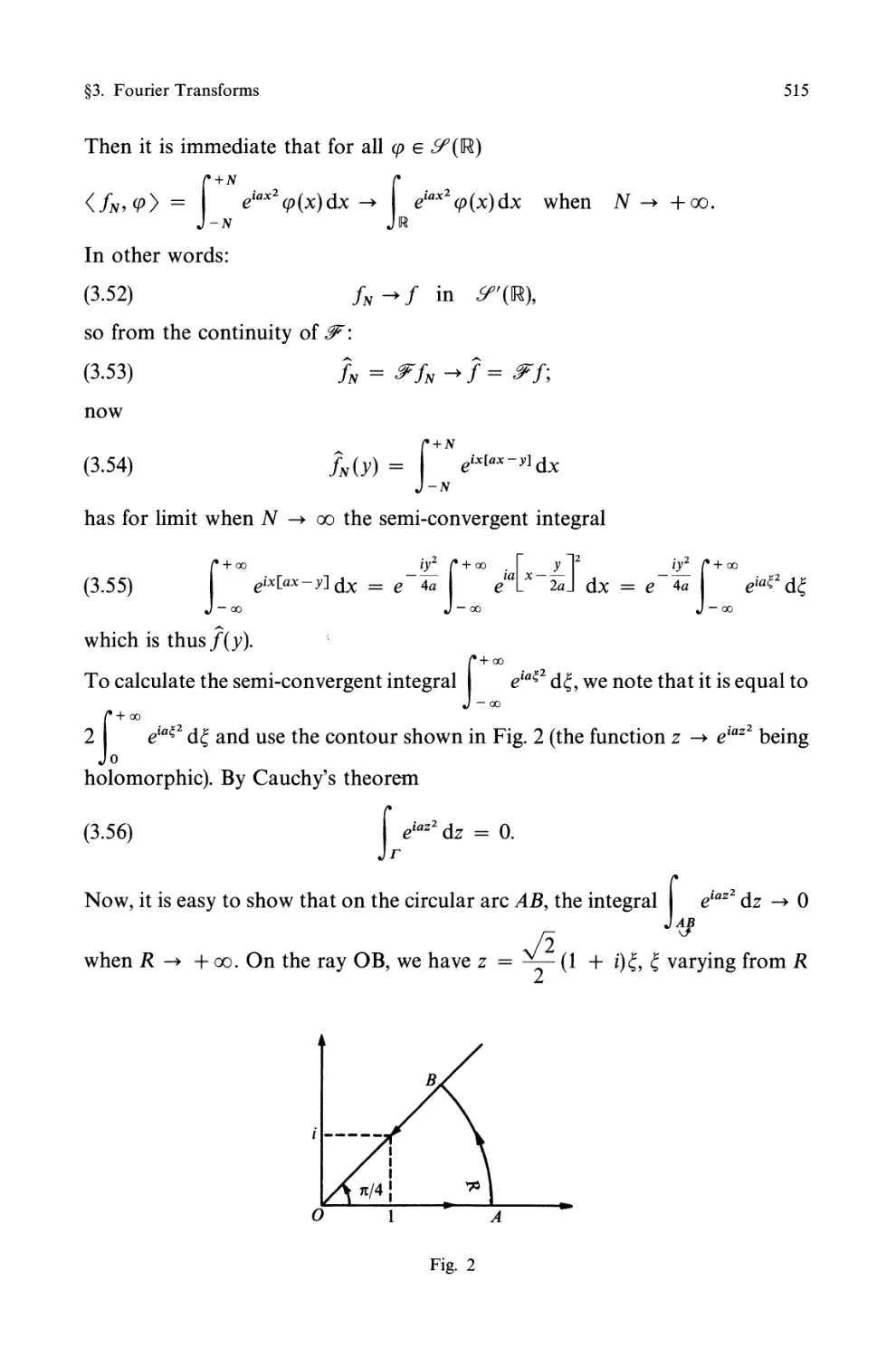
Similar

Text
Robert Dautray. Jacques-Louis Lions
.
Mathematical
Analysis and
, Numerical Methods
for Science and
Technology
Volume 2
Functional and Variational Methods
Mathematical Analysis and Numerical Methods
for Science and Technology
,
Robert \.Dautray Jacques-Louis Lions
\ '/
Mathell1atical Analysis
and NUll1erical Methods /1
for Science and Technology
v
1,;:/l'
/l)£f h
Q
v,
Volume 2
Functional and Variational Methods
,
With the Collaboration of
Michel Artola, Marc Authier, Philippe Benilan,
Michel Cessenat, Jean-Michel Combes, Heh ne Lanchon,
Bertrand Mercier, Claude Wild, Claude Zuily
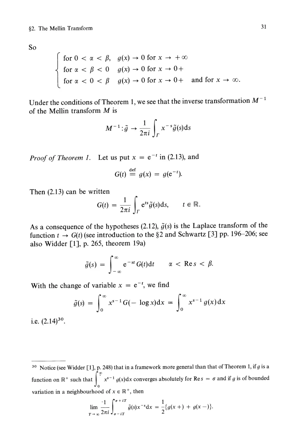
Translated from the French by Ian N. Sneddon
Springer- Verlag
Berlin Heidelberg New York
London Paris Tokyo
{;;
Robert Dautray
Ecole Poly technique
F-92128 Palaiseau Cedex, France
J acques- Louis Lions
College de France
11 place Marcelin Berthelot
F-75005 Paris, France
Title of the French original edition:
Analyse mathematique et calcul numerique pour les sciences
et les techniques, Masson, S.A.
(Q Commissariat a l'Energie Atomique, Paris 1984, 1985
With 20 Figures
Mathematics Subject Classification (1980): 35-XX, 41-XX, 42-XX, 44-XX,
45-XX, 46-XX, 47-XX, 65-XX, 73-XX, 76-XX, 78-XX, 80-XX, 81-XX
ISBN 3-540-19045-7 Springer-Verlag Berlin Heidelberg New York
ISBN 0-387-19045-7 Springer-Verlag New York Berlin Heidelberg
Library of Congress Cataloging-in-Publication Data
Dautray, Robert. [Analyse mathematique et ca1cul numerique pour les sciences et les techniques.
English]
Mathematical analysis and numerical methods for science and technology / Robert Dautray, Jacques-
Louis Lions; translated from the French by Ian N. Sneddon.
p. cm.
Translation of: Analyse mathematique et calcul numerique pour les sciences et les techniques.
Bibliography: v. 2, p. Includes index.
Contents: - v. 2. Functional and variational methods.
ISBN 0-387-19045-7 (U.S.: v. 2)
1. Mathematical analysis. 2. Numerical analysis. 1. Lions, Jacques-Louis. II. Title.
QA300.D34313 1988 515-dc19 88-15089 CIP
This work is subject to copyright. All rights are reserved, whether the whole or part of the material
is concerned, specifically the rights of translation, reprinting, reuse of illustrations, recitation, broad-
casting, reproduction on microfilms or in other ways, and storage in data banks. Duplication of this
publication or parts thereof is only permitted under the provisions of the German Copyright Law of
September 9, 1965, in its version of June 24, 1985, and a copyright fee must always be paid. Viola-
tions fall under the prosecution act of the German Copyright Law.
(Q Springer-Verlag Berlin Heidelberg 1988
Printed in Germany
Typesetting: Macmillan India Limited, Bangalore
Printing and binding: Konrad TriItsch GmbH, Wiirzburg
2141/3140-543210 - Printed on acid-free paper
Introduction to Volume 2
This second volume (which contains Chaps. III to VII) begins by introducing
some fundamental techniques: first of all, Fourier series (Chap. III) and the
Fourier transform (Appendix on Distributions) and by way of complement, the
Hankel and Mellin transforms (the Laplace transform comes in Chap. XVI,
Vol. 5); finally, for its importance in numerical applications, the method of the
fast Fourier transform. Chapter IV introduces the Sobolev spaces which play
a decisive role in the theory of partial differential equations as well as in
approximation procedures. These chapters III and IV both make use of the
theory of distributions, which is the subject of an Appendix (which can be read
independently).
Chapter V is a study of the linear differential operators in a sufficiently general
context. This setting goes a little beyond the strict needs of the applications
indicated in this work, but the generality introduced allows us better to make
the essentials more clear.We highlight the role of characteristics and the classi-
cal classification of linear differential operators into elliptic, parabolic and
hyperbolic operators.
For boundary value problems, a possible formulation is obtained by the use
of unbounded operators (the "domain" of the unbounded operator correspond-
ing, for example, to the boundary conditions, supposed homogeneous); this is
why it has seemed reasonable to include (in Chap. VI) a review of the principal
concepts relating to operators in Banach or in Hilbert spaces.
The last chapter of this volume, Chap. VII, introduces the very powerful
variational methods, which, together with the Sobolev spaces, play the most
important role throughout the theory (but which naturally are not the only
ones, and, besides, are not always applied!).
We give below the authors of various contributions, chapter by chapter.
Chapter III: M. Cessenat, B. Mercier, C. Zuily.
Chapter IV: M. Artola, M. Cessenat, C. Zuily.
Chapter V: P. Benilan.
Chapter VI: M. Artola, M. Cessenat, J.-M. Combes, C. Wild.
Chapter VII: M. Authier, M. Artola, P. Benilan, M. Cessenat, H. Lanchon,
B. Mercier.
Appendix. "Distributions": M. Artola, M. Authier, M. Cessenat.
Finally we mention the partial contributions of the following assistants of the
Commissariat a l'Energie Atomique: Messrs. Batail, Gambaudo, Giorla, Sznit-
man, Verwaerde.
VI
Introduction to Volume 2
Practical Guide for the Reader
Designation of subdivisions of the text:
number of a chapter: in Roman numerals
number of part of a chapter: the sign 9 followed by a numeral
number of section: a numeral following the above
number of a sub-section: a numeral following the above.
Example. II, 9 3.5.2 denotes Chapter II, Part 3, section 5, sub-section 2.
The reader wishing to become acquainted rapidly with the mathematical and
numerical essentials of the subject will find them in V ols. 1 and 2 omitting at
afirst reading 99 5, 6,7 and 8 of Chapter II (vol. 1) and 994, 5 of Chapter V
(vol. 2). These parts are distinguished by an asterisk at the appropriate part of
the text, and also in table of contents.
Table of Contents
Chapter III. Functional Transformations
Introduction
Part A. Some Transformations Useful in Applications
9 1 .
Fourier Series and Dirichlet's Problem
1. Fourier Series
1.1. Convergence in L 2 (If)
1.2. Pointwise Convergence on If
2. Distributions on If and Periodic Distributions
2.1. Comparison of ' (If) with the Distributions on 1R
2.2. Principal Properties of ' (If) .
3. Fourier Series of Distributions
4. Fourier Series and Fourier Transforms.
5. Convergence in the Sense of Cesaro
6. Solution of Dirichlet's Problem with the Help of Fourier Series
6.1. Dirichlet' s Problem in a Disk .
6.2. Dirichlet's Problem in a Rectangle.
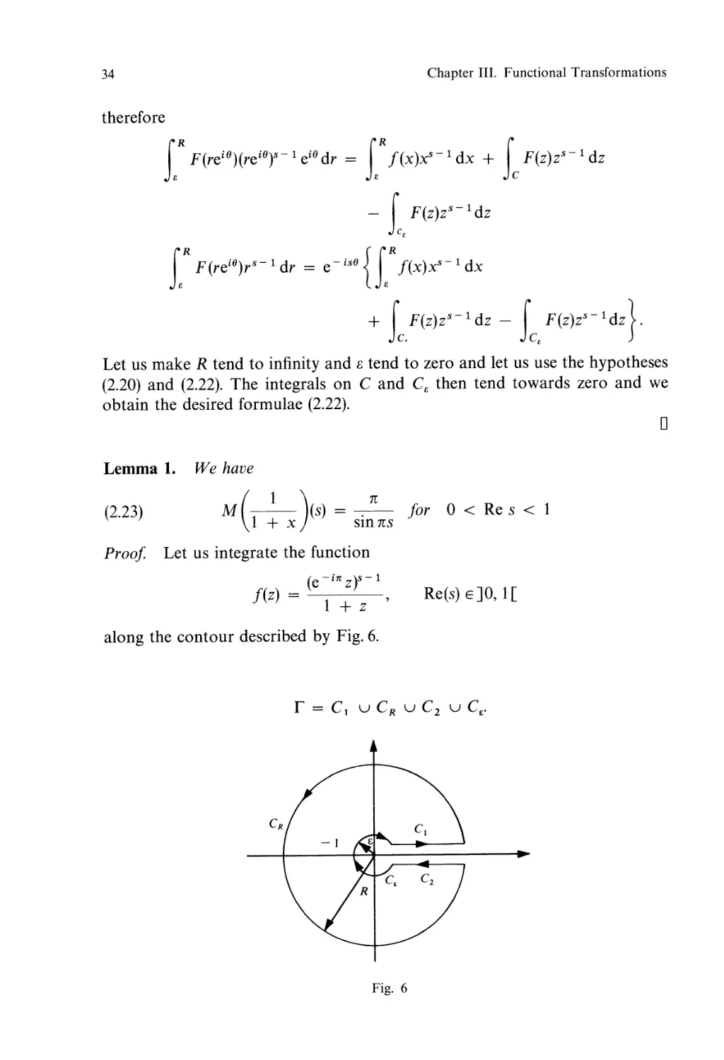
The Mellin Transform
1. Generalities
2. Definition of the Mellin Transform
3. Properties of the Mellin Transform
4. Inverse Mellin Transform.
5. Applications of the Mellin Transform
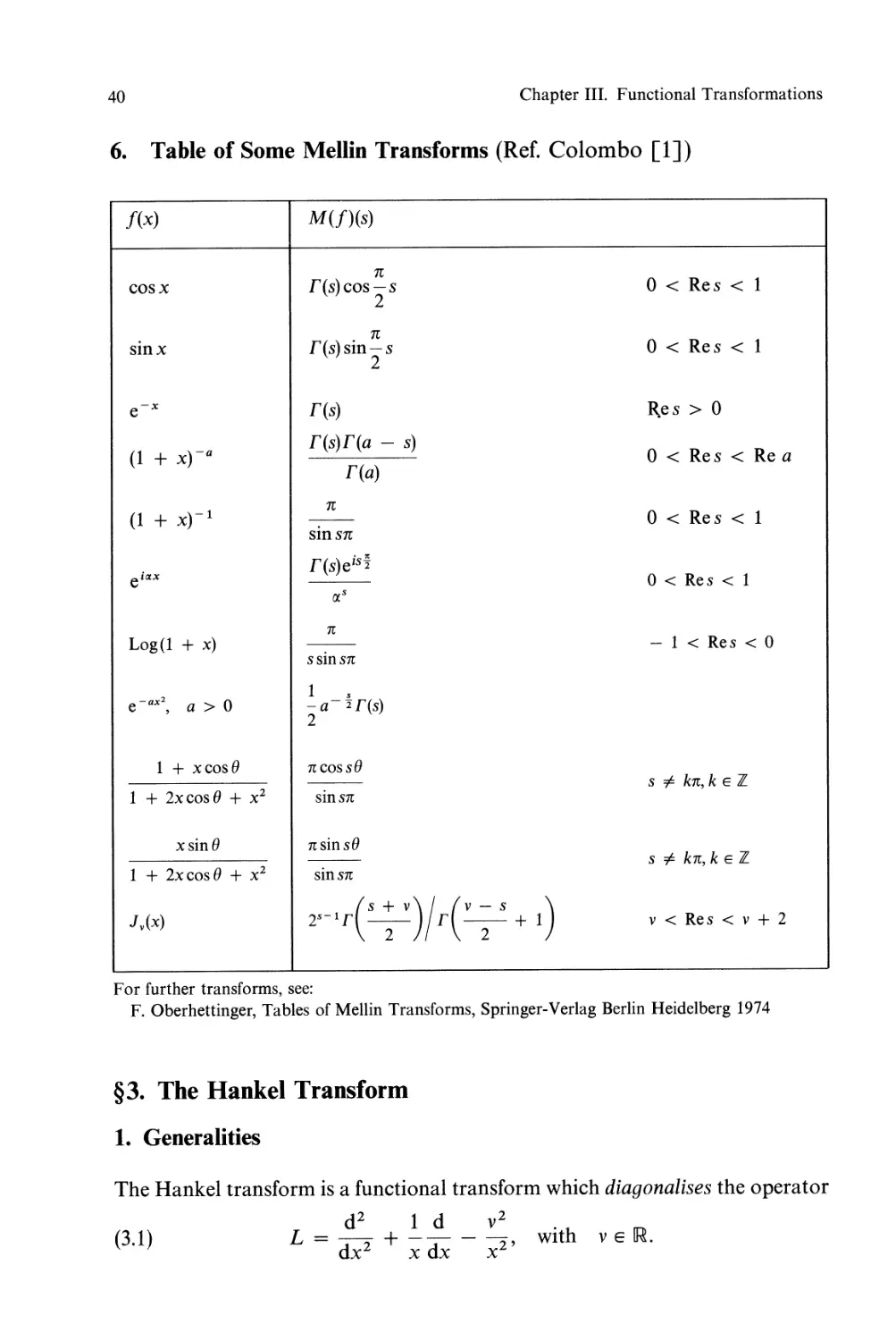
6. Table of Some Mellin Transforms .
2.
3.
The Hankel Transform . .
1. Generalities
2. Introduction to Bessel Functions
3. Definition of the Hankel Transform .
4. The Inversion Formula
5. Properties of the Hankel Transform
6. Application of the Hankel Transform to Partial Differential
Equations
1
4
4
4
5
5
7
7
9
10
14
15
17
17
20
24
24
26
28
30
32
40
40
40
42
47
48
50
53
VIII
Table of Contents
6.1. Dirichlet's Problem for Laplace's Equation in R. .
The Case of Axial Symmetry. . . . . . . . . . . . .
6.2. Boundary Value Problem for the Biharmonic Equation
in R. , with Axial Symmetry . . . . . . . . .
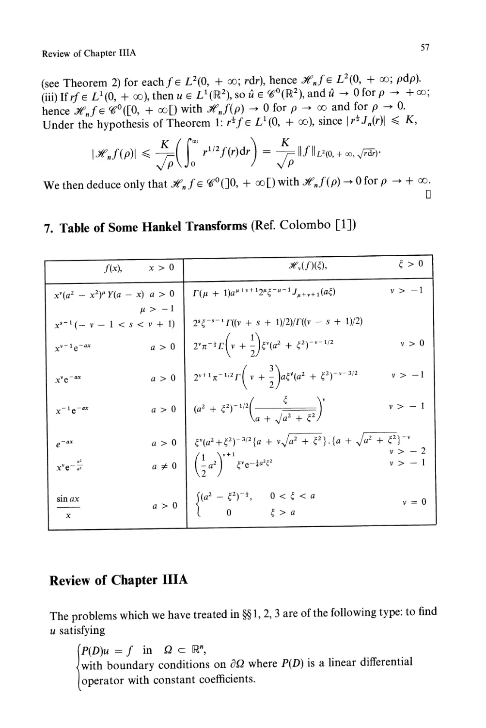
7. Table of Some Hankel Transforms . . . .
Review of Chapter III A . . . . . . . .
Part B. Discrete Fourier Transforms and Fast Fourier Transforms
9 1 .
9 2 .
9 3 .
9 4 .
9 5 .
Introduction . . . . . . . . . . . . . . . . .
Acceleration of the Product of a Matrix by a Vector . . . .
The Fast Fourier Transform of Cooley and Tukey . . . . . . .
The Fast Fourier Transform of Good-Winograd. . . . . . . .
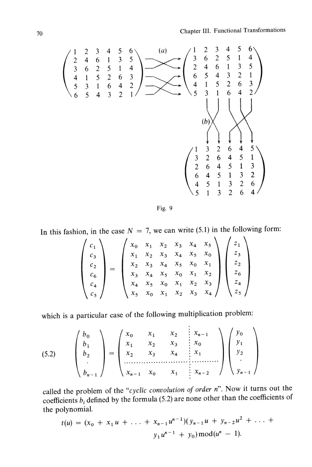
Reduction of the Number of Multiplications . . . . . . . . .
1. Relation Between the Discrete Fourier Transform
and the Problem of Cyclic Convolution . . .. ....
2. Complexity of the Product of Two Polynomials . . . . . . .
3. Application to the Cyclic Convolution of Order 2 . .
4. Application to the Cyclic Convolution of Order 3 . . . . . .
5. Application to the Cyclic Convolution of Order 6 . . . . . .
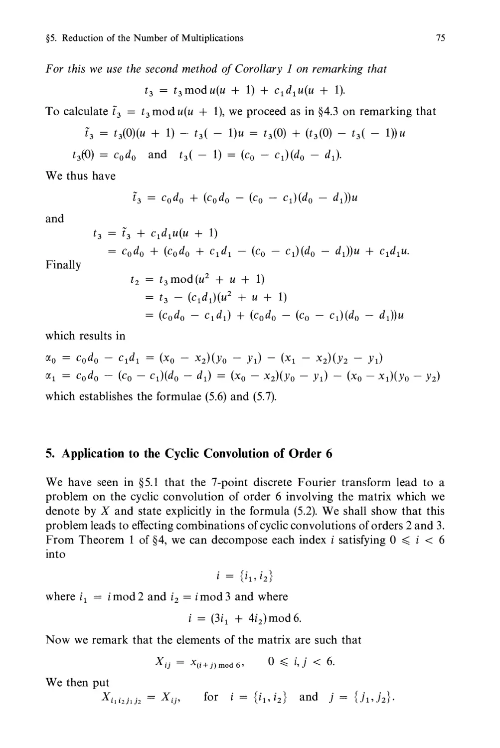
Fast Fourier Transform in Two Dimensions. .. ...
96.
9 7 . Some Applications of the Fast Fourier Transform . . . . .
1. Solution of Boundary Value Problems . . .. .....
2. Regularisation and Smoothing of Functions. .....
3. Practical Calculation of the Fourier Transform of a Signal
4. Determination of the Spectrum of Certain Finite Difference
Operators and Fast Solvers for the Laplacian . .....
Review of Chapter III B . . . . . . . . . . . . . . . . . . . .
Chapter IV. Sobolev Spaces
Introduction . . . . . . .
9 1 . Spaces Hi (Q), Ir(Q) . . . . . . . . .
9 2 . The Space Ir (R.n). . . . . . . . . . .
1. Definition and First Properties . . . .
2. The Topological Dual of HS(R.n) . . .
3. TheEquation(-L1+k 2 )u==f in R.n,kER.\{0} .
93. Sobolev's Embedding Theorem . . . . . . . . .
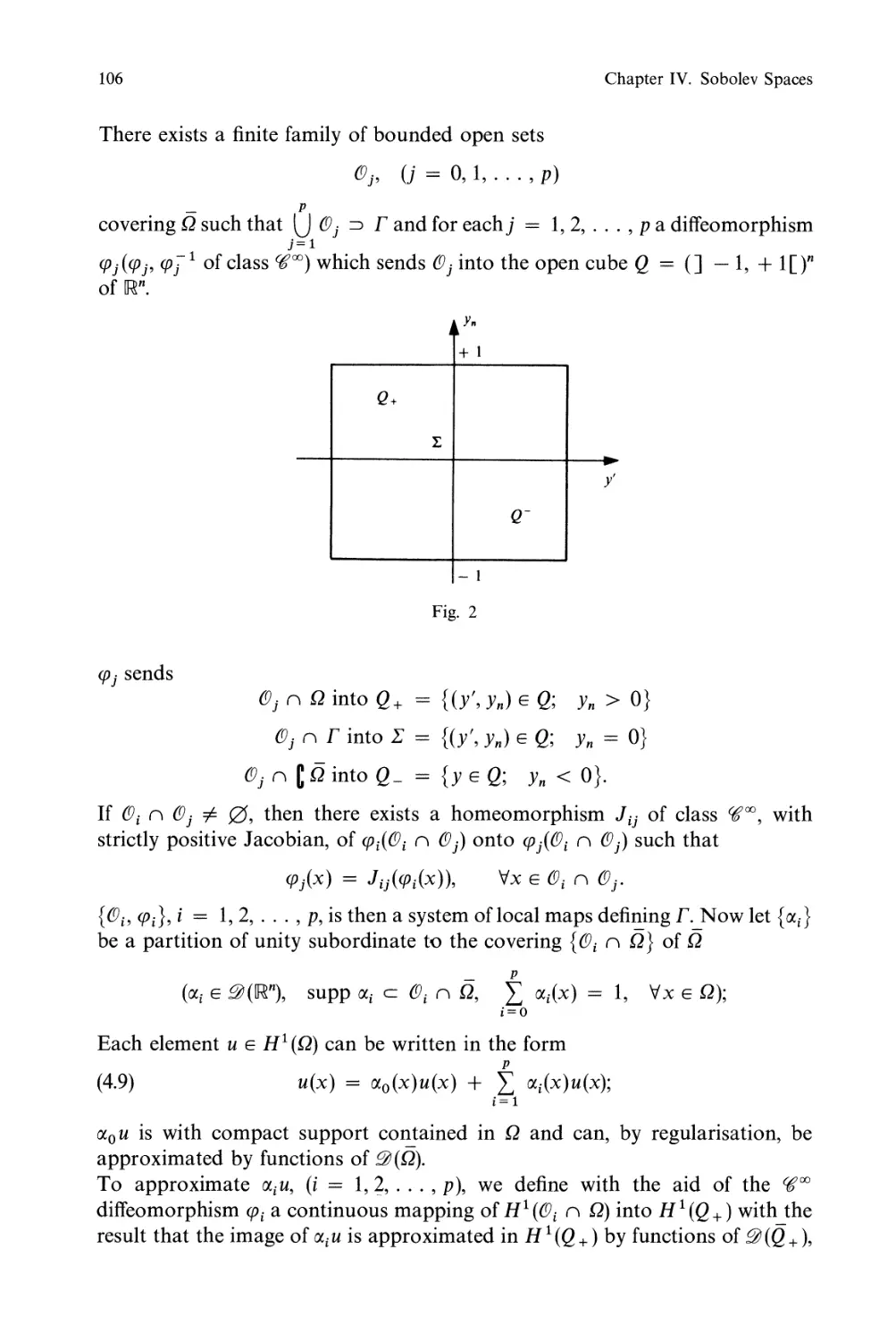
9 4 . Density and Trace Theorems for the Spaces Hm(Q),
(m E N * == N\ {O} ) . . . . . . . . . . . . . . .
53
55
57
57
59
59
62
64
66
69
69
71
72
73
75
77
78
78
81
83
84
91
92
92
96
96
98
100
100
102
Table of Contents IX
1. A Density Theorem. . . . . . . . . . . 102
2. A Trace Theorem for Hi (R. ) . . . . . . . . . . . . . . 107
3. Traces of the Spaces Hm(R. ) and Hm(Q) . . . 113
4. Properties of m- Extension . . . . . . . . . . 114
9 5 . The Spaces H-m(Q) for all mEN . . . . . . . . 120
96. Compactness . . . . . . . . . . . .. ...... 123
97. Some Inequalities in Sobolev Spaces . . . . . . . . . 125
1. Poincare's Inequality for H6 (Q) (resp. H'O (Q)). . . . . . 125
2. Poincare's Inequality for Hi (Q). . .. ... ... 127
3. Convexity Inequalities for Hm (Q) . . . . . . . 133
98. Supplementary Remarks . . . .. ... 138
1. Sobolev Spaces W m , P (Q).. ... . . . . . . 138
1.1. Definitions ....... ... ...... 138
1.2. So bolev Injections . . . . . . . 139
1.3. Trace Theorems for the Spaces Wm,P(Q) ...... 140
2. Sobolev Spaces with Weights ... ........ 141
2.1. Unbounded Open Sets . . . . . . . . . . . . . 141
2.2. Polygonal Open Sets . . . . . . . . .. .... 141
Review of Chapter IV . . . . .. ... . . . . . . 142
Appendix: The Spaces HS(r) with r the "Regular" Boundary
of an Open Set Q in R.n . . . . . . . . . . . . . . . . . . . . 143
Chapter V. Linear Differential Operators
Introduction . . . . . . . . . . . . .
91. Generalities on Linear Differential Operators . .. ....
1. Characterisation of Linear Differential Operators ....
2. Various Definitions . . . . . . . . . . . . . . . . . . .
2.1. Leibniz'sFormula . . . . . . . . . . .. ...
2.2. Transpose of a Linear Differential Operator . . . . . .
2.3. Order of a Linear Differential Operator ......
3. Linear Differential Operator on a Manifold . . . . . . . .
4. Characteristics . . . . . . . . . . . . . . . . .
4.1. Concept of Characteristics . . .. ........
4.2. Bicharacteristics . . . . . . .. ........
5. Opera tors with Analytic Coefficients.
Theorems of Cauchy-Kowalewsky and of Holmgren .
92. Linear Differential Operators with Constant Coefficients
1. Study of a l.d.o. with Constant Coefficients
by the Fourier Transform . . . . . . . . . . . . . . . .
148
149
149
152
152
153
154
155
157
157
159
163
170
171
x
Table of Contents
1.1. Existence of a Solution of Pu == f in the Space
of Tempered Distributions . . . . . . . . . . 171
1.2. Example 1: The Laplacian . . . . . .. ... 173
1.3. Elliptic and Strongly Elliptic Operators . .. ... 174
1.4. Hypo-Elliptic and Semi-Elliptic Operators . . . 177
1.5. Examples . . . . . . . . . . . . . . . . . . . . . 179
1.6. Reduction of Operators of Order 2 in a Homogeneous,
Isotropic "Medium" . . . . . . . . . . . . . . 181
2. Elementary Solutions of a l.d.o. with Constant Coefficients. . 182
2.1. Introduction . . . . . . . . . . . . . . . . . . . . 182
2.2. Elementary Solutions in !/' Examples . . . . . . . 184
2.3. Elementary Solution with Support in a Salient Closed
Convex Cone: Hyperbolic Operator . . . . . . . . 189
3. Characterisation of Hyperbolic Operators . . . . . . . . . 191
3.1. Characteristics of a l.d.o. with Constant Coefficients. . . 191
3.2. Algebraic Characterisation of Hyperbolic Operators . 194
3.3. Hyperbolic Operators of Order 2 . . . . .. ... 198
4. Parabolic Operators. . . . . . . . . . . . . . . . . . . 202
3. Cauchy Problem for Differential Operators
with Constant Coefficients . . . . . . . . . . . . . . . . . 204
1. Cauchy Problem and the Elementary Solution in {0' (JRn x JR +) 205
2. Propagation in Hyperbolic Cauchy Problems . . . . . . . . 209
3. Choice of a Functional Space: Well-Posed Cauchy Problem. . 214
4. Well-Posed Cauchy Problem in!/' . . . . . . . . . . . . 217
5. Parabolic and Weakly Parabolic Operators . . . . . 221
6. Study of the Particular Case P == a/at + Po . . . . . . . . . 223
6.1. Analysis of One-Dimensional Case . . . .. ... 223
6.2. Case in which Po is Strongly Elliptic . . . 224
6.3. Schrodinger Operator . . . . . . . . . .. ... 225
7. Well-Posed Cauchy Problem in {0': Hyperbolic Operators. 226
4. Local Regularity of Solutions*. . . . . . . . . . . . 230
1. Characterisation of Hypo-Ellipticity. . . . . . . . . . 230
1.1. Necessary Condition for Hypo-Ellipticity . . . . . . . 230
1.2. Algebraic Transformation of the Necessary Condition
for Hypo-Ellipticity. . . . . .. ........ 232
1.3. The Principal Result . .. ........... 233
2. Analyticity of Solutions . . . . . .. ... ... 234
2.1. Statement of Results . . . . . . . . . . . . . . . . 234
2.2. Estimates of Analyticity .. ........... 237
2.3. Generalisation: Gevrey Classes .. ... ... 240
3. Comparison of Operators . . . . . . . . . . . . . . . . 241
4. Local Regularity for Operators with Variable Coefficients
and of Constant Force . . . . . . . . . . . . . . . . . 245
5. Construction of an Elementary Solution . . . . . . . . 247
Table of Contents
9 5 . The Maximum Principle * . . . . . . . . . . .
1. Prerequisites . . . . . . . . . . . . . . . . .
2. Parabolic Maximum Principle and Dissipativity. . . . . . .
3. Characterisation of Operators P Satisfying
Maximum Principles . . . . . . . . . . . .
3.1. The Weak Maximum Principle . . . . . . . .
3.2. The Comparison Principle . . . . . . . . . . . . . .
3.3. The Strong Maximum Principle. . . . . . . .
3.4. The Principle of the Strong Parabolic Maximum . . . .
Review of Chapter V . . . . . . . . . . . . . . . . . . . . .
Chapter VI. Operators in Banach Spaces and in Hilbert Spaces
XI
250
250
252
259
259
261
263
265
268
Introduction 269
1. Review of Functional Analysis: Banach and Hilbert Spaces 270
1. Loc l1y Convex Topological Vector Spaces. N ormed Spaces
and Banach Spaces 270
2. Linear Operators 274
3. Duality . 281
4. The Hahn-Banach Theorem and its Applications 282
4.1. Problems of Approximation 282
4.2. Problems of Existence . 283
4.3. Problems of Separation of Convex Sets 285
5. Bidual, Reflexivity, Weak Convergence, Weak Compactness 285
5.1. Bidual 285
5.2. Reflexivity . 286
5.3. Weak Convergence 287
5.4. Weak Compactness 289
5.5. Weak-Star Convergence 290
6. Hilbert Spaces 291
6.1. Definitions 291
J 6.2. Projection on a Closed Convex Set 295
6.3. Orthonormal Bases 299
6.4. The Riesz Representation Theorem. Reflexivity 302
7. Ideas About Functions of a Real or Complex Variable
with Values in a Banach Space 304
7.1. Weak Topology 304
7.2. Weak Differentiability . 304
7.3. Weak Holomorphy 305
9 2 . Linear Operators in Banach Spaces 305
1. Generalities on Linear Operators 305
1.1. Domain, Kernel and Image of a Linear Operator 305
XII
Table of Contents
1.2. Nullity and Deficiency Indices . . . . . . . .
1.3. Basic Properties of Linear Operators . . . . . . .
2. Spaces of Bounded Operators . . . . .. ......
2.1. Introduction . . . . . . . . . . . .
2.2. Various Concepts of Convergence of Operators .
2.3. Composition and Inverse of Bounded Operators . . . .
2.4. Transpose of a Bounded Operator .... . .
2.5. Some Classes of Bounded Operators .....
2.6. Some Ideas on Functions of a Real or Complex Variable
with Operator Values; Families of Operators . . . .
3. Closed Operators . . . . . . . . . .
3.1. Definition and Examples ............
3.2. Basic Properties . . . . . . . . . . . . . . . .
3.3. The Set g- (X, Y) of Closed Operators from X into Y
3.4. Transpose of a Closed Operator . .. ......
3.5. Operators with Closed Image. .. ......
93. Linear Operators in Hilbert Spaces . . . . . . .
1. Bounded Operators in Hilbert Spaces . . . . . . . . .
1.1. Adjoint Sesquilinear Form . . . . . .
1.2. Hermitian Operators . . . . . .
1.3. Orthogonal Projectors. . . . . .
1.4. Isometries and Unitary Operators.
1.5. Hilbert-Schmidt Operators. . . . . . . . . . . .
2. Unbounded Operators in Hilbert Spaces
2.1. Adjoint of an Unbounded Operator. .
2.2. Symmetric Operators . . . . . .
2.3. The Cayley Transform. . . . . . . . . . . . . .
2.4. Normal Operators . . . . . . . . .
2.5. Sesquilinear Forms and Unbounded Operators .
Review of Chapter VI . . . . . . . . . . . . . . . . . . . . .
Chapter VII. Linear Variational Problems. Regularity
Introduction . . . . . . . . . . .
g 1.
Elliptic Variational Theory . . . . . . . . .
1. The Lax-Milgram Theorem . . .
2. First Examples . . . . . . . . . . .
2.1. Example 1. Dirichlet Problem .... . . . . . ·
2.2. Example 2. Neumann Problem
3. Extensions in the Case in which V and H are Spaces
of Distributions or of Functions . . . . . . . . . . . . .
4. Sesquilinear Forms Associated with Elliptic Operators
of Order Two . . . . . . . . . . . . . . . . . . . . .
307
307
310
310
313
316
322
325
332
334
334
336
339
342
346
348
351
353
353
354
355
357
361
361
361
362
366
367
374
375
375
376
378
379
380
383
384
Table of Contents
g2.
5. Sesquilinear Forms Associated with Elliptic Operators
of Order 2 m . . . . . . . . . . . . . . . . . . . . . .
6. Miscellaneous Remarks . . . . . . . . . . . . . . . . .
7. Application to the Solution of General Elliptic Problems
(of Dirichlet Type) . . . . . . . . . . . . . . .
Examples of Second Order Elliptic Problems . . . . .
1. Generalities . . . . . . . . . . .. ... ...
2. Examples of Variational Problems. .. ........
2.1. Mixed Problem. . . . . . . .. ... ...
2.2. Non-Local Boundary Conditions . . . . .
3. Problems Relative to Integro-Differential Forms on Q + r
3.1. Problem of the Oblique Derivative . . . . . .
3.2. Robin's Problem . . . . . . .. ... ...
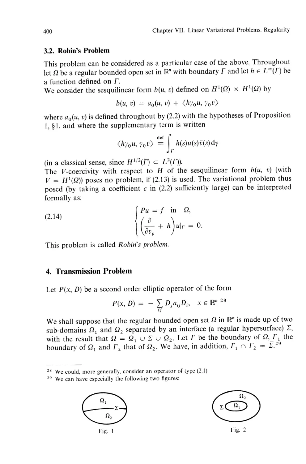
4. Transmission Problem. . . . . . . . . . . . . .
5. Miscellaneous Remarks . . . . . . . . . . . . .
6. Application: Stationary Multigroup Equation for the Diffusion
of N e u tr 0 n s . . . . . . . . . . . . . . . .. ...
7. Application: Statical Problems of Elasticity. . . . . . . . .
7.1. Introduction. . . . . . . . . .
7.2. Variational Formulation. . . . . . .
7.3. Korn's Inequality. . . . . .
7.4. Application to Problem (2.39)
7.5. Inhomogeneous Problem
8. Statical Problems of the Flexure of Plates . . .
g3. Regularity of the Solutions of Variational Problems . . . . . .
1. Introduction . . . . . . . . . . . . . . .
2. Interior Regularity . . . . . . . . . . . . . . . . .
3. Global Regularity of the Solutions of Dirichlet
and. Neumann Problems for Elliptic Operators of Order 2
4. Miscellaneous Results on Global Regularity . . . . . . . .
5. Green's Functions . . . . . . . . . . . . . . . . . . .
5.1. Case of the Laplacian in a Bounded Open Set Q
with Dirichlet Condition. . . . . . . . . . . . . . .
5.2. Some Other Particular Examples . . . . . . .
5.3. Green's Functions in a More General Setting. . . . . .
Review of Chapter VII . . . . . . . . . . . . . . . .
Appendix. "Distributions"
g 1. Definition and Basic Properties of Distributions .
1. The Space (Q) . . . . . .
1.1. Definition . . . . . . . . . . . . .
XIII
387
389
391
393
393
394
394
397
398
398
400
400
405
407
411
411
412
414
418
418
420
425
425
426
433
437
441
441
445
451
456
457
457
457
XIV
Table of Contents
1.2. Elementary Properties of the Convolution Product
of Two Functions. . . . . . . . . . . . . . . . . . 458
1.3. A Procedure for the Construction of Functions of f0(Q) . 459
1.4. The Notion of Convergence in f0 (Q) . .. .... 460
1.5. Some Inclusion and Density Properties . . . . . . . . 461
2. The Space f0' (Q) of Distributions on Q . . . . . . . . 463
2.1. Definition of Distributions and the Concept of Convergence
in f0' (Q). . . . . . . . . . . . . . . . . . 463
2.2. First Examples of Distributions: Measures on Q 464
2.3. Differentiation of Distributions. Examples . . . 467
2.4. Support of a Distribution. Distributions with
Compact Support. . . . . . . . . . . . . . . . . . 474
3. Some Elementary Operations on Distributions . . . . . . . 476
3.1. Product by a Function of Class rc oo . . . . . . . . . . 476
3.2. Primitives of a Distribution on a Interval of JR . . . . . 477
3.3. Tensor Product of Two Distributions . . . . . . . 480
3.4. Direct Image and Inverse Image of a Function and
of a Distribution by a Function of Class rc oo 481
4. Some Examples .. . . . . . . . . 482
4.1. Primitives of the Dirac Measure . . . . . . . . . 482
4.2. A Division Problem (Case n == 1) . . . . . 483
4.3. Derivative of a Function of JRn Discontinuous
on a Surface . . . . . . . . . . . . . . . . 484
4.4. Distributions Defined by Inverse Image from Distributions
on the Real Line . . . . . . . . . . . . . . . . . . 485
g2. Convolution of Distributions . . . . . . . . . . . . . . . . 492
1. Convolution of a Distribution on JRn and a Function
of f0 (JR n) . . . . . . . . . . . . . . . . . . . . . . . 492
2. Convolution of Two Distributions of Which One (at Least)
is with Compact Support . . . . . . . . . . . . 494
3. Distributions with Convolutive Supports. . . . . . . . 496
4. Convolution Algebras . . . . . . . . . . . . . . . . 497
93. Fourier Transforms . . . . . . . . .. ... ... 500
1. Fourier Transform of L I-Functions .. ...... 500
2. The Space g (JRn). . . . . . . . . . . . . . 502
3. F ourier Transform in L 2 . . . . . . . . . . . 506
4. Fourier Transforms of Tempered Distributions . . . 506
5. Fourier Transform of Distributions with Compact Support 509
6. Examples of the Calculation of Fourier Transforms . . . . . 510
7. Partial Fourier Transform . . . . . . . . . . . . 513
8. Fourier Transform and Automorphisms of JRn:
Homogeneous Distributions . . . . . . . . . . . . . . . 518
8.1. Fourier Transform and Automorphisms ofJRn . . . 518
8.2. Homogeneous Distributions . . . . . . . . . 519
Table of Contents XV
9. Fourier Transform and Convolution. Spaces (DM elRn)
and (D (JR n) . . . . . . . . . . . . . . . . 520
9.1. The Space (DM(JRn) (= (DM) . . . . . . . .. ... 520
9.2. The Space (D . . . . . . . . . .. ...... 521
10. Fourier Transform of Tempered Measures . . . . . . . . . 523
11. Distribution of Positive Type. Bochner's Theorem. . . . 525
11.1. Functions of Positive Type . . . . . 525
11.2. Distributions of Positive Type . . . . . . . . . . 525
12. Schwartz's Theorem of Kernels. . . . . . . . . . . . 527
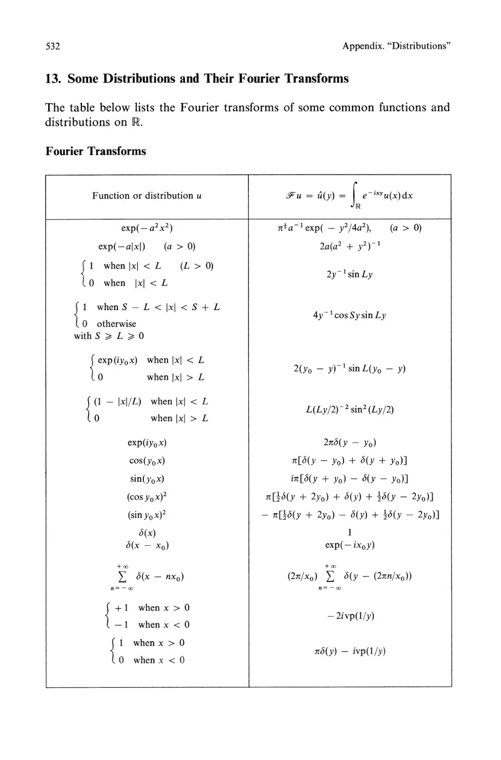
13. Some Distributions and Their Fourier Transforms. . 532
Bibliography. . . . .
533
Table of Notations
538
Index . . . . . . .
551
Contents of Volumes 1,3-6
557
Chapter III. Functional Transformations
Introduction
In this Chap. III, we study in Part A, in 91 Fourier series which we use to solve
boundary value problems on particular open sets of [Rn. These examples serve as
an introduction to the following chapter (devoted to Sobolev spaces) in showing
that, for the solution of the problem
L1 u == 0 in Q c [Rn, bounded,
u == g on oQ, the boundary of Q,
to have finite energy (a condition which we shall point out in Chap. IV is
u E H 1 (Q)), it is necessary that g satisfies a certain condition, which we shall see
later to be that g is in the Sobolev space Ht(oQ).
In 92 we study the Mellin transform, which is a particular form of the Laplace
transform, suitable for solving the Dirichlet problem for a cone in [Rn.
In 93 we treat the Hankel transform which arises naturally in the study of
Fourier transforms of functions in [R 2 , invariant under rotation, and which thus
enables us to solve problems possessing that symmetry. As a preamble, we study
the properties of Bessel functions of the first kind which form the kernels of the
Hankel transforms.
In Part B we next study the discrete Fourier transform and the fast Fourier
transform which are the indispensible numerical complements to the study of
Fourier series. Some particular examples of applications are given in 96.
There are other transforms, useful in applications, than those studied in this
chapter, notably the Fourier transform featured in the Appendix "Distri-
butions" and the Laplace transform, recalled and systematically used in
Chap. XVI. We should also cite the Hilbert transform discussed in the Appendix
"Singular integral operators" of Chap. XIII.
*
An essential motivation in the use of transforms in the theory of linear partial
differential equations, treated in subsequent chapters, is that a suitably chosen
transform can change a linear differential operator p(D)1 into a multiplication
1 Here P(D) includes the boundary conditions.
2
Chapter III. Functional Transformations
operator which we then say has "diagonalised" the operator P(D). This is a
concept which will be developed in Chap. VIII, where we shall find other useful
examples, such as the functions of Legendre, Hermite and Laguerre and the
polynomials of Tchebycheff.
The Fourier and Laplace transforms change linear differential operators with
constant coefficients into polynomials in the variables in the transform space.
Similarly the Mellin transform changes the operator r into multiplication by
ar
the variable in the transform space.
Finally, the Hankel transform of order v, changes into a multiplier the
a 2 1 a .v 2 a 2 1 a
operator a 2 + - _ a - 2 with r E ] 0, 00 [. As the operator a 2 + - - occurs in
r r r r r r ar
the Laplacian J of [R2 expressed in polar coordinates or in J of [R3 expressed in
cylindrical coordinates, the 'Hankel transform is useful in the solution of
problems of the type
J u = f, f given in [R2
(or for an iterated power of the Laplacian, say Jnu = f) or of problems
in an open set D of [R3, (with D the whole space [R3 or the half-space
D = [Rt = {(Xl' X2, X 3 ); X 3 > O} with OX 3 an axis of symmetry) such that 2
Ju = f
(f given in D),
(g given on aD).
u oG = g
with f and g independent of X 3 .
*
The diagonalisations mentioned are linked to the invariance of the problems to
be treated, by a group: group of translations of [Rn for Fourier series and the
Fourier and Laplace transforms, group of displacements of the plane [R2 - and
hence of rotations about a fixed point of [R2 -for the Hankel transforms, group
of homothetic transformations for the Mellin transform.
*
Functional transforms are of great use in the theory of partial differential
equations to obtain analytical solutions which can yield important qualitative
(and sometimes quantitative) results-behaviour at infinity or in the neighbour-
hood of singularities. Applications are given elsewhere throughout this work;
the present chapter serves as introduction and gives some fundamental proper-
ties which will not be taken up again elsewhere. One difficulty about the use of
functional transformations, often underlined, is that when the analytical calcu-
2 The Hankel transform is equally useful in the corresponding evolution problems involving
au a 2 u
- - L1u = f, or - - L1u = f(see Chap. XV).
at at 2
Introduction
3
lation becomes so complicated as not to yield a solution in closed form (as is
often the case) the "explicit" formula does not lend itself easily to numerical
computation. This view must be finely balanced, the example of the fast Fourier
transform (introduced in this chapter) having led to a complete re-assessment of
numerical methods in the representation of functions by Fourier series 3 .
Another difficulty of functional transformations :Y is that such a transformation
is useful only if it possesses an inversion formula; the domain of validity of these
inversion formulae implies the introduction of "ad hoc spaces". For the Fourier
transform, for example, these are L 2 or Schwartz's space of tempered distri-
butions. These spaces lS g- are thus "attached" to :Y.
We shall see that for a given physical problem f!JJ, considerations of invariance
(e.g. of the energy) lead to us "attaching" to this problem a "functional space"
lS [1jJ; these are generally Sobolev spaces constructed on L 2 or other spaces
such as Schauder spaces 4 . Hence we see that a difficulty could arise if lSf!/J and lS g-
did not coincide. The attitude which can be adopted, and which seems the best,
is first to show that the problem f!JJ is "well-posed" within the functional
framework lS f!/J; if then a functional transformation :Y leads to supplementary
conditions, we can carry out the calculations in a formal way, already assured of
their convergence in lSf!/J. This is the approach which will be adopted in the later
chapters of this book 5 .
3 As well as the use of "spectral" methods for the numerical analysis of certain models.
4 Spaces of m-times continuously differentiable functions, all of whose m-th derivatives satisfy
Holder conditions.
5 This is slightly similar to the position taken for elliptic boundary value problems in the last
chapter: we begin by considering the existence and uniqueness of weak solutions, then later prove
supplementary properties, notably regularity.
Part A. Some Transformations Useful in Applications
1. Fourier Series and Dirichlet's Problem
1. Fourier Series
Suppose that lr is the unit circle in the complex plane. Each function f on [R,
periodic with period 2n, may be identified with a function F on If by the formula
(1.1)
F (e it ) == f(t), \;/ t E [R.
In what follows, we write f in place of F. Notice that the functions t e int (for
n E Z) which are periodic functions (of period 2n) on [R are thus identifi d with
the polynomials z zn(n E Z) on If. The functions e int obviously don't belong
to either Ll([R) or to L2([R) (since they are periodic).
On the other hand, they are in L 1 (0, 2n) (resp. L 2(0, 2n)); we shall say also, (by
abuse of language) that they are in L 1 (If) (resp. L 2 (If)). We recall that the space
L 2(0, 2n) is a Hilbert space 6 for the scalar product
f 21t
(f, g) = 0 f(t)g(t) dt.
In the remainder of this Chap. III, the functions considered will be taken to have
complex values.
If f E L l(lf) the Fourier coefficient of order n off is defined by
1 f 21t .
(1.2) in = 2n 0 e-mtf(t)dt, n E 7L,
and the Fourier series of f is by definition the series
(1.3)
Sf(t) == L in e int , t E If.
nEZ
The problem which poses itself naturally is that of the convergence of this series,
and if it converges, the value of the sum.
In general, the series (1.3) will not converge in each point t E If towardsf(t) since
a modification of.fin one point, or more generally on a set of measure zero, does
6 A survey of Hilbert spaces is given in Chap. VI, 1.
1. Fourier Series and Dirichlet's Problem
5
not modify the value of the coefficients of Fourier. Nevertheless, in a certain
number of cases which we shall recall below, the convergence takes place in
certain functional spaces.
1.1. Convergence in L 2 (T)
Recall that a sequence {j;,}, n == 1,2,... of elements of L2(lr) converges in
L 2 (lr) towards f, if
lim f 2"1!n(t) - f(tWdt = O.
n oo 0
For f E L 2 (lr) eL l (lr), we can define the Fourier coefficients off We have the
theorem:
Theorem 1. Suppose that f and g are two elements of L 2 (lr), with corresponding
Fourier coefficients]" and g n .
1 ° The sequence of functions
SN,M(t)
M
L in e int
n= -N
converge to f in L2(lr) (the same for g) when Nand M 00.
2° The series L in gn is summable and we have the relation of Parseval
nEZ
(1.4)
f 2" f(t) g(t) dt = L J.. gn'
TC 0 nEZ
I n particular
_ 2 1 f 2" If(tWdt = L 1J..1 2 .
TC 0 nEZ
Theorem 1 expresses that the set {e int j(2TC)t, n E Z} is an orthonormal base
(complete orthonormal system) of L 2 (lr).
The Fourier series off is then the development off on this base.
Remark 1. Theorem 1 does not say anything about the pointwise convergence
of the Fourier series off
1.2. Pointwise Convergence on T
We could believe that if f is a continuous function on lr, it is a limit 7 in each
point of lr of its Fourier series. This is false in general. There exist complicated
7 In effect, there results from a theorem of Weierstrass that each continuous function on lr, is the
limit (uniformly on lr, hence on each point of lr) of a sequence of functions {fl'i} of the form
N
fN(t) = L IN,n e int , with fN,n E C.
n = - N
6
Chapter III. Functional Transformations
examples of continuous functions whose Fourier series diverge in some points. 8
It is necessary to make supplementary hypotheses on f9. Here is a sufficient
condition for pointwise convergence on u.
Theorem 2. Let f be a real function on u, continuously differentiable save in a
finite number of points, at which f and its derivative admit limits to the right and to
the left. Then the Fourier series off converges at every point of u and its limit is
equal to f(x) iff is continuous at the point x and to {f(x+) + f(x -)} /2 if f is
discontinuous at the point x E u.
In particular, iff E qj1 (u), its Fourier series converges towards it in each point.
This result is a consequence of the following fact 10 : iff satisfies the hypotheses of
Theorem 2, then
r 2 f f( ) sin A,( d = { f(O + ) if I == (0, a)
A n I t t t f(O-) if I == (- a, 0) with a > O.
In effect, a simple calculation shows that for 0 < x < 2n,
SN(X) = f e inX ]" = f 1[-txf(X + 2t) sin(2 + t)t dt
n = - N n - -1.. x SIn t
2
and we apply Dirichlet's lemma to the function t -+ /2 f(x + 2t).
SIn t
Remark 2. Under the hypotheses of Theorem 2, we have seen that for all t E U,
Ok 1
; oo k= Nhe' t = 2 (/(t+) + f(L)), (k Elf).
It is important to note that it is false in general that
M 1
N. OO k= Nheikt = 2(/(t+) + f(L)) (k Elf).
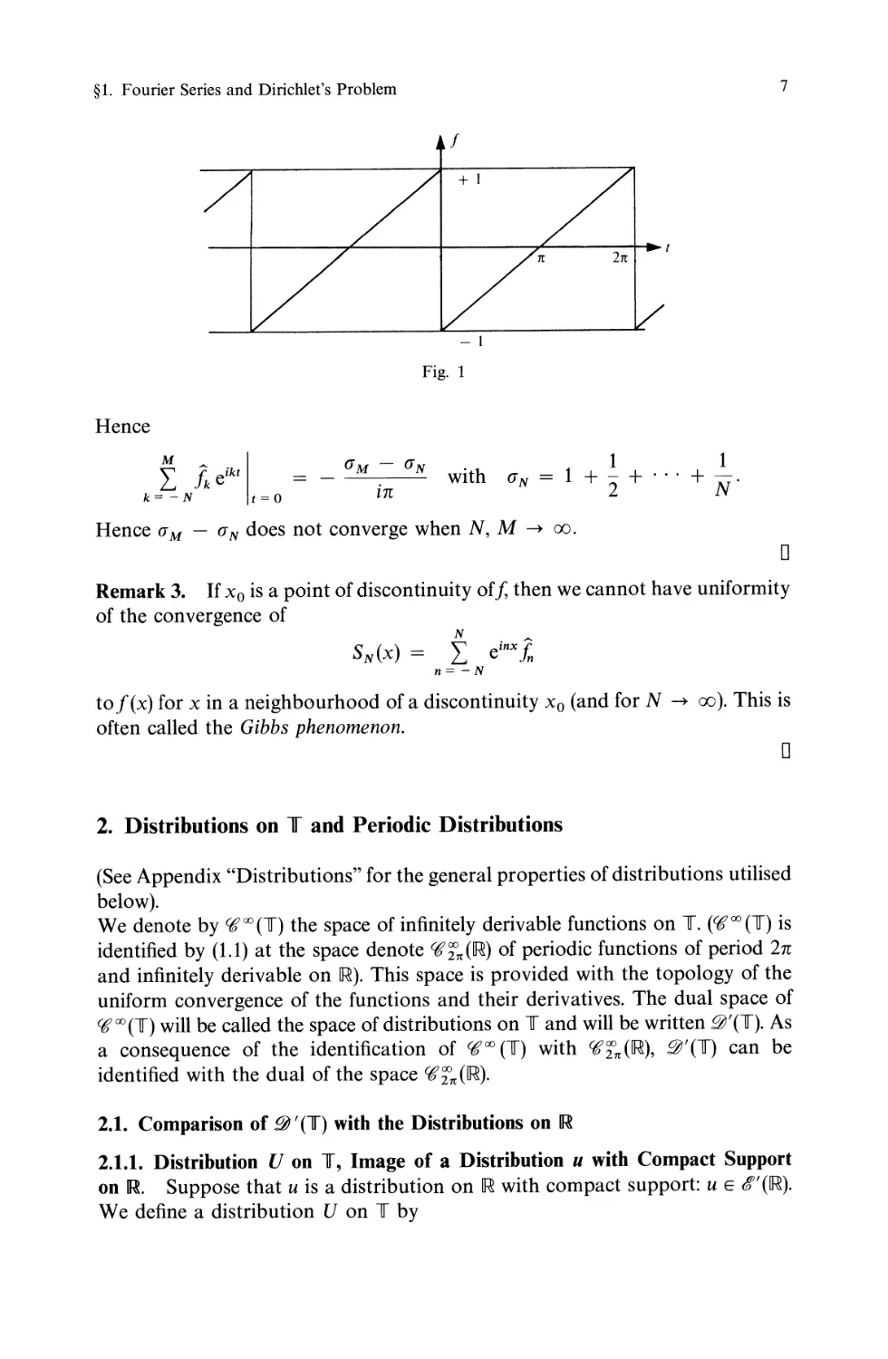
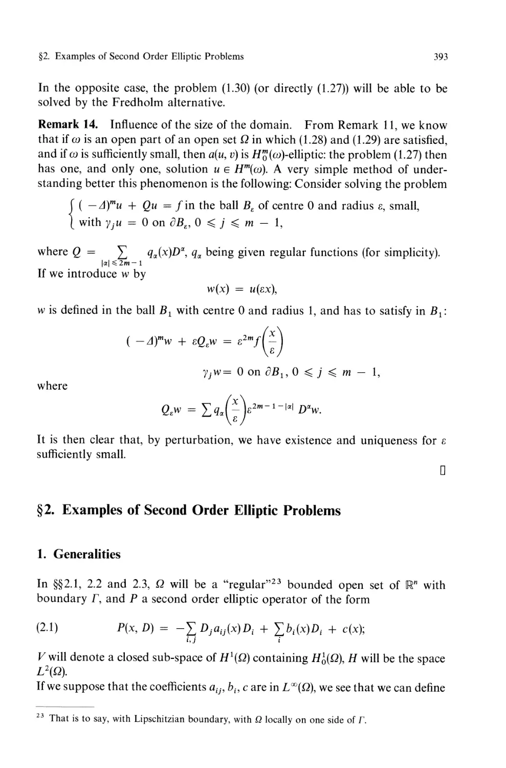
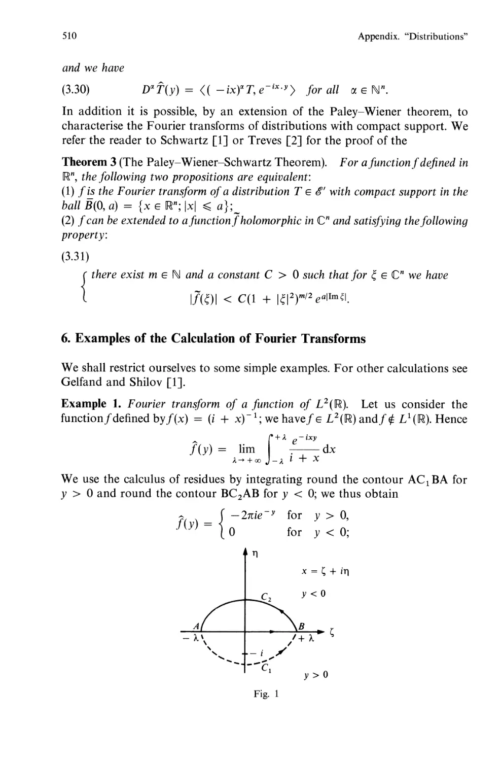
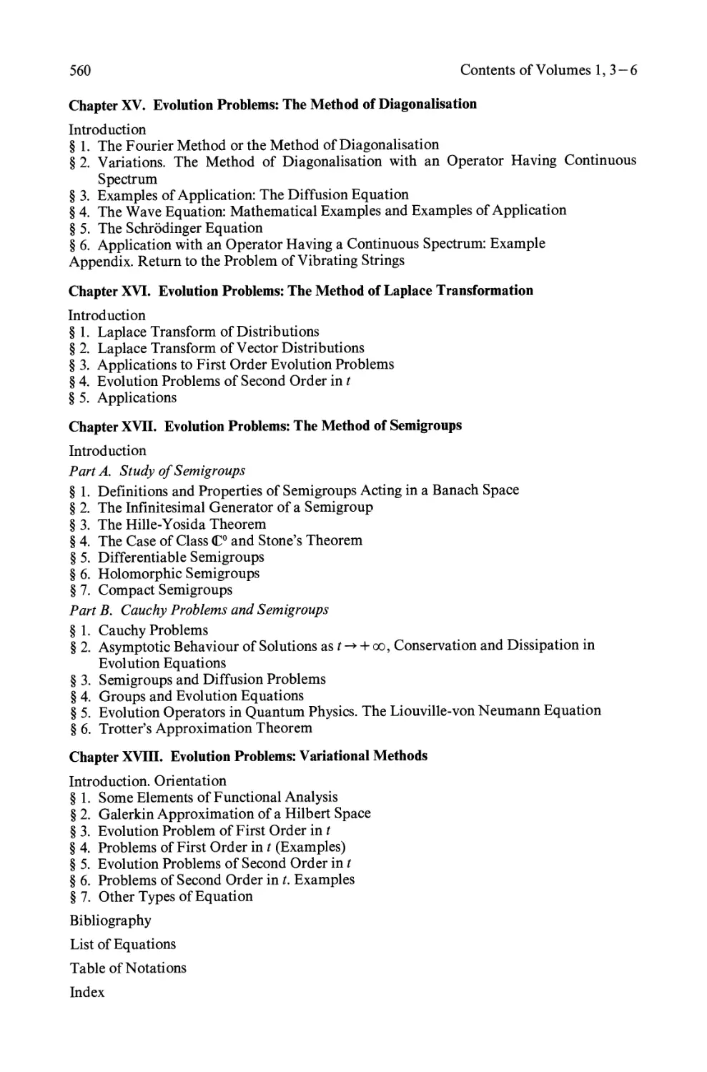
F or example, consider the function f of the Fig. 1.
We have:
in = f 21[ f(t)e-int dt = - f 1t: ( - l ) sinntdt
2n 0 non
1
-- if n=l=O
nin
o if n == O.
8 See Y osida [IJ, p. 72; theorem of condensation of singularities (application of Baire).
9 We shall show the uniform convergence of the Fourier series whenfis of class rc 2 (see Example 2).
10 Known generally under the name of Dirichlet's lemma (see Chap. XV, 1; see the references
Zygmund [IJ, Schwartz [2] and Sneddon [1]).
1. Fourier Series and Dirichlet's Problem
7
f
-I
Fig. 1
Hence
M M - N . 1
L fk e ikt = - . wIth N = 1 + _ 2 +
k= -N t=O l1r
1
+-
N'
Hence (JM - (IN does not converge when N, M 00.
o
Remark 3. If Xo is a point of discontinuity off, then we cannot have uniformity
of the convergence of
N
SN(X) = L e inx in
n =-N
to f(x) for x in a neighbourhood of a discontinuity Xo (and for N 00). This is
often called the Gibbs phenomenon.
o
2. Distributions on T and Periodic Distributions
(See Appendix "Distributions" for the general properties of distributions utilised
below).
We denote by CC 00 (If) the space of infinitely derivable functions on If. (CC 00 (If) is
identified by (1.1) at the space denote CCfn(!R) of periodic functions of period 2n
and infinitely derivable on IR). This space is provided with the topology of the
uniform convergence of the functions and their derivatives. The dual space of
CC 00 (If) will be called the space of distributions on If and will be written ' (If). As
a consequence of the identification of CC oo (If) with CCfn(IR), '(lf) can be
identified with the dual of the space CCfn(IR).
2.1. Comparison of ' (If) with the Distributions on IR
2.1.1. Distribution U on If, Image of a Distribution u with Compact Support
on IR. Suppose that u is a distribution on IR with compact support: u E ' (IR).
We define a distribution U on If by
8
Chapter III. Functional Transformations
( 1.5)
_ it
< U, <p> - < u, <p(e ) >, \;/ <p E CC oo CIf);
U is called the distribution image of u by!he mapping H: t E IR e it E If. We
have also defined by (1.5) a mapping H: u E ' (IR) U E ' (If). If u is a
function with compact support and integrable, U is given by
( 1.6)
i f 21l(k+ 1)
< u, qJ> == u(t)qJ(e it ) dt == L u(t)qJ(e it ) dt
keZ 21lk
f 21l
== L u(2nk + t)qJ(eit)dt.
o keZ
Thus U(t) is a function and
( 1.7)
U(t) == L u(2nk + t).
keZ
2.1.2. Distributions f on IR, Inverse of a Distribution F on T. At present
let F E L 1 (If) (defining thus a distribution on lr). Then the function f given
by the formula (1.1) from F belongs to Lloc(lR) and thus also defines a distri-
bution on IR. We can write for each qJ E (IR)
(1.8)
i f 21l(k + 1)
<f, qJ > == F(e it ) qJ (t) dt == L F(e it ) qJ(t) dt
k E Z 21lk
== f 2" F(e it ) [ L qJ(2nk + t) J dt.
o kEZ
In remarking that the function qJ defined on [0,2n] by
( 1.9)
qJ(t) == L qJ(2nk + t)
kEZ
can be considered as a function CC OO on If, we obtain
(1.10)
<f, qJ > == < F, qJ >
which also givesffrom F. This formula can be generalised by continuity to the
case in which F is a distribution on If. The distribution f on IR defined also by
(1.10) is called the inverse distribution of F by the mapping H: t --+> e it .
Such a distribution f on IR satisfies the relation
(1.11)
<f, qJ(x - 2n) > == <f, qJ >, \;/ qJ E (IR).
The distributions on IR satisfying (1.11) are said to be periodic distributions of
period 2n.
We notice that we can identify, by the formula (1.10), the periodic distributions
with the distributions on lr. Thus the mapping H*: F E '(lr) --+> f E '(IR)
1. Fourier Series and Dirichlet's Problem
9
defined by (1.10) is injective and has for image in £&'(IR) the space of periodic
distributions on .11
As a consequence of the identification of £&' (If) with the dual of CCfn(IR), each
periodic distribution f can be considered as acting continuously on the oo
functions on IR, which are periodic, of period 2n.
Remark 4. We can use the sections 2.1.1 and 2.1.2 to define a periodic
distribution ii from any distribution u on IR with compact support, by
ii = H* oH(u) by means of the formulae (1.5) and (1.10); ii is given by (1.7)
(with u replacing U)12.
F or example, to Dirac's £5-distribution on IR, corresponds Dirac's periodic
distribution
--
£5 - L £5(2nk + t) = L £5 2nk .
kEZ kEZ
o
2.2. Principal Properties of £&' (If)
The convolution of distributions on T is defined by using the group property of
If (compact and commutative). We use the same method as in the Appendix
"Distributions" to define the convolution of two distributions.
In particular the convolution off E £&' (If) and a regular function ({J E CC 00 (If) is
given by
(1.12)
(f * qJ )(s) = <I, ({Js>
where ({Js is defined by qJs(t) = qJ(s - t).
The Dirac £5-distribution on If defined by < £5, ({J > = ({J (0), V ({J E CC 00 (If) satisfies
(1.13) £5 * u = u * £5 = u, Vu E £&'(If).
The usual continuity properties of the convolution (on IR), are likewise satisfied.
We call attention again to the following two properties:
1) For each periodic distribution u, there exists a positive integer k, and a
continuous periodic function f such that
u = (1 - L1 )kf13.
2) Each periodic distribution is a tempered distribution 14 .
11 The mapping H* cannot possibly be the inverse of ii, for as a result of (1.11) there cannot exist a
non-null distribution which is both periodic and of compact support on IR.
12 it is called the periodic transform of u. The mapping H* a H : u E $' (IR) it can be extended to
more general distributions. (See Schwartz [1 J, p. 230).
13 See Schwartz [IJ, p. 230.
14 See below, Theorem 4, and Schwartz [1J, p. 253.
10
Chapter III. Functional Transformations
3. Fourier Series of Distributions
We have recalled in Sect. 1.1 the development offunctions in Fourier series. We
shall see here that distributions on lr also have developments in "Fourier series"
and we shall study them.
If u E !!fi' (lr), the Fourier coefficient of order n, (n E Z), of u is defined by
A 1 .
u == - ( u e -mt >
n 2n '
(1.14)
n E z.
,
Un is well-defined since e - int E CC 00 (lr). The Fourier series of u is by definition
L Un e int .
nEZ
We must study in what sense this series converges to the distribution u E !!fi' (lr).
We begin with an example which enables us to solve the general problem of the
convergence of the Fourier series of u.
Example 1. Let u == £5, the Dirac £5-distribution on If defined above. Its
Fourier coefficient of order n is Sn == 1/2n. We now show that the Fourier
series L e int / 2n converges to £5 in !!fi' (lr).
nEZ ,
F or all <p E CC 00 (lr), we have 15
/ f e int,<fJ ) = f <e-int,<fJ)
\ 2n n = - N 2n n = - N
( 1.15)
N
L cPn,
n =-N
cPn being the Fourier coefficient of order n of the function <po Since <p E CC oo (If),
N
the sequence SN == L cPn converges to <p(O) as N -+- 00; hence the Fourier
n= -N
series L e int converges to b in f?fi'(lf}
nEZ 2n
o
More generally, we have the
Theorem 3. The Fourier series of a distribution on If, converges to that dis-
tribution in !!fi' (If).
Proof By virtue of the continuity of the convolution we can write for each
u E !!fi' (If):
1 .
u == £5 * u == - i....J emt * u.
2n nEZ
N N
15 Because L e int = L e - into
n=-N n=-N
1. Fourier Series and Dirichlet's Problem
11
Now by using (1.12) we have
(e int * u) (s) == (u t , ein(S-t» == e ins (u, e - int) == 2nu n e ins ,
t
with the result that:
u(s) == L une inS .
nEZ
o
Example 2. Let us show by way of an application that iff E CC 2 (lr), its Fourier
series converges uniformly to f Indeed, to begin with,
1 f 211:. 1 f 211: .
n 2 fn == - n 2 e - wtf(t) dt == - e - wtf" (t) dt,
2n 0 2n 0
and so III cjn 2 , which implies that the Fourier series off is absolutely and
uniformly convergent. Its sum g is a continuous function.
We observe that we did not need distributions to establish that; but it still
remains for us to show that f == g, which is most easily done by, in the present
case, consideringf (and its Fourier series) as a distribution on lr. The Fourier
series off converges to fin .@'(lr) according to Theorem 3. We must therefore
havef == g almost everywhere, and therefore everywhere since bothfand g are
con tin uous.
o
Example 3. Suppose that g E .@' (lr) satisfies the condition 16
( 1.16)
(g,l) == 0
Let us show that there exists f E .@'(lr) such that dfj dt == g. Let us denote by gn
the Fourier coefficients of g. Then we shall have go == 0; let us put
def
f==
A
L g n int
-e
. ,
nEZ, n # 0 zn
t E lr.
Then f E .@' (If) and dfj dt is equal to g in the sense of distributions.
o
Remark 5. If g E .@'(lr) does not satisfy the condition (1.16), there does not
exist any f E .@' (lr) whose derivative is g. This can be verified by the use
of Fourier series, or by observing that differentiation in CCOO(lr) is such that
d . f . h df h
dt 1 == 0; hence 1 g IS such t at g == dt ' t en
<g, 1> = ( , 1 ) = - (f, ; ) = O.
f 21t
16 If g is a function, g E L ' (If), (1.16) can be written <g, 1> = 0 g(t)dt = O.
12
Chapter III. Functional Transformations
Thus the condition (1.16) is a necessary and sufficient conditionfor g E '(lr) to be
the derivative of a distribution on lr. To the contrary in the case of distributions
belonging to ' (IR), differentiation is not a surjective operation of ' (lr) onto
' (lr).
o
We now give a further example, analogous to Example 3, which we shall use in
applications.
Example 4. Suppose that g E ' (lr) is such that < g, 1> == 0; then there exists
fE '(lr) such that d 2 fjdt 2 == g.
In fact, in '(lr), we have g == L gn e int , t E lr. If we definefby
nEZ*
f == - L ( g ) eint
nEZ* n
thenfis an element of '(lr) and dfjdt is equal to g in the sense of distributions
in ' (lr).
Remark 6. Differences between distributions on lr and distributions on the open
interval JO, 2n[.
By adding the points 0 and 2n (identified) to the open interval ]0, 2n[, we are
able to construct a compact set isomorphic to lr. The difference between the two
types of distributions is therefore due to the properties that this compactification
introduces; this will be seen especially by the discontinuities of the function at 0
and 2n, due to the identification of the points 0 and 2n. It is this which we shall
develop below.
(1) We must not confuse the distributions on lr with the distributions on ]0, 2n[.
In particular, if u is a continuous function on ]0, 2n[, having limits at 0 and 2n
denoted by Uo and U 21P then the derivative du j dt in the sense of distributions
on lr and the derivative in the sense of distributions on ]0, 2n[ differ by
(uo - U2n)<5: 16a
( dU ) ( dU )
- == - + (u o - u 2n )<5
dt '(lr) dt '(]O, 2nD
where <5 is the Dirac distribution on lr at 0 (see Sect. 2.2).
(2) If u E L2(JO, 2n[) and if dujdt (differentiation in the sense of '(JO, 2n[)) is
such that duj dt E L 2(JO, 2n[), we .shall see in Chap. IV that these conditions
imply that u E ceO ([0, 2n J). Let {un} be the F ourier coeffi ients of u and { v n } the
Fourier coefficients of
(1.1 7)
v = ( ) f0'(]O,2n[)
16a See Schwartz [1], IV, 17.
1. Fourier Series and Dirichlet's Problem
13
(where the derivative is taken in the sense of £C'(JO, 2n[); these coefficients
satisfy:
L lu n l 2 < 00
nEZ
and L Iv n l 2 < 00.
nEZ
Let us now examine the derivative of u in the sense of £C' (lr). We have seen that
. ( dU ) "" A.
- == inune lnt .
dt '(lr) n E Z
Hence, taking account of (1.17), we have
. A A 1
lnU n == V n + 2n (u o - u 2n )
Vn E 7L.
Thus the develop]11ent of u E H l satisfies
( 1.18)
L lu n l 2 < 00
nEZ
and L n 2 1u n l 2 < 00
nEZ
if and only if U o - u 2n , i.e. if and only if the limiting values of u at 0 and 2n are
eq ual.
We observe that if (1.18) is valid, then it is possible to verify directly that
u(t) == L une int E CCO(lr),
nEZ
and so u E CCO([O, 2nJ) with u(O) = u(2n). This follows from the Cauchy-
Schwarz inequality:
L lunl < ( L n2IunI2 )( L ) .
nEZ nEZ nEl. 11
o
The question now arises (as a sequel to Theorem 3): how do we characterise a
sequence {cn}nEZ such that the C n are the Fourier coefficients of order n of a
distribution u E £C' (lr)? This is the object of
Theorem 4. The necessary and sufficient condition for a sequence {c n } n E Z to be
that of the Fourier coefficients of a distribution u E £C' (lr) is that the sequence {c n }
satisfies
1 . ICnl - 0
1m 2k -
Inl oo(l + n)
A sequence {c n }, (n E 7L and C n E C) satisfying the above formula is said to be of
slow growth. The set of these sequences is denoted by 0' 17.
For the proof (easy) we refer to Schwartz [lJ p. 225, Theorem 1.
for k sufficiently large, (k E IR).
17 Notice the analogy between 0' and g"(IR), the space of tempered distributions.
14
Chapter III. Functional Transformations
Theorem 4 allows the characterisation of the distributions on If. In the same
way, the functions "regular" on If (more precisely oo (If)) can be characterised
by their Fourier coefficients:
If f E 00 (If), then its Fourier coefficients in satisfy
(1.19)
lim Inlklll = 0
Inl oo
Vk E IR18.
A sequence {l}, (n E 7L,l E C) verifying (1.19) is said to be of rapid decay and the
set of these sequences is denoted by {).19
4. Fourier Series and Fourier Transforms
(1) First of all, we poillt out the following result:
The Fourier transform f of a 2n-periodic distribution is equal to the sum of Dirac
distributions at the points
y = 0, + 1, + 2, . . . , + n, . . .
'"
whose weights are given (to within 2n) by the Fourier coefficients fn of the
development off in the Fourier series:
J = I l2nb n
nE"Z
where b n denotes the Dirac-distribution at the point n.
Proof We recall that we have chosen (see Appendix "Distributions") for the
definition of J the Fourier transform of a function f E [/' (IR) or L 1 (IR)
J(y) = fn;!!(t)e-iYtdt o
and that we have
1 1 '"
f(t) = - f(y)e iyt dy.
2n
Suppose that b x is the Dirac-distribution on IR concentrated at y = x E IR. We
know that (see Appendix "Distributions") b x is the transform of the function
1 .
t _e lxt
2n
x, t E IR.
Consequently the Fourier transformation of the 2n-periodic distribution defined
by
f(t) = L le int
nEl
18 Notice that this result on the functions of ex) (u) implies, by duality, Theorem 4, on the
distributions of '(u).
19 Notice the analogy between d and Sf(IR), the space of functions of rapid decay.
91. Fourier Series and Dirichlet's Problem
15
is given by
J = L J:,2nb n .
nE"Z
The use of Fourier series is thus a (very practical) particular case of the use of
Fourier transforms in problems- involving periodic functions.
(2) On the other hand, just as the Fourier transformation ' diagonalises"20 the
operator - d 2 /dx 2 acting in L 2(!R) (see Appendix "Distributions") the mapping
f E L 2 (0, 2n) C!:}nEz E [2(Z) (with.!: the Fourier coefficient off in [2(Z) the set
of square summable sequences) "diagonalises,,20 the operator - d 2 /dx 2 acting in
L 2(0, 2n) with the periodic boundary conditions
u(O) = u(2n),
u' (0) = u' (2n).
This aspect of diagonalisation of an operator with the help of a transformation
will be met with in 99 1, 2, 3 of this Chap. IliA and will become plain in
Chap. VIII.
5. Convergence in the Sense of Cesaro
By definition, we say that a sequence {An} (n integers, n 0, An E C) converges
to A in the sense of Cesaro if
Ai + A 2 + + An
A = lim
n-+oo
n
It is immediate that a convergent sequence converges in the sense of Cesaro to
its limit, but the converse is, in general, false: the sequence {an = (- 1 r}
converges to 0 in the sense of Cesaro but it does not converge in the usual sense.
The notion of convergence in the sense of Cesaro is a notion of convergence in
mean.
Being given a trigonometrical series L Cke ikt , we introduce the sequence of
nE"Z
partial sums
Sn(t) =
n
'" c e ikt .
f...J k ,
k = - n
the convergence in the sense of Cesaro of this sequence (in a suitable functional
space) reduces then to the convergence of
CAt) = mtokXm Ck eikt - kln(l - 1 I )Ckeikt.
20 See the introduction to this Chap. III.
16
Chapter III. Functional Transformations
Observe first of all that when C n converges in flfi' (If), its limit has the C k as its
Fourier coefficients
2 I 2 1t Cn(t)e-iktdt = (1 - 1 I )Ck for n Ikl,
and so
C k = lim f 2" Cn(t)e -ikt dt,
n -+ 00 2rc 0
Vk E Z.
Using Theorem 3, we deduce:
A trigonometrical series L cne int converges in the sense of Cesaro in flfi' (If) if and
nE"Z
only if it converges in the usual sense in flfi' (If).
Let us consider now f EL I (If) and its Fourier coefficients
1 f 211: .
A = - f(t)e-lktdt.
2rc 0
We have:
1 f 211: + n
Sn(t) = 2n 0 f(s)un(t - s)ds with un(t) = kIn e ikt ,
and
Cn(t) = 2 I 2 " f(s)vn(t - s)ds with
A classical calculation shows that:
( ) _ uo(t) + . . . + un(t)
t - .
n
sin(n+ }
un(t) =
. t
Sln-
- 2
1
vn(t) = -
n
sin C ; 1 )t 2
. t
sIn 2
In particular we have
( 1.20)
1 f 211: n + 1
vn(t) 0 and _ 2 vn(t)dt =
rc 0 n
We then deduce:
Proposition 1. Suppose that f EL I (If) (resp. f E O(lf)), then the Fourier series of
f converges in the sense of Cesaro to fin L 1 (If) (resp. o (If)).
Proof. We have to show that
1 f 211:
lim - ICn(t) - f(t)ldt =0
n -+ 00 2rc 0
( res p . lim supICn(t) - f(t)1 = 0 ) .
n-+oo tElf
91. Fourier Series and Dirichlet's Problem
17
We know that for f sufficiently regular (e.g., fE 2(1"), after Example 2), the
Fourier series converges uniformly21 to f and so in particular Sn converges
uniformly to f, and a fortiori, C n converges in L 1 (1"), (resp. o (1")) to f
Now, from (1.20) we have
1 f 21t 1 f 21t n + 1 1 f 21t
_ 2 _ 2 f(s)vn(t - s)ds dt _ 2 If(s)lds.
rc 0 rc 0 n rc 0
( 1 f 21t n + 1 )
resp. sup _ 2 f(s)vn(t - s)ds suplf(t)1 .
tElf rc 0 n tElf
We thus deduce the result from the fact that regular functions are dense in L 1 (1")
(resp. o (1")).
o
Remark 7. For f E LP(1") with 1 < p < 00, by using the method above, we
obtain the convergence of the Fourier series offin the sense of Cesaro in LP(lr).
In fact, for p == 2 we know (see 91.1) that
lim
+m
L he ikt - f(t)
k = - n L 2
==0
,
n,m-+oo
which is much stronger than convergence in the sense of Cesaro. It is possible to
show (see Zygmund [1]) that this result is still valid for 1 < p < 00. On the
contrary, it becomes false for p == 1.
o
Remark 8. The Cesaro mean Cn(t) is much more regular than Sn(t), and
constitutes a very useful practical. method to "regularise" a weakly regular
function, and in particular, a discontinuous function, and thus to remove
the Gibbs phenomenon mentioned in Remark 3. (See later, part B of this
Chap. III).
6. Solution of Dirichlet's Problem with the Help of Fourier Series
6.1. Dirichlet's Problem in a Disk
Suppose that D is the disk with centre 0 and unit radius in [R2 and whose
boundary is 1". We seek a function u satisfying
{ L1 u == 0 in D
(1.21)
u == g on lr,
where g is a function (real or complex) whose regularity we shall make more
precise later. This problem has been treated in Chap. II, 94 by a method making
21 In the sense of the norm of the sup.
18
Chapter III. Functional Transformations
use of Poisson's integral formula. Here we make use of Fourier series. Using
polar coordinates (r, fJ) we put
(1.22)
u(r, fJ) = L un(r)e inlJ .
nE"Z
The function u being real analytic 22 in D is a fortiori continuous at 0 which
Imposes
( 1.23)
un(O) = 0, for n #- o.
On the other hand, the boundary condition
u(l, fJ) = g(fJ) = L gn einlJ
nE"Z
implies
(1.24)
u n (l) = gn,
'tin E 7L.
Finally, the equation L1u = 0 written in polar coordinates is
a 2 u 1 au 1 a 2 u
ar 2 + -;: ar + r 2 a fJ2 = 0,
from which we have
( u + u' - n 2 u ) e inlJ = 0,
f....J r n r 2 n
nE"Z
from which again we obtain for n E 7L the sequence of differential equations
1 n 2
u + - u - 2: Un = 0,
r r'
whose general solutions are:
un(r) = cnr:t n,
uo(r) = Co log r + c ,
The conditions (1.23) and (1.24) then lead to
un(r) = gn r1nl
uo(r) = colog r + go.
We recognise in uo(r) the elementary solution 23 of the Laplacian; we see that
L1u = 0 in D (and not only in D\{O}) imposes the condition Co = O. Finally
for n#-O
for n = o.
( 1.25)
u(r, fJ) = L gn r + Inl e inlJ .
nE"Z
22 See Chap. II, 2.
23 See Chap. V, 2.
1. Fourier Series and Dirichlet's Problem
19
Remark 9.
(1) The formula (1.25) has a meaning even for very irregular g's, for example
g E ' (lr) which implies that the sequence of gn's is of slow growth (Theorem 4)
with the result that (1.25) is convergent. We have even seen in Chap. II, 96 that
we can choose for g an "analytic functional".
(2) We have encountered the expression E(u) (corresponding in many appli-
cations to an energy of u)
def 1 f 1 r 1 r 2n ( au 2 1 au 2< )
E(u) = 2 DIVul2dx = 2Jo Jo or + r 2 of) rdrdf)
f l f l1
E(u) = n L lu (r)12rdr + n L n 2 -lu n (r)1 2 dr,
nEZ ° nEZ ° r
from which
(1.26) i)
E(u) = n L Inllgnl 2 .
nEZ
So that the energy of the solution u of the problem (1.21) is finite, it is necessary
and sufficient that g be sufficiently regular to satisfy the condition
(1.26) ii)
L Inllgnl 2 < 00.
n
We shall see in Chap. IV that this condition characterises the Sobolev space
H t (lr).
Let us give a counter example to this situation:
g(f)) = f e i (p!)6,
p=lP
1
This series is normally convergent since L 4 < + 00 and converges in rcO(lr)
p P
to g which is a continuous function. The solution u of the Dirichlet problem
(1.2.1) is then given by
00 (p!)
U = '" r i(p!) ()
e ,
p = 1 P
but this is not a solution with finite energy since
L Inllgnl 2 = L (p!) = + 00,
nEZ P P
o
Remark 10.
The interesting aspect of Fourier series in these problems (1.21) is that they
reduce the original problem - with a partial differential equation in two vari-
ables - to a simpler one, that of solving a system of uncoupled ordinary
20
Chapter III. Functional Transformations
equations. We have thus reduced a problem in two dimensions to a se-
quence of problems in one dimension.
More generally, we can reduce a problem in three dimensions ([R3) to one in two
dimensions ([R2) for a problem formulated in an open set Q c [R3 possessing an
axis of revolution. Passing to cylindrical coordinates (r, X3, fJ) and putting:
u(r, X3, fJ) == L un(r, x 3 )e in8 ,
nE"Z
we reduce the Dirichlet problem in Q to a sequence of Dirichlet problems in
OJ E [R2 where OJ is the meridian of Q.
In the same way, when we have an open set Q E [Rn which is of the form
Q == OJ x [R, with OJ c [Rn -1, putting x == {x', x n } with x' E OJ, the use of the
Fourier transform in X n allows a problem posed in Q to be reduced to one posed
In OJ.
o
6.2. Dirichlet's Problem in a Rectangle
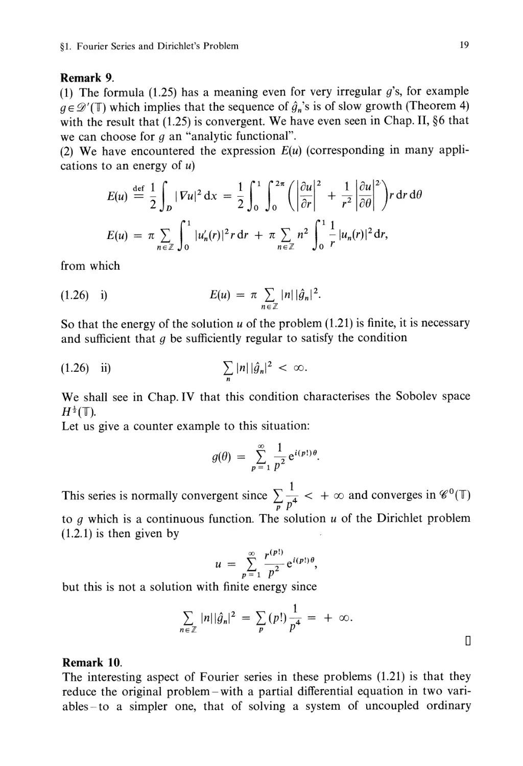
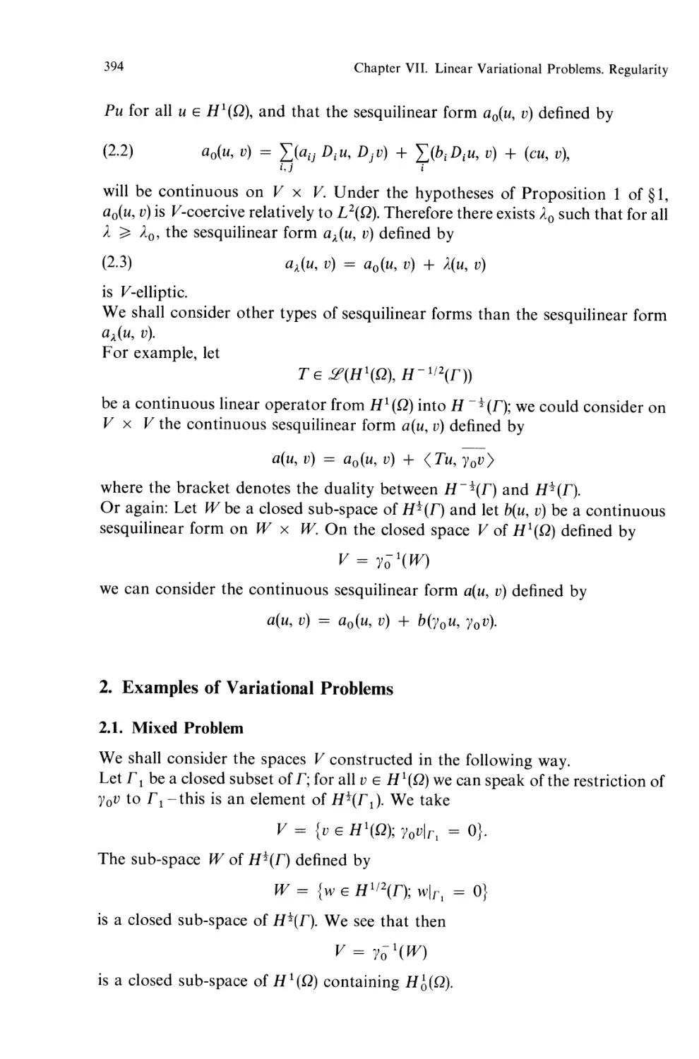
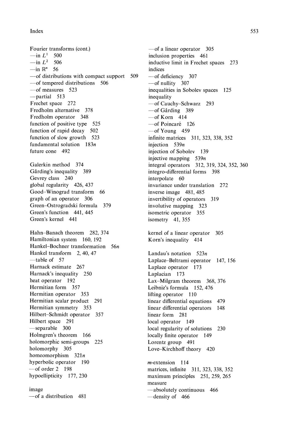
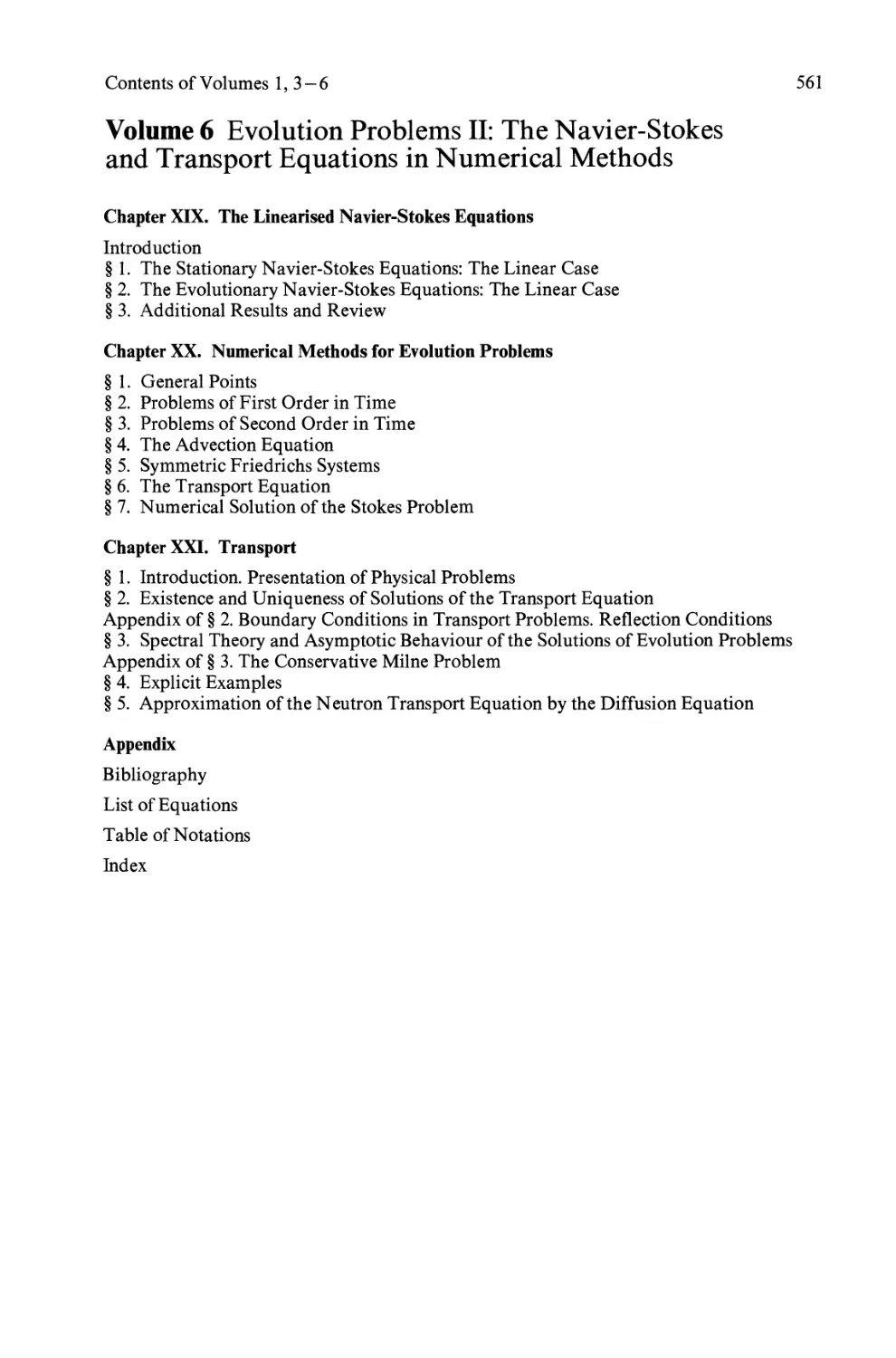
We consider a rectangle Q == ]0, a[ x ] - -tb, -tb[ in the plane [R;1, X2.
We propose to solve, by means of Fourier series, the Dirichlet problem:
i L1 u == 8 a2 + 8 a2 = 0 in Q
(1.27) Xl X2
u == g on a Q,
where g is a function given on aQ. The boundary 8Q is made up of the segments:
ro == {O} x]- bj2, + bj2[
r a == {a} x ] - b j2, + b j2 [
r'+ == ]0, a[ x {bj2}
r'_ == ]0, a[ x {- bj2}
with the result that we can write
g == gl + g2,
X 2 n
r'+
Q fa
-
a Xl
b
+-
2
fo
0
b
- -
2
r'_
Fig. 2
1. Fourier Series and Dirichlet's Problem
21
where:
gl == 0 on r 0 u ra
g 2 == 0 on r'+ u r'- .
The solution u of (1.27) is then U == U l + u 2 where U i is the solution of
( 1.27)'
L1 U i == 0 in Q,
U. == g . on 8Q
l l ,
i == 1, 2.
Now by the change of variables:
, b
Xl == X2 + 2'
,
X2 == Xl
a
2'
Q is transformed to:
( 1.28)
Q' == JO, b [ x J - a12, aI2[,
and the problem (1.27) to:
8 2 u' 8 2 u'
_ 8 '2 + _ 8 ,2 == 0
Xl X2
in Q'
,
U' == g' on 8Q',
with
U'(X , x;) == u(x 1, X 2 ),
g'(X , X;) == g(Xl' X2).
In particular, this transformation changes (1.27)' (i == 2) to (1.28) with the result
that it suffices to solve (1.27)' for i == 1. In other words we are led to solve (1.27)
taking g == 0 on r 0 u r a' i.e. to solve
i) L1 U == 0 in Q
ii) u(O, X2) == u(a, x 2 ) == 0 for X2 E [ - bj2, bl2J
iii) U(Xl' + bj2) == qJ:!:(Xl) for Xl E [0, aJ,
( 1.29)
where qJ + and qJ _ are functions given on ]0, a[. Writing
( 1.30)
. nnxl
U (x l' X 2) == f...J an (X 2) SIn
n=l a
where
2 f a . nnxl
a n (X2) == - U(Xl' X 2 ) SIn dx l ,
a 0 a
(1.31)
and hence in particular, by the condition on the boundary r':!:
+ def ( b ) 2 f a . nnx 1
ex;; == an + - == - qJ:!: (Xl) SIn dx l .
2 a 0 a
Now, we have
( " ( nn ) ) . nnx l
Au(x 1 , x 2 ) = 1..- an (x 2 ) - ----;; 2 a n (X2) SIn a '
with the result that L1 U == 0 in Q can be written:
a; - ( '; r an = 0 in ] - b12, b12[,
(1.32)
22
Chapter III. Functional Transformations
that is to say
(1.33)
nnx 2 nnx 2
a n (X 2 ) = Anch + Bn sh .
a a
Thanks to (1.31) the coefficients An' Bn are given by
nnb nnb +
An ch 2a + Bn sh 2a = an
nrcb nrcb
An ch 2a - Bn sh 2a = a;; ,
that is to say:
An= (ach n:b ) -1 J: [<p+(X 1 ) + <p-(xdJsin nna X1 dX 1
Bn= (ash n : b r 1 f: [<p+(xd - <p_(xdJsin nnax1 dx 1 0
Conversely, the formula (1.30) where an is given by (1.33), (1.34) determines a
solution of (1.29).
Remark 11. When u is of the form (1.30), the energy E(u) (see Remark 9) is
given by
(1.34)
(1.35) i)
1 i 00 f +Q. [ n 2 rc 2 J
E(u) = - I Vul 2 dx = L 2 la n (x 2 )1 2 + la (X2)12 dx 2 .
2 Q 4 n = 1 _Q. a
2
Integrating by parts and using (1.32) we obtain
rc [ nnb nnb 2 2 J
E(u) = 2 sh- 2 ch- 2 (An + Bn) .
n=l a a
nrcb nnb
Taking account of(1.34) and ofthefact that sh 2a ch 2a as n --+ 00, we find
that the solutions of finite energy
(1.35) ii)
E(u) < + 00
are such that
(1.35) iii)
00 ( f a nnx ) 2
L n qJ :!: (:X 1) sin 1 dx 1 < + 00.
n=l 0 a
We shall see that the condition (1.35) iii) is equivalent to saying that the
boundary data qJ + and qJ _ are in the space of traces of the functions with finite
energy.
o
1. Fourier Series and Dirichlet's Problem
23
Remark 12. Application of the Dirichlet problems (1.21) and (1.27).
The mathematical models (1.21) or (1.27) can be found in an electrostatic
problem (see Chap. I, 4.5.1) U representing the potential in the interior Q of a
hollow cylinder in [R3, (a dielectric occupying the domain Q), of circular or
rectangular cross-section, g representing the potential applied to the surface of
this cylinder:
E(u) is here the energy seen in Chap. lA, 4: we have seen the definition for
- the energy W of the whole domain in Chap.IA (4.42) (general case of
evolution),
- the energy WOK of a compact set K in Q in Chap. IA (4.114) (stationary case),
- the energy Wi per unit length of a cylinder in Chap.IA (4.141) (stationary
case ).
Using the system of natural units (see Chap. lA, 4) the expression E(u) is
precisely the electromagnetic energy per unit length of the cylinder:
E(u) = r C dXi dX 2 dX 3 = Wi
J Q x [0, 1 ]
where S, the energy density is defined in Chap. lA, (4.jO). We have pointed out in
Chap. lA, 4, that in problems in which the domain Q == Q x [R is modelled by
an infinite cylinder in [R3, we often have to require that the energy per unit length
be finite, so have the condition (1.26)ii) or (1.35)iii).
o
Remark 13. The use of Fourier series can equally well be used to determine the
spectrum of the Laplacian (see Chap. VIII) in the rectangle Q in [R2 with
homogeneous Dirichlet boundary conditions.
To simplify what follows let us suppose that Q == JO, n[ x JO, n[. The question
is to find u and A satisfying
(1.36) { i) L1 u + AU == 0 In Q c [R2 A E C.
ii) u == 0 on 8Q
Putting then (double development in series of sines )24:
00 00
U(Xi' x 2 ) == L L u nm sin nX i sin mX2
n=im=i
we find that equation (1.36)i) then becomes
L [-(n 2 + m 2 ) + AJunmsinnXi sinmx 2 == O.
n,m
24 The functions (sin nx 1 , sin mx 2 ), with m, n integers, form an orthogonal base in the Hilbert space
L 2(Q).
24
Chapter III. Functional Transformations
from which we deduce
[A -(n 2 + m 2 )Ju nm = 0,
Vn,mEN*,
so that u mn = 0 unless A = n 2 + m 2 .
We deduce that there is a denumerable infinity of isolated eigenvalues: 25
A = n 2 + m2
nm ,
n,mEN*,
having the associated eigenfunctions 25
U nm (Xl' X2) = sin nXl sin mX2.
The preceeding method can be used equally well to solve the Dirichlet problem
{ -L1u = f on Q
U = 0 on oQ,
by developing f in a double series of sines.
o
92. The Mellin Transform
1. Generalities
The Mellin transform appeared for the first time in the famous memoire of
Riemann [lJ on the theory of numbers. The reason is the following: if we
consider the Dirichlet series
00 a
cP(s) = L -i
n = 1 n
and if we introduce the function
f(x) = L an e -nx,
then
1 f oo
<1>(s) = r(s) 0 x s - 1 f(x) dx
in which there makes the appearance of the Mellin transform off defined by
Mf(s) = LX) x S - 1 f(x) dx.
If we associate with f the function on [R:
F(t) = f(e t )
25 See Chap. VIII.
2. The Mellin Transform
25
then
Mf(s) = f 00 e ts F(t) dt
We work here with s complex. We recall that the (bilateral) Laplace transform is
defined by
.2F(p) = f oo e- pt F(t)dt.
We therefore have
Mf(s) = 2 F( - s).
From this we deduce the inversion formula of M. In effect
1 f C+ioo
F(t) = lni c _ i 00 e pt .2 F(p) dp
with c a convenient real value (and with appropriate hypotheses on F). Hence
1 f C+ioo
F(t) = _ 2 . e- st Mf(s)ds
nl C - i 00
from which
1 f C+ioo
f(t) = -----=- x -s M f(s) ds.
2nl c-ioo
The connection thus put in evidence with the Laplace transform by the
change of variable t --+ e t = x gives the principal property of the Mellin
transformation from the point of view of applications to partial differential
equations. While the Laplace transformation diagonalises the operator dj dt
(giving multiplication by p), the Mellin transformation diagonalises the operator
xdjdx = A (giving multiplication by - s):
M(Af)(s) = - sMf(s).
[Notice otherwise that Af = sfis equivalent to f(x) = x- s .]
Now (and naturally these formulae are not "accidental": they all result from
in variance properties) if u satisfies
L1u = 0
in the plane, then u, being expressed in polar coordinates, satisfies (after
multiplication by r 2 )
v 2 u vu v 2 u
r 2 vr 2 + ra;: + ve 2 = 0
1.e.
v 2 u
A 2 u + ve 2 = o.
26
Chapter III. Functional Transformations
Let us now consider the following problem: in the angular domain 0 < r < 00,
- a < () < a, we seek u == u(r, ()), solution of
{ (i) L1 u == 0
(ii) u(r, a) == u(r, - a) == g(r).
(2.1 )
We then introduce the Mellin transform in r of u:
U(s, e) = Mr(u(r, e)) = IX) r s - 1 u(r, e) dr.
The problem (2.1) becomes then
a 2 u
ae 2 + S2 U = 0, - IX e IX
(2.2)
U ($, + a) == M g(s).
The explicit solution of this problem, in which s is a parameter, is elementary: the
two boundary values of U being equal (we could equally well treat the case in
which u takes distinct values for () == a and for () == - a!), U is even in (), thus
cos (s ())
U(s, e) = () Mg(s)
cos sa
and hence the solution of (2.1) is expressed by
1 f C + i 00 cos S ()
u(r, ()) == _ 2 . r- s Mg(s)ds.
1Cl c - i 00 cos sa
D
Let us now pass to a more precise expose of the properties of the Mellin
transform.
2. Definition of the Mellin Transform
Definition 1. The Mellin transform of the function with complex values g(x),
with x E [R + is given by the formula
M(g)(s) = t'X) x S - 1 g(x)dx,
(2.3 )
sEA C (:26
,
this formula having a sense if, for example:
x --+ X S - 1 g(x) EL l (0, + 00)
(and also in other cases as shown in the examples which follow).
26 The formula (2.3) only holds for the part of g defined on [R +, we are not concerned to know
whether or not g takes a value or not on [R -.
2. The Mellin Transform
27
Example 1. Let us calculate M (e - ax), for a > o. For all SEe satisfying
Res> 0, we have
M(e -/XX)(s) = L'X) x S - 1 e -/Xx dx = IX -s LX) x s - l e -x dx = IX s res).
Example 2. The functions cos x and sin x possess Mellin transforms: the
integral L'X) xs I cos x dx is convergent for Re s E ]0, 1[. Let us write
foR x S - 1 cosxdx = fol xS-Icosxdx + fIR xs-Icosxdx.
Th function X S - 1 cos x is in L 1 (0, 1) when Re s > 0 and integrating by parts we
have
fR xS-Icosxdx = [xS lsinx]f - (s - 1) f" x,s-2sinxdx
and x S - 2 sinx E L 1 (1, + (0) when Res < 1.
Let us proceed in the same way for the function sin x. To calculate the Mellin
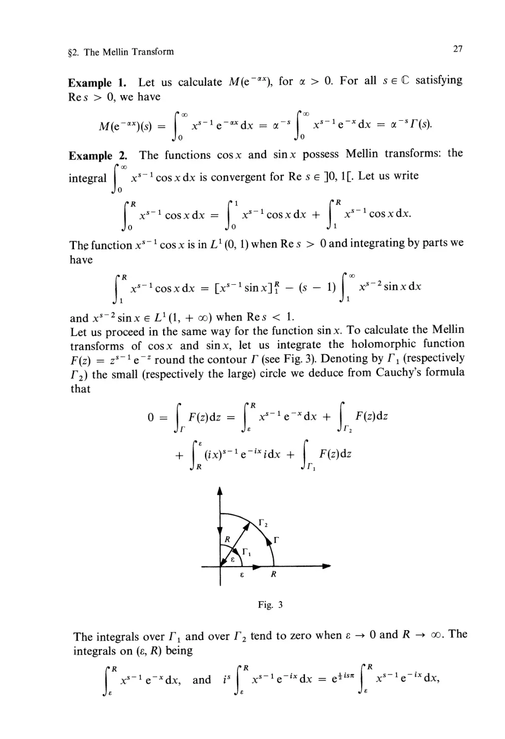
transforms of cos x and sin x, let us integrate the holomorphic function
F(z) = zS-1 e -z round the contour r (see Fig. 3). Denoting by r 1 (respectively
r 2) the small (respectively the large) circle we deduce from Cauchy's formula
that
o = f F(z)dz = fR x S - 1 e-xdx + f F(z)dz
r Je r 2
+ t (ixy- I e-ixidx + t, F(z)dz
E R
Fig. 3
The integrals over r 1 and over r 2 tend to zero when B --+ 0 and R --+ 00. The
integrals on (B, R) being
f.R x S - 1 e -x dx, and is f.R x S - 1 e -ix dx = e tis1t f.R x S - 1 e - ix dx,
28
Chapter III. Functional Transformations
it follows on making B --+ 0 and R --+ 00 that for Re s E J 0, 1 [
fo'" xS-le-ixdx = e- tis1t r(s)
from which we deduce that
(2.4)
M(cos x)(s) = cos( sn )ns)
M(sinx)(s) = sin( sn )ns)
SEe and such that Re S E JO, 1[.
D
3. Properties of the Mellin Transform
Let us at first give some simple formulae, easy to verify,fbeing a function with
complex values on IR or IR +: (see Definition 1 for the conditions on f)
d
M(Log xf)(s) = ds M(f)(s)
M(xaf)(s) = M(f)(s + li) li E C
(2.5)
def
M(fJ(s) = a- S M(f)(s) if h(x) = f(ax), a > 0
1 ( s ) def
M(fP)(s) = /3 M (f) /3 if fP(x) = f(x P ), /3 > 0 27 .
Let us calculate now the Mellin transform of the derivative of a functionf We
have
M(f')(s) = L"'!'(X)XS-1dX = [xS-lf(x)] - (s - 1) L'" x S - 2 f(x)dx.
If we suppose that
lim x s - 1 f(x) = lim x s - 1 f(x) = 0,
x-+O x-+oo
li < Re(s) < /3
and that M (f)(s - 1) exists in this band, we shall have
(2.6) M(f')(s) = - (s - l)M(f)(s - 1), SEe and li < Re (s) < fJ.
27 Notice that there are many other interesting properties of the Mellin transformation, and
def f oo ( x ) dy
notably that it transforms the convolution integral h * h = 0 h ; h(Y) to a product:
M(h*h) ) = M( ) ).M(h) ).
2. The Mellin Transform
29
More generally, let us suppose that
lim X s - n + k f(k) (x) = lim X s - n + k f(k) (x) = 0,
x o x oo
Re (s) E J li, Jj[ and k = 1, 2, . . . , n - 1,
and that M(f)(s - n) exists in this band, then
(2.7) M(f(n»)(s) = (- l)n(s - l)(s - 2) . . . (s - n) M(f)(s - n).
As an application of these formulae, we see that
M( x }s) = sM(f)(s).
(2.8)
This equation expresses the fact that the Mellin transform diagonalises the
d
operator 11 = x dx .
Remark 1. Let us place ourselves in the space of regular functions with
compact support on JO, 00 [ provided with the scalar product
f 00 dx
cpt/J-.
o x
The completion of this space is the Hilbert space L 2 (0, 00; dxjx). Then the
operator A = xdjdx is "antisymmetric", i.e. satisfies
f 00 dx f 00 dx
(Acp)t/J- = - cp(At/J)-,
o x 0 x
vcp,t/J E f0(JO, oo[).
We can show that the operator iA is essentially self-adjoint 28 in L 2 (0, 00; dxjx)
if its domain 28 is D(iA) = f0(JO, 00 C), and that its "proper generalized func-
tIons" are the functions x x - s (for Re s = 0).
D
Let us denote equally (with domains of validit y 29 eventually different)
(2.9)
M( t f(t)dt }s)
M ( LX) f(t) dt }s)
1
= - - M(f)(s + 1)
s
1
= - M (f)(s + 1).
s
28 See Chap. IA 6 (Appendix), Chap. VI and Chap. VII for all these notions.
29 See the conditions indicated for (2.6). For the two relations (2.9) to have a sense simultaneously, it
is necessary tha. t
f + 00
o f(t)dt = O.
30
Chapter III. Functiona Transformations
All of these formulae are frequently used in applications. In particular, let us
consider the Laplacian L1 in IR 2 in polar coordinates. We have
( 02 1 0 1 ( 2 )
(2.10) L1 u = or 2 + -;: or + r 2 oe 2 u.
Taking the Mellin transform with respect to the variable r, we obtain with the
aid of (2.7)
(2.11) M(L1u)(s) = [ + (s - 2f ] M(u)(s - 2, 0).
4. Inverse Mellin Transform
One of the interesting aspects of the Mellin transformation (as with the trans-
formations of Fourier or of Hankel etc.) is that it possesses an inverse. The
existence of this inverse is furnished by the
Theorem 1. Let g(s) be afunction which is holomorphic in {s E C; Res E ]li, P[}.
Suppose that
(i) lim g(s) = 0 uniformly in {s E C; Res E]li + B, P - B[}
I Ims I -+ 00
(2.12) V B such that 0 < B < t(P - li),
(ii) L I g (s) I db < + 00 if s = a + ib, V a E ] IX, P[.
Then the function g is the Mellin transform of a function g which is given by
g(x) = 2 1 . f x-Sg(s)ds,
1Cl r
(2.13)
xEIR+
,
in which
r = {s E C; S = y + i l5, l5 E IR, y fixed, y E ] li, P [} .
We then have
(2.14) g(s) = LX) xS-1g(x)dx, ReSE]IX,p[.
We can show (see Widder [1]) that a function g on IR+ is the inverse Mellin
transform of a function g with the above properties if and only if
(i) g E L c(]O, + 00 [),
(ii) for all (J E]li, P[, there exists A((J) E IR+ such that
Ig(x)1 x-a A ((J), Vx E]O, 00[.
2. The Mellin Transform
31
So
for 0 < Cl < /3, g(x) --+ 0 for x + 00
for Cl < /3 < 0 g(x) --+ 0 for x 0 +
for Cl < 0 < /3 g(x) --+ 0 for x --+ 0 + and for x --+ 00.
Under the conditions of Theorem 1, we see that the inverse transformation M- 1
of the Mellin transform M is
M- 1 :g f x-Sg(s)ds
21Cl r
Proof of Theorem 1. Let us put x = e - t in (2.13), and
def
G(t) == g(x) = g(e -t).
Then (2.13) can be written
G(t) = 2 1 . f ets g(s)ds,
1Cl r
t E .
As a consequence of the hypotheses (2.12), g(s) is the Laplace transform of the
function t --+ G(t) (see introduction to the 92 and Schwartz [3J pp. 196-206; see
also Widder [lJ, p. 265, theorem 19a)
g(s) = L'''oo e-stG(t)dt
Cl < Re s < /3.
With the change of variable x = e- t , we find
g(s) = too xs 1 G( - log x)dx = too xs 1 g(x) dx
i.e. (2.14)30.
30 Notice (see Widder [IJ, p. 248) that in a framework more general than that of Theorem 1, if g is a
function on IR+ such that I'?' X'-l g(x)dx converges absolutely for Res = (J and if 9 is of bounded
variation in a neighbourhood of x E [R +, then
-I f (1+iT 1
lim ---:- g(s)x -sdx = -{g(x +) + g(x - )}.
T -+ 00 2nl (1 - iT 2
32
Chapter III. Functional Transformations
5. Applications of the Mellin Transform
Dirichlet's problem in a wedge
Let us study the following Dirichlet problem (see Davies [lJ): find u satisfying
(2.15)
a 2 u au a 2 u
(i) r 2 L1u = r 2 a;: + r or + oe 2 = 0, 0 < r < 00, - a < e < a,
.. { 1
(11) u(r, + a) = g(r) = 0
o < r < 1
r > 1
. 1. 4
where a IS a given angle 0 < a < 2 1t (see FIg. ).
o
9=Ct.
8= -(1
Fig. 4
We have seen in Chap. II, that in the case of an unbounded open set, we must
have conditions at infinity on the unknown u to have uniqueness of the solution
of the Dirichlet problem. We suppose that when r --+ 00, u(r,O) 1'-1 r- P with
{3 > 0 and that in addition, u(r, 0) is bounded for r --+ O. The Mellin transform
with respect to r of the function u, say U, exists then 31 and we have
(2.16)
(i) [ dd;2 + S2 ] U(s, e) = 0, - a < e < a
(ii) U (s, a) = U (s, - a) = M g(s)
with
(2.1 7)
i 1 1
Mg(s) = r s - 1 dr = -.
o s
31 At least for Re S E JO, P[.
2. The Mellin Transform
33
We deduce from this (see (2.2) et seq.)
U (s, 0) = . cos(sO) .
S COS(Sli)
(2.18)
To calculate the inverse Mellin transform of U(s, 0) we shall utilise a certain
number of preliminary results, the final result being (2.34) below.
Proposition 1. Let f(x) be a function of (0, + (0) in possessing a Mellin
transform (Mf)(s) for s E {s E C; Re s E JS1' S2[}. We suppose that:
(2.19) f(x) is extended to a holomorphic function F (z) in a sector largzl < {3,
o < {3 < 1C of c.
(2.20) lim ZS F(z) = 0 for Res E Ja, b[ c JS1, S2[ and 32 largzl < {3.
Izl....oo
(2.21) lim ZS F(z) = 0 for ReSEJa, b[ c JS1' S2[ and 32 largzl < {3 for
z....o
each sub-interval Ja, b[ ofJs1' S2[.
Then for each 0 sucb that 101 < {3
{ M r [ReF(re i6 )](s) = M(f)(s).cossO,33
(2.22) Mr[Im F(rei6)](s) = - M(f)(s). sin sO, s such that Re s E]S l' S2 [.
Proof of Proposition 1. Let us integrate the holomorphic function F(z) along
the contour re = r 1e U r 2e U C U C e shown in Fig. 5.
e <
0 E r 2£ R
Fig. 5
We have
f F(z)zS - 1 dz == 0,
Fe
32 Uniformly for largzl < {3.
33 M r denotes the Mellin transform with respect to the variable r.
34
Chapter III. Functional Transformations
therefore
f.R F(re i9 )(re iO y-l eiO dr = f.R f(x)x S - 1 dx + t F(Z)ZS-l dz
- f F(z)zS-ldz
c/;
f.R F(re i9 )r S - 1 dr = e - is9 {f.R f(x)x S - 1 dx
+ f F(z)zS-ldz - f F(Z)ZS-ldZ } .
C. c/;
Let us make R tend to infinity and G tend to zero and let us use the hypotheses
(2.20) and (2.22). The integrals on C and C 8 then tend towards zero and we
obtain the desired formulae (2.22).
D
Lemma 1. We have
(2.23) M C x }s) = si:ns for 0 < Re s < 1
Proof Let us integrate the function
( e - i 1t z)S - 1
j(z) == 1 + z '
Re(s) E JO, 1 [
along the contour described by Fig. 6.
r == C 1 U C R U C 2 U CEo
C R
Fig. 6
2. The Mellin Transform
35
The theorem of residues implies that
tf(Z)dZ = 2ni(Resf)( - 1),
(2.24)
where (Re sf)( - 1) is the residue of f at the pole z == - 1.
Letting R 00 and 8 0, we see that the integral off on C Rand C e tends to
zero. In effect
f f 2n - a
f(z)dz == f(Re iO ) i Re i8 de
C R a
from which
r f(z)dz r 21t Rlf(Re i6 )ld8;
J C R J 0
we then use the fact that lim Rlf(ReiO)1 == 0 when Re(s) E JO, 1[. We proceed
R-+oo
in the same way for the integral on C e . On passing to the limit in (2.24), we
obtain:
(2.25) LX) f(x)dx - L'" f(e 21ti x)dx -= 2ni(Resf)( - 1);
now (remarking that f is a multivalued function)
2 . (e - i n x) s - 1 _ (e i n x) s - 1 . X s - 1
f(x) - f(e nl x) == == 2i SIn sn 1 '
1 + x + x
from which
(2.26)
roo X S - 1 dx == 2in (Resf)( - 1)
J 0 1 + x 2i sin (sn)
n
sin (sn)'
since (Re sf)( - 1) == 1.
D
Remark 2. The preceding method of calculation generalizes easily to that of
calculating the Mellin transform of a meromorphic function g(z), bounded at
infinity and with no pole on the positive real axis. If z 1, Z2, . . . , Zk are its poles,
we obtain
(2.27)
n k
M(g)(s) = . ( ) L (Re sf) (Zj),
SIn n s j = 1
where
f(z) == (e- in z)S-l g (z).
D
36
Chapter III. Functional Transformations
Application to the calculation of the inverse transform of the function U defined by
(2.18):
Let us apply the Proposition 1 with M (f)(s) = 1 ; we must find
s cos srx
f == M - 1 ( 1 ) and verify the conditions (2.19), (2.20), (2.21) of the Pro-
s cos srx
position 1. According to the inversion theorem,f(x) exists. To calculate f(x) we
shall proceed by successive reductions: from (2.23) and (2.5), we have
(2.28)
M( 1 ; x 2 }S) = 2sin tns) ' Re(s) E ]0, 2[
and from (2.9) (for Re s E JO, 1[):
M(f" 1 t t 2 }S) = M C : x2 )(1 + s) = 2ssin{t:(S + l)} '
which is equivalent to
M ( - 2 1 n - Arctgx ) (S) = 2 n 1 ·
S cos (-ins)
Setting p == nj(2rx), (where rx is the angle of the wedge), we have from (2.5)
(2.29)M G n - Arctgxp}S) = 2( )C:s( )' sEC'ReSE]0'p[,
1 n
Now -- == rx so
p2 '
(2.30)
2 M ( !n _ Arctgxp ) (S) = 1 .
n 2 s cos (srx)
In inverse form we have
(2.31 )
M -1 ( 1 ) (x) == 1
s cos (srx)
We use Proposition 1 with
2
- - Arctg x p .
n
2 1
F(z) == 1 - n Arctgz P , IArgzl < In.
We are able to verify the conditions (2.20), (2.21) with the equality:
(2.32)
2 1 zP + i
1 - -Arctgz P == - -Log
n i n zP - i'
1
IArgzl < 2 n ,
2. The Mellin Transform
37
in choosing the branch of the logarithm for which Arctg x E ]0, t n[, x O. It
follows then as a consequence of (2.22) and (2.31) that
(2.33) u(r, (}) = Ms-l (U(s, (})) = Re (1 - Arctgr P e ip6 ),
from which finally, using (2.32), we have
(2.34)
u(r, e) ==
1 1 A 2rP cos pe 1 . f [ 1]
rct g 2 rEO "
- n l-r P
1 A 2rPcospe 1 . f 134
rctg r >
- 2 1 '
n r P -
n
where p == 20: .
D
We have thus verified by this example that even if the boundary value (g on aO)
is discontinuous (see (2.13)), the solution of the nonhomogeneQus Dirichlet
problem, on 0, admits a re oo (and even analytic) solution in the interior of O.
We are able to verify that the obtained solution (2.34) of the problem (2.15) is a
solution of local energy E c(u), finite about the origin, where
def 1 f
(2.35) E c (u) == _ 2 I Vul 2 dx
KnQ
for each compact set K of [R2.
This condition, useful in electromagnetism (see Roubine [1] and also Chap. II,
8.7) is called Meixner's condition.
D
Remark 3. There is not, in general, uniqueness of the solution of the problem
(2.1) without supplementary conditions at infinity and at the origin; in the
present case of an angular sector, under the supplementary conditions
{ (i) u(r, e) 1"'.1 r - P for r 00, (with f3 > 0),
(ii) u(r, e) bounded for r 0,
(2.36)
we are going to show (result already announced above) that there is uniqueness
of the solution of the problem (2.1) if it exists.
We shall equally show that there is uniqueness of the solution of the problem
(2.1), (if it exists), under the conditions
34 We thus verify that u satisfies the required conditions at the start: u(r, 0) '" r - P for r CIJ with
f3 = p and u(r, 0) bounded for r O.
38
Chapter III. Functional Transformations
(2.37)
(i) u(r, e) bounded for r 00,
(ii) u(r, e) has finite local energy at the origin, i.e.
that there exists a compact neighbourhood K of
the origin such that (2.35) is finite.
Proof
(1) To study the uniqueness of the solution of(2.1), we must find if (by taking the
difference of two solutions), the problem
(2.38)
{ ) L1 u == 0 in Q,
(11) U 10Q == 0
admits a non-null solution. As a consequence of the invariance of this problem
(2.38) by the homothety of the centre 0, we need consider only the solutions of
(2.38) such that 35
(2.39)
u (r, e) == r S cp ( e),
where s is a real constant and cp a function of e (real or complex). Substituting
(2.39) into (2.38) and passing to polar coordinates we obtain the equation
0 2 U 1 ou 1 02U 2
A + + ( s {() + {()" ) rS - 2 '
LJ U == or 2 -; or r2 oe 2 == 'f' 'f'
showing that
(2.40)
cp" + S2 cp == o.
In addition, (2.38)ii) carries over to
(2.41 )
cp( - a) == cp(a) == O.
The boundary value problem (2.40), (2.41) has solutions:
(2.42)
cp ( e) == co sse
with
(2.43)
n
s == (2k + 1) 2a ' k E 7L.
35 In effect if u is a solution of (2.38) then v(r, 8) = t" u(Ar, 8)..1. -, - 1 dA is also a solution of (2.38)
with (2.39).
92. The Mellin Transform
39
Thus, the problem (2.38) admits the solutions
(2.44 )
u(r, 8) == r S cos s 8,
with s given by (2.43).
Without supplementary conditions to (2.1), there is no unIqueness of the
solution of (2.1).
(2) Let us suppose now that the supplementary condition (2.36)(i) or (2.37)(i) is
imposed; then the solutions (2.44) verifying it are such that
(2.45)
s < o.
The condition (2.36) (ii) at the origin implies s > 0, and so, only u == 0 is a
solution of (2.38) if (2.36) is verified; the solution of (2.1), (2.36) is unique, if it
exists.
The condition (2.37)(ii) leads to
f I Vul 2 dx == f [ au 2 + au 2 ] rdrde == f r2s-1 (S2cp2 + cp'2)drde
K K ar r ae K
ought to be finite and hence 2s - 1 > - 1, i.e. s > o. We reach the same
conclusion for (2.37) as for (2.36).
o
Remark 4.
(1) Even if the given function g (see (2.1)) is continuous on the boundary ao,
every solution of the problem (2.1) is not necessarily a solution of (2.1) in the
classical or quasi-classical sense (see Chap. II, 93): the solution u of (2.1) is not
in general continuous at the origin; in the particular case in which g is null on ao
(see (2.38)(ii)), only the solutions (2.44) with s > 0 are continuous at the origin.
(2) In the case of the problem (2.15), in which g is discontinuous at the points
r == 1 of ao, we have seen that the solution (2.34) of (2.15) is not continuous at
the point of its boundary r == 1, e == + (X. Thus u is a solution in a generalized
sense (see Chap. II, 94, Perron's method) of the problem (2.15).
o
For the resolution of problems more general than (2.1), for example in a wedge
or an open set with angular points, the reader should refer to Chap. VII and to
Grisvard [1], [2] and Kondratiev [1].
It is thus possible to study the Dirichlet problems (2.1) which arise in electro-
statics, heat conduction, elasticity, etc. . . with a "corner" geometry. The Mellin
transform is used in theoretical physics to study the asymptotic behaviour
of Feynman integrals (see Calan [1]) and to study diffusion ("scattering") in
quantum mechanics (Velo-Wightman [1]).
40 Chapter III. Functional Transformations
6. Table of Some Mellin Transforms (Ref. Colombo [1])
f(x)
M (f)(s)
cosx
n
r(s) cos-s
2
o < Re s < 1
SInx
n
r(s)sin-s
2
o < Re s < 1
e- X
r(s)
r(s)r(a - s)
r(a)
Re s > 0
(1 + x)-a
o < Re s < Re a
(1 + X)-l
n
o < Re s < 1
SIn sn
e iax
. 1t
r(s)e 'SI
o < Re s < 1
as
n
Log(1 + x)
- 1 < Re s < 0
s SIn sn
e - ax\ a > 0
1 s
-a-Ir(s)
2
1 + x cos ()
1 + 2x cos 8 + x 2
n cos s(}
s =1= kn, k E Z
SIn sn
x sin () n sin s(}
s =1= k n, k E Z
1 + 2x cos () + x 2
SIn sn
J v(x)
( s + V )j ( V - S )
2 s - 1 r 2" r 2" + 1
V < Re s < V + 2
For further transforms, see:
F. Oberhettinger, Tables of Mellin Transforms, Springer-Verlag Berlin Heidelberg 1974
3. The Hankel Transform
1. Generalities
The Hankel transform is a functional transform which diagonalises the operator
d 2 1 d v 2
L - + 2 ' W ith v E .
- dx 2 X dx -
(3.1)
3. The Hankel Transform
41
That such a "simple" transform exists results from two facts:
(i) If we work in the space of regular functions with compact support on
J 0, + 00 [ provided with the scalar product
Loo xcpljJ dx
(i.e. the space L 2(0, 00, /l) for the measure d/l(x) = x dx), then the operator L is
symmetric:
(3.2)
LOO x(Lcp )ljJdx = Loo xcp(LIjJ)dx
as is easily verified;
(ii) we seek then the "eigenvalues" of L, i.e. the functions w l such that
(3.3)
LWl = AWl
and we thus arrive at the Besselfunctions (naturally, all this demands to be made
precise; see,Chap. VIII and Naimark [1J).
We thus result in the Hankel transform of order v defined by
(3.4) £v(f)( ) = Loo f(x)Jv( x)xdx
in which J v(x) is a solution of
(3.5)
so that
LJ v = - J v
(3.6)
LJv( x) = - 2 J v( x).
For v - t, the inverse operator is expressed by the same formula and the
transformationf Yfv(f) is an isometry of the space L 2 (0, 00; xdx) onto itself.
D
This Hankel transform has a very rich structure and, like the Fourier transform,
can be found by starting from other considerations. First of all the Hankel
transform can be constructed in the body of group theory (see Miller [1J).
The Hankel transform is linked to the Fourier transform of functions of n
invariant under rotations; this is what permits (for example) the extension of the
Hankel transform to tempered distributions on J 0, 00 [. A presentation
of this connection is given below in Proposition 1. The Hankel transform ap-
pears equally in the theory of the transformations of differential operators; see
Lions [4J.
An "analytic" presentation enters into the theory of "general transformations"
introduced by Titchmarsl1 [1J, in which we seek functions k(A) such that if
$I( ) = Loo k(x )f(x)dx
then
X -1 = x.
42
Chapter III. Functional Transformations
Certainly, the basic tool for the Hankel transform is that of the Bessel
functions which are involved in many problems of mathematical physics, and to
the essentials of which we turn in the next section.
D
2. Introduction to Bessel Functions
The Hankel transform involves Bessel functions; this is why in this Sect. 2, we are
introducing these functions and giving several of their properties. These func-
tions are useful for the resolution of Laplace's equation in cylindrical co-
ordinates and will be considered again in Chap. VIII.
Let us consider the differential equation in the unknown u (with complex values)
(3.7) d 2 u + du + ( 1 _ v 2 ) u == 0 X E fR\ {O} and v given in fR.
dx 2 x dx x 2
One of the methods of solution of this type of equation is to seek solutions in the
form of a series of the type
00
u(x) == xll I anx n ,
n=O
a E fR.
Introducing this function into equation (3.7) and equating to zero the co-
efficients of the different powers of x, we obtain
(a 2 - v 2 )a o == 0
[(a + 1)2 - v 2 Ja 1 == 0
[ (a + n)2 - v 2 J an + an _ 2 == 0, n 2
where the first members are respectively the coefficients of xll - 2, xll - 1, X n + 1l - 2.
On supposing that a o #- 0, the first of these equations gives us that
a== + v
Taking a
v, we obtain as one solution of (3.7)
00 (_1)n(x/2)v+2n
Jv(x) == I
n = 0 n!r(v + n + 1)
which is called the Bessel function of the first kind (of order v).
If v is not an integer, the function J -v (x) which is also a solution of (3.7) is
independent of J v. To prove this, it is sufficient to calculate the Wronskian 36 of
these two functions; we find that it is of the form A/x with A == - (2/n) sin vn.
The general solution of (3.7) is then
(3.8)
u(x) == C 1 J v(x) + C 2 J - v(x),
X E fR\ {O}.
36 By definition, the Wronskian of two functions q; and t/! is the function w = q;' t/! - q;t/!'. If
w = 0, <p and t/! are proportional.
93. The Hankel Transform
43
In the case when v is an integer, v == n, say, it is easy to show that 37
J-n(x) == (- 1)nJ n (x).
In this case, another solution of (3.7) independent of I n may be found; it contains
a logarithmic term and will not be used in what follows.
Recurrence relations.
Bessel functions satisfy the following relations:
d v
dx [x J v(x)J == XV J v - 1 (x),
d
dx [x - v J v (x) J - - x - v J v + 1 ( x),
(3.9)
(3.10)
(3.11 )
d def V
- d Jv(x) == J (x) == J v - 1 (x) - -Jv(x),
x x
v
J (x) == - J v + 1 (x) + - J v (x),
x
(3.12)
(3.13)
x x
vJv(x) == 2 JV+1(x) + 2 J v - 1 (x).
These relations are easy to establish by using the expression (3.8) for J v (x).
I ntegral representations of Bessel functions. Let us consider the function
1 f 1 K(Z_1-)
K ( x ) == - z - v - e 2 z dz
v 2in c '
x > 0
where C is the contour described in Fig. 7 and v a given real number.
1m z
c
Re z
Fig. 7
This integral is convergent and the change of variable u == t z x gives
(x/2)V f -
Kv(x) == . u- v - 1 eUe 4udu.
21n c
This function can be extended to complex values of x and this is an integral
function of x. Let us replace e -x 2 J4u by its Taylor development and integrate
term by term: it becomes
K ( ) == (x/2)V (_1)k(X/2)2k f - (v + 1 + k) u d
v x 2 . i..J k , u e u,
In k = 0 . c
37 See Dieudonne [lJ and Watson [1].
44
Chapter III. Functional Transformations
which gives
00 (_1)k(Xj2)v+2k
K ( x ) =
v k ok!r(v + k + 1)'
Comparing with (3.8) we see that Kv(x) = Jv(x), i.e.
1 f 1 (z-.l)
( 3.14 ) J ( x ) = - z- v- e 2 z dz
v 2in c '
We are going to deduce a second integral representation of J v (x). For that, we
replace the preceding contour C by the contour C 1 of th€ Fig. 8 where 8 --+ O.
Let us return to the expression (3.14) for J V' We write first of all the contribution
of the circular part of C 1; putting z = e i8 , it takes the value (in the limit 8 --+ 0)
x > O.
I n e- i(v + 1)8 e (eiO-e-iO) ie i8 de
2 . ,
In -n
Rez
Fig. 8
that is to say
1 I n . 8 . . 8 1 f n
- e - lV e lXSm d8 = - cos(v8 - x sin 8)d8,
2n - n n °
as the integral between - nand n of sin(v8 - x sin 8) is zero.
The contribution of the straight parts is obtained by putting z = exp(t - in)
(for the upper straight part) and z = exp (t + in) (for the lower). It becomes (in
the limit 8 --+ 0)
1 I o . [ 1 J
e- vt + lnv exp - - x(e t - e- t ) dt
2In 00 2
1 f oo . [ 1 J
+ e - vt - lnv exp - - x(e t - e - t) dt
2zn ° 2
sin nv f 00
= - exp[ - xsht - vtJdt.
n °
3. The Hankel Transform
45
Finally, we obtain for x > 0
(3.15)
1 I n sin n v I 00
lv(x) = - cos(v8 - xsin8)d8 - exp[ - xsht - vtJdt.
non 0
In particular for v = n E N, we have
1 f + n . .. 1 I n .
(3.16) 1 n (x) = - e - w8 e lX sm 8 d8 = - cos (n8 - x SIn 8)d8.
2n - n n 0
Application to the Fourier transform. Let fEY (1R2) be a regular function of
"'-
two variables (of rapid decay). Writing g = f, its Fourier transform. Suppose
that the two functions f and g are expressed in polar coordinates
f(x) = f(r, 8) with x = {r cos 8, r sin 8},
g( ) = g(p,<p) with = {pcos<p,psin<p}.
Let us decompose f and g in Fourier series (see 9 1 )
(3.17)
f(r, 8) = L fn(r) e in8
nE"Z
(3.18)
g(p, <p) = L On (p )ein<P.
nE"Z
Let us seek the relations between the functionsfn and On" We have the
Proposition 1. Suppose that g is the Fourier transform offwherefE Y(1R2) and
let (3.17) and (3.18) be their Fourier series. Then we have the relations
.n f 00
"'- 1
f.,(r) = 211: 0 gn(p)J n(r p) p dp,
gn(P) = (- i)n 211: Loo J,,(r)J n(r p)r dr,
where 1 n is the Bessel function of the first kind of order n.
Proof By the definition of the Fourier transform we have
(3.19)
g(p, q» = Loo L21t e - ipr cos (9 - «J) f(r, 8)r dr d8,
and by the inversion formula (see Appendix "Distributions")
(3.20) f(r, 8) = (2:)2 LOO L21t e ipr cos (9 - «J) g(p, q» p dp dq>.
46
Chapter III. Functional Transformations
(3.21 )
Taking account of 1 (1.2)
1 f 21t
J;,(r) = 2n 0 f(r, e) e - inO de.
Substituting from (3.20) into (3.21), we obtain
1 f 21t . ( f ro f 21t . . )
in (r) = 3 e - wO e lpr cos (0 - ((J) L gm(P )elm({J pdp d<p dO.
(2n) 0 0 0 mEZ
Making the change of variable <p - 0 = t/J in the integral with respect to <p and
making use of the periodicity of the function e ipr cos '" + im"" we obtain
1 f 21t . f 00 f 21t . .
in(r) = 3 I el(m-n)OdO elPrCOS"'gm(p)elm"'pdpdt/J;
(2n) mEZ 0 0 0
now
f 21t ei(m - n)O de = { 0 f m =1= n.
o 2n If m = n
As a consequence
J;,(r) = (2:)2 too t 21t e ipr cos t/I rln(P )eint/l p dp dljJ.
On the other hand, putting t/J = 0 - tn, we obtain
1 f . ./,' ./, 1. 1t f 21t. . fj . fj
_ 21t e,prcos'I' e'n'l'dljJ = -e- m2 e,prStn0e'node.
21c 0 2n 0
As a result of (3.16) we have
J;,(r) = e ;:'i too rln (p)J -n (rp)p dp.
An analogous calculation would show that
rln(P) = ein'i (2n) t J;,(r)Ln(rp)r dr.
Thus the following transform is introduced naturally
f -+ too f(p)Jn(rp)pdp
and its inverse
g -+ too g(r)Jn(rp)rdr.
This leads to the Hankel transform which forms the subject of the Sect. 3 below.
3. The Hankel Transform
47
3. Definition of the Hankel Transform
Let us first of all give a formal definition which will be made precise later:
Definition 1. The Hankel transform of order v E IR of the function f: IR + --+ C,
is defined by
(3.22) J¥'v(f)( ) = LX) f(x)Jv(X ) x dx,
where J v is the Bessel function of the first kind of order v.
Example 1. Let us calculate the Hankel transform of order v of the function
f(x) = x V (a 2 - x 2 )1L Y(a - x),
j1 > - 1,
x, a E IR + ,
where Y is the Heaviside function defined by
Y( ) = { 1 if > 0
o if < o.
After (3.8) we have
00 (_ 1)n(x l2)v+2n
Jv(x ) = b 'T( + + 1) ,
n - 0 n. v n
from which we have
J¥'.(f)( ) = f (- nn( /2)' + 2n f a x2v + 2n + 1 (a 2 - X 2 )" dx.
n=On!r(V + n + 1) 0
On the other hand
f: X 2v + 2n + 1 (a 2 - X 2 )" dx = a 2 (v +" + n + 1) f01 tV + n(1 - t)" dt
1
= 2 a 2 (v + fl + n + 1) B(v + n + 1, j1 + 1),
where B denotes the usual Beta function which, we recall takes the value
B ( ) = r(p)r(q)
p, q r (p + q).
It thus becomes
00 ( _ n)n( j2)v + 2n a 2 (v + fl + n + 1) r(v + n + 1)r(j1 + 1)
J¥'v (f)( ) = n f:o n!r(v + n + 1) ' 2r(v + Jl + n + 2)
00 ( 1 ) n ( aJ: j 2 ) V + fl + 1 + 2n
= r (j1 + 1) afl + v + 1 - fl - 1 2 fl L S .
n = 0 n! r(v + j1 + n + 2)
48
Chapter III. Functional Transformations
Finally
(3.23)
Yfv(xV(a2 - X2)fl Y(a - x))( ) = r(/1 + l)a fl + v + 1 -fl-12fl JV+JL+ l(a ).
In particular, we have:
(3.24)
aV + 1
Yrv[X V Y(a - x)]W = J v + da ),
x, , a E IR + .
o
We shall see the consequences of these calculations later. On the other hand, we
shall give at the end of this part (Sect. 7 below) a table of the principal Hankel
transforms.
4. The Inversion Formula
In this section we shall exhibit a large class of functions which possess a Hankel
transform and give a reply to the following question: if gv is the Hankel transform
ofafunctionf, isfthe Hankel transform ofgv? The reply will be positive for the
functions of this class: we shall have Yfv 0 Yfv = I. We shall give a sufficiently
general theorem to cover this problem; the proof of this theorem is long and, in
the end, of little importance for those whose interest is in applications in respect
of the result itself. This is why we give only some applications of the theorem,
referring the reader to Sneddon [1] for the complete proof.
Theorem 1. Let f: IR + --+ IR be a function such that x --+ xi f(x) belongs to
L 1 (0, + (0). Then for each real number v satisfying v > - t, Yfv (f) defined by
(3.22) exists and
f oo 1
o Yrv (f)( )Jv(x ) d = :2 [f(x +) + f(x - )],
where f(x +) [resp. f(x -)] is the limit at the right [resp. at the left] off at the
point x in each point x in the neighbourhood of which f is of bounded variation.
Corollary 1. Let f: IR + --+ IR be a continuous function at the point Xo and such
that x --+ xi f(x) EL l (0, + (0). Then for each real number v satisfying v > - t,
Yfv(f) defined by (3.22) exists and
LX> Yrv(f)( )Jv(xo ) d = f(x o ).
Let us go back to the case of Example 1 38 . We have seen that
Yf v (x v (a 2 - X2)fl Y(a - x))( ) = r(/1 + l)a JL + v + 1 - fl- 1 2 fl J fl + v + 1 (a ),
38 See Davies [1].
3. The Hankel Transform
49
and we can apply Corollary 1 to the function whose Hankel transform we have
just calculated. This gives (for x =1= a, x > 0, v > - t, Jl > - 1:
f oo -I-L _ x V (a 2 - X2)1-L Y(a - x)
o J " + v + d a )J v (x ) d - r (Jl + 1) a" +v + 1 2" '
or again, on setting a = Jl + v + 1, we obtain:
f oo ;;-a +v + 1 J ( a;; ) J ( x;; ) d;; = x V (a 2 - x 2 )a-v-1 Y(a - x) .
o a S v S r (a _ v )aa 2 a - v - 1
For example for a = 1, v = 0 we have:
f oo Y(a - x)
J 1 (a ) J 0 (x ) d = ,
o a
x, a, E IR + , X =1= a.
Example 2. We shall prove that
o
(3.25)
[ v ] fixve-ax
:Yfv (a 2 + 2 r + 3/2 (x) = . ( 3 ) , a > 0
2V + 1 ar v + -
2
wi th a, , x E IR + and v > t .
Because of Corollary 1, it is enough to calculate the integral
F(a, ) = too XV + 1 e -ax Jv(x )dx = :Yfv(XV e ax).
For this, let us use the definition
00 (_ 1)n(x j2)v+2n
JJx ) = f: Ir( + + 1) '
n-O n. v n
to obtain
00 ( 1 ) n ( ;; j 2 ) v + 2n f 00
F(a, ) = L S x2v+2n+1e-axdx.
n = 0 n!r(v + n + 1) 0
I t is easy to see that
fo oo x2v+2n+le- ax dx = r(2v + 2n + 2)a-2V-2n-2,
and hence that
00 ( - 1 ) n ( ;; j 2 ) v + 2n r ( 2v + 2n + 2 )
F (a, ) = L a - 2 v - 2n - 2.
n=O n! r(V + n + 1)
Now, we have
r ( 2v + 2n + 2) ( 3 )
= n -1/2 2 2v + 2n + 1 r v + n + _ 2 .
r(V + n + 1)
50
Chapter III. Functional Transformations
It hence becomes
F(a, ) = f (- ,It ( /2t + 2nn-1/222v + 2n + 1 r ( v + n + ) a-2V - 2n - 2
n=O n. 2
gIvIng
F(a, ) = a 2v-2 v2v+ In-112 f [-( /a)2rr( + n + 3/2) .
n = 0 n.
From the binomial formula
(1 - x)-a = f r(a + n) x n Ixl < I"
n=O n!r(a) ,
we, deduce that
F(a, ) = a-2V-2 v2v+ln-1/2r(v + )(l + ( /a)2)-v-3/2,
and finally that
F (a, ) = n - 1/2 2 v + 1 r (v + ) a C (a 2 + 2) - v - 3/ 2 .
From this we obtain (3.25) on going back to the definition of F(a, ).
5. Properties of the Hankel Transform
First of all, let us quote two simple relations which are easy to establish. Let
a > 0 and letf: + be a function satisfying (for example) the hypotheses of
Theorem 1. Let us denote by fa the mapping x f(ax). Then
(3.26)
1
Yfv(fa)( ) = 2 Yfv(f)( /a),
a
E +.
Also:
(3.27)
v G f} ) = ;v { v-l(f)( ) + v+1(f)( )},
EIR+,V >
1
2'
this formula resulting from the recurrence relation (3.13) connecting the J v .
The Hankel Transform and Differentiation. Suppose that f is a function of
class 1 possessing (together with its derivative I') a Hankel transform. What
relation exists between Yfv(f) and YfV(f')? We have
3. The Hankel Transform
51
(3.28)
Yr v(f')( ) = LX) f' (x)J v(X ) X dx
f oo d
= [f(x)x Jv(x )]g' - 0 f(x) dx (xJv(x ))dx.
First of all, the quantity xtJv(x) is bounded in the neighbourhood of the origin
(for v > - !), from (3.8) andfbeing supposed continuous at zero, we have
lim xf(x)Jv(x ) = o.
x o
On the other hand, the quantity ft J v(t) is bounded (see, for example, Whittaker-
Watson [1]) and we can write
1 C
Ixf(x)Jv(x )1 = fi fi If(x)IRIJ'(x )1 fi filf(x)l,
x, E IR + .
It is sufficient for the vanishing of the bracket In (3.28) therefore that
lim fi f(x) = o. We have in this case
x 00
f oo d
Yrv(f')( ) = - 0 f(x) dx (xJv(x ))dx.
U sing the recurrence relations concerning J v we write
d x
dx (xJv(x )) = 2v [(v + 1)J v - 1 (x ) - (v - l)J v + 1 (x )].
We deduce finally the formula
(3.29) Yrv(f')( ) = - { v 1 Yrv _ 1 (f)( ) - v 1 Yrv +1 (f)W }, E !R + .
Proceeding as above, that' is to say integrating by parts and supposing that the
functionf is sufficiently regular and is such that all the brackets appearing in the
calculations are zero, the reader will be able to verify the following fundamental
formula
(3.30)
Yrv(f" + : f' - :: f)W = - e Yrv(f)( ).
( d2 1 d v 2 )
The Hankel transform diagonalises the operator + __ d - 2 . We shall
dx x x x
see that the Hankel transform (for suitable v) simplifies the study of Laplace's
52
Chapter III. Functional Transformations
equation in polar coordinates in {R2. In effect, let us solve Laplace's equation
in {R 2 :
L1u = f,
where f is known in polar coordinates in the form
f(r, 8) = I l,(r) e in8 .
nEZ
Let us put in the same way
u(r, 8) = I un(r) e in8 .
nEZ
We have seen in 9 1 that Laplace's equation can be decomposed into the
differential equations
1 n 2 "'-
Ail A, A f,
Un + - Un - 2 Un = n.
r r
Taking the Hankel transform of order n of this equation we obtain, from
equation (3.30), the equations
1 "'-
Yl'n(un)( ) = - 2 Yl'nCf,,)( ),
which by the inverse Hankel transform of order n gives the transforms Un'
Remark 1. Let us notice the analogy between the use of the Fourier or Laplace
transforms to resolve
def
Lv = - v" = g,
and the use we shall make of the Hankel transformation to resolve:
def 1 v 2
Lvv = - v" - - v' + 2 v = g.
r r
This is linked to the properties of the kernels of the two transformations: the
kernel G = e iax of the Fourier transform (or G = e ax for the Laplace transform)
satisfies
- LG = a 2 G'
,
the kernel G v = J v (ax) satisfies
LvGv = a 2 G v
(the functions J v (ax) are generalized eigenfunctions of Lv 39).
39 See Chap. VIII.
3. The Hankel Transform
53
Parseval's Relation. The following result is fundamental:
Theorem 2. F or v - t, the mapping
f --+ ytvf
(3.31 )
is an isometry of L 2 (0, 00; xdx) onto itself.
Stated otherwise: iff and 9 are in L 2 (0, 00; xdx) we have
f: f(x)g(x) x dx = f: Yt'J(x)Yt'vg(x)x dx.
By density, it is sufficient to show this formula to be true for functions f and 9
which are regular and have compact support; the result then follows from
Theorem 1 (for v > -t). The reader will find a proof in Titchmarsh [1],
Chap. 8, Sect. 8.18.
Example 3. Let us take, for example,
f(x) = XV Y(a - x),
g(x) = XV Y(b - x),
a, b > 0,
v
1
"2.
We have seen previously that
aV+ 1
Yt'v(f)( ) = TJV+l(a ),
bV+ 1
Yt'v(g)( ) = TJV+l(b ).
(3.32)
Parseval's relation then gives
(abt + 1 f co Jv+ 1 (a )Jv+1 (b ) d = (min (a, b))2v+ 2 .
o 2v + 2
D
6. Application of the Hankel Transform to
Partial Differential Equations
The Hankel transform is well suited to problems in 1R3 having symmetry about
an aXIS.
6.1. Dirichlet's Problem for Laplace's Equation in R .
The Case of Axial Symmetry
We set ourselves the problem of solving:
(i) L1u = 0 in Q = IRt = IR X1 x IR x2 x IRx;
(ii) u(x 1, x 2 , 0) = g(r) (for X 3 = 0) with r = (xi + X )1/2
(iii) lim u(x 1 , x 2 , x 3 ) = 0
X3 00
(3.33)
54
Chapter III. Functional Transformations
in which u takes real values and in which g is a given real function of r. Taking
account of the invariance of the data under rotations about the axis OX 3 let us
adopt cylindrical coordinates r, 0, Z such that
Xl = rcosO,
X Z = r sin e,
X 3 = Z (r > 0, e E (0, 2n), Z > 0).
Equation (3.33)i) becomes
8 z u 1 8u 1 8 z u 8 z u
(3.34) Au = 8r z + -;: 8r + rZ 80 z + 8Z z = O.
As a result of the invariance of the data in (3.33) under rotation about OX 3 let us
seek the solutions independent of 0, from which.
8u
80 = 0
8 z u
80 z = O.
The problem (3.33) becomes: find a (real) function u(r, Z) on + X + satisfying
8 z u 1 8u 8 z u
(i) 8r z + -;: 8r + 8Z z = 0
(ii) u(r, 0) = g(r)
(3.35)
(iii) lim u(r, Z) = O.
z oo
As we have seen Chap. II, the condition at infinity (3.33) (iii), [or (3.35 (iii)J is
necessary to ensure the uniqueness of the solution.
In addition to guarantee the interior regularity of the solution of (3.33) we shall
need to have that lim u(r, Z) exists for Z > o.
r O
Let us take the O-order Hankel transform of (3.34) which can be written (on
denoting by u and g the Hankel transforms of u and g),
(3.36) : - 2U = 0,
which yields, with (3.35) (ii) and (iii)
u ( , Z) = g ( ) e - z;; .
The inversion formula then gives
(3.37) u(r, Z) = f: g( ) e - z J o(r ) d .
Example 4.
sIn r
g(r) = -
r
f oo { (1 - Z) -1/Z
g( ) = 0 J o(r ) sin r dr = 0
0< <1
> 1.
93. The Hankel Transform
55
The solution of the problem (3.33) is thus
u(r,Z) = I e- Z(1 - 2)-1/2Jo(r ) d .
6.2. Boundary Value Problem for the Biharmonic Equation in R ,
with Axial Symmetry
We wish to treat the problem
(3.38)
(i) 11 2 u = 0 In [R
(ii) U(Xl' X 2 , 0) = g(r) on IR
( ... ) au ( )
111 Xl' X 2 , 0 = 0 on
uX 3
alR
(iv) lim U(X l , X 2 , X 3 ) = 0
X3 00
(with the notations at the beginning of the Sect. 6.1). As in the Sect. 6.1, we pass
to cylindrical coordinates (r, 0, Z) and look for a solution u(r, Z) of the equation
(3.39) ( :r 22 + :r + a 2 ) ( :r 22 + :r + a 2 )u = O.
(as a result of (3.38) (i)).
On taking the zero order Hankel transformation of (3.39) and (3.38) (ii), (iii), (iv)
we obtain
(3.40 )
( a 2 - 2)2 U = 0
u( , 0) = g( )
au
az ( 'O)=O
lim u( , Z) = 0
z oo
for Z 0 4 °,
of which the solution is
u( , Z) = g( )(1 + Z)e-z .
Example 5. Let us consider the case when the given boundary value is
g(r) = (1 + r 2 )-t;
in this case
g ( ) = yt ° (g) ( ) = - 1 e -
(see table below)
so that
u ( , Z) = - 1 (1 + Z) e - (Z + l)
40 Denoting by ii, 9 the Hankel transforms of order zero of u, g.
56
Chapter III. Functional Transformations
from which
u(r, Z) = f (1 + Z)e-(z+ l) Jo(r )d
u(r, Z)= J'to( -! e-(z+ l) ) + ZJ'to(e-(z+ 1) ).
Finally (see table)
r 2 + (Z + 1)(2Z + 1)
u(r, Z) = [(Z + 1)2 + r2 ]3/2 .
We verify that u(r, Z) is analytic, real in the half-space Z > 0 and we verify also
that the decay condition at infinity is such as to ensure that the inverse
transform exists.
o
Remark 2. The Hankel transform and the Fourier transform in IRn. In the case in
which a function F(x), (x E IRn) is invariant under rotation in IRn let "F(x) = F(r)"
\Ix, (r = Ixl); the Fourier transform P can be written as a function of quantities
invariant under rotation r = Ixl and p = I yl, (y being the variable conjugate to
x, y E IR n)
(2n )n/2 f oo n
F(p) = F(r)r 2 J E--l (pr) dr 41 .
n 2
p2-1 0
The transformation r1-1F(r) (2n)-1p1- 1 pep) is in effect the Hankel trans-
formation of order t n - 1 42 .
The preceding problem correspond to n = 2 i.e. to the order o.
Remark 3. Numerous properties of Hankel transformations of integer order
may be deduced directly from the properties of the Fourier transformation in 1R2
(see Appendix "Distributions"). In effect (see Proposition 1) each function (or
each tempered distribution) u on 1R2 of the form (in polars) u(r, 0) = In e - inO fer)
has for Fourier transform (in polars)
ff u(p, qJ) = u(p, qJ) = (- i)n e - inlp J't n u(p).
(i) The formula ff ff u(x) = (2n)2 u( - x) leads to the reciprocal formula
J'tn(J'tnf) = f(see Theorem 1).
1
(ii) Parseval's relation II u II i2( 2) = (211:)2 II u II i 2( 2) leads to:
f If(r)1 2 rdr = f I£J(p)12p dp
4i See Schwartz [IJ, p. 259, and Appendix "Distributions" for the definition of the Fourier
transformation used here.
42 The transformation F F is called Hankel-Bochner in Wolf [1].
Review of Chapter IlIA
57
(see Theorem 2) for eachfE L 2 (0, + 00; rdr), hence YfnfE L 2 (0, + 00; pdp).
(iii) If rf EL l (0, + (0), then U EL l ([R2), so U E rcO([R2), and U 0 for p + 00;
hence YfnfE rcO([O, + oo[) with Yfnf(p) 0 for p 00 and for p o.
Under the hypothesis of Theorem 1: ,-t f E L 1 (0, + (0), since I r t J n(r)1 K,
K ( f OO 1/2 ) K
l£nf(p)1 JP 0 r f(r)dr = JP IIfll£,(o,+ oo,JY<fr)'
We then deduce only that Yfnf E rcO(]O, + oo[) with Yfnf(p) 0 for p + 00.
o
7. Table of Some Hankel Transforms (Ref. Colombo [1J)
f(x), x > 0 Yfv(f)( ), > 0
x V (a 2 - X2)1l Y(a - x) a > 0 r (Jl + 1 )a Il + v + 12 1l - Il - 1 J Il + v + 1 (a ) v > -1
Jl> -1
X S - 1 (_ v-I < s < v + 1) 2S -S-1 r«v + s + 1)/2)/r«v - s + 1)/2)
x v-I e - ax a > 0 2 v n-' r(v + D V(a2 + 2)-V-1/2 V > 0
x v e - ax a > 0 2v+1n-1/2r( v + )a .(a2 + 2)-v-3/2 V > -1
X-I e - ax a > 0 (a 2 + 2)-1/2( )' V > - 1
a + Ja 2 + 2
e- ax a > 0 v(a2+ 2)-3/2{a + v J a 2 + 2}.{a + J a 2 + 2}-V
C Y+1 v > - 2
x 2
xVe-;;;- a * 0 "2 a 2 ve-ta2 2 v > - 1
SIn ax t2 - :2)-t, O< <a
- a > 0 v = 0
x > a
Review of Chapter IlIA
The problems which we have treated in 991, 2, 3 are of the following type: to find
U satisfying
{ P(D)U = f in 0 c [Rn,
with boundary conditions on cO where P(D) is a linear differential
operator with constant coefficients.
58
Chapter III. Functional Transformations
By a suitable change of variable, this problem is reduced to the following
problem:
(1) Case of Fourier Series. To find u' satisfying
{ P' (D)u' == f' in [Rd x Qo,
;.vith d cond tions o n the boundary of Qo and periodic conditions
In [R (perIod a - (a 1 , . - . ad)).
We suppose in addition that P'(D) is invariant under a translation a as well asf'.
Then the use of Fourier series diagonalises the part of the operator P' (D) acting
on [Rd. (In the examples treated in 91, the operator P' (D) is completely diag-
onalised and the problem reduces to the calculation of Fourier series).
(2) Case of-the Mellin transform. To find u' satisfying
{ P'(D)u' == f' in [R+ x Qo
with conditions on the boundary of [R+ x Qo-
We suppose that P'(D) andf' are invariant under homothetic transformations
in [R +. Then the Mellin transformation diagonalises the part of the operator
P' (D) acting on [R +.
(3) Case of the Hankel transform. To find u' satisfying
{ P'(D)u' == f' in [Rd x Qo
with conditions on the boundary of [Ra x Qo.
We suppose in addition that P'(D) and f' are invariant under rotations in [Rd_
The Hankel transform applied to the above equation diagonalises the part of the
operator acting on [Rd.
(In the examples of 93, we have d == 2 and Qo == [R+).
Part B. Discrete Fourier Transforms and
Fast Fourier Transforms
1. Introduction
Suppose thatf is a 2n-periodic function with complex values. Its development in
a Fourier series is given by
(1.1) f(x) = L cje ijX .
jEZ
From the orthonormality of the functions e ijx for the scalar product
1 f 21t
(h, g) = 2n 0 h(x)g(x) dx
there results the expression
(1.2) c j = (f, eijX) = ;n J:" f(x)e-ijX dx
for the coefficients C j.
Let Sn be the finite-dimensional space generated by the (2n + 1) basis functions
( ijX )
e -n j n.
The function};, E Sn, obtained by truncating the development (1.1) to .order n is
thus the best approximation to f in Sn (in the sense of the L 2- norm ). It is difficult
to calculate since we must evaluate integrals to calculate the coefficients c j .
On the other hand, the function gn of Sn of the form
+n
gn(x) == L aje ijX
j= -n
which coincides withf at the N = (2n + 1) points
2kn
Xk == N'
o k N - 1,
is such that a j satisfies the relations
(1.3)
n
L a je ijXk = f(Xk)
j= -n
60
Chapter III. Functional Transformations
(the function gn is in fact the interpolate off in Sn); these relations can be written
in the form
N-l
L ale2i1tkl/N = Zk
1=0
def def
with Zk == f(xk) and a l == a j for I = j (mod N).
On using the relation
(1.4)
1 N-l
- L e 2i1t (I- j)k/N
N k=O
{ I if I = j
<5 I } . = 0
otherwise
we conclude that
(1.5)
1 N-l ..
a. = - " e- 2l1t }k/N z
} N k,
k=O
o j N - 1.
To begin with we make a certain number of remarks which will not be
appropriate in the sequel.
Remark 1. Here, we have N = 2n + 1. The case N even corresponds to the
choice of Sn as the space generated by
( e i j X) j ,
which has dimension 2n.
-n+l j n
o
Remark 2.
The coefficients a j and c j are related by the formula
(1.6)
a j = L C j + 1N ,
fEZ
Ijl n.
In effect, for /l E 7L we can write
/l = v + IN where
Ivl nand
I E 7L'
,
as a consequence
f(x) = L cfle iflX = L L cv+1Nei(v+1N)X,
J1EZ fEZ Ivl n
so
Zk = L L Cv+1Neivxk
fEZlvl n
since NX k = 2kn. We deduce (1.6) by using (1.5) and the relation (1.4).
o
Remark 3. Estimate of the error for II f - gn II. Let us define the norm:
( ) 1/2
Ilflls = ,L (1 + j2)Sl c j l2
JEZ
91. Introduction
61
(this is the norm of the Sobolev space H (O, 2n) of periodic functions defined on
the interval }O, 2n[).
We then have for 0 m s the majorants
Ilf - fnllm C 1 n m - s Ilflls,
Ilf - gn 11m C 2 n m - s Ilflls
where C l' C 2 are positive constants independent of n and off.
These results have been established by Kreiss-Oliger [1J in the case m=O and
by Canuto-Quarteroni [1J in the general case.
o
Remark 4. The numerical quadrature formula
1 f 21C 1 N - 1
_ 2 f(x)dx - L f(x k )
noN k=O
(1.7)
is exact for fES N - 1 S2n.
We see that if we evaluate the coefficients c j by the formula (1.2) with the help of
the integration formula (1.7), we obtain in effect the coefficients a j .
o
Definition 1. We call the mapping eN eN which associates the (a j )f=-ol with
the (Zk)k=O,..., N-l according to the formula (1.5) the discrete Fourier
transform.
The inverse transformation can be expressed In an analogous and even
simpler form, since
(1.8)
N-l
Zk = L ajw j \
j=O
where w = e 21Ci / N is the principal root of order N of unity.
We see that the calculation of the Zk with respect to the aj, and reciprocally,
implies a priori O(N 2 ) operations (i.e. complex additions and multiplications)
since it is enough to carry out the product of art N x N matrix by a vector.
In fact, we shall see two different ways which enable us to reduce this number to
O(N log2 N) from which we derive a considerable saving of computing time
when performing calculations involving large values of N. This is what we call
the fast Fourier transform.
The first, studied in 93, is that due to Cooley and Tukey and applies in the case
in which N = 2 m (or 3 m ).
The second, studied in 4, is that of Good and Winograd and concerns the case
where N is a product of factors which are relatively prime.
Both rest on the principle of the acceleration of the product of a matrix by a
vector, when the vector satisfies certain decomposition properties ( 2).
We study in 5 principles of algebraic complexity which permit the acceleration
62
Chapter III. Functional Transformations
of the Good-Winograd transformation and thus render it competitive with that
of Cooley- Tukey.
We study the fast Fourier transformation in two dimensions in 9 6 . Finally in 9 7
we give some applications.
2. Acceleration of the Product of a Matrix by a Vector
Just as we have seen in 91, the problem of the discrete Fourier transformation
(direct or inverse) comes down to evaluating the product of an N x N matrix by
a column vector with N components. Let
a == Bz
i.e. choosing 0 and N -1 in place of 1 and N as bounds of variation for the
indices:
N-l
a j == L bjkz k ,
k=O
o j N - 1.
If the matrix B were arbitrary we should expect 0(N 2 ) operations, or more
precisely, N 2 multiplications and N 2 additions.
We shall show that we can carry out the product of the matrix B by an arbitrary
vector z in many fewer operations, on condition that the matrix B satisfies some
decomposition properties.
For pE N, we denote by I(p) the set
def
I(p) == {O, 1, . . . , p - 1}
of integers less than p.
Let us suppose that N == n 1 x n 2 x ... x n r is a product of r factors; these
decomposition properties will, in an essential way, make use of the fact that the
product set
I (n 1) x I (n 2 ) x ... x I (n r )
can be put in bijection with I(N).
An example of such a bijection is in the case in which
N == lor and n 1 == n 2 == . . . == n r == 10,
the mapping which, with a number of r digits, associates the r digits of its
decimal expansion: for example
983 -+ {9, 8, 3}.
Let us observe besides that the procedure is not unique since we can agree to put
them in a different order: For example:
983 -+ {3, 8, 9}.
9 2 . Acceleration of the Product of a Matrix by a Vector
63
Thus let N = n 1 x n 2 x ... x n r . Then we can be given a bijection
f: l(n 1 ) x l(n2) x . . . x I(n r ) I(N)
{j l' j 2, . . . , jr} j = f(j l' j 2, . . . , jr)'
In the general case we can equally well be given a second bijection
g :1(n 1 ) x l(n 2 ) x ... x I(n r ) I(N)
{ k l' k 2, . . . , k r } k = g ( k l' k 2, . . . , k r )
which does not necessarily coincide with f
We suppose that there exist na x na matrices B(a), a = 1, 2, . . . r
whose elements are denoted by bj:C, ja, ka E lena) and such that
(2.1 )
r
b Ok = b l k ) X b l 2 k ) X . .. X b l r k ) = TI b l a k )
J 111 22 rr /Xa
a=l
when j = f (j l' . . . , j r ) & k = g (k l' . . . , k r ).
Proposition 1. If B enjoys the decomposition property (2.1), then the product
of the matrix B by a vector z with N components can be brought about by
N(n 1 + n 2 + . . . + n r ) additions and as many multiplications.
Proof Let us put
z(r) = Z k
k 1 , k 2 , 0 0 0 , k r
for k = g(k 1 , . . . , k r ); z(r) is thus a list with r entries equally of dimension
nIx n 2 x . . . x n r .
By recurrence, suppose that we know z(a) (a E N * fixed, a r), a list of r entries
equally of dimension n 1 x n2 x . .. x n r .
We shall calculate z(a - 1) by the following formula
na - 1
(2.2) z(a-1) 0 0 = b a) z(a) . . .
k 1 . . 0 , ka-l1a, 0 0 0 ,lr i...J laka. k 1 ,. 0 . , kal a + l' . . . , lr'
ka = 0
in other words, k 1 , . . . , k a - 1 , ja+ 1, . . . , jr being fixed in
l(n 1 ), . . . , l(n a - 1 ), l(n a + 1)' . . . , l(n r ),
it is enough to calculate the product of the matrix B(a) by a vector with na
components which accounts for n; additions and as many multiplications.
Taking everything into account, the calculation of z(a - 1) starting from z(a) costs
(n 1 x . .. x na _ 1 X na + 1 X ... x n r ) x n; = N na
additions and multiplications.
We remark then that if
_ (0)
a o - z. .
J 11, . 0 . , Jr
64
Chapter III. Functional Transformations
for j = !(jl, j2, . . . , jr), then
(2.3)
N-l
a j = L bjkZ k
k=O
after (2.1). The calculation of a from Z accounts therefore for N(n 1 + n 2
+ . . . + n r ) additions and as many multiplications.
o
In the condition (2.1), the matrix B is in fact a tensor product B(a).
The limiting case N = 2 r shows therefore that we can hope in this favourable
case reduce the number of operations to 2N log2 N.
Remark 1. The preceding result is valid if the coefficients of the matrix B are of
the form
(2.4)
r
b. = TI b a). . k
J JI1.,JI1.+1,...,Jr'l1.
a=l
for j = !(jl,'" ,jr) and k = g(k 1 ,..., k r );
it suffices in effect to replace (2.2) by
(2.5)
Z(a-l) _
k 1 ,...,kl1.-1'jl1.'....'jr -
nil.
b a) . . z(a) . .
f..J JI1.,JI1.+1, . . . ,Jn k l1. k 1 ,..., kl1.,JI1.+1" . . ,Jr'
kl1.=O
There again the number of operations to calculate the N quantities
z(a-l) is Nn from which we deduce the total number of O p erations is
a'
N (n 1 + n 2 + . . . + n r ).
In this case B is no longer a tensor product of na x na matrices.
3. The Fast Fourier Transform of Cooley and Tukey
Let
N = n 1 x n 2 x . .. x n r
be.given and let w be the principal root of unity of order N. We recall (see 1)
that if Z E eN is given, its discrete Fourier transformation is the vector a E eN such
that
1 N-l .
a. = - w - Jk Z
J N f..J k,
k=O
o j N - 1.
We shall show that the matrix B whose elements are given by
1 'k
b jk = N w - J
(3.1)
satisfies the decomposition property (2.4).
3. The Fast Fourier Transform of Cooley and Tukey
65
For that, we choose the bijections f and g in the following way:
Let
def
ma = nix ... x na - 1
the product of the first (a - 1) factors of the number N (we agree to take
ml == 1); we put
r
(3.2) g(k 1 ,..., k r ) == L kama (with ka E I(na) for a == 1,. . . , r).
a=l
On the other hand, let
def
m = na + 1 X . . . x n r
the product of the last (r - a) factors of the number N (we agree that m == 1);
we put
r
(3.3) f(jl'... ,jr) == L jam (withjaE1(na) for a == 1,. . ., r).
a=l
Proposition 1. With the choice (3.2), (3.3) of the bijections f and g, the matrix B
defined by (3.1) (thus with its inverse defined by (1.8)) satisfies the decomposition
property (2.4).
Proof The proposition follows from the fact that w N == 1 and that w P == w q
when p = q (mod N).
(Congruence properties thus play an essential role). In effect, for
j == f(j l' . . . , j r)
k == g (k 1, . . . , k r ),
we have, in making use of (3.2)
r
jk == L ka(jma)
a=l
and from (3.3)
jma == (j 1 m'l + . . . + j a m + . . . + j r m ) ma .
Now
when f3 a - 1.
We deduce that
mam'p = 0 (mod N)
jma = (jam + . . . + jrm )ma (mod )
and that
Wjmrl == w(jam + ... + jrm )ma.
Finally, we have shown that
r
w jk == n wjkamrt
a=l
66
Chapter III. Functional Transformations
satisfies the property (2.4) with
def
b a) . == wjkama = w(jam + . . . + jrm )kama.
Ja, . . . , In ka
D
Remark 1. The number of operations which we indicate in Proposition 1 of 92
is an upper bound of the number of operations that will be realistically made: in
the case N = 4 we predict 16 additions and 16 multiplications, the matrix of the
w jk is made up in this case only of elements equal to + 1 or to + i, and there is
no multiplication whatever to make.
D
4. The Fast Fourier Transform of Good-Winograd
This concerns the case in which N = n 1 x n 2 x . .. x n r and where the
integers n 1 , n 2 , . . . , n r are relatively prime.
We recall first of all the Chinese remainder theorem (see Knuth [1J vol. 2,94.3.2).
Theorem 1. Suppose that n 1 , n 2 , . . . , n r are relative prime integers and that
N = n 1 x n 2 x , . . ., x n r .
Then for all r-tuples of whole numbers u 1 , U2, . . . , U r satisfying
o U a < na,
a = 1, 2, . . . r,
there exists a unique u satisfying
o u < Nand umodn a = u a , \fa.
D
We recall that the statement U a = u mod na is equivalent by definition to
U a = u(modulo na) and 0 U a < na 43.
Because of this Theorem 1, there exist therefore numbers qa, 1 a < r such
that
{ 1 if a = f3
qamodnp = b aP = 0 h .
ot erWlse.
We verify immediately that the relation between u and the U a is
U = Ctl Uaqa) mod N.
43 We recall that U a == u(mod na) means that 3ka E Z such that U - U a = naka. With the condition
o U a na, U a is therefore the remainder of the euclidean division of U by na.
4. The Fast Fourier Transform of Good-Winograd 67
Application to the discrete Fourier transform. Theorem 1 sets up a bijection
h: I (n 1) X . .. x I (n r ) I (N)
such that
hUb'" ,jr) = ( jaqa)mOdN.
We shall show that the matrix B of the discrete Fourier transform satisfies the
decomposition property (2.1) with
(4.1 )
f = g = h.
In effect, let
j = h(jl,...,jr)
k = h (k 1, . . . , k r ),
then, if I = jk, as a consequence of the properties of modular arithmetic, we have
I = h(11' 1 2 , . . . , lr) with 1(X = (j(Xk(X) mod n(X.
We deduce that
r
w jk = Wi = fl W1llqll
(X=1
from the expression (4.1) of the bijection h.
Now by definition of q(X, we know that q(X is a multiple of n 1 . . . n(X-l ncx+ 1 . . . n r ;
as a consequence
l(Xq(X - j(Xk(Xq(X (mod N)
so
w'llqll = wjllkll qll .
We have finally demonstrated that the matrix B = ((b jk )) satisfies the property
(2.1) with
(4.2)
b (X) = wjllkllqll
Jllkll .
That establishes, as we have in 2, that the number of operations is not greater
than N (n 1 + n 2 + . . . + n r ).
This number can be reduced as can be seen by remarking that the passage from
z«(X) to Z«(X-1) in the formula (2.2) is in fact a n(X-point discrete Fourier transform.
In effect let us fix
k l' . . . , k(X - 1 , j (X + l' . . . , j r
and put
Z k = Z«(X) . . and A. = Z«(X-1) . .
II - k 1 ,...,k ll ,)Il+1,...,Jr ill - k1,...,kll-1,JIl,...,Jr.
We see from (4.2) that
(4.3)
nCl-l
I k'
A. = OJ IlJIlZ k
ill Cl
kCl=O
68
Chapter III. Functional Transformations
def
where OJ == wq . Now (4.3) is clearly a formula for the discrete Fourier transform
with na points.
This results from
OJnrx = w qrxnrx == 1.
since qa is a multiple of n 1 . . . n a -l na+ 1 . . . n r .
We can thus hope to reduce the number of operations below N(n 1 + n 2
+ . . . + n r ) by the condition of being able to optimise each of the elementary
na-point discrete Fourier transforms by another method. Letfa be the "cost" of a
na-point Fourier transform; we can thus drop down to
N ( fl + . . . + f,. ) operations44.
n 1 n r
For example for N == 5040 == 5 x 7 x 9 x 16, it is enough, in optImlslng
them to write algorithms for Fourier transforms with 5, 7, 9 and 16 points.
Although 16 == 2 x 2 x 2 x 2 we are not able to further decompose in the
Good-Winograd formalism since the factors are no longer relatively prime. On
the other hand to optimise the 16-point discrete Fourier transform which will be
used many times (in fact 5 x 7 x 9 times) nothing prohibits us appealing to the
algorithm of Cooley- Tukey which will yield a number of operations much less
than 16 x 16.
It is the same for the 9-point Fourier transform since 9 == 3 x 3.
With n 1 == 5, n 2 == 7, n 3 == 9, n 4 == 16 we therefore have
fl 5 x 5, f2 7 x 7, f3 6 x 9, f4 8 x 16,
from which we deduce that the number of operations is less than or equal to
(5 + 7 + 6 + 8)N == 26 N operations 45
while 2N log2 N > 24N.
We see that if we succeed in optimising the Fourier transforms at 5 and at 7
points, we can perhaps succeed in achieving a number of operations comparable
with or eventually better than that of the Good-Winograd method. One of
means used for that is to try to minimize the number of multiplications (to the
detriment of the number of additions).
44 In effect in the proof of Proposition 1, the passage from z(a) to z(a-l) accounts for
(n 1 x ... x na-1na+l'.' n r ) x fa o perationsinplaceof(n 1 x ... xna-1na+l x ... n r ) x n;,
from which follows the result by summation over (1,.
45 Here an operation = one multiplication + one addition of complex numbers.
5. Reduction of the Number of Multiplications
69
5. Reduction of the Number of Multiplications
Orientation. We have seen that the principle of the fast Fourier transformation
of Good-Winograd is to decompose the problem into many discrete Fourier
transforms at a small number of points.
We study in this part the method of optimising these elementary Fourier
transforms which are destined to be used a large number of times.
We show in the first place that the calculation of the N-point discrete Fourier
transform can lead to a problem of cyclic convolution of order n = N - 1.
We show subsequently that the problem of cyclic convolution of order n is
equivalent to evaluate the coefficients of the product of two polynomials modulo
the polynomial un - 1.
1. Relation Between the Discrete Fourier Transform and
the Problem of Cyclic Convolution
The relation (1.8) can be written in the more detailed form 46
Go 1 1 1 1 Zo
G 1 1 W w 2 N-1 Zl
W
G 2 1 w 2 w 4 W2(N - 1) Z2
. . . . . . .. . .. . . . . ... ... .. .. . .. ....... .. . . . .. . .. . . . . .
G N - 1 1 N-1 W 2 (N-1) : W(N-1)(N-1) ZN-1
W
where we see that we can already eliminate the multiplications by one by
calcula ting
C 1 W w 2 N-1 Zl
w
(5.1) C 2 w 2 w 4 W2(N - 1) Z2
........ ...............................
C N - 1 N-1 W2(N -1) W(N - l)(N - 1)
W ZN-1
to begin with. By using the relation w N = 1, we see that the table of the
exponents of w is none other than the multiplication table of the integers modulo
N; (see Fig. 9 in the case N = 7).
Now, it happens 47 that when N is prime, we can reduce, after a suitable
permutation of the rows and of the columns, this table to a permutation matrix
of the integers 1 to N - 1.
46 a j and Zk have been permuted with respect to the formula (1.8).
47 Remark due to C.M. Rader and which results from the properties of the multiplicative group
7L/ N7L which has N - 1 non-zero elements and is a cyclic group.
70 Chapter III. Functional Transformations
1 2 3 4 5 6 (a) 1 2 3 4 5 6
2 4 6 1 3 5 =><: 3 6 2 5 1 4
3 6 2 5 1 4 2 4 6 1 3 5
4 1 5 2 6 3 3<:: 6 5 4 3 2 1
5 3 1 6 4 2 4 1 5 2 6 3
6 5 4 3 2 1 5 3 1 6 4 2
1 3 2 6 4 5
3 2 6 4 5 1
2 6 4 5 1 3
6 4 5 1 3 2
4 5 1 3 2 6
5 1 3 2 6 4
Fig. 9
In this fashion, in the case N == 7, we can write (5.1) in the following form:
c 1 Xo Xl X 2 X3 X4 Xs 2 1
C3 Xl X 2 X3 X 4 Xs Xo 23
c 2 X 2 X3 X 4 Xs Xo Xl 2 2
C6 X 3 X 4 Xs Xo Xl X 2 26
C 4 X4 Xs Xo Xl X2 X3 24
Cs Xs Xo Xl X2 X3 X 4 2s
which is a particular case of the following multiplication problem:
b o Xo Xl X2 X n -1 Yo
b 1 Xl X2 X3 . Xo Y1
(5.2) b 2 .
X2 X3 X 4 . Xl Y2
.................. ......... .............
.
b n - 1 X n -1 Xo Xl X n -2 Yn-1
called the problem of the "cyclic convolution of order n". Now it turns out the
coefficients b i defined by the formula (5.2) are none other than the coefficients of
the polynomial.
t ( u) == (x 0 + Xl U + . . . + X n - 1 Un - 1 ) ( Y n - 1 U + Y n - 2 U 2 + . . . +
Y1 U n - 1 + YO) mod (un - 1).
5. Reduction of the Number of Multiplications
71
To evaluate them, we shall use some results of theory of complexity due to
Winograd [1] concerning the minimal number of multiplications to evaluate the
product of two polynomials.
2. Complexity of the Product of Two Polynomials
In the first place we state the polynomial form of the Chinese remainder
theorem
m
Theorem 1. Suppose that p is a polynomial of degree n such that p == TI Pa,
a=l
where Pa are polynomials which are relatively prime; then there exist polynomials
qa such that qa mod Pp == b ap , lJ., f3 == 1, 2, . . . , m and such that for every
pol ynomial we have the identity
tmodp = Ctl taqa)mod P
(5.3)
def
where t a == t mod Pa, lJ. == 1, 2, . . . , m.
D
Corollary 1. Methodfor evaluating the product of two polynomials rand s modulo
p, where p == P1P2 . . . Pm' the polynomials Pa being relatively prime. Let
ra == rmodpa
Sa == s mod Pa
for lJ. == 1, 2, . . . , m; we then calculate
t a == rasa mod Pa
and t == rs mod p will be given by the formula (5.3).
It must be clearly seen that when we wish to calculate the product of two
polynomials rand s, the polynomial p occuring in Theorem 1 is arbitrary, and
we can choose its coefficients in a set G of numbers as simple as possible (for
example, powers of 2) such that the multiplications by numbers of G are
negligible (in machine time) before the multiplications between the coefficients of
the polynomials rand s (which are complex numbers in the applications which
we have in view).
We denote by d r the degree of r and by d s the degree of s.
We denote by C r (resp. c s ) the coefficient of the term of highest de gree of r (resp s).
We recall the following result due to Winograd [1].
Theorem 2. The minimal number of multiplications to evaluate the product of the
two polynomials rand s is m == d r + d s + 1.
72
Chapter III. Functional Transformations
This optimal number is obtained by two possible ways only.
1st method: We write the identity
rs = (rs) mod p
m
with p(u) = Il (u - ga) and ga E G, and we use Corollary 1 with Pa(u) =
a=l
u - ga.
2nd method: We observe that
rs = (rs) mod P + crcsp
m-l
where p(u) = Il (u - ga) is of degree m - 1, & ga E G.
a=l
There again, we use Corollary 1 to evaluate t = (rs) mod p.
o
Remark 1. We see that the optimal number of multiplications is obtained
when the polynomials Pa are all of first degree: Pa(u) = u - ga. In this case we
verify that
ra = rmodpa = r(ga).
The interpretation of the first method is particularly interesting; it reduces to
determining the polynomial t as being the polynomial of degree (m - 1)
interpolating the m values r(ga)s(ga) at the m points ga.
o
3. Application to the Cyclic Convolution of Order 2
The question is to evaluate
( b O ) = ( XO Xl )( YO )
b 1 Xl Xo Yl
in effecting a minimal number of multiplications.
(5.4)
Theorem 3. The cyclic convolution of order 2 described in (5.4) need only involve
two multiplications of the following kind:
Calculate
t 1 = (xo + X 1 )(Yl + Yo)
t 2 = (xo - x 1 )(Yo - Yl),
b o = (t 1 + t 2 )/2
b 1 = (t 1 - t 2 )/2.
Proof We remark that as in 95.1
then
(b o + b 1 u) = (xo + X 1 U)(Y1 U + Yo)mod(u 2 - 1)
9 5 . Reduction of the Number of Multiplications
73
and we apply the Corollary 1 with Pl = u - 1, P2 = u + 1. We remark that
ql = !(1 + u) and q2 = !(1 - u).
o
In this elementary case, we can also verify the result directly, but the method
used here is systematic.
4. Application to the Cyclic Convolution of Order 3
In the case of the 4-point Fourier transform we are led to the cyclic convolution
of order 3, i.e. to calculate
( bo ) ( Xo Xl X2 ) ( Yo )
b l = Xl X2 Xo Yl
b 2 X2 Xo Xl Y2
with the least possible multiplications. We have the result:
(5.5)
Theorem 4. We can evaluate b o , b l , b 2 with only four multiplications, by
proceeding in the following way: we calculate
mo = (xo + Xl + X2)(YO + Yl + Y2)
m l = (xo - X2)(YO - Yl)
m 2 = (Xl - X2)(Y2 - Yl)
m 3 = (xo - Xl) (Yo - Y2),
(5.6)
(5.7)
{ CXo _ m l - m2
CX l - m l - m3
and then we have
(5.8)
i bo _ (mo + 2a o - ad13
b l - (mo + 2cx l - cx o )/3
b 2 = (mo - CX o - cx l )/3.
o
Proof As we have seen in 5.1 the calculation of b o , b l , b 2 reduces to
evaluating the coefficients of the polynomial
t = (xo + Xlu + X2U2)(Y2U + Y l U 2 + Yo)mod(u 3 - 1)
which are precisely b o , b l and b 2 .
We again apply Theorem 1 with P = u 3 - 1
Pl = U - 1,
P2 = u 2 + u + 1
and we put
2
r = Xo + Xlu + X2 U
S = Y2U + Y l U 2 + Yo
74
Chapter III. Functional Transformations
from which
r 1 = rmodpl = r(1) = Xo + Xl + X 2
r 2 = rmodp2 = r - X 2 (U 2 + u + 1) = (xo - x 2 ) + (Xl - x 2 )u
and in the same way
Sl = Y2 + Y1 + Yo
S2 = (Yo - Yl) + (Y2 - Y1)U
from which
t 1 = (xo + Xl + x 2 )(Yo + Yl + Y2)
t 2 = ((xo - x 2 ) + (Xl - x 2 )u)((Yo - Y1) + (Y2 - Y1)u)mod(u 2 + u + 1).
Suppose known the coefficients of t 2 which is a polynomial of degree:::::;; 1:
t 2 = Ci o + Ci 1 u;
it remains to determine t = l mod (u 3 - 1) where
l = t 1 ql + t 2 q2 - a o + a 1 u + a 2 u 2 + a 3 u 3
and
q 1 = (1 + u + u 2 )/3
q 2 = (2 - u - u 2 )/3
satisfying qa mod Pp = b ap .
We shall have
t = a o + a 1 u + a 2 u 2 + a 3 u 3 - a3(u 3 - 1)
= (a o + a 3 ) + a 1 u + a 2 u 2 .
On the other hand
1
= - (t 1
3
F inall y
l = t 1 !(1 + u + u 2 ) + (et o + et 1 u)!(2 - u - u 2 )
3 3
1 1 2 1 3
+ 2Ci o ) + 3(t 1 + 2Ci 1 - Cio)U + 3(t 1 - Ci o - Ci 1 )U - 3 Ci1U .
b o = a o + a 3 = (t 1 + 2Ci o - Ci 1 )/3
b 1 = a 1 = (t 1 + 2Ci 1 - Ci o )/3
b 2 = a 2 = (t 1 - Ci o - Ci 1 )/3
which establishes the formulae (5.8) with mo = t 1.
It remains now to calculate the coefficients Ci o and Ci 1 of the polynomial t 2 with
respect to those of the polynomial
t 3 - (co + c 1 u)(d o + d 1 u)
where
Co = Xo - X 2 ,
d o = Yo - Yl,
C 1 = Xl - X2,
d 1 = Y2 - Yl.
5. Reduction of the Number of Multiplications
75
For this we use the second method of Corollary 1 on remarking that
t 3 = t 3 mod u (u + 1) + c 1 d 1 U (u + 1 ).
To calculate [3 = t 3 mod u(u + 1), we proceed as in 94.3 on remarking that
[3 = t 3 (0)(u + 1) - t 3 ( - 1)u = t 3 (0) + (t 3 (0) - t 3 ( - 1)) u
t 3 (O) = Co do and t 3 ( - 1) = (co - c l ) (do - d l ).
We thus have
[3 = cod o + (co do - (co - c l )(d o - d l ))u
and
t 3 = [3 + c l d l u(u + 1)
= cod o + (cod o + c l d l - (co - c l )(d o - d l ))u + c l d l u.
Finally
t 2 = t 3 mod(u 2 + u + 1)
= t 3 - (c l d l )(U 2 + u + 1)
= (cod o - C l d l ) + (cod o - (co - c l ) (do - d l ))u
which results in
a o = Co do - c l d l = (xo - x 2 )(Yo - Yl) - (Xl - X 2 )(Y2 - Yl)
a l = Co do - (co - c l )(d o - d l ) = (xo - x 2 )(Yo - Yl) - (xo - x l )(Yo - Y2)
which establishes the formulae (5.6) and (5.7).
5. Application to the Cyclic Convolution of Order 6
We have seen in 95.1 that the 7-point discrete Fourier transform lead to a
problem on the cyclic convolution of order 6 involving the matrix which we
denote by X and state explicitly in the formula ( 5.2). We shall show that this
problem leads to effecting combinations of cyclic convolutions of orders 2 and 3.
From Theorem 1 of 94, we can decompose each index i satisfying 0 i < 6
into
i = {i l , i 2 }
i mod 2 and i 2 = i mod 3 and where
i = (3i l + 4i 2 ) mod 6.
Now we remark that the elements of the matrix are such that
where i l
Xij = x(i+ j) mod 6'
o i, j < 6.
We then put
Xili2hj2 = Xij'
for i = { i l' i 2 } and j = {j 1 , j 2} .
76
Chapter III. Functional Transformations
On putting k = (i + j) mod 6 we have further
k = (3k l + 4k 2 ) mod 6
where k l = (i l + jl) mod 2, and k 2 = (i 2 + j2) mod 3; thus
X.. =
lJ
Xk = X 3 kl + 4k2
X 3 (il + h) mod 2 +4(i2 + h) mod 3 .
This shows that we can, for example, decompose the matrix X into four 3 x 3
sub-matrices which will be indexed by i l andjl and which will be each of them
matrices of cyclic convolution but of order 3 only.
To see it more easily, we can permute the indices of(bi)o i<6 and (Yj)O j<6 in
the formula (5.2) in such a way that we find the indices i l and i 2 in ascending
order
i = (((3i 1 + 4i 2 ), i 2 = 0, 1, 2), i 1 = 0, 1).
The formula (5.2) then becomes
b o Xo X 4 X 2 X 3 Xl Xs Yo
b 4 X 4 X 2 Xo Xl Xs X 3 Y4
b 2 X 2 Xo X 4 Xs X 3 Xl Y2
b 3 X 3 Xl Xs Xo X 4 X 2 Y3
b l Xl Xs X 3 X 4 X 2 Xo Yl
b s Xs X3 Xl X 2 Xo X 4 Ys
in which we see clearly the appearance of the four blocks of 3 x 3 cyclic
convolution, and which we can write in the form
( 5.9)
( :) ( : :) ( :)
which shows that the evaluation of the b i leads to a cyclic convolution of order 2.
We can thus make use of the method indicated in 5.3 to solve (5.9) and which
consists in calculating
t l = (X o + Xl)Cyo + Yl)
t 2 = (Xo - Xl)(Yo - Yl)'
then
b o = !(t l + ( 2 ), b l = !(t l - ( 2 ).
In addition to calculate t l and t 2 which are in effect two cyclic convolutions of
order 3, we shall use the method detailed in 5.4. We thus arrive at 8 multipli-
cations instead of the 36 which we would expect a priori.
Conclusion. We have shown by examples that it is in effect possible to reduce
noticably the number of multiplications to derive the Fourier transforms
6. Fast Fourier Transform in Two Dimensions
77
involving a (small) number of points, by using some sharp results of the theory of
complexity. These elementary Fourier transforms are subsequently used in the
fast Fourier transform of Good-Winograd described in 94, which we thus
come to render faster than that of Cooley- Tukey.
6. Fast Fourier Transform in Two Dimensions
We denote by Q the square of side 2n: Q = JO, 2n[ x ]0, 2n[ and by f a function
defined on Q and 2n-periodic in each of its arguments Its development in a
Fourier series is given by
f(x, y) = L CjkeiUx+ky).
j,kE 7L
We call again Sn the finite-dimensional space generated by the functions
ei(jx + k Y ), - n j, k n
which is now of dimension (2n + 1)2.
Putting N = 2n + 1, and
= 21n 0 1
l -, 2n;
N
we look for gn E Sn interpolating f at the points { b m} i.e. such that
gn( l' m) = f( l' m)'
o 1, m 2nt
If we put
Zlm = f( b m)
( ) aj " k e i(jx + ky)
gn X, Y = i...J
- n j, k n
we see that the (2n + 1)2 quantities a jk satisfy
a. e2 1t (ji + km) = Z
i...J jk 1m'
jk
from which
Z e- 2 1t (j'1 + k'm) = a. e 2 ;1t [0 - j')1 + (k - k')mJ
N 2 i...J 1m N2 i...J jk
I, m j,k,l,m .
= L a jk ( L e 2 (j - n 1 ) ( L e 2 ' (k - k')m )
jk N 1 N m
= Lajkbjj' b kk , = aj'k'
jk
where we have made use of the relation (1.4).
78
Chapter III. Functional Transformations
Finally, the problem of calculating the discrete Fourier transform in two
dimensions leads to evaluating
(6.1 )
a. = "z W + (jl + km)
Jk N 2 i...J lm ,
l, m
- n ::( j, k ::( n
where
2in
W = e N
We see that this problem reduces to the evaluation of 2N discrete Fourier
transforms in one dimension since we can write
(6.2)
1" °1
a jk = N 2 Lz w J b lk
where we have put
(6.3)
b -" km
lk - i...J W Z lm .
m
In effect for k fixed, (6.2) is a discrete Fourier transform in one dimension (and N
points).
It is the same for (6.3) with 1 fixed.
We thus obtain an algorithm involving O(N 2 1og 2 N) operations.
97. Some Applications of the Fast Fourier Transform
The principal interest in the fast Fourier transform is that it allows the
economical calculation of the coefficients in the development in Fourier series of
a function, known point by point, or more exactly of its interpolate. The most of
the applications of Fourier series are therefore applications of the fast Fourier
transform.
1. Solution of Boundary Value Problems
Let us consider the Poisson problem in one dimension with boundary values
periodic on the interval ] - n, + n[, i.e.
- u" = f on ] - n, n[
u( - n) = u(n),
u'( - n) = u'(n),
f : u(x)dx = 0
7. Some Applications of the Fast Fourier Transform
79
in which f is a periodic function which is sufficiently regular (for example, let
f +1t
f E H ( -n, +n)48 with s 0) satisfying -1t f(x)dx = 0).
To resolve this problem we can proceed in the following way:
We determine, by means of the fast Fourier transform, the coefficients a j of the
interpolate gn off in Sn as defined in 1; let
+n
gn(x) = L a j eijx
j= -n
with a o
0, and put
+n
U = " 11 . e ijx
n J '
j= -n
with
a.
A J
Uj = -=2'
]
j =1= 0, and
110 = O.
I t is verified immediately that
- u = gn on J - n, n[
u n ( - n) = un(n), u ( - n) == u (n).
We then have the convergence of Un to U as n 00. More precisely, with the
notation of Remark 3, 1, iffEH ( - n, + n), s 0, we have
Ilu - u n l1 2 ::( Ilf - gn 110 ::( cn-sllflls.
For a regular solution, we are thus able to obtain accuracy to about ten
significant figures with roughly ten terms, so the method is much more precise
than a finite difference method.
By using considerations of parity, we can also, in the same manner, resolve the
Neumann or the Dirichlet problem with boundary conditions, homogeneous on
the interval JO, n[.
This method is easily generalized to the case of the Laplacian on a square in two
dimensions or in a cube in three dimensions.
Case of non-constant coefficients. We consider the problem
- (au')' = f on J - n, n[
u(- n) = u(n), u'(-n) = u'(n)
f:: u(x) dx = 0
where f satisfies the previous conditions and a = a(x) is a variable coefficient
which is regular and periodic. For example a(x) could be piecewise 2 and
(7.1 )
48 See Remark 3, g 1.
80
Chapter III. Functional Transformations
continuous on [ - n, + nJ and strictly positive on [ - n, + nJ. The simplest
method then consists of looking for Un E Sn with
(7.2)
n
un(x) = L Uj e ijx
j = -n
and requiring (collocation method) that the equation (7.1) be satisfied at the
N = 2n + 1 points X k = 2kn/N, - n ::( k ::( + n.
We are thus led to solving a problem of the type
Au = f,
where u (resp.f) denotes the column vector with the values of un(x) (resp.f(x)) at
the points X k , a problem in which the N x N matrix is neither djagonal nor
sparse. We can solve this problem by the aid of an iterative method, remarking
that, if v E [Rn is given, the calculation of the matrix product Av does not
necessitate O(N 2 ) operations but again O(N log2 N) if the fast Fourier transform
is used many times 49 .
The effectiveness of the method, in this case, depends strongly on the regularity
of the coefficient a(x) and of the solution of the problem.
We can treat in the same manner the non-homogeneous Dirichlet and Neumann
problems. The method applies equally with the same reservations to first order
equations with periodic boundary conditions.
Case of non-periodic (or non-homogeneous) boundary conditions. We consider,
for example, the solution of the non-homogeneous Dirichlet problem
(7.3) -(aux)x = f on J - 1, + 1[
(7.4) u( - 1) = a, u( + 1) = p.
where f E reo ([ - 1, + 1J).
We then look for (collocation method) the approximate solution Un as being the
polynomial of degree n which satisfies equation (7.3) at the (n - 1) points
In
Xj = cos-,
n
j = 1,. . . , n - 1
and which satisfies the boundary conditions (7.4)50.
Taking N - n + 1, we are therefore led to a linear system of the type
Au =f
of which the N x N matrix A is neither diagonal nor sparse.
49 See Gottlieb-Orszag [1].
50 As a matter of fact, we could equally in this case apply the method of Fourier series
leading to homogeneous boundary conditions through the change of the unknown function:
w(x) = u(x) - (i(P - a)x + i(P + a)).
g7. Some Applications of the Fast Fourier Transform
81
To solve it, we would make use of an iterative method at each iteration of which
it would be necessary to form the product of the matrix A by a vector v.
We can form this product in O(N log2 N) operations by noticing that, if v == (v j)
and p is the polynomial of degree n such that
p(x j ) == v j , 0 ::( j ::( N,
we can decompose pinto Tchebycheff polynomials
n
p(x) == L a j 1] (x)
j=O
(where 1] (x) == cos(jO) for x = cos 0), the coefficients a j being calculable in
O(N log2 N) operations with the help of the fast Fourier transform.
We subsequently determine p' (x j) by using the recurrence formulae satisfied by
the Tchebycheff polynomials.
We then carry out the same operation for the polynomial
q(x) = a(x)p' (x),
and hence we have determined (Av)j == q'(x j ).
This method gives excellent results for regular solutions (see Gottlieb--Orszag
[1J).
2. Regularisation and Smoothing of Functions
Let us consider the problem
{ - BU + U e == U on ] - n, n[
u e ( - n) == ue(n), u ( - n) == u (n),
where U is a function given on [ - n, + nJ; (if U is not periodic nor dis-
continuous, the problem is in effect a singular perturbation problem). We know
thatifuEL 2 ( - n, n),
U e -4 U in L2( - n, n) when B -4 0,
hence U e is a function which regularises U (since U e is more regular than U for all
B > 0).
Now this problem is very easy to resolve by the method presented in 91. If we
replace U by its interpolate
(7.5)
+n
U == " u . e ijx
n J '
j = - n
we will have
(7.6)
u ==
J
A
U j
1 + Bj2'
+n
U == L uj e ijx .
j = - n
82
Chapter III. Functional Transformations
And the solution of this problem involves only O(N log2 N) operations.
We can obviously employ smoothing functions other than those proposed in
(7.6), and which consist essentially in cutting out the "high frequencies".
Regularisation by convolution. For regularisation, we can also use the convol-
ution by a regularising kernel p(X);51 for example p(x) = e- nx2 .
We then put
u e = Pe * u
where Pe(x) = (l/B) p(X/B) (we know that U e u when B 0).
If u j denote the coefficients of the development of u in a Fourier series, and u ej
those of U e we have
Lemma 1. If u is a periodic distribution, then
Uej = Pe(j)u j
where Pe denotes the Fourier transform of Pe.
Proof We have
u,(y) = f p,(z)u(y - z) dz.
Thus:
Utj = 2- f 2 t' e-ijYu,(y)dy = 2- r f 27t e-ijy p,(z)u(y-z) dzdy
2n 0 2n J 0
(f p,(z)e- ijz dz )u j
P e ( j) U j .
o
As Pe(w)
jJ(BW), the rule for transforming Fourier coefficients is thus,
U ej = p(Bj)U j .
For example, when p(x) = e- nx2 , we have p(w)
formation rule can be written
e - co 2 /4n and the trans-
(7.7)
A 10 2 P A
U ej = e- 4rr U j .
Obviously, in practice, we replace u by its interpolate u and the coefficients u j are
thus determined with the help of the fast Fourier transform.
51 We recall that the convolution w = u * v of two functions u and v is defined by
w(x) = t u(x - y) v(y) dy,
cJI functions defined on [0, 2n[ being extended by periodicity over the whole of [R.
g7. Some Applications of the Fast Fourier Transform
83
Remark 1. We can generalize the method to the two-dimensional case (on a
square).
D
3. Practical Calculation of the Fourier Transform of a Signal
Let g(t) be a signal (non-periodic gEL l(lR) n O(lR)) whose Fourier transform
g(w) = f g(t) e -iwt dt
we are seeking to eval ua te.
If we measure the values
(7.8) Zk - g(t k ), - N k N
of the signal at the (2N + 1) equidistant points
t k - k L1 t,
then a practical problem that arises is the determination of the values of the
Fourier transform at a certain number of points. This problem is obviously ill-
posed, since two signals gland g 2 taking the same values at the instants t k can
have very different Fourier transforms (for example if gl oscillates between the t k
and g2 does not oscillate).
What we shall show is that there exists a signal g(t) satisfying (7.8) whose Fourier
transform takes the values a j at equidistant points where the a j are the discrete
Fourier transforms of the Z k and are given by the formula:
a j = L1 t L w - jk Z k
k
where w = e2nilN.
Lemma 2. Let
g(t) = L1t L zkf(t - t k )
k
where
sin at d
f(t) = , an
nt
n
a =-'
L1 t'
then, on the one hand
g(t k ) = Zk,
- N k N,
and on the other hand
g(W j ) = a j ,
N j N,
where
2n
W . = J .L1 w a nd L1 w = -
J' N L1t"
84
Chapter III. Functional Transformations
Proof We first of all verify that
sin a(t l - t k ) { 0 1 if k = 1,
L1t f(t z - t k ) = = b lk =
a(t l - t k ) otherwise.
On the other hand, we know that
J(w) = { 1 if Iwl a,
o otherwIse
and if frJ.(t) - f(t + a)
l(w) = eiwrJ.J(w).
As a consequence, for Iwl a, we have
g(w) = Jr( Zk e -iwt k )
from which the result follows since wjt k = jk .
D
Remark 2. If we take into account an infinity of samples (L1 t fixed, N 00),
then the condition
g(w) = 0 for Iwl >
L1t
would suffice to determine the signal g uniquely (see Papoulis [lJ, p. 51).
D
Intuitively we could clearly derive this result from Lemma 2 since when N
grows, L1w diminishes, and g(w) is known at an increasing number of points in
the interval [ - n/ L1 t, n/ L1 t J.
4. Determination of the Spectrum of Certain Finite Difference
Operators and Fast Solvers for the Laplacian
Just as Fourier series enable us to find the spectrum of the Laplacian, so also
does the discrete Fourier transform enable us to find the spectrum of the 3-point
scheme or of the 5-point scheme for the Laplacian in. dimension 1 or 2.
1 st 3-point scheme for the Laplacian. Let us consider the one-dimensional
Poisson problem with periodic boundary conditions
{ - u" = f on J - n, n [
u( - n) = u(n), u'( - n) = u'(n).
(7.9)
we know that this problem has a solution defined, to within a constant, when
fEL2( - n, n) satisfies a condition which we shall determine.
g7. Some Applications of the Fast Fourier Transform
85
Letf = f1 + f2 wheref1 is odd andf2 is even; decomposing U in the same way
into an odd part and an even part, we see that U 1 is the solution of the Dirichlet
problem
(7.10)
{ - u = f1 on ] 0, n [
u 1 (0) = u 1 (n) = 0
and that U 2 js the solution of the Neumann problem
(7.11 )
{ - u = f2 on ] 0, n [
u (O) = u (n) = 0
which admits a solution, to within a constant, when
I " 12 dx = 0, which is equivalent to I " 1 dx = O.
o -n
Discretisation. When we discretise the problem (7.9) by the method of finite
differences 52 we end up with the system of equations
(7.12)
1
- h 2 (Uj+ 1 - 2u j + U j - 1 ) = fj,
- n ::( j ::( n,
where
I h
1 X j + "2
jj = h xj_/(x)dx,
with
In
x. = - for - n j ::( n,
J n '
h = n
,
n
and u j is an approximation of the solution of the problem (7.9) at the point x j ,
- n ::( j ::( n.
We put
Uj = uj' for j = j' + 2n,
. ,
- n ::( J ::( n.
We can again split the approximate solution (u j ) into an odd part (v j ) and an
even part (w j) by putting
1
v j = 2 (u j - U - j),
1
W j = 2 (u j + U - j );
52 See Chap. XIII.
86
Chapter III. Functional Transformations
we see that (v j ) satisfies
(7.13)
1
- h 2 (Vj+ 1 - 2v j + Vj 1) = 1)1)53, 1:( j :( n-l,
V o = v = 0
n ,
which is the 3-point scheme applied to the Dirichlet problem; on the other hand
W j satisfies
- :2 (W j + 1 - 2W j + wj-d = 1)2)53, 0:( j :( n,
W-i = Wi and W n +i = W n - i ,
which is the, 3-point scheme applied to the Neumann problem. The spectrum
associated with the 3-point scheme (7.12) will be determined by the eigenvalue
problem
(7.14)
1
- h 2 (u j + 1 - 2u j + U j - 1) = Au j 0::( j ::( 2n.
We put N = 2n, W = e iTt / n , and
(7.15)
1 N-i
A _ " - jk
Uk - - i....J W Uj
N j=O
which is the discrete Fourier transform of u j . Observing that
1 N-i
" - jk
N i o W u j + i
k A
W Uk'
1 N-i
- L W- jk Uj _ i = W-kU k ,
N j=O
we see that (7.14) leads to
(7.16)
1 k k
- - (w - 2 + W - ) Uk = AUk.
h 2
Putting
(7.1 7)
1 k _ k 2 ( kn )
A = - - ( w - 2 + W ) = - 1 - cos-
k h 2 h 2 n '
we must have A = Aka for ko given, or else Uk = 0, Vk. The eigenvalues of the 3-
point scheme are therefore the Ak defined in (7.17).
53 Here we denote by f(1) and f(2), respectively, the decomposition off into odd and even parts.
7. Some Applications of the Fast Fourier Transform
87
To determine the corresponding proper subspace, we have to observe that
A = Aka => Uk = 0 for Ikl -=I- ko and hence that the subspace is of dimension 2
for ko -=I- 0, n.
Suppose that (x, 13 E C and that we look for the eigenvector such that
A
U ka = (X,
U ka = 13 and U = 0 for Ikl -=I- ko;
we have
1 n-1
_ '" jk A
U j - - i..J W Uk'
N k=-n
from which we deduce
1 . k O k
U j = - ( (XW J a + f3w - J a).
N
Choosing (X = - 13 we obtain the odd eigenvectors which are the eigenvectors of
the Dirichlet problem (7.13), namely
(k ) 1. ( jk o )
v . a = - SIn - n ,
J n n
1 ko n - 1.
Choosing (X == 13, we obtain the even eigenvectors which are therefore those of
the Neumann problem; there are likewise (n - 1) to which must be added the two
eigenvectors associated with the simple eigenvalues Ao and An' so that, finally, we
have
W(k a ) == cos ( jko n ) ,
J n n
o ko n.
Remark 3. Let A be the matrix of the 3-point scheme defined in (7.12) and F
the matrix defined by jjk = w-jklJN (i.e. the matrix of the discrete Fourier
transform with the factor 11 IN added).
The matrix F satisfies
FF* == I
so it is a uni tary matrix.
The significance of the preceding result is that F diagonalises A, i.e. that the
matrix D = F AF * is a diagonal matrix (with a zero element on the diagonal, it
would demand special attention).
We see thus that to solve the linear system Au == f it suffices to calculate] == F f
then to solve D11 == j, and finally to calculate U == F - 1 11 to obtain an extremely
fast method of solution (involving O(N log2 N) operations).
But if we wish simply to solve the Dirichlet problem (7.13) a simple Gaussian
elimination would be faster.
o
Remark 4. Numerous other properties of the matrix F are demonstrated in
Auslander- Tolimieri [1J.
88
Chapter Ill. Functional Transformations
In particular, we have F 4 = I, which shows that the eigenvalues of F are equal
to + 1 and + i. The dimensions of the corresponding proper subspaces are:
m+ 1, m, m, m - 1, if N == 4m
,
m+ 1, m, m, m, if N=4m+ 1,
m+ 1, m + 1, m, m, if N = 4 m + 2,
m+ 1, m + 1, m + 1, m, if N = 4 m + 3.
D
2nd 5-point scheme. An analysis of the same type can be developed when we
wish to solve the Poisson problem with periodic boundary conditions on the
square Q == ] - n, n [ x ] - n, n [:
- Au = f on Q
u( - n, y) == u(n, y),
au au
ax ( -n, y) == ax (n, y),
au au
oy (x, - n) = oy (x, n),
-n y n
(7.18)
u(x, - n) = u(x, n),
- n x n.
In udxdy = 0
withf given,fEL 2 (Q) and LfdXdY = O.
Splitting f into f1 + f2 + f3 + f4 with
1
fl (x, y) = 4 [f(x, y) + f(x, - y) + f( - x, y) + f( - x, - y)]
1
f2(X, y) == 4 [f(x, y) - f(x, - y) + f( - x, y) - f( - x, - y)]
1
f3(X, y) == 4 [f(x, y) + f(x, - y) - f( - x, y) - f( - x, - y)]
1
f4(X, y) = 4 [f(x, y) - f(x, - y) - f( - x, y) + f( - x, - y)]
i.e. with f (i = 1, 2, 3, 4) such that
f1 is even in x and in y
f2 is even in x and odd in y
f3 is odd in x and even in y
f4 is odd in x and in y
7. Some Applications of the Fast Fourier Transform
89
and decomposing U in the same way we see that
- AU a = fa'
(X = 1, 2, 3, 4 on Q.
The boundary conditions for each of the U a being dictated by considerations of
even-ness and odd-ness, on
Qo = ]0, n[ x ]0, n[
we see that U I is a solution of a Neumann problem and U 4 of a Dirichlet problem,
while U2 and U 3 are solutions of a mixed problem.
The discretisation by finite differences of the problem (7.18) leads to the system
of equations
(7.19)
1
- h 2 ( j+1,k + Uj,k+l - 4u jk + Uj-l,k + Uj,k-l) = jj
(where h = n/n and u jk is an approximation to the .value of U at the point
{jh, kh}) whose matrix is called the matrix of the 5-point scheme.
We determine the spectrum of the 5-point scheme by using, this time, the two-
dimensional discrete Fourier transform described in 96: take A and U jk to satisfy
1
- h 2 (Uj+l,k + Uj,k+l - 4u jk + Uj-l,k + uj,k-d = AUjk'
(7.20)
We put w = e in1n , N = 2n and
u = '" U. w-(jl+km)
1m N i...J )k ,
jk
(7.21)
with the result that
'" U. W-(jl + +km) = W:tl U
N i...J ):t I, k 1m
jk
'" U. W -(jl +km) = W:tm U
N i...J ),k:tl 1m'
jk
and the relation (7.20) becomes
1 I I
- h 2 (w + w m - 4 + w- + w-m)U 'm = AUlm'
Let us put
Aim = - :2 (Wi + w m - 4 + w- I + w- m ) = 2 (2 cas 1: - cas n )
which is therefore the eigenvalue of multiplicity 4 for l, m -=I- 0, n. The associated
proper sub-space is given by
A
U 1m = (Xl'
A
U 1 , -m = (X2,
A .
U-1,m = (X3,
A
U-I, -m = (X4
and
Ul', m' = 0 for {l', m'} -=I- { + l, + m}.
90
Chapter III. Functional Transformations
Choosing a 1 == a 2 == a 3 == a 4 we find an eigenvector even in x and in y and
thus an eigenvector of the Neumann problem.
Choosing a 1 == - a 2 == - a 3 == a 4 we find an eigenvector odd in x and in y and
thus an eigenvector of the Dirichlet problem.
With a 1 == -a 2 == -a 3 == -a 4 and a 1 == a 2 == -a 3 == -a 4 ,
we should find the two eigenvectors of the two mixed problems. To pass from u
to U we use the inverse transformation
U. == "wjl+kmu
Jk N i...J 1m.
1m
For the Dirichlet problem, we therefore find for the eigenvector associated with
the eigenvalue Aim:
U jk == (wjl+km - w- jl+km - W j1 - km + w- jl-km)
N
== (wjl - w-j1)(W km _ w- km )
N
4 a 1. j l. km
== - - sIn n - sIn n -
,
N n n
1 l, m n - 1.
For the Neumann problem, we find
U jk == (wjl+km + w- jl+km + W j1 - km + w- jl-km)
N
4a 1 jl km
== -cosn-cosn-, 0 l, m n.
N n n
Application to the Solution of Problem (7.18). In an analogous way to the
Remark 3 we remark that the unitary matrix F of the two-dimensional discrete
Fourier transform (7.21) diagonalises the matrix A of the 5-point scheme and the
matrix D == F AF * is a diagonal matrix. As previously, to solve the problem
Au == f
we calculate J == Ff, then solve Du == J and finally obtain
F -1 A
U == u.
The number of operations is O(N 2 10g 2 N) to be compared with the O(N 4 )
operations of Gauss' method.
The method of the fast Fourier transformation is thus an extremely efficient way
of solving Laplace's equation on a square, appertaining to the family of
solutions of elliptic problems called ''fast solvers".
It is so fast that, when we solve a Dirichlet or a Neumann problem on an
arbitrary domain Q it may be useful to immerse this domain in a square and use
Review of Chapter IIIB
91
a uniform mesh in the interior and in the exterior of Q. The matrix of the discrete
problem will only be a perturbation of the matrix of the 5-point scheme which
we shall use as an auxiliary operator (see Proskurowski-Widlund [1] and
O'Leary-Widlund [1]).
All of this can be easily generalized to the three-dimensional case for which we
can define a fast solver involving O(N log2 N) operations when the domain is a
cube.
Review of Chapter IIIB
The discrete Fourier transform is the linear mapping which associates with the
N values of a trigonometrical polynomial at equidistant points, the N coefficients
of its development in Fourier series.
The fast Fourier transform is a sophisticated numerical method which allows us
to effect the passage of the values to the coefficients and the inverse passage in
o (N log2 N) operations.
We have seen that two distinct routes allow us to arrive at this remarkable
result: that of Cooley and Tukey which applies principally in the case that N is a
power of 2, 3 or 4, and that of Good and Winograd which allows us to envisage
the case in which N is a product of relatively prime factors.
Such a reduction in the number of operations -it would need O(N 2 ) operations
for an arbitrary linear mapping-is accompanied by a great numer of practical
applications which are in effect numerical applications of the method of Fourier
serIes.
We have reviewed a good number of topics: solution of particular boundary
value problems, smoothing of functions, Fourier transform, and finally "fast
solvers" for certain schemes of finite differences.
Chapter IV. Sobolev Spaces
Introduction
Dirichlet's principle (established, partially, in Chap. III) has already shown the
interest which is attached to the introduction of the spaces of functions
v E L 2 (Q) all of whose partial derivatives of the first order-taken in the sense of
distributions - are in L 2 (Q); this is the Sobolev space H 1 (Q) which we can endow
with the structure of a Hilbert space. This space, and all the spaces constructed
by a similar procedure, play an absolutely fundamental role in the analysis of
partial differential equations.
Our object is to introduce here, always with the minimum of pre-requisites, the
Sobolev spaces which are indispensable; (other spaces will be useful notably in
linear and non-linear problems and we shall introduce them at the appropriate
time). From this point of view the introduction of the spaces HS([Rn), (s non-
integral), as early as 92, may come as a surprise; in fact the space of traces of
functions of H1(Q) on the boundary r of Q is Ht(r) (as we shall see in 9 4 ) and
Ht(r) is defined by a collection of charts from Ht([Rn - 1); it is then both natural
and clearer (and does not introduce any additional complication) to introduce
HS([Rn) with s arbitrary. This is thus the object of 92. In 3, we give one of the
Sobolev embedding theorems (the simplest, proved by the Fourier transform)
and, in 94, we give the theorem of traces. That enables us to define, in a clear way,
a number of closed sub-spaces of H1(Q), particularly H (Q), its dual H-1(Q)
and, more generally H-m(Q). In 6, we study the compactness properties of the
injection between different Sobolev spaces for bounded domains Q c [Rn; these
properties are fundamental in the study of stationary problems in Chap. VII and
in the study of spectra of operators in Chap. VIII.
Finally in 7, we shall establish certain a priori inequalities in Sobolev spaces,
which are essential for the variational methods of Chaps. VII and VIII.
1. Spaces Hi (Q), Hm(Q)
In what follows we shall adopt the following notation: Q will denote an open set
in [Rn
,
a == (a l' . . . , an),
a j E N,
j == 1, 2, . . . , n
1. Spaces H 1 (Q), Hm(Q)
93
a multi-index and we shall use the notation
Da. = 0 1 . . . o n, where OJ = ,,0 .
uXj
If T is a distribution DC1.T will denote the derivative of order I a I == a 1 + a 2
+ . . . + an of T in the sense of distributions (see App. "Distributions").
Definition 1. We denote by H 1 (Q) the space of distributions identifiable with
functions of L 2(Q) whose partial derivatives are identifiable with functions of
L 2(Q).1
We shall adopt the following notation
H 1 (Q) = {u E L 2 (Q); ::i E L 2 (Q)
More generally we introduce
Definition 2. For mEN, we denote the following spaces
I = 1, . . . , n }.
Hm(Q) == {u E '(Q); DC1. u E L 2 (Q) lal m}.
Then for m == 0, we have HO(Q) == L 2 (Q) and for m == 1, we recover the space
introduced in Definition 1.
We endow Hm(Q) with the scalar product
(u, v)m == L f DC1.u(x)DC1.v(x) dx
1C1.I m Q
(1.1)
and the norm associated with this scalar product
(1.2) Ilullm,Q == ( L f I DC1.U(X)12dx ) 1/2 == ( L I IDC1. U lli 2 (Q» 1/2.
1C1.1 m Q 1C1.1 m
Remark 1. In the theory of partial differential equations, we make use also of
the spaces Wm,P(Q), mEN, p 1, obtained by replacing L 2 (Q) by LP(Q) in the
above definitions.
We pass now to the study of the spaces Hm(Q).
Proposition 1.
(i) If m m', Hm(Q) is contained, with continuous injection, in Hm' (Q).
(ii) Hm(Q) endowed with the scalar product (1.1) is a Hilbert space.
Proof Part (i) of Proposition 1 is obvious as it is easy to see that if m m',
u E Hm(Q) implies that u E H m ' (Q) and that II u 11m' Q II u 11m Q.
, ,
1 The functions (or distributions) considered can take either real or complex values. Here we
suppose (implicitly by the notation) that they are complex valued.
94
Chapter IV. Sobolev Spaces
To prove part (ii), it is sufficient to show that Hm(Q) is complete for the norm
II U Ilm,o. Let (Un)nE N be a Cauchy sequence in Hm(Q); then for all a, lal m, the
sequence (Daun)n EN is a Cauchy sequence in L 2(Q). This space being complete,
we have:
Un U in L 2 (Q) and Dau n U a in L 2 (Q), lal m
As the injection of L 2 (Q) into !?2'(Q) is continuous, this implies that un U in
!?2'(Q). Now the operator D a is a continuous mapping of !!fi' into itself and so
Dau n Da u in !!fi'(Q); from vThich U a == Da u for lal m and consequently
U E Hm(Q) and Un U in Hm(Q).
We thus have the following inclusions, for all mEN:
!?2(Q) c Hm(Q) c H m - 1 (Q) c . . . c H 1 (Q) c HO(Q) == L 2 (Q) c !?2'(Q).
We shall now study the particular case Q = lR n ; this case is interesting as use of
the Fourier transformation in L 2 (lR n ) will enable us to have another description
of the space H m .
If U denotes a function or a tempered distribution on lR n , we shall, throughout
this chapter, denote by 11 the Fourier transform of u.
If U E g(lR n ), 11 E g(lR n ) is defined by (see Appendix "Distributions").
u( ) = r u(x)e -i x dx.
J n
If U E g'(lRn), 11 will be defined by duality.
Proposition 2. Let m be a positive integer or zero, then:
(i) Hm(lR n ) c g' (lR n ), (the space of tempered distributions).
(ii) Hm(lR n ) coincides with the space of tempered distributions U such that
(1.3)
(1 + 1 12)m/211EL2(lRn)
where 11 is the Fourier transform of u.
(iii) The norm 1\ u II m, n is equivalent to
(1.4) lulm,[Rn = (tn (1 + 1 12tlu(OI2d Y/2.
Proof Part (i) of the Proposition is obvious since we have the inclusions
Hm (lR n ) c L 2 (lR n ) c g' (lR n) .
Part (ii) of the Proposition: We show first of all the following inequalities:
For all a, 0 < I a I m, there exists a real constant C, C > 0, such that
(1.5)
.n l jI2a:j ( 1 + .f l jI2 ) m C ( 1 + L ,n l jI2a:j )
J = 1 J = 1 ° < lal m J = 1
v E lR n .
1. Spaces H 1 (Q), Hm(Q)
95
The first inequality results from the fact that: a l + a2 + . . . + am m and
the second from the binomial formula.
Let us now demonstrate the assertion (ii).
(a) If u E Hm(lR n ), Dau E L 2 (lR n ) for I a I m, and so the Fourier transform of
Dau, which is equal to (i )au belongs to L 2 (lR n ). Then by the right-hand
inequality of (1.5) we have:
L r Wu( Wd = r ( 1 + L Ii l jIZaj ) lu( )12d
lal m J [Rn J [Rn 0 < lal m j = 1
C- 1 Ln (1 + 1 lz)mlu( Wd ;
so (1 + 1 12}!-mu( ) E L 2 (lR n ) and in addition the above inequality implies
lul;;'. n C 1 L r l au( W d Czll u 11;;'. n
lal m J [Rn
which proves a part of the assertion (iii).
(b) If (1 + 1 12}!-mu( ) E L 2 (lR n ), then U E L 2 (lR n ) since (1 + 1 12)tm 1, and
the first part of (1.5) implies that
LJjll jIZajlu( Wd C Ln (1 + 1 lz)mlu( Wd < + 00
that is to say au E L 2 (lR n ), so i9u E L 2 (lR n ), which implies that Dau E L 2 (lR n ) for
lal m or again that u E Hm(lR n ). Finally
Ilull;;'. n C' L r .Ii l jIZajlu( Wd C"lul;;'. n
lal m J [Rn ] = 1
which finishes the second part of (iii) and the proof of Proposition 2.
o
Example 1
1. The space g(lR n ) of oo functions with rapid decay is contained in Hm(lR n ) for
all mEN.
2. The inclusion g(lR n ) c Hm(lR n ) is strict. For this it is enough to consider the
following example: n = 1, u(x) = 1/(1 + x 2 ). We can easily verify that u Hm(lR)
for all m, but u g(lR).
o
The result (ii) of Proposition 2 suggests a way of defining new spaces, containing
as particular cases the spaces Hm(lR n ). Indeed, if Definition 2 when Q = lR n ,
requires m to be an integer, (1.4), on the contrary, can be extended to non-
integral values of m. This will be the object of the next section.
96
Chapter IV. Sobolev Spaces
2. The Space HS(IRft)
1. Definition and First Properties
Definition 1. For s E [R0, HS([Rn) is the space of tempered distributions u, such
that
(1 + 1 1 2 )s/2 . U E L 2 ([Rn),
E [Rn
(with 11 the Fourier transform of u).
We furnish HS([Rn) with the scalar product
(2.1) (u, v)s = r (1 + I 12)'u( ). v( ) d
J n
and the associated norm is
(2.2) lIulls = (Ln (1 + 1 12)SIU( Wd YI2.
Remark 1. For s == mEN, the space HS([Rn) coincides - as a result of Prop-
osition 2 of 1- with the space Hm([Rn) of the Definition 2 of 1 and the
prehilbertian structures defined by the scalar products (1.1) and (2.1) are the
same.
D
Let us state some properties of these spaces.
Proposition 1. For each real number s, the space HS([Rn) of the Definition 1
satisfies the following properties:
(i) HS([Rn) is a Hilbert space.
(ii) If S1 S2 then H S l ([Rn) c H S 2([Rn) and the injection is continuous.
Proof
(i) It is sufficient to establish that HS([Rn) is complete:. Let {jj} be a Cauchy
sequence in HS([Rn); we then deduce that {{ 1 + I 1 2 } t jj} is a Cauchy sequence
in L2([Rn) which is complete and so (1 + 1 12)tSJj g in L 2 ([Rn). Hence
g E g'([Rn) and since (1 + 1 12)-ts is of slow growth, (1 + 1 12)-tSg E g'([Rn);
thus there exists fE g'(lRn) such that (1 + 1 12)-tSg == J Then
f E g' ([Rn) and (1 + 1 1 2 )S/2 J E L 2 ([Rn)
i.e. f E HS([Rn) and jj converges to fin HS([Rn).
(ii) This results from the fact that
(1 + I 1 2 )S2 (1 + 1 1 2 )S 1 if s 1 S 2 .
D
Remark 2. We thus have the following inclusions: for all 8 1 S2 o.
g([Rn) C H S 1([Rn) C HS2([Rn) C . . . c HO([Rn)
== L2([Rn) C H- S 2([Rn) C H- S l([Rn) C g'([Rn).
D
I
+
2. The Space Hs( n)
97
We now turn to a result which is useful in the theory of partial differential
equations and which emphasizes the importance of the spaces HS(lR n ).
Theorem 1. Every distribution with compact support in lR n is in HS(lR n ) for a
certain s E lR.
For example b o , the Dirac distribution at the origin in lR n belongs to HS(lR n )
whenever s < -tn.
Corollary 1. Every distribution in lR n is locally in HS(lR n ) for a certain s E lR, i.e.
V T E ' (lR n ) V qJ E (lRn) 3s E lR: qJ T E HS(lR n ).
The corollary follows immediately from Theorem 1 since qJ T is a distribution
with compact support.
Proof of Theorem 1. We know (see Schwartz [lJ) that every distribution with
compact support can be written as a finite sum of derivatives of functions of L 2 .
There exists therefore a positive number k such that
T == L Dafa,
lal k
The distribution T being of compact support, is in Y'(lRn) and we have:
fa E L 2 (lR n ).
T( ) == L (i )a l( ).
lal k
Consequently
2 k I a I
(1 + ! I )-2! T( )! L (1 + 1 !2)kI2 Ihl c L Ifa!
lal k lal k
and L fa E L 2(lR n ) which clearly proves that f E H-k(lR n ).
lal k
We could equally well observe that D a maps L 2 (lR n ) into H-lal(lR n ), from which
again the result follows.
o
The theorem which follows, concerning the approximation of functions in
HS(lR n ) by more regular functions is important in the measure to which it allows
us to extend to HS(lR n ) certain properties valid for functions of (lRn).
Theorem 2. The space HS (lR n ) is a normal space of distributions, which means that
(lRn) is dense in HS(lR n ).
Proof Let f E HS(lR n ); thenf E Y' (lR n ) and (1 + I 1 2 )t s j E L 2(lR n ). Since (lRn)
is dense in L 2 (lR n ), there exists a sequence (qJj) E (lRn) which converges in
L 2 (lR n ) to (1 + 1 12)tsjwhenj 00. Let us define the sequence (gj)jEN by
gj( ) == (1 + 1 12)-S/2qJj( )'
which has a sense since
(1 + 1 12)-S/2qJj E (lRn) c Y(lR n ).
98
Chapter IV. Sobolev Spaces
Hence gjEY(lR n ) and by construction (1 + 1 12)SI2gj converges to
(1 + 1 12)sI2 Jin L 2 (lR n ); stated otherwise gj tends to fin HS(lR n ).
The theorem follows then from the following two facts: (lR n ) is dense in Y (lR n )
and Y(lR n ) is contained in HS(lR n ) and the injection is continuous.
D
Remark 3. We must guard against believing that Theorem 2 always remains
valid when we replace lR n by Q, an arbitrary open set (whose complement has
positive capacity) and with s a positive integer. Indeed, we shall see later that if
m 1 and if Q is a regular open set, not identical with lR n , (Q) is not dense in
Hm(Q); we shall give later appropriate results on the approximation of functions
of Hm(Q).
D
Remark 4. We can also define the space HS(lR n ) by interpolation between
L 2 (lR n ) and Hm(lR n ), (see Lions-Magenes [lJ, Chap. 1).
o
2. The Topological Dual of HS(lR ft )
This section is devoted to the characterisation of the spaces of continuous linear
forms on HS(lR n ). We first of all notice that a general result of functional analysis
informs us that if E c F are two topological vector spaces such that E is dense
in F, then the dual of F can be identified with a sub-space of the dual of E, which
we write F' c E' (see Chap. VI and Choquet [lJ, Bourbaki [2J).
Theorem 2 assures us that (Hs(lR n ))', the dual of HS(lR n ), satisfies (Hs(lR n ))' c
'(lRn), that is to say that the dual of HS(lR n ) is a space of distributions.
In fact, we even have (Hs(lR n ))' c Y'(lRn) c '(lRn) since Y(lR n ) is also dense in
HS(lR n ) (see the proof of Theorem 2).
Theorem 3. For all s E lR, the dual of HS(lR n ) coincides in '(lRn) (algebraically
and topologically) with H - S ( n). 2
The theorem means that there exists a linear mapping T: (H s )' --+ H-s which is
bijective and such that T and T- 1 are continuous.
Proof First of all the characterisation of continuous linear forms on a Hilbert
space H, applied to the case in which H = HS(lR n ) allows us to say that: for all
F E (H s )', there exists ({JF E H such that for all u E H S we have
(2.3) F(u) = (u, <fJF)s = r (1 + 1 12)s/2U( )(1 + 1 12y/2cPF( ) d
J n
2 This theorem which enables us to identify the dual of Hs( n) allows us also to identify the antidual
of Hs( n) (i.e. the set of continuous anti linear forms on Hs( n), see Chap. IV) with H-s( n).
2. The Space HS(IRn)
99
where (,)s denotes here the scalar product in H s(lR n )3 and II CfJ F II s == II F II (HS)" As
def
g == (1 + 1 12 )s/2 CfJF E L 2 (lRn) C Y'(lRn) ( denoting the Fourier transform-
ation), 'we have
(2.4)
def
TlpF == {(I + 1 12)s CfJ F } E Y'.
We show that TlpFE H-s(lR n ). Indeed, we have
{ (I + 1 12)-s/2 (TlpF) = (1 + 1 12)-s/2 {(1 + 1 12r/2g}
= constant. gEL 2 (lR n )
def
where g( ) == g( - ).
On the other hand
II TlpFII-s == 11(1 + 1 12)-s/2 TlpFIIL2 == CII(l + 1 12)s/2 CfJFIIL2 == CIICfJFlls.
From this we have
(2.5)
II Tlp F II - s == C II F II (HS)' .
Let us show that
(2.6) Tlp F -== F in '(lRn).
For this, we denote by <, > (resp. « ,») the duality ', (resp. Y', Y), and let
u E (lRn); then
< Tlp F' U > = « Tcp F' U » = « - 1 Tlp F' U »
== « (1 + 1 12)-s/2 -l TlpF' (1 + 1 12)s/2 U »
and (1 + 1 12) -s/2 ff- 1 TlpF == gEL 2(lR n ) and so
(T"'F' u> = f (1 + 1 12)'/2 u( )(1 + 1 12)SI2 CPF( ) d ;
using (2.3) we see it becomes
< Tlp F' U > == F (u )
Consequently, we obtain (2.6).
We consider now the mapping T:
Vu E (lRn).
{ (HS(lR n ))' H-s(lR n )
F T(F) == TlpF'
3 Corresponding to the norm (1.4).
100
Chapter IV. Sobolev Spaces
From (2.6) and (2.5) we deduce that the mapping T is injective and continuous.
To show that it is surjective, let v E H-s(lR n ) and put
qJ == ff{(l + 1 12)-s/2.(1 + 1 12)-s/2ffv} EHs(lR n ).
Now let F be the element corresponding to qJ in (H s )', that is to say qJ == qJp. The
preceding calculations show that T(F) == TlpF == v.
Then T is bijective and continuous and hence, by Banach's theorem,4 an
isomorphism.
D
3. The Equation (-A + k 2 )u = fin IR ft , k E IR\{O}.
As a first application of the introduction of the spaces HS(lR n ), let us consider the
partial differential equation in ' (lR n )
(2.7)
( - j + k 2 )u == f in lR n .
Theorem 4. Let s E lR. For all f E H S (lR n ), there exists a unique u in H S + 2 (lR n ),
solution of equation (2.7) with k E lR, k i= o.
Proof Indeed (2.7) is equivalent, after diagonalisation by the Fourier trans-
formation, to
( I 1 2 + k 2 ) U == f
I.e.
1
(2.8) U = 1 12 + k 2 f
If f E HS(lR n ) then (1 + 1 12s/2J E L 2(lR n ) and so, from (2.8) (1 + 1 12)(s+ 2)/2 U E
L 2 (lR) and conversely, from which the theorem follows.
D
The formula (2.8) shows in addition that u depends continuously in H S + 2 (lR n ) on
fin HS(lR n ): the operator ( - j + k 2 ) establishes an isomorphism of H S + 2 (lRn) on
HS(lR n ) for k E lR\ {O}.
3. Sobolev's Embedding Theorem
Theorem 1. Let s E lR and kEN, satisfying s > !n + k. We then have:
HS(lR n ) c Bk(lR n ) def {u E CCk(lR n ); lim IDau(x)1 == 0 lal::( k}
lal -+ 00
with continuous injection.
4 See Chap. VI, 91. This theorem is a consequence of the closed graph theorem. Notice that the
continuity of the mapping T- 1 thus results directly from (2.5). '
93. Sobolev's Embedding Theorem
101
Before giving the proof of this result, let us make several remarks.
Remark 1.
(1) If n == 1; we have H3(lR) c CC 2 (lR). As a consequence, if in Theorem 4 of 9 2 ,
f E H 1 (lR), the solution u of ( - L1 + k 2 ) U == f is in H 3 (lR) C CC 2 (lR); it is thus a
classical solution.
(2) If n == 2, k == 0; we must have 8 > 1 for H S (lR 2 ) c BO (lR 2 ).
(3) We can find functions u E H 1 (lR 2 ) which are unbounded in lR 2 (in particular
u BO (lR 2 )); for example
u(x, y) == qJ(x, y) [log(x 2 + y2 )]a
where 0 < rx < t, qJ E (lR 2 ), qJ == 1 in a neighbourhood of the origin.
This shows that the condition 8 > tn + k cannot be improved.
Proof
(a) Let us show the result for k == o.
Suppose that u E HS(lR n ); then if u == ff u, we have:
(3.1)
r lu( )1 d = r (1 + 1 12)s/2(1 + 1 12)-s/2Iu( )1 d
J n J n
( r d ) 1/2
Iluli s In;!n (1 + 1 12)S .
As 28 > n, this last integral is convergent and thus U E L 1 (lR n ). Now in Y'(lR n ),
u == .? - 1 U and so u E BO (lR n ) (see Appendix "Distributions"). We observe that
since U E L 1 (lR n ), then u(x) is given by
1 r A .
u(x) = (2nt J n;!n u( )e' x d ,
and u satisfies the inequality
(3.2) lIuIIBo( n) == sup lu(x)1 (2 1 ) n r lu(Old (2 C ) n lIulls,
x E n n J n n
using (3.1) with
( r d ) 1/2
C = In;!n (1 + 1 12y .
This implies that the injection H S BO(lR n ), for 8 > tn, continuous 5
(b) General case: we use the following (easily verifiable) fact:
u E HS(lR n ) Dau E Hs-1al(lR n ) c Hs-k(lR n ) Vlexl k.
5 We shall denote generally, in what follows, by a continuous injection.
102
Chapter IV. Sobolev Spaces
Then, from (a), since s - k > tn, we have
Dau E BO(lRn)
Vlexl k
or again u E Bk(lRn).
D
Corollary 1. The functions which belong to the space HS(lRn) for all s E IR are
infinitely differentiable, or again
n HS(lRn) c CC OO (IRn).
SE !R
D
Here, now, is a result which compares the space Hi (IRn) with other functional
spaces: the spaces LP (IRn).
Theorem 2. 6 When n > 2 we have the inclusion H 1 (lRn) LP(lRn) for all p
1 1 1
satisfying 2 p p where p is given by: - = _ 2 - -.
p n
Remark 2. The exponent p given above is the best possible in the sense in
which there does not exist p > p such that Ilu IILP ell u IIHi for all u E (lRn).
D
Remark 3. This result generalises to the spaces of functions of Hm(lRn) for
m < tn; we have
Hm(R n ) LP(lRn)
. 1 11m
wIth - - - - -.
2 ::;/ p ::;/ 2 n
D
4. Density and Trace Theorems for the Spaces
Hm(Q) (m E t\J* == t\J \ {O})
1. A Density Theorem
We have already proved (see Theorem 2 of 2) that (lRn) is dense in HS(lR n );
(Q) is not in general dense in Hm(Q) for m E N*.
Definition 1. Space (Q). Let Q be an open set in IRn; (Q) denotes the space of
restrictions to Q of the functions of (IRn).
We shall prove
6 Classical result due to Sobolev (see Sobolev [IJ). See proofs and complements in Adams [IJ,
Gagliardo [1].
4. Density and Trace Theorems for the Spaces Hm(Q) (m E N* = N \ {O})
103
Theorem 1. If Q is a sufficiently regular open set 7 , f0(Q) is dense in Hm(Q) for
m E N*.
Proof We shall establish the result for m == 1.
(1) The case Q == IRn follows immediately from Theorem 2, 2.
(2) The case of the "half-space": Q == IR .
Let x == (Xl' . . . , X n ) E IRn; we put
( ' ) . h ' - ( ) fTl)n - 1.
X == X, X n WI t X - Xl'...' X n - 1 E If\\ ,
then
(4.1 )
IR == {(X', X n ) E IRn; X n > O}
is the "open half-space" with boundary olR == r defined by
(4.2) r == {(x', x n ) E IRn; X n == O} - R n - l
(CCOO-variety of dimension n - 1), with the result that
(4.3)
IR == {(x', x n ) E IRn; X n O}.
We shall show (in three stages) that the functions of f0 (IR ) are dense in H l (IR ).
1 st stage: Truncation. We shall first establish the
Lemma 1. The space of the functions of H l (IR ) with compact support is dense in
H l (IR ).
Proof of Lemma 1. Let <P E f0(lRn) satisfying
{O l
<p(x) ==
if Ixi 1
if Ixi 2
Ix I == (lx l l 2 + . . . + I X nI 2 )1/2,
and define <Pk by
qJk(X) = qJ G ).
k E N*.
For v E H l (IR ) we put
V k == <Pk v;
then
{ (i) supp V k C supp <Pk n IR is compact
(4.4)
(ii) v k E H l (IR ).
oV k O<Pk OV 2
In effect, V k and -;- == ;;- v + <Pk -;- E L (Q) (i == 1,. . . , n) as <P E f0(lRn) is
uXi uX i uXi
bounded, together with its derivatives, on IRn.
Now
IV k - vli 2 (1R",.) :::; 2 r IvI 2 dx -+ 0,
Jk lxl 2k
when k 00.
7 See (3) of the Proof of the Theorem and Remark 1.
104
Chapter IV. Sobolev Spaces
Similarly,
av av
<P - 4> - in L2(1R ), when k 4> 00.
k ax. ax.
" "
On the other hand, as there exists a constant C i (independent of k) such that
a<p
sup _ a (x) C i (i == 1, 2, . . . , n),
XE [Rn Xi
we have:
a<Pk C.
- v - k " IvIL2([R ) 4> 0
a Xi L 2 ([R )
whenk +00. Itfollowsthatv k 4> v(whenk 4> oo)inHl(IR )andhencethe
lemma follows.
D
2nd stage. It follows from the first stage that -we can assume, without loss of
generality, that U E H l (IR ) with compact support.
Suppose that h > 0 (finally to tend to zero) and that
Uh(X) == u(x', X n + h);
then, as a result of the continuity of translations in L 2 , the restriction of U h to IR
denoted by U h I [R tends to U in H 1 (IR ) when h 4> O. Thus if we introduce
l1h E eel (IRn) with
{ 1 if X n > 0
l1 h (x) == 0 l . f h
X n < - ,
the function W h defined by
W h == l1 h . U h
satisfies
(4.5)
{ i) W h E H l (IRn), supp W h compact;
ii) W h I!R 4> U in H 1 (IR ) when h 4> O.
3rd stage: Regularisation. Because of the second stage it is sufficient to
approximate Wh (h fixed) by functions of (lRn).
We shall introduce to this effect a "regularising" sequence of functions {p j} in
the following manner.
Suppose that p E (lRn) is such that
p 0, r p(x)dx = 1;
J [Rn
we put
P j(x) == jn p(jx) (p j 4> b In g' (IRn)).
4. Density and Trace Theorems for the Spaces Hm(Q) (m E N* = N \ {O})
105
We then define qJ j by
<pix) = (Pj*wh)(x) = r pj(x - y')wh(y')dy'
J n
supp qJj c within a compact neighbourhood of order 1jj
of the support of Who
(4.6)
Now (for the properties of the convolution, see Schwartz [1] or Appendix
"Distributions") if VEL 2(lRn) and supp v is compact
Pj* v v in L 2 (lRn)
av
- E L 2 (lRn)
ax.
l
and if
a av av
- (Pj*v) = Pj*- - in L 2 (lR n )
ax. ax. ax.
l l l
with the result that
qJj W h in H i (lRn).
But the restriction operator r of Hi (IR n ) to Hi (IR ) is continuous (since r is linear
and II ru" Hl( ) "U II Hl( n)); it follows that
(4.7)
rqJj = qJjl rW h = whl
in H 1 (IR ). Hence the point (2) of the theorem.
o
(3) Case of arbitrary Q (sufficiently regular). We indicate briefly the main lines
of the proof referring to Lions- Magenes [1] for the details.
(i) By truncation, we can always reduce the problem to considering a function
with compact support, with the result that we may suppose
(4.8)
-
Q compact.
(ii) We then use the definition of the variety r = aQ by local maps. This
supposes a certain regularity in r, for example CC OO .
Fig. 1
106
Chapter IV. Sobolev Spaces
There exists a finite family of bounded open sets
(!) j, (j = 0, 1, . . . , p)
- p
covering Q such that U (!) j ::) r and for each j = 1, 2, . . . , p a diffeomorphism
j= 1
qJ j (qJ j, qJ j-l of class CC OO ) which sends (!) j into the open cube Q = (] - 1, + 1 [)n
of IRn.
n
h
+1
Q+
1:
-
-
y'
Q-
-1
y
Fig. 2
qJ j sends
(!) j n Q in to Q + = {( y', Y n) E Q; Y n > O}
(!)j n r into E = {(y', Yn) E Q; Yn = O}
(!)j n CQ into Q- = {y E Q; Yn < O}.
If (!)i n (!)j i= 0, then there exists a homeomorphism Jij of class CC oo , with
strictly positive Jacobian, of qJi((!)i n (!)j) onto qJj((!)i n (!)j) such that
qJj(x) = Jij(qJi(X)), \Ix E (!)i n (!)j.
{(!)b qJi}' i = 1,2, . . . , p, is then a system of local maps defining r. Now let {(Xi}
be a partition of unity subordinate to the covering {(!)i n Q} of Q
P
((Xi E (lRn), supp (Xi C (!)i n Q, L (Xi(X) = 1, \Ix E Q);
i=O
Each element U E H 1 (Q) can be written in the form
p
(4.9) u(x) = (Xo(x)u(x) + L (Xi(X)U(X);
i= 1
(Xo U is with compact support co ained in Q and can, by regularisation, be
approximated by functions of (Q).
To approximate (XiU, (i = 1, , . . . , p), we define with the aid of the CC OO
diffeomorphism qJi a continuous mapping of H 1 ((!)i n Q) into H 1 (Q+) with the
result that the image of (XiU is approximated in H l(Q +) by functions of (Q +),
4. Density and Trace Theorems for the Spaces Hm(Q) (m E N* = N \ {O})
107
which is permis ,ible because of the result for the half-space. By the inverse
diffeomorphism, (Xi u is approximated by functions of ((9i n Q) in H 1 ((!) i n Q)
and we show, using (4.9), that u is approximated in the sense of H 1 (Q) by
functions of (Q), from which the theorem follows.
D
Remark 1. We have supposed that r is a variety of class re oo (i.e. qJi and qJi 1 are
of class re OO ) and that Q is locally on one side of r.
The result for H l (Q) is valid if r is of class re l (i.e. qJi and qJi- l are of class re l ) and
for Hm(Q), m > 1 if r is of class rem (i.e. qJi and qJi- l are of class rem).
We can in fact weaken the hypotheses on r. For that, see Necas [1].
o
Definition 2. We denote by H'O(Q) the closure of (Q) in Hm(Q), m E N*.
2. A Trace Theorem for H 1 (IR )
Statement of the Problem. Let u be a continuous function on IRn. If x == (x', x n ),
then we can fix the coordinate X n == x and we obtain the function
v: x' 4> v(x') == u(x', x )
which is continuous on IRn-l. We say then that the function v is the trace ofu on
the hyperplane X n == x .
We cannot operate as simply with an element of H l (IRn) when n 2 as such an
element is not in general represented by a continuous function, as a result of
Sobolev's theorem (Theorem 1 of 3).
We shall show that we can define, for a function of H l (IR n ), an extension of the
notion of the trace on the hyperplanes X n == x ; after a final change of variable,
we may suppose that x == 0 and we shall show that we can define a notion of
trace for the functions of H l (IR ) on the boundary
r == {(X',Xn)E IRn; X n == O} = IRn-l.
For u E (IR ), we can define a mapping
(4.10) Yo: u 4> YoU such that x' 4> You (x') == u(x', 0);
Yo, thus defined is linear from (IR ) to (IRn - 1 ).
We shall prove the
Theorem 2.
(i) The linear mapping Yo defined by (4.10) is continuous from (IR ) furnished
with the topology of H l (IR ) into (lRn-l )furnished with the topology induced by
Ht(lRn-l).
108
Chapter IV. Sobolev Spaces
(ii) It can thus be extended to a continuous linear mapping from Hi ([R ) into
Ht([Rn-l), again denoted by Yo, which is surjective.
(iii) The kernel of Yo, denoted by Ker Yo is given by
(4.11) Keryo = H6([R +).
Remark 2. The mapping Yo is called a trace map of order zero.
D
Proof of Theorem 2.
Point (i) We have to show the existence of a constant C such that we have
{ IIYoullHl/2( n-l) CliullHl( ), for all u E ([R )
( 4.12)
where You (x') = u(x',O), x' E [Rn-i.
We then use the partial Fourier transform with respect to x', given by
J( ', x n ) = r e-i< ',x'> f(x', xn)dx'.
J n - 1
For u E ([R ) the norm II u II Hl( n) is equivalent to II u II 1 given by
IIulii = f +oo r (1 + 1 '12)lu( ', xnWd 'dxn
o J n - 1
+ f + 00 dX n r a o u( ', X n ) 2 d '
o J n-l X n
= r (1+ 1 '12) f +oo lu( ',xnWdxnd '
J n-l 0
i f +oo a 2
+ _ a u( ', x n ) dXn d '
n - 1 0 X n
the norm IIyou IIHl/2( n-1) is equivalent to IIyou II /2 given by
IIY o ulli/2 = tn-l (1 + 1 '12)1/2Iu( ',OWd '
with the result that the problem reduces to establishing an inequality of the type
(4.13)
IIY o uili/2 Cllulli
C constant > O.
We shall use
Lemma 2. Let v E H 1 ([R+), [R+ = ]0, + 00 [. Then v is (the class of) a con-
tinuous function on [R + and we have
(4.14)
Iv(O)1 2 2IvIL2( +) .Iv' IL2( +)).
4. Density and Trace Theorems for the Spaces Hm(Q) (m E N* = N \ {O})
109
Proof of the Lemma. From Theorem 1, (IR + ) is dense in H 1 (IR +) and it is
"enough to establish (4.14) for v E ( IR+ ) (the continuity follows, since 0 does not
.
playa particular role)
d
dt Iv(t)1 2 = 2 Re v(t)v'(t)
from which, on integrating from 0 to + 00, we deduce
Iv(OW = - 2Re L+oo v(t)v'(t)dt:::; 2 L+oo!V(t)"V'(t),dt.
Using the Cauchy-Schwarz inequality we derive (4.14).
D
We shall apply Lemma 2 to the function v (depending on the parameter ')
defined by
v(Xn) = u( ', x n ),
U E (IR ).
This gives
( f + 00 ) 1/2 ( f + 00
lu( ', OW :::; 2 0 lu( ', xnW dXn 0
a 2 ) 1/2
DX n u( ', X n ) dXn ;
from which we deduce
(1 + 1 '12)1/2Iu( ', 0)1 2
( f +oo ) 1/2 (f +00
:::; 2 (1 + 1 '12) 0 lu( ', xnWdx n 0
a 2 ) 1/2
DX n u( ', X n ) dXn
and using ab t(a 2 + b 2 )
(1 + 1 '12)1/2Iu( ', 0)1 2
f +oo f +oo
:::; (1 + 1 '12) 0 lu( , xnW dXn + 0
a D u( ', X n ) 2 dXn.
X n
Integrating over IRn-1 we obtain (4.13) with C = 1.
D
Point (ii)
Because of the density of (IR ) in H 1 (IR ), the mapping Yo extends to a linear
mapping Yo E 2(H 1 (IR ), Hi(lRn-1)). As r = a(IR ) = IRn-1, YoU E Ht(r) and
hence we can define the trace of u E H 1 (IR ) on the boundary r. Let us now
show that the mapping Yo is surjective.
For this let a E Hi (IRn-1); we shall show that we can construct <p E H 1 (IRn) such
that Yo <p = a.
110
Chapter IV. Sobolev Spaces
We consider a function tjJ of class CC OO with
(4.15)
{ tjJ is defined in IR +, tjJ(O) = 1
supp tjJ is compact;
we define cP(., x n ) by "
cP( ', x n ) = a( ')tjJ[(l + 1 '12)txn]' a E Ht(lRn-1)
with the result that, by the inverse partial Fourier transform, we can write
(4.16)
<p = Ra
where R (which is a convolution operator) is called a lifting operator, or more
briefly a lifting.
We shall verify that R E 2(Ht(lRn-1), H1(1R )) is a right inverse for Yo. Now in
an obvious way yo<p = yoRa = a as <;;;ip = a.
In addition, we have immediately:
( 4.1 7)
11(1 + 1 '12)1/2cPIIL2( ) c lIaI11/2;
further
a
_ a cP( ', X n ) = a( ')(l + 1 '12)1/2tjJ'[(1 + 1 '12)1/2Xn]
X n
and
(4.18) f +oo a o cP( ', X n ) 2 dXn = la( 'W(1 + 1 '12)1/2 f +oo 1jI'2(t)dt.
o X n 0
Integrating (4.18) over IRn-1 we find from (4.17) that
(4.19)
IIcPll1 c lI a 1l 1 / 2
from which we have point (ii).
o
Point (iii) - Ker Yo = H a(IR ).
It is immediate that Yo is a null operator on (IR ) which, by definition is dense
in Ha(IR ). The definition of Yo in H 1 (IR ) shows then that Yo is a null operator
on Ha (IR ).
We shall now show the converse
{ if U E H 1 (Q), Yo U = 0, then U E Ha(Q),
(4.20)
where Q = IR .
As a result of the density of functions of H 1 (Q) with compact support in Q
= IR we can suppose that
(4.21) U E H 1 (Q); Yo U = 0, supp U compact. ,
We shall show that U is the limit in H 1 (Q) ofa sequence of functions Urn E Ha(Q)
which will imply U E Ha(Q) since Ha(Q) is closed in H 1 (Q) by its definition.
4. Density and Trace Theorems for the Spaces Hm(Q) (m E N* = N \ {O})
111
For this we introduce the function (!)rn defined by
1 if X n 21m
mX n - 1 if X n E [ , ]
(!)rn(Xn)
o otherwise
and then define Urn by
Urn = (!)rn u ;
we verify immediately that Urn E {v E H5(Q); Yo v = O} and we have
supp Urn C IR .
By regularisation with the aid of the functions Pj (used in the proof of Theorem
1) withj > m, we can, for m fixed, approximate Urn by functions of ilR ), which
proves that we have
Urn E H 5(1R ) for all m.
It remains for us to show that Urn 4> U in H 1 (IR ).
Now IU m - UlhD;!'+) = r f ;. 1((I)m - 1)u1 2 dx' dXn
J n - 1 0
2 f ;. r Iu(x', xnW dx' dXn -+ 0
o J n - 1
when m 4> + 00.
In the same way
a au au
_ a ((!)rnU) = (!)rn _ a 4> _ a In
Xi Xi Xi
L 2(1R )
for i = 1, 2, . . . , n
We have
1.
a ((!) (!) ' au
_ a rnU)= rnU+(!)rn- a .
X n X rn
aU au .
(!)rn _ a 4> _ a In L 2(1R ) and we shall show that (!) u 4> 0 in L 2(1R )
X rn X n
I (I);" u I hD;!".) = r dx' f 2/m m21 u(x', X n ) 1 2 dXn.
J n - 1 l/rn
But for almost all X' E IRn-l, X n 4> U(X', X n ) is in H 1 (]0, + CIJ E), so is represented,
for almost all X', by a continuous function with respect to X n with u(x', 0) = 0,
(see Lemma 2 and point i)). We can then write
f x n au 2 f x n au 2
lu(x',xn)12 = _ a (x',y)dy X n _ a (x',y) dy a.e. in x'
o X n 0 X n
112
Chapter IV. Sobolev Spaces
so
lu(x ' , xnW x n r ;. u (x', y) 2 dy for
J 0 uX n
2
X n -.
m
Thus
1(i);"ulhlR",) r dx ' m 2 r XndXn f ;. u (x', y) 2 dy
J [Rn - 1 J In 0 u X n
_ 2 3 r dX' r ;. u _ (x', y) 2 dy 0 with 11m,
J [Rn- 1 J 0 uX n
from which we deduce point (iii) of the Theorem.
o
Application. Solution of the Dirichlet problem for the operator - A + k 2 in a
half space.
We seek u = u(x', x n ) satisfying
{ -Au + k 2 u = 0 in '(lR ),
(4.22) u(x',O) = g(X/), x' E IRn-l = r = alR
with g given and with k E lR \ {O} given.
As a result of Theorem 2 it is permissible to look for u satisfying
(4.23) u E H l (lR )
with g given in Ht(lR n - l ).
We have:
Theorem 3. For g E Ht (lR n - l) given, there exists u E H 1 (lR ) satisfying (4.22).
Proof We use, as in the proof of Theorem 2, the partial Fourier transform with
respect to x' with the same notation; (4.22) becomes
i) ( - ::?; + p + 1 /12 ) u( ', x n ) = 0, ' E IRn-l, X n E IR+
ii) u( /, 0) = g( '), ' E lR n - l .
(4.24 )
The differential equation (i) of (4.24) is a linear differential equation of the 2nd
order with constant coefficients with respect to X n but depending on the
parameter '. Every solution satisfying (4.24)ii) is given by
( 4.25)
{ u( ', x n ) = g( ')exp( - xn J k 2 + 1 '12) + 2Bsh(x n J k 2 + 1 '12)
B, an arbitrary function of ';
X n U ( ', x n ) having to be in H l (lR ) (which is a condition at infinity for
u( ', .)) it is necessary that we take B = O.
4. Density and Trace Theorems for the Spaces Hm(Q) (m E N* = N \ {O})
113
Hence the only possible solution of (4.24) is giv en by
(4.26) u( ', x n ) = g( ') exp( - X n J k2 + I ' 1 2 ).
It remains to notice that u E H1( ) (corresponding to (4.26)).
We easily verify, as in point ii) of Theorem 2 that (4.26) defines a lifting of g in the
space H 1 ( ) from which the theorem follows.
D
3. Traces of the Spaces Hm(IR ) and Hm(Q)
(1) Traces of the Spaces Hm( )
Definition 3. Let u E ( ).
We call the trace of order j, (j EN)" of u on the boundary o( ) =
linear mapping Yj defined by
{ Y j : u -+ Y j u, j = 1, 2, . . . , n
(4.27) oj oj
Yju(x') = ------; u(x', 0) = u(x', xn)lx = 0' x' E n-1.
ux J ux J n
n n
n-1 the
,
Using the density of ( ) in Hm( ), and the methods of Theorem 2, we
establish the
Theorem 4. Let mEN *
(i) The mapping I'm: U -+ Ym U = (YoU, Y1 u, . . . , Ym-1 u) defined on ( ) ex-
tends by density to a continuous linear surjection of Hm( ) onto
m-1
11 H m - j-t( n-1).
j=O
m-1
(ii) There exists a continuous lifting of 11 H m - j-t( n-1) into Hm( ) and we
j=O
have:
( 4.28)
Ker I'm = H ( ).
Proof We refer to Lions-Magenes [1].
(2) Traces for Hm(Q) (Q a "sufficiently regular" open set).
If Q is a "very regular" open set (r a variety of dimension N - 1 and class OO),
respectively "regular"8 (r a variety of class m) we can give (with the aid of local
maps defining r) a definition of HS(r) for s E (resp. s m (see Lions-
Magenes [1], Necas [1]).
For example for u E H 1 (Q) with oQ of dimension n - 1 and piecewise of class
1, we can define YoU as an element of Ht(r).
8 We suppose in addition that Q is situated, locally on one side of r.
114
Chapter IV. Sobolev Spaces
We shall now state a result for the proof of which we refer to Lions-Magenes [lJ
Necas [lJ and P. Grisvard [1J.
Let n be the exterior normal to r == aQ, the boundary of a sufficiently regular
- aju a a 1
open set Q. For U E '@(Q) we write Yju = on j / YoU = ulr, where on = on i is
the derivative along the exterior normal to r. We have the
Theorem 5. Let u be a "very regular" open set 8 in lR n and let mEN *.
(i) The mapping "1m: U Ym U == (You, . . . , Ym-1 u) defined on !?fi(Q) with values in
[22(r)Jm has an extension by density to a continuous linear surjection from Hm(Q)
m-1
onto TI H m - j-t(r).
j=O
m-l
(ii) There exists a continuous lifting of TI H m - j-t(r) into Hm(Q) and we have
j=O
( 4.29)
Ker "1m == H'l;(Q).
Remark 3. The relation (4.29) means that for m == 1
(4.30) H6(Q) == {u E H 1 (Q); ul r == O}.
and for m > 1
(4.31) H'(;(Q) = {u E H I (Q); r = 0, j = 0, 1, . . . , m - 1 },
aou
with --;-0 == u I r.
un r
o
4. Properties of m- Extension
Definition 4. We say that an open set Q c lR n possesses the m-extension
property mEN, if there exists an operator P such that
{ i) P E 2(H m (Q), Hm(lR n ))
ii) Pu == u a.e. in Q, Vu E Hm(Q).
(4.32)
We note the following two propositions.
Proposition 1. Let V c Hm(Q) be a dense subspace of Hm(Q) and let
P: V Hm(lR n ) be a continuous linear operator of V into Hm(lR n ) when provided
with the topology induced by Hm(Q) and such that we have
(4.33)
Pu == u in Q for u E v.
Then P has a unique extension into an operator of m-extension from Hm(Q) to
Hm(lR n ).
4. Density and Trace Theorems for the Spaces Hm(Q) (m E N* = N \ {O})
115
Proof We know that there is a unique extension of P into a continuous linear
operator of Hm(Q) into Hm( n); again let us denote this extension by P.
It remains therefore to show that Pu = u a.e. in Q for u E Hm(Q). This follows
from the fact that
{ the convergence of a sequence in Hm(Q) implies the convergence
( 4.34)
a.e. of an extracted sub-sequence.
o
Proposition 2. Let Q be an open set and Ql and Q2 such that
( 4.35)
Q = Ql U S u Q2;
S = a 1 n a 2 is the interface between Ql and Q2' assumed regular, for example of
class m+ 1, mEN.
Then let U'E m(Q) be such that
( 4.36)
ul.aj E (Qj)' } = 1, 2.
Under these conditions we have
( 4.37)
U E Hm+ 1 (Q).
Proof We shall establish the result for m = 0, leaving the task of adapting the
proof for the case m 1 to the reader.
Fig. 3
Let Vi E L 2 (Q) be defined by its restrictions to Q j, j = 1, 2:
a
Vi l.a- = _ a (u In), i = 1,. . . , n;
1 x. 1
l
to show that u E H 1 (Q) it is enough to show that the continuity of u across the
interface S implies that
au . ' ( )
Vi = _ a In Q.
x-
l
116
Chapter IV. Sobolev Spaces
Let qJ E (Q); we have
<Vi,qJ) = f viq>dx = t f q>;-(uIQj)dx.
il J = 1 ilj u X i
But on integrating by parts over Qj' we have
f 0 '+ 1 f f OqJ
qJ -;- (u Inj) dx = ( - ) J qJ (u I .Qj) ni dS - (u I ilj) -;- dx
n. uXi S n. uX l '
1
where (n i ) denotes the unit vector of the normal to S directed from Q1 towards
Q2; thus
<Vi' qJ) = f (UI.Ql - U.Q2)CP . nidS - f u q> dx
S il UX i
from which the result follows since u E O(Q) and UI.Ql - ul.Q2 = 0 on S by
hypothesis.
D
We shall now establish the
Theorem 6. The open set Q = [R possesses the m-extension property, mEN.
Proof
i) Case oim = 0
In this case, for an arbitrary open set Q it is enough to use the canonical extension
P defined by
"'" { u inQ
Pu = U =
o otherwise
and we have
II Pu II L 2 ( n) = II u II L 2 ( n) = II u II L 2 (Q) .
(ii) For m 1 we shall make use of Proposition 1 with V = ([R ).
Let u E ([R ) and
( ' ) { X' = (x l' . . . , X n - 1 )
X = x,y
y = X n .
We then put
(4.38)
( ) 1 u (x', y) if y 0
Pu x', y = m
L CXku(x', - ky) for y < 0
k=l
where the CXk are constants chosen in such a way that Pu E CC m - 1 (Q). For that we
write the continuity of derivatives in y up to order m - 1 on the boundary
r = {(x', y) E [Rn; y = O}; we obtain:
oj oj
Pu(x', 0_) = u(x', 0+), j = 0, 1, . . . , m - 1;
uyJ uyJ
4. Density and Trace Theorems for the Spaces Hm(Q) (m E N* = N \ {O})
117
but as u E ([R ), we have
oj oj m. oj
u(x', 0+) = u(x', 0) = L (- k)Jrx k u(x', 0),
uyJ uyJ k = 1 uyJ
which will be satisfied if we. impose the conditions
(4.39)
m
L (- k)jrx k = 1, j = 0, 1, . . . , m - 1.
k=l
The system (4.39) is a system (of van der Monde) which admits one, and only
one, solution (rxk)k = 1,2, . . . , m; Pu is thus of class ce m - 1 in [Rn and satisfies the
hypotheses of Proposition 2, so Pu E Hm([Rn).
We then show easily that we have:
( 4.40)
II Pu IIHm( n) y II U IIHm( ),
y constant > 0,
from which we have Theorem 6.
o
Remark 4. The extension thus defined by (4.38) is called extension by reflexion.
o
By the methods indicated in the proof of Theorem 1 (point (3)), we can, in
red ucing to the case of the half-plane, prove the
Theorem 7. Let Q be a bounded "regular"9 open set in [Rn (r of class ce m ,
m E t\J *). Then Q possesses the k-extension pro perty with 0 k m.
(See Lions-Magenes [1J).
Remark 5. Other open sets than those of Theorems 6 and 7 possess the m:-
extension property.
We cite for example
(1) an open cube of [Rn; more generally
Q = {x = (x l' . . . , x n ) E [Rn; ai < Xi < b i 1 = 1, 2, . . . , n} where
ai' b i E [R
(2) Q = [Rn+ = {x E [Rn; Xi > 6 i = 1, 2, . . . , n} "the positive. quarter-
plane" .
We can show in a manner similar to that used in Theorem 1 that ([Rn+) is
dense in Hm([Rn + ).
In addition, we use successively extensions by reflexion relatively to each
variable, the extension P is then obtained by
P = p n oP n - 1 oP n - 2 0 ... oP 1
where Pi is an extension by reflexion relative to Xi'
9 With again Q locally on one side of r.
/
118
Chapter IV. Sobolev Spaces
For example, for [R2 +, we begin by extending to the half-plane y > 0 by using Px
(which is called the Babitch extension in x).
Then we use Theorem 6 which ensures the extension in y; thus
Pu = Py 0 Pxu,
UE ([R2+).
D
Remark 6. Let Q be an open set of [Rn.
We can define for all s E [R
.Y(S(Q) = {u E '(Q), :3 U E HS(lR n ) such that u = U I Q};
provided with the quotient norm
II u II yeS(Q) = inf II U II Hs( n),
U
U I.Q= U
.Y(S(Q) is a Hilbert space.
For all s E [R, we have by definition
.Y(S([Rn) = HS([Rn).
Now if Q i= [Rn, for s = mEN
(4.41 )
.Y(m(Q) Hm(Q);
we have the following result:
Proposition 3. If Q has the m-extension property, then
(4.42)
.Y(m(Q) = Hm(Q)
with equivalence of the norms.
Proof Let u E Hm(Q), then Pu E Hm(lR n ) and Pu = u a.e. in Q which proves
that u E .Y(m(Q).
In addition
II u II yem(Q) II Pu IIHm( n) ell uIlHm(Q),
which proves that
(4.43)
Hm(Q) .Y(m(Q),
which together with (4.41) gives (4.42).
D
Theorem 8 (Extension of H (Q), mEN). Let Q be an open set of [Rn. The
canonical extension u u where
( 4.44)
u(x) = { (x),
xEQ
x Q
is a continuous mapping from H (Q) to Hm(lR n ).
g4. Density and Trace Theorems for the Spaces Hm(Q) (m E N* = N \ {O})
119
Proof As !0(Q) is dense in H (Q) by definition, it is obvious that for u E !0(Q),
U E !0( n) and that we have
II U IIH1( n) = II U IIH 1 (Q)
from which the result for m = 1 follows by Proposition 1 10 .
The case m 2 can be treated similarly.
D
Orthogonal decomposition of Hi (Q).
As H (Q) is a closed subspace of the Hilbert space Hi (Q), this latter space is the
direct sum of H (Q) and its orthogonal .Yr(Q)
( 4.45)
H 1 (Q) = H (Q) (f) .Yr(Q).
An element h of H 1 (Q) is then in .Yr(Q) if and only if
(h, V)Hl = 0,
as !0(Q) is dense in H (Q). That is to say
r - n r ah av
JQ h(x)v(x)dx + Jl JQ OX; (x). OX; (x)dx = O.
Vv E !0(Q)
(4.46)
The equality (4.46) is equivalent to the fact that, in the sense of distributions, we
have
( 4.47)
-L1h + h = O.
From (4.45) and (4.47), we deduce that for all u in H'(Q), there exists U o E H (Q)
and h E .Yr(Q) such that
(4.48)
{ u = U o + h
-L1u + u = -L1u o + U o .
Let us make (4.48) explicit in the case in which Q is a regular bounded open set.
We use the notation E = {f = -L1u + u, u E H 1 (Q)}; then from (4.48)
{ - L1v + v = f
'if fE E, 3v E H 1 (Q) such that Yov = 0;
thus we have solved the Dirichlet problem for the operator ( - LI + I).
We notice similarly that the orthogonal of H (Q) in H 1 (Q) is, for example,
when Q is bounded, of infinite dimension if n 2 and of dimension 2 if n = 1.
10 Proposition 1 remains true if Hm(Q) is replaced by Ho(Q).
120
Chapter IV. Sobolev Spaces
5. The Spaces H-m(Q) for all mEN
We have seen in 4 that, by definition, (Q) is dense in H (Q) when the latter is
endowed with the norm of Hm(Q). Consequently, the dual of Hm(Q) i.e. the
space of continuous linear forms on H (Q), is a sub-space of '(Q). We can
introduce the
Definition 1. For mEN, we denote by H -m(Q) the dual of the space H (Q).
This notation is motivated by the fact that when Q = n, we have
H (Q) = Hm(lR n ) and that Theorem 3 of 2 affirms that the dual of Hm(lR n )
coincides with the space H -m(lR n ). Our notation is thus coherent.
Proposition 1. Properties of the spaces H -m(Q).
(i) H -m(Q) is a Banach space!! when it is provided with the norm
I F(u)1
II F 11- m Q = sup
· lIullm,n 1 II u 11m. Q
u#O
(ii) if m > m', H -m' (Q) c H -m(Q) with continuous injection.
(5.1)
(i) is a general fact concerning the dual of a normed space and (ii) follows from
the density of H in H ' if m > m' since we have:
(Q) c H (Q) c H ' (Q)
and that (Q) is dense in H m ' (Q).
D
The following theorem provides a complete characterisation of H -m(Q). First of
all let us give the
Definition 2. For mEN, let Em be the space of distributions T E '(Q) which
can be written in the following (non unique) form
(5.2)
T = L D rx frx where frx E L 2 (Q),
Irxl m
provided with the topology induced by
II TII2 - inf L IIfrxll 2 .
fIX' 'L DlXflX = T Irxl m
Theorem 1.
H-m(Q).
The space Em coincides algebraically and topologically with
.
11 H -m(Q) is even a Hilbert space for this norm.
g5. The Spaces H-m(Q) for all mEN
121
Proof
(a) If T E '(Q) and T = L Dafa, then for all qJ of (Q) we have
lal m
< T, qJ > = L < D a fa, qJ > = L (- 1 )Ia l < fa, D a qJ >;
lal m lal m
consequently
<T, qJ> - L (- l)la l f fa(x)DaqJ(x) dx
lal m Q
so, by virtue of the Cauchy-Schwarz inequality
( ) 1/2
1< T, qJ >1 L II fa lIi2(Q) . II qJ IIHm(Q).
lal m
This shows that the mapping qJ < T, qJ > is linear and continuous on (Q)
provided with the norm of Hm(Q). Since @(Q) is dense in H (Q),_this mapping
extends to a continuous linear mapping T of H (Q) into C, i.e. T E (H (Q))'.
We therefore have a mapping:
{ Em _(H (Q))'
T T.
- -
Ihis mapping is injective for if T 1 = T 2 , their restrictions to (Q) coincide; but
T i I9(Q) = T i , so T 1 = T 2 .
This proves that Em can be identified with a sub-space of (H (Q))'.
(b) Conversely if F E (H Q)', the Hahn-Banach theorem 12 implies that F can
be written in the non-unique form
(5.3) F(u) = L f ga(x).Dau(x)dx where ga E L 2 (Q),
lal :::s m Q
for all u E H (Q). Indeed, it is enough to consider the mapping u (Dau )Ial m
of H '(Q) into (L 2 (Q))N where N is a suitable integer. This is an isometric linear
mapping; we can thus consider H (Q) as a closed sub-space of (L 2 (Q))N. From
the Hahn-Banach theorem, if F E (H Q)', F extends to a continuous linear form
on (L 2 (Q))N. The equality (5.3) then follows from the description of continuous
linear forms on a Hilbert space (here L 2 (Q)N).
Considering the restriction of F to (Q) which is dense in H (Q), we obtain from
(5.3)
F = L (- l)la l D a g a where ga E L 2 (Q), lexl m.
lal m
D
12 See Chap. VI.
122
Chapter IV. Sobolev Spaces
Having defined the spaces H -m(Q), we are now able to generalize Theorem 4 of
92 to the case in which we are considering an open set Q i= [Rn.
Theorem 2. The operator L = - A + I (where I is the identity) is an iso-
morphism of H (Q) onto H- 1 (Q).
Proof First of all if u E H (Q),
Lu = u + .f ,,0 ( - u ) E H -1 (Q)
l = 1 uX i uX i
by Theorem 1. Thus L sends H (Q) into H- 1 (Q).
We recall next that the scalar product on H (Q) is given by
(U,V)l = .f f u v dx + f u.vdx.
l= 1 QUX i uX i Q
If F E H -1 (Q) = (H (Q))', because of the characterisation of continuous linear
forms on a Hilbert space, here H (Q), we have
(5.4)
3u E H (Q): F(v) = (u, V)l,
Vv E H (Q).
In particular if v E (Q) we have, denoting by <,) the duality , ':
_ n \ au av )
F(v) = <F, v) = (u, V)l = <u, v) +,L -;-,-;-
l = 1 uX i uX i
that is to say
< F, v) = < - Au + u, v)
Vv E (Q)
which shows that in the sense of the distributions on Q, we have
(5.5)
-Au + u = F
and as u E H 5 (Q), (5.5) proves that ( - J + I) is surjective.
In addition, from (5.4) we have
II u 11 6(Q) = F(ii) II F IIH-l(Q) lI u IIH6(Q)
from which
(5.6) Il u IIH6(Q) II F IIH- 1 (Q) = II - Ju + u II H-l (Q).
We deduce from (5.6) that - J + I is injective.
In addition ( - A + I) is continuous because
IF(v)1
II -Llu + ull w l(Q) = sup II II
II v 111 1 V 1
v*O
sup
II V 111 1
v*O
I<u, v) I
II V 111 II U II Hb(Q).
Finally, the continuity of G = ( - J + I) - 1 follows from the application of
Banach's theorem or from the inequality (5.6).
D
g6. Compactness
123
6. Compactness
We recall that a linear operator A from a Banach space E into a Banach space F
is said to be compact if A transforms any arbitrary bounded set of E into a
relatively compact sub-set of F.
We shall see the importance of the compactness of the operator in L 2 {Q),
G == (- L1 + AI) - 1. Later we shall see that this property follows from certain
results on compactness in Sobolev spaces-results which form the object of the
present section.
Theorem 1 (Rellich's Theorem). Let Q be a bounded open set in n; thenfor all m
in N, the injection of H + 1 (Q) into H {Q) is compact.
Proof Let B be a bounded set in H + 1 (Q); we have to show that for each
sequence in B, we can extract a convergent sub-sequence in H {Q).
Let {Uk)k c.B, then IlukIIH +l C where C is independent of k.
Since a ball in a Hilbert space is weakly compact, we can extract from the
sequence (Uk), a subsequence, denoted by (v j ), weakly convergent in H + 1 (Q) to
v. Putting w j == v j - v, we can assume v == o.
Let us denote by v j the extension of v j by zero outside of Q. Then, from Theorem
8 of 94, we have
(6.1 )
V j E Hm+ 1 ( n) and II v j IIH (J2) = II V j II Hm([Rn)
and h.ence, denoting by :F the Fourier transform, it follows that
Il v j I11;;'(Q) = r (1 + 1 12)mlffvj( Wd .
J [Rn
We put
J 1 . j = r (1 + 1 12)mlffvi Wd
JI I R
J 2 . j = r (1 + 1 12)mlffvi Wd ,
JI I > R
so
II v.111m ( Q ) == J 1 . + J 2 ..
J 0 ,J ,J
Let us estimate the term
J 2. j = r (1 + I 1 2 ) - 1 (1 + I 1 2 )m + 11 ff V j( W d
JI I > R
(1 + R 2 )-1 f {1 + 1 12)m+ 11:F Vj{ )12 d
Rn
from which we deduce
J 2, j (1 + R 2 ) - 1 II v j 111 + 1 ( Q) .
124
Cha pter IV. So bo lev Spaces
Therefore 8 > 0 being fixed, there exists Ro such that for R Ro, we have
(6.2) J 2 ,j 8/2.
In what follows, R is a fixed number, R Ro.
Let us now estimate the term J l,j.
Since the open set Q is bounded, we have L 2 (Q) c L 1 (Q) and hence for all
E [Rn:
ffVj( ) = r vj(x)e-i<x' >dx = f vj(x)e-i<x' >dx.
J n Q
Let qJ E ([Rn) be equal to 1 on the compact set Q, then
(6.3) ffvi ) = r Vj(x)<p(x)e-i<x' >dx = (v j , <p(x)e-i<x' »L2(1Rn).
J n
By hypothesis, when j 00, v j converges weakly to zero in L2([Rn) and as
qJ(x)e-i<x, > E L 2 ([Rn), (6.3) implies
(6.4)
:F Vj( ) 0 for all E [Rn.
j -+ CX)
On the other hand, from (6.3) and by virtue of the fact that (v j ) C (Uk) C B
(6.5) I:F Vj( )1 II V j IIL2( n). II qJ IIL2( n) ell qJ IIL2( n).
Let us consider
J 1 ,j = r (1 + 1 12nffvj( Wd .
JI I R
From (6.4) and (6.5) we can apply Lebesgue's theorem and conclude that, 8 > 0
being given, for j sufficiently large
(6.6) J 1,j 8/2.
From (6.1), (6.2) and (6.6), the sequence v j converges to zero in H (Q). This
completes the proof of Theorem 1.
Remark 1.
(1) The result of Theorem 1 does not, in general, persist if Q is not bounded, or if
we replace H (Q) by Hm(Q). (See Theorem 2 below.)
(2) In particular we have: the injection of H5(Q) into L 2 (Q) is compact when Q is
bounded.
D
We shall now turn our attention to the spaces Hm(Q) and give a sufficient
condition on the open set Q for the analogue of Theorem 1 to be valid.
Theorem 2. Let Q be a bounded open set in [Rn possessing the (m + I)-extension
property. Then the injection of H m + l(Q) into Hm(Q) is compact.
g7. Some Inequalities in Sobolev Spaces
125
Proof Let B be a ball such that Q c Band V1 E (B), V1= 1 on Q. Denote by
P the operator extending Hm+l{Q) into Hm+l{[Rn). We have
p '"
{ Hm+l{Q) Hm+l{[Rn) H +l{B)
u Pu V1{Pu).
From the Leibnitz formula
DC1:{fg) = L C DPfDC1:-Pg,
P
we verify easily that the mapping u V1{Pu) from Hm+l{Q) into H;::+l{B) is
continuous.
On the other hand, the mapping G: H {B) Hm{Q), which is the operation
restricting to Q a function defined on B, is continuous.
Finally, the mapping H: H + 1 (B) H {B), which is the identity, is compact
by Theorem 1.
Denoting by j the injection of Hm+ 1 (Q) into Hm{Q), we can decompose it in the
following manner:
. I Hm+l{Q) Hm+l{[Rn) H +l{B) H {B) Hm{Q)
J:
u Pu V1{Pu) t/J{Pu) u.
Now the composition of a continuous mapping and a compact mapping is
compact and so j = Go H 0 V1 0 P is compact. This establishes the theorem.
o
7. Some Inequalities in Sobolev Spaces
1. Poincare's Inequality for H (Q) (resp. H';(Q».
Definition 1. Let E [Rn, I I = 1 and ] a, b [ c [R with mesJ a, b [ = d > 0,
d =1= 00. Putting
(7.1) B d ( ) = {x E [Rn; a < x. < b}
(x . = X 1 1 + x 2 2 + . . . . + X n n )
we say that Bd{ ) is a band of [Rn of width d in the direction .
We shall prove the
Proposition 1. Let Q be an open set in [Rn such that there exists a band Bd{ ) with
(7.2)
Q C Bd{ ).
126
Chapter IV. Sobolev Spaces
Then for all u E H5, we have Poincare's inequality
2 d 2 2
(7.3) luI L 2(Q) 2IVul(L2(Q»n
( IVu1fp(Q»n = Ig radu lfL2(Q))" = t f
= 1 Q
au 2 )
OX; dx .
Proof !0(Q) being dense in H5(Q) it is enough to establish (7.3) for u E !0(Q).
Let u E !0(Q); we can then write
u(x + t ) = I Vu(x + crO' dcr,
from which, on using the Cauchy-Schwarz inequality, we deduce
(7.4)
lu(x + t W (t - a) r IVu(x + cr W dcr.
But if P denotes the hyperplane of fRn orthogonal to and iff E L 2 (Q) (fbeing
naturally extended by 0 outside of Q) we have
L If(yWdy = r dt t If(x + t Wdx,
with the result that from (7.4), we deduce
2 (b - a)2 r 2
lulp(Q) 2 JQ IVul dx,
Vu E !0(Q),
D
which is the stated result.
(7.5)
Corollary 1. Let m E Nn and u E H (Q), with the hypothesis (7.2) on Q. Then
( d2 ) m
lulz2(Q) C m 2 L IDaulz2(Q)'
lal =m
C m == constant.
Proof The proof is immediate by iterating the inequality (7.3) and using the
density of !0(Q) in H (Q).
D
Corollary 2. Let Q be an open set in fRn contained in a band of finite width d. Then
(7.6) u ( i _ n l a au 2 ) 1/2, ( resp.: u ( L I DauIZ2(Q» ) 1/2 )
Xi L2(Q) lal = m
97. Some Inequalities in Sobolev Spaces
127
is a norm on H (Q) (resp. on H (Q)) equivalent to the norm
II u 111 = ( luli2(Q) + f. a au 2 ) 1/2
i = 1 Xi L2 (Q)
( resp. II u 11m = ( L I Dau 1£2(Q) ) 1/2 ) .
o lal m
Proof From (7.3) we have immediately
f. a au 2 II u II i ( 1 + d 2 2 ) . f. au 2
i = 1 Xi L2(Q) l = 1 aX i L2(Q)
and if m E N*, from (7.5) we have
L IDaul£2(Q) II u II c ( 1 + d 2 2 +... + ( d22 ) m ) L ID au l£2(Q)
lal = m lal = m
from which the result follows.
D
Remark 1. If Q is a bounded open set in [Rn, it is obviously contained in a band
of finite width.
D
2. Poincare's Inequality for HI (Q)
We shall now prove
Proposition 2. Let Q be a bounded connected open set in [Rn such that we have:
(7.7) the injection of H 1 (Q) into L 2 (Q) is compact 13 .
Then we have
(7.8)
for u E H 1 (Q) such that fQ u(x)dx = 0
n au 2
lul£2(Q) P(Q) L .
i=l aX i L2(Q)
M ore generally, we have
for u E H 1 (Q)
(7.9) . 2 1 f n au 2
lub(Q) - mesQ u(x)dx 2 P(Q) ; 1 ax;
;J& L2 (Q)
The best constant in (7.8), (7.9) is called Poincare's constant.
13 This takes place if Q is sufficiently regular; for example if Q possesses the I-extension property.
128
Chapter IV. Sobolev Spaces
Proof First of all we notice that (7.9) follows simply from (7.8). In effect if
u E Hl(Q) we put
u = 1 f u(x)dx
mes Q Q
then the function
-
v=u-u
satisfies
V E H 1 (Q),
fa VdX = 0,
av
ax-
1
au
ax- '
1
i = 1, 2, . . . , n
with the result that (7.8) gives (7.9) since
Ivl£2(Q) = lul£2(Q) - mes Q .luI 2 .
It is therefore enough to prove (7.8).
For that, let us suppose that (7.8) is not valid; then we can find a sequence {u m }
with
Urn E H 1 (Q) for all m, L umdx = 0
II um"lll = 1 for all m
and a sequence {(Xm} of positive real numbers with (Xm -+ + 00 when m -+ + 00
such that
(7.1 0)
m
1 lu m l£2(Q) (Xm L
i = 1
au 2
m
aXi L2(Q)
As Ilum"l = 1, we can extract from {um} a sub-sequence again denoted by {um}
which converges weakly in Hl(Q) to u.
As a result of (7.7) we can suppose that {u m } converges strongly in L 2(Q) to u,
with the result that
(7.11 )
lu m IL2(Q) -+ luI L 2(Q).
Then from (7.12) and as (Xm -+ + 00 for m -+ 00 we have:
au 2
m = 0
aXi L2(Q) ,
(7.12)
lim
i = 1, 2, . . . n.
m + 00
Since
aU m au
'- -+ - In '(Q),
ax. ax.
1 1
l = 1,. . . n,
(7.12) implies that
97. Some Inequalities in Sobolev Spaces
129
(7.13)
au _ 0
- ,
ax.
l
1 = 1,. . . n.
Since Q is connected, we deduce from (7.13) that
u(x) = U o = constant, a.e. in Q.
But the set of the f such that
f E L 2 (Q),
I/dX = O.
is closed in L 2(Q).
Thus
o = L um(x)dx -+ LU(X)dX = uo(mesQ) = 0
so U o = O.
Then on the other hand, from (7.11) and (7.12)
II Urn II f 0 for m + 00,
and on the other hand II Urn II f = 1 for all m, which is a contradiction, giving (7.8).
D
Remark 2. The open sets Q such that (7.9) is valid are called N ikodym open sets.
(see Deny-Lions [IJ).
A bounded connected open set having the I-extension property is thus a
Nikodym open set.
A more general situation is given by the bounded open sets having the cone
property (see Deny-Lions loco cit.).
D
Remark 3. It follows from Proposition 2 that u --+ ( f a au 2 ) 1/2 is a
i=l Xi L2(Q)
norm equivalent to the norm II . 111 on the sub-space V o (closed in H 1 (Q)) defined
by
(7.14 )
V o = {u E H 1 (Q); L u(x)dx = o}.
D
Remark 4. For simplicity suppose that Q is a bounded connected open set in
[Rn with a sufficiently regular boundary r (for example, satisfying the I-extension
property).
Suppose also that r = r 1 u r 2' with the capacity of r 2 > 0, and that
(7.15) V r2 = {u E H 1 (Q), ulr2 = O};
V r2 is a closed sub-space of H 1 (Q).
.
130
Chapter IV. Sobolev Spaces
Then from (7.9):
u Ct 1
ou 2 ) 1/2
OXi L2(Q)
is a norm on V r2 "equivalent to the norm induced by H 1 (Q). In effect if u E V r2
n OU Z
satisfies L = 0, (7.9) implies that u is constant in Q and of zero
i= 1 OX i L2(Q)
trace on r z so u = o.
D
Remark 5. The inconvenience of the proof of Proposition 2 is that it estab-
lishes only the existence of the constant P(Q), but does not make it precise.
We shall see that it is possible to relate the best constant P(Q) with the second
eigenvalue (or the first non-zero eigenvalue) of the Neumann problem in Q.
Let us put ourselves in the situation of Proposition 2. We see from Remark 3, the
sesq uilinear form
n I ou ov
a(u, v) = L _ 0 _ 0 dx
i=l Q Xi Xi
is continuous on V o x Vo, (V o defined by (7.14)) and coercive 14 on Vo. If
therefore
(7.16)
fEL 2 (Q) with Lf(X)dX = 0,
the problem of finding u E V o satisfying
(7.18) a(u, v) = Lf. iidx for all v E V o
admits a unique solution (see Chaps. VI and VII). Since from (7.18), the
antilinear form v -+ a(u, v) is continuous on V o for the topology of L 2 (Q), u
satisfies
(7.17)
(7.19)
-Ju E L 2 (Q)
(-Llu, v)g(Q) = IQJVdX for all v E V o .
The functions u satisfying (7.19) are then the functions of H 1 (Q) with Laplacian
in L 2(Q) and zero normal derivative (in a generalized sense) on the boundary of
Q, with the result that (7.19) is equivalent to the Neumann problem
(7.20)
-Ju = f
ou = o.
on r
14 See Chap. VI.
97. Some Inequalities in Sobolev Spaces
131
In general, the solutions of (7.20) are determined only up to a constant as
au
- L1 u = 0 - = 0, U E H 1 (Q) are equivalent to u = constant in Q; here the
, an r
condition u E V o fixes the constant (equal to zero).
We now use the spectral theory for the Laplacian in the Neumann problem, for
which we refer to Chap. VIII. We know that the eigenvalues of the operator - L1
(relative to L 2(Q)) in the Neumann problem form a discrete set, as from the
hypothesis (7.7) this operator has a compact resolvant 15 .
Denoting the n-th eigenvalue by An' we know that we have
(7.21 )
A 1 = 0 < A 2 A3 . . . An . . . An + 00
n +00
and that the sub-space corresponding to A 1 = 0 has dimension 1. From the
Min-Max formula 16 , we have
(7.22)
. a(u, u)
A2 = mIn 2 '
UEVO luI L 2(Q)
u*o
with the result for all u E V o
n au 2
A 2 I u li2(Q) L
i= 1 8Xi L2(Q)
and for arbitrary u E H 1 (Q)
2 2 1 f au 2
luIL2(Q) - mes Q lul A 2 . 1 aX l '
. L2(Q)
1/ A 2 being the best possible constant.
Thus, we have the
Corollary 3. Under the hypotheses of Proposition 2, the Poincare constant
P(Q) = 1/ A 2 , A2 being the second eigenvalue (i.e. the first non-zero eigenvalue)
of the Neumann problem.
o
(7.23)
Remark 6. If n 3 we have (Sobolev inclusion)17
H 1 (Q) L 2 *(Q)
1 1 1
- --
2* 2 n'
if Q is a bounded open set such that (7.23) is valid (Q is thus a Sobolev open set)
we have the following result on compactness:
15 See Chaps. VI and VII.
16 See Chap. VIII.
17 This result should be compared with Theorem 2 of 93.
132
Chapter IV. Sobolev Spaces
(7.24)
{ :or all 8 > 0, (1 < 2* - 8) the injection of H1(Q) into L2*-E(Q)
lS compact
D
We have in addition the following result, a proof of which will be found in
Stampacchia [lJ:
Proposition 3. Suppose that Q is a bounded convex open set oflR n , (n 3). Then
there exists a constant K == K (n) such that we have for all u E H 1 (Q):
d n ( n au 2 ) 1/2
(7.25) lu - UI L 2*(Q) K(n) Q L _ a
mes i = 1 Xi L2(Q)
with
u = 1 Q f u(x) dx, d == d(Q) == diameter of Q.
mes Q
From Holder's inequality, we deduce:
(7.26) lu IL2(Q) lu IL2*(Q) (mes Q)l/n
with the result that (7.25), (7.26) give again Poincare's inequality (7.9), with
(7.27)
d n
P(Q) = K(n) (mesQ)l-l/n
where K(n) depends only on n. More generally (see Gagliardo [lJ, Nirenberg
[2J), we have for Q bounded and sufficiently regular:
(7.28) luILP(Q) C IVul(L2(Q»rI lull;( ), u E H 1 (Q),
fnUdX=o
. 1 a (1 _r a)
wIth n > 2, - == - + , r 1, a E JO, 1 [ where C depends on Q,
p 2* r
p, r, n. (7.28) still remains valid for U E H 6(Q) under the condition f n U dx = 0,
then C depends only on p, r, n.
An inequality of this type important for applications is
{ luIL4(Q) CIVultL (Q»2Iull Q)' Vu E H6(Q),
(7.29) n == 2.
(for other inequalities of this type see Gagliardo and Nirenberg, loco cit.).
D
Remark 7. Suppose that Q is a bounded connected open set in IRn which is
"very regular" (r == aQ a variety of dimension n - 1 of class oo and Q locally
on one side of r).
9 7 . Some Inequalities in Sobolev Spaces
133
(i) We put:
(7.30)
n
Ilulltr = L
i = 1
au 2 f
+ r IYo(u)12dr
aXi L2 (Q)
(u E H 1 (Q))
where dr is the surface measure on rand u --+ You the trace map of order o. We
know that Yo sends H 1 (Q), continuously and surjectively, onto H 1 / 2(r) L 2(r).
Then by an argument similar to that in the proof of Proposition 2, we obtain
{ there exists C > 0 such that
(7.31) lIulll Cilulll,r for all u E H1(Q).
It follows that Ilul1 1 ,r is a norm equivalent to IIul1 1 on H 1 (Q).
(ii) Now let
(7.32)
V r = {UEH1(Q), fr}'oUdr = a};
V r is a closed sub-space of H 1 (Q).
An argument similar to that in the proof of Proposition 2 again shows that
(7.33)
U Ctl
au 2 ) 1/2
aX i L2 (Q)
is a norm equivalent to II u 111 on V r .
3. Convexity Inequalities for Hm(Q)
Fir t of all we introduce the notation
(7.34)
i) [uJo = luI L 2(Q)
( ) 1/2
ii) [uJp = L ID(Xuli2(Q) ,
I(XI = p
We shall establish the following result which states a property of intermediate
derivatives:
P E N*.
Proposition 4. Let Q = !R n or Q =1= !R n but having the m-extension property
\:1m E N*. For all m E N*, there exists a positive constant K = K(m, Q) such that
{ [uJr K. [uJb- . [uJ for all u E Hm(Q),
(7.35)
\:Ir satisfying 0 r m.
Proof
(i) First of all we observe that Proposition 4 is trivial for r = 0 or r = m and
remark that it suffices to prove it for m = 2. In effect let us suppose
that Proposition 4 is true for m, 2 m mo and show that it is true for
m = mo + 1.
134
Chapter IV. Sobolev Spaces
Let U E H m o+ 1 (Q), and r with 1 r mo.
Since au E Hmo (Q) (i = 1,..., n), we have from the recurrence hypo thesis
ox.
l
[ 0 ] [ 0 ] mo + 1 - r [ 0 ] r - 1
U U mo U1iiQ
a Xi r - 1 ::( K a Xi 0 a Xi mo
and also
[ OU ] 1 1 1
- K[uJo -r[uJ
OX i 0
from which we deduce Proposition 4 for m = mo + 1.
(ii) Let us prove the proposition for m = 2.
If Q is an open set possessing only the 2-extension property, there exists an
extension operator P, with
(7.36)
P E 2(H 2(Q); H.2(IRn))
Pv = v on Q for all v E H 2 (Q)
Pv = 0 outside a compact set containing Q in its interior.
Hence, it is enough to establish the result for m = 2, Q = IRn, and by the density
of ( n) in H 2 (IRn) to establish it for u E (IR n ). By the Fourier transform u U
the result is immediate starting from the inequality:
( n r ) 1/2 ( r ) 1/2
Jl J n I Ylu( Wd ::( c J n lu( Wd
x ( ?: r ( i jfIU( Wd ) 1/2
l,j J IRn
from which we deduce:
( n i OU 2 ) 1/2 ( 1 ) 1/2 ( ) 1/2
.L _ 0 dx C lu(x)1 2 dx L ID(XUli2( n)
l = 1 IRn Xi n I(XI = 2
and hence the result.
D
Corollary 4. Let Q be an open set of IRn having the m-extension property. Then
for all E > 0, there exists a constant K (E) (depending on E, Q, m) such that for all
u E Hm(Q)
(7.37) [u Jm-1 E[U]m + K(E)[U Jo.
Proof We use Proposition 4 and Young's inequality
(7.38)
1 1 1 1
ab - a(X + - b P - + - = 1
"(1 [3' (1 [3 .
7. Some Inequalities in Sobolev Spaces
135
Thus for a > 0, (from (7.35) with r = m - 1):
[UJm-l K [uJ -1)/m[u]6/m
K
[ aex [ u ] ] 1/ [ u ] liP
" m (aex)l/ 0
1 KP
s[uJm + P (s!X)/i/a [uJo
from which we deduce (7.37) with
1 Km
K (a) = m ( m a ) m - 1 (-+ + 00
m-1
(Where !X = m : l ' P = m )
when a -+ 0).
D
Remark 8. It follows from the corollary that
(7.39)
Illulll m = ([u] + [U];)1 / 2
is an equivalent norm to Ilu 11m on Hm(Q).
D
Remark 9. An estimate in L 00 (Q).
Above, we have given estimates for luI L 2(Q) or for luI L 2*(Q), u E Hm(Q),
(1/2* = 1/2 - l/n, for n > 2). It is sometimes possible to obtain an estimate
for lulvXJ(Q). We shall restrict ourselves, by way of an example, to consider a type
of inequality useful in theory of non-linear Schrodinger equations.
The method of proof is more useful than the result, since it is capable of
numerous variants.
Proposition 5. Let Q be a bounded open set in !R 2 with a sufficiently regular
boundary (i.e. possessing the 2-extension property). Then, there exist constants C 1
and C 2 such that
(7.40) luILOO(Q) C 1 + C 2 11 u 111, J log(1 + II u 112)
(where II u II m denotes the usual norm in Hm(Q), m = 1 or 2).
Proof
1 st stage: We begin by reducing to the case Q = !R 2 ; since Q enjoys the 2-
extension property, there exists an extension operator P satisfying
P E 2(H 2 (Q), H2(!R 2 )),
Pv = v on Q for all v E H 2 (Q),
Pv = 0 outside a compact set containing Q in its interior,
P E 2 (L 00 (Q), L 00 (!R 2) ). 1 8
18 See 4, No.4. For r = 8Q sufficiently regular, we construct P (using local maps) locally by
reflexion in the boundary, then we truncate the result to reduce it to functions with compact support.
136
Chapter IV. Sobolev Spaces
If we establish the inequality for Q = IRn, then applying the result to Pv, we
deduce the result for Q.
2nd stage: Hence let Q = IR2 and U E H 2 (IR2) with u a compact set in IR2. Since
(IR 2) is dense in H 2 (IR2), we can suppose that u E (IR 2). Let u be the Fourier
transform of u defined by
A 1 i .
u(y) = - u(x)e- 1X . Y dx
(7.41) 2n 2
x . y = Xl Y 1 + x 2 Y 2' X = (x l' X 2), Y = (y l' Y 2);
then
1 i A .
u(x) = - u( Y )e1X,y dy,
2n 2
so
1 A
lu Iv XJ 2n lu ILl
1 i A 1
_ 2 (1 + IYI)lu 1 1 + 1 1 dy
n lyl R Y
1 i 2 A dy
+ _ 2 (1 + Iyl )lu 1 1 + I 1 2
n lyl R Y
I Y 1 2 = YI + Y .
(7.42)
From the Cauchy-Schwarz inequality applied to (7.42) we deduce that
lulp ::;;; (t2 (1 + lyl)211Wdy Y/2(f: 2 1 lt ( : rf drY/2
. + (t2 (1 + ly12)211Wdy Y/ 2 (t+ oo 2 (1 :d 2)2 Y/2
From the definition of the spaces H m (IR 2 ) by the Fourier transformation, we
deduce from this last inequality that:
(7.43)
1/2 1
lul L CXJ C 2 11 U 111 (log(1 + R)) + Clil u 112. 1 + R
for all R > 0; the constants C i (i = 1, 2)
being independent of u and R.
We now choose R (depending on u) to be:
(7.44 )
from which (7.43) implies
lulLCXJ C l + C 2 11 u 111 J log(l + II u 112).
R = II u 112;
D
7. Some Inequalities in Sobolev Spaces
137
Remark 10. We draw attention to
Lemma 1. Let fE l(!R) with f' E LOO(!R). Then for u E H 1 (Q), with Q an
arbitrary open set in !R n , we have:
(7.45)
fou(= f(u)) E H 1 (Q)
and
(7.46)
grad(fo u) = (f' 0 u) grad u.
Proof Let U m E 1 (Q) with U m --+ u in H 1 (Q) when m --+ + 00; we have
f If(um) - f(u)1 2 dx [suplf'( )IJ2 f IUm - ul 2 dx --+ 0 when m --+ 00,
Q E Q
so f(u) E L 2 (Q) and it is obvious that
f' (u). grad u E (L 2(Q) )n.
In addition
(7.47)
f If'(um)Djum - f'(u)Dj(u) 1 2 dx [sup f'( )J2 f IDjum - Djul2 dx
Q E Q
+ fa'f'(U m ) -f'(uWID j uI 2 dx.
Now there exists a sub-sequence of (um)-again denoted by (um)-which con-
verges, almost everywhere in Q, to u. Sincef' is continuous f'(u m ) --+ f'(u) almost
everywhere in Q, so the second term of (7.47) tends to zero when m --+ 00 and
Djf(u m ) = f'(um)Dju m --+ f'(u )Dju.
As, on the other hand, Djf(u m ) converges to Djf(u) in the sense of distributions
we have Djf(u) = f'(u)Dju from which the lemma follows.
D
Remark 11. Let u be a function and put
(7.48)
u+ = sup(u,O),
u- = sup( -u, 0)
with the result that
u = u+ - U ;
lul=u++u-;
we have the
Proposition 6. Let u E H 1 (Q) with Q an arbitrary open set in !R n . Then
(7.49)
u+,u-,Iul E H 1 (Q).
Proof I t is enough to prove the result for u + .
First of all it is obvious that u + E L 2 (Q).
138
Chapter IV. Sobolev Spaces
Let us evaluate grad u+. For this purpose we introduce, for all 8 > 0 the
function
_ { ( 2 + 8 2 ) 1 1 2 - 8 if > 0
J.( ) - 0 if O.
For all 8 > 0, Ie is of class 1 (lR) with bounded derivative. From Lemma 1 it
follows that for U E H 1 (Q)
Ie 0 U E H 1 (Q).
Thus for cp E !0(Q)
f f uD.u
(1. 0 u )DiqJ dx = - qJ (2 1 2)1/2 dx,
n u>O u + 8
( Di = )
AX.
l
i == 1, 2, . . . , n.
Making 8 0 we obtain
f il U + D i qJ dx =
from which it follows that we have
- f cpDiudx
u>O
D + _ { DiU,
.u -
l 0
,
u - > 0,
u 0
l == 1, 2, . . . , n
and so
Diu+ E L 2(Q),
l == 1, 2, . . . , n.
o
Remark 12. The results of Lemma 1 and of Proposition 6, with a similar proof,
are valid for u E W 1 ,P(Q)19 P ): 1. For p ): 1, we should take
_ { ( P + 8P)11P - 8,
Ie( ) - 0
,
> 0
( o.
o
8. Supplementary Remarks
1. Sobolev Spaces Wm,P(Q)
1.1. Definitions.
For m an integer, 1 p 00 and Q c lR n we define
def
Wm,P(Q) == {u E LP(Q); D a U E LP(Q), 0 lal m}
19 See 8 following.
8. Supplementary Remarks
139
wherefor a == {a1,a Z '...' an} E Nn, we put
alIXlu
DIXu == and lal == a 1 + a z + . . . + an.
ax l ax 2 . . . ax n
This is a Banach space for the norm
( ) l
II u Ilm,p == L IDIXUlfp(Q) ,
O IIXI m
and in the case p == 00
1 p < 00,
Ilu 11m, 00 == max IDIXUILw(Q).
o IIXI m
In the particular case p == 2, we have
Wm,Z(Q) == Hm(Q)
which is the Sobolev space (which is also a Hilbert space) studied in this chapter.
The results concerning the spaces Wm,P(Q) are analogous to that obtained for
the spaces H m(Q). On the other hand the methods of proof are very different as
the use of the Fourier transform is excluded (even in the case Q == [Rn).
The definition of the spaces WS'P(Q) for non-integral values of s, can be given by
interpolation between LP(Q) and Wm,P(Q) (see Lions-Magenes [lJ) or by
suitable differential quotients (see Necas [lJ or Adams [lJ). We can verify that
in the case p == 2, the spaces W S , Z (Q) thus obtained coincide with the spaces
HS(Q) defined as the space of the restrictions to Q of the functions of HS([Rn),
itself defined by means of the Fourier transform (see Lions-Magenes [lJ).
In a manner analogous to Ho(Q), we define Wo'P(Q) as the closure in Wo'P(Q)
of the space 92(Q) of infinitely differentiable functions with compact support.
For q > 1 we then define w-m,q(Q) to be the dual of the space Wo'P(Q) where p
is the conjugate exponent of q, (i.e. l/p + l/q == 1). Since 92(Q) is dense in
Wo,P(Q), this is a space of distributions. We verify that differentiation maps
Lq(Q) continuously into w-1,q(Q). More generally for lal == m, the operator DIX
maps Lq continuously into w-m,q(Q), for 1 q 00.
The spaces Wm,P(Q) provide an essential tool for the solution of certain non-
linear problems. zo
They can be useful for linear problems, due in part to the richness of the results
concerning injections between So bolev spaces.
1.2. Sobolev Injections
We can prove (Adams [lJ) that if Q is a regular Z1 open set of [Rn
(8.1)
Wm,P(Q) C O(Q)
when mp > n, with continuous injection.
20 See Lions [6].
21 See the "minimal" conditions of regularity in Adams [1].
140
Chapter IV. Sobolev Spaces
If in addition Q is bounded, the injection is compact. Likewise, we can show that,
ifmp < n, and p q np/(n - mp)
(8.2) Wm,P(Q) C Lq(Q)
the injection being continuous.
If, in addition, Q is bounded, the injection is again compact if q < np /(n - mp).
Remark 1. In the limiting case mp = n, (8.2) is always true, but with p q <
+ 00. In particular, if n = p = 2, we find that
H1(Q) = W 1 ,2(Q) c Lq(Q)
for all finite q 2; (the result is not true in the limiting case q = (0). This result
complements Theorem 2 of 93 where we have Q = [Rn and n > 2..
o
Remark 2. As an example of their use, let us show that the Sobolev injections,
introduced above, enable us to obtain precise information on the regularity of
elliptic problems 22 , owing to the results on regularity of Agmon-Douglis-
Nirenberg [1]. For example, if u is the solution of the Dirichlet problem
{ - L1u = f in Q,
u == 0 on r = aQ
since the Laplacian is an elliptic operator of order 2, the results of
Agmon-Douglis-Nirenberg [1] shows that if f E LP(Q) with 1 < p < 00 and r
is regular, then u E W 2 ,p(Q)23.
We deduce that auf aX i E W1,P(Q), i == 1, 2, . . . , n. From (8.1), if p > n, then
auf aX i E O(Q), so that u E 1 (Q). 23
1.3. Trace Theorems for the Spaces Wm,P(Q)
Using methods anal6gous to those of 94, we can establish trace theorems for the
spaces w m , P (Q).
m-l
The mapping from Wm,P(Q) to n Wm-k-1/p,p(Q) defined by
k=O
u yu = {you,.... ,Ym-1 U }
(where Yju == aju/ an j on r is the trace of the normal derivative of order j of u on
r) is continuous and surjective.
In particular, a function of Wm,P(Q) admits a trace in Wm-1/p,p(r) (we recover
the results of the case p == 2 of 94).
22 See the general definition of an elliptic operator with constant coefficients in Chapter V.
23 For these results, and for others of this type, see Chap. II, 6.
8. Supplementary Remarks
141
2. Sobolev Spaces with Weights 24
2.1 Unbounded Open Sets
In this case of unbounded open sets, we know there is no unique solution of the
Dirichlet problem, except if we impose on the solution conditions of growth at
infinity (see Chap. II). We are thus lead to look for the solution in Sobolev spaces
with weights where the "weight" is adjusted in such a way as to ensure that the
solution satisfies reasonable conditions of growth, and that at the same time,
there is existence.
For example if Q' is the complement of Q, where Q is a regular bounded open set
in [Rn, a "good" space in which to look for the solution of the exterior Dirichlet
problem for the Laplacian is the space
{u; (1 + ,,2 )a u E L 2(Q'), ::i E L 2(Q') }
with a == - t. (The function (1 + r 2 )a is called a weight function and depends
solely on r == Ix I.)
We refer to Chap. XI for the statement of results concerning. such Sobolev spaces
with weights, and their use.
2.2. Polygonal Open Sets
The regularity results of Agmon-Douglis-Nirenberg applied to the problem of
the Laplacian
{ - L1u == f in Q
u == 0 on r == 8Q
and which state that iff E LP(Q), then u E W 2 ,P(Q) are not true in general in the
case in which Q is a polygonal open set.
On the other hand, they are true for such open sets in Sobolev spaces with
suitably chosen weights (see Grisvard [1]).
The regularity results of Agmon-Douglis-Nirenberg being valid outside of the
neighbourhoods of corners, it is enough to consider the regularity in the
neighbourhood of a given corner. We can thus reduce the problem to the case in
which Q is a cone with vertex the origin. We denote by pm,p the space of
functions u defined on Q such that
rial - m Dau E LP(Q),
Vial m.
We then have the following regularity for the Dirichlet problem:
f E pm,p(Q) => U E pm + 2,p(Q)
(see Grisvard [1]).
24 Kufner [IJ should be consulted.
142
Chapter IV. Sobolev Spaces
Review of Chapter IV
This chapter is essential for the sequel. In effect the space H 1 (Q) is in some
sense the optimal functional space for the study of the Dirichlet problem (for
bounded Q).
From the theoretical point of view, there is not always existence of a solution in a
space more regular than H 1 (Q), (for example if Q is a non-convex polygonal
open set, the solution is not in H 2 (Q)). On the other hand, if we work in a space
larger than H 1 (Q) the derived solutions do not, in general, make sense physi-
cally (e.g. may lead to infinite energy). On the numerical plane (see Chap. XII), we
shall see that it is much easier to construct sub-spaces of finite dimension
included in H 1 (Q) and verify acceptable approximation properties, than in other
smaller spaces such as, for example H 2 (Q) or l(Q).
In effect, if (QJi = 1, . . . , N is a partition of Q, and if the restriction of u to each of
the Qi is regular, it is sufficient that u be globally o on Q for u to be in H 1 (Q).
Now the conditions for fitting together the Qi in such a way that u be globally
continuous are easy to impose. Likewise, it must be noticed that the solution u of
the Dirichlet problem
- L1u == f on Q, u == 0 on r == oQ
is according to its regularity, a solution of the following three problems:
(1)
find u E H 2(Q) n H 6(Q) such that
In (Llu + f)v dx = 0, 'rIv E L 2(Q);
(2)
find u E H 6(Q) such that
In VuVvdx = In fvdX , 'rIv E H6(Q);
(3)
find u E L 2 (Q) such that
In (uLlv + fv)dx = 0, 'rIv E H 2 n H6(Q).
To approach numerically each of these three problems it is a question of
constructing a family of spaces U h approaching the space U described by the
solution and a family of spaces V h approaching the space V described by the test
function.
In the first case (U == H 2 n H 6(Q)), it is U h which is difficult to construct, and
in the third case (V == H 2 n H6(Q)), it is V h which is difficult to construct as the
approximation of H 2 (Q) necessitates the use of finite elements of class 1 (see
Chap. XIII).
Appendix
143
Finally, case (2) represents a compromise in which U and V are each relatively
easy to construct; it is enough to make use of finite elements of class ceo.
Another determining advantage is that (2) will lead, for the limiting problem, to
the solution of a linear system with a positive definite symmetric matrix,
contrary to the two other problems (1) and (3).
I t is the point of view (2) which will particularly be developed in Chap. VII,
concerned with the numerical approximation to the solution of the problem.
Appendix. The Spaces HS(r), with r the "Regular" Boundary
of an Open Set Q in (Rft
We make the following hypotheses:
(H.1) The boundary r of Q is an infinitely differentiable variety of dimension
n - 1, Q being locally on one side of r 25
(H.2) The open set Q is bounded.
Under the hypotheses (H.1) and (H.2) there exists:
(1) a finite family of "local maps", that is to say of couples (CD i, ({Jdi = 1 to N, such
that
(a) (CD di = 1 to N is a family of bounded open sets covering r
N
r c U CD i ,
i = 1
(b) (({Jdi = 1 to N is a family of diffeomorphisms 26 of (CD d onto the (cylindrical)
open set Q of [Rn defined by
(1) Q == {y,y == (Y',Yn), Iy'l < 1 and -1 < Yn < 1}.
with
(2)
({Ji(CD i n Q) == Q+ clef {y == (y', Yn) E Q, Yn > O}
and so
(3)
({Ji(CD i n r) == L clef {y == (y', Yn) E Q, Yn == O},
and with the following compatibility conditions: if CD i n CD j -# 0, there
exists a diffeomorphism Jij, with positive Jacobian, from ({Ji(CD i n CD j ) onto
({Jj (CD i n CD j ) such that
(4) ((Jj(x) == Jij(({Ji(X)), '\Ix E CD i n CD j ;
25 We say that Q is a variety with boundary of class f{jOO. The regularity f{jOO is not always necessary;
it does simplify the exposition appreciably.
26 Here this is to say: (fJi is infinitely differentiable from (9i onto Q and has an inverse (fJi- 1 = t/Ji itself
infinitely differentiable from Q onto {!)i' We also occasionally call it a f{jOO diffeomorphism, the f{jOO
regularity not always being implied.
144
Chapter IV. Sobolev Spaces
(2) "a regular partition of unity on r subordinate to ((!) di = 1 to N" that is to say: a
family of real functions (Cidi = 1 to N is defined on r such that:
(a) Ci i is an infinitely differentiable function on r with values in [0, 1].
(b) Cii has compact support in (!) i (\ r
(c)
N
L Cij = 1 on r.
j = 1
o
Let dy be the positive measure on r, called the measure element of area of the
boundary r or again the canonical measure (See Dieudonne [2], Chap. XXIII)
(this measure exists under the conditions H.1)).
(I) First of all let us recall the (intrinsic) concept of the integral of afunctionf on r.
If x = (Xl' . . . , x n ) denote the coordinates of a point x E Q in a system of
cartesian axes, and if x E (!)i, then x = <fJi- 1 (y) (with Y E Q+) is obtained by
prescribing n real functions such that (Y1, . . . , Yn) E Q + X k E [R: we denote
them X k (Y1' . . . , Yn).
We denote by:
(5) J7(Y') the value for Y = (y', Yn = 0) of the determinant obtained by starting
from the matrix
8x 1 8x 1
- -
8 '...'8
Y1 Yn
8x n 8x n
- -
8 '...'8
Y1 Yn
and suppressing the last column and the line with index k. We also write
k ( 8(X1' . . . , x k , . . . , x n ) )
Ji(y') - .
8 (y l' . . . , Y n - 1 ) Yn = 0
Let us put
(6)
( n ) 1/2
J;( y') = k f: 1 (J 7(y'))2 .
Then if f is a function given on r with support in (!)i, the integral of f on r is
defined by:
(7) f f(x)dr = r f(x)dr def J f(<fJi-1(y', 0))J i (y')dy'.27
r J((l nr E
The integration off on r is thus, in this case, reduced to the integration of the
function y' = .f(<fJi- 1 (y', 0)) on the ball L of [Rn-1.
27 See also Necas [IJ p. 120.
Appendix
145
The general case of a functionf given on r is treated by means of the partition of
unity (aJi = 1 to N (see (c)). We put
(8) L/(X) dr = jt 1 f /(X)lX j (X) dr 27
and each of the terms on the right side of (8) is meaningful, as a consequence
of (7).
This definition is intrinsic in the sense that it depends neither on the "maps" nor
on the partition of unity considered.
We shall not recall here the definition of the space ' (r) of the distributions on
r; we shall content ourselves with making reference 'to Schwartz [1] and also
Hormander [1], pp. 27-28.
(II) Sobolev Spaces HS(r), s E IR.
Letfbe a function (real or complex) given on r. We define the function (}ifon
IRn- 1 by
(9) ((}if)(y') == { (IXJ)(CPi-l(y" 0» if I y'l 1
o otherwIse.
We then have the
Definition 1. The Sobolev space HS(t) of index s (with s real and arbitrary sign)
is defined by
(10) HS(r) == {f; (}if E HS(IR ,-l) Vi == 1 to N}.
Proposition 1. Provided with the norm
(11)
IlfIIW(r) = Ct 1 118jflliI'(IR;,_,)Y/2
HS(r) is a Hilbert space.
Remark 1. The norm (11) depends on the particular choice of the system of
"local maps" (£Pi' CPJi= 1 ton and of the partition of unity.
On the other hand we can show that:
(a) the algebraic definition (10) is independent of the choice of the system of
local maps and of the partition of unity;
(b) the different norms (11) defined by different systems of local maps and
partitions of unity are all equivalent, with the result that the topology of the
space HS(r) is also independent of the system of local maps and of the partition
of unity.
o
Remark 2. We have used the regularity of the function y' Ji(y') defined by
(6) and the fact that Ji(y') -# 0, Vy', and that J i . is a bounded function to
eliminate the weights J i in the definition (10).
o
146
Chapter IV. Sobolev Spaces
Remark 3. In the case s = 0, the formula (11) leads to a norm of the space
L 2 (Q) which is not intrinsic.
o
Remark 4. Generalisations. More generally still, we can define the Banach
spaces WS,p(r), for all p such that 1 p 00 and all s E [R, by
WS,p(r) = {f, flif E WS,p([R ,-l), i = 1 to N}
with the norm
{ N } l/P
II f II W',P(F) = Jl II OJ II ''''P(IR ,-l)
with "analogous" properties to those of the spaces HS(r).
o
We say that the space HS(r) is defined by localisation and diffeomorphism.
(III) General properties of the spaces.
The principal properties of the spaces HS(r) are brought together in
Proposition 2.
(1) The space (r) is dense in HS(r), s ): o.
(2) Identifying HO(r) with its dual, we have
(HS(r))' = H -S(r).
For the proof of this proposition, we refer to Lions-Magenes [1].
Remark 5. On the regularity of the open setfor defining HS(r). If the open set Q
does not satisfy the regularity conditions (H.l), the trace theorems are less
general. Let us indicate here a result in the (particular) case in which Q is an open
set having the property called " k uniform-regularity"28 - essentially, the family
qJi considered previously is of class k as well as the inverse qJ i- 1 (see Adams [1]).
Then Theorem 5 of 4 is true up to the order m = k.
o
Remark 6. Another definition of HS(Q). We consider a field of first order
differential operators Ab . . . , An-l operating on r, regular and independent;
(these are the differential operators in [Rn tangential to r). We then define
H 1 (r) = {v, A 1 v, . . . , An _ 1 vEL 2 (Q ) }
provided with the usual norm of the graph; we define, for m an integer, Hm(r),
(m > 1), in the same way. We then define HS(Q) for s real in [0, m] by
interpolation between Hilbert spaces - then for s < 0 we define HS(r) as the
dual of H -S(r) when L 2(r) is identified with its own dual.
We recover (to an equivalence of norm) the previous spaces H S .
28 Or again Q a variety with boundary of class k.
Appendix
147
Remark 7. Yet another definition of HS(r). We consider the Laplace-Beltrami
operator - J r on the variety r. We consider - J r as a positive definite self-
adjoint operator in L 2 (Q), of domain D( -J r ). We then define
HS(r) == D((-J r )s/2) SE[R
provided with the norm of the graph
II v II H S ( r) == (II v II £2 ( n + II ( - J r )Sl 2 v II £2 (r) ) 1 1 2 ;
we again recover the preceding spaces (with an equivalence of norm).
The method of Remark 6 generalises to the spaces WS,p(r); that of the Remark
7 leads to different spaces of the WS,p(r) when applied in LP(Q) (and with a
suitable definition of ( - L1 r)s/2).
Chapter V. Linear Differential Operators
Introduction
In this chapter we study general linear differential operators, whose represen-
tation is given by
P = LaaDa
where the aa are functions of x = (x l' Xl' . . . , X n ) or constants (it is the case of
constant coefficients which is principally studied here).
This study, presented here, often goes beyond the needs of the problems of
physical origin which form the principal object of this work. But on the other
hand, the questions which are raised are of a sufficiently fundamental character
and the methods brought into play to derive solutions are also sufficiently basic,
that it is more natural (and at times more simple) to consider these problems in a
general framework.
In this spirit, we first of all reply to the question: what are the linear and local
operators; these are, precisely the linear differential operators (that is, in ad-
dition, linked with the theorem of Schwartz kernels). We introduce the concepts
of characteristic and of bicharacteristic and we prove ( 1) the theorems of
Cauchy-Kowalewsky and of Holmgren.
In 2, in the case of constant coefficients, we study the different types of
operators: elliptic, parabolic and hyperbolic by studying the support and the
regularity of an elementary solution.
An elliptic operator is one with an elementary solution which is analytic in
IRn\ {O}; a parabolic operator admits an elementary solution which is merely oo
in IRn\ {O}, but with support in a half-space; finally, a hyperbolic operator admits
an elementary solution with support contained in a salient cone.
In 3, we study the Cauchy problem for hyperbolic or parabolic operators, and
we show that, according to the case, it is well-posed in !/' (weakly parabolic
operator) and in ' (hyperbolic operator).
The study of the hypoellipticity and of the hypo analyticity of operators is the
subject of 4, allowing us to establish results on local regularity for the solutions
of Pu = fin '(Q). Finally, in 5 various formulations of the maximum principle
are studied.
We should consult especially, in parallel with this Chap. V and as a complement
to it, the book of Chazarain-Piriou [lJ.
91. Generalities on Linear Differential Operators
149
1. Generalities on Linear Differential Operators
1. Characterisation of Linear Differential Operators
Let Q be an open set in [Rn. For j = 1,. . . , n, Dj = %x j are the operators of
partial differentiation with respect to the jth coordinate x j; these operators of
/(Q) commute with each other (see Appendix "Distributions"), which allows us
to define
D a = D a l D an
1 ... n
for all (J., = ((J.,1, (J.,2, . . . , (J.,n) E r\jn, the product denoting the composition of the
operators.
The operators Dj and hence D a possess the property of diminishing the support
(see Appendix "Distributions" 91.2.4):
'if u E ' (Q), supp Dju C supp u.
This property is similarly satisfied by multiplication by a function, or more
generally by a distribution: being given a E &(Q)(resp. '(Q))
'if u E '(Q)(resp. &(Q)),
supp(au) c suppu.
More generally, it is satisfied by every operator of the form
(1.1)
P = 'LaaDa
where the sum is taken over all (J., E r\jn, the coefficients aa being elements of
&(Q) (resp. ' (Q)) and the family (aa) being supposed to be locally finite, that is to
say:
(1.2) for all compact K c Q, {(J.,; supp aa n K i= 0} is finite
This property (1.2) enables us to define Pu as elements of ' (Q) for all u E ' (Q)
(resp. &(Q)) and we have
(1.3)
suppPu c suppu.
It is obvious that the mapping u ---+ Pu is a continuous linear mapping from
'(Q) (resp. &(Q)) into '(Q) and hence a fortiori from (Q) into '(Q).
We notice that for a linear mapping P the property (1.3) is equivalent to:
for every open set U c Q,
Ul = U2 on U => PU 1 = PU2 on U,
that is to say that the trace of Pu on U depends only on the trace of u on U; we
say that P is a local operator.
It is worthy of note that every local continuous linear mapping is of the form
(1.1). More precisely we have:
Theorem 1. Let P be a continuous linear mapping from (Q) into ' (Q) be local,
i.e. P satisfies (1.3)for all u E (Q). Then there exists a unique family (aa)C( E N n of
150
Chapter V. Linear Differential Operators
locally finite elements of ' (Q), that is to say satisfying (1.2), such that P is given by
( 1.1 ).
This theorem leads us to frame the following definition:
Definition 1. Every local continuous linear mapping from (Q) into '(Q) is
called a linear differential operator (abbreviated to l.d.o.), on Q. From Theorem 1
P may be written in a unique way in the form (1.1): The distributions a(X are called
the coefficients of P.
We associate with P the formal series (with coefficients in '(Q))
P( ) = La(X (X
where (X == 1,. . . , n with the result that P = P(D).
This definition of a linear differential operator made its appearance at the
beginning of this chapter so that the concept of a linear differential operator is at
one and the same time algebraic and functional: this duality will appear more
and more clearly in the sequel.
We now state a characterisation of the l.d.o. with coefficients in G(Q):
Theorem 2. Let P be a local linear mapping of (Q) into '(Q). Thefollowing
properties are equivalent:
(i) for all u E (Q), Pu E (Q);
(ii) P extends to a continuous mapping of ' (Q) into itself;
(iii) P is a l.d.o. with coefficients in G(Q).
Further, when these are satisfied, the continuous extension of P to ' (Q) is unique;
we still denote this extension by P; it is local linear and given by (1.1).
We observe that in Theorem 2, we do not assume, a priori, that P is continuous,
which could be a hypothesis, difficult to verify a priori. In fact we have the
following result (see Peetre [1] for a proof):
Lemma 1. Let P be a local linear mapping of (Q) into ' (Q). Then there exists
a set A of isolated points of Q sueh that the restriction of P to (Q\A) is
continuous.
We shall prove these two theorems in the course of this Sect. 1, in proportion as
we shall adduce some consequences of Definition 1 and shall give some formulae
relating the operator P = L a(XD(X to its coefficients.
First of all, we observe that by making use of the local character of distributions
(see Schwartz [1]), we have that a local linear mapping P of (Q) into '(Q)
admits one and only one loeallinear extension of G(Q) into ' (Q); we again denote
this extension by P: for u E G(Q), Pu is defined by
{ for every open set V c c Q, Pu = P(au) on VI
where a is an arbitrary element of (Q) satisfying a = 1 on V.
1 U C c Q signifies that U is relatively compact in Q (i.e. [j is compact in Q).
91. Generalities on Linear Differential Operators
151
Let us suppose that Pu = L aaDa E ' (Q) for all u E (Q), then it is still true for
all u E G(Q). We can then recover the coefficients by means of the recurrence
formula
(1.4)
ap = ( p - L aa Da ) up
a<p
where a {3 means that a j {3j(j = 1,. . . , n), a < {3 means that a
a -# {3 and {3! = ({31!) . . . ({3n!).
We deduce immediately the
x P
up(x) = {J! '
{3,
Lemma 2. Let (aa) be a locally finite family of elements of '(Q); put
P = L aa Da . On the other hand, let Va be a subspace of ' (Q) satisfying
(Q)Va C Va; let us put V = {u E '(Q): (Q)u C Va}. Then P maps (Q)
into Va iff the coefficients aa belong to v.
Proof of Theorem 1. The uniqueness follows from Lemma 2 with Va =
{O}. To prove the existence we prescribe P a continuous linear mapping of Et1(Q)
into Et1'(Q). We can associate (one-to-one) with it the continuous bilinear form
on (Q) x (Q),
a(u, v) = (Pu, v>
From the theorem of Schwartz kernels (see Appendix "Distributions"), we can
associate (one-to-one) with it the distribution T on Q x Q such that
a (u, v) = (T, u @ v >.
Suppose now that P is local which may be expressed by
a(u, v) = 0 for all u, v E (Q) with supp u n supp v = 0,
or in other terms by
supp T c {(x, x); X E Q}.
We now consider an open set V c c Q. From the local representation
theorem 2 we deduce that there exists a finite family of measures on Q x Q
(which we denote by (/la,p)) satisfying
f sUPP JIIZ,P C sUPP T
l T = LLD D /la,p In '(V x V).
By the construction of T, we have for all u, v E (V)
(Pu, v) = LL( _l)IIZI+IPI f f DlZu(x) DPv(y) dJIIZ,p(x, y),
2 This theorem (see Schwartz [1], pp. 82 et seq.) states: Let T E £C'(Q) be a distribution and let U be a
relatively compact open set in Q, then there exists a finite number of measures J1rJ. on Q, whose
support is contained in a neighbourhood of tJ such that T = L DrJ. J1rJ. on U. We use here a stronger
theorem: If the support of T is contained in a regular closed set F, then we can choose measures J1rJ.
such that supp J1rJ. C F (see Schwartz [1], p. 99). In the present case, the support of T E £C'(Q x Q) is
contained in the diagonal of Q x Q which is closed and infinitely regular.
152
Chapter V. Linear Differential Operators
But supp /la,p C {(x, x); X E Q}; thus there exists a measure va,p on Q such that
/la,p is the image under x E Q ---+ (x, x) E Q x Q of the measure va,p and we have
(1.5) <Pu, v) = II(-l)I"I+IPI f D"u(x) DPv(x) dv".p(x).
Hence, given u E (U), we have
Pu = L I (_1)la l DP(va,pDa u ).
We develop DP(va,pDau) by Leibniz's formula and regroup; we see that there
exists a finite family (aa) of elements of ' (Q) such that
P = IaaDa on (U).
A priori this family depends on U; but if (b a ) is a family corresponding to an open
set V C C U, then from the uniqueness property we have
aa = b a on U n V for all a
from which the theorem follows.
o
To prove Theorem 2, we need several tools which we now introduce.
2. Various Definitions
2.1. Leibniz's Formula
We have already used Leibniz's formula which we recall:
a!
Da(uv) = I DPuDa- p v
P a P! (a - P)!
and which is valid for u E &(Q) and v E '(Q).
Being given a formal series P( ) = Iaa a we introduce the derivatives of P( )
a lPI a'
p(P>( ) = - P( ) clef L . aa a-p.
a p a P (a - P)!
If (aa) is a locally finite family of elements of ' (Q) we can associate with that
family the l.d.o.
a'
p(P) = P(P)(D) = I . , aaDa - p.
a P (a - P).
Leibniz's formula can then be written
(1.6)
1
P(uv) = - DPuP(P)v
P! .
91. Generalities on Linear Differential Operators
153
Further, we can introduce the formal series of the derivatives of the coefficients
of P:
a lPI
(DP P)( ) clef p P( ) = L (DP a cx ) cx.
aX cx P
In general (DP P)(D)u i= DP(P(D)u). In effect, by Leibniz's formula
DP(P(D)u) = L L P! (Dka,,)(DdP-k u ).
cx k pk!({3 - k)!
Suppose that we are given a second l.d.o. Q = L bpDP and that P or Q have
P
their coefficients in &(Q). We can then define the composition QP which is a
l.d.o. on Q. Regrouping the terms in the preceding formula, we deduce that: the
formal series associated with the product QP is
( 1.7)
1
(QP)( ) = L k! Q(k)( )(Dk P)( ).
2.2. Transpose of a Linear Differential Operator
Let P be a continuous linear mapping from f0(Q) into f0'(Q). We can then define
the transpose tp of P: it is the continuous linear mapping of f0(Q) into f0'(Q)
defined by
<tpu, v) = <Pv,u)
'ifu, v E f0 (Q).
We have already seen that the property: "p is local" is expressed by:
< Pu, v) = 0
'ifu, v E f0(Q) with supp u n supp v = 0;
so P is local iff t P is local. In other words: the transpose of a l.d.o. is a l.d.o.
Let us suppose that P = L acxD cx and let us determine tp. For all u, v E f0(Q), we
have
<t Pu, v) = L < acxDcx v , u) = L ( _1)lcx l <DCX(acxu), v).
So, for u E f!fi. (Q),
a'
tpu = L(-1)lcx I DCX(a cx u) = L L (_1)lcx l , . , (DPacx)(DCX-P u ).
cx P cx 13 . (a - 13) .
In other words, the formal series associated with the operator t P is
(1.8)
( - 1)IPI
CP)( ) = L P! (DP p(P»)( - ).
Using this formula and the fact that P is the transpose of tp, we deduce that P
has its coefficients in &(Q) iff the same is true of tp. On the other hand the
operator P can have regular coefficients (but not completely regular, i.e. in &(Q))
154
Chapter V. Linear Differential Operators
without the same being true for tp; for example if a is only of class m on Q with
m < 00, there will exist a E Nn such that the transpose of the l.d.o. aaDa has
coefficients which are not continuous. This justifies our considering l.d.o. with
coefficients which are distributions.
Proof of Theorem 2. Suppose that (iii) is satisfied; the formula (1.1) shows on
the one hand that P maps (Q) into itself, and on the other hand defines a local
continuous linear extension of P to ' (Q); finally, because of the density of (Q)
in ' (Q) (see Appendix "Distributions"), we have that a continuous extension of
p to '(Q) is unique. It thus remains for us to demonstrate the implications
(ii) => (iii) and (i) => (iii).
If (ii) is satisfied, P is in particular a l.d.o. and, because of the reflexivity of (Q),
tp maps (Q) into itself. Applying Lemma 2, we see that tp has coefficients in
& (Q) and therefore so also does P.
Finally, let us suppose that (i) is satisfied. As a result of Lemma 1, there exists A,
a discrete part of Q such that the restriction of P to (Q\A) is continuous.
Applying Theorem 1, we see that there exist aa E '(Q\A) such that
Pu = LaaDau in '(Q\A) for all u E &(Q\A). Since A is discrete, we find on
using the formula (1.4) repeatedly that aa E &(Q).
o
2.3. Order of a Linear Differential Operator
Let P = LaaDa be a l.d.o. on Q. If P is non-null, there exists a E Nn\ {O} such
that aa =1= 0 on Q. We then define the order m of P by
m = sup {Ial; aa =1= 0 on Q}.
We notice that this order could be infinite. If m is finite, we call
p. = L aa Da .
lal=m
the principal part of the operator P.
We shall characterise the order of P without appealing to the coefficients. Being
given cp E &(Q) we have Delp = elp Dcp. We deduce first of all: let , XO E en and
suppose that cp(x) = . (x - xO) for all x E U, an open set in Q, then
( 1.9)
P( ) = e-lp Pelp on U.
Now let'! E e and a E Nn with lal > 0; we see easily by recurrence on lal that
e- tlp Dae tlp is a polynomial in '! with coefficients in &(Q) and of supports
contained in supp Dcp, without constant term, of degree less than or equal to lal
and
e- tlp Dae tlp = (Dcp)a,!la l +
We then deduce
9 1 . Generalities on Linear Differential Operators
155
Proposition 1. Let P = L aa Da be a l.d.o. on Q.
a
cP E (Q) being given, the mapping Plp: TEe -+ e- tlp Pe tlp E '(Q) is a polynomial
with coefficients in ' (Q), of degree less than or equal to m and
Plp(T) = P.(Dcp)Tm + . . . + ao,
m = max {Ial; supp Dcp n supp aa i= 0}
where
p.( ) = L aa a.
lal = m
I n particular, the order of P is the least upper bound of the degrees of the
polynomials P lp for all cp E (Q).
and
We leave as an exercise to the reader the proof of the
Proposition 2. A l.d.o. on Q with coefficients in & (Q) is of finite order iff it maps
the space (Q) of distributions of finite order into itself.
For this, it will prove useful to make use of the following lemma which is a
consequence of the formula (1.8):
Lemma 3. Let P be a l.d.o. on Q. The order m of the transpose t P is equal to that
of P. If m is finite, then the principal part of t P is
(1.10)
CP). = (_1)m p..
We deduce: a l.d.o. on Q symmetric (resp. antisymmetric), that is to say tp = P
(resp. tp'= - P) has an even order (resp. odd).
3. Linear Differential Operator on a Manifold
The definition we have taken for a l.d.o. on an open set Q in [Rn can easily be
generalised to the case of a differentiable manifold. To avoid having to appeal to
the theory of distributions on a differentiable manifold and having to enter into
considerations of regularity, we shall assume that all the differentiable manifolds,
diffeomorphisms, etc. . . , are of class rrl 00 .
Definition 2. Let M be a differentiable manifold. We call every local linear
mapping P of rrlo (M) into itself a linear differential operator of class rrl oo
(abbreviated to l.d.o.)
If U is an open set of M, the restriction of P to rrlo (U) is a l.d.o. on U; it is the
trace of P on U. By a classical argument using the partition of unity P is null iff P
is null in the neighbourhood of every point of M. Thus P is completely
determined when it is determined in the neighbourhood of each point of M, and P
extends in a unique manner to a local linear mapping of rrl OO (M) into itself. Let h
156
Chapter V. Linear Differential Operators
be a diffeomorphism of M onto another manifold N. We define the image h*P of
P by h: it is the mapping:
vEqj (N) --+ hP(vo h)Eqj (N).
where for u E qjOO (M), hu == h(u) clef U ° h -1.
Obviously h*P is a l.d.o. on N.
In particular if h is a diffeomorphism of M onto itself we say that P is invariant
under h if h*P == P, in other terms if hand P commute
P(hu) == h(Pu)
Vu E qj (M).
Let us suppose now that M is of dimension n and that X is a map of M, that is to
say a diffeomorphism of an open set U of M on an open set Q of [Rn. The image
under X of the trace of P on U, denoted by px, is a l.d.o. on Q (with coefficients in
&(Q)). Thus there exists a unique locally finite family (aa) of elements of qjOO (U)
such that
(Pu)(X) == L aa(x)(DaXu)(X(x)) Vu E qj (U), Vx E U.
The functions aa are the coefficients of P in the map X and the operator
XD j clef X;l D j : u E qj (U) --+ (Djx u ) ° X E qj (U) is the derivative along thejth
coordinate curve of the map x.
Let qJ E qj (M). By Proposition 1, with the help of a partition of unity, we see
that
Plp: ! E C --+ e-tlpPe tlp E qjOO(M)
is a polynomial in ;: with coefficients in qjOO (M). We define the order of P as the
upper bound of the degrees of Plp when qJ runs over qj (M). If a map is defined
on U the order of px is equal to the order of the trace of P on U.
Example. The Laplace-Beltrami Operator. The Laplace-Beltrami operator L1(1
\
on the sphere
" clef S n - 1 " { I'Jl)n 2 2 I }
== == X E lJ\\ ; Xl + . . . + X n =
has been defined in Chap. II, 91.3 as the restriction to the sphere of the Laplace
operator L1. More precisely let us denote by a the variable of sn-1. L1(1 is defined
by
(1.11) (L1(1v)(a) = (L1u)(a)
where for all v E OO(sn-l), u(x) = v C:I }
In particular since it is so for the Laplacian 3 and sn-l, L1(1 is invariant under every
orthogonal transformation of sn - 1.
3 See Proposition 6 of 91.
9 1 . Generalities on Linear Differential Operators
157
The mapping h: x -+ (lxi, x/Ix!) is a diffeomorphism of [Rn* on JO, oo[ X sn-l; it
is the transformation to polar coordinates; the image of the Laplacian .1 by h is the
Laplacian in polar coordinates:
(1.12)
a 2
ar 2 +
n -
r
1 a 1
_ a + 2.1(1'
r r
that is to say, for every function: v E rc oo (]O, 00 [ x S n - 1)
a 2 v n - 1 av 1
(.1u)(rlT) = a 2 (r, IT) + _ a (r, IT) + 2 (.1(J v)(r, IT)
r r r r
(1.13)
where u is defined by u(rlT) = v(r, IT).
4. Characteristics
4.1. Concept of Characteristics
Let us consider a l.d.o. P on an open set Q of IRn which we shall suppose to be of
fini te order m:
P = L aa Da with principal part p. = L aa Da .
lal m lal =m
First of all, let us choose one of the variable X n . We can write
a k
P = L Qk _ a k
X n
where
a lal - k
Qk = L aa a al a a n -l
lal m Xl' .. X n - 1
an=k
does not contain the differential operator a j ax n .
The greatest k such that Qk =1= 0 is called the parcial order of P with respect to
a/ax n . It is immediate that the partial order of P with respect to ajax n is strictly
less than m, the total order of P, if and only if the distribution a(O, 0, . . . , m) is null,
that is to say iff
p.(O, . . . , 0, 1) = 0 in '(Q),
where, let us recall, for a l.d.o. P = Laa Da , P( ) = Laa a, E IRn. We shall
say that, in this case, the vector = (0,0, . . . , 1) is a characteristic vector of P or,
again, the hyperplanes {x; X n = constant} are characteristic hyperplanes of P.
More generally, let us consider M a manifold of dimension n - 1 ::1nd h a diffeo-
morphism of Q on an open set U of M x IR (in the preceding particular case,
M = IRn-l and h: x E Q -+ (x',x n ) E IRn-l x IR where x' = (Xl"..' Xn-l)).
For simplicity, let us suppose that the data are rc oo and that
U = M x I = {(x', t); x' E M, tEl}
158
Chapter V. Linear Differential Operators
where I is an interval of . We can consider the l.d.o. h*P which can be written
LQk(t)ak/at k where Qk(t) is a l.d.o. on a manifold M with CX)-coefficients de-
pending in a CX) way on tEl. The greatest k such that Qk =1= 0 is the partial order
of h*P with respect to a/at; it is immediate that it is always less than or equal to
m and that it is strictly less than m iff Qm = o.
Now let us denote by <p: Q -+ I the t-component of h:
h(x) == (x' (x), <p(x)).
We have (see Proposition 1),
e-UPPet({J==TmP.(D<p)+ . . .
== h -1 (e -tt(h* P)e tt ) == Tm(h -1 Qm) + . . .
and so Qm == hp.(D<p). We deduce that the partial order ofh*P with respect to
a/at is strictly less than m iff
P.(D<p) = o.
We say that the level surfaces {<p(x) == constant} are characteristics of P. In fact,
we shalllocalise the definition of a characteristic. We shall suppose that p. has
coefficients which are sufficiently regular; for simplicity, let us suppose that p.
has CX) -coefficients. We use the notation
p.(x, ) == L a(X(x) (X,
I(XI =m
X E Q, E n.
Definition 3. Being given XO E Q, we say that a vector E en, =1= 0 is a
characteristic of P at XO if p.(XO, ) == O. The set of E en such that p.(XO, ) == 0 is
called a characteristic cone of P at xo.
Being given <p E 1 (Q) with D<p(xO) =1= 0, we say that the surface {<p(x) ==
<p(XO)} is a characteristic of P at XO if p.(XO, D<p(xO)) == o.
We should not1ce that the property for a surface S == {<p(x) == <p(XO)}, regular in
xO(D<p(xO) =1= 0) to be a characteristic of P at XO is geometrical: it expresses that
the normal vectors to S at XO are characteristics to P at xO; in particular it is
independent of the function <p representing S in the neighbourhood of xo. The
concept of characteristic takes its full sense in the framework of differential
geometry. We shall content ourselves here with stating certain properties which
we shall find useful subsequently.
First of all, let us sharpen the concept of a characteristic. Let us consider E en,
=1= 0 to be a characteristic vector of P at xO. Since p. is homogeneous in , we
have Euler's formula
" ape ° . °
L- a j (x ' ) j = mP (x , ) = O.
1. Generalities on Linear Differential Operators
159
We say that is a simple characteristic of P at XO if
(1.14)
ape
L a j (xO, ) > 0,
that is to say, if there exists 1'/ E n such that
ape
L a j (xO, ) 1Jj -=I- 0,
which again expresses that t = 0 is a simple root of p. (XO, + t1'/).
Otherwise we say that is a multiple characteristic of P at Xo . We observe, from
Euler's formula, that a vector E en, =1= 0 is a multiple characteristic of P at XO
ape
iff a j (xO, ) = 0 for j = 1,. . . , n, since this implies that r(xO, ) = O. Using
Taylor's formula, we see that E en, =1= 0 is a multiple characteristic of P at XO
iff
p.(XO, + 1'/) = 0(11'/1 2 ) when 11'/1 o.
A regular surface S embedded in Q is a characteristic of P if it is a characteristic of
P at every point XES. It is a simple characteristic of P if at every point XES, the
normal vectors at x to S are simple characteristics of P at x. We shall show how
the search for simple characteristic surfaces is linked to the solution of an
ordinary differential system: the Hamiltonian system.
4.2. Bicharacteristics
We suppose here that the coefficients of p. are real (of class CC OO ) and we look for
the real characteristic surfaces of P.
First of all, let us consider <p E CC 2 (Q) real with D<p(x) =1= 0 for all x E Q and
suppose that the level surfaces {<p(x) = constant} are characteristics of P, that is
to say that
( 1.15)
p.(x, D<p(x)) = 0 for all x E Q.
Differentiating (1.15), we obtain for k = 1, . . . , n
ape ape a 2 <p
(1.16) (x, D<p(x)) + L ): (x, D<p(x)) a a (x) = 0, \Ix E Q.
UX k U j x j Xk
Let us fix XO E Q and consider the solution x(t) of the differential system
dX j ape .
(1.17) dt = a j (x, Dcp(x)) for ) = 1, . . . , n; x(O) = xO.
Putting (t) = D<p(x(t)), we find from (1.17) and (1.16) that
d k a 2 <p dx. ape
- d (t) = L a a (x (t)) - d J (t) = - (x (t), D<p(x(t))).
t x j X k t UX k
160
Chapter V. Linear Differential Operators
In other words (x(t), (t)) satisfies the differential system
dx. op.
J a(j (x, ()
dt
(1.18)
d k op.
- - -(x, )
dt OXk
for j = 1, . . . , n
for k = 1,. . . , n,
and the equation
(1.19)
p.(x, ) = O.
We observe that the curve x = x(t) is contained in the surface {<p(x) = <p(XO)},
since from Euler's identity
d o<p dx.
- d <p(x(t)) = L (x(t)) - d J (t) = mp.(x(t), D<p(x(t))) = O.
t uX. t
J
Finally, we observe that if the surface {<p(x) = <p(XO)} is a multiple characteristic
of P at xO, that is to say if the normal to the surface at XO is a multiple
characteristic of P at xO, we have by definition
op. ° °
a(j (x , Dcp(x )) = 0
for all j = 1,. . . , n and the solution of (1.17) is trivially x(t) = xo. On the
contrary, if the surface {<p(x) = <p(XO)} is a simple characteristic of P at xO, from
the uniqueness of the solution of (1.17), it is a simple characteristic at every point
of the curve x = x(t); in this case we have dx/dt =1= 0 for all t, that is to say that
the curve x = x(t) is regular 4 .
The differential system (1.18) is called the Hamiltonian system of the operator P.
Let us consider a solution (x(t), (t)) of the Hamiltonian system; we have
d op. dx. op. d .
dt p.(x(t), ((t)) = L ax. (x(t), ((t)) d/ (t) + aJ'. (x(t), ((t)) d/ (t) = 0,
J SJ
that is to say that p.(x(t), (t)) is constant. In particular, if (x (t), (t)) satisfies the
equation (1.19) for a value t = to, it satisfies it for all values of t. We notice
finally that to impose on the curve x = x(t) the condition to be regular, reduces
to imposing on (x(t), (t)) the condition of satisfying the inequality
op.
L a(j (x, () > O.
(1.20)
By definition, we shall call a bicharacteristic solution of P every solution
(x(t), (t)) of the Hamiltonian system of P (1.18) satisfying (1.19) and (1.20), that is
4 A regular (parametrised) curve (of class rem) is a mapping t -t x(t) (of class rem) such that
dx(t)/dt i= 0 for all t.
91. Generalities on Linear Differential Operators
161
to say every solution (x(t), (t)) of the Hamiltonian system (1.18) such that (t) =1= 0
is a simple characteristic of P at x(t). As we have seen, this reduces to the same
thing as saying that (x(t), (t)) is a solution of the Hamiltonian system passing
through the pair (XO, o) satisfying (1.19) and such that the curve x = x(t) is
regular; the curve x = x(t) is called a bicharacteristic curve of P.
Thus we come to present the
Proposition 3. Being given <p E 2(Q), real and satisfying (1.15) and XO E Q with
o = D<p(xO) a simple characteristic of P at xO, the solution (x(t), (t)) of the
Hamiltonian system (1.18) satisfying x(O) = xO, (0) = o is bicharacteristic; in
addition x(t) is the solution of (1.17) and (t) = D<p (x (t)).
Let us summarize the proof:
Proof. Being given <p E 2(Q) satisfying (1.15), XO E Q and o = D<p(xo) a
simple characteristic of P at xO, let x(t) be the solution of (1.17) with x(O) = xO;
we have dx/dt =1= 0 for all t (if dx/dt = 0 for t = to, then x(t) = x(t o ) would
be the solution of (1.17) passing through (to, x(t o )) and so x(t) the solution
of (1.17) passing through (to, x(t o )) would be constant, which is contrary to
dx/dt(O) =1= 0). Now putting (t) = D<p(x(t)), we have that (x (t), (t)) is the
solution of the Hamiltonian system satisfying x(O) = xo, (O) = o (this is
the calculation leading to (1.18)). Hence the solution of the Hamiltonian system
passing through (xo, o) is a bicharacteristic.
D
Proposition 4 below shows that every bicharacteristic solution can be defined in
this way. In particular in a change of variable y = h(x) where h is a diffeo-
morphism from Q onto an open set of n, if(x(t), (t)) is a bicharacteristic solution
of P, (y(t), 1'/ (t)) defined by
y(t) = h(x(t)) 1'/(t) = (t). Dh(x(t))-l
is a bicharacteristic solution of h* P. Indeed this result, of which we shall make
use in the proof of Proposition 4, is easily shown by remarking that the principal
of Q = h* P is defined by
Q.(h(x),1'/) = p.(x,1'/. Dh(x)).
In effect using Proposition 1 and the definition of h* P, Q. (h(x), 1'/) IS the
coefficient of t n in the polynomial
e- t 1].h(x) Pe t 1].h(x) = t n p.(x, 1'/. Dh(x)) + . . . .
This shows that the notion of a bicharacteristic curve is a geometrical concept like
that of a bicharacteristic surface.
Proposition 4. Let XO E Q, o E n, o =1= 0 and 1'/0 E n be such that
op.
L iJ j (XO, o)1'/o,j =1= 0,
p. (XO, o) = 0,
162
Chapter V. Linear Differential Operators
On the other hand let tjJ E OO(D) be such that DtjJ(xO) = o. Then in a neighbour-
hood Do of xO, there exists a unique function cp E oo (Do) such that the level
surfaces {x E Do: cp(x) = constant} are simple characteristics of P satisfying the
initial conditions
Dcp(xO) = o, cp(x) = tjJ(x) for all x E Do such that (x - xo). 110 = o.
Proof Let us put Ho = {x'; x' .110 = O}. From the implicit function theorem
we see that, in the neighbourhood of 0 in H 0' there exists in a neighbourhood of
o in , a unique solution t = t(x') of
p.(XO + x', DtjJ(xO + x') + t11o) = O.
Let us put (x') = DtjJ(xO + x') + t(x')110 and consider for all x' in the neigh-
bourhood of 0 in H o , the solution (x(x', t), (x', t)) of the Hamiltonian system
satisfying the initial condition,
x(x',O) = XO + x',
(x', 0) = (x').
By construction p. (x(x', 0), (x', 0)) = 0 and so (see above)
(1.21)
p. (x (x', t), (x', t)) = o.
Considering cp a solution of the problem defined in a neighbourhood Do of xO,
we have for all x' in the neighbourhood of 0 in H o ,
Dcp(xO + x') = DtjJ(xO + x') + i(X')110
where i(x') is a continuous function of x' with i(O) = 0; we deduce that
t(x') = t(x') and hence in the neighbourhood of 0 in H 0' Dcp (XO + x') = (x')
and x(x', t) is the solution of (1.17) with the initial condition XO + x'. We deduce
that
(1.22)
cp(x(x', t)) = tjJ(XO + x').
To complete the proof of the Proposition, we show that (1.22) defines a solution
of the problem. We notice, first of all, that the function t(x') is OO and hence so is
(x'); using regularity theorems on differential systems, we see that the functions
x(x', t) and (x', t) are OO in the neighbourhood of 0 in Ho x . From the
invariance of bicharacteristic solutions under change of variables, we can always
suppose that 110 = (0, . . . , 0, 1) and hence that
x' = (x , . . . ,x ) and : (XO, o) "# O.
The Jacobian at 0 of the field h: (x', t) x(x', t) is ap./a n (XO, o). We deduce
from the inverse function theorem that h is a diffeomorphism in a neighbour-
hood of 0 in H ° x onto a neighbourhood of XO in D. This shows that the
relation (1.22) defines a function of class OO in the neighbourhood of XO in D.
We still have to show that
(1.23)
Dcp(x(x',t)) = (x',t).
1. Generalities on Linear Differential Operators
163
Indeed, in making the change of variable defined by h, we can now suppose that
x(x', t) = XO + (x', t), that is to say that
x j (x', t) = xJ + xj for j = 1,. . . , n - 1,
We thus have
xn(x', t) = x + t.
; (x(x', t), (x', t)) = j (x', t) = 0 for ) = 1,. . . , n - 1
: (x(x', t), (x', t)) = d n (x', t) = 1.
Using Euler's formula
ap.
L - (x(x', t), (x', t)) j(x', t) = mp.(x(x', t), (x', t))) = 0,
a .
J
we deduce that
(1.24) n(x', t) = O.
Finally, we have for j = 1,. . . , n - 1
a
o = p.(x(x', t), (x', t))
uX'.
J
= r (x (x', t), (x', t)) + L a a P . (x (x', t), (x', t)) k (x', t)
uX. k uX.
J J
a .
- 0/ (x', t),
and thus
atjl
(1.25) j(x', t) = j(x') = (XO + x') for j = 1,. . . , n - 1.
uXj
This clearly proves (1.23), since in this change of variable
cp(x) = tjI(XO + x').
Remark 1. Supposing that the coefficients of p. are analytic (real or complex),
the reader will be able to develop the whole of this Sect. 4.2 to bicharacteristics
in the complex domain by continuing the coefficients to an open set of eN.
5. Operators with Analytic Coefficients. Theorems of
Cauchy-Kowalewsky and of Holmgren
We now suppose that the coefficients aa of P are analytic on Q. We have already
seen, in Remark 1 above, that we can extend the theory of bicharacteristics to
164
Chapter V. Linear Differential Operators
the complex domain. Here we shall be interested in existence and uniqueness
theorems in the neighbourhood of a surface which is not a characteristic.
Theorem 3 (Cauchy-Kowalewsky). Suppose that cp is a real analytic function on
Q such that
(1.26)
p.(x, Dcp(x)) =1= 0,
\Ix E Q.
Being given Do a relatively compact open set in D, there exists b > 0 such that for
each Xo E Qo and for all functions f and g analytic on Q, there exists one and only
one solution u which is analytic on th.e open set
where
U = {x E Q; dist (x, rxo) < b}
r X O = {x E Do, cp (x) = cp (x 0 ) } 5
of the Cauchy problem
(1.27)
Pu = f on U
{ (u - g)(x + tDcp(x)) = O(t m ) when
for all x E U with cp(x) = cp(XO),
where m is the order of the operator P.
t O
(1.28)
It should be observed that if cp(x) = X n - c the initial condition (1.28) becomes
aku akg
(1.29) ---;z (x) = --;:k (x) for k = 0, . . . , m - 1.
aX n UX n
Indeed, in the neighbourhood of each point xO, we can make a change of
variables y = h(x) such that hn(x) = cp(x) - cp(XO). This change of variable is
analytic with the result that h*P has analytic coefficients. Since alp = p.(. ,Dcp)
is non-zero, we can always divide P by alp' that is we can suppose that
am
h P = - - baD y a.
* O y m n
lal m
an < m
To demonstrate the uniqueness of the analytic solution of (1.27), (1.28) we
observe that for b chosen sufficiently small the connected components of U
intersect the surface {x E U; cp(x) = cp(XO)}. Then, by analytic continuation, the
uniqueness reduces to the following lemma:
Lemma 4. Suppose that ko 0 and that cp E m+ko(Q) with real values satisfy-
ing (1.26),
f E kO(D),
g E m+ko(D) and u E m+ko(D)
5 The point Xo E Qo is introduced only to express that {x E Qo, <p(x) = c} i= 0 when c = <p(Xo).
1. Generalities on Linear Differential Operators
165
a solution of the Cauchy problem (1.27), (1.28) (with U = Q). Further, suppose that
for all x E Q with <p(x) = <p(XO),
f(x + tD<p(x)) = O(t ko ) and Dag(x + tD<p(x)) = O(t ko )
as t 0, for all a with lal m.
Then
Dau(x) = Dag(x) for all a with lal m + ko and x E Q
with <p(x) = <p(XO).
F or the moment we assume this lemma and show how to prove the existence of a
£5 > 0 such that we can solve the Cauchy problem (1.27), (1.28) for all XO E Qo
and all prescribed f, g analytic on Q. We observe that the change of variables
y = h(x) in the neighbourhood of XO is uniform with respect to XO E Qo. By
uniform, we mean that there exists a fixed neighbourhood U o of 0 in [R such that
for all XO E Qo, XO + U ° c Q and we can define the change of variables h in the
neighbourhood of XO in XO + U o , such that h(xO + U o ) contains a fixed
neighbourhood V o of 0 in [R and that the coefficients b a of h* P are uniformly
bounded on V o ' We are then led to the following special case of the
Cauchy-Kowalewsky theorem:
Lemma 5. Suppose that Q is a neighbourhood of 0 in [Rn and that M > O. There
exists a neighbourhood U of 0 in Q such that for every family (aa)lal m,a < m of
functions analytic on Q with laal M, all functions f and g analytic on Q, there.
exists on U an analytic solution u of the Cauchy problem
emu
--;-m = L aa Dau + f on U,
UX n lal m
an < m
aku Ok g
k k on {x E U; X n = O} for k = 0, . . . , m - 1.
ax ax
n n
We shall not prove this lemma, referring for example to p. 483 of Treves [1] (see
also Hormander [1], p. 116). Using the above change of variable y = h(x) and
applying Lemma 5 to the neighbourhood V o of 0 in [R , we thus see that there
exists W o , a neighbourhood of 0 in [R such that for all functions f, g analytic on
Q and for all XO E Qo, there exists an analytic solution Uxo of the Cauchy
problem (1.27), (1.28) on the neighbourhood Uxo = XO + W o of xO. We can
always choose W o = B(O, (5). Taking account of the fact that D<p(x) =1= 0 for all
x E Q, we can always find £5 > 0 with the result that
Xl, x 2 E Qo, <p(x l ) = <p(x 2 ), U X l n U x 2 =1= 0
3xO E Qo n U X l n U X 2, <p(XO) = <p(x l ) = cp(x 2 ),
and by the uniqueness of the analytic solution in the neighbourhood of xO,
Xl, x 2 E Qo, <p(x l ) = <p(x 2 ) U x l = U x 2 on U x l n U x 2.
166
Chapter V. Linear Differential Operators
This shows that for all Xo E Qo, we can define u, analytic on the open set U of the
theorem by:
u == u x , for all x E Qo such that cp(x) == cp(Xo)
which is the solution of the Cauchy problem (1.27), (1.28).
D
Proof of Lemma 4. Since it is the question of a local result, we can always
suppose that, by a local change of variable, we have cp(x) == X n - x . We can
also suppose that p. (. , Dcp) - 1 after dividing P by p. (. , Dcp) ;/= 0, that is to
say
(1.30)
amu
Pu == p - L aa Dau == f
X n lal m
an < m
Finally replacing u by u - g andfby f - Pg, we can take g - o. Using (1.29)
we thus have
(1.31) Dau(x) == 0 for all a with an < m and x E Q with X n = 0,
Referring to (1.30) we obtain
amu
--;- (x) - f(x) == 0 for all x E Q with X n == 0,
ux m
n
and so (1.31) is true for all a with an m. Differentiating (1.30) with respect to
X n , we obtain the result by recurrence on k o .
D
This basic recurrence method will be developed in 3 within the framework of
spaces of distributions.
The Cauchy-Kowalewsky theorem is a local existence and uniqueness theoremfor
analytic solutions of the Cauchy problem. In fact, it is not necessary to assume
analyticity to obtain uniqueness: this is the basic uniqueness theorem for the
existence of the continuation of solutions outside of the characteristics:-
Theorem 4 (Holmgren's Theorem). Suppose that cp E 2(Q) with real values
satisfying (1.26) and that Qo is a locally compact open set in Q. Then there exists
J > 0 such that for every solution u E- [!fi' (Q) of Pu in [!fi' (Q) and all Xo E Qo,
u == 0 on {x E Q; cp(x) > cp(Xo)}
=> u == 0 on {x E Q; dist(x, Qo) < J, Icp(x) - cp(Xo) < J}
We shall reduce this result to the following proposition which is interesting in
itself:
Proposition 5. Suppose that cp is a real-valued analytic function on Q satisfying
(1.26) and u E @'(Q) a distribution with compact support in Q. If we define
Q+ == {x E Q; cp(x) > O}, then
Pu == 0 on Q + => U == 0 on Q +
1. Generalities on Linear Differential Operators
167
Proof of Proposition 5. The transpose operator tp has analytic coefficients and
by Lemma 3
CP).(x, D<p(x)) = (-l)m p.(x, D<p(x)) ;/= O.
We consider Qo a neighbourhood of supp u, locally compact in Q and denote by
J o the positive constant in the Cauchy-Kowalewsky theorem corresponding to
tp, <p and Qo. We choose J > 0 such that for all Xo E Qo,
U = {x E Q; dist (x, Qo) < J, l<p(x) - <p(Xo) < J}
C {x E Q; dist (x, {z E Qo, <p(z) = <p(Xo)}) < J o }
which exists since min ID<p(x)1 > O. Denoting
Qo
max {qJ(x); x E supp u} by c
we have to show that
Pu = 0 on Q + => C O.
Let us suppose to the contrary that:
Pu = 0 on Q + and c > O.
There exists Xo E Qo such that 0 < <p(Xo) < c < <p(XO) + J. Free to decrease it
we can always suppose that
Qo C {x E Q; <p(x) < <p(Xo) + J}.
From the Cauchy-Kowalewsky theorem, for every fanalytic in Q, there exists a
solution w, analytic in U, of
t Pw = f on U
w(x + tD<p(x)) = O(t m ) as t -4 0
for all x E U with <p(x) = <p(Xo).
We shall now define the function v on Qo by
( ) = { w(x) if x E Qo, rp(x) > <p(Xo) (we then have x E U)
V X 0 if x E Qo, <p(x) <p(Xo).
Now the distribution u, having compact support, is of finite order ko (see
Appendix "Distributions"). If we suppose that
(1.32) f(x + tD<p(x)) = o(t kO ) when t -4 0 for all x E U with <p(x) = <p(Xo)
we shall have by Lemma 4
Daw(x) = 0 for all a with lal m + ko and x E U with <p(x) = <p(Xo) and so
v E m+ko(Qo)' In addition then:
tpv = g on Qo,
168
Chapter V. Linear Differential Operators
where g is defined by
( 1 33 ) g( x ) = { f o (X) if <p(x) > <p(Xo)
. if <p(x) <p(Xo).
Since g is of class ko in a neighbourhood of supp u we can consider
< u, g> = < u, t Pv > = o.
since Pu = 0 on D + a neighbourhood of supp u n supp v.
To achieve this, let us show that
u = 0 on {x E Q, <p(x) > <p(XO)},
which will imply the contradiction c <p(XO). For this we take
( E ( {x E Do, <p(x) > <p(XO)}) and consider
fAx) = (<p(x) - <p(xO))k o +1(2n)-n/2 f p(x - ey)e- I 12 dy
where: p(x) = (<p(x) - <p(XO))-(k o +1)((X).
Since
f p(x - ey)e- 1Y / dy = e- n f p(y)e IX:, 12 dy
the function Ie is analytic on Q.
Since
{ <p(x + tD<p(x)) - <p(XO) = O(t) as
for all XED with <p(x) = <p(XO),
the function Ie satisfies (1.32). Since p E oo (D) and
f e- 1Y / dy = (2n)"/2
(<p(x) - <p(XO))-(k o + 1) Ie (x) -4 p(x) In
so Ie -4 ((x) = (<p(x) - <p(XO))ko + 1 p(x) In
and ge -4 ( in ko(Q)
where ge is defined by equation (1.33). We deduce that
<u, ,> = lim <u, ge> = o.
Proof of Theorem 4 (Holmgren's Theorem). There exist strictly positive con-
stants c and 11 such that for all XO E Qo
t-40
oo (D)
oo (Q)
\Ix E D with Ix - XO I < 11
p.(x, ) ;/= 0,
and E IR n with _ D<p(xO)
ID<p(xO)1
< c.
1. Generalities on Linear Differential Operators
169
We can always suppose that Q' = {x E Q; dist (x, Qo) < Yf} is locally compact in
Q with the result that there exists C such that
(1.34) qJ(x) qJ(XO) + DqJ(xO). (x - XO) - CIDqJ(xO)llx - XO 1 2
\Ix E Q', Xo E Q.
Free to reduce the value of Yf > 0, we can always suppose that
(1.35)
CYf
CYf < 1 and 1
- CYf
c
-;
2
we fix XO E Qo and set
DqJ(xO)
o = IDcp(xO)I ' t(x) = o. (x - XO), x'(x) = x - XO - t(x) o.
Since Ix - xOl 2 Ix - xOI (It(x)1 + Ix'(x)l), we have from (1.34), (1.35) that
Ix - XO I < Yf,
c
qJ(x) qJ(XO) => t(x) < "2 Ix' (x)l.
We now put
tjJ(x) = t(x) + C(28 - (Ix' (X)12 + 8 2 )1/2)
where 8 > 0 is chosen so that the set
K = {x; I x - XO I < Yf, qJ(x) qJ(XO), tjJ(x) O}
is compact in the ball B(xO, Yf) = {x; Ix - xOI < Yf}. This is always possible, since
if x E K, we have
C
c(lx'(x)1 - 28) t(x) "2 IXl (x)1
and so Ix'(x)1 48 and t(x) 28C (it is enough to take 8 = Yf/ J20 since c < 1).
The function t/1 is analytic on B(xO, Yf) and
c I x' (x) I
IDrf1(x) - ol = (lx'(xW + 8 2 )1/2 < C
so that it satisfies (1.26) on B(xO, Yf).
Let us consider ( E (B(xO, Yf)) such that ( = 1 in the neighbourhood of K.
Being given u E '(Q) solution of Pu = 0 in '(Q) with u = 0 on
{x E Q; qJ(x) > qJ(XO)},
the distribution v = (u E lS'(B(xO, Yf)) and satisfies
Pv = 0 on {x E B(xO, Yf); tjJ(x) > O}
since v = u in the neighbourhood of
K :::> {x E B(xO, Yf) n supp u; tjJ(x) > O}.
170
Chapter V. Linear Differential Operators
Using Proposition 5
v =0 on {x E B(xO, tl); tjJ(x) > O},
and so also
u = 0 on {x E B(xO, tl); tjJ(x) > O}.
Pu tting J = t C8, we have, since c < 1,
8 C8
Ix - xOI < J => Ix'(x)1 < 2 and t(x) > - 2 => tjJ(x) > o.
This completes the proof.
o
Remark 2. If q>(x) = o. x with o E n, I o I 1, we have C = 0 in (1.34);
hence we can take J = Ctl/2J20 where c, tl > 0 must satisfy tl < dist (Qo, 8Q)
and p. (x, ) =1= 0 for all x E Q with dist (x, Qo) < tl and E n with
I - ol < c.
o
2. Linear Differential Operators with Constant Coefficients
The operators D j are invariant under translations on n; i.e.
(Dj u)(x + y) = (Dj u( . , y))(x)
x, y E n.
It is thus the same for all1.d.o. on n with constant coefficients. Conversely, let P
be a locally linear mapping from ( n) into '( n), invariant under translation,
that is to say
P(u(. + y)) = (Pu)(. + y),
Vy E n, Vu E ( n),
where for a distribution f E ' ( n), f(. + y) is the distribution defined by
< f(. + y), v > = < f, v (. - y) >
Vv E ( n).
Then P is a l.d.o. on n with constant coefficients. Indeed, from Lemma 1 of 1,
there exists a non-empty open set U such that the restriction of P to (U) is
continuous. From the invariance under translation, P is therefore a l.d.o. on n.
Now, the operators D a being invariant under tlanslation, the coefficients of Pare
invariant under translation, i.e. are constants. We summarise these properties in:
Theorem 1. The l.d.o. on n with constant coefficients are the local linear
mappings, invariant under translation, from ( n) into ' ( n).
We propose to present in this section several useful techniques for the study of
l.d.o. with constant coefficients.
2. Linear Differential Operators with Constant Coefficients
171
Definition 1. A l.d.o. on n with constant coefficients is an operator P = P(D)
of '( n) where P( ) is a polynomial with coefficients in C.
The order m of P is the degree of P( ); the principal part of P is the l.d.o.
with constant coefficients p. = P.(D) where p.( ) is the homogeneous part of
degree m of P( ). The transpose t P of P is the l.d.o. with constant coefficients
tP(D) = P( - D) (see (1.8)).
The composition of two l.d.o. with constant coefficients P = P(D) and
Q = Q (D) is the l.d.o. defined by the product P( ) Q ( ); in particular P and Q
commute.
The reader will easily verify the following.
Proposition 1. A l.d.o. on a connected open set of n is with constant coefficients
iff it commutes with the operators D j f(Jr j = 1, 2, . . . , n.
From (1.9), for all E cn, we have
P( ) = e-lpPelp with <p(x) = .x.
In particular, we deduce the:
Proposition 2. If P is a l.d.o. with constant coefficients, then u(x) = e ' x is a
solution of Pu = 0 iff P( ) = o.
1. Study of a l.d.o. with Constant Coefficients by the Fourier Transform
1.1. Existence of a Solution of Pu = fin the Space of Tempered Distributions
An essential tool for studying the l.d.o. with constant coefficients is the Fourier
transform. We have in fact (see 3 of Appendix "Distributions") for u E /7
(resp. /7'), Dj u E /7 (resp. /7') and
15;?i(y) = iy j u(y)6.
We then define the characteristic polynomial of P by
(2.1 )
p(y) = P(iy). 7
We have immediately the:
Proposition 3. Suppose that P = P(D) is a l.d.o. with constant coefficients. For
all u E /7 (resp. /7'), we have Pu E /7 (resp. /7') and P'U = pu where p is the
characteristic polynomial of P defined by (2.1).
6 We denote by u the Fourier transform of u (see Appendix "Distributions").
7 We have P(D) = p(D/i); for this reason various authors (see Hormander [1]) reserve the notation
1 a
D for the operator - -.
i ax
172
Chapter V. Linear Differential Operators
Otherwise stated, being given u and f E g":
Pu = f <=> pu = J
From this we deduce the
Theorem 2. Suppose that P is a l.d.o. with constant coefficients and characteristic
polynomial p, and that
(2.2)
p(y) i= 0,
Vy E n.
Then, for all f E g", there exists one and only one u E g" such that Pu = f.
Proof. From Proposition 3, this is the same as showing that for all g E g" there
exists one and only one v E g" such that pv = g. From (2.2), p -1 = lip is in $
and so for all g E ' there exists one and only one v E ' such that pv = g. We
thus have only to show that under the hypothesis (2.2) p-1g E g" for all g E g",
i.e. that p - 1 E (!J M (see 3.9.1 of Appendix "Distributions").
Now, being given pEe [y J, there exists C E and b E Q) such that
inf {I p(y) I; y E n, 1 y I = L} I"'V CL t5 when L 00.
This follows from Lemma 1 below with
A (L, Y l' . . . , Y n) = (yi + . . . + y - L2)2
B(L, Y1, . . . , Yn) = - {(Re P(Y1' . . . , Yn))2 + (Imp(Y1' . . . , Yn))2}.
Now, when p satisfies (2.2), we necessarily have C > 0, and so there exists a
constant C' > 0 such that
Ip-1(Y)1 C'(l + IYI2)-t5 1 2, Vy E n.
Finally, for all (X E Nn, D a p -1 = PaP -Ial where Pa E C [y J, and so there exist
constants C a > 0 and b a E such that
ID a p-1(y)1 C a (l + IYI2)-t5 a I 2, Vy E n,
that is to say, p -1 E (!J M.
We have made use of the following lemma for a proof of which we refer the
reader to Hormander [lJ, p. 276:
Lemma 1. Let A and B be two polynomials, with real coefficients in r + 1 real
variables L, L l' . . . , L,. For aUL E , let us put
m ( L) = sup {B ( L, . . . , L,); L k E and A ( L, L l' . . . , L,) O}.
Then, ifm(L) = + 00 for L sufficiently large, there exist C E and b E Q) such that
m(L) I"'V CL t5 when L 00.
Remark 1. We can, indeed, show (see Treves [lJ, p. 313) that for a l.d.o.
with arbitrary constant coefficients, for all f E g", there exists u E g" such
that Pu = f.
2. Linear Differential Operators with Constant Coefficients
173
The uniqueness of the solution u E [//' of Pu = f is obviously equivalent to the
property
U E [//' and Pu = 0 u = 0
which by the Fourier transform becomes
v E [//' and pv = 0 v = 0;
since the Dirac distributions are in [//', this again is equivalent to the condition
(2.2). Hence, the conclusion of Theorem 2 holds iff P satisfies (2.2).
On the other hand, we have seen in the course of the proof of Theorem 2 that the
condition (2.2) implies the existence of a constant (j E such that
(2.3)
Ip(y)1 c(1 + lyI2)O/2
Vy E n with c > O.
When such a condition is satisfied, by the definition of Sobolev spaces
H U = {u E [//'; (1 + lyI2)u/2Iu(y)1 E L2}
(see Chap. IV), we have for all (j E
(2.4)
U E [//' and Pu E HU U E H U + o .
D
1.2. Example 1: The Laplacian
The Laplace operator or Laplacian, L1 = Di + D + . . . + D;, has -IYI2 =
- (yi + y + . . . + y;,) for its characteristic polynomi:al.
The operator P = A - L1 thus has characteristic poJynomial p(y) = A + lyl2
and we find that
P satisfies (2.2) if and only if A - = J - 00, OJ
and then P satisfies (2.3) with (j = 2.
We thus have: if A E e \ - , the restriction of A - L1 to [//' is an isomorphism of [//'
which maps H U + 2 onto HU for all (j E .
In the particular case A = 0, P is (apart from sign) the Laplacian. The condition
(2.2) is not satisfied, and the kernel of the operator P = - L1 is the set of
harmonic functions, and P is not an isomorphism of [//' into itself.
The surface L1 ( ) = i + . . . + ;, = k is a sphere in en: the operator L1 is the
standard type of elliptic operator.
The Laplacian is invariant under every isometry of the Euclidean space n: such
an isometry is composed of translations, symmetries and rotations. It is the same
for all operators P = L a k L1 k . Conversely, we have the
Proposition 4. Suppose that P is a local linear mapping of ( n) into ' ( n),
the invariant under the isometries of Euclidean space n. Then P = L a k L1 k .
Proof Being invariant under translation P is a l.d.o. with constant coefficients:
let p be its characteristic polynomial. An orthogonal transformation h of n
174
Chapter V. Linear Differential Operators
commutes with the Fourier transform in f// (see 3.8 of Appendix, "Distri-
butions"). Hence we have for all u E f//
h A
( * P) u = hP(h - uJ = h(p(h - u)) = (hp)u.
Since P is invariant under h, pu = (hp)u for all u E f// and so hp = p. This
being true for every orthogonal transformation of n, p is a polynomial in
(YI + . . . + Y;) and so P = p(D/i) is a polynomial in L1.
D
Let P = L a k L1 k be order 2m and let us suppose that
(2.5) L akA k i= 0, V A o.
Then the zeros A 1 , . . . , Am of the polynomial LakA k are in e\ -. Since
P = am ( L1 - A 1) . . . (L1 - Am),
we deduce:
Proposition 5. Under the hypothesis (2.5) the restriction to f//' of P = L a k L1 k of
order 2m is an isomorphism of f//' which maps H a + 2m onto H a for all (j E .
1.3. Elliptic and Strongly Elliptic Operators
Let us consider first of all a l.d.o. with constant coefficients of order 2 on n; it
can be written
0 2 0
P = L L a jk + L a j - + a
j k oxjox k j oX j
where (ajk) is a symmetric matrix. Let E en and cp(x) = ( . x). For u E .@'( n),
we have
Pu = el,OQ(e-l,Ou)
with
Q=LLajk aa +L ( 2Lajk k+aj ) - (} a +P( ).
j k Xj X k j k x j
In particular: if I ajk I i= 0, there exists a (unique) E en such that
Pu = el,OQ(e-l,Ou) with cp(x) = . x and Q = p. + P( ).
Now let us make a change of coordinate axes in the affine space n, x' = hx
where h = (h jk ) is a regular real matrix. We have
(}2
h*r = LLajk a 'a' with ajk = LLalrhjlhkr'
j k X j Xk 1 r
Let us suppose that (a jk ) is real, or, more generally that (Re a jk ) and (1m a jk )
commute. Then there exists a (real) orthonormal basis of eigenvectors of
(a jk ) and so there exists a regular real matrix (h jk ) such that a'jj = e iOj for
2. Linear Differential Operators with Constant Coefficients
175
j = 1,. . . , m, a}k = 0, for j i= k or j = k = m + 1,. . . , n where m is the
rank of (ajk) and 0 1 , . . . , Om the arguments of the non-zero eigenvalues of (ajk).
In particular, we deduce the
Proposition 6. Let P = LLajko2joXjOXk + Lajojox j + a. Suppose that the
matrices (Re ajk) and (1m ajk) commute and that the eigenvalues of(ajk) are all non-
zero and have the same argument O. Then there exists a change of coordinate axes
in the affine space n, x' = hx such that h* p. = e iO 11 x'.
We have thus, in this case, reduced P in the affine space n to A - 11. Such an
operator is said to be strongly elliptic. More generally we have
Definition 2. Let P be a l.d.o., with constant coefficients, of order m, and with
principal part p.; we say that P is O-strongly elliptic 8 (0 E j2nZ) if
(2.6) Re(e iO P.(i )) > 0, 'V E n\ {O}.
Proposition 7. Let P be a l.d.o., with constant coefficients, of order m and
O-stronglyelliptic. Then there exists Ao E [R such thatfor all A E C with Re A > Ao,
the restriction to [//' of the l.d.o. e - iO A + P is an isomorphism of [//' mapping
Ha + m onto Ha for all (J E .
Then we should observe that the order m of P is even and that the transpose tp of
P is also O-strongly elliptic.
Proof of Proposition 7. The characteristic polynomial of the l.d.o., e - iO A + P is
P;.(y) = e-iO() + q(y) + eiOi m p.(y))
where q is of degree strictly less than m.
Let us put c = min {Re(eiOi m p.( )); E n, I I = 1}; by the homogeneity of p.
Re(eiOimp.(y)) clylm, 'Vy E n.
We have
lim Re q(y) - clylm = - 00.
Iyl oo
We define Ao by
AO = max {Re q(y) - clylm; y E n}.
If Re A > Ao, there exists c' < c and A' < Re A such that:
Re q(y) c' I ylm + A',
'Vy E n,
and so
Ip;.(y)1 Re A + Req(y) + Re(eiOimp.(y))
(Re A - A') + (c - c')lylm.
8 We say also that P is strongly elliptic if there exists 8 E [R such that P is 8-strongly elliptic.
176
Chapter V. Linear Differential Operators
Thus p A. satisfies (2.3).
o
The strongly elliptic operators are a special case of elliptic operator:
Definition 3. We say that a l.d.o. with constant coefficients P is elliptic if its
principal part p. satisfies
(2.7)
p.( ) i= 0,
v E n\ {O}.
Remark 2. Ifn = 1, every operator is elliptic, and it is strongly elliptic if and only
if its order is even.
If n 2, an operator with real principal part is elliptic iff it is strongly elliptic:
indeed, the open set n\ {O} being connected, p.( n\ {O}) is an interval of ; to
say that p. satisfies (2.7) is thus equivalent to saying that p. satisfies (2.6) with
() = 0 or 7r.
That this is no longer true for an operator with complex principal part is shown
by the following example:
Example 2. The Cauchy-Riemann Operator. The Cauchy-Riemann operator
in the plane 2 = {(x, y)} is
a def ( + i )
2 ox oy
with characteristic polynomial
1
p( , r,) = 2(i - r,).
We have L1 = 400 where
o def ( - i ) .
2 ox oy
This decomposition of the Laplacian into the product of two first order l.d.o. is
no longer possible for n 3 since the polynomial i + . . . + ; is then
irreducible in C [fl' . . . , nJ. Identifying 2 and C, a distribution u E ' (0) is a
holomorphic iff OU = 0 and then OU is the derivative of u. We deduee:
Vu E ' (0),
ou = 0 in /(O) u analytic on O.
This property is a 'particular case of the hypo-analyticity of o.
More generally, a l.d.o. P with constant coefficients is said to be hypo-analytic if,
for all u E ' (0), Pu analytic on 0 implies that u is analytic on O.
As we shall see later (see Corollary 1 of 4), the hypo-analyticity of a l.d.o. P with
constant coefficients is equivalent to the ellipticity of P. It follows immediately that
o is elliptic.
o
2. Linear Differential Operators with Constant Coefficients
177
1.4. Hypo-Elliptic and Semi-Elliptic Operators
Definition 4. We say that a l.d.o. P with constant coefficients is hypo-elliptic if
for every open set 0 of n
U E 9)' (0),
Pu E $(0) U E $(0).
We shall show later (see (4.8) of 4) that a l.d.o. P with constant coefficients is
h ypoelliptic iff
{ there exists c: n + with C(y) 0 when Iyl 00 such that
(2.8) Ip(k)(y)1 C(y)lp(y)1 Vy E IR n , Vk E Nn, Ikl > 0,
where p(k) = a1k1p/ayk, p being the characteristic polynomial of P.
Being given a l.d.o. P with constant coefficients, we can consider P( ) to be a
polynomial in 1 with coefficients in C [ 2' . . . , nJ. We define the partial order
ofP with respect to a/ax l as the degree of P( ) with respect to l' Ifm l is this
partial order,
amI
p=p -+..'+P
m1 ml 0
UX l
where P m1' . . . , Po are operators on n-l = {(x 2 , . . . , x n )} with P m1 =1= O.
A consequence of (2.8) is: if P is hypo-elliptic, then P m1 is of order zero. Indeed, if
not, there would exist k' E Nn-l, with Ik'i > 0 such that p ? = a, a non-zero
constant. When IYll -* 00 we should then have
p(O,k')(Yl,O, . . . , 0) "'-1 ilk' I +m1 ayTl,
p(y,O, . . . ,0) = O(yT1)
which contradicts (2.8).
For an elliptic operator, all the partial orders of P are equal to the order m of P.
As a matter of fact, the principal part of P is
amI
p. = Q - + . . . + Q
ml m1 0
UXl
where Qml'. . . , Qo are the homogeneous parts of order m - m l , . . . , m
respectively of the operators P m1 , . . . , Po. If m l < m, then all these operators
will be of order 1 and so
p. (1, 0, . . . , 0) = Qml (0, . . . , 0) + . . . + Qo(O, . . . , 0) = O.
We now give a sufficiently general class of hypo-elliptic operators.
Proposition 8. Let P = L a(1D(1 be a l.d.o. with constant coefficients on n. We
denote by m l , . . . , m n the partial orders of P with respect to a/ax l , . . . , a/ax n
respectively. Being given a = (a l , . . . , an), we denote by la: m I the sum
(Xl/ml +. . . + an/m n and suppose that
178
Chapter V. Linear Differential Operators
(i) aa == 0 for all a E N n with la: ml > 1,
(ii) the characteristic polynomial po of po ==
L aa Da satisfies
la:ml =1
pO(y) i= 0
Vy E n\ {O}.
Then P is hypo-elliptic.
Proof For all t > 0,
ya == zatla: ml with
Yi
z.==-
l t l/mi .
Taking t == IY11 m1 + . . . + IYnl mn , we have
I z 1 1 m 1 + . . . + I z n I mn == 1.
(a) Since pO(y) == L i lal aaya, pO(y) == tpO(z) and so
la: ml =1
I p O (y ) I c ( I y 1 1 m 1 + . . . + I y n I m n )
with
c == inf {lpO(z)l; IZ11m1 + . . . + IZnlmn == 1} > 0;
(b) I yal ca(1 Y11 m1 + . . . + I Yn Imn)la: m l , with
c a == sup {I zal; I z 1 1 m 1 + . . . + I z n I mn == 1} .
Hence on the one hand
Ip(y)1 IpO(y)1 when Iyl -+ 00,
while on the other hand, for all k E Nn with Ikl > 0,
Ip(k)(y) I == o( I pO(y) I) when I y I -+ 00.
The proposition follows from (2.8).
D
Definition 5. We say that an operator satisfying the hypotheses of Proposition
8 is semi-elliptic.
We observe that an elliptic operator is a semi-elliptic operator whose partial
orders with respect to %x 1 , . . . , %x n are all equal.
We now prove
Proposition 9. Let P be a l.d.o. with constant coefficients of order m and with
principal part p.. Then P is elliptic iff it is hypo-elliptic and satisfies
(2.9)
L ape ( ) =I 0,
O j
v E n \ {O}.
2. Linear Differential Operators with Constant Coefficients
179
Proof Indeed if P is elliptic, it is semi-elliptic and hence hypo-elliptic. On the
other hand, from Euler's formula, p. being homogeneous of degree m,
op.
r(() = m L(j O(j (()
and so if L lop./o j( )1 vanishes, the same is true of p.( ).
Conversely, let us suppose that (2.9) is satisfied and that P is not elliptic, that is
to say there exists E n \ {O} with p.( ) = O. Then we have for y = t /i with
t E ,
p(y) = P(t ) = O(ltl m - 1 ) when I tl -+ 00
op oP m-l op.
L oYj (y) = L O(j (t() It I L O(j (() when It I -+ 00.
so P does not satisfy (2.8) and hence is not hypo-elliptic.
o
There exist other classes of hypo-elliptic operators than those of semi-elliptic
type (see Hormander [1J, p. 103). The heat operator is an example of a semi-
elliptic operator which is not elliptic.
1.5. Examples
In Chaps. XIV to XVIII, we shall encounter evolution operators, that is to say
operators involving a space variable x E n and a time variable t E , so the
operators are in the space n + 1.
Example 3. The heat operator. First of all we denote the heat operator by
o
P = - - L1
o ot x
whose characteristic polynomial is
p(y, s) = yi + . . . + y; + is.
The surface P o( , T) _ T - I 1 2 = A is a paraboloid of revolution in C n + 1; the
heat operator is the standard type of parabolic operator.
Considering
o
P, = A + - - L1
A ot x
we have:
P A, satisfies (2.2) iff Re A > 0;
and then P A, satisfies (2.3) with (j = 1. Indeed if Re A > 0
IpA,(y,s)1 = {(lyI2 + ReA)2 + (s + ImA)2}1/2 c(1 + lyl2 + Is!);
180
Chapter V. Linear Differential Operators
we can then apply Theorem 2. But we can remark that for u E ' ( n + 1),
P;.,u = e{f.l-;")t P I1 (e(;"-I1)t u ).
We thus have the result:
Proposition 10. Being given A E C, C > - Re A andfE '( n+l) with e-ctfE
g", there exists one and only one u E ' ( n + 1) with e - ct U E g" such that
( A + :t - L1x) u = f
We observe finally, and above all, that the heat operator is semi-elliptic, and hence
hypo-elliptic.
Example 4. The Schrodinger operator. We now consider more generally the
operator
a
- - wL1 with W E C*
at x
Its characteristic polynomial w(YI + . . . + Y;) + is vanishes on n + 1 for
Re w(YI + . . . + Y;) = 0,
s + 1m w(YI + . . . + Y;) = o.
If Re ill =f:. 0, a/at - wL1 x is semi-elliptic and therefore hypo-elliptic. In fact it
has all the properties of the heat operator.
If Re W = 0, the characteristic polynomial of a/at - wL1 x vanishes on the
paraboloid in n+ 1 with equation
s + (1m W)(YI + . . . + Y;) = 0:
it is not semi-elliptic; neither is it hypo-elliptic as ap/as = i and so p does not
satisfy (2.8).
With a trivial change in the time, we have the Schrodinger operator
1 a
-- - L1
i at x
which is of a special type. We note that its transpose is equal to its conjugate.
Example 5. The d' Alembertian. The wave operator or d' Alembertian is
a 2
o = at 2 - L1x
whose characteristic polynomial is
p(y,s) = YI + ... + Y; - S2.
The surface 0 ( , T) = T 2 - ( I + . . . + ;) = A is a hyperboloid of revol-
ution in cn + 1: the d' Alembertian is the standard type of hyperbolic operator.
In the case n = 1 the d' Alembertian factorises:-
a 2 a 2 ( a a ) ( a a )
at 2 - ax 2 = at - ax at + ax
2. Linear Differential Operators with Constant Coefficients
181
but such a decomposition is no longer possible for n 2. The d' Alembertian
satisfies (2.9) and is not elliptic: it is therefore not hypo-elliptic.
1.6. Reduction of Operators of Order 2 in a Homogeneous, Isotropic "Medium"
We have seen that a l.d.o. of order 2 on n invariant under the isometries of n is
of the form
a(A - L1).
Let us now consider a l.d.o. P of order 2 on n+ 1 which we assume is:
(i) invariant under every isometry of the space-variable;
(ii) invariant under every translation of the time.
Then P is invariant under translation on (x, t) and so has constant coefficients.
Its characteristic polynomial p(y, s) is invariant under isometries on the variable
y (also called orthogonal transformations); being of degree 2.
p(y,s) == ko + k 1 is - k 2 s 2 + k(YI +... + y;).
Therefore
8 8 2
P == ko + k 1 8t + k 2 8t 2 - k L1x.
We may suppose that k i= 0 and Ik 1 1 + Ik 2 1 i= 0, otherwise P reduces to an
ordinary differential operator or to ko - kL1x. We shall reduce P to a simple
form.
Case 1: k 2 i= 0
Let us put c == - k 1 /2k 2 , A == (k 2 /k)!. Then making the change of scale
x' == AX in the space variable and changing the independent function from u
to v where v(x', t) == e-ctu(x, t), we have
t ( 82 V '0 )
(Pu)(x, t) == Ce C a o v + 8t 2 + e l L1x'v (x', t)
with
C = k 2 , a o = : - ( ::J 2 and e = ar g (- :J .
We have thus reduced the operator P to
8 2 iO
Q == a o + 8t 2 + e L1 x' .
We distinguish two cases:
Elliptic case: From the Definition 3, the operator P is elliptic iff k 2 / k + , so iff
k 2 i= 0 and () i= n(2n)9. We observe that then P is strongly elliptic and that if
the principal part of P is real, then () == 0(2n) and Q == a o + L1(X',t).
Hyperbolic case: If k 2 i= 0 and P is not elliptic, we have k 2 /k E +, that is to say
() == n(2n). Then Q == a o + D(x',t).
9 We make use of the notation k(2n) (resp. k(n)) to denote the equivalence class of k modulo 2n
(resp. n).
182
Chapter V. Linear Differential Operators
Case 2: k 2 = 0
We then have k 1 :j:. O. Let us put c = -ko/k, A = Ik 1 /kl and make the change
of scale t' = At and the change of function v(x, t') = e-ctu(x, t); we then
have
with
(Pu)(x, t) = Ce ct ( e i8 ;;, - LlxV) (x, t')
k 1
C = k and e = arg k'
In other words, P is reduced to Q = e iO a/at' - L1x, which we have already
classified in two categories:
Parabolic case: if k 1 / k €f irR, i.e. if e =1= 1n(n), the operator P is semi-elliptic and
possesses the same properties as the heat operator. We remark that if P is real
then e = 0 or e = nand P is reduced to the heat operator or its transpose.
Finally, we notice that we pass from - a/at - L1 to a/at - L1 by inversion of the
time t' = - t.
Schrodinger case: if k 1 /k E irR, i.e. e = 1n(n), the operator P is reduced to the
Schr6dinger operator or its conjugate which also is its transpose.
To sum up we have:
Proposition 11. A. l.d.o. of order 2 in rR n + 1, invariant under isometry on the space
and under translation in the time can only be one of four types: elliptic, hyperbolic,
parabolic or of Schrodinger type. If it is real, it reduces to one of the three
operator s:
a o + L1(X, t),
a o + D (x,t),
a
at
L1x.
2. Elementary Solutions of a I.d.o. with Constant Coefficients
2.1. Introduction
A second fundamental tool 10 for the study of l.d.o. with constant coefficients is
the convolution (see Appendix "Distributions"). We have, in fact, the
Proposition 12. Suppose that P is a l.d.o. with constant coefficients and that u, v
are two distributions with convolutive supports 11 . Then Pu, v and u, Pv respectively
have convolutive supports and we have
P(u * v) = Pu * v = u * Pv.
10 From the Fourier transform, and moreover linked to it.
11 See Appendix "Distributions", 2.3.
2. Linear Differential Operators with Constant Coefficients
183
The Dirac b-distribution being the unit element for the convolution it is
interesting to give the:
Definition 6. Suppose that P is a l.d.o. with constant coefficients. We call an
elementary solution 12 of P ev:ery distribution E such that P E = b.
If E is an elementary solution of P andfa distribution with support convolutive
wit that of E, then
P(E * f) = E * Pf = f
In other words, the operator E * is a right inverse and a left inverse of the
restriction of P to the space of distributions with support convolutive with that
of E. By virtue of this, the existence of an elementary solution yields existence and
uniqueness results:
(a) iff is a distribution with support convolutive with that of E, there exists a
solution of Pu = f;
(b) if u is a distribution with support convolutive with that of E, then
Pu = 0 => u = O.
In particular, P is of order zero iff it admits an elementary solution with compact
support. The necessary condition being obvious, let us suppose that P admits an
elementary solution with compact support; in particular, then for every dis-
tribution u, Pu = 0 => u = O. But if E en is a solution of P( ) = 0, then
u(x) = e . x is a non-zero solution of Pu = O. Hence P( ) :j:. 0 for all E en,
which implies that P is of order o.
We observe that if P is hypo-elliptic, then every elementary solution of P is 00
on [Rn\ {O}. It is interesting to note that the converse is true; more precisely we
have the
Proposition 13. Suppose that P admits an elementary solution E of class 00 on
[Rn\ {O}. Then P is hypo-elliptic.
Proof We shall make use of the following property of the singular support of
the convolution of two distributions. Being given u E fl)' (Q) the singular support
ofu, (denoted by supp sing u), is the complement of the largest open set Q' c Q
such that the restriction of u to Q' is 00: the fact that this largest open set exists
results from the local character of a distribution and the nature of oo. We then
have 13 that, given u, v two distributions on [Rn, with convolutive supports.
supp sing u * v c supp sing u + supp sing v.
Since E is oo on [Rn \ {O}, supp sing E = {O}.
Now let us be given u E £&'(Q) such that Pu E oo(Q). Being given Q' relatively
compact in Q, let us be given cp E £&(Q) such that cp = 1 on Q'. Then cpu E C' (Q)
and we have P(cpu) = cpPu + v where v = 0 on Q'. Since P(cpu) has compact
12 Or, again, fundamental solution.
13 See Chazarain- Piriou [1] '
184
Chapter V. Linear Differential Operators
support, we have qJU == E * P(qJu) and hence
suppslngqJu c suppsing E + suppsingP(qJu)
- supp sing P( qJu) == supp sing v.
The last equality comes from the fact that qJPu E £&(Q). Now qJU U on Q' and
hence
supp sing U n Q' == supp sing qJU n Q' c supp sing v n Q' 0,
which shows clearly that U is oo on Q'.
o
We have an analogous result for analytic functions; we shall show in fact (see
Corollary 1 of 94) that every elliptic operator is hypo-analytic and conversely.
In dimension n 2, the open set IRn\ {O} is connected. Hence an analytic
function on IRn\ {O} cannot vanish on a non..empty open set.
An elementary solution of an elliptic operator on fRn with n 2 cannot vanish on a
non-empty open set. We shall see later that it is not the same in the general case:
the existence of elementary solutions with support in a half-space or a salient cone
and the regularity oo of this elementary solution on [Rn, enables us to generalise
the classification into parabolic and hyperbolic operators.
2.2. Elementary Solutions in !f'. Examples
We shall first of all, by examples, make precise the elementary solutions in !/'.
We observe that, since b E !/' and g == 1, a tempered distribution E E !/' is an
elementary solution of P iffpE == 1. We have seen in Remark 1 that there always
exists an elementary solution in !/' and that it is unique iff p does not vanish on
[Rn. We now give some examples of elementary solutions in !/'.
Example 6. Elementary solution in !/' of the operator p;. == A - 11.
We seek elementary solutions in !/' of the operator p;. == A - 11 where A E C.
The characteristic polynomial is P;.(y) == A + lyl2. We notice, first of all, p;.
being elliptic, that every elementary solution is oo (even analytic) on [Rn\ {O}.
Now if E is an elementary solution, the same is true of F defined by
F(x) = f E(IX1(f)d(f,
(fn
where d(f is the surface measure on the unit sphere in IRn and (f n is the total mass
of d(f. In addition if E E !/', so also does F. Thus to seek the elementary
solutions of p;. in !/' reduces to looking for the radial 14 elementary solutions in
!/' and the solutions U E !/' of p;.u == O.
14 That is to say, depending only on Ixl.
2. Linear Differential Operators with Constant Coefficients
185
We distinguish three cases:
(a) A E C \ IR-. Then PA does not vanish on IRn. Thus there exists one and only
one elementary solution E A of P A, in !/' given by
( 1 ) 1 k n - 2 f 00 n - 3
E A = ff- 1 = - e-klxlt(t2 - 1) dt
A + I y 1 2 (j n (n - 2)! 1
where k is the square root of A in C with positive real part. (See Chap. II, 9 8 ,
(8.109) for the explicit expression for E A ). This solution is obviously radial; it is in
fact the only radial elementary solution.
(b) A = O. We have the elementary solution of _11 15 (see Chap. II. 9 2 ):
1
for n = 1, E(x) = - 2: Ixl
1 1
E(x) = -Log-
2n Ixl
1
E(x) = ( _ 2) I In-2 ;
n (jn XI
for n = 2,
for n 3,
this solution is in !/' and is radial. To within an additive constant, it is the only
radial elementary solution. To within a harmonic polynomial, it is the only
elementary solution in !/' (see Chap. II, 9 2 ).
Finally, we notice that for n 3, the above elementary solution is the only
elementary solution tending to zero at infinity.
(c) A < O. Then P A = - (11 + k 2 ) with k > O.
In the case n = 1, an elementary solution of d 2 /dx 2 + k 2 is
( ) _ sinklxl
Ex - k .
In the case n 2, the explanation of a radial elementary solution is more
critical (see Chap. II, 9 8 ). We observe, however, that such a solution is not
unIque.
In the case n = 1,
U E g" and ( dd: 2 + k 2 ) U = 0 -= u(x) = acoskx + b sin kx with a, bE C.
Finally we notice the link between the elementary solutions of - (11 + k 2 ) and
those of the wave operator a 2 /at 2 - 11x. Being given, E !/(IR 1), we define the
Fourier transform in t by
fft(: (x, k) E n +1 f e - ikt ((x, t) dt.
15 These elementary solutions have been used frequently in Chap. II; they were used to define the
Newtonian potentials.
186
Chapter V. Linear Differential Operators
Being given F E g" (IRn + 1), we define fft F E g" (IRn + 1) by
< JFtF, ,> == <F, fft'> for all 'E g'(lRn + 1).
We verify, as in the case of the global Fourier transform, that fft is an
isomorphism of 9"(lRn+l) onto itself and that ( ) = -ik F and
b == b(x) Q9 1 (k); hence FE g"(lRn+1) is an elementary solution of
a 2 / at 2 - L1 x iff E == F satisfies
-(L1 + k 2 )E == b(x) Q9 l(k) in 9.&'(lRn+1).
o
Example 7. Elementary Solutions in g" of the operator P == L1\ kEN *.
Let us denote by E'k-1 an elementary solution of L1 k - 1 in IR n 16.
Then an elementary solution of L1 k in IRn may be found as a solution of the
equation
(2.10)
L1E'k == E'k-1.
(a) We shall seek the solutions of L1f == g depending only on the distance from
the origin i.e. f == f(r), g == g (r).
From the expression for the Laplacian in polar coordinates we must have
n - 1
f" (r) + f' (r) == g(r)
r
(2.11 )
where g(r) is of the form r A .
If A :j:. - 2 and A :j:. - n we find that the required s-olution is:
(2.12)
r A + 2
f(r) = (A + 2)(A + n) + C,
where C is an arbitrary constant.
If g(r) == r- 2, then
(2.13)
1
f(r) == n _ 2 Log r + C,
and if g(r) == r A Log r with A :j:. - 2 and A :j:. - n, we find that
r A + 2 Log r (n + 2A + 2) A+2
(2.14) f(r) = (A + 2)(A + n) (A + 2)2(A + n)2 r + c.
(b) We return to the determination of the E'k. We know (Example 6 1 7) that
E == C n r 2 - n
n 3.
16 With E = b.
17 Recall that C n = -{(n - 2)O"n}-1.
g2. Linear Differential Operators with Constant Coefficients
187
We then solve equation (2.10) with k == 2, or (2.11) with g(r) == C n r 2 -n; we find
that f(r) is given by
C 4-n
n r
f(r) = 2(4 - n) '
We verify thatf(r) E Lfoc(lRn) so thatf clearly defines a distribution on [Rn. We
must show further this distribution, denoted by
n :j:. 2, n :j:. 4.
C r 4 - n
En _ n
2 - 2(4 - n)'
n :j:. 2, n :j:. 4
satisfies in the sense of distributions
L1E == E
which is easily shown with the aid of Green's formula.
Recommencing the preceding process, we shall find:
C r 6 - n
E n _ n
3 -
2.4(4 - n)(6 - n)'
n :j:. 2, n :j:. 4, n -# 6.
If n is odd, the exponent 2k - n will never be equal to - 2. We therefore obtain
the formula
En == C r 2k - n
k n,k
(2.15)
. C n
C k == .
n, 2.4 . . . (2k - 2)(2k - n) . . . (4 - n)
If n is even, formula (2.15) is true only for 2k n - 2; for 2k n, the
exponents 2 - n, 4 - n arrive at the value - 2 and from (2.13) the following
stage will lead to the appearance of a logarithmic term and to the use of the
formula (2.14). In this case we find
En E- _ 1
2
C -2
n, n - 2 r
E
"2
Cn, n - 2
(n _ 2) Log r
En
k
C n ,n-2
r 2k - n Log r
(n - 2) (2k - n) n(n + 2) . . . (2k - 2)
== b r 2k - n Lo g r + pn ( r2 )
n,k k
(k )
where p is a polynomial of degree k - !n such that L1 k P (r2) == O. For all
n 2 we thus obtain for the elementary solution of L1 k in n:
188
Chapter V. Linear Differential Operators
(2.16)
{ C n k r2k-n, n odd or 2k < n
En - '
k - b r 2k - n Lo g r n even and n 2k 18
n,k , ".
Example 8. Elementary solution in [/' of the Cauchy-Riemann operator.
The function E, locally integrable on [R2, defined by
1
E(x,y) = n(x + iy)
- 1 ( 0 0 )
is the elementary solution of 0 == - - + i - .
2 ox oy
Proof The fact that E E Lfoc([R2) comes from the fact that
Ii dx dy f l f 21t P dp de
== == 2n 19
B(O, 1) I x + iy I 0 0 p .
On the other hand, we have for all q1 E Et1([R2)
- - -1 II oqJ(X y)
<oE,qJ) == -<E,oqJ) == - '. dxdy.
n x + zy
From Lebesgue's theorem, we then have
) 1 1 . If OqJ(X, y) d d
< u E, qJ == - - 1m . x y.
n f -+ 0 x 2 + y2 8 2 X + z Y
Passing to polar coordinates x == r cos e, y == r sin e, we see that the operator 0
transforms to
1 i8 [ 0 i 0 ]
:2 e or + oe .
Hence, we find, on putting ip(r, e) == qJ(r cos e, r sin e), that
1 f + 00 f 21t ( 0 - . 0 - )
< 8E, qJ) == -- 2 lim qJ + (r, e) dr de == lim If'
n f-+O fOur r UU f-+O
1 f 21t (f +000CP ) i f +00 (f 21t O ip ) dr
If == - - - (r, e) dr de - - - (r, e) de -,
2n 0 f or 2n f 0 oe r
1 f 21t i f + 00 dr
If == _ 2 ip(B, e) de - _ 2 [ip(r, 2n) - ip(r, 0)] -,
non f r
and hence that < aE, qJ) == cP(O, e) == qJ(O,O) == < £5, qJ ).
D
The function E(x, y) == {n(x + iy)} -1 being oo on [R2 \ {O}, the operator 8 is
hypo-elliptic (see Proposition 13). We know moreover from the theory of
18 This elementary solution does not satisfy the recurrence relation (2.10); we can verify that (2.16) is
certainly true for n = 2.
19 B(O, 1) denoting the unit ball in [R2.
2. Linear Differential Operators with Constant Coefficients
189
holomorphic functions that a solution u(x, y) of au == 0 is a holomorphic
function of the complex variable z == x + iy and hence an analytic function
of (x, y).
The function E(x, y) is a tempered distribution. Every elementary solution in /7'
of a is of the form
E(x, y) + L ak(x + iy)k.
kEr
In fact, the polynomials L ak(x + iy)k are the only entire functions of x + iy
defining a tempered distribution on [R2.
D
2.3. Elementary Solution with Support in a Salient Closed Convex Cone:
Hyperbolic Operator
A cone in [Rn (with vertex the origin) is a part C of [Rn such that AC c C for all
A > O. Let C 1 and C 2 be closed cones, with common vertex at the origin, such
that C 1 n ( - C 2 ) == {O} then C 1 and C 2 are convolutive: indeed if they were
not, there would exist sequences (x ) and (x;) of C 1 and C 2 respectively such
that the x + x; are bounded without x and x; being so; we can always extract
a sub-sequence such that An == Ix I --+ 00 and x / An --+ x. We then have x; / An --+
- x and so x E C 1 n (- C 2 ), which is a contradiction since Ixl == 1.
We say that a closed convex cone C with vertex 0 is salient if C n (- C) ==. {O}.
More generally, we say that a cone C with vertex 0 is salient if its closed convex
envelope is salient: this is equivalent (see, e.g. Rockafeller [1]) to the existence of a
closed half-space H such that H n (- C) c {O}. We then have H + C c H.
Let £&'(C) be the space of distributions with support in C. We know (see
Appendix "Distributions" 92.4) that it is a convolution algebra, that is to say that
f E £&' (C), E E £&'(C) => E * f E £&'(C). We can thus state:
Proposition 14. Let P be a l.d.o. with constant coefficients and C a salient closed
convex cone. The restriction of P to £&' (C) is a bijection iff there exists an
elementary solution of P in £&' (C).
Then this elementary solution is unique. If H is a closed half-space of [Rn such that
H n (- C) c {O}, the restriction of P to £&' (H) is a bijection, and for u, f E £&' (H).
Pu == f <=> u == E * f
Proof Suppose that P has an elementary solution E E £&'(C). Being given
H a closed half-space such that H n (- C) == {O}, for all f E £&'(H), the sup-
ports of f and E are convolutive and E * f E £&' (H + C) == £&' (H). Hence
u E £&' (H) --+ Pu E ' (H) is a bijection with inverse
f E '(H) --+ E * f E £&'(H).
We should obtain the same result by replacing H by a closed cone C' such that
C' n ( - C) == {O} and C + C' == C', in particular for C' == C. Finally, since
190
Chapter V. Linear Differential Operators
b E ' (C), if P is a bijection of ' (C) onto itself, there exists a unique E E ' (C)
such that P E == b.
D
Definition 7. Let C be a salient closed convex cone. We say that a l.d.o. with
constant coefficients is hyperbolic with respect to C if it admits an elementary
solution with support in C.
We remark that if P and Q are two hyperbolic operators with respect to a salient
closed convex cone C, the same holds for the composition PQ and the el-
ementary solution of PQ in '(C) is the convolution of the elementary solutions
of P and Q in '(C).
Example 9. Ordinary Differential Equation. Let
m d k
P == L a k d k ' (am -# 0)
k=O X
be a l.d.o. with constant coefficients on , and Ai' . . . , Am the zeros of the
m
polynomial L akA k . Then
k=l
P = am ( d - Ai) . . . ( dd x - Am );
+ is a salient closed convex cone of and for A E C,
EA(x) == Y(x)e AX
(where Y is Heaviside's distribution), is the elementary solution in '( +)
of djdx - A. Hence P is hyperbolic with respect to + and has elementary
solution in '( +) (am)-l E A1 * . . . * EArn. It is the only elementary solution of
P with support in +, even, moreover, with support bounded from below.
But there exist other elementary solutions with a support which is not bounded
from below: for example, we saw above the elementary solutions in [/' of
P == A - d 2 jdx 2 . It is interesting to note in this connection that an ordinary
differential operator is at one and the same time hyperbolic and elliptic and
moreover also parabolic according to the definition given later.
Example 10. Decomposable Operator in the Real Domain.
Let a == (ai' . . . , an) E n, A E C. The operator
a
a l _ a +
Xl
a
+a--A
n aX n
has elementary solution
E a ,;.: q> E g)(lR n ) -4 LO q>(ta) eAt dt
which is a measure with support on the half-line + a.
2. Linear Differential Operators with Constant Coefficients
191
We say that a l.d.o. P is decomposable in the real domain if
P = Ao Ii ( a kl ';') 0 +... + a kn ';')0 - Ak ) with Ak E C, a kj E fR.
k=1 UX 1 UX n
We can always choose 8 1 , . . . , 8m E { -1, + I} such that the closed convex cone
C generated by the vectors 8 1 a 1 , . . . , 8m am is salient, where a k == (a k1 , . . . , a kn ).
Then
8 1 . . . 8m
E = AO E" a, .e, A, * . . . * Eemam.emAm
is an elementary solution of P in ' (C): P is hyperbolic.
In particular, if a 1 , . . . , am are linearly independent, we can complete them to
form a basis in fR n ; let x' == hx be the change of variables in this basis, which
leads to 8 1 == . . . == 8m == 1 and then we have
<E,ip) = f(hip)(X'l"'" x;", 0,...,0) Y(X'l)'"
Y (x ) e A 1 X'l + ... + Am X dx'1 . . . dx .
Applying this to the d' Alembertian in fR2
0 2 0 2 ( 0 0 ) ( 0 0 )
o == ot2 - ox2 == ot - ox ot + ox '
we see that the operator 0 is hyperbolic with respect to the cone {t > Ixl} with
elementary solution t Y(t + x) Y(t - X)20.
Making use of a characterisation which we shall show later we shall see that this
is true for the d' Alembertian in a space of any dimension whatever.
D
3. Characterisation of Hyperbolic Operators
3.1. Characteristics of a l.d.o. with Constant Coefficients
We consider p. == I aaDa the principal part of the l.d.o. of order In, with
lal=m
constant coefficients, P == I aaDa. Following the definitions of 1.3, E cn,
lal m
.: :j:. 0 is a characteristic vector of P if
p. ( ) == O.
20 We observe (see Treves [3J, p. 47) that 0 is also hyperbolic with respect to the cones
(t -Ixl}, {x Itl}, {x -Itl}.
192
Chapter V. Linear Differential Operators
The vector is a simple characteristic if
L ar m -1= O.
a j
A regular surface S is a characteristic surface of P if the normal vectors at each
point of S are characteristic vectors of P. In particular if is a characteristic
vector of P, the hyperplanes {x: . x = c} are characteristic surfaces of P. We
notice that the translate of a characteristic surface is again a characteristic
surface (these properties follow from the fact that the coefficients of Pare
constants).
We give some examples. It follows from the definition that a l.d.o. with constant
coefficients is elliptic iff it does not have real characteristic vectors or, again, iff it
does not have real characteristic surfaces.
The heat operator and the Schrodinger operator, more generally the operators
(a/at - wL1 x ) in [Rn+ 1 with W E C*, admits as its only real characteristic vectors
the vectors (0, . . . , 0, A), (A E [R*); these are multiple characteristics; the only
real characteristic surfaces are hyperplanes {t = to}.
The wave operator D = 0 2 / at 2 - L1 x in [Rn + 1 has real characteristics
namely all the vectors ( , + I I) with E [Rn, =1= O. These vectors are simple
characteristics. Aside from the real characteristic hyperplanes, the surfaces
t = to + Ix - Xo I and t = to - Ix - Xo I for x =1= xo, are characteristic sur-
faces. This example shows that we can have characteristic surfaces which are
not hyperplanes.
The Hamiltonian system (see 1.4) of a l.d.o. with constant coefficients reduces to
dX j ape
eft = a;:.. ( ),
' J
d;:' .
=O
dt
ape
whose solutions are: (t) = o, xj(t) = xJ + a j ( o) t.
The bicharacteristic curves are thus the straight lines
ape
Xj(t) = xJ + a j ( o) t
where o is a simple characteristic vector of P.
For example in the case of the wave operator D, the bicharacteristic curves are
the straight lines in [R :t 1 :
x = Xo + (t - to) ° wi th ° E [Rn,
o =1= o.
D
A l.d.o. with constant coefficients is obviously included in the class of those with
analytic coefficients. We can therefore apply to it the theorems of Cauchy-
Kowalewsky and Holmgren. We note, first of all, that apart from the local
result of the theorem of Cauchy-Kowalewsky (see 91.5) we have a global result:
g2. Linear Differential Operators with Constant Coefficients
193
Proposition 15. Given E [Rn, =I 0 such that p.( ) =I 0, f and g analytic
functions on [Rn, and Xo E [Rn, there exists a unique analytic function u on [Rn which
is a solution of the Cauchy problem
Pu = f on [Rn,
(u - g)(x + t ) = O(t m ) as t 0,
'\Ix E [Rn with .(x - Xo) = 0,
where m is the order of P.
Proof From Lemma 5 of 1.5, there exists a neighbourhood U of the origin
such that for all Xo E [Rn, there exists a solution Uxo analytic on Xo + U of the
Cauchy problem
PUxo = f on Xo + U,
(uxo - g)(x + t ) = O(t m ) as t 0,
'\Ix E Xo + U with . (x - Xo) = o.
Since U is independent of xo, we obtain the result by analytic continuation.
D
We shall now make use of Holmgren's theorem to characterise the hyperbolic
operators. First of all, being given H a closed half-space of [Rn, we say that P is
hyperbolic with respect to H if it is hyperbolic with respect to a closed convex
cone C such that H n (- C) = {O}. We know (see Proposition 14) that it then
admits one and only one elementary solution in ' (H). Suppose that
H = {x; . x O} with E [Rn, =I 0;
we shall show later (see Corollary 3 of 3) that if P is hyperbolic with respect to
H, then is not a characteristic vector of P. We shall assume this result whose
proof makes use of a completely different technique and establish the following
characterisation:
Proposition 16. Let H ° = {x: o. x O} be a closed half-space of IRn with
o E [Rn, o =I O. Then P is hyperbolic with respect to H ° iff it satisfies the two
conditions:
(i) o is not a characteristic of P;
(ii) P admits an elementary solution with support in H 0.
Proof We have assumed for the moment the fact that the hyperbolicity of P
with respect to Ho implies (i). The necessary condition is thus obvious. Now
suppose that p.( o) =I 0 and that P has an elementary solution E E '(Ho). We
can always suppose that I ol = 1. Let us consider Co > 0 such that
p.( ) =I 0,
'\I E [Rn with I + ol < Co
194
Chapter V. Linear Differential Operators
and apply Holmgren's theorem; using Remark 2 of 1.5, we see that for every
neighbourhood Do of X O E H 0 n (- H 0) relatively compact in [Rn \ {O},
E = 0 on {x E [Rn; dist (x, Do) < £5, I o' xl < £5}
h s;: Co 11 . h 0 . f . d . ( n {O} )
were u = MA WIt 11 > satls Ylng 11 < 1st o, .
2yt20
In other words, for all X O E H 0 n (- H 0),
E = 0 on {x E [Rn; Ix - xOI < c lxOI}
. h I Co
WIt Co = MA'
2yt20
and so
suppE c {x E Ho; o' x c lxl},
and this shows that P is hyperbolic with respect to H o.
o
(2.17)
3.2. Algebraic Characterisation of Hyperbolic Operators
Let us be given o E [Rn, I ol = 1 and put Ho = {x: o'x O}. We shall show
in 3 (see Proposition 11), that a l.d.o. with constant coefficients P is hyperbolic
with respect to Ho iff
{ there exist To E [R, C E [R + such that for all (', z) E C n X C,
o., = 0 and P(z o + i') = 0 => Rez To + Cllm'l.
In addition then, P is hyperbolic with respect to the cone
{x + t o; o.x = 0, Ixl Ct}.
The technique used to prove this result is entirely different from those used in
this section. We shall use this characterisation to show (see Corollary 3 of 3)
that if P is hyperbolic with respect to Ho then p.( o) i= O. We shall likewise
make use of this characterisation to show (see Corollary 2 of 3) that P is
hyperbolic with respect to H 0 iff it is so with respect to - H 0 and hence that P is
hyperbolic with respect to a salient closed convex cone C iff tp is hyperbolic with
respect to C.
We shall simplify the algebraic condition (2.17). It is immediate that it implies
(2.18)
{ there exis s "0 E such that
P(T o + l ) = 0 => T To.
In fact, putting (J = o. , , = - (J o' z = T + i(J, and applying (2.17) we
have, since o., = 0 and' E [R1\ that
P(T o + i ) = 0 => T = Rez To + Cllm'l = To.
g2. Linear Differential Operators with Constant Coefficients
195
We can expand P(T o + i() into
TmoPmo(() + . . ., (Pmo =1= 0)
where pmo'... are polynomials in (E Ho n (-Ho). We shall prove in 9 3
(see Proposition 7) that the property (2.18) implies the existence of an elementary
solution of P with support in H 0 if it is assumed that Pmo(() i= 0 for
all ( E H 0 n (- H 0); this condition is obviously satisfied if p.( o) -:j:. 0, since
then mo == m and Pmo - p.( o).
As for the characterisation (2.17), this existence theorem is established by a
technique totally different from those of this section. Assuming these results, we
can now state, taking account of Proposition 16, the following algebraic
characterisation of hyperbolicity:
Proposition 17. A l.d.o. with constant coefficients P is hyperbolic with respect to
H 0 iff it satisfies the following two conditions:
(i) o is not a characteristic of P,
(ii) P satisfies (2.18).
When P is homogeneous, i.e. when P == p., the condition (2.18) reduces to
P.(T o + i ) == 0 => T == 0, V( , T) E [Rn+ 1
which, using homogeneity and decomposing == (J o + ( with o. ( == 0, we
rewri te as:
For all y E [Rn with o. Y == 0, the polynomial in Z E C, p.(y + z o) has all its
zeros real.
Since the condition p.( o) -:j:. 0 expresses the fact that the polynomial
p.(y + z o) is of degree m in z we obtain the particularly simple charac-
terisation contained in:
Corollary 1. A homogeneous l.d.o. p. of order m and with constant coefficients is
hyperbolic with respect to H 0 iff for all y E [Rn with o. Y == 0, the polynomial
p.(y + z o) has m real zeros (distinct or multiple).
In particular, to within a multiplicative constant, p. has real coefficients. We
observe that the principal part of a hyperbolic operator is again hyperbolic. In fact
P.(T o + i ) == lim 8 m P ( T O + i )
e-+ 0 8
SO P.(T O + i ) i= 0 implies P((T/8) o + i /8) i= 0 for 8 sufficiently small and
hence, if P satisfies (2.18), T/8 To for 8 sufficiently small, from which T == 0 21 .
The converse is, in general, false as we shall see in the examples below. On the
21 We make use of the fact that if a family of polynomials Pc;(z) of degree m converge to p(z) of the
same degree
{z E C; p(z) = o} C {z E C; 3£k 0, Zk z such that Pc;k(zd = O}.
196
Chapter V. Linear Differential Operators
contrary, it is true if the zeros of p.(y + a o) are simple, that is to say if the real
characteristics of P are simple. More exactly, let us prove:
Proposition 18. Let P be a l.d.o. with constant coefficients satisfying:
{ for all y E [Rn, y =1= 0 with o. Y = 0, the zeros of the polynomial
p.(y + z o) are real and distinct.
Then P is hyperbolic with respect to H o.
We say then that P is strictly hyperbolic (or hyperbolic in the sense of Petrovsky)
with respect to H 0 . We notice that P is strictly hyperbolic with respect to H 0 iff P
is hyperbolic with respect to H 0 and all its characteristics are simple; also P is
strictly hyperbolic with respect to H 0 iff it is so with respect to - H 0' and iff it is
true of its principal part.
Proof of Proposition 18. Let us suppose that there exist (rk' k) E [Rn+ 1 such
that
P(Lk O + i k) = 0 and Lk 00, when k 00.
Putting
ak = k. o, Yk = k - ak O'
Zk = ak - iLk and Ak = ILk O + i kl = IYk + Zk O I,
we have Ak Lk and so Ak 00 when k -+ 00. We can always suppose, after
extracting a subsequence, that
Yk
Ak -+ Yo
and
Zk
- Z
Ak 0
and we shall have
O.Yo = 0,
Iyo + zo ol
1.
Now there exists a constant C such that
IP( )I Ip.( )1 - CI lm-l,
and hence
p. ( Yk + Zk o ) = A;mlp.(Lk O + i k)1 CA;l.
Ak Ak
In the limit p.(yo + Zo o) = o. We have necessarily Yo =1= 0, since p.( o) =1= 0
and Iyo + zo ol = 1. Using the hypothesis and the implicit function theorem,
there exists U a neighbourhood of Yo in {y; o. Y = O}, r > 0 and a: U [R
such that
{ for all y E U, Z = a(y) is the unique zero of p.(y + z o) in
the disk {z; I Z - Z 0 I < r}.
g2. Linear Differential Operators with Constant Coefficients
197
In other words, there exist a constant c > 0 such that
{ p.(y + z o)1 clz - (J(Y) I
for all Y E U & Iz - Zo I < r.
For k sufficiently large, we have Yk/AkEU and I(Zk/Ak) - zol < r, so
C Ak r c: + : o) C Zk - Ak Cl c: )
and from the definition of Zk
Zk - Ak Cl c: ) 2 = Cl k - AkCl C: ) - iT k 2
( Yk ) 2
Cl k - Ak Cl Ak
2......... 2
+ Tk -;;::; T k ,
which contradicts the hypothesis that Tk -+ 00.
Finally we prove the
Proposition 19. Suppose that P with constant coefficients is hyperbolic with
respect to H o. Then the smallest closed convex cone containing the support of the
elementary solution of P in ' (H 0) is
c = {x E Ho; .x 0 for all E ro}
where r 0 = { E [Rn; p.( + ! o) i= 0 for all T O}.
(We call C the support cone of the elementary solution of P in ' (H 0)).
Proof First of all we observe that, being given E [Rn we have that the
polynomial p.( + z o) has all its zeros real, since on writing
= (J o + Y with (J = o. ; p.( + z o) = p.(y + (z + (J) o)'
Hence roE { E [Rn such that the zeros of the polynomial p.( + z o) are all
strictly negative}. We deduce by continuity, that r 0 is an open set of
r = { E [Rn; P · ( ) i= O} and to n r = r 0 .
We denote by E the elementary solution of P in '(Ho). The smallest closed
convex cone containing supp E being by definition salient is the intersection of
the closed half-spaces H = { . x O} such that supp E c {1]. x O} for every
1] in the neighbourhood of . Putting
r = { E [Rn, i= 0; supp E c {t].x O}, \/1] in the nbd. of }
we observe that it is an open convex cone and that from Proposition 18,
r n roe r .
Finally we remark that o E r 0 n r , and that r 0 is star-shaped with respect to
o' since being given E r 0 and A E JO, 1J,
r(A + (1 - A) o + T o) = Amr( + ( + 1 A ) o)#O,
\/T O.
198
Chapter V. Linear Differential Operators
By connectedness we deduce that r 0 == r ; as a matter of fact r 0 is a connected
open and closed set in r, so the connected component of o' r is a connected
open set in r so contained in ro; since r is closed in ro, it is equal to roo This
proves the Proposition.
D
Remark 3. We have shown that ro is an open convex cone and that ro is the
connected component containing o of the open set
r == { E [Rn; P · ( ) -1= O};
we see also that the support cone of the elementary solution of P in f0'(Ho)
depends only on the principal part of P.
D
3.3. Hyperbolic Operators of Order 2
We first of all consider the d' Alem bertian D == 0 2 / ot 2 - .1 x on [R 1. It is
homogeneous of order 2; for all y E [Rn, y -1= 0, the polynomial Z2 - y2 has two
simple real zeros z == + I y I. Hence D is strictly hyperbolic with respect to
[Rn X [R+ == {(x, t); x E [Rn, t > O}. Now
ro == {(y, s) E [Rn+l; (s + T)2 -1= y2, VT O}
is the open cone {(y, s) E [Rn+ 1; S > I yl}. Hence the support cone of the
elementary solution of D in f0' ([Rn X [R +) is {(x, t); t Ixl}.
We shall now consider the hyperbolic operators (with constant coefficients) of
order 2 on [Rn. We shall establish the
Theorem 3. Every hyperbolic operator of order 2 on [Rn can be redu.ced either to
0 2
- -;2 + a o
UX I
or to
0 2
_ 2 - .1 ( ) + a o , with s n - 1.
X2,...,Xs+l
UX I
Proof
(1 ) We consider first the case of a homogeneous l.d.o. of order 2.
0 2
P 2 == L L ajk 0 0 with ajk == akj E C.
j k X j X k
We know (see Corollary 1) that if it is hyperbolic, it has, within a multiplicative
constant, real coefficients. Hence ajk == Aa}k where (a}k) is a real symmetric
matrix.
Considering the eigenvalues of this real symmetric matrix, we can rank them
(AI' . . . , An - /11' . . ., - /1s, 0, . . . , 0) with Aj, /1k > 0; free to change A to
g2. Linear Differential Operators with Constant Coefficients
199
-A, we can suppose that 0 r s n and we have 0 < r + s n. There is
a change of variables in the affine space [Rn, x' = hx such that
0 2 0 2 0 2 0 2
h* A - 1 P 2 = X ' 12 + . . . + _ 2 - 2 -... - a ,2 .
u aX aX +1 X r + s
We show that P2 is hyperbolic iff r = 1 or (r = 0 and s = 1), which proves the
stated result in the homogeneous case. To simplify the notation, without loss of
generality, since P 2 is hyperbolic iff h* A -1 P2 is hyperbolic, we suppose that
0 2 0 2 8 2 0 2
(2.19) P = - + . . . + - - - . . . -
2 axi ax; ax;+ 1 ax;+s
with
o r s n,
o < r + s n.
From Corollary 1, P 2 is hyperbolic with respect to { o. X O} iff
{ for all Y E [Rn with 0 . Y = 0 the polynomial
P 2 (y + z 0) has two real zeros.
We have
P 2 (Y + z o) = P 2 (Y) + 2z( Y1 + . . . + Yr - + 1 Yr+ 1
- +sYr+s) + Z2 P2( 0)'
and hence the condition can be written
{ P2( 0) =I 0 and for all Y E [Rn with o. Y = 0
(2.20) ( Yl +... + Yr - +1Yr+l -... - +sYr+s)2 P2( O)P2(Y).
We notice that this implies that r = 1 or (r = 0, s = 1). In fact if r 2, since
s r, for all A 0, there exists Y E [Rn such that
;:0 1 Y 1 + . . . + ;:0 Y _;:0 Y + . . . + ;: Y - 0
S Sr r - Sr+1 r+1 S +s r+s - ,
Yj = 0 for j > r + s,
yi + . . . + Y; = 1, Y; + 1 + . . . + Y; + s = A.
Substituting in (2.20), we obtain the contradiction
P 2 ( 0) =I 0,
o (1 - A) P 2 ( 0 ),
V A o.
If r = 0 then necessarily s = 1. More precisely, we show that if P 2 is hyperbolic
with respect to { o. X O} with P 2 ( o) < 0 (which will be the case if r = 0)
then s = 1. In fact if s 2, then using Y E [Rn such that
Y1 = . . . = Yr = + 1 Yr+ 1 + . . . + +sYr+s = Yr+s+ 1
. . . = Yn = 0
and
Y 2 + ... + Y 2 - 1
r+1 r+s - ,
200
Chapter V. Linear Differential Operators
and substituting in (2.20), we obtain the contradiction
P2( O) < 0 - P2( O)P2(Y) = P2( O).
C I . f 02 .
onverse y, 1 r = 1, P 2 = - L1(X2' . . . , X s + 1 ) IS the d'Alembertian in
uX l
(X2, . . . , X s + 1; Xl)' hyperbolic with respect to the cone
{X E [Rn; Xl (x + . . . + X;+ 1 )1/2, X s + 2 = . . . = X n = O}
and if r = 0, s = 1, P 2 = - 0 2 joxi is hyperbolic with respect to the semi-
infinite straight line {(Xl' 0, . . . , 0); Xl o}.
(2) Considering now the general case of a l.d.o.
0 2 0
P = IL>jk a a + 2 Ib j -;- + 2a,
j k x j X k uX j
if P is hyperbolic, it has the same principal part
0 2
P 2 = I I ajk 0 0 .
j k X j X k
To within a multiplicative constant and a change of variables in the affine space
[Rn, we can therefore suppose
0 2 0 2
P 2 = - - or P 2 = - - L1 (
oxi oxi X2,..., xs+d.
We now show that P is hyperbolic iff b j = 0 for all j > 1 in the case
p 2 = - 0 2 j oxi and all j > s + 1 in the second case. Using then
Q = e -q> Peq> with qJ(x) = - b 1 Xl
0 2
in the case P 2 = -
uX l
and qJ(x) = b 1 Xl - b 2 X 2 - . . . - b s + 1 Xs+ 1 in the second case, we shall have
(see Sects. 1.3 and 1.6) Q = P 2 + a o reduce to one of the stated forms.
Let us recall first of all (see Proposition 19 and Remark 3) that if P is hyper-
bolic with respect to { o. X O}, the connected component roof o in
r = { ; P2( ) =I- O} is an open convex cone and P is hyperbolic with respect to
{ . X O} and { . X 0 } for all E r 0 .
In the case P 2 = - 0 2 joxi, r has two connected components: the open half-
spaces { 1 > O} and { 1 < O}; hence if P is hyperbolic, it is so with respect to
{Xl O}.
0 2
In the case P 2 = - L1(X2,..., Xs+ d with s 2, r has three connected com-
uX l
ponents: the cone { 1 > ( + . . . + ; + 1 )1/2} and its opposite and the open
2. Linear Differential Operators with Constant Coefficients
201
set { I < + . . . + ; + l} which is not a convex cone; hence, in the same
way, if P is hyperbolic, it is with respect to {Xl O}.
Finally in the case P 2 = 02joxI - 02jox , r has four connected components:
the cones { + l, + 2 > O}. Hence in this case we can, for the moment, only
affirm that if P is hyperbolic, necessarily it is with respect to one of the half-
spaces {Xl O} or {X2 O}.
Now to complete we suppose that P is hyperbolic with respect to {Xl O}.
Then, from Proposition 17, there exists a constant 'to such that
P(i l + 't, i 2' . . . , i n) = 0 => 't 'to for all E [Rn.
Suppose, e.g., that
P 2
0 2
--
OXI
A(X2,...,X s +d with s + 1 < n
and b n =1= o. We show that, given 't > 'tci = max(ro,O), there exists l' 2'
n E [R such that P(i 1 + 't, i 2' 0, . . . , 0, i n) = O. This contradicts the hypo-
thesis of hyperbolicity. The other cases are shown in the same way. We have
P(i l + 't,i 2,0,...,O,i n) = 't 2 + - I - 2Imbn n,+ 2Rea
+ 2i( 1 't + Re bn n + 1m a).
If b n =1= 0, there exists A E IR such that
( Re bnA + 1m a ) 2
. + 2 ImbnA .2 + 2Rea;
the values n = A, l = - T-l(RebnA + 1m a), and
2 = ( I + 2lmbn n - 't 2 - 2Rea)l/2,
give the solution of the problem.
o
To complete the analysis, we observe that being given an operator P of order 2
with real principal part P2 = L L a jk a a; , and without multiple charac-
j k Xj X k
teristics that is to say lajk I =1= 0, then we can distinguish three cases.
Case 1: the eigenvalues of (a jk ) all have the same sign; then P is elliptic and can
be reduced to A + ao.
Case 2: the eigenvalues all have the same sign, except for one of the opposite
sign; then P is strictly hyperbolic and can be reduced to D + a o .
Case 3: which arises only if the dimension n 4 when P can be reduced to
A - A + a o with 2 r .1 n
(x 1 , . . . , x r ) (X r + 1, . . . , X n ) 2
We then say that P is ultra-hyperbolic (but it is not hyperbolic).
202
Chapter V. Linear Differential Operators
4. Parabolic Operators
There exist numerous classes of operators which have elementary solutions with
support in a closed half-space. We already have the hyperbolic operators. If we
now consider the operator in IRn + 1,
a
p = at - wAx, with w E C* and -tn::::; arg w ::::; tn,
it has the elementary solution, with support in IR n x IR+ == {(x, t); t O} (see
93.6.2):
Y(t) ( Ixl2 inargw )
E(x, t) = (4n Iwl t)"!2 exp - 4wt - 2 .
In the case - tn < arg w < tn, this elementary solution is in CfjOO (IRn + 1 \ {O});
furthermore, we have already seen that in this case the operator P is hypo...
elliptic (see Sect. 1.5).
In the case larg wi == tn, i.e. to within a change of the time, the Schrodinger
operator, we have IE(x, t)1 == Y(t)/(4nlwlt)n/2 and E is not continuous at any
point (x, 0). A fortiori, E Cfj 00 (IRn + 1 \ {O}) and hence P is not hypo-elliptic.
For w = - i (hence for tbe operator :t + i Ax ). we find the "usual" formula:
Y(t) ( . nn ) ( .IX I2 )
E(x, t) = (4nt)"!2 exp 14 exp -1"4t, t 0
and iE(x, t) is thus the elementary solution ofthe operator ( :t + Ax), and for
w = + i (hence for the operator :t - iAx). we find
E(x, t) = (4:X !2 exp ( - i n ) exp (i 1: 2 ).
In a general way we have:
Definition 8. Let P be a l.d.o. with constant coefficients on IRn and H a closed
half-space in IRn. We say that P is parabolic with respect to H if it has an
elementary solution in f!fi' (H) n Cfjoo (IRn \ {O}).
We know that then P is hypo-elliptique (see Proposition 13). In the case n == 1,
every operator is parabolic with respect to IR + and IR -. In the case n 2, a
parabolic operator is not elliptic, since it admits an elementary solution which
vanishes on a non-empty open set. We shall see that it is no longer hyperbolic.
This results in:
2. Linear Differential Operators with Constant Coefficients
203
Proposition 20. Let P be a i.d.o. with constant coefficients, parabolic with respect
to H = { o. x O}. Then there exist constants c > 0 and C > 0 such that
{ 'VTo 0, 'V( , T) E IRn x [- To, 00[,
P(T O + i ) = 0 => ITI + I I Ce Cto .
We deduce the
Corollary 2. Suppose that n 2. If P is parabolic with respect to
H = { o. x O}, then o is a characteristic of P.
In particular, P is not hyperbolic.
Proof of Corollary 2. If o is not a characteristic of P, from Proposition 16, P
will be hyperbolic with respect to H and so also with respect to - H and so, since
P is hypo-elliptic, P will also be parabolic with respect to - H. Using the
Proposition, we see that there will exist C such that
{ for all ( , T) E IRn + \
P(T o + i ) = 0 => ITI + I I c.
Since n 2, there exists y E IRn+ 1 such that o. Y = 0 and Iyl > c.
Then the polynomial P(z o + iy) does not have zeros in C, for if z = T + ia,
P(z o + iy) = 0 => Iyl ITI + la o + yl C.
Hence P(z o + iy) is constant in z, that is to. say that P is independent of o and
hence a fortiori p.( o) = o.
o
Proof of Proposition 20. Let E be an elementary solution of P in '(H) n
rcoo(lRn \ {O}). Assume that we are given p E with p = 1 in the neighbourhood
of the origin. We have
P(pE) = b + t/J where t/J E and supp t/J c H.
Taking Fourier transforms we have
(2.21 )
/""--... A.
P pE = 1 + t/J
where p is the characteristic polynomial of P. Since pE and t/J have compact
/""--... A.
supports, pE and t/J extend to holomorphic functions in cn and the equality
(2.21) is still true for these extensions.
We consider ( = - iT o with ( , T) E IRn x [- To, 00 [ where To O. We
have
Re ( - i( . X) = - T 0 . x T 0 0 . x for all x E H.
Hence
I(j tfr(OI = r e - i , x Dj if; (X) dx eC<o r IDj if; (X) I dx,
J n J n
with c = sup { o. x; X E supp t/J}.
204
Chapter V. Linear Differential Operators
Since I'Ll + I I CoL I(il with Co depending only on I ol,
-A.
P('L o + i ) = p(() = 0 t/!(() = - 1 I'Ll + I I Ce to
with C = Co L f'Djl/t' dx.
o
Remark 4. We have adopted as the definition of a parabolic operator that due
to Hormander [1J (p. 152). We should however note that there exists a whole set
of operators having some of the essential properties of the heat operator and
that this definition of a parabolic operator does not enable us to recover all the
essential properties of the heat operator. This will appear clearly in 3.
o
3. Cauchy Problem for DitIerential Operators with
Constant Coefficients
Throughout this section, we shall take P to be a l.d.o. with constant coefficients
on IR . We can consider P( , 'L) as a polynomial in with coefficients in C [ J,
1.e.
am
p=p -+...+P
m atm 0
where Po, . . . , Pm are l.d.o. with constant coefficients on IRn. We suppose that m
is the order of P with respect to a/at, i.e. P m =f=. O.
Let] to, t 1 [ be an interval of IR with to > - CfJ (resp. t 1 < + CfJ). For kEN, the
spaces
k(]to, t1[; ')22 and k([to' t 1 [; ') (resp. k(]to, t 1 ]; '))
are spaces of distributions on Q = IR n x J to, t 1 [ and we have for all
dku aku
u E k(Jto, t 1 [; '), dt k = atk in '(Q).
Being given u o , . . . , U m - 1 E ' and f E '(Q), we shall consider the direct or
forward (resp. backward) Cauchy problem on]t o , t 1 [
U E m-1([to, t 1 [; ') (resp. m-1(Jto, t 1 J; '))
Pu = f in '(Q)
: (to) = Uk (res p . : (tt)=U k ) for k=O,..., m - 1.
22 Unless the contrary is stated, the notation , ', lff, lff' etc., will be reserved for distributions
on [Rn.
9 3 . Cauchy Problem for Differential Operators with Constant Coefficients
205
The operator P being invariant under a translation, we can always suppose that
to == 0 (resp. t 1 == 0). Then we pass from the backward Cauchy problem to the
direct Cauchy problem by reversal of the time, t' == - t; the image of P is
, a ( 1 ) m P am
P == Po - P 1 at' + . . . + - m a t'm .
We can therefore restrict ourselves to the study to the direct Cauchy problem on
JO, T[ with 0 < T 00.
With concern for suplicity, we shall suppose that T == 00 and denote by
PC ( Uo, . . . , Urn _ 1 ; f) the direct Cauchy problem on J 0, 00 [with the initial data
uo, . . . , Urn - 1 and the second member f
1. Cauchy Problem and the Elementary Solution in q}'«(Rft x (R+)
We notice that IR + == [0, 00 [ and ' (IR n x IR +) is the space of distributions
on IR n + 1 with support in IR n x IR + .
The operator Dt == a/at is an isomorphism of the space ' (IRn x IR +) onto
itself. The inverse operator D t - 1 is the convolution with F 0 == b(x) @ Y(t)23
whose support {O} x IR + is convolutive with IRn x IR + (see Appendix
"Distributions", 2).
Given u E ([0, 00 [; ,@'),
Y u : ( E .@ ( IR n +1) -+ LX) < u ( t), (( . , t) > d t E IR
is a distribution with support in IR n x IR + and the mapping u Yu is a
continuous injection of ([0, 00 [; ,@') into ' (IR n x IR + )24.
Suppose now that u E r([o, 00[; '); integrating by parts we have
or dku d r - k - 1 dru
ot' Yu = k"5;, dt k (0) (8) dt,-k-l J(t) + Y dt' .
In particular, considering
clef { d k U }
([O, 00 [; ') == U E r([o, 00 [; '); dt k (0) == 0 for k == 0, . . . , r -1
23 Recalling that b is the Dirac distribution (at the origin) in [Rn, Y is the Heaviside function (on [R),
we see that F 0 is the distribution on [Rn + 1,
(Fo,O = IX> (0, t)dt.
24 This is the "extension by 0" on [Rn X ] - 00, 0[.
206
Chapter V. Linear Differential Operators
we have
iyr dru
- Yu == Y - Vu E cer o([ O, 00 [ ; !!fi' ) .
at r dt r '
Passing to the inverse operator we see that
D t- r maps yce ([ 0, 00 [; !!fi') onto Yce ([0, 00 [; !!fi').
Let us takef E ce ([0, ex) [ ; C') and g E ce ([0,00 [; !!fi'). Then the supports of Yf
and Yg in [Rn+ 1 are convolutive and we have Yf * Yg == Y(f * g) wheref * g is
the element of ce ([0, 00 [; !!fi') defined by
(f* g)(t) = LI(t - s) * g(s)ds = LI(S) * g(t - s)ds.
IffE ce 1 ([0, 00 [;C') (resp. g E ce 1 ([0, oo[;!!fi')), then
1 * 9 E CC6 ([0,00 [; f0') and :t (f * g)(t) = 1(0) * g(t) + ( : * 9 }t)
(resp.!(t) * g(O)+(I* }t)).
By recurrence, we deduce that
(a) Iff E ce ([0, 00 [; C') g E ceo ([0, 00 [; !!fi') then
d r + s drf dSg
f * g E ce +s ([0, 00 [; !!fi') and dt r + s (f * g) == dtr * dt S '
(b) If, in addition,fE ce r + 1 ([0, oo[;C') (resp. g E ce s + 1 ([0, oo[;!!fi')) then
f * g E ce +s+ 1 ([0, 00 [; !!fi ').
We now state:
Proposition 1. Let Eo E ceo - 1 ([0, 00 [ ; !!fi '). Then YEo is an elementary solution
of P == Pm am / atm + P m-1 a m - 1 / at m - 1 + . . . Po iff fo * Eo is a solution of
PC(O,...,O;fo),wherefo(t) = 6 25 .
In addition, the functions Ek defined by
dE k
Ek+ 1 == (it + P m-kEO for k == 1,. . . , m - 1
(3.1) E 1 == PmEO'
are in ce m ([0, ex) [; !!fi') and for all Uo, . . . , u m - 1 E C' and f E ce ([0, 00 [; C'), the
function u defined by
(3.2)
u(t) == L Em-k (t) * Uk + (Eo * f)(t)
is a solution of PC(uo, . . . , u m - 1 ; f).
25 That is to say that fo is the C'.)ilstant mapping: t E [R + b E ',
Fo = Yfo = b(x) Q9 Y(t).
3. Cauchy Problem for Differential Operators with Constant Coefficients
207
I n particular, Em _ k is a solution of PC (0, . . . , b, 0, . . . ; 0) where b occupies the
(k + 1 )-th place (for k = 0, . . . , m - 1).
Proof. We have D t - l YE o = Yfo * YE o = Y(fo * Eo). Now since
Eo E CC'O-l ([0, 00 [; !0'),
fo * Eo E CC '0 ( [0, 00 [; !0')
and PY(fo * Eo) = YP(fo * Eo). Hencefo * Fo is a solution of PC(O,. . . ;fo)
iff
Yfo = YP(fo * Eo) = PY(fo * Eo) = PD t - l YE o = D t - l PYE o ,
i.e. PYE o = DtYfo = b, thus YE o is the elementary solution of P.
Then for fE CC([O, 00[; C'),f* Eo E CC'O-l ([0,00 [; !0') and
d m - l ( dm-l )
dt m - l (f * Eo)(O) = f * dt m - l Eo (0) = O.
On the other hand
PY(f* Eo) = Yf* PYE o = Yf hence P(f* Eo) =f In !0'(Q).
In other words f * Eo is a solution of PC(O, . . . , 0; f). We observe that if
f E CC l ([0, 00 [; C '), then f * Eo E CC'O ([0, 00 [; !0 ').
Now u is a s lution of PC (u o , . . . , u m - l ;f) iff ii = u - w is a solution of
PC(O, . . . , 0; f) with
t k _
w(t) = L k! Uk and f=f- Pw.
Hence for Uo,..., U m - l E C' and f E CC ([0, 00 [; C'), the function
u = w - Eo * Pw + Eo * fis a solution of PC(u o , . . . , u m - l ;f). Writing out
w - Eo * Pw, we have
(w - Eo * Pw)(t) = L Em-k(t) * Uk'
with
t k
Ek = fm-k - Eo * Pfm-k where h(t) = k! b.
We notice thatfm-k and Pf -k E CCOO([O, 00 [; C'), so
Eo * Pfm-k E CC'O([O, 00 [; !0') and Ek E CCm([O, 00 [; !0').
Finally let us show that the Ek are defined by (3.1). We have
d m - l
fm-l E CC'O([O, 00 [; C') and dt m - l fm-l (0) = b,
from which
PYfm-l = Pm b + YPfm-l
and
YE l Yfm-l - YE o * (PYfm-l - Pm b) = YPmEO.
208
Chapter V. Linear Differential Operators
For k = 1, . . . , m - 1
dE k
dt (t) = Ek+ 1 (t) - Eo(t) * Pfm-k(O)
which, since
Pfm-k(O) = P m - k b,
dE k
Ek+1 = dt + Pm-kEO'
D
becomes
This Proposition 1 shows that we can solve the Cauchy problem for data in C', if
we know an elementary solution in ' (IR n x IR +), having in addition a certain
regularity. We shall now show that when Pm is of order 0, this regularity is
automatically satisfied:
Proposition 2. Let us suppose that Pm is of order 0 and that E E ' (IRn x IR + ).
am am - 1
Then E is an elementary solution of P = Pm + P m - 1 a -1 + . . . + Po
ut m t m
iff Pm E = YE 1 where E 1 is a solution of PC(O,..., 0, b; 0). Also
E 1 E OO([O, CIJ [; ').
Proof. We may suppose that Pm = 1.
Suppose first of all that E 1 is a solution of PC(O, . . . , 0, b; 0). Then
am Ok
E 1 E O-1([0, CIJ [; ') and m E 1 = - L P k k E 1 E ([O, CIJ [; ').
ut k<m ut
Hence E 1 E m([o, CIJ [; ') and by recurrence E 1 E OO([O, CIJ [; '). On the
other hand, we have
d m - 1 E
PYE 1 = dt m - 11 (0) (8) b(t) YPE 1 = b,
so YE 1 is an elementary solution of P.
Suppose now that E is an elementary solution of P; to prove that P mE = YE l'
with E 1 a solution of PC(O, . . . , 0, b; 0) it follows from Proposition 1 that it
suffices to show that E E Y o-1 ([0, CIJ [; '), or also that for 0 < T < CIJ and
Q a bounded open set in IR n , (both arbitrary),
E E Y o-1 ([0, T]; '(Q)).
Now from the local representation theorem 26 , there exists r E N such that
Dt- r E E Y o-1 ([0, T]; '(Q)). Suppose, to the contrary, that the smallest
r E N such that
Dt- r E E Y o-1 ([0, T]; '(Q))
26 See footnote 2 in 1.
3. Cauchy Problem for Differential Operators with Constant Coefficients
209
is non zero. We should then have
D m - 1 D -r+1 E - D -r D m E = D-r b - '\' D k P D-r E
t t - t t t f...J t k t
k<m
which is in Yrc([O, T]; {0'(Q)) and so
D t- r + 1 E E D t- m + 1 yrc ( [0, T]; {0' ( Q) ) = Yrc - 1 ([0, T]; {0' ( Q)),
which is contradictory to the choice of the smallest value of r.
o
2. Propagation in Hyperbolic Cauchy Problems
We suppose here that P admits an elementary solution E = YE o with
Eo E rc -1 ([0, CIJ [; C'). We shall see later that it is equivalent to the hypothesis
that P is hyperbolic with respect to [Rn x [R+ (see Proposition 11). We remark
only that, from Proposition 1, this implies that Pm is of order 0, since d;t l_ o (0)
is an elementary solution of Pm in C'. We deduce that the functions satisfy
Ek E rc 00 ([0, ex) [; C') with, for all t E ]0, ex) [
supp Ek(t) C K(t) with K(t) x {t} = supp E n ([Rn X {t}).
For all U o , . . . , U m - 1 E {0' and f E rc([O, ex)]; {0'), the formula (3.2) defines a
solution U of PC(u o , . . . , u m - 1 ;f) which is, in fact, in rcm([O, ex) [; {0'). Using the
property of the support of a convolution, w e have, for all t E ]0, CIJ [,
supp u(t) c ( u sUPPU k + K(t) ) U ( U suppf(s) + K(t -S) ) .
O<s<t
Being given an open set Q of [Rn, let us put Q(t) = Q - K(t); hence
Q ( t) x { O} = (Q x {t} - s u pp E) n [R n X {O}.
Also let us put
Q(t) = U (Q - K(t - s)) x {s} = (Q x {t} - supp E) n [Rn X ]0, t[.
O<s<t
Then
Uk = 0 on Q(t) => (supp Uk + K(t)) n Q == 0
f= 0 on Q(t) => Q n ( U suppf(s) + K(t - S) ) = 0.
O<s<t
Finally, if U E rc m ( [0, ex) [; {0'), U is necessarily given by (3.2) with
dku
Uk = dt k (0) and f = Pu.
210
Chapter V. Linear Differential Operators
In effect, this reduces to showing that if u E CC'/; ([0, CIJ [; !0') with Pu == 0, then
u == 0; but if u E CC'/; ([0, CIJ [; !0'), P Yu == YPu and so Yu == Y(Pu * Eo), from
which u == 0 if in addition Pu == O. Then we have
Proposition 3. Let u E CC m ( [0, CIJ [; !0'), Q be an open set of IRn and t E ] 0, CIJ [;
let us suppose dkujdtk(O) == 0 on Q(t) for k == 0,. . ., m - 1 and Pu == 0 on
Q(t), then u(t) == 0 on Q.
The open set Q(t) is called the domain of dependence of Q x {t}; the value of u(t)
on Q depends only on the values of Pu on the domain of dependence Q(t) and on
that, for k 0, . . . , m - 1, of okuj ot k on the base of the domain of dependence,
Q(t) x {O}.
Q
o
domain of dependence Q(t)
x
base of domain of
dependence Q(t)
Fig. 1
The problem of the propagation of the singularities, that is to say the study of the
singular support 27 of u(t), is more delicate.
In the case f = 0, we have from the property of the singular support of a
convolution (see Dieudonne [IJ, Chap. XXIII, 9 2 3.12.11)
supp sing u(t) c U supp sing Uk + Ks(t)
where Ks(t) == supp sing E n IR n x {t}, as supp sing Ek(t) c Ks(t).
In the case f =1= 0, the difficulty comes from the fact that being gIven
g E CC([O, T]; !0'),
SUPP sing (f: g(s) ds )
is not, in general, contained in
U supp sing g(t),
O t T
27 See the definition in 92, in the proof of Proposition 13.
3. Cauchy Problem for Differential Operators with Constant Coefficients
211
since g(t) E CX)(Q) for all t E [0, T] does not imply that
f: g(t) dt E 'fl 00 (.0).
The theory of the singular spectrum 28 of a distribution enables us to describe the
phenomenon of the propagation of singularities in the case of general f (see
Hormander [2]).
We shall consider only the following particular case:
Proposition 4. Let u E m ([0, 00 [; ') and let Q be an open set of [Rn and
dku
t E JO, 00[. Suppose that dt k (0) E 'floo(.os(t))forallk = O,...,m - 1 and that
D Pu E Ll(Qs(t))for allll E N n , then u(t) E CX)(Q), where
Qs(t). x {O} == (Q x {t} - supp sing E) n [Rn X {O}
Qs(t) == (Q x {t} - suppsingE)n [Rn x ]0, t[.
Proof I t remains to prove that under the hypothesis D f EL l (Qs( t)) for all
rl E N n where f == Pu E ([0, 00 [; '), we have
If(S) * Eo(t - s)ds E 18"(.0).
Let Ql be an open relatively compact set of Q; there exists Pl E ([Rn X [0, t])
such that
SUPPPl c (Q x {t} - suppsing E) n [Rn X [O,t]
andpl == 1 onQl == (Ql x {t}-suppsingE)n [Rn x ]O,t[.
From the hypothesis, we have P 1 f EL l (0, t; ) and so, since
I Pi (s)f(s) * Eo(t - s)ds E f».
Eo E ([O, t J; g'),
Now let Q2 be an open relatively compact set in Ql and
P2 E ([Rn X [0, tJ) such that Q2 x {t} - supp P2 C Ql
and P2 == 1 in the neighbourhood of supp sing E in [Rn x [0, t]. We have
(1 - P2)E o E Et1([Rn x [0, tJ)
and so
I (1 - Pi (s))f(s) * (1 - P2(t - s))Eo(t - s) ds E f».
28 Called also "wave front set".
212
Chapter V. Linear Differential Operators
Finally, for all s E [0, t],
(supp(l - Pl(S)) + SUPPP2(t - s)) n 02 - 0,
hence
In short
I (1 - p1(s))f(s) * P2(t - s)Eo(t - s)ds = 0 on O 2 ,
I f(s) * Eo(t - s) ds E &'(0 2 ),
D
Example 1. Domains of Dependence.
(1) We have seen that in the case n = 1, the wave operator D
admits the elementary solution
8 2 8 2
---
8t 2 8x 2
1 . ) 1
E = 2 Y(t + x) Y(t - x) = YE o wIth Eo(t = 2 X[-t,t]
where X[-t,t] is the characteristic function of the interval [ - t, t]. We then have
supp E = {(x, t); I x I t} and supp sing E = {(x, t); I x I = t}.
Hence the domain of dependence of 0 x {t} is the trapezoid
Q(t) = {(x, s); d(x, 0) < t - s}
when the singularities propagate along the lines t = x + c and t = - x + c.
Q
Q
supp E
supp sing E
domain of
dependence
domain of
dependence of regularitie5-
Fig. 2
(2) In the case n 2, the d'Alembertian D = 8 2 /8t 2 - L1x admits the
elementary solution E = YE o where
Eo(t) = t n+1 G(i) with G = $'-1 Si ; 1
(see Remark 4 of Section 7).
3. Cauchy Problem for Differential Operators with Constant Coefficients
213
The exact value of G is more delicate to express, but let us recall only (see
Chap. XIV) that
{ {x; I x I 1} if n is even
suppG = {x;lxl = 1} ifnisodd,n 3.
supp sing G = {x; Ix I = 1}.
We deduce that the domain of dependence of Q x {t} is:
for n even, the truncated cone {(x, s); d(x, Q) < t - s},
for n odd (n 3), the conical crown
u {(x, s); Ix - xol = t - s}.
xoEil
Finally, the singularities are propagated along the conical surfaces
t = Ix - xol + c.
(3) Making use of the reduction of a hyperbolic operator of order 2 (see 2,
Theorem 3)
8 2 8 2 8 2 8 8
p = '" 2 + 2 L a j a a - L L a jk a a + b -;- + L b j -;:;- + a,
ut j Xj t j k Xj Xk ut j UXj
we see that, when P is homogeneous or strictly hyperbolic, considering the
elementary solution E of P in flfi' ([ n X ) and denoting by r the ellipsoid
{ E IRn; ajk j k + 2 L aj j = 1 },
for n = 1 and n even, supp E = {(x, t); .X t, V E r}
for n odd (n 3), supp E = { (x, t); sup . x = t }
Er
for arbitrary n, supp sing E = { (x, t); sup . x = t } .
E r
214
Chapter V. Linear Differential Operators
In a general manner, we can show (see Hormander [1], p. 137), that being given
P strictly hyperbolic with respect to Ho = {x; o. x O} with elementary
solution E E flfi' (H o ),
suppE c {x + t o; o.x = O, .x t V Er}
suppsingE c { X + t o; o.x = O,sup .x ='t } ,
Er
where
r = { ; o. = 0 and r( o - ) = O},
with p. denoting the principal part of P.
3. Choice of a Functional Space: Well-Posed Cauchy Problem
Definition 1. Suppose that Olf is a vector space of distributions on [Rn. We say
the direct Cauchy problem (associated with P) is well-posed in Olf if for all
U o , . . . , U m - 1 E Olf andf E ([O, 00 [; Olf)
there exists one and only one solution of PC(u o ,..., u m - 1 ; f) In
m( [0, 00 [; Olf).
We suppose that Olf is one of the classical spaces flfi'!/'{!)M' ' " {!) ,!/',flfi' (see
Appendix "Distributions"), or more generally that it satisfies the following three
conditions:
(i) Olf * ' c Olf and so Olf is invariant under translation and derivation;
(ii) ' n Olf is dense in Olf;
(iii) we can apply the closed graph theorem.
3. Cauchy Problem for Differential Operators with Constant Coefficients
215
Remark 1. This long series of possible choices of spaces Olf (which, we hasten to
add, can be largely extended to cover the indispensible applications!) can present
discouraging aspects for the reader. The guide lines are the following:
(i) The physical nature of the problem already fixes certain directions. The very
nature of the problem can furnish the functional framework. It is so in the case
of the Schrodinger equations. In other cases, we distinguish for example
according to the speed of propagation of the phenomena: if the speed of
propagation is finite, no condition of growth at infinity is to be imposed and it
will be appropiate to work in the spaces or '; if the speed of propagation is
infinite, then conditions of growth at infinity must be imposed and it is always
useful to make a preliminary analysis of the situation in !/'; the dual spaces
certainly appear inevitably and the spaces (!) M, (!) are indispensible from the
technical point of view.
(ii) The spaces introduced here are not Banach spaces and their analogues on
(unbounded) open sets Q of [Rn lend themselves very badly to the introduction
of boundary conditions; it is one of the reasons which make the introduction
of the Sobolev spaces wm,p (Q) (and also the Schauder spaces) absolutely
indispensible.
(iii) For numerical analysis, the most useful spaces are those "as close as
possible" to the Euclidean spaces, that is to say, the Hilbert spaces. It is one of
the reasons for the basic use of H m spaces.
D
We denote by ill the space of distributions e such that the convolution
e * .: , E ' n Olf e * , extends in a continuous mapping from Olf into itself.
If Olf =::: , , ' or ', then ill = ' (see Appendix "Distributions"); if
Olf = !/, {!)M, (!) or !/', then ill = (!) (see Appendix "Distributions"). From
(i)-and (iii)-we have ' c ill. We can show, for example by using the theorem
of kernels 29 , that the mapping which makes e correspond to the convolution
e * . is a bijection of ill onto the space of continuous linear mappings of Olf into
Olf, invariant under translation (or commuting with the derivations); this enables
us, in the general case, to define naturally a topology on ill and to verify that ill
also satisfies the properties (i), (ii), (iii) above; we deduce als9 that ill * ill c ill.
We notice that in the case in which the Dirac distribution is in Olf (resp. in the
dual Olf' of Olf), in particular if Olf = ', (!) , !/', ' (resp. , !/, (!)M, ), then the
inverse of the mapping e e * . is the mapping T E !£ (Olf, Olf) Tb (resp.
CT£5)( - .)). We do not then need to appeal to the theorem of kernels.
We shall now prove:
Proposition 5. With the above hypotheses and notations, the Cauchy problem is
well-posed in Olf iff P admits an elementary solution in y -l ([0, 00 [; ill). Then
29 See Appendix "Distributions".
216
Chapter V. Linear Differential Operators
this elementary solution is unique 30 , and it is in 00([0, 00 [; 1/1). In addition Pm is
an isomorphism from Olf onto Olf.
Proof. First of all, let us show the sufficient condition. Suppose that YE o with
Eo E -1 ([0, 00 [; 1/1)
is an elementary solution of P. We use Proposition 1. Firstly E 1 = Pm Eo is the
solution of PC(O, . . . , 0, £5; 0); so
d m - 1
em = dt m - 1 Eo(O)
is an elementary solution of Pm; since em E 1/1, Pm is an isomorphism of Olf onto
Olf with inverse isomorphism em * .; it is also an isomorphism of 1/1 onto 1/1.
Then, since
d m Eo "d k Eo. .
Pm d m = - i...J P k d k IS In ([0, ex) [; 1/1),
t k<rn t
Eo is in m([o, 00 [; 1/1) and by recurrence Eo E 00 ([0, 00 [; 1/1).
The same is true of the functions Ek defined by (3.1 ). We can then define U by (3.1)
for all U o ,..., Urn - 1 E Olf and f E ([0, 00 [; Olf); it is a solution of
PC(u o , . . . , u m - 1 ; f) in m([o, 00 [; Olf). For uniqueness, let us consider u, a
solution in m([o, 00 [; Olf) of PC(O, . . . , 0; 0); there exists a sequence Uk of
elements of ([O, 00[; Olf n g') such that Uk U in m([o, 00[; Olf). We have
YU k = YU k * PYE o = Y(Pu k * Eo),
from which Uk = PU k * Eo, but PU k 0 in ([O, 00 [; Olf) so
PU k * Eo 0 in ([O, 00 [; Olf) and U = O.
For the necessary condition, we observe that if the Cauchy problem is well
posed in Olf, the mapping U Pu is a bijection from ([O, 00 [; Olf) onto
([O, 00 [; Olf); by the closed graph theorem, this is therefore an isomorphism
with inverse isomorphism
P- 1: f E ([O, 00 [; Olf) U solution of PC(O, . . . , 0; f) in m([o, 00 [; Olf).
Considering for all , E Olf, h(t) = " the mapping
, E Olf P - 1 h E ([0, 00 [; Olf)
is continuous and invariant under translation. Hence
(P -1 h)(t) = F(t) *' where F E ([O, 00 [; 1/1).
Since PF(t) * , = 'for all t E [0, 00 [ and all , E f!fi we have by density
PF(t) == PF(t) * £5 == £5 for all t E [0,00 [;
30 In y -1 ([0, ex) [; 1/1).
3. Cauchy Problem for Differential Operators with Constant Coefficients
217
that is to say that F is the solution of PC(O, . . . , 0; 10 )31 and so Y is the
elementary solution of P.
D
This proposition shows in particular that it is equivalent to saying that the
Cauchy problem is well posed in f2, $, $' or f2' (resp. in !/, (!)M' (!) or !/'). The
first case will correspond to hyperbolic operators (see Sect. 7 below): let us study
first of all the second case by the method of the spatial Fourier transform.
4. Well-Posed Cauchy Problem in [/'
We are interested in the solutions of PC(u o , . . . , u m - 1 ;f) in m([o, co [; !/').
Then we must have
uo, . . . , U m -1 E!/' and f E ([o, 00 [; !/').
Under this hypothesis we define
Vk = Uk and g = xf
where x is the spatial Fourier transform which to f E ([o, 00 [; !/') makes
correspond xf E ([O, 00 [; !/') defined by
/'-...
( xf)(t) = f(t) for all t E [0, 00 [.
I t is immediate that x is an isomorphism of ([0, 00 [; !/') onto itself and that
if u E r ([0, 00 [; !/'), then
x U E r([o, 00 [; !/') and
d r dru
- u= -.
dtr x x dt r
Hence if u is a solution of PC(u o , . . . , U m - 1 ;f) in m([o, 00 [; !/'), then
v = xu is a solution of the ordinary differential problem
dmv
Pm dt 2 + . . . + POV = g
(3.3)
dkv
dt k (0) = Uk for k = 0, . . . , m - 1,
where Po, . . . , Pm are the characteristic polynomials of Po, . . . , Pm.
Conversely, if v is a solution of (3.3) in m([o, 00 [; !/'), then u = ; 1 V is a
solution of PC(u o , . . . , U m -l; f).
31 Where fo has been defined in Proposition 1; with the above notation it is k with' = b.
218
Chapter V. Linear Differential Operators
To study the differential problem (3.3), we introduce the notation
U = {y E [Rn; Pm{Y) =1= O};
it is a dense open set of [Rn. For all Y E U let us consider
(3.4)
So{Y, .) the elementary solution in '([R +) of L Pk{Y) d d k k
k t
Sl{Y'.) = Pm{Y)SO{Y'.)
d
Sk+l{Y'.) = dt Sk{Y,.) + Pm-k{Y)SO{Y'.) for k = 1,...,m - 1.
We recall that for k = 1,. . . , m, Sk{Y' .) is the solution of the ordinary Cauchy
problem
d m
Pm{Y) dt m Sk{Y'.) + . . . + PO{y)Sk{Y'.) = 0
d l
dt l Sk{Y'.) = bm-k,l for 1 = O,...,m - 1.
In particular from the classical theory of ordinary differential equations,
Sk E 00 (U x [0, 00 [). We deduce that (3.3) admits one and only one solution
in m ([O, 00 [; ' (U)) given by
m - 1 I t
v{t) = L Sm-k{., t)V k + So(., t - s)g{s)ds;
k = 0 0
(3.5)
from which we may state:.
Proposition 6. Under the hypothesis Pm{Y) =1= 0, V Y E [Rn, there exists at most
one solution of PC{u o , . . . , U m - 1 ; f) in m{[o, 00 [; g') and there exists one iff
the function v given by (3.5) is in m{[o, 00 [; !/'); this solution is then u = ; 1 v.
Let us now establish the
Proposition 7. The Cauchy problem is well posed in !/' iff P satisfies the
following two conditions:
(3.6)
Pm{Y) =1= 0,
Vy E [Rn,
{ there exists To E [R such that L Pk{Y)Zk =1= 0 for all
(3.7)
(y,z) E [Rn X C with Rez > To.
Then the elementary solution in Y o-l ([O, 00 [; (9 ) is given by E = ; 1 So,
where for all Y E [R n, So{Y,.) is the elementary solution in ' ([R +) of
L Pk{Y) dkjdt k .
Proof. From Proposition 5, the condition (3.6) is necessary for the Cauchy
problem to be well-posed in !/' (see Remark 1, 2). Let us now suppose that this
3. Cauchy Problem for Differential Operators with Constant Coefficients
219
condition is satisfied; then by the spatial Fourier transform (Proposition 6), the
Proposition reduces to:
So E Y oo([O, 00 [; (!)M) iff P satisfies (3.7).
First of all we shall prove the condition to be necessary. Let us suppose
So E Y 00 ([0, 00 [; (!)M) and take P E f!fi ([R) such that p == 1 on [0, 1J, p == 0 on
[2, 00 [ . Then '
d k
L Pk(Y) dt k pSo(Y, .) = b + t/J(y,.), where t/J E £0([1, 2J; (DM)'
In particular there exist (J E [R and C > 0 such that
It/J(y, t)1 C(1 + lyI2YT/2,
V(y, t) E [Rn+l.
Now making use of the Laplace transform we have for z E C:
(LPk(y)Zk) ff (pSo(Y, . ))(z) == 1 + fft/J(y,. )(z).
But if Re z 0
12t/J(y,.)(z)1 fe tRezlt/J(y,t)ldt C(1 + lyI2)'1 1 2 e -Rez.
Hence if z is a zero of L Pk(Y)Zk with Re z 0,
(3.8)
(J
Re z Log C + 2 Log(l + lyI2).
But making use of Lemma 1 of 2 with
A(T,T 1 ,T2'Yl.,Yn == I LPk(y)(T 1 + iT 2 )k12 + (IYI2 - T)2
B(T,T 1 ,T 2 ,Y1.,Yn) == T 1
we know that
(3.9) sup{Rez;zzeroofLPk(y)zk} clYIJ when Iyl 00.
From (3.8) we have c 0 and b 0, from which (3.7) follows
We now show the condition to be sufficient. We fix 0 < T < 00. We shall show
that the functions v == So and v == S 1 == PmSO satisfy
there exist (J E [R and C > 0 such that
alai +k
o y" otk v(y, t) C(l + I yI2)"/2, V(y, t) E [Rn X [0, T].
(3.10)
for all lJ, E N nand kEN. First of all we know that
Sl(Y'.) == E Z1 *. .. * E Zrn
where Zl, Zm are the zeros distinct or not of LPk(y)Zk and Ez(t) == Y(t)e zt (see
220
Chapter V. Linear Differential Operators
2.2.3. Example 9). On the other hand we easily verify by recurrence on m that
for Zl,... 'Zm E C with Rez k To,
t m - 1
IE Z1 * · . . * EZm(t)1 (m _ i)! e'ot,
Making use of the hypothesis (3.7), we hence see that v = S 1 satisfies (3.10) for
l/., = (0, . . . , 0) and k = O. To set up a recurrence relation, we make use of the
following three relations.
First of all (see proof of Theorem 2 of 2) we see from (3.6) that there exist
c > 0 and b E such that
\It E +.
(3.11) IPm(Y)1 c(l + lyI 2 )-J/2, \ly E n.
(see (2.3)). Then, for j = 1, . . . , n
a apk 1 1 Ok
(3.12) -;- Sl (y, t) = - L -;- (y) So(y, t - s) -;-k Sl (y, s)ds
uYj uYi ° ut
aS 1 . I . f
as v = ---;-- IS a so utIon 0
uYj
dkv apk d k S 1 dkv
L Pk dt k = - L OYj dt k ' dt k (0) = 0 for k = 0, · · · , m - 1.
Finally
(3.13)
a ( a ) k - m + 1
at S 1 (y, t) = - k m Pk(Y) at So(Y, t)
which we obtain by integrating d m Sl/dtm = - L Pk d k So/dt k .
k<m
Then, being given r E Nand k O EN, let us suppose that v = S 1 satisfies (3.10)
for alll/., E N n with Il/., I rand k ko; from (3.11) it will then be the same for
v = So; then from (3.13) v = Sl satisfies (3.10) for alll/., E N n with Il/.,l rand
k k O + 1; by recurrence v = S 1 and v = So hence satisfy (3.10) for alll/., E Nn
with Il/.,l r and all kEN. Applying then (3.12), v = Sl satisfies (3.10) for all
l/., E N n with Il/., I r + 1 and kEN; by induction, since the recurrence
hypothesis is true for r = 0 and k O = 0, v = Sl and v = So satisfy (3.10) for all
rx E N nand kEN.
D
Remark 2. Adapting the proof of Proposition 2, the reader will be able to show
that, under the hypothesis (3.6), every elementary solution of P in f2' ( +; !/') is
in fact in Y o-l ([0,00 [; (9M).
D
We shall later make the condition (3.7) explicit for an operator P = a/at + Po
(m = 1). Let us first of all apply Proposition 7 to the characterisation of
parabolic operators.
3. Cauchy Problem for Differential Operators with Constant Coefficients
221
5. Parabolic and Weakly Parabolic Operators
We recall (see Definition 8 of 2) that P is parabolic with respect to n x + if it
is hypo-elliptic and admits an elementary solution in ' ( n X +). The result
of Proposition 20 of 2 shows that there then exist c > 0 and C > 0 such that
for all To 0, (y,Z) E n X C
Re z - TO and Izi + Iyl > Ce C 7: 0 => L Pk(Y)Zk =t o.
We remark first of all that if P is hypo-elliptic, then Pm is of order 0 (see 2,
Sect. 1.4).
We therefore have as an immediate corollary of Proposition 7 (of this 3) and of
Proposition 20 of 2:
Corollary 1. Suppose that P is hypo-elliptic. Then the following three assertions
are equivalent:
(i) P admits an elementary solution in ' ( n X + );
(ii) the (direct) Cauchy problem associated with P is well-posed in [/';
(Hi) P satisfies (3.7).
As a consequence, if P is parabolic with respect to n x + it admits an
elementary solution, and a single one, in Y o-l ([0, 00 [; (D ). There is even
uniqueness of this elementary solution in '( +; [/') (see Remark 2) and this
solution is in y oo([O, 00 [; (D ) (see Proposition 5). As a matter of fact, from
Proposition 20 of 2, P satisfies a great deal more than (3.7); we deduce thaJ the
elementary solution of P in y -l([O, 00 [; (D ) is much more regular. (See
Remark 3 below)
We shall prove:-
Proposition 8. Suppose that the Cauchy problem is well-posed in [/' and denote
by E the elementary solution of P in Y o-l ([0, 00 [; [/'). Then the restriction of
E to n X ] 0, 00 [ is in 00 (] 0, 00 [; [/) iff P satisfies
(3.14) { for all To E , there exists C such that LPk(y)Zk =t 0,
for all (y, z) E [Rn X C with Iyl > C and Re z > To.
Proof We know that Pm satisfies (3.6). By the spatial Fourier transform, the
conclusion expresses that So E 00(]0, 00[; [/) iff P satisfies (3.14). We then
adapt the proof of Proposition 7, whose notation we follow.
For the necessary condition, being given p E ( ) with p = 1 on [0,1] and
p = 0 on [2, 00 [,
d k
L Pk(Y) dt k (, So(Y, .)) = b + t/J(y,.) with t/J E '@([1, 2]; Y).
In particular
f't/J(y, t)ldt -+ 0 when Iyl -+ 00.
222
Chapter V. Linear Differential Operators
U sing the Laplace transform, since, with (Re z) - == max(O, - Re z)
f e - tz t{I(y, t) dt e 2 (Re z) - f I t{I(y, t) I dt,
we see that ,if z is a zero of L Pk(Y)Zk, we have
- 2(Rez) - Log f I t{I(y, t)l dt,
and therefore that P satisfies (3.14).
For the sufficient condition, using Lemma 1 of 2 we have
sup{Rez; z zero of L Pk(Y)Zk} clyl when Iyl 00;
but using the hypothesis (3.14), we necessarily have c < 0 and b > O. In other
words there exists To E , Co > 0 and b o > 0 such that
L Pk(Y)Zk == 0 => Re z To - Co IYI ;
we then prove as in Proposition 7, that v == So and v == Sl satisfy, for all a E Nn
and kEN,
there exist C > 0, T E and c > 0 such that
alai +k
o ya ot k v(y, t) Ce(! - cIYI'O)t, V(y, t) E [Rn X [R + .
Hence So E ((j 00 (]O, 00 [; g).
o
It follows immediately from Proposition 20 of 2, that a parabolic operator with
respect to n x + satisfies (3.14). For this reason we frame the
Definition 2. We say that P is weakly parabolic with respect to n x + if it
satisfies the hypotheses (and the conclusion) of Proposition 8.
We shall see that there exist weakly parabolic operators which are not hypo-
elliptic and therefore not parabolic (see Sect. 6.1).
Remark 3. Suppose that P is weakly parabolic with respect to n x +. Then
the functions Ek defined by (3.1) are in ((joo(] 0, 00 [; g). Since g' * g C (9M, we
deduce that, for U o , . . . , U m - 1 E g', the solution of PC(u o , . . . , u m - 1 ; 0) in
m([ 0, 00 [; g') is in ((j 00 (]O, 00 [; (9 M); assuming greater regularity at infinity in
the initial data, we shall obtain greater regularity at infinity in the solution: for
example,
if U o ,..., U m - 1 E U H(J, then u E ((j00 ( ]O, 00[; n H(J ) , etc. . .
(JE (JE
9 3 . Cauchy Problem for Differential Operators with Constant Coefficients
223
The inhomogeneous problem is more difficult; we shall not deal with it here. The
properties of such operators are developed in theory of differentiable or
regularising semi-groups. (See Chap. XVIII).
D
6. Study of the Particular Case P = :t + P 0
We suppose that P = a/a t + Po, where Po is a l.d.o. with constant coefficients
on [Rn and with characteristic polynomial Po.
We then have So(y, t) = Y(t)e-tPo(y) and can rewrite (3.7) as
(3.15)
inf {Re Po(y);y E [Rn} > - 00.
Hence the direct Cauchy problem associated with P = a/at + Po is well-posed in
!/' iff Po satisfies (3.15); then the elementary solution in Y ([0, 00 [; (D ) is
E = Yff;l e -t Po .
Inverting the time we see that the backward Cauchy problem is well posed in !/'
iff sup {Re Po(Y); Y E [Rn} < 00. Since a real polynomial is bounded iff it is
constant it follows that the direct and backward Cauchy problems are both well-
posed in !/' iff Re Po is constant.
The condition (3.14) can be written
(3.16)
lim Re Po(Y) = + 00.
Iyl-+oo
Hence, P = a / at + Po is weakly parabolic with respect to [Rn x [R + iff Po
satisfies '(3.16).
6.1. Analysis of One-Dimensional Case
To analyse these conditions, we consider the case n = 1: we then have
a k
Po = La k ox k '
Po (y) = L akikyk,
Re Po(Y) = Re a o + 1m a 1 Y - Re a2y2 - I ma3y 3 + . . .
We then distinguish several cases:
(a) deg Re Po is odd: then
sup {Re Po(Y); Y E [R} = - inf {Re Po(Y); Y E [R} = + 00
so neither the direct nor the backward Cauchy problem is well-posed in !/'.
(b) Re Po is constant: then both the direct and backward Cauchy problems are
well-posed in !/'.
(c) deg Re Po is even and 0 < deg Re Po < deg Po: then P is weakly parabolic
with respect to [R x [R + or [R x [R - according to the sign of the leading
224
Chapter V. Linear Differential Operators
coefficient of Re Po; but P is not parabolic. In fact, when n = 1, a / at + Po is
hypo-elliptic iff deg Re Po = deg Po > O. This follows from the criterion for
hypo-ellipticity (see (2.8) and also 94.1): the characteristic polynomial of
a / at + Po is is + Po(Y); hence a/at + Po is hypo-elliptic iff
lim I is + Po (y ) I - 1 = 0
Isl+lyl-+oo
and
lim Ipba)(y)I/lis + Po(y)1 = 0
Isl+lyl-+oo
Va E Nn,
a =1= o.
The first condition reduces to the second if deg Po > O. As for the second
condition, since
lis + Po(y)1 = ((s + 1m Po(y))2 + (Re Po(y))2)1/2,
it reduces to
1 . Ipba)(y)1 = 0
1m ,
Iyl-+oo IRepo(y)1
When n = 1, this states clearly that deg Re Po = deg Po.
(d) deg Re Po = deg Po is positive and even: then P is parabolic. We deduce the
hypo-ellipticity by the above argument. We may also remark that P is
semi-elliptic and apply Proposition 8 of 2.
Finally, we note that if Po has real coefficients, then
Re Po(Y) = a o - a2y2 + a4y4 - . . . ;
Va E r\jn,
a =1= O.
hence the case (a) does not arise, the case (b) corresponds to: Po has only terms of
odd order, the case (c) corresponds to: Po is of odd order but admits terms of
even positive order, the case (d) corresponds to: Po is of even positive order. In
the above case (d), the operator Po is 0 or n-strongly elliptic following the sign of
the leading coefficient of Re Po.
6.2. Case in which Po is Strongly Elliptic
Suppose now that, for arbitrary n, Po is O-strongly elliptic, the case n-strongly
elliptic following by an inversion of the time. Then Po satisfies (3.16) (see the
proof of Proposition 7 of 2) and P = a / at + Po is semi-elliptic, hence hypo-
elliptic (see Proposition 9 of 2); in short, P is parabolic with respect to n x +.
When Po is homogeneous, (3.16) can be written
Repo(Y) > 0,
VYE n\{o}
that is to say Po is O-strongly elliptic. Hence, we have:-
Proposition 9. When Po is homogeneous, the following assertions are equivalent:
(i) Po is O-strongly elliptic,
(ii) P = a / at + Po is parabolic,
(iii) P = a / at + Po is weakly parabolic.
3. Cauchy Problem for Differential Operators with Constant Coefficients
225
But these equivalences do not hold in the general case, as is shown by the case (c)
above and the example
a 4 a 2
Po = _ a 4 - _ a 2
Xl X 2
in 2 which is not elliptic, but nevertheless P = a/at + Po is parabolic with
respect to [R2 x + since on the one hand Po satisfies (3.16), while on the other
hand P is semi-elliptic, hence hypo-elliptic.
When Po is O-strongly elliptic, the operator P = a/at + Po possesses more
properties than do those of the class of parabolic operators: principally the
elementary solution in y ([ 0, 00 [; g') is analytic with respect to X E n for all
t > O. This can be shown easily in the case Po = - wL1 x with Re w > 0, since
the elementary solution of a/at - wL1 x is defined on n X ]0, 00 [ by
( IX I2 in arg W )
E(x, t) = ff;l e-wlyl2t = (4nlwlt)-n/2 exp - 4wt + 2 .
In the general case, this will result from the hypo-analyticity with respect to X of
the operator a/at + Po when Po is O-strongly elliptic (see Corollary 2 of 94). We
must not confuse analyticity with respect to x with analyticity in ] 0, 00 [ into g.
Proposition 10. The operator P = a/at + Po admits an elementary solution in
y '0 - I ([0, 00 [; g ') analytic in ] 0, 00 [ into g iff Po satisfies
(3.17) there exists c > 0 such that lim Re Po(y) + c 11m Po(y)1 = + 00
y-+oo
(where Po(Y) is the characteristic polynomial of Po).
Proof It is enough to prove that (3.17) is equivalent to the analyticity of e- tpo
in ]0, 00 [into g, that is to say that e- ZPO E g for all z in a neighbourhood of
]0,00 [ in C. Now e- zpo E g iff
lim Re (zPo(Y)) = + 00,
Iyl-+oo
that is to say, supposing Re z > 0, iff
lim Re Po(Y) + (tg arg z) 1m Po(Y) = + 00.
Iyl-+oo
The result follows.
The property (3.17) is, in particular, satisfied if Po has real coefficients satisfying
(3.16); for example in 2, Po = a 4 / ax,! - a 2 / ax .
This analyticity property and its consequences are generalised in the theory of
analytic or holomorphic semi-groups (see Chap. XVII A. 9 6 ).
6.3. Schrodinger Operator
Finally, we return to the case Re Po constant, i.e. to the case in which both the
direct and backward Cauchy problems are well posed in g'. When Po = -wL1 x '
226
Chapter V. Linear Differential Operators
this corresponds to Re OJ == 0, i.e., to within a change of the time variable, to the
Schrodinger operator (1/i)8/at - L1x. Then for all U o E !/' and fE ( ; !/'),
there exists one and only one solution of the bilateral Cauchy problem 32 ,
U E ( ; !/')
au
+ P f 1 . n rM' ( /Tl)n+l )
-;- 0 U == ;;LJ If\\
ut I
u(O) == Uo
and this solution is given by
u(t) = E(t) * U o + L E(t - s) *f(s)ds
where E(t) == ff -; 1 e- tpo .
We note that here E is clearly continuous from into !/'; the elementary
solution is YE.
Now if Uo E L 2 and f - 0, using Parseval's formula (see formula (3.15) of
Appendix "Distributions") we have
/""-..
II u(t) IIL2 == (2nt 12 11 u(t) IIL2 == (2nt 12 II e-tpouo.11 L2
== e -tRe Po (2n)nI2 II U O IIL2 == e -t Re Po II U o IIL2.
Hence the function t e t Re Po II u(t) IIL2 is constant. This property and its con-
sequences are generalised in the theory of one-parameter semi-groups on a Hilbert
space ( see Chap. XVII).
In the case of the Schrodinger operator a / at - iL1x we have
i sign t ( X2 )
E(x, t) == (4n I tl) -n12 e- nn - TtT .
We see directly that E E OO( *; lP M ) and that E is analytic on n X *.
These properties enable us to classify the operators- a/at + Po satisfying Re Po
constant and more generally the operators
am
P == Pm _ a +.. . + Po
t m
for which the bilateral Cauchy problem is well-posed in !/'.
7. Well-Posed Cauchy Problem in p)': Hyperbolic Operators
We now return to the general case of an operator
am
P == P m - + . . . + Po with Pm =1= o.
at m
32 That is to say in p as opposed to the direct t 0 used in Definition 1.
3. Cauchy Problem for Differential Operators with Constant Coefficients
227
From Proposition 5, the Cauchy problem is well posed in , C, C' or ' iff P
admits an elementary solution in y -l ([0, 00 [; C'). In particular, since
C' c (!)o the Cauchy problem will then be well posed in !f'. By the spatial
Fourier transform, the Cauchy problem is therefore well posed in ' iff it is well
posed in !f' and So E y -l ([0, 00 [; ffx C').
We shall then make use of the characterisation of ffxC' by the Paley-Wiener
theorem (see 3, Sect. 5 of Appendix" Distributions"): a tempered distribution is
in C' { { I x I R}) iff its Fourier transform can be extended to an en tire function
F on en satisfying
{ there exist C > 0 and (J E such that
I F ( () I e R I 1m I (1 + I ( 1 2 YJ / 2 , V ( E en.
We shall establish the following characterisation:
Proposition 11. The following assertions are equivalent:
(i) P is hyperbolic with respect to n x +
(ii) the direct Cauchy problem associated with P is well posed in '
(iii) Pm is of order zero and P satisfies
(3.18) { there exist To E and C > 0 such that for all ((, z) E en x e,
LPk(()Zk = 0 => Rez To + CII:n(I.
Then P is hyperbolic with respect to the cone {(x, t); Ixl Ct}.
Proof
(i) => (ii). Let E be the elementary solution of P in '( n X +). There exists
C > 0 such that
supp E c {(x, t) E n+ 1; Ixl Ct}.
We now prove that E E y -l ([0, 00 [; C'); for this we adapt the proof of
Proposition 2. We fix T E ] 0, 00 [; from the local representation theorem, we
know that there exists r E N such that D t- r E E y - 1 ([0, T]; C'); we suppose
r =1= 0 and prove that Dt- r + 1 E E y -l ([0, T]; C'). Since
D m - 1 P D- r + 1 E = D-rb - " DkpD-rEE Y ([ O T ] .C' )
t m t t t k t ",
k<m
we have P mDt- r + 1 E E y -l ([0,00 [; C'). Now we have also
su pp D t- r + 1 E c {(x, t) E n + 1; I x I C t } ;
using an elementary solution em of Pm in ' (see 4.5 or Hormander [1] for its
existence), the distribution F m = em (8) b(t), elementary solution of Pm in
g'( n+ 1) has support, convolutive with that of Dt- r + 1 E; hence
Dt- r + 1 E = F m * P mDt- r + 1 E E y -l([O, 00 [; C').
D
(ii) => (iii) We have seen that the Cauchy problem is well posed in !f' and that
So E y 00 ([0, 00 [; ffx C'). On the other hand, from Proposition 5, Pm is an
228
Chapter V. Linear Differential Operators
isomorphism on ' and hence of order zero. We can then, for all ( E en,
consider F 0((, .) to be the elementary solution in ' ( +) ofL Pk (()d k /dt k : for all
t E , F 0(' , t) is the holomorphic continuation of So(' , t). We then follow the
proof of the necessary condition in Proposition 7.
Given p E ( ) with p = 1 on [0, 1] and p = 0 on [2, ex) [, we have for all
'E en
d k
L Pk (() d t k (p F 0 ( (, . )) = lJ + F ((, . )
where F (. , t) is the holomorphic continuation of t/J(. , t) with t/J E ([1, 2];
ff x S '). Using the Paley-Wiener theorem we find that there exists R, C, (J such
that
IF ((, t) I C(l + I (1 2 YJ/2 e R11m I,
V((, t) E en x .
By the Laplace transform we deduce that if Re z 0,
(J
LPk(()Zk = 0 => Rez Rllm(1 + LogC + 2 Log(l + 1(1 2 );
which, by an application of Lemma 1 of 92, completes the proof.
o
(iii) => (i). Since (3.18) trivially implies (3.7), the Cauchy problem is well posed
in !f'. Now from (3.18), with the above notation
t m - 1
I F ( r t ) I e ( 1: 0 + C I 1m ( I) t
o S, "(m - 1)!
and hence by the Paley-Wiener theorem, Eo(t) = ff; 1 So(. , t) has support in
{x; I x I C t }.
o
An important consequence of the characterisation (iii) is
Corollary 2. P is hyperbolic with respect to n x + iff it is hyperbolic with
respect to n x - .
Proof Since Pm is of order 0, we can always take Pm = 1. Given (E en, we
denote by Zl,... 'Zm the zeros ofLPk(()zk. We have
Zl + . . . + Zm = - Pm-l ((),
(3.19)
and so from (3.18)
{ - Re Pm-l (() m(To + Cllm (I)
Re Zk - (Re Pm-l (() + (m - l)(T o + Cllm (I)).
It is enough to show that (3.19) implies that Pm-l is of degree 1. Then
Pm-l (() = a o + ia. ( and we have, from (3.19),
Ima.Re( = - Repm-l(() + Rea o - Rea.lm( T + C/llm(1
3. Cauchy Problem for Differential Operators with Constant Coefficients
229
so
1m a = 0 and Re Pm-l(() Re a o + IRe alllm(l.
To show that Pm-l is of degree 1 we can always suppose that n = 1 since
degpm-l = sup {degree in A of Pm-l(AY); Y E n};
we then have Pm-l (() = i(ar(f + . . . + a o ) with a r =I 0 and
- Repm-l(() = Llakll(lksin(Ok + kO) with Ok = argak,O = arg(.
Taking ( = ne iO / n , we find that:
L lakln k sin ( Ok + k: ) is uniformly bounded when n -4 r:f) for 0 bounded.
We deduce that k 1.
D
In fact, by an argument, a little more elaborate, we can prove:
Corollary 3. Suppose that P is hyperbolic with respect to n x +. Then m is
the total order of P.
In other words, the hyperplane {t = O} is not a characteristic of p. 33 It is this
essential result that we stated and used systematically in 92 for the charac-
terisation of hyperbolic operators.
Proof We can always, as above, reduce to the case n = 1; we then have (see
Hormander [1], p. 275), for 1(1 large
L Pk( ()Zk = Pm(()(z Z 1 (()) . . . (Z - Zm( ()).
in which the functions z(() = Zk(() can be developed in Puiseux series for large
1 (I, that is to say, if Zk =1= 0,
z(() = a o ((l/V)CT + a 1 ((l/V)CT-l + . .. with v E N *, (J E lL, a o =I O.
Taking ( = TeiO/r: with 0 E , T > 0, we have for large T
( (JO ) CT - 1 ( ((J - 1 ) 0 )
Rez k (() = laoITCT/VCOS 0 0 + + la 1 1!-----;-cos 0 1 + VT + ...
where Ok = arg a k , (k = 0, 1, . . . ).
Now, from (3.18) and Corollary 2, Re Zk(() is bounded as T -+- 00 uniformly for ()
bounded. We deduce that (J v. Therefore
Zk(() = O(() and p(() = o((m-k) as I (I -+- 00.
This shows clearly that the total order of P is m.
D
33 Unlike the parabolic case.
230
Chapter V. Linear Differential Operators
Remark 4. Using the spatial Fourier transform, we can calculate explicitly the
elementary solutions in ' ( n X +) of a hyperbolic operator.
F or exam pIe, let us consider the d' Alem bertian 0 = a 2 / at 2 - L1 x; the
elementary solution in ' ( n X +) is Y ff; 1 So where YSo(Y,.) is the
elementary solution of d 2 /dt 2 + lyl2 given by So(Y, t) = sin(lylt)/lyl and
hence
E(x, t) = Y(t)ff: 1 Si ;f' t = t! G( ) with G = ff: 1 Si ;tl .
o
4. Local Regularity of Solutions*
1. Characterisation of Hypo-Ellipticity
We consider P a l.d.o. operator, with constant coefficients on n, of order m and
with characteristic polynomial p. We study here the local regularity of U E ' as
a function of that of Pu. In particular, we shall characterise the hypo-ellipticity
(resp. the hypo-analyticity) of P; we recall the definition:
for every open set Q of n and all U E '(Q),
Pu E C(Q) (resp. Pu analytic on Q) => u E C(Q) (resp. u analytic on Q).
1.1. Necessary Condition for Hypo-Ellipticity
Given a non-empty open set Q E n we consider
% = {u E '(Q); Pu = O}.
This is a closed sub-space of '(Q), stable under derivation. Suppose that P is
hypo-elliptic, then % is contained in C(Q): from the closed graph theorem,34 for
all Frechet spaces ff 1 , ff 2 with C(Q) C+ ff i C+ '(Q), the topologies induced by
ff 1 and ff 2 on % are identical. Afortiori, for example, the topologies induced by
Lloe(Q) and H foe (Q) are identical; that is to say that being given Ql, a non-empty
relatively compact open set in Q, there exists an open set Q2 relatively compact
in Q and a constant C such that
(4.1 )
f IDjul2 dx C 2 f lul2 dx,
J ill il2
Vu E %.
34 See Bourbaki [2]. The closed graph theorem in the context of Banach spaces is treated in
Chap. VI.
94. Local Regularity of Solutions
231
Now, given ( E en, we see that u(x) = e 'x is in % iff P(() = o. We have
f le .xI2dx = f e2Re .xdx IQ2Ie2c2IRe l.
n2 n2
f IDjul2dx = '(l2 f e2Re .xdx 1(12IQlle-2clIRe l,
J nl nl
where IQi I is the measure of Qi and C i = sup {Ixl; x E Qi}. Substituting in (4.1) we
obtain
1'1 C C :: Y/2 e(C1 +c2)IRe,I,
In short, if P is hypo-elliptic, then
{ for every constant C 1 there exists a constant C 2 such that
(4.2)
P(() = 0, IRe (I C 1 1(1 C 2 .
We shall show later (see Theorem 1) that this condition is sufficient. We-remark
that we have used only the particular case of hypo-ellipticity:
{ there exists a non-empty open set Q of [Rn such that
(4.3)
u E Lloc(Q) and Pu = 0 U E Hloc(Q).
It is not obvious a priori that this property implies the hypo-ellipticity of P nor
even that % is contained in S(Q).
It is interesting to note that we can obtain the necessary condition (4.2) under
the following hypothesis which is a priori much weaker than (4.3):
(4.4) { there exists a non-empty bounded open set Q of [Rn such that
{u E S(Q); IlullL oo 1, Pu = O} is relatively compact in Lloc(Q).
As a matter of fact, given ( E en let us consider
u (x) = e .x-cIRe 1 where c = sup {Ixl; x E Q}.
Using (4.4) and the compactness criterion in L 1, given Qo a non-empty open set
relatively compact in Q, there exists 8: [R + [R + , continuous with 8(0) = 0 such
that for ( E en with P(() = 0 and all h E [Rn with Ihl < b = dist (Qo, aQ)
f u (x + h) - u (x)1 dx 8(lhl),
no
that is to say
le P - 11 r e ReCx dx B(lhl)e clRe ,I,
Jno
This clearly implies (4.2). Indeed if (4.2) is not satisfied, there exists a constant C 1
and a sequence ((k) such that
P((k) = 0, IRe(kl C 1 and I(kl 00, for k 00.
232
Chapter V. Linear Differential Operators
We have 11m (kl 00; we can therefore suppose that 11m 'kl > n/2b with the
result that we can apply the above relation to , = 'k with
n 1m 'k
h = 211m C k l 2 ;
We then have
I e . h - 11 = 11 - ie Re . h I 1
and so
I Q ol e-eCl ( n ) eCl
"G 211m (k Ie,
a contradiction in the limit.
o
1.2. Algebraic Transformation of the Necessary Condition for Hypo-Ellipticity
First of all we introduce the function d: [Rn [R + defined by
d(y) = distance of iy from {( E en; P(() = O},
which, in terms of the characteristic polynomial becomes
d(y) = inf {I(I; ( E en, p(y + () = O}.
The condition (4.2) can then be written
(4.5)
lim d(y) = + 00.
!y! oo
But, using Lemma 1 of g2, we see that there exist C E [R, b E Q such that
inf {d(y); I y I = T} ro...I CT b when T 00
so that (4.5) is equivalent to
{ there exist C > 0 and b > 0 such that
(4.6) 1 + d(y) c(l + y2)Jf 2 , Vy E [Rn,
We shall transform these conditions by expressing them by means of derivatives
of p. We observe, first of all, that by Taylor's formula
1(llk!
Ip(y + () - p(y)1 L - k ' Ip(k)(y)1
k*O .
from which
(4.7)
I p(y)J L d( lkl J p(k)(y)l.
k*O .
9 4 . Local Regularity of Solutions
233
We deduce that (4.5) is implied by
{ there exists c: IRn IR + with lim c(y) = 00 such that
(4 8) Iyl oo
. c(Y)lp<k)(y)1 Ip(y)l, Vy E IRn, Vk E f\jn \ {O}.
Let us now prove the inequality:
(4.9)
d(y)lk1Ip<k)(Y)1 2 m lkl ! Ip(y)l, Vy E IR n ,
Vk E f\jn.
By Cauchy's inequali ty 35, this is a consequence of:
(4.10)
1'1 d(y) => Ip(y + ()I 2 m lp(y)l.
To prove (4.10) we can always suppose that 0 < 1'1 d(y); then by the
definition of d, the zeros Zj of the polynomial g(z) = p(y + z() all satisfy
d(y) Izj(l = Izjll(l and so Izjl 1.
We then have
Ip(y + ()I
Ip(y)1
g(1) = n 1 _ 2 m
g(O) Zj
from which (4.10) follows.
From (4.9), the condition (4.6) hence implies
{ there exist C and b > 0 such that
(4.11) blkl
Ip<k)(y)1 C(1 + y2)--Y-(1 + Ip(y)l), Vy E IRn, Vk E f\jn.
In short, the conditions (4.2), (4.5), (4.6), (4.8) and (4.11) are equivalent.
1.3. The Principal Result
We have the
Theorem 1. Let P be a l.d.o. with constant coefficients on IRn. Then P is hypo-
elliptic iff it satisfies the equivalent conditions (4.2), (4.5), (4.6), (4.8), (4.11).
Proof It remains to prove the sufficient condition. For that, we use the
condition (4.11). Suppose we are given an open set Q of IR n and u E '(Q) with
Pu E C(Q). Restricting ourselves to an open set relatively compact in Q, we see
from the local representation theorem, that we can always suppose that
u E (Q), a space of distributions of finite order 36 . Since
(Q) = U Hfoc(Q) and C(Q) = n Hfoc(Q),
35 f(O = p(y + 0 being holomorphic on 1" ::::; d = d(y)
Ikl!
If(k)(O)1 ::::; - sup If(')I.
d Ikl I I d
36 See, for example, Schwartz [1], p. 85.
234
Chapter V. Linear Differential Operators
the theorem follows by induction over r E Z:
p(k)U E H 1 +lkl)b(Q) V k E r\jn \ {O} => p(k)U E H lkl)b(Q)
To prove this implication, we suppose that
p(k)U E H 1 + Ikl) b (Q) V k E r\j n\ {O}
and we take p E f0(Q). From Leibniz's formula,
1
P(k)(pU) = L, D a pp(k+a)u,
rx.
V k E r\j n\ { O} .
Vk E r\jn,
we have, from the hypothesis, p(a)u E Hl c(Q) for all rx E r\jn (for rx = 0 this
comes from Pu E S(Q)). Hence P(pu) E H rb . Since pu E H rb , we have
...............
(1 + y2)rb/2(1 + Ip(y)1) I pul E L 2 .
On the other hand, using (4.11), we have
............... ...............
1 (p(k)(pu))1 = Ip(k)11 pul C(1 + y2)lk l b/2(1 + Ip(y)1) I pul,
hence P(k)(pU) E H(r+lkl)b.
Finally for rx =1= 0, p(k+a)u E H l+lk+aDb c H lkl)b. Hence
1
pp(k)U = p(k)(pU) - L ,Dapp(k+a)u E H(r+lkl)b.
a*Orx.
D
2. Analyticity of Solutions
2.1. Statement of Results
We consider Q, an open set in [Rn, and G a linear subspace of [Rn. We say that u is
analytic in S(Q) with respect to G if the mapping E G u(. + ) is analytic in
S(Q) in the neighbourhood of = O.
In other words, u is analytic in S(Q) with respect to G iff u E S(Q) and
{ for all compact K of Q and all rx E r\jn, there exists a constant C such that
I( . DY Dau(x)1 (CI lrY Vr E r\j*, Vx E K, V E G 37 .
It is clear that u is analytic in Q iff u is analytic in S(Q) with respect to G = [Rn. In
the contrary case, it is a question of a partial analyticity with respect to certain
variables.
37 In the case of one variable, the classic condition for the analyticity off(x) in the neighbourhood of
Xo is (If(r)(x o )llr!)l/r ::::; C; but from Stirling's formula, ('r!)l/r rle as r -+ 00, this condition is
therefore equivalent to
If(r)(xo)1 ::::; (CrY, (with another constant C)
4. Local Regularity of Solutions
235
We shall prove the following result:
Proposition 1. Suppose that P is a l.d.o. with constant coefficients on [Rn.
Consider the set G of the E [Rn satisfying
{ there exists a constant C such that
(4.12) I'; .YI1klp(k)(y) C(1 + Ip(y)l), Vk E f\,jn, Vy E IRn.
This is a linear sub-space of[Rn and for every open set Q of[Rn and u E 9(Q) we have
Pu analytic in 9(Q) with respect to G
=> u analytic in 9(Q) with respect to G.
We say that P is hypo-analytic with respect to G. Before proving this proposition,
which will be a little long, let us state and prove the converse:
Proposition 2. Let P be a l.d.o. with constant coefficients on [Rn, and E [Rn.
Suppose P is hypo-elliptic and that there exists Q an open set of [Rn and X O E Q
such thatfor all u E 9(Q) with Pu = 0, thefunction t u(X O + t ) is analytic in
the neighbourhood oft = o. Then satisfies (4.12).
We note that, as for hypo-ellipticity, the property of hypo-analyticity with
respect to G is implied by quite a small part of this property. We note the
i
immediate corollary:
Corollary 1. A l.d.o. with constant coefficients on [Rn is hypo-analytic iff it is
elliptic.
Proof of Corollary 1. From Propositions 1 and 2, we have to prove that P is
elliptic iff (4.12) is satisfied for all E [Rn. Now, (4.12) is satisfied for all E [Rn iff
{ there exists a constant C such that
(4.13) lyI1k1Ip(k)(y)1 C(1 + Ip(y)l), Vk E f\,jn, Vy E IR n .
Since
" I Yl lkl l P (k) (y)l ............ I 1 m th
i.-J -;:::; Co Y wi Co =
k
L Ip(k)1 > 0
Ikl=m
and
L lyI1k1Ip(k)(y)1 C o (l + Iylm) with Co < 00,
k
(4.13) is equivalent to
{ there exists a constant C such that
Iylm C(l + Ip(y)l), Vy E [Rn
that is to say, P is elliptic.
o
236
Chapter V. Linear Differential Operators
Let us give another example:
Corollary 2. Suppose that Po is a l.d.o. with constant coefficients on [Rn. The
operator P = a/at + Po is hypo-analytic with respect to IRn x {O} iff Po or
( - Po) is O-strongly elliptic.
Then, we recall (see Proposition 9 of 3), P is parabolic with respect to IRn x IR +
or IRn x IR- and its elementary solution in Y ([O, 00[; g') is analytic with
respect to x for all t > O.
Proof of Corollary 2. We have
a1kl +1
alas' p(y, s)
Ip(y, s)1 2 = (s + 1m Po(y)1 2 + (Re PO(y))2
1 if 1 = 1 k = 0
,
o if 1 1, 1 + I kl
I p )(Y)1 if 1 = 0, k =1= 0;
> 1
so (4.12) is satisfied for ( , 0) E IRn+ 1.
I . Yllkllp )(Y)1 C(l + IRe Po(y)l), \lk E N n , \ly E IRn.
Repeating the argument of Corollary 1, we find that (4.12) is satisfied for all
( , 0) E IRn+ 1 iff
Iylm C(l + IRe Po (y)l),
that is to say, iff Po or ( - Po) is O-strongly elliptic.
D
Proof of Proposition 2. We consider % = {u E Lloc(Q); Pu = O}. This
is a closed sub-space of Lloc(Q) and hence is a Frechet space for the
induced topology. By hypothesis % c S(Q) and for u E %, the function
g(t) = u(x o + t ) is analytic in the neighbourhood of 0; in other words, there
exists C such that
I( . DY u(xO)1
d r g (0) (C ) r
r,
d(
\lr E N*.
For C E IR, we consider
%c = {u E %; I( . Dru(xO)1 (Crr, \lr E N*}.
By hypothesis % = u % c. Now % c is an equibrated convex set, closed in %,
since the topologies induced by S(Q) and Ltoc(Q) on % are equivalent by the
closed graph theorem.
From Baire's theorem 38 , there exists therefore, C E IR such that %e contains a
neighbourhood of zero in %; by homogeneity, there exists therefore a compact
set K c Q and Co E IR such that
38 For Baire's theorem, see Chap. VI, 91 or Dieudonne [2], Y osida [1].
94. Local Regularity of Solutions
237
I( . D)' u(xO)1 (Cr)' Co L JuJ dx,
Applying this to u(x) = eC(X-x O ), we obtain
Vu E..AI, Vr E N*.
I . 'I r (CrYCoIKI ecIRe l,
V( E en with P(() = 0, Vr E N*.
Given ( E en with P(() = 0, we apply this result with r the smallest integer
greater than IRe 'I. We obtain
I .(I C 1 (1 + IRe(!),
V( E en with P(() = 0
where C 1 = Ce c sup (C o IK!)l/r < 00.
r E N*
Given Y E IRn, we consider ( E en with P(() = 0 such that d(y) = I iy - (I; we
have IRe (I d(y) and hence
I . yl C 1 (1 + d(y)) + I I d(y);
using (4.9), we deduce (4.12).
D
2.2. Estimates of Analyticity
We now prove Proposition 1. We fix E IRn satisfying
( 4.14 )
I . YI1k1Ip(k)(y)1 1 + Ip(y)l,
Vk E Nn, Vy E IR n .
Given an open set Q of IRn and K a compact subset of Q, we shall estimate the
quantities II( . Dy u IIL2(K) as a function of the quantities II( .D r ) Pu II L 2(,Q). Prop-
osition 1 will then be deduced easily. We shall split these estimates into several
lemmas.
Lemma 1. There exists a constant C such that for aU8 E JO, 1J, v E Hm({lxl <
8}) and satisfying (4.14)
(4.15) L 8- 21kl r IP{k)( .DvWdx ( C ) 2 L8 -2 I k l r IP{k)VJ 2 dx.
k*O JIXI<t:/2 8 k JIXI<t:
Proof First of all we remark that there exists a constant Co such that
(4.16) 1 .YI2 L 8-2Ikllp(k)(y)12 ( Co ) 2L8-2IkIIP{k)(yW.
k*O 8 k
Indeed, if I . yl 1/8, the inequality is trivial with Co 1. Now if 8- 1 I . yl,
using (4.14), we have
1
I . yl8 -Ikll p(k)(y)1 - (1 + I p(y)!)
8
238
Chapter V. Linear Differential Operators
and the ineq uali ty is true with
1 + A
Co (N - 1) sup ( ) 1/2'
). 0 I I pk 1 2 + A 2
Ikl=m
where N is the number of k E Nn with Ikl m.
Let us now take P E with supp P c {Ixl < 1} and P = 1 on {Ixl t} and
put Pe(x) = p(X/E) and V e = PeV. On {ixi < tE} we have
p(k)( . Dv) = PeP(k)( . Dv) = p(k)( . Dv e ).
Hence, using Parseval's formula (see Appendix "Distributions")
r IP(k)( .DvWdx :::;: f IP(k)( .DVe)12dX = f IP(k)(Y)Ve(Y) .YI2dY.
J Ixl < e/2
We denote by 'E the first member of(4.15); using the above inequality, (4.16) and
Parseval's formula,
}; :::;: ( o r B - 21kl f lP(k) V, 1 2 dx.
Now, from Leibniz's formula
1 1 (1 ) 1/2
IIP(k)v e II L 2 I, II(D a Pe)(p(k+a)v)IIL2 I, IID a PellL OO IP(k+a)vI 2 dx ;
a rx. a rx. Ixl<e
now
(Dap,)(x) = B-1al(Dap)( ; ). so
IIDapenLOO E-laIIiDapIlLOO.
We deduce that
'E ( C O ) 2 NII IDa "LOO B- 21 k+ a l r IP(k+a)vI 2 dx,
E k a rx. J Ix I < e
from which the result follows by regrouping the terms.
D
Lemma 2. There exists a constant C such that for E n satisfying (4.14), for all
r E N*, Q an open set of n, K a compact sub-set of Q, u E Hm+r-1(Q) and
E E JO, r J with E dist(K, 8Q)
( 4.17)
( r ) 21kl f
I - IP(k)( .DruI2dx
k*O E K
( Cr ) 2(r- j) f ( Cr ) 2r ( r ) 21kl f
- 1( .D)jPuI2dx + - I - IP(k)uI 2 dx.
O<J<r E {J EkE {J
94. Local Regularity of Solutions
239
Proof First of all, let us prove the result for r == 1. Putting
Qo == {x' E Q; dist (x', K) < 18} we have, for W EL l (Q)
r dx' r Iw(x + x')1 dx b'/3 f Iwl dx
Jno Jlxl <8/3 K
and f dx' r Iw(x + x')1 dx < b 2 '/3 i Iwl dx
no J Ixl < 28/3 n
where b 8 is the measure of the ball {Ixl < 8}.
We now apply (4.15) with 28/3 and v(x) == u(x + x') with x' E Qo, and integrate
over x', using the above inequalities. We then obtain (4.17) (in the case r == 1),
with as constant 2 n / 2 (3/2)mc, where C is the constant of Lemma 1. Let us now
prove it for arbitrary r E N*. We consider for j == 1,. . . , r
{ . (r - j + 1) 8 }
Qj == X E Q; dlst(X, K) < r
and
Kj = {x E Q; dist(x, K) < (r j)8 }.
Applying the inequality (4.17) with r j == 1, Qj, Kj, u j == ( . D)j-1 U and
8j == 8/r, we have
( r ) 21kl i ( Cr ) 2 ( r ) 2Ikl i
L - IP(k)( .D)juI2dx - L - IP( )( .D)j-1uI2dx.
k=t=O 8 K. 8 k 8 .
J &J
Multiply these inequalities by (Cr/8)2(r- j) and sum over j == 1,. . . , r. Since
Qj c K j - 1 for j == 1, . . . , r - 1, Kr == K and Q1 c Q, we obtain (4.17) in the
general case.
D
Proof of Proposition 1. First of all, in using the equality
S(Q) == {u E Lfoc(Q); Dau E Lfoc(Q), Va E N n },
and remarking that Go == { E [Rn; I I 1, satisfies (4. 14)} is a neighbourhood
of 0, bounded in G, we see that u is analytic in S(Q) with respect to G iff
{ for every compact K of Q and a E Nn, there exists C such that
II( . DY Dau IIL2(K) (CrY, Vr E N*, V EGo.
Hence let us fix a compact set K in Q, a E N n and take Qo to be an open
neighbourhood of K relatively compact in Q. Using u E S(Q), we see that
Co = ( IIP(k)Daulli2(Qo)Y/2 < 00
240
Chapter V. Linear Differential Operators
and, using the analyticity of Pu in S(Q) with respect to G, that
1
C 1 = sup sup - II( . Dr PDaulll (Qo) < 00.
r E N* E Go r
Finally we put G = inf(1, dist(K, oQo)) and Co = ( L I p(k) 1 2 ) 1/2 > O. Ap-
Ikl=m
plying (4.17) with EGo, r E N*, Qo, K, Dau, G, we have
c6 ( ) 2m f I( . Dr D a ul 2 dx::::; L ( Cr ) 2(r- j) (Cd)2 j + ( Cr ) 2r ( ) 2m ci';;
G K 0 <j<r G G G
from which
1
sup sup - II( . Dr Daullllf(K) < 00.
r E N* E Go r
D
2.3. Generalisa tion: Gevrey Classes
More generally, given Q an open set of IR n , G a linear sub-space of IR n al}d b > 0,
we say that u is in the Gevrey class of order b in S(Q) with respect to G 39 if
{ for each compact set K of Q and each (X E N n , there exists a constant C
such that I( . Dr Dau(x)1 ::::; (CI \rl/0Y, Vr E N*, Vx E K, V E G.
In taking up again the proofs of Propositions 1 and 2 we can prove (see Treves
[1J, Hormander [1J, pp. 113-114):
Proposition 3. Given b > 0, let us consider the set G lJ of the of IRn satisfying
{ there exists a constant C such that
I . YIOlkllp(k)(y)\ ::::; C(1 + Ip(y)1) Vk E Nn, Vy E IR n .
( 4.18)
It is a linear subspace of IRn and for every open set Q of IRn and u E S(Q),
Pu is in the Gevrey class of order b in S(Q) with respect to Go
=> U is in the Gevrey class of order b in S(Q) with respect to Go.
Proposition 4. Given b > 0 and E IR n , suppose that P is hypo-elliptic and
that there exists an open set Q of [Rn and X O E Q such that for all u E S(Q) with
39 The Gevrey class of order <5 in (Q) with respect to G = [Rn is the set of u E (Q) satisfying
{ for all compact K of Q, there exists C such that
IDau(x)1 (ClaI 1 / O )la l , Va E Nn, Vx E K
It coincides with the space Mk(Q) defined in Lions-Magenes [1], Vol. 3 (definition 1.3) for
M k = kk/".
94. Local Regularity of Solutions
241
Pu = 0, the mapping t u(Xo + t ) is in the Gevrey class of order £5, i.e.
{ there exists a constant C such that
I ( . Dyu(xO)1 (Crl/ y, Vr E N*.
Then satisfies (4.18).
Example 1. Suppose that P is semi-elliptic of total order m 1. Let us denote
by m j the order of P with respect to Dj. We then have (see the proof of
Proposition 8 of g2)
1 + Ip(y)1 c o (1 + IYll m1 + . . . + IYnl mn ) with Co > 0
and
Ip(k)(y)1 C o (1 + IYll m1 - k1 + . . . + IYnl mn - kn ).
Hence
m.
IYjl n: 1k1Ip(k)(Y)1 C(1 + Ip(y)l).
We deduce that for £5 > 0, G is the sub-space generated by the base vectors e j
such that mj/m £5.
D
In the general case, the mapping £5 G is decreasing.
We note that if £5 > 0 and G =1= {O}, then £5 1 since from (4.18), for E C
col l/jm.t'jm < C(l + p G ) ) < C(l + Am), VA > O.
Finally, if P is hypo-elliptic, from (4.11) we see that there exists £5 > 0 such that
G = n. In other words, if P is hypo-elliptic, there exist, possibly after change
of coordinates, £5 1 ,. . . , £5 n > 0 such that for all £5 > 0, G is the subspace
generated by the base vectors e j such that £5 j £5. The reader will then be able to
show that then u is, for all £5 > 0, in the Gevrey class of order £5 in S(Q) with
respect to G iff
{ for every compact set K of Q, there exists a constant C such that
I D il u (x) I C I ill ex 1/ 1 . . . ex n / n , V X E K , Vex E N n.
The class r(Q) thus defined, satisfies
u E f0'(Q) and Pu E r(Q) :z> U E r(Q).
3. Comparison of Operators
We have seen, throughout the course of this study of local regularity, the
importance of the function defined on n X + by
242
Chapter V. Linear Differential Operators
(4.19) p(y, t) def ( t 2Ik1 Ip(k)(yW Y/2.
We call p the weight function associated with P.
We note that there exist c > 0, depending on P such that
(4.20) ct m p(y,t) c- 1 (1 + t 2 + y2)m/2, V(y,t)E IR n x IR+.
Proposition 5. Let P and Q be two l.d.o. with constant coefficients on IR n ; then the
following assertions are equivalent:
(1 . ) h . 0 h h I q (y ) I
t ere eXlsts t > suc t at sup _ ( ) < 00
Y E [Rn P y, t
( . . ) h . 0 h h q(y, t)
11 t ere eXlsts t > suc t at sup _ ( ) < 00
Y E [Rn P y, t
( ... ) fi 11 0 q(y, t)
111 or aT> , sup sup _ ( ) < 00.
t T Y E [Rn P y, t
Definition 1. When the equivalent conditions of Proposition 5 are satisfied we
say that Q is weaker than P, denoted by Q >- P. If P >- Q and Q >- P, we say
that P and Q are of the same force.
Finally we say that Q is dominated by P, denoted by Q P, if for all A E C, P and
P + AQ are of the same force.
Proof of Proposition 5. We have trivially that (iii) (ii) (i); let us now show
that (i) (iii). First of all, by Taylor's formula
(4.21) Ip(y + ()I C1P(y,I(I), Vy E IR n , V( E cn with
C 1 = ( L ( ) 2 ) 1/2
O lkl m k! .
We now consider ((a) a family of distinct points of {( E cn; 1'1 1} indexed by
A = {a E N n ; lal m}. We then have
(4.22) p(y, t) C 2 sup Ip(y + t(a)1
aEA
where C 2 depends only on the family ((a).
Indeed, from Lagrange's interpolation formula (see e.g. Laurent [lJ, 95.4),
there exists a family of polynomials (Pa)aEA such that for every polynomial P of
degree m
p = LP((a)Pa.
Applying this result to the polynomial ( p(y + t() we have
p(y + t() = L p(y + t(a) Pa(()
from which by differentiating with respect to ( at the point ( = 0 we obtain
tiki p(k)(y) = L p(y + t(a) p k)(O);
4. Local Regularity of Solutions
243
we deduce (4.22) with C 2 == L L Ip k)(O)I.
lal m Ikl m
We can always suppose P and Q to be of order m and take (a E IR n . Let us
suppose that Iq(y)1 Cop(y, to); we then have for all t > 0
q(y, t) C 2 sup! q(y + t(a)1 C 2 Co sup p(y + t(a, to)
a
a
C Cosupsuplp(y + t(a + to(p)1 C COCIP(y,t + to)
a p
QC o c 1 (1 + t; r p(y,t).
o
We note first of all that P is elliptic of order m iff
p(y, 1) c(l + y2)m/2
with c > O. Hence, using (4.20), we find that all elliptic operators of the same
order mare of the sameforce; in addition they are stronger than (resp. dominate)
all operators of order m (resp. < m).
The reader will be able to show that in a general way, semi-elliptic operators of
the same partial orders m 1 , . . . , m n are of the same force and that they are
stronger than (resp. dominate) the operators P == L aaDa (resp.
la:ml 1
P == L aa Da ) (see Proposition 8 of 9 2 ).
la:ml < 1
An elliptic operator is of the same force as its principal part. More generally, we
have the
( 4.23)
Proposition 6. Suppose that the principal part p. of P satisfying
ape
I O j m # 0,
V ElRn\{o}
then P and p. are of the same force.
This result stems from Proposition 9 of 92; the proof makes apparent the
property of domination: in effect, this result expresses that p. dominates all
operators of order less than m.
Proof By homogeneity, we have
p.(y, t) == tmp. ( , 1 ) t m ( I opO ( ) 2 + I I p O(k)1 2 ) 1/2
t j aYj t Ikl = m
ct(tm-1 + !ylm-l)
244
Chapter V. Linear Differential Operators
with
{( ) 1/2 ( op. 2 ) 1/2 }
C = min L Ip.(k)1 2 , inf a ( ) > o.
Ikl=m 1 1=1 ] yj
On the other hand, there exists C such that for all (y, t) E IR n x [1, 00 [
Ip(y, t) - p.(y, t)1 p - p.(y, t) C(t m - 1 + IYlm-1)
so for t > max(l, Cjc),
(1 - ) p. (y, t) p (y, t) (1 + ) p. (y, t),
from which the result follows.
o
We refer to Hormander [lJ for a more systematic study of the comparison of
operators. In particular, it is proved that Q P iff
1 . q(y, t)
1m sup ,.., = o.
t -+ 00 Y E [Rn P ( y, t)
Let us, meanwhile, prove the
Proposition 7. Let P and Q be two i.d.o. with constant coefficients on IRn of the
same force. Then P is hypo-elliptic iff Q is.
Proof. Suppose that P is hypo-elliptic. Then from the characterisation (4.11),
there exist b > 0 and C such that
blkl
Ip(k)(y)1 C(l + y2)-T(1 + Ip(y)I),
which shows that
p(y, (1 + y2)d/2) NC(l + Ip(y)1)
where N is the number of elements kEN h such that I k I m.
Since Q -< P we deduce that for a certain constant C
q(y, (1 + y2)d/2) C(l + Ip(y)I).
Now since P -< Q for a constant C
1 + Ip(y)1 Cq(y,l);
so for a certain constant C
q(y, (1 + y2 )d/2) Cq(y, 1).
We deduce that
L [(1 + y2)lk l d - C 2 Jlq(k)(y)1 2 (C 2 - 1)lq(Y)1 2 ,
k=l=O
from which the hypo-ellipticity of Q follows.
o
4. Local Regularity of Solutions
245
4. Local Regularity for Operators with Variable Coefficients
and of Constant Force
We consider an open set Q of IR n and P = L aa Da a 1.d.o. on Q with variable
coefficients aa which for simplicity we assume to be in $ (Q).
Definition 2. We say that P is of constant force if for all xl, x 2 E Q, the
operators with constant coefficients L aa(xi )D a and aa(x 2 )D a are of the same
force.
Example 2. We say that P is elliptic if its principal part p. satisfies
p.(x, ) =1= 0, Vx E Q, V E IRn\ {O},
that is to say if, for all x E Q, the 1.d.o. with constant coefficients L aa(x)D a is
elliptic of order m. Since all the elliptic 1.d.o. with constant coefficients of the
same order are of the same force, an elliptic operator is of constant force.
o
Example 3. Let Q be an open set of IRn+ 1 and P = a%t + Po a 1.d.o. on Q
with coefficients in $(Q), where Po = L aa Da depends only on the deriva-
lal m
tives with respect to the space variables D a = aa / ax a . We suppose that for all
(x, t) E Q,
{ a(x, t) =1= 0; we put e(x, t) = arg a(x, t)
L aa(x, t)D a is e(x, t)-strongly elliptic.
Then P is of constant force. This comes from the fact that if Po and Qo are two
e-strongly elliptic 1.d.o. with constant coefficients on IRn, then a/at + Po and
c/at + Qo are of the same force.
o
We now state the
Proposition 8. Let P = aaDa be a l.d.o. on Q with coefficients in $ (Q) (resp.
analytic on Q). We suppose that P is of constant force and that for x E Q, the l.d.o.
\vith constant coefficients L aa(x)D a is hypo-elliptic (resp. hypo-analytic). Then P
is hypo-elliptic (resp. hypo-analytic), that is to say:
U E !»' (Q) and Pu E $ (Q) (resp. analytic on Q) u E $ (Q) (resp. analytic on Q).
We shall give a proof of the hypo-ellipticity property: for a proof of the hypo-
analyticity property we refer the reader to Hormander [1], pp. 178-180 and
Lions-Magenes [1].
Proof. We take Xo E Q and put Po = aa(xO)D a . We show that in the
neighbourhood of xO, Pou is 00. It is obvious that the set of 1.d.o., with con-
stant coefficients, weaker than Po is a finite-dimensional linear space; let us
consider Pi' . . . , P N 1.d.o. with constant coefficients weaker than Po such that
246
Chapter V. Linear Differential Operators
Po, . . . , P N is a base in this linear space. In the neighbourhood of X O we can,
after division by a function of $ (Q) which nowhere takes the value 0, hence
suppose that
P = Po + L crPr with C r E $ (Q) and cr(X O ) = o.
Using the hypo-ellipticity of Po we see that there exist C and b > 0 such that its
characteristic polynomial Po satisfies (4.11). Given (J E IR, suppose that there
exists Q(:T' an open neighbourhood of X O in Q such that Pou E H1:c(Qa): this is
always true for (J sufficiently small. Using Pr « Po in the proof of Theorem 1, we
see that
Pr(k)U E H Ik 1 t5(Qa) V k E N n and r = 0, . . . , N.
Given p E !» (Qa) we have
pPou = pPu - L crpPr u .
pPru = Pr(Pu) - L - k 1 Dkpp?)U, so
k =1= 0 !
Now:
where
Po(pu) = f - L c;Pr(pu)
f = pPu - L .2, Dkp ( P6 k )U - L CrPr(k)U ) E Ha+t5
k=l=ok. r
and c E !» with c = C r in the neighbourhood of supp p. But, using Pr « Po, we
see that there exists C r such that IPr I C r (1 + Ipo I); we deduce that
IIc P,pulll.H = fi''2*p;Ptl,2(Y)(1 + y2)"Hdy
C,2 ff (2(y - y'W(1 + IPo(Y')1)21 (y'W(1 + y2)"Hdydy'.
Now
(1 + y2)a+t5 C(1 + y'2)a+t5(1 + (y _ y')2)la+t5 1
so there exists a constant C r such that
II c;PrPu II H a + b C r II c II Hla+bl (II pu II H a + b + II Po(pu) II H a + b ).
Taking the support' of p sufficiently small, we can always suppose that
C = L C r II c II Hla+bl < 1,
and hence that:
1
IlpullHa+b + IIPo(pu)IIH a + b (1IpuIIHa+b + IlfIIH a + b ).
1 - C
We obtain the stated result by induction.
o
4. Local Regularity of Solutions
247
5. Construction of an Elementary Solution
We suppose again that P is a l.d.o. with constant coefficients; we put
p(y) == p(y, 1 ). We shall construct an elementary solution E of P satisfying
( 4.24)
/'.....
ppE E L OO
Vp E 5».
This property expresses a local regularity of the elementary solution which we
shall construct.
Remark 1.
(1) If P is elliptic, (4.24) can be written
/'.....
(1 + y2)m/2pE EL oo ,
VpE5»
or agaIn
(4.25) pDrxE E % -1 L OO , Vp E 5», Va E N n with lal m.
(2) The reader will verify that in the case of a semi-elliptic operator, (4.24)
expresses that
pD rx EE%-1L OO , VpE5», VaEN n with la:ml 1.
We should notice that this local regularity is the best that we can hope for, at
least in the neighbourhood of zero (see Treves [1], Hormander [1]).
o
We now take Y1, . . . , Yr a finite sequence of elements [Rn such that
( 4.26)
p(y) C sup inf Ip(y + eiOYj)l, . Vy E [Rn.
1 j reE[R
Such a sequence always exists: it can even be shown (see Hormander [1], p. 68)
that given N the dimension of the space of l.d.o. with constant coefficients of
order m, and Y1, . . . , YN a sequence of N distinct elements of [Rn, there exists a
constant C such that (4.26) holds with the sequence of the N(m + 1) elements
'kYj/m; k == 0,..., m,j == 1,... ,N} for each operator of order m.
\'le notice also that (4.26) is satisfied with the single element Y1 == 0 iff
Ip(k)(Y)1 CI p(y)l, Vk E N n , and Y E IRn.
This is the case for P == )" - L1 with )" E C \ IR -. It is also the case for
P = A + :t - L1 with Re}, > O.
Having chosen Y1, . . . , Yr satisfying (4.26), we consider the closed parts:
Fj == {y E [Rn; p(y) Clp(y + eiOYj)1 ve E IR}.
By hypothesis uF j == [Rn. We shall denote by ((Jj the characteristic function of
Fj (F 1 u . . . U F j - 1 ). Remember only that
248
Chapter V. Linear Differential Operators
(4.27)
({J l' . . . , ({Jr are measurable functions from IR n into [0, 1] such that
({J 1 + . . . + ({J r = 1 and for j = 1, . . . , rand Y E IR n
((Jj(Y) > 0 p(y) Clp(y + eiO Yj)1 \Ie E IR.
Given u E , we then define
(4.28) E(u) = (2n) -n-l f ({J. (y) dy i 21t (ff it )(y eiO Yj) de
'1] 0 p(y + e l8 Y j)
where it(x) = u( -x).
We note first of all that the integral is convergent and that E: u E(u) is a
distribution on IR n . Indeed from (4.27) and (4.20)
L ((Jj(Y) C -1.
Cc ,
j Ip(y + eiOYj)1 p(y)
on the other hand for all kEN
1 ( ff it ) (y + eiO Y j ) 1 (1 + Y 2 ) - k II (1 - L1)k ( e - ie i6 Y j x U ( - x) II L 1 .
Now
oW
Ck(u) = sup II (1 - L1 )k(e- Ze YjX U ( - x)) II L1
8 E [R
1 j r
is a continuous semi-norm on , and for k > n12,
M k = f (1 + y2) kdy < 00.
Hence, for all u E , the integral defining E(u) is convergent and
IE(u)1 (2n)-n c -l CMkCk(U).
We then state the
Proposition 9. Given elements Yl, . . . , Yr of IRn satisfying (4.26) and ({Jl, . . . , ({Jr
satisfying (4.27), the formula (4.28) defines an elementary solution of P satisfying
/""'-....
pE E!/' and ppE E L OO
for all p E $ such that
p(x)ch(yjx) E!/ for all j = 1,. . . , r.
Note that in particular E satisfies (4.24). The property stated in the proposition
expresses, in addition to the local regularity of E, its behaviour at infinity.
Proof First of all, E is an elementary solution of P. Given u E , we have
(PE, u) = (E, tpu) and CPu)( -x) = (Pu)(x);
9 4 . Local Regularity of Solutions
249
so
(PE, u) = (2n)-n-l f Ipj(y)dy fit ($'i't)(y + eiOyJdB.
But for v E ,
i 21t '>i .0 f . i . dz '>i
u(y + e t Yj) dlJ = e-tYxv(x) dx e -tZYjX = 2nv(y).
o I Z I = I lZ
Hence using I ([Jj = 1,
(PE, u) = (2n)-n f ($'i't)(y)dy = «(j, u),
this being true for all u E , PE = b.
Now we fix P E $ such that p(x)ch(yjx) E!/ for j = 1,. . . , r. 40 Taking
u(x) = p(x)v( -x) with v E , we have
($'u)(y + ei6 y J = f e-ixty+ei.yJp( -x)v(x)dx = p;)(y)
. i6
with PO,j(x) = e- te YjX p( -x).
Using (4.28) and (4.27), we thus have
I(E, u)1 = IE(u)1 :( (2n)-n-1C fit
We shall show that
/"--....
Po, j v
dlJ.
p
L1
(4.29)
/"-....
P o .V
, ]
A
V
:( Mo -
L1 P L1
"'"
p
where M 0 depends only on v.
We shall then have shown that for all u of the form pv with v E ,
A
v
I(E, u)1 :( (2n)-nM
P L1
where M = CM or does not depend on v. In other words for all w of the form
ff -IV/p with v E ,
I (pE, (pw) 1 :( M II w II L1.
The Proposition then follows from the density in L I of the set of the w's of the
form /F-I!V/p with v E .
To prove (4.29) we observe first of all that the functions
e -ie i6 Yjx
ch(yjx)
40 Note that the conditions p E ff, p(x)ch(yjx) E g imply that
p = {p(x)ch(yjx)} ch(y j x)-l E g.
250
Chapter V. Linear Differential Operators
all lie in a bounded set of (!) M. Hence, from the hypothesis, the functions Po, j all
lie in a bounded set of f//. It is therefore the same for the f ;}ctions P;;; in
particular
M = sup f (l + y2)m/21 p (Y)1 dy < 00.
OE[R
1 j r
/'--... /'-... A
Now we have PO,jV = PO,j * v and by Taylor's formula
p(y') C(l + (y - y')2)m/2 p(y),
so that
I Po, J .v(y)1 f "v(y')
C (1 + (y - y')2)m/2 Po .(y - y') '" dy'
p(y) , J p(y')
from which
P o .V
, J
A
V
MC -
P L1
P L1
o
5. The Maximum Principle*
1. Prerequisites
We assume that we are given an open set Q of IR n . We recall the most classic form
of the maximum principle (see Chap. II, 2, Proposition 8):
1 Suppose that Q is connected and that u is harmonic on Q;
then either u is constant on Q, or
infu < u(x) < sup u, Vx E Q
(said otherwise: u attains neither its maximum nor its minimum at any point of
Q).
Note the link with Harnack's inequality (see Chap. II, 2, Proposition 12) which
we express in the following form:
1 Suppose that Q is connected and that K c Q is compact; then
(5.2) there exists a constant C such that for every positive harmonic
function u on Q
max u C min u.
K K
(5.1 )
Since if u is harmonic, the same is true of Au + J1 so (5.1) leads in effect to the
property:
{ suppose that Q is connected and that u is positive and harmonic on Q,
then there exists x E Q, u(x) = 0 => u = 0,
which is a trivial consequence of (5.2).
95. The Maximum Principle
251
An immediate consequence of the maximum principle (5.1) is the uniqueness of
the solution of the Dirichlet problem for the Laplacian:
! Suppose that Q is bounded and tha there exists a function u
harmonic on Q and continuous on Q, then
u = 0 on aQ => u = 0 on Q.
(5.3)
We recall (see Chap. II, 94.6) that a sub-harmonic function on Q is a mapping
u: Q [- 00, 00 [ u.c.s. satisfying
! for ever open set Qo relatively compact in Q and every function
U o E (Qo) harmonic on Qo,
u U o on aQo => u U o on Qo.
We have the maximum principle (see Chap. II, 9 4 . 6 ):
(5.4)
! Suppose that Q is connected and that u is sub-harmonic on Q,
then either u is constant on Q or
u(x) < sup u, Vx E Q.
We shall refer to this result as the principle of the strong maximum in contrast to
the following principle of the weak maximum which it trivially implies:
(5.5)
Suppose that Q is bounded and that u is sub-harmonic (resp. harmonic)
on Q and u.c.s. (resp. continuous) on Q, then
(res p . and min u = n: u ).
max u = max u
an
(where U.c.s. means upper semi-continuous.)
Now if u E 2(Q), then u is sub-harmonic on Q iff L1u(x) 0, Vx E Q41.
Another weak form of (5.4) is therefore the local property:
{ Suppose that u E 2(Q) and x E Q, then
(5.6)
u(x) = max u => L1 u(x) O.
which we can verify directly.
We shall see that this property is in direct relation with the maximum principle
for the heat operator (ajat - L1) and the dissipativity of the Laplacian for the
uniform norm.
41 More generally, moreover, given U E Ll c(Q), there exists u: Q ---+ [ - 00, 00 [ sub-harmonic such
that u = u almost everywhere on Q iff L1u 0 in !0'(Q) (see Chap. II, 9 4 . 6 ).
252
Chapter V. Linear Differential Operators
2. Parabolic Maximum Principle and Dissipativity
We take T E ]0,00 [and denote by Q the product Q x ]0, T[. By the parabolic
boundary of Q we mean the part:
apQ = Q x {O} u aQ x [0, T].
We put m,l(Q) = l(]O T[; (Q)) n (]O, T[; m(Q). Given a locally
compact space X(X = Q, Q, Q, etc. . . . , not necessarily bounded), we define
o(X) = {u E (X); VB > 0, {x E X; lu(x)1 B} is compact in X};
it is a closed sub-space of
b(X) = {u E (X); u bounded on X}42
We shall prove the
Theorem 1. Let P be a l.d.o. with (real) continuous coefficients on Q of order m
and c E IR. The following assertions are equivalent:
(i) P is of order m 2, that is to say
a 2 a
P = L L ajk a a + L . aj ax . + a o
j k X j X k J J
and satisfies
(5.7)
L L ajk(x) j k 0
j k
and
ao(x) c
(ii) for all u E m(Q) and x E Q
u(x) = max u 0 Pu(x) cu(x);
Vx E Q, V E IRn;
42 If X = Q is a bounded (resp. non-bounded) open set of [Rn, o(X) identifies with {u E (Q);
u = 0 on oQ (resp. and lim u(x) = O)}.
Ixl-+oo
If X = Q, then
o(X) = (Q) (resp. {u E (Q); lim u(x) = O}).
Ixl-+oo
Finally, when Q is bounded, {u E (Q); u = 0 on opQ} identifies with o(X) with X = Q x ]0,
T]; if Q is non-bounded, for X = Q x ] 0, T],
o(X) = {u E (Q); u = 0 on opQ and lim u(x, t) = 0 uniformly w.r.t. t}.
Ixl-+oo
Note also that o(X) is the closure in b(X) of the space of continuous functions with compact
support in X.
95. The Maximum Principle
253
(iii) for all u E m(Q) n o(Q) and A > 0 with AC < 1,
II U IIL oo (1 - AC)-l II u - APU IIL oo ;
(iv) for all u E m,l(Q) n ([O, T]; o(Q)),
lIu(T)llv" :::; eCTllu(O)llv" + I T ec(T-t) (t) - Pu(t) L'" dt;
(v) the coefficient ao = Pi satisfies ao(x) c, Vx E Q, and for all u E m, 1 (Q)
au -
- Pu on Q and u+ E o(Q\apQ) u 0 on Q;43
at
(vi) for every bounded open set Qo contained in Q and u E m, 1 (Q 0) n (Q 0)44,
au
_ a Pu on Qo maxu(T)=maxeC(T-t)u+(x,t).
t BpQo
We shall prove the theorem according to the following scheme:
(v) (iv) (iii) (ii) (i) (ii) (v) and (vi)
11
(vi)
Proof.
Proof that (v) (iv)
Given u E m,l(Q) n ([O, T]; o(Q)), let us consider
ii(x, t) = u(x, t) - (e ct II u(O) II L'" + I ec(t-s) (s) - Pu(s) L'" dS).
We have U E m,l(Q), u+ E o(Q\apQ),
au au au
at (t) - Pii(t) = at (t) - Pu(t) + (a o - c)(u(t) - ii(t}} - at (t) - Pu(t) L '"
Using ao :::; c on Q, we find that :::; Pii on Q. Hence, using (v) we have ii :::; 0
on Q and, by continuity
u(x, T) :::; e cT II u(O) II L'" + I T ec(T-t) (t) - Pu(t) L'" dt.
Replacing u by -u we hence obtain (iv).
o
43 u+ = max u(x, 0).
44 Where Qo = Qo x ] 0, T[.
254
Chapter V. Linear Differential Operators
Proof that (iv) (iii)
Given U o E CCm(Q) n CCo(Q) and A > 0 we consider
u(x, t) = et;;.uo(x).
We have u E m,l(Q) n CC([O, T]; CCo(Q)) and
OU
at - Pu = A -1 etlA(u o - APU o )'
(iv) then gives
e T 1.1. II U o II L'" ::::;; e cT II Uo II L'" + (IT A - 1 e(tl A) +c(T - t) dt) II U o - APU o II L""
Supposing AC < 1, we then have
(e T /;' - eCT)lIuollLoo (1 - Ac)-l(e T / A - eCT)llu o - APuoII L oo
from which we deduce (iii) on dividing by e T / A - e cT > o.
o
Proof that (iii) or (vi) (ii)
We take u E CCm(Q) and Xo E Q with u(Xo) = max u o. We put
v(x) = p(x)(u(x) + 8), where 8 > 0 and p E (Q) satisfy
suppp C {x E Q;u(x) - 8},
o p(x) < p(Xo) = 1 for all x E Q \ {XO}, and
DClp(xO) = 0 for all a E N n with 0 < lal m.
We have
V E m(Q) n o(Q),
o v(x) < v(XO) = u(XO) + 8 for all x E Q \ {XO}, and
Pv E o(Q), Pv(XO) = Pu(XO) + 8a o (xO).
Let us suppose (iii). Given A > 0 with AC < 1 we consider
x A E Q such that I v(x A) - APV(X A) I = II v - APV II L OO .
We have
II V IIL oo = v(XO) v(x A ) = Iv(xA)1 II v IIL oo - 2A II Pv IIL oo .
Hence v(x;.) --+ v(XO) when A --+ O. Using the fact that v(XO) is a strick maximum
of v, we find that x;. --+ XO when A --+ O. Now we have
v(x A ) - APV(X A ) v(XO) > 0 when A --+ 0
and so for A sufficiently small
v(x A) - APV(X A) = II v - APV II L 00.
g5. The Maximum Principle
255
From (iii) we then have
( ) v(x;J - II v - APV IIL oo
Pv X A = A
v(x A ) - (1 - AC) II V IIL f 0 )
CV,X .
A
Passing to the limit we find that Pv(XO) cv(XO), that is to say
Pu(XO) cu(XO) + e(c - ao(xO)).
Letting e --+ 0, we obtain (ii).
Now let us assume (vi). Suppose that Pu(XO) > cu(XO); then we show that
this leads to a contradiction. For e sufficiently small, we shall also have
Pv(XO) > cv(XO); by continuity there will exist r o E ]0, dist(xO, 8Q)[ and c' > c
such that
Pv c'v on Qo = {Ix - xOI < r o }.
Putting w(x, t) = ec't v(x), we have
w E m,l(Qo) n (Qo), ; Pw on Qo,
max ec(T-t)w + (x, t) = max ( e CT Il!.ax v(x), ec'T max V(X) )
OpQo no ono
< ec'T v(XO) = max w(T).
which contradicts (vi).
o
Proof that (ii) <=> (i).
We assume (ii) and first of all show that I a(lD(l is of order m 2. Given XO E Q
and a E N n with lal > 2, we take A E and P E (Q) satisfying
o P 1, P = 1 in the neighbourhood of xO,
{ a! }
supp p c x; Ix - xOllal-2 21AI
with the result that the function
( Ix - xOl 2 A )
u(x) = p(x) 1 - 2 + -(x - xO)a
a!
satisfies u E (Q), u(XO) = 1 = max u and
8 2 u
Du(xO) = 0, a a (XO) = b jk , DPu(xO) = b ap for IPI > 2.
Xj X k
Using (ii), we have Pu(XO) = c(XO) + Aa(l(xO) c, where
c(XO) = I ap(xO)DPu(xO)
IPI 2
256
Chapter V. Linear Differential Operators
is independent of A. Varying A over , we deduce that a(l(xO) = O.
We shall show now that P satisfies (5.7). Given XO E Q, we consider for A 0
and E n the function
1
u(x) = A - 2( .(x - XO))2;
we have u E t!(Q), u(XO) = max u = A,
Du(xO) = 0, 00 2 0 u (XO) = - j k'
x j Xk
Using (ii), we have
Pu(XO) = Aao(xO) - I L ajk(xO) j k AC,
that is to say (5.7).
We now assume (i) and take u E CC 2 (Q) and XO E Q with u(XO) = max u O.
The eigenvalues A l , . . . , An of the real symmetric matrix (aij(xO)) are all real
non-negative. We consider (e'l' . . . , e ) an orthonormal basis of associated
eigenvectors; with respect to the coordinates (X/l' . . . , x ) in this basis P can be
wri tten
P _ "", 0 2 ", a
- i...J i...J a jk a ' a ' + i...J a j - a ' + a o
X j Xk x j
where a}k(xO) = Ajb jk . Since u attains its maximum at xo,
au ° 02U
- a ' (x ) = 0, _ 0 ,2 (XO) 0; hence
x j x j
° " ( 02U ° , ° au 0 ) ° 0 °
Pu(x ) = i...J Aj OX'.2 (x ) + a j(x ) ax'. (x) + ao(x )u(x ) cu(x ).
J j
o
Proof that (ii) => (v) and (vi).
First of all, we assume (ii) and show that it implies (v). Let us take
au -
u E m,l(Q) with at:::;; Pu on Q and u+ E o(Q \opQ);
Suppose, on the contrary, that there exists (xo, to) E Q such that u(XO, to) > O.
Given c' > c, consider v(x, t) = e-c'tu(x, t); we have
v+ E CCo(Q/opQ) and v(XO, to) > 0;
hence there exists (x, "i) E Q x JO, toJ such that v(x, t) = max v. We then
n x ] 0, to]
have ov/ot(x, t) 0, and, using (ii), Pv(x, t) cv(x, t); but
OV _ c' t ( au ) ' ,
- - Pv = e - - Pu - c v - c v
at at '
5. The Maximum Principle
257
so (c' - c)v(x, t) < 0, which contradicts c' > c and v(x, t) v(X O , to) > O.
Now we shall prove (vi). The hypothesis (ii) is local, so we can apply the result (v)
to every open set Qo contained in Q. We suppose Qo is bounded and take
- au
u E m, l(QO) n (Qo) with at Pu on Qo;
we put:
m = max e-ctu(x, t) and v(x, t) = u(x, t) - mect;
OpQo
we have v E m,l(Qo)n (Qo)' V 0 on opQo,
ov au t
- - Pv = - - Pu + ( a - C ) me C o.
at at 0 ,
applying the preceding result, we deduce that v 0 on Qo.
D
Remark 1. The property (v) is a parabolic comparison principle. Note that when
Q is bounded, the condition u+ E o(Q\opQ) is implied by u E (Q) and u 0
on opQ; this is no longer the case when Q is not bounded, this hypothesis
including a condition at infinity.
D
When Q = n and P is the Laplacian, we have for u E 1([0, T]; !7') (see 3)
(5.8) u(T) = E(., T) * u(O) + LT E(., T - t) * ( (t) - AU(t)) dt,
where E is the elementary solution of the heat operator:
Y(t) _
E(x, t) = (4ntt/ 2 e 4'.
Since E 0, we deduce
{ Vu E 1([0, T]; !7') with ou/ at Au in '( n x] 0, T [) and u(O) 0
in ', we have u(T) 0 in '.
The condition at infinity is here very weak. We s all prove now the parabolic
comparison theorem under the following sufficiently genral conditions:
Proposition 1. Let Q be an open set of n X ]0, T[,
a ( 02 A )
.P = _ a - LLa jk a a + La j - o + a o
t j k Xj Xk j Xj
a l.d.o. with (real) continuous coefficients on Q and u, v E 2, l(Q) n (Q). We
suppose
LLajk(x, t) j k 0 and ao(x, t) c, V(x, t) E Q, V E n.
j k
258
Chapter V. Linear Differential Operators
When Q is not bounded, we assume in addition that
Ia jj ,
j
Ilajl,
j
u - v
have an upper bound in Q. Then
fflu fflv on Q and u v on opQ u v on Q.
When Q is an arbitrary op n set of n x J 0, T [, the parabolic boundary 0 pQ
of Q is the complement in Q of
{(XO, to) E Q; 3r > 0, {Ix - xOI < r} x Jt o - r, toE c Q}
and rem, l(Q) is the space of the u E re(Q) such that ou/ot and D u are continuous
on Q for all a E Nn with lal m.
Proof of Proposition 1. By linearity we can always reduce to the case v = O. In
the case when Q is bounded, the proof is identical with that of the implication
(i) (v) in Theorem 1; Q not necessarily being of the form Q x JO, T[ it is
enough to remark that there exists a sequence (Qn) of open sets, relatively
compact in Q U opQ, covering Q. We consider now the case Q unbounded;
replacing u by e-ctu, we can always suppose that c = O.
Taking (XO, to) E Q and being given R > 0, we consider
QR = Q n {Ix - xOI < R} x JO, T[
and
M
UR(X, t) = u(x, t) - 2 (Ix - xOl 2 + 2(c + c'R)t)
R
where
M = supu, c = sup Ia jj , c' = sup Ilajl.
Then QR is a bounded open set of [Rn x J 0, T [, U R E re 2 ,1(QR) n re(QR)'
2M ( " " 0' 1 ° 2 )
fflu R = 2u + R 2 i...Jajj - c + i...Jaj(Xj - X j ) - c R + 2 aolx - x I 0
OpQR C opQ U {Ix - xOI = R} x [0, TJ,
U R U 0 on opQ, U R u - M 0 on {Ix - xOI = R} x [0, TJ.
Applying the result in the bounded case, we have that UR 0 on QR, and hence,
in particular, that
° 2M , )
u(x , to) ---z(c + c R to.
R
In the limit when R --+ 00, we therefore have u(XO, to) O.
o
----
g5. The Maximum Principle
259
3. Characterisation of Operators P Satisfying Maximum Principles
3.1. The Weak Maximum Principle
We take P to be a l.d.o. of order m with (real) continuous-coefficients on an open
set 0 in n. When 0 is bounded, we say that P satisfies the weak maximum
principle on 0 if45
Vu E rcm(O) n rc(O) with Pu 0 on 0, max u = max u.
aD
We prove the
Proposition 2.
(a) Suppose that for every open set 0 0 , relatively compact in 0, P satisfies the
weak maximum principle on 0 0 , then P is of order m 2 without a zero order
term:
(5.9)
8 2 8
P = LLa jk 8 8 + La j ;;-
j k x j X k uX j
and satisfies
(5.10)
LLajk(X) j k 0,
j k
VXEO, V E n.
(b) Let P be given by (5.9) satisfying (5.10); suppose 0 is bounded and
(5.11) there exists cp E 2(0) such that Pcp(x) > 0 for all x E Q.
Then P satisfies the weak maximum principle on o.
Proof Under the hypothesis of (a), we show that for u E rcm(O) and Xo E 0
u(xo) = max u => Pu(xo) o.
The conclusion of (a) will then be a consequence of the implication (ii) => (i) of
Theorem 1. As we have seen in the proof of the implication (iii) or (iv) => (ii), we
can always suppose that u(x) < u(xo) = max u for all x #- xo. Given r
with r E JO, dist(xo, 80)[, we apply the weak maximum principle on
Or = {I x - Xo I < r}; since max u < u(xo), there exists X r E Or such that
aQo
Pu(xr) < 0; letting r --+ 0, we obtain Pu(xo) o.
We now prove (b). We suppose that there exists u E rc 2 (0) n rc(Q) such that
Pu 0 on 0 and m = max u > max u. Replacing u by u - max u, we can
aD aD
always suppose that maxu = o. We consider 0 0 = {x; u(x) > tm}: this is an
ail
45 From Proposition 2 we see that operators satisfying the maximum principle are generators of
diffusion processes.
260
Chapter V. Linear Differential Operators
open set, relatively compact in Q; hence there exists 8 > 0 such that
maxcp < m/48. We then have max(u + 8cp) > im > max(u + 8cp) which
Do Do aDo
contradicts, by Theorem 1, the fact that P(u + 8cp) > 0 on Qo.
o
Remark 2. The necessity of the conclusion in (a) of Proposition 2 is linked to
the localisation of the hypothesis: we can obtain maximum principles for l.d.o. of
order greater than two. For example the operator P = A - A 2 satisfies:
Vu E CC 2 (1R n ) n g'(lRn) with Pu 0 in '(lRn) and u non-constant on IR n ,
u(x) < max u(x'),
Ix' - xl = r
In fact P = (1 - A)A, and the operator 1 - A is a bijection of g' onto itself so
(1 - A) - 1 conserves the order; hence if u E g'(lRn) with Pu 0 in '(lRn), we
have
Vx E IR n ,
Vr > O.
Pu E g'(lRn) and Au = (1 - L1) - 1 Pu 0 in '(lRn);
if u E CC 2 (lR n ), we deduce that u is sub-harmonic from which the conclusion
follows.
We observe that if h is a diffeomorphism of IR n onto a bounded open set Q, then
the operator Q = h*P satisfies the weak maximum principle on Q: in effect if
v E CC 2 (Q) n CC(Q), then
u = v 0 h E CC 2 (lR n ) n g'(lRn) and Qv 0 on Q if Pu 0 on IR n .
o
Remark 3. Suppose that P is given by (5.9) and satisfies (5.10). First of all if it
has constant coefficients it satisfies (5.11) if and only if it is non-null. In effect if P
does not satisfy (5.11), for all E n
LLajk j k = 0 and Ibj j = 0
j k j
then P is null; (it suffices to apply the negation of(5.11) to cp(x) = + .x and
cp(x) = e . x in using (5.10)).
N ow let us consider P with variable coefficients. We suppose that its co-
efficients are not all zero at Xo E Q, so that it satisfies (5.11) and hence the weak
maximum principle in the neighbourhood of Xo.
But the weak maximum principle on Q is not a local property. The operator
2 + d 2 d
P = (1 - x) dx 2 - x dx
satisfies the weak maximum principle in the neighbourhood of every point of IR
but does not satisfy the weak maximum principle on any open interval contain-
95. The Maximum Principle
261
ing [ -1, 1] since the function u(x) = - (Ixl - 1) + P is of class rc 2 for p > 2
and satisfies Pu O.
Finally we note that when P satisfies the weak maximum principle on every
open set, relatively compact in Q, it satisfies it on Q. In particular, if P satisfies
(5.11) on every open set, relatively compact in Q, it satisfies the weak maximum
principle on Q. It is, in particular the case if P satisfies either
(5.12) there exists E IR n such that Laj(x) j =1= 0, Vx E Q,
j
or
(5.13) there exists E IR n such that LLajk(x) j k =1= 0, Vx E Q.
j k
In the first case, it follows by continuity that Laj(x) j has a constant sign, for
j
example positive; we take cp (x) = . x. In the second case, we deduce, again by
continuity, that for every open set Qo, relatively compact in Q, there exists C( E IR
such that
C(2LLajk(x) j k + C( Laj(x) j > 0, Vx E Qo;
j k j
take cp(x) = ea( .x).
o
3.2. The Comparison Principle
We say that a l.d.o. P satisfies the comparison principle on Q if
{ Vu E rcm(Q) with Pu 0 on Q,
u + E rc o(Q) => u 0 on Q.
It is immediate that, when Q is bounded, if P satisfies the weak maximum
principle on Q, then it satisfies the comparison principle on Q; the converse is
true if the coefficient of order 0 is null on Q. We state the
(5.14)
Proposition 3. (a) Suppose that for every open set Qo relatively compact in Q, P
satisfies the comparison principle on Qo, then P is of order m 2:
8 2 8
P = LLa jk a 8 + Laj + a o
j k Xj X k j uXj
satisfying (5.10).
(b) Let P be given by (5.14) with its coefficients satisfying (5.10); suppose that
(5.15) there exists cp E rc 2 (Q) such that inf cp > 0, and Pcp(x) < 0, Vx E Q.
Then P satisfies the comparison principle on Q.
262
Chapter V. Linear Differential Operators
Proof. To prove (a), we show as in Proposition 2 that for u E m(Q) and Xo E Q
u(xo) = max u => Pu(x o ) ao(xo)u(x o );
which, with the help of Theorem 1, completes the proof.
To prove (b), suppose there exists u E 2(Q) with Pu 0 on Q, u+ E o(Q) and
max u > O. Considering v = uj cp, we have v E 2(Q), V + E o (Q), max v > 0
and Qv 0 on Q, where
with
0 2 0
Q = LLb jk a a + Lb r : 1 + b o
j k x j X k j uX j
ocp
b jk = <{Jajk, b j = <(Ja j + 2 La jk ax k ' b o = P<{J.
Considering Xo E Q such that v(xo) = max v, we have from Theorem 1,
Qv(Xo) bo(xo)v(xo) < 0
from which a contradiction follows.
o
Remark 4. We can develop comments about localisation and globality for the
comparison principle similar to those made above for the weak maximum
principle. However, we shall content ourselves with studying the condition (5.15)
in the case of constant coefficients: hence, let P given by (5.14) and satisfying
(5.10) have constant coefficients a jk , a j on Q. We distinguish two cases:
(1) Weakly parabolic case: that is to say when P satisfies
there exists .E IR n such that LLajk j k = 0 and Laj j =1= 0
then whatever the value of a o E IR, P satisfies (5.15) and hence the comparison
principle; it is enough to take cp(x) = eC .x with c E IR such that c Laj j < a o .
In this case we have constructed a parabolic comparison theorem (see Prop-
osition 1).
(2) Weakly elliptic case: that is to say, P satisfies
v E IR n ,
L La jk j k = 0 => La j j = O.
j k j
Considering the sub-space H' of IR n orthogonal to
{ E IR"; fajk j k = o},
and for all x E Q, the open set of H/:Qx = {x' E H'; x + x' E Q}, we are
brought back to the (strongly) elliptic case:
LLajk j k > 0,
j k
v E IR n \ {O},
which we now assume.
95. The Maximum Principle
263
We consider the operator Q defined by Qv = e -lfJo P( e lfJO v), where
CPo (x) = e o.x with 2 Lajk + a j = 0, j = 1,. . . , n
k
with the result that
0 2
Q = LLa jk + b o with b o = a o - LLajk J .
j k oxjox k j k
We suppose that Q is bounded: then P satisfies the comparison principle on Q
(resp (5.15)) iff the same is true for Q. To within an affine change of coordinates
we can therefore reduce the problem to P = L1 + a o . We then consider
A(Q) = inf {Llgrad ul 2 dx; U E '@(Q), Lu 2 dx = 1}.
We know this is the first eigenvalue of -,1 on Q with the Dirichlet boundary
conditions (see Chap. VIII). We can then conclude:
) If a o < (Q), then by continuity, there exists Q', an open neighbourhood of
Q such that a o < A(Q'). Considering u E CCo(Q'), u =J= 0 such that - L1u = A(Q')U
on Q', we can always suppose that u > 0 on Q'. Then the restriction cp of u to Q
satisfies inf cp > 0 and sup Pcp < O. That is to say, P satisfies (5.15) on Q.
(b) If a o A(Q), considering u E CCo(Q), u =J= 0 such that - L1u = A(Q)U, we
know that u has a constant sign on Q (see Chap. VIII); we can always suppose
that u < 0 on Q. We then have
Pu = (a o - A(Q))U 0 on Q.
Hence P does not satisfy the comparison principle on Q.
We leave to the reader the task of discussing the case when Q is unbounded: we
remark only that when a o 0, P satisfies the comparison principle on Q since it
satisfies the strong comparison theorem (see Remark 5).
o
3.3. The Strong Maximum Principle
We now study the strong maximum principle:
Proposition 4. Suppose that P given by (5.9) satisfies
( 5.16)
LLajk(X) j k > 0 Vx E Q, V E [Rn\{o}
and that Q is connected. Then P satisfies the strong maximum principle on Q:
{ Vu E CC 2(Q) with Pu 0 on Q and u non-constant on Q
u(x) < sup u, Vx E Q.
Proof. Suppose that u E CC 2 (Q) is non-constant with Pu 0 and attains its
maximum m on Q. Then Qo = {x E Q; u(x) < m} is an open set of Q and
264
Chapter V. Linear Differential Operators
aDo n D =1= 0. Let Xo E Do be such that dist(xo, aDo) = ro < dist(x o , aD)
and Yo E aDo with Iyo - xol = ro; we have Yo E D, u(Yo) = m and the open
annulus B = {!r o < Ix - xol < ro} is relatively compact in Q.
We consider the function
I 0 1 2 2
v(x) = u(x) - m + e(e- Cl x - x - e- Clr o )
where e > 0 and ex > 0 are determined in order that
v 0 on aB and Pv;;: 0 on B
that is to say, since v = u - m 0 on Ix - xol = ro, if
e(e- ClrU4 - e- Clr 5 ) m -
max u(x),
ro
Ix - xol = "2
and, since
Pv ;;: ePe- Cllx - xOl 2 = 2exee- Cllx - x ol2 ( 2ex LLajk(Xj - xJ) (x k - x2)
j k
- L(ajj + aixj - xJ)))
if
r C ro
cex _ 2 ;;: Co + 1 2 where c = mil!. LLajk(x) j k > 0
XEB j k
I I = 1
and Co = m:x ajj(x), C 1 = m:x ( fa j (x)2 Y/2.
Ap:"'lying the weak maximum principle on B, with v 0 on B, i.e. in particular
for all t E J!, 1[,
2 2 2
e(e- Clt ro - e- Clr o ) U(yO) - U(tyo + (1 - t)xo).
Since u attains its maximum at Yo, Du(yo) = O. Dividing both sides of the above
inequality by (1 - t) and letting t 1 we obtain
2
2exee - Clr o 0
which gives a contradiction.
o
Remark 5. Suppose that P given by (5.14) satisfies (5.16) and ao 0 on D.
Then P satisfies the strong maximum principle on D: for all u E 2(D) with
Pu ;;: 0 on Q, if u attains a positive maximum on D, then u is constant on D. In
fact if u(xo) = max u > 0, then on Do = {x; u(x) ;;: O}, we have (P - ao)u ;;: 0
and u(x o ) = max u, which contradicts Proposition 4. We can, in fact, show by
Do
5. The Maximum Principle
265
taking up the proof of Proposition 4, that u cannot attain a non-negative
maximum (see Gilbarg and Trudinger [1]).
o
We note the particular case which explains the importance of the Laplacian:
Proposition 5. Let P be a l.d.o. on IR n invariant under isometries of IR n . Then the
following assertions are equivalent:
(i) P = cL1 with c > 0;
(H) P is non-null and there exists an open set Q of IR n such that for all u E 8(Q)
and all x E Q
u(x) = max u => Pu(x) 0;
(iH) for every bounded open set Q of IR n , P satisfies the weak maximum principle
on Q.
,
(iv) for every connected open set Q of IR n , P satisfies the strong maximum principle
on Q.
Proof It is immediate that (iv) => (Hi) => (H). The implication (ii) => (i) follows
from Theorem 1 and from the invariance under isometries (see Proposition 4 of
2). The implication (i) => (iv) follows from Proposition 4.
o
3.4. The Principle of the Strong Parabolic Maximum
We can, in the same way, characterise the heat operator a/at - L1 on IRn+l. We
profit by establishing a principle of the strong parabolic maximum.
Proposition 6. Suppose that P is a l.d.o. on 1R t 1 invariant under isometries in the
space variable and under translations in the time variable. Then the following
assertions are equivalent:
(i) P = coo/at - cL1 with Co > 0, c > 0;
(H) P is not independent of a/ax and for every bounded open set Q of IR n and
o < T < 1, P satisfies the principle of the weak parabolic maximum on
Q = Q x ]0, T[, that is to say
Vu E 8(Q) (\ rc(Q x [0, T[) with Pu 0 on Q,
sup u = sup u;
Q Op Q
(Hi) for every connected open set Q of IR n and 0 < T < 00, P satisfies the
principle of the strong parabolic maximum on Q = Q x ] 0, T [:
Vu E 8(Q) (\ rc(Q x ]0, T]) with Pu 0 on Q
and u non-constant on Q,
u(x, T) < sup U,
Q
Vx E Q.
266
Chapter V. Linear Differential Operators
Proof It is immediate that (iii) => (ii).
Now the principle of the weak parabolic maximum implies the weak (elliptic)
maximum principle: from Proposition 2, when it satisfies (ii), P is of order less
than or equal to two without a term of order zero. Using the invariances
0 2 a
P = - cLi + k ot 2 + Co at .
(see Sect. 1.6, 2). It is easy then to see that k = 0 and Co > 0: given a bounded
open set Q in IRn, we consider Ao = A(Q) the first eigenvalue of - Li in Q with
Dirichlet boundary conditions (see Remark 4) and Uo E o(Q) such that
- Liu o = AoU o on Q. For cp E (J 0, T[) we have
P( cp(t)uo(x)) = (kcp"(t) + coCP' (t) + AOCCP (t))u o (x);
we can assume U o > 0 on Q, hence P(cp(t)uo(x)) 0 on Q iff
kcp" + coCP' + AoCCP 0 on JO, T[.
The hypothesis (ii) thus implies
{ for all cp E (JO, T[) (\ ([O, TJ)
kcp" + coCP' + AoCCP 0 on JO, T [ and cp(O) > 0 => cp(T) cp(O),
which is satisfied only when k = 0, Co > 0 and AoC ;;: O. From this we have the
implication (ii) => (i).
The implication (i) => (iii) is a simple consequence of the following lemma.
Lemma 1. Let B =.{Ix - xol < r}, Q = B x JO, T[ with Xo E IRn, 0 < T
2
< 00; and let.u E 2,1(Q) (\ l,O(Q) with u ;;: 0 and au/at;;: Liu on Q then
2n
(5.17) L (r 2 - Ix - Xo 12)u(x, 0) dx E( ,TT) u(xo, T)
where
(5.18) E(r, t) = (4nt)-n/2 e -r 2 /4t.
Proof of Lemma 1. We can always assume that Xo = O. Let us consider
p(x, t) = E(lxl, T - t) - E(r, T - t).
We have p > 0 on Q,p = 0 and op/on < 0 on oB x JO, T[,
op E(r, T - t)
P E C(Q), at + LJp = (r 2 - 2n(T - t» 4(T _ tf > 0 on Q
and p(., t) --+ b when t --+ T (we recall that Y(t)E(lxl, t) is an elementary
solution of the heat operator (see 2, Sect. 4 and 3.6.2)). We then obtain,
95. The Maximum Principle
267
u(O, T) - Ip(X, O)u(x, O)dx = LT dt I (u + P : )dX
LT dt I (pAu - uAp)dx = LT dt IB(p : - u :: )d{) O.
Remarking that
( r 2 - l xI 2 ) E(r T)
p(x,O) = E(r, T) e 4T - 1 ;;: (r 2 - Ix1 2 ) 4'T .
we achieve the stated result.
o
Completion of the Proof of Proposition 6. Considering u E rc 2 , l(Q x ] 0, T[)
n rc(Q x ] 0, T]) with au/at Au, and applying Lemma 1 to sup u - u, we
see that if
u(xo, to) = sup u in (xo, to) E Q x ]0, T[
then u(x, t) = sup u for (x, t) E Q x ]0, T[ such that
_ Ix - xol 2
o < t < to, B(xo, Ix - xoD c Q and (to - t) 2n .
By connectedness, we deduce that if u (xo, T) = sup u at Xo E Q, then on
Q x ]0, T[, u = supu.
o
Remark 6. Lemma 1 has a certain link with Harnack's formula. We note
however that it is impossible to obtain for positive solutions of au/at = Au on Q
a Harnack estimate
max u C min u
K K
where K being a compact subset of Q, C would depend only on Q and K. Indeed
if this were true, by applying it to a neighbourhood Q of K = B(0,1) x {1},
and to the functions u(x, t) = E(lx + Xo I, t), there would exist a constant C
such that
e1xo + xI2 -Ixo + x'1 2 C V x E IRn Vx x' E B ( O 1 )
-....;;::;, 0 " ,
which is obviously false.
We remark, likewise, that if the principle of the weak parabolic maximum
implies the weak maximum principle, the principle of the strong parabolic
maximum does not imply the strong maximum principle, which is not satisfied
by the heat operator. Finally we observe that we can establish a strong
maximum principle for strongly parabolic operators with variable coefficients
see Lions-Magenes [1], vol. 2, p. 91).
268
Chapter V. Linear Differential Operators
Review of Chapter V
This chapter has introduced many fundamental concepts and methods:
the concepts of characteristic and of bicharacteristics,
the theorems of Cauchy-Kowalewsky and of Holmgren,
the elementary solutions (of which examples and applications are gIven,
notably to the Cauchy problem),
local regularity properties: infinitely differentiable regularity (hypo-elliptic
operators): analytic regularity (elliptic operators),
the maximum principle in its different forms.
All of these properties are used frequently throughout this work.
Apart, perhaps, from the general notion of a hypo-elliptic operator, all the other
concepts currently enter into very many applications.
We have restricted ourselves to the classical theory of distributions; all the
spaces considered are sub-spaces of spaces of distributions. It might be
important to go outside of this theory and make use of ultra-distributions, or of
spaces of analytic functionals. We refer the reader to Hormander [3], vol. 1,
Chap. 9.
Chapter VI. Operators in Banach Spaces and in
Hilbert Spaces
Introduction
In the preceding chapters we have been led to consider a great number of
functional spaces: m(Q), (Q), '(Q) constructed on an open set Q of IRn and
which are locally convex topological vector spaces whose topology is not
defined by a norm or a semi-norm, and Banach and Hilbert spaces, like the
spaces LP(Q) and the Sobolev spaces Hm(Q), whose topology is defined by a
norm.
The interest of the normed spaces (and very particularly of the Banach and
Hilbert spaces) is very great for applications particularly because of the large
number of physical quantities which need to be measured globally and it is
interesting to have a physical model which shows it clearly. It is for this reason,
for example, that the space H 1 (Q) is sometimes called the energy space, since it
serves to model, among others, problems on systems with finite energy.
We have therefore gathered together in this Chap. VI a group of results
concerning complete normed spaces, as well as the theory of linear operators in
these spaces, which we shall use throughout the rest of the work 1.
We have given some proofs to help the reader, but many of the results are given
without proof, with a reference to the bibliography (which is extensive) on the
subject. The detailed proofs are those which, from the methodological point of
view, are the most important for numerical analysis.
1 gives the essential results of the fundamentals of functional analysis.
2 studies the theory of bounded, or closed, linear operators in Banach spaces.
3 gives a succinct account of the Vrincipal es lts concerning the Hilbert
theory of linear operators.
1 Furthermore, certain results or concepts of this chapter have already been used previously! This
chapter is specially directed to users who wish to review rapidly the essential ideas on topological
vector spaces.
270
Chapter VI. Operators in Banach and Hilbert Spaces
1. Review of Functional Analysis: Banach and Hilbert Spaces
1. Locally Convex Topological Vector Spaces. Normed
Spaces and Banach Spaces
Let E be a vector space over the field IK (IK = or C).
Definition 1. E is a topological vector space, if E is furnished with a topology
compatible with the structure of the vector space, i.e. such that the mappings
{ Ex E --+ E: (x, y) --+ X + Y
IK x E --+ E: (A, x) --+ AX
(1.1)
are con tin uo us.
We shall use the notation: + = ]0, + 00[, + = [0, + 00[; then
Definition 2. A map x --+ f(x), E --+ + is called a semi-norm if it satisfies the
following properties:
(1) fis sub-additive, i.e. \/x, y E E,f(x + y) f(x) + f(y);
(1.2) (2) f is positively homogeneous of degree 1, i.e. \/x E E, \/ A E IK,
f(AX) = IAlf(x).
We deduce from (1.2) (2) thatf(O) = O.
Definition 3. A semi-norm is called a norm if
(1.3)
f(x) = 0 => x = O.
Example 1. Let Q be an open sub-set of n and K c Q compact. If U E O(Q)
(the space of functions continuous on Q), jK defined by
(1.4)
jK(U) = sup lu(x)1
XEK
is a semi-norm on O(Q).
D
Example 2. Let x = (Xl' . . . , x n ) E IKn; for p 1
(1.5) x -4 IIxll p = Ctl Ixkl P YIP
is a norm, such that
(1.6)
lim Ilxll p = IIxll oo = max Ixkl.
p oo k
D
1. Review of Functional Analysis: Banach and Hilbert Spaces
271
Example 3. If LP(Q) (Q an open set of [Rn) denotes the space of the (classes of)
functions with measurable complex values in Q and such that
f Q Iv(xW dx < + 00 (p :;?; 1),
then
( 1. 7)
V -4 (f Q Iv(x)IP dx YIP
is a norm on LP(Q).
D
Definition 6. We say that E is a locally convex topological vector space if E is
(1) We say that "p is stronger than q" (p >- q) if there exists a constant C > 0
such that
(1.8)
q(x) Cp(x) \/x E E.
(2) p and q are said to be equivalent if at the same time p >- q and q >- p.
Example 4. In [Kn (and, more generally, in every finite-dimensional vector
space) all the norms are equivalent.
Definition 5. Iff is a semi-norm (resp. a norm), we call:
an open semi-ball (resp. ball) of centre Xo and radius p associated with f, the set
( 1.9)
def
Bf(xO,p)=={XEE;f(x - xo) < p};
closed semi-ball (resp. ball) of centre Xo and radius p associated with f, the set
(1.10)
Bf(xo, p) = {x E E;f(x - xo) p}.
We denote by Bf the open unit semi-ball (resp. ball), i.e.
Bf = {x E E,f(x) < I}.
Then the open unit semi-ball (resp. ball) of centre Xo is the set Xo + Bf.
Definition 6. We say that E is a locally convex topological vector space if E is
endowed with a topology which possesses the following property: every
neighbourhood of Xo contains the set Xo + BB f relative to a semi-norm f,
continuous on E and for suitably chosen B > O.
The space E is then said to be separated if the set:
(1.11)
{x E E; infp(x) = O} = {O},
P
the inf being taken over all the continuous semi-norms on E. The simplest
example of a separated locally convex topological vector space is then given by:
272
Chapter VI. Operators in Banach and Hilbert Spaces
Definition 7. Suppose that p is a norm on a vector space E, then the pair (E, p)
is called a normed vector space. We generally denote the norm p by 11.11 E or 11.11.
The distance between two elements x, y of a normed vector space E is then
defined by
(1.12)
def
d(x, y) = IIx - yll
and we note that this distance is invariant under translation
d (x + y, z + y) = d (x, z) for all x, y, Z E E
(we verify indeed that the axioms of distance are satisfied:
(i) d(x, y) = 0 implies x = y
(ii) d(x, y) = d(y, x)
(iii) d(x, z) d(x, y) + d(y, z)).
Thus a normed space is a metric space, and the open balls, centred at the origin,
form a basis of neighbourhoods of the origin.
In a metric space (E, d), a sequence (xn)nEN converges to x when n 00 if
lim d(x n , x) = o.
n 00
In a normed space (E, II . liE)' the convergence relative to the distance defined by
the norm will be described as strong convergence in E.
A Cauchy sequence in a metric space is a sequence {xn}nEN which satisfies
(1.13)
{ V8 > 0, 3N(8) E N
d(x n , x m ) < 8.
A metric space is said to be complete, if and only if, every Cauchy sequence is
convergent.
A complete normed space is called a Banach space.
A complete metrizable 2 locally convex topological vector space is called a
Frechet space.
such that (m, n) E N x N, m, n > N e , implies
Example 5. Suppose that KeIRn is compact. The space rcO(K) endowed with
the norm lIuli oo = suplu(x)1 is a Banach space.
Example 6. It is the same for the space rck(K), k E N*, endowed with the norm
(1.14)
k
Iluli k = L IIDjuli oo .
iii =0
. ail + j2 +. . . + jn
DJ = .. . .
ax{l ax 2 . . . ax n
2 A topological space is said to be metrizable if its topology can be defined by a distance (or metric).
91. Review of Functional Analysis: Banach and Hilbert Spaces
273
Example 7. Let Q be an open set of n. Then O(Q) and k(Q), k E N* are not
Banach spaces.
However, if {Kn}nEN is a sequence of compact sets of Q such that
(1.15)
00
Q = U Kn,
n=O
we can define the sequence of the semi-norms Pn such that
( 1.16)
Pn(u) = sup lu(x)l.
XEK n
Then, endowed with the distance
(1.1 7)
00 Pn(u - v)
d( u, v) = L an 1 (_) ,
n = 0 + Pn U v
where {an}nEN is a sequence of positive terms such that L an is convergent, the
space O(Q) is a Frechet space.
In a similar way, we can define on k(Q) a Frechet space structure by defining the
sequence of semi-norms {P }nEN:
( 1.18)
k
p (u) = L Pn(Dju)
j=O
where Pn is defined by (1.16), and the associated distance by a relation similar to
(1.17).
D
Example 8. Let Q be an open set in n. The spaces g(Q), (Q), (Q) which
are respectively: the space of continuous functions with compact support in Q,
the space of functions of class k with compact support in Q, the space of
functions of class oo with compact support in Q are neither Banach spaces nor
Frechet spaces, but inductive limits of Frechet spaces (spaces IE ff) for which we
refer the interested reader to Schwartz [1], Horvath [1] or Treves [2].
D
Example 9. Q being an open set in n, LP(Q), 1 P < + 00 endowed with
the norm:
IIflle(Q) = (Llf(X)lPdxY1P,
and Loo(Q), given the norm IIflloo = sup. ess If(x)l, are Banach spaces.
XEQ
Likewise, Sobolev spaces constructed from LP(Q) are Banach spaces.
D
Definition 8. Let F be a subset of a topological vector space E; we say that F is
dense in E if every neighbourhood of a point of E contains a point of F.
274
Chapter VI. Operators in Banach and Hilbert Spaces
If E is a Banach space, this can be translated by
(1.19) \:Iu E E, \:18 > 0, 3v E F such that Ilu - v II < 8.
In an equivalent way to (1.19), we see that F is dense in E if for all u E E there
exists a sequence {un} nE r\J Un E F for all n, such that Un u in E.
Example 10. Let Q be an open set in [Rn; .f0(Q) is dense in LP(Q),
1 p < + 00, but .f0(Q) is not dense in L 00 (Q).
D
2. Linear Operators
Let E and F be two topological vector spaces; A is a linear operator from E
into F if
(1.20)
{ A(x + y) == A(x) + A(y) for all
A(2x) == 2A(x) for all
x, Y E E,
2 E IK, x E E;
A is a continuous operator if
(1.21)
x y in the topology of E
implies:
(1.22)
A(x) A(y) in the topology of F.
We denote by 2 (E, F) the vector space of continuous linear mappings of E into F.
If E == F, we write 2(E) def 2(E, E).
When E and Fare normed spaces, the idea of a continuous linear operator
coincides with that of a bounded operator, i.e. an operator such that the image of
a bounded set of E is a bounded set of F.
We cite (without proof) the
Proposition 1. Let E and F be two normed spaces. Then A E 2(E, F), if and only
if there exists a constant M > 0 such that
(1.23)
IIA(x)IIF M IlxilE for all x E E.
"Under the conditions of Proposition 1, we can then put
(1.24 )
IIAII = sup IIAxllF =
XEE Ilxil E
X =1= 0
sup IIAxII F . 3
Ilxil E 1
We verify that the mapping A IIA II defined by (1.24) is a norm on 2(E, F). A
natural question is: When is 2(E, F) a Banach space? We have the
3 We write, indiscriminately A(x) or Ax. We shall keep this last notation for circumstances in which
there will be no risk of confusion.
1. Review of Functional Analysis: Banach and Hilbert Spaces
275
Proposition 2. Suppose that E is a normed space and F a Banach space. Then
2(E, F) is a Banach space.
Proof Let {An} be a Cauchy sequence in 2(E, F) endowed with the norm
defined by (1.24). By definition
{ \:IB > 0, 3N t E N such that m, n > Nt implies
(1.25)
IIAn - Amll < B.
It follows then from (1.25) that:
(1.26) n, m > Nt implies IIAn(x) - Am(x)IIF BllxlIE.
Hence {An(X)}nEN is a Cauchy sequence in the Banach space F, and so there
exists W x E F such that lim An x == W x .
n -+ 00
We can verify easily that the mapping x W x is linear and we put W x == A (x).
Then (1.26) implies:
(1.27) lim IIAn(x) - Am(x)IIF == IIAn(x) - A(x)IIF c;llxIIE'
m-++oo
and for n sufficiently large
(1.28) IIA(x)IIF IIAn(x) - A(x)IIF + IIAn(x)11 Bllxli E + IIAn II IIxII E .
But, since {An}nE N is a Cauchy sequence in 2(E, F), n IIAn II is bounded, i.e.
there exists a constant C > 0 such that II An II < C < + 00.
From (1.28) we deduce
IIA(x)IIF C 1 11x11 E , (C 1 constant> 0), \:Ix E E.
Thus A E 2(E, F).
Likewise, (1.27) implies
{ c; > 0, 3N t such that
n > Nt => IIAn - All < B,
which signifies that An A in 2 (E, F); hence Proposition 2 follows.
D
We shall now prove the following important theorem, known as the Principle of
Uniform Boundedness
Theorem 1 (The Banach-Steinhaus Theorem). Suppose that E is a Banach
space and F a normed space. Let {Ai}ieI be afamily (not necessarily denumerable)
of continuous linear operators from E into F. If
(1.29)
sup IIAi(X)IIF < + 00 for each x E E,
ieI
276
Chapter VI. Operators in Banach and Hilbert Spaces
then
(1.30)
sup IIAi II < + 00.
iel
Remark 1. The proof of Theorem 1 rests on an important property of complete
metric spaces - known as Baire's property - which we shall first of all, recall and
prove.
D
Lemma 1 (Baire's lemma). Suppose that (X, d) is a complete metric space and
that X n' n 1 is a sequence of closed sets in X. We suppose that 4
o
X n == 0
00
for each n 1. Then the interior of U X n is empty:
n=l
( 0 xn ) O = 0.
n=l
Proof of Lemma 1. Let On == ex n which is then a dense open set. We shall
00
prove that 0 == n On is dense in X which is equivalent to the conclusion of the
n=l
lemma.
Let Q be a non-empty open set of X; we shall show that Q nO=/:. 0. For this,
we choose Xo E Q and ro > 0 such that 5 :
B(xo, ro) c Q
We next choose Xl E B(xo, ro) n 0 1 and r 1 > 0 such that
! B(Xl' r 1 ) c B(xo, ro) n 0 1 ,
ro
o < r 1 < 2'
which is possible since 0 1 is a dense open set.
Step by step, we construct, by recurrence, two sequences {x n } and {r n} such that
! B(xn+ 1, rn+ 1) C B(x n , r n ) n On+ 1, n 0,
r n
o < rn+ 1 < 2.
4 Y denotes the interior of Y c X.
5 For all x E X, and r > 0, we denote, in the whole of this section, by B(x, r) (resp. B(x, r)) the open
(resp. closed) ball
B(x, r) = {x' E X, d(X', x) < r} (resp. B(x, r) = {x' E X; d(X', x) r}).
1. Review of Functional Analysis: Banach and Hilbert Spaces
277
It follows that {xn} is a Cauchy sequence in X which is complete. Hence X n x.
As X n + p E B(xn, r n ) for all n 0 and all p 0, a passage to the limit as
p + 00, shows that
X E B(xn, r n ),
\:In o.
In particular x E Q n 0, from which the lemma follows.
D
Remark 2. In numerous applications (of which the proof of Theorem 1 is one)
Baire's property is used in the following form. Let X be a non-empty complete
00
metric space and let {X n}n 1 be a sequence of closed sets such that U X n == X.
o n=l
Then there exists no such that X no i= 0.
D
Proof of Theorem 1. For all n 1, let us put
X n == {x E E; \:Ii E I IIAixliF n};
as for all i E I, Ai E 2 (E, F), X n is closed. From (1.29), we have
00
U X n = E.
n=l
o
It follows then from Lemma 1 (Remark 2) that Xno i= 0 for a certain no 1.
Then let Xo E E and r > 0 be such that B(xo, r) c Xno. We have
IIAi(xo + rz)IIF no,
\:Ii E I, \:Iz E B(O, 1).
We deduce that
1 2no
IIA i " -(no + IIAix o II F) -
r r
from which (1.30) follows.
D
An immediate corollary of the Banach-Steinhaus theorem is then
Corollary 1. Suppose that E and F are both Banach spaces, and that {An}n 1 is a
sequence of operators with An E 2(E, F )for each n, such that for all x E E, An(x)
converges, when n 00, to a limit, denoted by A(x). Then, we have:
(i)
(ii)
(iii)
sup IIAnl1 < + 00,
n
A E 2(E, F)
II A II lim II A nil.
Proof
(i) follows immediately from Theorem 1.
(ii) There exists, therefore, a constant C > 0 such that
IIAn(x)IIF Cllxll E ,
\:In, \:Ix E E.
278
Chapter VI. Operators in Banach and Hilbert Spaces
From this we deduce
IIA(x)IIF Cllxll E ,
\:Ix E E.
As, in addition, A is obviously linear we obtain (ii).
(iii) follows, finally, from
IIAn(x)IIF IIAnll.llxII E ,
\:Ix E E.
D
Theorem 2 (The Open Mapping Theorem). Suppose that both E and Fare
Banach spaces. If u E 2 (E, F) is surjective, then u is an open mapping (that is u
sends open sets of E onto open sets of F).
Proof (i) It is enough to show that there exists a constant c > 0 such that
(1.31)
u(BE(O, 1)) ::> BF(O, c).
Indeed, let Q be an open set of E and let us show that u(Q) is an open set of F if
(1.31) holds.
Let Yo E u(Q) with the result that Yo == u(xo) with Xo E Q and let r > 0 be such
that BE (xo, r) c Q (i.e. Xo + BE (0, r) c Q). We then have
Yo + u(BE(O, r)) c u(Q).
Now, from (1.31) we have
u(BE(O, r)) ::> B(O, rc),
and as a consequence
B(yo, rc) c u(Q);
Q being an open set in E is the union of open balls; it is thus the same for u(Q)
which is thus an open set in F.
(ii) We prove now that (1.31) holds under the hypotheses of the Theorem, in two
stages.
First stage. Let u be a linear operator and surjective from E onto F. Then there
exists c > 0 such that
(1.32)
u(BE(O, 1)) ::> B(O, 2c).
00
Proof Let X n == nu(BE(O, 1)); as u is surjective, we have U X n == F and from
o n=l
Baire's property there exists no such that X no i= 0; it follows that
o
u(BE(O, 1)) i= 0.
Let c > 0, Yo E F be such that
B(yo, 4c) C u(BE(O, 1));
1. Review of Functiona] Analysis: Banach and Hilbert Spaces
279
In particular Yo E u(BE(O, 1)) and, by symmetry, we have also
- Yo E u(BE(O, 1)),
from which, by addition
B(0,4c) C u(BE(O, 1)) + u(BE(O, 1)).
Since u(BE(O, 1)) is convex, we have
u(BE(O, 1)) + u(BE(O, 1)) == 2u(B E (0, 1)),
from which we deduce (1.32).
D
Second stage Let u E 2 (E, F) satisfying (1.32). Then we have
(1.31)'
u(BE(O, 1)) :::> B(O, c).
Proof Fix Y E F with IlyliF < c. We seek x E E such that
IlxilE < 1 and u(x) == y.
From (1.32), we know that
\:Ie; > 0, 3z E E with
1
IlzIIE <:2 and Ily - u(z)IIF < e;;
choosing e; == tc, we obtain Z1 E E with
1
II z 111E < :2'
c
II y - u(z1)IIF < :2.
In the same way, by considering y - U(Z1) in place of y and with 8 == ic, we
obtain Z2 E E such that
1
II z 211E < 4'
c
Ily - U(Z1) - u(z2)IIF < 4.
By iteration of this procedure, we obtain a sequence {zn} nE N* with
1
IlznllE < 2 n '
c
II y - U(Z1 + . . . + zn)IIF < 2 n '
\:In 1.
If we write X n == Z 1 + . . . + Zn, it follows that {x n } nE N* is a Cauchy sequence
in E which is complete. We thus have X n x when n 00, and x satisfies
Ilxil E < 1 and y == u(x), since u is continuous, proving the theorem.
D
We deduce immediately from Theorem 2 the
Corollary 2. Let E and F be two Banach spaces. Suppose that u E 2(E, F) and
in addition that u is a bijection from E onto F. Then u- 1 E 2(F, E).
280
Chapter VI. Operators in Banach and Hilbert Spaces
Proof From (1.31) we see that for all x E E such that lIu(x)IIF < c, we have
IIxliE < 1. By homogeneity, IlxllE (l/c) lIu(x)IIF' \:Ix E E, so u- l is continuous.
D
Remark 3. Let E be a vector space furnished with two norms II 111, II 112; we
suppose that each of the normed spaces
(E, II 111 ),
(E, II 112)
is a Banach space and that there exists constant c > 0 such that
IIxll2 cllxll l , \:Ix E E.
Then the two norms II 111 and II 112 are equivalent (i.e. there exists c' > 0, with
II x 111 C' II X 112, \:I x E E).
Indeed, this follows immediately from Corollary 2 with
E == (E, II 111)'
F == (E, II 112)
and for u the identity.
D
Theorem 3 (The closed graph theotem). Suppose that E and F are two Banach
spaces, and that u is a linear mapping of E into F. Then u E 2(E, F), if and only if,
its graph
(1.33)
G == {(x, Y) E E x F; y == u(x)}
is closed in the product space E x F.
Proof
(i) If u is continuous, it is obvious that G is closed.
(ii) Let us show that G closed entails u E 2(E, F).
Let us consider the two norms
Ilxlll == IIxllE + lIu(x)IIF
IIxl12 == IlxiI E .
on E. As G is closed, E endowed with the norm II 111 is a Banach space. In
addition, IIxll 2 IIxll l , so by using Remark 3, we deduce that these two norms
are equivalent: hence there exists a constant c > 0, such that Ilxlll cllxll 2 .
Therefore lIu(x)IIF c'llxIl E .
D
The closed graph theorem remains valid for topological vector spaces more
general than the Banach spaces. See Schwartz [2J, Martineau [lJ.
D
\
1. Review of Functional Analysis: Banach and Hilbert Spaces
281
3. Duality
We take E to be a topological space over the field tK (tK == lR or C).
Definition 9.
(i) A linear form on E is a linear mapping of E into tK
(ii) An antilinear form on E is an antilinear (or semi-linear) mapping of E into C
(f antilinear or semi-linear means:
f(x + y) == f(x) + f(y) and f(2x) == 2f(x), \Ix, y E E, 2 E C)
(iii) We call 2(E, tK), the space of continuous linear (resp. antilinear) forms on
E, the dual (resp. antidual) of E and denote it by E'.
If fEE', the value off on the vector u will be denoted by
(1.34)
f(u) == < f, u),
where < . , . ) denotes (according to the case) the bracket in the duality (resp.
antiduality) between E' and E.
If E is a normed space with norm denoted by II II, then the dual norm II 11* is
defined by
(1.35)
1< f, x)1
11111* = f Ilxll .
x =1= 0
As tK is complete, we deduce from Proposition 2:
(1.36) E' endowed with the norm II. II * is a Banach space.
We note that we have
( 1. 3 7)
I<f, u)1 Ilfll*.llull,
\luEE, fEE',
which is a kind of Cauchy-Schwarz inequality.
Example 11. Let Q be an open of lR n , E == LP(Q), 1 p < + 00. Then
E' == L q (Q) with p - 1 + q - 1 == 1.
D
Example 12. See in 5 of Chap. IV, the duality of Sobolev spaces.
o
Example 13. '(Q) is the dual of (Q) but is not a Banach space. (See
Appendix: "Distributions".)
o
Example 14. In the same way g'(lRn) is the dual of the Frechet space g(lR n )
but is not a Banach space.
D
282
Chapter VI. Operators in Banach and Hilbert Spaces
Example 15. The space lP, 1 p < + 00 of sequences x == {X n }nEN*5a of
complex numbers, endowed with the norm
II x II P == ( L IX n I P ) l/ P ,
nEr\J*
is a Banach space. Its dual is the space lq with p-l + q-l 1, 1 p < 00.
D
4. The Hahn-Banach Theorem and its Applications
The most important property of locally convex topological vector spaces is
expressed by the Hahn-Banach theorem.
Theorem 4 (Analytic form of the Hahn-Banach theorem). Let:
E be a vector space, M a vector sub-space of E, p a semi-norm on E, f a linear form
on M.
,
we suppose that
(1.38)
I < J: x> I p (x),
\:Ix E M.
--
Then there exists a linear form f defined on E such that
(1.39)
{ l(x) == f(x)
11(x)1 p(x)
\:Ix E M,
\:Ix E E.
--
We say that f is an extension of f to E.
Proof Consult any text on functional analysis for a proof; see the bibli-
ography, e.g. Dunford-Schwartz [1J, Treves [2J etc. . . .
D
The applications of the Hahn-Banach theorem are very varied and numerous.
We shall indicate briefly three important types of problems in which this
theorem is applied:
(1) problems of approximation,
(2) problems of existence,
(3) problems of separation.
'"
4.1. Problems of Approximation
We shall consider, for example, a normed space E, but it is possible to consider a
locally convex topological vector space whose topology is defined by a family of
semI-norms.
Sa In the course of the text, we sometimes also take the set N in place of N* as the index set for
the space IP.
91. Review of Functional Analysis: Banach and Hilbert Spaces
283
Let M be a closed vector sub-space of E and M 0 a vector sub-space of M.
Suppose that we wish to prove that every element of M is the limit of elements
belonging to Mo.
(The reader can imagine that E is a space of functions, M a closed sub-space of E
formed by the solutions of a functional equation, and M 0 a known special class
of solutions of this equation).
In other words, suppose that we should wish to show that M 0 is dense in M.
To this end, we can use the
Corollary 3. Let E be a locally convex vector space 6 , M a closed vector subspace
of E, and M 0 a subspace of M. Then M 0 is dense in M iff every continuous linear
form on E which vanishes on M 0 vanishes on M.
Proof See Schwartz [1J.
D
We can similarly deduce from the Hahn-Banach theorem the following
corollaries.
Corollary 4. Let E be a normed vector space, M a vector sub-space of E and
m' EM'. Then there exists x' E E' such that
( 1. 40)
{ <x', x) == < m', x),
IIx'lI* == Ilm'II*.
\:Ix E M
Corollary 5.
x' E E' with
Let E be a normed vector space, x E E, x i= O. Then there exists
(1.41)
{ II x' II * == 1
< x', x) == II x II .
Corollary 6. Let E be a normed vector space, M a closed vector sub-space of E,
Xo E E, Xo i M. Then there exists x' E E' such that
(1.42) { <x', x) == 0 \:Ix E M
< x', xo) i= 0 ( == 1 for example).
We recall now that a topological space is said to be separable if it contains a
dense denumerable set. Then
Corollary 7. Let E be a normed space. If E' is separable, then E is also
separable 7 .
4.2. Problems of Existence
Let E, F be two locally convex spaces (e.g. spaces of differentiable functions) and
E', F' their respective duals (e.g. spaces of distributions). Suppose also that u is a
linear mapping from E to F (e.g. u == P(D)), a linear differential operator.
6 For example, a normed space or a space of distributions.
7 See Y osida [IJ, p. 126.
284
Chapter VI. Operators in Banach and Hilbert Spaces
Then if we are given y' E F', it is always possible to define y' 0 u E E'. Indeed the
mapping y' y' 0 u is linear from F' E'. We thus have
Definition to. The mapping of F' E' defined by y' y' 0 u is called the
transpose of u and is denoted by t u .
The application of the Hahn-Banach theorem will enable us to prove the
possibility of the existence of a solution y' E F' of the equation
(C)
tu(y') == y'o,
when y is given in E', (e.g., if u == P(D), a differential operator, and y == b,
then y' is an elementary solution of P(D)).
In such a situation, it is possible to make use of the following consequence of the
Hahn-Banach theorem.
Corollary 8. Let E, F, t u , y be given as above with the condition: y (x) == 0 for
all x E E satisfying u(x) == O. Let 1m u be the image of u in F, and suppose that the
linear form (defined on 1m u):
u(x) y (x) == <y , x)
is continuous when 1m u is endowed with the topology induced by F. Then there
exists y' E F' such that tu(y') == y .
Remark 4. Generally, the solution y' of the Corollary 8 is not unique. Indeed, if
z' is a solution of the homogeneous equation
(C 1)
tu(z') == 0
(i.e. z' E Ker t u == N eu) == kernel of t u ), it is obvious that y' + z' is again a
solution of (C). From the Hahn-Banach theorem, it follows that the equation
(C 1) has solutions, different from zero, if and only if 1m u is not dense in F.
o
We have the
Corollary 9. Let E, F, u, t u be defined as above. The following two conditions are
equivalent:
t.. (i) 1m u is dense in F;
(ii) t u is injective.
Corollary 9 is often used to show that certain spaces are spaces of distributions.
Example 16.
(i) (Q), G LP(Q), 1 p < + 00, where Q is an open set of IRn, i denotes a
i
continuous injection, and i( (Q)) is dense in LP(Q). Then the transpose ti of i is
an injection. We have
LP' (Q) G ' (Q),
q
1 1
-+-==1.
P p'
9 1 . Review of Functional Analysis: Banach and Hilbert Spaces
285
(ii) ( n) G g( n), i( ( )) is dense in g( n)); then
i
g' ( n) G ' ( n).
t.
l
(iii) In a similar way, with Q open in n,
(Q) G H5(Q)
i
(Sobolev space, see Chap. IV)
i( (Q)) is dense in H5(Q); then
H-l(Q) G '(Q) where H-l(Q) = (H5(Q))'.
ti
We note also that Corollary 4 has been of use to us in Chap. IV to give us the
structure of an element of (H5(Q))' = H- l (Q) with the help of
HO l (Q) r7 (L 2 (Q)) n + 1 d fi d b ( )
-; e ne y u -4 u, ::/ . . . , ::n .
o
4.3. Problems of Separation of Convex Sets
We recall that a set K of a vector space is said to be convex if
(1.43) x, y E K implies (1 - t)x + ty E K, Vt E [0, 1].
It is easy to prove that the closure of a convex set is again a convex set.
We then have the
Corollary 10. Let E be a normed pace on , M a closed convex set in E, x E E,
x if: M. Then it is possible to find TEE', T#-O and rx E such that
(1.44)
T(x) < rx T(y) for all y E M.
We shall give an application of this corollary in 95.3 below, (Corollary 11).
5. Bidual, Reflexivity , Weak Convergence, Weak Compactness
5.1. Bidual
The dual of a normed space E being a Banach space E', E', will, in turn, have a
dual which is a Banach space, called the bidual of E, and is denoted by E".
In general it is not possible to identify E" with E. We shall now study the relation
between E and E"; we denote by II . II * * the norm in E".
We have the
286
Chapter VI. Operators in Banach and Hilbert Spaces
Proposition 3. Let E be a normed space. There exists J E fLJ(E, E") such that
(i) J is injective,
(ii) II J(x) II ** = IlxilE for all x E E.
Proof Let x E E. For all x' E E' we have
I<x', x)1 Ilx' II * .llxIlE'
The mapping J(x):x' -+ J(x)(x') = <x', x) is a continuous linear form on E', so
J(x) E E", Vx E E. On the one hand, we have
I<x', x)1
IIJ(x)II** = sup II '11 :::; IIxllEo
x' E E' X *
Thus
But it is possible to find (Corollary 5 of the Hahn-Banach theorem) y' E E' with
{ < y;, x>_ = IlxilE
lIyll* - 1.
I J(x)(y') I I J(x) (y')1
sup
y'EE' Ily'lI* lIy'lI*
II J(x) II ** =
Ilxil E .
It follows that
(1.45)
II J(x) II **
Ilxil E .
It is easy to see that x -+ J(x) is a linear mapping; (1.45) shows that it is
continuous and injective.
o
5.2. Reflexivity
We see from Proposition 3, that it is possible to identify E with the vector
subspace J(E) c E". We then have
Definition 11. We say that a normed space E is reflexive if we have
( 1.46)
J(E) = E".
From this definition there follows
Proposition 4. If E is a reflexive Banach space, then its dual E' is a reflexive
Banach space.
We also note the following proposition whose proof we omit (see Brezis [1]).
Proposition 5. Let E be a reflexive Banach space, M a closed subspace of E. Then
M is reflexive.
Example 17.
(1) Let Q be an open set of n. For p satisfying 1 < p < + 00, LP(Q) is a
reflexi ve Banach space.
(2) The dual of L 1 (Q) is L 00 (Q), but L 1 (Q) is not reflexive.
91. Review of Functional Analysis: Banach and Hilbert Spaces
287
(3) The Sobolev spaces Wm,P(Q), 1 < p < + 00, mEN are reflexive Banach
spaces; again with 1 < p < + 00, mEN, W ,P(Q) is a closed sub-space of
Wm,P(Q) which, by Proposition 5 above is therefore reflexive.
D
5.3. Weak Convergence
Let E be a topological vector space, E' its dual (or antidual).
Definition 12. We say that a sequence {xn} nE 1\P X n E E, Vn, converges weakly in
E to x if we have
(1. 4 7)
lim <x', x n ) - <x', x) for all x' E E'.
n-+oo
We denote this variously by
w
x n x or X n ----+' x or x n -+ X weakly.
Remark 5. It follows from the Hahn-Banach theorem that if the weak limit of
a sequence exists it is unique.
D
Remark 6. In a normed space (E, II liE)' we call strong convergence the
convergence in the sense of the norm, i.e. Ilxn - xllE -+ 0 as n -+ 00, which we
denote by X n -+ X (without qualification).
Then if X n -+ x, we have IIxn II -+ Ilxll (which follows from the inequality
Illxnll E - IlxliEI Ilxn - xIIE)'
D
Remark 7. If X n -+ X in (E, II liE)' then X n -+ X weakly in E. (We have in fact
( 1.48)
I<x', x n ) - <x', x)1 Ilx'I*"x n - xII E ).
D
Remark 8. If E is finite-dimensional the concepts of strong convergence and of
weak convergence, defined above, coincide.
D
Remark 9. If E is not finite-dimensional, the converse of the properties
contained in Remarks 6 and 7 above is false.
Let us verify that by an example: Let Q = ]0,1[; E = L 2 (Q) = E' (see Sect. 6
below),
x n : t -+ j2sin(nnt), n E N*;
(1.49) IIxnli E = (I 2Sin 2 (nnt)dtY / 2 = 1 for all n E N*.
288
Chapter VI. Operators in Banach and Hilbert Spaces
In addition, for all y E L 2(Q) = E', we have:
(1.50) <y, xn> = J2 f y(t)sin(nnt)dt -. 0 when n -. 00,
[indeed, if y E (Q), (1.50) holds, for after an integration by parts
constant
I<y, xn>1 0 when n 00,
n
and we deduce (1.50) for Y E L 2 (Q) because of the density of (Q) in L 2 (Q)].
Thus, X n x = 0, weakly in L 2(Q); however
IIxnli E 1 =1= 0 = IlxllE
and {x n } does not converge strongly to o.
o
We note the following very important property of weak convergence.
Proposition 6. Let E be a Banach space. Every sequence {xn}nEN weakly
convergent to x in E is bounded. In addition, we have:
(1.51)
IIxllE lim inf IIxnlI E .
n-+oo
Proof
(i) We define An E 2(E', !K) = E" by
An = J (xn) where J is defined in Proposition 3,
and we note that II An II = II J(xn)11 ** = Ilxn liE' from (1.45).
From the hypothesis, IIAn(x')1I is bounded for each x' E E'; then, from Theorem
1, we obtain: 3C > 0, IlxnllE < C < + 00, \In.
(ii) We see from Corollary 5, that there exists x' E E' such that
<x', x> = Ilxil E and Ilx' II * = 1.
By hypothesis, we have
<x', x n > <x', x> = IIxII E , and I<x', xn>1 Ilx n II;
so
lim <x', x n > = IIxllE lim inf Ilx n II,
n-+oo
from which the result follows.
o
We shall now prove the very important:
Corollary 11. Let E be a normed space on , K a convex subset of E. Then, if K is
closed in the strong topology, it is also weakly closed and conversely.
91. Review of Functional Analysis: Banach and Hilbert Spaces
289
Proof
(i) K strongly closed => K weakly closed.
Let {x n }, (xn E K, Vn), be a sequence which converges weakly to x. We wish to
prove that x E K.
Suppose that x if: K; then (Corollary 10) there exists a couple (T, ex) with
TEE' ex E
,
T (y) ex for all y E K
T(x) < ex.
In particular T(xn) ex, Vn and T(x) < ex, so it IS impossible to have
lim T(xn) == T(x) - hence a contradiction.
n-+oo
(ii) K weakly closed => K strongly closed.
This follows immediately from the fact that strong convergence implies weak
convergence.
D
5.4. Weak Compactness
We shall state, without proof, the following important result concernIng
reflexive Banach spaces.
Theorem 5. Let E be a reflexive Banach space, {xn}nEN a bounded sequence in
E. Then it is possible to extract from {xn} n a subsequence which converges
weakly in E.
For proof, see Brezis [1], Theorem III, 16.
Remark 10. Theorem 5 expresses a result on weak compactness. It is some-
times stated in the following form:
"The unit ball in a reflexive Banach space is weakly sequentially compact."
We note that the result of Theorem 5 is also a necessary and sufficient condition
for reflexivity.
D
Remark 11. In applications, we frequently encounter the following situation.
A priori estimates lead us to consider a sequence
{ xn} n EN, II X n II E C < + 00.
Then, from Theorem 5, we see that it is possible to extract from the sequence
{Xn}n E N a sub-sequence {xn'} which converges weakly to x in E.
Let us now suppose that it is possible to prove that the limit x is independent of
the extracted sub-sequence, for example because we know in advance that the
solution of our problem is unique. Then the whole sequence converges weakly to
x as is shown by:
Proposition 7. Let E be a reflexive Banach space and {Xn}nEN a sequence of
elements of E. We suppose that
290
Chapter VI. Operators in Banach and Hilbert Spaces
(i) IIx n liE C < + 00 for all n E N,
(ii) the sequence {x n , n EN} possesses a unique weak limit point x.
Then the sequence {x n } x weakly in E.
Proof Suppose that the sequence {x n } does not converge weakly to x. Then it
is possible to find 8 > 0, x' E E' and a sub-sequence, {x m } say, of {x n } such that
(1.52) I<x', X m - x)1 > 8 0 for all m.
But {x m } is a bounded sequence of E and from Theorem 5, there exists a sub-
sequence {xm'} of {xm} which converges weakly to a certain element of E which,
by hypothesis, can only be x, and we have
lim <I, X m - x) = 0 for all fE E',
m-+ 00
which contradicts (1.52).
o
5.5. Weak-Star Convergence
Definition 13. Let E be a normed space, E' its dual. Weak-star convergence is
defined in the following manner: we say that a sequence {x }n EN, X E E', Vn, is
weak-star convergent to x' E E' if
(1.53)
lim <x , x)
n-+ + 00
<x', x) for all x E E.
We denote this convergence by
(1.54)
x x' weak-*.
Weak convergence in E' is the following: x x' in E' if
(1.55)
<x , x) <x', x) for x E E".
Weak-star convergence is therefore a new concept only when E is not reflexive.
Example 18. Let Q be an open set of n and take
E = LP(Q),
1 < p < + 00,
E' = LP' (Q);
weak convergence in E (resp. in E') is the following:
J;,(resp.f ) f(resp. f') in E(resp. E') weakly
if
f/ngfdx(resp. f/ 9dX) -4 f/ gfdX (resp.llgdX)
for all g' (resp. g) belonging to E' (resp. to E).
o
91. Review of Functional Analysis: Banach and Hilbert Spaces
291
Example 19. Let Q be an open set in n. The dual of L 1 (Q) is L 00 (Q); fn -+ f
weakly in L 1 (Q), if:
f /ng dx -4 f /g dx for all gEL 00 (Q).
But (L 00 (Q))' does not coincide with L 1 (Q) as L 1 (Q) is not reflexive (unlike LP(Q),
1 < p < + 00 ).
Thus we can define weak-star convergence in Loo(Q):
.in -+ f in L oo(Q) weak - *,
if
f/;,gdX -4 f/gdX for all g E L 1 (Q).
o
We have for weak-star convergence the analogue of Theorem 5 and of Prop-
osition 7.
Theorem 6. Let E be a separable normed space. Then from every bounded
sequence in E', it is possible to extract a sub-sequence which is weak-star
convergent in E'.
Proposition 8. Let E be a separable Banach space and {X }nE N a sequence of
elements of E'. We suppose that
(i) IIx IIE C < +00, \In E N;
(ii) the set {x , n EN} possesses a unique weak-star limit point x'.
Then x -+ x' weak-* in E'.
6. Hilbert Spaces
6.1. Definitions
In the space n the scalar product is linked to the Euclidean norm as follows:
if
x = (x 1, . . . , x n ), Y = (y 1, . . . , Y n) E n,
n
(x, Y) = L XiYi and
i = 1
( n ) 1/2 8
Ilxll = Jl Ixd 2 .
In the same way in en we define the hermitian scalar product by:
n
(z, z') = L ZiZ ,
i= 1
( n ) 1/2
Ilzll = if: 1 I Z il 2
8 We often use the notation Ixl for II x II.
292
Chapter VI. Operators in Banach and Hilbert Spaces
where
z = (Z l' . . . , Zn),
, ( , , ) t0n
Z = Z l' . . . , Zn E "--' .
Hilbert spaces are particular Banach spaces which are generalisations of the
spaces [Rn and c n .
Definition 14. Let E be a vector space on C. A sesquilinear form on E is a
mappIng
{ (x, y) -+ a(x, y)
ExE-+C
wi th the properties
(1.56)
(i) a(x 1 + x 2 , y) = a(x 1 , Y) + a(x 2 , y)
a(x, Yl + Y2) = a(x, Yl) + a(x, Y2)
(ii) a(Ax, y) = Aa(x, y)
(iii) a(x, AY) = Aa(x, y).
Thus the mapping x -+ a(x, y) is a linear form for y fixed while the mapping
y -+ a(x, y) is anti- (or semi-) linear form for x fixed.
Definition 15. A hermitian form a( . , . )9 on E is a sesquilinear form satisfying
( 1. 5 7)
a(x, y) = a(y, x) for all x, Y E E.
Remark 12.
(1) A hermitian form is a symmetric sesquilinear form.
(2) If E is a real vector space, the notion of a sesquilinear form becomes that of a
bilinear form and the notion of a hermitian form becomes that of a symmetric
bilinear form.
o
Definition 16. A sesquilinear form a( . , . ) is said to be non-degenerate if it
satisfies the following conditions:
{ if x E E is such that a(x, y) = 0, Vy E E, then x = 0
if y E E is such that a(x, y) = 0, Vx E E, then y = o.
(1.58)
We are here especially interested in sesquilinear forms which are positive definite,
that is to say which satisfy
(1.59)
Vx E E, x =1= 0,
a(x, x) > o.
In particular, it is easy to prove that a positive definite sesquilinear form lS
hermitian. In addition, a sesquilinear form is a hermitian form iff we have
(1.60)
Vx E E,
a(x, x) E ,
9 In the sequel, we shall often use the notation a(x, y) or a(u, v) to denote a( . , . ).
91. Review of Functional Analysis: Banach and Hilbert Spaces
293
and it is obvious that a positive definite sesquilinear form is non-degenerate. We
say further that a sesquilinear form is non-negative (or again, positive) if it
satisfies:
(1.61)
Vx E E,
a(x, x) o.
We then have the
Proposition 9. Let a( . , . ) be a non-negative sesquilinear form on E. Thenfor all
x, y E E we have the Cauchy-Schwarz inequality:
(1.62)
la(x, y)1 2 a(x, x) a(y, y).
Proof The sesquilinear form a(x, y) being non-negative:
o a(x + 2y, x + 2y) = a(x, x) + 2Re {Ia(x, y)} + 121 2 a(y, y), V 2 E C.
The choice
a(x, y) .
A = t I )1 (t E IR) If a(x, y) of- 0,
a(x, y
leads to a trinomial of the second degree in t which is positive for all t, and hence
to (1.62).
If a(x, y) = 0, (1.62) is obvious.
o
It follows immediately from Proposition 9 that
{ (i) if a( . , . ) is non-negative, x (a(x, x)}t is a semi-norm on E.
(1.63)
(ii) if a( . , . ) is positive definite, x (a(x, x)}t is a norm on E.
Definition 17. Let E be a vector space over IK = C (or ) and a( . , . ) a
sesquilinear (or bilinear) positive definite form on E.
(i) The pair (E, a( . , . )) is called a complex (or real) pre-Hilbert space,
(ii) A pre-I-Iilbert space which is complete is called a Hilbert space.
A Hilbert space is a particular case of a Banach space. When (E, a( . , . )) is a
Hilbert space, we say that a( . , . ) is a scalar product on E.
In the sequel, we denote such a scalar product by ( . , . )E.
Conversely, being given a normed space (E, II. liE) we can ask the question as to
whether or not it is a pre-Hilbert space, i.e. does there exist a positive definite
sesquilinear form a( . , . ) such that (a(x, x))t = Ilxll E ? The reply is given by
Proposition 10. The norm II II E is a Hilbert norm iff the following relation holds:
1
Ilxlli + Ilyili = "2 [llx + ylli + Ilx - ylliJ
( 1. 64)
(the parallelogram equality).
Proof If (1.64) holds, we define a(x, y) by
(1.65) a(x, y) = Re a(x, y) + i 1m a(x, y),
294
Chapter VI. Operators in Banach and Hilbert Spaces
with
( 1.65)'
1
Re a(x, y) = 4 (II x + YII - Ilx - Y II )
1
1m a(x, y) = 4 (II x + iy ll - Ilx - iy ll ).
The converse is immediate.
The hermitian form we are seeking is thus given by the formula (1.65) with
(1.65)'.
o
Examples 20.
(1) IR n and en are Hilbert spaces.
(2) [2 = {x = {xn}n E N*; X n E C, L IXn 1 2 < + 00 }
n
is a Hilbert space with the scalar product
00
(x, Y)l2 = L XnYn,
n=l
(Xn, Yn E C),
and the associated norm
( 00 ) 1/2
Ilxll,2 = Jl Ix n l 2 .
(3) Let Q be an open set in IRn.
L 2 (Q) = the space of (the classes of) functions, measurable in Q for the
Lebesgue measure, and the square of whose modulus is integrable on Q, is a
Hilbert space for the norm
IIull L 2 = (f.a'U(xWdX Y/2,
and the scalar product
(u, V)L2 = f.a u(x) V (x) dx.
(4) The Sobolev spaces Hm(Q) (already seen in Chap. IV) are Hilbert spaces.
o
Definition 18. In a pre-Hilbert space E, two elements x and yare said to be
orthogonal when (x, Y)E = O.
In this case we have
( 1. 66)
IIx + Y IIi = Ilxlli + II Ylli.
91. Review of Functional Analysis: Banach and Hilbert Spaces
295
6.2. Projection on a Closed Convex Set
Theorem 7. Let K be a non-empty closed convex set in a (real or complex)
Hilbert space E and let x E E. Then there exists a unique element Xo E K such that
( 1. 67)
Ilx - Xo liE == inf Ilx - IIE'
EK
Proof
(a) Existence of Xo.
We may always suppose that x == o.
Let d == inf II IIE; there exists a sequence {xn}n E N*, X n E K such that
EK
d == lim II X n II E .
n oo
With the aim of proving that {xn} is a Cauchy sequence in E, we note that
!'(x n + x m ) E K (since K is convex) with the result that
11!(x n + xm)IIE d,
\:1m, n.
Then, from (1.64), it follows that
Ilxn - X m IIi == 2(llx n Iii + Ilxm Iii) - Ilxn + X m Iii 2(llx n Iii + Ilx m IIi) - 4d 2 ,
from which we deduce that IIxn - X m liE 0 when nand m 00. Thus {xn} is a
Cauchy sequence in E which is complete. Then X n Xo in E and, as K is closed,
Xo E K, and we have
lim II X n II E == II x 0 II E == d.
n oo
(We note that the Hilbert space structure of E is brought into play by the
utilisation of (1.64)).
(b) Uniqueness of xo.
Suppose that there exist two elements xo, Xl E K with
Xl =1= Xo,
IIxo liE == II Xl liE == d.
Then we have
d Xo + Xl
2
1
2 (1lx o liE + Ilxlll E ) == d,
E
from which
Xo + Xl
2
== d.
,
E
296
Chapter VI. Operators in Banach and Hilbert Spaces
and from (1.64) we obtain
II 11 2 2 ( II 11 2 I IxlIIE 2 - IIxo + 2 XlIIi ) = 0,
Xo - Xl E = Xo E +
from which we have Xo = Xl.
o
Definition 19. The element Xo defined in Theorem 7 is called the projection ofx
on K. We write
(1.68)
Xo = Px.
Theorem 8 (Characterisation of the Projection). Let X E E be given. The
following three propositions are equivalent:
i) Xo E K, IIx - Xo liE IIx - yliE for all y E K;
ii) Xo E K, Re (x - Xo, Y - XO)E 0 for all y E K;
iii) Xo E K, Re (x - y, Xo - Y)E 0 for all Y E K.
Proof
(a) (i) (ii). Let Y E K and let Y = (1 - t)xo + ty E K, t E JO, 1J
IIx - xolli IIx - Ylli =
IIx - xolli - 2tRe(x - Xo, Y - XO)E + t 2 11y - xolli,
from which
2Re(x - Xo,y - XO)E tlly - xolli;
Letting t + 0, we obtain (ii).
(b) (ii) (iii). If Re (x - Xo, Y - XO)E 0 we can write
o Re(x - y + Y - Xo,y - XO)E = Re(x - y,y - XO)E + lIy - xolli;
from which (iii) follows.
(c) (iii) (ii). Let y E K and Y = Xo + t(y - xo) E K, t E JO, 1J.
Re(x - Y,x o - Y)E 0 - tRe(x - Xo,y - XO)E
+ t 2 11 y - Xo IIi 0;
from which
tlly - xolli Re(x - Xo,y - XO)E;
we obtain (ii) by letting t + o.
(d) (ii) (i). We have
Re(x - Xo, Y - XO)E = Re(x - Xo, Y - x + x - XO)E 0
Re(x - Xo, Y - X)E + Ilx - Xo IIi 0;
1. Review of Functional Analysis: Banach and Hilbert Spaces
297
from which we deduce
IIx - Xo 11 2 Re(x - xo, x - Y)E IIx - Xo liE IIx - Y liE
by the Cauchy-Schwarz inequality; this proves (i) and hence the theorem.
o
Remark 13. The projection P defined by (1.68) is a contraction mapping or a
contraction 10.
Indeed if x, y E E have projections Px, Py on K we have:
Re(x - Px, z - PX)E 0,
Re (y - Py, z - PY)E 0,
Vz E K,
Vz E K;
we choose z = Py in the first of the above inequalities, z = Px in the second,
and add the two inequalities to obtain
Re(x - Px, Py - PX)E + Re(y - Py, Px - PY)E 0,
from which we derive
IIPx - Pylli Re(x - y, Py - PX)E;
by use of the Cauchy-Schwarz inequality, we obtain
(1.69)
IIPy - Pxll E Ilx - yiIE'
which proves that P is a contraction.
o
(1.70)
A closed vector sub-space of E being a particular example of a closed convex set,
we obtain the
Proposition 11. Let E be a Hilbert space; V a closed vector subspace of E. Let
u E E be given. Then there exists one (and only one) element U o E V such that
{ (u - U O , CP)E = 0 Vcp E V,
U o = Pu.
Proof
(i) Let U o = Pu, where P defined by (1.68), is the projection on V; then from
Theorem 8 (ii)
Re (u - Pu, v - PU)E 0,
Vv E V.
Here we can choose v = Pu + cP, cP E V, from which we have
+ Re(u - Pu, CP)E 0,
Vcp E V,
1 0 We call a mapping A a contraction if
"Axil !Ixll, \Ix E X, a Banach space.
298
Chapter VI. Operators in Banach and Hilbert Spaces
so
(1.71 )
Re (u - Pu, CP)E == 0,
Vcp E V.
(ii) Now if we replace cP by + icp in (1.71) we obtain
in to tal:
1m (u - Pu, CP)E == 0,
(u - Pu, CP)E == 0,
Vcp E V;
Vcp E V.
o
Remark 14. Let E and V be as in Proposition 11. We introduce the notation
(1. 72)
V-1 == {x E E; (X,V)E == 0, Vv E V}.
Proposition 11 shows that u - Pu == u - U o E V -1.
Conversely, if u - V o E V -1 then V o == Pu == U o .
Every element u E E can thus be written in the unique manner
{ u == v + v-1,
v == Pu.
We say that P is the orthogonal projection or the orthogonal projector 11 on V.
If Q denotes the orthogonal projector on V -1 (we note that V -1 is always closed,
even if V is not), (1.73) can be written as
(1.73)
V E V,
v-1 E V-1
(1.74)
u == Pu + Qu,
which is a very important property of Hilbert spaces which distinguishes them
among all the Banach spaces.
We say that E is decomposed into the direct sum of the orthogonal spaces Vand
V -1 and we write
( 1. 7 5)
E == V Ef) V-1;
V being closed, it is easy to verify that (V -1)-1 == V and we can state the
Theorem 9. Let V be a closed sub-space of a Hilbert space E, and let P be the
orthogonal projection on V. Then P E fi?(E) == fi?(E, E) and we have
(1.76) { P == p2
(Pu, V)E == (u, PV)E for all u, v E E.
Conversely, every P E fi?(E) satisfying (1.76) is the orthogonal projector on
V == P(E).
Proof
(i) We easily verify that P is linear by using (1.70). The continuity of P follows
from the fact that P is a contraction. Obviously, p2 == P and if Q denotes the
orthogonal projector on V-1
11 The word "orthogonal" can be omitted when there is no risk of ambiguity.
1. Review of Functional Analysis: Banach and Hilbert Spaces
299
(Pu, V)E == (Pu, Pv + QV)E == (Pu, PV)E
== (Pu + QU, PV)E == (U, PV)E,
from which (1.76) follows.
(ii) Conversely, let us put V == P(E); P E 2(E) implies that V is a vector
subspace of E.
We shall prove that we have:
( 1. 77)
U E V <=> U == Pu.
First of all if u E V, then by definition, there exists v E E such that u == Pv.
Hence (1.76) implies
u == Pv == p 2 v == Pu.
Now if V rn E E and if PV rn w when m 00 we have (by continuity of P)
P PV rn Pw when m 00,
or again (p2 == P):
PV rn Pw.
Thus V is closed.
Let P be the orthogonal projection on V, Q the orthogonal projection on V1-.
We shall prove that P == P.
If v E V we have v == Pv from (1.76) and Pv == v, so Pv == PV.
If v E V 1-, Pv == o.
From (1.76), JPv, PV)E == (v, P 2 V)E == (v, Pv) == 0 as v E V1-, Pv E V; hence
Pv == 0 and Pv == PV.
If v E E, we decompose v into Pv + Qv and use the preceding two cases; the
theorem is therefore proved.
o
6.3. Orthonormal Bases
(1) Sets of orthonormal vectors
Definition 20. A set {Xl}lE A' (A an index set), of elements Xl E E, a Hilbert
space, is called an orthonormal family in E if the elements Xl satisfy
{ 1 if A == A'
(1.78) (Xl' Xl')E == b l , l' == 0
if A i= A'.
We note that the Xl are linearly independent.
n
Indeed, if L CXiX li == 0, CX i E IR or C then:
i= 1
CX j == ( .f OI:i X Ai' X Aj ) == 0,
l= 1 E
] == 1, 2, . . . , n.
300
Chapter VI. Operators in Banach and Hilbert Spaces
Conversely, by using the Schmidt orthonormalisation procedure, we can from any
sequence Xl' . . . , X n , . . . of linearly independent elements of E, construct an
orthonormal sequence of elements Wi' . . . , W n' . . . defined in the following
manner:
Vi = Xl'
(1. 79)
n l (X n , VJ 2 E V i
V n = X n - f...J
i= 1 II Vi liE
W n
V n
, Vn.
IIvnll E
(2) Generation of a Hilbert space
Definition 21. A family {Xl}AE A is said to be total (or complete) in the Hilbert
space E if
(1.80) (v, X..)E = 0 } 0
for all A E A V = .
Let us denote by V A the closure in E of the vector sub-space generated by the
family (x l } lEA'
Let P A be the orthogonal projection on V A and Q A the orthogonal projection on
V . We have:
for all X E E, X = PAX + QAx,
and
so
(QAX,Xl) = 0, VA E A;
QAX = 0 for all X E E.
X = PAX, Vx E E
Thus
with the result that E - VA.
In other words: the vector sub-space generated by a total family is dense in E.
A Hilbert space is said to be separable if it contains a denumerable total family. It
follows then from the Schmidt orthonormalisation procedure that if E is
separable, then E contains a denumerable total orthonormal family.
Definition 22. A total orthonormal family is called an orthonormal base.
Remark 15. We can prove, with the help of Zorn's lemma, that every Hilbert
space (=1= {O}) contains an orthonormal base.
o
Remark 16. Suppose that E is separable, and let {wm}m E N* be an orthonormal
base. Let u E E; we can approximate u by a sequence Urn = L (X W n where at
n
most a finite number N (m) of the coefficients (X are non-zero.
1. Review of Functional Analysis: Banach and Hilbert Spaces
301
If PN(m) is the orthogonal projection on the sub..space of finite dimension N(m)
generated by W l' W z , . . . , W N (m)' we have
II PN(m)U - uIIE lIu m - ulI E ,
with the result that PN(m)u u when m 00.
Thus, if Pm denotes the orthogonal projection on the vector sub..space
V m == {wl,...,w m },wehave
(1.81 )
Pmu u in E when m 00.
Let us put Pmu
we have:
m
L Un. W n . From the characterisation (1.70) of the projection,
n=l
(u - Pmu, Wj)E == 0,
) == 1,. . . , m,
which leads to
(1.82)
U j == (u, w j ),
} == 1,. . . , m.
The coefficients u j given by (1.82) are sometimes called Fourier coefficients
relative to the orthonormal base {wn}n E N*. Thus
(1.83)
m
Pm U == L (u, W j ) E W j .
j= 1
In addition
(1.84)
IIPmulli
m
L I (U, W j ) E 1 2 .
j= 1
Since Pmu u in E we have:
(1.85)
00
L I (u, w j )E1 2 - II ulli;
j=l
(1.85) is called Parseval's relation.
If u E E, we then denote
(1.86)
00 00
u - L UjW j == L (u, Wj)EWj,
j=l j=l
the sense of the series in (1.86) being
lim II Pm u - uliE == O.
m oo
o
Remark 17. In the preceding remark, the mapping u {uj}j E N*, is an iso..
metry from E onto 1 2 , from (1.82)-(1.86).
o
302
Chapter VI. Operators in Banach and Hilbert Spaces
Remark 18. Let {Wn}n E N*, be a denumerable non-total orthonormal family in
E, and let V be the closure of the vector sub-space generated by {wn}n E N*, then
E == V ffi v-I-, V-L =1= {O}.
Let P be the projector on V, Q that on V -L. If Pm is the projector on
V m == {w 1 ,..., W m }12 then, from Remark 16, Pmu Pu in E. We have for
all u E E
{ u == Pu + Qu,
Qu =1= o.
Iluili == IIPulii + IIQulli,
Thus
IIPulli Iluili.
As a result we have the Bessel-Parseval inequality
( 1. 8 7)
00
L I(u, w j )El 2 lIull
j= 1
which is an equality only when u E V.
o
6.4. The Riesz Representation Theorem 13. Reflexivity
Let E be a Hilbert space, E' its dual. We denote by < . , . ) the duality between E'
and E and II . II * the dual norm of II. liE.
We then have the very important (see 3):
Theorem 10 (Riesz' theorem). Iff E E', there exists a unique element u f E E such
that we have
(1.88)
{ <I, v) == (v, Uf)E \Iv E E
Ilfll* == IIU f liE.
Conversely, every element u E E defines an element fu E E' such that
(1.89)
{ <fu, v) == (v, U)E
Ilfull* == Iluli E .
\Iv E E
Proof
(i) The converse of the theorem is obvious.
(ii) The direct theorem falls into two parts:
(a) Uniqueness ofu f . If <I, v) == (v, U})E == (v, U})E for all v E E, we have
(v, u} - U})E == 0, \Iv E E,
1 _ 2
so U f - U f .
12 This denotes here the vector space generated by WI' . . . , W m .
13 Also called the Riesz-Frechet theorem (see Brezis [IJ).
1. Review of Functional Analysis: Banach and Hilbert Spaces
303
(b) Existence of U f. If f == 0, U f == 0 answers the question. If f =1= 0, let N ==
Ker f == {v; V E E, <I, v) == O} (the kernel off); N is a closed vector sub-space
of E. If N.l is the orthogonal sub-space of N in E, then we easily see that
dim N.l == 1. Let U o E N.l and put
(1.90)
U f ==
< I, U o )
U
Ilu o Iii 0,
U f E N.l.
Then:
(1) if v EN, (v, U f ) E == 0 == < I, v),
(2) if v E N.l then v == AU o (because dim N.l == 1)
(v, Uf)E == A<f, u o ) == <I, AU o ) == <I, v)
(3) if v E E == N Ef) N.l, V == V N + vN.l and we have again from (1)-(2) above:
<I, v) == (v, u f )E.
In addition
II fll* == sup I <I, v)1
IIvll E = 1
sup I( v, U f )E I II U f II E,
Ilvil E = 1
11111* \f, Ilu IIE ) = Clu IIE ' U f t
IIU f liE;
so
II f II * == II U filE'
completing the proof of the theorem.
o
Remark 19.
(1 ) We can therefore identify a Hilbert space with its anti-dual.
(2) Denote by E' the anti-dual of E. There exists, in an obvious way, a variant of
the Riesz theorem for the antidual E'.
(3) It is also possible to identify E and E" and the Riesz theorem therefore shows
that a Hilbert space is a reflexive Banach space.
In particular, the unit ball in a Hilbert space is weakly sequentially compact.
It follows, again from the Riesz theorem, that a sequence {un}n E N converges
weakly to U in E if
(un, V)E (u, V)E'
\Iv E E
or
(v, Un)E (v, U)E,
\Iv E E.
We then show easily that if a sequence {Un}n E N satisfies the conditions
{ i) Un U in E weakly;
( 1.91)
ii) "un liE IluIIE when n 00,
304
Chapter VI. Operators in Banach and Hilbert Spaces
then
( 1.92)
Un u in E when n 00
o
7. Ideas About Functions of a Real or Complex Variable with
Values in a Banach Space
Let X be a Banach space, and Q a part of IR or C. We consider a mapping
t x(t) of Q into X; the ideas of limits, continuity, differentiability and
integrability (in the Riemann sense) of continuous functions with values in X,
endowed with the strong topology, are supposed to be known already; there are in
addition few differences in the case when X is finite dimensional.
We give here the analogous concepts when X is endowed with the weak
topology.
7.1. Weak Topology
A mapping t -+ x(t) defined in a neighbourhood of to in IR or C is said to be
weakly continuous at to if:
Vx* E X', the mapping t -+ <x*, x(t) > is continuous at to.
It follows from Theorem 1 (or from Proposition 6) that if x is weakly continuous
at to, then IIx(t)11 is bounded in the neighbourhood of to.
7 .2. Weak Differentiability
A mapping t x(t) is said to be weakly differentiable at to E IR if:
Vx* E X', the mapping t -+ <x*, x(t) is differentiable at to.
If this derivative has the form <x*, u), u E X is called the weak derivative of x
at to.
We call attention to the particular property:
Proposition 12. If the mapping t -+ x(t) is weakly differentiable on ]a, b[ an
interval of IR and if its weak derivative vanishes identically, then x is constant
on ]a, be.
Proof Indeed, by hypothesis
Vx* E X', t -+ <x*, x(t) is constant on ]a, be;
from which
<x*, x(t) = <x*, x(t ' ), Vt, t ' E ]a, be.
This being true for all x* E X', we deduce that:
x(t) = x(t ' ), Vt, t ' .
o
g2. Linear Operators in Banach Spaces
305
7.3. Weak Holomorphy
Let Q be an open set in C; a mapping z x(z) on Q with values in C is said to be
weakly holomorphic if:
Vx* E X' the mapping z (x*, x(z) is holomorphic on Q with values in C.
However, the following theorem, which we shall find useful in 2, shows that it is
pointless to distinguish between the concepts of weak or strong holomorphy.
Theorem 11. Let Q be a domain in C; if the mapping z x(z) is weakly
holomorphic on Q, then it is holomorphic in the sense of the norm (i.e. it is strongly
differentiable ).
Proof For x* E X', we can apply Cauchy's integral formula to the function
z (x*, x(z) to obtain
* - 1 f (x *, x (() )
(x , x(z) - _ 2 . ( d(, Vz E Q,
In r - z
where r is a circle with centre at z and contained in Q.
Let us then form:
/ x*, x(z + h) - X(Z) ) _ <x*, x(z) > = f <x*, x(0) d(.
\ h dz 2in Q (( - z - h)(( - Z)2
Since x is weakly continuous on r and hence bounded
I(x*, x(()1 Cllx* 11 *.
Consequently the first member converges to 0 uniformly on the ball IIx*I!* 1
in X' when h o.
It follows that x(z) is strongly differentiable, hence holomorphic.
o
2. Linear Operators in Banach Spaces
1. Generalities on Linear Operators
1.1. Domain, Kernel and Image of a Linear Operator
Let X and Y 14 be two Banach spaces; in a general way, by a linear operator A
from X to Y, we mean a linear mapping defined on a sub-space 15 D(A) of X and
with values in Y.
14 Throughout this g2, X and Yare Banach spaces.
15 We use throughout g2 the terminology "sub-space" for "vector sub-space".
306
Chapter VI. Operators in Banach and Hilbert Spac s
The sub-space D(A) is called the domain of A. If D(A) == X, A is defined
everywhere. If D(A) is dense in X, A is said to be densely defined.
The particular case Y == IR or C corresponds to the linear forms of 1.
Example 1. X == Y == IP (1 :( p :( (0).
We define the operator "translation to the right" Ad defined by
x == (x 1, X 2, . . . , x n , . . . ) Ad X == (0, Xl' . . . , X n + l' . . . ).
(d for "droite"). It is a linear operator defined on the whole of I p. In the same
way, the operator "translation to the left" Ag defined by
x == (Xl,X2,...,Xn,...) Agx == (X 2 ,X3'...'X n + 1 ,...).
(g for "gauche") is an example of a linear operator defined on the whole of I p.
D
Example 2. X == Y == C(j0 ([0, 1 J).
Taking for the domain
D(AM) == C(jl ([0, 1J),
we define a differentiation operator AM == d/dx "in the classical sense" in the
space C(j0 ([0, 1 J), by:
du
A M u == -
dx'
Vu E C(jl ([0, 1J).
We can also consider AM as an operator (defined everywhere) from
X == C(jl([O, 1J) into Y == C(jO([O, 1J).
D
Let A: D(A) c X Ybe a linear operator. The sub-space R(A) of Y defined by
R(A) def {y E Y; there exists x E D(A) such that y == Ax},
is called the image of A; it is also denoted by 1m A.
Let E be a sub-space of X; we shall denote by A(E) the image of E n D(A) by A.
In particular we have
R(A) == A(D(A)).
We define the kernel of A, denoted by Ker A, or ker A or again by N(A) to be the
sub-space of X
def { }
N(A) == x E D(A), Ax == 0 .
Finally, we call the sub-space of X x Y defined by
G (A) def {{x, y} E X X Y,
the graph of A.
X E D(A), y == Ax}.
g2. Linear Operators in Banach Spaces
307
We verify that a subspace G of X x Y is the graph of a linear operator iff
(2.1) G does not contai an element of the form {O, y}, with y -# o.
1.2. Nullity and Deficiency Indices
We recall that if E is a vector sub-space of the Banach space X we define its
orthogonal E.l by
E.l def {f EX', < f, X> == 0, V X E E} ,.
If E.l is of finite dimension 13, we say that E is of finite codimension 13 in X.
We then define the defect (or the deficiency index) fJ(A) of an operator A to be the
codimension of its image R(A) in Y (with the convention that fJ(A) == + 00 if
R(A) is of infinite dimension).
We call the dimension cx(A) of the kernel N(A) the nullity (or the index of nullity),
with the convention that cx(A) == + 00 if N(A) is of infinite dimension.
Example 3.. Again taking up the operators Ag and Ad defined in Example 1, we
see easily that
R(Ad) == {xEIP,x == {0,X 2 ,X 3 ,...}}
is of codimension 1, so fJ(Ad) == 1; on the other hand the kernel of Ad is reduced
to 0 so CX(Ad) == 0 (Ad is injective). In the same way, we have R (Ag) == IP,
so fJ(Ag) == 0 (Ag is surjective)16; the kernel of Ag is
N (Ag) == {x E 1 P, x == {x 1 , 0, 0, . . . }}
and so cx(Ag) == 1.
o
Example 4 (see Example 2). The operator djdx is surjective from re 1 ([0, 1])
onto reO([O, 1]), and its kernel is the set of constant functions.
o
1.3. Basic Properties of Linear Operators
1.3.1. Extension, Sum and Composition of Operators. Let A and B be two
linear operators from X to Y with D(A) c D(B) with Ax == Bx for all x E D(A).
We say then that B is an extension of A (this idea generalises to linear operators
the extension of linear forms envisaged in Theorem 4, 1).
Conversely, A is called the restriction of B to D(A). We observe that there is an
inclusion of graphs: G(A) c G(B). If A and B are two linear operators from X to
Y, we define the operator A + B by
(A + B)x == Ax + Bx
and its domain by D(A + B) == D(A) n D(B).
16 We note that, with the definition given above, P(A) = 0 does not lead to the conclusion that A is
surjective but to the conclusion that R(A) is dense.
308
Chapter VI. Operators in Banach and Hilbert Spaces
Let A be a linear operator from X to Y, B a linear operator from Y to Z; we
define the composition operator BA as the linear operator from X to Z with
domain A -1 (D(B))17, such that
(BA) x clef B(Ax) for all x E A -1 (D(B)).
Remark 1. In the preceding definitions, the domain of the operator A + B or
that of the operator BA can find itself reduced to {O}.
o
Let A be a linear operator from X to Y, with N(A) = {O}, that is to say injective;
we can then define its inverse A -1: Y X to have domain R(A) and to be such
that
x = A - 1 Y <=> Y = Ax.
We then have the following properties
(2.2)
(i) the image of A -1 coincides with the domain of A: R(A -1) = D(A),
(ii) the operator A -1 A coincides with the identity on D(A),
(iii) the graph of A - 1 is GS(A), the inverse graph of A.
Finally, if A and B are respectively injective linear operators from X into Yand
from Y into Z, we have
(2.3) (BA) - 1 = A - 1 B- 1 .
1.3.2. Quotient Ope!ator. Let A be a linear operator from X to Yand N(A) its
kernel. Denote by X = XjN(A) the quotient space provided with the norm
II x II = in( II x II.
XEX
where x is the equivalence of x.
This is a Banach space. __
We then define the quotient operator A by:
--
Ax = Ax,
--
\Ix E X;
--
A is injective by construction.
1.3.3. Transposed Operators. We denote by X' and Y' the respective duals of
X and of Y and consider two operators:
A: D(A) c X Y
and B: D(B) c Y' X'.
def
17 For E c Y, we define A -1(E) = {x E D(A); Ax E E}.
g2. Linear Operators in Banach Spaces
309
We say that A and B are two mutually transposed operators if
(2.4)
(y', Ax )y' x y == (By', X )x' x x'
"Ix E D(A),
Vy' E D(B)
( we say also that B is a transpose of A).
The following basic properties are immediate:
If Bl c B then A and Bl are also mutually transposed.
On the other hand: it follows from (2.4), that if A and B are mutually transposed,
the two subspaces G(A), the graph of A and G S ( - B) the inverse graph of ( - B),
are orthogonal in the duality of X x Y and X' x Y'.
1.3.4. Examples. Let us take up the body of examples already described above
to illustrate the definitions which we come to introduce.
Example 5. In the situation of Example 1, taken up again in Example 3, we
verify easily that:
(i) the products of Ad and Ag are given by:
Ag Ad == 1 on X == Z p
AdAg: x == {Xl' . . . , X n , . . . } {O, X2, . . . , X n , . . . },
(ii) Ad is invertible, and in addition:
A - l A
d C g'
(Ai 1 is the restriction of Ag to R(A d )).
(iii) Ag is such _that N(Ag) == {{Xl' 0, . . . ,0, . . . }, Xl E [R}l8 IS closed, the
quotient space X can be identified with
{{O, X2, . . . , X n , . . . }} == R(A d ),
and we have
Ag ( x) == {x 2' X 3' . . . , X n + l, . . . } == Ag (X) == Ag {O, X 2' . . . , X n , . . . };
(iv) finally as far as concerns duality, we identify X' with zq where p-l + q-l
== 1 for 1 < p < + 00, then the operators
Ad in ZP and Ag in zq
Ag in ZP and Ad in zq
are mutually transposed.
o
Example 6. In the context of Example 2 for X == C(j0 ([0, 1 J), we introduce
successively the different operators of differentiation:
dx
AM defined on D(A M ) == C(jl([O, 1J) by AMx == -
dt
18 Or C if we are working in the complex field.
310
Chapter VI. Operators in Banach and Hilbert Spaces
and the different restrictions corresponding to the particular boundary con-
ditions:
* Ak on D(A k ) = {x E c&l ([0, 1]); x(O) = kx(1)}, with in particular:
Ao on D(Ao) = {x E c&l ([0, 1]); x(O) = O}
Aoo on D(Aoo) = {x E c&l ([0, 1]); x(1) = O}
* Aoo on D(Aoo) = {x E c&l ([0, 1]); x(O) = x(1) = O}
* and finally Am on D{Am) = '@(]O, 1 [) functions infinitely differentiable and
with compact support on ]0, 1 [.
In these conditions we verify easily that: we have the sequence of inclusions
Am C Aoo c Ak C AM'
Vk.
,
the operator AM is not injective and hence not invertible, but on the contrary Ak
is invertible iff k -# 1, its inverse being defined everywhere by
Ak 1 y(t) = 1 k [L y(u)du + k f y(u)du 1
but the restriction Aoo is invertible only on the domain
D(AoOl) = {x E O([O, 1 ]); J: x(t) dt = O},
and its inverse is defined by
AOOl y(t) = L y(u) du;
finally Am sends .@(] 0, 1 [) into .@(] 0, 1 [) but IS only invertible on
.@(JO, 1 [) n D(AoOl).
D
Remark 2. We see, right now, by this example the necessity of making precise
the domain at the same time as the operator; the datum of an operator A is that of
its graph G(A).
D
2. Spaces of Bounded Operators
2.1. Introduction
Let X and Y be two Banach spaces and recall that 2(X, Y) is the set of all
bounded linear operators from X into Y. We have seen (Proposition 2 of 91) that
this is a Banach space.
2. Linear Operators in Banach Spaces
311
After having studied some examples of bounded linear operators we study in
this section the various concepts of the convergence of operators (uniform,
strong, weak).
We study also the composition and invertibility of bounded operators, then the
spectral radius and the resolvant set.
Finally we make precise the notions of continuity, of differentiability and of
weak holomorphy, introduced in 1, in the case of functions of complex (or real)
variables with values in a space of operators.
Example 7. Every linear operator defined on a finite-dimensional space is
bounded.
o
Example 8. We recall the operators Ad and Ag of Example 1: they are bounded
on IP with, in addition
IIAdlllP == IIAglllP == 1;
indeed, \Ix E IP:
IIAdxl1 == Ilxll,
IIAgxl1 IIxll
(the equality holding, for example, for the sequences en == {O, . . . , 0, 1, 0, . . . }).
o
Example 9. "Infinite matrices in 1 p." Let X == 1 P and let {a h , k} N* x N* be a
given double sequence, real or complex. For every x == {Xl' . . . , x n , . . . }, we
can associate the sequence Y == {Yn}nE N* where
(2.5)
clef 00
Yn == Lan, kXk
k=l
(when this expression exists).
We shall show that, if
00
L lah,kl M'
k=l
(2.6)
00
I I M "
a h , k" ,
h=l
the definition (2.5) allows to define an operator A (denoted by the "infinite"
matrix (ah,k)) x Ax == Y, bounded on X with
1 1 1 1
IIAII M'li M"li where - + - == 1.
p q
Indeed, (2.5) gives
00
1 1
IYhl lah,kllilah,kllilxkl;
k=l
312
Chapter VI. Operators in Banach and Hilbert Spaces
we apply Holder's inequality to obtain
p
IYhI P :::; [ktllah,kl]'[ktllah,kllxkIP 1
We can then form
00 00 00
p
I IYhl P :( M'q I I lahkllxkl P ,
h=1 h=1 k=1
the convergence being assured by Fubini's theorem; inverting the order of the
summations, we obtain:
00 00 00
I IYhl P :( M'f I Ixkl P I lah,kl.
h=1 k=1 h=1
By the hypothesis, we find from this:
00 00
I IYhl P :( M'fM" I Ixkl P ,
h=1 k=1
and the result by:
II Ax II :( M' M"t 1/ x II,
\/x E X,
(the modification is immediate for p == 1 or p == + (0).
o
Remark 2 bis. The displacement operators introduced in Example 8 and taken
up later are particular cases of infinite matrices with:
.f d . I h . h { 1, k == h - 1,
lor Ad' ISp acement to t e rIg t, ah k == h . 19
, 0 ot erWIse ;
. { 1, k == h + 1,
for Ag, dIsplacement to the left, a h k == h .
, 0 ot erWIse.
o
Example 10. Integral 0 peratars. Let Q be an open set in IRn, Q' an open set in
IR m and k: Q' x Q IR or C a given mapping.
We can prove, as previously, that if
(2.7)
to! I k(t, u)1 du < M, Vt E Q', and
f Q' Ik(t, u)1 dt < M ' , Vu E Q
19 Hence, in particular, ah,k = 0 if h = 1 (otherwise h - 1 = 0, which is forbidden).
2. Linear Operators in Banach Spaces
313
then the mapping of LP(Q) into Lq(Q'), x M y, defined by
. y(t) def to! k(t, u)x(u) du, Vx E U(Q)
allows to define a bounded operator A: LP(Q) Lq(Q') such that y == Ax. We
then have:
1 1
IIAII < M1/qM,1/p for - + - == 1.
q p
D
Remark 3. Let us consider the operator Ao defined in Example 6; we verify that
its inverse given by y == AD" 1 x with
y(t) = J: x(u)du
is a simple particular case of an integral operator with
k(t, u) == X[O,t](u) (characteristic function of the interval JO, t[).
Incidentally, we have shown that the solution of the equation
AoY == x
that is to say, y == AD" 1 x is unique and depends continuously on the given x
since AD" 1 is a bounded operator.
In the more general context of partial differential equations, when the problem is
well-posed, the solution depends continuously on the data. The mapping which
associates the solution of the problem with the data is a fundamental example of
a bounded operator. We have had numerous examples in the previous chapters:
for example the mapping which with f E L 2(Q) associates the solution u of the
Dirichlet problem
{ - L1u == fin Q, an open bounded set in IR n , grad u E L 2(Q)n,
u==o on oQ,
defines a bounded operator of L 2 (Q) into L 2 (Q).
D
2.2. Various Concepts of Convergence of Operators
We say that a sequence of linear operators {An} C 2(X, Y) IS uniformly
convergent if it converges in norm, that is to say if
(2.8)
lim II An - A II == 0,
n-+oo
where II II is the norm in 2(X, Y) defined in (1.24).
u
We shall also denote this by A == u - lim An or by An A when n 00.
n-+oo
314
Chapter VI. Operators in Banach and Hilbert Spaces
In the context of partial differential equations, if A denotes the linear mapping
which associates with the data g, the solution of the problem, and An the
solution of a modified problem (for example the problem approximated by the
method of finite elements studied in Chap. XII), a result of the type (2.8) will be
particularly interesting, for it will 'prove that the convergence of the solution of
the modified problem to the solution of the exact problem is independent of the
data.
This concept of convergence is too strong in many applications, so we also
introduce weaker notions of convergence.
In the context, raised above, of partial differential equations they will corre-
spond to a convergence, which contrary to uniform convergence, does depend
on the data. We say that the sequence of operators {An} converges strongIy 20 to
A if
(2.9)
\/x E X,
Anx Ax, when n 00;
in other words, if for all x E X, Anx converges strongly to Ax in Y. We shall then
write
s
An A or A == s - lim An.
n-+oo
In the same way, we say that the sequence of operators {An} converges weakIy21
to A if
(2.10)
\/x E X,
w
Anx Ax when n 00;
otherwise said, if for all x E X, Anx converges weakly to Ax in Y.
We shall then write
w
An A, or else A == w - lim An.
n-+oo
It is obvious that uniform convergence implies strong convergence, and that
strong convergence implies weak convergence:
u s w
An A => An A => An A.
The converse properties are not, in general, true except in the case of finite
dimension.
Example 11. Let X == Y == IP and let the sequence of bounded operators Ak
be defined by
x == {x m } Akx == Yk with Yk == (x k + 1, . . . , X n + k + 1, . . .)
20 Note the difference with strong convergence previously defined in a Banach space.
21 Do not confuse either this notion with weak convergence in 2(X, Y) in the sense of Definition 12
of 1.
2. Linear Operators in Banach Spaces
315
(these are the iterated powers of the operator Ag - see Remark 2bis - in the sense
of the composition of operators which will be studied later).
This sequence of operators Ak satisfies: II Ak II == 1, \I kEN.
However:
s-lim Ak == 0;
as a matter of fact, \I x E lP,
IIYkl1 = C= +l IXhl P YIP 0 as k 00
D
We shall now call attention to the following fundamental theorem on the
properties of weak convergence as related to convergence in norm.
Theorem 1. Every weakly convergent sequence {Ak} E 2(X, Y) is uniformly
bounded.
Proof By definition, we know that \Ix E X, the sequence {Anx} c Y is weakly
convergent and hence bounded by Proposition 6 of 1. Consequently, \Ix E X
the set {Anx; n EN} is bounded in Y. From the Banach-Steinhaus theorem of
1 (Theorem 1), we deduce that
II An II c,
\In E N.
D
The result is a fortiori true if the sequence An converges strongly.
Corollary 1. If a sequence {An} C 2(X, Y) converges weakly or strongly to A
then A is bounded and
(2.11 )
II A II lim inf II An II.
n-+oo
Proof If we suppose weak convergence, we are led, thanks to Proposition 6 of
1, to: II Ax II lim inf II Anx II, \Ix E X which to all intents and purposes is the
n-+oo
case of strong convergence for which the result is immediate.
D
Corollary 2. The space 2(X, Y), X and Y being Banach spaces, is sequentially
complete in the sense of strong convergence. In addition, if Y is reflexive, then
2(X, Y) is weakly sequentially complete.
Proof
(i) The first part of the Corollary follows directly from Corollary 1 of 1.
(ii) Let (An) be a Cauchy sequence in 2(X, Y) for the topology of the weak
convergence of operators. Then, for each x E X, (Anx) is a Cauchy sequence in Y
for the weak topology, hence converges weakly in Y since Y is reflexive (see
Bourbaki [2J, Chap. IV, 3.3, p. 88). Let Ax be this limit; the mapping
316
Chapter VI. Operators in Banach and Hilbert Spaces
X E X Ax E Y is linear; in addition by applying the Banach-Steinhaus
theorem (twice), we verify that this mapping is bounded, from which the
corollary follows. 0
Remark 4. Let V be a dense subset of X. We can prove that if a sequence of
operators (An) is bounded and satisfies
\/x E V,
An x Y E Y when n 00
then the sequence (An) converges strongly to an operator A E 2(X, Y).
o
Remark 5.
(1) It may be shown that if < I, Anu) converges uniformly to < I, Au) for all u and
f such that II u IIx :( 1 and IIfil Y' :( 1, then An converges uniformly to A.
s
(2) If An A, then the sequence (A x) converges uniformly to Ax in Y for x in
any compact set in Y.
w
(3) If An A, then for given x E X, the sequence <I, Anx) converges uniformly
to < I, Ax) for f in any compact set in Y'.
o
The above remarks explain why these three concepts of convergence coincide in
a finite-dimensional space which is characterised by the fact that the bounded
closed sets are compact (which is not true in a space of infinite dimensions).
o
2.3. Composition and Inverse of Bounded Operators
2.3.1. Definition. In the case of bounded operators, the composition of two
operators is easier to define, since the domain of a bounded operator is a
complete space. Let us consider two operators A E 2(X, Y), B E 2(Y, Z); the
following correspondence:
X I-+' Ax I-+' B(Ax)
defines everywhere a bounded operator c: X Z, denoted by BA .and satisfying
(2.12)
II C /I II B II II A II
(which follows immediately from the definitions of the norms).
Example 12. Let us take up again the material of Example 9 with X = Y
= Z = IP and two infinite matrices
A = {ah,k}N* x N* and B = {bh,k}N* x N*
satisfying (2.6).
2. Linear Operators in Banach Spaces
317
We can verify that we generalise also the product of finite-dimensional matrices:
the composition BA (also called the "product") is associated with an infinite
matrix C == (c h , k) such that
00
Ch,k == I bh,jaj,k, Vh, k.
j=1
on checking that Ch, k exists thanks to the hypotheses (2.6) on A and B and that C
itself satisfies these same hypotheses.
D
Example 13. In the same way if we consider the situation of Example 10 for
integral operators, we obtain analogous results.
Let Q, Q', Q" be open sets in IRn, IRn', IRn" respectively;
x == LP(Q),
Y == LP(Q') and Z == LP(Q");
A E 2(X, Y) and B E 2( Y, Z) defined by the respective kernels k on Q' x Q
and k' on Q" x Q' satisfying the hypotheses (2.7).
Then the composition BA E 2(X, Z) is defined by a kernel kIf on Q" x Q,
where:
k"(v, u) == i k'(v, t)k(t, u)dt
Q'
and which satisfies (2.7).
D
The study of the passage to the inverse of an operator A E 2 (X, Y) is limited to
the case in which A -1 E 2( Y, X). That when A -1 is an unbounded (but closed)
operator and that of an injective, closed, unbounded operator A admitting a
bounded inverse will be studied in Sect. 3.
2.3.2. Continuity of the Composition
Proposition 1. Let X, Y and Z be three Banach spaces; the mapplng
(A, B) BA of 2(X, Y) x 2( Y, Z) into 2(X, Z) is continuous.
Proof The result is immediate by forming classically
B' A' - BA == B'(A' - A) + (B' - B)A,
thanks to (2.12).
D
We now examine continuity in the sense of strong convergence:
Proposition 2. We consider two sequences {An} C 2(X, Y)
[resp. {Bn} C 2(Y, Z)] converging strongly to AE2(X, Y) [resp. BE2(Y, Z)],
then: the sequence {BnAn} C 2(X, Z) converges strongly to BA in 2(X, Z).
318 Chapter VI. Operators in Banach and Hilbert Spaces
Proof Let us form
BnAn x - BAx = Bn{An - A)x + {Bn - B)Ax,
We can then, thanks to (2.12) derive the inequality:
II BnAn x - BAx II II Bn" "{An - A)x" + II{Bn - B)Ax II;
Vx E X.
the result comes from the definition (2.9) and from the fact that the sequence
{Bn} is uniformly bounded in !e (Y, Z) (see Theorem 1 and Corollary 1).
D
These results on continuity are false in general for weak convergence, as is shown
in the following example:
Example 14. In X = L2{ ), let us define the sequences {An} and {Bn} by:
(Anx)(t) = eintx{t), 2
(B n x) (t) = e - int X ( t) V X E L ( );
manifestly:
AnBn = BnAn = I, Vn.
Now:
w w
An 0, Bn 0;
indeed, if we identify X with its anti-dual, the weak convergence, which can be
written:
t e:!:intx(t)Y(t)dt 0
is a consequence of the Riemann-Lebesgue lemma.
Vy E X,
D
2.3.3. The Algebra 2{X). In the case in which X = Y, the preceding results
show that the composition operator provides the space !e{X) = !e{X, X) of
bounded operators of X into itself with an algebraic structure; !e{X) is thus a
Banach algebra 22 . A continuous linear operator taking X into itself is also called
an endomorphism. For endomorphisms we use the terms "product" or "com-
position" indiscriminately.
An important property is then to be able to introduce power series of operators
which allows us study inversion in !e{X) (see, likewise, the definition of etA for
A E !e{X) in Chap. XVIIA, 1). For this, we must introduce the notion of the
spectral radius:
22 A normed algebra A is an algebra provided with a norm x --1- II x II such that
" xy II "x II. II y II, V x, YEA
A Banach albegra is a complete normed algebra (i.e. one whose underlying normed vector space is a
Banach space).
S2. Linear Operators in Banach Spaces
319
Proposition 3. Let A E 2(X), then the following limit exists: 23
def
(2.13) r(A) == lim II An Ill/n == inf II An Ill/n
n -. ex)
and the quantity r(A) is called: the spectral radius.
'rhe proof is similar to the tinite-dimensional case; in particular we have
r(A) II All.
Example 15. Displacement operators in lP (see Example 1). The iterated
powers of the operators Ad and Ag are defined by (see Example 11):
x == {x n } A x == {O,... O,x l ,.. .},
i
in k-th place
X {x n } A;x == {X k + l ,... 'X n + k + l '.. .},
sa tisfying
II A II == II A; II == 1,
\lkEN;
conseq uently:
r(Ad) == r(Ag) 1.
(We remark that in the finite-dimensional case, these operators are nilpotent 24
with the result that their spectral radius is zero.)
Example 16. Integral operators. In the context of Example 2, let us consider
the operator A on reo ([0, 1 J) defined by
Ax(t) = I x(u)du, Vx E O([O, t]).
A classical calculation (iterated primitive) shows that
n I t (t - u)n-l
(A x)(t) = _ 1)' x(u)du,
° (n .
\Ix E reo([O, 1J);
in this case, r(A) == O. Such operators are said to be quasi-nilpotent.
D
2.3.4. Invertibility of Operators in 2(X). We study at present the invertibility
of operators in the class 2(X). The result which follows is particularly interes-
ting when we have to solve an equation of the form
(I - A)u == f;
23 An denotes the operator AA. . . A applied n times.
24 A nilpotent operator is one which raised to a certain power is the null operator: for example the
matrix ( :) is nilpotent.
320
Chapter VI. Operators in Banach and Hilbert Spaces
(it shows, in fact, that u is the limit of the sequence un defined by un + 1 == Au n + f
with U O == 0).
Lemma 1. (The "Neumann series"). Let A E 2(X) be such that r(A) < 1; then
the operator (I - A) is invertible in 2(X), and the operator (I - A)- \ (where I
is the identity in 2(X)) satisfies: 25
(2.14)
(I - A)-l
00
LAn.
n=O
Proof The hypothesis r(A) < 1 and the definition of r(A), ensure that the
series (2.14) converges in norm in 2(X).
The result then follows from the passage to the limit in the classic identity in
2(X):
N
I - A N + 1 == (I - A) L An
n=O
when N +00.
Application. Let A E 2(X); then for all A E C such that IAI > r(A), the oper-
ator (AI - A) == (A - A) is invertible in 2(X). It is enough, in effect, to apply
Lemma 1 to the operator A(I - AI A); in this case:
00 An
( A - A ) - 1 == " -
1n + 1
n=O /t,
IAI > r(A).
For IAI r(A), we can ask if the operator (A - A) is invertible (or, what comes
to the same thing, if the equation AU - Au == f admits a solution). This leads us,
here and now, to give definitions which will be recalled in Chap. VIII.
Definition 1. The set of numbers A E C for which the operator (AI - A) is
invertible in 2 (X) is called the resolvent set of A and is denoted by p(A); its
complement in C is the spectrum of A and is denoted by a(A).
For A E p(A), the operator (AI - A) -1, denoted by R(A, A) is called the resolvent
operator (or, simply, the resolvent) of A.
We have thus proved the following result:
Proposition 4. The resolvent set of a bounded operator A of 2(X) is not empty:
it contains the set {A E C; IAI > r(A)} (in an equivalent manner a(A) == {A E C;
IAI :( r(A)}. For IAI > r(A):
(2.15)
00 An
R(A, A) = n o An+ 1 .
Lemma 2. The set J(X) of the linear operators of X into X, bounded, invertible
in 2(X), is an open set of 2(X) (provided with the topology of the norm).
25 With AO = I.
2. Linear Operators in Banach Spaces
321
Proof If A E J (X), B E 2(X), we can apply Lemma 1 to:
(A - B)-1 == (I - A- 1 B)-IA-l
if II A-I B II < 1, in particular, if: II B II < 1/ II A-III.
Consequently, for A E J(X), the ball with centre A and of radius 1/ IIA -111 is
contained in J(X).
o
Theorem 2. The passage to the inverse in 2 (X): A A-I is continuous: this is
a homeomorphism 26 on J(X), provided with the topology induced on J(X) by the
topology of the norm on 2(X).
Proof Let A E J(X) be fixed. Let A' == A - B where B is such that
II B II < 1/ II A-I II; A' is invertible from Lemma 2.
Let us calculate the inverse, with the help of Lemma 1:
A,-I = L o (A-IBt]A- I .
Let us then form
( 2.16)
A,-I - A-I = [n 1 (A-IBt]A- I .
There follows the inequality
(2.17)
II A' - 1 - A-I II
II A-I 11 2 II B II
1 - II A-I IIII B II '
and hence the result, if II B II is taken sufficiently small.
o
2.3.5. Passage to the Inverse in !£ (X, Y)
Theorem 3. The passage to the inverse A A -1 is a continuous (non-linear)
mapping of 2(X, Y) into 2(Y,X)for the norm.
Proof The proof is similar to that of the previous theorem: if A and A' ==
A - B belong to 2(X, Y), we can write:
A' == [If - BA-IJA,
since A is invertible in 2(X, Y); [I y - BA -1 ] is invertible in 2( Y) as long as
II B II < 1/ II A -1 II.
The majoration of II A-I - A' - 1 II is then analogous to (2.17).
o
26 Homeomorphism: this is a bijectionf: Y ---1- Z (where Yand Z are two topological spaces) such
that the image by f of an open set in Y is an open set in Z, and conversely. In other words f is
bicontinuous.
322
Chapter VI. Operators in Banach and Hilbert Spaces
Example 17. In the context of Example 16, let us again take up the integral
operator A on O([O, 1J) by:
(Ax)(t) = f x(u)du, VXE'li'°([O,l]).
We have seen that reA) = 0; it follows that the resolvent set of A is C*
C\ {O}. Following (2.15) we can then calculate:
(R(A, A)x)(t) = xi t ) + ;2 I exp C u )X(U)dU,
\:I A # 0, \:I x E o ([0, 1 J ).
o
Remark 6. The results on continuity obtained in Theorems 2 and 3 are, in general
false for strong convergence. Thus, for example, in Hilbert spaces (see 3), the
identity (hence invertible) is the strong limit of degenerate operators 27 . However,
as an exercise, the reader using the same method as that for Theorems 2 and 3
will be able to prove:
Proposition 5. Let {An} C 2(X, Y) be a sequence which converges strongly to
A and satisfies: An is invertible with A; 1 uniformly bounded \:In E N; and A is
invertible. Then the sequence {A; 1 } converges strongly to A -1 in 2( Y, X).
o
2.4. Transpose of a Bounded Operator
2.4.1. Definition. Let X and Y be two Banach spaces with duals X' and Y'
respectively. We have seen in 1 (see Definition 10) that we can associate with
every linear operator A: X Y, defined on all of X, a transpose, denoted by tA
and defined by
(2.18)
<tAy,x)x'xx = <y,Ax)y,x y,
\:Ix E X,
Y E Y'.
Theorem 4. Let A E 2(X, Y) be a bounded operator; its transpose tA has the
following properties:
(i) tA E 2( Y', X'),
(ii) II tA II = II A II :
the mapping A tA is thus an isometry of 2(X, Y) into 2( Y', X').
Proof Let us prove that the transpose tA of A E 2(X, Y) is bounded. Indeed
IltAy'lI* = sup l<tAy',x)1 IIAlllly'lI*
/lx/l < 1
(as a result of using (2.18)).
27 A degenerate operator is one whose image is finite-dimensional (see Sect. 2.5.2.4).
2. Linear Operators in Banach Spaces
323
Thus it follows that tA E 2(Y', X') with
(2.19)
II tA II II A II.
We now show the equality of the norms. For this, let us introduce the bi-
def
transpose of A, t = tCA) E 2(X", Y"); if we identify X with a sub-space of X"
by the injection: x -+ x" defined by (see Proposition 3, 1):
<x",f) = <I, x),
Vf EX',
it appears that t is an extension of A.
In fact: let us write successively the following equalities: V x E X, Vy' E Y'
< ttAx", y' )
<x", tAy') (definition of ttA by (2.18))
<tAy', x) = <y', Ax) (by (2.18))
< (Ax)", y' );
consequently Ax is identified with (ttA)x" in Y" and A, considered as an operator
from X" into Y", of domain X therefore admits ttA as an extension, which
implies that
(2.20) II A II II ttA :: .
We deduce then, from (2.19) and (2.20), the set of inequalities:
II tA II II A II II ttA II II tA II
and finally:
II A II II tA II.
o
Remark 7. If X and Yare reflective, so identifiable with their biduals X" and
Y":
ttA = A
,
VA E 2(X, Y)
and the mapping A -+ tA is involutive (a mapping B is said to be involutive if B
composed with B is equal to the identity).
o
2.4.2. Examples
Example 18. "Infinite matrices". Let us take up again the situation of Ex-
ample 9 with X = Y = IP for 1 < p < + 00 and an operator A defined by the
infinite matrix (a h , k)N* x N* satisfying (2.6); we shall prove easily that tA is defined
by the infinite matrix (ak,h)N* x N*, the transposed of A 28 .
28 Transposed matrix: let A = (ak,h) be a matrix, its transposed is the matrix tA = Cak,h) with
t
ak,h = ah,k.
324
Chapter VI. Operators in Banach and Hilbert Spaces
That generalises the finite-dimensional case, in particular:
- if 1 < p < + CIJ, IP is reflexive and ttA == A;
-for the displacement operators (see Example 1)
tAd == Ag,
t A == A 29
g d.
o
Example 19. Integral operators. We verify in the same way for an integral
operator
A == LP(Q) LP(Q')
defined as in Example 10 by a kernel
k:(t, u) E Q' x Q C
that the operator tA is defined by the kernel tk:(u, t) E Q x Q' C, adjoint of k
and defined by
tk(u, t) == k(t, u),
Vu E Q,
t E Q'.
o
2.4.3. Continuity for Other Topologies. From Theorem 4, the mapping A tA
is an isometry and hence a continuous mapping of 2(X, Y) into 2( Y', X') for
the norm of these spaces; the continuity result is false, in general, for strong
convergence. However, it is true for weak convergence if X is reflexive. We then
have
Proposition 6. If X is reflexive, let {An} C 2(X, Y) be a sequence weakly
convergent to A, then the sequence {tAn} converges weakly to tA in 2 ( Y', X').
Proof Passing to the limit on the two members of the equality defining tA we
have:
<tAny', x) == < y', Anx),
Vx E X,
y' E Y';
the second member converges to < y', Ax) == <tAy', x), so Vy' E Y',
w*
tAny' tAy' (weak*-convergence, see 1)
from which the result follows if X == X".
o
2.4.4. Algebraic Properties. We verify easily that the transpose of the sum is
eq ual to the sum of the transposes:
(2.21)
teA + B) == tA + tB.
We now study the properties of the transpose of BA for two operators Band A.
29 The operators Ad and Ag in the member on the right being taken in [q.
92. Linear Operators in Banach Spaces
325
Proposition 7. Let X, Yand Z be three Banach spaces and let A E 2(X, Y) and
B E 2 ( Y, Z) then
(2.22)
t(BA) = tA tB in 2(Z', X').
Proposition 8. If A E 2 (X, Y) is invertible and if A - 1 is in 2 ( Y, X), then tA is
likewise invertible and CA)-l is in 2(X', Y') and satisfies:
(2.23)
CA) -1 = teA - 1).
Proof It is sufficient to apply Proposition 7 to:
AA- 1 = I y and A- 1 A = Ix.
D
2.5. Some Classes of Bounded Operators
In this section, we shall examine some classes of sufficiently general bounded
operators which we shall take up again in 3 in the particular case of Hilbert
spaces.
2.5.1. Projections. An operator P belonging to 2(X) and idempotent (i.e. such
that p2 = P), is called a projection.
We verify immediately that if P is a projection, so also is I - P.
We deduce (with the notation of 2.1.1) that
def
N = N(P) = R(I - P)
(2.24)
def
M = R(P) = N(I - P),
and in particular that M and N are closed in X.
The identity x = Px + (I - P)x, valid for all x E X, shows that
MffiN=X
that is to say that every element can be decomposed into the sum of an element
of M and an element of N and in a unique way. In this case we say that M and N
are supplementary or that M is a supplement of N. Conversely, if M and N are
supplementary closed sub-spaces of X, then for every x E X, there exist a unique
X M E M and a unique X N E N such that
x = XM + X N .
We can thus define a projection operator P on M (along N) by
def
Px = X M ,
\:Ix E X,
but this operator is not necessarily continuous.
326
Chapter VI. Operators in Banach and Hilbert Spaces
If M is a closed sub-space of X, we say that M' admits a topological supplement if
there exists a projection operator P continuous on X onto M, and we say that
N = N(P) is a topological supplement of M.
Example 20.
(1) Every sub-space M of afinite-dimensional Banach space admits a topological
supplement.
(2) Every sub-space M of finite co-dimension admits a topological supplement.
(3) In a Hilbert space, every closed subspace M admits a topological supple-
ment. This follows from Theorem 9, 1.
o
Remark 8. We should point out that nevertheless, even in reflexive spaces,
we can construct closed sub-spaces which possess no topological sup-
plement. A remarkable result is that every Banach space not isomorphic to a
Hilbert space possesses closed sub-spaces with no topological supplements
(Lindenstrauss- Tzafriri [1]).
o
Example 21. Let X be a Banach space, x E X and f E X' given. Then the
operator P defined on X by
Pu = <I, u)x,
is a projection if and only if <I, x) = 1.
In these conditions:
\:Iu E X
R(P) = Cx
N(P) = (Cf)-L n X.
o
Example 22. Let X = o([ -a, +a]), a > 0, M[resp. N] the sub-space of
even [resp. odd] functions, then the projection P on M along N [resp. the
projection (I - P) on N along M] is defined by
1
Px(t) = 2 [x(t) + x( - t)],
\:Ix E X,
t E [ - a, + a]
1
[resp. (I - P)x(t) = -[x(t) - x( - t)]].
2
o
Let us return to the general case:
- If P E 2(X) is a projection, its transpose tp E 2(X') is a projection.
-Let P l ,P 2 E 2(X) be two projections; we say that
P l P 2 ,
if we have P l P 2 = P 2 P l = Pl. This defines an order relation on the set of
92. Linear Operators in Banach Spaces
327
projections of X. We verify that if P and Q commute 30 , we have the relations
sup{P,Q} = P + Q - PQ
inf {P, Q} = PQ.
Other properties will be pointed out in 3 in the context of Hilbert space.
2.5.2. Compact Operators
2.5.2.1. Definitions. A bounded linear operator A E 2(X, Y) is said to be
compact (or, again, completely continuous) ifit transforms every bounded set of
X to a relatively compact part 31 of Y.
Then, from every bounded sequence {xn} in X, we can extract a sub-sequence
{ x nk } such that {Ax nk } converges in Y.
The compact operators form an extremely important class of bounded oper-
ators. In particular, we shall see in Chap. VIII that a compact operator possess a
purely point spectrum.
We shall deduce in Chap. XVII asymptotic properties for the semi-groups
generated by compact operators, or by operators with compact inverses.
In the context of partial differential equations, it happens in many applications
that the operator, which associates with the data the solution of the problem, is
not only continuous, but compact.
For example, if Q is a bounded open set in [Rn, the operator which associates with
f E L 2 (Q) the solution U E H5(Q) of the Dirichlet problem
-L1u = f
w s
is compact in L 2 (Q). This means that even only iffn fin L 2 (Q), Un u in
L 2 (Q).
We shall see numerous other examples.
Example 23. If one of the spaces X or Y is of finite dimension, then every
operator A E 2(X, Y) is compact.
In particular, I x the identity on X is compact iff X is finite-dimensional.
o
Example 24. Let Q and Q' be two compact sets of [Rn and [Rn' respectively, k
an integral kernel continuous on Q' x Q satisfying the conditions (2.7) (see
Example 10). Then: A is a bounded compact linear operator mapping
X def L l(Q) into Y def O(Q').
In effect, from
IAx(t) - Ax(t')1 :( t Ik(t, u) - k(t', u)llx(u)1 du,
V t t' E Q'
, ,
30 Operators P and Q are said to commute if PQ = QP.
31 A relatively compact part is a set whose closure is compact.
328
Chapter VI. Operators in Banach and Hilbert Spaces
it follows that
IAx(t) - Ax(t')1 IIxll max Ik(t, u) - k(t', u)l.
uefJ
Hence, since k is uniformly continuous on Q' x Q, the second member can be
made as small as we please with It - t'l, uniformly on all II x II M
It follows that:
- the family {Ax; x such that II x II M} is equicontinuous,
-in addition, under the same conditions, it is equibounded.
Consequently, from Ascoli's theorem (see Schwartz [2]) {Ax; II xii M} IS
relatively compact in O(Q').
D
2.5.2.2. The Space .ff(X, Y). We denote by .ff(X, Y), the set of compact
operators of 2(X, Y).
Theorem 5. The set .ff(X, Y) is a closed vector sub-space of 2(X, Y) (in the
sense of uniform convergence).
Proof Let us denote by S the unit ball of X; it is enough to prove that:
(i) if A' and A" belong to .ff(X, Y), from each sequence {x n } of S, we can extract
a sub-sequence {x nk } such that {(A' + A")x nk } converges in Y. For that, it
suffices to extract from {x n } a sub-sequence {x n ' } such that {A' X n ' } converges in
Y; then from this we extract a new sub-sequence {x n "} such that {A" x n "}
converges in Y.
The sub-sequence X n " = x nk answers the question.
(ii) if {An} C .ff(X, Y) is a sequence of compact operators converging to A in
2(X, Y), then A(S) is totally bounded 32 , hence relatively compact:
Let B > 0 be given and let us choose n(B) such that II A - An II B12.
Since An is compact, An(S) can be covered by a finite number of balls B(Yk, !B),
k = 1, . . . , p(B). For all XES, there exists k such that
B
IIAn x - Yk II < 2;
from which
II Ax - Yk II IIAx - Anxil + IIAn x - Yk II < B.
Consequently, we have proved that for all B > 0 there exists pEN and
{Yk}k=l,...,P such that
P
A(S) c U B(Yk, B),
k=l
from which the result follows.
D
32 A set M in a complete metric space is said to be totally bounded if VB > 0, M can be covered by a
finite family of balls of radius B, with centres belonging to M (see Y osida [1]).
92. Linear Operators in Banach Spaces
329
We point out an important algebraic property whose proof is easy:
Proposition 9. Every product on the left or on the right of a bounded operator by
a compact operator is compact.
Corollary 3. .ff(X) def .ff(X, X) is a two-sided ideal of .P(X).
Corollary 4 (See Example 23). A compact operator on X can be invertible in
2(X) only if dim X < + 00.
Example 25. In many examples (see Chap. VII) we encounter the following
situation in which A is a closed linear operator 33 from X into X, with domain
D(A), such that
(i) A is bijective,
(ii) D(A) c; X is compact.
Then, the operator A - 1 is not only continuous (from the closed graph theorem,
see Theorem 3, 1) but compact (indeed A - 1 transforms the bounded sets of X
to bounded sets of D(A) which are relatively compact in X from (ii).
A concrete example of this situation is furnished by the case in which
X = L 2(Q), Q being a bounded open set in [Rn, A = - L1 and
D(A) = {v E H (Q); L1v E L 2 (Q)}.
o
2.5.2.3. Transpose of a Compact Operator
Theorem 6. (Schauder). Let A be a linear operator, continuous from X into Y,
compact (A E .ff(X, Y)), then its transpose tA is compact CA E .ff(Y', X')).
Proof Let S (resp. T') be the unit ball of X (resp. Y'); {y } a sequence in T'. Let
us consider the sequence of mappings
y E Y -+> < y , y >;
it is equibounded, equicontinuous:
I < y , y> - < y , z> I II y - Z II ,
Vy,ZE Y.
Therefore, from Ascoli's theorem, this sequence is relatively compact on every
compact set in Y (in particular on A(S) by hypothesis).
There exists then a subsequence {y k} uniformly convergent on A(S): or, as
< y , Ax> = < tA y , x>,
Yx E S,
the sequence {tAy } converges uniformly on the unit ball of X, hence in X'. We
have therefore proved that tA is compact. Conversely if tA is compact, then so is
33 See later in Sect. 3 of this 92.
330
Chapter VI. Operators in Banach and Hilbert Spaces
ttA, and hence if S" is the unit ball of X", ttA(S") is totally bounded. The same is
true for A(S) identified with a part of ttA(S").
It follows that A(S) is compact and that A E %(X, Y).
o
2.5.2.4. Operators of Finite Rank or Degenerate. An operator A E 2(X, Y) is
said to be degenerate if its image R(A) is of finite dimension. The rank of A,
denoted by rank A is defined by
rank A = dim R(A);
this being finite such an operator is compact.
From Theorem 5, if A E 2(X, Y) is the limit (in the sense of uniform conver-
gence) of operators An E %(X, Y) of finite rank, then A E %(X, Y).
We note that, in general, (Banach's approximation problem) the converse is false:
a compact operator cannot, in general, be approximated in the topology of
2(X, Y) by operators of finite rank, if Y is arbitrary (Enflo [lJ).
[This converse is however true when Y is, for example, a Hilbert space, see
Brezis [lJJ.
The degenerate operators form a sub-space of %(X, Y), in general not closed;
however the algebraic properties analogous to those of Proposition 9 are still
valid, if we replace "compact" by "degenerate".
In addition, every degenerate operator A admits a canonical representation in
terms of a base {Yl, . . . , Ym} of R(A).
Indeed, for every x E X, there exists a sequence of scalars {Xl'. . . , x m } de-
pending on x and on A such that
m
Ax = I XiYi.
i = 1
As this sequence depends linearly on x, we can associate with Yi a linear form x ,
(i = 1,. . . , m)
\:Ix E X,
These linear forms are bounded as:
Xi = <x ,x).
Ixil CIIAxll (equivalence of norms on R(A))
We shall write symbolically
(2.25)
m
A = I < x , · ) Y i .
i = 1
If we introduce the operator tA, transpose of A, then, by definition,
m m
<tAy', x) = <y', Ax) = L <y', Yi) <x , x) = L < <y', Yi)X , x),
i=l i=l
\:I x EX, y' E Y'.
2. Linear Operators in Banach Spaces
331
This shows that RCA) is generated by the x , i == 1,. . . , m and hence that
(i) tA is degenerate.
(ii) rank tA == rank A.
(iii) In addition, the decomposition of tA can be written
(2.26)
m
tA == L <.'Yi)X
i = 1
Conversely if tA is degenerate, the same is true of A considered as the restriction
of ttA itself degenerate.
We have thus proved
Proposition 10. An operator A E 2(X, Y) is degenerate iff its transpose is, and
in this case rank A == rank tA.
2.5.2.5. Nuclear Operators.
Definition 2. Let X and Ybe two Banach spaces and let T E 2(X, Y). If there
exist sequences {x } eX', {Yn} c Y, {cn} c C such that
sup II x II * < + 00
sup II Yn II < + 00
00
L Icnl < + 00
n=O
and that we may write
(2.27)
\:Ix E X,
m
Tx == lim L C n <x , x) Yn'
m-oon=l
then T is called a nuclear operator.
Proposition 11. A nuclear operator is compact.
Proof From Theorem 5, it is enough to show that T is the uniform limit of the
operators of finite rank {Tm} defined by
m
Tm x == L c n < x , x) Y n .
n=l
Let us form:
II Tx - Tmxll
00
L
j=m+ 1
00
cj<xj,X)Yj C L
j=m+ 1
Icjlll x II.
As a result of the hypothesis on the sequence {C n }:
II T - Tm II o.
m oo
o
332
Chapter VI. Operators in Banach and Hilbert Spaces
2.6. Some Ideas on Functions of a Real or Complex Variable with
Operator Values; Families of Operators
I
Here we make precise the results for vector-valued functions pointed out in 1 in
the case where the Banach space is a space of operators.
Semi-groups, studied in Chap. XVII, form a very important particular case.
2.6.1. Continuity. Let A: IR -+ 2(X, Y); t -+ A(t) be a mapping defined on a
neighbourhood of to E IR or C with values in 2(X, Y). If we express the idea of
the limit t -+ to following the convergences defined in 2.2.2, we say that the
function t -+ A(t) is uniformly continuous at to if
lim "A (to + h) - A(t o ) II = O.
h.....O
In the same way, we say that it is strongly continuous at to if
\Ix E X,
lim II A(t o + h)x - A(to)x II = 0,
h.....O
and weakly continuous if
\Ix E X,
y' E Y' ,
lim < y', A(t o + h)x - A(to)x> = o.
h.....O
Some useful properties. If the mapping A is uniformly continuous at to, then the
same is true of the mapping t -+ II A(t) II.
This property does not hold, in general, for the other types of convergence;
however: if the mapping A is weakly continuous (and afortiori if the mapping A is
strongly continuous), then t -+ II A(t) II is locally bounded 34 , and lower semi-
continuous (see Theorem 1 and its Corollaries 1 and 2).
2.6.2. Differentiability
For a function t -+ A(t) from IR into (X, Y), (and without here going into the
details) we can define its uniform derivative by
A'(t) = u - lim [A(t + h) - A(t)J
its strong derivative by
\Ix E X,
A'(t)x = lim _ h I [A(t + h)x - A(t)xJ,
h.....O
and its weak derivative in a similar way.
34 A measurable function which is bounded on the bounded sets is said to be locally bounded.
9 2 . Linear Operators in Banach Spaces
333
2.6.3. Integration
We shall limit ourselves here to continuous families t A(t) of [a, b] (a and b
finite) into 2(X, Y) (provided with the uniform, resp. strong, topology). We
introduce:
B(t) = f A('r) dT.
If A is strongly continuous, the above integral is defined by
B(t)x = f A(T)xdT,
Vx E X;
In every case
II B(t) II f II A(T) II dT
and
d
dt B(t)x = A(t)x,
Vx E X.
2.6.4. Holomorphy
We can also define in different senses: complex differentiation, and integration
along a curve in C of a mapping A:C 2(X, Y); z 1-+ A(z).
But for the concept of holomorphy on a domain of C, this is not useful (as in
1.7): the notions of strong, weak and uniform holomorphy coincide. Therefore
let z 1-+ A(z) be a mapping, A defined on a domain D c C with values in
2(X, Y).
Suppose that the mapping A is weakly holomorphic on D, i.e.: Vx E X, Vy' E Y',
the mapping z <y',A(z)x) is holomorphic on DeC. Then by a proof
similar to that of Theorem 11 and 1, thanks to the fact that II A(z) II is locally
bounded, we can show that the mapping A is u-holomorphic, that is to say is
differentiable in the sense of the norm at every point of D.
Hence, we have
Theorem 7. Every mapping A: z A(z) weakly holomorphic in a domain D c C
with values in 2(X, Y) is holomorphic in the sense of the norm.
Properties. The mapping A admits a development in Taylor series about every
point Zo E D:
00
(2.28) A(z) = A(zo) + L An(z - zo)n
n=l
uniformly convergent on every disk centred at Zo and contained in D. Con-
versely, if a series expansion of this form converges weakly on an open disk Do, it
converges uniformly on every disk D c Do (with strict inclusion).
The radius of convergence of the series (2.28) is given by
Iz - zol < [lim sup II An Ill/n]-l
334
Chapter VI. Operators in Banach and Hilbert Spaces
from the Cauchy-Hadamard theorem (see Saks-Zygmund [1J, p. 93).
Example 26. Let us consider the case in which An clef An, with A E 2(X). The
radius of convergence of the series (2.28) is given by (r(A)) - 1 and with the
notation of Definition 1, we deduce that R(A, A) = (AI - A) -1 is holomorphic
on p(A).
D
3. Closed Operators
3.1. Definition and Examples
Definition 3. A linear operator A: X Y with domain D (A) is said to be
closed if for every sequence {x n } c D(A) satisfying
{ Xn x in X (strong)
(2.29)
AX n y in Y (strong) when n 00,
then x E D(A) and y = Ax.
Proposition 12. Let X and Y be two Banach spaces and A: X Y have domain
D (A); then the following assertions are equivalent:
(i) A is closed;
(ii) the graph G(A) is closed in X x Y;
(iii) the sub-space D(A) is complete for the "norm of the graph" II IID(A) defined by
(2.30)
clef
II x II D(A) = II x II X + II Ax II y .
We remark that a sequence {x n } satisfying (2.29) is convergent in D(A) for the
norm of the graph. We sometimes write x = A - lim X n .
n..... 00
The closed operators are thus the operators with closed graphs. Bounded
operators are closed; but the converse is, in general, false. We frequently study
closed operators whose inverses are bounded; this is the case in partial dif-
ferential equations: the operator ( - L1) defined on H 2 (Q) n H5 (Q)35 is a closed
(unbounded) operator of L 2 (Q) into L 2 (Q) whose inverse is bounded. It is the
operator which is involved in the study of the Dirichlet problem. We shall
encounter numerous other examples.
Example 27. On X = rcO([O, 1J) the operator AM defined on D(A M ) =
rc 1 ([0, 1)J by x dxjdt is closed.
35 For Q a regular bounded open set in [Rn.
92. Linear Operators in Banach Spaces
335
In fact: let {Xn } be an AM-convergent sequence, i.e. {Xn} C rc 1([0, IJ) such that
X n x In rcO([O, 1])
dXn °
dt Y In rc ([0, IJ).
From classical theorems on uniform convergence it follows that x is differ-
entiable on [0, IJ and that dx/dt == y on [0, IJ.
In addition the norm of the graph is equivalent to the norm on rc 1([0, IJ)
defined by:
dx
II X 111 == II x IIccO([o, 1J) + dt
CC O ([O,1J).
D
Remark 9. Closable operators. Let the operator A: X Y be linear, with
domain D(A). We say that is closable if it ad mits a closed extension. We verify
immediately that A is closable iff the closure G(A) of the graph of A is a graph.
In other words (see 2.1), A is closable iff
(2.31 )
X n E D(A),
X n 0 and AX n y implies y == O.
The (closed) operator A whose graph is G(A) is called the closure of A.
For example, the differentiation operator Am' defined in Example 6 ( 1.3.4) with
domain D (Am) == !!2 (J 0, 1 [) is closable. Indeed, if X n E !!2 (J 0, 1 [) is such that
X n 0 and dXn/dt y in rcO([O, IJ), it follows, from classical results on
uniform convergence, that
Xn(t) = J: n (U)du -+ 0 = f>(U)dU,
from which we deduce that y == O.
Vt E [0, IJ,
D
Remark 10. A closed operator A:X Yand with domain D(A), can be
considered as a bounded operator from its domain D(A) into Y, with D(A)
provided with the norm of the graph.
This results immediately from the definition (2.30) of the norm of the graph.
Example 27 gives us an illustration of this remark.
D
Finally, the closed graph theorem stated in 1 (Theorem 3) shows that a closed
operator A: X Y, defined throughout X is bounded.
In conclusion, we shall limit ourselves in the sections below to the study of
unbounded closed operators (in so far as they are such or are extensions of
closable operators). Indeed we can now make precise the result: an unbounded
closed operator does not admit a bounded extension; in particular its domain is
336
Chapter VI. Operators in Banach and Hilbert Spaces
not closed (in many applications the operators are densely defined). The data of
an unbounded operator are then either those of its graph or of the pair
(A, D(A)). We find again the importance of the data of the domain (see, in
particular, Example 6).
Example 28. Case of a closed, but unbounded, operator. In Example 27, we
have proved that the operator of differentiation AM is closed on its domain
1([0, 1J) O([O, 1J). We note that it is unbounded; indeed, let us consider
the sequence {x n } C 1 ([0, 1 J) defined by xn(t) == t n for which II X n II == 1, but
dXn = n, showing that the sequence {Amxn} is not bounded in O([O, 1]).
dt
D
Example 29. Case' of an unbounded closable operator. Let us return to Example
9: the operator Am with domain D(Am) == (JO, 1 [) is closable, but is not closed.
The closure of the graph
G(Am) c 60([0, 1 J) x g([O, 1 J)
(where we denote by g([O, 1J) def {X E 0([0, 1J), X(O) == x(1) == O}
60 ( [0, 1 J) def {X E 1 ([ 0, 1 J), x (0) == x ( 1) == x' (0) == x' ( 1) == O}.)
defines an operator Ago, restriction of Aoo (see Example 6) with the domain
D(Ag o ) == 60([0, 1J).
D
Example 30. We leave to the reader the task of proving, beginning with
classical theorems on uniform convergence, that the operators Aoo and Ak (k
arbitrary) of Example 6 are likewise closed.
D
Let X and Y be two Banach spaces.
We denote by (X, Y) the set of closed linear operators mapping X into Y. We
shall study the properties of this set (which is not a vector space) in Sect. 3.3.
In Sect. 3.4, we shall study the transpose of a closed operator, of domain D(A)
dense in X, the only category of closed operators for which we can define a
transpose in a unique manner.
Finally, in Sect. 3.5, we study more particularly the operators whose image is
closed.
3.2. Basic Properties
Proposition 13. Let A be a closed operator from X into Y with domain D(A).
Then its kernel N (A) is closed.
92. Linear Operators in Banach Spaces
337
Proof In effect, if { Xn} c N (A) is a sequence which converges to x EX: then
AX n = 0, \:In. Since A is closed, we have from (2.29):
x E D(A) and Ax = 0 so X E N(A).
o
,..., def
As a consequence, X = XjN(A) is a Banach space, for the norm defined by
(2.32)
II x II def inf II x II ,
,...,
\:Ix E X
XEX
,...,
(see Sect. 1.3.2). We can then define the quotient operator A on:
(2.33)
D(A) = {x E X; X E D(A)}
with values on Y given by
,...,
Ax = Ax
(if x EX)
,...,
We recall that A is, by construction, injective, and hence invertible.
Propositio 14. Let A: D(A) c X Y be such that N(A) is closed. Then A is
closed iff A is closed.,
Proof Let us suppose that A is closed.
Let {xn} c D(A) be a sequence such that
,...,
x n x in X,
,...,
AX n y in Y.
As
Ilxn - xii
inf Ilxn - x - II,
E N(A)
there exists n E N(A)
{ Xn - n X
A(x n - n) = AX n y.
Since A is closed:
{ X E D(A)
Ax = y,
it follows that
{ E D(A)
Ax = y
,...,
and hence that A is closed.
,...,
Conversely, let us suppose that A is closed.
Let {xn} E D(A) be a sequence such that
X n x in X,
AX n y in Y;
338
Chapter VI. Operators in Banach and Hilbert Spaces
then
--
{ Xn -+- X in X
AX n = AX n -+- Y In Y
with
{ E D(A)
Ax = Y (by hypothesis).
Therefore
{ XED(A)
Y = Ax
so A is closed.
D
Remark 11. Let A: X -+- Y be a closed operator satisfying
!lAx II Mllxll,
Vx E D(A),
then D(A) is closed in X.
The converse is true and an unbounded closed operator cannot have a closed
domain.
D
Example 31. "Unbounded infinite matrices." Let X == Y = IP and suppose that
we are given a double sequence {ah,k}N* x N* as in Example 9; with each
x = {Xl'. . ., Xn," .} we associate a sequence {Yn} defined by
00
Yh = L ah,kxk
k=l
(whenever this expression exists). We then define an operator A on the domain
by
D(A) = {x E IP; {Yn} = Y E [P}
Ax = y.
The properties depend on the double sequence {ah,k}' For example, let us
consider the case of a "diagonal matrix" in which
a h , k = h 2 b h , k
Vh, k E N*
(where bh,k is the Kronecker symbol). Then the operator A associated with the
sequence {a h , k} is densely defined 36 and closed.
D
Example 32. Differentiation in LP(JO, 1 [)37, 1 p < 00. Let X = LP(JO, 1 [)
= Y; let us introduce on X the differentiation operators analogous to those in
Example 6 on the space rcO([O, 1J).
36 Indeed Coo c D(A) where coo is the set of sequences which are null from a certain rank.
37 We also denote this space more simply by LP(O, 1).
2. Linear Operators in Banach Spaces
339
First of all let AM be the (maximal) operator defined by
dx
AMx(t) = dt (t)
(the differentiation being taken in the sense of .@' (]O, 1 [)) on
dx
D(A M ) = {x E LP(]O, 1 E); dt E LP(]O, 1 [)} = WI, P(]O, 1 E).
As these functions are almost everywhere equal to absolutely continuous
functions we can, by introducing boundary conditions on D(A M ), consider
restrictions of AM of the type considered in Example 6.
D(A k ) = {x E D(A M ); x(O) = kx(I)},
with the particular cases:
k = 0, with x(O) = 0
k = 00, with x(l) = 0;
D(Aoo) = {xED(AM);x(O) = x(l) = O}
and
D(Am) = '@(]O, 1 E).
Then, these operators are densely defined; their domains contain D(Am) dense in
x.
The operator AM is closed; indeed, let {x n } C X be such that
x n --+- X
in LP(O, 1), hence in .@'(]O, 1 E);
dX n
dt = AMx n --+- Y
if follows that y = ; in ,@'(]O, t[), and hence x E D(A M ).
We should prove, by using the trace theorems seen in Chap. IV, that the
operators Ak (for all k) and Aoo are closed.
D
3.3. The Set ff (X, Y) of Closed Operators from X into Y
Naturally the properties seen in the preceding sections for bounded operators
do not extend at all.
For example (X, Y) is not in general a vector space. Indeed, let A E (X, Y)
be unbounded, with domain D(A). Let us put B = - A; then the operator
(A + B) defined on D(A) satisfies A + B = o. It cannot be closed since, from
Remark 11, D(A) is not closed. Hence if A and B are closed unbounded operators,
the operator A + B is not, in general, closed.
340
Chapter VI. Operators in Banach and Hilbert Spaces
However, we can prove the following results:
Proposition 15. If A E !E(X, Y) (i.e. is bounded) and if B is closed, then A + B is
closed.
Proposition 16. If A: X Y is closed, if B: Y Z is closed and if B- 1 : Z Y
is continuous, then BA: X Z is closed.
(The verification of these results, which is simple, is left to the reader.)
Proposition 17. Let X and Y be two Banach spaces and let A be a linear operator
from X to Y with domain D(A) c X and image R(A) c Y. We suppose that the
mapping A is injective. Then, the operator A of domain D(A) is closed iffits inverse
A-I (of domain R(A)) is.
Proof The result comes immediately from the property of the graphs of A
and A-I
G(A- l ) == GS(A) (inverse of the graph of A),
with the result that if one is closed so is the other.
D
Corollary 5. If A E !E(X, Y) (i.e. is bounded) and if the mapping A is injective,
then the inverse A-I of A is a closed operator.
Corollary 6. If A E 9' (X, Y) (i.e. is closed) and the mapping A is injective,
then for its inverse A -1 to be bounded it is sufficient that the image R(A) satisfies
R(A) == Y.
(These two corollaries follow from the closed graph theorem: see 1, Theorem 3.)
Example 33. Returning to Example 31 in the case of the "diagonal matrix" on
lP defined by
x == {Xl'. . . , Xn,. . . } Ax == Y == {Xl' 2 2 x 2 ,. . ., n2xn, . . . },
we see that: A is invertible and its inverse A-I is bounded on lP; in fact, A is
injective and A -1 is defined everywhere on lP by
Y = {Yl,...,Yn,"'} -+A-1y = x = {Yl""' ; ""}'
and is manifestly bounded.
It follows from Proposition 17 that the operator A is closed.
D
Example 34. In the context of Example 32, we can prove that the results of
Example 6 seen on rcO([O, IJ) remain valid on X == LP(JO, 1 C), 1 p < 00,
that is to say that:
(1) The operator AM == djdt, from D(A M ) == W l ,P(JO, 1[) into LP(JO, 1[) is
not invertible.
92. Linear Operators in Banach Spaces
341
(2) The operator Ak is invertible iff k -=I- 1 and the inverse of Ak defined
everywhere on X by (k -=I- 1)
(2.34) A;ly(t) = t k [f>(U)dU + kf y(u)du J
is bounded on LP(]O, 1 E). (Here again, it follows from Proposition 17 that Ak is
closed.)
(3) The operator Aoo is invertible on
D(Aol) = {y E LP(]O, t[); f>(t)dt = O}
and defined by: AOOI y(t) = t y(u) duo
D
We see in another example that, for operators from X into Y with the same
"expression", but defined on different spaces, we can have invertibility or not.
Example 35. Let us consider again the differentiation operator djdt on IR in the
following spaces:
We define X P as the space LP(IR) for 1 p < 00 and X 00 not as La) (IR) but as
the space of uniformly continuous and bounded functions on IR.
In all of these cases djdt is densely defined; we denote by Ap the operator on X P'
1 p 00, defined by:
for
P E [1, 00 [
dx
D(A p ) = {x E LPIR); dt E LP(IR)}
dx
Apx = dt
wi, P(IR)}
and for
p = + 00:
D(Aoo) = {x E Xoo; : E Xoo}
dx
A 00 x = dt .
(1) On Xoo,Aoo is not invertible: N(Aoo) contains the constant functions.
(2) On Xl' Al is invertible, but All is not densely defined; indeed R(A I ) is not
dense in X I: Let us consider the continuous linear form:
<p:y E LI(IR) = Xl f--+ flRy(t)dt;
this form is not null, but it vanishes on R(A I ).
342
Chapter VI. Operators in Banach and Hilbert Spaces
(3) On X p' 1 < p < + 00, Ap is invertible and A; 1 is densely defined: let us
show that the orthogonal of R(A p ) in Lq(IR), 1jp + 1jq == 1 reduces to {O}. Let
y E Y' == Lq(IR) such that
L y(t) (t)dt = 0, Vx E D(A p ) = Wl,P(IR).
Then for all x E !0(IR), denoting by <, ), the duality !0'(IR), !0(!R) we have:
\ y, ) = \ - , x ) = 0
and hence, dyjdt == 0, y == constant; now y E Y' so Y == o.
o
Remark 12. As far as the topological properties of the set ff(X, Y) are
concerned, we can provide ff(X, Y) with a metric space topology by a
Hausdorff distance on the graphs of the operators (which are closed in X x Y)
(see Kato [lJ).
o
Remark 13. Starting from the operator A associated with an operator
A E ff(X, Y) (see Sect. 3.2), we can define a number y(A) by
y(A) clef inf II Ax II = inf II A_x II ;
x E D(A) II X II x E D(A) II X II
y(A) is called the reduced minimal modulus of A (with the convention that
y(A) == 0 if A - 1 is unbounded, and y(A) == + 00 if A -1 is null).
The interest in this number is that y(A) > 0 is equivalent to saying that A has a
closed image.
Indeed, ify(A) > 0, A -1 (which is closed by Propositions 14 and 17) satisfies the
hypotheses of Remark 11, so D(A -1) == R(A) == R(A) is closed.
Conversely, if R(A) is closed, then A -1, which is an operator defined on the
whole of !3(A) and closed, is from the closed graph theorem (see 1) bounded on
R(A) in X, so that y(A) > o.
o
3.4. Transpose of a Closed Operat-or
Let X' and Y' be respectively the duals of X and Y and let A be an operator
from X into Y. If A is bounded (on X), the passage to the transpose has been
studied in 2.2.4; if A is not defined everywhere, a fortiori if A is unbounded, the
situation is much less simple. Only the case of operators densely defined
(sufficiently frequent in applications) is relatively easy. Recall ( 2.1.3.3) that two
operators A: X Y and B: Y' X' are said to be mutually transposed if
(2.35) <y', Ax )y, x y == <By', x )x' x x, X E D(A) c X, y' E D(B) c Y'..
2. Linear Operators in Banach Spaces
343
As indicated in Sect. 1.3.3 if B 1 is a restriction of B:B 1 c B, then A and B 1 are
likewise mutually transposed.
The problem of finding, for a given A, a transposed operator, denoted by tA,
which is maximal in the sense of the inclusion of operators and such that A and
tA are mutually transposed, is treated by the:
Theorem 8. Let A be a linear operator from X into Y, the domain D(A) being
dense in X, then there exists a transposed operator, denoted by t A, closed and
maximal, defined in a unique fashion on its domain
(2.36)
DCA) = {y' E Y'; 3x' E X' such that <y', Ax)
b y :
tAy' = x';
<x',x)Vx E D(A)} c Y'
tA will be called, more briefi y, the transpose of A.
Proof Let us construct the operator tA in the following way:
DCA) = {y' E Y'; X <y', Ax)y, x y is continuous on D(A) for the topology
in.duced by X}. Following the hypothesis of the density of D(A) in X, this
mapping has an extension which is continuous on the whole of X defining
x' E X'. On the other hand, always as a result of the density hypothesis, the
correspondence y' x' is unique; in addition it is linear and hence defines an
operator tA: DCA) X'. This is maximal in the sense of the inclusion of
operators: indeed, let B satisfy (2.35); Vy' E D(B), the mapping x <By',x) is
continuous on X; hence D(B) c DCA). In addition, following the density of
D(A) in X,
By' = tAy'.
We therefore certainly have
B c. tA.
Finally, let us prove that tA is closed: its graph is closed as GS( - tA)
closed in X' x Y'.
G(A)-1- is
o
Example 36. If we take up again Example 31 in the particular case of the
diagonal matrix in IV (1 p < 00)
A: x = {x l' . . . , x n , . . . } {X 1, . . . , n 2 x n , . . . } 38,
we verify immediately that
tA: x = {X 1, . . . , x n , . . . } {X 1, . . . , n 2 x n , . . . } in lq with
l/p + 1/q = 1 39 .
38 With, we recall, D(A) = {x E [P, Ax E [P}.
39 With, likewise, DCA) = {x E [q, tAx E [q}.
344
Chapter VI. Operators in Banach and Hilbert Spaces
Example 37. Let us take up again the different operators of differentiation (see
Example 32) AM' Ak Aoo in LP(]O, 1 C), 1 < p < + 00, and denote by B M , B k ,
Boo their homologues in Lq(]O, 1 [) with lip + l/q = 1.
We shall show that
tAM = -Boo
(in the same way we shall have: tA k = -Bilk' k finite or not; tA oo = -B M ). AM
and - Boo are mutually transposed, indeed:
r y(t) : (t)dt = [y(t)x(t)JA - r x(t) (t)dt = - r x(t) (t)dt
\Ix E D(A M ), \ly E D(Boo); hence tAM:::) -Boo.
Conversely: for y* E DCA M ) let us define x* = tAMy*; by definition
I x*(t)x(t)dt = I y*(t) : (t)dt, Vx E D(A M ).
Let us put z(t) = J: x* (u) du, that is to say
dz
dt (t) = x*(t), t E ]0, 1[
z(O) = o.
Integrating by parts, we find that
I (y*(t) + z(t)) : (t)dt - z(l)x(l) = O.
Now the set { : ' x E D(A M ), x(l) = o} is identical with X. Hence
z(t) = -y*(t), "it E ]0,1[.
In addition: z( 1) = O.
Finally: y* is absolutely continuous,
y* = -x* with y*(O) = y*(l) = 0;
dt
from which:
y* E D(Boo) and x* = tAMy* = -BooY*,
and the inclusion tAM c Boo.
D
Remark 14.
(1) Let A and B be two mutually transposed operators, then, if the domain of one
is dense, the other is closable.
2. Linear Operators in Banach Spaces
345
Indeed, let us suppose that D (A) is dense, then, from the preceding theorem
BetA is therefore closable (as the restriction of a closed operator).
The verification of the implication "D(B) dense in Y' implies that A is closable"
is left to the reader (see Kato [1], p. 168.)
(2) If the Banach spaces X and Yare reflexive, A closable and of dense domain,
then tA is closed, of dense domain, and ttA is the closure of A. In particular, if A is
closed, tfA = A (see Kato [1], p. 168).
For example, we know that the operator Am of Example 32 admits Aoo for its
closure. In a manner similar to Example 37, we can show that
tAm = -B M .
Applying the preceding result, we find that Aoo = tB M .
D
We now study the existence of an inverse for the transpose of an operator A.
Proposition 18. Let X and Y be two Banach spaces, and let A E (X, Y) have
domain D(A) dense in X, and such that its inverse A -1 E !.t(Y, X) (i.e. exists and
is bounded). Then the inverse of the transpose tA of A, CA) - 1 say, exists, is likewise
bounded (CA)-1 E !.t(X', Y')), and satisfies
CA)-1 = t(A -1).
Proof From Theorem 4, if A -1 E !.t( Y, X) then t(A -1) exists in !.t(X', Y').
For y' E DCA) and y E Y:
(t(A- 1 )tAy',y) = (tAy',A- 1 y) = (y',AA-1y) = (y',y);
so
(2.37)
t(A -1 )tAy' = y',
Vy' E D(A).
For x' E X', X E D(A):
(t( A - 1 )x', Ax) = (x', A - 1 Ax) = (x', x ),
so t(A -1 )x' E DCA) and by definition:
(2.38)
tACA -1 )x' = x',
Vx' EX'.
The relations (2.37) and (2.38) show clearly that tA IS invertible and that
CA ) - 1 = t( A - 1 ).
D
Example 38. Let I denote the interval] 0, 1 [ . We can verify directly the results
of Proposition 18 on the differentiation operators A k , k =1= 1, defined on LP(I)
(see Example 32).
346
Chapter VI. Operators in Banach and Hilbert Spaces
Thus, for k = 0 we have seen in Example 37 that tA o = - Boo on the space
Lq(I) with l/p + l/q = 1. On the other hand
Ao 1 : y f-+ f> (u) du on U (I),
-B;;,t:Yf-+ fY(U)dU on Lq(I).
From Fubini's theorem we have
I (J: y(u)du )X(t)dt = I y(u) (r x(t)dt ) du
\Ix E LP(I), Y E Lq(I), that is to say
I (Ao1y)xdt = I y(-B;::,tx)du;
from which it follows that Ao 1 = t( - B /) in agreement with Proposition 18.
o
Remark 15. Let A E ff(X, Y) be a closed operator with dense domain, then
A and tA have the same reduced minimal modulus (see Remark 13), i.e.
y(A) = yCA) (Kato [1], p. 234).
In particular, if A has a closed image, then tA has a closed image.
o
3.5. Operators with Closed Image
This is the sole class of closed operators which we shall study in.the context of
Banach spaces (for Hilbert spaces, see 93).
We shall first of all give the properties of the inverse of an operator with closed
Image.
Proposition 19. Let X and Y be two Banach spaces and let A E ff (X, Y) have
domain D(A) and image R(A). Then, the following properties are equivalent.
(i) The operator A is injective, and the inverse of A, say A -1, is bounded on R( A)
(provided with the topology of Y) in X.
(ii) There exists a positive real number m, such that
(2.39)
IIAxl1 mllxll,
\Ix E D(A).
(iii) R(A), the image of A, is closed in Yand N(A), the kernel of A, is reduced
to {O}.
Proof We give a quick demonstration:
(i) => (ii). By definition, if A -1 exists R(A) -+ D(A), is bounded:
IIA- 1 yll mllyll,
\ly E R(A),
2. Linear Operators in Banach Spaces
347
and the result (2.39) follows, since Vy E R(A), 3x unique, such that
y = Ax,
X E D(A).
(ii) => (iii). In an obvious way: N(A) = {O}.
In addition, if {x n } c D(A) is such that
AX n y in Y, for n 00
(2.39) implies that {x n } is a Cauchy sequence in X so
X n x for n 00.
The result then comes from the fact that A is closed.
(iii) => (i). This is a consequence of the closed graph theorem (Theorem 3 of 9 1 )
applied to A - 1.
o
Application. We have defined in 92.2.3 the notions of the spectrum a( A), the
resolvent set p(A) and the resolvent operator R(A, A), for a bounded operator
A E !.t(X). We can extend these notions to closed operators. Thus, the set p(A)
is defined to be the set of complex numbers A E C such that the operator AI - A
is invertible, in other words that it has the entire space X for its (closed)
image and that it is injective. Then, from Proposition 19, the operator
R(A, A) = (AI - A)-l is bounded:
A E p(A) R(A, A) E !.t(X).
We shall return in Chap. VIII to a study of these concepts which form part of
spectral theory.
However, we point out the following:
Proposition 20. Let X be a Banach space and A a closed linear operator in X,
with domain D (A), whose resolvent p( A) is not empty.
Then,for every polynomial Pn of degree n on C the (linear) operator Pn(A) in X
with domain D(Pn(A)) = D(A'1) is closed.
Proof. The result is trivial for n = 1. We prove the result by induction, and
suppose it to be true for n - 1:
Pn(A) = (A - AoI)Pn-1(A) + CI,
AO E p(A).
Since (A - AoI) is closed, since (A - AoI)-l E !.t(X) and since P n - 1 (A) is
closed, it follows from Proposition 16 that P n (A) is closed.
On the other hand x E D(Pn(A)) iff
x E D(Pn-1 (A)) = D(A n - 1 ) (induction hypothesis) and P n - 1 (A)x E D(A);
348
Chapter VI. Operators in Banach and Hilbert Spaces
we show then, by induction, that An-Ix E D(A), that is to say that
D(Pn(A)) = D(A n ).
D
We now study the properties of the transpose of an operator with closed image.
Proposition 21 (The closed image theorem). Let X and Y be two Banach spaces
and let A E ff(X, Y) have domain D(A), dense in X, and image R(A). Let tA be its
transpose. Then there is an equivalence between the two assertions: "the image
R(A) of A is closed" and "the image ReA) oftA is closed". In addition, under this
hypothesis,
R(A)-L = NeA), ReA) = N(A)-L
ex(A) = peA) and exCA) = p(A)40.
The proof, which is simple, is left to the reader (see Y osida [1], p. 205).
Remark 16. A closed operator, with closed image, whose indices of nullity and
deficiency ex and 13 are finite, is called a Fredholm operator.
Operators of this type are used, for example, in perturbation theory.
D
3. Linear Operators in Hilbert Spaces
Introduction. Hilbert spaces being particular Banach spaces, all the properties
concerning operators in Banach spaces will be valid in Hilbert spaces. However
the fact that the norm of a Hilbert space is derived from a scalar product given
by a continuous sesquilinear form, is going to imply particular properties among
which pride of place is given to Riesz' theorem which plays a fundamental role,
as it gives the structure of the dual (resp. of the anti-dual) of such a space.
Let V be a complex Hilbert space and denote by (( . , . )) the scalar product and
by II. II the norm in V. If V' denotes the anti-dual of V with norm denoted by
II . II * we recall
Riesz' theorem.
(3.1)
{ for all ! E V', there exists (unique) u E V such that
((u, v)) - <f, v), \Iv E V,
with
(3.2)
Ilull
Ilfll*;
40 See above ( 2.1.2) the definitions of the indices of nullity and deficiency rx and p.
3. Linear Operators in Hilbert Spaces
349
(3.1) and (3.2) show that there exists an (isometric) isomorphism of V onto V',
that is to say J E 2(V, V'), J- 1 E 2(V, V) such that
{ Ju = f, U E V
IIJull* = Iluli.
(3.3)
We know that, if we wish, we can then identify V and V'.
A classic example of this situation is then the following: we take V = HA (Q), Q a
bounded open set in [Rn. We know (see Sobolev spaces, Chap. IV) that provided
with the scalar product
n f au oi} f -
((u, v)) = L _ 0 dx = Vu Vvdx,
i = 1 Q uX i Xi Q
V is a Hilbert space for the norm
lIull = Ctl fQ ::; 2 dx Y/2 = (LIVU I2 dX Y/2,
From (3.1), VfE H- 1 (Q), there exists unique u E HA(Q), such that
((u, v)) = <f, v), Vv E HA(Q).
It is easy to see by taking v E (Q)
< - j u, v) = < f, v ), V V E ( Q),
with the result that, (Q) being dense in HA (Q), (3.3) is interpreted by
(3.4)
- j u = f E H - 1 ( Q),
U E HA(Q)
II - JU llw 1 (Q) = (f Q IVU I2 dX Y/2;
(- j) appears here then as an isometric isomorphism of HA (Q) onto H- 1 (Q) (so
(-11) E 2(HA(Q), H- 1 (Q))), i.e., is a bO,unded operator and (3.4) is the resol-
ution of a Dirichlet problem.
Besides, as HA(Q) c; L 2 (Q), the injection having a dense image, it follows from
the Hahn-Banach theorerrl that the transpose of this injection is an injection (see
1, Corollary 9 and Example 16) and we have
(L 2 (Q))' c; H- 1 (Q),
with the result that if, thanks to Riesz' theorem, we identify L 2 (Q) and its anti-
dual (L 2 (Q))', we have
(3.5)
HA(Q) c; L 2 (Q) c; H- 1 (Q);
we may then wish to consider (-j) as an unbounded operator in H = L 2 (Q),
associated with the Dirichlet problem, where H is provided with the norm
350
Chapter VI. Operators in Banach and Hilbert Spaces
lul = (fQ1U(xWdX Y/2 and with the scalar product (u,v) = fQ u(x) v(x) dx.
The domain D ( - L1) is then
D( -L1) = {u E H6(Q);
L1u E L 2 (Q)}
and we can show that, if the boundary of Q is sufficiently regular, we have
(3.6)
D( -L1) = H6(Q) n H 2 (Q).
From (3.1), (3.4) and (3.5), ( - L1) is an isomorphism of D ( - L1), provided with the
norm of the graph, on H = L 2 (Q).
Thus, in this example, with the sesquilinear form ((u, v)) continuous on V x V,
we associate an op.erator - L1 E 2(H6 (Q), H- i (Q)) which appears as the exten-
sion to V of an unbounded operator in H = L 2 (Q), (denoted again by -L1)
with domain D( -L1) = H 2 (Q) n H6(Q) dense in V (and in H).
This example shows also that, conversely, to the operator ( - L1) considered as
the unbounded operator in L 2 (Q) associated with the Dirichlet problem, with
domain D ( - L1) defined by (3.6), we can make a correspondence with a
sesquilinear form u, v ((u, v)) by
( (u, v)) = ( - L1 u, v ) for u, v E D ( - L1) x D ( - L1 ).
This sesquilinear form can again be defined on H6(Q) x H6(Q) and even on
H i (Q) x H i (Q).
We have indicated how Riesz' theorem applied to V = H6 (Q) allows us to
recover (- L1) as an operator with domain defined by (3.6). The argument
leading to this result is no longer valid if we consider (( u, v)) to be defined on
H i (Q) x H i (Q). We shall see in Chap. VII that, by using the methods
developed in this section, the consideration of ((u, v)) defined on Hi (Q)
x Hi (Q) leads to an unbounded operator ( - L1) associated with a domain
different from (3.6).
In the light of what has gone before, we can pose the following natural questions:
Q1. Let Vbe a real (resp. complex) Hilbert space, V' its dual (resp. antidual) and
a(u, v) a bilinear (resp. sesquilinear) form, continuous on V x V. Does the form
a(u, v) define an isomorphism A E 2(V, V')?
Q2. Is this isomorphism the extension to V of an unbounded operator in a
Hilbert space H such that V H (V dense in H) with D(A) c V?
Q3. Given an unbounded operator A in a Hilbert space H, with domain D(A),
can we associate with it a sesquilinear form with domain V dense in H, such that
A extends to an isomorphism of V into V'?
We shall reply to this type of question in this section ( 3). We begin by studying
the linear operators, bounded or continuous, from one Hilbert space X into
another Y by defining the idea of an adjoint, and then generalising it to
unbounded operators.
Next we reply, or give the elements of reply to the questions Q.1, Q.2, Q.3 posed
above.
g3. Linear Operators in Hilbert Spaces
351
1. Bounded Operators in Hilbert Spaces
Sesquilinear forms and bounded operators. Let X and Y be two complex
Hilbert spaces. We use the notation:
( . , .)x (resp. I. Ix) the scalar product (resp. the norm) in X,
(., .)y (resp. 1.ly) the scalar product (resp. the norm) in Y.
Here we identify X and Y with the antiduals X' and Y' respectively. We recall
the 41
Definition 1.
(1) A sesquilinear form on X x Y is a mappIng of X x Y c:
{x, y} a(x, y) satisfying the conditions:
(3 7) { (i) for fixed y E Y, X a( x, y) is linear on X;
. (ii) for fixed x E X, Y a(x, y) is anti-linear (or semilinear) on Y.
(2) A sesquilinear form on X x Y is said to be continuous or bounded on
X x Y if there exists a constant C > 0 such that
(3.8)
la(x, y)1 < Clxlxlyly,
Vx E X,
Vy E Y;
the smallest constant C for which (3.8) holds is called the norm of a and is
denoted by II a II.
We denote by !/(X x Y)(!/(X) if Y = X) the set of continuous sesquilinear
forms on X x Y.
We then have the:
Theorem 1. There exists an isomorphism of !/(X x Y) onto 2(X, Y) which
associates with a sesquilinear form a(x, y) the operator A E 2(X, Y) defined by
(3.9)
(Ax, y)y = a(x, y),
Vx E 'X,
Y E Y
and we have
(3.10)
II all = II A II.
Proof Let x E X be fixed; the mapping y a(x, y) is then a continuous
antilinear form on Y. From Riesz' theorem, there exists y* E Y such that
a(x, y) = (y*, y)y,
Vy E Y.
ThemappingA:x Ax = y*islinearandcontinuous(asa(x,y) E !/(X x Y)
and satisfies (3.9)).
The proof of the converse is immediate, as is that of (3.10).
D
41 See g1.6, Definition 14.
352
Chapter VI. Operators in Banach and Hilbert Spaces
Example 1. "Infinite matrices" on 1 2 . We consider the particular case in which
X = Y = 1 2 (on C); we take the double sequence {a hk }, a hk E C, Vh, k with
(3.11 )
00
L la hk l 2 < + 00.
h, k = 1
F or all x = {x k }, Y = {Yk} E 1 2 , we put
00
a(x, y) = L ahkxkYh;
h, k = 1
now, by use of the Cauchy-Schwarz inequality, it can be easily seen that
( 00 2 ) 1/2 ( 00 ) 1/2
la( x, y)l:::;; h f: 1 i>hkXk . h 11 Yh 1 2
( 00 ) 1/2 ( 00 ) 1/2 ( 00 ) 1/2
1 a( x, y) I:::;; h. 1 I a hk 1 2 . k 1 1 X k 1 2 . h 1 I Y h 1 2 .
( 00 ) 1/2
Thus a(x, y) defines A E 2(X), II A II:::;; h, 1 1 ahk 1 2 with:
x Ax = x = (Xl' . . . , X h , . . .)
00
X h = L ahkxk.
k=l
(3.12)
Example 2. Integral operators. We consider (see also Example 10 of 92)
X = L 2 (Q), Q c !R n
Y = L2(Q'), Q' c !R m
and the kernel k: Q x Q' C with
ff Ik(t,u)12dtdu< +00;
Q' x Q
we consider
a(x, y) = ff k(t, u)x(u)y(t)dtdu where x E L 2 (Q), Y E L2(Q').
{1' x Q
It is easy to verify that
I a(x, y) 1 ( f 1 k(t, U )1 2 dt d u ) 1/2IXIL2(Q) 'Iy IL 2 (Q');
Q' x Q
a(x, y) thus defines A E 2(L 2 (Q), L 2 (Q')) given by: Ax = x with
x(t) = fQ k(t, u)x(u)du.
o
9 3 . Linear Operators in Hilbert Spaces
353
1.1. Adjoint Sesquilinear Form
Let a E !/(X x Y). We define the adjoint sesquilinear form a* E !/( Y x X) by
(3.13)
a*(y, x) = a(x, y), for y E Y, X E X.
Riesz' theorem shows that we have:
(3.14)
a*(y,x) = (A*y,x),
Vy E Y,
"Ix E X,
where A* E 2(Y, X) is called the adjoint of A.
o
Example 3. Returning to Example 1, A* is defined by (lk,h and
(3.15)
00
a*(y, x) = L (lk,hYkXh.
h, k = 1
o
Example 4. We take up again Example 2. If A is associated with the kernel k on
Q' x Q, then A * is associated with the kernel k* on Q x Q' where k* satisfies:
(3.16)
k* (u, t) = k( t, u),
Vu E Q, t E Q',
and
a*(y, x) = f r k(t, u )x(u)y(t) dt duo
QJQI
o
1.2. Hermitian Operators
We suppose here that Y = X.
If A E 2(X) is such that A = A* where A* E 2(x) is the adjoint of A, we say
that A is a hermitian operator 42 . In this case, the sesquilinear form associated
with the operator A satisfies the condition of hermitian symmetry43.
(3.17)
a(u, v) = a(v, u),
Vu, VEX.
If X is a real Hilbert space, we say that A (resp. a( u, v)) is symmetric.
Example 5. In the context of Example 1; a(x, y) = a*(x, y) and A = A* iff
(3.18)
-
ah,k = ak,h
o
42 We also sometimes say self-adjoint, but the term self-adjoint is often reserved for the case of
unbounded operators.
43 See 91.6, Definition 15.
354
Chapter VI. Operators in Banach and Hilbert Spaces
Example 6. Returning to Example 2, we see that the integral operator A is
hermitian if its kernel is:
(3.19)
k(t, u) = k(u, t), a.e. t E Q', U E Q.
D
We then have the
Proposition 1. Let A E 2(X), A = A*. Then:
(3.20) 1 (i) a(x, x) E!R, \:Ix E X,
(ii) II A II = sup (Ax, x).
Ixl 1
Proof
(i) a(x, x) = (Ax, x) = a(x, x) E!R, \:Ix E X.
(ii) Let a = sup (Ax, x) = sup a(x, x);
Ixl 1 Ixl 1
then we have from Theorem 1:
a II A II.
To prove the opposite inequality, we form for u and v E X, A E !R
I(A(u + AV), u + Av)1 = I(Au, u) + 2A Re(Au, v) + A 2 (Av, v)1
alu + Av1 2 ,
from which there follows
14ARea(u, v)1 a(lu + Avl 2 + lu - Av1 2 ) = 2a(lul 2 + A 2 IvI 2 );
f\
taking A = lul/lvl, we obtain
IRe ( Au, v) I = I Re a (u, v) I a I u II v I ;
-
observing that we can replace v by iv, we obtain
la(u, v)1 alullvl, \:Iu, v E X,
from which it follows that II A II a, by Theorem 1. Hence we have (3.20).
D
1.3. Orthogonal Projectors
In 92 we have defined the projection operators on Banach spaces as idempotent
operators and in 91 the orthogonal projection on a closed vector sub-space of a
Hilbert space.
If V is a closed vector sub-space of the Hilbert space H, then \:Iu E H, there exists
a unique element v = Pu E V called the orthogonal projection of u on V,
characterised by (see proposition 11 of 91)
(3.21 )
(u - Pu, v) = 0,
\:Iv E V.
93. Linear Operators in Hilbert Spaces
355
We verify easily (see Theorem 9 of 1) that
(3.22)
p2 == P
,
P == p*
,
P E 2(H).
In addition, (3.22) characterises a projection operator or a projector on
N(P) == Ker P, called the orthogonal projector since the image R(P) of P and
N (P) are orthogonal.
We can prove also that if {P n}n E N is a sequence of orthogonal projectors which
converge in 2(H) to P, then P is an orthogonal projector.
1.4. Isometries and Unitary Operators
A linear operator A E 2 ( X, Y) is said to be isometric if
(3.23)
lAxly == lxix,
Vx E X
(we say also that A is an isometry).
In an equivalent way, we can define the isometries as the operators A E 2(X, Y)
such that
(3.24) (Au, Av)y == (u, v)x Vu E X, Vv E X.
Indeed, (3.24) implies (3.23) trivially. Conversely, if the condition (3.23) is valid,
we have
1 2 1 2 1 2
== 2 1u + vlx - 2 1ulx - 2 1vlx == Re(u, v)x.
111
Re(Au, Av)y == -IA(u + v)l - -IAul - -IAvl
222
Hence, if we change v to iv, we obtain (3.24).
We say that A is unitary if A is an isometry and if, in addition, R (A) == Y.
Proposition 2. An operator A E 2(X, Y) is an isometry iff A * A coincides with
the identity of X, where A * E 2 ( Y, X) is the adjoint of A. In this case, A A * is then
equal to P the orthogonal projection of Y onto R (A ).
Proof The first point follows from (3.24). Indeed, for u E X
( A u, A v ) y == (A * A u, v) == (u, v) x'
Vv E X;
from which
A * A u == u.
On the other hand, from (3.23), the image R (A) of A is closed, and so we can
define the orthogonal projection on R (A ).
Then let Z E R(A) and z == Ax, with x E X. We have
AA*z == AA*(Ax) == A(A*Ax) == Ax == z,
and AA * coincides with the identity on R(A).
356
Chapter VI. Operators in Banach and Hilbert Spaces
On the other hand, AA* is obviously null on R(A)-L = N(A*), the kernel of A*,
from which it follows that AA * = P.
D
Corollary 1. An operator A E 2(X, Y) is unitary iff
A* A = Ix
AA * = I y
where I x and I y denote the identities of X and of Y.
In particular, A * is also unitary.
We also verify the following properties:
(1) If Al and A 2 are isometric, AIA2 is isometric.
(2) If {An} is a sequence of isometric operators converging strongly to A, then A
is isometric.
Remark 1. We encounter operators A such that
(3.25)
A*A = Px
AA * = P y
where P x and P yare orthogonal projections into X and into Y (such operators
are called partially isometric).
In this case A is unitary on R(Px) into R(Py) and null on R(Px)-L.
Let { An} be a sequence of operators satisfying (3.25) and converging strongly to
A. Then if { A:} converges strongly to A *, A also satisfies (3.25).
D
Example 7. Let X = [2; the operator of displacement to the right
A : x = {x n } --+- {O, X I' x 2 , . . . , X n + I' . . .}
is isometric but not unitary.
D
Example 8. The Fourier transform (see Appendix "Distributions").
Let X = Y = L 2([Rn); with u E L 2([Rn), we associate its Fourier transform
u(y) = f e-ix'Yu(x)dx.
[Rn
The mapping IF so defined admits for inverse IF - I defined by
I A 1 f . A 1 * A
(IF- u)(x) = - elx.Yu(y)dy = - (IF u)(x).
(2n)n [Rn (2n)n
We therefore have that the mapping (2n)- tn IF is unitary.
D
Example 9. Fourier Series (see Chap. IlIA, 1). Let X = L 2 (0,2n) and
Y = [2(Z).
3. Linear Operators in Hilbert Spaces
357
The mapping ff which with u E L 2 (O, 2n) associates the sequence {Uk}k E d:
defined by
A 1 f 21t .
Uk == - e - lkO U ( fJ) dfJ
2n 0
is unitary (to within a factor (2n)-t). In fact, the inverse mapping is given by the
mapping {Uk} u defined by
u( 8) == L uke ikO ,
kEd:
and satisfies Parseval's relation (see Chap. IliA, 9 1 )
1 f 21t
- lu(8)1 2 dfJ == L lu k l 2 .
2n 0 kEd:
o
Remark 2. We shall see other examples of isometric or unitary operators in the
sequel:
(a) isometric operators and the Cayley transform,
(b) partially isometric operators and self-adjoint extensions of symmetric oper-
a tors,
(c) unitary semi-groups of class o (see Chap. XVIIA, 9 4 ).
o
Remark 3. If inf (Ax, x) > 0, the hermitian operator or the associated
Ixl ;?: 1
hern1itian form 44 are said to be positive definite; then the hermitian form a( u, v)
defines on H a scalar product equivalent to the initial scalar product.
o
1.5. Hilbert-Schmidt Operators
We recall that a continuous linear operator T: X Y is compact if the trans-
forms by T of the bounded sets of X are relatively compact in Y.
Example 10. The compactness of the injection HS(Q) <=+ L 2 (Q), s > 0, for Q
sufficiently regular, implies that of several inverse operators of closed operators
A of domain D(A) c HS(Q) for a certain s > 0 (see Chap. IV, Chap. VII and
Chap. VIII.)
o
The spectral properties of compact operators will be studied in detail In
Chap. VIII.
We study here a class of special compact operators: the Hilbert-Schmidt operators.
Let us suppose that X is a separable Hilbert space; the space X therefore admits
44 For the hermitian form, that is in accord with the definition of 1.
358
Chapter VI. Operators in Banach and Hilbert Spaces
an orthonormal base {en}n E r j, that is to say such that
{ I n==m
(en, em) == 0 th .
o erWlse
and that the series L (u, en}e n converges to u, for all u E X. In particular, we
nEN
have, for all u E X, the relation:
(3.26)
lul 2 == L I(u, e n }12.
n E N
Let T E 2(X, Y}; we say that T is a Hilbert-Schmidt operator if
def ( ) 1/2
IITII2 == L ITenl < +00.
nEN
The quantity II TI12 thus defined is a norm called the Hilbert-Schmidt norm. Let
us verify that it is independent of the choice of the base (en). Let (fm) be an
orthonormal base in Y. We then have, by applying the analogue of the relation
(3.26):
(3.27)
I Tenl == L I(Te n ,fm}yI2 == L I(e n , T*fm}xI 2 ;
mEN mEN
from which, on summing over n E N, and interchanging Land L 45 , we have
n m
L I Tenl == L L I(e n , T*fm}li == L I T*fml ,
nEN mENnEN mEN
which shows at the same time that the two members are independent of the
orthonormal base chosen.
II T 112 == II T * 112
where T* E 2( Y, X) is the adjoint of T.
We introduce the space
2 2 (X, Y) == {TE2(X, Y}: IITI12 < +oo}
of Hilbert-Schmidt operators.
We shall show that it is a Hilbert space for the scalar product
(T, S) 2 == L (Ten, S en )y .
n E N
We state as a preliminary the following properties whose verification is left to
the reader 46 .
45 Which is permissible for series with positive terms.
46 See Chap. VIII and Aubin [1], p. 261.
3. Linear Operators in Hilbert Spaces
359
Proposition 3.
(i) IfTE 2 2 (X, Y) and BE 2(Z,X), then TB E 2 2 (Z, Y) with
II TB 112 II TI12 II B 112(Z, Y).
(ii) If T E 2 2 (X, Y) and A E 2( Y, Z). then AT E 2(X, Z) with
IIATI12 IIAI12(x,z)IITI12.
(iii) For T E 2 2 (X, Y), we have inequality
(3.28) II TII II T 112.
Proposition 4. The space fE 2 (X, Y) is complete for the norm II. II (so it is a
Hilbert space).
Proof Let us consider a Cauchy sequence {Tn} c: fE 2 (X, Y) for the norm
II. 112; it is also a Cauchy sequence for the norm of 2 (X, Y) (see (iii) above);
hence it converges to T E 2(X, Y).
We now show that Tis Hilbert-Schmidt. For every prescribed 8 > 0 and for all
I, we have:
1
L I(Tm - Tp)ekl 8 2 ,
k=l
for m and p sufficiently large (independently of l); hence for p 00
1
L I(Tm - T)ekl 8 2 , Vl.
k=l
It follows that II Tm - TI12 < 8 for m sufficiently large, and hence that
TE 2 2 (X, Y); in addition T = lim Tm in the sense of the norm 11.112.
m 00
D
Proposition 5. The Hilbert-Schmidt operators are compact:
2 2 (X, Y) c: x(X, Y).
00
Proof In effect since L I Tek I < 8 2 for n sufficiently large, denoting by Tn
k=n+l
the operator of finite rank defined by
{ Tnek _ Tek,
(3.29)
T"e k - 0,
k n
k > n,
the inequalities
II T - Tn 11 2 II T - Tn II 8 2 , n sufficiently large,
show that T, the uniform limit of the sequence {Tn} of compact operators is
compact.
D
360
Chapter VI. Operators in Banach and Hilbert Spaces
Remark 4. The space 2 2 (X, Y) is not closed in ff(X, Y) (nor in 2(X, Y)) for
the norm II. II of !e(X, Y).
In fact, with the help of spectral theory, we can show (see Chap. VIII) that every
compact operator is the uniform limit of operators of finite rank on a Hilbert
space; now, there exist compact operators which are not of Hilbert-Schmidt
type (see Remark 5 below).
In particular in !e(X), !e 2 (X) = !e 2 (X, X), the space of Hilbert-Schmidt
operators on X is a two-sided ideal not closed in X but a Banach algebra for the
norm II . II 2.
o
Example 11. Integral operator of Hilbert-Schmidt type. Let A: L 2 (Q) L 2(Q')
be the integral operator considered in Example 2 as arising from a kernel k
satisfying
(3.30)
IIkll 2 = II Ik(t,u)12dtdu < 00;
Q' x Q
it is of Hilbert-Schmidt type.
As a matter of fact, if { xn} and {x } are two complete orthonormal systems in
L 2 ( Q) and L 2 (Q'), {X n @ x } is also acorn plete orthonormal system in
L 2 ( Q x Q').
II A II = n; I(Ax n , x;"W n; I IQ'xQ k(t, u)Xn(u)x;"(t)dtdu 2
= II Ik(t, u)1 2 dtdu = IIkll 2 .
Q'xQ
This example is used especially in Chap. VIII.
o
Remark 5. Conversely, as stated previously, all compact operators are not
necessarily Hilbert-Schmidt operators.
More precisely, we show that a compact oper tor A: X Y is of Hilbert-
Schmidt type iff there exist orthonormal bases { en} n E N and {1m} mEN in X and Y
respectively and a sequence of scalars {An}n ENE 1 2 such that
Ax = L An(e n , x) fn.
n EN
(Indeed, in this case we have
( ) 1/2
" A 112 = L I An 1 2 < + 00.)
n EN
(In the case X = Yand where the two bases {en} and {fn} are identical the An
are the eigenvalues of A.)
o
3. Linear Operators in Hilbert Spaces
361
Remark 6. We shall see later (see Chap. VIII) another category of compact
operators: the operators of the trace class (or nuclear operators).
D
2. Unbounded Operators in Hilbert Spaces
2.1. Adjoint of an Unbounded Operator
As in the general case of Banach spaces, we encounter the diverse notions of
closed operator, with closed image, and of transposed operator.
In the context of a Hilbert space (on C) the notion of adjoint operator arises in a
natural way (because of a scalar product which uses the antidual rather than the
dual).
Let X and Y be two complex Hilbert spaces as in 93.1 and with the notation of
93.1. Let A be a linear operator with domain D(A) c X into Ywith D(A) dense
in X. The closed operator A * : Y X defined by
(3.31 )
D(A*) == {y E Y; 3x* E X such that (y, Ax)y == (x*, x), \Ix E D(A)}
and
(A *y, x)x == (y, Ax )y,
\Ix E D(A) and y E D(A*),
is called the adjoint of A.
We can verify that the graph of A and the inverse graph of - A * are orthogonal
in X x Yand supplementary. 0
Finally, X and Y being reflexive, the domain of A * is likewise dense and, on the
other hand, if A is closed, it coincides with the double adjoint or biadjoint A **.
We also have the orthogonality relations
(3.32)
N(A *) == R(A)-1- and N(A) == R (A *)-1-.
If in addition R (A) is closed, then (Prop. 21, 92) R (A *} is closed and we have the
reciprocal orthogonality relations
(3.33)
R ( A) == N ( A * )-1- and R ( A *) == N ( A )-1- .
2.2. Symmetric Operators
We consider Y == X.
Definition 2. An unbounded operator A, with domain D(A) dense in X, is said
to be symmetric if one of the following three equivalent conditions is satisfied:
(i) A * :::> A,
(ii) (Au, v) == (u, Av),
(iii) (Au,u) E IR
\lu, v E D(A),
\lu E D(A).
362
Chapter VI. Operators in Banach and Hilbert Spaces
If, in addition, A = A* (hence with D(A) = D(A*)), the operatorA is said to be
self-adjoint.
2.3. The Cayley Transform
An interesting tool enabling the passage from self-adjoint operators to unitary
operators is the Cayley transform which will be useful in Chap. VIII (spectral
decomposition) as for problems of evolution (see semi-groups, Chap. XVIII).
We remark first of all that if A is symmetric, then
(3.34)
I(A + il)vl 2 = I Avl 2 + Iv1 2 ,
Vv E D(A);
we deduce immediately that if A is symmetric, the operator A + ail, (8 = + 1) is
injective and hafi a closed image.
It follows that the operator
(3.35) U A = (A - il)(A + il)-l
is well defined on D( U A) = R( A + iI).
This operator U A is called the Cayley transform of the operator A. Its interest
lies in the fact that it allows us to characterise self-adjoint operators.
First of all, let us note the
C",
Theorem 2 (von Neumann). Let A be a<c :)Symmetric operator whose domain
D ( A) is dense in X. Then:" ./
(i) its Cayley transform is a closed isometry from R( A + il) into R( A - il);
(ii) the operator (1 - UA) is invertible;
(iii) A = i(l + UA)(l - UA)-l, D(A) = R(l - UA);
(iv) R(l - UA) is dense in X.
Proof
(i) This point follows from (3.34) which shows that the operators (A + il) are
isometries on D(A) provided with the norm of the graph: hence U A is similarly
an isometry of R(A + il) into R(A - il); these spaces are closed, hence U A is
closed.
(ii) Let us prove that (1 - U A) is invertible:
let y E R(A + il) be such that (1 - UA)y = 0; writing
(3.36) { Y = (A + il)x, x E D(A)
UAy = (A - il)x
it follows that
(3.37)
1
x = 2i (1 - UA)Y = 0
1
Ax = 2 (1 + UA)y = 0;
from which y = o.
3. Linear Operators in Hilbert Spaces
363
(iii) The expression for A as a function of V A follows immediately from the
preceding calculation:
A == i(/ + V A )(/ - VA)-l on D(A) == R(/ - VA).
D
Let us now examine the inverse correspondence:
Theorem 3 (von Neumann). Let V be a closed isometric operator such that
R(1 - V) is dense in X. Then, there exists one and only one closed symmetric
operator A whose Cayley transform is V.
Proof.
(i) Let us first show that (/ - U) is invertible: for that we assume that there
exists y such that (1 - V)y == O.
For all Z E R(/ - V), let z == (/ - V)x; we form:
(y, z) == (y, x) - (y, Vx) == (Vy, Vx) - (y, Vx) == (Vy - y, Vx) == O.
As R (1 - U) is dense in H it follows that y == O.
(ii) Let us put:
A == i(/ + V)(1 -V)-l on D(A) == R(/ - V);
then:
(a) A has a dense domain;
(b) A is symmetric;
indeed, for x == (1 - V)u and y == (1 - V)v in D(A), let us form
(Ax, y) == (i (1 + V)u, (1 - V)v) == i [( U u, v) - (u, V v ) ]
== ((1 - V)u, i(1 + V)v) == (x, Ay).
The Cayley transform of the operator A, so constructed, coincides with V;
indeed, let x == (1 - V)u then Ax == i(1 + V)u. A simple calculation shows
that
(3.38) { 2iu == (A + i1)x
2iVu == (A - i1)x.
Bringing together these results with (3.36)47 we have
D(V A ) == {2iu; u E D(V)} == D(V)
and
V A (2iu) == 2iVu == V(2iu),
from which: V == V A.
To complete the proof, let us show that A is closed; let {Un} c D(A) be a
sequence such that
X n == (1 - V)u n x with AX n == i(1 + V)u n y.
W itten for arbitrary Y E R(A + iI).
364
Chapter VI. Operators in Banach and Hilbert Spaces
From (3.38), the sequences {Un} and {V Un} converge, and V being closed:
Un ---+- U
U Un ---+- V U.
It follows that
x n ---+- X = (I - V)U
AX n ---+- y = i(I + V)u = Ax
from which we have the stated result.
D
We now state the theorem on the characterisation of self-adjoint operators.
Theorem 4. A symmetric operator A is self-adjoint iff
(3.39)
R (A + iI) = R (A - iI) = X.
Proof
(i) The condition is necessary. If A is self-adjoint, therefore closed.
R(A + aiI)1- = N(A - ail) = {O}, a = + 1,
and since R(A + ail) is closed, R(A + c;iI) = X.
(ii) The condition is sufficient. Let us suppose that (3.39) holds; we shall show
that
A* c A
,
which together with A c A * (A symmetric) will imply A = A *.
Let y E D(A *); there exists x E D(A) such that
(A* + iI)y = (A + iI)x = (A* + iI)x;
from which (A* + iI)(y - x) = 0 and y - x E N(A* + iI);
but N(A* + iI) = R(A - iI)1- = {O},
so y = x from which the result follows.
D
From Theorems 2, 3, 4 we deduce the
Corollary 2. A symmetric operator A: D (A) X ---+- X is self-adjoint iff its
Cayley transform
VA = (A - iI)(A + iI)-l
is unitary.
Proposition 60 If A is a self-adjoint operator in X, with domain D(A) which is
injective, then A-I is likewise self-adjoint.
Proof
(i) First of all, (A - 1)* exists as D (A - 1) = R (A) is dense in X; indeed:
R(A)1- = N(A*) = N(A) = {O}.
3. Linear Operators in Hilbert Spaces
365
(ii) A -1 is symmetric. Indeed, let x, y E R(A). Then there exist u, v E D(A) such
that x = Au, y = Av and we have:
(A - 1 x, y) = (u, A v) = (A u, v) = (x, A - 1 Y ).
(iii) Now, let us prove that A -1 satisfies (3.39)
R(A- 1 + iI) = (A- 1 + iI)R(A) = + i(A + iI)A- 1 R(A)
= + i(A + iI)D(A) = X.
Hence the result follows.
D
In a similar fashion we can prove the
Proposition 7. If A' is self-adjoint in X, then An is self-adjoint in X.
Finally, we draw attention to the following result due to von Neumann which
describes an important class of self-adjoint operators.
Theorem 5. Let X and Y be two Hilbert spaces and let B: D(B) c X Y be a
closed operator whose domain is dense in X. Then B* B is self-adjoint in X.
Proof We have already pointed out that in the Hilbert space X x Y provided
with the natural scalar product, the subspaces G(B), graph of B, and G S ( - B*),
the inverse graph of - B* are orthogonal and supplementary.
(i) Let us prove that B* B satisfies the conditions of Theorem 4, remarking that
in this theorem, the choice of + i and - i can be replaced by a E provided (see
Chap. VIII) that - a does not belong to the spectrum of the operator A. Here
(B*Bx, x)x = (Bx, Bx)y = IBxl 0, x E D(B*B) c D(B);
hence taking a = + 1, we shall show that:
(3.40 )
R(I + B*B) = X.
We note that for all Z E X, we have the following decomposition:
(Z,O) = (x, Bx) + (-B*y, y)48
xED (B),
Y E D(B*),
so
(3.41 )
{ Z = x - B*y
o = Bx + y,
it follows that x E D(B* B) and that Z = x + B* Bx from which (3.40) follows.
(ii) We now establish that D(B* B) is dense in X: Let Z E D(B* B) in X; with the
decomposition (3.41), we have in particular
o = (z, x) = Ixl 2 + (B*Bx, x) = Ixl 2 + IBxI 2 ,
from which x = Z = O. The Theorem 5 follows.
D
48 Do not confuse (,), which here denotes a pair, with the scalar product.
366
Chapter VI. Operators in Banach and Hilbert Spaces
Remark 7. Self-adjoint extensions of a symmetric operator. Being given a
symmetric operator A with domain D(A) dense in X, we can propose to study
the existence of symmetric opeators Al (eventually self-adjoint) extending A.
In these conaitions
A C Al c Ai c A*.
Such strict extensions may not exist. A symmetric operator will be said to be
maximal symmetric if it does not admit of a strict symmetric extension. We note
tha t:
(a) a maximal symmetric operator is closed, so A == A **,
(b) every closed symmetric extension of A is an extension of A **,
(c) if A * == A **, then A * is the sole symmetric extension of A; the operator A is
then said to be essentially self-adjoint: its closure A == A ** == A * is a self-
adjoint operator.
We can give conditions bearing generally on the Cayley transform in order that
an operator admits symmetric extensions. For that we refer to Akhiezer-
Glazman [1J, Kato [1J and the bibliographies contained in.
We note only that a closed symmetric operator is self-adjoint iff its deficiency
indices 49 are (0, 0) and that a closed symmetric operator admits strict self-
adjoint extensions iff its deficiency indices (m, n) satisfy m == n > O.
2.4. Normal Operators
Definition 3. Let N be a closed operator in X with domain D(N) dense in X; N
is said to be normal if it commutes with its adjoint:
N* N == N N* 50
Examples of normal operators are given by:
self-adjoint or hermitian operators,
bounded unitary operators,
functions of hermitan or self-adjoint operators (see Chap. VIII).
The interest of normal operators rest more especially in the fact that compact
normal operators admit a particularly simple spectral decomposition and that
many operators occurring in applications have compact normal inverses (see
Chap. VIII, Spectral decomposition).
We now give the important result on the characterisation of normal operators:
Proposition 8. An operator N: D(N) c X X, closed and densely defined, is
normal iff:
(3.42)
{ (i) D(N) == D(N*)
(ii) INxl x == IN*xlx,
\/x E D(N).
49 When A is a closed symmetric operator, the deficiency index f3(A I) (defined in 2.1.2) for
E C remains constant in each of the half-planes Im > 0, Im < 0; we then denote by the
deficiency indices of the symmetric operator A the pair of these constant values.
50 Note that this means that D(N* N) = D(N N*).
3. Linear Operators in Hilbert Spaces
367
Proof Since N is closed, then, by Theorem 5, N N* and N* N are self-adjoint.
(1) The condition is sufficient: (ii) is equivalent to
(Nx, Ny) = (N*x, N*y),
\Ix, y E D(N) = D(N*).
Then if x E D(N* N), and Nx E D(N*), the mapping
y (Nx, Ny)x = (N* Nx, Y)x = (N*x, N*y)
is continuous and antilinear, so:
N*x E D(N**) = D(N), hence x E D(N N*);
in addition:
(NN*x,y)x = (N*Nx,y)x,
from which N* N x = N N* x.
We have thus proved the inclusion: N* N c N N*. (We can, in a similar way
show that N N* c N* N.)
(2) The condition is necessary: if N is normal:
\ly E D(N) dense in X
from which
(x,N*Nx) = (x,NN*x), \lxED(N*N)
INxl x = IN*xlx.
We prove that the equality is true for x E D(N) and also D(N*) (which are
therefore equal) in passing to the limit since D(N N*) = D(N* N) is dense in
D(N*) and D(N) for the norm of the graph (see Kato [1]).
D
2.5. Sesquilinear Forms and Unbounded Operators
Let V be a complex Hilbert space. We denote by ((., .)) (resp 11.11) the scalar
product (resp. the norm) in V.
Let (u, v) a(u, v) be a continuous sesquilinear form on V x V, that is to say
satisfying
(3.43)
{ there exists a constant C > 0 with
I a( u, v) I ell u 11.11 v II for all u, v E V.
From Theorem 1, we can associate with a(u, v) a continuous linear operator
.91 E 2(V). With the adjoint sesquilinear form of a defined by
(3.44 )
a*(u, v) = a(v, u)
is then associated .91* E 2(V), the adjoint of .91, satisfying:
,
((.91 u, v)) = ((u, .91* v)) for all u, v E V. 4-
Now let V' be the antidual of V, which we do not here identify with V. If !/( V)
denotes the set of the continuous sesquilinear forms on V x V, we then have the
analogue of Theorem 1.
368
Chapter VI. Operators in Banach and Hilbert Spaces
Theorem 6. There exists an isomorphism of !/ (V) onto 2 (V, V') which associ-
ates with a sesquilinear form a(u, v) the operator A E 2(V, V') defined by:
(3.45)
a(u, v) = <Au, v),
\lu, v E V « , ) antiduality between V' and V)
and we have
(3.46)
II a II = II A 11 (v, V').
Proof The proof is similar to that of Theorem 1. We observe. that for u fixed in
V, the mapping v a(u, v) defines u* E V' such that a(u, v) = <u*, v), \lu E V,
the correspondence u u* being linear.
D
The operator A * E 2(V, V') defined by a*(u, v) satisfying (3.44) is the adjoint of
A defined by a(u, v) (see (3.14)). We verify easily that we have
{ N(A) = R(A*)1- 51
(3.47) N(A *) = R(A)-L,
orthogonality being taken in the sense of the antiduality between Vand V'. We
shall now give a condition ensuring that A (resp. A *) are isomorphisms of V
onto V' which corresponds to (3.1) and replies to the question Q.1 of the
introduction.
Definition 4. The sesquilinear form a(u, v) E !/(V) is said to be V-coercive 52 if it
satisfies
{ there exists a constant a > 0 such that
(3.48) Rea(u, u) allul1 2 , Vu E V.
We then have the
Theorem 7 (The Lax-Milgram .Theorem). Let a(u, v) be a continuous sesqui-
linear form on V x V which is V-coercive and let A be the associated operator.
Then A E 2(V, V') is an isomorphism of V onto v'.
Proof
(i) a(u, v) being continuous V-coercive we have:
a II v 11 2 Re a( v, v) = Re < A v, v) II A v II * II v II ,
so
(3.49)
IIAvll* all vii,
\Iv E V.
(ii) As Re a*(u, v) = Re a(u, v) = Re a(u, v), we have, in a manner similar to that
in establishing (3.49), that
(3.50)
IIA*vll* all vii,
\Iv E V.
51 See (3.32).
52 We say V-coercive or V-elliptic.
3. Linear Operators in Hilbert Spaces
369
(iii) It follows from (3.47), (3.49) and (3.50) that A (resp. A *) is injective with an
image which is dense, and closed in V'.
Hence we obtain the theorem.
o
Remark 8. Theorem 7 is valid, with the same proof, under the hypothesis,
la(u, u)1 all u11 2 ,
a > 0,
Vu E V.
o
Remark 9. Theorem 7 means that
{ 'iff E V there exists a unique U E V such that
a(u, v) - <I, v), Vv E V,
(3.51)
or again that
{ Vf E V', there exists a unique u E V such that
(3.51)'
Au =f
We shall see numerous applications of this theorem in Chap. VII.
o
Remark 10. In many situations (e.g. concerning evolution equations, semi-
groups, Laplace transform) we are not required to find u satisfying
Au = I,
but do have to find u satisfying
f given in
V'
,
Au + AU = f
This leads to introduce two Hilbert spaces instead of the single space V (V I is
intrinsically linked with V).
Thus let us consider the following situation:
We introduce two Hilbert spaces V and H with
(3.52) { V C; H
the continuous injection C; having its image dense in H.
Then we can identify H with its antidual H', and therefore
(3.53)
V c; H c; V';
we denote by (. , . ) (resp. 1.1) the scalar product (resp. the norm) in H.
Instead of denoting by <I, v) the scalar product in the antiduality between V I
and V, we denote it by (I, v) which is justified by the identification of H with H',
the antiduality limiting itself in H to the usual scalar product.
370
Chapter VI. Operators in Banach and Hilbert Spaces
Hence we now consider the problem:
Find u E V such that we have:
(3.54)
a(u, v) + A(U, v) == (f, v),
Vv E V
A being a given complex number.
We are thus led to modify Definition 4.
Definition 5. The sesquilinear form a(u, v) is said to be V-coercive with respect
to H if there exist Ao E and a > 0 such that
(3.55) Rea(u, u) + A o lul 2 allul1 2 , Vu E V.
Corollary 3. If a(u, v) satisfies (3.55) the problem (3.54) has a unique solution for
all A E C satisfying
(3.56)
Re A Ao.
Proof The proof is immediate from the observation that A + AI is defined by
the sesquilinear form a;.(u, v) == a(u, v) + A(U, v) which is continuous on V x V
and V-coercive in the sense of Definition 4 if (3.56) holds.
o
Unbounded operator A defined by the triplet (V, H, a(u, v)).
Let us consider V, H two Hilbert spaces in the situation (3.52) and let
a(u, v) E Y( V) be V-coercive in the sense of Definition 4.
If in (3.51), we take f E H, there exists unique u E V such that Au == f E H. Let
(3.57)
D(A) == A- 1 (H) == {u E H; Au E H}.
We shall see that we can consider A restricted to A -l(H) as an unbounded
operator in H with domain D(A), Theorem 7 signifying that AlA -l(H) is an
isomorphism of D(A), provided with the norm of the graph, onto H.
We prove the
Proposition 9. Under the preceding hypotheses:
(i) We have the following characterisation of D( A):
{ space of the u E V such that v a(u, v)
(3.58) D(A) ==
is continuous on V for the topology of H
(with an analogous characterisation of D( A *));
(ii) D(A) (resp. D(A *)) is dense in H;
(iii) the restriction of A E 2(V, V'), denoted again by A, which domain D(A), is
closed (same result for A *).
Proof
(i) If W denotes provisionally the space described by the second member of
(3.58), we have by takingfE H in (3.51):
<Au, v) == a(u, v) == <I, v) == (I, v), Vv E V,
3. Linear Operators in Hilbert Spaces
371
with the result that
la(u, v)1 == ICt: v)1 Ifl.lvl,
Vv E V,
so
U E Wand D(A) c W.
The converse is immediate.
(ii) Let us suppose that there exists f E H with
(u, f) == 0,
Vu E D(A).
Using (3.51) with A replaced by A *, we see that there exists unique u* E D(A *)
such that A *u* == f
Thus:
(u, f) == (u, A *u*) == (A *u*, u) == a*(u*, u) == a(u, u*) == (Au, u*) == 0
But (Theorem 7 and (3.57)) A maps D(A) onto H; u being arbitrary in D(A),
Au == y is arbitrary in H with the result that (y, u*) == 0, Vy E H, which implies
u* == 0 so f == o.
(iii) Let Un E D(A) with Un u in H and Au fin H.
We put fn == Au n ; fn f in H and in V' from (3.53). Let us introduce
A -1 E 2(V', V); then Un == A -lfn converges to A -if in V hence in Hand
u = A-if
Thus u E D(A) and Au = f
o
Remark 11.
(i) We have
(3.59) D(A) is dense in V.
To see this, it is enough to note that if there exists f E V such that ((u, f)) == 0,
Vu E D(A), then introducing d* E 2(V) there exists u* E V such that
d*u* = f, and
((u, f)) = a*(u*, u) == a(u, u*) == (Au, u*) = 0, Vu E D(A),
from which u* = o.
(ii) We note also that v (Rea(v, v))!- is an equivalent norm to the norm on V,
with the result that V is the closure of D(A) for this norm.
o
Let us now prove the
Proposition 10. Under the preceding hypotheses, the operator A * with domain
D( A *) defined by the triplet { V, H, a* (u, v)} is the adjoint of the unbounded A with
domain D(A).
- -
Proof _Let A be the adj2int of A. We shall show that A = A*, that is to say
that D(A) = D(A *) and Au == A *u for u E D(A *).
372
Chapter VI. Operators in Banach and Hilbert Spaces
Let v E D(A); then the form u (Au, v) is continuous on D(A) for the topology
of H and we have
--
(Au, v) == (u, Av).
Then, let v* E D(A *) be the unique solution of
--
A *v* == Av.
,
we have
(Au, v) == (u, A *v*) == a* (v*, u) == (Au, v*),
so
(Au, v - v*) == 0 for all u E D(A),
and hence
--
v - v* == 0 and v E D(A*), Av == A*v.
-- --
We thus have D(A) c D(A *) and as D(A *) c D(A) is obvious, the proposition
is proved.
o
Consequence: If a E g(V) is V-coercive and hermitian (a(u, v) == a*(u, v)), then
the unbounded operator A with domain D(A) defined by (3.58) is selfadjoint.
Remark 12. The operators A and A* E 2(V, V') (defined by a(u, v) and
a*(u, v) E g(V) and V-coercive) are the extensions to V of the unbounded
operators denoted again by A and A * defined respectively by the triplets (V, H,
a) and (V, H, a*). Numerous examples of this situation are given in Chap. VII.
o
Remark 13. An operator A (unbounded in H) is said to be accretive if for all
u E D(A) we have
(3.60)
Re(Au, u) O.
A self-adjoint operator which is accretive is said to be posltlve. Thus, an
unbounded operator A defined by a triplet (V, H, a(u, v)), with a E g(V) and V-
coercive, is accretive, and if a(u, v) is V-coercive with respect to H, then A + AI is
accretive for suitable A E .
More generally, a sesquilinear form a(u, v) is said to be regularly accretive if:
(3.61 )
(i) for all G > 0, there exists a( e) > 0 such that
Re a(v, v) + elvl 2 a(e)11 v 11 2 , \Iv E V
(ii) 11m a(v, v)1 f3 Re a(v, v), \Iv E V.
The unbounded operator A defined by the triplet (V, H, a(u, v)) (then said to be
"regularly accretive") is accretive.
If A is accretive with domain D( A) dense in H, we can seek all the accretive
3. Linear Operators in Hilbert Spaces
373
extensions __ of A; A is said to be maximal accretive 53 if there does not exist an
operator A with
(3.62)
--
A :::J A,
where A is accretive and where the inclusion is strict.
o
Remark 14. Sectorial operators. An unbounded operator in H with domain
D(A) is said to be sectorial if there exists 8 E [0, tn[ such that
(Au, u) E S ( 8 )
lul 2 '
(3.63)
Vu E D(A)
where
(3.64)
S(8) == {A E C; ArgA 8}
is the sector in the complex plane of angle 28, vertex the origin and symmetric
with respect to the real axis.
In particular, the operator A is accretive.
We should also notice that the accretive self-adjoint operators
(A == A*,
(Au, u) 0,
Vu E D(A))
are in particular sectorial operators with 8 == o.
The sectorial and accretive operators plays an important role in the theory of
semi-groups and we shall give (see Chap. XVII on semi-groups) a character-
isation of the m-accretive operators.
o
Remark 15. We corne to see how it is possible to reply to the questions Ql and
Q2 of the introduction.
Let us give some indications of how to reply to Q3.
Suppose that A is an unbounded operator in H defined on 1/ c H, 1/ without
topology and also that A is strictly accretive on 1/ (i.e. Re(Au, u) > 0, u i= 0,
U E 1/).
Then we can associate with A, the sesquilinear form a(u, v) defined by:
(3.65)
which satisfies
a(u, v) == (Au, v),
Vu,v E 1/,
(3.66) Re a(u, u) 0, Vu E 1/, a(u, u) == 0 =? U == o.
Then
(3.67)
II v II == (Iv1 2 + Re a(v, V))1/2
gives 1/ a structure of a pre-Hilbert space.
Let V be the completion of 1/ for this norm.
53 Or m-accretive.
374
Chapter VI. Operators in Banach and Hilbert Spaces
If V is also contained in H (that is to say if the injection 1/ H extends to a
continuous injection of V H), then the sesquilinear form a(u, v) which extends
by continuity to V (in fact V x V) to a sesquilinear form again denoted by
a(u, v), defines with the help of the triplet (V, H, a(u, v)) an accretive operator
(again denoted by A) with domain D(A) :::::) 1/.
If the operator A (defined on 1/) is also sectorial, then we can prove (see, for
example, Kato [1J) that V is contained in H, and the sesquilinear form a(u, v)
extended to V also satisfies:
(3.68) 11m a(u, u)1 f3 Re a(u, u), Vu E V,
and (V, H, a(u, v)) defines an operator, again denoted by A, regularly accretive 54 ,
with domain D(A) :::::) 1/, satisfying (3.61).
We do not here dwell further on these questions. For a deeper study of accretive
operators and their extensions, we refer to Chap. XVII, semi-groups, Chap. XVI,
Laplace transform, and to Kato [1J.
Review of Chapter VI
In 1 of this chapter, we have given successively the fundamental results of
functional analysis indispensable to the reader for the sequel.
We have directed the study on normed spaces, but many of the results extend to
more general spaces.
Tbe Hahn-Banach theorem plays here a considerable part notably in the theory
of duality and is used time and again in the course of this work (Sobolev spaces,
Appendix "Distributions", . . .).
The use of the property of weak compactness of the unit ball of a reflexive
Banach space (hence of a Hilbert space) is of constant use for passing to the limit
in the majority of the constructive methods of solution of variational problems
(Galerkin method, finite difference method, . . .).
2 is the study of linear operators, bounded or not, and of their adjoints in
Banach spaces; it shows the importance of closed operators.
3 specialises the properties encountered in 2 to Hilbert spaces, which are very
special Banach spaces; certain of the properties are simpler in this con text.
The concepts of self-adjoint, normal, compact and unitary operators are funda-
mental for the understanding of later chapters, particularly VII and VIII. Finally
it is noted that if the data of an operator A is in fact the data of its graph, it is
sometimes more advantageous, when this is possible, to define this operator by a
suitable sesquilinear form. This is the point of view which has been taken up in
3, in Sect. 2.5, and which paves the way to the following chapter,
Chap. VII.
54 The operator A is then also sectorial, with the same angular sector 8(8) (see (3.63), (3.64)) as the
operator A, given initially).
Chapter VII. Linear Variational Problems. Regularity
Introduction
The first part of this chapter ( 1 and 2) is devoted to the study of the variational
method of solving boundary value problems involving elliptic operators, as, for
example, the Dirichlet problem or the Neumann problem for the Laplacian
operator or more general operators.
Let V be a real Hilbert space, a a continuous bilinear form on V x V, and L a
continuous linear form on V; we consider the following problem:
Find u E V such that
a(u, v) = L(v),
\Iv E V.
This is called the abstract variational problem.
We recall (see Chap. VI, 3, Definition 4) that the bilinear form a is said to be V-
elliptic (or V-coercive) if there exists a > 0 such that
a(v, v) allvl1 2 ,
\Iv E V.
Questions of existence and uniqueness are treated with the help of the Lax-
Milgram theorem.
We next give two very simple examples (Sect. 2, 1), then complements in the
case (Q) eVe H c '(Q) (Sect. 3, 1).
We give some results on V-ellipticity for elliptic operators of order 2m with the
help of Garding's inequality in Sect. 5, 1. Several examples are given in 2.
Finally, the more delicate question of the regularity of the solutions is taken up
in 3 of which is enough to accept the statement of the results for the reading of
subsequent chapters of this work.
91. Elliptic Variational Theory
The Hilbert spaces which we shall consider here will be supposed a priori to be
complex except when express mention is made to the contrary. We denote by V'
the antidual of V.
376
Chapter VII. Linear Variational Problems. Regularity
1. The Lax-Milgram Theorem
Let V be a complex Hilbert space, a(u, v) a sesquilinear linear form continuous
on V x V, and LEVI, a continuous antilinear form on V. l We consider the
following problem:
{ Find u E V such that
a(u, v) == L(v), \Iv E V,
called the abstract variational problem.
We prove the following existence result:
(1.1)
Theorem 1 (Lax-Milgram Theorem). Under the preceding hypotheses, if in
addition the sesquilinear form a is V-elliptic, i.e. if there exists a > 0 such that
(1.2)
Rea(v, v) allvlj ,
\Iv E V,
then the problem (1.1) admits a unique solution.
Remark 1. This follows immediately from Chap. VI, 3, Theorem 7, the
operator A y defined below (like At) being an isomorphism of V onto VI.
We give here a different proof.
Proof The sesquilinear form a being continuous, there exists M > 0 such that
ja(u, v)1 Mllull y Ilvll y .
We introduce the operator Ay: V V defined by
(Ayu, v)y == a(u, v),
\Iv E V
where (. , .)y denotes the scalar product in V.
The existence of Ayu follows from the Riesz theorem 2 , the antilinear form
v a(u, v) being continuous on V.
We verify immediately that A y is bounded:
I(Ayu, v)yl
IIAvuliv = sup II II ::( Mllull v .
veY v y
v* 0
(1.3)
On the other hand, again from the Riesz theorem, there exists b E V such that
(b, v)y == L(v),
\Iv E V.
Setting, for u E V,
Tu == u - p(Ayu - b),
the problem reduces to finding the fixed points of T.
1 See Chap. VI, for the definition of these terms and the notation used.
2 See Chap. VI, 1, Theorem 10.
1. Elliptic Variational Theory
377
We have
II TU2 - TUlll == II(U2 - u 1 ) - P(A y U 2 - AYUl)ll
II U2 - u l l1 2 - 2p Re(a(U2 - Ul, U2 - U 1 ))
+ p211Ay(U2 - ul)ll
(1 - 2pa + p 2 M 2 )11 U2 - ulll .
Hence T is a strict contraction in V for 0 < p < 2a/ M 2 , and as a result admits
a unique fixed point u.
The problem (1.1) therefore admits a unique solution.
D
Remark 2.
(1) The preceding proof is constructive in the sense that it gives a recurrence
relation u n + 1 == Tun converging strongly to the solution of the problem.
(2) The operator Ay constructed in the proof is thus an isomorphism of V into V.
D
Remark 3. In the case in which the sesquilinear form is hermitian, that is to say
(see Chap. VI, 1, Definition 15)
a(v, u) == a(u, v),
\I u, V E V,
we verify that the solution u of the problem (1.1) is also the solution of the
optimisation problem: find u E V satisfying
(1.4)
J(u) == inf J( v)
veY
where J: V is the quadratic function defined by
1
J(v) == 2a(v, v) - ReL(v).
Indeed, the gradient of J at u, J'(u) say, is given by3
<J'(u), v) == lim - e 1 [J(u + ev) - l(u)]
8-+0
= ! [eRea(U,V) + e; a(v,v) - eReL(V)]
== Re (a(u, v) - L(v)) == 0, \Iv E V.
The optimality condition J'(u) == 0 for the solution of the problem (1.4) is thus
equivalent to
Re (a(u, v) - L(v)) == 0,
\Iv E V
3 The bracket <, > denotes the antiduality V, V'.
378
Chapter VII. Linear Variational Problems. Regularity
which is clearly equivalent to (1.1) since v can be chosen to be complex. We note
that the function J is strictly convex if a is V-elliptic.
,.Jj
D
Remark 4. Let Vand H be two Hilbert spaces with V H, V dense in H. If V'
is the antidual of V, we can identif y 4 Hand H' and we have
(1.5)
V H V'.
Again let a(u, v) be a sesquilinear form. V-coercive with respect to H;5 let us
suppose that the injection V H be in addition compact 6 (see especially
Chap. IV for examples of this situation). We then have the following alternative:
(1) ker A {O} and A is an isomorphism of D(A) onto H;7 or
(2) ker A i= {O}, then ker A is of finite dimension, and the problem
Au == f
withf E H given, has solution only iff belongs to the image of A (equal to the
orthogonal to the kernal of A * which is finite-dimensional).
This result is a consequence of the Fredholm alternative (see Chap. VIII, 9 2 ).
Indeed, the equation
Au == f
is equivalent to
(A + AoI)u - AoU == f,
that is to say (for - Ao E p(A)8)
U - Ao(A + AoI)-lu == g where g == (A + AoI)-lf
It is sufficient then to verify that (A + AoI)-l is compact; now this follows from
the fact that (A + A o I)-l is an isomorphism of H onto D(A), (see Chap. VI, 9 3 )
that D(A) c V and that the injection of V into H is compact.
D
2. First Examples
We give, for the present, two elementary examples of variational problems.
4 See Chap. VI, 991 and 3.
5 I.e. a(u, v) + Ao(U, v) is V-coercive for suitable Ao.
6 The bounded sets of V are relatively compact in H (see Chap. VI).
7 For the definition of D(A) see Chap. VI, (3.57).
8 p(A), the resolvent set of A is defined in Chap. IV, 9 2 .2.3.
1. Elliptic Variational Theory
379
2.1. Example 1. Dirichlet Problem
Let Q c n be a bounded open set. The space V == H J (Q) is a Hilbert space 9 for
the scalar product
(u, V)l def f ( t DiU DJ5 + Uv ) dx.
Q l=l
The sesquilinear form
a(u, v) def f ( t DiU DiV ) dx
Q l=l
is V-elliptic, from Poincare's inequality (see Chap. IV, 9 7 ).
LetfE L 2 (Q) be given and
L(v) def f./ v dxo
The variational problem
(1.6)
f ( t DiU DiV ) dx == f fv dx,
Q l=l Q
\Iv E H6(Q)
therefore admits a unique solution u E H6(Q).
Just now let us interpret the solved problem: let us choose v == cp where
cp E (Q) is arbitrary; we have
< -L1u,cp) == f ( of. DiUDi<fJ ) dX == <f,cp)
{J l=l
for all cp E (Q), from which it follows that
- L1u == f in '(Q).
As on the other hand u E H6(Q) we have (with an interpretation which depends
on the regularity of the boundary r of Q, see Chap. II and IV)
'You == ul r == 0,
the solved problem is the (homogeneous) Dirichlet problem for the Laplacian.
Conversely, if u is the regular solution of the classical Dirichlet problem
{ -L1u =f
u == 0 on
In Q 10
,
r,
the Green-Ostrogradski formula
f (L1u)v dx == f a au v dr - f of. DiU Div dx
Q r n Q l=l
immediately implies that (1.6) holds.
9 au
See Chap. IV, 4. We put DiU = -.
aX i
380
Chapter VII. Linear Variational Problems. Regularity
We note that everything that comes to be said remains valid, without change,
withfE H- l (Q) (instead offE L 2 (Q)).
Remark 5. If we wish to solve the inhomogeneous problem
{ -Jw == f
w == g on r
In Ql0,ll
where g E Ht(r) is given, we can proceed in the following way. The trace map
Yo: H l (Q) Ht(r) having a continuous lifting (see Chap. IV, 4), there exists
z E H l (Q) such that YoZ == g. We then make the change of the unknown
varia ble
w==u+z
with the result that u is the solution of the homogeneous Dirichlet problem:
{ -Ju ==f+ Jz inQ
u == 0 on r.
The second member f + Jz is then in H- l (Q), but this leaves us free to choose
L(v) == <f + Jz, v),
where the bracket <,) denotes the duality between H- l (Q) and H6(Q). Obvi-
ously, L is continuous on H6(Q).
o
2.2. Example 2. Neumann Problem
Let Q c IRn be a bounded open set 12 .
The space V == H l (Q) is a Hilbert space 13 for the scalar product
(u, V)l == f ( .f D i U DJ5 + Uv ) dx.
[} l=l
We choose the sesquilinear form a(u, v) to be equal to the scalar product (u, V)l,
and take
L(v) def f /v dx + f /v dr
where f E L 2(Q), gEL 2(r) are given.
The antilinear form L being visibly continuous on H l (Q), (thanks to the trace
theorem proved in Chap. IV, 4), the preceding result (Theorem 1) gives the
10 With "regular" (Lipschitzian) boundary.
11 In addition we suppose here that Q is situated locally on one side of r.
12 Supposed regular (r Lipschitzian), and locally on one side of r.
13 See Chap. IV, 1.
1. Elliptic Variational Theory
381
existence and uniqueness of the solution of the problem
(1.7) f ( t DiUDiV + UV ) dX = f fiJdx + f giJdr
[} l=l [} r
Vv E H 1 (Q).
It remains now to interpret the problem so resolved. If we choose
iJ = qJ E (Q), (1.7) can be written
< - J u + u, qJ > = < f, qJ >
where the bracket denotes the duality between '(Q) and (Q); from this we
have since qJ is arbitrary in (Q):
(1.8)
-Ju + u = f in '(Q).
We shall prove that (1.7) also implies the boundary condition:
au
l . n H - 1/2 (r).
Y1 U = - == g
an r
( 1.9)
For that, we use the following results:
Lemma 1. Let H(J, Q) def {v E H 1 (Q); Jv E L 2 (Q)} be provided with the norm
IlvIlH(LI,Q) = (1Iv ll1I l(Q) + II JVlli2(Q)Y/2,
The trace mapping Yl : (Q) (r) (or k(r)) defined by14
au
Yl u == -
an r
has an extension, again denoted by Yl, which is a continuous mapping of H(J, Q)
into H-t(Q).
Proof Let u E (Q). For w E Ht(r), we put
l(w) = f r wdr.
From Theorem 4 of 4 of Chap. IV, there exists v E Hi (Q) having w for its trace
and such that
II V IIH 1 (Q) ell w II H l/2(T).
au
14 The mapping u - sends (Q) into the functions (r) if r is a oo-variety. In general
an r
au
- E k(r) if r is (k + 1) times differentiable. Here, we can suppose r to be Lipschitzian.
an
382
Chapter VII. Linear Variational Problems. Regularity
(1.10)
Using Green's formula 15 we can write
l(w) == f Juvdx + f t Di UD J5dx.
[J [J z=l
From Schwarz's inequality, we therefore have
l(w) IluIIH(A,Q) Il v ll H l(Q) Cli u II H (A,Q)II w II H l/2(T)
which proves that I E H-t(Q) and, in addition, that the mapping 'Y1: u E
(Q) I E H- 1 / 2 (r) is bounded on (Q) provided with the norm of H(J, Q); it
can therefore be extended by density16 to a continuous linear mapping of
H(J, Q) into H-t(r).
o
Corollary 1. For u E H(J, Q) and v E H 1 (Q) we have the generalized Green's
formula
( 1.11) ( 'Y 1 U, v> == f J u . 8 dx + f t D i U DJj dx
[J [Jz=l
where (,) denotes the duality between H-t(r) and Ht (r).
o
Let us now prove that (1.9) is valid if u is the solution of the problem (1. 7). From
(1.8), we see that u E H(J, Q). The generalized Green's formula (1.11) implies that
t/ -Au + u)vdx + ('Y1 U ,V) = f/ VdX + f/ vdr ,
for all v E H 1 (Q). From (1.8), we thus have
('Y1U - g,8) == 0,
\Iv E H 1 (Q)
from which it follows that
'Y1 U == 9 in H- 1 / 2 (r).
The interpretation of the variational problem (1.7) in terms of a boundary value
problem is therefore the following:
{ - Ju + u == f in '(Q)
'Y1U == 9 in H- 1 / 2 (r)
i.e. the (inhomogeneous) Neumann problem for the operator ( - J + I).
Conversely, it is immediate that every solution of the "classical" Neumann
15 Also called the Green-Ostrogradski formula; see Chap. II.
16 Indeed it can be proved that (Q) is dense in H(J, Q) (see Lions-Magenes [IJ).
1. Elliptic Variational Theory
383
problem
- J u + u == f In Q
au
- == g
an
on r 17
satisfies (1. 7).
We shall see other, less "standard", examples of variation problems in 2 which
is devoted to examples.
3. Extensions in the Case in Which V and H are Spaces of
Distributions or of Functions
We shall consider the special case in which
(Q) eVe H c /(Q),18
where Q is an open set in [Rn. In addition we suppose that all the injections are
continuous and that (Q) is dense in H.
That occurs in particular in the examples treated in Sect. 2, with H == L 2(Q).
We observe that (Q) is not, in general, dense in V (e.g. (Q) is not dense in
H 1 (Q)), and hence V'is not, in general, identifiable with a sub-space of /(Q).
Let a(u, v) be a continuous sesquilinear form on V x v.
For fixed u E V, we consider the mapping
cp a(u, cp),
(Q) c;
this is a continuous antilinear form on (Q). Thus, there exists Pu E ' (Q) such
that
(1.12)
< Pu, cp > == a(u, cp),
Vcp E (Q),
where the bracket <, > denotes the antiduality between /(Q) and (Q).
We have thus defined a continuous linear mapping P: V /(Q); (if (Q) were
dense in V, the operator P would coincide with the operator sf: V V I defined
by < sf u, v > == a (u, v) 1 9).
We then denote by A the restriction of P to
{ D(A) == {u E V; Pu E H, a(u, v) == (Pu, v), Vv E V}
(1.13)
== {u E V; 3y E H such that (y, v) == a(u, v), Vv E V}.
17 For Q with sufficiently regular (Lipschitzian) boundary r.
18 Here we denote by /(Q) the antidual of (Q).
19 The bracket <, > denotes here the antiduality between V' and V.
384
Chapter VII. Linear Variational Problems. Regularity
In other words D(A) is the set of the u E V such that the antilinear form v a(u, v)
defined on V can be extended to a continuous antilinear form on H.
Consequently
(1.14) D(A) == D(A)
and A coincides with the operator A defined by the triplet (V, H, a(u, v)).
We have seen that, if the sesquilinear form is V-elliptic, the operator A is an
isomorphism of D(A) onto H.
Let G == A -1 be the inverse isomorphism.
We consider now the restriction of G to (Q). We see from the inclusion of H in
'(Q) that G is, in particular, an operator from (Q) into '(Q). From
Schwartz's kernel theorem (see Appendix "Distributions") we know such a
mapping is defined by a distribution
Gx,y E '(Qx x Qy)
by means of the formula
( 1.15)
< Gu, v> == < G x, y, u(x)v(y) >
for all u E (Q) and v E (Q). In this formula, the first bracket denotes the
antiduality between ' (Q) and (Q), and the second bracket, the duality
between '(Qx x Qy) and (Qx x Qy).
The distribution G x, y so defined is called the Green's kernel of the variational
problem
(1. 16) a (u, v) == (I, v), V V E V.
We shall see in the examples the reasons for this name. We shall return in 3 to
the study of the regularity properties of Gx,y.
4. Sesquilinear Forms Associated with Elliptic Operators of Order Two
We take Q to be an open set (bounded or not) of n and H == L 2 (Q). Let V be a
closed subspace of H 1 (Q) containing H6(Q); we consider on V the sesquilinear
form:
(1.17) a(u, v) def . t f aij(x)DjuD i V dx + f ao(x)uv dx.
l, ) = 1 [} [}
We make the following hypotheses:
( 1.18)
(i) a ij , ao E L OO(Q)
(ii) Re L aij i[j a(I 112 + . .. + l nI2) a.e. x E Q, for
i, j
all E C where a > 0 is given (independent of x)
(iii) Re ao(x) f3 a.e. x E Q,
where f3 is a prescribed positive constant.
1. Elliptic Variational Theory
385
It is then immediately obvious that the sesquilinear form a(u, v) is V-elliptic if fJ is
strictly positive.
If fJ == 0, the sesquilinear form a(u, v) is only V-coercive relative to L 2 (Q)
If the matrix of the coefficients aij is hermitian (note that in this case, a(u, v) is \.
hermitian if ao E ), the condition (ii) means that the matrix (aij) is positive
definite and that its smallest eigenvalue is bounded below by a.
Remark 6. If the coefficients aij are real, the condition
(1.19) L aij(x) i j a(I 112 + . . . + l nI2)
ij
for all real i (V E n), is equivalent to (1.18) (ii). Indeed, if we put
1
b.. == - ( a.. + a.. )
IJ 2 IJ Jl
we have
L bij(X) i j == L aij(x) i j'
ij ij
V E n.
Hence the (symmetric) matrix (b ij ) has its smallest eigenvalue uniformly
bounded below by a if (1.19) holds. We deduce that
L b ij (X) i j a(l iI2 + . . . + l nI2)
ij
and hence that (1.18) (ii) holds, since
Re" a..J:."J". == " b..J:."J".
L lJ l J L IJ l r
Let us now consider a slightly more general sesquilinear form of order two: for
example
(1.20) b(u, v) = a(u, v) + L r (bi(x)(Di u)i! + b; u Dii!) dx,
i J Q
where a(u, v) is defined as in (1.17), and where b i and b are given functions of
x E Q.
Proposition 1. Under the hypotheses (1.18), if in addition bi' b E LOO(Q),
i == 1,. . . , n, then the sesquilinear form b( u, v) defined in (1.20) is V-coercive
relatively to L 2(Q).
Proof. Let us denote by (,)m and II . II m the scalar product and the norm in the
space Hm(Q), for m a positive integer (in particular, since HO(Q) == L 2(Q), II 11o
is the norm of L 2(Q) and (,) == (, )0).
From (1.18), a(u, v) is V-coercive relatively to L 2 (Q), that is to say
(1.21) R e a( v, v) + a II v 116 a II v II i, V V E H 1 (Q).
386
Chapter VII. Linear Variativnal Problems. Regularity
The coefficients b i and b being bounded on Q, there exists a constant Co such
that
I ( biD i u, u) I CO II u II 0 II U 111
I(b u, Diu)1 Collullollull l
for i == 1,. . . , n and arbitrary u E HI (Q). From the inequality
1 8 .
afJ -a 2 + _fJ2, valId for all 8 > 0, we have
28 2
8 2 Co 2
Colluolilluil l 2 Collull l + 2;llullo,
from which, by choosing 8 == aj(2C o n), we deduce the inequality
C 2 2
" b b ' a 2 on 2
Re '7 [( iDi U , u) + ( i U , DiU)] - 2 lIull l - 2 a lIuli o
from which, by addition with (1.21), we derive the lower bound
( C2 n 2 ) a
(1.22) Re b(u, u) + 2 : + ex lIul15 2"llulli VUEH 1 (Q)
which proves the desired result.
o
Remark 7. The preceding result is still true if (1.18) (iii) holds with fJ < 0 finite
(the coefficient of II u 116 in the first member of (1.22) is then increased by - fJ).
o
Remark 8. The operator P:V '(Q) defined by (1.12) with the help of the
sesquilinear form a(u, v) given by (1.17) is the elliptic operator of order two:
- L Di(aijD j ) + ao.
ij
The operator Q: V '(Q) defined with the aid of the sesquilinear form b (given
by (1.20)) by (1.12) contains in addition the first order terms
L (biD i - D i b ).
i
o
Remark 9. If we wish to solve the problem
(1.23)
b(u, v) == L(v), \Iv E V
H6(Q) eVe H'(Q) and H == L 2 (Q)
with
where LEV' is given, it is not sufficient to know that b is V-coercive relatively to
1. Elliptic Variational Theory
387
H. From Remark 4, this problem can indeed not have a solution (from the
Fredholm alternative).
In the particular case where b(u, v) is given by (1.20) and V == H6(Q), (the
coefficients aij, ao, b i and b being given once for all), we wish to know for what
class of open sets w c Q, we can guarantee that the form b is not only H6(W)-
coercive relatively to L 2 (w), but is H6(w)-elliptic. The answer is the following:
there exist two positive constants Co and p such that
Re(b(u, u)) Co Iluili
for all u E H6(W), on condition that the open set w is regular and that the diameter of
OJ is less than p. In other words, when placed in V == H ( w) for w sufficiently
small, the problem (1.23) admits a unique solution.
This result is a consequence of Poincare's inequality (see Chap. IV, 97) which
expresses that
Ilullo,w yp L IIDiUllo,w, VUEH6(W)
i
where y is a positive constant and p is the diameter of w.
Recalling the estimates of Proposition 1, we have:
a ( 2n2C2 )
R e b( u, u) "2 f II DiU II . '" - ex 0 + f3 II u II . '"
(where we suppose as in Remark 7 that fJ can be negative). We therefore have
[ a ( 2nC )]
Re b(u, u) "2 - y2p2 ex + f3 f IIDiull ,,,,
Whence we have the stated H6(w)-ellipticity of b, since p is sufficiently small.
o
5. Sesquilinear Forms Associated with Elliptic Operators of Order 2m
We consider throughout a bounded open set Q of n and H == L 2(Q). Let
P(x, D) be a linear differential operator, with coefficients in L 00 (Q), of order 2m
where m is a positive integer (see Chap. V, 91). The expression
(Pu, v) def t (P(x, D) u (x)) . v(x)dx
has a meaning for all u, v E oo (Q).
We shall call a sesquilinear form 20 associated with the elliptic operator P(x, D) or
20 Do not confuse this with the notion of the sesquilinear form associated with a selfadjoint
operator A in a Hilbert space H (see Chap. VI, 3).
388
Chapter VII. Linear Variational Problems. Regularity
a Dirichlet form, every sesquilinear form a(u, v) defined on OO(Q) x OO(Q), of
the type
a(u, v) = t Aj(x, D) u (x) (Bj (x, D)v(x)) dx,
where the Aj and Bj are differential operators of order m and such that
a( u, v) == (Pu, v),
Vu, V E (Q).
Remark 10. Several Dirichlet forms a(u, v) with different formal expressions
(but certainly identical on (Q)) can be associated with the same elliptic
operator P.
For example, in Q c 1R2, if P == - j, we can associ ate with it
a 1 (u, v) = t grad u. grad v dx,
or equally well
a 2 (u, v) = t ( :x + i :y )u( :x + i :y )v dxdy.
In the same way in Q c IRn, we can associate with P == j2
a 3 (u, v) = t Llu Llvdx
or just as well
i a2u a 2 v
a4(u, v) == L a a a a dx.
Q i } . X. x. x. x.
· l } l }
We now give a coercivity result for the sesquilinear forms associated with elliptic
operators of order 2m.
Let a(u, v) be a sesquilinear form of the type
(1.24) a(u, v) == I f aaP(X) Da u DP v dx,
lal m, IPI m Q
where a {ai' . . ., an}, fJ == {fJi" . ., fJn} are multi-indices, and
a1a1u
Dau ==
a x a 1 . . . a x n an '
lal == a i + a 2 + . . . + an.
We say that the sesquilinear form a(u, v) is uniformly strongly elliptic 2i on Q if
21 Note that the terminology adopted in Chap. II, 98 in the case where m = 1 is a little different
from that used here.
1. Elliptic Variational Theory
389
there exists a constant C > 0 such that for all x E Q and for all E IRn we have
Re L aap(x) a P CI 12m,
lal = IPI =m
(1.25) 0 -
aap E rc (Q) lal = IPI = m,
aap E L 00 (Q), otherwise.
We then have the following result due to Garding:
Proposition 2. Let Q be a bounded open set and a(u, v) a sesquilinear form of the
type (1.24) whose coefficients satisfy (1.25); then the following two properties are
equivalent:
(i) a(u, v) is uniformly strongly-elliptic on Q,
(ii) a(u, v) is H (Q)-coercive relatively to L 2(Q): i.e. there exist Co 0, C 1 0
such that
Re a( v, v) + Co 1\ v 116 C 111 v \I ,
\tv E H (Q).
For the proof of this result, we refer to Garding-Lions [1]. For the more general
case in which H (Q) eVe Hm(Q), we refer the reader to Agmon [1].
Remark 11. In a similar fashion to Remark 9, we could show that the
restriction of the sesquilinear form to H (OJ) for OJ with diameter p sufficiently
small is H (OJ)-elliptic and not only H (w)-coercive relatively to L 2(W).
D
6. Miscellaneous Remarks
Before developing other classes af examples, we shall make some remarks.
Remark 12. The variational method applies neither to the Dirichlet problem
for the totality of elliptic operators, nor to the boundary value problems arising
in application. Referring to pp. 200 et seq. of Vol. 1 of Lions-Magenes [1] for a
study of the domain of application of this method, let us merely give an example
which shows that if a linear differential operator P is elliptic it does not
necessarily belong to the variational class (V,H = L 2 (Q), a) where a(u,v) is a
sesquilinear form V-coercive with respect to H, associated with the linear
differential operator P.
Example 3 (See Seeley [1], Lions-Magenes [1 ], Vol. 1, p. 203). In 1R2, let Q be the
bounded open set defined in polar coordinates (r, 0) by
Q = {(r, 0); rc < r < 2rc, 0 0 < 2rc}
and let P be the elliptic operator (in the sense of Chap. V) defined by
P = _ ( ei6 ) 2 _ e 2iO ( 1 + )
ao or 2 .
390
Chapter VII. Linear Variational Problems. Regularity
Then the problem
( 1.26)
{ (P + A)U == 0
ulr == 0
admits, for all A E [R, the non-null solutions
u == sin r cos(fJe - iO)
U == sin r sin (fJe - iO);
when A -# 0, fJ E C is such that fJ2 == A; for A == 0, we have
u == SIn r
u == e- iO sin r.
Let us suppose that there exists a Hilbert space V contained in L 2(Q), containing
E.0(Q), and a sesquilinear form a(u, v) on V x V, V-coercive (with respect to
L 2(Q)) such that the boundary value problem is the Dirichlet problem
{ Pu == f
ulr == O.
The sesquilinear form a(u, v) would satisfy
Re a(u, u) Cllu" - Ao"u11 ,
and the sesquilinear form a).Ju, v) defined by
a)..(u, v) == a(u, v) + A(U, v)o
would hence be V-elliptic for all A such that Re A Ao, and the problem (1.26)
would therefore have a unique solution, namely the null solution, in con-
tradiction to the found results.
o
Remark 13. The preceding examples, and most of those of this 1, have
referred to elliptic operators (with which we associate coercive forms on Sobolev
spaces Hm(Q)). But it must be remarked that ellipticity only plays a role on
account of the choice for V of a space linked with the Sobolev spaces. Indeed,
suppose, for example, let P be the square of the wave operator (which,
obviously, is not elliptic!)
Pu == D(Du);
let Vbe the completion of E.0(Q), with Q a regular bounded open set, for the norm
Ilull == (Du, DU)1/2;
the sesquilinear form a(u, v) defined by
a(u, v) == (Du, D v)
is a V-elliptic form, the boundary value problem associated with d defined by
1. Elliptic Variational Theory
391
the Lax-Milgram theorem (Theorem 1) starting from a(u, v):
d: V V'
can be interpreted as a "Dirichlet problem" for P.
For example, for n = 2, after a change of coordinates transforming P to the
form D;D;, the problem obtained is
Pu = f
ulr = 0
au = 0
av r
where
au def au au
oi' r (t) = x' (t) ox (x(t), y(t)) - y' (t) oy (x(t), y(t))
if r admits the parametric representation (x(t), y(t)).
We can generalize what has gone before to every operator P satisfying
{ <PqJ,ifJ) 0
IlqJllo CII PqJllo
for all qJ E (Q). The variational method thus has a domain of application very
much greater than that of the elliptic problems, provided that V is adapted to
the operator studied. But the difficulty of applying the method will be trans-
ferred to the study of the space V.
o
7. Application to the Solution of General Elliptic Problems
(of Dirichlet Type)
Let Q be a bounded open set in [Rn with regular boundary r. 22 We consider the
following problem:
Find u solution of:
def
P(X, D)u == ( - l)la l I Daaap(x)DP u = f
lal m, IPI m
(1.27)
You = ul r = go
au
Y1 U = - = gl
an r
am - 1 U
Ym-1 U = a m-l = gm-l
n r
22 That is to say, r is a variety of dimension n - 1, infinitely differentiable, with Q locally on one
side of r.
392
Chapter VII. Linear Variational Problems. Regularity
where n is the outward unit normal vector to r, withf E L 2(Q) a given function
together with the functions gk E Hm - k -! (r).
We make the following hypotheses:
i P(x, D) is a differential operator of order 2m uniformly strongly
(1.28) elliptic, that is to say such that
Re (p.(x, )) CI 12m, V E [Rn,
where p.(x, ) is the characteristic polynomial of the principal part p. of P (see
Chap. V, 1);
(1.29)
{ aap E o(Q) for all a, /3 such that lal == 1/31 == m,
and aap bounded and measurable for all (a, /3) satisfying lal + 1/31 2m.
The problem (1.27) can be resolved in the following manner:
1 st stage. Generalizing the method of 1.2.1 of solving the problem in u:
{ LJu == f
YoU == g,
to begin with we use a lifting of the boundary conditions: as a result of Theorem
5 of Chap. IV, 94, there exists v E Hm(Q) such that Yk v == gk for k == 0 to m - 1.
2nd stage. We make the change u == v + w of the unknown function. The
problem (1.27) is then equivalent to the following problem in w:
{ P(x, D)w == h
(1.30)
Yk w == 0, k == 0, . . . , m - 1
with h == f - P(x, D)v E H-m(Q).
3rd stage. By Proposition 2, the sesquilinear form a(u, v) defined on
H (Q) x H (Q) by
a(u, v) = L r aap(x)Dau DPii dx
lal m, IPI m JQ
(1.31 )
is H (Q)-coercive relatively to L 2(Q). There therefore exists a real Ao such that
for all real A Ao, the operator P(x, D) + AI is an isomorphism of H (Q) onto
H-m(Q).
This allows to assert the existence and uniqueness of the solution w of the
problem:
(1.32) { (P(x, D) + AI)w == h
Yk W == 0, k == 0, . . . , m - 1.
If it is possible to take A == 0 (i.e. if Ao 0) in (1.32), that is to say if the
sesquilinear form a(u, v) is H (Q)-elliptic (and not only H (Q)-coercive relatively
to L 2(Q)), we have therefore solved the problem (1.30), hence (1.27).
2. Examples of Second Order Elliptic Problems
393
In the opposite case, the problem (1.30) (or directly (1.27)) will be able to be
solved by the Fredholm alternative.
Remark 14. Influence of the size of the domain. From Remark 11, we know
that if (J) is an open part of an open set Q in which (1.28) and (1.29) are satisfied,
and if (J) is sufficiently small, then a(u, v) is H ((J))-el1iptic: the problem (1.27) then
has one, and only one, solution u E H m ( (J)). A very simple method of under-
standing better this phenomenon is the following: Consider solving the problem
{ ( - A)m u + Qu == f in the ball Bt; of centre 0 and radius 8, small,
with YjU == 0 on aBt;, 0 j m - 1,
where Q == L qa(x)D a , qa being given regular functions (for simplicity).
lal 2m - 1
If we introduce w by
w(x) == U(8X),
W is defined in the ball B 1 with centre 0 and radius 1, and has to satisfy in B 1 :
( - L1)m w + 8Q,W = 8 2m 1 (; )
'Y j w == 0 on a B 1, 0 j m - 1,
where
Q,w = Lqa (; }2m-l- 1 a l Daw.
It is then clear that, by perturbation, we have existence and uniqueness for 8
sufficiently small.
o
9 2 . Examples of Second Order Elliptic Problems
1. Generalities
In 2.1, 2.2 and 2.3, Q will be a "regular"23 bounded open set of [Rn with
boundary r, and P a second order elliptic operator of the form
(2.1 )
P(x, D) == - L Djaij(x)D i + Lbi(x)D i + c(x);
i, j i
V will denote a closed sub-space of H 1 (Q) containing H5(Q), H will be the space
L 2 (Q).
Ifwe suppose that the coefficients aij, bi' c are in L OO(Q), we see that we can define
23 That is to say, with Lipschitzian boundary, with Q locally on one side of r.
394
Chapter VII. Linear Variational Problems. Regularity
Pu for all u E H 1 (Q), and that the sesquilinear form ao(u, v) defined by
(2.2) ao(u, v) == I(aij D i u, D j v) + I(b i Diu, v) + (cu, v),
i, j i
will be continuous on V x V. Under the hypotheses of Proposition 1 of 9 1 ,
ao(u, v) is V-coercive relatively to L 2(Q). Therefore there exists Ao such that for all
A Ao, the sesquilinear form a).(u, v) defined by
(2.3)
a).(u, v) == ao(u, v) + A(u, v)
is V-elliptic.
We shall consider other types of sesquilinear forms than the sesquilinear form
a). (u, v).
F or example, let
T E 2(H i (Q), H- i / 2 (r))
be a continuous linear operator from Hi (Q) into H -t(r); we could consider on
V x V the continuous sesquilinear form a(u, v) defined by
a(u, v) == ao(u, v) + < Tu, Yov>
where the bracket denotes the duality between H-t(r) and Ht(r).
Or again: Let W be a closed sub-space of Ht(r) and let b(u, v) be a continuous
sesquilinear form on W x W. On the closed space V of H i (Q) defined by
V == Yo l(W)
we can consider the continuous sesquilinear form a(u, v) defined by
a( u, v) == a o (u, v) + b (1' 0 u, l' 0 v).
2. Examples of Variational Problems
2.1. Mixed Problem
We shall consider the spaces V constructed in the following way.
Let r 1 be a closed subset of r; for all v E H i (Q) we can speak of the restriction of
YoV to r i -this is an element of Ht(r i ). We take
V == {v E H1(Q); YoVIT! == O}.
The sub-space W of Ht(r) defined by
W == {w E H 1 / 2 (r); wiT! == O}
is a closed sub-space of Ht(r). We see that then
V == Yol(W)
is a closed sub-space of Hi (Q) containing H (Q).
2. Examples of Second Order Elliptic Problems
395
Let r 2 be the complement of r 1 in r and let gEL 2(r 2) be given. Likewise, let
f E L 2(Q) be given; we put, for all v E V,
(2.4) L(v) = r fv dx + f giJ dr 2.
JQ r 2
From the continuity of the trace map: 'Yo: H 1 (Q) Ht(r) we deduce that the
anti linear form L is continuous on V.
We then consider the variational problem
(2.5)
ao(u, v) == L(v),
Vv E V;
under suitable assumptions on the coefficients aij, b i and c, the sesquilinear form
ao(u, v) is V-elliptic, and this problem admits a unique solution u E V.
The difficulty is to interpret the solution of the problem thus obtained.
By choosing v == qJ E E.0(Q) in (2.5), we obtain immediately
(2.6)
P(X, D)u == f in E.0'(Q).
In addition, we know, from the definition of V, that
(2.7)
u == 0 on r 1 .
I t remains to interpret the boundary condition on r 2.
Let
P 2 (X, D) == - L Djaij(x) D i
ij
be the principal part of P.
We put
H(P, Q) == {v E H 1 (Q); P 2 v E L 2 (Q)};
in a similar way to the proof of Lemma 1 of 1.2.2, we can show that the trace
mappIng
au
'Yp: u _ a
Vp r
a
where _ a denotes the boundary operator defined by
Vp
(2.8)
a au
_ a u == I a ij _ a cos(n, xJ,
v p ij X j
and n denotes the unit vector in the direction of the outward normal to r, can be
extended to a continuous mapping
'YP : H(P, Q) H- 1/2(r).
In a similar way to the Corollary 1 of 1.2.2, we have the generalized Green's
396
Chapter VII. Linear Variational Problems. Regularity
formula
( :v: ' v) t - (Pu)vdx + ao(u, V),24
for all u E H(P, Q) and v E H 1 (Q).
For u a solution of (2.6) (with f E L 2(Q)), we have
t Puvdx = t fVdX .
As u E H(P, Q) from (2.6) the generalized Green's formula (2.9) and (2.4) and (2.5)
imply
(2.9)
( :v u p ' v) = fr2 gvdr 2 ,
which gives (since v is "free" on r 2)25
(2.10)
Vv E V,
au
- == g on r 2.
av p
Conversely, if u is a sufficiently regular solution of the mixed problem
(2.11 )
P(x, D)u == f in Q
u == 0 on r 1
au
_ a == g on r 2,
v p
then we can verify easily that u is the solution of the variational problem (2.5).
Remark 1.
(1) If u is regular, e.g. u E H 2 (Q), then a Ou E L 2(r) and (2.10) can be written
V p
f2 ( ::p - g)vdr 2 , \Iv E V
and the equality (2.11) is therefore valid in L 2(r 2) and hence almost everywhere
on r 2 (in effect for all regular qJ with compact support in r 2' there exists v E V
admitting qJ for trace, and on the other hand the regular functions with compact
support in r 2 are dense in L 2(r 2).
(2) In the general case, we can show that (2.11) holds in (H66 2 (r 2 ))' (anti)dual of
24 With the antiduality Ht(r), H-t(r).
25 See Remark 1.
2. Examples of Second Order Elliptic Problems
397
the space H5 2(r 2), itself defined in the followIng way:
def
H5 2(r2)={VEL2(r2);3wEH1(Q),w == 0 on r1w == v on r 2 }26
(it differs from the space H 1 / 2 (r 2) which can be defined as the space of the
restrictions to r 2 of the functions of H 1 / 2 (r)). The result (2.11) then follows from
a trace theorem which states that the mapping
1'0,2 : v E V YO,2 V == Yovlrz
is continuous and surjective from V onto H5 2(r 2) (see the bibliography given in
Lions- M agenes [1], Vol. III, p. 307 and Baiocchi-Capelo [1]).
The antilinear form
l(v) = ( ::p ' v)
is then continuous on V, and hence on H5 2(r 2) and therefore clearly defines an
element of (H5 2(r 2))' the antidual of H5 2(r 2).
au
The formula (2.10) then shows that _ a == g In (H5 2(r 2))' (in effect
V p
L 2(r 2) c (H5 2(r 2))').
o
Remark 2. The limiting case r 1 0 reduces to the Neumann problem, while
the limiting case r 2 == 0 reduces to the Dirichlet problem.
o
2.2. Non-Local Boundary Conditions
Throughout, let Q be a regular bounded open set in [Rn, with boundary r. Since
H 1 / 2 (r) c L 2(r) c L l(r), we can, for all u E H1(Q), define Sr Yo u dy; the linear
form
u -4 fQ youdy
is thus a continuous form on H 1 (Q). We consider the space V defined by
V def {u E H 1 (Q); L youdy = o}
This is a closed sub-space of H 1 (Q) and it quite obviously contains H5(Q). For a
26 This space is provided with the topology of the quotient norm
II v II HM1(r 2) =-
inf
Ilwll v .
weV
wlr 2 = v & wlrl = 0
398
Chapter VII. Linear Variational Problems. Regularity
given f E L 2 (Q), we can consider the variational problem
ao(u, v) = (f, v),
Vv E V,
(ao(u, v) defined by (2.2) with the hypotheses of Proposition 1 of 1) and interpret
the corresponding boundary value problem. For that we make use of the
generalized Green's formula (2.9) and we find the following interpretation:
Pu = f in E.0'(Q)
ou . )
_ 0 = constant (not gIven
V p
t youdy = 0,
o .
where - IS defined by (2.8).
oVp
in H -1/2(r)
3. Problems Relative to Integro-Differential Forms on Q x r
Throughout this section V is a closed sub-space of H 1 (Q) containing H (Q), but
we shall make use of a different sesquilinear form from the se$quilinear form
a o ( u, v) defined in (2.2).
3.1. Problem of the Oblique Derivative
Let Q be a bounded open set of [Rn, with regular boundary r 27 , let T be a
differential operator of order one, tangent to r, defined in the following manner:
In each system of local coordinates s = {s l' . . . , Sn _ 1} on r, the operator Tis
expressed by
n-l ocp
Tcp = i l IXi(S) OSi ' IX i E 1(r).
We can then verify that the mapping
u Tyou
of E.0(Q) into 1 (r) extends to a continuous mapping of H 1 (Q) into H -t(r). For
example, when Q c [R2 and
du
(Tyou)(s) = a(s) ds
where s is the curvilinear abscissa, and a is a regular function; this result follows
from the continuity in the sense of distributions
d
ds : H 1 / 2 (r) H- 1 / 2 (r).
27 That is to say, here, of class rei (at least), with Q locally on one side of F.
2. Examples of Second Order Elliptic Problems
399
We can then consider on H 1 (Q) x H 1 (Q) the sesquilinear form b(u, v) defined by
(2.12) b(u, v) == ao(u, v) + < Tyou, Yo v)
where the bracket denotes the anti-duality between H -t(r) and Ht(r) and
ao(u, v) is the sesquilinear form defined by (2.2) with the hypotheses of Prop-
osition 1 of 1.
We show that the sesquilinear form b(u, v) is H 1 (Q)-coercive relatively to L 2(Q).
For that, we first of aU show that there exists a constant Co such that
IRe < Tyo v, Yo v)1 Co II Yo v II 12(r).
This is the essential point. This follows from the fact that the expression:
i acp 1 f a
Re (X i(S)- a ijJdr=- 2 Re (X i(S)- a Icpl2dr
Q Si r Si
(after integrations by parts) does not contain derivatives of cp.
Then we show that, for all s > 0, there exists C( s) > 0 such that
(2.13)
IIYovIIL 2 (r) sllvll 1 + C(s)lIvll o
on using for example standard theorems on the trace and the fact that the
injection of HS(Q) into H S ' (Q), S > Sf, is compact (Q is bounded and regular (see
Chap. IV, 6)).
We then make use of Proposition 1 of 1; there exist constants (X > 0 and A E [R
such that, for all u E H 1 (Q)
Re ao(u, u) Clilull - Allull6.
Taking s == ta/co in (2.13), we see that
Re b(u, u) Ilull - (A + C( 2:J ) Ilu116,
from which the desired result follows.
It is then possible, by addition of a positive constant to the coefficient c of (2.2),
to obtain a H 1 (Q)-elliptic sesquilinear form b(u, v). The variational boundary
value problem relative to the sesquilinear form b(u, v) is then interpreted (with
the help of a Green's formula which can be justified) as
f Pu = f in Q,
1 ( a p + T)U = 0 in H- 1 / 2 (r).
This is a problem of the regular oblique derivative (at every point of r, the
differential operator + T is transversal to r).
av p
400
Chapter VII. Linear Variational Problems. Regularity
3.2. Robin's Problem
This problem can be considered as a particular case of the above. Throughout
let Q be a regular bounded open set in [Rn with boundary r and let h E L OO(r) be
a function defined on r.
We consider the sesquilinear form b(u, v) defined on H 1 (Q) x H 1 (Q) by
b (u, v) == ao (u, v) + < hy 0 u, Yo v >
where ao(u, v) is defined throughout by (2.2) with the hypotheses of Proposition
1, 1, and where the supplementary term is written
def f
(hyo u, Yo v> = r h(s)u(s)v(s) dy
(in a classical sense, since H 1 / 2 (r) c L 2(r)).
The V-coercivity with respect to H of the sesquilinear form b(u, v) (with
V == H 1 (Q)) poses no problem, if (2.13) is used. The variational problem thus
posed (by taking a coefficient c in (2.2) sufficiently large) can be interpreted
formally as:
(2.14)
{ Pu == f in Q,
( O p + h)U 1r = O.
This problem is called Robin's problem.
4. Transmission Problem
Let P(x, D) be a second order elliptic operator of the form
P(x, D) == - L DjaijD i , x E [Rn 28
ij
We shall suppose that the regular bounded open set Q in [Rn is made up of two
sub-domains Ql and Q2 separated by an interface (a regular hyper surface) L,
with the result that Q == Ql U L U Q2. Let r be the boundary of Q, r 1 the
boundary of Ql and r z that of Q2. We have, in addition, r 1 n r 2 == f. 29
28 We could, more generally, consider an operator of type (2.1)
29 We can have especially the following two figures:
Fig. 1
Fig. 2
2. Examples of Second Order Elliptic Problems
401
Let at be the restric ion of aij to Qk' k = 1,2; we suppose that the coefficients at
are continuous on Qk' for k = 1,2, but that they can be discontinuous across E.
We put, for k = 1, 2
adu, v) = r ( atDiUDjV ) dX
J Qk lJ
with the result that
(2.15) a(u, v) = t (t: a ij DiU DjV) dx = a 1 (u, v) + a 2 (u, v).
Let f E L 2(Q) and V = Hb(Q); we call U E V the solution of the variational
problem
(2.16)
a(u, v) = (f, v),
\:Iv E V
(the existence of u is assured by suitable ellipticity hypotheses). Then let U I and
U 2 be the restrictions of u to QI and Q2; we shall show that U I and U2 are
solutions of a transmission problem, i.e. of a problem posed on Ql for u 1 ,
coupled with a problem posed on Q2 for u 2 .
Let
Pk(X, D) = - L Djat(x) D i
ij
be the restriction of the operator P(x, D) to Qk'
By choosing v ({Jk E f0(Qk)' k = 1, 2 in (2.16), we deduce immediately that
(2.1 7)
PkU = h in '(Qk)' k = 1, 2
where h = flQk is the restriction off to Qk' k = 1, 2.
On the other hand, since U E H (Q) we have the boundary conditions
Uk = 0 on r n r k , k = 1, 2.
It remains to interpret the "transmission" conditions on E expressIng the
coupling between U 1 and U 2 .
First of all, from the continuity of the trace on E, we must have
(2.18) (i)
U I = U 2 on E.
(2.18) (ii)
Finally, we shall prove that
oU I oU 2
- + - = 0 on E,
oV P1 oVpz
where O au k , k = 1, 2 is defined in a manner similar to au , the normal vector nk
v Pk oV p
being chosen exterior to Qk (in particular on E, we have n i + n2 = 0). For that,
402
Chapter VII. Linear Variational Problems. Regularity
we proceed in a "formal" manner by supposing that the Green's formula
(2.19) f 8 U iJdr k = r - (Pku)iJdx + ak(u, v), "Iv E (Q).
r k Pk J Qk
is applicable. Now, from (2.17) we have
L r (PkUk)iJdx = r fiJdx,
k J JQ
from which, on making use of the Green's formula (2.19) and the variational
equation (2.16), we derive
(2.20) L r iJdrk = f ( + ) VdL == 0, Vv E V,
k Jr k aV Pk L aV P1 aV P2
where we have used the fact that v is null on r.
Since v is "arbitrary" on L, we deduce the transmission condition (2.18) (ii).
Remark 3. If we wish to establish rigorously the transmission condition (2.18)
(ii) and know in which space it is valid, we must proceed in a manner similar to
that of Lemma 1, 1.2.2 in the case of Fig. 1 which we shall consider here (the
case of Fig. 2 presents no particular difficulty).
Let U E (Q); for W E Hb(Q), we put
f ( aUi aU2 )
l(w) == _ a + _ a wdL
L v P1 v P2
== L f :Uk wdr k = L r - (PkUk)wdx + a(u, w)
k Tk V Pk k JQk
where we have applied Green's formula (2.19) which is permissible since U is very
regular.
We deduce that
l(w) :S; CllwIIH'(Q) (IIUIIH'(Q) + f II PkUk II L 2 (Q)).
Let Z12 be the space of functions U E Hb(Q) such that PkU k E L 2 (Qk)' k == 1,2
where Uk == UIQk is the restriction of U to Qk; we see that for U E Z12 the anti-
linear form I is continuous on Hb(Q), and hence on Hb 2(L)30 from the trace
theorem quoted in Remark 1. We deduce that I E (H5 2(L))', and that the
def
30 With H6 2(1:) == {v E L 2(1:), 3w E H6(Q) such that WIE = v}, this space being provided with the
quotient norm
II v II = inf II w II Hl(Q)'
WE H5(Q)
wlI = v
g2. Examples of Second Order Elliptic Problems
403
mappIng
YE : U E f!C(Q) n H (Q) I E (H } (17))'
can be extended to a continuous linear mapping of Z12 into (H 62(17))'. In other
words the functions of Z 12 admits a trace
OU OU2 ( 1/2 ( )) '
_ 0 + _ 0 E Hoo 17 .
v P1 vP 2
In addition, we have the generalized Green's formula
\ OUl OU 2 ) " i -
_ 0 + _ 0 ' v = - (Pkuk)vdx + a(u, v)
v P1 v P2 k Qk
for U E Z 12 and v E H (Q), where the bracket is interpreted as the antiduality
between (H 62(17))' and Hoo(17).
The rigorous analogue of (2.20) is thus
\ OUl + OU2 v) _ _ 0 1
Vv E Ho(Q)
oVP 1 oVP 2 ' ,
from which
OU 1 OU 2 2
- + - = 0 In (H 6 (17))'
OVPl oVP 2
from the surjectivity of the mapping v H viE of H (Q) into H 62(17).
This shows (with Remark 1) once more:
(1) that the formal interpretations can be justified,
(2) that the variational formulations avoid many complications.
D
Conversely, let U 1 and U 2 be solutions, supposed to be sufficiently regular 31 of the
transmission problem:
i) Pi U 1 = 11 In Ql
ii) P 2 U 2 = 12 In Q2
(2.21 )
iii) U 1 =0 on r 1 nr
iv) U 2 =0 on r 2 n r
(2.22) i) U 1 = U 2 on 17
00) au! au 0
11 -+-= on 17,
OVPl OV P2
31 We recall that the study of transmission problems of the type (2.21), (2.22) with the study of their
solution (hence of U 1 and u 2 ) has been done in Chap. II, g8.
404
Chapter VII. Linear Variational Problems. Regularity
then the function U whose restriction to Qk is Uk for k = 1, 2 satisfies
(1) U E H (Q), by generalization of Proposition 2, 4 of Chap. IV,
(2) for v E H (Q)
'\' f au k _
a(u, v) = I ak(u k , v) = _ a v + (f, v)
k k r k v Pk
from Green's formula (2.19).
Finally, the transmission condition shows that
a (u, v) = (I, v),
Vv E H (Q).
Remark 4. We can thus verify that
P 1 u 1 = f1 In Q 1
P 2 U 2 = f2 In Q2
plus the transmission conditions (2.22) between U 1 and U 2 on r, imply that
Pu =f
in '(Q).
D
Remark 5. Other boundary conditions. Naturally, we should have been able
to envisage other boundary conditions on r than conditions of Dirichlet type.
The method is the same, and the transmission conditions unchanged.
D
Remark 6. We can also remark that the transmission conditions show that if
the coefficients are discontinuous across L:, the normal derivative of u will
involve a measure on L: and hence that u rt H 2 (Q).
D
Remark 7. It is interesting to state exactly the conditions (2.22) in a particular
case which occurs often in practice: the case in which
{ a 1 <5 ij , x E Q1
aij(x) = Q
a 2 U ij, x E 2
(2.23)
with a 1 and a2 E C and Real and Rea2 > 0, a 1 =1= a 2 .
Equation (2.22) then becomes a condition on the normal derivatives of U 1 and U 2
on L::
(2.24 )
au 1
aI- a
n E
aU2
= a2-
an E
where n is the normal to L: directed from Q1 towards Q2.
D
2. Examples of Second Order Elliptic Problems
405
5. Miscellaneous Remarks
Remark 8. We have seen (Remark 10 of 1) that a given elliptic differential
operator can correspond to several sesquilinear forms. We shall return, by an
example, borrowed from Lions-Magenes [1J, Chap. II, on this question. Let J
be the aplacian in the plane: Let Q c [R2 be a regular bounded set and let
C E reOO(Q) be a real function. To study the Neumann problem in Q, we have used
in 1.2.2, the sesquilinear form a(u, v) on H 1 (Q) defined by
r ( au au au au )
a(u, v) = JQ aX ax + oyoy dxdy
and the Green's formula
r - r au_
- JQ Lluvdxdy = a(u, v) - Jr an vdr.
We can also associate with the sesquilinear form b(u, v) on H 1 (Q) defined by
i ( au av au av au av
b(u v) == -- + -- + c-- -
, Q ax ax ayay ax ay
ac au _ ac au _ )
+ --v - --v dxdy
ayax ax ay ,
the corresponding Green's formula being
- fQ Lluvdxdy = b(u, v) - fr G + C : )VdY
au av
c--
ayax
where a / ay denotes the derivative along the element of arc r.
In other words, the boundary value problem, corresponding to the given
sesquilinear form b(u, v) in H 1 (Q) == V, that is to say the "Neumann problem"
for this form, can be interpreted by
! -Ju ==1
au au
an + C oy = 0 on r;
this is a problem of the regular oblique derivative for the Laplacian (see Sect. 3.1).
Thus, with the same elliptic operator P, we can associate two different sesqui-
linear forms (see also Remark 10 of 1) and hence two different boundary value
pro blems.
In Q
D
Remark 9.
The hypotheses "Q a bounded open set, situated locally on the one side of its
boundary r, a variety of class re oo " are often made for simplicity. The hypotheses
are too restrictive in a certain number of situations (transmission problems, see
406
Chapter VII. Linear Variational Problems. Regularity
Sect. 4, open sets with "corners" etc.). As long as we are neither interested in
regularity properties of the solutions (see 93) nor in a precise characterisation of
the spaces of possible boundary values for inhomogeneous problems, we can
enlarge the differentiability conditions on the boundary of Q; we can suppose it
to be piecewise-ct 1 or Lipschitzian, for example, (without touching the other
hypotheses: Q bounded and on one side only of its boundary). One of the crucial
points is the possibility of extending the functions of Hm(Q) to elements of
Hm([Rn), which is possible under sufficiently general conditions (see Chap. IV, 4
and also see Agmon [lJ for example).
An important situation involving domains not situated locally on only side of the
boundary is that of cracks (we can refer to the collective work I.I.M ecanique de la
rupture", (Ecoles CEA-INRIA-EDF, 1982-83)). Thus let (Fig. 3) Q be an open set
of [R2 whose boundary oQ is composed of the I.l. ex terior boundary" r and of the
"internal boundary" ff which models a crack 32 ; in the neighbourhood of .:F, the
domain Q is locally on both sides of ff.
We look for a function u which is a 'I. su itable" solution of
- L1 u = f In
u = 0 on
Q,
oQ = r u Y
,
where f E L 2 (Q) is given.
This problem admits a unique solution (the general theory, valid with an
arbitrary open set, is of course valid!) in the space H (Q).
But it is not true that u is in H 2 (Q) (which would be the case if there were no
crack).
However, we know exactly how we must I.l.correct" u to obtain a function in
H 2 (Q).
Denoting by Q the open set Q u _ff (i.e. without crack; see Fig. 4) and by w an
arbitrary open set, contained in Q, and containing the origin (chosen to be the
internal extremity of ff).
Fig. 3
Fig. 4
32 Refer to the work cited for the physical justification - very partial- of this model.
2. Examples of Second Order Elliptic Problems
407
We introduce
Sdx) = 1m (Xh + iX2)1/2 = r l/2 sin if Xl + lX2 re w .
Then there exists a constant c such that
u - cS 1 E H 2 (w)
(with the same constant c whatever w is).
This type of result (see P. Grisvard [1 J, [2J which contains more general results)
is very useful in numerical applications (to the "base functions" serving for
approximation, for example for the finite element method, we add S 1).
o
6. Application: Stationary Multigroup Equation for the
Diffusion of Neutrons
We propose to solve the following problem:
Find (ug)g = 1 to G the solution of the system of equations
G
f i) - div(d g grad u g ) + h.f: l (JghUh = /g in Q, 9
t ii) u g = 0 on r, 9 = 1 to G,
where Q c [R3 is a bounded domain with boundary r.
This system of equations models the diffusion of neutrons in a nuclear reactor
(see Chap. lA, 5) with a given source of neutrons, represented here by
(1;)g = 1 to G. This inhomogeneous problem is interesting 34 only in the case where
the medium under consideration is sub-critical (see Chap. lA, 5 - for this
notion).
The (real) coefficients d g , and (J" gh are supposed to satisfy the following
conditions:
1 to G 33
,
(2.25)
(2.26)
(i) d g & (J"gh E L 00 (Q) for all g & h
(ii) there exists l5 > 0 such that
1 to G,
dg(x) l5
a.e. x E Q, g == 1 to G.
33 This notation is to be compared with that of the analogous equation IA (5.36). To simplify the
writing, we add here the diagonal matrix ( + L:i) and the matrices ( - L:f -+ g) and (- KgVg'L: )
which furnish the matrix (jgg' denoted here by (jgh' The notation is equally modified for Dg, sg, f/>g;
they become d g , /g, u q respectively.
34 The physical problem most frequently studied is that of a critical medium without source, this
leads to equations of the type (2.25), but with /g = 0 (g = 1 to G). This is a spectral problem (see
Chap. VIII and XII).
408
Chapter VII. Linear Variational Problems. Regularity
We shall see that this problem (2.25) is an example of a variational problem,
choosing the Hilbertian framework (nevertheless see Remark 10 below on this
subject) below:
Let us put
v = (H (Q))G,
H = (L 2 (Q))G,35
these spaces being provided respectively with the norms:
( G ) 1/2
lIullv = g 11IugIl11(il) ,
( G ) 1/2
II U II H = g 1 II u g III2(.Q) .
Introducing, on V, the bilinear form:
def r ( G G )
a(u, v) = In g l dggraduggradv g + g. l (JghUhVg dx
where
u = {u 9 } 9 = 1 to G V = {v 9 } 9 = 1 to G E V.
The problem (2.25) is then equivalent to the variational problem:find u E V such
that
(2.27) a(u, v) = L(v), Vv = {V 9 }9=1 to G E V,
def G f
with: L(v) = g l fVgdx,/g E L 2 (Q)(or, even/g E H- 1 (Q)), for g = 1 to G.
Under the hypotheses (2.26), the bilinear form a( u, v) is continuous on V x V;
let us study the coercivity of a( u, v).
Let M be a positive real number such that:
II d g IILcc M and II O"gh IILcc M for g and h = 1 to G.
We verify immediately that the bilinear form a( u, v) is V-coercive relatively to H:
(2.28) a(u, u) + /lo II u II £5 II u II , Vu E V
with /lo = M G 2 + £5.
If (2.28) is verified with /lo = 0, the medium is said to be "sub-critical"36, and
from the Lax-Milgram, the variational problem (2.27) admits a unique solution
in V.
If, on the contrary, (2.28) can only be satisfied with /lo > 0, the problem (2.27)
does not necessarily have a solution (the solution of (2.25) or of (2.26) could be
obtained by the Fredholm alternative).
35 The spaces here are taken to be real.
36 We shall see in the sequel that this notion coincides with the definition that we give then of sub-
criticality in a general framework. (Recall that these notions have been introduced intuitively in
Chap. lA, 5).
2. Examples of Second Order Elliptic Problems
409
Remark 10.
(1) The interpretation of Remark 9 of 1 is here the following: if the diameter of
the domain {J is sufficiently small (the properties of the materials, hence the
coefficients d g and ()" gh being fixed), then the bilinear form is V-coercive, and the
medium is "sub-critical".
(2) In general ()" gh =1= ()" hg' and the bilinear form a (u, v) is not symmetric.
(3) We have solved the problem (2.29) for a "sub-critical" medium by making
use of the pair of spaces
V == (Hb(Q))G and H == (L 2 (Q))G.
In fact the natural space in which to work on the physical problem considered is
the space (L 1 (Q))G (rather than (L 2 (Q))G because f L ug(x)dx, which rep-
ng
resents the total flux of neutrons (for u g 0, V g), has to be finite.
The domain Q being bounded, the space (L 2 (Q))G is contained in (L 1 (Q))G (with
continuous injection and density), with the result that the solution of the
problem (2.27) in (L 2 (Q))G (for f == {!;} 9 = 1 to G E (L 2 (Q) )G) belongs also to
(L 1 (Q))G. Note however that we have not obtained the solution of the problem
for the given functions h ELl (Q), h rt L 2 (Q), g == 1 to G.
A natural approach to the problem (2.25) in the monokinetic case (G == 1), in
the space L 1 (Q) is the following:
We consider A a 2nd order elliptic operator with regular coefficients, and in an
open set Q with regular bound ary 37. [All that we shall say is valid for a 2nd
order system or an elliptic system of arbitrary orderJ.
Consider then the problem
{ Au == f in Q
(2.29) U == 0 on r.
We show that iff E W -1, P(Q) (1 < p < 00), then there exists a unique solution
U E Wb' P (Q) of (2.29).
This is the result established in this chapter if p == 2 and which can be extended,
by means of the theory of singular integrals, to the case p =1= 2, 1 < p < 00.
o
We can deduce from that the results relative to the case f EL l (Q). In effect
(2.30)
L 1 (Q) C W- 1 ,p (Q)
. f 1 I . 1 1 ( 1 1
1 W,P (Q) c LOO(Q) 1.e. -; - - < 0 - + - ==
p n p' p
1}
37 With Q c [Rn, n arbitrary, for greater generality.
410
Chapter VII. Linear Variational Problems. Regularity
In fact we then have W1,p' (Q) c rcO(Q) and hence
9Jl(D) c W-1,P(D) if 1 - - < 0 38
P n
(2.31 )
n
I.e. p < (p arbitrary but finite if n == 1).
n - 1
Hence:
(2.32)
Iff ELl (Q) (and even iff E m(Q), for example if
f = b(x - a) = Dirac mass at the point a E Q), then
U E W6,P(D) with p < n 1 (p arbitrary but finite if n
n-
1 ).
(4) It remains to determine the regularity of the solution thus found, which shall
be done in 3, and to verify that if the source f = {h} 9 = 1 to G is positive, then the
solution {u g } 9 E G (representing the flux of neutrons) is itself39.
(5) Many other types of boundary conditions are possible (see Chap. lA, 5):
existence and uniqueness results can be stated in a similar fashion for the
corresponding boundary value problems.
D
Remark 11. Global balance of neutrons. Let us suppose that
f == { h } 9 = 1 to G E (L 2 (Q) )G.
We take the scalar product of (2.25) (i) with the element v = {V g }g= 1 to G, such
that v 9 = 1 in Q (characteristic function of Q).
We then obtain by integration by parts
(2.33) gtlfrdg dr + g,tlf/J9hUhdX - gtffdX.
This relation can be considered as the global balance of the neutrons:
-the 1st term ( - f f dg OUg dr ) is the flux of neutrons across the
9 = 1 r on
surface r;
- the 2nd term ( - f f (J gh U h dx ) represents the internal production of the
h, 9 = 1 Q
neutrons (or their internal absorption);
-finally, the last term is due to the neutron sources in the medium. We recall
38 Where 9Jl(Q) denotes the space of bounded (Radon) measures on Q.
39 That necessitates supplementary hypotheses on the coefficients (Jgh and on Q, notably: Vg, h,
9 i= h, (J gh is non positive on Q (see Stewart [1]) and will be a consequence of the Krein-Rutman
theorem.
2. Examples of Second Order Elliptic Problems
411
that the total flux of neutrons is here given by the expression
L f ugdx.
9 = 1 to G il
It is possible to make local balances of neutrons by integrating (2.25) (i) over
(open) domains Q' contained in Q. This will be done, for example, in Chaps. XV
and XVIII.
D
7. Application: Statical Problems of Elasticity
7.1. Introduction
We shall study here the statical problems of elasticity (problems of the type III of
Chap. lA, g2).
In a continuous medium occupying the domain 40 Q c [R3 subjected to given
volume forcesf(x) and surface forces F(x) on a part r F of the surface r or Q, we
plan to determine the displacement field u(x) (vector in [R3 with components U i ,
i == 1, 2, 3), and the stress tensor O"(x) (symmetric 3 x 3 tensor with com-
ponents O"ij, 1 i, j 3).
They satisfy the equations
(2.34)
a
- L -;:-O"ij == 1;, x E Q, 1 i 3
j uX j
(2.35)
0" ij == L a ijkh Bkh (u), 1 i, j 3
kh
(2.36)
where B( u) is the linearised strain tensor associated with U by the formula
1 ( au. au. )
Bij(U) = 2 ax: + ax ' 1 i,j 3.
The stress tensor satisfies on r F the boundary conditions
(2.37)
"O"..n. == F. on r F
lJ J l
j
where n == (n j) is the unit vector of the exterior normal to r. On the com-
plementary part r u == r\r F , we suppose that the continuous medium is fixed, so
we have the boundary conditions
(2.38)
u i == 0 on r u 41.
40 We shall suppose in what follows that Q is a regular bounded open set (see Theorem 1) situated
locally on one side of r.
41 We shall suppose in the sequel that r u is a closed part of r.
412
Chapter VII. Linear Variational Problems. Regularity
7.2. Variational Formulation
Let H be the sub-space in (L 2 (Q))9 of symmetric 3 x 3 tensors with square-
integrable components (this space is isomorphic to (L 2 (Q))6 since a symmetric
3 x 3 tensor has only six independent components).
We introduce into H the scalar product
(0", ,) = fn 0" ., dx
where (J. L = L (JijLij is the Euclidean scalar product in [R9.
Then, let
V={vE(H 1 (Q))3;V=O onr u }
be the space of admissible displacements (of finite energy), and
L( v) = r f. v dx + r F. v dT
JQ Jr F
(in this case, we take the spaces to be real, since all the physical quantities to be
found are real).
IffE (L 2 (Q))3 and F E (L 2 (r F ))3 we shall suppose hereafter, LEV'. We then
have the following result, called the "The theorem of virtual power".
Lemma 1. Let (J E H be a stress tensor; then the following conditions are
equivalent:
(i) (J satisfies the equation (2.34) and the boundary condition (2.37) together with
(2.38);
(ii) (J satisfies the variational equation
((J, c;(v)) == L(v),
\Iv E V. 42
Proof. This result is an immediate consequence of the Green's formula:
i f i o(J..
(J.c;(v)dx == (Jijnjvidr - lJ vidx.
il r lJ il lJ U X j
The implication (i) (ii) presents no difficulty if we suppose that (J is suf-
ficiently regular for the integrals on the right side to exist.
The converse (ii) (i) involves the same difficulties as the interpretation of the
mixed problem (see Remark 1, Sect. 2.1). Using the same technique we find that
if (ii) holds, then (2.34) is satisfied in '(Q) and (2.37) in ((H6 2(rF))3)'.
D
42 Where for v E V, we denote by e( v) the strain field associated with v, defined by (2.36).
2. Examples of Second Order Elliptic Problems
413
Remark 12. The physical interpretation of this result is the following: In the
stationary case the total virtual power of all the forces both internal
- i (Y. .8. . ( v ) dx
1J 1J
il
and external
r fvdx + r Fvdx
Jil Jr F
is zero - this being true for each virtual displacement defined by a field v E V (see
9 3 . 3 of the Appendix "Mechanics" of Chap. IA).
Here, we have taken advantage of the conservation laws for (2.34), (2.37) and
(2.38) (see Chap. I, relations (2.14), (2.15) and (2.16)) and we deduce from them
the "Theorem of virtual power"; but we have seen in 3 of the Appendix
"Mechanics" of Chap. IA that we can adopt a different point of view which
would establish the above physical interpretation in a principle called "the
principle of virtual power" and from which we should then deduce the relations
(2.34) and (2.37) when we have imposed the conditions (2.38) on the choice of the
set of the "virtual displacements".
D
Lemma 1 shows that the desired displacement field U E V has to be the solution
of the variational problem
(2.39)
a(u, v) == L(v),
\Iv E V
where a( u, v) is the bilinear form on V x V defined by
(2.40) a(u, v) = (0", s(v)) = r L aijkhBkh(U)Bij(v)dx.
J il i, j, k, h
From the hypotheses made on the coefficients a ijkh (see (2.8) to (2.11), Chap. lA,
9 2 ), the bilinear form a( u, v) is symmetric and positive.
We shall see 43 that under the assumption of the existence of a > 0 such that
(2.41 )
L aijkhXijXkh aX. X 44
ijkh
for all X E ;, that is to say for X a 3 x 3 symmetric tensor, the bilinear form
a( u, v) is in fact V-elliptic and therefore there follows the existence and
uniqueness of the displacement u in the problem (2.39) and hence (2.34), (2.37),
(2.38) by the Lax-Milgram theorem.
43 See the corollary below.
44 The hypothesis (2.41) implies the strict convexity of the functional of potential energy introduced
later in Sect. 7.4 and hence the uniqueness of its minimum and so of the solution. To deform a
material satisfying (2.41), we must hence provide a strictly positive energy.
414
Chapter VII. Linear Variational Problems. Regularity
Remark 13.
(1) The coefficients of elasticity a ijkh can depend on x in the case of a hetero-
geneous medium.
(2) We recall that in the case of a homogeneous, isotropic material, the coef-
ficients a ijkh can be expressed in a simple way as functions of Lame's constants A
and /1 (see Chap. lA, 2.3) and that the inequalities
/1 > 0 and k 3A + 2/1 > 0
seen in 2.3 of Chap. IA are sufficient to ensure the existence of rx such that (2.41)
is valid.
D
7.3. Korn's Inequality
Theorem 1 (Korn's inequality). If Q is a bounded open set with regular
bound ary 45, there exists a constant C > 0 depending on Q such that
(2.42) L (s( v) . s( v) + v. v) dx q v II L
where II . 111 denotes the norm in (H 1 (Q))3.
\Iv E (H 1 (Q))3
Remark 14. By definition of II . 111, we have
(2.43) II viii = L(vv.vv + v.v)dx
where Vv(x) is the 3 x 3 tensor with components (ovi/ox j ), 1 i,j 3, which
is not, in general, symmetric.
From the properties of the decomposition of a tensor into a symmetric part and
an antisymmetric part, we have
1
Vv 8(V) + "lcurl v,
and
1
Vv. Vv 8(V). 8(V) +"l curl v. curl V. 46
This shows that Korn's inequality (2.42) is not obvious: in effect it proves that if
45 For example, piecewise ri 2 .
46 In this formula, the term curl v. curl v denotes the scalar product in [R3 of curl v with itself; here
curl v is considered as a vector, and not as an antisymmetric tensor.
2. Examples of Second Order Elliptic Problems
415
8(V) is a symmetric 3 x 3 tensor such that 8(V) E (L 2 (Q))9 and v E (L 2 (Q))3 then
(i) Vv == gradvE(L 2 (Q))9
(ii) v E (Hi (Q))3
(iii) curl v E (L 2 (Q))3
(that is to say the "control" of the symmetric part of the gradient of a function v
implies that of the antisymmetric part of the gradient of this function v and
hence the control of the whole gradient of v).
o
Remark 15. The result of Theorem 1 is quickly established in the particular
case in which ru == r, and thus: V == (H6(Q))3.
Applying Green's formula, we have
f OVi oV j d (f oVi d f 02Vi )
-- x == n.v.- r - v.dx
ij QOX j OX i ij r l J OX j [JOXiOX j J
(f ( OVi OVi ) i OVi OV j )
== niVj- - nj-V j dr + --dx
ij r OX j OX i Q OX i OX j
= L l diVV 12 dX.
where we have used the fact that v E (H6(Q))3 is null on r.
As
s(v).s(v) = L ( OVi + OVj ) 2 = L [( OVi ) 2 + ( OViOV j )]
l ' J .4 ox. ox. 2 l ' J ' ox. ox. ox.
J l J J l
we have, for v E (H6(Q))3:
LS(V).S(V)dX = L Vv. Vvdx + LldivVl2dX
from which the result follows.
o
Remark 16. It is interesting to remark that
f s(v). s(v)dx = f I curl vl 2 dx + r Idiv vl 2 dx,
Q 2 Q JQ
\Iv E (H6(Q))3,
so
L (Vv. Vv)dx = LICUrlVl2dX + LldiVV12dX, v E (H6(D»3
416
Chapter VII. Linear Variational Problems. Regularity
which gives the norm of the gradient of each function v E (Ha(Q))3 in terms of
the norm of the curl and the divergence of this function.
D
The proof of Korn's inequality in the general case rests on
Lemma 2. If Q is a bounded open set with sufficiently regular boundary47 we
have
IIpllL 2 (Q) C(IIpllk- 1 (Q) + IIVpll(H- 1 (Q))3}.
In other words ifp E H- 1 (Q) has its derivatives in H- 1 (Q), then p E L 2 (Q).
Proof of Theorem 1. Everything is based on the identity
V 2 V i v v v
v v = -;- 8ik ( v) + -;- 8 ij ( v) - -;- 8 jk ( V )
X j X k uX j uX k uX i
which shows that if eij(v) E L 2 (D) ( so a k eik(v) E H- 1 (D) since the derivative
is continuous from L 2 (Q) into H- 1 (Q) ) , then a 2 v; E H- 1 (D). We can then
vxjvx k
VV i . vV i 2 ..
apply Lemma 2 to p = -;-; thIS shows that -;- E L (Q), whIch IS none other
uX j uX j
than Korn's inequality.
D
With the view of establishing the V-ellipticity of the bilinear form, defined in
(2.40), we establish the following result:
Theorem 2. Under the hypotheses of Theorem 1, if r u has non-zero measure, then
there exists a positive constant C such that
(2.44) in e( v) . e( v) dx CII V lI l(Q))" \Iv E V.
Proof We prove first of all that
Ile(v)IIH = (Le(v).e(V)dX Y/2
is a norm on V, that is to say that if v E V and
II 8 ( v) II H = 0 v = o.
But
II 8(V) IIH = 0 8(V) = 0 a.e. in Q;
47 See Duvaut-Lions [1], p. 112, for the case in which Q has a regular boundary, and Bolley-Camus
[1] for the case in which Q is polyhedral.
2. Examples of Second Order Elliptic Problems
417
now 8( v) = 0 implies that v is of the form 48
(2.45)
v(x) = a + b x x
with a, b E [R3 gIven. In other words v is an infinitesimal rigid body dis-
placement.
But r u being of non-zero measure, the boundary condition v = 0 on r u implies
that a = b = 0, in other words that v = o.
We then reason by reductio ad absurdam: if (2.44) were not true, there would exist
a sequence {v n } E V such that
II V n "(L 2 (Q))3 = 1 and " 8( v n ) "H O.
This sequence being bounded in (H 1 (Q))3 it follows, from Theorem 1, that we
can extract a weakly convergent sub-sequence {v n '} converging to v E V in
(Hi (Q))3, from which it follows that
"8(V) 11 2 lim inf 118(V n ,) 11 2 = 0
n' - 00
from which, after the preceding, we have v = O.
But the injection H 1 (Q) L 2 (Q) being compact, we deduce also that the
sequence {v n '} converges strongly to v in (L 2 Q)3, from which we have
II v II (L2(Q))3 = 1
hence, aeon tradiction.
D
Corollary 1. Under the hypothesis (2.41) and the hypotheses of Theorem 2, the
bilinear form a( u, v) defined in (2.40) is V-elliptic.
Remark 17. Let R be the set of infinitesimal rigid body displacements of the
form (2.45). If r u = 0, the preceding proof would show that the bilinear form
a(u, v) is V-elliptic on the quotient space
V = (H 1 (Q))3jR
from which we deduce in this case, the existence of the displacement u to within
an infinitesimal rigid body displacement, provided the linear form L( v) defined
by
L(v) = LfoVdX + LFoVdr fE L 2 (D)3, FE L2(T)3
is likewise defined on the quotient space, that is to say if L vanishes on R, in other
words if the general resultant of the external forces, and their resultant moment are
zero.
D
48 Where b x x denotes the vector product of the vector b E [R3 by the vector x E [R3.
418
Chapter VII. Linear Variational Problems. Regularity
Remark 18. The method used to prove Theorem 2 could be applied also to the
Neumann problem for the Laplacian:
-L1u==f on Q
au
an == g on r.
We could show therefore that this problem admits a solution u defined within a
constant in H 1 (Q), iff
Lf dX + frgdr = O.
D
7.4. Application to Problem (2.39)
The above Corollary 1 enables us, by use of the Lax-Milgram, to conclude the
existence (and the uniqueness - to within infinitesimal rigid body displacements
in the case r v == 0) of the displacement u, solution of the variational problem
(2.39).
The bilinear form a( u, v) being symmetric, we know (see Remark 3, 1) that u is
also solution of the optimisation problem: find u E V satisfying
J ( u) == inf J ( v )
V E V
where J: V IR is the quadratic functional defined by
1
J(v) == -a(v, v) - L(v).
2
This "minimum principle" has a physical interpretation, the functional J being
interpreted as a potential energy (see Mandel [1J), and the displacement field
solution u hence appearing as the element from the set of kinematically admiss-
ible displacement fields (i.e. those satisfying the boundary conditions) which
gives the minimal potential energy.
The space (H 1 (Q))3 also appears as the space of displacements having a finite
energy, and this explains why it is the "good" space in which to work.
7.5. Inhomogeneous Problem
We finish this Sect. 7 by saying some words on the inhomogeneous problem,
that is to say, solving (2.34) to (2.37) but replacing the boundary condition (2.38)
by
(2.38)'
u. == U. on r v
l l ,
i == 1 to 3,
92. Examples of Second Order Elliptic Problems
419
where Vi E H 1 / 2 (r) is given, and which corresponds physically to the case in
which we apply an imposed displacement on the part r u of the boundary.
Then let Uo E (H 1 (Q))3 such that Uo == V on r; we put
w == u - Uo
with the result that w satisfies the homogeneous boundary conditions. We find
then that w E V is the solution of the variational problem
a(w, v) == L(v) - a(u o , v)
which, by the Lax-Milgram theorem, therefore admits a solution, since
L(v) - a(u o , v)
is clearly a continuous linear form on V.
We deduce the existence and uniqueness of the solution u of the inhomogeneous
problem (2.34) to (2.37) and (2.38)'.
It is interesting to note that if we put
Ol1 ad == {v E (H 1 (Q))3; V == V on ru},
the displacement u of the inhomogeneous problem is then the solution of the
optimisation problem (with constraints): find u E Ol1 ad such that
. 1
J(u) == Inf J(v) (where J(v) == -a(v, v) - L(v))
v E °71 ad 2
which is interpreted again as a minimum energy principle.
Remark 19. Elasticity operator. With the bilinear form a( u, v) defined on
V x Vby (2.40), we can associate, as in 1 of this Chap. VII, and in Chap. VI, 3:
(1) considering a(u, v) as a continuous bilinear form.on V x V, an operator d
continuous from V into V', the dual of V by
a (u, v) == < d u, v >,49 V V E V, U E V.
As a result of Theorem 2 of this 250 and of the Lax-Milgram theorem, d is an
isomorphism of V onto V', if r u has non-zero measure. But we must note that if
r F == r\ru also has non-zero measure, the space V is different from the space
(H6 (Q))3 and V' is not a space of distributions;
(2) the continuous linear mapping, denoted by P, of V into (H - 1 (Q ))3 defined
by (see 1, Sect. 3)
( PU)i = - L -!- ( L a ijkh 8kh ( U ) ) ,
j = 1 a 3 u X j k, h = 1 a 3
l
1 to 3
49 Here the bracket <, > denotes the duality V, V'.
50 We suppose again that the open set Q is bounded.
420
Chapter VII. Linear Variational Problems. Regularity
and thus such that:
a(u, cp) = <Pu, <p >, u E V, & cp E Cgfi(Q))3 or cp E (H6(Q))3
where <, > denotes the duality between ' (Q) and (Q) or between (H- 1 (Q))3
and (H6(Q))3;
(3) considering now the real Hilbert space (L 2(Q))3, and a(u, v) as an un-
bounded bilinear form in (L 2 (Q))3, the operator A, unbounded in (L 2 (Q))3,
defined by one of the following equivalent ways:
(i) D(A) = {u E V; du E (1 2 (Q))3}
(ii) D(A) = {u E V; Pu E (L 2 (Q))3, a(u, v) = (Pu, v) Vv E V}
(iii) D(A) = {u E V; such that the map u a(u, v) is continuous on V
with the topology of (L 2 (Q))3}
and Au = Pu, u E D(A).
It follows from Theorem 2 of this 92 and of Chap. VI that A is a closed operator,
with domain dense in (L 2 (Q))3, and that A is an isomorphism of D(A) onto
(L 2 (Q))3. Moreover, by the symmetry of a(u, v):
tA = A. 51
D
8. Statical Problems of the Flexure of Plates
We have discussed in Chap. IA (92.5.7) the equations of the flexure of plates in
the context of the Love-Kirchhoff theory.
The median section of the plate at rest being represented by an open set Q c 1R2,
we look for a real function w(x), x E Q, representing the transverse displacement
of the plate and a field of symmetric tensors M, of order 2 (the flexure tensor)
such that
[ a2w ] 52
(2.46) Map = - G h vLlw Dap + (1 - v) oX a oX p on Q (IX, P = 1, 2)
where G h = Eh 3 /12(1 - v 2 ) is a coefficient depending on the Young's modulus
E, and on the Poisson's ratio v of the material forming the plate, and h the
thickness of the plate.
51 Complexifying the space (L 2 (.Q))3 (i.e. considering complex functions), we should therefore
obtain a self-adjoint operator A.
52 The coefficients given in this expression (and in many works; see, e.g. Duvaut-Lions [IJ) are
different from those given in Chap. IA (2.78). Thjs arises from slightly different mechanical situations
(v, E are related to A, fJ by IA (2.27) and (2.28)).
2. Examples of Second Order Elliptic Problems
421
LetfE L 2 (Q) be the transverse pressure supported by the plate; we then have
the equilibrium equation (see Chap. lA, 92)
0 2 MaP
(2.46)' a a = -f on Q.
ap Xa x p
Finally, the boundary conditions can be of several types. We shall suppose
that the plate is clamped on a part r u of its boundary and is free on the other
part r F . 53
We thus have the boundary conditions
ow
w = 0 - = 0 on r u
, an
(2.47)
(2.48)
(i) M n = 0
and
(ii) oM, + Q = 0 on r F
aT
where
M n = LMapnanp
ap
(n - (na) is the unit vector of the outward-drawn normal to r),
Mt = L Mapna Lp
ap
L = (La) is the unit vector to the tangent to r (making an angle + tn with the
outward-drawn normal),
Q = LMap,pna.
ap
We introduce the space H = (L 2(Q)) of the fields of symmetric 2 x 2 tensors,
square integrable on Q, and the space
v = {v E H 2 (Q);
ov
v = 0, an = 0 on ru}
of the fields of kinematically admissible transverse displacements. We then
establish a "Theorem of virtual work".
53 In the sequel, we shall suppose that Q is a regular bounded open set (with a piecewise- 2
boundary) of [R2, situated locally on one side of its boundary r, and that r u is a closed part of r.
422
Chapter VII. Linear Variational Problems. Regularity
Lemma 3. Let M E H; then the following two conditions are equivalent:
(i) M satisfies the equilibrium equation (2.46)', and the boundary conditions (2.47),
(2.48)
(ii) M satisfies the variational equation
(2.49)
(M, D 2 v) = - (f, v),
\Iv E V
where in the second member of (2.49) (. , .) denotes the scalar product in L 2 (Q) and
where in the first member of (2.49), (. , .) denotes the scalar product in H defined in
terms of the Euclidean scalar product in 1R4, M . N = L MaP NaP, by
ap
(M,N) = t M.Ndx;
finally D 2 v is the 2 x 2 tensor formed from the second derivatives of v:
a 2 v
(D 2 v)aP = a a ' a, [3 = 1,2.
Xa x p
Proof. The result is a consequence of Green's formula
i a2v i ( av ) i 02 M
MaP a a dx = - MaP,pna v - M"pnp dr + ap vdx
Q Xa x p r vX a Q oXtY. oX p
which implies (by summation over a and [3)
2 i " 0 2 MaP i f ( av av )
(M,D v) = 1...; 0 a vdx - Qvdr + Mn + Mt dr
Q ap Xa x p r r vn vI:
f "a 2 M ap i ov f ( aMt )
= L... a a vdx + Mn dr - --;- + Q vdr
Q ap Xa xp r vn r vI:
where we have used an integration by parts on r.
We see immediately that (i) => (ii).
Conversely if (2.49) holds for all v E V, we have (2.46)' immediately, in the sense
of distributions, in Q. We then deduce with the help of Green's formula that
r av r ( a Mt )
Jr u M n an dr - Jr u ----a;- + Q v dr = 0,
\Iv E V;
as v and avian can be chosen arbitrarily on r F , we deduce (by a purely formal
argument) that
M n = 0 on r u
2. Examples of Second Order Elliptic Problems
423
and
oM t
+ Q = 0 on r F
(the rigorous argument goes through by Sobolev space methods and is techni-
cally a little complicated).
D
Conclusion. We then deduce immediately from this result that the displace-
ment w, solution of (2.46)' with (2.46), (2.47) and (2.48) is the solution of the
variational problem
(2.50)
a( w, v) = (f, v),
\Iv E V,
where
(2.50)' a( w, v) = G h f} v Aw Av + (1 - v )D 2 w D 2 v] dx.
We verify (inequality of Poincare type) that the bilinear form a(u, v) is V-elliptic
on condition that the measure of r u is non-zero. In this case, by the
Lax-Milgram theorem, we can assert the existence and uniqueness of the
solution w of the problem (2.50).
In the contrary case (signifying that the plate is free on the whole of its
boundary) we can prove the existence of a displacement w to within an affine
function (the affin functions are interpreted as the rigid transverse displace-
ments of the plate) on condition that the mean value off is zero, and that its first
order moments are zero, which can be interpreted as a transverse loading on the
plate whose general resultant and whose resultant moment are both zero.
D
Remark 20.
(1) The results on local regularity of 3 (see also Chap. V, 2) show that if
f E L 2 (Q), then U E H c(Q).
Even in the purely clamped case (r u = rand r F = 0), the global regularity
resultf E L 2 (Q) => u E H4( Q) is only true under the hypotheses of regularity on
the boundary r. In particular if r is a convex polygon, we only have
u E H 3 +e(Q), with 8 > 0 sufficiently small (see Kondratiev [1]). If r possesses
re-entrant angles, we have regularity results only to within singular terms (see
2.5 and Grisvard [1] [2]).
(2) We could have envisaged the case of a plate simply resting for which the
boundary conditions are
{ Mn = 0 on r
w = 0 on r
(see Chap. lA, 2.5. 7).
424
Chapter VII. Linear Variational Problems. Regularity
We come back again to the variational problem (2.50), but choosing
V = H 2 (Q) n H (Q) (instead of V = H6(Q) as in the purely clamped case). In
this connection, we point out "Babuska's paradox" (see Necas [1]): let (QN )N> 0
be a family of polygons tending to an open set Q when N 00 (supposing, for
example, that QN is a polygon with N sides). Then, let UN be the solution of the
problem obtained by replacing Q by QN (in other words substituting a plate with
polygonal boundary for one with curved boundary); the sequence UN does not
converge to U as N 00 (for any "reasonable" topology).
This will pose some problems for the approximation of solutions by the method
of conformal finite elements (see Chap. XII).
o
Remark 21. Operator for the flexure of (bounded) plates. As for the preceding
example, we can associate with the bilinear form a( u, v) defined on the space
V = {v E H 2 ( Q); v = :: = 0 on r u }
by
(2.50')
a(w, v) = G h t (vAwAv + (1 - v)D 2 wD 2 v)dx
continuous mappings - again denoted by .91, P - defined respectively on V into
V', and on V into H- 2 (Q), by:
a(w, v) = <dw, v),
Vw E V, V E V
(with <, > denoting the duality between V and V')
a(w, v) = <Pw, v), Vw E V, V E (Q), or v E H6(Q)
(with <,) denoting the duality between (Q) and ' (Q) or between H6(Q) and
H- 2 (Q)). Thus P is expressed by
Pw = -G h L i7 i7 [ VAW£5",p + (1 - v) i7 2 w ]
a, p Xa Xp iJx a iJx p
[ iJ4w ]
=-G h vL1 2 w+(1-v)L iJ 2 c 2 ;
a, p Xa Xp
if r u has non-zero measure, then (by the Lax-Milgram theorem) .91 is an
isomorphism of V onto V' (but V' is not a distribution space if r F has non-zero
meas ure ).
o
3. Regularity of the Solutions of Variational Problems
425
3. Regularity of the Solutions of Variational Problems
1. Introduction
We have seen that the variational problem:
Problem PD(Q,f)
Find u E H (Q) such that
L Vu. Vvdx = <f, v), \Iv E H6(Q)
where f E H- 1 (Q) is given,
admits a unique solution, u E H (Q), satisfying
- L1u = f in gfi' (Q).
We are interested in the possible regularity of this solution, in particular to
examine the connection with the idea of a "classical" solution whose existence
for the Dirichlet problem has been established in Chap. 11 54 .
In the case in whichf E H- 1 (Q), there is, in general, no supplementary property
of u related to the connection with H (Q), since - L1 is an isomorphism of H (Q)
onto H- 1 (Q).
We are then led to consider the case wherefE L 2 (Q) or elsefE Hk(Q) with
k 0, and we shall see that under suitable hypotheses for the boundary of the
open set Q, the solution u of the problem PD(Q,f) then belongs to Hk+2(Q).
Owing to the injection theorems of Sobolev (established in Chap. IV, 3) we thus
deduce, according to the values of the integer k, the order of differentiability of
the solution' of the problem.
These results will allow us also to give the regularity properties of the Green's
function.
For a more general variational problem, associated with a boundary value
problem on an open set Q c n, three factors are involved in determining the
regularity of the solution:
(1) the regularity of the coefficients of the elliptic operator,
(2) the geometry of the open set Q and in particular the regularity of its
boundary,
(3) the type of boundary conditions imposed.
As far as the regularity result itself is concerned it may be placed in one of two
subdivisions of partial results.
54 Note also that the study of the regularity of the solution of this problem has been made in
Chap. II, 96.
426
Chapter VII. Linear Variational Problems. Regularity
1. A result of "regularity in the interior" applicable to the interior of the open set
Q and which depends only on the regularity of the coefficients of the elliptic
operator.
In the case of the Dirichlet problem or, more generally, of a problem involving
an elliptic operator of order two, the result is stated in the following way:
fE Hfoc(Q) => u E Hfo 2(Q)
where we recall that
Hfoc(Q) = {f E !0' (Q); fep E Hk(Q),
Vep E !0(Q)};
this type of result compares with the properties of the hypoelliptic operators
with constant coefficients established in Chap. V, 4.
2. A result of global regularity, that is to say up to the boundary of the open set,
being stated (for the Dirichlet problem or more generally for a problem
involving an elliptic operator of order two):
fE Hk(Q) => U E Hk+2(Q).
F or this type of results, the last two factors listed above (geometry of the open set
and type of boundary conditions) are involved in a crucial manner.
By way of an example, let Q c 1R2 be a 'bounded polygon, there exist functions
U E H (Q) such that
-
L1 u E rc 00 (Q),
but U HI + : (Q) where OJ is the measure of the largest of the internal angles of
the polygon. In particular, if the polygon is not convex, the solution of the
Dirichlet problem cannot be in H 2 (Q) even if the second member f is very
regular.
2. Interior Regularity
We shall now prove the following interior regularity theorem:
Theorem 1. Let Q be an open set of IR n , and
def
P(x, D) == L aa(x)D a
lal 2m
an operator associated with a uniformly strongly elliptic sesquilinear form of order
2m with coefficients aa(x) E rcoo(Q), lal 2m. Then u E !0'(Q) and
Pu E Hfoc(Q) imply: U E Hfo 2m(Q) for all k E lL.
Thanks to Sobolev's injection theorems (Chap. IV, 3) we deduce in particular
that the operator P is hypo-elliptic (see Chap. V, 2 or 4), that is to say that
Pu E rcoo.(Q) implies that U E rc oo (Q).
The interior regularity result depends upon an a priori inequality we shall
establish first of all.
93. Regularity of the Solutions of Variational Problems
427
Proposition 1. Let Q be an open set in [Rn, OJ a bounded open set such that w c Q
and
def
P(x, D) = L aa(x)D a
letl 2m
a strongly elliptic operator 55 in Q with infinitely differentiable coefficients. For
every integer s, positive or zero, there exists a constant C > 0 such that, for all
u E H (OJ) we have
(3.1)
II u II S C ( II Pu II S - 2m + II u II s - 1 )
where II . II s denotes the norm of H S (OJ ).
Proof The proof is carried out in three stages (see Lions-Magenes [1], Chap.
II, 3). First of all, using the Fourier transform, we shall establish the result in the
case of a homogeneous operator with constant coefficients.
We then extend this result to an operator with variable coefficients by noticing
that locally this is a perturbation of an operator with constant coefficients.
It will then be easy to treat the general case of a non-homogeneous operator
with variable coefficients.
1 st stage (P homogeneous with constant coefficients). The idea is to employ the
Fourier transform; u E H (OJ) can be extended to a distribution, again denoted
by u, of H ( [Rn) (sub-space of the distributions of H S ([Rn) with support in the
compact set OJ). We have
(3.2)
( ) = (2in)2m ( L (aa a)u( ) )
letl = 2m
/'--..
(the denoting the Fourier transforms) using the fact that P is homogeneous
with constant coefficients. We shall now make use of:
"- the ellipticity of P: there exists c > 0 such that
(3.3)
L aa a cl 12m,
letl = 2m
-the standard inequality
(1 + I \)S 2 k (1 + I 1 2 )s - k (1 + I 12k)
valid for all E [Rn, all s E [R and all kEN,
- the inequality, obvious for all k > 1:
II u II S - k II u II S - l'
leading, after integration, to the inequality
(3.4)
Ilull; 2 2m c- 1 1IPull;_2m + 2 k llull;_1,
55 See Chap. V, 92 Definition 2, formula (2.6).
428
Chapter VII. Linear Variational Problems. Regularity
from which, in an obvious way, we obtain the sought inequality in this case by
taking C = 2 m [sup(c-1, 1)]1/2.
2nd stage (P homogeneous with variable coefficients). We shall denote by Pxo the
homogeneous operator with constant coefficients
Pxo(D) = P(x o , D).
The strong ellipticity of P in Q is translated into the existence for all x E Q of
constants c(x) such that
L aa(x) a c(x)1 1 2m .
lal = 2m
We then remark that OJ being compact, we can take c(x) independent of x in w;
we shall denote this constant by c. The result of the first stage then allows to
assert that there exists a constant Co, independent of Xo E cO, such that for all
u E H (w) and Xo E OJ, we have
(3.5)
(3.6)
Iluli s Co(IIPxoulls-2m + Ilull s - 1 ).
The problem is thus to evaluate
(3.7) II Pu - P xou lis - 2m = L (aa(x) - aa(xo))Da u
"Ial = 2m s - 2m
For that, we shall make use of the following lemma:
Lemma 1. Let Q be a bounded open set of n, k and 1 two positive integers,
Xo E Q and cp a rc 00 -function in Q such that cp (x o ) = O. Then for all 8 > 0, there
exists b > 0 such that
(3.8) II cpDa u Ilk -1 < 811 U Ilk
for all a c Nn such that lal = 1 and all u E Hk(Bt5(xo)) (Bt5(xo) denotes the ball
contained in Q of centre Xo and radius b); in addition b depends only on sand land
the pper bounds of cp and its derivatives of order less than or equal to sup (l, k, 1)
on Q.
The proof of this lemma is simple enough, we can deduce it, for example, from
Lemma 3.2 of Chap. II of Lions-Magenes [1].
To evaluate (3.7), we shall majorize the terms of the form
(3.9)
II (aa(x) - aa(xo))Dau lis - 2m
where u E H (w) and lal = 2m. The preceding lemma will ,give such an eval-
uation when the support of u is small. We know that thus there exists b a > 0,
which we can take to be independent of Xo in the compact set OJ from the last
assertion of the lemma, such that
(3.10)
1
II(a",(x) - a,.(xo))D"'ull s -2m ::::; 2n 2m C o lIuli s
3. Regularity of the Solutions of Variational Problems
429
for all U E H (Bf> (x o )), where Co is given by (3.6). By taking
Cl
b == inf lal = 2m b a
and remarking that there are at most n 2m terms (3.9), we see, by applying (3.6)
that
II U lis Co (II p xoU lis - 2m + II U lis - I)
Co (II PU lis - 2m + II PU - P xoU lis - 2m + II u lis - I)
1
C o (IIPull s -2m + 2C o Iluli s + Ilulls-d
from which it follows that
(3.11 )
Iluli s 2C o (IIPulls-2m + Ilulis-l)
for all U E H (B (xo)).
It now suffices to remark that the compact set w can be covered by a finite
number of balls of radius b. We take a differentiable partition of unit sub-
ordinate to this covering: (t/1j)I j q say. Using (3.11) we have:
'lulls L Iit/ljulis 2C o L (IiPt/ljulls-2m + IIt/1 j ulls-l).
I j q
1 j q
Now
(3.12) II pt/1 j u Ils- 2m II t/1jPU IIs- 2m + II Pt/1 j u - t/1jPU IIs- 2m.
Starting from (3.12), we obtain, by obvious inequalities
(3.13)
IIPt/1 j ulls-2m C 2 1lpulls-2m + C 3 11ulls- I
as (Pt/1 j - t/1 jP) is an operator of order 2m - 1 with rc OO coefficients in Q, and
hence acts continuously from H -1 (co) into Iis-2m(co). We deduce (3.1) in an
obvious way.
3rd stage (General case). P can be written in the form
P(x, D) == pO (x, D) + pI (x, D)
where po is the principal part of P
po (x, D) == L aa(x)D a
lal = 2m
and where pI is an operator of order less than or equal to 2m - 1. Obviously
we do not change pI U by multiplying the coefficients of pI by a function of E0(Q)
taking the value 1 on w, in other words we can suppose that the coefficients of pI
are in E0(Q). We then have
(3.14)
II PI U lis-2m C 4 11 U lis-I.
430
Chapter VII. Linear Variational Problems. Regularity
Now, from the second stage, there exists a constant C s > 0 such that
II u lis C s ( II pOU lis-2m + II u Ils-1)
Cs(II(P - p 1 )ull s - 2m + Ilull s - 1 )
C S ( II Pu lis-2m + (1 + C 4 ) II u Ils-1)
on using (3.14). Hence we have established the proposition.
o
From Proposition 1, we shall now extract the interior regularity result stated
above (Theorem 1), but first we shall introduce a method of proof which will
often serve us well in the future. It is a question of the method of differential
quotients (Nirenberg [lJ).
First of all let us give some notation. Let x E lR n ; we shall denote by LX the
translation by the vector x, and hence, by LX u, the image of the distribution u by
LX. Now let (e j )l j n be the canonical base of lR n and h E lR; we shall denote by
L1 J the differential quotient of the distribution
. 1
L1 u == h (The j U - U).
(3.15)
More generally, let a E f\jn be a multi-index and H a set of lal real numbers
H == (h jk) 1 j n ;
1 k r:xj
we denote
(3.16)
IHI
L Ihjkl
1 j n
1 k aj
and
(3.17) L1 u == ( n n L1 jk ) U.
1 j n 1 k aj
In the sequel we shall make use of the following three lemmas.
Lemma 2. Let s be an arbitrary integer S6 ; let a be a multi-index and u a
distribution in HS(lR n ); Dau E HS(lR n ) iff L1 u remains bounded in HS(lR n ) when
IHi o.
Proof We shall consider only the case lal == 1, in other words take
Aa _ Aj
LJh - LJh.
56 The result remains valid, with the same proof, if s is an arbitrary real number.
93. Regularity of the Solutions of Variational Problems
431
Since U E HS(rR n ), we can take the Fourier transform of iJi U: 57
. sinn .h
iJ u( ) = 2iem jh h J u( ).
Let us suppose that Dju E H S ; using the fact that
sin n jh
h nl jl
for all h and all j we find that
II L1 u II; f (1 + I 12)' 12in jfi( ) 1 2 d II Dj u II;
which is the desired result in this case.
If Dju H S ,. then
lim r (1 + 1 12)' 12in ju( W d + 00.
A -+ 00 J I I A
In other words, for all B > 0, there exists A such that
r (1 + 1 12),12n ju( W d ;::, B.
JI I A
sin n . h .
Now on every compact set, h J tends unIformly to n j when h O. Hence
for every 8 > 0, there exists h, 0 < h < 8, such that
II L1 II; ;;:: r (1 + I W)' 2 sin n j h U ( ) 2 d ;::, B .
JI I A h 2
Hence, we have the second part of the lemma.
o
Lemma 3. For all S E Z and all cp E !/(rR n ), the mapping
u [iJ , CPJu = iJ (cpu) - cp.iJ u
from HS(rR n ) into Hs--Ial + 1 (rR n ) is bounded. 58
This lemma can be proved without difficulty.
5 7 We take here:
u( ) = i e - 21ti(x . ) u(x) dx (as for (3.2))
IR n
't heJ U = u(x + he j ).
58 This result is valid for all S E .
432
Chapter VII. Linear Variational Problems. Regularity
Lemma 4. Let P(x, D) == L aa(x)D a be a differential operator with coefficients
lal i
in ?(lR n ). Then the commutator [LiB' P] is a bounded mapping of HS(lR n ) into
H S - 1 - l a l +l(lR")for all S.E Z; the norm of this operator is independent of H. 58
This is almost a direct consequence of the two preceding lemmas and of the fact
that, for all {3 E f\jn and every distribution
J (DPu) == DP(J u).
Before proving Theorem 1, we shall first of all give the proof in the following
particular case:
Lemma 5. The hypotheses being those of Theorem 1, let us suppose that, in
addition, u E Hfo 2m - 1 (.0); then u E Hfo 2m(Q).
Proof. It must be shown that, for all qJ E (Q), qJU E Hk+2m(Q), knowing that
qJU E H k + 2 m-l (.0) and that qJPu E Hk(Q). We see immediately that then
P(qJu) E Hk(Q).
In effect, [P, qJ] is a differential operator of order 2m - 1 at most, and
P( qJu) == qJPu + [P, qJ] u.
Let us suppose, first of all, that k + 2m - 1 O. Let j E {I, . . . , n} and
h > 0, the distributions J qJU59 (notation (3.15)) all belong to H +2m-l(w) for a
fixed bounded set w such that OJ C .0, when h is sufficiently small. We can
therefore apply (3.1)
11L1 qJullk+2m-l C(IIP(L1 qJu)llk-l + 11L1 qJullk+2m-2)
from which, using Lemma 4, we have
(3.18)
11L1 qJullk+2m-l C'(II L1 P(<pu)llk-l + IlqJullk+2m-l + 11L1 <pullk+2m-2).
By making use of Lemma 2, we see then that the second member of (3.18) is
bounded, from which we have the conclusion sought from this same Lemma 2
since then DjqJu E Hk+2m-l(Q) for allj E {I,. . . , n}.
If k + 2m - 1 < 0, we are led to the preceding case by the following method.
By identifying qJU by its extension by 0 outside of .0, we can consider its Fourier
transform q;u and define a distribution v on .0 as the restriction to .0 of the
distribution W on lR n whose Fourier transform is
./""'-...
"" qJU
W = (1 + 1 12)1 '
59 We denote LJ (qJu) by LJ qJU.
3. Regularity of the Solutions of Variational Problems
433
In other words, v is a solution in Q of (1 - L1)1 V = qJU. It is immediate that
v E H k + 2m - 1 +21(Q) and that, from the preceding
P(1 - L1)IV E Hk(Q).
We take I such that k + 2m - 1 + 21 0; we are led to the preceding case for
the elliptic operator P(1 - L1)1 of order 2(m + I) and the distribution v. From
this we easily deduce the stated result.
D
Proof of Theorem 1. Throughout let qJ E (Q), and qJPu E Hk(Q), qJU has
compact support, so there exist S E Z such that qJU E HS([f n), each distribution
being locally of finite order.
If S k + 2m - 1, on account of the preceding there is nothing to prove. If
S < k + 2m - 1, qJPu E H s - 2m + 1 (Q) since k > S - 2m + 1; as qJU E HS(Q),
Lemma 5 allow'S us to assert that qJU E HS+1(Q), from which, by a finite number
of steps of this type, we are led to the case s k + 2m - 1.
D
3. Global Regularity of the Solutions of Dirichlet and Neumann
Problems for Elliptic Operators of Order Two
The global regularity results are, in general, technically complicated to establish.
We shall develop on y a simple case but one which allows us to show the general
ideas clearly. We shall give other results in the following section. We denote by Q
a regular bounded open set of n (with oo boundary) and by r its bound ary 60.
N ow let be the half-space
n = { X E [Rn. X > O }
+ , n
and
Br+ = {xE ;lxl < r}
the open half-ball with centre the origin and radius r contained in . We know
that for all Xo E r, there exists a neighbourhood V of Xo in n and a diffeo-
morphism lJ such that
{ lJ( V n Q) = Br+
lJ(x o ) = O.
We shall make use of this property in the sequel. _
Let P(x, D) be a differential operator of order 2 with oo (Q)-coefficients
P(x, D) = - L Djaij(x) D i + L bj(x)D j + c(x).
l i n l d n
l j n
60 With Q situated locally on one side of r.
434
Chapter VII. Linear Variational Problems. Regularity
We shall suppose P to be uniformly strongly elliptic in Q. We associate with it
the integro-differential form on Q defined by (2.2). However, we shall now
denote this form by a(u, v); V will denote either the space H5(Q) or the space
HI (Q); the sesquilinear form a(u, v) is V-coercive relatively to L 2 (Q). By the
possible addition of a positive constant to the function c(x), we can suppose that
the sesquilinear form a(u, v) is V-elliptic.
Finally, for allf E L 2(Q), we denote by u the solution of the variational problem
{ Pu == f
u E D(A)
where D(A) is the sub-set of the u E V such that the mapping v I---+- a(u, v) is
continuous on V provided with the norm of L 2 (Q).
The preceding hypotheses and notation will, without repetition, remain valid
throughout this section. We shall now state the principal result.
Theorem 2. Under the preceding hypotheses, iff E H k (Q), then u E Hk+ 2 (Q),
Vk E N.
Before proving this result, we shall give some corollaries. The first among these
concerns the inhomogeneous Dirichlet problem: iffE H-I(Q) and if g E Ht(r),
we know that there exists a unique solution v E HI(Q) of
Pv == f,
Yov == g,
V E HI(Q).
(3.19)
3
Corollary 1. Under the hypotheses of this section, iff E Hk(Q) and g E Hk+z(r),
then the solution v of (3.19) belongs to H k + 2 (Q), for all kEN.
3
Proof The trace mapping Yo being surjective from Hk+ 2(Q) into Hk+z(r), (see
Chap. IV, 4, Theorem 5) and admitting a continuous lifting, we know that we
can find W E Hk+ 2(Q) such that Yo W == g. Putting u == v - w we have
Pu E Hk(Q).
In effect, P operates continuously from Hk+2(Q) into Hk(Q), so Pw E Hk(Q); on
the other hand u E H5(Q) (characterisation of H6(Q) in HI(Q) by the nullity of
the trace on r), u belongs therefore to Hk+2(Q) from Theorem 2, giving the
required result.
D
- -
Corollary 2. Under the hypotheses of this section, iff E CfjOO (Q), then u E CfjOO (Q).
This is an immediate consequence of 3 and 4 of Chap. IV.
D
3. Regularity of the Solutions of Variational Problems
435
Before coming to the proof properly so-called of Theorem 2, we shall give a
preliminary result on estimates in the half-balls playing for Theorem 2, the role
Lemma 1 played for Proposition 1. The proof is quite technical; we shall give
only the main steps.
Lemma 6. Under the hypotheses of this section (u E D(A) and Pu == f), let us
suppose that Q == Br+ andfE Hk(B r +), k 0; then for all p < r, u E H k + 2 (B;)
and there exists a constant C > 0 (depending only on p and k) such that
(3.20) II u IIH k + 2 (B;) C( IlfIIHk(B r +) + II U IIHI(Pr+)).
Remark 1. Br+ is not a regular open set, but this hypothesis does not enter the
proof.
D
Proof. It is made in several stages each of which we shall incorporate into a
lemma. First of all we need a variant of the method of differential quotients.
Lemma 7. Let u E Hk(B r +), be null in the neighbourhood of Ixl == r; let a E f\jn
with an == 0, then Da u E H k (Br+) iff L1 u is bounded in H k (Br+) when h --+ O.
This lemma can be obtained by a suitable extension of u to [Rn and an
application of Lemma 2. We can also state in this case a lemma analogous to
Lemma 3.
By the method of differential quotients, we then obtain:
Lemma 8. Under the hypotheses of Lemma 6, let p < r, I k + 1 and Y E f\jn
such that lyl == I and Yn == 0, then DY u E H 1 (B;) and there exists a constant C
(depending only on p and I) such that
(3.21) II DY u II H I (B;) C ( II fll Hk(Br+) + II u II HI (Br+ )).
Besides the method of differential quotients, the proof of this lemma uses
induction on I (for I == 0 the result is obvious) and the coercivity of the
sesquilinear form a.
It is now necessary to take into account the derivatives with respect to x n ; it is
the subject of the following lemma.
Lemma 9. Under the hypotheses of Lemma 6, let p < r, I k + 2 and Y E f\jn
with Y n I; then D Y u E L 2 (B;) and there exists a constant C > 0 such that
(3.22) II DY u IIL 2 (B;) C(llfIIHk(B r +) + II U IIHI(Br+)).
The proof of this lemma uses the ellipticity of P in the following form: the
coefficient an,n(x) never vanishes on Br+; we therefore have
1
D;u == - (f - Q(x, D)u)
an, n
where Q is an operator of order 2, containing no derivative with respect to X n of
order strictly greater than 1. We can then argue by induction of I: the result is
436
Chapter VII. Linear Variational Problems. Regularity
true for I = 0 and for I = 1 from Lemma 8 (pay attention to the passage from
HI to L 2 between (3.21) and (3.22)).
Let us put for I 2, y' = (Y1'. . ., Yn-1, Yn - 2). We have
DY u = DY'D;u = DY' [ (f - Q(X,D)U) ] .
an,n
Now Iy'l k and DY' Q(x, D) only contains derivatives with respect to X n of
order I - 1 at most and is of order k, from which (3.22) follows by use of the
induction hypothesis.
o
Consequently, Lemma 6 becomes almost obvious from (3.22); it suffices to write
the norm of u in Hk(B;) as a sum of norms in L 2(B;) of elementary derivatives
of u, and apply (3.22) to each of them. We can find a complete proof of the lemma
in Lions-Magenes [lJ, Chap. II, 4, in a much more general case, in Lions-
Magenes [lJ, Chap. VII, in the case treated here, and in Agmon [lJ, Sect. 9, for
the Dirichlet problem for an operator of order 2m.
We can now return to the proof of Theorem 2.
Let V o , VI' . . . , Vz and W o , W 1 , . . . , be two finite open coverings of Q
s tisfying:
V o c Q,
, i 1 is contained 'in a domain of a local map e such that
e( n Q) = Br+,
o = Va,
c , for all i 1,
finally let (qJi) be a partition of unity subordinated to the covering ( ).
Let io 1 be fixed; we shall show that qJio u E Hk+2(Q) sincef E Hk(Q). In order
to simplify the notation we suppress the index io in the proof which follows. We
introduce a sequence of open sets satisfying
W = Uk C U k - 1 . . . c U o c V
and we recall that the function qJU we are studying has its support in W n Q. A
priori qJU E H 1 (V n Q), hence PqJu E L 2 (V n Q) since
(3.23)
PqJU = qJf + [P, qJJu
and that [P, qJ J is of order 1. Lemma 6 then allows to assert that U E H 2 (U O n Q).
The argument proce ds in an obvious way: from (3.23) PqJu E H 1 (U o n Q), so,
from Lemma 6, qJU E H 3 (U I n Q), from which it follows in k stages that
qJU E H k + 2 (W n Q), which is the result we were looking for. The case of W o is
dealt with by the use of Proposition 1 instead of Lemma 6. Theorem 2 is
therefore completely proved.
o
The preceding results are valid for the Neumann problem and the Dirichlet
problem for Laplace's equation or Poisson's equation; we therefore again
3. Regularity of the Solutions of Variational Problems
437
encounter here the problems treated in Chap. II. We shall study a little later (see
Sect. 4) the regularity properties of the Green's function.
4. Miscellaneous Results on Global Regularity
In this section, we shall state, without proof, a more general result of global
regularity than that of the preceding section. We shall follow closely Lions-
Magenes [lJ and shall need a certain number of definitions which we shall now
give with the hypotheses of this section.
The open set Q will again be taken to be regular and bounded (with CfjOO
boundary), and its boundary will always be denoted by r. 6i The operator:
(3.24)
P(x, D) == L aa(x)Da
lal 2m
with principal part p.:
p.(x, D) == L aa(x)Da,
lal=2m
will be supposed to h ve coefficients in Cfjoo (Q) and to be properly elliptic in an
open set containing Q, that is to say:
Definition 1. The operator P given by (3.24) is properly elliptic in an open set U,
if it is elliptic in U, and if for all x E U and all E [Rn\ {O}, ' E [Rn\ {O} the
polynomial in T
(3.25) p.(x, + T ') == L aa(x)( + T ')a
lal=2m
has m roots with (strictly) positive imaginary part.
This is always true for an elliptic operator when n 3 and for an elliptic
operator with real coefficients when n == 2, see Lions- Magenes [1 J, p. 122.
The following hypotheses are related to conditions on the boundary and require
some developments on the boundary operators. Such an operator B is of the
form
B(x, D) == L bp(x)DP
IPI J1
where b p E fJfi(r) {the multi-index P always denoting (Pi' P2' . . . , Pn) E f\jn). It
operates on Cfjoo (Q) in the following fashion:
Bg == L bp(x)yo(DP g)
IPI J1
61 We again suppose that Q is locally on one side of r.
438
Chapter VII. Linear Variational Problems. Regularity
where Yoh represents the restriction of h E reOO(Q) to r. We see that we can
extend B with suitable theorems on the trace, to certain Sobolev spaces. We shall
call the integer Jl, the order of B.
Definition 2. Let (B j )l j r be a system of boundary operators of order f.lj
respectively; we say that this system is normal on the open set r 1 of r if:
(a) Jlj =I- Jli if j =I- i,
(b) for all x E r 1 , and all E [Rn\ {O} normal to r at x:
L bjp(x) P =I- O.
IPI=pj
Example 1. Ifwe denote by alan the normal derivative to r, every system of the
form ((alan)llj)l j r with Jli =I- Jlj if i =I- j (and with the following convention for
Jl == 0: (a I an)O == id 0) is a system of boundary operators. This system is normal
on r.
o
We see that this property is independent of the operator for which we wish to
study a boundary value problem. It is the property which we shall define now
which involves this operator.
Definition 3. Let P(x, D) be a properly liptic operator of order 2m with
coefficients re oo in an open set containing Q; let (Bj)O j m-l be a system of m
boundary operators; we say that it covers P on the open set r 1 of r if, for all
x E r 1 , all E [Rn\{o} tangent to r-at x, all ' E [Rn\{o} normal to r at x, the
polynomials L bjp(x)( + t ')P in t, 0 j m - 1, are linearly independ-
IPI = Pj
ent modulo the polynomial TI (t - tt (x, , ')), where the ti+ are the m
l i m
roots with positive imaginary part of the equation P-(x, + t ') == O.
This property is invariant under a diffeomorphism. We shall give an equivalent,
but more manageable, form in the case of operators with constant coefficients
and of a plane part of the boundary. For that, we introduce the following
notation
[R == {(y, t); Y E [Rn-l, t > O};
we shall write the operator with constant coefficients P(D) in the form
P(D) == L aaD;' D:n,
lal 2m
and the boundary operators in the form
rx == (rx', rx n ),
P' Pn
Bj(D) == bjpDy Dt ,
IPI Pj
we denote by 11 the dual variable of y, t the dual variable of t.
P == (P', Pn);
93. Regularity of the Solutions of Variational Problems
439
Assume that P is properly elliptic, that is to say that
p. (17, T) == L aa17 a 'T an
lal=2m
is non-null for (17, T) E [Rn\ {O} and, as a polynomial in T, has m roots with positive
imaginary part for all 17 E [Rn-l \ {O}. We shall denote these roots by Tt (17),
1 i m and we shall put
M+ (17, T) == Il (T - Tt (17))
1 i m
L c: (17)T m - k .
O k m
Then let Bj be a boundary operator; we shall denote by Bj(17, T) the remainder of
the Euclidean division (as polynomial in T) of the polynomial Bj(17, T)
Bj (17, T) == L b jp 17 P ' T Pn
IPI = Pj
by M+ (17, T); this is a polynomial in T of degree less than or equal to m - 1, with
coefficients analytic in 17. We then have
Lemma 10. Under the above hypotheses and with the above notation, if
Bj(17, T) == L bjk(17)T m - k ,
O k m-l
the system ofm boundary operators (Bj)O j m-l covers P iff the matrix of the
(bjk(17))O j m-l is invertible for all 17 E [Rn-l \ {O}.
O k m-l
The verification of this lemma is easy.
We shall now state the regularity result we had in view; the reader can find a
proof in Lions-Magenes [1J (Chap. II, 5, Theorem 5.1).
Proposition 2. Let Q be a regular bounded open set in [Rn, let P(x, D) be a
properly elliptic operator of order 2m with coefficients which are Cfjoo in an open set
containing Q, let (Bj)O j m-l be a system ofm boundary operators on r, covering
P, and such that 0 ' Jlj 2m - 1; let u be a solution in H 2m (Q) of the boundary
value problem 62
{ P(x, D)u == f in Q
Bju == gj on r.
If fE Hk(Q), gj E H k + 2m -/lj-t (r), 0 j m - 1, then u E H 2m + k (Q),
Vk E N. 63
62 For the existence and uniqueness of the solution of this problem by the Fredholm alternative, see
Lions-Magenes [1J, Chap. II 95.
63 This regularity result can also be presented in the form: Let U E H 2m (Q) be such that
P(x, D)u E Hk(Q), Bju E H k + 2 m-/tj-t(r), a j m - 1, then U E H 2m + k (Q).
440
Chapter VII. Linear Variational Problems. Regularity
Remark 2. This result is valid for boundary value problems formulated by
other methods than the variational method.
D
Example 2.
1. If we take the system ((ajan)j)O j m-l as the normal system of boundary
operators, then for every properly elliptic operator, the hypotheses of Propo-
sition 2 are satisfied; the preceding result is then applicable to the Dirichlet
problem, for which m = 1 and
Bou = u = (8j8n)Ou.
2. In the case of the Laplacian and a plane part of the boundary, we see (by
using Lemma 10, for example) that the problems of Dirichlet, of Neumann, and
of the regular oblique derivative are included in the preceding group.
D
The hypothesis on the regularity of the coefficients of the boundary operators
can be insufficiently restrictive: for example, in the mixed probems (g2.2.1), the
condition is not satisfied. In fact, the regularity result is not then valid.
D
Example 3. Application to the regularity of the solution of the stationary
multigroup problem of the diffusion of neutrons (see Sect. 6 of 2). . The previous
results enable us to assert that if the diffusion coefficients d g and the absorption
coefficients (J gh are very regular and the boundary r of Q is very regular, then
f = {fg} E (L 2 (Q))G implies that the solution u of the equation (2.25) of g2.6
satisfies the following regularity result:
(3.26)
U E (H 2 (Q))G.
Then using the injection result of Sob ole v (see Adams [lJ), we deduce from the
injection
H 2 (Q) c O,A(Q),
O<A t
true for a regular bounded set Q c [R3, that the solution of the problem is in fact
continuous and Holderian of order A, that is to say
lu(x) - u(y)1 Klx - yl\
-
\;f x, Y E Q
by definition of the space o, A(Q).
The regularity result (3.26) is still valid if the coefficients d g and (Jgh satisfy (with
r = aQ a variety of class rc 2 , Jl) only (with (2.26))
d g E l,Jl(Q)
(Jgh E O'Jl(Q)
for 0 J.1 1 (where l,Jl(Q) denotes the space of continuous functions whose
derivatives are in rco,Jl(Q)) (see Stewart [lJ). It is also valid if the boundary r
3. Regularity of the Solutions of Variational Problems
441
may have angular points with angles less than 11: (see Grisvard [1J or
Kondratiev [1J).
The interior regularity results (Sect. 1) show that if f is regular in the interior,
then u is regular in the interior, in particular twice continuously differentiable,
and hence the "classical" solution of equation (2.25) in the sense of Chap. II.
We know (Remark 6 of 2.4) that if the coefficients d g are discontinuous, it is not
possible for the solution to have H 2 -regularity. On the other hand, we can, for all
that, show (Stewart [1J) that U E o').(Q) if the coefficients d g admit a finite
number of sufficiently regular surfaces of discontinuity.
D
5. Green's Functions
5.1. Case of the Laplacian in a Bounded Open Set Q with Dirichlet Condition
We shall now return to the study of the Green's kernel begun in 1.3. We start
with a particular case (that of the Dirichlet problem for the Laplacian in a
regular bounded open set Q (with oo-boundary) in [Rn) and recover results of
Chap. II. To simplify the writing, the spaces considered here will, in the first
instance, be taken to be real.
Hence, let us consider in a regular bounded set Q c [Rn the situation of 1.2.1.
(3.27)
v = H6(Q),
H = L 2 (Q)
a(u, v) = L (DiU, Div);
l i n
taking account of the remarks made in 1.2.1, we shall study the reciprocal
isomorphism G of
(3.28)
-L1: H6(Q) H- 1 (Q),
which extends in an obvious way that which was studied in 1.3. The Green's
kernel Gx,y E /(QX x Qy) is defined by
<Gu, v> = <Gx,y, u(x)V(y»64
for all u E (Q) and all v E (Q) (see 1.3).
Before giving the properties of the Green's operator G and of the Green's kernel
Gx,y we shall give some definitions concerning kernels. We recall that we call a
distribution defined on Q x Q a kernel 65 , that is to say, a kernel is an element
of /(Q x Q).
64 The function spaces considered here are taken to be real (as distinct from 1.3).
65 See Chap. V, 1.
442
Chapter VII. Linear Variational Problems. Regularity
Definition 4. Let Kx,y E '(Qx x Oy) be a kernel; we say that Kx,y is symmetric
if
<Kx,y, u(x )v(y) > = <Kx,y, v(x )u( y) >
for all u and v of (Q). We say that Kx,y is very regular if:
(i) Kx,y is a OO-function on Qx with values in '(Qy),
(ii) Kx,y is a OO-function on Qy with values in '(Qx),
(iii) the restriction of Kx, y to the complement of the diagonal
D = {(x, y); X E Q, y E Q, x = y} of Qx x Qy
is a rc oo -function.
We then have:
Proposition 3. The Green's kernel of the Dirichlet problem (1.1), g1 with (3.27),
(3.28) is symmetric and very regular.
Proof Let us define the mapping G: (Q) --+ '(Q) by
(3.29)
< Gu, v) = < G x, y, u (x) v ( y) >
for u, v E (Q). We therefore have
< G x, y, u (x) v ( y) > = < Gu, v > = < Gu, - L1 Gv >
a(Gu, Gv) = L: / -;:,0 GU,:- GV )
1 i n \ uXi uXi
a(Gv, GU) = <Gv, -L1GU) = <Gv, U>
<Gx,y, v(x)u(y»
from which we have the first assertion. The second part of the proposition is a
general property consequent upon the hypo-ellipticity of the Laplacian (see
Chap. V, g2).
D
To be able to identify the Green's function (which is now a function Gx,y regular
for x i= y) with the Green's function G Q defined in Chap. II, g4, we need the
following property.
Proposition 4. G extends to an isomorphism of H - 1 (Q) + s' (Q) onto
H (Q) + S'(Q).66
Proof It follows from the regularity results of Sect. 1, that G is an isomorphism
of H- 1 (Q) n S(Q) onto H (Q) n S(Q) (the closed graph theorem ensuring
66 In a general way, if V and Ware topological vector spaces with V n W dense in V and in W, we
denote by V' + W'the (strong) dual of the space V n W (with V n W given the coarsest topology
making the natural injections V n W -+ V and V n W -+ W continuous). The space V' + W' is
then made up of the linear forms v E V n W -+ L(v) + M(v) with LEV' and M E W'.
3. Regularity of the Solutions of Variational Problems
443
the continuity). On the other hand, the calculation made in (3.29) shows that,
on this space, G coincides with its transpose which, itself, is an isomorphism of
H- 1 (Q) + @'(Q) onto H (Q) + @'(Q).
D
We shall denote by G(x, y) the value at the point (x, y) of the function G and by
G(., y), Y E Q, (resp. G(x, .), X E Q) the mapping x G(x, y) on Q\ {y} (resp.
y G(x, y) on Q\{x}).
We then have
Theorem 3. For all y E Q, G(.,y) is the unique solution in H (Q) + @'(Q), of
t he equation
(3.30)
-L1 x G(.,y) = by
Proof We first verify that - L1 is the reciprocal isomorphism of G between the
spaces H.6(Q) + @'(Q) and H- 1 (Q) + @'(Q). We know that -L1 operates
continuously from Hb(Q) + @'(Q) into H- 1 (Q) + @'(Q), and, on the other
hand, that 2fi( Q) is dense in each of these two spaces and that finally for all
u E 2fi(Q)
u = -L1(Gu) = G( -L1u).
Let us now calculate G(b y ) for y E Q. We have defined G on H- 1 (Q) + @'(Q) as
the transpose of the restriction to H- 1 (Q) n @(Q) of the Green's kernel G;
hence G(b y ) is a distribution on Q whose value on the function u E 2fi(Q) is given
by
< G( by) , u > = < by, Gu >
(the second "scalar product" is that of the duality (@'(Q), @(Q))); thus
<G(b y ), u> = (Gu)(y);
the mapping
K = Gu : y --+ < G ( by), u )
is therefore oo on Q, it defines a distribution on Q by the formula
<Cu, v) = fQ(CU)(Y)V(Y)d Y ,
Vv E 2fi(Q)
or again, by using the kernel G x, y
<Gu, v) = <Gx,y, u(x)v(y».
The kernel Gx,y can thus be obtained (as a distribution in x with value a
distribution in y) by
Gx,y = Gx(b y )
from which, in an obvious way, we have (3.30). The theorem is thus completely
proved.
D
444
Chapter VII. Linear Variational Problems. Regularity
In the set of the functions LP(Q), it follows from (2.32) (applied to the case in
which A ::z: - L1) that:
n
G( . , y) E W ' P ( Q) if p < V Y E Q
n - 1 ' .
Note that from Proposition 5 below, that this comes down to saying that the
elementary solution satisfies:
E E W 1 ,p ( lRn )
n loe
i.e. that if n 3, rn 2 ' a: i ( rn 2 ) are in U(B), where B is the ball of centre 0
and radius 1. This is satisfied if xir- n E LP(B) i.e. if(n - 1)p < n, and we recover
the above condition on p (obvious variants if n = 1 or n = 2).
o
Proposition 5. The Green's kernel for the problem (1.1) g1 with (3.27), (3.28) is
given in terms ofG!b the Green'sfunction of the open set Q (see g3.1 of Chap. II) by
the formula G(x, y) = - G .Q(x, y). From the definition of G.Q (see Definition 8, g4
of Chap. II)
G(x, y) = -G.Q(x, y) = vy(x) - En(x - y)
where v y is for each y E Q the unique solution in H 1 (Q) of the Dirichlet problem
{ L1xVy = 0
(3.31 )
YoV y = Yo(En(x - y)),
which from Corollary 2 (of Theorem 2) is OO(Q) 67 and En is the elementary
solution of the Laplacian (see Chap. I I).
Proof Let v y be the solution in H 1 (Q) of(3.31); we consider the distribution Ty
on Q defined by
Ty = +v y - En(. - y).
We have
(3.32) - L1x Ty = by.
On the other hand, we can write, cp being a function of (Q) taking the value 1
on a neighbourhood of y
Ty '= -En(. - y)cp + [v y - En(. - y)(1 - cp)]
the first term of the sum is in $' (Q); the second is the sum of an element of H 1 (Q)
and of a function of OO (Q), it therefore belongs to H 1 (Q), its trace on the
boundary of Q is null, by definition of v y , this second term therefore belongs to
67 If r is of class rc oo .
3. Regularity of the Solutions of Variational Problems
445
H (Q), from which
(3.33) Ty E H6(Q) + /(Q).
Now G(y,.) is the only distribution satisfying (3.32) and (3.33) by Theorem 3.
D
We recall that we have given in Chap. II, 4 several examples of Green's
functions relative to the Laplacian with Dirichlet condition, and in particular
-in a bounded interval Ja, b[ of (Example 10, 4),
-in a ball of n (n 2) (Example 11, formulae (4.24) and (4.25)),
- in an unbounded interval J a, 00 [ of (Example 12, 4),
-in the exterior of a ball of n (n 2) (Example 17),
-in the half-space of n (n 2) (Example 18)
and (in 7 of Chap. II) in a half-ball of n (by the method of images).
5.2. Some Other Particular Examples
After having studied the Green's function associated with the Dirichlet problem
for the Laplacian in a regular bounded open set of n, we propose to examine
some other simple cases 68 .
(a) Green'sfunction associated with the Neumann problemfor the Laplacian, in a
regular, bounded and connected open set in n.
The determination of the Green's function N(x, y) in the case of the Neumann
problem (written in a fashion similar to the Dirichlet problem) reduces to
solving the problem:
-L1xN(., y) = b(x - y) = by
aN
--;- (x, y) = 0, X E r
un x
for each y E Q. Now this problem does not admit of solution.
In effect the Gauss condition (see for example Chap. II, formula (6.56)) of the
problem
- L1 u = J.1 in Q
au
an = v on r
68 We recall also that in Chap. II, 8.6, we have studied some other examples of Green's functions
than those indicated previously (see the Examples 4, 5, 6, 7, 8, Chap. II) in particular the Green's
function for the problems of Neumann and Robin for the Laplacian, these examples being
considered below in a different light, resulting certainly in the same analytical expressions.
446
Chapter VII. Linear Variational Problems. Regularity
with given J1 and v (bounded Radon measures), the condition which can be
written:
L dfl + L dv = 0,
is not verified for J1 = by, v = o.
Another way of taking account of the non-existence of the Green's function for
the Neumann problem, is to look for a function N(x, y) of the form
N(x, y) = -En(x - y) + vy(x),
the function v y having to satisfy
-L1xVy = 0
oV y
on x (n
In Q
)<Tn a x ( IX _ lYln_z )
oEn
on x
on r n 3. 69
Now v y being a harmonic function on Q must satisfy the Gauss condition
f Vy (x)dr(x) = 0;
r un x
but (see Chap. II, g3), we know that
f oEn
- dr(x) = 1!
r on x
It is nevertheless possible to have a technique for solving the Neumann problem
by using a function analogous to a Green's function. Let us consider
problem PN ( Q, by _ 1 Q )
mes 5J
- L1xH(x, y)
1
by(x) - mesQ
In Q70
oH
-;-(x,y)
un x
0,
X E r 71
,
69 With (J n the area of the unit sphere in [Rn.
70 With mes Q = volume of the bounded domain Q.
71 We recall that, in Chap. II, 8, we have also called the Green's function (of the Neumann problem
for the Laplacian) the solution of this problem with the condition In H(x, y)dx = 0; this termin-
ology is particularly justified by the properties of this solution.
3. Regularity of the Solutions of Variational Problems
447
for each y E Q. Since the Gauss condition
f ( <5y - 1 ) dx = 0
n mes Q
is satisfied, this problem clearly admits a solution (determined to within an
additive constant, with the hypothesis that the open set Q is connected). To
verify it, we look for H of the form
H(x, y) = -En(x - y) + wy(x)
with En an elementary solution of the Laplacian, and w y a solution of:
1
L1 x w y (x) = In Q
mesQ
DW y = DEn (x _ y) on r,
an x an x
for each y E Q. We know the existence of the solution (to within an additive
constant) of this problem (in H 1 (Q)). We consider at present the problem
PN(Q,f):
{ - L1u = f in Q
au
_ a = 0 on r,
u r
with f E L 2(Q) a given function such that f n f dx = O. Using the formula (see
Chap. II, gl, formula (1.9)):
fn (uL1v - vL1u)dx = L( u : - v :: )dr,
formally with v = H (., y) (naturally this can be justified), we obtain
-u(y) + 1 f UdX + f H(x, y)f(x)dx = 0,
mes Q n
or, agaIn:
u(x) - 1 f UdY = f H(y, x)f(y)dy.
mes Q n
Putting, then
def 1 f f
U(x) = !-t(x) - Q udy = H(y, x)f(y)dy,
mes n
we see that U is the solution of the Neumann problem PN(Q,f) satisfying
f n U(x)dx = O.
448
Chapter VII. Linear Variational Problems. Regularity
..........., --
Let us denote then by L 2(Q), V, D(A N ) the following sets
U(Q) ={fE L 2 (Q), I/dX = O},
- .--..../
V == H 1 (Q) n L 2 (Q),
D(AN) == D(AN) n U(Q)
with D(A N ) == domain of the Laplacian in L 2(Q) with Neumann condition. The
bilinear form a(u, v) == I grad u grad v dx, defined on the space V, being V-
n
coercive (see Chap. IV, 7), the unbounded operator in L 2(Q), AN associated
- ,,--../
with a(u, V)72 (hence defined by the variational class V, L 2 (Q), a(u, v)) is, as a
result of the Lax-Milgram theorem, an isomorphism of D(A N ) onto j) (Q) with
inverse H == AN 1 . As in the case of Proposition 3, we can show that the kernel
H x, y of this operator is symmetric and very regular. In addition, the operator H
extends to an isomorphism from the space
(L 2 (Q) + $'(Q)f def {fE 'L 2 (Q) + $'(Q), In fdX = o}
- def { I }
onto the space (D(A N ) + $'(Q)) = U E D(A N ) + $'(Q), n udx = 0 .
We shall again have H(f) == U solution of the problem PN(Q,f) for all
f E (L 2 (Q) + $'(Q))-, and in particular H(b y ) == H(., y), which identifies
the kernel Hx,y of H with the function H(x, y) solution of the problem
PN ( Q, by - 1 ) , chosen in such a way that
mesQ
In H(x, y)dx = 0
\
Vy E Q.
Thus H(x, y) can be considered as the Green'sfunction of the Neumann problem
relative to the Laplacian.
(b) Green'sfunction associated with the Robin problemfor the operator - L1 + A,
A > 0 in a regular bounded open set Q.
We give now an example of the use of the Green's function, in the
Problem PR(Q,f):
i) (- L1 + A) u == f in Q
. . ) d ef au h a
11 Bu = _ a + u == 0 on r == Q
n r
72 This operator is identical with the opposite of the Laplacian with Neumann boundary condition,
in the space l2(Q).
3. Regularity of the Solutions of Variational Problems
449
for Q a bounded open set in n, with regular ( OO) boundary r = 8Q, with
A > 0, h a given positive function, also supposed regular ( OO (r)), and with a
given j such that j E L 2 (Q).
As a consequence of g2.3.2, we know that this problem P R(Q, j) with Robin
boundary condition 73 can be put into variational form by putting:
V = H 1 (Q), H == L 2 (Q)
and
a(u, v) = In(gradUgradV + Auv)dx + IrhUVdr;
the bilinear form a(u, v) thus defined and under the hypotheses made, V-
coercive; by the Lax-Milgram theorem, the operator A, unbounded in L 2(Q),
associated with a(u, v) is an isomorphism of D(A) onto L 2 (Q). Let G == A -1 its
inverse, (which is thus an isomorphism of L 2 (Q) onto D(A)) and Gx,y, the kernel
of G, defined by
def
<Gx,y, u(x)v(y» == <Gu, v>
Vu, V E !0(Q).
We can again verify, as in Proposition 3, that Gx,y is symmetric and very regular..
We can show (see Lions [3J) that the mapping G = A - 1 can be extended to an
isomorphism of L 2 (Q) + $'(Q) onto D(A) + $'(Q), and that G(b y ) == Gx(b y ),
denoted by G(x, y) is the solution of the Robin problem:
f ( - L1 x + A) G (x, y) = by in Q
8G
l on x (x, y) + h(x)G(x, y) = 0 on r.
Utilising Green's formula
In[U(A - A)V - v(A - A)uJdx= Ir[U( :: + hV) - v( : + hU) Jdr
formally74 with v = G(. ,y), we obtain the solution u of the problem PR(Q,j) in
the form
U(x) = In G(x,y)f(y)dy.
Thus the function G(x, y) is clearly the Green's function of the problem
PR(Q,j).
73 From which we derive the notation of the problem.
74 This can be justified by passage to the limit.
450
Chapter VII. Linear Variativnal Problems. Regularity
Remark 3. An interesting generalisation of the problem P R(Q, f) is:
Problem PR'(Q,f, g):
( - L1 + 2) u = f in Q
def au
B == (Xu + f3;;- = g on r
un r
with 2 E , (X and f3 given (regular) functions on r such that (X + f3 = 1, and the
givenfE L 2 (Q), g E Ht(r).
Suppose that there exists a Green's function G defined on Q x Q\D (with
D = {(x, x), X E Q}), such that
f(-L1x +2)G(x,y) =l5(x-y) in Q
l BG(x, y) = 0 on r
for each y E Q.
Then, using the following Green's formula
I}U(,1 - A)V - v(,1 - A)U] dx
= I r [ ( au + P ) ( - v + : ) - ( - u + ) ( av + P : ) ] dr,
and replacing v formally by G( . , y) we obtain the solution of P R' (Q, f, g) in the
form
u(x) = In G(x, y)f(y)dy + Ir[ G(x, y) - (x, y) ]g(y)dr(y).
But the justification of these results would be much more delicate.
o
(c) Green's function associated with the biharmonic operator L1 2 , with Dirichlet
conditions, in a regular bounded set Q c n.
Let us now consider the variational framework:
v = H6(Q), H = L 2 (Q),
a( u, v) = I n ,1 u ,1 v dv;
a is a V-coercive bilinear form, and defines an isomorphism: L1 2 = L1L1 of H6(Q)
into H- 2(Q)75.
Let G be the reciprocal isomorphism, and G x, y its kernel which is therefore
defined by
<Gu, v) = <Gx,y, u(x)v(y)
Vu, V E fJfi(Q).
75 The situation considered here is a particular case (for v = 1) of that of Remark 21, 2.
9 3 . Regularity of the Solutions of Variational Problems
451
By a method similar to that used in Propositions 3 and 4, we can show that
(i) G x, y is symmetric and very regular,
(ii) G can be extended to an isomorphism oj H- 2 (Q) + $'(Q) onto H6(Q) +
$'(Q) and finally thatJor all y E Q, Gx,y also denoted by G(x,y) is the unique
solution in H6(Q) + $'(Q) oj the equation
L1 G(x, y) = by in Q;
G(x, y) appears therefore as the Green's function of
Problem P(Q,f, g, h):
L1 2 u =J In Q
ulr =g on r
au = h
- on r
an r
withJ: g, h given such thatJE H- 2 (Q), g E H 3 / 2 (r), h E H l / 2 (r).
Using the Green's formula
f.a (u Ll 2 v - VLl2 u) dx = f }(u Ll 2 v - Llu Llv) + (Llu Llv - v Ll2 u)] dx
f ( a L1v ou av a L1u )
= u - - - L1v + L1u - - - v dr
r an an an an
(formally) with v = G(., y); the solution u of the Dirichlet problem P(Q,J: g, h)
can then be written
u(x) = + f.a G(x, y)f(y)dy
+ f g(y) _ a a LlyG(x, y)dr(y) - f h(y)L1yG(x, y)dr(y).
r ny r
In the case in which Q is the unit disk in (R2, we can give an explicit expression:
I' - 171 2 -, 1
G(Xl' X2, Yl, Y2) = - 8n Log 11 - - - - (1111 2 - 1)(1(1 2 - 1)
17 - , 16rc
x = (Xl' X2) E Q, y E (Yl, Y2) E Q,
where we have put ,= Xl + iX2, 17 = Yl + iY2, ,= Xl - lX2,
17 = Yl - lY2.
F or other examples involving Green's functions in a more or less explicit fashion
see Chap. XI; see also Lavrentiev-Shabat [1], Rektorys [1] and Butkovsky [1].
5.3. Green's Functions in a More General Setting
We shall now consider more general situations. For that, we shall first fix the
notation and give some preliminary properties. Let a(u, v) be a sesquilinear
452
Chapter VII. Linear Variational Problems. Regularity
form 76 on Hm(Q) (Q a regular bounded open set in (Rn) given by
(3.34)
a(u, v) == I (a(Xp D(Xu, DP v),
lal m
IPI m
a(Xp E CC OO (Q).
The adjoint form a*(v, v) defined by
(3.35)
a*(u, v) == a(v, u),
Vu, V E Hm(Q),
is given by
a * (u, v) == I (DP u, a rxp D(X v ).
lal m
IPI m
If, to the sesquilinear form a(u, v) there corresponds the differential operator A
(3.36)
A(x, D) == I (-1)IPI DP a(Xp D(X
lal m
IPI m
linked to a(u, v) by (1.12) there corresponds to the sesquilinear form a*(u, v) the
formal adjoint differential operator of A:
(3.36)'
A * (x, D) == I ( _1)1(X1 D(X a(Xp DP
lal m
WI m
satisfying
(A *(x, D )u, v) == (u, A(x, D)v), Vu, V E (Q).
(a) Green's kernel in a variational setting.
Now, let V be a closed sub-space of Hm(Q) with
H'[;(Q) eVe Hm(Q).
We suppose that a(u, v) is V-elliptic; the operator A, unbounded in L 2 (Q),
defined by this variational scheme, and the domain D(A) defined by (1.13) is
therefore (by the Lax-Milgram theorem) an isomorphism of D(A) onto L 2 (Q); it
is obvious that a*(u, v) is also V-elliptic. We can prove (see Chap. VI, 3) that the
operator A * in L 2 (Q) with domain D(A *) associated with the adjoint form
a*(u, v), is the adjoint of A with domain D(A) and that A* is an isomorphism of
D(A *) onto L 2 (Q). Let G x , y (resp. G;, y) the Green's kernel of the problem
{ Au == f,f given in L 2 (Q) ( res . { A*U == f, f given in L 2 (Q) )
u E D(A) P u E D(A*)
and G == A -1 (resp. G* == A*-l) the mapping of L 2 (Q) into D(A) (resp. D(A*))
76 Here, the spaces are taken to be complex.
3. Regularity of the Solutions of Variational Problems
453
whose restriction to (Q) is defined by
(3.37) < Gu, v> = < G x , Y' u(x )v(y) >
(resp. < G*u, v> = < G;, Y' u(x )v(y) > ),77 Vu, V E (Q);
we have the
Proposition 6. The kernel G x, y possesses the following properties:
(a) G x , y = G:, x,
(b) G x, y is very regular.
Proof The point (a) is established by a calculation identical with that used in
the proof of Proposition 3.
The point (b) follows from the fact that A and A * are strongly elliptic
from 1.5, therefore hypo-elliptic, from which the desired property follows
(see Chap. V, 2).
Proposition 7. The operator G, defined by (3.37), in terms of the Green's
kernel Gx,y can be extended to an isomorphism from L 2 (Q) + $'(Q) onto
D(A) + $'(Q).
We cannot employ the same method of proof as was used in Proposition 4 as,
(Q) not necessarily being dense in V, we canr:ot use the transpose of a regularity
result. We assume this result; for a proof see Lions [3J, 12.
(b) Green's function for a problem not necessarily variational.
We take up the operators A and A * given by (3.36) and (3.36)', but without
assuming a priori the existence of a variational framework for these differential
operators.
We shall give a Green's formula permitting us to give a sense to the notion of
"adjoint boundary value problem". The discussion which follows is taken from
Lions-Magenes [lJ (Chap. II, 2) to which we refer for the proofs.
Proposition 8. The differential operators A and A * defined by (3.36) and (3.36)'
being supposed elliptic, let (Bj)o j m-l be a normal system (see Definition 2) of
boundary operators of orders less than or equal to 2m - 1. We can choose (in a
non-unique way) another system of boundary operators (Sj)o j m-l having the
same properties as (B j ) such that the system of 2m boundary operators (Bo, . . . ,
B m - 1 , So, . . . , Sm-l) is normal. Then there exist 2m boundary operators C j , Tj
such that the system (Co, . . . , C m - 1 , To, . . . , T m - 1 ) is normal, that for all j,
O j m-1
order B j + order Tj = order C j + order S j = m
77 In the member on the left, the <, > denotes the antiduality 92'(.0), 92(.0) and in the member on the
right, the < , > denotes the duality 92' (.0 x .0), 92(.0 x .0).
454
Chapter VII. Linear Variational Problems. Regularity
and that
(3.38) f Au.vdx - f u. A*v dx = L f Sju Cjv dy
n n O j m-l r
.L f Bju Tj v dy, Vu, V E fYfi(Q).
O J m-l r
The C j and Tj are determined in a uniquefashion, once the choice of the Sj has been
made.
The Green's formula (3.38) lets us talk of adjoint problems in the sense of this
formula: the operators A, A *, Bj being given, there are several formulae possible,
depending on the choice made of the Sj.
Definition 5. The system of operators (C j ) is said to be the adjoint of the system
(B j) with respect to (3.38).
The justification of this definition emerges from the following remark: If
u E fYfi(Q), we have Bju = 0 for 0 j m - 1 iff
f.Q Au . v dx = f .Q u . A * v dx
for all v E fYfi(Q) such that Cjv = 0 for 0 j m - 1. Again we say that the
boundary value problem
{ A*U =f in Q
Cju = gj on r, 0 j m - 1
is the adjoint with respect to the Green's formula (3.38) of the problem
{ AU=f in Q
Bju = gj on r, 0 j m - 1.
(For example the Dirichlet problem for the Laplacian Ltu = f, with u I r = 0, is its
own adjoint (for any Green's function whatsoever of the type (3.38)).)
D
(3.39)
Suppose that the posed problem is interpreted as
{ Au _ I in Q Ig.i ve n in L 2 (Q), _
Bju - 0 on r, ] - 0, 1, 2, . . . , m 1
where the system of boundary operators (B j ) satisfies the conditions of Prop-
osition 8. We shall explain what we are looking for when building a "Green's
function" for this problem, without for the moment being pre-occupied with
conditions of validity. We then write Green's formula (3.38) and give the name
Green's function to a function 78 (x, y) G(x, y), oo on Q x Q\D (where D is
78 If it exists.
3. Regularity of the Solutions of Variational Problems
455
(3.40 )
- - -
the diagonal of Q x Q: the set (x, y) E Q x Q such that x = y) satisfying
{ A*G(., y) = by
C j G ( ., y) = 0, j = 0,,1, . . . , m - 1
for all y E Q. We see then that the solution u (if it exists) of the problem (3.39)
satisfies
(3.41 )
u(y) = fn G(x,y)f(x)dx.
We can rigorously justify the above formal argument.
Remark 4. If U is an open set containing Q, suppose that we have in U x U a
kernel E(x, y) satisfying
A E(x, y) = b(y - x)
for all y and all x in U . We can verify (ellipticity of A *) that E is very regular. Let
H be defined by
H = E - G.
We see (on examining the adjoint problem of (3.39) to justify the Green's
formula) that
and
{ A*H(.,y)=O
CjH(., y) = -CjE(., y)
{ AH(X,.) = 0
B j H (x, .) = - B j E ( . , y)
- -
which shows, when Proposition 2 can be applied, that G E OO(Q x Q\D). The
only interest of the remarks that we are about to make is an a posteriori
justification of the calculations made to find, in concrete cases, the Green's
functions of boundary value problems.
D
(c) Identification of Green's kernel and Green's function in a variational frame-
work. Let us suppose afresh that the operator A occurring in (3.39) with
differential expression (3.36), with the boundary conditions B j u = 0 on r,
j = 0, . . . , m - 1, is defined by the variational scheme of (a), V, L 2 (Q) and the
V-elliptic sesquilinear form a(u, v). (For the operators A and the boundary
operators Bj having this property, see Lions-Magenes [lJ, Chap. II 9, p. 220).
Thus A is an unbounded operator in L 2 (Q) whose adjoint A* (which is the
unbounded operator in L 2 (Q) defined by the variational scheme V, L 2 (Q), and
the sesquilinear form a* (u, v)) is, under sufficiently general conditions (see
Lions-Magenes [lJ, Vol. 1, p. 196, identified with the realisation in L 2 (Q) of the
differential operator A * (see (3.36)') with the boundary conditions Cju = 0 on
r, 0 j m - 1.
456
Chapter VII. Linear Variational Problems. Regularity
The problem (3.39) is then a problem of the form
{ Au = f
u E D(A)
where H = L 2 (Q), D(A) cHand A is a bijective operator.
Let G = A -1: H --+ D(A), the inverse operator. We have defined the Green's
kernel 79 G x, y E fYfi' (Q x Q) by
< Gf, v) = < G x , y,f (x)v(y),
Vf and v E fYfi(Q).
In other words, since u = Gf, we have shown that
< u, v) = < G x, y' f (x ) v ( y) ) ,
Vv E fYfi(Q)
which is the analogue of (3.41).
On the other hand Propositions 6 and 7 permit us to assert that G., y is, for all
y E Q the unique solution in D(A*) + g'(Q) of A*G.,y = by which is the
analogue of (3.40). Finally, Proposition 6 states precisely that G x, y is very
regular and that G x, y = G(x, y).80
Review of Chapter VII
As related to the methods developed in the earlier chapters, the variational
method developed in 1, 2 has several significant advantages.
On the mathematical plane, it allows us to establish existence and uniqueness for
a large class of elliptic problems with discontinuous coefficients.
With regard to the classical methods (for example the theory of the potential
developed in Chap. II), it has the advantage of a very great generality resulting
from the methods and from the fact that, in the first place, we have for objective
only the existence (and uniqueness) of weak solutions.
A great advantage of the variational method is that it gives rise easily to
systematic methods of approximation as we shall see in Chap. XII.
In what concerns the regularity of the solutions, supplementary methods and
hypotheses are necessary. In the best of the cases (very regular coefficients and
open sets Q), for an elliptic problem of order 2m, if the second member is in
Hk(Q), the solution will be in H k + 2 m(Q).
79 In this case real.
80 Note that we have thus obtained the existence of the Green's function, solution of (3.40).
Appendix. "Distributions"
It is necessary in problems involving linear differential operators to make use of
the theory of distributions "which re-establishes differentiation as a simple
operation of analysis" 1.
We have gathered together here several definitions and elementary properties of
distribution with the aim of aiding the reader's memory. It makes no pretension
therefore to being a treatise on the theory of distributions and the greater part of
the results stated are given without proof.
This appendix thus contains neither a historical survey nor an exhaustive
bibliography on the subject. We refer the reader above all to Schwartz [1].
1. Definition and Basic Properties of Distributions
1. The Space (Q)
1.1. Definition
Let Q be an open set in n; we denote by (Q) the space of infinitely
differentiable functions with compact support in Q and with values in C.
(This space corresponds to the case k = + 00 of the definition of rct (Q), with
the result that in the literature we occasionally encounter the notation rc (Q)
for (Q)).
It is obvious that (Q) is a vector space on the field C of complex numbers, but
this vector space could be reduced to {O}.
We shall thus show, in the first place, the existence of non-null functions
belonging to , and then give a systematic procedure for constructing such
functions showing that the space (Q) is sufficiently rich to serve as a space of
"test functions".
The existence of non-null functions of (Q) follows from the
1 Schwartz [1].
458
Appendix. "Distributions"
Lemma 1. For all Xo E Q andfor all r > 0 such that the closed ball B(xo, r) with
centre Xo and of radius r is contained in Q, there exists a function qJ E (Q)
satisfying
(1.1)
supp qJ c B(xo, r),
qJ 0,
L cp(x)dx = 1.
Proof. Let us introduce the function tjJ defined in Q by
( 1.2)
tjJ(x) =
[ - r 2 ]
exp
r 2 - Ix - x o l 2
o otherwise.
if Ix - xol < r,
(1.3)
then the function qJ defined by
cp(x) = r/J(x) I L r/J(x) dx
answers the question.
D
We shall give a systematic proceClure for the construction of functions belonging
to (Q).
This procedure uses the concept of the convolution product of two functions, so
we shall, to begin with, recall several properties of this convolution product.
(1.4)
1.2. Elementary Properties of the Convolution Product of Two Functions
To fix- our ideas (see Remark 1 below), suppose that u and v are two continuous
functions on n of which at least one has compact support. We define their
convolution product 2 u * v by:
u * v(x) = r u(x - y)v(y)dy
J n
which satisfies the following elementary properties:
(1.5) u * v = v * u
(1.6) supp(u * v) c suppu + suppv. = {x + y; x E suppu, y E suppv}.
2 We find sometimes in the literature that this is called the composition of u and v.
1. Definition and Basic Properties of Distributions
459
If two at least of the three functions u, v, ware of compact support:
( 1. 7)
(u * v) * w = u * (v * w).
Remark 1. Of course, it is not necessary to suppose that u and v are continuous
to define their convolution product, nor that one of the two functions is of
compact support.
For example, if
(1.8)
1 1 1
- = - + - - 1,
r p q
1 p, q < + 00
U E LP, v E Lq then u * v E L r with
and
(1.9)
II u * V IILr II u IILP.II v IILq
( Young's inequality)
with the result that, we have, in particular
{ i) p = q = 1, r = 1
ii) p; 1 < p _ < + 00, q = 1, r = p.
(1.10)
o
The convolution product of two functions is particularly interesting because of
its regularising properties and these are precisely the properties we shall system-
atically exploit.
For example: if u and v are of compact support then:
(1.11) u * v is of compact support (from (1.6)),
(1.12) if u is continuous then u * v is also,
{ if DkU exists and is continuous, then Dk(U * v) exists and is
(1.13)
continuous and we have Dk(U * v) = (Dku) * v.
The above remarks lead to:
1.3. A Procedure for the Construction of Functions of (Q)
For 8 > 0, we introduce the function Pe defined
p.(x) = :n <po( : )
(1.14)
where <Po is the function introduced in Lemma 1- and so defined by (1.2) and
(1.3)-with Xo = 0, r = 1. We then have the
460
Appendix. "Distributions"
Lemma 2. Let u be a function locally integrable in Q and with compact support
c Q. Then for 8 sufficiently small
( 1.15)
belongs to f0(Q).
Proof The proof is immediate. From (1.6), supp U e is contained in a compact
neighbourhood of order 8 of the support of u.
As supp u is compact and is included in Q, we have supp U e c Q for 8 sufficiently
small.
In addition Pe E f0(Q) and from (1.13):
u e = Pe * u
( 1.16)
for all a E N n
Dau e = D a Pe * u.
o
Lemma 2 shows that the space £t1(Q) is sufficiently "rich". In fact, we shall see
that this space is dense in the numerous common functional spaces constructed
on Q. A very interesting application, generalising U rysohn's theorem, 3 is given
by:
Lemma 3. Let K be a compact set in lR n and 8 > 0 arbitrary. Then there exists a
function qJe E f0, (f0 = f0(lR n ) following our conventions), having the properties
1 qJ e (x) = 1 for all x E K, qJ e 0
(1.1 7)
supp qJe C Ke = U B(X,8).
XEK
Proof From Urysohn's theorem, there exists a continuous function u equal to
'Ion K e / 3 and such that supp u C K 2e / 3 .
Then qJe = Pe/3 * u, (with Pe defined by (1.14)), answers the question.
o
1.4. The Notion of Convergence in !'.d(Q)
We can provide the space f0(Q) with a topology of a topological vector space
(see Schwartz [1], Treves [2]), but this topology (inductive limit of Frechet
spaces) is not also easy to manipulate as a topology of a Banach space.
Fortunately, for practical purposes, the notion of convergence of sequences is
sufficient for the majority of applications.
Definition 1. Let {qJp }PEN be a sequence of functions of f0(Q). We say that such
a sequence converges- in f0(Q) to qJ E f0(Q) if the following conditions are
satisfied:
(i) there exists a fixed compact set K in Q such that
sUPPqJp c K for all pEN;
3 See, for example, Dieudonne [2].
1. Definition and Basic Properties of Distributions
461
(ii) for all a E N n , the sequence {DaqJp }pEN of the lal-th derivatives of qJp converge
uniformly on K to D a qJ.
1.5. Some Inclusion and Density Properties
We shall now give some inclusion and density properties of the space f0(Q)
in certain familiar functional spaces. For that, we begin by considering the
case Q = IR n .
Definition 2. We put k(lRn) = k.4 We say that a sequence {Up}PEN converges
in k to u in k if for all a E N n , 0 lal k the sequences {Da(u p - u) }pEN
converge uniformly to zero on every compact set in IR n .
o
Proposition 1. The.space f0 is contained in and is dense in \ 0 k + 00. In
addition every sequence which is convergent in converges in k ( is contained in
k with a finer topol ogy 5).
Proof First of all, it is obvious that is contained algebraically in k. The
proof of the density of in k is made in two stages by "truncation" and
"regularisation" :
1st stage: "Truncation". We show that t = t(lRn) is dense in k.
2nd stage: "Regularisation". We show that we can approximate thefunctions of
by the functions of f0(Q).
1st stage. We make use of Lemma 3. From this lemma we know that we can
find a function qJ E such that qJ = 1 on the closed ball B(O, 1). For p E N*, we
then define qJ p by:
cpp(x) = cp G )'
Then qJp E takes the value 1 on B(O, p).
Under these conditions for every function u E \ the sequence of functions
{Up}pEN defined by:
up (x) = qJp(x)u(x)
satisfies up E t for all p and it is immediately verified that Dau p converges
uniformly to Dau on every compact set in IRn.
Thus up u in \ from which the result follows (1st stage).
Rema 2. The multiplication of the function u by qJp ensures that up is equal to
u on B(O, p) and is of compact support. We say that we have "truncated" the
function u, from which we derive the name operation of truncation given to this
first stage.
o
4 More generally, the symbol [Rn will be omitted for the spaces of functions or distributions on [Rn
(i.e. Q = [Rn).
5 We sometimes indicate this by <:+ k.
462
Appendix. "Distributions"
2nd stage. We now show that f!fi is dense in by making use of the
regularising properties of the convolution with a function of f!fi (hence the name
of "regularisation" given to this stage).
Let p E f!fi satisfy Lemma 1 with Xo = 0, and r = 1. For pEN *, we define pp
by:
(1.18) pp(x) = pn p(px)
in order that we have
r pp(x) dx = 1.
J n
Now let u E and let us define {up }pEN* by
( 1.19)
Up = u * pp.
It follows from the properties of the convolution product, outlined above, that
we have:
f up E f!}j
1 Da(u p - u)(x) = t. [Dau(x - y) - Dau(x)]pp(y) dy.
To verify the uniform convergence of DCX(u p - u) to 0 on every compact set it is
sufficient to verify this property for a = O.
But u being continuous and of compact support, is uniformly continuous on n
and the property to be verified follows immediately. Finally, taking account of
the definitions of the convergence of sequences in f!fi and k, it is immediate that
every sequence which converges in f!fi to a function of f!fi converges to that
function in the sense of k, which completes the proof.
(1.20)
o
Proposition 2. The space f!fi is contained in and is dense in LP, 1 p < + 00
and every convergent sequence in f!fi converges in LP.
Proof Propositio 2 is a consequence of Proposition 1 and of the density of g
in LP.
It is not uninteresting also to proceed directly. The method is similar to that
used in the proof of Proposition 1.
1st stage. Truncation. We multiply u E LP by the continuous function Xrn which
is equal to 1 on the ball B(O, m) and to zero for Ixl 2m, where mEN. The
function Urn = uXrn E LP. In addition, it is easily verified that Urn ---+ u in LP as
m 00, 1 p < + 00. Hence the functions of LP with compact support are
dense in LP.
2nd stage. Regularisation. From the result of the 1st stage, it is enough to
approximate a function v E LP with S1;lPP v compact by functions of f!fi. For
91. Definition and Basic Properties of Distributions
463
mEN, we then introduce Prn by (1.18) and V rn by
(1.21 )
We have
v rn = V*Prn.
(1.22)
f V m E f?fi
l (v m - v)(x) = t. [vex - y) - V(X)]Pm(y)dy.
We then show (left as an exercise to the reader) by using Holder's inequality
and the continuity of the translation in LP (see also Chap. XVIIA)-which
here replaces the property of uniform continuity used in the proof of
Proposition 1 - that
(1.23)
r Ivm(x) - v(x)lPdx 0 when m 00.
J n
Hence we have the result.
Thus is dense in LP, 1 p < + 00.
It remains for us to show that convergence in implies convergence in LP. Now,
if Urn u in , Urn u uniformly on a compact set K in IRn (where supp Urn c K
and supp u c K). This implies the convergence of Urn to u in the sense of LP.
o
For the space (Q), with Q c IRn, the results are similar.
For example, by using the fact that (Q) is identifiable (by extending by 0 the
functions to the exterior of Q) with the subspace of k consisting of functions
ha ving their support in Q, we verify the
Proposition 3. The space (Q) is contained in and is dense in (Q)for all k 0
and in LP(Q) for all p such that 1 p < 00. Every sequence which converges in
(Q) converges in each of these spaces.
We have a similar statement for the spaces k(Q).
2. The Space ' (Q) of Distributions on Q
2.1. Definition of Distributions and the Concept of Convergence in '( Q)
Definition 3. A continuous linear form on Q is called a distribution on Q. We
denote by ' (Q) the set of distributions on Q.
If T E '(Q), we denote by < T, qJ> its value on the function qJ E (Q). To say
that T is continuous on (Q) means that
for every sequence {qJp }pEN in (Q) such that qJp qJ in (Q)
(1.24) when p 00 we have
< T, qJ P > < T, qJ > in C.
464
Appendix. "Distributions"
We then verify easily that ' (Q) is a complex vector space which (by definition)
is none other than the topological dual of (Q).
We can supply £0'(Q) with topologies (see Schwartz [1]), but we shall content
ourselves, as for £0(Q), with the following notion of convergence of sequences
which is sufficient for applications:
Definition 4. A sequence of distributions {Tp }pE N converges to the distribution
T if for every qJ E (Q)
(1.25)
< Tp - T, qJ > 0 in C when p + 00.
Remark 3.
(1) The question there is one of weak convergence in '(Q); but we shall
systematically omit the qualification "weak" when we are concerned with the
convergence of a sequence of distributions.
(2) We notice that we can prove the following property which follows from a
theorem of Banach and Steinhaus (see Schwartz [1]):
Proposition 4. If {T p } pEN is a sequence of distributions such that for all
qJ E (Q), < Tp, qJ> converges in C when p 00, then the linear form
qJ lim < Tp, qJ >
p-+ 00
is an element of £0'(Q).
2.2. First Examples of Distributions: Measures on Q
Definition 5. We call every continuous linear form on the space g(Q) of
continuous functions with compact support, a measure on Q. The space of
measures on Q (the dual of g (Q)) is denoted by '(Q).6
Of course Definition 5 makes sense only if we have made the topology of g(Q)
precise. Just as for £0(Q), we content ourselves - and this is sufficient for
applications - with the following idea:
Definition 6. A sequence {qJp }PE N of functions of g(Q) converges to a function
qJ E g if (and only if):
(1) there exists a fixed compact set K in Q such that sUPP qJp C K, \lp E N;
(2) qJp converges uniformly to qJ on K.
Denoting by </1, qJ> the value of a linear form /1 on qJ E g(Q), to say that
/1 E ' (Q) reduces to verifying that for each sequence {qJp}PE N with qJp qJ in
g(Q) when p + 00; we have:
( 1.26)
< /1, qJ p > < /1, qJ > in C.
6 We also use the notation m(Q).
91. Definition and Basic Properties of Distributions
465
Observing that the convergence of {<Pp}pEN to <P in the sense of '@(Q) implies
that of {<PP}PE N to <P in the sense of g(Q) (this we denote by '@(Q) c; g(Q)), we
see that if /1 E '(Q), </1, <Pp> </1, <P> for every sequence {<Pp}pEN such that
<Pp <P in '@(Q) when p 00.
This leads to the observation that /1 E '(Q) defines an element of £0'(Q). Thus
' (Q) c; £0' (Q), the notion of (weak) convergence in ' (Q) being:
( 1.27)
{ /1p E '(Q) /1 in ' (Q) if for every <P E g(Q),
< /1 P' <P > < /1, <P > in C.
Remark 4. It is usual in the case of measures to use the notation /1( <p) in place
of </1, <P> for the value of /1 on the "test function" <P E g(Q).
We say also that /1( <p) is the integral of the function <p relative to the measure /1
and we write
Jl( q» = f.a q>(x) dJl.
Naturally we can define /1( <p) for functions other than functions <p E g(Q); for
example for functions which are continuous and different from zero in the whole
of Q, or even discontinuous functions. This can be done by extension methods,
for example, using the density of g(Q) in various spaces.
The measurable functions <p for which we can thus extend the definition of /1( <p)
are called summable functions 7 for the measure /1.
In particular, if the continuous function which is equal to 1 for all x E Q is
summable for the measure /1, we say that /1 is summable on Q or summable 8 if
Q = [Rn.
We again denote by
( 1.28)
Jl(f) = L f(x)dJl
the integral of a function summable for the measure /1. The set of functions
summable for /1 depends of course on /1, but by definition the functions
<p E g(Q) are summable for every measure /1 E '(Q).
Example 1. Densities with respect to Lebesgue measures. We recall that Lloc(Q)
is the space (of classes) of functions, integrable on every compact set in Q. With
f E Lloc(Q) given we can define a corresponding measure /1f by:
Jl J(q» = f.a j(x)q>(x) dx.
( 1.29)
7 Or (more often) integrable. These functions are such that 1l{1<p1) < + ex).
8 We say also that the measure II is bounded.
466
Appendix. "Distributions"
The correspondence which associates f.1 f with (the class of)9 f is an injection
L c(Q) f(Q) (and hence into f(Q)).
The image of L c(Q) in f(Q) under this correspondence is called the set of
absolutely continuous measures in Q; f is called the density of f.1 f with respect to
the Lebesgue measure (which we denote by df.1 f = f(x) dx) which plays a
particular role in Q c [Rn.
I t is usual to identify the measure f.1 f with its density f (in fact the class of f).
We always write f.1 f = f and indiscriminately f.1 f (<p) or <f, <p > to interpret (1.29)
and we say that such a measure is afunction. Afortiori, f.1f defining a distribution,
we say that this distribution is the function f (in fact the class of the function).
Remark 5. We have
(1.30)
LP(Q) c; L c(Q) with 1 p + 00.
(1.31 )
Hence every element of LP(Q), 1 p + 00, defines a distribution on Q
(which is a measure on Q).
Similarly, every function of class \ 0 k + 00 defines a distribution (or a
measure) on Q.
Of course, there exist measures which are not functions.
Example 2. The Dirac measure.
Definition 7. Let Xo E Q. The mapping <p E g <p(xo) defines a measure
belonging to f(Q) denoted by b xo and called the Dirac measure at the point Xo.
We verify immediately in fact that this mapping is linear, that if <Pp - <p in the
sense of g(Q), <pp(xo) <p(xo) in C, the uniform convergence implying the
pointwise convergence.
Remark 6. The measure b xo was introduced initially by Dirac to meet certain
needs in quantum mechanics, as a measure of mass + 1, placed at the point
Xo E [Rn and is improperly called "the Dirac delta function" by certain physicists,
who manipulate it like a summable density of mass + 1, that is to say write
i) 15 xo (cp) = cp(xo) = r cp(x)15(x - xo) dx
J n
ii) 1 = r 15(x - xo)dx.
J n
Such a "function" x b(x - xo) has to be zero for x i= Xo and take the value
+ 00 at the point x = Xo. According to the classical theory of functions, its
integral on [Rn shall be zero which is in contradiction with (1.31) (ii). The Dirac
measure is thus a measure and it is even the simplest example of a measure which
is not a function.
9 g belongs to the class off iff (x) = g(x) a.e.
1. Definition and Basic Properties of Distributions
467
(1.32)
However we shall abuse the notation and write b(x - xo) for b xo and make use
of the formulae (1.31) which ought to be understood in the sense of Remark 4.
For Xo = 0, we denote b o by b
c5 (cp) = cp(O) = r cp(x)c5(x) dx
J n
r c5(x) dx = 1.
J n
o
Remark 7. Positive measures and positive distributions. Being given J1 E '
(resp. T E gj)'), we can define ji (resp. T) the complex conjugate of J1 (resp. of T')
by:
ji (<p) = J1( cp) (resp. < T, <p > = < T, cp> )
(cp denoting the complex conjugate function of <p). _
A measure J1 (resp. a distribution T) is real if ji = J1 (resp. T = T). A measure J1
(resp. a distribution T) is said to be positive, denoted by J1 0 (resp. T 0) if
J1( <p) 0 for all <p 0, <p E g (resp. T( <p) 0 for all <p 0, <p E gj)(Q)). Of
course, a positive measure defines a positive distribution. Conversely we can
prove (see Schwartz [1], p. 29) the
Proposition 5. A positive distribution is a positive measure.
o
When the positive measure J1 is summable on Q, we define the total mass of J1 on
Q (or the mass of J1 if Q = [Rn) to be the value of J1(I) (1 being the function which
is equal to 1 for all x E Q) which is by definition the integral S n dJ1. Thus b xo is a
positive measure with mass equal to + 1 (b xo (1) is defined and has value + 1).
It would be futile to introduce the space gj)' (Q) if all distributions were measures.
Examples of distributions which are not measures will be given later.
2.3. Differentiation of Distributions. Examples
The differentiation of distributions (which coincides with the usual differen-
tiation of continuously differentiable functions) is the essential property which
justifies the introduction of distributions.
Definition 8. If T E gj)' (Q) the derivative D i T, i = 1, . . . , n, of T is the distri-
bution on Q defined by:
(1.33)
< D i T, <p > = - < T, D i <p >,
i = 1, 2, . . . n.
If a E Nn
(1.34)
< DC/. T, <p > = ( - 1 )Ia l < T, DC/. <p >
for all <p E gj)(Q).
o
468
Appendix. "Distributions"
From the Definition 8 and the notion of convergence in '(Q) we deduce
immediately the
Proposition 6. If {T p }PE N is a sequence of distributions which converges to Tin
' (Q) when p 00, then we have:
(1.35) for all (X E t\jn, DcxT p DcxT in '(Q) when p 00.
Proof Since for all cp E (Q), Dcxcp E (Q) for all (X E Nn, we have
<D cx Tp, cp) = ( -l)lal < Tp, Dcxcp) ( -l)lal < T, Dcxcp > = <D cx T, cp),
when p 00.
o
Let us now give some examples:
Examples 3. Let
(1.36)
{ +l x>O
Y:x Y(x) =
o x < 0
( 1. 3 7)
(the Heaviside function).
This is a locally summable function which thus defines a distribution.
derivative D Y in the sense of ' (lR) is given for cp E (lR) by:
(+00
<DY, cp) = - Jo cp'(x)dx = cp(O).
The
We therefore have
(1.38)
D Y = b.
The derivatives of order m > 1 are thus the m-th derivatives of the Dirac
measure at the origin defined by:
(1.39) <Dmb,cp) = (-l)m<b,Dmcp) = (-l)mDmcp(O).
To define Dmb, it is therefore necessary to consider test functions which belong
to the class m on lR. Hence Dmb for m 1 is not a measure and we have here the
first examples of distributions which are not measures.
In general, a derivative in the sense of ' (Q) of a measure on Q defines a
distribution which is not a measure except in the case in which the measure is a
sufficiently regular function.
Example 4. Derivative of a regular function. Let f be of class 1 and denote by
f' its usual derivative. Now let us calculate the derivative Df offin the sense of
' (lR). It satisfies:
(1. 40)
<Df, cp) = - f f(X)CP'(X)dX;
1. Definition and Basic Properties of Distributions
469
(1.41 )
as a result of an integration by parts:
<Df, <p) = It (x)<p(x)dx.
Thus Dfis the distribution (Radon measure) defined by ff, the usual derivative
off.
Example 5. Derivative of the locally summable function x Log lxi, the pseudo-
function l/x or the principal value of l/x. Let us consider the measure defined
by the locally summable function on IR defined by x Log Ixl. Its derivative in
the sense of distributions is defined by
f +oo
<D Log lxi, <p) = - <Log lxi, <p') = - -00 Loglxl<p'(x)dx
= lim - r Loglxl<p'(x)dx
e 0 J Ixl [;
. { f + 00 <p(x) - <p( -x) }
hm + Log 8[<p(8) - <p( -8)] + dx
e O e X
lim f + 00 <p (x) - <p ( - x) dx
e O e X
since (<p(8) - <p( -8))Log8 0, as a result of the mean value theorem. We
introduce the notation
(1.42) lim f + 00 <p(x) - <p( - x) dx = Pf f + 00 <p(x) dx.
e O e X -00 x
The symbol Pf denotes the partie finie (the finite part) of the divergent integral
f:oo <P x) dx
a concept introduced by J. Hadamard for the needs of the theory of hyperbolic
partial differential equations.
Since we also have
(1.43)
1 . f +oo<p(X) - <p( -x) d 1 . 1 <P(X) d
1m x = 1m - X
e 0 e X e 0 Ixl [; x
= the Cauchy principal value of f oo <p(x) dx
- 00 x
470
Appendix. "Distributions"
we sometimes write (vp for "valeur principale")
f + 00 <p(x) f + 00 <p(x)
Pf - = vp - dx;
-00 x -00 x
so we have
f + 00 <p(x) f + 00 <p(x)
<DLoglxl,<p> = Pf -dx = vp -dx.
-00 x -00 x
We verify immediately that the mapping <p pf f +oo <p(x) dx is linear and
- 00 x
continuous on ([R) (but not on g([R)); it therefore defines a distribution (which
is not a measure) which we denote by
(1.44)
PC ( or vp )
and which we call "Pseudo-function l/x" (or "principal value of l/x").
Example 6. Piecewise regular functions. Let {xv} V E Z be a sequence of distinct
real numbers such that
lim Xv = + 00,
v + 00
lim Xv = - 00.
v -oo
( 1.45)
Suppose that we are given a functionf which possesses the following properties:
(1) for all v E 7L,f is infinitely differentiable in the classical sense in the intervals
]xv, X v + 1 [, V E 7L.
(2) f and its derivatives of order pEN in the usual sensef(p) have discontinuities
of the 1st kind at the points xv, v E 7L (the set of which have zero Lebesgue
meas ure in [R).
Such a functionf is called a piecewise regular function. We observe thatf and all
its derivatives in the classical sense f(p) are in the space Lloc( [R) with the result
that f(p), p 010 define distributions (which are measures) which we identify
withf(p), p O. As a distribution,f admits an infinity of derivatives which we
denote by DPf, pEN \ {O}. It is interesting to make precise the link which exists
between DPf and the distribution defined by f(p) (identified with f (P»).
Suppose that Xv is a point of discontinuity of the first kind off (P), p 0, the
limit from the rightf(P)(x v + 0) and the limit from the leftf(P)(x v - 0) both
exist. We introduce the notation:
s P) is the "saltus" off (p) at Xv defined by
s p) = f(p)(x v + 0) - f(P)(x v - 0),
s O) = Sv (the saltus off at xv),
10 We use the notationf(O) = f
1. Definition and Basic Properties of Distributions
471
The distributional derivative Df off is defined by:
(1.46) (Df,cp) = -(f,cp') = - r j(x)cp'(x)dx = - I f x v+l f (X)Q/(X)dX
J v Xv
for all <p E ; an integration by parts shows that
(Df, cp) = I cp(Xv)Sv + r f' (x) cp (x) dx
v J
(1.47)
which is written
(1.48)
Df = ff + I Svb(x - Xv).
v
Thus the discontinuitie.s of f appear in the derivative in the form of Dirac
measures.
Proceeding step by step, we shall have
(1.49) DPf = f{P) + I S p-l) b xv + I s P- 2) b v + . . . + I svb T-l)
v v v
(where b b 2) , . . . , b<j:-l) denote the derivatives of b x = b(x - xv)).
v v v v
Example 7. The monomial pseudo-functions Pfx , Pfx .11 Let A be a complex
number. If Re A > -1, the function
x A + = { XA X > 0
(1.50) 0 x < 0
is locally summable and defines the distribution:
(1.51) (x , cp> = t+ oo x cp(x)dx.
More generally, for arbitrary A E C, we can define Pfx by
(1.52) (Pfx , cp> = Pf t+ 00 x cp(x) dx
= finite part of the integral L+ 00 x cp(x) dx.
ForRd> -1,Pf L+oo x cp(x)dx = L+oo x cp(x)dx and the symbol Pf is
redundant.
11 Denoted x and x by Gelfand and Shilov [1]. Here we use the notation of Schwartz [1].
472
Appendix. "Distributions"
For A i= -l, 1 E N -{O}, we have
I + 00 { i + 00 eA. + 1
(1.53) Pf xAcp(x)dx = lim xAcp(x)dx + cp(O) 1
o e O e It. + 1
eA.+2 cp(k) (0) e).+k+l }
+ cp'(O) A + 2 + . . . + k! A + k + 1
where kEN is defined by:
(1.54) Re A + k + 1 < 0, Re A + k + 2 > O.
If A = -l, 1 E N \ {O}, in the formula (1..53) we have to replac the term eO /0 by
log e.
Thus in the case A = - 1, we have:
(1.55)
( 1 ) f +oo cp(x) {f +oo cp(x) }
Pf-, cp = Pf -dx = lim -dx + cp(O)Loge ;
x + 0 X e--+O 0 X
in the case A = -2
( 1 ) f +oo cp(x)
Pf 2 , cp = Pf -Zdx
x+ 0 x
. {f +oo cp(x) cp(O) }
= hm -zdx - - + <(J'(O)Loge .
e--+O 0 X e
The function A < Pfx , cp) is, for all cp E ([R) an analytic function of the
complex variable A except for A = -l, 1 E N \ {O}.
We shall verify that
(1.56)
(1.57)
if A i= -l, 1 E N
D{Pfx } = A PfX -l (D = d: ).
In other words, the rule of differentiation is the classical one for the differen-
tiation of a monomial.
To verify it, it is sufficient to confirm that (1.57) is true (without the symbol Pf)
when ReA> O.
Then the functions A <D{Pfx }, cp) and A <APfx -l, cp), which are
analytic for A i= -l, 1 E N \ {O} and which coincide for Re A > 0, will coincide
throughout the whole domain of analyticity, from which (1.57) follows.
For A = -l, we verify by a direct calculation that:
(1.58)
[ 1 ] { I } J b (I)
D Pf- = (-l) Pf- + (-l)t_
Xl+ Xl++ 1 l!
1. Definition and Basic Properties of Distributions
473
where £5(l) is the I-th derivative of the Dirac delta function. Then when A = -I
,
1 E N, we an define PfX=' by:
( 1 ) f o <p(x)
Pf I' <p = Pf ---y- dx;
x_ -00 x
we have:
(1.59)
[ 1 ] { 1 } £5(l)
D Pf - = (-I) Pf - - ( - 1) I -,
X'_ X'_+ 1 I!
. 1
wIth the result that we can define Pf l by:
x
(1. 60)
1 1 1
Pf - = Pf - + Pf-
x' X'+' X'_
and we have:
(1.61 )
D[ Pf l ] = (-I)Pf Xl l '
If we wish to define Pf x , there is a place to choose suitably the determination
of ( -1 )A.
We therefore define:
(1.62)
A { o x>O
x_ = ei1tAlxlA x < 0
(for A = -I, we thus have a good definition of 1/X', x < 0). Then:
f o 1 +00
< Pf x , <p> = Pf e i1tA Ixl A <p(x) dx = Pf e i 1t'A Ixl A <p( - x) dx,
-00 °
so:
(1.63)
< Pfx':., <p > = e i1t ). Pf f" Ixl). cp(x) dx = e i1t ). < Pf x'i-, cp >
where cp(x) = <p( - x).
We are thus able also to define Pfx A or Pflxl A by:
(1.64) Pf x A = Pf x + Pf x
where
(1.65)
Pflxl A = Pf x + e- i1tA Pf x .
474
Appendix. "Distributions"
We observe that we come to need to consider the family of pseudo-functions
(1.66)
1
Y;. = r(2) Pfx -l, 2 #- -[ (with r denoting the gamma function)
Y - I = b (l) if A = -1, 1 EN.
For all cp E ([R), the mapping A Y..l is (thanks to the factor 1jr(A) an entire
analytic function of the complex variable A.
We then have the differentiation formula:
(1.67)
DY..l=Y..l- l .
We shall see other examples later.
2.4. Support of a Distribution. Distributions with Compact Support
(1) Restriction of a distribution to an open set. Let us consider two open sets Q
and Q' of [Rn with Q c Q', and let T E '(Q'). We can associate with T a
distribution T Q called the restriction of T to Q, defined for all cp E (Q) by:
(1.68)
<TQ,cp) = <T,(fJ),
where (p is the extension by 0 of cp to Q'.
It is necessary to pay attention to the following two facts:
(a) Contrarily to the case of c'ontinuous functions, if Q is dense in Q', two distinct
distributions on Q', can have the same restriction to Q. For example: Let Xo E Q'
and Q = Q' - {xo}, the null distribution and the Dirac measure b(x - xo)
ha ve the same restriction to Q.
(b) Not every distribution on Q is the restriction to Q of a distribution on Q'.
For example, let Q' = [R and Q = [R\ {O}; the distribution defined on Q by the
OO-function x e- 1 / x is not the restriction to Q of any distribution on [R. We
now give a criterion for "recognition" of a distribution which is often rather
useful:
Proposition 7. Let Q be an open set of [Rn and E a locally convex topological
vector space of functions on Q satisfying:
{ (Q) is contained in and is dense in E,
(1.69)
every convergent sequence in (Q) converges in E.
Then the continuous linear forms on E are identified with distributions.
The identification is made in the following manner: let T be a continuous linear
form on E, then the restriction of T to (Q) is the distribution we are looking
for.
1. Definition and Basic Properties of Distributions
475
(2) Support of a distribution.
We can easily verify that if the restriction of a distribution to each of two open
sets is null, then its restriction to their union is null. This allows us to define the
"largest open set" in which a distribution T is null: it is the union of all the open
sets such that the restriction is null.
We then have the
Definition 9. Let T E q)'(Q); the support of T, denoted by supp T is the
complement of the largest open set OJ of Q such that the restriction of T to OJ is
null.
For example, the support of b xo ( = b(x - xo)) is the set consisting of the single
point xo.
The support of T E q)'(Q) is a closed set of Q (for example Q itself). For a certain
number of questions, it is useful to know how to characterise the distributions
with compact support in Q; this is what we shall now do.
(3) Distributions with compact support. The space &'(Q). We denote by &(Q) (or
OO(Q)) the space of infinitely differentiable functions on Q; &(Q) is a Frechet
space when it is provided with the family of seminorms:
Ilullm,K = sup IDiXU(x)1
lal m
XEK
where m ranges over Nand K over a denumerable family of compact sets in Q,
increasing and "tending" to Q; a sequence {Up}pE N converges to U o E &(Q) if for
every compact set K and all a EN, the sequence {DiXu p } pEN converges uniformly
on K to DiXu O . We have the
Proposition 8. Let! E q)'(Q) have compact support; there exists a unique con-
tinuous linear form T on &(Q) whose restriction to q)(Q) is T.
Thus, let T E q)'(Q) and let <p E &(Q); we take t/J E q)(Q) to have the value 1 on a
neighbourhood of supp T; we put
--
< T, <p > = < T, <pt/J >;
we verify easily that the linear form T on & (Q), thus defined on & (Q) IS
continuous and that it does not depend on the choice of t/J.
D
Conversely, we have
--
Proposition 9. Let T be a continuous linear form on &(Q); its restriction T to
(Q) is a distribution with compact support.
Proof From Proposition 7, we see that it suffices to verify the support pro-
perty of T. Now every open set Q of [Rn can be written as the union of an
476
Appendix. "Distributions"
increasing sequence of compact sets:
Q = U Kp.
peN
Let w p = Q\Kp (complement of Kp in Q); if supp T is not compact, the
restriction of T to w p , for all p, is not null. We can therefore find qJp E (w p )
such that
(T, qJp> = 1.
Now the sequence (qJp)pE N converges to 0 in If (Q), from which it follows, in an
obvious fashion that we have a contradiction.
D
We denote by If'(Q) the set of distributions with compact support in Q.
Proposition 10. The space If' (Q) is identified with the space of distributions of
If' (rR n ) with compact support contained in Q.
The verification of this proposition presents no problem.
Proposition 11. If T is a distribution with compact support S T, then its deriva-
tives DCI. T have compact supports included in S.
Proof Let ill = Q \ ST the complement of ST in Q. We have by hypothesis
( T, qJ > = 0,
v qJ E (ill),
from which we deduce that
(DCl.T, qJ> = (_1)1Cl.1 (T, DCl.qJ> = 0,
v qJ E (w ).
D
3. Some Elementary Operations on Distributions
3.1. Product by a Function of Class CCCX)
Definition 10. Let t/f E If (Q); for all T E ' (Q) we define the distribution t/fT
(called the product of T by t/f) by the formula:
(1.70)
(t/fT, qJ> = (T, t/fqJ >
v qJ E f0 (Q).
D
(1.72)
We verify immediately that (1.70) generalises the product of a function by a
function of class 00 .
Among the properties of this product, we can point out
(1.71) Dj(t/fT) = (Djt/f)T + t/fDjT, j = 1,2, . . . , n,
the formula for differentiating a product and more generally Leibnitz's formula
D CI. ( t/f T) = L ( rJ. ) D CI. - P t/f D P T, rJ., f3 E I\J n,
p CI. f3
91. Definition and Basic Properties of Distributions
477
where P li means Pi lii for i E {1, 2,... ,n} and
( P li ) = ( P li 2 l ) ( P li2 2 ) . . . ( P lin n ) with ( li i ) = lii! .
Pi Pi! (lii - P J !
Finall y
(1.73)
supp ( t/J T) = supp t/J n supp T.
3.2. Primitives of a Distribution on an Interval of IR
Let / be an open interval of rR; first of all we show the
Proposition 12. The equation
(1.74) DT = 0
admits the constant functions as its only solutions.
Proof The constant functions are obviously solutions of (1.74).
Conversely, if DT = 0, we have:
(1.75) <DT, qJ> = - < T, qJ' > = 0 for all qJ E (/).
We verify easily that a necessary condition for qJ E (/) to be the derivative t/J'
of a function t/J E (/) is that
(1.76) i qJ(t)dt = O.
From (1.75), T a solution of (1.74) satisfies
(1.77) < T, qJ> = 0 for all qJ E (/) satisfying (1.76).
We notice then that the space of functions of (/) satisfying (1.76) is of
codimension 1 in (/) and that a supplement is generated by a function
() E (/) such that
(1.78)
i 8(t)dt= 1.
In effect, every function qJ E (/) can be written in the form:
(1.79)
qJ = [i qJ(t)dt] 8 + IjJ
t/J E (/) and satisfying (1.76).
478
Appendix. "Distributions"
With this notation we have
(T, f{J) = [i f{J(t)dt] (T, 8) + (T, 1/1)
= i (T, 8)f{J(t)dt,
and T is identified with the constant < T, ().
D
From this result we deduce the
Proposition 13. A distribution S E ' (/) admits an infinity of primitives (that is
to say there is an infinity of distributions T E '(/) such that DT == S). Two such
primitives differ by a constant.
Proof We have to solve
(1.80)
DT == S
,
or agaIn
<DT, qJ)
<S, qJ) for all qJ E (/),
that is to say
(1.81)
< T, qJ') ' - <S, qJ) for all qJ E (/);
T is thus known on the subspace of the functions of (/) satisfying (1.76). It
suffices then to arbitrarily prescribe < T, () in the preceding proof, where
() E (/) and satisfies (1.78). The result follows.
D
Remark 8. Distributions whose derivatives are measures. It is interesting to
characterise the distributions which are the primitives of a measure.
We have the following proposition for a proof of which we refer to Schwartz [1].
Proposition 14.
(1) For a distribution of '([R) to have a measure as its derivative, it is necessary
and sufficient that it be of bounded variation on every finite ntervaI12.
(2) For a distribution to have a positive measure as its derivative, it is necessary
and sufficient that it be an increasing function ("in the large" sense).
We shall make use of this result in the proof of Bochner's theorem (see 3).
Further, we have the following theorem
12 We recall that the variation of a function f on a bounded interval is defined as the quantity:
Var(f) = sup I If(xJ - f(x i - dl where the supremum is taken over all the sub-divisions
i
a = Xo < Xl < . . . < X N = b.
g 1. Definition and Basic Properties of Distributions
479
Theorem 1.
(1) If, almost everywhere, a continuous function f has a derivative g (in the usual
sense) summable on every compact set of and iff is the indefinite integral of g, the
distribution f has the distribution g for its derivative.
(2) If a distribution has for its derivative a (locally summable)function g, it is itself
an absolutely continuous function f, an indefinite integral of g. It has g(x) as its
derivative (in the usual sense) almost everywhere and at every point x where g is
continuous.
It follows that if the derivative of order k + 2 of a distribution is a measure, the
derivative of order k is a continuous function 13 . We then have the:
Corollary to Theorem 1. A distribution all of whose derivatives are measures is a
function of the class 00 in the usual sense.
This corollary can be extended to the case of several variables, but we shall not
study this case here; for the sequel we refer to Schwartz [1J.
Linear Differential Equations with Constant Coefficients
We have the
Proposition 15. The solutions in ' (I) of the differential equation with constant
coefficients
(1. 82) T (m) + am _ 1 T (m - 1) + . . . + a o T = 0
are the usual 00 solutions of this equation.
Proof. We use the fact that the mapping
(1.83) u eAXu
is, for all A E C, a bijection of '(I) onto itself with inverse mapping
u e - AX u.
If A is a solution of the equation
A m + am _ 1 A m - 1 + . . . + a o = 0,
the mapping (1.83) transforms the equation (1.82) to an equation of order m - 1
for u', from which the result follows by recurrence from Proposition 12 (the
preceding method is also called the method of "variation of parameters").
o
To complete this section we give the following additional result.
13 For other results of this type see g3.2 of Chap. II (vol. 1)
480 Appendix. "Distributions"
Proposition 16. The solutions of the equation
(1.84) xT = 0
in ' (I) (I an interval of [R containing 0), are the distributions
(1.85)
T = c
where c E C.
Proof Every distribution of the form (1.85) is obviously a solution of (1.84).
Conversely, suppose that T satisfies (1.84), we fix e E (1) such that e(O) = 1;
then every function <p E (1) splits up in the unique fashion
<p = <p(O)e + t/J
where t/J E (I) and satisfies t/J(O) = 0; we deduce that the function X defined by
(1.86)
t/J(x)
X ---+ -,
X: x
o ---+ t/J' (0)
x =1= 0
is also in (I); we then have
< T, <p) = <p (0) < T, e) + < T, t/J) = < T, e) < , <p) + < T, x X)
= <T, e) < , <p) + <xT, X) = <T, e) < , <p)
from which we deduce the solution we are seeking.
o
3.3. Tensor Product of Two Distributions
Let Q be an open set in [Rn, Q' an open set in [RP, f a function of Q and g a
function on Q'; we denote by x the variable in [Rn, by y the variable in [RP. We
give the name tensor product of f and g to the function defined on Q x Q' by
f (8) g(x, y) = f(x)g(y).
If now we have two distributions, 8 E '(Q) and T E '(Q'), we can state the
following result, which serves as the definition of the tensor product of two
distributions:
Proposition 17. Let 8 E '(Q) and T E '(Q'); there exists a unique distribution
8 (8) T satisfying 8 (8) T E '(Q x Q') and such that
(1.87) <8 (8) T, <p (8) t/J) = <8, <p) < T, t/J)
for all cp E (Q) and all t/J E (Q').
91. Definition and Basic Properties of Distributions
481
Denoting by Sx (resp. Ty) "a distribution of the variable x" (resp. "of the variable
y"), we then have
(1.88)
{ for all qJ E 9fi(Q x Q')
<S (8) T, qJ) == <Sx, < Ty, qJ(x, y) )
and also
(1.89)
<S Q9 T, qJ) == < Ty, <Sx, qJ(x, y) ).
Further, we have the following properties of the tensor product:
(1.90)
supp S (8) T == supp S x supp T
(thus, for example:
(1.91)
l5(X) (8) l5(y) == l5(x, y),
and
(1.92)
D D: (S (8) T) == D S (8) D: 'T
Remark 9.
(1) Of course, the tensor product defined above coincides with the tensor
product of two functions when Sand T are functions.
(2) Not every distribution on Q x Q' is the tensor product of a distribution on
Q and a distribution on Q'.
o
3.4. Direct Image and Inverse Image of a Function and of a Distribution
by a Function of Class ft 00
Let h be a mapping of class 00 from an open set Q in [Rn into an open set Q' in
[RP. We seek to see if we are able, and how, to transform functions and
distributions by h.
Functions are transformed naturally by the inverse image.
With every qJ E C (Q') we associafe the inverse image of qJ by h, h*qJ E C (Q)
defined by
(1.93)
h* qJ == qJ 0 h
for all qJ E S (Q').
If, in addition, h is a proper mapping, that is to say is such that the inverse image
h -1 (K) of every compact set K in Q' is a compact set in Q, then h*qJ E (Q) for
all qJ E (Q').
The direct image h* T of T E S' (Q) by h is the distribution with compact support
on Q' defined by
(1.94)
for all qJ E S (Q').
<h* T, qJ) == < T, h* qJ)
482
Appendix. "Distributions"
If, in addition h is proper we see that (1.94) allows us to define h* T for all
T E '(Q) (h*T then belongs to '(Q')) since, in this case, for all cp E '(Q),
h*cp E (Q).
For certain que tions, we shall need to define inverse images 14 of distributions.
In the case in which h is a diffeomorphism, we then define the inverse image h*T
of T E '(Q') by
(1.95) h*T = Idethl-l(h-l)*T
where Idet hi is the absolute value of the Jacobian determinant of h. This extends
to much more general conditions on h. 15
4. Some Examples
4.1. Primitives of the Dirac Measure
We recall that the Dirac measure at the point Xo is defined by
l5 xo == l5(x - xo): cp --+ cp(x o ).
We shall denote by
{ 1 if x > Xo
(1.96) Y XQ = Y(x - xo) = 0 if x < Xo
the translate by amount Xo E IR of the usual Heaviside function defined in the
examples of 1.2.3.
We have, of course:
(1.97) { l5xo == l5(x - xo) == D Y(x - xo)
DP l5 xo = l5 ): cp --+ (- l)P cp(p)(x o ), V qJ E (IR).
Let us now consider the family of distributions {Vm}mEz defined by
( 1.98)
(x - xo)lml
V m - 1 == Y(x - xo) for' m \
Iml!
V-I = Y(x - x o ), V o = l5(x - x o ),
V m = l5(m)(x - xo) for m O.
-1
,
14 Especially when we are led to make changes of variables or to seek the transform of a distribution
by the action of a symmetric group. The idea of an inverse image of a distribution extends in a natural
way (by continuity) the concept of an inverse image offunctionsf E Lloc (Q') (defined as in (1.93)). We
should notice that even when h* h* T and h*h* T have a meaning, h*h* T and h*h* T are in general
different from T. With (1.95) we have in particular h*h* T = Idet hl- l(h - l)*(h)* T = Idet hl- 1 T.
15 See, for example, Schwartz [1], Chap. IX.
91. Definition and Basic Properties of Distributions
483
It is clear that
( 1.99)
dkU
m _
dX k
U m - k .
4.2. A Division Problem (Case n == 1)
A problem analogous to that of looking for primitives is that of the division of a
distribution by a function. This problem is important in applications; we shall
here consider a very simple example and refer the reader to Schwartz [1] for a
more thorough study.
Statement of the problem. We wish to find T E ' (IR) such that
(1.100) xT == 1.
We remark, first of all, that if we are working in the open set Q == IR \ {O}, the
solution in '(Q) is none other than the function l/x. It is thus only in the
vicinity of 0 that T is unknown and we are not able to affirm its existence. We
notice that if T 1 and T 2 are two solutions of (1.100), we have: x(T l - T 2 ) == 0
and from Proposition 16:
(1.101) T 1 == T 2 + cl5, C E C.
Hence if we know a particular solution of (1.100), we know all the solutions by
( 1.1 01).
By the rules for the multiplication of a distribution by an infinitely differentiable
function, we can remark that we have:
\ 1 ) \ 1 ) f + 00 xcp f + 00
xPf-,cp == Pf-,xcp ==Pf -dx== cp(x)dx
x x -00 x -00
for all cp E (IR), with the result that x. Pf l/x == 1.
Thus all the solutions of (1.100) are given by
(1.102)
(1.103)
1
T == Pf - + cl5,
x
c an arbitrary complex constant.
In a general manner, for every integer I E f\J \ {O} the solution of:
(1.104) x I T == 1
is given by
(1.105)
1
T==Pf-+
Xl
L
c l5 (p)
p ,
O p l-l
(c p arbitrary constants). [In effect, if T' is another solution of (104),
484
Appendix. "Distributions"
xl(T - T') = 0 so supp (T - T') = {O} with the result that
T - T' = I c p l5(P)].
O p l-I
4.3. Derivative of a Funclion of R ft Discontinuous on a Surface
Let Q be a bounded open set in [Rn, r its boundary of class oo (a closed infinitely
differentiable hypersurface) and Q locally on a sin le side of r. Let f be_ an
infinitely differentiable function in the usual sense in Q (i.e. the res riction to Q of
an infinitely differentiable function in [Rn) and null for x E [Rn \ Q.
Thus f is a function having a discontinuity of the first kind along r. We denote
by DPf the usual derivati e of order Ipi = PI + . . . + Pn of f (which is only
defined in Q and in [Rn\Q as a function of class OO) and which also has a
discontinuity of the. first kind all along r.
Taking as a basis in [Rn, (e I , . . . , en), I e j I = 1, j = 1, 2, . . . , n, and denoting by
n the outward normal to r, we put: n j = (n, e j ) = n. e j , j = 1, 2, . . . , n. We
denote by dr the surface measure on r.
Then D j f is defined by
<Djf,cp)
f acp
-<f,Djcp) = - f(x)- a dx
n x j
- f rf(x)qJ(x)n j dr + f n DJ(x)qJ(x) dx.
( 1.1 06)
Therefore
(1.107) Djf = Djf + J.1,
so Djfis the sum of the distribution defined by Djf,j E [1, 2, . . , n] and of the
measure J.1 possessing the surface density - f(x)n j and satisfying supp J.1 - r.
11 a2 a 2 a 2 d . h L 1 . . ITl)n
More genera y A = -z + -z + . . . + _ a 2' enotlng t e ap aCIan In lI\\ ,
ax 1 aX 2 X n
we have
(1.108)
(L1f, qJ) = (I, L1qJ) = f n f (X)L1 qJ (X) dx
and
( 1.1 09)
f f acp f af
(L1f,qJ) = nqJL1 f dx + r f an dr - r qJ on dr
for all cP E [Rn,
1. Definition and Basic Properties of Distributions
485
with a a CP = grad cP . n = f a acp ni = the derivative following the normal n.
n i = 1 Xi
Equation (1.109) states that the Laplacian L1fin the sense of distributions is the
sum of the distribution defined by the usual Laplacian L1f and of a measure f.1
af
with supp f.1 = r which is a density defined by -- and of a distribution
an
cP --+ f r f : dr carried by r.
(1.111)
4.4. Distributions Defined by Inverse Image from Distributions on the Real Line
1. Inverse image of a distribution T on (an open set of) IR by a mapping
p:Q c IR n IR.
Let p be a reoo-mapping of an open set Q E IR n onto an open set J of 1R,16
such that Igradpl(x) =/:. 0, Vx E Q. (In numerous application J = IR\K and
Q = IRn\K' with K and K' finite sets of points of IR and IR n resp.). For every
functionfE reO(J) (orfE Ltoc(J)), we put
(1.110) p*f = fop E reo (Q) (or Ltoc (Q)).
We then define a distribution on Q by:
< p* f, cP > = r f{p{x)) cP (x) dx,
J n
v cp E ( Q ).
(1.112)
We can show (from the theory of integration 1 7_ see, for example, Chap. 6 of
Bourbaki [1] - and from differential geometry18 and this corresponds to our
making a change of variable in which p is taken as the independent variable)
that for p E J, there exists on the surface Sp = {x E Q: p(x) = p} (a manifold of
dimension n 1) a unique positive measure w p such that:
<p*f,cp) = f d Pf(P) f cp(x)wp.
J Sp
Denoting by dS p the surface measure on S p' we verify easily that w p is of the
16 We can generalise these conditions (e.g. taking I, J to be rc oo-manifolds of dim. m. n).
17 We use the disintegration of the measure dx by the mapping p (see Bourbaki [1]).
18 We use the correspondence between measures and differential forms: denoting by
dx = dX 1 A . . . A dXn a differential form corresponding to the Lebesgue measure on [Rn, we define
a (unique) [differential form OJ p on the surface Sp = {x E Q: p(x) = p} by dp A OJ p = dx (with A
denoting the exterior product, see Gelfand-Shilov [IJ): we obtain
n op
OJ p = Igradpl-2 I (-I)j-l-dx 1 A ... A dx j - 1 AdX j + 1 A ...Adx n .
j = 1 OX j
486
Appendix. "Distributions"
form w p = (XdS p with the function (X defined by the (a priori formal) formula:
dp dp
dx = dpw p = dn (X dn dS p = dn (Xdx
(where n is the unit normal oriented in such a way that the normal derivative of
d ( d ) -1
P' d: ispositive,fromwhichll. = d: = Igradpl- 1 ,w p = Igradpl- 1 dS p '
It should be observed that w p depends essentially on the function p. For all
cp E (Q) let us put
(1.113) Mcp(p) = f cp(x)wp.
sp
The mapping M cp: p E J --+ M cp(p) (denoted also by p* cp or again pcp and
called the direct image of cp by p) is such that M cp E (J), V cp E (Q). Finally
we .can write (1.112) as
(1.114)
(p*f,cp) = L dpj(p)Mcp(p).
This formula enables us to define the inverse distribution p* T for every distri-
bution T on J by
( 1.115)
< p* T, cp) = < T, M cp ), for all cp E (Q).19
If (fn) is a sequence of continuous functions on J, which converges to T in '(J)
then, by (1.114), p* fn converges to p* T in '( Q).
The mapping T E '(J) --+ p* T E '(Q) thus appears as the transpose of the
mapping M = p*: cp E (Q) --+ Mcp E (J).
( 1.116)
Remark 10.
(i) If Ko is the support of T E '( J), then supp p* T = P -1 (Ko).
(ii) We can immediately verify the differentiation formula
(p* T) = ap p*T'
ax. ax.
l l
(where T' is the derivative in '( J) of the distribution T) which generalises the
differentiation of composite mappings.
Indeed, for allfE 1(J) we have
a ( ap )
ax; (foP)(X)= ax; f'op(x)
19 Or again < p* T, q» = < T, p* q», V q> E (.Q).
1. Definition and Basic Properties of Distributions
487
and thus for all cp E '@(Q):
i 0 f ap ( op I )
_ 0 fa p(x)cp(x)dx = f' a p(x)- o cp(x)dx = _ 0 p*(f),cp .
[Rn Xi Xi Xi
From this we deduce (1.116) (because of the density of 1 (J) in .@' (J)).
o
2. Application. Dirac distribution concentrated on a surface S
(a) Let Po E J. The inverse distribution of the Dirac distribution at Po is then
(from (1.115)) given by
(1.11 7) < p * J Po' cp > = < J Po ' M cp > = M cp ( Po).
This distribution is also denoted by J(p(x) - Po) or even more improperly by
J (S Po) (it is called the Dirac distribution of the surface S Po; its support is the
surface S Po ).
By comparison of (1.117) with (1.114) (or (1.115)) we see that a knowledge of the
family of distributions (J (S p))p E J is essential for the determination of every
inverse distribution p* T of T by p.
We should notice that in a system of "local orthogonal" coordinates
(u i , . . . , Un-i) of Spo (thus such that (u i , . . . , u n - i , n)20 form a system of local
orthogonal coordinates of n in the vicinity of Spo) the expression (1.113) (or
(1.117)) for J(Spo) is given by:
(1.118) <lJS po ' qJ> = r I 1d I qJ(u 1 , . . . , U n -l, Po)du 1 . . . dU n - 1
J [Rn - 1 gra p
( or again < lJS po ' qJ> = r 1d I qJ(X', Po)dx' ) .
J [Rn - 1 I gra p
(b) Differentiation of piecewise continuous functions on Q whose discontinuities
follow a surface Spo
Let Qpo = {x E Q: p(x) Po} and let XQpo be the characteristic function (in Q)
of this set, and Y po the characteristic function in of the set [Po, + 00 [. We then
have, in an obvious way
XQ = Y p a p = p*( Y p ).
po 0 0
Then, applying the differentiation formula (1.116) we obtain
o ( ) _ 0 p * ( I ) _ 0 p * ( J ) _ qp J ( )
_ a XQpo - _ 0 P Y po - _ 0 P Po - _ 0 Spo
Xi Xi Xi Xi
(since Y o is the Dirac distribution J p = J(p - Po) on ). Thus the Dirac
20 Where n is the normal to Spo; in this coordinate system Spo is identified with the plane X n = Po.
488
Appendix. "Distributions"
distribution of the surface S Po is (to within the factor ::j ) the derivative of the
characteristic function XQ of Q p :
Po 0
(1.119)
a ap ap
_ a (XQpo) = _ a £5(Spo) = _ a £5(p(x) - Po).
Xi Xi Xi
This formula is clearly in agreement with the formula (1.107), so that we can
write here by introducing the function pS (defined in the vicinity of S Po) such that
we have at the same time pS(x) = Po on Spo and since s = 1, Igrad pSI = 1,
aps
grad pS = n, normal to S Po' ax. = n i
l
(1.120)
- a 8 (XQ ) = ni(j( pS(x) - Po) = ni(j(S o)'
x. Po
l
More generally, the'formula (1.107) can be written for a functionfcontinuous on
Q p and on n\Q p , having a discontinuity [f]s 21 on crossing S p :
o 0 Po 0
(1.121) Dif = Dif + [f]Sponi£5(S o)'
Certainly, this relation is directly linked with the Stokes formula as we have seen
in Sect. 4.3. (For other generalisations of this formula see Schwartz [1]).
(c) Successive derivatives of the Dirac distribution on S Po'
We can also define for Po E J, the successive derivatives £5(k)(p(X) - Po) (again
denoted by £5(k)(Spo)) of the Dirac distribution £5(p(x) - Po) = £5(Spo) for
kEN, by the inverse image by p of the distributions £5(k)(p - Po) on J:
(1.122)
def
£5(k)(p(X) - Po) = £5(k)(Spo) == p*(£5 ) = p*(£5(k)(p - Po))
or again with the aid of (1.115)
d k
(1.123) < (j(k) (Spo)' q> > = < (j(k) (p - Po), M q> > = ( -1)k dpk M q>(po). 22
3. Some Examples
(a) Case in which p is the mapping.
x = (x l' . . . , X n - l' X n ) = (X', X n ) E R ---+ X n E .
21 Here [f(x)] = Urn f(x') - lim f(x"),
spo
x' - X x" _ x
\:Ix E Spo.
p(X') > Po p(x") < Po
22 For other expressions for b(k)(Spo)' see Gelfand and Shilov [1].
91. Definition and Basic Properties of Distributions
489
For this simple example, we have J = , Q = n. The surfaces Sp are the
planes X n = p. The mapping T E .@' ( ) p* T E .@' ( n) has for its image the
set of distributions independent of the variables Xl' . . . , X n _ l' that is to say the
set of distributions invariant under the translation La, a E ,- 1 (this is a closed
vector subspace of.@' ( n). We denote generally by T the element p* T E .@' ( n)
(as for functions). The Dirac distributions l5(Sp) and its successive derivatives
l5(k)(Sp) are then given (with the aid of (1.118) and (1.123)) as
( 1.124)
< (j ( x n - p), cp) = r cp ( Xl' . . . , X n - l' P ) dx l' . . . , dXn - 1
J n - 1
= r cp ( X', p) dx'
J n - 1
i ak<p
< l5(k) (Xn - p), <p > = ( - 1 )k _ a k (X', P ) dx', V <p E .@ ( n).
n - 1 X n
We give, by way of example, the distribution Pf(xn) on n, defined by
< Pf(xn) ' cp) = < Pf p , t,-, cp (x', p )dx'),
V<p E .@( n).
o
(b) Case in which p is the mapping X E n Ixi E +.
In this example, we have J = ]0, +oo[ = +, Q = n\{o} - :. The sur-
faces Spare the spheres j X I = p.
The mapping T E .@'( +) p* T E .@'( ) has for image the set of distributions
on which are invariant under rotations.
The Dirac distributions l5(Spo) concentrated on the spheres Ixi = Po(Po =1= 0)
and l5(k)(Spo) are obtained simply by passing to spherical coordinates:
Putting <p(x) = <p(lxl, 8), 8 E sn -1, V<p E .@( ), we have
(1.125)
< l5(lxl - Po), <p> = M <p(Po) = f <p(Po, 8)p -1 dB = f <p(x)dSpo
sn-1 S
PO
(1.126)
(we have here with the notation of (1.113), OJ p = dS p = pn - 1 de), and also
< (j(k)(lxl - Po), cp) = (-l)k dk cp) (Po)
f ak
= (- l)k a k [<p pn - 1] I p = po d8
sn-1 p
( - l)k f ak
= n - 1 [<p pn - 1] I p = po dS Po'
Po s PO P
490
Appendix. "Distributions"
We observe that if we replace the mapping p:x Ixl by the mapping
p: x Ix1 2 , (the sets J, Q are then unchanged), the Dirac distributions
l5(p(x) - Po) = l5(lxI 2 - Po) (concentrated on the sphere Spo) and
l5(k)(p(X) - Po) = l5(k)(lxI 2 - Po) are given by
(1.127)
< l5(lxI 2 - Po), qJ >
- ) _ ) 1 1
= (Mcp (Po = 2$0 Mcp(y Po) = 2$0 <u(lxl - yPo),cp)
= - 2 1 f qJ($o,8)p -2)/2d8,
sn -1
and
(1.128) < b(k)(lxI 2 - Po), cp) = < b o' M cp(p) = (-l)k d k M cp(Po)
or, agaIn
(1.128)'
< l5(k) (I x 2 1 _ P6), qJ > = (_ 1 )k ( ) k ( M qJ ( p ) ) .
2p dp 2p p = Po
Remark 11. We should remark that these formulae agree with the fact that the
mapping ,0 can be written ,0 = Pop where P is the function P (A) = A 2 on + .
Indeed we have, by the transitivity of the composition
{ *T _ p*(P*T), VTE /( +)
p * qJ - P * (p * qJ), V qJ E I ( ).
(1.129)
We verify immediately that
(1.130)
1
PA/(2) = JI rfJ(JI),
2 A
v t/J E I ( + ),
so
(1.131)
P*Cp(Po) = 2 (p*cp)(jP;;),
Po
V qJ E I ( ),
in agreement with (1.127).
(c) Case in which p is the mapping x = (x', x n ) E n - 1 X x; - X'2 E .
The case in which n = 4 is of particular interest for physics. (In this case we
write X 4 = t, and x' = x, or we equally well use the dual variables of the
Fourier transform).
1. Definition and Basic Properties of Distributions
491
We have J = \ {O} = *' Q = n\ {O} = . The surfaces Sp are the
hyperboloids x; - X,2 = p, of one sheet if p < 0, of two sheets if p > 0, and
the cone x 2 - X,2 = O.
To determine the Dirac distributions £5(Sp), we calculate the integral
r f( x;; - x,Z) cp (x', x n ) dx' dX n by changing the variables and splitting the
J n
domain of integration into two parts
* = {x = (x', x n ) E : p(x) = x; - X,2 O}
(called "the light cone") and \ * = {x E : p(x) < O}.
On *' the mapping x = (x', x n ) (p(x), x') E + X [Rn-l\{O} is
bijective, the abs olute val ue of the Jacobian of this mapping being
1 J I = 21 X n I = 2 J (p + X,2), (i= 0). On \ *, there exist points at which the
Jacobian of this transformation vanishes; also it is preferable to make the
following change of variable:
(1.132) x = (x', x n ) E \ * (p, OJ, t) E ; X sn-2 X
with x' = rOJ, r = Ix' I, t = X n , P = t 2 - r 2 so r = (t 2 _ p)1/2.
With the notation introduced in (1.111), (1.114) and (1.117) we easily obtain:
(i) if p < 0, V qJ E 92 ( ):
(1.133)
< £5(p(x) - p), qJ> = < £5(Sp), qJ> = M qJ(p)
= f qJ(rOJ,t)rn-2dOJdt(withr = (t 2 - p)1/2);
2 sn - 2 X
(ii) if p > 0, V qJ E 92 ( ):
(1.134) < £5(p(x) - p), qJ> = < £5(Sp), qJ> = M qJ(p)
r dx'
= J .-1 [cp(x', - (p + X'Z)l/Z) + cp(x',(p + X'Z)l/Z)] 2(p + X,Z)l/Z o
In physics, we usually have p = m 2 > O.
The image set of 92' ( *) by p*: {p* T E 92' ( ), V T E 92' ( *)} is also the set of
distributions on [R which are invariant under the group G of linear transformations
in leaving invariant the quadratic form p(x) = x; - X,2 (i.e. for n = 4, G is
the Lorentz group).
We observe that for p > 0, we can split the Dirac distribution £5(Sp) into
(1.135)
£5(Sp) = £5(S:) + £5(S;)
where S: (resp. S;) denotes the positive sheet i.e. with X n > 0 (resp. negative,
492
Appendix. "Distributions"
x n < 0) of the hyperboloid Sp, with
36 ) () ( :!:: ) > - i ( ' ( , 2 ) 1/2 ) dx'
(1.1 < S p , qJ - qJ x, + p + x 2( + ,2 ) 1/2 .
IRn - 1 P X
These distributions can also be obtained directly as the inverse image of () p by
the mapping p + (resp. p _) defined by:
p:!:: = pllR \ +, with :!:: = {(x', x n ) E , Ix' I < + x n }
( + is called "the future cone" and _ "the past cone"). (These distributions are
invariant under the elements of G which conserve :!::, called (in the case n = 4)
proper Lorentz groups). For further developments on this example, refer the
reader to Methee [1] to Schwartz [1] and to Faraut [1].
2. Convolution of Distributions
In this section we shall generalise to distributions the definition of the convol-
ution product of two continuous functions one of which has compact support,
recalled in 1.1.
We shall not be interested in the extension of the convolution product to
functions of the class LP ( n) nor to summable measures (which are used in
particular in probability theory) other than as particular cases of distributions.
Also, we shall not study the convolution product on groups other than n.
[We follow very closely, 1.6 of Chap. 1 of Hormander [1] to which we refer the
reader. ]
The reader should also consult Schwartz [1] and Treves [2].
1. Convolution of a Distribution on (Rft and a Function of ((Rft)
Let T E ' ( n) and qJ E ( n); we shall put, for all x E n:
(2.1 )
( T * qJ ) ( x) = < T ( y), qJ (x - y) >,
the notation of the second member denoting the value of the distribution T on
the function qJx E ( n) defined, for all y E n by
qJx ( y) = qJ (x - y).
This definition obviously extends that given in 1.1.2.
Proposition 1. Let T E ' ( n) and let qJ and t/J be long to ( n ).
(a) T * qJ E 00 ( n) and D a ( T * qJ) = (Da T) * qJ = T * Da qJ.
(b) supp( T * qJ) C supp T + supp qJ.
(c) T * (qJ * t/J) == (T * qJ) * t/J = (T * t/J) * qJ.
2. Convolution of Distributions
493
These properties are practically obvious and generalise the properties (1.5), (1.6)
and (1.7) of 1.1 (see the works cited there for a proof).
One of the interesting points about the convolution which we shall define rests
in the possibility of "regularising" distributions, i.e. of approaching them as
limits of regular functions.
Proposition 2. Let Q be an open set of [Rn and T E [i)' (Q); then there exists a
sequence { qJ p } pEN of functions in [i) (Q) converging, in [i)' ( Q), to T.
Proof As in numerous proofs of density (see Proposition 2 of 1 for example)
we can proceed by "truncation and regularisation".
(a) (Truncation). Let (K p ) be a sequence of compact sets in Q whose union is Q;
let {t/Jp} a sequence of functions of [i) (Q) satisfying, for x E Kp:
t/Jp(x) = 1;
(such functions exist: see Lemma 3, 1.1.3). The sequence {t/J p T} obviously
converge to Tin [i)' ( Q). This allows us to assume in the remainder of the proof
that T is of compact support in Q.
(b) (Regularisation) Let T E g'(Q) and K = supp T, we consider a sequence
( 8 p) of functions of [i) ( [Rn) satisfying
(2.2)
supp8 p c B(O, lip)
r Op(x)dx = 1
J n
(such a sequence exists, see the proof of Proposition 2, 1). We see that for p
sufficiently large, T * 8 p E [i)(Q) (Proposition Ib), ( 2.1) and we verify without
difficulty that T * 8 p converges to T in [i)' (Q).
o
Remark 1. We should be able in the same fashion as above, define the
convolution of a distribution with compact support and arc OO-function (without
condition on support).
Let T E g' ( [Rn) and qJ E g( [Rn), we then write as in (2.1)
(2.3)
( T * qJ) ( x) = < T (y), qJ (x - y) >,
and we verify without difficulty the assertions of Proposition 1 in this case. As
far as regularisation is concerned we bring forward the following:
- if qJ is analytic on [Rn, then T * qJ is analytic,
- if qJ is a polynomial, then T * qJ is a polynomial.
We shall find a verification of these facts in Schwartz [1], Chap. 6.
o
Remark 2. The convolution product which we have defined has properties of
continuity with respect to its factors. We can verify that:
494
Appendix. "Distributions"
- the mapping
(2.4)
T T*cp
of / ([Rn) into $ ([Rn) is continuous (in the following sense: cp is fixed, if { } is a
convergent sequence in ' ([Rn), then { * cp} is a convergent sequence in
$ ( [Rn ) ),
- the mapping
(2.5) cp T * cp
of ([Rn) into $( [Rn) is continuous.
We can give results similar to those of Remark 1 for the convolution. The proofs
will be found in Hormander [lJ, 1.6 or Schwartz [lJ, Treves [2J.
o
2. Convolution of Two Distributions of Which One
(at Least) is with Compact Support
The definition is based on the following
Proposition 3. Let U be a continuous linear mapping of ( [Rn) into rc 00 ([Rn),
which commutes with the translations; then there exists a unique distribution
T E ' ([Rn) such that
U(cp)=T*cp
for all cp E ([Rn).
Proof Suppose that !h is the translation x x + h; the image of cp, !hCP is
then defined by:
(2.6)
! h cp ( x) = cp (x - h),
and the property in the statement is written
U(!hCP) = !hU(CP)
for all cP E ([Rn).
The mapping cP (p defined by
cP(x) = cp( -x)
being obviously continuous in ([Rlf) into itself, the linear form
(p (U cp) (0)
is continuous by hypothesis and defines a distribution T E '([Rn). We therefore
have
( U cp ) (0) = < T, cP > = (T * cp) (0).
Applying then to the two members the translation operator! -h which com-
2. Convolution of Distributions
495
mutes with U and the convolution, we obtain the desired result
( U qJ ) ( h) == (T * qJ) ( h ),
Vh E [Rn.
o
Now let T E '([Rn) and S E ' ([Rn); the mapping
qJ T*(S*qJ)
satisfies the hypothesis of the preceding proposition; there therefore exists a
unique distribution W such that
W * qJ == T * (S * qJ);
we shall reach a similar conclusion by studying
qJ S*(T*qJ)
(see Remark 1). We can then give the following definition.
Definition 1. Suppose that T and S are two distributions on [Rn, one at least
having compact support; we denote by T * S the convolution product of T
(2.7)
for all qJ E ([Rn).
We verify that this definition generalises all those we have met with until
now. The basic properties of the convolution are resumed in the following
proposition:
(T*S)*qJ == T*(S*qJ)
Proposition 4. Suppose that U, Vand Ware three distributions of which two at
least are of compact support. Then
(a) U * V == V * U
(b) supp( U * V) c supp U + supp V
(c) D a ( U * IV) == DaU * V == U * D a V, for all a E N n .
(d) (U * V) * W == U * ( V * W).
A proof of these properties will be found in the works already cited.
Examples
(a) Let U E ' ([Rn) and let l5 (x - y) be the Dirac measure at the point y E [Rn,
then
(2.8)
U *(l5(x - y)) == TyU
x
(where Ty is the translation: x x + y in [Rn defined on U by
< T y U, qJ > == < U, T y qJ >, T y qJ (x) == qJ (x + y)).
(b) 'The property (d) of the preceding proposition (associativity) is valid only
under the hypotheses of the proposition; we can find distributions U, V, W such
that the two members of the stated equality are defined and different:
496
Appendix. "Distributions"
(2.9)
for example, suppose that on we have the distributions U = 1, V = £5'(x),
W = Y(x), Y being Heaviside's function, then
{ U * V = 0 and ( U * V) * W = 0
V * W = £5 and U * ( V * W) = U.
The associativity stated in part (d) of the preceding proposition is not verified,
and this takes account of the fact that only one of the three distributions has
compact support.
3. Distributions with Convolutive Supports
In view of certain applications (see in particular the following paragraph) it is
necessary to be able to define the convolution of two distributions of which
neither has compact support.
Definition 2. l,et U and V be two distributions on n; we say that their supports
are convolutive if when x E supp U and y E supp V and x + y goes over a
bounded set of n, then x and y go over both bounded sets.
Examples. An arbitrary distribution and a distribution with compact support
have their support convohitive.
If U = V = Y(x), Heaviside's function, U and V have their support con-
volutive.
If U = Y(x) and V = Y( -x), U and V do not have their support convol-
.
utive.
o
We notice then that the convolution product of two distributions U and V, at
least one of which has compact support,' satisfies:
(2.10) < U * V, qJ> = < U(x), < V(y), qJ(x + y) > > for all qJ E ( n).
Now the second member of this formula retains its meaning when the supports
of U and V are only convolutive; we take (2.10) as the definition of U * V when
the supports of U and V are convolutive.
We can then state the
Proposition 5. Let U and V be two distributions on n with convolutive supports;
then we have
(a) U * V = V * U,
(b) supp (U * V) c supp U + supp V,
(c) D a ( U * V) = D a U * V = U * DaV, for all lJ. E N
(d) If U, V, Ware three distributions whose supports satisfy: if x E supp U
Y E supp V, Z E supp W, and x + y + Z goes over a bounded set of n, then x, y
g2. Convolution of Distributions
497
and z go over bounded sets and
(2.11 )
(U * V) * w == U * ( V * W)
(all the distributions written have their supports convolutive).
We can find a proof in Schwartz [1], Chap. 6. We shall see in 3 other
generalizations of the convolution product, where the conditions on the support,
essential here, are replaced by conditions "at infinity" (convolution of
tempered distribution and of a distribution of rapid decay).
4. Convolution Algebras
We know that we call an algebra on the field of the real numbers, or on that of
the complex numbers, a set A endowed with three operations: sum, product by a
scalar and product having the following properties:
- A endowed with a sum and product by a scalar is a vector space;
-the product is then a bilinear mapping of A x A into A;
- the product is associa ti ve.
We shall be interested in several examples of subspaces of'@' which are algebras
for the operations: sum of two distributions, product of a distribution by a
scalar, convolution of two distributions.
Let .91 be such a space; it is necessarily a vector subspace of .@', and it must be
verified in addition (and this will be sufficient) that:
-the convolution of two distributions of .91 is defined and is an element of d,
- the convolution is associative when we restrict it to the elements of d.
The interest of such algebras is, in particular, the following:
if bEd (d is thus an algebra with unit element), and
if U E .91 admits an inverse U* E .91 for the convolution, that is to say
(2.12)
U * U* == U* * U == b,
this inverse is unique, and we shall know how to solve all convolution equations
(in V) of the form
(2.13)
V*U==w
where WEd; in effect such an equation has, in .91, the unique solution
V == W * U*.
Among the convolution equations, we know that we can find all the partial
differential equations with constant coefficients since
(2.14)
P(D)T == [P(D)b] * T
for each distribution T on [Rn.
498
Appendix. "Distributions"
Example 1. Algebra C' of distributions with compact support. The distributions
with compact support on IRn form, in an obvious fashion an algebra of con-
volution (Proposition 4) which has for its unit element the Dirac distribution at
the origin. This algebra is not very interesting for partial differential equations as
we can show that the only invertible elements for the convolution in C' are of the
form Ab (where A is a scalar); in fact it can be shown that if U E C' is not of the
form Ab, the equation (in V)
(2.15)
V*U==b
does not admit any solution with compact support.
o
Example 2. Algebra fl)'+ of the distributions on IR with support in
[0, + 00 [. This is, in an obvious fashion, a commutative algebra containing
the null element b. Its interest arises from possible applications to linear
differential equations with constant coefficients.
Let, in effect, W E fl)'+ ; the search for the U E fl)'+ satisfying
(2.16) P(D)U == DmU + a m _ 1 D m - 1 U + ... + aoU == W
reduces to the solution in fl)'+ of
(2.1 7)
[P(D)b] * U == W;
it is enough, therefore, to know how to invert P(D)b in fl)'+.
Let us suppose that we have
(2.18)
P (A) == (A - A 1 )m 1 . . . (A - Ak )m k
where the Aj E C are distinct and the m j are strictly positive integers; we see that
(2.19)
P ( D ) b == (b' - A 1 b )m 1 * . . . * (b' - A k b )m k
where
(2.20)
(b' - Ab)m def (b' - Ab) * . . . * (b' - Ab).
It is enough, therefore, to know how to invert (b' - Ab); now
(2.21)
Y ( x ) e AX * ( b' - Ab) == b.
To exploit more systematically this type of calculus, we notice that there exists
an isomorphism between the algebra of rational fractions C {p} with one
indeterminate and the subalgebra (for the convolution) of fl)'+ generated by b'
and Y. This isomorphism is determined by
{ p b'
lip Y.
Taking this isomorphism into account we see that the calculation of the inverses
in fl)'+ of the elements of this algebra is reduced to the analogous calculation in
(2.22)
g2. Convolution of Distributions
499
c {p}, an algebra which we know well and which we use as a tool to effect
decomposition into simple elements; (the calculus so developed is sometimes
called Heaviside's symbolic calculus).
For example: We consider the integro-differential equation
u' + 2u + f: u(t)dt = (j
(2.23)
in !?)'+. This equation can be written
(2.24 )
( b' + 2b + Y) * u == b.
We must thus seek the inverse of the rational fraction
(2.25)
1 p2 + 2p + 1
p+2+-==
p p
Now
(2.26)
P
p2 + 2p + 1
1
P + 1
1
(p + 1 )2
so
(2.27) (b' + 2b + Y)- 1 == Y(x)e- x - Y(x)xe- x
( We notice that the inverse of ((j' - A,(j r is Y( x) (: - : )! e Ax ).
D
Example 3. Algebra!?)'r of distributions on [Rn with support limited to the left
relatively to a strictly convex cone r.
Let r be a cone, closed in [Rn, with vertex 0; we shall suppose it to be strictly
convex, that is to say convex and such that there exists a vector N such that
<x, N> > 0 for all x E r\ {O}. (We say also that r is salient).
We then consider distributions T on [Rn such that there exists a translation L Xo r
of r such that
supp T C Lxor;
we shall say that T belongs to !?)'r.
We easily verify that two distributions of !?)'r have their supports convolutive;
!?)'r is then a convolution algebra with unit algebra.
We can verify that there are no divisors of zero in !?)'r?3
We have seen in Chap. V that a class of differential operators admits elementary
solutions (i.e. convolution inverses) in this algebra. In effect, let P be a hyperbolic
23 That is, if U, V E 'r and satisfies U * V = 0, then necessarily one (at least) of the two
distributions U and V is null. That is a consequence of a theorem on the closed convex envelopes of
the supports of convolution products. (see Lions [1 J, [2J).
500
Appendix. "Distributions"
operator in n with respect to the half-space {x, x. N O} N E n; then there
exists a strictly convex cone r (satisfying x. N > 0 for all x E r\ {O} and a
(unique) elementary solution E of P with support in r. The calculus in the
algebra 'r yields the solutions of Cauchy problems (with data on hyperplanes
x . N == a).
3. Fourier Transforms
1. Fourier Transform of L I-Functions
For u ELl, we may define the Fourier transform of u, denoted b u (or by ff u )
by the formula:
(3.1) u(y) = .? u(y) = r e- ix.y u(x) dx Y E IR n .
J n
The mapping u --+- u defined by (3.1) is obviously linear. From the inequality:
lu(Y)1 r lu(x) I dx for all Y E IRn,
J n
(3.2)
we deduce:
{ if U ELl, U is a bounded continuous function on n with
II u II 00 II u II 1 .
In addition we have the Riemann-Lebesgue theorem:
(3.3)
u(y) --+- 0 in C when Iyl --+- 00.
In effect, first of all if u E , we have, as a result of an integration by parts with
respect to the variable X k
/II. 1 I .
u ( y) == -=- e - lX. Y Dk U ( X ) dx,
l Y k n
from which we deduce
A 1
lu(y)1 I Yk I II Dku 111 -+ 0, when lyl -+ 00.
Now, as is dense in L l , if v ELl, for all B > 0, we can find u E such that
IIu - vlll 1£. Thus from
v(y) == ( )(y) + u(y),
(3.4)
g3. Fourier Transforms
501
we deduce on using (3.4)
188
Iv(Y)1 Ilu - vll l + IYkl llDkulll < :2 + :2 = 8
for I y I sufficiently large, from which (3.3) follows.
D
Let us denote by Bo ( [Rn) = Bo the space of bounded continuous functions on
[Rn which tend to zero at infinite. Provided with the norm II u /I 00 = sup lu(x)l,
x E [Rn
Bo is a Banach space. We can thus summa rise the properties (3.2) and (3.3) in
Proposition 1. The mapping u u defined by (3.1) is linear and continuous from
L 1 into Bo.
(3.5)
Remark 1. We can also consider defined by
ff u (y) = r e ix . Y U (x) dx
J [Rn
y E [Rn
which also possesses the property of the Proposition 1 and which we sometimes
call the Fourier co-transform.
D
To make further precise the properties of the Fourier transform of L 1, let us
denote by:
La f the translate of the function f of amplitude a E [Rn defined by
(3.6) La f(x) = f(x - a) for all x E [Rn, a E [Rn given.
'"
f the symmetriser of the function f defined by:
(3.7)
'"
f(x) = f( -x) for all x E [R.
Again for x E [Rn, a E N, we put xrJ. = X l. X2 2 . . . x n; we then have the
Proposition 2. For u, VEL 1, we have 24
'-....,/
(3.8)
(i) if = (u) = #"(u); #"(u) = (u) = u, (u) = (u),
(ii) r u(x)v(x)dx = r u(y)v(y)dy,
J[Rn J[Rn
( ... ) { (y) = e-ia.yu(y), a E [Rn, y E [Rn
llZ . A
( e - la . X . u) = L _ a U.
24 In the sequel we denote indiscriminately by :F (u) and :F u the Fourier transform of u.
502 Appendix. "Distributions"
(iv) (a) If xau ELi, I al k, then 11 E rri k and we have
(3.9) D a (11) == (- i )lalW
(b) IfuErrikwithDPuELlforall[3ENn,I[31 k,
then y P I1 E L 00 and
(3.10) i lPI yP u = J)P;;
Remark 2.
(1) The property (iii) expresses that the Fourier transform exchanges translation
of amplitude a and multiplication by the exponential e- ia. y .
(2) The property (iv) expresses that the Fourier transform exchanges differen-
tiation of order I a I and multiplication by x a , or again, differentiability and decay
at infinity.
(3) It is interesting to be able to introduce a subspace of L 1 such that property
(iv) of Proposition 2 be true for all kEN. This is the reason for the introduction
of the space !/ ([Rn) == !/.
D
2. The Space ff ( (Rn)
We put
!/ ( [Rn) == !/ == {u E rri 00; Va, [3 E N n, za DP U 0 as I x I + 00 };
!/ is the space of functions of class rri 00 of rapid decay at infinity, which is not a
normed space, but of which the topology can be defined by the (denumerable)
sequence of semi-norms:
U sup I x a DP u(x)1 == daP(u)
x E [Rn
which yields a complete metrisable space.
" d ap (u - v)
Indeed d(u, v) = aap 1 d ( _ )' u, V E 9', where the aap are chosen
CX,fJE r\jn + ap U v
to be such that L aap == 1, is a distance on g.
a,p
We should notice that if U E !/, then x a DP U E LP for all p 1 and for all
a, [3, E N n .
Further, !/ is dense in LP for all p with 1 p < 00 (on the contrary !/ is not
dense in L 00 ).
For U E g, we can thus define its Fourier transform by (3.1), as well as the
Fourier transforms of x a DP u for all a, [3 E N n . Then we also have
(3.11 )
11 E g.
Thus!/ is a dense subspace of L 1 which is stable by!F (which is not the case for
g3. Fourier Transforms
503
.L 1 ) and, in addition, we have the inversion formula 25
11'. 1 r A' 1 - A
u(x) = :F - (u)(x) = (2n)" J [Rn u(y )e'x,y dy = (2n)" :F (u )(x)
for all x E n;
(3.12)
and the properties stated in Proposition 2 are still valid, the property (iv) being
replaced by:
{ iY?i = (iyYx u
(3.13) ________
DPCt = (- ix)Pu for all U E!/ and for all lJ., [3 E r\jn.
In addition:
{ :F is an isomorphism of !/ onto itself with inverse :F - 1
(3.14) defined by (3.12)
and we have:
(3.15)
1 A A 26
(u, v) = (2n)" (u, v) (Parseval's formula) ,
1 A
II u II = (2n)"/2 II u II (Plancherel's formula).
Remark 3. The formulae (3.15) show that the Fourier transform :F and its
inverse :F - 1 are continuous maps of !/ onto itself when we provide !/ with the
topology induced by that of L2; they also show that (to within a factor 1j(2n)n/2)
the norm in L 2 of a function in !/ is conserved by the Fourier transform.
Similarly, the scalar product of two functions is conserved (to with a factor
1j(2n)n). It is because of that that it is sometimes more convenient for reasons of
symmetry to define the Fourier transform by the formula
1 i .
:Fu (y) = e-lx'Yu ( x ) dx
(2n) 2 n '
(then we have :F - 1 = :F) or again by
:F u(y) = r e- 2i1tx.y u(x) dx.
J n
With one or the other of these last definitions, :F conserves exactly the scalar
product and the L 2 -norm of the elements of !/.
25 We give below a demonstration of this fundamental property.
26 Where (u, v) = f u(x) v(x) dx and II u" = (u, U)1/2.
n
504
Appendix. "Distributions"
Our choice of the definition of ff by (3.1) is motivated by the fact that it is that
definition which is the most generally adopted by research workers in partial
differential equations. We shall thus state the
Theorem 1 2 7 . The Fourier transform ff (resp. # ) is (to within a constant factor)
an isometry of !/ onto itself when !/ is given the topology induced from L 2.
An example of a function of !/.
F or a > 0, the function t/1 a defined
(3.16)
t/1a(X) =
- alxI2
e
is in !/.
Its Fourier transform is given by
( 3.1 7)
.A. ( n ) n/2 i
Wa(Y) = - e- 4a and fa(Y) dy = (2n)n.
a [Rn
Let us verify (3.17). For that, it is enough to prove the result for n =
Fubini's theorem:
1 for, from
(3.18)
f +oo f +oo
fa(Y) = e- axi e- i X 1Yl dX 1 . . . e- ax ; e-iXnYndxn;
-00 -00
let us suppose therefore that n = 1.
The function t/1a is the unique solution of the differential equationf' + 2axf = 0
satisfying tf(X)dX = . Using (3.13), we see that tfra is the unique sol-
ution of the differential equation 2ag' + yg = 0 satisfying g(O) = . Hence
tfrAy) = e-Y2/4a when n = 1, and we deduce (3.17).
D
Proposition 3. The space is contained with continuous injection and density in
the space !/.
Proof We notice the preceding property by: !/.
To verify the density of in !/, we realise a truncature operation by multiplying
a function u E !/ by qJp E such that for all p E N*, we have:
p(x) = ( ; )
where qJ E is such that qJ(x) = 1 for Ixi 1.
27 After having introduced the tool of tempered distributions (see No.4 below), we shall give a
simple demonstration of this fundamental result.
93. Fourier Transforms
505
We thus construct up E f!fi such that
up (x) = qJp(x)u(x)
Vp E N*,
and we verify (exercise left to the reader!) that up --+ u for the metric on fI/
defined above.
Finally on the notion of convergence in f!fi and fI/, it is easy to see that if a
sequence converges in the sense of f!fi, it converges in the sense of fI/ from which
the continuity of the injection of f!fi into fI/ follows.
o
Remark 4. The space f!fi is not stable under the Fourier transform: if u E f!fi (IRn),
then U E fI/ (IRn) and we cannot expect also that U E f!fi!
In a general way, the Fourier transform of a function with compact supp0rt is
never of compact support, for it is analytic. Indeed if f(x) is (for example) in
L I (IR) and with support in [XO, Xl]' then
I X!
J(y) = e- ixy f(x) dx
Xo
is continued analytically to an entire function, defined by
(3.19) J (y + il1) = I x 1 e - ix(y + i'l> f (x) dx;
Xo
hence y --+ f{y) only has compact support if f = 0 i.e. (after the Fourier
inversion theorem) f ==- O.
o
It is interesting to characterise the Fourier transforms of the functions qJ E f!fi.
Such a characterisation is given by the
Theorem 2. (The Paley-Wiener theorem). Let a > O. The following two prop-
ositions are equivalent:
(1) if1 is the Fourier image of a function qJ E f!fi with support contained in the ball
B(O, a) = {x E IRn; Ixl a}. __
(2) if1 can be continued to a holomorphic function if1 in en and possessing the
following properties:
{ f all kEN, there exists C k > 0 such that
.1 if1(z)1 C k (1 + Iz12) -k/2 ealIrnzl, Z E en.
(3.20)
where
n
11m Z/2 L 11m Zj12, Z = (Zl, . . . , zn), 1m Zj = imaginary part of Zj.
j= I
For the proof of this theorem, we refer to Schwartz [1].
506
Appendix. "Distributions"
3. Fourier Transform in L 2
The space !/ being dense in L 2 and :F and :F - 1 being continuous from !/ onto
itself when this space is furnished with the topology of L 2 , we can extend :F and
ff - 1 to L 2 in a unique manner.
The Fourier transform of a function of L 2 will thus be a function of L 2 satisfying
(3.15).
We can also say that the Fourier transform in !/, which, is to within a constant
factor, an isometry of !/ endowed with the topology induced by that of L 2, can
be extended in a unique manner to an isometry (to within a constant) of L 2
which is called the Fourier transform in L 2. We again denote this transform by
:F and write u = :F(u) for the transform ofu E L 2 .
Although the integral r u(x)e -ix.y dx does not then have a meaning in so far as
J n
the Lebesgue integral r lu(x)1 dx diverges for u E L 2 with u rt= L \ we again use
J n
the notation
u(y) = ff u(y) = r u(x)e- ix . y dx
J n
for the Fourier transform of u E L 2 .
Remark 5. This misuse of notation can be justified in the following way. Let us
suppose for simplicity that n = 1.
We can show (see Remark 9, (3.95)) that for u E L2(1R) we have:
f +A
U (y) = lim u (x) e - ix . y dx
A-++OO -A
f +OO
The Fourier transform of u E U(IR) is thus given by an integral _ 00 taken in a
generalised sense.
Similarly, for the inversion formula we have
(3.21 )
a.e. In y.
(3.22)
1 f +A .
u(x) = lim - u(y)e lX . y dy,
A-++OO 2n -A
a.e. In x.
o
4. Fourier Transforms of Tempered Distributions
To extend the Fourier transform to distributions, taking account of the fact,
already indicated above, that !!fi is not stable under this transform, we are led to
introduce the vector space of continuous linear forms on !/ which we denote by
!/' (or more precisely by !/'(lRn)).
93. Fourier Transforms
507
From Proposition 3, the injection of !!fi into !/ being continuous with dense
image, the transpose of this injection is an injection with the result that the space
!/' can be identified with a subspace of !!fi'. It follows that the elements of !/' are
th us distributions. We call them tempered distributions.
The space !/' will be furnished with the following notion of convergence:
(3.23) { a sequence {T p }PEN of tempered distributions tends to T in
!/' if, for all qJ E !/, < Tp, qJ > --+ < T, qJ > in C when p --+ + 00.
The bracket <, > denotes here the duality between !/' and !/.
It is, as for !!fi', a question of the notion of weak convergence, but as in the case of
!!fi', we shall always omit this qualification in the sequel. We are then able to
define the Fourier transform for tempered distributions by transposition:
for each T E !/', the Fourier transform of T, denoted by T or ff T will be the
tempered distribution defined by:
.A. A
(3.24) < T, qJ> = < T, qJ> for all qJ E !/.
Remark 6. The elements of LP, 1 p + 00 can be identified with tempered
distributions (and in particular !/ c !/').
In effect, as for 1 p < + 00, !/ c;: LP with density, we deduce, by trans-
position of the injection, that U' <:+ [7' with + = 1 so for 1 < pi :::;; + 00.
P p'
A direct study shows that the elements of L 1 also define tempered distributions.
[We verify easily that the mapping of !/ --+ C defined for fELl by
cp --+ r f(x)cp(x)dx is continuous on [7]. Then, using Fubini's theorem, we
J n
easily establish that (3.24) yields the classical Fourier transform of functions of
L 1 defined by (3.1) with the result that (3.24) very well provides an extension to
tempered distributions of the classical definition of ff.
o
Remark 7.
(1) As we have already indicated if qJ E !!fi, {p E !/ (but not to !!fi) with the result
that (3.24) does not allow us to define the Fourier transform of an arbitrary
distribution T.
An arbitrary distribution T will not have a Fourier transform (at least as a
distribution).
(2) Numerous distributions, useful in applications, are tempered distributions.
Thus the distributions with compact support are tempered (lif' c;: !/'). We have
seen (see Remark 6) that the elements of LP, 1 p + 00 identify with
elements of !/'.
The polynomials on [Rn identify with tempered distributions, in the same way as
every functionf E Lfoc with slow growth at infinity, that is to say majorised, for Ixl
sufficiently large, by a polynomial in x.
508
Appendix. "Distributions"
Furthermore, it is because of this "slow growth" at infinity that the distributions
of !f/ have been qualified as "tempered".
The locally summable function on IR: x eX does not define a tempered distri-
bution.
We easily verify that the derivative of a tempered distribution is tempered in
exactly the same way as its product by a polynomial.
o
We can characterise the tempered distributions in the following manner (see
Schwartz [1]):
Proposition 4. F or a distribution T to be tempered, it is necessary and sufficient
that it be a derivative of a continuous function with slow growth in the usual sense,
that is to say of afunction which is the product of P(x) = (1 + IxI 2 )k/2, kEN by a
bounded continuous function on IRn.
Thus T E !f/' is of the form:
(3.25)
T = DP(P(x)f(x)),
f bounded and continuous on IRn.
Proposition 4 thus justifies the name of tempered distributions (or of slow
growth) as stated above.
In particular it shows that:
(1) in the case n = 1, eX does not Jdefine a tempered distribution, for none of its
primitives is a function of slow growth (see previous Remark 7);
00 x m
(2) in the same way the series L , is not convergent in !f/'(IR), since the partial
o m.
N m
sums L (which are in !f/'(IR)) are not bounded by a polynomial.
om!
A. 1
(3) We observe finally that the pseudo-functions Pfx+, Pf , are tempered
x
distributions.
For other characterisations of tempered distributions, the reader should consult
L. Schwartz [1].
We defin La T the translation of amplitude a and the transform by symmetry (as
by (3.7)) T of the distribution T by
{ <: aT, qJ> _ = < L-aqJ>
(3.26) _
< T, qJ > - < T, qJ >.
We can then state:
Proposition 5.
(a) The Fourier transform:F defined by (3.24) and ff (defined in a similar way) are
two isomorphisms of !f/' onto !f/'.
(b) For all a E IR n , we have:
{ :F (La T . ) = e - ia . y. :F ( T)
( 3.27 )1
:F ( e - la . x. T) = 7: _ a . :F ( T).
g3. Fourier Transforms
509
(c) For aU a, f3 E r\jn, we have
{ :F(Da T) = (iy)a :F(T)
DP:F(T) = :F[( -ix)PT].
(3.27)2
Remark 8. The fundamental results expressed by Theorem 1 and
Proposition 5 are all consequences of the formula
(3.28) :F 1 = b(y) on ,
(where we take here as definition :Fu(y) = Je-2niXYu(x)dx).
Indeed we deduce immediately that in n
:F (e2niax) = b(y - a) = b(Y1 - a 1 , . . . , Yn - an).
Then if qJ E !f/, we have
(:F(e2niaX), qJ) = (e2niaX, ff qJ) = (b(y - a), qJ) qJ(a)
so
q>( a) = f e 2 1[iax dx f e - 21[ixy q>(y) d y
which is the inversion formula from which all the results of Theorem 1 and
Proposition 5 follow.
Proof of (3.28). Let us put :F 1 = S. We observe that
ff( :x 1 ) = ffO = 0 = 2niyff1 = 2niyS
so yS = 0 and so (Proposition 16, 1.3) S = cb. Hence with (3.17)
(:F1, e- ny2 ) = (cb,e- ny2 ) = c = (1, :F(e- ny2 ) = (1, e- nX2 )
'= f +oo e-1[X2 dx = 1,
- 00
from which (3.28) follows.
o
5. Fourier Transform of Distributions with Compact Support
We have already observed that every distribution T E lC' is tempered. In this
case, the obtaining of the Fourier transform is particularly simple:
Proposition 6. Let T E lC', then Tis afunction of class C(;j00 (which can be extended
to a holomorphic function in en) given by
(3.29)
T(Y) = (T, e- ix . y ) for all y E n,
510
Appendix. "Distributions"
and we have
(3.30) D a T(Y) = < ( - ix)a T, e- ix . y > for all li E r\jn.
In addition it is possible, by an extension of the Paley-Wiener theorem, to
characterise the Fourier transforms of distributions with compact support. We
refer- the reader to Schwartz [1] or Treves [2] for the proof of the
Theorem 3 (The Paley-Wiener-Schwartz Theorem). For afunctionf defined in
n, the following two propositions are equivalent:
(1) f is the Fourier transform of a distribution T E C' with compact support in the
ball B(O, a) = {x E n; Ixl a };_
(2) f can be extended to a function f holomorphic in en and satisfying the following
property:
(3.31 )
{ there exist mEN an: a constant C > 0 such that for E en we have
If( )1 < C(l + 1 12)m/2 eaIIm l.
6. Examples of the Calculation of Fourier Transforms
We shall restrict ourselves to some simple examples. For other calculations see
Gelfand and Shilov [1].
Example 1. Fourier transform of a function of L2( ). Let us consider the
functionf defined by f(x) = (i + x) -1; we havef E L 2( ) andf ft L 1 ( ). Hence
.A. f + A. e - ixy
f(y) = lim . dx
A.-++OO -A. 1 + x
We use the calculus of residues by integrating round the contour AC 1 BA for
y > 0 and round the contour BC 2 AB for y < 0; we thus obtain
J(y) = { 0 -2nie-y for y > 0,
for y < 0;
T}
x = + iT}
y<O
A
- ),.\
\
,
"-
..........-
B
1+ ),.
/
- i ,
,"'"
--C 1
y>O
Fig. 1
3. Fourier Transforms
511
We verify Plancherel's theorem:
I dx 1 1 + 00 1 A.
IIfl1 2 = 2 = n = - 4n 2 e- 2Y dy = -llfI1 2 .
[R,1 + x 2n 0 2n
o
Example 2. Fourier transform of the characteristic function
[ - a, a] c lR. Xa is defined by
(3.32) X (x) def { 1 x E [ - a, + a],
a 0 X [ - tl, + a]
Xa E LP(lR) 1 p +00.
of the interval
a > 0
An elementary calculation shows that
(3.33)
" ( ) = 2 SIn a y
Xa Y .
Y
Since Xa defines a distribution of type C' (lR), it is left to the reader to verify the
Paley-Wiener-Schwartz theorem in this case.
Example 3. Fourier transforms of Dirac measures and their derivatives. The
Dirac measure b at the origin in lR n is, as we have seen, a distribution with
compact support reduced to the origin. Hence t is a function of class rc oo given
by:
(3.34) t(y) = < b, e - ix.y > = 1 for all y E lR n ;
in addition we have:
/"'.... A.
(3.35) Dkb(Y) = (iy)k. b = (iy)k for all y E lR n , k E Nn;
\
and we can again observe that
(3.36)
(b) = #(b) = 1,
with the result that we recover the result (3.28) of the Remark 8 (for the Fourier
transform used here):
(3.38)
(3.37) (1) = (2n)nb
(indeed from (3.36), we deduce (1) = (g-(b)), but g- = (2n)n -1 with the
result that (1) = (2n)n ( -1(b)) from which (3.37) follows).
Now as b(x - a) is the translate Lab of b, (with a E lR n ) we have with the
notation b a = b(x - a)
{ (b ) (y) = (Lab) (y) = e - iay ( b) (y) = e - iay
(ela.x.b) = Laff(b) = 1;
512
Appendix. "Distributions"
similarly (see also Remark 8)
{ ff (b a) = < b a' e ix . Y) = e ia . Y = ff ( b - a)
(3.39) ff(e ia . x ) = ff( (ba)) = (211:)" ff ff-l(b a ) = (211:)"b a .
o
(3.40 )
Example 4. Fourier transform of the tempered distribution defined by the function
x cos ax, a E !R given. x cos ax is a bounded function so (see Remark 6)
defines a tempered distribution.
From: cos ax = !(e iax + e - iaX), we deduce on using (3.39) for n = 1
i ff(cosax) = n(b a + b_ a )
OZ--l ( ) ba + b_ a
!#' cos ax = 2 .
The reader will verify that x cos ax satisfies the Paley-Wiener-Schwartz
theorem.
o
Example 5. Poisson's summation formula. Let us consider the distribution
(3.41)
+00
S = L b(x - n).
'- 00
We verify without difficulty that this is a tempered distribution since
+00
cp <S,cp) - L cp(n)
-00
is linear and continuous from Y to .
Defining in this example ff cp by
ff cp(y) = f e- 21tixy cp(x) dx = <,O(y)
we shall verify that S is invariant under ff:
(3.42)
As < ff S, cp )
ff S = S.
< S, ff qJ ), it is equivalent to showing that
(3.43)
+00 +00
L cp(n) = L <{J(n),
-00 -00
't/qJEY.
More generally, with cp E Y let us associate the function Pcp defined by
(3.44 )
00
Pcp (x) = L cp(x + n).
-00
We verify without difficulty that (3.44) has a meaning and defines a function Pcp
g3. Fourier Transforms
513
which is rc oo and of period 1:
Pcp (x + 1) = Pcp (x)
\Ix E .
Hence
But using (3.44)
r 1 i n + 1
Jo Pcp(x)e - 21tikx dx = L n cp(x)e - 21tikx dx = <$(k)
Pcp(x) = X (J: Pcp(x)e-21tikxdx )e21tikX.
so
(3.45)
+00
Pcp(x) = L <{J(k)e21tikx.
-00
Comparing (3.44) and (3.45), we thus have the identity
+00 +00
L cp(x + n) = L <{J(k)e21tikx
-00
-00
which reduces to (3.43) for x = o.
o
Other examples are given in 97 below.
7. Partial Fourier Transform
Let Q be an open set of q; we denote by (x, ) the current point of n x Q. It is
possible and useful to define the "partial Fourier transform with respect to the
variable x" of a distribution T E qfi' ( n X Q) provided that the distribution is
"tempered with respect to the variable x".
We restrict ourselves here to some situations which will prove useful to us.
(1) Let T = Tl Q9 T 2 , Tl E g'( n), T 2 E qfi'(Q). Then the partial transform
with respect to x of Tis:
(3.46) ffx(T) = Tl Q9 T 2 where Tl = ff(T 1 ) E g'( n).
For example if T = c5(x) Q9 c5( ), c5(x) (resp. c5( )) Dirac measure at the origin in
n (resp. in q), then:
ffx(T) = 1 Q9 c5( )
that is to say:
< fFA T), cp> = r cp(y, 0) dy, for all cp E !?C(lRn x IRq).
J n
In a similar manner, we can, in this case, define
ff (T) = c5(x) Q9 1
514
Appendix. "Distributions"
by
Let us define u( ) : x u(x, ) = e
(2 TC )n
and calculate ffx(u( )).
Froln (3.16), (3.17) which we apply with a = l , we have:
Ixl 2
ffx(e -4f) = 2n( )ne- IYI2,
<ff' (T),cp> = r cp(O,y)dy for all cpE'@(lRn X IRq).
J n
(2) Let us suppose that for all E Q, u( ) E [/' ( ).
The mapping u( ) is then a distribution-valued function of Q (i.e. a function
with vector values). Then for all E Q, we can calculate ffx(u( )); a frequent
situation is that in which u( ) is a function of L 1 ( n) or of L ( n) (i.e.
u( ): x u(x, ) is.in L 1 or L 2); then we have
(3.47) (ff'x u)(y, ) = r e - ix.y u(x, ) dx.
J n
For example, let Y( ) = { 1, ; > 0 the Heaviside function defined in IR = Q,
0, < 0
Ixl 2
4 ,
X E n
> 0,
so
(3.48)
ffx(u( ))(y) = Y( )e IYI2,
Y E n.
o
(3) Let T = Tl Q9 T 2 where Tl E [/'( n), T 2 E [/,( q).
Then T E [/'( n X q) = [/'( n+q) has a Fourier transform which is the
tensor product of partial Fourier transforms with respect to x and with respect
to , i.e.
(3.49)
..... ..... .....
T = Tl Q9 T 2 .
(3.50)
Application to the calculation of the Fourier transform of the distribution defined
by the function x eialxl2, x E n with a > o.
As eialxl2 = e iaxi e iaxi . . . e iax ;, (3.49) shows that it is sufficient to calculate the
Fourier transform of the distribution defined by the bounded function f such
thatf(x) = e iax2 , x E . For all qJ E [/( ) we have:
< f, cp> = t e iax2 cp(x) dx.
(3.51 )
For all N E N, we introduce fN by
fN (x) = { f O (x) if Ixl < N
otherwise.
3. Fourier Transforms
515
Then it is immediate that for all qJ E Y( )
<IN' qJ) = f +N eiax2cp(x)dx r e iax2 cp(x)dx when N +00.
-N J
In other words:
(3.52)
IN I In Y'( ),
so from the continuity of !F:
(3.53)
.A. .A.
IN = !F IN I = !F I;
now
(3.54)
IN(Y) = f +N eix[ax-y] dx
-N
has for limit when N 00 the semi-convergent integral
(3.55)
L+: eix[ax Y]dx = e- ; L+: eia[x ;J dx = e- ; L+: eiaed
which is thus J(y).
To calculate the semi-convergent integral f:: eia 2 d , we note that it is equal to
2 L+ 00 eia 2 d and use the contour shown in Fig. 2 (the function z e iaz2 being
holomorphic). By Cauchy's theorem
(3.56) L e iaz2 dz = O.
Now, it is easy to show that on the circular arc AB, the integral f eiaz2 dz 0
AB
when R + 00. On the ray OB, we have z = .j2 (1 + i) , v:rying from R
2
i-----
I
I
I
1t/4 :
1
A
Fig. 2
516
Appendix. "Distributions"
to O. Thus
1 R eia 2 d
- f eiaz2 dz + (1 + i) fi i R e-a 2 d
AB 2 0
V
and
(3.57)
1+ 00 eia 2d = (1 + o f 1+ 00 e-a 2d = (1 ;Jafi 1+ 00 e- 2d .
i + oo fie
As 0 e- 2 d = 2' then from (3.55) (3.57) we deduce that
q;:: i y2
(3.58) J(y) = ; (1 + i)e - 4a
Finally, we see that 28
(3.59)
:F (eialxI2)(y)
[ Jbc I n _ i1Y12
( 1 + i) e 4a.
2fi
In a similar manner we have
ff-l(eialxI2) = 1 #(eialxI2) = ff(eialxI2)
(2n)n (2n)n
from which we deduce that
[ 1 + 1 I n _ ilYl2
:F -1 (eialxI2) = e 4a
2 .
Another demonstration of the formula (3.59). The following demonstration of
(3.59) contains several ideas which prove to be useful in other circumstances. It
takes up for its essential element the proof of (3.17) given previously.
It is sufficient to consider the case n = 1. We observe that the function
(3.60)
. 2 . 2
a --+ "x --+ e laX " = e laX
is holomorphic from 1m a > 0 --+ [/', continuous from 1m a 0 --+ [/'.
We define
(3.61 )
. 2
f(y, a) = :Fx(e laX );
the function a --+ f(., a) is holomorphic from 1m a > 0 to [/' and continuous
28 With, it will be recalled, a real and positive, a =1= O.
3. Fourier Transforms
517
from 1m a 0 to /7'. We notice that
(3.62) f(y, i) = ff(e- X2 ) = fie- y2 / 4 .
We then calculate that
( d. 2 ) . 2
ffx dx e WX == iyf(y, a) = ff x (2iaxe WX )
of
- 2a oy (y, a)
so that
(3.63)
of iy
oy (y, a) + 2a f(y, a) = 0
with the result that
(3.64)
f(y, a) = c(a)e-iy2/4a,
with c(a), holomorphic for 1m a > 0, to be determined.
We notice that
of 2 . 2 0 2
oa (y, a) = ffAix e laX ) = -i oy2 f(y, a)
so that
of . 0 2
(3.65) oa (y, a) + oy2 f(y, a) = O.
Using (3.64) in (3.65) we obtain
1
(3.66) c'(a) + 2a c(a) = 0
so that
(3.67)
{ c(a) = ka- 1 / 2 = klal-l/2e-i8/2, 0 f} n,
a = lale i8 .
From (3.62) and (3.67), c(i) = fi = k C ;/ ) giving k = 1 ; i ; hence
we have
f(y, a) = (1 + i)lal-l/2e-iO/2 e- iy2 / 4n
(from which (3.59) is recovered for a > 0).
(3.68)
518
Appendix. "Distributions"
8. Fourier Transform and Automorphisms of (RII:
Homogeneous Distributions
8.1. Fourier Transform and Automorphisms of IRn
Let h: x h(x) be an automorphism of n, that is to say a bijective linear
mapping from n to n. We denote by th its transpose, i.e.:
th(x).y = x.h(y)
't/x, Y E n.
We can define, as in 91.3.4, for each tempered distribution T E /7' ( n), its direct
image h* T by h, by
(3.69) < h* T, qJ> = < T, qJ 0 h> 't/ qJ E /7( n).
Naturally h* T E /7'( n).
We can also define for each tempered distribution T E /7' ( n), its inverse image
th* T by th, with the aid of the formula (1.95); directly, th* T is the distribution
(also denoted, with the help of the variable y, as Tth(y») obtained by the change of
variable y th(y).29,30
We shall show the following result:
The Fourier transform of the direct image by h, an automorphism of n, of every
tempered distribution T on n is the reciprocal image by th of the Fourier transform
of T, or again
(3.70)
. /""-..
(the sIgn
/""-.. .....
h T-th*T
* -
denoting the Fourier transform g-).
Proof We have in effect, by the definition, for every function qJ E /7( n):
(3.71 )
/""-..
< h* T, qJ > = < h* T, <P > = < T, <p 0 h > .
Now
fp 0 hey) = r e-ix.h(Y)cp(x)dx = r e-ith(X).Ycp(x)dx
J n J n
and with the change of variable z = th(x)
fp 0 hey) = r e-iz.Ycpeh-l(z))ldetthl-ldz = Ideehl-1W(y).
J n
Taking back this result to (3.71), we have, for all qJ E /7( n):
/""-.. .....
< h* T, qJ > = 1 det t h 1- 1 < T, qJ 0 t h - 1 > = 1 det t h 1- 1 < t h; 1 T, qJ >
29 Or, again, if he is a sequence of functions of Ltoc([I ) converging to T E g'( n) in g'( n) (or in
'( n)), th* T is the limit of the sequence of functions he 0 th E Ltoc( )'
30 The use of th instead of h in this part is explained in the sequel (see (3.70)).
3. Fourier Transforms
519
so with (1.95):
/'.. ..............
h*T= Idetthl-lth;lT= th*T.
o
8.2. Homogeneous Distributions
Let h;. be the homothety in n of ratio A (A > 0): h;.(x) = AX, with inverse
h; 1 = h 1 /;..
A function f E Lfoc ( n) is said to be homogeneous of degree m E 7L if
(3.72)
f(AX) = Am f(x),
hence iff 0 h;. = Am f.
We extend this concept in a natural fashion to distributions T E qfi' ( n) (by
continuity) with the aid of the inverse image of T by h;.: a distribution T is said to
be homogeneous of degree m E 7L if
(3.73) hi T = Am T
or again, in an equivalent fashion, by (1.95), with the aid of the direct image of T
by h; 1 :
(3.74)
h- 1 T - A m + n T 31
;.* -
which may be rewritten as
(3.75) < h;*l T, qJ> = < T, qJ 0 h; 1 > = A m+n < T, qJ >
't/ qJ E £0( n). 32
We can characterise such distributions, as in the case of functions, by Euler's
relation
n aT
L x j - a = mT.
j= 1 X j
The search for elementary solutions of differential operators can lead in certain
cases to the search of the Fourier transform of homogeneous distributions. This
search is facilitated by the following result:
Proposition 7. Let T be a tempered distribution on n; T is homogeneous of
degree m if and only if its Fourier transform t is homogeneous of degree - m - n.
Proof. Let T E- y'( n) be homogeneous of degree m. Using (3.70) with
h = h;. = th;., and (3.74) we obtain:
....... .......
hi T = h;.*T = h1/l*T = A-m-nT
so T is clearly homogeneous of degree - m - n.
The converse presents no difficulty.
o
31 On remarking that det h;. = An.
32 We could also use (3.74) or (3.75) as the definition of homogeneity of degree m of a distribution,
but the definitions (3.74) and (3.75) are a priori less natural than (3.73).
520
Appendix. "Distributions"
Example 6. The Dirac b-distribution is homogeneous of degree - n and its
Fourier transform !F b = 1 is homogeneous of degree 0; we write in the usual
fashion:
1
b(Ax) = An b(x) (A > 0).
More generally, every partial derivative Dab of b(ex E r\jn) has for Fourier
transform (iy)a (see (3.35)) which is homogeneous of degree lexl, so Dab IS
homogeneous of degree - lexl - n.
o
We shall observe again that the concepts of image of distributions by homo-
theties and of homogeneous distributions are important in physics for the
changes of systems of units.
o
9. Fourier Transform and Convolution. Spaces (9M(lR ft ) and (9 (lRft)33
(3.76)
First of all, let us consider two functions qJ, .p E f/. We can then define their
convolution product by:
cp * ljJ(y) = r cp(y - x) ljJ(x) dx,
J n
the integral on the right being absolutely convergent.
It is then possible to verify that qJ * IjI E f/, and if we calculate !F(qJ * 1jI), we
obtain
(3.77)
!F (qJ * 1jI) = !F (qJ )!F (1jI).
In other words, the Fourier transform in f/ transforms the convolution product
into the ordinary product.
To be able to extend (3.77) to the convolution product of two distributions, it is
necessary to introduce new spaces-the spaces (9M( n) and (9 ( n).
9.1. The Space (9M( n) ( = (9M)
If ex is a function belonging to lC ( n), we say that ex is a multiplicator of f/' ( n)
(resp. f/( n)) if the mapping 34
(3.78)
T exT
is continuous from f/'( n) (resp. f/( n)) into itself.
We already know multiplicators of f/', namely the polynomials on n.
It is clear from the definition of the product of a distribution by a function of the
33 We use also the notation m M or me (see Chap. II and V)
34 See definition 10 of 1.
3. Fourier Transforms
521
space (see 91.3.1) that each multiplicator of f/' is a multiplicator of f/ and
conversely.
Weare thus led to introduce a subspace (!) M of the space , which leaves stable by
multiplication the space (whence the notation "M" for multiplicator).
This space is the space of infinitely differentiable functions of slow growth in n
as well as all their derivatives.
The space (!) M is thus characterised by:
{ a E (!)M if and only if, a E and for all k E n, Dka is
(3.79) majorized by a polynomial (whose degree depends on k)35
F or example, the function x e iax2 is in (!) M( )' its derivative of order m being
the product of e iax2 by polynomial h m of degree equal to m.
SIn ax
In the same way x E (!)M( ) as well as x cos ax.
x
We remark that, clearly (see (3.58)) the Fourier transform of x e iax2 will again
b . .. I h J.' h . J.' f SIn ax d
e In (!)M' It IS no onger t e same lor t e FourIer translorms 0 x an
x
x cos ax (see (3.32), (3.33), (3.40))
9.2. The Space (!)
From (3.76), if a is given in f/, then a (defined by a(x) = a( - x) is also in f/ and
the mapping qJ a * qJ sends f/ into [/ and we can show that this mapping is
continuous from f/ into f/.
This allows us to define the convolution product of T E f/' by a E f/ by the
formula
(3.80)
< a * T, qJ) = < T, a * qJ),
which defines a * T as an element of f/,36.
Put this way, we say that T is a convolutor of f/( n) if:
{ T E f/', the mapping qJ qJ * T ( = T * qJ) is continuous
(3.81 )
from f/ into itself.
The set of convolutors of f/ is denoted by (!)c ("C" for convolution); it is a vector
space which we call the space of distributions of rapid decay.
We have the following characterisation of the elements of (!)c:
1 for T E (!) it is necessary and sufficient that for all m 0, T be
(3.82) the finite sum of derivatives of continuous functions whose
product by (1 + Ixl 2 )m j 2 are bounded on m.
35 We put D°(X = (X.
36 Notice that if (X or T has compact support, (3.80) reduces to the definition of 2.
522
Appendix. "Distributions"
For example the function x ---+- eialxI2 which we know already is in (!)M is also in
(!) .
Indeed, let us verify this for n = 1.
We have seen that the derivative of order k of e iax2 is the product of e iax2 with a
polynomial precisely of order k which we denote by h k . Then these polynomials
h k , k 2m form a basis in the vector space of polynomials of degree less than or
equal to 2m with the result that we can develop (1 + x2)m in terms of these
polynomials. We then obtain:
(3.83)
(1 + x2)m = L /lkhk(X)
k::::;2m
from which we deduce that
(3.84)
2 . 2 " . 2 "d k . 2
(1 + x )m e Wx = i....J /lk e laX hk(x) = i....J /lk d k e laX ;
k ::::; 2m k ::::; 2m X
on dividing both sides of (3.84) by (1 + x2)m, we see, thanks to integrations by
parts, that e iax2 is a linear combination of derivatives of order less than or equal
to 2m of functions majorized by Cj(1 + x 2 )m. The result follows from (3.82).
o
This example shows in addition that (!) M and (!) are. not in duality as f defined by
. 2 - - . 2
f(x) = e WX and f defined by f(x) = e -laX are both in (!) M and (!) and
tf(X) !(X) dx = + 00.
The interest in the introduction of (!) resides in the fact that it is possible to
define the convolution of T E (!) with S E !/'.
We proceed in the following manner:. '"
First of all if T E (!) , we notice that T E (!) and so the mapping qJ ---+- T * qJ is
continuous from y; into itself: in these conditions, we can define T * S E !/',
T E (!) , S E !/' by the formula
(3.85)
'"
< T * S, qJ > = < S, T * qJ > for all qJ E !/.
We should notice that if T and S are in lS', the convolution product defined by
(3.85) is that of 2.2 and possesses especially the proper lies of Proposition 5 of 2
of this Chapter.
It is easy to verify that (!) is a vector subspace of !/'. It is the space of the
convolutors of !/'; if T E (!) , then r, 7: rx T, DP T, Xk T are again in (!) .
The space (!) contains in particular the distributions with compact support, and
the locally integrable functions with rapid decay at infinity.
The reader will verify thus that the Fourier transforms of the functions of (!) M,
. I 1 2 sIn ax .
X ---+- ela X , X ---+- cos ax, x ---+- are In (D .
x
3. Fourier Transforms
523
This holds in general for the functions of (!) M and is made precise in the following
proposition:
Proposition 8.
( 1 ) The Fourier transform interchanges the spaces (!) M and (!) (% ( (!) M) = (!) and
conversely).
(2) If S E !/', T E (!) , a E (!) M,
{ %(T * S) = %(T)%(S)
(3.86) %(O(S) = (In)-n %(0() * %(S).
10. Fourier Transform of Tempered Measures
A measure fl on IRn is with slow growth or tempered in the space ' (IRn) of
measures if there exists mEN such that
(3.88)
r /dfl/
(3.87) JlRn (1 + Ixl 2 )m < + 00.
If B(O, a) denotes the ball of centre 0 and of radius a > 0, the condition (3.87)
reduces to saying that:
there exists m' E I\J such that;
!(a) = r Idjll = O(a m ')37 when a -4 + 00
J B(O, a)
or agaIn
(3.89) fl is the product of a polynomial by a summable measure on IRn.
For example, the complex measure fl having for density with respect to
the Lebesgue measure dx in IR the function f such that f(x) = eialxl\ satisfies
Idjll = dx and is a measure with slow growth or tempered (it satisfies (3.87)
with m = 1). In the same way, the Dirac measure b is of slow growth in '.
We then state the following result, for the proof of which we refer the reader to
Schwartz [1J, Chap. III.
Proposition 9. If fl is a positive measure on IRn, then a necessary and sufficient
condition for fl to belong to !/'(lRn) is that it be of slow growth in '.
If T = fl is a measure with slow growth and if A is a bounded measurable set in
IRn, then the part fl A of the measure fl carried by A is summable with the result
that its Fourier transform % f.1A is a continuous bounded function which is
expressed by a usual Fourier integral.
37 O(a m ), in Landau's notation, expresses that !(a)/a m is bounded as a -+ 00.
524
Appendix. "Distributions"
Let us suppose that {Ak}kEN be bounded measurable parts of lR n with
Ak C Ak + l'
lR n = U Ak
kEN
(for example, Ak = B(O, k), kEN).
Then we can show that we have:
(3.90)
llAk II in!/'
with the result that
(3.91 )
/lAk /l in!/';
(3.92)
we shall then write
$'(Jl) = A = r e- ix . y dJl = lirn f e-ixy dll
J n k -+ 00 Ak
the limit being understood in the sense of !/'.
Remark 9. We notice that this is the method of calculation that we have used
for calculating the Fourier transform of the function x e iax2 which can be
interpreted as the "density" of a measure (see formulae (3.50) to (3.55)).
In the case of this example, the integral
f + 00 e iax2 e- ixy dx = r e- ixy dJl
- 00 J
is semi-convergent.
But (3.92) permits the justification of writing in the form of integrals (divergent in
the usual sense and not semi-convergent) formulae used classically in electricity,
quantum mechanics, etc. . . .
F or example, we shall write (for n = 1):
(3.93) 2n£5 = %(1) = f +oo e-iXYdx = r+ oo cosxydx.
- 00 Jo
Of course, the integrals figuring in (3.93) are not even semi-convergent and (3.93)
has to be understood in the sense of (3.92), that is to say:
1 2n £5 = lim f H e-ixYdx = lirn 2 r k cosxydx
(3.94) k-+oo -k k-+oo Jo
in !/' (lR).
We remark again that each functionfE LP, p 1 defines a measure II having
for density f, with slow growth.
We verify in effect (3.87) with m > 0 thanks to Holder's inequality. We will thus
3. Fourier Transforms
525
be able to obtain the Fourier transform off E LP, p 1, by:
(3.95) !Ff= lim f e-ix.Yf(x)dx,
a + 00 B(O, a)
the limit being taken in the sense of !/'. This justifies Remark 5; let us recall that
it is just the method of calculation which we have used in Example 1 of 93.6 for
the functionf E L2(1R) defined by f(x) = 1/(i + x).
o
11. Distribution of Positive Type. Bochner's Theorem
11.1. Functions of Positive Type
A functionf continuous on IR n is of positive type (we write f 0) if for all points
X 1 'X 2 '... 'X k of IR n and complex numbers Zl, Z2,... ,Zk we have:
(3.96)
'Lf(x j - X1)ZjZl o.
j,l
Taking successively k = 1 and k = 2 in ( .96), the properties of Hermitian
forms show that we have: on the one handf( - x) = f(x) which we can write:
(3.97)
on the other hand
"'V _ ,."., ,.,."
f = f or f = f, f(x) = f( - x);
(3.98)
f(O) 0 and If(x)1 f(O);
a function 0 is thus bounded on IR n .
Using the properties of Riemann sums, we can show (see Schwartz [1]) that the
condition (3.96) is equivalent to
(3.99) t.+/ (x - )<p(x)<p( ) dx d 0 for all <p E !!fi.
By the operation v and using the operation defined above, we deduce from
(3.99) the equivalent condition:
t.+/(X + )<p(x)ciJ( )dxd 0,
(3.100)
VqJE!!),
(3.101)
which can be interpreted again (making the change of variable t = x + ) as:
<f, qJ * ip> = j . f(t)<p * ciJ(t) dt 0
n
VqJ E !!).
11.2. Distributions of Positive Type
We can then define distributions of positive type and write T 0 if we have:
(3.102)
< T, qJ * ip > 0,
VqJ E !!).
526
Appendix. "Distributions"
The set of distributions of positive type form a closed set for c0E-vergence in
'([Rn) and we see immediately that if T 0 it is the same for T (defined by
- -.....,..,.."",
(T, qJ) = (T, ijJ »), T, T. We have the
Proposition 10 (See Schwartz [1], pp. 275-276).
(1) Each distribution T of positive type possesses the symmetric Hermitian
property T = Tor T = T, and is a bounded distribution on [Rn (hence in y').38
(2) A distribution of positive type, which in the neighbourhood of the origin, is a
continuous function, is in [Rn a continuous function of positive type.
A characterisation of the distributions of positive type is then given by the
Theorem 4 (The Bochner-Schwartz theorem). In order that a distribution T be
of positive type, it is necessary and sufficient that it be the Fourier transform of a
measure II 0 with slow growth.
Proof.
(1) The condition is necessary. If T is a distribution 0, we have seen (Prop. 10)
that it is in Y'; it is thus the image by the Fourier transform of a distribution
U E Y. We have:
(3.103) (T, qJ * ip) = (:FU, qJ * ip) = (U, :F(qJ * ip) = (U, c{J.tp)
for all qJ E Y.
Putting u = c{J E Y in (3.103), we thus have from (3.102):
(3.104) 0 (T, qJ * ip) = (U, u. ii) .
We shall deduce that we have:
(3.105)
( U, tjJ) 0 for tjJ 0,
tjJ E Y;
the space being dense in Y, it is enough to show it for tjJ E .
Of course, each function tjJ E , tjJ 0 is not of the form u. ii = lul 2 for at the
least for n > 1, ft is not differentiable in the neighbourhood of a point at
which tjJ is null.
But we must observe that tjJ is the limit in of functions of the form u. ii. Let us
introduce in effect (see Lemma 3,91) a E with
(3.106) a 0, a = 1 in the neighbourhood of supp tjJ
38 A distribution T is bounded if the set {'1:a T: a E [Rn} is bounded in P}'. This property is equivalent
to saying that T is defined by a continuous linear form on the space of summable functions together
will all their derivatives.
3. Fourier Transforms
527
Then
(3.107)
t/J = lim cx 2 (t/J + 8)
e-+ 0
e> 0
where the function of the second me mber of (3.107) is of the form u.u with
(3.108) u = cx J t/J + 8 E .
Then, from (3.104), we deduce (3.105).
This proves that U is a distribution 0, so because of the Proposition 5 of 91, a
measure II O. As it is tempered, we see from Proposition 9 that it is of slow
growth in '.
(2) The condition is sufficient. Conversely, if T = g- (U) with U = II E ' and
II 0, with slow growth then U = II satisfies (3.105) and it is immediate that T
satisfies (3.104) so that T O.
Hence the theorem of Bochner-Schwartz.
o
Remark 10. The proof of the Bochner-Schwartz shows that, for the topology
of !/, the v * v, V E , are dense among the functions with rapid decay of
positive type (qJ E !/ and qJ 0).
(3.109) T 0 is equivalent to < T, qJ > 0 for qJ E !/, qJ 0,
we have thus the two analogous definitions ( being dense in !/)
(3.110)
{ T 0 if T( qJ) 0 for qJ > 0,
T 0 if T( qJ) 0 for qJ 0,
qJE
qJ E .
o
12. Schwartz's Theorem of Kernels
We shall in this section adopt the following notation: we consider
IRP = X P
,
X E XP
IRq = yq
,
Y E yq
and we denote
x = (XP),
y = (yq),
We consider also the product space
XP x yq
= '(XP),
; = ,(yq).
528
Appendix. "Distributions"
and we write
(XP x yq) = xy
'(XP x yq) = Y.
Let 2( x, ;) be the space of continuous linear mappings from x into y
which is a complete space 39 .
We shall establish the
Theorem 5 (Schwartz's theorem of kernels). The space of continuous mappings
from x into ;, coincides algebraically and topologically with the space y of
distributions on X p x yq.40
Remark 11. The theorem of the kernels means: let A be a continuous linear
operator from x into ;; then we can associate with it a distribution of y
(which we call a kernel distribution, or kernel.)
Ax, y = A(x, y)
(denoting distributions as functions) and a unique element such that
(3.111)
A cp(y) = (A(x, y), cp(x) XP
VcpE x.
Proof It is carried out in three stages.'
1st stage. Operator associated with T E y.
Let T be a given distribution in y. We can associate with it an operator
AT: x ; in the following manner:
If cp E x'
(3.112)
tjJ H (T, cp (8) tjJ) = (T(x, y), cp(x)tjJ(y) )x p x yq
is a continuous linear form on y; hence it can be written
(3.113) < T(x, y), cp (x) fjJ(y) ) X p x yq = < A T ( cp), tjJ),
AT(cp) E ;.
It is easy to verify that cp HAT (cp) is continuous from x into ; (i.e. that
AT E 2( x, ;)).
In addition, the set of linear combinations of functions of the type
cp (8) tjJ: (x, y) H cp (x) fjJ (y )
39 See Garding-Lions [2J from which we draw the inspiration for the proof here of the theorem of
the kernels.
40 The space y is provided with the topology of the space of distributions. We furnish .!.e( £0 x , ;)
with the topology corresponding to the following notion: a sequence;;' E .!.e( x, ;) converges to
f E .!.e ( x, ) if </,,( cp), f/J> --+ <f( cp), f/J> uniformly for cp and f/J in the bounded sets of x and of Y'
3. Fourier Transforms
529
being dense in !!)Xy, the mapping T AT is injective with the result that we can
identify !!) y with a sub-space of 2 (!!)x, !!);).
In the 2nd stage, we shall compare on !!) y the natural topology and the topology
induced by 2(!!)x, !!);).
2nd stage. We shall show the
Proposition 11. The natural topology of !!) y and the topology induced by
:£ (!!)x, !!);) coincide.
Proof
(i) First of all let us show:
(3.114) the mapping T AT is continuous from !!) y into 2( !!)x, !!);).
Indeed, if Tn 0 in !!) y and if Bx is a bounded set in !!)x, we have to prove that
(3.115) A Tn ( qJ) 0 in!!); uniformly for qJ E Bx
i.e. < ATn (qJ), t/J > 0 uniformly for qJ E Bx, t/J E B; where B is a bounded set
of !!)y.
But from the definition of AT:
< ATn (qJ), t/1 > = < 1;" qJ (8) t/J> for all n
and when qJ E Bx, t/J E B;, qJ (8) t/J remains in a bounded set of !!)Xy, from which
(3.115) results and (3.114) is demonstrated.
(ii) Let us suppose now that
(3.116)
ATn 0 in 2(!!)x, !!) ).
We deduce that, being given Bx, B; bounded sets of !!)x and !!)y respectively, we
have
(3.117) < 1;" qJ (8) t/1 > 0 uniformly for qJ E Bx and t/J E B;.
To achieve the demonstration of Proposition 11, we have to show that (3.117)
implies
(3.118) < ,X> 0 uniformly for X E Bxy
where Bxy is a bounded set of !!)Xy. Now (3.118) follows from
Lemma 1. Let B be a bounded set of!!)xy. Then we canjind B 1 and B 2 , bounded
sets respectively of!!)x and !!)y such that for all X E B we can write
(3.119)
X ( x, y) = L)w i qJ i ( X ) t/J i (y )
i
with
(3.120)
L IAil < M,
i
qJi E B 1 ,
t/Ji E B 2 Vi.
530
Appendix. "Distributions"
Proof The functions of B have their supports in a finite "cube",] - a, a[ p +q
say. Let us put
a = a + 1,
Q = ] - a, + a[p+q.
F or X E B, let X be the extension of X by periodicity of period 2a in each variable.
We can then develop X in a Fourier series of the form
with
x(x, y) = L Ck,1 exp(ink.x/a) exp(inl.y/a)
k, I
k = [k 1 , . . . , k p ],
1 = [11,...,1q]
k. x = k 1 Xl + k 2 X 2 + . . . + kp. x p
l.y = 1 1 Y1 + 1 2 Y2 + . .. + 1q.Yq.
We verify by integrating by parts in the formulae giving C k , I that these are of
rapid decay (that is to say, for each polynomial P, there exists a constant Mp
such that
I P(k, 1) C k , II Mp uniformly for X E B).
Let 8 E (Q) be such that
(3.121) { 8(x, y) = 8 1 (x) 8 2 (y)
8(x, y) = 1 for (x, y) E ] - a, + a[p+q;
then
x = Ox = C k ,{ 0 1 exp C: k.x )Oz exp C: 1.y ) J.
which can be written in the form
(3.122)
- Ck,1 ( 1/3 [ in J)( 1/3 [ in J)
x(x, Y) - h I C k ,llz / 3 0Il Ck,ll exp --;; k. x Oz/Cd exp --;; 1. Y
observing now that
1/3 [ in ] _
8 1 1 C k , II exp -;;: k. x - ({Jk, I E a bounded set of x
1/3 [ In J _
8 2 1 C k,11 exp --;;l.y - t/lk,1 E a bounded set of y
we obtain Lemma 1.
o
3. Fourier Transforms
531
Proposition 11 is thus completely demonstrated.
o
3rd stage. Completion of the proof of the theorem of kernels. We shall establish
Lemma 2.
(1) Let A E 2(!0 x , Sy) C 2(!0 x , !0;). Then there exists T E !0 y such that
A = AT;
(2) !0 y is dense in 2 (!0 x , !0;).
Proof
(i) If qJ E !0 x , qJ H A(qJ)(Y) is a continuous linear form on !0 x so can be written
A(q»(y) = <Sy(x), q>(x)xp Sy(x) E !0 .
The function y H Sy(x) is infinitely differentiable from yq !0 . If we put
Sy(x) = T(x, y), then it is clear that
A = AT
from which the point (i) of Lemma 2 follows.
(ii) Let A E 2(!0 x , !0;) and let Pn, Pn E !0 y for all n, be such that
Pn J.
If qJ E !0 x , let us put
(3.123)
An(q» = Pn * A(q».
We define in this way An E 2(!0 x , Sy). From the point (i) of the Lemma, there
exists with
An = ATn.
As Pn J, (3.123) implies that An A so ATn A in 2(!0 x , !0;). Lemma 2
follows as a consequence.
o
As !0 y is a subspace of 2(!0 x , !0;) for the induced topology and is complete, it is
closed in 2(!0 x , !0;). Since, from Lemma 2, !0 y is dense in 2 (!0 x , !0;) we deduce
that
!0 y = 2('@x' !0;)
Schwartz's theorem of kernels is thus proved.
o
Remark 12. If Q is an open set of IRP, (!) an open set of IRq, the same proof as
given above shows that
(3.124)
!0'(Q x (!)) = 2(!0(Q), !0'((!))).
o
532
Appendix. "Distributions"
13. Some Distributions and Their Fourier Transforms
The table below lists the Fourier transforms of some common functions and
distributions on IR.
Fourier Transforms
Function or distribution u
ffu = u(y) = L e-;XYu(x)dx
exp( - alxl)
(a > 0)
n t a- 1 exp( - y2/4a 2 ), (a > 0)
2a(a2 + y2)-1
exp( - a 2 x 2 )
{ I when Ixl < L
o when Ixl < L
(L > 0)
2y-l sin Ly
{ 1 when S - L < Ixl < S + L
o otherwise
with S L 0
4y-l cos Sy sin Ly
{ e o xp (iyox) when Ixl < L
when Ixl > L
2(yo - y)-l sin L(yo - y)
{ ( 0 1 - Ixl/L) when Ixl < L
when Ixl > L
L(Ly /2) - 2 sin 2 (Ly /2)
exp(iyox)
cos(yox)
sin(yox)
(cos YoX)2
(sin YoX)2
2nb(y - Yo)
n[b(y - Yo) + b(y + Yo)]
in[b(y + Yo) - b(y - Yo)]
n[tb(y + 2yo) + b(y) + tb(y - 2yo)]
- n[tb(y + 2yo) - b(y) + tb(y - 2yo)]
1
exp( - ixoY)
b(x)
b(x - xo)
+00
+00
I b(x - nxo)
(2n/xo) I b(y - (2nn/xo))
n=-oo
n=-oo
{ + 1 when x > 0
- 1 when x < 0
{ I when x > 0
o when x < 0
- 2ivp(l/y)
nb(y) - ivp(1 /y)
Bibliography
Adams, R. A.
[1] Sobolov Spaces. Academic Press, New York 1975
Agmon, S.
[1] Lectures on Elliptic Boundary Value Problems. Van Nostrand, New York 1965
Agmon, S., Douglis, A., Nirenberg, L.
[1] Estimates near the Boundary for Solutions of Elliptic Partial Differential Equations
Satisfying General Boundary Conditions. I. Comm. Pure Appl. Math., 12 (1959) 623-727 II.
Comm. Pure Appl. Math. 17 (1964) 35-92
Akhiezer, N. I., Glazman, I. M.
[1] Theory of Linear Operators in Hilbert Space. Vol. 1 & 2. Pitman, London 1981
Aubin, 1. P.
[1] Cours d'analyse fonctionnelle. Universite Paris IX
Auslander, L., Tolimieri, R.
[1] Is Computing with the Finite Fourier Transform Pure or Applied Mathematics? Bull. Amer.
Math. Soc. 1 (1979) 847-897
Baiocchi, C., Capelo, A.
[1] Variational and Quasivariational Inequalities: Applications to Free-Boundary Value Problems.
Wiley, New York 1984
Berezanskii, 1. M.
[1] Expansions in Eigenfunctions of Selfadjoint Operators. Amer. Math. Soc. Translat. of Math.
Monographs No. 17 (1968)
Bochner, S.
[1] Lectures on Fourier Integrals, (with supplement) Princeton Univ. Press, 1959
Bolley, P., Camus, J.
[1] Regularite pour une classe de problemes aux limites elliptiques degeneres
variationnels. C.R. Acad. Sci. Paris, Ser. A 282 (1976) 45-47
Bourbaki, N.
[1] Elements de mathematique: Integration. Hermann, Paris 1968
[2] Topological Vector Spaces. Springer-Verlag, Berlin, Heidelberg 1987
Brezis, H.
[1] Functional Analysis. Springer- Verlag, New York 1988
Butkovskiy, A. G.
[1] Green's Functions and Transfer Function Handbook. Halsted Press,-New York 1982
Calan, C. de
[1] Theorie perturbative des champs. Centre de physique theorique, Ecole Poly technique, Paris
1982
Canuto, C., Quarteroni, A.
[1] Propfietes d'approximation dans les espaces de Sobolev de systemes de polynomes orthogon-
aux, C.R. Acad. Sci. Paris, ser. A, 290 (1980) 925-928
Cartan, H.
[1] Differential Calculus. Kershaw Publishing Co., London 1971
534
Bibliography
[2] Elementary Theory of Analytic Functions of One or Several Complex Variables,
Addison-Wesley, Reading, Mass. 1972
Chazarain, J., Piriou, A.
[1] Introduction a la theorie des equations aux derivees partielles linea ires. Gauthier-Villars, Paris
1981
Choquet, G.
[1] Cours d'analyse. Masson, Paris 1973
Colombo, S.
[1] Les transformations de Mellin et de Hankel. Editions du CNRS, Paris 1959
Davies, B.
[1] Integral Transforms and their Applications. Springer-Verlag, New Y<Ork 1978
Deny, J., Lions, J-L.
[1] Les espaces du type de Beppo-Levi. Ann. Inst. Fourier 5 (1953-.!54) 305-370
Dieudonne, J.
[1] Infinitesimal Calculus. Kershaw Publishing Co., London 1973
[2] Treatise on Analysis.
V 01. II Academic Press, New York 1970
Vol. VII Academic Press, New York 1979
Vol. VIII Academic Press, New York 1981
Dunford, N., Schwartz, J. T.
[1] Linear Operators.
Vol. 1 General Theory, Wiley, New York 1958
Vol. 2 Spectral Theory, Wiley, New York 1964
Vol. 3 Spectral Operators, Wiley, New York 1971
Duvaut, G., Lions, J-L.
[1] Inequalities in Mechanics and Physics, Springer-Verlag, Berlin, Heidelberg 1976
Enflo, P.
[1] A Counterexample to the Approximation Problem in Banach Spaces. Acta Math. 130 (1973)
309-317
Faraut, J.
[1] Distributions spheriques et equations differentielles singulieres. Seminaire Goulaouic-
Schwartz de l'Ecole Poly technique, 1976-1977 (Expose nO IV)
Gagliardo, E.
[1] Ulteriori proprieta di alcune classi di funzioni in piu variabili. Richerce di Mat. 8 (1959) 24-51
Garding, L., Lions, J - L.
[1] Functional Analysis. Varenna 1958
[2] Functional Analysis. Supp1. AI, vol. XIV, Ser. X, del Nouvo Cimento (1959)
Gelfand, I. M., Shilov, G. E.
[1] Generalized Functions. Vol. 1 Properties and Operations, Academic Press, New York 1964
Gilbarg, D., Trudinger, N. S.
[1] Elliptic Partial Differential Equations of the Second Order. 2nd ed. Springer- Verlag, New York
1983
Gottlieb, D., Orszag, S. A.
[1] Numerical Analysis of Spectral Methods. SIAM Philadelphia 1977
Grisvard, P.
[1] Behaviour of the Solutions of an Elliptic Boundary Problem in a Polygonal or Polyhedral
Domain. Numerical Solutions of Partial Differential Equations III, Ed.: Hubbard, B.
Academic Press, New York 1976; 207-274
[2] Comportement de la solution d'un probleme aux limites elliptique dans un domaine plan
avec fissure. In: Mecanique de la rupture, Ecoles CEA-INRIA-EDF, October 1982; 183-192
[3] Boundary Value Problems in Nonsmooth Domains. Halstead Press, New York 1986
Hormander, L.
[1] Linear Partial Differential Operators. Springer-Verlag, Berlin, Heidelberg 1963
Bibliography
535
[2] Linear Differential Operators. Congres International des mathematiciens (Nice, 1970),
Gauthier- Villars, Paris 1971
[3] The Analysis of Linear Partial Differential Operators. Vol. I and II. Springer- Verlag, Berlin,
Heidelberg 1983
Horvath, J.
[1] Topological Vector Spaces and Distributions. Addison-Wesley, Reading, Mass. 1966
Kato, T.
[1] Perturbation Theory for Linear Operators. 2nd ed., Springer-Verlag, Berlin, Heidelberg 1984
Knuth, D. E.
[1] The Art of Computer Programming, Vol. 2. Semi-numerical Algorithms. Addison- Wesley,
Reading, Mass. 1979
Kondratiev, V. A.
[1] Boundary Problems for Elliptic Equations in Domains with Conical or Angular Points. In:
Trans. Moscow Math. Soc. 16 (1967) English translation, A.M.S. (1968), pp. 227-313
Kreiss, H. 0., Oliger, J.
[1] Stability of the Fourier Method, SIAM J. Numer. Anal. 16 (1979) 421-433
Kufner, A.
[1] Weighted Sobolev Spaces. Teubner, Leipzig 1980
[2] The Analysis of Linear Differential Operators. Vol. I & II, Springer- Verlag, Berlin 1983
Laurent, P. 1.
[1] Approximation et optimisation. Hermann, Paris 1972
Lavrentiev, M., Shabat, B.
[1] Methodes de la theorie desfonctions d'une variable complexe, MIR, Moscow 1972
Lindenstrauss, J., Tzafriri, L.
[1] On the Complemented Subspaces Problem. Israel J. Math. 9 (1971) 263-269
Lions, J. L.
[1] Supports de produits de convolution.
I. C.R. Acad. Sci. Paris 232 (1951) 1530-1532
II. C.R. Acad. Sci. Paris 232 (1951) 1622-1624
[2] Supports dans la transformation de Laplace.
J. Analyse Math. 2 (1953) 369-380
[3] Lectures on Elliptic Partial Differential Equations. Tata Inst., Bombay 1957
[4] Operateurs de transmutation singuliers et equations d'Euler-Poisson-Darboux
generalisees. Rend. Sem. Mat. Fis. Milano. XXVIII (1959) 3-16
[5] Problemes aux limites dans les equations aux derivees partie lies. Les Presses de l'Univ. de
Montreal 1967
[6] Quelques methodes de resolution des problemes aux limites non linea ires. Dunod, Paris 1969
Lions, J-L., Magenes, E.
[1] Non-Homogeneous Boundary Value Problems and Applications.
Vol. 1 Springer-Verlag, Berlin 1972
Vol. 2 Springer- Verlag, Berlin 1972
Vol. 3 Springer- Verlag, Berlin 1973
Lions, J-L., Peetre, J.
[1] Sur une classe d'espaces d'interpolation. Inst. Hautes Etudes Scientifique Pub. Math. 19 (1964)
5-68
Mandel, J.
[1] Cours de mecanique des milieux continus. Tome 1: M ecanique des fiuides; Tome 2: M ecanique
des solides. Gauthier-Villars, Paris 1966
Martineau, A.
[1] Sur Ie theoreme du graphe ferme. C.R. Acad. Sci. 263A, Paris (1966) 870-871
Methee, P. D.
[1] Sur les distributions invariantes dans Ie groupe des rotations de Lorentz. Comm. Math. Helv.
28 (1954) 225-269
536
Bibliography
Miller, W.
[IJ Symmetry Groups and their Applications. Acad. Press, New York 1972
Miranda, C.
[IJ Partial Differential Equations of Elliptic Type. Springer-Verlag, Berlin, Heidelberg 1970
Mizohata, S.
[IJ The Theory of Partial Differential Equations. Cambridge Univ. Press 1973
Naimark, M. A.
[IJ Linear Differential Operators, Vol. 1 & 2, Harrap, London 1968
Necas, J.
[IJ Les methodes directes en theorie des equations elliptiques. Masson, Paris 1967
Nirenberg, L.
[1 J Remarks on Strongly Elliptic Partial Differential Equations. Comm. Pure Appl. Math. 8 (1955)
648-674
[2J An Extended Interpolation Inequality. Ann. Scuola Norm. Sup. Pisa Cl. Sci. 20 (1966) 733-737
[3J Lectures on Linear Partial Differential Equations. Regional Conference Series in Mathematics,
No. 17, A.M.S., Providence R.I.
O'Leary, D. P., Widlund, O.
[IJ Capacitance Matrix Methods for the Helmholtz Equation on General Three-Dimensional
Regions. Math. Comput. 33 (1979) 849-879
Papoulis, A.
[1 J The Fourier Integral and its Applications. McGra w- Hill, New York 1962
Proskurowski, W., Widlund, o.
[IJ On the Numerical Solution of Helmholtz's Equation by the Capacitance Matrix Method.,
Math. Comput. 30 (1976) 433-468
Peetre, J.
[IJ Rectification a l'artic1e "Une caracterisation abstraite des operateurs differentiels". Math.
Scand. 8 (1960) 116-120
Raviart, P. A., Thomas, J. M.
[IJ Introduction a l'analyse numerique des equations aux derivees partielles. Masson, Paris 1983
Rektorys, K.
[IJ Variational Methods in Science and Engineering. Reidel, Dotdrecht 1977
Riemann, B.
[1 J Uber die Anzahl der Primzahlen unter einer gegebenen Grosse. Gesammelte M athe-
matische Werke. Teubner, Leipzig (1876) 136-144
Rockafellar, R. T.
[IJ Convex Analysis. Princeton Univ. Press, 1970
Roubine, E.
[IJ Complements d'electromagnetisme. Ecole superieure d'electricite, Paris 1980
Saks, S., Zygmund, A.
[IJ Analytic Functions, P. W. N., Warsaw 1952
Schwartz, L.
[1 J Theorie des distributions. Hermann, Paris 1966
[2J Cours de l'ecole poly technique, Paris
[3J Transformation de Laplace des distributions. Communication of the Mathematical Seminar of
the University of Lund. Supplementary volume (1952), dedicated to Marcel Riesz
Seeley, R. T.
[IJ Extensions of COO-functions. Proc. Amer. Math. Soc. 15 (1964) 625-626
Sneddon,!. N.
[IJ The Use of Integral Transforms. McGraw-Hill, New York 1974
Sobolev, S. L.
[IJ Applications of Functional Analysis in Mathematical Physics. AMS, Providence, R.I. 1963
Bibliography
537
Stampacchia, G.
[IJ Equations elliptiques du second ordre a coefficients discontinus. Les Presses de l'Univ.
M on treal, 1966
Stewart, H. B.
[IJ Spectral Theory of Heterogeneous Diffusion Systems, J. Math. Anal. Appl. 54 (1976) 59-78
Ti tchmarsh, E. C.
[IJ Introduction to the Theory of the Fourier Integral, Oxford Univ. Press 1937
Treves, F.
[IJ Linear Partial Differential Equations with Constant Coefficients. Gordon & Breach, New York
1966
[2J Topological Vector Spaces, Distributions and Kernels, Academic Press New York 1967
[3J Basic Linear Partial Differential Equations. Academic Press, New York 1975
Velo, G., Wightman, A. S.
[IJ Rigorous Atomic and Molecular Physics. Plenum, New York 1981
Watson, G. N.
[IJ A Treatise on the Theory of Bessel Functions. Cambridge Univ. Press 1958
Weil, A.
[IJ L'integration dans les groupes topologiques et ses applications. Hermann, Paris 1953
Whittaker, E. T., Watson, G. N.
[IJ A Course of Modern Analysis. Cambridge Univ. Press 1947
Widder, D. V.
[IJ The Laplace Transform. Princeton Univ. Press 1946
Winograd, S.
[IJ Some Bilinear Forms whose Multiplicative Complexity Depends on the Field of Constants.
Math. Systems Theory 10 (1977) 169-180
Wolf, K. B.
[IJ Integral Transforms in Science and Engineering. Plenum, New York 1979
Y osida, K.
[IJ Functional Analysis, 6th ed., Springer-Verlag, Berlin, Heidelberg 1980
Zygmund, A.
[IJ Trigonometrical Series. 2nd ed., Cambridge Univ. Press 1968
Table of Notations
The Theorems, Propositions, Lemmas, Definitions, Remarks, Examples and
Formula are numbered by Sections. Figures and footnotes are numbered by
Chapters.
Generalities
def
=>
ij, )
o
V
3
iff
I.e.
o
equality by definition
arrows of mapping (see A below)
implication sign
Kronecker delta (0 if i # j, 1 if i = j, i and j EN)
denotes the end of a passage forming a logical sequence
(remark, proof, . . . ) if necessary for the clarity of the text
for all
there exist
if and only if
that is
the empty set
A. Notations Relating to Sets and Mappings
Let E, F, G be three sets and let A be subset of E. We denote by:
{xEE;P}
E x F
En
E\A
f.E F }
. X f( X )
the subset of E consisting of the elements possessing
the property P
the cartesian property of E and F
the n-th power of E (n a positive integer)
the complement of A in E
the mapping of E into F which is
such that to the element X E E
there corresponds f (x) E F 1
or: x E E f( x) E F
1 We often writefx instead off(x) whenfis a linear operator.
Table of Notations
I E or I
fog
fn
Imf == f(E)
f- 1
flA
f( . , t)
{ ak} or (a k )
(a ij )
539
the identity mapping in E
the composite mapping off:F G and g:E F 2 i.e
x E E (fo g)(x) = f(g(x)) E G
the composite mapping of order n of f: E E (n a
positive integer): fn == f 0 f 0 . . . f (n factors)
the image off: E F in F 3
the inverse of f if f is injective 4; f- 1: f( E) E
=> f- 1 (y) == X E E iff f(x) == y E f(E); thus f- 1 0 f
== I E and f 0 f- 1 == I f(E) 5
the restriction off: E F to the subset A of E
the function defined by x H f( x, t) for fixed t
the sequence a 1 , a 2 , . . . , a k , . . .
the matrix whose ij-th element is a ij
B. Notations Relating to Topology
Q
B (x, a)
F E
F cc E
usually denotes an open set in a topological space
the open ball with centre x and radius a > 0
the set F is contained in E with continuous injection
the set F is contained in E with compact injection
Let A be a proper subset of a topological space E. We denote by:
A
o
A
8A or r
supA
infA
diam A
d (A, B)
supf(x)
XEB
(resp. inf f(x))
XEB
lim Un
(or lim infu n )
the closure of A
the interior of A
the boundary of A
the supremum or upper bound of A in [R
the infimum or lower bound of A in [R
the diameter of A c [Rn
the distance between A, B c [Rn
for sup A (resp. inf A) wherefis a mapping of set B into
[R, and where A == f(B) c [R 6
the lower limit
lim inf Un == sup ( inf Urn)
nEN m;::;n
2 We often writefg instead offo 9 whenfand 9 are linear operators.
3 The mapping f is said to be surjective, or a surjection, if f( E) = F (i.e. Vy E F, 3x E E such that
f(x) = y.
4 The mappingfis said to be injective, or an injection iff(x) = f(x') x = x'.
5 If the mappingf is both surjective and injective it is called bijective or a bijection.
6 We also use the notation maxf(x) to indicate that sup f(x) is attained at a point of B.
xeB
540
lim un
(or lim sup Un)
lim sup f(x)
Ixl -+- 00
lim inf f(x)
Ixl -+- 00
lim f(x)
x-+ +0
lim f( X ) )
x-+ -0
f( X + )
(resp. f(x -1))
O(x)
o(x)
f I"V g for X 0
Table of Notations
the upper limit
lim sup Un = inf ( sup Urn)
nEI\J m;::;n
the upper limit of the real function f when I x I CIJ
limsupf(x) = inf sup f(x)
Ix I -+ 00 r ;::; 0 Ixl > r
the lower limit of the real function f when I x I CIJ
liminff(x) = sup inf f(x)
Ixl -+- 00 r ;::; 0 Ixl > r
the limit off: [R E when x tends to zero through
positive (resp. negative) values
the limit to the right ( resp. left) of fat x E
a function satisfying IO(x)/xl k, a positive constant.
a function satisfying lo(x)/xl 0 as x 0
functions f and g are real and such that
f(x) = g(x) {I + B(X)} where B(X) 0 as x 0
c. Notations Relating to Numbers
N, 7L, and e denote the sets of natural numbers, (positive and negative)
integers, real numbers and complex numbers.
def
A * = A \ {O} with A a subset of n or en containing 0
{x E ; a x b}
{x E ; a < x < b}
{x E ; a < x b}
{x E ; a x < b}
Ifl) def ] 0 [ Ifl) def ] _ CIJ , 0 [ ,
+ == , + CIJ , _
+ def [0, + CIJ [
- def
== u { - 00, + CIJ }
C 1 Sub-sets of IRII and CII
A*
[a, b] =
] a, b [ =
] a, b] =
[a, b [ =
+, -, +
-
n
x
(resp )
T or Sl
sn - 1
the n-th power of , when the generic element is
denoted by x
the half-space {x = (Xl' . . . , x n ) E n; X n > 0
(resp. X n O)}
the one-dimensional torus or the unit circle in 2
the unit sphere in n
Table of Notations
541
C 2 Numbers
Let n E N *, a == (a l' . . . , an) E N n, X == (x l' . . . , x n ) E [Rn, Z E C
def
lal the modulus of a, lal == a 1 + . . . + an
X CX
x X Y
x.y
Ix I
Re(z) or Rez
Im(z) or Imz
arg(z) or arg z
z
Izl
an or Qn
k n
[m]
X CX == X CX1 X CXn
1 ... n
vector product of x and y belonging to [R3
'scalar product of X, y with X and y belon ging to [Rn
h 1 . f def J ( .
t e euc Idean norm 0 x: I x I == (x. x) sometImes
denoted by r in the text)
the real part of z
the imaginary part of z
the argument of z
the complex conjugate of z
the modulus of z
the surface area of the unit sphere in [Rn
defined by k 2 == 2n, and k n == (2 - n)a n for n > 2
the integral part of m E [R
D. Notations Relating to Functions and Distributions
D 1 Principal notations
Y (or Y(x))
C> (or C>(x))
C>a (or C>a(x))
vp
Pf
the Heaviside function on [Rx
the Dirac distribution, sometimes denoted by C>O or
C>o(x)
the Dirac distribution concentrated at a E [Rn
def
ba(X) == C>(x - a)
Cauchy principal value (of an integral)
finite part (of an integral)
Let f and g be two (possibly vector) functions or distributions on Q c [Rn; we
denote by:
ff f or J
fff
the Fourier transform off; iff: [Rn C is integrable on
[Rn, we have
J(y) deC r e ixy f(x) dx
J n
the Fourier co-transform off:
ff f(x) deC r e ixy f(y) dy
J n
if f is integrable on [Rn.
542
Table of Notations
ff - If
the inverse Fourier transform off:
1 def 1 .
ff - f(x) = (2n)- n e1XYf(y) dy
[Rn
i.e. ff - 1 = (2n)- n #.
f * g the convolution product of f and g. If f and g are
continuous with compact support in n, we have
(1* g)(x) deC r f( - y)g(y)dy
J [Rn
f@g
the tensor product off and g. Iff and g are two real
functions, we have
def
(f @ g) (X, y) = f(x)g(y)
suppf
sing suppf
sing sUPPaf
f O
f O
the support off'
the singular support off
the singular analytic support off
positive function or distribution
function or distribution of positive type
D 2 Differential calculus and linear differential operators
Let f be a (possibly vector) function on or Q c n with values in a Banach
space X. We denote by:
D f( a)
the derivative of f: X at the point a E 7
the derivative of order n off at a E . Notice that
f(O)(a) = f(a), f(I)(a) = ff (a),
f(2)(a) = f"(a)
The Frechet derivative of f: n X at the point
a E n:
ff ( a )
f(n)(a)
f( a + h) = f( a) + D f( a ) . h + I h I 0 ( h )
D k f( a)
The Frechet derivative of order k off: n X at the
point a E n
. 8f 8f
7 In mechanics, we also use f for - and f i for -.
8t 8x i
Table of Notations
of
Dkfor _ 0
X k
(or 0kf)
olalf
Daf or _ 0
x a
(or oaf)
of and of
OZ oz
gradf or Vf
(or Df)
divf or v. f
curl v or V x v
(or rot v)
543
the partial derivative of f: n X with respect to the
variable x k 7, 8
the partial derivative of order I a I of f: n X
def
D a f == (D 1 )a 1 . ( D 2 )a 2 . . . (D n )a n f,
where a = (al,az,...,a n )
f being a function of x and y (both real)
of def ( of _ i of ) . of def ( of + i Of )
oz 2 ox oy' oi 2 ox oy
. def ( Of Of )
the gradIent ofj:Q -+ IR or X: Vj = ax! "'" ax.
the divergence off: Q n or en,
of of
V .f=- o +...+- 0
Xl x n
the curl of v: 3 3:
curl v def ( OV3 _ OVZ OV 1 _ OV 3 OV 2 _ OVI )
OXZ OX 3 'OX 3 OX 1 'OX I oX 2
More generally, iff: Q n
V x f = ( oj; _ ofj )
ox.ox."- 1
J 1 1, J - ,..., n
the Laplacian off: Q n:
0 2 f 0 2 f
L1f = _ 0 2 + + _ 0 2
Xl X n
02f
Of or Onf the d'Alembertian of f:Q : Of = 0 z - L1f,
with here Q c X t t
J f the Jacobian off: n n: Jf(x) def Idet(ojJ;(x))1
Let v be the external normal to 0 Q with j-th direction cosine cos (v, Xj)9; we
L1f or L1n f
8 In the case in whichfis a function of the space-variable x E [Rn and of the time-variable t E [R, with
values in X, we also denote the partial derivative off with respect to t by a f ; we consider thenfto be
at
a function of time t f(', t) with values in a space of functions (or of distributions) of x E [Rn into X.
9 We also often use the notation n to denote the normal to aQ.
544
Table of Notations
denote by:
floo or fir
or Yo f
of
ov or ovf
(or Y1f)
Ynf
of
OVA
the trace of order zero of: Q [R (or C or X)
the trace of order 1 off: Q [R (i.e. the partial
derivative with respect to V)10 an!
the trace of order n off:Q IR, Ynf = _ 0
v n n
with f: [R x [Rt [R and A an operator:
n
A = L 0 i ( aij (x, t ) OJ) + L ai (x, t) a i + -a o (x, t)
i. j = 1
we have
D a
of def n
_ 0 L aij(x,t)Ojf.cos(V,Xi)
V A i. j = 1
the differential operator Dj = 0 0 and
x j
D a - D a l D an wl . th - ( )
- 1'.' n a - a 1, . . . , an
p(y)
the differential operator P(D) = I aa Da where (aa)
is a locally finite family aE Nn
the characteristic polynomial associated with P(D):
P(D)
p(y) = L aa(iy)a=p(iy)11
a E Nn
P*(D)
P.(D)
the formal adjoint of P(D)
the principal part of P (D)
E. Notations Relating to Spaces of Continuous Functions and of Distributions
E 1 Spaces of continuous functions
(a) Functions with real or complex values.
Suppose that Q is an open set of [Rn, K a compact set of [Rn, /tad the seminorm 12
of of
10 We also use - and - where v+ and v- are respectively the external and internal normals
ov + ov -
to oQ.
11 We also find in publications the alternative notations:
1 0
D = -; in this case the characteristic polynomial is p(y) = p (y);
1 ox
o
D = i -; in this case the characteristic polynomial is p(y) = P( - y).
ox
12 See 1 of Chap. VI.
Table of Notations
545
defined by f sup I DCXf{x) I, (a E n and d c [Rn) and k E we denote
generally by:
b{[Rn) or 8O{[Rn) the space of bounded continuous functions on [Rn. It is
a Banach space for the norm /to, [Rn
o ([Rn) or 80 0 ([Rn) the space of continuous functions on [Rn tending to
zero at infinity. It is a Banach space for the norm /to, [Rn
80k ([Rn) the space of functions of class k on [Rn which,
together with all derivatives of orders k, tend to
zero at infinity. It is a Banach space for the norm
f sup (/ta, [Rn (f)).
lal k
(K) or O{K) the space of functions continuous on K. It is a Banach
space for the norm /to, K
k{ Q) the space of functions of class k on Q, provided with
the seminorms
{/tCX, K, lal k, K c Q}
(Q) the space of functions of class k{Q) with compact
support contained in Q
0, cx ( Q), 0 < a 1 the space of Holder functions of order a on Q, i.e. the
space of functions f continuous on Q such that
sup If(x) - f(:) 1 < + 00.
x, Y E Q I x - y I
k,CX{Q)
tne space of functions f E f£k (Q) such that
Dj f E o, CX{Q), Vj, Ij I k.
the space of the functions 00 on Q, provided with the
semI-norms
oo{Q) or G{Q)
Y ( [Rn )
{/tCXK, a E n, K c Q}
the space of rapidly decreasing functions of G ([Rn)
such that all the derivatives satisfy: IxlkIDCXf{x)1 -+ 0
as Ixl -+ 00, V k E , Va E n; this space can be pro-
vided with the semi-norms
{f sup{lxlkDCXf{x)),k E ,a E n}
XE n
(Q)
the space of slowly increasing functions of G{[Rn),
together with all their derivatives (space of multipli-
cators of Y)
the space of those functions of G (Q) which have
compact support in Q. The sequence (A) of (Q)
(9M{[Rn)
546
Table of Notations
tends to zero in !!2 (Q) if U supp fk C K is compact
in Q and kEN
Ita, K(fk) -+ 0, Va E n
the space of functions on [a, b J which can be extended
to functions of !!2([R). The sequence (A) of !!2([a, bJ)
tends to zero in !!2[a, bJ if /ta,[a,bJ(A) -+ 0, Va E n
when k -+ 00
the space of the functions of !!2 (Q) with support in K,
provided with the semi-norms {fta, K, a E } 13
If Q = [R or [Rn = [R we denote by f!lj, f!ljo, . . . , !!2,!!2 K the sets f!lj ([R),
f!lj 0 ( [R), . . . , ( [R), !!2 K ( [R )
(b) Functions with values in a Banach space X, with norm II . II.
The preceding definitions can be generalized to functions with values in X. The
semi-norm ft ,d then becomes
!!2 ( [a, b J )
!!2 K (Q)
f sup II Daf(x) II.
XEd
We denote the corresponding spaces by
f!lj ([Rn, X), f!ljo ([Rn, X), f!ljk ([Rn, X), (K, X) or o (K, X) etc. . . .
In the same way if Q = [R or [Rn = [R, we denote
f!lj ( [R, X), f!ljo ( [R, X) etc. . . . by f!lj (X), f!ljo ( X), etc. . . .
E 2 Spaces of integrable functions
Let Q be an open set in [Rn, and s a real number greater than or equal to 1.
(a) Functions with real or complex values
L S (Q) the space of classes of measurable functions on Q such
that x If(x)IS is integrable on Q. This is a Banach
space for the norm
ff-+ [fn1f(X)ISdX TIS
L 00 (Q)
the space of classes of measurable functions on Q such
that x I f(x)1 is essentially bounded. This is a
Banach space for the norm
f sup ess f(x)
XEQ
Lfoc (Q)
the space of classes of measurable functions on Q such
that x I f( x) IS is locally integrable
13 We also use the notation f?fi (Q) to denote the set of the restrictions to Q of the functions of f?fi ([R _).
Table of Notations
547
L (Q)
the space with weight p: Q +, locally integrable,
of the classes of measurable functions such that
x p(x)1 f(x)IS is integrable on Q. It is a Banach
space for the norm
fH [fn'f(X)!S p(x)dx TIS
the space of the classes of square integrable functions
for the measure J1
If Q = ] a, b [, these spaces are denoted by LS(a, b), L 00 (a, b), . . . , L; (a, b). We
also use the notation L S , L 00, . . . , L; when there is no risk of confusion about
the domain Q.
(b) Functions with vector values in a Banach space.
The preceding definitions can easily be generalised to functions with values in X.
We denote the corresponding spaces by:
L; ( )
LS(Q, X), Loo(Q, X) etc.
If X is a Hilbert space, so is the space L 2 (Q, X).
E3 Spaces of distributions
(a) Distributions with real or complex values.
f!t)' (Q) the space of distributions on Q, i.e. the set of continu-
ous linear forms on f!t) ( Q):
def
f!t)' ( Q) = 2 ( f!t) ( Q), or C)
G' ( n)
the space of distributions with compact support
on n, i.e. the set of continuous linear forms on G( n):
def
G'( n) = 2(G( n), or C)
?' ( n)
the space of tempered distributions on n, i.e. the set of
continuous linear forms on ? ( n):
?'( n) = 2(?( n), or C)
the space of tempered distributions on n which, with
all their derivatives, are rapidly decreasing (or the
space of convolutors of ? ( n)).
If Q = or n = we denote these spaces by f!t)', G', ?' and (!) .
(b) Distributions with vector values in X, a Banach space
The above definitions can be generalised and the corresponding spaces
in trod uced:
(!) ( n)
f!t)'(Q, X), G'( n, X), ?'( n, X) and (!) ( n, X).
548
Table of Notations
E4 Sobolev spaces
Let Q be an open set in n and that m E , 1 p < 00, S E . We denote by:
def
Hm(Q) Hm(Q) = {fE L 2 (Q); DafE L 2 (Q), Va E n,
lal m}. This is a Hilbert space with sca lar product
(f,g) def L f Daf(x).Dag(x)dx
lal m Q
Ho(Q)
H-m(Q)
The closure of '@(Q) in Hm(Q)
The dual space of Ho (Q): H -rn(Q) def !f(Ho(Q), [R).
This is a Hilbert space with the norm
H S ( [Rn)
I <F,f>1
F H ;E Ilfll .
Hs( n) def {fE ?'([Rn); (1 + IYI2)S I 2 fffE L2([R )}
If S == m and Q == [Rn, H m ( Q) and H S ([Rn) coincide.
H foe clef {f E .@' ( Q); V qJ E .@ ( Q), f. qJ E H S ( Q ) }
def
Wm,P(Q) = {fE LP(Q);Va E n,
lal m=>DafELP(Q)} This a Banach space for
the norm
H foe ( Q )
w m , P(Q)
[ J IIP
f 1--+ L II Dafil P
lal m
W(f,P(Q)
the closure of '@(Q) in wm, P(Q)
If Q == [R or n == [R we denote these spaces also by H m , Ho, etc. . . .
F. Notations Relating to Linear Operators
Generalities on the spaces relative to the operators considered
In a general way, we denote by
00
the sum of two parts A and B of a vector space
the direct sum of two vector spaces F and G
the tensor product of two vector spaces F and G
the quotient space of F by G if G c F
the orthogonal complement of H in a prehilbert space
the exterior Hilbert sum of a sequence (Hn) of Hilbert
spaces
A+B
F G
F@G
FIG
H.1
Ef) Hn
n = 1
Table of Notations
549
Let X be a Banach space with dual X' (see Sect. F 2 ) we denote by:
dim X the algebraic dimension of X
IIxllx or II xii the norm of x E X
or Ixlx or Ix I
II x' II'
< x, x' >
I x or id x or I
the norm of x' E X'
the bracket of duality between x E X and x' E X,14
the identity operator in X
F 1 Linear operators
Let X, Y be Banach spaces and A:X Y a linear mapping; we adopt the
following notations (when the entities exist)
ker A(or N(A))
1m A (or R(A))
D(A)
G(A)
G S ( A )
a( A) or S ( A )
p(A)
A -1
A*
tA
A
R (A, A) or R (A)
VA
a(A)
{3(A)
rang A or rg ( A )
detA
tr A or Tr A
r(A)
II A II
A 2 ::) A 1
the kernel of A
the image of A
the domain of A
def
the graph of A: G(A) ==
{(x,y) EX x Y;xED(A),Y == Ax}
the inverse graph of A:
GS(A) def { (y, x); (x, y) E G(A)}
the spectrum of A
the resolvent set of A: p(A) == C\a(A)
the in verse of A
the adjoint of A
the transpose of A
the closure of A
the resolvent operator of A:
R (A, A) def (A - AI) - 1 for A E P (A) 15
the Cayley transform of A:V A == (A + iI)(A-iI)-1
h 11 . . d def
t e nu Ity In ex of A == dim N(A)
h d fi .. def
tee clency Index of A == codim R(A)
the rank of A
the determinant of A
the trace of A
the spectral radius of A
the norm of A
the operator A 2 is an extension of the operator A 1
14 If H is a Hilbert space we denote the scalar product of x and y in H by (x, Y)H or (x, y) or « x, y)).
15 We sometimes adopt the definitions R (A, A) = (AI - A) - 1.
550
Table of Notations
F 2 Spaces of linear operators
Let X and Y be two topological vector spaces, real or complex. We denote by:
the set of continuous (or bounded) linear mappings of
X with values in Y
If X and Yare both Banach spaces, then so is
f£(X, Y), provided with the norm:
II A 112(x, Y) = sup II Ax II
Ilxllx = 1
def
f£(X) == f£(X, X)
the dual space of X, i.e. f£ (X, [R or C), the set of
continuous linear forms on X 16
the bidual space of X, i.e. the dual of X' for the
topology of the norm
IIxll" = sup l<x',x)l.
x' E x'
Ilx'll = 1
Let H be a complete separable complex Hilbert space; we denote by
f£ 1 ( H), the trace class, i.e. the set of nuclear operators in f£ ( H). This is a
Banach space with norm 8 tr 181. 17
f£(X, Y)
f£(X)
X'
-
l
X"
16 We also frequently denote by X' the antidual of X, i.e. the set of continuous antilinear forms
on X.
def * 1
17 We shall see in Chaps. VI and VIII that ISI == (8 8 )2, 8 E f£ (H).
Index
Babuska's paradox 424
backward Cauchy problem 204,223
Baire's lemma 276
Baire's property 276
ball 271
Banach algebra 318n
Banach space 272
Banach's approximation problem 330
Banach-Steinhaus theorem 275
Bessel functions 42
-integral representation 43
-recurrence relations 43
Bessel-Parseval inequality 302
Bessel's equation 42
bicharacteristic 159
bicharacteristic curve 161
bicharacteristic solution 160
bidual 285
biharmonic equation 55
biharmonic operator 450
bijection 539n
bilinear form 292
Bochner-Schwartz theorem 526
bounded operator 274
Cauchy problems 164, 204, 209, 214, 217
Cauchy-Kowalewsky theorem 164
Cauchy-Riemann operator 176, 188
Cauchy-Schwartz ine1iuality 121, 293
Cauchy sequence 272
Cayley transform 362
Cesaro mean 17
Cesaro summability 15
characteristics 157
-multiple 159
-simple 159
characteristic cone 158
characteristic hyperplane 157
characteristic polynomial 171
characteristic vector 157
Chinese remainder theorem 71
closable operator 335
closed graph theorem 280
closed image theorem 348
closed operator 335, 361
closure of an operator 335
codimension 307
coercive sesquilinear form 368
collocation method 80
compact operator 123
compactness (weak) 289
comparison of operators 241
comparison principle 261
complete family 300
complete metric space 272
composition of operators 307, 316
cone
-future 492
-past 492
constant force operator 245
continuity 332
continuous operator 274
contraction 297n
convergence
-strong 287, 317
-weak 287, 318
(
abstract variational problem 375
accretive boundary value problem 453
accretive extension 372
accretive operator 372
adjoint operator 353, 361
adjoint sesquilinear form 353
algebra 497
- Banach 318n
-normed 318n
-of convolutions 497
-of distributions 498
analytic semi-groups 225
analyticity of solutions 234
antidual of a topological space 281
anti linear form 281
automorphisms of [Rn 518
552
convergence (cont.)
- weak -star 290
convergence of operators 313
convex set 285
convexity inequalities 133
convolution of distributions 492
convolution of functions 458
convolution algebra 497
convolutive support 496
convolutor 521
Cooley- Tukey transform 64
cracks 406
cyclic convolution 69
-of order 2 72
-of order 3 73
-of order 6 75
d'Alembertian 180, 230
decomposable operator 190
degenerate operator 322
density 273, 461
denumerable total family 300
diagonalisation of operators 15, 25, 29, 51
differentiability 332
differential quotients, method of 430
differentiation in LP 338
diffusion of neutrons 440
Dirichlet problems 17, 20, 32, 53, 112, 379
Dirichlet's lemma 6n
Dirac distribution 466
-on a surface 487
Dirac measure 466
-primitives of 482
Dirac's periodic distribution 9
direct Cauchy problem 205, 223
discrete Fourier transform 59
discretisation of Poisson problem 84
displacement operators 319
dissipativity 251
distance 272
distributions
-bounded 526n
-convolution of 492, 494
-differentiation of 467, 488
-homogeneous 519
-invariant under rotation 489
-invariant under translation 489
- normal space of 97
-of positive type 525
-of rapid decay 521
-of slow growth 507
- periodic 7
Index
-positive 467
-restriction of 474
-tempered 507
- tensor product of 480
-with compact support 475
- with convolutive support 496
division problem 483
domain of a linear operator 305
domain of dependence 210
dual of a topological space 281
elasticity operator 419
elastostatics 411
elementary solution of an operator 149, 183
elliptic problems of 2nd order 393
energy space 269
equivalent norms 280
equivalent semi-norms 271
estimates of analyticity 237
Euler's relation (identity) 160, 519
extension
- by reflexion 117
-canonical 116
-m-extension 114
-of a linear operator 282, 307
famil y
-complete 300
-orthonormal 299
- total 300
fast Fourier transform
-applications 78
-in two dimensions 77
-of Cooley and Tukey 64
-of Good and Winograd 6
fast solvers for Laplacian 84
finite part 469
five-point scheme 85
flexure of plates 420
force of an operator 242
form
-antilinear (or semi-linear) 281
-bilinear 292
-linear 281
-sesquilinear 292, 351, 367
forward Cauchy problem 204
Fourier coefficient 5, 10, 301
Fourier cotransform 501
Fourier inversion formula 503
Fourier transforms 356, 500
-calculation of 510
-fast 61, 64, 66
Index
Fourier transforms (cont.)
-in L 1 500
-in L 2 506
-in [Rn 56
-of distributions with compact support 509
-of tempered distributions 506
-of measures 523
-partial 513
Frechet space 272
Fredholm alternative 378
Fredholm operator 348
function of positive type 525
function of rapid decay 502
function of slow growth 523
fundamental solution 183n
future cone 492
Galerkin method 374
Garding's inequality 389
Gevrey class 240
global regularity 426, 437
Good-Winograd transform 66
graph of an operator 306
Green-Ostrogradski formula 379
Green's function 441, 445
Green's kernel 441
Hahn-Banach theorem 282, 374
Hamiltonian system 160, 192
Hankel-Bochner transformation 56n
Hankel transform 2, 40, 47
-table of 57
Harnack estimate 267
Harnack's inequality 250
heat operator 192
Hermitian form 357
Hermitian operator 353
Hermitian scalar product 291
Hermitian symmetry 353
Hilbert-Schmidt operator 357
Hilbert space 291
-separable 300
Holmgren's theorem 166
holomorphic semi-groups 225
holomorphy 305
homeomorphism 321n
hyperbolic operator 190
-of order 2 198
hypoellipticity 177, 230
Image
-of a distribution 481
553
-of a linear operator 305
inclusion properties 461
inductive limit in Frechet spaces 273
indices
-of deficiency 307
-of nullity 307
inequalities in Sobolev spaces 125
inequality
-of Cauchy-Schwarz 293
-of Garding 389
-of Korn 414
-of Poincare 126
-of Young 459
infinite matrices 311, 323, 338, 352
injection 539n
injection of Sobolev 139
injective mapping 539n
integral operators 312,319,324,352,360
integro-differential forms 398
interpolate 60
invariance under translation 272
inverse image 481, 485
invertibility of operators 319
involutive mapping 323
isometric operator 355
isometry 41, 355
kernel of a linear operator 305
Korn's inequality 414
Landau's notation 523n
Laplace-Beltrami operator 147, 156
Laplace operator 173
Laplacian 173
Lax-Milgram theorem 368, 376
Leibniz's formula 152,476
lifting operator 110
linear differential equations 479
linear differential operators 148
linear form 281
local operator 149
local regularity of solutions 230
locally finite operator 149
Lorentz group 491
Love-Kirchhoff theory 420
m-extension 114
matrices, infinite 311, 323, 338, 352
maximum principles 251, 259, 265
measure
-absolutely continuous 466
-density of 466
554
Index
one-parameter semi-groups 226
open mapping theorem 278
operator in Banach or Hilbert spaces
-adjoint 353, 361
-bounded 274, 325
-compact 327
-continuous 274
-degenerate 322
- Fredholm 348
- Hermitian, positive definite 353
- Hilbert-Schmidt 357
- isometric 355
-nilpotent 319n
-nuclear 331
-orthogonal projection 354
- partially isometric 356
-projection 325, 355
-quasi-nilpotent 319
- restriction 307
-symmetric 361
-transpose 322, 343
-unitary 355
operators, linear differential
-antisymmetric 155
-characteristic polynomial of 171
-decomposable 190
-elli ptic 176
-formal series associated with 150
-hyperbolic 190
-hypo-analytic 176, 235
-hypo-elliptic 177, 221
-locally finite 149
-of constant force 245
-order of 154
- parabolic 202
-partial order of 157
-principal part of 154
-semi-elliptic 247
-strictly hyperbolic 196
-strongly elliptic 175n, 224
-symmetric 155
-8-strongly elliptic 175
-transpose -153
-ultra-hyperbolic 201
-weakly parabolic 222
-with analytic coefficients 163
-with constant coefficients 170
operators (not necessarily bounded)
-accretive 372
-bounded 274
-closable 335
-closed 335, 361
-compact 123
-continuous 274
-essentially self-adjoint 336
-invertibility 319
-lifting 110
-maximal symmetric 336
-mutually transposed, 309
- normal 366
-sectorial 373
-self-adjoint 362
-transpose 309, 343
-with closed image 346
order of a linear differential operator 154
orthogonal decomposition 119
orthogonal elements 294
orthogonal projection of an operator 298, 355
orthogonal projector 298, 355
orthonormal base 300
orthonormal family 299
measure (cont.)
-of mass + 1 466
-of slow growth 523
-positive 467
-summable 465
-tempered 523
Meixner's condition 37
Mellin transform 2, 24
- table of 40
mixed problem 394
monomial pseudo-functions 471
multiplicator 520
mutually transposed operators 309
Neumann problems 380, 448
Neumann series 320
neutrons, global balance of 410
Newtonian potentials 185n
Nikodym open sets 129
non-local boundary conditions 397
norm 270
normal space of distributions 97
normed algebra 318n
normed vector space 272
nuclear operator 331
nullity 307
Paley-Wiener theorem 505
Paley- Wiener-Sch wartz theorem 510
parabolic boundary 252
parabolic comparison principle 257
parabolic maximum principle 252
Index
parabolic operator 202
parallelogram identity 293
Parseval's relation 53, 301, 357, 503
partial Fourier transform 513
periodic distribution 7
periodic transform 9n
Plancherel's formula 503
Poincare's constant 127
Poincare's inequality 126, 379
Poisson's integral formula 18
Poisson's summation formula 512
positive definite form 357
pre-Hilbert space 293
primitives of a distribution 477
primitives of the Dirac measure 482
principal part of a linear differential oper-
ator 154
principle of the strong maximum 251
principle of the strong parabolic maXI-
mum 265
principle of the weak maximum 259
principle of uniform boundedness 275
projection 296, 328
projection operator 355
projector 355
propagation of singularities 210
proper mapping 481
properly elliptic operator 437
pseudo functions Pf 471
quadrature formula 61
quasi-nilpotent operator 319
quotient operator 308
quotient space 308
radial function 56
rank of an opera tor 330
reduced minimal modulus 342
reflexivity 286, 302
regularisation 81, 104,461
regularity of solutions of variational problems
-global 426,437
-interior 426
relatively compact part 327n
Rellich's theorem 123
resolvent operator 320
resolvent set 320
restriction of a distribution 474
restriction of an operator 307
Riemann-Lebesgue theorem 500n
Riesz-Frechet theorem 302n
555
Riesz representation theorem 302
Robin's problem 400, 448
salient cone 189
saltus 470
scalar product 291
-hermitian 291
-on a Hilbert space 293
Schauder spaces 3
Schauder's theorem 329
Scheme with five points 88
Scheme with three points 84
Schmidt's orthonormalisation method 300
Schrodinger operator 180, 192
Schwartz's proposition 526
Schwartz's theorem of kernels 528
sectorial operators 373
self-adjoint operator 351 n
semi-ball 271
semi-groups 225
semi-norm 270
sesquilinear form 292, 351, 367
-adjoint 353
-non-degenerate 292
-non-negative 293
-positive definite 292
-uniformly strongly elliptic 389
So bolev spaces 92, 138
-density theorems 102
-trace theorems 113, 140
-with weights 141
Sobolev's embedding theorem 100
Sobolev's inclusion 131
Sobolev's injections 139
space
- Banach 272
-complete metric 272
-energy 269
- Frechet 272
-Hilbert 291
-locally convex topological 271
- metric 272
-metrisable 272n
-normed vector 272
-of bounded operators 310
-of distributions 463
-of tempered distributions 507
-of test functions 457
- of traces 22
-pre-Hilbert 291
-reflexive normed 286
-Schauder 3
556
space (cont.)
-separable 283, 300
-separated topological 271
-Sobolev 92
spectral radius 319
spectrum of an operator 84, 320
speed of propagation 215
statical problems of elasticity 411
Stirling's formula 234n
strong co vergence 287
strong maximum principle 263
strong parabolic maximum 265
sub-critical medium 405
subharmonic function 251
sum of operators 307
summability 15
support of a distribution 474
support cone of an elementary solution 189
surjection 539
surjective map 539
Table
-of Fourier transforms of distributions 532
-of Hankel transforms 57
-of Mellin transforms 40
Tchebycheff polynomials 81
tempered distributions 184, 507
tensor product of two distributions 480
tensor product of two functions 480
test functions 457
3-point scheme 84 /
topological supplement 326
topological vector space 270
to tal family 300
'totally bounded set 328n
trace map 108
traces of Sobolev spaces 113
transform
-bilateral Laplace 25
-discrete Fourier 59
-fast Fourier 64
- Fourier 2
Index
- Hankel 2, 40
- La place 2
- Mellin 2, 24
transformation
-Cooley- Tukey 64
-Good-Winograd 66
- to the left 306
- to the right 306
transmission conditions 401
transmission problem 400
transpose
-of a linear differential operator 153
-of an operator in Banach or Hilbert
space 343
truncation 103, 461
uniform boundedness 275
uniform derivative 332
unitary operator 355
variation of a function 478n
varia tion of parameters 479
vector space 270
virtual power 412
von Neumann's theorems 362
wave front set 211n
wave operator 180
weak compactness 289
weak convergence 287
weak derivative 332
weak differentiability 304
weak holomorphy 305, 333
weak maximum principle 259
weak-star convergence 290
weak topology 304
weakly parabolic operator 221
weight function 242
weighted Sobolev space 141
well-posed Cauchy problem 214, 217
Young's inequality 459
Contents of Volumes 1, 3 - 6
Volume 1 Physical Origins and Potential Theory
Chapter I. Physical Examples
Introduction
Part A. The Physical Models
1. Classical Fluids and the N avier-Stokes System
2. Linear Elasticity
3. Linear Viscoelasticity
4. Electromagnetism and Maxwell's Equations
5. Neutronics. Transport and Diffusion Equations
6. Quantum Physics
Appendix. "Mechanics" - Basic Ideas Concerning the Problems of Mechanics
I. Indicial Calculus. Elementary Techniques of the Tensor Calculus
2. Notation, Nomenclature and Conventions in Mechanics
3. Ideas About the Principle of Virtual Power
Part B. First Examination of the Mathematical Models
1. The Principal Types of Linear Partial Differential Equations Introduced in
Chapter I.A
2. Global Constraints Imposed on the Solution of a Problem: Inclusion in a Function
Space; Boundary Conditions; Initial Conditions
Chapter II. The Laplace Operator
Introd uction
1. The Laplace Operator
2. Harmonic Functions
3. Newtonian Potentials
4. Classical Theory of Dirichlet's Problem
5. Capacities
6. Regularity
7. Other Methods of Solution of Dirichlet's Problem
8. Elliptic Equations of the Second Order
Bibliography
Table of Notations
Index
558
Contents of Volumes 1, 3-6
Volume 3 Spectral Theory and Applications
Chapter VIII. Spectral Theory
Introduction
1. Elements of Spectral Theory in a Banach Space. Dunford Integral and Functional
Calculus
2. Spectral Decomposition of Self-Adjoint and Compact Normal Operators in a
Separable Hilbert Space and Applications
3. Spectral Decomposition of a Bounded or Unbounded Self-Adjoint Operator
4. Hilbert Sum and Integral Associated with the Spectral Decomposition of a
Self-Adjoint Operator A in a Separable Hilbert Space H
Appendix. "Krein-Rutman Theorem"
Chapter IX. Examples in Electromagnetism and Quantum Physics
Introduction
Part A. Examples in Electromagnetism
1. Basic Tools: Gradient, Divergence and Curl Operators
2. Static Electromagnetism
3. The Spectral Problem in a Bounded Open Domain (Cavity) with Perfect Conductor
Boundary Conditions
4. Spectral Problems in a Wave Guide (Cylinder)
Part B. Examples in Quantum Physics
Introduction on the Observables of Quantum Physics
1. Operators Corresponding to the Position, Impulse and Kinetic Moment Observables
2. Hamiltonian Operators in Quantum Physics
Appendix. Some Spectral Notions
Bibliography
Table of Notations
Index
Volume 4 Integral Equations and Numerical Methods
Chapter X. Mixed Problems and the Tricomi Equation
Introduction
1. Description and Formulation of the Problem
2. Methods for Solving Problems of Mixed Type
Chapter XI. Integral Equations
Introduction
Part A. Solution Methods Using Analytical Functions and Sectionally Analytic Functions
Introduction
I. The Wiener-HopfMethod
2. Sectionally Analytic Functions
3. The Hilbert Problem
4. Application to Some Problems in Physics
Contents of Volumes 1,3-6
559
Part. B. Integral Equations Associated with Elliptic Boundary Value Problems
in Domains in]R3
1. Study of Certain Weighted Sobolev Spaces
2. Integral Equations Associated with the Boundary Value Problems of Electrostatics
3. Integral Equations Associated with the Helmholtz Equation
4. Integral Equations Associated with the Problems of Linear Elasticity
5. Integral Equations Associated with the Stokes System
Chapter XII. Numerical Methods for Stationary Problems
Introduction
1. Principal Aspects of the Finite Element Method Applied to the Problem of Linear
Elasticity
2. Domains with Curved Boundaries
3. A Non Conforming Method of Finite Elements
4. Application to the Problems of Plates and Shells
5. Approximation of Eigenvalues and Eigenvectors
6. An Example of the Approximate Calculation for a Problem of the Eigenvalues of a
non Self-adjoint Operator
Chapter Xill. Approximation of Integral Equations by Finite Elements. Error Analysis
Introduction
1. The Case of a Polyhedral Surface
2. The Case of a Regular Closed Surface
Appendix. "Singular Integrals"
Introduction
1. Operator, Convolution Operator, Integral Operator
2. Hilbert Transform
3. Generalities on Singular Integral Operators
4. Operators with Symbols, Operators on L2
5. The Calderon-Zygmund Spaces Theorem
6. Marcinkiewicz Spaces
Bibliography
Table of Notations
Index
Volume 5 Evolution Problems I
Chapter XIV. Evolution Problems: Cauchy Problems in]RD
Introd uction
1. The Ordinary Cauchy Problem in Finite Dimensions
2. Diffusion Equations
3. Wave Equations
4. The Cauchy Problem for the Schrodinger Equation, Introduction
5. The Cauchy Problem for Evolution Equations Related to the Convolution Product
6. An Abstract Cauchy Problem. Ovsjannikov's Theorem
560
Contents of Volumes 1, 3 - 6
Chapter XV. Evolution Problems: The Method of Diagonalisation
Introduction
1. The Fourier Method or the Method of Diagonalisation
2. Variations. The Method of Diagonalisation with an Operator Having Continuous
Spectrum
3. Examples of Application: The Diffusion Equation
4. The Wave Equation: Mathematical Examples and Examples of Application
5. The Schrodinger Equation
6. Application with an Operator Having a Continuous Spectrum: Example
Appendix. Return to the Problem of Vibrating Strings
Chapter XVI. Evolution Problems: The Method of Laplace Transformation
Introd uction
1. Laplace Transform of Distributions
2. Laplace Transform of Vector Distributions
3. Applications to First Order Evolution Problems
4. Evolution Problems of Second Order in t
5. Applications
Chapter XVII. Evolution Problems: The Method of Semigroups
Introd uction
Part A. Study of Semigroups
1. Definitions and Properties of Semigroups Acting in a Banach Space
2. The Infinitesimal Generator of a Semigroup
3. The Hille- Y osida Theorem
4. The Case of Class ([0 and Stone's Theorem
5. Differentiable Semigroups
6. Holomorphic Semigroups
7. Compact Semigroups
Part B. Cauchy Problems and Semigroups
1. Cauchy Problems
2. Asymptotic Behaviour of Solutions as t + 00, Conservation and Dissipation in
Evol ution Equations
3. Semigroups and Diffusion Problems
4. Groups and Evolution Equations
5. Evolution Operators in Quantum Physics. The Liouville-von Neumann Equation
6. Trotter's Approximation Theorem
Chapter XVIII. Evolution Problems: Variational Methods
Introduction. Orientation
1. Some Elements of Functional Analysis
2. Galerkin Approximation of a Hilbert Space
3. Evolution Problem of First Order in t
4. Problems of First Order in t (Examples)
5. Evolution Problems of Second Order in t
6. Problems of Second Order in t. Examples
7. Other Types of Equation
Bibliography
List of Equations
Table of Notations
Index
Contents of Volumes 1, 3 - 6
561
Volume 6 Evolution Problems II: The Navier-Stokes
and Transport Equations in Numerical Methods
Chapter XIX. The Linearised Navier-Stokes Equations
Introd uction
1. The Stationary N avier-Stokes Equations: The Linear Case
2. The Evolutionary N avier-Stokes Equations: The Linear Case
3. Additional Results and Review
Chapter XX. Numerical Methods for Evolution Problems
1. General Points
2. Problems of First Order in Time
3. Problems of Second Order in Time
4. The Advection Equation
5. Symmetric Friedrichs Systems
6. The Transport Equation
7. Numerical Solution of the Stokes Problem
Chapter XXI. Transport
1. Introduction. Presentation of Physical Problems
2. Existence and Uniqueness of Solutions of the Transport Equation
Appendix of 2. Boundary Conditions in Transport Problems. Reflection Conditions
3. Spectral Theory and Asymptotic Behaviour of the Solutions of Evolution Problems
Appendix of 3. The Conservative Milne Problem
4. Explicit Examples
5. Approximation of the Neutron Transport Equation by the Diffusion Equation
Appendix
Bibliography
List of Equations
Table of Notations
Index