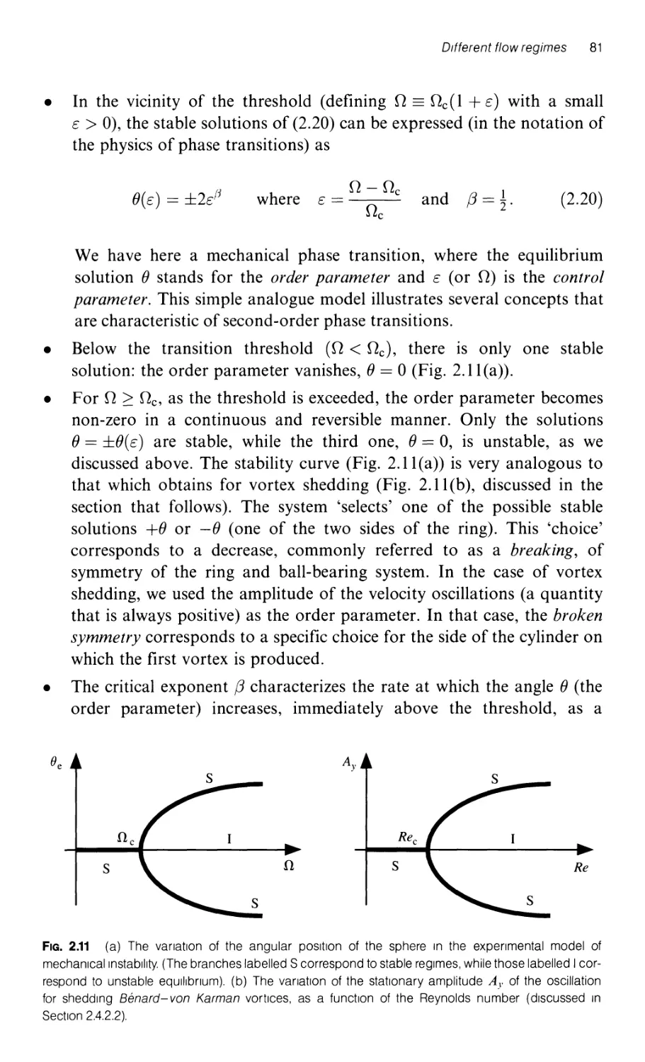
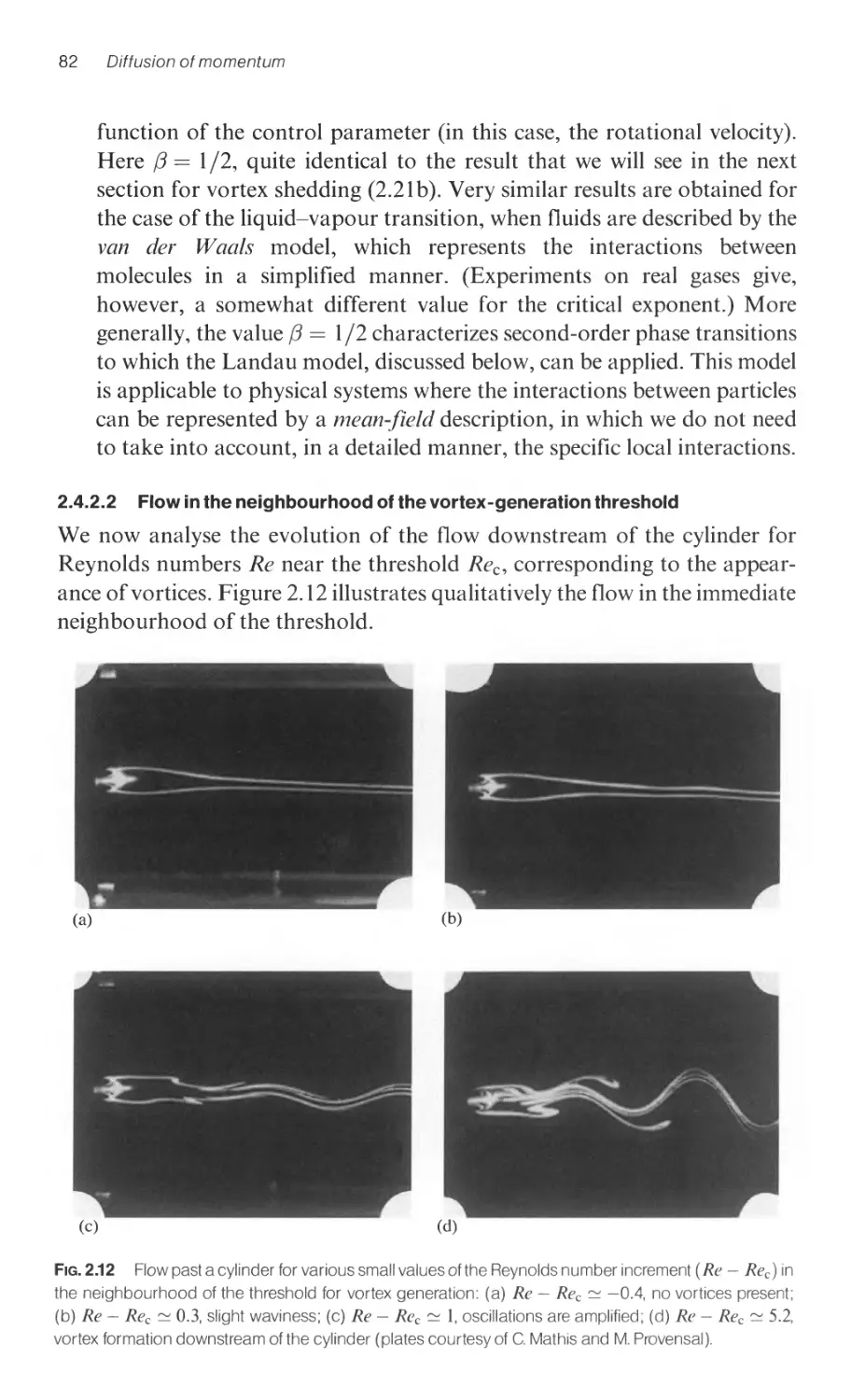
/


Author: Guyon E. Hulin J.-P. Petit L. Mitescu C.D.
Tags: physics physical hydrodynamics
ISBN: 0-19-851746-7
Year: 2001


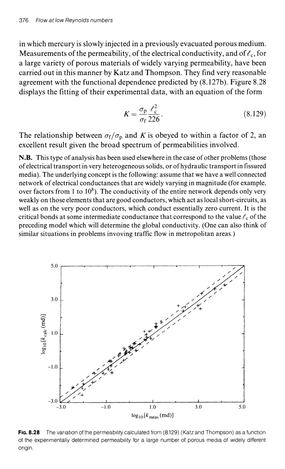
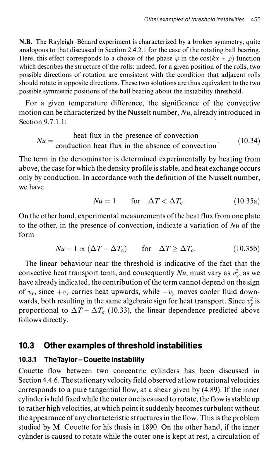
Text
Physical Hydrodynamics
Physical Hydrodynamics
Etienne Guyon
Directeur, Ecole N ormale Superieure, Paris
Pro.{essor, Universite Paris XI
Jean-Pierre Hulin
Directeur de Recherche, CNRS Laboratoire Fluides,
Automatique et Systemes Thermiques, Universite Paris Sud, Orsay
Luc Petit
Professor, Universite de Nice-Sophia Antipolis
and
Catalin D. Mitescu
Seeley W. Mudd Professor of Ph.,vsics, Pomona College,
Claremont, California
UNIVERSITY PRESS
@
OXFORD
UNIVERSITY PRESS
Great Clarendon Street, Oxford OX2 6DP
Oxford University Press is a department of the University of Oxford.
It furthers the lJniversity's objective of excellence in research, scholarship,
and education by publishing worldwide in
Oxford New York
Athens Auckland Bangkok Bogota Buenos Aires Cape Town
Chennai Dares Salaam Delhi Florence Hong Kong Istanbul Karachi
Kolkata Kuala Lumpur Madrid Melbourne Mexico City Mumbai
Nairobi Paris Sao Paulo Singapore Taipei Tokyo Toronto Warsaw
with associated companies in Berlin Ibadan
Oxford is a registered trade mark of Oxford University Press
in the UK and in certain other countries
Published in the United States
by Oxford University Press Inc., New York
Translated from the French edition by Catalin D. Mitescu
French edition tj Intereditions et CNRS Editions, 1991
This English edition (g Oxford University Press, 2001
The moral rights of the author have been asserted
Database right Oxford University Press (maker)
First published in French as Hydrodynamique physique 1991
First published in English 200 I
All rights reserved. No part of this publication may be reproduced,
stored in a retrieval system, or transmitted, in any form or by any means,
without the prior permission in writing of Oxford University Press,
or as expressly permitted by law, or under terms agreed with the appropriate
reprographics rights organization. Enquiries concerning reproduction
outside the scope of the above should be sent to the Rights Department,
Oxford University Press, at the address above
You must not circulate this book in any other binding or cover
and you must impose this same condition on any acquirer
A catalogue record for this book is available from the British Library
Library of Congress Cataloging in Publication Data
(Data available)
ISBN 0 19 851746 7 hbk
ISBN 0 19 851745 9 pbk
Typeset by Newgen Imaging Systems (P) Ltd., Chennai, India
Printed in Great Britain
on acid-free paper by
Biddies Ltd., Guildford & King's Lynn
Foreword
Fluid mechanics is an auberge espagnole' (a Spanish inn) where, as in Andre
Maurois' words, one finds whatever one puts into it: the poetry of Lucretius,
van Karman's precise analysis, or R. P. Feynman's inspired physics. In this
day and age, this branch of mechanics is taught within rather specialized
subdisciplines, well versed in applied mathematics, and strongly coupled to the
industrial world. But the profound physical understanding which character-
ized a man like G. I. Taylor has become too rare in our day, with the result that
most hydrodynamics textbooks have become dry and formal. They do not
succeed in fully training our future engineers and inventors, who will be called
upon to master new materials, and phenomena as yet unknown. Thus, the
current syllabus of most fluid mechanics courses effectively bypasses super-
fluidity, polymers, colloidal suspensions, liquid crystals, interface phenom-
ena, randomly disordered media, and so on-all subject areas in which
remarkable progress has been achieved in the past 30 years.
The present book has been written with the intent of correcting somewhat
this state of affairs. The very arrangement of its subject matter is revolutionary
(pedantic logicians will be certainly disturbed to see the word pressure' first
introduced in a discussion of subtle capillary effects!). But the reader must
recall that this textbook, written as a result of long teaching experience, is not
directed towards students who are totally uninitiated. Digesting this book
does require some effort, but to those who are willing to make the investment,
it opens up remarkable vistas on matter -in the fluid or quasi-fluid state-and
on flows. More importantly, it never gets lost in mathematics before under-
scoring the underlying physical concepts.
It is my sincere hope that the cultural message here present will come across
to students and lecturers alike, and I trust that this work will continue to be
appreciated for a long time to come.
Pierre-Gilles deGennes
Preface
The place of fluid mechanics is somewhat ill-defined. It is often viewed merely
as a branch of applied mathematics. In recent times, this viewpoint has been
further reinforced by significant developments in computational fluid
dynamics (particularly since the number of exact solutions to problems in fluid
mechanics is small indeed). On the other hand, engineering communities have
long mastered technical problems that deal with complex flow situations, even
in many practical instances where a basic understanding was lacking. A
consequence of this state of affairs has been that physicists, and chemists too,
who are in between, have been largely ignorant of this subject, even though
flow problems are regularly encountered in their fields of scientific interest.
Yet another reason for this ignorance has been the strong polarization of
current cutting-edge physics research towards problems on an atomic or
subatomic scale, or towards relativity, even while the pioneering giants in these
very fields (Bohr, Heisenberg, Einstein, and so on) were not themselves
neglectful or ignorant of fluid mechanics. Thus, physicists failed to keep up
with important developments in the subject-such as boundary layer effects,
well-developed turbulence, or the existence of coherent structures in highly
turbulent flows (of which the flow around the red spot of Jupiter provides a
most spectacular example).
Fortunately, this situation has been gradually changing: over the past two
decades, much progress in the discipline can be attributed to physicists who
were not, at the outset, deeply grounded in fluid mechanics, but who did
possess, however, a basic fundamental knowledge of various unusual fluids-
for example, superfluid helium, liquid crystals, and polymers; these had
themselves contributed to the development of some of the most modern
measurement techniques, often using applications of coherent-light optics,
and they had used, in their research experience, fundamental tools, such as
those refined in nearly a century of explosive growth in statistical physics.
These scientists had also brought to bear on the treatment of certain prob-
lems-such as those of hydrodynamic instabilities-generalized theoretical
tools originally developed in the study of phase transitions. (We discuss,
towards the end of this book, the particularly striking example of the study of
the mechanisms for transition to chaotic regimes.) As a matter of fact, dif-
ferences in outlook are fading-much more so than the disagreements-and
Preface VII
few can deny the richness that different perspectives and contacts between the
various communities can providc when applied to the same problem.
This book was written primarily from the point of view of an experimental
physicist. In fact, the name hydrodynamics' is a bit too confining, because
many of the concepts we present here apply just as well to gases, so long as the
flows are slow enough. But, in using this term, we have intentionally excluded
those problems specific to high-velocity gases, where compressibility effects
must be taken into account. In that case, fluid dynamics must be coupled to
thermodynamics, by means of the equation of state. Specifically, our physi-
cist's approach attempts to tie in, as often as possiblc, the macroscopic
behaviour of fluids to their local properties. It oftentimes relies much more
strongly on order-of-magnitude arguments than on formal derivation. Thus,
we frequently introduce and express dimensionless quantities, such as the
Reynolds number, as a ratio (Greek, aVaA01'U ) of the magnitudes of similar
quantities--characteristic times, energies, and so on-rather than as an alge-
braic manipulation bascd solely on arguments from dimensional analysis. In
so doing, we give up mechanical, 'cookbook' prescriptions, to gain in exchange
a deeper physical insight, particularly necessary in this field so firmly grounded
in experimental observation.
The organization of this textbook is as follows.
We begin, in Chaptcr 1, with a broad overview of the microscopic properties
of fluids, outlining how, when a system of particles is slightly perturbed from
its cquilibrium state, this perspective leads directly to transport properties-
specifically, mass and thermal diffusion. We also describe the use of modern,
non-invasive, optical-spectroscopy techniques in the characterization of the
corresponding parameters of the fluid.
Chapter 2 then prescnts an introduction to the several regimes of flow. We
emphasize the similarity between the viscosity and diffusion coefficients,
introducing the conccpt of the Reynolds number., the fundamental criterion
for the description of the nature of fluid flows. Finally, we describe the
shedding of vortices behind a cylindrical obstacle, analysing the threshold for
their appearance in the spirit of the "Landau' mcchanism of phase transitions. t
Chapters 3 and 4 describe the characterisation of flow-velocity fields
(kincmatics) and of the constraints (dynamics) associated with them; it is the
relationship bctwecn thesc two sets of parameters that forms the basis of fluid
dynamics.
A large number of the concepts that we introduce are equally applicable to
other problems in the mechanics of continuous media: it suffices there to
replace the concept of the flow-velocity gradient, the most significant
t We have chosen the terminology, Benard von Karlnan vortex street, instead of the more
commonly used ron Karman vortex street, in recognition of the historical precedence (1910) of
the papers of the French physicist Henri Benard on the subject.
viii Preface
parameter for fluid flow, with that of the gradient of the distance between two
adjacent points. Our discussion of kinematics puts specific emphasis on the
visualization of flow fields and., more generally, on their experimental char-
acterization. The chapter on dynamics leads to the derivation of the Navier--
Stokes equation as the master equation of motion for fluids.
We then proceed, in Chapter 5, to a discussion of the conservation laws for
fluids: these are evidently nothing more than integral representations of the
local relations derived in earlier chapters. They are particularly useful in the
case of ideal (non-viscous) fluids, of which a prime, real example is liquid
helium. But they have another important application in the determination of
velocity profiles in the flow of normal fluids, in regions far enough removed
from boundary walls, where viscosity effects become negligible.
The laws of conservation of mass, momentum, and energy" lead, for many
flow problems, to much simpler solutions" in those cases where we do not need
a detailed representation of the velocity fields. Such solutions rely, however, on
stringent assumptions about the nature of the flow, assumptions seen as jus-
tifiable upon the introd uction, in Chapter 9, of the concept of boundary layers.
Chapter 6 becomes then an obvious extension, in which we discuss the
dynamics of ideal fluids for which the velocity field is usually everywhere curl-
free. This chapter is written in close analogy to the treatment of electrostatic
problems, for which the electric field, the gradient of a potential function also
has zero curl.
In Chapter 7, we develop the concept of vorticity to a much greater depth
than it is customary in fluid mechanics textbooks. Vorticity is present in a large
variety of flows, and its evolution leads to a preliminary understanding of the
mechanisms of turbulence. The very equation of motion of a vortex reflects
the law of conservation of angular momentum in traditional mechanics. We
acknowledge that our familiarity with this approach owes much to earlier
investigations, both of the remarkable properties of quantized vortices in
superfluid helium (discussed in a separate Appendix at the end of this text-
book).. and to those of singularities in the physics of condensed matter.
Chapter 8 brings us back to a discussion of very-Iow-Reynolds-number
flows (also known as creeping flows) in which viscosity effects are paramount.
In this instance, although, the governing equation of motion, the Stokes'
equation, is linear, exact solutions are here also few and difficult to obtain-
even in the seemingly simple case of a sphere moving at uniform velocity in a
fluid. The use of asymptotic solutions in this and most problems is the general
rule. We conclude this chapter with an extensive discussion of very applied
topics" such as the flow of suspensions and that through porous media.
The discussion of the laminar boundary layer carried out in Chapter 9 allows
us to treat a broad class of high-velocity flows around solid obstacles. It has
wide practical application. In retrospect, it stresses the significance of the
discussion of ideal fluids in Chapter 6. Those concepts provide a good
Preface
.
IX
approximate treatment of the problems of flow fields outside boundary-layer
.
regIons.
Chapters 6-9 provide the basis offluid mechanics. We have structured them
in such a way that they can be studied independently and in arbitrary order.
'inally, Chapter 10, dealing with hydrodynamic instabilities, can be con-
sidered as a set of applications of the various concepts discussed in all nine
previous chapters. In the case of convective instabilities, of the Rayleigh
Benard type, it finds further justification because of the vast recent develop-
ment of the field, and because the mathematical and physical approaches used
here have much broader applicability thanjust to problems in fluid mechanics.
We also believe that these developments constitute an important first step in
the understanding of the yet poorly mastered problems of turbulence at large
Reynolds numbers of which the Kelvin-Helmholtz instability is one exam-
ple. We include some discussion of recent experiments on fully developed
turbulence.. and on vorticity in turbulent flows.
If we havc emphasized our background as physicists" it is not to underrate
the import and influence of the understanding that we have acquired in our
contacts with the community of those specializing in the field of mechanics
(P. Germain, R. Moreau, H. K. Moffatt, and S. A. Orszag), first met at a
summer school in Les Houches in 1973. How also could we fail to acknowledge
our debt to the British school of fluid mechanics (where the great tradition of
Professor G. I. Taylor continued to flourish around G. K. Batchelor), and
of thc American chemical engineering school centered around A. Acrivos?
P. (1. deGennes' courses at the College de France (unfortunately unpublished),
the two striking chapters on "dry water" and "wet water' in the reynman
Lectures in Phrsics., as well as L. Landau"s textbook on fluid mechanics have
also contributed greatly to our apprenticeship.
Even more perhaps, it is the ideas and teachings of our colleagues and
friends, P. Berge, J. Brady, B. Castaing, J. Hinch, G. Homsy, and D. Lhuillier
that we have "shamelessly' used and developed, which have led to the writing of
this textbook. We thank also R. Blanc, A. M. Cazabat, Y. Couder, the late
M. Hulin, J. F. Joanny, D. Lhuillier" and B. Perrin for their friendly yet critical
readings at different stages of the drafts of this manuscript. We are also
grateful to Emmanuel CJuyon for his assistance in the Ioaeronautical' sections of
Chapter 9'1 as well as in the preparation of many of the figures in the original
Frcnch edition. J:-'inally we should not forget the students, both undergraduate
and graduatc, with whom we have Iobroken in' various parts of this book" or the
many "informal' discussions with all our research colleagues.
In its original edition, this book was first written by three of us (E. G., J. P. H.,
and L. P.), for a French-speaking physics audience where we felt that there
was a considerable lack of basic culture in fluid mechanics. It appears to havc
had an impact on the evolution of the teaching of this subject in French
universities.. as well as in "prep' schools. By the addition of the fourth author, a
x Preface
long-time colleague and professor at an American university, yet very familiar
with French research and teaching, we have intended this English edition to be
much more than an English-language version of the original text. We have
striven to adapt the style and form to one which might prove more comfortable
to North American audiences, while keeping the spirit of the French school -
as exemplified by people such as P. G. deGennes.
The text has been extended in particular to increase the content in applica-
tions, and bring it a step closer to an engineering approach. For the benefit of
North American readers, vector-derivative notation and the definition, and
orientation, of curvilinear co-ordinates (relative to corresponding Cartesian
axes) have been reformulated to correspond to the usage that is virtually uni-
versal throughout the USA and Canada, and the notations in two- and three-
dimensional representations have been made internally fully self-consistent.
Individual chapters in our book contain a number of example problems,
worked out in some detail, and which could often be extended into further
exercises. But we have elected not to include at the end of each chapter the
selection of often repetitive problems frequently found in US textbooks. We
are, however, keeping open the option of a companion problem text at some
future time.
Before closing, we must express our gratitude to many people who have been
very instrumental in helping us to complete this new edition. First of all.. we are
most thankful to Mrs. Connie Wilson, senior secretary in the Pomona College
Physics Department, who gave up much free time to type most of the original
draft of the English manuscript. We are also grateful to Nicole Mitescu, and to
Natalie Mitescu, (C. D. M.'s wife and daughter, respectively) who completed
the remainder of tha t draft. Pomona College '94 graduates Sarah ' Avon"
Russell and Amy Schmieder, while taking an independent study course in fluid
mechanics in their senior year, worked through an early version of the
manuscript their input has been most valuable. And, finally, C. D. M. would
like to express his thanks to the ESPCI, where he was able to carry out part of
the work on the manuscript during scientific research visits.
This book was written with the passion that accompanies the later discovery
of a fascinating subject, which none of us learned in a classroom environment
but, rather, out of practical experience in research and teaching at the under-
graduate and postgraduate levels. hence the significant role we assign to
images such as those found in An Album oj'Fluid MOlion, and even to problems
that have not yet been fully solved. It is our hope that both students who first
become acquainted with it as a classroom text't as well as research scientists,
and even the curious, who will have come to a knowledge of fluid mechanics
later as we did ourselves will come to share some of our enthusiasm!
E. Guyon, J. P. Hulin, L. Petit, and C. D. Mitescu
Contents
1 The physics of fluids
1.1 The liquid state
1.1,1 The different states of matter: model systems and real media
1.1.1.1 The visual representation of different states of matter
by means of an air table
1.1.1.2 Numerical simulations in terms of a hard -disc model
1.1.1.3 Three-dimensional models
1.1.2 The solid -liquid transition: a sometimes nebulous process
1.1.2.1 Modelling plastic flow in two dimensions
1.1.2.2 The effect of the rate of change of the stresses on the
deformation of a medium
1.2 Macroscopic transport coefficients
1.2.1 Thermal conductivity
1.2.1.1 A definition of thermal conductivity: the equation for
heat under stationary conditions
1.2.1.2 Application of the thermal conductivity equation to a
cylindrical geometry
1.2.1.3 Thermal exchanges under non-stationary
conditions: the Fourier equation
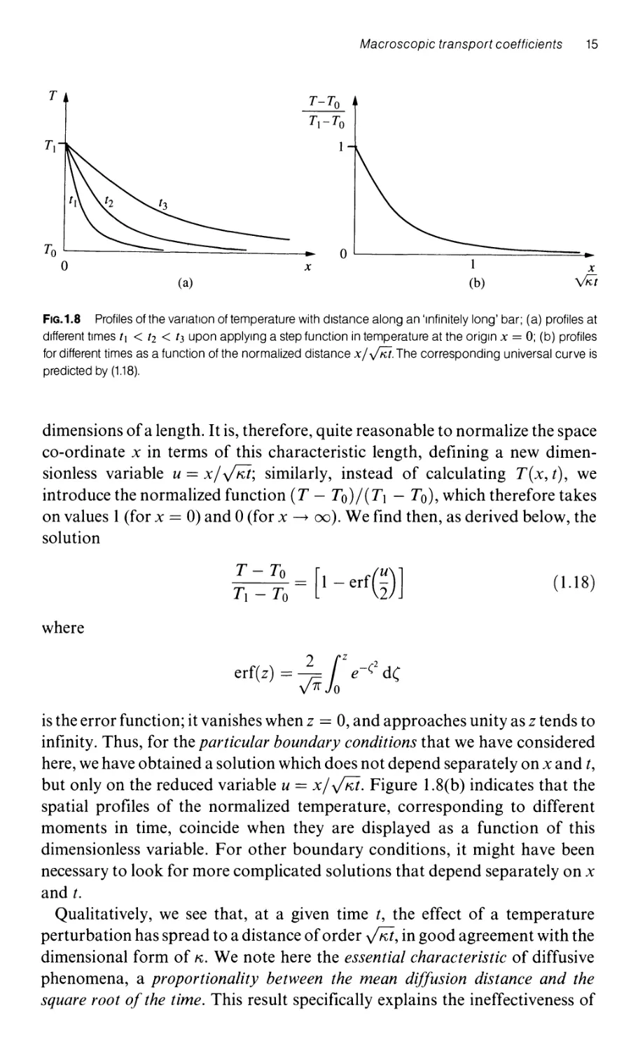
1.2.1.4 Application to the one-dimensional propagation of
temperature variations
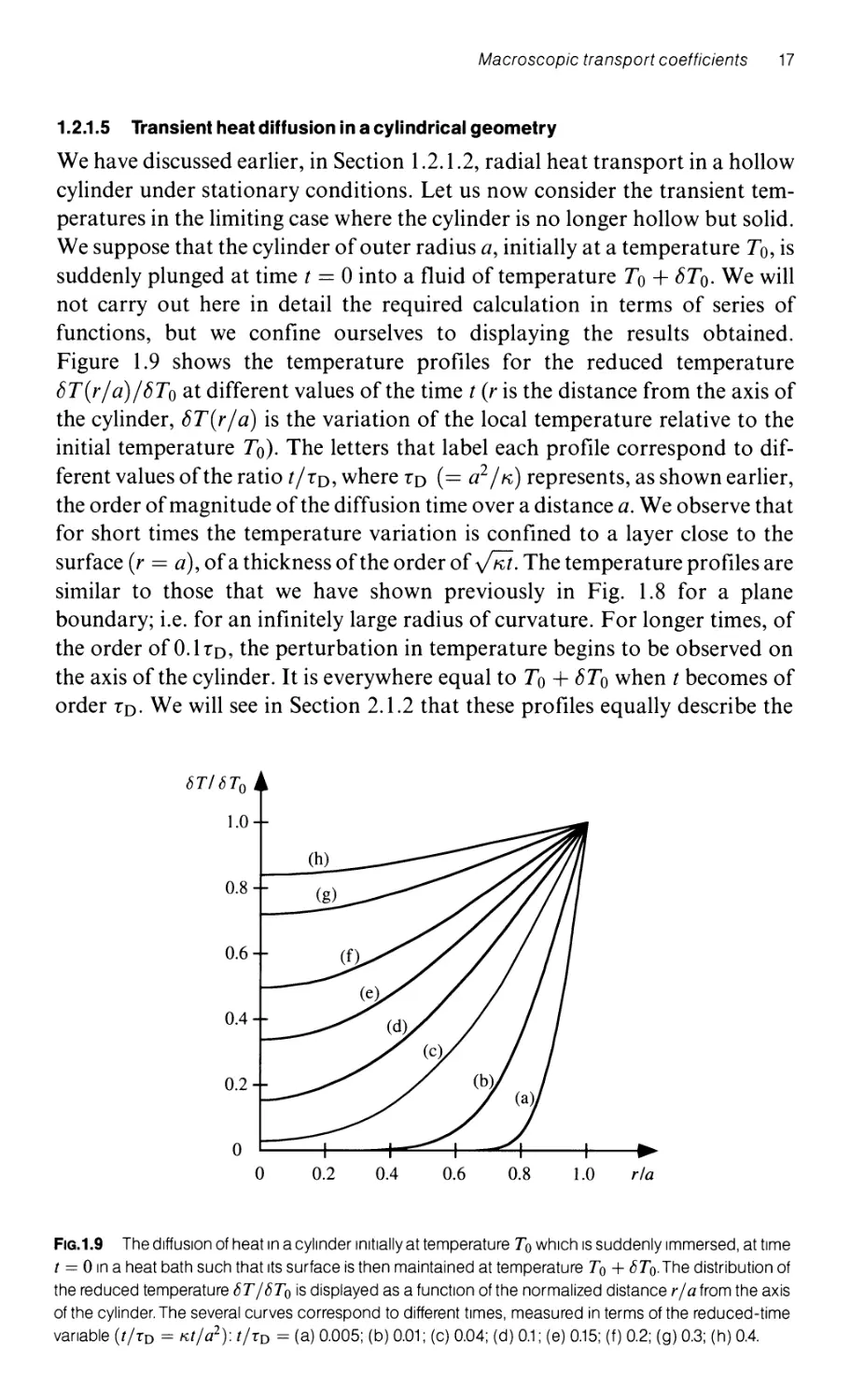
1.2.1.5 Transient heat diffusion in a cylindrical geometry
1.2.1.6 Propagation: diffusion versus wave motion
1.2.2 Mass diffusion
1.2.2.1 Conservation of mass for a diffusing substance
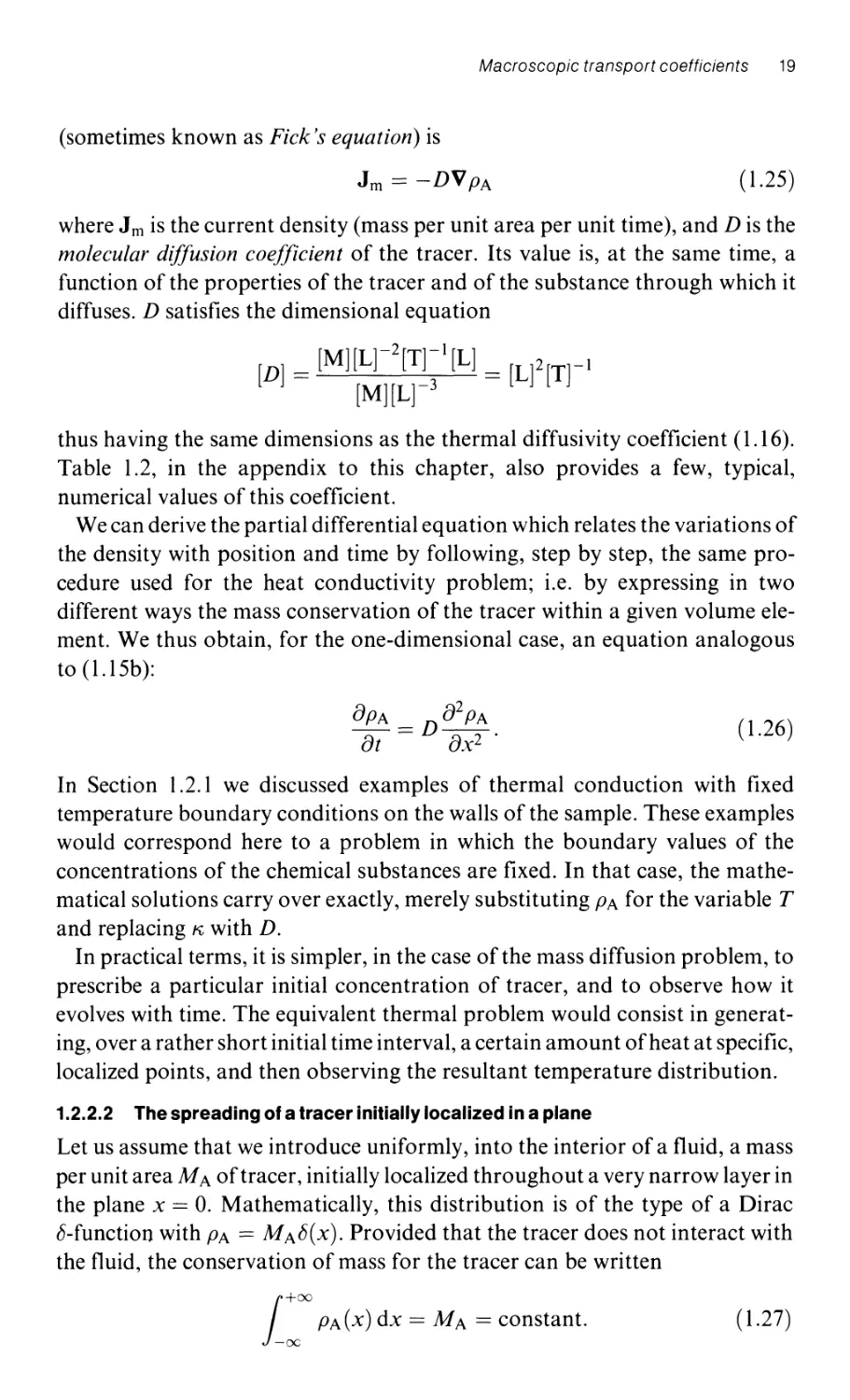
1.2.2.2 The spreading of a tracer initially localized in a plane
1.3 Microscopic models for transport coefficients
1.3.1 A different approach to mass diffusion: the random walk
1.3.2 Transport coefficients for an ideal gas
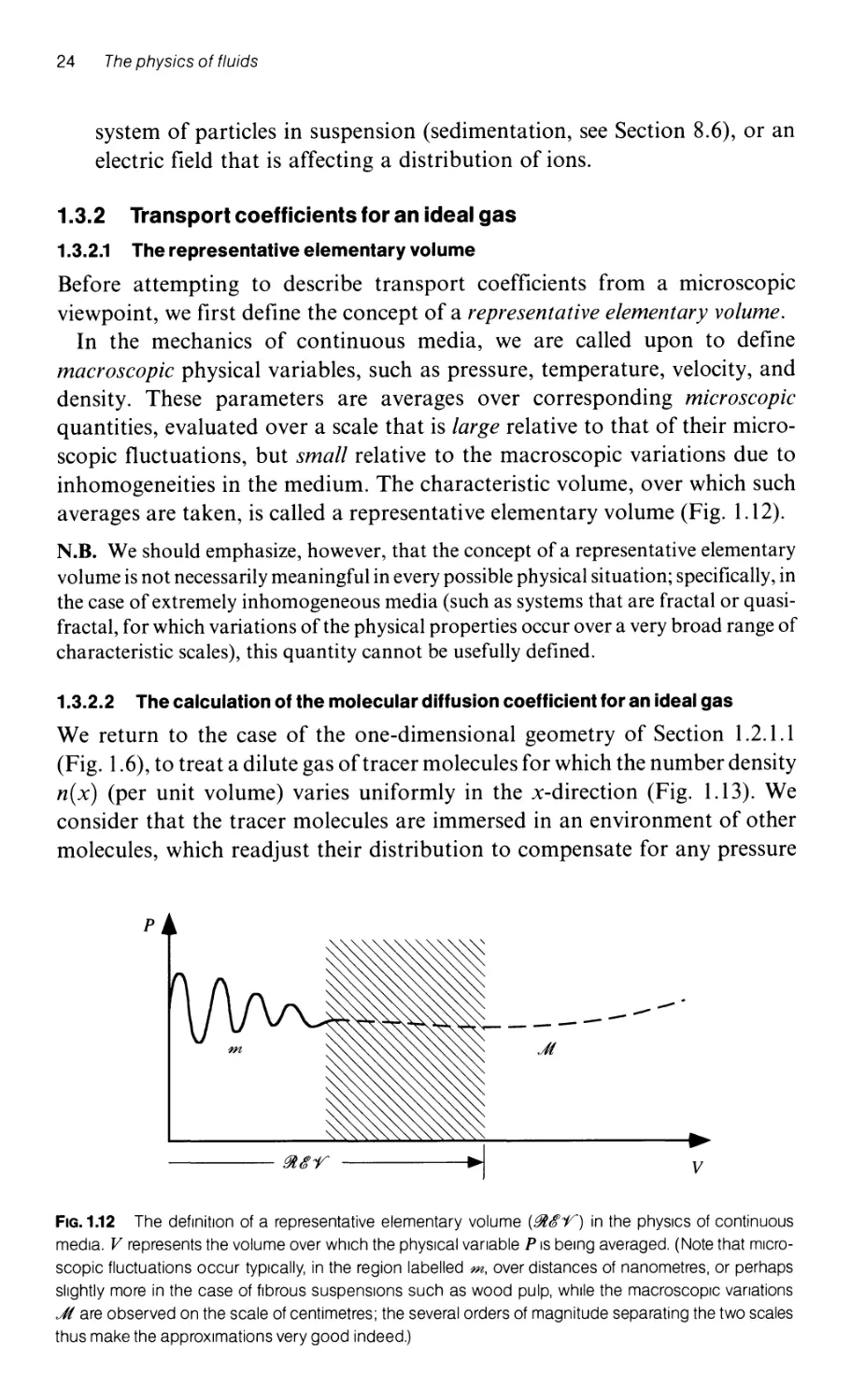
1.3.2.1 The representative elementary volume
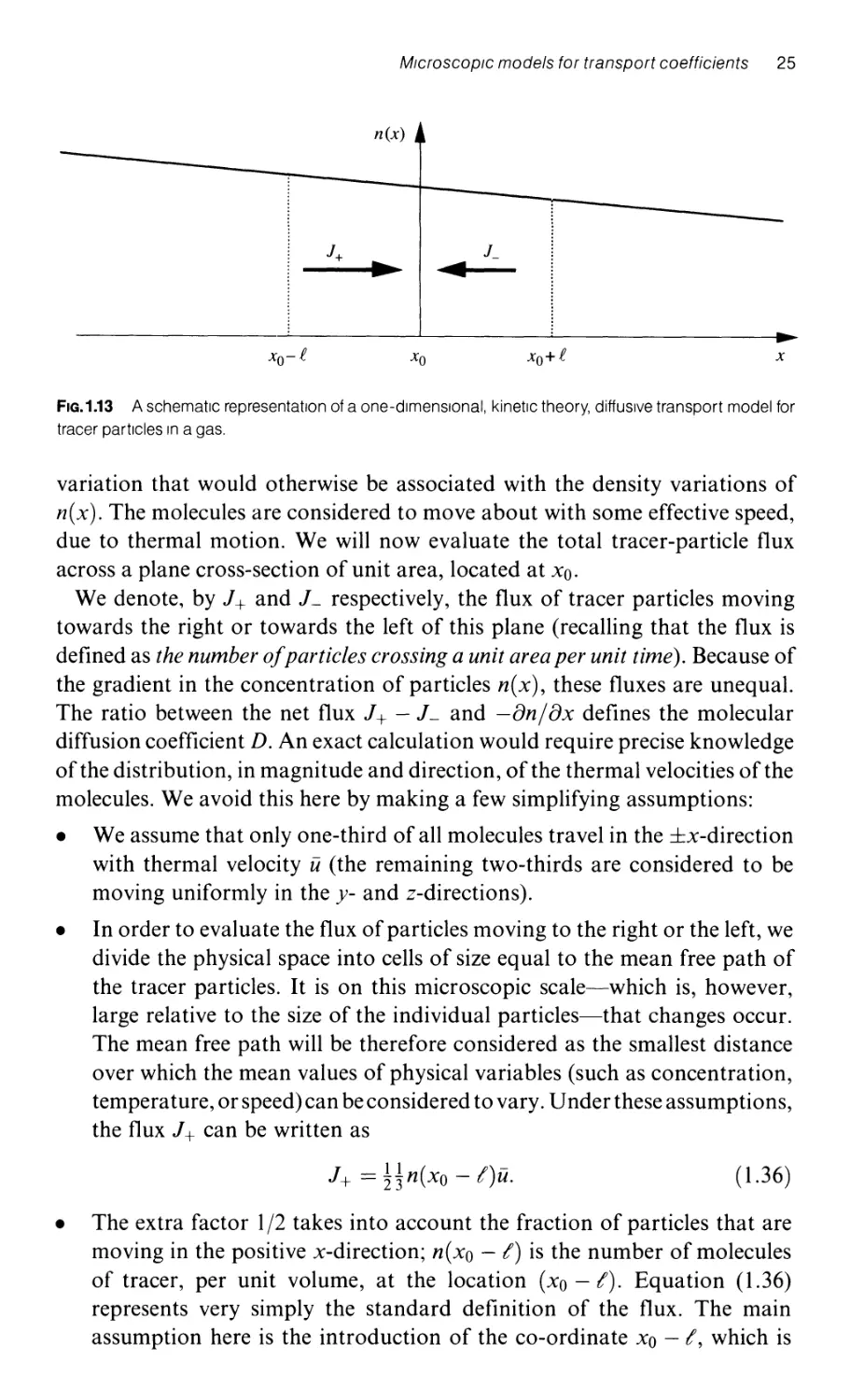
1.3.2.2 The calculation of the moleculardiffusion
coefficient for an ideal gas
1.3.2.3 The calculation of thermal diffusivity for an ideal gas
1.3.2.4 The applicability of the ideal gas model
1.3.3 Diffusive transport phenomena in liquids
1.3.3.1 The molecular diffusion coefficient for liquids
1
2
2
4
5
7
7
8
8
9
9
11
12
14
17
18
18
18
19
21
21
24
24
24
27
28
28
29
xii Contents
1.3.3.2 The thermal conductivity of liquids 30
1.3.3.3 A comparison of the numerical values of diffusive
transport coefficients in different liquids and gases 31
1.4 Surface and surface tension effects 31
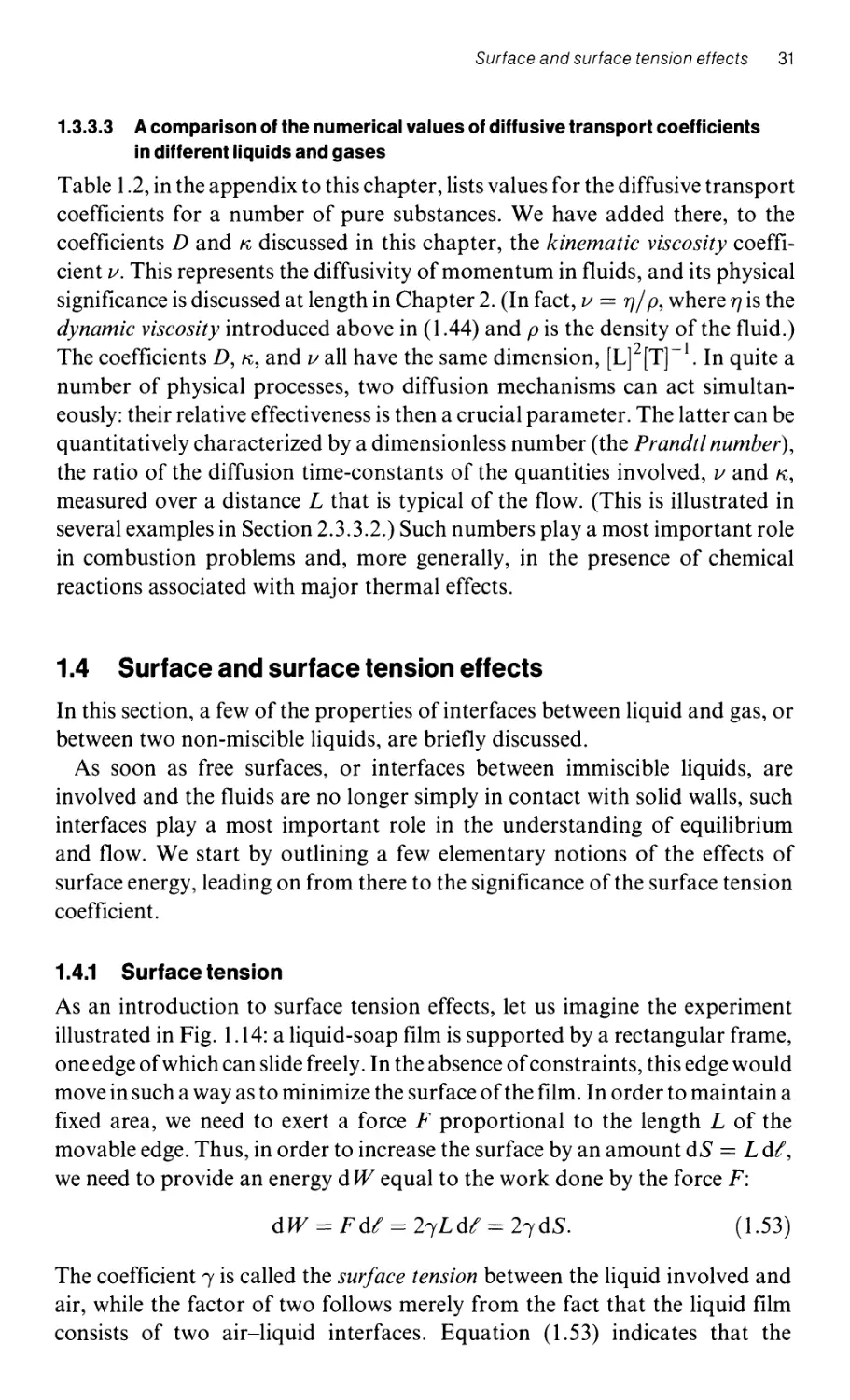
1.4.1 Surface tension 31
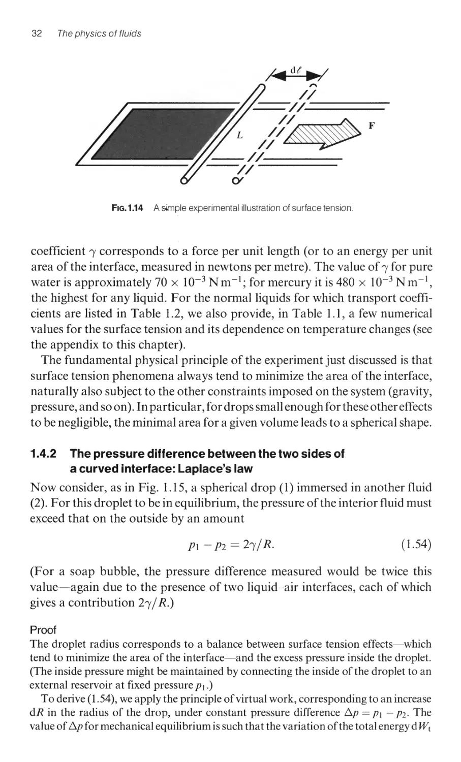
1.4.2 The pressure difference between the two sides of a
curved interface: Laplace's law 32
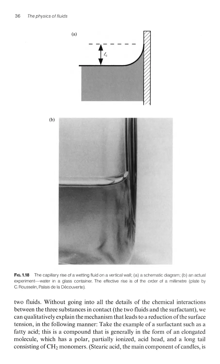
1.4.3 Variations in the surface tension due to a surfactant 35
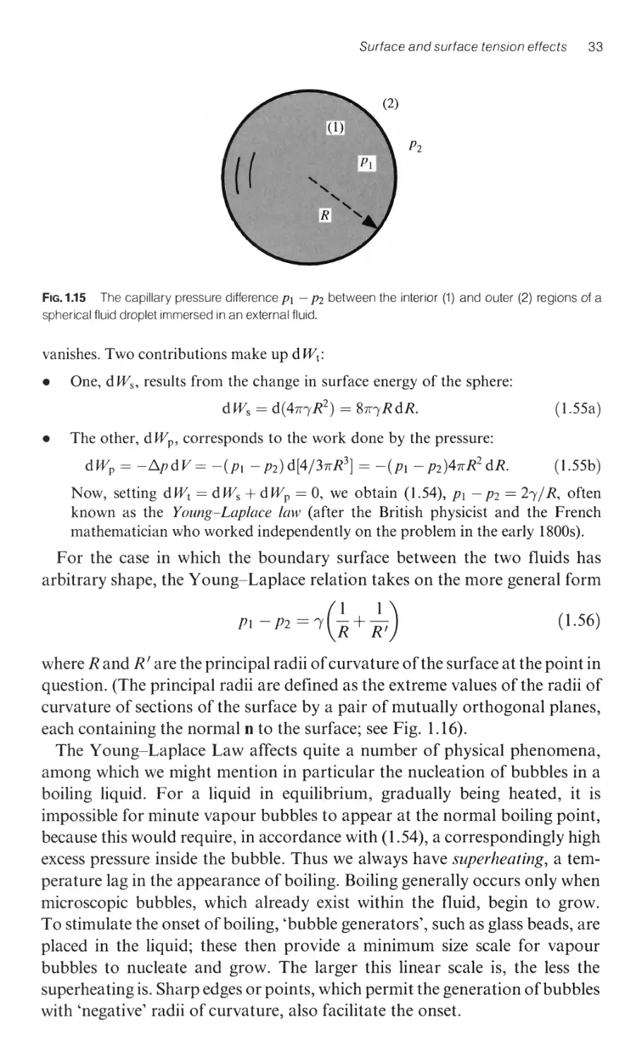
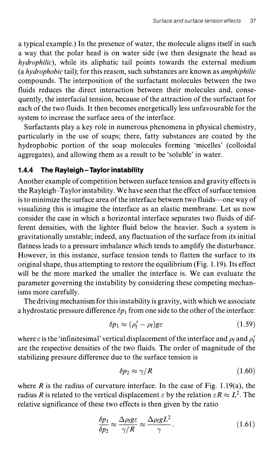
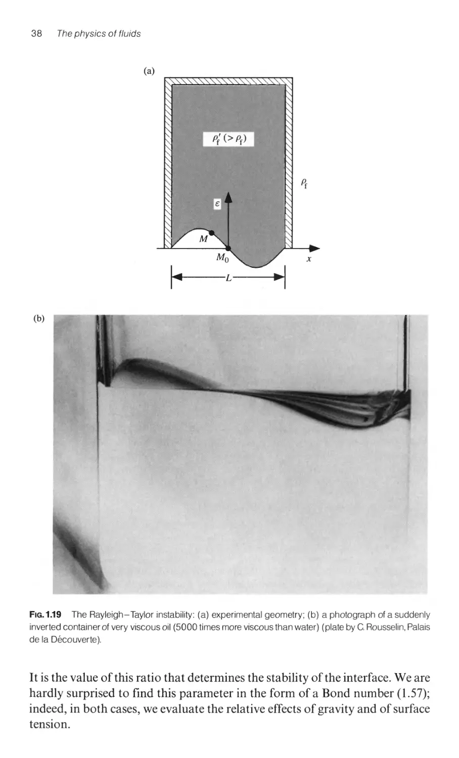
1.4.4 The Rayleigh-Taylor instability 37
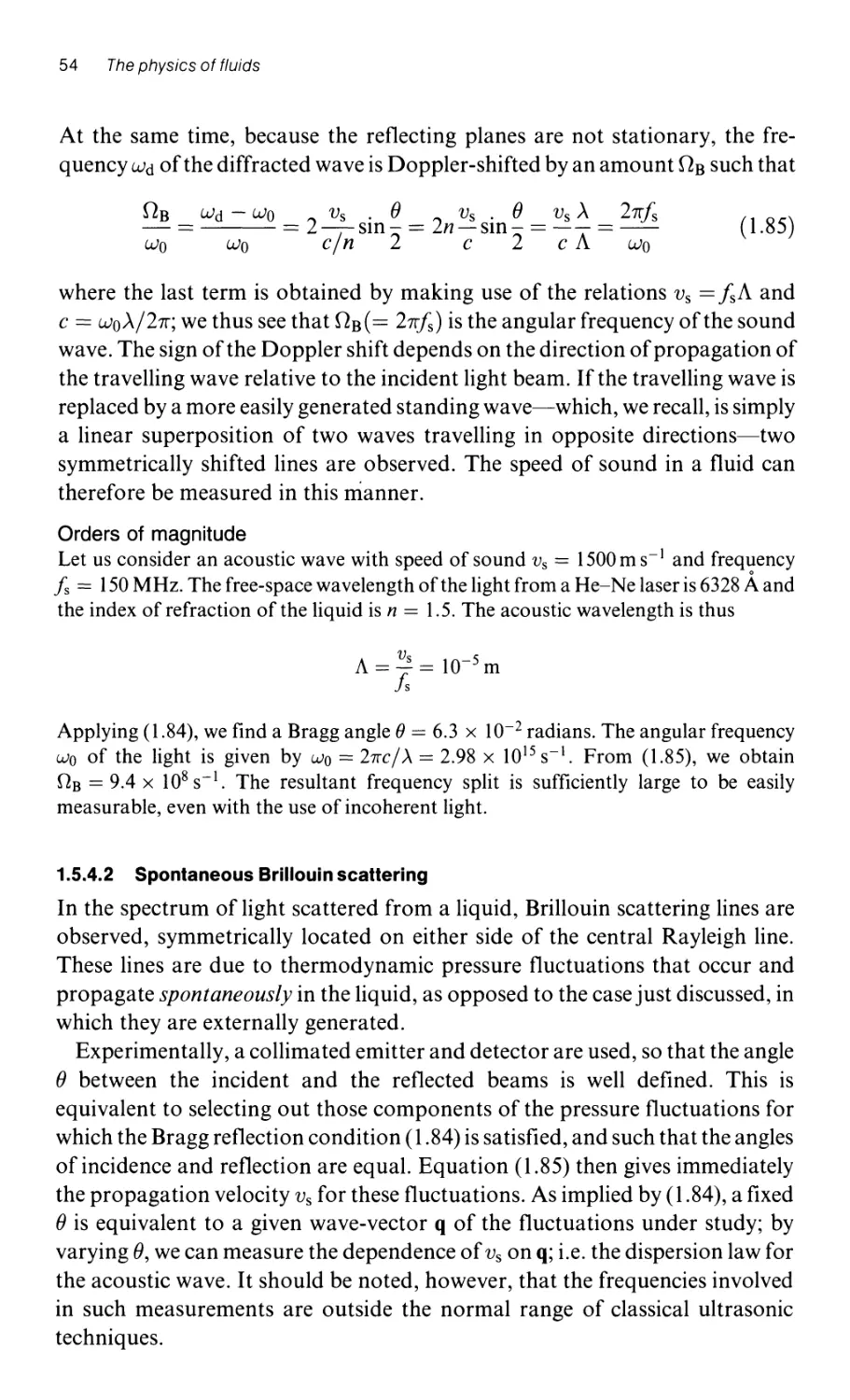
1.5 The spectroscopy of liquids 40
1.5.1 Some common techniques for probing
the microscopic structure of liquids 40
1.5.1.1 Macroscopic properties and microscopic probes 40
1.5.1.2 Characteristic orders of magnitude for
standard probe techniques 41
1.5.2 The form factor and elastic X-ray diffraction: an example of
the use of scattering on an atomic scale 42
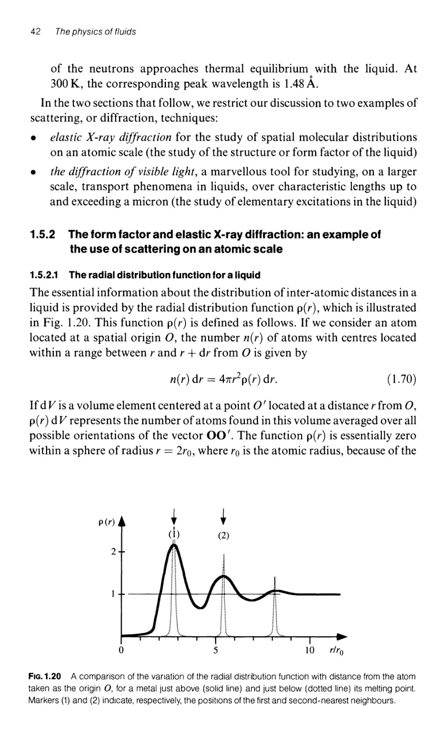
1.5.2.1 The radial distribution function for a liquid 42
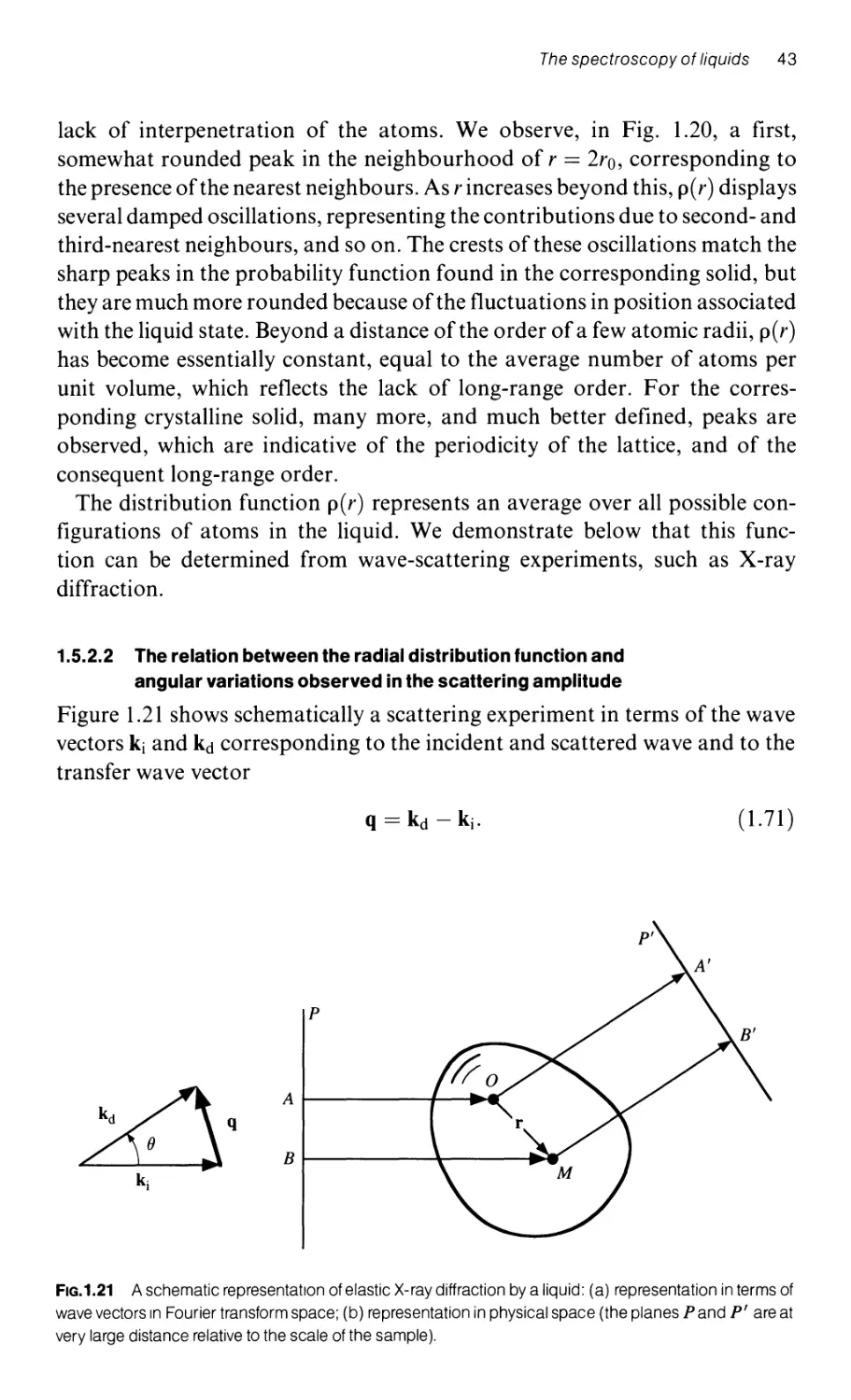
1.5.2.2 The relation between the radial distribution function and
angular variations observed in the scattering amplitude 43
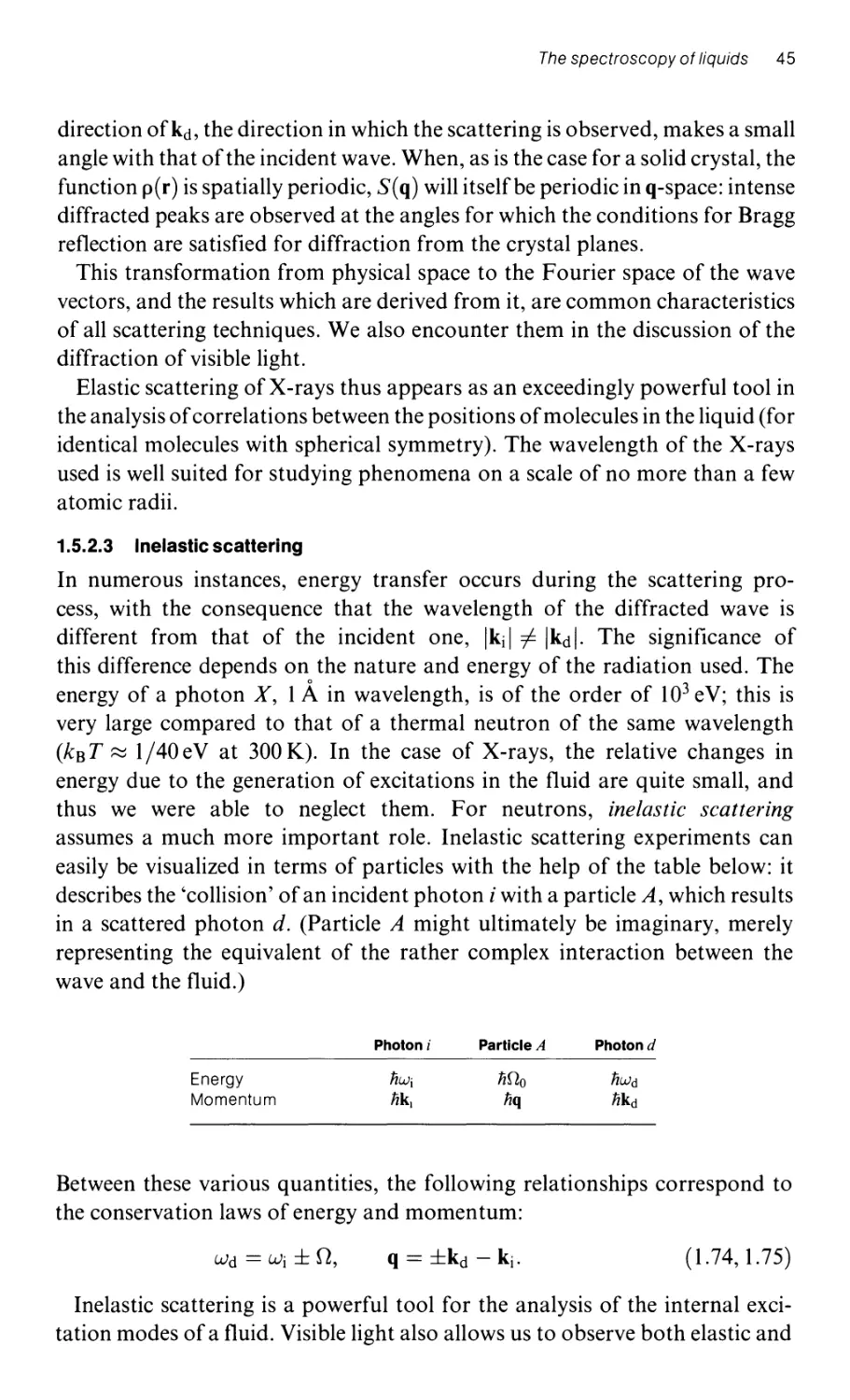
1.5.2.3 Inelastic scattering 45
1.5.3 Elastic and quasi-elastic scattering of light: a tool for the
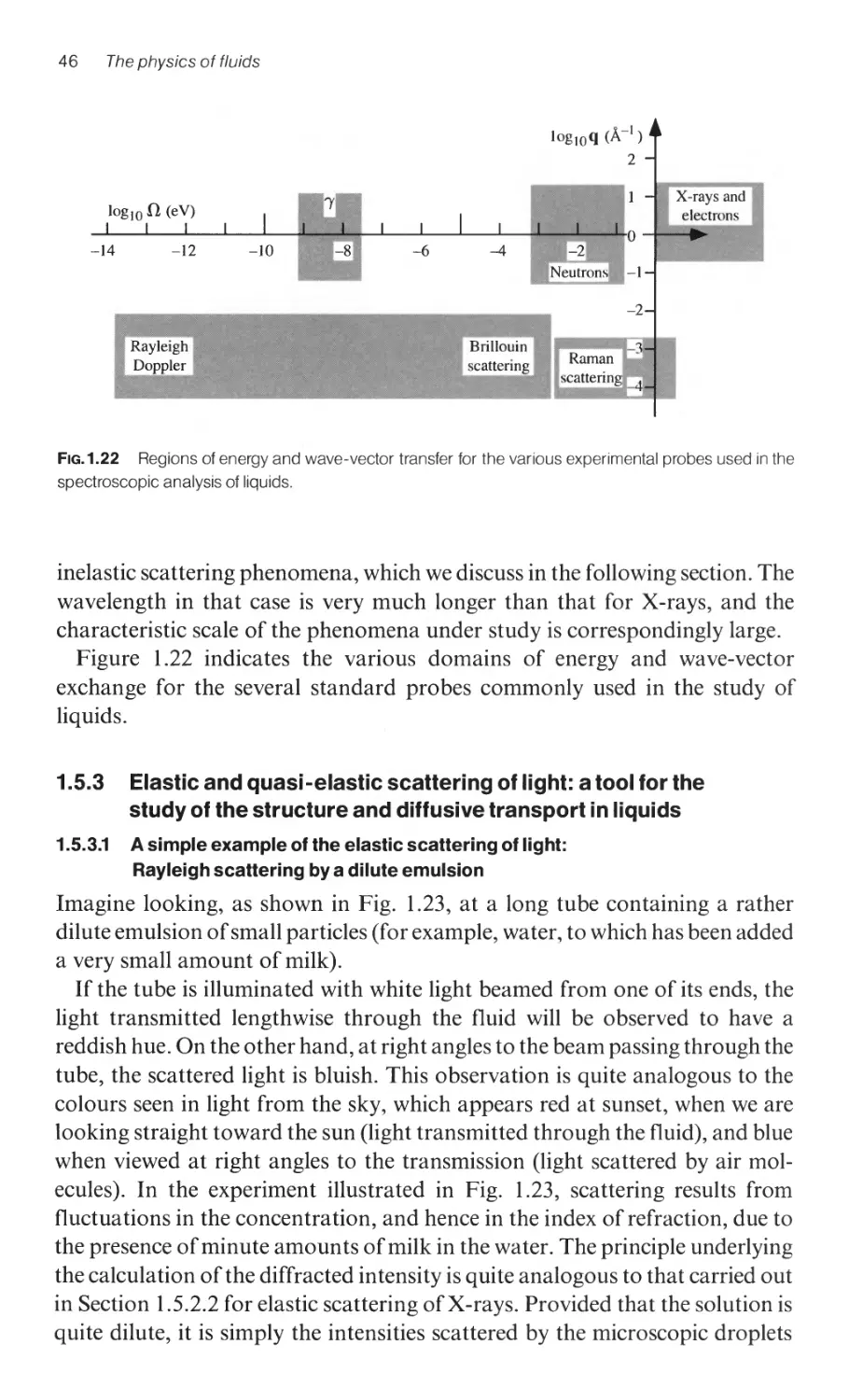
study of the structure and diffusive transport in liquids 46
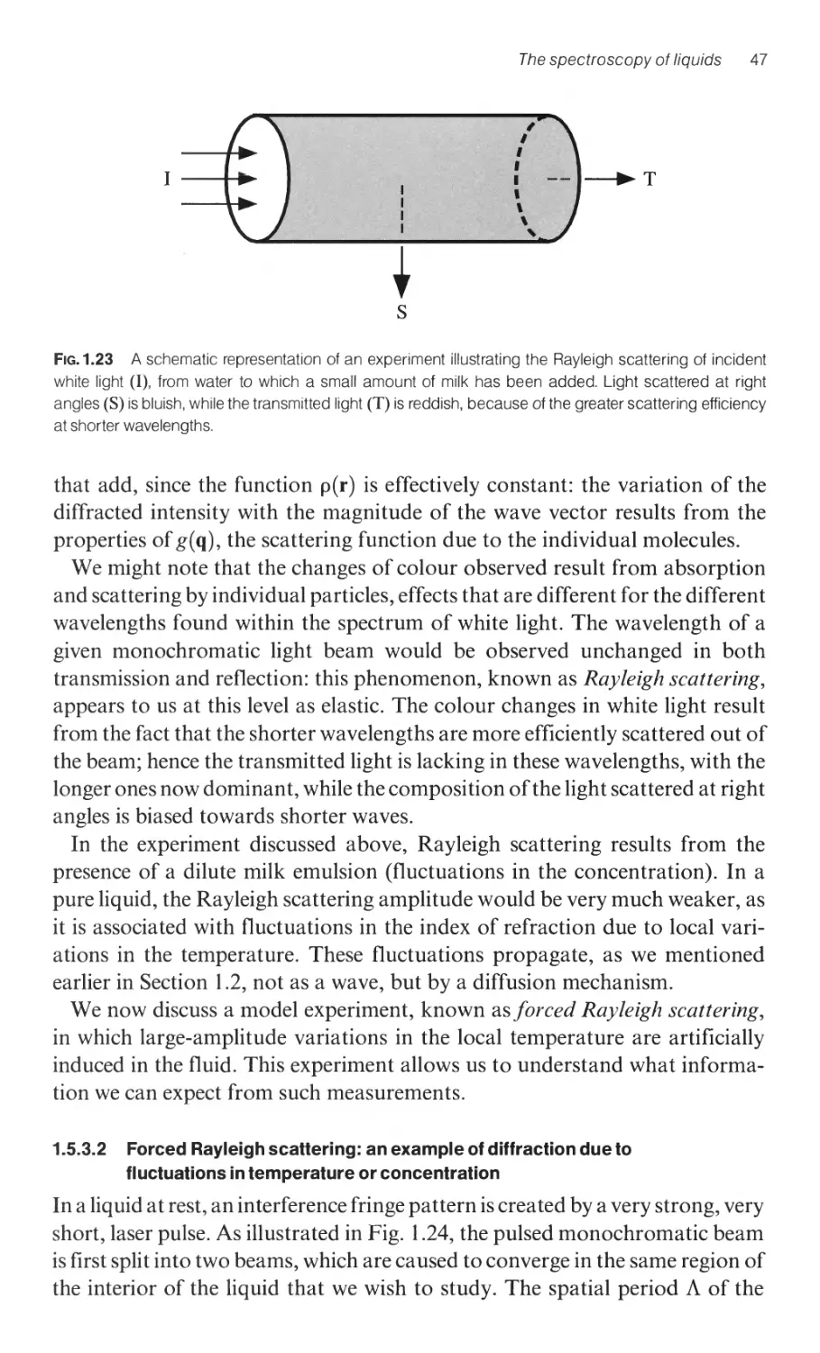
1.5.3.1 A simple example of the elastic scattering of light:
Rayleigh scattering by a dilute emulsion 46
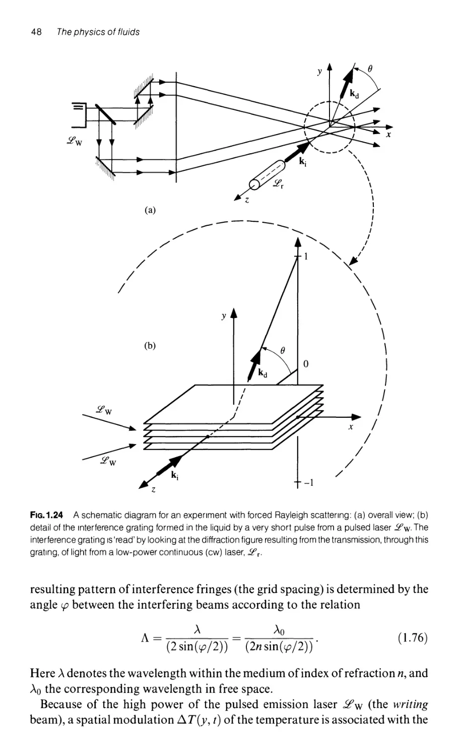
1.5.3.2 Forced Rayleigh scattering: an example of diffraction
due to fluctuations in temperature or concentration 47
1.5.3.3 Spontaneous Rayleigh scattering of visible light 51
1.5.4 Inelastic scattering of light in liquids 52
1.5.4.1 An illustration of inelastic Doppler scattering:
forced Brillouin scattering 52
1.5.4.2 Spontaneous Brillouin scattering 54
Appendix: typical orders of magnitude for a number of physical parameters
characteristic of the interfacial properties of ordinary liquids 55
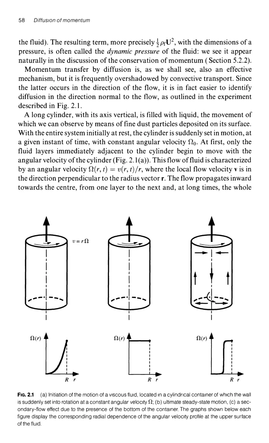
2 The diffusion of momentum under various flow conditions 57
2.1. Diffusive and convective momentum transport in flowing fluids 57
2.1.1 Diffusion and convection of momentum:
two illustrative experiments 57
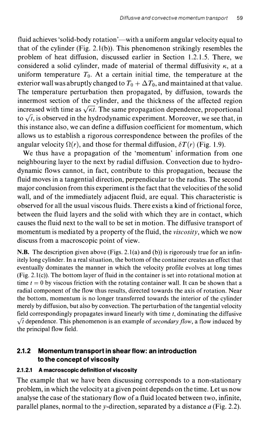
2.1.2 Momentum transport in shear flow: an introduction to
the concept of viscosity 59
2.1.2.1 A macroscopic definition of viscosity 59
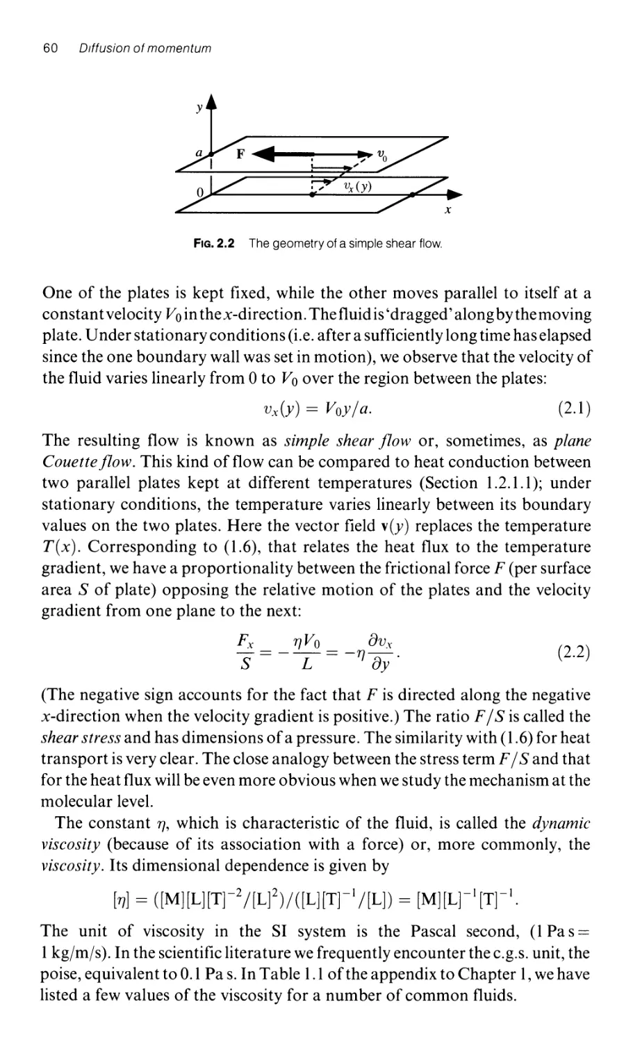
2.1.2.2 The diffusion equation for momentum 61
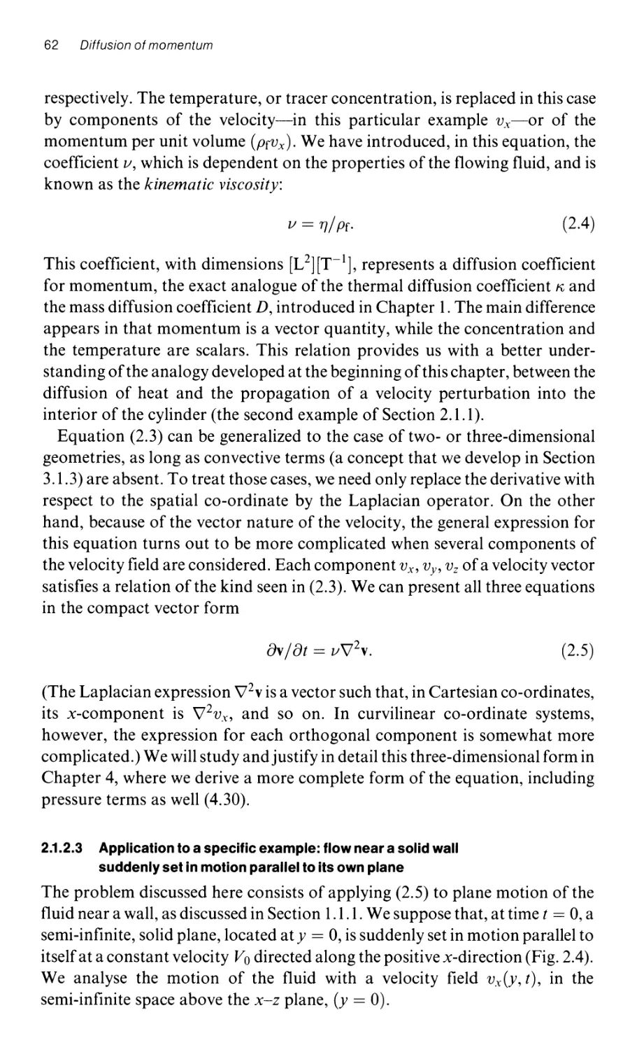
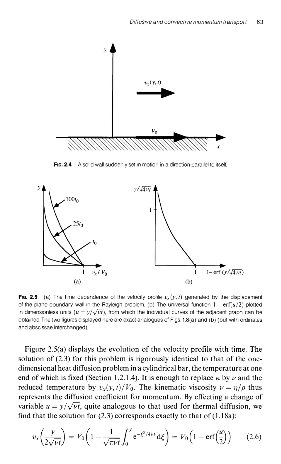
2.1.2.3 Application to a specific example: flow near a solid wall
suddenly set in motion parallel to its own plane 62
Contents xiii
2.2. Microscopic models of viscosity 64
2.2.1 The viscosity of gases 64
2.2.2 The viscosity of liquids 67
2.2.3 Numerical simulation of the particle trajectories in a flowing fluid 69
2.3 A companson of diffusion and convection mechanisms 71
2.3.1 The Reynolds number 71
2.3.2 Convective and diffusive mass and heat transport 73
2.3.2.1 Mass transport 73
2.3.2.2 Heat transport 74
2.4 The description of different flow regimes 76
2.4.1 Different flow regimes in the wake of a cylinder 77
2.4.2 Transitions in the shedding of vortices behind a cylinder:
the Landau model 79
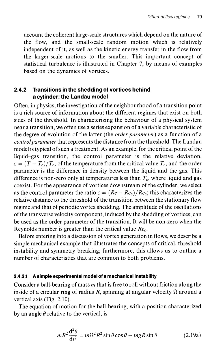
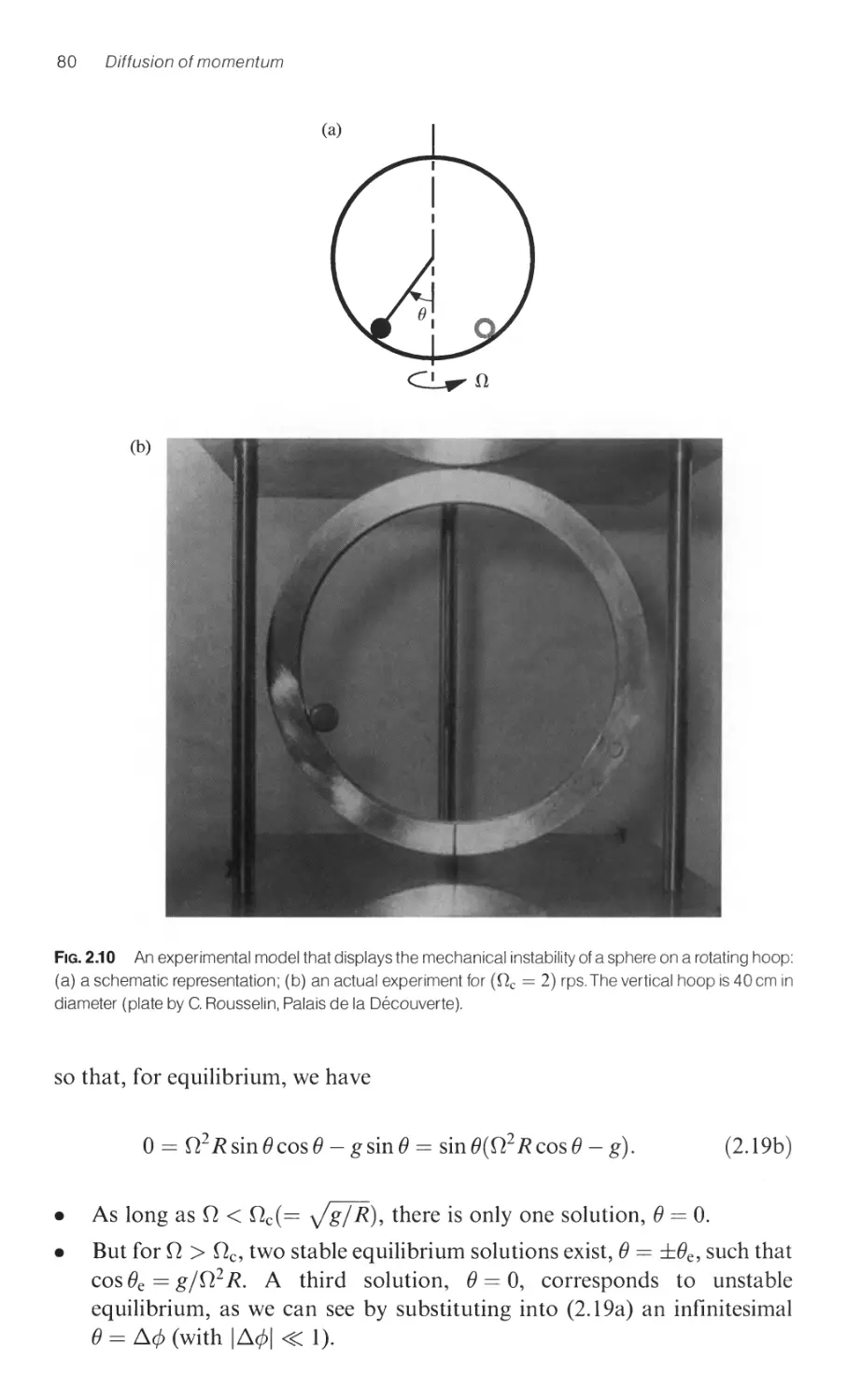
2.4.2.1 A simple experimental model of a mechanical instability 79
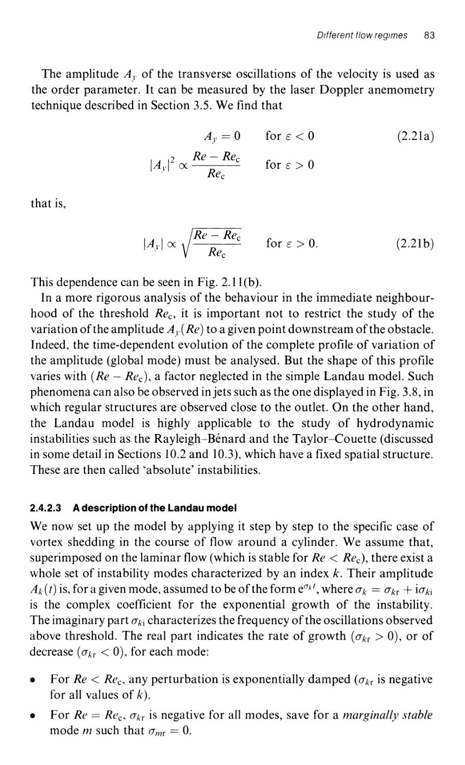
2.4.2.2 Flow in the neighbourhood of the vortex-generation threshold 82
2.4.2.3 A description of the Landau model 83
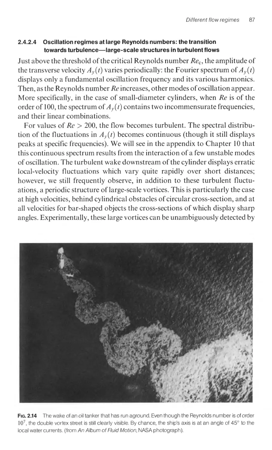
2.4.2.4 Oscillation regimes at large Reynolds numbers:
the transition towards turbulence-large-scale
structures in turbulent flows 87
3 The kinematics of fluids 89
3.1 The description of motion of a fluid 89
3.1.1 Characteristic linear scales and the hypothesis of continuity 89
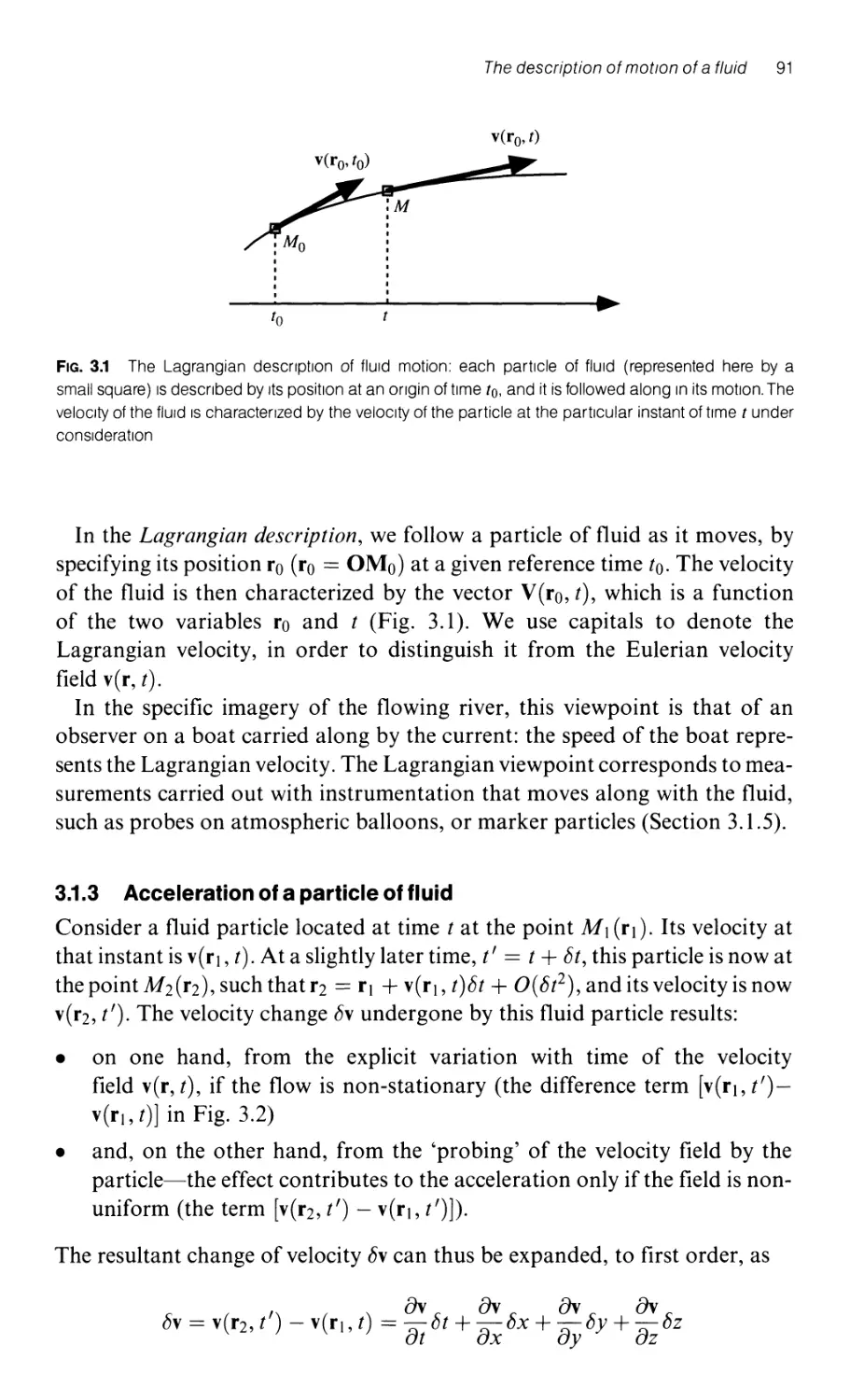
3.1.2 The Eulerian and Lagrangian descriptions of fluid motion 90
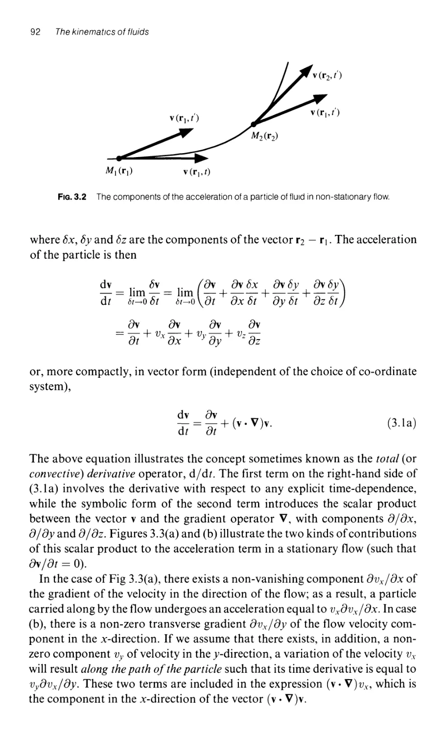
3.1.3 Acceleration of a particle of fluid 91
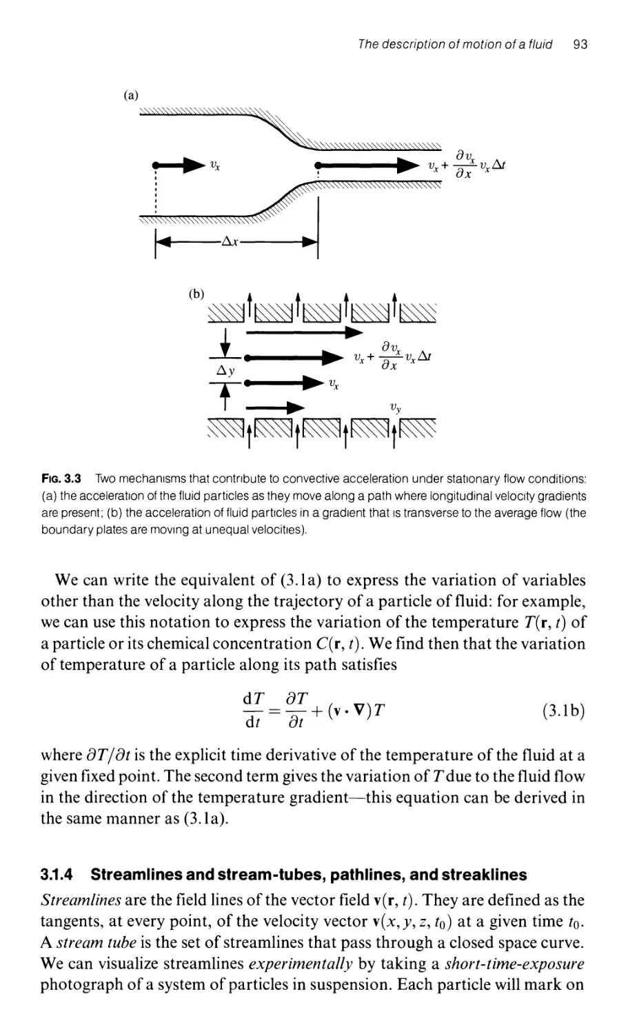
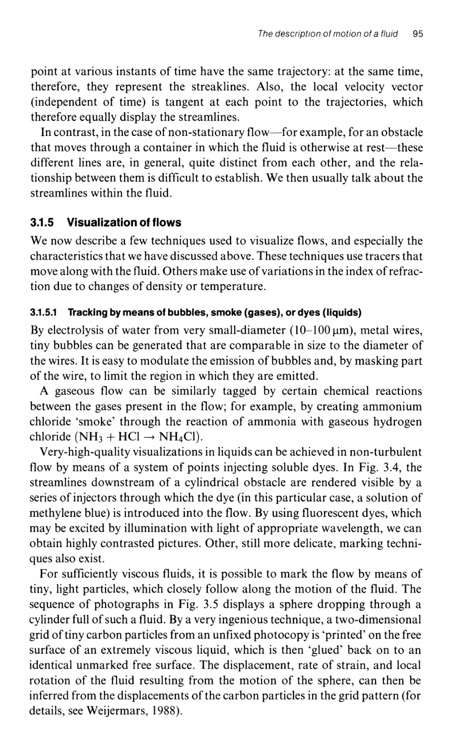
3.1.4 Streamlines and stream-tubes, pathlines, and streaklines 93
3.1.5 Visualization of flows 95
3.1.5.1 Tracking by means of bubbles, smoke (gases),
or dyes (liquids) 95
3.1.5.2 Visualization by the use of anisotropic, reflecting particles 97
3.1.5.3 Visualization by means of photo-active substances 97
3.1.5.4 Visualization of variations in the index of
refraction by the Schlieren method 98
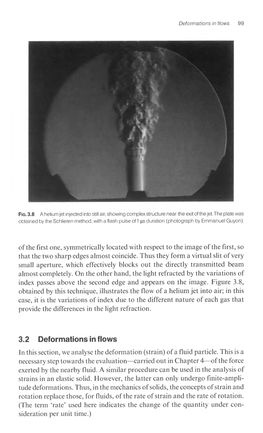
3.2 Deformations in flows 99
3.2.1 The local components of the velocity gradient field 100
3.2.2 Analysis of the symmetric component: pure strain (deformation) 100
3.2.2.1 Deformations due to the diagonal terms of the
velocity-gradient tensor 101
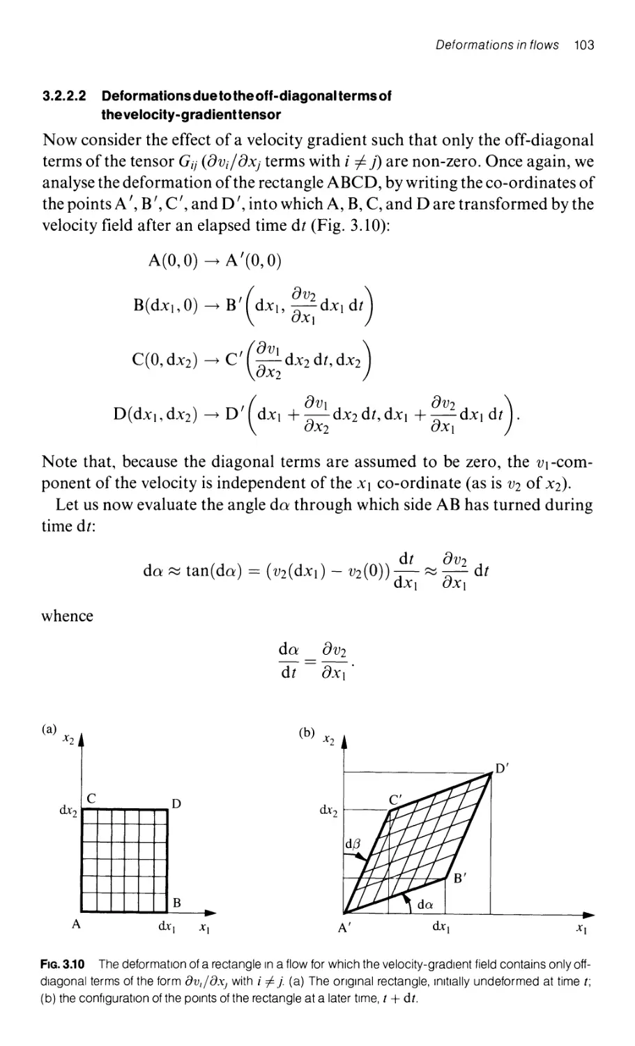
3.2.2.2 Deformations due to the off-diagonal terms of
the velocity-gradient tensor 103
3.2.3 Analysis of the antisymmetric component: pure rotation 104
3.2.4 Small and large deformations 106
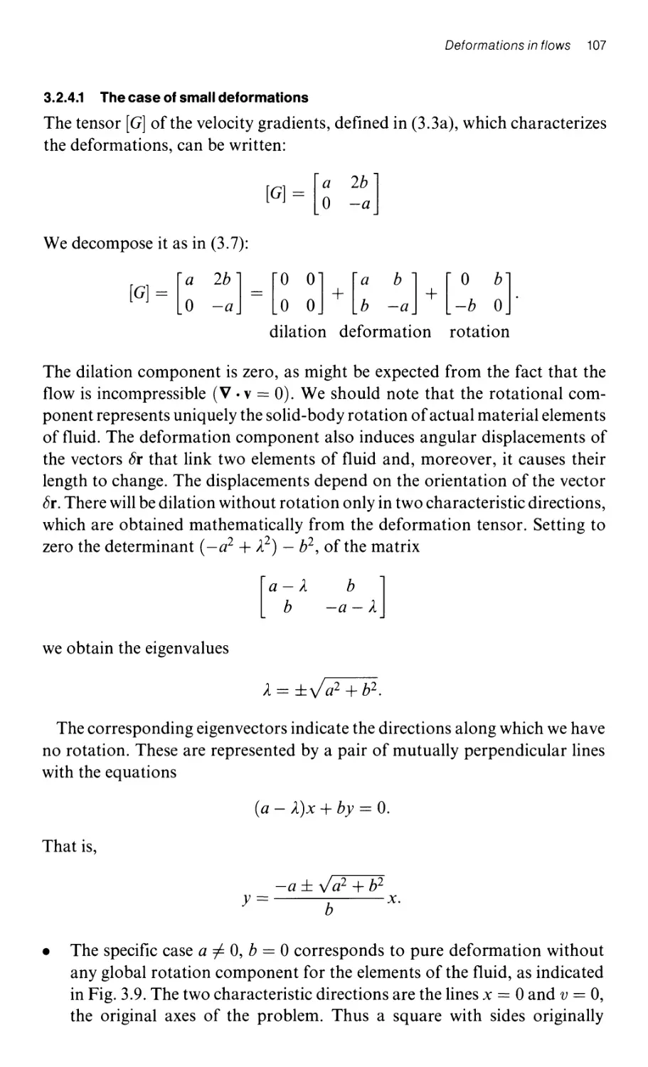
3.2.4.1 The case of small deformations 107
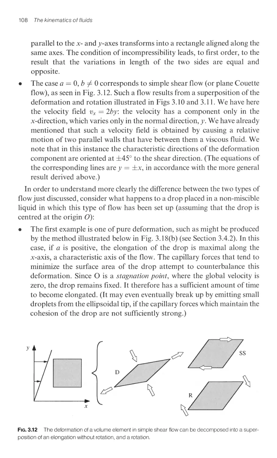
3.2.4.2 Large deformations 109
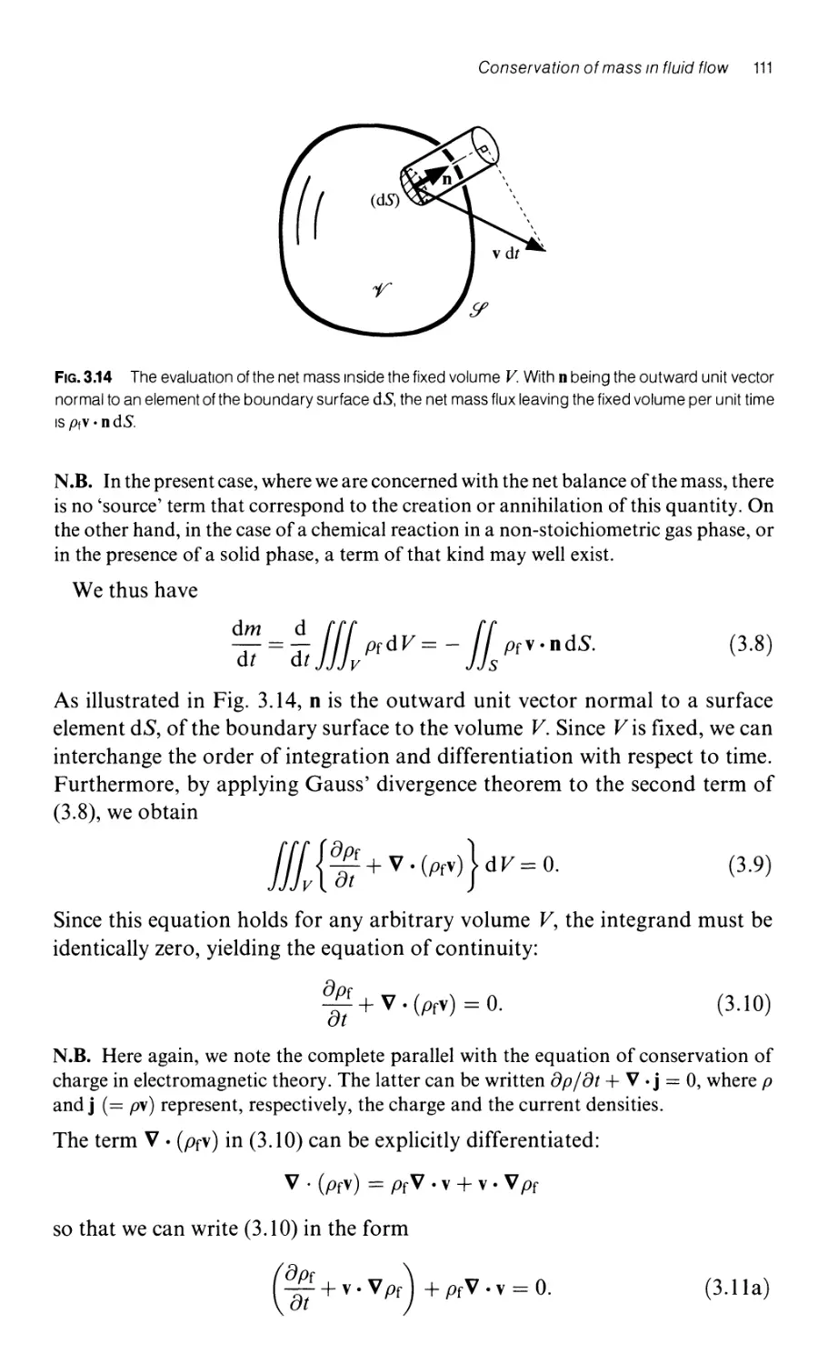
3.3 The conservation of mass in fluid flow 110
3.3.1 The equation of continuity 110
3.3.2 The incompressibility of a fluid 112
3.3.3 Analogies with electromagnetic theory 114
xiv Contents
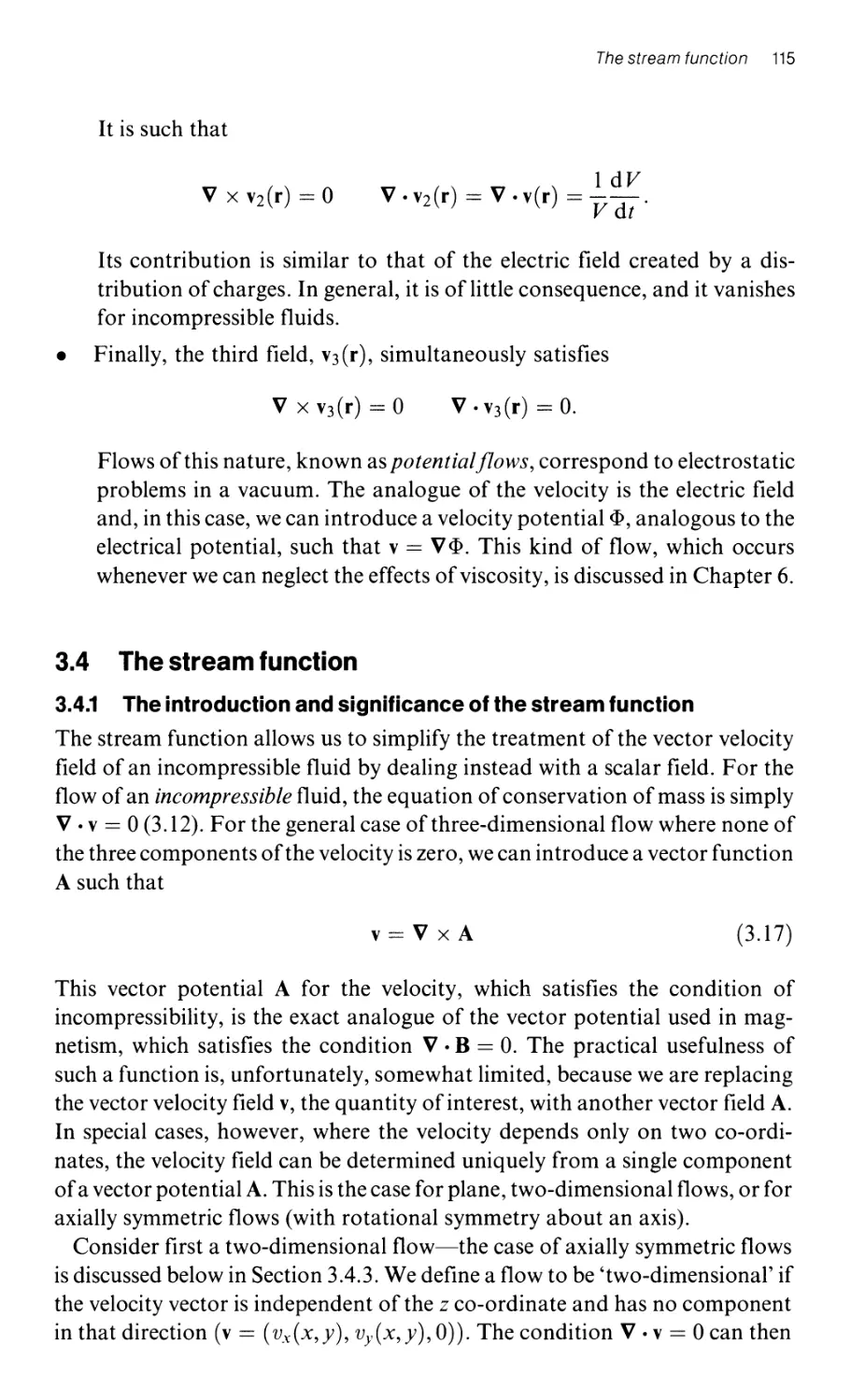
3.4 The stream function 115
3.4.1 The introduction and significance of the stream function 115
3.4.2 Examples of two-dimensional flows and of their stream functions 117
3.4.3 Axially symmetric flows 121
3.5 Some measurements of velocity and of velocity gradients in fluid flows 122
3.5.1 Measurement of the local velocity of a fluid:
laser Doppler anemometry 122
3.5.1.1 The relationship between the fluid velocity and
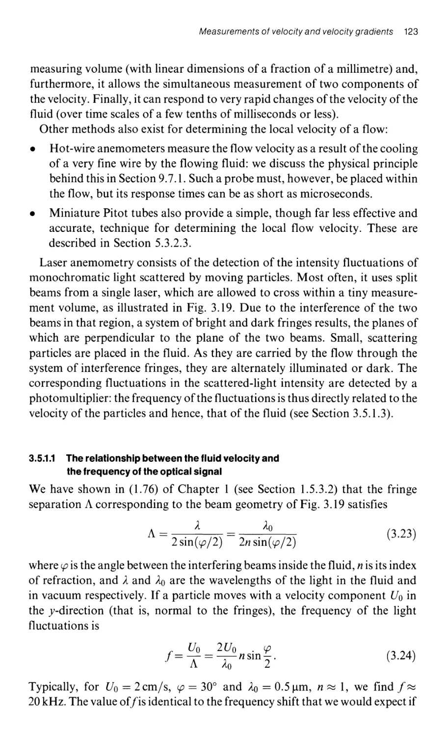
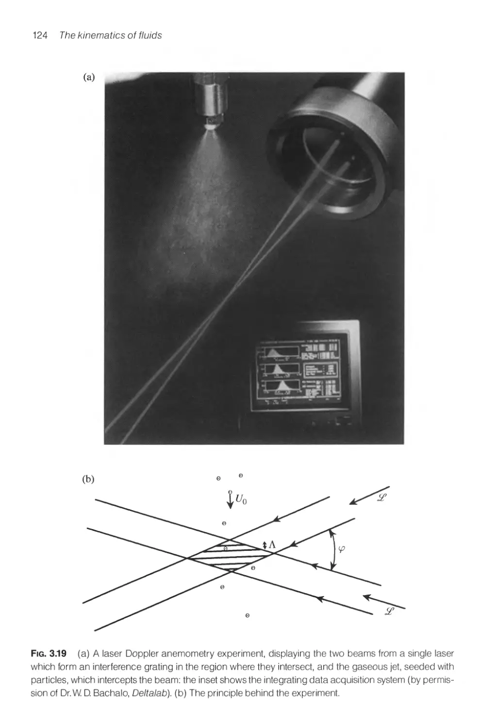
the frequency of the optical signal 123
3.5.1.2 Advantages of laser Doppler anemometers 125
3.5.1.3 Problems and limitations 125
3.5.2 Determination of the local velocity gradients 125
3.5.2.1 The use of thermal marking 126
3.5.2.2 The use of partially reflecting particles 127
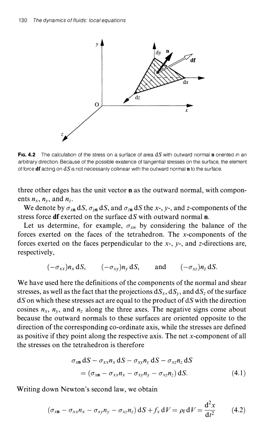
4 The dynamics of fluids: local equations 128
4.1 Su rface forces 128
4.1.1 The general expression for the surface forces 128
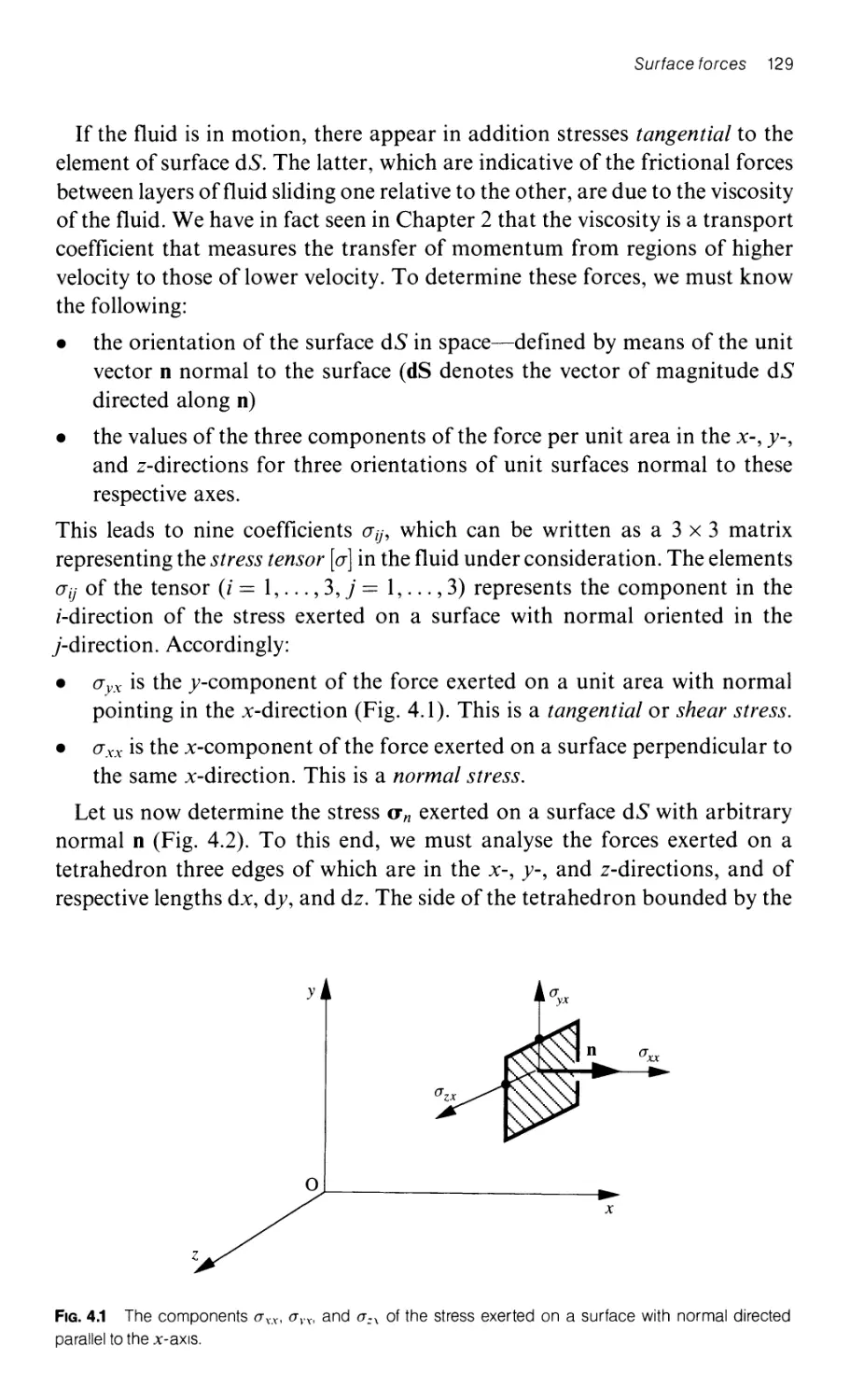
4.1.1.1 The stress tensor 128
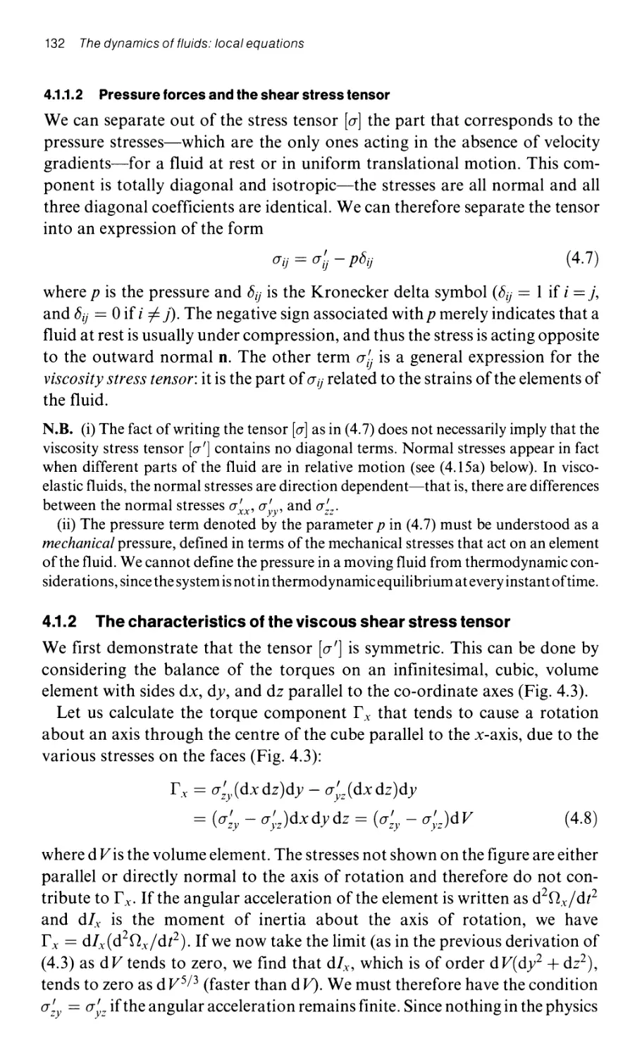
4.1.1.2 Pressure forces and the shear stress tensor 132
4.1.2 The characteristics of the viscous shear stress tensor 132
4.1.3 The viscous shear stress for a Newtonian fluid 134
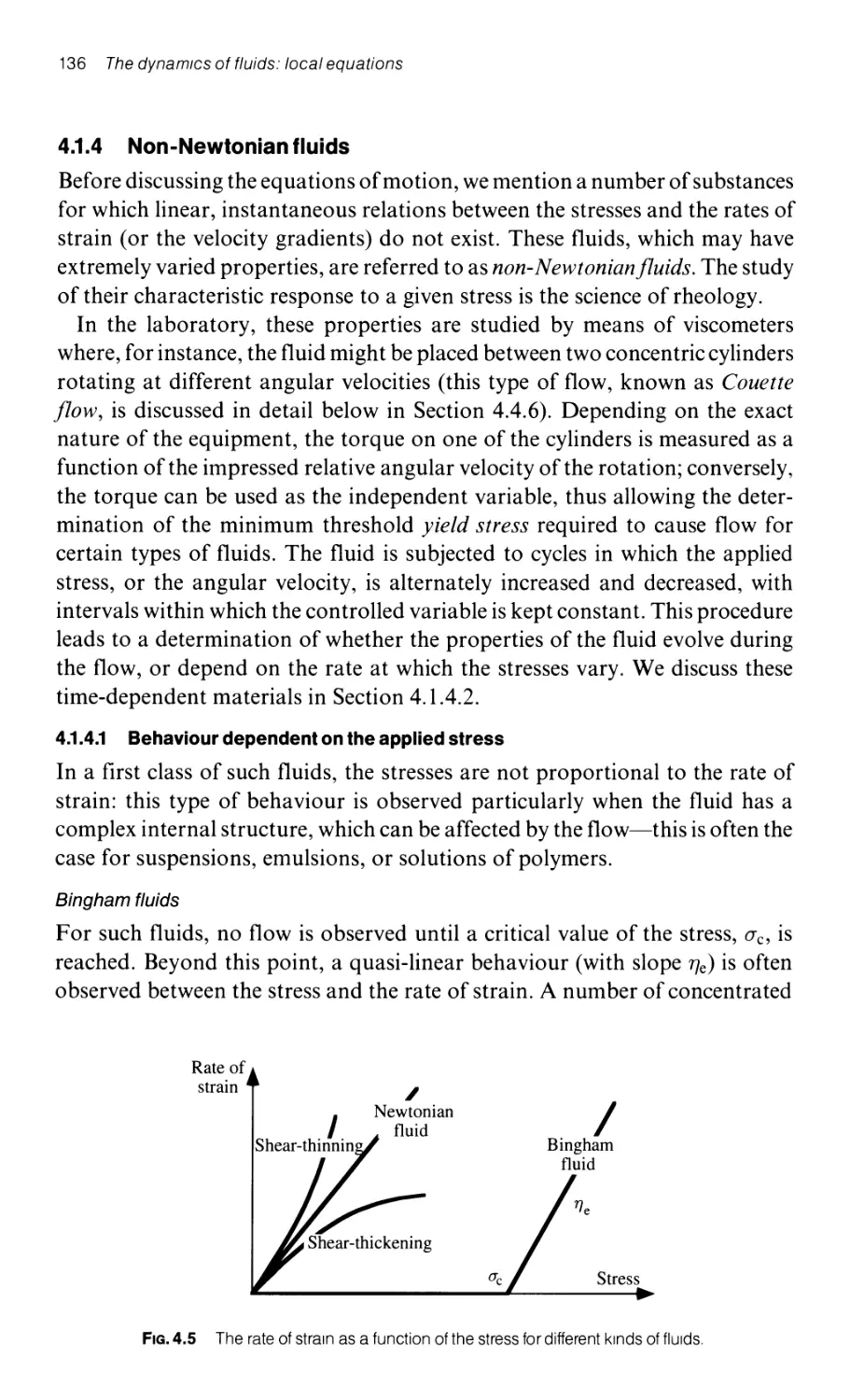
4.1.4 Non-Newtonian fluids 136
4.1.4.1 Behaviour dependent on the applied stress 136
4.1.4.2 Non-Newtonian time-dependent fluids 138
4.1.4.3 Some types of complex non-Newtonian behaviour 139
4.2 The equation of motion for a fluid 140
4.2.1 The general equation for the dynamics of a fluid 140
4.2.2 The Navier-Stokes equation of motion for a Newtonian fluid 142
4.2.3 Euler's equation of motion for an ideal fluid 143
4.2.4 The dimensionless form of the Navier -S1okes equation 143
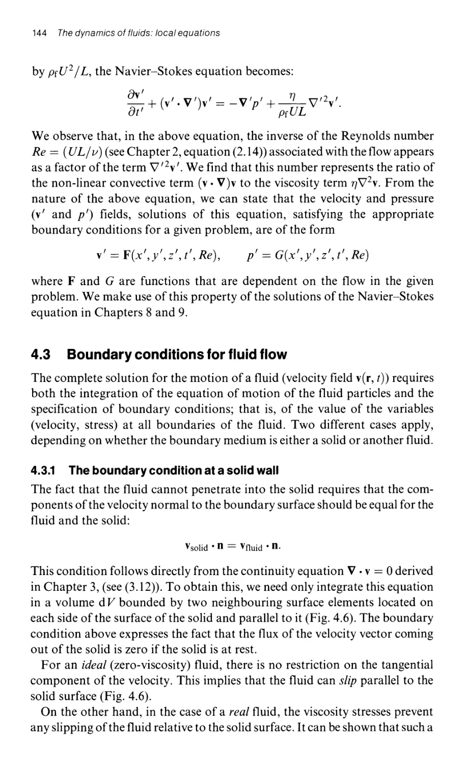
4.3 Boundary conditions for fluid flow 144
4.3.1 The boundary condition at a solid wall 144
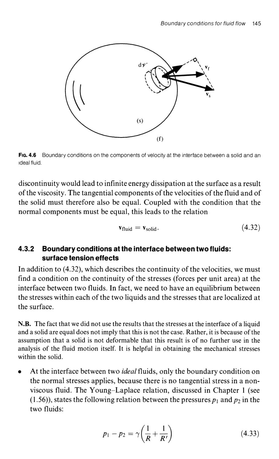
4.3.2 Boundary conditions at the interface between two fluids:
su rface tension effects 145
4.4 A few specific solutions of the Navier-Stokes equations 147
4.4.1 The Navier -Stokes equation for one-dimensional flow 147
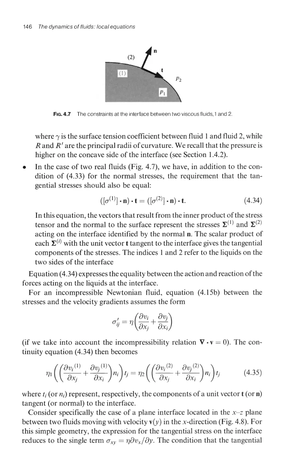
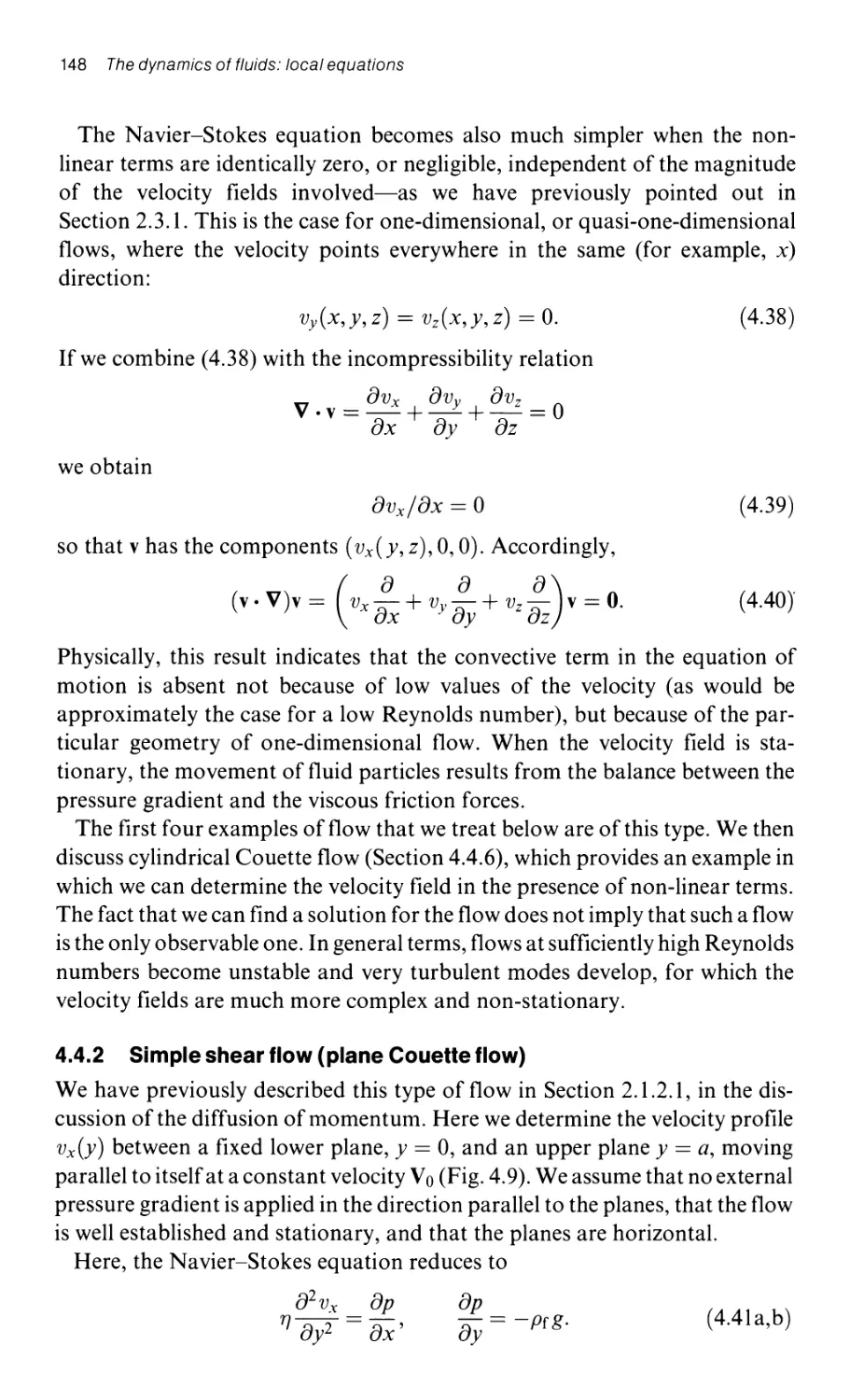
4.4.2 Simple shear flow (plane Couette flow) 148
4.4.3 Poiseuille flow (a viscous fluid flowing in a stationary conduit) 149
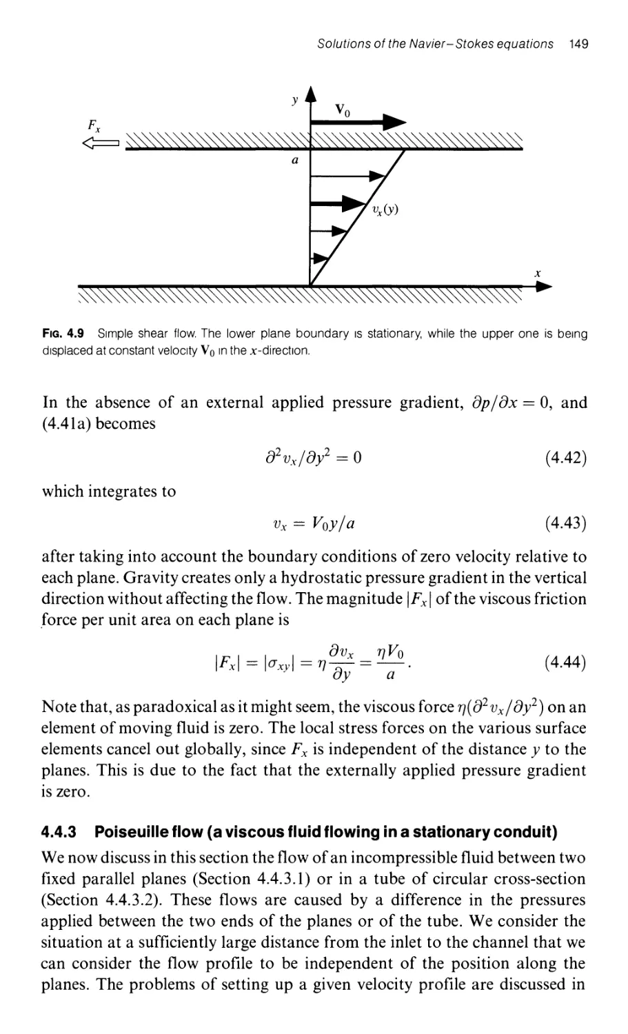
4.4.3.1 Flow between parallel planes 150
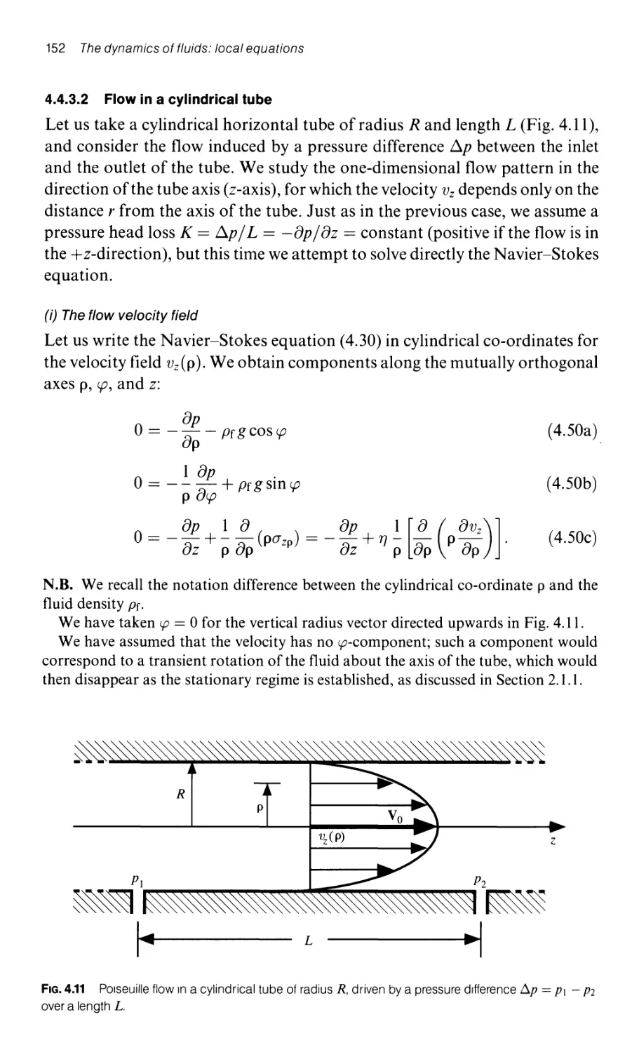
4.4.3.2 Flow in a cylindrical tube 152
4.4.4 Oscillating flows In a viscous fluid 155
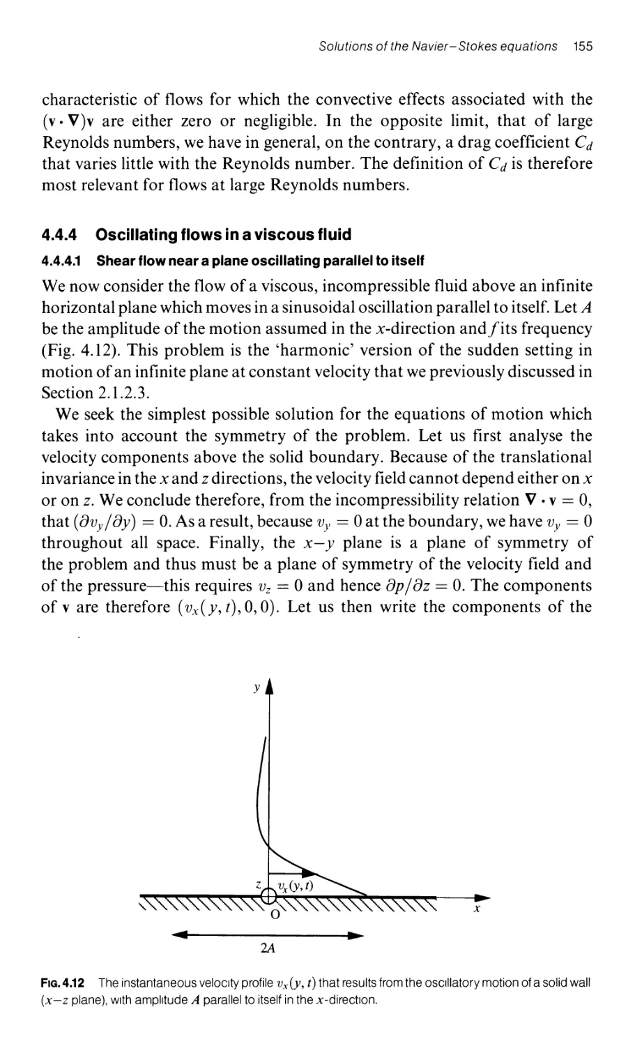
4.4.4.1 Shear flow near a plane oscillating parallel to itself 155
4.4.4.2 The flow between two parallel planes induced by
an oscillating pressure gradient 158
4.4.5 Flow driven by a gradient in the surface tension
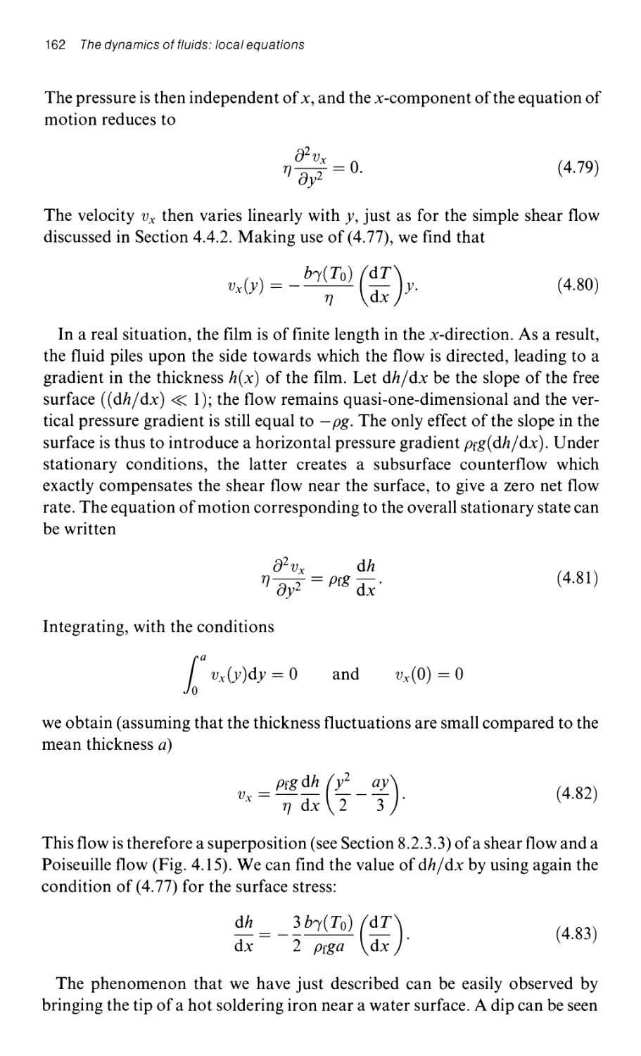
(the Marangoni effect) 160
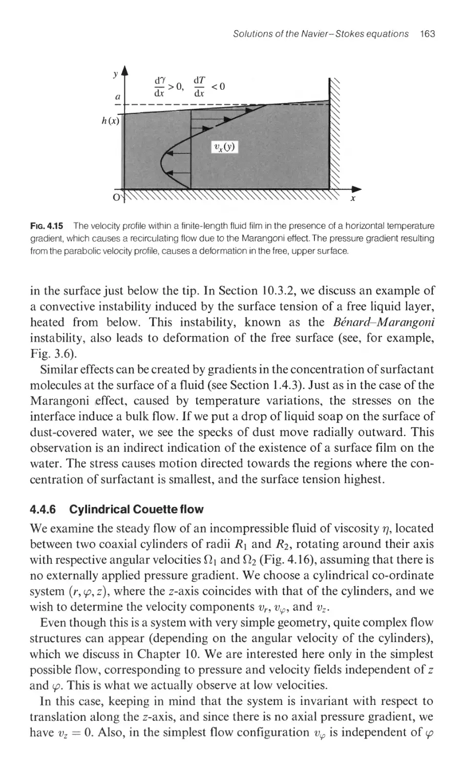
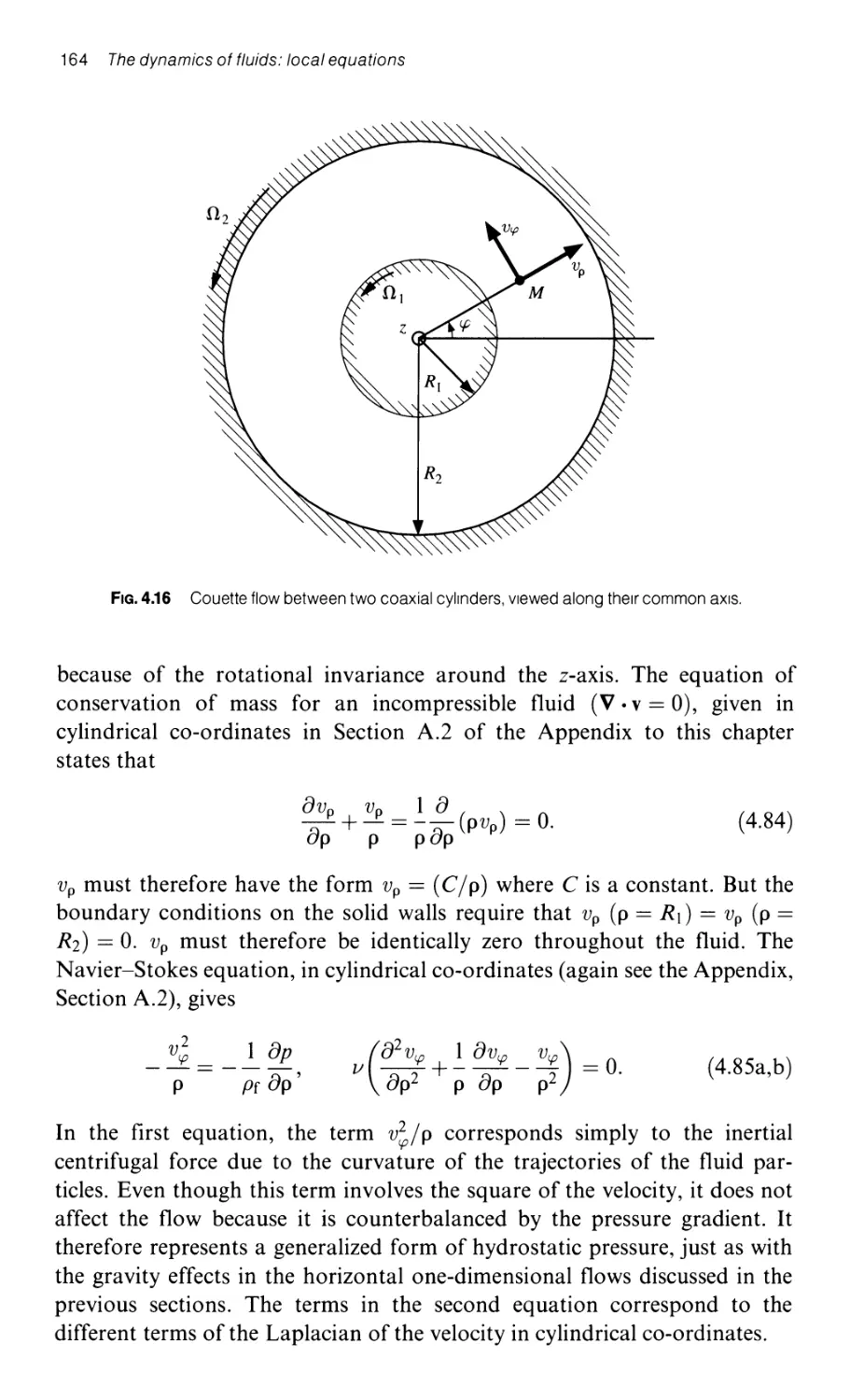
4.4.6 Cylindrical Couette flow 163
Contents x v
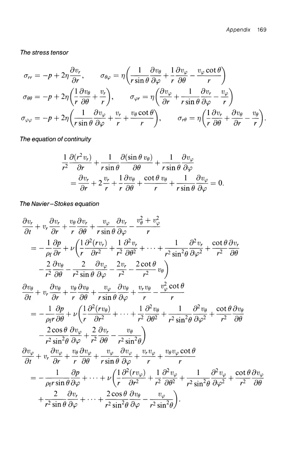
Appendix: representation of the stress tensor, the equation of continuity,
and the Navier-Stokes equations, for Newtonian fluids,
in the most commonly used co-ordinate systems 167
A.1 Cartesian co-ordinates (x, y, z) 167
A.2 Cylindrical co-ordinates (p, '(J, z) 167
A.3 Spherical po lar co -ord i nates (r, (), c.p) 168
5 The conservation laws 170
5.1 Conservation of mass 170
5.2 Conservation of momentum 171
5.2.1 The local equation 171
5.2.2 The integral expression of the law of conservation of momentum 172
5.2.2.1 The integral of the equation for conservation of
momentum 172
5.2.2.2 The case of an incompressible Newtonian fluid 173
5.2.2.3 The application of the momentum conservation
laws to simple flows 174
5.3 The conservation of kinetic energy: Bernoulli's equation 176
5.3.1 The conservation of energy for a flowing incompressible
fluid with or without viscosity 177
5.3.1.1 Derivation of the conservation equation 177
5.3.1.2 Kinetic energy dissipation through viscosity
in a simple shear flow 178
5.3.1.3 Kinetic energy dissipation in a Newtonian fluid 179
5.3.2 Bernoulli's equation: applications 180
5.3.2.1 Bernoulli's equation for stationary flow 180
5.3.2.2 Bernoulli's equation for potential flow 181
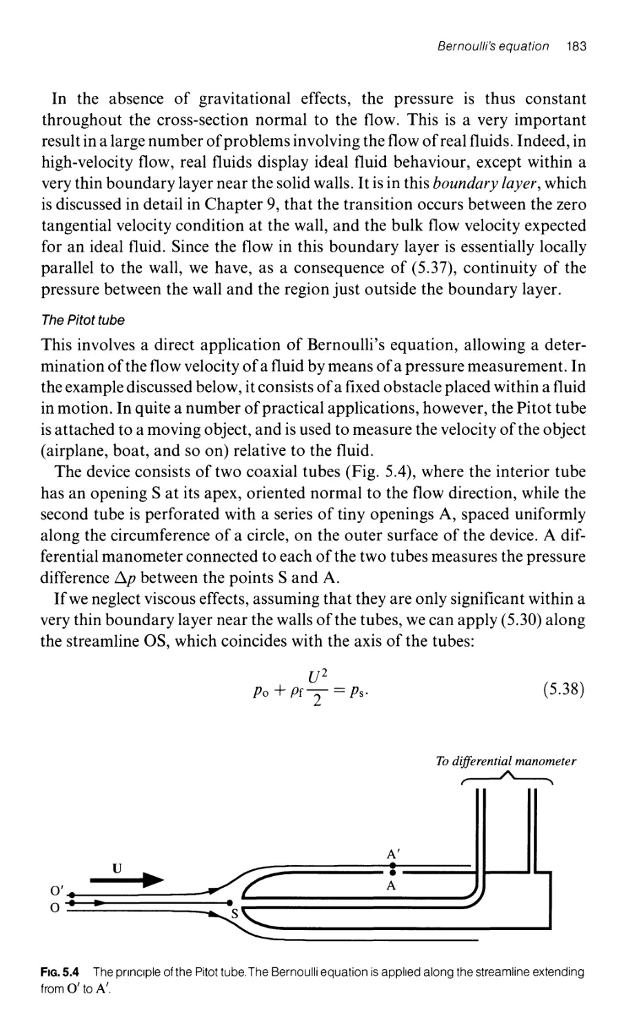
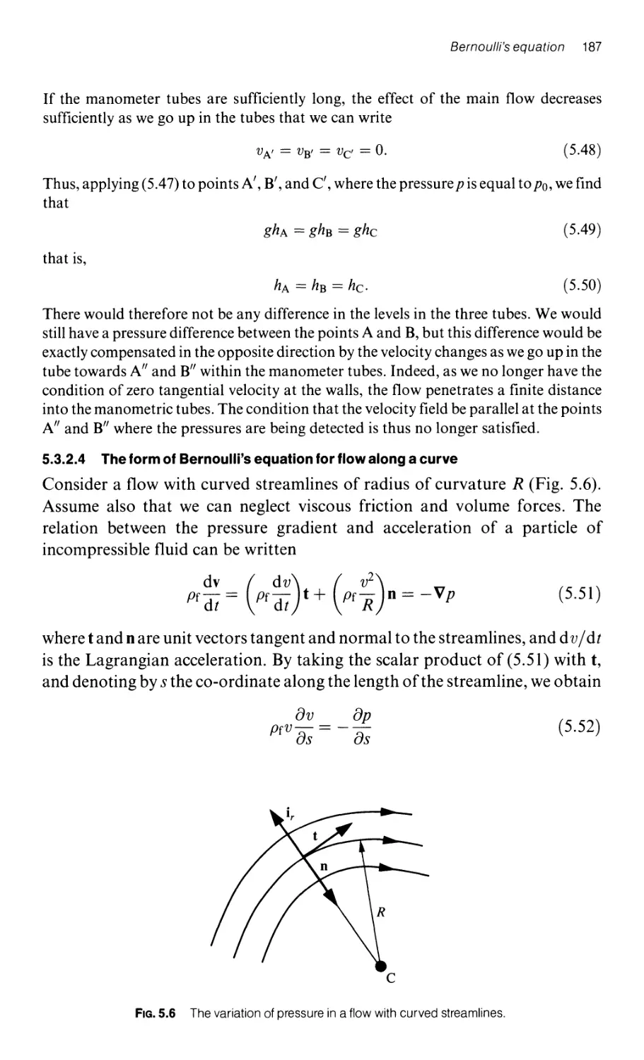
5.3.2.3 Applications of Bernoulli's equation 182
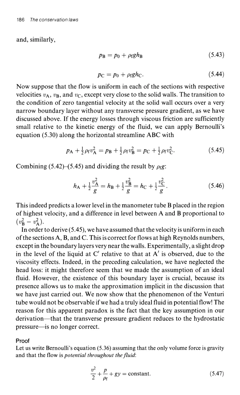
5.3.2.4 The form of Bernoulli's equation for flow
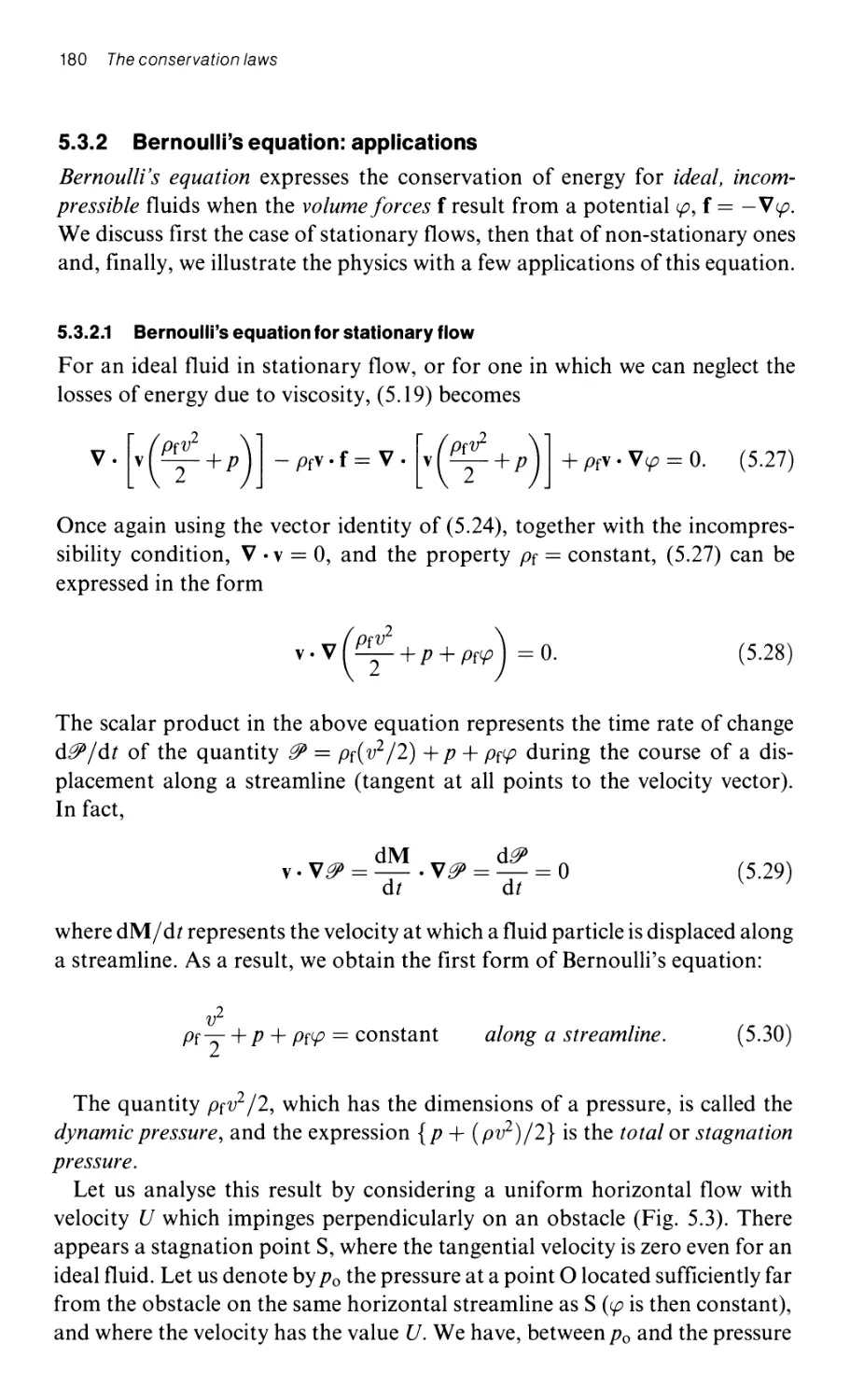
along a curve 181
5.4 Applications of the laws of conservation of energy and momentum 189
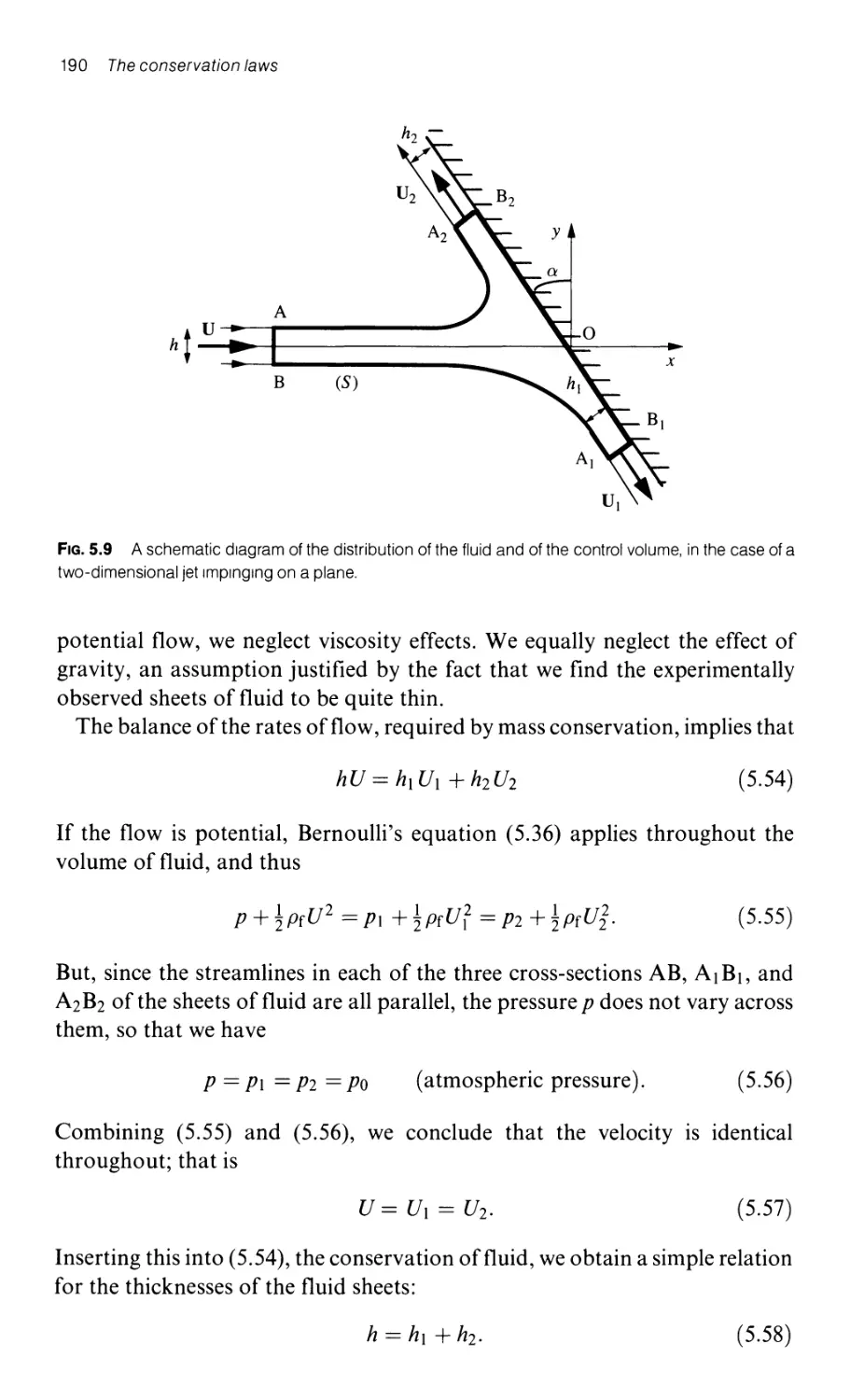
5.4.1 A jet incident on to a plane 189
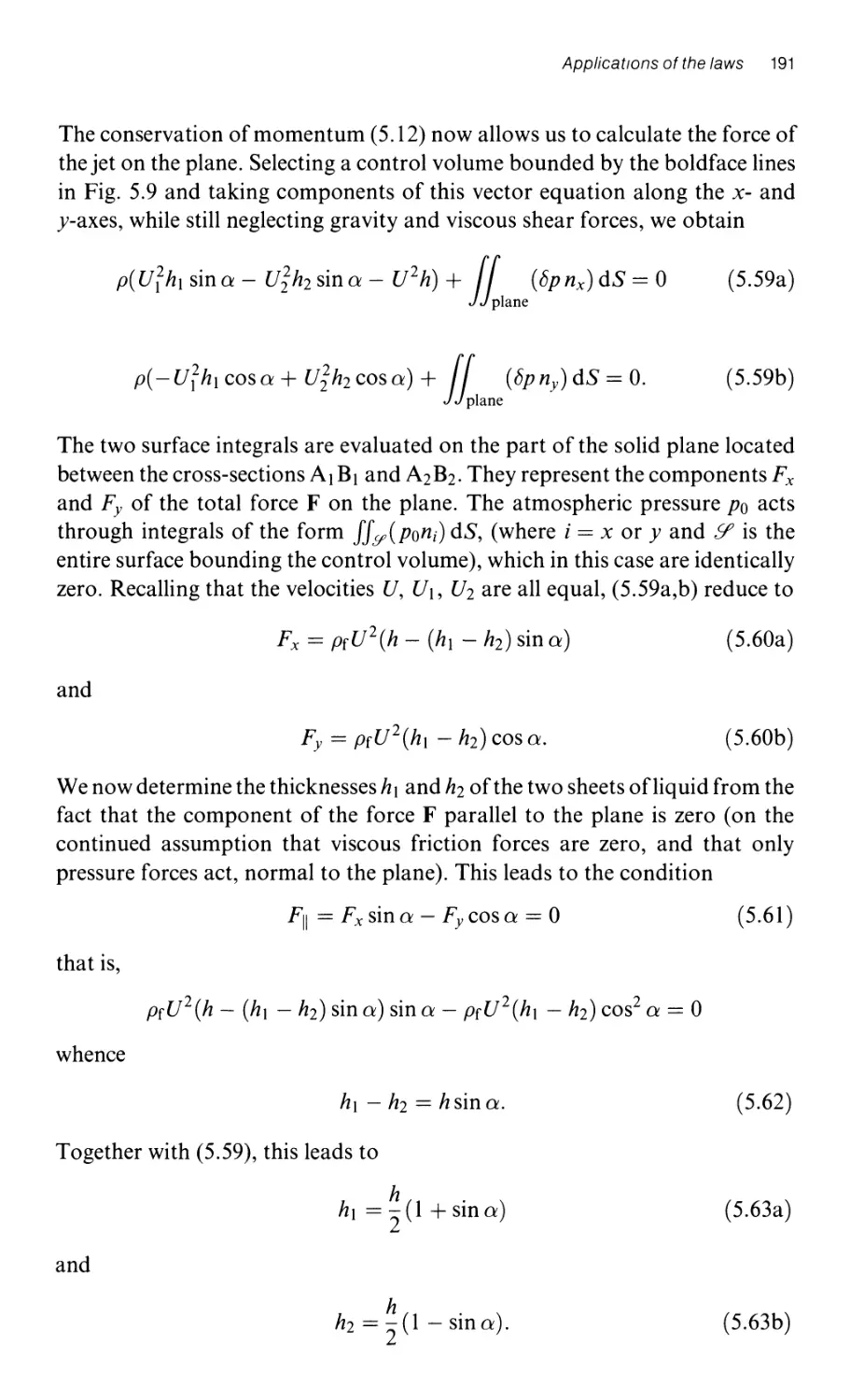
5.4.2 The exit jet from an opening in a reservoir 192
5.4.2.1 The determination of the velocity in the exit jet 192
5.4.2.2 Calculation of the vena contracta 193
5.4.2.3 The force exerted by the fluid on the container 194
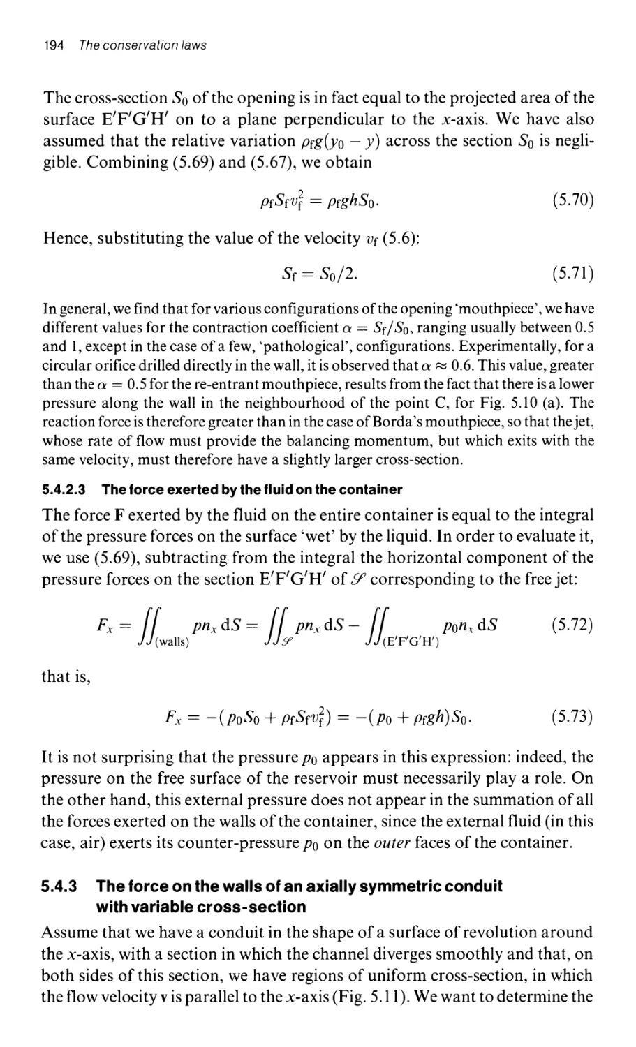
5.4.3 The force on the walls of an axially symmetric conduit
with variable cross-section 194
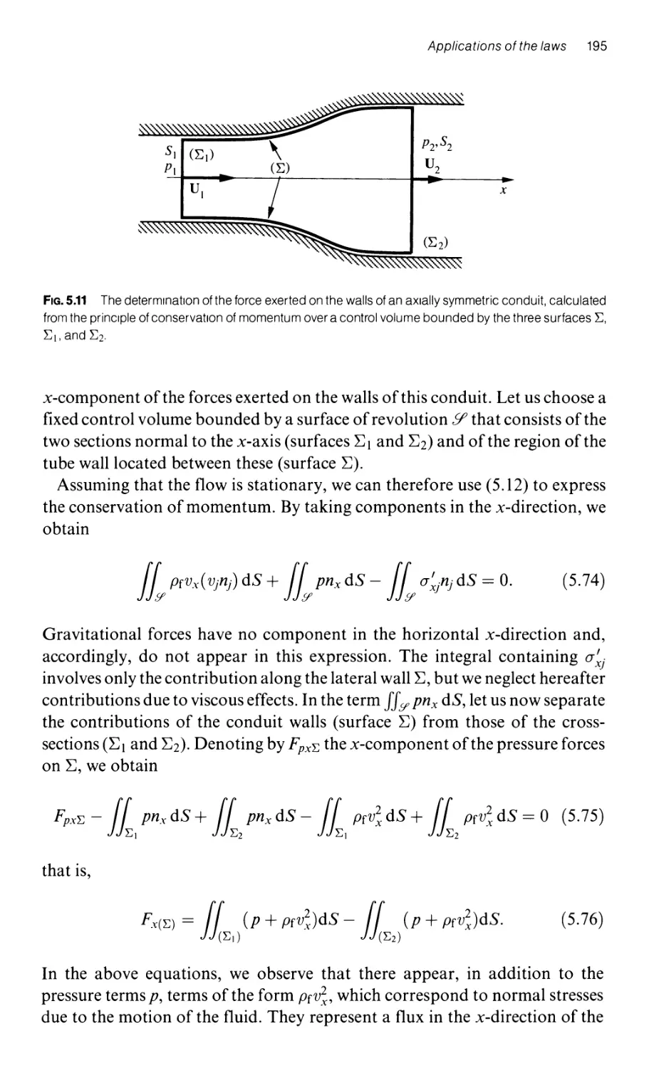
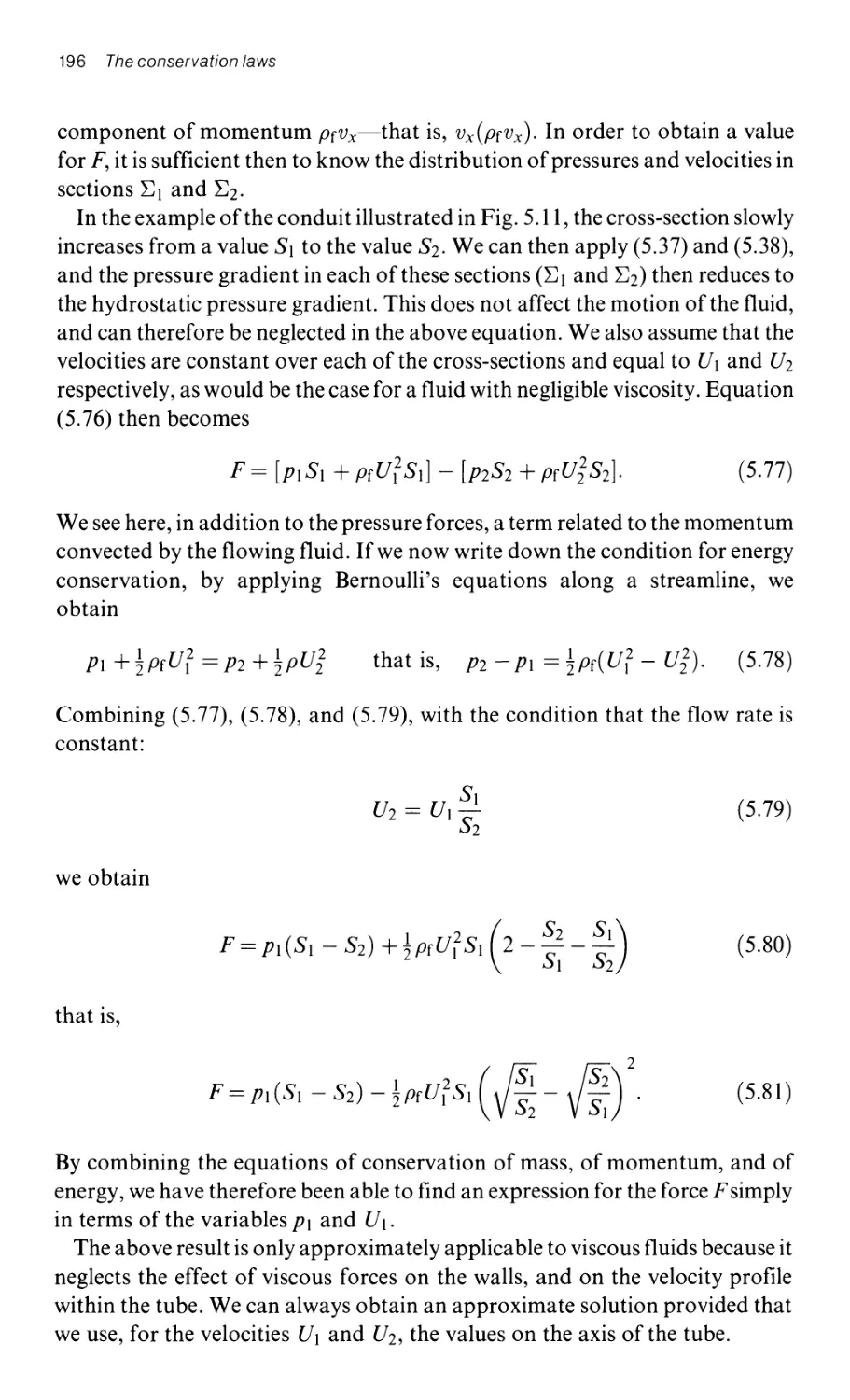
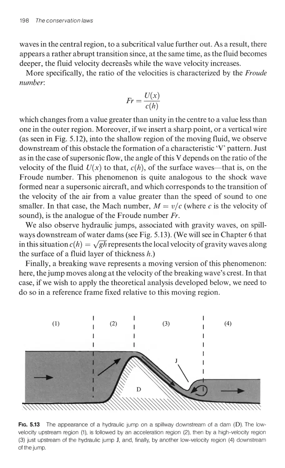
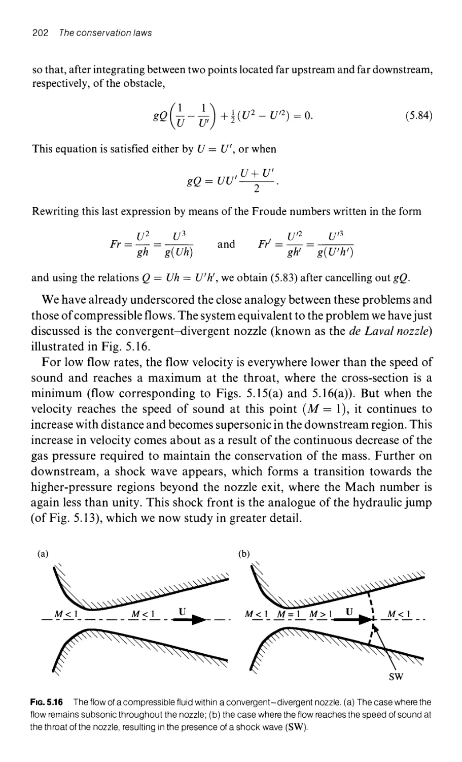
5.4.4 The hydraulic jump 197
5.4.4.1 The qualitative properties of hydraulic jumps 197
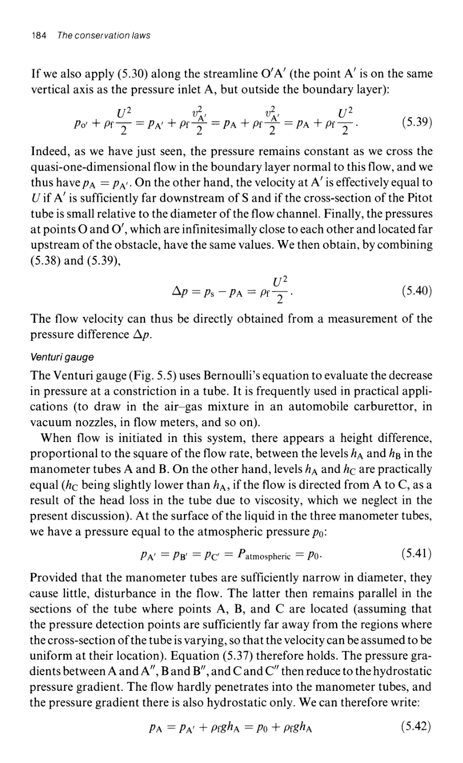
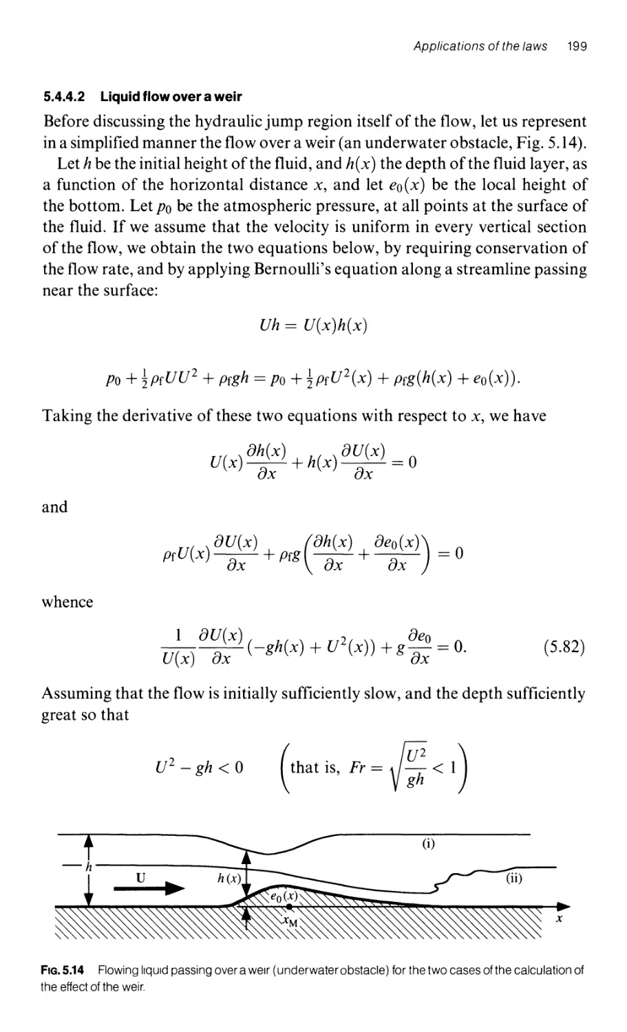
5.4.4.2 Liquid flow over a weir 199
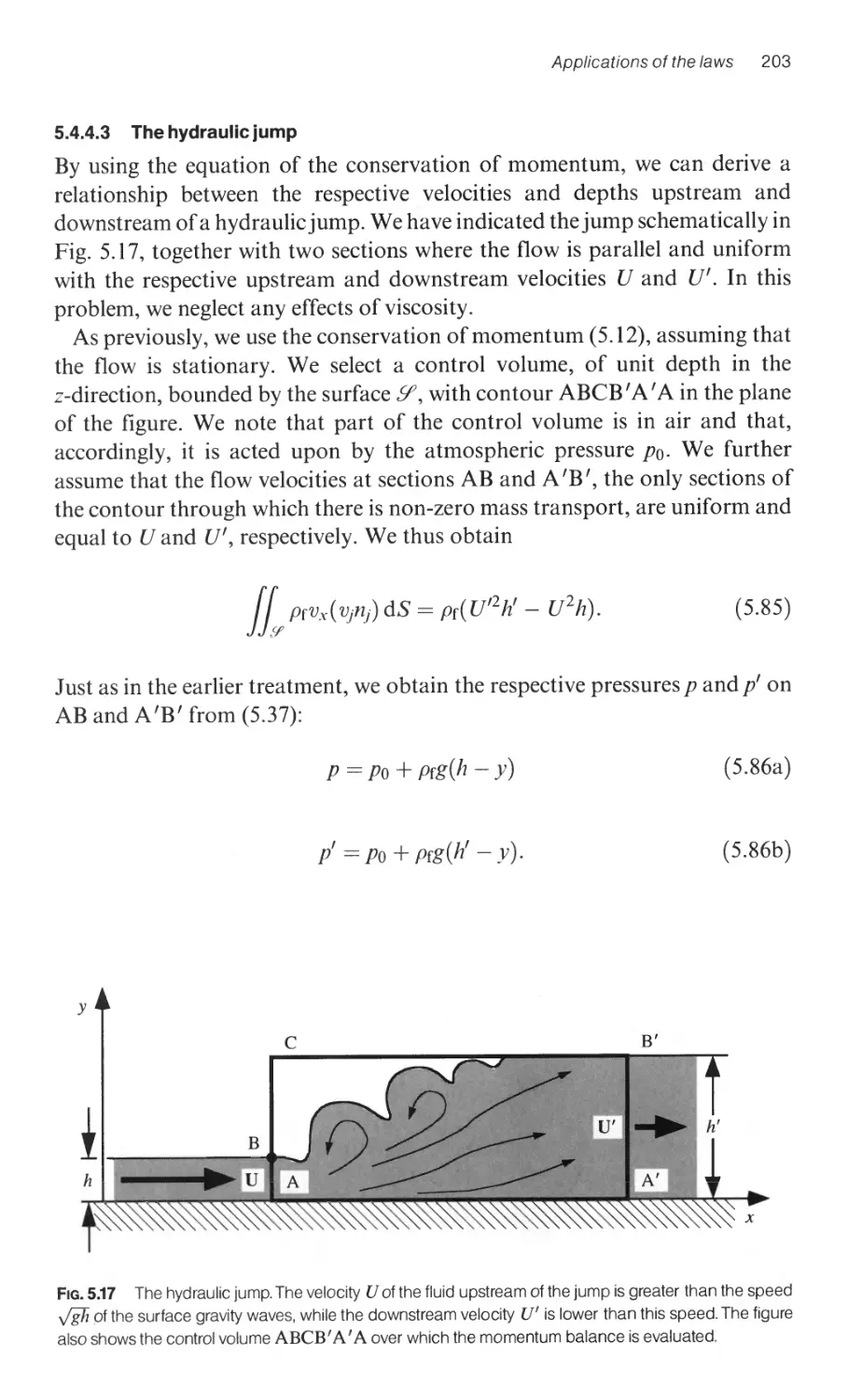
5.4.4.3 The hydraulic jump 203
5.4.4.4 The relation between the fluid levels and the velocities on
the two sides of the jump ?05
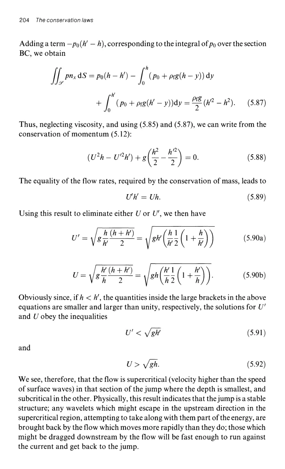
5.4.5 Another applicatIon: a discharge sluice gate in a channel 205
5.4.5.1 The reaction force on the sluice gate 206
5.4.5.2 The critical Froude number resulting from the
application of Bernoulli's equation 207
xvi Contents
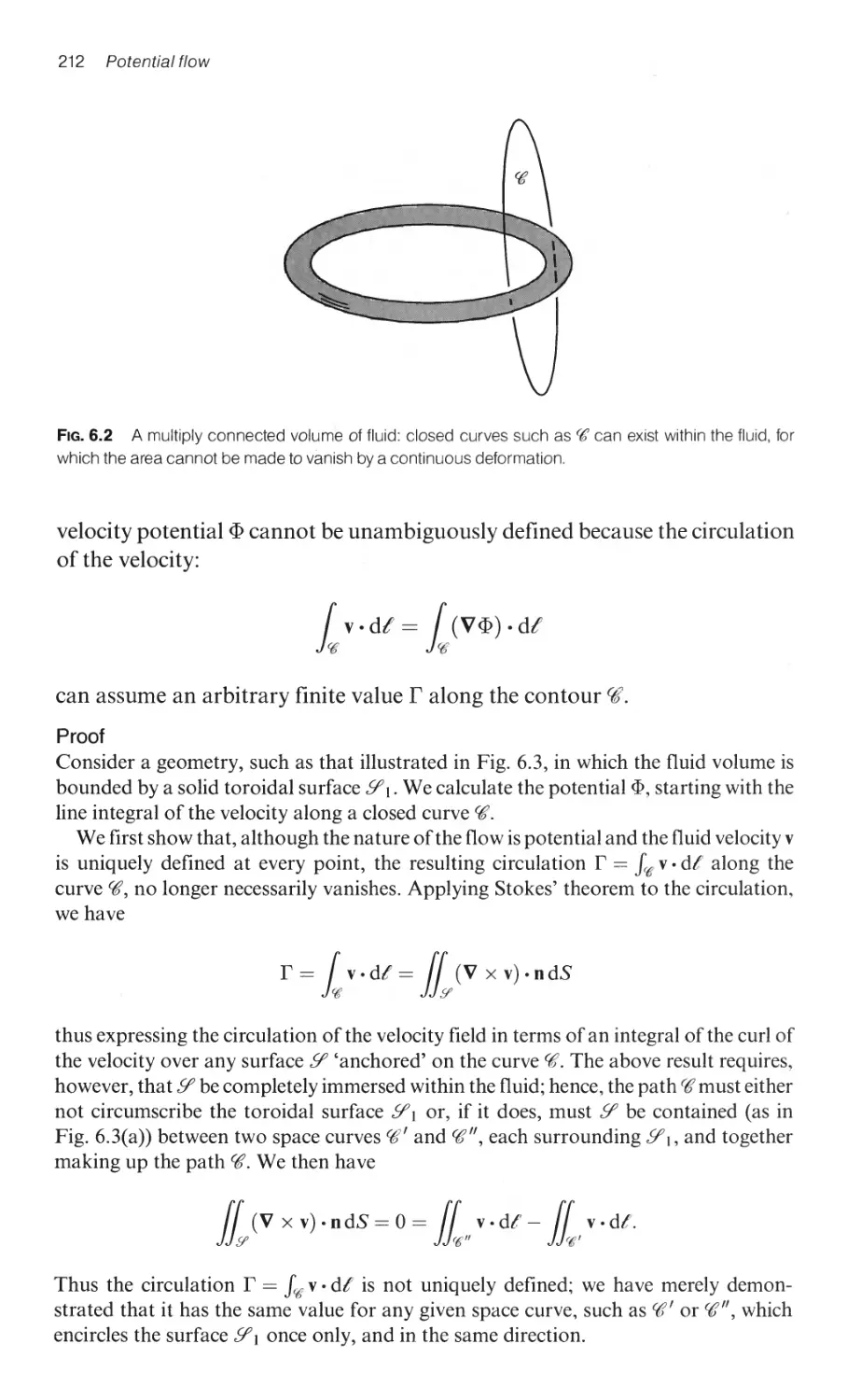
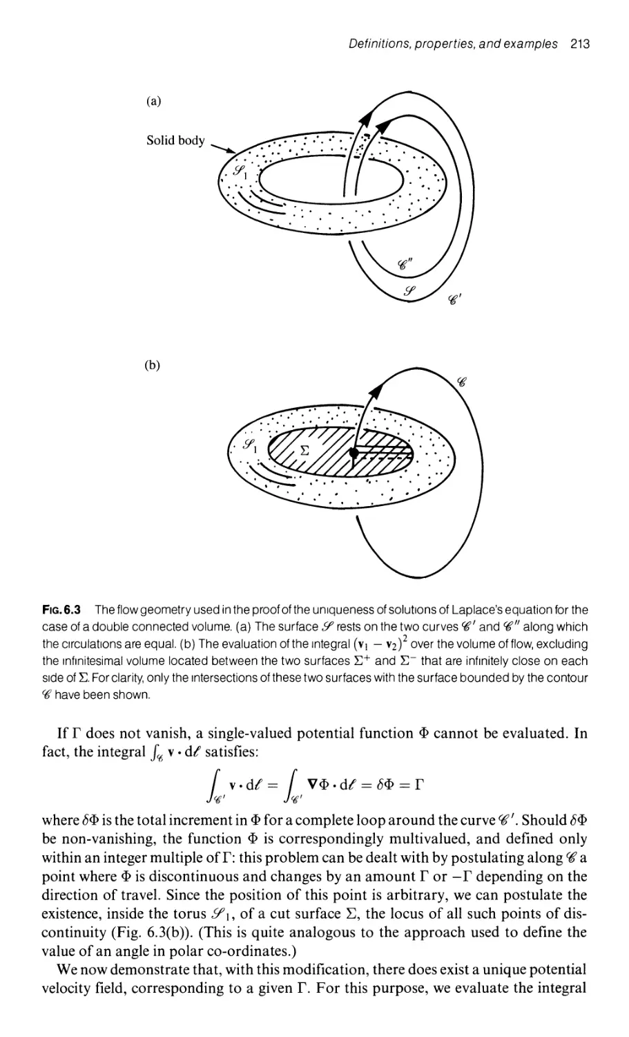
8 Potential flow 208
6.1 Introduction 208
6.2 Definitions, properties, and examples of potential flow 210
6.2.1 Characteristics and examples of the velocity potential 210
6.2.2 The uniqueness of the velocity potential 210
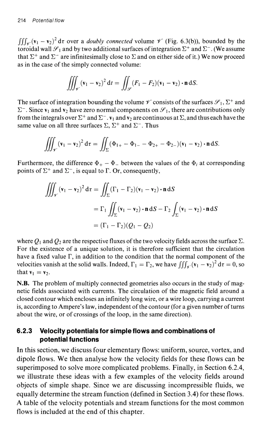
6.2.3 Velocity potentials for simple flows and combinations of
potential functions 214
6.2.3.1 Uniform parallel flow 215
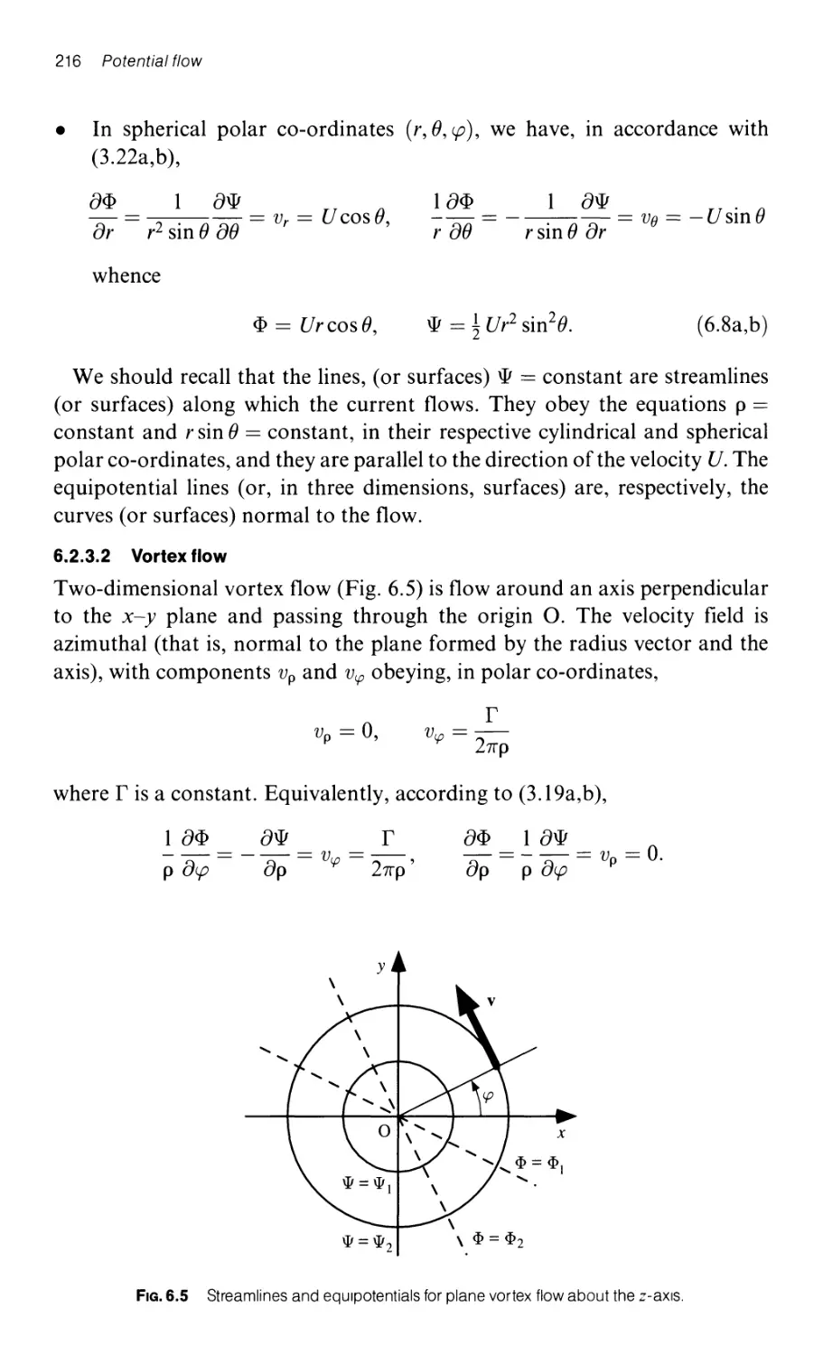
6.2.3.2 Vortex flow 216
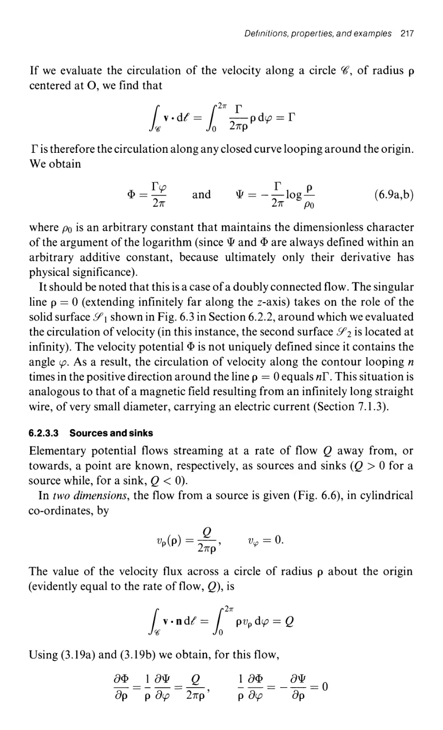
6.2.3.3 Sources and sinks 217
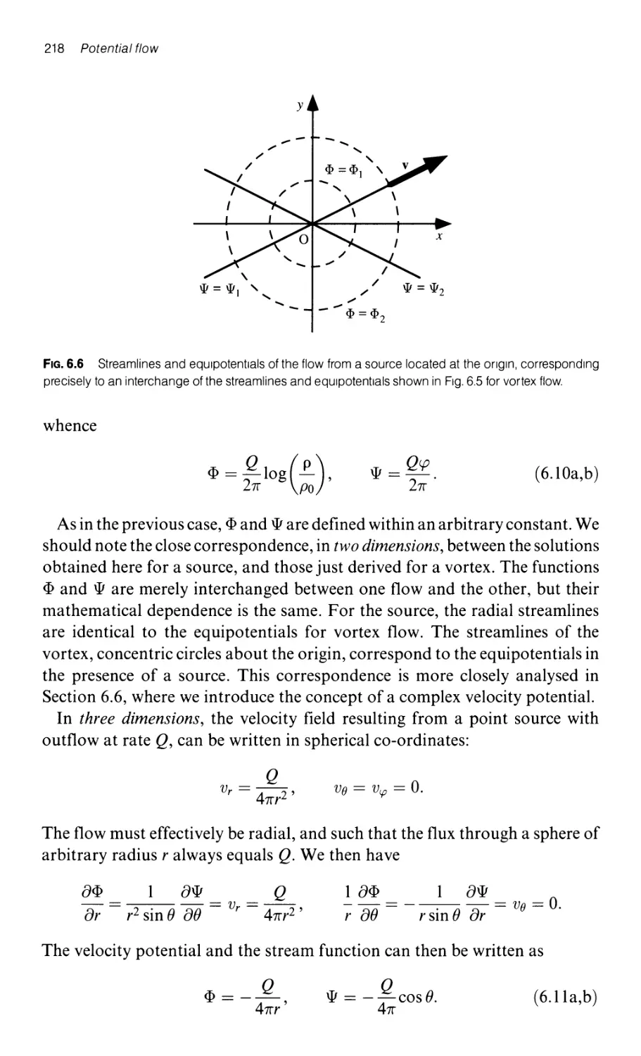
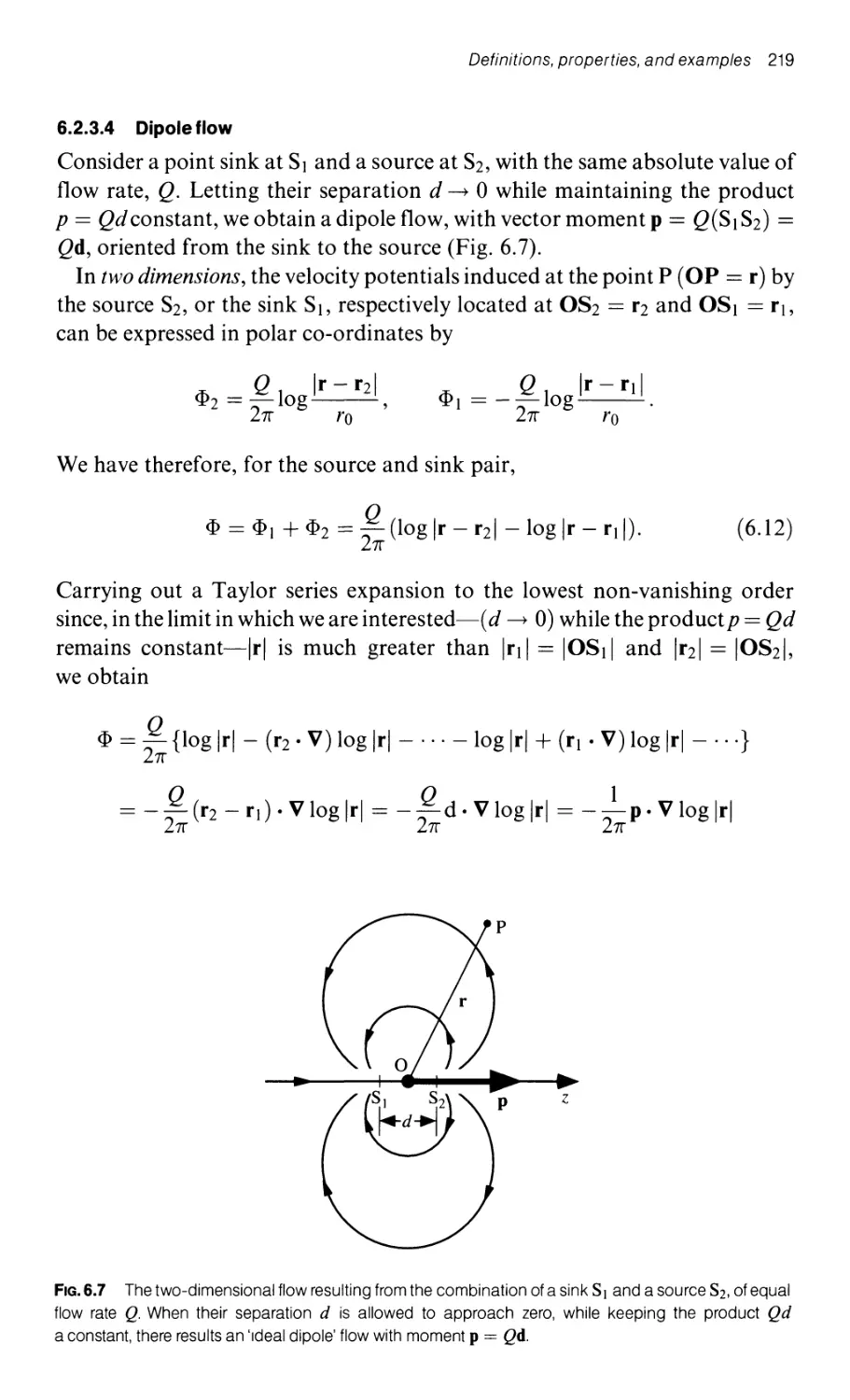
6.2.3.4 Dipole flow 219
6.2.3.5 Solutions of Laplace's equation: superposition and
separation of variables 220
6.2.4 Examples of simple potential flows 221
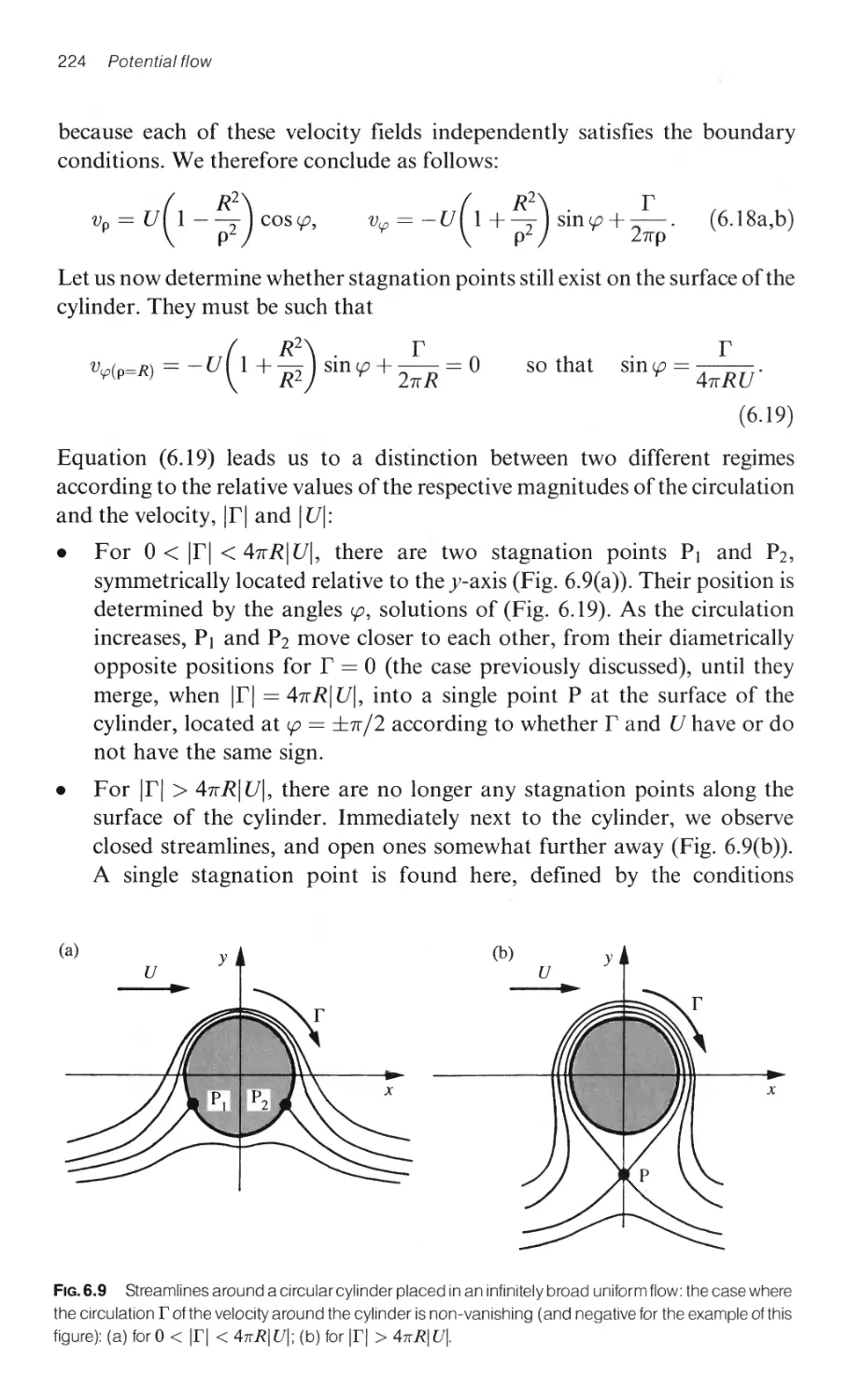
6.2.4.1 Flow around a circular cylinder 221
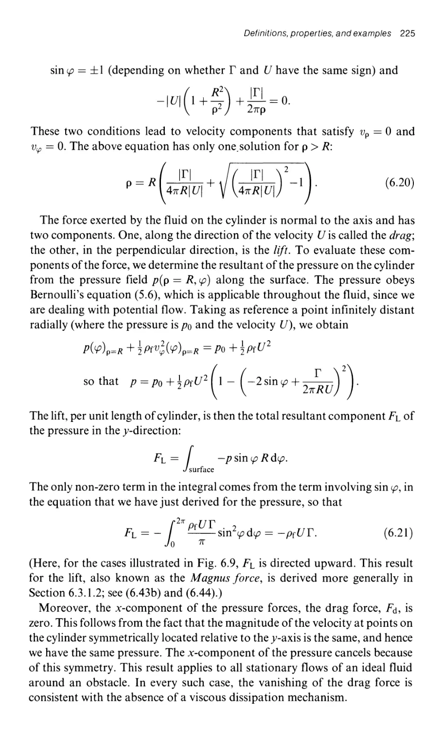
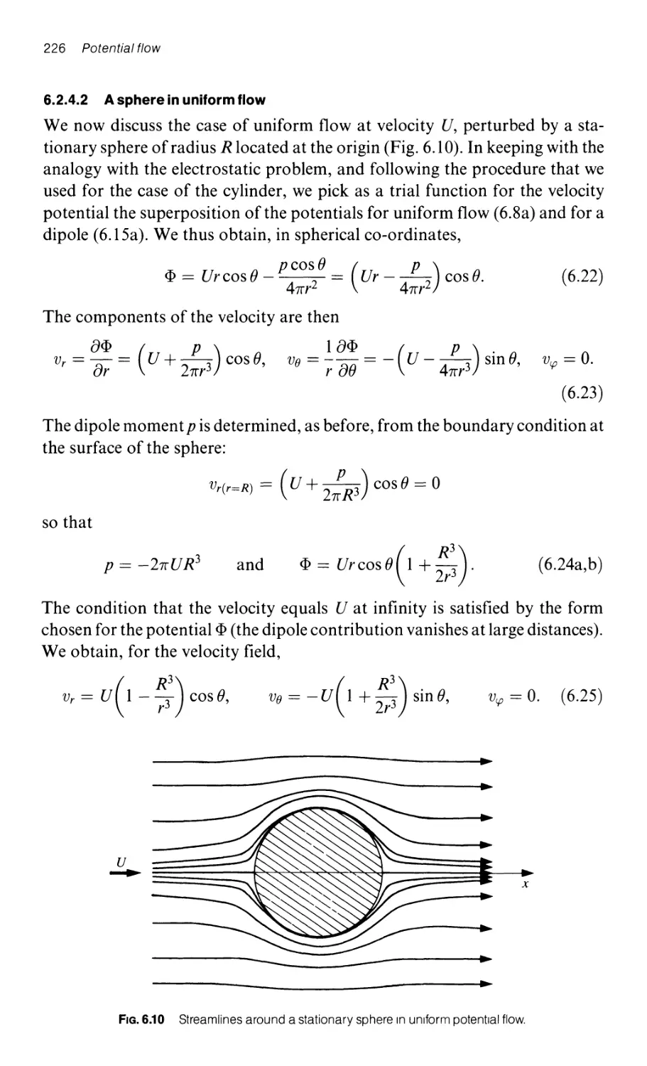
6.2.4.2 A sphere in uniform flow 226
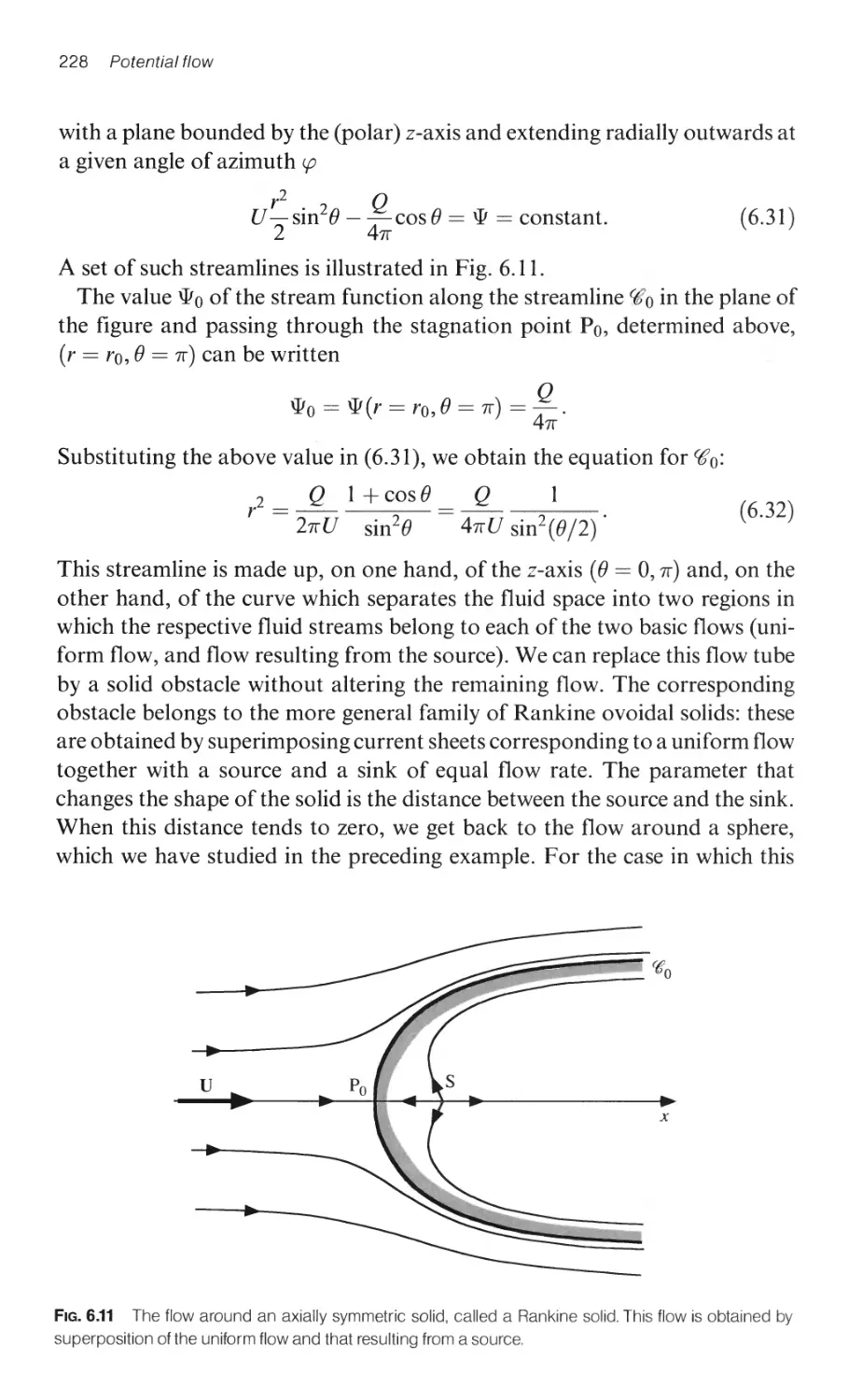
6.2.4.3 The Rankine solid 227
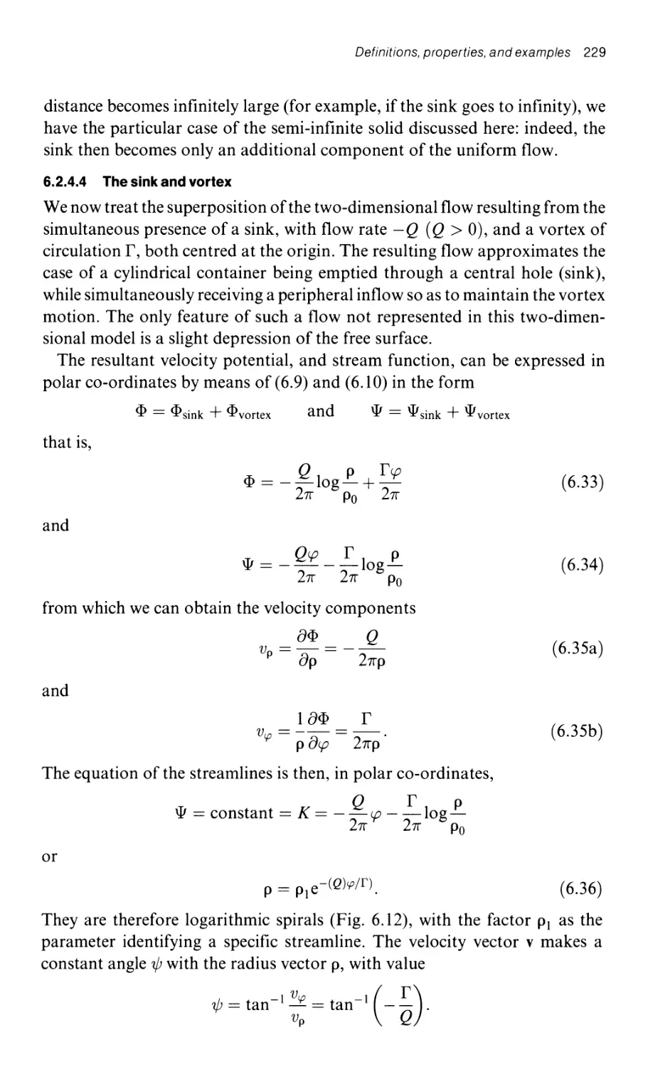
6.2.4.4 The sink and vortex 229
6.3 Forces acting on an obstacle in potential flow 230
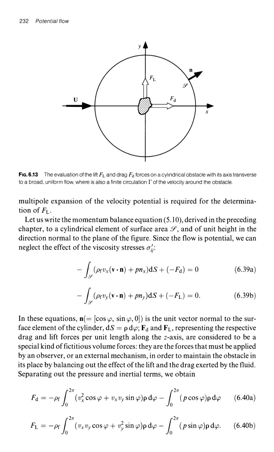
6.3.1 Two-dimensional flow 230
6.3.1.1 The velocity potential 230
6.3.1.2 The forces acting on a two-dimensional obstacle 231
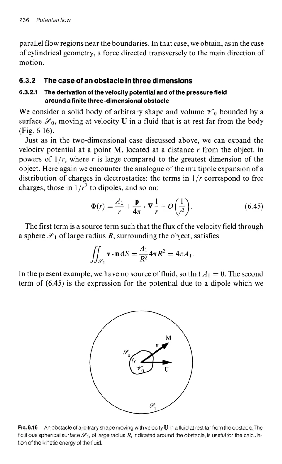
6.3.2 The case of an obstacle in three dimensions 236
6.3.2.1 The derivation of the velocity potential and of the
pressure field around a finite three-dimensional obstacle 236
6.3.2.2 The kinetic energy of the fluid 237
6.3.2.3 Impulse 239
6.3.2.4 The force on a solid object 240
6.3.2.5 The particular case of a spherical object 240
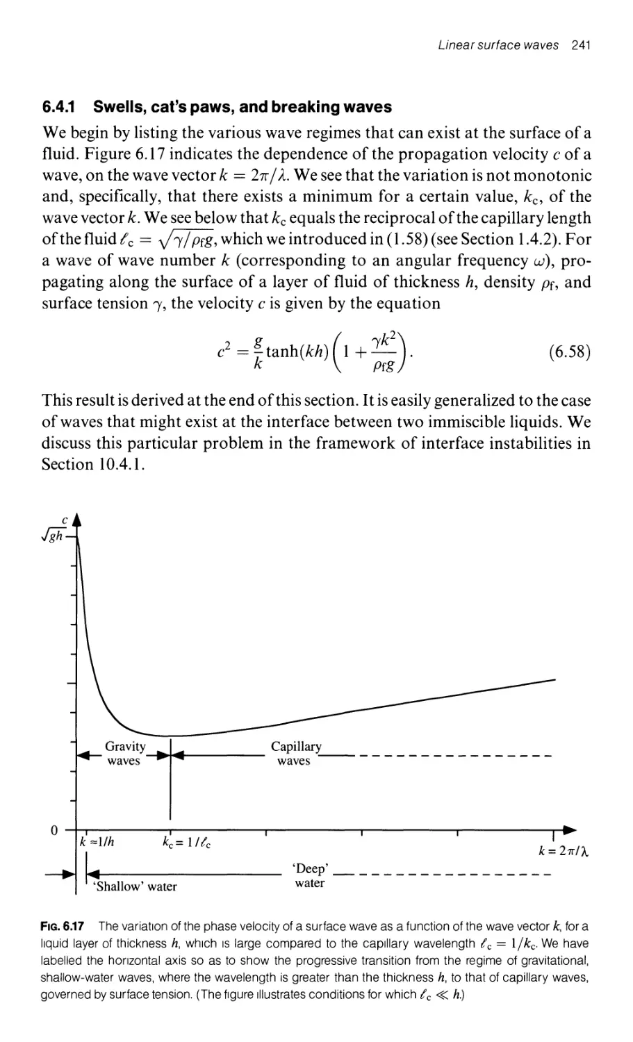
6.4 Linear surface waves on an ideal fluid 240
6.4.1 Swells, cat's paws, and breaking waves 241
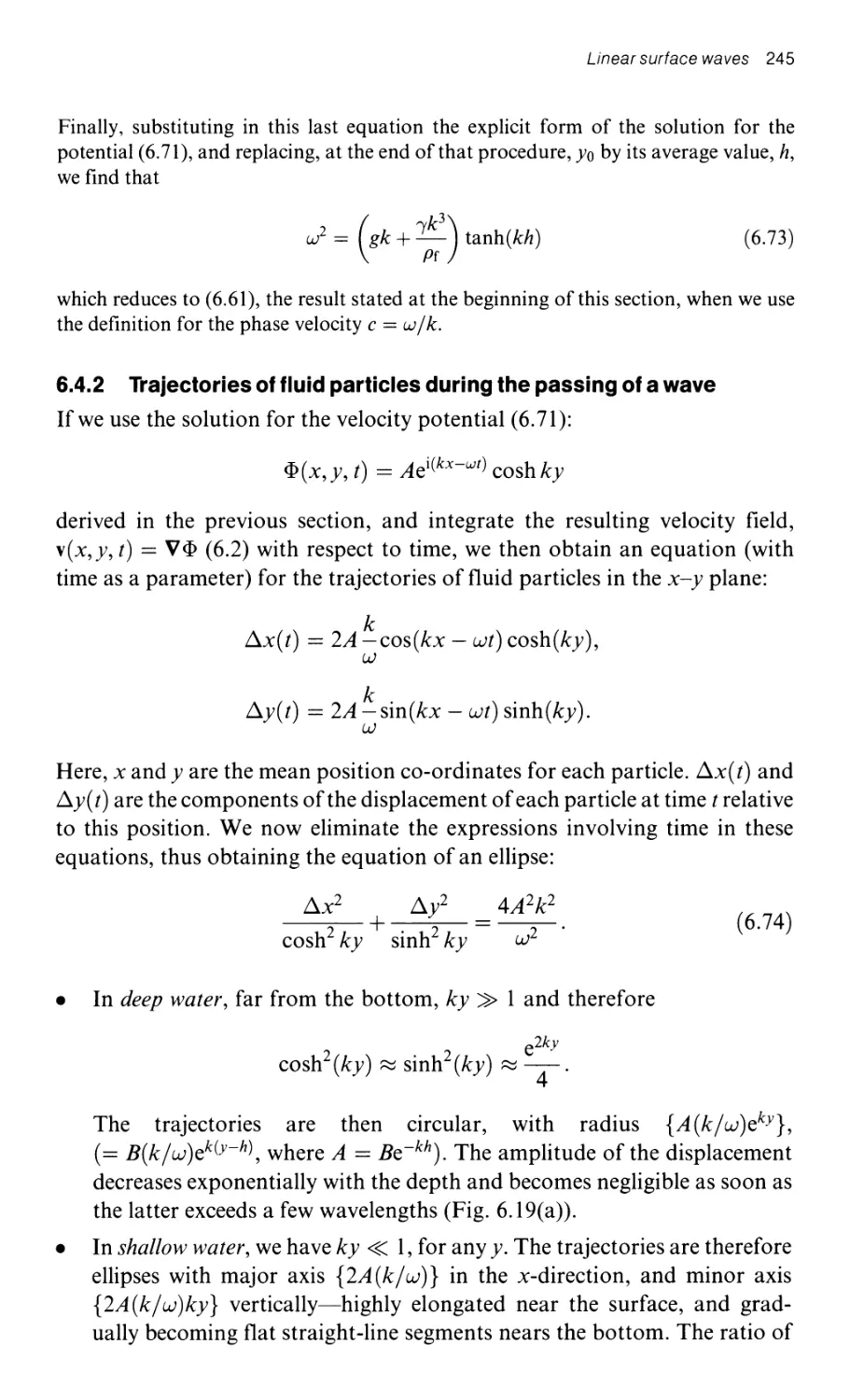
6.4.2 Trajectories of fluid particles during the passing of a wave 245
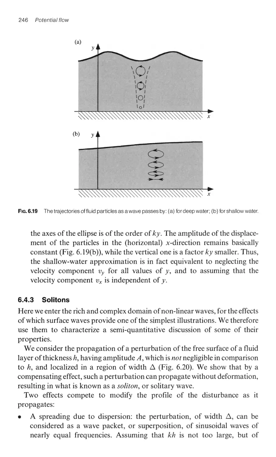
6.4.3 Solitons 246
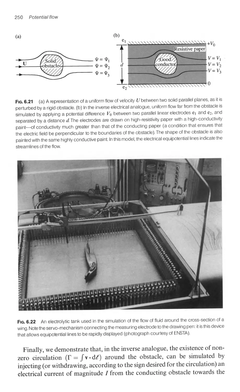
6.5 An electrical analogue for two-dimensional potential flows 248
6.5.1 Direct analogue 249
6.5.2 Inverse analogue 249
6.6 The complex velocity potential 252
6.6.1 The definition of a complex potential 252
6.6.2 Complex potentials for several types of flow 253
6.6.2.1 Uniform parallel flow 253
6.6.2.2 Source and vortex 253
6.6.2.3 Dipole flow 254
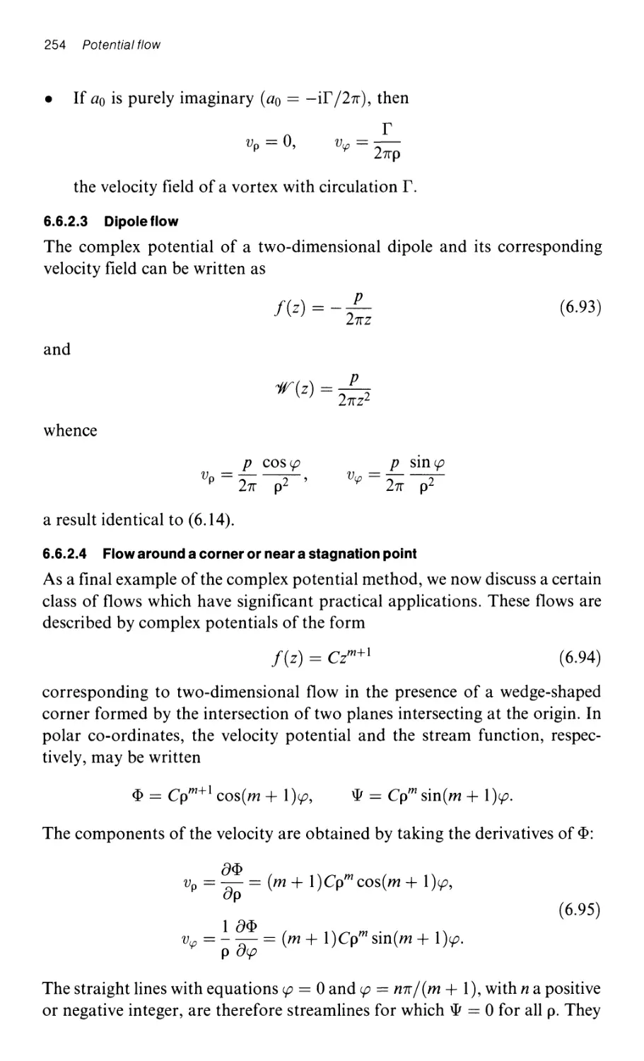
6.6.2.4 Flow around a corner or near a stagnation point 254
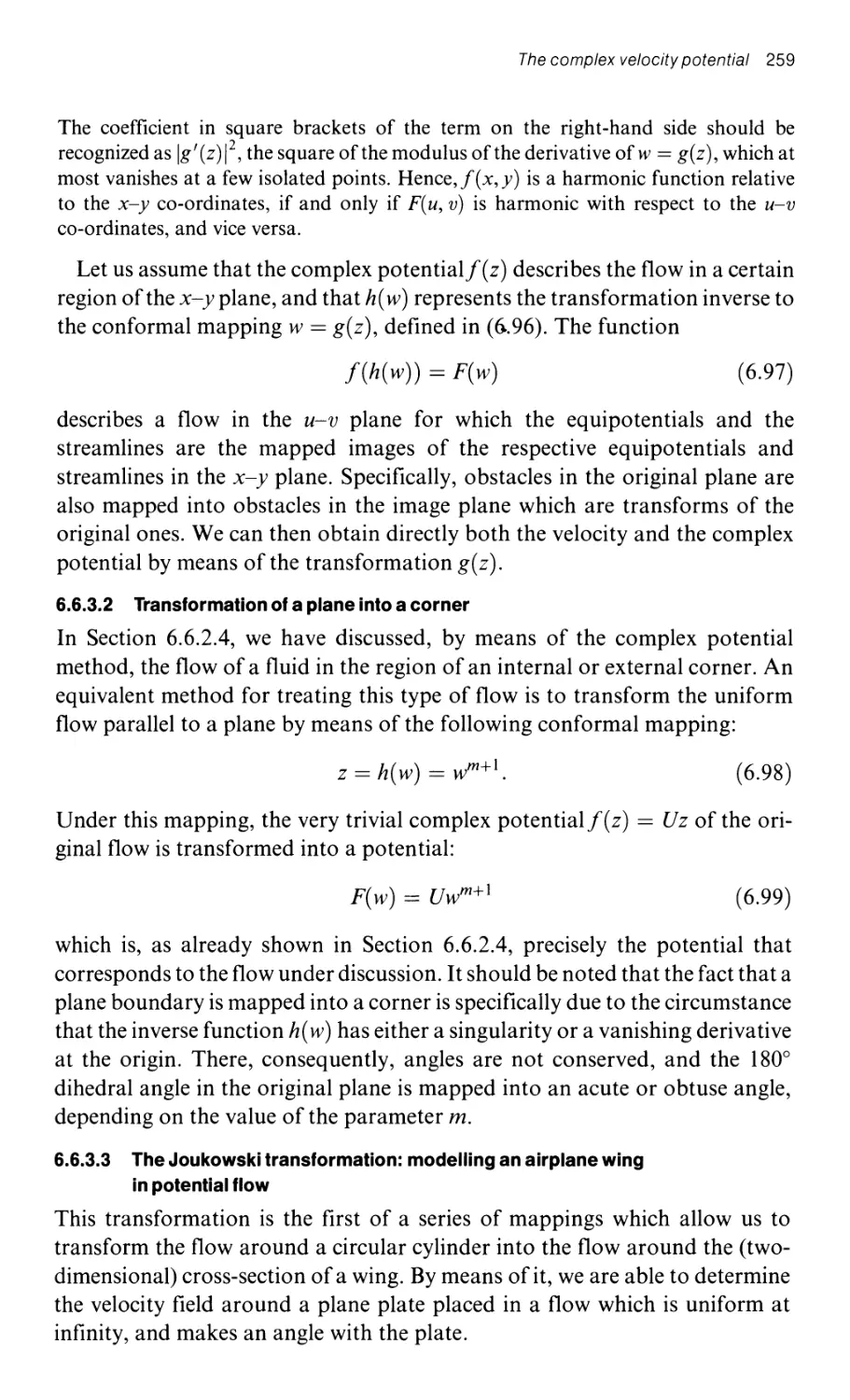
6.6.3 Conformal mapping 256
6.6.3.1 The conformal mapping method 256
6.6.3.2 Transformation of a plane into a corner 259
6.6.3.3 The Joukowski transformation: modelling
an airplane wing in potential flow 259
Contents xvii
Appendix A1: velocity potentials and stream functions for two-dimensional flows 266
Appendix A2 267
A2.1 Derivation of the velocity components from
the stream function
A2.2 Derivation of the velocity components from
the velocity potentia!
267
267
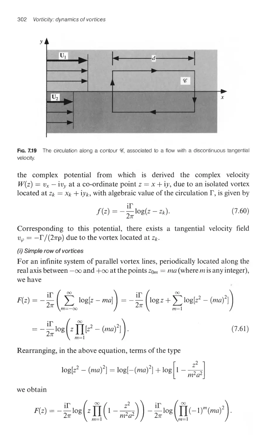
7 Vorticity: dynamics of vortices 268
7.1 Vorticity and its electromagnetic analogue 268
7.1.1 The vorticity vector 268
7.1.2 The electromagnetic analogue 269
7.1.3 Straight vortex tubes: the analogy with the magnetic field
due to a current-carrying wire 271
7.1.3.1 The magnetic field around a straight wire and
velocity field resulting from a straight vortex tube 271
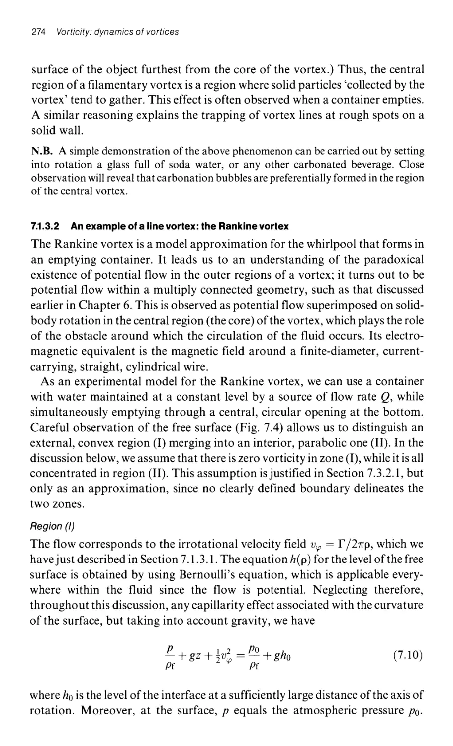
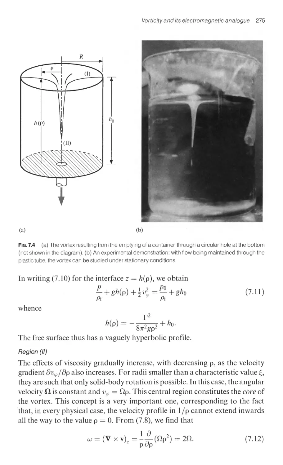
7.1.3.2 An example of a line vortex: the Rankine vortex 274
7.1.3.3 The kinetic energy per unit length of a line vortex 276
7.1.4 The application of the electromagnetic analogy in
dealing with arbitrary distributions of vorticity 277
7.1.4.1 The hyd rodynamic equivalent of the law of
Biot and Savart 277
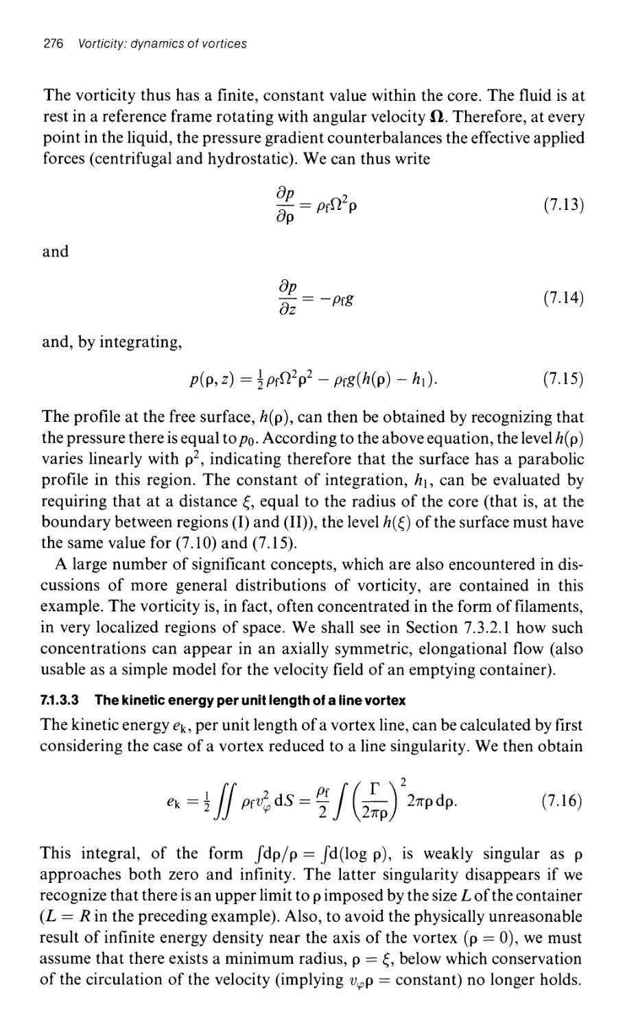
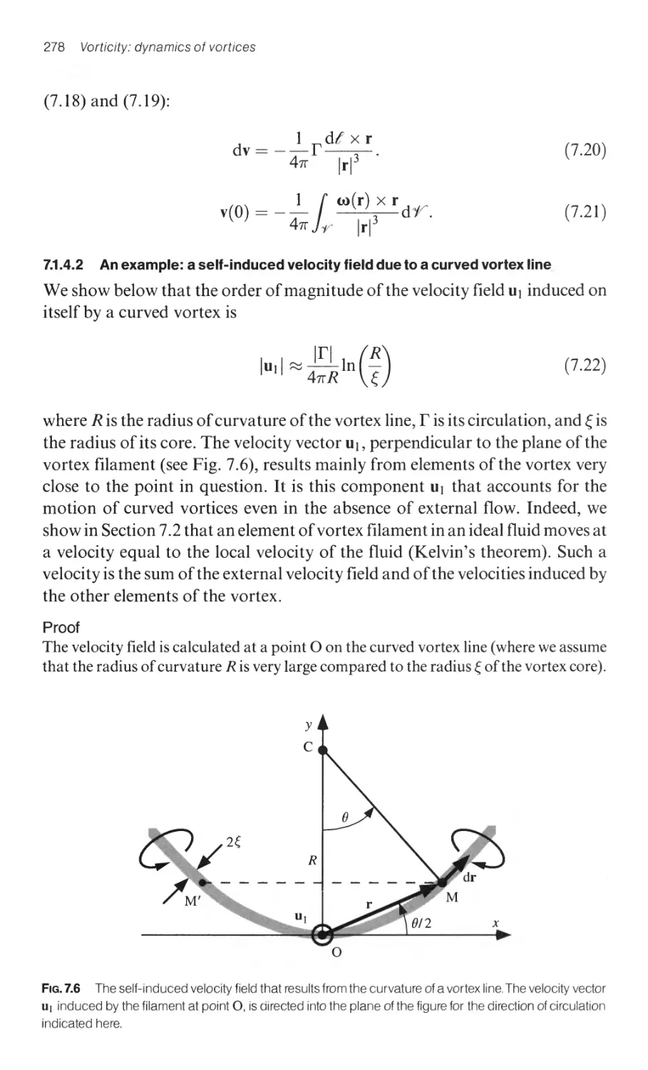
7.1.4.2 An example: a self-induced velocity field
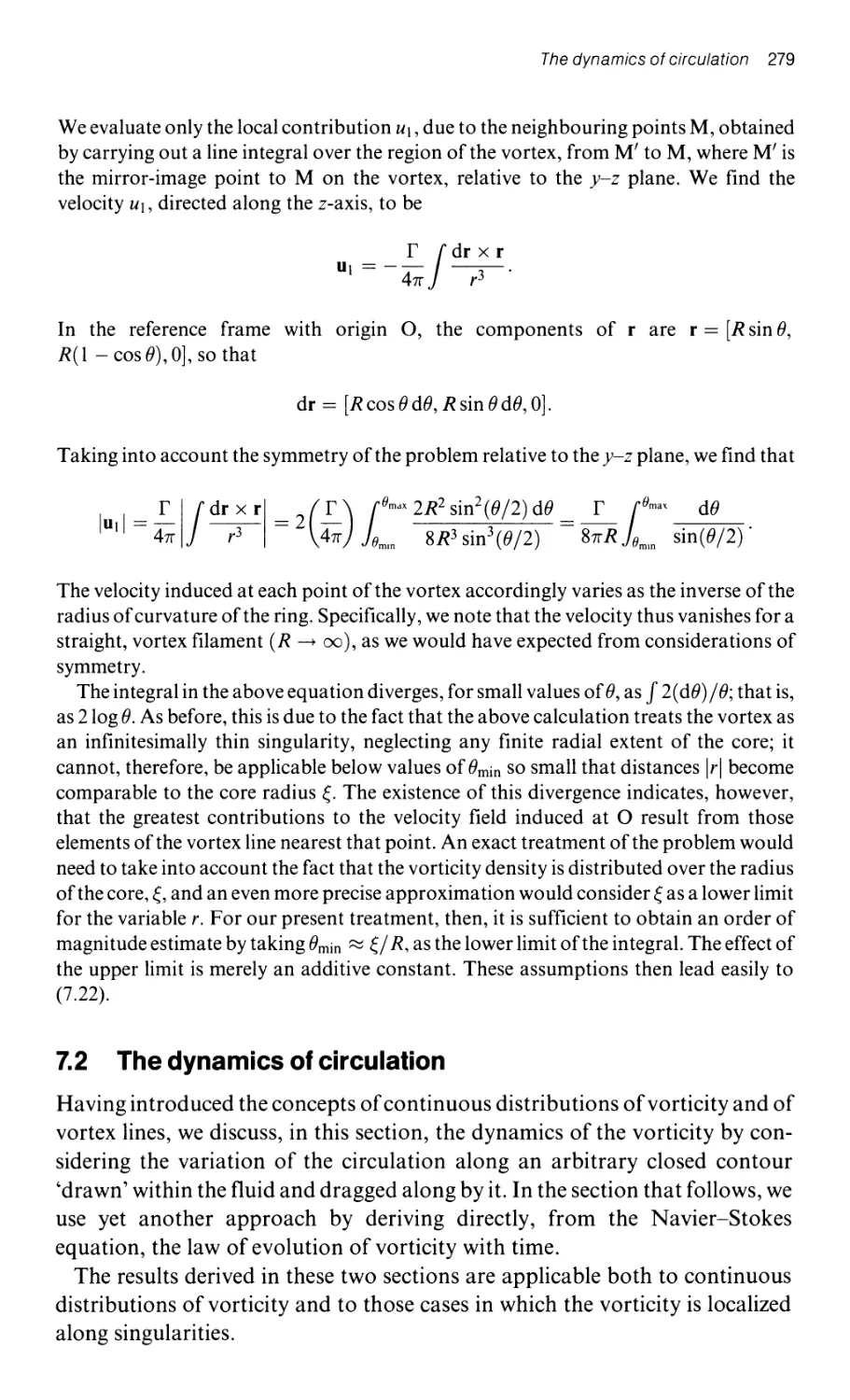
due to a curved vortex line 278
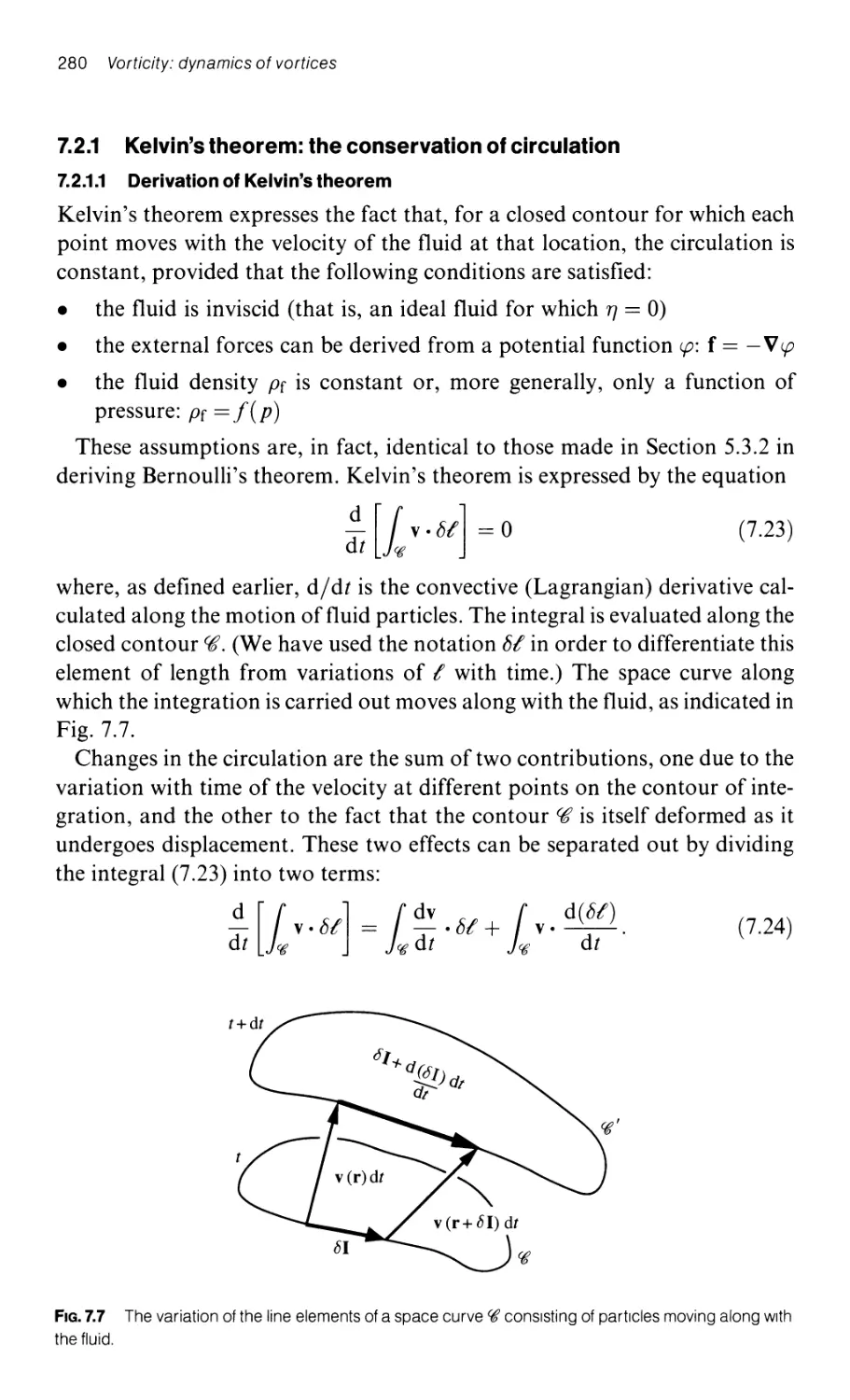
7.2 The dynamics of circulation 279
7.2.1 Kelvin's theorem: the conservation of circulation 280
7.2.1.1 Derivation of Kelvin's theorem 280
7.2.1.2 The physical significance and
consequences of Kelvin's theorem 281
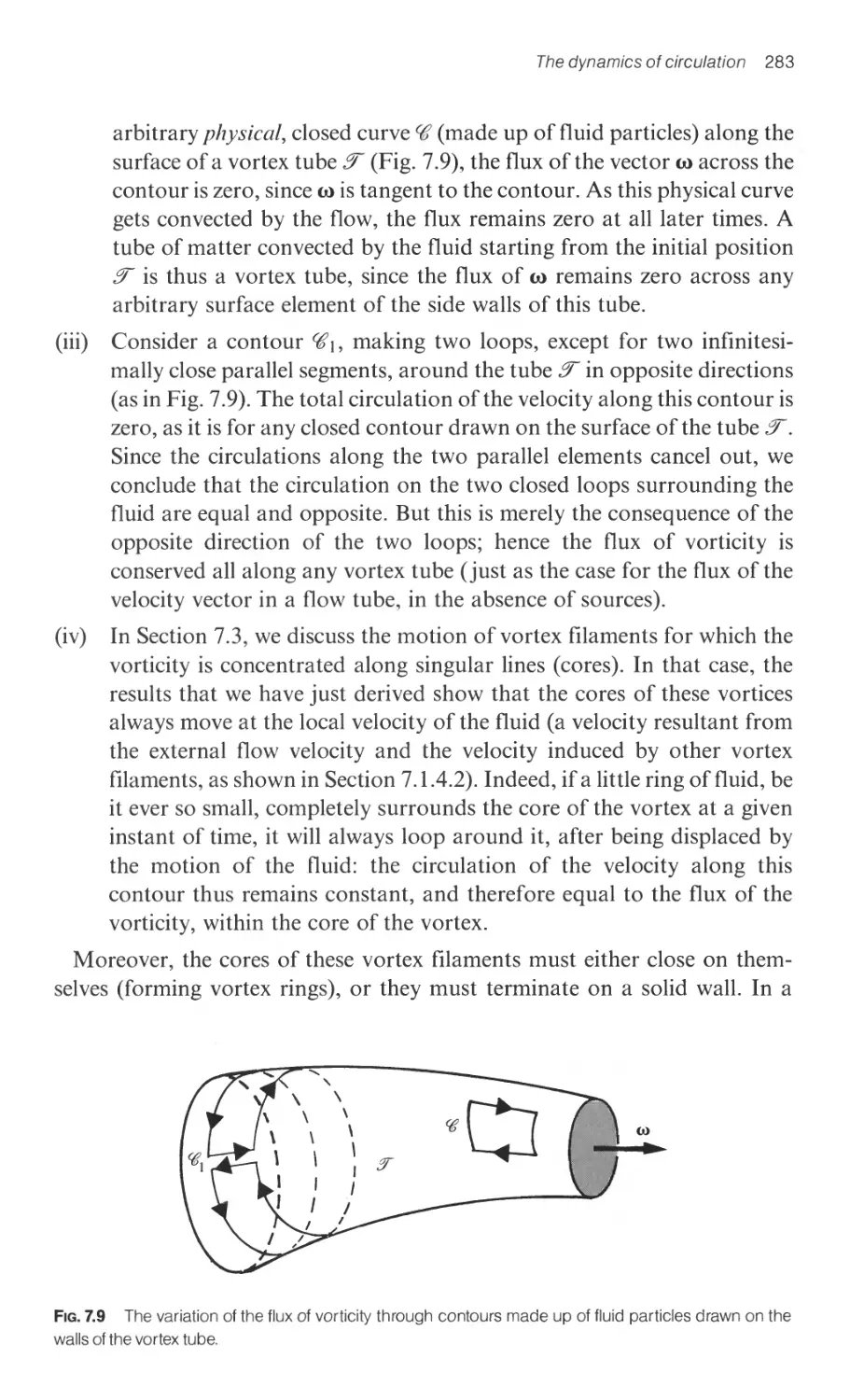
7.2.2 Sources of circulation in the flow of VISCOUS or compressible
fluids, or in the presence of non-conservative forces 284
7.2.2.1 Non-conservative volume forces (term I of (7.30)) 284
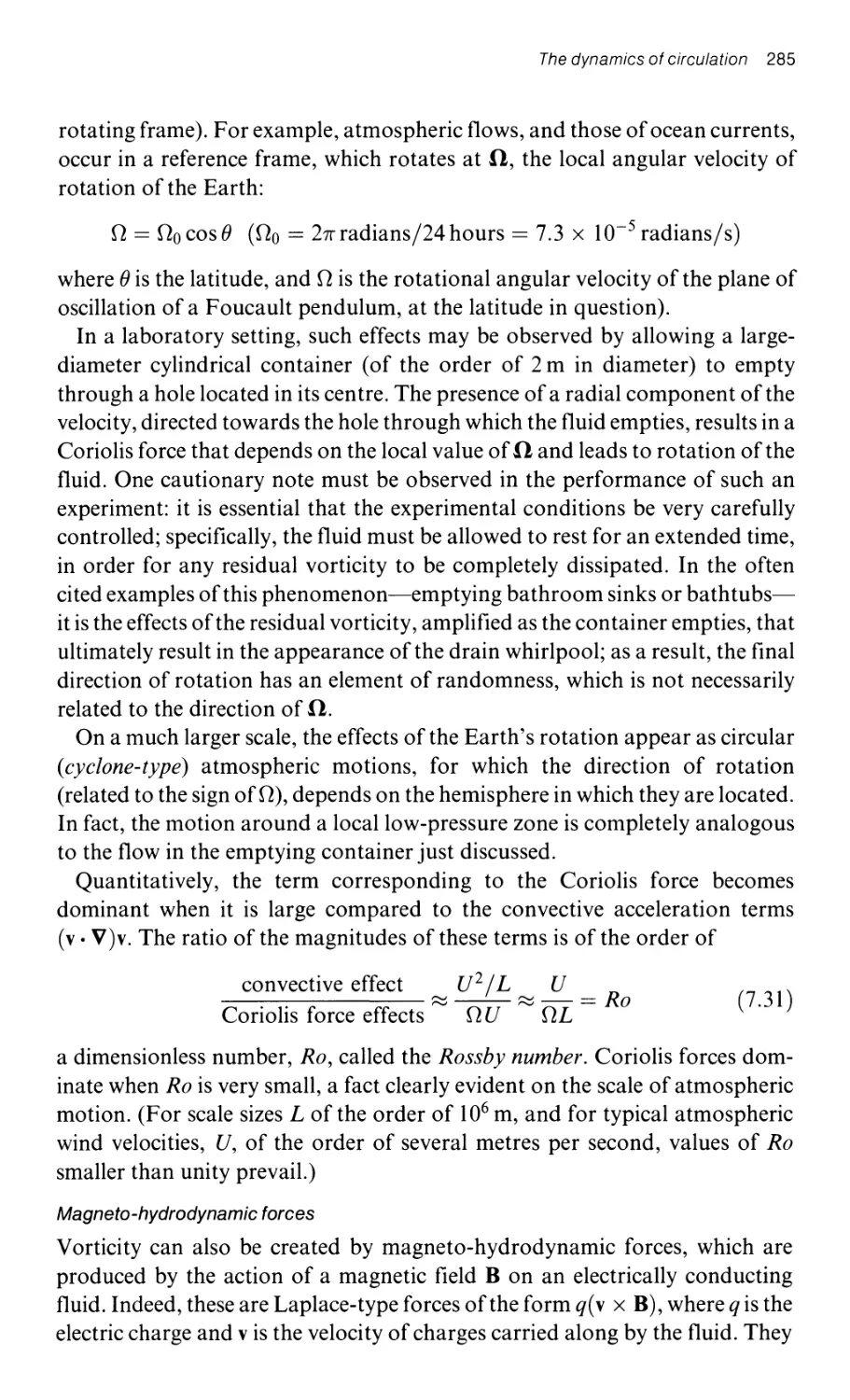
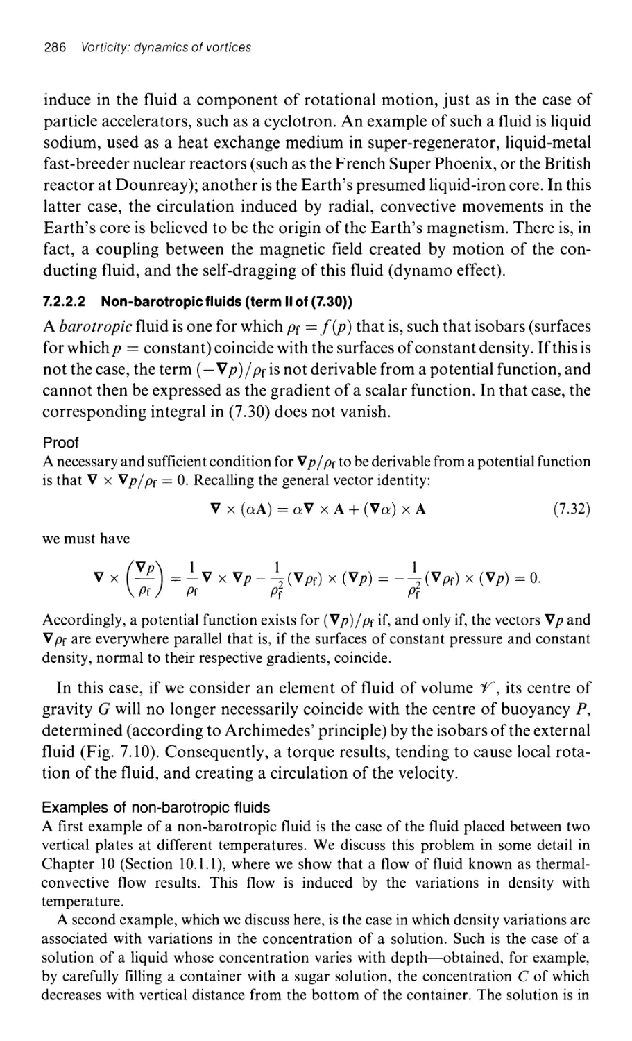
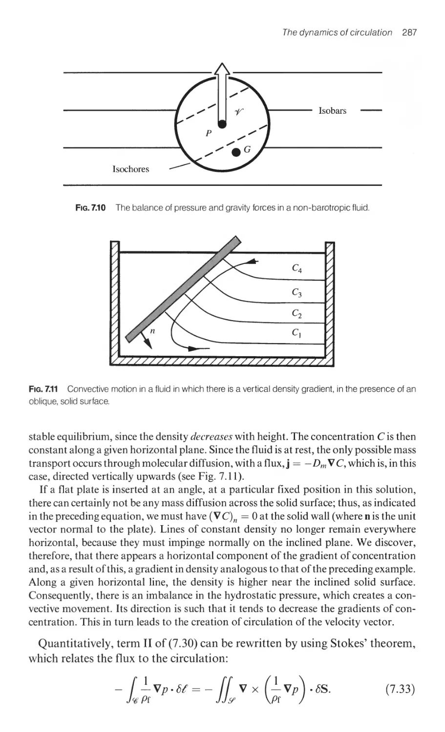
7.2.2.2 Non-barotropic fluids (term II of (7.30)) 286
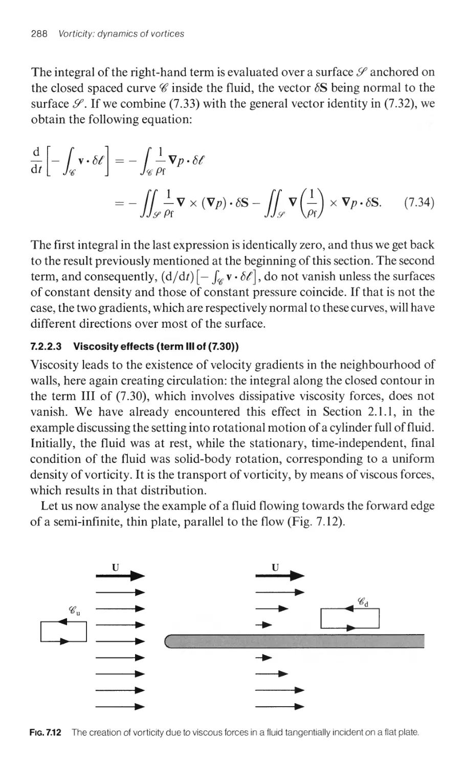
7.2.2.3 Viscosity effects (term III of (7.30)) 288
7.3 The dynamics of vorticity 289
7.3.1 The transport equation for vorticity, and its consequences 289
7.3.1.1 The Helmholtz equation for an incompressible fluid 289
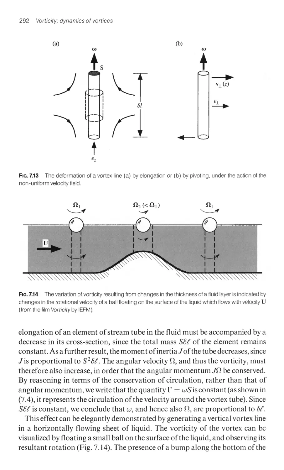
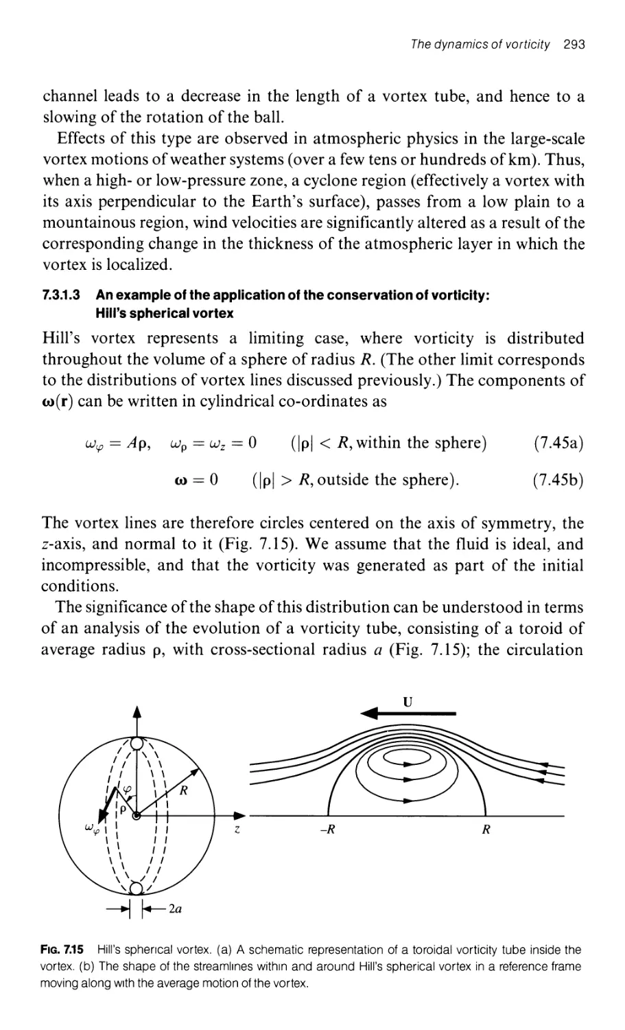
7.3.1.2 Elongation and twisting of vortex tubes 291
7.3.1.3 An example of the application of the
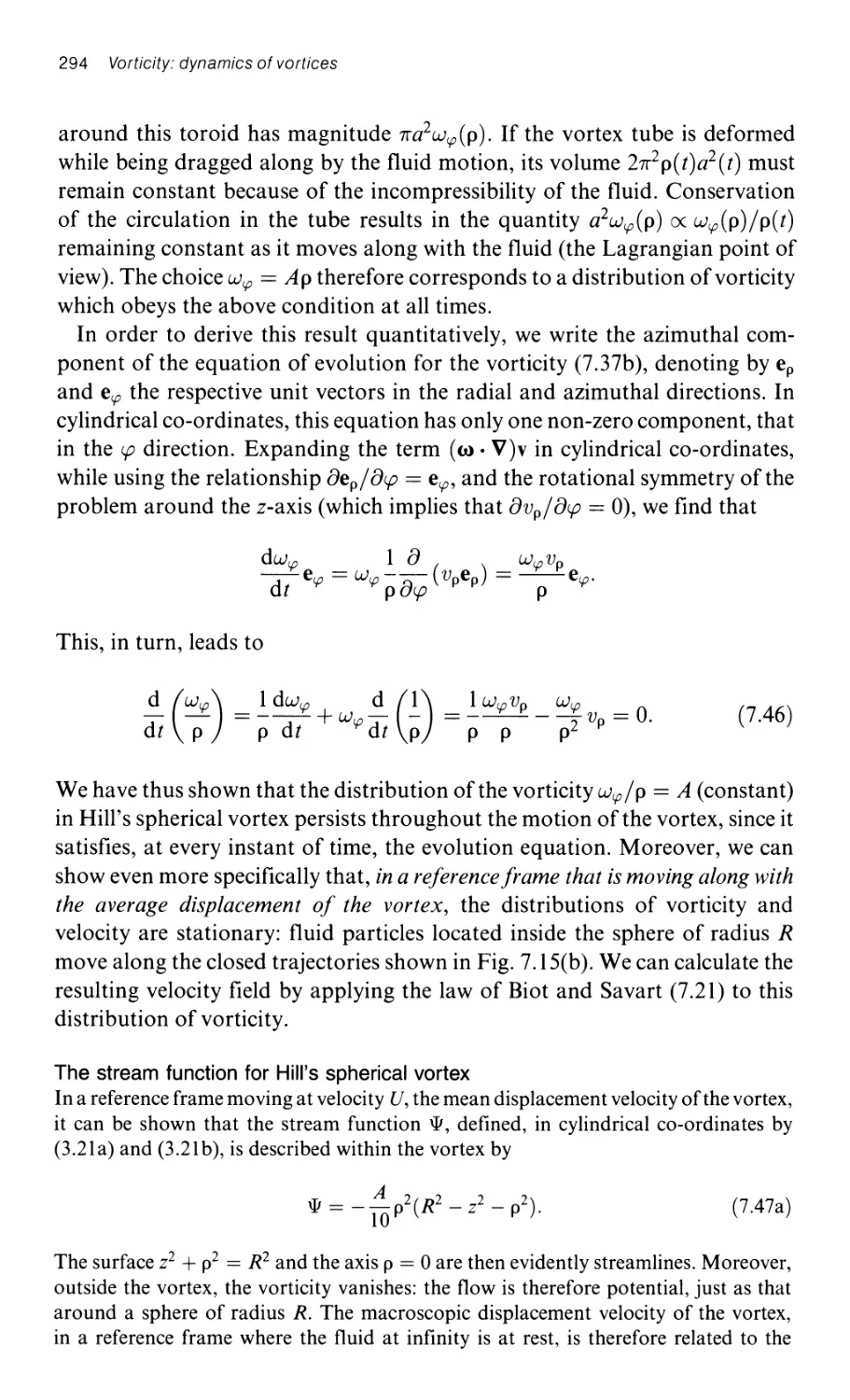
conservation of vorticity: Hill's spherical vortex 293
7.3.2 Equilibrium between elongation and diffusion in
the dynamics of vorticity 295
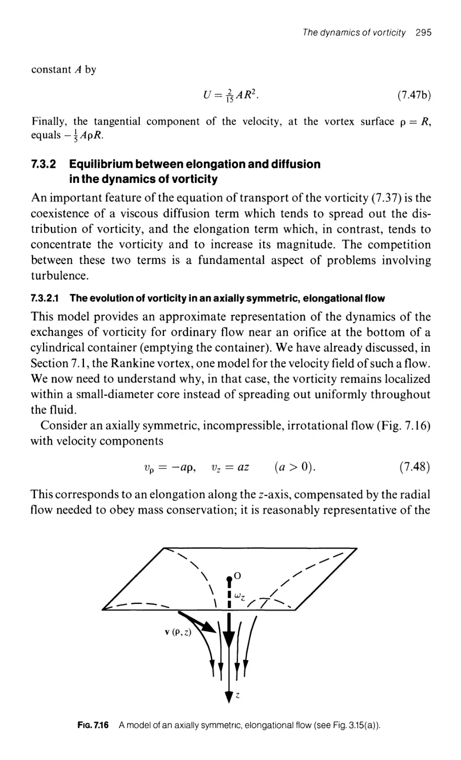
7.3.2.1 The evolution of vorticity in an axially
symmetric, elongational flow 295
7.3.2.2 The creation and annihilation of vorticity in turbulent flow 297
7.3.2.3 A qualitative model for turbulence 298
7.4 A few examples of distributions of vorticity concentrated
along singularities: systems of vortex lines 298
7.4.1 A few cases with vorticity concentrated in vortex filaments 298
xviII Contents
7.4.2 The dynamics of a system of parallel line vortices
7.4.2.1 Parallel, line-vortex paIrs
7.4.2.2 Continuous and discrete vortex sheets
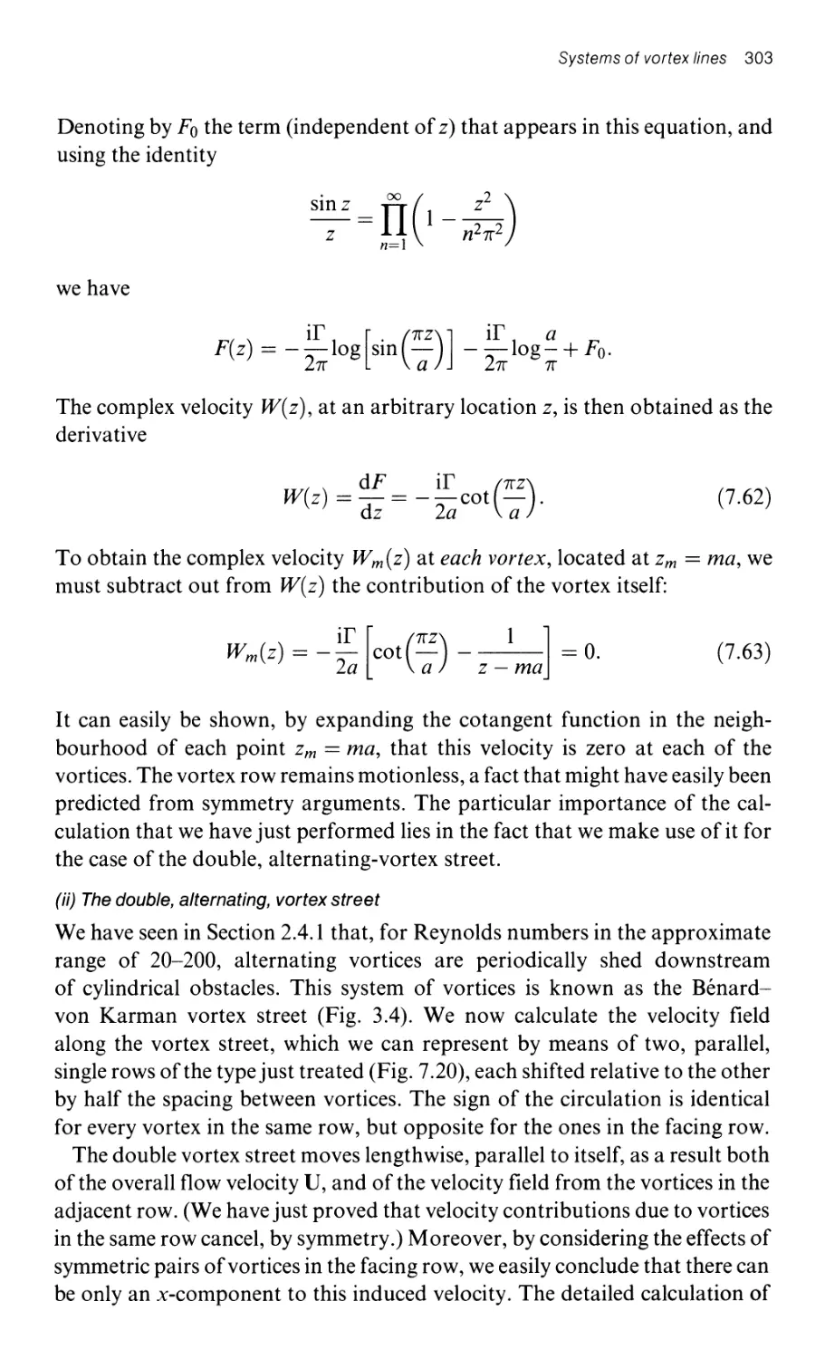
7.4.2.3 Vortex streets
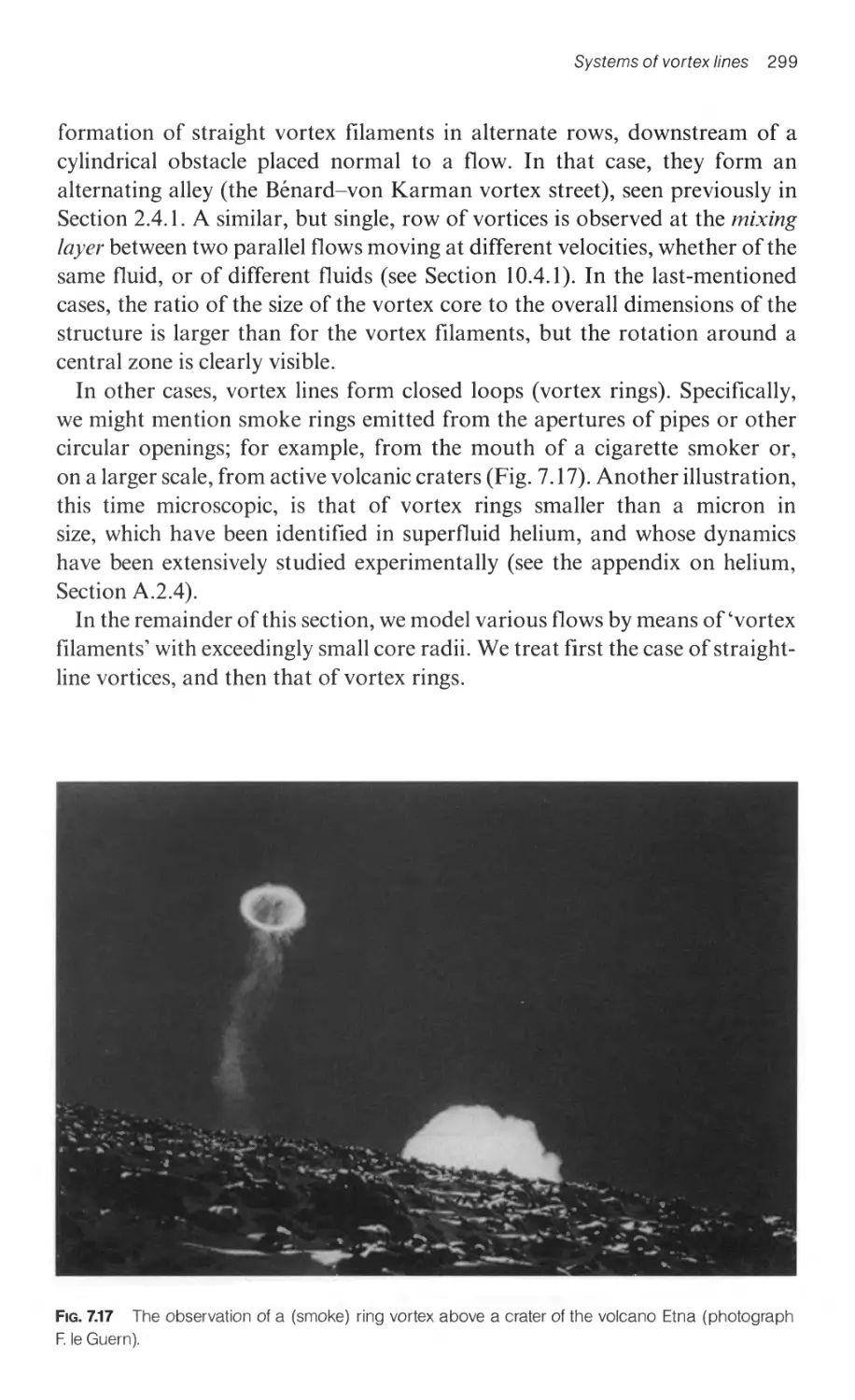
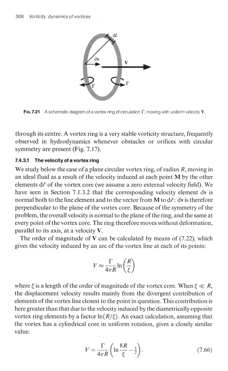
7.4.3 Vortex rings
7.4.3.1 The velocity of a vortex ring
7.4.3.2 The kinetic energy of a vortex ring
7.4.3.3 The momentum of a vortex ring
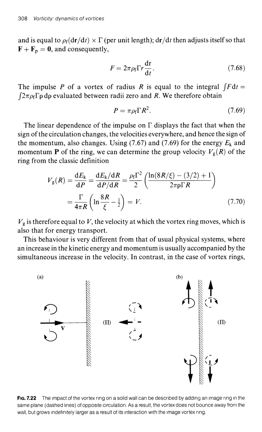
7.4.3.4 Interactions between vortex rings, or between
a ring and a solid wall
300
300
301
301
305
306
307
307
310
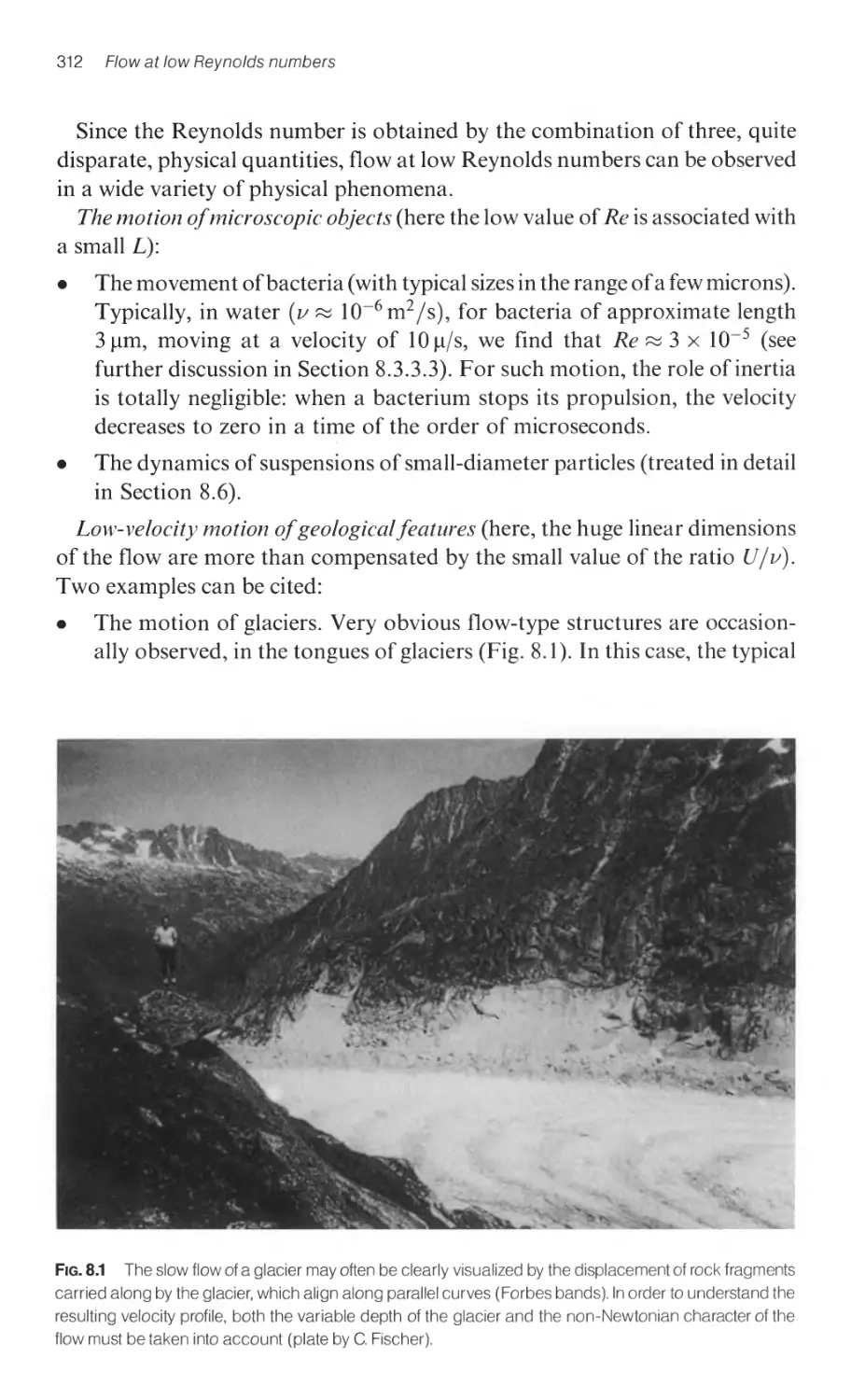
8 Flow at low Reynolds numbers 311
8.1 Examples of low-Reynolds-number flows 311
8.2 The equation of motion at low Reynolds number 313
8.2.1 The Stokes equation 313
8.2.2 Further equivalent representations of the Stokes equation 314
8.2.3 Properties of solutions of the Stokes equation 31
8.2.3.1 Uniqueness 315
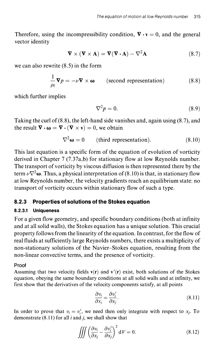
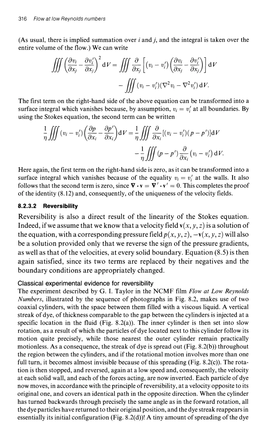
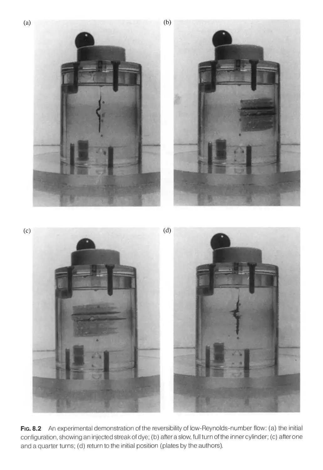
8.2.3.2 Reversibility 316
8.2.3.3 Superposition in the solutions of the Stokes equation 321
8.2.3.4 A minimum in the energy dissipation 322
8.2.4 Dimensional-analysis predictions for flows at low
Reynolds number 323
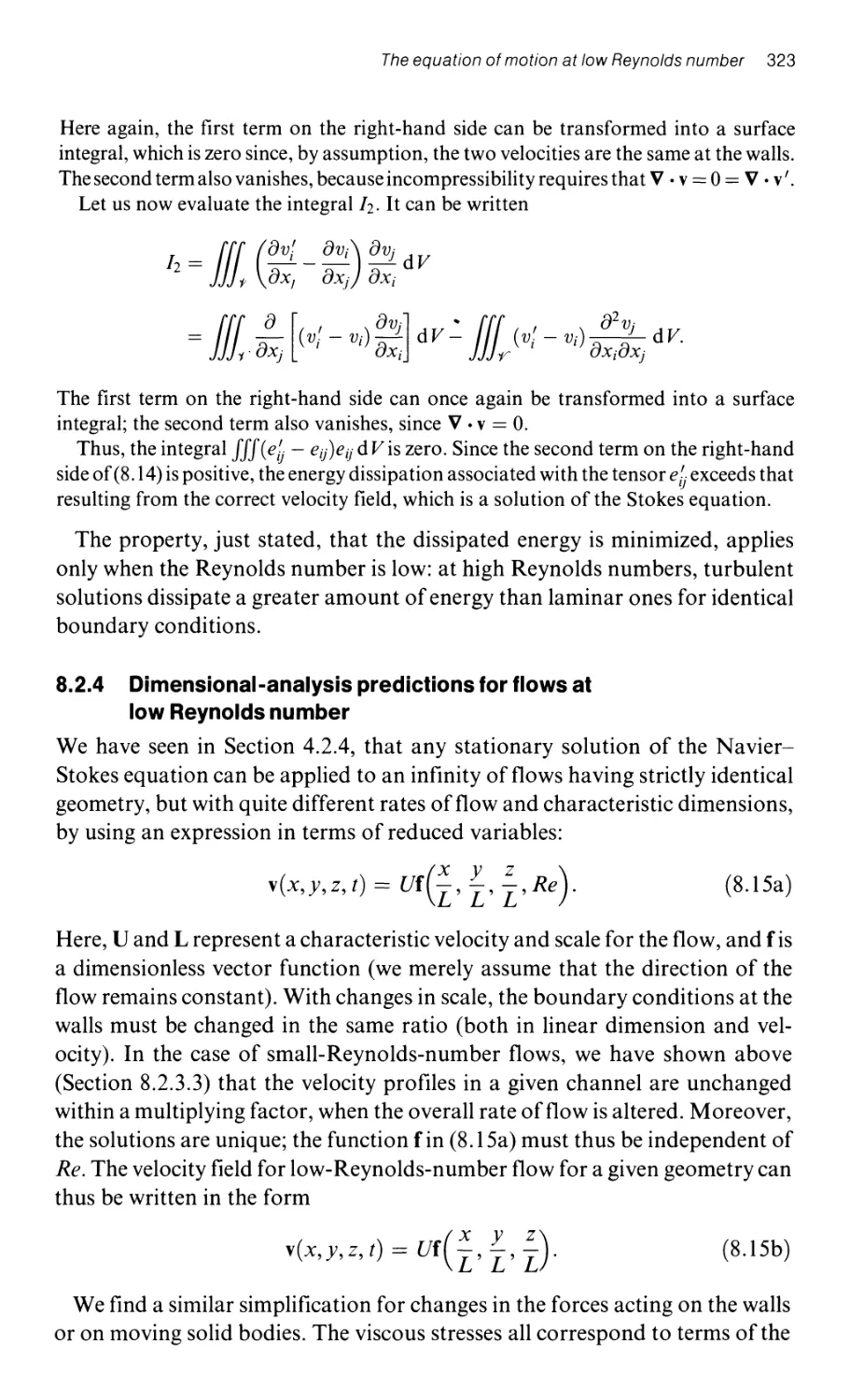
8.3 The forces and torques acting on a moving solid body 324
8,3.1 Linear proportionality between the velocity of
the solid body and the external forces 325
8.3.2 General symmetry properties of the tensors AU, Bill C ll . and D(J 326
8.3.3 The effect of the symmetry of solid bodies on
the applied forces and torques 327
8.3.3.1 Relationships between tensor coefficients for
a solid body having a plane of symmetry 328
8.3.3.2 Bodies with three mutually perpendicular
planes of symmetry 329
8.3.3.3 Translational-rotational coupling for a body
devoid of planes of symmetry 331
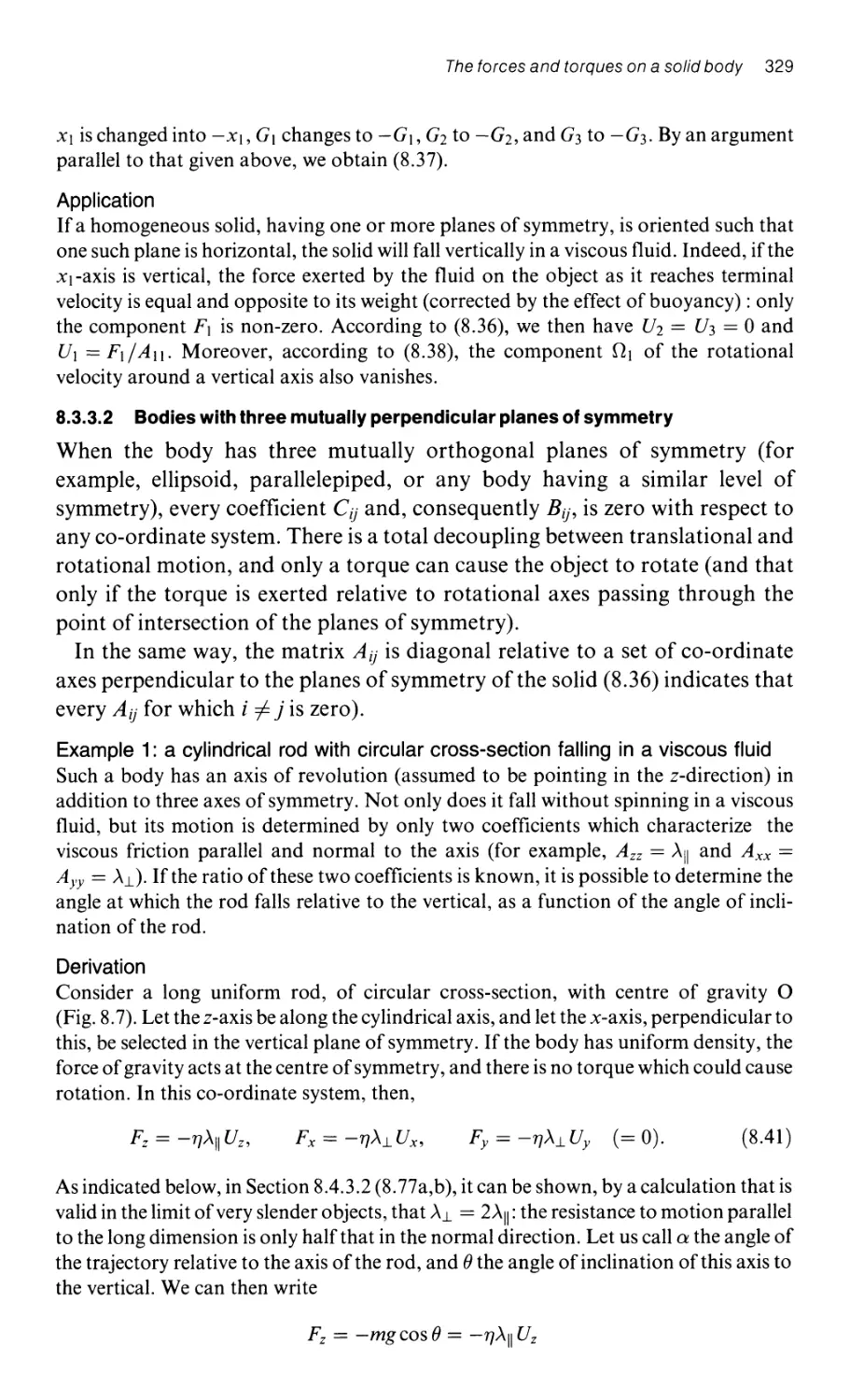
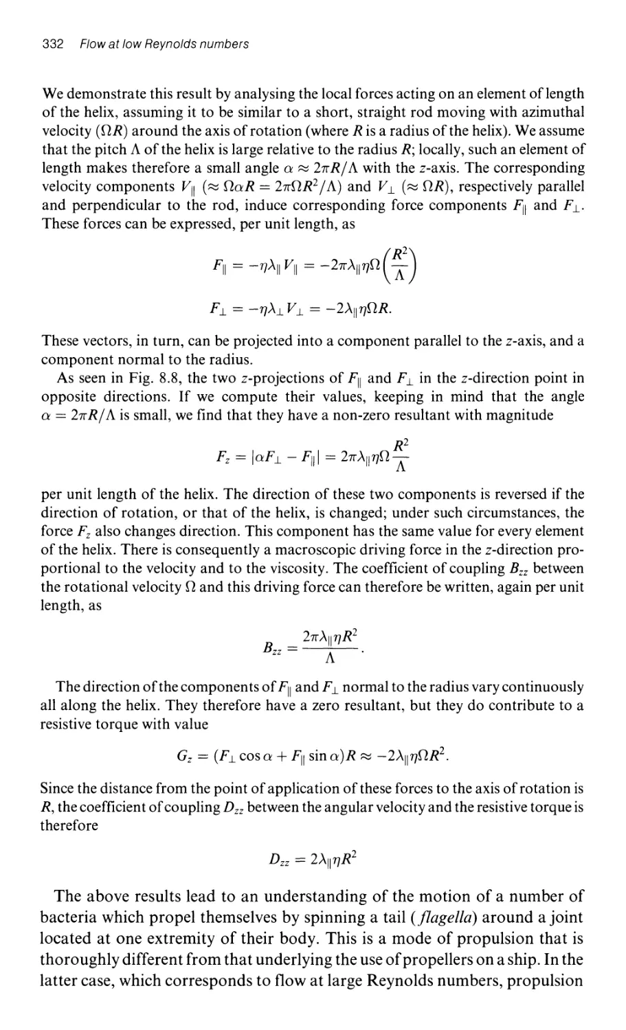
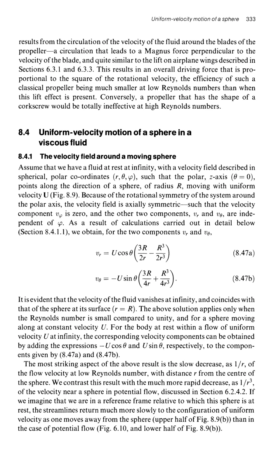
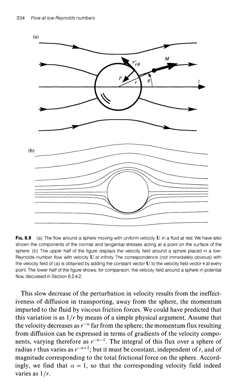
8.4 Uniform-velocity motion of a sphere in a viscous fluid 333
8.4.1 The velocity field around a moving sphere 333
8.4.1.1 Th e calcu I a tio n of th e pressu re fie Id 335
8.4.1.2 The vorticity field corresponding to
the distribution of pressure 335
8.4.1.3 The evaluation of the stream function \II from the vorticity 336
8.4.1.4 The calculation of the velocity field 337
8.4.2 The force acting on a moving sphere in a fluid of infinite extent:
the drag coefficient 338
8.4.3 The generalization of the solution of the Stokes equation to
other experiments 340
8.4.3.1 A drop of fluid in motion within another immiscible fluid 340
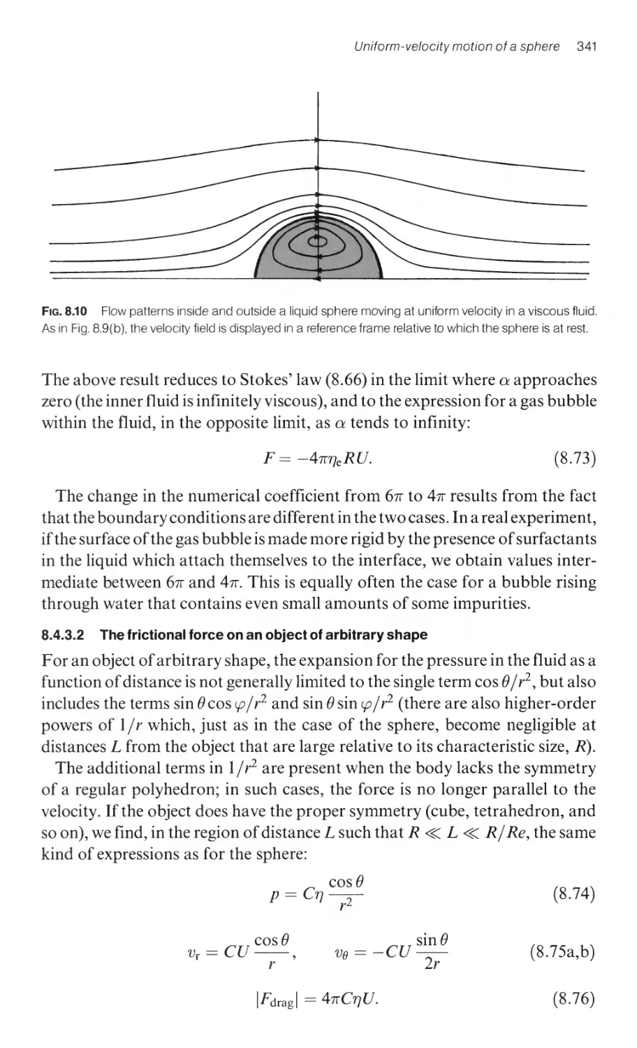
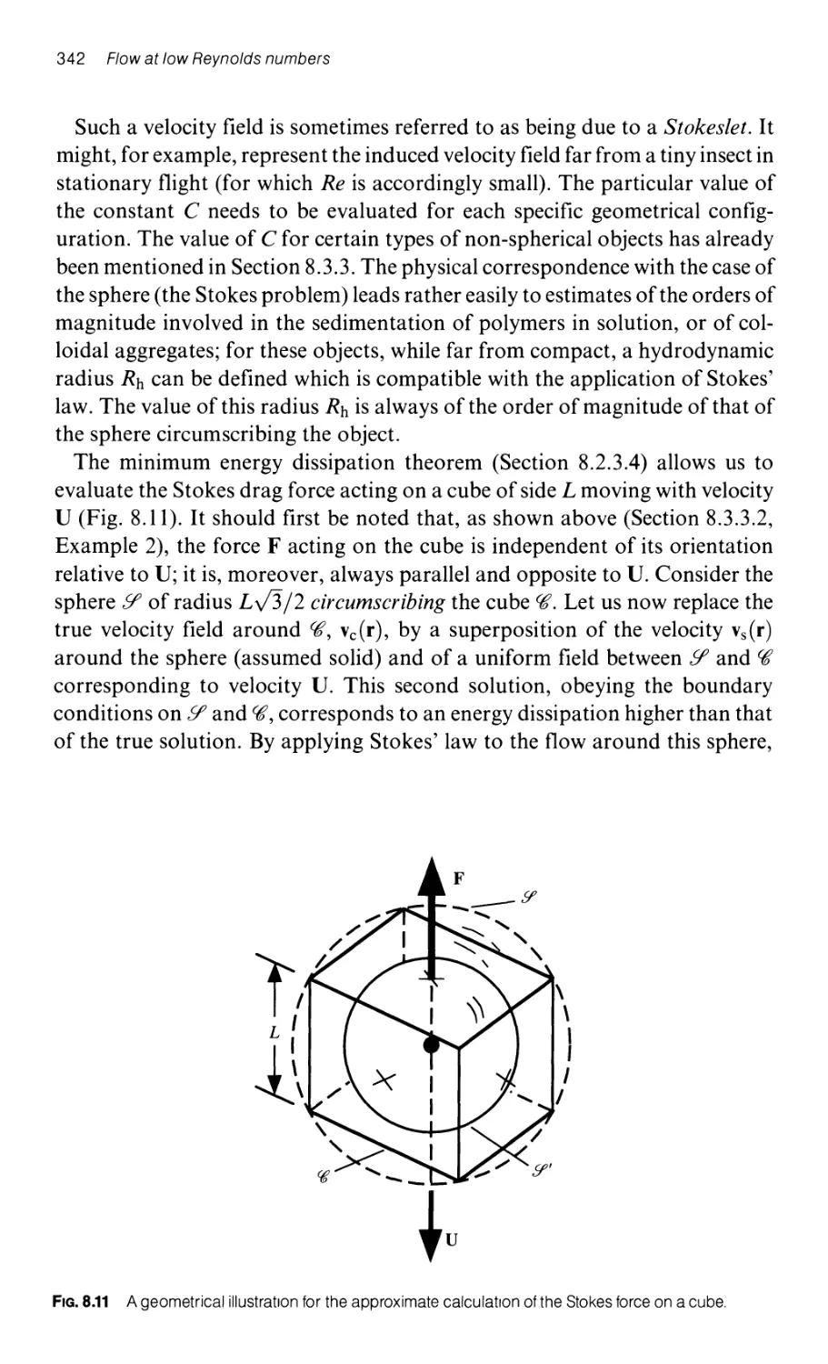
8.4.3.2 The frictional force on an object of arbitrary shape 341
Contents xix
8.4.4 Limitations on the Stokes treatment of flow at
low Reynolds numbers: the Oseen equation 343
8.4.4.1 The kinetic energy of the fluid flowing far from the sphere 344
8.4.4.2 Convection and acceleration effects far from the sphere:
the Oseen equation 344
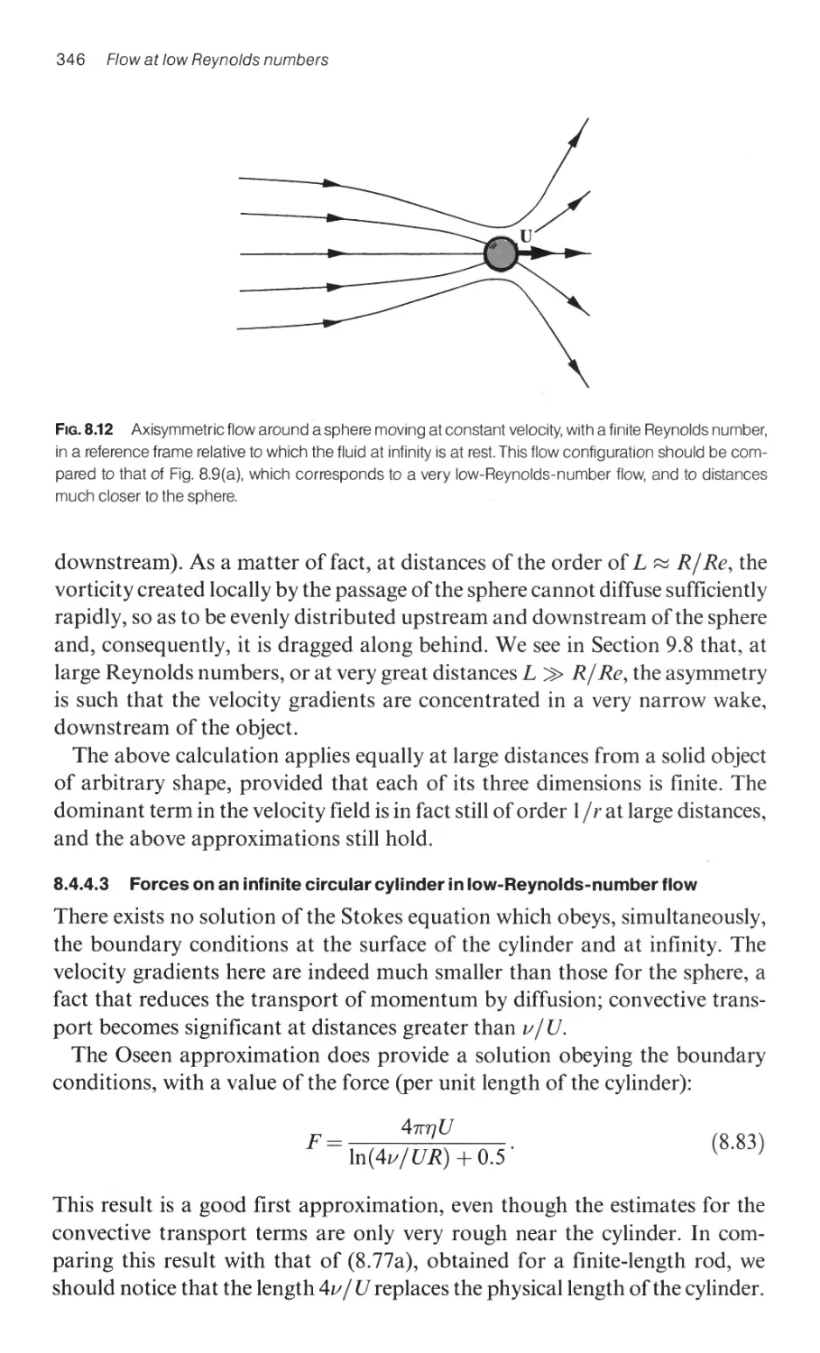
8.4.4.3 Forces on an infinite circular cylinder in
low-Reynolds-number flow 346
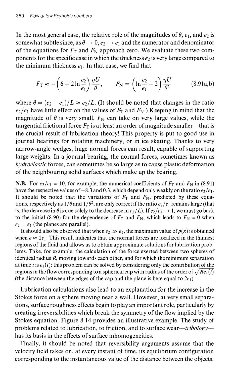
8.5 QuasI-parallel flows at low Reynolds numbers: lubrication 347
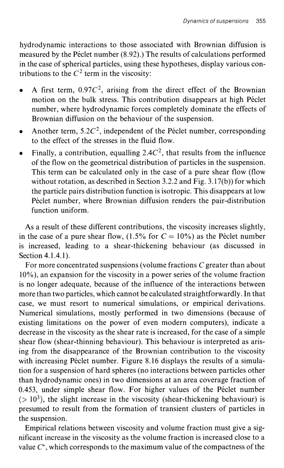
8.6 Dynamics of suspensions 351
8.6.1 The rheology of suspensions 352
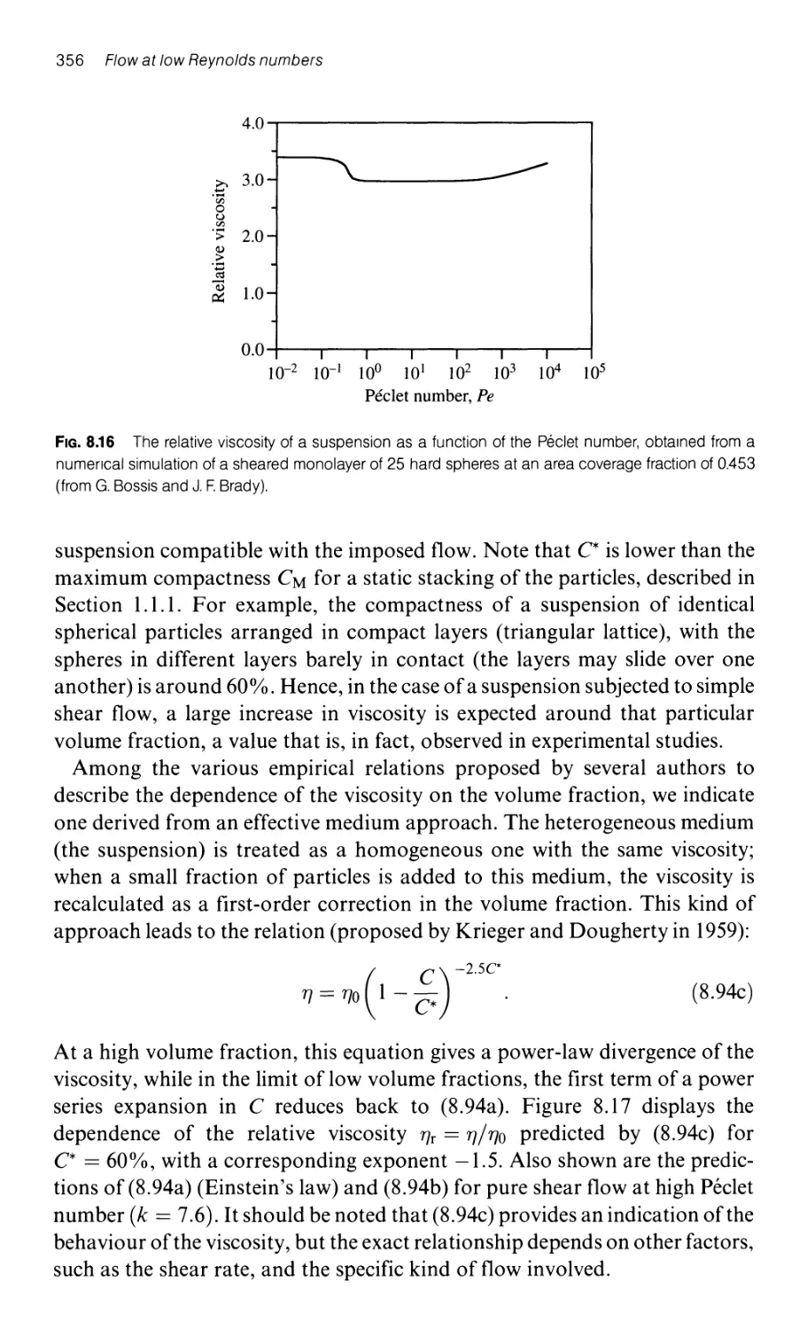
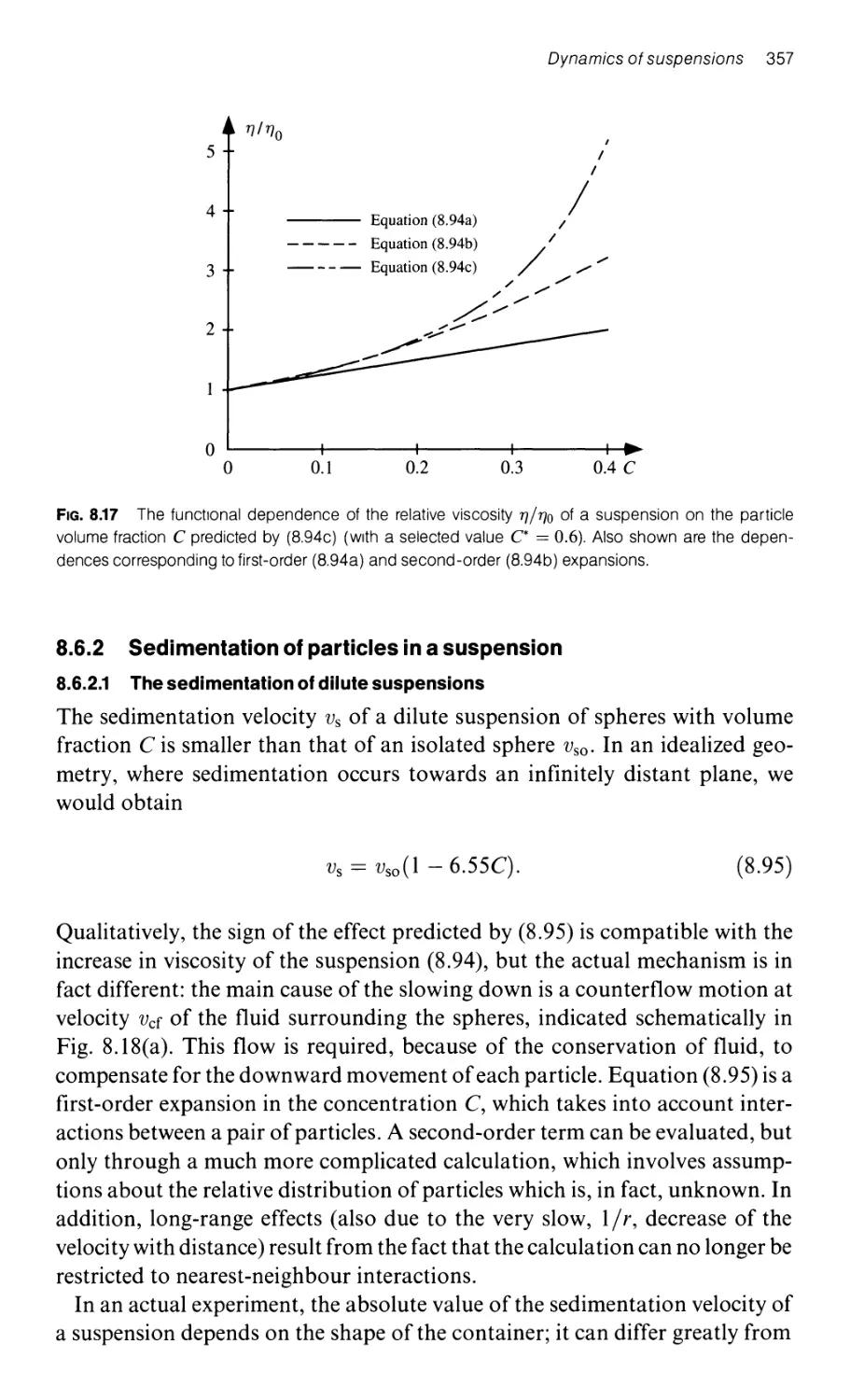
8.6.2 Sedimentation of particles in a suspension 357
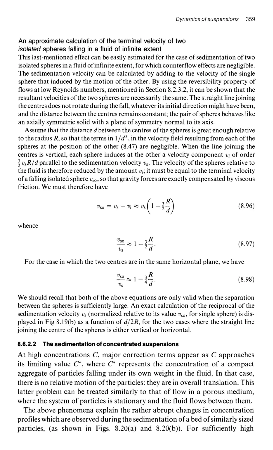
8.6.2.1 The sedimentation of dilute suspensions 357
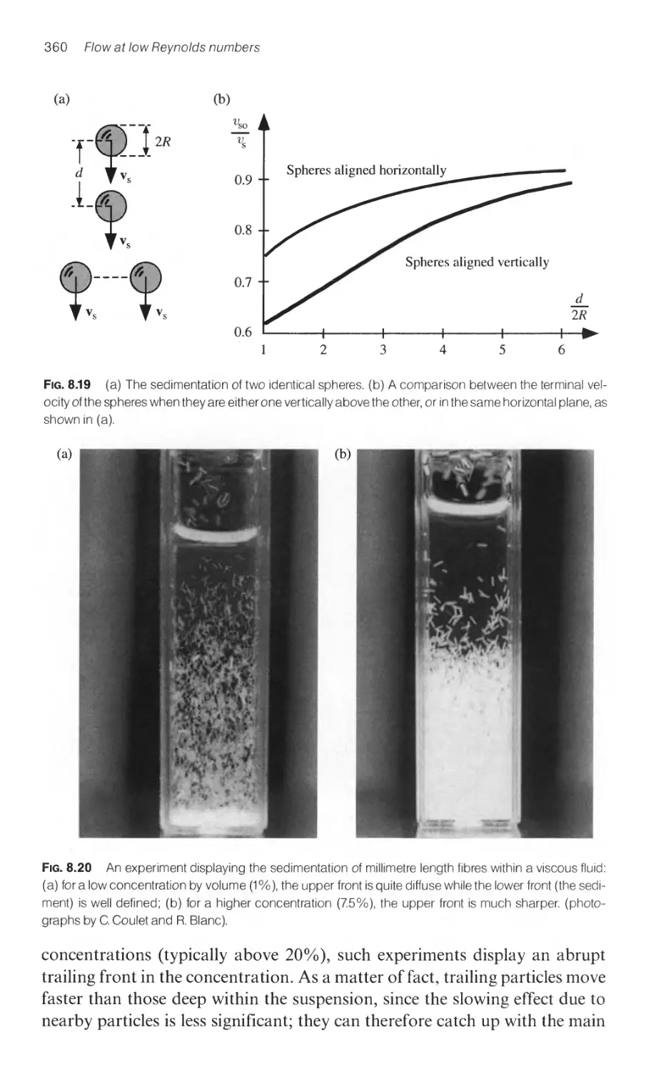
8.6.2.2 The sedimentation of concentrated suspensions 359
8.7 Flow in porous media 361
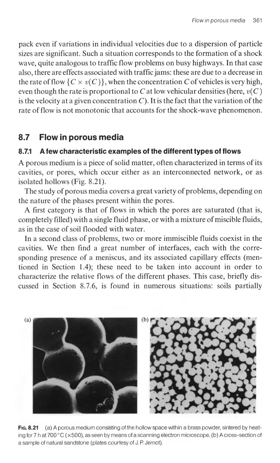
8.7.1 A few characteristic examples of the different types of flows 361
8.7.2 Parameters characterising a porous medium 362
8.7.2.1 Porosity 362
8.7.2.2 Pore size 362
8.7.2.3 Pore geometry 362
8.7.2.4 Length scales characteristic of porous media 364
8.7.3 Flow in porous media: Darcy's law 366
8.7.3.1 One-dimensional low-velocity flow 366
8.7.3.2 The Darcy equation generalized to three
dimensions 367
8.7.3.3 The pressure-flow rate relation at high velocities
in a porous medium 368
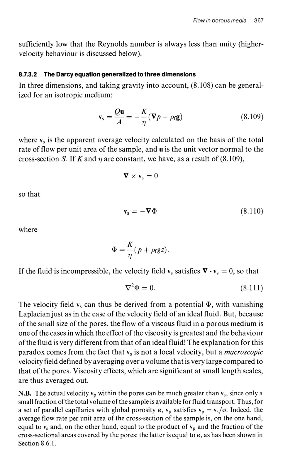
8.7.3.4 A two-dimensional model of a porous medium:
the Hele-Shaw cell 368
8.7.4 Permeability models for media with cylindrical pores 370
8.7.4.1 An estimate of the permeability for a porous
medium modelled by a group of parallel capillaries 370
8.7.4.2 The permeability of a system of winding capillaries 371
8.7.4.3 The Carman-Kozeny relation 372
8.7.5 The permeability of porous media containing channels
of variable cross-section 373
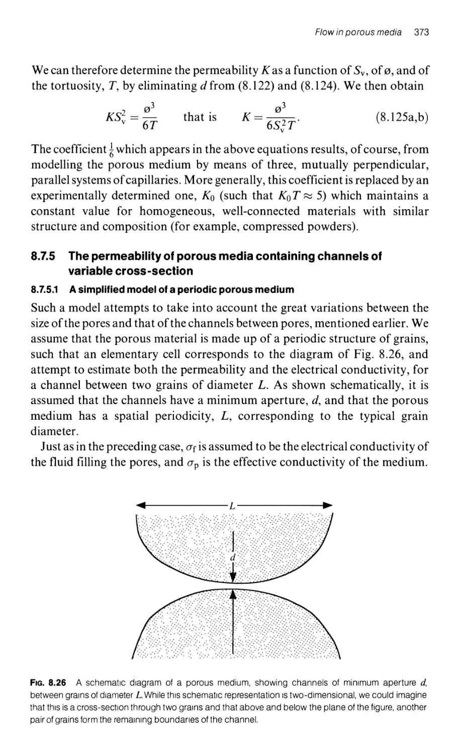
8.7.5.1 A simplified model of a periodic porous medium 373
8.7.5.2 The relationship between the size of the grains,
the permeability, and the electric conductivity for
a medium made from sintered glass beads 374
8.7.5.3 The relationship between the sizes of channels,
the conductivity, and the permeability for
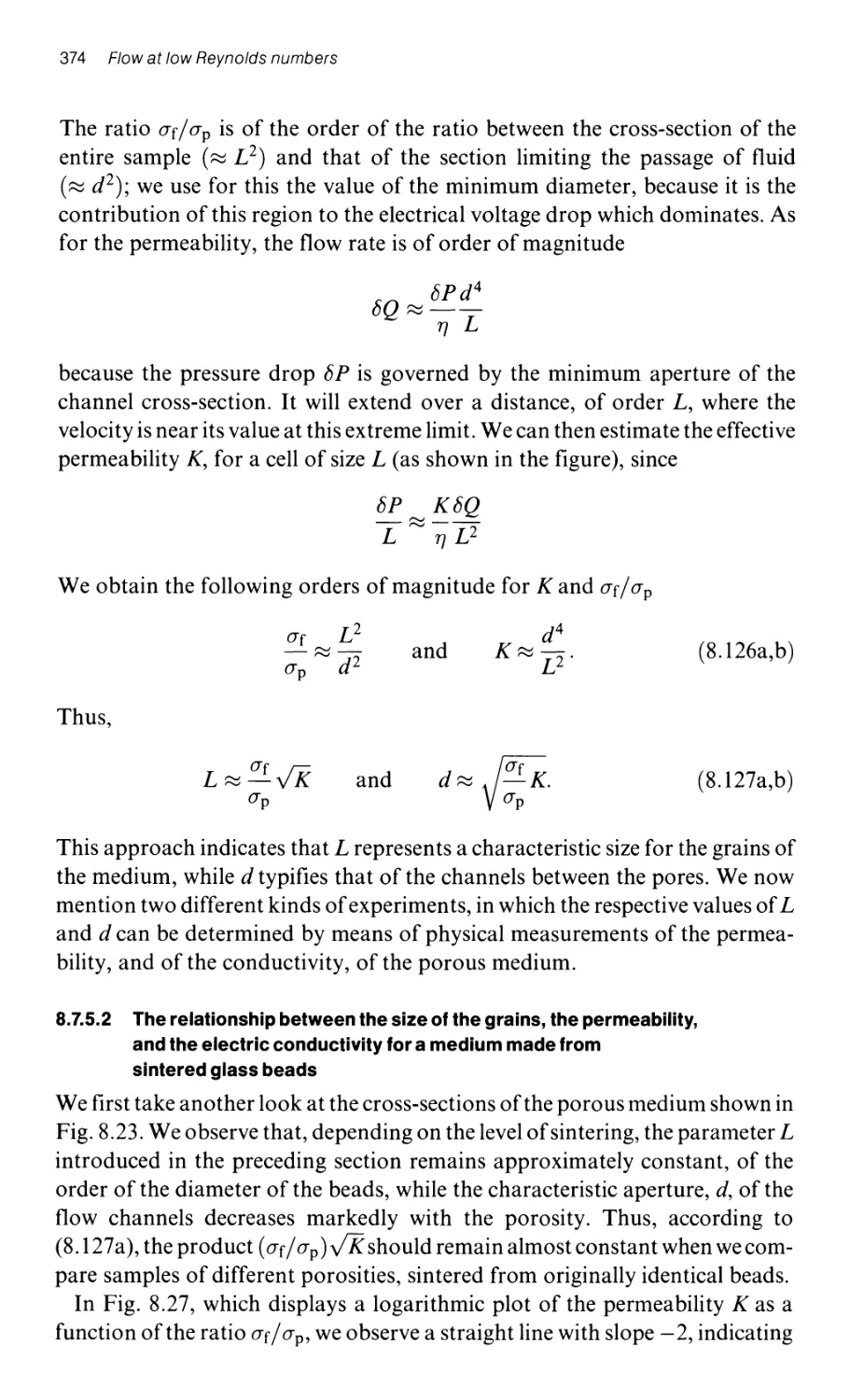
natural porous samples 375
8.7.6 The flow of immiscible fluids in a porous medium 377
8.7.6.1 The effects of capillary forces on two-phase
flows in porous media 377
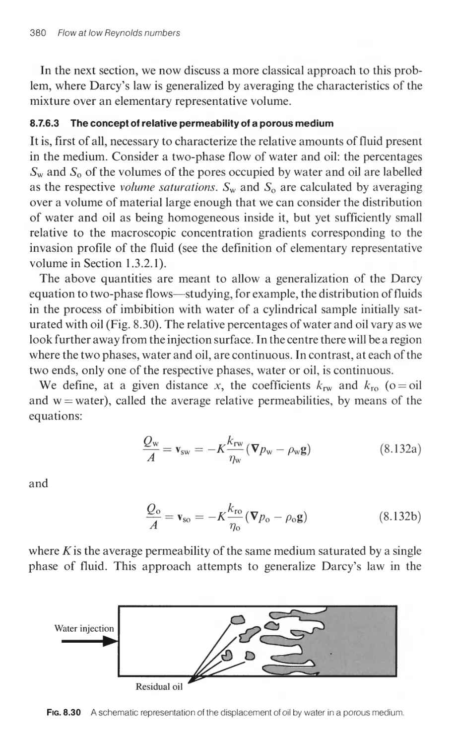
8.7.6.2 Drainage flows at very low velocity 378
8.7.6.3 The concept of relative permeability of a
porous medium 380
xx Contents
9 Laminar boundary layers 383
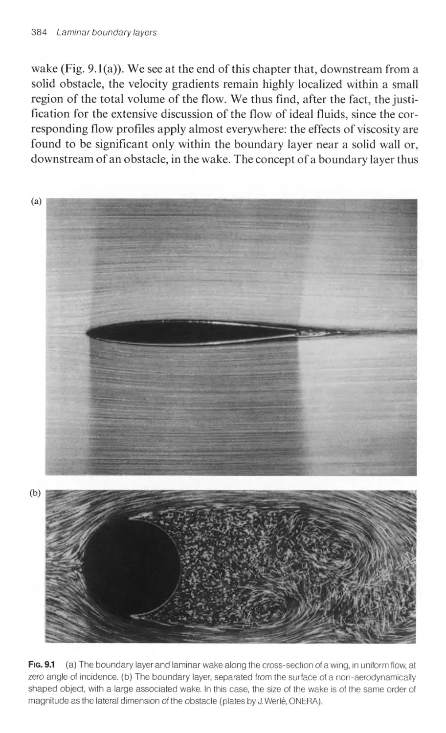
9.1 Introduction 383
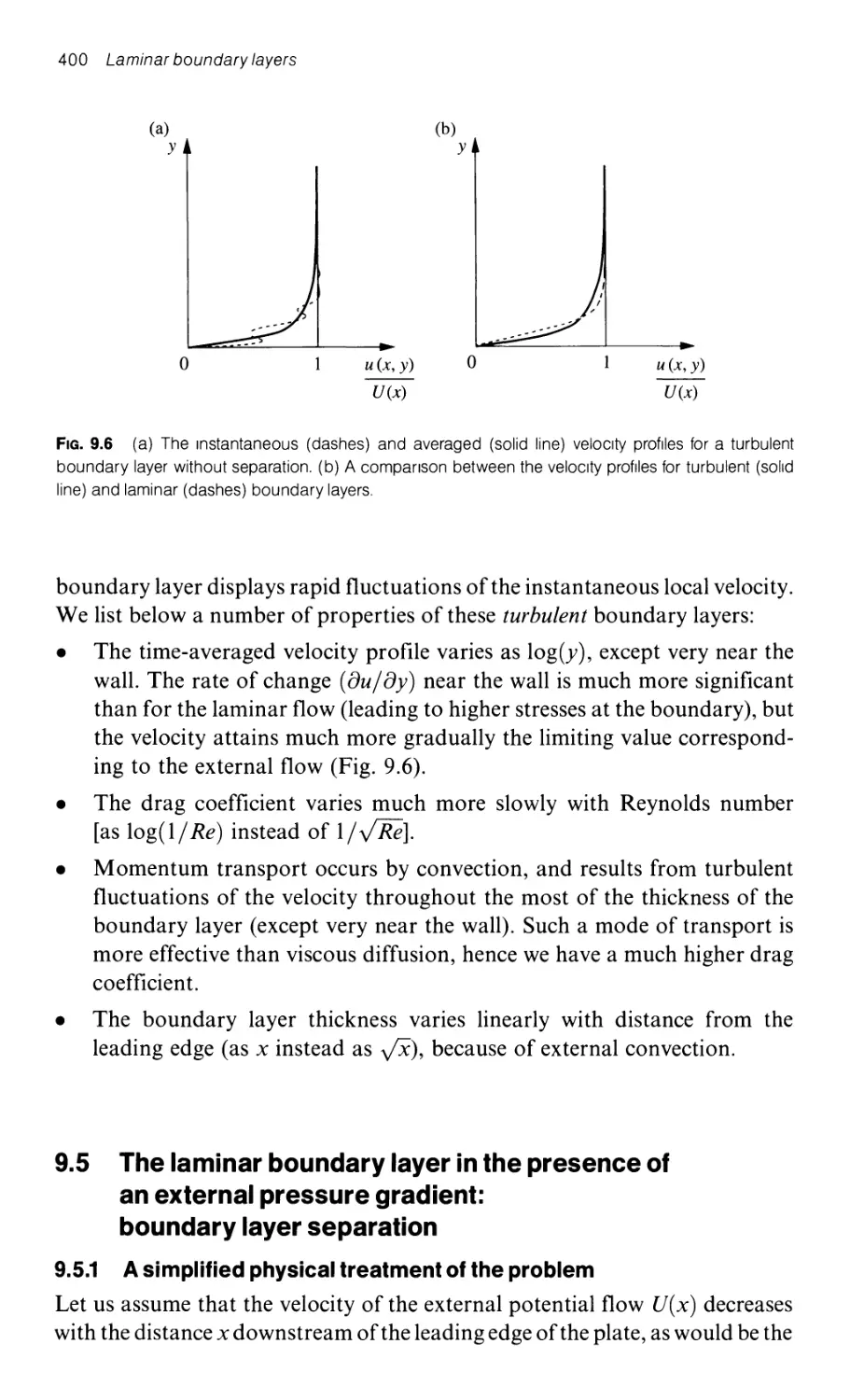
9.2 A qualitative physical discussion of the structure of
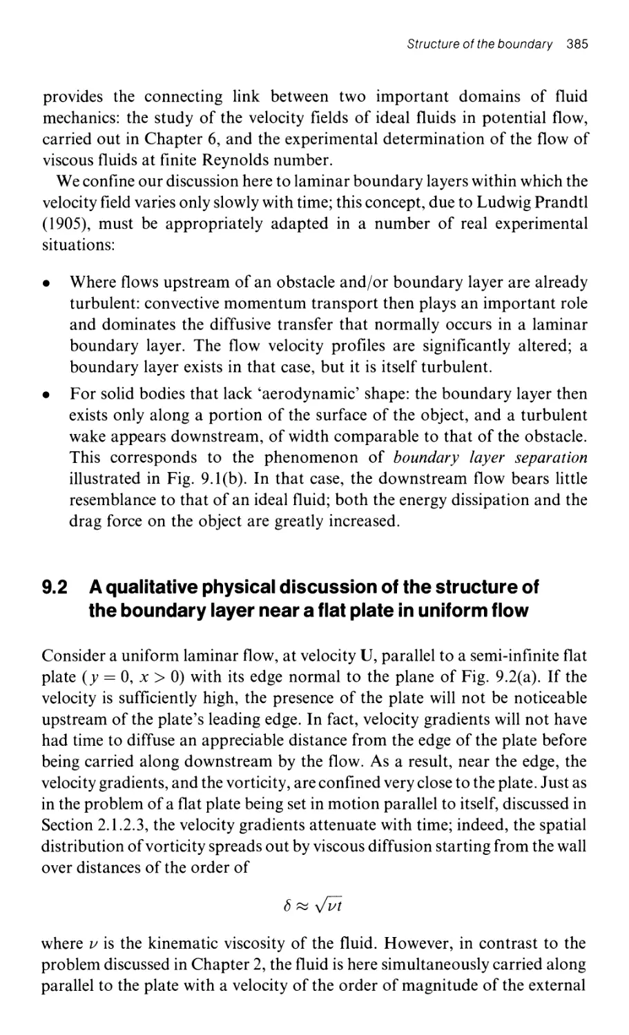
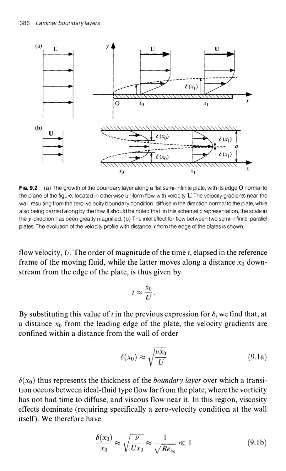
the boundary layer near a flat plate in uniform flow 385
9.3 The equations of motion within the boundary layer: Prandtl theory 388
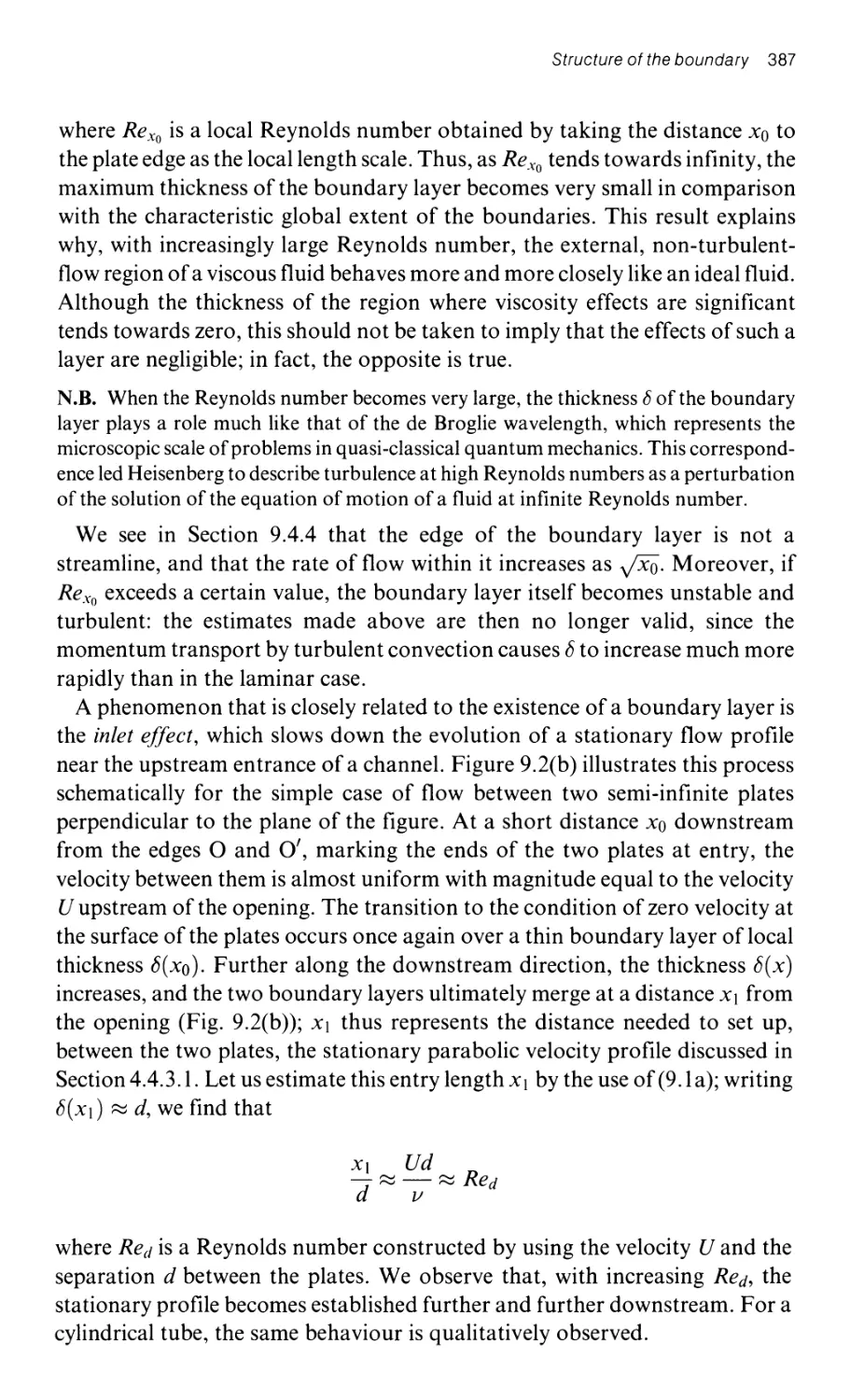
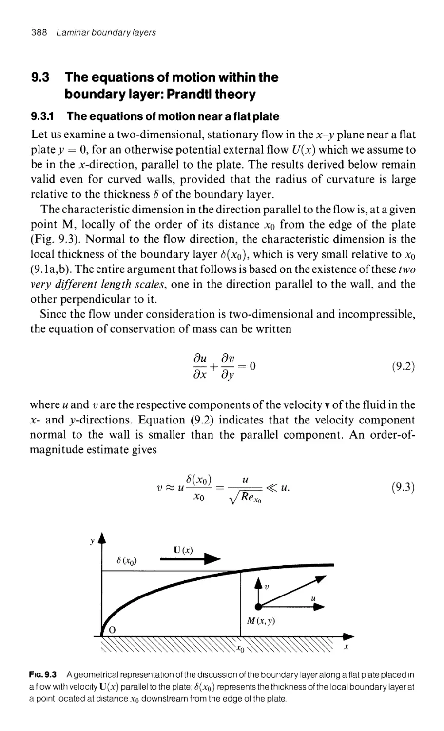
9.3.1 The equations of motion near a flat plate 388
9.3.2 Transport of vorticity in the boundary layer 390
9.3.3 Self-similarity of the velocity profiles in the boundary layer
for the case of uniform, constant, external velocity 390
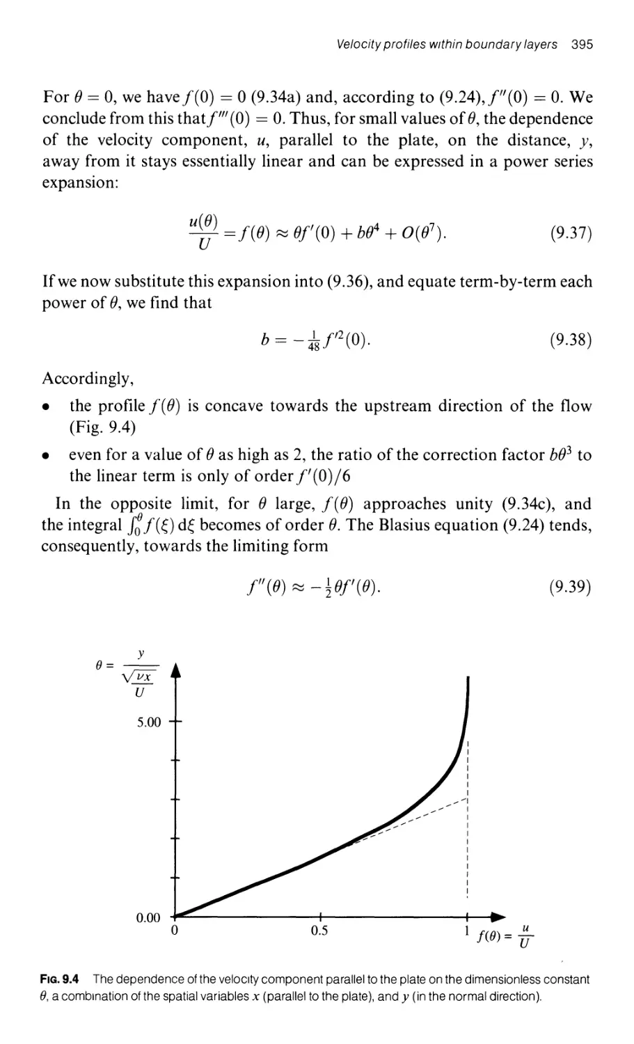
9.4 Velocity profiles within boundary layers 393
9.4.1 The Blasius equation for uniform external flow
along a flat plate 393
9.4.2 An approximate solution of the Blasius equation 394
9.4.3 The frictional force on a flat plate in a uniform flow 397
9.4.4 The thickness of boundary layers 397
9.4.4.1 The displacement thickness b* 398
9.4.4.2 The momentum thickness b** 399
9.4.5 The hydrodynamic stability of a laminar boundary layer:
turbulent boundary layers 399
9.5 The laminar boundary layer in the presence of an external
pressure gradient: boundary layer separation 400
9.5.1 A simplified physical treatment of the problem 400
9.5.2 Self-similar velocity profiles: flows such that U(x) = cxn 401
9.5.2.1 The Falkner-Skan equation 401
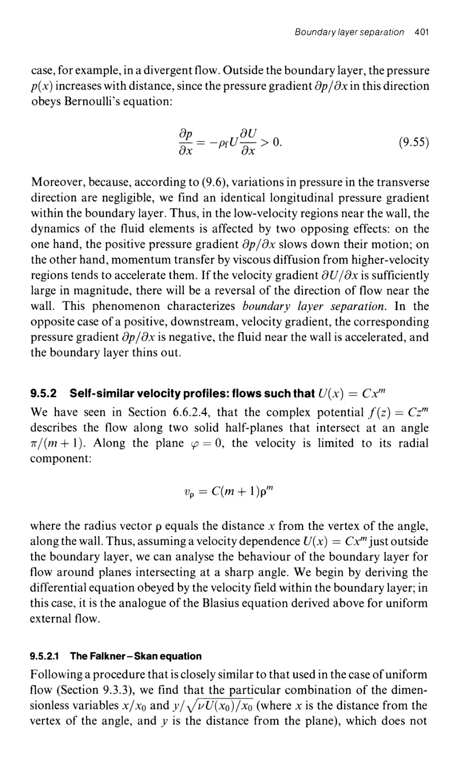
9.5.2.2 Velocity profiles within the boundary layer 402
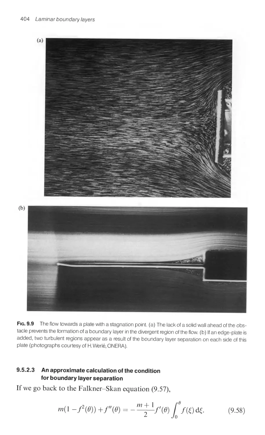
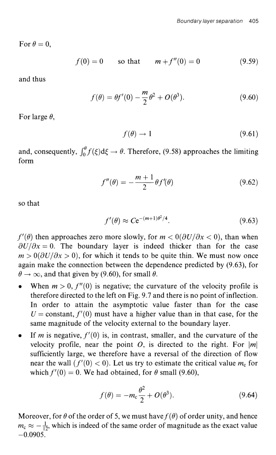
9.5.2.3 An approximate calculation of the condition
for boundary layer separation 404
9.5.3 Boundary layers with constant thickness 406
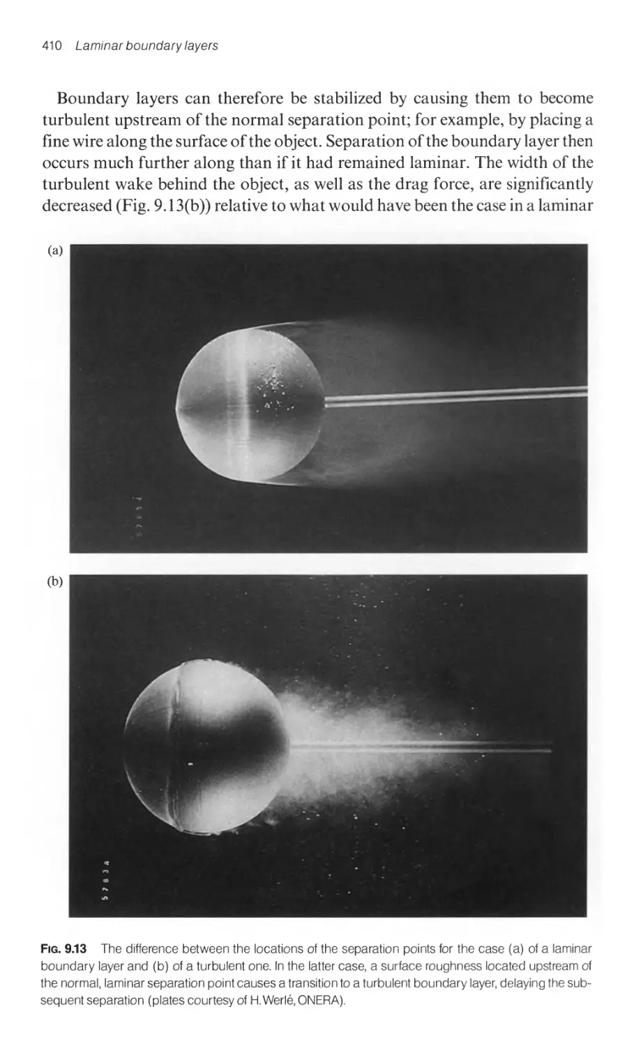
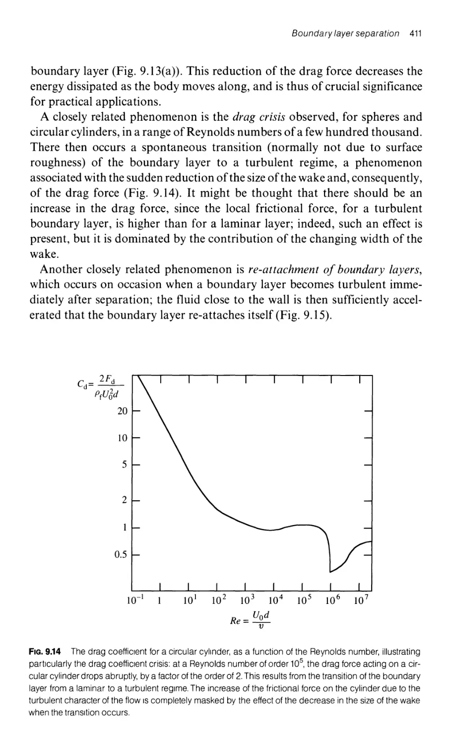
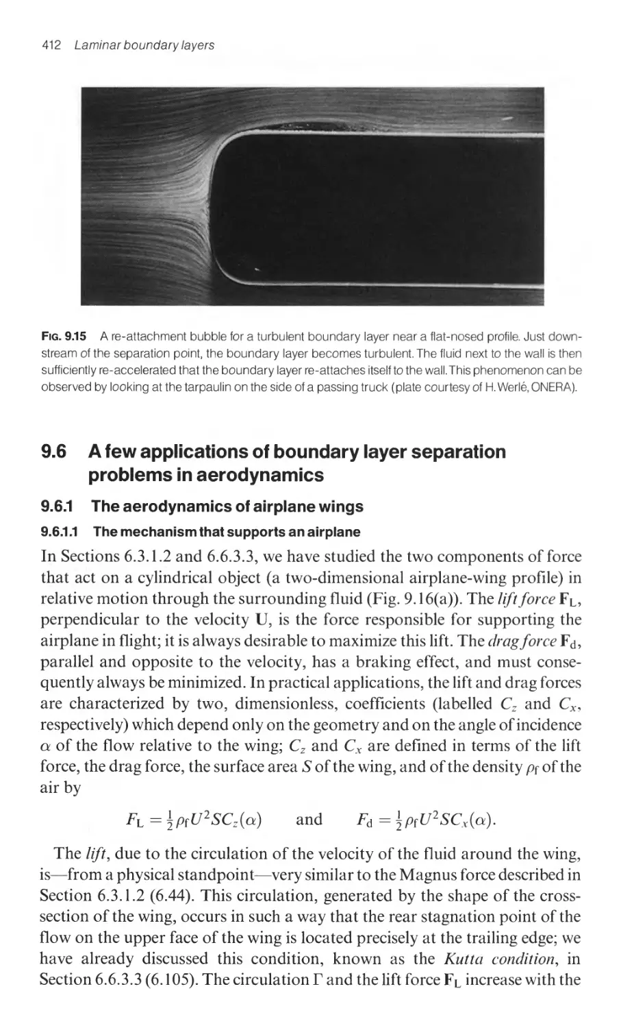
9.5.4 Flows lacking self-similarity: boundary layer separation 407
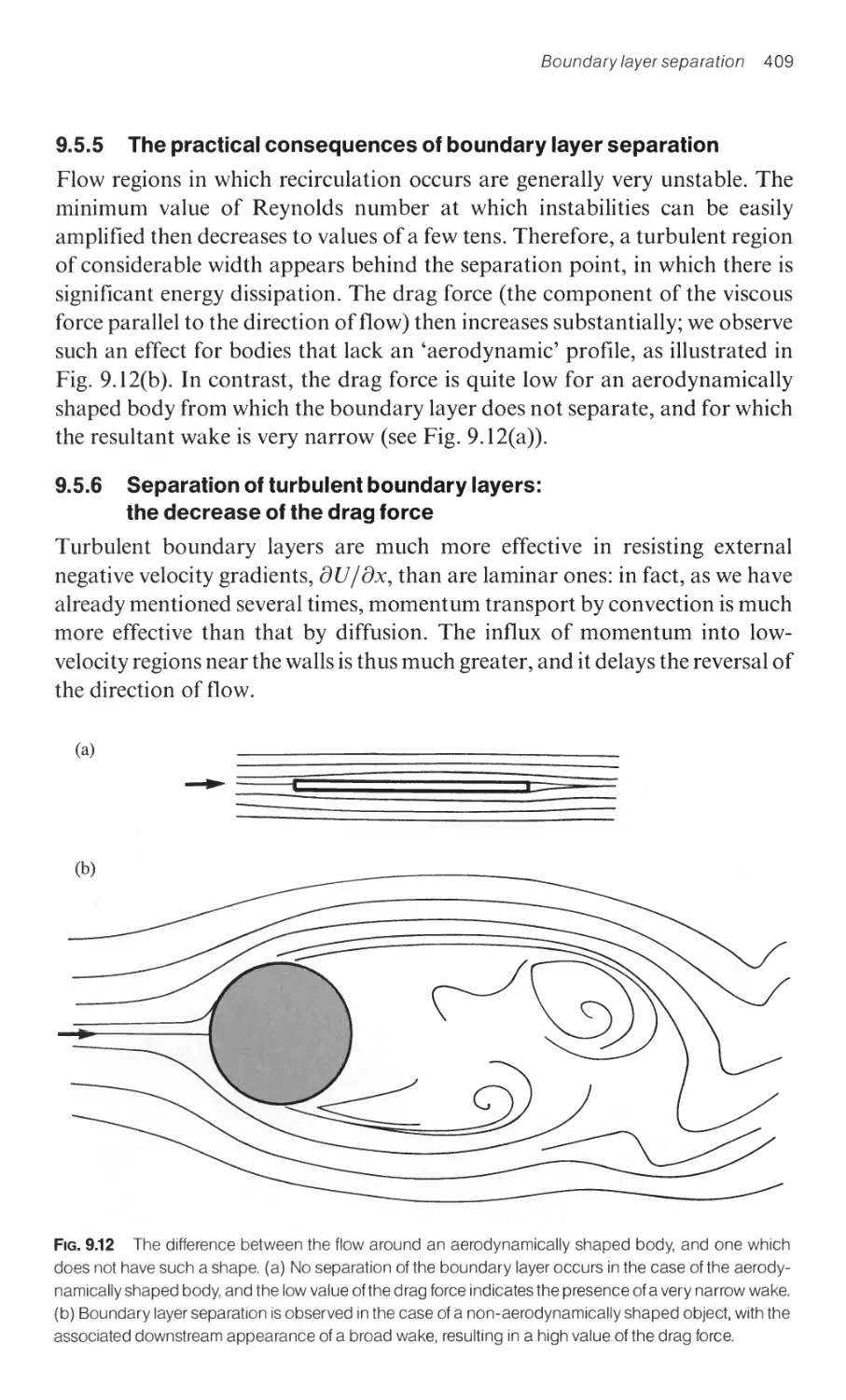
9.5.5 The practical consequences of boundary layer separation 409
9.5.6 Separation of turbulent boundary layers:
the decrease of the drag force 409
9.6 A few applications of boundary layer separation
problems in aerodynamics 412
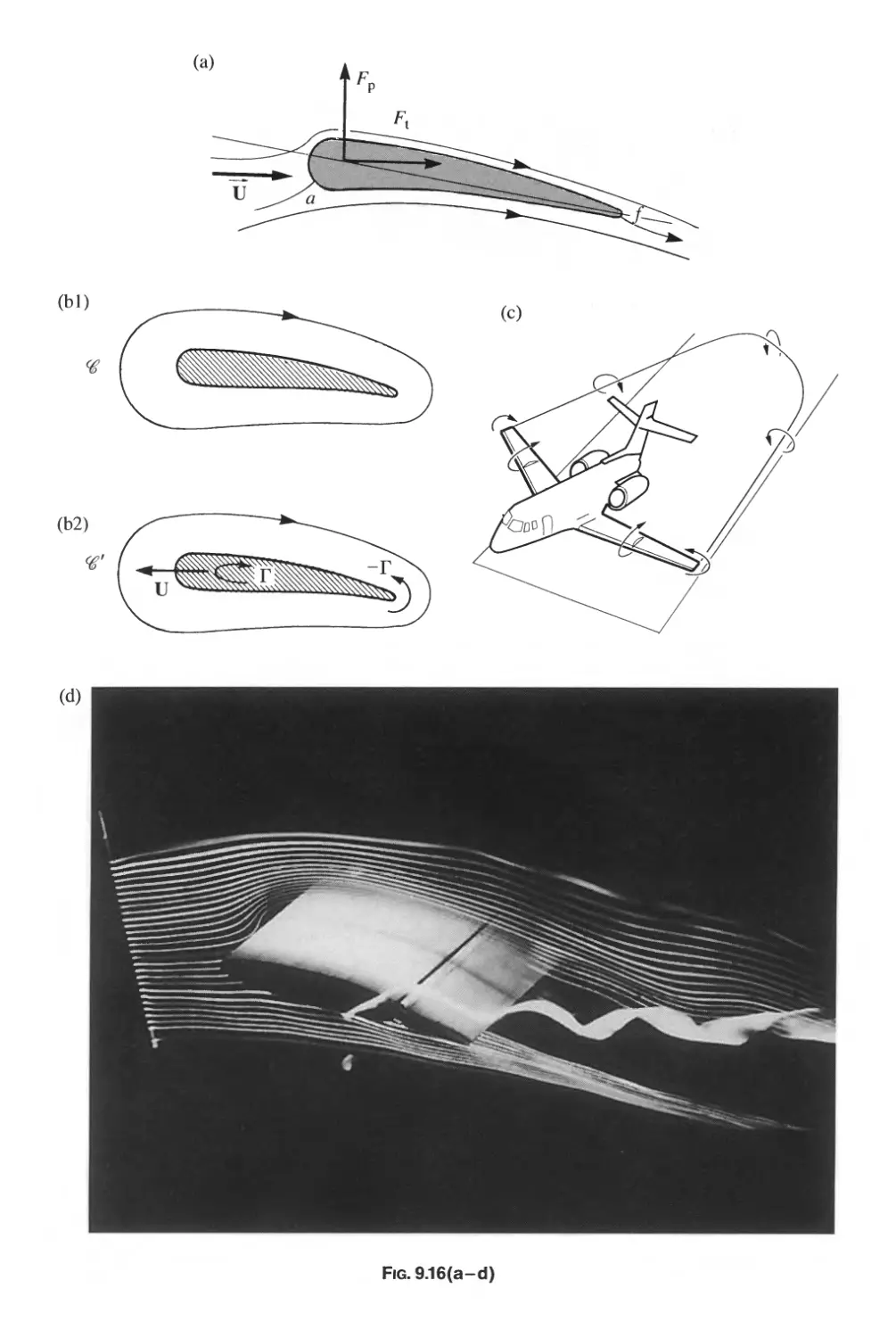
9.6.1 The aerodynamics of airplane wings 412
9.6.1.1 The mechanism that supports an airplane 412
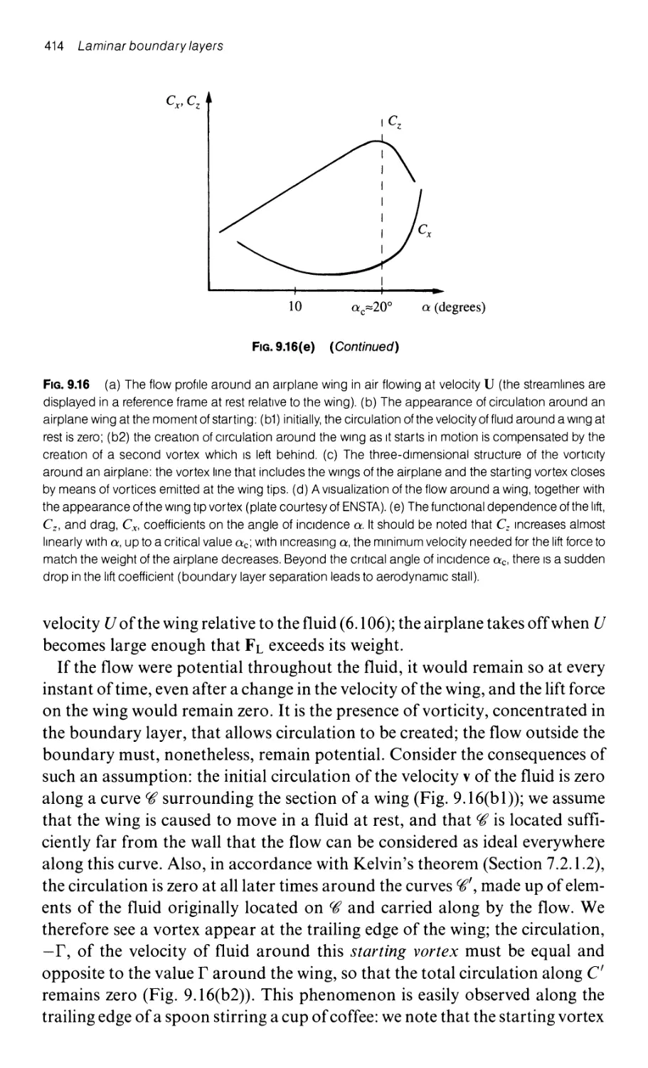
9.6.1.2 The separation phenomenon 415
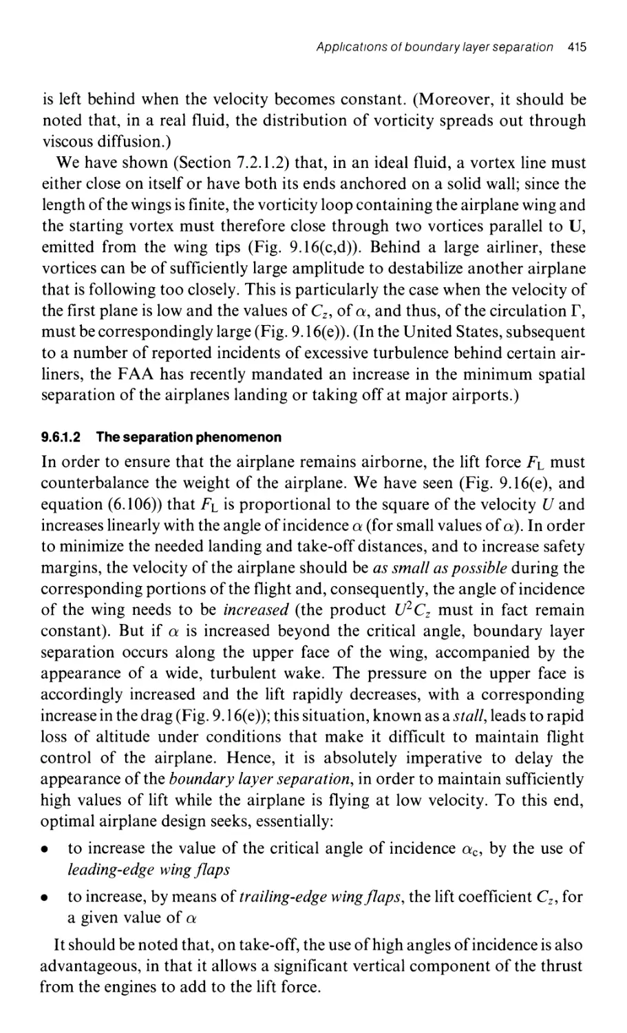
9.6.1.3 Control of the boundary layer by means of
leading-edge wing flaps 416
9.6.1.4 Control of the boundary layer by means of
trailing-edge wing flaps 417
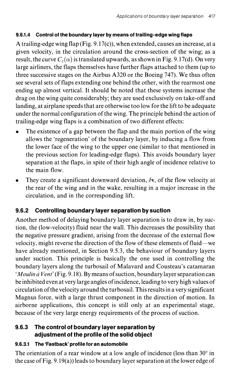
9.6.2 Controlling boundary layer separation by suction 417
9.6.3 The control of boundary layer separation by adjustment of
the profile of the solid object 417
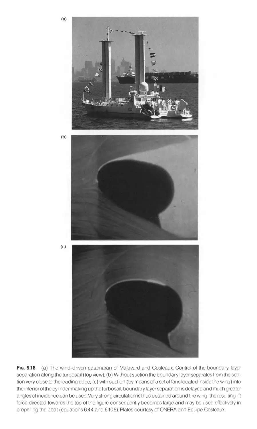
9.6.3.1 The 'Fastback' profile for an automobile 417
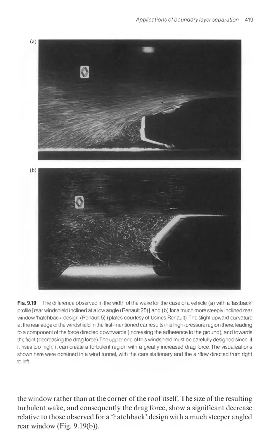
9.6.3.2 An aerodynamic baffle over the gap between
the cab and trailer, in a tractor-trailer combinatton 420
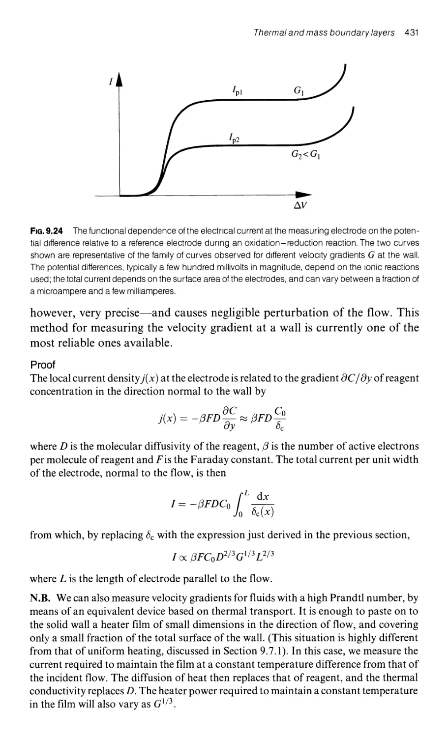
9.7 Thermal and mass boundary layers 420
Contents XXI
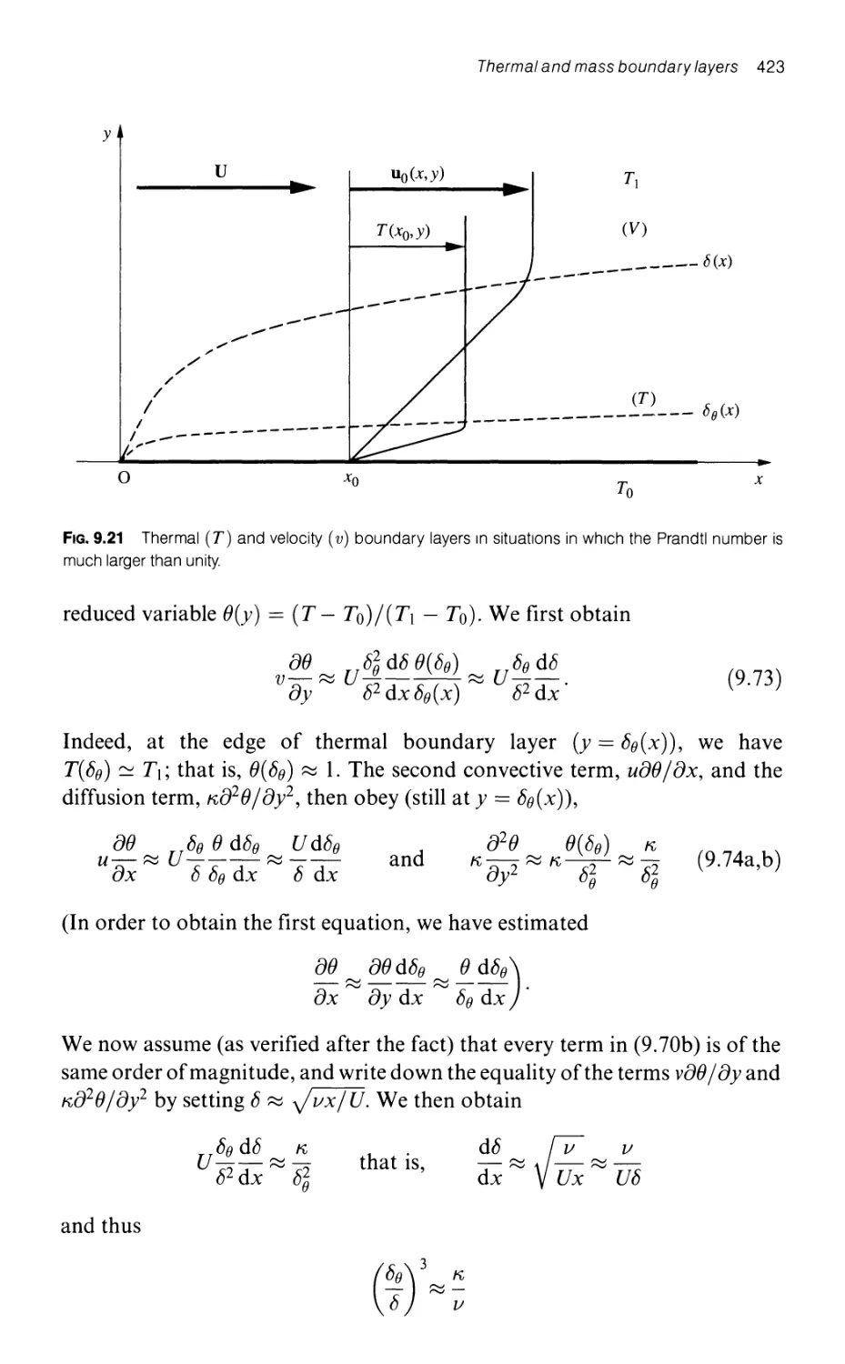
9.7.1 Thermal boundary layers 421
9.7.1.1 The case of a Prandtl number much greater than unity 422
9.7.1.2 The case of a Prandtl number much smaller than unity 425
9.7.1.3 The case of a Prandtl number of order unity 425
9.7.1.4 An application of the heat exchange laws between
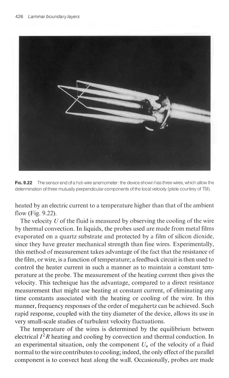
a solid and a flowing fluid: the hot-wire anemometer 425
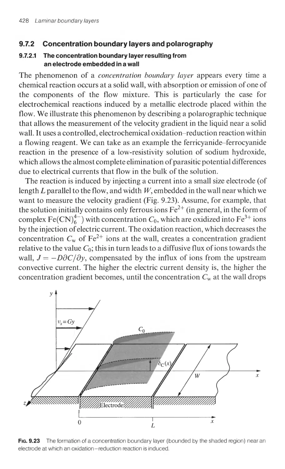
9.7.2 Concentration boundary layers and polarography 428
9.7.2.1 The concentration boundary layer resulting from
an electrode embedded in a wall 428
9.7.2.2 Measurement of a velocity near a wall by
a polarographic method 430
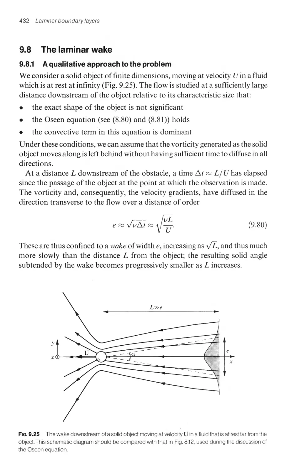
9.8 The laminar wake 432
9.8.1 A qualitative approach to the problem 432
9.8.2 The solution of the equation of motion in the wake far from the object 433
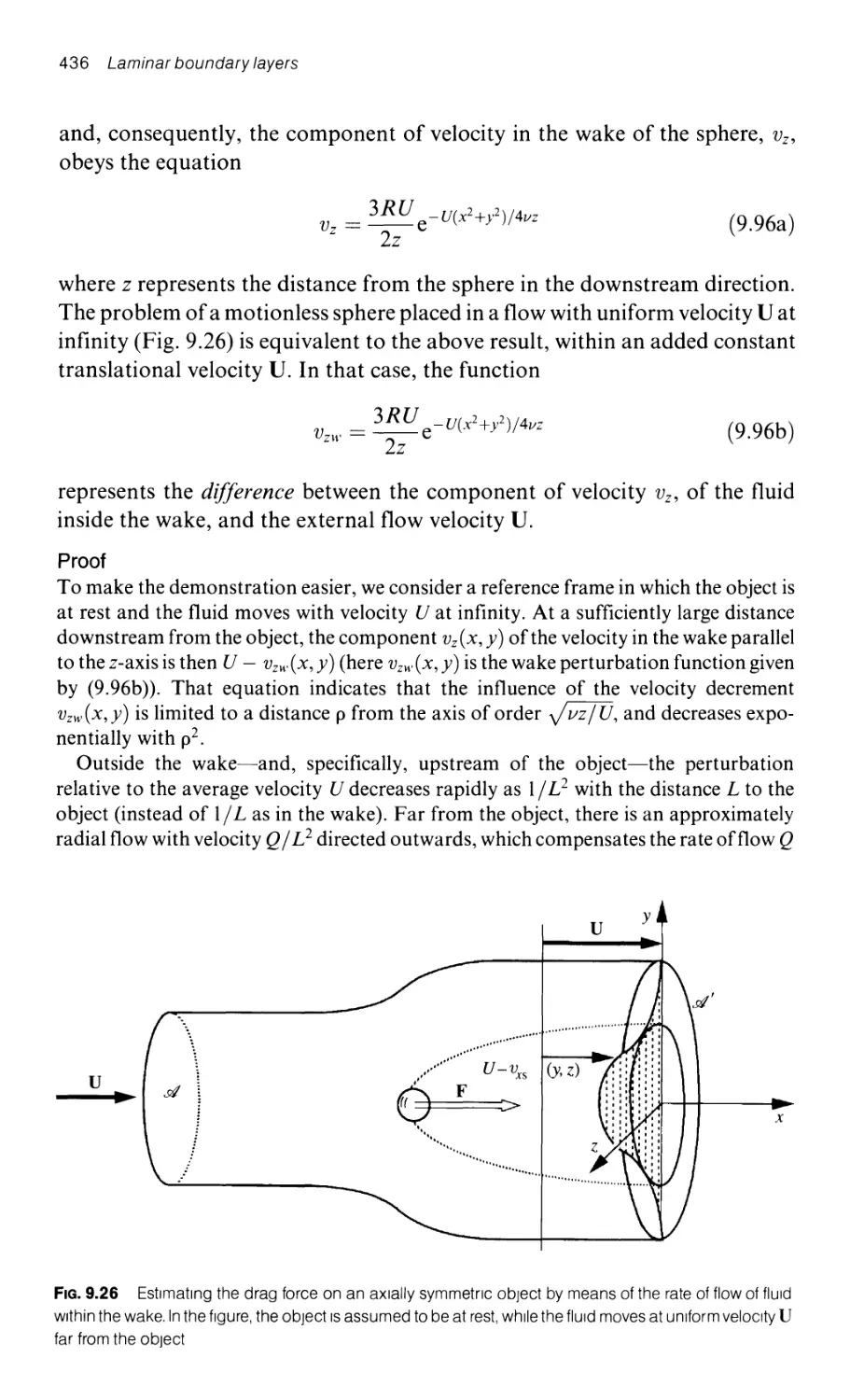
9.8.2.1 The wake behind an object that is finite in all directions 433
9.8.2.2 The wake behind an infinitely long cylinder 435
9.8.3 The drag force on a body: the relationship with
the velocity profile in the wake 435
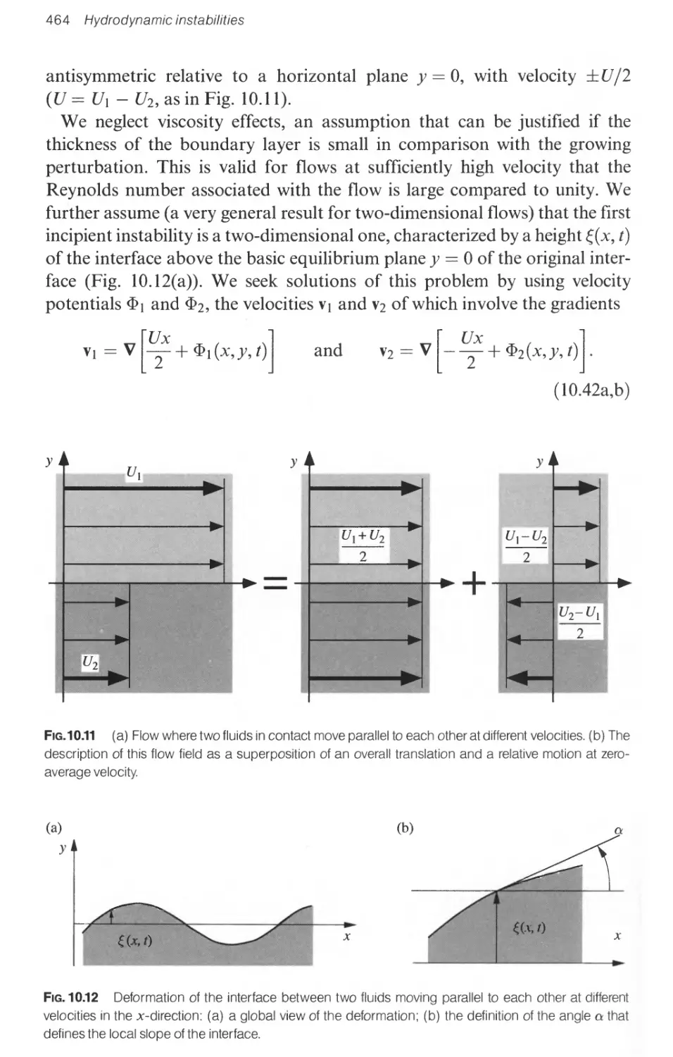
10 Hydrodynamic instabilities 439
10.1 Thermal convection 439
10.1.1 Convective transport equations for heat 439
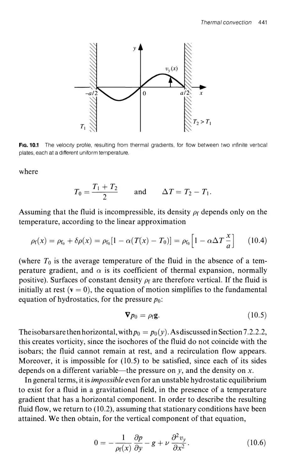
10.1.2 Thermal convection resulting from a horizontal
temperature gradient 440
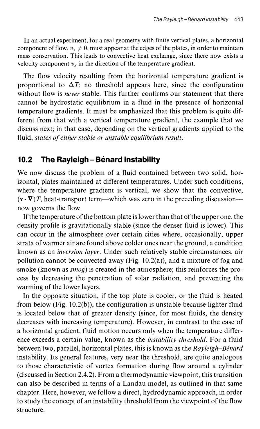
10.2 The Rayleigh - Benard instability 443
10.2.1 A description of the Rayleigh - Benard instability 444
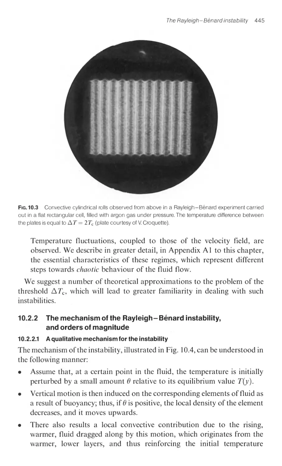
10.2.2 The mechanism of the Rayleigh-Benard instability,
and orders of magnitude 445
10.2.2.1 A qualitative mechanism for the instability 445
10.2.2.2 The physical criterion for the instability (Pr » 1) 446
1 0.2.3 The two-dimensional solution of the Rayleigh - Benard problem 448
10.2.3.1 An approximate calculation ofthe instability threshold 448
10.2.3.2 The domain of Instability as a function
of the wave vector 452
10.2.3.3 Amplitude variations as a function of distance
above the threshold 453
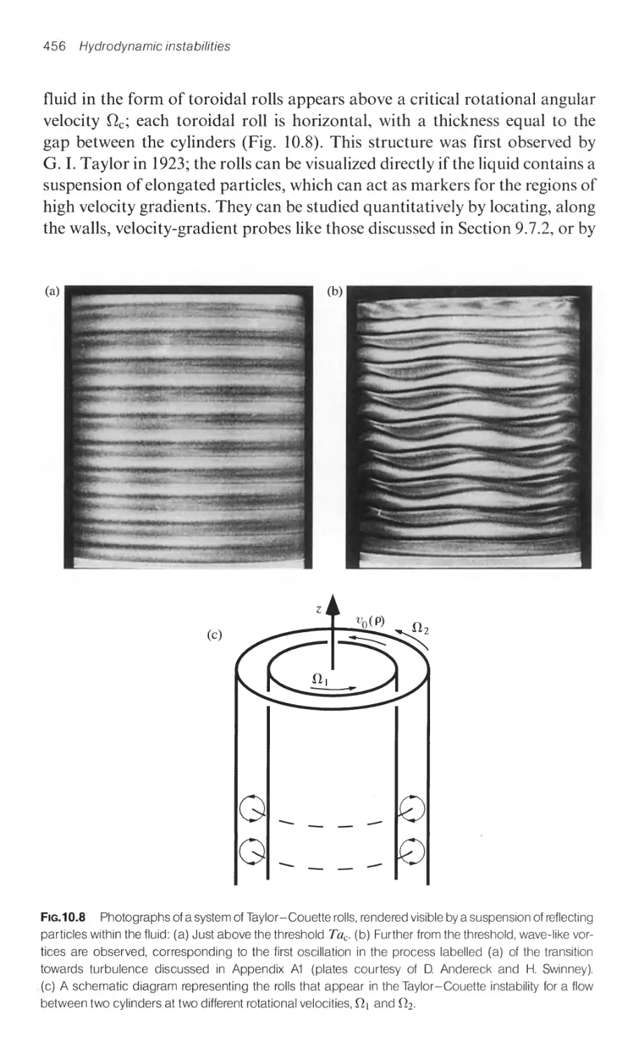
10.3 Other examples of threshold instabilities 455
10.3.1 The Taylor-Couette instability 455
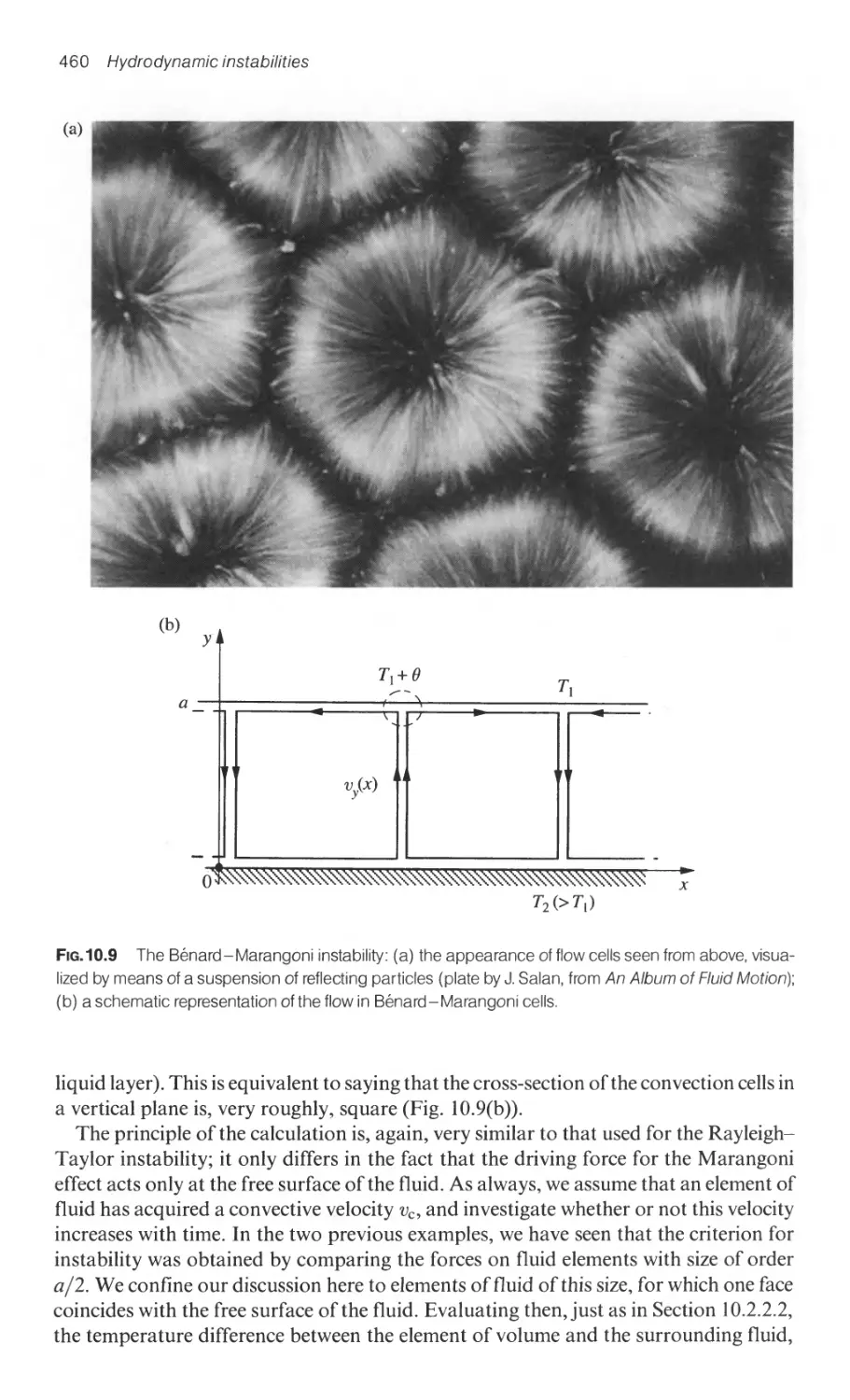
10.3.2 The Benard - Marangoni instability 459
10.4 Other classes of instability 462
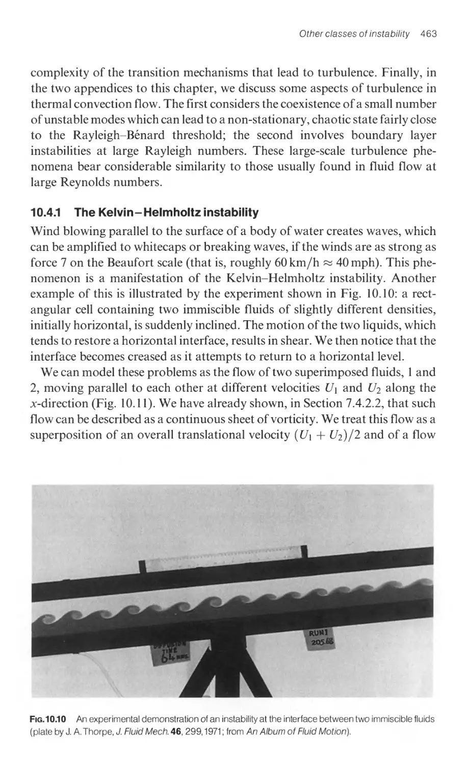
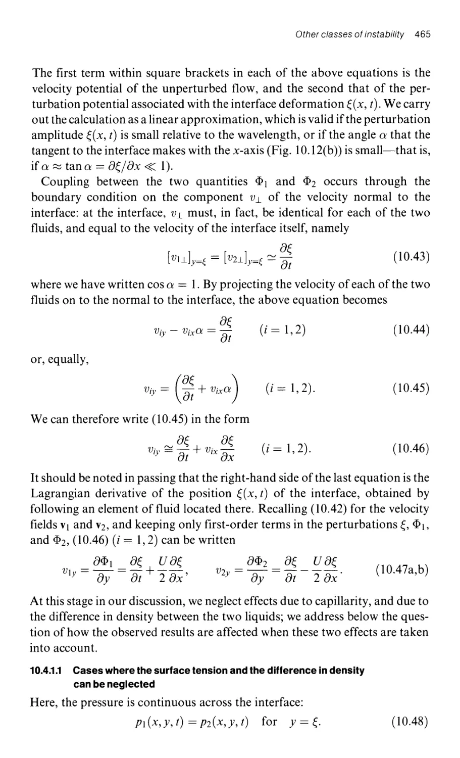
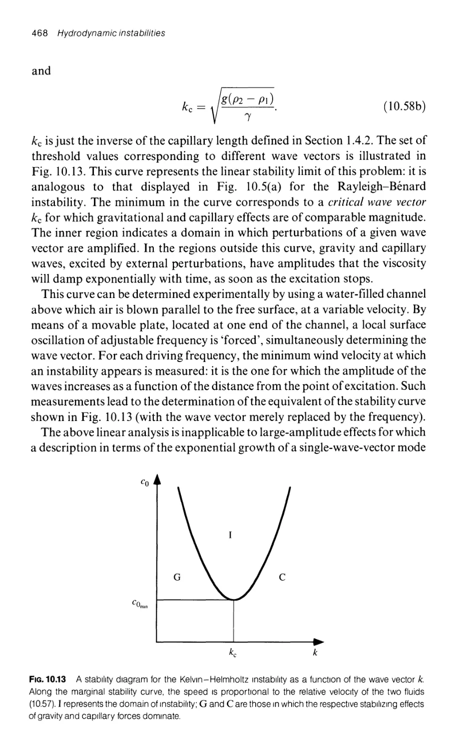
10.4.1 The Kelvin - Helmholtz instability 463
10.4.1.1 Cases where the surface tension and the difference
in density can be neglected 465
10.4.1.2 Effects due to surface tension and differences in density 467
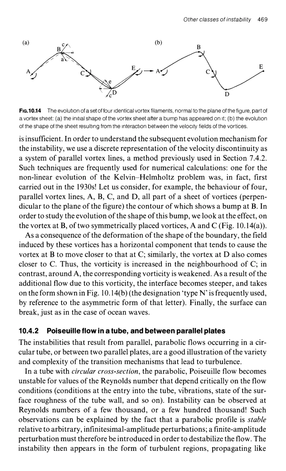
10.4.2 Poiseuille flow in a tube, and between parallel plates 469
10.4.3 Th e role of the sha pe of the velocity and va rticity profiles 470
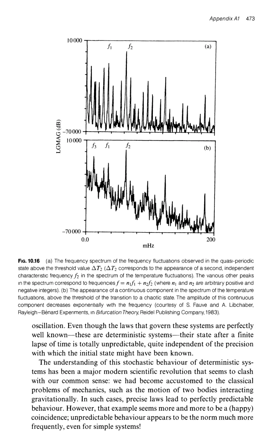
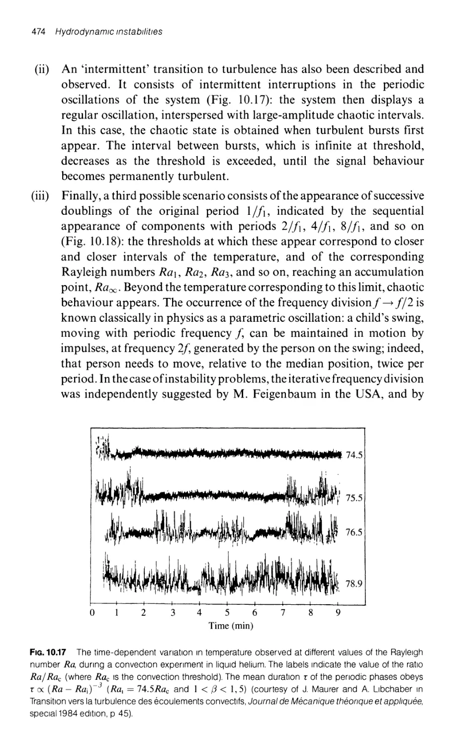
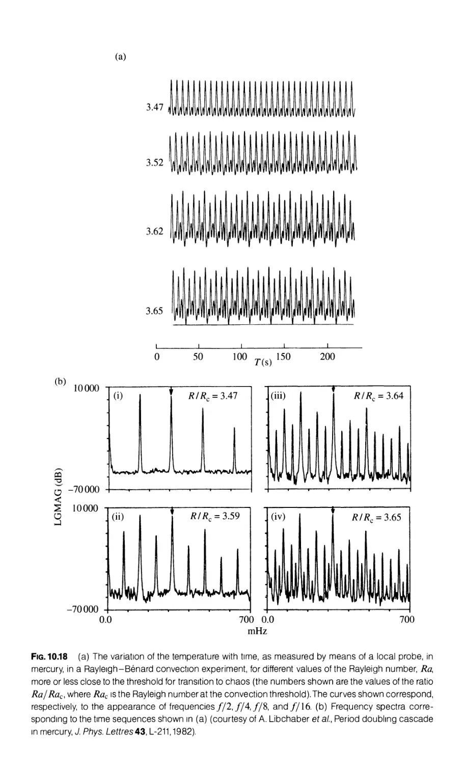
Appendix A1: transition to chaos 471
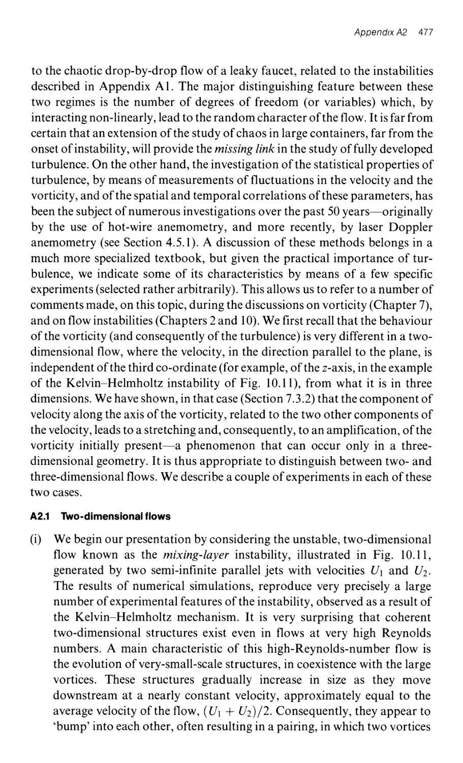
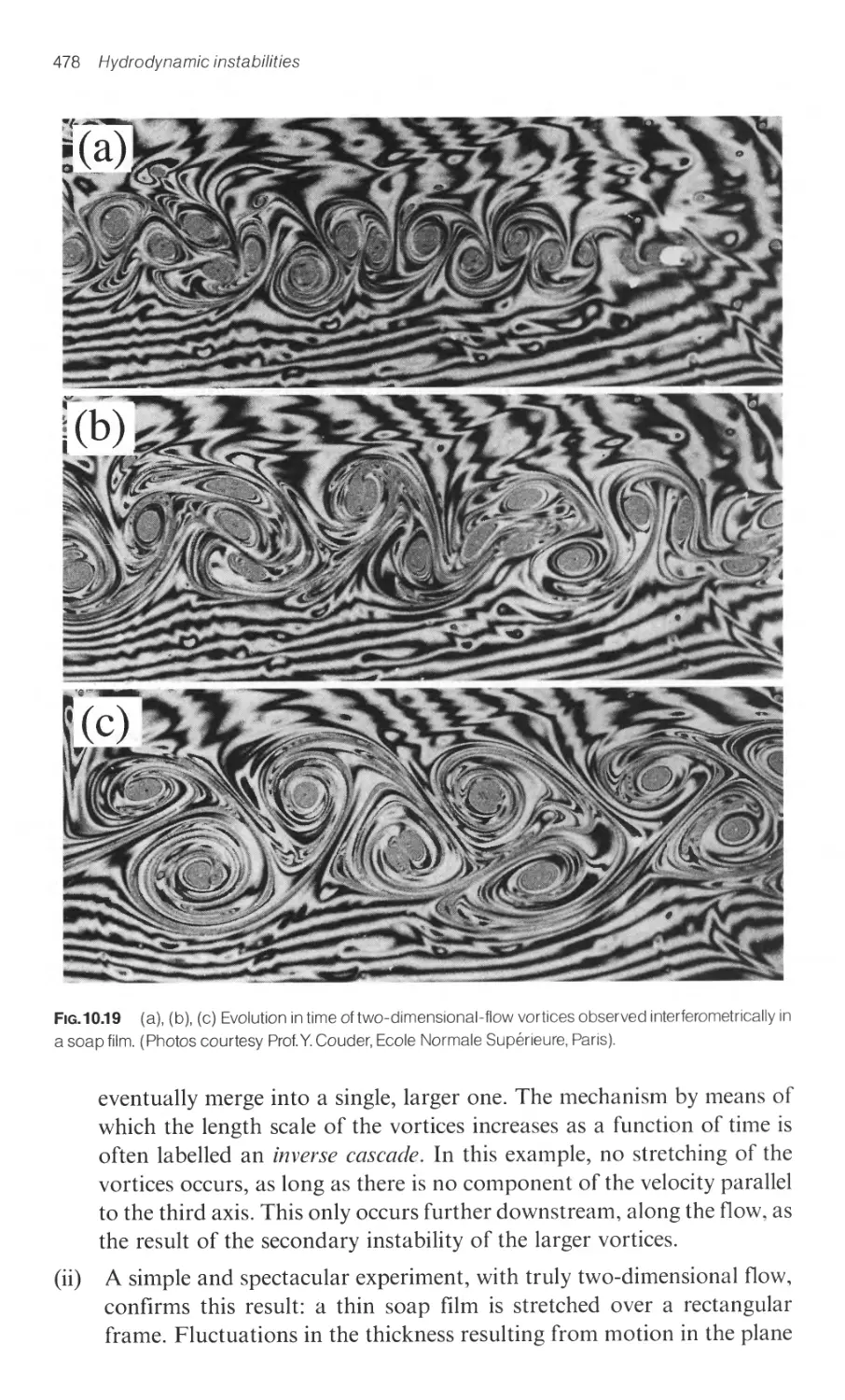
Appendix A2: experiments in fully developed turbulence 476
xxii Contents
A2.1 Two-dimensional flows
A2.2 Three-dimensional flows
477
479
Appendix Superfluid helium: an (almost) ideal fluid
A.1 Important properties of Helium II at finite temperatures
A.1.1 The two-fluid model for Helium II
A.1.2 Quantization of the circulation of the superfluid velocity V S
A.1.3 Experimental evidence for the existenc8 of a superfluid
component flowing with no energy dissipation
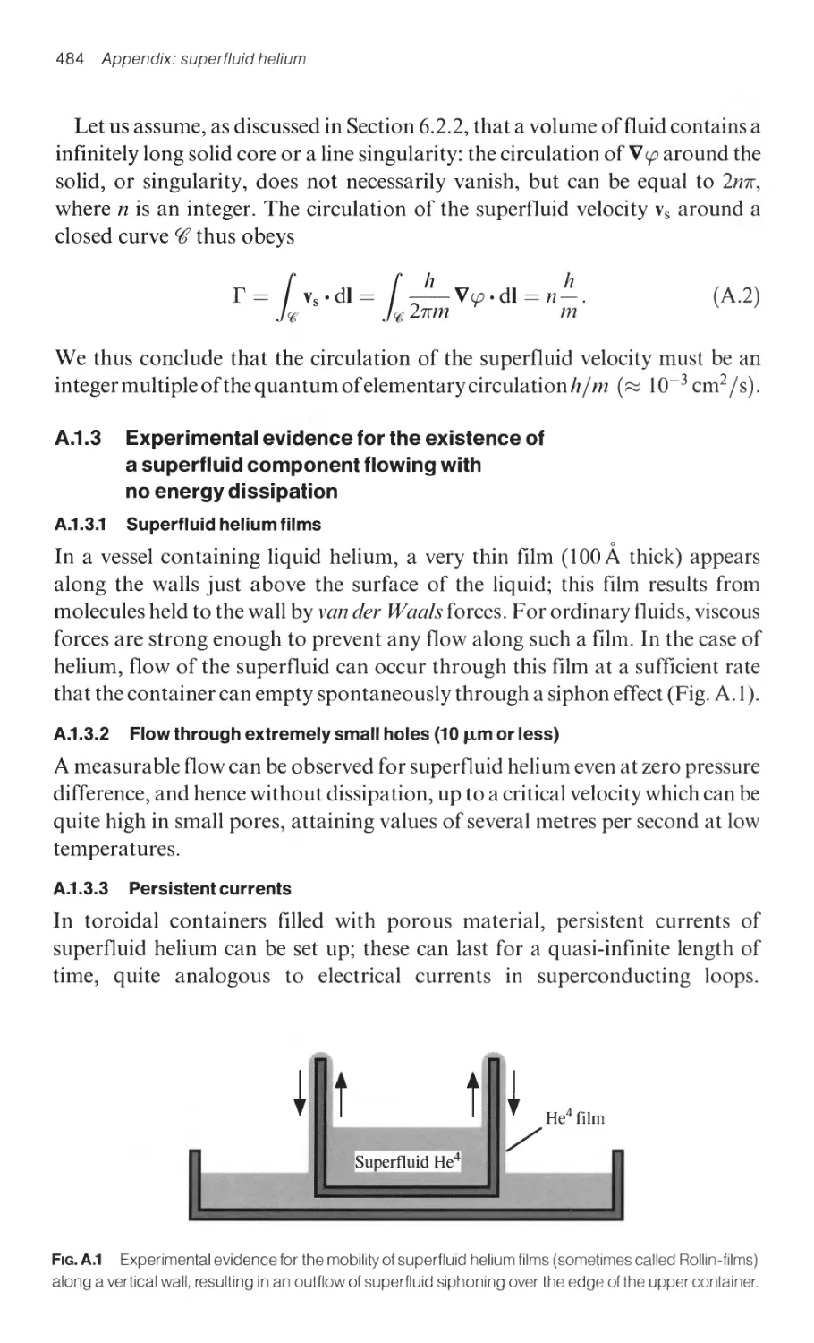
A.1.3.1 Superfluid helium films
A.1.3.2 Flow through extremely small holes (10 Jlm or less)
A.1.3.3 Persistent currents
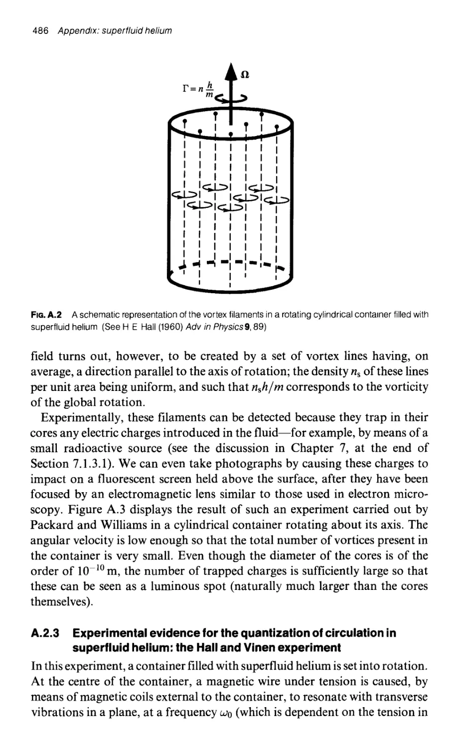
A.2 Vortices in superfluid helium
A.2.1 The existence of vortex filaments in superfluid helium
A.2.2 Setting a volume of superfluid helium in rotation
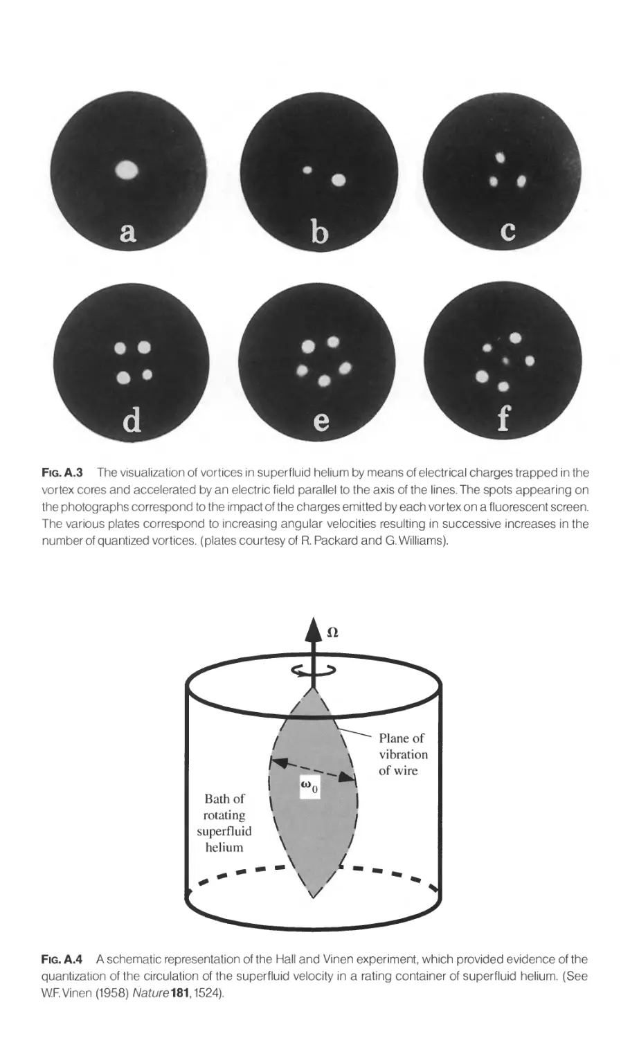
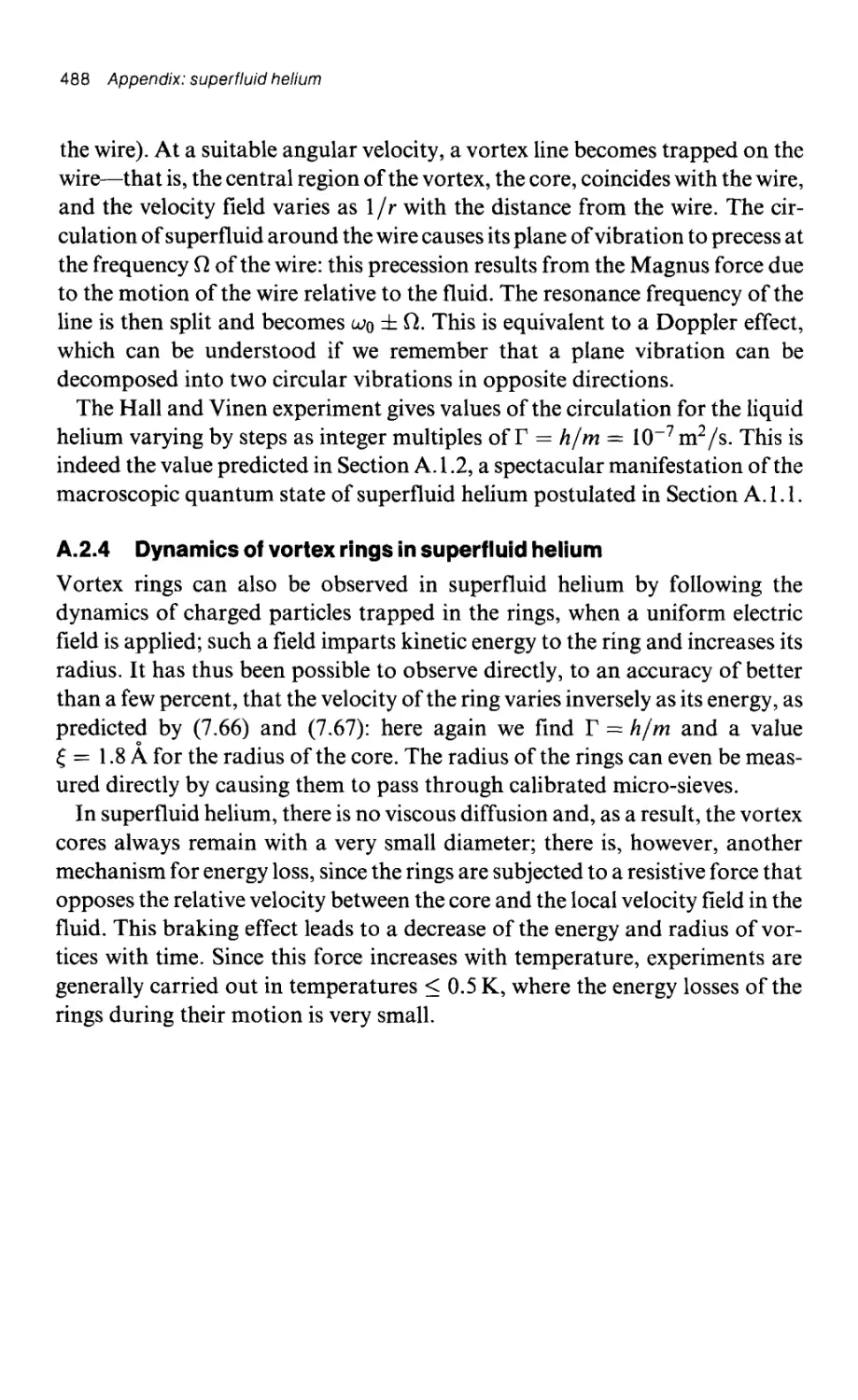
A.2.3 Experimental evidence for the quantisation of circulation in
superfluid helium: the Hall and Vinen experiment
A.2.4 Dynamics of vortex rings in superfluid helium
482
482
482
483
484
484
484
484
485
485
485
486
488
Bibliography
489
Index
496
1 The physics of fluids
Abstract
From a microscopic viewpoint, the study of the physics of fluids can be considered as a
branch of thermodynamics. In a classical thermodynamic approach, we study the equilib-
rium states of pure substances-solids, liquids, and gases-and the changes of state
between these several phases. A generalization of this approach is the study of fluctuations
in the immediate neighbourhood of an equilibrium state; these fluctuations are not only
characteristic of the state, but also indicative of the properties that tend to restore equilibrium.
Thus, for a physical system with a large number of particles, which has undergone a 'small
disturbance' relative to its state of thermodynamic equilibrium, there exist straightforward
proportionality relations between the fluxes that tend to restore equilibrium and the extent
of the displacement.
The study of these relations, and the definition of the transport coefficients that characterize
them, constitutes the core of this first chapter. The discussion first emphasizes a macroscopic
viewpoint (Section 1.2) and then proceeds microscopically (Section 1.3). We also analyse
(in Section 1.4) some of the surface phenomena which appear when two fluids have a
common boundary (interface). Finally, we provide a brief overview of the application of optical
spectroscopy and of X-ray techniques to the study of liquids (Section 1.5); such measurements
permit the study of fluctuations about the equilibrium point and the subsequent evaluation of
the transport coefficients. At the outset, though, we present in Section 1.1 a simple description
of the microscopic nature of a fluid, and attempt to describe the influence of its microscopic
characteristics on its macroscopic properties.
1.1 The liquid state
The periodic arrangement of atoms in a crystal is quite familiar to us from
X-ray studies of its microscopic structure, or from the observation of its
external shape. In this-the solid-state of matter, atoms remain fixed relative
to one another except for small-amplitude vibrations that result from thermal
motion. In the other extreme limit, gases at low pressure are nothing but a
dilute system of particles with mutual interactions, weak except at the moment
of a collision. Kinetic theory models of gases allow us to understand, from a
microscopic viewpoint, the evolution of their equilibrium variables, such as
temperature or pressure, except in the neighbourhood of a critical point.
2 The physics of fluids
On the other hand, the precise description of a liquid-with characteristics
midway between those of gases and solids-is much more delicate: Should we
consider it as a very dense gas or a disordered solid? Microscopic models of
liquids often combine features from these two extremes. In particular, model
two-dimensional systems, both microscopic and macroscopic, provide a
powerful tool for the analysis of both the structure and the static properties of
the various states of matter.
1.1.1 The different states of matter: model systems and real media
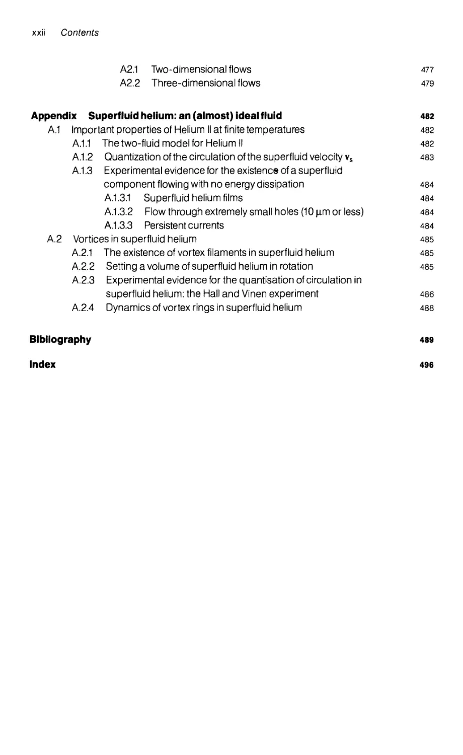
1.1.1.1 The visual representation of different states of matter by
means of an air table
An air table consists of a large horizontal plate drilled with a pattern of
identical, small-diameter, uniformly spaced holes, through which air at high
pressure is forced upwards. A set of identical discs of radius R, placed on the
table, and levitated by the air flow, can thus move around with negligible
friction. 'Thermal motion' of these discs can be simulated by vibrations of the
supporting horizontal plate, or of its lateral boundaries. Depending on the
mean concentration of the discs, we observe the characteristics of the different
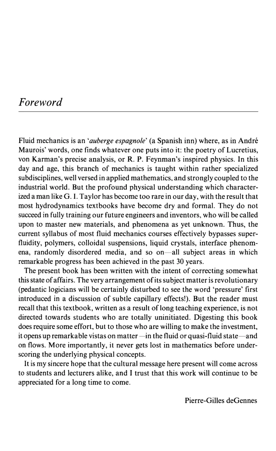
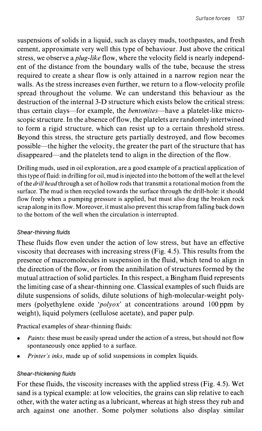
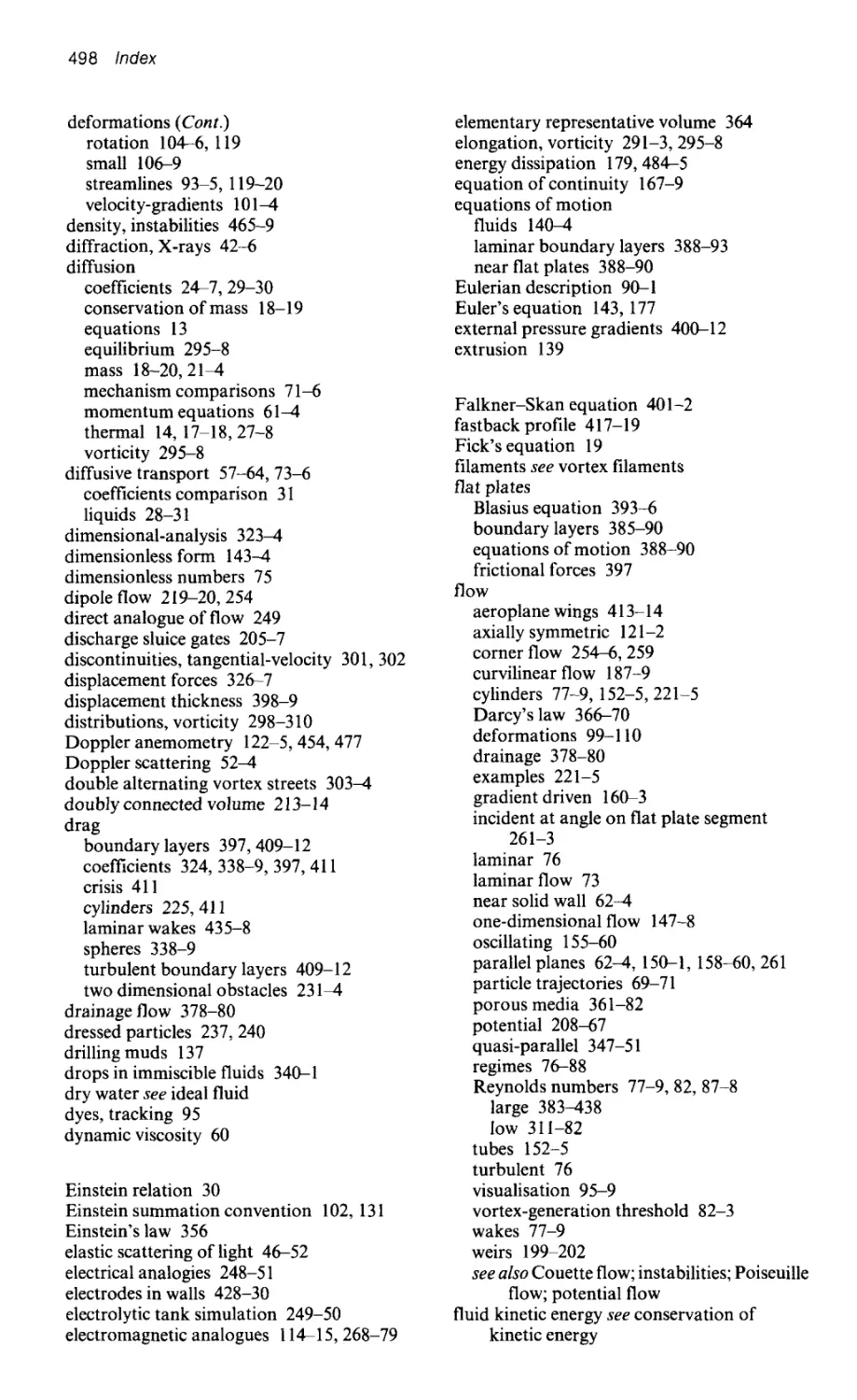
states of matter. Figures 1.1(a) and 1.1(b) were obtained by fastening a small
light source on each disc and recording photographically the corresponding
trajectories (with an exposure time much longer than the mean time between
collisions). The trajectories of the discs appear as white traces on the figures.
The concentration is characterized by the ratio of the surface area covered by
the discs to the total area of the table-a ratio defined as the compactness
(or packing fraction), C.
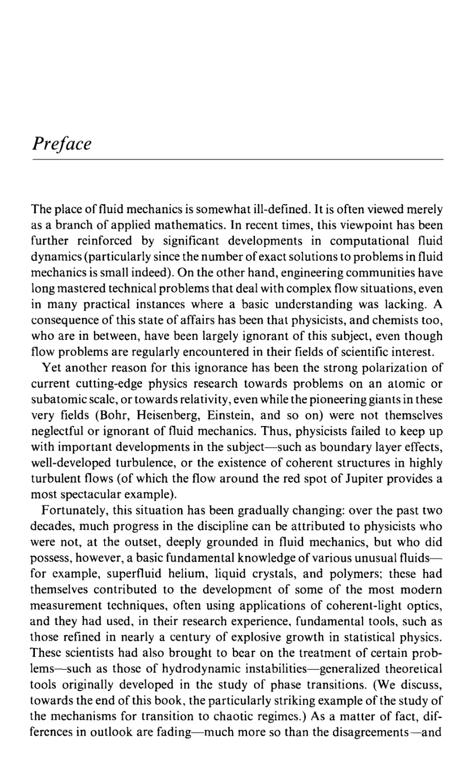
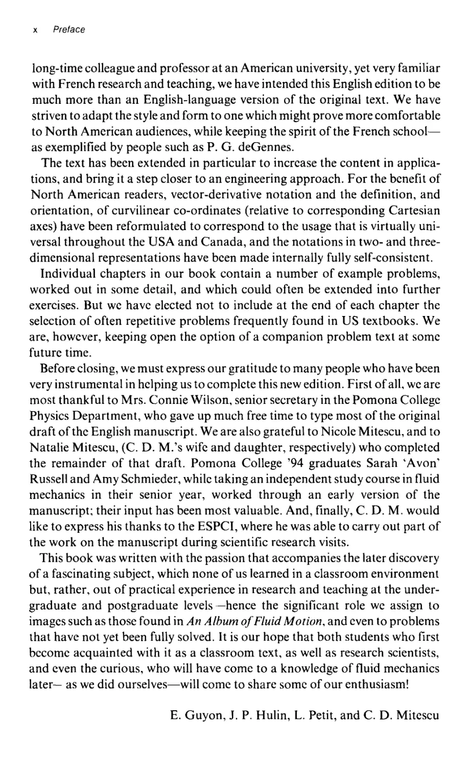
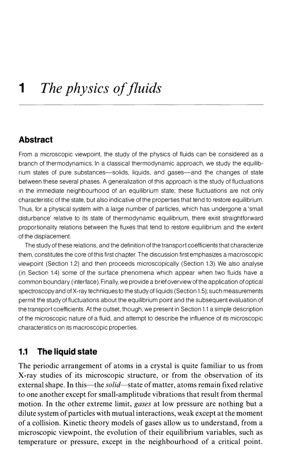
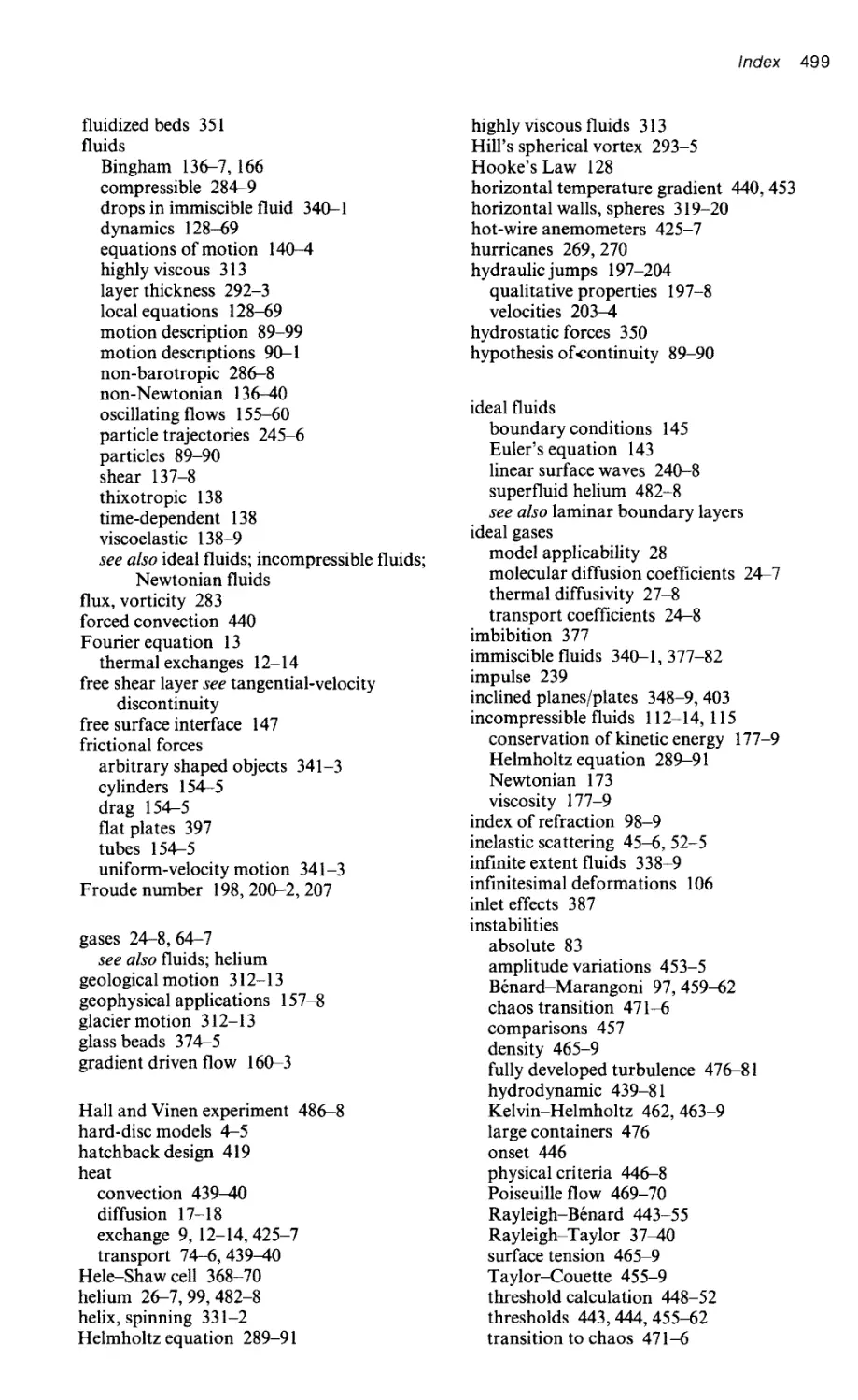
Maximal compactness, C == C M
The maximum value CM, for two-dimensional systems of discs, is obtained
with a compact triangular packing. The discs then form a perfect, two-
dimensional crystal lattice (Fig. 1.2); this state represents that of a perfect
crystal with no thermal vibrations. In this configuration, the elementary
pattern (unit cell) which, repeated periodically, leads to the triangular lattice, is
a diamond-shaped figure ('L') of surface area So == (2R) (2R) V3 /2. The unit
cell contains exactly the equivalent area of one disc, Sp == 7r R 2 . We hence find a
compactness:
S 7r R 2
C M == -.E. == == 0.901.
So 2R2 V3
(1.1)
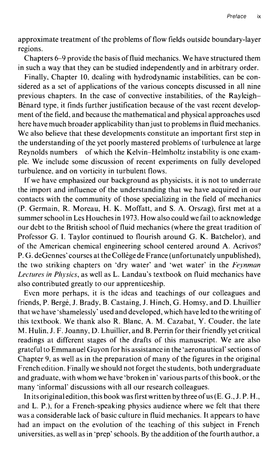
High compactness
As long as the compactness remains close to CM, the discs, as observed from the
trajectories of the luminous points (Fig. 1.1(a)), undergo limited displacements
around their equilibrium positions. Their mean positions remain, however,
The liquid state 3
.,
,
...
"
... . ,
: "
.11
.y
,,'-
"
...,
.'
..
.
,. ,:. ..
'"
or-
- .",
. -
.. -,. '"
.. >
.
.. *
. "
" '\
. ..
"1', .
.
'" ;- ...
, '.
"
.:. '\
. ...
.. t
"-
'II
...
1
(a) -
.
\.
..
f. .... ..
\ ,
. ..
)
. .....
"
, , \
.
.
" , ......
..'..
.. "'
""
'"
.. "
.. '.
too
-: .. ""
....
i
\.
t..
.. '* .
.
(b)
. .
.
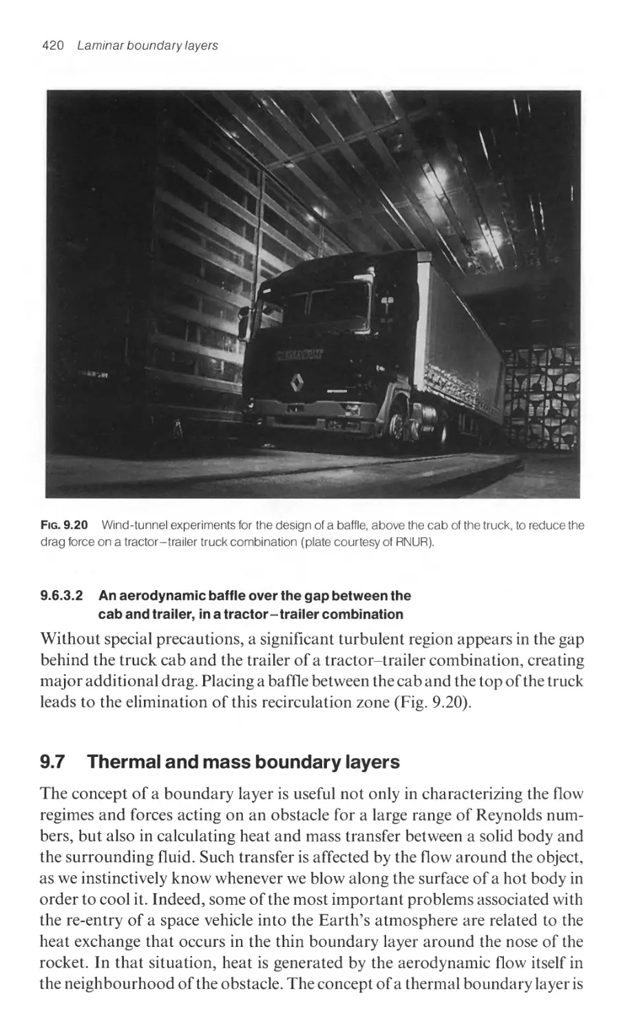
FIG.1.1 The configurations observed as a result of the movement of discs on a vibrating air table, corre-
sponding to different values of the compactness, C: (a) model for the solid state, C = 0.815; (b) liquid-
state simulation, C = 0.741 (plates courtesy of Piotr Pieranski).
4 The physics of flUIds
RV3
RV3
2R
FIG.1.2 A maximally compact configuration for a packing of uniform diameter discs: their centres form a
plane, triangular, crystalline lattice.
constant and the resultant average structure is periodic: there, we have an
image of atomic vibrations in a solid. Such vibrations are associated with
sound propagation; the displacements of individual particles are transmitted
from one neighbour to the next in response to an impressed disturbance at the
other end of the solid, leading to propagation modes known as phonons. But, in
this packing, it is virtually impossible for two neighbouring rows to undergo a
relative displacement greater than R and, consequently, each particle retains
the same neighbours. The amplitude of any resulting slippage is thus quite
limited, and elastic restoring forces result.
Medium compactness
For a compactness smaller than Co 0.8, we have a transition to a different
regime: an individual particle is now able to escape from the 'cage' created by
its neighbours. In this instance, particles no longer have a fixed position
relative to immediately adjacent ones; the system now simulates a two-
dimensional 'liquid' (Fig. 1.1(b)). Simultaneously, the periodicity of the
crystal has vanished. The resulting fluidity of the system leads to the occur-
rence of massive displacements of the discs in response to relative motion of
the side walls of the container.
Low compactness: C « Co
In this final instance, we have a 'gas' of particles. The relative distance between
'nearest neighbours' can now be quite large (of order R/ VC), whereas it was of
order R for the 'liquid'.
1.1.1.2 Numerical simulations in terms of a hard-disc model
Results similar to those of Section 1.1.1.1 can be obtained by means of
numerical simulations in which the interaction between particles is of the hard-
disc type; in this case, the interaction potential between pairs of particles is zero
when the distance r between their centres is greater than 2R, and infinitely
The liquid state 5
repulsive when r < 2R. These calculations confirm and extend the results of
the analogue model that we have presented above. But the main feature of
these simulations is that they allow us to introduce more realistic interaction
potentials-such as the Lennard-Jones potential, which, for three-dimen-
sional systems, is of the form
[ ( 2R ) 12 ( 2R ) 6 ]
V(r) == Vo -;:- - -;:- .
( 1.2)
This potential allows us to take into account the very slight interpenetration
between pairs of particles, strongly limited by the Pauli exclusion principle,
when r < 2R; it also introduces a weak, attractive, van der Waals interaction
between particles, which becomes dominant at large distances (r» R).
Equation (1.2) predicts the existence of the minimum in the potential V(r) for a
value of ro of the order of 2.2R-thus indicating a potentially stable equili-
brium state that is absent in the hard-disc or hard-sphere model. By introducing
this potential, we alter slightly the equation of state of the two-dimensional
ideal gas, and obtain a result similar to the van der Waals equation for pure
substances. More specifically, there appears to be a domain in which liquid-
gas coexistence is possible.
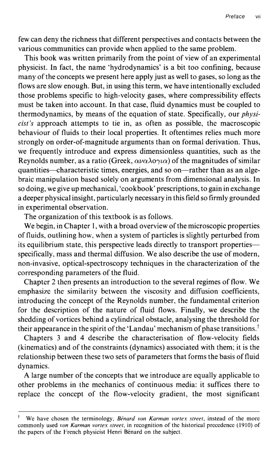
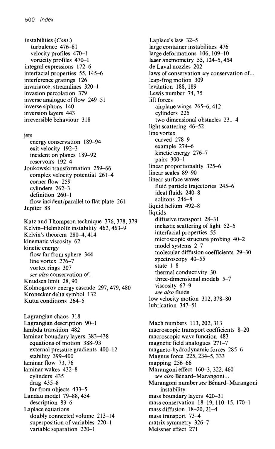
1.1.1.3 Three-dimensional models
In Section 1.1.1.1, we simulated the structure of solids and the solid-liquid
transition by a system of flat circular discs. Can we also create similar models
in three dimensions by stacking beads of uniform diameter, which we rear-
range by shaking, or by fluidization techniques (keeping them temporarily
apart by forcing through an upward stream of fluid from the bottom of the
stack)? We find that it is indeed possible to represent certain structural forms
of matter with the help of periodic packings of beads; such is the case, for
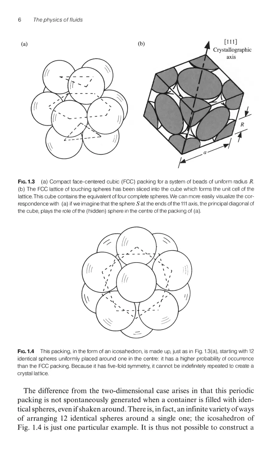
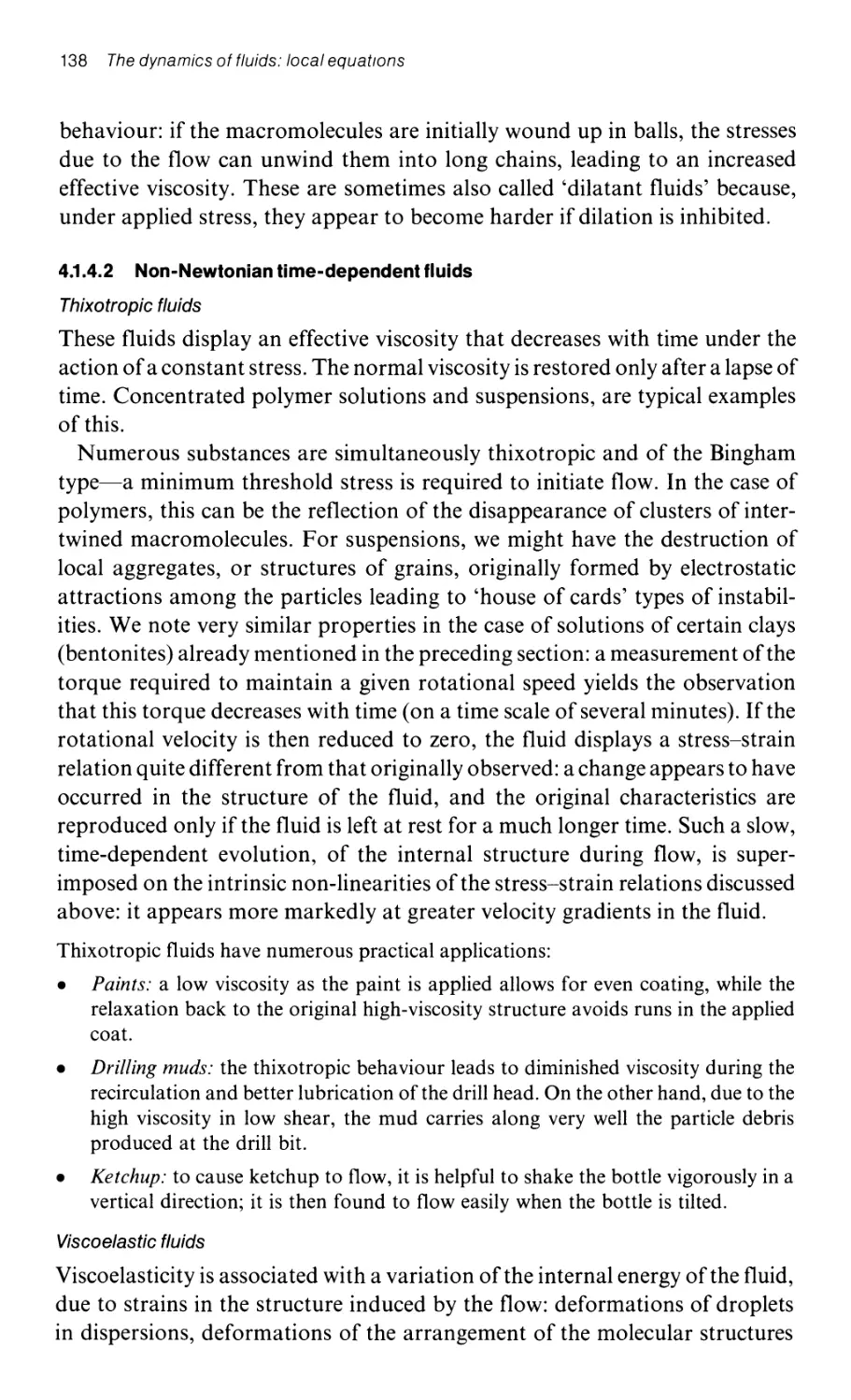
example, for the face-centered cubic (FCC) lattice (Fig. 1.3(a)).
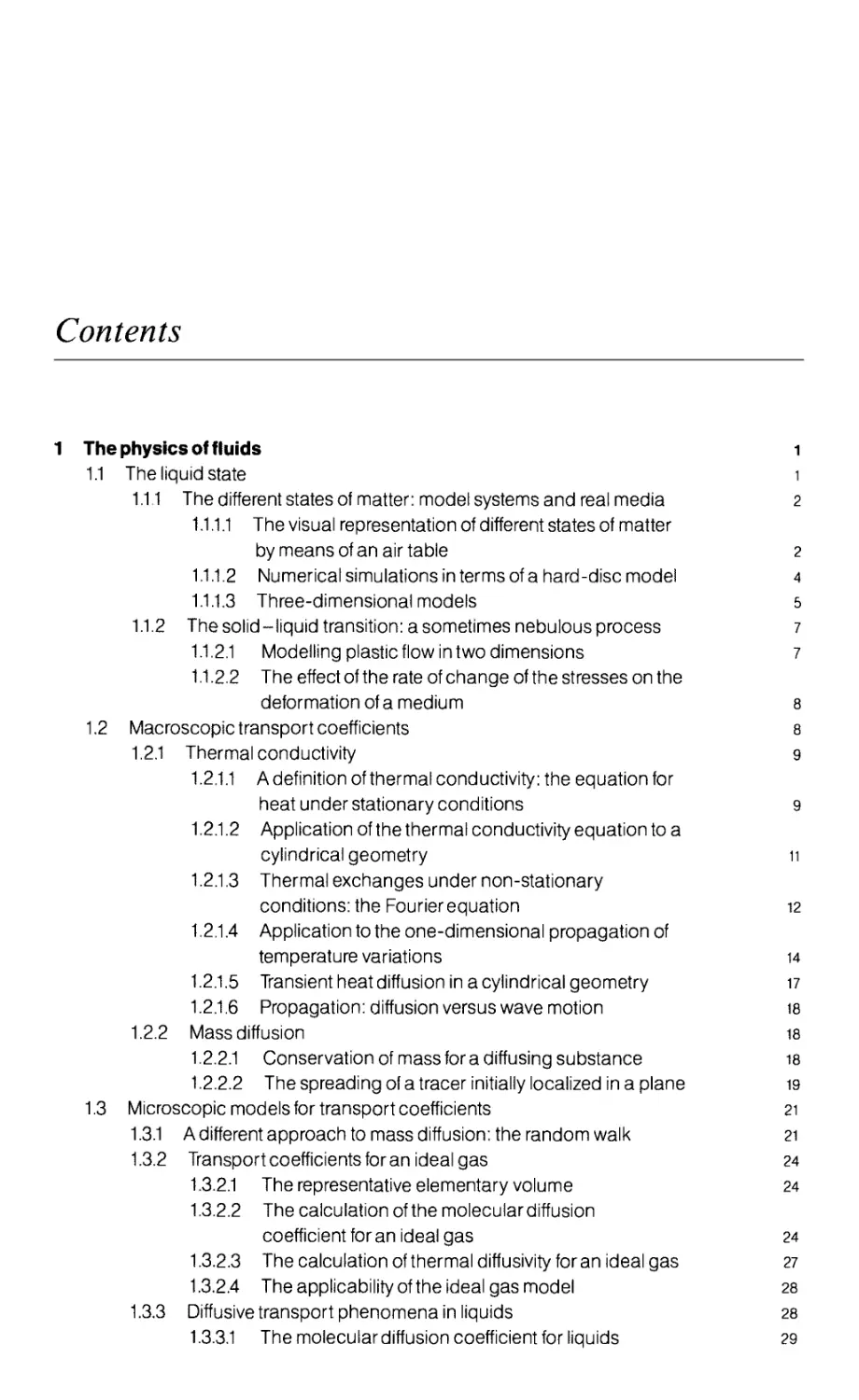
Let us first estimate the compactness of this structure; in this packing, the
basic repetitive pattern turns out to be a cube of side a == (4R/ V2) (Fig. 1.3(b )),
since the diagonal of the faces of this cube has length 4R; this unit cell contains
the equivalent of four complete spheres of radius R. The compactness C (the
fraction of the volume taken up by the adjacent spheres) is thus
4 7r R 3
C == 3
a 3
4 7rR3 7r
3 == - == 0.74.
(4R/ V2)3 3V2
(1.3 )
The value ofO. 74 for the compactness of the FCC structure is the highest that
we know for any packing of spheres of uniform diameter R. Once created, this
packing ensures long-range periodic order, just as does the triangular lattice in
two dimensions.
6 The physics of fluids
(a)
(b)
[Ill]
Crystallographic
aXIS
FIG. 1.3 (a) Compact face-centered cubic (FCC) packing for a system of beads of uniform radius R.
(b) The FCC lattice of touching spheres has been sliced into the cube which forms the unit cell of the
lattice. This cube contains the equivalent of four complete spheres. We can more easily visualize the cor-
respondence with (a) if we imagine that the sphere S at the ends of the 111 axis, the principal diagonal of
the cube, plays the role of the (hidden) sphere in the centre of the packing of (a).
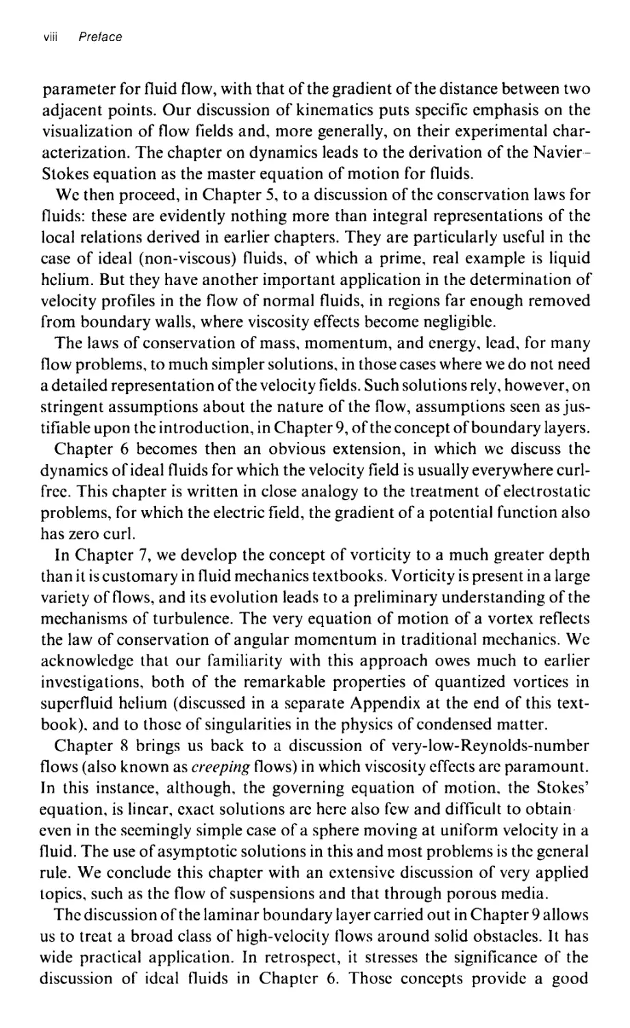
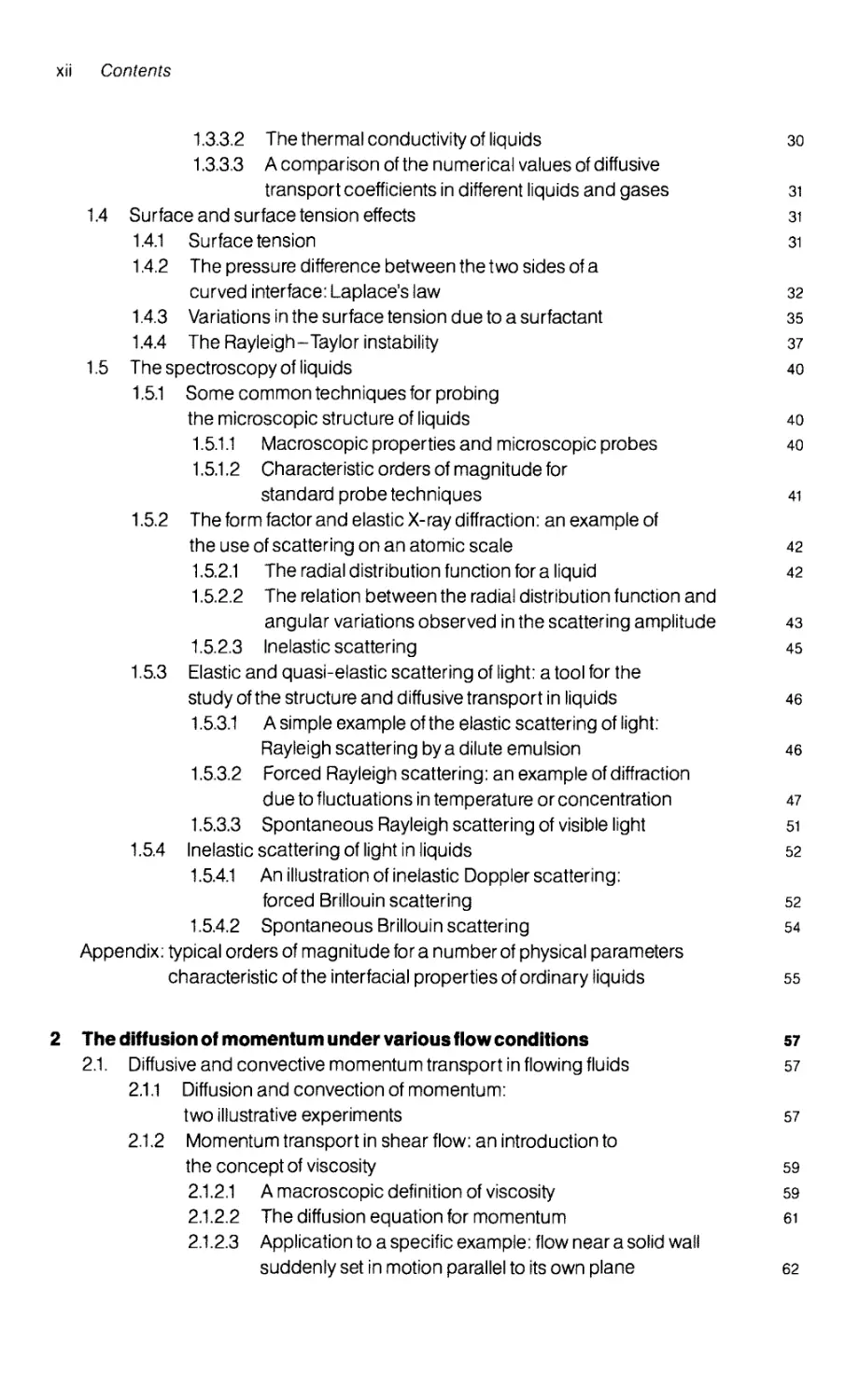
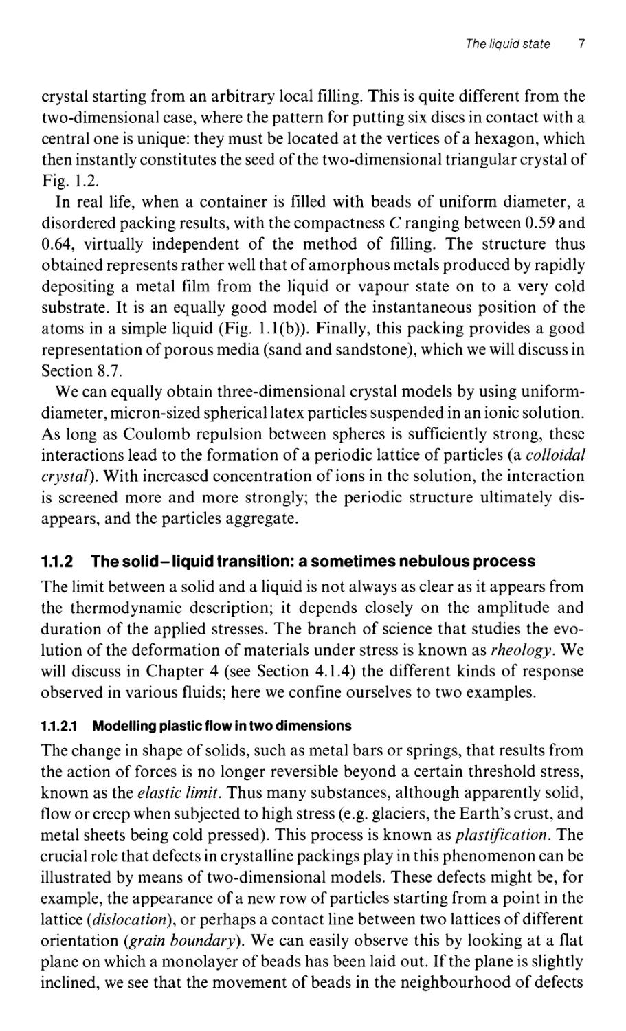
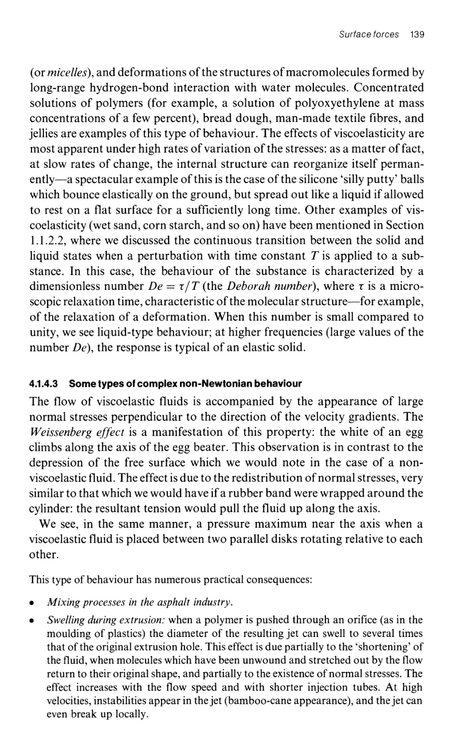
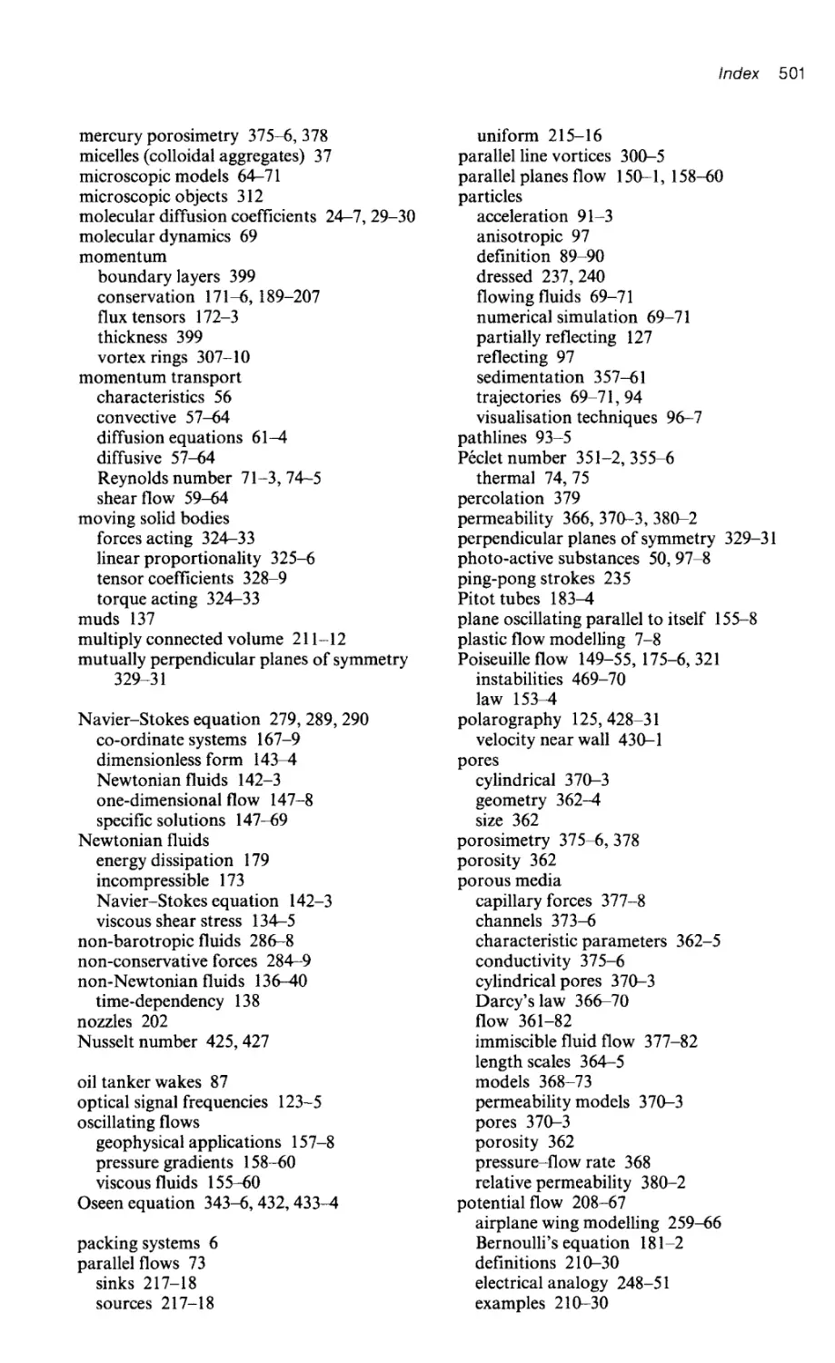
FIG.1.4 This packing, in the form of an icosahedron, is made up, just as in Fig. 1.3(a), starting with 12
identical spheres uniformly placed around one in the centre: it has a higher probability of occurrence
than the FCC packing. Because it has five-fold symmetry, it cannot be indefinitely repeated to create a
crystal lattice.
The difference from the two-dimensional case arises in that this periodic
packing is not spontaneously generated when a container is filled with iden-
tical spheres, even if shaken around. There is, in fact, an infinite variety of ways
of arranging 12 identical spheres around a single one; the icosahedron of
Fig. 1.4 is just one particular example. It is thus not possible to construct a
The liquid state 7
crystal starting from an arbitrary local filling. This is quite different from the
two-dimensional case, where the pattern for putting six discs in contact with a
central one is unique: they must be located at the vertices of a hexagon, which
then instantly constitutes the seed of the two-dimensional triangular crystal of
Fig. 1.2.
In real life, when a container is filled with beads of uniform diameter, a
disordered packing results, with the compactness C ranging between 0.59 and
0.64, virtually independent of the method of filling. The structure thus
obtained represents rather well that of amorphous metals produced by rapidly
depositing a metal film from the liquid or vapour state on to a very cold
substrate. It is an equally good model of the instantaneous position of the
atoms in a simple liquid (Fig. 1.1(b)). Finally, this packing provides a good
representation of porous media (sand and sandstone), which we will discuss in
Section 8.7.
We can equally obtain three-dimensional crystal models by using uniform-
diameter, micron-sized spherical latex particles suspended in an ionic solution.
As long as Coulomb repulsion between spheres is sufficiently strong, these
interactions lead to the formation of a periodic lattice of particles (a colloidal
crystal). With increased concentration of ions in the solution, the interaction
is screened more and more strongly; the periodic structure ultimately dis-
appears, and the particles aggregate.
1.1.2 The solid -liquid transition: a sometimes nebulous process
The limit between a solid and a liquid is not always as clear as it appears from
the thermodynamic description; it depends closely on the amplitude and
duration of the applied stresses. The branch of science that studies the evo-
lution of the deformation of materials under stress is known as rheology. We
will discuss in Chapter 4 (see Section 4.1.4) the different kinds of response
observed in various fluids; here we confine ourselves to two examples.
1.1.2.1 Modelling plastic flow in two dimensions
The change in shape of solids, such as metal bars or springs, that results from
the action of forces is no longer reversible beyond a certain threshold stress,
known as the elastic limit. Thus many substances, although apparently solid,
flow or creep when subjected to high stress (e.g. glaciers, the Earth's crust, and
metal sheets being cold pressed). This process is known as plastification. The
crucial role that defects in crystalline packings play in this phenomenon can be
illustrated by means of two-dimensional models. These defects might be, for
example, the appearance of a new row of particles starting from a point in the
lattice (dislocation), or perhaps a contact line between two lattices of different
orientation (grain boundary). We can easily observe this by looking at a flat
plane on which a monolayer of beads has been laid out. If the plane is slightly
inclined, we see that the movement of beads in the neighbourhood of defects
8 The physics of fluids
allows wholesale deformations of the system. Thus, defects lead to flow
properties in solid matter. This observation is the basis of modern metallurgy.
1.1.2.2 The effect of the rate of change of the stresses on the
deformation of a medium
The rate at which stresses vary plays a role that is as important as their
magni tude in the behaviour of a substance. We will see in Section 4.1.4 that the
response of some substances to variable-frequency perturbations displays a
transition from a solid-like state (at high frequencies) to a liquid-like one (at
lower frequencies). The crossover between these two regimes occurs in the
neighbourhood of a frequency Iii, that is characteristic of the substance.
A typical example of this change of behaviour with frequency is the case of wet
sand. We need only compare the very shallow footprints imprinted in wet sand
when we run with the much deeper ones that result when we stand still. A very
simple experiment of the same nature can also be performed, using a con-
centrated starch paste in which we insert a teaspoon at varying rates: the
teaspoon sinks into the paste only if slowly inserted; yet the starch can be
spooned out as a solid lump if the teaspoon is removed rapidly. Another
classical example of this type of behaviour is the case of a polymer with the
polymeric chains all twisted up one within the other. A characteristic time i is
required for the macromolecules to disentangle. If the characteristic time scale
of the excitation is much shorter than i, the polymer behaves as a solid;
conversely, at lower frequencies (times much longer than i), it deforms irre-
versibly, just as a liquid would.
1.2 Macroscopic transport coefficients
Let us now discuss the transport phenomena that appear in fluids due to small
deviations from equilibrium conditions, deviations small enough for the
system response to continue to be approximately linear. Three types of
transport can then be studied:
. the transport of heat (energy) resulting from spatial variations of
temperature
. the transport of matter due to variations in concentration
. the transport of momentum in a moving fluid
Although it is this last transport property that is treated in particular depth in
this textbook, in the present chapter we consider only the first two types listed
above.
These several kinds of transport phenomena frequently coexist in the physics
of fluids, as indicated in the following examples:
. A warm object (at temperature T+), placed in a motionless fluid at a
lower temperature T _, frequently generates a convective circulation in the
Macroscopic transport coefficients 9
(a)
(b)
T
v
T
.
Q Q t
T:
T:
FIG.1.5 Heat exchange between a fluid and a heated plate: (a) In the presence of spontaneous con-
vective fluid motion Induced by the eXisting temperature difference (discussed in detail in Chapter 10);
(b) between an air stream and a warm body, resulting from the formation of a boundary layer (see
Chapter 9).
upper region of the fluid (Fig. 1.5(a)). In turn, the fluid motion increases
the heat exchange between object and fluid.
. When we blow air on a glowing wooden ember, we simultaneously affect
the transport of mass, of matter, and of heat (Q); the kinetics of the
exothermic burning process is correspondingly accelerated (Fig. 1.5(b)).
We see, in these examples, a superposition of a number of exchange
mechanisms: not only convective (drag by the moving fluid), radiative, and
chemical (associated with the reactions that occur), but also diffusive or con-
ductive exchange. These depend only on the microscopic properties of the fluid
and can be an a lysed in terms of small deviations from the equilibrium state.
In this chapter, we mainly discuss the diffusive effects.
We first consider, from a macroscopic viewpoint, the familiar example
of heat conduction, and proceed from there to look at mass diffusion
(Section 1.2.2); in Section 1.3 we provide a microscopic picture of these effects
in gases and liquids. In Chapter 2, we will note how the viscosity of a fluid
results from a similar diffusion of momentum. The reason for our simulta-
neous presentation of diffusive transport of these three physical quantities
(heat, mass, and momentum) is the fact that the equations that describe each
process and its observed characteristics are mathematically identical. The
results obtained for heat transport are thus easily translated to that of mass, or
momentum (requiring only a change of definition of the associated coefficients
and, for the momentum, a change from scalar to vector quantities).
1.2.1 Thermal conductivity
1.2.1.1 A definition of thermal conductivity: the equation for
heat under stationary conditions
A semi-infinite homogeneous body (solid, liquid, or gas) occupying the space
corresponding to positive values of x is subjected to a temperature gradient
aT / ax, in the direction of the x-axis. This gradient is obtained by applying a
temperature difference T I - T2 between two planes PI and P 2 , a distance L
10 The physics of fluids
L
I
J Q ' ,
_ _--L
I I
, ,
\
.
x
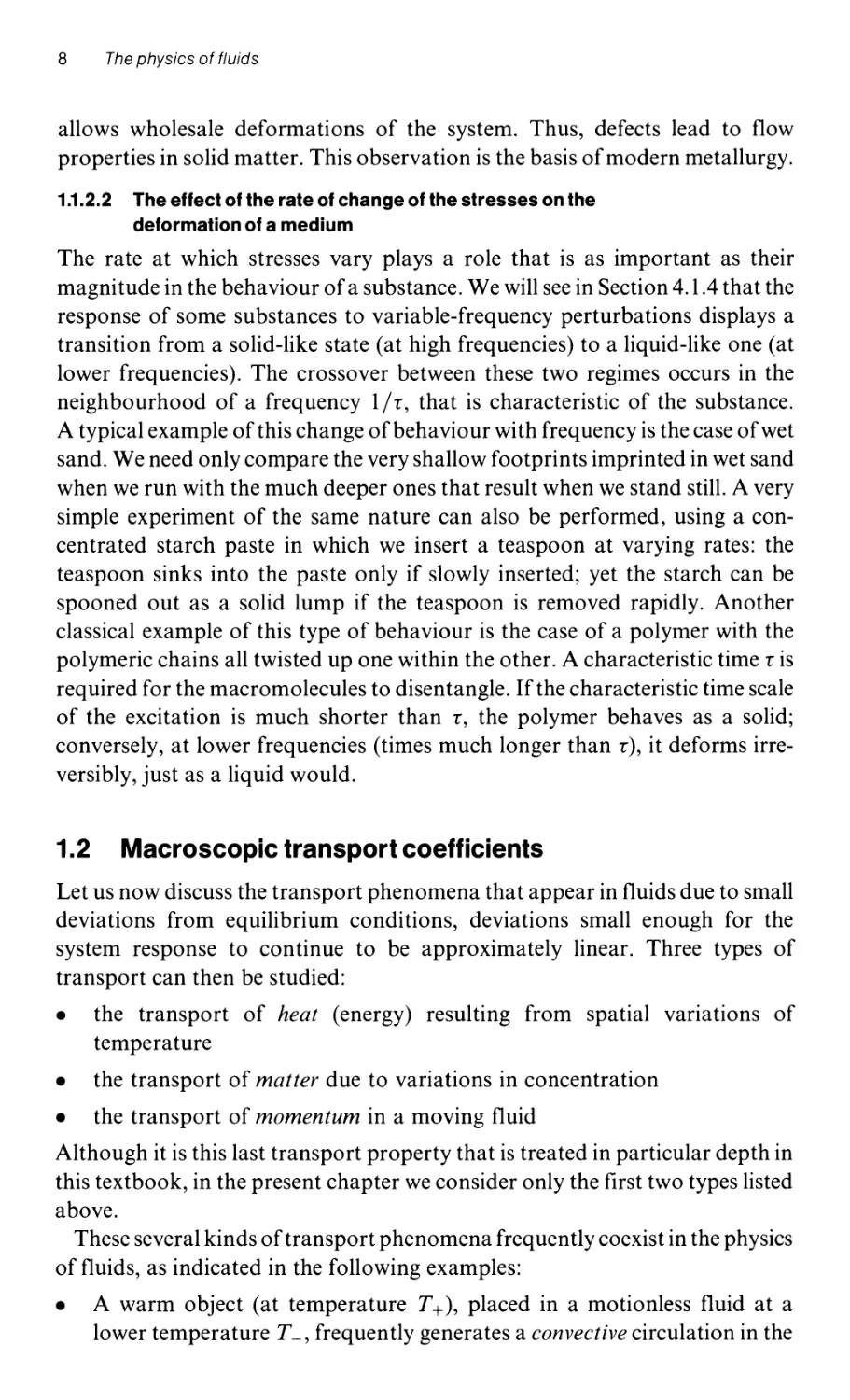
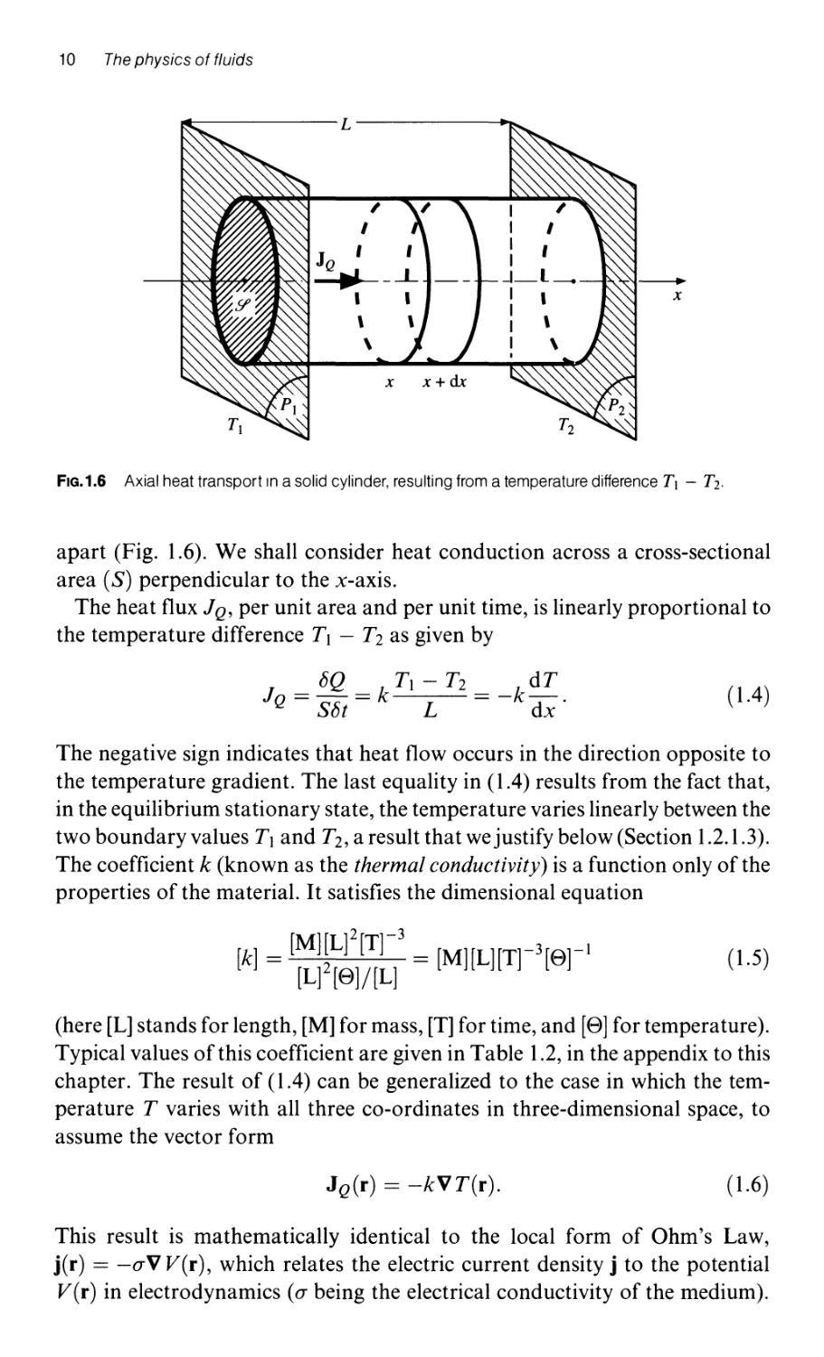
FIG.1.6 Axial heat transport In a solid cylinder, resulting from a temperature difference Tl - T2.
apart (Fig. 1.6). We shall consider heat conduction across a cross-sectional
area (S) perpendicular to the x-axis.
The heat flux J Q , per unit area and per unit time, is linearly proportional to
the temperature difference Tl - T2 as given by
J == 8Q == k Tl - T2 == -k dT .
Q S8t L dx
( 1.4)
The negative sign indicates that heat flow occurs in the direction opposite to
the temperature gradient. The last equality in (1.4) results from the fact that,
in the equilibrium stationary state, the temperature varies linearly between the
two boundary values Tl and T 2 , a result that we justify below (Section 1.2.1.3).
The coefficient k (known as the thermal conductivity) is a function only of the
properties of the material. It satisfies the dimensional equation
[k] = [M][L]2[Tr 3 = [M][L][Tr 3 [Or l
[L] 2 [8] / [L]
(1.5)
(here [L] stands for length, [M] for mass, [T] for time, and [8] for temperature).
Typical values of this coefficient are given in Table 1.2, in the appendix to this
chapter. The result of (1.4) can be generalized to the case in which the tem-
perature T varies with all three co-ordinates in three-dimensional space, to
assume the vector form
JQ(r) == -kVT(r).
( 1.6)
This result is mathematically identical to the local form of Ohm's Law,
j(r) == -aV V(r), which relates the electric current density j to the potential
V(r) in electrodynamics (a being the electrical conductivity of the medium).
Macroscopic transport coefficients 11
We can now easily understand why, under stationary conditions, the
temperature varies linearly with distance in the geometry of Fig. 1.6, just as
the potential varies linearly between two parallel electrodes (at different
potentials) immersed in a conducting fluid. The linear dependence in (1.6)
expresses a proportionality between a flux (of heat) and a thermodynamic
force (the temperature gradient); we find similar relations in the other trans-
port phenomena in the neighbourhood of equilibrium conditions.
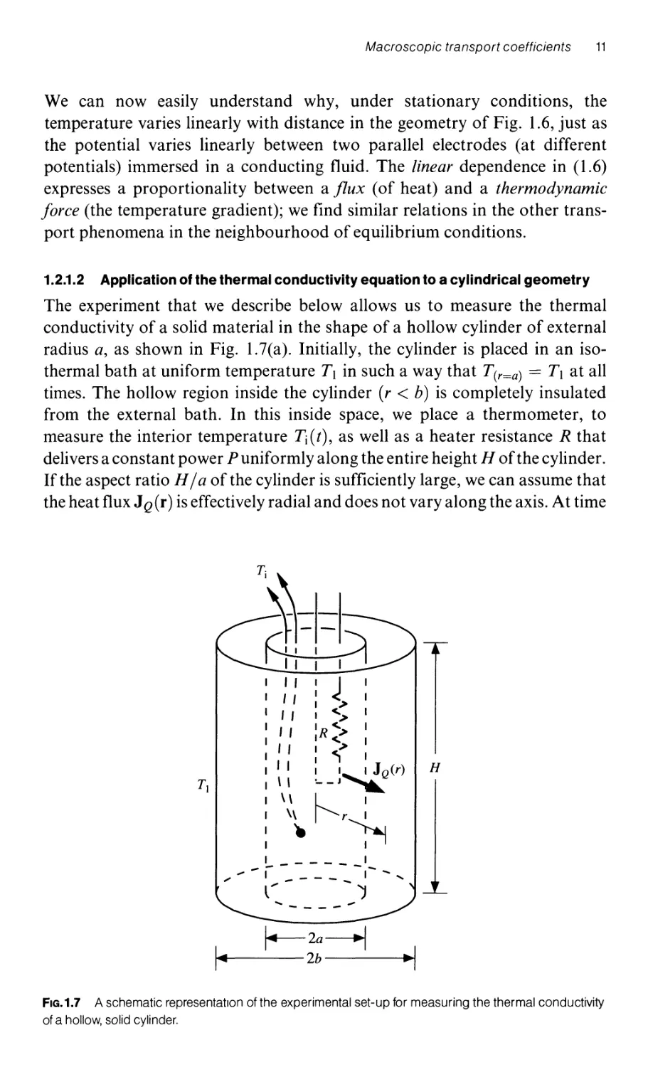
1.2.1.2 Application of the thermal conductivity equation to a cylindrical geometry
The experiment that we describe below allows us to measure the thermal
conductivity of a solid material in the shape of a hollow cylinder of external
radius a, as shown in Fig. 1.7(a). Initially, the cylinder is placed in an iso-
thermal bath at uniform temperature Tl in such a way that T(r=a) == Tl at all
times. The hollow region inside the cylinder (r < b) is completely insulated
from the external bath. In this inside space, we place a thermometer, to
measure the interior temperature Ti (t), as well as a heater resistance R that
delivers a constant power P uniformly along the entire height H of the cylinder.
If the aspect ratio H / a of the cylinder is sufficiently large, we can assume that
the heat flux J Q (r) is effectively radial and does not vary along the axis. At time
I I
I I
I I
I I
, ,
I I H
T} \ \
\ \
\\
'-
_---_ 1
..... - I -1- " ,
" l..... - - - - -
" -- - - ....
1-- 2a .1
2b
FIG.1.7 A schematic representation of the experimental set-up for measuring the thermal conductivity
of a hollow, solid cylinder.
12 The physics of fluids
t == 0, the heater is turned on, and we observe the variation of the interior
temperature Ti (t) of the cylinder, as measured by the thermometer (Fig. 1. 7).
At the end of a sufficient time lapse, this temperature stabilizes at a value T 2 .
Measurement of the temperature difference T 2 - T I provides us with the
value of the thermal conductivity k of the cylinder, as follows. If we calculate
the radial heat flux JQ(r) per unit area (for b < r < a) between the two infi-
nitesimally close cylinders at radii rand r + dr, the magnitude of the heat
fl ux is
P == 27rrH1 Q (r) (1.7)
where
dT ( 1.8)
lQ(r) == -k .
Under stationary conditions, the heater power P is constant. Combining
these two results, we obtain the differential equation
dr == _ 27rHk dT
r P
( 1.9)
Integrating, and recalling the steady temperatures at the boundaries, we
obtain the thermal conductivity:
P a
k == log -.
27rH(T2 - TI) b
(1.10)
This calculation, which is valid in a stationary regime, is identical to that for
the electrical conductivity of a conductor formed by two coaxial cylinders
under a potential difference V2 - VI (corresponding to the temperature dif-
ference T 2 - T}) and carrying a current I (which corresponds to the heater
power P).
1.2.1.3 Thermal exchanges under non-stationary conditions:
the Fourier equation
The previous example was discussed under the assumption that a stationary
condition had been achieved, with the temperature at every point independent
of time. We then measured heat diffusion under a fixed gradient. Let us now
look at a more general case, in which the temperature T is a function of both
position and time. In the preceding section, this corresponded to the transient
observed with the set-up illustrated in Fig. 1.7. Initially, we now examine the
simpler case of temperature variation in the one-dimensional geometry of
Fig. 1.6. The changing temperature T(x, t) can be described by studying the
thermal energy balance for an infinitesimal volume element of the material,
Macroscopic transport coefficients 13
bounded by the planes at x and x + dx (Fig. 1.6). The heat flux entering
this volume element during a time interval dt through the surface S is,
from (1.4),
aT(x, t)
JQ(x)S dt == -k ax S dt.
(1.11)
Similarly, the outgoing flux is
aT(x + dx t)
JQ(x+dx)Sdt==-k ax' Sdt.
(1.12)
The algebraic difference between the entering and exit fluxes represents the
quantity of heat being stored in the volume bounded by the two planes:
JQ(x)S dt - JQ(x + dx)S dt = kS dt [ _ aT ;, t) + aT(x dx, t) ]
= kS dt a 2 ' t)
(1.13)
where we have carried out a first-order Taylor expansion of the above
expression. Because of the thermal capacity of the material, the heat accu-
mulating in the volume element leads to a variation of the temperature with
time, aT(x, t) / at, given by
pCS dx aT , t) dt = kS dt a2 , t) dx
(1.14)
where p is the density of the substance and C its specific heat. Simplifying
(1.14), we obtain the heat conduction equation, generally known as the dif-
fusion equation (but sometimes also referred to as Fourier's equation). This
provides, in one dimension, a relation between the partial derivatives of the
temperature T with respect to time t and to the space co-ordinate x:
C aT(x, t) = k a 2 T(x, t) (1.l5a)
p at ax 2
or
aT(x, t) a 2 T(x, t) ( I.15b )
==Ii
at ax 2
where
Ii = k/pC. ( 1.16)
14 The physics of fluids
The coefficient Ii is called the thermal diffusivity of the material. A large
thermal diffusivity corresponds either to a large thermal conduction coeffi-
cient, k, or to small thermal inertia, as measured by the product pC. Dimen-
sionally, (1.15b) implies that the units of Ii are [L]2[T]-I.
The form of (1.15b) is very general, and characteristic of all diffusion phe-
nomena: we find it in identical form, but with different variables, in problems
of mass or momentum transport. It is frequently advantageous to make use of
this correspondence where the diffusivity coefficients have identical dimen-
sions but different numerical values. We note that, under stationary condi-
tions in one-dimensional geometry, (1.15) reduces to
8 2 T(x, t) == 0
8x 2 .
We then have, in that particular case, a temperature gradient that is constant
with respect to the space co-ordinate x and consequently, as originally
assumed in (1.4), a linear variation of the temperature with position.
More generally, in a problem where the temperature is a function of all three
co-ordinates in three-dimensional space, the term 8 2 T(x, t)/8x 2 in (1.15) is
replaced by the Laplacian:
r72 T 82 T(r, t) 8 2 T(r, t) 8 2 T(r, t)
v == + +
8x 2 8y2 8z2
whence
8T(r, t) k 2 2
at = pC V' T(r, t) = K,V' T(r, t)
( 1.17)
which is the three-dimensional heat-diffusion equation (Fourier's equation).
1.2.1.4 Application to the one-dimensional propagation of
temperature variations
Let us now consider again a plane one-dimensional geometry, where a semi-
infinite body is initially at a uniform temperature T == To for all time t < o. At
the instant t == 0, we apply a particular temperature on the boundary plane,
x == 0, by putting the body in contact with a heat reservoir at a uniform
temperature Tl == T(x == 0, t > 0). The temperature profile as a function of
distance from the plane passing through the origin is shown in Fig. 1.8(a) for
different instants of time. We observe the gradual spreading, under the effect
of heat conduction, of the perturbation that was introduced initially at the
orIgIn.
The solution of this problem sheds light on numerous other examples of
diffusion. We might note first of all that, by using the thermal diffusivity Ii
and the time variable t, we can construct a new variable v;::i, which has the
Macroscopic transport coefficients 15
T
T)
T-T o
Tl - To
To
o
o
x
1
(b)
x
\1M
(a)
FIG.1.8 Profiles of the vanatlon of temperature with distance along an 'Infinitely long' bar; (a) profiles at
different times t) < t2 < t3 upon applYing a step function in temperature at the origIn x = 0; (b) profiles
for different times as a function of the normalized distance xl V'K]. The corresponding universal curve is
predicted by (1.18).
dimensions of a length. It is, therefore, quite reasonable to normalize the space
co-ordinate x in terms of this characteristic length, defining a new dimen-
sionless variable u = xl v;:;:i; similarly, instead of calculating T(x, t), we
introduce the normalized function (T - To)/(T} - To), which therefore takes
on values I (for x = 0) and 0 (for x 00). We find then, as derived below, the
solution
T- To
T} - To
[1 - erf( ) ]
(1.18)
where
2 (Z 2
erf(z) = ..j7i Jo e-( d(
is the error function; it vanishes when z = 0, and approaches unity as z tends to
infinity. Thus, for the particular boundary conditions that we have considered
here, we have obtained a solution which does not depend separately on x and t,
but only on the reduced variable u = xlv;:;:i. Figure 1.8(b) indicates that the
spatial profiles of the normalized temperature, corresponding to different
moments in time, coincide when they are displayed as a function of this
dimensionless variable. For other boundary conditions, it might have been
necessary to look for more complicated solutions that depend separately on x
and t.
Qualitatively, we see that, at a given time t, the effect of a temperature
perturbation has spread to a distance of order v;:;:i, in good agreement with the
dimensional form of K. We note here the essential characteristic of diffusive
phenomena, a proportionality between the mean diffusion distance and the
square root of the time. This result specifically explains the ineffectiveness of
16 The physics of fluids
diffusive mechanisms at great distances: if it takes a time t L for a temperature
perturbation to diffuse through a distance L, it will need a time tlOL == 100tL
for it to diffuse through a distance ten times as long! For air, for example,
VKi == I cm for t == 10 s; VKi == 10 cm for t == 10 3 S 16 minutes. If we heated
our houses only by means of thermal diffusion processes, such heating would
be extremely inefficient; fortunately, free-convection mechanisms (as illu-
strated in Fig. 1.5(a)), forced convection through air circulation (Fig. 1.5(b )),
or radiation are used in practice to assist heat conduction. We see again, in
Section 2.1.2.3, a mathematical solution virtually identical to that presented
here for thermal conduction: that case involves the variation of a velocity field
near a solid plane which is suddenly caused to move parallel to itself in a
viscous fluid.
The derivation of (1 .18)
We seek trial solutions of the form
T(x, t) = f( ) = f(u).
(1.19)
Substituting (1.19) into (1.17) and writing the corresponding partial derivatives of T
with respect to t and x,
aT(x, t) = _It- 3 / 2 I' (u)
at 2
and
a 2 T(x, t) = f"(u)
ax 2 lit
we obtain the relation
I"(u) +!ul'(u) = o.
(1.20 )
Defining F(u) = I '(u), the differential equation for F(u) in term of the reduced vari-
able u becomes
F' (u) + uF(u) = 0
2
(1.21 )
with the solution
F = Foe- u2 /4.
( 1.22)
We thus conclude that
f(u) = A erf G) +B
( where u = ).
(1.23)
The constants A and B are determined from the boundary values for the temperature:
T == Tl == A at x = 0, and T = To == A + B for x 00.
Macroscopic transport coefficients 17
1.2.1.5 Transient heat diffusion in a cylindrical geometry
We have discussed earlier, in Section 1.2.1.2, radial heat transport in a hollow
cylinder under stationary conditions. Let us now consider the transient tem-
peratures in the limiting case where the cylinder is no longer hollow but solid.
We suppose that the cylinder of outer radius a, initially at a temperature To, is
suddenly plunged at time { == 0 into a fluid of temperature To + 8To. We will
not carry out here in detail the required calculation in terms of series of
functions, but we confine ourselves to displaying the results obtained.
Figure 1.9 shows the temperature profiles for the reduced temperature
8T(rla)18To at different values of the time {(r is the distance from the axis of
the cylinder, 8T(r I a) is the variation of the local temperature relative to the
initial temperature To). The letters that label each profile correspond to dif-
ferent values of the ratio {I TO, where TO (== a 2 I K) represents, as shown earlier,
the order of magnitude of the diffusion time over a distance a. We observe that
for short times the temperature variation is confined to a layer close to the
surface (r == a), ofa thickness of the order of VKi. The temperature profiles are
similar to those that we have shown previously in Fig. 1.8 for a plane
boundary; i.e. for an infinitely large radius of curvature. For longer times, of
the order of 0.1 TO, the perturbation in temperature begins to be observed on
the axis of the cylinder. It is everywhere equal to To + 8To when { becomes of
order TO . We will see in Section 2.1.2 that these profiles equally descri be the
8 T / 8 To
1.0
0.8
0.6
0.4
0.2
o
o
0.2
0.4
0.6
0.8
1.0
rIa
FIG.1.9 The diffusion of heat In a cylinder Initially at temperature To which IS suddenly Immersed, at time
t = 0 In a heat bath such that ItS surface is then maintained at temperature To + 8To. The distribution of
the reduced temperature 8T / 8To is displayed as a function of the normalized distance r / a from the axis
of the cylinder. The several curves correspond to different times, measured in terms of the reduced-time
variable (tj-ro = K,t/ a 2 ): tj-rD = (a) 0.005; (b) 0.01; (c) 0.04; (d) 0.1; (e) 0.15; (f) 0.2; (g) 0.3; (h) 0.4.
18 The physics of flUIds
temporal and spatial variation of the fluid velocity, in a cylinder filled with
fluid, which is suddenly set into rotation.
1.2.1.6 Propagation: diffusion versus wave motion
In order to estimate the effectiveness of various processes, let us compare
(1.17), the diffusion equation, to the classical equation of wave propagation
for a wave of amplitude A travelling in the positive x-direction:
a 2 A
ax 2
1 a 2 A
--
c 2 at 2
(1.24 )
where c is the speed of the wave. We know that for (1.24) the most general
solution is of the form A(x, t) == fl (x - ct) + f2(x + ct). These equations
describe wave propagation, in the positive and negative x-directions respec-
tively, at a constant speed c; the distance d covered by the wave is linearly
proportional to the time. We have seen that (1.17) has solutions for which the
propagation distance x varies as the square root of the time t; thus the 'effective
speed of propagation' xl t decreases with distance. Physically, this result is due
to the fact that the flux of the variable that is diffusing (temperature, con-
centration, and so on) is proportional to the gradient of this variable: the more
the variation front spreads out, the slower the propagation is.
Thus, a simple change in the order of the derivative with respect to time
yields completely different behaviour for the cases of wave propagation and
for diffusion. Diffusive phenomena are efficient at short times, or for relatively
small distances. On the other hand, wave propagation, and fluid convection
resulting from the fluid motion (which also leads to a displacement linear in
time), dominate in every other situation.
1.2.2 Mass diffusion
1.2.2.1 Conservation of mass for a diffusing substance
Let us replace, in the one-dimensional example of Fig. 1.6, the temperature T
by the concentration of a substance diluted by the main fluid: this tracer
substance might be another gas, or smoke within the gas, ions, dye molecules,
or radioactive isotopes in the liquid. In this experiment of gradient diffusion, we
are interested in determining the flux of tracer which results from a gradient in
its concentration. We could also investigate the phenomenon of self-diffusion
which describes the redistribution of , tagged' molecules (even in the absence of
a gradient) among other unmarked molecules of the same type. In a dilute
solution, the gradient diffusion and self-diffusion coefficients have identical
values. For the case in which diffusing particles interact, these two coefficients
can take on different values.
The concentration can be measured by the number density, n(x, t), of tracer
particles per unit volume, or by the mass density PA of the tracer, per unit
volume of the mixture. In this case, the expression equivalent to (1.6)
Macroscopic transport coefficients 19
(sometimes known as Fick's equation) is
J rn == -DV PA
( 1.25)
where J rn is the current density (mass per unit area per unit time), and D is the
molecular diffusion coefficient of the tracer. Its value is, at the same time, a
function of the properties of the tracer and of the substance through which it
diffuses. D satisfies the dimensional equation
[D] = [M][Lr 2 [Tr l [L] = [Lf[TrI
[M][L]-3
thus having the same dimensions as the thermal diffusivity coefficient (1.16).
Table 1.2, in the appendix to this chapter, also provides a few, typical,
numerical values of this coefficient.
We can derive the partial differential equation which relates the variations of
the density with position and time by following, step by step, the same pro-
cedure used for the heat conductivity problem; i.e. by expressing in two
different ways the mass conservation of the tracer within a given volume ele-
ment. We thus obtain, for the one-dimensional case, an equation analogous
to (1.l5b):
apA == D a 2 pA
at ax 2 .
( 1.26)
In Section 1.2.1 we discussed examples of thermal conduction with fixed
temperature boundary conditions on the walls of the sample. These examples
would correspond here to a problem in which the boundary values of the
concentrations of the chemical substances are fixed. In that case, the mathe-
matical solutions carryover exactly, merely substituting PA for the variable T
and replacing Ii with D.
In practical terms, it is simpler, in the case of the mass diffusion problem, to
prescribe a particular initial concentration of tracer, and to observe how it
evolves with time. The equivalent thermal problem would consist in generat-
ing, over a rather short initial time interval, a certain amount of heat at specific,
localized points, and then observing the resultant temperature distribution.
1.2.2.2 The spreading of a tracer initially localized in a plane
Let us assume that we introduce uniformly, into the interior of a fluid, a mass
per unit area M A of tracer, initially localized throughout a very narrow layer in
the plane x == O. Mathematically, this distribution is of the type of a Dirac
8-function with PA == M A 8(x). Provided that the tracer does not interact with
the fluid, the conservation of mass for the tracer can be written
1 +00
-ex; PA(X) dx = MA = constant.
( 1.27)
20 The physics of fluids
To check these constraints, we can take, with respect to the variable x, the
derivative g(x, t) of the solution of the thermal diffusion equation (1.23),
obtained above in Section 1.2.1.4:
g(x, t) = A e- u2 / 4 (1.28)
2 Y7rlit
where u == x I Jfij. The solution of (1.23) corresponds to the response to a step
function in the tracer concentration, not to a very localized injection of tracer,
as considered in this example. The function g( x, t) is also a solution of (1.15b).
Indeed, by differentiating that equation with respect to x, we find that, if a
function is a solution of the equation, its derivative with respect to x is also a
solution. Finally, replacing Ii by D, we obtain
P ( X t ) == MA e - x 2 /4Dt .
A, 2 Y7rDt
( 1.29)
The solution to this problem is evidently a Gaussian (Fig. 1.lO(a)). Its width
increases in proportion to the square root of the time: this is illustrative of the
variation of the propagation distance with Vi, which is characteristic of dif-
fusive phenomena. At the same time, the amplitude decreases as 1 I Vi, so that
the area under the curve is conserved-this area represents the total mass of
tracer injected. As was the case for Fig. 1.8(b), we discover that, by using the
co-ordinate u == xl Jfij as abscissa, and the product ViPA(x, t) as the ordinate,
we can superimpose the different results on the universal curve displayed in
Fig.l.l0(b).
t=O
P A (x, t)
o
x
o
x
fl5i
FIG.1.10 Spreading, by means of molecular diffusion, of a drop of tracer initially localized in the plane
x = 0 at time t = 0; (a) concentration profiles at times t = 0, t = t1 and t = 2t1, (b) the universal curve
that represents the superposition of all results of (a) when we use the normalized variable xl/75i as
abscissa and the amplitude VtPA (x, t) as ordinate. The graph corresponds to the Gaussian of (1.29).
(Note that the use of such reduced, or normalized, units plays a crucial role In the solution of physical
problems, particularly in fluid dynamics. It IS closely associated with the notion of dimensional analysIs,
or the dimensionless ratios that we will see recurring throughout this text.)
Microscopic models for transport coefficients 21
1.3 Microscopic models for transport coefficients
The macroscopic laws that we have derived for heat and mass diffusion have
very general applicability to fluids and solids. Up to this point, we have con-
sidered neither the microscopic nature of these transport processes nor the
relation between the diffusion coefficients and the structure of the medium in
which the transport occurs. We are going to give, below, a simplified description
of the microscopic mechanisms of transport. In the sections that follow, we
proceed to discuss mass diffusion in terms of a random walk, we apply kinetic
theory to transport processes in gases, and, finally, we treat the case of liquids.
1.3.1 A different approach to mass diffusion: the random walk
We again study here the spread of a drop of tracer, initially localized at a point.
Let us analyse the movement of the tracer particles, which might be molecules,
or very small particles much less than a micron in size, sometimes called
Brownian particles. Because of thermal motion, these particles are not
stationary, but follow rather complex trajectories that entail a sequence of
random changes in direction (Brownian motion).
To analyse this process, we use the model of a random walk (sometimes also
known as the 'staggering drunk' problem!). Starting from an origin 0 at initial
time t == 0, our drunk takes steps of constant length t and time duration T-
setting out, at each subsequent step, in a new direction that is completely
independent of the preceding one. We wish to evaluate the mean distance from
the origin 0 at which the walker (representing one of the tracer molecules) is to
be found at the end of a number of steps N == tiT. In statistical physics, we are
concerned with averages: we therefore need to calculate the mean-square
displacement (R(t)2) averaged over an ensemble of independent random
walks. (The mean value of the vector displacement R( t) is of little interest
because it is trivially equal to zero, due to the fact that all directions are equally
probable.) Physically, t corresponds to the mean free path of the molecules,
and T to the mean time t Iii of travel between two collisions (11, defined below,
represents the mean speed of a tracer molecule). (R(t)2) is thus a mean-square
spatial 'spreading' of the drop of tracer (the time T used here should not be
confused with the internal relaxation time of particles, which appears in the
study of the flow of complex fluids). This physical interpretation is very
straightforward since, in the case of ideal gases, molecules are assumed to
travel in straight lines in the interval between collisions with other molecules.
At the end of the one step, (R( T)2) == R( T)2 == t 2 . We demonstrate, by
mathematical induction, that we have, after N steps,
(R 2 (NT)) == Nt 2 .
( 1.30)
Suppose that after N - 1 steps, (R 2 ((N - I)T)) == (N - 1)(2. For a given walk, such as
that illustrated in Fig. 1.11(a), let us denote by M N - 1 the position at the end of step
22 The physics of flUIds
(a)
MN-I
MN
M3
M 2
(b)
FIG. 1.11 (a) The displacement of a tracer particle during a Brownian random walk; we assume that
each step has the same size. (b) A real-life Brownian trajectory obtained by Image analysIs for a polystyr-
ene sphere which was followed for 33 min. An elementary displacement lasts on average 1 s. 1 cm on the
graph corresponds to 3.5 Jlm (document G. Bossls).
N - 1, and by M N that after the next (Nth) step. Thus we have the vector equality
(OM N )2 == (OM N - 1 +MN_IMN)2
== (OM N _d 2 + (MN_IMN)2 + 20M N . MN-IMN.
(1.31)
Now consider the average value of (1.31) over a large set of independent walks,
each starting from the origin 0 at time t == O. Because of the fact that each step is
completely independent of the previous one, the mean value of the scalar product
OM N - 1 · MN-IMN is zero (this product naturally assumes, with equal probability,
Microscopic models for transport coefficients 23
positive and negative values). We find therefore the expected result:
(OM N )2 == (N - 1)t 2 + t 2 + 0 == Nt 2
( 1.32)
which can also be wri Hen
2 t 2 t 2
(R(t) ) == -t == - t == Dt. (1.33)
T T
Here, we again obtain a diffusion law where V (R(t)2), the r.m.s. displacement relative
to the initial position, increases as the square root of the time. Further, using the
relation t == fiT, where u is the characteristic speed during a step, we find
t 2
D == - == fit.
T
(1.34 )
To complete this qualitative discussion, let us emphasize the following
essential points:
. The proof of (1.33) does not depend on the dimensionality of the space in
which the random walk, or diffusion, takes place. For the particular case
of a one-dimensional walk, it is quite easy to show that the mathematical
relation that describes the probability of spreading from a given initial
point on this line is a Gaussian. We can also independently derive the
result of (1.29), which was obtained earlier by a purely macroscopic
approach. The proof is based on the binomial expansion
(p + q) N == pN + N pN -1 + . . . + c pr qN -r + . . . + qN .
( 1.35)
Here p and q (with p + q == 1) are the respective probabilities of taking a
step to the right or to the left. The general term with the coefficient C;'
gives the probability of a walk with r steps to the right and (N - r) to the
left. In the limit of a very large number of steps (N 00), it can be shown
mathematically that the terms of the binomial distribution tend to a
Gaussian, centered at the origin if p == q == 1/2.
. If the random walk takes place on a slightly inclined plane, each step is
slightly biased. Thus, after N steps, the distribution is no longer centered
about the origin 0 but, rather, at a point 0' such that 00' points in the
downhill direction. We see, in this instance, a convective effect, super-
imposed on the diffusive mechanism of the random walk: the convective
effect will be dominant at longer times, since the length of 00' increases
linearly with time while the diffusive transport grows as Vi. This problem
can be treated in the context of the previously discussed one-dimensional
random walk provided that we assign unequal probabilities p and q to
steps directed to the right and left. We then find that the 'centre of mass'
of the diffusive distribution is given by 00' == N( p - q )t', but the spread
remains Gaussian. This result corresponds to the physical example of a
tracer biased by a permanent-volume force field, such as gravity, on a
24 The physics of fluids
system of particles in suspension (sedimentation, see Section 8.6), or an
electric field that is affecting a distribution of ions.
1.3.2 Transport coefficients for an ideal gas
1.3.2.1 The representative elementary volume
Before attempting to describe transport coefficients from a microscopic
viewpoint, we first define the concept of a representative elementary volume.
In the mechanics of continuous media, we are called upon to define
macroscopic physical variables, such as pressure, temperature, velocity, and
density. These parameters are averages over corresponding microscopic
quantities, evaluated over a scale that is large relative to that of their micro-
scopic fluctuations, but small relative to the macroscopic variations due to
inhomogeneities in the medium. The characteristic volume, over which such
averages are taken, is called a representative elementary volume (Fig. 1.12).
N.B. We should emphasize, however, that the concept of a representative elementary
volume is not necessarily meaningful in every possible physical situation; specifically, in
the case of extremely inhomogeneous media (such as systems that are fractal or quasi-
fractal, for which variations of the physical properties occur over a very broad range of
characteristic scales), this quantity cannot be usefully defined.
1.3.2.2 The calculation of the molecular diffusion coefficient for an ideal gas
We return to the case of the one-dimensional geometry of Section 1.2.1.1
(Fig. 1.6), to treat a dilute gas of tracer molecules for which the number density
n(x) (per unit volume) varies uniformly in the x-direction (Fig. 1.13). We
consider that the tracer molecules are immersed in an environment of other
molecules, which readjust their distribution to compensate for any pressure
p
---
-"
---"
At
PA$r
I
v
FIG.1.12 The definition of a representative elementary volume (PA$r) in the physIcs of continuous
media. V represents the volume over which the physical variable P IS being averaged. (Note that micro-
scopic fluctuations occur typically, in the region labelled m, over distances of nanometres, or perhaps
slightly more in the case of fibrous suspensions such as wood pulp, while the macroscopic variations
At are observed on the scale of centimetres; the several orders of magnitude separating the two scales
thus make the approximations very good indeed.)
Microscopic models for transport coefficients 25
n (x) i
-
-
J+
J_
...
-
-
xo-f
Xo
xo+f
x
FIG.1.13 A schematic representation of a one-dimensional, kinetic theory, diffusive transport model for
tracer particles In a gas.
variation that would otherwise be associated with the density variations of
n(x). The molecules are considered to move about with some effective speed,
due to thermal motion. We will now evaluate the total tracer-particle flux
across a plane cross-section of unit area, located at Xo.
We denote, by J+ and J_ respectively, the flux of tracer particles moving
towards the right or towards the left of this plane (recalling that the flux is
defined as the number ofparticles crossing a unit area per unit time). Because of
the gradient in the concentration of particles n(x), these fluxes are unequal.
The ratio between the net flux J + - J _ and -ani ax defines the molecular
diffusion coefficient D. An exact calculation would require precise knowledge
of the distribution, in magnitude and direction, of the thermal velocities of the
molecules. We avoid this here by making a few simplifying assumptions:
. We assume that only one-third of all molecules travel in the ::!::x-direction
with thermal velocity u (the remaining two-thirds are considered to be
moving uniformly in the y- and z-directions).
. In order to evaluate the flux of particles moving to the right or the left, we
divide the physical space into cells of size equal to the mean free path of
the tracer particles. It is on this microscopic scale-which is, however,
large relative to the size of the individual particles-that changes occur.
The mean free path will be therefore considered as the smallest distance
over which the mean values of physical variables (such as concentration,
temperature, or speed) can be considered to vary. Under these assumptions,
the flux J+ can be written as
J+ == !tn(xo - t)u.
(1.36)
. The extra factor 1/2 takes into account the fraction of particles that are
moving in the positive x-direction; n(xo - t) is the number of molecules
of tracer, per unit volume, at the location (xo - t). Equation (1.36)
represents very simply the standard definition of the flux. The main
assumption here is the introduction of the co-ordinate Xo - t, which is
26 The physics of fluids
equivalent to implying that all the particles arriving at Xo have made a
step of length equal to the mean free path t. Quite similarly, we write, for
the flux J _ of particles coming from the right,
J_ ==in(xo+t)u.
( 1.37)
. The net flux J == J + - J _ resulting from the concentration gradient
dn/dx is therefore
J = lu[n(xo - t) - n(xo + t)] = - lut dn(x) = -D dn(x)
6 3 dx dx
( 1.38)
where
D - 1 -p
== "3 u'-' .
( 1.39)
. Equation (1.39) (including the coefficient 1/3) turns out to be identical
to the result of the exact calculation (taking into account the molecular
velocity distribution) for ideal gases.
We note that (1.39) agrees (to within a factor of 1/3) with the earlier result
obtained from the random walk model of Section 1.3.1, provided that we use
the thermal velocity of the molecules as the speed for each step, and take the
length of the step as equal to the mean free path. This demonstrates the
equivalence, for this particular case, of the two spreading processes-that of a
drop of tracer and the flux induced by a concentration gradient. These two
approaches, of the kinetic theory of gases and of the random walk, are
evidently quite equivalent.
A quantitative application to helium gas
We can put into (1.39) values for helium gas at STP conditions. The atomic mass of
helium is m == M / N, where N == 6.02 X 10 23 atoms/mole is Avogadro's number and,
for helium, the molar weight is M == 4 x 10- 3 kg/mole. The r.m.s. speed U r . m . s . for a
helium atom is obtained from
!m u 2 = kBT (with U r . m . s . = vfU2' )
and Boltzmann's constant k B == 1.38 x 10- 23 J /K.
Therefore,
J3kB T
U r . m . s . == ----;;:;- == 1305 m/ s.
From the standard result of kinetic theory, the mean free path t is
1
t==
V2na e
where a e 1.5 x 10- 19 m 2 is the effective collision cross-section for a helium atom.
(The latter implies that in the volume of a cylinder of cross-section a e and length t,
Microscopic models for transport coefficIents 27
which represents the volume 'swept out' by a particle moving through a distance t, there
is on average one molecule with which the original molecule collides.) The number
density of atoms is n N I V, where V 22.4 x 10- 3 m 3 is the molar volume of the gas.
H then follows that
t 1.8 x 10⁻⁷m
and
D 1ut 8x 10⁻⁵m 2 /s.
We finally observe that, for this case of an ideal gas (of non-interacting particles), the
diffusivity D increases with temperature as VT at constant density.
(Note that a rigorous kinetic theory ap proach distinguishes between the root-mean-
square speed Ur.m.s. H y! 3k B Tim, which appears in the microscopic derivation
of the pressure in an ideal gas of non-interacting particles, and the mean speed
il = 1U[ = /'ii kBT
7r m
which is, in fact, the quantity involved in the derivation of transport properties.
However, the two expressions differ by only 8 0 10 as a result of their slightly different
numerical coefficients-a matter which is not relevant here, where we are mainly
interested in approximate numerical magnitudes.)
1.3.2.3 The calculation of thermal diffusivity for an ideal gas
For this case, we assume that we have particles of one kind only and that their
number density n is a constant. We further assume that a constant temperature
gradient exists along the direction of the x-axis, and that a local relationship
exists between temperature and the Lm.s. thermal speed ii (we have, therefore,
equally a gradient of the velocity ii). We expect, therefore, that equations
similar to (1.36) or (1.37), which relate to the flux of tracer particles, are now
going to represent heat fluxes, which we label JQ
JQ+ == iprCvT(xo - t)u(xo - t)
( 1.40a)
and
J Q _ == iPrCvT(xo + t)u(xo + t).
(1.40b)
In these two expressions, pr is the density of the gas and C v is its specific heat.
The quantity prCvT represents the energy per unit volume associated with the
thermal motion of molecules. We also recall that
u = J3 B fl.
(1.41 )
We should note that, in contrast with the preceding case of mass diffusion, we
have here spatial variations of the Lm.s. thermal velocity ii, due to the tem-
perature gradient. Using (1.40) and (1.41), the net global heat flux J Q can then
be written
1 - dT(x) dT(x)
J Q == J Q + - J Q _ == -2prCVu(xo)t dx == -k dx
( 1.42)
28 The physics of fluids
where
k == ! prCyu(xo)t
( 1.43a)
and
k u(xo)t
---
III - prCy - 2 .
(1.43b)
We observe that the thermal diffusivity Ii has a value very similar to that of D.
The mechanism that governs the transport (i.e. diffusion by thermal motion),
is effectively the same for the two cases.
We note further that the thermal conductivity k is independent of the
number density n of the molecules as long as the ideal gas approximation is
valid. Indeed, prC is proportional to the number density n, and (1.43a) con-
tains the product fn == n/ (V2na c ), which is independent of n! This result,
surprising at a first glance, is easily understood if we recall that, as the number
n of particles per unit volume is increased, the collision frequency between
particles increases but, correspondingly, the mean free path (and thus the
effectiveness of the transport) is decreased.
1.3.2.4 The applicability of the ideal gas model
The results obtained in Sections 1.3.2.2 and 1.3.2.3 are not valid for the case of
gases at very low pressures, nor for very dense gases whose behaviour is much
closer to that of liquids:
. In the first instance, if the mean free path t becomes larger than the linear
size L of the container in which the gas is confined, collisions effectively
occur only with the walls, and very rarely between particles. But it is
these inter-particle collisions that must occur in order for the concept of
statistical equilibrium, assumed by the kinetic theory of gases, to be
meaningful. This regime, known as the Knudsen limit, is obtained under
moderate-vacuum conditions: at pressures of the order of 10- 3 Torr
(1 Torr being the current unit for a pressure of 1 mmHg), the mean free
path for a typical gas becomes of the order of 5-15 cm. The Knudsen limit
can thus be attained at low pressures in microscopic flow channels, and
also in small, confined geometries, such as porous media with micropores.
. The second limit is that for which the mean distance between particles (of
the order of n- I / 3 ) is comparable to the mean free path. This is the case
for liquids, which we discuss below.
1.3.3 Diffusive transport phenomena in liquids
In contrast to gases, we cannot obtain the various transport coefficients
for liquids from a simple, unique model such as that of kinetic theory.
MIcroscopic models for transport coefficients 29
Nonetheless, we still discuss here briefly the case of mass and heat diffusion
for liquids.
1.3.3.1 The molecular diffusion coefficient for liquids
In treating transport phenomena in gases, we have assumed that interactions
between molecules are negligible during the time interval that separates
molecular collisions. In liquids, however, these interactions always remain
very important. Thus, we begin by studying the diffusion of spherical particles
of radius R used as tracers. In this case, if the particle moves relative to the
liquid with a velocity v, the force of interaction exerted by the liquid is given by
Stokes' law:
F I == -67rTJRv
( 1. 44 )
where TJ, known as the coefficient of viscosity, is characteristic of the particular
fluid. (It is more rigorously defined in Section 2.1.2.1. while (1.44) is derived in
detail in Section 8.4.) If the particle is small enough (typically with Riess
than 1 ).lm), thermal motion effects are sufficiently important that they must be
taken into account in calculating the diffusion coefficient. It is then possible to
extrapolate to smaller radii in order to estimate the diffusion of a molecular
tracer. Equation (1.44) can also be cast in the form
FI == -v/J-l
( 1.45)
where J-l, the mobility, has the value
1
J-l == .
67rTJR
( 1.46)
In his famous 1905 paper on Brownian motion, Einstein derived the following
general relation between the diffusion coefficient D and the mobility J-l:
D == J-lkB T.
( 1.47)
It should be noted that the diffusion coefficient D corresponds to free diffusion
in the absence of an external force field, but in the presence of thermal motion;
the mobility J-l is, on the other hand, defined in terms of an external force field
Fl. Combining (1.46) and (1.47), we have
D == k B T .
67rTJR
(1.48 )
This result appears to be applicable down to particle radii of molecular
dimensions, and provides an order-of-magnitude value for the diffusion
coefficient in liquids. Thus, for a molecule 10- 9 m in diameter with viscosity
30 The physics of fluids
TJ == 10- 3 Pas (SI unit), we obtain D == 2.2 X 10- 10 m 2 Is. This value is con-
siderably smaller than that obtained for gases.
The derivation of the Einstein relation
To obtain the Einstein relation, we write out, for a specific case, the balance between the
effects of thermal motion and those of an external force. Let us assume that we have a set
of particles of some kind of tracer (molecular or other), having mobility J-L and diffusion
coefficient D, subjected to a constant force field f and pointing in the x-direction. In a
real situation, this model might simulate the behaviour of a system of Brownian par-
ticles sedimenting under the action of gravity. We assume that they are in thermal
equilibrium with a thermal bath at temperature T. This force field leads to a poten-
tial U == -Ix. The presence of this potential causes a gradient (dn/dx) in the number
density n of particles; locally, n(x) satisfies the Boltzmann distribution:
n(x) == noe- U / kBT == noefr:/kBT
( 1.49)
whence
I dn
n dx
I
kBT'
(1. 50)
The gradient dn/dx leads to a diffusive current density J m of particles
dn I
J m == -D - == -Dn -.
dx kBT
(1.51)
But the forcel induces, for the particles, a mean drift velocity Vd == J-LI. We observe that
Vd is an average centre-of-mass velocity for the set of particles; it can be very much
smaller than the thermal velocities of individual particles, which are, however, ran-
domly oriented. Associated with Vd, we have a current density Jd of particles, such that
Jd == nVd == nJ-Lf
( 1.52)
For statistical equilibrium, the two current densities must balance, so that J m + Jd == O.
Substituting (1.51) and (1.52) into this last balance equation, we obtain the Einstein
result (1.47).
1.3.3.2 The thermal conductivity of liquids
In liquids, two mechanisms exist for heat transfer: the first corresponds to the
propagation, from one neighbour to the next, of the vibrations of individual
liquid molecules, as visualized in the model experiment using a system of
dense, vibrating discs (Fig. 1.1). The second, which is dominant in the case of
liquid metals (Hg, Na, and so on), occurs through the mechanism of electronic
interactions, which are also responsible for electrical conductivity. These two
processes, which are quite similar to those that explain heat conduction in a
crystalline solid, are not discussed here. We should, however, keep in mind
that electronic heat transfer is in fact extremely efficient, and thus liquid metals
are good heat conductors, while also having a rather high specific heat.
Accordingly, liquid sodium is often used as a heat transfer fluid in nuclear
breeder reactors.
Surface and surface tension effects 31
1.3.3.3 A comparison of the numerical values of diffusive transport coefficients
in different liquids and gases
Table 1.2, in the appendix to this chapter, lists values for the diffusive transport
coefficients for a number of pure substances. We have added there, to the
coefficients D and Ii discussed in this chapter, the kinematic viscosity coeffi-
cient v. This represents the diffusivity of momentum in fluids, and its physical
significance is discussed at length in Chapter 2. (In fact, v == TJ / p, where TJ is the
dynamic viscosity introduced above in (1.44) and p is the density of the fluid.)
The coefficients D, Ii, and vall have the same dimension, [L]2[T]-I. In quite a
number of physical processes, two diffusion mechanisms can act simultan-
eously: their relative effectiveness is then a crucial parameter. The latter can be
quantitatively characterized by a dimensionless number (the Prandtl number),
the ratio of the diffusion time-constants of the quantities involved, v and Ii,
measured over a distance L that is typical of the flow. (This is illustrated in
several examples in Section 2.3.3.2.) Such numbers playa most important role
in combustion problems and, more generally, in the presence of chemical
reactions associated with major thermal effects.
1.4 Surface and surface tension effects
In this section, a few of the properties of interfaces between liquid and gas, or
between two non-miscible liquids, are briefly discussed.
As soon as free surfaces, or interfaces between immiscible liquids, are
involved and the fluids are no longer simply in contact with solid walls, such
interfaces playa most important role in the understanding of equilibrium
and flow. We start by outlining a few elementary notions of the effects of
surface energy, leading on from there to the significance of the surface tension
coefficient.
1.4.1 Surface tension
As an introduction to surface tension effects, let us imagine the experiment
illustrated in Fig. 1.14: a liquid-soap film is supported by a rectangular frame,
one edge of which can slide freely. In the absence of constraints, this edge would
move in such a way as to minimize the surface of the film. In order to maintain a
fixed area, we need to exert a force F proportional to the length L of the
movable edge. Thus, in order to increase the surface by an amount dS == L dt,
we need to provide an energy d W equal to the work done by the force F:
dW == Fdt == 2,Ldt == 2,dS.
(1.53)
The coefficient, is called the surface tension between the liquid involved and
air, while the factor of two follows merely from the fact that the liquid film
consists of two air-liquid interfaces. Equation (1.53) indicates that the
32 The physics of fluids
"
//
//
// F
/: /
//
//
0'
FIG.1.14 A ple experimental illustration of surface tension.
coefficient corresponds to a force per unit length (or to an energy per unit
area of the interface, measured in newtons per metre). The value of for pure
water is approximately 70 x 10- 3 N m- I ; for mercury it is 480 X 10- 3 N m- I ,
the highest for any liquid. For the normal liquids for which transport coeffi-
cients are listed in Table 1.2, we also provide, in Table 1.1, a few numerical
values for the surface tension and its dependence on temperature changes (see
the appendix to this chapter).
The fundamental physical principle of the experiment just discussed is that
surface tension phenomena always tend to minimize the area of the interface,
naturally also subject to the other constraints imposed on the system (gravity,
pressure, and so on). In particular , for drops small enough for these other effects
to be negligible, the minimal area for a given volume leads to a spherical shape.
1.4.2 The pressure difference between the two sides of
a curved interface: Laplace's law
Now consider, as in Fig. 1.15, a spherical drop (1) immersed in another fluid
(2). For this droplet to be in equilibrium, the pressure of the interior fluid must
exceed that on the outside by an amount
PI - P2 == 2 / R.
( 1.54 )
(For a soap bubble, the pressure difference measured would be twice this
value-again due to the presence of two liquid-air interfaces, each of which
gives a contribution 2 / R.)
Proof
The droplet radius corresponds to a balance between surface tension effects-which
tend to minimize the area of the interface-and the excess pressure inside the droplet.
(The inside pressure might be maintained by connecting the inside of the droplet to an
external reservoir at fixed pressure Pl.)
To derive (1.54), we apply the principle of virtual work, corresponding to an increase
dR in the radius of the drop, under constant pressure difference P == PI - Pl. The
value of P for mechanical equilibrium is such that the variation of the total energy d W t
Surface and surface tension effects 33
P2
FIG.1.15 The capillary pressure difference PI - P2 between the interior (1) and outer (2) regions of a
spherical fluid droplet immersed in an external fluid.
vanishes. Two contributions make up d W t :
. One, d W s , results from the change in surface energy of the sphere:
dW s = d(47r,R 2 ) = 87r,RdR.
(1.55a)
. The other, d W p , corresponds to the work done by the pressure:
dW p = - pdV = -(PI - P2) d[4/37rR 3 ] = -(PI - P2)47rR 2 dR. (1.55b)
Now, setting dW t =dWs+dW p =0, we obtain (1.54), PI -P2 =2,/R, often
known as the Y Dung-Laplace law (after the British physicist and the French
mathematician who worked independently on the problem in the early 1800s).
For the case in which the boundary surface between the two fluids has
arbitrary shape, the Young-Laplace relation takes on the more general form
PI - P2 = 'Y( + , ) (1.56)
where Rand R' are the principal radii of curvature of the surface at the point in
question. (The principal radii are defined as the extreme values of the radii of
curvature of sections of the surface by a pair of mutually orthogonal planes,
each containing the normal n to the surface; see Fig. 1.16).
The Young-Laplace Law affects quite a number of physical phenomena,
among which we might mention in particular the nucleation of bubbles in a
boiling liquid. For a liquid in equilibrium, gradually being heated, it is
impossible for minute vapour bubbles to appear at the normal boiling point,
because this would require, in accordance with (1.54), a correspondingly high
excess pressure inside the bubble. Thus we always have superheating, a tem-
perature lag in the appearance of boiling. Boiling generally occurs only when
microscopic bubbles, which already exist within the fluid, begin to grow.
To stimulate the onset of boiling, 'bubble generators", such as glass beads, are
placed in the liquid; these then provide a minimum size scale for vapour
bubbles to nucleate and grow. The larger this linear scale is, the less the
superheating is. Sharp edges or points, which permit the generation of bubbles
with 'negative' radii of curvature, also facilitate the onset.
34 The physics of fluids
(a)
\
\
\
\
\
'\ i V ' R
R'
I
(1)
(b)
FIG.1.16 (a) The geometry of an arbitrary boundary surface between two fluids, (1) and (2), illustrating
the corresponding definition ofthe principal radii of curvature Rand R ' . (b) A soap film stretched between
two circular loops has equal pressure on both sides, thus requiring (1.56) that the sum of the two principal
radii of curvature be zero at every point. The resulting catenoidal surface achieves a minimal surface area
while satisfying this constraint (photograph courtesy of Palais de la Decouverte).
Capillary effects, which are again directly related to the curvature of the
interfaces, are significant when we look at small-scale phenomena. For large
objects, they are overridden by the effects of volume forces such as gravity. As
an illustration of this, examine the sequence of mercury droplets of different
sizes placed on a horizontal surface, in Fig. 1.17. The smallest are spherical,
while the larger ones display a flattened shape due to the effect of gravity. We
characterize the relative importance of the surface tension and gravity forces
(hydrostatic pressure) by the ratio
2prg R prg R2
Bo== (1.57)
2'"Y / R '"Y
Surface and surface tension effects 35
FIG.1.17 The flattening, under the action of gravity, of mercury droplets of various sizes lying on a flat
plane. The mercury does not wet the glass, so that the interface in contact with the glass is convex.
The smallest droplet has a diameter of the order of 2 mm.
called the Bond nunlher. A large value of the Bond number corresponds to
gravity being dominant in comparison to surface tension effects. The value
Bo == I defines, for a given liquid, a characteristic size predicted by (1.57). This
length, called the capillary length, t c , has the value
t c = Jp g"
(1.58 )
For mercury., t c 2 mm., while for water., t c 3 mm. For objects smaller than
this critical size, capillary effects dominate. Small values of the Bond number
are also encountered in hydrodynamic experiments in a micro gravity
environment. The effective density-or, more precisely, the density difference
that appears in (1.57)-can be reduced by using two immiscible fluids of very
nearly equal density; that case is then referred to as compensated gravity
(through Archimedes' buoyancy effects). To determine the relative impor-
tance of the surface tension in given flow conditions, we compare t c to the
characteristic dimensions of the flow environment. Physically, t c is of the
order of magnitude of the height to which a fluid rises along a vertical wall
when the fluid wets the wall; i.e. when the centre of curvature of the interface is
external to the liq uid., as shown in Fig. 1.18 (in contrast to the case of Fig. 1.17,
where mercury is a non-wetting fluid). In giving this physical estimate for t c ,
from Fig. 1.18, we neglect the very thin film which appears above the apparent
interface if the liquid wets the wall well.
1.4.3 Variations in the surface tension due to a surfactant
Let us now discuss the variation of surface tension due to presence of a third
compound at the interface between the two fluids. Normally, the presence of
such a substance, called a surfactant, reduces the surface tension between the
36 The physics of fluids
t c
(a)
(b)
FIG. 1.18 The capillary rise of a wetting fluid on a vertical wall; (a) a schematic diagram; (b) an actual
experiment-water in a glass container. The effective rise is of the order of a millimetre (plate by
C. Rousselin, Palais de la Decouverte).
two fluids. Without going into all the details of the chemical interactions
between the three substances in contact (the two fluids and the surfactant), we
can qualitatively explain the mechanism that leads to a reduction of the surface
tension, in the following manner: Take the example of a surfactant such as a
fatty acid; this is a compound that is generally in the form of an elongated
molecule, which has a polar, partially ionized, acid head, and a long tail
consisting of CH 2 monomers. (Stearic acid, the main component of candles, is
Surface and surface tension effects 37
a typical example.) In the presence of water, the molecule aligns itself in such
a way that the polar head is on water side (we then designate the head as
hydrophilic), while its aliphatic tail points towards the external medium
(a hydrophobic tail); for this reason, such substances are known as amphiphilic
compounds. The interposition of the surfactant molecules between the two
fluids reduces the direct interaction between their molecules and, conse-
quently, the interfacial tension, because of the attraction of the surfactant for
each of the two fluids. It then becomes energetically less unfavourable for the
system to increase the surface area of the interface.
Surfactants playa key role in numerous phenomena in physical chemistry,
particularly in the use of soaps; there, fatty substances are coated by the
hydrophobic portion of the soap molecules forming 'micelles' (colloidal
aggregates), and allowing them as a result to be 'soluble' in water.
1.4.4 The Rayleigh - Taylor instability
Another example of competition between surface tension and gravity effects is
the Rayleigh-Taylor instability. We have seen that the effect of surface tension
is to minimize the surface area of the interface between two fluids-one way of
visualizing this is imagine the interface as an elastic membrane. Let us now
consider the case in which a horizontal interface separates two fluids of dif-
ferent densities, with the lighter fluid below the heavier. Such a system is
gravitationally unstable; indeed, any fluctuation of the surface from its initial
flatness leads to a pressure imbalance which tends to amplify the disturbance.
However, in this instance, surface tension tends to flatten the surface to its
original shape, thus attempting to restore the equilibrium (Fig. 1.19). Its effect
will be the more marked the smaller the interface is. We can evaluate the
parameter governing the instability by considering these competing mechan-
isms more carefully.
The driving mechanism for this instability is gravity, with which we associate
a hydrostatic pressure difference bPI from one side to the other of the interface:
bPI (p; - pr)gc
(1. 59)
where c is the 'infinitesimal' vertical displacement of the interface and pr and P;
are the respective densities of the two fluids. The order of magnitude of the
stabilizing pressure difference due to the surface tension is
bP2 ,IR
( 1. 60 )
where R is the radius of curvature interface. In the case of Fig. 1.19( a), the
radius R is related to the vertical displacement c by the relation cR L 2 . The
relative significance of these two effects is then given by the ratio
bPI prgc prgL2
-
bP2 ,IR ,
(1.61 )
38 The physics of fluids
(a)
I}
1--
L
I
(b)
.
FIG.1.19 The Rayleigh- Taylor instability: (a) experimental geometry; (b) a photograph of a suddenly
inverted container of very viscous oil (5000 times more viscous than water) (plate by C. Rousselin, Palais
de la Decouverte).
It is the value of this ratio that determines the stability of the interface. We are
hardly surprised to find this parameter in the form of a Bond number (1.57);
indeed, in both cases, we evaluate the relative effects of gravity and of surface
tension.
Surface and surface tension effects 39
The instability can easily be observed by using, for demonstration purposes,
a sufficiently viscous fluid; the viscosity affects merely the time scale for the
growth of the deformation of the interface, thus rendering it more easily
observable (Fig. 1.19(b )). If, for example, we suddenly turn a pot of honey
upside down, we soon notice the appearance of a bulge in the interface on one
side of the mouth of the container, and a corresponding depression on the
other.
A detailed discussion of the Rayleigh-Taylor instability
Consider a fluid of density pI in a container that is open at the bottom, with an opening
of length L in the x-direction (Fig. 1.19(a)), and of much greater length in the direction z
normal to the page, so that curvature effects in that direction can be neglected. This
system is then placed above a second fluid of lower density Pr. We assume an initial
infinitesimal deformation of the interface in the plane of the figure, designating the
displacement of the boundary from its initial horizontal plane by E(X, t). At a point M,
where an interface deviation exists, we know, from the fundamental concepts of
hydrostatics, that the pressure difference relative to a point Mo which has undergone
no displacement is
8p == Plower - Pupper == prgE(X, t).
( 1.62)
At the stability threshold, 8p must be just balanced, at every point of the interface, by
the pressure difference -,(d 2 E/dx2) due to the surface tension for an interface having
a radius of curvature R == (d 2 E/dx2)-I. We therefore obtain
d 2 E prg
d 2 == --E(X,t).
x ,
(1.63 )
This has a general solution:
E(X, t) == A cos kx + B sin kx
where
k = J!::>. fg .
( 1. 64 )
Assuming further that the interface is anchored at the sides, E(X, t) satisfies the
boundary conditions: Ex=O == Ex=L == O. Moreover, the mean displacement of the
interface Jo L E(X, t) dx must vanish due to the requirement for conservation of mass.
The combined effect of these conditions leads to the solution
E(X, t) == B sin kx
( 1.65)
where k == 2n7r / Land n is an integer. The threshold is obtained for the smallest value of
k that satisfies these conditions (n == 1), so that
211' - J!::>.Pfg
- -
L ,
( 1.66)
40 The physics of fluids
or, also,
Pfg L 2 == 47r 2 .
,
( 1.67)
We recognize in this expression the form of the parameter in (1.61). An order-
of-magnitude calculation for an air-water interface ( Pf == 10 3 kg/m 3 and ,::::::
70 x 10- 3 N m- 1 ) gives a critical threshold value:
)47r 21
Lc == :::::: 1.7 x 10- 2 m
uPfg
(1.68)
We therefore find that, in the great majority of cases, we are in a situation with an
unstable interface (L > Lc).
The approach that we have used in this problem is very generally used in the
understanding of hydrodynamic instabilities. We assume a certain type of deformation
(or instability mode) (1.64) and look for the conditions where this is at an instability
threshold (that is, where it gives a time-independent solution of the equation of
motion). It is the instability mode associated with the lowest threshold that corresponds
to the appearance of the dominant instability.
A stable configuration for a Rayleigh-Taylor system can be rendered
unstable by locally reducing the surface tension. As discussed earlier, this
can be achieved by adding a surfactant to the interface (see Section 1.4.3).
Finally, we conclude by emphasizing the major practical importance, in
physical chemistry, of problems related to interfaces: the spreading of films,
wetting, and multi-phase hydrodynamics-where liquid, solid and vapour
phases coexist with or without mixing, or changes of phase.
1.5 The spectroscopy of liquids
1.5.1 Some common techniques for probing the
microscopic structure of liquids
1.5.1.1 Macroscopic properties and microscopic probes
We have demonstrated above, in Section 1.3, the close relationship between
the transport properties of fluids and their microscopic structure. This
structure, as well as motion on a very small scale, can be studied by analys-
ing the diffraction of a wave incident on the substance. The wavelength
involved must be comparable to, or larger by a few orders of magnitude
than, inter-atomic distances. We can use not only electromagnetic waves
(X-rays or visible light), but also beams of electrons or neutrons. For
atomic particles, the equivalent probe wavelengths are given by the de Broglie
relation:
A== ==
p mv
( 1. 69 )
The spectroscopy of liquids 41
where h is Planck's constant, while p, m, and v are, respectively, the
momentum, mass, and velocity of the particle, which is assumed to be non-
relativistic.
The spectroscopic methods listed above are currently the most frequently
used in the study of liquids. Neutron diffraction techniques use reactors that
are frequently dedicated exclusively to this purpose (e.g. in Europe, the Laue-
Langevin reactor in Grenoble; in the U.S.A., the one at Los Alamos, New
Mexico). They have recently acquired significant importance: neutron spec-
troscopy is particularly sensitive to the presence of light elements (H, 0, C, N)
which are major constituents of simple organic liquids. This results from the
fact that neutrons interact with the nuclei, not with the electron cloud around
atoms, and thus their effective scattering cross-section varies as the square of
the radius of the nucleus; i.e. as Z2/3, where Z is the atomic number. On the
other hand, the other two spectroscopic methods discussed 'see' the electrons
surrounding the atoms, and hence their sensitivity increases much more
rapidly with the atomic number: these latter techniques are therefore par-
ticularly suited to the study of heavier elements.
A most useful characteristic of these experimental methods is that they
allow, depending on the wavelength and the particular method used, an
analysis of either the structure of the liquid or its elementary excitations. The
latter might, for example, be pressure waves, or thermally excited elementary
diffusive modes. With wavelengths of the order of Angstroms, we obtain
information about the structure at the scale of a few atomic distances. By using
longer wavelengths, we can analyse larger-scale density, or composition,
fluctuations in a fluid.
1.5.1.2 Characteristic orders of magnitude for standard probe techniques
We mention here the orders of magnitude of a few of the important parameters
associated with these three major spectroscopic techniques. In each case, we
use wavelengths of the order of inter-atomic distances; i.e. on the scale of
o
Angstroms:
. X-rays. These are classically generated by bombarding a metallic anode
with electrons accelerated by an electron gun. The corresponding
wavelengths are of the order of a few Angstroms (e.g. 1.39 A for the
K-line of copper).
. Electrons. For electrons accelerated through a potential difference of
200 V, the de Broglie wavelength is 0.87 A. These are slow, low-energy,
non-relativistic electrons.
. Neutrons. The neutrons used most frequently are slow, so-called thermal
neutrons. They are obtained in nuclear reactors, and are slowed by
passage through a 'moderator' liquid at ordinary temperatures; after a
number of collisions with the nuclei of the liquid, the velocity distribution
42 The physics of fluids
of the neutrons approaches thermal equilibrium with the liquid. At
o
300 K, the corresponding peak wavelength is 1.48 A.
In the two sections that follow, we restrict our discussion to two examples of
scattering, or diffraction, techniques:
. elastic X-ray diffraction for the study of spatial molecular distributions
on an atomic scale (the study of the structure or form factor of the liquid)
. the diffraction of visible light, a marvellous tool for studying, on a larger
scale, transport phenomena in liquids, over characteristic lengths up to
and exceeding a micron (the study of elementary excitations in the liquid)
1.5.2 The form factor and elastic X-ray diffraction: an example of
the use of scattering on an atomic scale
1.5.2.1 The radial distribution function for a liquid
The essential information about the distribution of inter-atomic distances in a
liquid is provided by the radial distribution function p(r), which is illustrated
in Fig. 1.20. This function p(r) is defined as follows. If we consider an atom
located at a spatial origin 0, the number n(r) of atoms with centres located
within a range between rand r + dr from 0 is given by
n(r) dr == 47rr 2 p(r) dr.
(1. 70)
If d V is a volume element centered at a point 0' located at a distance r from 0,
p(r) d V represents the number of atoms found in this volume averaged over all
possible orientations of the vector 00'. The function p(r) is essentially zero
within a sphere of radius r == 2ro, where ro is the atomic radius, because of the
per)
+
+
(!:) (2)
2
o
5
10 rlro
FIG.1.20 A comparison of the variation of the radial distribution function with distance from the atom
taken as the origin 0, for a metal just above (solid line) and just below (dotted line) its melting point.
Markers (1) and (2) indicate, respectively, the positions of the first and second-nearest neighbours.
The spectroscopy of liquids 43
lack of interpenetration of the atoms. We observe, in Fig. 1.20, a first,
somewhat rounded peak in the neighbourhood of r == 2ro, corresponding to
the presence of the nearest neighbours. As r increases beyond this, p(r) displays
several damped oscillations, representing the contributions due to second- and
third-nearest neighbours, and so on. The crests of these oscillations match the
sharp peaks in the probability function found in the corresponding solid, but
they are much more rounded because of the fluctuations in position associated
with the liquid state. Beyond a distance of the order of a few atomic radii, p(r)
has become essentially constant, equal to the average number of atoms per
unit volume, which reflects the lack of long-range order. For the corres-
ponding crystalline solid, many more, and much better defined, peaks are
observed, which are indicative of the periodicity of the lattice, and of the
consequent long-range order.
The distribution function p(r) represents an average over all possible con-
figurations of atoms in the liquid. We demonstrate below that this func-
tion can be determined from wave-scattering experiments, such as X-ray
diffracti on.
1.5.2.2 The relation between the radial distribution function and
angular variations observed in the scattering amplitude
Figure 1.21 shows schematically a scattering experiment in terms of the wave
vectors ki and kd corresponding to the incident and scattered wave and to the
transfer wave vector
q == kd - ki.
(1.71)
p
A
q
B
k
1
FIG.1.21 A schematic representation of elastic X-ray diffraction by a liquid: (a) representation in terms of
wave vectors In Fourier transform space; (b) representation in physical space (the planes P and P' are at
very large distance relative to the scale of the sample).
44 The physics of fluids
q represents the momentum transfer from the incident wave to the medium.
We assume here that the scattering is elastic, with no net exchange of energy,
so that the magnitudes of kd and k i are equal.
Let us evaluate the scattered amplitude in the direction of kd, as schemat-
ically represented in Fig. 1.21. Let g( q) be the contribution to the complex
amplitude of the scattered wave due to a single molecule. (We further assume
that the scattering molecules have spherical symmetry, so that there is no
angular dependence due to the relative orientation of the scattering molecular
relative to the incident wave-vector.) Now consider a specific molecule as the
origin 0, and assume that there is a second molecule at a point M, such that
OM == r. We calculate the phase difference cp between the waves scattered,
respectively, at 0 and M, by means of the difference in the optical paths AOA I
and BM B ' (The wavefront planes P and P' are, respectively, normal to the
incident and scattered wave vectors). By taking the projection of OM on MB
and MB / , we obtain cp == (ki - k d ) · r == -q · r.
The amplitude of the resulting wave is thus
AO+M == g(q)(l + e-i <p) == g(q)(l + e iq . r ).
(1. 72)
In order to obtain a meaningful value for the overall amplitude, we must
average this expression over all possible vectors r corresponding to possible
positions of the second molecule, weighting this average by means of the
probability density function p(r). This results in an amplitude A(q):
A(q) = Cg(q)(I + fflp(r)eiq-rd3r).
(1. 73)
The resulting total scattered amplitude in the direction kd == ki + q is thus
determined to be the product of two factors:
. one, g( q), related to the structure of the individual molecules
. a second, S(q) == (1 + JJJv p(r)e iq . r d 3 r), also known as the form (or
structure) factor
It is determined by the distribution of the relative positions of the various
molecules in the liquid. We might note that the integral in (1.73) is the Fourier
transform of p(r), used to pass over into the 'momentum'-space of the wave
vectors q. An inverse Fourier transform thus allows us to find our way back
from a measurement of S(q) to the function p(r); it is this property that
underscores the power of this technique. Since it is the product q · r that occurs
in the integral expression for S(q), information about the structure at large
distances is obtained from very small values of the wave vector q. The
corresponding experiment is referred to as small-angle scattering since, with
the magnitudes of kd and ki being equal, small values of q occur when the
The spectroscopy of liquids 45
direction ofk d , the direction in which the scattering is observed, makes a small
angle with that of the incident wave. When, as is the case for a solid crystal, the
function p(r) is spatially periodic, S(q) will itself be periodic in q-space: intense
diffracted peaks are observed at the angles for which the conditions for Bragg
reflection are satisfied for diffraction from the crystal planes.
This transformation from physical space to the Fourier space of the wave
vectors, and the results which are derived from it, are common characteristics
of all scattering techniques. We also encounter them in the discussion of the
diffraction of visible light.
Elastic scattering of X-rays thus appears as an exceedingly powerful tool in
the analysis of correlations between the positions of molecules in the liquid (for
identical molecules with spherical symmetry). The wavelength of the X-rays
used is well suited for studying phenomena on a scale of no more than a few
atomic radii.
1.5.2.3 Inelastic scattering
In numerous instances, energy transfer occurs during the scattering pro-
cess, with the consequence that the wavelength of the diffracted wave is
different from that of the incident one, Ikd # Ikd I. The significance of
this difference depends on the nature and energy of the radiation used. The
energy of a photon X, 1 A in wavelength, is of the order of 10 3 e V; this is
very large compared to that of a thermal neutron of the same wavelength
(kBT 1/40 eV at 300 K). In the case of X-rays, the relative changes in
energy due to the generation of excitations in the fluid are quite small, and
thus we were able to neglect them. For neutrons, inelastic scattering
assumes a much more important role. Inelastic scattering experiments can
easily be visualized in terms of particles with the help of the table below: it
describes the 'collision' of an incident photon i with a particle A, which results
in a scattered photon d. (Particle A might ultimately be imaginary, merely
representing the equivalent of the rather complex interaction between the
wave and the fluid.)
Photon i
Particle A
Photon d
Energy
Momentu m
liWi
lik 1
Ii 0,0
liq
liWd
likd
Between these various quantities, the following relationships correspond to
the conservation laws of energy and momentum:
Wd == Wi :i:: 0,
q == :i::kd - ki.
(1.74, 1.75)
Inelastic scattering is a powerful tool for the analysis of the internal exci-
tation modes of a fluid. Visible light also allows us to observe both elastic and
46 The physics of fluids
10glOq (A-I)
2
10glO n (eV)
I I I
-14 -12
'Y
X-rays and
electrons
-10
I
-8
I
-6
I
-4
I I 0
-2
Neutrons -I
-2
Rayleigh
Doppler
Brillouin
scattering
Raman
'\cattering 4-
'\
FIG.1.22 Regions of energy and wave-vector transfer for the various experimental probes used in the
spectroscopic analysis of liquids
inelastic scattering phenomena, which we discuss in the following section. The
wavelength in that case is very much longer than that for X-rays, and the
characteristic scale of the phenomena under study is correspondingly large.
Figure 1.22 indicates the various domains of energy and wave-vector
exchange for the several standard probes commonly used in the study of
liquids.
1.5.3 Elastic and quasi-elastic scattering of light: a tool for the
study of the structure and diffusive transport in liquids
1.5.3.1 A simple example of the elastic scattering of light:
Rayleigh scattering by a dilute emulsion
Imagine looking, as shown in Fig. 1.23, at a long tube containing a rather
dilute emulsion of small particles (for example, water" to which has been added
a very small amount of milk).
If the tube is illuminated with white light beamed from one of its ends, the
light transmitted lengthwise through the fluid will be observed to have a
reddish hue. On the other hand, at right angles to the beam passing through the
tube, the scattered light is bluish. This observation is quite analogous to the
colours seen in light from the sky" which appears red at sunset, when we are
looking straight toward the sun (light transmitted through the fluid), and blue
when viewed at right angles to the transmission (light scattered by air mol-
ecules). In the experiment illustrated in Fig. 1.23, scattering results from
fluctuations in the concentration, and hence in the index of refraction, due to
the presence of minute amounts of milk in the water. The principle underlying
the calculation of the diffracted intensity is quite analogous to that carried out
in Section 1.5.2.2 for elastic scattering of X-rays. Provided that the solution is
quite dilute, it is simply the intensities scattered by the microscopic droplets
The spectroscopy of liquids 47
,
I
I
I
I I T
,
,
\
,
.
S
FIG.1.23 A schematic representation of an experiment illustrating the Rayleigh scattering of incident
white light (I), from water to which a small amount of milk has been added. Light scattered at right
angles (S) is bluish, while the transmitted light (T) is reddish, because of the greater scattering efficiency
at shorter wavelengths.
that add, since the function p(r) is effectively constant: the variation of the
diffracted intensity with the magnitude of the wave vector results from the
properties of g( q), the scattering function due to the individual molecules.
We might note that the changes of colour observed result from absorption
and scattering by individual particles, effects that are different for the different
wavelengths found within the spectrum of white light. The wavelength of a
given monochromatic light beam would be observed unchanged in both
transmission and reflection: this phenomenon, known as Rayleigh scattering,
appears to us at this level as elastic. The colour changes in white light result
from the fact that the shorter wavelengths are more efficiently scattered out of
the beam; hence the transmitted light is lacking in these wavelengths, with the
longer ones now dominant, while the composition of the light scattered at right
angles is biased towards shorter waves.
In the experiment discussed above, Rayleigh scattering results from the
presence of a dilute milk emulsion (fluctuations in the concentration). In a
pure liquid, the Rayleigh scattering amplitude would be very much weaker, as
it is associated with fluctuations in the index of refraction due to local vari-
ations in the temperature. These fluctuations propagate, as we mentioned
earlier in Section 1.2, not as a wave, but by a diffusion mechanism.
We now discuss a model experiment, known as forced Rayleigh scattering,
in which large-amplitude variations in the local temperature are artificially
induced in the fluid. This experiment allows us to understand what informa-
tion we can expect from such measurements.
1.5.3.2 Forced Rayleigh scattering: an example of diffraction due to
fluctuations in temperature or concentration
In a liquid at rest, an interference fringe pattern is created by a very strong, very
short, laser pulse. As illustrated in Fig. 1.24, the pulsed monochromatic beam
is first split into two beams, which are caused to converge in the same region of
the interior of the liquid that we wish to study. The spatial period A of the
48 The physics of fluids
Y w
x
Y w
I
I
I
I
)
............
""-
"
.... /
---"" ,
,
\
\
\
\
\
\
\
I
I
,
I
I
I
I
/
" /
\
\
\
\
\
\
I
I
I
/
/
/
/
/
/
(a)
",..
/'"
,/'
/
/
/
/
---- - -- ----
-- --
y
(b)
/
-1
FIG.1.24 A schematic diagram for an experiment with forced Rayleigh scattering: (a) overall view; (b)
detail of the Interference grating formed in the liquid by a very short pulse from a pulsed laser Yw. The
interference grating IS 'read' by looking at the diffraction figure resulting from the transmission, through this
grating, of light from a low-power continuous (cw) laser, 2r.
resulting pattern of interference fringes (the grid spacing) is determined by the
angle cp between the interfering beams according to the relation
A A
(2 sin( cp /2))
AO
(2n sin( cp /2)) .
(1. 76)
Here A denotes the wavelength within the medium of index of refraction n, and
AO the corresponding wavelength in free space.
Because of the high power of the pulsed emission laser ffw (the writing
beam), a spatial modulation T(y, t) of the temperature is associated with the
The spectroscopy of liquids 49
interference fringe pattern, such that
27rY
T(y) == TocosT.
The amplitude To(t) of this temperature variation attenuates with time,
because of thermal diffusion effects. The wavelength A of the modulation,
however, remains nearly constant in time. The local temperature deviations
T(y, t) must satisfy the heat diffusion equation (1.17). Substituting into that
equation a solution of the form
27rY
T(y, t) == To(t) cosT
we find that
a To(t) == _ 47r 2 K ( )
at A2 0 t
whence
To(t) == Toe-K(27r/A)2t.
( 1.77)
In order to measure the amplitude of these temperature variations, we illu-
minate the fringe system in the direction of the z-axis, normal to the plane of the
interfering beams, by means of a second, low-power, continuous-wave laser If r
of wavelength A. This reading beam is diffracted as a result of the modulation of
the index of refraction due to the inscribed local temperature variations. Since
this 'grating' is periodic, we observe diffraction maxima for certain wave-
vectors. The phenomenon is the exact equivalent, for the case of visible light,
of the elastic scattering of X-rays, with exchange of momentum described
in Fig. 1.21. The transfer wave-vector q == kd - ki, which corresponds to the
highest-intensity peak, has magnitude q == 27r / A. The diffracted wave-vector
kd makes, in fact, an angle () with the incident wave-vector ki, such that
. () q A
sln 2 == 2k 2A
(1. 78)
(here, k is the magnitude of vectors kd and ki). We have seen earlier, in
Section 1.5.2.2, that the scattered amplitude is proportional to the magnitude
of the density fluctuations. The diffracted intensity varies as the square of the
amplitude To(t) of the modulations in temperature. As indicated in (1.77), it
therefore decreases with time as
I d ( t) ex: e - Kq2 t == e - 2 ( t / T Q) .
(1. 79)
This decay law enables us to measure K, since q is known (q == 27r / A).
We might note that, as discussed in Section 1.2.1.4, TQ is the characteristic
50 The physics of fluids
heat diffusion time across distances of the order of the wavelength A of the
grating.
In certain instances, we can have in the same experiment a superposition of
the relaxation mechanism associated both with variations in the index of
refraction (the phase grating resulting from fluctuations in temperature), and
with the variations in the concentration of the chemically active compounds in
the fluid (the amplitude grating related to varying absorption). Figure 1.25
presents the result of such an experiment using a liquid solution containing
photochemically active molecules; i.e. molecules whose shape, and conse-
quently, absorption spectrum, changes under the impact of a photon of
appropriate wavelength. We observe in the figure both a short-time-constant
exponential decay, indicative of thermal diffusion effects, and a much longer
one, dominant at long times, associated with the relaxation of the modulation
in the chemical composition 'written' at the same time as the temperature
grating. The ratio of the time constants for the two phenomena, appearing on
the same grating, is (D / Ii) -1. For a liquid, this ratio is much greater than unity,
since the diffusion of mass is much less effective than that of heat.
I (t)
TQ
o
5
10
15
20
t (ms)
FIG. 1.25 The variation with time of the diffracted Intensity in a forced RayleIgh scattermg experiment,
for a liquid containing photochemically active molecules. Two exponential decay regions are observed.
the first corresponds to heat diffusion In the fluid while the second, much slower, IS associated with the
mass or concentration diffusion of the activated molecules (courtesy of M. Fermlgler).
The spectroscopy of liqUIds 51
In principle, Rayleigh scattering occurs with no alteration of the wavelength
of the light: there is no Doppler effect, since the fringe grating is stationary
relative to both the fluid and the laboratory reference frames. However, let us
write out the instantaneous amplitude of the electromagnetic wave of the dif-
fracted light beam: as again predicted by (1.77), it should have a variation of
the form
E(t) ex: eiwO/e-",q21 == eiWo/e-I/TQ
( 1.80)
where Wo is the (rather large) radian frequency of the visible light beam
(> 10 15 S-I). A very similar expression would be written for the case of dif-
fraction in the presence of mass diffusion. Because of the finite lifetime of the
induced grating (time constants TQ or T m ), the frequency of the scattered wave
can only be defined within accuracy w, as predicted by the uncertainty
principle:
w t 1 (1.81)
whence
1 (1. 82)
w -.
T",
The quantity w defines the line width for the diffracted light, the uncertainty
in the wavelength A/A == w/wo. By calculating the Fourier transform of
the amplitude written in (1.80), and then squaring the absolute magnitude of
that result, we can check that the spectral width of the resultant power spec-
trum is indeed w. If we now go back to the particle model developed in
Section 1.5.2.3, we see that energy is only approximately conserved: forced
Rayleigh scattering is only quasi-elastic. A close quantitative analysis of the
diffraction spectrum resulting from a monochromatic excitation yields the
coefficients for the various diffusive processes active in the liquid.
1.5.3.3 Spontaneous Rayleigh scattering of visible light
The technique of forced Rayleigh scattering is thus of interest in its own right
for the measurement of diffusion coefficients. It also provides an excellent
model for understanding diffraction effects related to the spontaneous fluc-
tuations in temperature or concentration due to thermal motion. These fluc-
tuations can be considered as a superposition of elementary excitations similar
to those we have just discussed in the previous section, with the corresponding
wave-vectors assuming all possible directions and magnitudes. The diffracted
amplitude is then also a linear combination of the amplitudes scattered by each
excitation. The intensity of the detected scattered light is normally exceedingly
weak-for a 100 m W laser beam power, it varies from a few photons to
10 7 photons per second.
52 The physics of fluids
N.B. By selecting a direction of observation for the scattered light-such as in (1.75)-
we simultaneously choose the direction and the wavelength of the fictitious grating that
scatters the light. This allows us to filter out from the set of wavelengths of the spon-
taneous fluctuations only those components that give a maximum in the direction
selected.
The broadening w of the spectrum around the frequency Wo of the incident
wave enables us to determine the coefficients of the diffusive processes that
occur in the fluid, just as we did in the case of forced Rayleigh scattering (1.82).
This broadening can vary widely: it can range from a fraction of 1 Hz (for
experiments studying the very slow diffusion of large particles) to 10 MHz or
more for rapid processes.
The broadest spectra can be measured by classical spectroscopic methods
(Michelson or Fabry-Perot interferometry). When higher resolution is
needed, the diffracted wave of frequency Wd is mixed with a fraction of the
incident beam, at WOo The resultant beam is then found to have beats, with total
intensity
I(t) == E5 + Ef + 2EoEI cos(wo - Wd)t.
(1.83 )
We note here that I(t) contains a modulation term at the difference frequency
w == Wo - Wd «< wo), with amplitude proportional to the field E 1 . This
technique (known as heterodyning) can be used to shift the signal that we wish
to observe down to a frequency range that is sufficiently low that it can be
detected using more conventional spectrum analysers or autocorrelators.
1.5.4 Inelastic scattering of light in liquids
When the spectrum of light scattered from a fluid is analysed with high enough
resolution, a pair of satellite lines is found on either side of the central unshifted
Rayleigh-scattered line. These side peaks, illustrated in Fig. 1.26, and known
as Brillouin scattering, result from the diffraction of the beam by spontaneous
density (or pressure) fluctuations, propagating as acoustic waves in the fluid.
In order to understand the physics of this phenomenon, we proceed, just as in
the case of Rayleigh scattering, to describe a model experiment in which
density fluctuations are externally created.
1.5.4.1 An illustration of inelastic Doppler scattering:
forced Brillouin scattering
A high-frequency, acoustic travelling wave is generated within a liquid by
means ofa quartz transducer (Fig. 1.27). This wave consists ofa modulation of
the pressure and density of wavelength A, propagating through the liquid.
Visible light of free-space wavelength A and frequency Wo is beamed at an angle
() /2 to the planes of the acoustic wave. The optical beam is reflected at an equal
angle from the acoustic wave-planes, and the beams reflected at each plane
The spectroscopy of liquids 53
/(w)
R
B
B
wo- 0B
w o
w o + °B
w
FIG.1.26 An expanded-scale scattered-light spectrum with two Brillouin scattering lines Wo ::I:: OB sym-
metrically located about the central, unshifted Rayleigh-scattering line. The line-broadening of each
spectral line provides a measurement of the relaxation time constants for mass and concentration fluc-
tuations The separation between the Rayleigh and Brillouin lines is of the order of a few gigahertz.
Ar-
A
T
'"
V s
FIG.1.27 Forced Brillouin scattering of a monochromatic light beam of wavelength A from an acoustic
wave of wavelength A induced in a fluid by the transducer T.
interfere. Since the optical path difference from one plane to the next IS
2A sin( () /2), we have constructive interference, provided that the relation
2A . () A
sln- == p-
2 n
(1.84 )
is satisfied. In (1.84), n is the index of refraction of the liquid, and p is any
integer (assumed hereafter to be unity, corresponding to the first-order dif-
fraction peak). It should be observed that this expression is precisely identical
to the Bragg condition for the reflection of X-rays from the planes of a crystal.
It can be derived by following each of the steps in Section 1.5.2.2 for (1.78).
54 The physics of fluids
At the same time, because the reflecting planes are not stationary, the fre-
quency Wd of the diffracted wave is Doppler-shifted by an amount OB such that
OB == Wd - Wo == 2 sin == 2n V s sin == V s A == 27r!s
Wo Wo c / n 2 c 2 c A Wo
( 1.85)
where the last term is obtained by making use of the relations V s ==!sA and
c == wOA/27r; we thus see that OB( == 27r!s) is the angular frequency of the sound
wave. The sign of the Doppler shift depends on the direction of propagation of
the travelling wave relative to the incident light beam. If the travelling wave is
replaced by a more easily generated standing wave-which, we recall, is simply
a linear superposition of two waves travelling in opposite directions-two
symmetrically shifted lines are observed. The speed of sound in a fluid can
therefore be measured in this manner.
Orders of magnitude
Let us consider an acoustic wave with speed of sound V s == 1500 m s-] and frequency
Is == 150 MHz. The free-space wavelength of the light from a He-Ne laser is 6328 A and
the index of refraction of the liquid is n == 1.5. The acoustic wavelength is thus
A == V s == 10- 5 m
Is
Applying (1.84), we find a Bragg angle () == 6.3 x 10- 2 radians. The angular frequency
Wo of the light is given by Wo == 27rc/ A == 2.98 X 10]5 S-l. From (1.85), we obtain
OB == 9.4 x 10 8 S-l. The resultant frequency split is sufficiently large to be easily
measurable, even with the use of incoherent light.
1.5.4.2 Spontaneous Brillouin scattering
In the spectrum of light scattered from a liquid, Brillouin scattering lines are
observed, symmetrically located on either side of the central Rayleigh line.
These lines are due to thermodynamic pressure fluctuations that occur and
propagate spontaneously in the liquid, as opposed to the case just discussed, in
which they are ex ternall y generated.
Experimentally, a collimated emitter and detector are used, so that the angle
() between the incident and the reflected beams is well defined. This is
equivalent to selecting out those components of the pressure fluctuations for
which the Bragg reflection condition (1.84) is satisfied, and such that the angles
of incidence and reflection are equal. Equation (1.85) then gives immediately
the propagation velocity V s for these fluctuations. As implied by (1.84), a fixed
() is equivalent to a given wave-vector q of the fluctuations under study; by
varying (), we can measure the dependence of V s on q; i.e. the dispersion law for
the acoustic wave. It should be noted, however, that the frequencies involved
in such measurements are outside the normal range of classical ultrasonic
techniques.
The spectroscopy of liquids 55
As a generalization of these ideas, Brillouin scattering can be used directly to
characterise the velocity distribution of a system of particles in suspension in a
fluid. In such a case, the frequency variations that occur during scattering from
the moving objects are measured. This idea has been applied practically in the
construction of a 'laser sperm-velocity meter', a device used in the diagnosis of
male sterility by means of data on the mobility of the sperm. A very similar
technique is laser anemometry, described in detail in Section 3.5.1. This
method uses light, suspended particles to obtain information about the
movement of a fluid. By illuminating the particles by means of a laser beam,
and observing the frequency shift in the scattered light, the speed of the par-
ticles can be determined.
N.B. In the diffraction spectrum, other lines more distant from the Rayleigh scattering
peak than the Brillouin lines can be seen; these are due to the excitation of (rotational
and vibrational) internal modes of the molecules, and correspond to the phenomenon
of Raman scattering, which we shall not discuss here.
In conclusion, we find that the Brillouin and Rayleigh scattering techniques
are highly complementary for studying transport phenomena in liquids:
. Rayleigh scattering leads to the analysis of diffusive transport phenom-
ena, and the measurement of the related coefficients.
. Brillouin scattering provides information about convective and wave-
transport modes.
Appendix: typical orders of magnitude for a number of
physical parameters characteristic of the
interfacial properties of ordinary liquids
Table 1.1 Typical orders of magnitude for a number of physical parameters characteristic of the
interfacial properties of ordinary liquids
Surface
tension, r
(N/m)
Liquid metals
Organic liquids
Molten salts
Silicone oils
Water
Molten glass
1 0- 2 -1
5 x 10- 1
10- 1
2 x 10- 2
7 x 10- 2
10- 1
Temperature
dependence of
the surface
tension b = - 1 d')
, ') dt
(K- 1 )
1 0- 2 -1 0- 1
1 0- 2 -1 0- 1
10- 2
10- 2
10- 1
10- 2
Capillary
length, Ie = U
V Prg
(m)
Coefficient of
thermal
expansion, OT
(K- 1 )
1 0- 5 -1 0- 4
10- 3
10- 4
10- 3
10- 4
10- 4
(2-5) x 10- 3
(1-3) x 10- 3
(2-3) x 10- 3
10- 3
2 x 1 0- 3
5 x 1 0- 3
I
a -:t
.: r- a
:: Q) :::'111: I a
'tS .Q (") a I
c E I
ca I ....-- (") r:::.
... 1-0 a I a a 00
0. C Q.. 0
......
:::::.
II (") (") U")
I
------. I I (") a
E a a a
u
'E 'C;; C/) I I I X
ca 0'-" -:t -:t (") N (") L()
cu............ I I I I I
en 0) a a a a a a
C ,- ..Y
> '-" r- .,....- .,....- .,....- r-
<D <D U")
I
:::::. I I I a
u a a a
::: ....-- ....--
ca -
E 'C;; ------. I I I X
o C/) co r- <D U") <D N
Q) u............ I I I I I I (Y)
C enC\J a a a 00 a
S2 ,- E
> '-" .,....-.,-.,....-.,-.,....-.,....-
-
'S:
'C;;
-:t r- U")
- I
- I I
:s a a a
m I ....-- ....--
E.:<\tU)' I I X
... ............ <D co r- r- <D
Q) II C\J I I I I I I
000 a 00 C\J
.,....- .,....- .,....- .,....- .,....- .,....- C\J
(")
a (")
(") a
X a
(:;' ----. X
E a X(") ex)
en........... C\J a (J')
C 0) 1(") C\J ....-- (") C\J C\J
Q) ..y C\JO 22 22 a 22
c'-" '-" ....-- ....--
tn
'0
'5
;:
..
ca
c
:c
..
o
-
o
..
CD
.a
E
c
ca
..
o
-
E
-
c
CD
E
o
E
'0
C
ca
-
ca
CD
.c
..
o
-
tn
-
C
CD
'u
:;:
-
CD
o
u
-
..
o
Q.
tn
C
ca
..
-
u
;:
tn
.
CD
-
U
ca
..
ca
.c
o
------.
Q
u C\JC/)
'u ...:::::::::
Q) ca C\J
(")
(") (")
00
X""--....--(") (")
8 xxoO
'bl xx
....-- 1....-- ex) (")
22 8 22 a
..::(
------. <D (") N
I I
';: 00 I
m ,- C') ....-- ....-- a
- C/) L()
E u............ a
-6 E a ....-- r- N X
... . r-
Q) C 0) ....-- a I I I <.0
0 ..y I 22 a a . a
u '-" ....-- ....-- 0....-- C\J
N
,....
CD
:a
..---..
a
0......
ooro,--.
2-
'-" II 0
Cf)r--,O
CJ) -M
o ro "@ II
Q) 0) CJ)
c c ro
o Q) Q) 0)"'0
U == 0 '-" c
w ro
(j)S 4:
CJ)
CJ)"'O
-. CJ) CJ)
w 0-==
Q) ro
E u CJ)
"'0 .c
ro+-,
o- o
o
2 The diffusion of momentum under
various flow conditions
Abstract
In the previous chapter, we have seen how heat-or miscible tracers-are transported by
diffusion. The flux of heat, or of tracer, is then proportional to the gradient of the quantity being
transported (temperature or tracer concentration) and directed along this gradient, the
direction of the flux being such as to tend to attenuate the gradients. There exists another
mechanism, often much more effective, of heat or tracer transport: convection through flow.
Thus, In a region of rapidly flowing fluid, a drop of dye is displaced on average at the speed of
the fluid-all the while displaying some spreading due to the effect of molecular diffusion or of
velocity gradients.
At the beginning of this chapter (Section 2.1), we show that the momentum of a moving fluid
can be transported, like heat (or tracer concentration), simultaneously by diffusion and by
convection. However, an important difference from the cases just mentioned comes about in
that momentum is a vector quantity, whereas temperature and concentration are scalars. In
Section 2.2, we include a simplified discussion of the microscopic models of the related coef-
ficient, the viscosity, paralleling that of Chapter 1 for the other transport coefficients. We then
compare (Section 2.3) the relative effectiveness of the convection and diffusion mechanisms,
being led to the definition of the Reynolds number. Finally, by specific reference to the flow
around a cylinder, we illustrate (Section 2.4) the changes that occur in the flow regime as the
Reynolds number increases.
2.1 Diffusive and convective momentum
transport in flowing fluids
2.1.1 Diffusion and convection of momentum:
two illustrative experiments
I t is easy to understand the transport of momentum by convection, if we first
consider a liquid in uniform parallel flow with a constant vector velocity U.
Every element of fluid carries along (convects) its momentum while being
displaced at its own velocity, the local velocity U of the flow. The momentum
flux (per unit area, per unit time) is equal in this case to the product of U and
the quantity being transported, the momentum prU (where pr is the density of
58 Diffusion of momentum
the fluid). The resulting term, more precisely! PfU 2 , with the dimensions of a
pressure, is often called the dynamic pressure of the fluid: we see it appear
naturally in the discussion of the conservation of momentum ( Section 5.2.2).
Momentum transfer by diffusion is, as we shall see, also an effective
mechanism, but it is frequently overshadowed by convective transport. Since
the latter occurs in the direction of the flow, it is in fact easier to identify
diffusion in the direction normal to the flow, as outlined in the experiment
described in Fig. 2.1.
A long cylinder, with its axis vertical, is filled with liquid, the movement of
which we can observe by means of fine dust particles deposited on its surface.
With the entire system initially at rest, the cylinder is suddenly set in motion, at
a given instant of time, with constant angular velocity 0 0 . At first, only the
fluid layers immediately adjacent to the cylinder begin to move with the
angular velocity of the cylinder (Fig. 2.I(a)). This flow of fluid is characterized
by an angular velocity O(r, t) == v(r, t)/r, where the local flow velocity v is in
the direction perpendicular to the radius vector f. The flow propagates inward
towards the centre, from one layer to the next and, at long times, the whole
v=rfl
I
I
I
I
I
I
I
---.I -...,
I
,
I
I
I
I
I
---.I -...,
I
,
t t t
fl(r)
fl(r)
fl(r)
R r
R r
R r
FIG. 2.1 (a) Initiation of the motion of a VISCOUS fluid, located In a cylindrical container of which the wall
is suddenly set into rotation at a constant angular velocity 0; (b) ultimate steady-state motion, (c) a sec-
ondary-flow effect due to the presence of the bottom of the container. The graphs shown below each
figure display the corresponding radial dependence of the angular velocity profile at the upper surface
of the fluid.
DiffusIve and convectIve momentum transport 59
fluid achieves 'solid-body rotation'-with a uniform angular velocity equal to
that of the cylinder (Fig. 2.1 (b)). This phenomenon strikingly resembles the
problem of heat diffusion, discussed earlier in Section 1.2.1.5. There, we
considered a solid cylinder, made of material of thermal diffusivity K, at a
uniform temperature To. At a certain initial time, the temperature at the
exterior wall was abruptly changed to To + To, and maintained at that value.
The temperature perturbation then propagated, by diffusion, towards the
innermost section of the cylinder, and the thickness of the affected region
increased with time as VK]. The same propagation dependence, proportional
to 0, is observed in the hydrodynamic experiment. Moreover, we see that, in
this instance also, we can define a diffusion coefficient for momentum, which
allows us to establish a rigorous correspondence between the profiles of the
angular velocity O(r), and those for thermal diffusion, 8T(r) (Fig. 1.9).
We thus have a propagation of the 'momentum' information from one
neighbouring layer to the next by radial diffusion. Convection due to hydro-
dynamic flows cannot, in fact, contribute to this propagation, because the
fluid moves in a tangential direction, perpendicular to the radius. The second
major conclusion from this experiment is the fact that the velocities of the solid
wall, and of the immediately adjacent fluid, are equal. This characteristic is
observed for all the usual viscous fluids. There exists a kind of frictional force,
between the fluid layers and the solid with which they are in contact, which
causes the fluid next to the wall to be set in motion. The diffusive transport of
momentum is mediated by a property of the fluid, the viscosity, which we now
discuss from a macroscopic poin t of view.
N.B. The description given above (Figs. 2.1 (a) and (b)) is rigorously true for an infin-
itely long cylinder. In a real situation, the bottom of the container creates an effect that
eventually dominates the manner in which the velocity profile evolves at long times
(Fig. 2.1 (c)). The bottom layer of fluid in the container is set into rotational motion at
time t == 0 by viscous friction with the rotating container wall. It can be shown that a
radial component of the flow thus results, directed towards the axis of rotation. Near
the bottom, momentum is no longer transferred towards the interior of the cylinder
merely by diffusion, but also by convection. The perturbation of the tangential velocity
field correspondingly propagates inward linearly with time t, dominating the diffusive
Jl dependence. This phenomenon is an example of secondary flow, a flow induced by
the principal flow field.
2.1.2 Momentum transport in shear flow: an introduction
to the concept of viscosity
2.1.2.1 A macroscopic definition of viscosity
The example that we have been discussing corresponds to a non-stationary
problem, in which the velocity at a given point depends on the time. Let us now
analyse the case of the stationary flow of a fluid located between two, infinite,
parallel planes, normal to the y-direction, separated by a distance a (Fig. 2.2).
60 Diffusion of momentum
FIG.2.2 The geometry of a simple shear flow.
One of the plates is kept fixed, while the other moves parallel to itself at a
constant velocity Vo in the x-direction. The fluid is 'dragged' along by the moving
plate. Under stationary conditions (i.e. after a sufficiently long time has elapsed
since the one boundary wall was set in motion), we observe that the velocity of
the fluid varies linearly from 0 to Vo over the region between the plates:
vx(y) == Voy j a.
(2.1 )
The resulting flow is known as simple shear flow or, sometimes, as plane
Couette flow. This kind of flow can be compared to heat conduction between
two parallel plates kept at different temperatures (Section 1.2.1.1); under
stationary conditions, the temperature varies linearly between its boundary
values on the two plates. Here the vector field v(y) replaces the temperature
T(x). Corresponding to (1.6), that relates the heat flux to the temperature
gradient, we have a proportionality between the frictional force F (per surface
area S of plate) opposing the relative motion of the plates and the velocity
gradient from one plane to the next:
F.x _ TJV o _ Bv x
S - - L - -TJ By .
(2.2)
(The negative sign accounts for the fact that F is directed along the negative
x-direction when the velocity gradient is positive.) The ratio F j S is called the
shear stress and has dimensions of a pressure. The similarity with (1.6) for heat
transport is very clear. The close analogy between the stress term F j S and that
for the heat flux will be even more obvious when we study the mechanism at the
molecular level.
The constant TJ, which is characteristic of the fluid, is called the dynamic
viscosity (because of its association with a force) or, more commonly, the
viscosity. Its dimensional dependence is given by
[TJ] == ([M][L][T]-2 j[L]2)j([L][T]-1 j[L]) == [M][L]-l [T]-l.
The unit of viscosity in the SI system is the Pascal second, (1 Pa s ==
1 kg/m/s). In the scientific literature we frequently encounter the c.g.s. unit, the
poise, equivalent to 0.1 Pa s. In Table 1.1 of the appendix to Chapter 1, we have
listed a few values of the viscosity for a number of common fluids.
Diffusive and convective momentum transport 61
2.1.2.2 The diffusion equation for momentum
Let us now come back to the non-stationary problem that we first discussed in
Section 2.1.1, and consider the simple case of a plane geometry (Fig. 2.3). We
assume that there is a flow in the x-direction with velocity component vx(y, t),
which is a function of the y co-ordinate only, perpendicular to the flow. We
want to obtain the partial differential equation which relates variations of the
velocity field vx(y, t) with position y and time t.
Let us write the balance of forces on a volume element bounded by two,
plane, parallel surfaces having cross-section S and located at y and y + dy
(Fig. 2.3). The face located at co-ordinate height y is subjected to a shear force
-1]S[8v x (y)/8y], exerted by the fluid located below and directed in the nega-
tive x-direction. That situated at y + dy is similarly subjected to a force
+1]S[8v x (Y + dy)/8y], exerted by the fluid located above and directed in the
positive x-direction. There is, therefore, a net resultant force on the volume
element S dy, which causes it to have an acceleration 8v x / 8t given by Newton's
law:
_ S 8v x (y) S 8v x (y + dy) _ S 8 2 v x d _ Sd 8v x
1] 8y + 1] 8y - 1] 8y2 Y - Pf Y 8 t
where P is the density of the fluid. This equation can therefore be written in the
form
8v x TJ 8 2 v x 8 2 v x
-----v-
8t - Pf 8y2 - 8y2.
It expresses, for velocities (or for momentum, if we multiply each side by pf),
the equivalent of (1.17) and (1.26) for heat diffusion and mass diffusion
(2.3)
y
8v
TJS 8yx (y + dy)
VX(y, t)
y
x
y+dy
S 8vx
-TJ -(y)
8y
z
FIG. 2.3 The shear forces acting on an element of volume of the fluid located between two planes In
relative shear motion
62 Diffusion of momentum
respectively. The temperature, or tracer concentration, is replaced in this case
by components of the velocity-in this particular example vx-or of the
momentum per unit volume (prvx). We have introduced, in this equation, the
coefficient v, which is dependent on the properties of the flowing fluid, and is
known as the kinematic viscosity:
v == TJ/ Pr.
(2.4)
This coefficient, with dimensions [L 2][T-I], represents a diffusion coefficient
for momentum, the exact analogue of the thermal diffusion coefficient"" and
the mass diffusion coefficient D, introduced in Chapter 1. The main difference
appears in that momentum is a vector quantity, while the concentration and
the temperature are scalars. This relation provides us with a better under-
standing of the analogy developed at the beginning of this chapter, between the
diffusion of heat and the propagation of a velocity perturbation into the
interior of the cylinder (the second example of Section 2.1.1).
Equation (2.3) can be generalized to the case of two- or three-dimensional
geometries, as long as convective terms (a concept that we develop in Section
3.1.3) are absent. To treat those cases, we need only replace the derivative with
respect to the spatial co-ordinate by the Laplacian operator. On the other
hand, because of the vector nature of the velocity, the general expression for
this equation turns out to be more complicated when several components of
the velocity field are considered. Each component v x , v y , V z of a velocity vector
satisfies a relation of the kind seen in (2.3). We can present all three equations
in the compact vector form
8v / at == v\7 2 v.
(2.5)
(The Laplacian expression \72v is a vector such that, in Cartesian co-ordinates,
its x-component is \72v x , and so on. In curvilinear co-ordinate systems,
however, the expression for each orthogonal component is somewhat more
complicated. ) We will study and justify in detail this three-dimensional form in
Chapter 4, where we derive a more complete form of the equation, including
pressure terms as well (4.30).
2.1.2.3 Application to a specific example: flow near a solid wall
suddenly set in motion parallel to its own plane
The problem discussed here consists of applying (2.5) to plane motion of the
fluid near a wall, as discussed in Section 1.1.1. We suppose that, at time t == 0, a
semi-infinite, solid plane, located at y == 0, is suddenly set in motion parallel to
itself at a constant velocity Va directed along the positive x-direction (Fig. 2.4).
We analyse the motion of the fluid with a velocity field vx(y, t), in the
semi-infinite space above the x-z plane, (y == 0).
Diffusive and convective momentum transport 63
y
V x (y, t)
----.
FIG.2.4 A solid wall suddenly set In motion in a direction parallel to itself.
y
y/ J4vt
1 V x / Va
(a)
1- erf (y/ J411t)
(b)
FIG. 2.5 (a) The time dependence of the velocity profile V x (y, t) generated by the displacement
of the plane boundary wallin the Rayleigh problem. (b) The universal function 1 - erf(uj2) plotted
In dimensionless units (u = y j vz;i), from which the individual curves of the adjacent graph can be
obtained. The two figures displayed here are exact analogues of Figs.1.8(a) and (b) (but with ordinates
and abscissae interchanged).
Figure 2.5(a) displays the evolution of the velocity profile with time. The
solution of (2.3) for this problem is rigorously identical to that of the one-
dimensional heat diffusion problem in a cylindrical bar, the temperature at one
end of which is fixed (Section 1.2.1.4). It is enough to replace Ii by v and the
reduced temperature by vx(y, t) / Vo. The kinematic viscosity v == TJ/ P thus
represents the diffusion coefficient for momentum. By effecting a change of
variable u == y / vz;i, quite analogous to that used for thermal diffusion, we
find that the solution for (2.3) corresponds exactly to that of (l.I8a):
VX( 2 ) = VO(I- lY e- 2/4vtd ) = Vo(l-erfG)) (2.6)
64 Diffusion of momentum
where the function
2 1 U 2
erf(u) == e- Z dz
y1r a '
(as seen earlier, in equation (1.18) of Chapter 1). The ratio v x / Va thus, depends
only on the variable u. Every velocity profile can be thus obtained from a
previous one by dilating the length scale in the y-direction by a factor pro-
portional to Vi: this is an example of a self-similar problem. The functional
dependence of v x / Va on y and t predicted by (2.6) is identical to the tem-
perature variation that we found in Chapter 1 for the equivalent problem of
thermal diffusion (1.18). Figure 2.5(b) is the analogue of Fig. 1.8(b), displaying
the dependence of the ratio v x / Va on u: the region in which the influence of the
perturbation is significant has a thickness of the order of the diffusion length,
A 2y1Vi, but the variation of V x does extend, weakly, to longer distances.
The larger the viscosity TJ, and the lower the density pr-and, consequently,
the inertia-the more rapid is the setting in motion of a fluid by viscous
coupling. For water, as an example, the diffusion length for the velocity per-
turbation is of the order of 3 mm for t == lOs, and 10 cm for t == 10 4 S
(approximately three hours). This underscores the lack of effectiveness of the
diffusion mechanism at long times, as already pointed out in Chapter 1, in the
case of thermal diffusion; the variation of the diffusion length as Vi (which is
characteristic of all diffusion phenomena), makes the mechanism of viscous
diffusion rather ineffective at large distances. Thus we find that convective
effects, which are often rather complex, take over as soon as flows exist in
sufficiently large containers. Such mechanisms have propagation lengths that
increase linearly with time, just as in the case of wave motion. The term just
used, 'sufficiently large', is somewhat imprecise: an analysis in terms of
dimensionless numbers will enable us to formulate this more quantitatively, in
the section that follows.
2.2 Microscopic models of viscosity
Just as for the cases of mass and heat transport, an understanding of the
microscopic mechanisms that are responsible for viscosity leads to a better
grasp of the phenomenon. Here again, these mechanisms turn out to be quite
different depending on whether we are discussing gases (where our treatment
parallels rather closely that used for the other transport coefficients) or liquids.
2.2.1 The viscosity of gases
In this section, we adapt the kinetic theory model, already used in Section1.3.2,
to analyse momentum transport in a shear flow, and to evaluate the viscosity
coefficient defined in the previous section. We consider a stationary shear flow
Microscopic models of viscosity 65
y
y+t
vx(y+t) u/6
y
x
y-t
vx(y-t) i u/6
FIG. 2.6 A schematic representation of the simplified calculation from which the viscosity of a gas
may be obtained.
in a gas, with the plane geometry illustrated in Fig. 2.6. The streamlines are
parallel to the x-axis, and a velocity gradient exists along the y-direction
normal to the flow.
We evaluate here the transfer, by way of the existing components of the
thermal motion in the y-direction, of the average x-component of the
momentum, mvx(Y) (where m is the mass of a molecule). We encounter two
completely different velocity scales: u, the average magnitude of the thermal
velocity of individual molecules, which is very much greater than the bulk
velocity v x , which represents a slight bias of the thermal motion in the positive
x-direction; V x exists because of the relative motion of the boundary planes.
Let us calculate the average momentum flux J_, per unit area and unit time,
crossing the plane at height y, and originating from above (see Fig. 2.6). The
magnitude of this flux is
J_ == imvx(Y + t)nu
where, as in Chapter 1, t is the mean free path of the molecules, and n is their
number density. As in the earlier treatment, the geometric factor 1/6 comes
about from taking into account all of the various possible directions of the
molecular velocities, assuming an isotropic distribution.
Similarly, the magnitude of the momentum flux, J+, associated with mol-
ecules crossing the plane from below, is
J+ == imvx(Y - t)nu.
(If the temperature is uniform, u is independent of y.) Thus, in the presence
of a non-vanishing velocity gradient Bv x / By, there is a net transfer of the
x-component of momentum across the x-z plane located at height y. The
resulting momentum flux is thus
J+ - J_ == imnu(vx(Y - t) - vx(Y + t)].
66 Diffusion of momentum
The existence of this non-zero momentum flux can be interpreted as equivalent
to a frictional force F, acting in the x-direction, between two layers of liquid
located on either side of the plane, at height y. The direction of this force
corresponds to an effective drag on the slower-moving layers by the faster-
movIng ones.
N.B. This effect is identical to the phenomenon described in a simple mechanics pro-
blem that is often encountered in introductory physics courses: that of two trains,
carrying gravel, travelling on parallel tracks at slightly different velocities, with VI > V2.
If workmen on each train shovel some of the gravel, at equal rates dm/ dt, on to the
adjacent train, there is no net transfer of mass between the two trains, but the slower
train gains momentum at a rate (VI - V2) dm/ dt, while the faster train loses an
equivalent amount. The process amounts to the existence of an effective 'frictional
force' between the two trains, even though they are clearly not in mechanical contact.
The rate of change of momentum per unit area is equivalent to a component,
F\;, of a force per unit area:
Fx 1 _ ] 8vx
S = (;mnu[vAy - t) - vAy + t) = -TJ 8y
(2.7a)
where
I - t
TJ == "3 mnu .
(2. 7b)
The relationship thus obtained between the force and the velocity gradient is
effectively identical to (2.2), with the dynamic viscosity coefficient TJ given by
(2. 7b). Combining this with (2.4), we can immediately determine the kinematic
viscosi ty coefficient:
v == !l == i ut.
pr
(2.8)
v assumes, for perfect gases, the same value as the diffusion coefficients for
heat and mass, Ii and D, discussed in Section 1.3.2. This underscores even more
strongly the correspondence with the two other transport mechanisms that our
microscopic analysis had previously suggested. For perfect gases, as a result of
combining (2. 7b) with the results of Section 1.3.2.2, kinetic theory leads to the
relation
vmT
TJCX
(J"c
where m is the mass of each molecule, (J"c is the effective collision cross-section,
and T is the absolute temperature of the gas. We further observe that, just as in
the case for the thermal conductivity k, the viscosity TJ is independent of the
density of the gas (or of the corresponding pressure), since the product
MicroscopIc models of vIscosity 67
nt 1/ a c is independent of these variables. As previously indicated in
Chapter I (Section 1.3.2.4), this result is not applicable to gases at extremely
low, or extremely high, pressures.
2.2.2 The viscosity of liquids
We previously discussed, in Chapter I, the diffusion mechanism for particles in
a liquid: we had then assumed that it was governed by 'viscous friction' forces,
exerted by the fluid on the various particles.
The viscosity forces within the liquid can also be analysed by an extension of
the same model, but we use here a different one: we assume that the molecules
of the liquid are all of the same size and move about just like grains in a powder.
The relative motions of grains associated with a shear flow occur by having
each grain pass from the cavity created by its nearest neighbours, which we
assume to be in contact with it, to a nearby one (schematically illustrated in
Fig. 2.7).
Consider the simple shear flow with velocity vx(y). The shear stress a due to
the velocity gradient Bv x / By tends to favour a jump by particle I towards the
neighbouring cavity J to its right (a > 0), rather than towards the cavity on the
left, J'. The cavity effect in the system can be represented by a graph on which
g(x) displays the variation with distance x of the potential energy of a particle
in the direction of the velocity flow. In a fluid at rest, particle I lies in a potential
well, the depth go of which represents the activation energy required to pass
between the neighbouring particles (I) and (2). A particle can overcome the
potential barrier as a result of the thermal activation energy k B T; thus the
frequency at which jumps occur from a site I to the neighbouring cavity J
satisfies the Maxwell-Boltzmann equation:
kBT
f - e- gO/kBT
h
(2.9)
where h is Planck's constant.
The presence of the shear stress introduces an asymmetry between the height
of the potential barriers toward the si tes J and J'. The change in the heights of
these barriers is proportional to the shear stress a-i.e. to the frictional force
per unit area between the layers:
- g == - go ::i: aa.
(2.10)
We observe that the change is of first order in a: the term aa is a measure of the
energy provided by the shear tending to lower ( or raise) the energy barrier in
the direction of the flow (or in the opposite direction) and a is a coefficient with
dimensions of a volume. As a result, we have a difference between the fre-
quenciesf+ andf- for jumps from I to J and I to J' and, consequently, a net
68 Diffusion of momentum
---- J
e
y
x
g
,-
f2Qa
/- I
V go
t
1-------. J
x
FIG.2.7 An illustration of the principle underlying the calculation of the viscosity of liquids. The potential
barriers preventing the passage of a particle I to the neighbouring potential wells, J and J', become
asymmetric in the presence of a shear stress, thus favouring a corresponding shear flow.
mobility of the grains. Quantitatively,
f r-..J k B T e -( o-aa)/kB T
+ r-..J -
h
I J
and
I J'
f kBT e -( go+aa)/A.BT
- Iz .
Ifwe take the lower layer as the zero velocity reference, the mean velocity, VI,
of molecules I in the intermediate layer is of the order of the product of the
Microscopic models of viscosity 69
distance, a, covered at each step by the resultant frequency (f+ - f-):
VI = a(f+ - f-) a k T e-t;.go/kBT (e aa / kBT _ e-aO"/kBT).
The velocity gradient relative to the lower layer is then
G - Bv x f"'V V I f"'V 2 kB T - gO / kB T . h aa
- - f"'V - f"'V - e SIn -.
By a h k B T
(2.11 )
In the limit of weak shear, sinh(aa/kBT) aa/kBT. The above expression
can be related to (2.2), which defines the viscosity TJ (a == TJG), so that
h
TJ - e gO/kB T.
a
(2.12)
This last equation indicates that the viscosity of liquids should decrease with
increasing temperature, in an Arrhenius-type relation that describes the
thermal activation process for particles over potential barriers. This case is
quite opposite to that of gases, where the viscosity increases with temperature
as fl.
An empirical approximation based on (2.12) allows us to estimate the
viscosity of a liquid in terms of its molar volume V and of its boiling point Tb:
h
TJ == e3.8Tb/T.
V/N
(2.13 )
Replacing g by an energy proportional to k B Tb is easily understandable.
Boiling takes place when the temperature is sufficiently high that two adjacent
particles have a significant probability of separating. We used a similar idea in
discussing the thermally activated transition of particle I between particles (1)
and (2) (Fig. 2.7). To obtain (2.13), we have inserted for the volume a the mean
molecular volume V / N (where N is Avogadro's number).
Example
To calculate the viscosity of benzene at room temperature, we take V == 89 x
10- 6 m 3 mole -1, Tb == 353 K, N == 6.02 x 10 23 , and h == 6.6 x 10- 34 1 s. Substituting
these values into (2.13) gives a value 'TJ == 4.5 x 10- 4 Pa s, which is quite comparable to
the experimentally observed value of 6.5 x 10- 4 Pa s.
2.2.3 Numerical simulation of the particle
trajectories in a flowing fluid
We can model the microscopic mechanism of the viscosity by means of
a numerical simulation technique, known as molecular dynamics, which
analyses trajectories of individual particles. (Due to considerations of com-
putation time, these simulations are normally carried out in two dimensions,
70 DiffusIOn of momentum
=1= *
o
N
00
\0
o
......
N
......
00
\0
N
--.
.D
'-'
A
o
N
\0
00
o
N
00
\0
--.
'-'
A
o
o
N
Ir)
o
o
o
Ir)
N
o
o
N
o
Ir)
o
o
o
Ir)
o
o
o
Ir)
N
8
N
o
Ir)
8
o
Ir)
o
o
s
co E
£
"0
o Q)
...c c
co
c15
co 0
U5
c co
o co
U"O
co Q)
.9
"0£
Q)
t5 0
Q)
.:::t:.
..0 -
::JQ.
CJ) 0
"O
-j
L.
N 0
N CJ)
II
N
"00....
.9
N .2
II
N
c co
Q)
S
8
"0
Q)
x
..=
Q)
...c ::J
-- 0-
>.,-=
..0 Q)
"0£
Q) C
"O...c
c __
6
..o
.E 0.
co .£
c u
o 0
.(j) Q)
c >
Eg
"0 0
,..0
o co
-- 0.
o
Ir)
8
co
c
Q) Q)
u E
-E Q)
co...c
0.1-
.gl)'
u--
Q)
0. x
CJ) co
Q)
Q)
CO...c
0.--
Q) CJ)
CJ) C
00.-
co ciJ
- "0 6
o Q) -
>.,t5
o ::J
t5"O
Q) co
ro.c U
L. .- CJ)
-- > u
Q) E
...c CJ) co
I- CJ) C
'-CO>.,
...c"O
co CJ) ::J
N Q)
ci 2 0
u: .9 E
DiffusIon and convection mechanisms 71
and with a limited number of particles.) In these calculations, we keep track of
the individual local attractions between moving particles, of the effects of
walls, themselves represented by sets of particles, and of the forces applied to
the fluid. Figure 2.8(a) displays the trajectory of two particles confined
between two, fixed, parallel planes and under the effect of a field of force, such
as gravity, acting in the direction of the horizontal axis. The density of particles
is sufficiently high that this two-dimensional model represents a liquid; this
explains the numerous collisions observed in the figure. We also note that the
effect of the longitudinal acceleration due to gravity is reduced in the neigh-
bourhood of the solid walls: particles adjacent to the wall are at rest, as
expected for the flow of viscous fluid. Figure 2.8(b) displays the velocity profile
at ten different positions between the walls. This figure has been obtained by
averaging the individual velocities of particles, for a very large number of
particles, and at different times. This parabolic velocity profile displays an
essential characteristic of the flow of viscous fluids; it is the subject of detailed
study in Section 4.4.3.
2.3 A comparison of diffusion and
convection mechanisms
2.3.1 The Reynolds number
In an arbitrary flow of a fluid, convective and diffusive mechanisms for
momentum transport are simultaneously active but, depending on the
velocity and the geometry of the flow, they will not be quantitatively equally
effective. Let us look, for example, at the case of fluid flow in a channel of
arbitrary geometry, and evaluate orders of magnitude for these two transport
processes:
. Convection. The momentum flux associated with convection is of order
prU 2, where pr is the density of a fluid and U is the magnitude of a
velocity characteristic of the flow; e.g. the average velocity over a cross-
section. The momentum per unit volume is in fact the order of prU (even
when taking into account geometrical factors), and we obtain the order
of magnitude of the corresponding flux by multiplying this by U.
. Diffusion. In the case of the parallel flows discussed above, the transverse
momentum flux associated with the viscosity was TJav x / aYe In a general
case, it remains of the order of the product of TJ with various
combinations of first derivatives of the velocity components. It is of
order TJ U / L, where L is a characteristic length of the flow . We can
therefore form the dimensionless ratio
convective flux of momentum pr U2 == UL - Re
diffusive flux of momentum TJU / Lv.
(2.14)
72 Diffusion of momentum
This ratio defines the Reynolds number, which provides a quantitative
characterization of the relative importance of momentum transport by
convection and by viscous diffusion.
It is equally instructive to consider the Reynolds number as the ratio
between the respective characteristic transport times for diffusion and con-
vection over distances of order L. Since v represents the diffusivity of
momentum, the characteristic diffusion time over a distance L is, as for the
other diffusive processes, of order L 2 Iv. The characteristic convection time
is of order LI U-which corresponds to the transit time over a distance L
at velocity U. We can therefore express the ratio of the two characteristic
times as
typical diffusion time U L
typical convection time = -;;- = Re.
(2.15)
It is the fastest mechanism for the propagation of perturbations that will
dominate, and determine the nature of the velocity field:
. In low Reynolds number flows, viscous forces and the associated
diffusive transport dominate. The velocity profile results from the
equilibrium between viscous drag forces and the pressure gradients or
externally applied volume forces. As we might infer from the expression
for Re, such flows are observed at low velocities, and/or in systems of
very small size-as in the case of bacteria or micro-organisms-or for
very viscous fluids, where the frictional forces between fluid layers are
quite important. In such cases, the very stable flow, with well-defined
velocity profiles, is known as creeping flow. It is treated in detail in
Chapter 8.
. On the other hand, in high Reynolds number flows, momentum transport
by convection is dominant, and results principally from non-linear terms
which contain products of components of the velocity and their
gradients: we see these explicitly in Chapter 3. The flows corresponding
to this situation are much less stable: they are, for example, turbulent
eddies which correspond to an infinite set of possible solutions of the
equations of motion. These are observed at high velocities, in fluids of
very low viscosity, or in very large-scale systems. Such flows generally
appear as superpositions of vortices of quite different sizes. We note,
however, that on length scales of the order of, or smaller than, the dimen-
sion of the smallest vortices, diffusive transport becomes once again
significan t.
. In certain cases, even for high Reynolds numbers, the terms correspond-
ing to convective transport can remain negligible as a result of the
geometry of the system. In such cases, the flow configuration can still
Diffusion and convection mechanisms 73
correspond to that of a low-velocity flow. The simplest example of this is
the case of 'one-dimensional', parallel flows, where one component only
of the velocity is non-zero-as in the example of the rotating cylinder
discussed in Section 2.1.1. In that case, there could be no momentum
transfer in the direction perpendicular to the streamlines, except by
viscous diffusion. The flow remains therefore determined by the viscosity
effects, independent of the Reynolds number, as long as the velocity
profile remains parallel. Such flows, known as laminar flows, are studied
in Section 4.4. Nevertheless, if local transverse components of the
velocities accidentally appear, momentum transport by convection is no
longer zero, and new solutions can result. In such an instance, the flow
generally becomes unstable and turbulent.
We describe in Section 2.4 below, using the example of the flow downstream
of a cylinder, a sequence of transitions between different flow regimes, as the
Reynolds number progressively increases.
2.3.2 Convective and diffusive mass and heat transport
Mechanisms for convective and diffusive transport can also act simultan-
eously in problems of heat propagation, or in the dispersion of tracers, just as
in the case of momentum transport discussed above. The analysis of the
convective effects is, in fact, even simpler in these two instances, because the
velocity appears in the convective transport terms only, and the convected
quantity (temperature or concentration) is a scalar.
2.3.2.1 Mass transport
Let us consider, for example, the transport of tracer A of local concentration
PA (x, t) by a flow of characteristic velocity U. If we can neglect the effects of
the difference in density introduced by the presence of the tracer, the latter is,
on one hand, dragged along at the local velocity of the flow, while on the other
hand, it spreads out by molecular diffusion. Let L be a characteristic length
scale along which the velocity varies. The diffusive flux of the tracer obeys the
equation
IJrnl == I-DV PAl DpA/ L
where D is the molecular diffusion coefficient for the tracer (see (1.25) in
Chapter 1). For the convective flux, by exactly the same argument used for the
momentum in the previous section, we have
J conv PA u.
74 Diffusion of momentum
The ratio of the fluxes associated with the two mechanisms is expressed by
J conv == PAU == UL ==Pe.
J m DpAIL D
(2.16)
The ratio Pe, called the Peclet number, represents the equivalent for mass
transport phenomena of the Reynolds number for momentum. We can also,
just as for the Reynolds number, define the Peclet number as the ratio of the
characteristic times for mass transport by diffusion and convection over a
distance of order L.
2.3.2.2 Heat transport
For heat transport, we make the same comparisons between the effectiveness
of convective and diffusive transport phenomena. This leads us to define, just
as in the previous section, a thermal Peclet number:
Pee == ULlli
where Ii is the thermal diffusivity defined in Chapter 1. On the other hand, in
order to evaluate the relative effectiveness of heat and momentum transport,
we are frequently led to compare heat diffusion and momentum diffusion
effects. We are then led to define the Prandtl number, as a ratio between the
kinematic viscosity and the thermal diffusivity coefficients:
Pr == viii == Peel Re.
(2.17)
In other words, Pr represents the ratio of the respective characteristic dif-
fusion times L 2 I Ii and L 2 Iv of the temperature and velocity fluctuations
over similar distances L. In the same manner, the Lewis number, Le == DIK,
often encountered in combustion and reactive problems, represents a ratio
between thermal and mass diffusion time constants. Table 2.1 summarizes
the definitions of the various dimensionless numbers that involve diffusion
coefficients.
For gases, the thermal diffusion coefficient Ii, the mass diffusion coefficient
D, and the kinematic viscosity v are of the same order of magnitude, as we have
seen in Section 2.2.1. As a result, the Prandtl and Lewis numbers are of order
unity. In problems of gas dynamics, where mass and momentum transport
occur simultaneously, the Peclet and Reynolds numbers are also of compar-
able orders of magnitude. On the other hand, for liquids, the Prandtl number
can take on very different values, depending on which microscopic heat
conduction mechanisms dominate. Thus, for liquid metals, it is electronic heat
transport by conduction electrons that dominates. This leads to a very high
Diffusion and convection mechanisms 75
Table 2.1 Dimensionless numbers that characterize the relative importance of the
several diffusion and convection mechanisms
Reynolds number
Re = UL/v
mass diffusion time constant
mass convection time constant
thermal diffusIon time constant
thermal convection time constant
thermal diffusion time constant
thermal convectIon time constant
thermal diffusion time constant
momentum diffusion time constant
mass diffusion time constant
momentum diffusion time constant
thermal diffusion time constant
mass diffusion time constant
Peclet number
Pe = UL/D
Thermal Peclet number Pee = U L/ Ii
Prandtl number
Pr=v/Ii
Schmidt number
Sc=v/D
Lewis number
Le = D/Ii
thermal diffusion coefficient and consequently to a very small Prandtl number.
However, for liquids that are electrically insulating but have high viscosity
(e.g. organic oils), the thermal diffusivity varies little from one oil to another,
while the viscosity and hence, the Prandtl number, can become very large.
In very similar fashion, we can define a 'mass' Prandtl number, Sc == v / D
(also called the Schmidt number). Ifwe recall the evaluation of the coefficient D
for liquids, carried out in Section 1.3.3, we see that, when the kinematic
viscosity v of the medium increases, the diffusion coefficient D correspond-
ingly decreases. It is thus very easy to have large values of Sc in very viscous
liquids (for water, which is in fact a low-viscosity liquid, the Schmidt number
Sc is of order 10 3 ). Under these conditions, even for very low values of
Reynolds number, the convective transport of tracers is far more efficient than
diffusive transport. Except at extremely low velocities, the spreading of
a drop of tracer (e.g. a dye), in the presence of velocity gradients in the flow, is
much more significant than we would expect from molecular diffusion
considerations.
An example of this difference is the dispersion of tracers in porous media,
discussed in Section 8.7. In such a medium, the size of the flow channels is very
small, and the Reynolds number Re is, in most cases, also small. Because of the
rapid changes in velocity from one point to the next, due to the random
geometry of the medium, the spread of tracers under the action of these
velocity gradients gives rise to a dispersion that plays the role of a diffusivity
for this problem: this coefficient is generally very much larger than D. Even
more markedly, in turbulent flows where the local velocity at a given point
varies with time, convective transport will always be dominant, except at very
short range, where mixing by molecular diffusion takes place more rapidly
than by convection.
76 Diffusion of momentum
A few examples of these problems are mentioned in our consideration of
creeping flow (Chapter 8), and of boundary layers (Chapter 9).
2.4 The description of different flow regimes
We have shown throughout this chapter that, depending upon the flow
velocities and geometries, either diffusive or convective mechanisms
dominate momentum transport in a fluid. The measure of the relative
importance of these transport mechanisms is the Reynolds number, Re.
We now discuss, on the basis of experimental observations, how variations
in the transport processes, related to the values of the Reynolds number,
affect the flow, and how transitions between the various flow regimes
take place.
Everyday life provides us with numerous examples of the diversity of
flows-from the perpetually fluctuating appearance of river rapids ('turbu-
lent' flow) to the extremely smooth, stable aspect of a high-viscosity oil
being poured from one container to another ('laminar' flow). There are
also intermediate cases, where the flow is only intermittently turbulent, or
where it varies with time in a very evident, periodic manner. This is the case
for air flow past a telephone wire ('the singing wire') or a suspension bridge.
If such a bridge has been poorly designed, it can begin to resonate at the
oscillation frequency of the flow, even to the extent of collapse-as was the
case for the Tacoma Narrows Bridge across Puget Sound, in Washington
S ta te.
We can actually observe the entire range of these phenomena by viewing the
flow from a water tap at a kitchen sink: at very low, but still continuous, flow
rates, the flow is very stable, and streamlines are regularly spaced relative to
one another-we refer to such flow as laminar. As the flow rate increases, the
flow becomes unstable: at a certain distance from the tap, droplets are formed
periodically. If the flow velocity is increased still further, a regime appears
where large and small drops alternate regularly: in that case, the frequency of
production of the droplets is halved. Very careful experimentation (see
Appendix A I of Chapter 10) indicates that the frequency then divides by 4, 8,
and so on, up to a threshold flow rate at which the flow becomes chaotic.
Turbulence is also evident in the appearance of zones where the flow is non-
uniform, zones that are easily visible because of the way in which they perturb
the outline of the jet, and of their gradual increase in size, as they proceed
downstream. This concept of intermittency is crucial in the study of turbu-
lence. The fraction of time during which these 'puffs' are present increases with
the flow rate. In the end, the flow becomes completely turbulent, with a con-
stantly fluctuating velocity.
The kind of fluid involved also plays a very important role. Thus, at
equivalent flow rates, oil flowing from a car engine, through the drain at the
Different flow regimes 77
bottom of the oil pan, forms a perfectly stable, vertical, cylindrical jet. If we
were to drain water from a container of the same dimensions, we would see, on
the contrary, a very turbulent jet, from which many tiny little droplets spray
off. We see in this example the influence of the viscosity or, more precisely, of
the Reynolds number: in the case of oil, which is much more viscous than
water, turbulence occurs only at much higher flow rates, at significantly higher
veloci ties.
We now proceed to a discussion of the velocity field created by placing a
cylinder transverse to a flow. This example, which has the advantage of a
precisely defined geometry, allows us to observe a large variety of structures as
the Reynolds number is increased.
2.4.1 Different flow regimes in the wake of a cylinder
A cylinder of diameter d, with its axis aligned along the z-direction, is
placed transverse to the flow of a fluid moving with uniform velocity U in
the x-direction. A sequence of the structures observed at increasing values
of the Reynolds number can be seen in Fig. 2.9. (These photographs
were obtained by illuminating the cylinder with a sheet of light normal to its
axis, which is itself perpendicular to the plane of the pictures.) The same
experiment can also be set up by using a container, with water a few centi-
metres deep, in which there is a suspension of very tiny, elongated particles; the
particles are found to line up with the flow, and to reflect the light aniso-
tropically. By displacing through the liquid a vertical cylindrical object with
diameter d, ofa few millimetres, we can observe the different regimes displayed
in Fig. 2.9.
As a function of the value of the Reynolds number, Re == Ud/v, we observe
the following flow regimes:
. At very low velocities (Re« 1) (Fig. 2.9(a)), the flow is laminar and
completely symmetric between the upstream and downstream sides of the
cylinder. This feature results from the reversibility of the flow at low
Reynolds numbers, discussed in more detail in Chapter 8: when the
direction of the velocity is reversed, the streamlines are unchanged.
. For a value of Re somewhat larger than unity (Fig. 2.9(b)), we observe
two eddies, rotating in opposite directions, at a fixed location in space,
downstream of the cylinder (recirculation flow).
. For a critical value Re c typically about 47, the flow is no longer sta-
tionary and the velocity of the fluid depends explicitly on time: vortices
are shed periodically downstream of the flow (Fig. 2.9(c)). The resulting
double row of vortices formed is often referred to as a von Karman-or
sometimes, Benard-von Karman-vortex street. Such a structure can be
78 Diffusion of momentum
0 ....::" . .. . : . . . . . '
. .
'- .
.....
......, ,""-"
"'"
(a)
(b)
-.
. " w/,,..
"';
........,
"" "..-, :. ..
f ...... ",,,,,' ., ' >. ...." .'
'io:' . '1 '1.',
. « . j.<; t . .' '
"". . , ""...
<$>< .
.....
-:;.
,.0<"1
..' ":"'"
+.w
f . .
. . -....
. ."'1,.
t-
..J..
........
, '"". "
f'.. . .
.. .,..,..
. .....
--
(c)
(d)
FIG. 2.9. A visualization of the flow patterns beyond a cylinder at various Reynolds numbers: (a) sym-
metric upstream and downstream regions at very low Reynolds numbers; (b) two fixed recirculation
eddies appear beyond the cylinder (Re = 26); (c) the formation of periodic vortices as a Karman vortex
street (Re = 140); (d) turbulent wake (Re = 2000) (plates (a-c) S.Taneda; plate (d) H.Werle,ONERA,
An Album of Fluid Motion).
observed up to very high values of the Reynolds number in oceanog-
raphic flows downstream of islands, or in atmospheric flows behind very
long obstacles. The frequency at which these vortices are produced is
characterized by a dimensionless number (the Strouhal nUll1ber):
Sr fd/U
(2.18)
which is approximately constant, and of order unity. The frequency f is
thus proportional to the fluid velocity U. In the case of the 'singing wire',
or of King David's aeolian harp, a wire stretched across an air flow comes
into resonance with the periodic formation of vortices.
. For flows at very high Reynolds number (Fig. 2.9(d», we observe a
superposition of large-scale coherent structures, and incoherent turbu-
lent motion on much smaller spatial scales-scales that become smaller
and smaller as Re increases (in fact, their minimum size decreases as
1/ ..JRe). Modern treatments of turbulence simultaneously take into
Different flow regimes 79
account the coherent large-scale structures which depend on the nature of
the flow, and the small-scale random motion which is relatively
independent of it, as well as the kinetic energy transfer in the flow from
the larger-scale motions to the smaller. This important concept of
statistical turbulence is illustrated in Chapter 7, by means of examples
based on the dynamics of vortices.
2.4.2 Transitions in the shedding of vortices behind
a cylinder: the Landau model
Often, in physics, the investigation of the neighbourhood of a transition point
is a rich source of information about the different regimes that exist on both
sides of the threshold. In characterizing the behaviour of a physical system
near a transition, we often use a series expansion of a variable characteristic of
the degree of evolution of the latter (the order parameter) as a function of a
control parameter that represents the distance from the threshold. The Landau
model is typical of such a treatment. As an example, for the critical point of the
liquid-gas transition, the control parameter is the relative deviation,
E == (T - Tc)/Tc, of the temperature from the critical value Tc, and the order
parameter is the difference in density between the liquid and the gas. This
difference is non-zero only at temperatures less than Tc, where liquid and gas
coexist. For the appearance of vortices downstream of the cylinder, we select
as the control parameter the ratio E == (Re - Re c ) / Re c ; this characterizes the
relative distance to the threshold of the transition between the stationary flow
regime and that of periodic vortex shedding. The amplitude of the oscillations
of the transverse velocity component, induced by the shedding of vortices, can
be used as the order parameter of the transition. It will be non-zero when the
Reynolds number is greater than the critical value Re c .
Before entering into a discussion of vortex generation in flows, we describe a
simple mechanical example that illustrates the concepts of critical, threshold
instability and symmetry breaking; furthermore, this allows us to outline a
number of characteristics that are common to both problems.
2.4.2.1 A simple experimental model of a mechanical instability
Consider a ball-bearing of mass m that is free to roll without friction along the
inside of a circular ring of radius R, spinning at angular velocity [2 around a
vertical axis (Fig. 2.10).
The equation of motion for the ball-bearing, with a position characterized
by an angle () relative to the vertical, is
mR 2 : = mn 2 R 2 sin () cas () - mg R sin ()
(2.19a)
80 Diffusion of momentum
n
(b)
FIG. 2.10 An experimental model that displays the mechanical instability of a sphere on a rotating hoop:
(a) a schematic representation; (b) an actual experiment for (Dc = 2) rps. The vertical hoop is 40 cm in
diameter (plate by C. Rousselin, Palais de la Decouverte).
so that, for equilibrium, we have
o == Q2 R sin (} cos (} - g sin (} == sin (}(Q2 R cos (} - g).
(2.19b)
. As long as Q < Oc( == vi gj R ), there is only one solution, (} == O.
. But for Q > Qc, two stable equilibrium solutions exist, (} == ::I:(}e, such that
cos (}e == gjQ2 R. A third solution" (} == 0" corresponds to unstable
equilibrium, as we can see by substituting into (2.19a) an infinitesimal
(} == cP (with l cPl « 1).
DIfferent flow regimes 81
. In the VICInIty of the threshold (defining 0 - Oc (1 + E) with a small
E > 0), the stable solutions of (2.20) can be expressed (in the notation of
the physics of phase transitions) as
()( E) == :::i:2E#
where
[2 -Oc
E==
Oc
and
{3 -1
- 2.
(2.20)
We have here a mechanical phase transition, where the equilibrium
solution () stands for the order parameter and E (or 0) is the control
parameter. This simple analogue model illustrates several concepts that
are characteristic of second-order phase transitions.
. Below the transition threshold (0 < Oc), there is only one stable
solution: the order parameter vanishes, () == 0 (Fig. 2.11 (a)).
. For 0 > Oc, as the threshold is exceeded, the order parameter becomes
non-zero in a continuous and reversible manner. Only the solutions
() == :::i:()( E) are stable, while the third one, () == 0, is unstable, as we
discussed above. The stability curve (Fig. 2.11(a)) is very analogous to
that which obtains for vortex shedding (Fig. 2.11 (b), discussed in the
section that follows). The system 'selects' one of the possible stable
solutions +() or -() (one of the two sides of the ring). This 'choice'
corresponds to a decrease, commonly referred to as a breaking, of
symmetry of the ring and ball-bearing system. In the case of vortex
shedding, we used the amplitude of the velocity oscillations (a quantity
that is always positive) as the order parameter. In that case, the broken
symmetry corresponds to a specific choice for the side of the cylinder on
which the first vortex is produced.
. The critical exponent {3 characterizes the rate at which the angle () (the
order parameter) increases, immediately above the threshold, as a
Be Ay
S
Oe
Re e
s
s
o
s
Re
s
s
FIG. 2.11 (a) The variation of the angular position of the sphere In the experimental model of
mechanical Instability. (The branches labelled S correspond to stable regimes, while those labelled I cor-
respond to unstable equIlibrium). (b) The variation of the stationary amplitude Ay of the oscillation
for shedding Benard- von Karman vortices, as a function of the Reynolds number (discussed In
Section 2.4.2.2).
82 Diffusion of momentum
function of the control parameter (in this case, the rotational velocity).
Here (3 == 1/2., quite identical to the result that we will see in the next
section for vortex shedding (2.21 b). Very similar results are obtained for
the case of the liquid-vapour transition., when fluids are described by the
van der Waals model, which represents the interactions between
molecules in a simplified manner. (Experilllents on real gases give.,
however, a somewhat different value for the critical exponent.) More
generally., the value (3 == 1/2 characterizes second-order phase transitions
to which the Landau model, discussed below, can be applied. This model
is applicable to physical systems where the interactions between particles
can be represented by a lnean-field description, in which we do not need
to take into account, in a detailed manner, the specific local interactions.
2.4.2.2 Flow in the neighbourhood of the vortex-generation threshold
We now analyse the evolution of the flow downstream of the cylinder for
Reynolds numbers Re near the threshold Re c , corresponding to the appear-
ance of vortices. Figure 2.12 illustrates qualitatively the flow in the immediate
neighbourhood of the threshold.
(a)
(b)
---" ...:-.
"
-
\
(c)
(d)
FIG. 2.12 Flow past a cylinder for various small values of the Reynolds number increment (Re - Re c ) in
the neighbourhood of the threshold for vortex generation: (a) Rc - Re c -0.4, no vortices present;
(b) Re - Re c rv 0.3, slight waviness; (c) Re - Re c 1, oscillations are amplified; (d) Re - Re c 5.2,
vortex formation downstream of the cylinder (plates courtesy of C. Mathis and M. Provensal).
DIfferent flow regImes 83
The amplitude Ay of the transverse oscillations of the velocity is used as
the order parameter. It can be measured by the laser Doppler anemometry
technique described in Section 3.5. We find that
Ay == 0 for E < 0 (2.2Ia)
IAyl2 ex Re - Re c for E > 0
Re c
that is,
JArl ex: JRe Re c for E > O. (2.2Ib)
. Re c
This dependence can be seen in Fig. 2.11 (b).
In a more rigorous analysis of the behaviour in the immediate neighbour-
hood of the threshold Re c , it is important not to restrict the study of the
varia tion of the ampli tude A y ( Re) to a gi ven poin t downstream of the 0 bstacle.
Indeed, the time-dependent evolution of the complete profile of variation of
the amplitude (global mode) must be analysed. But the shape of this profile
varies with (Re - Re c ), a factor neglected in the simple Landau model. Such
phenomena can also be observed injets such as the one displayed in Fig. 3.8, in
which regular structures are observed close to the outlet. On the other hand,
the Landau model is highly applicable to the study of hydrodynamic
instabilities such as the Rayleigh-Benard and the Taylor-Couette (discussed
in some detail in Sections 10.2 and 10.3), which have a fixed spatial structure.
These are then called absolute' instabilities.
2.4.2.3 A description of the Landau model
We now set up the model by applying it step by step to the specific case of
vortex shedding in the course of flow around a cylinder. We assume that,
superimposed on the laminar flow (which is stable for Re < Re c ), there exist a
whole set of instability modes characterized by an index k. Their amplitude
Ak (t) is, for a given mode, assumed to be of the form eO}!, where O"k == O"kr + iO"ki
is the complex coefficient for the exponential growth of the instability.
The imaginary part O"ki characterizes the frequency of the oscillations observed
above threshold. The real part indicates the rate of growth (O"kr > 0), or of
decrease (O"kr < 0), for each mode:
. For Re < Re c , any perturbation is exponentially damped (O"kr is negative
for all values of k).
. For Re == Re c , O"kr is negative for all modes, save for a marginally stable
mode m such that O"mr == O.
84 Diffusion of momentum
. For Re > Re c , akr is negative for most modes, but there will exist a
narrow range of modes for which akr > O. We denote with the suffix m
the dominant mode, that for which a mr is most positive.
This last regime represents the onset of the instability generating vortices
immediately after the Reynolds number Re has exceeded the critical value Re c .
At short times, the amplitude of the velocity then increases at an exponential
rate Ay( t) ex e CJmrt . The magnitude of the square of the amplitude thus obeys the
equation
d 2 2
dt IA(t)1 == 2a mr IA(t)1 .
(2.22)
The right-hand side of the above equation represents, in fact, the first non-
vanishing term of a power series expansion in A(t) and its complex conjugate
A*(t). We are effectively interested not so much in the expression for the
derivative d(IAI2)/dt as in that for its time-average. This averaging must be
carried out over a time interval that is much longer than the period of the
oscillation T == 27r / aki, but still sufficiently short relative to the characteristic
time constant T l/akr over which the amplitude Ak(t) changes significantly.
These two constraints define the range of applicability of the Landau equa-
tion. They can be simultaneously satisfied only if ai » a r , a condition that
holds near the threshold, where a mr goes through zero.
The expression for the amplitude predicted by (2.22) cannot be correct for
long times, because the amplitude of the perturbation must remain finite. To
achieve this saturation, Landau suggested that (2.22) be modified by the
addition of higher order terms from the power series expansion in powers of
IAm(t)l. The third-order term contains a periodic factor that averages out to
zero, so that the next non-vanishing term is the fourth-order one. This leads to
d 2 2 4
dt IAml == 2a mr lAmi - 2BI A mi .
(2.23)
We emphasize that IAml2 denotes here a time-average of the amplitude,
(IAmI2). The coefficient of the fourth-order term must be negative, to coun-
teract the exponential divergence of IA I. Equation (2.23) can then be trans-
formed into the form (in the equations below, the explicit notation of the mode
subscript m is dropped)
d 1 = ariA 1- BIAI3.
(2.24)
In fact, we should write a more general expression for the complex amplitude
A == IAlei<p:
dA 2 . 2
dt == aA - BIAI A == (a r + lai)A - BIAI A.
(2.25)
Different flow regimes 85
This decomposes into two equations for the real variables /A I and cp: (2.24) for
the magnitude IAI, as well as a new equation for the time-dependence of the
phase:
dcp/dt ai.
(2.26)
ai w is therefore the frequency for vortex production. Thus, (2.25) accounts
for the various characteristics of the appearance of vortices downstream of a
cylinder:
. The steady-state solution in amplitude is IAeql J a r / B. Ifwe expand a r
in a power series of the deviation of the Reynolds number from its critical
value, we obtain:
a r k' (Re - Re c ) + O(Re - Re c )2
where k' is the positive characteristic frequency of the problem. The sta-
tionary amplitude of the oscillation therefore satisfies
IAeql J ar/Bcx J Re-Re c .
(2.27)
We see thus that the variation of the order parameter IAeq I with the control
parameter c for this instability is indeed of the same type as those indicated
in Fig. 2.11. It agrees with the experimental data for velocities measured by
means of laser Doppler anemometry in the neighbourhood of the
threshold Re c .
. The time-constant 1/ a r that characterizes the dynamics of the instability
satisfies
IAI 1 Re c
-cx
dlAI/dt a r Re - Re c .
(2.28)
This result agrees with experimental observations both above and below the
instability threshold. In the latter case, the negative value of a r denotes the
damping of a perturbation associated with the random transient shedding of a
vortex; the Landau equation thus allows us to describe precursor effects that
are observed just below the threshold, where a slight perturbation in the flow
field is sufficient to stimulate the formation of a vortex, which then decays
exponentially with time.
Figure 2.13 displays the evolution in time of the oscillation in the transverse
velocity component induced by a weak perturbation upstream of the obstacle
in the flow, for several negative values of the parameter c. The wake forms
vortices for a limited time on both sides of the cylinder. Moreover, we see that
86 DiffusIOn of momentum
(a)
(b)
(c)
I
I \
I III
H
I I
I
1
I 'II
! .I I !' I!ii / I!
i\ I! III/ III!) . IIII /
V ! M II Ii I\!i\!
If\j '\! 1\1 11 \ 1 \
I' I \1 I i
II I
I \
: I
I
I
FIG. 2.13 The variation of the amplitude response of the velocity oscillation subsequent to an Initial
impulse applied below Re c for different values of E = Re - Re c . The hOrizontal time scale is Identical for
the three graphs: provided for (a) E = -9.44; (b) E = -2.70; (c) E = -1.25.lt should be noted that while
the frequency IS quite insensitive to the exact value of E, the relaxation time becomes qUite long (In fact, It
diverges) as the threshold is approached.
the frequency of the induced oscillations is very close to the natural frequency
aj of the natural oscillations that appear in the flow at the threshold, since aj
has no discontinuity at the value Re c .
Experimentally, we find that the characteristic time constant for the
exponential relaxation varies as IRe - Recl- 1 , as predicted by (2.28). The
divergence of this time constant as the Reynolds number approaches the crit-
ical value Re c is known as critical slowing: we find this phenomenon recurring
in all continuous phase transitions. The critical Reynolds number that occurs
in this divergence has the same value as that associated with the growing
amplitude. More specifically, we find experimentally that the relaxation time
T, expressed in dimensionless form by dividing it by the viscous diffusion time
d 2 / v (where d is the diameter of the obstacle, and v is the kinematic viscosity of
the liquid), satisfies
I d 2
T==-==5
a r v(Re - Re c ) .
(2.29)
It should be noted that we have been able to develop this first treatment of
hydrodynamic instabilities without having to know the details of the under-
lying equations of fluid mechanics. We observe a similar situation in Chapter
10, where we discuss thermal convection (Rayleigh-Benard) instabilities.
Furthermore, in these specific cases it is possible to determine the coefficients
in the Landau model on the basis of hydrodynamic variables.
Different flow regimes 87
2.4.2.4 Oscillation regimes at large Reynolds numbers: the transition
towards turbulence-large-scale structures in turbulent flows
Just above the threshold of the critical Reynolds number Re c , the amplitude of
the transverse velocity Ay(t) varies periodically: the Fourier spectrum of Ay(t)
displays only a fundamental oscillation frequency and its various harmonics.
Then, as the Reynolds number Re increases, other modes of oscillation appear.
More specifically, in the case of small-diameter cylinders., when Re is of the
order of 100, the spectrum of Ay(t) contains two incommensurate frequencies,
and their linear combinations.
For values of Re > 200, the flow becomes turbulent. The spectral distribu-
tion of the fluctuations in Ay(t) becomes continuous (though it still displays
peaks at specific frequencies). We will see in the appendix to Chapter 10 that
this continuous spectrum results from the interaction of a few unstable modes
of oscillation. The turbulent wake downstream of the cylinder displays erratic
local-velocity fluctuations which vary quite rapidly over short distances;
however, we still frequently observe, in addition to these turbulent fluctu-
ations, a periodic structure of large-scale vortices. This is particularly the case
at high velocities, behind cylindrical obstacles of circular cross-section, and at
all velocities for bar-shaped objects the cross-sections of which display sharp
angles. Experimentally, these large vortices can be unambiguously detected by
-'. :",..tf
#
ii
fi,
"' I
. I ,
-f
..
4
.
.
t .
-<'a ..
? {.
..
" .
, .,
.. ,
. .,.."
,
J
.. :.":;
"1
t" J .
Ii, Jf( .
. 0"-"1 '" ....
. .%
.J,
t" .: .
. .
:;'". - .
fI<. I
..
... "Jilt
1 ..
0»
.. '-..,I : . . , . .
I r
,. '-t . _ . .
· I .. t .., ..
.", ."",.. . .
., ...
. 1
FIG.2.14 The wake of an oil tanker that has run aground. Even though the Reynolds number is of order
10 7 , the double vortex street is still clearly visible. By chance, the ship's axis is at an angle of 45° to the
local water currents. (from An Album of Fluid Motion, NASA photograph).
88 Diffusion of momentum
means of huge oscillations in the pressure that they exert on the cylinder walls:
these can be so strong that they have been known to cause window panes to fall
out of skyscrapers. Similar regular structures have been observed on an even
larger scale in atmospheric phenomena. In Fig. 2.14, we see a 'vortex street' in
the wake of a tanker that has run aground, in a situation in which the Reynolds
number is very large ('" 10 7 ). On even larger scales, the vortex structures
observed behind the well-known 'red spot' on Jupiter occur at an estimated
Reynolds number of 1014. The fact that coherent structures, such as the red
spot, can coexist with fine-scale turbulence even in highly turbulent flows, is an
important new development in the study of turbulence; as late as the 1970s, the
accepted 'dogma' was that turbulence was associated with a complete loss of
both spatial and temporal order.
3 The kinematics of fluids
Abstract
This chapter covers the study of the motion of a fluid including, in particular, the analysis of its
deformations (or strains), without concerning itself with the origin of these strains, which is
discussed In Chapter 4. We start by Indicating the methods used to characterize the motion
of the fluid (Section 3.1 )-the definition of the velocity of a particle of fluid, the Eulerian and
Lagrangian descriptions, the acceleration and paths characteristic of a flow-and then we
analyse (in Section 3.2) the strains in the fluid. This analysis will highlight numerous analogies
with problems involving strains that are encountered in the mechanics of solids. The next
section (Section 3.3) is devoted to setting up the mathematical formulation for the law of
conservation of mass, and its consequences for an incompressible fluid-this is the case for
the fluids considered throughout this volume. We also mention, in the same section, a number
of parallels with electromagnetic theory, which are covered in greater detail in the following
chapters. We then introduce the concept of a stream function for plane (two-dimensional) or
aXially symmetric flows (Section 3.4), and discuss a few examples of plane flows and of the
system of streamlines associated with these. Finally, in Section 3.5, we conclude by describing
a number of experimental methods used to characterize the velocity field (velocity and velocity
gradients) of a fluid.
3.1 The description of motion of a fluid
3.1.1 Characteristic linear scales and the hypothesis of continuity
We define a fluid particle as an element of fluid of volume V such that its size
a V I/3 is:
. Very small relative to the length scale L that is characteristic of the flow-
the width of a channel, the radius of a tube, or the size of an obstacle.
. Very large relative to the mean free path t of a molecule. If this were not
the case, molecules could cross the entire volume of a particle with no
change in their energy or momentum. On a scale that small, a significant
average distribution of the velocity could not then be defined.
The macroscopic length scale L of a flow might be as small as a fraction of a
millimetre in the case ofa blood-vessel capillary, or ofa micron for the holes in
90 The kinematics of fluids
a porous medium. The mean free path t (the lower-scale limit), is of the order
of microns for gases at normal pressure, and will generally be much, much
smaller than L in most applications. On the other hand, for gases at very low
pressures (less than 10- 6 Torr) or for scales L sufficiently small, the mean free
path could be of the same order of magnitude as the macroscopic dimensions
of the container; in such situations, the concept ofa particle of fluid makes no
sense. In the molecular regime, known as the Knudsen regime, the study offluid
flow reverts back to problems of the mechanics of discrete objects, which we
can describe in terms of collisions between the individual objects and the walls.
We referred to this case in Section 1.3.2.4, in discussing the definition of the
diffusion coefficients of gases.
N .B. We must be careful not to confuse the particle of fluid with the molecule (or atom)
that makes up the fluid. As discussed above, the fluid particle will always contain a very
large number of molecules.
When the model of particles of fluid is applicable, the fluid can be treated as
a continuous medium. We then define the local velocity of a fluid-the velocity
of a particle of fluid-as the average value of the velocities of the molecules
located inside this fluid particle. This average is independent of the size a of the
particle as long as the assumption a » t holds.
We have seen in Section 2.2.3 how computer simulations allow us to follow
the motion of a small number of 'individual molecules'. Figure 2.8 displayed
very clearly the difference between the average velocity of a fluid and the
velocities of individual molecules.
3.1.2 The Eulerian and Lagrangian descriptions of fluid motion
The set of velocities v of particles of a fluid at each individual location r and at
time t (r == OM), defines a vector field v(r, t).
In the Eulerian description of the movement ofa fluid, we are concerned with
the velocity v(r, t) of a fluid particle that is located at time tat the fixed point M
that has vector position r. At each instant of time, the field v(r, t) describes the
velocity of different particles. At a later time, t', the velocity at the same point r
will have become v(r, t'). This viewpoint is that of an observer at rest in the
reference frame in which the velocity v is measured, and corresponds exactly to
the experimental measurements carried out with probes that are fixed relative
to the motion of the fluid. These techniques are discussed in Section 3.1.5. It is
Eulerian velocity that we observe when we look down at water flowing under
a bridge. The particles of fluid at which we look are different at each instant
of time. Their velocity is a function both of the time at which we make the
observation, and of the point r (fixed relative to the bridge) where we look.
This Eulerian description confronts us, however, with the inconvenience of
introducing non-linear terms in the expression for the acceleration, as we will
see in Section 3.1.3.
The description of motion of a fluid 91
v(ro, t)
v(ro, to)
.
to
FIG. 3.1 The Lagrangian description of fluid motion: each particle of fluid (represented here by a
small square) IS described by ItS position at an origin of time to, and it is followed along In its motion. The
velocity of the fluId IS characterized by the velocity of the particle at the particular instant of time t under
consideration
In the Lagrangian description, we follow a particle of fluid as it moves, by
specifying its position ro (ro == OM o ) at a given reference time to. The velocity
of the fluid is then characterized by the vector V(ro, t), which is a function
of the two variables ro and t (Fig. 3.1). We use capitals to denote the
Lagrangian velocity, in order to distinguish it from the Eulerian velocity
field v(r, t).
In the specific imagery of the flowing river, this viewpoint is that of an
observer on a boat carried along by the current: the speed of the boat repre-
sents the Lagrangian velocity. The Lagrangian viewpoint corresponds to mea-
surements carried out with instrumentation that moves along with the fluid,
such as probes on atmospheric balloons, or marker particles (Section 3.1.5).
3.1.3 Acceleration of a particle of fluid
Consider a fluid particle located at time t at the point M1(rl). Its velocity at
that instant is v(rl, t). At a slightly later time, t' == t + 8t, this particle is now at
the point M2 (r2), such that r2 == rl + v(rl' t)8t + O( 8t 2 ), and its velocity is now
v(r2, t'). The velocity change 8v undergone by this fluid particle results:
. on one hand, from the explicit variation with time of the velocity
field v(r, t), if the flow is non-stationary (the difference term [v(rl' t')-
v(rl, t)] in Fig. 3.2)
. and, on the other hand, from the 'probing' of the velocity field by the
particle-the effect contributes to the acceleration only if the field is non-
uniform (the term [v(r2' t') - v(rl, t')]).
The resultant change of velocity 8v can thus be expanded, to first order, as
, 8v 8v 8v 8v
8v = v(r2' t ) - v(rt, t) = at 8t + ax 8x + ay 8y + az 8z
92 The kinematics of fluids
v(rt,t')
Mt (rt)
v(rl,t)
FIG.3.2 The components of the acceleration of a particle of fluid in non-stationary flow.
where 8x, 8y and 8z are the components of the vector f2 - fl. The acceleration
of the particle is then
dv == lim 8v == lim ( av + av 8x + av 8y + av 8 Y )
dt 8t-tO 8t Dt-tO ot ox 8t oy 8t oz 8t
av av av ov
== ot + V x ox + v y oy + V z oz
or, more compactly, in vector form (independent of the choice of co-ordinate
system),
dv av
- == - + (v. V)v.
dt ot
(3.1a)
The above equation illustrates the concept sometimes known as the total (or
convective) derivative operator, d/dt. The first term on the right-hand side of
(3.1a) involves the derivative with respect to any explicit time-dependence,
while the symbolic form of the second term introduces the scalar product
between the vector v and the gradient operator V, with components 01 ox,
oloy and oloz. Figures 3.3(a) and (b) illustrate the two kinds of contributions
of this scalar product to the acceleration term in a stationary flow (such that
avlot == 0).
In the case of Fig 3.3(a), there exists a non-vanishing component ovxlox of
the gradient of the velocity in the direction of the flow; as a result, a particle
carried along by the flow undergoes an acceleration equal to vxovxlox. In case
(b), there is a non-zero transverse gradient oV x loy of the flow velocity com-
ponent in the x-direction. If we assume that there exists, in addition, a non-
zero component v y of velocity in the y-direction, a variation of the velocity V x
will result along the path of the particle such that its time derivative is equal to
vyovxloy. These two terms are included in the expression (v. V)v x , which is
the component in the x-direction of the vector (v. V)v.
The description of motion of a fluid 93
(a)
""""""""""""""""""""""""""""""""""""""""""
. ,,,"' """"""""""
av x A.
VX V X +- a VXUl
I . x
i ""''''''''''''''''''''''
,,"""""""""""""""""""""""""""""""""""""""""""""""", '" I
,... fu
(b) t t t t
. v x + :V x vxill
y x
T 1 vx
v y
t t t t
FIG.3.3 Two mechanisms that contnbute to convective acceleration under stationary flow conditions:
(a) the acceleration of the fluid particles as they move along a path where longitudinal velocity gradients
are present; (b) the acceleration of fluid particles in a gradient that IS transverse to the average flow (the
boundary plates are moving at unequal velocities).
We can write the equivalent of (3.1 a) to express the variation of variables
other than the velocity along the trajectory of a particle of fluid: for example,
we can use this notation to express the variation of the temperature T(r, t) of
a particle or its chemical concentration C(r, t). We find then that the variation
of temperature of a particle along its path satisfies
dT aT
- == -+ (v. V)T
dt at
(3.1b)
where aT/at is the explicit time derivative of the temperature of the fluid at a
given fixed point. The second term gives the variation of T due to the fluid flow
in the direction of the temperature gradient-this equation can be derived in
the same manner as (3.1a).
3.1.4 Streamlines and stream-tubes, pathlines, and streaklines
Streamlines are the field lines of the vector field v (r, t). They are defined as the
tangents, at every point, of the velocity vector v(x,y,z, to) at a given time to.
A stream tube is the set of streamlines that pass through a closed space curve.
We can visualize streamlines experimentally by taking a short-time-exposure
photograph of a system of particles in suspension. Each particle will mark on
94 The kinematics of fluids
the photograph a short segment that indicates the direction of the local
velocity vector. The individual lengths are proportional to the magnitude of
the velocity. In Section 3.1.5, just below, we provide a few additional details
on the methods used to visualize flows.
Mathematically, the streamlines are defined as the set of points M(x, y, z)
such that a displacement dM( dx, dy, dz) along the line will be co-linear with
the velocity vector v. This condition can be expressed as
dMxv==O
or
dx dy dz
V x v y V z
We can obtain the equation for the streamlines by integrating these two
differential equations.
The trajectory, or pathline, of a fluid particle is defined as the path that this
particle follows in time; that is, the set of successive positions through which
this particle passes during its motion. We can visualize these experimentally
by taking a long-time-exposure photograph of the displacement of a tracer
emitted for a very short time at a point in the fluid (dye, light scattering par-
ticles, hydrogen bubbles, and so on). We obtain the mathematical expression
for the path by integrating with respect to time the Lagrangian velocity field
V(ro, t)-that is, the system of equations
dx
- d == Vx(ro, t),
t .
dy
- d == Vv(ro, t),
t .
dz
dt == Vz(ro, t).
Indeed, if r is the position of a particle of fluid at instant t, and r + dr its
position at time t + dt, we have, by definition of the Lagrangian velocity
V(ro, t) (as the particle is followed along in its movement),
dr
V(ro, t) == dt
whence, by direct integration, we have
r(t) = ro + r V(ro, t') dt'.
Jto
A streakline represents the set of positions, at a given time t, of a particle of
fluid which coincided at instants in the past with the point Mo(xo, Yo, zo). They
are experimentally obtained by continuous emission of a tracer (for example,
dye) at the point Mo, and provide an instantaneous photograph of the whole
set of the positions of the tracer.
In the case of a stationary flow, the velocity field does not explicitly depend
on time, so that 8v / at == o. In this case, the streamlines, pathlines, and
streaklines coincide. Indeed, different marker particles emitted from the same
The descriptIon of motion of a fluid 95
point at various instants of time have the same trajectory: at the same time,
therefore, they represent the streaklines. Also, the local velocity vector
(independent of time) is tangent at each point to the trajectories, which
therefore equally display the streamlines.
In contrast, in the case of non-stationary flow-for example, for an obstacle
that moves through a container in which the fluid is otherwise at rest-these
different lines are, in general, quite distinct from each other, and the rela-
tionship between them is difficult to establish. We then usually talk about the
streamlines within the fluid.
3.1.5 Visualization of flows
We now describe a few techniques used to visualize flows, and especially the
characteristics that we have discussed above. These techniques use tracers that
move along with the fluid. Others make use of variations in the index of refrac-
tion due to changes of density or temperature.
3.1.5.1 Tracking by means of bubbles, smoke (gases), or dyes (liquids)
By electrolysis of water from very small-diameter (10-100 11m), metal wires,
tiny bubbles can be generated that are comparable in size to the diameter of
the wires. It is easy to modulate the emission of bubbles and, by masking part
of the wire, to limit the region in which they are emitted.
A gaseous flow can be similarly tagged by certain chemical reactions
between the gases present in the flow; for example, by creating ammonium
chloride 'smoke' through the reaction of ammonia with gaseous hydrogen
chloride (NH 3 + HCl -t NH 4 Cl).
Very-high-quality visualizations in liquids can be achieved in non-turbulent
flow by means of a system of points injecting soluble dyes. In Fig. 3.4, the
streamlines downstream of a cylindrical obstacle are rendered visible by a
series of injectors through which the dye (in this particular case, a solution of
methylene blue) is introduced into the flow. By using fluorescent dyes, which
may be excited by illumination with light of appropriate wavelength, we can
obtain highly contrasted pictures. Other, still more delicate, marking techni-
ques also exist.
For sufficiently viscous fluids, it is possible to mark the flow by means of
tiny, light particles, which closely follow along the motion of the fluid. The
sequence of photographs in Fig. 3.5 displays a sphere dropping through a
cylinder full of such a fluid. By a very ingenious technique, a two-dimensional
grid of tiny carbon particles from an unfixed photocopy is 'printed' on the free
surface of an extremely viscous liquid, which is then 'glued' back on to an
identical unmarked free surface. The displacement, rate of strain, and local
rotation of the fluid resulting from the motion of the sphere, can then be
inferred from the displacements of the carbon particles in the grid pattern (for
details, see Weijermars, 1988).
j
FIG.3.4 The visualization of a non-stationary flow corresponding to a Reynolds number slightly greater
than that of the flow in Fig. 2.10(d). Because of the short time-exposure of the photograph, each particle
appears as a short dash, from which the streamlines can be reconstructed. The streamlines and streak-
lines are evidently quite different (plate by M. Fermigier).
. <
.-
.
.', I
.. < '. '0
.: t::J ;>,t\ J;;;.;, :;;1: 1 :
· .¥. .' " < iJ ., ;' . .1!1. "" ,, ;
.. "".\ r.,.. "'.
. A!..... .-\,.i.t, ,. .;.
lit' '''... . ) \g ,. .,'-?....."\,
..t .. .._. ''''if'.' . . . .i'i'
'i. ... .' . ., '.' ..
,} I : . i'! :[ '.
.. "\ ."..
. 1-. 11 ..
. ., t, ..
" =1:'::: . \ , '.
> 1It.{. .. : r.
:; J; " ·
, . ..
,.,.
.. ,.
,.J.+$:tfh
, " .'
. i . ::: , .
I "... . .
I, t.,". " .
, t t.:;: ; :;
11 f '"*..,;. . .'
',:;::.: :. <
."
...........
.
.......J
.. . .
FIG.3.5 A steel sphere, 1 cm in diameter, falling within a lucite cylinder filled with very viscous oil (5000
times the viscosity of water), under conditions such that inertial effects are negligible (Reynolds number
rv 10- 9). The grid of lines and dots was created in a vertical, diametric plane, before the ball was dropped,
by 'printing' the pattern of fine carbon particles. The photographs correspond to elapsed times t = 0,80,
and 110 minutes (plates by R. Weijermars).
The description of motion of a fluid 97
3.1.5.2 Visualization by the use of anisotropic, reflecting particles
This method is effective when there exist significant variations of the direction
offlow from one point to the next. We can use small aluminium flakes (such as
those which can be found in aluminium paints) or suspensions of particles that
have the shape of thin long platelets. When these particles are in suspension in
a liquid, they line up under the influence of velocity gradients; this allows the
flows to be visualized by the resulting contrast in reflected light. Figure 10.9(a)
illustrates an application of this technique, as a means of visualizing the flow at
the free surface of a liquid heated from below. For a sufficiently large tem-
perature gradient, an instability-known as the Benard-Marangoni instabil-
ity-appears, which we discuss in Section 10.3.2; that flow is seen as a system
of periodic hexagonal cells. Figure 3.6 illustrates yet another method of
visualizing such cells by the spreading of an injected dye.
3.1.5.3 Visualization by means of photo-active substances
Photo-active dyes allow a true 'marking' of a flow. They consist of molecules
that can be stimulated from a ground state to an excited one by the action of
electromagnetic radiation with a wavelength near the absorption maximum in
the ground state. The lifetime of the excited state can be as long as tens of
seconds. We can also 'print', by means of a high-intensity light pulse, complex
. .
..
.!"
.
ft':
'.
.
. '.
. :
.
.
. -, . ..
. '.
'" .. . ' .
. "
.. '.
. .'
. . "
..
..
. .
, .'
.
. . .
.. ..'
. "
.
. '"
. . .
'" .....'.
.
.-c. ..
" : .
.
'. .,U .
,
\
.
\
FIG.3.6 A system of Benard - Marangoni convection cells seen from above. A dye particle was injected
in the central cell. Successive photographs of the same experiment indicate how the dispersion pro-
gresses in the nearby cells, and at the same time provide an indication of the fluid velocity. The regularity
of the convection cells has been improved by slightly forcing the pattern: tiny obstacles (appearing as
black spots) were placed on the lower plate (photograph by P Cerisier).
98 The kinematics of fluids
figures (such as grids) within a flow. The resulting visualizations are very
similar to those in Fig. 3.5, but this technique has the added advantage that it is
free of the presence of foreign particles.
Intense radiation can also lead to an irreversible change in a dye molecule, such that its
absorption spectrum for visible light is different from that of the original structure. In
such a case, the marked molecule no longer has a finite lifetime. Light can also be used
to induce local chemical reactions in gases (e.g., 2NO ---7 N 2 0 2 ), again resulting in
marking effects. Such methods are flexible, local, and cause negligible disturbance of
the overall flow; they underscore some of the particular advantages of the use of
physico-chemical techniques in fluid mechanics.
3.1.5.4 Visualization of variations in the index of refraction
by the Schlieren method
There is a wide spectrum of optical methods based on the refraction of light
rays due to local fluctuations in the index of refraction. Such variations can
result from gradients in the density (and hence" in index)" induced by tem-
perature differences, as in the case of thernlal convection phenonlena. They
may also be associated with density fluctuations due to conlpressibility effects,
as we might find in high-velocity gas flows. The Schlierel1111ethod is an exanlple
of such a technique. Its underlying concept is to create an image of the flow
region through the use of an optical device that eliminates most of the nor-
mally refracted light. The only rays transmitted are those diffracted by the
variations in the index, so that the latter are renlarkably enhanced.
Figure 3.7 illustrates the principle of one of the experinlental variations of
the method. In this particular example, a light beanl is caused to converge
successively on to two knife edges, between which the flowing fluid is located.
As seen in the figure, the second knife-edge is loca ted in the plane of the inlage
KE I (I) S
LJ L2 I DL I
'
"
I ......... I
....
KEI I Regio.n of KE2
varYIng
index
FIG.3.7 The principle of the Schlieren method used to visualize variations in the index of refraction within
a flow. KE1 and KE2 are knife-edge screens; L 1 and L2 are converging lenses; and DL is a beam of direct
light, blocked by the screen.
Deformations in flows 99
""" ","
FIG.3.8 A helium jet injected into still air, showing complex structure near the exit of the jet. The plate was
obtained by the Schlieren method, with a flash pulse of1 JlS duration (photograph by Emmanuel Guyon).
of the first one, symmetrically located with respect to the image of the first, so
that the two sharp edges almost coincide. Thus they form a virtual slit of very
small aperture, which effectively blocks out the directly transmitted beam
almost completely. On the other hand, the light refracted by the variations of
index passes above the second edge and appears on the image. Figure 3.8,
obtained by this technique'l illustrates the flow of a helium jet into air in this
case, it is the variations of index due to the different nature of each gas that
provide the differences in the light refraction.
3.2 Deformations in flows
In this section, we analyse the deformation (strain) of a fluid particle. This is a
necessary step towards the evaluation-carried out in Chapter 4-ofthe force
exerted by the nearby fluid. A similar procedure can be used in the analysis of
strains in an elastic solid. However, the latter can only undergo finite-ampli-
tude deformations. Thus, in the mechanics of solids, the concepts of strain and
rotation replace those, for fluids, of the rate of strain and the rate of rotation.
(The term rate' used here indicates the change of the quantity under con-
sideration per unit time.)
100 The kinematics of fluids
3.2.1 The local components of the velocity gradient field
Consider, at a given time t, a particle of fluid located at a point r with velocity
v(r, t). The velocity of a nearby particle, located at the point r + dr, is corre-
spondingly v + dv. For each component d Vi (i == I,. . . ,3) of dv, the velocity
increment can be written, to first order relative to the components of the
displacement dx} (j == I,. . . , 3), as
3 ( aVi )
dVi == L _ a . dx}.
}= I XI
(3.2)
We note that the fact of discussing only the change in velocity between two
adjacent points is equivalent to neglecting the global translational motion of
the entire system of particles; such translation, indeed, results in no defor-
mation. The quantities G ii == aVi/ ax} are the elements of a second-rank tensor
[G]-the velocity-gradient tensor for a fluid. It can be written as a 3 x 3, or
2 x 2, matrix, in three or two dimensions respectively, which can always be
decomposed into symmetric and anti symmetric components:
Gij = 8vj = ( aVi + aVi ) +! ( aVi _ av} )
aXi ax} aXi aXi aXi
(3.3a)
Defining
er == 1 ( aVi + aVi )
I 2 ax} aXi
and
1 ( aVi av} )
Wij == 2 - - -
aXi aXi
(3.3b,c)
we can rewrite
G ij == eij + Wij.
(3.3d)
Let us now consider, in turn, each of the terms eii and Wij, for the case of two-
dimensional deformations (in a plane). These could be observed experimen-
tally by marking a liquid at a given initial time t with a plane grid, such as that
shown in Fig. 3.5, or by 'seeding' the free surface of the liquid with a similar
pattern of dust-like particles.
3.2.2 Analysis of the symmetric component: pure strain (deformation)
The tensor of the components eij is, by definition, symmetric (eij == e.ii), and
generally contains both diagonal (i == j) and off-diagonal (i i= j) terms. We
consider successively the effect of each of these two sets of terms on a 'lest' grid,
such as that of Fig. 3.5.
Imagine, therefore, at a given time t, an elementary rectangle ABCD in the
(Xl, X2) plane, with sides dXI and dX2 (Fig. 3.9(a)), and the correspondingly
Deformations In flows 101
dx 2
h
C D
B
-
-
(b)
x2
.
C' D'
B'
-
, -
(a) x2
dx 2 +v 2 dt
A
dx) xI
A
dx) +v) dt
X)
FIG. 3.9 The deformation of a rectangle In a flow for which the velocity-gradient field consists of only
diagonal terms of the type (Dv 1 / ax l ). (a) The original grid at Initial time t; (b) the configuration of the grid
at the later time r + dr.
deformed rectangle A'B'C'O' at a later time t + dt (Fig. 3.9(b )). The point A is
taken as the origin of the XI- and X2-axes, and we assume that we are located in
a reference frame moving with the velocity of this point (that is, with respect to
which A is at rest). The point A', the transform of A, is thus the new origin at
the later time t + dt. Finally, we assume that there is no change in velocity in
the X3 -direction (perpendicular to the plane of the figure).
3.2.2.1 Deformations due to the diagonal terms of the velocity-gradient tensor
Under the action of a velocity-gradient field that contains only diagonal terms
(of the type 8Vi/8xi), the grid ABCO transforms, at a later time t + dt, into the
grid A'B'C'D' (Fig. 3.9(b)), with the corners A', B', C', and 0', having the
new co-ordinate locations
A(O, 0) A'(O, 0)
) , ( 8VI )
B( dXI, 0 -7 B dXI + ox] dx] dt, 0
qo, dX2) -7 C' (0, dX2 + dX2 dt)
, ( 8v I 8 V 2 )
D( dXl, dX2) -7 0 dx] + ox] dx( dt, dX2 + oX2 dX2 dt .
Terms such as 8VI /8XI represent the first-order terms of the series expansion
of the velocity VI (dXI), in (3.2).
We note, first of all, that the different sides of the grid remain parallel to their
original orientations, but that the grid undergoes a dilation (or a contraction)
in the XI- and the x2-directions. The length of the side A'B', for example,
satisfies
A'B' == dXI + (VI (dXI) - VI (0)) dt dXI + 8 8vI dXI dt.
Xl
102 The kinematics of fluids
The relative increase in length of the side AB during the time interval dt is thus
(AB) == aVI dt
AB ax 1
and similarly, for AC,
(AC) _ aV2 d
AC - aX2 t.
This demonstrates that the diagonal terms G ii of the tensor Gij (== aVi/ ax))
represent the rate of elongation of an element of fluid in the respective
i-direction. The relative change of surface area S of the rectangle ABCD is
therefore
S == (AB AC) == (AB) + (AC) == ( aVI + aV2 ) dt
S AB AC AB AC aXI aX2
==(V.v)dt.
(3. 4a )
Indeed, we note that the trace of the tensor [G]-the sum of the diagonal
elements (aVi/ aXi)-is in fact none other than the divergence of the velocity
field, and represents the rate of expansion of the fluid element under discus-
sion. In our two-dimensional example, this expansion is equivalent to an
increase of surface area. More generally, in the case ofa flow subject to velocity
variations in all three co-ordinate directions, the relative change in a paralle-
lepiped volume element V is
V == ( aVI + a V 2 + aV 3 ) dt == V.vdt.
V aXI aX2 aX3
(3.4b)
Thus, the rate of volume expansion is still V · v, as expected. For an incom-
pressible fluid V / V == 0, so that the velocity field has zero divergence
(V · v == 0). It is also useful to recall that the trace of a tensor is invariant under
unitary, rotational transformations, so that the above result is completely
independent of the orientation chosen for the three orthogonal axes.
N.B. For the above and similar equations, and from now on, we will use the follow-
ing convention, called the Einstein summation convention for repeated indices. If two
subscripts are repeated in an equation, there is assumed to be an implicit summa-
tion over all values of the indices. Thus, with this convention, (8v 1 / 8Xi) means the
following:
8Vi _ 8Vi
-- -
8Xi - i=] 8x l '
Deformations in flows 103
3.2.2.2 Deformations due to the off- diagonal terms of
the velocity-g radient tensor
Now consider the effect of a velocity gradient such that only the off-diagonal
terms of the tensor G ij (8Vij8xj terms with i i= j) are non-zero. Once again, we
analyse the deformation of the rectangle ABCD, by writing the co-ordinates of
the points A', B', C', and D', into which A, B, C, and D are transformed by the
veloci ty field after an elapsed time dt (Fig. 3.10):
A(O, 0) A'(O, 0)
B ( dx 1 , Q) -> B I ( dx I, : dx 1 dt)
qQ, dX2) -> c' ( : dX2 dt, dX2 )
D( dXI, dX2) -> D' ( dXl + : dX2 dt, dXl + : dXI dt).
Note that, because the diagonal terms are assumed to be zero, the VI-com-
ponent of the velocity is independent of the Xl co-ordinate (as is V2 of X2).
Let us now evaluate the angle da through which side AB has turned during
time dt:
dt 8V2
d a tan(da)==(v2(dxI)-v2(0))- d - 8 dt
Xl Xl
whence
da 8V2
dt 8XI'
(a) x2 (b) x2
dx 2
C D
B
..
-
dx 2
D'
A
dx l xI
A'
dx}
Xl
FIG.3.10 The deformation of a rectangle In a flow for which the velocity-gradient field contains only off-
diagonal terms of the form aV I / ax} with i =I j. (a) The onglnal rectangle, Initially undeformed at time t;
(b) the configuration of the pOints of the rectangle at a later time, t + dt.
104 The kinematics of fluids
Calculating similarly the angle d/3 through which the side AC has turned
(d/3 == - 8V I /8X2 is negative for the case of our figure), we find for the rate of
change d /dt of the angle between the sides A'B' and A'C':
d == _ (da - d/3) == _ ( 8V 2 + 8VI ) == - 2e I2.
dt dt 8XI 8X2
Thus, the cross-terms of the velocity-gradient tensor represent the local
angular-deformation velocities. This analysis of the contribution of each of the
terms of the velocity-gradient field (both the diagonal and the off-diagonal
ones) suggests the usefulness of decomposing the symmetric tensor eij-
usually called the rate-of-strain tensor-into a diagonal term, and one having
zero trace:
eij == * bijeU + [eij - * bijeu] == tij + d ij .
(3.5)
The diagonal tensor tij is associated with the volume dilation of the elements of
the fluid. The tensor dij, known as the deviator, is associated with deformations
of a fluid element, without change of volume. We can then instantly verify that
its trace (sum along the major diagonal) is zero.
3.2.3 Analysis of the antisymmetric component: pure rotation
Let us now consider the anti symmetric term
Wij =! ( :: - : )
defined in Section 3.2.1. If we go back to the method of analysis of the
deformation of an elementary rectangle used in Section 3.2.2, we observe that
the term wij introduces no elongation of the fluid elements, because such an
elongation is associated solely with the diagonal terms of the deformation
tensor, and all diagonal terms of the antisymmetric tensor wi} are zero. Now
consider the effect of a velocity field for which only the tensor wij is non-zero.
The angle da, through which the side AB of the test rectangle rotates in time dt,
is (Fig. 3.11):
8V2
da _ 8 dt.
Xl
In the same manner, the angle d/3, through which the side AC turns during the
same time interval, can be expressed as
8 V I
d/3 - - dt == da
8X2
Deformations in flows 105
(a)
x2
dx 2
J.
C D
B -
-
(b)
B'
V 2 (dx)) dt
A
dx)
x)
v) (dx 2 ) dt A'
dx)
x)
FIG. 3.11 The effect of the antlsymmetric part of the velocity-gradient field on a gnd The velocity-
gradient tensor contains only off-diagonals of the kind aV I / ax} = -av} / aXi (with i =I j). (a) The onglnal
rectangle, Initially undeformed at time t; (b) the configuration of the points of the rectangle at a later time,
t + dt.
since we have selected a velocity field that contains only the antisymmetric
term wij (so that 8Vi/8x) == -8v)/8xa. Thus we conclude that, for this case, the
variation d, == - (da - dJ3) of the angle between the sides AB and AC is zero.
This indicates that the rectangle undergoes no deforlnation from the action of
the term wij of a velocity field but, rather, simply a solid-body rotation through
an angle:
8V2 1 ( 8V2 8Vl )
da == - == 2 - - - dt == W2l dt.
8Xl 8Xl 8X2
The term wij thus represents the angular velocity da/ dt of local rotation
without deformation of an element of fluid.
We can also express the general antisymmetric tensor Wij as the pseudo-
vector w such that
Wk == -cijkWij
where cijk == 0, unless all three indices are unequal, in which case Eijk == + 1, if
{ijk} are in a proper cyclic permutation, while cijk == -1 for a non-cyclic
permutation. The vector w (called the vorticity of the flow) can then be written
in the form
w == V x v.
(3.6)
We note in particular that, for two-dimensional flows, the vorticity vector w
is perpendicular to the plane of the flow.
The concept of vorticity is of major importance in fluid mechanics; we
devote all of Chapter 7 to it. The vector a == ! V x v represents the local
angular velocity of an element of fluid. Thus, in the preceding example, we
have seen that da/dt == [2 == W2l == !W3. If, in the same manner, in three
106 The kinematics of fluids
dimensions, we consider a velocity field corresponding to 'solid-body' rotation
around the z-axis perpendicular to the x-y plane, and we denote by 0 the
angular velocity of rotation, the velocity field v == a x r has, as cylindrical co-
ordinate components, v p == 0, Vcp == Op, V z == O. Its curl is equal to
v x v = ( V; + V; }z = 2m z = 20.
We can demonstrate experimentally the local rotation of a fluid (and thus
the vorticity), by looking at the rotation of a rigid system of two little sticks,
oriented at right angles to each other and floating horizontally on the surface
of water. Other, more elaborate, methods of measurement are described in
Section 3.5.2.
To summarize the discussion of deformations in this section, and to combine
(3.3d) and (3.5), we should recall that the velocity-gradient tensor Gij ==
8Vi/8xj can always be decomposed into three terms of the form
Gij == tij + dij + wij
(3.7)
where:
. tij is a diagonal tensor representing the change in volume (or, in two
dimensions, of area) of the elements of a fluid. It is zero for an incom-
pressible fluid.
. dij is a symmetric tensor with zero trace. It is related to the deformations
of the elements of the fluid, without any change in volume.
. wij is an anti-symmetric tensor, which represents the local 'solid-body'
rotation of the elements of a fluid.
3.2.4 Small and large deformations
We now discuss, for a particular example, the difference between infinitesimal
deformations (which we have been considering up to now) and large-scale
deformations. The former correspond to the evolution of the fluid between
two instants of time that are very close together, or to elastic deformations
of a solid; the latter are characteristic of the liquid state over long time
intervals, and also of the case of highly deformable solids.
Consider the case of an incompressible, two-dimensional flow characterized
by the stationary velocity field v(x, y) (v x == ax + 2by, v y == -ay). We first
show that, for the case of infinitesimal deformations, this flow combines the
various kinds of deformation and stretching offluid elements that we just have
discussed. It turns out to be a field with zero net flow, in which the velocity is
zero at the origin 0(0, 0), and with velocity anti symmetric relative to reflection
in the origin o.
Deformations in flows 107
3.2.4.1 The case of small deformations
The tensor [G] of the veloci ty gradients, defined in (3. 3a), which characterizes
the deformations, can be written:
[G] == [ a 2b ]
o -a
We decompose it as in (3.7):
[G] = [ 2: ] = [ ] + [: a] + [ b J.
dilation deformation rotation
The dilation component is zero, as might be expected from the fact that the
flow is incompressible (V · v == 0). We should note that the rotational com-
ponent represents uniquely the solid-body rotation of actual material elements
of fluid. The deformation component also induces angular displacements of
the vectors 8r that link two elements of fluid and, moreover, it causes their
length to change. The displacements depend on the orientation of the vector
8r. There will be dilation without rotation only in two characteristic directions,
which are obtained mathematically from the deformation tensor. Setting to
zero the determinant (-a 2 + A2) - b 2 , of the matrix
[ a-A b ]
b -a - A
we obtain the eigenvalues
A == :f: vi a 2 + b 2 .
The corresponding eigenvectors indicate the directions along which we have
no rotation. These are represented by a pair of mutually perpendicular lines
with the equations
(a-A)x+by==O.
That is,
-a:f: va 2 + b 2
y == b x.
. The specific case a i= 0, b == 0 corresponds to pure deformation without
any global rotation component for the elements of the fluid, as indicated
in Fig. 3.9. The two characteristic directions are the lines x == 0 and v == 0,
the original axes of the problem. Thus a square with sides originally
108 The kinematics of fluids
parallel to the x- and y-axes transforms into a rectangle aligned along the
same axes. The condition of incompressibility leads, to first order, to the
result that the variations in length of the two sides are equal and
opposite.
. The case a == 0, b -=I 0 corresponds to simple shear flow (or plane Couette
flow), as seen in Fig. 3.12. Such a flow results from a superposition of the
deformation and rotation illustrated in Figs 3.10 and 3.11. We have here
the velocity field V x == 2by: the velocity has a component only in the
x-direction, which varies only in the normal direction, y. We have already
mentioned that such a velocity field is obtained by causing a relative
motion of two parallel walls that have between them a viscous fluid. We
note that in this instance the characteristic directions of the deformation
component are oriented at :f:45° to the shear direction. (The eq uations of
the corresponding lines are y == :f:x., in accordance with the more general
result derived above.)
In order to understand more clearly the difference between the two types of
flow just discussed, consider what happens to a drop placed in a non-miscible
liquid in which this type of flow has been set up (assuming that the drop is
centred at the origin 0):
. The first example is one of pure deformation, such as might be produced
by the method illustrated below in Fig. 3.18(b) (see Section 3.4.2). In this
case, if a is positive, the elongation of the drop is maximal along the
x-axis, a characteristic axis of the flow. The capillary forces that tend to
minimize the surface area of the drop attempt to counterbalance this
deformation. Since 0 is a stagnation point., where the global velocity is
zero, the drop remains fixed. It therefore has a sufficient amount of time
to become elongated. (It may even eventually break up by emitting small
droplets from the ellipsoidal tip, if the capillary forces which maintain the
cohesion of the drop are not sufficiently strong.)
y
D
x
FIG.3.12 The deformation of a volume element in simple shear flow can be decomposed into a super-
position of an elongation without rotation, and a rotation.
Deformations in flows 109
. In the second case, the elongation is, as we have just discussed, greatest
at 45° to the direction of the velocity in simple shear flow, and tends to
deform the drop. However, because of the rotational component of the
flow, the particles within the drop also tend to rotate. The average
elongation effect is therefore mostly cancelled out and, in general, the
drop does not break up. At very high velocities, it can even be shown that
it achieves a stationary state, with ellipticity 0.25.
3.2.4.2 Large deformations
We confine our discussion to the case of pure deformation (a i= 0, b == 0). We
can no longer make the assumption of infinitesimal deformations, which
amounts to writing that the displacement during time 8t, of a particle initially
located at ro is equal to v(ro)8t. We must take the point of view ofa Lagrangian
reference frame, in which we take into account the variation of the velocity
of the fluid elements as they move along. The equation of motion of a fluid
particle is then
dr
dt == v(r(t))
instead of
dr
dt == v(ro).
We therefore have
dx
- == ax
dt
and
dy
- == -ay
dt
which we can integrate, to give
x == xoe at
and
yoe -at.
By taking the product of these two results, we find that x(t)y(t) == XoYo: the
trajectories of the particles are therefore branches of hyperbolae (Fig. 3.13).
We should note that for a rectangle of which the diagonal corner has an initial
position (xo,Yo), the area at time t is equal to x(t)y(t) (since the point 0 is
fixed), and therefore remains constant. The components of the displacement
8x(t) and 8y(t) relative to the initial position are therefore 8x(t) == xo(e at - 1)
and 8y( t) == Yo( e- at - 1), a result that can be expressed in the matrix form
[ 8x( t) ] == [ eat - 1
8y( t) 0
-a ] [ x o ] == [D] [ Xo ] .
e - 1 Yo Yo
If we assume that the deformations are infinitesimal-that is, for t small-
we find a linear variation as a function of time, with 8x(t) == (xoat) and
8y(t) == (-yoat) or, in matrix form,
[ 8x( t) ] == t [ a 0 ] [ x o ] == [G] t [ xo ] .
8y(t) 0 -a Yo Yo
110 The kinematics of fluids
y
o
x
I
I
I
I
I
1_ __
FIG. 3.13 The deformation of a rectangular volume of fluid under the action of a pure-deformation
incompressible flow.
We see then that, for the general case of large-scale deformations, the dis-
placement no longer varies linearly either with time, or with the velocity-
gradient tensor [G]. Nonetheless, the incompressibility condition is still,
satisfied. On the other hand, for very short times, we can verify, by means of a
power series expansion of the exponentials, that the two matrix expressions
given above are equivalent.
3.3 The conservation of mass in fluid flow
By writing down the global balance for the mass of fluid inside afixedvolume,
we obtain a local equation for the conservation of mass, also known as the
equation of continuity. The same procedure is followed in Chapter 5, to derive
the conservation laws for the various other important properties; for example,
energy and momentum.
3.3.1 The equation of continuity
We consider an arbitrary volume 1/', fixed in the reference frame used for
describing the flow of fluid, and bounded by a closed surface!/ (Fig. 3.14). At
every instant of time, fluid enters and exits from this volume. The rate of
change of the mass m contained within the volume is equal and opposite to the
flux leaving the boundary surface.
Conservation of mass In fluid flow 111
FIG.3.14 The evaluation of the net mass Inside the fixed volume V With n being the outward unit vector
normal to an element of the boundary surface dS, the net mass flux leaving the fixed volume per unit time
IS PfV . n dS.
N .B. In the present case, where we are concerned with the net balance of the mass, there
is no 'source' term that correspond to the creation or annihilation of this quantity. On
the other hand, in the case of a chemical reaction in a non-stoichiometric gas phase, or
in the presence of a solid phase, a term of that kind may well exist.
We thus have
dm = i. fff pr dV = - ff pr v . DdS.
dt dt lllv lls
As illustrated in Fig. 3.14, n is the outward unit vector normal to a surface
element dS, of the boundary surface to the volume V. Since V is fixed, we can
interchange the order of integration and differentiation with respect to time.
Furthermore, by applying Gauss' divergence theorem to the second term of
(3.8), we obtain
(3.8)
ffi { r + V. (prv)} dV = O.
(3.9)
Since this equation holds for any arbitrary volume V, the integrand must be
identically zero, yielding the equation of continuity:
apr
at + V · (pr v ) = O.
(3.10)
N.B. Here again, we note the complete parallel with the equation of conservation of
charge in electromagnetic theory. The latter can be written 8p/8t + V · j == 0, where p
and j (== pv) represent, respectively, the charge and the current densities.
The term V · (prv) in (3.10) can be explicitly differentiated:
V . (prv) = pr V · v + v · V pr
so that we can write (3.10) in the form
( a pr )
at + v. V pr + pr V · v = O.
(3.11a)
112 The kinematics of fluids
We note that the quantity in parentheses represents exactly the variation
(dpr / dt) of the fluid density with time, for an element of fluid that is followed
along with the flow (the convective derivative corresponding to the
Lagrangian description). We can therefore rewrite (3.11a) in the form
dpr
- + pr V · v == 0
dt
(3.1lb)
which is another form of the equation of conservation of mass.
3.3.2 The incompressibility of a fluid
For an incompressible fluid-that is, one such that the density of each element
remains constant during the course of the motion (dpr/dt == O)-the equation
of conservation of mass (3.11) assumes the very simple form
V · v == o.
(3.12)
N.B. (i) This result is hardly surprising, since we have already seen in Section 3.2.2 that
the term V · v, which is also the trace of the velocity-gradient tensor, represents the local
rate of volume expansion of an element of the fluid.
(ii) Recalling (3.11 b), and replacing there V · v by its equivalent expression in terms of
the rate of volume expansion
IdV
V.v --
V dt
((3.4b), see Section 3.2.2), we see clearly that this rate of volume expansion is in fact just
the converse of the rate of change of the density, since pr V constant, so that
dpr + d V 0
pr d t V d t
The conditions under which a fluid can be considered as incompressible can
in most cases be described by the inequality
U« c
(3.13)
where U represents a characteristic velocity for the flow and c is the speed of
pressure waves in the given fluid (for example, the speed of sound). Below, we
sketch out a quick derivation of this inequality.
The order of magnitude of the pressure changes due to a high-velocity flow is prv2. The
terms indeed represent the convected momentum flux through unit area-a result that
we discuss at greater length in Chapter 5, when we consider Bernoulli's equation. If the
compressibility of the fluid is X, the corresponding relative density fluctuations are
8pr/ pr Xpr v2 . The compressibility of the fluid can therefore be neglected, provided
that 8pr / pr « 1; that is, v « 1 / ylxpr , where 1/ ylxpr is none other than the speed of
sound, c.
Conservation of mass in fluid flow 113
Equation (3.13) can be written in a very simple dimensionless form by using
the concept of the Mach number, M, defined as the ratio U I c:
M«1.
(3.14)
This condition is clearly not satisfied in studies of the dynamics of high-
velocity gases (in aeronautical applications, or shock waves); to neglect the
compressibility of a fluid in such instances is indeed equivalent to the
assumption that the velocity of the sound is infinite.
Now consider the case of a non-stationary flow, for which there exists a
characteristic time scale T(for example, the period of an acoustic wave). In this
situation, the condition of (3.13) must be supplemented by a relation between
the time scale T and the characteristic time L I c over which a typical pressure
perturbation is convected by the flow over a distance L. This condition can be
wri tten
T» Llc.
(3.15)
For a periodic flow with period T, (3.15) can be rewritten in the form of a
comparison between the wavelength A( == cT) and the spatial scale L:
A » L.
(3.16)
Finally, we consider one of the consequences of incompressibility in three-
dimensional flows near a stagnation point. We can write the deformation
tensor, eij, in terms of co-ordinate axes coinciding with the principal axes of the
tensor. Since the trace of the tensor is invariant under a rotational transform-
ation of axes, the condition of incompressibility (that the trace of the tensor is
equal to zero) requires that two of the eigenvalues be negative and one positive
or, conversely, that only one eigenvalue be negative. These two types of local
deformations correspond to very different kinds of flows. In the first case,
shown in Fig. 3.15(a), the fluid tends to 'pile up' towards the origin from all
directions in the plane of the negative eigenvalues, and hence to 'stretch'
in the third, orthogonal direction. An elongated particle placed in this flow
will therefore line up along this third axis. In the opposite case, shown in
Fig. 3.15(b), we might expect that a particle in the shape of a thin flat disc
would align in the plane of the positive eigenvalues. Beside this orientation
effect, we can also observe a deformation by locating a drop of dye, or non-
miscible fluid, at the stagnation point o. The elongation of the drop, in the first
case, and its flattening out, in the second, indicate the very different aspects of
the velocity field in the two instances.
If we go back for a moment to the example of two-dimensional flow dis-
cussed in Section 3.2.4, we no longer have two different kinds offlow, as in the
above discussion, because in that situation we have only two equal and
114 The kinematics of fluids
(a)
(b)
FIG.3.15 The three-dimensional flow near a stagnation pOint, such that two of the three eigenvalues of
the velocity-gradient tensor are respectively (a) negative and (b) positive.
opposite eigenvalues for the deformation tensor. There is only one possible
kind of deformation of a drop placed at a stagnation point: it assumes the
shape of an ellipse, with its major axis oriented in the direction of the positive
eigen val ue.
3.3.3 Analogies with electromagnetic theory
Depending on whether the flow is such that it is incompressible (V · v == 0) or
irrotational (V x v == 0), we can have two types of analogy. In very general
terms, a vector field v(r) can be represented as a sum of three terms:
v(r) == VI (r) + V2(r) + V3(r).
. The first field, VI (r) corresponds to a local rotation with angular velocity
0==00/2 (00, the vorticity, is defined as in (3.6)). It satisfies the
conditions
V .vI(r) == 0
V X VI (r) == oo.
This velocity field can be determined in complete analogy with problems
involving magnetic fields generated by quasi-stationary currents. Here,
vorticity corresponds to the electric current density, while velocity cor-
responds to the magnetic field. These flows, called rotational flows, which
are of great importance in fluid mechanics, are discussed in Chapter 7.
. The component V2 takes into account volume dilation effects,
IdV
--
V dt .
The stream function 115
It is such that
v x V2(r) == 0
1dV
V .V2(r) == V .v(r) == --.
V dt
Its contribution is similar to that of the electric field created by a dis-
tribution of charges. In general, it is of little consequence, and it vanishes
for incompressible fluids.
. Finally, the third field, v3(r), simultaneously satisfies
V x v3(r) == 0
V.v3(r) ==0.
Flows of this nature, known as potentialflows, correspond to electrostatic
problems in a vacuum. The analogue of the velocity is the electric field
and, in this case, we can introduce a velocity potential <P, analogous to the
electrical potential, such that v == V <P. This kind of flow, which occurs
whenever we can neglect the effects of viscosity, is discussed in Chapter 6.
3.4 The stream function
3.4.1 The introduction and significance of the stream function
The stream function allows us to simplify the treatment of the vector velocity
field of an incompressible fluid by dealing instead with a scalar field. For the
flow of an incompressible fluid, the equation of conservation of mass is simply
V · v == 0 (3.12). For the general case of three-dimensional flow where none of
the three components of the velocity is zero, we can introduce a vector function
A such that
v==VxA
(3.17)
This vector potential A for the velocity, which satisfies the condition of
incompressibility, is the exact analogue of the vector potential used in mag-
netism, which satisfies the condition V. B == O. The practical usefulness of
such a function is, unfortunately, somewhat limited, because we are replacing
the vector velocity field v, the quantity of interest, with another vector field A.
In special cases, however, where the velocity depends only on two co-ordi-
nates, the velocity field can be determined uniquely from a single component
of a vector potential A. This is the case for plane, two-dimensional flows, or for
axially symmetric flows (with rotational symmetry about an axis).
Consider first a two-dimensional flow-the case of axially symmetric flows
is discussed below in Section 3.4.3. We define a flow to be 'two-dimensional' if
the velocity vector is independent of the z co-ordinate and has no component
in that direction (v == (vx(x,y), vy(x,y), 0)). The condition V · v == 0 can then
116 The kinematics of fluids
be represented at every instant of time by the simpler relation
8v x + 8v y == 0
8x 8y
which is, in turn, automatically satisfied by a simpler scalar function W such
that
V x == 8w j8y,
v y == -8wj8x.
(3.18a,b)
Comparing this result with (3.17), we discover that, for this case,
A == (0,0, Az), and furthermore,
w - Az.
(3.18c)
The scalar function w(x,y)-known as the stream function-thus represents
the component of the vector potential A in the direction normal to the plane of
the flow, in this example the z-direction. Note that we can introduce a stream
function W for any two-dimensional, incompressible flow, whether viscous or
not. As mentioned in Section 3.3.3, and discussed in more detail in Chapter 6, a
separate velocity-potential function <I> can also be defined, but only for ideal
fluids with zero viscosity.
In cases in which it is desirable to use polar co-ordinates (p, cp) in the plane of
the flow, the relationships between the velocity components and the stream
function W can be written as follows:
18w
v ---
p - p 8cp
and
8w
Vcp == - 8p .
(3.19a,b)
N.B. The reader's attention is drawn to the notational convention followed in this text:
pr (in italics) is used to represent the density (mass/unit volume) offluids; the pair (p, i.p)
indicates polar co-ordinates in two dimensions; finally, in three dimensions, cylindrical
co-ordinates are denoted by (p, i.p, z), while the set (r, 0, i.p) is used for the spherical polar
case. Thus p (non-italicized) will always represent the radius vector in a horizontal
plane, while i.p is always the azimuth angle. For spherical polar co-ordinates, the polar
axis is chosen to coincide with the Cartesian z-axis, and 0 indicates, as usual, the
(conical) polar angle.
By listing the properties of the stream function, we may better understand its
significance:
. The curves W == constant coincide with the streamlines. We demonstrate
this for the case of plane, two-dimensional flow. (A very similar
argument would apply for the axially symmetric case.) Evaluating the
scalar product y. Vw, in the representation of (3.18a,b), we have
8w 8w 8w8w 8w8w
y. Vw == V x -+ V,- == -- --- == O.
8x y 8y 8y 8x 8x 8y
The stream function 117
\{J = \{J 1
\{J = \{J 2
FIG.3.16 The streamlines for a two-dimensional incompressible flow (tangent at every point to the local
velocity vector) cOincide with the curves that correspond to the stream function \l1 being constant. The
flow rate may be obtained by considering the flux of the velocity across an arbitrary arc M 1 M2 that joins
the two streamlines.
In other words, the velocity field v is orthogonal at every point to the
vector field Vw. Since it is well known mathematically that Vw is
orthogonal to the contours W == constant, it follows that v must be tangent
to these contours, thus completing the proof.
. F or the case of two-dimensional flow, the difference W == W 2 - WI
represents the rate of flow Q of fluid in a current tube of rectangular
cross-section bounded by the streamlines W == WI and W == W2, and of unit
depth in the z-direction. To demonstrate this property, consider the rate
of flow Q under the flow conditions illustrated in Fig. 3.16. We then have
Q= l\von)dl.
Butifdl == (dx,dy,O), then (ndl) == (+dy,-dx,O). We therefore have
(M2 [ OW ( OW ) ] {M2
Q= 1M! oy dy+ - ox (-dx) = 1M! dW=W2- W [.
Accordingly, this demonstrates that, for this incompressible flow, the rate
of flow through such a tube is constant along the tube.
3.4.2 Examples of two-dimensional flows and of
their stream functions
The basic elementary flows (uniform flow, vortices, sources and their com-
binations) are discussed in Chapter 6. We study here only the case of plane
flows for which the stream function is of the form
W(x,y) == ax 2 + by2
118 The kinematics of fluids
where a and b are real constants. The components of the flow velocity field thus
satisfy
aw
V x = 8y = 2by,
aw
v y = - - = -2ax
ax
while the streamlines are given by the equation
w(x,y) = constant.
We have illustrated in Fig. 3.17 the velocity profiles and the streamlines cor-
responding to different values of the ratio a/b.
. For a/ b = 0 (Fig. 3.17(a)), we then have
V x = 2by,
V y = O.
We have already encountered this as a simple shear flow (plane Couette flow)
in Section 2.1.2.1, and in Section 3.2.4 of this chapter. It is the kind of flow
obtained for a viscous fluid placed between two parallel planes, a distance d
apart, that are moving parallel to each other at a relative velocity U. The
velocity field is characterized by the value of the velocity gradient, or shear rate
G = U / a, having units of reciprocal time. Streamlines correspond to the lines
y = constant, parallel to the planes.
. If a/ b = -1 (Fig. 3.17(b )), the equation of the streamlines is
W = a(x 2 - y2) = constant.
They represent, therefore, a system of equilateral hyperbolae, with the lines
y = ::i:x, the bisectors of each of the quadrants, as asymptotes. The corres-
ponding velocity field has components
V x = 2by,
V y = 2bx.
Calculating the curl of the velocity field, we obtain
V - ( av y avx ) . - 0
x v - - - - lz-
ax ay
where i z is the unit vector in the z-direction. Such a flow field is therefore
irrotational. It corresponds to a pure deformation (or strain) field with no
rotation, already discussed in Sections 3.2.2 and 3.2.4.
This is a velocity field characterized by components that tend to elongate, or
stretch out, the fluid in the direction of the flow. We encounter it, for example,
in the case of fluid flow through an opening in the form of a slit (Fig. 3.18(a)),
or between four counter-rotating cylinders (Fig. 3.18(b)). In this last instance,
(a)
y
y .
-
-
-
-
-
-
--
x
-
-
-
-
-
-
(b)
x
y
(c)
x
y
FIG. 3.17 The set of velocity profiles (left) and streamlines (right) for two-dimensional flows having a
stream function of the form 'l1(x,y) = ax 2 + by2, for specific values of the ratio a/b. (a) Simple shear,
a/b = 0; (b) pure shear, a/b = -1; (c) pure rotation, a/b = 1.
120 The kinematics of fluids
<
x
o
o
YL
OX
o
FIG.3.18 The form of the streamlines for certain fluid flows. (a) Through an opening in the form of a slit;
(b) between four cylinders rotating in opposing directions.
we note that the centre point 0 is a stagnation point, which makes this geo-
metry of particular interest if we wish to study deformations of an object (or
droplet) without having it in translational motion due to the flow.
· For ajb == 1 (Fig. 3. 17(c)), the velocity components are then
V x == 2ay
and
V y == - 2ax
yielding for the curl of the velocity field:
v x v == -4ai.:.
This flow corresponds to pure rotation of the fluid about the z-axis, normal to
the plane of the flow. The magnitude of the angular velocity is 0 ==
I! V x vi == 2a (a case that we have discussed in Section 3.2.3). We easily
observe that the streamlines are concentric circles given by
\II == a(x 2 + y2) == constant.
For the general case, where the coefficients a and b in the equation
\II(x,y) == ax 2 + by2 are not equal in magnitude, we can always express \II in
the form
b+a 2 2 b-a 2 2
\II (x, y) == 2 (x +)' ) + 2 (y - x ) == \{frat + 'lJshear
where
· the stream function \II shear corresponds to pure shear (the coefficients of
x 2 and y2 are equal and opposite);
The stream function 121
. the stream function w rot corresponds to a pure rotation (with the
coefficients of x 2 and y2 being equal). The magnitude 0 of the angular
velocity of rotation is then b + a.
Since the relationship between the stream function wand the velocity field is
mathematically linear, the latter is then a linear superposition of the velocity
fields corresponding to a pure rotation and pure shear. That is,
V x == (b + a)y + (b - a)y
and
V y == -(b + a)x + (b - a)x.
The analysis of this general case yields, for b == a and b == -a, the respective
limiting cases of pure rotation and pure shear flows, previously discussed. The
above set of equations therefore describes a continuous transition between one
limiting solution and the other.
3.4.3 Axially symmetric flows
These are flows that have an axis of symmetry relative to which the velocity
field is rotationally invariant. In order to satisfy automatically the equation of
conservation of mass, we introduce, just as in the previous case, a scalar
function-called the Stokes stream junction-which we also denote by w.
. In the case of a problem with cylindrical symmetry, we write the equation
of conservation of mass for an incompressible fluid (V. v == 0) in
cylindrical co-ordinates (p, cp, z) (cf. Section A.2 of the Appendix to
Chapter 4):
! 8(pv p ) +! 8v + 8v z == o.
p 8p p 8cp 8z
Because of the axial symmetry, the field is independent of cp, and the
equation reduces to
8(pv p ) 8v z _ 0
8p + p 8z -
(3.20)
which is automatically satisfied provided that the function W is such that
18w
v ---
p - p 8z
and
18w
V z == --- 8 .
p p
(3.21a,b)
. For a problem with spherical symmetry, it is natural to use spherical polar
co-ordinates (r, (), cp) (cf. Section A.3 of the appendix to Chapter 4). The
equation of conservation of mass is then
8(r 2 v r ) 1 8( sin ()vo) 1 8v'P _ 0
r 2 8r + r sin () 8() + r sin () 8cp - .
122 The kinematics of fluids
Here again, for flows with axial symmetry about the polar (z- )axis, the
velocity components are independent of cp and the above equation
becomes
8(r 2 sin 0 v r ) 8(r sin 0 VB) _ 0
8r + 80 -
which is also automatically satisfied by a stream function (still denoted by
w) such that
1 8w
V r ==
r 2 sin 0 80
and
1 8w
VB == - -
r sin 0 8r .
(3.22a,b)
A number of examples of the use of this stream function are found in
Sections 6.2.4 and 8.4.1.
N.B. The definition of the stream function \II for axially symmetric flows leads to a
different dimensionality from that for plane flows: in this case, it has the dimensions of
the product of a velocity and a surface area (m 3 /s), instead of the product of a velocity
and a length (m 2 / s), as for plane flow . (We should keep in mind, though, that plane flow
always implicitly assumes unit depth.)
We summarize all of the relations between the components of the velocity
and the stream function in Appendix 2 of Chapter 6.
3.5 Some measurements of velocity and of
velocity gradients in fluid flows
The most common, everyday-life measurements offlow all rely on the average
flow rate. They are based on a wide diversity of physical parameters, such as
the loss of pressure head across an opening (discussed in Section 5.4.2), the
angular velocity of a propeller which is caused to spin by the flow, or the
frequency at which vortices are emitted downstream of an obstacle-the latter
physical phenomenon having been described in Section 2.4.1.
Laboratory measurements allow much more precise analysis, by deter-
mining the local velocity of the fluid, the velocity gradient or the local com-
ponent of the rotation. In the remainder of this section, we illustrate by an
example each of these methods of measurement. Later on, we mention
examples of other techniques, as part of the discussion of the corresponding
physical phenomena.
3.5.1 Measurement of the local velocity of a fluid:
laser Doppler anemometry
This technique has the major advantage of not requiring the presence of an
invasive physical probe within the flow. It provides directly a precise, quan-
titative measurement of the velocity of the fluid, carried out over a very small
Measurements of velocity and velocity gradients 123
measuring volume (with linear dimensions of a fraction of a millimetre) and,
furthermore, it allows the simultaneous measurement of two components of
the velocity. Finally, it can respond to very rapid changes of the velocity of the
fluid (over time scales of a few tenths of milliseconds or less).
Other methods also exist for determining the local velocity of a flow:
. Hot-wire anemometers measure the flow velocity as a result of the cooling
of a very fine wire by the flowing fluid: we discuss the physical principle
behind this in Section 9.7.1. Such a pro be must, however, be placed wi thin
the flow, but its response times can be as short as microseconds.
. Miniature Pitot tubes also provide a simple, though far less effective and
accurate, technique for determining the local flow velocity. These are
described in Section 5.3.2.3.
Laser anemometry consists of the detection of the intensity fluctuations of
monochromatic light scattered by moving particles. Most often, it uses split
beams from a single laser, which are allowed to cross within a tiny measure-
ment volume, as illustrated in Fig. 3.19. Due to the interference of the two
beams in that region, a system of bright and dark fringes results, the planes of
which are perpendicular to the plane of the two beams. Small, scattering
particles are placed in the fluid. As they are carried by the flow through the
system of interference fringes, they are alternately illuminated or dark. The
corresponding fluctuations in the scattered-light intensity are detected by a
photomultiplier: the frequency of the fluctuations is thus directly related to the
velocity of the particles and hence, that of the fluid (see Section 3.5.1.3).
3.5.1.1 The relationship between the fluid velocity and
the frequency of the optical signal
We have shown in (1.76) of Chapter 1 (see Section 1.5.3.2) that the fringe
separation A corresponding to the beam geometry of Fig. 3.19 satisfies
A A
2sin(cp/2)
AO
2n sin( cp /2)
(3.23)
where cp is the angle between the interfering beams inside the fluid, n is its index
of refraction, and A and AO are the wavelengths of the light in the fluid and
in vacuum respectively. If a particle moves with a velocity component U o in
the y-direction (that is, normal to the fringes), the frequency of the light
fluctuations is
U o 2Uo . cp
f A nsln2'
Typically, for Uo 2 cm/s, cp 30° and AO 0.5 J-lm, n 1, we find f
20 kHz. The value offis identical to the frequency shift that we would expect if
(3.24)
124 The kinematics of fluids
(a)
.. , I!
.
..
.- .
. 1
"'t.
(b)
o
o
-tuo
o
FIG.3.19 (a) A laser Doppler anemometry experiment, displaying the two beams from a single laser
which form an interference grating in the region where they intersect, and the gaseous jet, seeded with
particles, which intercepts the beam: the inset shows the integrating data acquisition system (by permis-
sion of Dr. W D. Bachalo, Deltalab). (b) The principle behind the experiment.
Measurements of velocity and velocity gradients 125
the moving particle were a source of light: accordingly, by analogy, we talk
about a Doppler effect. The frequency is measured by means of an oscillator
phase-locked on the signal from the photomultiplier, or by means of counters
that determine the frequency of the wave trains that originate from a scattering
particle. V eloci ties measured in this way can be as high as 100 m/s. The fre-
quency response to turbulent velocity fluctuations can extend to 10-20 kHz.
3.5.1.2 Advantages of laser Doppler anemometers
. Measurements are non-intrusive, causing no perturbation in the flow of
fluid. Dust particles already present in the liquid are often sufficient to
give an easily detected scattering signal. In the case of gases, however, it is
usually necessary to 'seed' the flow with tiny particles.
. They are able to detect the direction of the flow by causing, by means of a
variable optical delay system, a continuous motion of the fringes. (Because
the frequency shift results from the velocity of the particles relative to the
fringe system, it is, under these circumstances, different for two particles
that are moving with the same velocity in opposite directions).
. This allows an absolute determination of the velocity, independent of
fluctuations in the temperature or composition of the fluid.
. Measurements are possible even within a flame.
. The simultaneous measurement of two components of the velocity is
possible, by means of a laser having two wavelengths, or two different
polarizations of ligh t.
3.5.1.3 Problems and limitations
. It is not the velocity of the fluid that is measured directly but, rather, that
of the scattering particles. (Typically, particles of size 0.25 Ilm can
follow velocity variations up to 10 kHz, while particles as large as 4 Ilm
cannot exceed 1-2 kHz). Moreover, the need to 'seed' the fluid with
particles can present other limitations, especially when there is a
possibility of chemical reactions between the particles and the fluid.
. Measurements are difficult to make near boundary walls, because of the
clustering of particles and of parasitic reflections.
. No measurements are possible for opaque fluids.
3.5.2 Determination of the local velocity gradients
We now discuss two techniques that permit the measurement of velocity
gradients within the flow. We also describe, in Section 9.7.2, a different
technique again, polarography, by means of which velocity gradients can be
measured, for instance, near a solid wall.
126 The kinematics of fluids
3.5.2.1 The use of thermal marking
We have seen in Section 1.5.3.2 that the technique of 'forced' Rayleigh scat-
tering allows the selection of a wavelength within the liquid, by means of which
we can investigate the thermal diffusivity. The technique now mentioned is in
fact the same, with the difference that, in addition, the liquid is flowing.
Analysis of the evolution in time of the diffraction pattern yields not only the
microscopic constants that are characteristic of the liquid (for example, the
thermal diffusion coefficient), but also the characteristics of the flow itself
(the velocity gradient). In the forced Rayleigh scattering technique, the peri-
odic modulation of the fluid temperature with wavelength A results, as
described in Section 1.5.3.2, from the interference of the split beams of a
pulsed, high-power laser (the 'writing' beams). The diffraction of the beam of a
second laser (the 'reading' laser) by the phase grating results in a set of bright
diffraction maxima (Fig. 3.20(a)) in the angular directions Om such that
. 0 AO
SIn m = m nA
(3.25)
where m, a positive integer, is the order of the diffraction peak; A is the spacing
between planes of the phase grating; AO is the vacuum wavelength of the light
from the second laser; and n is the index of refraction of the fluid. As a function
of time, the resultant grating is then:
. attenuated by thermal diffusion, with a time constant inversely propor-
tional to the thermal diffusion coefficient of the liq uid, (see (1. 77))
Flow
qyj
r:
f
f i Fourier
of ..
f/ f/ i plane
// _ .
/'
- ! qx
"'1
.
q ex .: !
y
Ij
:/1
/1
/
U(x) !
'Writing'
beans
t
k.
I
FIG.3.20 (a) The Interference grating is 'written' in the liquid, just as in the experiment of Fig. 1.24, by the
interference of two laser beams £w. The diffraction pattern results from a second, 'reading' laser beam
with incident wave-vector k i . (b) In the presence of a shear flow velocity field vy(x), the deformation of
the figure is such that the diffraction spots move along the x-axis at a speed proportional to the velocity
gradient.
Measurements of velocity and velocity gradients 127
. in global translation at the local average velocity of the flow
. deformed by the spatial variations of the velocity (velocity gradients)
Let us analyse this last statement in more detail by considering a shear flow the only
non-zero velocity component of which is vy(x), in the y-direction, varying only along
the x-eo-ordinate (Fig. 3.20(b». We assume that we are in a reference frame moving at
the local velocity U, the value of the velocity at the centre of the detection region. (This
region is determined by the diameter of the beam of the second, 'reading' laser, which is
being diffracted by the temperature grating.) After time t, each fringe will have rotated
about its midpoint M through an angle Q such that
( dvy x ) / ( dVy )
tanQ == 2 dx T t x == dx t.
(3.26)
Associated with this global rotation of the grating is a resulting rotation-through the
same angle-of the axis along which the diffraction orders are lined up. Measurement
of this angle Q yields the velocity gradient (d v y / dx) . We should also note that, simul-
taneously, the spacing of the fringe grating has been reduced from A to A' == A cos Q.
Consequently, the mth order diffraction peaks initially observed at an angle
Om (sin Om == m(Ao/nA)) are now found at the angle O such that
. 0 ' Ao sin Om
SIn == m - == .
m nA I cos Q
(3.27)
The above equation corresponds exactly to the separation of the bright maxima in the
x-direction. Indeed, their angular spacing projected on to the y-axis is
sin O COS Q == sin Om == constant.
This result should not be surprising because, as we have already seen in Sections 3.2.2
and 3.2.3, a dVy/dx type of velocity-gradient field is decomposable into a local rotation
term and a deformation term. The angle Q through which the grating has turned shows
the effect of rotation. On the other hand, the decrease in grating separation results from
compressional strain in the direction normal to the fringes (while, at the same time, the
fringes of the grating are stretched in the other perpendicular direction-that is, along
their length).
3.5.2.2 The use of partially reflecting particles
Finally, we mention a method that provides a direct measurement of the
components of the vorticity, the rotational part of the velocity-gradient field of
the flow. It consists of seeding the fluid with spherical particles which are made
reflecting on one part only of their surface area. Under the action of the
rotational component of the flow, the particles begin to turn at an angular
velocity 0 which is half the local vorticity of the fluid (0 == (V x v)/2, as seen
in Section 3.2.3), provided that they are sufficiently small so that they follow
the rotation of the fluid. As they spin, the particles periodically reflect the light
from a beam passing through the liquid. By carrying out a frequency analysis
of signal from the resulting flashes, we obtain the rotational velocity of the
particles, and hence the vortici ty.
,
4 The dynamics of fluids:
local equations
Abstract
Having introduced in the previous chapter the concept of the rate of strain of a flowing fluid, we
discuss here the manner in which such deformations can be produced by application of a
stress (external force, pressure, and so on). In the mechanics of solids, there exists a pro-
portionality between the strain (or relative deformation) and the stresses, as long as the
stresses are not too strong. This relationship (Hooke's law) was first described by Robert
Hooke who wrote, three centuries ago, the law ut tensio, sic vis ('as the strain, so is the force').
The corresponding relationship for viscous fluids, first expressed by Newton, indicates the
proportionality between the rates of strain and the stresses: it applies to flows at low Reynolds
number and to the so-called Newtonian fluids.
In this chapter, we first write (Section 4.1) the expression for the surface forces (pressure
and viscosity) that act upon an element of the fluid. We then consider (Section 4.2) the
equation of motion for a fluid (Navier-Stokes equation), under circumstances in which the
effects due to the viscosity of the fluid cannot be neglected (that is, for a real fluid.) We then
discuss (Section 4.3) the boundary conditions at the walls that delimit the fluid flow. We dis-
cover (Section 4.4) that we can analyse exactly a few flows with simple geometries: in these
flows, the convective acceleration terms of the form (v. V)v introduced in Chapter 3 are
generally identically zero, due to geometrical considerations.
4.1 Surface forces
4.1.1 The general expression for the surface forces
4.1.1.1 The stress tensor
Let us consider a surface element of area dS in a fluid. We analyse the force
exerted by the 'piece' of fluid located on one side of this element on the fluid
located on the other side. In mechanics, a stress is defined as a force per unit
area. In a fluid at rest, it acts normal to the surface elements and its magnitude
is independent of the orientation of these elements. Since the stress is isotropic,
a single number is sufficient to characterize its value at each point: this is the
hydrostatic pressure.
Surface forces 129
If the fluid is in motion, there appear in addition stresses tangential to the
element of surface dS. The latter, which are indicative of the frictional forces
between layers of fluid sliding one relative to the other, are due to the viscosity
of the fluid. We have in fact seen in Chapter 2 that the viscosity is a transport
coefficient that measures the transfer of momentum from regions of higher
velocity to those of lower velocity. To determine these forces, we must know
the following:
. the orientation of the surface dS in space-defined by means of the unit
vector n normal to the surface (dS denotes the vector of magnitude dS
directed along n)
. the values of the three components of the force per unit area in the x-, y-,
and z-directions for three orientations of unit surfaces normal to these
respective axes.
This leads to nine coefficients aij, which can be written as a 3 x 3 matrix
representing the stress tensor [a] in the fluid under consideration. The elements
aij of the tensor (i == 1,. . . , 3, j == 1,. . . , 3) represents the component in the
i-direction of the stress exerted on a surface with normal oriented in the
j-direction. Accordingly:
. a yx is the y-component of the force exerted on a unit area with normal
pointing in the x-direction (Fig. 4.1). This is a tangential or shear stress.
. a xx is the x-component of the force exerted on a surface perpendicular to
the same x-direction. This is a normal stress.
Let us now determine the stress (J'n exerted on a surface dS with arbitrary
normal n (Fig. 4.2). To this end, we must analyse the forces exerted on a
tetrahedron three edges of which are in the x-, y-, and z-directions, and of
respective lengths dx, dy, and dz. The side of the tetrahedron bounded by the
y
o
x
FIG. 4.1 The components a tX, an, and a=\ of the stress exerted on a surface with normal directed
parallel to the x-axIs.
130 The dynamics of fluids: local equations
y
FIG. 4.2 The calculation of the stress on a surface of area dS with outward normal n oriented In an
arbitrary direction. Because of the possible existence of tangential stresses on the surface, the element
of force df acting on dS IS not necessarily collinear with the outward normal n to the surface.
three other edges has the unit vector D as the outward normal, with compon-
ents n x , ny, and n z .
We denote by a xn dS, a yn dS, and a zn dS the x-, y-, and z-components of the
stress force df exerted on the surface dS with outward normal D.
Let us determine, for example, a xn by considering the balance of the
forces exerted on the faces of the tetrahedron. The x-components of the
forces exerted on the faces perpendicular to the x-, y-, and z-directions are,
respectively,
( -a xx )n x dS,
( -a xy )ny dS,
and
( -a xz )n z dS.
We have used here the definitions of the components of the normal and shear
stresses, as well as the fact that the projections dS x , dS y , and dS z of the surface
dS on which these stresses act are equal to the product of dS with the direction
cosines n x , ny, and n z along the three axes. The negative signs come about
because the outward normals to these surfaces are oriented opposite to the
direction of the corresponding co-ordinate axis, while the stresses are defined
as positive if they point along the respective axis. The net x-component of all
the stresses on the tetrahedron is therefore
a xn dS - axxn x dS - a xyny dS - axzn z dS
== (a xn - axxn x - axyn y - a.,(Zn=) dS.
(4.1 )
Writing down Newton's second law, we obtain
d 2 x
(a xn - a:c'(n x - axyn y - axzn z ) dS + 1'( d V == pr d V == dt 2 (4.2)
Surface forces 131
where d Vis the volume element, pr is the density of the fluid, and d 2 x/dt 2 is the
acceleration; Ix is the total x-component of any volume forces present-for
example, gravity. Let us now take the limit as d V approaches zero by reducing
each of its sides proportionately; this keeps the direction of the unit vector D
constant. But d V approaches zero as dS 3 / 2 . Thus the two terms with factor d V
in (4.2) tend to zero more rapidly than the term with factor dS, and cannot
compensate for it. We therefore conclude that this term must be identically
zero. Whence
a xn == a xxnx + a xyny + a xznz.
(4.3)
N.B. The above traditional reasoning, originally introduced by Cauchy in 1823, is
correct in its conclusion but deficient in rigour, since it involves a comparison between
the rate of variation of two quantities, d V and dS, which are not dimensionally
equivalent. It has recently been pointed out (by Professor J. Hinch, University of
Cambridge) that for the comparison to be correct, we must compare the net total
forces-the products of the volume force by the infinitesimal volume d V, and that of
the surface forces by the corresponding areas on which they act. Thus, for example, if
we consider a volume element of fluid of density pr and linear dimension I the total
volume force will be of order prgP, while the surface forces are typically (prgH)P, where
prgH is typically a pressure that results from a macroscopic height of fluid H, while I is
the infinitesimal length scale of the volume element d V. The corresponding ratio of
the surface to volume forces is thus of order H / I, which does indeed become very large
as I becomes smaller and smaller. In the case of water, for example, for a pressure
difference of one atmosphere, H is of order 10 Jlm, so that even for an element with I as
large as 1 Jlm, H / I is of order 10 7 . Clearly then, the volume forces in (4.2) are completely
negligible, and the stress components must balance.
By cyclic permutation of the indices, we find equivalent relations for the two
other components a yn and a zn . This leads to the matrix equation
( :: ) == ( :: :.;
a zn a zx a zy
a xz ) ( n x )
a yz ny
a zz n z
(4.4)
which can also be written in the form
df
- == (In == [a] · D
dS .
(4.5)
The term [a] · D expresses the inner product of the second rank tensor [a] with
the vector D. We also make frequent use of the notation
a in == a ijn)
(4.6)
where there is implicit summation on the index j (the Einstein summation
convention).
132 The dynamics of fluids: local equations
4.1.1.2 Pressure forces and the shear stress tensor
We can separate out of the stress tensor [a] the part that corresponds to the
pressure stresses-which are the only ones acting in the absence of velocity
gradients-for a fluid at rest or in uniform translational motion. This com-
ponent is totally diagonal and isotropic-the stresses are all normal and all
three diagonal coefficients are identical. We can therefore separate the tensor
into an expression of the form
aij == a - p8ij
(4.7)
where p is the pressure and 8ij is the Kronecker delta symbol (8ij == I if i == j,
and 8ij == 0 if i i= j). The negative sign associated with p merely indicates that a
fluid at rest is usually under compression, and thus the stress is acting opposite
to the outward normal D. The other term aij is a general expression for the
viscosity stress tensor: it is the part of aij related to the strains of the elements of
the fluid.
N.B. (i) The fact of writing the tensor [0"] as in (4.7) does not necessarily imply that the
viscosity stress tensor [0"'] contains no diagonal terms. Normal stresses appear in fact
when different parts of the fluid are in relative motion (see (4.15a) below). In visco-
elastic fluids, the normal stresses are direction dependent-that is, there are differences
between the normal stresses O" x' O";'y' and O":z'
(ii) The pressure term denoted by the parameter p in (4.7) must be understood as a
mechanical pressure, defined in terms of the mechanical stresses that act on an element
of the fluid. We cannot define the pressure in a moving fluid from thermodynamic con-
siderations, since the systemis notin thermodynamic equilibrium at every instantoftime.
4.1.2 The characteristics of the viscous shear stress tensor
We first demonstrate that the tensor [a'] is symmetric. This can be done by
considering the balance of the torques on an infinitesimal, cubic, volume
element with sides dx, dy, and dz parallel to the co-ordinate axes (Fig. 4.3).
Let us calculate the torque component r x that tends to cause a rotation
about an axis through the centre of the cube parallel to the x-axis, due to the
various stresses on the faces (Fig. 4.3):
r x == a;y(dxdz)dy - a;z(dxdz)dy
== (a;y - a;'z)dxdydz == (a;y - a.:'z)dV
( 4.8)
where d V is the volume element. The stresses not shown on the figure are either
parallel or directly normal to the axis of rotation and therefore do not con-
tribute to rx. If the angular acceleration of the element is written as d 2 0 x /dt 2
and dfx- is the moment of inertia about the axis of rotation, we have
r x == dl x (d 2 0 x /dt 2 ). Ifwe now take the limit (as in the previous derivation of
(4.3) as dV tends to zero, we find that d/ x , which is of order dV(d y 2 + dz 2 ),
tends to zero as d V 5 / 3 (faster than d V). We must therefore have the condition
a;y == a;'z if the angular acceleration remains finite. Since nothing in the physics
Surface forces 133
,
CT Zy
-CT X
y
o
x
FIG. 4.3 Torques associated with the viscous forces that act on the faces of a cube located within
the fluid
of the above derivation is peculiar to the labelling of the x-axis, the relation
carries over exactly to the other components of the stress tensor. That is,
, ,
a.. == a..
lj Ji.
(4.9)
Thus, the symmetry of the viscous stress tensor merely reflects the equilibrium
of the torques on an infinitesimal element. (The above derivation can be made
fully rigorous by a procedure completely analogous to that described in the
note immediately following (4.3).)
Let us now specify the relation between the viscous stresses, the tensor [a'],
which acts on a fluid, and the strains of the fluid. These stresses cancel out
when an element of fluid moves without strain and, for this reason, depend
neither on the velocity (global translation) nor on the local rotation. The latter
is governed by the general anti symmetric tensor:
Wij = !( : - )
(4.10)
(the componentswij are associated with the vorticity pseudo vector w == V x v,
which was defined in Section 3.2.3). Thus, the components aij of the viscosity
stress tensor, which we have just shown to be symmetric must depend only on
the symmetric components eij of the tensor [e] of the velocity gradients. That is,
1 ( aVi aVj )
eij = '2 ax} + aXi .
( 4.11 )
The reasoningjust carried out above immediately allows us to conclude that,
in the most general case, the components of the tensor [a'] can be a function of
the tensor [e] only.
134 The dynamics of fluids: local equations
4.1.3 The viscous shear stress for a Newtonian fluid
Throughout most of this text, we discuss almost exclusively those fluids,
known as Newtonian fluids, for which the components aij of the viscosity stress
tensor are assumed to depend linearly on the instantaneous values of the
strains. This assumption leads to the result
, ..
a ij == 2Aeij + BUijell
(4.12)
where A and B are real constants that are characteristic of the fluid (and
repeated indices imply summation, according to the Einstein convention).
Justifying the relation between aij and eij
To first order, the components of the tensor [a'] are linearly dependent on the com-
ponents of the strain eij: these components must, in fact, change sign when the com-
ponents of the strain change sign. The element aij is thus written
a == Aijklekl
(4.13 )
where Aijkl is a fourth-rank tensor for an isotropic medium, for which it can be shown
that the most general form is
Aijkl == A8ik8jl + A' 8U 8 jk + B8ij8kl.
Because the tensor [a'] is symmetric (aij == aji)' Aijkl must be symmetric with respect to
interchanging of i and j, so that A == A'. It then follows that
a == A (8ik8jlekl + 8u8jkekl) + B8ij8k1ekl == A (eij + eji) + B8ijell (4.14)
that is,
a == 2Aeij + B8ijell.
We write (4.12) in the equivalent form
aij == TJ (2eij - 8ij e ll) + (( 8ij e ll)
( 4.15a)
which uses the decomposition of the strain tensor obtained in Chapter 3 (3.5).
The first term above corresponds to deformation without change in volume,
while the second one represents isotropic dilation. It is therefore zero for an
incompressible fluid.
Let us first check that TJ is indeed the viscosity coefficient introduced in
(Section 2.1.2), for the particular case of simple shear flow that we used in that
introduction (Fig. 4.4). Assume, for example, that the velocity of the fluid v has
only an x-component V x that varies only along the y-direction. According to
(4.15a), the only non-zero term of [a'] is then
, Bv x
a xy == TJ By .
( 4.16)
Surface forces 135
y
V x (y)
..
dx
I
I
""- - - - - - -
a{2 = a
- .- - - 4
I I ""
a l2 = axy ""
t dY
x
z
FIG.4.4 Shear stress in a simple shear flow.
This is indeed the definition of the shear viscosity introduced in Chapter 2 in
discussing the tangential stresses due to the relative motion of the various
layers of fluid.
The second coefficient (that appears in (4.15a) is called the second viscosity,
or the bulk viscosity. Its corresponding coefficients (diagonal terms of the
tensor [a'] having the form (V · v) are related to changes in the volume of the
fluid due to compression effects. This term vanishes in the study of incom-
pressi ble fluids because V · v is zero in that case (the circumstances under
which a fluid can be treated as incompressible have been discussed in
Section 3.3.2). In such cases, (4.15a) simplifies to
a ij == 2TJeij.
( 4.15b )
The coefficient (appears in 'incompressible' fluids only in measurements of
the attenuation of sound-the propagation of sound in any fluid is necessarily
accompanied by compressional effects; otherwise, the velocity of sound would
be infinite. In the case of ordinary liquids, sound attenuation measurements
lead to very small values of (.
The viscosity coefficients TJ and ( defined above are both positive. We shall
prove this for the case of TJ in Chapter 5 (Section 5.3.1.3). In the appendix to the
present chapter, the reader will find representations of the stress tensor [a'] in
the most frequently used co-ordinate systems.
136 The dynamIcs of fluids: local equations
4.1.4 Non-Newtonian fluids
Before discussing the equations of motion, we mention a number of substances
for which linear, instantaneous relations between the stresses and the rates of
strain (or the velocity gradients) do not exist. These fluids, which may have
extremely varied properties, are referred to as non-Newtonianjluids. The study
of their characteristic response to a given stress is the science of rheology.
In the laboratory, these properties are studied by means of viscometers
where, for instance, the fluid might be placed between two concentric cylinders
rotating at different angular velocities (this type of flow, known as Couette
flow, is discussed in detail below in Section 4.4.6). Depending on the exact
nature of the equipment, the torque on one of the cylinders is measured as a
function of the impressed relative angular velocity of the rotation; conversely,
the torque can be used as the independent variable, thus allowing the deter-
mination of the minimum threshold yield stress required to cause flow for
certain types of fluids. The fluid is subjected to cycles in which the applied
stress, or the angular velocity, is alternately increased and decreased, with
intervals within which the controlled variable is kept constant. This procedure
leads to a determination of whether the properties of the fluid evolve during
the flow, or depend on the rate at which the stresses vary. We discuss these
time-dependent materials in Section 4.1.4.2.
4.1.4.1 Behaviour dependent on the applied stress
In a first class of such fluids, the stresses are not proportional to the rate of
strain: this type of behaviour is observed particularly when the fluid has a
complex internal structure, which can be affected by the flow-this is often the
case for suspensions, emulsions, or solutions of polymers.
Bingham fluids
For such fluids, no flow is observed until a critical value of the stress, a c , is
reached. Beyond this point, a quasi-linear behaviour (with slope TJe) is often
observed between the stress and the rate of strain. A number of concentrated
Rate of
strain
J
Shear-thinnin
Newtonian
fluid
/
Bingham
fluid
Stress
ere
FIG.4.5 The rate of strain as a function of the stress for different kinds of fluids.
Surface forces 137
suspensions of solids in a liquid, such as clayey muds, toothpastes, and fresh
cement, approximate very well this type of behaviour. Just above the critical
stress, we observe a plug-like flow, where the velocity field is nearly independ-
ent of the distance from the boundary walls of the tube, because the stress
required to create a shear flow is only attained in a narrow region near the
walls. As the stress increases even further, we return to a flow-velocity profile
spread throughout the volume. We can understand this behaviour as the
destruction of the internal 3-D structure which exists below the critical stress:
thus certain clays-for example, the bentonites-have a platelet-like micro-
scopic structure. In the absence of flow, the platelets are randomly intertwined
to form a rigid structure, which can resist up to a certain threshold stress.
Beyond this stress, the structure gets partially destroyed, and flow becomes
possible-the higher the velocity, the greater the part of the structure that has
disappeared-and the platelets tend to align in the direction of the flow.
Drilling muds, used in oil exploration, are a good example of a practical application of
this type offluid: in drilling for oil, mud is injected into the bottom of the well at the level
of the drill head through a set of hollow rods that transmit a rotational motion from the
surface. The mud is then recycled towards the surface through the drill-hole: it should
flow freely when a pumping pressure is applied, but must also drag the broken rock
scrap along in its flow. Moreover, it must also prevent this scrap from falling back down
to the bottom of the well when the circulation is interrupted.
Shear-thinning fluids
These fluids flow even under the action of low stress, but have an effective
viscosity that decreases with increasing stress (Fig. 4.5). This results from the
presence of macromolecules in suspension in the fluid, which tend to align in
the direction of the flow, or from the annihilation of structures formed by the
mutual attraction of solid particles. In this respect, a Bingham fluid represents
the limiting case of a shear-thinning one. Classical examples of such fluids are
dilute suspensions of solids, dilute solutions of high-molecular-weight poly-
mers (polyethylene oxide 'polyox' at concentrations around 100 ppm by
weight), liquid polymers (cellulose acetate), and paper pulp.
Practical examples of shear-thinning fluids:
. Paints: these must be easily spread under the action of a stress, but should not flow
spontaneously once applied to a surface.
. Printer's inks, made up of solid suspensions in complex liquids.
Shear-thickening fluids
For these fluids, the viscosity increases with the applied stress (Fig. 4.5). Wet
sand is a typical example: at low velocities, the grains can slip relative to each
other, with the water acting as a lubricant, whereas at high stress they rub and
arch against one another. Some polymer solutions also display similar
138 The dynamics of fluids: local equatIons
behaviour: if the macromolecules are initially wound up in balls, the stresses
due to the flow can unwind them into long chains, leading to an increased
effective viscosity. These are sometimes also called 'dilatant fluids' because,
under applied stress, they appear to become harder if dilation is inhibited.
4.1.4.2 Non-Newtonian time-dependent fluids
Thixotropic fluids
These fluids display an effective viscosity that decreases with time under the
action of a constant stress. The normal viscosity is restored only after a lapse of
time. Concentrated polymer solutions and suspensions, are typical examples
of this.
Numerous substances are simultaneously thixotropic and of the Bingham
type-a minimum threshold stress is required to initiate flow. In the case of
polymers, this can be the reflection of the disappearance of clusters of inter-
twined macromolecules. For suspensions, we might have the destruction of
local aggregates, or structures of grains, originally formed by electrostatic
attractions among the particles leading to 'house of cards' types of instabil-
ities. We note very similar properties in the case of solutions of certain clays
(bentonites) already mentioned in the preceding section: a measurement of the
torque required to maintain a given rotational speed yields the observation
that this torque decreases with time (on a time scale of several minutes). If the
rotational velocity is then reduced to zero, the fluid displays a stress-strain
relation quite different from that originally observed: a change appears to have
occurred in the structure of the fluid, and the original characteristics are
reproduced only if the fluid is left at rest for a much longer time. Such a slow,
time-dependent evolution, of the internal structure during flow, is super-
imposed on the intrinsic non-linearities of the stress-strain relations discussed
above: it appears more markedly at greater velocity gradients in the fluid.
Thixotropic fluids have numerous practical applications:
. Paints: a low viscosity as the paint is applied allows for even coating, while the
relaxation back to the original high-viscosity structure avoids runs in the applied
coat.
. Drilling muds: the thixotropic behaviour leads to diminished viscosity during the
recirculation and better lubrication of the drill head. On the other hand, due to the
high viscosity in low shear, the mud carries along very well the particle debris
produced at the drill bit.
. Ketchup: to cause ketchup to flow, it is helpful to shake the bottle vigorously in a
vertical direction; it is then found to flow easily when the bottle is tilted.
Viscoelastic fluids
Viscoelasticity is associated with a variation of the internal energy of the fluid,
due to strains in the structure induced by the flow: deformations of droplets
in dispersions, deformations of the arrangement of the molecular structures
Surface forces 139
(or micelles), and deformations of the structures of macromolecules formed by
long-range hydrogen-bond interaction with water molecules. Concentrated
solutions of polymers (for example, a solution of polyoxyethylene at mass
concentrations of a few percent), bread dough, man-made textile fibres, and
jellies are examples of this type of behaviour. The effects of viscoelastici ty are
most apparent under high rates of variation of the stresses: as a matter of fact,
at slow rates of change, the internal structure can reorganize itself perman-
ently-a spectacular example of this is the case of the silicone 'silly putty' balls
which bounce elastically on the ground, but spread out like a liquid if allowed
to rest on a flat surface for a sufficiently long time. Other examples of vis-
coelasticity (wet sand, corn starch, and so on) have been mentioned in Section
1.1.2.2, where we discussed the continuous transition between the solid and
liquid states when a perturbation with time constant T is applied to a sub-
stance. In this case, the behaviour of the substance is characterized by a
dimensionless number De = TIT (the Deborah number), where T is a micro-
scopic relaxation time, characteristic of the molecular structure-for example,
of the relaxation of a deformation. When this number is small compared to
unity, we see liquid-type behaviour; at higher frequencies (large values of the
number De), the response is typical of an elastic solid.
4.1.4.3 Some types of complex non-Newtonian behaviour
The flow of viscoelastic fluids is accompanied by the appearance of large
normal stresses perpendicular to the direction of the velocity gradients. The
Weissenberg effect is a manifestation of this property: the white of an egg
climbs along the axis of the egg beater. This observation is in contrast to the
depression of the free surface which we would note in the case of a non-
viscoelastic fluid. The effect is due to the redistribution of normal stresses, very
similar to that which we would have if a rubber band were wrapped around the
cylinder: the resultant tension would pull the fluid up along the axis.
We see, in the same manner, a pressure maximum near the axis when a
viscoelastic fluid is placed between two parallel disks rotating relative to each
other.
This type of behaviour has numerous practical consequences:
. Mixing processes in the asphalt industry.
. Swelling during extrusion: when a polymer is pushed through an orifice (as in the
moulding of plastics) the diameter of the resulting jet can swell to several times
that of the original extrusion hole. This effect is due partially to the 'shortening' of
the fluid, when molecules which have been unwound and stretched out by the flow
return to their original shape, and partially to the existence of normal stresses. The
effect increases with the flow speed and with shorter injection tubes. At high
velocities, instabilities appear in the jet (bamboo-cane appearance), and the jet can
even break up locally.
140 The dynamics of fluids: local equations
. Behaviour during weaving: viscoelastic textile fibres can be easily woven because
there is a strengthening of the fibre at the thinner regions, the opposite of what
occurs for ordinary materials.
. The inverse siphon: we observe this when a viscoelastic fluid is poured out from a
container. If the jet is cut with scissors, the upper part of the jet returns to the
container.
4.2 The equation of motion for a fluid
4.2.1 The general equation for the dynamics of a fluid
We apply Newton's second law, which relates the vector sum of the (volume
and surface) forces acting to the rate of change of momentum of a volume of
fluid V. The volume V is made up of a given amount of matter which moves along
with the fluid and remains within V:
:1 [/llpr vdi ] = Illprfdi+ 11[a].nd .
( 4.17)
Here, dT is the differential volume of a small amount of material, d is a
surface element of the closed surface S that bounds V, and [0-] is the tensor of all
the (pressure and viscosity) forces acting on d . The volume force f per unit
mass of fluid might be, for instance, a gravitational force, an electrostatic
force on a charged fluid, a Coriolis force in a rotating reference system, or
the magnetic force on a fluid containing a suspension of magnetic particles
(a ferrofluid).
We might recall that the derivative (d/dt) is a Lagrangian derivative, evalu-
ated in a reference system which moves with the fluid (as discussed in
Section 3.1.2). In this reference frame, the product pdT, which represents the
mass of a small amount of fluid material, is a constant: in fact, any element of
the fluid always encloses, by definition, the same molecules as they move along
in the local velocity field of the flow. This result allows us to differentiate only
the factor v in the first term of (4.17), so as to write
:1 [/llpr vdi ] = III pr : di.
(4.18 )
To be rigorous, we should undertake a detailed evaluation of the momentum
balance within the volume V, but the simpler derivation that we have used
above discloses the essential physical content of the problem.
Furthermore, the total component in the i direction of the surface forces can
be written
[11 [a] · nd ] i= 11 aijnjd .
(4.19 )
The equation of motion for a fluid 141
This represents the flux of the components (aix, aiy, aiz) across surface S.
Equation (4.19) can be transformed into a volume integral by means of Gauss'
divergence theorem:
rr rrr aaij
JJs aijn}d = JJJv ox} dr.
( 4.20)
(In the integrals of (4.19) and (4.20) we use the Einstein implicit-summation
convention over repeated indices.) Equation (4.17) can therefore be written as
JJ[Pf : dr = JJ[Pffdr + JJ[ V. [a] dr.
(4.21 )
The term V. [a] here represents the vector with components aaijjax}. We
further recall that, in (4.21), the integrals are evaluated over a volume V that
moves along with the fluid. Taking the limit as this volume tends to zero and
dividing by the value of the volume element, we obtain the local equation of
motion for a particle of fluid:
dv
pr dt == pr f + V · [a].
( 4.22)
To be fully rigorous, as we have already mentioned in Section 3.1.1, the
smallest volume over which the integral is to be evaluated-the volume of a
particle of fluid-should the smallest volume to which the assumption of a
continuous medium applies. This limitation is significant only in some very
specific instances, such as the case of gases at extremely low pressures.
Let us now separate out of [a] the part due to the pressure from that related
to the viscous forces, as we did in (4.7) (aij == aij - p8ij). We then have
(V . [ a]). = (V . [a']) - o(p8ij) = (V . [a ']) . _ op .
1 1 ax} 1 aXi
( 4.23)
Equation (4.22) thus becomes
dv [ I ]
pr dt ==prf-Vp+V. a .
(4.24 )
This equation is applicable to any fluid, as we have made no assumption about
the form of the stress tensor [a ' ]. Most often, this equation is written by
replacing the total time-derivative dvjdt by 8vjat + (v. V)v,just as we have
done in Section 3.1.3. Thus:
pf : + pf (v. V)v = prf - V p + V · [a / ].
( 4.25)
. The first term on the left-hand side of (4.25) represents the acceleration of
a particle due to the explicit time-dependence of its velocity in a fixed,
142 The dynamics of fluids: local equations
Eulerian reference frame (acceleration in a homogeneous non-stationary
field v(r, t)).
. The second term corresponds to the changes in velocity as a particle of
fluid is convected through the veloci ty field. This leads to an acceleration
term even if the velocity field v(r) is time-independent.
. On the right-hand side, the term pcf represents the resultant of the
volume forces applied to the fluid.
. The next term, -v p, which indicates the effect of the pressure, cor-
responds to normal stresses that are present even in the absence of fluid
motion (hydrostatic pressure). For a motionless fluid (v == 0), (4.25)
simplifies to the fundamental law of hydrostatics:
PC f - V p == O.
( 4.26)
. Finally, the last term, V. [a'] represents the viscous forces due to the
strain of the fluid elements. It contains both the tangential shear stresses,
and the normal stresses that might result during the motion of a
compressible or viscoelastic fluid.
4.2.2 The Navier-Stokes equation of motion for a Newtonian fluid
If we substitute for the tensor [a'] the explicit form obtained in (4.15a), we
obtain for the ith component of the viscous forces:
{V . [a']}; = (Jaij = 'TJ &v; + ( ( + ) ( aVI ) .
ax} ax} ax} 3 aXi aXI
N.B. We have implicitly assumed that the spatial variations aTJI ax) and a(1 ax) of the
viscosity coefficients TJ and ( are negligible, an assumption that holds experimentally
in most cases. We should, however, point out the case of suspensions, discussed in
Chapter 8. There, spatial variations in the concentration lead to significant local vari-
ations in the viscosity.
( 4.27)
Equation (4.27) can be written in the vector form
V · [a'] = 'TJV'2 v + (( + ) V (V · v).
( 4.28)
If we substitute this in (4.25), we obtain the equation of motion for a com-
pressible or incompressible Newtonian fluid:
8v 2 ( TJ )
pc at +Pc(v.V)v==pcf-VP+TJ\! v+ (+3 V(V.v).
( 4.29)
If the fluid flow is such that compressibility effects are negligible, V · v == 0 and
the second viscosity coefficient (disappears. The resulting equation, known as
the Navier-Stokes equation, finds repeated use throughout the remainder of
The equation of motion for a fluid 143
this text:
8v 2
pr Bt +pr(veV)v=prf-Vp+TJ\7 v.
The appendix at the end of this chapter lists explicit representations of this
equation in the several co-ordinate systems in common use.
( 4.30)
4.2.3 Euler's equation of motion for an ideal fluid
Euler's equation is the equation of motion for an ideal, incompressible fluid
in which viscosity effects are absent. This is just a special case of the
Navier-Stokes equation (4.30) in which we put TJ = 0, to obtain
Bv
pr Bt +pr(veV)v=prf-Vp.
(4.31 )
This equation is rigorously applicable to an ideal fluid-that is, one with
zero viscosity. This is the case for liquid He 4 which behaves, when cooled
below 2.172 K, like a mixture of two fluids, with a relative ratio that is a
monotonic function of the temperature, one of which has identically zero
viscosity (In the Appendix to this book, the reader will find more details about
the properties of this remarkable superfluid.)
Euler's equation is also applicable to the flow of real fluids for which per-
turbations in the velocity due to viscosity (for example, zero velocity on a solid
wall) do not have the time to propagate by a viscous diffusion mechanism
during the time which the fluid moves: this can be the case for non-stationary
flows over short time intervals, or at high frequencies, as discussed in
Section 4.4.4.
Similarly, for large Reynolds number flows, Euler's equation holds at a
sufficiently large distance from the boundary walls, if the bulk flow is not
turbulent. The existence and the characteristics of zones in which Euler's
equation does not apply (boundary layers near a solid wall, or the wake behind
an obstacle) are discussed in Chapter 9.
4.2.4 The dimensionless form of the Navier - Stokes equation
We can also write the Navier-Stokes equation (4.30) in terms of dimensionless
parameters (that we label with 'primes') for the different variables. Let Land U
be the respective scale factors for the spatial characteristic length and velocity
of the flow. We then have:
I r
r =-
L'
v'
v
U'
I t
t = (L/ U) ,
I P - Po
P = 1 2 .
2 PrU
In defining p', we have subtracted out the value Po, which the pressure
assumes in the absence of flow (hydrostatic pressure). After dividing each side
144 The dynamics of fluids: local equations
by PfU2 / L, the Navier-Stokes equation becomes:
{)V' + (v' . V ')v' = -V 'p' + 'TJ \J'2v',
at' PfUL
We observe that, in the above equation, the inverse of the Reynolds number
Re == (UL/v) (see Chapter 2, equation (2.14)) associated with the flow appears
as a factor of the term V,2 v '. We find that this number represents the ratio of
the non-linear convective term (v. V)v to the viscosity term T/V 2 v. From the
nature of the above equation, we can state that the velocity and pressure
(v' and p') fields, solutions of this equation, satisfying the appropriate
boundary conditions for a given problem, are of the form
, F( ' , , , R )
v == x,y,z,t, e,
, G( ' , , , R )
p == x,y,z,t, e
where F and G are functions that are dependent on the flow in the given
problem. We make use of this property of the solutions of the Navier-Stokes
equation in Chapters 8 and 9.
4.3 Boundary conditions for fluid flow
The complete solution for the motion of a fluid (velocity field v(r, t)) requires
both the integration of the equation of motion of the fluid particles and the
specification of boundary conditions; that is, of the value of the variables
(velocity, stress) at all boundaries of the fluid. Two different cases apply,
depending on whether the boundary medium is either a solid or another fluid.
4.3.1 The boundary condition at a solid wall
The fact that the fluid cannot penetrate into the solid requires that the com-
ponents of the velocity normal to the boundary surface should be equal for the
fluid and the solid:
V solid · D == V fluid · D.
This condition follows directly from the continuity equation V · v == 0 derived
in Chapter 3, (see (3.12)). To obtain this, we need only integrate this equation
in a volume d V bounded by two neighbouring surface elements located on
each side of the surface of the solid and parallel to it (Fig. 4.6). The boundary
condition above expresses the fact that the flux of the velocity vector coming
out of the solid is zero if the solid is at rest.
For an ideal (zero-viscosity) fluid, there is no restriction on the tangential
component of the velocity. This implies that the fluid can slip parallel to the
solid surface (Fig. 4.6).
On the other hand, in the case of a real fluid, the viscosity stresses prevent
any slipping of the fluid relative to the solid surface. It can be shown that such a
Boundary condItions for fluid flow 145
'" ",0\
\
\ Vf
\
\
\
\
\
(f)
FIG.4.6 Boundary conditions on the components of velocity at the interface between a solid and an
Ideal fluid.
discontinuity would lead to infinite energy dissipation at the surface as a result
of the viscosity. The tangential components of the velocities of the fluid and of
the solid must therefore also be equal. Coupled with the condition that the
normal components must be equal, this leads to the relation
V fluid == V solid.
(4.32)
4.3.2 Boundary conditions at the interface between two fluids:
surface tension effects
In addition to (4.32), which describes the continuity of the velocities, we must
find a condition on the continuity of the stresses (forces per unit area) at the
interface between two fluids. In fact, we need to have an equilibrium between
the stresses within each of the two liquids and the stresses that are localized at
the surface.
N.B. The fact that we did not use the results that the stresses at the interface of a liquid
and a solid are equal does not imply that this is not the case. Rather, it is because of the
assumption that a solid is not deformable that this result is of no further use in the
analysis of the fluid motion itself. It is helpful in obtaining the mechanical stresses
within the solid.
. At the interface between two ideal fluids, only the boundary condition on
the normal stresses applies, because there is no tangential stress in a non-
viscous fluid. The Young-Laplace relation, discussed in Chapter 1 (see
(1.56)), states the following relation between the pressures PI and P2 in the
two fluids:
Pl-P2= ( + / )
(4.33)
146 The dynamics of fluids: local equations
DB
P2
PI
FIG.4.7 The constraints at the interface between two viscous fluids, 1 and 2
where / is the surface tension coefficient between fluid 1 and fluid 2, while
Rand R' are the principal radii of curvature. We recall that the pressure is
higher on the concave side of the interface (see Section 1.4.2).
. In the case of two real fluids (Fig. 4.7), we have, in addition to the con-
dition of (4.33) for the normal stresses, the requirement that the tan-
gential stresses should also be equal:
([a(1)] . n) · t == ([a(2)] · n) · t.
( 4.34)
In this equation, the vectors that result from the inner product of the stress
tensor and the normal to the surface represent the stresses ( I ) and (2)
acting on the interface identified by the normal n. The scalar product of
each (i) with the unit vector t tangent to the interface gives the tangential
components of the stresses. The indices 1 and 2 refer to the liquids on the
two sides of the interface
Equation (4.34) expresses the equality between the action and reaction of the
forces acting on the liquids at the interface.
For an incompressible Newtonian fluid., equation (4.15b) between the
stresses and the velocity gradients assumes the form
, _ ( OVi OVj )
a ii - 'r} 0 + 0
'J Xj Xi
(if we take into account the incompressibility relation V. v == 0). The con-
tinuity equation (4.34) then becomes
(( aV i(1) OVj(l) ) . ) . _ (( OVi(2) OVj(2) ) . ) .
'r}I a + 0 n , t J - 'r}2 0 + 0 J1, t J
Xj Xi Xj Xi
( 4.35)
where ti (or ni) represent, respectively, the components of a unit vector t (or n)
tangent (or normal) to the interface.
Consider specifically the case of a plane interface located in the x-z plane
between two fluids moving with velocity v(y) in the x-direction (Fig. 4.8). For
this simple geometry, the expression for the tangential stress on the interface
reduces to the single term a xy == 'r}ovxjoy. The condition that the tangential
SolutIOns of the Navier-Stokes equations 147
y
(2)
x
o
(1)
FIG. 4.8 The boundary condition at the Interface between two viscous fluids for a velocity field In a sim-
ple shear flow. In the example of this figure, fluid 11s more viscous than fluid 2.
stresses be equal leads then immediately to the condition
Bv (I) Bv (2)
x x
TJI By == TJ2 By .
( 4.36)
This simply states that the velocity gradients at the interface are inversely
proportional to the dynamic viscosities of the two fluids.
Equation (4.36) turns out to be even simpler if one of the two fluids is a gas-
the interface is then referred to as a free surface. In that case, the very low
viscosity of gases allows us to write that the tangential stress in the liquid at the
interface is essentially zero, so that
( a l ' d . n ) · t == 0
lqUl .
( 4.37)
For the specific example just treated, this would imply that Bv x / By == 0 in the
liquid at the free surface.
4.4 A few specific solutions of the Navier-Stokes
equations
4.4.1 The Navier-Stokes equation for one-dimensional flow
The equation of motion for an incompressible viscous fluid (4.30) does not
have, in general, an analytic solution. This is most often the case because of the
presence of the non-linear term pf(V. V)v, which represents the exploring of
the spatial variations of the velocity field by the particles of fluid. But at low
velocities this term is negligible relative to the TJ\l2v term, which represents the
viscous friction effects. In such a case, we have a linear equation of motion
(Stokes' equation). This is the case for low Reynolds number flows, which we
discuss in Chapter 8.
148 The dynamics of fluids: local equations
The Navier-Stokes equation becomes also much simpler when the non-
linear terms are identically zero, or negligible, independent of the magnitude
of the velocity fields involved-as we have previously pointed out in
Section 2.3.1. This is the case for one-dimensional, or quasi-one-dimensional
flows, where the velocity points everywhere in the same (for example, x)
direction:
vy(x,y,z) = vz(x,y,z) = O.
If we combine (4.38) with the incompressibility relation
V . v = av x + av y + av z = 0
ax ay az
( 4.38)
we obtain
aVxjax = 0
so that v has the components (vx(y, z), 0, 0). Accordingly,
( a a a )
(v. V)v = V x ox + v y oy + V z oz v = O.
Physically, this result indicates that the convective term in the equation of
motion is absent not because of low values of the velocity (as would be
approximately the case for a low Reynolds number), but because of the par-
ticular geometry of one-dimensional flow. When the velocity field is sta-
tionary, the movement of fluid particles results from the balance between the
pressure gradient and the viscous friction forces.
The first four examples of flow that we treat below are of this type. We then
discuss cylindrical Couette flow (Section 4.4.6), which provides an example in
which we can determine the velocity field in the presence of non-linear terms.
The fact that we can find a solution for the flow does not imply that such a flow
is the only observable one. In general terms, flows at sufficiently high Reynolds
numbers become unstable and very turbulent modes develop, for which the
velocity fields are much more complex and non-stationary.
( 4.39)
( 4.40)"
4.4.2 Simple shear flow (plane Couette flow)
We have previously described this type of flow in Section 2.1.2.1, in the dis-
cussion of the diffusion of momentum. Here we determine the velocity profile
vx(y) between a fixed lower plane, y = 0, and an upper plane y = a, moving
parallel to itself at a constant velocity V 0 (Fig. 4.9). We assume that no external
pressure gradient is applied in the direction parallel to the planes, that the flow
is well established and stationary, and that the planes are horizontal.
Here, the Navier-Stokes equation reduces to
a 2 v x ap ap
'TJ oy2 = ox ' oy = -pr g. (4.41 a,b)
Solutions of the Navier-Stokes equations 149
FIG. 4.9 Simple shear flow. The lower plane boundary IS stationary, while the upper one is being
displaced at constant velocity V 0 In the x-direction.
In the absence of an external applied pressure gradient, fJp / fJx == 0, and
(4.41a) becomes
fJ 2 V x / fJ y 2 == 0
( 4.42)
which integrates to
V x == Voy/a
( 4.43)
after taking into account the boundary conditions of zero velocity relative to
each plane. Gravity creates only a hydrostatic pressure gradient in the vertical
direction without affecting the flow. The magnitude IFxl of the viscous friction
force per unit area on each plane is
fJv x TJ Vo
IFxl == laxyl == TJ- ==-.
fJy a
Note that, as paradoxical as it might seem, the viscous force TJ( fJ 2 v x / fJy2) on an
element of moving fluid is zero. The local stress forces on the various surface
elements cancel out globally, since Fx is independent of the distance y to the
planes. This is due to the fact that the externally applied pressure gradient
IS zero.
( 4.44 )
4.4.3 Poiseuille flow (a viscous fluid flowing in a stationary conduit)
We now discuss in this section the flow of an incompressible fluid between two
fixed parallel planes (Section 4.4.3.1) or in a tube of circular cross-section
(Section 4.4.3.2). These flows are caused by a difference in the pressures
applied between the two ends of the planes or of the tube. We consider the
situation at a sufficiently large distance from the inlet to the channel that we
can consider the flow profile to be independent of the position along the
planes. The problems of setting up a given velocity profile are discussed in
150 The dynamics of fluids: local equations
Section 9.2, as we study the variation of thickness of boundary layers with
position. The case of flow between two parallel planes is discussed directly on
the basis of the forces applied to an element of fluid, so as to show that there is
more than one method of solving the problem. The flow profile for a circular
tube is determined by the use of the Navier-Stokes equation that we derived
earlier in Section 4.2.2.
4.4.3.1 Flow between parallel planes
We study the flow of a viscous fluid between two fixed and parallel horizontal
planes, located at y == -a/2 and y == a/2. The flow is caused by a pressure
gradient 8p/8x == -K == - p/ L in the x-direction. The pressure gradient is
negative if the flow proceeds in the positive x-direction.
Let us consider an element of fluid of dimensions dx, dy, and dz (Fig. 4.10)
and evaluate the x-component of the forces acting on this element. On the faces
ABCD and A'B'C'D', we have the pressure force (normal stress) exerting
fIx == -p(x + dx)dy dz + p(x)dy dz.
That is,
( 8 P ) p
fIx - 8x dxdydz == ydxdydz == Kdxdydz.
On the upper (ABB' A') and lower (DCC'D') faces, the viscous stresses
a y == 7]( d v x / dy) yield a total force in the x-direction:
f2x == [a y(Y + dy)dxdz - a y(y)dxdz].
y
y+dy
B'
B
p (x) dydz
y
>
p (x + dx) dydz
D
x
x+dx
x
FIG. 4.10 The balance of forces on an element of fluid in the form of a rectangular parallelepiped in
one-dimensional flow.
Solutions of the Navier-Stokes equations 151
That is,
oa y d 2 v x
!2x = 8y dxdydz = 'TJ dy2 dxdydz.
We observe that the only effect of gravity for a horizontal channel is to
introduce a difference in the hydrostatic pressure between the upper and
lower walls: this difference counterbalances the weight of an element of fluid
and does not affect its movement. When a permanent flow regime has been
established, the sum of the forces applied to the element is zero:
fIx + f2x == 0
whence
d 2 v x
'TJ dy2 +K=O.
( 4.45)
The last equation above is simply the x-component of the Navier-Stokes
equation for this particular problem. Integrating (4.45), together with the
boundary conditions on the walls of the channel (v x == 0 for y == -:t:.a/2), we
find:
V x == K ( -i + a 2 ) == _ op ( -i + a 2 ) == Vo ( 1 _ 4y2 ) .
2TJ 4 ox 2TJ 4 a 2
( 4.46)
The resulting velocity profile is parabolic, with the velocity taking on its
maximum value Vo in the plane of symmetry of the channel (y == 0) with
V o = K ; = - ( ) ; .
( 4.4 7)
The flow rate of fluid, Q, per unit width of the channel in the z-direction, then
satisfies
j a l 2 a3 f1p a 3
Q == vx(y) dy == K- 12 == - L _ 12 .
-a12 TJ TJ
The flux Q varies as a 3 for a given pressure difference, thus decreasing much
more rapidly than the cross-section (proportional to a). The viscous forces,
which increase with the pressure gradient, and which are therefore much
greater in small capillaries, are responsible for this result.
We can define, in terms of the flow rate Q, a mean flow velocity U from the
relation Ua == Q, whence
( 4.48)
a 2 2 V o
U = K 12'TJ = 3'
( 4.49)
152 The dynamics of fluids: local equations
4.4.3.2 Flow in a cylindrical tube
Let us take a cylindrical horizontal tube of radius R and length L (Fig. 4.11),
and consider the flow induced by a pressure difference D.p between the inlet
and the outlet of the tube. We study the one-dimensional flow pattern in the
direction of the tube axis (z-axis), for which the veloci ty V z depends only on the
distance r from the axis of the tube. Just as in the previous case, we assume a
pressure head loss K == D.p / L == -8p / 8z == constant (positive if the flow is in
the +z-direction), but this time we attempt to solve directly the Navier-Stokes
equation.
(i) The flow velocity field
Let us write the Navier-Stokes equation (4.30) in cylindrical co-ordinates for
the velocity field vz(p). We obtain components along the mutually orthogonal
axes p, cp, and z:
8p
o == - - - pr g cos cp
8p
O 1 8p .
== - - - + pr g SIn cp
p 8cp
8p 1 8 8p 1 [ 8 ( 8vz ) ]
o = - 8z + p 8p (po-zp) = - 8z + 'TJ P 8p P 8p .
( 4.50a)
(4.50b)
(4.50c)
N.B. We recall the notation difference between the cylindrical co-ordinate p and the
fluid density Pr.
We have taken rp == 0 for the vertical radius vector directed upwards in Fig. 4.11.
We have assumed that the velocity has no rp-component; such a component would
correspond to a transient rotation of the fluid about the axis of the tube, which would
then disappear as the stationary regime is established, as discussed in Section 2.1.1.
PI
1--
R
p
Va
V z (p)
z
L
P 2
.1
FIG. 4.11 POlseuille flow In a cylindrical tube of radius R, driven by a pressure difference P = PI - P2
over a length L.
Solutions of the Navier-Stokes equations 153
The absence of a radial velocity component v p can be derived from the incompress-
ibility equation V. v == O. If V z is independent of z, the latter equation reduces to
(ljp)8j8p(pv p ) == O. Integrating this, with the boundary condition vp(R) == 0, leads to
the result that v p be everywhere identically zero.
Equation (4.50c) could be derived directly by looking at the balance of forces gov-
erning the velocity profile, as we did earlier in the case of the plane Poiseuille flow
(Section 4.4.3.1). In that case we would use a volume, bounded by two concentric
cylinders of radii p and p + dp, to which we apply the viscous stresses, and two planes a
distance dz apart on which the pressure gradient acts. We then have the equation
8p
27r(p + dp) dz(azP)p+dp - 27rpdz(a zp )p == 27rpdpdz 8z ' (4.51)
Equations (4.50a) and (4.50b) indicate that the only effect of gravity is to set
up across the section of the tube a hydrostatic pressure gradient that has no
effect on the flow. This pressure gradien t is independen t of the distance z along
the axis of the tube. 8p / 8z is equally independent of p and <po We then obtain
(p ; ) = - : .
(4.52)
Integrating this equation together with the relevant boundary conditions on
the tube walls (vz(R) == 0), we have
K 2 2 ( p2 )
V z = 47) (R - p ) = Vo 1 - R2
(4.53)
where
KR 2
Va == -
41]
in which Va is the maximum value of the velocity, found along the axis of the
tube (r == 0). The flow rate Q through a cross-section of the tube can be written
(R 7rKR4
Q = Jo vz(p )27rp dp = 87) .
(4.54 )
We can express the flow rate as a function of the tube diameter d, of its length
L, and of the pressure difference p between the two ends:
Q = 6.p d 4 .
1281] L
( 4.55)
This result, known as Poiseuille's law, indicates that the rate of flow varies as
the fourth power of the diameter of a circular tube; that is, proportional to the
square of the cross-section of the tube. (We should note here the difference in
the change in the exponent a a 3 between the cross-section and the flow rate
154 The dynamics of fluids: local equations
for the case of the plane Poiseuille problem (4.48), and the corresponding
change d 2 d 4 in the case of the circular tube.) Let us compare, for example,
the flow rates Q caused by the same pressure gradient in a tube of diameter R
and in 100 tubes of diameter R/ 10 connected in parallel, which have the same
total cross-section: the flow rate is 100 times lower in this latter case! This result
is quite different from that obtained in a problem involving electric current
transport: if the two groups of tubes are filled with the same conducting fluid,
we find the same total resistance in the two cases for current flowing parallel to
the axes of the tubes. The difference between these two physical situations
comes from the zero-velocity boundary conditions at the walls for the case of
viscous fluid flow, a condition that does not hold in the case of electric current.
Because of this condition, the velocity gradients, and consequently the vis-
cous-friction forces, increase markedly when the diameter of the tubes
decreases. This is well known in the case of blood flowing in capillaries, where
the greater part of pressure gradients occurs.
(ii) The frictional drag force on the walls of a circular tube
The drag force exerted by the fluid on the tube can be calculated from the stress
on the wall:
F= ({ [o-].ndS.
J J(wall)
( 4.56)
The component Fz in the z-direction (of the flow) can be simply written as
Fz = {{ [o-:pP]p=R dcp dz = {L dz (br [o-:pP]p=R dcp.
JJ(wall) Jo Jo
( 4.57)
Referring to the expression a;p == TJ( 8v z / 8p) given in Section A.2 of the
Appendix to this chapter, we obtain the force fz per unit length of tube:
fz == 47rTJ V o.
( 4.58)
It is customary to define a dimensionless drag coefficient, Cd, by normalizing
this force by the quantity (1/2)p f VJR. As previously discussed in Section
2.3.1, this term (1 /2)pf VJ corresponds to a dynamic pressure term, or to a
convective flux of momentum. We then obtain
Cd = fz = 87r ( TJ ) == 87r
(1/2)pfVJR pfVoR Re
( 4.59)
where the Reynolds number associated with this flow has been defined as
Re == (VORpf) / TJ. This kind of (1/ Re) dependence of the drag coefficient is
Solutions of the Navier-Stokes equations 155
characteristic of flows for which the convective effects associated with the
(v. V)v are either zero or negligible. In the opposite limit, that of large
Reynolds numbers, we have in general, on the contrary, a drag coefficient Cd
that varies little with the Reynolds number. The definition of Cd is therefore
most relevant for flows at large Reynolds numbers.
4.4.4 Oscillating flows in a viscous fluid
4.4.4.1 Shear flow near a plane oscillating parallel to itself
We now consider the flow of a viscous, incompressible fluid above an infinite
horizontal plane which moves in a sinusoidal oscillation parallel to itself. Let A
be the amplitude of the motion assumed in the x-direction and fits frequency
(Fig. 4.12). This problem is the 'harmonic' version of the sudden setting in
motion of an infinite plane at constant velocity that we previously discussed in
Section 2.1.2.3.
We seek the simplest possible solution for the equations of motion which
takes into account the symmetry of the problem. Let us first analyse the
velocity components above the solid boundary. Because of the translational
invariance in the x and z directions, the veloci ty field cannot depend ei ther on x
or on z. We conclude therefore, from the incompressibility relation V · v == 0,
that (8v y j8y) == O. As a result, because v y == 0 at the boundary, we have v y == 0
throughout all space. Finally, the x- y plane is a plane of symmetry of
the problem and thus must be a plane of symmetry of the velocity field and
of the pressure-this requires V z == 0 and hence 8p j 8z == O. The components
of v are therefore (vx(y,t),O,O). Let us then write the components of the
x
2A
FIG. 4.12 The instantaneous velocity profile V x (y, t) that results from the oscillatory motion of a solid wall
(x- z plane), with amplitude A parallel to itself in the x-direction.
156 The dynamics of fluids: local equations
Navier-Stokes equation (4.30) in the x- and y-directions:
ov x I op TJ 02v x I op 02v x
-== ---+--== ---+v-
ot pr ox pr oy2 pr ox oy2
I op
o == - - - - g.
pr 8y
(4.60a)
(4.60b)
The z-component of the vector equation allowed us to write op/8z == 0, since
V z == O. Equation (4.60b) indicates that the pressure gradient in the y-direction
simply corresponds to the hydrostatic pressure and does not affect the fluid
motion. This vertical pressure gradient is the same for all x and z. Thus, if at a
certain height Yo we have p(x, Yo, z) == constant (free surface under atmo-
spheric pressure), p(y) is everywhere independent of x and z, and op / ox == O.
We now look for a solution of (4.60a) in the form of a function V x == v(y, t),
periodic in time:
v(y, t) == f(y) cos(wt + rp) == Re([(y)e iwt )
(4.61 )
where [(y) is a complex function (the symbol Re is the standard notation for
taking the real part of a complex expression). Substituting this in (4.60a), we
obtain
. 82f
lW[(Y) = v oy2
( 4.62)
for which the general solution is
[(y) == C 1 e-(1+i)k y + C2 e (1+i)k y
with
k == v w/2v
( 4.63)
whence
v( y, t) == Re{ C 1 e -ky ei(wt-ky) + C2ekYei(wt+kY)}.
(4.64 )
Physically, this velocity must remain finite for all positive y no matter how
far we are from the oscillating plane, implying that C2 == O. Also, the boundary
condition at the solid wall (y == 0) requires that v(O, t) == wA cos wt, leading to
the evaluation of the first constant of integration CI == wA, so that
v(y, t) == wAe- ky cos(wt - ky).
( 4.65)
This indicates that the velocity oscillation imposed at the surface of the plane
propagates towards the interior of the viscous fluid as an exponentially
damped, transverse wave with velocity s == w/k. We define the penetration
Solutions of the Navier-Stokes equations 157
depth 8 of the velocity as the distance from the oscillating plane for which the
amplitude of the disturbance is decreased by a factor lie. Thus
8 = = j¥ .
( 4.66)
As an example of realistic orders of magnitude, consider the propagation of an
oscillating motion at a frequency f == 2 Hz, in a fluid of kinematic viscosity
v == 10- 3 m 2 Is (a thousand times greater than the viscosity of water). We then
find 8 10- 2 m.
This problem is the exact analogue of the skin effect in electrical con-
ductivity, or of the penetration of seasonal temperature variations into the
ground. In the case of the electrical skin effect, the analogue of the viscosity
coefficient is the resistivity of the electrical conductor (within a factor Mo inside
the square root); for that of seasonal variations of temperature in the ground,
it is the thermal diffusivity. In each of these cases, we have a penetration depth
8 that varies as I I JW and a complex wave vector k with magnitude equal to
I 18. These results characterize all propagation phenomena by diffusion
mechanisms.
The principal result of the above analysis is the conclusion that a shear wave
will not propagate over significant distances in a viscous liquid. The corres-
ponding acoustic wave is said to be critically damped. We have here an essential
difference between liquids and solids: in solids, there exists the propagation-
in addition to the 'traditional' compressional wave (ordinary sound)-of two
oscillation modes transverse to the direction of propagation, shear waves with
two orthogonal polarizations.
Geophysical application
A seismograph located at a certain distance from a place where an earthquake has
occurred normally detects three signals, corresponding to the three types of waves-
two shear, tangential (T) and one compressional, longitudinal (L) wave-which can
propagate through the solid Earth. Nevertheless, if the source and the detector are
located at more or less diametrically opposite ends of the Earth, the seismograph
detects only the one signal corresponding to the compressional wave: in fact, the shear
waves will not propagate across the central core of the Earth, of which the outer layer
(for distances of 2800-5100 km from the centre) is liquid.
The drag force, F.'(, on the oscillating plane can be expressed as
F., = rr axynydxdz = rr TJ ( vx ) dxdz.
JJ(Plane) JJ(plane) Y y=o
( 4.67)
Combining (4.63), (4.65), and (4.67), we can calculate the value of the drag
force fx per unit area:
J, = (TJwAk) cos ( wt - 3; ) = Aw 3 / 2 JPfr7 COS ( wt _ 3; ).
( 4.68)
158 The dynamics of fluids: local equations
We note that the drag force fx has a phase lag of 3/8 of a period relative to the
velocity v(O, t) of the plane. If we normalize (in a manner similar to our pro-
cedure in the case of the circular tube) the amplitude of fx by the dynamic
pressure (1/2)prA2w2, using the peak value U = wA of the velocity. We again
obtain the drag coefficient:
C d = fx =2 ) v =
! prA2w2 wA2 vfl[e
( 4.69)
where Re = (wA 2 ) Iv is the Reynolds number for the flow constructed by using
the speed U and the length A. We find here that the drag coefficient Cd is
inversely proportional to the square root of the Reynolds number. This is a
slower decrease than the 1 I Re that we previously obtained for the parallel
laminar flows considered in Section 4.4.3.
4.4.4.2 The flow between two parallel planes induced by
an oscillating pressure gradient
When the rate of flow is modulated, the inertial effects from the fluid increase
with the frequency of the modulation, and oscillating boundary layers, very
similar to the ones we have encountered in the previous example, can appear
near the walls of a capillary tube. Let us analyse such a phenomenon for the
simple case of a flow between two fixed planes y = -::laI2, where the local
velocity u( y) has only an x-component (Fig. 4.13).
Assume that we have a longitudinal pressure gradient ap I ax sinusoidally
modulated at angular frequency w, with amplitude (apl ax) (w). We now write
the Navier-Stokes equation, including the acceleration term au I at-as dis-
cussed above, u is oriented along the x-direction. The non-linear term (v. V)v
vanishes here also, because this is a parallel flow. For a steady-state sinusoidal
y
y = a/2
_ ap e iwt
ax
...
o
x
U(w) e iwt
4 .
y = - a/2
FIG.4.13 The oscillating flow induced between two fixed, plane, parallel walls by a sinusoidal pressure
gradient directed parallel to the planes.
Solutions of the Navier-Stokes equations 159
solution for u, at frequency w, we obtain, in complex-number notation,
au. 1 a p ( ) iwt a 2 u
- == lWU == - - - w e + v - .
at pr ax ay2
The complex function solution u( w, y)e iwt of this linear differential equation,
satisfying the boundary conditions u == 0 for y == a/2, is
i ap ( C OShk(W)y )
u(w,y) = pr w ax (w) 1 - cosh[k(w)a/2]
(4.70 )
where
k(w) = I-€- = (I + i) /f .
Integrating over the variable y, we obtain the mean value of the complex
amplitude of the velocity oscillations:
U(w) = ap (w) ( 1 _ t anh[k(w)a/2] ) .
prwax k(w)a/2
(4.71 )
Here k(w) is the complex wave vector of the damped oscillating shear wave
propagating from a n oscillating wall into a viscous fluid (4.63). The expression
l/lk(w)1 == V 2v / w then gives the order of magnitude of the penetration
depth 8(w) of a wave oscillating at frequency w. The response of the system is
very different depending on whether 8(w) is large or small compared to the
channel width a between the planes:
. Ik(w)la« 1, or 8(w) » a (the low-frequency regime in which viscosity
forces dominate).
Ifwe expand tanh(ka/2) in a power series for small ka, we obtain
a 2 ( a p ) ( . a 2 w )
U(w) = - 121] ax (w) 1 - l lOv .
(4.72 )
The first term in the expression is dominant. It merely represents the
velocity that we calculated for the stationary flow. The flow is only weakly
affected by inertial effects, which are represented by the second, small, out-
of-phase term.
We might observe that the correction term a 2 w/v represents the ratio of
the non-stationary flow effects-the p( &v / at) in the equation of motion-
to the viscosity effects (the TJ\l2v term).
. Ikla » 1 or 8(w) « a (the high-frequency regime in which inertial effects
are dominant).
160 The dynamics of fluids: local equations
Using the notation a == (1/2) y' wa 2 /2v, and using the identity
tanh(ix) == i tan( ) (valid for all real x), we expand the hyperbolic tangent
of the complex number (ka)/2:
h k(w)a h[ (I . )] tanh a + i tan a
tan == tan a + 1 == . .
2 I + 1 tanh a tan a
But for a » I, tanh(a) is very close to unity, so that
k ( w ) a
tanh I
2
whence
i ap ( 2 )
U(w) - - (w) 1-
PfW ax k(w)a
i ap ( . g v )
--(w) 1- (I-I) - .
PfWaX wa 2
(4.73)
The dominant term (i/ pfW) (ap/ax) corresponds to a solid-body oscilla-
tion of the mass of the fluid with an amplitude determined completely by
its inertial response to the oscillating pressure, and out of phase with the
pressure. It is only over a thickness of fluid of order 8(w) that viscosity
effects are significant, and lead to energy dissipation , which is represented
by the real part of the correction term. The ratio y' (2v / wa 2 ) between the
two terms of (4.73) also gives the order of magnitude of the ratio of the
thickness of the boundary layers to the total width of the channel.
4.4.5 Flow driven by a gradient in the surface tension
(the Marangoni effect)
The gradients in the surface tension due to variations in temperature or con-
centration can create surface stresses and cause fluid motion. Thus, variations
in the temperature Tfrom one point to another of a liquid-air or liquid-liquid
interface create variations in the surface tension, of the form
,(T) == ,(To)(1 - b(T- To)).
(4.74 )
The coefficient b is positive, indicating that the surface energy decreases as
the cohesion of the liquid decreases with increasing temperature. Indeed, ,
vanishes at the critical temperature of the fluid, where liquid-gas differences
disappear.
A temperature gradient parallel to the surface of a liquid causes a tangential
stress on it (Fig. 4.14). Indeed, along a strip of width dx, the surface tension
forces are no longer in balance. The resultant force is directed towards the
regions of lower temperature. Corresponding to a temperature gradient
Solutions of the Navier-Stokes equations 161
)
TJ (> T 2 )
FJ
....
.....
.... -
A
.
///// / 1' X
// L
/
/ 2
/ / /
_______ __J_______
1'- ./
dx
FIG.4.14 The appearance of tensile stresses at the free surface of a liquid as a result of a horizontal
temperature gradient.
d T j dx, there is a gradient in the surface tension:
dl' = dl' dT = -bl'(T o ) ( dT ) .
dx dT dx dx
(4.75)
This gradient causes a stress a 'V, in the x-direction, on the surface element
Ldx, where
a = dF = F 2 - FI = (')'2 -l'I)L = dl' = -bl'(To) ( dT ) .
. Ldx Ldx Ldx dx dx
(4.76)
The negative sign appearing in atO indicates the fact that the resultant tension
acts in the direction where the t mperature is lower. ai'V thus creates a flow
parallel to the surface. This onset oftluid motion, as a result of surface tension
gradients, is known as the Marangoni effect. For a free, plane gas-liquid
interface" the tangential stress must vanish (4.37). The viscous friction stress,
a ! == -7]( Bv x j By), resulting from the flow must therefore balance out al}!.
As a result
(,,) (v) _ _ dT _ ( Bv x ) _
a xy + a xy - b'Y ( To) d 7] B'. - o.
x ) mterface
(4.77)
Let us now calculate the resultant flow profile in a fluid film bounded from
below by a solid horizontal plane y == 0, of average thickness a, and extending
infinitely in the :--direction. We assume, as in the previous sections, that the
flow is one-dimensional, the only non-zero component being vxCv). The
pressure gradient in the y-direction satisfies BpjBy == -Pfg. Let us assume
that, at the onset, the upper surface is perfectly horizontal. The pressure
satisfies everywhere the equation
P == Patmospheric + pfg(a - y).
(4.78 )
162 The dynamics of fluids: local equations
The pressure is then independent of x, and the x-component of the equation of
motion reduces to
fJ 2 v x
'TJ oy2 = O.
(4.79)
The velocity V x then varies linearly with y, just as for the simple shear flow
discussed in Section 4.4.2. Making use of (4.77), we find that
( ) _ _ b,(To) ( dT )
V x Y - d y.
TJ x
(4.80)
In a real situation, the film is of finite length in the x-direction. As a result,
the fluid piles upon the side towards which the flow is directed, leading to a
gradient in the thickness h(x) of the film. Let dh/dx be the slope of the free
surface ((dh/dx) « 1); the flow remains quasi-one-dimensional and the ver-
tical pressure gradient is still equal to - pg. The only effect of the slope in the
surface is thus to introduce a horizontal pressure gradient prg( dh/dx). Under
stationary conditions, the latter creates a subsurface counterflow which
exactly compensates the shear flow near the surface, to give a zero net flow
rate. The equation of motion corresponding to the overall stationary state can
be written
fJ 2 v x dh
TJ fJ y 2 == prg dx '
( 4.81 )
Integrating, with the conditions
1° vAy)dy = 0
and
vx(O) == 0
we obtain (assuming that the thickness fluctuations are small compared to the
mean thickness a)
_ Prg dh ( y2 ay )
v -- ---
x - TJ dx 2 3.
( 4.82)
This flow is therefore a superposition (see Section 8.2.3.3) ofa shear flow and a
Poiseuille flow (Fig. 4.15) . We can find the value of dh / dx by using again the
condition of (4.77) for the surface stress:
dh == _ b,(To) ( dT ) .
dx 2 prga dx
(4.83)
The phenomenon that we have just described can be easily observed by
bringing the tip of a hot soldering iron near a water surface. A dip can be seen
Solutions of the Navier-Stokes equations 163
y
a
d1' dT < 0
dx > 0, dx
h(x}
o
FIG.4.15 The velocity profile within a finite-length fluid film in the presence of a horizontal temperature
gradient, which causes a recirculating flow due to the Marangoni effect. The pressure gradient resulting
from the parabolic velocity profile, causes a deformation in the free, upper surface.
in the surface just below the tip. In Section 10.3.2, we discuss an example of
a convective instability induced by the surface tension of a free liquid layer,
heated from below. This instability, known as the Benard-Marangoni
instability, also leads to deformation of the free surface (see, for example,
Fig. 3.6).
Similar effects can be created by gradients in the concentration of surfactant
molecules at the surface of a fluid (see Section 1.4.3). Just as in the case of the
Marangoni effect, caused by temperature variations, the stresses on the
interface induce a bulk flow. If we put a drop of liquid soap on the surface of
dust-covered water, we see the specks of dust move radially outward. This
observation is an indirect indication of the existence of a surface film on the
water. The stress causes motion directed towards the regions where the con-
centration of surfactant is smallest, and the surface tension highest.
4.4.6 Cylindrical Couette flow
We examine the steady flow of an incompressible fluid of viscosity 'TJ, located
between two coaxial cylinders of radii RI and R2, rotating around their axis
with respective angular velocities 0 1 and O 2 (Fig. 4.16), assuming that there is
no externally applied pressure gradient. We choose a cylindrical co-ordinate
system (r, cp, z), where the z-axis coincides with that of the cylinders, and we
wish to determine the velocity components V r , v<p, and V z .
Even though this is a system with very simple geometry, quite complex flow
structures can appear (depending on the angular velocity of the cylinders),
which we discuss in Chapter 10. We are interested here only in the simplest
possible flow, corresponding to pressure and velocity fields independent of z
and cp. This is what we actually observe at low velocities.
In this case, keeping in mind that the system is invariant with respect to
translation along the z-axis, and since there is no axial pressure gradient, we
have V z == o. Also, in the simplest flow configuration v<p is independent of cp
164 The dynamics of fluids: local equations
FIG.4.16 Couette flow between two coaxial cylinders, viewed along their common aXIs.
because of the rotational invariance around the z-axis. The equation of
conservation of mass for an incompressible fluid (V. v == 0), given in
cylindrical co-ordinates in Section A.2 of the Appendix to this chapter
states that
8v p + v p = (pv ) = O.
8p p p 8p P
(4.84 )
V p must therefore have the form v p == (C / p) where C is a constant. But the
boundary conditions on the solid walls require that v p (p == R 1 ) == v p (p ==
R2) == o. v p must therefore be identically zero throughout the fluid. The
Navier-Stokes equation, in cylindrical co-ordinates (again see the Appendix,
Section A.2), gives
v 1 8p
---
p pr 8p ,
v ( 8 2 vip + 8vip _ Vip ) == O.
8p2 P 8p p2
(4.85a,b)
In the first equation, the term v / p corresponds simply to the inertial
centrifugal force due to the curvature of the trajectories of the fluid par-
ticles. Even though this term involves the square of the velocity, it does not
affect the flow because it is counterbalanced by the pressure gradient. It
therefore represents a generalized form of hydrostatic pressure, just as with
the gravity effects in the horizontal one-dimensional flows discussed in the
previous sections. The terms in the second equation correspond to the
different terms of the Laplacian of the velocity in cylindrical co-ordinates.
Solutions of the Navier - Stokes equations 165
Equation (4.85b) can also be obtained by writing the result that the total torque on a
volume bounded by two concentric cylinders of unit height and respective radii p and
p + dp must vanish, so that
27r(p2a'PP)(p + dp) - 27r(p2a'PP)(p) == 0
( 4.86a)
whence, taking the limi t as dp approaches zero,
D 2
Dp (p a'PP) == O.
(4.86b)
As a matter of fact, a 'PP is the only non-vanishing component of the stress tensor given
the symmetry of the velocity field v == (0, v'P(p), 0) (This can be proved from the explicit
representations of the stress tensor in cylindrical co-ordinates given in Section A.2 of
the Appendix). a 'PP is therefore
(J p = G + a;; _ v; ) = ( a;; _ v; ) = p :p ( v; ) (4.87)
(we note that a'PP indeed vanishes for the solid-body rotation with v'P == wp). Sub-
stituting the above expression in (4.86b), which expresses the zero net torque on an
annular volume, we recover (4.85b) in the form
( p3 ( v'P ) ) == O.
Dp Dp p
Looking now for solutions of (4.85b) in the form of powers of r, we find
b
v'P == ap + -
p
( 4.88)
(hereafter, we omit the index cp from v'P). The constants a and b are determined
by the boundary conditions
v (p == R I ) == OIR 1
and
v (p == R 2 ) == 02R2
gIvIng
02R - 01 R T (01 - 02)R RT 1
v == R 2 _ R 2 P + R 2 _ R 2 P
2 1 2 1
( 4.89)
The pressure distribution can be calculated by integrating (4.85a).
Let us now consider a few special cases, for different values of the rotational
velocities of the cylinders and for their radii:
. When the radii of the two cylinders tend towards infinity, while the
difference R2 - Rl == d remains constant, we find the velocity field cor-
responding to plane Couette flow.
166 The dynamics of fluids: local equations
. If 0 1 == O 2 (the two cylinders turn at the same angular velocity 0), then
v == Ope This velocity field corresponds to solid-body rotation of the
fl ui d.
. If O 2 == 0 (the outer cylinder is fixed) and we let R2 approach infinity (this
is equivalent to removing the outer cylinder) then v == (OIRi)/p. This is
the irrotational velocity field of a two-dimensional vortex flow, which we
discuss in Section 6.2.3.2.
N.B. In the case in which only the inner cylinder rotates, and if its rotational velocity
0 1 is higher than a critical value Oc, we show in Section 10.3.1 that the basic flow is
unstable. We then observe a secondary flow in the form of toroidal, Taylor-Couette
rolls.
We now evaluate the torques due to the viscosity stresses acting on the
cylinders (tangential forces). Using (4.87) to find a'Pp, we obtain
2bTJ
a'PP == --
p2
( 4.90)
where b is the coefficient of the 1/ p term of the velocity field in (4.89). Let us
now calculate the viscous drag torque f l , acting per unit length (along the z-
direction) on the cylinder of radi us R I. f 1 is equal to the product of the stress
a'Pp(RI) of the surface 27rR 1 on which the stress acts, and of the distance RI
between the axis and the line of action of the force. The resultant torque on the
inner cylinder is thus
22bTJ (02 - 0 1 )R Ri
f RI == 27r RI e z == -47rTJbe z == 47rTJ 2 2 e z
RI R 2 - RI
(4.91 )
where e z is the unit vector in the z-direction. This result shows that it is
possible to measure the viscosity coefficient TJ by measuring the resistive
torque exerted by the fluid on one of the two cylinders (the Couette
viscometer). Two different types of measurement can be carried out,
depending on whether we decide to specify the angular velocity or the stress. In
the first method, we measure the stress on the fixed cylinder for a given angular
velocity of the second one: this is the most commonly used method, because it
is easiest to set up. In the second one, we apply a torque of adjustable, known
magnitude on the movable cylinder, and we measure the corresponding
rotational velocity. This measurement is much more delicate to set up in the
laboratory, but the method allows us to study 'threshold' fluids, such as
Bingham fluids (see Section 4.1.4.1), which only flow when a critical stress is
exceeded.
Appendix 167
Appendix: representation of the stress tensor, the equation of
continuity, and the Navier-5tokes equations, for Newtonian fluids,
in the most commonly used co-ordinate systems
A.1 Cartesian co-ordinates (x, y, z)
The stress tensor
av x
(J"xx == -p + 2TJ ax '
av y
(Tyy = -p + 27] By ,
av z
(J"zz == -p + 2TJ az
( av x avy )
(J"xy == TJ ay + ax '
( av y avz )
(J"yz == TJ az + ay ,
( av z avx )
(J"zx == TJ ax + az .
The equation of continuity
av x av y av z _ 0
ax + ay + az - .
The Navier-Stokes equation
av x av x av x av x _ 1 ap ( a 2 v x a2vx a 2 v x )
_ a +vx- a +vY- a +vz- a - --- a +v _ a 2 +- a 2 +- a 2
t x y z prx x y z
av y av y av y av y _ 1 ap ( a 2 v y a2Vy a 2 v y )
_ a +vx- a +vY- a +vz- a - --- a +V _ a 2 +- a 2 +- a 2
t x Y z prY x Y z
av z av z av z av z 1 ap ( a 2 v z a2vz a 2 v z )
at + V x ax + v y ay + V z az == - pr az + v ax 2 + ay2 + az 2 .
A.2 Cylindrical co-ordinates (p, rp, z)
z
......
......
......
......
......
x
FIG. 4A.1
168 The dynamIcs of fluids: local equations
The stress tensor
8v p
a pp = -p + 2'TJ op ,
_ ( 8V 'P 8Vz )
a 'P Z - TJ 8 + 8
z P <p
8v z
a zz == -p+2TJ 8z '
( 8V z 8VP )
a zp == TJ 8p + 8z
a == TJ ( 8vp + 8v'P _ V'P ) .
P'P P 8<p 8p p
( 1 8v'P V p )
a ==-p+2TJ --+- ,
'P'P P 8<p p
The equation of continuity
8(pv p ) + 8v'P + 8v z == 8v p + v p + 8v'P + 8v z == O.
p 8p p 8<p 8z 8p p p 8<p 8z
The Navier-Stokes equation
2
8v p 8v p V'P 8v p 8v p v'P
-+v -+--+v ---
8t p 8p p 8<p z 8z p
1 8p ( 8 2 v p 1 8 2 v p 8 2 v p 18v p 2 8v'P V p )
== - PC 8p + v 8p2 + p2 8<p2 + 8z2 + P 8p - p2 8<p - p2
8v'P 8v'P v'P 8v'P 8v'P v p v'P
-+v -+--+v z -+-
8t p 8p p 8<p 8z p
1 8p ( 8 2 v'P 1 8 2 v'P 8 2 v'P 1 8v'P 2 8v p v'P )
== - PcP 8<p + v 8p2 + p2 8<p2 + 8z2 + P 8p + p2 8<p - p2
8v z 8v z v'P 8v z 8v z
_ 8 + v P - 8 +-- 8 + v Z - 8
t p p <p z
1 8p ( 8 2 v z 1 8 2 v z 8 2 v z 18v z )
== - Pc 8z + v 8p2 + p2 8<p2 + 8z2 + P 8p .
A.3 Spherical polar co-ordinates (r, 0, <.p)
x
FIG.4A.2
Appendix 169
The stress tensor
a(} == 1] ( 1 av() +! av'P _ v'P cot () )
'P r sin () acp r a() r
( 1 av() V r ) ( av'P 1 aV r v'P )
alJlJ = -p + 2'TJ -;: oB + -;:-' a<pr = 'TJ or + r sin B ocp --;:
_ _ 2 ( 1 av'P V r v() cot () ) _ ( ! aVr av() _ V(} )
a y'P - P + 1] . () a + + , a r(} - 1] a() + a .
r sIn cp r r r r r
aV r
a rr == -p + 21] ar '
The equation of continuity
1 a(r 2 v r ) 1 a( sin () V(}) 1 av'P
r 2 ar + r sin () a() + r sin () acp
== aV r + 2 V r +! av(} + cot () v(} + .1 av'P == o.
ar r r a() r r sIn () acp
The Navier-Stokes equation
a a a a v2 + v2
v r v r v(} v r v'P v r () 'P
-+v -+--+
at r ar r a() r sin () acp r
1 ap ( 1 a 2 (rv r ) 1 a 2 v r 1 a 2 v r cot () aV r
== - pr ar + v ar 2 + r 2 a()2 +... + r 2 sin 2 () acp2 + 7 a()
_ OVIJ _ 2 oV<p _ 2V r _ 2 cot B VIJ )
r 2 a() r 2 sin () acp r 2 r 2
aV(} av(} v(} aV(} v'P av(} V r V(} v cot ()
-+V -+--+ +--
at r ar r a() r sin () acp r r
1 ap ( 1 a2(rv(}) 1 a 2 V(} 1 a 2 v(} cot () av(}
== - prr a() + v ar 2 +. . . + r 2 a()2 + r 2 sin 2 () acp2 + 7 a()
2 cos () av'P 2 aV r V(} )
- r 2 sin 2 () acp + r 2 a() - r 2 sin 2 ()
av'P av'P v(} av'P v'P av'P v r v'P v(}v'P cot ()
-+v -+--+ +-+
at r ar r a() r sin () acp r r
1 ap ( 1 a 2 (rv'P) 1 a 2 v'P 1 a 2 v'P cot () av'P
== - Prr sin () acp + . . . + v ar 2 + r 2 a()2 + r 2 sin 2 () acp2 + 7 a()
+ aV r + . . . + 2 cos () aV(} _ v'P ) .
r 2 sIn () acp r 2 sin 2 () acp r 2 sin 2 ()
5 The conservation laws
Abstract
This chapterdeals with various conservation laws for a moving fluid: conservation of mass, of
momentum, and of energy. The question of the conservation of mass, already derived in
Chapter 3, is only briefly restated here (Section 5.1), while the conservation of circulation
(angular momentum) is treated in detail in Chapter 7.
The equations of motion for real fluids have been derived in the previous chapter. Together
with the equation of conservation of mass, they lead to the derivation of the equation of con-
servation of momentum (Section 5.2). By applying this equation to a suitably chosen volume
within the fluid, called the 'control volume', we are able to analyse the exchange of momentum
in simple flows.
We then discuss the equation of conservation of energy, stated in the form of Bernoulli's
equation (Section 5.3), and we apply it to a number of classical examples (the Pitot tube, the
Venturi gauge, and so on). Finally, we conclude (Section 5.4) by dealing with a few more
complex problems. The latter illustrate how we can analyse quantitatively a number of flows by
means of the conservation laws, without requiring a complete determination of the velocity
field in the fluid.
5.1 Conservation of mass
The equation of conservation of mass was derived earlier, in Section 3.3.1. We
recall here, briefly, the two equivalent ways of expressing it, which correspond
to the two different reference frames:
the Eulerian point of view (3.10),
apr V . ( ) _ apr a(prVj) - o.
a + pr v - a + a -,
t t JCj
(5.1 )
the Lagrangian one (3.11 b),
dpr dpr aVj
- + pr V · v = - + pr - = o.
dt dt aJCj
(5.2)
The convective derivative dpr/dt refers to the change in density of a particle
of the fluid that we follow along in its movement (see (3.la)). (Just as in the
Conservation of momentum 171
previous chapter, we retain the Einstein convention of summing over any
repeated indices.)
In situations in which there is a source term for the fluid-for example, a
reactive flow in which a certain chemical species of partial density PA can be
formed-(5.l) then becomes
apA
7ft == -v. (PAV) + qA.
(5.3)
Here qA indicates the rate at which the density of species A is being produced
per unit time. Equation (5.3) expresses the rate of change of density apA/ at in
terms of the negative divergence, or influx, of PA v together with a volume
source term qA. This is the most general form of the conservation equation.
5.2 Conservation of momentum
5.2.1 The local equation
The momentum per unit volume ofa fluid is equal to pv. The time derivative of
its ith component (i: x, y, z) is then
a(prVi) apr aVi
at == Vi at + pr at .
(5.4)
We then combine (5.4) and (5.1) together with the ith component of the pre-
viously derived general form of the equation of motion for a fluid (4.25), which
is restated here:
aVi aVi ap aaij
Pr- == -pr v }- - - + - + pfi.
at ax} aXi ax}
(5.5)
We obtain
a a(prV}) aVi ap aaij
- (prVi) == -Vi - Pr V }- - - + - + pfi.
at ax} ax} aXi ax}
That is,
:t (prVi) = - a (prViVj + pDij - aij) + pr/;
J
(5.6)
where prfi is a force per unit volume and aij is the viscous stress tensor. In the
above derivation, we have introduced the pressure term ap / aXi as a( p8ij) / ax}.
In this very general form, (5.6) is valid for all fluids, Newtonian or not,
compressible or incompressible. We find here a term a(prVi) / at for the rate of
change of momentum, the divergence of a flux (prViV) + p8ij - aij) and a source
term prfi. In order to understand the physical significance of these various
terms more precisely, we look for a global expression of (5.6), by integrating
over a macroscopic volume of the fluid.
172 The conservation laws
5.2.2 The integral expression of the law of
conservation of momentum
5.2.2.1 The integral of the equation for conservation of momentum
Going back to the above equation, and integrating over a volume 1Ifixed in
space (such that particles of fluid can cross its outer boundaries), we obtain
fff 8(pf V i) fff 8 ( I
JJJ'f/ at dV= - JJJ1- aX ; Pf V i V j+p8ij-(Jij)dV
+ III pffidV.
(5.7)
Now, transforming the first integral on the right-hand side by means of the
divergence theorem, we have
Ill a( :vi) dV = - IL (pfViVj + p8ij - (J )n;dS + III pffidV (5.8)
where f/ represents the boundary surface for the volume 11. Using the fact
that this volume 11 is fixed, we can write, for the time-derivative of the ith
component of the momentum within 11,
:t (/11- PfVi dV ) = - IL (pfViVj + p8ij - (J[)njdS + Ill. pffidV (5.9)
or, in vector form, with n being the outward normal,
:t (Ill. PfV d v) = - IL (pfV(V' n) + pn - (1'. n) dS
+ 111 Pffdv.
(5.10)
The first integral on the right-hand side of the above equation describes the
contribution to the change of momentum of the flux through surface f/.
Momentum being a vector quantity, the corresponding flux is a second-rank
tensor that has the most general term
IIij == PfViVj + pbij - a .
(5.11)
IIij is called the momentum flux tensor: it is the flux in the j-direction of the ith
component of the momentum. It consists of three terms:
. PfViVj, the transport of the ith component of the momentum, PfVi, by
particles moving in the j-direction
ConservatIon of momentum 173
. p8ij, the momentum transport associated with pressure forces
. -aij, the transport of momentum associated with the viscous friction
forces
The integral- JJC;) pn dS is a resultant of the pressure forces exerted normalto
the surface f/. The integral JJy (1' · n dS is equal to the viscous friction force
exerted on the surface f/.
The second integral on the right-hand side represents the rate of generation
of momentum, due to the external force field f, within the volume under
consideration.
Equation (5.10) appears in the classical form that is characteristic of any
conservation law: the time derivative of a certain physical quantity (here, prY)
is equal to the sum of a flux term and a source term. The importance of this
equation is that it allows us, in certain cases, to determine the parameters of a
flow without needing to know all of its details within the volume Y. It is
sufficient to know what the flow is at the boundaries of the volume. Indeed, if
we are dealing with a stationary flow (velocity and pressure fields independent
of time), the term on the left-hand side of the equation of conservation (5.10),
the only one involving a volume integral of the velocity field of the fluid, is then
identically zero. The equation then takes on a much simpler form (assuming
that gravity is the only volume force):
IJ,/Pfv(von)dS+ ILpnds- ILu1onds- IlipfgdV=O. (5.12)
By an appropriate choice of the volume of integration, usually called the
control volume (bounded, for example, by the walls of a channel within which
the fluid flows, or by surfaces that either coincide with the flow tubes or are
normal to them), we can then easily determine the force exerted on the walls of
this volume by the moving fluid. We illustrate the use of this property by means
of a few specific examples in Section 5.4.
5.2.2.2 The case of an incompressible Newtonian fluid
Throughout the remainder of this section, we confine ourselves to the study of
incompressible Newtonian fluids. In such a case, we have the simple relation-
ship [a'] == 2'T][e] between the stress tensor [a'] and the rate-of-strain (or
deformation) tensor [e] (4.15b). Equation (5.10) then becomes
:t (1IipfVdV) = - IL (pfV(V 0 n) + pn - 2rJ[e] 0 n) dS
+ IlipffdV.
(5.13)
We now discuss a few examples of simple flows to which we can apply local
and integral momentum conservation equations.
174 The conservation laws
5.2.2.3 The application of the momentum conservation laws to simple flows
In Chapter 4, we have derived the equation of motion for a viscous fluid, and
applied it to simple flows, such as Poiseuille flow, or to simple shear flow
between two planes. Here we analyse these flows in terms of the conservation
of momentum, rather than in terms of the equilibrium of forces.
Consider first the case of a stationary, simple-shear (Couette) flow of an
incompressible Newtonian fluid located between two planes y == 0 and y == G,
the lower plane being fixed while the upper one moves in parallel at the con-
stant velocity Vo in the x-direction. As shown in Chapter 4, the velocity field v
has components (VoY / G, 0, 0). We assume that the flow is stationary and that
gravity effects are insignificant. Let us consider the momentum balance for a
volume d1 , of unit depth in the z-direction, and with dimensions dx and dy
along the two other directions (see Fig. 5.1).
Since the velocity field is everywhere in the x-direction, the only non-zero
component of momentum is along the x-axis. In this direction, the momentum
flux entering through the face located at x is, according to (5.11),
J x == IIxxnx == PfV + p.
But the velocity V x depends only on the y co-ordinate, and the pressure p is
constant throughout the flow. The flux exiting through the face located at
x + dx is thus opposite to the entering flux (the change of sign comes about
because of the opposite orientation of the outward normal). As a result there
is simply only a passive transport of momentum across the element. The
momentum flux in the y-direction can be written
, 8v x
J y = IIxyny = -(J xyny = -17 8)' .
a
]
V o
y
y+dy
Di
y
o
x
x
x+dx
FIG. 5.1 The definition of the volume element d1/- used in the calculation of the momentum balance
in a simple shear flow between two parallel planes with no external pressure gradient
Conservation of momentum 175
This flux is directed downwards because the layers of fluid located near the
plane moving with velocity V o drag along the others. Here also, since the
velocity gradient aVxj ay does not depend on y, we have simply a passive
transfer of momentum in the y-direction.
We obtain a very different result in the case of Poiseuille flow between two
fixed parallel planes, y == aj2 and y == -aj2, induced by a constant pressure
gradient (apjax) (see Fig. 5.2).
In Chapter 4, we derived the velocity field vx(Y) for Poiseuille flow (4.46), a
parabolic profile given by
( 4y2 )
vx(Y) == V o 1 - a 2
(5.14)
where
a 2 ap
V o == ---.
8TJ ax
(5.15)
Just as in the preceding case, only the PfV x component of the momentum is
non-zero. In the absence of gravity, there is no pressure gradient in the
direction normal to the flow.
The momentum flux in the x-direction is
J x == IIxxnx == PfV;(Y) + p(x).
y
y
o
x
a
2
y+dy
a
2
FIG.5.2 The definition of the volume element d1/" for calculating the momentum balance in Poiseuille
flow between two planes y = al2 and y = -aI2. The flow is driven by a horizontal pressure gradient
8p18x.
176 The conservation laws
In this case, the flux varies along the x-axis, as a result of the pressure gradient
ap / ax. This variation tends to generate, within the volume element, a rate of
change of the x-component P x of the momentum which can be written using
(5.7) as
ap x a ( allxx ap
---at == at P[V x ) dxdy == - ax dxdy == - ax dxdy.
( 5.16)
The y-component of the flux of momentum can be expressed as
av x 81] VoY
J y == llxyny == -1] - (y) == .
ay a 2
This flux is a function of y, but it is zero in the plane of symmetry, y == O. Its sign
is such that it is oriented towards the nearest wall, and its magnitude is greatest
at the wall. The gradient of llxy compensates for the change in momentum in
the given volume element, due to the pressure gradient (5.16). In fact, it induces
a change opposite in sign:
ap x - ( )d d _ _ all xy _ _ 81] V o
a - a p[Vx x y - a - 2.
t t Y a
(5.17)
By combining the expressions in (5.16) and (5.1 7), we find that
a all xx all xy
at (PfVx) dxdy = - ax dxdy - oy dxdy
== ( _ ap _ 81] V o ) dxdy.
ax a 2
( 5.18)
The total change in momentum within the element dY' is therefore zero, as
expected from the fact that the flow is stationary.
In summary, the pressure gradient ap/ax leads to a uniform increase of
momentum throughout the entire fluid. This momentum is 'flushed out' trans-
versely towards the walls through the mechanism of viscous diffusion.
5.3 The conservation of kinetic energy:
Bernoulli's equation
We first evaluate the rate of change in the kinetic energy per unit volume for a
moving fluid. For the specific case of an ideal fluid, this leads us to Bernoulli's
equation, one of the forms that express the conservation of energy. Thereafter,
we discuss applications of Bernoulli's equation to a few real flow situations,
where we find that the effects of viscosity may be neglected.
Bernoulli's equation 177
5.3.1 The conservation of energy for a flowing
incompressible fluid with or without viscosity
5.3.1.1 Derivation of the conservation equation
We consider the case of a flowing incompressible fluid. The kinetic energy per
unit volume can be written
dEc pfV 2
e c == d V == 2 .
Calculating the Eulerian derivative of e c with respect to time at a fixed point,
we obtain the equation, derived below,
a ( Pf v2 ) [ ( Pfv2 ) ( I )] I aVi
- - ==-v. y -+p - a.y +pfy.f-a..-.
at 2 2 l} ax.
J
(5.19)
The derivation of (5.19)
We can write:
a ( Pfv2 ) 8v aVi
at T == pfV. at == PfVi at .
( 5.20)
Replacing aVi/ at by its value from the equation of motion of the fluid (4.25),
( aVi aVi ) ap aaij
Pf -+ v}- == --+-+ Pfii
at ax} aXi ax}
(5.21)
we obtain
a ( Pfv2 ) aVi ap aaij
at T == - PfVi V } ax} - Vi aXi + Vi ax} + PfViJi
a ( PfV2 ) ap a ' ) , aVi
== - V} ax} T - Vi aXi + ax} ( via ij - a ij ax) + PfViii
( V 2 ) ' ) ' aaVi
==-V.V pf-+P +V. ( a.v -a,,-+ p fv.f
2 l} ax. .
J
( 5.22)
(5.23)
Applying the vector differentiation identity, we find that
[ ( Pfv2 ) ] ( Pfv2 ) ( Pfv2 )
V. v T+P == T+P V.v+v.V T+P .
( 5.24)
By substitution of the above result and of the condition for incompressibility, V · v == 0,
into (5.23), the result of (5.19) follows in a straightforward manner.
In order to understand more easily the physical significance of the terms in
the local equation (5.19), we carry out an integration that leads to the integral
178 The conservation laws
form of the same equation. We choose a volume of integration 1/, fixed in
space, and apply Gauss' divergence theorem, to introduce the corresponding
flux vectors:
:1 (1lLpf 2 dV) = - li pf vondS- lipvonds
+ Ii ((1' 0 n) 0 vdS + Ilipff 0 vdV
rrr , 8V i
- JJlr IJij 8Xj dV.
( 5.25)
. The first term on the right-hand side of the above equation represents the
overall flux of kinetic energy prv2/2 convected by the fluid across the
surface !/.
. The second and third terms give, respectively, the work done by the
pressure forces and by the components of the viscous stresses which act
normal to the surface !/, enclosing the volume 1/.
. The fourth term corresponds to the increase in energy resulting from
external forces (equal to prr per unit volume). This term is positive when
prr and v are in the same direction, as would be the case for a fluid flowing
downwards within the Earth's gravitational field (r == g), leading to an
increase in the kinetic energy. These first four terms represent, then, the
complete set of possible changes in the energy due to convective effects
resulting from the work done by the forces exerted on the surface !/, or
from an external force field. (In this last case, if the field is conservative,
we have an exchange of kinetic and potential energy.)
. Finally, the last term (-JJJ r aij.(8vi/8xj) dV) represents the irreversible
transformation of kinetic energy, by viscous dissipation, into internal
energy of the fluid in the form of heat.
The presence of the two terms in which we find the viscous stress tensor [a'] is
an important result, which we discuss by means of a specific example.
5.3.1.2 Kinetic energy dissipation through
viscosity in a simple shear flow
Let us analyse, for the case of a simple shear flow, the respective significance of
the two terms on the right-hand side of (5.25) that contain the tensor [a'].
Consider a volume element of sides dx and dy along the x- and y-directions
respectively, and of unit depth in the z-direction (see Fig. 5.1). The difference
between the viscous friction forces acting on the lower and upper sides of the
element is equal to (8a_ y/8y) dxdy. The work done per unit time due to this
resultant force is equal, in first order, to vx(8a. y/8y) dxdy. It contributes to
Bernoulli's equation 179
the global acceleration of the element and consequently, to an increase in its
kinetic energy.
On the contrary, the last term in (5.25) is equal to a y(8vx/8y) dxdy and
corresponds only to work due to deformation. Indeed, in a reference frame
moving along with velocity vx(y), a y(8vx/8y) dxdy is the work done by the
force a. y dx exerted on the upper surface of the element: the point of action of
this force moves along, relative to the lower face, at velocity (8v x / 8y) dYe If the
element were solid, this work would be stored in the form of potential energy of
elastic deformation. In a fluid, it is dissipated as heat and transformed into
internal energy.
The term V. (a'. v) of (5.19), represented by IIy(a'. n). vdS in (5.25), is
equal to [8(a yvx)/8y] dxdy-that is, the sum of the two preceding terms. We
have thus shown, for the case of a simple shear flow, that IIy( a' · n) · vdS
represents the total work done by shear stresses on the surface of an element
of the fluid. A fraction of this (the term III "f/' V x (8a y / 8y) dx d y d V) is
transformed into kinetic energy, as a result of the dragging of the fluid
layers by viscous forces. The other part (corresponding to the term
III f' aij(8vi/8 i) d V) is converted to heat. This is the reason why it appears
with a negative sign in (5.25), since it is that part of V · ([(1'] · v) that does not
contribute to the rate of increase of the kinetic energy.
5.3.1.3 Kinetic energy dissipation in a Newtonian fluid
Let us try to make very explicit the last term of (5.25), for the case of an
incompressible Newtonian fluid, by making use of the symmetry of the tensor
aij(aij == aji) and the linear relationship aij == TJ(8Vi/8x} + 8v}/8xi). We then
have:
, 8Vi l' 8Vi 1 , 8Vi l' 8Vi 1 , 8v}
aij 8x. == 2 a ij 8x. + 2 a }i 8x. == 2 a ij 8x. + 2 a ij 8x.
I J J J 1
== Tj ( 8Vi + 8V} ) ( 8Vi + 8V} ) .
2 8x} 8Xi 8x} 8Xi
Integrating this term over the entire volume 11 of the fluid, we obtain the rate
of kinetic energy dissipation through viscous mechanisms:
8Ee == _ Tj r r r ( 8V i + 8V} ) ( 8Vi + 8V} ) d V.
8t 2 JJJ'f 8x} 8Xi 8x} 8Xi
( 5.26)
The integral itself is necessarily positive, because the integrand is positive
definite. Since the term 8Ee/8t corresponds to an irreversible dissipation of
energy, it is always negative, so that the viscosity coefficient TJ must always be
positive. (We indicated this particular property in Section 4.1.3.)
180 The conservation laws
5.3.2 Bernoulli's equation: applications
Bernoulli's equation expresses the conservation of energy for ideal, incom-
pressible fluids when the volume forces f result from a potential ep, f == - Vep.
We discuss first the case of stationary flows, then that of non-stationary ones
and, finally, we illustrate the physics with a few applications of this equation.
5.3.2.1 Bernoulli's equation for stationary flow
F or an ideal fluid in stationary flow, or for one in which we can neglect the
losses of energy due to viscosity, (5.19) becomes
v · [v ( P;v 2 + P ) ] - pr v · f = V · [v ( p1 + P ) ] + prv · V cp = O. (5.27)
Once again using the vector identity of (5.24), together with the incompres-
sibility condition, V. y == 0, and the property pr == constant, (5.27) can be
expressed in the form
( pr v2 )
y · V 2 + P + Prep == O.
( 5.28)
The scalar product in the above equation represents the time rate of change
d&> / dt of the quantity &> == pr( v 2 /2) + P + Prep during the course of a dis-
placement along a streamline (tangent at all points to the velocity vector).
In fact,
dM d&>
y. V&> == -. V&> == - == 0
dt dt
( 5.29)
where dM/ dt represents the velocity at which a fluid particle is displaced along
a streamline. As a result, we obtain the first form of Bernoulli's equation:
v 2
prl: + P + Prep == constant
along a streamline.
(5.30)
The quantity prv2/2, which has the dimensions of a pressure, is called the
dynamic pressure, and the expression {p + (pv 2 )/2} is the total or stagnation
pressure.
Let us analyse this result by considering a uniform horizontal flow with
velocity U which impinges perpendicularly on an obstacle (Fig. 5.3). There
appears a stagnation point S, where the tangential velocity is zero even for an
ideal fluid. Let us denote by Po the pressure at a point 0 located sufficiently far
from the obstacle on the same horizontal streamline as S (ep is then constant),
and where the velocity has the value U. We have, between Po and the pressure
Bernoulli's equation 181
: -=
u
0 Po Ps
:
FIG.5.3 The flow in the neighbourhood of a stagnation point S, which occurs when a fluid is incident on
an obstacle.
Ps at S, the relationship
u 2
Ps == Po + PfT
(5.31 )
where Ps is equal to the total pressure, thus justifying its name, the stagnation
pressure.
Equation (5.30) predicts that an increase in the velocity at a certain point ofa
streamline is associated with a decrease of the pressure at the same point. This
effect explains cavitation phenomena: if the velocity increases sufficiently so
that the pressure drops down to the saturation vapour pressure of the fluid at
the corresponding temperature, the fluid displays local boiling. The resulting
vapour bubbles formed within the fluid impinge afterwards on solid surfaces
(turbine blades, propellers, and so on) causing, in time, very undesirable
pitting of the surfaces.
5.3.2.2 Bernoulli's equation for potential flow
Let us now consider the case of potential flow (discussed in detail in Chapter 6).
The velocity field v can then be derived from a potential <P such that
v == V<P.
( 5.32)
We continue to assume that the flow is incompressible, with a constant density
P and acted upon by volume forces f that can be derived from a potential <po
However, we no longer assume that the velocity field is stationary. We now
derive Bernoulli's equation directly from Euler's equation (4.31) (we could
also, of course, have used this same method to derive Bernoulli's equation in
the general case):
av a(V<I» ( a<P )
pf at ==Pf at ==V Pfat ==-pf(V-V)V-Vp-V(pf<P).
(5.33)
182 The conservation laws
Using the vector identity
V 2
(V. V)V == V - - v x (V x v)
2
(5.34)
and, further, using the fact that the flow velocity v is irrotational (V x v 0)
(because it satisfies (5.32), (5.33) can be transformed into the expression
( a<I> v 2 )
V pr at + pr 2 + P + prep == 0
( 5.35)
so that
a <I> v 2
pr- a + pr- + P + prep == constant.
t 2
( 5.36)
If the flow is stationary, such that pr( a <I> / at) == 0, this equation seems to revert
to (5.30). The crucial difference is in that here the quantity (pr v2 / 2 + P + prep)
is constant throughout the volume of the flow, instead of only along a streamline
as in Section 5.3.2.1.
5.3.2.3 Applications of Bernoulli's equation
Bernoulli's equation leads to the understanding of a large number of effects in
which a change in the velocity along the flow (for example, due to the nar-
rowing of a tube) results in an opposite change in pressure. The examples
below give a few illustrations or applications of these effects. Moreover, we
will see how Bernoulli's equation can be applied, at least to a good approx-
imation, to the flow of real fluids.
Introductory reminder: an important property of one-dimensional flows
Before taking up these examples, we should recall a key result that we have
already discussed for Couette and Poiseuille flows in Chapter 4. Consider
a volume of flowing fluid within which the velocity is always in the same,
x-direction. We demonstrate that, in this case, the transverse change in pres-
sure along a cross-section normal to the flow reduces to the gradient of the
hydrostatic pressure: there is no additional term due to the flow. Indeed,
because the condition of incompressibility, V · v == 0, together with the fact
that v y == V z == 0, leads to av x / ax == 0, the term (v. V)v is identically zero.
Moreover, the viscous friction forces are in the x-direction. The equation of
motion thus reduces to
ap
8y + Prg = 0
in the vertical, y-direction
(5.37a)
and
ap == 0
az
in the other direction normal to the flow.
(5.37b)
Bernoulli's equation 183
In the absence of gravitational effects, the pressure is thus constant
throughout the cross-section normal to the flow. This is a very important
result in a large number of problems involving the flow of real fluids. Indeed, in
high-velocity flow, real fluids display ideal fluid behaviour, except within a
very thin boundary layer near the solid walls. It is in this boundary layer, which
is discussed in detail in Chapter 9, that the transition occurs between the zero
tangential velocity condition at the wall, and the bulk flow velocity expected
for an ideal fluid. Since the flow in this boundary layer is essentially locally
parallel to the wall, we have, as a consequence of (5.37), continuity of the
pressure between the wall and the region just outside the boundary layer.
The Pitot tube
This involves a direct application of Bernoulli's equation, allowing a deter-
mination of the flow velocity of a fluid by means of a pressure measurement. In
the example discussed below, it consists ofa fixed obstacle placed within a fluid
in motion. In quite a number of practical applications, however, the Pitot tube
is attached to a moving object, and is used to measure the velocity of the object
(airplane, boat, and so on) relative to the fluid.
The device consists of two coaxial tubes (Fig. 5.4), where the interior tube
has an opening S at its apex, oriented normal to the flow direction, while the
second tube is perforated with a series of tiny openings A, spaced uniformly
along the circumference of a circle, on the outer surface of the device. A dif-
ferential manometer connected to each of the two tubes measures the pressure
difference p between the points Sand A.
If we neglect viscous effects, assuming that they are only significant within a
very thin boundary layer near the walls of the tubes, we can apply (5.30) along
the streamline as, which coincides with the axis of the tubes:
u 2
Po + PfT == Ps.
(5.38)
To differential manometer
A
r
"'
u
.
A'
.
.
A
0 ,
.
o .
FIG.5.4 The pnnclple of the Pitot tube. The Bernoulli equation is applied along the streamline extending
from 0' to A',
184 The conservation laws
If we also apply (5.30) along the streamline 0' A' (the point A' is on the same
vertical axis as the pressure inlet A, but outside the boundary layer):
u 2 vi, vi, u 2
Po' + PfT == PA' + PfT == PA + PfT == PA + PfT'
( 5.39)
Indeed, as we have just seen, the pressure remains constant as we cross the
quasi-one-dimensional flow in the boundary layer normal to this flow, and we
thus have PA == P A'. On the other hand, the velocity at A' is effectively equal to
U if A' is sufficiently far downstream of S and if the cross-section of the Pitot
tube is small relative to the diameter of the flow channel. Finally, the pressures
at points 0 and 0', which are infinitesimally close to each other and located far
upstream of the obstacle, have the same values. We then obtain, by combining
(5.38) and (5.39),
u 2
P == Ps - PA == PfT.
( 5 .40 )
The flow velocity can thus be directly obtained from a measurement of the
pressure difference p.
Venturi gauge
The Venturi gauge (Fig. 5.5) uses Bernoulli's equation to evaluate the decrease
in pressure at a constriction in a tube. It is frequently used in practical appli-
cations (to draw in the air-gas mixture in an automobile carburettor, in
vacuum nozzles, in flow meters, and so on).
When flow is initiated in this system, there appears a height difference,
proportional to the square of the flow rate, between the levels h A and h B in the
manometer tubes A and B. On the other hand, levels h A and he are practically
equal (he being slightly lower than h A , if the flow is directed from A to e, as a
result of the head loss in the tube due to viscosity, which we neglect in the
present discussion). At the surface of the liquid in the three manometer tubes,
we have a pressure equal to the atmospheric pressure Po:
P A' == PB' == Pe' == P atmospheric == PO.
(5.41 )
Provided that the manometer tubes are sufficiently narrow in diameter, they
cause little, disturbance in the flow. The latter then remains parallel in the
sections of the tube where points A, B, and e are located (assuming that
the pressure detection points are sufficiently far away from the regions where
the cross-section of the tube is varying, so that the velocity can be assumed to be
uniform at their location). Equation (5.37) therefore holds. The pressure gra-
dients between A and A", Band B", and e and e" then reduce to the hydrostatic
pressure gradient. The flow hardly penetrates into the manometer tubes, and
the pressure gradient there is also hydrostatic only. We can therefore write:
PA == PA' + pfgh A == Po + pfgh A
(5.42 )
(a)
A'
c'
y
A"
h A
B'
c"
he
B"
A
........ ........... ............... .......... ...................................... ........... B
c
o
/
'-
(b)
. . * ; - ..
"" ....
q
I
B
t
0#
'_.
.
-.
...."
-
. :t
. ,;::' . -to
. ."1/tf.
...4
:. "..
'''';
.' ' ,."
........,.
..
.....
'.4
. .f
."..,. /' . -:..,..- ...
p
n
, ':P
"1
.;
, J
&
,(
. .
fI
i'
.: \{
FIG.5.5 (a) The pressure drop at the throat of a Venturi gauge. (b) A reproduction from Bernoulli's ori-
ginal book 'Hydrodynamica': the pressure drop at the level nln of the tube, measured by the difference
between the levels AB and f, allows the measurement of the flow velocity of the liquid in the tube RSHN
at the level of b (plate courtesy of Ecole Poly technique, J. L. Deniel).
186 The conservation laws
and, similarly,
PB == Po + prghB
(5.43)
Pc == Po + prghc.
( 5 .44 )
Now suppose that the flow is uniform in each of the sections with respective
velocities VA, VB, and vc, except very close to the solid walls. The transition to
the condition of zero tangential velocity at the solid wall occurs over a very
narrow boundary layer without any transverse pressure gradient, as we have
discussed above. If the energy losses through viscous friction are sufficiently
small relative to the kinetic energy of the fluid, we can apply Bernoulli's
equation (5.30) along the horizontal streamline ABC with
1 2_ 1 2_ 1 2
PA + 2prVA - PB + 2prVB - Pc + 2prVC.
(5.45)
Combining (5.42)-(5.45) and dividing the result by Prg:
2 2 2
1 V A 1 VB 1 V c
h A + -- == h B + -- == hc + --.
2g 2g 2g
( 5 .46 )
This indeed predicts a lower level in the manometer tube B placed in the region
of highest veloci ty, and a difference in level between A and B proportional to
(v - vi).
In order to derive (5.45), we have assumed that the velocity is uniform in each
of the sections A, B, and C. This is correct for flows at high Reynolds numbers,
except in the boundary layers very near the walls. Experimentally, a slight drop
in the level of the liquid at C' relative to that at A' is observed, due to the
viscosity effects. Indeed, in the preceding calculation, we have neglected the
head loss: it might therefore seem that we made the assumption of an ideal
fluid. However, the existence of this boundary layer is crucial, because its
presence allows us to make the approximation implicit in the discussion that
we have just carried out. We now show that the phenomenon of the Venturi
tube would not be observable if we had a truly ideal fluid in potential flow! The
reason for this apparent paradox is the fact that the key assumption in our
derivation-that the transverse pressure gradient reduces to the hydrostatic
pressure-is no longer correct.
Proof
Let us write Bernoulli's equation (5.36) assuming that the only volume force is gravity
and that the flow is potential throughout the fluid:
v 2 P
_ 2 + - + gy == constant.
pr
( 5.47)
Bernoulli's equation 187
If the manometer tubes are sufficiently long, the effect of the main flow decreases
sufficiently as we go up in the tubes that we can write
V A' == VB' == VC' == O.
( 5.48)
Thus, applying (5.47) to points A', B / , and C ' , where the pressure P is equal to Po, we find
that
gh A == gh B == ghc
( 5.49)
that is,
h A == h B == hc.
( 5.50)
There would therefore not be any difference in the levels in the three tubes. We would
still have a pressure difference between the points A and B, but this difference would be
exactly compensated in the opposite direction by the velocity changes as we go up in the
tube towards A" and B" within the manometer tubes. Indeed, as we no longer have the
condition of zero tangential velocity at the walls, the flow penetrates a finite distance
into the manometric tubes. The condition that the velocity field be parallel at the points
A" and B" where the pressures are being detected is thus no longer satisfied.
5.3.2.4 The form of Bernoulli's equation for flow along a curve
Consider a flow with curved streamlines of radius of curvature R (Fig. 5.6).
Assume also that we can neglect viscous friction and volume forces. The
relation between the pressure gradient and acceleration of a particle of
incompressible fluid can be written
dv ( d V ) ( V2 )
pf-== Pf- t+ pf- n==-Vp
dt dt R
(5.51)
where t and n are unit vectors tangent and normal to the streamlines, and d v / dt
is the Lagrangian acceleration. By taking the scalar product of (5.51) with t,
and denoting by s the co-ordinate along the length of the streamline, we 0 btain
aV ap
PfV- == --
as as
( 5.52)
c
FIG.5.6 The variation of pressure in a flow with curved streamlines.
Po
11m
\
Po
FIG.5.7 A jet deflected by a cylindrical object placed across its path (I, incident jet; D. deflected jet).
(b)
,
,
\
...
FIG.5.8 The levitation of a ball by means of an air jet: (a) a schematic diagram of the forces acting;
(b) an experimental demonstration with a light ball in a medium-speed jet of compressed air, for several
angles of incidence (plate courtesy of C. Rousselin, Palais de la Decouverte).
Applications of the laws 189
which is a local form of the equation of motion (recall that v == ds / dt).
Similarly, by taking the scalar product of the same equation with n, we have
v 2 8p . 8p
pf - == - n · V P == - n. -I r - -
R 8r 8r
(5.53 )
(i r is the radial unit vector opposite in direction to n). The pressure therefore
increases as we go away from the centre of curvature C of the streamline.
This result is behind the explanation of the Coanda effect, sometimes also
called the teapot effect. This can be easily demonstrated simply at home, by
observing that a jet of water from a tap has the property of adhering to, and
going around, a cylindrical obstacle placed normal to the flow (Fig. 5.7).
It is this same effect that leads to the 'levitation' of a small, light ball, such as
a ping-pong ball, in an air jet impinging on the ball at an angle (Fig. 5.8). The
fact that the ball floats is not due to an excess pressure effect from the air jet,
but to the existence of a decreased pressure that results from the curvature of
the streamlines, as we can understand from the qualitative analysis of (5.53).
In accordance with (5.53), the pressure decreases as we approach the centre
of curvature of the streamlines. It therefore changes from a value Po to a lower
value Pl. The pressure difference PI - Po between the upper and the lower
surfaces leads to a force F p directed nearly perpendicular to the direction of the
incident jet, which compensates for the weight of the ball and the drag force R
due to the flow. The force Fp can also be understood as balancing the rate of
change of momentum of the jet due to its deflection by the ball.
5.4 Applications of the laws of conservation of
energy and momentum
In this section we describe a number of flows that can be analysed by the
application of the laws of conservation of momentum, of mass, and of energy,
avoiding in this manner a complete determination of the velocity field of the
fluid, a task that is frequently impossible in a real situation.
5.4.1 A jet incident on to a plane
The problem that we are about to discuss is closely related to simple obser-
vations that might be made when the ordinary stream of water from a tap lands
on obstacles of different shapes (a watch glass, spoon, and so on).
Consider an ideal two-dimensional, rectangular jet of liquid (Fig. 5.9) of
width h and unit depth in the z-direction, perpendicular to the plane of the
figure, impinging at an angle upon a plane wall. Assume that the velocity U of
the fluid is uniform throughout its cross-section. Upon impact with the wall,
the jet splits up into two sheets of thicknesses hI and h 2 , and respective velo-
cities UI and U2. Assuming in this problem essentially an ideal fluid in
190 The conservation laws
A
ht U
B (S)
FIG. 5.9 A schematic diagram of the distribution of the fluid and of the control volume, in the case of a
two-dimensional jet Impinging on a plane.
potential flow, we neglect viscosity effects. We equally neglect the effect of
gravity, an assumption justified by the fact that we find the experimentally
observed sheets of fluid to be quite thin.
The balance of the rates of flow, required by mass conservation, implies that
hV == hI VI + h 2 U2
( 5.54 )
If the flow is potential, Bernoulli's equation (5.36) applies throughout the
volume of fluid, and thus
P + ! PfU 2 == PI +! pfuf == P2 + ! pfui.
(5.55)
But, since the streamlines in each of the three cross-sections AB, Al B I , and
A 2 B 2 of the sheets of fluid are all parallel, the pressure P does not vary across
them, so that we have
P == PI == P2 == Po
(atmospheric pressure).
( 5.56)
Combining (5.55) and (5.56), we conclude that the velocity IS identical
throughout; that is
V == UI == U2.
( 5.57)
Inserting this into (5.54), the conservation of fluid, we obtain a simple relation
for the thicknesses of the fluid sheets:
h == hI + h 2 .
( 5.58)
ApplicatIons of the laws 191
The conservation of momentum (5.12) now allows us to calculate the force of
the jet on the plane. Selecting a control volume bounded by the boldface lines
in Fig. 5.9 and taking components of this vector equation along the x- and
y-axes, while still neglecting gravity and viscous shear forces, we obtain
p(Ufhisina- Ufh 2 sina- U 2 h) + rr (8pn x )dS=O
) } plane
(5.59a)
p(-Ufhicosa+ufh 2 cosa)+ rr (8pn y )dS=O.
) } plane
(5.59b)
The two surface integrals are evaluated on the part of the solid plane located
between the cross-sections Al BI and A 2 B 2 . They represent the components Fx
and Fy of the total force F on the plane. The atmospheric pressure Po acts
through integrals of the form JJy(poni) dS, (where i == x or y and f/ is the
entire surface bounding the control volume), which in this case are identically
zero. Recalling that the velocities U, VI, U2 are all equal, (5.59a,b) reduce to
Fx == pfU 2 (h - (hI - h 2 ) sin a)
(5.60a)
and
Fy == PfU2(hi - h 2 ) cos a.
(5.60b)
We now determine the thicknesses hI and h 2 of the two sheets of liquid from the
fact that the component of the force F parallel to the plane is zero (on the
continued assumption that viscous friction forces are zero, and that only
pressure forces act, normal to the plane). This leads to the condition
FII == Fx sin a - Fy cos a == 0
(5.61)
that is,
pfU 2 (h - (hI - h 2 ) sin a) sin a - pfU 2 (h i - h 2 ) cos 2 a == 0
whence
hI - h 2 == hsina.
(5.62)
Together with (5.59), this leads to
hi = (I + sin a)
(5.63a)
and
h 2 = (1 - sin a).
(5.63b)
192 The conservation laws
The force F J.. normal to the plane, per unit depth, is therefore
FJ.. == Fx cos a + Fy sin a == pfU 2 h cos a.
( 5 . 64 )
This equation displays the standard dependence of inertial resistance forces in
the absence of viscosity-a resistive force proportional to the square of the
velocity, and to the density of the fluid.
5.4.2 The exit jet from an opening in a reservoir
We consider here a container emptying through a small circular opening
located somewhere in its lower region (Fig. 5.1 O(a)). If the cross-sectional area
So of the opening is not too small, viscous losses can also be neglected here. As
usual, we denote the atmospheric pressure by Po, and we observe that it acts on
the free surface of the container, and on the outside of the exit jet.
5.4.2.1 The determination of the velocity in the exit jet
Experimental observation indicates that, as the jet exits from the opening, it
contracts down to a minimum cross-section, the vena contracta, which we
denote by Sf. When this minimum value has been attained, the streamlines
have become parallel. The pressure has therefore, in accordance with (5.37a)
and (5.37b), the same value Po in the jet as outside it. (We neglect the gradient
of hydrostatic pressure over the dimension of the jet.) Also, if the area of the
container is large compared to that of the section Sf, the velocity at which the
level of the liquid inside the large container drops is negligible relative to
the velocity of the jet (since the flow rate must be conserved). Let Yo be the
elevation of the fluid surface in the container and let h be the difference in
elevation between the upper water level and the opening of the jet. Writing
(a)
A Po
(b)
z
E'
Po h
Sf
Vf
o
x
. . 0" .' .' .0 0" ." .0 .0 .0 .0 .0 . 00 .0
/ / / / . / / / / / / / / / / /
.' .... .... .... .... .... ..-" .... .... .... .... ." .... .... .... .... ....
FIG. 5.10 (a) The efflux jet from a circular orifice in a reservoir. (b) A re-entrant opening, known as
Borda's mouthpiece for which the final cross-section Sf of the jet equals half the initial cross-section So.
Applications of the laws 193
Bernoulli's equation along a streamline, such as ABC on Fig. 5.10(a), then
leads us to
Po + prUgyo == Po +! prvf + prUg(yo h).
( 5.65)
The velocity Vr at the minimal section is then
Vr == fiih.
( 5.66)
5.4.2.2 Calculation of the venacontracta
Let us apply the conservation of momentum (5.12) to a control volume
bounded by a surface f/, which consists of the free surface at the top of the
reservoir, of the walls of the container 'wet' by the fluid, of a surface of the jet
up to its minimum cross-section Sr, and finally of Sr itself. The horizontal
component of the vector (5.12) is then
Ii prvx( Vjnj) dS + Ii pnx dS = O.
( 5.67)
The first integral above reduces simply to prSrvf. The second one can only be
precisely evaluated for the case of a re-entrant tube going relatively deeply into
the container (a configuration known as Borda's mouthpiece, and illustrated
in Fig. 5.1 O(b )). The pressure P is everywhere equal to the hydrostatic pressure
except on the lateral surface of the jet, and across its cross-section Sr, where it is
equal to Po. If P were everywhere equal to the hydrostatic pressure:
Phydro == Po + prg(yo - y)
we would have obtained the integral ffyPhydrondS equal to the weight W of
fluid contained in f/ (y being the vertical co-ordinate of the point under
consideration). Thus the component of this integral in the x-direction is zero:
Ii Phydronx dS = O.
(5.68)
Since P differs from Phydro only over the region E'F' G'H' of the surface of
integration, where P is equal to Po, we have
rr pnxdS= rr Phydronx dS + rr (PO-Phydro)nxdS
JJ y JJ y JJ(E'F'G'H')
or, using (5.68) and the equation for Phydro:
lipnxdS = -prghSo.
(5.69)
194 The conservation laws
The cross-section So of the opening is in fact equal to the projected area of the
surface E'F'G'H' on to a plane perpendicular to the x-axis. We have also
assumed that the relative variation prg(yo - y) across the section So is negli-
gible. Combining (5.69) and (5.67), we obtain
prSrvf == prghSo.
(5.70)
Hence, substituting the value of the velocity Vr (5.6):
Sr == So /2.
(5.71)
In general, we find that for various configurations of the opening 'mouthpiece', we have
different values for the contraction coefficient Q == Sr/ So, ranging usually between 0.5
and 1, except in the case of a few, 'pathological', configurations. Experimentally, for a
circular orifice drilled directly in the wall, it is observed that Q 0.6. This value, greater
than the Q == 0.5 for the re-entrant mouthpiece, results from the fact that there is a lower
pressure along the wall in the neighbourhood of the point C, for Fig. 5.10 (a). The
reaction force is therefore greater than in the case of Borda's mouthpiece, so that the jet,
whose rate of flow must provide the balancing momentum, but which exits with the
same velocity, must therefore have a slightly larger cross-section.
5.4.2.3 The force exerted by the fluid on the container
The force F exerted by the fluid on the entire container is equal to the integral
of the pressure forces on the surface 'wet' by the liquid. In order to evaluate it,
we use (5.69), subtracting from the integral the horizontal component of the
pressure forces on the section E'F' G'H' of f/ corresponding to the free jet:
Fx = rr pnx dS = rr pnx dS - rr ponx dS
JJ(walls) JJy; JJ(E'F'G'H')
(5.72)
tha tis,
F.'( == -(PoSo + prSrvf) == -(Po + prgh)So.
( 5.73)
It is not surprising that the pressure Po appears in this expression: indeed, the
pressure on the free surface of the reservoir must necessarily playa role. On
the other hand, this external pressure does not appear in the summation of all
the forces exerted on the walls of the container, since the external fluid (in this
case, air) exerts its counter-pressure Po on the outer faces of the container.
5.4.3 The force on the walls of an axially symmetric conduit
with variable cross-section
Assume that we have a conduit in the shape of a surface of revolution around
the x-axis, with a section in which the channel diverges smoothly and that, on
both sides of this section, we have regions of uniform cross-section, in which
the flow veloci ty v is parallel to the x-axis (Fig. 5.11) . We wan t to determine the
Applications of the laws 195
-'''' ''' '''»I ''
'\ ,, -=. ,.
51 ( ]) \ P2,5 2
PI ( ) V 2
VI x
FIG. 5.11 The determination of the force exerted on the walls of an aXially symmetric conduit, calculated
from the principle of conservation of momentum over a control volume bounded by the three surfaces ,
L: I, and L: 2 .
x-component of the forces exerted on the walls of this conduit. Let us choose a
fixed control volume bounded by a surface of revolution f/ that consists of the
two sections normal to the x-axis (surfaces Eland E 2 ) and of the region of the
tube wall located between these (surface E).
Assuming that the flow is stationary, we can therefore use (5.12) to express
the conservation of momentum. By taking components in the x-direction, we
obtain
IL PfVx( vjnj) dS + IL pnx dS - IL a jnj dS = O.
(5.74 )
Gravitational forces have no component in the horizontal x-direction and,
accordingly, do not appear in this expression. The integral containing a j
involves only the contribution along the lateral wall E, but we neglect hereafter
contributions due to viscous effects. In the term JJy pnx dS, let us now separate
the contributions of the conduit walls (surface E) from those of the cross-
sections (E 1 and E2). Denoting by Fpx the x-component of the pressure forces
on E, we obtain
F pxE - l lPnxdS+ 1 /nxdS- 1 /fV;dS+ 1 /fV;dS=O (5.75)
that is,
F,(E) = ff (p + Pfv;)dS - ff (p + Pfv;)dS.
) J( J) } J( 2)
(5.76)
In the above equations, we observe that there appear, in addition to the
pressure terms p, terms of the form P[V;, which correspond to normal stresses
due to the motion of the fluid. They represent a flux in the x-direction of the
196 The conservation laws
component of momentum pfvx-that is, Vx(pfV x ). In order to obtain a value
for F, it is sufficient then to know the distribution of pressures and velocities in
sections E I and E 2 .
In the example of the conduit illustrated in Fig. 5.11, the cross-section slowly
increases from a value SI to the value S2. We can then apply (5.37) and (5.38),
and the pressure gradient in each of these sections (E I and E 2 ) then reduces to
the hydrostatic pressure gradient. This does not affect the motion of the fluid,
and can therefore be neglected in the above equation. We also assume that the
velocities are constant over each of the cross-sections and equal to VI and V2
respectively, as would be the case for a fluid with negligible viscosity. Equation
(5.76) then becomes
F== [PISI + pfufsI] - [P2 S 2 + Pf V i S 2].
(5.77)
We see here, in addition to the pressure forces, a term related to the momentum
convected by the flowing fluid. Ifwe now write down the condition for energy
conservation, by applying Bernoulli's equations along a streamline, we
obtain
I V 2 - I V 2
PI + 2 Pf I - P2 + 2 P 2
that is, P2 - PI == ! pf( vf - Vi). (5.78)
Combining (5.77), (5.78), and (5.79), with the condition that the flow rate is
constan t:
SI
V2 == VI S2
(5.79)
we obtain
I 2 ( S2 SI )
F=PI(51- 5 2)+2pr U I 5 1 2- 51 - 52
(5.80)
that is,
I 2 ( rs; fS; ) 2
F= PI (51 - 52) - 2 PrU I 51 V S; - V S; .
(5.81 )
By combining the equations of conservation of mass, of momentum, and of
energy, we have therefore been able to find an expression for the force Fsimply
in terms of the variables PI and VI.
The above result is only approximately applicable to viscous fluids because it
neglects the effect of viscous forces on the walls, and on the velocity profile
within the tube. We can always obtain an approximate solution provided that
we use, for the velocities VI and V2, the values on the axis of the tube.
Applications of the laws 197
5.4.4 The hydraulic jump
5.4.4.1 The qualitative properties of hydraulic jumps
Anyone who has looked at water flowing down from a tap into a sink has
probably noticed, on the surface on which the water impinges, a circular bulge
in the water flow centered around the jet (Fig. 5.12). This bulge, known as a
hydraulicjun1p, occurs at the border between a central region where the fluid is
shallow, and an outer one where the fluid is considerably deeper. The
boundary between these two regions corresponds to a transition of the flow
velocity U(x) from a value higher than the local velocity c(h) of the surface
Incident water jet
High- peed,
supercriticaJ-flow region
\
Slow, subcritical-flow region
I
.
FIG.5.12 The formation of a 'hydraulic jump'-type bulge where a jet is incident on a solid plane. In the
central region, where the fluid velocity exceeds that of the surface waves shock-wave effects are
observed, quite similar to those that lead to a 'sonic boom' from an airplane that is flying supersonically
(plate from Palais de la Decouverte).
198 The conservation laws
waves in the central region, to a subcritical value further out. As a result, there
appears a rather abrupt transition since, at the same time, as the fluid becomes
deeper, the fluid velocity decreases while the wave velocity increases.
More specifically, the ratio of the velocities is characterized by the Froude
number:
17 _ U(x)
rr - c(h)
which changes from a value greater than unity in the centre to a value less than
one in the outer region. Moreover, if we insert a sharp point, or a vertical wire
(as seen in Fig. 5.12), into the shallow region of the moving fluid, we observe
downstream of this obstacle the formation of a characteristic 'V' pattern. Just
as in the case of supersonic flow, the angle of this V depends on the ratio of the
velocity of the fluid U(x) to that, c(h), of the surface waves-that is, on the
Froude number. This phenomenon is quite analogous to the shock wave
formed near a supersonic aircraft, and which corresponds to the transition of
the velocity of the air from a value greater than the speed of sound to one
smaller. In that case, the Mach number, M = vie (where c is the velocity of
sound), is the analogue of the Froude number Fr.
We also observe hydraulic jumps, associated with gravity waves, on spill-
ways downstream of water dams (see Fig. 5.13). (We will see in Chapter 6 that
in this situation c(h) = Vih represents the local velocity of gravity waves along
the surface of a fluid layer of thickness h.)
Finally, a breaking wave represents a moving version of this phenomenon:
here, the jump moves along at the velocity of the breaking wave's crest. In that
case, if we wish to apply the theoretical analysis developed below, we need to
do so in a reference frame fixed relative to this moving region.
(1)
(2)
(3)
(4)
..
FIG. 5.13 The appearance of a hydraulic jump on a spillway downstream of a dam (0). The low-
velocity upstream region (1), is followed by an acceleration region (2), then by a high-velocity region
(3) just upstream of the hydraulic jump J, and, finally, by another low-velocity region (4) downstream
of the jump.
Applications of the laws 199
5.4.4.2 Liquid flow over a weir
Before discussing the hydraulic jump region itself of the flow, let us represent
in a simplified manner the flow over a weir (an underwater obstacle, Fig. 5.14).
Let h be the initial height of the fluid, and h(x) the depth of the fluid layer, as
a function of the horizontal distance x, and let eo (x) be the local height of
the bottom. Let Po be the atmospheric pressure, at all points at the surface of
the fluid. If we assume that the velocity is uniform in every vertical section
of the flow, we obtain the two equations below, by requiring conservation of
the flow rate, and by applying Bernoulli's equation along a streamline passing
near the surface:
Uh == U(x)h(x)
Po + !pr UU2 + prg h == Po + !pr U2 (x) + prg(h(x) + eo (x)).
Taking the derivative of these two equations with respect to x, we have
U(x) a ) + h(x) a x) = 0
and
( ) aU(x) ( ah(X) aeo(x) ) _ 0
pr U x ax + Prg ax + ax -
whence
1 au(x) 2 aeo
U(x) ax (-gh(x) + U (x)) + g ax = o.
( 5.82)
Assuming that the flow is initially sufficiently slow, and the depth sufficiently
great so that
U 2 - gh < 0
(that is, Fr = J : < I)
FIG. 5.14 Flowing liquid passing over a weir (underwater obstacle) for the two cases of the calculation of
the effect of the weir.
200 The conservation laws
we see the appearance of two types of behaviour, at the moment that the flow
passes over the position XM where the crest of the weir, of height eOM, is located,
and where (8eoj8x) == O. Equation (5.82) can in fact be satisfied in two ways:
. 8U(x)j8x == O. In this case, we have also, from the equation of
conservation of mass, (8h(x)j8x) == O. (This corresponds to case I in
Fig. 5.14, and to Fig. 5 .15( a)). After passing over the crest of the weir, the
thickness of the fluid layer increases again, and the velocity returns to its
original value U.
. U 2 (x) == gh(x). In this second case, 8U(x)j8x no longer changes sign,
and thus the velocity continues to increase, and the thickness of the fluid
to diminish, after passing over the point XM. Equation (5.82) can still be
satisfied because U 2 (x) - gh(x) becomes positive, and 8eoj8x also
changes sign, as it passes over the point x == XM (case II in Fig. 5.14,
and Fig. 5.15(b )).
We can see the key role that the Froude number plays in these phenomena.
In case (i), the Froude number is everywhere less than one. In case (ii), it
increases and goes through the value 1 exactly at the point XM, then becoming
greater than one (supercritical flow). The fluid then returns to a state of
smooth flow with a large depth in a very abrupt manner, by means of a
hydraulic jump, as illustrated in Figs. 5.14 and 5.15. (We discuss this phe-
nomenon in Section 5.4.4.3.) We can observe the transition from one beha-
viour to the other by gradually increasing the velocity of the fluid at constant
depth until the value Fr == 1 is reached at the point XM.
The above discussion assumes that there can be two different values of the
velocity, and of the depth of the fluid, for the same height eo(x) of the weir at a
fixed flow rate; one corresponding to a Froude number Pr greater than unity,
and the other to a number Pr' less than one. For the specific case eo == 0 (region
far downstream of the obstacle, where U' is the velocity and h' is the depth of
the fluid), we find a second solution Fr' i= Fr such that
F r 1 / 3 F r' 1 /3 ( Pr 1 / 3 + P r' 1 /3) == 2.
(5.83)
If Pr is less than one, this equation can effectively only be satisfied if Pr' is
greater than one. Indeed, if this were not the case, the sum in (5.83) would be
less than two, and each of the factors in the product would be smaller than
uni ty .
Proof
Let us rewrite (5.82), eliminating the height h(x) by means of the flow rate relation
Q = U(x)h(x). We obtain:
Q ( ) 1 aU 2 (x) aeo(x) - 0
g ax U(x) + 2 ax + g ax -
(a)
(b)
FIG.5.15 The flow of liquid over a weir in a rectangular channel: (a) the case for which the Froude num-
ber Fr is everywhere smaller than unity; (b) the case where the flow is supercritical upstream of the
obstacle (plates by M. Devillers, ENSTA).
202 The conservation laws
so that, after integrating between two points located far upstream and far downstream,
respectively, of the obstacle,
( 1 1 ) 1 2 12 )
gQ V - V' + 2 (V - V == o.
( 5 . 84 )
This equation is satisfied either by V == V', or when
gQ = VV' V V' .
Rewriting this last expression by means of the Froude numbers written in the form
V 2 V 3
Fr == gh == g( Vh)
and
V 12 V 13
Fr ' == - ==
gh ' g(V'h')
and using the relations Q == Vh == V' h', we obtain (5.83) after cancelling out gQ.
We have already underscored the close analogy between these problems and
those of compressible flows. The system equivalent to the problem we have just
discussed is the convergent-divergent nozzle (known as the de Laval nozzle)
illustrated in Fig. 5.16.
For low flow rates, the flow velocity is everywhere lower than the speed of
sound and reaches a maximum at the throat, where the cross-section is a
minimum (flow corresponding to Figs. 5.15(a) and 5.16(a)). But when the
velocity reaches the speed of sound at this point (M = 1), it continues to
increase wi th distance and becomes supersonic in the downstream region. This
increase in velocity comes about as a result of the continuous decrease of the
gas pressure required to maintain the conservation of the mass. Further on
downstream, a shock wave appears, which forms a transition towards the
higher-pressure regions beyond the nozzle exit, where the Mach number is
again less than unity. This shock front is the analogue of the hydraulic jump
(of Fig. 5.13), which we now study in greater detail.
(a)
FIG.5.16 The flow of a compressible fluid within a convergent-divergent nozzle. (a) The case where the
flow remains subsonic throughout the nozzle; (b) the case where the flow reaches the speed of sound at
the throat of the nozzle, resulting in the presence of a shock wave (SW).
Applications of the laws 203
5.4.4.3 The hydraulic jump
By using the equation of the conservation of momentum, we can derive a
relationship between the respective velocities and depths upstream and
downstream of a hydraulic jump. We have indicated the jump schematically in
Fig. 5.17, together with two sections where the flow is parallel and uniform
with the respective upstream and downstream velocities V and V'. In this
problem, we neglect any effects of viscosity.
As previously, we use the conservation of momentum (5.12), assuming that
the flow is stationary. We select a control volume, of unit depth in the
:--direction, bounded by the surface f/, with contour ABCB I A I A in the plane
of the figure. We note that part of the control volume is in air and that,
accordingly, it is acted upon by the atmospheric pressure Po. We further
assume that the flow velocities at sections AB and A 'B I, the only sections of
the contour through which there is non-zero mass transport, are uniform and
equal to V and V', respectively. We thus obtain
Ii prvx( Vjnj) dS = pr(U,2h' - U 2 h).
( 5.85)
Just as in the earlier treatInent, we obtain the respective pressures p and p' on
AB and A/B ' from (5.37):
p == Po + prg(h - )')
(5.86a)
p' == Po + prg(h ' - y).
(5.86b)
y
c
s'
h
B
V' h'
t
I A'
FIG.5.17 The hydraulic jump. The velocity Vof the fluid upstream of the jump is greater than the speed
JiIi of the surface gravity waves, while the downstream velocity V'is lower than this speed. The figure
also shows the control volume ABCB I A I A over which the momentum balance is evaluated
204 The conservation laws
Adding a term -Po(h' - h), corresponding to the integral of Po over the section
BC, we obtain
fLpn x dS = Po(h - h') -l h (Po + pfg(h - y)) dy
h'
+ 1 (Po + pfg(h' - y))dy = p;g (h,2 - h 2 ). (5.87)
Thus, neglecting viscosity, and using (5.85) and (5.87), we can write from the
conservation of momentum (5.12):
(U 2 h - U,2h') + g C; - h 2 ) = O.
(5.88)
The equality of the flow rates, required by the conservation of mass, leads to
U' h' == Vh.
( 5.89)
Using this result to eliminate either U or U', we then have
U'==
h (h + h')
g h' 2 ==
gh' ( , (I + , ) )
(5.90a)
V==
h' (h + h')
gh 2 ==
( h' 1 ( h' ) )
gh h2 1 + h .
(5.90b)
Obviously since, if h < h', the quantities inside the large brackets in the above
equations are smaller and larger than unity, respectively, the solutions for V'
and U obey the inequalities
v' < Viii
(5.91)
and
v > yIih.
( 5.92)
We see, therefore, that the flow is supercritical (velocity higher than the speed
of surface waves) in that section of the jump where the depth is smallest, and
subcritical in the other. Physically, this result indicates that thejump is a stable
structure; any wavelets which might escape in the upstream direction in the
supercritical region, attempting to take along with them part of the energy, are
brought back by the flow which moves more rapidly than they do; those which
might be dragged downstream by the flow will be fast enough to run against
the current and get back to the jump.
Applications of the laws 205
5.4.4.4 The relation between the fluid levels and the
velocities on the two sides of the jump
In order to determine the ratio h' / h, we rewrite (5.90b) in the form
gh '2 + ghh ' - 2V 2 h == o.
(5.93 )
Taking the positive root of this quadratic in h, we find that
u
V'
-gh + V(gh)2 + 8U2gh
2gh
h'
h
-1 + vI + 8Fr
2
( 5.94 )
where Fr is the Froude number for the upstream flow . We see again that if h' / h
is greater than unity, Fr must be greater than one and the flow must be
supercritical upstream of the jump. We equally observe that, if Fr == 1, we have
h' == h, which corresponds to the limiting case of a jump of infinitesimal
amplitude where the two velocities are each near ViIi.
5.4.5 Another application: a discharge sluice gate in a channel
By placing a sluice gate [f in a free-surface channel of rectangular cross-
section (Fig. 5.18), the depth of the water changes abruptly from a height h to a
lower value h'. We want to find the force exerted by the fluid on the wall. This
problem is very analogous to the phenomenon of the hydraulic jump that we
have just discussed in the preceding section. In both cases, there is an abrupt
transition between two free-surface channels where the fluid levels are quite
different. However, while in the case of the hydraulic jump, momentum was
conserved, in this situation part of the momentum is transferred to the dis-
charge sluice gate !7 as the action of a force. Here again we assume that the
velocities far upstream and far downstream of the sluice gate are uniform, with
respective values Vand V'. Just as in the previous case, we again neglect the
effect of viscous friction forces on the bottom of the channel. We use the same
'A
C
Po
U
E
hoD
0 V'
//
x
Y B
h
FIG.5.18 A discharge sluice gate in a free-surface channel. The equation of conservation of momentum
allows us to calculate the reaction force R on the gate
206 The conservation laws
equation for the conservation of mass:
Uh == U'h'
( 5.95)
5.4.5.1 The reaction force on the sluice gate
Let us write in integral form the conservation of the x-component of
momentum. We select here as a control volume a cylinder of unit depth per-
pendicular to the figure, and the base of which is the contour ABCDD'EF A
(We denote by !/ the lateral surface of this cylinder.) Except for the two sec-
tions (AB and EF) normal to the flow in the region where the flow is uniform,
the contour follows the streamlines along the bottom of the channel, AF,
along the sluice gate, CDD!, and along the free surface, BC and D'E. Take the
x-component of(5.12): the convective term JJy pcv x ( vjnj) dS differs from zero
only along the sections of the contour which are crossed by the fluid flow-
that is, on AB and EF. We therefore have
Ii pfV x ( Vjnj) dS = pfU( - U)h + Pf U '( U')h',
( 5.96)
Let us now calculate the x-component of (5.12), JJypnx dS. The regions
AF and BC contribute nothing to this integral, because the pressure force is
vertical. The integral of p over the region CD equals the sum of the global
reaction force R on the sluice gate (per unit length in the z-direction) and to the
counter pressure effect po(h - ho), due to the atmospheric pressure Po, exerted
on the side that is in contact with the air. The horizontal component corre-
sponding to D'E is the product of -Po and the vertical stretch (h' - ho) of this
part of the contour. Finally, let us calculate the integrals - J: p dS and
J: p dS. On AB and EF, the pressure p satisfies the same equations (5.86a) and
(5.86b) as it did in the case of the hydraulic jump. The only non-zero con-
tribution in the viscous stress term - JJy (J". jnj dSis the friction force along the
bottom AF of the channel. We assume that this is negligible. We therefore
conclude that
- pcU 2 h + pcU,2h' + R + po(h - ho) - po(h' - ho)
h W
- 1 (Po + pfg(h - y))dy + 1 f(Po + pfg(h' - y))dy = O.
( 5.97)
After integrating and adding,
(h 2 h '2 )
2 '2 ,
R == PC( U h - U h) + Pcg 2 - 2 .
(5.98)
This equation differs from (5.88) through the presence of an additional
reaction term R.
Applications of the laws 207
5.4.5.2 The critical Froude number resulting from the application of
Bernoulli's equation
We now apply Bernoulli's equation, assuming that the velocities at the sections
AB and EF are uniform and are equal to Vand V', respectively. We consider
the streamline very close to the bottom of the channel (y == 0), using for the
pressure the values obtained from (5.86a) and (5.86b). We then have
Po + pfgh + ! PfU 2 == Po + pfgh ' + ! pfV '2
(5.99)
that is,
V ,2 V 2
g( h - h') == 2 .
( 5. 1 00 )
Expressing V' as a function of V, h, and h', by means of the equation of
conservation of mass (5.95), we obtain
2gh '2 - U 2 (h ' + h) == o.
(5.101)
Solving this quadratic equation for h', and keeping only the physically
meaningful positive root, we then have
h' V 2 ( )
h = 4gh 1 + V 1 + [j2 .
(5.102)
Hence, upon introducing the Froude number Fr for the upstream flow,
h' Fr ( )
-';==4 I+yl+ h .
(5.103)
The flow at the discharge sluice gate corresponds to a downstream level h'
lower than the upstream level h. Substituting this condition in (5.103), we
obtain the result
Fr < 1.
( 5. 1 04 )
In a similar manner, we obtain the condition Fr ' > I by eliminating V, instead
of V', from (5.100). Thus this flow can only be observed if the upstream Froude
number is smaller than unity, while the downstream Froude number Fr ' is
greater than one. The upstream velocity of the flow must therefore be smaller
than the speed of gravity waves at the surface of the fluid.
6 Potential flow
Abstract
The study of an ideal (perfect) fluid-'dry water', as Richard P Feynman refers to it in the
Feynman Lectures in Physics-is a crucial part of fluid dynamics. In the mechanics of solids,
the laws of motion can be expressed, in the absence offriction, in terms of conservation laws. In
a similar way, the absence of viscosity in fluid mechanics allowed us, in Chapter 5, to express in
a simpler way the energy and momentum conservation laws, and to solve a number of prob-
lems without needing a detailed knowledge of the local motion. The lack of viscosity also leads
indirectly to a persistence of the irrotational nature of the velocity field, defining the flow of an
ideal fluid. We derive this result in the first, introductory, section of this chapter, where we also list
the cases for which the theory of potential flow applies.We then introduce the velocity potential
and its properties (Section 6.2), together with a numberof illustrations. Next, in Section 6.3, we
deal more generally with the case of potential flow around an obstacle of arbitrary shape. We
then continue with a discussion of linear waves along the surface of a fluid, a specific example
of potential flow (Section 6.4). The following section (Section 6.5) discusses the analogy
between potential flow and electromagnetic theory. Then, in Section 6.6, we introduce the
concept of the complex potential, providing a number of illustrative examples. We conclude,
finally, with a description, and two explicit examples, of the use of conformal mapping for the
solution of a number of flow problems.
6.1 Introduction
The motion of ideal (non-viscous) fluids is described by Euler's equation,
derived earlier in Section 4.2.3:
&v(r, t)
P[ at + P[ (v · V) v ( r, t) === p[ f - V p.
( 6.1 a)
One of the fundamental properties of such fluids is the possibility of inducing
in them flow that remains permanently irrotational, so that
Vxv(r,t) 0 (6.1b)
everywhere within the fluid. The condition of (6.1 b) is automatically satisfied
when a velocity field can be written as the gradient of a velocity potential <1>:
v(r) === V<1>(r).
(6.2)
Introduction 209
Consequently, such flows are called potential flows. We will in fact prove, in
Sections 7.2.1.2 and 7.3.1, that if the flow is irrotational at a given instant of
time (for example, if the fluid is initially at rest, with v(r) 0), it will remain so
for all time. This persistence of the irrotational character of the velocity field of
an ideal fluid is a consequence of the absence of viscosity, together with the
usual assumptions that ensure the applicability of Bernoulli's theorem (that all
external volume forces can be derived from a potential, that the fluid is
incompressible, and so on). This theorem, derived in Section 5.3.2.2, states
that, for potential flow,
a <1> v 2
pr at + pr 2 + P + Prep == constant (throughout the volume of the fluid)
where ep is the potential associated with volume forces. The equation describes
the time-dependence of the velocity potential <1>: it thus indirectly indicates the
persistence of potential flow. Indeed, if the potential is known at a given initial
time-for example, if the fluid is at rest-it is possible to determine it at any
later time by step-by-step integration. We might point out that the math-
ematical form for the velocity field v(r) is quite analogous to that of the electric
field E(r) in electrostatic problems, or even in electrodynamic ones, provided
that the frequency is low enough so that V x E(r) O. Equation (6.2) is thus
the analogue, within a minus sign, of the definition of the electric field E(r) in
terms of the electrical potential V( r).
As a matter of fact, the results of potential flow are applicable even when the
viscosity is not strictly zero, under the same conditions as those we have stated
in Section 4.2.3.
Potential flow solutions are also applicable to certain kinds of non-sta-
tionary flow, even when the Reynolds number is very small. Examples of this
are flows resulting from a high-frequency (w == 21r/T) alternating motion of
an object of size L. This is also the case in the initial moments, lasting a short
time T, of the accelerated motion of an object, immersed in a liquid, which is
suddenly released. In both of these situations, the diffusion of vorticity is
confined within a very short distance (proportional to M) of the object, and
the flow outside this range remains that of an ideal fluid. We have discussed
such examples in Sections 2.1.2.3 and in 4.4.4.
Finally, a special, very interesting case of potential flow is that of superfluid
helium. Below a certain critical temperature T;. == 2.172 K, the viscosity of
liquid helium (specifically, for the isotope He 4 ) drops abruptly to zero. It is
possible to generate persistent flows such that no measurable decrease in their
velocity is observable over several days! In the Appendix at the end of this
book, we list a number of properties of this unusual fluid. We also discuss the
characteristics of superfluid flows which are irrotational except at a number of
singularity lines along the axes of isolated vortices.
210 Potential flow
6.2 Definitions, properties, and examples of
potential flow
6.2.1 Characteristics and examples of the velocity potential
Recalling the condition (V · v == 0), derived earlier for incompressible fluids
(3.12), and combining it with (6.2), we find that, for such fluids,
V · v == V · [V<l>(r)] == \72<l>(r) == O.
(6.3)
We note the mathematical correspondence with the electrostatic condition for
the electric field in a charge-free region. The search for solutions for the vector
velocity field is thus equivalent to that for scalar potentials satisfying Laplace's
equation. We can therefore, as previously mentioned in Section 3.3.3, bring to
bear on this problem the entire arsenal of techniques already familiar to us
from electrostatics.
The fact that no fluid can flow through a solid wall imposes boundary
conditions on the normal component V n , of the velocity relative to any con-
tainer walls:
[Vn]y = [ ] . = o.
(6.4)
Similarly, at the interface between two ideal fluids I and 2, the boundary
condition V nl == V n2 is equivalent to
a<l> 1
an
a<l>2
an .
( 6.5)
On the other hand, because of the absence of viscous forces, we have no pre-
scribed boundary condition on the tangential component of the velocity. As
previously discussed in Section 4.3.1, it is only the presence of viscosity which
requires, in the case of real fluids, the equality of the latter components.
6.2.2 The uniqueness of the velocity potential
Here again, we recognize the classical proofs from electrostatics. Within a
simply connected volume of incompressible fluid (Fig. 6.1), there exists a
unique potential velocity field, associated with given normal components
of velocity at all solid surfaces and with a specified velocity distribution at
infinity.
Proof
Let us assume that there do exist two different velocity fields VI = V<I>I and V2 = V<I>2
corresponding to the same boundary conditions. We prove below that the integral
fff(vi - V2)2 dT is identically zero, over the entire volume of the flow. Since the
Definitions, properties, and examples 211
reI
o
re 2
FIG. 6.1 An example of a simply connected volume of fluid: the areas of the curves re may be made to
vanish by continuous deformation without intersecting the shaded solid surface.
integrand is positive definite, this consequently implies that the velocity fields VI and V2
are everywhere equal.
Let us define v - VI - V2 and <1> <P 1 - <1>2. We then have
JJ1 (VI - vddr = JJ1 v. (ViI»dr = JJl. V. (viI» dr - JJl. iI>V .vdr.
The second integral in the last expression vanishes because of the incompressibility
condition V · v = o. We can then, by Gauss' theorem, transform the integral into a sum
of surface integrals over the solid walls and at infinity. Hence
JJ1 (VI - V2/ dr = JJ1v. (viI»dr = JL iI>(v. n)dS.
The last integral vanishes at each solid wall because of the zero boundary condition for
the normal component of velocity, v. n = o. It is equally zero over the part of the
surface Y located at infinity since, as we see in Section 6.3.2 of the present chapter, the
effect of any obstacle on the velocity field vanishes, for a large distance r, as 1 /r 3 .
Consequently, since the surface of integration increases only as r 2 , the outer surface
integral over the distant portion of the surface f/ vanishes as the outer boundary tends
to infinity.
A method similar to that just described can be used to prove that, among
those fields that satisfy V · v == 0 and the boundary conditions, it is this same
veloci ty field that minimizes the total kinetic energy.
A volume of fluid is said to be multiply connected if there exist solid walls
with at least one infinite dimension (that is, an infinite cylinder) or with tor-
oidal geometry (Fig. 6.2). In both these cases, a closed curve rc, which cannot
be reduced to zero area by continuous deformation without cutting through
solid surfaces, can be drawn completely }1,ithin the fluid. In such a geometry, the
212 Potential flow
FIG. 6.2 A multiply connected volume of fluid: closed curves such as rc can exist within the fluid, for
which the area cannot be made to vanish by a continuous deformation.
velocity potential <I> cannot be unambiguously defined because the circulation
of the velocity:
[vodt= [(Vip)odt
}q; )
can assume an arbitrary finite value r along the contour C(; .
Proof
Consider a geometry, such as that illustrated in Fig. 6.3, in which the fluid volume is
bounded by a solid toroidal surface /7 1 . We calculate the potential <I>, starting with the
line integral of the velocity along a closed curve CC.
We first show that, although the nature of the flow is potential and the fluid velocity v
is uniquely defined at every point, the resulting circulation r == It v- dt along the
curve CC, no longer necessarily vanishes. Applying Stokes' theorem to the circulation,
we have
r = [v 0 d{ = 1L (V x v) 0 n dS
thus expressing the circulation of the velocity field in terms of an integral of the curl of
the velocity over any surface /7 'anchored' on the curve <6. The above result requires,
however, that /7 be completely immersed within the fluid; hence, the path (Cmust either
not circumscribe the toroidal surface Y] or, if it does, must /7 be contained (as in
Fig. 6.3(a)) between two space curves rg' and ((j", each surrounding /7], and together
making up the path CC. We then have
ff (V xv)-ndS==O== ff v-d{- ff v-dl.
}}y }}r€" }}r6'
Thus the circulation r == J - v - dt is not uniquely defined; we have merely demon-
strated that it has the same value for any given space curve, such as re' or re", which
encircles the surface /7 1 once only, and in the same direction.
Definitions, properties, and examples 213
(a)
(b)
FIG.6.3 The flow geometry used in the proof of the uniqueness of solutions of Laplace's equation for the
case of a double connected volume. (a) The surface !/ rests on the two curves ee' and ee" along which
the circulations are equal. (b) The evaluation of the Integral (VI - V2)2 over the volume of flow, excluding
the Infinitesimal volume located between the two surfaces + and - that are infinitely close on each
side of . For clarity, only the Intersections of these two surfaces with the surface bounded by the contour
ee have been shown.
If f does not vanish, a single-valued potential function <I> cannot be evaluated. In
fact, the integral Jt{, v · dt satisfies:
{ v. dt == { V <I> · dt == 8<I> == f
lfljl lfljl
where 8<I> is the total increment in <I> for a complete loop around the curve /. Should 8<I>
be non-vanishing, the function <I> is correspondingly multi valued, and defined only
within an integer multiple off: this problem can be dealt with by postulating along a
point where <I> is discontinuous and changes by an amount f or - f depending on the
direction of travel. Since the position of this point is arbitrary, we can postulate the
existence, inside the torus Y 1, of a cut surface , the locus of all such points of dis-
continuity (Fig. 6.3(b )). (This is quite analogous to the approach used to define the
value of an angle in polar co-ordinates.)
We now demonstrate that, with this modification, there does exist a unique potential
velocity field, corresponding to a given f. For this purpose, we evaluate the integral
214 Potential flow
ffIr(VI - V2)2 dT over a doubly connected volume 1/ (Fig. 6.3(b)), bounded by the
toroidal wall gl and by two additional surfaces of integration + and -. (We assume
that + and - are infinitesimally close to and on either side of it.) We now proceed
as in the case of the simply connected volume:
flL (VI - vd dt = lL (F 1 - F 2 )(vl - V2) · n dS.
The surface of integration bounding the volume 1/ consists of the surfaces Y I, + and
-. Since VI and V2 have zero normal components on Y I, there are contributions only
from the integrals over + and - . VI and V2 are continuous at , and thus each have the
same value on all three surfaces , + and -. Thus
flL(VI -V2)2dT= (<I>l+ -<1>1- -<1>2+ -<I>2-)(VI-v2).ndS.
Furthermore, the difference <I> + - <I> _ between the values of the <I>i at corresponding
points of + and -, is equal to f. Or, consequently,
flL(Vl -V2)2dT= (rl-r2)(VI -v2).ndS
=r 1 (VI-v2).nds-r21(vl -v2).ndS
== (fl - f 2 )(QI - Q2)
where QI and Q2 are the respective fluxes of the two velocity fields across the surface .
For the existence of a unique solution, it is therefore sufficient that the circulation
have a fixed value f, in addition to the condition that the normal component of the
velocities vanish at the solid walls. Indeed, f l == f 2 , we have ffIr(VI - V2)2 dT == 0, so
that VI == V2.
N.B. The problem of multiply connected geometries also occurs in the study of mag-
netic fields associated with currents. The circulation of the magnetic field around a
closed contour which encloses an infinitely long wire, or a wire loop, carrying a current
is, according to Ampere's law, independent of the contour (for a given number of turns
about the wire, or of crossings of the loop, in the same direction).
6.2.3 Velocity potentials for simple flows and combinations of
potential fu nctions
In this section, we discuss four elementary flows: uniform, source, vortex, and
dipole flows. We then analyse how the velocity fields for these flows can be
superimposed to solve more complicated problems. Finally, in Section 6.2.4,
we illustrate these ideas with a few examples of the velocity fields around
objects of simple shape. Since we are discussing incompressible fluids, we
equally determine the stream function (defined in Section 3.4) for these flows.
A table of the velocity potentials and stream functions for the most common
flows is included at the end of this chapter.
Definitions, properties, and examples 215
6.2.3.1 Uniform parallel flow
Consider uniform flow at velocity U in the x-direction (Fig. 6.4), with corres-
ponding components
v x == U == constant, v y == 0
(for a two-dimensional flow)
and
V x == U == constant, v y == V z == 0
(for flow in three dimensions).
In two dimensions, as shown in (3.18) of Chapter 3, we have
8 <I> 8w
- - V - U
---- x-
8x 8y .
and
8 <I> 8w
- - v - o
----- y-
8y 8x
whence
<I> == Ux
and
w == Uy.
(6.6a,b)
In three dimensions, since the flow is axially symmetric, we can write a similar
result by introducing the Stokes stream function (see Section 3.4.3). In this
case, we assume that the flow is directed along the polar, z-axis.
. In cylindrical co-ordinates (p, cp, z), we obtain, from (3.21a,b),
8 <I> 1 8w
- - v - U
------ z-
8z p 8p ,
8<I> == 8w == v == 0
8p p 8z p
whence
<I> == Uz
,
p2
W==-U 2 .
(6.7a,b)
y
W = WI
U
W = W2
X
W = w 3
W = w 4
q> = q>l q> = q>2 q> = q>3
FIG.6.4 Streamlines (w = constant) and equlpotentlals (q> = constant) for uniform, 2-D flow with
velocity U.
216 Potential flow
. In spherical polar co-ordinates (r, 0, cp), we have, in accordance with
(3.22a,b),
0<1> 1 8w
or r 2 sin 0 00 == V r == U cos 0,
10<1>
r 00
1 ow . ()
. 0 0 == VB == - U SIn
r SIn r
whence
<1> == Ur cos 0,
w == ! Ur 2 sin 2 0.
(6.8a,b)
We should recall that the lines, (or surfaces) W == constant are streamlines
(or surfaces) along which the current flows. They obey the equations p ==
constant and r sin 0 == constant, in their respective cylindrical and spherical
polar co-ordinates, and they are parallel to the direction of the velocity U. The
equipotential lines (or, in three dimensions, surfaces) are, respectively, the
curves (or surfaces) normal to the flow.
6.2.3.2 Vortex flow
Two-dimensional vortex flow (Fig. 6.5) is flow around an axis perpendicular
to the x-y plane and passing through the origin O. The velocity field is
azimuthal (that is, normal to the plane formed by the radius vector and the
axis), with components v p and v'P obeying, in polar co-ordinates,
V p == 0,
r
v --
'P - 27fp
where r is a constant. Equivalently, according to (3.19a,b),
1 0<1> ow r
------v --
p ocp - op - 'P - 27fp'
0<1> == ow == v == O.
op p ocp p
......
......
W=W 2
FIG.6.5 Streamlines and eqUipotentials for plane vortex flow about the z-axIs.
Defmitions, properties, and examples 217
If we evaluate the circulation of the velocity along a circle , of radius p
centered at 0, we find that
1 1 27r r
v · dt == - p dcp == r
rc 0 27rp
r is therefore the circulation along any closed curve looping around the origin.
We obtain
<I> == rcp
27r
and
r p
w == --log-
27r Po
(6.9a,b)
where Po is an arbitrary constant that maintains the dimensionless character
of the argument of the logarithm (since wand <I> are always defined within an
arbitrary additive constant, because ultimately only their derivative has
physical significance).
It should be noted that this is a case of a doubly connected flow. The singular
line p == 0 (extending infinitely far along the z-axis) takes on the role of the
solid surface [/1 shown in Fig. 6.3 in Section 6.2.2, around which we evaluated
the circulation of veloci ty (in this instance, the second surface [/2 is located at
infinity). The velocity potential <I> is not uniquely defined since it contains the
angle cpo As a result, the circulation of velocity along the contour looping n
times in the positive direction around the line p == 0 equals nr. This situation is
analogous to that of a magnetic field resulting from an infinitely long straight
wire, of very small diameter, carrying an electric current (Section 7.1.3).
6.2.3.3 Sources and sinks
Elementary potential flows streaming at a rate of flow Q away from, or
towards, a point are known, respectively, as sources and sinks (Q > 0 for a
source while, for a sink, Q < 0).
In two dimensions, the flow from a source is given (Fig. 6.6), in cylindrical
co-ordinates, by
Q
vp(p) == _ 2 '
7rp
The value of the velocity flux across a circle of radius p about the origin
(evidently equal to the rate of flow, Q), is
Vip == o.
L v.oM = 1 27r pVpdcp = Q
Using (3.l9a) and (3.l9b) we obtain, for this flow,
8 <I>
8p
18w
--
p 8cp
Q
27rp'
1 8<I> _ 8w _ 0
-- --
- -
p 8cp 8p
218 Potential flow
,...
......
I
/
/
"
,...
- q>=q>
2
......
FIG.6.6 Streamlines and equlpotentlals of the flow from a source located at the origin, corresponding
precisely to an interchange of the streamlines and equlpotentlals shown in Fig. 6.5 for vortex flow.
whence
<I> = glog ( ) ,
27f Po
,Tr == Qcp
':l' 27f .
(6.1 Oa,b)
As in the previous case, <I> and Ware defined within an arbitrary constant. We
should note the close correspondence, in two dimensions, between the solutions
obtained here for a source, and those just derived for a vortex. The functions
<I> and Ware merely interchanged between one flow and the other, but their
mathematical dependence is the same. For the source, the radial streamlines
are identical to the equipotentials for vortex flow. The streamlines of the
vortex, concentric circles about the origin, correspond to the equipotentials in
the presence of a source. This correspondence is more closely analysed in
Section 6.6, where we introduce the concept of a complex velocity potential.
In three dimensions, the velocity field resulting from a point source with
outflow at rate Q, can be written in spherical co-ordinates:
Q
V r == _ 4 2'
7fr
VB == V'P == O.
The flow must effectively be radial, and such that the flux through a sphere of
arbitrary radius r always equals Q. We then have
8<I> _ I 8w _ _ Q
-- --V r --
8r r 2 sin 0 80 47fr 2 '
1 8<I>
--
r 80
I 8w
r sin 0 8r == VB == O.
The velocity potential and the stream function can then be written as
Q
<I>==--
47fr '
Q
w == --cosO.
47f
(6.1la,b)
Definitions, properties, and examples 219
6.2.3.4 Dipole flow
Consider a point sink at S} and a source at S2, with the same absolute value of
flow rate, Q. Letting their separation d 0 while maintaining the product
p == Qd constant, we obtain a dipole flow, with vector moment p == Q(S} S2) ==
Qd, oriented from the sink to the source (Fig. 6.7).
In two dimensions, the velocity potentials induced at the point P (OP == r) by
the source S2, or the sink S}, respectively located at OS2 == r2 and OS} == r},
can be expressed in polar co-ordinates by
<I> -gl Ir- r 21
2 - 2 og ,
7r ro
<PI = -glog Ir - rJ! .
27r ro
We have therefore, for the source and sink pair,
Q
<I> == <I>I + <I>2 == 27r (log Ir - r21 -log Ir - r}I).
(6.12 )
Carrying out a Taylor series expansion to the lowest non-vanishing order
since, in the limit in which we are interested-( d 0) while the product p == Qd
remains constant-Irl is much greater than Ir}1 == 10S}1 and I r 21 == IOS21,
we obtain
Q
<I> == - {log Irl - (r2 · V) log Irl - . . . - log Irl + (r} · V) log Irl - . . .}
27r
Q Q 1
== - - (r2 - rI) · V log Irl == - - d · V log Irl == - - p · V log Irl
27r 27r 27r
FIG.6.7 The two-dimensional flow resulting from the combination of a sink Sl and a source S2. of equal
flow rate Q. When their separation d is allowed to approach zero, while keeping the product Qd
a constant, there results an 'Ideal dipole' flow with moment p = Qd.
220 Potential flow
that is,
<I> == _ == _ L cos cp
2 7rp 2 27r P
(6.13 )
(where p == Qd, and cp is the angle between d == 8 1 8 2 and the radius vector r,
with magnitude p). From the gradient of the potential <I>, we obtain the
components of the velocity:
8 <I> p cos ()
v -----
p - 8p - 27r p2
and
1 8<I> p sin cp
v ------
'P - r 8() - 27r p2 .
(6.14a,b)
The potential and the velocity field resulting from this dipole flow are seen
therefore to have the same mathematical dependence as the potential and the
electric field due to an electric dipole with dipole moment p. The stream
function w is once again obtained by means of (3.19), by integration of the
velocity components:
w == L SIn cp == p x r
27r p 2 7rp 2 .
(6.14c)
Going through a similar set of steps for a three-dimensional flow, we obtain
the potential for dipole flow in spherical polar co-ordinates:
p cos () p · r
ffi_ _
'¥ - - 47rr 2 - - 47rr 3
(6.15a)
with corresponding components V r and VB for the velocity field:
p cos ()
V r == 2 3
7rr
and
p sin ()
VB == 4 3
7rr
(6.15b,c)
and a stream function W obtained by use of (3.22):
\[I = p sin 2 e .
47rr
(6.l5d)
6.2.3.5 Solutions of Laplace's equation: superposition and
separation of variables
As a result of the linearity of Laplace's equation, linear combinations of
solutions are themselves also a solution. We can therefore construct the
velocity field for a potential problem by superimposing simple solutions in
such a way that the resulting function obeys the boundary conditions. Also,
just as for the case of the electrostatic potential resulting from a distribution of
electric charges, we can write the velocity potential for a flow as a multipole
Definitions, properties, and examples 221
expansion. This corresponds to a sum of elementary potentials related to
distributions of more and more complicated sources of fluid (simple source,
dipole, quadrupole, and so on). We will see that the velocity potential of a
dipole can describe simple velocity fields such as those corresponding to flow
around a sphere or a cylinder.
Another approach consists of looking for particular solutions of Laplace's
equation written as a product of separate functions of the individual variables:
in that case, we must use co-ordinate systems that reflect the symmetry of the
problem. Problems with cylindrical symmetry lead to solutions involving
Bessel functions. Those with spherical symmetry involve the same Legendre
polynomials as encountered in quantum mechanics in the description of
atomic orbitals. A simple example of this method is the study of the propa-
gation of waves along the surface of a fluid, discussed below, in Section 6.4.
6.2.4 Examples of simple potential flows
The examples that follow involve the elementary flows that we have just
discussed. We discuss, in order, uniform flow around a circular cylinder
(Section 6.2.4.1), three-dimensional flow around a sphere located in an
otherwise uniform flow (Section 6.2.4.2), flow around a Rankine solid
(Section 6.2.4.3), and finally, the superposition of flows resulting from a sink
and a vortex (Section 6.2.4.4).
6.2.4.1 Flow around a circular cylinder
We consider uniform flow at veloci ty U, perturbed by the presence of a circular
cylinder of radius R, with its axis normal to the direction of the velocity. Given
that this problem is invariant for translations along the axis of the cylinder, we
can treat it as two-dimensional. We examine the case where (i) there is no
circulation of the velocity around the cylinder, and then (ii) include the effects
of an existing circulation, thus observing the effect of lift. We discuss this effect
in a more general approach in Section 6.3.1.2, where we treat the case of a two-
dimensional obstacle of arbitrary cross-section.
(i) Circular cylinder, with no circulation
Consider, in polar co-ordinate notation, the velocity potential <I> resulting
from a superposition of the potential corresponding to uniform flow at
velocity U in the direction cp == 0 (6.9a) and of a dipole of moment p pointing
in the same direction (6.13). We then have
p cos cp
<I> == <I>uniform flow + <I> dipole == Up CoS cp - 2
7rp
( Up - 2 P ) coscp.
( 6.16)
222 Potential flow
This equation provides a first logical step: the dipole potential is in fact the first
non-zero term of a multipole expansion since, by assumption, there is no
source of fluid within the cylinder. Given the uniqueness of potential solutions
with a certain circulation, (6.16) is the solution of our problem if it satisfies the
boundary conditions at the walls. If this is not the case, we will have to add in
higher order terms of the multipole expansion. From (6.16) for the potential,
we obtain the velocity components:
a <I> ( P )
v p = op = U + 2 np 2 cas cp,
v == a<I> == _ ( u - -.L ) sin cpo
'P p acp 2 7rp 2
We now enquire whether there is a value for p such that the velocity field obeys
the boundary conditions
v == U at infinity
vp(p == R) == 0 (normal component of the velocity zero at
the surface of the cyclinder, p == R).
The first condition is obeyed trivially, since the dipole contribution vanishes as
1/ p2 at large distances. The second implies
P
27rR2 == U
whence <I> = Up cas cp (1 + ;: )
thus yielding the required value of the dipole moment p as a function of the
velocity U. Accordingly, the velocity field has the form
V p = U(l - ;: ) cascp,
V<p = -U(l + ;: ) sincp.
(6.17a,b)
Due to the uniqueness of the solutions of Laplace's equation, this velocity
field, obeying the required boundary conditions at infinity and along the
surface of the cylinder, must therefore be the correct solution for our problem.
The stream function W for this flow can equally be constructed from those
for uniform flow and for the dipole. We can, however, obtain it more easily,
from the velocity field derived above, by direct integration of (3.19a,b). We
thus obtain
\II = Up sin cp (1 - ;: ).
(6.l7c)
The streamlines for this flow are shown in Fig. 6.8. We observe the existence
of a particular streamline corresponding to W == O. It consists of two
Definitions, properties, and examples 223
. .-",>- y ..
.....
.......
FIG.6.8 A display of streamlines around a circular cylinder placed in a flow uniform at infinity, for the
case where the circulation around the cylinder is zero. The present figure was obtained experimentally
in a Hele-Shaw cell, which provides a means of simulating plane potential flows by means of the flow
around an obstacle placed between two parallel plates with a small separation between them, a techni-
que described in Chapter 8 (see Section 8.7.5 and Fig. 8.22) (photograph by H. Peregrine, An Album of
Fluid Motion).
semi-infinite lines starting from the stagnation points p == Rand <p == 0 or 7r
(the points along the circumference of the cylinder where the velocity is zero).
(ii) Flow around a circular cylinder accompanied by circulation
In this case, we obtain the velocity potential by adding to the previous
potential (6.16) the potential of a vortex of circulation r (6.9a). As a matter of
fact, the velocity field of the vortex is tangent to the circles p == constant, and
vanishes at infinity. It therefore automatically satisfies the two boundary
conditions. Since there is only a single potential flow corresponding to a given
value of the circulation r, the sum of these two velocity potentials must be the
correct solution to the problem. Thus, if we write U as the magnitude of the
velocity parallel to the x-axis:
<I> == ( Up - L ) cos<p + <p.
27rp 27r
In the same manner, we obtain the velocity components by superposition of
the solutions:
v == V cylinder + V vortex
224 Potential flow
because each of these velocity fields independently satisfies the boundary
conditions. We therefore conclude as follows:
V p = u( 1 - ;: ) cos ,
( R2 ) r
v == - V 1 + - sin cp + - .
cp p2 27rp
(6.18a,b)
Let us now determine whether stagnation points still exist on the surface of the
cylinder. They must be such that
( R2 ) r
Vcp(p=R) == - V 1 + R2 sin cp + 27r R == 0
so that
. r
SIn cp == 47rRU.
( 6.19)
Equation (6.19) leads us to a distinction between two different regimes
according to the relative values of the respective magnitudes of the circulation
and the velocity, Irl and IVI:
. For 0 < Irl < 47rRI VI, there are two stagnation points PI and P 2 ,
symmetrically located relative to the y-axis (Fig. 6.9(a)). Their position is
determined by the angles cp, solutions of (Fig. 6.19). As the circulation
increases, PI and P 2 move closer to each other, from their diametrically
opposite positions for f == 0 (the case previously discussed), until they
merge, when If I == 47rRIVI, into a single point P at the surface of the
cylinder, located at cp == T.7r/2 according to whether rand V have or do
not have the same sign.
. For Irl > 47rRIVI, there are no longer any stagnation points along the
surface of the cylinder. Immediately next to the cylinder, we observe
closed streamlines, and open ones somewhat further away (Fig. 6.9(b)).
A single stagnation point is found here, defined by the conditions
(a)
(b)
x
FIG. 6.9 Streamlines around a circular cylinder placed in an infinitely broad uniform flow: the case where
the circulation r of the velocity around the cylinder is non-vanishing (and negative for the example of this
figure): (a) for 0 < Irl < 47rRI VI; (b) for Irl > 47rRI VI.
Definitions, properties, and examples 225
sin cp == ::i: 1 (depending on whether rand U have the same sign) and
-IUI ( I + R2 ) +J!1 == o.
p2 27rp
These two conditions lead to velocity components that satisfy v p == 0 and
v'P == O. The above equation has only one,solution for p > R:
( Irl
p = R 41!-RIUI +
( Irl ) 2 )
41!RIUI -I .
( 6.20)
The force exerted by the fluid on the cylinder is normal to the axis and has
two components. One, along the direction of the velocity U is called the drag;
the other, in the perpendicular direction, is the lift. To evaluate these com-
ponents of the force, we determine the resultant of the pressure on the cylinder
from the pressure field p(p == R, cp) along the surface. The pressure obeys
Bernoulli's equation (5.6), which is applicable throughout the fluid, since we
are dealing with potential flow. Taking as reference a point infinitely distant
radially (where the pressure is Po and the velocity U), we obtain
p( cp )p=R + PfV ( cp )p=R == Po + PfU 2
so that P=PO+!Pf U2 (1- (-2sin<p+ 21! U r).
The lift, per unit length of cylinder, is then the total resultant component F L of
the pressure in the y-direction:
F L == 1 -p sin cp R dcp.
surface
The only non-zero term in the integral comes from the term involving sin cp, in
the equation that we have just derived for the pressure, so that
1 271" prur . 2
F L == - sIn cp dcp == -prur.
o 7r
(6.21 )
(Here, for the cases illustrated in Fig. 6.9, FL is directed upward. This result
for the lift, also known as the Magnus force, is derived more generally in
Section 6.3.1.2; see (6.43b) and (6.44).)
Moreover, the x-component of the pressure forces, the drag force, Fd, is
zero. This follows from the fact that the magnitude of the velocity at points on
the cylinder symmetrically located relative to the y-axis is the same, and hence
we have the same pressure. The x-component of the pressure cancels because
of this symmetry. This result applies to all stationary flows of an ideal fluid
around an obstacle. In every such case, the vanishing of the drag force is
consistent with the absence of a viscous dissipation mechanism.
226 Potential flow
6.2.4.2 A sphere in uniform flow
We now discuss the case of uniform flow at velocity U, perturbed by a sta-
tionary sphere of radius R located at the origin (Fig. 6.10). In keeping with the
analogy with the electrostatic problem, and following the procedure that we
used for the case of the cylinder, we pick as a trial function for the velocity
potential the superposition of the potentials for uniform flow (6.8a) and for a
dipole (6.15a). We thus obtain, in spherical co-ordinates,
p cos 0 ( p )
<I> == UrcosO - 2 == Ur - cosO.
4nr 4nr
( 6.22)
The components of the velocity are then
8 <I> ( p )
V r == 8r == U + 2nr 3 cos 0,
1 8<I> ( p ) .
VB == -;. 80 == - U - 4nr 3 SIn 0,
V'P == o.
(6.23)
The dipole moment p is determined, as before, from the boundary condition at
the surface of the sphere:
Vr(r=R) = (u + 2:R3 ) cos () = 0
so that
<T> = urCOS()(1 + : ).
The condition that the velocity equals U at infinity is satisfied by the form
chosen for the potential <I> (the dipole contribution vanishes at large distances).
We obtain, for the velocity field,
Vr=U(I- : )COS()' VIJ=-U(I+ : )Sin(), v",=O. (6.25)
p == -2nUR 3
and
(6.24a, b)
.
.
:
x
:
.
.
-- ------
u
....
------
FIG.6.10 Streamlines around a stationary sphere In uniform potential flow.
Definitions, properties, and examples 227
The streamlines are obtained from the stream function, itself derived from the
velocity potential by integration of the two equations below (see also (3.22)):
= (r 2 sin B) = U (r2 - 3 ) sin B cas B (6.26a)
oW . 00ip ( R3 ) . 20
or == -sIn 00 == U r + 2r 2 sIn .
(6.26b)
Thus, within a constant of integration,
U ( 2 R3 ) . 2
W =="2 r - -;- sIn O. (6.27)
Figure 6.10 displays the distribution of the corresponding streamlines. The
surface W == 0 is made up of the sphere (r == R) and of the axes of symmetry
(0 == 0 and 0 == 7r). We should note that the magnitude of the velocity decreases
as 1/ r 3 for large values of r . We discuss in Section 8.4.1 the flow of a fluid
around a sphere at low Reynold's numbers, when viscosity forces dominate
(contrary to the present case); in that case, the magnitude of the velocity
decreases as 1/ r, much more slowly than for the potential flow discussed here.
6.2.4.3 The Rankine solid
This example is the case of a source placed in a uniform flow . We show that the
resultant flow field is identical to that of the flow around an obstacle having a
specific shape, called a 'Rankine solid', which has axial symmetry around the
direction of the unperturbed flow.
We start with a velocity potential and a stream function corresponding to the
superposition of a uniform flow and that of a source located at the origin:
ip == ipuniform flow + ipsource and W == W uniform flow + W source
so that, in spherical polar co-ordinates (6.8) and (6.11),
Q r 2 . 2 Q
ip==UrcosO-- and W==U-sInO--cosO. (6.28a,b)
47rr 2 47r
We obtain the velocity components from (6.28a):
oip Q loip.
V r == or == U cos 0 + 47rr 2 ' VB == -; 00 == - U sIn 0, V'P == O. (6.29)
There is a stagnation (zero-velocity) point Po on the z-axis (0 == 0 or 7r,
depending on the sign of Q relative to that of U) when
r = ro = J4 tl '
( 6.30)
The streamlines are then surfaces of revolution around the z-axis. More pre-
cisely, each streamline is the intersection of one of these surfaces of revolution
228 Potential flow
with a plane bounded by the (polar) z-axis and extending radially outwards at
a given angle of azimuth <.p
r 2 Q
U 2 sin 2 e - 47r cos e = \[1 = constant. (6.31 )
A set of such streamlines is illustrated in Fig. 6.11.
The value Wo of the stream function along the streamline "o in the plane of
the figure and passing through the stagnation point Po, determined above,
(r == ro,() == 7r) can be written
Q
Wo == w(r == ro, () == 7r) == 47r .
Substituting the above value in (6.31), we obtain the equation for o:
2 Q 1 + cos () Q 1
r = 27rU sin 2 e = 47rU sin 2 (e /2) . (6.32)
This streamline is made up, on one hand, of the z-axis (() == 0, 7r) and, on the
other hand, of the curve which separates the fluid space into two regions in
which the respective fluid streams belong to each of the two basic flows (uni-
form flow, and flow resulting from the source). We can replace this flow tube
by a solid obstacle without altering the remaining flow. The corresponding
obstacle belongs to the more general family of Rankine ovoidal solids: these
are obtained by superimposing current sheets corresponding to a uniform flow
together with a source and a sink of equal flow rate. The parameter that
changes the shape of the solid is the distance between the source and the sink.
When this distance tends to zero, we get back to the flow around a sphere,
which we have studied in the preceding example. For the case in which this
u
-
(£'
fJo
x
FIG. 6.11 The flow around an axially symmetric solid, called a Rankine solid. This flow is obtained by
superposition of the uniform flow and that resulting from a source
Definitions, properties, and examples 229
distance becomes infinitely large (for example, if the sink goes to infinity), we
have the particular case of the semi-infinite solid discussed here: indeed, the
sink then becomes only an additional component of the uniform flow.
6.2.4.4 The sink and vortex
We now treat the superposition of the two-dimensional flow resulting from the
simultaneous presence of a sink, with flow rate -Q (Q > 0), and a vortex of
circulation f, both centred at the origin. The resulting flow approximates the
case of a cylindrical container being emptied through a central hole (sink),
while simultaneously receiving a peripheral inflow so as to maintain the vortex
motion. The only feature of such a flow not represented in this two-dimen-
sional model is a slight depression of the free surface.
The resultant velocity potential, and stream function, can be expressed in
polar co-ordinates by means of(6.9) and (6.10) in the form
<I> == <I>sink + <I>vortex and w == W sink + W vortex
that is,
Q P f<p
<I> == - -log- +-
27r Po 27r
(6.33)
and
\¥ = - Qcp - log2-
27r 27r Po
from which we can obtain the velocity components
8 <I> Q
v -----
p - 8p - 27rp
(6.34)
(6.35a)
and
1 8<I> f
v -----
'P - P 8<p - 27rp .
The equation of the streamlines is then, in polar co-ordinates,
Q f P
W == constant == K == - -<p - -log-
27r 27r Po
(6.35b)
or
P == PI e-(Q)'P/ r ). (6.36)
They are therefore logarithmic spirals (Fig. 6.12), with the factor PI as the
parameter identifying a specific streamline. The velocity vector v makes a
constant angle 'lj; with the radius vector P, with value
'lj; == tan-I v'P == tan- I ( _ f ) .
v p Q
230 Potential flow
x
FIG.6.12 Streamlines for the flow resulting from the superposition of a sink and a vortex located at the
origin. In the figure, the vortex has been chosen to have positive circulation.
This angle is zero (radial streamlines) if r == 0 (sink only), or 7r /2 (circular
streamlines) if Q == 0 (vortex only).
6.3 Forces acting on an obstacle in potential flow
In this section, we discuss the problem of the forces exerted by a fluid in
potential flow on a solid obstacle of arbitrary shape placed within it. The treat-
ment is based on the fact that we can use a multipole expansion of the velocity
potential, the solution of Laplace's equation. We must also include the
boundary conditions for the normal component of the velocity at the surface
of the object (zero for an object at rest). For calculating the field, at large
distances p from the object, we take into account only the first non-vanishing
contribution, to lowest order in 1/ p.
By means of the equations of conservation of momentum, the force exerted
can be determined from the velocity field, evaluated far enough from the body
that the preceding dipole approximation holds. In two dimensions, we must
also take into account the possible existence of a circulation, related to the lack
of uniqueness of the solutions for the potential, as discussed in Section 6.2.2.
6.3.1 Two-dimensional flow
6.3.1.1 The velocity potential
A circular cylinder, or the cross-section of an infinitely long wing, are classical
examples of two-dimensional obstacles. We assume these objects to be fixed,
as it would be the case in a wind tunnel in which the fluid has velocity U,
Forces acting on an obstacle 231
uniform at large distances from the obstacle, and normal to the z-axis of the
cylinder. We also assume, a priori, that a finite circulation f exists around the
obstacle without worrying, for the time being, about the manner in which
this circulation might be induced. (This point is addressed explicitly in
Section 9.6.1, in the discussion of boundary layers.)
. At a distance p from the obstacle that is large compared to its dimensions
in the x-y plane, the velocity field, and the velocity potential, result from
a linear combination of those terms corresponding to uniform flow at
velocity U and to a vortex (just as in example (ii) in Section 6.2.4.1):
v(r) = U + VI (r) = U + V <I> I (r) + 0 ( :2 )
(Irl == p)
(6.37)
where <PI (r) == fcp/21r + constant (6.9a). This last term expresses the
effect, on the velocity field, of the circulation around the obstacle.
. At an arbitrary distance from the obstacle, the velocity field can be
wri tten in the form:
v(r) == U + V<PI (r) + V<P2(r).
( 6.38)
The potential <P2 (r) expresses changes in the velocity potential due to the
presence of the obstacle. We write <P2 as a multipole expansion (simple source,
dipole, quadrupole, and so on). Normally, the flow does not contain sources,
so that the first non-vanishing term is the dipole, and hence (6.13):
A. r
<P2 == -
r 2
where A is a constant vector that is characteristic of the dipole. For the specific
case in which the obstacle is a circular cylinder, this potential is the exact
solution of the problem (Section 6.2.4.1). For an obstacle of arbitrary shape, it
merely represents the expansion term which dominates at large distances. We
now demonstrate that this expansion is sufficient to determine the forces
which act on the obstacle.
6.3.1.2 The forces acting on a two-dimensional obstacle
We calculate the lift F L and drag F d forces, the forces exerted on the body in the
directions respectively normal and parallel to the flow. For this purpose, we
evaluate, along the x- and y-axes, the total components of the momentum
(5.10), within a cylindrical slice located around the obstacle, of radius p large
relative to its dimensions in the x-y plane and of unit length along the z-axis
(Fig. 6.13): we thus avoid the integration of the pressure field over the entire
surface of the obstacle. We shall see that the exact form of the cross-section of
the obstacle in the plane of the figure is not relevant in the calculation of the
lift force FL. This results from the fact that only the dominant term of the
232 Potential flow
y
u
FIG. 6.13 The evaluation of the lift F L and drag Fd forces on a cylindrical obstacle with its axis transverse
to a broad, uniform flow, where is also a finite circulation r of the velocity around the obstacle.
multipole expansion of the velocity potential is required for the determina-
tion of FL.
Let us write the momentum balance equation (5.10), derived in the preceding
chapter, to a cylindrical element of surface area f/, and of unit height in the
direction normal to the plane of the figure. Since the flow is potential, we can
neglect the effect of the viscosity stresses aij:
- r (pfV.y(v. n) + pnx)dS + (-Fd) = 0
Jff
(6.39a)
- r (prvy(v. n) + pny)dS + (-h) = o.
J,
(6.39b)
In these equations, n( == [cos <p, sin <p, 0]) is the unit vector normal to the sur-
face element of the cylinder, dS == p d<p; Fd and F L , representing the respective
drag and lift forces per unit length along the z-axis, are considered to be a
special kind of fictitious volume forces: they are the forces that must be applied
by an observer, or an external mechanism, in order to maintain the obstacle in
its place by balancing out the effect of the lift and the drag exerted by the fluid.
Separating out the pressure and inertial terms, we obtain
{2 {2
Fd = -pr Jo (v; cos cp + vxv y sin cp)p dcp - Jo (p cos cp)p dcp
(6.40a)
{2 {2
h = -pr Jo (vxv y cos cp + v; sin cp)p dcp - Jo (p sin cp)p dcp.
(6.40b)
Forces acting on an obstacle 233
The pressure field is given by Bernoulli's equation, which IS applicable
throughout the fluid, since we have potential flow:
I 2 _ I U 2
P + 2 pr v - Po + 2 pr
(6.41 )
where Po is the uniform pressure, sufficiently far away from the obstacle that
Ivi == U. Using the expansion of v(r) in (6.37), and writing v == U + VI,
we obtain:
P == Po +! pr U2 - ! pr(U + VI)2 == Po - prUVlx - ! prvI
( 6.42)
where VI == V<PI. The potential <PI (6.9a), corresponds to the circulation of
fluid around the cylinder. In the above expression, we have left out the terms
associated with the perturbation of the velocity field due to the presence of the
obstacle. The dominant term is the dipole contribution, which decreases as
I I p2 with distance p from the object (6.14). Its con tri bution to the integrals of
(6.40) vanishes as lip far from the cylinder, since its p-dependence is the
product of I I p2 with the surface element p dcp. By substituting (6.42) into
(6.40), and noting that the constant term Po from the pressure does not con-
tribute to the integral, we obtain:
Fd = -Pr 1 27r [( U + Vl x )2 cas cp + (U + Vlx)Vly sin cp]p dcp
+ pr 1 2 " [UVI x +! vi] peas cp dcp
h = -pr 1 27r [( U + Vlx)Vl y cas cp + vT y sin cp]p dcp
+ pr 1 2 " P [UVlx + ! vi] p sin cp dcp.
We can equally neglect second-order terms of the type VlxVly, vI y or
vI (1/ p 2). They lead, as we have seen above, to a surface integral which
vanishes as lip when p tends to infinity. By expanding the previous equations,
we therefore obtain:
{27r
Fd = -Pr Jo [- UVl x cas cp - UVl y sin cp]p dcp
{27r
h = -Pr Jo [- UVl y cas cp + UVlx sin cp]p dcp
so that
{27r (27r
Fd = -pr U J o VI. npdcp = -pr U Jo VI. ndS = O.
(6.43a)
234 Potential flow
0, with components cos <p and sin <p, is the unit vector normal to the surface of
integration. The drag force Fd is then proportional to the flux of the velocity
field VI across the surface [/ and therefore equals zero. This results from the
fact that there is no dissipation of energy in the stationary, potential flow of
ideal fluids. Denoting by r& the curve of intersection of [/ with the plane of the
figure, we also obtain
h = -prU r (vlxdx+ vlydy) = -pr U r v.d! = -pr ur .
J J
(6.43b)
Thus, only the term I r<pj(27r), resulting from the presence ofa circulation
of the velocity around the object contributes to the lift force FL. This lift force,
known as the Magnusforce, can be expressed as a vector by defining the cir-
culation as an axial vector f parallel to the z-direction. f is directed into the
plane of the figure, if the rotation is in the direction shown in Fig. 6.14, and out
of the plane in the opposite case. (This notation will be seen as more natural in
the next chapter, where the circulation is shown to be related to the vorticity
vector, also directed along the z-axis.) The lift force is then given by the
expreSSIon
F L PfU x f.
(6.44 )
We can obtain the sign of the force qualitatively by applying Bernoulli's
equation to two opposite points located above and below the object (Fig. 6.14).
With the direction of circulation around the object as shown, the absolute
value of the velocity v+ at a point above the obstacle is larger than the velocity v_
below it. Consequently, the pressures on the object are unequal, in such a way
that the pressure p_ above (the upper surface of an airplane wing) is lower than
the pressure p+ underneath; accordingly, there results a net, upward, lift force.
This Magnus force is responsible for the fact that airplanes can fly through
the air. It is the angle of attack of the wings that is, as a matter of fact, at the
u
v+-+ p_
x
v_ -+ p+
FIG. 6.14 The determination of the direction of the lift force F L from considerations of Bernoulli's
theorem.
Forces acting on an obstacle 235
1
---
FIG. 6.15 The aerodynamics of ping-pong ball strokes. (The vertical vectors shown represent the force
of gravity; those at an angle, the combined effects of drag and 11ft.) A player hitting the ball has three
techniques to affect the ball's trajectory. (1) Topspin. If the hand moves upwards at the Instant of impact,
the edge of the ball starts to move with velocity VI in the direction tangent to the impact, since It does not
slip relative to the racket. A rotation n l VI / d results and, as a further consequence, the ball experi-
ences a lift force proportional to n I. The trajectory will curve downwards, leading to a higher initial velocity,
without overreaching the boundaries of the table. (2) Straight stroke. This is the usual stroke of a begin-
ner, pushing the ball. The player does not affect In any way the curvature of the ball's path. (3) Slice. This is
the converse of topspin. The tangential velocity V3 leads to an upward lift, and a much flatter trajectory.
origin of the circulation of air around each wing. This force is also the basis of
the mechanisms for propulsion and support resulting from the action of a
propeller (in ships, airplanes, helicopters, and so on). Finally, we can use it to
explain a pitcher's curve ball in a baseball (or the bowler's in a cricket) game, as
well as 'topspin' and 'slices' in tennis or ping-pong strokes (Fig. 6.15). We
should point out, however, that there can never be circulation of the velocity in
potential flow of an ideal fluid around objects that have finite dimensions in all
directions: whatever contour of integration we might choose, we can always
find a surface !/ anchored on which lies entirely within the fluid. The cir-
culation of the velocity v along the contour is then equal to the flux of the curl
of v through the surface !/, which is identically zero. It is the dragging of the
fluid by viscous forces in the neighbourhood of the surface of the ball that leads
to lift in the case of real fluids: Bernoulli's theorem can then be invoked, as in
Section 5.3.2, by assuming that the pressure is continuous across the almost
236 Potential flow
parallel flow regions near the boundaries. In that case, we obtain, as in the case
of cylindrical geometry, a force directed transversely to the main direction of
motion.
6.3.2 The case of an obstacle in three dimensions
6.3.2.1 The derivation of the velocity potential and of the pressure field
around a finite three-dimensional obstacle
We consider a solid body of arbitrary shape and volume Yo bounded by a
surface !/ 0, moving at velocity U in a fluid that is at rest far from the body
(Fig. 6.16).
Just as in the two-dimensional case discussed above, we can expand the
velocity potential at a point M, located at a distance r from the object, in
powers of 1/ r, where r is large compared to the greatest dimension of the
object. Here again we encounter the analogue of the multipole expansion of a
distribution of charges in electrostatics: the terms in 1/ r correspond to free
charges, those in 1/ r 2 to dipoles, and so on:
Al P 1 ( 1 )
<l>(r) == - + - · V - + 0 - .
r 47r r r 3
( 6.45)
The first term is a source term such that the flux of the velocity field through
a sphere !/ I of large radius R, surrounding the object, satisfies
{ { v. n dS = A 47r R 2 = 47r A I .
}}[f\ R
In the present example, we have no source of fluid, so that A I == O. The second
term of (6.45) is the expression for the potential due to a dipole which we
FIG. 6.16 An obstacle of arbitrary shape moving with velocity U in a fluid at rest far from the obstacle. The
fictitious spherical surface !/ 1, of large radius R, indicated around the obstacle, is useful for the calcula-
tion of the kinetic energy of the fluid.
Forces acting on an obstacle 237
derived in (6.15) of Section 6.2.3.4. Keeping in mind the superposition prin-
ciple (Section 6.2.3.5), the components of the dipole moment p, and those of
the velocity V, obey a linear relationship, which can be written
Pi == aij U j
(summation implied over the repeated index j)
( 6.46)
where aij is an element of a matrix [a] that is characteristic of the shape of the
solid object. For the particular case of the sphere, (6.46) takes the form
p == 27rVR 3
so that aij == 27r R8ij.
(6.47a,b)
We have derived this relationship from (6.24a), by changing the sign of the
dipole moment p: the flow around a sphere moving at velocity V is in fact, in
the reference frame of the sphere, equal and opposite to that for a motionless
sphere within a flow of velocity -V.
An essential characteristic of potential flow is the effect of the acceleration of
the fluid by the moving object, when it itself undergoes acceleration. This
effect is not due to internal friction between fluid particles, as would be the case
for a viscous fluid, but to a drag due to inertial effects in the incompressible
fluid displaced by the solid. Indeed, when the solid object is accelerated, the
fluid that it displaces must also undergo acceleration. It is this phenomenon of
the solid being dressed t by the surrounding fluid which causes an increase in
the inertial effects.
We calculate, one by one, the kinetic energy of the fluid set in motion by the
object, the impulse which it senses as a result of the acceleration of the object
and, finally, the force exerted on it. This leads us to introduce the concept of
added mass.
6.3.2.2 The kinetic energy of the fluid
We calculate the kinetic energy Ek for a large volume of fluid 1/1, surrounding
the object, and bounded by the sphere g;1 of radius R. For this purpose, we use
the following expansion, which will be seen to be independent of the volume
1/ 0 of the object:
P ;2 = Ill., v 2 dV = IIi, u 2 dV + IIi, (v - U). (v + U)dV = h + h
(6.48)
where
II == U 2 [17r R 3 - 1/0] .
( 6.49)
t Physicists with some exposure to quantum electrodynamics will recognize the analogy with
the difference between a bare particle's mass or charge and those of one dressed by interactions.
238 Potential flow
In order to evaluate /2, we begin with the vector identity
V.(fv) ==v.vf+fv.v.
Writingf == <I> + U · r, and making use of the condition of incompressibility,
V · v == 0, we then have
V · [( <I> + U · r) (v - U)] == (v - U) · V (<I> + U · r)
== (v - U) · v + (v - U) · V (U · r)
that is,
(v - U) · (v + U) == V · [(v - U) (<I> + U · r)] .
The volume integral is then transformed into two surface integrals, one over
the surface f/o of the object, and the other over the surface f/ 1 of the sphere of
radius R. We thus obtain
h = 1 L 0 [( v - U)( <I> + U · r)] · 0 dS + 1 L I [(v - U)( <I> + U · r)] · 0 dS.
The first integral on the right-hand side is identically zero because, at the
surface of the object, (v - U) · n == O. Expanding the product in the second
integral, we find that
h = ILl [<I>v - <I>U + (U. r)v - (U. r)U]. odS. (6.50)
The first term in the integral is of order
1 1
--
R2 R3
so that its surface integral vanishes as R tends to infinity. The velocity field
resulting from the potential <I> == -(p. n)/47rr 2 of the dipole (6.15) can be
written
p ( p.n )
v == - 47rr 3 + 3 47rr 3 n
(o= ).
Therefore, we can write /2 in the following form:
h 2 3 dO
/2 == [(p. n)(U · n) + (U · n)( -p. n + 3p. n) - 47r(U · n) R ] -
YI
where dO is the element of the solid angle sub tended by the surface element dS
at the centre of the sphere f/ 1 with radius R (dS == R 2 dO).
Forces acting on an obstacle 239
In order to evaluate 12, we use the following general vector identity, which is
applicable for any constant vectors A and B:
J J 47r 47r
(A. o)(B. o)dO = AiBj ninjdO = 3 Ai B j8ij = TA. B.
We then obtain
47r 2 3
12 = P · U - T U R .
(6.51)
Substituting (6.49) and (6.51) into (6.48), we have
pr pr 2
Ek = 2(1 1 + 12) = 2[P. U - oU].
(6.52)
The total kinetic energy of the fluid Ek thus involves a quadratic form of the
velocity U, since p is itself linearly proportional to U, as shown in (6.46). As a
result, we obtain
pr
Ek ="2 (aijUiU j - OUiUi).
(6.53 )
6.3.2.3 Impulse
Let us denote by P the momentum of the fluid associated with the motion
resulting from the displacement of the solid body (P should not be confused
with the dipole moment p). For a change of velocity of the object 8U, the
resulting increase in the kinetic energy of the fluid caused to move is related to
Pby
8Ek = p. 8U.
( 6.54)
Ifwe now use (6.53) for the kinetic energy and assume that aij = aji (which can
always be achieved by symmetrising the expression), we can then write
pr [
8Ek = 2 aij2U j 8U i - 2 OUi8Ui] = pr[aijU j - V o U i ]8U i .
Comparing this with (6.54), we find that
P = PrP - pr oU.
( 6.55)
The significance of these two terms is as follows: assume that we eliminate the
object and replace it by the (pure) dipole moment p. The velocity field resulting
at the surface !/ 1 will be the same in both cases. The term PrP therefore
represents the momentum associated with the dipole itself, while P(,!/' oU is
then the added effect due to the presence of the finite solid object.
240 Potential flow
6.3.2.4 The force on a solid object
From the expression for the impulse, we deduce the force that the fluid exerts
on the object:
dP dp dU
F == -- == -pr-+ prYo-.
dt dt dt
( 6.56)
This force therefore vanishes when the object moves at constant velocity. Since
we have neglected frictional effects due to viscosity, it is only to be expected
that the drag force (the component of the force in the direction of the velocity
U) should be zero when U is constant. But the lift force (the component normal
to U) also vanishes: this differs from the case for cylindrical geometry, and
results from the absence of circulation of the velocity field, in potential flow,
around an object that has finite dimensions in all three spatial directions.
6.3.2.5 The particular case of a spherical object
Since the kinetic energy depends on the velocity U at which the object moves,
additional force must be exerted to account for changes in energy as U varies.
For the case in which the object is a sphere of radius R, the dipole moment p
can be expressed as a function of U (6.47a). We then obtain, for the kinetic
energy of the fluid,
7r 3 2
Ek == "3 prR U .
In the same manner, we deduce a value for the force F from (6.47) and (6.56):
(6.57a)
F == _ prYo dU
2 dt.
(6.57b)
The effect of the fluid on the acceleration of the sphere is thus the same as if we
had added to the mass of the sphere half the mass of the fluid that it displaces.
(We recall that, throughout this chapter, pr represents the density of the fluid.)
This fictitious mass, called the added mass, represents the effect of the sphere
being dressed by the surrounding fluid.
6.4 Linear surface waves on an ideal fluid
An important class of problems, which can be described in terms of the
properties of an ideal fluid-as long as we are willing to neglect attenuation
effects which arise from viscosity-is that of surface waves. These problems
involve the coupling between deformations of the surface and the bulk flows
that result from them. The mechanisms which tend, as the wave propagates, to
restore the free surface to its equilibrium configuration are gravity, which
counteracts deviations of the surface from the horizontal, and surface tension,
which opposes any curvature of the interface.
Linear surface waves 241
6.4.1 Swells, eat's paws, and breaking waves
We begin by listing the various wave regimes that can exist at the surface of a
fluid. Figure 6.17 indicates the dependence of the propagation velocity c of a
wave, on the wave vector k = 21r/ A. We see that the variation is not monotonic
and, specifically, that there exists a minimum for a certain value, kc, of the
wave vector k. We see bel ow that kc equals the reciprocal of the capillary length
of the fluid t c = vi , / Prg, which we introduced in (1.58) (see Section 1.4.2). For
a wave of wave number k (corresponding to an angular frequency w), pro-
pagating along the surface of a layer of fluid of thickness h, density Pr, and
surface tension " the velocity c is given by the equation
c 2 = tanh(kh) (I + ; ; ).
( 6.58)
This result is derived at the end of this section. It is easily generalized to the case
of waves that might exist at the interface between two immiscible liquids. We
discuss this particular problem in the framework of interface instabilities in
Section 10.4.1.
c
Iii
o
Capillary
waves
k l/h ke = 1/ Ie
l hallOw' water
k = 21r/'A
'Deep' _ _ _ _ _ _ _ _ _ _ _ _ _ _ _ _ _
water
FIG.6.17 The variation of the phase velocity of a surface wave as a function of the wave vector k, for a
liquid layer of thickness h, which IS large compared to the capillary wavelength Ie = 1/ ke. We have
labelled the hOrizontal axis so as to show the progressive transition from the regime of gravitational,
shallow-water waves, where the wavelength is greater than the thickness h, to that of capillary waves,
governed by surface tension. (The figure Illustrates conditions for which Ie « h.)
242 Potential flow
Let us evaluate the relative importance of the different terms in (6.5 8). We
can do this by introducing explicitly the capillary length t e == v ' I Prg:
c 2 = tanh(kh)(1 + k2t ).
( 6.59)
In the discussion below, we consider the case in which the thickness h of the
fluid layer is significantly larger than the capillary length t e (for water this
length is about 3 mm, amply justifying this assumption).
In (6.59), the factor tanh(kh) is of the order of unity for those surface waves,
called deep-water waves, for which h is large relative to the wavelength
A == 27r I k. In that case, (6.59) simplifies to
c 2 (I + k2t ).
(6.60)
. The first term on the right-hand side, which is dominant for wavelengths
that are large relative to the capillary length t e (kt e « I), corresponds to
gravity waves. Their phase velocity
c == Vi7k
(6.61 )
decreases as the wave vector increases. This wave corresponds to ocean
swells.
. In the other limit, for short wavelengths (kt e » 1), the second term
dominates. The phase velocity for capillary waves then becomes
c Jikt e == v ,kIPr.
( 6.62)
On the ocean surface, such waves, often driven by wind squalls, are known
to sailors as cat's paws.
The minimum in the wave velocity (Fig. 6.17) corresponds to the case in
which the respective contributions due to capillarity and gravity are of the
same order of magnitude-that is, where the corresponding wavelength Ae is
comparable to t e . The capillary length is thus the boundary between the
regions where gravitational and capillarity effects each dominate:
AC = 21ft c = 21f V I .
Prg
(6.63)
In the case in which the wavelength is large compared to both the depth h of
fluid and the capillary length t e (that is, kh « 1 and kt e « 1), (6.59) takes on
the approximate form
c y'ih.
( 6.64 )
Linear surface waves 243
In this case, known as that of shallow-water waves, it is the thickness of the
fluid layer that determines the wave velocity. This provides the explanation for
the phenomenon of breaking waves, in a situation, such as at a steep beach,
where the depth changes rapidly. The crest of the wave, where the water is
significantly deeper than in the trough just ahead of it, propagates much faster
and actually overtakes the trough.
The most spectacular example of shallow-water breaking waves is that of the tidal wave,
or tsunami, usually triggered by a major earthquake. Such waves (with typical wave-
lengths of several hundred km) satisfy the conditions of (6.64) at all ocean depths. In
mid-ocean, they have moderate amplitudes, of the order of a metre or even less, but
travel at velocities of 100-200 mls (for h 1-4 km). As they approach the shore,
particularly in areas devoid of an extensive, shallow, continental shelf, the rapidly
decreasing depth leads to the formation of truly mountainous breaking waves. Where
these happen to be directed toward a re-entrant, 'sheltered' harbour, they concentrate
enough energy to destroy major portions of a city.
Derivation of the dispersion equation for surface waves
Consider a layer of liquid of average depth h (Fig. 6.18) bounded below by the plane
y == o. We seek solutions for two-dimensional waves characterized by the velocity
potential <I>(x,y, t). On the one hand, we assume that the amplitude of the wave is
sufficiently small that terms of the type (v · grad)v are negligible, and that, on the other
hand, the curvature of the interface remains always small.
This is equivalent to assuming 8yo(x, t)/8x « 1, where yo(x, t) represents the
instantaneous position of the surface. Bernoulli's equation (5.36) for a non-stationary
problem of this type takes the form (writing rp == gy and neglecting the if /2 term)
8 <I> P
_ 8 + - + gy == constant. (6.65)
t pr
The pressure at the surface of the liquid is given by (1.56), with R' -+ 00)
,
P == Po - - (6.66)
R
y
Yo (x, t)
...
x
FIG.6.18 The geometry of a liquid layer for the analysis of the propagation of surface waves.
244 Potential flow
where Po is the external pressure above the interface, , is the coefficient of surface
tension and R = (8 2 Y / 8x 2 ) -1 is the instantaneous local curvature of the interface. At
the bottom of the container (at y = 0), the velocity normal to the surface is zero, so that
( 8<I» = 0
8y (y=O) .
( 6.67)
At the interface, we require the vertical component of the velocity of the fluid to equal
that of the interface. Therefore:
Vy(y=yO) = ( y ) = 8;t O .
(Y=YO)
( 6.68)
This expression is in, fact, correct only to first order, and there is a higher-order term,
whose significance we shall discuss in Section 10.4.1, and which takes into account the
effect of horizontal convective motion on the displacement of the interface. The
potential function that we seek here is a solution of Laplace's equation \72<I> = 0,
satisfying the boundary conditions stated above. We obtain a solution for <I> by the
method of separation of variables, which we have mentioned in Section 6.2.3.5. We
therefore need a solution in the form of the product ofa function/(u), where u = x - ct,
representing a wave travelling at speed c in the x-direction, with a function q(y),
dependent on the vertical y co-ordinate:
<I> (x, y, t) = I( u )q(y).
( 6.69)
Substitution into Laplace's equation leads to
8 2 1 8 2 q
8u 2 q + I 8y2 = 0
or
1 8 2 1
--
18u 2
1 8 2 q
---
q 8y2.
Since each side of the latter equation is, respectively, a function of only one of the
independent variables u and y, it must necessarily be a constant, so that
1 8 2 1 1 8 2 q 2
- - = - - - = constant = -k .
I 8u 2 q 8y2
(6.70)
We have chosen the constant to be negative for the x-dependent left-hand side, because
we want sinusoidally propagating solutions of the form ei(kx-wt) in the x-direction.
Taking into account the boundary conditions, (6.67) and (6.68), we then obtain for the
potential function a solution of the form
<I>(x,y, t) = I(x - ct)q(y) = Aei(kx-wt) cosh(ky)
(6.71 )
where A is a constant that is proportional to the amplitude of the wave. The y-
dependence indicates an attenuation of the wave with depth. Taking the derivative of
(6.65) with respect to time, and once again using the boundary condition (6.68), we
obtain the equation
[ 8 2 <I> 8 <I> , 8 3 <I> ]
+g--- 2 =0.
8t 8y pr 8x 8y Y=Yo
(6.72)
Linear surface waves 245
Finally, substituting in this last equation the explicit form of the solution for the
potential (6.71), and replacing, at the end of that procedure, Yo by its average value, h,
we find that
w 2 = (gk + 1';3 ) tanh(kh)
(6.73)
which reduces to (6.61), the result stated at the beginning of this section, when we use
the definition for the phase velocity c == wjk.
6.4.2 Trajectories of fluid particles during the passing of a wave
Ifwe use the solution for the velocity potential (6.71):
<I> (x, y, t) == Aei(kx-wt) cosh ky
derived in the previous section, and integrate the resulting velocity field,
v(x,y, t) == V<I> (6.2) with respect to time, we then obtain an equation (with
time as a parameter) for the trajectories of fluid particles in the x-y plane:
k
x(t) == 2A -cos(kx - wt) cosh(ky),
w
y(t) = 2A k sin(kx - wt) sinh(ky).
w
Here, x and yare the mean position co-ordinates for each particle. x( t) and
y( t) are the components of the displacement of each particle at time t relative
to this position. We now eliminate the expressions involving time in these
equations, thus obtaining the equation of an ellipse:
X2 y2
+.
cosh 2 ky slnh 2 ky
4A 2 k 2
2 .
W
(6.74 )
. In deep water, far from the bottom, ky » 1 and therefore
e 2ky
cosh 2 (ky) sinh 2 (ky) 4'
The trajectories are then circular, with radius {A(k/w)e kY },
(== B(k/w)ek(Y-h), where A == Be- kh ). The amplitude of the displacement
decreases exponentially with the depth and becomes negligible as soon as
the latter exceeds a few wavelengths (Fig. 6.19(a)).
. In shallow water, we have ky « 1, for any y. The trajectories are therefore
ellipses with major axis {2A(k/w)} in the x-direction, and minor axis
{2A(k/w)ky} vertically-highly elongated near the surface, and grad-
ually becoming flat straight-line segments nears the bottom. The ratio of
246 Potential flow
(a)
\ 0 I
\ I
\ I
\ 0 1
\ I
, I
\0'
I I
\ 0 I
(b) y
o
Q
,. c
FIG. 6.19 The trajectories of fluid particles as a wave passes by: (a) for deep water; (b) for shallow water.
the axes of the ellipse is of the order of ky. The amplitude of the displace-
ment of the particles in the (horizontal) x-direction remains basically
constant (Fig. 6.19(b )), while the vertical one is a factor ky smaller. Thus,
the shallow-water approximation is in fact equivalent to neglecting the
velocity component v y for all values of y, and to assuming that the
velocity component V x is independent of y.
6.4.3 Solitons
Here we enter the rich and complex domain of non-linear waves, for the effects
of which surface waves provide one of the simplest illustrations. We therefore
use them to characterize a semi-quantitative discussion of some of their
properties.
We consider the propagation of a perturbation of the free surface of a fluid
layer of thickness h, having amplitude A, which is not negligible in comparison
to h, and localized in a region of width (Fig. 6.20). We show that by a
compensating effect, such a perturbation can propagate without deformation,
resulting in what is known as a soliton, or solitary wave.
Two effects compete to modify the profile of the disturbance as it
propagates:
. A spreading due to dispersion: the perturbation, of width , can be
considered as a wave packet, or superposition, of sinusoidal waves of
nearly equal frequencies. Assuming that kh is not too large, but of
Linear surface waves 247
..
h
FIG.6.20 A soliton, with amplitude A that is non-negligible relative to the thickness h of a fluid layer, can
propagate along the surface of the liquid, without any deformation.
reasonable value, we expand (6.58) to lowest order, predicting the
velocity of the gravity wave. Neglecting also the term corresponding to
capillarity, we obtain
( k2h2 )
c(k) yfih 1 - 6 .
(6.75)
We note that components of the wave with the shorter wavelengths (larger
wave vector) propagate more slowly. If the spatial extent of the wave is ,
the spectrum of its wave vectors extends approximately over 0 < k <
k max ( 1 / ). The veloci ty difference 8e between these extremes has order
of magnitude
h 2
1&1 '" yfih /),.2 '
(6.76)
This velocity difference between the various components of the wave
spectrum tends to cause spreading of the wave packet, a result typical of
the classical phenomenon known as dispersion.
. The steepening of the wave front results from non-linear effects; since the
wave velocity increases with increasing depth h, the crest and the trough
of the deformation tend to propagate with the respective velocities
e' == Jg (h + A)
and
e == yfih.
The crest thus propagates more rapidly than the trough, tending to steepen
the wave, and often causing it to break. The corresponding difference in
velocity is of order
c' - c .
(6.77)
The dispersion and non-linearity effects cancel out when the two velocity
differences above, (6.76) and (6.77), are of the same order of magnitude;
248 Potential flow
that is, when
h 2 fi
Jih 2 Vh A
so that
h 3
A 2 .
(6.78)
The wave propagates without any deformation if the cancellation is exact
everywhere along the profile of the wave. It can be shown by a more elab-
orate calculation that this can be achieved for a precisely determined
shape, having the mathematical form
A
y==h+
cosh 2 (xj )
with
A 2 == 1 h3
(6.79,6.80)
and a velocity of propagation
c == y'g (h + A).
(6.81)
The propagation of such waves, known as solitons, can be observed in
canals over distances of several miles. Also typical of this phenomenon are
waves occurring at flood tide, known as tidal bores, which propagate
upstream from the sea in the channels of rivers such as that of the Seine
in France (until a few decades ago), the River Severn in England, the
Amazon, and in the Bay of Fundy in Nova Scotia.
6.5 An electrical analogue for two-dimensional
potential flows
We have indicated in Section 3.3.3 that there is a correspondence between the
velocity of potential flow of an incompressible fluid, and the electric field in a
quasi-static regime. We will elaborate on this analogy here.
Consider a two-dimensional, potential, incompressible flow. As indicated in
(3.18) and (6.2), the velocity field can be derived from the velocity potential
<I>(x,y), or from the stream function w(x,y):
B<I> Bw
V x == - == -
Bx By
and
B<I> Bw
v y == By == - Bx .
( 6.82)
Since V · v == 0 and V x v == 0, each of the functions <I>(x,y) and w(x,y) obeys
Laplace's equation:
\72<I> == 0,
\72w == o.
(6.83a,b)
Similarly, the electrical potential V resulting, in vacuum, from a static or a
quasi-static distribution of charges obeys the identical equation
\72V==0.
(6.84 )
An electrical analogue for potential flows 249
With due care in the use of appropriate boundary conditions, it is therefore
possible to establish a correspondence between, on the one hand, the electrical
potential Vand, on the other, the veloci ty potential <I> (direct analogue), or the
stream function W (inverse analogue). In the latter case, we see that it is suf-
ficient to prescribe an electrical equipotential function with the geometry of
the solid walls-all other equipotentials then describe the streamlines. This
correspondence is used in analogue models that are employed in the study of
the flow of ideal fluids in two dimensions. These models are constructed by
passing an electric current through an electrolytic tank, or through a graphite-
coated sheet of paper.
6.5.1 Direct analogue
In this case, the velocity potential <I> (x, y) corresponds to the electrical
potential V(x,y), and the velocity field v = V<I>, to the current density
j = aE = -aV V. The streamlines of the hydrodynamic problem, being tan-
gent to a solid obstacle, require this object to be replaced by an insulator of
identical geometry. The equipotentials of the electrical problem (easily
determined experimentally) then correspond to velocity equipotentials. The
streamlines for the hydrodynamic problem could then be obtained by drawing
the system of curves orthogonal to these equipotentials. The resulting method
is somewhat impractical; it is preferable by far to use the inverse analogue.
6.5.2 Inverse analogue
In this case, the electrical equipotentials correspond directly to the streamlines
of the fluid. Here, the hydrodynamic obstacle is replaced by a perfect con-
ductor: the particular streamline, which forms the boundary of the object in the
hydrodynamic problem, corresponds to the equipotential boundary for the
similar object in the electrical model.
In practice, we use a weakly conducting piece of paper on which is painted,
using a highly conducting paint, a contour of the same shape as that of the
obstacle in hydrodynamic flow. The flow conditions far from the obstacle are
simulated by applying an electrical potential between a pair of appropriately
located electrodes (Fig. 6.21). The velocity equipotentials are obtained point-
by-point, by moving an electrode along the surface of the paper, in such a way
as to follow the electrical equipotentiallines.
In electrolytic tanks, the conducting paper is replaced by a thin layer, of
depth h, of a weak electrolyte. Cylindrical, metallic obstacles are inserted in the
liquid to simulate the cross-section of solid objects, and to introduce equi-
potential surfaces corresponding to them (Fig. 6.22). An electrode connected
to a high-impedance voltmeter is moved along in such a way that its potential
remains constant. As it moves, it traces out an electrical equipotentialline
that represents a streamline around the obstacle for the fluid flow under
consideration.
250 Potential flow
(a) (b)
T el ,,,,,, ,,,,,,, ""' ::i: : ; +V o
V= VI
d V=
JL / V=
e2 ' ' O
w = \lI1
\lI = \lI 2
\lI=\lI
3
FIG. 6.21 (a) A representation of a uniform flow of velocity V between two solid parallel planes, as it is
perturbed by a rigid obstacle. (b) In the inverse electrical analogue, uniform flow far from the obstacle is
simulated by applying a potential difference Vo between two parallel linear electrodes e) and e2, and
separated by a distance d. The electrodes are drawn on high-resistivity paper with a high-conductivity
paint-of conductivity much greater than that of the conducting paper (a condition that ensures that
the electric field be perpendicular to the boundaries of the obstacle). The shape of the obstacle is also
painted with the same highly conductive paint. In this model, the electrical equipotentiallines indicate the
streamlines of the flow.
.
f"'-
. .
.'
.....
"\
. ....
w. ".:
.'
'!o.c.<
..
. .......
I
...:
. ., " ".'
..','.'
't/'J
. .'+.0,:
;
.,\
.
.
.
.
.
...
.
..
."r'. f f
.' " .'
,.' .'. .' . ' .. . . t' '.
..t · .
--''', \
t\ i ; i ,. '.
,,'
'" '1 -1 , .. . ....
'\ ,
."
.
\
.
FIG. 6.22 An electrolytic tank used in the simulation of the flow of fluid around the cross-section of a
wing. Note the servo-mechanism connecting the measuring electrode to the drawing pen: it is this device
that allows equipotentiallines to be rapidly displayed (photograph courtesy of ENSTA).
Finally, we demonstrate that, in the inverse analogue, the existence of non-
zero circulation (r == J v. dt) around the obstacle, can be simulated by
injecting (or withdrawing, according to the sign desired for the circulation) an
electrical current of magnitude I from the conducting obstacle towards the
An electrical analogue for potential flows 251
liquid, or the conducting paper. The total amount I of current emitted is
given by
I = r j. o(h dt') = IJeh r E. 0 M.
}re } rc
( 6.85)
Here h is the thickness of the liquid sheet, a e is its electrical conductivity, j is
the current density, n is the unit vector normal to the contour ( ) along which
the circulation is calculated (Fig. 6.23), and dt is an element of length along
this contour. We thus have
E == V \}I.
( 6.86)
Noting that n dt == (-dy, dx, 0), and using (3.18), we can write (6.85) as
1= IJh r V\}I. oM = IJh r (-v y )( -dy) + V x dx = IJh r v. M = (IJh)r
h) }
( 6.87)
proving that the magnitude of the current flowing from the obstacle into the
liquid is, within a factor of ah, the analogue of the circulation. We might recall
that, as noted in Section 6.2.3.3, there exists, for velocities associated with a
two-dimensional source and a vortex, a reverse correspondence between the
stream functions and the potential functions.
<I> = constant
I
.,
I
I
I
I
........
""""-
........
........
........
I
FIG.6.23 Simulation of the circulation of velocity around an obstacle by injection of an electrical current
through the conducting electrode Into the resistive circuit. The equlpotentials then have the same geo-
metry as the streamlines around the obstacle.
252 Potential flow
6.6 The complex velocity potential
6.6.1 The definition of a complex potential
The conjugate functions harmonic functions <I> and w-satisfying (6.82),
which the reader will recognize as none other than the Cauchy-Riemann
conditions for the real and imaginary parts of an analytic function of a com-
plex variable-constitute, therefore, in the complex plane, a complex potential
function f (z), such that
f(z) = <I>(x,y) + iw(x,y).
( 6.88)
The Cauchy-Riemann conditions are both necessary and sufficient forf(z) to
be an analytic function of the complex variable z = x + iy. The derivative of
f(z) is then called the complex velocity:
1f!(z) = df/dz.
(6.89)
Choosing, for instance, the increment dz along the real axis (= dx + iO), we
find that
nil/' ( ) _ 8(<I> + iw) _ 8<I> .8w _ .
H' Z - - - + 1- - V x - 1 V y
8x 8x 8x
while an independently chosen displacement in the imaginary direction
(dz = 0 + i dy) leads to the identical conclusion:
8(<I> +iw) _ 8w _ . 8 <I> _ _. _ nil/' ( )
i8y - 8y 1 8y - V x 1 V y - 11' z.
Thus the result is completely general, applying for any arbitrary increment
dz = dx + i dy:
:z J(z) = "#'(z) = V x - ivy.
( 6.90)
We can also determine the physical significance, over a closed contour , of
the complex circulation defined by
C(z)= L"#'(Z)dZ= L(Vx-ivy)(dX+idY)
= L (v x dx + v y dy) + i L (v x dy - v y dx)
that is,
C(z) = Lv. dt + i Lv. oM = r + iQ
(6.91)
The complex velocity potential 253
where n represents a unit vector normal to the line element dt. The real part of
C(z), r, is thus the circulation of the fluid, and the imaginary part, Q, is the rate
of flow of the fluid (per unit length normal to the plane of the flow) resulting
from sources inside the contour . For a source-free flow within a simply
connected region, C(z) == O. Along a closed contour, the function f(z) is
uniquely defined at each point.
6.6.2 Complex potentials for several types of flow
The following complex potentials can be shown to correspond to the flows
discussed in Sections 6.2.3 and 6.2.4.1.
6.6.2.1 Uniform parallel flow
The potential
f(z) == Uz
where U (== U x - i U y ) is a complex constant, represents uniform flow in an
arbitrary direction in the x-y plane.
6.6.2.2 Source and vortex
We have seen above, in Sections 6.2.3.2 and 6.2.3.3, the correspondence
between the streamlines of one of these flows and the equipotentials of the
other one. These two flows can be described together by the complex potential
f(z) == ao log z
( 6.92)
where the coefficient ao is complex. The complex velocity is, as always, the
derivative of the complex potential. If we evaluate the derivative in the radial
direction, the increment in z is
(dz)'P == dp el'P
so that
nil/' ( ) == df == ( 8<1> . 8W ) -i'P
H' Z dz 8p + 1 8p e .
Since f(z) == ao log z, we have
"#'(z) = df = ao = ao e-icp
dz z p
so that, in polar co-ordinates, v p - i v'P == ao/ p.
. For real ao (ao == Q/27r), then
Q
v p == 27rp ,
v'P == 0
which we recognize as the velocity field of a source with flow rate Q.
254 Potential flow
. If ao is purely imaginary (ao == -if /27r), then
f
v --
'P - 27rp
v p == 0,
the velocity field of a vortex with circulation f.
6.6.2.3 Dipole flow
The complex potential of a two-dimensional dipole and its corresponding
veloci ty field can be written as
p
f(z) ==--
27rz
(6.93)
and
P
1II(z) == _ 2 2
7rZ
whence
p cos <p
v p == 27r p2 '
p SIn <p
v ---
'P - 27r p2
a result identical to (6.14).
6.6.2.4 Flow around a corner or near a stagnation point
As a final example of the complex potential method, we now discuss a certain
class of flows which have significant practical applications. These flows are
described by complex potentials of the form
f(z) == Cz m + 1
( 6.94)
corresponding to two-dimensional flow in the presence of a wedge-shaped
corner formed by the intersection of two planes intersecting at the origin. In
polar co-ordinates, the velocity potential and the stream function, respec-
tively, may be written
<1> == Cpm+l cos(m + 1 )<p,
w == Cpm sin(m + 1 )<p.
The components of the velocity are obtained by taking the derivatives of <1>:
8<1>
v p = 8p = (m + 1 )Cpm cos(m + 1 )cp,
v", = cf> = (m+ l)C p m s in(m+ l)cp.
p u<p
(6.95)
The straight lines with equations <p == 0 and <p == n7r / (m + 1), with n a positive
or negative integer, are therefore streamlines for which W == 0 for all p. They
The complex velocity potential 255
(a)
(b)
(c)
,
(d)
.
a.
..
',",", "",.....,......... ....,......... "' . ,'
(e)
FIG.6.24 Flows for which the velocity potential has the form j(z) = Cz m + 1 , (a) m > 1; (b) m = 1;
(c) 0 < m < 1; (d) m = 0; (e) -1/2 < m < 0; (f) m = -1/2.
represent the intersection of plane rigid walls with the plane of the flow . We
now discuss different shapes of these corners determined by different values of
the parameter m (Fig. 6.24).
. The case m > 1 represents the flow inside an acute-angled re-entrant
corner (Fig. 6.24(a)). In this instance, the magnitude of the velocity at the
origin approaches zero as pm.
. For m == l,f(z) == Cz 2 , we have flow inside a right angle-or in the neigh-
bourhood of a stagnation point at a plane \-vall (provided that, in this
second case, we add in the symmetric flow relative to the y-axis)
(Fig. 6.24(b )). In this situation, we see a streamline perpendicular to the wall
which ends at the stagnation point on the wall, where the velocity is zero.
. When 0 < m < 1, the function f(z) represents flow inside an obtuse-
angled corner with opening Q == 1T 1 (m + 1), bounded by the solid walls
cp == 0 and cp == 1T 1 m + 1, corresponding, respectively, to n == 0 and n == 1
(Fig. 6.24(c)).
. If m == 0, we have the simple case of flow parallel to a plane.
. For -112 < m < 0, we have, corresponding to the values n == 0 and n == 1
at the solid walls, flow around the outside of a corner-obtuse-angled
(ifm> -1/3)oracute-angled(whenm < -1/3)-asshowninFig.6.24(e).
256 Potential flow
. Finally, m == -1/2 corresponds to flow around the edge of a semi-infinite
flat plate (Fig. 6.24(f)).
For negative m, with the flow outside the corner, the magnitude of the
velocity at the origin diverges as pm, in contrast with the situation when m was
positive. Such divergence is, of course, unphysical; we shall see below, in
Section 9.5.2, that we must reconsider this particular result, taking into
account the viscosity of this fluid. The existence of viscosity requires that the
velocity approach zero continously at stationary, solid walls. The solutions
that we have just discussed apply at sufficiently large distances from such
walls; they are found to connect to the condition of zero velocity, by means of
a transition region known as a boundary layer.
6.6.3 Conformal mapping
6.6.3.1 The conformal mapping method
Consider the pair of complex variables z == x + iy and w == u + iv, each
represented by a point in its own (complex) plane, and such that w is an analytic
function of z:
w == g(z) == u(x,y) + iv(x,y).
(6.96)
Equation (6.96) is then called a conformal transformation, mapping a given
point (x,y) in the z-plane into a specific point (u, v) in the w-plane. Conse-
quently, it maps the family of streamlines w(x, y) == constant (and corres-
ponding equipotentials <I> (x, y) == constant) into respective families in the
u-v plane (Fig. 6.25).
One of the fundamental properties (I) of conformal mappings is that angles
between intersecting curves are preserved, as shown directly below. Thus,
w = g(z)
v
Cfj'
1
y
Cfj2
W=C2
CfjI
q> = CI
x
u
FIG. 6.25 Mapping of the families of streamlines, and of the corresponding equipotentlals, by means
of the conformal transformation w = g(z). The angles of intersection between curves are unchanged,
preserving the orthogonality of the curves, wherever g(z) IS analytic at the pOint of Intersection Zo and
its derivative g' (zo) =1= o.
The complex velocity potential 257
while two arcs of curves l and 2, intersecting at a point zo, map in the
w-plane, macroscopically distorted and rotated, the angles between their
tangents are preserved (Fig. 6.25). More specifically, streamlines and equi-
potentials, mutually orthogonal in the x-y plane, remain so in their repre-
sentations as mapped on to the u-v plane.
A second important property (II) is that if a functionf(x, y) is harmonic (if it
obeys Laplace's equation in the x-y plane), its conformally mapped coun-
terpart F(u, v) is also harmonic with respect to the u-v variables. The physical
consequence of this last property is that it ensures that streamlines and equi-
potentials not only preserve their mutual orthogonality, but are guaranteed to
be themselves the respective streamlines and equipotentials of the mapped
flow. Thus, if we somehow know, or have solved for, these characteristic
curves in a certain known flow geometry, we will, in general, immediately have
at hand the solutions corresponding to any conformal mapping of the original
geometry!
Proof
(I) Consider a point Zo being mapped into a corresponding point Wo = g(zo), and an
arbitrary nearby point z, correspondingly mapped into w. Because the function g(z) is
analytic in the neighbourhood of Zo, it has a Taylor series expansion:
w = g(z) = g(zo) + g'(zo)(z - zo) + . ..
= Wo + g' (zo) (z - zo) + . . .
that is,
w - Wo = g'(zo)(z - zo) +...
(provided that g'(zo) =I- 0)
since this is a relation between complex factors, we have
Iw - wol = Ig'(zo)llz - zol
and
Arg(w - wo) = Arg{g'(zo)} + Arg(z - zo).
The above equations demonstrate that, with the given mapping, any infinitesimal line
segment (z - zo) maps into a corresponding line segment (w - wo) scaled by the
(locally) constant factor Ig' (zo) I and rotated through the constant angle Arg{g' (zo)}.
Since each infinitesimal line segment intersecting at Zo is rotated by the same constant
amount, the angles between the original curves are preserved.
N.B. The above proof breaks down if (i) the function g(z) has a singularity (being thus
non-analytic) at the pointzo, or (ii) if the function is analytic but each of the first (n - 1)-
order derivatives of g(z) vanish at ZOo
. In case (i), no a priori statement can be made about the angle between curves
intersecting at ZOo
. In case (ii) the angles are multiplied by a factor n, since
g(n) (zo)
W = g(z) = g(zo) + , (z - zo)n + . . .
n.
g(n) (zo) n
= Wo + (z - zo) +... (to first non-vanishing order)
n'
258 Potential flow
that is,
g(n) (zo) n
W - Wo := (z - zo) +...
n!
(where now g(n)(zo) =1= 0)
and we have
Iw - wol = Ig(n)(zo)l lz - zoln and Arg(w - wo) = Arg{g(n) (zo)} + nArg(z - zo).
n!
Thus, each line segment (w - wo) is rotated through a constant angle plus n times the
argument of (z - zo). The angle between curves intersecting at is not preserved, but
magnified by the factor n.
(II) Given an analytic transformation function, w := I(z) := u(x,y) + iv(x,y), consider
an image function F( u, v) mapped by means of this transformation from an original
function/(x,y); that is/(x,y) := F[u(x,y), v(x,y)]. Differentiating/(x,y) with respect
to x, we have, by the chain rule,
81 8F8u 8F8v
-:=--+--
ax 8u ax 8vox
and, further,
8 2 1 := 8 2 F ( 8U ) 2 + 2 8 2 F ( 8U ) ( 8V ) + 8 2 F ( 8V ) 2 + 8F 8 2 u + 8F 8 2 v
8x 2 8u 2 ax 8u8v ax ax 8v 2 ax 8u 8x 2 8v 8x 2 .
Similarly,
8 2 1 _ 8 2 F ( 8u ) 2 +2 8 2 F ( 8U ) ( 8V ) + 8 2 F ( 8v ) 2 + 8F8 2 u + 8F8 2 v
8y2 - 8u 2 8y 8u8v 8y 8y 8v 2 8y 8u 8y2 8v 8y2 .
Adding,
( 8 21 + 8 21 ) := 8 2 F [( 8U ) 2 + ( 8U ) 2 ] + 8 2 F [( 8V ) 2 + ( 8V ) 2 ] + 8F { 8 2 U + 8 2 u }
8x 2 8y2 8u 2 8x 8y 8v 2 8x 8y 8u 8x 2 8y2
+ 8F { 8 2 V + 8 2 v } +2 8 2 F { ( 8U ) ( 8V ) + ( 8U ) ( 8V ) }
8v 8x 2 8y2 8u8v ax 8x 8y 8y .
Because the transformation function w := g(z) is analytic, the functions u(x,y) and
v(x,y) obey the Cauchy-Riemann conditions:
8u 8v
8x 8y ,
8v 8u
8x 8y
and are consequently also harmonic functions. Applying these relationships, we note
that all coefficients in curly brackets, { }, for the three terms on the right-hand side of
the equation just derived, vanish. Furthermore, the coefficients in square brackets are
identical, so that our equation becomes
( 8 21 + 8 21 ) := ( 8 2 F + 8 2 F ) [( 8U ) 2 + ( 8V ) 2 ] .
8x 2 8y2 8u 2 8v 2 8x 8x
The complex velocity potential 259
The coefficient in square brackets of the term on the right-hand side should be
recognized as Ig' (z) /2, the square of the modulus of the derivative of w == g(z), which at
most vanishes at a few isolated points. Hence, f(x, y) is a harmonic function relative
to the x-y co-ordinates, if and only if F(u, v) is harmonic with respect to the u-v
co-ordinates, and vice versa.
Let us assume that the complex potentialf(z) describes the flow in a certain
region of the x-y plane, and that h( w) represents the transformation inverse to
the conformal mapping w == g(z), defined in (6..96). The function
f(h(w)) == F(w)
(6.97)
describes a flow in the u-v plane for which the equipotentials and the
streamlines are the mapped images of the respective equipotentials and
streamlines in the x-y plane. Specifically, obstacles in the original plane are
also mapped into obstacles in the image plane which are transforms of the
original ones. We can then obtain directly both the velocity and the complex
potential by means of the transformation g(z).
6.6.3.2 Transformation of a plane into a corner
In Section 6.6.2.4, we have discussed, by means of the complex potential
method, the flow of a fluid in the region of an internal or external corner. An
equivalent method for treating this type of flow is to transform the uniform
flow parallel to a plane by means of the following conformal mapping:
z == h ( w) == w m + 1 .
(6.98 )
Under this mapping, the very trivial complex potentialf(z) == Uz of the ori-
ginal flow is transformed into a potential:
F(w) == Uw m + 1
( 6.99)
which is, as already shown in Section 6.6.2.4, precisely the potential that
corresponds to the flow under discussion. It should be noted that the fact that a
plane boundary is mapped into a corner is specifically due to the circumstance
that the inverse function h( w) has either a singularity or a vanishing derivative
at the origin. There, consequently, angles are not conserved, and the 180 0
dihedral angle in the original plane is mapped into an acute or obtuse angle,
depending on the value of the parameter m.
6.6.3.3 The Joukowski transformation: modelling an airplane wing
in potential flow
This transformation is the first of a series of mappings which allow us to
transform the flow around a circular cylinder into the flow around the (two-
dimensional) cross-section of a wing. By means of it, we are able to determine
the velocity field around a plane plate placed in a flow which is uniform at
infinity, and makes an angle with the plate.
260 Potential flow
(i) Definition
The 10ukowski transformation is defined by the equation
R 2
w=g(z) =z+-
z
(6.1 00)
where R is a real number. It maps a circle of radius p, centered at the origin in
the x-y plane into an ellipse in the u-v plane. For z = pei'P (the polar equation
of a circle), we have
w = u + iv = pe iip + :2 e- iip = (p + :2 ) coscp + i(P _ :2 ) sincp.
By eliminating cp from the equations for u and v, we obtain
u 2 / (p + :2 ) 2 +v 2 / (p _ :2 ) 2 = 1
which is the equation of an ellipse with foci PI and P2, located on the real axis,
at the points with co-ordinate u = -::l2R (Fig. 6.26).
When p = R (the radius of the circle is equal to the parameter of the
10ukowski transformation), we obtain
w = 2Rcoscp.
The ellipse then flattens into the line segment (E), the locus of points with
co-ordinates -2R < u < 2R, and v = o. We should make particular note of
the fact that, in this last case, when an original point moves around the circle,
its mapped image covers the line segment twice. One can imagine that it travels
FIG. 6.26 Mapping of a circle under the Joukowski transformation. The resulting ellipse collapses
into a straight-line segment ( )[ -2R, +2R] when the radius of the circle being mapped equals the
parameter R In the equation for the transformation.
The complex velocity potential 261
once along the 'upper' section of the line segment (for <p varying between 0
and 1T), and once along the 'lower' section (when <p varies between 1T and 21T).
The fact that angles are not preserved at points PI and P 2 , the mapped images
of the points PI and P2 with co-ordinates z == -:1R, follows directly from the
circumstance that g'(z) == 1 - (R2/z2), the derivative of the function g(z),
defining the conformal mapping, vanishes at the points PI and P2.
(ii) Inverse transformation of a flow parallel to a flat plate segment
Let us now consider, in the u-v plane, a uniform flow, parallel to the plate (II)
which coincides in the figure with the segment ( ) which we have just discussed
(Fig. 6.27). The complex potential for this flow is
F( 17) == Uw.
In the original x-y plane, the corresponding flow is one around a circle ( ) of
radius R, centered at the origin, with uniform velocity U in the regions far from
the cylinder (Fig. 6.27(b )). The corresponding complex potential can be
written directly as
j(z) = F[g(z)] = u(z + :2 ).
(6.101)
Taking the real part of f(z), we recover the velocity potential <1>, already
derived in Section 6.2.4.1.
In the neighbourhood of the stagnation point PI of circle ( ), we have locally
the same kind of flow as one normal to a plane (Fig. 6.24(b )). In the trans-
formation, this corresponds to the flow at the leading edge of a plate ( ) and
parallel to it (Fig. 6.24( d)).
(iii) Complex potential for a flow incident at an angle on a plate segment
Now consider flow around the plate segment ( ) in the u-v plane, when the
direction of the velocity U makes an angle a with the direction of ( ), and
(a)
(b)
PI
-2R
E
P 2
+2R u
-
v
.J+
/'
x
FIG. 6.27 (a) The flow around a plate at zero angle of incidence. (b) Its image under the inverse
Joukowski transformation (6.100).
262 Potential flow
where, moreover, there is a circulation r of the velocity around (E). This
problem is a simplified model of the flow around a wing. We begin by deriving
the complex potential in the x-y plane. This is easily done by rotating the axes
through an angle a: z is then mapped into ZI == ze- ia (Fig. 6.28(a)). We then
add to this the complex potential corresponding to flow with circulation r
(b)
y
y
x
p
x
FIG. 6.28 (a) Flow around a circular cylinder at an angle of incidence lX, with circulation r. (b) Mapping
of this flow by means of the Joukowskl transformation.
The complex velocity potential 263
around the cylinder (see (6.9) and (6.92)). This leads to
( . R 2 ) r ( z )
f2(z) == U ze- 1Q + . + i- 2 log - .
ze- 1Q 7r R
(6.102)
Conformal mapping preserves the angles at all points where the derivative
does not vanish. The angle of incidence in the u-v plane is thus also equal to a.
It can also be shown that the mapping also preserves the circulation. The
complex potential,
F 2 (w) == 12 (g -1 (z))
obtained from (6.1 02) by the transformation inverse to g(z), therefore repre-
sents the potential for the flow around the element of plate (2:) (Fig. 6.28(b )).
As a matter of fact, the transformation inverse to g( z) is not analytic and,
consequently, the corresponding potential F2 cannot be written directly.
However, we are only interested in the complex velocity, which is easily
determined.
(iv) Complex velocity at the solid plane
We have
"#'(z) = dF2 = dh dz = dh 1
dw dz dw dz g'(z)
(6.103a)
that is,
( z2 ) [ ( . R 2 e ia ) r ]
1II(z) == z2 _ R2 U e- 1Q - z2 + i 27rz .
(6.l03b)
We shall confine our analysis to the calculation of the complex velocity at the
surface of the plane segment (2:). Since this is the image of the circle ( ), we
need only substitute z == Rei'P in the above equation, so that
"#'(z) = U. ( ( e-ia _ e i (a-2ip)) + i e-iip )
1 - e- 21 'P 27r R
== . U . ( ( ei(ip-a) _ e-i(ip-a)) + i )
e1'P - e-1'P 27r R
that is,
"#'( 'P) = U sin( 'P -,0:) + r /41!-R ,
SIn cp
We observe that the velocity 111 in the image plane has been expressed as a
function of the radius R of the circle and of the polar angle cp in the original
( 6.1 04 )
264 Potential flow
plane of Fig. 6.28(a). We should recall that w == u + iv and cp are related by the
transformation formula (6.100). On the circle p == R, the relationship is
u == 2R cos cp and v == O. As might have been predicted, the expression that we
have obtained is real, since the component of the velocity normal to the plane
segment must vanish. We see in Figs. 6.28(a) and 6.28(b), respectively, the
outline of the streamlines in the x-y and u-v planes. We should pay particular
attention to the two stagnation points PI and P2 on 2:. These two points
correspond to values of cp such that
sin(ip-O:) = _ r
47f R U
(6.105a)
which are located asymmetrically in the presence of a circulation. These points
are the places where 111 == 0, and they exist only if the magnitude of the cir-
culation r is smaller than 47f R U.
(v) The Kutta condition
We now seek the particular value of the circulation which results in the point
P2, the image of the stagnation point P2, being located precisely at the sharp,
trailing (downstream) edge F of the plate, as illustrated in Fig. 6.28(b). It can
be shown that this corresponds to the stable configuration of flow around the
cross-section of a wing at a finite angle of incidence (angle of attack) ex: the
value of the circulation around the wing adjusts itself to that necessary to
satisfy this condition (paradoxically, this is the condition, for flow around a
wing of a viscous fluid, that allows it to be treated as though it were non-
viscous). The point P2 then coincides with the point of the contour ( ) whose
image is the trailing edge F in the u-v plane. This point corresponds to cp == 0,
and we must therefore have
111 ('P=O) == 0
that is,
. r 0
- USlnex +- ==
47fR
so that
r == 47fRU sin ex.
(6.105b)
The above equation constitutes the Kutta condition. We should nonetheless
observe that at the point P 2 (the image of the stagnation point P2), the velocity
is not zero, since the denominator of the complex velocity 111 also vanishes
(Fig. 6.29(a)). The trailing edge is, in fact, a singular point of the transform-
ation. We find the velocity at that point by taking into account (6.105b), and
expanding (6.104) in the neighbourhood of cp == 0:
1II('P=O) == U cos ex == V P2 == V F .
N.B. The velocity would be zero at the trailing edge if the angle between the upper and
lower bearing surfaces were finite, as is the case for real cross-sections (in the case of
The complex velocity potential 265
(a)
v p = u cos ex # 0
2
(b)
,,
VF=O
FIG.6.29 A comparison of the velocities at the trailing edge of an angle of intersection: (a) zero; (b) finite.
Figs. 6.28 and 6.29(a), this angle is zero). As a matter of fact, we have seen, during the
discussion offlows near the point of a wedge (Section 6.6.2.4), that the velocity vanishes
at a corner where the angle is smaller than 180 0 (as is the case for Figs. 6.24(b), (d),
and (e)). A finite angle trailing edge of a bearing surface would correspond to the same
situation (Fig. 6.29(b )).
(vi) Estimate of the lift force on a wing
The expression obtained above for the circulation allows us to evaluate the lift
force on an airplane wing at takeoff. It can, in fact, be expressed in the form
( 6.44)
F L == pfD x r.
Taking into account (6.105b), we find, for the order of magnitude of the lift
force per unit length in the direction normal to the plane of the flow,
F L 7rpfU 2 ( 4R) sin Q.
If we call ff the wingspan of the wing and t == 4R its width, known as the
chord, we obtain finally, for the lift force on the entire wing,
F L 7rPfU2(fft) sin Q. (6.106)
The orders of magnitude for three different types of airplanes are as follows:
Aircraft type Takeoff Chord, t Wingspan Angle of Lift force, Gross
speed, U attack F L takeoff
(degrees) weight
Boeing 747 300 km/ h 9m 60m 10 3 x 10 7 N 300 000 kg
airliner (190mph) (30 ft) (200 ft) (6.7 x 10 6 Ib-f) (650 000 Ib)
Cessna 100 km/h 1.70 m 9m 13 10 4 N 900 kg
private (60 mph) (6 ft) (30 ft) (2200 I b-f) (2000 Ib)
aircraft
Mirage F1 350 km/h 5m 9m 20 6 x 1 0 5 N 16000 kg
fighter (220 mph) (16 ft) (30 ft) (130000Ib-f) (35 000 Ib)
airplane
266 Potential flow
We note that an airliner takes off thanks to its large wing area, but with a
small attack angle, for reasons of passenger comfort. The small private plane
requires a much smaller lift, because of its low weight. Finally, the fighter plane
takes off at very high angles of attack and at high velocity, to compensate for
its much smaller wing area.
The finite, lifting plate segment that we have just discussed represents only a
crude approximation to the cross-section of a real airplane wing. It illustrates,
however, the major physical principles behind the mechanisms which generate
lift, by the combined effect of flow at an angle of attack, and of the presence of
circulation of the velocity around the section. Moreover, if the circle to which
we apply the loukowski transformation is shifted so that its centre is no longer
at the origin, we obtain images, known as Joukowski airfoils, which bear a
much closer resemblance to the cross-sections of real wings.
In closing, we should remark that these two-dimensional models of flow
around a wing neglect important effects related to its three-dimensional
nature. Specifically, in real situations, a vortex structure appears, which trails
off from the wing tips (this is discussed briefly in Section 9.6.1).
Appendix A1: velocity potentials and stream functions for
two-dimensional flows
Type of flow
Uniform flow In two dimensions
Uniform flow In three dimensions at
velocity U (cyllnd rlcal co-ordinates)
Uniform flow In three dimensions at
velocity U
(spherical polar co-ordinates)
Vortex (cyllnd rical co-ordinates)
Velocity potential
<P = U x
<P = U::
<P = Urcos()
<P = r'P
27r
2-D pOint source
(cylindrical co-ordinates)
<P = IOg ( )
27r Po
3-D pOint source
(spherical polar co-ordinates)
2-D dipole flow
(cylindrical co-ordinates)
3-D dipole flow
(spherical polar co-ordinates)
Flow around a circular cylinder
Q
<P =--
47rr
Flow around a sphere
(spherical polar co-ordinates)
Corner with
(dihedral) angle Q = 7r/(m + 1)
p.p
<P=--
27rp 2
p.r
<P=--
47rr 3
q, = UPCOS (I + :: )
q, = urcose( I + :,: )
<P = Cpm+l cos(m + 1)'P
Stream function
\II = Uy
\II=-U p 2/2
\II = ! Ur 2 sin 2 ()
r p
\II = --log-
27r Po
Q
\II=--'P
27r
Q
\II = --cosO
47r
\II = _.L SIn 'P
27r p
\II = p sin 2 0
47rr
\ft = -uPsin (I - :: )
U ( 2 R3 ) . 2
\II ="2 r - -;- SIn 0
\II = Cpm sin(m + 1)'P
Appendix A2 267
Appendix A2
Derivation of the velocity components from the stream function
Type of flow
Velocity potential
Stream function
2-D flow (Cartesian co-ordinates)
aw
v x =-
ay
law
v ---
p - p arp
law
v ---
p - p az
I aw
v, =
r 2 sin B aB
aw
v y = - ax
aw
v ---
'P - ap
law
v - ---
z - p ap
I aw
v() = ---
rsinB ar
2-D flow (polar co-ordinates)
AXially symmetric flow
(cyli nd rical co-ordinates)
AXially symmetric flow
(spherical polar co-ordinates)
Derivation of the velocity components from the velocity potential
The equations displayed in this table are merely explicit representations of the
general relationship v = V <I> in the respective Cartesian, polar, cylindrical, and
spherical polar co-ordinates.
Co-ordinate system
2-D flow (Cartesian co-ordinates) a<I» a<I»
v x = ax v x =-
ay
2-D flow (polar co-ordinates) a <I» I a <I»
v p =- v =--
ar 'P p arp
3-D flow (Cartesian co-ordinates) a <I» a<I» a <I»
v x = ax v x =- v_=-
ay .. az
3-D flow (cylindrical co-ordinates) a <I» I a <I» a<I»
v p =- v =-- v z =-
ap 'P p arp az
3-D flow (spherical polar co-ordinates) a<I» I a <I» I a<I»
v,=- v() = -- v =--
ar r aB 'P r sin B arp
7 Vorticity: dynamics of vortices
Abstract
In the discussion (Section 3.2) of deformations of an element of fluid, we have seen the
appearance of a term involving the local rotation-the antisymmetric part of the velocity gra-
dient tensor. The corresponding local rotation vector equals half the vorticity vector, defined
as the curl of the velocity field. Thus, vorticity is the tool that enables us to characterize the
local rotation within a fluid. In some cases, it can be localized in space, as in vortices; in
others, it is continuously distributed, as in a fluid in uniform rotation.
We begin this chapter by reviewing the definition of vorticity, and then proceed to study in
detail the mathematical parallel between the velocity and a magnetic field, and between the
vorticity and the electric current which generates that field (Section 7.1). We then discuss the
transport of vorticity in an ideal fluid: on the one hand, from the point of view of the dynamics of
the circulation (Kelvin's theorem, in Section 7.2), then by deriving directly an equation for the
evolution of the vorticity (Section 7.3). Kelvin's theorem allows us to justify, after the fact, the
discussion of potential flows that we have carried out in Chapter 6. We demonstrate that, for
an ideal fluid under a few, specific, restrictions, flow that was initially potential remains potential
at subsequent times. Finally, we describe the dynamics of a system of vortices, corresponding
to flows within which all of the vorticity is concentrated along singular lines (Section 7.4).
7.1 Vorticity and its electromagnetic analogue
7.1.1 The vorticity vector
In Section 3.2.3, we have defined the vorticity vector at a point r by
w(r) == V x v(r)
(7.1 )
where v(r) is the velocity field of the flow. The vorticity w(r) corresponds to the
anti symmetric part of the velocity-gradient tensor G that has components
Gij == aVi/ ax}. As we have seen in Section 3.2.1, this tensor can be expanded in
the form Gij == eij + wij, where
er == 1 ( aVi + av} )
r.J 2 ax} aXi
Vorticity and its electromagnetic analogue 269
the symmetric term, represents pure deformation, while the term
Wij =! ( :: - : )
is related to the vorticity pseudo-vector w(r) by Wk = -EijkWij (recall that Eijk
is the unit, third-rank, anti symmetric tensor, which equals zero if two indices
are the same, + 1 for a cyclic permutation of the indices i ---+ j ---+ k, and -1 for
an inverted permutation). Finally, we have also shown that w equals twice
the local rotation vector, the vorticity vector, 0, of the fluid.
V orticity appears whenever the flow is not purely potential and, accordingly,
in viscous fluids. It plays a particularly important role in turbulent flows,
which we can frequently consider as a superposition of an average transla-
tional motion and of local rotations over a large spectrum of different length
scales. In a number of cases, the flow is, in fact, potential outside a line (or
'core') of diameter , which is small relative to the macroscopic dimensions
of the flow: the fluid then rotates around this core, within which the vorticity
is localized. We come across such rotational flows (also called vortex flows) in
tornadoes and hurricanes (Fig. 7.1). They also appear, on a completely
different scale, in the vortices in superfluid helium (with core diameter
10- 10 m, described in an appendix at the end of this book) or, much more
prosaically, in the whirlpool that forms when a bathroom sink or bathtub
empties. In other instances, the vorticity is less clearly localized, but rotational
flow structures remain easily identifiable. This is the case for shear layers
between fluids moving at different velocities, which we discuss in Section 7.4.2.
Finally, structures of this type, several tens of thousands of kilometres in size,
are clearly visible in the atmosphere of Jupiter. We have also seen, in Chapter 2
(Section 2.4), the periodic formation of vortex structures in the wake behind an
obstacle.
7.1.2 The electromagnetic analogue
Equation (7.1), which relates the velocity field v(r) and the vorticity w(r), is
effectively identical to the electromagnetic equation, j(r) = {V x B(r)} / /Lo,
which gives the dependence, under stationary or quasi-stationary conditions,
of the current density j(r) on the magnetic field B(r) in a vacuum.
We now elaborate on this analogy (already mentioned in Section 3.3.3,
where the concept of a stream function was introduced). First of all, for an
incompressible fluid, the field v is source free-as is the magnetic field B-since
they satisfy
V.B=O
and
V · v = o.
(7.2a,b)
Similarly, recalling Ampere's law (relating the circulation of B along a
contour , defined by the path around a conductor carrying current I), which
(a)
(b) - ... f .......
,
'.' "-
- .. .
.......... .. -
.
"'.
.. i
.
.-
.
f
.. " .
..
.' . ..
.
,,'
, .
. " .
:-
..
"
." -'
10
ii'
,. :.
.- j
':wf
'"
'",
" ..
oIf
..
l'
\"
. >.
.:i;- . ...
'. ;<.,1'
" ,,' Jf
.
'"
..
.
: .
.*
A:.- .
.
--
FIG. 7.1 (a) The funnel of a tornado (IEMF plate). (b) An infrared satellite picture of hurricane Gilbert
(14 September 1988; NASA plate).
Vorticity and its electromagnetic analogue 271
states that
1= rr j.dS= rr (V xB).dS= r B.dt (7.3)
) },Cf J-lo }} y; J-lo } rJ
we have, for the circulation, in an exact parallel, the equation
f= 1 v.dt= IL(V xv).dS= IL ro.dS.
(7.4)
In both cases, the transformation from a surface integral, to a line integral
along a contour on which the surface f/ is anchored, follows from Stokes'
theorem. The circulation r is obviously an exact analogue of the electric cur-
rent I. It also represents, as illustrated in Fig. 7.3 below, the flux of the vorticity
vecto r .
An exact mathematical correspondence is thus seen to exist between the
magnetic field B and the fluid velocity v, provided that the boundary conditions
are also identical. In hydrodynamics, the normal component of the velocity is
zero at all static solid walls (v -1 == 0): this condition, discussed in Section 4.3.1,
leads to streamlines that are parallel to solid boundaries. We find similar
boundary conditions in electromagnetic problems in the very special case of
superconductors which, due to a feature known as the Meissner effect, expel
magnetic fields from their interior. In the discussion below, we therefore use
the analogy between the velocity and the magnetic field only when the latter
results from a system of current-carrying wires in free space. This is equivalent
to the case of a fluid in an infinitely large container, where we need not be
concerned with boundary conditions at the walls. We now make quantitatively
explicit the above results for a straight vortex tube, and for an infinitely long,
straight wire.
7.1.3 Straight vortex tubes: the analogy with the magnetic field
due to a current-carrying wire
7.1.3.1 The magnetic field around a straight wire and velocity field
resulting from a straight vortex tube
We now discuss the parallel features of the effect of a continuous, uniform
current density j, and a uniform density of vorticity 00, each inside a cylindrical
tube of radius Po, which is infinitely long and pointing in the z-direction
(Fig. 7.2) (for P > Po, the current density and the vorticity are both assumed to
be zero). This example helps to illustrate the correspondence between these
two fields.
This first problem corresponds to the magnetic field around the straight wire
carrying an electric current with uniform density throughout the cross-section
of the wire. The second one represents approximately the vortex that can be
272 Vorticity: dynamics of vortices
l-1-J
FIG.7.2 (a) A magnetic field induced by a straight, current-carrying wire. (b) The fluid-velocity field
resulting from a rectilinear vortex filament.
FIG.7.3 The calculation of the circulation of a vector field F along a closed space curve Cfj, from the flux
of V x F through any surface !/ 'anchored' on Cfj.
observed when a container is emptied through a circular hole (for example,
when a bathtub empties). The velocity field v of the fluid corresponds to the
magnetic field B in the azimuthal direction around the straight wire, both of
which have identical symmetry. We have the integral r === J6° w27rp dp of the
vorticity W of the fluid, over the cross-section of the vortex tube, corresponding
to the total current I === J6° j 27rp dp in the wire.
In each problem, the distribution of the field F (B or v) can be obtained from
Stokes' theorem (Fig. 7.3):
1 F · dt = Ii (V x F) · n dS
(7.5)
where n represents the unit normal at every point of the surface. As usual,
this direction is defined according to the right-hand rule relative to the space
curve ( ).
Thus, the two surface integrals of the current density and of the vorticity are,
respectively, equal to the circulation of the magnetic field, and of the velocity
of the fluid along closed curves surrounding the central tube of radius Po. Ifwe
apply (7.5) to the flow velocity around the circle of radius p > Po centered
Vorticity and its electromagnetic analogue 273
about the axis of the tube, and in a plane perpendicular to this axis, we find,
using the result that w == (V xv) z is zero for P > Po:
(PO
27rpvcp(p) = Jo w2npdp = wnp = r
(7.6)
so that
r
v (p) == _ 2 .
7rp
The circulation of the velocity r == W7rP6 is thus independent of P as long as
P > Po. It characterizes the strength of the vortex, and corresponds to the total
current in the example of Fig. 7.2(a). More generally, the circulation has the
same value for all closed contours of arbitrary shape encircling the vortex line
once, as can be very simply verified by applying Stokes' theorem to any of these
contours. These results are equally valid for the special case in which the core
of the vortex is reduced to a line of zero radius with an infinite density of
vorticity (the analogue of the electromagnetic problem in which a magnetic
field is generated by an infinitesimally thin wire carrying a current of magni-
tude I). If the integral of this singular distribution of vorticity is finite, it
represents the circulation of the velocity around the core of the vortex.
The decrease of v as p-l is characteristic of any curl-free azimuthal velocity
field. Indeed, if the only non-vanishing component of the velocity field is v ,
and it is a function of p only, the condition V x v == 0 then becomes
(7.7)
1 d
(V x v)z == -- d (pv ) == O.
p p
(7.8)
Thus, v is proportional to 1/ p. The variation of pressure p around the vortex
is obtained here by applying Bernoulli's equation in the irrotational part of the
velocity field of the vortex (5.36). The pressure p decreases as one approaches
the centre of the line in such a way that
1 2 1 r 2
p + 2. PfV == P + 2. pf 4 2 2 == constant.
7rp
(7.9)
N.B. The reader is reminded of the distinction, throughout the book, between the
radial cylindrical co-ordinate p and the density of the fluid, pr--in italics.
If the pressure is sufficiently low in the central region of the vortex, vapor-
ization of the rotating liquid can occur. We have discussed such cavitation
phenomena in Section 5.3.2.1. Another consequence of this decrease in pres-
sure, in the central region of a vortex, is that solid, finite-sized particles, placed
near the axis of a vortex line, are subjected to radial forces directed toward the
centre of the vortex. (In fact, according to (7.9), the pressure is highest on the
274 Vorticity: dynamics of vortices
surface of the object furthest from the core of the vortex.) Thus, the central
region of a filamentary vortex is a region where solid particles 'collected by the
vortex' tend to gather. This effect is often observed when a container empties.
A similar reasoning explains the trapping of vortex lines at rough spots on a
solid wall.
N .B. A simple demonstration of the above phenomenon can be carried out by setting
into rotation a glass full of soda water, or any other carbonated beverage. Close
observation will reveal that carbonation bubbles are preferentially formed in the region
of the central vortex.
7.1.3.2 An example of a line vortex: the Rankine vortex
The Rankine vortex is a model approximation for the whirlpool that forms in
an emptying container. It leads us to an understanding of the paradoxical
existence of potential flow in the outer regions of a vortex; it turns out to be
potential flow within a multiply connected geometry, such as that discussed
earlier in Chapter 6. This is observed as potential flow superimposed on solid-
body rotation in the central region (the core) of the vortex, which plays the role
of the obstacle around which the circulation of the fluid occurs. Its electro-
magnetic equivalent is the magnetic field around a finite-diameter, current-
carrying, straight, cylindrical wire.
As an experimental model for the Rankine vortex, we can use a container
with water maintained at a constant level by a source of flow rate Q, while
simultaneously emptying through a central, circular opening at the bottom.
Careful observation of the free surface (Fig. 7.4) allows us to distinguish an
external, convex region (I) merging into an interior, parabolic one (II). In the
discussion below, we assume that there is zero vorticity in zone (I), while it is all
concentrated in region (II). This assumption is justified in Section 7.3.2.1, but
only as an approximation, since no clearly defined boundary delineates the
two zones.
Region (I)
The flow corresponds to the irrotational velocity field v'P == r /27rp, which we
have just described in Section 7.1.3.1. The equation h(p) for the level of the free
surface is obtained by using Bernoulli's equation, which is applicable every-
where within the fluid since the flow is potential. Neglecting therefore,
throughout this discussion, any capillarity effect associated with the curvature
of the surface, but taking into account gravity, we have
P I 2 Po h
- + gz + -v == - + g 0
P[ 2 'P p[
(7.10)
where ho is the level of the interface at a sufficiently large distance of the axis of
rotation. Moreover, at the surface, P equals the atmospheric pressure Po.
Vorticity and its electromagnetic analogue 275
h (P)
ho
(a)
(b)
FIG.7.4 (a) The vortex resulting from the emptying of a container through a circular hole at the bottom
(not shown in the diagram). (b) An experimental demonstration: with flow being maintained through the
plastic tube, the vortex can be studied under stationary conditions.
In writing (7.10) for the interface z == h(p), we obtain
P 1 2 Po
- + gh(p) + 2: v<p == - + gho
Pc Pc
(7.11 )
whence
r 2
h (p) == - 8 2 2 + ho.
7r gp
The free surface thus has a vaguely hyperbolic profile.
Region (II)
The effects of viscosity gradually increase, with decreasing p, as the velocity
gradient 8v<p/8p also increases. For radii smaller than a characteristic value ,
they are such that only solid-body rotation is possible. In this case, the angular
velocity n is constant and v<p == Op. This central region constitutes the core of
the vortex. This concept is a very important one, corresponding to the fact
that, in every physical case, the velocity profile in 1/ p cannot extend inwards
all the way to the value p == O. From (7.8), we find that
1 8
w == (V x v)z == -- 8 (Op2) == 20.
p p
(7.12)
276 Vorticity: dynamics of vortices
The vorticity thus has a finite, constant value within the core. The fluid is at
rest in a reference frame rotating with angular velocity O. Therefore, at every
point in the liquid, the pressure gradient counterbalances the effective applied
forces (centrifugal and hydrostatic). We can thus write
8p 2
8p = pro' p
(7.13)
and
8p
- == -Prg
8z
(7.14 )
and, by integrating,
p(p, z) == ! prf22p2 - prg(h(p) - hI).
(7.15)
The profile at the free surface, h(p), can then be obtained by recognizing that
the pressure there is equal to Po. According to the above equation, the level h(p)
varies linearly with p2, indicating therefore that the surface has a parabolic
profile in this region. The constant of integration, hI, can be evaluated by
requiring that at a distance , equal to the radius of the core (that is, at the
boundary between regions (I) and (II)), the level h( ) of the surface must have
the same value for (7.10) and (7.15).
A large number of significant concepts, which are also encountered in dis-
cussions of more general distributions of vorticity, are contained in this
example. The vorticity is, in fact, often concentrated in the form of filaments,
in very localized regions of space. We shall see in Section 7.3.2.1 how such
concentrations can appear in an axially symmetric, elongational flow (also
usable as a simple model for the velocity field of an emptying container).
7.1.3.3 The kinetic energy per unit length of a line vortex
The kinetic energy ek, per unit length of a vortex line, can be calculated by first
considering the case of a vortex reduced to a line singularity. We then obtain
ek =! 11 prv dS = 1 C p ) 227rpdp.
(7.16)
This integral, of the form Jdp/p == Jd(1og p), is weakly singular as p
approaches both zero and infinity. The latter singularity disappears if we
recognize that there is an upper limit to p imposed by the size L of the container
(L == R in the preceding example). Also, to avoid the physically unreasonable
result of infinite energy density near the axis of the vortex (p == 0), we must
assume that there exists a minimum radius, p == , below which conservation
of the circulation of the velocity (implying v'PP == constant) no longer holds.
Vorticity and its electromagnetic analogue 277
This result is similar to that, derived just above for the Rankine vortex, where
we have already introduced the concept of a 'vortex core'. Distances p <
correspond, then, to the interior of the core, for which the kinetic energy is
equal to !JO , where J == 7rp 4 /2 is the moment of inertia, and O == 1001/2 ==
r /27r 2 is its angular velocity of rotation. We thus obtain, for the total kinetic
energy per unit length,
r 2 ( L 1 )
ek == Pr- log-+- .
47r 8
(7.17)
7.1.4 The application of the electromagnetic analogy in
dealing with arbitrary distributions of vorticity
7.1.4.1 The hydrodynamic equivalent of the law of Biot and Savart
In electricity and magnetism, the element of magnetic induction dB resulting at
a point 0 (chosen as the origin) from a line element dt, carrying current I, and
located at the radius vector r(r == OM), is given by
dB == _ J-lo I dt x r .
47r Irl 3
(7.18)
This can be generalized to the case of a distributed current density j(r),
throughout a volume (1/), to yield
B(O) = _ /-Lo r j(r) : r d'i'.
47r if Irl
(7.19)
Mathematically identical expressions hold for the velocity field, dv, that
results from an element dt of a filamentary vortex of circulation r, or from
a distribution of vorticity oo(r) within a volume (1/) (Fig. 7.5). It is enough,
for this purpose, to recall the substitutions B/ J-lo f-t 00 and I f-t r. Accord-
ingly, we obtain, for the velocity at the origin r == 0, equations analogous to
FIG.7.5 The velocity field induced by a distribution of vorticity with density w(r).
278 Vorticity: dynamics of vortices
(7.18) and (7.19):
dv == _ r d{ x r .
4w I r l 3
v(O) = - r w(r) 3 X r dr.
4w J r Irl
(7.20)
(7.21 )
7.1.4.2 An example: a self-induced velocity field due to a curved vortex line
We show below that the order of magnitude of the velocity field Ul induced on
itself by a curved vortex is
Irl ( R )
lutl -In -
4w R
(7.22)
where R is the radius of curvature of the vortex line, r is its circulation, and is
the radius of its core. The velocity vector Ul, perpendicular to the plane of the
vortex filament (see Fig. 7.6), results mainly from elements of the vortex very
close to the point in question. It is this component Ul that accounts for the
motion of curved vortices even in the absence of external flow. Indeed, we
show in Section 7.2 that an element of vortex filament in an ideal fluid moves at
a velocity equal to the local velocity of the fluid (Kelvin's theorem). Such a
velocity is the sum of the external velocity field and of the velocities induced by
the other elements of the vortex.
Proof
The velocity field is calculated at a point 0 on the curved vortex line (where we assume
that the radius of curvature R is very large compared to the radius of the vortex core).
y
C
dr
CJ / 2(
11 -----
/"M'
r
M
()/2 x
U1
o
FIG.7.6 The self-induced velocity field that results from the curvature of a vortex line. The velocity vector
UI induced by the filament at point 0, is directed into the plane of the figure for the direction of circulation
indicated here.
The dynamics of circulation 279
We evaluate only the local contribution Ul, due to the neighbouring points M, obtained
by carrying out a line integral over the region of the vortex, from M' to M, where M' is
the mirror-image point to M on the vortex, relative to the y-z plane. We find the
velocity Ul, directed along the z-axis, to be
U 1 == - J dr x r .
47r r 3
In the reference frame with origin 0, the components of rare r == [R sin B,
R(l - cos B), 0], so that
dr == [R cos B dB, R sin B dB, 0].
Taking into account the symmetry of the problem relative to the y-z plane, we find that
Ul == J dr x r == 2 ( ) rBmdx 2R 2 sin 2 (B /2) dB == r Bmax . dB .
I I 47r ,3 47r 10 mm 8R3 sin 3 (lI/2) 87rR 10 mm sm(lI/2)
The velocity induced at each point of the vortex accordingly varies as the inverse of the
radius of curvature of the ring. Specifically, we note that the velocity thus vanishes for a
straight, vortex filament (R ---+ 00), as we would have expected from considerations of
symmetry.
The integral in the above equation diverges, for small values of B, as J 2( dB) / B; that is,
as 210g B. As before, this is due to the fact that the above calculation treats the vortex as
an infinitesimally thin singularity, neglecting any finite radial extent of the core; it
cannot, therefore, be applicable below values of Bmin so small that distances Irl become
comparable to the core radius . The existence of this divergence indicates, however,
that the greatest contributions to the velocity field induced at 0 result from those
elements of the vortex line nearest that point. An exact treatment of the problem would
need to take into account the fact that the vorticity density is distributed over the radius
of the core, , and an even more precise approximation would consider as a lower limit
for the variable r. For our present treatment, then, it is sufficient to obtain an order of
magnitude estimate by taking B min / R, as the lower limit of the integral. The effect of
the upper limit is merely an additive constant. These assumptions then lead easily to
(7.22).
7.2 The dynamics of circulation
Having introduced the concepts of continuous distributions of vorticity and of
vortex lines, we discuss, in this section, the dynamics of the vorticity by con-
sidering the variation of the circulation along an arbitrary closed contour
'drawn' within the fluid and dragged along by it. In the section that follows, we
use yet another approach by deriving directly, from the Navier-Stokes
equation, the law of evolution of vorticity with time.
The results derived in these two sections are applicable both to continuous
distributions of vorticity and to those cases in which the vorticity is localized
along singularities.
280 Vorticity: dynamics of vortices
7.2.1 Kelvin's theorem: the conservation of circulation
7.2.1.1 Derivation of Kelvin's theorem
Kelvin's theorem expresses the fact that, for a closed contour for which each
point moves with the velocity of the fluid at that location, the circulation is
constant, provided that the following conditions are satisfied:
. the fluid is inviscid (that is, an ideal fluid for which TJ == 0)
. the external forces can be derived from a potential function cp: f == - V cp
. the fluid density p[ is constant or, more generally, only a function of
pressure: p[ == f (p )
These assumptions are, in fact, identical to those made in Section 5.3.2 in
deriving Bernoulli's theorem. Kelvin's theorem is expressed by the equation
:t [i v · M] = 0
(7.23 )
where, as defined earlier, d/dt is the convective (Lagrangian) derivative cal-
culated along the motion of fluid particles. The integral is evaluated along the
closed contour CC. (We have used the notation 8t in order to differentiate this
element of length from variations of t with time.) The space curve along
which the integration is carried out moves along with the fluid, as indicated in
Fig. 7.7.
Changes in the circulation are the sum of two contributions, one due to the
variation with time of the velocity at different points on the contour of inte-
gration, and the other to the fact that the contour CC is itself deformed as it
undergoes displacement. These two effects can be separated out by dividing
the integral (7.23) into two terms:
[ r v. 8t ] = r dv .M + r v. d(M) . (7.24)
dt Jrc Jrc dt JrJ dt
FIG.7.7 The variation of the line elements of a space curve Cfj consisting of particles moving along with
the fluid.
The dynamics of circulation 281
The first integral is evaluated by the use of Euler's equation:
dv I
-==-Vcp--Vp.
dt pr
(7.25)
If the fluid density p depends only on the pressure (p == f(p)), the second term
of (7.25) can also be expressed as the gradient of a function
1 dp
g(p) = f(p) .
In accordance with the fundamental property of gradients, the circulation of
these two gradients and, consequently, that of the vector dv Idt along the
closed curve , is then zero. The second integral of (7.24) obeys the following
sequence of equalities:
r v. d( 8t) = r Vi d 8t i = r Vi ( OVi 8{j ) == { ( v 2 ) 8t}
Jrc dt Jrc dt Jrc ax} Jrc ax} 2
= 1 v( ) .8t=O.
Indeed, the variation with time d( 8t) I dt of a line element of the contour of
length 8t is due to the difference 8v between the velocities of the two points
located at the two ends of this element (Fig. 7.7), so that each component
d(8t i )/dt is equal to the product (aviI8x})8t). Combining these two results
leads then to (7.23). By using (7.5), Kelvin's theorem can be written in the form
:t (IL V x v · 88 ) = :t (IL w. 88) = O.
(7.26)
Thus, the flux of vorticity vector ro through any surface anchored on the space
curve moving with the fluid-that is, the total vorticity in -remains
constant during the flow.
7.2.1.2 The physical significance and consequences of Kelvin's theorem
The result just derived above expresses the conservation of angular momen-
tum in an ideal fluid, thus making complete our presentation of the con-
servation laws in Chapter 5. This statement can be justified by means of the
following argument, which is applicable, as we have previously discussed, to
non-viscous fluids. Consider an elementary tube of vorticity of length 8t
resting on a circle of radius p perpendicular to ro (Fig. 7.8). We have seen
previously that the local angular velocity vector, 0, of an element of fluid
equals ro/2. Since the circulation r of the velocity along the circle of radius p
is equal to the total flux of the vorticity through the circle, r is related to the
282 Vorticity: dynamics of vortices
I'"
bf
I
FIG.7.8 The evaluation of the angular momentum for an element of a vorticity tube.
magni tude w of the vorticity by
r = i v · 81 = 1fp 2 w.
The product 7rp 2 W can be rewritten so as to include explicitly the magnitude
O( == w/2) of the local rotational velocity, as well as the moment of inertia J of
the cylinder of length 8t:
(7.27)
2 8 mp 2 w 47r
7rp W == 228m == KJO.
(7.28)
Here 8m == p7rp 2 8t is the mass of fluid, with density p contained in the element
of the cylinder, J == 8mp2/2 is the moment of inertia associated with this fluid,
and K == 47r / 8m. Thus, since the mass 8m of fluid in the element of vorticity
tube is necessarily constant, conservation of the circulation r with time is
equivalent, according to (7.27) and (7.28), to the conservation of the angular
momentum JO of the fluid in the tube element.
We can draw a number of physical conclusions from the circulation
theorem:
(i) If, at an initial time, the circulation around any closed contour is zero,
it remains zero subsequently. Specifically, an inviscid fluid (TJ == 0) set in
motion from a state of rest will continue, at any subsequent time, in irrota-
tional flow (that is, such that the vorticity vector w(r) is identically
zero everywhere). In fact, the circulation along any closed curve drawn
within the fluid being zero initially, it remains so for all time. Since such
curves can be drawn arbitrarily small, it follows, by the application of
Stokes' theorem, that w(r) is everywhere zero. This result, originally
stated in Section 6.1, allowed us to make the connection between the
study of potential flows and that of ideal fluids. A specific application
of this property is the presence of an incipient vortex downstream of
the trailing edge of an airplane wing inclined at an angle to the air flow,
discussed in Section 9.6.1.1.
(ii) In flow where the vorticity vector w(r) is no longer identically zero,
vorticity lines (and tubes) move by following precisely the motion of
the lines (or surfaces) made up of fluid particles. Indeed, if we draw any
The dynamics of circulation 283
arbitrary physical, closed curve qj (made up of fluid particles) along the
surface of a vortex tube g- (Fig. 7.9), the flux of the vector w across the
contour is zero, since w is tangent to the contour. As this physical curve
gets convected by the flow, the flux remains zero at all later times. A
tube of matter convected by the fluid starting from the initial position
g- is thus a vortex tube, since the flux of w remains zero across any
arbitrary surface element of the side walls of this tube.
(iii) Consider a contour I, making two loops, except for two infinitesi-
mally close parallel segments, around the tube g- in opposite directions
(as in Fig. 7.9). The total circulation of the velocity along this contour is
zero, as it is for any closed contour drawn on the surface of the tube :!I .
Since the circulations along the two parallel elements cancel out, we
conclude that the circulation on the two closed loops surrounding the
fluid are equal and opposite. But this is merely the consequence of the
opposite direction of the two loops; hence the flux of vorticity is
conserved all along any vortex tube (just as the case for the flux of the
velocity vector in a flow tube, in the absence of sources).
(iv) In Section 7.3, we discuss the motion of vortex filaments for which the
vorticity is concentrated along singular lines (cores). In that case, the
results that we have just derived show that the cores of these vortices
always move at the local velocity of the fluid (a velocity resultant from
the external flow velocity and the velocity induced by other vortex
filaments, as shown in Section 7.1.4.2). Indeed, if a little ring of fluid, be
it ever so small, completely surrounds the core of the vortex at a given
instant of time, it will always loop around it, after being displaced by
the motion of the fluid: the circulation of the velocity along this
contour thus remains constant, and therefore equal to the flux of the
vorticity, within the core of the vortex.
Moreover, the cores of these vortex filaments must either close on them-
selves (forming vortex rings), or they must terminate on a solid wall. In a
........
,
\
\
\
\
,ff
J
I
I
D
w
.
FIG.7.9 The variation of the flux of vorticity through contours made up of fluid particles drawn on the
walls of the vortex tube.
284 Vorticity: dynamics of vortices
perfect fluid, they cannot have a dangling, loose, end. If, in fact, we assume
that such a free end exists, and calculate the circulation r of the velocity of a
fluid along a contour surrounding the vortex, we find that r equals the flux
of the vorticity w across a surface !/ anchored on . Depending on the
position of!/ relative to the free end,!/ might or might not intersect the core of
the vortex, so that the value of the integral would be different depending on the
position of !/. Such a result would then be contrary to the existence of a well
defined value of circulation of the velocity along .
7.2.2 Sources of circulation in the flow of viscous or
compressible fluids, or in the presence of
non-conservative forces
Let us recall the proof of the circulation theorem, starting with (7.24). When
the three conditions stated at the beginning of Section 7.2.1 are not satisfied,
the circulation of the velocity around a particular piece of matter is no longer
constant. The second term of that equation remains zero, and we need to
evaluate the first term by expressing dv /dt starting from the Navier-Stokes
equation (4.30) (instead of Euler's equation (4.31), which we used in
Section 7.2.1):
dv 1 2
-=f--Vp+vV'v.
dt pr
Equation (7.24) then becomes
(7.29)
[ r v. 8t ] = r dv . 8t
dt Jrc Jrc dt
= r f. 8t - r (V p) . 8t + r v'V 2 v. 8t.
Jrc Jrc pr Jrc
I II III
(7.30)
We now examine, term by term, the physical significance of each of the three
terms I, II, and III.
7.2.2.1 Non-conservative volume forces (term I of (7.30»
Any forces f (per unit volume) which are not derivable from a potential, and
which are therefore such that their circulation along a closed contour is not
zero, are capable of creating circulation. In hydrodynamic problems, we find,
two important examples of such forces, as follows.
Coriolis (pseudo-) forces
These appear as a term (-20 x v), when we write the equation of motion of a
fluid in a reference frame rotating at an angular velocity 0 (the term 'pseudo'
indicates that these forces are not really physical forces, but that they merely
result from the change of reference frame, since the velocity v is measured in the
The dynamics of circulation 285
rotating frame). For example, atmospheric flows, and those of ocean currents,
occur in a reference frame, which rotates at 0, the local angular velocity of
rotation of the Earth:
o == 0 0 cos 0 (0 0 == 27r radians/24 hours == 7.3 x 10- 5 radians/s)
where 0 is the latitude, and 0 is the rotational angular velocity of the plane of
oscillation of a Foucault pendulum, at the latitude in question).
In a laboratory setting, such effects may be observed by allowing a large-
diameter cylindrical container (of the order of 2 m in diameter) to empty
through a hole located in its centre. The presence of a radial component of the
velocity, directed towards the hole through which the fluid empties, results in a
Coriolis force that depends on the local value of 0 and leads to rotation of the
fluid. One cautionary note must be observed in the performance of such an
experiment: it is essential that the experimental conditions be very carefully
controlled; specifically, the fluid must be allowed to rest for an extended time,
in order for any residual vorticity to be completely dissipated. In the often
cited examples of this phenomenon-emptying bathroom sinks or bathtubs-
it is the effects of the residual vorticity, amplified as the container empties, that
ultimately result in the appearance of the drain whirlpool; as a result, the final
direction of rotation has an element of randomness, which is not necessarily
related to the direction of O.
On a much larger scale, the effects of the Earth's rotation appear as circular
(cyclone-type) atmospheric motions, for which the direction of rotation
(related to the sign of 0), depends on the hemisphere in which they are located.
In fact, the motion around a local low-pressure zone is completely analogous
to the flow in the emptying container just discussed.
Quantitatively, the term corresponding to the Coriolis force becomes
dominant when it is large compared to the convective acceleration terms
(v. V)v. The ratio of the magnitudes of these terms is of the order of
convective effect U 2 / L U
- == Ro
Coriolis force effects 0 U OL
(7.31)
a dimensionless number, Ro, called the Rossby number. Coriolis forces dom-
inate when Ro is very small, a fact clearly evident on the scale of atmospheric
motion. (For scale sizes L of the order of 10 6 m, and for typical atmospheric
wind velocities, U, of the order of several metres per second, values of Ro
smaller than unity prevail.)
Magneto-hydrodynamic forces
Vorticity can also be created by magneto-hydrodynamic forces, which are
produced by the action of a magnetic field B on an electrically conducting
fluid. Indeed, these are Laplace-type forces of the form q(v x B), where q is the
electric charge and v is the veloci ty of charges carried along by the fluid. They
286 Vorticity: dynamics of vortices
induce in the fluid a component of rotational motion, just as in the case of
particle accelerators, such as a cyclotron. An example of such a fluid is liquid
sodium, used as a heat exchange medium in super-regenerator, liquid-metal
fast-breeder nuclear reactors (such as the French Super Phoenix, or the British
reactor at Dounreay); another is the Earth's presumed liquid-iron core. In this
latter case, the circulation induced by radial, convective movements in the
Earth's core is believed to be the origin of the Earth's magnetism. There is, in
fact, a coupling between the magnetic field created by motion of the con-
ducting fluid, and the self-dragging of this fluid (dynamo effect).
7.2.2.2 Non-barotropic fluids (term II of (7.30»
A barotropic fluid is one for which pr == f(P) that is, such that isobars (surfaces
for whichp == constant) coincide with the surfaces of constant density. If this is
not the case, the term ( - V p) / pr is not derivable from a potential function, and
cannot then be expressed as the gradient of a scalar function. In that case, the
corresponding integral in (7.30) does not vanish.
Proof
A necessary and sufficient condition for V p / pr to be derivable from a potential function
is that V x V P / pr == O. Recalling the general vector identity:
V x (aA) == aV x A + (Va) x A
(7.32)
we must have
( V P ) I 1 1
V x - == -V x Vp -2(Vpr) x (Vp) == -2(Vpr) x (Vp) == O.
pr pr Pr Pr
Accordingly, a potential function exists for (V p) / pr if, and only if, the vectors V p and
V pr are everywhere parallel that is, if the surfaces of constant pressure and constant
density, normal to their respective gradients, coincide.
In this case, if we consider an element of fluid of volume 1/, its centre of
gravity G will no longer necessarily coincide with the centre of buoyancy P,
determined (according to Archimedes' principle) by the isobars of the external
fluid (Fig. 7.10). Consequently, a torque results, tending to cause local rota-
tion of the fluid, and creating a circulation of the velocity.
Examples of non-barotropic fluids
A first example of a non-barotropic fluid is the case of the fluid placed between two
vertical plates at different temperatures. We discuss this problem in some detail in
Chapter 10 (Section 10.1.1), where we show that a flow of fluid known as thermal-
convective flow results. This flow is induced by the variations in density with
temperature.
A second example, which we discuss here, is the case in which density variations are
associated with variations in the concentration of a solution. Such is the case of a
solution of a liquid whose concentration varies with depth-obtained, for example,
by carefully filling a container with a sugar solution, the concentration C of which
decreases with vertical distance from the bottom of the container. The solution is in
The dynamics of circulation 287
Isochores
Isobars
FIG.7.10 The balance of pressure and gravity forces in a non-barotropic fluid
FIG. 7.11 Convective motion in a fluid in which there is a vertical density gradient, in the presence of an
oblique, solid surface.
stable equilibriun1, since the density decreases with height. The concentration C is then
constant along a given horizontal plane. Since the fluid is at rest, the only possible mass
transport occurs through molecular diffusion, with a flux, j == - Dm V C, which is, in this
case, directed vertically upwards (see Fig. 7.11).
If a flat plate is inserted at an angle, at a particular fixed position in this solution,
there can certainly not be any mass diffusion across the solid surface; thus, as indicated
in the preceding equation, we must have (V C)n == 0 at the solid wall (where n is the unit
vector nonnal to the plate). Lines of constant density no longer remain everywhere
horizontal, because they must impinge normally on the inclined plane. We discover,
therefore, that there appears a horizontal component of the gradient of concentration
and, as a result of this, a gradient in density analogous to that of the preceding example.
Along a given horizontal line, the density is higher near the inclined solid surface.
Consequently, there is an imbalance in the hydrostatic pressure, which creates a con-
vective movement. Its direction is such that it tends to decrease the gradients of con-
centration. This in turn leads to the creation of circulation of the velocity vector.
Quantitatively, term II of (7.30) can be rewritten by using Stokes' theorem,
which relates the flux to the circulation:
- f Vp. 8{ = - ff V x ( vp ) · 88.
}C(; pr }} f/ pr
(7.33)
288 Vorticity: dynamics of vortices
The integral of the right-hand term is evaluated over a surface g anchored on
the closed spaced curve inside the fluid, the vector t5S being normal to the
surface g. Ifwe combine (7.33) with the general vector identity in (7.32), we
obtain the following equation:
[ - { v. t5 t ] = - r V p · 8f
dt ire ire pr
= - IL :r V x (Vp).8S- Ii v Gr ) x Vp.8S.
(7.34 )
The first integral in the last expression is identically zero, and thus we get back
to the result previously mentioned at the beginning of this section. The second
term, and consequently, (dj dt) [- fC6 v · t5t], do not vanish unless the surfaces
of constant density and those of constant pressure coincide. If that is not the
case, the two gradients, which are respectively normal to these curves, will have
different directions over most of the surface.
7.2.2.3 Viscosity effects (term III of (7.30»
Viscosity leads to the existence of velocity gradients in the neighbourhood of
walls, here again creating circulation: the integral along the closed contour in
the term III of (7.30), which involves dissipative viscosity forces, does not
vanish. We have already encountered this effect in Section 2.1.1, in the
example discussing the setting into rotational motion of a cylinder full of fluid.
Initially, the fluid was at rest, while the stationary, time-independent, final
condition of the fluid was solid-body rotation, corresponding to a uniform
density of vorticity. It is the transport of vorticity, by means of viscous forces
which results in that distribution.
Let us now analyse the example of a fluid flowing towards the forward edge
of a semi-infinite, thin plate, parallel to the flow (Fig. 7.12).
u U
CC u : d I
0
(
FIG.7.12 The creation of vorticity due to viscous forces in a fluid tangentially incident on a flat plate
The dynamics of vorticity 289
Circulation is created in the immediate neighbourhood of the leading edge of
the plate. Upstream of the edge, the velocity field U is uniform, and the net
circulation of the velocity is zero along a closed contour of the type u shown
in Fig. 7.12. On the other hand, downstream of the leading edge of the plate, a
velocity gradient appears, because the velocity must be zero at the wall, while
again approaching U sufficiently far from the plate. The circulation along the
closed contour d, bounded on one side by the plate, is thus non-zero
downstream of the sharp edge. The creation and growth of the boundary layer,
the region near the plate where velocity gradients exist, is discussed in
Chapter 9. An even more striking example of the generation of vorticity due to
viscosity effects is the downstream shedding of vortices from a cylinder placed
normal to a flow (Figs. 2.9 and 2.10).
7.3 The dynamics of vorticity
7.3.1 The transport equation for vorticity, and its consequences
7.3.1.1 The Helmholtz equation for an incompressible fluid
We now recall and generalize the results of the preceding section, by con-
sidering directly the evolution of the vector field of vorticity w. We start by
writing the Navier-Stokes equation in the form
8v 1
- v x 00 + V(lv 2 ) == f - - Vp + v\72v
ot 2 pr
(7.35)
where the (v. V)v term has been replaced by its equivalent (5.34) expression:
-vxw+V(!v 2 ).
Taking the curl of this equation, we obtain
!!....(V x v) - V x (v x (0)) = V x ( f - VP ) + vV x (\72v).
ot pr
(7.36)
Assuming now that the volume forces f are conservative-that is, the gradient
of a potential-that the density pr is constant, and that the kinematic viscosity
is finite (assumptions equivalent to neglecting type I and II terms in (7.30), the
evolution equation for the vorticity), (7.36) becomes
ow 2
ot - V x (v x 00) == vV x (\7 v).
As shown below, this can be put in the form
ow 2
At + (v. V)w == (00. V)v + v\7 w.
(7.37a)
290 Vorticity: dynamics of vortices
The above equation, fundamental for the evolution of the vorticity, plays for
w(r, t) a role similar to that which the Navier-Stokes equation plays for v(r, t).
Recognizing that the terms on the left-hand side are none other than the
Lagrangian derivative, we can equally write
dw
dt = (w · V)v + vV' 2 w.
(7 .37b)
We should emphasize that this transport equation holds for all kinds of flow,
whether laminar or turbulent. Describing a flow in terms of its vorticity field is
thus always a legitimate alternative to a description in terms of the velocity.
The choice of approach is governed by practical considerations related to the
specific configuration of the flow.
The derivation of (7.37a) from (7.36)
Using the generalized vector identity, for arbitrary vectors A and B:
v x (A x B) == (B. V)A - (A. V)B - B(V · A) + A(V · B) (7.38)
we write
v x (v x w) == (w. V)v - (v. V)w - w(V .v) +v(V .w).
Assuming the fluid to be incompressible, so that V · v == 0, and given that V · w ==
V · (V x v) 0 for any vector field, we have
V x (v x w) == (w. V)v - (v. V)w.
(7.39)
For the term vV x (\72v), we further recall the vector identity
V x (V x v) == V (V · v) - \72v
(7.40 )
and simply write
V(\7 2 v) == V X {V(V .v) - V x (V x v)}
== -V x (V x w) == \72w - V(V .w)
(7.41 )
since V x V rp 0 (for any rp). Recalling also the above result (V · w 0), we finally
obtain
vV X {\72v} == v\7 2 w.
Substitution of (7.42) into (7.36) then yields (7.37a).
In (7.37a), the first two terms describe the effect of the non-stationary flow
and of the convection of the vorticity; the last term gives the decay of vorticity
due to viscous effects. Were it not for the term (w · V)v, this equation would be
very similar to the heat transport, or mass diffusion, equations ((1.17) and
(1.26)). Here, we see the kinematic viscosity v as the diffusion coefficient for
the vector vorticity w.
(7.42)
The dynamics of vorticity 291
An important consequence of this equation is the persistence of the irrota-
tional state in an ideal fluid (TJ == 0) that is initially at rest. Indeed, if
oo(r, t == 0) == 0 initially, we have
doo
-==(oo.V)v==O
dt
(7.43 )
so that, for all time t, oo(r, t) remains identically zero. We have already stated
this fundamental property during our discussion of potential flow at the
beginning of Chapter 6, and also derived it in the preceding section, on the
basis of Kelvin's theorem (Section 7 .2.1.2(i)).
7.3.1.2 Elongation and twisting of vortex tubes
The additional term (00 · V)v in (7.37a) involves the variations of the velocity
vector v along the direction of the vorticity vector 00, since it contains the
projection of the gradient operator on the vector oo. We should keep in mind
that this term is present even in the case of ideal fluids, in situations where an
initial, non-zero vorticity 00 exists. Throughout the present section, in fact,
viscosity effects will be neglected; their consequences are treated in the section
that follows.
Here, we describe variations in 00 in terms of the deformations of an element
of a vorticity tube of cross-section f/, and length 8/, parallel to oo. We have
already seen in Section 7.2.1 that tubes of vorticity are convected by the fluid
just as if they were real matter. For purposes of our analysis, the elongational
term (00 · V)v can be split into components along two, mutually perpendicular,
directions: one parallel to the vector 00 (which we assume, in the discussion to
follow, to be pointing along the z-axis), and the other (labelled' ..l') in the plane
perpendicular to oo. With such a choice of co-ordinates, (7.37b) can then be
written in the form
doo 8v z 8v 1-
dt == W 8z e z + W 8z e1-
(7 .44 )
where e z and e1- are the respective unit vectors along the z-axis and normal
to it.
. The term w8v::/8z represents the effect of 'elongation' of an element of
the vortex tube. As 8/ increases (Fig. 7 .13( a)), the cross-section f/
decreases, and the magnitude of the vorticity 00 increases.
. The term w8v1-/8z indicates a tendency of the vortex tube to tilt in the
presence of a velocity gradient (Fig. 7 .13(b)), with no change in the length
of the tube, nor in the magnitude of oo.
Physically, the elongation term is the direct consequence of the conservation
of the angular momentum, already mentioned in Section 7.2.1.2, associated
with the conservation of circulation around the vortex tube. Indeed, any
292 Vorticity: dynamics of vortices
(a)
w
ts
\
t
e z
(b)
w
t
T
8l
(1
.
V 1. (z)
e1.
.
...
FIG.7.13 The deformation of a vortex line (a) by elongation or (b) by pivoting, under the action of the
non-uniform velocity field.
fi 1 fi 2 «fit> fi 1
'----.A '--4 '----.A
Q ff O ff Q ff
I I
I I
II 1'--41 II
II I I II
---...-- /
I I I I
""""""""""""""""""""Z "' "\ "'''' "'''' '" -\ '" '" "''''''' '" "'''''''''''\
FIG.7.14 The variation of vorticity resulting from changes in the thickness of a fluid layer is indicated by
changes in the rotational velocity of a ball floating on the surface of the liquid which flows with velocity U
(from the film Vorticity by IEFM).
elongation of an element of stream tube in the fluid must be accompanied by a
decrease in its cross-section, since the total mass S8f of the element remains
constant. As a further result, the moment of inertia J of the tube decreases, since
J is proportional to S28t. The angular velocity 0, and thus the vorticity, must
therefore also increase, in order that the angular momentum JO be conserved.
By reasoning in terms of the conservation of circulation, rather than that of
angular momentum, we write that the quantity r == wS is constant (as shown in
(7.4), it represents the circulation of the velocity around the vortex tube). Since
S8t is constant, we conclude that w, and hence also 0, are proportional to 8t.
This effect can be elegantly demonstrated by generating a vertical vortex line
in a horizontally flowing sheet of liquid. The vorticity of the vortex can be
visualized by floating a small ball on the surface of the liquid, and observing its
resultant rotation (Fig. 7.14). The presence of a bump along the bottom of the
The dynamics of vorticity 293
channel leads to a decrease in the length of a vortex tube, and hence to a
slowing of the rotation of the ball.
Effects of this type are observed in atmospheric physics in the large-scale
vortex motions of weather systems (over a few tens or hundreds ofkm). Thus,
when a high- or low-pressure zone, a cyclone region (effectively a vortex with
its axis perpendicular to the Earth's surface), passes from a low plain to a
mountainous region, wind velocities are significantly altered as a result of the
corresponding change in the thickness of the atmospheric layer in which the
vortex is localized.
7.3.1.3 An example of the application of the conservation of vorticity:
Hill's spherical vortex
Hill's vortex represents a limiting case, where vorticity is distributed
throughout the volume of a sphere of radius R. (The other limit corresponds
to the distributions of vortex lines discussed previously.) The components of
w(r) can be written in cylindrical co-ordinates as
W'P == Ap, w p == W z == 0
(Ipl < R, within the sphere)
(7 .45a)
(7 .45b)
w == 0
(Ipl > R, outside the sphere).
The vortex lines are therefore circles centered on the axis of symmetry, the
z-axis, and normal to it (Fig. 7.15). We assume that the fluid is ideal, and
incompressible, and that the vorticity was generated as part of the initial
conditions.
The significance of the shape of this distribution can be understood in terms
of an analysis of the evolution of a vorticity tube, consisting of a toroid of
average radius p, with cross-sectional radius a (Fig. 7.15); the circulation
u
-R
R
2a
FIG. 7.15 Hill's sphencal vortex. (a) A schematic representation of a toroidal vorticity tube inside the
vortex. (b) The shape of the streamlines within and around Hill's spherical vortex in a reference frame
moving along with the average motion of the vortex.
294 Vorticity: dynamics of vortices
around this toroid has magnitude 7ra 2 w'P (p). If the vortex tube is deformed
while being dragged along by the fluid motion, its volume 27r 2 p( t)a 2 (t) must
remain constant because of the incompressibility of the fluid. Conservation
of the circulation in the tube results in the quantity a2w'P(p) ex w'P(p)/p(t)
remaining constant as it moves along with the fluid (the Lagrangian point of
view). The choice w'P == Ap therefore corresponds to a distribution of vorticity
which obeys the above condition at all times.
In order to derive this result quantitatively, we write the azimuthal com-
ponent of the equation of evolution for the vorticity (7.37b), denoting by e p
and e'P the respective unit vectors in the radial and azimuthal directions. In
cylindrical co-ordinates, this equation has only one non-zero component, that
in the cp direction. Expanding the term (w. V)v in cylindrical co-ordinates,
while using the relationship 8e p /8cp == e'P' and the rotational symmetry of the
problem around the z-axis (which implies that 8v p /8cp == 0), we find that
dw'P 1 8 w'P v p
- d e'P == w'P-- 8 (vpep) == -e'P'
t p cp P
This, in turn, leads to
( w'P ) ==! dw'P + w ( ! ) ==! w'Pvp _ w'P V == o.
dt p p dt 'P dt p p P p2 P
(7.46 )
We have thus shown that the distribution of the vorticity w'P/p == A (constant)
in Hill's spherical vortex persists throughout the motion of the vortex, since it
satisfies, at every instant of time, the evolution equation. Moreover, we can
show even more specifically that, in a reference frame that is moving along with
the average displacement of the vortex, the distributions of vorticity and
velocity are stationary: fluid particles located inside the sphere of radius R
move along the closed trajectories shown in Fig. 7 .15(b ). We can calculate the
resulting velocity field by applying the law of Biot and Savart (7.21) to this
distribution of vorticity.
The stream function for Hill's spherical vortex
In a reference frame moving at velocity U, the mean displacement velocity of the vortex,
it can be shown that the stream function \II, defined, in cylindrical co-ordinates by
(3.21a) and (3.21 b), is described within the vortex by
A
\II = __p2(R2 _ z2 _ p2).
10
(7.47a)
The surface z2 + p2 = R 2 and the axis p = 0 are then evidently streamlines. Moreover,
outside the vortex, the vorticity vanishes: the flow is therefore potential, just as that
around a sphere of radius R. The macroscopic displacement velocity of the vortex,
in a reference frame where the fluid at infinity is at rest, is therefore related to the
The dynamics of vorticity 295
constant A by
u== 1 2 S AR2.
(7 .47b)
Finally, the tangential component of the velocity, at the vortex surface p == R,
equals -! ApR.
7.3.2 Equilibrium between elongation and diffusion
in the dynamics of vorticity
An important feature of the equation of transport of the vorticity (7.37) is the
coexistence of a viscous diffusion term which tends to spread out the dis-
tribution of vorticity, and the elongation term which, in contrast, tends to
concentrate the vorticity and to increase its magnitude. The competition
between these two terms is a fundamental aspect of problems involving
turbulence.
7.3.2.1 The evolution of vorticity in an axially symmetric, elongational flow
This model provides an approximate representation of the dynamics of the
exchanges of vorticity for ordinary flow near an orifice at the bottom of a
cylindrical container (emptying the container). We have already discussed, in
Section 7.1, the Rankine vortex, one model for the velocity field of such a flow.
We now need to understand why, in that case, the vorticity remains localized
within a small-diameter core instead of spreading out uniformly throughout
the fluid.
Consider an axially symmetric, incompressible, irrotational flow (Fig. 7.16)
with velocity components
V p == -ap, V z == az
(a > 0).
(7.48)
This corresponds to an elongation along the z-axis, compensated by the radial
flow needed to obey mass conservation; it is reasonably representative of the
"-
"-
\
\
\
"""..
"""..
,.;
,0 //
Iw /
I z/7...........,
FIG.7.16 A model of an axially symmetnc, elongational flow (see Fig. 3.15(a)).
296 Vorticity: dynamics of vortices
velocity field near an orifice at the bottom of a container. Now assume that this
flow is perturbed by the introduction of a small-amplitude distribution of
vorticity wz(p, t) (the emptying whirlpool). Let us now write, for this dis-
tribution, the equation of transport for the vorticity (7.37a), in cylindrical
co-ordinates:
aWz = .!!...- (W z p2) + .!!...- ( p awz )
at 2pap pap ap
(7.49)
where the first term on the right-hand side corresponds to the sum of the
elongation and convection terms in (7.37a). Under stationary conditions, the
left-hand side is zero (aw z / at == 0), so that (7.49), after integration with respect
to p, becomes
a 2 aw z
2w z P + vp ap == constant.
(7.50)
The constant in the above equation must necessarily be zero; otherwise, fur-
ther integration of (7.50), in the region of small p, leads to a logarithmic
divergence of the vorticity W z . Furthermore, at large radii p, it would decrease
as 1/ p2, so that the total vorticity, integrated over the radial cross-section of
the flow-that is, the circulation-would also diverge. From physical con-
siderations, however, it must remain finite and constant, because in this
situation no mechanism exists for creating vorticity. The distribution of
vorticity must therefore obey the equation
W z == wle-ap2/4v.
(7.51 )
This result corresponds to a compensation, over a characteristic distance
8D yI;Ta, between the effects of elongation of the vorticity under the action
of the elongational field v, and those of a spreading due to diffusion. In the case
of flow through a hole of diameter d, with a characteristic velocity U, we have
U
a -
d
and
8 D (V fT
d V Ud V &
(7.52)
where Re is the Reynolds number (Re == Ud/v). Thus, the larger the Reynolds
number characteristic of the flow, the more concentrated will the vorticity
be inside a small-diameter core. The model of the Rankine vortex (Section
7.1.3.2) represents only an approximation to the structure of such vortices
(there is no definite boundary to the core), but it describes correctly the fact
that most of the vorticity of the flow is concentrated within a very small radius
inside the core. The dependence of this radius on 1/ VRe is indicative of the
balance between convection and diffusion. We come across an identical
The dynamics of vorticity 297
dependence in Chapter 9, as we study boundary layers, where equilibria of the
same type are evident. This result also provides us with similarities with the
mechanisms of energy exchange in homogeneous and isotropic turbulence,
which we describe below, in the next section. In these models, we assume that
the energy transfer is carried out by convective, non-dissipative, mechanisms,
from large-scale turbulent structures to smaller and smaller vortices (the
Kolmogorov energy cascade). The elongation and bending of vortex tubes
plays an essential role in this process. Viscosity comes in only at the scale of the
smallest vortices and, just as in the problem we have discussed, it is mainly
significant over distances on the scale of the vortex core.
7.3.2.2 The creation and annihilation of vorticity in turbulent flow
In the example just discussed, the position and geometry of the vortex were
well defined. However, we observe similar mechanisms in disordered turbulent
flows. Indeed, in such flows, any vorticity, however faint, is amplified by the
combined effects of elongation and bending of the vortex tubes as a result of
velocity gradients: this effect dominates, on average, over the decrease that
occurs in compressional cycles. As we see below, amplification of the vorticity
can lead to an actual divergence, within a finite interval of time, if the viscosity
IS zero.
A simple model for the growth of vorticity in turbulent flow
Let us tackle the problem in an approximation in which we neglect the viscosity and
convective transport terms. If we take the scalar product of (7.37a), the equation of
transport of vorticity , with w, we obtain the following equation for the magnitude of w:
1 aw 2 "'" aVi
2-=w,(w,V)v= WiWj-'
at .. ax ) "
I}
(7.53)
Dimensionally, the term on the right-hand side is of order w 3 , since the velocity gradient
terms can be written as a linear superposition of vorticity terms Wi. Symbolically, then,
the vorticity obeys the equation,
1 dw 2 = Aw 3
2 dt
(7.54)
where A is a constant of the order of unity. Equation (7.54) then has a solution of the
form
1 1
- - - = At
Wo W
(7.55)
where Wo is the initial vorticity at t = o. Hence
W
Wo
1 - Awto
to
-
to - t
(where we define to = A J .
(7.56)
Wo
298 Vorticity: dynamics of vortices
In this model, we see that the vorticity w diverges at the end of a time to == 1/ (Awo),
the catastrophe time, which is of the same order of magnitude as the time it takes to tilt
by rotation the original vortex packet. In real problems, the effect of the viscosity leads
(5.26) to a dissipation of energy per unit volume 2'rJ(V x v)2 'rJw 2 and prevents the
vorticity from diverging. Its stationary statistical distribution throughout a turbulent
flow results from a compensation between the creation of vorticity by elongation of the
vortex tubes and their viscous diffusion. This catastrophe, and the stabilizing role of the
viscosity, can be studied by using simple initial configurations for the vorticity; for
example, a pair of adjacent vortex lines, with opposite circulation, leads to a divergence
in a finite time.
7.3.2.3 A qualitative model for turbulence
The mechanism described by the elongation-rotation term (w · V)v illustrates
an essential step in the understanding of turbulent three-dimensional flows.
These can be visualized as a system of vortex tubes for which the diameter
(representing the smallest spatial scale-the 'graininess'-of the variations in
the flow velocity) is the smaller, the weaker the effects of viscosity are (or, the
greater is the Reynolds number).
In contrast, in two-dimensional flows where the velocity field v is
independent of one of the co-ordinates (for example, the vertical), the (w. V)v
term is identically zero. This property is characteristic, on large scales, of
the turbulence in atmospheric and oceanographic flows. It is due to the finite
vertical extent of these flows (corresponding to the depth of oceans, or the
thickness of the atmosphere), and especially also to the influence of the
rotation velocity a of the Earth: this rotation tends to decouple the compo-
nents of motion perpendicular and parallel to the surface of the Earth. (This
result is a subtle but essential consequence of these flows.) The effect of the
rotation, characterized by the Rossby number, is often very important, as we
have seen in Section 7.2.2.1.
We have previously discussed the dynamics of vortex lines by considering
them to be isolated, and assuming that they are subjected to an external
velocity field. In both two- and three-dimensional flows, we must also take into
account the interaction between different vortex tubes. Finally, for curved
vortices, we must also consider the interaction with the velocity field of the
vortex itself (Section 7.1.4.2). We study these effects in the following section,
which is dedicated to the dynamics of filamentary vortices.
7.4 A few examples of distributions of vorticity
concentrated along singularities:
systems of vortex lines
7.4.1 A few cases with vorticity concentrated in vortex filaments
We have already mentioned, in Section 7.1.1, a number of examples of flows
where the vorticity is concentrated along lines. We might also recall the
Systems of vortex lines 299
formation of straight vortex filaments in alternate rows, downstream of a
cylindrical obstacle placed normal to a flow. In that case, they form an
alternating alley (the Benard-von Karman vortex street), seen previously in
Section 2.4.1. A similar, but single, row of vortices is observed at the mixing
layer between two parallel flows moving at different velocities, whether of the
same fluid, or of different fluids (see Section 10.4.1). In the last-mentioned
cases, the ratio of the size of the vortex core to the overall dimensions of the
structure is larger than for the vortex filaments, but the rotation around a
central zone is clearly visible.
In other cases, vortex lines form closed loops (vortex rings). Specifically,
we might mention smoke rings emitted from the apertures of pipes or other
circular openings; for example, from the mouth of a cigarette smoker or,
on a larger scale, from active volcanic craters (Fig. 7.17). Another illustration,
this time microscopic, is that of vortex rings smaller than a micron in
size, which have been identified in superfluid helium, and whose dynamics
have been extensively studied experimentally (see the appendix on helium,
Section A.2.4).
In the remainder of this section, we model various flows by means of 'vortex
filaments" with exceedingly small core radii. We treat first the case of straight-
line vortices, and then that of vortex rings.
-
......
.... ......
. ...,
..... .
..
.. .. ..
..
..
';,;"" ....
.
..
. ....
'" "
. .
'!
.. .
...
,
....
",,'
.
.. "
. * .. ......
.. ...
.. "'.
...
FIG.7.17 The observation of a (smoke) ring vortex above a crater of the volcano Etna (photograph
F. Ie Guern).
300 Vorticity: dynamics of vortices
7.4.2 The dynamics of a system of parallel line vortices
We discuss distributions of parallel-axis, straight-line vortex filaments cor-
responding to a number of the examples cited above. In the absence of vis-
cosity, every element of the vortex core moves at the local fluid velocity at that
point. This velocity is the sum of the external velocity field and of the velocity
resulting from all other vortices, since a straight-line vortex does not affect
itself. As seen in Section 7.2.1, this result is a direct consequence of Kelvin's
theorem as it applies to ideal fluids.
7.4.2.1 Parallel, line-vortex pairs
We begin with the simplest example, that of two parallel vortex filaments with
respective circulations r} and r 2 , located at O} and O 2 (Fig. 7.18(a)). The
velocity field at the core of each line, and its consequent motion, is due solely to
the velocity resulting from the other vortex. This velocity is directed normal to
the line segment o} O 2 and has respective magnitudes v} = r 2 /27rd and
V2 = r} /27rd, where d is the separation between the vortex cores.
Two special cases are important experimentally:
. r} + r 2 = 0 (the vortex pair shown in Fig. 7 .18(b)). The pair of vortices
moves at constant speed in the direction normal to the line joining them.
In this case, the linear velocity has magnitude r /27rd, where r is the
magnitude of each circulation. We find a similar result in the case of
vortex rings. There, the circulations of the fluid velocity around the core
at two diametrically opposite points of the ring are equal and opposite.
. r} = r2 (Fig. 7.18(c)). The pair of lines rotates, with angular velocity
r /7rd 2 , around the centre C of the line segment O} 02.
More generally, for an arbitrary value of the ratio r} /r 2 , the vortex lines
rotate around their 'centre of gravity' G (located along O} O 2 , and such that
CG = (d/2)(r2 - r})/(r 2 + r}) with angular velocity (r} + r 2 )/27rd 2 .
(a)
(b)
(c)
ry-:-
O 2 °2
:J
. - r}
f}
---{
f}
FIG.7.18 The velocity fields in the presence of two parallel straight-line vortex filaments with respective
circulations f 1 and f 2 : (a) the general case; (b) r 1 + r 2 = 0, the line segment 0 1 0 2 moves parallel to
itself; (c) f 1 = f 2 , the line segment 0 1 02 rotates about the common centre C.
Systems of vortex lines 301
(In our example of the pair of equal and opposite vortices, the centre of gravity
is evidently at infinity.)
The results just discussed for the case of vortex pairs are an indirect con-
sequence of the laws of conservation of momentum and angular momentum,
for the ideal fluid within which the lines are moving. Thus, in the more general
case of arbitrary numbers of lines, the following results hold:
. the total circulation ri remains constant during the motion
. the centre of gravity G of the system of vortices, defined by the equation
riGOi == 0, remains fixed
We now continue by discussing a number of specific distributions of vorti-
city, which are good approximations to real flows.
7.4.2.2 Continuous and discrete vortex sheets
A tangential-velocity discontinuity (a free shear layer) can result from the
superposition of two layers (whether of the same fluid or not) initially sep-
arated by a very thin wall and in tangential contact with each other at two
different velocities, independent of the co-ordinate location:
U x == UI (y > 0),
U x == U 2 (y < 0).
Corresponding to this flow, there is an infinitely thin vortex sheet, which is
continuous along the plane y == 0 and with a uniform density of vorticity, ')'1,
per unit length along the x-axis:
')'1 == lim [j E w d Y ] .
E--O -E
(7.57)
')'1 can be evaluated by applying Ampere's law to the contour CC in Fig. 7.19.
(U I - U2)d == ')'Id
(7.58)
whence
')'1 == (U I - U2).
(7.59)
(It should be noted that, in these equations, ')'1 has the dimensions ofa velocity,
since it represents circulation per unit length.) In a real experimental situation,
such a vortex sheet is unstable; the vorticity concentrates in vortex cores
periodically located along a line parallel to the x-axis, along the direction of the
flow. This instability is discussed in more detail in Section 10.4.1.
7.4.2.3 Vortex streets
We now consider the case of a regular pattern of line vortices located along one
or two lines (a single row, or double, vortex street). The velocity field at an
arbitrary point can be easily calculated by superposition of the velocity fields
resulting from each individual vortex. We have seen in (Section 6.6.2.2) that
302 Vorticity: dynamics of vortices
y
VI
1--
d
I
rJ
U 2
x
FIG. 7.19 The circulation along a contour rJ, associated to a flow with a discontinuous tangential
velocity.
the complex potential from which is derived the complex velocity
W(z) == V x - ivy at a co-ordinate point z == x + iy, due to an isolated vortex
located at Zk == Xk + iYk, with algebraic value of the circulation r, is given by
ir
I(z) == - 27r log(z - Zk).
( 7.60 )
Corresponding to this potential, there exists a tangential velocity field
Vcp == - r / (27rp) due to the vortex located at Zk.
(i) Simple row of vortices
For an infinite system of parallel vortex lines, periodically located along the
real axis between -00 and +00 at the points ZOm == Ina (where In is any integer),
we have
.r ( 00 ) .r ( 00 )
F(z) = - ;n m oo log[z - ma] = - ;n logz + log[zz - (ma)z]
.r ( 00 )
= - ;n log z n [zz - (ma)z] .
(7.61 )
Rearranging, in the above equation, terms of the type
log[z2 - (ma)2] == log[-(ma)2] + log [ I - Z z ]
In a
we obtain
.r ( 00 ( 2 ) ) .r ( 00 )
F(z) = - ;n log z n I - m aZ - ;n log n (-I )m(ma)z .
Systems of vortex lines 303
Denoting by Fo the term (independent of z) that appears in this equation, and
using the identity
sinz == rr oo ( 1 _ )
z n2 2
n=l
we have
if [ . ( Z ) ] if a
F(z) == --log SIn - --log-+Fo.
2 a 2
The complex velocity W(z), at an arbitrary location z, is then obtained as the
derivative
dF if ( Z )
W(z) == - == --cot - .
dz 2a a
(7.62)
To obtain the complex velocity Wm(z) at each vortex, located at Zm == ma, we
must subtract out from W(z) the contribution of the vortex itself:
if [ ( Z ) 1 ]
Wm(z) == -- cot - - == o.
2a a z - ma
(7.63)
It can easily be shown, by expanding the cotangent function in the neigh-
bourhood of each point Zm == ma, that this velocity is zero at each of the
vortices. The vortex row remains motionless, a fact that might have easily been
predicted from symmetry arguments. The particular importance of the cal-
culation that we have just performed lies in the fact that we make use of it for
the case of the double, alternating-vortex street.
(ii) The double, alternating, vortex street
We have seen in Section 2.4.1 that, for Reynolds numbers in the approximate
range of 20-200, alternating vortices are periodically shed downstream
of cylindrical obstacles. This system of vortices is known as the Benard-
von Karman vortex street (Fig. 3.4). We now calculate the velocity field
along the vortex street, which we can represent by means of two, parallel,
single rows of the type just treated (Fig. 7.20), each shifted relative to the other
by half the spacing between vortices. The sign of the circulation is identical
for every vortex in the same row, but opposite for the ones in the facing row.
The double vortex street moves lengthwise, parallel to itself, as a result both
of the overall flow veloci ty U, and of the veloci ty field from the vortices in the
adjacent row. (We have just proved that velocity contributions due to vortices
in the same row cancel, by symmetry.) Moreover, by considering the effects of
symmetric pairs of vortices in the facing row, we easily conclude that there can
be only an x-component to this induced velocity. The detailed calculation of
304 Vorticity: dynamics of vortices
a
04 ..
D G G
'4 ..
0
U
.. b
C
FIG. 7.20 A schematic representation of the van Karman double vortex street generated in the wake of a
cylinder. inserted within uniform flow of velocity U (see also Fig. 3.4).
this velocity is found below. It can be shown, by a linear instability analysis (as
in Section 1.4.4), that the only solution for an infinitely long vortex street,
stable to first order, is one for which the vortices are located in alternate
positions in the two rows, with a ratio b / a 0.3 independent of the velocity. In
that case, since the velocity is identical at each vortex, the system lTIOVeS with
no deformation.
Calculation of the velocity of a double vortex street
Let W u be the complex velocity field, resulting from the vortices with circulation r
located in the lower row (at z = (In + I j2)a + iO). at the upper vortex situated at the
point z = 0 + ib. Taking into account the result, derived above, that the upper row
creates zero net velocity at one of its own members, and using (7.62) and (7.63),
determined for the case of the single row, we obtain
if [ 7r ( a )]
Wu=--cot- z+-
2a Q 2 z=ih
that is,
if ( i7rb ) r ( 7rb )
Wu = +-tan - = --tanh - .
2a a 27rQ a
(7.64a)
Similarly. if we denote by W L the corresponding velocity field from vortices with cir-
culation r located in the upper row (at = InQ + ib), at the lower vortex situated at the
point z = aj2 + iO, we can write
W L = - if cot [ (z - ib) ]
2a a z=a/2+iO
that is,
if ( i7rb ) f ( 7rb )
W L = +-tan - = --tanh - .
2a a 27rQ a
(7 .64b)
We can thus write Wu = W L = W,justifying our previous remark that the vortex street
is displaced globally at velocity W. Recalling further the relation W = V x - ivy, (7.64)
confirms that the only resulting velocity is in the x-direction.
Systems of vortex lines 305
Let us now estimate the vortex shedding frequency f corresponding to the
example in Fig. 7.20. The velocity of the vortex street relative to the cylindrical
obstacle is proportional to U, the incident flow velocity. Indeed, the velocity W
which we have just calculated is itself proportional to the external flow vel-
ocity. On the other hand, the transverse spacing b is slightly larger than the
diameter D of the obstacle. The vortex formation frequency thus satisfies
f ';::;j U + W ';::;j a U
a D
where Q is a real number of the order of unity. Hence:
f
Sr = U/D ';::;j a.
(7.65)
The dimensionless quantity Sr, previously defined in Section 2.4.1, is known as
the Strouhal number. Under the assumptions that we have made, it is inde-
pendent of the velocity and the nature of the fluid for a given obstacle, and thus
constitutes a dimensionless parameter characteristic of the flow. Experimen-
tally, it is observed that Sr is of the order of 0.2 for a circular cylinder, and that
it is little dependent on the nature of the fluid or on the Reynolds number, as
long as the latter is sufficiently large (over a few thousands, if we take the size of
the object as the typical length scale).
These characteristics have led to the design of anemometers, to measure fluid
velocity by means of the frequency at which the vortices are formed. Sharp-
edged obstacles are used, since the vortex shedding is then more stable and Sr is
much less dependent on the Reynolds number. The formation of vortices can
be detected by the sensing of oscillations in the pressure difference between the
two faces of the obstacle, parallel to the flow.
This periodic formation of vortices can also have highly undesirable con-
sequences, especially in the case of structures subjected to high winds: when the
shedding frequency equals that of a mechanical resonance of the structure,
large-amplitude destructive oscillations can arise. A famous example (see
Section 2.4) is that of the Tacoma Narrows bridge in the northwestern United
States: this collapse resulted not from particularly strong wind conditions, but
because the vortex-shedding frequency happened to coincide with a torsional
resonance of the bridge road-bed. Finally, unusually strong wind gusts, and
falling windows, have been 0 bserved around a number of skyscrapers (see also
Section 2.4.2.4).
7.4.3 Vortex rings
A vortex ring can be imagined as a small diameter vortex tube closed on itself,
very similar to an infinitesimally thin doughnut (Fig. 7.21). The circulation r is
constant along any contour looping once one turn around the doughnut
306 Vorticity: dynamics of vortices
v
,
r
FIG. 7.21 A schematic diagram of a vortex ring of circulation f, moving with uniform velocity V.
through its centre. A vortex ring is a very stable vorticity structure, frequently
observed in hydrodynamics whenever obstacles or orifices with circular
symmetry are present (Fig. 7.17).
7.4.3.1 The velocity of a vortex ring
We study below the case ofa plane circular vortex ring, of radius R, moving in
an ideal fluid as a result of the velocity induced at each point M by the other
elements dt of the vortex core (we assume a zero external velocity field). We
have seen in Section 7.1.3.2 that the corresponding velocity element dv is
normal both to the line element and to the vector from M to df: dv is therefore
perpendicular to the plane of the vortex core. Because of the symmetry of the
problem, the overall velocity is normal to the plane of the ring, and the same at
every point of the vortex core. The ring therefore moves without deformation,
parallel to its axis, at a velocity V.
The order of magnitude of V can be calculated by means of (7.22), which
gives the velocity induced by an arc of the vortex line at each of its points:
V ln ( R )
47r R
where is a length of the order of magnitude of the vortex core. When « R..
the displacement velocity results mainly from the divergent contribution of
elements of the vortex line closest to the point in question. This contribution is
here greater than that due to the velocity induced by the diametrically opposite
vortex ring elements by a factor In(R/ ). An exact calculation.. assuming that
the vortex has a cylindrical core in uniform rotation, gives a closely similar
value:
v == ( In 8R _ 1 ) .
47r R 2
(7.66)
Systems of vortex lines 307
We should note that, for comparable values of circulation r, the larger the
radius of the vortex ring is, the slower it moves. This result is very reminiscent
of that obtained above for two parallel line vortices of opposite circulation r,
separated by a distance d, for which the displacement velocity, equal to r /27rd,
also varies as 1/ d. Moreover, a vortex ring has kinetic energy and momentum,
corresponding to the kinetic energy and momentum of the fluid that it causes
to move because of this structure: this is the reason why an impulse can be
detected when a smoke ring impacts on to a solid surface. We now estimate the
magnitudes of these quantities directly.
7.4.3.2 The kinetic energy of a vortex ring
We start with the calculation in (7.17), of the kinetic energy ek per unit length
of a straight vortex filament. If the radius of curvature R of the ring is large
relative to the core radius , the total kinetic energy Ek of the ring is
approximately 27r Rek, so that
2R R
Ek ::::::: pr f 21n .
In the above equation, we have neglected any distortion of the velocity field by
distant elements of the vortex line and we assume L == R as the upper length
scale of the radius p in the integral. In fact, at larger distances, the decrease of
the velocity field is much faster (as 1/ p3 , just as for a magnetic dipole) so that its
contribution to Ek becomes negligible. The exact value of Ek, obtained by
precise integration, is very close to our estimate:
Ek = pr f2R ( In 8R _1 )
2 2.
(7.67)
We see, therefore, that in spite of the fact that the displacement velocity
decreases in vortex rings, as their radius becomes larger, the overall kinetic
energy Increases.
7.4.3.3 The momentum of a vortex ring
Let us now calculate the momentum associated with a vortex ring by assuming
that the vortex core is subjected to a constant force F, parallel to the axis and
directed along its motion: such an experiment has, in fact, been performed in
superfluid helium by trapping electric charges in vortex rings and accelerating
them by means of an electric field. The vortex responds to this force by an
increase in its radius, which allows it to store the work done by the force F as
additional kinetic energy. This change in radius leads to a Magnus force Fp (see
Section 6.3.1.2), parallel to F, since it is everywhere perpendicular to the vortex
core and to the radial velocity. According to (6.44), Fp is directed opposite to F,
308 Vorticity: dynamics of vortices
and is equal to pf( dr 1 dt) x f (per uni t length); dr 1 dt then adjusts itself so that
F + Fp == 0, and consequently,
dr
F == 27rPffr dt .
(7.68)
The impulse P of a vortex of radius R is equal to the integral J F dt ==
J27rPffp dp evaluated between radii zero and R. We therefore obtain
P == 7rpff R 2 .
(7.69)
The linear dependence of the impulse on f displays the fact that when the
sign of the circulation changes, the velocities everywhere, and hence the sign of
the momentum, also changes. Using (7.67) and (7.69) for the energy Ek and
momentum P of the ring, we can determine the group velocity Vg(R) of the
ring from the classic defini tion
V (R) = dEk = dEk/ dR = pr f2 ( In(8R/ ) - (3/2) + 1 )
g dP dP IdR 2 27rpf R
= 4 R (In 8; -!) = v.
(7.70)
V g is therefore equal to V, the velocity at which the vortex ring moves, which is
also that for energy transport.
This behaviour is very different from that of usual physical systems, where
an increase in the kinetic energy and momentum is usually accompanied by the
simultaneous increase in the velocity. In contrast, in the case of vortex rings,
o
"
"
"
e.o.
"
....
"
" '
"
° 0 ° 0
I
I
(
(rr) l_
.l
(_J
(b)
.... t
:::::: II
::.::: \
" -
"
"
° 0 °.
"
° 0 ".
0.0.
"
"
° 0 °.
"
"
r ..:'./-
::: :: \ I J
:"':' + -
"
"
"
"
° 0 °.
"
° 0 ° 0
(rr)
(a)
v
o
FIG.7.22 The Impact of the vortex nng on a solid wall can be descnbed by adding an Image nng In the
same plane (dashed lines) of opposite circulation, As a result, the vortex does not bounce away from the
wall, but grows Indefinitely larger as a result of its Interaction with the Image vortex ring,
Systems of vortex lines 309
(a)
. J '\
(b)
"
(c)
,., A
..' \"
,..
>/
(d)
'\
FIG.7.23 The relative 'leapfrog' motion of two coaxial vortex rings is shown in a sequence of four photo-
graphs (from An Album of Fluid Motion by M. Van Dyke).
310 Vorticity: dynamics of vortices
the velocity decreases while the radius, kinetic energy, and momentum all
Increase.
The laws governing the dynamics of vortex rings that we have just described
have been verified with great precision in the case of superfluid helium. We
describe these experiments in the Appendix on helium at the end of this book.
7.4.3.4 Interactions between vortex rings, or between a ring and a solid wall
The dynamics of a system of vortex rings can be described, like that for parallel
vortex lines, by considering the field induced at one vortex by all the others.
Impact of a vortex ring on a solid plane
The behaviour of a ring approaching normally a flat plane II can be described
by replacing the plane with an image ring (Fig. 7.22). The presence of the ring
image ensures that the normal component of the velocity at the plane is zero;
the tangential component need not vanish, because we are discussing the case
of a non-viscous fluid. As a result, the radius of the ring increases indefinitely,
but it remains at a finite distance from the wall (it does not bounce away!). In
fact, as a result of the image ring, the original ring experiences an outward,
radial-velocity component, which is greater the closer the ring is to its image.
Therefore, the closer the incident ring is to the wall, the more rapidly will its
SIze Increase.
Coaxial vortex rings with identical circulation
The interaction of two vortex rings, such as might be created at the exit of a
circular jet, leads to an amusing leapfrog phenomenon (Fig. 7.23). Each ring
passes through the inside of the ringjust ahead of it, while its radius decreases.
It is then itself passed by the ring now behind it, and so on.
The velocity field, created around ring Al by the ring A 2 ahead of it, results in
a radial component of velocity Vrl, at AI, directed towards the axis: this tends
to decrease the radius of Al and, consequently, increases its velocity U I .
Simultaneously, ring Al induces on A 2 an outward radial velocity component
V r 2 which, conversely, increases its radius, and causes it to slow down. The
process goes on until Al has caught A 2 , and passed through it, a sequence
which repeats indefinitely.
8 Flow at low Reynolds numbers
Abstract
Flows at low Reynolds number, a concept introduced in Chapter 2, are characterized by the
fact that viscosity effects dominate inertial ones. The Stokes equation, which describes these
flows, is linear, because the convective non-linear term (v. V)v can be neglected. For
the case of parallel flows discussed in Chapter 4, this convective term was rigorously zero. In
the present chapter, its vanishing is only an approximation. Starting by listing several examples
of flows of this type (Section 8.1), we outline in Section 8.2 a number of general properties of
such flows (reversibility, superposition, and minimum energy dissipation) which follow from the
linearity of the Stokes equation and lead to simple solutions; these properties clearly set these
flows apart from those at large Reynolds number. Problems of flow around very small objects
(or related to the motion of such objects in a fluid at rest) constitute an important set of appli-
cations, discussed in Section 8.3. Flow around a sphere (the Stokes problem) is a crucial
example which requires careful solution (Section 8.4). In Section 8.5, we deal with lubrication
theory, describing the flow of very thin layers of fluid between two solid boundaries, or with one
free surface. Finally, we consider in some detail, in Section 8.6, the motion of systems
(suspensions) of particles and, in Section 8.7, the flow of fluids within a fixed, solid matrix
(a porous medium).
8.1 Examples of low-Reynolds-number flows
We start by recalling the definition of the Reynolds number, introduced earlier
in Chapter 2 (Section 2.3.1):
Re == U L
v
(8.1)
where U and L represent, respectively, a velocity and a linear dimension that
are characteristic of the flow, while v is the kinematic viscosity of the fluid. In
physical terms, the Reynolds number can be considered as the ratio of the
characteristic time Td for diffusive transport of momentum over a typical
distance L (Td == L 2 Iv) to that for convective transport (Tc == LI U). It can
also represent the ratio of a normal stress term (pfU 2 ), related to inertial effects
to a viscous friction one (TJ U I L ).
312 Flow at low Reynolds numbers
Since the Reynolds number is obtained by the combination of three, quite
disparate, physical quantities, flow at low Reynolds numbers can be observed
in a wide variety of physical phenomena.
The !notion of n1icroscopic objects (here the low value of Re is associated with
a small L):
. The movement of bacteria (with typical sizes in the range of a few microns).
Typically, in water (v 10- 6 m 2 Is), for bacteria of approximate length
3 }lm, moving at a velocity of 10 }lIs, we find that Re 3 x 10- 5 (see
further discussion in Section 8.3.3.3). For such motion, the role of inertia
is totally negligible: when a bacterium stops its propulsion, the velocity
decreases to zero in a time of the order of microseconds.
. The dynamics of suspensions of small-diameter particles (treated in detail
in Section 8.6).
LOH'-velocity n10tion of geologicalfeatures (here, the huge linear dimensions
of the flow are more than compensated by the small value of the ratio U Iv).
Two examples can be cited:
. The motion of glaciers. Very obvious flow-type structures are occasion-
ally observed, in the tongues of glaciers (Fig. 8.1). In this case, the typical
"
- ,
- i
:.#
.""
,- 1"
, \...
""
". .
, -.-
'"
.
.." ,it'"
.. -
.
""\
..
., ,. -
.....
-- - ,
"Ii
... ,
"'"
FIG. 8.1 The slow flow of a glacier may often be clearly visualized by the displacement of rock fragments
carried along by the glacier, which align along parallel curves (Forbes bands). In order to understand the
resulting velocity profile, both the variable depth of the glacier and the non-Newtonian character of the
flow must be taken into account (plate by C. Fischer).
The equatIOn of motion at low Reynolds number 313
sizes for the flow are in the range of kilometres, but the velocities are
of order of I m per year. The corresponding Reynolds number is then
10- 11 .
N.B. More rigorous theoretical analysis indicates that the mere fact that the fluid
velocity is small relative to the velocity of sound is not a sufficient criterion for
incompressibility. The more precise condition is that the square of the Mach number
should be small compared to the Reynolds number. For the case of the glacier motion
above, these two quantities are only of comparable magnitude and thus do not fully
satisfy the more stringent inequality. [We are grateful to one of our reviewers for
drawing our attention to this.]
. The motion of the Earth's mantle. With typical numbers (L 100 km,
U 10- 5 mis, and kinematic viscosity v 10 20 m 2 Is, we find values of
Re 10- 20 .
The flow of highly viscous fluids, such as petroleum tars, alimentary pasta,
plastics, or honey. A number of heavy crude oils have, at ordinary tempera-
tures, viscosities more than a million times greater than that of water.
The Newtonian behaviour of very viscous fluids, for which the relationship between
stress and velocity gradients remains linear, whatever the frequency at which the stress
is applied, should not be confused with the rheological behaviour of viscoelastic
materials; in the latter case (discussed earlier, in Section 4.1.4), the response, at high
frequencies or under weak stress, is that of an elastic solid while, otherwise, it behaves
like a viscous fluid.
8.2 The equation of motion at low Reynolds number
8.2.1 The Stokes equation
In every case that we have just listed, the fluid can be considered to be
incompressible. In fact, the velocity of the fluid remains very small relative to
the velocity of sound (see Section 3.3.2), and we can therefore make use of the
Navier-Stokes equation, which is applicable to incompressible Newtonian
fluids (4.30):
ov 1 2
-+(v.V)v== --Vp+f+vV v.
ot pr
(8.2)
The external forces f per unit mass, assumed to be potential in nature, can be
ex pressed as V Po == pr f. (For the case of gra vi ty, f g, so that V Po represents
the gradient of the hydrostatic pressure.)
The fundamental assumption, in the discussion of flow at low Reynolds
numbers, is that the magnitude of the {(v. V)v} terms, corresponding to
inertial forces, is small relative to that of the viscous friction per unit volume
(v\72v).
314 Flow at low Reynolds numbers
Yet another dimensionless number, N, used to compare the contributions of
the non-stationary term ov I at and that due to viscosity, is defined as
N == lov/otl == L 2
Iv 2vl vT
(8.3)
where Trepresents a time that characterizes changes in velocity. The condition
of low Reynolds number makes no implicit assumption about the flow being
stationary, and therefore about the value of N. However, throughout most of
the present chapter, we confine our discussion to flows for which the velocity
profiles are quasi-stationary, so that the parameter N is also small compared to
unity. This implies that, over the characteristic time T, changes in velocity can
propagate by viscous diffusion over distances that are much larger than the
characteristic extent L of the flow. Under such conditions, the 8v lot term in
the equation of motion can also be neglected; thus, under this combination of
assumptions, the Navier-Stokes equation reduces to
I 2
-V(p-Po)==v v.
Pf
(8.4)
Here V Po represents the effect of the hydrostatic pressure gradient (with,
usually, Po == -pgz). We disregard volume forces, unless they lead to an
exchange of energy with the flow. We thus take into account the effect of
gravity by writing (8.4) in the form known as the Stokes equation:
1
- Vp' == v 2v
pf
(8.5)
where p' == p - Po. (In subsequent discussions, we follow the usual convention
of dropping the prime from the symbol p'.)
8.2.2 Further equivalent representations of the Stokes equation
The Stokes equation can be rewritten by introducing the components G"ij of the
surface stresses within the flow. Recalling (4.7):
G"ij == G" - pbij
where G"ij. represents the viscosity stress tensor with oG"ijlox} == TJ 2Vi ==
VPf 2vi, (8.5) becomes
OG"ij == 0
ax.
J
(first representation).
(8.6)
Low-Reynolds-number flow can also be described (just like any other flow)
in terms of the vorticity vector w == V x v, instead of the velocity v itself.
The equation of motion at low Reynolds number 315
Therefore, using the incompressibility condition, V · v == 0, and the general
vector identity
V x (V x A) == V(V .A) - \72A
(8.7)
we can also rewrite (8.5) in the form
I
- V p == -vV x 00
pr
which further implies
(second representation)
(8.8)
\72 p ==0.
(8.9)
Taking the curl of (8.8), the left-hand side vanishes and, again using (8.7), and
the result V · 00 == V · (V x v) == 0, we obtain
\7200 == 0
(third representation).
(8.10)
This last equation is a specific form of the equation of evolution of vorticity
derived in Chapter 7 (7.37a,b) for stationary flow at low Reynolds number.
The transport of vorticity by viscous diffusion is then represented there by the
term v\7 2 oo. Thus, a physical interpretation of (8.1 0) is that, in stationary flow
at low Reynolds number, the velocity gradients reach an equilibrium state: no
transport of vorticity occurs within stationary flow of such a type.
8.2.3 Properties of solutions of the Stokes equation
8.2.3.1 Uniqueness
For a given flow geometry, and specific boundary conditions (both at infinity
and at all solid walls), the Stokes equation has a unique solution. This crucial
property follows from the linearity of the equation. In contrast, for the flow of
real fluids at sufficiently large Reynolds numbers, there exists a multiplicity of
non-stationary solutions of the Navier-Stokes equation, resulting from the
non-linear convective terms, and the presence of vorticity.
Proof
Assuming that two velocity fields v(r) and v'(r) exist, both solutions of the Stokes
equation, obeying the same boundary conditions at all solid walls and at infinity, we
first show that the derivatives of the velocity components satisfy, at all points
aVi
ax}
aV
1
ax..
J
(8.11 )
In order to prove that Vi == V:' we need then only integrate with respect to Xj. To
demonstrate (8.11) for all i andj, we shall show that
(jj ( aVi _ av: ) 2 d V == o.
ax. ax.
J J
(8.12)
316 Flow at low Reynolds numbers
(As usual, there is implied summation over i and j, and the integral is taken over the
entire volume of the flow.) We can write
fJJ ( aVi - avf ) 2 d V == fJJ [ (Vi - V:) ( aVi - avf )] d V
ax. ax. ax. ax. ax.
J J J J J
- J!!(V i - VJ)(\J2Vi - \J2vJ) dV.
The first term on the right-hand side of the above equation can be transformed into a
surface integral which vanishes because, by assumption, Vi == vf at all boundaries. By
using the Stokes equation, the second term can be written
{{{(Vi - v:) ( a p - ap' ) dV== {{{ [(Vi - v:)(p - p')]dV
'fJ JJJ aXi aXi 'fJ JJJ aXi
- J!! (P - p') 8 i (Vi - vI) d V.
Here again, the first term on the right-hand side is zero, as it can be transformed into a
surface integral which vanishes because of the equality Vi == v[ at the walls. It also
follows that the second term is zero, since V · v == V' · v' == o. This completes the proof
of the identity (8.12) and, consequently, of the uniqueness of the velocity fields.
8.2.3.2 Reversibility
Reversibility is also a direct result of the linearity of the Stokes equation.
Indeed, if we assume that we know that a velocity field v(x, y, z) is a solution of
the equation, with a corresponding pressure field p(x, y, z), -v(x, y, z) will also
be a solution provided only that we reverse the sign of the pressure gradients,
as well as that of the velocities, at every solid boundary. Equation (8.5) is then
again satisfied, since its two terms are replaced by their negatives and the
boundary conditions are appropriately changed.
Classical experimental evidence for reversibility
The experiment described by G. I. Taylor in the NCMF film Flow at Low Reynolds
Numbers, illustrated by the sequence of photographs in Fig. 8.2, makes use of two
coaxial cylinders, with the space between them filled with a viscous liquid. A vertical
streak of dye, of thickness comparable to the gap between the cylinders is injected at a
specific location in the fluid (Fig. 8.2(a)). The inner cylinder is then set into slow
rotation, as a result of which the particles of dye located next to this cylinder follow its
motion quite precisely, while those nearest the outer cylinder remain practically
motionless. As a consequence, the streak of dye is spread out (Fig. 8.2(b)) throughout
the region between the cylinders, and if the rotational motion involves more than one
full turn, it becomes almost invisible because of this spreading (Fig. 8.2(c)). The rota-
tion is then stopped, and reversed, again at a low speed and, consequently, the velocity
at each solid wall, and each of the forces acting, are now inverted. Each particle of dye
now moves, in accordance with the principle of reversibility, at a velocity opposite to its
original one, and covers an identical path in the opposite direction. When the cylinder
has turned backwards through precisely the same angle as in the forward rotation, all
the dye particles have returned to their original position, and the dye streak reappears in
essentially its initial configuration (Fig. 8.2( d))! A tiny amount of spreading of the dye
(a)
(b)
.",
"
.
It
: W*i -1.-;.
(c)
(d)
.
/ ; .
.
.
FIG.8.2 An experimental demonstration of the reversibility of low-Reynolds-number flow: (a) the initial
configuration, showing an injected streak of dye; (b) after a slow, full turn of the inner cylinder; (c) after one
and a quarter turns; (d) return to the initial position (plates by the authors).
318 Flow at low Reynolds numbers
is nonetheless observed due molecular diffusion effects which, for their part, are irre-
versible. Had a less viscous fluid been used, or the rotational velocity been sufficiently
great that the non-linear (v. V)v terms were no longer negligible, the dye would have
been mixed up by the vortices resulting from velocity gradients, and the resulting dis-
persion irreversible.
A recent counter-example of irreversible behaviour: 'Lagrangian chaos'
Very recent research has, however, unearthed evidence for situations in which, even at
very low values of the Reynolds number, irreversible behaviour is displayed. For
example, in the above-cited experiment, two interior, non-coaxial, movable cylinders,
rotating about parallel axes, can be introduced, and the experiment described above
repeated. This causes the cylinders to counter-rotate even very slowly, alternating one
at a time, and then reversing exactly the original rotation sequence undergone by each
cylinder. It is found that the original configuration of the dye cannot, in fact, be
restored. Careful analysis reveals that the sequence of alternating counter-rotations
generally leads to a cusp in the path followed by the dye, which cannot then be precisely
reversed. In fact, upon reversal, it is found that in certain regions of the fluid, initially
closely adjacent dye particles end up following chaotic paths with widely varying spatial
separation, a situation which has been given the name of Lagrangian chaos.
We now continue with the discussion of a few of the consequences of rever-
si bili ty .
Symmetry of low-Reynolds-number flow around a stationary,
finite-size object having a plane of symmetry
When an object has a plane of symmetry, and the flow velocity far away is
normal to this plane, x = 0, the streamlines upstream and downstream of the
object are symmetrical.
Proof
Upon reversal of the direction of the flow, we have at every point v(x,y, z) -t -v(x,y, z)
(reversibility). On the other hand, given the symmetry of the object, a flow config-
uration is then obtained which is the mirror image of the initial one relative to the plane
x == 0 (the upstream face is now the downstream face). Therefore
Vx(x,y,z) -t -vx(-x,y,z)
(== -vx(x,y,z) according to the above argument)
and
vy,z(x,y,z) -t vy,z(-x,y,z)
(== -vy,z(x,y,z))
which clearly implies symmetric streamlines.
This result is a very sensitive test for small values of the Reynolds number.
Just as we saw in Section 2.4.1, for the case of the flow around a cylinder, as
soon as Re becomes of order unity, recirculation zones appear on the down-
stream face of the obstacle. For rapid flow, a large turbulent wake is observed
downstream, while, upstream, the streamlines remain perfectly stable.
If the obstacle lacks a plane of symmetry, low-Reynolds-number flow is no
longer symmetric between the upstream and the downstream sides. However,
The equation of motion at low Reynolds number 319
upon reversal of the direction of the flow, the fluid follows the identical
streamlines in the opposite direction.
Imagine a flow obtained either by blowing or suction through a funnel. At low Reynolds
numbers, the streamlines diverge almost radially in the flared section (Fig. 8.3(a)), and
are essentially the same whether under blowing or suction; only the direction of the flow
is changed. This is not quite what goes on in a real-life experiment, because we most
frequently find that this is a situation in which the Reynolds number is, in fact, large and
where consequently reversibility of flow no longer holds. We can always blowout a
candle by blowing into the narrow end of the funnel, but never by suction! This results
from the fact that, when blowing, we create a jet of air which occupies only a part of a
tube (Fig. 8.3(b)), as we discuss in the next chapter (Section 9.5.4). In contrast, in
suction, the flow occurs throughout the cross-section of the funnel, and the resultant
velocity is much lower for a comparable pressure difference.
The motion of a sphere dropping towards a rigid horizontal wall
Now imagine a sphere dropping within a liquid towards a horizontal plate
(Fig. 8.4(a)), under the effect of its own weight (modified by buoyancy forces).
Because of the symmetry of the situation, it falls vertically towards the plane,
FIG.8.3 (a) The appearance of the flow at low Reynolds numbers through a divergent tube; the result-
ant flow is reversible, and the streamlines are identical whether under suction or positive pressure from the
narrow aperture. (b) The condition at large Reynolds number; here the jet exiting through the divergent
side is confined to the central region, while recirculation zones appear along the flared walls.
(a)
(b)
(c)
p
. -Mg-U
ff "ff
p p
FIG.8.4 (a) A sphere falling vertically towards a horizontal plate in a viscous fluid. (b) A sphere falling
vertically in a viscous fluid away from a horizontal plate. (c) The flow resulting from reversing everywhere
the velocity in (a) while also inverting the direction of the acceleration due to gravity.
320 Flow at low Reynolds numbers
slowing down, because of the increasing effect of viscosi ty, as the separation
e( t) between the sphere and the plane tends to zero (see Section 8.5, note on
p. 350). As a matter of fact, the velocity approaches zero as e( t) does, and the
time it takes to come into contact with the plate would diverge were it not for
effects associated, in real-life experiments, with the roughness of the surfaces.
Now consider the variation e'(t ' ) of the distance between the sphere and the
plane in the configuration of Fig. 8.4(b), where the sphere falls downward
away from a solid, upper horizontal plate. We show that the magnitudes (e(t)
and e'(t ' ) both being taken positive) obey
e(t - to) == e'(t - t ' )
where to and t are the times at which the distances e and e ' assume, respec-
tively, the same value eo.
Let us first assume that, at a given distance e from the sphere to the plane, we
reverse at every point the local velocity v(r) of the flowing fluid (v' (r) == -v(r)),
as well as the acceleration g due to gravity. As a result of the boundary con-
ditions at the solid wall (Fig. 8.4(c)), this implies that the velocity U(e) of the
sphere is replaced by its opposite -U(e), with de(t)jdt == -de'(t')jdt ' . Such a
flow satisfies the equation of motions, since the components of the stress forces
on the sphere are also replaced at every point by their opposite values. They
accordingly compensate the new value - Mg of the weight of the object. We
can then return to the situation (b) by a reflection symmetry relative to the
plane P, and we again obtain the velocity U(e): thus, when e and e ' have the
same value e, we have dejdt == -de'jdt ' and, by integration with respect to t
and t I, we obtain the expected relationship.
N.B. This result is only valid to the extent that we can neglect the time-dependent
acceleration term dv /dt in the Stokes equation. We have indeed assumed that there
exists, at every instant of time, equilibrium between the weight of the sphere and the
viscous forces acting on it. This is equivalent to saying that the velocity of the fluid near
the walls takes on instantaneously the values required by the stated boundary condi-
tions-a condition that is normally easily satisfied. Should this is not be the case, there
would appear a hysteresis term which would give different values for the position e(ltl),
depending on whether the sphere moves towards or away from the plane.
Another consequence of reversibility is the fact that when a sphere falls, at
low Reynolds number, near a 'vertical' wall, its path is parallel to the wall; this
result follows directly, as discussed below in Section 8.3.3 (8.37), from the fact
that, for objects displaying a plane of symmetry, the velocities and the cor-
responding hydrodynamic forces on the object are parallel.
Invariance of the streamlines with changes in the rate of flow at
low Reynolds numbers
This is a further consequence of the linearity of the Stokes equation. Indeed, if
v is a solution, so is AV (A real), provided that the velocities at the solid walls, the
The equation of motIon at low Reynolds number 321
pressure gradients, and the external forces, are changed by the same factor A.
The new solution is then obtained by multiplying everywhere the initial
solution v(r, t) by the factor A by which the flow rate itself has been changed
(reversibility is a special case of this feature, for which A == -1). Since the
direction of the velocity remains the same at all points, the shape of the
streamlines, which are tangent to it, stays unchanged, and only the magnitude
of the velocity varies. Thus, in a flow where the boundaries are at rest, we have
the same flow profile for any velocity, so long as the condition of low Reynolds
number is obeyed.
8.2.3.3 Superposition in the solutions of the Stokes equation
This property is again an immediate consequence of the linearity of the Stokes
equation: ifvI(r, t) and v2(r, t) are two solutions of this equation, then AIVI+
A2V2 is also a solution with a corresponding pressure gradient, which can be
wri tten
VP==AIVPI +A2 V p2.
The velocity at the walls is the linear combination of the velocities for solutions
1 and 2 with the same coefficients Al and A2. Since there exists a unique velocity
field corresponding to given boundary conditions, it is the solution Al vI + A2V2
that is observed experimentally. We can therefore superimpose linearly the
velocity fields corresponding to different flows, in channels with identical
geometry, provided that we combine linearly, with the same coefficients, the
values of the velocities at the walls.
The example in Fig. 8.5 illustrates the combining of Couette and Poiseuille flows
between two parallel planes, which were independently discussed in Chapter 4. Couette
flow (a) results from a relative motion of the two planes with no pressure gradient in the
direction parallel to the planes. The Poiseuille flow (b), on the other hand, created by an
external pressure gradient between two stationary planes, is characterized by a sym-
metrical, parabolic, velocity profile. When we combine the effects of a pressure gradient
and a relative motion, we obtain the velocity profile (c) by the addition of typical
Couette and Poiseuille profiles. Depending on the relative amplitude of these two
components, the flow velocity mayor may not go through a maximum within the fluid.
(a)
(b)
(c)
v:;t 0
v:;t 0
v:;t 0
.-.
FIG. 8.5 The superposition of (a) simple shear (Couette) flow and (b) a plane Poiseuille flow. By
combining the first two we obtain (c), an Intermediate type of flow in which both a shear and a pressure
gradient, in the direction of the flow, coexIst.
322 Flow at low Reynolds numbers
Superposition was also involved in the discussion of the Marangoni effect
(Section 4.4.5).
8.2.3.4 A minimum in the energy dissipation
For given boundary conditions at the walls and at infinity, a flow which obeys
the Stokes equation V p == TJ'\l2v corresponds to a minimum in the rate of
dissipation of energy c. Using for c the expression obtained in Section 5.3.1.3,
we have
( ) 2
I 8Vi TJ 8Vi 8Vj 2
E = ffl aij ax) dV ="2 ffl ax} + ax; dV = 27] ffleijdv.
(8.13 )
Proof
Let eij be the rate-of-strain tensor which is a solution of the Stokes equation, and assume
that another tensor e ij exists, which obeys the same boundary condition, and the
condition of incompressibility, V. v' == 0, but which is not a solution of the Stokes
equation. We can then write
217 JJL e 2 dV = 217 J/L e dV + 2171fL (e - eij)2 dV + 417 JJL (e - eij)eijdV.
(8.14)
We will prove that the last integral is zero. As a matter of fact, it can be written in the
form
2 fff (e - eij)eij d V = fff ( 8V: _ 8Vi ) aVi d V + fff ( av: _ aVi ) 8v} d V
JJJj/ JJJ}' ax} ax) ax; JJJ'! ax) ax} ax[
== II + /2
(recalling again that we use the usual summation convention for repeated indices; these
are therefore dummy indices which can be permuted). We have then, for the first
integral,
II = JJL G - :;J :; dV
rJ1 a [ I aVi ] rJ1 I a 2V i
== (Vi-Vi) dV- (vi-vi) dV.
'I/" ax) ax) 'I ax;
The first term on the right-hand side can be changed into a surface integral, for which
the integrand vanishes at the walls. The second term can be written, as a result of the
Stokes equation,
rJ1 ( I ) a2Vi 1 rJ1 I ap
vi-vi dV==- (vi-vi)-dV
'I' ax) 'rJ '1/' aXi
fff a ( I fff a( v: - Vi)
== JJJ'r aXi p ( Vi - Vi)) d V - JJJ'I P a Xi d V.
The equation of motion at low Reynolds number 323
Here again, the first term on the right-hand side can be transformed into a surface
integral, which is zero since, by assumption, the two velocities are the same at the walls.
The second term also vanishes, because incompressibili ty requires that V · v == 0 == V · v'.
Let us now evaluate the integral 12. It can be written
1 2 == fff ( av: _ aVi ) aVj d V
JJJ t aX j ox} OXi
fff a [( ' ) aVj ] .. fff, ) a2Vj
= JJJ," 8Xj vi - Vi 8Xi d V - Jjj.y (Vi - Vi 8x i 8Xj d V.
The first term on the right-hand side can once again be transformed into a surface
integral; the second term also vanishes, since V · v == o.
Thus, the integral JJJ(eij - eij)eij d V is zero. Since the second term on the right-hand
side of(8.14) is positive, the energy dissipation associated with the tensor eij exceeds that
resulting from the correct velocity field, which is a solution of the Stokes equation.
The property, just stated, that the dissipated energy is minimized, applies
only when the Reynolds number is low: at high Reynolds numbers, turbulent
solutions dissipate a greater amount of energy than laminar ones for identical
boundary conditions.
8.2.4 Dimensional-analysis predictions for flows at
low Reynolds number
We have seen in Section 4.2.4, that any stationary solution of the Navier-
Stokes equation can be applied to an infinity of flows having strictly identical
geometry, but with quite different rates of flow and characteristic dimensions,
by using an expression in terms of reduced variables:
( X Y z )
v ( x, y, z, t) == Uf L ' L ' L ' Re .
(8.15a)
Here, U and L represent a characteristic velocity and scale for the flow, and fis
a dimensionless vector function (we merely assume that the direction of the
flow remains constant). With changes in scale, the boundary conditions at the
walls must be changed in the same ratio (both in linear dimension and vel-
ocity). In the case of small-Reynolds-number flows, we have shown above
(Section 8.2.3.3) that the velocity profiles in a given channel are unchanged
within a multiplying factor, when the overall rate of flow is altered. Moreover,
the solutions are unique; the function fin (8.15a) must thus be independent of
Re. The velocity field for low-Reynolds-number flow for a given geometry can
thus be written in the form
( X Y Z )
v ( x, y, z, t) == Uf -, -, - .
L L L
(8.15b)
We find a similar simplification for changes in the forces acting on the walls
or on moving solid bodies. The viscous stresses all correspond to terms of the
324 Flow at low Reynolds numbers
form Tj8Vi/8xj. They are therefore proportional to the product of TjU / Land
dimensionless functions of the variables x / L, y / L, and z / L. The macroscopic
frictional forces are obtained by integrating the stresses over the entire area of
the walls, resulting in an additional factor L 2 multiplied by a dimensionless
constant vector A. We therefore write, dimensionally,
total frictional force A(TjU/L)L 2 == A(TJUL).
(8.16)
We can use a very similar argument for the pressure forces, the gradient of
which obeys the Stokes equation (8.5). Integrating V p from a region in which
the pressure is constant, and then integrating again all the pressure stresses
over the walls, we obtain an expression similar to (8.16) for the effect of the
total pressure on an obstacle. The total force F acting on the walls thus satisfies
F == CTjUL
(8.17)
where C is a vector that depends only on the direction and the geometry of
the flow and of the solid walls. By convention, we frequently normalize this
force by the factor! PfU2 S, where! PfU2 is the order of magnitude of the
dynamic pressure, defined in Section 5.3.2.1, and S L 2 is a characteristic
area for the walls. We therefore obtain, for small-Reynolds-number flows, a
drag coefficient:
IFI
Cd 1 2 2
2. Pf U L
TJ
pfUL
1
(8.18)
-.
Re
A drag coefficient inversely proportional to the Reynolds number is char-
acteristic of low-Reynolds-number flows. We have previously encountered
this same property in the case of laminar flows discussed in Section 4.4.3, for
which the convective momentum transport is zero, purely as a result of the
flow geometry . We should, however, note that this dependence on 1/ Re is
artificial only; it results from the normalization chosen-this definition of Cd
is, in fact, well suited mainly for turbulent flows at large Reynolds numbers,
where inertial effects are dominant. In that case, on the contrary, Cd varies
quite slowly with the Reynolds number (with a logarithmic dependence).
8.3 The forces and torques acting on a
moving solid body
One of the consequences of the Stokes equation is the direct proportionality
between the forces on solid walls and the characteristic velocity of the fluid. We
generalize these results to the case of arbitrary motion of a solid, in a fluid
which is at rest at infinity. We are thus able to predict relationships between the
forces and rotational and translational velocities, on the basis of the symmetry
properties of the solid object.
The forces and torques on a solid body 325
8.3.1 Linear proportionality between the velocity of
the solid body and the external forces
Any displacement of a solid object can be described at a given instant of time as
the superposition ofa translation, at velocity U(t), and ofa rotation at angular
velocity V(t) (Fig. 8.6). The local velocity obeys, at all times,
v==U+Vxr
(8.19)
where r is the radius vector drawn from the origin of the co-ordinate axes.
Let us denote by F i and G i the respective components of the force and torque
acting on a solid object (the torque is calculated relative to a set of axes through
the origin of the co-ordinate system). These components are the result of
integrating the local viscous and pressure stresses over the surface of the solid.
They thus obey the equations
F i == -TJ(AijU j + Bijrl))
G i == -TJ( CijU) + DijO)).
(8.20)
(8.21)
The coefficients A ij and D ij give the respective relationships between the forces
and torques and the translations and rotations. The coefficients Bij and Cij
represent, on the other hand, cross-term effects indicating, respectively, forces
that result from a rotation and torques due to translational motion. Thus, a
propeller rotating at low velocity around its axis in a very viscous fluid is
subjected to a force parallel to its axis: this corkscrew-type effect is discussed in
Section 8.3.3.3. Such a force is due to the lack ofa plane of symmetry normal to
the axis of rotation; it is very different from inertial phenomena, like the
Magnus force, which accounts for the motion of ships or airplanes, propeller-
driven through water or air (low-viscosity fluids).
It should be noted that (8.20) and (8.21) can be obtained as linear combin-
ations, with the same coefficients, of two velocity fields, which are solutions of
r
'\
y
x
z
FIG.8.6 The force and torque acting on an object which IS both moving and rotating In a VISCOUS fluid.
326 Flow at low Reynolds numbers
the Stokes equation, and of their corresponding pressure fields (provided that
we superimpose in like manner the boundary conditions of the velocity at the
walls). We should note, finally, that the coefficients Aij have dimensions of a
length, Bij and Cij those of an area, and Dij that of a volume.
8.3.2 General symmetry properties of the tensors Aij, Bij, Cij, and Dij
The tensors Aij, Bij, Cij, and Dij that appear in (8.20) and (8.21) have very
general symmetry properties which do not depend on the shape of the body.
They are quite similar to the Onsager relations, in thermodynamics, which
relate the coefficients between fluxes and forces in irreversible processes. These
properties imply the relations
Aij == A ji ,
Dij == Dji,
Bij == Cji.
(8.22-8.24)
The equality of the tensors Bij and C ji implies a reciprocity relation between the
force on a rotating object and the torque on an object in translation.
Proof of the symmetry of the matrix relating the forces to the displacements
Let Ui and u: be two velocity fields obeying the Stokes equation and aij and aij the
corresponding stresses at the surface of a solid object. Let us first prove the equality
JJ IJ"ijujni dS = JJ IJ"ijUjni dS
(8.25)
(these surface integrals are evaluated over solid walls and at infinity). We first rewrite
the right-hand side of (8.25) in the form
ff I fff 8(aijuj) fff 1 8u j
JJ a ijUjni dS == JJJ 8Xi d V == JJJ a ij 8Xi d V.
(8.26)
Indeed, 8aij/8xi == 0, according to the Navier-Stokes equation, as stated in (8.6).
We can use the symmetry relation aij == aji to replace 8uj/8xi with the tensor
eij ==! (8Ui/8xj + 8uj/8xi). Equation (8.26) then becomes
JJJ IJ" ij : d V = JJJ IJ" ije ij d V.
(8.27)
But aij == _p' bij + 2'rJeij, so that (8.27) can be written
JJJ IJ"ij : d V = JJJ 21]eijeij d V - JJJ p' eii d V.
(8.28)
The last term vanishes, since eu == 0 for an incompressible fluid. The integral in (8.26)
therefore reduces to that of a product eijeij. Its value is the same for both sides of (8.25),
thus proving that result.
Equation (8.25) holds for any value of the (incompressible) velocity field at the surface
of the solid. Let us apply it in the case of two translational motions without rotation at
The forces and torques on a solid body 327
velocities V and V', with corresponding forces Fj and Fj. At every point on the surface
of the solid object, the local velocity is equal to V and V', respectively. Therefore:
!/17ijU j n; dS = V j !/17 ijn; dS = VjF;
(8.29)
and, from (8.25), we have
UiFj == Uj ',
(8.30)
We then obtain the desired symmetry relation, by applying the above equality to a
situation of pure translation, with non-zero components in only one direction. If, for
example, we choose U2 == U 3 == U{ == U == 0, we find, using (8.20) and (8.30), that
A12UIU == A21UIU
(8.31)
so that (8.22) follows:
A 12 ==A 21 .
(8.32)
Equations (8.23) and (8.24) can be proved by a similar set of steps, showing that
nkG == n Gk
and
UiFj == njG i .
(8.33, 8.34)
Since the matrix Aij, which relates F i and Uj, is symmetric, it can be diag-
onalized. There thus exists, for a body of arbitrary shape, a set of orthogonal
co-ordinate axes, along which each component of the force is directly pro-
portional to the corresponding component of the velocity:
F i == -TJAi U i
(8.35)
(contrary to our usual notation, there is no implied summation on the index i,
in the above equation). The scalar product F. U represents the energy loss
through viscous dissipation. It must therefore be negative for any value of U,
implying that the three eigenvalues Ai are all positive. From a geometrical
point of view, the relation F. U < 0 indicates that the angle between the force
F and the direction of motion must always be greater than a right angle.
For any solid object having specific symmetry properties (planes or axes of
symmetry), further relationships appear between the coefficients Aij, Bij, Cij,
and Dij, as we see in the section below.
8.3.3 The effect of the symmetry of solid bodies on
the applied forces and torques
If an object has elements of symmetry, these are reflected in the symmetry of
the resistance tensors Aij, Bij, Cij, and Dij. We discuss a few examples of this
below.
328 Flow at low Reynolds numbers
8.3.3.1 Relationships between tensor coefficients for a solid body
having a plane of symmetry
Take a solid that has Xl == 0 as a plane of symmetry; the coefficients Ai) obey
(see proof below) :
A l2 == A 2l == Al3 == A 31 == o.
(8.36)
Physically, this indicates that the force corresponding to motion perpendicular
to a plane of symmetry is itself normal to this plane. Moreover,
CII == C 22 == C 33 == C 32 == C23 == 0
(8.37)
from which it follows, according to (8.24), that
BII == B 22 == B33 == B 32 == B 23 == o.
(8.38)
This shows that a corkscrew effect (the appearance of a force parallel to the
axis of rotation Xl of a solid body) can exist only if the plane perpendicular to
the axis of rotation is not a plane of symmetry of the body (BII i= 0). Finally,
D l 2 == D21 == Dl3 == D 31 == o.
(8.39)
Proof
Select a co-ordinate system where two of the axes (X2 and X3) lie in the plane of sym-
metry Xl = O. The coefficients Ai] are then unchanged under the symmetry operation
Xl -Xl. Under this same operation, F I changes into F{ = -F I and VI into -VI,
while the other components stay unchanged. Equation (8.20) for the components F I
and F{ is then
FI = -7](AII VI + A 12 U 2 + A U V 3)
and
F; = -7](A I I(-U I ) + AI2V2 + A u V 3 ).
Since the two above equations have equal and opposite values (F{ = -FI), it follows
that
A12=A 13 =O.
( 8.40 )
Since the tensor All is symmetric (8.22), A21 and A 31 are also zero.
In the case of the tensor D ij , that indicates the relationship between the torque G
and the rotational velocity vector Q (8.21), we find that the same components vanish
as for All' since both of these pseudo-vectors are characterized by the same symmetry.
We obtain quite different results for the coefficient CII' which relates the components
G J of the applied torque to those of the velocity. Indeed, G is a pseudo-vector with the
same kind of symmetry as a rotational velocity (it is obtained from vector products of
the type F x r). I t therefore does not change sign under a reflection in a plane normal to
it, but does become inverted relative to a plane parallel to its own direction. Thus, when
The forces and torques on a solid body 329
Xl is changed into -Xl, G I changes to -G I , G 2 to -G 2 , and G 3 to -G 3 . By an argument
parallel to that given above, we obtain (8.37).
Application
If a homogeneous solid, having one or more planes of symmetry, is oriented such that
one such plane is horizontal, the solid will fall vertically in a viscous fluid. Indeed, if the
xl-axis is vertical, the force exerted by the fluid on the object as it reaches terminal
velocity is equal and opposite to its weight (corrected by the effect of buoyancy) : only
the component FI is non-zero. According to (8.36), we then have V2 == V3 == 0 and
VI == FI / All. Moreover, according to (8.38), the component 0 1 of the rotational
velocity around a vertical axis also vanishes.
8.3.3.2 Bodies with three mutually perpendicular planes of symmetry
When the body has three mutually orthogonal planes of symmetry (for
example, ellipsoid, parallelepiped, or any body having a similar level of
symmetry), every coefficient Cij and, consequently Bij, is zero with respect to
any co-ordinate system. There is a total decoupling between translational and
rotational motion, and only a torque can cause the object to rotate (and that
only if the torque is exerted relative to rotational axes passing through the
point of intersection of the planes of symmetry).
In the same way, the matrix Aij is diagonal relative to a set of co-ordinate
axes perpendicular to the planes of symmetry of the solid (8.36) indicates that
every Aij for which i i= j is zero).
Example 1: a cylindrical rod with circular cross-section falling in a viscous fluid
Such a body has an axis of revolution (assumed to be pointing in the z-direction) in
addition to three axes of symmetry. Not only does it fall without spinning in a viscous
fluid, but its motion is determined by only two coefficients which characterize the
viscous friction parallel and normal to the axis (for example, Azz == All and Axx ==
Ayy == A-L). If the ratio of these two coefficients is known, it is possible to determine the
angle at which the rod falls relative to the vertical, as a function of the angle of incli-
nation of the rod.
Derivation
Consider a long uniform rod, of circular cross-section, with centre of gravity 0
(Fig. 8.7). Let the z-axis be along the cylindrical axis, and let the x-axis, perpendicular to
this, be selected in the vertical plane of symmetry. If the body has uniform density, the
force of gravity acts at the centre of symmetry, and there is no torque which could cause
rotation. In this co-ordinate system, then,
Fz == -7]AII V z ,
Fx == -7]A-L V x,
Fy == -7]A-L V y (== 0).
(8.41 )
As indicated below, in Section 8.4.3.2 (8. 77a,b), it can be shown, by a calculation that is
valid in the limit of very slender objects, that A-L == 2AII: the resistance to motion parallel
to the long dimension is only half that in the normal direction. Let us call a the angle of
the trajectory relative to the axis of the rod, and () the angle of inclination of this axis to
the vertical. We can then write
Fz == -mg cos () == -7]AII V z
330 Flow at low Reynolds numbers
z
mg
FIG.8.7 A cylindrical rod falls obliquely in a viscous fluid.
and
F.'( = -mg sin f) = -'rJAl.. U x = - 2'rJAII U x
(8.42)
so tha t
U'( tan f)
tanQ= =-.
U: 2
The angle of deviation f) - Q of the trajectory relative to the vertical direction then
sa tisfies
tan f) - tan Q (1 - )tan f) tan f)
tan( 1:1- 0:) = 1 + tan 1:1 tan 0: = (1 + 1 tan 2 1:1) = (2 + tan 2 1:1)"
(8.43)
For f) = 0 and 7r /2, f) = Q, and the rod falls vertically; we are back in the specific cases
where the applied force (the weight of the rod) is perpendicular to a plane of symmetry
of the solid. The maximum value of the trajectory angle f) - Q occurs when tan f) = J2
and tan(f) - Q) = V2/4, corresponding to f) - Q I"'Y 19.5°.
Example 2: the case of a cube or a sphere
In the case of a cube, planes parallel to the cube faces, passing through the centre of
symmetry, are mutually orthogonal symmetry planes, and the tensor Ai) is diagonal in
the corresponding co-ordinate system. Since these planes are all equivalent, the three
corresponding eigenvalues are thus equal, hence:
[A] = A[I]
( 8 .44 )
The forces and torques on a solid body 331
where [I] is the identity matrix-a result that also holds for any object that displays
cubic symmetry. Accordingly, the tensor Aij is invariant in all co-ordinate systems and,
for pure translational motion, the viscous friction force is collinear with the velocity in
any possible direction, so that
F == -7]LAU
(8.45)
where L is a dimension characteristic of the solid and A is a constant. The force F acts at
the centre of symmetry of the object. This result holds equally for a sphere of radius
R (== L), with A == 67r (as we show in Section 8.4.2). Moreover, since this force acts at
the centre of symmetry of the solid, it cannot induce rotation. Thus, a body of uniform
density with spherical symmetry such as a cube, or a regular tetrahedron, will always
fall vertically in a viscous fluid at low Reynolds numbers, whatever might have been the
initial orientation of its faces relative to the vertical! We will calculate the viscous
friction force in such a case later (see Section 8.4.3.2).
For pure rotation, the tensor Dij giving the relationship between the torque and the
rotational velocity vector is also proportional to [I] (provided that the axis of rotation
passes through the centre of symmetry). Accordingly,
G == -7]L 3 Dn.
(8.46 )
For a sphere of radius R (== L), it can be shown that D == 87r.
8.3.3.3 Translational- rotational coupling for a body devoid of planes of symmetry
Consider, for example, the motion of an object with helical symmetry around
an axis in the z-direction (Fig. 8.8). Since the x-y plane is not a plane of
symmetry, the coefficients Bzz and C zz do not vanish. A rotation of the helix
with angular velocity Oz thus induces a propulsive force BzzOz in the z-direc-
tion, parallel to the axis of rotation, its direction dependent on whether the
spiral is right- or left-handed.
I. A I
-{ f ::_-- ft ;-;7 - --
, "
, "
\ , -- -
" ",; F '-:"',
I ,
" ......... / " / ' ,
, I Fl.. \
\, /F '
" " II \
, , I
, I ...
\ I I --
" , z
'\ ,/
\ "
' ,
, ,
, ,
,
" ,,
............---.-;--'
FIG.8.8 The movement of a helix spinning in a viscous fluid.
332 Flow at low Reynolds numbers
We demonstrate this result by analysing the local forces acting on an element of length
of the helix, assuming it to be similar to a short, straight rod moving with azimuthal
velocity (DR) around the axis of rotation (where R is a radius of the helix). We assume
that the pitch A of the helix is large relative to the radius R; locally, such an element of
length makes therefore a small angle a 21rR/ A with the z-axis. The corresponding
velocity components VII ( OaR == 21rOR 2 / A) and V 1- ( DR), respectively parallel
and perpendicular to the rod, induce corresponding force components FII and F1-.
These forces can be expressed, per unit length, as
FII = -1]AII VII = -27rAII1]D ( )
F 1- == -'rJA1- V 1- == - 2AII 'rJ OR .
These vectors, in turn, can be projected into a component parallel to the z-axis, and a
component normal to the radius.
As seen in Fig. 8.8, the two z-projections of FII and F 1- in the z-direction point in
opposite directions. If we compute their values, keeping in mind that the angle
a == 21rR/ A is small, we find that they have a non-zero resultant with magnitude
R 2
Fz == laF 1- - Fill == 21r AII'rJ O A
per unit length of the helix. The direction of these two components is reversed if the
direction of rotation, or that of the helix, is changed; under such circumstances, the
force Fz also changes direction. This component has the same value for every element
of the helix. There is consequently a macroscopic driving force in the z-direction pro-
portional to the velocity and to the viscosity. The coefficient of coupling Bzz between
the rotational velocity 0 and this driving force can therefore be written, again per unit
length, as
21r All 'rJR2
Bzz ==
A
The direction of the components of FII and F1- normal to the radius vary continuously
all along the helix. They therefore have a zero resultant, but they do contribute to a
resistive torque with value
G z == (F1- cos a + FII sin a)R -2AII'rJ OR2 .
Since the distance from the point of application of these forces to the axis of rotation is
R, the coefficient of coupling Dzz between the angular velocity and the resistive torque is
therefore
Dzz == 2AII'rJ R2
The above results lead to an understanding of the motion of a number of
bacteria which propel themselves by spinning a tail (flagella) around a joint
located at one extremity of their body. This is a mode of propulsion that is
thoroughly different from that underlying the use of propellers on a ship. In the
latter case, which corresponds to flow at large Reynolds numbers, propulsion
Uniform-velocity motion of a sphere 333
results from the circulation of the velocity of the fluid around the blades of the
propeller-a circulation that leads to a Magnus force perpendicular to the
velocity of the blade, and quite similar to the lift on airplane wings described in
Sections 6.3.1 and 6.3.3. This results in an overall driving force that is pro-
portional to the square of the rotational velocity, the efficiency of such a
classical propeller being much smaller at low Reynolds numbers than when
this lift effect is present. Conversely, a propeller that has the shape of a
corkscrew would be totally ineffective at high Reynolds numbers.
8.4 Uniform-velocity motion of a sphere in a
viscous fluid
8.4.1 The velocity field around a moving sphere
Assume that we have a fluid at rest at infinity, with a velocity field described in
spherical, polar co-ordinates (r, (), cp), such that the polar, z-axis (() == 0),
points along the direction of a sphere, of radius R, moving with uniform
velocity U (Fig. 8.9). Because of the rotational symmetry of the system around
the polar axis, the velocity field is axially symmetric-such that the velocity
component v'P is zero, and the other two components, V r and VB, are inde-
pendent of cpo As a result of calculations carried out in detail below
(Section 8.4.1.1), we obtain, for the two components V r and VB,
( 3R R3 )
V r == U cos () 2r - 2r 3
(8.47a)
. ( 3R R3 )
VB == - U sIn () - + - .
4r 4r 3
(8.47b)
It is evident that the velocity of the fluid vanishes at infinity, and coincides with
that of the sphere at its surface (r == R). The above solution applies only when
the Reynolds number is small compared to unity, and for a sphere moving
along at constant velocity U. For the body at rest within a flow of uniform
velocity U at infinity, the corresponding velocity components can be obtained
by adding the expressions - U cos () and U sin (), respectively, to the compon-
ents given by (8.47a) and (8.47b).
The most striking aspect of the above result is the slow decrease, as 1/ r, of
the flow velocity at low Reynolds number, with distance r from the centre of
the sphere. We contrast this result with the much more rapid decrease, as 1/r 3 ,
of the velocity near a sphere in potential flow, discussed in Section 6.2.4.2. If
we imagine that we are in a reference frame relative to which this sphere is at
rest, the streamlines return much more slowly to the configuration of uniform
velocity as one moves away from the sphere (upper half of Fig. 8.9(b)) than in
the case of potential flow (Fig. 6.10, and lower half of Fig. 8.9(b )).
334 Flow at low Reynolds numbers
(a)
z
(b)
FIG. 8.9 (a) The flow around a sphere moving with uniform velocity U in a fluid at rest. We have also
shown the components of the normal and tangential stresses acting at a point on the surface of the
sphere. (b) The upper half of the figure displays the velocity field around a sphere placed In a low-
Reynolds-number flow with velocity U at Infinity. The correspondence (not immediately obvIous) with
the velocity field of (a) is obtained by adding the constant vector U to the velocity field vector v at every
point. The lower half of the figure shows, for comparison, the velocity field around a sphere in potential
flow, discussed In Section 6.2.4.2.
This slow decrease of the perturbation in velocity results from the ineffect-
iveness of diffusion in transporting, away from the sphere, the momentum
imparted to the fluid by viscous friction forces. We could have predicted that
this variation is as 1/ r by means of a simple physical argument. Assume that
the velocity decreases as r- a far from the sphere; the momentum flux resulting
from diffusion can be expressed in terms of gradien ts of the velocity compo-
nents, varying therefore as r- a - l . The integral of this flux over a sphere of
radius r thus varies as r- a + l ; but it must be constant, independent of r, and of
magnitude corresponding to the total frictional force on the sphere. Accord-
ingly, we find that a == I, so that the corresponding velocity field indeed
varies as 1/ r.
Uniform-velocity motion of a sphere 335
We show below a step-by-step calculation of this velocity field. The result is
based initially on an intuitive guess of a trial function for the distribution of
pressure around the sphere; this distribution is then used in the calculation of
the velocity field obeying the required boundary conditions, from which we
evaluate the arbitrary constants of the trial function. Since we have shown
above that solutions for the velocity field are unique, the resultant solution
must be the correct solution.
8.4.1.1 The calculation of the pressure field
The pressure field p(r), which satisfies \J2p == 0 (8.9), is consequently a har-
monic function. We can therefore expand p(r) in spherical polar co-ordinates
(r, (), cp) as a linear combination of a term in 1/ rand of its successive derivatives
relative to the various co-ordinates; each of these terms is a solution of Laplace's
equation, and corresponds to the multipole field resulting from a charge, a
dipole, a quadrupole, and so on. The leading terms of this expansion are
A ( 1 ) r ( 8ij XiX} )
CPo ex -;: , <f> 1 ex V -;. == - r 3 and CP2 such that CP2ij ex r 3 - 3 --;:5 .
(8.48)
If we neglect the hydrostatic pressure term, and assume that the remaining
components of p vanish at infinity, no constants, or terms containing positive
powers of r, appear in p(r). We thus use, as a trial function, the simplest of
these terms that obeys the symmetry of the problem. The pressure field must be
in the form cpU, since p is proportional to U, as we have seen above, in
Section 8.2.4. The only term compatible with the scalar form of p is the
componen t of <f> 1 parallel to U; that is, (8/ 8z) ( 1/ r) == - ( cos ()) / r 2 (indeed, the
terms of the form (sin () cos cp) / r 2 and (sin () sin cp) / r 2 do not display the axial
symmetry around the polar axis, chosen along U). We can therefore write
cos () ( 1 ) ( U )
p == CTJU -;:2 == -CTJU · V -;. == -CTJV. -; .
(8.49)
The forces acting are thus proportional to the velocity and to the viscosity. We
now investigate whether there exists a velocity field that corresponds to this
pressure distribution, which obeys the Stokes equation, and the boundary
conditions at the walls of the sphere. If this should not be the case, we would
have to add, into p(r), higher-order terms in the expansion. (This is, in fact, the
case for a body that has a shape that is more complex than that of a sphere.)
8.4.1.2 The vorticity field corresponding to the distribution of pressure
Starting with the form of the Stokes equation (8.8), and combining it with
(8.49), we obtain
-C7]V( V. ) = -7]CV x (V x ) - C7]\?2 = -7]V x w.
(8.50)
336 Flow at low Reynolds numbers
But we have
\72( ) = U\72G) = 0
(8.51 )
so that
w = CV x ( ) + Vg(r)
(8.52)
where g(r) is a function obeying Laplace's equation, as can be seen by taking
the divergence of (8.52). But only the component w'P is non-zero, since v'P == 0
and v is independent of <po The unknown function g(r) must therefore be of the
form a<p + j3, where a and j3 are constants. However, w is independent of <p
because of the axial symmetry, so that the constant a must be zero. Since the
vorticity also vanishes at infinity, the constant (3 is zero as well; that is, the
function g(r) is identically zero. Now using the vector identity V x (mA) ==
m(V x A) + (Vm) x A, we conclude that
w = CV x ( ) = -cu x V G)
(8.53)
that is,
sin 0
WcjJ == Cu .
r
(8.54 )
8.4.1.3 The evaluation of the stream function W from the vorticity
If we now introduce the Stokes stream function W (3.22), such that
I 8w
V r == -
r 2 sin 0 80
(8.55)
and
I 8w
V(} == - -
r sin 0 8r
(8.56)
we then obtain
I ( 8(rVB) 8v r ) 1 8 2 w 1 8 ( I 8W )
w'P == -;: 8r - 80 == - r sin 0 - 8r 2 - r 3 80 sin 0 80 .
(8.57)
Substituting (8.57) into (8.54), we have
I 8 2 w 1 8 ( 1 8W ) _ CU sin 0
- r sin 0 8r 2 - r 3 80 sin 0 80 - ---;:2 .
(8.58)
Uniform-velocity motion of a sphere 337
We can achieve separation of variables by assuming that w == U sin 2 0f(r)-a
form justified by the fact that the z-axis must be a streamline. Equation (8.58)
then becomes, after factoring out the terms in sin 0,
1 d 2 f 2f C
---+-==-
r dr 2 r 3 r 2 .
(8.59)
Solutions to the homogeneous form of the above equation can be written L/r
and Mr 2 , where Land M are the required arbitrary constants, while a partic-
ular solution is Cr /2. Therefore:
\II = USin2B( + Mr 2 + r ).
(8.60 )
8.4.1.4 The calculation of the velocity field
The components of the velocity field can now be obtained from (8.55) and
(8.56) :
1 ow ( c 2L )
V r == 2 . 0 l) == U cos 0 - + 3"" + 2M
r SIn uu r r
(8.61a)
1 ow . ( C L )
VB == - - == - U sIn 0 - - - + 2M
r sin 0 or 2r r 3
(8.6lb)
and we evaluate the arbitrary constants by the use of the following boundary
conditions:
. v 0, for r 00, so that M == 0
. at r == R, we must have V r == U, for 0 == 0, and VB == - U for 0 == 7r /2,
so that
C == 3R/2
and
L == -R 3 /4.
Equations (8.61) thus give precisely the velocity field stated earlier in (8.47).
Denoting by n the unit vector along the radius vector OM, the corresponding
expressions for the pressure and the vorticity are
cos 0 U · n
p == IT}UR- == IT}R-
2 r2 2 r2
(8.62)
and
_ 1 R sin 0 _ 1 R U x n
w'P - 2 U 2 - 2 2 .
r r
(8.63)
338 Flow at low Reynolds numbers
8.4.2 The force acting on a moving sphere in a fluid of infinite extent:
the drag coefficient
The normal stress, due to the pressure at the surface of the sphere, can be
written
3 TJU COs 0
P(r=R) == 2 R .
(8.64a)
It points towards the centre of the sphere (Fig. 8.9(a)) and is maximal on the
z-axis. There also appears a tangential stress associated with the viscosity
which, as stated in Appendix A2 of Chapter 4, has the form
I _ [( ! 8vr 8 v o _ Vo )] _ J TJU sin 0
a rO - TJ r 80 + 8r r - 2 R .
r=R
(8.64b)
We observe that it is largest at right angles to the polar axis. All of the other
terms of the stress tensor vanish; the resultant force per unit area at every point
on the sphere can therefore be written
dF I I
dS == -per + a · n == -per + aroeo
that is,
dF
dS
3 TJU COs 0 3 TJU sin 0 3 TJU
- - e + - eo == - --
2 R r 2 R 2R.
(8.65)
This is independent of 0 and, in fact, exactly opposite to U, since the two
components of U in the radial direction, and normal to it, are (U cos 0) and
(- U sin 0) respectively. We therefore conclude that the total drag force is
dF
F = dS 47r R 2 = -67r'TJRU.
(8.66)
Experimentally, it is found that this expression, known as Stokes' law, is
closely obeyed up to Reynolds numbers of the order of unity (even though it
has been derived under the much more restrictive assumption Re « 1). The
drag force F has, moreover, the specific dimensional form that we had indi-
cated in Section 8.2.4.
The presence of plane or cylindrical walls parallel or normal to the motion of
a falling sphere greatly increases the corresponding frictional effects. It should
be particularly emphasized how sensitive the Stokes force is to the presence of
such boundaries; for a sphere placed in a tube ten times its radius, the force is
increased by approximately 20 % . The increase is due the presence of the side
walls, as well as to the 'braking' effect of the upward counterflow of the liquid
Un/form-velocity motion of a sphere 339
that the moving sphere displaces, and resulting from the combination of the
incompressibility of the fluid, and the fact that any container must ultimately
have a bottom.
Application to the determination of the terminal velocity for a falling sphere
in a viscous fluid at low Reynolds numbers
When a sphere of radius R and density Pb falls within a fluid of infinite extent, of density
pr and viscosity 'rJ, it reaches a terminal velocity that is the result of equilibrium between
the Stokes' law drag force and the effect of gravity, corrected by the buoyancy due to the
fluid; this velocity can be written
2 (pb - pr)gR 2
Vterminal = 9
'rJ
(8.67)
For a glass bead 1 mm in diameter (pb = 2.5 gl cm 3 ), dropping through glycerine
(pr = I g/cm 3 , 'rJ 1 PI), the corresponding Vterminal 1 mm/s; if we estimate the
Reynolds number for this flow, we find Re = 10- 3 , thus verifying that the low-
Reynolds-number condition is well obeyed.
This relationship between the terminal velocity of the bead and the viscosity of a
fluid is used in viscometers; there, the time of fall of a calibrated bead over a known
distance is used for the measurement. In practical terms, such viscometers consist of
vertical tubes for which the diameter is not large relative to that of the bead. As we have
just seen above, this leads to significant correction factors in the resulting frictional
force. The viscosity is determined by calibrating the device by means of liquids of
known viscosity.
The drag coefficient defined in Section 8.2.4 can now be calculated, knowing
the Stokes force (8.66), in the form
F 24
Cd == == -
(7f R2) pr U2 Re
(8.68)
where Re == 2 U R / v. (7f R 2 is the projected area of the sphere on a plane per-
pendicular to the flow velocity U.) This drag coefficient displays the variation
as 1/ Re predicted on the basis of dimensional analysis in Section 8.2.4. It is
also the same form that we have obtained earlier in Chapter 4 for the case of
Poiseuille flow. The exact calculation has allowed us to determine precisely the
associated numerical coefficients.
N.B. We note that, in contrast to the mere determination of its functional dependence
by dimensional analysis, the exact calculation of the force exerted on a sphere by a low-
velocity flow (a problem which appears, at first glance, particularly simple because of
the symmetries involved), is quite complicated. This underscores the great importance,
in fluid mechanics, of the search for approximate solutions illustrating the underlying
principles, and leading to expressions, such as (8.18), in terms of dimensionless par-
ameters. The evaluation of the exact numerical coefficients, determined by the specific
shapes of the flow, can often only be carried out by numerical calculations or by
experimen tal trial.
340 Flow at low Reynolds numbers
8.4.3 The generalization of the solution of the Stokes equation
to other experiments
The Stokes problem can be generalized to the motion of spheres in the presence
of walls, to ellipsoidal objects (of which the cylindrical rod, treated in Section
8.3.3.2, is a limiting case) or, even more simply, to the case where the solid
sphere is replaced by a drop of another fluid. We discuss a few of these results
below.
8.4.3.1 A drop of fluid in motion within another immiscible fluid
Consider a fluid sphere of viscosity TJi moving at velocity U in another, non-
miscible fluid with viscosity T/e == aT/i. In order to determine the external
velocity field, we use the general form of (8.61). Within the drop, a calculation
similar to that carried out above leads us to a velocity field of the form
V r == U cos O(A + Br2)
V(} == - U sin O(A + 2Br2)
(8.69a)
(8.69b)
where A and B are arbitrary constants, which we evaluate by the use of the
boundary conditions that the velocity and the shear stresses at the surface of
the sphere are continuous. We note that the r dependence of the two velocity
fields is quite different; this is understandable since, on the one hand, the
distribution of vorticity inside the drop is not the same as that obtained in
(8.54) and, on the other, the boundary conditions are also different-for
example, the absence of terms of the type 1/ r n (n > 0) in the inner velocity field
is required by the fact that the velocity at the centre of the sphere must be finite.
We obtain for the two external velocity fields (Fig. 8.10):
[ 3 + 2a R 1 R 3 ]
V r = U cos () 2 (I + 0:) --;: - 2 (I + 0:) r3
. [ 3 + 2a R 1 R 3 ]
VIJ = -Usm () 2(1 + 0:) 2r + 2(1 + 0:) 2r 3
(8.70a)
(8.70b)
while, inside the drop,
[ 2 + 3 a a r 2 ]
V r = U cos () 2 (I + 0:) - 2 (l + 0:) R2
. [ 2 + 3 a a r 2 ]
VIJ = -Usm() 2(1 + 0:) - (I + 0:) R2 .
(8.71a)
(8.71b)
The Stokes force acting on the sphere is then
1 + la
F == -67r'n RU 3 .
. Ie 1 + a
(8.72)
Uniform-velocity motion of a sphere 341
FIG.8.10 Flow patterns inside and outside a liquid sphere moving at uniform velocity in a viscous fluid
As in Fig. 8.9(b), the velocity field is displayed in a reference frame relative to which the sphere is at rest.
The above result reduces to Stokes' law (8.66) in the limit where a approaches
zero (the inner fluid is infinitely viscous), and to the expression for a gas bubble
within the fluid, in the opposite limit, as a tends to infinity:
F == -47r7]eR U.
(8.73)
The change in the numerical coefficient from 67r to 47r results from the fact
that the boundary conditions are different in the two cases. In a real experiment,
if the surface of the gas bubble is made more rigid by the presence of surf act ants
in the liquid which attach themselves to the interface, we obtain values inter-
mediate between 67r and 47r. This is equally often the case for a bubble rising
through water that contains even small amounts of some impurities.
8.4.3.2 The frictional force on an object of arbitrary shape
For an object of arbitrary shape, the expansion for the pressure in the fluid as a
function of distance is not generally limited to the single term cos () /,2, but also
includes the terms sin () cos cp /,2 and sin () sin cp /,2 (there are also higher-order
powers of 1/, which, just as in the case of the sphere, become negligible at
distances L from the object that are large relative to its characteristic size, R).
The additional terms in 1/,2 are present when the body lacks the symmetry
of a regular polyhedron; in such cases, the force is no longer parallel to the
velocity. If the object does have the proper symmetry (cube, tetrahedron, and
so on), we find, in the region of distance L such that R « L « R/ Re, the same
kind of expressions as for the sphere:
C cos ()
p== 7]-
,2
(8.74)
_ CU cos()
V r - ,
,
sin ()
Ve == -CU -
2r
(8.75a,b)
I F drag I == 47rC7]U.
(8.76)
342 Flow at low Reynolds numbers
Such a velocity field is sometimes referred to as being due to a Stokeslet. It
might, for example, represent the induced velocity field far from a tiny insect in
stationary flight (for which Re is accordingly small). The particular value of
the constant C needs to be evaluated for each specific geometrical config-
uration. The value of C for certain types of non-spherical objects has already
been mentioned in Section 8.3.3. The physical correspondence with the case of
the sphere (the Stokes problem) leads rather easily to estimates of the orders of
magnitude involved in the sedimentation of polymers in solution, or of col-
loidal aggregates; for these objects, while far from compact, a hydrodynamic
radius Rh can be defined which is compatible with the application of Stokes'
law. The value of this radius Rh is always of the order of magnitude of that of
the sphere circumscribing the object.
The minimum energy dissipation theorem (Section 8.2.3.4) allows us to
evaluate the Stokes drag force acting on a cube of side L moving with velocity
U (Fig. 8.11). It should first be noted that, as shown above (Section 8.3.3.2,
Example 2), the force F acting on the cube is independent of its orientation
relative to U; it is, moreover, always parallel and opposite to U. Consider the
sphere f/ of radius LJ3 /2 circumscribing the cube . Let us now replace the
true velocity field around , vc(r), by a superposition of the velocity vs(r)
around the sphere (assumed solid) and of a uniform field between !/ and
corresponding to velocity U. This second solution, obeying the boundary
conditions on f/ and , corresponds to an energy dissipation higher than that
of the true solution. By applying Stokes' law to the flow around this sphere,
".
/'
/
t,l
L I
\ /
\
I
'----
tv
FIG. 8.11 A geometrical illustration for the approximate calculation of the Stokes force on a cube.
Uniform-velocity motion of a sphere 343
we obtain an upper limit for the energy dissipated, namely
37fV3 TJ LU 2 > F · U.
Fand U are the magnitudes of the force and the velocity, while F. U is the true
rate of energy dissipation around the cube . The left-hand term of the
inequality represents the energy dissipated by a sphere of radius LV3 /2, while
the rate of dissipation between the sphere and is zero, since the velocity is
uniform. Now consider similarly the sphere f/', of radius L/2, inscribed within
; the rate of dissipation due to //' is lower than that obtained for the solution
corresponding to uniform flow of velocity U between f/' and and to the
unknown flow pattern around . Accordingly, we now find a lower limit to the
dissipation: 37fTJLU 2 . Combining these two inequalities, we conclude that
the force F, acting on the cube, is bounded by
37fTJLU < F < 37fV3 TJ LU.
It should be noted that these two limits bracket the exact solution rather
closely. In very general terms, the force acting on a finite-size object, of maxi-
mum linear dimension L, is very nearly that acting on a sphere of diameter L.
Specifically, for a long rod of radius R and length L, aligned parallel (F I1 ) or
perpendicular (FJJ to the force of gravity, a detailed calculation leads to the
expreSSIons:
47fTJLU
F-
II -In(L/R) -!
and
F == 87fTJLU
-1 In (L / R) + ! .
(8.77a,b)
The ratio of these two values of the force is very close to two; it is this result that
we used earlier in calculating the angle at which a long rod falls (Section 8.3.3.2,
Example I), and the force induced by the rotation of a spinning corkscrew
(Section 8.3.3.3). The above two values are also each close to that for the force
on a circumscribing sphere of diameter L. These results are an indication of the
long range of hydrodynamic interactions at small Reynolds numbers, leading
to a weak dependence of the flow profiles, as well as of the resulting forces, on
the details of the shape of the moving object.
8.4.4 Limitations on the Stokes treatment of flow at low
Reynolds numbers: the Oseen equation
The proof of the Stokes equation presented in this chapter relies on the
assumption that the (v. V)v, inertial terms, as well as the non-stationary
(8v / at) ones, are negligible relative to those, in the equation of motion, that
involve the viscosity. We now show, using the specific example of flow around
a sphere that these assumptions are not satisfied at a large distance from the
object in motion.
344 Flow at low Reynolds numbers
8.4.4.1 The kinetic energy of the fluid flowing far from the sphere
At a distance (r » R) sufficiently far from the sphere, we can approximate the
components of the velocity (8.47) by
3 R
V r 2 - U cos ()
r
and
3 R . ()
VB - 4 - U SIn .
r
(8. 78a,b)
From these, we can infer a lower bound for the kinetic energy per unit volume
of fluid:
_ 1 2 ( ) 9 U 2 R2
ek - 2 pr v r > 32 pr 2 .
r
The total kinetic energy (dEk/dr)dr located between radii rand r + dr
therefore satisfies
2 97r 2 2
dE k == ek 47rr dr > "8 pr U R dr.
Integration over all space leads to an unbounded total kinetic energy. We
therefore conclude that the Stokes equation must necessarily fail at a large
enough distance from the sphere.
(8.79)
8.4.4.2 Convection and acceleration effects far from the sphere:
the Oseen equation
Now assume that the sphere S moves at velocity U in a fluid at rest, where
Re == 2UR/v « 1. Let us evaluate the order of magnitude of the various terms
in the Navier-Stokes equation at a large distance L from the sphere. There, the
order of magnitude of the velocity is v UR/L (8.78). An observer in a
reference frame at rest relative to the very distant fluid, located at a distance L
from S, sees the velocity field described by (8.47) drift by, as it is dragged along
by the motion of S. Even if the sphere moves at constant velocity, the flow is
not precisely stationary in this reference frame. Local variations in velocity are
observed:
av
-==-(U.V)v
at
so that
av _u av U ( U R ) == U2R .
at ax L L L2
Therefore, the term pra v / at drops off as 1/ L 2 , in contrast to the term invol-
ving viscous stresses, which is of order
2 R 1 UR
1]1\7 vi 1]U L L2 1] L3
thus varying as 1/ L 3 . The ratio of these two terms is thus U L/ v, increasing
with distance. Therefore, at a distance from the sphere L such that
L 1
R Re
Uniform-velocIty motion of a sphere 345
we have UL/v 1 and the quasi-stationary assumption fails. In contrast, still
for the case of a fluid at rest at infinity, the convective transport term (v. V)v
obeys
U 2 R 2 UR
I(v, V)vl V «vlV' 2 vl v V .
It is therefore seen to vary as 1/ L 3 , and remains negligible. Let us now contrast
this with the example of a sphere at rest immersed in a fluid that has constant
velocity U at infinity. Here, contrary to the previous case, the non-stationary
term (&v / at) is identically zero for an observer at rest at any location. At
sufficiently large distances, the velocity v of the fluid approaches U, and the
convective term (v. V)v can be approximated by (U · V)v. It is this term which
is here of order U 2 R/ L 2 , and therefore no longer negligible, at large distances,
relative to the viscous dissipation term but, rather, becomes of the same order
of magnitude.
Thus, in an infinite volume offluid, the Stokes equation is an approximation
that is applicable only sufficiently close to the object. Because the velocity field
drops off so slowly with distance, errors made in this approximation can
become significant. Far from the sphere, we therefore need to replace, as a first
approximation, the Stokes equation by the Oseen equation:
pf(U · V)v == - V p + T/V 2 V.
(8.80 )
Getting back to the case first discussed, that of an object moving at constant
velocity within a fluid at rest at infinity, we discover that we need only add, to
the Stokes equation, the time-varying term Pf( &v / at) == -Pf(U · V)v, just
discussed, in order to obtain
Pf(-U.V)V== -VP+T/V 2 V.
(8.81 )
From these equations, we can improve the estimate for the drag force F,
obtaining
F == -67r1]RU(1 + Re) + 0(Re 2 ).
(8.82)
Although the Oseen equation represents an improvement over the Stokes
equation for the description of the flow field far from the sphere, it is incorrect
too close to the sphere, since its estimates of the non-linear and acceleration
terms are in error. More complicated expansions are needed in order to con-
nect the two types of solutions.
Contrary to Stokes-type flows, the velocity fields we obtained here are
asymmetric relative to a diametral plane normal to the flow. Figure 8.12
represents a moving sphere in a fluid at rest. The streamlines are closer toge-
ther behind the sphere than in front of it (the vorticity is more concentrated
346 Flow at low Reynolds numbers
FIG.8.12 Axisymmetric flow around a sphere moving at constant velocity, with a finite Reynolds number,
in a reference frame relative to which the fluid at infinity is at rest. This flow configuration should be com-
pared to that of Fig. 8.9(a), which corresponds to a very low-Reynolds-number flow, and to distances
much closer to the sphere.
downstream). As a matter of fact, at distances of the order of L R/ Re, the
vorticity created locally by the passage of the sphere cannot diffuse sufficiently
rapidly, so as to be evenly distributed upstream and downstream of the sphere
and, consequently, it is dragged along behind. We see in Section 9.8 that, at
large Reynolds numbers, or at very great distances L » R/ Re, the asymmetry
is such that the velocity gradients are concentrated in a very narrow wake,
downstream of the object.
The above calculation applies equally at large distances from a solid object
of arbitrary shape, provided that each of its three dimensions is finite. The
dominant term in the veloci ty field is in fact still of order 1/ r at large distances,
and the above approximations still hold.
8.4.4.3 Forces on an infinite circular cylinder in low-Reynolds-number flow
There exists no solution of the Stokes equation which obeys, simultaneously,
the boundary conditions at the surface of the cylinder and at infinity. The
velocity gradients here are indeed much smaller than those for the sphere, a
fact that reduces the transport of momentum by diffusion; convective trans-
port becomes significant at distances greater than v / u.
The Oseen approximation does provide a solution obeying the boundary
conditions, with a value of the force (per unit length of the cylinder):
F == 47r1] U
In(4v/UR) + 0.5.
(8.83)
This result is a good first approximation, even though the estimates for the
convective transport terms are only very rough near the cylinder. In com-
paring this result with that of (8.77a), obtained for a finite-length rod, we
should notice that the length 4v / U replaces the physical length of the cylinder.
Quasi-parallel flows 347
8.5 Quasi-parallel flows at low
Reynolds numbers: lubrication
In Chapter 4, we have treated Poiseuille and Couette flows. They represent
two, different, parallel flows where (v. V)v, the convective momentum-
transport term, vanishes identically, since the fluid-velocity gradient is normal
to the velocity v itself. Accordingly, the velocity fields of such flows obey the
Stokes equation simply because of their geometry. It is for this reason that we
discuss them in this chapter, although they can occur even for Reynolds that
are numbers significantly greater than unity.
More generally, problems of flow in thin films play an important role in a
number of applications, such as the spreading of a film, or the lubrication of a
hydraulic, journal bearing. The dynamics of the spreading of a liquid film, in
the first instance, and the forces between solid surfaces moving relative to each
other, in the second, can be calculated by making the simplifying assumption
that the flows occur principally in the direction of the plane of the film. Spe-
cifically, it is the effect of varying pressure along the film that accounts for the
force between the two components of the bearing. We elaborate here on the
example of lubrication, by describing a simple, tabletop experiment: if a sheet
of paper is propelled parallel to the horizontal surface of a smooth table, the
existence of a thin layer of air, between the table and the sheet, allows the sheet
to slide with little friction. On the other hand, if the paper is perforated with a
few holes, it slips poorly indeed, because there is no longer a significant
pressure difference between the external atmosphere and the layer of air.
The pressure difference, which exists in the first example, is due to the for-
mation of a low-angle wedge towards the back, between the sheet and the
table, illustrated schematically in Fig. 8.13(a). For the purposes of this cal-
culation, we assume that the two planes are infinitely long in the transverse
direction (normal to the plane of the figure). We therefore evaluate the forces
for corresponding flow rates per unit length along this direction. We further
suppose that the sheet of paper is at rest, and that it is the bottom plane that
moves with velocity -D. The distance between the planes is given by
e(x) = el + Ox
where the angle 0 = (e2 - el) / L is small. The equation of conservation of mass
can be written
8v x 8v y _ 0
8x + 8y - .
Estimating the magnitude of each of the two terms above, we find that the
vertical velocity component is of order
e
v y V x L
348 Flow at low Reynolds numbers
where L represents the projected length of the upper plane on the horizontal
direction; the velocity component v y is therefore smaller than V x by an order of
magnitude. This allows the flow to be considered locally as one-dimensional,
with a velocity vx(x, y) in the x-direction (we omit the subscript x in the
equations that follow). The inertial terms in the Navier-Stokes equation can
therefore be neglected, and the equation written as
8p ( 8 2 V 8 2 V )
- ax + 'T] ax2 + ay2 = 0,
8p = 0
8y .
(8.84a,b)
Comparing the order of magnitude of the last two terms of the first equation,
we have
8 2 v v 8 2 v V
- -«- -
8x 2 L2 8y2 e 2
as a result of which, (8.84a) can be written approximately as
8p 8 2 v
- - + 'TJ- o.
8x 8y2
Equation (8.84b) indicates that the pressure p depends only on x. Taking
into account the boundary conditions v[y=O] = - U and V[y=e(x)] = 0, we can
integrate (8.85) with respect to y, obtaining
(8.85)
1 dp e(x) - y
v(x,y)=---y[e(x)-y]-U .
2'TJdx e(x)
(8.86)
It should be noted that the velocity field obtained above is in fact a super-
position of a Poiseuille flow (the first term, parabolic in y, occurring if a
pressure gradient exists), and of a Couette-type flow (linear in y, related to the
motion of the plane boundary at velocity - U). Figure 8.13(a) illustrates the
corresponding velocity profile.
We now evaluate the distribution of pressure along the upper wall. For this
purpose, we use the conservation of the rate of flow Q at different values of x;
that is,
re(x) 1 dpe(x)3
Q=constant= Jo vdY=-ry dx 12
Ue(x)
2
(Q is the rate of flow per unit width of the plates). Accordingly, we infer
dp
dx
12'TJQ
e(x)3
6'TJ U
2 .
e(x)
(8.87)
The magnitude of the pressure field can be evaluated by integrating the above
equation with respect to x, taking into account the condition p[x=O] = Po
Quasi-parallel flows 349
(a)
(b)
P
Po
L x
FIG. 8.13 (a) A schematic representation of the flow resulting from the relative motion of an Inclined
plane moving relative to a horizontal plane. The velocity field has been Indicated In a reference frame
where the Inclined plane IS stationary. (b) Variation of the pressure In the region between the two
boundaries.
(the pressure outside the thin film is atmospheric). We then find that
6TJQ [ I I ] 6TJ U [ I I ]
p(x) ==po +- 2 -2 +- --- .
() e(x) e} () e(x) e}
(8.88)
The rate of flow Q can be obtained by writing that the pressure is also Po at the
other end of the film (where e == e2). We thus find that
Q==_ e}e2 U.
e} + e2
(8.89)
The distribution of the pressure between the two surfaces is illustrated in
Fig. 8.13(b). The force supporting the sheet, F N , is due to the excess pressure
induced by the flow. It is given by the integral
_ i L ( ) d - 6TJU [1 e2 2(e2 - e}) ]
FN- P-PO x-- og-- .
o ()2 e} e2 + e}
(8.90a)
We can also determine the tangential frictional force on the plane:
FT = {L 'TJ 8v dx = (L ( e(x) dp + TJU ) dx == 2TJU [ -In e2 _ 3(e2 - e}) ] .
Jo 8y Jo 2 dx e(x) () e} e2 + e}
(8.90b)
350 Flow at low Reynolds numbers
In the most general case, the relative role of the magnitudes of (}, el, and e2 is
somewhat subtle since, as (} -t 0, e2 -t el and the numerator and denominator
of the equations for F T and FN approach zero. We evaluate these two com-
ponents for the specific case in which the thickness e2 is very large compared to
the minimum thickness el. In that case, we find that
( e2 ) TJU
FT - 6+2In- -,
e} (}
( e2 ) TJ U
FN== In--2 -
e 1 (}2
(8.91a,b)
where (} == (e2 - e}) I L e21 L. (It should be noted that changes in the ratio
e2le} have little effect on the values of FT and FN.) Keeping in mind that the
magnitude of (} is very small, FN can take on very large values, while the
tangential frictional force FT is at least an order of magnitude smaller-that is
the crucial result of lubrication theory! This property is put to good use in
journal bearings for rotating machinery, or in ice skating. Thanks to very
narrow-angle wedges, huge normal forces can result, capable of supporting
large weights. In a journal bearing, the normal forces, sometimes known as
hydroelastic forces, can sometimes be so large as to cause plastic deformation
of the neighbouring solid surfaces which make up the bearing.
N.B. For e21eI == 10, for example, the numerical coefficients of FT and FN in (8.91)
have the respective values of -8.3 and 0.3, which depend only weakly on the ratio e21 el.
I t should be noted that the variations of F T and F N , predicted by these equa-
tions, respectively as 1 I () and 1 I ()2, are only correct if the ratio e21 e} remains large (that
is, the decrease in () is due solely to the decrease in e21 L). If e21 el -t 1, we must go back
to the initial (8.90) for the dependence of F T and F N , which leads to FN == 0 when
e2 == e} (the planes are parallel).
It should also be observed that when e2 » eI, the maximum value of p(x) is obtained
when e 2eI. This result indicates that the normal forces are localized in the thinnest
regions of the fluid and allows us to obtain approximate solutions for lubrication prob-
lems. Take, for example, the calculation of the force exerted between two spheres of
identical radius R, moving towards each other, and for which the minimum separation
at time tis el (t): this problem can be solved by considering only the contribution of the
regions in the flow corresponding to a spherical cap with radius of the order of V ReI (t)
(the distance between the edges of the cap and the plane is here equal to 2ed.
Lubrication calculations also lead to an explanation for the increase in the
Stokes force on a sphere moving near a wall. However, at very small separa-
tions, surface roughness effects begin to play an important role, particularly by
creating irreversibilities which break the symmetry of the flow implied by the
Stokes equation. Figure 8.14 provides an illustrative example. The study of
problems related to lubrication, to friction, and to surface wear-tribology-
has its basis in the effects of surface inhomogeneities.
Finally, it should be noted that reversibility arguments assume that the
velocity field takes on, at every instant of time, its equilibrium configuration
corresponding to the instantaneous value of the distance between the objects.
Dynamics of suspensions 351
(a)
(b)
FIG.8.14 The difference between the displacements of two spheres in relative motion (a) for the case of
two ideal spheres having no Interactions other than those due to hydrodynamic effects, and (b) for the
case of real spheres, with some surface roughness. In the latter instance, the trajectories of the two
spheres undergo a lateral displacement, after Interaction, Instead of returning to their initial path (a similar
effect would be seen in the case where the two spheres have some other kind of interaction between
them).
As a matter of fact, changes in velocity occur with a time constant determined
by the viscosity. In the case of two approaching spheres, this time, of order
d 2 Iv, must be short relative to the convection time, dl U, so that the Reynolds
number resulting from their ratio is small. Should this not be the case,
the motion of the sphere would depend on its previous history. We do not
elaborate on this last alternative, since it is seldom encountered in real
experiments.
8.6 Dynamics of suspensions
This topic is of great practical importance. It covers the sedimentation of
particles, the flow of suspensions (clay-drilling muds, cements, and extruded
foods-such as varieties of pasta), as well as the behaviour of fluidized beds
(consisting of a system of solid particles levitated by the upward injection of a
fluid from the bottom of the container, resulting in a suspension of separated
particles ).
The behaviour of suspensions differs greatly depending on the size of the
particles involved. In the case of very small, Brownian particles, the effects of
thermal motion are very significant. For large particles, hydrodynamic effects
dominate. The relative importance of these two mechanisms is measured by
the Peclet number, Pe, defined in Chapter 2 (2.16) as
UL
Pe == - .
D
We have shown in Chapter I (1.48) that the diffusion coefficient obeys the
relation
D == k B T
67rTJR
where R is the radius of the particles, and TJ is the viscosity of the fluid. We take
as a characteristic length L == R, and as a characteristic velocity the product
352 Flow at low Reynolds numbers
GR, where G is the velocity gradient in the fluid (the dynamics of the particles
is, in fact, affected not so much by the average motion of the fluid as by changes
in velocity over a distance comparable to their size). Therefore:
61TTJG R3
Pe .
kBT
(8.92)
A priori, the change of behaviour of a particle from Brownian for Pe « I to
non-Brownian for Pe » I depends on the magnitude of the velocity gradients.
However, because of the large exponent in the R dependence, it is particularly
the size of the particles that determines the crossover between the two types of
behaviour. Take the example of a suspension of particles in water, at room
temperature. The limit Pe I corresponds to a particle diameter of I Jlm, for
velocity gradients G IS-I.
We might point out the following rule of thumb in remembering the
boundary between these two regimes: for particles I Jlm in diameter, sus-
pended in water at room temperature, in a flow with velocity gradients of I S-l,
the Brownian diffusion coefficient is D I (Jlm)2 Is, the corresponding char-
acteristic time is TD R 2 I D I s, and the Peclet number is also of order one.
In other words, taking the micron and the second as basic units for these
various coefficients, we can summarize this property by
2R D G TD Pe 1.
(8.93)
The above estimates indicate that we can place the boundary between
Brownian and non- Brownian particles at a size of the order of I Jlm.
There is an additional factor that must be considered in the discussion of the
hydrodynamic motions of small objects. It involves the need to take into
account van der Waals forces between particles or, if the particles carry electric
charge, and the solvents have polar molecules, electrostatic forces. The cor-
responding (colloidal) interactions playa dominant role when particles come
into very close proximity (at distances typically smaller than a thousand
Angstroms).
8.6.1 The rheology of suspensions
Dilute suspensions behave as homogeneous Newtonian fluids with a viscosity
TJ greater than TJo, the viscosity of the fluid alone. The expression for the
viscosity TJ obeys a relation derived by Einstein in 1905, in his famous paper on
the theory of Brownian motion:
TJ == TJo (I + 2.5C)
(8.94a)
where C«< 1) is the volume fraction occupied by the particles. This result is
remarkably simple and general. Specifically, it does not depend on whether the
Dynamics of suspensions 353
particles are Brownian or non-Brownian. The only assumption on which it
rests is that of a lack of hydrodynamic interactions between particles. This
assumption allows us to consider only the perturbation to the flow due to the
presence of a single particle, and to sum this perturbation over all particles.
Such a summation implies that the global contribution to the viscosity is
proportional to the volume fraction.
In order to understand the result of (8.94) qualitatively, imagine the trans-
mission of an impulse along a line L drawn at random in the suspension
(Fig. 8.15). Such transport is diffusive in the fluid region DE between two
particles, but occurs quasi-instantaneously along the segment EF within a
solid grain, which effectively short-circuits the transport. Overall, everything
goes on as though the length of the line were foreshortened by the effects of the
particles that it traverses.
According to a theorem in stereo logy which we outline below, the fraction of
length located inside solid particles, along a line passing at random through the
suspension., is equal to the volume fraction C of the particles. The ratio of the
lengths DF and DE is then, on average,
DE EF
- == 1 - - == I-C.
DF DF
2£
o
(]
o
o
FIG.8.15 The approximate calculation of the viscosity of a dilute suspension, and analysis of the rela-
tionship between the concentration of particles by volume, and the fraction of the length of a random
straight line passing through them.
354 Flow at low Reynolds numbers
If we now write an expression for the diffusion time to for momentum along
the line DF in two different ways, we obtain
DF 2 DE 2 [DF(I - C)]2
to - - - -
- TJ/ P[ - TJo/ p[ - TJo/ p[
The first expression involves the overall viscosity TJ of the suspension of fluid
and particles; in the second, we only include the viscosity of the fluid, while
taking into account the fact that diffusion through the fluid occurs only over
the distance DE. Expanding to first order in C, we find that
TJ == TJo (I + 2 C)
in reasonable agreement with the exact result.
Justification of the relationship between the particle concentration and
the intercepted fraction of a randomly drawn line
Along a line element L, drawn at random through a heterogeneous medium, imagine
that we construct a cylinder of infinitesimal radius E (such that E is much smaller than
any characteristic dimension of the solid components of the substance). The volume
fraction of the above cylinder intercepting particles is equal to the fraction f of the
length of a line L that is located inside these particles. Indeed, in the calculation of
the volume ratio, the same factor 7rE 2 appears in the numerator and the denominator.
Since the cylindrical tube was randomly drawn through the suspension, the volume
fraction of solid matter within the tube equals the average volume fraction in the
entire system, provided that the length L is taken to be much greater than the size of
individual particles.
The result given by (8.94a) is correct up to a volume fraction C of a few
percen t. For these values, the average distance between the particles is 5-10
times their radius. For larger volume fractions, the terms neglected in the
calculation of the perturbation of the velocity field by the interactions between
particles are larger than the correction to the viscosity itself. It is therefore
necessary to take into account the hydrodynamic interactions between par-
ticles. In a first approximation, only the contribution due to interactions
between pairs of particles need be considered; this is then summed over all
pairs of particles in the suspension, giving a term in the viscosity of the sus-
pension proportional to the square of the volume fraction C:
TJ == TJo (I + 2.5 C + k C 2 ) .
(8.94b)
However, despite the above assumption (of interactions only between pairs of
particles), the calculation leading to this formula is rather involved, partly
because of the presence of integrals which are not absolutely convergent. In
addition, the coefficient k of the C 2 term depends of the nature of the flow to
which the suspension is subjected, and of the diffusion resulting from
Brownian motion of the particles. (The ratio of the magnitude of the
Dynamics of suspensions 355
hydrodynamic interactions to those associated with Brownian diffusion is
measured by the Peclet number (8.92).) The results of calculations performed
in the case of spherical particles, using these hypotheses, display various con-
tributions to the C 2 term in the viscosity:
. A first term, 0.97 C 2 , arising from the direct effect of the Brownian
motion on the bulk stress. This contribution disappears at high Peclet
number, where hydrodynamic forces completely dominate the effects of
Brownian diffusion on the behaviour of the suspension.
. Another term, 5.2C 2 , independent of the Peclet number, corresponding
to the effect of the stresses in the fluid flow.
. Finally, a contribution, equalling 2.4C 2 , that results from the influence
of the flow on the geometrical distribution of particles in the suspension.
This term can be calculated only in the case of a pure shear flow (flow
without rotation, as described in Section 3.2.2 and Fig. 3.17(b)) for which
the particle pairs distribution function is isotropic. This disappears at low
Peclet number, where Brownian diffusion renders the pair-distribution
function uniform.
As a result of these different contributions, the viscosity increases slightly,
in the case of a pure shear flow, (1.5% for C== 10%) as the Peclet number
is increased, leading to a shear- thickening behaviour (as discussed in
Section 4.1.4.1).
For more concentrated suspensions (volume fractions C greater than about
1 O°A», an expansion for the viscosity in a power series of the volume fraction
is no longer adequate, because of the influence of the interactions between
more than two particles, which cannot be calculated straightforwardly. In that
case, we must resort to numerical simulations, or empirical derivations.
Numerical simulations, mostly performed in two dimensions (because of
existing limitations on the power of even modern computers), indicate a
decrease in the viscosity as the shear rate is increased, for the case of a simple
shear flow (shear-thinning behaviour). This behaviour is interpreted as aris-
ing from the disappearance of the Brownian contribution to the viscosity
with increasing Peclet number. Figure 8.16 displays the results of a simula-
tion for a suspension of hard spheres (no interactions between particles other
than hydrodynamic ones) in two dimensions at an area coverage fraction of
0.453, under simple shear flow. For higher values of the Peclet number
(> 10 3 ), the slight increase in the viscosity (shear-thickening behaviour) is
presumed to result from the formation of transient clusters of particles in
the suspension.
Empirical relations between viscosity and volume fraction must give a sig-
nificant increase in the viscosity as the volume fraction is increased close to a
value C* , which corresponds to the maximum value of the compactness of the
356 Flow at low Reynolds numbers
4.0
>-. 3.0
.
tJJ
o
U
tJJ
.S: 2.0
.:::
......
1.0
0.0
10- 2 10- 1 10 0 10 1 10 2 10 3 10 4 10 5
Peelet number, Pe
FIG. 8.16 The relative viscosity of a suspension as a function of the Peclet number, obtained from a
numerical simulation of a sheared monolayer of 25 hard spheres at an area coverage fraction of 0.453
(from G. Bossis and J. F. Brady).
suspension compatible with the imposed flow. Note that C* is lower than the
maximum compactness C M for a static stacking of the particles, described in
Section 1.1.1. For example, the compactness of a suspension of identical
spherical particles arranged in compact layers (triangular lattice), with the
spheres in different layers barely in contact (the layers may slide over one
another) is around 60 % . Hence, in the case of a suspension subjected to simple
shear flow, a large increase in viscosity is expected around that particular
volume fraction, a value that is, in fact, observed in experimental studies.
Among the various empirical relations proposed by several authors to
describe the dependence of the viscosity on the volume fraction, we indicate
one derived from an effective medium approach. The heterogeneous medium
(the suspension) is treated as a homogeneous one with the same viscosity;
when a small fraction of particles is added to this medium, the viscosity is
recalculated as a first-order correction in the volume fraction. This kind of
approach leads to the relation (proposed by Krieger and Dougherty in 1959):
( C ) -2.5C*
TJ == TJo 1 - C* .
(8.94c)
At a high volume fraction, this equation gives a power-law divergence of the
viscosity, while in the limit of low volume fractions, the first term of a power
series expansion in C reduces back to (8.94a). Figure 8.17 displays the
dependence of the relative viscosity TJr == TJ/TJO predicted by (8.94c) for
C* == 60%, with a corresponding exponent -1.5. Also shown are the predic-
tions of (8.94a) (Einstein's law) and (8.94b) for pure shear flow at high Peclet
number (k == 7.6). It should be noted that (8.94c) provides an indication of the
behaviour of the viscosity, but the exact relationship depends on other factors,
such as the shear rate, and the specific kind of flow involved.
Dynamics of suspensions 357
1]/1]0
5
3
Equation (8.94a)
- - - - - Equation (8.94b)
- - - - Equation (8.94c) / ,/ ;'"
/ ,/
/ ,/
,/,/
/
/
/
4
/
/
2
o
o
0.1
0.2
0.3
0.4 C
FIG. 8.17 The functional dependence of the relative viscosity 1]/1]0 of a suspension on the particle
volume fraction C predicted by (8.94c) (with a selected value C* = 0.6). Also shown are the depen-
dences corresponding to first-order (8.94a) and second-order (8.94b) expansions.
8.6.2 Sedimentation of particles in a suspension
8.6.2.1 The sedimentation of dilute suspensions
The sedimentation velocity V s of a dilute suspension of spheres with volume
fraction C is smaller than that of an isolated sphere V so . In an idealized geo-
metry, where sedimentation occurs towards an infinitely distant plane, we
would obtain
V s == V so (I - 6.55C).
(8.95)
Qualitatively, the sign of the effect predicted by (8.95) is compatible with the
increase in viscosity of the suspension (8.94), but the actual mechanism is in
fact different: the main cause of the slowing down is a counterflow motion at
velocity Vcf of the fluid surrounding the spheres, indicated schematically in
Fig. 8.18(a). This flow is required, because of the conservation of fluid, to
compensate for the downward movement of each particle. Equation (8.95) is a
first-order expansion in the concentration C, which takes into account inter-
actions between a pair of particles. A second-order term can be evaluated, but
only through a much more complicated calculation, which involves assump-
tions about the relative distribution of particles which is, in fact, unknown. In
addition, long-range effects (also due to the very slow, I/r, decrease of the
velocity with distance) result from the fact that the calculation can no longer be
restricted to nearest-neighbour interactions.
In an actual experiment, the absolute value of the sedimentation velocity of
a suspension depends on the shape of the container; it can differ greatly from
358 Flow at low Reynolds numbers
(a)
(b)
(c)
V s
Low
concentration -/
7
High
concentration
FIG. 8.18 (a) The local counterflow effect during the sedimentation of a suspension of spheres (b) The
macroscopic recirculation effect when a suspension sediments in a spherical container. (c) The Boycott
effect, when sedimentation occurs in a tube inclined at an angle to the vertical.
the value obtained (8.95) for sedimentation towards a solid horizontal plane.
For example, the sedimentation velocity of particles v ss ( C) in a large-radius
spherical container is found to be
v ss (C) == V so (1 - 3.55C).
The difference observed here is related to the presence of a recirculation flow
having a downward velocity along the vertical axis of the sphere, and an
upward component near the walls (Fig. 8.18(b )).
This recirculation is due to wall and geometrical effects on the resulting
velocity field of the entire system of particles (which should be distinguished
from effects due to the presence of concentration gradients). Walls playa
spectacular role in the Boycott effect (named after its discoverer), which is
observed when particles are allowed to settle in a slightly inclined tube
(Fig. 8.18(c)). In that case, sedimentation is much more rapid than with a
vertical tube. This is due to the combined effect of a geometrically shorter
vertical distance (through which the particles fall before reaching the solid
wall, and the existence, along the upper section of the tube, of an upward,
recirculation current which results from a horizontal gradient in the con-
centration of particles (and hence in their average density) due to the sedi-
mentation of the particles towards the lower wall. (This effect is the more
marked, the higher the angle of inclination of the tube.) We have already
described, in Section 7.2.2.2, convection phenomena associated with hori-
zontal, concentration gradients, which also appear in Section 10.1.2, this time
driven by temperature gradients.
In the experiments on the sedimentation of suspensions that we have just
described, the slowing due to counterflow completely overcomes the inter-
action between velocity fields around each individual particle: if this interac-
tion were the only effect acting, it would have led, as we see below, to an
increase in the sedimentation velocity.
Dynamics of suspensions 359
An approximate calculation of the terminal velocity of two
isolated spheres falling in a fluid of infinite extent
This last-mentioned effect can be easily estimated for the case of sedimentation of two
isolated spheres in a fluid of infinite extent, for which counterflow effects are negligible.
The sedimentation velocity can be calculated by adding to the velocity of the single
sphere that induced by the motion of the other. By using the reversibility property of
flows at low Reynolds numbers, mentioned in Section 8.2.3.2, it can be shown that the
resultant velocities of the two spheres are necessarily the same. The straight line joining
the centres does not rotate during the fall, whatever its initial direction might have been,
and the distance between the centres remains constant; the pair of spheres behaves like
an axially symmetric solid with a plane of symmetry normal to its axis.
Assume that the distance dbetween the centres of the spheres is great enough relative
to the radius R, so that the terms in 1/ d 3 , in the velocity field resulting from each of the
spheres at the position of the other (8.47) are negligible. When the line joining the
centres is vertical, each sphere induces at the other a velocity component Vi of order
vsR/ d parallel to the sedimentation velocity V s . The velocity of the spheres relative to
the fluid is therefore reduced by the amount VI; it must be equal to the terminal velocity
ofa falling isolated sphere V so , so that gravity forces are exactly compensated by viscous
friction. We must therefore have
V so = V s - Vi V s (1 - )
(8.96)
whence
V so 3 R
- 1 -2 d .
V s
(8.97)
For the case in which the two centres are in the same horizontal plane, we have
V so 1 3 R
- - --
4 d .
V s
(8.98)
We should recall that both of the above equations are only valid when the separation
between the spheres is sufficiently large. An exact calculation of the reciprocal of the
sedimentation velocity V s (normalized relative to its value V so , for single sphere) is dis-
played in Fig 8.19(b) as a function of d/2R, for the two cases where the straight line
joining the centre of the spheres is either vertical or horizontal.
8.6.2.2 The sedimentation of concentrated suspensions
At high concentrations C, major correction terms appear as C approaches
its limiting value C*, where C* represents the concentration of a compact
aggregate of particles falling under its own weight in the fluid. In that case,
there is no relative motion of the particles: they are in overall translation. This
latter problem can be treated similarly to that of flow in a porous medium,
where the system of particles is stationary and the fluid flows between them.
The above phenomena explain the rather abrupt changes in concentration
profiles which are observed during the sedimentation of a bed of similarly sized
particles, (as shown in Figs. 8.20(a) and 8.20(b)). For sufficiently high
360 Flow at low Reynolds numbers
(a) (b)
-f- ' 12R
d v
.L6)s
'v s
e;)----6)
, V s , V s
V so
V s
0.9
Spheres aligned horizontally
0.8
Spheres aligned vertically
0.7
0.6
1
2
3
4
5
6
FIG.8.19 (a) The sedimentation of two identical spheres. (b) A comparison between the terminal vel-
ocity of the spheres when they are either one vertically above the other, or in the same horizontal plane, as
shown in (a).
(a)
(b)
--
,
, ..
,
,
' ..
. .-:-
"':':. .
'. ,
. .-
, ..
'. "
;',. .'.
. "" .
",:ie :.' hh
j
.
. , ,. .
.: ;; . · .1-
." .
. ,.,.
.. .,;
. t:,<:,:" "t '.' .
;"j:. « *"
....
FIG. 8.20 An experiment displaying the sedimentation of millimetre length fibres within a viscous fluid:
(a) for a low concentration by volume (1 %), the upper front is quite diffuse while the lower front (the sedi-
ment) is well defined; (b) for a higher concentration (7.5%), the upper front is much sharper. (photo-
graphs by C. Coulet and R. Blanc).
concentrations (typically above 20 % ), such experiments display an abrupt
trailing front in the concentration. As a matter of fact.. trailing particles move
faster than those deep within the suspension, since the slowing effect due to
nearby particles is less significant; they can therefore catch up with the main
Flow in porous media 361
pack even if variations in individual velocities due to a dispersion of particle
sizes are significant. Such a situation corresponds to the formation of a shock
wave, quite analogous to traffic flow problems on busy highways. In that case
also, there are effects associated with traffic jams: these are due to a decrease in
the rate of flow {C x v( C)}, when the concentration C of vehicles is very high,
even though the rate is proportional to C at low vehicular densities (here, v( C)
is the velocity at a given concentration C). It is the fact that the variation of the
rate of flow is not monotonic that accounts for the shock-wave phenomenon.
8.7 Flow in porous media
8.7.1 A few characteristic examples of the different types of flows
A porous medium is a piece of solid matter, often characterized in terms of its
cavities, or pores, which occur either as an interconnected network, or as
isolated hollows (Fig. 8.21).
The study of porous media covers a great variety of problems, depending on
the nature of the phases present within the pores.
A first category is that of flows in which the pores are saturated (that is,
completely filled) with a single fluid phase, or with a mixture of miscible fluids,
as in the case of soil flooded with water.
In a second class of problems, two or more immiscible fluids coexist in the
cavities. We then find a great number of interfaces, each with the corre-
sponding presence of a meniscus, and its associated capillary effects (men-
tioned in Section 1.4); these need to be taken into account in order to
characterize the relative flows of the different phases. This case, briefly dis-
cussed in Section 8.7.6, is found in numerous situations: soils partially
(a) (b) . t
.
,
. ,
..t.
" .(
t" .. ....
.
.... . .
,..
.
,
FIG. 8.21 (a) A porous medium consisting of the hollow space within a brass powder, sintered by heat-
ing for 7 hat 700 °C (x500), as seen by means of a scanning electron microscope. (b) A cross-section of
a sample of natural sandstone (plates courtesy of J. P Jernot).
362 Flow at low Reynolds numbers
saturated with water (where the second phase is high-humidity air), or mix-
tures of water and oil in petroleum-bearing rocks.
Finally, the transport of solid particles is highly important in filtration
problems, either on the surface of the filter or within its bulk. This generally
affects the fluid flow, and leads to time-dependent hydrodynamic properties in
the medium.
8.7.2 Parameters that characterize a porous medium
8.7.2.1 Porosity
This is defined by the ratio
o == pore volume == 1 - C
total volume
(8.99 )
where C is the compactness, defined in Section 1.1.1. It can be shown that, for
an isotropic, homogeneous medium, 0 also equals the fraction of the surface
corresponding to the pores in a plane cross-section of the material (or the
fraction, in the pore space, of the length of a straight line passing at random
through the medium, as seen above in the simplified proof of the Einstein
relation (8.94)).
8.7.2.2 Pore size
It is difficult to define a precise length scale for the case of pores with random
geometry. On the other hand, it is relatively easy to measure experimentally the
internal-wall area, Sv, per unit volume, of the porous medium (the specific
area, a quantity which has the dimensions of an inverse length); if we allow a
molecular species to be progressively adsorbed in the medium which had been
previously well evacuated, the completion of the first adsorbed molecular
monolayer can be detected by a step in the observed pressure. We then have
S _ Va
v-
aV
(8.1 00)
where Va is the volume of molecules of size a, adsorbed within the volume Vof
the porous medium. The quantity Sv corresponds to the inverse of a local size
of the pores, as it is easy to show for the case of simple geometries. Thus, for a
cylinder of length L and diameter d, we find that
47radL 4
Sv == 7rad2 L d.
(8.101)
8.7.2.3 Pore geometry
This description introduces the concept of the connectivity; that is, of the
complexity of the elaborate continuous network through the space of the
Flow in porous media 363
pores. We deal with dangling arms (the 'railroad sidings' in the flow), which
are particularly significant in highly heterogeneous media with small numbers
of pores. To take these different factors into account, we define a parameter T,
called the tortuosity, in terms of the effective electrical conductivity a p of the
porous medium, intrinsically an insulator, when saturated with a conducting
fluid of known conductivity af:
af T
a p 0
(8.102)
In order to appreciate the significance of tortuosity, we model a porous
medium by means of a system of parallel, straight, or wavy capillaries
(Figs. 8.22(a) and (b)), and estimate the electrical conductivity of such a
medium. If we represent by V the potential difference between two cross-
sections S, a distance L apart in the porous medium (Fig. 8.22), and by I the
electric current passing through the medium, we have
V== L I.
apS
(8.103)
Similarly, for each individual capillary, we can write
1 Leap
V == - - leap
af Seap
( 8. 1 04 )
where Leap represents the mean length of the capillaries and Seap their cross-
sectional area. The ratio 1/ leap is equal to the number of capillaries n in the
volume Ls. Since the volume of each capillary equals LeapSeap, the porosity of
the material obeys the relation 0 == nLeapSeap/ LS. The ratio of (8.103) and
I
L
(b)
(a)
..........
.........
'"
..........
'"
........
..........
........ .-
........ < . i.: < :. <:::.. ..'
.........
........
.........
.......
,,'
...........
VI
PI
V2=VI- V
P 2 =PI- P
FIG.8.22 A model for the geometry of a porous medium shown as a set of (a) parallel or (b) wavy
capillaries; this model allows us to define the tortuosity of the medium on the basis of its electrical con-
ductiVity measured by applying a potential difference Vand recording the corresponding current I.
364 Flow at low Reynolds numbers
(8.104) can therefore be rewritten as
a p
af
L I Seap
---
Leap leap S
( L J 2 0.
(8.105)
The tortuosity defined by (8.102) appears in this case as the ratio
T == 0 af == ( Leap ) 2.
a p L
(8.106)
In the case in which the capillaries are straight (Fig. 8.22(a)), Leap == Land,
consequently, T == 1. For wavy capillaries, on the other hand, Leap is greater
than L and the tortuosity exceeds unity (Fig. 8.22(b )).
As we see below, real, porous materials do not have a pore space consisting
of cylindrical tubes, whether straight or winding. Thus it is difficult to predict
changes in Tfrom one porous substance to another. It is found experimentally,
however, that for a number of porous media with sufficiently simple geome-
tries the electrical conductivity satisfies experimentally a number of empirical
relations, sometimes known as Archie's Law, of the form
a
-.£. 0 m
af
thus T t'.J 0 1 - m
(8.107a,b)
(a p is, as always, the effective conductivity of a porous medium saturated with
a fluid of conductivity af). Such laws are frequently used in practical situa-
tions, particularly in the petroleum industry, but they are only approximately
valid for a set of samples of very similar rocks, differing only in their porosity
and, in particular, having a common geophysical history. They are also only
valid if the porosity is sufficiently high so that there are a few pores which are
isolated from the external boundaries. The exponent m can vary from one type
of rock to another, but it is frequently taken to be of order 1.5, particularly in
the case of sedimentary rocks such as sandstone.
N.B. Parameters such as the porosity or the specific area are obtained, in classical
models, by averaging over a certain volume V m of the sample, as we have discussed in
Section 1.3.2.1. This elementary representative volume cannot always be defined for
every material, particularly not for highly heterogeneous media. A classical description
is then insufficient, and statistical approaches must be used which take into account
explicitly the high level of disorder.
8.7.2.4 Length scales characteristic of porous media
In a real situation, the geometry of the pore space bears little relationship to
that of a set of capillary tubes having a well defined constant diameter d. In
most cases, the pore space consists of large sections ('pores') having an aper-
ture comparable to the size of the grains, interconnected by narrow passages.
It is these narrow channels that limit the flow of fluid, or of an electric current,
Flow in porous media 365
(a)
(b)
.. ,
iff . .
"II' _
- , j
.
"
. 'P.
-..
.'
.
I'
1
...
.,
.....
\;
,
"
."..
;#
,.
'"
>#
.'"
"
.
,
c '
...
*'
t
\
..
.,
#;f J
, ..
'\
. '\
-
--
"
'III"""
"
"
'- "
· 'f: '\
#
l'
<11
J
"" 'J:
....
..
;'
FIG.8.23 Cross-sections of samples made from glass beads 200 J.lm in diameter, (a) heat-sintered for a
short time, porosity 0 = 31.50/0 and (b) highly sintered, porosity 0 = 6.50/0 (plate courtesy of P Z. Wong,
J. Koplik, and J. Tomanic).
while the greater part of the pore volume is associated with the larger regions.
Moreover, a large number of porous media are made up of grains of widely
varying sizes; in certain cases even, the pore volume and/or the pore walls
display a "fractal' geometry: the latter is characterized by a continuous power-
law distribution ()f the sizes descriptive of the features of the structure.
Figure 8.23 displays two cross-sections of samples made from sintered glass
beads with respective porosities 31.5% and 6.1 %. Sintering is carried out by
heating glass beads to a temperature of the order of 600°C, until they soften,
begin to deform, and weld to one another. The length of time for the sintering
process was short for sample (a) and long for sample (b). We observe that,
from one sample to the other, the aperture of the channels is considerably
reduced. Even for the more porous sample, there is, in the displayed cross-
sections, no continuous two-dimensional path located in the pore space
through which the sample can be crossed. In order to pass through the sample,
fluid elements must necessarily exit from the plane of the cross-section, and
their trajectories are therefore three-dimensional. In the sample with lower
porosity, the passages are extremely tortuous and a significant fraction of
the pores are completely shut off. On the other hand, the grains from which
the sintered material was created are easily identifiable in both cases, and the
length of individual channels remains of the order of the initial size of the
beads.
366 Flow at low Reynolds numbers
8.7.3 Flow in porous media: Darcy's law
8.7.3.1 One-dimensional low-velocity flow
If the flow is at sufficiently low velocity that the Reynolds number defined by
the use of the pore size and the local velocity is much smaller than 1, it can be
assumed, under stationary conditions, that the pressure gradients are pro-
portional to the flow velocities in the pores (Poiseuille's law applied to each
pore). This proportionality, which is valid in the case of each individual pore, is
maintained if we average over the flow rate and the pressure gradients over
a volume large relative to the size of the pores. For a sample of length Land
cross-section A (Fig. 8.24), the rate of flow Q therefore satisfies
Q = K A !lP .
TJ L
(8.108)
The constant of proportionality is the permeability, which is one of the char-
acteristics of the porous medium. It has, as shown below (Section 8.7.4), the
dimensions of a surface area, of the order of magnitude of the cross-section of
an individual pore. A common unit for the permeability is the Darcy (1 J-lm 2 ),
a size that is very appropriate for the orders of magnitude encountered in
natural porous media (Table 8.1).
Darcy's law is well-satisfied so long as the porous medium is sufficiently
homogeneous, and the flow velocity and the size of the individual pores are
'
L
"
Q .
PI
PI-D..P
FIG.8.24 A schematic representation of Darcy's law flow In a porous media.
Table 8.1 A few typical values for the permeability of Substance
some porous materials.
Salls
Brick
Calcites
Sandstone
Cigarette
Glass fibres
Sand
Silicate powders
Powdered slate
Permeability
(Darcys)
0.3-15
0.005-0.2
0.002-0.05
0.0005-5
1000
20-50
20-200
0.01-0.05
0.05-0.1
Flow in porous media 367
sufficiently low that the Reynolds number is always less than unity (higher-
velocity behaviour is discussed below).
8.7.3.2 The Darcy equation generalized to three dimensions
In three dimensions, and taking gravity into account, (8.108) can be general-
ized for an isotropic medium:
Qu K
V s == - == --(Vp - pfg)
A TJ
(8. 1 09 )
where V s is the apparent average velocity calculated on the basis of the total
rate of flow per unit area of the sample, and u is the unit vector normal to the
cross-section S. If K and TJ are constant, we have, as a result of (8.109),
v x V s == 0
so that
V s == - V <I>
(8.110)
where
K
<I> == - (p + PfgZ).
TJ
If the fluid is incompressible, the velocity field V s satisfies V · V s == 0, so that
\72<I> == o.
(8.111)
The velocity field V s can thus be derived from a potential <I>, with vanishing
Laplacian just as in the case of the velocity field of an ideal fluid. But, because
of the small size of the pores, the flow of a viscous fluid in a porous medium is
one of the cases in which the effect of the viscosity is greatest and the behaviour
of the fluid is very different from that of an ideal fluid! The explanation for this
paradox comes from the fact that V s is not a local velocity, but a macroscopic
velocity field defined by averaging over a volume that is very large compared to
that of the pores. Viscosity effects, which are significant at small length scales,
are thus averaged out.
N.B. The actual velocity v p within the pores can be much greater than v s , since only a
small fraction of the total volume of the sample is available for fluid transport. Thus, for
a set of parallel capillaries with global porosity 0, v p satisfies v p = V s /0. Indeed, the
average flow rate per unit area of the cross-section of the sample is, on the one hand,
equal to V s and, on the other hand, equal to the product of v p and the fraction of the
cross-sectional areas covered by the pores: the latter is equal to 0, as has been shown in
Section 8.6.1.
368 Flow at low Reynolds numbers
8.7.3.3 The pressure-flow rate relation at high velocities in a porous medium
Equation (8.109) holds at low velocities. At higher velocities (more specifi-
cally, for values of Reynolds number between one and ten) the pressure rate of
flow characteristic is no longer linear but, rather is described by a relation of
the type
Vp
- == A + B Re.
v s
(8.112)
This law takes into account the effect of the non-linear convective terms in the
equation of motion of the fluid. In this case, turbulence in the pores does not
necessarily occur and the flow remains stationary. But, even in the case of
laminar flow, large variations in the magnitude and direction of the velocity
from one pore to the next can make the inertial terms (v. V)v significant. This
represents a limiting case quite opposite to that of parallel flows, where these
terms can remain negligible even for quite large Reynolds numbers. We should
also point out that, at higher Reynolds numbers, recirculation zones of the
fluid velocity can appear behind the grains which form the porous medium,
and even periodic isolations of the flow velocity can occur.
8.7.3.4 A two-dimensional model of a porous medium: the Hele-Shaw cell
A Hele-Shaw cell consists of two parallel plates very close to one another (with
a separation that is small relative to the size L of obstacles) which are separated
by spacers of thickness Q, in the shape of obstacles (Fig. 8.25).
This system is used in order to represent the velocity fields of two-dimen-
sional potential flow of ideal fluids around an obstacle. We have shown an
example of this in Fig. 6.8 for flow around a cylinder. Just as for the case of
porous media, at first glance this result appears paradoxical since, given the
proximity of the plates, viscous friction forces affect very essentially the
z
L
............................................................................................... .................................................................
"
"
+a
o
-a
................
..............
x
FIG.8.25 The geometry of the Hele-Shaw cell containing an obstacle of size L that is large relative to
the thickness 2a of the cell. Figure 6.8 showed a top view of the streamlines around a thin cylindrical
obstacle placed in such a cell. These streamlines thus display two-dimensional potential flow around a
disk.
Flow in porous media 369
characteristics of the flow. In fact, just as in the case of porous media, it is
the average velocity field over the separation between the plates that can be
derived from a potential, not the local velocity.
Between the plates, the flow is nearly parallel to the x-y plane therefore we
have V z O. This can be explained on the basis of the equation of conservation
of mass, which reads
v . v == 8v x + 8v y + 8v z == o.
8x 8y 8z
Since the length scales in the z-direction (of order a) are very small relative to
those in the y-direction, of order L, we can estimate that the order of magni-
tude of the component V z is
a
V z L vx(or y) « vx(or y).
(8.113)
The large difference between the scales of length normal and parallel to the
plane of the plates further allows us to write the following inequalities:
8 2 V x ( or y) 8 2 V x ( or y)
8x 2 « 8z2
and
8 2 V x (or y) 8 2 v x (or y)
8y2 « 8z2
(8.114)
Moreover, the inertial terms pi (v. V)vl are negligible relative to those 11]\72vl
since the flow occurs at low Reynolds numbers; keeping in mind (8.113) and
(8.114) the Navier-Stokes equation reduces to
8 2 v x 8p
1]- ==--
8z2 8x
and
8 2 v y 8p
1]- ==--
8z2 8y
where
8p 8p
-«-
8z 8x
and
8p 8p
-«-
8z ' 8y
or, in vector form,
8 2 vII
1]- == -V li P
8z2
(8.115)
where
p == p(x,y).
The subscript II indicates that only the components in the x-y plane of the
velocity and the gradient must be used. Considering (8.115), separation of
370 Flow at low Reynolds numbers
variables can be carried out:
VII (x, y, z) == vII (x, y, z == O)f(z)
(8.116)
where the dependence of vII on x and y is very slow relative to that off(z) on z.
From (8.115) and (8.116), we can derive
v II (x, y, z) = v II (x, y, z = 0) (1 - : ).
(8.117)
Finally, the velocity field between the plates obeys
a 2
vII (x, y, 0) = - 2'TJ V liP
and
vz(x,y,O) == O.
(8.ll8a,b)
Thus the direction of the velocity v is everywhere parallel to that of V p;
moreover, this direction does not vary along the direction of the thickness of
the fluid layer, even if the magnitude of v is highly dependent on z. Equation
(8.ll8a) thus represents, for a Hele-Shaw cell, the equivalent of Darcy's law
for porous media. From that (8.ll8a), we conclude
VII x [vII (x,y, 0)] == VII x [(Vp)] == o.
(8.119)
The streamlines in the plane of constant z are thus the same for all values of z
and are identical to those for two-dimensional potential flow of an ideal fluid
are obstacles with geometry identical to that of the spacers. Near the spacers,
there is a boundary condition of zero velocity, but its effect is limited to a
distance from the boundary, which is of order a.
8.7.4 Permeability models for media with cylindrical pores
8.7.4.1 An estimate of the permeability for a porous medium modelled by
a group of parallel capillaries
In this instance, we use, as a model for the porous medium, a set of straight
parallel capillaries, each of diameter d (Fig. 8.22(a)), just as we did in
the interpretation of the tortuosity in Section 8.7.2. For a single capillary,
the relation between the pressure drop and the flow rate 8Q is given by the
Poiseuille relation derived earlier (4.55):
8Q = D.P d 4 ,
1281] L
Let n be the number of capillaries per unit area normal to the direction offlow
and K the permeability for flow in that direction. The total rate of flow across
Flow in porous media 371
the entire cross-section of area S is given by
Q 7rd 4 p
S = n8Q = n 128'T7 y'
According to Darcy's Law, Q also obeys
Q
S
K P
--
TJ L
Further taking into account the relationship obeyed by the porosity
0== n(7rd 2 /4), we find that
0d 2
K == 32 .
(8.120)
Thus, at a given porosity, the permeability varies as the square of the diameter
of the channels: the pressure head for a given flow rate increases greatly as the
size of the pores decreases, even for a constant total volume of the pores. This
result is very different from that obtained for the electrical conductivity a p of
an identical porous medium filled with a fluid of given electrical conductivity
ar. In this case, the ratio ar/ a p for parallel circular channels is uniquely a
function of the porosity 0 of the medium.
8.7.4.2 The permeability of a system of winding capillaries
For a porous medium for which the geometry is that of Fig. 8.22(b), (8.120)
becomes
0d 2 l
K == 32 T .
(8.121)
where
= ( L J 2,
Proof
The pressure-flow rate relation for a single capillary of diameter d is
8Q == p d 4 == p d 4 .
128"7 Leap 128"7 L Leap
The volume V t of an individual tube is 7r(d 2 j4)L eap and, therefore, the number of tubes
n in a sample of cross-section S, length L, and porosity 0, is then
0LS 4 S L
n == - == -0 2 -,
V t 7r d Leap
372 Flow at low Reynolds numbers
Therefore, the relationship between the total flow rate Q in the sample and the macro-
scopic pressure gradien t p / L becomes
Q = nDQ = 0d 2 ( ) 2 P S == K P S
32 Leap L L
where K is indeed as given by (8.121).
For this model, and that discussed in the previous section, it is assumed that
all capillaries, whether straight or winding, are on average parallel to one
particular direction, an assumption corresponding to a highly anisotropic
porous medium. But we can also make a simple estimate of the permeability of
an isotropic porous medium, by assuming it to consist of three sets of
mutually perpendicular capillaries. For a pressure gradient directed along one
of these sets, only that particular one contributes to fluid transport, reducing
the effective permeability by a factor of three. If the pressure gradient is
oriented in an arbitrary direction, flows along the three sets of channels
combine to give the same average flow in the direction of the gradient. We
thus have
0d 2
K == 96T .
(8. 122)
8.7.4.3 The Carman - Kozeny relation
The Carman-Kozeny relation attempts to relate the permeability, K, of a
porous medium to experimentally measured, physical parameters-in this
case, the porosity and the specific area of the material.
For the particular model of a network of capillaries of the type repre-
sented in Fig. 8.22(b), we study the kind of relationship which might be
expected, and which we then attempt to generalize. The surface area of the
walls of an individual channel is 7rdL cap ; the specific area, Sv (the area of the
pore walls per unit volume, defined in (8.100) of Section 8.7.2), is therefore
given by
S == n7rdL cap
v AL.
(8.123)
We have seen earlier that the number of channels n in a volume AL is related to
the porosity by the equation nL cap 7rd 2 /4 == 0AL, where d is the cross-
sectional diameter of a channel. Substituting into (8.123) the expression for
n7rdL cap from this equation, we find that
40
Sv == d .
( 8. 124 )
Flow in porous media 373
We can therefore determine the permeability K as a function of Sy, of 0, and of
the tortuosity, T, by eliminating d from (8.122) and (8.124). We then obtain
0 3
KS = 6 T
tha t is
0 3
K == 6S 2 T .
y
(8.125a,b)
The coefficient i which appears in the above equations results, of course, from
modelling the porous medium by means of three, mutually perpendicular,
parallel systems of capillaries. More generally, this coefficient is replaced by an
experimentally determined one, Ko (such that Ko T ';::j 5) which maintains a
constant value for homogeneous, well-connected materials with similar
structure and composition (for example, compressed powders).
8.7.5 The permeability of porous media containing channels of
variable cross-section
8.7.5.1 A simplified model of a periodic porous medium
Such a model attempts to take into account the great variations between the
size of the pores and that of the channels between pores, mentioned earlier. We
assume that the porous material is made up of a periodic structure of grains,
such that an elementary cell corresponds to the diagram of Fig. 8.26, and
attempt to estimate both the permeability and the electrical conductivity, for
a channel between two grains of diameter L. As shown schematically, it is
assumed that the channels have a minimum aperture, d, and that the porous
medium has a spatial periodicity, L, corresponding to the typical grain
diameter.
Just as in the preceding case, G"f is assumed to be the electrical conductivity of
the fluid filling the pores, and G"p is the effective conductivity of the medium.
....
L
.
.' . '. ". .................. .............. ..... ............... '.. ....................-:. ....................
. '. ......:. .:.:--. . .....<.::......::.::............. ........ ...... ................................. ................. ....
. ...... ." ..... . .... -.:". . .........:..... <......... ..:....:.....: .....::......:..:.:::.:......\..:....:.::.:..: :..:.:..:.\......:.::...:.............. '.
.... ..... ..... .... ........................... ........ ...... ..... .... .:...... ........... ........................ ....................................................................
.' ......0........."0.0.. . . . '0 ...0..'0. . '.... '0 '0' '0.... '0 '0 '0 '0.. 0 ....:.. 0 .. ':" ...... '0. .... '0 . .. . .
. ..' . '0.... ..... '0 ........ ..... ,0. ........ .0 '0 .... ........ . .........
FIG. 8.26 A schematic diagram of a porous medium, showing channels of minimum aperture d,
between grains of diameter L. While this schematic representation IS two-dimensional, we could imagine
that this is a cross-section through two grains and that above and below the plane of the figure, another
pair of grains form the remaining boundaries of the channel.
374 Flow at low Reynolds numbers
The ratio af / a p is of the order of the ratio between the cross-section of the
entire sample ( L 2) and that of the section limiting the passage of fluid
( d 2 ); we use for this the value of the minimum diameter, because it is the
contribution of this region to the electrical voltage drop which dominates. As
for the permeability, the flow rate is of order of magnitude
8Q 8P d 4
TJ L
because the pressure drop 8P is governed by the minimum aperture of the
channel cross-section. It will extend over a distance, of order L, where the
velocity is near its value at this extreme limit. We can then estimate the effective
permeability K, for a cell of size L (as shown in the figure), since
8P K 8Q
- --
L TJ L2
We obtain the following orders of magnitude for Kand af/ap
af L 2
- -
a d 2
p
and
d 4
K L2 .
(8.126a,b)
Thus,
af h;
L -yK
a p
and
t}< f
d -K.
a p
(8.127a,b)
This approach indicates that L represents a characteristic size for the grains of
the medium, while d typifies that of the channels between the pores. We now
mention two different kinds of experiments, in which the respective values of L
and d can be determined by means of physical measurements of the permea-
bility, and of the conductivity, of the porous medium.
8.7.5.2 The relationship between the size of the grains, the permeability,
and the electric conductivity for a medium made from
sintered glass beads
We first take another look at the cross-sections of the porous medium shown in
Fig. 8.23 . We 0 bserve that, depending on the level of sin tering, the parameter L
introduced in the preceding section remains approximately constant, of the
order of the diameter of the beads, while the characteristic aperture, d, of the
flow channels decreases markedly with the porosity. Thus, according to
(8.127a), the product (af/ ap)yK should remain almost constant when we com-
pare samples of different porosities, sintered from originally identical beads.
In Fig. 8.27, which displays a logarithmic plot of the permeability K as a
function of the ratio af/ a p , we observe a straight line with slope -2, indicating
Flow in porous media 375
10 4
"0
-8 10 2
::=
:E
10 1
E
o 44-53 J.1ffi beads
c 88-106 J.1ffi beads
b 177-210 J.1ffi beads
10 3
10 0
10- 1
10 0
10 1
10 2
10 3
Formation factor
FIG.8.27 The log -log dependence of the permeability as a function of the ratio F = CTf / CT p for samples
of sintered glass beads of three different grain sizes a = 49Jim, 97 un, and 193 Jim. (data courtesy of
P Z. Wong, J. Koplik and J. Tomanlc).
that, for a given grain size, K is inversely proportional to ((J"f / (J" p)2. Further-
more, when the measured permeability K is normalized by the square of the
bead size, a, all the data collapse on to a single universal dependence:
K= 14.la2( r
(8.128)
where K is expressed in Darcys, and a in Ilm. We thus see excellent agreement
with the prediction of(8.l27a), if we take the characteristic length L to be equal
to the initial diameter, a, of the glass beads. It should be pointed out that the
above results are valid for moderate levels of sintering, for porosities 0
between 10% and 40%; for smaller values of the porosity, the effects of closed
pores, and of the permeability threshold, alter this result.
8.7.5.3 The relationship between the sizes of channels, the conductivity,
and the permeability for natural porous samples
In thi s section , we discuss an experimental verification of (8.l27b),
d J ((J"f / (J"p)K, relating the electrical conductivity (J"p, the permeability K,
and the aperture d, of the channels that connect the large pores of a porous
medium. The major experimental difficulty is, of course, the determination of
the typical diameter, d, for a natural medium in which the distribution of
channel sizes is generally quite broad; this is difficult, in fact, for artificially
created porous materials as well.
A common technique for determining the characteristic size t c of the
channels is mercury porosimetry (described in more detail in Section 8.7.6.2),
376 Flow at low Reynolds numbers
in which mercury is slowly injected in a previously evacuated porous medium.
Measurements of the permeability, of the electrical conductivity, and of fe, for
a large variety of porous materials of widely varying permeability, have been
carried out in this manner by Katz and Thompson. They find very reasonable
agreement with the functional dependence predicted by (8.127b). Figure 8.28
displays the fitting of their experimental data, with an equation of the form
a p t
K==--.
ar 226
(8.129)
The relationship between ar/ a p and K is obeyed to within a factor of 2, an
excellent result given the broad spectrum of permeabilities involved.
N.B. This type of analysis has been used elsewhere in the case of other problems (those
of electrical transport in very heterogeneous solids, or of hydraulic transport in fissured
media). The underlying concept is the following: assume that we have a well connected
network of electrical conductances that are widely varying in magnitude (for example,
over factors from I to 108). The conductivity of the entire network depends only very
weakly on those elements that are good conductors, which act as local short-circuits, as
well as on the very poor conductors, which conduct essentially zero current. It is the
critical bonds at some intermediate conductance that correspond to the value t c of the
preceding model which will determine the global conductivity. (One can also think of
similar situations in problems invoving traffic flow in metropolitan areas.)
5.0
3.0
,.........,
"0
E
'-"
u 1.0
u
0
OJ)
..9
-1.0
"
-f /'
" "
" "
+,t' /'
/' /'
"
t- " /'
i /' /'
+-Y /'
-3.0
-3.0
-1.0
1.0
log 10 [k meas (md)]
3.0
5.0
FIG.8.28 The variation of the permeability calculated from (8.129) (Katz and Thompson) as a function
of the expenmentally determined permeability for a large number of porous media of widely different
ongin.
Flow in porous media 377
8.7.6 The flow of immiscible fluids in a porous medium
This type of flow occurs when two or more immiscible fluids (or a liquid and
a gas) are simultaneously present in a porous environment-a situation
that occurs in oil-bearing rocks, as well as in the hydrology of non-saturated
soils.
The analysis of the flow is complicated by the fact that, even for higher-
velocity flows, the effects of surface tension forces are not negligible, and that
hydrodynamic instabilities often result from viscosity differences between the
two fluids. Furthermore, in very heterogeneous media, the broad distribution
of pore sizes, over many decades, defeats the effectiveness of traditional
averaging models. Below, we will attempt to analyse some of these effects in
greater detail.
8.7.6.1 The effects of capillary forces on two-phase flows in porous media
In accounting for such effects, a particularly important consideration is the
ability of each fluid to wet the walls of the porous material. Initially, in a
practical situation, the medium is completely saturated by one of the fluids, the
other fluid being injected into the sample from one particular face. We dis-
tinguish between two major types of processes:
. Drainage. Fluid already present is being replaced by a second fluid with
poorer wetting properties (for example, the invasion of a dry system of
glass beads by mercury, which does not wet glass). In this case, Laplace's
law determines the functional dependence of the excess pressure, f1p,
needed for the fluid to penetrate, on the diameter of a given pore. As
discussed in Section 1.4, f1p obeys the equation for capillary pressure:
!).p = 4')' co s ()
d m
(8.130)
here d m is the diameter of the narrowest section of the flow channel
through which fluid is entering, and, is, the surface tension. Figure 8.29
illustrates such a drainage process schematically.
. Imbibition. This is the converse of drainage: a wetting fluid displaces a
poorer-wetting one (for example, the displacement of oil by water, in the
course of petroleum recovery from an oil reservoir, from rocky material
more easily wet by water). In drainage, external pressure must be applied
in order to force the entering fluid through the channels in the porous
medium, and the smallest pores will be the most difficult to penetrate. On
the other hand, during imbibition, the medium is spontaneously invaded
as a result of the capillary forces. Here, the largest pores are the most
difficult to fill, since the capillary, driving pressure is weakest there. In all
cases, even when the process is effectively complete, a residual saturation
of the displaced fluid remains.
378 Flow at low Reynolds numbers
Wetting fl ijjly id .-:-:....
....... .
......... .
............ .
............. .
............. .
............. .
.............. .
.............. .
.............. .
.............. .
............. .
............ .
. ............ .
............ .
........... .
.......... .
. .........
FIG. 8.29 A schematic representation of the penetration of a non-wetting fluid into a porous medium
that is initially either empty or saturated with another fluid with stronger wetting properties.
In concluding, we should indicate that continuous films of the fluid with
the higher wetting ability frequently appear along the wall surfaces. In con-
trast, in the case of the poorer-wetting fluid, isolated droplets often form
in the centre of the flow channels. (These droplets, which are quite difficult
to move, thus represent a 'residual' amount of the corresponding fluid
phase. )
8.7.6.2 Drainage flows at very low velocity
In this case, the velocity of flows is so low that the viscous pressure drop is
always much smaller than the differences in capillary pressure. A typical
example of such flow is inporosimetry, the process mentioned earlier in which
mercury is injected, by means of a very gradual increase of the injection
pressure, into a previously evacuated porous sample. Because the mercury is
non-wetting, a driving pressure must be applied to overcome the capillary
forces. The required pressure is highest at the narrowest channels; conse-
quently, an analysis of the variation of the injected volume with applied
pressure permits an estimate of the distribution of pore sizes.
A technique, effectively an extension ofporosimetry, was used by Katz and
Thompson to obtain the curves displayed in Fig. 8.28. It consists of injecting
mercury into an initially evacuated, porous medium, while measuring, as a
function of the pressure, the electrical resistivity between opposite faces of the
sample.
At a pressure, Pc, at which a continuous path of mercury first appears across
the sample, the electrical resistivity is no longer infinite. Pc is therefore
the pressure needed to pass through the narrowest passages, along the 'easiest'
path that crosses the sample. Accordingly, dm, taken to be equal to the
Flow in porous media 379
diameter t c of this channel, is related to Pc by
4, cos ()
Pc ==
t c
(8.131)
where, ( 485 dynes/cm) is the value of the surface tension at a mercury-
vacuum interface, and () ( 130°) is the meniscus angle.
It can be shown that such flows can be discussed in terms of models based on
the field of statistical physics known as percolation. Such models can be used to
describe the behaviour of a network of electric conductances in which a certain
fraction of the elements have been randomly cut. When the fraction, p, of
active, conducting bonds decreases below a certain threshold value, Pc, the
resulting bulk conductivity of the network vanishes. (This would also be
the case for a filter in which the channels become plugged, at random, one after
the other; the permeability vanishes for a critical concentration of blocked
pores, whereas the porosity is still finite. It is this example that is at the root of
modern percolation theory, and from which it derives its name.) Just above the
percolation threshold Pc, parameters such as the average bulk conductivity, or
the fraction of resistances connected to the entry or exit faces of the sample,
obey power laws of the form (p - Pc)x. The exponents corresponding to a
given parameter have a same universal value for a number of very different
physical phenomena, provided that these phenomena belong to the same
'universality class'. In the case of the experiment described above, the narrow
channels between pores in the medium are equivalent to resistances of the
network. At a given injection pressure p, only those pores in which fluid can
enter are considered active (the diameter of their apertures must be greater
than the value computed for p in (8.130)).
N.B. The value fe, predicted by (8.131), is in good agreement with that used above in
the estimations of Katz and Thompson. Indeed, breakthrough is obtained when the
smallest-diameter pores needed to ensure continuity of the non-wetting phase are
invaded. These 'critical pores' govern the permeability in samples with a sufficiently
broad distribution of pore sizes (see also the note on p. 376). This particular model is
sometimes more specifically denoted as invasion percolation. Conversely, we can also
imagine a porous medium invaded by a single fluid phase, in which the permeability
gradually decreases, through the blocking of pores (for example, during a process of
filtration or during sintering). As active pores are blocked, a critical threshold is
reached at which the fluid is no longer able to pemeate indefinitely through the porous
medium. It was this particular model that Broadbent and Hammersley had in mind in
describing the modern concept of percolation.
The shape of the curves in Fig. 8.31, and the existence of saturation
thresholds for fluid flow to exist, also indicate effects analogous to percola-
tion. In order for a continuous flow for a given fluid to occur, the regions
occupied by the fluid must in fact form a continuous path throughout the
ma terial.
380 Flow at low Reynolds numbers
In the next section, we now discuss a more classical approach to this prob-
lem, where Darcy's law is generalized by averaging the characteristics of the
mixture over an elementary representative volume.
8.7.6.3 The concept of relative permeability of a porous medium
It is, first of all, necessary to characterize the relative amounts of fluid present
in the medium. Consider a two-phase flow of water and oil: the percentages
Sw and So of the volumes of the pores occupied by water and oil are labelled
as the respective volume saturations. Sw and So are calculated by averaging
over a volume of material large enough that we can consider the distribution
of water and oil as being homogeneous inside it, but yet sufficiently small
relative to the macroscopic concentration gradients corresponding to the
invasion profile of the fluid (see the definition of elementary representative
volume in Section 1.3.2.1).
The above quantities are meant to allow a generalization of the Darcy
equation to two-phase flows-studying, for example, the distribution of fluids
in the process of imbibition with water of a cylindrical sample initially sat-
urated with oil (Fig. 8.30). The relative percentages of water and oil vary as we
look further away from the injection surface. In the centre there will be a region
where the two phases, water and oil, are continuous. In contrast, at each of the
two ends, only one of the respective phases, water or oil, is continuous.
We define, at a given distance x, the coefficients k rw and k ro (0 == oil
and w == water), called the average relative permeabilities, by means of the
equations:
Qw k rw (V )
- == V sw == -K- Pw - Pwg
A 1]w
(8.132a)
and
Qo k ro (V )
- == V so == -K- Po - Pog
A o
(8.132b)
where K is the average permeability of the same medium saturated by a single
phase of fluid. This approach attempts to generalize Darcy's law in the
Residual oil
Water injection
FIG. 8.30 A schematic representation of the displacement of oil by water in a porous medium
Flow In porous media 381
simplest manner possible: we take into account the presence of two fluids
uniquely through two multiplying numerical factors k rw and k ro (the relative
permeabilities). The components of the surface velocities V sw and V so of the
water and oil are set equal to the current density of fluid across a unit area
perpendicular to the co-ordinate axes. T/w, pw, T/o, and Po are the respective
viscosities and densities for water and oil. The pressures Pw and Po within the
water and oil can differ because of the effect of the capillary pressure on one
side and the other of the oil-water interface. The terms Pwg and Pog correspond
to the hydrostatic pressure gradients.
It is normally assumed, particularly in the petroleum industry, that the
parameters k rw and k ro are functions of Sw only. In fact, these parameters can
depend on the prior history of the flow, and routine industrial measurements
of the relative permeabilities are always carried out with a very specific
experimental procedure. In practice, the values of k rw and k ro are obtained, on
the basis of (8.132a,b), from continuous measurements of the amounts of
water and oil that are ejected from a sample during the injection process.
Figure 8.31 indicates the typical functional dependence of k rw and k ro on the
saturation Sw. We observe that k rw vanishes at a finite, non-zero value of the
saturation Swi: this indicates that the water films, or droplets, that are still
present at still lower values of the saturation no longer form a continuous path
through the sample, and can therefore no longer be caused to move by the
action of a small pressure gradient (irreducible water saturation). Quite
similarly, there must be a minimum oil saturation, 1 - Soi, in order for a
continuous path to exist within the oil, and thus to have a flow of oil at low
pressure gradients. This value corresponds to the percolation threshold dis-
cussed just above, in the model of invasion percolation. The fact that, in a
certain region, both k rw and k ro are different from zero does not imply in the
least that no water or oil is to be found in the form of isolated droplets, but
simply that there is at least one continuous path present for the corresponding
fl ui d .
kro
or
k rw
o
Swi
l-S oi 100 Sw(%)
FIG. 8.31 A typical dependence of the relative permeabllitles for water and all as a function of the relative
saturation of the pore space with water.
382 Flow at low Reynolds numbers
The definition of relative permeability makes the implicit assumption that
there exists a homogeneous distribution of water and oil on the scale of the
averaging volume over which the saturation Sw and the flow rates Qw and Qo
are defined. This condition fails in very heterogeneous porous media, or in the
presence of hydrodynamic instabilities. The model of relative permeability has
historical precedence, and continues to be used empirically, because it is the
one with which a great many people are relatively familiar. In terms of gaining
a deeper insight and understanding of the fundamentals offlow phenomena in
porous materials, it is sometimes superseded by the more modern models just
discussed.
9 Laminar boundary layers
Abstract
The concept of a boundary layer is crucial to the understanding of the flow around an obstacle
at large Reynolds numbers. Far from the object, as long as the incident flow is not turbulent, the
terms corresponding to viscous forces, in the Navier-Stokes equation, are negligible; the flow
velocity profile is then effectively that of an ideal fluid. The transition between the solution
corresponding to ideal fluid flow far from the boundary walls, and the zero-velocity condition
at the walls themselves, occurs over a region known as a boundary layer, which becomes
progressively thinner as the Reynolds number increases. There, both the viscous and con-
vective flow terms must be simultaneously taken into account. This chapter thus provides the
necessary complement to the earlier discussion, in Chapter 6, of potential flow in ideal fluids
(which assumed perfect slip at all boundaries).
We start by defining the boundary layer, in Section 9.1, and then by deriving its structure by
means of a comparison between the effects of viscosity and convection, in Section 9.2. For this
purpose, it is useful to introduce the concept of two typical length scales, for distances normal
and parallel to the flow near an obstacle, respectively. A more careful treatment, in Section 9.3
and Section 9.4, leads to a detailed study of the self-similar structure of boundary layers. In
Section 9.5, we consider the additional effect of a pressure gradient in situations where the
surface of an obstacle is not parallel to the flow. The phenomenon of boundary layer separ-
ation is an important cause of turbulence in flows; paradoxically, the existence of turbulence in
the boundary layer tends to limit this effect. We are then led, in Section 9.6, to the discussion of
number of applications of boundary layers in aerodynamics. Significant temperature or con-
centration gradients, near the walls of an object, lead to the existence of thermal and mass
boundary layers (coupled to, but distinct from those associated with the fluid velocity). Section
9.7, which deals with these problems, has numerous applications in thermal and chemical
engineering. The concluding section deals with the problem of the laminar wake behind an
obstacle, which can in fact be considered as a non-localized boundary layer near a solid wall.
9.1 Introduction
In laminar flow at high Reynolds number (Re == UL/v » I) around a solid
object, the viscous terms in the equation of motion (4.30) need only be taken
into account in a narrow region close to the object, known as the boundary
layer. Vorticity created near the walls is then carried along downstream in the
384 Laminar boundary layers
wake (Fig. 9.1(a)). We see at the end of this chapter that, downstream from a
solid obstacle, the velocity gradients remain highly localized within a small
region of the total volume of the flow. We thus find, after the fact, the justi-
fication for the extensive discussion of the flow of ideal fluids, since the cor-
responding flow profiles apply almost everywhere: the effects of viscosity are
found to be significant only within the boundary layer near a solid wall or.,
downstream of an obstacle, in the wake. The concept of a boundary layer thus
(a)
(b)
.-' "',__ "f', .. '_""" _ __ _..;___ ...
_w ,, '_ _ J t,,;:..:i\ .. \ _: - .. ,'''-. ___ ' _
' 2' . ,:,;. · ..( ': t/.. \)' < ':" ".' ,
. : ,'''' · J .......,:.-... Y. ., -;J\ k -'t'.:t
',,- .\; ",i,\..' ..,'" '. .' - -! 'f l\' ;"'"
. . ,<"'i,': ".':', . \. ' : '; :, :. ...d . ; , ."' ,
./ ; . . . .: ; . )'- . - . ' . -_-'-""-" r' - .,'" .:, - ,- ,,-
""'I - - -, -', r.. '_ 1 _ _ j. -_ _.,-
. . ' -;J. .- -. - _ t - .. ( - j · - - -.. f t '.
.." l1:......u . , __. ' _ · '. ;: '!:.. - _ .,;.___ -,. _ · - 110 j ... .. .-.
- ' ., :f: j: ·
__ _ ' _ ufo. _- - '_
.- -
-"'" , _.-,
, .";:
-;- /
- ,-
/'/
- - ...... "- 0<
_-"'--7-. \
,- - ..,.'- - - --
:-,>'> ' '
.. . . -" . .... =
........,-.:::- :..::...,
'"
.. 'Iib..:;::
FIG. 9.1 (a) The boundary layer and laminar wake along the cross-section of a wing, in uniform flow, at
zero angle of incidence. (b) The boundary layer, separated from the surface of a non-aerodynamically
shaped object, with a large associated wake. In this case, the size of the wake is of the same order of
magnitude as the lateral dimension of the obstacle (plates by J. Werle, ONERA).
Structure of the boundary 385
provides the connecting link between two important domains of fluid
mechanics: the study of the velocity fields of ideal fluids in potential flow,
carried out in Chapter 6, and the experimental determination of the flow of
viscous fluids at finite Reynolds number.
We confine our discussion here to laminar boundary layers within which the
velocity field varies only slowly with time; this concept, due to Ludwig Prandtl
(1905), must be appropriately adapted in a number of real experimental
situations:
. Where flows upstream of an obstacle and/or boundary layer are already
turbulent: convective momentum transport then plays an important role
and dominates the diffusive transfer that normally occurs in a laminar
boundary layer. The flow velocity profiles are significantly altered; a
boundary layer exists in that case, but it is itself turbulent.
. For solid bodies that lack 'aerodynamic' shape: the boundary layer then
exists only along a portion of the surface of the object, and a turbulent
wake appears downstream, of width comparable to that of the obstacle.
This corresponds to the phenomenon of boundary layer separation
illustrated in Fig. 9 .1 (b). In that case, the downstream flow bears little
resemblance to that of an ideal fluid; both the energy dissipation and the
drag force on the object are greatly increased.
9.2 A qualitative physical discussion of the structure of
the boundary layer near a flat plate in uniform flow
Consider a uniform laminar flow, at velocity U, parallel to a semi-infinite flat
plate (y == 0, x > 0) with its edge normal to the plane of Fig. 9.2(a). If the
velocity is sufficiently high, the presence of the plate will not be noticeable
upstream of the plate's leading edge. In fact, velocity gradients will not have
had time to diffuse an appreciable distance from the edge of the plate before
being carried along downstream by the flow. As a result, near the edge, the
velocity gradients, and the vorticity, are confined very close to the plate. Just as
in the problem of a flat plate being set in motion parallel to itself, discussed in
Section 2.1.2.3, the velocity gradients attenuate with time; indeed, the spatial
distribution of vorticity spreads out by viscous diffusion starting from the wall
over distances of the order of
8 ';:::j VVi
where v is the kinematic viscosity of the fluid. However, in contrast to the
problem discussed in Chapter 2, the fluid is here simultaneously carried along
parallel to the plate with a velocity of the order of magnitude of the external
386 Laminar boundary layers
(a)
u
y
u
u
-
..
--
....
--
....
-
..
(b)
u
Xo
XI
X
FIG.9.2 (a) The growth of the boundary layer along a flat semHnflnlte plate, with Its edge 0 normal to
the plane of the figure, located in otherwise uniform flow with velocity U. The velocity gradients near the
wall, resulting from the zero-velocity boundary condition, diffuse In the direction normal to the plate, while
also being carried along by the flow. It should be noted that, In this schematic representation, the scale In
the y-dlrection has been greatly magnified. (b) The Inlet effect for flow between two semHnfinlte, parallel
plates. The evolution of the velocity profile with distance x from the edge of the plates is shown.
flow veloci ty, U. The order of magni tude of the time t, elapsed in the reference
frame of the moving fluid, while the latter moves along a distance Xo down-
stream from the edge of the plate, is thus given by
Xo
t';::::j-.
U
By substituting this value of t in the previous expression for 8, we find that, at
a distance Xo from the leading edge of the plate, the velocity gradients are
confined wi thin a distance from the wall of order
JVXO
8(xo) ';::::j U
(9.la)
8(xo) thus represents the thickness of the boundary layer over which a transi-
tion occurs between ideal-fluid type flow far from the plate, where the vorticity
has not had time to diffuse, and viscous flow near it. In this region, viscosity
effects dominate (requiring specifically a zero-velocity condition at the wall
itself). We therefore have
8(xo) 1 1
Xo ;::;j V ;::;j V Re Xo «
(9 .1 b)
Structure of the boundary 387
where Re xo is a local Reynolds number obtained by taking the distance Xo to
the plate edge as the local length scale. Thus, as Re xQ tends towards infinity, the
maximum thickness of the boundary layer becomes very small in comparison
with the characteristic global extent of the boundaries. This result explains
why, with increasingly large Reynolds number, the external, non-turbulent-
flow region of a viscous fluid behaves more and more closely like an ideal fluid.
Although the thickness of the region where viscosity effects are significant
tends towards zero, this should not be taken to imply that the effects of such a
layer are negligible; in fact, the opposite is true.
N .B. When the Reynolds number becomes very large, the thickness 8 of the boundary
layer plays a role much like that of the de Broglie wavelength, which represents the
microscopic scale of problems in quasi-classical quantum mechanics. This correspond-
ence led Heisenberg to describe turbulence at high Reynolds numbers as a perturbation
of the solution of the equation of motion of a fluid at infinite Reynolds number.
We see in Section 9.4.4 that the edge of the boundary layer is not a
streamline, and that the rate of flow within it increases as y'XO. Moreover, if
Re xo exceeds a certain value, the boundary layer itself becomes unstable and
turbulent: the estimates made above are then no longer valid, since the
momentum transport by turbulent convection causes 8 to increase much more
rapidly than in the laminar case.
A phenomenon that is closely related to the existence of a boundary layer is
the inlet effect, which slows down the evolution of a stationary flow profile
near the upstream entrance of a channel. Figure 9.2(b) illustrates this process
schematically for the simple case of flow between two semi-infinite plates
perpendicular to the plane of the figure. At a short distance Xo downstream
from the edges 0 and 0', marking the ends of the two plates at entry, the
velocity between them is almost uniform with magnitude equal to the velocity
U upstream of the opening. The transition to the condition of zero velocity at
the surface of the plates occurs once again over a thin boundary layer of local
thickness 8(xo). Further along the downstream direction, the thickness 8(x)
increases, and the two boundary layers ultimately merge at a distance Xl from
the opening (Fig. 9.2(b)); Xl thus represents the distance needed to set up,
between the two plates, the stationary parabolic velocity profile discussed in
Section 4.4.3.1. Let us estimate this entry length Xl by the use of (9.1 a); writing
8(XI) d, we find that
Xl Ud
- - Red
d v
where Red is a Reynolds number constructed by using the velocity U and the
separation d between the plates. We observe that, with increasing Red, the
stationary profile becomes established further and further downstream. For a
cylindrical tube, the same behaviour is qualitatively observed.
388 Laminar boundary layers
9.3 The equations of motion within the
boundary layer: Prandtl theory
9.3.1 The equations of motion near a flat plate
Let us examine a two-dimensional, stationary flow in the x-y plane near a flat
plate y == 0, for an otherwise potential external flow U(x) which we assume to
be in the x-direction, parallel to the plate. The results derived below remain
valid even for curved walls, provided that the radius of curvature is large
relative to the thickness 8 of the boundary layer.
The characteristic dimension in the direction parallel to the flow is, at a given
point M, locally of the order of its distance Xo from the edge of the plate
(Fig. 9.3). Normal to the flow direction, the characteristic dimension is the
local thickness of the boundary layer 8(xo), which is very small relative to Xo
(9.1a,b). The entire argument that follows is based on the existence of these two
very different length scales, one in the direction parallel to the wall, and the
other perpendicular to it.
Since the flow under consideration is two-dimensional and incompressible,
the equation of conservation of mass can be written
au + av == 0
ax ay
(9.2)
where u and v are the respective components of the velocity v of the fluid in the
x- and y-directions. Equation (9.2) indicates that the velocity component
normal to the wall is smaller than the parallel component. An order-of-
magnitude estimate gives
8 ( xo ) u
v u == « u.
Xo V Re xo
(9.3)
y
8 (xo)
v (x)
M (x, y)
FIG. 9.3 A geometrical representation of the discussion of the boundary layer along a flat plate placed In
a flow with velocity U (x) parallel to the plate; 8(xo) represents the thickness of the local boundary layer at
a pOint located at distance Xo downstream from the edge of the plate.
Prandtl theory 389
Similarly,
8 2 u U U 8 2 u
- »- -
8y2 8 2 (xo) x6 8x 2
allowing us to neglect this last term. In contrast, the term v8uj8y is of the same
order of magni tude as u8u j 8x. In fact,
8u 8(xo) u
v- u
8y Xo 8(xo)
u 2
-.
Xo
The small magnitude of v is compensated by the large value of the gradient
8uj 8y in the direction normal to the wall, along which the length scales are
smallest.
Taking into account the various inequalities outlined above, the x- and y-
components of the Navier-Stokes equation can therefore be written
8u 8u 1 8p 8 2 u
u-+v-== ---+v-
8x 8y pr 8x 8y2
(9.4)
and
8v 8v 1 8p 8 2 v
u-+v-== ---+v-.
8x 8y pr 8y 8y2
(9.5)
In order to go from (9.4) to (9.5), we replace 8p j 8x by 8p j 8y, and substi tute
v for the component u in the three other terms; since v is very small compared
to u, these three terms are each smaller by an order of magni tude than the
corresponding terms in (9.4). Changes in pressure in the y-direction will
therefore have a negligible effect on the velocity profile, when compared to the
variations in the x-direction which appear in (9.4). We can therefore write
8p O
8y
so that
p p(x).
(9.6, 9.7)
This result is very similar to the absence of a pressure gradient normal to
streamlines in parallel flow, a property proved in Section 5.3.2.3 (here the flow
is only quasi-parallel and (9.6) holds only approximately).
Outside the boundary layer, viscous effects are negligible, and we can apply
Bernoulli's law just as in the case of an ideal fluid, namely
p + prU2(x) == constant
tha tis,
8p 8U(x)
8x + prU(x) 8x == o.
(9.8, 9.9)
390 Laminar boundary layers
Combining (9.4) and (9.9), we obtain
au au au(x) a 2 u
u ax + v ay = U(x) ax + v ay2 '
N.B. At the edge of the boundary layer, at a distance 8(xo) from the wall, the convective
momentum transport term, u8uj 8x, and the term for diffusive momentum transport
v8 2 uj8y2 are of the same order of magnitude. In fact, u8uj8x is of order U 2 jxo, while
v8 2 uj8y2 satisfies, for y 8(xo),
(9.10)
8 2 u U U U 2
v- v vU- -.
8y2 8 2 (xo) vXo Xo
9.3.2 Transport of vorticity in the boundary layer
Recalling that the general equation for transport of vorticity in a Newtonian
fluid (7.37a) can be written
aoo 2
at + (v. V)oo = (00. V)v + v\l 00
(9.11 )
it can be simplified in the present case, since only the W z component is non-zero
and the flow is stationary. As a result, the term (00 · V) vanishes. Hence,
aw z aw z a 2 w z
u ax + v ay = v ay2 .
(9.12)
The above equation expresses the balance between the transport of vorticity by
convection and by diffusion. Changes in W z associated with the stretching of
vorticity tubes do not, in fact, occur, as a consequence of the two-dimensional
character of the flow . (We have previously discussed these properties in
Chapter 7, as part of our study of vorticity.)
9.3.3 Self-similarity of the velocity profiles in the
boundary layer for the case of uniform,
constant, external velocity
As we have already seen above, the length scales Xo and 8(xo) parallel and
normal to the wall are very different. The same is true of the corresponding
velocity scales u( U) and v( U / vf][e). Moreover, there is no unique char-
acteristic length scale that is applicable at every point in the flow. Locally, we
use two very different scales:
. a distance Xo, measured from the edge of the plate parallel to the direction
of flow
. the local thickness of the boundary layer, in the y-direction normal to
the wall,
JVXO Xo
8(xo) - .,JRe;; '
U Re xo
Prandtl theory 391
We then rewrite the Navier-Stokes equation using a system of dimensionless
variables (which we denote by the use of 'primes'), defined in terms of these
two velocity scales, and of the two corresponding length scales:
. U parallel to the plate
. U / V Re xo normal to this (9.3)
We then have
, x
x ==-
Xo
, y
y ==
8 (xo)
y
xo/ V Re xo
(9.13a,b)
,
u
u
U'
, v
v ==
U / V Re Xo .
(9.13c,d)
Equations (9.2) and (9.10) then become
8u' 8v'
ax' + ay' = 0
and
8u' 8u' 8 2 u'
, ,
u 8 x' + v 8y' == 8y,2 .
(9.14,9.15)
It should be recalled that the velocity U, outside the boundary layer, is con-
stant; the term U(x)8U(x)/8x therefore vanishes and, according to (9.9),
8p/8x == o.
Mathematically, the right-hand side of (9.15), representing viscous
momentum transport, plays a role quite comparable to that of the convective
terms, a fact indicative of the true physical situation. This is not the case in the
limit of infinite Reynolds number, in the dimensionless Navier-Stokes equa-
tion, obtained by using a single length scale; indeed, in that instance, the
equation reduces simply to the Euler equation for ideal fluids, derived in
Section 4.2.3. By using the two different length scales, normal and parallel to
the wall, we succeed in accounting properly for the role of the viscosity inside
the narrow boundary layer near the walls.
Solutions for (9.14) and (9.15) are of the form
u' == f(x', y')
and
v' == g(x', y')
(9.16, 9.17)
so that
u = f( ' 8( o) ).
(9.18)
Combining these expressions with (9.14), we obtain a similar expression for v:
fVD ( X y )
v == v g xo ' 8(xo)
or
v= JVUh ( , () ) (9.19,9.20)
x Xo 8 Xo
392 Laminar boundary layers
where h( a, b) == yag( a, b). The components u and v are functions of the two
variables a == xl Xo and b == y I 8(xo), independent at first glance. We now show
that the functions f and h cannot involve these two variables independently,
but only in a combination which does not involve Xo explicitly: the initial
choice of the length scale Xo parallel to the plate being arbitrary, the final
solution of the problem cannot in fact depend on it. If we define a dimen-
sionless variable () in terms of x I Xo and y I 8 (xo), such that () is independent of
xo, we have
y' Y (9.21 )
()---
- jXi- J vxlU
Hence
=f( J /U) =f(()) (9.22)
and
= ff h( Y ) = ff h(()) (9.23)
U Ux J vxlU Ux.
Such a profile is known as a self-similar profile: the dependence of the com-
ponent u of the velocity on the di stance y from the surface of the plate is always
the same, within a scale factor J vxl U, for any distance x from the edge of the
plate.
The concept of self-similari ty, and the method just used, apply very generally
in a wide variety of situations. We have already encountered an example of a
self-similar velocity profile in Section 2.1.2.3, in the discussion of the flow
induced by the motion of a plate in a direction parallel to its own plane. In that
case, the velocity profile depended only on the dimensionless parameter
y I , involving the distance y from the plate and the elapsed time t. The
variable t is analogous, for a non-stationary problem, to the distance x from
the edge of a plate in the case of the stationary boundary layer discussed here.
We note another similar example at the end of the chapter, where we study
the shape of the transverse velocity profile in a laminar wake behind a solid
obstacle. We also find self-similar profiles for jets, and for mixing layers
between two adjacent fluids at different velocities.
N.B. The self-similarity property of a velocity profile in the boundary layer is observed
whenever there exists no characteristic length scale in the velocity profile outside the
boundary layer; we have just seen an example of this for the case of a flat plate. Yet
another example occurs in the family of flows of the form of U(x) == cx m corres-
ponding to the flow near the angle of intersection of two planes, mentioned in
VelocIty profiles wIthin boundary layers 393
Section 6.6.2.4, and which we discuss in terms of the behaviour of the boundary layer in
the presence of a pressure gradient in the external flow (Section 9.5.2).
9.4 Velocity profiles within boundary layers
9.4.1 The Blasius equation for uniform external flow
along a flat plate
In order to determine the differential equation obeyed by the velocity field
within the boundary layer, along a flat plate again located in uniform flow of
velocity U, parallel to its plane, we express the velocity component u(x, y) as a
function of the reduced variable 0, introduced in (9.21), and of the magnitude
U of the velocity, as given by (9.22), in the form
u(x,y) == Uf(O)
and
0== y
J vx/U.
Substi tuting these expressions in (9.2) and (9.10), which hold wi thin the
boundary layer, we obtain the equation known as the Blasius equation:
f"(B) = -!J'(B) llJf(Od .
(9.24)
Proof
We can use the incompressibility condition (9.2) in order to express the velocity com-
ponent vas a function of x and O. We have
8u = _ 8v = Uf'(O) 80 = -Uf"(O) .
8x 8y 8x 2x
(9.25)
Moreover,
8v _ 8v8y _ 8v f5 x
80 - 8y80 - 8y U'
(9.26)
Combining these two equations, we obtain
8v _ JVU o f'(O)
80 - x 2
(9.27)
from which, after integration by parts with respect to 0 while keeping x constant (and
calling the variable of integration between 0 and 0), we derive
v = ($- (!{}f({}) -! J f(Od ).
(9.28)
The constant of integration that determines the limits of the integral appearing in the
expression for v is evaluated below by using the boundary conditions. We calculate the
394 Laminar boundary layers
terms in (9.10) by replacing v by the above expression:
u au == 0
ax
(9.29)
u au == u 2 ( -fJf(fJ) f'(fJ) )
ax x 2
(9.30)
v au = u 2 I' (B) ( 1 fJf( fJ) - 1 J f( fJ) dfJ )
ay x 2 2
(9.31)
v a [j2 = u 2 I" (B).
y x
(9.32)
We then obtain
f" (B) = -!I' (B) J I( B) dB
(9.33)
by combining the different terms in (9.10) that we have just solved, and cancelling out
the factor U 2 / x. This allows us to eliminate completely the variable x from the equation
and confirms the self-similarity property (fJ is indeed the only remaining variable). We
now determine the limits of integration in (9.28) and (9.33) by the use of the boundary
conditions at the surface of the plate, and at infinity. We have, in effect,
u(y=O)
U == j(o=O) == 0
and
v(y=O) == v(o=O) == 0
y! vU/x y! vU/x
(9.34a,b)
and
lim == lim f( fJ) == l.
y-oo U O-x
(9.34c)
The conditions of (9 .34b) determine the limits of integration for v in (9.28), which
becomes
v = JV: (!Bf(B) -! 1° I( ) d ).
(9.35)
They determine simultaneously the limits of integration appearing in (9.33), which then
take on the form given in (9.24).
9.4.2 An approximate solution of the Blasius equation
The derivative of the Blasius equation (9.24) can be written
fIll (B) = -! (r' (B)f( B) + f" (B) 1(} f( ) d ) .
(9.36)
Velocity profiles wIthin boundary layers 395
For () == 0, we havef(O) == 0 (9.34a) and, according to (9.24),1"(0) == O. We
conclude from this thatf'" (0) == O. Thus, for small values of (), the dependence
of the velocity component, u, parallel to the plate, on the distance, y,
away from it stays essentially linear and can be expressed in a power series
expanSIon:
u( B) = f( B) Bf' (0) + b(}4 + O( (7)
U .
(9.37)
Ifwe now substitute this expansion into (9.36), and equate term-by-term each
power of (), we find that
b == - 4 1 8 f,2 ( 0 ) .
(9.38)
Accordingly,
. the profile j'( ()) is concave towards the upstream direction of the flow
(Fig. 9.4)
. even for a value of () as high as 2, the ratio of the correction factor b()3 to
the linear term is only of order f'(0)/6
In the opposite limit, for () large, f( ()) approaches unity (9 .34c), and
the integral J f( ) d becomes of order (). The Blasius equation (9.24) tends,
consequently, towards the limiting form
f" (()) -! ()f' ( ()).
(9.39)
y
{}=
VVX
U
5.00
1
1
1
I
1
1
1
//1
/ I
I
I
I
I
I
I
1
I
1
1
0.00
o
0.5
1 f({}) =
u
FIG. 9.4 The dependence of the velocity component parallel to the plate on the dimensionless constant
{}, a combination of the spatial variables x (parallel to the plate), and y (in the normal direction).
396 Laminar boundary layers
Upon integrating this expression, we find that f' (0) is of order ke-(}2 /4. Thus,
the profilef( 0) approaches exponentially its asymptotic value of unity: as soon
as 0 == 4 or 5, f' (0) is in fact of the order of a few thousandths. This result
underscores the usefulness of the concept of a boundary layer: at any sig-
nificant distance from the walls, we are back within the external, uniform flow.
By combining the two limits (0 0 and 0 00), we can predict that f( 0)
changes rather abruptly from a linear dependence to its asymptotic value. The
exact result, obtained by numerical integration of the Blasius equation, is
displayed in Fig. 9.4. We obtain
f' (0) == 0.332 !
and
f(O == 5) == 0.99.
In the case of turbulent flows, we see in Section 9.4.5 that the velocity
approaches its asymptotic value much more slowly.
A simple estimate of the slope, f'(O), of the velocity profile near the plate
The order of magnitude of f' (0), the slope at the origin, can be obtained by an
approximate expansion of(9.37). Such an expansion predicts an initial variation which
is quite linear, followed by a sharp rounding (corresponding to the bend in the profile
shown on Fig. 9.4), after whichf(O) achieves its maximum for a value Om obtained by
taking the derivative of (9.37) with respect to 0:
( 12 ) 1/3
Om = f'(O)
(9.40 )
The corresponding maximum value off(O) is very close to unity (the asymptotic value
is attained exponentially by the velocity profile after the bend). We have therefore,
as a first approximation,
f(Om) = Omf' (0) - 4 1 8 f'2(0)0 = 1.
Now, replacing Om by its value from (9.40), we find
f' (0) = 0.29
and
Om = 3.44
which are very acceptable approximations for the results from numerical integration
given above.
The solution of the Blasius equation (9.24) is a good example of the
problem of connecting two simple solutions, each valid only in a limited region
(here, 0 « I and 0» I). This technique, called the method of asymptotic
matching, is widely used in the fluid mechanics. We have already encountered
an example of it in Section 8.4.4 for flows at low Reynolds number around the
sphere. In that case, we needed to connect the solution of Stokes equation,
applicable near the sphere, to that of the Oseen equation, valid at larger
distances.
Velocity profiles within boundary layers 397
9.4.3 The frictional force on a flat plate in a uniform flow
The frictional stress a xy has the local value
[ au av ] ' ( ) a() ' ( ) f!x
a xy == TJ _ a + _ a == TJUf 0 _ a == TJUf 0 -
y x y=o Y v x
so that, by factoring out a term of the form PfU 2 , which has the dimensions of a
pressure (the dynamic pressure term), we can write equivalently:
(9.41 )
(Txy = pr U2 f'(0) V v .
Ux
(9.42)
In order to obtain the total force exerted by the fluid on the plate, we integrate
a xy over both sides of the flat plate (assuming length L in the direction of the
flow, and unit width), and find
2 " ) fV (L dx 2' )
Flolal = 2pr U j (0 V u Jo .jX = 4pr U f (0 V [j'
(9.43)
Ifwe construct a Reynolds number (ReL == UL/v) by using the characteristic
size L of the plate in the direction of flow, and take I' (0) !, we then obtain
4 2 f£
Ftatal == 3 Pf U L -.
ReL
( 9.44 )
The drag coefficient Cd is evaluated by normalizing the force per unit area by
the product of the dynamic pressure (! prU2) and of the surface area in contact
with the fluid (2L), so that
Ftatal
Cd = pr U2L
1.33
vi Re L .
(9.45)
This variation of the drag coefficient Cd as 1/ vi ReL is slower than the variation
as 1/ Re L obtained for flow at low Reynolds numbers, where the transport is
controlled by viscous diffusion (8.18). On the other hand, the dependence is
much more rapid than for turbulent flow at high Reynolds numbers: in the
latter case, convective transport dominates, the force is proportional to the
square of the velocity, and Cd is approximately constant. The transport of
momentum by viscous diffusion is in fact confined within the small region of
the boundary layer, and is enhanced by the presence of velocity gradients
significantly higher than those existing when the Reynolds number is small
compared to unity.
9.4.4 The thickness of boundary layers
We have shown that, in the prese nce of a flow with velocity U, the thickness of
the boundary layer varies as J vx/ U. In order to evaluate the constant of
proportionality more precisely, we take the thickness of the boundary layer 8
398 Laminar boundary layers
as equal to the value y for whichf(O) == u(y)/ Uhas a given value. For instance,
80.99 (corresponding to u/ U == 0.99) is given by
80.99 = s J'; . (9.46)
We outline below two other definitions for the thickness of a boundary layer,
which differ from the above expression only by a numerical factor.
9.4.4.1 The displacement thickness 8*
A more universally accepted definition for the boundary layer corresponds to
the displacement 8* of the streamlines of the potential flow external to it. This
displacement varies with the distance from the leading edge of the plate in the
direction of the flow. In order to evaluate the quantity 8*, we write the integral
for the rate of flow within a stream tube of unit width along the direction
perpendicular to the plane of Fig. 9.5, and of thickness D upstream of the plate
(D must be considerably larger than 8*):
D D+8* D+8* D+8*
1 Udy= 1 udy= 1 (u- U)dy+ 1 Udy. (9.47)
If D is sufficiently large, we can consider that u - U is zero beyond the distance
D + 8*, leading to the equation
l D + 6 ' (u - U) dy = 1 00 (u - U) dy. (9.48)
If the flow is uniform, (9.47) then becomes
UD-U(D+8*)= 1 OO (u-U)d y
so that
8*(x) = 1 00 (I - u( y) ) dy
(9.49, 9.50)
___t__
FIG. 9.5 An estimate of the thickness of the boundary layer along a flat plate, In terms of the dIsplace-
ment 8* of the streamlines external to the boundary layer (the vertical scale is highly magnified).
VelocIty profiles wIthin boundary layers 399
and we obtain, by numerical integration,
8* = l.73 JV; .
(9.51)
9.4.4.2 The momentum thickness 8**
Quite similarly to the displacement of the streamline, we can define the
thickness ofa boundary layer in terms of the change in the momentum inside a
stream tube or on the basis of changes in the kinetic energy. Thus:
8** == upstream momentum flux - flux at a distance x
pr U2
1 00 u(u - U) 1 00 ( U ) 2
== 2 dy == 1 - - dYe
o U 0 U
(9.52)
For uniform external flow, we then obtain
8**(x) = O.66 JV .
(9.53)
9.4.5 The hydrodynamic stability of a laminar boundary
layer: turbulent boundary layers
So far, we have defined in this chapter Reynolds numbers using, as length
scales, distances in the direction of the flow. We have thus used Re xo == Uxo/v
and ReL == UL/v, where Xo and L are, respectively, the local distance from
the edge of the wall and the total length of the flat plate in the direction of flow:
the criteria Re xo » I and ReL » I must be satisfied if the thickness 8 of the
boundary layer is to be small relative to Xo and L. The stability of a laminar
boundary layer is, in contrast, determined by the value of the local Reynolds
number, evaluated by using the thickness of the boundary layer as the length
scale (similarly, in order to determine whether the flow in a tube is laminar or
turbulent, we take the diameter of the tube, not its length, as a characteristic
length for the corresponding Reynolds number). For example, we define
R - U8 0 . 99 JUx
e Do 99 - ex .
v v
(9.54 )
This number increases as the square root of the distance x from the edge of the
plate. Accordingly, even at high flow velocities, hydrodynamic instabilities
appear only beyond an appreciable distance from the leading edge. These first
take the form of regular two-dimensional oscillations of the velocity, and later
of three-dimensional fluctuations. Beyond a certain amplitude of the fluc-
tuations, turbulent regions appear. At still higher velocities, the whole of the
400 Laminar boundary layers
(a)
y
(b)
y
o
u (x, y)
v (x)
o
u (x, y)
v (x)
FIG. 9.6 (a) The Instantaneous (dashes) and averaged (solid line) velocity profiles for a turbulent
boundary layer without separation. (b) A comparison between the velocity profiles for turbulent (solid
line) and laminar (dashes) boundary layers.
boundary layer displays rapid fluctuations of the instantaneous local velocity.
We list below a number of properties of these turbulent boundary layers:
. The time-averaged velocity profile varies as log(y), except very near the
wall. The rate of change (Bul By) near the wall is much more significant
than for the laminar flow (leading to higher stresses at the boundary), but
the velocity attains much more gradually the limiting value correspond-
ing to the external flow (Fig. 9.6).
. The drag coefficient varies much more slowly with Reynolds number
[as log(ll Re) instead of liVRe].
. Momentum transport occurs by convection, and results from turbulent
fluctuations of the velocity throughout the most of the thickness of the
boundary layer (except very near the wall). Such a mode of transport is
more effective than viscous diffusion, hence we have a much higher drag
coefficien t.
. The boundary layer thickness varies linearly with distance from the
leading edge (as x instead as yX), because of external convection.
9.5 The laminar boundary layer in the presence of
an external pressure gradient:
boundary layer separation
9.5.1 A simplified physical treatment of the problem
Let us assume that the velocity of the external potential flow U(x) decreases
with the distance x downstream of the leading edge of the plate, as would be the
Boundary layer separation 401
case, for example, in a divergent flow. Outside the boundary layer, the pressure
p(x) increases with distance, since the pressure gradient ap / ax in this direction
obeys Bernoulli's equation:
ap au
- == -prU- > o.
ax ax
(9.55)
Moreover, because, according to (9.6), variations in pressure in the transverse
direction are negligible, we find an identical longitudinal pressure gradient
within the boundary layer. Thus, in the low-velocity regions near the wall, the
dynamics of the fluid elements is affected by two opposing effects: on the
one hand, the positive pressure gradient ap / ax slows down their motion; on
the other hand, momentum transfer by viscous diffusion from higher-velocity
regions tends to accelerate them. If the velocity gradient au/ax is sufficiently
large in magnitude, there will be a reversal of the direction of flow near the
wall. This phenomenon characterizes boundary layer separation. In the
opposite case of a positive, downstream, velocity gradient, the corresponding
pressure gradient ap / ax is negative, the fluid near the wall is accelerated, and
the boundary layer thins out.
9.5.2 Self-similar velocity profiles: flows such that U( x) == C x m
We have seen in Section 6.6.2.4, that the complex potential f(z) == cz m
describes the flow along two solid half-planes that intersect at an angle
7r / (m + I). Along the plane cp == 0, the velocity is limited to its radial
component:
V p == C(m + l)pm
where the radius vector p equals the distance x from the vertex of the angle,
along the wall. Thus, assuming a velocity dependence U(x) == cx m just outside
the boundary layer, we can analyse the behaviour of the boundary layer for
flow around planes intersecting at a sharp angle. We begin by deriving the
differential equation obeyed by the velocity field within the boundary layer; in
this case, it is the analogue of the Blasius equation derived above for uniform
external flow.
9.5.2.1 The Falkner-Skan equation
Following a procedure that is closely similar to that used in the case of uniform
flow (Section 9.3.3), we find th at the parti cular combination of the dimen-
sionless variables x/xo and y/ J vU(xo)/xo (where x is the distance from the
vertex of the angle, and y is the distance from the plane), which does not
402 Laminar boundary layers
depend on the local distance Xo from the vertex, is
JU(X) Jcxm-l
()==y ==y .
vx v
(9.56)
Ifwe now express the various terms in (9.10) in terms of the variable (), we find a
differential equation satisfied by the ratio u(x,y)/U(x) of the velocity com-
ponent parallel to the plane, to the external flow velocity U(x):
m(l - f2(B)) + f"(B) = - m; I f'(B) 1(} f(O d .
(9.57)
This equation, sometimes known as the Falkner-Skan equation, reduces, as
we might expect, to the Blasius equation (9.24) for the specific case of uniform
flow, m == O.
9.5.2.2 Velocity profiles within the boundary layer
From the numerical solution of the Falkner-Skan equation, we find the
velocity profiles of the type shown in Fig. 9.7-the larger and more positive the
exponent m is, the smaller is the corresponding boundary layer. As m
decreases, the boundary layer thickness increases and, for a small negative
critical value me == -0.0905, the velocity gradient at the wall vanishes. For
even more negative values of m, the direction of the flow near the wall is
reversed, the phenomenon is known as boundary layer separation.
{} = y
VVX/ Vex)
7.00
4.00
6.00
5.00
3.00
0.00
o
0.5
f({}) = u (x, y)
Vex)
1
FIG. 9.7 The shape of the velocity profiles within a boundary layer for external flows of the type
V(x) = Cx m , for different values of the exponent m; u(x, y) IS the component of velocity parallel to the
wall.
Boundary layer separation 403
. :
. . ...._1
,.. ,
. .
FIG. 9.8 Generalized boundary layer separation for flow at the leading edge of an inclined plate.
The figure displays an angle of incidence greater than 20° I a value close to the limit 18° beyond which
boundary layer separation occurs (plate courtesy of ON ERA).
The critical angle (Xc, corresponding to the appearance of a flow reversal, is
eq ual to
(Xc == 7r == 198°.
mc + 1
There is therefore a 'break', between the two planes, at an angle 198° - 180° ==
18°. Figure 9.8 illustrates the type of flow observed when the break exceeds 20°.
The larger the absolute value of Iml (with m < 0), the more slowly f(())
reaches its asymptotic value of unity. In the limiting case where n1 becomes
equal to -1, the velocity no longer has an asymptotic limit. Physically, this
corresponds to divergent flow from a vertex between two planes (U ex I/x),
and a boundary layer no longer exists.
For /11 > 0, the boundary layer is thinner than for U == constant and, when
m == I (flow towards a stagnation point), its thickness remains constant with
the distance away from the point of incidence (Fig. 9.9(a)).
N.B. The question might be asked as to why a slow reversal in the divergent region of a
flow is not observed in the example of the stagnation point illustrated in Fig. 9.9(a). This
is due to the absence of a solid wall at that point: there is, therefore, no low-velocity
region in which the kinetic energy of the fluid could be easily counteracted by a pressure
gradient opposite to the flow. Ifwe introduce a second, flat plate, normal to the wall on
which the fluid is incident (Fig. 9.9(b)), a recirculation zone appears within the angle
formed by the two plates.
404 Laminar boundary layers
(a)
==
,"- _ ..- ..J!I' ".
/
&..
- ..-,..
'-
'1
," .
"
-
:- -- ..., ;... .... ..:
- ......... "
r ':' " L-. ' & .
- - '-- --- - -----'-- ,----.... - --...... - _ - X '
- . - "-- : ' \
' _ -.._ -; __'-:7 ---':: w ......... _ _ _ ' . - . _-- _'-..: -
----- ---- , _ m
----- - -- -
---..;, .. - - - - .. -........
. ..-Iv
-
.'t:
(b)
. -
-- . .....'\"
FIG.9.9 The flow towards a plate with a stagnation point. (a) The lack of a solid wall ahead of the obs-
tacle prevents the formation of a boundary layer in the divergent region of the flow. (b) If an edge-plate is
added, two turbulent regions appear as a result of the boundary layer separation on each side of this
plate (photographs courtesy of H. Werle, ONERA).
9.5.2.3 An approximate calculation of the condition
for boundary layer separation
Ifwe go back to the Falkner-Skan equation (9.57),
m(1 - f2(O)) + f"(O) = - m; I f ,(O) 1(} f(t;,) dt;,.
(9.58)
Boundary layer separation 405
For () == 0,
f(O) == 0
so that
m + f"(O) == 0
(9.59)
and thus
f(B) = Bf'(O) - ; B 2 + O(B 3 ).
( 9.60 )
For large (),
f(()) -t 1
(9.61 )
and, consequently, J f( )d -t (). Therefore, (9.58) approaches the limiting
form
f" (B) = - m + 1 B f'( B)
2
(9.62)
so that
f'(()) Ce-(m+l)(P/4.
(9.63)
f'(()) then approaches zero more slowly, for m < O(au/ax < 0), than when
au/ax == O. The boundary layer is indeed thicker than for the case
m > O(au/ax > 0), for which it tends to be quite thin. We must now once
again make the connection between the dependence predicted by (9.63), for
() -t 00, and that given by (9.60), for small ().
. When m > 0, f" (0) is negative; the curvature of the velocity profile is
therefore directed to the left on Fig. 9.7 and there is no point of inflection.
In order to attain the asymptotic value faster than for the case
U == constant, f' (0) must have a higher value than in that case, for the
same magnitude of the velocity external to the boundary layer.
. If m is negative, f' (0) is, in contrast, smaller, and the curvature of the
velocity profile, near the point 0, is directed to the right. For Iml
sufficiently large, we therefore have a reversal of the direction of flow
near the wall (f'(O) < 0). Let us try to estimate the critical value me for
whichf'(O) == o. We had obtained, for () small (9.60),
()2
f(B) = -m c2 + O(B 3 ).
( 9.64 )
Moreover, for () of the order of 5, we must havef(()) of order unity, and hence
me - /2 ' which is indeed of the same order of magni tude as the exact value
-0.0905.
406 Laminar boundary layers
9.5.3 Boundary layers with constant thickness
. A constant-thickness boundary layer can appear when the thickening of
the boundary layer resulting from the diffusion of vorticity is compensated
by a velocity component directed towards the wall. Thus, in the example of
Fig. 9.9(a), flow towards the stagnation point has such a component. In
the idealized case of a stagnation point in two dimensions, the stream
function outside the boundary layer is w(x,y) == kxy, with corresponding
velocity components u == kx and v == -ky (for a stagnation point located
at x == 0 and y == 0). The thickness 8(x) then obeys the equation
E fV
8(x) V u(x) V k
(9.65)
so that 8(x) is independent of distance: there is compensation between the
opposing effects of convective transport towards the wall and diffusion
away from it.
. We encounter a closely related case by considering the effect, on the
Blasius problem, of suction perpendicular to the plate, with a normal
velocity component at the wall v y == -V, which is independent of x
(Fig. 9.10). Such a technique has been suggested in order to limit the
boundary layer separation on airplane wings. A related example is
the effect of suction on the 'turbosails' of the Cousteau-Malavard
catamaran, described below in Section 9.6.2.
Now assume that there exists a solution to the equations of motion corres-
ponding to a boundary layer where the thickness, and the velocity profile, are
independent of x. In such a case, u and v are dependent only on y, and the
y
u
8(V)
-v
l l "'w
1
l l
FIG.9.10 A boundary layer In the presence of suction at a uniform velocity V along the wall.
Boundary layer separation 407
velocity component v, normal to the wall, satisfies 8v / 8y == 0, as a result of the
condition of incompressibility, V. v == o. We thus have v == constant == - V
throughout the volume of the fluid. For the transport of vorticity in the
stationary regime, (9.12) can be written
8w z 8 2 w z
-V-==v-
8y 8y2
(9.66)
since the term 8w z /8x is zero. Let us integrate this equation once, obtaining
( dwz
- V W z - wo) == v-
dy
(9.67)
where Wo represents the vorticity at a large distance from the plate (where
dw/dy 0), and is equal to zero if the flow outside the boundary layer is
uniform. Ifwe now integrate again, choosing the constants of integration such
that u == U, far from the plate, and u == 0 for y == 0, we obtain
_ 8u _ A -Vy/v
W z - By - e ,
u= U(l-e- VY / v )
and
A == UV .
v
We find that we have indeed, as initially assumed, a boundary layer of constant
thickness 8( V) == v / V. This is indicative of the fact that, at the edge of the
boundary layer, the convective and diffusive transport terms for the vorticity,
in (9.66), of order Vw z /8 and vw z /8 2 respectively, are in balance. In the proof
outlined above, while we have used (9.12) for the transport of vorticity, we
could also have used the equations of motion (9.4)-(9.6) to find the same
solution.
. Another class of boundary layers with constant thickness corresponds to
periodic flows with zero average translational velocity. A first example,
already mentioned in Section 4.4.4.1, is that of flow near a plate in
oscillation with angular frequency w, parallel to its own plane. The effect
of the motion of the plane decays exponentially over a distance
8w Jv/w ; here, 8w is the order of magnitude of the distance over
which changes in velocity diffuse during a period of the oscillation.
9.5.4 Flows lacking self-similarity: boundary layer separation
For the self-similar flows just discussed (uniform flow, or flow with a velocity
profile of the form Cx m ), a reversal of the direction of flow occurs at the same
time over the entire boundary wall. In a number of real experimental cases, of
flows with velocity decreasing in the downstream direction, the boundary
layer separates only at a certain point, known as the separation point, beyond
which a recirculation zone appears. Such is the case for flows around bodies
that lack an aerodynamic shape (Fig. 9.1(b)) or that have a divergent-flow
408 Laminar boundary layers
profile (Fig. 9.11). Thus, for velocity dependences of the kind U(x) == Vo - QX,
there appears a characteristic length Vol Q.
Let us now consider how the magnitude of the Reynolds number affects the
location of the separation point. Very generally, in accordance with (9.16)-
(9.18), the velocity field u(x, y) inside the boundary layer obeys the equation
u(x,y) = I ( x L )
V(x) L' 8 L
(9.68)
where x and yare local co-ordinates that are, respectively, parallel and normal
to the boundary wall, L is the length characteristic of the flow in the direction
parallel to the wall, and 8 L is the thickness of the corresponding boundary
layer. When the thickness 8 L is small compared to L, the external velocity
profile V(x) is independent of the Reynolds number (the effect of the
boundary layer region on the external flow is negligible). The condition
[aul ay]y=o == 0, which gives the position of the separation point, becomes
I' G ' 0) = o.
(9.69)
Thus, the value of the ratio xl L, which determines the posItIon of the
separation point, is independent of the Reynolds number, ifit is large enough
for a boundary layer to have become well established upstream.
--
-
=
.. ., . .
. .
.', ,
1<... ..
f/f. #
""
,...
,. \.I' )
" .,
,. . ",'
,
...
..".
,\ ' )
t
FIG. 9.11 The velocity profile in a high-angle, divergent channel The occurrence of a stagnant zone is
observed, followed by a recirculation region induced by the instability initiated by the differences in vel-
ocity (see Section 10.4.1) (plate courtesy of H. Werle, ON ERA).
Boundary layer separation 409
9.5.5 The practical consequences of boundary layer separation
Flow regions in which recirculation occurs are generally very unstable. The
minimum value of Reynolds number at which instabilities can be easily
amplified then decreases to values of a few tens. Therefore, a turbulent region
of considerable width appears behind the separation point, in which there is
significant energy dissipation. The drag force (the component of the viscous
force parallel to the direction of flow) then increases substantially; we observe
such an effect for bodies that lack an 'aerodynamic' profile, as illustrated in
Fig. 9.12(b). In contrast, the drag force is quite low for an aerodynamically
shaped body from which the boundary layer does not separate, and for which
the resultant wake is very narrow (see Fig. 9.12(a)).
9.5.6 Separation of turbulent boundary layers:
the decrease of the drag force
Turbulent boundary layers are much more effective in resIstIng external
negative velocity gradients, au / ax, than are laminar ones: in fact, as we have
already mentioned several times, momentum transport by convection is much
more effective than that by diffusion. The influx of momentum into low-
velocity regions near the walls is thus much greater, and it delays the reversal of
the direction of flow.
(a)
(b)
---
FIG.9.12 The difference between the flow around an aerodynamically shaped body, and one which
does not have such a shape. (a) No separation of the boundary layer occurs in the case of the aerody-
namically shaped body and the low value of the drag force indicates the presence of a very narrow wake.
(b) Boundary layer separation is observed in the case of a non-aerodynamically shaped object, with the
associated downstream appearance of a broad wake, resulting in a high value of the drag force.
410 Laminar boundary layers
Boundary layers can therefore be stabilized by causing them to become
turbulent upstream of the normal separation point; for example, by placing a
fine wire along the surface of the object. Separation of the boundary layer then
occurs much further along than if it had remained laminar. The width of the
turbulent wake behind the object, as well as the drag force, are significantly
decreased (Fig. 9.13(b)) relative to what would have been the case in a laminar
(a)
...# ..
. . .
... . '10-
. ."
on
(b)
......., ..
-..
C
I"J
!III
....
""
FIG.9.13 The difference between the locations of the separation points for the case (a) of a laminar
boundary layer and (b) of a turbulent one. In the latter case, a surface roughness located upstream of
the normal, laminar separation point causes a transition to a turbulent boundary layer, delaying the sub-
sequent separation (plates courtesy of H. Werle, ONERA).
Boundary layer separation 411
boundary layer (Fig. 9.13(a)). This reduction of the drag force decreases the
energy dissipated as the body moves along, and is thus of crucial significance
for practical applications.
A closely related phenomenon is the drag crisis observed, for spheres and
circular cylinders, in a range of Reynolds numbers of a few hundred thousand.
There then occurs a spontaneous transition (normally not due to surface
roughness) of the boundary layer to a turbulent regime, a phenomenon
associated with the sudden reduction of the size of the wake and, consequently,
of the drag force (Fig. 9.14). It might be thought that there should be an
increase in the drag force, since the local frictional force, for a turbulent
boundary layer, is higher than for a laminar layer; indeed, such an effect is
present, but it is dominated by the contribution of the changing width of the
wake.
Another closely related phenomenon is re-attachment of boundary layers,
which occurs on occasion when a boundary layer becomes turbulent imme-
diately after separation; the fluid close to the wall is then sufficiently accel-
erated that the boundary layer re-attaches itself (Fig. 9.15).
5
C - 2Fd
d-
P fufjd
20
10
2
0.5
10- 1 1
10 1 10 2 10 3 10 4 10 5 10 6 10 7
Re = Uod
v
FIG. 9.14 The drag coefficient for a circular cylinder, as a function of the Reynolds number, illustrating
particularly the drag coefficient crisis: at a Reynolds number of order 10 5 , the drag force acting on a cir-
cular cylinder drops abruptly, by a factor of the order of 2. This results from the transition of the boundary
layer from a laminar to a turbulent regime. The increase of the frictional force on the cylinder due to the
turbulent character of the flow IS completely masked by the effect of the decrease in the size of the wake
when the transition occurs.
412 Laminar boundary layers
. . ' '" \
FIG. 9.15 A re-attachment bubble for a turbulent boundary layer near a flat-nosed profile. Just down-
stream of the separation point, the boundary layer becomes turbulent. The fluid next to the wall is then
sufficiently re-accelerated that the boundary layer re-attaches itself to the wall. This phenomenon can be
observed by looking at the tarpaulin on the side of a passing truck (plate courtesy of H. Werle, ONERA).
9.6 A few applications of boundary layer separation
problems in aerodynamics
9.6.1 The aerodynamics of airplane wings
9.6.1.1 The mechanism that supports an airplane
In Sections 6.3.1.2 and 6.6.3.3, we have studied the two components of force
that act on a cylindrical object (a two-dimensional airplane-wing profile) in
relative motion through the surrounding fluid (Fig. 9.16(a)). The liflforce F L,
perpendicular to the velocity U, is the force responsible for supporting the
airplane in flight; it is always desirable to maximize this lift. The drag force Fd,
parallel and opposite to the velocity, has a braking effect, and must conse-
quently always be minimized. In practical applications, the lift and drag forces
are characterized by two, dimensionless, coefficients (labelled C z and Cx,
respectively) which depend only on the geometry and on the angle of incidence
0: of the flow relative to the wing; C z and C x are defined in terms of the lift
force, the drag force, the surface area S of the wing, and of the density pr of the
air by
F L == !pr U2SC z(O:)
and
Fd == !pr U2SC x(O:).
The lift, due to the circulation of the velocity of the fluid around the wing,
is-from a physical standpoint-very similar to the Magnus force described in
Section 6.3.1.2 (6.44). This circulation, generated by the shape of the cross-
section of the wing, occurs in such a way that the rear stagnation point of the
flow on the upper face of the wing is located precisely at the trailing edge; we
have already discussed this condition, known as the Kutla condition, in
Section 6.6.3.3 (6.105). The circulation r and the lift force F L increase with the
(a)
_. ;
.<.... -
. .
u
(bl)
C(j
(b2)
C(j'
" u .1:
(d)
--
;
G V
..,
-- '-
, -.-.
'-
FIG.9.16(a-d)
414 Laminar boundary layers
Cx' C z
I C z
10
a :::::20 0
C
a (degrees)
FIG.9.16(e) (Continued)
FIG.9.16 (a) The flow profile around an airplane wing in air flowing at velocity U (the streamlines are
displayed in a reference frame at rest relative to the wing). (b) The appearance of circulation around an
airplane wing at the moment of starting: (b1) initially, the circulation of the velocity of fluid around a wing at
rest is zero; (b2) the creation of circulation around the wing as It starts in motion is compensated by the
creation of a second vortex which IS left behind. (c) The three-dimensional structure of the vorticity
around an airplane: the vortex line that includes the wings of the airplane and the starting vortex closes
by means of vortices emitted at the wing tips. (d) A visualization of the flow around a wing, together with
the appearance of the wing tip vortex (plate courtesy of ENSTA). (e) The functional dependence of the 11ft,
C z , and drag, C x , coefficients on the angle of incidence a. It should be noted that C z Increases almost
linearly with a, up to a critical value a c ; with Increasing at the minimum velocity needed for the lift force to
match the weight of the airplane decreases. Beyond the critical angle of incidence aCt there IS a sudden
drop in the 11ft coefficient (boundary layer separation leads to aerodynamic stall).
velocity U of the wing relative to the fluid (6.106); the airplane takes off when U
becomes large enough that F L exceeds its weight.
If the flow were potential throughout the fluid, it would remain so at every
instant of time, even after a change in the velocity of the wing, and the lift force
on the wing would remain zero. It is the presence of vorticity, concentrated in
the boundary layer, that allows circulation to be created; the flow outside the
boundary must, nonetheless, remain potential. Consider the consequences of
such an assumption: the initial circulation of the velocity v of the fluid is zero
along a curve ee surrounding the section of a wing (Fig. 9 .16(b 1)); we assume
that the wing is caused to move in a fluid at rest, and that ee is located suffi-
ciently far from the wall that the flow can be considered as ideal everywhere
along this curve. Also, in accordance with Kelvin's theorem (Section 7.2.1.2),
the circulation is zero at all later times around the curves ee', made up of elem-
ents of the fluid originally located on ee and carried along by the flow. We
therefore see a vortex appear at the trailing edge of the wing; the circulation,
- r, of the velocity of fluid around this starting vortex must be equal and
opposite to the value r around the wing, so that the total circulation along C'
remains zero (Fig. 9.16(b2)). This phenomenon is easily observed along the
trailing edge of a spoon stirring a cup of coffee: we note that the starting vortex
ApplicatIons of boundary layer separation 415
is left behind when the velocity becomes constant. (Moreover, it should be
noted that, in a real fluid, the distribution of vorticity spreads out through
viscous diffusion.)
We have shown (Section 7.2.1.2) that, in an ideal fluid, a vortex line must
either close on itself or have both its ends anchored on a solid wall; since the
length of the wings is finite, the vorticity loop containing the airplane wing and
the starting vortex must therefore close through two vortices parallel to U,
emitted from the wing tips (Fig. 9.16(c,d)). Behind a large airliner, these
vortices can be of sufficiently large amplitude to destabilize another airplane
that is following too closely. This is particularly the case when the velocity of
the first plane is low and the values of C z , of a, and thus, of the circulation r,
must be correspondingly large (Fig. 9.l6(e)). (In the United States, subsequent
to a number of reported incidents of excessive turbulence behind certain air-
liners, the FAA has recently mandated an increase in the minimum spatial
separation of the airplanes landing or taking off at major airports.)
9.6.1.2 The separation phenomenon
In order to ensure that the airplane remains airborne, the lift force F L must
counterbalance the weight of the airplane. We have seen (Fig. 9.l6(e), and
equation (6.106)) that F L is proportional to the square of the velocity U and
increases linearly with the angle of incidence a (for small values of a). In order
to minimize the needed landing and take-off distances, and to increase safety
margins, the velocity of the airplane should be as small as possible during the
corresponding portions of the flight and, consequently, the angle of incidence
of the wing needs to be increased (the product U 2 C z must in fact remain
constant). But if a is increased beyond the critical angle, boundary layer
separation occurs along the upper face of the wing, accompanied by the
appearance of a wide, turbulent wake. The pressure on the upper face is
accordingly increased and the lift rapidly decreases, with a corresponding
increase in the drag (Fig. 9.16( e)); this situation, known as a stall, leads to rapid
loss of altitude under conditions that make it difficult to maintain flight
control of the airplane. Hence, it is absolutely imperative to delay the
appearance of the boundary layer separation, in order to maintain sufficiently
high values of lift while the airplane is flying at low velocity. To this end,
optimal airplane design seeks, essentially:
. to increase the value of the critical angle of incidence a c , by the use of
leading-edge wing flaps
. to increase, by means of trailing-edge wing flaps, the lift coefficient C z , for
a given value of a
It should be noted that, on take-off, the use of high angles of incidence is also
advantageous, in that it allows a significant vertical component of the thrust
from the engines to add to the lift force.
416 Laminar boundary layers
9.6.1.3 Control of the boundary layer by means of leading-edge wing flaps
The use of a leading-edge wing flap, illustrated in Fig. 9.17(a), results in an
increase of the critical angle Qe, which appears in the dependence of the lift
coefficient C z on Q (Fig. 9 .17(b )). Due to the effect of the flap, air from the
region below the wing is injected tangentially along the upper surface; it thus
"regenerates' the boundary layer across the top of the wing by increasing the
velocity of the fluid near the wall. At large angles of incidence, the effect of the
inverse pressure gradient is thus reduced, and the critical angle of incidence Qe
correspondingly increases.
(a)
(b)
C z
u
u' >u
/-,
// \
/
/
G c --..-
G
(c)
t 1.+hv
(d) C z
/-...
" \
/
/
/
"
/
,
G c
G
FIG.9.17 (a) A leading-edge wing flap. (b) The functional dependence of the lift coefficient C;: on the
angle of incidence with (dashes) and without (solid line) a leading-edge wing flap (c) A trailing-edge
wing flap, which results in a significant increase in the circulation around the wing for a given velocity and
angle of incidence. (d) A comparison of the dependence of the lift coefficient C z on the angle of incidence
G with (dashes) and without (solid line) a trailing-edge wing flap.
ApplicatIons of boundary layer separation 417
9.6.1.4 Control of the boundary layer by means of trailing-edge wing flaps
A trailing-edge wing flap (Fig. 9.17(c)), when extended, causes an increase, at a
given velocity, in the circulation around the cr()ss-section of the wing; as a
result, the curve Cz(a) is translated upwards, as shown in Fig. 9.17(d). On very
large airliners, the flaps themselves have further flaps attached to them (up to
three successive stages on the Airbus A320 or the Boeing 747). We thus often
see several sets of flaps extending one behind the other, with the rearmost one
ending up almost vertical. It should be noted that these systems increase the
drag on the wing quite considerably; they are used exclusively on take-off and
landing, at airplane speeds that are otherwise too low for the lift to be adequate
under the normal configuration of the wing. The principle behind the action of
trailing-edge wing flaps is a combination of two different effects:
. The existence of a gap between the flap and the main portion of the wing
allows the 'regeneration' of the boundary layer, by inducing a flow from
the lower face of the wing to the upper one (similar to that mentioned in
the previous section for leading-edge flaps). This avoids boundary layer
separation at the flaps, in spite of their high angle of incidence relative to
the main flow.
. They create a significant downward deviation, bv, of the flow velocity at
the rear of the wing and in the wake, resulting in a major increase in the
circulation, and in the corresponding lift.
9.6.2 Controlling boundary layer separation by suction
Another method of delaying boundary layer separation is to draw in, by suc-
tion, the (low-velocity) fluid near the wall. This decreases the possibility that
the negative pressure gradient, arising from the decrease of the external flow
velocity, might reverse the direction of the flow of these elements of fluid-we
have already mentioned, in Section 9.5.3, the behaviour of boundary layers
under suction. This principle is basically the one used in controlling the
boundary layers along the turbosail of Malavard and Cousteau's catamaran
, Moulin a Vent' (Fig. 9.18). By means of suction, boundary layer separation can
be inhibited even at very large angles of incidence, leading to very high values of
circulation of the velocity around the turbosail. This results in a very significant
Magnus force, with a large thrust component in the direction of motion. In
airborne applications, this concept is still only at an experimental stage,
because of the very large energy requirements of the process of suction.
9.6.3 The control of boundary layer separation by
adjustment of the profile of the solid object
9.6.3.1 The 'Fastback' profile for an automobile
The orientation of a rear window at a low angle of incidence (less than 30° in
the case of Fig. 9.19(a)) leads to boundary layer separation at the lower edge of
(a)
i --
-..
.....
.",
..
II;
It '.
1;
.
,
\.
..a.
--It
#-
..,.
"
''\'';, --: - f'
I. 'Xl"
., 11-
I , f
...... " '
:,.:
..J:- "
,0.
j I ,
(b)
(c)
FIG.9.18 (a) The wind-driven catamaran of Malavard and Costeaux. Control of the boundary-layer
separation along the turbosail (top view). (b) Without suction the boundary layer separates from the sec-
tion very close to the leading edge, (c) with suction (by means of a set of fans located inside the wing) into
the interior of the cylinder making up the turbosail, boundary layer separation is delayed and much greater
angles of incidence can be used Very strong circulation is thus obtained around the wing: the resulting lift
force directed towards the top of the figure consequently becomes large and may be used effectively in
propelling the boat (equations 6.44 and 6.106). Plates courtesy of ON ERA and Equipe Costeaux.
Applications of boundary layer separation 419
(a)
,\
,
/
..'1.
" '
,
(b)
*'''-
.. -, ;
- ..... "... ..,,
, _ "," ._ ..e.-
o, :.. . ..
\ . ...'"
"
" . .j.
. '-" ... .' .
...
<,' .
,. #<' l"
'"
" ,.
.; ,
'"
-
..."....... .
FIG.9.19 The difference observed in the width of the wake for the case of a vehicle (a) with a 'fastback'
profile [rear windshield inclined at a low angle (Renault 25)] and (b) fora much more steeply inclined rear
window, 'hatchback' design (Renault 5) (plates courtesy of Usines Renault). The slight upward curvature
at the rear edge of the windshield in the first-mentioned car results in a high-pressure region there, leading
to a component of the force directed downwards (increasing the adherence to the ground), and towards
the front (decreasing the drag force). The upper end of this windshield must be carefully designed since, if
it rises too high, it can create a turbulent region with a greatly increased drag force. The visualizations
shown here were obtained in a wind tunnel, with the cars stationary and the airflow directed from right
to left.
the window rather than at the corner of the roof itself. The size of the resulting
turbulent wake, and consequently the drag force, show a significant decrease
relative to those observed for a 'hatchback' design with a much steeper angled
rear window (Fig. 9.19(b)).
420 Laminar boundary layers
" , '\.
\\
\
. \
'.
t/III
\
. .\
\
,\
..
#,
.\<
t
,.
"&.
..." ... .
,..
-,
r '.-.<'
lilt
.
'.
. .., ...-
.
..
..
..,
- ...
.. ff .. ".
, .... "
....
.:
"
'"',
... "
FIG.9.20 Wind-tunnel experiments for the design of a baffle, above the cab of the truck, to reduce the
drag force on a tractor-trailer truck combination (plate courtesy of RNUR).
9.6.3.2 An aerodynamic baffle over the gap between the
cab and trailer, in a tractor-trailer combination
Without special precautions, a significant turbulent region appears in the gap
behind the truck cab and the trailer of a tractor-trailer combination, creating
major additional drag. Placing a baffle between the cab and the top of the truck
leads to the elimination of this recirculation zone (Fig. 9.20).
9.7 Thermal and mass boundary layers
The concept of a boundary layer is useful not only in characterizing the flow
regimes and forces acting on an obstacle for a large range of Reynolds num-
bers, but also in calculating heat and mass transfer between a solid body and
the surrounding fluid. Such transfer is affected by the flow around the object
as we instinctively know whenever we blow along the surface of a hot body in
order to cool it. Indeed, some of the most important problems associated with
the re-entry of a space vehicle into the Earth's atmosphere are related to the
heat exchange that occurs in the thin boundary layer around the nose of the
rocket. In that situation, heat is generated by the aerodynamic flow itself in
the neighbourhood of the obstacle. The concept of a thermal boundary layer is
Thermal and mass boundary layers 421
closely related to that of the hydrodynamic boundary layer that we have just
been discussing. It results from a combination of the effects of heat convected
longitudinally by the velocity field, and heat conducted transversely by diffusive
transfer. Nonetheless, its structure is strongly affected by the fact that it
coexists with a velocity boundary layer. More specifically, the structure
depends on the relative effectiveness of diffusive heat and momentum trans-
fers, measured by means of the Prandtl number Pr == v / Ii, defined earlier,
in Section 2.3.2.2. A very parallel phenomenon, the mass boundary layer,
is similarly governed by the Schmidt number, Sc == v / D. The concepts of
thermal and mass boundary layers have numerous practical applications in the
domain of heat or mass transfer. This is particularly the case for electro-
chemical reactions at plane electrodes; we discover that when the thermal or
mass boundary layers are thin relative to the velocity boundary layer, a
measurement of the characteristics of mass transfer leads to a determination of
the velocity gradient near the walls.
9.7.1 Thermal boundary layers
Consider again the geometry of Fig. 9.2(a), with the introduction of a tem-
perature difference, between a value To at the flat plate and the uniform
temperature Tl of the fluid far from the wall. Once the temperature and
velocity profiles have become stationary, the temperature differs appreciably
from Tl only over a thin region near the wall. In order to study the structure of
this thermal boundary layer, we must add to the Navier-Stokes equation,
which results in the Blasius velocity profile, another one taking into account
heat transport. Such an equation is derived-just like the equation of motion
for a fluid-by writing that the variation dT/dt of the temperature of an
element of fluid, in a reference frame moving with the fluid element, satisfies
the heat conduction equation (1.17). It then takes on the form
dT aT 2
- == - + (v · V) T == Ii \l T.
dt at
(9.70a)
We have used (3.1 b), derived in Chapter 3, to describe and relate the time
derivatives dT/dt and aT/at of the temperature, respectively, along the tra-
jectory of an element of fluid, and at a fixed point. Just as for a velocity
boundary layer, the spatial derivatives in the direction of flow are smaller by
an order of magnitude than those in the direction normal to the wall. We can
therefore write
aT aT aT a 2 T
at + u ax + v ay == K ay2
neglecting the diffusion term lia 2 T/ ax 2 . In the case of heat transfer, the
second, convective term on the left-hand side of the above equation plays the
(9.70b)
422 Laminar boundary layers
same role as that in the Navier-Stokes equation for momentum. We now
include the boundary conditions:
T(x,O) == To for x > 0
and
T(x,y) == Tl for large y.
I t should be noted that the form of (9. 70a, b) implies the following assumptions:
. that there are no sources of heat such as those appearing in the presence
of high-speed flow or very high velocity gradients near solid walls (as in
the case, mentioned above, of a re-entering space vehicle)
. that we neglect the effects of buoyant forces on warmer, less dense fluid-
such effects are taken into account, in Chapter 10, in the discussion of
convective instabilities
. finally, that we assume the viscosity independent of temperature
With the above assumptions, the thermal problem can in principle be solved
once the velocity field of the fluid is known, if there is no corresponding effect
on the hydrodynamic response due to thermal variations. We now discuss the
structure of boundary layers found for different values of Prandtl number,
Pr == v/ .
9.7.1.1 The case of a Prandtl number much greater than unity
We find that this is the case for insulating and/or viscous liquids. Transverse
heat conduction is then quite inefficient in comparison with the diffusion
of momentum. But it is this transverse conduction that determines the growth
of thermal boundary layers as a function of the distance downstream parallel
to the flow. The thickness of the layer in fact identifies the distance from the
wall at which diffusive and convective transport phenomena are equally
effective (we have pointed out this result, for the velocity boundary layer, in
Section 9.3.1). The thickness 80(x) of the thermal boundary layer must
therefore be small relative to that, 8(x), for the velocity (Fig. 9.21): we can then
assume that, within the thickness of the thermal boundary layer (0 < y < ( 0 ),
the velocity varies linearly with y, such that
y
u = U 8(x)
(9.71)
where 8(x) == J vx/ U is the thickness of the velocity boundary layer. Upon
combining (9.71) with (9.2) for the conservation of mass, we obtain
av == _ au == u y d8
ay ax 82(x) dx
so that
y2 d8
v U 8 2 dx .
(9.72)
Closely paralleling the procedure used in Section 9.3.1, we now estimate the
order of magnitude of the different terms in (9.70), for heat transport at
the edge of thermal boundary layer (y == 80(x)), using, for the temperature, the
Thermal and mass boundary layers 423
y
u
Uo(x,y)
Tl
T(xo, y)
(V)
_----- 8 (x)
-- ---.----
------
---
--
..............
".......
,.,
./
/
/
/
/
/
I
/ ----
'/
(T)
8 e (x)
-----------------
o
Xo
To
x
FIG. 9.21 Thermal (T) and velocity (v) boundary layers In situations in which the Prandtl number is
much larger than unity.
reduced variable O(y) == (T - To)/(T 1 - To). We first obtain
80 8 d8 O( ( 0 ) 8 0 d8
v- U-- U--
8y 8 2 dx 80(x) 8 2 dx.
(9.73 )
Indeed, at the edge of thermal boundary layer (y == 80(x)), we have
T( ( 0 ) T 1 ; that is, 0(8 0 ) 1. The second convective term, u80/ 8x, and the
diffusion term, li8 2 0/8 y 2, then obey (still at y == 80(x)),
80 8 0 0 d8 0 U d8 0
u- U--- --
8x 8 8 0 dx 8 dx
and
8 2 0 O( ( 0 ) Ii
Ii- Ii 2: (9.74a,b)
8y2 8 0 8 0
(In order to obtain the first equation, we have estimated
80 80 d8 0 0 d( 0 )
- -- -- .
8x 8y dx 8 0 dx
We now assume (as verified after the fact) that every term in (9. 70b) is of the
same order of magnitude, a nd wr ite down the equality of the terms v80/ 8y and
li8 2 0/8 y 2 by setting 8 J vx/U. We then obtain
8 0 d8 Ii
U 8 2 dx 82
o
tha tis,
d8 if v
- - -
dx Ux U8
and thus
( r :
424 Laminar boundary layers
namely,
8e K if 1
-I""..,J - -.
8 v Pr
(9.75)
Thus,
d8 e _ 1 d8
8e dx - 38 dx.
We now estimate the order of magnitude of the term uao / ax, finding by means
of the above results, and of (9.73) and (9.74), that
ao U d8 e 8e d8 ao
u- -- U-- v-.
ax 8 dx 8 2 dx ay
We have therefore indeed shown, after the fact, that the three terms in the heat
transport eq ua tion are of the same order of magni tude. By using (9.75), we can
also verify that, if Pr > 1, the thickness 8e (x) of the thermal boundary layer is
small relative to that for velocity, 8(x). Moreover, 8e(x) increases as JX,just as
8(x) does.
We can also estimate, by means of this calculation, the heat exchange
between a solid and the fluid. We assume in fact that, within the thermal
boundary layer, diffusive heat exchange dominates. It is only at the edge of this
layer that convective heat transfers become of the same order of magnitude as
diffusive ones. The heat flux dQ through an element of surface of length dx in
the direction of the velocity U (and of unit length in the z-direction), is
To - T 1 Pr 1 / 3
dQ = k 8 0 dx = k( To - T,) 8 dx
(9.76)
where k the thermal conductivity of the fluid. By integrating over the entire
length of the plate and writing T To - T 1 , we find the heat flux Q:
Q ex kt:J..TPr'/3 {L dx ex 2kt:J..T (fJ L'/2 Pr'/3
Jo J vx/ u V--;;
ex 2k TRel/2 Pr 1 / 3 .
(9.77)
The Reynolds number Re is taken here to be UL/v, where L is the total length
of the plate in the direction of flow. Equation (9.77), which gives the depend-
ence of the heat flux on Pr and Re, is a crucial result of this calculation: it is
frequently rewritten by replacing Q with the dimensionless parameter
Nu Q/(k T), the Nusselt number. Nu represents the ratio between the
actual heat flux in the presence offluid flow and that which would be obtained
under the same conditions of geometry and temperature difference in the
Thermal and mass boundary layers 425
absence of convective effects. We obtain
Nu == CRe l / 2 Pr l / 3 .
(9.78)
The above form is precisely that which an engineer would find upon looking up
the solution for a heat transfer problem in tables. For this specific case of flow
parallel to a warm plate, the coefficient of proportionality, C, is approximately
0.34. It varies according to the geometry of the system, but the respective
exponents! and! for Pr and Re are characteristic of heat transfer for Prandtl
numbers much larger than unity.
9.7.1.2 The case of a Prandtl number much smaller than unity
This situation is found only for liquid metals (for example, Pr == 0.01 for
mercury). In this limit, the viscous boundary layer is, in contrast to the pre-
ceding case, much thinner than the thermal one; it is thus the velocity that is
uniform and of value U throughout the thickness 8 0 . In this case, we can reuse
the arguments from Section 9.2, replacing the ratio u/ Uby () and the viscosity v
by the thermal conductivity Ii (we might also carry out the same calculation as
in Section 9.7.1.1, by taking the velocity to be a constant at the edge of the
boundary layer.) We then have
fKX
8o(x) VU
and
8(x) fV
8o(x) V .
(9.79)
Carrying out exactly the same calculation as in the above section, we find a
dependence of the Nusselt number of the type Nu Re l / 2 Pr l / 2 ; thus the
dependence Re l / 2 is preserved with respect to the velocity, but the interchange
in the relative thickness of the velocity and temperature boundary layers
causes the exponent for the Prandtl number to change from! to !.
9.7.1.3 The case of a Prandtl number of order unity
In this case, the growth of the thermal boundary layer occurs at the same rate
as that of the viscous one, and the two thicknesses are of the same order of
magnitude (this is in fact equivalent to taking the limit, as Pr == I, of the two
equations obtained above). Physically, such a situation corresponds to the
case of gases for which the thermal conduction and momentum diffusion
coefficients are of the same order of magnitude.
9.7.1.4 An application of the heat exchange laws between a solid and
a flowing fluid: the hot-wire anemometer
This device is frequently used in the laboratory for precise measurements of
velocity fluctuations in turbulent flow. For gases, the anemometer uses plati-
num or alloy wires, a few microns in diameter and about a millimetre in length,
426 Laminar boundary layers
"
FIG.9.22 The sensor end of a hot-wire anemometer: the device shown has three wires, which allow the
determination of three mutually perpendicular components of the local velocity (plate courtesy of T81).
heated by an electric current to a temperature higher than that of the ambient
flow (Fig. 9.22).
The velocity U of the fluid is measured by observing the cooling of the wire
by thermal convection. In liquids, the probes used are made from metal films
evaporated on a quartz substrate and protected by a film of silicon dioxide..
since they have greater mechanical strength than fine wires. Experimentally,
this method of measurement takes advantage of the fact that the resistance of
the film, or wire, is a function of temperature; a feedback circuit is then used to
control the heater current in such a manner as to maintain a constant tem-
perature at the probe. The measurement of the heating current then gives the
velocity. This technique has the advantage, compared to a direct resistance
measurement that might use heating at constant current, of eliminating any
time constants associated with the heating or cooling of the wire. In this
manner, frequency responses of the order of megahertz can be achieved. Such
rapid response, coupled with the tiny diameter of the device, aHows its use in
very small-scale studies of turbulent velocity fluctuations.
The temperature of the wires is determined by the equilibrium between
electrical [2 R heating and cooling by convection and thermal conduction. In
an experimental situation, only the component Un of the velocity of a fluid
normal to the wire contributes to cooling; indeed, the only effect of the parallel
component is to convect heat along the wall. Occasionally, probes are made
Thermal and mass boundary layers 427
with three mutually perpendicular wires, in order to determine the three
components of the velocity (Fig. 9.22). By means of experimental measure-
ments, it is found that the Nusselt number, which corresponds to thermal heat
exchange between the wire and the flow, obeys the equation
Nu == 0.42Pr l / 5 + 0.57 Pr 1 / 3 Re 1 / 2 .
At high velocities, the heat exchange law is the same as that for a laminar boundary
layer near a wall. This result might at first seem surprising, since these probes are often
specifically designed for measurements in turbulent flows. In fact, the probe is suffi-
ciently small relative to the size of the vortices that occur in the flow that, on the scale of
the wire diameter, the flow appears to be laminar. The fact that the probe is not a flat
plate parallel to the flow, but a circular bar with stagnation points, explains why we
have an added term in the expression, independent of the Reynolds number.
Experimental justification
Measurements of the resistance R of the hot wire as a function of the normal velocity Un
yield the empirical formula
[2R
= A + BU O . 5
R-R o n
where
A = O.427r ktdPr l / 5
aRo
B = O.577r ktdPr l / 3
aR o V
and Ro is the resistance of the wire at the temperature To of the fluid far from the probe,
[is the magnitude of the current, t is the length of the wire, k is the thermal conductivity
of the fluid, Un is the normal component of the fluid velocity, d is the diameter of the
wire, a is the temperature coefficient of resistance of the wire (R = Ro (1 + a( T w - To))
and T w is the temperature of the wire.
We now introduce the Nusselt and Reynolds numbers for the problem, by taking
7rtdk(T w - To) as the order of magnitude of the heat conduction flux in the absence of
flow, and writing R - Ro as a function Tw - To. Since [2 R is the electric power dis-
sipated in the hot wire and (R - Ro)/ Ro = a(Tw - To), we have
[2R
Nu=
7rtdk(T w - To)
[2 RaR o aRo 0.5
7rtdk(R - Ro) = 7rtdk (A + BUn ).
If we replace A and B by the values given above, and use for the Reynolds number
Re = Und/v, we obtain the stated result.
Just like laser anemometry, the technique of hot-wire anemometry allows
measurements of turbulent fluctuations. Compared to the laser measure-
ments, it has the drawbacks that it requires calibration, because of its non-
linear response, and that it introduces a probe that may perturb the flow;
however, as pointed out earlier, it has an excellent frequency response (up to
several h undred kHz).
428 Laminar boundary layers
9.7.2 Concentration boundary layers and polarography
9.7.2.1 The concentration boundary layer resulting from
an electrode embedded in a wall
The phenomenon of a concentration boundary layer appears every time a
chemical reaction occurs at a solid wall, with absorption or emission of one of
the components of the flow mixture. This is particularly the case for
electrochemical reactions induced by a metallic electrode placed within the
flow. We illustrate this phenomenon by describing a polarographic technique
that allows the measurement of the velocity gradient in the liquid near a solid
wall. It uses a controlled, electrochemical oxidation-reduction reaction within
a flowing reagent. We can take as an example the ferricyanide-ferrocyanide
reaction in the presence of a low-resistivity solution of sodium hydroxide,
which allows the almost complete elimination of parasitic potential differences
due to electrical currents that flow in the bulk of the solution.
The reaction is induced by injecting a current into a small size electrode (of
length L parallel to the flow, and width W, embedded in the wall near which we
want to measure the velocity gradient (Fig. 9.23). Assume, for example, that
the solution initially contains only ferrous ions Fe 2 + (in general, in the form of
complex Fe(CN):-) with concentration Co, which are oxidized into Fe 3 + ions
by the injection of electric current. The oxidation reaction, which decreases the
concentration C w of Fe 2 + ions at the wall, creates a concentration gradient
relative to the value Co; this in turn leads to a diffusive flux of ions towards the
wall, J == -D8Cj8y, compensated by the influx of ions from the upstream
convective current. The higher the electric current density is, the higher the
concentration gradient becomes, until the concentration C w at the wall drops
y
vx=Gy
Co
-------
---
- - -,..... ......-.-.----
x
------------
. ------------ be (x)
,---
z
..Electrode
I
o
I
L
.
x
FIG.9.23 The formation of a concentration boundary layer (bounded by the shaded region) near an
electrode at which an oxidation-reduction reaction is induced
Thermal and mass boundary layers 429
to zero; at that point, all of the Fe 2 + ions reaching the electrode by diffusion
and convection are oxidized-any attempt to increase the current further
results in a corresponding increase in the electrical potential difference, and the
triggering of other oxidation-reduction reactions. This boundary condition is
equivalent to the condition of constant temperature or zero velocity at the
walls. Just as in the cases of thermal and velocity boundary layers, the thick-
ness be of the concentration boundary layer is the distance at which the dif-
fusive and convective fluxes become comparable.
In most solutions, the molecular diffusion coefficient D for ions is much
smaller than the kinematic viscosity v. The problem is therefore very similar
to that of a thermal boundary layer, for a Prandtl number that is very
large compared to unity. The Schmidt number, introduced in Section 2.3.2.2
(Table 2.1), is the ratio Sc v / D, which plays the role of the Prandtl number;
values of Sc of the order of 1000 are common for many liquids. From this point
of view, the dynamics of exchanges is therefore quite analogous to that dis-
cussed in Section 9.7.1.1 for the thermal boundary layer (for the case of large
Prandtl number): the concentration boundary layer is therefore, in this case
also, much thinner than that due to the velocity.
The difference between the present experiment and the thermal problem
is that the electrode covers only a small portion of the length of the solid wall
in the direction of the flow (In contrast, in the example discussed in
Section 9.7.1.1, the plate was assumed to be heated throughout its length).
Specifically, the momentum boundary layer, initiated far upstream, is already
highly developed at the electrode: we therefore assume that its thickness, and
consequently the velocity gradient G Bv x / By at the wall, are constant over
the length of the electrode.
As shown below, the thickness be of the concentration boundary layer
varIes as
8 1 3DX
e G
where x is the distance from the upstream edge of the electrode. The con-
centration boundary layer thus grows as x l / 3 , instead of xl/2 in the example of
Section 9.7.1.1: the difference appears because the velocity gradient G, normal
to the wall, is constant over the active region of the electrodes, instead of
decreasing with distance x. It should be noted that concentration boundary
layers can occur even in well established flows where a velocity boundary layer
is absent. It is sufficient that
8c(x) 1 3D 2 « l.
x Gx
Proof
We calculate the thickness <5c(x) of the boundary layer by locating the origin, x = 0, at
the upstream edge of the electrode, and letting Co be the ionic concentration in the
430 Laminar boundary layers
incident solution outside the boundary layer. In a stationary regime, the transport
equation for tracer concentration obeys
8C 8C 8 2 C
U 8x + v 8y = D 8y2 .
We now estimate the magnitude of the different terms in this equation. Just as in
Section 9.7.1, we determine the thickness 8e of the concentration boundary layer by
writing that it is the distance from the wall for which the convective transport and
diffusive transport terms become comparable. Since we have assumed that the velocity
gradient is constant over distance x, we have parallel flow with v = 0: the second
convective term v = 8C / 8y is therefore itself zero. On the other hand, at the edge of the
concentration boundary layer, y = 8e(x), we have u = G8e(x). Thus, the first con-
vective term has an order of magnitude
u 8C u 8C 88e(x) G8 e (x) 88 e (x) GC o 88e(x) .
8x 8y 8x 8e(x) 8x 8x
(Just as in Section 9.7.1.1, we have taken
8C 8C 88e(x) 88 e (X) )
8x 8y 8x 8e(x) 8x .
The diffusion term D8 2 C / 8y2 is of order DC o / 8 since the characteristic distances over
which changes in the concentration Co occur in the y-direction are typically 8 e .
Equating the convective and diffusive terms, we obtain
8 2 88e(x) = D
e 8x G
so that, by integration with respect to x, 8e V 3Dx/G.
We now show that a detailed analysis of the mass transfer within the con-
centration boundary layer leads to the measurement of the transverse velocity
gradient G near the solid wall.
9.7.2.2 Measurement of a velocity near a wall by a polarographic method
In a practical experiment, the potential difference V between the probe
electrode and a reference electrode (maintained, by construction, at a fixed
potential with respect to the solution) is kept constant. After stabilization, the
current I at the electrodes is measured for several values of V (Fig. 9.24).
A minimum value of the potential difference is required in order to induce
the oxidation reaction Fe 2 + ---+ Fe 3 +; beyond this value, the current increases
with V, while the concentration C w of tracer at the wall decreases. The flat
dependence of the current is attained when C w == 0; that is, when all Fe 2 + ions
diffusing in from the edge of the boundary layer are being oxidized. The
plateau value Ip varies with the velocity gradient G == BVt/ By near the wall as
Ip ex G 1 / 3 .
Thus the measurement of Ip leads to a determination of G. The G 1 / 3 depen-
dence of the signal complicates the use of this type of measurement-which is,
Thermal and mass boundary layers 431
Ipl
I
G I
I p2
G 2 <G I
LlV
FIG.9.24 The functional dependence of the electrical current at the measuring electrode on the poten-
tial difference relative to a reference electrode dunng an oxidation-reduction reaction. The two curves
shown are representative of the family of curves observed for different velocity gradients G at the wall.
The potential differences, typically a few hundred millivolts in magnitude, depend on the Ionic reactions
used; the total current depends on the surface area of the electrodes, and can vary between a fraction of
a microampere and a few milliamperes.
however, very precise-and causes negligible perturbation of the flow. This
method for measuring the velocity gradient at a wall is currently one of the
most reliable ones available.
Proof
The local current density j(x) at the electrode is related to the gradient 8C / 8y of reagent
concentration in the direction normal to the wall by
. 8C Co
j(x) == -{3FD- {3FD-
8y be
where D is the molecular diffusivity of the reagent, {3 is the number of active electrons
per molecule of reagent and Fis the Faraday constant. The total current per unit width
of the electrode, normal to the flow, is then
{L dx
1== -(3FDC o Jo be (x)
from which, by replacing be with the expression just derived in the previous section,
I ex {3 FC oD2/ 3 G I /3 L2/3
where L is the length of electrode parallel to the flow.
N.B. We can also measure velocity gradients for fluids with a high Prandtl number, by
means of an equivalent device based on thermal transport. It is enough to paste on to
the solid wall a heater film of small dimensions in the direction of flow, and covering
only a small fraction of the total surface of the wall. (This situation is highly different
from that of uniform heating, discussed in Section 9.7.1). In this case, we measure the
current required to maintain the film at a constant temperature difference from that of
the incident flow. The diffusion of heat then replaces that of reagent, and the thermal
conductivity replaces D. The heater power required to maintain a constant temperature
in the film will also vary as G I 13 .
432 Laminar boundary layers
9.8 The laminar wake
9.8.1 A qualitative approach to the problem
We consider a solid object of finite dimensions, moving at velocity U in a fluid
which is at rest at infinity (Fig. 9.25). The flow is studied at a sufficiently large
distance downstream of the object relative to its characteristic size that:
. the exact shape of the object is not significant
. the Oseen equation (see (8.80) and (8.81)) holds
. the convective term in this equation is dominant
Under these conditions, we can assume that the vorticity generated as the solid
object moves along is left behind without having sufficient time to diffuse in all
directi ons.
At a distance L downstream of the obstacle, a time !J.t L/ U has elapsed
since the passage of the object at the point at which the observation is made.
The vorticity and, consequently, the velocity gradients, have diffused in the
direction transverse to the flow over a distance of order
e Vv6.1 Jv .
(9.80)
These are thus confined to a wake of width e, increasing as VI, and thus much
more slowly than the distance L from the object; the resulting solid angle
sub tended by the wake becomes progressively smaller as L increases.
y
x
z ·
FIG.9.25 The wake downstream of a solid object moving at velocity U in a fluid that is at rest far from the
object. This schematic diagram should be compared with that in Fig. 8.12, used during the discussion of
the Oseen equation.
The laminar wake 433
As already mentioned in this chapter, this kind of profile is typical of flows
in which convective momentum and vorticity transport occur in only one
direction (the corresponding transport in the normal direction being purely
diffusi ve ).
Away from the object, the width e, of the wake, subtends an angle, at
distance L:
e rv fV ra I ra
a L Y Vi Y lk Y L vi Rea Y L
(9.81 )
where Rea is the Reynolds number obtained by taking a typical dimension, a,
of the object as the scaling length. Thus, even for moderate Reynolds numbers,
the angle a is small provided that L is such that
L 1
-»-.
a Rea
(9.82)
The velocity and vorticity gradients are therefore concentrated in a very small
region of space. We now assume (and later justify) that the velocity of the fluid
decreases with the distance from the body as 1/ L. We then have
a
V z U L .
(9.83)
The total flow rate of fluid through the cross-section of wake is then
2 Ua vL
Q v",e -- av constant.
.. L U
(9.84)
Quite surprisingly, Q does not depend on the velocity of the solid object: the
characteristic increase in velocity is, in fact, exactly compensated by the
decrease in the width of the wake. The local passage of the solid induces a flow
of fluid directed towards the object and concentrated inside the wake. This
flow is then compensated by an outward component of flow distributed
throughout all space.
9.8.2 The solution of the equation of motion in
the wake far from the object
9.8.2.1 The wake behind an object that is finite in all directions
By a more careful analysis, using the Oseen equation, we show below that
_ QU -U p 2j4vz
V7 - -e
47rVZ
(9.85)
where Q is the rate of flow of fluid through the wake, and p2 x 2 + y2.
At a small distance from the solid of order a, V z must return to the order of
434 Laminar boundary layers
magnitude of U: we therefore find, indeed, that the rate offlow Q is of the order
of the product va, which thus confirms the earlier assumption according to
which V z is of order U a / L. Below, we determine Q exactly, by reference to the
drag force on the object.
Proof
At a sufficiently large distance from the body so that u « U, we can use the Oseen
equation (8.81), which can be written as
pr( -U · V)v = - Vp + 'rJ\l2v.
(9.86)
Since the streamlines in the wake are almost parallel, we have
e
V x = v y V z - « V z .
L
(9.87)
By taking the various components of (9.86) in the x, y, and z directions, we find that the
terms that determine 8p / 8x and 8p / 8y are smaller by an order of magnitude, e / L, than
those that determine 8p / 8z. We can therefore neglect the changes in pressure in the
direction normal to the velocity of the fluid, both within the wake and outside it.
Moreover, as we are neglecting gravity forces, the pressure outside the wake (where
velocity of the fluid is very low), is uniform as soon as we are sufficiently far away from
the moving object. We can therefore neglect the variations of the pressure in the
direction parallel to the axis of the flow outside the wake. By combining the two above
results, we conclude that the pressure inside the wake can be considered to be uniform.
Moreover,
8 2 v z e 2 8 2 v z 8 2 v z
- --«-
8z2 L2 8x 2 8y2 .
(9.88)
Keeping these relative magnitudes in mind, the z-component of (9.86) becomes
_ 8v z = ( 8 2 v z + 82vz ) .
8z U 8x 2 8y2
(9.89)
We therefore have the equivalent of a heat conduction equation in two dimensions
(where the time variable is replaced by z/ U). Given that V z must vanish at infinity, we
find the axially symmetric solution that satisfies this equation:
_ CU -U(x 2 +y2)/4vz _ CU -U p 2/4vz
V z --e --e
vz vz
( 9.90 )
The flow rate Q through the wake is therefore given by
Q = J 27rpv z (p )dp :::::: 4C 1'JC e _0' diP
where
()2 = U p 2
4vz
(9.91)
so that Q = 4C = constant, thus leading to (9.85).
Along each of the paraboloids that obey the equation U p 2 /4vz == constant,
the velocity is a specific fraction of the maximum velocity Q U / 47rvZ along the
The laminar wake 435
axis (p == 0), parallel to the direction of motion. These paraboloids are at the
same time stream tubes; indeed according to (9.85), the rate of flow Q(po(z))
across the section of radius Po(z) of such a parabola obeys
l PO(Z) l Po(Z) Q U 2
27rV z pdp == -e- up /4vz p dp
o 0 2vz
{PO (x) ( U 2 )
= Jo Qe Up2 / 4vz d 4:z = Q (1 - e-UP5/4VZ).
The flux is therefore independent of z for a given paraboloid (P6(z))/z ==
constant).
9.8.2.2 The wake behind an infinitely long cylinder
For a two-dimensional flow behind a cylinder that is infinitely long in the
z-direction, the shape of the wake remains parabolic. Eliminating derivatives
in the z-direction in the Oseen equation and integrating the result, we find that
_ Q -Uy2/4vx
V x - 4 e .
7rVX
(9.92)
Here, Q again represents the volume flux inside the wake (per unit length in the
z-direction); it is independent of x just as in the previous case. In contrast, the
velocity maximum decreases with distance much more slowly, as l/VL
instead of 1/ L.
9.8.3 The drag force on a body: the relationship
with the velocity profile in the wake
In the previous discussion, the flow rate Q of fluid through the wake was
unknown. We show that it can be expressed as a function of the drag force Fd
on the object by
Fd = - JJ prUvzdxdy = -prUQ.
(9.93)
The above expression is only valid in its present form for bodies that have
either spherical symmetry or the symmetry of a regular polyhedron, for which
the force Fd is parallel to the velocity U. Thus, for a sphere, we have
F == -67rTJRU
and
Q == 67rV R.
(9.94 )
For this case, the constant C, introduced in (9.90), is
c == 7rvR
(9.95)
436 Laminar boundary layers
and, consequently, the component of velocity in the wake of the sphere, V z ,
obeys the equation
_ 3RU -U(x2+y2)/4vz
V z - e
2z
(9.96a)
where z represents the distance from the sphere in the downstream direction.
The problem of a motionless sphere placed in a flow with uniform velocity U at
infinity (Fig. 9.26) is equivalent to the above result, within an added constant
translational velocity U. In that case, the function
_ 3RU -U(x2+y2)/4vz
V zw - T e
(9.96b)
represents the difference between the component of velocity V z , of the fluid
inside the wake, and the external flow velocity U.
Proof
To make the demonstration easier, we consider a reference frame in which the object is
at rest and the fluid moves with velocity U at infinity. At a sufficiently large distance
downstream from the object, the component vz(x, y) of the velocity in the wake parallel
to the z-axis is then U - V zw (x, y) (here V zw (x, y) is the wake perturbation function given
by (9.96b)). That equation indicates that the influence of the velocity decrement
V zw (x, y) is limited to a distance p from the axis of order vi 1/Z / U , and decreases expo-
nentially with p2.
Outside the wake-and, specifically, upstream of the object-the perturbation
relative to the average velocity U decreases rapidly as 1/ L 2 with the distance L to the
object (instead of 1/ L as in the wake). Far from the object, there is an approximately
radial flow with velocity Q/ L 2 directed outwards, which compensates the rate offlow Q
.
d
.................... ..............
.... U - V xs (y, z)
o F :>
"
"
.................. ..............
., ""
x
u
FIG. 9.26 Estimating the drag force on an aXially symmetric object by means of the rate of flow of fluid
within the wake. In the figure, the object IS assumed to be at rest, while the fluid moves at uniform velocity U
far from the object
The laminar wake 437
in the wake (the approximate shape of the velocity field is shown in Fig. 9.25). Writing
the conservation of total flow across the cross-sections .91 and .91' of the same stream
tube, situated upstream and downstream of the object respectively (Fig. 9.26), we have
AU = Jj"" [U - vzw(x,y)] dxdy = A' U - Ji, vzw(x,y) dxdy.
(9.97)
Indeed, if the selected cross-section .91 is sufficiently far upstream of the object, the
contribution of the radial flow (which decreases as 1/ L2) to the integral over the cross-
section ,s;1 is negligible relative to that due to the wake (where the velocity decrement
decreases as 1/ L). We now also write the conservation equation for momentum within
the volume of the stream tube bounded by .91 and .91' (5.12):
ff prVzvjn j dS == ff azjnj dS + (-Fz).
} } curren t sheet } } curren t sheet
(9.98)
The only volume force that appears is a force - Fz, equal and opposite to the drag force,
which must be applied to the body in order to maintain it in equilibrium. The con-
tribution to the integral on the left-hand side of (9.98), due to the walls of the stream
tube, is zero. The integral is thus reduced to the contribution of sections .91 and .91'
perpendicular to the z-direction. Neglecting second-order terms in V zw (which tend to
zero, since the integral II V zw dy dz is finite and V zw tends to zero at infinity), the left-
hand side of (9.98) then becomes
Jj"" pr( U - v zw )( U - v Zlf ) dS - Ji pr U2 dS
prU2(A' - A) - 2prU Jj"" V ZIV dxdy.
Combining (9.97), (9.98), and (9.99), we find that
(9.99 )
- pr U Jj"" V zw dx dy = JJ (Jzjnj dS - Fz.
(9.100)
The term au includes the components associated with both viscous and pressure forces.
Outside the wake, we can neglect the effect of viscous forces. Inside the part of the
integral over the surface .91' only a;x is non-zero, and it does not contribute to the
integral, so that
JJ cl XJ nj dS = O.
The integral II -pn z dS (the contribution from the pressure) is also zero. Indeed, out-
side the wake we can apply Bernoulli's equation:
p + prV2 == constant.
V and, consequently p, are therefore constant. Inside the wake, the streamlines are
almost parallel; thus the pressure does not vary along the direction perpendicular to the
streamlines. It therefore has the same constant value inside the wake as outside. The
438 Laminar boundary layers
integral JJ -pn z dS reduces to -p JJ n z dS, which is zero over the entire closed surface.
Equation (9.100) yields then, as expected, (9.93).
The relationship between the drag force and the flow rate of fluid within the
wake has a very general physical significance, not limited to laminar flows.
Behind an aerodynamically shaped body, the wake has a very small width, and
the rate of flow inside the wake is correspondingly small (the velocity decre-
ment vz(x,y) is of the order of magnitude ofU). We then have, according to
(9.93), a resulting low drag force. In contrast, behind an object that lacks an
aerodynamic shape, we frequently find a very large turbulent wake as soon as
the velocity becomes significant. In that instance, the flow rate Q and the drag
force are much greater.
10 Hydrodynamic instabilities
Abstract
On repeated occasions, we have underscored the effectiveness of convective processes in
the transport of physical quantities by the velocity field as opposed to diffusive processes. This
is particularly the case when the Peclet numbers (Pe = Val Ii or Pe m = Val D'-with a
representing a typical linear dimension characteristic of the flow geometry) representing,
respectively, the ratio of the thermal or mass diffusion times (TQ = a 2 I Ii or Tm = a 2 I D) to the
convective transport time (Tc = al V), are sufficiently large. Using heat transport as an
example, we illustrate in Section 10.1 the coupling between diffusive mechanisms and flow
fields, which leads to the phenomenon of thermal convection. Rayleigh - Benard convection,
which occurs in a fluid between two horizontal plates maintained at different temperatures,
then provides an illustration of a threshold instability (Section 10.2). We then indicate
(Section 10.3) the further correspondence with other classical instabilities, Benard-
Marangoni driven by gradients of the surface tension, and Taylor-Couette, by those of cen-
trifugal forces. As an instability threshold is gradually exceeded, a sequence of bifurcations
leads to a state of chaos, or of weak turbulence. We discover that this phenomenon bears a
close relationship to that of the instabilities of the flow around a cylinder, discussed in Chapter 2.
There are a number of other ways to reach turbulence, which we shall discuss by using several
examples in Section 10.4; thus, Poiseuille flow between parallel plates, or through a tube, dis-
plays quite different transition routes to chaos and turbulence.We give a detailed description of
the nature of shear flow instabilities using as an illustration the Kelvin-Helmholtz Instability,
which arises when two parallel sheets of fluid move at different velocities. In a first Appendix
(A1), we discuss the transition, beyond a first instability threshold, to more complex behaviour
which leads eventually to chaos. Finally, in Appendix A2, we touch upon a few recent devel-
opments in the understanding of fully developed turbulence in two- and three-dimensional
systems.
10.1 Thermal convection
10.1.1 Convective transport equations for heat
In this section, we discuss the interaction between temperature variations
within a fluid and the flow velocity fields. A coupling between temperature and
fluid velocity appears in the two equations involving these quantities: the
equation for heat transport, and the Navier-Stokes equation. In the first
440 HydrodynamIc instabIlities
equation, convective thermal transport terms lead to temperature variations
induced by the flow. In the second, it is changes in density due to the tem-
perature that affect the flow of fluid.
Given a flow velocity field v, and no distributed sources of heat, the heat
transport equation derived in Chapter 9 (see Equation (9. 70a), in Section 9.7.1)
is written
dT aT 2
- == - + (v · V) T == Ii \7 T.
dt at
(10.1)
It should be emphasized that this equation is simply the application, to an
element of moving fluid, of the heat transport equation discussed earlier
(Chapter 1, see equation (1.17)). Here, d T / dt is the usual Lagrangian deriva-
tive of the temperature (see (3.1)), for a co-moving element of fluid, used
throughout this textbook for different physical quantities associated with such
an element (velocity, temperature, tracer concentration, and so on). The
derivative aT/at represents explicit changes in temperature at a given, fixed
point; the second term, (v. V) T, in the expression for dT/dt describes the
convective heat transport due to the flow of fluid.
The velocity field v that appears in (10.1) for diffusion-convection can
represent an externally applied flow, then labelledforced convection. Here, we
are interested in the opposite limit of free convection, where flow results from
spatial variations of temperature-for example, in the case of the circulation
of warm air around a heater.
The second equation governing this problem is the Navier-Stokes equation,
derived in Section 4.2.2 (see (4.30)). After dividing through by Pr, it can be
written
av 1 2
- + (v. V)v == - - V p + v\7 v + g.
at pr
(10.2)
The crucial features that link the fluid velocity and the spatial variations in the
temperature are the changes in the fluid density pr with temperature T. These
changes in pr appear, in fact, in the - ( 1/ pr) V p term of the N a vier-Stokes
equation.
10.1.2 Thermal convection resulting from a horizontal
temperature gradient
Consider the example, as in Fig. 10.1, of a fluid placed between two infinite,
parallel, vertical plates, each at a constant temperature, T} and T2, and located
at x == a/2. This results in a temperature distribution T(x) with a horizontal
gradient. Solving (10.1), under stationary conditions and no flow, we obtain
x
T(x) == To + T-
a
(10.3)
Thermal convection 441
T 2 > Tl
FIG. 10.1 The velocity profile, resulting from thermal gradients, for flow between two Infinite vertical
plates, each at a different uniform temperature.
where
'T' _ Tl + T2
10 -
2
and
T == T 2 - Tl.
Assuming that the fluid is incompressible, its density pr depends only on the
temperature, according to the linear approximation
pf(X) = Pfo + 8p(x) = pfo[I - a(T(x) - To)] = Pfo [I - a T : J
(10.4 )
(where To is the average temperature of the fluid in the absence of a tem-
perature gradient, and a is its coefficient of thermal expansion, normally
positive). Surfaces of constant density pr are therefore vertical. If the fluid is
initially at rest (v == 0), the equation of motion simplifies to the fundamental
equation of hydrostatics, for the pressure Po:
v Po == Prg.
(10.5)
The isobars are then horizontal, withpo == Po (y). As discussed in Section 7.2.2.2,
this creates vorticity, since the isochores of the fluid do not coincide with the
isobars; the fluid cannot remain at rest, and a recirculation flow appears.
Moreover, it is impossible for (10.5) to be satisfied, since each of its sides
depends on a different variable-the pressure on y, and the density on x.
In general terms, it is impossible even for an unstable hydrostatic equilibrium
to exist for a fluid in a gravitational field, in the presence of a temperature
gradient that has a horizontal component. In order to describe the resulting
fluid flow, we return to (10.2), assuming that stationary conditions have been
attained. We then obtain, for the vertical component of that equation,
1 ap a 2 v y
0=- () - a -g+V- a 2.
prX Y x
(10.6)
442 Hydrodynamic Instabilities
Here, we have used the fact that the flow is translationally invariant in the
y- and z-directions, parallel to the plates, which are assumed to extend to
infinity in those directions. The velocity field v is then a function of x only, and
the incompressibility condition, V. v == 0, is simply 8v x /8x == O. When the
zero-velocity boundary conditions are applied at each wall, this leads to
V X O. (v. V)v terms do not then appear in (10.6). Keeping only first-order
terms in 8p, the equation becomes
1 8p 8 2 v y 8pr
0==- --g+ v ---g.
Pro (x) 8y 8x 2 Pro
(10.7)
Therefore, an additional force term appears on each element of fluid, which
can be written, using (10.4), as
8prg == -( apr o 8T )g
(10.8)
where 8T is the local temperature fluctuation relative to the average value To.
Let us now further assume that there exists no external pressure gradient, and
that the vertical pressure gradient, 8p / 8y, reduces to the gradient of the
hydrostatic pressure in the absence of flow, as given by (10.5), taking, for the
value of the density Pr, its average value Pro' Combined with (10.3) and (10.5),
(10.7) can then be wri tten
8 2 v y T
v - + ga - x == 0
8x 2 a
(10.9)
from which we obtain the solution
ga T x 3
vy(x) == - _ 6 + Ax + B
va
(10.10)
so that, using the boundary conditions at the vertical plates v y (x=:f:a/2) == 0:
_ _ ga Tx ( 2 _ a 2 )
v y - 6va x 4'
(10.11)
It should be noted that this velocity profile is antisymmetric with respect to the
plane x == 0, guaranteeing an average rate of flow equal to zero between the
plates, and corresponding to the profile illustrated in Fig. 10.1.
N.B. In this geometry, vertical flow does not result in convective heat transport, since
the term (v. V) Tis identically zero (the direction of the velocity is normal to that of the
temperature gradient).
The Rayleigh-Benard instability 443
In an actual experiment, for a real geometry with finite vertical plates, a horizontal
component of flow, V x # 0, must appear at the edges of the plates, in order to maintain
mass conservation. This leads to convective heat exchange, since there now exists a
velocity component V x in the direction of the temperature gradient.
The flow velocity resulting from the horizontal temperature gradient is
proportional to T: no threshold appears here, since the configuration
without flow is never stable. This further confirms our statement that there
cannot be hydrostatic equilibrium in a fluid in the presence of horizontal
temperature gradients. It must be emphasized that this problem is quite dif-
ferent from that with a vertical temperature gradient, the example that we
discuss next; in that case, depending on the vertical gradients applied to the
fluid, states of either stable or unstable equilibrium result.
10.2 The Rayleigh-Benard instability
We now discuss the problem of a fluid contained between two solid, hor-
izontal, plates maintained at different temperatures. Under such conditions,
where the temperature gradient is vertical, we show that the convective,
(v. V) T, heat-transport term-which was zero in the preceding discussion-
now governs the flow.
If the temperature of the bottom plate is lower than that of the upper one, the
density profile is gravitationally stable (since the denser fluid is lower). This
can occur in the atmosphere over certain cities where, occasionally, upper
strata of warmer air are found above colder ones near the ground, a condition
known as an inversion layer. Under such relatively stable circumstances, air
pollution cannot be convected away (Fig. IO.2(a)), and a mixture of fog and
smoke (known as smog) is created in the atmosphere; this reinforces the pro-
cess by decreasing the penetration of solar radiation, and preventing the
warming of the lower layers.
In the opposite situation, if the top plate is cooler, or the fluid is heated
from below (Fig. 1 O.2(b )), the configuration is unstable because lighter fluid
is located below that of greater density (since, for most fluids, the density
decreases with increasing temperature). However, in contrast to the case of
a horizontal gradient, fluid motion occurs only when the temperature differ-
ence exceeds a certain value, known as the instability threshold. For a fluid
between two, parallel, horizontal plates, this is known as the Rayleigh-Benard
instability. Its general features, very near the threshold, are quite analogous
to those characteristic of vortex formation during flow around a cylinder
(discussed in Section 2.4.2). From a thermodynamic viewpoint, this transition
can also be described in terms of a Landau model, as outlined in that same
chapter. Here, however, we follow a direct, hydrodynamic approach, in order
to study the concept of an instability threshold from the viewpoint of the flow
structure.
444 Hydrodynamic instabilitIes
(a)
(b)
r'
r--
FIG.10.2 Contrasting conditions for the dispersion of smoke from the chimney of a factory: (a) the
atmosphere is stili, due to the presence of an inversion layer (temperature Increasing with altitude);
(b) In the opposite case, convective motion results In efficient mixing and dispersion of the smoke.
10.2.1 A description of the Rayleigh - Benard instability
Defining Tl as the temperature of the upper plate (at y a), and T2 as that of
the bottom one (y 0), we first describe the observed experimental results:
. As long as the difference in temperature, T T 2 - T], is lower than a
critical value Tc, the transfer of heat occurs exclusively through
conduction (just as in the case where the fluid is heated from above).
. When T reaches the value Tc, incipient motion in the fluid is
observed: a system of parallel, cylindrical rolls, alternately rotating in
opposite directions, and of diameter very nearly equal to the distance
separating the plates, appears simultaneously throughout the cell
(Fig. 10.3). The velocity of the fluid in the rolls increases continuously
and reversibly as the temperature difference ( T - Tc) increases above
the threshold.
. At a temperature difference sufficiently higher than Tc, other thresh-
olds appear, leading to non-stationary phenomena; these can be detected
by analysing the changes in electrical signal from sets of thermocouples
measuring the local temperature at various points on the plates.
The Rayleigh- Benard instability 445
'
FIG.10.3 Convective cylindrical rolls observed from above in a Rayleigh-Benard experiment carried
out in a flat rectangular cell, filled with argon gas under pressure. The temperature difference between
the plates is equal to .6. T = 2 Tc (plate courtesy of V. Croquette).
Tenlperature fluctuations, coupled to those of the velocity field, are
observed. We describe in greater detail, in Appendix Al to this chapter,
the essential characteristics of these regimes, which represent different
steps towards chaotic behaviour of the fluid flow.
We suggest a n unl ber of theoretical approximations to the pro blenl of the
threshold !J. Tc'l which will lead to greater fanliliarity in dealing with such
instabili ties.
10.2.2 The mechanism of the Rayleigh-Benard instability,
and orders of magnitude
10.2.2.1 A qualitative mechanism for the instability
The nlechanisnl of the instability, illustrated in Fig. 10.4, can be understood in
the following nlanner:
. Assume that, at a certain point in the fluid, the temperature is initially
perturbed by a snlall anl0unt () relative to its equilibriunl value T(y).
. Vertical motion is then induced on the corresponding elements of fluid as
a result of buoyancy; thus, if () is positive, the local density of the elenlent
decreases, and it nloves upwards.
. There also results a local convective contribution due to the rising,
warmer, fluid dragged along by this nl0tion, which originates from the
warnler, lower layers, and thus reinforcing the initial temperature