/


Text
Springer Series in Molecular Biology
Series Editor: Alexander Rich
Springer Series in Molecular Biology
Series Editor: Alexander Rich
Yeast Genetics
Fundamental and Applied Aspects
J.F.T. Spencer, Dorothy M. Spencer, A.R.W. Smith, eds.
Myxobacteria
Development and Cell Interactions
Eugene Rosenberg, ed.
DNA Methylation
Biochemistry and Biological Significance
Aharon Razin, Howard Cedar, Arthur D. Riggs, eds.
Cooperativity Theory in Biochemistry
Steady-State and Equilibrium Systems
Terrell L. Hill
Molecular Biology of DNA Methylation
Roger L.P. Adams, Roy H. Burdon
Protein Compartmentalization
Arnold W. Strauss, Irving Boime, Gunther Kreil, eds.
Peptides of Poisonous Amanita Mushrooms
Theodor Wieland
Structure, Function and Genetics of Ribosomes
Boyd Hardesty and Gisela Kramer
Host-Parasite Relationships and the Yersinia Model
Akira Wake, Herbert R. Morgan
Linear Aggregation Theory in Cell Biology
Terrell L. Hill
Cytochromes c: Biological Aspects
Graham W. Pettigrew and G.R. Moore
Terrell L. Hill
Linear
Aggregation Theory
in Cell Biology
With 119 Figures
Springer-Verlag
New York Berlin Heidelberg
London Paris Tokyo
Terrell L. Hill
National Institute of Diabetes and
Digestive and Kidney Diseases
National Institutes of Health
Bethesda, Maryland 20892, USA
Series Editor:
Alexander Rich
Department of Biology
Massachusetts Institute of Technology
Cambridge, Massachusetts 02139, USA
Library of Congress Cataloging-in-Publication Data
Hill, Terrell L.
Linear aggregation theory in cell biology.
(Springer series in molecular biology)
Bibliography: p.
Includes index.
1. Proteins-Synthesis. 2. Polymers and polymerization.
3. Biopolymers. 4. Statistical mechanics. I. Title.
II. Series.
QP551.H495 1987 574.87'6042 87-4867
ISBN-13: 978-1-4612-9134-3
e-ISBN-13: 978-1-4612-4736-4
DOl: 10.1007/978-1-4612-4736-4
© 1987 by Springer-Verlag New York Inc.
Softcover reprint of the hardcover 1st edition 1987
All rights reserved. This work may not be translated or copied in whole or in part without the
written permission of the publisher. (Springer-Verlag, 175 Fifth Avenue, New York, New York
10010, USA), except for brief excerpts in connection with reviews or scholarly analysis. Use in
connection with any form of information storage and retrieval, electronic adaptation, computer
software, or by similar or dissimilar methodology now known or hereafter developed is forbidden.
The use of general descriptive names, trade names, trademarks, etc. in this publication, even if
the former are not especially identified, is not to be taken as a sign that such names, as understood
by the Trade Marks and Merchandise Marks Act, may accordingly be used freely by anyone.
Typeset by Asco Trade Typesetting Ltd., Hong Kong.
9 8 7 6 5 432 1
ISBN-13: 978-1-4612-9134-3
Springer-Verlag New York Berlin Heidelberg
To Marie-France earlier and Marc Kirschner
Series Preface
During the past few decades we have witnessed an era of remarkable growth
in the field of molecular biology. In 1950 very little was known ofthe chemical
constitution of biological systems, the manner in which information was
transmitted from one organism to another, or the extent to which the chemical
basis oflife is unified. The picture today is dramatically different. We have an
almost bewildering variety of information detailing many different aspects of
life at the molecular level. These great advances have brought with them
some breathtaking insights into the molecular mechanisms used by nature
for replicating, distributing, and modifying biological information. We have
learned a great deal about the chemical and physical nature of the macromolecular nucleic acids and proteins, and the manner in which carbohydrates,
lipids, and smaller molecules work together to provide the molecular setting
ofliving systems. It might be said that these few decades have replaced a near
vacuum of information with a very large surplus.
It is in the context ofthis flood of information that this series of monographs
on molecular biology has been organized. The idea is to bring together in one
place, between the covers of one book, a concise assessment of the state of the
subject in a well-defined field. This will enable the reader to get a sense of
historical perspective-what is known about the field today-and a description of the frontiers of research where our knowledge is increasing steadily.
These monographs are designed to educate, perhaps to entertain, certainly to
provide perspective on the growth and development of a field of science that
has now come to occupy a central place in all biological studies.
The information in this series has value in several perspectives. It provides
for a growth in our fundamental understanding of nature and the manner in
which living processes utilize chemical materials to carry out a variety of
activities. This information is also used in more applied areas. It promises to
V111
Series Preface
have a significant impact in the biomedical field where an understanding of
disease processes at the molecular level may be the capstone that ultimately
holds together the arch of clinical research and medical therapy. More recently, in the field of biotechnology, there is another type of growth in which
this science can be used with many practical consequences and benefit in a
variety of fields ranging from agriculture and chemical manufacture to the
production of scarce biological compounds for a variety of applications.
This field of science is young in years but it has already become a mature
discipline. These monographs are meant to clarify segments of this field for
the readers.
Cambridge, Massachusetts
Alexander Rich
Series Editor
Contents
Introduction. . . . . . . . . . . . . . . . . . . . . . . . . . . . . . . . . . . . . . . . . . . . . . . . .
xi
I. Linear Equilibrium Aggregates
1. Statistical Thermodynamic Background . . . . . . . . . . . . . . . . . . . . . . . .
...
...
...
...
4
6
18
23
2. Attached Single-Stranded Polymer . . . . . . . . . . . . . . . . . . . . . . . . . . . .
32
5. Attached Polymer at Equilibrium or Steady State . . . . . . . . . . . . . . . .
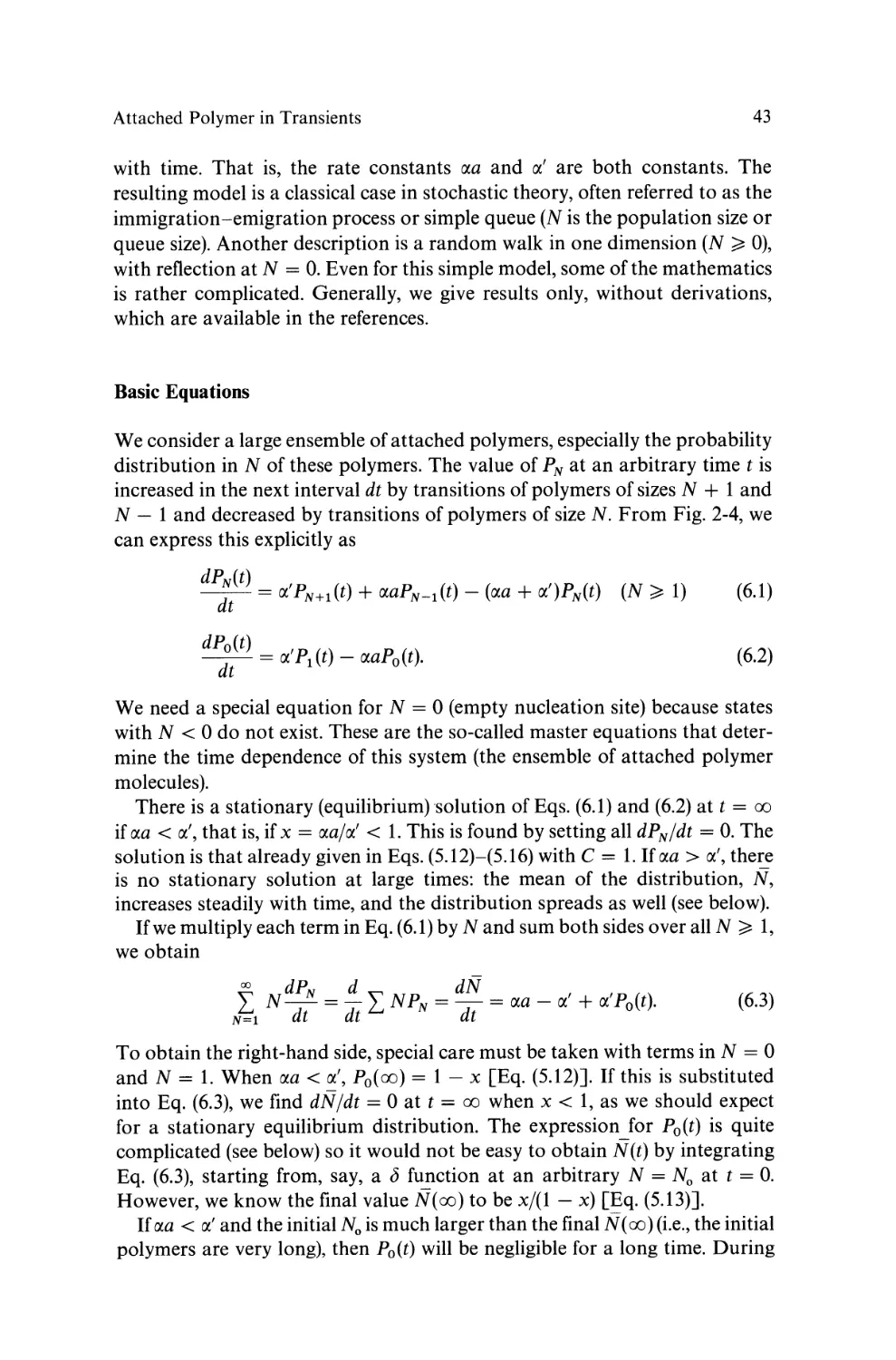
6. Attached Polymer in Transients. . . . . . . . . . . . . . . . . . . . . . . . . . . . . .
7. Attached Polymer under a Force. . . . . . . . . . . . . . . . . . . . . . . . . . . . .
33
42
51
3. Free Single-Stranded Polymer. . . . . . . . . . . . . . . . . . . . . . . . . . . . . . . .
78
8. Free Polymer at Equilibrium. . . . . . . . . . . . . . . . . . . . . . . . . . . . . . . .
9. Kinetic Aspects for a Free Polymer . . . . . . . . . . . . . . . . . . . . . . . . . . .
78
90
1.
2.
3.
4.
Canonical and Grand Partition Functions. . . . . . . . . . . .
Aggregation and Osmotic Pressure Vi rial Coefficients . . .
Partition Function for an Open, Independent Aggregate.
The Macroscopic Aggregate as a Limiting Case. . . . . . . .
.
.
.
.
.....
.....
.....
.....
.
.
.
.
3
Contents
x
4. Single-Stranded Polymer Modified by a Second Component, a
Bound Ligand, or a Cap . . . . . . . . . . . . . . . . . . . . . . . . . . . . . . . . . . . ..
110
10. Two-Component Single-Stranded Polymer . . . . . . . . . . . . . . . . . . . . .
11. Single-Stranded Polymer with Bound Ligand or Cap. . . . . . . . . . . . . .
110
122
5. "Surface" Properties of Some Long Multi-Stranded Polymers. . . . . .
137
12.
13.
14.
15.
...
. ..
...
...
137
144
156
167
6. Some Attached Multi-Stranded Polymers at Equilibrium and in
Transients. . . . . . . . . . . . . . . . . . . . . . . . . . . . . . . . . . . . . . . . . . . . . . . . .
174
16.
17.
18.
19.
General Discussion of the Models. . . . . . . . . . . . . . . . . . . . . . . . .
Equilibrium and Steady-State Properties of Aligned Models. . . . .
Equilibrium and Steady-State Properties of Staggered Models. . . .
Models with Dimers as Subunits. . . . . . . . . . . . . . . . . . . . . . . . . .
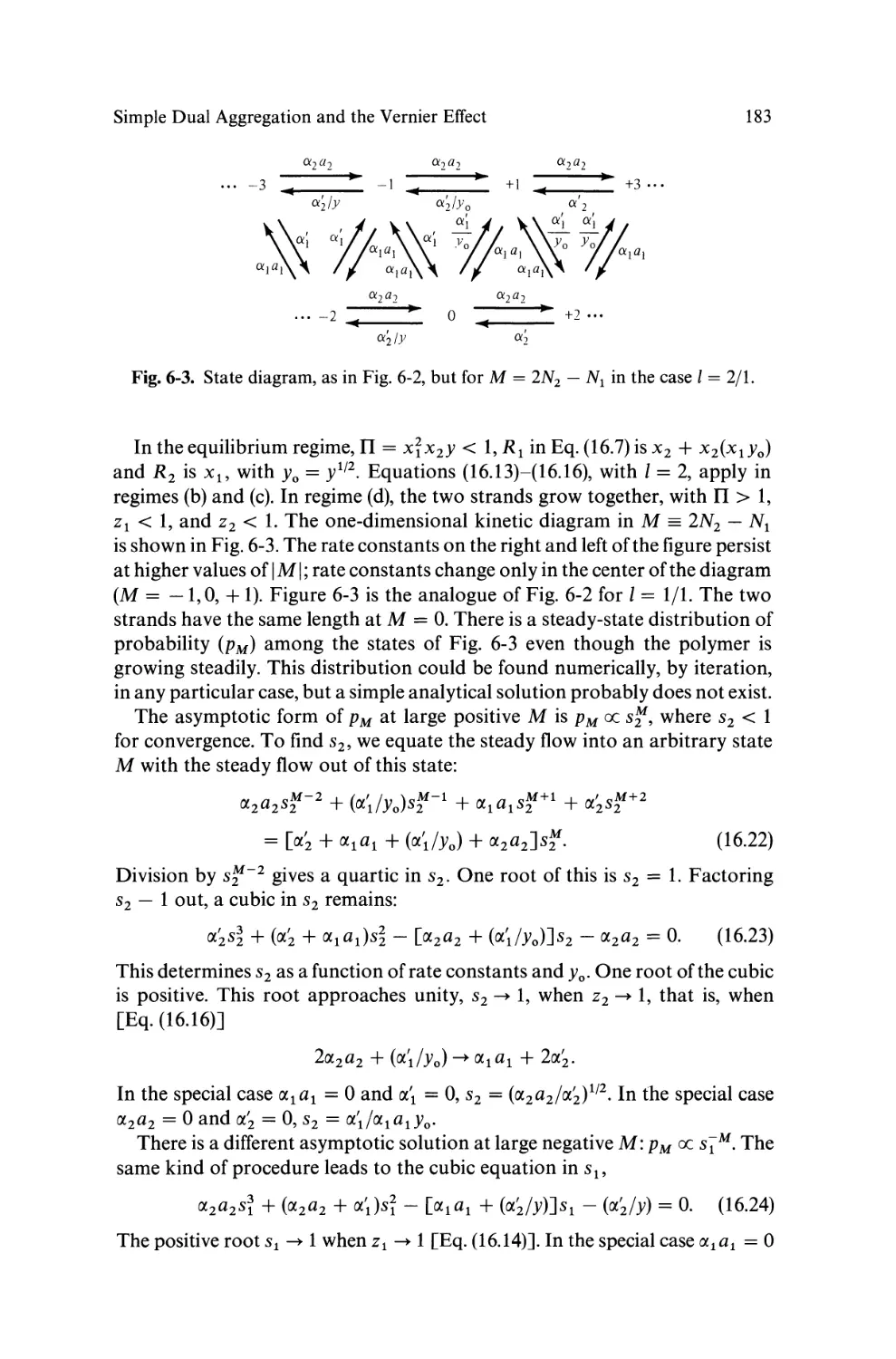
Simple Dual Aggregation and the Vernier Effect.
Dual Aggregation with Vernier Enhancement. . .
A Further Example of Dual Aggregation. . . . . . .
Aligned Tubular Models at Equilibrium. . . . . . . .
.
.
.
.
.
.
.
.
....
.. . .
....
....
. ..
.. .
...
...
. ..
...
...
...
. ..
.. .
...
...
.
.
.
.
174
184
190
193
II. Linear Steady-State Aggregates
7. Enzymatic Activity at Polymer Tips Only
199
20. Enzymatic Activity along the Polymer Length. . . . . . . . . . . . . . . . . ..
21. Enzymatic Activity at Polymer Tips Only: Bioenergetics and Fluxes..
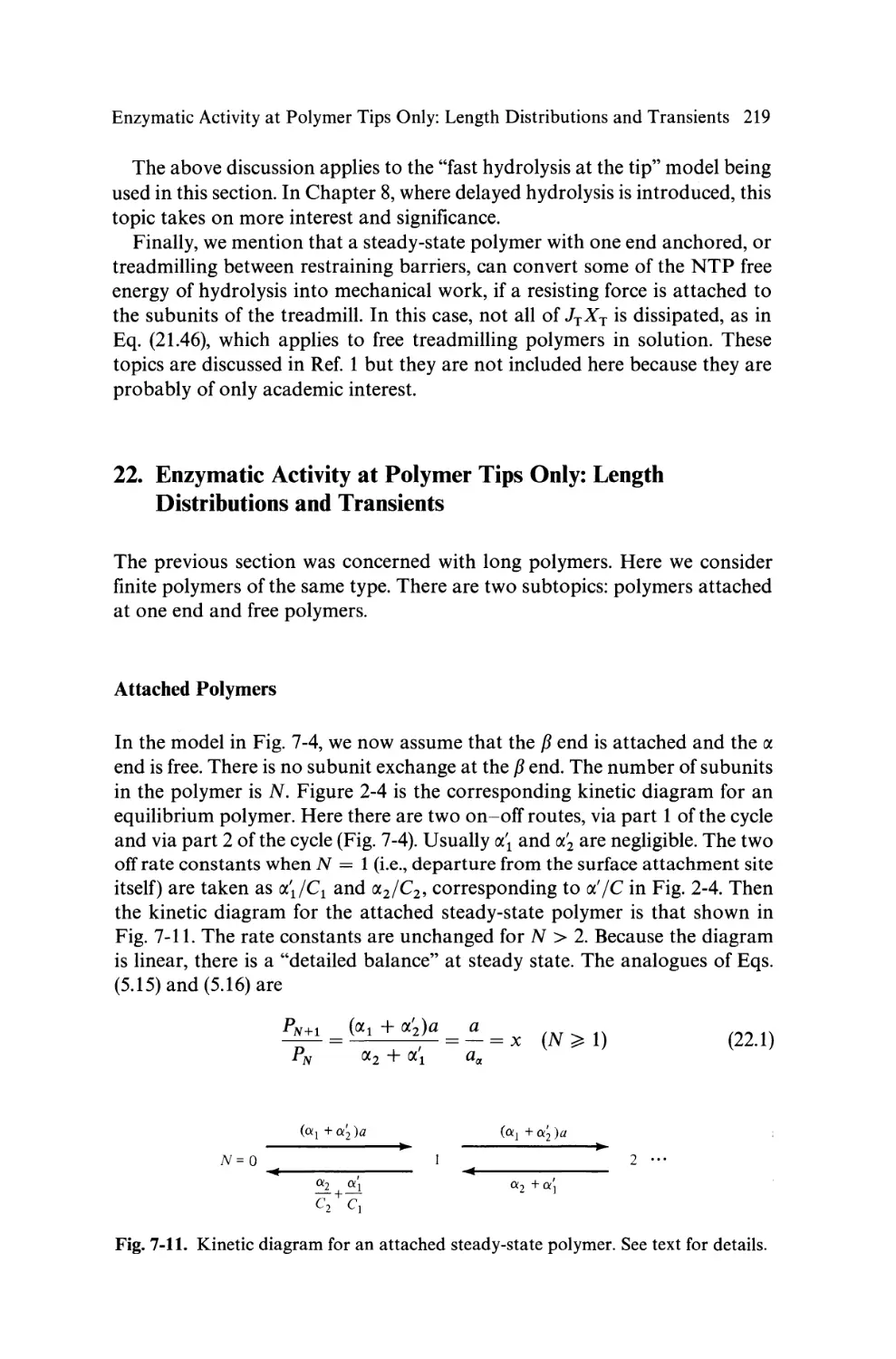
22. Enzymatic Activity at Polymer Tips Only: Length Distributions and
Transients. . . . . . . . . . . . . . . . . . . . . . . . . . . . . . . . . . . . . . . . . . . . ..
23. Fluctuations in the Polymer Length Distribution. . . . . . . . . . . . . . . ..
200
203
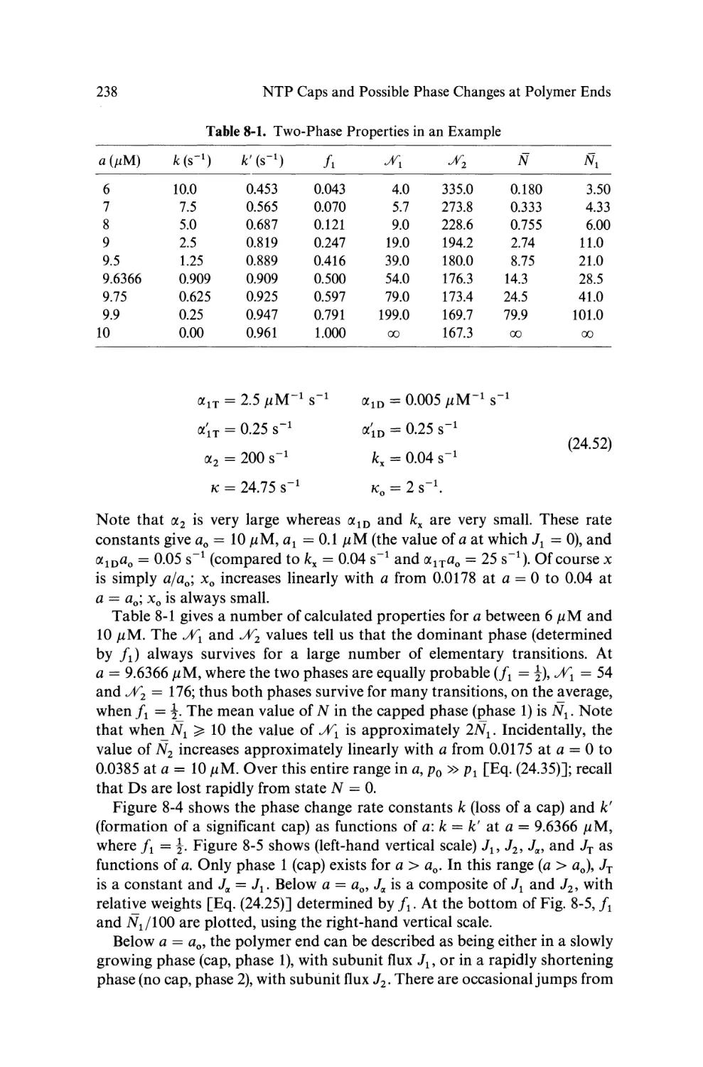
8. NTP Caps and Possible Phase Changes at Polymer Ends. . . . . . . . ..
227
24.
25.
26.
27.
Illustrative Biochemical Models that Generate Phase Changes. . . . .
Attached Polymer with Phase Changes at the Free End. . . . . . . . . .
Free Polymer with Phase Changes at the Ends. . . . . . . . . . . . . . . . .
Simulation of Two "Phases" by Aggregation of One Component on
Another. . . . . . . . . . . . . . . . . . . . . . . . . . . . . . . . . . . . . . . . . . . . . .
219
223
..
..
..
228
244
265
..
284
Index. . . . . . . . . . . . . . . . . . . . . . . . . . . . . . . . . . . . . . . . . . . . . . . . . . . . . ..
303
Introduction
The coverage ofthis book is quite limited. The aim is to give a unified theoretical treatment of the basic physical and chemical principles involved in the
reversible aggregation of independent linear polymer molecules. Generally
these polymers are aggregates of protein monomers or subunits. The emphasis
in the book is on basic principles as illustrated by simple models, not on
particular applications or on particular polymers (though microtubules and
actin are at present the only known examples of some fundamental phenomena
to be described). "Reversible aggregation," above, refers to linear polymer
molecules that can gain or lose subunits continuously from their ends (unless
capped or blocked): aggregation occurs because of physical forces between
subunits (van der Waals, electrostatic, etc.), not from more permanent chemical
bonds (as in DNA, for example). The term "independent," used above, will
limit the discussion (with a few exceptions) to solutions that are dilute in
polymer molecules (so that interpolymer interactions can be neglected) or to
noninteracting polymers attached to a surface or nucleating center. The
aggregation properties of independent polymer molecules are not only fundamental but also are sufficiently complicated to provide more than enough
material for a book of reasonable size.
The emphasis is on equilibrium or steady-state behavior. Transients do not
receive much attention.
The choice of material outlined above parallels, not coincidentally, my own
contributions to the subject. In fact, the book is essentially a cohesive account
and extension of this work. I hope that this more systematic treatment will
make the theory easier to follow and more useful in applications to both
students and researchers. I would be especially gratified if the book serves to
interest physical chemists, physicists, and theoreticians in this subject.
This book is related in fundamental ways to two previous books: my own
Thermodynamics of Small Systems, Part II (Benjamin, New York, 1964) and
xn
Introduction
Thermodynamics of the Polymerization of Protein by F. Oosawa and S. Asakura
(Academic Press, New York, 1975). The present volume is not meant to
supplant the pioneering work by Oosawa and Asakura, but rather to supplement it, in part by more recent advances. In fact, most space in the two books
is devoted to rather different topics. A significant difference is that the present
book uses statistical mechanics as the starting point.
The book on small systems, mentioned above, provides a rigorous thermodynamic background for the present analysis (see Chapter 10, especially). Also,
the pertinent partition function Y is introduced and applied to simple aggregation models.
The first six chapters of the present volume, which are the most fundamental,
are devoted to general physical aggregation systems. The treatment in these
chapters is based, for the most part, on quite simple illustrative models (not
on particular real polymers). "Physical" here signifies that the on and off
transitions of the subunits at the ends of an aggregate do not involve any
chemical reaction. In contrast, Chapter 7 relates to the aggregation of enzyme
molecules. Although the enzyme molecules themselves aggregate because of
simple physical interaction forces, the detailed catalytic properties of the
enzyme (e.g., in the overall reaction E + S -+ E + P) are altered as a conseqnence of the aggregation. The modified enzymatic activity at and near
the polymer ends has a number of interesting consequences. Actin filaments
and microtubules are the two known examples of this kind of behavior at
the present time (actin catalyzes ATP -+ ADP + Pi and tubulin catalyzes
GTP -+ GDP + PJ Finally, Chapter 8 deals with a special case of the enzyme
aggregation problem of Chapter 7. In this case, the subunits at and near a
polymer end can exist in one of two "phases": practically all ES or practically
all EP, with occasional changes from one phase to the other. If these two
phases have very different subunit on and off rate constants, phase changes
can have dramatic effects on polymer stability. So far, micro tubules are the
only known example of this kind of two-phase activity.
For greater generality, the free subunit activity a is used throughout the
book in place of the more conventional concentration c whenever no additional complication ensues.
The book contains much material not previously published. On the other
hand, my original papers on this subject (some with collaborators) contain
many details not included in the book. For the convenience of readers interested in pursuing these details, the following is a list of the pertinent references:
1. Molecular clusters in imperfect gases. 1. Chem. Phys. 23, 617-622 (1955).
2. Statistical Mechanics (McGraw-Hill, New York, 1956; also Dover, New
York, 1987), Section 27 (Exact treatment of physical clusters).
3. Thermodynamics of Small Systems, Part II (Benjamin, New York, 1964),
Chapter 10.
4. Theory of aggregation in solution. Biopolymers 12, 1285-1312 (1973).
With Y. Chen.
5. Bioenergetic aspects and polymer length distribution in steady-state head-
Introduction
6.
7.
8.
9.
10.
11.
12.
13.
14.
15.
16.
17.
18.
19.
20.
21.
22.
23.
24.
Xlll
to-tail polymerization of actin or microtubules. Proc. N atl. Acad. Sci. USA
77,4803-4808 (1980).
Steady-state head-to-tail polymerization of actin or microtubules. II.
Two-state and three-state kinetic cycles. Biophys. J. 33, 353-372 (1981).
Microfilament or microtubule assembly or disassembly against a force.
Proc. Natl. Acad. Sci. USA 78, 5613-5617 (1981).
Subunit treadmilling of micro tubules or actin in the presence of cellular
barriers: possible conversion of chemical free energy into mechanical work.
Proc. Nat!. Acad. Sci. USA 79, 490-494 (1982). With M.W. Kirschner.
Bioenergetics and kinetics of microtubule and actin filament assemblydisassembly. Int. Rev. Cytol. 78, 1-125 (1982). With M.W. Kirschner.
Regulation of microtubule and actin filament assembly-disassembly by
associated small and large molecules. Int. Rev. Cytol. 84, 185-234 (1983).
With M.W. Kirschner.
Steady-state theory ofthe interference of GTP hydrolysis in the mechanism
of microtubule assembly. Proc. N atl. Acad. Sci. USA 80, 7234-7238 (1983).
With M.F. Carlier.
Use of Monte Carlo calculations in the study of microtubule subunit kinetics. Proc. Natl. Acad. Sci. USA 80, 7520-7523 (1983). With Y. Chen.
Interference of GTP hydrolysis in the mechanism of microtubule assembly:
an experimental study. Proc. Natl. Acad. Sci. USA 81, 771-775 (1984).
With M.F. Carlier and Y. Chen.
Phase changes at the end of a microtubule with a GTP cap. Proc. Nat/.
Acad. Sci. USA 81, 5772-5776 (1984). With Y. Chen.
Introductory analysis of the GTP-cap phase-change kinetics at the end
of a microtubule. Proc. N atl. Acad. Sci. USA 81, 6728-6732 (1984).
Phase-change kinetics for a microtubule with two free ends. Proc. Natl.
Acad. Sci. USA 82, 431-435 (1985).
Monte Carlo study of the GTP cap in a five-start helix model of a microtubule. Proc. Nat!. Acad. Sci. USA 82,1131-1135 (1985). With Y. Chen.
Theoretical treatment of microtubules disappearing in solution. Proc.
Natl. Acad. Sci. USA 82, 4127-4131 (1985). With Y. Chen.
Theoretical problems related to the attachment of micro tubules to kinetochores. Proc. Natl. Acad. Sci. USA 82, 4404-4408 (1985).
A model for actin polymerization and the kinetic effects of ATP hydrolysis.
Proc. Natl. Acad. Sci. USA 82, 7207-7211 (1985). With D. Pantaloni, M.F.
Carlier, and E.D. Korn.
Theoretical study of a model for the ATP cap at the end of an actin
filament. Biophys. J. 49, 981-986 (1986).
Effect of fluctuating surface structure and free energy on the growth of
linear tubular aggregates. Biophys. J. 49,1017-1031 (1986).
A theoretical study of cooperative dual linear aggregation and the vernier
effect. Biophys. Chern. 25,1-15 (1986).
Synchronous oscillations in microtubule polymerization. Proc. N atl.
Acad. Sci. USA 84 (1987), in press. With M.-F. Carlier, R. Melki,
D. Pantaloui, and Y. Chen.
xiv
Introduction
I am much indebted to Yi-der Chen, Marc Kirschner, Marie-France Carlier,
Tim Mitchison, and Dominique Pantaloni for their stimulation and collaboration in this field over a number of years. Also, I received help on particular
points from Bruce Nicklas, Attila Szabo, William Eaton, Harold Erickson,
Robert Rubin, and Otto Berg.
Finally, I thank Kathy Van Tassel for her prompt and expert typing of the
manuscript.
I
Linear EquilibriuIn
Aggregates
1
Statistical Therm.odynam.ic
Background
By an "equilibrium aggregate" is meant one whose formation involves physical attractive forces only (e.g., van der Waals and electrostatic interactions
between protein molecules). This is the simplest case and is the subject of
Part I of this book. Part II treats "steady-state aggregates." This term refers
to cases in which the monomers are enzyme molecules and a chemical reaction, catalyzed by the aggregated enzyme, accompanies or follows monomer
attachment to the aggregate. Actin and micro tubules provide examples of
this, in which the chemical reactions are the hydrolysis of ATP or of GTP,
which are bound to the respective monomers. Furthermore, in the case of
microtubules, at least, it is possible for a microtubule end to spend most of its
time in either of two distinct states or phases: the subunits at and near the end
have GTP bound (not yet hydrolyzed) or these subunits have GDP bound
(i.e., the GTP has been hydrolyzed). In the first phase, the microtubule end
is stable; in the second it is unstable. This two-phase behavior is novel and
requires separate treatment (Chapter 8).
An "equilibrium aggregate" can be at equilibrium, in a steady state (i.e.,
growing or shortening at a steady rate), or in a transient. The present chapter
is concerned with general equilibrium background only. Applications and
illustrations will be reserved for later chapters. Kinetic aspects will be introduced in particular cases, beginning in Chapter 2.
If desired, the reader may regard Sections 1-3 as appendices, to be consulted
only for results, as needed. In particular, although Section 2 provides the
general and fundamental approach to equilibrium aggregation theory, many
readers may find the details uninteresting or too complicated. These details
are hardly needed for the remainder of the book. They are included primarily
for readers with an intrinsic interest in fundamentals.
Section 4 contains necessary reference material, mostly thermodynamic,
that pertains to very large aggregates.
Statistical Thermodynamic Background
4
1. Canonical and Grand Partition Functions
In this section, we review a few properties of the two most important partition
functions, for a one-component system. Generalizations will be required later,
but these will be introduced as needed.
Canonical partition function. We consider an equilibrium thermodynamic
system with independent variables N (number of molecules), V (volume), and
T (temperature). The system might be gas, liquid, or solid. The temperature
is fixed by a surrounding heat bath. We are interested in the connection
between the macroscopic thermodynamic properties of this system, on the
one hand, and its (quantum mechanical) molecular properties, on the other.
Statistical mechanics provides the desired formal connection, which can be
made explicit for systems that are not too complicated.
If Ej(N, V) is the energy (eigenvalue) of the j-th energy eigenstate of the
system, then the canonical partition function is
Q(N, V, T) =
I
(1.1)
e-Ej(N,V)/kT,
j
where the sum is over all statesj, and k is the Boltzmann constant. Degenerate
energy levels are represented by several equal terms in the sum. In practice,
in solution physical chemistry (where there is more than one component),
usually the internal vibrational partition function of each molecule is separated out, and the remaining coordinates (translation, external and internal
rotation) are taken care of by a classical phase integral over e- H / kT , where H
is the Hamiltonian function of these coordinates. Details are given in Ref. 1,
pp. 262-264.
The connection with thermodynamics is made via the Helmholtz free
energy:
A(N, V, T) = - kTln Q(N, V, T)
(1.2)
and
dA = -SdT - pdV
+ /ldN
(1.3)
or
d( - A/kT) = -
Ed(l/kT) + (p/kT) dV -
(/l/kT) dN,
(1.4)
where S is the entropy, p the pressure, /l the chemical potential, and E the
mean energy (E fluctuates). Differentiation of - kTln Q, Eq. (1.3), or In Q,
Eq. (1.4), gives various thermodynamic properties of interest.
An example, from Eq. (1.4), is
- (81n
Q)
81/kT
E = -
From Eq. (1.1), we then find
V.N·
(1.5)
Canonical and Grand Partition Functions
L
if =
5
Eje-Ej/kT
(1.6)
--"jI=-e----;;EJ--;;./k-OOT;- •
j
This shows that the probability that the system, at equilibrium, will be observed
in state j is e-EJikT/Q. This is the famous Boltzmann probability distribution.
Grand partition function. 2 Here the one-component system is open with
respect to N: the system exchanges molecules with a reservoir of the same
molecules at chemical potential /1 and temperature T Consequently, N
fluctuates. The independent thermodynamic variables are now /1, V, T rather
than N, V, T
The corresponding partition function, introduced by Gibbs, is the grand
partition function:
2.(/1, V, T)
L
=
Q(N, V, T)e NJl /kT
(1.7)
Q(N, V, T)A N,
(1.8)
N~O
L
=
N~O
where A (the absolute activity) == eJl/kT, and the sum goes over all possible
values of N. The notation QN(V, T) for Q(N, V, T) is used in the next section.
Incidentally, when N = 0, Q(O) = 1 (unless the system includes an always
present "background"). The term "grand" refers to the second, or higherorder, sum over N; the first sum is over j for each N, as in Eq. (1.1). The
connection with thermodynamics is
p V = kTln 2.(/1, V, T),
d(pV)
=
SdT
2.
=
e PV /kT ,
+ pdV + Nd/1.
(1.9)
(1.10)
Of course Eqs. (1.3), (1.4), and (1.10) are all equivalent thermodynamic rela-
tions, rearranged for convenience (according to the choice of independent
variables).
From Eqs. (1.7), (1.8), and (1.10), we find the important relations
N = kT(Oln2.)
0/1
I
A(Oln2.)
OA T,V
=
T.V
(1.11)
NQ(N, V, T)A N
N~O
L Q(N, V, T)A
N
(1.12)
N~O
Equation (1.12) shows that
PN
=
Q(N, V, T)AN
_
c.
(1.13)
is the probability that this open system contains exactly N molecules. If
Q(O) = 1, the probability that the system is empty (N = 0) is 1/2.. Equation
(1.13) is the analogue of the Boltzmann probability distribution for a closed
Statistical Thermodynamic Background
6
system (see above). In other words,just as the separate terms in the canonical
partition function, Eq. (1.1), give the relative probabilities that the closed
system has various energy values Ej , so the separate terms in the grand
partition function, Eq. (1.8), give the relative probabilities that the open system
contains various numbers of molecules N.
A further differentiation of Eq. (1.12),
N8
L
=
NQ(N, V, T)2 N,
N;;'O
leads to the variance in N:
(J~
--
(ON)
= N 2 - N2 = (N - N)2 = 2 - 02
.
(1.14)
T,V
In summary: the first differentiation ofln 8 with respect to 2 gives N, Eq. (1.11),
and the second gives (J~, Eq. (1.14).
For the special case of a very dilute gas (2 ~ 0), we have from Eqs. (1.8) and
(1.11):
8 =
ePVjkT
=
1 + Q(I)2
pV/kT = Q(I)2 = N,
J1
+ ...
e == N/V
= Q(I)2/V
= J1°(T) + kTln e
J1°(T)
=
-kTln[Q(I)/V].
(1.15)
(1.16)
(1.17)
(1.18)
Equation (1.17) is the familiar thermodynamic expression for J1 as a function
of concentration e and T. Equation (1.18) gives the expression for the thermodynamic standard chemical potential J1°(T) in statistical mechanical terms.
When the gas is not dilute,
J1(c, T)
=
J1°(T)
+ kTln a(e, T)
(1.19)
defines the concentration activity a(c, T). The activity coefficient y(e, T) is
defined by a = ye. The activity has the property a ~ e as e ~ 0; also, in this
limit, y ~ 1. The osmotic solution version of some of these equations appears
in the next section.
2. Aggregation and Osmotic Pressure Virial Coefficients
Aggregation or cluster formation in an imperfect one-component gas can be
treated exactly. !, 2 The McMillan- Mayer solution theory!' 2 allows the formal
methods of imperfect gas theory to be extended without change to a solution
that is in an osmotic equilibrium. Thus, aggregation of solute in a solution
can also be treated exactly, at least in principle.
The formal procedure 3 is outlined in this section. The method is actually
quite general and not limited to linear aggregates, the special topic of this
Aggregation and Osmotic Pressure Vi rial Coefficients
7
book. The aggregates may have any shape, but we shall always have linear
aggregates in mind.
The "solute," in a solution, is the aggregating species. We are interested,
in this book, in cases in which the intermolecular forces between solute
molecules, leading to aggregation, are quite strong, strong enough, in fact,
to produce equilibrium linear aggregates of macroscopic length at a finite
concentration c of the solute (called the "critical concentration," ce). In addition to these forces that produce the aggregation, there will be additional
nonaggregating forces between the aggregates themselves, at the least "hard"
interactions that arise from the fact that two aggregates cannot occupy the
same space in the solution at the same time.
Except in Section 8, we shall assume in this book that the large aggregates
or polymers of primary interest (e.g., F-actin and micro tubules) are dilute
enough so that hard interactions between polymers can be ignored: the strong
aggregating forces completely dominate; the polymers can be treated as
independent open systems. 4 This assumption is made to simplify the analysis
and also to help limit the size of the book. It excludes aggregates such as
tobacco mosaic virus 5 and HbS,6 solutions of which can actually separate into
two macroscopic phases because of hard interactions between non-dilute
polymers.
The stacking of nucleosides or bases is an example of equilibrium linear
aggregation in which the aggregating forces are not very strong, partly because
the aggregate is single-stranded. The dominating aggregates are relatively
small: dimers, trimers, tetramers, etc. For such systems, with weak aggregating
forces, hard interactions between aggregates should not be ignored. The
present section is especially pertinent for such systems but we shall not pursue
this particular application 3 here.
It is usually assumed, for simplicity, that the actual transitions that occur
at the ends of a large equilibrium linear aggregate are the arrivals and
departures of monomers. Section 5 will include the more general model in
which these exchanges at polymer ends may involve not only monomers
but also dimers, trimers, etc. The present section will provide the needed
background theory.
With this introduction, we turn now to the general theoretical approach. 3
The object is to show formally but exactly the way in which osmotic pressure
virial coefficients En for an aggregating solute in a solution can be decomposed into contributions arising from aggregation (or "association") equilibria
and from interactions (for brevity, this term will refer, in this section, to all
nonassociating interactions between aggregates).
The essential point is the formal mathematical identity between aggregation
in a one-component imperfect gas and aggregation of solute molecules in
an "osmotic" solution. Once we establish this relationship, we shall revert
to the much simpler notation appropriate to a one-component gas with the
understanding that we are in fact primarily interested in the osmotic solution
case.
Statistical Thermodynamic Background
8
Consider a solution 2 at pressure p + II, temperature T, volume V, with
solute molecules at chemical potential fl, and solvent molecules (any number
of components) at fla' flp, .... This solution is in contact and in equilibrium,
via a membrane permeable to all solvent components but not to solute, with
a large solvent reservoir at p, T, fla' flp, .... Let QN.N.,Np,.JV, T) be the
canonical partition function for the solution with numbers of molecules N
(solute), Na , N p , .... Then the grand partition function of the solution is
(2.1)
where A = e fl / kT , Aa = e fl ./kT , etc. This is a generalization of Eqs. (1.8) and (1.9).
Equation (2.1) can be rewritten as
e(p+II)V/kT
L
=
'¥N AN,
(2.2)
N~O
where
This is a sum over the numbers of all solvent components but with a fixed
number N of solute molecules. The special case '¥o is the grand partition
function for a volume V of the solvent reservoir:
HI
_
pV/kT _
"
Q o,N.,Np, ... /LIN.1Np
(2.4)
TO - e
L...,
/Lp .•..
N.,Np, ••• ~ 0
a
Then, from Eqs. (2.2) and (2.4),
e IIV / kT =
L
('¥N/'¥o}AN.
(2.S)
N':i30
Equation (2.5) may be compared with the grand partition function of a
one-component gas, Eq. (1.8):
e PV / kT
=
L
QN(V, T)A N.
(2.6)
N~O
The vi rial coefficients and related properties of the gas can be expressed 2 in
terms of the QN with N = 1, 2, 3, .... There is no restriction on the nature of
the gas molecules except that a vi rial expansion must exist. These same
expressions hold for the solution 2 with II replacing p and '¥N/'¥O replacing
QN' In the solution case, the influence of the solvent appears implicitly through
the dependence of,¥Nand '¥0 on fla' flp, .... Also, the potential of mean force 2
between solute molecules plays the role of the intermolecular potential energy
in the gas. If the solute molecules are charged, the solvent must include an
electrolyte (in order to have a virial expansion). The osmotic virial expansion
will diverge when macroscopic aggregates are formed, that is, at the critical
concentration C = Ceo Hence, this procedure is valid only for C < ceo
We use Eq. (2.5) as our starting point but from here on, for simplicity of
notation, we denote '¥N/'¥O by QN' Since gas cluster theory 2 begins with
Aggregation and Osmotic Pressure Virial Coefficients
9
Eq. (2.6), we can take over the essentials ofthat theory, without change, in our
consideration of solute aggregation in solution.
Q2 (= '1'2/'1'0) is a partition function for exactly two solute molecules in
solvent (V, T, J.1~, J.1P'···)· Q2 includes an integral over all possible positions of
the two solute molecules in V and over all rotational orientations (Ref. 1, pp.
264, 271, and 277). If there are forces leading to aggregation, Q2 may be split
into two parts (usually by a specified division of the translational-rotational
configuration space),
Q2
=
Q200 ...
+ QOlO ... ,
(2.7)
where Q200 is the partition function of two (interacting) monomers in V and
is the partition function of one dimer in V This is an exact split up of
Q2; no approximation is involved. In general, in QN, the boldface N == N1,
N 2 , .,. represents a set of Nl monomers, N2 dimers, N3 trimers, etc., in V
Q2 is the complete partition function for two molecules. It includes both
"interaction" and "association" forces between the molecules. The dimer state
is included implicitly in Q2' On the other hand, the right-hand side of Eq. (2.7)
makes the existence of dimers explicit. The division of Q2 into Q200 and QOlO
is a nonthermodynamic procedure that depends on the definition of a dimer.
But in practice, with strong associating forces, there will be little ambiguity
about the definition. 3
Figure 1-1 provides an idealized illustration. The solute monomers are
uniform (hard) spheres except for sites A and B, at the two ends of a diameter,
which have a very strong attraction for each other. Consequently, a linear
chain of spheres can form by aggregation. An "association" between two
monomers is considered to have been formed if the distance between sites
A and B is less than some preassigned value (a few A). Figure 1-1(a) shows
Q010
(a)
(}
(c)
(b)
Fig. 1-1. Illustration of linear association by strong interactions between sites A and
B on spherical molecules. (a) Two monomers in a "hard" interaction. (b) Monomer
and dimer. (c) Dimer and trimer.
10
Statistical Thermodynamic Background
a hard interaction between two monomers, not an association. Figures l-l(b)
and 1-1 (c) show, respectively, a hard interaction between a dimer and a
monomer and a hard interaction between a trimer and a dimer.
Corresponding to Eq. (2.7), we have for N = 3 and N = 4,
+ Q110 + Q0010
Q40 + Q210 + Q1010 + Q020 + Q00010'
Q3
= Q30
(2.8)
Q4
=
(2.9)
where Q30 is the partition function of three monomers in V, Qll0 refers to one
monomer and one dimer, etc. On the right-hand side, all sets of subscripts are
used such that N = Nl + 2N2 + 3N3 + ....
A digression on notation is needed at this point. We have introduced
the symbol QN above (instead of using QN) because eventually [following
Eq. (2.52)] we shall want to use Q2 for QOlO (dimer), Q3 for Q0010 (trimer), Q4
for QOOOIO (tetramer), etc. That is, Q2 is only part of Q2' etc. However, for
a monomer, there is no subdivision as in Eqs. (2.7)-(2.9), hence Q1 = Q1' and
we shall always use Q1 for the partition function of a monomer in solvent
(i.e., for 'Pd'Po).
Equation (2.5), with QN == 'PN/'PO' includes aggregates implicitly. As in
Eqs. (1.16) and (1.19), we define the concentration activity a == Q1A/V so that
a --+ e when e --+ 0, where e = R/v (the concentration of solute). Then,2 on
taking the logarithm of both sides ofEq. (2.5), after replacing A by aV/Q1, we
obtain
IT/kT
=
a
+ b2 a 2 + b3 a3 + "',
(2.10)
where the bj are related to the QN (in the first few cases) by2
v2
2!Vb2
=
Z2 -
3!Vb3
=
Z3 - 3VZ2
4!Vb4
= Z4 -
4VZ 3
+ 2V 3
-
3z1
(2.11)
+
12V 2 Z 2
ZN == QN VNN!/Qf·
-
6V 4
(2.12)
ZN is the so-called configuration integral (translation and rotation) for N
molecules (see Ref. 1, pp. 264, 271, and 277). The bj are generally used in actual
calculations rather than the QN'
To obtain the osmotic virial expansion, IT/kT in powers of e rather than of
a [Eq. (2.10)], we use the solution equivalent of Eq. (1.11):
e
iJIT/kT
= a--- =
aa
L jbja .
J,
(2.13)
j?3 1
where b1 == 1. This gives e as a power series in a. This series can easily be
inverted (we omit details) to give a as a power series in e. Substitution of
the latter series, aCe), in Eq. (2.10) then produces the desired result:
(2.14)
11
Aggregation and Osmotic Pressure Virial Coefficients
where
B z = -bz,
B4
=
Bs = 112bi -
B3 = 4bi - 2b 3,
+ 18bz b3 - 3b4 ,
144bib3 + 32b z b4 + 18bj -
(2.15)
-20bi
4b s .
The Bn are functions of T, fla' flp, •...
The above relations, Eqs. (2.10)-(2.15), refer to the system of aggregating
solute molecules but these equations do not display the aggregation explicitly:
the forces leading to association appear implicitly in the calculation of the QN'
Alternatively, we can treat aggregates explicitly by writing Eq. (2.5) in the
form
e nV/kT =
"
L...
N;>O
QNl\l
lN 1 1Nz
I\z ...
(2.16)
for a multicomponent mixture of solute aggregates of sizes s = 1, 2, 3, ...
(monomers, dimers, etc.). These are the QN of Eqs. (2.7)-(2.9). In this case,
we define a concentration activity for each species by
(2.17)
The identity of A1 and 2 follows from Eqs. (2.5) and (2.16) in the limit A --+ O.
The corresponding concentrations are
Cs
=
Ns/V with
C1
+ 2c z + 3c 3 + ... =
(2.18)
c.
The activities have the property that as --+ Cs for all s when all Cs --+ O. The as
differ from the Cs because of the interactions between aggregates.
The aggregates of various sizes are in equilibrium with each other so that
the As in Eq. (2.16) are not independent. The equilibrium condition is As = AS
for all s ;;. 1 (i.e., fls = Sfl). For example, 2z = 2 2 , together with Eq. (2.17), leads
to the relation
(2.19)
where K2 is the concentration equilibrium constant for dimer formation from
monomers. K z is a function of T, fla' flp, .... The partition functions appear
here in the conventional wayZ for a chemical equilibrium. A theoretical
calculation of K z requires formulation of Q1 and QOlO (see Section 8 for an
example). Similarly, from
A3
=
A3,
-
(QdV)3 -
=
A4 ,
etc.,
a 4 _ Q00010/ V = K
a 3 _ QOOlO/V = K
a3
A4
3,
a4 - (QdV)4 -
4,
etc.
(2.20)
Note that K3 is the association constant for trimers from monomers, etc.
Statistical Thermodynamic Background
12
The notation Ks is shorthand for a partition function quotient. The Ks should
not be regarded here as empirical equilibrium constants.
The more conventional equilibrium constants are
+ dimer <=± trimer;
monomer + trimer <=± quad rimer;
monomer
K~ =
K3/K2
K~ =
K4/K3
(2.21)
etc., or
(2.22)
We return now to Eq. (2.16). We replace the As by the as' using Eq. (2.17),
take logarithms, and find the muiticomponent generalization of Eq. (2.10):
II
-k
T
=
a 1 + a 2 + a 3 + ...
. . ...
+ "L. bjaila~2
j
(j1
+ j2 + ... ~ 2)
(2.23)
where the boldfacej refers to the setj1,j2' ... and
2! Vb 20 = Z20 - V 2
3!Vb30 = Z30 - 3VZ20
+ 2V 3
2! Vb020 = Z020 - V 2
1! 1! Vb 11 0
=
(2.24)
Z110 - V 2
2! 1! Vb 210 = Z210 - VZ 20 - 2VZ 110
+ 2V 3,
with
ZN =
QN V N 1+ N2+···N1 !N2 ! ...
Nl
N2
N3
Q1 Q010Q0010···
(2.25)
ZN is the configuration integral for the set of solute molecules N = N 1 , N 2 , ••••
Again, the bj are used in practice 3 rather than the QN. The bj are related to
multicomponent virial coefficients Bn in a generalization of Eqs. (2.15) [see
Eq. (89) of Ref. 3]. Whereas the Ks include the forces that lead to aggregation,
the bj (or Bn) take into account the remaining forces of interaction between
aggregates. At the least, the latter would include "hard" or "space-filling"
interactions; ifthe aggregates are charged, and in an electrolyte solution, there
would be a screened electrostatic potential of mean force as well, etc.
Our aim here is to express the operational thermodynamic quantities Bn ,
of Eq. (2.14), in terms of the theoretical quantities Ks and the bj • We do this
via the bj since the Bn and bj are rather simply related by Eqs. (2.15). If we
substitute a 1 = a, a2 = K 2a 2, a3 = K 3a 3, etc., in Eq. (2.33), we will obtain
a power series in the single variable a that must be identical with Eq. (2.10).
We can then equate coefficients of like powers of a to find the bj in terms of
the Ks and bj :
b2 = K2
+ b20
Aggregation and Osmotic Pressure Virial Coefficients
13
(2.26)
Actually, these equations can be written down as easily as Eqs. (2.7)-(2.9),
because both sets depend on the same subscript rules.
Substitution of Eqs. (2.26) into Eqs. (2.15) gives:
B 2 = -K2 - b20
B3
=
B4
=
(2.27)
+ 2K 2(4b 20 - bll0 ) + 4bio - 2b30
-3K4 + 18K 2K 3 - 20K~ + 3K 3(6b 20 - b1010 )
+ 3K~(6bll0 - 20b20 - b020 ) + 3K2(6bll0b20
- 20bio + 6b 30 - b210 ) + 18b2o b3o - 20bio - 3b40 .
-
2K 3 + 4K~
(2.28)
(2.29)
Thus, we have the beginning of the osmotic pressure virial expansion,
Eq. (2.14), with the Bn expressed explicitly in terms of the association equilibrium constants, Eq. (2.20), and nonassociating interactions among aggregates,
Eqs. (2.24). In principle, the procedure can be continued to higher Bn but in
practice B5 is about the limit. As already mentioned, this virial expansion
would diverge at e = ee (where indefinitely large aggregates are formed).
When the aggregation forces are very strong, the bi in Eqs. (2.27)-(2.29) can
be neglected, as a reasonable approximation. That is, the solute in solution
is treated as an ideal mixture of aggregates. This approximation is discussed
in some detail in the next subsection. When aggregation forces are weak,
leading to small aggregates only, the bi should not be and need not be
neglected. An explicit example of this type, including both the Ks and the bi ,
can be found in Ref. 3, pp. 1300-1311. The Ks part of this example is treated
in Section 8. When association does not occur at all (all Ks = 0), Eqs. (2.27)(2.29) reduce to Eqs. (2.15).
Note that in the "ideal" case (all bi = 0), values of the Ks can be deduced
from the experimental Bn alone. But in the "real" case, where both the Ks and
the bi are included, some theory (e.g., of the bi ) and/or nonthermodynamic
experiments have to be invoked in order to divide the Bn between the Ks
and the bi . This situation is to be expected because aggregation is an extrathermodynamic concept.
It is of some interest to have equations for the as and the e., especially
the latter, as functions of e. The dependence of a 1 (= a) on e is, like that of II
on e, thermodynamic in nature (i.e., the explicit recognition of aggregates is
not involved). The relation is
aCe)
where
~
<pee) = L...
k;;' 1
=
ee'P(cl,
(k- k+-1)
(2.30)
Bk+l e
k
.
(2.31 )
14
Statistical Thermodynamic Background
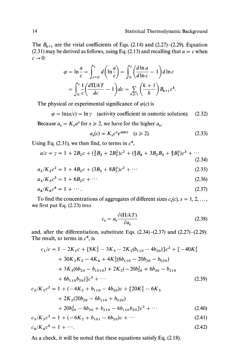
The Bk+1 are the virial coefficients of Eqs. (2.14) and (2.27)~(2.29). Equation
(2.31) may be derived as follows, using Eq. (2.13) and recalling that a = c when
c --> 0:
<p
=
a IC
(a)
fC
In ~ = c=o d In ~ = 0
-_ fC
(ddInIn ac -
)
1 dIn c
~(dIT/kT _ 1)dc -_ ~
~ (~) Bk+l C k •
dc
o c
k
k;:' I
The physical or experimental significance of <p(c) is
<p
=
Because as
In (a/c) = In y
=
(activity coefficient in osmotic solution).
(2.32)
Ksa s for s ~ 2, we have for the higher as'
as(c)
=
KscSeS'P(C)
(s
~
2).
(2.33)
Using Eg. (2.31), we then find, to terms in c4 ,
a/c
y = 1 + 2Bl c + GB3
=
+ 2Bi}c l + (4B4 + 3BlB3 + tBi)c 3 + ...
(2.34)
+ 4Bl c + (3B3 + 8Bi}c l + ".
1 + 6Bl c + ".
1 + ....
al/Klc l
= 1
(2.35)
a3/K3c3
=
(2.36)
a4/K4c4
=
(2.37)
To find the concentrations of aggregates of different sizes cs(c), s = 1,2, ... ,
we first put Eg. (2.23) into
Cs
=
as
o(IT/kT)
and, after the differentiation, substitute Eqs.
The result, to terms in c 4 , is
cdc
= 1 - 2K l c
cZ/Klc l =
c3/K3C3
=
c4/K4C4
=
+ [8K~
(2.38)
oas
(2.34)~(2.37)
- 3K3 - 2K l (b 110
-
and
4blO )]C l
(2.27)~(2.29).
+ [-40K~
+ 30K l K 3 - 4K4 + 4K~(6bll0 - 20blO - bOlO)
+ 3K 3(6b lO - blOlO) + 2K l ( -20bio + 6b 30 - bllO
+ 6bllOblO)]C3 + ".
1 + (-4K z + b llO - 4b zo )c + [20K~ - 6K3
+ 2K l (20blO - 6b llO + bOlO)
+ 20bio - 6b 30 + b210 - 6bllOb20]Cl + ".
1 + (-6Kl + bIOI - 6blO )c + ...
1 + . ".
As a check, it will be noted that these equations satisfy Eq. (2.18):
(2.39)
(2.40)
(2.41)
(2.42)
Aggregation and Osmotic Pressure Virial Coefficients
15
Also of some interest are the "apparent" equilibrium quotients, in powers
of c:
c2/K 2ci
=
C3/K 3ci
=
C4/K4Ci
=
1 + (b ll0 - 4b 20 )c
+ [2K 2(-2b llO + 4b 20 + b020 )
+ 20bio - 6b 30 + b210 - 6bllOb20]C2 + ...
1 + (b l010 - 6b 20 )c + ...
1 + ....
(2.43)
(2.44)
(2.45)
Note that, as expected, these are all unity if the bj are all zero (ideal mixture
of aggregates), or if c ---> O. Of course, the activity quotients ajKsa S == 1 under
any conditions.
Noninteracting Aggregates
With very strong association forces between solute molecules, it may be a good
approximation to neglect non-association interactions between aggregates.
This is the "ideal mixture of aggregates" case already mentioned. However,
even with this simplification we still have an imperfect solution of solute in
solvent (i.e., fI/kT =1= c) because of the association interactions themselves.
These interactions are contained in the Ks [Eqs. (2.19) and (2.20)].
In the equations above, we set all of the bj = o. This leads to relatively simple
relations that we summarize here, for convenience.
The osmotic pressure virial expansion is
fI/kT = c
+ B2c 2 + B3C3 + ...
with
B z = -K z ,
B4
-3K4
=
B3 = -2K3
+
+ 4K~,
18K 2K3 - 20K~,
etc.
(2.46)
Equation (2.23) becomes
fI/kT = a l
Then Eq. (2.38) gives
Cs
+ a 2 + a3 + ....
= as for all s. In particular, because a 1 = a, we have
(2.47)
where
c=
Cl
+ 2c 2 + 3c 3 + ....
Thus, although Cs = as for all s, we have c =1= a (for the reason mentioned at
the beginning of this subsection). Using as = Cs == Ksa s [Eq. (2.20)], other
expressions for fI/kT are
fI/kT =
Cl
+ C2 + C 3 + ...
(2.48)
Statistical Thermodynamic Background
16
From Eqs. (2.34)-(2.37) or from (2.39)-(2.42), we have
y = a/c = cdc = 1 - 2K 2c
+
+ (8K~
(-40K~
+ 30K 2K 3 - 4K 4)C 3 + ...
+ (20K~
1 - 6K 2c + ...
1 + ... .
c2/K 2c 2 = 1 - 4K 2e
c3/K3e3 =
c4/K4C4 =
- 3K 3)C 2
- 6K3)C2
+ ...
(2.49)
(2.50)
(2.51)
(2.52)
To simplify notation, let us write Q2 for QOlO (a dimer), Q3 for QOOIO
(a trimer), etc. Then, from Eq. (2.20), we have
a = e = K as = Qs!V (Ql"l,)S = Qs AS.
S
S
(Ql/VY
S
V
(2.53)
V
Thus, the relative abundance of aggregates of size s is proportional to QsA s.
The resemblance to Eq. (1.13) should be noted. We shall return to this result
in the next section (where N is used for the size of an aggregate rather than s).
Hard Spheres: Numerical Examples
In this subsection we go to the opposite extreme and consider solute molecules
that interact as hard spheres but do not associate except to form polymers.
This rather paradoxical behavior is, in fact, exhibited by HbS. 7 ,8 Correspondingly, the critical concentration C e for polymer formation at 37°C is
2.5 mM, which is about 1000 times larger than the critical concentration of
actin or tubulin (to form micro tubules).
A very accurate semiempirical expression for flv/kT for hard spheres of
volume v at a concentration c is 9
ve[1
flv
+ ve + (vef
kT
- (ve)3]
The "density" ve = 1 is never reached; at close packing ve
integrating the thermodynamic equation [see Eq. (2.13)J
d (~)
kT
(2.54)
(1 - ve)3
=
! (Dn/kT)
e
DC
de
(T constant)
=
0.7405. By
(2.55)
T
one can then deduce
lny
Table 1-1 gives values ofy
concentration: 8
=
ve[8 - 9vc
=
+ 3(ve)2]
(1- ve)3
(2.56)
a/c for several values of vc. For HbS at the critical
Aggregation and Osmotic Pressure Virial Coefficients
17
Table 1-1. Hard-Sphere Activity
Coefficients
ve
y = ale
ve
y = ale
0.001
0.01
0.02
0.04
0.06
0.08
0.10
1.00805
1.085
1.181
1.413
1.715
2.117
2.659
0.12
0.14
0.16
0.18
0.20
0.25
0.30
3.41
4.47
6.00
8.29
11.8
33.7
130.5
v
=
g-l
51.0 M- 1
=
0.16 g cm- 3 = 2.48 mM
=
Ce
VC e
0.79 cm 3
(2.57)
= 0.1264, y = ae/c e = 3.71.
Thus the activity and concentration are quite different. For comparison, if
we treat tubulin as a sphere and take Ce = 10 .uM, we have
v = 0.736 cm 3
VC
e = 7.36
X
10- 4 ,
g-I
= 73.6 M- 1
Y = ae/c e = 1.0059.
(2.58)
Clearly, hard interactions are not significant at this low concentration. This
suggests that any differences between a and C for tubulin and actin could be
treated by the previous subsection.
Incidentally, an alternate semi empirical expression for In y in Ref. 8 (in the
form of a polynomial) gives essentially the same values of y presented here in
Table 1-1 and in Eqs. (2.57) and (2.58).
It is sometimes usefup·3 to employ the molality of solute (or mole ratio,
which is practically the same thing) instead of C as the composition variable. In
the simple special case 3 that the solvent has only one component (denoted a)
and that the volume of solution is additive,
(2.59)
where v (volume of a solute hard sphere) and Va (volume of a solvent molecule)
are constants, the relation between the two composition variables is
Nv
(
(2.60)
1+t
vC=~=~-
V
( is the volume ratio of the two components. In this special case, it is more
natural to use ( than the mole ratio N/Na • On substituting Eq. (2.60) into
Eq. (2.54),
TIv
kT
(1
+ 4( + 6(2 + 2(3)
1+
(
(2.61)
Statistical Thermodynamic Background
18
On using the Gibbs-Duhem equation (Ref. 2, pp. 364-368), the mole-ratio
activity coefficient y' is found to be
2 [---In(I+~)-1+2~--~
1
3 2J .
9 +
lny , =6~+-~
2
1+
2
~
(2.62)
This expression is valid provided that ~ < 1. The quantity in brackets is of
order ~3.
Finally, we give the power series expansions of Eqs. (2.54)9 and (2.61):
IIv
-
kT
= vc
+L
00
i=l
(3i
+ i2)(vc)'+1
•
(2.63)
(2.64)
3. Partition Function for an Open, Independent Aggregate
We begin with some needed statistical mechanical background that is a continuation of Section 1. Equation (1.8) gives the grand partition function
3(11, V, T) for a one-component system of volume V that is open with respect
to the number of molecules, N. That is, 11 is the independent variable, whose
value is determined by an outside reservoir of molecules,and N fluctuates.
The size of the system is fixed by V
We can go one step further and allow fluctuations in V as well as N (i.e., p
becomes the independent variable, not V). In this case, the partition function 4
is
1(11, p, T) =
L Q(N, V, T)2
N
(e- p / kTlV •
(3.1)
N,V
The independent variables are nominally 11, p, and T. However, for a onecomponent macroscopic system, only two of these three intensive variables
can be independent. This leads to difficulties 1 in handling this partition
function. However, the difficulties disappear if 1 is applied to a finite (small)
system 4 rather than to a macroscopic system. For example, if l1e is the chemical
potential of the macroscopic system at the given p and T, then we must choose
11 < l1e to make the system finite. With this limitation, 11, p, and T can all be
independent variables. Whereas the macroscopic system at l1e' p, T has an
indeterminate size (there is no independent extensive variable), the small
system has well-defined values of N and V determined by p, T, and 11 < l1e'
This kind of system is called "completely open" because no extensive variable
has a fixed (or assigned) value. An example of such a system is a small
crystallite at p and T in equilibrium with vapor at f.1 < f.1e'
Partition Function for an Open, Independent Aggregate
19
The fundamental statistical thermodynamic relations 4 are
(3.2)
tS'= -kTlnY=E- TS+pV-J1N
dtS'
=
-SdT + Vdp - NdJ1
(3.3)
N __ (atS')
_kT(alnY) _A(alnY)
aJ1 p.T
aJ1 p,T
aA p,T
=
~
L
Y N,V
NQAN(e-pVlkTt,
(3.4)
(3.5)
with analogous relations for V. tS' is a new thermodynamic function that does
not appear in macroscopic thermodynamics. Equation (3.5) and the corresponding equation for V show that
(3.6)
is the probability that the completely open system will be observed to have
the values N and V at given J1, p, and T. It then follows, on differentiating
Eq. (3.5), that the variance in N is
2
(IN
= -N2 - N-2 = kT (aN)
-
aJ1 p.T
= A (aN)
-
aA p,T
.
(3.7)
There is a similar expression for (J~.
For small systems that are assumed to be incompressible (for example, one
might reasonably use this approximation for the crystallite mentioned above),
V is always proportional to N and hence is not a separate operational
extensive variable. The properties of such a system do not depend on the
pressure p. In this case, we have the simpler relations [using the notation
QN(T) now in place of Q(N, T)]:
Y(J1, T)
=
L QN(T)A
(3.8)
N
N
tS' = -kTin Y,
N
=
A(aln Y)
8A
dtS'
T'
=
-SdT - NdJ1
(J~ =
PN = QNANjY.
A(aN)
8A
T
(3.9)
(3.10)
(3.11)
The last equation gives the probability that the system contains N molecules.
Equation (3.8) resembles Eq. (1.8) (grand partition function), but there is a
fundamental difference: in Eq. (1.8) the size of the system is fixed by the
specification of V whereas in Eq. (3.8) the system is completely open and its
mean size N is determined by how close J1 is to J1e (as J1--+ J1e' N --+ (jJ).
Fluctuations in N in Eq. (1.8) are normal (small), but they are large in Eq. (3.8)
when J1 is near J1e' Equation (3.8) is fundamental for much of the remainder
of the book.
20
Statistical Thermodynamic Background
Independent Aggregate in Solution
As at the end of Section 2, we consider equilibrium aggregates, in a solution
of volume V, that are sufficiently dilute to be regarded as independent of each
other (except for solute exchange with the same pool offree solute molecules).
Aggregating forces are strong and the degree of polymerization (i.e., number
of subunits, or monomers, or solute molecules in the polymer) is usually in
the range 10 2 to 104 , or more. Because of the independence of the aggregates
or polymers, we can select a single aggregate as the small or finite statistical
thermodynamic system of interest (analogous to the crystallite above). The
entire collection of aggregates in V then has the status of an ensemble of such
systems. A time average of some fluctuating quantity over the states of a single
system (polymer) will then be the same as an instantaneous ensemble average
over the whole collection (in the limit that the time and ensemble size both
approach infinity).
Implicit in the above comments is the following point of view that we adopt
in the remainder of the book (except in part of Section 8): our primary interest
is in large polymers that we assume are dilute enough to be independent of
each other; the large polymers are in contact with a pool or reservoir of ("free")
solute molecules that may contain small clusters (dimers, trimers, etc.) or
whose molecules may otherwise interact with each other (e.g., hard-sphere
interactions), or both. That is, although the polymers are assumed independent of each other, we do not necessarily make the same assumption about
the constituents of the pool or reservoir of free (i.e., non-polymer) solute
molecules. See the last two subsections of Section 2 in this connection.
We now denote the partition function Qs in Eq. (2.53) by QN' This is the
partition function of a single aggregate of size N (degree of polymerization,
number of monomers or solute molecules in the aggregate) in the volume V,
with the properties ofthe solvent appearing implicitly in QN through J1a' J1p, ...
[see Eqs. (2.5) and (2.6)]. QN includes (Sections 4 and 8) translation, rotation,
vibration of the N subunits relative to each other, internal vibration within
each subunit, and the intermolecular interactions between neighboring subunits. The translational partition function is proportional to V. Because the
intrinsic properties of the polymer (e.g., its size distribution) have nothing to
do with the volume V of the container in which the polymer moves, it is
preferable to use QN/V instead of QN in our definition of Y:
Y(J1, T) =
L (QN/V)A N,
(3.12)
N
where J1 (in A = e IL1kT ) is the chemical potential of solute molecules (Section 2).
The solvent variables J1a' J1p, ... are implicit in QN and Y, and are not shown
in Eq. (3.12). The pressure is determined by all the chemical potentials and T.
Equation (3.12) is an example of Eq. (3.8). Hence, Eqs. (3.9)-(3.11) apply.
The summand in Eq. (3.12) is in fact the same expression as in Eq. (2.53).
Therefore, Y in Eq. (3.12) has the physical significance of LN eN (the total
Partition Function for an Open, Independent Aggregate
21
concentration of all polymers). A similar relationship, using different composition variables, is discussed in detail (in its thermodynamic aspects) in
Ref. 4, pp. 120-135.
As A is increased in Eq. (3.12), terms at large N will eventually no longer
converge. This occurs at /l = /le' where N -+ 00 (the polymer becomes
macroscopic).
The Chemical Potential
For simplicity, we shall often assume that noninteracting monomers are in
equilibrium with a sizable polymer (the small system) and that small clusters
(e.g., dimers and trimers) are insignificant. That is, a = c. In this case, in
Eq. (3.12),
A=
/l
eJl/kT
=
(V/Ql)C
= /l0(T) + kTln c
(3.13)
/lO(T) = -kTln(QdV),
where Eq. (2.17) has been used and c is the concentration of free monomers
(all other species, including polymers, make a negligible contribution to the
total concentration c of solute). A less drastic assumption (see above) is
that very dilute (independent) polymers are in equilibrium with interacting
monomers or with small solute clusters (e.g., monomers, dimers, trimers),
which in turn are in equilibrium with each other. In this case [Eq. (2.17)]
(3.14)
where the activity a is related to the total solute concentration c by Eqs. (2.27)(2.29) and (2.34) (the polymers are so dilute that they make a negligible
contribution to c). Implicit in the small-cluster case (see Ref. 4, p. 121) is the
not unreasonable assumption that some intermediate-size cluster or clusters
(e.g., N = 5 to 7) represent a minimum in stability, have very small concentrations, and would present a free energy barrier to be surpassed in the polymer
nucleation process (see Section 9).
The physical significance of Ql' and hence of /lo, is discussed in detail in
Ref. 10, pp. 6-12. In summary, Ql has contributions of the following types:
(a) Translation and external rotation ofthe single solute molecule (monomer),
just as for a single solute molecule in the gas phase. The translational
partition function is proportional to V; hence Ql is proportional to V.
(b) Internal vibration (and rotation) within the solute molecule, including any
perturbations caused by the solvent molecules surrounding the solute
molecule.
(c) Intermolecular interactions between the solute molecule and the surrounding solvent molecules.
(d) Perturbation of all the degrees of freedom and of the related intermolecular
Statistical Thermodynamic Background
22
interactions ofthose solvent molecules in the immediate neighborhood of
the solute molecule as it moves about the volume V.
A simplified example is included in Section 8.
Independent Aggregate Attached to a Surface
An independent linear polymer or aggregate with one end attached to a surface is a very important special case in cell biology. The polymer is immersed
in solvent as before, but it is no longer free to rotate or translate. These
degrees of freedom for a free polymer become additional vibrational degrees
offreedom for an attached polymer. The partition function QN for an attached
aggregate of size N (Section 5) does not include a factor V. Hence, Eq. (3.8),
for Y, applies to this case without modification. Although Y is different
(Chapter 2) for the same kind of aggregate depending on whether it is attached
or free to move in solution, divergence of Y will occur at the same f.1 = f.1e in
both cases. This follows because f.1e is a property of the macroscopic polymer,
for which free rotation and translation of the entire polymer, if present, are
inconseq uen tial.
A more general situation for an attached polymer is shown in Fig. 1-2(a).
Here we assume that the polymer is a straight rod of length L and that
an external (axial) force F acts on the "free" end. F is (arbitrarily) taken as
positive if it is an extending force and negative if it is a compressing force
(the opposite of the pressure p in a conventional thermodynamic system).
Subunits can still exchange with the polymer, at one or both ends. The
attached polymer discussed in the preceding paragraph is the special case
F = O. The critical value f.1 = f.1e (where N -> 00) depends on F (Section 4).
This is also a completely open system, but with independent variables f.1, F,
T The appropriate partition function is [in Eg. (3.1) replace V by Land p
by -F]
Y(f.1,F, T) =
I
N,L
QN(L, T)AN(eF/kT)L.
(3.15)
Also,
f!= -kTlnY=E- TS-FI-f.1N
F(fixed)
(a)
(b)
(3.16)
Fig. 1-2. (a) Linear rod-like polymer of length L under a fixed
force F (positive in the direction
shown). Double arrows indicate
possible monomer exchange at
the polymer ends. (b) Polymer
between two rigid barriers a fixed
distance L apart.
23
The Macroscopic Aggregate as a Limiting Case
dt&'
- _
-SdT - IdF - Ndp
=
(Oln
Y)
I
N -..1.:11'
2
(iN
=
=
F. T
(J1l
(ON)
..1.;;-;Ull
2
,(iL
=
(3.17)
Y)
kT(oln
:1
uF
(3.18)
!l. T
(OL)
kT -
of
F.T
.
(3.19)
!l.T
Fluctuations in N are large, as are fluctuations in L (because L is essentially
proportional to N). For a given N, L has small fluctuations, associated with
the vibration of subunits relative to each other (i.e., associated with the slight
axial compressibility of the rod-like polymer). A detailed discussion of an
example of dual fluctuations of this type, in a completely open system, is given
in Ref. 4, pp. 90-94.
Another system of interest is shown in Fig. 1-2(b). Here the polymer is
attached to (or pushing against) surfaces (rigid barriers) at both ends. In this
case, p > Pe (Section 7). The length L is fixed. The independent variables are
p, L, T. This system is not completely open because the extensive variable L
is fixed, as is V in Eq. (1.7). N -+ 00 is not possible. The grand partition function
IS
I
3(p, L, T) =
QN(L, T)A N.
(3.20)
N
Also,
FL
d(FL)
=
=
-SdT
- A(0In3)
N
=
-kTln3
~
+ FdL
2
T.L
,(iN
=
(3.21)
- Ndp
(ON)
aT
A
(3.22)
T.L
.
(3.23)
The fluctuations in N are normal (small). Large fluctuations occur only in
completely open systems because the polymer size for such systems becomes
indeterminate as the critical concentration of solute is approached.
Many of the above relations will be needed and illustrated in Chapter 2.
4. The Macroscopic Aggregate as a Limiting Case
At the critical concentration C e of solute, an open aggregate becomes macroscopic in size (N becomes very large but has no definite value). Thus, at C e ,
we have a conventional two-phase equilibrium between a one-dimensional
solid (the aggregate) and free solute molecules. 4 • 11 The equilibrium conditions
are the same whether the aggregate is free or attached to a surface at one end
(because the six rotational and translational degrees of freedom of the free
aggregate become negligible compared to all the other degrees of freedom
Statistical Thermodynamic Background
24
when N --+ 00). The concentration Ce may be regarded as the solubility of the
macroscopic polymer in the solvent.
Let 1l0(T) be the chemical potential per subunit (solute molecule) of the
macroscopic polymer. A particular statistical mechanical model would provide an explicit expression for 1l0(T) (see the end of this section). Because of
the equilibrium between polymer and free solute molecules, the chemical
potentials of these molecules in the two phases must be equal:
(4.1)
where Eq. (3.14) has been used and the activity a e is a function of Ce as in
Eqs. (2.27)-(2.29) and (2.34). The subscript e always refers to a macroscopic
equilibrium; usually we are interested in a nonmacroscopic equilibrium involving finite aggregates at C < Ceo If we can neglect small clusters and other
intersolute interactions in the free solute (as it is customary to do for simplicity),
a e = C e and
(4.2)
If we use K(T) to denote the equilibrium constant for adding solute molecules to the macroscopic polymer, then
solute(in solution) +:t solute(in polymer)
K(T) =
=
e-I!.Go/kT
=
e[!'O(T)-!'o(T)]/kT
(4.3)
lla e ~ liCe·
Besides depending on T, the equilibrium constant K also is a function of the
solvent chemical potentials Ila' IIp, ... (Section 3), but we leave this as implicit.
The critical concentration Ce marks a separation point between two polymer
regimes along the C axis. If C > C e and C is held fixed, the polymer will grow
steadily; this is a steady-state system, not an equilibrium one (Chapter 2). If
C < C e (c is held fixed) and we start with a very large polymer, the polymer
will shorten at a steady rate (this is also a steady-state system). However,
if C < C e has a value rather close to Ce, the polymer will eventually stop
shortening at some definite sizable mean finite size (depending on c). This is
an equilibrium system (Section 3).
Macroscopic Aggregate under a Force F
We consider the macroscopic thermodynamics (Ref. 12, pp. 44-48) of the
polymer in Fig. 1-2(a), which has a length L, is subject to an external force F,
and contains N molecules (or subunits). As in Eq. (l.3), we have
dA
=
-SdT
+ FdL + IlpdN,
where the subscript p on II p refers to the polymer (Il p
(4.4)
=
110 when F
=
0, as
25
The Macroscopic Aggregate as a Limiting Case
above). Integration of Eq. (4.4), holding intensive properties constant, gives
A
=
FL
+ /lpN,
dG
= -
G == /lpN
=
A - FL
(4.5)
and then
+ /lpdN
(4.6)
d/l p = -(SjN)dT - (LjN)dF.
(4.7)
SdT - LdF
The important result for present purposes is
d/l p = -ldF
(T constant)
(4.8)
where 1== LjN (length per subunit). We let 10 be the value of I when F = 0
(rest length per subunit; 10 = 6.15 Afor a microtubule). Whereas I is a function
of F and T, 10 depends on T only. Again, as in Section 3, the solvent plays only
an implicit role, through /la' /lp, ....
We assume that the linear rod-like polymer is slightly compressible: the
subunits in the polymer have an optimal spacing relative to each other,
determined by the intermolecular forces, but this spacing can be altered
somewhat by a compressing (F negative) or extending (F positive) force. The
equation of state (i.e., the relation between F and L) for such a system can be
written
(4.9)
Actually, we shall use only the first term in applications; the other terms
(considered negligible) are included for generality and perspective. In fact, for
many purposes even the first term is not needed: the polymer can be considered
to be incompressible (h is very large, I ~ 10)' The coefficient h(T) is the Hooke's
law constant.
For simplicity, we assume that the polymer does not bend under a compressing force. In the case of actin, this implies use of a bundle of actin
filaments.
Our primary concern is to find the dependence of /lp on F (or I) because
this effect will alter the critical activity a e or concentration C e [Eqs. (4.1) and
(4.2)] when the polymer is in equilibrium with free solute. Because ofthe form
of Eq. (4.9), the simplest procedure is to rewrite Eq. (4.8) as
d/l p =
-
(l - 10
dF
+ 10) d(l _ 10) d(1 - 10)'
Then, using Eq. (4.9) to obtain the derivative, integration from zero to I - 10
gIVes
/lp = /lo - 10F -
WF2
10)F - ih 2 (l- 10)3 - ...
~ /lo - 10F - 2h ~ /lo - 10F.
(4.10)
(4.11)
The first correction term in Eq. (4.10), -loF, is of order hlo(l - 10)' the second
26
Statistical Thermodynamic Background
is of order h(l - 10)2, the third is of order h2(l- U 3 , etc. Usually it suffices to
use /1 p = /10 - 10F (as for an incompressible polymer). In some cases, the term
-F 2/2h [Eq. (4.11)] provides a small correction. The ratio between 10F and
F2/2h is 210/(l - U which is large.
The chemical potential /1 p is increased [Eq. (4.11)] when the polymer is
under compression (F negative). That is, the subunits in the polymer are less
stable than at F = 0 and will have a greater "escaping tendency" (to relieve
the compressive force). Conversely, /1 p is decreased when the polymer is subject
to an extending force: subunits in the polymer are more stable than at F = 0;
this encourages subunits in the solution to add to the polymer (which will
relieve the extensive force). We therefore expect the critical concentration Ce
to increase under compression (c e is the "solubility" of the polymer, a measure
of its escaping tendency) and to decrease under extension.
As in Eq. (4.1), the formal relation that determines the connection between
C e and F is
(4.12)
where the activity ae is a function of C e [Eq. (2.34)]. If we denote the value of
ae at F = 0 by a~, then
/10
+ kTln a~ =
/10
and
kTln(ae/a~) = -loF - (F 2/2h).
(4.13)
Usually we can omit the term in F2. Then
In a e
=
In a~ - (IJ /kT).
(4.14)
As a further approximation, a e ~ C e and a~ ~ c~. Thus, at least approximately,
In C e depends linearly on F: In C e increases when the polymer is under compression (F is negative), etc.
The (linear) thermodynamic compressibility can be defined in the conventional way:
K
(IOF)-l
=
~(OL) =
L of N.T
01
[hlo + (h + 2h2/0)(l- 10) + ... r
~
1/hlo·
=
(4.15)
1
(4.16)
If h -+ 00, K -+ 0 (incompressible polymer).
In Fig. 1-2(b), where the polymer has grown at subunit activity a (with
a > a~) so that it is in contact with two rigid barriers, L is held constant.
When the polymer first touches the two barriers, F = O. The number of
subunits in the polymer at this point is denoted by No (thus, 10 = L/No). As N
increases by addition of further subunits at one or both ends of the polymer,
F decreases (compression of the polymer) until Eq. (4.14) is satisfied (with
27
The Macroscopic Aggregate as a Limiting Case
the activity a, of free solute, in place of ae in this equation). The polymer at
the final F and N is at equilibrium with free solute at a.
The above suggests that an alternative form of F = h(l - 10 ) should be
useful for open aggregates when L is constant: F = - const. x (N - No). The
constant is easily found:
F
=
h(1 - 10 )
=
hlo
--(N - No)
No
=
hL
(~ - ~J
(L constant)
(4.17)
to the linear term in N - No. A dimensionless form of this equation is
IJ/kT
=
(4.18)
-y*(N - No)'
where
(4.19)
is a force constant of sorts. The asterisk is used to avoid confusion with the
activity coefficient y. Another way to write Eq. (4.18), using Eq. (4.16), is
(4.20)
This shows the three ingredients on which N - No depends, N - No being the
number of subunits that must be inserted into a polymer of compressibility K,
and originally with No subunits, in order to raise F = 0 to - F, keeping L
( = 10No ) constant. In Fig. 1-2(b), the value of - F is determined by the
preassigned values of a (for a e ) and a~ in Eq. (4.14).
Incidentally, the next higher term in Eq. (4.17) is easy to find:
- N0 )
F = -hlo ( N No
- N
+ (hl o + h2/~) (N No
0
)2 + ...
(L constant)
(4.21)
Numerical Examples
We illustrate some ofthe above quantities using a microtubule as an example. 12
The same qualitative conclusions would be drawn about polymerized HbS or
F-actin bundles. The value of the Hooke's law constant, h, for a microtubule
has been estimated as 1.1 x 10 4 dyn cm- l (Ref. 12, p. 47). The length per
subunit (tubulin dimer) is 10 = 6.15 A. The largest force likely to be of interest
is F = 5 X 10- 6 dyn (this extending force, per microtubule, suffices to stop
chromosome movement in anaphase l3 ). Most in vivo forces are much smaller
than this.
In Eq. (4.13), the ratio of the second correction term to the first, using the
above numbers, is
F2/2h
loF
=
F
2h1o
=
0.0037.
Statistical Thermodynamic Background
28
Hence, even allowing for some error in the estimate of h, the second correction
term in Eq. (4.13) can be neglected: in Eq. (4.14) the polymer is treated as
incompressible (h does not appear).
With the above values of F and 10, 10F/kT = 7.5 at 25°C. This corresponds
to ae/a~ = 5.7 x 10- 4 in Eq. (4.14). For F = 10- 7 dyn, a more common
order of magnitude, 10F/kT = 0.15 and ae/a~ = 0.86. For F = _10- 7 dyn
(a compressing force), ae/a~ = 1.16. Similarly, a ratio ae/a~ = 5 corresponds
to lJ/kT = -1.6 and F = -1.1 X 10- 6 dyn. Thus, typically, 101F1/kT is of
order unity.
From Eq. (4.17),
N - No
No
-F
hlo '
where N - No is the number of extra subunits that need to be inserted in
a polymer of No subunits, held at constant length, in order to increase the force
from zero to - F. This fraction will be very small in cases of interest because
it is just twice the ratio of correction terms examined above. Thus, (N - No)!No
is -0.0074 for F = 5 X 10- 6 dyn and it is 0.0016 for F = -1.1 X 10- 6 dyn.
In the latter case, if No = 2 X 10⁴ (a microtubule oflength 12.3 Jlm), N - No =
32. That is, insertion of only 32 subunits in this microtubule, held at constant
length, would increase F = 0 to - F = 1.1 X 10- 6 dyn.
The value of the compressibility K, from Eq. (4.16), is 1.5 x 10 3 dyn- 1 and
the value of y* in Eg. (4.19), if we take No = 2 X 10⁴ , is 0.05. Equation (4.18)
or (4.20) can be used to check N - No = 32 for the example given above.
The Critical Concentration of a Simple Einstein Model
In Chapters 2 through 6, we shall use extensively a simple Einstein modeF of
a linear crystal to represent finite aggregates with various structures. As an
introduction, we consider here the limiting case of infinite (very long) linear
aggregates. The Einstein model will lead to a simple expression for the critical
activity a e (or concentration ce) via Eg. (4.1) or (4.2). The same approach
applies to the Einstein model of a three-dimensional crystal in a solvent; in
this case Ce is generally referred to as the solubility of the crystal.
For illustrative purposes, we consider the five examples of linear polymers
in Fig. 1-3. Because the polymers are assumed to be very long, it is immaterial
whether they are free in solution or attached to a surface (i.e., translation and
rotation of the polymer as a whole are negligible, thermodynamically, in any
case). The subunit (monomer) in all these cases is assumed to be an essentially
isotropic spherical protein molecule.
A free monomer in the solvent has three translational, three rotational, and
a large number of internal vibrational degrees of freedom.2 Together with
interactions between protein and solvent, these degrees of freedom determine
JlO(T) in Eg. (3.13) via Ql/JI, where, it will be recalled, Ql == 'l'd'l'o in Eg. (2.5)
[for details, see Ref. 10, pp. 6-12 and the discussion following Eg. (3.14)].
29
The Macroscopic Aggregate as a Limiting Case
z = :2
z= 3
z=4
(a)
(b)
(c)
w
w
z=4
z=6
(d)
(e)
Fig. 1-3. Sections oflong idealized polymers comprised of isotropic spherical monomers.
Nearest-neighbor interactions have a free energy w; each monomer has z neighbors.
(a) Single strand. (b) Two strands, aligned. (c) Two strands, staggered. (d) Eight strands
in a tube, aligned. (e) Four strands forming a 2-start helix (flattened for clarity). The
dotted monomers are repeats of monomers in the left-hand strand.
The protein molecules are packed together in various ways in the hypothetical polymers shown in Fig. 1-3. In Fig. 1-3(d), rings of eight molecules
are aligned on top of each other. Figure 1-3(e) illustrates a polymer comprised
of four strands with a 2-start helical structure such that each molecule has
six nearest neighbors. For example, six open circles are nearest neighbors of
the shaded circle. The value of z given in the figure in each case is the number
of nearest neighbors. The lines in the figure represent the nearest-neighbor
interactions of an arbitrary subunit. Each interaction has a free energy w,
which is negative. That is, w is the isothermal reversible work necessary to
bring two subunits together in the solvent, to the neighbor distance in the
lattice, starting with the subunits widely separated in the solvent; w is also
called the potential of mean force 1 ,2 between two subunits. The interaction
free energy per subunit in each of the structures in Fig. 1-3 is then zw/2
(division by 2 is required because each interaction is shared by two subunits).
The larger the value of z, the more stable the polymer is.
In the Einstein model, 2 we assume that each subunit in the polymer has
Statistical Thermodynamic Background
30
a partition function q that represents: intermolecular interactions between
the free subunit and the solvent; the internal vibrations (and rotations) within
the subunit; three vibrational degrees of freedom of the center of mass of
the subunit in the potential field of its lattice neighbors; and three rocking
degrees of freedom, also in the potential field of its neighbors. The latter two
contributions correspond to (i.e., are residual forms of) the unrestricted translational and rotational degrees of freedom, respectively, of the free monomer.
An explicit example of q is discussed in Section 8. Of course, q would not be
the same in all of the examples in Fig. 1-3 even if w is the same: the smaller
the value of z, the looser the vibrational and rocking motion in the field of the
neighbors, and hence the larger q.
With the above ingredients, the complete canonical partition function for
a large polymer with N subunits is then
(4.22)
From [Eq. (4.4)]
dA
=
-SdT
+ 1l0dN
A = -kTlnQ
(4.23)
we find
JlnQ
110 = -kT~ = _kTln(qe-zw/2kT).
(4.24)
Then, from Eq. (4.1),
(4.25)
(4.26)
In some cases, we can put ae ~ C e • The polymer is more stable and ae (c e is
the "solubility" of polymer) is smaller when - w is large (e.g., actin and
microtubules versus HbS), z is large, and q is large. A larger q would be
associated with a smaller z, as already mentioned, but this is a second-order
effect compared to the effect of z in ezw/2kT. On the other hand, a e is increased
by a larger QdV (free monomer more stable). The contributions of the large
number of internal vibrational degrees of freedom to Q1 and q would cancel,
to a good approximation. Perhaps the most important conclusion from
Eq. (4.26) is that, other things being equal, a polymer with larger values
of - wand of z (more neighbor interactions) will have a smaller critical
concentration. In a tubular polymer, the maximum value of z is 6 (close
packed, two dimensions), as in Fig. 1-3(e). In HbS, a solid rod of 14 strands,
not all subunits are equivalent but the average value of z is greater than 6.
Of course, real polymers do not have spherical isotropic subunits.
Equation (4.26) also applies (in the Einstein model) to a three-dimensional
crystal with solubility Ce' If the lattice is close packed, z = 12.
An explicit illustration of Eq. (4.26) is included in Section 8.
The MacroscopIc Aggregate as a LImItmg Case
31
We assume throughout the book, for simplicity, that subunits exchange at
polymer ends only, not in the body of the polymer. To lose a subunit from
the polymer body (thus creating a vacancy for an incoming subunit) requires
that z neighbor "bonds" be broken. The number of bonds broken in the loss
of a subunit from a polymer end is at least one less than z (the end may not
be "smooth"; see Chapters 5 and 6). Each broken bond "costs" a free energy
- w. For a polymer to exist in the first place, - w cannot be small. We therefore
assume, on energetic grounds, that subunit exchange with the polymer body
is negligible.
References
1. Hill, T.L. (1956) Statistical Mechanics (McGraw-Hill, New York; also Dover,
New York, 1987).
2. Hill, T.L. (1960) Introduction to Statistical Thermodynamics (Addison-Wesley,
Reading, MA; also Dover, New York, 1986).
3. Hill, T.L. and Chen, Y. (1973) Biopolymers 12, 1285.
4. Hill, T.L. (1964) Thermodynamics of Small Systems, Part II (Benjamin, New York).
5. Onsager, L. (1949) Ann. N.Y. Acad. Sci. 51, 627.
6. Minton, A.P. (1977) J. Mol. BioI. 110, 89.
7. Ross, P.D. and Minton, A.P. (1977) J. Mol. BioI. 112,437.
8. Ferrone, F.A., Hofrichter, J., and Eaton, W.A. (1985) J. Mol. BioI. 183,611.
9. Carnahan, N.F. and Starling, K.E. (1969) J. Chem. Phys. 51, 635.
10. Hill, T.L. (1985) Cooperativity Theory in Biochemistry (Springer, New York).
11. Oosawa, F. and Asakura, S. (1975) Thermodynamics of the Polymerization of
Protein (Academic, New York).
12. Hill, T.L. and Kirschner, M.W. (1982) Int. Rev. Cytol. 78, 1.
13. Nicklas, R.B. (1983) J. Cell BioI. 97, 542.
2
Attached Single-Stranded
PolYlIler
In the remainder of the book, except for Chapters 5 and 6 and Section 24, we
shall treat linear polymers formally as if they consist of a single strand only,
as in Fig. 2-1 (a). To be more precise: we shall assume that there is only a single
subunit attachment or departure site at a polymer end or if there are several
such sites, that they are all equivalent. In effect, then, there is a single overall
on rate constant for a polymer end and a single off rate constant, and these
rate constants are constant (see below). This model would be exact for the
structure in Fig. 2-1 (a) and it would also be exact in Figs. 2-1 (b) and 2-1 (c) if
the intersubunit interactions in the polymer are so strong that there is always
only one significant addition site (see the arrows in the figure) and only one
significant departure site despite the fact that there is more than one strand.
Figure 2-1(b) illustrates a I-start, 2-strand helical structure (as in actin) and
Fig. 2-1 (c) shows a I-start, 3-strand helical structure (flattened). In the limiting
case just mentioned, both structures would behave kinetically like a single
helix (i.e., in effect, a single strand). This would be true of any I-start tubular
helical polymer in the strong-interaction limit.
In general, however, if a polymer has several strands, it will also have several
on and off sites at an end, with associated fluctuating rate constants that
depend on the instantaneous arrangement of subunits at the end (see Chapters
5 and 6). Such polymers will have average overall on and off rate constants
but these rate constants will, in general, not be constant: they will depend on
the free subunit concentration (Chapters 5 and 6). However, as an approximation, such polymers will be included in the single-strand model that we
adopt here and use in most of the book. It should be added that this approximate treatment of multistranded polymers (e.g., actin, HbS, microtubules) as
operationally single-stranded is, in fact, conventional throughout the research
literature. This is, of course, done for simplicity, on the assumption that the
approximation made is not very serious. As will be apparent from this book,
33
Attached Polymer at Equilibrium or Steady State
Fig. 2-1. Polymer ends with only
a single subunit attachment or departure site. The total interaction
free energy between the terminal
subunit and its neighbor or neighbors is w. The arrows refer to transitions that are possible (1) or not
possible (-t). (a) Single strand. (b) 1start, 2-strand structure. (c) 1-start,
3-strand helix (flattened). Subunit
A is shown twice.
HH
H
IV
IV
IV
HUH
..}
::.~
.....
(a)
(b)
(c)
many of the problems that arise, even for an effective single-strand polymer,
are already quite complicated.
The approximation just mentioned is, however, avoided in Chapters 5 and
6 and Section 24. The additional complexity that ensues is considerable. 1. 2
We adopt, then, Fig. 2-1(a) as our simple working model ofa linear polymer.
The model should not be taken literally in the sense that, with physical and
not chemical forces holding the subunits together, such a structure (with z = 2
only, Fig. 1-3) would tend to be unstable. The free energy w in Fig. 2-1(a) is
the interaction free energy between the terminal subunit and its neighbor (or
neighbors-see below). It is also the interaction free energy per subunit in the
bulk polymer. If Fig. 2-1 (a) is used as a working picture to represent Fig. 2-1(b)
or Fig. 2-1(c), then w includes several interactions, as shown in the latter
figures. If a complicated structure such as a microtubule (13 strands) is
represented by Fig. 2-1(a), as an approximation, w should be considered to be
the interaction free energy per subunit in the bulk polymer. This is one-half
of the interaction free energy between one particular subunit and all of its
neighbors [i.e., zw/2 in the notation of Eq. (4.22)]. On the average, when one
subunit is added to the end of the polymer, the end does not change but one
subunit has been added to the interior ofthe polymer. Hence the average interaction free energy change is just the interaction free energy per subunit in the
bulk polymer.
This chapter (Sections 5-7) is concerned with a single-stranded equilibrium
polymer attached to a surface (e.g., grown from a nucleating site on the surface)
or extending between two surfaces (Section 7). Chapter 3 treats the same kind
of polymer free in solution, while Chapter 4 introduces the complications of
two-component polymers, binding on subunits, caps on a polymer end, etc.
5. Attached Polymer at Equilibrium or Steady State
We begin by considering the equilibrium properties 3 of the single-stranded
polymer with N subunits shown in Fig. 2-2. The polymer is in contact with a
pool offree subunits at activity a (or concentration c). The polymer is attached,
Attached Single-Stranded Polymer
34
Fig. 2-2. Polymer attached to a nucleating site on a
surface. The notation is described in the text.
with an interaction free energy w', to a nucleating site on a surface; the intersubunit interaction free energy is w. All subunits have a partition function q
(Section 4) except the distal terminal subunit, which has q' (the motion of this
subunit is somewhat less restrained than that of the others so we would expect
q' > q). A slightly more general model (not used) would also assign a different
q to the first subunit, the one in contact with the attachment site on the surface.
We neglect the slight motion of the entire polymer that is the residue of centerof-mass translation and overall rotation of the free polymer (Chapter 3).
The basic statistical thermodynamic equations for this model are Eqs.
(3.8)-(3.11). For the model as just described [compare Eq. (4.22)],
Qo
=
1,
QN = q' e-w'/kT(qe-w/kTt-l
(5.1)
where
q' e-w'/kT
qe w/kT .
(5.2)
C=--~
Presumably - w' ~ - wand q' > q (see above) so C > 1; however, we shall
usually take C = 1 for simplicity and because C, as an end effect, is not
important in any case when N is large.
The partition function for this completely open system (the polymer) is
Y =
L
00
QNAN = 1 + C
N=O
=
1+C
f
N=l
L (qJee-W/kT)N
00
N=l
xN
=
1- x
+ Cx
(5.3)
1- x
where
(5.4)
Note that x ex:. Je and Je ex:. a (or c). The series in Eq. (5.3) converges for x < 1.
The probability of a polymer of size N (i.e., with N subunits) is
QNJe N
Y
PN = - - =
The probability of an empty site is
CxN(l - x)
1 - x + Cx
(N
~
1).
(5.5)
Attached Polymer at Equilibrium or Steady State
Po
1
35
1- x
=-=-----
Y
1- x
+ Cx
(5.6)
Because x < 1, PN falls off exponentially with N.
As a consequence of PN oc x N , large polymers dominate as x ---+ 1. There is
an equilibrium between free subunits and bulk polymer at Xe = 1, which value
defines the critical activity a e or critical concentration Ce:
Xe
= 1 = q2 e e- w / kT = q(VIQ1)e- w /kT a e
(5.7)
(5.8)
where we have used Eq. (3.14) for 2. Equation (5.7) is the same as Eq. (4.26)
for this case (z = 2). For an arbitrary x,
x = q2e- w /kT = q(VIQ1)e- w /kT a
(5.9)
= alae ~ clc e·
Thus the operational meaning of x is alae or, approximately, clc e.
The size distribution PN oc (clcet, is wellknown,3.4 but it is usually assumed,
incorrectly, to apply to free polymers in solution. Free polymers have a
somewhat different distribution, the difference arising from free translation
and rotation of the polymer as a whole (Chapter 3). The distribution PN oc
(alae)N is a property of immobile linear polymers only.
The distribution PN = QN2 NIY refers to the fluctuations in size of a polymer
on a single site over a very long period of time or to the polymer size distribution observed in a large ensemble of independent and equivalent surface sites
at one particular time.
On differentiating Eq. (5.3) twice, Eqs. (3.10) give
-
Cx
N=----,---:------:-
(1 - x)(1 - x
(J~
&2
+ Cx)
1 - x 2 + Cx 2
Cx
(5.10)
(5.11)
The mean polymer size, &, is shown as a function of x for small & in Fig. 2-3.
Large values of & occur only when x is very near 1. For example, if x = 0.99,
& = 99 for C = 1 and & = 99.9 for C = 10. The relative variance in Eq. (5.11)
is large, of order unity rather than 1/&, which is its usual order for open
thermodynamic systems. For a typical open system, PN has a Gaussian peak
centered at N = & and has a standard deviation (IN of order &1/2. Also, the
value of & is proportional to the fixed size of the system, determined for
example by V In the present completely open system, with no fixed size, the
distribution PN is very different: when x ---+ 1 and & is large, PN is almost flat.
H is interesting that Eq. (5.10) has exactly the same form as the BrunauerEmmett-Teller (B.E.T.) isotherm for the physical adsorption of a gas on a
surface. This is a consequence of a very unrealistic model (independent piles
of molecules) for the gas adsorption problem.
Attached Single-Stranded Polymer
36
Fig. 2-3. Mean polymer size N as a
function of x = alae for C = 1 and C =
10.
4
3
2
0.6
x
0.8
1.0
= alae
As already mentioned, we shall usually take C
properties simplify to
1
y=-1 - x'
X
N=--,
I-x
PN = xN(I - x)
(J2 N -
x)2'
1. In this case, the above
(N;::' 0)
(J~
X
(1 _
=
-&2
1
X
(5.12)
(5.13)
As an equilibrium system, the polymer properties derived above are completely independent of the kinetic mechanism involved in the formation and
maintenance of the polymer size distribution. Thus, the various kinetic assumptions made in the remainder of this section have no influence on these
equilibrium properties.
Rate Constants and Subunit Flux
Subunits go on and off the free end of the equilibrium polymer in Fig. 2-2. We
assume throughout the book, except in the next subsection, that this subunit
exchange involves monomers only.
We now introduce monomer rate constants that are functions of temperature only (the solvent chemical potentials are implicit, as usual), not functions
of the free subunit concentration c. It is convenient to begin with subunit exchange at the free end (the ri end) of a very long (bulk) polymer at equilibrium,
that is, at c = Ce and a = a e . The "off" rate constant ri'(T) is defined as the
mean number of subunits that leave the bulk polymer end per unit time. This
is a first-order rate constant with units s-1, ms- 1 , etc., which, it is reasonable
to assume, is indeed independent of the free subunit concentration as required.
We then define the second-order "on" rate constant ri(T) as ri'(T)K(T), where
37
Attached Polymer at Equilibrium or Steady State
K(T) is the equilibrium constant for addition of subunits to bulk polymer,
defined in Eq. (4.3). Thus we have the conventional relation between equilibrium
constant and rate constants: K = a/a'. Furthermore, because K = l/a., we
have aa e = a'. This expresses the off-on detailed balance at the a end of the
bulk polymer at equilibrium: a' is the rate of departure, as already mentioned,
and aa e is the mean number of subunits that add to the bulk polymer end per
unit time. The product aa e is a psuedo-first-order rate constant. At an arbitrary
activity a and concentration c, the first-order off and on rate constants for the
polymer end are then a' and aa, respectively, because a' and a are independent
of subunit concentration c. Of course, the conventional approximation is to
use ac in place of aa.
The on and off rate constants for the end of a finite polymer, as in Fig. 2-2,
will still be aa and a', respectively, because the properties of the polymer tip
are independent of N provided that N :;?; 2. The partition function q' has no
effect because one q' is present in QN before and after any transition. However,
if we assume that the on rate constant for the empty site (N = 0) is also aa
(e.g., because this rate is diffusion controlled), then the off rate constant for
N = 1 must be a'/C (i.e., if C > 1, a' is reduced because the lone subunit when
N = 1 has extra stability, through w' and q').
The above conclusions about rate constants are summarized in Fig. 2-4,
where the individual states shown represent the polymer with various sizes
N. At equilibrium, for a finite polymer (a < a e ), there must be a detailed
balance between any two successive states. That is, the transition rates in
opposite directions must be equal. These detailed balance relations can be
used to verify that the rate constant assignments in Fig. 2-4 are consistent with
Eqs. (5.5) and (5.6), which were obtained without consideration of kinetics or
mechanism. Thus, from Fig. 2-4,
aaPo = (a'/C)P1 ,
aaPN
= a'PN +1
(N:;?; 1).
(5.14)
Then we find
(Xa
(X'
P +
a
ae
-N -1 = ~ = Ka = ~ = x
PN
P1
~
Po
(XaC
aC
(x'
ae
= - - = KaC = -
(5.15)
(N:;?; 1)
= Cx.
(5.16)
These results are in agreement with Eqs. (5.5) and (5.6). Note that Eq. (5.14)
is consistent with aa e = a' for a bulk polymer because PN = PN + 1 in the limit
x--+l.
-- ow
N= 0
ex'ie
~
ex
exa
cw
2
3 ••.
~
ex
Fig. 2-4. Linear kinetic diagram, with rate constants, for a polymer with N subunits.
38
Attached Single-Stranded Polymer
When the above discussion of rate constants for a single-stranded polymer
is used, as an approximation, for a multi-stranded polymer, IXa and IX' represent
total on and off rates for the entire polymer end, including contributions from
all strands.
If the polymer end grows (a > ae ) or shrinks (a < ae ) at a steady rate, the
net mean subunit flux (in subunits per unit time) is
(5.17)
Ja = IXa - IX' = IX(a - ae )
= IXc[l
~
+ 2Bzc + (!B3 + 2Bnc z + ... ] -
IXC - IX',
IX'
(5.1S)
(5.19)
where we have used IX' = IXa e and Eq. (2.34) for a(c). Thus a single-stranded
polymer that exchanges only monomers at the IX end will have a flux Ja that
is linear in a, but Ja would, in general, be only approximately linear in c. Note
that Ja = 0 (bulk equilibrium) when a = ae and c = Ce, where Ce is the value
of c that makes a(c) equal to IX'/IX. If an experimental plot of Ja(c) is actually
linear in c, it can be concluded that the osmotic virial coefficient corrections
in Eq. (5.1S) are negligible.
In order to apply Eq. (5.17) to a shortening polymer (a < ae , Ja < 0), the
polymer would have to be rather long to begin with. Eventually the polymer
would stop shortening at a finite equilibrium size, with fluctuations, depending
on the value of alae.
Equations (5.17)~(5.19) would also apply to one end (the IX end) of a very
long polymer free in solution because IX and IX', like K, would be the same for
a long polymer whether it is attached or unattached (see Section 4). Comparison of the kinetic properties of the two ends of a long free polymer will be
reserved for Chapter 3.
Exchange of Dimers, Trimers, etc. at a Polymer End
We shall usually assume, for simplicity, that only monomers exchange at a
polymer end. In fact, we shall often go further, as is conventional, and take
a = c and Ja = (Xc - (X'. However, in this subsection we recognize that the free
subunit pool may contain dimers, trimers, etc., and that these might exchange,
with significant rate constants, with the polymer end. Of course it is possible
that an appreciable population of dimers, trimers, etc., exists but that the on
and off rate constants for these species are so small that only monomer
exchange is significant kinetically. In this case, the treatment in the previous
subsection applies but, because of the dimers, trimers, etc., we would have
a =I- c (Section 2).
We now consider dimer, trimer, etc., exchange. We recall from Section 2
that a small cluster (dimer, trimer, etc.) of size s, at equilibrium, has the
properties
39
Attached Polymer at Equilibrium or Steady State
As
=
AS,
as
as
=
Ksa s,
K
s
=
QsA,/V
(5.20)
=
Q,/V
(Ql/V)"
(5.21)
where the notation Qs was introduced in Eq. (2.53) and Ks is the equilibrium
constant for forming an s-cluster from monomers. Also, from Eq. (5.20),
Ps
+ kTln as>
(5.22)
== - kTln(Q'/V).
(5.23)
= p~
where
p~
Equilibrium aspects of the exchange of an s-cluster at the end of a macroscopic (bulk) polymer can be summarized as follows [as in Eq. (4.3) for
monomers]:
s-cluster (in solution) f=± s subunits in polymer
P; =
t1G~
= sPo(T) -
p~(T)
+ kTln a; =
p~(T),
K(S)(T) =
(5.24)
sPo(T)
e-IlGUkT
= l/a;.
(5.25)
The equilibrium constant K(s) refers to the addition of an s-cluster to the end
of a bulk polymer and a; is the value of as at a = a e , C = Ceo
The first-order rate constant for the loss of an s-cluster from the bulk
polymer IX end is denoted IX~(T). This is the mean number of s-clusters lost per
unit time. We then define the second-order on rate constant for an s-cluster
by IX,(T) = IX~(T)K(S)(T) so that
K(s)(T)
= IXs(T)
IX~(T)
,
IXsa;
= IX~.
(5.26)
K(1), Ql, 1X1' and 1X'1 here are the same as K, Qe' IX, and IX' in the previous
subsection (for monomers). The latter of Eqs. (5.26) expresses the detailed
balance for s-clusters at the IX end of a long polymer at equilibrium (a = a e ,
C = ce). The first-order on and off rate constants for s-clusters at an arbitrary
a and c are then IXsa s and IX~, respectively, because IXs and IX~ are independent
of c (or a). The on rate constant can also be written as IXsKsas.
For a long polymer at an arbitrary a and c, the total subunit on rate from
clusters of all sizes (s = 1,2, ... ), expressed in monomers per unit time, is
on rate
+ 2IX z a z + 31X 3a3 + ...
1X1 a + 2IX z K z a 2 + 31X3K3a3 + ....
= 1X1 a
=
(5.27)
Similarly, the total off rate is [using Eqs. (5.21) and (5.26)]
off rate
+ 21X~ + 31X~ + ...
1X1 ae + 21X2K2a~ + 31X3K3a~ + ....
= 1X'1
=
(5.28)
Attached Single-Stranded Polymer
40
Equations (5.27) and (5.28) assume that the small-cluster equilibrium is maintained while the polymers are out of equilibrium. Thus, the net subunit flux,
in monomers per unit time, is
Ja
=
on rate - off rate
=
a 1 (a - a e )
+ 2a 2 K 2 (a 2
-
a;)
+ 3a3K3(a3 -
a~)
+ ... .
(5.29)
The first term on the right is the net monomer flux, the second term the net
dimer flux (measured in monomers), etc. Note that each separate net flux is
zero at a = a e (a consequence of detailed balance at equilibrium). Clearly, if
there is significant dimer, trimer, etc., exchange, Ja will not be a linear function
of a, and even less so of c.
The rate constant ratios and equilibrium constants are not independent of
each other. From a~ = Ksa! and Eq. (5.26), we have
a'a: = Ks (a'a: )S = KK: = K(s)'
1
(5.30)
where K == K(l) as already mentioned. Another fundamental relation, from
Eq. (5.18), is
(5.31)
This equation determines ae and C e if a and a' are specified. Expressions for
B2 , B3 , etc., are given in Eqs. (2.27)-(2.29).
Finally, a word about the magnitude of the cluster rate constants. For an
actin-like structure (z = 4), as in Fig. 2-1 (b), the departure of a monomer (in
the a'l process) requires the breaking oftwo neighbor "bonds." The departure
of a dimer, trimer, etc., requires the breaking of three such bonds. The corresponding free energy in each case represents, essentially, the free energy
barrier for escape. Hence we would expect a'l to be considerably larger than
a~, a~, ... . For a close-packed tubular structure (z = 6), such as Fig. 2-1(c) or
Fig. 1-3(e), departure of a monomer, dimer, trimer (triangular), etc., requires
the breaking of 3, 5, 6, etc., bonds, respectively. Hence monomer departure
is even more strongly favored here (relative to dimer, etc.). Thus the conventional implicit assumption that a~, a~, etc., are small compared to a'l is
probably a good one.
From the relation a~ = asKsa;, already used in Eq. (5.28), we have to
conclude that if a~ is small (by the above argument), then either as or Ks or
both are small. In any case, the nonlinear terms in Eq. (5.29) would be relatively
small.
The unrealistic nature of our working model, Fig. 2-1 (a), becomes especially
evident if the above considerations are applied to it: only one bond is broken
for any s = 1,2,3, ... ; hence, roughly speaking, the polymer is as likely to
break at one place as at another (including loss of a monomer).
41
Attached Polymer at Equilibrium or Steady State
Exchange of Monomers at the Attached Polymer End
We now generalize Fig. 2-4 (monomer exchange at the free IX end of the
polymer) to allow monomer exchange at the attached {3 end as well, as shown
in Fig. 2-5. Presumably the rate constants {3 and {3' are significantly smaller
than they would be if the attached end were also free. For example, a subunit
escaping from the {3 end would have to break the additional bond (w') between
subunit and surface, thus reducing the off rate constant {3'. Similarly, the on
rate constant {3 would be reduced because of the difficulty of inserting a subunit
between the surface and the polymer end.
The model in Fig. 2-5 would actually be quite unrealistic for a single-stranded
polymer as shown, because the entire polymer is likely to escape from the
surface following a monomer departure from the {3 end. However, the model
becomes more realistic if the polymer has many strands (one subunit is lost
at a time so the other strands could maintain attachment to the surface). Still
more realistic would be exchange of subunits at the end of a polymer that is
attached to a surface by insertion in a sleeve (Sections 7 and 25).
Gain or loss of a subunit from the attached end of a very long polymer at
equilibrium actually alters the number of bulk subunits and not the state of
the attached end itself. The same is true, of course, for gain or loss of a subunit
from the free end. The polymer has the same initial and final states no matter
which end gains or loses a subunit. Thus the standard free energy change and
equilibrium constant are the same for subunit exchange at either end. Hence
we have
1
ae
{3
{3'
rx
K=-=-=IX'
IXa e = IX',
(5.32)
(5.33)
{3a e = {3'.
In general rx =f. {3 and rx' =f. {3', but the ratios rx/rx' and {3/{3' must be equal.
With subunit exchange possible at either end, the kinetic diagram changes
from Fig. 2-4 to Fig. 2-6. Equation (5.16) is unaltered but Eq. (5.15) becomes
PN+1
-- =
PN
(rx + {3)a
rx' + {3'
=
a
ae
Ka = -
Fig. 2-5. Introduction of subunit exchange
at the attached end of the polymer.
=
x
(N?:- 1).
(5.34)
Attached Single-Stranded Polymer
42
(a + ~)a
aa
N=O ......._ __
a'ie
(a
•
2
c/ + {3'
+ ~)a
•
3 ...
a' +~'
Fig. 2-6. Kinetic diagram, as in Fig. 2-4, when subunit exchange is possible at both
ends.
As we should expect, the equilibrium distribution PN is unaffected by the
presence of a new kinetic pathway (/3, /3').
For a long attached polymer, the separate subunit fluxes at the two ends are
Ja = aa - a'
and
Jp = /3a - /3'.
(5.35)
The total subunit flux (both ends) is then
J
=
Ja
+ Jp = (a + /3)a -
(a'
+ /3').
(5.36)
These three subunit fluxes are illustrated in Fig. 2-7. All three fluxes are zero
at the same point, a = a e •
6. Attached Polymer in Transients
Most of this book examines equilibrium and steady-state properties of linear
polymers, rather than transients. This section is one ofthe exceptions. We deal
here with transients in the kinetic model in Fig. 2-4, but we take C = 1 to
simplify the mathematics. Also, again for simplicity, we consider that the
polymers are dilute enough so that a and c for the free subunits do not change
J~
a b===-"(-~==--:::=======a
.i5
Fig. 2-7. Subunit flux as a function of activity a for C( and f3 ends
separately and together (J).
Attached Polymer in Transients
43
with time. That is, the rate constants aa and a' are both constants. The
resulting model is a classical case in stochastic theory, often referred to as the
immigration-emigration process or simple queue (N is the population size or
queue size). Another description is a random walk in one dimension (N ?: 0),
with reflection at N = O. Even for this simple model, some of the mathematics
is rather complicated. Generally, we give results only, without derivations,
which are available in the references.
Basic Equations
We consider a large ensemble of attached polymers, especially the probability
distribution in N of these polymers. The value of PN at an arbitrary time t is
increased in the next interval dt by transitions of polymers of sizes N + 1 and
N - 1 and decreased by transitions of polymers of size N. From Fig. 2-4, we
can express this explicitly as
dPN(t)
,
,
----;It = a PN+I(t) + aaPN-I(t) - (aa + a )PN(t) (N?: 1)
dPo(t)
----;It
= a
,
(6.1)
(6.2)
PI (t) - aaPo(t)·
We need a special equation for N = 0 (empty nucleation site) because states
with N < 0 do not exist. These are the so-called master equations that determine the time dependence of this system (the ensemble of attached polymer
molecules).
There is a stationary (equilibrium) solution of Eqs. (6.1) and (6.2) at t = 00
if aa < a', that is, if x = aa/a' < 1. This is found by setting all dPN/dt = O. The
solution is that already given in Eqs. (5.12)-(5.16) with C = 1. If aa > a', there
is no stationary solution at large times: the mean of the distribution, N,
increases steadily with time, and the distribution spreads as well (see below).
If we multiply each term in Eq. (6.1) by N and sum both sides over all N ?: 1,
we obtain
L
00
N=I
dPN
dN
d
Nd- =d-INPN=-d =aa-a
t
t
t
I
+ a Po (t).
I
(6.3)
To obtain the right-hand side, special care must be taken with terms in N = 0
and N = 1. When aa < a', Po(CX») = 1 - x [Eq. (5.12)]. If this is substituted
into Eg. (6.3), we find dN/dt = 0 at t = CX) when x < 1, as we should expect
for a stationary equilibrium distribution. The expression for poet) is quite
complicated (see below) so it would not be easy to obtain N(t) by integrating
Eq. (6.3), starting from, say, a J function at an arbitrary N = No at t = O.
However, we know the final value N( CX») to be x/(1 - x) [Eg. (5.13)].
If aa < a' and the initial No is much larger than the final N (00) (i.e., the initial
polymers are very long), then poet) will be negligible for a long time. During
44
Attached Single-Stranded Polymer
this period,
dN
dt = Ja = aa -
+ (aa
N(t) = No
a',
- a')t.
(6.4)
The polymers shorten at a steady rate Ja = dN/dt < 0, as in Eq. (5.17).
When aa > a', the term a'Po in Eq. (6.3) will quickly become negligible (ifit
is not negligible to begin with) and Eqs. (6.4) will again hold, with Ja > O. The
polymers grow indefinitely at a steady mean rate.
If we multiply Eq. (6.1) by N 2 and sum over N, in the same way as above,
we find
dN 2
-
dt
_
2(aa - a')N(t)
=
and then, from (J~ = N 2
a' Po(t),
_
= aa + a' - a' [l + 2N(t)]Po(t).
~
dt
(6.5)
N2 and Eq. (6.3),
-
d(J2
+ aa + a' -
(6.6)
When aa < a', the Po(oo) and N(oo) expressions used above give dN 2/dt = 0
and d(JMdt = 0 at t = 00, as expected. When Po(t) is very small (e.g., long
polymers),
d(J~
dt
=
aa
+a,
I
(J~(t) = (J~(O)
+ (aa + a')t.
(6.7)
For an initial b function, (J ~(O) = O. The distribution spreads with time in a
simple way.
When the important values of N are large, or as an approximation, N as
well as t can be treated as a continuous variable. Then the distribution function is denoted P(N, t) and
IX) P(N, t)dN =
1.
(6.8)
In Eq. (6.1), we substitute the Taylor expansions
P(N
+ 1) =
P(N - 1)
=
ap
1 a 2p
ap
P(N) - aN
1 a 2p
+ 2" aN2
P(N)
+ aN + 2" aN2 + ...
(6.9)
+ ...
and arrive at the Fokker-Planck differential equation
ap
at =
1
2(exa
I
a2p
+ ex ) aN2 -
I
ap
(exa - ex ) aN·
(6.10)
The physical significance of the combinations aa - a' and aa + a' has already
appeared in Eqs. (6.4) and (6.7).IfEq. (6.10) is regarded as a diffusion equation,
Attached Polymer in Transients
45
the coefficient of az p/aN z is the diffusion coefficient D. The evolution of peN, t)
with time, in this approximation, is now governed by Eq. (6.10).
If we start with an ensemble of long polymers, all of size No at t = 0, we can
ignore the reflection at N = 0 (except at long times, when x < 1). In this case,
the solution of Eq. (6.10) is the Gaussian function
peN, t)
1
=
[21UTMt)] l/Z exp
[N - N(t)]Z}
{
20'~(t)
(6.11)
,
where N(t) is given in Eq. (6.4) and O'~(t) in Eq. (6.7), with O'~(O) = O. The peak
of the distribution, at N = N(t), moves at the steady rate J~ = aa - a'. At the
same time, the Gaussian (with standard deviation O'N) spreads, with O'~ increasing at the steady rate aa + a'.
If monomers can be exchanged at the attached f3 end of the polymers as
well as at the free a end, as in Fig. 2-6, then in Eqs. (6.4) and (6.7) aa is replaced
by (a + f3)a and a' by a' + f3'. The same changes are made in Eqs. (6.10) and
(6.11).
As a slightly more complicated case, suppose both monomers and dimers
can exchange at the free polymer end only. The kinetic diagram now appears
as in Fig. 2-8, where the notation is taken from Section 5. The master equation
for N ~ 3 is
- (a~
+ a'l + ala + aZaZ)PN'
(6.12)
In the continuous-N approximation,
peN
+ 2) =
peN)
ap
azp
aN
aN
+ 2 - + 2 -z + ...
(6.13)
'
etc., so that
The coefficient of oP/oN is the subunit flux
J~
[Eq. (5.29)].
Fig. 2-8. Kinetic diagram for a
polymer that can exchange monomers and dimers at the free end
only.
4 ...
2
N= 0
3 ...
'"
Attached Single-Stranded Polymer
46
PN(t) with Reflection at N
=0
We return now to the master equations, (6.1) and (6.2). The general solution,
starting with PNo = 1 at t = 0, is not easy to derive (Ref. S, pp. 249-2S0 and
Ref. 6, pp. 193-196) and the final result is complicated. For any N ~ 0,
PN(t)
= x(N-No)/2e-(aa+a')t[IN_No(2t~)
+ X- 1/2 1N+No+l(2t~)
+ (1
- x)
I
j=2
x- j/2 1N+No+i2t~)],
(6.1S)
1v(z) = Lv(z)
(6.16)
where
x = aa/a',
1v(z)
=
00
(z/2)" + 2,
Jo r!(v + r)!
-+
(2nz) 1/2
eZ
(z
(v ~ 0)
-+ 00),
(6.17)
(6.18)
fv(z) is a modified Bessel function. When x < 1, PN( 00) is given by Eq. (S.12).
To see how this result follows from Eq. (6.1S), as t -+ 00, requires "appreciable
further analysis" (Ref. 6, p. 196), which we do not pursue.
Equation (6.1S) simplifies considerably if x = 1, that is, if a = a e and aa e = a'.
In this case, the rate constants are the same in both directions (Fig. 2-4). Then
(6.19)
If the initial ensemble consists of empty nucleation sites (No = 0), and x = 1,
(6.20)
Figure 2-9 shows Po(t) and Pi (t) at early times, from Eq, (6.20). As t -> 00, Eq.
(6.19) or (6.20) gives PN -+ 1/(na't)1/2 for any N. Because x = 1, the distribution
tends to spread uniformly to zero over the entire half-space (N ~ 0). Equation
(6.26), below, with t -+ 00 gives more detail about this asymptotic behavior.
We turn now to the solution of the same problem (N = No at t = 0; reflection at N = 0) in the continuous-N approximation. Equation (6.10) has to be
solved with the boundary conditions just mentioned. To simplify notation, we
use here
1
D = "2(aa
+ a'),
Ja = aa - a',
(6.21)
where D is the diffusion coefficient in N -space. The solution is found to be
(Ref. 5, p. 52 and Ref. 6, pp. 223-225, with typographical errors corrected)
1
{
[(N - No - Jat)2]
P(N, t) = 2(nDt)1/2 exp
4Dt
47
Attached Polymer in Transients
0.2
2
3
4
2a't
6
5
7
8
Fig. 2-9. poet) (empty site) and PI (t) starting with all empty sites at t = 0, in the special
case a = a e (x = 1), based on Eq. (6.20).
(6.22)
where
( ) -
cp s
=
1
(2n)I/2
fro e
-y2/2
s
d
(6.23)
y.
When J~ < 0 (i.e., x < 1), Eq. (6.22) has a stationary equilibrium solution at
t ...... co:
(6.24)
This can easily be seen to be consistent with PN = x N (1 - x) [Eq. (5.12)] if x
is near unity: when J~ < 0, the continuous-N approximation is a good one at
large t only if N( co) = x/(l - x) is large.
Equation (6.22) is certainly easier to use than Eq. (6.15) but it is still
moderately complicated. However, it becomes quite simple in the special case
J~ = 0 (i.e., x = 1, a = ae , exa e = ex', D = ex'):
P(N,t) =
2(nex~t)I/2 {exp [
(N
~,~o)2J + ex p [ -
When No = 0 (empty sites at t = 0), and
J~ =
(N
:a,~o)2J}.
(6.25)
0,
peN, t) = (nex,lt)I/2 exp ( -
~~t).
(6.26)
Attached Single-Stranded Polymer
48
° °
This is the right half of a Gaussian function, with peak at N = at all t,
multiplied by two (for normalization). The <5 function at t = spreads over
N > as t increases.
When No = but rxa and rx' are arbitrary, Eq. (6.22) becomes
°
°
_
1
peN, t) - (nDt)1/2 exp
[(N 4Dt
- Jat)2] _ JaD e J.N/D <p (NJ2Dt
+ Jat)
.
(6.27)
The polymers all start from empty nucleation sites and grow in accordance
with this equation.
If the initial distribution is not a <5 function at N = No but some broader
normalized distribution over No, PNo' the results in Eqs. (6.15) and (6.22) have
to be averaged over PNo • This simple procedure is appropriate because each
polymer in the ensemble behaves independently (except for sharing the same
pool of free subunits). Thus, if the left-hand side of Eq. (6.15) is now denoted
by PN.N,(t), then
(6.28)
As an example, PNo might be the equilibrium distribution, Eq. (5.12), at one
subunit concentration (and activity) and then the concentration is switched
at t = so that the new activity is a. The new activity then prevails in the time
evolution of the system.
°
PN(t) with Absorption at N = 0
There are two circumstances, in the present context, for which absorption at
is the appropriate boundary condition. In the first, we start (t = 0) with
an ensemble of polymers at N = No and ask about the time it takes for some
or all of these polymers to first dissolve completely (i.e., reach N = 0, an empty
site). Of course, a given polymer that eventually dissolves both gains and loses
subunits on the way: this is a stochastic process. Hence this problem is not
directly related to the rate of label loss, if the original polymers are labeled
and the free subunits are unlabeled (see Section 9). Furthermore, once a
polymer first dissolves (reaches N = 0), subunits can be added at the same site
and start a new polymer. However, in this problem, we have lost interest in
and no longer count such a polymer: we keep track only of first disappearances
of the original polymers that started at N = No. It is because of this that
absorption at N = is the relevant boundary condition. The probability distribution in the time at which first disappearance occurs is the so-called first
passage time distribution to N = 0, which we denote by g(t).1f Ja > (growing,
on the average), the integral of get) over all t is less than unity because some
polymers never reach N = 0. However, if Ja :::::; 0, this integral is unity.
A second circumstance in which absorption at N = 0 is the appropriate
boundary condition is the following. Suppose that, at t = 0, we start with an
ensemble of polymers at N = No, and, in addition, we introduce a ligand that
N =
°
°
°
Attached Polymer in Transients
- IXa
N= 0
--:IX
49
IXa
2
3 '"
------:--
~
IX
IX
Fig. 2-10. Kinetic diagram with absorption at N = O.
binds rapidly and strongly on any nucleating site that becomes empty (N = 0)
and "caps" the site. That is, the ligand effectively removes empty nucleation
sites from the ensemble whenever they first appear. The boundary condition,
absorption at N = 0, is especially obvious in this case.
If we start with a b function at N = No, and have absorption at N = (Fig.
2-10), the probability distribution in the size of the surviving polymers at an
arbitrary time is found to be (Ref. 5, p. 16)
°
PN(t)
x(N-No)/2e-("a+"·)'[IN_NJ2t~) - I N+NJ2tJaaa')]'
=
(6.29)
where x = aa/a' as before. The sum of PN(t) over all N starts at unity and
generally decreases with time because of the absorption at N = 0. The rate of
absorption at N = is the first passage time probability distribution:
°
g(t)
=
d:ro =
a'P1 =
Noclx-No/2e-("a+<X')'INJ2t~),
(6.30)
where we have used the recursion relation
1'-1 (z) - 1.+1 (z)
=
When J" < 0, the mean first passage time from No to
from Fig. 2-10 to be (Ref. 7, p. 205)
t
=
too tg(t)dt
=
(6.31)
(2v/z)I.(z).
No /
-
°
is easily found directly
(6.32)
J".
This is what one would expect intuitively.
We consider now the continuous-N approximation. The solution of Eq.
(6.10) with a b function at N = No at t = 0, and with absorption at N = 0, is
(Ref. 5, p. 52 and Ref. 6, p. 221)
P(N, t)
=
1
{
[(N-No -J"t)2]
2(nDt)1/2 exp 4Dt
_ ex p [ - J"No _ (N
D
+ No 4Dt
J"t)2]}.
(6.33)
°
This is the probability distribution in the size of the surviving polymers, that
is, those that have never reached N = 0. In the special case J" = (i.e., a = a e ,
aa e = a', D = a'):
P(N, t)
=
1
{
[(N - No)2]
[(N + No?]}
2(na't)1/2 exp
4a't
- exp 4a't
. (6.34)
50
Attached Single-Stranded Polymer
The integral of peN, t) in Eq. (6.33) over all N is the fraction of polymers
still surviving at t:
p*(t) ==
f"
peN, t)dN
-JNID (No-Jat)
=rp ( -No-Jat) _eocorp
fiDt
(6.35)
fiDt '
°
where rp is defined in Eq. (6.23). If Ja ~ 0, p*(t) --+ as t --+ 00. That is, all
polymers eventually reach N = 0. However, if Ja > (the polymers are growing,
on the average),
p*( (0) = 1 - e-JocNo/D.
(6.36)
°
The fraction of polymers that reach N = 0, through stochastic fluctuations, is
e-JocNo/D.
The mean number of subunits in surviving polymers, per original polymer,
IS
N(t)
=
=
I'"
N peN, t)dN
(Dt) 1/2 e-(No+Joct)2/4Dt
n
+ (No + Jat)rp (- No -
Jat)
fiDt
_e-JocNo/D[ (~tyI2 e-(No-Joct)2/4Dt - (No - Jat)rp(Nfi-it)
°
J
(6.37)
At t = 0, N = No. If Ja < 0, N(00) = because the polymers shorten (on the
average) until none survive. If Ja > 0, N increases steadily at large times (the
surviving polymers grow) in accordance with
dN = (1 - e-JocNo/D)J .
dt
a
-
°
(6.38)
The situation when Ja = is anomalous because polymers disappear (reach
N = 0) very slowly at large times while other polymers grow. In fact, insofar
as the total number of subunits in polymers is concerned, the growth of
survivors just offsets the shrinkage of other survivors and the absorption at
N = 0, at all values of t: it is easy to show from Eqs. (6.34) and (6.37) that
N(t) = No at any t. Thus, at large times, fewer and fewer survivors get longer
and longer on the average, keeping N = No. An example will be discussed in
Section 9.
Here the first passage time (No to 0) probability distribution get) is clearly
just - dp* /dt (the rate of polymer absorption at N = 0). A straightforward
differentiation of Eg. (6.35) gives (see also Ref. 6, p. 221)
t)2] .
No
[(No + Ja
get) = 2(nDt 3 )1/2 exp
4Dt
(6.39)
51
Attached Polymer under a Force
When Ja = 0, g(t) approaches zero very slowly as t --+ 00: g(t) ex C 3/ 2 • This
approach to zero is much faster for either positive or negative Ja . The integral
of g(t) over all t is unity for Ja ~ 0 and is e- JaN./D for Ja > o. Using Laplace
transforms (Ref. 6, pp. 211-212 and 221-222), the mean and variance in the
first passage time distribution, when Ja < 0, are found to be [compare Eq.
(6.32)]
(6.40)
The comment at the end of the preceding subsection applies to this subsection as well: if the initial distribution in polymer size is not a (j function,
one has to average the above results over the initial distribution, as in Eq.
(6.28).
7. Attached Polymer under a Force
In this section, we consider a very long polymer under a force,s at equilibrium
or steady state (i.e., steady growth or shortening). There are several possible
arrangements of polymer and force. We begin with the most fundamental case,
shown in Fig. 2-11 [also Fig. 1-2(a)]. For generality, we assume that subunit
exchange (monomers only) can occur at both ends, with the first-order rate
constants shown. The free subunit activity is a. The relevant equilibrium
statistical thermodynamic expressions are Eqs. (3.15)-(3.19).
As in Section 5, we introduce rate constants for the (long) polymer at
equilibrium (a = ae ) and then use these rate constants at steady state as well
(a # ae , J # 0). The principal question here is: how do the rate constants
depend on F?
As in Eq. (4.13), when F = 0 in Fig. 2-11, we have at equilibrium
(7.1)
From Eq. (4.12), when F is arbitrary (but the last term is negligible),
kTlna e
=
(7.2)
/10 - /10 - [oF.
"
OIQ
Fig. 2-11. First-order rate constants for monomer exchange at both ends when a polymer is under a force F
(positive for an extending force).
01
F
Attached Single-Stranded Polymer
52
The polymer at F = 0 is in equilibrium with free subunits at activity a~; at F,
the polymer is in equilibrium with free subunits at a e •
The equilibrium detailed balance relations at the two ends when F = 0 are
(7.3)
These are the same as Eqs. (5.33) but subscripts and superscripts have been
introduced here to refer explicitly to the F = 0 case. These rate constants relate
to the situation in Fig. 2-11 with F = 0, not to a polymer with free ends. Both
a~/ao and [3~/[30 are equal to a~. The equilibrium constant for subunit addition
is Ko = l/a~ [Eq. (5.32)]. The same would be true of the corresponding rate
constant ratios for the two free ends (because the thermodynamic properties
of a very long polymer do not depend on the status of the two ends), but the
individual rate constants would be expected to be different.
When the polymer is under a force F, and at equilibrium with free subunits
at a e , the analogous detailed balanced relations are written
[3a e
aa e = a',
=
[3'.
(7.4)
The rate constants a, a', [3, and [3' are all functions of F, in general. When
F ---+ 0, a ---+ ao , etc. The equilibrium constant for subunit addition is K(F) =
l/a e [Eq. (5.32)].
On combining Eqs. (7.1)-(7.4), we obtain
~
=
e-loF/kT
=
a~
a' ao
aa~
(7.5)
On rearrangement,
(7.6)
[3
[3'
-
=
[30 1 F/kT .
-eo
[3~
(7.7)
These equations show how the ratios a/a' and [3/[3' depend on F. Typically,
101FI/kT is of order unity (see Section 4). These relations were derived by
consideration of an equilibrium polymer but they also apply to a steady-state
polymer (a =I- a e ) because all of the rate constants in Eqs. (7.6) and (7.7) are
independent of a or c (see Section 5).
The rate constant ratios a/a' and [3/[3' in Eqs. (7.6) and (7.7) increase with
F. Thus, aggregation is encouraged by extension (F > 0) and discouraged by
compression (F < 0). This is a thermodynamic statement, already implicit in
Eq. (4.14).
The separate rate constants a and a' (the following remarks also apply to
[3 and [3', of course) also depend on F but this is a kinetic, not a thermodynamic,
matter. The effect of eloF/kT on a/a' is necessarily divided between a and a'.
Whatever the division, it can be expressed conveniently in terms of a dimensionless parameter f~, as follows:
Attached Polymer under a Force
53
Fig. 2-12. Physical significance of /.; free
energy barrier that determines the on-ofT
rate constants in the case of compression.
On
(7.8)
The corresponding equations for [3 and [3' are
(7.9)
Typically, fa and ffJ would fall between 0 and 1. In general, they would be
functions of F (see below).
Figure 2-12 illustrates the physical significance of fa in the case of attachment
under compression (F < 0). The full curve in Fig. 2-12 shows the hypothetical
free energy of interaction of a monomer with the end of the polymer and with
the surface to which the polymer is attached, when F = 0, as a function of the
distance of the monomer from its attachment site on the polymer. When the
polymer is under compression, the attached state is less stable than when
F = 0 [Eq. (4.11)], and the attachment free energy well is raised an amount
-loF to curve C. At the same time, the rate constants change from ex o and ex~
to ex and ex'. The new (F) free energy curve from "off" to C might have various
levels at the position of the transition state (maximum). If fa = 0, the transition
state level is unaffected by F, and ex = ex o ' In this case, the full effect of F is in
ex', which is increased over ex~ by a factor e- V /kT (because the free energy barrier
to escape, on --+ off, is reduced). If fa = 1, the transition state level is increased
by the full -loF. In this case, there is no effect of F on ex~(ex' = ex~) but ex is
smaller than ex o by a factor eloF/kT (because the barrier to attachment is higher).
If fa = 1/2, ex is smaller than ex o and ex' is larger than ex~, but both by less severe
factors.
When the polymer is under significant compression, it seems intuitively
reasonable that it will be more difficult for an incoming monomer to squeeze
between the polymer end and the attachment surface and also that the compression will tend to push end monomers out of the polymer. That is, ex will
decrease and ex' increase. Hence we might expect an intermediate fa, say
fa ~ 1/2, when F is large and negative. On the other hand, extension (F > 0)
should make it easier for monomers to attach, though ex at large F cannot
exceed the diffusion-controlled limit. Thus, for large F, we might expect
fa oc l/F, so thatfJ becomes constant in Eq. (7.8). Figure 2-13 shows, qualita-
Attached Single-Stranded Polymer
54
Fig.2-13. Illustration of how fa might depend
on the force F.
Compress
o
Extend
tively, the above-described F dependence of fa. This should be considered as
merely a plausible possibility.
Turning now to steady polymer growth or shortening at a =1= ae , using the
rate constants shown in Fig. 2-11, the net rates of addition of mon6mers to
the two ends, at arbitrary F, are
la = exa - ex',
lp = /3a -
/3',
(7.10)
where the F dependence of the rate constants is given in Egs. (7.8) and (7.9).
For example,
(7.11)
The total rate of addition is 1 = la + lp. The dependence of these rates on
force is illustrated for la in Fig. 2-14. The three solid lines are for loF/kT = + 1,
0, -1, taking fa = 1/2 in the + 1 and -1 cases. Both slopes (ex) and intErcepts
( - ex') change with force. The broken line represents the loF /kT = + 1 case if
we take fa = 0 for this F. In this case, the on rate is unaffected by F: ex = ex o •
la = 0 for each line at a = ae; ae itself depends on loF/kT according to Eg.
f.
=
Y2
loF/kT = + 1
Fig. 2-14. Illustration of the effect
of F on J. for an equilibrium
polymer.
Attached Polymer under a Force
55
Fig.2-15. The In a versus 10F/kT
plane for an equilibrium polymer. On the line a = a., polymer
is in equilibrium with monomer.
In a
III
II
o
Compressing
Extending
(4.14). This latter dependence is shown in Fig. 2-15, where the heavy line is
the logarithm of the critical activity, In a., as a function of the extending or
compressing force [oF /kT
If we were to include Jp lines in Fig. 2-14 (using, say, fa = /P), they would
cross the corresponding Ja lines on the abscissa [Eqs. (7.4)], but the slopes
would generally be different (i.e., rto "# /30)'
Free Energy Transduction
We can rewrite Eqs. (7.10) as
Ja = r,(rta
trtf
--1 )
(7.12)
'
where [see Eqs. (7.1), (7.4), and (7.5)]
(7.13)
with Afl defined by [compare Eq. (4.1)]
Afl ==
f l - flo
=
flO
+ kTlna -
flo
=
kTln(a/a~).
(7.14)
The expressions in Eq. (7.13) are alternative ways of writing e X / kT , where
(7.15)
is the total thermodynamic force (the same at rt and /3 ends) driving monomers
from the solution onto the polymer ends when the polymer is under a mechanical force F. When free monomers in solution are in equilibrium with monomers
in the polymer, a = a e , X = 0, and Ja = Jp = O. When X > 0, that is, when
a > a e for a given F, Ja and Jp are both positive. In this case the polymer grows
at the total rate
Attached Single-Stranded Polymer
56
J = Ja
+ Jp =
(IX'
+ [3')(e X / kT -
1).
(7.16)
°
Thus the polymer grows for all points in the plane of Fig. 2-15 above the heavy
line a = a e • Conversely, the polymer shortens when a < a e and X < (points
in Fig. 2-15 below the heavy line).
The two separate contributions to X are the intrinsic (or pure) monomer
or subunit aggregation thermodynamic force 11/l and the mechanical force
term loP' 11/l is the thermodynamic force driving monomers onto the polymer
in the absence of a mechanical force F. 11/l [Eq. (7.14)] is positive above the
horizontal line a = a~ in Fig. 2-15 and negative below this line.
For any choice of a and F in region I of the plane of Fig. 2-15, the polymer
is under compression (F < 0) yet it grows (X > 0, J > 0) against the compressive force because the intrinsic subunit thermodynamic force 11/l is large
enough (a > ae) to counteract the opposing effect of loF. An illustration would
be the growth of a bundle of actin microfilaments (ignoring ATPase activity
for the moment), or HbS aggregates, against a cell membrance that resists the
growth, thus pushing the membrane out and distorting the cell shape. This is
an example of free energy transduction: mechanical work is done against the
force F at the expense of the intrinsic subunit aggregation thermodynamic
force 11/l. In the aggregation (growth) process, some subunit free energy is converted into mechanical work. The efficiency of the conversion is IJ = -loF/ 11/l.
If -loF is close to 11/l (a ~ a e), IJ -+ 1. The rate of free energy dissipation is
d.S
Tit = JX = J(I1 /l
+ IJ) > 0,
(7.17)
where J [Eq. (7.16)] and X are both positive. Note that this free energy transduction process does not involve any NTPase activity; rather, part of the
subunit aggregation free energy is converted into mechanical work.
The other case of primary interest in Fig. 2-15 corresponds to region II.
Here the subunit concentration is low enough (a < a e ) so that the polymer
shortens (X < 0, J < 0) despite the extending force F > that opposes the
shortening. The intrinsic subunit force - 11/l favoring depolymerization exceeds
loF. Hence some of the subunit free energy -11/l is used to do work against
the resisting mechanical force F. The efficiency of free energy transfer is
IJ = loF /( - 11/l). The rate of free energy dissipation is again given by Eq. (7.17),
but in the present case both J and X are negative.
An example would be the shortening of a group of micro tubules (ignoring
the GTPase activity) that are attached to a chromosome which offers viscous
resistance to its movement (caused by the shortening).
°
Maintenance of Attachment under an Extending Force
Maintenance of contact between the two polymer ends and the surfaces to
which they are attached, in Fig. 2-11, is not a problem under a compressing
force (F < 0). However, when F is an extending force (F > 0), the question
57
Attached Polymer under a Force
naturally arises as to how the polymer can maintain its attachment to a surface
when subunits are being exchanged at the polymer end in contact with that
surface. If the polymer does not penetrate the surface, but has only superficial
contact, this trick would appear to be impossible for a single-stranded polymer,
or even a double-stranded polymer like actin. It would seem to be possible
though still improbable for a multi-stranded polymer (microtubule, HbS) or
a tight bundle of actin filaments. In this case, the strands could take turns
either holding onto the surface or exchanging subunits (Ref. 8, pp. 57-59), so
that some contact is always maintained.
Much more likely is that a subunit-exchanging polymer end, under an
extending force, is held by a sleeve into which the polymer end is inserted, as
shown schematically for the IX end in Fig. 2-16(a). Free subunits, at activity a,
can be exchanged through the empty part of the sleeve. There are attractive
intermolecular interactions between the subunits of the polymer outer wall
and the wall of the sleeve. These interactions create the intermolecular force
that induces the polymer to penetrate further into the sleeve (Ref. 8, p. 59).
This penetration is opposed by the extending external force F and by a net
loss of subunits from the IX end (such loss is the case of interest). The bestknown example is the apparent penetration of micro tubules into the outer
layer of the kinetochore, while subunit loss at this end shortens the microtubules and pulls the attached chromosome toward the pole in anaphase. 9 ,lo
For pedagogical purposes only, we shall compare hypothetical subunit
exchange at the {3 end in Fig. 2-16(a), as already introduced in this section,
with subunit exchange from the sleeve at the IX end. We begin by recalling the
thermodynamic aspects of the following process: one subunit leaves the {3 end
and enters the surrounding free subunit pool, which is at activity a. The
respective chemical potentials of subunits in the polymer and in the pool are
:.
"'~U71
(a)
~
...
(b)
Fig.2-16. (a) Polymer with IX end inserted in sleeve. An external force F pulls the sleeve
structure to the left; a corresponding force is set up in the polymer. (b) Significance of
variable n and of some rate constants. See text for details.
58
Attached Single-Stranded Polymer
(Section 4)
p,p = P,o - loF,
p, = p,0
+ kTln a.
(7.18)
The free energy change AG for the process is then
AG = p, - p,p = Ap,
+ [oF =
X,
(7.19)
as in Eqs. (7.14) and (7.15). The case of interest (region II in Fig. 2-15) is a < a e ,
AG = X < 0, Ap, < 0, and F > O. The subunit on and off rate constants at the
13 end are given in Eqs. (7.9). Also, from Eq. (7.13),
f3a
_
13'
a
= _ =
ae
e!!Il-IkT eloF/kT
=
e X / kT .
(7.20)
The efficiency offree energy transfer is 1] = loF I( - Ap,)(see above) and the rate
of free energy dissipation is JpX, where both Jp and X are negative.
Implicit in these properties just summarized for the 13 end is the assumption
that the relationship between the polymer end and the adjacent attachment
surface is maintained without change when the subunit departs (in the above
process). That is, operationally there is a single kinetic process only: the
polymer end and adjacent surface readjust instantaneously as the subunit
leaves. There is a single off rate constant (13') and a single on rate constant (13).
Because there is no change in the state of the 13 end itself in the above process,
the actual change is the loss of one subunit from the bulk polymer (under the
force F).
We examine now the same process as above, but at the r:t end: that is,
loss of one subunit from the polymer to the pool, leaving the state of the r:t
end unchanged. The net free energy change is again AG: the bulk polymer
undergoes the same process (loss of a subunit) whichever end is used. However,
there is not a single kinetic process at the r:t end; two separate processes are
involved,10 which we consider after introducing the interaction free energy.
Let w be the interaction free energy (negative) between one subunit in the
polymer wall and the wall of the sleeve. The integer n in Fig. 2-16(b) is used
to locate the tip of the polymer within the sleeve. The maximum value of n
is M. If the polymer passes all the way through the sleeve, n ::::; O. The total
free energy of interaction between polymer and sleeve is (M - n + l)w, if
1 ::::; n ::::; M. When n ::::; 0, this interaction free energy is Mw. The interaction
free energy tends to pull the polymer into the sleeve (i.e., reduce the value of
n, until n = 1). The corresponding mechanical force is - wllo •
When the tip of the polymer is at n and one subunit is lost, the tip (not the
polymer) moves to n + 1. To restore the r:t end to its former state n, the sleeve
structure must move to the right, against the external force F, a distance 10
(one subunit). The order of these two subprocesses may be reversed. The free
energy changes in the two subprocesses are Ap, - wand [oF + w, respectively,
with sum AG = Ap, + [oF as in Eq. (7.19). In the first subprocess, one interaction is lost ( - w). Note also that the polymer tip is not under the tension F,
as is the bulk polymer in Fig. 2-16(a). In the second subprocess, one interaction
Attached Polymer under a Force
59
is gained (w) and an amount of work [oF is done against the external force.
When n ~ 0, the two subprocess free energy changes above become tl.J1 and
[oF, because w is no longer involved.
Each subprocess has its own pair of rate constants. For the subunit on and
off rate constants we use rioa and ri~S, respectively, where S == e w /kT < 1. Here
we are assuming that the full effect of w is felt by the off rate constant: the
subunit has to pull away from the attraction of the sleeve wall. The constants
rio and ri~ would be those of the free ri end if access of subunits to the polymer
tip through the open end of the sleeve is considered to be uninhibited. Otherwise, rio and ri~ would be reduced somewhat, but by the same factor. The
relations to thermodynamics are [compare Eq. (7.13)J
(7.21)
(7.22)
When n ~ 0, sand ware omitted from Eq. (7.22) because the departing subunit
is not in contact with the sleeve structure.
The sleeve structure is assumed to undergo brownian motion with a rate
constant K for discrete steps in either direction (tl.n = ± 1) of length [0' However, when the polymer is penetrating the sleeve (1 ~ n ~ M), a move of the
sleeve structure to the left (tl.n = + 1) reduces the number of interactions w
by one. This presents a potential barrier - w to movement (Fig. 2-17). The
corresponding rate constant is thus reduced to KS. This effect is missing if
n ~ 0.
Another modification is required because of the presence of the external
force F. A step by the sleeve structure to the right (tl.n = -1) requires a free
energy increase of [oF. This free energy effect is assumed (because of symmetry)
to be split evenly between the two K rate constants, giving KqJ to the right and
KSqJ -1 to the left, where qJ2 == e-loF/kT < 1. This qJ is not related to the qJ in Eq.
(6.23). Steps to the left (tl.n = + 1), leading to less penetration of the sleeve by
the polymer, are favored by this effect.
There is still another perturbation of these rate constants to be expected.
A significant w implies close contact between polymer and sleeve. As a consequence of molecular "roughness" in both polymer and sleeve, especially the
detach
Fig. 2-17. Schematic free energy curve showing the
origin of parameters s = e w / kT and r = e- b / kT •
tI
Free
Energy
o
60
Attached Single-Stranded Polymer
subunit periodicity of the polymer surface, one would expect a resistance
(potential barrier) to movement ofthe polymer in the sleeve, in either direction,
that increases linearly with the extent of penetration of the sleeve by the
polymer. This is indicated schematically in Fig. 2-17, where the unit potential
barrier is b. We define r == e- b / kT < 1. For example, in Fig. 2-17, for n = M 1 -+ n = M, the barrier is 2b and the corresponding rate constant factor is r2.
For n -+ n + 1, the factor is r M- n +1. When n :::;; 0, the factor is rM. This effect
tends to reduce penetration in steady shortening of the polymer (a < a e ), but
it would have no effect at equilibrium (a = a e ) because the reduction factor is
the same in both directions. The final rate constants for motion of the sleeve
structure, when 1 :::;; n :::;; M, are then
Kr(n
+ 1)
(7.23)
(n
+ 1 -+ n)
(7.24)
n
K((n) = Ksr M- n +1 qJ-l
(n-+n
+ 1) =
Kr M- n +1qJ
and, for n :::;; 0,
K((n) = Kr M qJ-l
(n
-+
+ 1)
(7.25)
+ 1) =
(n
+ 1 -+ n)
(7.26)
Kr(n
KrMqJ
where the subscripts I and r refer to left and right.
Corresponding to Eq. (7.22), we have for the second subprocess
K((n)
= ~ =
Kr(n + 1)
qJ2
K((n)
~c-----,-,--
Kr(n
+ 1)
=
1
~
qJ2
=
e(l,F+w)/kT
(1 :::;; n:::;; M)
(7.27)
eloF/kT
(n :::;; 0).
(7.28)
If we now combine the two subprocesses [see Eq. (7.22)], the analogues of
Eq. (7.13) are
Kln) =
Kr(n + 1)
lXoa
IX~
K((n)
---'--'---- =
Kr(n
+ 1)
e(!!I'-w)/kT e(loF+w)/kT
e!!l'/kT eV/kT
=
=
e X / kT
eX/kT
(1
(n:::;; 0).
~
n
~
M)
(7.29)
(7.30)
Equations (7.20), (7.29), and (7.30) all agree in their final outcome, as we
should expect because this is a thermodynamic result that refers to the same
thermodynamic process. The efficiency of free energy transduction is again
1] = loF /( -11f.1). It is clear, though, that kinetic behavior at the IX end is much
more complicated than at the f3 end, a subject we shall return to below.
Although our primary interest is in steady shortening at the rx end, we
digress here to consider the probability distribution Pn among all possible n
values, at equilibrium (i.e., when a = ae ). This is the distribution in position
of the sleeve structure on the polymer end; it is not concerned with the length
distribution of the (long) polymer itself. The distribution is found most easily
Attached Polymer under a Force
61
not from rate constants but by using the free energy Gn of the sleeve structure
in the presence of the external force F and of the polymer. If we arbitrarily
assign Gn = 0 at n = 1, then
Gn
+ loF)
=
-(n - 1)(w
=
-(n - 1)loF
(n;:: 1)
(7.31)
1).
(7.32)
(n
~
Here F > 0, W < 0 and, in real cases, Iwi is much larger than loF. The minimum
in Gn is at n = 1, where there is full contact between polymer and sleeve. Gn
increases linearly with n on both sides of n = 1, but more steeply on the
positive n side. The equilibrium probability Pn of any n value is simply proportional to e- Gn / kT • Hence n = 1 (full penetration) has the largest Pn, with the
distribution tailing off (exponentially; see below) on either side ofn = 1 (overpenetration, n < 1; under-penetration, n > 1). From Eqs. (7.31) and (7.32), we
find easily
Pn =
(scp-2r!(1 - cp2)(1 - Scp-2)
1-
S
(cp2)1-n(1 - cp2)(1 - Scp-2)
1- s
(n ;:: 1)
(7.33)
(n
(7.34)
~
0).
Clearly we require s < 1, cp2 < 1, and Scp-2 < 1. We are assuming in Eqs. (7.31)
and (7.33) that convergence is reached before n = M. The probabilities of any
n ;:: 1 or of any n ~ 0 are then
1 - cp2
Pn?>! = -1--
(7.35)
cp2 _ 8
Pn';;;O =-1--'
(7.36)
-8
-8
These latter quantities are of interest because from them we can calculate the
average off rate constant at equilibrium. When n ;:: 1, the off rate constant
is IX~S, and when n ~ 0 the off rate constant is IX~. Thus is
rz
,
IX=
rz
(1 - cp2)IX~S + (cp2 - S)IX~
'2
, - / F/kT
=IXcp
=IXe
1-s
0
0
•
(7.37)
0
This is just what we should expect from the relations
(7.38)
The last equation is the overall on-off detailed balance relation at equilibrium.
It is easy to confirm from detailed balance between nand n + 1 at equilibrium
that the on, off rate constants IXoa e , IX~S (n ;:: 1) and IXoa e , IX~ (n ~ 0), and Eqs.
(7.23)-(7.26), are consistent with Eqs. (7.33) and (7.34). In other words, Eqs.
(7.33) and (7.34) could also have been derived either from the on-off rate
constants or from the K l , K, pairs.
62
Attached Single-Stranded Polymer
o
KsrMlp-1
01
KrMcp
+ Q'~S
+ Q'oa
..
KSrM-1lp-l
+ Q'~S
2
KrM-1cp
..
+Q'oa
1···
KSr2cp-l
3··· M - 1
01
Kr2qJ
+ o;~S
+ (ioa
..
Ksrqr 1 + Q'~ S
M
..
detach
Fig. 2-18. Kinetic diagram and rate constants for position of polymer tip in (or
through) the sleeve.
Equilibrium (a = a.) is actually a limiting case. Our primary interest here
is in a polymer that is steadily losing subunits (a < a e ) at the r:t. end but is still
held onto by the sleeve. (Here we consider the f3 end to be inactive.) Thus the
sleeve structure, despite the resisting force F, is pulled toward the f3 end.
The rate constants already discussed permit us to write the kinetic diagram for the states n at an arbitrary a ~ a e , as shown in Fig. 2-18. In steady
shortening of the polymer, there will be a steady-state probability distribution
Pn among the states in this diagram. This distribution relates physically to the
location of the tip of the polymer within or through the sleeve. In some cases,
the full distribution falls within the interval 1 < n < M, but in others n < 1
has significant probability. Obviously, if PM has a non-negligible value, the
polymer will have a finite chance in a given time interval of being pulled out
of the sleeve (Fig. 2-18).
Because the kinetic diagram is linear, there will be a "detailed balance"
solution of the rate equations (dPn/dt = 0) even though the system is at a nonequilibrium steady state. The solution cannot be expressed in closed form
(except at equilibrium, a = a e) but it is easy to find the Pn numerically in any
given case by starting, say, at Pl (to be determined at the end of the calculation
by normalization) and then calculating, successively, P2, P3' ... ' and also Po,
P-l, ... in terms of Pl. The n ~ 0 part of this calculation can be done analytically
because the rate constants are independent of n. For n > 1 (Fig. 2-18),
(7.39)
etc. Typical distributions confined to n ~ 1 (see Fig. 2-20 and Fig. 3 of Ref.
10) are approximately Gaussian in shape, with peaks located mid-range in the
interval 1 < n < M.
When the peak of the Pn distribution is well into the n ~ 1 region, it is
possible to find a closed expression 1 0 for nmaX' the location of this peak. Let
n* be the value of n that gives equal forward and backward rate constants
between n* and n* + 1, so that Pn* = Pn*+1. Then, from Fig. 2-18,
(7.40)
63
Attached Polymer under a Force
If we solve this equation for n*, then nmax = n*
+ (1/2). Thus we find
(7.41)
In this equation In r is negative and, in realistic cases, In [ ] is positive (K is
a relatively large rate constant; see Section 25). We can see from Eq. (7.41)
that nmax is increased (less penetration of the sleeve by the polymer) if r is
decreased ("rougher" surfaces), if K is decreased, if qJ is decreased (stronger
force F), if s is increased (weaker interactions), if rx~ is increased, or if rxoa is
decreased.
There are cases where Eq. (7.41) locates a minimum rather than a maximum.
However, these have no real interest because in such cases the Pn will not
converge before n = M is reached.
If the full distribution falls within 1 < n < M, the rate of loss of subunits
from the rx end is (Jp = 0, J = J,,)
(7.42)
where n* is given by Eq. (7.41) [n* = nmax - (1/2)]. The speed of movement
of the sleeve structure toward the f3 end is in any case - J1o. If the Pn distribution has a significant component in n ~ 0, where the net off rate is larger,
rx~ - rxA -J has to be found by averaging as in Eq. (7.37), but using the
steady-state Pn distribution. If a is increased toward ae, we approach the
equilibrium situation in Eqs. (7.31)-(7.38).
The efficiency offree energy transduction, as already mentioned, is 11 = 10F/
(-11/1). The flux J does not enter this expression because it cancels from
numerator and denominator. The rate of free energy dissipation is
(7.43)
where J is given by Eq. (7.42), or is averaged, including n ~ 0, if necessary.
Both J and X are negative except at equilibrium (a = a e ), where J = 0 and
x=o.
We consider next a numerical example based on parameters appropriate
for a microtubule attached to a kinetochore (see the end of Section 25 for
further details on the initial parameters). We take M = 65, K = 1800 s-l, and
rx~ = 340s- 1 . Nicklas 11 has found that an imposed force F = 5 X 10- 6 dyn,
per microtubule, suffices to stop chromosome movement (J = 0) toward the
pole in anaphase. This F gives 10F/kT = 7.474 at 25°C, with 10 = 6.15 A
(microtubule). For an equilibrium polymer, J = 0 implies equilibrium. From
Eqs. (7.3) and (7.5),
=
340e- 7 . 474
=
0.1930
S-I.
That is, we choose rxoa = 0.1930 S-1 so that J ---+ 0 as F ---+ 5 X 10- 6 dyn (we
are interested, primarily, in J as a function of F, holding 1X0a constant). From
Attached Single-Stranded Polymer
64
cpZ
=
e- 7 .474
=
5.677 x 10- 4 ,
at equilibrium, we are led to choose s = 4.5 X 10- 4 in order to achieve safe
convergence of Pn (i.e., well before n = M = 65) at equilibrium [note scp-z in
Eq. (7.33), and see Fig. 2-19(b)]. This value of s corresponds to the rather large
value w = -4.57 kcal mol- 1 and a mechanical force (Ref. 8, p. 59) - w/l o =
5.16 x 10- 6 dyn tending to pull the microtubule into the kinetochore. An
external force F slightly larger than 5 x 10- 6 dyn, namely, F = - w/lo ' leads
in the calculations below to scp-z = 1, nonconvergence of the steady-state Pn
by M = 65, and detachment of the microtubule from the kinetochore.
The final parameter, r, is chosen as follows. The (mean) rate of movement
of an uninhibited chromosome toward the pole 11 is 0.73 pm min-l, which
corresponds to a loss of 19.8 subunits S-l. The frictional resisting force to this
movement is smaller than loF/kT = 7.474 (above) by a factor 1 1.1Z of about
7000. So we take J = -19.8 S-l at lJ/kT = O. The value ofr required to give
J = -19.8 S-l at F = 0 is found, by computation, to be r = 0.9338.
With the above set of parameters, - J has been calculated as a function of
loF/kT, holding CXoQ constant, as shown in Fig. 2-19(c). -J is the speed of
movement of the chromosome toward the pole expressed as the number of
subunits lost from the microtubule per second. Figure 2-19(c) is the so-called
force-velocity curve for this equilibrium polymer. The efficiency offree energy
conversion (recall that there is no NTPase activity) is simply proportional to
the force:
'1=
loF/kT
-11f.1/kT
lJ/kT
7.474 .
0.20
20
0.15
15
","
0.10
rl'
loF/kT ~ 0
(7.44)
=--
10
0.934
0.05
-1
0
4
8
12
16 20
/J
n
(a)
(b)
24
6
8
Fig. 2-19. Numerical example discussed at length in text. (a) Pn distribution when
F = O. (b) Pn distribution when lJ jkT = 7.474 (equilibrium; J = 0). (c) Force-velocity
curve for this example.
65
Attached Polymer under a Force
Thus 1J = 0 at F = 0 and 1J = 1 at J = 0 (equilibrium) whereas in muscle
contraction 1J = 0 at both F = 0 and J = 0 (isometric contraction, but with
ATPase activity). In muscle contraction, 1J refers to the partial conversion of
ATP free energy of hydrolysis into mechanical work.
There is a Pn distribution for each F. The two extreme examples (loF /kT = 0
and 7.474) are shown in Figs. 2-19(a) and 2-19(b). Figure 2-19(a) has very small
fluctuations around the full insertion position (n = 1). Figure 2-19(b) is the
equilibrium distribution, which is shifted considerably to higher n (less penetration) as a consequence of the large external force imposed. The population
fraction in n ;;:, 1 is 0.99988. The value of Po is 1.2 X 10- 4 • If we take
loF
w
= - - = -Ins = 7.7063
kT
kT
'
-
(7.45)
which is not a large increase over loF/kT = 7.474 in Fig. 2-19(b), the Pn curve
is flattened considerably and convergence is not achieved by n = M = 65
(PdP65 = 3.07). Thus the microtubule would soon pull out of the kinetochore
sleeve at this force.
As a second numerical example, we alter some of the parameters above. We
take lY.oa = 0 (subunits do not add to the polymer end) and s = 19.8/340 (so
that the off rate when the polymer tip is within the sleeve will be 19.8 S-l).
This value of s corresponds to w = -1.69 kcal mol- 1 and to a mechanical
force - w/lo = 1.90 x 10- 6 dyn tending to pull the microtubule into the
kinetochore. We then choose r = 0.925 so that, when F = 0, the Pn distribution
(Fig. 2-20) is in the lower range of n values but does not penetrate significantly
into the region n ~ O. In fact, the Pn distribution for F = 0 and r = 0.925 in
Fig. 2-20 has Pn~ 1 = 0.99974 and J = -19.9 S-l. The value of Po is 2.5 X 10- 4 .
As determined by Eq. (7.41), the peak of this distribution moves to larger n if
F is increased, holding other parameters constant. At loF /kT = 2.5 (Fig. 2-20),
0.12
0.10
0.08
"
Fig. 2-20. Two Pn distributions for a modified (see text) numerical example.
66
Attached Single-Stranded Polymer
or F = 1.67 X 10- 6 dyn, the distribution just begins to reach n = M = 65
(P65 = 7.3 x 10- 4 ). The value of J is -19.8 S-l. For F values larger than this,
detachment from the kinetochore would occur in due course. Corresponding
to Eq. (7.45), we have here -In s = 2.84. In this second example, equilibrium
is not a possible state because we have chosen Q(oa = O. Note that the value
of J is essentially constant at -19.8 S-l from F = 0 to loF/kT = 2.5.
There are a new additional comments on this sleeve model at the end of
Section 25.
Polymer between Two Rigid Barriers 8
In this subsection we consider cases in which the free subunit concentration
c is high enough to cause a polymer with free ends to grow until, in the course
of its growth, the polymer encounters obstacles or barriers at both ends. In
another case the polymer may be anchored at one end to begin with and grows
until the other end reaches a barrier. Even if, as we assume in this subsection,
monomer exchange is still possible at both ends after the polymer has made
contact with both barriers, net growth of the polymer will quickly cease. The
physical reason for this is that addition of further monomers to the polymer
(between barriers) will induce a rising compressive force F (negative) within
the polymer that, in turn, will increase the critical concentration for growth
of the polymer. When the critical concentration reaches c, the polymer will
stop growing. Because these polymers are rather incompressible, not many
additional monomers will be required to raise the compressive force enough
to turn off the growth. As usual, we assume that the polymer is rod-like and
does not bend. In the case of actin, we would be dealing with a bundle of actin
filaments, to provide rigidity.
In Fig. 2-21 [see also Fig. 1-2(b)], there are rigid barriers a fixed distance
L apart. Somewhat elastic barriers are treated in the next subsection. The
solution contains free subunits at an activity a that is arbitrary except that it
is larger than the critical activity a~ for growth of the free polymer.
In Fig. 2-22, which presents an illustrative case, the dotted lines labeled Ja*
and Jt represent the growth rates of the two ends of the free polymer (Section
Fig. 2-21. Equilibrium polymer that has grown up against
rigid barriers a distance L apart. The free subunit activity
is a > a~.
Attached Polymer under a Force
67
A'"
·T
.."' 1
1
J' "
1
. ... C 1
J
.
:
.a
Fig.2-22. Subunit flux changes when an equilibrium polymer, with subunit activity a,
encounters barriers at the two ends.
9). The points A and B on these lines are the rates of addition of monomers
to the two ends of the free polymer at the particular subunit activity a. When
the growing polymer first reaches the barriers, the force on the polymer is still
F = but the growth rates change to points C and D on the lines J; and J3,
with rate constants, lXo ' IX~, Po, p~. These rate constants refer to polymer in
contact with barriers but with F = [Eq. (7.3)]. The critical activity is still a~
because the barrier merely acts as an inhibitory cap. At this point (F = 0),
let No be the number of monomers in the polymer of length L [as in Eqs.
(4.17)- (4.21)]. Then 10 = L I No • Because a > a~, a few more monomers (v)
will add to the polymer until the compression (F < 0, N = No + v, I = L I N)
is sufficient for the lines J; and J3 in Fig. 2-22 to shift (arrows) to the lines
Ja and Jp with rate constants IX, IX', p, p'. Here the rate constants refer to
a force F (negative) just sufficient to increase the critical activity from a~
to a, or just sufficient to move points C and D in Fig. 2-22 to point E on the
abscissa. Of course, in the aggregation process at activity a, just described,
only point E on the lines Ja and J(J is actually realized. The lines themselves
represent hypothetical growth rates at the same F but at variable monomer
concentrations.
We now examine the quantitative aspects of the above discussion. The
chemical potential of free subunits is
°
°
J1.
= J1.0 + kTlna.
(7.46)
For the polymer just in contact with the barriers, at F = 0, and in equilibrium
with subunits at a~, the chemical potential of monomers in the polymer is [Eq.
(4.13)]
68
Attached Single-Stranded Polymer
flo
=
flo
+ kTlna~.
(7.47)
Because a > a~ and hence fl > flo, monomers at a will add to the polymer until
F becomes sufficiently negative to raise fl for monomers in the polymer up to
the value of fl in Eq. (7.46). At this point, the polymer will be in equilibrium
with subunits at a [Eq. (4.12)]:
(7.48)
This equation determines F as a function of a. The independent thermodynamic variables here are T, L, and a (or fl in place of a). At the beginning
of this section, on the other hand, F was the independent variable. On
combining Eqs. (7.47) and (7.48), the explicit expression for F(a) is
a
In- = y*v.
[oF
-- =
kT
a~
(7.49)
We have included y*v here from Eq. (4.18). If y* is known, v as well as F can
be calculated from a. However, the much more important relation is F(a); this
does not depend on knowledge, or an estimate, of y*.
Because a/a~ would usually be of order 10 or less, the three expressions in
Eq. (7.49) are usually of order 2 or less. For example, if y* v = 1 and y* = 0.05,
v = 20. In this connection, see the numerical examples following Eq. (4.21).
The individual rate constants shown in Fig. 2-21 are functions of F, as given
in Eqs. (7.8) and (7.9), but here F is determined by the activity a offree subunits
[Eq. (7.49)].
We turn now to a consideration of the equilibrium fluctuations in v, the
number of monomers added to the polymer in passing from F = 0 to the final
F in Eq. (7.49). The quantity v in Eq. (7.49) is more appropriately designated
v (see below). The independent variables for the polymer in Fig. 2-21 are fl, L,
and T, with fl determined by the subunit pool, Eq. (7.46). This system is open
with respect to the number of subunits N in the polymer; that is, N fluctuates.
The appropriate partition function for these variables is the grand partition
function [Eq. (3.20)]
3(fl, L, T)
=
L Q(N, L, T)eNl'lkT,
(7.50)
N
where Q is the canonical partition function (given below). This system, which
is essentially a one-dimensional solid, has normal (small) fluctuations in N.
The size ofthe system is set by L.1t suffices to use macroscopic thermodynamic
functions below (No is of order 104 ). The finite aspect of the polymers dealt
with in this book is important only for completely open systems.
We need first an explicit expression for Q(N, L, T) for a macroscopic polymer
with independent variables N, L, T We shall obtain Q from the free energy
A and the relation Q = e- AlkT [Eq. (1.2)]. We start with the polymer with
variables F = 0, N = No, L, and T, and then increase N from No to an arbitrary
N, holding Land T constant (as in Fig. 2-21). The initial value of A is No flo·
The change in A can then be found by integrating dA = flpdN [Eq. (4.4)], but
Attached Polymer under a Force
69
first we need f.1 p as a function of N. From Eq. (4.8) and F
=
h(l -
U
df.1 = -ldF = _l(OF) dl = -hldl
p
ol T
.
On integrating from 10
=
(7.51)
LINo to 1 = LIN, we have
(7.52)
Next we integrate dA
=
f.1 pdN from No to N, with L constant:
A - Nof.1o
=
IN f.1p(N)dN
(7.53)
No
A
kT
Nf.1o
kT
=
+
W _ y*v 2
kT = -2-'
hl;(N - No)2
2NkT
(7.54)
(7.55)
v = N - No·
In writing Eq. (7.54), we have put N ~ No in the denominator. W is the
isothermal work required to insert v subunits at the polymer ends, keeping L
constant. From Eq. (4.18) we see that
F=
y*vkT
dW
10
d( vlo )
(7.56)
---= ---
is the force produced when v subunits have been inserted.
The grand partition function can now be written as
3(f.1,L, T)
=
L
(7.57)
e-NlLo/kT e- r *v'/2 e NIL/kT.
N
Omitting factors in No, the probability of observing a given value of v is
(7.58)
where C is a normalization constant. As a slight approximation, we treat v as
a continuous variable and Pv as a Gaussian distribution with mean v (to be
determined). From
InPv
olnPv
=
InPv + (OlonPv )
v
f.1- f.10
kT
Jv - v) + !(02In/v)
v=v
2
- - = - - - y* v = 0 (for v = v)
ov
ov
(v - V)2
+ ...
(7.59)
v=v
(7.60)
(7.61)
Attached Single-Stranded Polymer
70
we find [Eqs. (7.46) and (7.47)]
y*v = J.l -
J.lo
kT
P
v
= In ~ =
a~
_loF
(7.62)
kT
* )1/2 -y*(v-v)2/2
= (~
2n
e
.
(7.63)
The variance in v is
u; = v
2 -
v2 =
1jy* = N 2 -
f,P =
(7.64)
u~.
Equation (7.62) agrees with Eq. (7.49). Also, Eq. (7.64) can be confirmed with
the aid of macroscopic thermodynamics. From Eqs. (4.7) and (4.15):
L (aF)
[2 (aF)
( aJ.lp)
aN L, T = - N aN L. T = N az T
NK
(7.65)
We now apply this result to the present system, starting with Eq. (3.23) and
using Eq. (4.16):
2
UN
= kT
(aN)
aJ.l
y* '
L.T
(7.66)
where we have introduced J.l = J.l p (equilibrium), N ~ No, and I ~ 10' If y* =
0.05, U v = UN = 4.5. Note that UN is very small compared to N (of order 104 )
but U v is significant compared to v (of order 30).
The above discussion recognizes the fact that v (or N) fluctuates at equilibrium. Of course, v also fluctuates when the system is not at equilibrium, that
is, in a transient. An example of a transient is the further addition of subunits
after the polymer just comes in contact with the second barrier (Fig. 2-21). Let
Pv(t) be the probability that the polymer has v extra subunits at t. The
probability distribution Pv changes with time and approaches Eq. (7.58) as
t --> 00. Pv represents an average over an ensemble of identical systems, or an
average for a single system if the same experiment is repeated a large number
of times.
Figure 2-23 (see also Fig. 2-21) shows the rate constant notation we use in
following transitions between different values of v (i.e., we follow the gain and
loss of individual subunits). The rate constants depend on v because the work
of inserting or removing a subunit depends on v. The differential equation in
Pv(t) is, from Fig. 2-23,
... v - J
v + J ...
v
Fig. 2-23. Kinetic diagram for excess number of subunits (v
brium polymer between rigid barriers.
=
N - No) in an equili-
71
Attached Polymer under a Force
(7.67)
There is an equation like this for each value of v. At equilibrium (which is the
only case we consider here), each pair of terms in parentheses must vanish
separately because of detailed balance.
We now consider the rate constants a v and a:+ 1 for the process v ~ v + 1
at the a end of the polymer. If there were no work or force involved in the
addition or subtraction of a subunit, these rate constants would be ()(o and ()(~,
as in Eq. (7.3). We need to correct these rate constants for the work of insertion.
The work L1 W necessary to add one subunit to a polymer already with v excess
subunits is given by [Eq. (7.55)]
L1W
kT
y*(v
+ 1)2
y*v 2
2
2
(2v
+
l)y*
(7.68)
2
This is also the value of -loF/kT in Eq. (7.56) at v + (1/2). Thus
(7.69)
where
x
== e- y*/2 <
1.
This x is unrelated to the x in Eq. (5.4) and other equivalent uses of x. Equation
(7.69) is the discrete analogue of Eq. (7.6). Note that when we deal with insertions explicitly, y* becomes a key parameter. For the separate rate constants
we write, as in Eqs. (7.8),
(7.70)
Similarly, at the
f3 end,
(7.71)
These are the rate constants one would use in Eq. (7.67) in studying a particular transient. A possible complication here is that ia and i p may vary with F
and F in turn depends on v [Eq. (7.56)]. Thus, in general,fa and ill depend on v.
At equilibrium, from Eq. (7.67), for v ~ v + 1 at the a end,
(7.72)
72
Attached Single-Stranded Polymer
where we have made use of Eq. (7.3) in the last form. This same result would
be found on considering detailed balance at the f3 end.
As a check on the above kinetic argument, let us also derive Eq. (7.72)
directly from the equilibrium grand partition function. Pv is given in Eq. (7.58).
For Pv +1' we replace v by v + 1. Then we find
(7.73)
having used Eq. (7.62).
As a final point, we note that if 1Y.v!1Y.~+1 in Eq. (7.69) (the equilibrium constant
for subunit addition after v subunits have been added) is averaged over the
equilibrium distribution Pv in Eq. (7.63), the result is the same as in Eq. (7.6):
IY.
=~
IY.~
(y*)1/2
2n
f
{y*
}
exp --[2v+ 1 +(V-V)2] dv
2
(7.74)
Such simple averaging over the separate rate constants IY. v and
carried out because of the likely dependence of f~ on v.
1Y.~+1
cannot be
Polymer between Slightly Elastic Barriers8
The polymer may grow, at monomer activity a > a~, against an elastic barrier
or barriers, instead of against rigid barriers. Examples of this may be the
plasma membrane or a cortical array of actin. In this case, as the compressive
force F (negative) is built up in the polymer, the barriers are pushed back in
accordance with some macroscopic law offorce appropriate to the particular
barrier material or materials. In Fig. 2-24, the barriers are a distance Lo apart
(lo = Lo/No) when the polymer first contacts the barriers (F = 0). After growth
F
F
Fig. 2-24. Encounter of a growing polymer with slightly
elastic barriers that yield to the extent La ..... L.
Attached Polymer under a Force
73
has ceased, the barriers are a distance L apart (L > L o' I = LIN), and the force
F in the polymer is again determined only by a, from Eq. (7.49). Because of
the mechanical equilibrium, this same force F acts on the barriers. To keep
the remaining discussion simple, we now assume that the response of the
combined barriers (when pushed by the polymer) follows another Hooke's
law relation, F = A(Lo - L), and that the length change, L - L o' is small
compared to Lo (e.g., L - Lo is several hundred A whereas Lo is of order
10 5 A). The constant A here is not related to J1 (as it usually is).
In the final equilibrium state, a, F, and L here have the same significance
for the polymer as in the preceding subsection, so most of the discussion of
the equilibrium state there is still valid. However, there are now two contributions to v == N - No, which we consider below [y*v in Eq. (7.49) needs
modification]. Fluctuations in Nand L are also different here; these will also
be treated below.
The activity a determines the equilibrium F, and F then determines L from
F = A(Lo - L):
kT a
L=L +-Ino
Alo a~'
(7.75)
where the last term is much smaller than Lo. With L available, N can then be
found from the polymer equation
-F = h(Lo _ L) = kT In~.
No
N
10
a~
(7.76)
If we put
because No » v, and use Eq. (7.75) for L, we then deduce from Eq. (7.76),
kT
v = ( AI;
1)
a
+ y* In a~'
(7.77)
From Eq. (7.75) we can see that the new contribution to v, here is equal to
(L - LoVio' which is of order 30 to 40. This is of the same magnitude as the
term in y*-l. The new term in v is obviously due to the extra space made
available to subunits when the barriers are pushed back (Lo --+ L).
Aside from the extra contribution to v, elastic barriers do not introduce any
really new features. Land F refer to the final state with stretched barriers.
We now examine fluctuations in Nand L in the above system. We proceed
as we did in deriving Eq. (7.57). Because the barriers obey the Hooke's law
relation F = A(Lo - L), the associated barrier free energy is A(L - Lo)2/2
relative to an arbitrary zero at L = Lo. To find the free energy A ofthe polymer
at arbitrary N, L, we start at No, Lo (with No = Lo/lo) and first increase No to
N, holding Lo constant. We then increase Lo to L, holding N constant. In the
74
Attached Single-Stranded Polymer
first step, Eq. (7.52) is still applicable except that 10
then leads to
= Lo/No.
Equation (7.53)
(7.78)
We then integrate [Eq. (4.4)]
dA
=
FdL
=
h(~ -/o)dL
(N, Tconstant)
from Lo to L to obtain
(7.79)
On combining Eqs. (7.78) and (7.79),
A = NfJo
Nh (LN
+2
-/0
)2 == NfJo + W'.
(7.80)
This is a rather obvious result, intuitively.
We now construct a grand partition function [analogous to Eq. (7.57)] for
the system polymer plus barriers with summand factors e- A/kT , e-).(L-Lo)2/2kT ,
and eN/l/kT ;
S(fJ,Lo, T) =
L e-N/lo/kTe-W'/kTe-).(L-Lo)2/2kTeN/l/kT.
(7.81)
N.L
There are fluctuations in Nand L; the macroscopic size of the system is set
by Lo. As usual,
fJ = fJo
fJ - fJo
=
+ kTlna
kTln(a/a~)
=
(7.82)
-/oF.
F is the final equilibrium force shown in Fig. 2-24, determined by the value
of a.
The probability of the system having particular values of Nand L, for given
fJ (determined by a), Lo and T, is proportional to the summand in Eq. (7.81).
We denote this summand by O. We shall treat 0 as a continuous Gaussian
distribution in two variables. If we expand In 0 about N, L, where Nand L
are the values of Nand L that satisfy
81nO/8N
=
0,
81nO/8L
=
0,
(7.83)
then we have, to quadratic terms,
InQ(N,L)
=
2
2
- + (8
- - + -1 (8
In Q(N,L)
-1nO)
8
2
(N - Nf
-1nO)
8
8
2
N
N.r
N L N,r
- L)
x (N - N)(L
2
+ -1 (8- -1nQ)
2(L - L)2
2 8L
-N,L
+ ....
(7.84)
75
Attached Polymer under a Force
Using InQ from Eq. (7.81), Eqs. (7.83) give
(7.85)
and
A(Lo - L)
=
h(~ - 10).
(7.86)
Equation (7.85) is the same as Eq. (7.52) and Eq. (7.86) is simply the condition
for mechanical equilibrium. That is, these are thermodynamic results already
encountered. Equation (7.85) provides L/N as a function of /1. Equation (7.86)
gives L as a function of L/N and hence as a function of /1. Finally, Land L/N
determine N(/1). These expressions are:
(7.87)
(7.88)
N - No
=
_ No (/1 - /10) (
h )
v=
hi;
1 + ANo .
(7.89)
In all of these equations, /1 - /10 is given by Eq. (7.82).
To simplify notation, we define w~, W~L' and wi by
(a~~2Q)
N,£
= -
~~, (~~~~)
N.r
=
W~L' (a:~2Q)
N,r
= -
~i'
(7.90)
Then from InQ(N,L) [Eq. (7.81)], we deduce
kTN 3
hL2
w~=-_-,
w2
L
kTN 2
W~L=---'
hL
(7.91)
kTN
---=
- h + AN
Equation (7.84) can now be rewritten in Gaussian form as
_
- [(N Q(N,L) - Q(N,L)exp
N)2 + (N
2
2WN
-
N)(L
- L) - (L - 2L)2] •
2
W NL
(7.92)
2WL
By completing the square in the quadratic form, the cross term can be
eliminated. The necessary integrals are then easy to carry out. We find for the
desired variances
2
WN
- 2
(N - N) 2 = - = (v - v)
l-1{1
(7.93)
76
Attached Single-Stranded Polymer
(7.94)
(7.95)
where
hjAN
1 + (hjAN)'
Explicitly,
(N - N)2
=
kT!l3 (h + AN)
hL2
AN
~~
y*
(N - N)(L - L)
------,=-:-2
(L - L) =
(1 +
kTY*)
AI;
(7.96)
=
NkT
AI
=
kT
T'
(v _
vy
(7.97)
(7.98)
(7.99)
These fluctuations are all small in magnitude. In Eq. (7.97), kTy* j AI; is of order
unity [Eq. (7.77)]; the fluctuations in N and v are about twice as large as in
the rigid barrier case [Eq. (7.64)], but they are still small.
Finally, we note from Eqs. (7.82) and (7.89) that
a
loF
- kT = In a~ = [1
y*v
+ (kTy*j.,U;)] '
(7.100)
which differs from Eq. (7.62). However, both of these equations can be put in
the form
v=
(N 2 - N 2)( -/oFjkT),
(7.101)
which is related to Eqs. (4.20) and (7.66):
-
V
=
No/(( -F)
=
No
[/o(N2 - N2)]
NokT
(- F).
(7.102)
References
1. Chen, Y. and Hill. T.L. (1985) Proc. Nat!. Acad. Sci. USA 82, 1131.
2. Hill, T.L. (1986) Biophys. J. 49, 1017.
3. Hill, T.L. (1964) Thermodynamics of Small Systems. Part II (Benjamin, New York),
Chapter 10.
4. Oosawa, F. and Asakura, S. (1975) Thermodynamics of the Polymerization of
Protein (Academic, New York).
5. Goel, N.S. and Richter-Dyn, N. (1974) Stochastic Models in Biology (Academic,
New York).
Attached Polymer under a Force
77
6. Cox, D.R. and Miller, H.D. (1965) The Theory of Stochastic Processes (Wiley, New
York).
7. Karlin, S. (1969) A First Course in Stochastic Processes (Academic, New York).
8. Hill, T.L. and Kirschner, M.W. (1982) Int. Rev. Cytol. 78, 1.
9. Mitchison, T.J., Evans, L.M., Schulze, E.S., and Kirschner, M.W. (1986) Cell 45,
515.
10. Hill, T.L. (1985) Proc. Natl. Acad. Sci. USA 82, 4404.
11. Nicklas, R.B. (1983) J. Cell BioI. 97, 542.
12. Nicklas, R.B. (1965) J. Cell BioI. 25, 119.
3
Free Single-Stranded PolYlIler
Chapter 2 dealt with single-stranded polymers attached to a surface. This
chapter is a companion piece that is concerned with the same kind of polymer,
but free in solution. The introduction to Chapter 2 applies here as well, and
should be reviewed. In particular, it should be noted that the term "singlestranded" has a rather broad connotation.
8. Free Polymer at Equilibrium
In this section we investigate the equilibrium length distribution in an ensemble of independent aggregating linear polymers, and related topics. The
method used is statistical mechanics. Rate constants and kinetic behavior will
not be considered until the next section.
Explicit Model as an Example: Equilibrium Constants
Primarily for pedagogical purposes, we introduce the subject of this section
by a study of a simple explicit model of a linear aggregate. This model is rather
unrealistic for the aggregation of protein molecules; it was designed originallyl
for the stacking of bases, nudeosides, etc. (which, however, do not form the
very long linear aggregates of primary interest in this book). Even this simple
model must be treated approximately (essentially as an Einstein-like onedimensional crystal, as in Section 4). The advantage of the use of this model
is that the reader can see typical but not very complicated expressions for
partition functions, aggregation equilibrium constants, etc. These results will
79
Free Polymer at Equilibrium
then serve as a foundation for our discussions of Y, PN , etc., in the following
subsection.
In this model, the monomers of mass m are considered to be rigid "checkers"
(diameter d, height l) of uniform density that also stack like checkers. That is,
an aggregate of N monomers has the shape of a right circular cylinder of
diameter d, length Nl. The aggregation is caused primarily by strong attractive
forces between adjacent monomers in a stack. We assume that each monomer
adds to the stack in the same definite, preferred orientation.
We write for the approximate partition functions QN of aggregates of sizes
N = 1,2,3, ... ,
Ql =
qP)q~l)qye-(W,+W;)/kT
(8.1)
QN = qlN)q~N)q~e-(W,+NW;)/kT q~-le-(N-l)W/kT.
(8.2)
Equation (8.1) is the partition function for a monomer; Eq. (8.2) applies to any
N ~ 1. We now discuss the various factors appearing in these equations.
The translational partition function for an N-mer in the solution of volume
Vis
qlN) =
(
2nNmkT)3/2
h2
V (N ~ 1).
(8.3)
Each monomer has a partition function qy for internal vibrational (and
internal rotational) motion; further, qy is assumed to be unperturbed by
stacking. The external rotational partition function q~N) of a cylinder of
uniform density, diameter d, and length Nl, considered a rigid symmetrical
top with symmetry number unity (in view of the complex molecular structure),
IS
(8.4)
where IAN is the moment of inertia about the cylindrical axis and I BN ( = I cN )
is the other principal moment. These moments are easily found by integration
to be
md 2 N
8
I AN = - -
IBN =
mN(3d 2 + 4[2 N 2)
48
.
(N
~
1)
(8.5)
For a thin rod (dII-+ 0), IBN = mI2 N 3 112.
The other factors in Eqs. (8.1) and (8.2) are less routine. The free energy of
interaction, or potential of mean force, between the monomer and the solvent
is represented roughly by Ws (contribution of top and bottom of cylinder) + w;
(contribution of side of cylinder). For an N-mer, this becomes Ws + Nw;. This
contribution would include, of course, not only direct solute-solvent interac-
Free Single-Stranded Polymer
80
tions but also the perturbation of solvent structure and of solvent-solvent
interactions owing to the presence of the N -mer in the solvent.
When two monomers are brought together to form a dimer, the six translational and six external rotational degrees of freedom of the two monomers
become, for the dimer, three translational, three external rotational, and six
vibrational, rocking, or hindered rotational degrees of the two rigid monomers
relative to each other (in the neighborhood of their equilibrium configuration).
These latter six degrees of freedom have a partition function that we denote
by qtr; the subscript tr refers to the translation-rotation origin (in the monomers) of these degrees offreedom, which are essentially vibrational and much
more restricted in the dimer. Similarly, for a trimer we introduce the factor q~
in Eq. (8.2) and, in general, we use q;:-l for an N-mer. This is an Einstein-like
approximation. Actually, the relative motions of the monomers about equilibrium configurations at the N - 1 boundaries in an N-mer are not independent of each other, as implied by the simple product q;:-l, but should be
treated by a combined normal coordinate analysis.
Finally, in Eq. (8.2), W is the interaction free energy, between the two
neighboring monomer surfaces at each pair contact in the N-mer, with the
monomers in their relative equilibrium configuration.
Equation (8.2) can be rewritten in more compact form (for N ~ 1):
(8.6)
where
(8.7)
The physical significance of w is that it is the potential of mean force (or free
energy of interaction) between two neighboring monomers in the polymer, in
their most stable positions, relative to infinite separation in the solvent. This
follows because when two monomer surfaces are brought together, not only
is the new monomer-monomer interaction W produced but also, in the
process, these two surfaces lose their previous contacts with solvent (w s ). The
partition function q in Eq. (8.7) is that of a single subunit in bulk polymer, as
already introduced just before Eq. (4.22). The last factor in Eq. (8.6) is an end
effect, the same' for any N.
When N is very large (bulk polymer),
In QN
~ N In(qe- w / kT ).
(8.8)
That is, the leading two factors (three degrees of freedom each) and the last
factor in Eq. (8.6) are negligible for bulk thermodynamic purposes. Equation
(8.8) is a special case of Eq. (4.22). In this special case, Eqs. (4.3) and (4.26)
become
qtr e- w / kT
(qpl /V)q~l) ,
where K is the equilibrium constant for the process
(8.9)
81
Free Polymer at Equilibrium
solute (in solution) P: solute (in polymer).
(8.10)
As can be seen from Eq. (8.9), this equilibrium constant is made smaller by
the greater freedom of motion (translation and rotation) of the solute when
free in solution [(ql1) /V)q~1) compared to qtr] but it is made larger by the
attractive potential of mean force between neighboring solute molecules in
the polymer (e- W / kT ).
Returning now to arbitrary N values, the equilibrium constant for formation of an N-mer from monomers is [Eqs. (2.20) and (8.6)]
K _ QN/V _ (q(f) /V)q~N)(qtre-w/kTt-l
N - (Ql/ V t [(qP)/V)q~l)]N
(8.11)
On using Eqs. (8.3), (8.4), and (8.9), this simplifies to
KN
=
+ 4N2]KN-l
3(d/lf + 4
N 3[3(d/l)2
(N ~ 2).
(8.12)
KN is important because it determines the activity aN of an N -mer [Eqs. (2.17)
and (2.20)]:
(8.13)
For large N, KN is proportional to N 5 and to K N- 1 • If, as we almost always
assume, polymers of significant size are very dilute and independent of each
other [Eqs. (2.53) and (3.12)],
QNAN
N
aN = CN = - - = KN a
V
(8.14)
Y=IcN=IQNA N.
(8.15)
N
N
V
The new feature here is that we have explicit expressions above for QN and
KN (for this model). Equation (8.14) allows us to calculate CN' the concentration of polymers of size N, at a given activity a of free subunits. In many cases,
we can use a ~ c.
The equilibrium constant for adding a single monomer to an (N - I)-mer
to form an N-mer is [Eq. (2.21)]
I
KN
=
KN
K N- 1
=
(N)3
[3(d/l)2 + 4N 2]
N _ 1 . [3(d/l)2 + 4(N _ 1)2] . K,
(8.16)
where K (for similar addition to the bulk polymer) is given by Eq. (8.9).
Equation (8.16) is valid for N ~ 2 (recall that K2 = K 2J Table 3-1 gives
values of K~/K for d/l = 1 and d/l = 3. K~ differs from the bulk K-by more
than 5% for N up to 100. This has obvious implications for the on and off rate
constants at the two polymer ends (Section 5) for free N -mers of order
N = 10 2 or smaller, as will be discussed in Section 9. The last column in
Free Single-Stranded Polymer
82
Table 3-1. Equilibrium Constant for
Monomer Addition to an
1)-mer
(N -
N
d/l = 1
d/l = 3
(N~1Y
2
4
6
8
10
20
50
100
200
1000
21.714
4.072
2.466
1.943
1.691
1.292
1.106
1.052
1.025
1.005
11.097
3.424
2.327
1.894
1.669
1.290
1.106
1.052
1.025
1.005
32.000
4.214
2.488
1.950
1.694
1.292
1.106
1.052
1.025
1.005
K~/K
K~/K
Table 3-1 shows that [N/(N - 1)]5 is a good approximation to K;'/K except
for N < 10.
The correction factors in Eq. (8.16) that convert K into K;' arise from
translation and rotation of the finite polymers of sizes Nand N - 1. The two
columns in Table 3-1 labeled K;'/K show that the early steps in the aggregation process (N < 10) are considerably enhanced thermodynamically from
these effects, compared to aggregation onto bulk polymer. The enhancement
tapers off as N increases. This effect should be included in the corresponding
rate constants (Section 9).
The qualitative origin of the above effect (Table 3-1) is the following. A free
subunit loses less of its translational and rotational entropy when it adds on
to a short aggregate (N = 2, 3, etc.) than when it adds on to the end of a very
long polymer. Hence it is less reluctant to do the former and the corresponding
equilibrium constant (K;') is relatively large. This effect tends to promote
aggregation in the early stages and leads to an equilibrium distribution that
is relatively depleted in small polymers (see the next subsection).
Linear polymers may fragment or anneal. Without regard to the rate
constants for these processes, which are presumably small enough to ignore
in many cases, we may study the size dependence ofthe equilibrium constant 2
using the above analysis. Of course, if fragment -anneal equilibrium is reached
in a polymer solution, this process will have no influence on the polymer length
distribution, etc., because such equilibrium properties are independent of
mechanism. For the fragmentation reaction
N-mer +=1 N1-mer
+ N2 -mer,
(8.17)
(8.18)
Free Polymer at Equilibrium
83
Fig. 3-1. Plots of K' (dissociation), K (association), and Kr
(dissociation equilibrium constant) as functions of N2 in a
numerical example with n = 5,
N = 1000, and all functions normalized to unity at the midpoint
N2 = 500, about which there is
symmetry [n refers to the exponent in Eq. (8.19)].
3.0
2.0
N
N
~
j
~
1000
1000 - N2
n~5
1.0
f----------=~
0.5
100
200
300
400
500
600
N2
with QN' etc., given by Eq. (8.6). Equation (8.18) is obviously consistent with
Eq. (8.13). For polymers of significant size (N > 10),
K
~C*
f -
N)5
(NN
'
_1_2
(8.19)
where C* is a collection of factors that do not depend on polymer size:
C* =
(2n 2 )5/2 d1 2 (mkT/h 2 )3
3qtr e w/kT
--c:-----;,-;;;---
(8.20)
Equation (8.19) predicts that the polymer is most likely to fragment in the
middle, as illustrated in Fig. 3-1. In this example, N = 1000. The fragmentation constant K f (normalized to unity at its maximum) is plotted against N 2 ,
one of the fragment sizes (N constant). The curve has a Gaussian shape,
symmetrical around the maximum at N2 = 500.
Equation (8.19) also predicts that a longer polymer is more likely to fragment. Figure 3-2 shows how K f varies with N ( = 2N1 ) for breakage in the
middle (N1 = N 2 ), normalized to unity at N = 1000.
The size dependence shown in Eq. (8.19) is also a translation-rotation effect.
If translation and rotation are ignored (as is common), one would mistakenly
conclude that K f is independent of polymer or fragment size.
As an appendix to this subsection, we give the generalization of Eqs. (8.5)
84
Free Single-Stranded Polymer
500
N
Fig. 3-2. Plots of K' (dissociation), K (association), and Kr (dissociation equilibrium
constant) as functions of N in a numerical example with n = 5, Nt = N2 = N /2 (i.e.,
symmetrical dissociation and association), and all functions normalized to unity at
N = 1000.
for a model more appropriate to a microtubule. This is a cylindrical rod with
a cylindrical hole in the middle. The outer diameter is d and the inner diameter
is do. Then one finds
(S.21)
IBN
=
mN(3d 2
For a microtubule we would use d
+ 3d; + 4[2 N 2 )
4S
=
300
A,
do
=
(S.22)
.
140
A, [ =
6.15
A,
and
m is the mass of a tubulin dimer. Thus each dimer is represented here by a
very thin ring with the full microtubule cross section. The term in N 2 in Eq.
(S.22) is ten times larger than the sum of the terms in d 2 and d;; when N = 147
(about 11 dimers per strand, which is similar to the condition N > 10 used
above).
85
Free Polymer at Equilibrium
Polymer Size Distribution at Equilibrium 3
In this subsection, we are interested in free polymers of significant size (IV is
of order 10 2 , 103, or more, and a is near a e ) that are dilute enough to be
considered independent of each other. In this case each polymer molecule may
be treated as a completely open system with partition function Y, as in Eqs.
(3.12) and (8.15). The collection of polymer molecules in the solution of volume
V is the ensemble. The probabilities and averages we calculate may be regarded as long time averages for a single polymer molecule or ensemble
averages over the collection of polymer molecules (in the limit of a very large
ensemble).
Because very small values of N are unimportant in the equilibrium distributions here (IV large), we need not confine ourselves to an explicit model as in
the previous subsection. It is clear that any long linear polymer, regardless of
its structural details, will have q:N) as in Eq. (8.3), IAN proportional to N, and
IBN proportional to N 3 (mass x length 2, with both mass and length proportional to N). These three sources provide a factor N 3/2 . N l /2 • N 3 = N 5 in QN.
Depending on the structure of the polymer, it is possible that the vibrational
motion of the subunits relative to each other [corresponding to q~ in Eq. (8.6)]
might introduce another factor in QN with N to some small positive or negative
power (not necessarily an integer). For generality, we shall use N n where n is
probably between 4 and 6; n = 5 is reasonable as a first approximation.
Also, in order not to suggest any particular model or class of models, we
can replace qe- w / kT (bulk polymer factors) in Eq. (8.6) by e-/l o/kT . This follows
from
Q = e- A/kT
=
e-N/lo/kT
(8.23)
for an incompressible bulk polymer [see Eq. (4.23)]. There will also be endeffect factors that depend on the particular case. Instead of Eq. (8.6), then, we
use
(8.24)
where C' is a collection of factors that are independent of N. This is more
general than Eq. (8.6) but, on the other hand, C' is not specified explicitly.
The partition function Y is then [Eqs. (3.12) and (8.15)]
Y
=
C'
L
Nn(e-/lo/kTt AN.
(8.25)
N:;'l
Recalling that [see Eq. (4.1)]
A = e/l/kT , fl
fle = flO
we have
= flO
+ kTlna
+ kTln ae =
flo,
(8.26)
86
Free Single-Stranded Polymer
(8.27)
x == a/a e •
The sum converges if x < 1, that is, if a < ae • Bulk polymer is formed at a = ae .
The choice oflower limit in the sums here is not important because terms with
very small N are negligible in any case (a near a e ; N large). For example, one
might take the point of view, already mentioned, that the sum over N for
polymers begins with the size of the critical nucleus; smaller values of N belong
to free subunits, which may include small clusters (dimers, trimers, etc.).
If n is an integer, the sum in Eq. (8.27) can be evaluated. For example, if
n = 5,
Y = C'x(l
+ 26x + 66x 2 + 26x 3 + x 4 )
(1 - X)6
(8.28)
If x is near 1, we put x = 1 in the numerator and 1 - x = In(l/x) in the
denominator:
Y
~(
5!C'
1)6.
(8.29)
Inx
Actually, Eq. (8.29) is a very close approximation to Eq. (8.28) even for x as
small as 0.2 (the two equations give Y/C' = 6.9046 and 6.9043, respectively,
in this case). Equation (8.29) is also obtained by treating N as a continuous
variable in Eq. (8.27) and integrating:
f
CT(n
ro
y" C'
0
N"xNdN
+
1)
~ (ln~)"H
'
(8.30)
where r(n) is the gamma function. When n is an integer, r(n + 1) = n! Because
Eq. (8.30) is very accurate, we shall adopt this expression for Y.
The probability that the polymer has size N is then, from Eqs. (8.27) and
(8.30),
1
( In~
)n+l NnxN
r(n
+ 1)
(8.31 )
The peak in this distribution, at N = Nm , can be located by using 0 In PN/oN =
o. One finds
n
Nm=-l"
1nx
(8.32)
Free Polymer at Equilibrium
87
For example, if x = 0.95 and n = 5, Nm = 97.5. Note that here we can calculate
PN but not eN [Eq. (8.14)] because C' has not been specified (it depends on the
particular model).
Equations (3.1 0) give the mean and variance of the distribution:
aln Y
-
n
+1
(8.33)
N=x--=--
ax
aN
2
(J'N
=
X
ax
n
= (
In~
x
+1
1
1)2'
In-
(8.34)
n+1
x
Incidentally, by convention (for a polymer),
wt. ave. == N 2 IN,
no. ave. == N,
(8.35)
so that
wt. ave.
1
----1=--.
no. ave.
n+1
(8.36)
As usual for a completely open system, the fluctuations in N are large: (J'~/N2
is of order unity rather than the usual order liN.
Equation (8.31) can be written in a useful reduced form:
PN = NnxN =
PNm
N::,x Nm
[~exp(l
Nm
_
~)Jn
(8.37)
Nm
This function is plotted in Fig. 3-3 for n = 4 and 6. Note that PN is not
symmetrical; this property has been implied already by the difference between
Nand Nm • Equation (8.37) shows that different PN curves for the same polymer
but with different N m values, obtained by varying a near a e , should superimpose if plotted in the above reduced form. Of course, actual observation of
the true equilibrium probability distribution PN is a problem: it may take a
1.00
0.75
~E
",<
0.50
0.25
Fig. 3-3. Theoretical polymer
length distribution; reduced probability plots of PNIPNm versus N /Nm
for n = 4 and 6.
1.0
1.5
2.0
N/N m
2.5
3.0
3.5
88
Free Single-Stranded Polymer
very long time to reach the final distribution; and some methods may introduce artifactual results.
The conventional belief is that PN ex x N (i.e., n = 0). This is correct for an
attached rod-like polymer (Section 5) but it is not correct for a free polymer
of this type. The translational and external rotational motion of a free finite
polymer cannot be ignored.
First Effect of Polymer Concentration on Polymer Size Distribution
Elsewhere in this book we assume that polymer molecules are very dilute and
independent of each other. This subsection is an exception. Here we consider
the very first effect (second vi rial coefficient) of polymer-polymer interactions
on the polymer size distribution, PN •
The derivation of the main result, Eq. (8.44), is quite general. It applies not
only to an aggregation equilibrium (Ref. 4, p. 370) but also to an equilibrium
between isomers 5 or to a multiple binding equilibrium on a solute 6 (e.g., a
protein). However, we shall use notation appropriate to an aggregation equilibrium. The starting point (Ref. 6, p. 46) is the activity aN of a polymer of size
N expressed as a power series in the concentrations CN' of polymers of all sizes:
aN
=
CN (
1+2
~
BNN,C N ,
+ ... ).
(8.38)
This is a general thermodynamic expansion for a multicomponent solute,
whether there is an equilibrium among solute components or not. The BNN ,
are osmotic pressure second virial coefficients; the osmotic pressure of the
polymer mixture (or multicomponent solute) is
(8.39)
We define P~ as the equilibrium probability distribution among polymers
in the absence of polymer-polymer interactions (i.e., with all BNN , = 0). This
is the distribution in Eq. (8.31), where these interactions were not taken into
account In this case aN = CN in Eq, (8,38), so that
(8.40)
We now rewrite Eq. (8.38) in the following forms:
P~L
CN
aN'
= - - - - - -N'- ' - - - - -
(8.41)
89
Free Polymer at Equilibrium
(8.42)
1 + 2 I BNN,C N, + ...
N'
P~(l + 2c N,N'
I BNN'P~P~, + ... )
p
=
'P~[l + 2C
p
(B -
~BNN'P~) +
where the total polymer concentration is cp
=
·.,l
(8.43)
(8.44)
IN CN'
(8.45)
and we have introduced P~ for cN/c p in the sums because we are working only
to the linear term in cp in Eq. (8.44). B has the physical significance of the
second virial coefficient of the polymer mixture viewed, thermodynamically,
as a single component with an internal equilibrium among substates N. From
this point of view, Eq. (8,39) becomes
II
-k
T
=
cp
= Cp
+ c~
I
N,N'
.BNN'P~P~,
+ ...
+ Bc~ + ....
(8.46)
Equation (8.44) is the main result in this subsection, It will be illustrated below,
If we multiply Eq. (8.44) by N and sum over N, we obtain
N = N° - 2c p
where N° is the mean of the
calculation, one finds
(J~ = (J,// - 2c p
I
I
N,N'
P~
(N - N°)BNN'P~P~,
+ ... ,
(8.47)
distribution. Similarly, after a slightly longer
[(N - NO)2 - (J7/]BNN'P~P~,
N,N'
+ ....
(8.48)
The above results, Eqs. (8.44), (8.47), and (8.48), are quite general: they apply
to any multicomponent solute with an equilibrium among all solute components.
We now examine the special case of aggregating long rod-like polymers
with hard (space-filling) interactions. For two cylinders with diameter d and
lengths Nil and N 2 l, Onsager 7 showed that
nd[2 NiN2
BN,N2 -- ---=----=4
(8.49)
90
Free Single-Stranded Polymer
if N 1 /, NzI » d. Using this
BNl N 2 ,
we find on carrying out the sums:
ndl Z No
B=--4
2
PN =
(8.50)
p,z:[ 1 + 2Bcp( 1 -
;0) + ... J
- (
2Bc
N = N° 1 - n + ~
+ .. .)
(J02 (1 _ 4Bc p
N
n+1
+ ... )
(Jz
N
=
(8.51 )
(8.52)
'
(8.53)
where P~, N°, and (J~2 are given by Eqs. (8.31), (8.33), and (8.34), respectively.
Equation (8.51) shows that PN is increased (compared to P~) for N < N° and
decreased for N > N°. Correspondingly, N is less than N° as a result of the
hard interactions. Similarly, (J~ is less than (J~2, but (J~/Nz is the same as
(J~2 / No 2 (to the linear term in c p ).
Let us use microtubules 8 as a numerical example, even though these are
not equilibrium polymers. If we take n = 5, d = 300 A, 1= 6.15 A, N° = 15,000
(9.2 11m), and cp = 3 X 1011 cm- 3 , we find Bcp/(n + 1) = 0.100 for use in Eqs.
(8.52) and (8.53).
Actin provides another example. 9 We take n = 5, d = 104.5 A, 1= 28 A,
N° = 923 (2.58 11m), and cp = 9.40 X 10 12 cm- 3 • These parameters lead to
Bcp/(n + 1) = 0.0858. In both examples, linear terms are not sufficient in Eqs.
(8.51)-(8.53).
9. Kinetic Aspects for a Free Polymer
In this section, we introduce on-off rate constants for both long and finite
polymers, examine rate constants for breaking and annealing a linear polymer,
and then turn to several transient problems, including nucleation and growth.
On-Off Rate Constants for Long Polymers; Steady State
We have already discussed on-off transitions at the two ends of a long
attached polymer in connection with Eqs. (5.32)-(5.36). Because the polymer
is very long, the thermodynamic aspects are the same for an attached and a
free polymer (e.g., the critical activity is a e for both). Even a free polymer has
two different ends, because the subunits comprising the polymer are not
isotropic. Thus, if the on-off rate constants at the two ends of a free polymer
are 0:, 0:' and [3, [3' (usually the more active end is designated 0:), we have again,
as in Eqs. (5.32), (5.35), and (5.36),
Kinetic Aspects for a Free Polymer
91
Fig. 3-4. Steady-state subunit flux, as a
function of free subunit activity a, for rJ.
end, f3 end, and both ends combined.
a
(9.1)
= aa - a', Jp = f3a - 13'
(9.2)
= Ja + Jp = (a + f3)a - (a' + 13').
(9.3)
Ja
J
The three steady-state fluxes are illustrated in Fig. 3-4. This figure differs from
Fig. 2-7 in that Jp is much larger (on-off transitions at the 13 end are no longer
inhibited by an attachment).
If dimers, trimers, etc., can exchange at both polymer ends, as well as
monomers, all of the thermodynamic relations in Eqs. (5.20)-(5.31) apply here
also. The kinetic expressions among these equations (for the rJ. end) are also
valid for the 13 end (replace the letter a everywhere by 13). For example,
Jp
=
131 (a - ae ) + 2f32K2(a2 - a;) + 3f33K3(a3 - a;) + ...
13;
f3s
=
K
s
(f3~)S = a~
131
as
=
K (a'l)S
s a1
=
Ks
K
S
=
_1_.
K(s)
(9.4)
(9.5)
The total subunit flux is
N-Dependence of On-Off Rate Constants for Finite Polymers
In the previous section we derived Eq. (8.31) for the equilibrium probability
distribution PN when N is of moderate size or larger (a is near ae). In this case,
values of N < 10 are not significant (at equilibrium). For example, if we take
n = 5 and x = alae = 0.95, then N = 117.0, Nrn = 97.5, and PNjP10 = 990.
92
Free Single-Stranded Polymer
Under these conditions, we also have, for the important values of N [Eq. (8.16)
and Table 3-1J,
K~=K(N~IY'
(9.7)
This is the equilibrium constant for adding a monomer to an (N - I)-mer to
form an N-mer.
Equation (8.31) for PN was derived from strictly equilibrium considerations,
without mention of rate constants. Our object here is to relate this result to
a kinetic approach in order to learn something about the N-dependence of
the on and off rate constants.
We let aN and /3N be the second-order on rate constants (at the two ends)
for a polymer of size N and we let a~ and /3'" be the first-order off rate constants
for the same polymer. Thus, when the free subunit activity is a,
(9.8)
is a piece of the kinetic diagram for a end transitions. For the /3 end, replace
the letter a by /3 in (9.8). Here we are making the usual assumption that only
monomers exchange at the two ends. There is detailed balance in these
elementary transitions at equilibrium:
/3N-l aPN- 1 =
(9.9)
/3'"PN·
We then have, from Eqs. (8.31), (9.7), and (9.9), the interrelations
~
= (~)n ~ = (~)n Ka = K~a
P
N - 1 a
N - 1
N- 1
e
aN-1a
a~
/3N- 1a
(9.10)
----p;;-.
Thus
(N)n a( -N
-)n
- a' N - 1
N- 1
aK ,-K - N a~ N - 1
=
/3N-l
/3'"
=
(N)n
K N - 1
=
/3 ( N
/3' N - 1
)n .
(9.11)
The rate constants a, a', /3, /3' refer to a very long polymer [Eq. (9.1)].
Equations (9.11) show that the ratios of inverse on and off rate constants
for finite polymers are N dependent. The last column of Table 3-1, for N ~ 10,
illustrates the order of magnitude of this effect. However, Eqs. (9.11) do not
tell us how the factor [Nj(N - l)]n is divided between the individual rate
constants a N- 1 and a~ (and between /3N-l and /3',,). Some assumption about
this must be made.
Kinetic Aspects for a Free Polymer
93
As a rather general example, we begin by assuming that the on rate constant
is diffusion controlled. As is well known (see the next subsection), the secondorder rate constant for a diffusion-controlled bimolecular reaction is proportional to the sum of the two diffusion coefficients. Risem'an and Kirkwood 10
found that for a linear string of N touching spheres,
DN
=
D1lnN
--=--N '
(9.12)
where D1 and DN are the diffusion coefficients of monomer and N-mer. Thus
the rate constant for a monomer adding to an N-mer is proportional to
(9.13)
When N --+ 00, the sum approaches D1 (i.e., the N-mer is essentially immobile).
D1 can be expressed by Stokes law, if desired. For a slightly different geometry,
we would expect an additional numerical factor of order unity in Eq. (9.12),
which would depend on the particular case. In our example we take, in Eqs.
(9.11 ),
Cl. N - 1
and simHarly for
PN-l'
= CI. [
1 + In(N_-~I)J
_
(9.14)
N - I
It then follows from Eqs. (9.11) that
CI.~ =
CI.'[ 1
+ In:_-/)J(N;; 1
y,
(9.15)
and similarly for p'". The ratio Cl.N-dCl.~ is, of course, consistent with Eqs. (9.11).
Table 3-2 gives some numerical values of Cl.N-lICl. and CI.~ICI.', with n = 5.
Compared to very long polymers, finite polymers have an increased on rate
constant and a decreased off rate constant. The ratio of these two quotients
is K~/K, the last column (in this approximation) in Table 3-1.
The rate constants in Eqs. (9.14) and (9.15), or suitable modifications for
Table 3-2. Size Dependence
of On and Off Rate Constants
in an Example, with n = 5
N
rt.N-drt.
r:t~/a'
10
20
50
100
200
1000
1.244
1.155
1.079
1.046
1.027
1.007
0.735
0.894
0.976
0.995
1.001
1.002
94
Free Single-Stranded Polymer
slightly different models, should be used in transients as well as at equilibrium. However, for many transients (e.g., homogeneous nucleation and early
growth) small values of N must also be considered. In this case, a refinement
such as in Eq. (8.16) would have to be introduced as well as a modification of
Eq. (9.12).
The Fragment-Anneal Rate Constants
The equilibrium constant Kr for fragmentation of a sizable N-mer into an
N1 -mer and an N2 -mer, where N1 + N2 = N, is given in Eq. (8.19), for a
particular model. More generally we shall write this as
K
~
r -
C*
N)n
(NN
'
_1_2
(9.16)
where C* would be an appropriate modification of Eq. (8.20) that would
depend on the model.
We shall designate the association (annealing) rate constant as K and the
dissociation (fragmentation) rate constant as K', so that Kr = K' /K. All three
of these quantities depend on N1 and N 2. Our procedure will be to give a
simple and approximate derivation of K and then to obtain K' from KK r,
because Kr is already available in Eq. (9.16).
We use the general kind of argument 11 • 12 in Ref. 2 but with a significant
qualitative improvement suggested by O.G. Berg (private communication). In
a simple bimolecular association in solution, A + B ..... AB, the association
rate constant is 4n(D A + Dn) R, where D A and Dn are the two translational
diffusion coefficients and R is the small critical center-to-center approach
distance (the bimolecular complex is considered to be formed whenever
the center-to-center distance ~ R). The present problem, in which two rods
(N1 , N 2 ) associate, adds several new features. In the first place, a given polymer
can form an association at either end (the two ends are different). Whichever
end is used, though, the associating partner must use its opposite end. Because
of this two-end feature, the factor 4n above becomes 8n. Further, we assume
that, in order for association to occur, two conditions must be satisfied. The
angle 8 between the two rods must be less than some small maximum value
8m (Fig. 3-5); and the ends of the two rods must be within some small distance
....
~
...... ......
. .....
Fig. 3-5. Two polymers aligned at the maximum angle Om that permits annealing
(schematic).
Kinetic Aspects for a Free Polymer
95
b of each other. Then
(9.17)
Here sin 2 (8m /2) is the small solid angle fraction that is actually reactive and
D ~ 2(DNl
+ DN,) =
InNI
2Dl ( ~
InN2)
+ Ii; .
(9.18)
DNI and DN2 are translational diffusion coefficients as in Eq. (9.12) and the
factor of 2 in Eq. (9.18) corrects approximately for rotational diffusion. 13
Finally,
(9.19)
The dependence of K and K' on Nl and N2 is confined to D and the factor
(NIN2/N)n.
To illustrate the N 1 , N2 dependence of the rate constants, K and K' are
plotted in Fig. 3-1 as functions of N 2 , with n = 5 and N = 1000 = constant.
That is, breakage (or the inverse) occurs at different places in a polymer of
constant length. All curves are symmetrical about N2 = 500 and are normalized to unity at N z = 500. Thus K f and K' (dissociation) have maxima for
symmetrical fragmentation (Nl = N z ) whereas K (association) has a minimum
at Nl = N z . Figure 3-2 shows K and K' as functions of N for n = 5 and breakage
or annealing in the middle (Nl = N z = N /2). All curves are normalized to
unity at N = 1000. The association rate constant K decreases for longer
polymers whereas the fragmentation rate constant K' increases.
Finally, we give a hypothetical numerical example of the calculation of K
from Eq. (9.17). We take Nl = N z = 2000, Dl = 7 X 10- 7 cm z s-1, b = 10 A,
and 8m = 4°. This leads to K = 3.26 X 10- 17 cm 3 S-1 or to K = 1.96 X 10⁴ M- 1
S-I. This happens to be the same order of magnitude found experimentally
for microtubule annealing. 14
Mean First Passage Time in an Example
As an interesting but only somewhat realistic illustration of a transient problem related to the N-dependent on-off rate constants introduced above, we
derive expressions for the mean time it takes for a free polymer of size No + 1
to disappear (i.e., reach N = 1), when a < a•. The system is considered open,
not closed, and a is a constant, independent of time. The kinetic diagram we
use is shown in Fig. 3-6. This includes on-off transitions at both ends of the
polymer. The mathematical problem is to find the mean first passage time to
N = 1, starting at an arbitrary No + 1. As will be seen from the rate constants
in this figure, two simplifications are being made here (in order to render the
algebra tractable): the diffusion coefficient correction in Egs. (9.13)-(9.15) is
96
Free Single-Stranded Polymer
(O!
N~l
+ {Jla
(O!
.....~--
+ {J)a
4···
3
d)"(c/+{J')
(1)"(0!'+{J')
Fig. 3-6. Kinetic diagram used in an example of a calculation of the mean time to
disappearance of a polymer when a < a e •
K'"
omitted [thus the full effect of the N-dependence of
in Eqs. (9.11) is placed
on the off rate constants, rt'" and P~] and the resulting expressions for rt'" and
P~ are used all the way down to N = 2, not correcting for small N as in Eq.
(8.16). Despite these simplifications, this calculation will give a qualitative idea
of the possible influence of N -dependent on -off rate constants.
Figure 3-7 shows the conventional rate constant notation, used in books
on stochastic theory, for absorption at i = O. This notation will be employed
in this subsection only, to avoid confusion with prior usage (chemical potential, absolute activity). The mean time to absorption at i = 0, starting at i = 1,
is (Ref. 15, p. 205)
1
0)1 = ~1
Similarly, starting at i
+ -,1,1- +
,1,1,1,2
~1~2
~1~2~3
+ ....
(9.20)
2, 3, ... , the mean time to absorption at i
=
0)3 = 0)2
1
,1,2
,1,2,1,3
~2
~2~3
~2~3~4
+ - + -- +
0)2 = 0)1
+ -1 + -,1,3- +
~3
~3~4
+ ...
,1,3,1,4
=
0 is
(9.21)
+ ...
(9.22)
~3~4~5
etc. Figure 3-6 is obviously a special case of Fig. 3-7 (actually a different case
for each value of n). We shall use the notation t No +1 to denote the mean first
passage time from N = No + 1 to N = 1 in Fig. 3-6.
When n = 0, application of Eqs. (9.20)-(9.22) leads to
_
t
N o +1
x=
N o (1
+ x + x 2 + ... )
rt' + P'
(rt
rtf
+ p)a
+ P'
rta
~
0
pa
a
P'
ae
-
rt'
(9.24)
- -- -- -Aj
i
(9.23)
= --------
III
112
A3
A2
3
2
113
4···
114
Fig. 3-7. First-order rate constant notation used, conventionally, in calculation of
the mean time to absorption at i = O.
97
Kinetic Aspects for a Free Polymer
Then
t
-
No+! -
No
(a'
J = (a
+ /3')(1
+ f3)a
No
-- x) - -J
(9.25)
+ /3').
(9.26)
- (a'
Here J is the total subunit flux (negative) for a long polymer molecule, as in
Eq. (9.3). Equation (9.25) is essentially the same result as given in Eq. (6.32)
for an attached polymer. Equation (9.25) has an obvious physical interpretation and serves as a useful reference point.
When n = 1, we find from Eqs. (9.20)-(9.22)
[ No (1 - x)
t N~+l =
+ ( 1 + ~ + ~ + ... + ~J]
(a'
u
+ /3')(1
- x)
(9.27)
2
The mean first passage time here is larger than in Eq. (9.25), as should be
expected, because the off rate constants in Fig. 3-6 (leading toward N = 1) are
smaller, especially for small values of N. Clearly, in Fig. 3-6, as n increases in
the sequence n = 0, 1,2, ... , we should expect t No+! to increase at each stage
because of reduced off rate constants. When No is large, Eq. (9.27) simplifies to
-
t No+!
No [
y + In No ]
~ -J 1 + N o (1 _ x) ,
(9.28)
where y = 0.577216 is Euler's constant.
When n = 2, the analogue of Eq. (9.27) is
[No (1 - X)2
t
No+!
+ 2(1
L
- x) (k- 1 ) + (1
(a' + /3')(1 _ X)3
=
+ x) ~)k-2)]
(9.29)
'
where both sums are from k = 1 to k = No, as in Eq. (9.27). When No is large,
2 ) -+ ((2) = n 2 /6, where ((5) is the Riemann zeta function. Then, for large
No,
L(k-
t
C':::
No+l -
No [1
-J
+
2(y
+ In No)
N o (1 - x)
(1 + X)((2)]
+ N o(1 - X)2 .
(9.30)
The same procedure can be carried out for n = 3, 4, ... , but the algebra
becomes lengthy. We shall give the result for n = 5, from which the generalization to any integral n will be obvious:
tNo+!
=
(a'
+ /3Tl(l
- xf6[No (1 - X)5
+ 5(1
- x)4I(k- 1 )
+ 10(1 - x)3(1 + x)I(k- 2) + 10(1 - X)2(1 + 4x + x 2)I(k- 3)
+ 5(1 - x)(1 + llx + llx 2 + x 3)I (k- 4)
(9.31)
For large No,
98
Free Single-Stranded Polymer
-
~ No [1
+
t No +1 = -J
+
+
10(1
5(y
+ In No)
N o (1 - x)
+ 4x + x 2 )((3)
No (1 -
(1
+
X)3
10(1 + x)((2)
N o (1 - X)2
+
5(1
+ llx +
llx 2 + x 3 )((4)
No (1 - X)4
+ 26x + 66x 2 + 26x 3 + X 4 )((5)]
No (1 -
X)5
'
(9.32)
where ((3) = 1.20206, ((4) = n4/90, and ((5) = 1.03693. The binomial coefficients should be noted. The symmetrical polynomials that appear here are the
same as those encountered in the sums I kixk. For example,
~ k3
L.
k~l
k _
x -
x(1
+ 4x +4 x 2 )
(1 - x)
(
1)
x<.
(9.33)
The sum of the coefficients in the numerator is 31. See also Eq. (8.28).
As a numerical example, if we take No = 1000 and x = 0 (i.e., a = 0) in Eq.
(9.32), the quantity in the brackets [ ] becomes 1 + 0.0723. The correction
(relative to n = 0) is not large. However, for No = 1000 and x = 0.5, the
corresponding quantity is 1 + 2.420. Obviously, the correction becomes very
large as x --+ 1.
Disappearance of Polymers at the Critical Concentration
We consider here an illustration of Eq. (6.35) in the special case J = O. That
is, we start (t = 0) with free polymers, all with size No, at a = ae . The total on
rate constant is ((X + f3)a e and the total off rate constant is (x' + f3'; in fact, these
total rate constants are equal (a = ae , J = 0). We neglect the size dependence
of free-polymer rate constants here, as an approximation, in order to be able
to use Eq. (6.35). Of course, the rate constants for attached polymers (Section
6) are not size dependent. In Eg. (6.35) as used here, D = (x' + [3' because both
ends are involved.
The fraction of free polymers still surviving at t, p*(t), is then
p*(t)
-No)
= qJ ( - -
.j2Dt
qJ (No)
--
.j2Dt
(9.34)
Incidentally, in Section 6, we had to invoke a hypothetical ligand that capped
empty sites in order to keep a new polymer from appearing on a site vacated
by an original polymer that has dissolved. This is not necessary here. Because
homogeneous nucleation is relatively slow, we can assume that free polymers
99
Kinetic Aspects for a Free Polymer
1.0
10
20
2DI/N~
Fig. 3-8. Theoretical calculation of the fraction of surviving polymers, as a function
of time, at a = a e •
that disappear do not reappear on the time scale of the process being considered.
As explained following Eq. (6.38), the concentration offree subunits remains
constant (even in a closed system) because surviving polymers grow longer at
a rate just sufficient to incorporate those subunits made available by shrinking
and disappearing polymers. In fact, Eq. (6.34) (with D = (x' + {3' in place of (X')
gives the size distribution of surviving polymers at t. This distribution can be
visualized (for N ~ 0) as a Gaussian function that starts as a 15 function at
N = No and spreads symmetrically, from which is subtracted a similar "image"
Gaussian centered at N = - No' Clearly, P(O, t) = 0 at all t (physically, because
of the "absorption" at N = 0).
Figure 3-8 gives a plot of p* as a function of t, from Eq. (9.34). After a
relatively rapid drop (actually there is a very short lag period starting at t = 0,
not visible in the figure), surviving polymers disappear quite slowly. The
disappearance of sonicated F -actin at the critical concentration behaves in
this way,16 with parameters No = 22 and D = (X' + {3' = 7 S-I. In this case
p* = 0.50 at t = 77 s (see also Section 22).
Rate of Label Loss from Polymer 17
We consider an ensemble of completely labeled large free polymers of size No
(at t = 0) in a large solution of unlabeled monomers at constant activity a.
The number of labeled monomers lost from the polymers to the solution is
negligible compared to the original number of unlabeled monomers. Hence
monomers that add to the polymers are always unlabeled. We are interested
in the rate of loss of label from polymers in two cases: a < a e , so that the
polymers are shortening, and a = ae , so that the polymers maintain a steady
mean size. The case a > ae is not interesting because the label in a polymer
molecule is quickly "capped" at both ends by added unlabeled monomers.
Free Single-Stranded Polymer
100
o
= unlabeled
0=
labeled
Fig. 3-9. rx. end of a labeled polymer that is losing monomers to a
solution of unlabeled monomers.
a end
0000000 .. ·.. ·
I
I L l_ _ _ _ _ _ _ _ _ _ _ __
q
N
Much of the notation in this subsection is rather special and is not used
elsewhere.
We consider first a < ae : the equilibrium polymer shortens at both ends.
Figure 3-9 shows the a end of a single-stranded polymer at an arbitrary time
at which the polymer has N labeled subunits and q unlabeled subunits at the
a end. The /3 end has its own variable analogous to q. At t = 0 there are No
labeled subunits and no unlabeled subunits (q = 0). Some of these labeled
subunits are lost from both ends as time passes; thus N :( No. No is a large
number whereas q is zero or a positive integer, usually small. N can decrease
to N - 1 by a loss at the a end only when q = 0; if q ~ 1, the a end is
temporarily "capped" (Section 27 is somewhat related).
This system can be treated in detail stochastically but here we give a
condensed and somewhat intuitive discussion. The activity at the a end can
be summarized as follows: aa is the rate of adding unlabeled monomers; rl is
the total rate of losing monomers (of which aa are unlabeled); and a' - aa is
the rate of losing labeled monomers. Labeled monomers never return to the
polymer, once lost. In effect, then, the kinetics of label loss can be treated as
a unidirectional random walk on the integers N with total rate constant
(a' + /3') - (a + /3)a, or -J, for each step N -+ N - 1. The temporary cap of
the a end by unlabeled monomers (excursions in q with q ~ 1) is responsible
for the effective reduction of a' to a' - aa as the a end rate constant for
N-+N-1.
Let P(N, t) be the probability of a polymer having N labeled monomers at
t. Because N is large, we treat it as a continuous variable. Then, as in Eq. (6.10),
P(N, t) satisfies the differential equation
oP
1
(j2p
at ="2( -J) oN
2
oP
+ (-J) oN'
(9.35)
This equation has the Gaussian solution [see Eq. (6.11)]
[N -
N(t)]2}
20"~(t)
,
(9.36)
where mean and variance change with time according to
N(t)
=
No - (-J)t
"
O"~(t) = (-J)t = No - N(t).
(9.37)
101
Kinetic Aspects for a Free Polymer
aa
aa
au
_-3···
a'
q = 0 ..........-:--_
a'
Fig. 3-10. Kinetic scheme for Fig. 3-9 in following fluctuations in q.
In summary, N(t) is the mean number of labeled monomers still remaining at
t, per polymer, No - N(t) is the mean number of labeled monomers lost by t,
and - J is the mean rate of loss of labeled monomers.
We return now to the variable q (at the rx end). The excursions in q to q ?! 1
are very limited in extent so q must be treated discretely. Figure 3-10 shows
the rate constant scheme that governs these excursions. This applies to every
value of N. Shifting of N with t does not perturb the distribution in q.
Consequently, after a brief transient, an equilibrium is set up among the q
values. Let Pq be the equilibrium probability of q, irrespective of N value. Then,
as in Eq. (5.12), we find
Pq = x Q(1 - x)
(q?! 0)
x = rxa/rx' < 1.
(9.38)
We then have
x
rxa
rx' - rxa
(9.39)
rxarx'
(rx' - rxa)2 .
(9.40)
q=--=--1-
2
(J
Q
=
X
X
(1 - X)2
= .,....,------,-;;-
The q unlabeled subunits are like an attached polymer (Section 5), the attachment being to the rx end of the long labeled polymer (Fig. 3-9).
The probability that the rx end has no unlabeled subunits is Po = 1 - x. The
probability that it has at least one unlabeled subunit is 1 - Po = x. Hence the
rate of losing labeled subunits is rx' Po or rx' - rxa, and the rate of losing
unlabeled subunits is rx'(1 - Po) or rxa. These two rates were mentioned above
without a real justification.
We turn now to the more complicated case a = ae . We consider the rx end
only; the treatment of the f3 end would be completely analogous. At the rx end,
rxa e = rx': the on and off rates are the same; J~ = O. Figure 3-11 shows a
sampling of the states passed through by the rx end of the polymer, in a
hypothetical sequence, as time passes. The mean position of the end of the
polymer remains at s = 0, because on and off rate constants are the same, but
labeled monomers are gradually lost as a result of fluctuations that temporarily remove all of the unlabeled monomers. These fluctuations become less
frequent, because they must be larger, as more labeled monomers are lost. We
are interested in the amount of label lost by time t and in the rate at which
label is lost at t.
This problem is a random walk on the integers s (Fig. 3-11), starting at s = 0
Free Single-Stranded Polymer
102
F
-2
-I
3
4
0:0:0:0:0 .. ·
0000000··· 0
o 0 0 0··· 0
00000···
000···
000000···
6
•
•
•
1=0-
Q'
=Iabclcd
= unlabeled
end
Fig. 3-11. Hypothetical sequence of polymer states at the IX end in the special case of
the system in Fig. 3-9 when the mean gain or loss of monomers at this end is zero. The
variable s locates the polymer end, whether labeled or not.
(with completely labeled polymer), and with rate constant ex' for steps in either
direction. We are interested in cases with a large number of steps. The mean
time between steps is 1/2ex'. The number of steps by time t is 2ex't. This is the
maximum possible number of labeled monomers lost by t. Chandrasekhar
(Ref. 18, Eq. 24) practically gives the solution, but in different notation. The
probability that the walk has never gone beyond (to the right) a particular
positive s value, after time t, is
P (t)
S
=
1
fS
(4nex't)1/2_00
[e-m2/4~'t
-
e-(2S-m)2/4~'t]
dm.
(9.41)
After a change of variable in the second integral, this can be simplified to
Ps(t) =
1
(nex't)1/2
IS e- m2 /
0
4a "dm.
(9.42)
It then follows that the integrand,
Rm(t) = e- m2 /4a 'I/(nex't)1/2,
(9.43)
is the probability (density) that m is the largest value of s that has been reached
in a walk lasting a time t. Thus, Rm(t) is the probability that m labeled
monomers have been lost to the solution between t = 0 and t.
The mean number of labeled monomers lost by t is then
(9.44)
The rate of loss of label, after the transient, is
Kinetic Aspects for a Free Polymer
~7 = (:~y/2
103
(9.45)
This approaches zero slowly as t ~ 00.
As a numerical illustration of Eq. (9.44), suppose a' = lOs-I. Then the mean
number of labeled monomers lost from the a end, per polymer molecule, is
3.6 at t = 1 s, 11.3 at t = 10 s, 35.7 at t = 100 s, and 112.8 at t = 1000 s (16.7
minutes).
As a postscript, the reverse problem should be mentioned. Suppose that the
designation of the two types of monomers in Fig. 3-11 is simply exchanged.
We are interested, then, in the rate at which label from solution penetrates
into an end of an initially unlabeled polymer when the end has zero mean
growth. Clearly, the mathematical argument just given applies and Eq. (9.44)
is again the result. However, min Eq. (9.44) now represents the mean penetration of label, in monomer units, by time t.
Nucleation and Growth of Polymers
The classical homogeneous nucleation problem is the condensation of a liquid
from its vapor via small droplets ("critical nuclei") which present a free energy
barrier that must be surmounted. 19 The barrier is a consequence of an excess
surface free energy term (compared to bulk liquid) that is proportional to N2/3.
At the molecular level, this term arises from the fact that molecules on the
surface of a droplet have missing intermolecular interactions. Other homogeneous nucleation problems in three dimensions are similar. In two dimensions, there is an analogous "surface" excess free energy term proportional to
N 1/2 and a corresponding free energy barrier (critical nuclei). The above are
dimensional (or geometrical) effects that do not arise in one dimension where
the excess free energy term is a constant and there is no associated free energy
barrier. However, in particular one-dimensional systems (see the discussion
of actin below), there may be a free energy barrier of sorts at very small N
owing to the individual characteristics of the early aggregation steps.
A feature of two- and three-dimensional homogeneous nucleation systems,
arising from the "dimensional" free energy barrier referred to above, is the
existence of a critical supersaturation ratio l9 (clc e > 1) below which the rate
of the condensation process is completely negligible, even though condensation is favored thermodynamically.
The homogeneous nucleation of HbS polymerization is in essence a threedimensional problem, with critical supersaturation playing a crucial role. 20
This is complicated by subsequent heterogeneous nucleation on polymers
once formed and by very large activity coefficient corrections (because of the
relatively high concentration ofthe protein). Furthermore, translational, rotational, and vibrational partition functions of the various polymer species
have been included in the theoretical interpretation of experimental results.
Although this system is outside of the scope of the present chapter (on
104
Free Single-Stranded Polymer
single-stranded or effectively single-stranded polymers, with one-dimensional
"nucleation"}, the reader would do well to study Ref. 20 as a model of
completeness in this field.
The homogeneous nucleation of micro tubules from tubulin 2 1,22 is a problem somewhat related to HbS. This is essentially a two-dimensional nucleation
system; again critical supersaturation is involved. The two-dimensional critical nucleus is a small piece (seven subunits in two strands) of the microtubule
wall. 22 There is then a second-stage nucleation, similar in principle to the
heterogeneous nucleation mechanism used for HbS in Ref. 20, that leads to a
widening of the initial patch of microtubule wall. This is followed by tube
formation and then conventional longitudinal growth. Computer simulation 22 leads to rather good agreement between theory and experiment.
Presumably, in vivo, microtubules are almost always initiated by heterogeneous rather than by homogeneous nucleation (e.g., from the centrosome). That
is, the microtubule is attached (as in Chapter 2) rather than free.
This chapter is concerned with effective single:stranded polymers that are
free in solution. Insofar as the initiation and growth of such polymers is
concerned, this implies a one-dimensional system, and hence excludes microtubules (two-dimensional) and HbS (three-dimensional). We shall use the
growth of actin, below, as a concrete one-dimensional example. However, first
we consider, essentially as an exercise, a simple hypothetical example of
growth in an open system (experimental studies on nucleation and growth are
carried out in a closed system where the total number of subunits, free or in
polymers, is held constant).
In the remainder of this subsection, we use concentrations in place of
activities (as an approximation) because of the need to count subunits. As
a further more serious approximation, we use on-off rate constants that
are independent of polymer size. In this example, we start, at t = 0, with
a monomer-dimer equilibrium, and no polymers. We assume that a fast
monomer-dimer equilibrium is maintained throughout the transient. From
Eq. (8.13), C2 = K2C 2 is the concentration of dimers for an assigned value of
c. K z is very small. The monomer concentration c exceeds Ce; hence J> o.
"Polymers" start with dimers. The rate (concentration per unit time) at which
trimers are formed from dimers is (0( + fJ)cc 2 • Because the system is open, c
and C 2 are constant concentrations, independent of time. Thus trimers are
formed steadily, at the above rate. To follow these trimers as time passes, we
shall use the continuous-N approximation, introduced in Section 6. In this
approximation, we denote a trimer as N = 1 and a dimer as N = 0. Once a.
trimer is formed, Eqs. (6.33)-(6.40) are applicable, with No = 1; these equations
apply to absorption at N = 0. Absorption (rather than reflection) is the
appropriate boundary condition when trimer -+ dimer because a constant
supply (C2) of dimers is already provided by the fast monomer-dimer equilibrium. Thus, when a trimer becomes a dimer by loss of a subunit, this or some
other dimer would become two monomers, in order to maintain the equilibrium concentration C z .
Kinetic Aspects for a Free Polymer
105
Consider the (a + f3)cc 2 dt' trimers formed from the pool of dimers between
t' and t' + dt'. Equation (6.37) with
No
1,
=
t
t',
-H -
J = (a
D = t[(a
+ f3)c
+ f3)c - (a' + 13') >
+ a' + 13']
0
(9.46)
gives the mean number of polymer subunits at t, N(t - t'), per polymer
(trimer) initially formed at t'. Thus the total concentration of subunits in
polymers at t, c;(t), is
c;(t) = (a
+ f3)K 2 c3
I
(9.47)
N(t - t')dt'.
After an initial transient, the integrand is [see Eq. (6.38)]
N(t - t')
~ (1 - e-J/D)J' (t -
t').
(9.48)
The first factor on the right is the fraction of initial polymers (No = 1) never
absorbed at N = 0 [see Eq. (6.36)]. Then Eq. (9.47) becomes, on integration,
(9.49)
Thus, approximately, in this open system, c; ex t 2 , and this quadratic time
dependence continues indefinitely. If this same system were closed, before the
initial c changes significantly one would again expect (after an early transient)
c; ex t 2 • This would be temporary behavior only, however, because of the
decrease of c with time (eventually, c ~ Ce in a closed system).
Wegner and Engel 9 applied the above model, with a fast monomer-dimer
equilibrium, to the growth of actin (treated as an equilibrium polymer-but
see Section 22) in a closed system. Because c changes with time, it is more
convenient to return to a discrete approach rather than to use the continuousN approximation. Because of the assumed fast equilibrium, we have c2 (t) =
K 2 c(t)2 at any t. For polymers, starting with trimers, we have the master
equations [compare Eqs. (6.1)]
dC 3
dt
=
dC
dt4 =
etc., for
CS,
c6 ,
(a
+ f3)K 2 c 3
(a
••••
+ f3)CC3
- (a'
- (a'
+ f3')C3 + (a' + f3')c 4
+ {3')c 4 + (a' + {3')c s -
-
(a
(a
+ {3)cc 3
+ {3)cc 4 ,
(9.50)
(9.51)
The total concentration of subunits, a constant, is
Ctot = C
+ I
j:;,2
jCj >
Ceo
(9.52)
Wegner and Engel 9 solved the full set of equations numerically, by computer,
in a few cases as a check on approximations that they found to be accurate
and relatively easy to handle. However, we omit details of this analysis and
turn instead to the later paper of Wegner and Savk0 23 in which a modified
model is used to obtain better agreement with experiment.
Free Single-Stranded Polymer
106
In the modified model, there are two generalizations: (a) the fast equilibrium
is between monomers and small aggregates up to size n (effectively, the "critical
nucleus"; n = 3 or 4 in the actual cases studied) and (b) polymers may fragment
[see Eq. (9.19)] with rate constant K'. It is assumed that K' has the same value
for breakage at any bond between polymer subunits (i.e., K' is independent of
Nl and N 2 ). Annealing is not included in the model.
Omitting fragmentation for the moment, Eq. (9.50) becomes (using Cn =
Knc n)
dC n+1 = (a
dt
+ fJ)K nc n+1
- (a'
+ fJ')cn+1 + (a' + fJ')c n+ 2 -
(a
+ fJ)CC n+1'
(9.53)
The higher equations are obvious from Eq. (9.51). There is no way, in the work
being described, to separate a and fJ or a' and fJ'; Wegner and Savko use the
notation k = a + fJ and k' = a' + fJ'.
Based on the computer tests made by Wegner and Engel,9 approximations
were used instead of solving (numerically) the full set of master equations. We
sketch the approximate argument here. The small aggregates N = 2 (dimer),
... , n are increasingly unstable thermodynamically, owing to not well understood details of molecular packing. The "critical nucleus" N = n is the least
stable of all aggregates (including polymers, N ~ n + 1) and has the minimum
concentration (c n). Because this is a minimum, Cn+ 1 ~ Cn (after an early transient). Also, after the early transient, the sum C z + ... + Cn is small compared
to Cn + 1 + Cn +2 + ... , and can be neglected. Conservation relations are:
C tot
~
c*p
=
C
+ c~
(9.54)
L
L
jCj
(9.55)
cj •
(9.56)
j?; n+1
Cp
=
j~n+l
Obviously, cp is the concentration of polymers (N ~ n + 1) and c~ is the
concentration of subunits in polymers. In this closed system, Ctot is a constant,
but the other concentrations in Eqs. (9.54)-(9.56) change with time. The time
derivative of cp is
-dc
p
dt
~ ( a + fJ) CC n -
=
('
a
+ fJ') Cn +1 + K , cpo*
(9.57)
The first term on the right represents the formation of new polymers from
n-mers by monomer addition, the second term refers to the loss of polymers
(n + 1 --+ n) by monomer departure, and the third term gives the rate of
production of new polymer molecules by breakage (which might occur between any polymer subunits). Using Cn ~ Cn+ 1 (see above) and Cn = Knc n, Eq.
(9.57) becomes
(9.58)
107
Kinetic Aspects for a Free Polymer
~.........._
c',o, = A . I 101M
20
~=..",.,.......
IS
17.7
11.7
9.4
6.9
o
1X IO~
I Cs)
Fig.3-12. Calculated "best agreement" polymerization curves 23 (solid) for actin in the
presence of Ca 2 +. Broken curves are optimal when fragmentation is not allowed
(K' = 0). See text for further details.
Finally, the net rate ofloss of monomers (by polymer on-off transitions) is
~~ ~
- [(0:
+ [3)c
- (0:'
+ [3')] cpo
(9.59)
Equations (9.58) and (9.59) for C and c p can be solved numerically, starting
with c = C tot and c p = 0 at t = O.
Wegner and Savk0 23 studied the growth of actin in the presence of (separately) K +, Ca 2+ , and Mg2+. There was no detectable fragmentation in the K +
case (i.e., seven plots of c~ as a function of time, with Ctot ranging from 7.4 to
20 11m, could be fitted very well taking K' = 0). However, with Ca 2 + and Mg2+,
the introduction of fragmentation improved the agreement between theory
and experiment considerably. This is shown in Figs. 3-12 and 3-13, respectively. In these figures, the experimental points are omitted but the solid curves
(only 5 out of 7 and 3 out of 7 are shown) represent the data very well. 23 The
optimal parameters are
= (0:' + [3')1(0: + [3) = 2.0 11M,
=4
(9.60)
X 10 5 M- 3 s-2} Ca 2 +
(0:' + [3')2 K n = 32
•
(0:' + [3')K' = 2.5 X 10- 9 S-2
(9.61)
(0:' + [3')2 Kn = 1.9 X 10 5 M- 3 s-2} M 2+
(0:' + [3')K' = 7.5 X 10- 8 S-2
g.
(9.62)
Ce
n
in both cases, and also
Recall that c~ = Ctot - C so that these c~(t) curves essentially give c(t) as well
(e.g., the asymptotic value of c~ is C tot - ce). The dashed curves are best-fitting
Free Single-Stranded Polymer
108
ig.3-13.
25
20
:::E
arnea in
ig.3-12
except for actin in the pr ence I3
of Mgl .
15
14.9
.3
O Co
t.;
6. 7
5
--------0
I X Q'I
1
_x 1Q'I
3X 10'
I( )
curves in the special case K' = 0 (no fragmentation). In this case, n = 3 for
Ca 2 + and n = 2 for Mg2+. The dashed curves are rather different from the
solid curves (and are therefore unsatisfactory), especially for Mg2+ (note that
the K' parameter is 30 times larger for Mg2+ than for Ca 2+ ).
Incidentally, the K + curves mentioned above but not shown, with n = 3
and K' = 0, resemble the Ca2+ family qualitatively.
Although the agreement between theory and experiment is very satisfactory,
it should be recalled that the size dependence of on-off rate constants and of
K' (fragmentation) has been omitted from the model. Also, annealing has not
been included. However, the authors 23 have made it clear that their object
was to find the simplest model that would account for their data.
References
1.
2.
3.
4.
5.
6.
7.
8.
9.
10.
11.
12.
13.
14.
Hill, T.L. and Chen, Y. (1973) Biopolyrners 12, 1285.
Hill, T.L. (1983) Biophys. J. 44, 285.
Hill, T.L. (1980) Proc. Natl. Acad. Sci. USA 77, 4803.
Hill. T.L. (1981) Biophys. J. 33, 353.
Hill. T.L. (1961) J. Chern. Phys. 35, 303.
Hill, T.L. (1968) Thermodynamics for Chemists and Biologists (Addison-Wesley,
Reading, MA), pp. 46-49.
Onsager, L. (1949) Ann. N.Y. Acad. Sci. 51, 627.
Mitchison, T. and Kirschner, M.W. (1984) Nature 312, 237.
Wegner, A. and Engel, J. (1975) Biophys. Chern. 3, 215.
Risernan, J. and Kirkwood, J.G. (1950) J. Chern. Phys. 18,512.
Hill, T.L. (1975) Proc. Natl. Acad. Sci. USA 72, 4918.
Hill, T.L. (1976) Proc. Natl. Acad. Sci. USA 73, 679.
Doi, M. (1975) Chern. Phys. 11, 115, Eq. 16.
Rothwell, S.W., Grasser, W.A., and Murphy, D.B. (1986) J. Cell BioI. 102, 619.
Kinetic Aspects for a Free Polymer
15.
16.
17.
18.
19.
20.
21.
22.
23.
109
Karlin, S. (1969) A First Course in Stochastic Processes (Academic, New York).
Carlier, M.F., Pantaloni, D., and Korn, E.D. (1984) J. BioI. Chern. 259, 9987.
Hill, T.L. and Kirschner, N.W. (1982) Int. Rev. Cytol. 78, 1.
Chandrasekhar, S. (1943) Rev. Mod. Phys. 15, 1.
Abraham, F.F. (1974) Homogeneous Nucleation Theory (Academic, New York).
Ferrone, F.A., Hofrichter, J., and Eaton, W.A. (1985) J. Mol. BioI. 183, 611.
Erickson, H.P. and Pantaloni, D. (1981) Biophys. J. 34, 293.
Voter, W.A. and Erickson, H.P. (1984) J. BioI. Chern. 259, 10430.
Wegner, A. and Savko, P. (1982) Biochemistry 21, 1909.
4
Single-Stranded Polytner
Modified by a Second
Cotnponent, a Bound Ligand,
or a Cap
In this third and final chapter on single-stranded, or effectively single-stranded,
polymers, we consider perturbations produced by a second molecule. In
Section 10, the "second molecule" is a second component that aggregates
along with the first component. In Section 11, the "second molecule" is a
ligand that binds to the aggregating species all along the polymer or, in other
cases, the ligand binding is confined to the ends of the polymer. Section 27
deals with a somewhat related topic.
10. Two-Component Single-Stranded Polymer
In the first subsection of this section we extend the treatment, in Section 8,
of the polymer size distribution at equilibrium to a two-component polymer.
Some kinetic considerations for this type of polymer are then discussed in
a second subsection. We shall have a free polymer in mind for generality.
An attached polymer is accommodated as the special case n = 0.
To avoid complexity of a rather inconsequential sort (in the translational
and rotational partition functions), we shall assume that the aggregating two
components, 1 and 2, have, approximately, the same shape and mass. Thus,
for a polymer with Nl arid N2 subunits of the two components, the simple
factor N n in Eq. (8.24) is retained, where N == Nt + N 2. That is, Nt and N2
do not appear separately in this factor, as they would in a more general model.
Actually, this assumption is not very restrictive because copolymerization 1
(i.e., co crystallization in one dimension) presumably would not occur unless
the two components have similar shapes. Further, two proteins with similar
shapes will generally have similar masses.
Two-Component Single-Stranded Polymer
111
Fig. 4-1. Linear array of components 1 and 2 showing nearest-neighbor free energies
of interaction wij'
Because an attached polymer does not rotate and translate (n = 0), the
above assumption is not needed in this special case.
Although the two components are assumed to have similar shapes, they
may have rather different intermolecular interaction free energies wll , W 12 '
and W 2 2 (Fig. 4-1) because of local contacts. Note that we take W 12 = W21
(a simplifying but not necessary assumption 2 ). The model we use (Fig. 4-1) is
strictly single-stranded, in order to lead to tractable algebra when these
different interactions are included in the statistics.
Distribution in Size and Composition at Equilibrium
There are two kinds of free subunits, with activities a 1 and a 2 . Component 1,
by itself, would form infinite polymer at ae1 and component 2 at a e2 • Equations
(8.26) become
l1ei =
11~
+ kTln aei =
(i = 1,2)
(10.1)
110i'
The third equation here refers to pure (one component) bulk polymer i in
equilibrium with free subunits at activity aei .
The values of a 1 and a 2 of interest here produce, at equilibrium, a twocomponent polymer that is of significant size (N of order 10 2 , 10 3 , or more).
The polymer is a one-dimensional two-component solid solution. Following
Eqs. (8.23) and (8.24), we shall proceed by writing, for a polymer with N1 and
N2 subunits of the two kinds,
(10.2)
where N = N1 + N2 (see above) and Q = e- A / kT refers to bulk properties for
a mixture of N l , N2 molecules. The actual finite size of the system appears
in C' and N n . Fortunately, the statistical mechanical problem in evaluating
Q, including the statistical effects of different values of W ll , W 12 , and W 22 ,
has already been solved exactly: this is the classical one-dimensional Ising
problem. The result is (Ref. 3, pp. 379-380)
A = -kTlnQ
=
A1
+ A2 + AAmix + AAexcess
(10.3)
(10.4)
Single-Stranded Polymer Modified by a Second Component
112
(10.5)
=
NkT[(1 - 8)ln(1 - 8)
(R + 1 - 28)
NkT [ (1 - 8)ln(R + 1)(1 _ 8)
AAexcess =
8 == N 2 /N,
+ 81n8]
+ 8ln
R == [1 - 48(1 - 8)(1 _
(R - 1 + 28)J
(R + 1)8
y)]1/2
(10.6)
(10.7)
W < 0 and y > 1 correspond to positive cooperativity: subunits tend to cluster
together (in the linear chain) with other subunits of the same kind. In these
equations, Al and A2 refer to pure polymers, AAmix is the free energy of
random mixing of the two components, AAexcess is the excess free energy
arising from the intermolecular interactions (note that this term is zero if
W = 0 and hence y = 1 and R = 1), and 8 is the mole fraction of component
2 in the polymer (1 - 8 is the mole fraction of component 1). Incidentally,
Ref. 3 refers to the above results as the "quasi-chemical approximation." In
one dimension, however, they are exact. Equation (10.3) then yields
(10.8)
The open-system partition function corresponding to Eq. (8.25), for a
polymer in which NI and N2 are free to fluctuate (by on-off transitions), is
Y
=
L (QN1N2) A~l A~2
N 1 ,N2
V
L NnQA~lA~2
C' L Nn[ xl(R + 1) J1[ x
= C'
=
N
R
+1-
28
2 (R + 1)
R - 1 + 28
J2
N
(10.9)
(10.10)
In writing Eq. (10.9), we have used Eqs. (10.1).
The probability PN1N2 that the open equilibrium polymer contains N I , Nz
subunits of the two kinds is proportional to the summand in Eq. (10.9).
However, the variables N, 8 are more convenient than N 1 , N2 (N gives the
total size of the polymer and 8, the mole fraction of component 2, specifies
the composition). With these variables,
P
N,
°
oc N n { [
Xl (R + 1) JI-O[ x 2(R + 1) JO}N.
R
+1-
28
R - 1
+ 28
(10.11)
Note that if W = 0 and hence R = 1 (random mixing, "ideal" solid solution),
PN,o oc N n
)l-O(X8 )OJN
[( 1 X
~8
2
.
(10.12)
Two-Component Single-Stranded Polymer
113
Incidentally, in the nonideal solid solution,3
R
(R
+1+ 1)(1
R - 1 + 28
(R + 1)8
28
- 8)
and
(10.13)
are the mole fraction activity coefficients for components 1 and 2, respectively.
Equation (10.11) could be rewritten in terms of these activity coefficients.
At a given 8, the N dependence of PN,o has the same form as in Eq. (8.31).
Hence fluctuations in N are large [see Eq. (8.34)]. However, fluctuations in 8
at a given N are normal, that is, small, as will be seen below.
The most probable value of 8, which we denote by 8*, can be found from
aIn PN • o/a8 = 0 and Eq. (10.11). After some algebra and cancellation, one finds
that the equation
R*
+ 1-
28*
R* - 1
+ 28*
(10.14)
determines 8* as a function of Xl and X2 (actually, as a function, say, of x2/xd.
Here R* means R(8*) in Eq. (10.7). The value of 8* does not depend on N.
It should be noticed that, in view ofEq. (10.14), the two expressions in square
brackets in Eq. (10.11) are equal to each other at 8 = 8*. Let us denote X2/X l
by X2l ' for brevity. Then, from Eq. (10.14), we can deduce the useful relations
8*(1 - 8*)
8* =
1
+ (x 21
= X 2l
/B
(10.15)
- 1)yl/2 B- 1/2
2
1 - _(x-=2::.::1________
- 1)yl/2 B-_ l /2
1 - 8* = _
2
R*2 = y(l
B
+ X21 )2/B
== 4X2l + y(1
(10.16)
(10.17)
(10.18)
- x2d 2.
(10.19)
Equation (10.16) gives 8* explicitly as a function of X2 l = X2/X l ' When W = 0
and hence y = 1, these relations simplify to
B=(1+X 2l f,
8*=
1
X2l
+ X2 I
,
R*=1.
(10.20)
As already mentioned, the two expressions in square brackets in Eq. (10.11)
are equal at 8 = 8*. Substitution of Eqs. (10.16) and (10.18) into either square
bracket leads to
(10.21)
This quantity is now denoted by X for convenience. When Q 2 = 0, X = Xl;
when Q I = 0, X = X 2 ; and when W = 0, y = 1, we have l X = Xl + X 2 • The
probability distribution in N at the most probable composition 8 = 8* is then,
114
Single-Stranded Polymer Modified by a Second Component
from Eq. (10.11),
(10.22)
which has the same mathematical form as Eq. (8.31) for a one-component
polymer. The two-component polymer becomes very long (macroscopic)
when X --+ 1. Correspondingly, Y diverges (the 0 = 0* terms are the largest
in Y). A finite but large two-component polymer exists when X is less than
but near X = 1. The most probable and mean values of N are given by
Eqs. (8.32) and (8.33) with X in place of x. When X > 1, the polymer will
grow indefinitely (see the next subsection).
For a macroscopic polymer in equilibrium with solution, only one of Xl and
X 2 can be independent. This is a consequence of the phase rule. Alternatively,
if the composition 0* of the bulk polymer is chosen as independent variable,
both Xl and X 2 are determined (these are related to the solubilities of the two
components). If we put X = 1 in Eq. (10.21), we can find, say, Xl as a simple
function of X 2 :
(10.23)
This function is plotted in Fig. 4-2 for three values of y. When y = 10 (positive
cooperativity), W = -1.36 kcal mol- l at 25°C. A finite polymer has one more
degree of freedom.4 Hence, although, in the y = 10 case, a macroscopic
polymer is confined to the y = 10 curve in Fig. 4-2, a band of points inside of
but near to this curve (X < 1) can represent finite polymers.
If we take pairs of Xl' x 2 values along the y = 10 curve, and substitute
X 21 = X 2 /X I from these in Eq. (10.16), we obtain Fig. 4-3, which shows Xl
and X 2 as functions of 8* for the bulk polymer. Of course, for a bulk polymer,
0* is the only value of 0 of interest (because of very small fluctuations). The
straight guidelines in Fig. 4-3 also represent the case y = 1. Curves like those
in Fig. 4-3 will be familiar to students of solution physical chemistry.
Fig. 4-2. Plot of Xl as a function of
from Eq. (10.23) for a macros co pie
two-component polymer at equilibrium, for three values of y.
X2
Two-Component Single-Stranded Polymer
115
1.0
Fig. 4-3. Plot of Xl and X 2 as functions of e* for a macroscopic twocomponent polymer at equilibrium,
for y = 10 and y = 1 (straight lines).
~-----------~
0.8
0.6
0.6
0.4
0.8
1.0
0'
We now consider fluctuations in () about ()
expansion
In P
=
In P(()*)
= ()*.
+"21 (02Inp)
----afj2 0* (() -
To do this we use the
()*)2
+ ....
(10.24)
The first derivative is omitted because it is equal to zero. Then
P = P(()*)e-(0-0*)2/2"5
1 _
(Ji - -
(02Inp)
~
0.'
(10.25)
(10.26)
where (Ji is the variance in (). We start with Eq. (10.11) and obtain
a 1nP
2
----afj2
2
(Jo
N
R()(l - ())
yl/2X21(1
=
+ X21)
NB 3/2
(10.27)
(10.28)
Thus (Ji is of order liN; fluctuations in () are practically negligible for a sizable
polymer. When W = 0, y = 1, we have
(10.29)
Finally, then, we can write for PN,o in Eq. (10.11), using Eqs. (10.22) and (10.25),
PN,O oc N nxN e-(0-0*)2/2"5 ,
(10.30)
with (Ji given by Eq. (10.28). Normalization of PN,o is easy, by first integrating
over ()((Ji involves N) and then over N, but we omit the result.
Finally, for completeness we mention that the two chemical potentials in
Single-Stranded Polymer Modified by a Second Component
116
the bulk polymer are 3
III
=
1101
112 = 1102
+ kTln(1
- 8*)
(R* + 1 + kTln (R* + 1)(1
+ kTln 8* + kTln
28*)
_ 8*)
(R* - 1 + 28*)
(R* + 1)8* .
(10.31)
(10.32)
The last terms are activity coefficient terms [see Eq. (10.13)]. Then, from
Eqs. (10.1),
Xl =
R*
+ 1 - 28*
,
R* + 1
X2 =
R* - 1 + 28*
R*
+1
(10.33)
Thus, the bulk polymer has a somewhat stronger form of Eq. (10.14):
R*
+ 1-
28*
R* - 1 + 28*
R*
+ 1.
(10.34)
For a finite polymer, 8* determines X 2 /X l but not Xl and X 2 • For a bulk
polymer, 8* determines Xl and X 2 (with the same X 2 /X l as in the finite case).
Kinetic Topics
A two-component linear aggregate is a rather special system from a kinetic
point of view. The uniqueness arises from the fact that the components can
interchange at a given position in the polymer, and hence introduce fluctuations in composition, only via on-off transitions at the polymer ends. Hence,
the given position must reach one of the ends in order ever to change state
(i.e., exchange components). A system in which a ligand can bind on each
subunit of a one-component polymer (thus each subunit has two possible
states) is quite different kinetically: interior polymer subunits can change states
readily; the mechanism does not require use of a polymer end (see Section 11).
Because a two-component polymer does not have an always present dynamic
equilibrium in which interior subunits can change states (components), under
most conditions the polymer cannot sample the full range of possible arrangements of the two components. Hence, such a polymer will generally find itself
in a metastable configuration (arrangement) that depends on its past history.
For example, a steadily shortening long polymer will shorten at a rate
determined by a composition and component distribution that would have
been established in a prior session of growth.
An exception is equilibrium at X < 1, in which case finite polymers form.
Fluctuations in polymer size (N) are large [Eq. (10.22) and Fig. 3-3] so that
an ensemble of these polymers should attain a true equilibrium distribution
in a reasonable time through on-off end transitions.
On the other hand, a growing polymer (X> 1) will tend to have a random
sequence of components, determined by the random order of addition of the
Two-Component Single-Stranded Polymer
117
two components from the surrounding solution. To the extent that they occur,
off transitions will introduce some order into the otherwise random sequence.
Because of this complication of metastability, kinetic aspects of twocomponent polymers are not very amenable to analytical discussion. We
consider two rather limited topics here: first, detailed balance at the ends of
an equilibrium polymer when X ::::; 1 and, second, the kinetics of growth
(X > I) when the growth is fast enough to produce a random, rather than
ordered (by molecular interactions), sequence of components.
We examine on-off detailed balance at the (I. end (the f3 end has a completely
analogous treatment) of an equilibrium two-component polymer with X ::::; 1.
X is related to Xl and X 2 by Eq. (1O.21). Let (1.1 and (1.'1' for component 1, and
(1.2 and (I.~, for component 2, be the on and off rate constants at the (I. end of
bulk pure polymer 1 or pure polymer 2, respectively, as in Eq. (9.1). Then
(10.35)
For finite pure polymers of size N, we use the notation and relations
(10.36)
as in Eqs. (9.11). Note that, at this point, we are adopting the model introduced
in the previous subsection (the two components have essentially the same size
and mass).
Consider, in the equilibrium ensemble of two-component polymers at X
[i.e., Xl and X 2 are specified, in Eq. (10.21)], those polymers with size N. Let
Pii be the fraction of these that have component i at the tip position at the (I.
end and component j at the next position (Fig. 4-4). The sum of the four Pii is
unity. Also, the probability that the tip position is component 2 is denoted (J1.
Then
(10.37)
We omit an index N on Pii and 81 because these quantities turn out to be
independent of N (for N not too small).
Now consider the detailed balance in which a molecule of type 1 adds, at
the (I. end, to a tip molecule of type 1 in a polymer of size N - 1 to form a tip
11 ... (Fig. 4-4) in a polymer of size N; the inverse process is the removal of
the 1 from the 11 ... tip. The rates of these two microscopic processes must
be equal at equilibrium (detailed balance). The on and off rate constants will
Fig.4-4. Four possible states of the two tip positions at the rx end of a two-component
polymer at equilibrium.
118
Single-Stranded Polymer Modified by a Second Component
be the same as for pure 1 polymer of the same size. Hence the two rates are
(10.38)
When we introduce Eqs. (10.22), (10.35), and (10.36), this simplifies to
(10.39)
Next, consider the addition, at the a end, of a 1 to an N - 1 polymer with
a 2 at the tip, forming a polymer 12 ... of size N. In this case an interaction
free energy W12 is produced when the subunit attaches rather than Wll' as in
the previous case. If this free energy difference appears entirely in the off rate
constant, the off rate constant in the present case will be
a'l.N(Yll/Yl2);
Yij
== e-wij/kT.
Actually, the free energy factor Yll/Yl2 might be divided between on and
off rate constants,2 but such a division would have no influence on the
equilibrium properties we derive. The detailed balance expression in this case
is then
a1.N-l a l 8l PN-1.o* = a'1.N(Yll/Yl2)P12 PN.O*,
(10.40)
which simplifies to
(10.41)
In similar fashion, by examining the attachment of a type 2 molecule to a 2
or to a 1, we find, respectively,
pzz
= 8 1(X 2/X), PZ1 =
(1 - 81)(xZ/X)(Y12/Y2Z)·
(10.42)
Note that P12 =1= P2l.
At this point we introduce the simplified notation
Y1
Yl2
==-,
Yll
Yl2
Yz==-,
Y22
Y
-1 _
=
(10.43)
Y1YZ,
In this notation,
P21 = ~2Y2(1 - 81),
P22 = ~281·
(10.44)
If we substitute Eqs. (10.44) into Eqs. (10.37), we find two expressions for 81 :
1 - ~2
+ ~2Y2·
(10.45)
From the two right-hand members, we deduce
(1 - ~1)(1 - ~2)
= ~1~2y-l.
(10.46)
This is a generalization of Eq. (10.23) that is equivalent to Eq. (10.21). In other
words, we have here a self-consistency check.
119
Two-Component Single-Stranded Polymer
We note that 81 at the tip is not the same as 8* in the interior of the polymer
[Eq. (10.16)] because 8* depends on Y = YllY22/yi2 whereas 81 depends on
Y12/Yll and Y12/Y22 separately [~1 and ~2 in Eq. (10.45) are functions of y].
However, if all of the Yij are equal (as would be the case, for example, if
component 2 differs from component 1 only by carrying a permanent nonperturbing label),
X2
81 -- 8* -_
Xl
(10.47)
+ X2
In general, though, there is an end effect: the tip composition 81 is not the
same as the interior composition 8*.
Substitution of one of the two expressions for 81 from Eq. (10.45) into
Eqs. (10.44) gives explicit alternative expressions for the four Pij. These expressions (which we omit) depend on Y12/Yll and Y12/Y22 separately (not on
Y alone, as for the interior PO; see below). When the Yij are all equal, it follows
from Eqs. (10.47) that
(10.48)
where 81 = 8* [Eq. (10.47)]. These represent a random distribution both at
the tip and in the interior, as expected.
Incidentally, in the interior the pair probabilities are 3 [see Eqs. (10.11) and
(10.21)]
P!l=
(1 - 8*)(R* + 1 - 28*)
R*+l
=(1-8*)~1
P*22 --
O*(R* - 1 + 28*)
-- 8*;;"'2
R* + 1
pt2 = pil =
(10.49)
28*(1 - 8*) 1 - (1 R* + 1 =
8*)~1
2
-
8*~2
Let 82 be the probability that the second subunit from the
Then
\J.
.
end is type 2.
(10.50)
From Eqs. (10.44) and (10.45),
82 = (1 - ~d(~2
+ ~lYl)
1-~1+~lYl
= ~~Y2
+ (1
- ~d(1 - ~2).
1-~2+~2Y2
(10.51)
One can verify that the two right-hand members are consistent with Eq. (10.46).
The equilibrium detailed balance relations in Eqs. (10.38) and (10.40) can
easily be extended from subunits in positions one-two at the tip (as in the
above equations) to two-three, three-four, etc. For example ("two-three"),
if we add a 1 to a 21 ... tip,
(10.52)
Single-Stranded Polymer Modified by a Second Component
120
This leads to P121 = P21~IYl' There are seven other such Pijk expressions.
From these eight equations we deduce, using Eqs. (10.44),
PlIl
= ~W - 8d,
P211
= ~1~2Y2(1- 81 ),
P112
= ~IY181
P212
=
P121
=
P221
=
~1~2y-181'
P122 = ~1~2Y181'
~1~2y-l(1 - 8d,
~~Y2(1 - 8d
(10.53)
P222 = ~~81'
These equations allow us to verify the expressions for 81 and 82 given above
and also to obtain, for the third position from the polymer end,
+ P212 + P122 + P222
[~lYl(~1 + ~2) + ~~ + (1 - ~d(l - ~2)](1
1 - ~1 + ~lYl
~~Yz + (1 - ~d(l - ~2)(~1 + ~2 + ~2Y2)
1 - ~2 + ~2Y2
83 = Pl12
- ~1)
(10.54)
(10.55)
Again one can show that Eqs. (10.54) and (10.55) are consistent with Eq. (10.46).
Two examples at the next stage are
(10.56)
From the eight such expressions with 2 for the fourth subscript, we find
84
=
g~Yz
+ (1
+ (1
+ ~1 ~2 + ~~ + ~2Y2(~1 + 2~2)]
~2 + ~2Y2)'
(10.57)
- ~d(l - ~2)[~I
- ~1)2(1 - ~2)2}/(1 -
On examining Eqs. (10.53) and (10.56), one can infer the general rule
involved in writing such expressions, for arbitrarily large groups of n subunits
at the tip [n = 4 in Eqs. (10.56)]. There is a close relation to the form of
the terms in an Ising grand partition function (Ref. 2, Chapter 8). Using this
general rule it is easy to see that, for large n, 8n ~ 8* as expected.
It is easy to verify that [see Eq. (10.46)J
~1
1 - ~1'
(10.58)
~1~2
p!lPi2
p!~
Pi2
P!2
=
(1 - ~1)(1 - ~2) = y.
(10.59)
The last is a so-called quasichemical relation (Ref. 2, p. 331). One can show
from the Pij' Pijk' and Pijkl that, at least as far as n = 4, analogues of Eqs. (10.58)
and (10.59) hold also for pairs at positions (from the tip) 1, 2, at 2, 3, and
at 3, 4. Presumably this extends to arbitrary n, n + 1. For example, for
positions 1, 2:
PlI
P12
~1
1 - ~1'
P22
P21
~2
1 - ~2
(10.60)
Two-Component Single-Stranded Polymer
121
PllP22
--=y.
P12P21
(10.61)
A numerical example may be informative. Let us take Xl = 0.75, x 2 = 0.70,
= 0.2, Y2 = 0.5, and Y = 10 (as in Figs. 4-2 and 4-3). Then ()* = 0.4458,
X = 0.9555, and N m = 109.8 (most probable size). The values of (}1 to (}4 are
then found to be 0.5780, 0.5142, 0.4812, and 0.4641, respectively (converging
toward 8*). Also,
Pll = 0.3312
P!l = 0.4350
Y1
P12
= 0.0907
P!2
= 0.1192
P21
= 0.1546
Pil
= 0.1192
P22
= 0.4235
Pi2
= 0.3266.
(10.62)
Although we started with detailed balance (kinetic) relations above, we
deduced equilibrium properties that do not depend on rate constants. Thus
all of these properties would be the same at the f3 end as at the iX end.
In summary: use of detailed balance kinetic equations has allowed us to
deduce equilibrium properties of the polymer tip at the two ends. These
properties differ from corresponding quantities in the polymer interior.
Finally, in this subsection, we turn to the problem of steady growth. The
difficulty with the use of on or off rates, as in Eqs. (10.38) and (10.40), for
a polymer end that is growing steadily (X > 1, N large) is that 81 and the Pij
are no longer known and cannot be calculated analytically. Of course, this
problem does not even exist in the steady growth of a one-component polymer.
In steady growth of a two-component polymer, in contrast to equilibrium,
single detailed balance relations are no longer available. For example, in
Eq. (10.40), P12 (in an off process) is related to (}1 (on) (at equilibrium), but
at steady state, in addition, P12 (in on processes) is related to Pl12 and P2l2
(off). Furthermore, this extra complexity propagates itself (to Pijkl, etc.). We
therefore abandon the general subject and conclude with an approximate,
limiting example.
If we put intermolecular interaction effects entirely into the off rate constants, we have for the two steady growth rates at the iX end of a long polymer,
(10.63)
Ja2 =
iX 2 a 2 -
"
iX2P22 -
Y22
iX 2 - P 2 l '
Y12
where the four Pij are not known in general. However, if on transitions are
much more frequent than off transitions, the subunit sequence will be approximately random. Thus Eqs. (10.48) can be used for the Pij in Eqs. (10.63), where
(10.64)
122
Single-Stranded Polymer Modified by a Second Component
This equation may be used to find
calculated.
(J1'
and then Ja1 ((J1) and Ja2 ((Jd may be
11. Single-Stranded Polymer with Bound Ligand or Cap
In this section we treat, rather briefly, a number of topics 5 related to the
possible attachment of a ligand M (we have already used extensively the letter
L, conventional for "ligand," as a length) to the ends or along the whole length
of a long, effectively single-stranded, polymer. Because of the new molecular
species and the related rate constants that arise, special notation is introduced.
Also, to reduce other complications, we shall use concentrations rather than
activities throughout this section.
Steady-state polymers are treated and particular examples of real molecules
M are mentioned in Ref. 5. We confine ourselves here to fundamentals for
equilibrium polymers.
Capping by M
We consider a linear polymer in equilibrium with monomers. The monomer
or subunit exists in two forms that are designated A(solution) or A(s) and
A(polymer) or A(p). The polymer is assumed to be polar, with ends rx and /3.
The second-order association rate constant on the rx end is rx and on the /3 end
it is [3. The first-order dissociation rate constant on the rx end is rx' and on
the /3 end it is /3'. The subunit flux at the two ends can be different but a single
equilibrium constant Ce (the critical concentration) governs the equilibrium at
both ends [Eq. (9.1)].
In this subsection we introduce a ligand, M, that is confined to the polymer
ends. We ask what effect the presence of M will have on the aggregation
thermodynamics and kinetics. This same question is asked in later subsections
as well, where M plays different roles. We assume that M can interact both
with the free monomer, A(s), and with the monomers A(p) at the ends of
the polymer. We assume that each subunit A(s) can bind one M to form AM(s),
with binding constant Ks. The concentration of free M in solution is CM. The
total concentration of free subunits is c. Because of the binding of M, this is
divided into two parts:
and
(11.1 )
for A(s) and AM(s), respectively.
An end subunit of the polymer can be in state A(p) or AM(p). All non-end
subunits of the polymer are in state A(p). That is, M is confined to the ends
(hence the term "capping"). To maintain this restriction on M, we assume that
Single-Stranded Polymer with Bound Ligand or Cap
123
Fig. 4-5. Allowed transitions in equilibrium
capping model.
CA
eM
I\(s) + M
Ks
••
cA.M
J\M (s)
~H~~tKI
(I -'7 0 ) J\(p)+M
• ~
J\M (p) ('70)
J\(p)
J\(p)
J\(p)
J\(p)
either A(s) or AM(S) can attach to an end A(p) but neither can attach to an end·
AM(p), for this would make the AM(p) a non-end subunit. Also, M can bind
on an end A(p) or M can leave an end AM(p), but M cannot bind on a non-end
A(p). The allowed transitions (a end) for this model, with rate constants
introduced below, are shown in Fig. 4-5.
The binding constants for M on an end A(p) are designated K~ and Kp.
Because the free energy change on binding M to an end subunit does not
involve the bulk polymer, but only the ends, we expect K~ #- Kp (the ends are
different). The binding of M to (or release from) either A(s) or an end A(p)
is assumed to be relatively fast: M binding is always at equilibrium, as in
Eq. (11.1). The fractions of a and f3 end subunits with M bound, i.e., the
fractions in state AM(p), are denoted by I]~ and I]p. Then
1'/ =
~
K~CM
1 + K~CM '
1'/p =
Kpc M
1 + Kpc M
(11.2)
We consider now the subunit kinetics at the a end (only notational changes
are required for the f3 end). The mean rate at which A(s) adds to the a end of
a polymer molecule is ac A(1 - 1],,), where 1 - 1]" is the fraction of the polymer
ends in state A(p) and a is a rate constant. The corresponding mean off rate
for A(p) from the a end of one polymer molecule is a'(l - I]~). For the binding
of the liganded form, AM' the on rate is KCAM(l - I]~) and the off rate is K'I]~,
where K and K' are the rate constants for these two processes (Fig. 4-5). The a
and K "on" expressions, above, both include the factor 1 - I]~ because the end
subunit must be A(p) in order to receive either A(s) or AM(S). The mean net
rate of gain of subunits at the a end, at arbitrary c, is denoted by J~. Then
(11.3)
At equilibrium, there is detailed balance: the two pairs of terms in Eq. (11.3)
are separately equal to zero. Then, using Eq. (11.2),
a'
e
CAM
'
(11.4)
where cX is the critical concentration for the unliganded form of A and CXM
is that for the liganded form. The critical concentration eX is the same whether
124
Single-Stranded Polymer Modified by a Second Component
M is present or not. However, the concentration of the unliganded form is
reduced by binding M to A [Eq. (11.1)].
From Eqs. (11.1) and (11.4), we find the relation
K
el
K~
K'
el'
Ks·
(11.5)
The ratios ~/el' and K/K' are equilibrium constants for attaching A(s) or AM(S)
to an el end.
The critical subunit concentration, Ce, for polymer aggregation [A(s) --+ A(p)]
is, from Eqs. (11.1) and (11.4),
(11.6)
An increase of CM increases the required C e because binding of M to A(s)
reduces the concentration of A(s) available for bulk aggregation [Eq. (11.1)].
Note that Eq. (11.6) is a "bulk" thermodynamic equation; K~ is not involved.
Similar considerations at the f3 end lead to
1
f3
el
-=-=c~
f3' el'
and
V
K
Kp
-=_.v'
K' K~·
(11.7)
The rate constants v and v' at the f3 end are analogues of K and K' at the el end.
Three different critical concentrations are used in Eqs. (11.4), (11.6), and
(11.7). We shall generally use Ce, below. This is what is often measured
experimentally. The choice is a matter of convention.
We return now to Eq. (11.3) to make J~ more explicit. From Eqs. (11.1) and
(11.2),
(el'
(1
+ K' K~CM)
+ K~CM) .
(11.8)
This relation also leads to Eq. (11.6) for C e on putting J~ = 0 and using
Eq. (11.5). When no M is present (c M= 0), J~ = elC - el'. On the other hand,
if CMis very large, J~ = (K/K~CM)C - K'. The effective on rate constant here,
K/K~CM' is small because an end subunit of the polymer is seldom in the
"receiving" state A(p).
An interesting feature of the fluxes J~ and Jp is that they depend on K~ and
Kp, which can in general be different. Thus, although the critical concentration
of the two ends must be the same for an equilibrium polymer, owing to the
requirement for detailed balance in each reaction, away from equilibrium
the on rates or off rates at the two ends can be differentially affected by M.
Thus, for example, M can decrease the on rate at the el end more than it
decreases the on rate at the f3 end. In general, therefore, a capping protein can
differentially affect the polymerization or depolymerization rates of the two
ends of an equilibrium polymer even though it would not affect the critical
concentration at the two ends.
Single-Stranded Polymer with Bound Ligand or Cap
125
If M is a fairly large ligand, or if M in AM alters the shape of A, so that
attachment of AM is inhibited, we would have K and Ka very small [see
Eq. (11.5)]. In this case,
J
=
a
o(c
1 + Ksc M
-
0('.
(11.9)
Here the rate of subunit addition and loss would be governed by 0( and 0(', and
the concentration of unliganded A would simply be reduced by the factor
1 + Ksc M • At the other extreme, if M is relatively small and A and AM behave
the same kinetically, so that K = 0( and K' = 0(' [note, from Eq. (11.5), that this
implies Ka = K.], then again we obtain Eq. (11.9). In Eq. (11.9), CMlowers
the slope of Ja but does not affect the intercept.
Equations completely analogous to Eqs. (11.8) and (11.9) may, of course,
be written for the f3 end.
Although the effect of CMon Ce is quite simple [Eq. (11.6)], CM may have
a variety of effects on the slope and intercept of the linear Ja(c) relation in
Eq. (11.8), depending on the relative magnitudes in the pairs Ks and K a , 0( and
K, and 0(' and K'. Figure 4-6 illustrates the effect of M on aggregation kinetics
in a special case, Eq. (11.9) (applicable at both ends).
Finally, we relate the ratios of rate constants to chemical potentials. Let 110
be the chemical potential per subunit A(p) of the bulk polymer (the ends make
a negligible contribution). At equilibrium between A(s) and A(p), the two
chemical potentials are equal:
IlX + kTln cX =
110'
(11.10)
J
Fig. 4-6. Illustration of effect of ligand M on aggregation kinetics of a polymer,
according to Eq. (11.9).
Single-Stranded Polymer Modified by a Second Component
126
where IlX is a standard chemical potential for A(s). From Eq. (11.4),
a
a'
(11.11)
kTln- = IlX - 110'
We can replace a/a' here by P/P'. From Eq. (11.5) we also have
K
kTln- = IlX - 110
K'
For v/v', replace
K~
'K~
+ kTln-.
Ks
(11.12)
by Kp.
Small Hybrid Structural Cap
Two types of capping elements have been described: large macromolecular
structures, which we call structural caps, that probably interact with a number
of subunits at the end of actin and microtubules; and small molecules or
proteins that interact with single subunits, which we call molecular caps.
Kinetochores and centro somes for micro tubules or membrane insertion sites
for actin filaments are potential examples of structural caps. In some cases the
structure is large enough to be visible in the light microscope. Small drugs like
cytochalasin B or colchicine that interact stoichiometrically with monomers
at the end of the polymer are examples of molecular caps.
Chapter 2 is concerned with structural caps, without using this terminology.
The major difference between the two types of capping elements is that, by
remaining attached to the filament at all times, the structural cap can more
effectively influence the further assembly of subunits, usually by inhibiting it.
The molecular cap, as we have defined it, once removed diffuses away from
the end of the filament and does not influence the assembly reaction. There
is now considerable discussion of subunit insertion where filaments meet
structural elements such as at the kinetochore, or centrosome, or membrane
attachment sites for actin filaments (see Section 7, for example).
In the previous subsection we have treated only molecular caps. In this
subsection we present the analysis of a simple hybrid model of a small
structural cap that illustrates how the special properties of structural caps
arise.
In this hybrid model we suppose that M is a rather large molecule that does
not bind to a free subunit A(s) (Ks = 0) but it may bind, in a rapid equilibrium,
to an end subunit A(p) [Eq. (11.2)] to form an end AM(P). The binding constant
is K~. A free subunit A(s) may add onto an end A(p) but not onto an end
AM(P), just as above. An end A(p) may leave the polymer but an end AM(p)
cannot leave. The rate constants for A attachment-detachment at the a end
are a and a', as above. So far this is just the model in the preceding subsection
with Ks = 0, K' = 0, and no free AM(S). Consequently, the rate constants K and
K' are not involved. The new feature here is that we also assume that a subunit
A(s) may insert itself between M and the end subunit, with rate constant k,
Single-Stranded Polymer with Bound Ligand or Cap
127
c
Fig. 4-7. Allowed transitions in a model of
incomplete blockage by M of the (J. end of
a polymer.
1\ (s)
c
a ItA!
t
u
(1)0)
Ka
M
k
~
k
(1-1)a)l\(p)+M::;:=I\(p)
I\(p)
I\(p)
1\ (p)
1\ (p)
I\(s)
and the end subunit itself may detach with rate constant k', leaving M behind.
Thus there is incomplete blockage of attachment-detachment. The allowed
transitions are summarized in Fig. 4-7.
Figure 4-8 presents an explicit but hypothetical example to illustrate exactly
how subunits might insert while M remains attached. This is the a end of
an actin-like polymer with two strands and a I-start helix (there is only one
site for addition or loss of a subunit at each end). The polymer end can exist
in six possible states, A through F. An M bound to the polymer may be in
binding state I or II. There is a rapid equilibrium between I (i.e., B + E) and
II (i.e., C + F); I is strongly favored in the I +2 II equilibrium because it has
a lower free energy. The two equilibrium state probabilities are denoted PI
and Pn, with PI + Pn = 1 and PI » Pn' The overall binding constant of M to
the polymer end is Ka; the hypothetical separate binding constants are PIKa
and PnKa. The elementary rate constants for the possible transitions are
shown in the figure. In the a; transition in B, state B --+ F. Similarly, for the
transition an in C, C --+ E; for a; in E, E --+ C; and for an in F, F --+ B. The mean
rate constants k and k', introduced above, are then expressed in terms of
the elementary rate constants, in this example, by k = anPn and k' = a;PIThat is, when M is bound, a subunit can add to state II only and a subunit
can be lost from state I only. Thus, in this example, we have an explicit model
for incomplete blockage by M.
Returning now to the general argument, the detailed balance rates at
equilibrium are [compare Eq. (11.3)]
(11.13)
with '1a determined by
CM
in Eq. (11.2). The critical concentration of A(s) is
~. ~~
···
...
A
B
c
D
E
F
Fig. 4-8. Explicit model of incomplete blockage of a polymer end by M, as in Fig. 4-7.
Elementary rate constants and states are shown.
128
Single-Stranded Polymer Modified by a Second Component
C
e
a'
a
k'
=-=-
k .
(11.14)
Bulk polymer is in equilibrium with A(s) by two different mechanisms; however,
the free energy change and equilibrium constant are the same. At arbitrary c,
the rate of growth at the a end is then
(11.15)
It is easy to see that this gives the same Ce as in Eq. (11.14), if we put Ja = 0,
because 1 - '1a and '1a occur in the same way in the two brackets, [ ].
Consequently the apparent '1a dependence of Cc drops out.
If when M binds it precludes any further subunit exchange (i.e., the rate of
subunit addition in the presence of a cap is zero), then k = 0 and k' = O.
This is the same system as in the previous subsection with Ks = 0 and K' = 0
[see Eq. (11.3) and Fig. 4-5]. If, however, the cap is not present (c M= 0 and
'1a = 0), Eq. (11.15) reduces to Ja = ac - a', as in simple aggregation. If CM--+ 00
and '1a --+ 1, we have partial blockage of subunit exchange by an alwayspresent cap, M: Ja = kc - k'. By varying CMbetween CM= 0 and CM= 00, we
pass continuously from the a, a' system to the k, k' system, but with a constant
critical concentration Ce (see Fig. 2-7).
Capping with No Exchange of M on Polymer
The present case is a variation on the first subsection. No known example
exists. However, since both micro tubules and actin polymers are always
isolated in equilibrium with their subunits, it is difficult to know if a cap
binds first to a free subunit before binding to the polymer. In this subsection
we assume that M cannot bind reversibly to an end subunit on the polymer,
but can bind reversibly to the free monomer. When the complex binds to
the filament it blocks further subunit addition, as in the cases treated before.
We now assume that M cannot bind on an end A(p) nor can M be released
from an end AM(P). Otherwise the present model is the same as in Fig. 4-5.
Thus A(s) and AM(S) can attach to A(p) but not to AM(p), etc. The allowed
transitions are shown in Fig. 4-9. The present case could arise, for example,
if the binding site for M on A is covered or blocked by a neighboring polymer
subunit when A or AM attaches to a polymer end, thus preventing M from
entering or leaving the binding site. A rapid equilibrium of M on A(s) in
solution, with binding constant K s' is still assumed. The binding constants Ka
and K p are still well defined, e.g., by Eq. (11.5), even though the rate constants
for binding M on an end A(p) or for the release of M from an end AM(p) are
essentially zero.
The equilibrium properties of the polymer are necessarily unchanged because, in this new model, we have merely eliminated some transitions from
the kinetic mechanism without making any states inaccessible.
Single-Stranded Polymer with Bound Ligand or Cap
Fig. 4-9. Allowed transitions when M cannot
exchange with the polymer end.
129
C,\
eM
A(s) + M
(1-1)0)
-K,
~
A'J (s)
A(P)
AM(p) (1)0)
A(p)
A(p)
A(p)
A(p)
Equilibrium Binding of M on Bulk Polymer Only
For micro tubules several proteins have been described that interact stoichiometrically with the bulk mass of protein in the polymer. Tropomyosin was
the first actin-associated protein that was found to bind along the length of
the actin helix. It is also associated with actin in nonmusc1e cells. To describe
these and other ligands that interact with the bulk polymer, M is no longer
confined to the ends but permeates the bulk polymer.
We assume here that M binds on subunits of the polymer, A(p), but not
on free subunits, A(s). Thus there are molecules ofM and A(s) free in solution
but no AM(S) (Ks = 0). The attachment -detachment transitions at the polymer
ends involve A only, not A complexed with M. The binding and release of M
on or from the polymer are assumed to be relatively fast transitions; there is
always binding equilibrium. M is presumably but not necessarily a large
molecule (e.g., tropomyosin on actin or tau protein or MAPs on microtubules)
that binds to n polymer subunits, where n ~ 1. In the case of tropomyosin,
n = 7. The fraction of polymer subunits occupied or covered by bound M is
called 0; the range of 0 is 0 ~ 0 ~ 1. The model is shown in Fig. 4-10.
Bound M influences attachment-detachment in this system by lowering
the chemical potential of A(p). This stabilizes the polymer and lowers the
t
A(s)
~ t~,
eM
K
O:;f: 0
A(p)
A(p)
A(p)
Alp)
OA
A(p)
Fig. 4-10. Allowed transitions in model in which M (shown as a
rectangle) binds to the bulk equilibrium polymer but not to free
subunits. In this case n = 2.
(1')
A(p)
Single-Stranded Polymer Modified by a Second Component
130
critical concentration Ceo In order to deal with this effect quantitatively, we
consider the polymer to be an equilibrium solid solution (see Section 10 and
Ref. 3, Chapter 20). The solid solution is in contact with another phase
containing M and A(s) in water as solvent. There is an analogy with osmotic
equilibrium that will be pointed out below. The total number of subunits in
the polymer is called N, NA is the number of unoccupied subunits, and NM is
the number of bound molecules M. Because each bound M covers n subunits,
the number of occupied subunits is then nNM, and N = NA + nNM. Also,
8 = nNM/N.
To begin with we choose Nand NM as composition variables for the binary
solid solution (the polymer). Then the respective chemical potentials /lA and
/lM are defined in terms of the Gibbs free energy G by
dG
= /lA dN + /lM dNM
G = /lAN
(T, p constant)
+ /lMNM'
(11.16)
The chemical potential /lM is relevant in the binding equilibrium of M because
in this process NM changes with N held constant. Also, /lA is relevant in the
attachment-detachment equilibrium of A at the polymer ends, because in
this process NA changes with NM held constant, which is equivalent to a
change in N with NM constant (because N = NA + nNM, dN = dNA when
NM = constant). An alternative choice of variables is NA and N M:
dG = /lA(dNA + ndNM)
+ /lMdNM
(11.17)
G
=
/lANA
+ /lAMNM,
where /lAM == n/l A + /lM' Incidentally, Eq. (11.17) confirms our interpretation
of /lA above.
At binding equilibrium of M,
/lM(polymer)
= /l~
+ kTln cM(solution).
(11.18)
To maintain generality, we assume that the extent of binding, 8, is measured
as a function of CM' to give 8(c M) or the inverse function cM(8). If n = 1 and
the binding of M on A(p) is noncooperative, this relation is simple and wen
known:
(11.19)
where Kp is the binding constant for M on subunits of the polymer. But, in
general, 8(cM) might be quite complicated (n > 1; cooperativity). For some
models (see below) cM(8) is available explicitly, but not 8(cM).
With 8(c M) available (experimentally, or from a model), we can use /lM to
obtain /lA' required below, at arbitrary CM or 8, as follows. From Eqs. (11.16),
we have the Gibbs-Duhem equation
Single-Stranded Polymer with Bound Ligand or Cap
N dl1A
+ NM dl1M =
0
131
(p, T constant)
and then
(11.20)
Note that I1A always decreases as CM increases. On integrating between CM
and CM' we obtain
I1A =
+ kTln H,
110
=
0
(11.21)
where 110 is the same as in Eq. (11.1 0) and
l1
In H(c M ) == --
n
cM
0
8(c~) d In c~.
(11.22)
The term kTlnH, which is always zero or negative (i.e., H ~ 1), is the correction to 110 owing to the binding of M on the polymer, with In H = 0 (i.e., H = 1)
when CM =
and In H --+ -00 (i.e., H --+ 0) when CM --+ 00. In case cM (8) is
available analytically, but not 8(cM ), an alternative form (after an integration
by parts) is
°
InH(8)
=
~[ -8Inc
M
(8)
In the special case ofEq. (11.19) with n
H =
=
1 + Kpc M
+
J:
In cM (8' )d8J
(11.23)
1,
=
1- 8.
(11.24)
If the binding of M is on sites that are in independent one-dimensional
grooves of the polymer, with nearest-neighbor interactions and n ;:, 1, as is
apparently the case with tropomyosin on actin,6 then the McGhee-von
Hippel theory (see Ref. 2, pp. 344-350, for a review) provides a moderately
complicated but exact and explicit expression for cM (8). However, when n > 1,
In H would have to be found in a particular case by numerical integration of
Eq. (11.22) or (11.23). When n = 1, this binding model is the same as the usual
one-dimensional Ising problem. In this case (Ref. 3, Eq. 14-16),
H
R
+ 1 - 28
R +1 '
= -=-----:--
(11.25)
where
(11.26)
and w is the interaction free energy between two M molecules bound on
nearest-neighbor subunits (or w might be due to altered interactions between
the subunits themselves). Equations (11.21) and (11.25) are equivalent to
Eq. (10.31). When w = 0, Eq. (11.25) reduces to Eq. (11.24). The binding
isotherm corresponding to Eq. (11.25) is [Ref. 3, Eq. 14-13 and Eqs. (10.33)]
Single-Stranded Polymer Modified by a Second Component
132
K
C
eW/kT(R - 1
+ 1-
+ 28)
=-------
R
P M
28
(11.27)
.
This reduces to Eq. (11.19) when w = O.
Turning now to the subunit exchange (A, not AM) at the two ends of the
equilibrium polymer, with bound M, we have, corresponding to Eqs. (11.4),
(11.10), and (11.11),
I1X + kTln Ce = 110 + kTln H.
rxce = rx',
(11.28)
Here rx and rx' are mean rate constants for the rx end of the polymer. Then
rx
kTin rx'
If we use the notation
=
rxoc~ = rx~
I1X -
110 - kTin H(c M )·
in the absence of binding (c M
(11.29)
=
0), then
I1X + kTlnc~ = 110
(11.30)
Recalling that H < 1 when CM > 0, we verify that binding of M stabilizes the
polymer and reduces Ceo
For a single small ligand (n = 1) showing no cooperativity of binding
[Eq. (11.24)], the result of these calculations is that
C
e
= c°(1 - 8) =
e
CO
1
e
+ Kpc M
(11.31)
Equations (11.28)-(11.30) also apply at the p end of the polymer (replace
the rxs by ps) because H is a bulk property of the polymer, not an end property.
The thermodynamic equation Ce = c~H, for example, is not concerned with
the ends at all.
A close analogy to osmotic pressure may be of interest. Binding of M
reduces I1A [Eq. (11.21)] whereas a compressive force on the polymer ends,
- F (F negative), increases I1A [Eq. (4.11)] by an amount -IJ, where 1o = LIN
and L is the polymer length. The force - F just necessary to maintain I1A at
the value 110 and Ce at the value c~, in the presence ofa small amount of binding
8 = nKpc M , is easily seen from Eq. (11.22) to be
kT8
-/oF=-kTlnH=-
n
or (-F)L=NMkT.
(11.32)
The latter equation has the familiar osmotic form; a small amount of binding
is a "colligative" property.
There are obvious resemblances and differences between the above treatment and Section 10. In both cases the polymers have two components but
the two components are permanent in Section 10 whereas here the two
components are rapidly interchangeable via the binding equilibrium.
Single-Stranded Polymer with Bound Ligand or Cap
133
If there are two different molecules M1 and M 2 , at concentrations C 1 and
c2 , that bind on the polymer, the above treatment is changed very little in its
fundamental aspects. In fact, the formal extension to any number of bound
species is easy. If N1 molecules of species 1 are bound, each occupying n 1
subunits, and similarly for component 2, then
(11.33)
(11.34)
The Gibbs-Duhem equation in this case is
N df.1A
+ N1 df.11 + N2 df.12
=
0 (p, T constant)
(11.35)
so that
(11.36)
Here (]1 and (]2 are both measurable functions of C 1 and
between C 1 = C2 = 0 and c 1 , c2 , we obtain
f.1A = f.10
C2'
+ kTlnH
On integrating
(11.37)
(11.38)
The path used in this integration (and corresponding binding experiment) is
arbitrary, because H is a state variable that can depend only on the final
concentrations C 1 and c 2 • For example, C 1 could be raised from C 1 = 0 to C 1
holding C2 = 0 constant, and then C 2 could be increased from C2 = 0 to C 2
holding C 1 constant. The important point is that kTln H, using this extended
definition of In H, is the correction to f.10 (to obtain f.1A) irrespective of whether
one, two, or more kinds of molecules bind on the polymer. Equations such as
(11.28)-(11.30) are unchanged; only the calculation of H is different.
In the simple special case n 1 = 1, n 2 = 1 and noncooperative, competitive
binding of the two species M1 and M2 on the subunits of the polymer, it is
easy to see that
(11.39)
H
where Kp1 and
subunits.
Kp2
=
1-
(]1 - (]2 = - - - - - - -
1+
K p1 C 1
+K
are the binding constants for
M1
p2 C 2 '
and
M2
(11.40)
on the polymer
Single-Stranded Polymer Modified by a Second Component
134
Equilibrium Binding of M on Bulk Polymer and on Free Subunits
In the preceding subsection we had in mind, primarily, molecules M that are
so large that they do not bind significantly to free subunits in solution but
they do bind on a lattice of subunits (the polymer). Here we consider much
smaller molecules M that bind, at equilibrium, either on free subunits in
solution [Eq. (11.1), binding constant Ks] or on individual subunits of the
polymer (n = 1, binding constant Kp). The simple binding in Eq. (11.19) is
presumably the most important case, but the binding of M on the polymer
could be cooperative [Eq. (11.27) is an example]. To retain generality in this
respect, we use In H as in Eq. (11.22) (with n = 1).
We assume that there is exchange of both A and AM between polymer ends
and the solution. The model is shown in Fig. 4-11. The two polymer chemical
potentials that are relevant in these equilibria are J1A and J1AM in Eq. (11.17)
where J1AM == J1A + J1M' Incidentally, this same relation between chemical potentials holds in solution because of the equilibrium binding of M on A(s) to
form AM(S). As in Eqs. (11.10) and (11.28), in the A(s) ~ A(p) equilibrium,
acX
=
a', J1A + kTln cX
= J10
+ kTln H.
(11.41)
Both a and a' are averages over the a end composition, A(p) or AM(P). We
then obtain in this case Eq. (11.6) for Ce and Eq. (11.29) for ala' or PIP'. If we
use Eq. (11.1) to relate cX to Ce' and denote the criticalconcentration at CM = 0
by c~ (H = 1 here), then we find [compare Eq. (11.30)]
ce
_
-
0
ce (1
+ KscM)H --+
c~(l
1
+ KscM )
+ Kpc M
,
(11.42)
where the last form is for the usual simple binding case. In this case, CM has
no effect on Ce if Ks = Kp.
In the AM(S) ~ AM(p) equilibrium,
(11.43)
where J1M is given in Eq. (11.18). Both
c"
Ids)
eM
+
~
M
---- ;;:
Ks
K
and
K'
are also averages over the a
ci\M
A M(s)
A(p) or AM(p)
A(p)
eM
K
P
Alp)
M~AM(P)
AM(p)
A (p)
Fig. 4-11. Allowed transitions for a model of a
polymer in which M can bind on individual free
subunits as well as on subunits (n = 1) of the
polymer. In general, both A(s) and AM(S) may
attach to either A(p) or AM(p) at the polymer end.
Single-Stranded Polymer with Bound Ligand or Cap
135
end composition, A(p) or AM(P). If we use the conventional relation
(11.44)
.uXM -.uX -.u~ = -kTlnKs
to eliminate .uXM from Eq. (11.43), we then obtain for
for the polymer)
K/K'
(the affinity of AM
(11.45)
The same equation holds for v/v' at the f3 end. On comparison with Eq. (11.29),
we find
(11.46)
This is consistent with Eq. (11.1). In the Eq. (11.19) special case, if we put
H
=
1-
e,
CM =
(1 _
e
e)Kp'
(11.47)
Eqs. (11.29) and (11.45) become
IX
kTln- =.uX
IX'
K
kTln-,
K
=
-.uo -
0
/I
""A
-
""0
/I
-
kTln(1 - e)
eKs
kTln-.
K
( 11.48)
p
The binding constants here take care of the relative stability of M in AM(S)
and in AM(p) [compare Eq. (11.12)]. The terms in eand 1 - eare expected from
the statistical thermodynamics of ideal binary solutions (Ref. 3, Section 20-1).
The rate constants in this problem are influenced by bulk thermodynamic
effects, not by end effects (as in the capping models). Simple and plausible
possibilities are IX' ex 1 - e, K' ex e, with IX and K independent of e.
Equilibrium Binding of M on Free Subunits Only (Kp =F 0)
In this system M binds rapidly on A(s) to form AM(S) but there is no exchange
of M with polymer subunits. Both A and AM can enter and leave the polymer
at the ends, so that the bulk polymer contains both A(p) and AM(p) (again we
consider M to be a small enough molecule so that n = 1). The inability of M to
exchange directly with polymer subunits has a kinetic, not a thermodynamic,
origin: the binding site for M on A(p) is buried or blocked by neighbors in the
polymer lattice.
The equilibrium polymer, at equilibrium, has the same properties as in the
previous subsection: though direct M exchange with A(p) does not occur, the
polymer is, in principle at least, able to reach the same final equilibrium state
(with M bound to bulk polymer) through AM exchange at the polymer ends.
Single-Stranded Polymer Modified by a Second Component
136
(' A
f\(s)
eM
+ M
~
:x
AM(s)
A(p) or AM(p)
Fig. 4-12. Allowed transitions for a model of a polymer in which M can bind only on individual free
subunits, even though Kp "# O.
A(p)
A(p)
AM(p)
AM(p)
A(P)
Consequently Eqs. (11.41)-(11.48) all still apply. The model is illustrated in
Fig. 4-12. The binding constant Kp is still well defined, for example, using
f) = Kpc M , at equilibrium, when f) and CM are small and have been measured
(i.e., Kp = f)/c M ).
There is, however, the same practical limitation on reaching equilibrium in
some circumstances as has been discussed already in Section 10.
References
1. Oosawa, F. and Asakura, S. (1975) Thermodynamics oj the Polymerization oj Protein
(Academic, New York).
2. Hill, T.L. (1985) Cooperativity Theory in Biochemistry (Springer, New York).
3. Hill, T.L. (1960) Introduction to Statistical Thermodynamics (Addison-Wesley, Reading, MA; also Dover, New York, 1986).
4. Hill, T.L. (1964) Thermodynamics oj Small Systems, Part II (Benjamin, New York).
5. Hill, T.L. and Kirschner, M.W. (1982) Int. Rev. Cytol. 84, 185.
6. Wegner, A. (1979) J. Mol. BioI. 131, 839.
5
"Surface" Properties of Som.e
Long Multi-Stranded Polym.ers
This chapter 1 and the next deal explicitly with simple multi-stranded polymers. Hitherto some multi-stranded polymers have been included only as
"effectively" single stranded. We use simple, illustrative models rather than
realistic ones (e.g., a microtubule); even some of these simple models require
Monte Carlo calculations.
This chapter is specialized in the sense that it is not concerned with the full
polymer molecule but rather only with its "surface" or tip: we consider the
structure and properties of one end of a long polymer molecule. It is immaterial
whether the other end is attached or free. The concentration here on properties
of the polymer tip or surface is reminiscent of a similar preoccupation in the
second part of Section 10 (on two-component polymers). The full open partition function for finite attached polymers, for some of the simpler models
treated here, will be considered in Section 19 (Chapter 6), after a new method
for handling such partition functions has been introduced. However, in this
chapter, only a surface partition function appears.
12. General Discussion of the Models
This chapter provides an introductory treatment of the surface free energy,
which is related to molecular roughness, at an end of a long tubular linear
polymer or aggregate comprised of s strands. Structural roughness arises as
a consequence of gain or loss of individual subunits at concentration c and
activity a. The polymer end may be in a dynamic equilibrium with the free
subunits (a = a e ) or may be gaining or losing subunits at a steady rate (a # a e ).
The inspiration for-this study is the aggregation of micro tubules, which have
"Surface" Properties of Some Long Multi-stranded Polymers
138
s= 3. Case 1:3
s = 3, Case 0:3
_---1l2 :::
--------1/1
',·/13
. '"
+1
-
------1112
=0
=- 1
=+ 1
s= 3
h
h
v
.... f---+--+---1
1
i
(b)
=3
2
3
( c)
Fig. 5-1. (a) Tip of three-stranded (i = 1,2,3) "staggered" tubular polymer with 1/3
vertical rise as i increases. Dotted subunits (i = 3) show tubular structure. Vertical
neighbor interaction v; horizontal interaction h. Height of a strand (nJ is measured in
thirds of a subunit height, relative to n1 = 0. (b) Cross-sectional view of three-stranded
tubular polymer. (c) "Aligned" tubular polymer with three strands. The m i measure
strand height in full subunit heights, relative to ml = 0. Arrows indicate missing
horizontal interactions.
13 strands (s = 13). However, much simpler cases are examined here. These
simpler cases have their own intrinsic interest because surface roughness
would be a general property of multi-stranded aggregates. Also, these cases
demonstrate that the usual linear subunit flux equation, J = aa - a', Eq.
(5.17), would not generally be expected to hold for multi-stranded polymers
(s> 1); i.e., J(a) is nonlinear. This is a second source of nonlinearity in J(c), if
a =F c [see Eq. 5.18].
We consider simple tubular aggregates constructed from hypothetical isotropic subunits or blocks (e.g., protein molecules) that are generally staggered
helically [Fig. 5-1 (a)] but may be aligned horizontally as a limiting case [Fig.
5-1 (c)]. Figure 5-1 (b) is a transverse section showing, for s = 3, that i = 3 is
a neighbor of i = 1 (to form a tube). Figure 5-1(a) is the case s = 3 in which
the principal neighbor to the right of any subunit is raised 1/3 of a subunit
height, thus forming a I-start right-handed helix (which we designate 1: 3).
Viewed as a left-handed helix, this same structure would be designated 2: 3.
Hence the right-handed cases 1: 3 and 2: 3 would have the same kinetic and
thermodynamic properties; we need not consider both cases. The same is true
for any pair s': sand s - s': s (e.g., 5: 13 and 8: 13 in a microtubule).
We shall assume in all models that there are no lattice vacancies (each strand
is solid to its end), that subunits do not migrate from one strand to another
[i.e., surface structures, as in Fig. 5-1 (a) and 5-1 (c), change only by subunit on
and off transitions], and that vibrational partition functions of subunits do
not contribute significantly to the surface free energy differences introduced
below, and hence can be ignored.
For any case s': s, in the bulk polymer (tube) each subunit [e.g., see the heavy
General Discussion of the Models
139
subunit in Fig. 5-1 (a)] interacts with both horizontal (h) and vertical (v)
nearest neighbors. Let W h and Wv be full subunit-subunit nearest-neighbor
interaction free energies (these are negative quantities relative to a zero at
infinite separation). Any given bulk subunit [e.g., the heavy subunit in Fig.
5-1(a)] is involved in interactions with total free energy 2wv + 2wh , but only
half of this can be assigned to the given subunit. Thus, bulk polymer with N
subunits has a total interaction free energy N(wv + wh ). This should be compared with Eq. (4.22) where z = 4 and Wv = Wh = W [see also Fig. 1-3(c)].
If a long polymer with 2N subunits is broken in half to form two new ends
and surfaces, s vertical interactions and 2m horizontal interactions are lost,
where m ~ 0 depends on the surface structures created in the break; m may
be a fraction. After the break, the total polymer interaction free energy is
2N(wv
+ wh )
-
SWv -
2mwh ·
This is larger (wv and Wh are negative) than the pre-break free energy
2N(wv + wh ). The difference in the two quantities, per end, is the surface
free energy of one (either) end:
(12.1 )
This is a positive quantity. The vertical contribution to G" - swv!2, is the same
for every break, but the horizontal contribution depends on m. Thus the term
- mWh is the interesting part of Gs ; m is an index of molecular roughness at
the polymer end.
For example, if the surface structure in Fig. 5-1(c) is thought of as having
been formed by a break, two horizontal interactions are missing (arrows):
2m = 2 and m = 1. Incidentally, the minimum possible value of m for this
polymer is m = O. In Fig. 5-1 (a), missing horizontal interactions at the surface
are 1/3 (between strands i = 1, 2), 2/3 (i = 2, 3), and 1/3 (i = 3, 1). Thus,
2m = 4/3 and m = 2/3. This is actually the minimum possible value of m for
this case (1 : 3).
For any given surface structure, m may be calculated systematically as
follows. In the special (aligned) case 0: s [as in Fig. 5-1 (c)], we arbitrarily select
strand i = 1 as the reference strand and assign the position of its end the value
m1 == O. The position (height) of the end or tip of each strand i = 2, ... , s is
then measured relative to the end of strand i = 1, in units of subunit height,
and denoted mi' which may be a positive or negative integer, or zero. For
example, in Fig. 5-1(c), m2 = 1 and m3 = O. Then
(12.2)
The sum here is a measure of the amount of exposed vertical suface at the
polymer end and hence a measure of missing horizontal interactions and of
molecular roughness.
In other cases s' : s, with s' > 0 (staggered), for convenience we first measure
the amount of vertical surface not in integral units (as above) but in fractional
units l/s. Just as m i measures the height of the end of strand i relative to the
140
"Surface" Properties of Some Long Multi-stranded Polymers
end of strand 1 in units of subunit height, ni is used here to express the same
quantity in units of lis of the subunit height. As before, n i == O. The ni are
positive or negative integers, or zero. Hence
(12.3)
The division by s here corrects for the fractional units (lis) used. That is,
In21 = slm21, etc. As an example, in Fig. 5-1(a), the sum in Eq. (12.3) is
1 + 2 + 1 = 4 and m = 4/6 = 2/3 (as already found).
Equilibrium Surface Partition Function
When the polymer end is in equilibrium with free subunits (a = a e ) via on and
off transitions, the polymer end will pass, stochastically, through (in principle)
an infinite number of discrete surface structures, each with a definite value of
m, as calculated from Eq. (12.2) or Eq. (12.3). There is a Boltzmann probability
distribution at equilibrium among these structures, a structure with m having
a relative weight emwh/kT = pm, where 0 ~ p == e wh/kT ~ 1. The limiting case
p = 1 (i.e., Wh = 0) corresponds to independent strands. When the strands are
independent, fluctuations in strand height differences become indefinitely
large. Also, when Wh ~ -00, P ~ O. The larger the value of m, the rougher the
surface, the larger the surface free energy [Eq. (12.1 )], and the lower the relative
weight of the state. Note that Wy is not involved here because the Wy term in
Eq. (12.1) is the same for all stuctures.
In staggered cases, to avoid fractions, it is usually convenient (but not
necessary) to introduce n = sm and Yf == pl/s so that pm = pols = Yf". In realistic
cases both p and Yf lie between 0 and 1.
All possible surface structures can be generated by allowing each of m 2 to
ms in Eq. (12.2) (aligned cases) or each of n2 to ns in Eq. (12.3) (staggered cases)
to take on all possible values from -00 to +00. Several or many structures
so generated may have the same value ofm. Let R(m) be the number ofstructures (degeneracy) with a particular m. Then the surface partition function,
the sum over all surface states, is
Qs ==
I
m
R(m)pm =
I
(12.4)
S(n)Yf",
"
where these sums are over all possible values of m
~
0 or n
~
0 and R(m)
=
Sen) is the degeneracy. The subscript s on Qs or Gs refers to "surface," not to
the number of strands. In nontrivial cases, early R(m) or Sen) can be found by
computer enumeration. In many cases Qs can be expressed in closed form (see
Sections 13 and 14).
It should be noticed that we are not concerned here with the length of the
polymer, which has large fluctuations, but only with the distribution in surface
structures (at the polymer end), which have different values ofm corresponding
to different degrees of molecular roughness.
General Discussion of the Models
141
The probability that the surface has a particular value of m or n is
P = R(m)pm = P* = S(n)l'/n
Qs
m
n
(12.5)
Qs·
The asterisk is used when the index is n = sm. From this it follows that
_
p dQs
1 1'/ dQs
m=--=---
Qs dp
(12.6)
s Qs dl'/
2
din
1 din
am = p dp = ~ 1'/ dl'/ '
(12.7)
where in is the mean value of m and a;' is the variance in m.
Because all strands are equivalent (at equilibrium or steady state), the mean
values of the separate terms in the sums in· Eqs. (12.2) and (12.3) must all be
equal. Hence
_
sq
r
m=-=2
2'
(12.8)
where q and r are used h~re to represent anyone of the terms in the sum in
Eq. (12.2) or (12.3), respectively, for example, Im21 or In21. Of course r = sq.
Although it is easy to calculate the mean values q orr [from in, Eq. (12.8)],
the determination of the complete probability distribution in q or r requires
further details, which we turn to below. This distribution is of some interest
because Pm or Pn* gives the distribution in molecular roughness for the complete surface but the probability distribution in q or r refers to the individual
elements of roughness (height difference) between two neighboring strands.
Each of the R(m) surface structures with the same m value has the same
weight in the equilibrium distribution. Also, each of these structures has s
values of q [Eq. (12.2)], all with the same weight. Some of these q values may
be repeats. The total number of q values for a given m is then sR(m). Of these,
let W(q, m) be the number with a particular value of q. Then Lq W(q, m) =
sR(m). The probability of a given m and also a given q is then
R(m)pm W(q, m)
Qs
sR(m)
W(q,m)pm
(12.9)
sQs
Then the probability of a given q, irrespective of the m value, is
1
Pq = -Q
L W(q, m)pm.
(12.l0)
Ssm
This is the desired probability distribution in q (e.g., 1m2 I)· Values of W(q, m),
for q and m not too large, can be found by computer enumeration. Closed
expressions for the Pq can be obtained in some cases (see Sections 13 and 14).
With the Pq available, at least in principle one can calculate, for example, the
mean q [already known from in, Eq. (12.8)] and the variance
Note that the
a;.
142
"Surface" Properties of Some Long Multi-stranded Polymers
series in Eq. (12.10) has p to the power m, not q. Hence equations like Eqs.
(12.6) and (12.7) are not applicable.
r
Exactly the same argument applies if we use (for staggered cases) the ni and
[Eq. 12.3)] in place of the m i and q [Eq. (12.2)]. The result is
P:( = pq )
1
= -Q L U(r, n)'1 n ,
s
(12.11)
s n
where the asterisk is used for the index r = sq, and U(r, n) [ = W(q, m)] is the
number of occurrences of a particular value of r among the sS(n) terms in Eq.
(12.3) for the S(n) surface structures with a given value of n. Just as r = sq, we
also have (); = S2();. The two modes of calculation (mi> q; ni , r) are completely
equivalent; the choice is a matter of notational convenience only.
Rate Constants and Detailed Balance
Consider, at equilibrium, a particular surface structure or state A and another
structure or state v that is reached from A on the addition of one subunit from
solution (a = a e ) onto the end of one of the s strands of the polymer originally
in state A. Aside from the change in surface structure, in effect one subunit has
been added to the bulk polymer. However, this feature does not involve any
free energy change because of the equilibrium between polymer and solution.
The values of m in the two states are designated m(A) and m(v). The change in
surface free energy in the process A -4 V is then [Eq. (12.1)J
L1Gs = [ -m(v)whJ - [-m(A)whJ = [m(A) - m(v)]wh.
(12.12)
The ratio of the probability of the two states (at equilibrium) is
(12.13)
Let a",v be the second-order rate constant for the on process, A -4 v, and let
a:", be the first-order off rate constant for v -4 A. Because of detailed balance
between the two states at equilibrium,
(12.14)
Reference on and off rate constants, a and a', are defined and apply when
.1.Gs = O. Examples with .1.Gs = 0 are shown in Fig. 5-2. The constants a",v and
a:", differ from a and a', respectively, because of the surface free energy change.
When states A and v are such that .1.Gs = 0,
aa e P1 =
In the general case (.1.Gs
=1=
a'p~,
p~
=
p~,
and
(12.15)
0), then,
p~ = e- f1G ,/kT = a"'vae
a:",
p1
aa e = a'.
a",v/a
a:",/a' .
(12.16)
General Discussion of the Models
143
Case 1:3
Case 1: 2
(a)
(b)
Fig. 5-2. Two examples in which addition of a subunit (arrow) does not change the
surface free energy.
If we put IX AV = IXb;.v and IX~A = IX' b~A' then bAV and b~A are factors that perturb
the reference rate constants that arise from the surface free energy change ,1Gs
in the process A ---+ v. The factor e-A.G,/kT is the corresponding perturbation of
the equilibrium ratio p~/p~ (which is equal to 1 if ,1Gs = 0); e-A.G,/kT is split
between the rate constant perturbation factors bAV and b~A in such a way that
e-A.G,/kT = bAv!b~A [Eq. (12.16)]. A practical way to express this will be introduced in Section 13.
At equilibrium (a = ae) or steady state (i.e., steady growth or steady shortening of the polymer when a f= ae), the subunit on rate for the particular
process A ---+ v is IXAVapA [Eq. (12.14)]. The PA are state probabilities at steady
IXAVapA' where the sum is over the
state. The total on rate for state A is then
s possible states v (i.e., a subunit may be added to the end of anyone of the s
strands in state A). If we now sum over all individual surface states A, we obtain
the mean subunit on rate for the s-stranded polymer:
Iv
(12.17)
where ri is the mean (operational) on rate constant per strand. Similarly, on
summing the subunit off rate IX~APV over v and A, we obtain
the mean off
rate constant per strand:
a:,
"L..
V,A
'
IXVAPV
-
= IX"s,
IX
1
=-
",
L.. IXVAPV'
s V,A
(12.18)
The mean subunit flux per strand is then J(a) = ria - IX'. We shall find in
Sections 13 and 14 that, in general, ri and depend on a and hence that J(a)
is nonlinear. Except in very simple cases, the steady-state probabilities PA'
needed above, cannot be found analytically. Instead we use (Sections 13 and
14) Monte Carlo simulation to obtain J(a) and other properties ofthe polymer
end.
If, at equilibrium, we sum both sides of the detailed balance Eq. (12.14) over
a:
"Surface" Properties of Some Long Multi-stranded Polymers
144
v and A, we obtain
(12.19)
Thus [Eq. (12.15)],
a'
ae = - =
IX
cx~
=-.
(12.20)
IXe
Incidentally, if tip subunits moved from strand to strand rapidly compared
to on and off transitions (we are assuming the opposite in this chapter), the
equilibrium distribution p~ among the surface states would be maintained
even when a "# a e • In this hypothetical case, J = flea - IX~ would be linear.
However, in general, the steady-state p,\ depend on a and hence fl and r2 depend
on a.
The remainder of the chapter is devoted to a number of special cases,
including some numerical results.
13. Equilibrium and
Steady~State
Properties of Aligned Models
In this section we consider, at equilibrium and steady state, cases of the type
O:s, as illustrated in Fig. 5-1(c). We start with these systems at equilibrium
(a
= a e ).
For s = 2 [also regarded as a tube, as in Fig. 5-3(a)], one strand always
ends at m 1 = and the other ends at m 2 = 0, ± 1, ± 2, ... [Fig. 5-3(b)]. The
°
s= 2, Case 0:2
5=2
.---+---1- --111 1 =
0
i= 1
i
(a)
=
1
2
(b)
Fig. 5-3. Two-stranded tubular aligned model showing (a) cross-sectional view and
(b) a tip structure.
Equilibrium and Steady-State Properties of Aligned Models
145
value of m [Eq. (12.2)] is simply Imzl; that is, m is the height difference between
the two strands, measured in subunit heights.
The horizontal interaction free energy between two subunits is 2Wh [Fig.
5-3(a)]. This assignment is made in order to include s = 2 in the sequence of
tubes s = 3,4, .... For a model with two piles of aligned cubic blocks (not a
tube), the properties are the same as derived below if the horizontal interaction
free energy between two blocks is called 2wh.
All possible surface structures or states are enumerated by mz . The state
with m = mz = 0 (flat surface) is the most stable and has a term 1 in Qs [Eq.
(12.4)]. The next most stable states are m z = ± 1, each with a term p = e Wh / kT
in Qs' etc. The complete Qs is
1+p
Qs = 1 + 2(p + pZ + p3 + ... ) = - - .
1-p
(13.1)
Probabilities of the various m values are [Eq. (12.5)]
1
Po = - ,
Qs
2pm
Pm = Qs
(m
~
1).
(13.2)
From Eqs. (12.6) and (12.7), the mean and variance are
_
2p
m = 1 _ pZ'
z 2p(1 + pZ)
(Jm = (1 _ pZ)Z .
(13.3)
The bottom curve in Fig. 5-4 shows iii for this case as a function of - wh/kT.
Strong horizontal attractions in the polymer (p ---+ 0) cause Po ---+ 1 and iii ---+ 0
(flat surface); weak horizontal attractions (p ---+ 1, independent strands) lead to
iii ---+ 00. Vertical interactions (wJ are not involved in surface roughness.
For s = 3 [Fig. 5-1(c)], for m1 == 0 and each ofmz = 0, ±1, ±2, ... , one
can sum pm from m3 = -00 to +00. These series are then summed (over mz)
to obtain
Qs
1 + 4p
=
+ p2
(1 _ p)Z
(13.4)
An alternative procedure for finding Qs' practical for s = 3, 4, 5 but not
beyond, is to express Qs as the trace of a matrix product. This is possible
because this is a type of linear nearest-neighbor interaction problem.2 I am
indebted to Dr. T. Tsuchiya for confirming Qs in this way for s = 3, 4, 5. The
most practical method, however, up to about s = 8, is to enumerate individual
surface states by computer, letting m z , m 3 , ... range as far as necessary on
either side of zero. The value of m is calculated (in the computer program) for
each state [Eq. (12.2)] and tallied, to provide the R(m) values in Eq. (12.4). If
R(m) extends accurately to large enough m, Newton's forward interpolation
formula applied to successive R(m) values can be used to find R(m) as a
polynomial in m. Summation over m [Eq. (12.4)] then gives a closed expression
for Qs' The s = 3 case is expecially simple (Newton's formula is not needed):
"Surface" Properties of Some Long Multi-stranded Polymers
146
9
8
7
6
5
IE:
4
3
2
6
10
8
0.001
0.0001
Fig. 5-4. Curves of if! as a function of - wh/kT (p = e wh/kT) for four different cases, all
at equilibrium.
Qs
=
1 + 6p
+ 12p2 + 18p 3 + 24p4 + ...
=
6p
1 + (1 _ p)2'
(13.5)
which again leads to Eq. (13.4).
Probabilities of different m values for s
Po
1
=
Q:
Pm
=
3 are [Eqs. (12.5) and (13.5)]
6mp m
=
Q.
(m ~ 1).
(13.6)
From Eqs. (12.6) and (12.7),
_
m=
(J
2
m
=
-------_:_
6p(1 + p)
(1 - p)(1 + 4p + p2)
(13.7)
6p(1 + 2p + 6p2 + 2p 3 + p4)
(1 _ p)2(1 + 4p + p2)2
(l3.8)
---'----'--_-'---c~-=--------'-~_=_'_--'-
The curve m( - wh/kT) is included in Fig. 5-4.
The mean height difference between neighboring strands for s = 3 is q =
Im21 = 2m/3 [Eq. (12.8)]. For example, at p = 0.5, m = 2.769 [Eq. (13.7)] and
q = 1.846. To find the probability distribution in q [Eq. 12.10)], lV(q, m) is
needed. These numbers can be obtained in the same computer program
147
Equilibrium and Steady-State Properties of Aligned Models
Table 5-1. Initial Values of W(q,m) for
the Case 0:3
m=
0
q=O
3
6
12
1
2
3
4
2
3
4
6
12
18
6
12
12
24
6
12
12
12
30
mentioned above by tallying the 3R(m) values of q for each m according to q
value. Table 5-1 gives W(q, m) for this case for small values of q and m (the
pattern is obvious from this fragment but the computing went well beyond
Table 5-1). From Eg. (12.10), then, we obtain
1 _ p2
Po = 1 + 4p
P =
q
2[(q
(13.9)
+ p2
+ l)pq - (q - l)pq+1] (1
1 + 4p + p2
- p)
(q ~ 1).
(13.10)
As a check, one finds Lq Pq = 1. Numerical values of the Pq are given in Table
5-2 for p = 0.5. The most likely neighbor height differences are q = 0, 1, and
2, but convergence in Pq is rather slow at large q.
For s = 4, we find by the computer enumeration method described above,
Qs
=
1 + 12p
=
1 + 2p
+ 42p2 + 92p3 + 162p4 + 252p 5 + ...
L
00
(6
k=O
1 + 9p + 9p2
(1 _ p)3
+ 10k + 5k 2)pk
(13.11)
+ p3
(13.12)
Then, from Eg. (12.6),
Table 5-2. Values of Pq for the
Case 0:3 at p = 0.5
q
Pq
q
Pq
0
1
2
3
4
5
0.2308
0.3077
0.1923
0.1154
0.0673
0.0385
6
7
8
9
10
11
0.0216
0.0120
0.0066
0.0036
0.0020
0.0011
148
"Surface" Properties of Some Long Multi-stranded Polymers
Table 5-3. Initial Values of W(q,m) for the Case 0:4
m=
0
q=O
4
1
2
3
4
5
72
96
168
144
120
120
120
216
192
168
144
168
2
24
24
48
120
96
80
72
48
3
4
5
_
12p(1 + 3p + p2)
(1 - p)(1 + 9p + 9p2 + p3)"
(13.13)
m=-----,---:------:--'-----::-~'----;;-:-
Table 5-3 contains values of W(q, m) for this case (s = 4), obtained by
computer (see above). For each m, the total number of q values is 4R(m), where
R(m) is the coefficient of pm in Eq. (13.11). The q = 0 row and the diagonal
require separate treatment. Otherwise, first differences in the rows are all 48.
One finds from Eq. (12.10),
+ 4p + p2)(1 - p)
1 + 9p + 9p2 + p3
(1
Po =
Pq
=
pq [(
Qs q
+ 1)( + 2) + 6p(q + 2 -
(1 - pf
q
(13.14)
qP)J
(q
~
1).
(13.15)
Lq q
Again,
P = 1 as required.
It will be noticed in Eqs. (13.1), (13.4), and (13.12) (s = 2,3,4) that the
coefficients in the numerator of Qs are the squares of binomial coefficients.
The above computer enumeration method has been used to confirm this
property for s = 5 and 6. A less complete calculation has also been made
to confirm the squared binomial coefficients for s = 7 and 8, as far as the
central binomial coefficients (symmetry would then account for the remaining
coefficients). Based on the special cases s = 2 to 8, the general expression for
arbitrary s thus appears to be
1
Qs
s-l [
= (1 - py-l
k~O
(s - I)!
k!(s - 1 - k)!
J2
k
(13.16)
p.
From Eq. (12.6) we then find for arbitrary s,
L2
_
(s - l)sp
m = -----'-~=
(1 - p) Ll '
where
L1 is the sum in Eq. (13.16) and
L2 = Sf
(s - 1)!(s k=O k!(s - 1 - k)!(k
The first few
L2 are
(13.17)
2)!pk
+ 1)!(s -
.
2 - k)!
(13.18)
Equilibrium and Steady-State Properties of Aligned Models
s = 2,
L2 = 1;
s
L2 = 1
S
L2 = 1 + P
+ 3p + p2
L2 = 1 + 6p + 6p2 + p3
L2 = 1 + lOp + 20p2 + lO p3 + p4.
= 4,
S =
s = 3,
5,
= 6,
149
(13.19)
L2
The sum of the coefficients in
are the Catalan numbers 1,2,5, 14,42, ....
The limit s ~ 00 is of theoretical interest. This refers to an infinitely wide
tube with local fluctuations in roughness along the one-dimensional surface
of s subunits. To study this case, we can use the familiar maximum term
method in statistical mechanics (Ref. 3, Chapter 2). Let the summand in
L1 [Eq. (13.16)J be denoted t k • Then 0 In tdok = 0, using s ~ 00, leads to
k*
=
Sp1/2
(13.20)
1 + p1/2
---:-=
as that value of k which maximizes t k. Using only this tk in In Qs we obtain
[Eq. (12.6)]
Sp1/2
_
sp
Sp1/2
(s ~ 00)
(13.21)
m=--+--~
1 - P 1 + p1/2
I-p
where the term spl(l - p) arises from the factor (1 - p)s-l in Qs. Note that
m is an extensive thermodynamic property (prol?()ttional to s). The mean
nearest-neighbor height difference along the surface is
Ii =
2m
-
s
2p1/2
= --
1- p
(s -+ 00).
(13.22)
At P = 0.5, Ii = 2.828. For the same p, Ii = 1.333 for s = 2, 1.846 for s = 3,
and 2.095 for s = 4.
The variance in m is
2
(Jm
dm
= P dp =
sp1/2(1 + p)
2(1 _ p)2
(s -+ 00).
(13.23)
Thus (J;;,lm 2 is of order lis ~ 0, which is normal for a fluctuating extensive
thermodynamic property. The probability distribution in m is very sharp;
indeed, this was already assumed [from the form of Eq. (13.16)] in using the
maximum term method.
A method for extending some of the above results to finite aligned polymers
at equilibrium (a < a e ) is considered in Section 19.
Aligned Models at Steady State
Because aligned models are rather unrealistic (i.e., they have a simple square
lattice), we consider in this section only s = 2 and s = 3. The s = 2 case (also
designated 0: 2) can be handled analytically and hence provides a convenient
"Surface" Properties of Some Long Multi-stranded Polymers
150
introduction to steady-state systems. The s = 3 case (i.e., 0: 3) requires Monte
Carlo calculations to obtain steady-state properties.
The 0: 2 case is illustrated in Fig. 5-3. If we could add one subunit to the
end of the polymer without changing Gs (i.e., ~Gs = 0), the reference on and
off rate constants iX and iX' would be applicable and the interaction free energy
change would be Wv + Wh (bulk polymer increases by one subunit). The
equilibrium constant for this process would be K = iX/iX' = 1/ae (Section 5).
Actually, for the 0:2 case, this process is hypothetical; it is necessary to add
one subunit to each strand in order to obtain ~Gs = O. The equilibrium constant is then (iX/iX')Z and the free energy change is 2(wv + wh ). From either point
of view,
(13.24)
This shows how iX/iX' depends on Wv and Wh ; we are not concerned here with
other contributions. Equation (13.24) should be compared with Eq. (4.26) with
z = 4, or with Eq. (8.9) (where z = 2).
In actual transitions (~Gs =1= 0), there are two categories, as shown in Fig.
5-5. In Fig. 5-5(a), adding a subunit [2 -+ v in Eq. (12.12)] increases m by 1.
Thus ~Gs = -Wh and [Eq. (12.16)]
(13.25)
Similarly, in Fig. 5-5(b), adding a subunit decreases m by 1. Hence,
and
e- wh / kT
0'1
1
p
=-
iXz/iX
iX z
iX 1
a~/a' '
iX~
iX' P
~Gs = Wh
(13.26)
(Xi
It:
Q' 1
Q'~
Jt:
"-
rn
(a)
.--
"'2
"'2
\d
"'2
ffi
"'2
I---
I
(b)
Fig. 5-5. Two different pairs of rate constants, shown in (a) and (b), for the case 0:2.
Dotted subunit is added, with rate constants IX! and 1X 2 . Removal of this subunit has
rate constants IX'! and IX~.
Equilibrium and Steady-State Properties of Aligned Models
151
2
•
Cl'
,fl- 1
P
+ Cl'ap
-f,
-
Fig. 5-6. Kinetic diagram for case 0: 2 in terms of m values of surface structures.
To split AGs =1= 0 between a and a' [see Eq. (12.16)] in a manner consistent
with Eqs. (13.25) and (13.26), we introduce the formalism [see Eq. (7.8) and
Ref. 2]
al
=
apJI,
a'l
=
a' pJI-l
a2
=
ap-h,
a~
=
a'pl-h,
(13.27)
where 11 and 12 are constants, usually but not necessarily between 0 and
1. The factors, involving p, that modify a and a' in Eqs. (13.27) all arise
from surface free energy effects. The most realistic assumption is probably
11 = 12 = O. That is, the on rate constant a is, say, diffusion controlled and
is not influenced by neighbor interactions (wh). In this case, a'l = a' p-l and
a~ = a' p; the full effect of AGs is felt by the off rate constants (neighbor interactions must be broken for a subunit to escape).
Figure 5-6 shows the kinetic diagram, at an arbitrary a, that relates the
different m values. The rate constants are unchanged at larger m values. There
is only one surface state at m = 0 (flat surface) but there are two surface states
(exchange the strands) for each of m = 1, 2, .... The steady-state probability
of m is denoted Pm. Because the diagram in Fig. 5-6 is linear, there is a simple
"detailed balance" solution 2 for the Pm. One finds
1- z
p. - - 0-1+z'
p. __ 2zm(1 - z)
m
1+z
(
m~
1)
(13.28)
where
z(a)
==
aapJI
+ a'pl-h
+ aap J
a' p J1- 1
2
aa
= a' p
+ a'pl-J,-h
1
+ aap - J J'
I
2
(13.29)
The z here is, of course, not to be confused with z as the number of nearest
neighbors (Section 4). In the special case a = a e = a'/a (equilibrium), z = p.
Equations (13.2) and (13.28) are then the same. Because Pm OC zm, in analogy
with Eq. (13.2),
2z
m=-1-'
-z 2
(13.30)
as in Eq. (13.3). The average surface free energy at steady state is, from Eq.
(12.1), -Wv - mWh with m given by Eq. (13.30).
From Fig. 5-6, we see that the total (both strands) on rate is 2aap J, when
"Surface" Properties of Some Long Multi-stranded Polymers
152
m = 0 and is aapf. + aap-h when m
mean on rate constant a(a) is
=
1,2, .... Thus, as in Eq. (12.17), the
(13.31)
Similarly,
+ p1-h)
1+z
rl(zpf.-1
(13.32)
Both a and a' depend on a because z is a function of a. The subunit flux per
strand is J = aa - ri.
At equilibrium (a = ae ), z = p and
_
a(pf'
+ p1-h)
1+P
ae =
(13.33)
a'(pf. + p1-h)
a' = -'---------'----
1+
e
P
This confirms Eq. (12.20) for this particular case.
In the important special case 11 = 12 = 0,
Z
=
+ a' p
+ a' p l '
aa
aa
_
a = a,
----;
a =
a'(z
p(1
+ p2)
+ z) .
(13.34)
We might illustrate the involvement of Eq. (13.24) here. Usually a dependence
is the feature of main interest, with p = e kT assigned a fixed value. However,
if the full effect of variations in W h is to be studied, Eq. (13.24) cannot be ignored.
That is, the reference rate constants also depend on Who In this special case
(fl = 12 = 0), it is natural to take, in Eq. (13.24), a as a constant and a' = a~p,
where a~ is the value of a' when Wh = 0 (we assume that Wv is held constant).
When Wh = 0, the two strands are independent. Then
Wh /
z
=
a'
=
+ a~p2 _
a= a
aa + a~ ,
aa
+ p2) + 2a~p2J
2aa + a~(1 + p2)
a~[aa(1
(13.35)
----'-"'----'--------'-------oc'-'--
We shall defer numerical results until the case 1: 2 in Section 14. This case
(1: 2) is very similar to 0: 2 and is more realistic (in fact, polymerized actin is
an example).
Equilibrium and Steady-State Properties of Aligned Models
153
Fig. 5-7. Three types of rate constant pairs for case
0:3.
-
_
i
~
......._ .
1
2
3
We turn now to s = 3, that is, case 0:3 [Fig. 5-1(c)] at steady state. There
are three categories of rate constants in this case, as illustrated in Fig. 5-7. In
the solid part of the figure, m 2 = - 2, m3 = -1, and m = 2 [Eq. (12.2)]. If a
subunit is added to strand 1, m increases by 1. As in Eqs. (13.25) and (13.27),
(13.36)
If a subunit is added to strand 2, m decreases by 1:
(13.37)
If a subunit is added to strand 3 (to give m 2 =
- 2, m3 = 0), there is no change
in m; the rate constants are IX and IX'.
It is not difficult to construct the kinetic diagram for this case, analogous
to Fig. 5-6. However, here the diagram is a two-dimensional array of states
associated with the possible values of m 2 = 0, ± 1, ... and of m3 = 0, ± 1, ....
Unfortunately, it does not seem possible to deduce the steady-state state
probabilities, analytically, from the diagram. We turn, therefore, to the Monte
Carlo approach.
In all of the Monte Carlo calculations in this section (case 0: 3) and in
Section 14 (cases 1: 3 and 2: 5), we take all J; = 0 (diffusion-controlled attachment; all interaction effects in IX'). All on rate constants are then IX and the
off rate constants are calculated as follows, in the course of the computer
simulation. In the simulation, we follow the stochastic succession of detailed
surface states (characterized by the mJ passed through by the end of the
polymer. In a particular state of the sequence, a subunit might add to any of
154
"Surface" Properties of Some Long Multi-stranded Polymers
the strands (with first-order rate constant aa) or a subunit might be lost from
anyone of the strands. The off rate constant must be calculated for each strand.
Let a* be the off constant for an arbitrary strand. To find a*, first th€ value
of m is calculated from the mi [Eq. (12.2)] in the initial state. This is m(v) in
Eq. (12.12). With a subunit removed from the arbitrary strand, m is recalculated
from the new set of mi to give m(A). Then Am == m(v) - m(A) is related to AG.
in Eq. (12.12) by AG. = - WhAm. Note that A is defined in both cases in the
direction of adding a subunit. Then Eq. (12.16) becomes (because the on rate
constant is alway a)
(13.38)
Examples are a'l = a' p-t, a~ = a' p, and a~ = a' in Eqs. (13.36) and (13.37).
For any particular surface state in the stochastic sequence of states, there
are (for the 0: 3 case) six possible transitions (three on, three off), each with a
definite first-order rate constant. The reciprocal of the sum of these six rate
constants gives the mean lifetime of the state, which is used in time-averaging
various quantities of interest (e.g., m, m 2 , Im21, etc.) over all states in the
sequence. The actual transition that is selected to produce the next state in
the sequence is determined by a random number generator; the probability
of a given transition (one of six) is proportional to the corresponding firstorder rate constant.
The mean (time averaged) off rate constant is calculated for each strand;
these in turn are averaged over all strands (they differ because of fluctuations)
to give ri. Then J = aa - ri. As a check on the program, J is also calculated
by the actual counting of individual on and off transitions; this latter J
fluctuates more and is therefore less reliable.
The number of transitions used to obtain averages varied from 10,000 to
40,000 (in Section 14,50,000 forl:3 and 60,000 for 2:5), depending on the
extent of fluctuations in the different cases (values of a and p). Monte Carlo
results at a = a e could be compared with exact equilibrium properties, as a
further check on the program.
All steady-state calculations (in this section and Section 14) were made using
the reference values a = 1 and a' = 2 (a e = 2). Because a' = a~p [Eq. 13.35)J,
this means in effect that when p was changed a~ was also adjusted to keep a~p
constant. This procedure was adopted in order to expose surface effects rather
than bulk effects.
Figure 5-8 gives Monte Carlo J(a) results for the 0: 3 case at three different
p values. The asymptotic straight lines aa - a' (p ~ 1; independent strands)
and J = 0 (p ~ 0) are included for reference. J(a) is decidedly nonlinear at
p = 0.1 and 0.01 because ri(a) is not a constant. This is contrary to conventional wisdom. Figure 5-9 shows m(a) in the same examples. These are
essentially also q(a) curves because q = 2m/3 [Eq. (12.8)]. Surface roughness,
as measured by mor q, increases with a because on transitions become more
dominant and these occur at random on the three strands. As p ~ 0, m~ 0 (the
Equilibrium and Steady-State Properties of Aligned Models
155
(,
S
0:3
1, =12 =0
4
3
J
~
o ~--~~~==~------------~
p=o
3
4
a
5
7
Fig. 5-8. J(a) Monte Carlo results at steady state for 0 : 3case with II = 12 = 0, rx = 1,
and rx' = 2.
o
0:3
p = 0.5
II =11 =0
iii
IJ
Fig. 5-9. Results for m(a) corresponding to Fig. 5-8.
156
"Surface" Properties of Some Long Multi-stranded Polymers
Table 5-4. Monte Carlo SteadyState Properties for the Case 0: 3
(J;'/m 2
(J;/q2
65.4
16.9
9.92
6.21
3.81
97.9
26.3
14.8
9.53
6.02
p
a
0.01
0
2
3.5
5
8
0.1
0
2
3.5
5
8
5.48
1.74
1.12
0.977
0.688
8.40
2.91
1.85
1.60
1.25
0.5
0
2
3.5
5
8
0.731
0.560
0.518
0.464
0.567
1.31
0.964
0.945
0.826
1.05
surface approaches flatness). Of course J and mat a = a e = 2 have equilibrium
values [Eq. (13.7) and Fig. 5-4].
Table 5-4 contains Monte Carlo values of (J;,lm 2and (J; Iq2 (the separate m,
and hence q = 2m13, values are shown in Fig. 5-9). The large values in Table
5-4 at p = 0.01 and a = 0 arise from m = 0.01522, (J;' = 0.01515, q = 0.01021,
and (J; = 0.01021. The probability distributions in m and q were also calculated
but are omitted to save space.
14. Equilibrium and Steady-State Properties of Staggered
Models
We begin, in this section, with a sampling oftubular staggered (helical) models
ofthe type shown in Figs. 5-1(a), 5-1(b), and 5-2, at equilibrium. In many cases
we merely give the surface partition function Qs; mand (J;' are easy to derive,
if desired, from Eqs. (12.6) and (12.7). We give most details about the cases 1: 2
(related to actin), 1: 3, and 2: 5. The fractional stagger in the latter two cases
(1/3 and 215) is similar to that in a microtubule (5/13 = 0.385).
We begin with the simplest case, 1:2 [Figs. 5-2(a), 5-3(a), and 5-1O(b)].
However, first we digress to point out that the 1: 2 model is formally identical
to a realistic model for polymerized actin. In Fig. 5-1O(a), each subunit in the
actin-like structure has two interactions Wh with neighbors. The same is true
in the 1:2 case [Fig. 5-10(b)] because of the assumed tubular configuration
Equilibrium and Steady-State Properties of Staggered Models
._j
AClin
Ca .
C"s~ I : ~
157
I:~
:... .: ---II~
~
+3
;
ES---"' ..,
II'h
-- ---",'0
IIIh
II'h
II'
,
III,
.
(a)
ee)
(b)
Fig.5-10. (a) Model of actin structure, with significance ofw h and W (b) Two-stranded
staggered case (1: 2) with neighbor interactions (Wh and wvJ shown. (c) Illustration of
n z values for case 1: 2 (n! = 0 always).
y •
[Fig. 5-3(a)]. Thus, in bulk polymer, both structures have an interaction free
energy of W h + Wy per subunit. All of the properties given in this section for
the 1: 2 case apply as well to the model of actin in Fig. 5-1O(a).
As explained in Section 12, it is convenient to use pm = YJn here, where
n = 2m and p = e kT = YJ z. As can be seen from Fig. 5-1O(c), n1 == 0 and
nz = ± 1, ±3, .... The surface can never be flat. In Eq. (12.3), n = 2m = Inzl.
Hence
Wh /
2pl/2
(14.1)
1-p
Then, from Eqs. (12.6) and (12.7),
_
m
l+p
p)'
= 2(1 _
2
am
p
= (1 _ p)z'
(14.2)
From Eqs. (12.5) and (14.1), the probability of a given n is
Pn* =
When p -+ 0 and YJ
a;' -+ 0, and Pt
-+
2YJn
Q.
(n
= 1,3,5, ... ).
(14.3)
-+ 0 (i.e., strong attractive interactions, Wh -+ -00), in -+ 1/2,
1. That is, the only important surface structures in this limit
are n2 = ± 1 [Fig. 5-10(c)]. Successive subunits go on to or off of alternate
strands of the polymer; the polymer behaves like a single helix (I-start helical
growth). It is generally assumed that this is the situation in actin. The determining factor here is the magnitude of Wh compared to kT, not Wh compared
to Wv (the value of Wv has no influence on surface structure).
We consider next case 1: 3, already illustrated in Figs. 5-1 (a), 5-1 (b), and
5-2(b). As mentioned at the beginning of Section 12, this system has the same
"Surface" Properties of Some Long Multi-stranded Polymers
158
properties as 2: 3. We use p = e whl kT = '1 3 and n = 3m (Section 12). Qs can be
found analytically by summing pm = '1n over n3 = ... , -4, -1,2, 5, ... for
each of n2 = ... , - 5, - 2, 1, 4, ... (with n 1 = 0 in all cases). One finds from
these series the closed expression
(14.4)
Either by expansion of Eq. (14.4) or by computer enumeration, we also have
Qs
=
I
n
S(n)'1n = 3('1 2 + 2'15
+ 3'1 8 + ... + '14 + 2'17 + 3'1 10 + ... ).
(14.5)
This provides Pn* [Eq. (12.5)], the probability of a given n. The leading term
in Eq. (14.5) is 3'1 2, which has n = 2. There are three structures with n = 2.
Thus, the smallest possible value of m is 2/3 (i.e., m = n/3). The structures in
both Figs. 5-1(a) and 5-2(b) have m = 2/3; the surface cannot be flat.
From Eqs. (12.6) and (12.7),
m=
2
(Jm
=
~~~~~~~~
2(1 + 2'12 + 2'1 3 + '15)
3(1 - '1 3)(1 + '12)
(14.6)
2'12(2 + 9'1 + 14'1 3 + 9'15 + 2'16)
---'---'-----::-9--:-(1--'_-'1-:;C3)-O;2'c-:(1-+-'1";;"2)-0;2----'----'-
(14.7)
The curve mas a function of - wh/kT is included in Fig. 5-4.
It will be recalled [Eq. (12.8)] that r represents anyone of the terms in the
sum in Eq. (12.3), for example, In21. This is the height difference between
nearest-neighbor strands measured in thirds. The mean value of r is related
to m by r = 2m [Eq. (12.8)]. Hence Fig. 5-4 gives essentially r as a function of
-wh/kT The probability distribution in r, p~, follows from U(r, n) [Eq.
(12.11)], which can be obtained by computer. The U(r, n) table in this case
(not shown) is very simple (almost all entries are 0 or 6). From Eq. (12.11), we
obtain
pT
=
p~
=
2'12
Qs(1 _ '13)
[(r
(14.8)
+ 1)/3] '1'(1
- '1 3) + 2'1'+2
Qs(1 _ '13)
[(r - 1)/3]'1'(1 - '1 3) + 2'1'+1
Qs(1 - '1 3 )
(r
= 2,5,8, ... )
(r = 4,7,10, ... )
(14.9)
(14.10)
with Qs given by Eq. (14.4).
In the limit p --+ 0 and '1 --+ 0 (strong horizontal interactions),
Qs --+ 3'1 2,
m--+ 2/3,
if --+
2,
r --+ 4/3,
Ft --+ 1, pt --+ 2/3, p! --+ 1/3.
(14.11)
This set of limits corresponds physically to the use of only three surface struc-
159
Equilibrium and Steady-State Properties of Staggered Models
tures: ni = 0, 1, 2; ni = 0, 1, -1; and ni = 0, - 2, -1. The first two structures
are those in Figs. 5-2(b) and 5-1 (a), respectively. The polymer gains or loses
subunits only via a single right-handed I-start helix.
In the remaining cases considered in this section, Qs was obtained from Eq.
(12.4) after computer tabulation of S(n). Several series had to be summed in
each case, some ofthem rather complicated. Details are omitted. Considerable
computer time is needed for s ): 8. The cases included here are 1: 4, 2: 4, 1 : 5,
2 :5, 1: 6, 2: 6, 3: 6, and 4: 8. These cases, with 1: 2 and 1: 3 above, comprise a
complete set of staggered tubes for s = 2 through 6.
For cases of type 1 :s, we already have 1:2 [Eq. (14.1)] and 1:3 [Eq. (14.4)].
In addition,
Qs
=
41]3(1 + 31]3 + 1]6)
(1 _ 1]4)3
_ 51]4(1
Qs -
Qs
=
61]5(1
(14.12)
(1: 4, P = 1]4)
+ 61]4 + 61]8 + 1]12)
(1 _ 1]5)4
.
_
5
(14.13)
(1. 5, P - 1] )
+ 101]5 + 201]10 + 101]15 + 1]20)
(1 _ 1]6)5
(1: 6, P = 1]6).
(14.14)
The expressions for in and (J;' are easy to derive [Eqs. (12.6) and (12.7)]. The
coefficients in the Qs sums are the same as in Eqs. (13.18) and (13.19).
In the limit P ~ 0, 1] ~ 0 (strong horizontal interactions), Qs ~ S1]S-1 for the
general case 1: s. The surface has regular steps as shown in Fig. 5-2(b) (for
1 : 3). The lowest step can be at any strand; hence the degeneracy factor s in
Qs. With regular steps, it is easy to see that n = s - 1. In order words, in this
limit for any s, the polymer gains and loses subunits only via a single righthanded I-start helix.
As one would expect, it is possible, using a modification of Eq. (13.18) in Qs
for arbitrary s, to show that Eq. (13.21) holds for in here in the limit s ~ 00.
Another connected series of cases is 1: 2, 2: 4, 3: 6, and 4: 8. The Qs for 1: 2
is given in Eq. (14.1). For the other cases,
Qs=
Qs=
41]9(5
21]4(3 + 41]2 + 31]4)
(1-1]4)3
+ 151]3 + 231]6 + 151]9 + 51]12)
(1-1]6)5
21]16(35
(14.15)
(2:4,p=1]4)
(3:6,p
=
(14.16)
1]6)
+ 1681]4 + 3991]8 + 5121]12 + 3991]16 + 1681]20 + 351]24)
Qs=
(1-1]8)7
(4:8,p = 1]8).
(14.17)
The remaining two examples studied are 2: 5 and 2: 6. In the latter case,
31]8(5
Qs
=
+ 21]2 + 201]4 + 151]6 + 151]8 + 201]10 + 21]12 + 51]14)
(1 _ 1]6)5
(2:6,p
=
1]6).
(14.18)
"Surface" Properties of Some Long Multi-stranded Polymers
160
In the former case, which will also be considered at steady state (below),
Qs
=
5rJ6(2
+ rJ2 + 4rJ3 + 4rJ5 + rJ6 + 2rJ8)
(1 _ rJ5)4
(2:5,p
= rJ5).
(14.19)
From Eq. (12.6) for 2: 5,
~
4(3
+ 2rJ2 + 9rJ3 + 18rJ5 + 3rJ6 + 3rJ7 + 18rJ8 + 9rJl0 + 2rJll + 3y 13)
5(1 - rJ5)(2 + rJ2 + 4rJ3 + 4rJ5 + rJ6 + 2rJ8)
m=~--~----~--~----~--~--~~~~~~~--~~
(14.20)
In the limit p --+ 0, rJ --+ 0, we have m--+ 6/5. Figure 5-4 includes mas a function
of -wh/kT
From a rather complicated U(r, n) table (in the 2: 5 case), obtained by
computer, we find for the
[Eq. (12.11)],
P:
p!
2rJ6(3
=
* _ ~{k(k + l)(k + 2)rJr
Pr - Qs
+
12
rJ6[(k
+
l)(k
+ 2rJ2 + 2rJ3 + 3rJ5)
Qs(l _ p)3
2rJr+9
- p)3
+ (1
+ 2)pk(1
+
* _ ~{j(j + l)(j + 2)rJr
Pr - Qs
+
12
rJ9[(j
2rJr+6
+ (1 _ p)3 +
+ 1)(j + 2)pi(1
3rJr+6[2 + k(l - p)]
(1 _ p)3
- p)2 + 2pk+l<k
(1 _ p)3
k
+2-
(k
+ l)P)]}
(14.22)
= (r - 3)/5, r = 3,8,13, ...
3rJr+4[2 + j(l - p)]
(1 _ p)3
- p)2 + 2pi+1<j
(1 _ p)3
°
(14.21)
+2-
(j
+ I)P)]}
(14.23)
j = (r - 7)/5, r = 7,12,17, ...
When p --+ and rJ --+ 0, Qs --+ lOrJ6. There are ten different surface structures
with the five r values 2, 2, 2, 3, 3. These r values, on summing, give n = 12/2 = 6.
Also, , = 12/5, m = ,/2 = 6/5, p! = 3/5, and pj = 2/5. Two of the ten surface
structures are shown in Fig. 5-11 (anyone of the five strands can have the
lowest position).
Staggered Models at Steady State
We consider three cases, 1: 2, 1: 3, and 2: 5. The first can be handled analytically.
The other two require Monte Carlo calculations. As already mentioned, 1: 2
is equivalent to polymeric actin whereas 1: 3 and 2: 5 resemble microtubules
(5: 13) in the fractional extent of stagger (1/3, 2/5, 5/13).
The algebra in the 1: 2 case is similar to that for 0: 2 (Section 13). Figure
Equilibrium and Steady-State Properties of Staggered Models
r = :2
i
~
t
1
2
3
3
161
3
r~ 2
3
t
4
i
~
1
2
3
2
3
t
~
4
(b)
(a)
Fig. 5-11. The two types of most stable surface structure for the case 2: 5. In (a),
r = 2,2, 2, 3, 3; in (b) r = 2,2, 3, 2, 3. In both examples i = 1 is the lowest strand but
any of the others can be. Arrows show subunit additions or departures that leave
the surface free energy unchanged.
5-12 shows the three sets of rate constants that arise for 1 :2. In Fig. 5-12(a),
there is no change in surface free energy. Hence the rate constants are the
reference constants (X and (X'. In Fig. 5-12(b), Lln = 2 and Llm = 1 (on addition
ofa subunit). In Fig. 5-12(c), Lln = -2and Llm = -1. Therefore, Eqs. (13.25)(13.27) all apply to the present model. The kinetic diagram in terms ofn values
is shown in Fig. 5-13. The rate constants are unchanged between pairs of successive states in the linear diagram. Each state (n value) is doubly degenerate
(exchange strands). The rate constants (X and (x' apply between the two substates of n = 1 [Fig. 5-12(a)], but they do not appear in Fig. 5-13 (however,
ex ex'
(a)
ill
(b)
(e)
Fig. 5-12. Three types of rate constant pairs for case 1: 2.
"Surface" Properties of Some Long Multi-stranded Polymers
162
aa/ I + a'p I f l
11=1
..
..
3
5
•
a'/l-l+aap-h
p')
p')
p'I
...
Fig. 5-13. Kinetic diagram for case 1 : 2 in terms of n values of surface structures. Rate
constants for 3 +:i: 5, etc., are the same as those for 1 +:i: 3.
see Ci and rt.' below). Because the diagram is linear, there is a "detailed balance"
solution at steady state (as for Fig. 5-6). The successive states n = 1, 3, 5, ...
have relative probabilities 1, z, Z2, ... , where z is the same as in Eq. (13.29).
Hence the normalized probabilities are
(n = 1,3,5, ... ).
Pn* = z(n-1)/2(1 - z)
(14.24)
At equilibrium (eta = a'), z = p = 1'/2, thus recovering Eq. (14.3). From Eq.
(14.24), using n = 2m, we find
m=
1+z
2(1 _ z)'
z
(1 _ Z)2'
2
(Jm
=
(14.25)
These are generalizations of Eqs. (14.2).
The total subunit on rate for both strands is aa + aapf' when n = 1 and is
aapf' + aap-h for all other values of n. The corresponding off rates are
a' + a' p1-h for n = 1 and a' pI. -1 + a' p1-h otherwise. Using Pi = 1 - z and
1 - Pt = z, we find for the mean rate constants per strand
Ci(a) = (a/2)[(1 - z)(l
a'(a) = (a' /2) [(1 - z)(l
+
+
pf')
+
p1-h)
z(pf,
+
+
p-h)]
(14.26)
+
(14.27)
z(pfl-1
p1-h)].
These then give J = Cia - a', the mean subunit flux per strand. At equilibrium
(z = p),
(14.28)
a' =
(a'/2)(1
°
+ pf'
_ P
+ p1- h ).
°
(14.29)
°
Thus Ci/a' = a/a' [Eq. (12.20)].
When p -+ and!l and!2 are between and 1, z -+ and Ci -+ a/2, a' -+ a'/2.
The polymer behaves as ifit has only one strand (n2 = ± 1); subunits alternate
strands in their arrivals and departures, using the reference rate constants a
and a' [Fig. 5-12(a)].
In the important special case!l = !2 = 0, z is given in Eq. (13.34) and
Ci = a,
a' =
(a'/2)(1 - p - z
+ Zp-1).
(14.30)
To illustrate some of the above results, we plot J(a) in Fig. 5-14 and mea) in
Fig. 5-15 for a = 1, a' = 2,11 = 12 = 0, and p = 0.5,0.1, and 0.01. The J(a)
163
Equilibrium and Steady-State Properties of Staggered Models
11./1
0.1
0.0.5
6
5
4
....
0.0:0 . . 0.5
1.1
0.5.0
1.0
1.2
11 = h = 0
J
C
o ~----~~------------------------
5
7
"
Fig. 5-14. Curves are analytical results for lea) in case 1: 2 with 11 = 12 = 0, IX = 1,
and IX' = 2. Short arrows at a = 8 show values of 1 at a = 8 for p = 0.5 but with
different pairs 11, 12 .
curve in Fig. 5-14 for p = 0.1 is noticeably nonlinear. The p = 0.01 curve is
close to the asymptotic line discussed above (p --+ 0), J = (eta - a')/2. Also, the
p = 0.5 curve is not far from J = exa - ex' (for p --+ 1; independent strands).
The behavior of mea) in Fig. 5-15 is similar to that already seen in Fig. 5-9
(0: 3) except that m = 1/2 is the lower limit (the surface cannot be flat). The mea)
curves are linear in a [Eqs. (13.34) and (14.25)]. The mea) curves in the other
examples in this chapter (Figs. 5-9, 5-17, and 5-19), all for 11 = 12 = 0, are also
at least approximately linear. In the 0: 2 case [Eqs. (13.30) and (13.34)], mea) is
also approximately linear, but it is not exactly linear.
Although most choices are very unrealistic, the effect of varying 11 and 12 is
also included in Figs. 5-14 and 5-15 for the case p = 0.5. In Fig. 5-14, we merely
show (short arrows) the value of J at a = 8 for p = 0.5 and various pairs 11'
12' Of course, all curves (not shown) pass through J = 0, a = 2. In Fig. 5-15,
the complete mea) curves are given for p = 0.5 and the same set of 11 J2 choices.
In the 1, 1 case, surface free energy effects are confined entirely to the on rate
constants; the off rate constant is always a' [see Eqs. (13.27)]. Hence, when a
is small and random off transitions dominate, fluctuations in the strand that
loses the subunit can lead to large values of m. The equilibrium value of iii (i.e.,
at a = 2) is not influenced by the kinetic parameters 11,12'
"Surface" Properties of Some Long Multi-stranded Polymers
164
I
!
I
,
i
0.0
!
.I
\
I
\
i
\
\
-- -- ------ --
0.0.5
_ - - - - 0.5.0
o
.0.
0.1
1.0
- -- ' - '- ' - ' - ' - · - 1.1
p=o
.l
(,
"
Fig. 5-15. Results for m(a) corresponding to Fig. 5-14 (solid curves'!1 =!2 = 0). The
non-solid curves are for p = 0.5 and different pairs!I'!2'
(>
p = 0.5
5
..j
1.3
II =h = 0
J
2
O~----~~~-------------------------
5
7
a
Fig.5-16. J(a) Monte Carlo results at steady state for 1: 3 case with!1 =!2 = 0, er; = 1,
and er;' = 2.
Equilibrium and Steady-State Properties of Staggered Models
165
Fig. 5-17. Results for mea)
corresponding to Fig. 5-16.
p = 0.001
3
4
5
"
a
Finally, we give Monte Carlo results for 1: 3 and 2: 5, taking all i = 0, rt = 1,
and rt' = 2. The discussion of the Monte Carlo approach before and after Eq.
(13.38) applies here as welL Figures 5-16 and 5-17 show lea) and mea), respectively, for 1: 3. The lea) curve for p = 0.1 is very nonlinear. The asymptotic
lea) lines are rta - rt' (for p -+ 1) and (rta - rt')!3 (for p -+ 0). In the latter limit,
growth is via a single right-handed helix [Eq. (14.11)].
Figures 5-18 and 5-19 gives lea) and mea) for 2: 5. Distinctly nonlinear lea)
curves are found for p = 0.1 and 0.01. The limiting lea) line for p -+ 0 is not
(2/5)(rta - rt') as one might expect, but (3/10)(rta - rt'). The reason for this is
the following. When p -+ 0, only ten surface structures are used [Qs -+ 10'1 6 in
Eq. (14.19)], all with minimal surface free energy (n = 6). Five are of the type
in Fig. 5-11 (a) and five of the type in Fig. 5-11 (b). In Fig. 5-11 (b), there are
two addition and two departure sites that leave the surface structure within
the class of ten (i.e., still with n = 6). However, in Fig. 5-11 (a), there is only
"Surface" Properties of Some Long Multi-stranded Polymers
166
7
6
2:5
5
1.=11=0
4
J
3
3
4
6
7
a
Fig.5-18. J(a) Monte Carlo results at steady state for 2: 5 case with fl = f2 = 0, rx = 1,
and rx' = 2.
one such site of each type. Hence 2-helix growth cannot be maintained at the
nominal rate (2/5)(lXa - IX'); 2/5 and 1/5 are averaged to give the factor 3/10
above. A related problem has been discussed for microtubules. 4 • 5
Tables 5-5 and 5-6 give Monte Carlo values of O-;;.!if!2 and(Ji /q2 (as in Table
5-4) for 1: 3 and 2: 5, respectively. The separate if! values (also, q = 2if!/s) are
in Figs. 5-17 and 5-19. These tables differ qualitatively from Table 5-4 at
small p because if! -40 and q -4 0 as p -40 in the Table 5-4 case (0: 3) but in
Tables 5-5 and 5-6, if! and q are always finite. Note that because r = sq and
(Jr2 = S2 (Ji,
Models with Dimers as Subunits
167
Fig. 5-19. Results for m(a) corresponding to Fig. 5-18.
14
12
10
III
6
p
= 0.01
p = 0.0001
p= o
J
4
5
6
7
a
u; u;
q2
,2'
(14.31)
Conclusion: consideration of fluctuating microscopic surface structures and
microscopic rate constants in a class of multi-stranded "equilibrium" polymers shows that the assumption of a linear J(a) curve is not justified except
in special cases. The corresponding J(c) curve would have a second source of
nonlinearity if a -=1= c [Eq. (5.18)].
168
"Surface" Properties of Some Long Multi-stranded Polymers
Table 5-5. Monte Carlo Steady-State
Properties for the Case 1: 3
p
a
(J;,/m 2
(Ji /([2
0.001
0
2
3.5
5
8
0.000342
0.0138
0.0251
0.0368
0.0681
0.D1
0
2
3.5
5
8
0.1
0.5
Table 5-6. Monte Carlo Steady-State
Properties for the Case 2: 5
P
a
(J;,/m 2
(Ji/([2
0.125
0.142
0.157
0.169
0.222
0.001
0
2
3.5
5
8
0.000133
0.00338
0.00664
0.00905
0.0192
0.0422
0.0585
0.0719
0.0874
0.109
0.00620
0.0752
0.125
0.165
0.258
0.133
0.228
0.296
0.347
0.501
0.D1
0
2
3.5
5
8
0.00963
0.0541
0.0792
0.111
0.157
0.0755
0.229
0.327
0.413
0.537
0
2
3.5
5
8
0.111
0.307
0.357
0.407
0.403
0.278
0.564
0.632
0.708
0.738
0.1
0
2
3.5
5
8
0.0774
0.156
0.190
0.225
0.232
0.300
0.546
0.699
0.758
0.808
0
2
3.5
5
8
0.490
0.445
0.489
0.501
0.482
0.860
0.796
0.866
0.871
0.895
0.5
0
2
3.5
5
8
0.216
0.246
0.235
0.247
0.252
0.759
0.801
0.785
0.795
0.997
15. Models with Dimers as Subunits
This section is a generalization of Section 14 in which, mimicking micro tubules,
we assume that the subunits of the polymers are dimers. This leads to more
complicated horizontal neighbor interactions. The treatment we give is rather
brief. We consider structures 1 : 3 and 2: 5 only.
The two components of a dimer are denoted a and /3 in Fig. 5-20. It is
assumed that subunit neighbor interactions in the polymer are accounted for
by aa, a/3, /3a, and /3/3 interactions, as indicated by the labeled lines in the figure.
These lines show all of the neighbor interactions in which the central subunit
is engaged. Lines v, 1, ... represent interaction free energies W Wi' •.•. Because
interactions 1, 2, and 3, on either side of the central subunit, always occur as
a group, we define Wd == Wi + W2 + w3 • Then the three interactions we have
to contend with are Wv (as in Section 12), Wd , and W 4 . The interaction free
energy per subunit in the bulk polymer is Wv + W4 + Wd . What we called Wh
in Section 12 is W4 + Wd here:
V,
(15.1)
Models with Dimers as Subunits
169
Fig. 5-20. Part of a staggered polymer with dimers
(ap) as subunits. 1 refers to WI' etc. Wd is defined as
Ci
WI + W2 + W3 ·
Ci
.6
Ci
{3
Ci
{3
{3
Ci
Ci
Ci
{3
Ci
{3
{3
Whereas, in Sections 12-14, we had to count missing interactions Wh (or
fractions thereof) at the tip of a polymer to obtain the surface free energy Gs
[Eq. (12.1)], here we have to count missing interactions W4 and Wd separately.
We turn now specifically to the case 1 :3, at equilibrium to begin with. As
shown in Fig. 5-1(a), there are three n i values: n 1 = 0, n 2 , and n 3 . We denote
the possible values of ni +1 - ni (for i = 1,2, 3, where i + 1 == 1 when i = 3) by
Ui' Possible values of the U i are ... , - 5, - 2, + 1, + 4, .... For example, in
Fig. 5-1(a), the three values are U 1 = + 1, u2 = - 2, and U 3 = + 1. Comparison
with Fig. 5-20 shows that when U i = + 1, the missing horizontal interaction
between strands i and i + 1 is W 4 • Similarly, when U i = - 2, the missing interaction between strands i and i + 1 is Wd . It is easy to see by drawing the
structures that for the sequence Ui = + 1, + 4, + 7, ... , the missing interactions
are W4 , 2W4 + Wd , 3w4 + 2wd , ••• , and for the sequence U i = - 2, - 5, - 8, ... ,
the missing interactions are Wd , W4 + 2wd , 2W4 + 3wd , •...
The total of missing horizontal interactions for any complete surface structure is obtained by adding the separate missing interactions associated with
Ul> U 2 , and U 3 . For the structure in Fig. 5-1(a), with ni = 0,1, -1 and U i = 1,
-2, 1, this total is W4 + Wd + W4 = 2W4 + wd. In fact, this is the minimum
possible total (it also occurs with ni = 0, 1,2 and 0, - 2, - 1). The corresponding
horizontal contribution to - Gs [Eq. (12.1)] is half ofthis: W4 + (Wd/2). Because
of this result, we shall count, usingj and k, in units ofw4 and Wd/2, respectively,
and define
(15.2)
Then
Qs
=
I
i,k
Q(j, k)cpiljJk
is the generalization of Eq. (12.4), where j
=
1, 2, 3, ... , k
(15.3)
=
1, 3, 5, ... , and
QU, k) is the number of structures with givenj and k. Gs for a given structure
"Surface" Properties of Some Long Multi-stranded Polymers
170
with j and k is
(Wd)
2'
. - k G = - -3 W -]W
2
s
Ui
4
v
(15.4)
The formal connections between j and k for a given structure and its three
values are
(15.5}
Because there are only three strands, it is not difficult to enumerate aU
possible states, as in Eg. (14.4). From such an enumeration, we find n = 3,6,
9, ... for j, k = 1, 1; 2, 3; 3, 5; ... and also the same set of n values for j, k = 1,
3; 2, 5; 3, 7; .... All other values of n are zero. Equation (15.3) then gives
Qs
~
3cpl/l(1 + 1/1 2)
(1 _ cpl/l2)2
(15.6)
Qs diverges when p ~ 1, as in Eg. (14.4). It is conceivable (e.g., electrostatic
repulsion) that cp > 1 or 1/1 > 1, but cpl/l2 < 1. As a check on self-consistency,
we note that the 1: 3 case in Section 14 corresponds here to the choices
(15.7)
Substitution of cp = 1/1 = '1 in Eg. (15.6) produces Eg. (14.4), as expected.
Because of the form of Eq. (15.3), it follows that
-;- aIn Qs
] ='Cpaq;-'
2
(Jj
=
(15.8)
oj
cp acp ,
We then have, from Eg. (15.6),
-;-
1 + cpl/l2
1+P
--- 1 - cpl/l2 - 1 - p
(15.9)
]-
_
k
=
2 _
(J. J
1 + 31/12 + 3cpl/l2 + cpl/l4
(1 - cpl/l2)(1 + 1/1 2)
---'---~,----'------,=---
2cpl/l2
2p
(1 _ cpl/l2)2
(1 _ p)2
-,-----'--'--c-c~
(15.10)
(15.11)
41/1 2_
(1 _
+_
2cp_
+_
2cpl/l2
+ 2cpl/l4 + cp21/1 4)
(J2- _
~--~=---_
k(1 _ cpl/l2)2(1 + 1/1 2)2
(15.12)
The mean surface free energy is then
-(Wd)
3
-;G=--w-]w-ks
2 v
4
2'
(15.13)
Models with Dimers as Subunits
171
Next, we give some Monte Carlo results for 1: 3 at steady state. We take all
!; = 0, a = 1, and a' = 2, as before. As a reasonable guess, we take the relative
magnitudes of WI' ... , W4 (Fig. 5-20) to be 0.75, 1.0,0.75, 1.0, respectively. This
gives Wd = 2.5w4 and
!/J
=
e wd/ 2kT
<p = p2f7,
!/J
= <p5/4
(15.14)
= p5/I4.
Thus, each choice of p determines values of <p and !/J.
Table 5-7 presents numerical results for three values of p and of a. Exact
values from Eqs. (15.9)-(15.12) are given for a = a e = 2; these provide a check
on the Monte Carlo program. The surface roughness, without regard to the
distinction between W4 and Wd , is shown by the values of q [Eq. (12.8)] and
in the last two columns of the table. The flux values (J) are virtually the
same as in Fig. 5-16, at the same p and a.
We consider now the case 2: 5 at equilibrium. Possible Ui values are ... , - 8,
-3, +2, +7, .... For example, the structures in Fig. 5-11 (with minimum
surface free energy) use U i = - 3 and + 2 only. Drawing a few possible 2: 5
structures shows that the missing interactions for the sequence U i = + 2, + 7,
... are W4' 2W4 + Wd , 3w4 + 2wd , ••• , and for the sequence U i = - 3, - 8, ... ,
the missing interactions are Wd , W4 + 2wd , 2W4 + 3wd , ..•• The minimum
missing interactions for a complete structure (Fig. 5-11) are 3w4 + 2Wd' The
corresponding contribution to - Gs is then 3(w4 /2) + Wd • Thus the simplest
integers j and k in this case are obtained if we define
(J;
(15.15)
These definitions are not the same as in Eq. (15.2). The surface partition function
is then
Qs
=
I
i,k
(15.16)
QU, k)cpi!/Jk,
Table 5-7. Monte Carlo Steady-State Properties for the Case 1: 3 (Dimers)
p
a
0.001
0
2
8
1.0002
1.0020a
1.016
0.000155
0.02004 a
0.01617
0.1
0
2
8
1.040
1.2222a
1.952
0.04116
0.2469 a
1.436
0.5
0
2
8
1.732
3.000a
7.200
j
(J2
)
1.032
4.000a
23.28
a Exact equilibrium values.
k
k
q
1.0004
1.0183 a
1.086
0.000857
0.03639 a
0.1705
0.4444
0.4506
0.4667
0.02476
0.02846
0.04393
1.164
1.768 a
3.518
0.3222
1.530a
6.608
0.4886
0.6541
1.215
0.06585
0.2371
1.211
3.006
5.7574a
14.27
(J2
4.810
16.941a
93.6
1.066
1.901
4.698
(J2
q
0.8726
3.020
18.08
"Surface" Properties of Some Long Multi-stranded Polymers
172
Table 5-8. Initial values of Q(j, k) for the Case 2: 5 (Dimers)
k=
j=3
5
7
9
11
10
5
2
3
20
60
20
5
90
180
50
4
5
6
7
20
240
400
100
50
500
750
100
900
175
where j = 3, 5, 7, ... and k = 1, 2, 3, .... Other subsidiary relations for this
case are
(15.17)
j =
±
lUi
+ 31,
i=l
5
k
=
±
lUi -
i=l
10
21.
(15.1S)
The values off.! have been found by computer enumeration (Table 5-S). The
diagonal series in this table can be summed using variations on Eq. (9.33). The
result is
(15.19)
The 2: 5 case in Section 14 is the special case here of
<p
=
pl/5
=
1],
1/1 =
p3/5
= 1]3.
(15.20)
Substitution of <p = 1] and 1/1 = 1]3 in Eq. (15.19) recovers Eq. (14.19).
Equations (15.8) and (15.19) lead to
j
6 + 5cp2 + 121jJ + 31jJ2 + 30cp21jJ + 30cp21jJ2 + 3cp41jJ + 12cp41jJ2 + 5cp21jJ3 + 6cp41jJ3
(1- cp21jJ)(2 + cp2 +41jJ +4cp21jJ + 1jJ2 + 2cp21jJ2)
(15.21)
The variances can be found from these expressions [Eqs. (15.S)], but are not
given here.
Steady-state calculations have been made for J; = 0, IX = 1, and IX' = 2. The
relative values of Wi' ... , W4 were taken as 0.5, 1.0,0.5, 1.0, respectively. Thus
Wd = 2W4 and
<p =
eW4/2kT
<p = pl/6,
= 1/1 1/4
1/1 =
p2/3.
(15.23)
Models with Dimers as Subunits
173
Table 5-9. Monte Carlo Steady-State Properties for the Case 2:5 (Dimers)
p
a
0.01
0
2
8
3.060
3.291 a
4.070
0.1175
0.5578
2.050
0.1
0
2
8
3.424
4.364"
7.554
0.7880
2.872
12.708
0.5
0
2
8
6.687
11.821 "
27.78
j
(J2
J
9.431
34.67
182.3
k
q
1.0231
1.1353"
1.602
0.02303
0.1317
0.5723
0.4906
0.5342
0.7137
0.02141
0.07200
0.2831
1.230
1.8221 "
3.591
0.2166
0.8303
3.393
0.5663
0.8095
1.481
0.1010
0.3957
1.856
k
3.135
5.7882"
13.81
(J2
2.479
8.63
45.50
1.309
2.083
6.154
(J2
q
1.378
3.451
33.81
"Exact equilibrium values.
Numerical results are given in Table 5-9. Exact values of J and k from Eqs.
(15.21) and (15.22) are included for a = ae = 2. These values provided a check
on the Monte Carlo program. The flux values (J) are essentially unchanged
from those in Fig. 5-18. Incidentally, the minimum possible value of q is
1'/5 = 0.48 [see the paragraph following Eq. (14.23)].
Recent work 6 suggests that the conventional 5-start helix model of a microtubule 7, used in this book, may need modification.
References
1. Hill, T.L. (1986) Biophys. J. 49, 1017.
2. Hill, T.L. (1985) Cooperativity Theory in Biochemistry (Springer, New York).
3. Hill, T.L. (1960) Introduction to Statistical Thermodynamics (Addison-Wesley,
Reading, MA; also Dover, New York, 1986).
4. Hill, T.L. and Kirschner, M.W. (1982) Int. Rev. Cytol. 78, 1.
5. Chen, Y. and Hill, T.L. (1985) Proc. Natl. Acad. Sci. USA 82,1131.
6. Mandelkow, E.-M., Schultheiss, R., Rapp, R., Miiller, M. and Mandelkow, E. (1986)
J. Cell BioI. 102, 1067.
7. Amos, L.A. and Klug, A. (1974) J. Cell Sci. 14, 523.
6
Sotne Attached Multi-Stranded
Polytners at Equilibriulll and in
Transients
Section 10 in Chapter 4 is concerned with a two-component single-stranded
polymer: the two components are mixed together in the same strand (see also
Section 27). Most of this chapter (Sections 16, 17, and 18) deals with a somewhat related problem: 1 two different components grow separate pure strands
from a surface, but the strands are adjacent to each other and interact laterally
so that there is some degree of cooperativity between them. This problem has
a certain intrinsic interest in relation to self-assembly of various structures.
In addition, the possibility of a "vernier effect" (Ref. 2, p. 126) can be studied
using this model; this is the subject of Sections 16 and 17.
A method introduced in Section 16 for the formulation of completely open
partition functions, and extended in Sections 17 and 18, is also applicable 1 to
some of the simpler models in Chapter 5. The new method allows a more
general treatment than that given in Chapter 5. This topic is the subject of
Section 19.
16. Simple Dual Aggregation and the Vernier Effect
A well-known problem in biophysics is the fact that some linear biopolymers
seem to know when to stop growing. One suggestion, in the case of side-byside dual linear aggregation of two components of different unit lengths, is
that a vernier effect (Ref. 2, p. 126) may operate to terminate the growth.
That is, growth will cease, because of extr~. stability, when the two adjacent
aggregates happen to achieve exactly the same length. This section and the
following one consider some aspects of this problem. To anticipate: it is found
Simple Dual Aggregation and the Vernier Effect
175
1=3/2
~
K':x
'"
/
\
'\.1)2
WI
,
/
'\
\
11=1
I
I
1
1
I
1
2
I\LI___----'I NZ = 3
IV
Fig.6-1. Illustration of a simple dual polymer with 1= 3/2. The interaction free energy
w (see shaded area) refers to the interaction of one molecule of type 2 with the
neighboring one and one-halftype 1 molecules. The first vernier package is completed
at n = 1.
that a simple vernier effect is probably inadequate for the purpose mentioned;
some special source of extra stability needs to be involved at the "vernier
length."
In this model, two species of monomers, 1 and 2, at activities a 1 and a 2 ,
form a side-by-side linear aggregate at a nucleating site on a surface, as shown
in Fig. 6-1. The molecules (or subunits) usually have different lengths: 12 = 1
(2 is assigned unit length and is always longer, if the lengths are unequal) and
11 ~ 1. We always take 11 to be a ratio of integers, i2/i1 (11 = 2/3 in Fig. 6-1).
The ratio 12/11 = idi2 is denoted 1 and is used to designate the different cases
(Fig. 6-1 is the case 1 = 3/2). The number of molecules in strand 1 is N1 and
the number in strand 2 is N 2 • The two strands have the same length if
N 1 11 = N 2 12 , that is, if N 1 : N z = i1: i2, 2i1 : 2i z , etc. It is assumed that the two
strands are continuous: there are no subunit vacancies. The strands might
wrap around each other in helical fashion, but this is not shown.
The interaction free energy (Fig. 6-1) between nearest neighbors in strandj
is Wj; the interaction free energy with the surface is wi (j = 1,2). The lateral
interaction free energy between the two strands is assumed to be simply
proportional to the amount of overlap. This is measured in units of length of
component 2, with a free energy W per unit, and is expressed as Nw. Thus, in
Fig. 6-1, N = 8/3. With this definition, N is the lesser of N2 and Ndl. It is
convenient to define y == e- w /kT and Yo == y1/1. Of course Wj' wi, and ware all
negative, and y ;?! Yo ;?! 1. In the special case w = 0 and y = Yo = 1, the two
strands aggregate independently of each other. A large value of y tends to
favor vernier structures (3:2, 6:4, etc., in Fig. 6-1) because in these structures
there are no missing lateral interactions. A value y = 1000 corresponds to
w = - 4.1 kcal mol- 1 at 25°C.
To avoid extra and unimportant (for present purposes) algebra, we shall
take wi = Wj (j = 1,2), as if the nucleating site on the surface already contains
a molecule of each type (or the equivalent) on which to build.
176
Some Attached Multi-stranded Polymers at Equilibrium and in Transients
Partition Function for an Open System
We begin by considering the dual polymer when it is in equilibrium with
monomers at activities a 1 and a2 such that the polymer has a finite, though
possibly large, mean size.
To introduce notation, let us review first the one-component special case
a2 = O. The reader will find the necessary background in Eqs. (4.1), (4.22)(4.26), and (5.1)-(5.13) (where C = 1). The canonical partition function for
strand 1 with a given size N1 is
(16.1)
where q1 is the partition function of a single subunit in the polymer (ignoring
possible minor end effects). Strand 1, in the presence of monomers at a 1 < aL
is an open system with a finite mean size. The appropriate partition function
for the open system is
1 =
L
<Xl
QNJf' =
N,=O
en
L
(q 1 e-w,/kT A1 )N,
N 1 =O
(16.2)
where
x = q e-w,/kT A = ~
1 -
1
1
a~
.
(16.3)
That is, Xl is proportional to a 1 . Analogous equations apply to strand 2,
when a 1 = o.
The dual polymer of definite size N 1 , N2 has the canonical partition function
(16.4)
where (see above) N = N2 if N1 > N21 (strand 1 is longer) or N = Ndl if
N21> N1 (strand 2 is longer). In the former case yN = yN2; in the latter case,
yN = y:'. The factor yN arises from the free energy of interaction Nw between
the two strands. The partition function for the open dual polymer, in contact
with monomers at a 1 , a2 , is
1=
where X2 is defined in the same fashion as
a dual polymer of size N 1 , N2 is
(16.5)
Xl
in Eq. (16.3). The probability of
(16.6)
We shall see below that PN ,N2 has local peaks in cases of interest at the vernier
structures N 1: N2 = i 1 :i2, 2i 1: 2i 2, ....
Simple Dual Aggregation and the Vernier Effect
177
The simplest way to find a closed expression for Y is the following. The
terms in Eq. (16.5) are collected into three groups, according to whether the
two strands are equal in length (vernier structures), strand 2 is longer, or
strand 1 is longer. The three groups produce the following respective contributions to Y:
(16.7)
where II = X~l X~2 i2 [this is the partition function term ofthe smallest vernier
package in Eq. (16.5)], R 1(X 1Yo) is an always positive polynomial in X1Yo of
degree i1 - 1 with coefficients that are powers of X 2, and R 2(X 2Y) is an always
positive polynomial in X 2Y of degree i2 - 1 with coefficients that are powers
of x l ' An example will be given below. However, the general form of Eq. (16.7)
suffices to show that Y diverges (the polymer becomes very large) if Xl --+ 1 or
x 2 --+ 1 or II --+ 1. The case of primary interest in the present context is Xl « 1,
X 2 « 1, Y » 1, and II --+ 1. That is, when Y is large (strong attractive interaction
between the two strands), bulk dual polymer is formed (II --+ 1) even though
both Xl and X 2 « 1. In other words, the aggregation is cooperative. It is easy
to confirm, using Eq. (16.4), that the equilibrium condition
(16.8)
between bulk dual polymer and monomers, is equivalent to II = 1. More
generally (i.e., II ~ 1), if X == i1fl1 + i2fl2 - flo is the thermodynamic force
driving monomers to aggregate, then II = e X / kT . At equilibrium, X = 0.
Cooperative aggregation, arising from lateral interactions, can also occur
in one-component polymers [see the discussion of Fig. 1-3 and of Eq. (4.26)].
For example, a bundle of laterally touching actin filaments would aggregate
at a lower critical concentration than would a single actin filament.
Let us now use the case 1 = 4/3 to illustrate Eq. (16.7). In this example,
II = xix~y3. The first term in Eg. (16.7) arises from all vernier terms in
Eq. (16.5): 1 + II + II2 + .... The second term (strand 2 is longer) in Eq. (16.7)
represents (a) a vernier structure of any size plus (b) 0, 1, 2, or 3 additional
molecules of type 1, together with 1, 1,2, or 3 molecules of type 2, respectively
(so that strand 2 is longer), plus (c) any number of additional molecules of
type 2. The first of the above three components in the second term contributes
thefactor 1/(1 - II), the second leads to R1 (x 1Yo), and the third gives 1/(1 - xz)'
The explicit expression for R1 is
(16.9)
Note how the integers 0, 1, 2, 3 and 1, 1, 2, 3, above, occur as powers of Xl
and xz, respectively, in R 1. The maximum number of type 1 molecules in R1
is i1 - 1 = 3 (in order not to make another i 1, i z package).
The third term (strand 1 is longer) in Eq. (16.7) is similar. There can be (a)
any number of vernier packages plus (b) 0,1, or 2 (i.e., iz - 1) type 2 molecules,
together with 1, 2, or 3 type 1 molecules, respectively (so that strand 1 is
178
Some Attached Multi-stranded Polymers at Equilibrium and in Transients
longer), plus (c) any number of additional type 1 molecules. The three contributions to the third term are then 1/(1 - II), Rz(xzy), and 1/(1 - xd,
respectively, where
(16.10)
Note that the integers 0,1,2 and 1,2,3 appear here as powers of X z and Xl'
respectively. Rl and R z are found in any example with arbitrary i l , iz , by
comparing lengths as above.
The simplest special case (the two molecules have the same length) is I = 1/1,
II = X1XZy, Rl = Xz, and R z = Xl' If the two components are the same,
Xl = Xz = X and II = XZ y, this case becomes essentially the two-stranded
aligned model already treated to some extent in Section 13 (see also Section 19).
The separate terms in 1 are proportional to state probabilities [Eq. (16.6)].
Hence the three terms in Eq. (16.7) are proportional to the probability that
the strands are equal (vernier), strand 2 is longer, or strand 1 is longer,
respectively. The separate terms in Rl and R z have a similar probability
interpretation. Because 1 - II appears in all three terms in Eq. (16.7), the
probability that the polymer has n complete vernier packages (irrespective of
additional molecules) is IIn(l - II), as in Eq. (5.12). The mean value of n, ii, is
II/(l - II).
If the common factor 1/(1 - II) is removed from the three terms in Eq. (16.7),
the remaining partition function is the same (for this model) as the "roughness"
partition function 10' to be introduced in Section 19.
In any given case, the values of Xfl Xf2 yN in Eq. (16.6) are easily calculated
and presented in an N l , N2 table, as illustrated in Table 6-1. The probability
of any vernier structure Nl = nil' N2 = ni 2 relative to its four immediate
neighbors in the table is easily seen to be
P N1N2
Xl
PNl+l.N2
P N1N2
Xz
P N1 • N2 +1
,
P N1N2
P Nl -l,N2
,
P N1N2
P N1 ,N2
-l
= X1Yo,
(16.11)
=
X2Y·
Table 6-1. Values of X / 1xz N2 y N = YPN1N2 for a Case" with
1=3/2
N2 =
Nl
=0
0
2
3
4
0.0001
1
2
1.0000
0.1000
0.0100
0.0316
0.3162
0.3162
0.0010
0.0100
0.1000
0.0003
0.0032
3
0.0010
0.0316
1.0000
0.03i6
0.0010
4
5
6
0.0001
0.0032
0.0003
0.1000
0.0100
0.0010
0.3162
0.3162
0.0316
0.0100
0.1000
1.0000
"y = 1000, Xl = Yo -1 /2,
X2
= y- 1/2, II = 1.
Simple Dual Aggregation and the Vernier Effect
179
In cases of interest for the vernier problem, all of these quantities are > 1.
That is, any vernier structure is represented by a local peak in the probability
table. The peak is symmetrical in both directions (l/Xl = X1Yo and 1/x2 = X2Y)
for the particular values Xl = y;;-1/2 and X2 = y-l/2. For this choice of Xl and
X2' n = 1. The example in Table 6-1 is ofthis type: I = 3/2, Y = 1000, Yo = 100,
Xl = 0.1, and X2 = 0.03162. Because n = 1, Table 6-1 continues indefinitely
with a repeating pattern (Y diverges but the relative probabilities are significant). The vernier values (nn = 1) are underlined. If Xl and X2 are chosen
so that n < 1, the table converges (the vernier values are nn < 1). The highest
peaks in Table 6-1 are at the vernier values but there are smaller peaks at:
N2 = 1, Nl = 1 or 2; N2 = 3, Nl = 4 or S; etc. This occurs for any choice of 1:
the state probability is relatively high if the two strands have almost equal
lengths, though not exactly equal lengths. Because of this feature, simple
vernier structures do not have the dominant uniqueness required to produce
the kind of vernier effect mentioned at the beginning of this section; there is
significant competition from near-vernier structures.
Rate Constants and Kinetics
We take the on and off first-order rate constants for a single strand [as in
Eqs. (16.1)-(16.3)] to be ala l and a'l' respectively, for component 1 and a 2 a 2
and a~ for component 2. Using a l a l and a'l in the kinetic diagram for Nl = 0,
1,2, ... (see Fig. 2-4 with C = 1), at equilibrium (detailed balance), it is easy
to see that PN1 ex (alal/a'd N1 • Comparison with Eq. (S.12) shows that Xl =
alat/a'l and X2 = a2a2/a~, as in Eq. (S.1S).
In the dual polymer, the attractive interactions between the strands must
influence the on and off rate constants. We shall assume throughout this
chapter that the full effect of these interactions appears in the off rate constants
(e.g., the on rate constants are diffusion controlled).
Let Nw be the lateral interaction free energy, as already defined, in an
arbitrary state Nt> N 2. If N21 ;;: N l , then N = Nt/I; otherwise N = N 2. If
a type 1 molecule is lost from the N l , N2 polymer, the value of N becomes,
say, N(l). If now Nzi ;;: Nl - 1, then N(l) = (Nl - 1)/1; otherwise N(1) = N z .
If a type 2 molecule is lost, the value of N becomes N(2). If (N2 - 1)1;;: N l ,
then N(Z) = Nt/I; otherwise N(Z) = N2 - 1. The two off rate constants are
then
°
(16.12)
°
The above algorithm takes care of all possible cases except (a) a'l = if Nl =
and (b) a~ = if N z = 0. The most common special cases are at = a'l if
strand 1 is initially longer by at least one type 1 molecule, a! = a~ if strand 2
is initially longer by at least one type 2 molecule, at = a't/yo if strand 2 is
initially equal in length or longer, and a! = a~/y if strand 1 is initially equal
in length or longer. These latter two rate constants are much reduced (y » 1)
because the departing subunit must pull away from the adjacent attracting
°
180
Some Attached Multi-stranded Polymers at Equilibrium and in Transients
strand. There are also various "fractional" cases (depending on I) in which
only part of a molecular interaction is lost in the off transition.
In principle, one could now proceed to fill in all the rate constants in a
two-dimensional kinetic diagram with states Nb N2 (as in Table 6-1). If the
kinetic system were allowed to come to equilibrium (11 < 1), the equilibrium
distribution among states would be the same as in Eq. (16.6) (using Xl =
a 1a 1/a'1 and X 2 = a2a2/a~). However, to study transients and cases in which
the polymer grows (11 > 1), it is necessary to use Monte Carlo calculations.
There are four principal steady regimes: (a) 11 < 1 and equilibrium; (b)
11 > 1 with strand 1 always longer and growing faster than strand 2; (c) 11 > 1
with strand 2 always longer and growing faster than strand 1; and (d) 11 > 1
with the two strands growing together, that is, maintaining equal lengths
except for fluctuations. Regime (a) has been discussed already.
In regime (b), the net mean subunit fluxes in the two strands are
and
J2
=
a~
aza z - - .
Y
(16.13)
The condition for strand 1 to be growing is a 1a 1 > a'l or Xl > 1. For strand
1 to be growing faster (so that strand 2 does not catch up), the condition is
J 1 > lJ2 • This is equivalent to Zl > 1, where
Zl
==
a1 a 1
+ (Ia~/y)
.
+ a'l
la z a 2
The term in 1/y is usually very small because y » 1.
In regime (c),
a'
J 1 = a 1a 1 - ~ and Jz = a 2 a2 - a~.
Yo
(16.14)
(16.15)
The condition for strand 2 to be growing is a Z a2 > a~ or X z > 1. For strand
2 to be growing faster, lJz > J 1 • This is equivalent to Zz > 1, where
(16.16)
F or the strands to grow together, regime (d), we need 11 > 1 and also
< 1 and Z2 < 1. The latter two conditions insure that whenever one strand
becomes longer through a fluctuation, the other strand will, on average, grow
faster and catch up. The actual rate of dual growth is not easy to express
analytically except in the simple case I = 1/1 (see below). If successive pairs of
N 1 , N2 values are followed (i.e., one transition at a time) in the course of
a Monte Carlo simulation in a typical case of this kind (e.g., 1= 8/3, y» 1),
starting at N1 = 0, N z = 0, the dual polymer is seen to increase in size
stochastically but with significant pauses in the neighborhood of each vernier
structure, nil' niz (n = 1,2, ... ), where there is extra stability. Thus, the mean
rate of growth of the dual polymer is determined essentially by the mean first
passage times from one vernier structure n to the next (n + 1 or n - 1).
A number of examples of the above four regimes have been followed by
Zl
Simple Dual Aggregation and the Vernier Effect
181
Monte Carlo simulation, especially for the case I = 8/3 and with Y = 10 3 to
10 5 . Both in regime (a) transients with II ~ 1 and in regime (d) with II > 1,
vernier structures (n = 1,2, ... ) do indeed exhibit the extra stability expected,
but the additional lifetime spent by the kinetic system at and near the vernier
structures (n = 1 is the most important structure for the vernier effect mentioned at the beginning of the section) does not appear to be sufficient for a
particular such structure (e.g., n = 1) to have a good chance to be incorporated
(in vivo) into some superstructure that would freeze the vernier structure
permanently. Some additional source of stability of vernier structures seems
to be needed. One possibility would be to have as a third component present
in solution a ligand that binds very tightly to the end of both strands if both
strands have exactly the same length. The bound ligand could then serve as
a cap that prevents subunits of either type (l or 2) from leaving or adding to
the polymer. Because, in the growth process starting from Nl = 0, N z = 0,
the vernier structure n = 1 is encountered first, the cap would tend to stabilize
this particular structure.
Three other mechanisms for stabilizing vernier structures, without using
a third component, are discussed in Section 17.
Dual Aggregation in the Case 1= 1/1
It has been pointed out already that in Eq. (16.7), in the case I = 1/1, we have
R1 = X 2 , R2 = Xl' and II = Xl X2Y' The aggregation is cooperative. Dual bulk
polymer will form if II = X 1 X 2 Y ~ 1, even though Xl < 1 and X 2 < 1. This is
not a vernier example, but it has its own intrinsic interest.
In this case (l = 1/1), it is relatively simple to construct the two-dimensional
kinetic diagram for the states Nl , N 2 • From this one can write the master
equations in dPN,N,/dt (for N1 > N 2 , N2 > Nu and Nl = N z ) and then find
the intuitively obvious subunit flux equations,
(16.17)
where PN2 <N, is the sum of PN1N2 over all N1 and over all N2 < N l , etc. These
equations apply even in transients.
For steady dual growth of type (d), discussed in the previous subsection, it
is of interest to find the Ps in Eqs. (16.17) in order to deduce explicit expressions
for J 1 and J 2 • This is easy to do using a one-dimensional kinetic diagram for
the quantity m == N z - N l . This is shown in Fig. 6-2. Although the polymer
is growing, Fig. 6-2 has a stationary solution for the probabilities Pm' That is,
the tip of the growing polymer has a steady-state distribution of states m
(Chapter 5). The probabilities Pm are found from the "detailed balance" between
neighboring pairs of states in the linear diagram: 3
182
Some Attached Multi-stranded Polymers at Equilibrium and in Transients
a2a2
m=N 2 -N I =···-2
..
O'la t
+ a}
Q2 a2
~
+ a'r
~
-1
>II
+ Q'l
Y
O'ial
0
+ Ql
Y
+ Q'~
Y
~
>II
O'lal
el2a2
+ ell
-
Y
+1
+ 0'2
Po
P-I
P-2
Qla2
~
4
alaI
PI
+2 ...
+ 0'2
P2
Fig.6-2. State diagram, with rate constants, for m = N2 - Nl in the case of an I = 1/1
dual polymer, both of whose strands are growing steadily and together.
where Zl and Zz are given by Eqs. (16.14) and (16.16) with 1 = 1 and Yo = y.
We then find, for use in Eqs. (16.17),
(16.19)
Equations (16.18) and (16.19) are valid provided that Zl < 1 and Zz < 1.
Equations (16.17) become, then
.
J 1 = a 1Q 1 -
Jz = azQz -
a'l z l(1 - zz)
1a~zz(1
1-
ZlZz
- Zl)
ZlZZ
a'l(1 - zd
- ----y(1 - Z1ZZ)
-
a~(1 -
zz)
y(1 - Z1ZZ)
(16.20)
.
The two strands in Eqs. (16.20) (II> 1, Z1 < 1, Zz < 1) are in fact growing
together. Hence we should expect J 1 = Jz. Substitution of Eqs. (16.14) and
(16.16) (with 1 = 1 and Yo = y) confirms this, after considerable algebra. In fact,
both fluxes simplify to the symmetrical expression
+ a~)(a1 Q 1azQzy - a'l a~)
y(a 1Q 1a'1 + azQza~) + a'la~(1 + y)
(a'l
J 1 = Jz = -------'-'-----"-------
(16.21)
Note that the numerator is proportional to II-I, that is, to e X / kT - 1, where
X is the thermodynamic force driving aggregation of component 1, 2 pairs
[see the discussion of Eq. (16.8)].
Dual Aggregation in the Case I
= 2/1
This is the next simplest case, in which type 1 subunits are exactly half as long
as type 2 subunits. Even for this case there seem to be only a few simple
analytical results.
Simple Dual Aggregation and the Vernier Effect
...
Ct'2 a1
-2
•
183
Ct'2 Q 2
0
(X2/Y
• 0';
Fig. 6-3. State diagram, as in Fig. 6-2, but for M =
•
+7 ...
2N2 -
N1
in the case 1 = 2/1.
In the equilibrium regime, n = xi XzY < 1, R1 in Eq. (16.7) is X z + XZ (x 1 Yo)
and R z is Xl, with Yo = y1/Z. Equations (16.13)-(16.16), with 1 = 2, apply in
regimes (b) and (c). In regime (d), the two strands grow together, with n > 1,
Zl < 1, and Zz < 1. The one-dimensional kinetic diagram in M = 2Nz - N1
is shown in Fig. 6-3. The rate constants on the right and left of the figure persist
at higher values of IM I; rate constants change only in the center ofthe diagram
(M = - 1,0, + 1). Figure 6-3 is the analogue of Fig. 6-2 for I = 1/1. The two
strands have the same length at M = O. There is a steady-state distribution of
probability (PM) among the states of Fig. 6-3 even though the polymer is
growing steadily. This distribution could be found numerically, by iteration,
in any particular case, but a simple analytical solution probably does not exist.
The asymptotic form of PM at large positive M is PM ex sr, where Sz < 1
for convergence. To find 8 z, we equate the steady flow into an arbitrary state
M with the steady flow out of this state:
rtzazsr- z
+ (rt'l/Yo)8r- 1 + rt 1 a 1 Sr+ 1 + rt~8r+z
(16.22)
Division by 8r- z gives a quartic in 8z . One root of this is 8 z
8 z - 1 out, a cubic in 8z remains:
= 1. Factoring
(16.23)
This determines 8 z as a function of rate constants and Yo' One root of the cubic
is positive. This root approaches unity, 8z ~ 1, when Zz ~ 1, that is, when
[Eq. (16.16)]
+ (rt'dYo)~rtlal + 2rt~.
= 0 and lJ('l = 0, 8z = (lJ(zaz/IJ(~)1/2. In the special case
2rt z a z
In the special case rtla l
rt 2 a 2 = 0 and rt~ = 0,82 = rt'drtlalyo'
There is a different asymptotic solution at large negative M: PM ex 81M. The
same kind of procedure leads to the cubic equation in 8 1 ,
rt z a 2 8i
+ (rt z a 2 + rt'l)8i
The positive root 8 1
~
1 when Zl
- [rtla l
~
+ (rt~/Y)]8l
- (rt~/Y) = O.
(16.24)
1 [Eq. (16.14)]. In the special case rt 1 a 1 = 0
184
Some Attached Multi-stranded Polymers at Equilibrium and in Transients
°
and a~ = 0,
and a'l = 0, Sl = (a~/a2a2y)l/2. In the special case a 2a 2 =
S1 = a 1ada'l'
One can verify numerically that these asymptotic solutions at large IMI do
not persist to the center of the diagram (Fig. 6-3).
The formal equations for the subunit fluxes, the analogues of Eqs. (16.17),
are (from Fig. 6-3)
(16.25)
In steady growth, J 1 = 2J2 • However, the Ps in Eqs. (16.25) are not available
without a solution for all the PM'
17. Dual Aggregation with Vernier Enhancement
In the discussion following Eq. (16.16) it was mentioned that, in simple dual
aggregation, vernier structures are indeed favored as expected, but not in a
very dominating way. A ligand that binds strongly to the tip of both strands
of vernier structures only, essentially capping such a structure, could enhance
the vernier effect considerably. In this section we discuss three other models
for vernier enhancement that do not involve a third component (the ligand,
above). The first of these models is actually unsatisfactory but is included for
comparison. The other two models are rather similar. Kinetics and numerical
results are discussed only for the third model.
Partition Functions for an Open System
The first model is shown schematically in Fig. 6-4(a), for the case 1= 3/2.
Both components have terminal appendages that interact with each other,
with free energy W < 0, at each of the n vernier points in the dual polymer.
This special interaction supplements the lateral interaction between strands,
Nw, already introduced in Section 16. We define Y = e- W / kT • Because each
vernier package in the polymer (whether there are additional subunits or not)
is further stabilized by a factor Y > 1, Eq. (16.7) for Y is modified by replacing
II everywhere by IIY. The polymer becomes very large when IIY -+ 1: the
cooperativity between the two strands is stronger because of Y; the monomer
concentrations needed for "condensation" of bulk polymer are smaller. The
equilibrium probability PN,N2 of a state N 1, N 2 , when IIY < 1, is xf' x~2yNyn/y.
Although vernier packages i 1 , iz receive extra stability in this model, this
extra stability persists when additional subunits are added [e.g., the structure
Dual Aggregation with Vernier Enhancement
185
NI
=4
n
=I
N2 = 3
(a)
e
~B
----H
-A
NI=3
N 2="
-
------
2
(b)
_l-d.
KY
w
Monomers
B
H
2
KH
---"--~
)A
A
lA
(e)
Fig.6-4. (a) Model (the case I = 3/2 is shown) in which each vernier package has extra
stability because ofthe interaction (W) between the aligned tips of the two components.
(b) In this model the tips of the two components are flexible and can form (state B) a
reversible bond, but only at the very end of the polymer (in a vernier structure).
(c) A similar model in which component 2 (only) undergoes a conformational change
(A ~ B) such that state B interacts strongly with the end of strand 1 in a vernier
structure.
in Fig. 6-4(a) is stabilized by a factor Y]. That is, an exact vernier structure is
enhanced by a factor Y relative to slightly smaller structures but not relative
to slightly longer structures.
In the second model, Fig. 6-4(b), the distal tips of both components are
assumed to have some flexibility, allowing a reversible bond to be formed
(state B) between the two terminal subunits of a vernier structure. The bond
is broken in state A. The equilibrium constant for A <=± B is K » 1. Because
of the distortion at the subunit tips in state B, further subunits cannot add to
this state. The polymer can grow beyond a vernier structure only from state A.
This model stabilizes only the final vernier package of a vernier structure.
The A <=± B equilibrium is possible only in vernier structures. In effect, in this
model, there is a reversible internal cap.
The contribution to Y of the vernier structure Nl = nil' N z = niz (with
186
Some Attached Multi-stranded Polymers at Equilibrium and in Transients
n ~ 1) is rr n- 1 . rr(1 + K) or rrn(1 + K). The factor 1 + K arises from the
A ~ B equilibrium. 3 Hence Eq. (16.7) becomes
(17.1)
The individual state probabilities are as in Eq. (16.6) except that each vernier
structure (n ~ 1) has an extra factor 1 + K. Thus, if K is large, the vernier
structures can be very dominant in a probability table such as Table 6-1.
The third model is similar. Type 1 molecules have no special properties but
the distal end of a type 2 molecule can undergo a conformational change
[A <=± B in Fig. 6-4(c)], the main feature of which is that state B, in a vernier
structure, interacts strongly (free energy W < 0) with the tip of strand 1. This
stabilizes the vernier structure and forms a reversible internal cap (as in the
second model).
Monomers of component 2 are in an A <=± B equilibrium. The activities are
a ZA and a ZB = KaZA, where K is an equilibrium constant of order unity.
Strand 2, by itself(i.e., a 1 = 0), has the following properties. A new monomer
(A or B) can add only to a terminal subunit of the polymer that is in state A.
Also, only the terminal subunit can undergo the A ~ B transitions (again with
equilibrium constant K). Hence all internal subunits in strand 2 are in state A.
Corresponding to Eq. (16.2) [compare also Eq. (17.1)], the open partition
function for strand 2 alone is then
Y = 1+
co
L xf2-
1 .
xz(1
+ K)
N2=1
=1+
(1
+ K)x z
1~
Xz
1 + Kxz
1 ~ Xz
=---
(17.2)
'
where Xz relates to a 2A (that is, X2 = a 2A /a2A) because the bulk polymer, when
X z -+ 1, is virtually all A.
When both strands are present, the A ~ B transitions at the tip of strand 2
are possible only if strand 2 is at least as long as strand 1 (so that there is
room for the structural change). If the strands have the same length (vernier
structure), the A ~ B equilibrium constant is KY, where Y = e- w /kT » 1. A
vernier structure in state B cannot add a subunit of any type (1, 2A, 2B). A
monomer of type 1 cannot add to the polymer if strand 2 is in state Band
strand 2 is not longer than strand 1 by at least 11 (otherwise there would be
interference with the strand 2 tip). Similarly, a type 2 monomer in state B
cannot add to the polymer unless the addition will make strand 2 at least
as long as strand 1.
With this model, Eq. (16.7) is modified to
Y = 1 + (1 + KY)rr + (1 + K)R 1 (X 1 Yo) +
1 ~ IT
(1 ~ xz)(1 ~ IT)
(1
Rz(xzY)
~
x 1 )(1
~
(17.3)
IT)
Dual Aggregation with Vernier Enhancement
187
Table 6-2. Values of YPN,N z for a Vernier-Enhanced Case" with
1=8/3
N2 =
Nl
=0
1
2
3
4
5
6
7
8
9
10
0
1.000
0.152
0.023
0.004
0.001
0.304
0.616
1.249
0.534
0.081
0.012
0.002
2
3
0.046
0.094
0.190
0.385
0.780
1.580
0.285
0.043
0.007
0.001
0.007
0.014
0.029
0.058
0.119
0.240
0.487
0.987
101.000
0.152
0.023
"y = 1000, Y = 100, K = 1, Xl =
X2
4
5
0.001
0.002
0.004
0.001
0.009
0.001
0.018
0.003
0.037
0.006
0.074
0.011
0.145
0.023
0.304
0.046
0.616
0.094
1.249
0.190
.................
= 0.15199, II = 1.
The values of K and Y have no effect on the "condensation" point II = 1.
Corresponding to Eq. (17.3), the state probabilities in Eq. (16.6) are multiplied
by 1 + KY for vernier structures (n ~ 1) and by 1 + K whenever strand 2 is
longer than strand 1. Because K is of order unity and Y » 1, vernier structures
have unusually high probabilities.
We consider, as a numerical example, a case with 1= 8/3 (as in Ref. 2, p. 126).
We take as reasonable parameters y = 1000 (hence Yo = 13.34), Y = 100,
K = 1, and Xl = X z = 0.15199. These values of Xl and X z were chosen to
give II = x~x~y3 = 1. Values ofYPN,N2 are given in Table 6-2 for small values
of Nl and N z . However, because II = 1, the family of numbers between
N l , N z = 0, 0 and 8, 3 repeats itself between 8, 3 and 16, 6, between 16, 6 and
24, 9, etc. The vernier value of YPN,N z is always 101.0 (n ~ 1). Without this
model's vernier enhancement (put K = 0), all values in Table 6-2 above the
dotted lines (strand 2 is longer) would be divided by two and 101.0 would
become 1.0. It is apparent that vernier enhancement can produce the desired
qualitative effect.
Rate Constants and Kinetics
The rate constants a l and a'l are the same as in Section 16. For component 2,
we assume that a z and a~ apply to both A and B conformations (but in general
aZA and aZB are different: aZB = KaZA)' We then have X z = aZaZA/a~. The new
interaction parameter Y affects both aT and a! in Eq. (16.12) (we assume
Y has no effect on a l and a z ). Because Y applies to vernier structures only,
188
Some Attached Multi-stranded Polymers at Equilibrium and in Transients
ex!
ex'
=_1
YoY
and
ex'
ex!=~.
yY
(17.4)
That is, the off rate constants are further reduced by the necessity to break
the W "bond." For other than vernier structures, a! and a! are unchanged
[Eq. (16.12)].
When strand 2 is longer, the rate constant for A -4 B is k1 and for B -4 A is
k 2. Hence K = k 1/k 2. When the strands have the same length, we take for
the corresponding perturbed rate constants,
k 'l = k1 y1/2
an d
k'2 = y1/2·
k2
(17.5)
This divides the free energy effect (W) equally in the two directions. We need
not be concerned with A +2 B monomer kinetics; we assume a large equilibrium reservoir of monomers with fixed a2A , a2B , and a 1 •
The discussion of the four steady regimes in Section 16 still applies here
except that in Eqs. (16.13)-(16.16) a2 is replaced by a2A . In Eq. (16.15), a2a2
must be divided by 1 + K because strand 2 can receive a new monomer only
when the tip of the strand is in state A; this alters ex 2a 2 to a 2 a 2A .
Some kinetic properties of the first vernier structure in a number of cases
related to Table 6-2 (/ = 8/3) are given in Table 6-3. The first case in Table 6-3
is a reference case with the same thermodynamic parameters (y, Y, K, Xl' X2)
as in Table 6-2 and in addition the kinetic parameter choices ex 1 = a 2 = 1 and
a'l = a~ = k2 = 1 (in arbitrary units of time and concentration). With these
choices of a i and a; (which are not varied), Xl = a 1 and X 2 = a 2A . Thus, in
the reference case, a 1 = a2A = 0.15199. The value of k1 is not independent:
k1 = k 2K. Thus, k1 = 1 in the reference case. Except for the last two cases in
Table 6-3, where several parameters are changed, other cases in the table have
only one parameter change from the reference set. These changes are indicated
in column (1).
For each ofthe 13 cases in Table 6-3, a Monte Carlo simulation was carried
out to determine the number of transitions of any kind and the time required
(a) for a polymer originally in state N1 = 0, N2 = 0 (i.e., empty aggregation
sites) to reach the first vernier structure N1 = 8, N2 = 3 and (b) for a polymer
originally in state N1 = 8, N2 = 3 to escape from the neighborhood of this
vernier structure (which has a free energy minimum). Each of the 26 simulations was repeated between 100 and 200 times, and averages taken.
To be more precise, in process (a) the vernier structure was considered
to have been reached when the conditions N1 ;?; 8 and N2 ;?; 3 were first
simultaneously satisfied. In process (b), escape from the neighborhood of the
vernier structure was deemed to have occurred when either of the conditions
N1 + N2 = 5 or N1 + N2 = 17 was satisfied (note that the first vernier structure, the starting point, has N1 + N2 = 11 and the second has N1 + N2 = 22).
Column (2) in Table 6-3 gives the value of II for each case (recall that II > 1
would lead to indefinite polymer growth). Columns (3) and (4) give, in the first
189
Dual Aggregation with Vernier Enhancement
Table 6-3. Mean First Passage Times for the Table 6-2 Case
(1)
Parameter
change
(2)
n
(3)
Mean no.
transitions
(4)
Mean
time
(5)
Escape
high
574
496
439
1901
0.574
0,0 ---> 8,3
Out of8, 3
a l x 0.8
0.168
1001
520
798
1997
0.408
a l x 1.2
4.30
293
465
216
1796
0.760
113
225
78
891
0.977
a l x 2.0
256
alA x 0.5
0.125
993
557
989
2270
0.268
alA x 2.0
8
317
327
181
1089
0.852
553
636
384
303
489
718
332
2450
0.581
395
2091
374
4144
0.577
314
549
239
2153
0.735
265
71
454
126
0.578
370
102
1175
325
0.600
446
92
750
161
0.570
K= 2
kl
= 0.5
y= 200
Y = 2000
8
K=O
K = 0, Y = 104
*al' *a lA
K=O
**a l , **a lA
*a l = a 2A = 0.081113
**a l = Yo -1/2 = 0.2738, alA
°
=
0.545
(6)
Time
ratio
4.3
2.5
8.3
11.4
2.3
6.0
7.4
5.3
11.1
9.0
0.28
0.28
0.21
y-1 /2 = 0.0316.
line of each case, the mean number of transitions and the mean time required
to reach state 8, 3 from 0, (i.e., to produce the vernier structure by aggregation, starting from nothing). The second line of each case gives the mean
number of transitions and the mean time during which the first vernier
structure survives in its own neighborhood (in the N I , N2 plane) before either
the polymer dissolves (approaches Nl = 0, N2 = 0) or approaches the second
vernier structure (Nl = 16, N2 = 6). The longer the dual polymer survives in
the neighborhood of state 8, 3, the more chance the vernier structure can be
incorporated into some superstructure that will confer an indefinite lifetime
190
Some Attached Multi-stranded Polymers at Equilibrium and in Transients
on the vernier structure. Most of the time spent "in the neighborhood of"
state 8, 3 is actually spent at 8, 3 itself: in the reference case, over a long period
of time, the fraction of time spent at each of the states Nl , N z would be
proportional to the numbers in Table 6-2 (at and around state 8, 3). In fact,
this feature was used in several cases to check the Monte Carlo computer
program.
Column (5) records the fraction of escapes from state 8, 3 that occurred on
the high side (Nl + N z = 17 was reached first). This fraction tends to be high
for II > 1 and low for II < 1, as expected. Column (6) gives the ratio of the
mean survival time at state 8, 3 to the mean formation time of this state, in
each case.
The parameter changes (from the reference set) in Table 6-3 are not meant
to be exhaustive but rather are designed to show the influence of each parameter. The most favorable case listed (large survival time, large ratio in the last
column) is Y = 200. This is not surprising because Y is the principal vernierenhancing parameter.
The last three cases in the table (K = 0) refer to simple dual polymers
without vernier enhancement (as in Section 16). State B does not exist. In the
next to last case, we have K = 0, y = 104 , and a l = aZA adjusted to give II = 1
again. This is a simple dual polymer but with stronger lateral interactions. In
the last case, we return to the reference value y = 1000 but choose a l and
aZA as prescribed following Eq. (16.11). These three cases without vernier
enhancement (K = 0) are seen to be the least satisfactory in the table. Vernier
enhancement again seems necessary in order to obtain desired properties.
18. A Further Example of Dual Aggregation
In this section, we obtain the equilibrium open partition function Y for
another kind of dual aggregation. This model is not concerned with the vernier
effect; it is suggested by virus self-assembly.
The model is presented in Fig. 6-5. Figure 6-5(a) shows a transverse section
through the dual polymer and Fig. 6-5(b) is a very schematic longitudinal
picture. Molecules of the two components, 1 and 2, have the same length but
in each such unit of length in the polymer there may be two molecules of
component 1 that wrap around one molecule of component 2 [Fig. 6-5(a)].
This is a lateral version of the longitudinal 1= 2/1 case in Section 16. The
lateral interaction free energies of types 1-1 and 1-2 are denoted wand u,
respectively, as shown in the figure. The longitudinal interaction free energies
are denoted Wl and W z [Fig. 6-5(b)]. There are three strands in the polymer,
with numbers of molecules Nl l , N 1Z ' and N z [Fig. 6-5(b)J. The strands have
no vacancies. The polymer is nucleated by sites on a surface.
For definite values of Nll , N 1Z , and N z , the canonical partition function is
[compare Eq. (16.4)J
191
A Further Example of Dual Aggregation
(b)
(a)
I~
I.
(I)
5.
(I) V
II
1.
(1)11
6.
(I) II IV
III
3.
(I) III
7.
(I) III IV
IV
4.
(I) IV
8.
(I) III V
(c)
(d)
Fig. 6-5. (a) Transverse section in a simple dual aggregation model in which two
components have the same length but each level may be comprised of two molecules
of component 1 and one molecule of component 2. (b) Very schematic longitudinal
diagram of the same model. (c) Possible types of combinations of molecules at any
level of the polymer. (d) Possible sequences of combinations, each of which contributes
a term to Y.
(18.1)
where y == e- w /kT , z == e- u / kT , N is the lesser of Nll and N 12 , and M is the
number of 1~2 interactions [M = 5 in Fig. 6-5(b)]. The partition function for
an open system (in contact with monomers at a l and a 2 ) is then
(18.2)
where the sum is over N ll , N 12 , and N2 (from 0 to (0), and Xl and X2 are
defined as in Section 16. The probability of particular values of N ll , N 12 , and
N 2 , in the open system at equilibrium, is
(18.3)
The easiest way to deduce a closed expression for Y in Eq. (18.2) is to use
a modification of the method introduced for Eq. (16.7). At any level of the
polymer, there are five possible types of combinations of molecules, labeled I
to V in Fig. 6-5(c). For example, the successive levels in Fig. 6-5(b) are I I III
192
Some Attached Multi-stranded Polymers at Equilibrium and in Transients
V. In such a sequence, because vacancies are not allowed, a I can be followed
by anyone ofI, ... , V, a II can be followed by a II or a IV, a III can be followed
by a III, IV, or V, and a IV or V only by a IV or V, respectively. These
possibilities then allow the eight types of sequences shown in Fig. 6-5(d) where
(I) indicates any number of successive I combinations, including zero, and
II, III, ... indicate any number of successive II, III, ... combinations, not
including zero. Each of these sequences contributes terms to Y. That is,
Y = Y I + ... + Y 8, where
1
Xz
Ys =--·--1 - II 1 - x z '
(18.4)
Xz Y s = - 1_ · 2x l xzz . _
I-II 1-x l x z z 1-x z '
where II = xi xzY z ZZ and factors of 2 have been included where a degeneracy
requires it. The quantity YjY is the probability of observing a sequence of
type i. A more compact form for Y follows on combining 1, 2, 4, 6 and 3, 7
and 5, 8:
Y
=
1 + Xl
(1 - II)(l - xiyz)(1 -
xd
+ - - - -2x-l x-Z z- - - (1 - II)(l - xlxzz)(l -
x z (1 + XIXZZ)
(1 - II)(l - xlxzz)(l - xz)
+--------------:-
(18.5)
xi xzY z ZZ --+ 1.
Condensation of bulk dual polymer occurs when II =
equations
-
Nz
81nY
= -81--'
nx
z
81nY
N=-81ny Z '
-
2Nll
=
Xl)
-
2N12
81nY
= -8-1nX
81n Y
M=-8lnz
The
I
(18.6)
can be used to find the mean values indicated, when II < 1, but we do not
pursue this.
In the special case Xl = 0, we have Y = 1/(1 - Xz), as in Eq. (16.2). If Xz = 0,
1 + Xl
Y--,-,---------:-c-:----='-------;;,-----;;-:- (1 - x l )(1 - xiyz)·
(18.7)
193
Aligned Tubular Models at Equilibrium
This is the 1= 1/1 case, with Xl = X 2 = X, already mentioned following Eq.
(16.10), except that here there are two contacts, w, between the two strands. If
there are no lateral interactions (y = 1,z = 1), Eq. (18.5) simplifies to
Y=
1
(1 -
xd
2
(1 - x 2 )
(18.8)
'
as expected (the three strands are independent).
19. Aligned Tubular Models at Equilibrium
In Chapter 5 we examined the "roughness" at an end of a long tubular
aggregate of s strands where the subunits in the different strands might be
either aligned or staggered relative to each other. Here we use the method of
the previous sections (see especially Fig. 6-5) to extend some of the results
given in Section 13 of Chapter 5 for aligned tubular models at equilibrium.
There is only one type of subunit; the vernier effect is not involved. We shall
continue to use the notation already introduced in the present chapter.
We consider an aligned tubular aggregate of s strands, initiated by sites
on a surface (as in the other sections of this chapter). The aggregate is at
equilibrium and has a finite size. In Section 13, the only equilibrium state
considered was at the critical activity a e of free subunits, where bulk polymer
is formed. Here we generalize to a ~ a e •
Figures 6-6(a) and 6-6(b) show transverse sections for s = 2 and s = 3. The
interaction free energy W here was called W h in Chapter 5. Note that there
are two lateral interactions, w, in Fig. 6-6(a). This is in contrast with the
nontubular two-stranded model in Fig. 6-6(c) (the 1 = 1/1 case of Section 16,
with Xl = x 2 ), which has only one lateral interaction w. We define, as usual
in this chapter, y
=
e- wjkT and [Eq. (16.3)]
\ =3
= :!
'\ -=
'"
G~ @
DO
1\'
(=)
(=) -
(==)
(==)=
X2
<==)<==)=
X3
X3
X6
II '
II'
(J)
~
(b)
(e)
hlJ
(e)
Fig. 6-6. (a) Cross section of a tube with two strands. (b) Cross section of a tube with
three strands. (c) Cross section of a nontubular two-stranded aggregate. (d) Types of
configurations in the s = 2 (tube) case. (e) Types of configurations in the s = 3 case.
194
Some Attached Multi-stranded Polymers at Equilibrium and in Transients
(19.1)
The interaction free energy W1 is the same as Wv in Chapter 5.
We first adapt the method used in Fig. 6-5(d) to the s = 2 case [Fig. 6-6(a)].
The open partition function Y for this aggregate has two contributions, shown
diagrammatically in Fig. 6-6(d):
y=_I_+
I-II
2x
(I-II)(I-x)'
(19.2)
where II = x 2 y2. The first term represents any number of complete packages
x 2 y2, from 0 to 00, attached to the surface. The second term includes this
contribution plus at least one additional subunit (1 to 00) on one of the two
strands. All possible configurations of the aggregate are included in the two
terms in Y. Bulk condensation of the aggregate occurs when II -+ 1, that
is, when x -+ 1/y (recall that x is proportional to the subunit activity a).
Equation (19.2) is valid for II < 1 or x < l/y. Note that Eq. (19.2) is the same
as Eq. (18.7), as expected. Also, l/y = e w /kT is the same as p in Chapter 5.
Let us digress at this point to compare some critical activities ae • First, we
recall that a e is proportional to the "absolute activity" Ae [Eq. (4.1)]:
(19.3)
For a single strand (with no lateral interactions), Y = 1/(1 - x) [Eq. (16.2)]
and condensation occurs as x --+ 1. From Eq. (19.1) in this limit,
(19.4)
We use this as a reference result. For a two-stranded aggregate with only one
lateral interaction [Fig. 6-6(c)], II = x 2 yin Eq. (19.2) and II --+ 1, x --+ y-l/2
determines the critical activity. Thus
(19.5)
That is, the critical activity is reduced (w < 0) by the lateral interactions, as
expected, because these interactions increase the stability of the condensed
phase (i.e., they lower its chemical potential). With two lateral interactions at
each level [Fig. 6-6(a)], II -+ 1, x --+ llY (see above), which gives a still lower
critical activity (for the same value of w):
(19.6)
Note that this is the same result as in Eq. (13.24) [see also Eq. (4.26)]. Equation
(19.6) is, in fact, found for any aligned tubular aggregate of s strands (s > 1),
because II = xSyS --+ 1, and x -+ l/y for any s. This simple result occurs because
there is one lateral interaction per subunit in a complete tubular package of
any size, s > 1.
We return now to the main argument. One can factor 1/(1 - II) out of both
terms in Eq. (19.2), leaving
y =1+~=l+x
o
1- x
1 - x'
(19.7)
Aligned Tubular Models at Equilibrium
195
which is valid for x ~ l/y (see below). The physical significance of the partition
function Yo is that it represents the sum over all aggregation states of the
polymer beyond the last complete package (x 2 y2). This is, then, a "surface
roughness" partition function (Chapter 5). Incidentally, the fact that 1/(1 - II)
can be factored out of Y for all of these models (i.e., for any s) corresponds to
the fact that the distribution of "rough" states is the same for any number n
of underlying complete packages X S yS. In the simple s = 2 case, roughness can
arise only from extra subunits on one strand or the other. The reason y does
not appear in Eq. (19.7)is that no lateral interactions can occur with one strand
only.
The polymer becomes infinitely long (a ~ a e ) when x = l/y = e w /kT , but Yo,
which we have denoted by Qs in this limit (Chapter 5), remains well behaved
(i.e., the singularity has been removed from Y). The result (using x = e w / kT = p)
is the same as Eq. (13.1). However, Eq. (19.7) is more general; it applies
whenever x ~ l/y.
From Eq. (19.7), the mean number of subunits beyond the last complete
package is
2x
_ 8lnYo
m=---=--(19.8)
8lnx
1 - x2 ·
This is the same as Eq. (13.3) in the limit a ~ ae , x ~ p.
We turn now to s = 3 [Fig. 6-6(b)], an aligned aggregate of three strands.
All possible configurations of such an aggregate are represented by the four
diagrams in Fig. 6-6(e). For example, the last diagram refers to configurations
with any number (0 to 00) of complete packages x 3y3 as a base, supplemented
by at least one level (i.e., 1 to 00) with subunits in two strands (three choices),
and this supplemented by at least one further subunit on one of these two
strands (two choices). The four diagrams in Fig. 6-6(e) correspond to four
terms in Y:
1
3x 2 y
3x
6x 3 y
2
y= I-II + (I-II)(I-x y) + (I-II)(I-x) + (I-II)(I-x2y)(l-x)'
(19.9)
where II = x 3 y3. This equation is valid for x < l/y. The separate terms are
proportional to the probability of observing configurations of the different
types. The "roughness" partition function Yo follows on factoring out 1/(1 - II).
After simplification, we find
1 + 2x + 2x 2 y + x 3 y
(l-x 2y)(l-x)
Y=---~-'------o
(19.10)
This agrees with Eq. (13.4) in the limit x = l/y = e w / kT = p but Eq. (19.10)
is more general: it is valid for x ~ l/y.
For any s ~ 3, Yo will be a function of x and y, as in Eq. (19.10). The derivative 8 In Y 0/8 In x then gives the mean number of subunits in the aggregate
beyond the last complete package xSys. Also, 8lnYo/8lny gives the mean
number of lateral interactions, w, in this part of the aggregate. If we subtract
the latter from the former, we obtain
196
Some Attached Multi-stranded Polymers at Equilibrium and in Transients
_
0 In Yo
0 In Yo
olnx
olny ,
m=-----
(19.11)
where m is one-half the mean number of "missing" interactions III the
aggregate.
This terminology, introduced in Chapter 5, refers to the fact that in bulk
(i.e., very long) polymer there is one lateral interaction per subunit (as in a
complete package, X S yS), but in the "rough" part of the aggregate, beyond the
last complete package, there are more subunits than lateral interactions. That
is, some lateral interactions are missing, compared to bulk polymer; one-half
the mean number of these is given by Eq. (19.11). A special case is Eq. (19.8)
for s = 2, where 0 In Y
In y = o. The rougher the end of the aggregate, that
is, the more exposed surface, the larger the value of m.
The two derivatives in the s = 3 case are
%
+ x 2 y) + 6x 2 y(l - x)(l + x)
- x)(l + 2x + 2x 2 y + x 3 y)
o In Yo
olnx
3x(1 - x 2 y)(l
olnYo
olny
3x 2 y(1 +x)
(1 - x 2 y)(1 + 2x + 2x 2 y
(1 - x 2 y)(1
+ x 3 y)·
(19.12)
(19.13)
Then
_
3x(1 - x 2 y)(l + x 2 y) + 3x 2 y(l - x)(l + x)
(1- x 2 y)(1 - x)(l + 2x + 2x 2 y + x 3 y) .
m=----,:-------------;::----;o--
(19.14)
This agrees with Eq. (13.7) when x = l/y = p.
The algebra becomes rather lengthy for the s = 4 case, so we abbreviate the
discussion. There are now 12 diagrams of the type shown in Fig. 6-6(e), and
there are 12 corresponding terms in Y. If we factor 1/(1 - IT) out of each term,
where IT = x4y4, the 12-term expression for Yo can then be simplified somewhat to give
10
=
[(1-x 4 y)(1 +3x+ 3x 2y+3X 3y 2 +x 4 y2)+x 2(1-x)(1 +xy+x 2y2 +x 3y 3)+3x 4y(y-l)]
(1-x 3 y 2)(1-x 2y)(1-x 2)(1-x)
.
(19.15)
This equation is valid for x ::;;; l/y. This reduces properly to Eq. (13.12) if
x = l/y = P and to (1 - x 4 )/(1 - X)4 if y = 1. That is, Y = 1/(1 - X)4 in the
latter case (four independent strands).
References
1. Hill, T.L. (1986) Biophys. Chern. 25,1.
2. Alberts, B., Bray, D., Lewis, J., Raff, M., Roberts, K., and Watson, J.D. (1983)
Molecular Biology of the Cell (Garland Publishing, New York).
3. Hill, T.L. (1985) Cooperativity Theory in Biochemistry (Springer, New York).
II
Linear Steady-State
Aggregates
7
Enzytnatic Activity at Polytner
Tips Only
In the first six chapters of this book, we have examined a simple aggregation
process that involves physical interactions only. There is no chemistry. These
are termed "equilibrium aggregates." Chapters 7 and 8 are more complicated
in that we study the aggregation of enzyme molecules: in addition to the
intermolecular (i.e., interenzyme) forces that produce the aggregation, the
subunits of the polymer may be engaged in enzymatic activity. Such polymers
are called 1 "steady-state aggregates."
The principal subject of this chapter is covered in Sections 21 and 22. This
is the idealized limiting case in which enzymatic activity is restricted to the
terminal subunit at each end of a free polymer (again, as in Chapter 2-4, we
consider single-stranded or effectively single-stranded polymers). For example, if E is the aggregating enzyme and E catalyzes S ~ P, the aggregating
subspecies from solution might be ES, which very rapidly becomes and
remains EP while in the polymer. In this case, the polymer is essentially all
EP. It was generally believed, 2.3 for a few years, that the aggregation of both
actin and tubulin followed essentially this pattern with S = ATP and P =
ADP in the case E = actin, and with S = GTP and P = GDP in the case
E = tubulin dimer. It is now realized that both of these systems are considerably more complicated than this; in fact the details in both cases are somewhat
controversial. Despite these complications, the model treated in Sections 21
and 22 remains significant as a reference standard and as a relatively simple
limiting case. On the other hand, because this model seems much less important than it once did, many published details of its theoretical properties
will not be included here. The interested reader should consult the original
papers l - 7 for this material.
For completeness (and contrary to the title of this chapter), we include
Section 20, which presents a very brief discussion of an aggregated enzyme
200
Enzymatic Activity at Polymer Tips Only
that carries out enzymatic activity along the entire length of the polymer
(unlike the models in Sections 21 and 22 and Chapter 8). Also, Section 23 is
essentially an appendix that examines fluctuations in the polymer length
distribution PN when PN is obtained from a finite sample of polymers.
20. Enzymatic Activity along the Polymer Length
Consider an enzyme E that catalyzes S ---+ P by means of a three-state cycle:
E ---+ ES ---+ EP ---+ E. Now, to simplify, suppose (as is conventional) that EP is
a transient intermediate so that E operates, in effect, by means of a two-state
cycle: the two states are E and ES. We suppose further that free molecules of
E and ES in solution can produce a long single-stranded linear aggregate,
each subunit of which can still carry out the same two-state enzymatic cycle.
Note that this is the steady-state generalization of the next-to-last subsection
of Section 11 (on the equilibrium binding of M on both free and polymer
subunits).
The first-order rate constants of the two-state cycle for free enzyme molecules in solution are indicated in Fig. 7-1. The constant concentrations of Sand
P are embedded in these rate constants. For example, K is proportional to Cs
(we use concentrations rather than activities in this section). States E and ES
are also referred to as states 1 and 2, respectively. Each subunit in the polymer
changes state stochastically, between states 1 and 2. There are nearest-neighbor interactions wij (i, j = 1, 2) in the polymer, with W 12 = W 21 • Because of
these interactions, the instantaneous cycle rate constants for a given subunit
depend on the instantaneous states of its two neighbors; as the neighbors
change state in their cycles, the rate constants in the cycle of the given subunit
also change, as described in detail in Chapters 9-11 of Ref. 8. The rate
constants of free subunits in solution, shown in Fig. 7-1, are reference or
unperturbed rate constants; rate constants of a polymer subunit are perturbed
by interactions wij with neighboring subunits. We assume here (unlike Sections
21 and 22) that these interactions are the only source or cause of rate constant
alterations when a subunit enters the polymer.
In the last subsection of Section 10, we studied the influence ofintermolecular interactions wij on the mean composition near the end of a two-component
polymer at equilibrium. The present problem is similar but more complicated.
Fig. 7-1. First-order rate constants for two-state enzymatic cycle. The dominant direction is clockwise.
201
Enzymatic Activity along the Polymer Length
There are again two interacting components in the polymer (E and ES) but
the polymer is at a steady state rather than at an equilibrium. Even bulk
steady-state polymer properties cannot be deduced analytically and exactly,
except in special cases (see Chapters 9-11 of Ref. 8). The composition near a
polymer end is even more complicated, especially because it is perturbed by
on-off transitions from the pool of E, ES free in solution at a still different
composition. Incidentally, there are two thermodynamic forces and fluxes in
this system: the S ~ P force and flux and the subunit aggregation force and
flux [see Eq. (7.14) and the discussion thereof].
The above problem can be handled exactly only by Monte Carlo calculations. Instead, we outline here a simple and very approximate treatment that
will at least serve to introduce the various ingredients that are pertinent.
The total concentration of free enzyme molecules is C = CE + CES' In view
of the rate constants in Fig. 7-1, the fraction of these molecules that are in
state 2 (that is, in state ES) at steady state is
e
s
+ y'
+ 1(' + y + y'
I(
(20.1)
=------'----I(
The subscript s refers to "solution." Thus CES = esc and C E = (1 - es)c.
We use the Bragg-Williams 8 (or mean field) approximation for the (long)
polymer. The probability that any subunit in the polymer is in state 2, at steady
state, is denoted e. The essence of the BW approximation is that the neighbors
of a given subunit are assumed to have a mean composition e rather than
fluctuating stochastically between states 1 and 2. We assume, as part of the
approximation, that the same eapplies to all positions in the polymer, including the ends. From Eqs. (47.8) and (47.9) of Ref. 8, the equation that determines
e is
{} =
I(
I(
y fK
Y
Y1
Y fK
+ 1(' y fK
+ y' y 1- f,
+ y y f, + y' y1
----;c-----:-----;---;-------;-----:---;--;c
Y12
==-,
Yll
yiO-O)
== -2-0-'
Y2
Y12
Y2==-'
Y22
1
Yij
f,
== e-w;;/kT
1
YllY22
Y==--=--2-'
Y1Y2
Y12
(20.2)
(20.3)
(20.4)
The definitions in Eqs. (20.4) are the same as in Eq. (10.43). The Yexpressions
in Eq. (20.2) are the rate-constant perturbation factors that arise in the
polymer from intermolecular interactions [compare Eq. (20.1)]. Y contains e
so that Eq. (20.2) is an implicit equation for the determination of e (numerically). The parameters fK and fy are constants that relate to the splitting of
intermolecular free energies into forward and backward rate constant contributions [see Eq. (7.8) and Fig. 2-12]. Reasonable choices might be fK = 0 and
fy = 0.5.
202
Enzymatic Activity at Polymer Tips Only
We turn now to a consideration of the on and off rate constants at the (;(
end of the polymer. The f3 end can be treated in the same way. The on and off
rate constants for pure polymer 1 (i.e., pure E) and for pure polymer 2 (i.e.,
pure ES) are denoted (;(1' (;('1 and (;(2' (;(2' respectively. These are related to the
two corresponding critical concentrations by [Eq. (10.35)J
(20.5)
We assume that (;(1 is the (diffusion controlled) rate constant for adding an E
onto the (;( end whether the (;( tip subunit is an E or an ES. This implies, then,
that the corresponding off rate constant includes the full intermolecular force
effect, as follows. If an E departs from the (;( tip leaving behind another E at
the tip (just as in pure polymer 1), the off rate constant is ex'I' Also, recall that
ex'l is proportional to e w,likT because a 11 interaction has to be broken [see
Eq. (5.8), where Ce = ex'/ex is proportional to e W / kT ]. However, if an E departs
from the ex tip leaving behind an ES at the tip, the off rate constant will be
proportional to e wulkT because a 12 interaction has to be broken. That is, the
off rate constant in this case will be
(20.6)
Similarly, if an ES departs from an ES the off rate constant is ex2 whereas if it
departs from an E the off rate constant is ex2Y21. The probabilities of the four
kinds of ex end mentioned above (in the same order) are
W
... 11
(1-
... 21
8(1 - 8)
... 22
82
.. . 12 8(1 - 8) .
The rates of adding free subunits to the (;( end are (;(1 c(1 - 8s ) for E and ex 2c8s
for ES. The net mean rate of adding subunits of either species (E or ES) to the
(;( end is then
on
=
Ja = on - off
(20.7)
ex 1 c(1 - 8s ) + ex 2c8s
(20.8)
off = ex'l(1 - 8)2 + ex'IY118(1 - 8) + ex282 + ex2Y218(1 - 8).
(20.9)
If desired, one can eliminate ex'l and ex2 from Eq. (20.9) by using Eqs. (20.5). Ja
depends linearly on c (8 and 8s depend on Cs and C p but not on c). The value
of c at which Ja = 0 is
COO =
a
The superscript
00
off
ex 1 (1-8s )+ex 2 8s
refers to steady state, i.e., t
= 00.
(20.10)
At this total concentration
Enzymatic Activity at Polymer Tips Only: Bioenergetics and Fluxes
203
of E, the (I. end has zero mean growth. The concentration c:' is a steady-state
analogue of an equilibrium Ceo
Even though Ja = 0 at c = c:" the separate species (E and ES) do not, in
general, have zero mean flux at this concentration. If we define Ja1 (and
similarly for JaZ ) as the component 1 (i.e., E) terms in Eq. (20.7), then
(20.11)
Substitution of Eq. (20.10) for c in (1.1 c(1 - Os) leads to
Ja1(C~) = -JaZ(c~)
(l.1(1.~0(1 - 0.)[0
+ Y21(1
- 0)] - (l.z(I.'10s(1 - 0)(1 - 0
(1.1 (1 - Os)
+ (1.2 Os
+ Yi10)
(20.12)
For example, if Os is small and 0 is near unity, it is possible to have a net flow
of E on to the nongrowing (I. end and a net flow of ES off of the (I. end because
of the compensating enzymatic activity on the polymer. This has a formal
resemblance to "treadmilling," which is introduced in the next section.
21. Enzymatic Activity at Polymer Tips Only: Bioenergetics
and Fluxes
In Section 20 we discussed an enzyme that could carry out its activity when
free in solution or, when aggregated, at any position in the polymer. However,
nearest-neighbor interactions in the polymer perturb the rate constants in the
enzymatic cycle.
The model in this section l - 3 is much more specialized, or nonuniform. It
was believed for a few years to apply to actin Z and microtubules, but is now
generally thought to be too simple in both cases. The model is shown in
general terms (i.e., for an arbitrary enzyme E that catalyzes S --+ P) in Fig. 7-2.
Dotted lines represent transitions that are negligibly slow (in either direction).
Arrows indicate the dominant direction in the diagram. Vertical lines are
subunit attachment-detachment transitions. Only the polymer tip subunit
(either end) is included in the figure because ES --+ EP is very fast at the tip,
and interior (i.e., non-tip) subunits are assumed to be frozen in state EP. Thus,
in this model, (a) no reactions occur in the polymer interior, (b) conversion of
S --+ P does not occur in free subunits, and (c) exchange of S for P does not
occur at the polymer tips. However, there is hybrid enzymatic activity (arrows)
that makes use of some transitions from each ofthe two three-state (triangular)
cycles as well as on and off (aggregation) transitions. In the hybrid cycle,
on-off transitions are tightly coupled to S --+ P transitions. The net effect of
one complete cycle is conversion of one S to one P in solution with no change
in the amount of polymer aggregation: the thermodynamic force driving the
Enzymatic Activity at Polymer Tips Only
204
In Solution
E
/~"
~ G
EP .•.•.•. .•...
Off \
i. . . .J
Fig.7-2. Kinetic diagram for an enzyme that operates in solution or on the tip of a linear aggregate.
Solid lines show important transitions (either direction); arrows show dominant direction in composite
cycle. The two dominant states are enclosed by
squares.
0"
~.
ES
At Polymer Tip
cycle is simply Ils - IIp. However, not all cycles are completed when subunits
aggregate. Those subunits in the polymer represent only half-completed cycles
(i.e., ES in solution to EP in the polymer).
In this model, the presumption is that the transition S -4 P on E requires
aggregation of ES in order to be activated (perhaps by a conformational
change induced by the aggregation) and also that neither S nor P can escape
from the enzymatic site once the subunit is aggregated (perhaps because of
blockage by the next deeper neighbor in the polymer).
As a further simplification, it is assumed that the only important states in
Fig. 7-2 are ES in solution and EP at the polymer tip (i.e., EP and E are
transient intermediates in solution and ES is a transient intermediate at the
polymer tip). Thus the hybrid cycle (arrows) reduces, effectively, to a two-state
cycle. If the assumption that ES -4 EP is very fast at the polymer tip (compared
to on-off transitions) is not made, it is possible to have, on the polymer, a
residual "cap" of ES units near the polymer ends that have not yet been
converted to EP. This kind of model, 9 which is presumably more realistic for
both actin and microtubules, is dealt with in Chapter 8.
Throughout this section, the polymer is considered to be long. Finite
polymers will be considered in Section 22.
From this point on, we use notation appropriate to the special case that E
is an NTPase so that the reaction S -4 Pis NTP -4 NDP + Pi. This will be
abbreviated as T -4 D + P. In the case of actin, T is ATP, and in the case of
microtubules, T is GTP. Following Section 11, we use the notation A(s), AT(s),
AD(p), etc., to represent, respectively, subunits or monomers (a) in solution
with no bound T,D, or P, (b) in solution with T bound, (c) on the polymer
with D bound, etc. It should be mentioned that in the case of microtubules a
subunit or "monomer" is actually a tubulin dimer.
A four-state cycle for the hydrolysis of NTP by a monomer in solution is
shown above the horizontal line in Fig. 7-3 (which is the four-state analogue
of Fig. 7-2). This is the minimal cycle required to include all necessary mole-
Enzymatic Activity at Polymer Tips Only: Bioenergetics and Fluxes
Fig. 7-3. A possible NTPase cycle
involving a combination of monomer
states from free monomers in solution and from monomers on the end
of a polymer. T = NTP; D = NDP;
P = Pi. The squared species are dominant in the overall NTPase cycle.
205
In SolutIOn
A -_--
/1
On
AD •••••••••••• ~ •••• AJ).p
.... •• A ••••• ~ ••/•••••••••• AT
Off
5J
....
....
:
:
- - _ - A D•P
At Polymer Tip
cular events. The same four-state cycle, at the bottom of the figure, refers to
NTPase activity on a terminal (tip) monomer. The vertical transitions in Fig.
7-3 represent reversible attachment and release of monomers, in either the
AD or AT form, from either end of the polymer. The hybrid six-state cycle that
remains if we ignore the dotted lines, operating in the clockwise direction, is
a complete NTPase cycle: NTP is hydrolyzed, and products are released.
This complete cycle is put together from parts of two four-state cycles that
are separately ineffective in hydrolyzing NTP. Incidentally, this feature of
combining complementary partial enzymatic cycles, along with on <=± off
transitions of the enzyme, is not novel. Essentially the same concept is used
in most muscle contraction models: part of the complete myosin-ATPase cycle
is traversed when myosin-ATP is free and part when it is bound to an actin
monomer of a thin filament.
We now simplify the above kinetic model considerably (as in Fig. 7-2) by
assuming that AD and A in solution and AT and A D.p on either polymer end
are unimportant transient intermediate states. Hence the only significant
states remaining are AT in solution and AD on the polymer (as indicated by
the boxes in Fig. 7-3): the six-state NTPase cycle becomes a two-state cycle.
If AD in solution is also considered to be a significant species, 1 0 the reduced
cycle is a three-state rather than a two-state cycle. Treatment of the threestate case 4 (omitted here) is more complicated but the final results are not
very different.
Figure 7-4 shows, schematically, the polymer with its two-state enzymatic
activity at each end. The rate constant notation for the two different ends is
shown in Fig. 7-4(a) while the corresponding NTPase events (from Fig. 7-3) are
given in Fig. 7-4(b). Thus (Xl and /31 are second-order rate constants for the
overall process (Fig. 7-3) that leads from AT in solution to AD on the polymer,
(21.1)
while
(X2
and
/32
are first-order rate constants that refer to the transition from
206
Enzymatic Activity at Polymer Tips Only
AT(solution)
"'~ ~"'
AT(solution)
:::(0 },
AD
Polymer
AD
AD
AD
AD
AD
AD
AD
AD
AD
AD
AD
AD
"t ~" ::
( [ AD
~
AT (solution)
(a)
Polymer
AD
(AD ) ( P
Q
AT (solution)
(b)
Fig. 7-4. (a) Rate constant notation for two-state NTPase cycles at the two ends
f3 below) ofa steady-state polymer. (b) Gain and loss of ligands in the course
of the two-state NTPase cycles.
(Ill. above,
AD on the polymer to AT in solution,
(21.2)
The inverse rate constants (with primes) are probably negligible under ordinary conditions, where the concentration of AD(s) is small compared to that
of AT(S) and the hydrolysis of NTP on AT(P) is fast compared to the release
of AT from the polymer. However, these inverse rate constants must be
included in order to understand the connections between the kinetics and the
thermodynamics of the problem.
The two inverse pairs of rate constants a, a' and /3, /3', each operative at one
end of an equilibrium polymer (Section 9), are replaced here by two NTPase
cycles, with two inverse pairs aI' a'l and a2, a~ at the a end and two inverse
pairs /31' /3~ and /32' /3; at the /3 end. There are now two biochemically distinct
modes of attachment and detachment of monomers at each end (e.g., at the a
end, a 1 and a~ for attachment and a z and a'l for detachment). Also, there is a
thermodynamic force (the negative of the NTPase free energy of hydrolysis)
dirving each of the NTPase cycles. Thus, there are altogether new conceptual
features present in the steady-state polymer compared to the equilibrium
polymer. z. 3 WegnerZ was the first to recognize that "treadmilling" (see below)
is a consequence of these features.
Enzymatic Activity at Polymer Tips Only: Bioenergetics and Fluxes
207
Thermodynamic Force and Rate Constants
The eight individual rate constants for the processes shown in Fig. 7-4 are
related to the free energy of NTP hydrolysis. In this subsection we examine
this relationship explicitly.
Because we make the simplifying assumption that the concentrations of Ao
and A in solution are negligible, the free monomer activity a now refers to AT
in solution. As usual, we denote the chemical potential of AT, at a, by
/1I1.T
/1XT
=
+ kTln a.
(21.3)
Similarly, the chemical potentials of NTP, NDP, and Pi in solution are
written
/1T
=
/10
=
/1p
=
+ kTln aT
/1'0 + kTln ao
/1~ + kTln ap •
/1~
(21.4)
The only thermodynamic force driving the cycles in Figs. 7-3 and 7-4 is the
free energy of hydrolysis of NTP. At activities aT' ao, and ap (the activity a of
AT is not involved), this force is
XT
_
=
/1T - /10 - /1p
=
0
0
0
aT
/1T - /10 - /1p + kTln--.
aoa p
(21.5)
This quantity is usually of order 12-14 kcal mol-I. The standard free energy
ofNTP hydrolysis is /1'0 + /1~ - /1~, which is of order -7 kcal mol-I. X T can
obviously be varied by changing aT' ao, and a p •
The monomers in the polymer are in state Ao. The chemical potential of
these monomers is denoted /111.0' which is a property of the bulk polymer, not
of its ends. The chemical potential /111.0 is the analogue of /10 in Section 4.
Because AT occurs only in solution and Ao only in the polymer, we have
omitted sand p in /1I1.T(S) and /1l1.o(p), above.
We are now in a position to derive the fundamental relation between the
NTP force X T and the rate constants in Fig. 7-4(a). We first consider the
hypothetical but possible situation in which all transitions in Fig. 7-4(a) are
blocked by inhibitors except the (inverse) a l and a'l processes, that is, AT(s) <=±
Ao(p) + Pi. Ifthe activity of AT in solution is now adjusted (a == a~l») so that
there is equilibrium between AT and the polymer, at some fixed activity a p of
Pi' then we have
(21.6)
The only new feature here, compared to Eq. (4.1), is the extra /1p term on the
left, which arises because, on attachment of a AT subunit to the polymer, AT
becomes Ao (thus increasing the number of bulk Ao by one) and one Pi is
released to the solution. Also, because there is a true monomer-polymer
attachment equilibrium and detailed balance, we have al a~l) = a'l. If we use
Enzymatic Activity at Polymer Tips Only
208
this relation to eliminate a~1) from Eq. (21.6), we obtain
(21.7)
This is a relation between intrinsic molecular properties that obviously does
not depend on the free monomer activity a. Although the condition a = a~1)
was used as a convenient device to derive Eq. (21.7), the equation provides a
property of the rate constants 1X1 and 1X'1 that is valid under any conditions,
including steady states and transients.
If we apply the same argument to the /31, /3~ pair at the other end of the
polymer, the free energy difference on the right-hand side of Eq. (21.7) and
hence a~l) [Eq. (21.6)] are necessarily the same as at the IX end because initial
(AT) and final (AD, PJ states in the attachment process [Eq. (21.1)J are the
same. (It is not necessary that the intermediate biochemical details be the same
at the two ends.) Therefore, 1X 1/1X'1 = /3d/3~. This is, of course, equivalent to
IX/IX' = /3//3' in Eq. (9.1), even though there is some biochemistry involved in
the attachment process in 1X1' 1X'1 and /31 /3~ [Eq. (21.1)]. The key point here is
that each end participates in the same equilibrium reaction and hence by
detailed balance the equilibrium constant must be the same for both ends. As
in Section 9, once a subunit (AD) has been added to the polymer, free in
solution, at either end (IX or /3), by the same overall biochemical process, the
polymer "cannot tell" which end was used-it is in the same state in either
case.
The 1X2' IX~ (and /32, /3;) transitions, for the process AD(p) + T ~ AT(s) + D,
can be treated in essentially the same way. At given activities aT and aD' we
start with
/lAD
+ /IT =
/l"t.T
+ /lD =
/l~T
+ kTln a~2) + /lD'
(21.8)
instead of Eq. (21.6), and lX~a~2) = 1X2' and obtain
(21.9)
where X T is the NTP thermodynamic force defined in Eq. (21.5). By the same
argument as above, we also have 1X2/1X~ = /32//3;.
If we now add Eqs. (21.7) and (21.9), which apply to the two biochemically
different [Eqs. (21.1) and (21.2)] parts of the NTP cycle, there results
1X11X2
/31/32
kTln-,-, = kTln/3' /3' = X T·
1X11X2
1 2
(21.10)
These are the desired relationships between NTP cycle rate constants and XTo
They hold under any conditions (transients, steady state, etc.); they are selfconsistency requirements of the two-state aggregation model we are using.
Figure 7-5 expresses Eqs. (21.7), (21.9), and (21.10) graphically, in terms of
Enzymatic Activity at Polymer Tips Only: Bioenergetics and Fluxes
Fig. 7-5. Schematic basic free energy levels for the two-state NTPase
cycle at either end of a steady-state
polymer.
kTIn "'I
209
i"';
= kTin {Jji{J'1
!\D(P) + P
ji
kTln"'2i"'2
XT
= kTln{J2/{3;
~:~~c
Energy
r
!\T(s)+P+D-T
iii
free energy levels for a single cycle. The total free energy drop XT in a cycle
is broken down into its two component parts, for the two steps in the cycle
[Eqs. (21.1) and (21.2)J. The levels i, ii, and iii in Fig. 7-5 may be termed "basic
free energy levels," for convenience, because of their analogy to the basic free
energy levels 11 introduced for the biochemical cycles of independent enzyme
molecules. However, special treatment has been required here because of the
aggregation of the enzyme molecule.
Because X T is usually of order 12-14 kcal mol- 1 , e XT / kT is usually of order
109 or 10 10 . The separate dimensionless factors in
()(la.~ = /31 a .~ =
()('1 ()(~ a
/3~ /3; a
e XT /kT
(21.11 )
are then perhaps of order 104 to 106 , though they obviously depend on a.
Consequently, the reverse rate constants (primed) are presumably negligible
for kinetic (not thermodynamic) purposes.
Equation (21.5) shows that XT depends on the activities ofNTP, NDP, and
Pi through the term kTln(aT/aDa p ). Thus, from Eq. (21.10), we have
()(1()(2
()(1()(2
/31/32
aT
oc - - .
/31/32
aDa p
-,-, = -,-,
(21.12)
Correspondingly, for the reactions (partial cycles) represented by Eqs. (21.7)
and (21.9), or Fig. 7-5,
(21.13)
If a particular detailed biochemical scheme is adopted, such as the one shown
in Fig. 7-3, then it is possible to relate the individual rate constants ()(1' ()('l' etc.
of the two-state cycle (which considers certain states negligible) to the more
elementary rate constants (not shown in Fig. 7-3) of the complete biochemical
scheme. In this way the separate explicit dependences of ()(l, ()('l, etc., on aT' aD'
Enzymatic Activity at Polymer Tips Only
210
kTlIl "'] u/",']
= kTln {3]a/{3']
iii
Ao(p)+P
kTln "'2/"'2a
XT
= kTln {32 /{32 a
Gross
Free Energy
r
AT(s)+P+D-T
iii'
Fig. 7-6. Same as Fig. 7-5 but for gross (actual) free energy levels.
and ap can be found. Examples have been published elsewhere 3 • 4 but we shaH
not pursue this subject here.
Comparison of Eqs. (21.10) and (21.11) suggests an alternative breakdown
of the overall free energy drop X T into two constituents. If we rewrite Eqs.
(21.7) and (21.9) as (or replace rx by 13)
(21.14)
(21.15)
then these free energy differences represent the actual free energy changes in
the two parts of a cycle at an activity a of AT(S). These new free energy levels
are shown schematically in Fig. 7-6. By analogy with the treatment of in de pendent enzyme molecules,11 these levels might be called "gross free energy
levels." The locations of the top and bottom levels in Fig. 7-6 depend on a but
the difference between these two levels is always X T [Eq. (21.11)]. Figures 7-5
and 7-6 refer to the same processes and system; by adding kTln a to Il'h, we
are simply changing from a standard chemical potential for AT(S) in Fig. 7-5
to the actual chemical potential in Fig. 7-6.
Figure 7-6 brings out an important new property possessed by steady-state
polymers but not by equilibrium polymers: the polymer can simultaneously
be more stable than free subunits (via part 1, i' --+ ii' in Fig. 7-6, of the NTPase
cycle) and also less stable than free subunits (via part 2, ii' --+ iii', of the NTPase
cycle). That is (Fig. 7-6),
IlAT(S) > IlAD(P)
IlAD(P)
+ IIp(s) >
+ IIp(s)
(part 1)
IlAT(S) - X T (part 2).
(21.16)
This is possible because of the availability of the free energy of hydrolysis of
NTP, - X T • Thus, in principle (with suitable controls), even at a single end of
a steady-state polymer at a fixed activity a, the polymer end can aggregate
spontaneously and also disaggregate spontaneously. As of this writing, it
seems very likely that this is the fundamental basis of the transitory nature of
Enzymatic Activity at Polymer Tips Only: Bioenergetics and Fluxes
211
many microfilaments (actin) and microtubules 12 , 13 in cell biology. Also, this
property provides a justification for the involvement of an NTP in the aggregation of actin and tubulin; otherwise such an involvement would appear to
be very wasteful. We shall return to this topic at the end of this section and
especially in Section 25 of Chapter 8.
Treadmilling Rate and NTP Flux
The rate of tread milling (defined below) and the rate of NTP hydrolysis can
be related to the individual rate constants. It is simplest to consider these rates
as a composite of contributions from the four individual reversible pairs of
transitions [Fig. 7-4(a)]. These contributions are introduced by means of the
illustration in Fig. 7-7, where several fluxes are plotted against the monomer
activity. The two pairs of broken lines in Fig. 7-7 correspond to reversible
transitions between AT(S) and Ao(p) and are analogous to the Ja , Jp pair of
lines in Fig. 3-4. Because a'l and /3~ are very small, the lines a 1a - a'l and
/31 a - /3~ intersect at a~1) ~ O. Correspondingly, because a~ and /3; are very
small, the lines a;a - a2 and /3;a - /32 are almost horizontal and intersect at
a very large value of a, a~2). As in Fig. 3-4, flux curves for the same reaction at
the two ends of the polymer must intersect at the same critical activity.
The rate of adding monomers at the a end of the polymer is simply the sum
of the fluxes for the a 1, a'l and a2, a; reactions:
ao
./1:
a~
a
(3'2 a - 2
(3
, , ( a(2)
:
" /
'''/
----------------------Y /
: /
,
:/
----------~~~~---------~/
Fig. 7-7. Various equilibrium and steady-state fluxes, as described in the text, for a
steady-state polymer with free ends. The critical activity a~l) is very small, but not zero.
Note the scale change needed because a~2) is very large.
Enzymatic Activity at Polymer Tips Only
212
(21.17)
(21.18)
where Eq. (21.18) is presumably a very accurate approximation, as explained
above. la is shown as a solid line in Fig. 7-7, with slope (ad the same as for
the line ala - a'l and intercept (-a 2) the same as for the line a~a - a 2.
Similarly, at the f3 end,
lp = (f31
+ f3;)a
- (f32
+ f3'1)
(21.19)
(21.20)
~f31a-f32·
lp is also included as a solid line in Fig. 7-7, with properties analogous to la.
la = 0 at a = aa' where aa ~ a 2/a 1. This can be called the critical activity for
the a end. Also, lp = 0 at a a p, where a p ~ f32/ f31, which is the critical activity
for the f3 end. Unlike a~l) and a~2), aa and a p are not equilibrium properties
because a 1 and a 2 do not pertain to inverse transitions, nor do f31 and f32 [see
Fig. 7-4(a)]. There are no thermodynamic relations that determine the ratios
a2/a 1 and f32/f31 [compare Eqs. (21.7) and (21.9)]. Whereas a~l) and a~2) have
extreme values, aa and a p are in the measurable range, usually of order 1 tLM
(a 1 and f31 are of order 10 tLM-1S-1; a 2 and f32 are of order 10 S-l).
Because aa < a p, the a end in the illustration in Fig. 7-7 is the so-called +
end of the polymer and the f3 end is the - end: in the free monomer activity
range of primary interest, aa .::;; a .::;; a p, la is positive (monomers add to the +
or a end) and lp is negative (monomers depart from the - or f3 end). Thus, in
this activity range there is a net flux of monomers through the polymer.
=
The net total rate of addition of monomers to the polymer is
1
=la + lp
(21.21)
~ (a 1 +
(21.22)
(31)a - (a 2 + (32)·
This is included as a solid line in Fig. 7-7. 1 intersects lp at aa, where the rate
of addition to the a end is zero. 1 intersects la at ap , where the rate of addition
to the f3 end is zero. 1 = 0 at a = aoo , where la = -lp (vertical line). That is,
this is the definition of aoo • Necessarily, aa < a oo < a p. Because 1 = 0 at a = aoo ,
the mean number of subunits in a polymer remains constant with time, at this
activity (except for large fluctuations-see Section 22), though monomers are
being added at the + (a) end and are being lost at the - (f3) end. This
phenomenon 2 is usually referred to as treadmilling (or head-to-tail polymerization). The explicit expression for a oo , which is a joint steady-state property
of both ends of the polymer, from Eqs. (21.17), (21.19), and (21.21), is
a
=
00
a2 + f32
a 1 + f31
+ a'l + f3~
+ a; + f3;
--=---'--=------=---'----=-
(21.23)
(21.24)
Enzymatic Activity at Polymer Tips Only: Bioenergetics and Fluxes
213
If in a closed system with many polymer molecules we start with a > aO'),
there will be net growth (1 > 0) of the polymers and the free monomer activity
a will decrease to aO'). Similarly, if a < aO') at the outset, there will be net loss
of monomers from the polymers and a will increase to aO'). Thus aO') is the stable
value of a in a closed system of this type.
We shall usually use the term "treadmilling" to refer to the particular case
1 = 0 (polymer of constant mean length). But, from a more general point of
view, treadmilling is a meaningful concept in the entire monomer activity
range aa < a < a p, where 1a is positive and 1p is negative. In this range,
excluding fluctuations, a monomer added to the If. end will make its way
through the polymer and leave at the f3 end. However, the monomer itself is
not moving; rather, the If. end is growing and the f3 end receding. The action
is similar to that of the caterpillar tread on a tractor. The rate at which a
monomer, newly added at the If. end, approaches the f3 end is called (here) the
treadmilling rate, 1m. This is, of course, also the rate at which the f3 end
approaches the added monomer, that is, the rate at which the f3 end recedes.
Thus Jm (in units of monomers S-l per polymer molecule) is defined as -Jp,
in the interval aa < a < a p. Hence 1m ~ f32 - f31 a. This is shown as a heavy
line in Fig. 7-8, which represents the same hypothetical system as in Fig. 7-7.
The value of 1m at a = aO') is of special interest; this is denoted 1;:; (also called
the monomer flux). Here the "tractor" maintains a tread of constant length.
At a = a(X"
Fig. 7-8. Some fluxes taken from Fig. 7-7, together with additional fluxes defined in
the text.
214
Enzymatic Activity at Polymer Tips Only
J:;: == -Jp(a oo )
= Ja(a oo )
((l.1PZ - (l.zPd(l -
(21.25)
e-XTlkT)
(1.1 + PI + (1.2 + P;
'" (1.1 pz - (l.ZP1
(1.1 + PI
(21.26)
(21.27)
=
where Eq. (21.26) follows on substituting Eq. (21.23) into Eq. (21.17) or (2-1.19),
and using
(1.1
PI
(l.z
a~
p~'
a~
pz
p;'
(21.28)
and Eq. (21.10). The treadmilling rate J:;: [Eq. (21.26)] is zero if the two ends
of the polymer are alike ((1.1 = P1'(l.Z = (2) or if (hypothetically) aT' an, and a p
have values such that X T = 0 (i.e., at NTP hydrolysis equilibrium). Thus, a
nonzero NTP driving force XT is a necessary condition for steady-state
treadmilling in solution.
The approximate Eq. (21.27) follows because usually (1.2' P;, and e-XTlkT (of
order 10- 1 °) are all negligible. J:;: is necessarily positive because we chose
aa < ap:
If a polymer is either growing or shrinking, the total net flux (from both
ends) for subunits participating in part 1 of the NTP cycle, J10 involving the
addition of AT(s) [Eq. (21.1)], is not equal to the total net flux, J 2 , in part 2 of
the cycle, involving the dissociation of An(P) [Eq. (21.2)]. The definitions of
the fluxes corresponding to the two parts of the NTP cycle are:
+ (PIa - PD == Ja1 + Jp1
(l.2 a) + (P2 - p;a) == Ja2 + Jpz
J 1 == ((1.1 a - (I.'d
J2 == ((1.2 J
=
J 1 - Jz.
(21.29)
(21.30)
The subdivision into Ja1 , etc., will be needed in the next subsection. Under
conditions when the polymer is either growing or shrinking and J1 i= J2 , the
NTP flux, JT, is defined·as the lesser of J 1 and Jz , because it is only this amount
of the flux that refers to completed NTP cycles (i.e., part 1 and part 2). In the
usual excellent approximation, we have
(21.31)
The J 1 flux is proportional to the free monomer activity; the Jz flux is constant.
These two lines are included in Fig. 7-8. Because the NTP flux, JT , is defined
as requiring a complete NTP cycle [addition of AT(S) and removal of An(P)],
JT increases with monomer activity until aoo • At this point subunits add and
come off at the same rate. Above this activity JT follows Jz: subunits are being
added faster than they come off; JT is independent of monomer activity. The
Enzymatic Activity at Polymer Tips Only: Bioenergetics and Fluxes
215
heavy portions of the lines J 1 and J2 in Fig. 7-8 represent the two branches of
JT . Explicitly,
(21.32)
The superscript (-) refers to the shortening case, whereas (+) refers to
lengthening. The first branch of JT, J+-l, is parallel to J.
It is simple to verify from the definitions that J 1 = J2 when JI1. + Jp = 0; that
is, J 1 = J2 at a = aoo. At a = aoo, JT is denoted J;:
J;
=
J 1(a oo ) = Jz(a oo )
(a 1 + /3d(a z
a1
~
az
+ /3z)(l - e-XTlkT)
+ /31 + a~ + /3;
+ /3z,
(21.33)
(21.34)
(21.35)
where we have used Eqs. (21.10), (21.23), (21.28), and (21.29). If the two ends
of the polymer are the same, J; is still positive (unlike J:;:, which is zero in this
case). However J; = 0 when X T = 0 (NTP hydrolysis equilibrium).
In the example shown in Fig. 7-8, based on Fig. 7-7, the flux of subunits
through the polymer, Jm , is significantly smaller than the number of complete
cycles of assembly and disassembly, JT • The ratio
J:;:
s == -
j;
a 1/3z - a z /31
(a 1 + /31)(a Z + /3z)
= -------
(21.36)
at aoo is of particular interest. It should be noted that Eq. (21.36) follows from
Eqs. (21.26) and (21.34) without the usual approximation that the reverse
transitions can be neglected. A similar relation was obtained by WegnerZ
without including reverse transitions, but was expressed in terms of aoo.
Because the terms a 1/3z and a z /31 appear in both numerator and denominator
in Eq. (21.36), necessarily s < 1. One can regard s as a kind of kinetic (not
thermodynamic) efficiency: the treadmilling rate of the subunits (at a = aoo)
relative to the total rate of NTP turnover at both ends of the polymer.
In the steady-state kinetics of independent enzyme molecules with multicycle kinetic diagrams,ll a considerable conceptual simplification is realized
if one regards the observable fluxes as being made up of separate contributions
from the various cycles of the diagrams. The same is true here, at a = aOO" We
have so far referred to the two NTP cycles at the ends of the polymer. Actually,
there are four NTP cycles, as shown in Fig. 7-9. Cycles c and d make mixed
use of the two ends. All of these cycles have the same force, XT • The relations
between force and rate constants are (using the cycle designations in Fig. 7-9):
(21.37)
Enzymatic Activity at Polymer Tips Only
216
Polymer
c
"'1
(3)
~
i32
r-..
~I
"'2
I
I
c
~
"')
Fig.7-9. Component cycles that
contribute to the steady-state
NTPase flux.
i32
.....--....
I a
~
d
'--'"
(3)
I
The flux J; in Eq. (21.34) may now be regarded as a superposition of separate
contributions from the four cycles:
+ J b + Jc + Jd
lX'llX~)/D, J b = Uh f32
(21.38)
J; = Ja
Ja
= (1X11X2
-
Jc = (1X1f32 - lX'lf3;)/D,
D
==
1X1
- f3~ f3;)/D
Jd = (1X2f31 - 1X~f3~)!D
(21.39)
+ f31 + IX~ + f3;.
The general form of the connection between Eqs. (21.37) and (21.39) is conventional; 11 only the composition of D is different (because of enzyme aggregation
here). Neglecting reverse rate constants, the relative contributions of the
separate cycles a, b, c, and d to JT are proportional to 1X11X2' f31f32' 1X1f32' and
1X2f31' respectively.
Furthermore, we see from Eq. (21.26) that
(21.40)
In view of Fig. 7-9, this is just what we should expect: cycles a and b make no
contribution to the tread milling motion or rate; cycle c makes a positive
contribution (a subunit is added at the IX end and another is removed at the
f3 end); and cycle d makes a negative (wrong-way) contribution.
Rate of Dissipation and Storage of Free Energy
We return now to Fig. 7-6 for more detailed discussion. Figure 7-10(b) is an
extension of Fig. 7-6 in which the free energy levels are plotted as functions
ofln a (one particular value of a was chosen in Fig. 7-6). For comparison, Fig.
7-1O(a) shows the corresponding plot for an equilibrium polymer [see Eq. (4-1)
for notation]. Figures 7-7 and 7-8 should also be compared with Fig. 7-1O(b):
Figs. 7-7 and 7-8 refer to the same system as in Fig. 7-1O(b) but various fluxes
are plotted as functions of a (rather than In a).
In Fig. 7-1O(a), the polymer is either less stable than, more stable than, or
in equilibrium with free subunits, depending on the value of a. The situation
in Fig. 7-10(b) for the steady-state polymer is more complicated. For values
of a between a~l) and a~2), the polymer is both more stable than free subunits
(via part 1 of the NTPase cycle) and less stable than free subunits (via part 2
of the cycle). The definitions of !J./11 and !J./12 are obvious from the labels in
217
Enzymatic Activity at Polymer Tips Only: Bioenergetics and Fluxes
E
c:
"
o
"'OJ
u
E
..c:
"
U
Subunits
In a-+
(a)
(b)
Fig.7-10. (a) Plot offree subunit and polymer chemical potentials, for an equilibrium
polymer, as functions of In a. (b) Same for the steady-state polymer of Figs. 7-6, 7-7,
and 7-8.
the figure (see also Fig. 7-6):
11/11 = (/1h
11/12
+ kTln a) -
(/1AD
+ /1p)
= (/1AD + /1p) - (/1h + kTlna 11/11
+ 11/12 =
XT•
XT)
(21.41)
(21.42)
(21.43)
These expressions apply, of course, at both ends of the polymer. Between a~l)
and a~2), both 11/11 and 11/12 are positive (because a~l) is very small and a~2) is
very large, this property holds essentially over the entire range of a of any
interest). Figure 7-10(b) is a strictly thermodynamic diagram. Figure 7-7,
Enzymatic Activity at Polymer Tips Only
218
which has to do with related kinetics, shows that aa' aaJ' and ap all fall between
a~l) and a~Z), in the order given.
For a between aa and a p, the CI. end grows and the f3 end shortens. At the CI.
end, Ja1 [Eq. (21.29)J > 0 (a gain of subunits) because LlJ11 > 0 and JaZ > 0 (a
loss of subunits) because LlJ1z > o. Both are spontaneous processes, in accordance with the second law of thermodynamics. The net Ja = Ja1 - JaZ [see Eq.
(21.30)J is positive; the CI. end grows. To the extent that the CI. end has net
growth, free energy is being stored in the CI. end subunits because part 2 of the
cycle, with LlJ1z > 0, has not occurred yet for these subunits. At the f3 end,
Jp1 > 0 (a gain of subunits) because LlJ11 > 0 and J pz > 0 (a loss of subunits)
because LlJ1z > o. The net J p = Jp1 - Jpz is negative (the f3 end shortens). To
the extent that the f3 end shortens, there is an extra dissipation of free energy
(LlJ1z per subunit) from previously polymerized subunits.
For a > ap, both ends grow and store free energy as above for the CI. end.
For a < aa' both ends shorten and dissipate extra free energy as above for the
f3 end.
The total rate of free energy dissipation, at any a, is
d·S
Tit
+ JpdLlJ11 + (JaZ + JPZ )LlJ12
=
(Ja1
=
J1LlJ11
+ J2 Ll J1Z·
(21.44)
(21.45)
In the special case a = aaJ' where the polymer has no net growth and as many
cycles are completed (part 2) as started (part 1), Eq. (21.45) simplifies, as
expected, to
(21.46)
in view of Eqs. (21.33) and (21.43).
Incidentally, it is easy to show that each of the four terms in Eq. (21.44) is
always positive or zero, as required by the second law. We use the first term
as an example. We have
(21.47)
(21.48)
where the LlJ11 expression follows from Eqs. (21.7) and (21.41). Obviously, then,
Ja1 and LlJ11 always have the same sign and hence their product is positive (or
zero at a = a~l»).
The overall rate of storage of free energy (positive or negative) in the
polymer, in the sense used above, can be written in several ways:
J LlJ12 = (J1 - J2)8fJ,2
=
J 1X T
-
(J1 LlfJ,l
There is zero storage at a = aoo , J = O.
+ J28J12)·
(21.49)
Enzymatic Activity at Polymer Tips Only: Length Distributions and Transients 219
The above discussion applies to the "fast hydrolysis at the tip" model being
used in this section. In Chapter 8, where delayed hydrolysis is introduced, this
topic takes on more interest and significance.
Finally, we mention that a steady-state polymer with one end anchored, or
treadmilling between restraining barriers, can convert some of the NTP free
energy of hydrolysis into mechanical work, if a resisting force is attached to
the subunits of the treadmill. In this case, not all of JTXT is dissipated, as in
Eq. (21.46), which applies to free treadmilling polymers in solution. These
topics are discussed in Ref. 1 but they are not included here because they are
probably of only academic interest.
22. Enzymatic Activity at Polymer Tips Only: Length
Distributions and Transients
The previous section was concerned with long polymers. Here we consider
finite polymers of the same type. There are two subtopics: polymers attached
at one end and free polymers.
Attached Polymers
In the model in Fig. 7-4, we now assume that the f3 end is attached and the a
end is free. There is no subunit exchange at the f3 end. The number of subunits
in the polymer is N. Figure 2-4 is the corresponding kinetic diagram for an
equilibrium polymer. Here there are two on-off routes, via part 1 of the cycle
and via part 2 of the cycle (Fig. 7-4). Usually a'l and a~ are negligible. The two
off rate constants when N = 1 (i.e., departure from the surface attachment site
itself) are taken as a'l/C l and a 2 /C 2 , corresponding to a'IC in Fig. 2-4. Then
the kinetic diagram for the attached steady-state polymer is that shown in
Fig. 7-11. The rate constants are unchanged for N > 2. Because the diagram
is linear, there is a "detailed balance" at steady state. The analogues of Eqs.
(5.15) and (5.16) are
(22.1)
(<>1
N= 0
"
+ <>~)a
Q';
-+(\'2
C2
(<>1
0(
(\'2
+ <>2)a
•
2
...
+ Q'i
C1
Fig. 7-11. Kinetic diagram for an attached steady-state polymer. See text for details.
220
Enzymatic Activity at Polymer Tips Only
(22.2)
(22.3)
In Eq. (22.1), aa follows from Eq. (21.17) when Ja = O. If the primed rate
constants are negligible,
(22.4)
Because of the formal agreement between Eqs. (22.1) and (22.2) on the one
hand and Eqs. (5.15) and (5.16) on the other, Eqs. (5.5), (5.6), and (5.10)-(5.13)
all hold for the steady-state polymer at steady state. Thus the probability
distribution PN formally is the same as for an equilibrium polymer. However,
it should be emphasized that these are not equilibrium relations and they
cannot be deduced from a partition function, as in Section 5: the only method
available is steady-state kinetics (Fig. 7-11). In Eq. (22.4), aa ~ a z /a 1 is the
critical concentration (x --+ 1) for formation of the attached infinite steadystate polymer (IV --+ 00), but a 1 and a z are not inverse rate constants: a 1 and
a z refer to two different chemical processes [Figs. 7-3 and 7-4(b)]. Unlike ala'
in Eq. (5.15), a 1 /a z is not equal to an equilibrium constant (but ada'l and az/a~
are). In brief, a 1 and a z are independent rate constants.
Specification of the kinetic diagram, as in Fig. 7-11, is equivalent to specification of the differential equations for dPNldt, as in Eqs. (6.1) and (6.2), for use
in transients. In fact, all of Section 6, except Eqs. (6.12)-(6.14), applies to an
attached steady-state polymer if we take C
notational changes:
=
1 and make the following
(22.5)
Although the distinction between equilibrium and steady-state polymers
should be kept in mind, the fact remains that steady-state polymers with fast
two-state enzymatic activity at the tips behave formally like equilibrium
polymers, both in steady properties and in transients. This will be seen again
in the next subsection.
Free Polymers
The principal simplification we make here is that the transitions of the twostate cycles in Fig. 7-4 can be treated as elementary transitions in assigning
the N-dependence of the rate constants. This is an approximation, though
probably a good one, because the true elementary transitions are (for example)
those shown in Fig. 7-3. Equilibrium polymer N-dependences, as in Eqs. (9.14)
and (9.15), can be applied to the true elementary transitions but these de-
Enzymatic Activity at Polymer Tips Only: Length Distributions and Transients 221
pendences become more complicated when the elementary transitions are
"collapsed," as in Fig. 7-4, because of assumed transient intermediates. This
complication is dealt with in Ref. 4 but we omit it here.
We begin, then, by assuming that Eqs. (9.14) and (9.15) apply to each of the
four on-off inverse pairs of rate constants in Fig. 7-4(a). N effects (i.e., size
effects) are, of course, the same at the a and [3 ends and for parts 1 and 2 of
the cycles. The equilibrium polymer of Eqs. (9.8), (9.9), (9.14), and (9.15) has a
kinetic diagram, including both ends, of the form
... N-l(
+ [3) [N]a
'N ... ,
+ [3') [N] (N)
(a
(a'
(22.6)
where
[N] == 1 + In(N - 1)
N -1
(N)
(22.7)
(N- l)n
== ------;:;- .
(22.8)
The individual rate constants in Eq. (22.6) are related by K = a/a' = [3/[3'.
Correspondingly, with the assumption mentioned at the beginning of this
paragraph, the kinetic diagram for the steady-state polymer, including both
ends, is
+ a~ + [31 + [32) [N] a
IN. . . .
(a 2 + a'l + [32 + [3~)[N](N)
... N - 1 (
(a 1
(22.9)
The rate constant relations here are [Eq. (21.28)]
[31' '
(22.10)
a ,2
The equilibrium polymer has the same critical activity
a' [3'
a' + [3'
1
a =-=-=---=e
a
[3
a+[3
K
(22.11)
at both ends, but this is not true of the steady-state polymer (Fig. 7-7):
aa
=
a 2 + a'l
[32
, # a p = [3
a1 + a2
1
+ [3~
+ [3'2 .
(22.12)
Although relationships among rate constants are less simple in the steadystate case, the steady-state PN distribution for free polymers will have the same
formal appearance 3 ,4 as in the equilibrium case [Eqs. (8.31) and (9.10)]
because Eqs. (22.6) and (22.9) differ only by the notational changes
+ [3 -+ a 1 + a~ + [31 + [3;
a' + [3' -+ a 2 + a'l + [32 + [3~
a
~
a 1 + [31
(on)
~
a 2 + [32
(off).
(22.13)
222
Enzymatic Activity at Polymer Tips Only
Thus we have
P (N)n
N - 1 x,
N
PN -
1
=
a
aGO
(22.14)
X=-
(22.15)
a2 + a'l
aGO
= a1
+ /32 + /3~ a2 + /32
+ a~ + /31 + /32 ~ a 1 + /31 .
(22.16)
The critical activity aGO was introduced in Eq. (21.23). The various properties
of the PN distribution are the same as found in Section 8. Again we see that
this model of a steady-state polymer exhibits quasiequilibrium properties.
The mean value of anyone of the on rate constants in Eq. (22.9), say a 1 ,
averaged over N at steady state, is
(22.17)
Similarly, for anyone of the off rate constants, say a 2 ,
a2 = a2
I
N
[N](N)PN = a 2x
I
N
[N]PN- 1,
(22.18)
where the last form follows from Eqs. (22.8) and (22.14). Consequently, if we
sum [Eq. (22.9)]
(a 1 + a~
+ /31 + /3'z)[N]aPN- 1 =
(a2
+ a'l + /32 + /3~)[N](N)PN
(22.19)
over N, we find
(a 1 + a~
= a2
+ /31 + /3'z)a
+ a'l + /32 + /3~
=
+ /31 + /3'z)a I
[N]PN- 1
+ a'l + /32 + /3Dx I
[N]PN- 1·
(a 1 + a~
= (a2
N
N
(22.20)
The two expressions on the right lead to Eq. (21.23) (as a check) and the two
expressions on the left give
(22.21)
which is the analogue of Eq. (21.23) when a < aGO (finite polymer).
Beginning on p. 95, Section 9 treats a few transient problems for free
equilibrium polymers. Using Eqs. (22.13) and ae -> aGO' these results can also
be taken over for steady-state polymers. The subsection on "Rate of Label
Loss from Polymer" (p. 99) is an exception in that the two ends must be
223
Fluctuations in the Polymer Length Distribution
considered separately (because aa oF ap for a steady-state polymer). The appropriate discussion of this case is given in Ref. 1, pp. 104-108 and will not be
repeated here.
23. Fluctuations in the Polymer Length Distribution
We have repeatedly discussed equilibrium or steady-state probability distributions PN • The problem we consider here is the following (the discussion
applies to a wide class of probability distributions; it is not limited to polymers). Suppose PN is the normalized probability of observing N for a given
polymer or system. For an infinitely large ensemble of systems, PN would be
the fraction of systems in the ensemble with N. The mean of the distribution
PN is N and the variance is N 2 - N2 • Now in a particular experiment, suppose
only a finite sample M of these polymers or systems is observed, say M = 200
or 300 rather than M = 00. In this sample, let the number of systems with k
be Mk (we use k as the index for the finite sample M, and N as the same index
for the "true" or M = 00 distribution). Let M represent the complete set of
numbers MkCLkMk = M). For the set M, the mean and variance are denoted
I< and v. A practical question is: how much are I< and v likely to differ from N
and N 2 - N2 , respectively? It seems unlikely that these questions are new. We
merely sketch the necessary derivations.
For a sample of size M, the normalized probability of observing the particular set M is
p(M)
=
M!Il pr'
Il kMk! .
(23.1)
k
If M k, Mt, etc., are averaged over all sets M, we find the well-known results
Mk =
L MkP(M) = MPk
(23.2)
Mt
=
MPk + M(M - 1)Pk2
(23.3)
MkMI
=
M(M - 1)PkPI (k of- l)
(23.4)
M
etc.
To answer the first question above, we average (I< - N)2 over all sets M:
LP(M) ( L kMk- M
k
M
_)2
N
=
I
L kMkM
l -2- k,l
M
N 2•
(23.5)
The sum is over all k and l. We can use the expression in Eq. (23.4) in this sum,
224
Enzymatic Activity at Polymer Tips Only
but there is an extra contribution M Pk from Eq. (23.3) when k = ,. Thus we find
(k _ N)2 = N 2 ~ jlP
This is the simple final result for the mean value
Eq. (8.36),
(23.6)
k. In our polymer example,
1-
(k - Nf
(n
N2
(23.7)
+ I)M
Thus, if M = 200 and n = 5, the root-mean-square deviation of k from jJ is
0.029N.
Turning now to the variance, we first calculate the mean of v(M), averaged
over all sets M:
=
N2
-
I
k,l
klMkMl
M2
(23,8)
(23.9)
Our primary interest is not in P itself but in the variance in the variance,
v2 - p2. For this, we need v2 :
(23.10)
These sums are handled essentially as above (though they are more complicated), taking due care whenever two or more indices are equal. We find for
the three sums:
(23.11)
I
klmn
=
(M - I)(M - 2)(M - 3) jJ 4
M3
( )
+
6(M - I)(M - 2) N2jJ2
M3
(23.13)
The final result can be put in the relatively compact form (for M
~
3)
225
Fluctuations in the Polymer Length Distribution
2
V
-
-2
1 (1- M
1 )2 (N - N) 4 - M
1 (1- M
1) ( 1 - M
3 ) [(N - N) 2] 2
V = M
(23.14)
(23.15)
Using the distribution in Eq. (8.31),
v2
1)2
-
2M- 1 [en
+ 4) -
v2
~ 2(n
- M(n
M-1(n + 7)
(1-Ml)2(n+l)
+ 3M- 2]
+ 4)
+ 1)"
(23.16)
(23.17)
For example, if M = 200 and n = 5, the root-mean-square deviation from
is 0.1221) = 0.122(N2 - jJ2).
A slightly different quantity is
I)
(23.18)
This is the mean square deviation of v from the true variance. This is easily
shown to be the same as v2 - 1)2 in Eq. (23.14) except for a small added term
(23.19)
which makes no contribution to Eq. (23.15).
A final deviation we consider, from the true PN , is the average over all sets
M of Lk(Mk - MPk)2. This is the sum of the squares of the differences, over
the entire distribution (all k), between each Mk and the corresponding "true"
value MPk • This average is easily found to be
L
p(M) L (Mk M
MPk)2 = M(l -
k
L P 2).
k
(23.20)
k
To normalize, both sides of the equation should be divided by M2, because
the absolute magnitude of the deviation Mk - M Pk should be compared with
M Pb the sum of which over k is M.
With the distribution in Eq. (8.31), we find
1
+ 1)lnX
= [rcn + 1)]222n+l .
rc2n
f
"
2
Pk
(23.21)
Because In (l/x) is a small quantity, this sum is almost negligible in Eq. (23.20).
For example, if n = 5,
"L.,.Pk2
k
1
=0.1231n-.
x
If x = 0.95, the right-hand side of Eq. (23.20) is 0.994M.
(23.22)
Enzymatic Activity at Polymer Tips Only
226
References
1.
2.
3.
4.
5.
6.
7.
8.
9.
10.
11.
12.
13.
Hill, T.L. and Kirschner, M.W. (1982) Int. Rev. Cytol. 78, 1.
Wegner, A. (1976) 1. Mol. BioI. 108, 139.
Hill, T.L. (1980) Proc. Natl. Acad. Sci. USA 77, 4803.
Hill, T.L. (1981) Biophys. 1. 33, 353.
Hill, T.L. (1981) Proc. Natl. Acad. Sci. USA 78, 5613.
Hill, T.L. (1982) Proc. Natl. Acad. Sci. USA 79, 490.
Hill, T.L. and Kirschner, M.W. (1983) Int. Rev. Cytol. 84, 185.
Hill, T.L. (1985) Cooperativity Theory in Biochemistry (Springer, New York).
Carlier, M.F. and Pantaloni, D. (1981) Biochemistry 20,1918.
Niedl, C. and Engel, 1. (1979) Eur. 1. Biochem. 101, 163.
Hill, T.L. (1977) Free Energy Transduction in Biology (Academic, New York).
Mitchison, T. and Kirschner, M.W. (1984) in Molecular Biology of the Cytoskeleton, eds. Borisy, G.G., Cleveland, D.W., and Murphy, D.B. (Cold Spring Harbor
Laboratory, Cold Spring Habor, NY), p. 27.
Hill, T.L. (1985) Proc. Natl. Acad. Sci. USA 82, 4404.
8
NTP Caps and Possible Phase
Changes at Polyltler Ends
The principal topic in Chapter 7 was a treatment of aggregation of NTP
subunits accompanied by fast NTPase activity at the polymer tips. Actin and
micro tubules were believed, at one time, to behave in this relatively simple
way. As of this writing, it seems clear that, in both cases, NTP subunits
actually penetrate (or survive) into the polymer ends by virtue of addition of
subsequent subunits: conversion of an added NTP subunit into an NDP
subunit is in fact not fast compared to on-off transitions.! Thus there may be
a collection or "cap" of surviving NTP subunits at each polymer end. Though
this much seems clear, further details are in the process of being worked out
and are by no means generally agreed upon. For this reason, in this chapter
we bypass biochemical details (except for illustrative examples in Section 24)
and devote the bulk of the chapter to a consideration of two-phase behavior
at the polymer ends. The two phases referred to are a polymer end either with
or without an NTP cap. This subject can be dealt with without a commitment
to a particular detailed biochemical model; we merely assume that some
unspecified biochemical mechanism exists that generates two-phase activity
(see Section 24 for examples). Actually, so far there is evidence for two-phase
activity in microtubules 2 - 4 but not in actin.
Theoretical aspects of two-phase behavior at polymer ends are treated in
Sections 25 and 26. Section 24 provides an introduction to this subject. Section
27 is essentially an appendix that deals with a related topic.
228
NTP Caps and Possible Phase Changes at Polymer Ends
24. Illustrative Biochemical Models that Generate Phase
Changes
We shall designate a subunit with an NTP bound by T and one with an NDP
bound by D. We assume that the only important free subunits are Ts, as in
Chapter 7. If Ts newly attached to a polymer end do not hydrolyze (T --+ D)
quickly, which is what we postulate throughout this chapter, a polymer end
may contain a number of still surviving Ts. The interior of a long polymer,
however, would be all Ds because the reverse rate constant for D --+ T is
considered to be negligibly small as is the rate constant for interior exchange
ofNTP for NDP, which also would convert D to T. The Ts at a polymer end
will be referred to as an NTP cap, or simply as a cap. There are two especially
simple assumptions that can be made about NTP hydrolysis in this cap: (a)
hydrolysis (T --+ D) occurs at a significant rate only at the boundary (deepest T)
between a solid cap of Ts and the all-D interior or (b) hydrolysis is equally
likely to occur at any surviving T in the cap (hence the cap will not be a solid-T
cap: Ds will be scattered among the Ts). To illustrate two-phase behavior at
a polymer end, we consider first a simple model of type (a) above that can be
handled analytically and then turn to three models of type (b) (two of which
are somewhat more complicated than indicated above).
As an aside, it should be mentioned that the NTP cap might, in fact, be an
NDP' Pi cap. That is, when an NTP subunit adds to a polymer end, hydrolysis
per se {NTP --+ NDP' PJ may indeed be fast but with the subsequent release
of Pi (NDP' Pi --+ NDP + PJ relatively slow. Such appears to be the cases for
actin' A TP at least. For brevity and generality, however, we shall continue to
refer to polymer Ts and to an NTP cap.
Hydrolysis at the Cap Boundary Only
This simple, pedagogical model was suggested by the Appendix of Ref. 6 and
by Ref. 7 and 8. No real system is known to behave in precisely this way. We
consider the a end of a long, effectively single-stranded, polymer with a solid
string of N Ts at the a end, where N = 0, 1, 2, .... The polymer interior
(beyond the cap) is comprised of solid Ds. When N = the entire polymer
is D (except possibly for a cap at the f3 end, which we are not considering).
The successive positions at the a end ofthe polymer are designated n = 1,2, ...
[Fig. 8-1 (a)]. Hydrolysis (T --+ D) can occur only at position n = N, provided
that N ? 1. At position n = 1 only (i.e., at the polymer tip), when N = (i.e.,
when the polymer is all D), D can be converted back to T by exchange ofNTP
for NDP:
°
°
subunit· NDP
--+
subunit --+ subunit· NTP
(n = 1).
(24.1)
This is the same exchange reaction that is assumed (Chapter 7) to occur very
rapidly whenever a D leaves the polymer end to become free in the solution.
229
Illustrative Biochemical Models That Generate Phase Changes
n
~
1
2
3
4
5
6
f }N~3
D
D
D
N~
alDa+k x
0
«
alTa
•
alTa
2
a'm + Ko
clIT + K
(b)
(a)
N~
0
--Phase 2
~
--:---
-
:k
--:---
2
«
---
•
3···
a~T + K
3···
Phase 1
k' :
(e)
Fig. 8-1. (a) The IX end of a polymer with three Ts (N = 3) at the end. (b) Kinetic
diagram for the polymer IX end in terms of N values. (c) Definition of phases and of
rate constants between phases.
We now list all possible transitions in the model, along with the corresponding first-order rate constants. All inverse (primed) rate constants are
included, for thermodynamic completeness, though some of these can be
ignored for kinetic purposes. The list follows:
1.
2.
3.
4.
5.
6.
Hydrolysis at n = N = 1: Ko; inverse K~
Exchange at n = 1, N = 0: k x ; inverse k~
Hydrolysis at n = N ~ 2: K; inverse K'
Addition of a T to a D (N = 0): IXlDa; inverse lX'lD
Addition of a T to a T (N ~ 1): alTa; inverse a'lT
Loss of a D from a D (N = 0): a 2; inverse a~a.
(24.2)
The notation for a rate constants is a generalization of Fig. 7-4(a). As usual,
a is the activity of free T. The kinetically negligible rate constants are K~, k~,
K', and a~. Required thermodynamic relations among the complete set of rate
constants, corresponding to Eq. (21.10), are
Kok x
a 1o K o a 2
K~ k~
a'lD K~ a~
(24.3)
Note that position n = 1, with N = 0 or 1, is special: the hydrolysis rate
constant Ko (N = 1) is different from K (presumably Ko < K or Ko « K); the
exchange reaction (kx' D --+ T) can occur only at n = 1 in the all-D polymer
(N = 0); and the rate constant for addition of a T to a D (N = 0) is different
from that for the addition of a T to a T (N ~ 1) (presumably a lD « a lT ).
Position n = 1 is, in effect, the nucleating site for formation of a cap and state
230
NTP Caps and Possible Phase Changes at Polymer Ends
N = 1 is a nucleus preceding formation of a significant cap (N ~ 2). If the
polymer end is in the all-D state (N = 0), the first T (N = 1) can be established
at the polymer tip (n = 1) either by exchange (k x ) or by addition of aT (C(lDa).
Once the first T is in place, subsequent Ts have a better chance to add (and
form a significant cap) because C(lTa » kx and C(lT » C(lD.
For this model, the two phases referred to above will be defined as: phase 1,
with a significant cap of Ts, N ~ 2, and phase 2, without a significant cap,
N = 0 or 1. In order for this model to exhibit rather clear two-phase behavior
[by this is meant that usually there are a large number of elementary transitions, Eq. (24.2), within each phase before a phase change, N = 1 ~ N = 2,
occurs], the following conditions are necessary: (a) C(2 should be much larger
than kx and C(lD so that an all-D polymer (phase 2) will lose many subunits
before a significant cap (N ~ 2) grows from a nucleus (N = 1) and (b) once a
significant cap is formed (phase 1), the cap should grow to reasonable size
(N)> 1) so that a fluctuation back to N = 1 and N = 0 (phase 2) will be slow.
The kinetic diagram for N, the number of Ts in the solid cap, is shown in
Fig. 8-1(b). In this diagram, we have omitted the kinetically negligible rate
constants K~, k~, K', and C(~. Also, C(2 does not appear in the diagram because
the state N = 0 remains in state N = 0 following an C(2 transition (loss of a D
from an all-D polymer). It should be noted that there are no restraints (i.e.,
required relations) among the rate constants in Fig. 8-1(b), including C(2: the
omitted negligible rate constants provide the necessary flexibility required
to satisfy Eqs. (24.3), whatever the choice of rate constants in Fig. 8-1 (b)
(including C(2).
In steady growth or shortening of the C( end of the long polymer, the cap
will achieve a steady-state distribution among the N values in Fig. 8-1(b).
This distribution is easy to find because the kinetic diagram is linear. From
Fig.8-1(b),
(24.4)
(N
~
1).
From these we obtain, after normalization (LN PN = 1),
1- x
Po=---1 -x + xo
(24.5)
(24.6)
Thus PN falls off with N as X N- 1 • The mean value of N is
Illustrative Biochemical Models That Generate Phase Changes
_
N
X
ro
=
231
L NPN =
(1 - x
N=O
+ x o )(1
0
- x)
(24.7)
•
Note that N -4 00 when x -4 1. The PN above converge provided that x < 1.
The value of a at which x = 1 is obviously a critical value (denoted ao ): ,
a~T
ao =
+K
,x
a lT
a
ao
(24.8)
=-.
The above treatment is valid for a < ao . The variance in N relative to
found, as in Eq. (24.7), to be
1 - x2
(J~
&2
+ xox
&2
is
(24.9)
Xo
This is of order unity, corresponding to relatively large fluctuations [compare
Eq. (5.11)].
Let Pn be the probability that position n has a T. Then
Pn = Pn
+ Pn+1 + Pn+2 + ...
(n ~ 1).
(24.10)
1).
(24.11)
+ P2 + P3 + ....
(24.12)
From Eq. (24.5),
p =
n
x n-
X
0
1- x
l
+ Xo
(n
~
An alternative expression for N [Eq. (24.7)] is
N
=
Pl
The steady-state subunit flux Ja can be written as a sum of contributions
from each value of N. From Fig. 8-1(b), including a2 transitions,
Ja = po(alDa - a 2) + Pl(alTa - a/lD)
+ (1
- Po - Pl)(alTa - a/lT)·
(24.13)
As in Chapter 7, we denote the polymer hydrolysis rate (rate of production of
PJ by JT . From Fig. 8-1(b) again,
JT = Pl Ko
+ (1
- Po - Pl)K
x o [(1 - X)Ko +
1 - x + Xo
XK]
(24.14)
This quantity is always positive. Using the detailed balance relations
[Fig.8-1(b)]
po(alDa
+ k x) =
+ Ko)
PN+1(a /lT + K)
Pl (a /lD
PN(alTa) =
(24.15)
(N ~ 1)
(24.16)
one can rewrite Eq. (24.13) as
Ja = -a 2Po - kxPo
=
-a 2Po
+ JT
-
+ KoPl + K(1
kxPo,
- Po -
pd
(24.17)
232
NTP Caps and Possible Phase Changes at Polymer Ends
with Po given in Eq. (24.5) and JT in Eq. (24.14). The term -lXZPo is the D
subunit flux whereas JT - kxPo is the T subunit flux: the net rate at which Ts
are added to the polymer by on-off transitions must equal, at steady state,
the net rate at which Ts disappear from the polymer by hydrolysis and
exchange.
When a = 0,
x
=
0,
1
kx
x
=--o
Po = 1 + xo'
lX'lD
+ /(0
xo
Pl = 1 + xo
(24.18)
(24.19)
(24.20)
(24.21)
When a > ao , the cap is always present but has no definite mean size: it
increases steadily with time. The hydrolysis rate in this case is JT = /(, a
constant, and the net rate at which subunits are added to the polymer end is
Ja = lXlTa - lX'lT. The steady rate at which the cap grows is then Ja - JT > O.
At a = ao , the a < a o regime and the a > a o regime have the same properties:
(24.22)
There is a discontinuity in the slope of Ja at a = ao • At a = a o +, the slope is
lX lT . The slope at a = a o - is easy to derive but the expression is a little lengthy
and is omitted. With the rate constants of interest here (especially Cl:zlarge and
k., lXlD small), this latter slope is much larger than lXlT (see the numerical
example below, in Fig. 8-5).
So far we have introduced an explicit detailed or "microscopic" biochemical
model for the behavior of the lX end of a hypothetical polymer. We now turn
to an alternative way oftreating the same system, using "macroscopic" parameters that are composites of the microscopic or elementary rate constants of
the original mechanism. The macroscopic parameters relate to a view of the
polymer end in which the end is in one of only two "macroscopic" states or
phases: either the polymer end has a significant cap (phase 1, N ~ 2) or it
does not have such a cap (phase 2, N = 0 or 1). This point of view will not be
useful for any arbitrary set of microscopic parameters but only for those sets
for which transitions between phases (N = 1 <=± N = 2) are very infrequent
compared to elementary transitions within each phase.
Of course the present model is so simple that there would appear to be no
need for an alternative approach to the system kinetics. The equations already
given contain, implicitly at least, the essentials of the steady-state behavior of
the system. However, for some parameter sets the two-phase treatment will
bring out, explicitly, dominant kinetic behavior that would otherwise be
missed (see below).
Unlike the present simple model, for almost any realistic microscopic
Illustrative Biochemical Models That Generate Phase Changes
233
mechanism for this type of polymer, an analytical treatment of the system
kinetics will not be possible: Monte Carlo calculations will be needed (see
the next subsection). In these cases, if the Monte Carlo calculations indicate
two-phase activity, the two-phase kinetic alternative provides a much simpler
way of handling the kinetics of the system. In fact, many aspects oftwo-phase
"macroscopic" kinetics can be studied analytically (Sections 25 and 26).
It is also possible that suitable experiments might provide a full set of
empirical two-phase macroscopic parameters without any consideration at
all of the elementary (microscopic) kinetic mechanism.
With the above introduction, we turn now to the two-phase formulation of
the model in Eqs. (24.1)-(24.21), when a < ao • Figure 8-1(c) restates our
definition of the two phases: phase 1 is the capped phase with N ~ 2 whereas
phase 2 is the uncapped phase with N = 0 or 1. We define f1 and f2 as the
probabilities that the rx end is in phase 1 or phase 2, respectively, at steady
state. Then [Eq. (24.6)]
(24.23)
f2 = Po
+ P1
=
1 - f1 =
+ xo)
.
+ Xo
(1 - x)(l
1- x
(24.24)
When x --t 1 (i.e., a --t ao), f1 --t 1. When x --t 0 (i.e., a --t 0), f2 --t 1. The subunit
flux is denoted J 1 when the rx end is in phase 1 and J 2 when the rx end is in
phase 2. [Note that the J 1 , J2 notation here and in Section 25 is not the same
as J 1 , J2 in Chapter 7; see Eqs. (21.29) and (21.30).J Thus
Ja = f1 J 1 + f2 J 2
=
f1 (rxlTa - rx'lT)
(24.25)
+ po(rxlDa -
rx 2) + P1 (rxlTa - rx'lD),
(24.26)
where Eq. (24.26) is essentially the same as Eq. (24.13). Comparison of Eqs.
(24.25) and (24.26) gives
(24.27)
(rxlDa - rx 2) + xo(rxlTa - rx'lD)
1 + Xo
(24.28)
The relative weights of states N = 0 and N = 1 in phase 2 are 1 and xo. When
rx 2 is relatively large, which is the case of primary interest, J2 ~ - rx 2/(1 + x o ).
Thus, when a > rx'lT/rxlT, phase 1 (cap) is a growing phase (J1 > 0). The on
and off rate constants for phase 1 are rx lT and rx'lT, respectively. The corresponding on and off rate constants for phase 2 are, from Eq. (24.28),
(24.29)
NTP Caps and Possible Phase Changes at Polymer Ends
234
.
off .
,
a(Z)
- az
=
+ x o a'1D
1 + Xo
(24.30)
These two rate "constants" are functions of a through
Similarly, if we write
Xo'
JT = 11 Jil ) + IzJ+Z)
(24.31)
for the hydrolysis rate, then Eq. (24.14) leads to
Jf!) =
K
(24.32)
JT(Z) -_
P1 K o
Po + P1
(24.33)
for the hydrolysis rates in the two phases.
The mean value of N in phase 1 is
2pz + 3P3 + ...
N1 =-----pz + P3 + ...
2- X
1- x
(24.34)
Similarly, in phase 2,
-
Nz =
P1
(24.35)
--'-=--
Po
+ P1
Also,
(24.36)
Figure 8-2(a) is the two-phase macroscopic kinetic diagram we are in the
t!
--
frlTa
+1
m+ 1
k'
fr;T
fr(2)a
t!fr(2)
m+ I
k'
fIt
m
k'
-
fr(2)
at! fr(2)
m
fIt
(a)
!
-f2
m
! -f2
k
m - I
m -I
k'
Phase 1
+1
k'
k
m- I
III
k
k
m
frlTat !fr'lT
k
k
III
m - I
k'
Phase 2
Phase 1
Phase 2
(b)
Fig. 8-2. (a) Two-phase kinetic diagram with on and off rate constants in the two
phases. Subunit gain or loss is counted by the integer m. (b) Simplification in which
one-way composite rate constants are used in place of the on-off transitions in (a).
Illustrative Biochemical Models That Generate Phase Changes
235
process of developing. The subunit on and off rate constants for the two
phases, just introduced, are included in Fig. 8-2(a). The integer m counts
subunit gain or loss from the ex end, with an arbitrary origin (m = 0).
We consider now the phase change rate constants k and k', which also
appear in Fig. 8-2(a). At steady state, because k and k' apply to every m in
Fig. 8-2(a) (k and k' depend on the NTP cap, not on the length of the polymer),
k/1 = k'fz (detailed balance). That is
k'
k
11
Iz
1 - Po - PI
Po
(24.37)
+ PI
XoX
(1 - x)(1
(24.38)
+ xo)'
Note that k = k' and 11 = t when XoX = (1 - x)(1 + xo ). If Xo is small, this
relation is Xo ~ 1 - x.
The two steady-state transition rates between states N = 1 and N = 2 in
Fig. 8-1 (b) are also (by definition) the two steady-state rates between phases 1
and 2 [Fig. 8-1 (c)]. Furthermore, these two rates are equal, because of detailed
balance. Thus, at steady state,
rate phase 1 ~ 2
=
(ex'l T + K)Pz
= k/1
(24.39)
k'f2'
(24.40)
= rate phase 2 ~ 1 = ex lT apl =
From these relations we find
(24.41)
(24.42)
Thus k decreases linearly with a and k
k
,
=
~
cxlTa(pdlz)
0 as a -+ ao . Also,
cx 1T ax o
= --.
1+
Xo
(24.43)
Hence k' increases with a. Note that Eqs. (24.41) and (24.43) are consistent
with Eq. (24.38). The quantities Pzll1 and pdlz are state probabilities within
the separate phases. The form of k and k' is reminiscent of the Eyring rate
theory.
A representative part of the full kinetic diagram for an ex end in which we
follow both the cap size (N) and the gain or loss of subunits from the end (m)
is shown in Fig. 8-3. Figure 8-3(a) indicates the possible transitions in and out
of the various states m, N and Fig. 8-3(b) provides the corresponding rate
constant labeling. Because every m level in Fig. 8-3(a) has the same transitions
and rate constants, the full two-dimensional diagram [Fig. 8-3(a)] can be compressed vertically, without approximation, into the one-dimensional diagram
in Fig. 8-1(b). On the other hand, compression horizontally into the onedimensional two-phase diagram in Fig. 8-2(a) (the phase 1,2 order is reversed)
is, in general, not exact because the N values within each phase are not
NTP Caps and Possible Phase Changes at Polymer Ends
236
-
N=O
m+ 1
m
m -J
"
I~
I //
"
"
•
•
•
Phase 2 : Phase 1 --+
"
I
I
I
I
I
I
I
I
•
~
•
I
I
I
I
I
J/
"
3
2
I
I
I
//
"
{/
"
I
I
(a)
"
jOilD~D
k,
0i2
"0
•
""
OilT~'
OilT
"
OilT~
OilT
(b)
Fig. 8-3. (a) Detailed kinetic diagram, including both m and N, for the
constant labeling for the transitions in (a).
~
end. (b) Rate
equivalent. However, the approximation will become very accurate if the two
phases are cleanly separated, that is, if phase 2 is concentrated at N = 0 and
if phase 1 is dominated by states with large N (N » 2). Concentration at N = 0
in phase 2 requires xo« 1 and N »2 in phase 1 requires x near 1. An
equivalent definition of "clean separation" is that when the two phases are
about equally probable (fl ~ 0.5), there are, on the average, a large number
of elementary transitions within each phase before a phase change occurs.
Let us digress to be more explicit about the "not exact" comment above.
Actually, at steady state, Eqs. (24.23)-(24.43) are formally exact by definition,
whatever the choice of elementary rate constants in the model and whether
or not there is clean separation between the two phases. However, to be useful
and significant, a kinetic diagram like Fig. 8-2(a) must be valid not only
at steady state but also in transients-e.g., any approach to steady state.
However, Fig. 8-2(a) will be a good approximation to use for transients only
if the elementary transitions within each phase are fast relative to transitions
between phases so that each phase is practically in an internal steady state
that is essentially unperturbed by the comparatively slow leakage between
Illustrative Biochemical Models That Generate Phase Changes
237
phases (i.e., phase changes). Thus, "not exact," above, refers to the general
applicability of Fig. 8-2(a), not simply to steady states.
We denote the mean number of elementary transitions during the mean
lifetime of phase 1 by ~; %2 has a similar meaning for phase 2. For any state
(N ~ 2) in phase 1, there are three possible elementary transitions: ell n IX1 Ta,
and K. The mean time t1 between transitions is then
_
t1
1
=------
IX'lT
+ K + IXlTa
(24.44)
The mean lifetime of phase 1 is k- 1 • Hence, from Eq. (24.39),
(24.45)
l+x
I-x
(24.46)
can be large only when x is near 1.
In phase 2, states N = 0 and N = 1 have relative steady-state populations 1
and Xo and mean times between transitions in these states:
~
(24.47)
(24.48)
Thus
-
t2
=
tN=O
-
+ xotN=l
--'--~--'---'----=-
1
+
Xo
(24.49)
and, using Eq. (24.43),
1
.A(=2
k't2
(IX'1O
= Xo(1X1 Ta
+ Ko + IX lT a)(IX2 + IX10a + k x )(1 + x o )2
+ XoI(2)'
(24.50)
(24.51)
The approximation in Eq. (24.51) follows if IX2 is large, IX1 Ta is intermediate in
magnitude, and Xo is small. In these circumstances, %2 » 1.
We consider now a numerical example designed to produce two-phase
behavior and to resemble an IX microtubule end qualitatively (see the next
subsection). The microscopic rate constants chosen are:
NTP Caps and Possible Phase Changes at Polymer Ends
238
Table 8-1. Two-Phase Properties in an Example
a (flM)
k (S-l)
k' (S-l)
f1
%1
%2
N
N1
6
7
8
9
9.5
9.6366
9.75
9.9
10
10.0
7.5
5.0
2.5
1.25
0.909
0.625
0.25
0.00
0.453
0.565
0.687
0.819
0.889
0.909
0.925
0.947
0.961
0.043
0.070
0.121
0.247
0.416
0.500
0.597
0.791
1.000
4.0
5.7
9.0
19.0
39.0
54.0
79.0
199.0
335.0
273.8
228.6
194.2
180.0
176.3
173.4
169.7
167.3
0.180
0.333
0.755
2.74
8.75
14.3
24.5
79.9
3.50
4.33
6.00
11.0
21.0
28.5
41.0
101.0
(XlT
=
2.5 ,uM- 1
(X'lT
=
0.25
(X2
=
200
K =
S-l
S-l
24.75
S-l
00
0.005 ,uM- 1
(XlD
=
(X'lD
= 0.25
kx
=
S-l
0.04 S-l
00
00
S-l
(24.52)
S-l
Note that (X2 is very large whereas (XlD and kx are very small. These rate
constants give ao = 10 ,uM, a1 = 0.1 ,uM (the value of a at which 11 = 0), and
(XlDao = 0.05 S-l (compared to kx = 0.04 S-l and (Xl Tao = 25 S-l). Of course x
is simply a/a o; Xo increases linearly with a from 0.0178 at a = 0 to 0.04 at
a = ao ; Xo is always small.
Table 8-1 gives a number of calculated properties for a between 6 ,uM and
10 ,uM. The JIll and.JV; values tell us that the dominant phase (determined
by 11) always survives for a large number of elementary transitions. At
a = 9.6366 ,uM, where the two phases are equally probable (f1 = i), JIll = 54
and J112 = 176; thus both phases survive for many transitions, on the average,
when 11 = i. The mean value of N in the capped phase (phase 1) is &1. Note
that when &1 ~ 10 the value of JIll is approximately 2&1. Incidentally, the
value of &2 increases approximately linearly with a from 0.0175 at a = 0 to
0.0385 at a = 10 ,uM. Over this entire range in a, Po » P1 [Eq. (24.35)]; recall
that Ds are lost rapidly from state N = O.
Figure 8-4 shows the phase change rate constants k (loss of a cap) and k'
(formation of a significant cap) as functions of a: k = k' at a = 9.6366 ,uM,
where 11 = i. Figure 8-5 shows (left-hand vertical scale) 11 , 12 , la, and lT as
functions of a. Only phase 1 (cap) exists for a > ao. In this range (a > ao), lT
is a constant and la = 11. Below a = ao, la is a composite of 11 and 12 , with
relative weights [Eq. (24.25)] determined by II. At the bottom of Fig. 8-5,f1
and &dlOO are plotted, using the right-hand vertical scale.
Below a = ao , the polymer end can be described as being either in a slowly
growing phase (cap, phase 1), with subunit flux 1 1 , or in a rapidly shortening
phase (no cap, phase 2), with subunit flux 12 • There are occasional jumps from
239
Illustrative Biochemical Models That Generate Phase Changes
Fig. 8-4. Phase change rate constants as functions of a in a numerical example.
10
k,k'
(5- 1 )
2
4
8
6
10
J 1 ,J.
J1
20
JT
h
0
al
2
4
6
8
a(!1M)
a.
ao
-."
~
II
-100
0.8
0.6
NI
-200
II'TOO
0.4
0.2
NI
Fig. 8-5. Various properties discussed in the text for the same numerical example as
in Fig. 8-4.
240
NTP Caps and Possible Phase Changes at Polymer Ends
one phase to the other (k, k') that produce, over a sufficient period of time, the
average value la. Without the two-phase analysis beginning with Eq. (24.23),
we would have been able to calculate la(a) and IT(a) directly [Eqs. (24.14)
and (24.17)] but we would have missed, in so doing, the dominant kinetic
characteristic of this particular model: the system spends its time in either a
capped phase or an uncapped phase, with relatively irifrequent jumps between
phases. Thus the subunit kinetics [Eq. (24.2)] can be well described by the
simplified ("macroscopic") diagram in Fig. 8-2(a). In fact, as we shall see in
the next section, Fig. 8-2(a) can be simplified further, as a very good approxi··
mation, using composite one-way rather than two-way vertical transitions, as
shown in Fig. 8-2(b). Thus the subunit kinetics of the polymer end can be
represented by only four macroscopic kinetic parameters: k, k', 11 , and 12 , all
of which would in general be functions of a (although 12 in Fig. 8-5 is almost
constant).
A very similar, though slightly more complicated, model that produces two
phases has been discussed in Ref. 8. This same model, but with different
numerical values for the microscopic rate constants, has been applied to actin
in Refs. 7 and 8. Two-phase behavior is absent in the actin case.
A second related model (for micro tubules) was discussed in Ref. 9. In this
case 0::10 = 0 and K = 0 but the Ko and kx transitions at n = 1 can occur in
a cap of any size (these rate constants are called K' and Kif, respectively, in
Ref. 9). Thus, for any cap size, position n = 1 can be a D or a T. This leads to
a double-tiered linear kinetic diagram; there are two tiers because n = 1 may
be D or T. The model can be treated analytically but the algebra is a little
more complicated than above.
A third related model, a generalization of the one just described, has also
been discussed briefly (see the Appendix of Ref. 6). In this case, we still have
0::10 = 0 but /( i= 0 (hydrolysis of the deepest T is possible, as well as of a T at
n = 1). The algebra has still further complications, but an analytical solution
is possible.
Hydrolysis of Any T in the Cap
We continue here our discussion of illustrative microscopic kinetic models
that lead to two-phase behavior at the 0:: end of a polymer with an NTP cap.
The new feature in this subsection is that we allow any T in the cap to be
hydrolyzed to D, rather than restricting the hydrolysis to a T at n = 1 or to
the deepest T in the cap (as in the previous subsection). This leads to non-solid
caps: Ds are distributed among Ts in the cap, though the deep interior of
the polymer is all-D. The mathematical consequence of this is that the exact
or detailed structure of the polymer end (i.e., for each n, is there a D or aT?)
must be followed, transition by transition. This is necessary primarily in order
to know whether the departure of a D or a T from n = 1 (i.e., an off transition)
will leave behind a D or a T at n = 1. The detailed structure is also needed if
Illustrative Biochemical Models That Generate Phase Changes
241
the model is to include cooperativity in the hydrolysis transition K (i.e., the
value of K for a T at n depends on whether n - 1 and n + 1 have a D or aT).
The conclusion that follows from the above is that if a microscopic model is
used in which hydrolysis is possible at any T in the cap, the amount of necessary detail precludes an analytical treatment of such a model and necessitates
a Monte Carlo simulation approach.
Three microscopic models (based on micro tubules) that produce two-phase
behavior will be discussed below. These are not put forward as models that
are expected to withstand the test of time but rather only as illustrations. The
object is simply to show that plausible microscopic models can produce
macroscopic two-phase behavior. The next two sections will then be devoted
to the properties of two-phase models, without regard to their microscopic
origins.
The first case we mention (see Table 4 of Ref. 10) has microscopic parameters
[compare Eq. (24.52)]
IXlT =
0.849 IlM- 1
lX'lT =
0.45
1X2 =
K =
298
S-l
IXlD =
0
lX'lD =
0.45
kx
S-l
0.0579
S-l
=
S-l
0.204 S-l
(24.53)
S-l
The value of K here is much smaller than in Eq. (24.52) because it applies to
every T in the cap except a T at n = 1 (Ko and kx apply at n = 1, irrespective
ofthe presence or absence of other Ts in the cap). Note that IXlD = 0; initiation
of a new cap when the polymer IX end is all-D rests entirely on k x • A Monte
Carlo simulation at a = 1.521lM ~ aa (as usual, Ja = 0 at a == aa) showed clean
phase changes: the polymer end alternated, stochastically, between periods of
(a) slow, steady growth (Ja > 0) with a cap present and (b) rapid loss of subunits
(Ja < 0) from an all-D end. The mean number of Ts (including both phases)
in positions n ~ 2 was 13.5. The cap (growing phase) was rather "porous":
some Ds were scattered at random among the Ts of the cap.
In the second example, the above model was altered only by introducing
positive cooperativity in the hydrolysis rate constant K (the object was to cause
the Ts of the cap to aggregate together). In this example, the rate constants
chosen were
(24.54)
where, for example, the subscript TD refers to a T at any n ~ 2 that has for
neighbors a T at n - 1 and a D at n + 1. In this case, Monte Carlo simulation
(300,000 transitions) led to aa ~ 2.542 IlM, at which value of a the mean
number of Ts in positions n ~ 2 was 28.6. After a IO,OOO-transition discard
(to achieve steady state), the first 10 lifetimes (in numbers of transitions) of
phases at this a were found to be 1550 (phase 1), 10,050 (phase 2), 1625, 350,
NTP Caps and Possible Phase Changes at Polymer Ends
242
0.09
I
I
I
I
I
0.08
I
I
0.07
I
I
0.06
I'
~
I
I
0.05
ill
0.04
I
I
I
I
I
I
I
0.03
0.02
0.01
0.5
I
I
I
I
,
1.0
2.0
1.5
2.5
3.0
a, I'M
Fig. 8-6. Variation of k, k', and J1 with a, from a series of Monte Carlo simulations.
9175, 1450,3725,225, 15,050, and 300. These are much larger than the values
of %1 and %2 in Table 8-1. The phase changes were extremely clean-cut
in this example (Ref. 10, Table 3). The statistically averaged value of K at
a = 2.542 pM was the same as Kin Eq. (24.53) [in fact, this is how the value
of Kin Eq. (24.53) was chosen].
In this second example, a simulation was carried out for 10 other values of
a as well, in the range 0.75 to 3.0 pM. Clean phase changes occurred. Included
in the printout in each case was the amount of time spent in each phase and
the time-averaged subunit flux while in each phase. Thus we have values of
fdf2 = k'jk, 1 1 , and 12 , Also, the number of phase transitions was counted in
each simulation; this count was supplemented by additional simulation runs
at some concentrations. This gives the mean time per pair of phase transitions
(e.g., 1 ---+ 2 and 2 ---+ 1), which is equal to (k + k')jkk'. Thus k and k' can be
calculated. The 11 points for each of 11 , 12 , k, and k' were then plotted as
functions of a, and smooth curves were drawn; these curves are shown in
Figs. 8-6 and 8-7. Figures 8-6 and 8-7 are analogues of Figs. 8-4 and 8-5 in
the previous subsection. 12 at small a is taken from Eq. 28 of Ref. 9. 1a is a
composite of 11 and 12 [Eq. (24.25)]. 1a = 0 at aa ~ 2.432 pM (the difference
from aa ~ 2.542 pM, above, is simply a Monte Carlo fluctuation). The 11 curve
is a quite accurate straight line:
11 = 0.873a - 0.583,
a 1 = 0.668 pM.
(24.55)
Note that the rate constants in Eq. (24.55) are not simply an and a'n.
The capped phase (1d and the uncapped phase (12) have very different
fluxes. It is apparent that the cap (phase 1) protects the polymer from possible
dissolution (phase 2). The steady-state distribution between the two phases
(/1) causes the composite 1a(a) to shift from 11 (a) at high a to 12(a) at Iowa,
with a resulting bend in 1a(a) near 1a = 0, but not a discontinuity.
Illustrative Biochemical Models That Generate Phase Changes
243
1.0
a, pM
Fig. 8-7. Variation of 11,12,1., and J1 with a, from the same series of Monte Carlo
simulations as in Fig. 8-6. 1. is a composite of 11 and 12 at any a; J1 is the steady-state
probability of phase 1 (the capped growing phase).
The balance between J 1 and J2 (at one polymer end) at a = aa is somewhat
reminiscent of the balance between Ja and J p (at two ends) at a = aro in a
tread milling conventional steady-state polymer (Section 21).
In the third and final example in this subsection, the above treatment for
a single stranded polymer was extended to a rather more complicated 5-start
helical model of a microtubule. 11 The rate constants used apply to each of
the five helices in the model:
a1T
=
2.0 IlM-1
a'lT = 0.20
S-l
a2 = 140
S-l
K=
S-l
a lO
=
a'lO =
kx
0.01875 IlM-1
0.20 S-l
= 0.10 S-l
S-l
(24.56)
1.0s- 1 .
These rate constants were selected to simulate some of the experiments of
Mitchison and Kirschner. 2,3 The four K values in Eq. (24.54) were used for
each T in the cap (cooperativity within each of the five helices) combined with
six additional cooperativity factors (details omitted) that relate to nearestneighbor subunit interactions between different helices. As already mentioned,
244
NTP Caps and Possible Phase Changes at Polymer Ends
Table 8-2. Some Monte Carlo Results at
Several Values of a
a
JT(S-l)
IV
No. of phase
changes
0
0.384
0.556
0.978
1.98
6.70
9.75
10.8
13.2
14.7
15.9
18.6
20.0
0
0.125
1.07
6.89
69.2
111
129
172
198
214
258
286
0
0
2
8
23
50
54
54
59
62
48
25
1.5
3
4.5
6
7
8
9
10
11
13
15
the first cooperativity feature [Eq. (24.54)] has the effect of keeping the Ts in
each helix rather compact. Similarly, the second set of six cooperativity factors
was chosen to establish similar cap sizes in the different helices.
Clean phase changes at the polymer end were again observed in the Monte
Carlo simulations, over a wide activity range. Following the same procedure
that led to Figs. 8-6 and 8-7, we obtain here Figs. 8-8 and 8-9. Also, Table 8-2
contains values of JT , N (number of Ts at n ;?: 2), and the number of phase
changes that were observed in the 600,000 transitions used at each value of a.
It will be noticed that the number of elementary transitions per phase change
is very large. The JT and N values in Table 8-2 refer to the full polymer end
(five helices).
Thus, all of the examples in this subsection indicate that, for polymer ends
that exhibit two-phase behavior, the microscopic kinetics can be replaced by
an equivalent but much simpler macroscopic kinetic scheme [Fig. 8-2(b)]
characterized by the four parameters k, k', J 1 , and J2 , all of which are functions
of a. The polymer end is either growing slowly (11 > 0, phase 1, NTP cap) or
receding rapidly (J2 < 0, phase 2, no NTP cap); there are infrequent transitions
between these two "macroscopic" phases.
25. Attached Polymer with Phase Changes at the Free End
In this section, we take the empirical point of view that two phases exist at
the free (0:) end of an attached polymer, that one phase (phase 1) is a growing
phase, that the other (phase 2) is a relatively rapidly shortening phase, and
that phase changes (1 ~ 2) are relatively infrequent. The experimental work
Attached Polymer with Phase Changes at the Free End
Fig. 8-8. Phase change constants k
and k', as functions of a, found from
a 5-start Monte Carlo example.
245
0.05
0.04
0.03
~
:",
~
0.02
0.01
10
15
100
LO
0.5
<
-400~----~------~-------L--~0
10
15
a.{JM
Fig. 8-9. Macroscopic rate constants J 1 and J2 (mean growth rate in the two phases)
found in the 5-start Monte Carlo example! Ja is the composite growth rate of the
microtubule end at steady state. The critical1l-ctivity is aa = 9.97 (the value of a at which
Ja = 0). The 11 curve represents the fractiorl of time the microtubule end is in state 1
(growing, with cap), at steady state. At a = aa, 11 = 0.865.
246
NTP Caps and Possible Phase Changes at Polymer Ends
of Mitchison and Kirschner 2 - 4 on microtubules is considered to be sufficiently convincing to justify a theoretical examination (in this section and in
Section 26) of the consequences of the two-phase assumption (Mitchison and
Kirschner refer to this model as "dynamic instability"). See also the discussion
ofthe work ofHorio and Hotani and of Walker, et al. at the end of the chapter.
The formal kinetic properties that are derived in the first part of this section
do not depend on any assumption about the molecular nature of the two
phases. However, in the second part of the section, we use the idea 6 ,9 that
phase 2 consists essentially of an all-D end that is thermodynamically unstable
whereas phase 1 has an NTP cap that stabilizes the polymer end. There is no
requirement that the cap be large (contrary to the microscopic models in
Section 24); the assumption of a large cap is made (below) only in the discussion of Fig. 8-16, and even there it is not a crucial part of the argument.
Of course, if the cap is not large, some other microscopic mechanism would
have to account for the apparent long survival times (small k) of phase 1.
Before embarking on the subject of this section, we recall two earlier results
needed for reference below. First, as in Eqs. (24.25) and (24.37), for the rx end
of a very long polymer at steady state, the fraction of time that the polymer
end spends in the two phases (f1'/2) is related to the phase change rate
constants (k for 1 --+ 2 and k' for 2 --+ 1) by ("detailed balance")
k'
k
(25.1)
If J 1 and J2 are the steady-state subunit fluxes in the two phases, then the mean
flux at the rx end is
(25.2)
The above results will be obtained in a more formal way in Section 26. Ja
at a = aa' For this value of a, we have
11
f2
-J2
J1
k'
k .
=
0
(25.3)
The second previous result needed is the mean size of an attached equilibrium
polymer or of an attached steady-state polymer that has NTPase activity at
the tip only [see Egs. (5.13) and (22.1)-(22.4), with C = 1]. As in Section 24,
we continue to use m as the polymer size (N is the cap size). In the abovementioned equations, m= xl(1 - x), where x = alae (equilibrium polymer) or
x = alaa (steady-state polymer). The mean value of m, excluding m = 0, is
easily found from Eg. (5.12) to be
1
m=--.
I-x
(25.4)
247
Attached Polymer with Phase Changes at the Free End
This kind of mean value (over m
polymers.
~
1) is used below for two-phase attached
Approximate Size of an Attached Two-Phase Polymer
As an introduction to the next subsection, we give here a simple semiquantitative argument 10 that some readers may find helpful. The next subsection treats the same subject in a more formal and much more complete way.
The two-phase attached polymer (with free rx end) that we study in this
section has the kinetic diagram shown in Fig. 8-10 [compare Fig. 8-2(a)]. State
m = 0 is the bare attachment site (e.g., on a centrosome, for a microtubule).
Polymers with sizes m ~ 1 can be in either phase 1 or phase 2. Pm and Rm are
state probabilities; the sum of all these is unity. Large values of m are of
primary interest so possible complications and refinements at very small m
are ignored. Note that growth is initiated (from the bare site) only into
phase 1. The first-order on and off rate constants shown in the figure (A,
A', fl, fl') may have complicated relationships to microscopic rate constants
(Section 24). In general, all of A, A', fl, fl' would be functions of the free subunit
activity a. The subunit fluxes in the two phases are
(25.5)
Presumably fl is very small and may usually be neglected.
Let 11 = 0, i.e., A = A', at a == a 1 • In order for significant polymer growth to
be initiated from a bare site, it is necessary to have a > a 1 and 11 > O. On the
other hand, when a > a~ and 1~ > 0 [Eq. (25.2)J, the attached polymer will
grow indefinitely; a steady-state size distribution for finite polymers will not
exist. The activity range a 1 < a < a~ is thus the one of interest: polymer growth
is initiated and a steady-state polymer size distribution is eventually reached.
Because k and k' in Fig. 8-10 are very small compared with 11 and -12'
the most common stochastic behavior is slow growth in phase 1 at the mean
rate 11 out to a rather large value of m, followd by a phase change to phase 2
and then rapid shortening at the mean rate - 12 until the polymer disappears
~
'//k
h'
(P 0) 0
,
A'
u''\.
11
-t- t-- tA
A
1
~
A
- - A' k
k' I'
1
A
2
~
I'
~
3
A' k
k' I'
2
~
JJ.
~
•• , Phase 1
A'
k' I'
3
~
•• , Phase 2
JJ.
Fig. 8-10. Macroscopic two-phase kinetic scheme for the end of an attached polymer.
The integers m = 0, 1, 2, ... refer to the size of the polymer. The rate constants Aand
/l here are not to be confused with the absolute activity (A) and chemical potential (/l).
248
NTP Caps and Possible Phase Changes at Polymer Ends
at state O. Growth can then start again in phase 1 from state O. Thus there is
reflection, in the mathematical sense, at m = O. Occasionally there will be
multiple phase changes (e.g., 1 --+ 2,2 --+ 1, 1 --+ 2) before state 0 is reached via
state 2. Because of the extensive sessions in either phase between phase
changes, the steady-state Pm and Rm values will be practically constant (except
possibly for small m), falling off only very slowly with m. As a consequence of
this very slow decrease of Pm and Rm with m, as an approximation let us treat
Pm as a constant step function with the value P out to m = m and the value 0
for m > m, and similarly for Rm. We then equate the three net steady-state flow
rates among the states in Fig. 8-10: the flow to the right in phase 1; the net flow
downward, phase 1 --+ 2; and the flow to the left in phase 2. This gives
PJ1
=
kmP - k'mR
=
R( -J2 ).
(25.6)
Then
P
k
R
k'
(25.7)
PIR is the same as Idl2 in this case. We see then that 11/12 is equal to -J2/11
for an attached two-phase polymer (with reflection at m = 0 into phase 1)
whereas 11/12 is equal to k'ik [Eq. (25.1)] for the same polymer end if the
polymer is very long (because of detailed balance between the phases, and no
reflection). These results are very different. Because - J2» J1, 11 is near 1 in
the attached case. Figures 8-7 and 8-9 illustrate 11 in the long-polymer case.
Because k and k' are small compared to J 1 and - J2 over a considerable
range in subunit activity (see Figs. 8-6 to 8-9 for examples), mis large in this
range [Eq. (25.7)]. Note that m--+ 00 as a --+ aa [compare Eqs. (25.3) and
(25.7)].
The above behavior of an attached two-phase polymer is very anomalous.
In the first place, one might expect infinite polymers to form for a above the
critical value a 1 of the growth phase 1. This is not the case because, though k
is small, phase 1 will eventually change to phase 2, and a previously growing
polymer will begin to shorten rapidly. Thus mis finite above a 1 • At the same
time, though, the long survival of phase 1 (because k is small) causes m to be
large well below a = aa (even though m--+ 00 only at a --+ aa). This is very
unusual: Eq. (25.4) for a conventional attached polymer gives a large m only
when a is very close to aa'
We pursue these matters in more detail in the next subsection.
Attached Two-Phase Polymer at Steady State
We return now to the model of a two-phase attached polymer in Fig. 8-10,
and give a more systematic analysis. 12
The differential equations that govern the behavior of this kinetic system
follow directly from Fig. 8-10:
249
Attached Polymer with Phase Changes at the Free End
dPo
dt
=
l'
/c
P1
+ 11 R 1 ,
1
(25.8)
/cPo
(25.9)
(25.10)
dR
---'" = IlR m-l + Il'R m +1 + kPm - (11 + 11' + k')R m (m
dt
~ 2).
(25.11)
Except for brief mention of transients at the end of this subsection, we restrict
ourselves here to steady-state solutions of Eqs. (25.8)-(25.11). For this purpose, the derivatives on the left of these equations are all set equal to zero.
Because k and k' in Fig. 8-10, in cases of interest here, are small compared
with the other rate constants, the steady-state solution is hardly affected (see
below) if we replace A, A' by the unidirectional composite J 1 and/or 11, 11' by
the composite - J2 , as shown in Fig. 8-11. Both J 1 and - J2 are positive. The
model in Fig. 8-11 is especially useful because its mathematical properties are
so simple. In practice, it is probably not possible to decompose J2 into 11 and
11' in any case. Also, as already mentioned, 11 would usually be negligible.
We discuss and compare four cases below (the first three prove to be slight
approximations to the fourth):
I. Fig. 8-11, using composite J 1 and -J2 •
II. Use composite -J2 , but retain both A and X.
III. Use composite J 1 , but retain both 11 and 11'.
IV. Fig. 8-10, unchanged (i.e., retain A, X, 11, 11').
Cases III and IV are included for completeness only; they are not of any
practical interest. Also, the distinction between cases I and II is probably
significant only for transients.
We consider case I first (Fig. 8-11) and in most detail. In Eqs. (25.8)-(25.11)
put X -+ 0, 11 -+ 0, .Ie -+ J 1 , and 11' -+ - J 2 • The steady-state solution of these
equations is easily found to be
_
Fig. 8-11. Simplified version of
Fig. 8-10 in which composite Js
are used. This is referred to as
case I in the text.
-
J[
-J 2
••• Phasel
•.• Phase2
250
NTP Caps and Possible Phase Changes at Polymer Ends
R
J P. x m -J2
1
=_1_0_ _
m
(m
~
1)
(25.12)
-J2 (1 - x)
Po = - - - " - - ' - - -
(25.13)
J 1 (k' - J2 )
x=-----J2 (k + J 1 )
(25.14)
J1
-
J2
The sum Pm + Rm is the probability of a polymer with m subunits. The
normalization relation is
Po +
I
m~l
Pm +
I
m~
1
Rm = Po + 11 + 12 = 1.
(25.15)
Note that both Pm and Rm resemble PN in Eqs. (5.12) and (22.1); x here is
analogous to a/a~ in Eq. (22.1). However, because k and k' are relatively small
in Eq. (25.14), x is near unity. To illustrate this, we use the same numerical
example (from Monte Carlo printouts) introduced in Figs. 8-6 and 8-7. This
provides activity dependences of all rate constants. The curve labeled x(I) in
Fig. 8-12 shows x(a) calculated from Eq. (25.14) for this example. This x is
very close to unity over a considerable range in a, unlike the corresponding
1800
1600
1400
1200
1.0
1000
0.8
800
0.6
600
0.4
400
0.2
200
IE:
0
~
'"
""
~
0
2.0
2.5
a,J,IM
Fig.8-12. The two curves in the lower right corner and the a/a. line relate to Eqs. (25.4)
and (25.23) for a simple polymer, with mo = 100 and a. = 2.432 liM. The remaining
curves in the figure relate to a numerical example of a two-phase attached polymer,
cases I and II [Eqs. (25.12)-(25.33)].
Attached Polymer with Phase Changes at the Free End
251
alaa in the same figure for the aggregation of a conventional polymer. Where
x is near 1, Pm and Rm fall off very slowly with increasing m. This was the basis
of the approximate argument leading to Eqs. (25.6) and (25.7), which provides
a qualitative understanding of the odd behavior of this two-phase model. In
this connection, note that Eq. (25.14) gives, for k and k' small,
k
k'
11
(-12)
1-x~----.
(25.16)
This is related to Eq. (25.7) for iii [see Eq. (25.21) below].
The probabilities Pm and Rm converge in Eq. (25.12) for x < 1. At x = 1,
infinite polymers are formed. This locates the critical activity aa' On putting
x = 1 in Eq. (25.14), we find that
(25.17)
as in Eq. (25.7) (iii -+ 00). Note, from Eq. (25.3), that la = 0 at a = aa for the end
of a long polymer molecule in solution (i.e., the same free end would have the
same aa whether the polymer is attached or not).
Other properties in case I are as follows:
f1
=
'"
Pox
L. Pm = - 1- x
(25.18)
- -11 Po
R -m
-12 (1-x)
(25.19)
m;'l
f 2-- '"
L.
m;'l
Pm
Rm
f1
f2
k'-12 -12
k + 11 - 11
-=-=---~--
_
1
m=--
1 - x'
(J~
-=X
iii 2
(25.20)
(25.21)
(25.22)
where iii is the mean size of polymers with m ;::, 1 and Pocc is the probability
that m > mo. This quantity is of interest if, for example, it takes a polymer of
size greater than mo to be detected visually (by electron microscope, say).
The subscript occ refers to visual occupation of the site. Note, as already
mentioned in the previous subsection, that f11f2 in Eq. (25.20) for the free end
of an attached polymer is different (except at a = aa) from fdf2 = k'ik for
an end of a very long polymer molecule in solution under steady conditions
[Eq. (25.1)].
The above algebra is still simple if the first on rate constant (0 -+ 1) in
Fig. 8-11 differs from the others (Jd. But we omit details.
To illustrate numerically, Fig. 8-12 includes (for the numerical example
referred to above) iii and Pocc (with mo = 100) as functions of a (aa = 2.432 flM).
Pocc corresponds to Fig. 4 of Mitchison and Kirschner. 2 These curves are
strikingly different from those in the lower right corner of Fig. 8-12 for a
252
NTP Caps and Possible Phase Changes at Polymer Ends
conventional nucleated polymer with the same aa (chosen to facilitate comparison). The iii curve at the lower right corresponds to Eq. (25.4) with x = alaa
and, from Eq. (5.12),
(25.23)
The two-phase behavior (with reflection into phase 1 at the origin) allows
long but finite attached aggregates to exist in a range of a above a 1 (11 = 0)
but far below a = aa' Incidentally, 11 ~ 1 (phase 1 dominates in the time
average) over the whole range of calculation in Fig. 8-12 for an attached
steady-state polymer [Eq. (25.20)], because - J2 » J 1 , but this is not. true of
11 for the corresponding end of a long polymer in solution, at steady state
with respect to the phase transition [see Fig. 8-7 and Eq. (25.1)].
The resemblance of Pocc to Fig. 4 of Ref. 2 would be much closer if a much
larger J 1 (a) had been used. Such a J 1 (a) was in fact fOtllld by Mitchison and
Kirschner 3 (see the next example below). Qualitatively, what the analysis of
the model suggests is that, well above a = a 1 and well below aa' a site can, at
a slow rate, grow a long polymer because k is very small. But when the phase
change (1 -4 2) finally occurs, the polymer shortens rapidly, quite possibly to
disappearance (because k' is also small). The empty site thus formed can then
start the process over again. The equations above provide the average steadystate properties of the polymer on a site, over a long period of time.
Further comments on Fig. 8-12: x ~ ! when J 1 = k (because k' is very
small); mo = 100 was chosen because this approximate size (for a single microtubule helix out of five) is needed for detection;2 Fig. 4 of Mitchison and
Kirschner 2 does not reach full saturation at a = aa' as Pocc does in Fig. 8-12,
probably because a true steady state has not yet been reached.
As a second numerical example, for case I, we return to the Monte Carlo
5-start microtubule example in Figs. 8-8 and 8-9. The four functions k, k',
J 1 , and J 2 are available from these figures. The value of aa is 9.97 pM,
where 11 = 0.865. Calculated curves of x, 11 (attached), Pocc (solid curve; using
mo = 500), and iii, as functions of a, are shown in Fig. 8-13. We use a five times
larger mo here than in the previous example because there are five helices
(this mo corresponds to a length of 0.3 pm). Compared with the corresponding
curves in Fig. 8-12, we observe here that x is near 1 even for quite small alaa
(because J 1 is much larger). Consequently, Pocc starts its upward trend at a
much smaller alaa, despite the larger mo. The experimental curve (Fig. 4 of
Ref. 2) starts up at about alaa = 0.2. Correspondingly, iii also reaches large
values at relatively small alaa. It should be noted that the x curve must drop
quite sharply for a < 2 pM because x ~ ! at J 1 = k and x = 0 at J 1 = O.
Inspection of this Monte Carlo example shows that it is a quite good
approximation to use
(25.24)
Attached Polymer with Phase Changes at the Free End
253
9000
8000
7000
6000
5000
IE:
4000
3000
2000
1000
8
10
a, 11M
Fig.8-13. Plots of X,fl' in, and P occ (solid curves) from Eqs. (25.14), (25.18), (25.21), and
(25.22), using the Monte Carlo rate constant functions k, k', J 1 , and J2 in Figs. 8-8
and 8-9, and mo = 500. The dashed curve for Pocc is based on Eq. (25.24), using the
Mitchison-Kirschner (M-K, Ref. 2) J 1 line.
up to about a/aa = 0.7. The experimental 3 J 1 line (for the plus end) is significantly above the Monte Carlo 11 curve. If we make a hybrid calculation
using the Monte Carlo k from Fig. 8-8 and the larger experimental J 1 (this is
5.364a - 0.37, with the a scale adjusted to our aa value), Eq. (25.24) leads to
the dashed curve in Fig. 8-13 for Pocc. This curve starts up at about a/aa = 0.2,
in agreement with experiment. 2
We turn now to case II. In Egs. (25.8)-(25.11) put /1-+ 0 and /1' -+ -J2 .
Case II is similar to case I but the algebra is more complicated. The main
properties are found to be as follows:
(25.25)
(1 - x)y
(25.26)
Po=--~
x+y
/1
xy
= X
+ y' 12 =
/1
Pm
12
Rm
X
X
+y
-=~=y
_
1
1 - x'
m=~~
(J;'
m2
~=X
(25.27)
(25.28)
(25.29)
NTP Caps and Possible Phase Changes at Polymer Ends
254
(1
P
occ =
+ y)x mo+1
X +Y
,
(25.30)
where
A'(k' - J2) - J2(k + Je) -2A'J2
vi'
x
=
-----::-:-:----~-
Y
=
A'(k' - J2) + J2(k
2A'k
vi' == [Ji(k + Je)2 + 2A'J2(Je -
(25.31)
+ Je) + vi'
(25.32)
k)(k' - J2) + A'2(k' - J2)2F2.
(25.33)
Note that Je and A' appear separately; J1 = Je - A'. The critical concentration
a = aa' defined at x = 1, occurs when -J2k = (Je - A')k', as expected [here
also Ja = 0 in Eq. (25.2) for the tI. end of a very long polymer]. In the numerical
example in Fig. 8-12, the Pocc and mcurves are unchanged (on this scale), but
there is an alteration in x, denoted x(II) in the figure, at Iowa (where k is no
longer small).
In Case III, there is no simple analytical solution and there is no x variable
as above [e.g., in Eq. (25.25)J except asymptotically for large enough m.
However, the Pm and Rm are easy to calculate successively, starting, say, with
Po == 1 (normalization is postponed to the end).
In case IV, the successive calculation of the Pm and Rm cannot be done
directly as in case III; an iteration procedure must be used. Again there is
an asymptotic x for large m.
Cases III and IV were compared numerically with cases I and II in an
example similar to Figs. 8-6 and 8-7 in which empirical analytical functions
were used for all rate constants. Suffice it to say that, for all practical numerical
purposes, in the range of a of interest (1.4 ~ a ~ aa), the four models are
essentially equivalent. The conclusion is that the simple case I (Fig. 8-11) is
an excellent approximation to all the other cases, including case IV, and might
as well be used for steady states provided that k and k' are small (x near 1).
Case II, as well as case I, might be important for transients.
As an appendix, we mention that R.J. Rubin 13 has investigated the timedependent solution ofEqs. (25.8)-(25.11) in case I, starting with Po = 1 at t = 0
(bare site). The analysis is very elegant but too complicated to summarize here.
The only simple closed expression occurs in the special case k' = 0:
(m(t)
=
kJ + J 1 J1
X
[ J1
-
k
1
J2 -
(
J 2 e-kt -
J1
J1
)
J2 - k
-
k
J1
-
J2
ltJ
-J
e-(J1
2.
(25.34)
This is the mean value ofm including m = 0 [unlike Eq. (25.21)]. Incidentally,
at steady state (t = (0), this mean value (with k' = 0 or k' i= 0) is related to m
in Eq. (25.21) by (1 - Po)m, with Po given by Eq. (25.13).
Attached Polymer with Phase Changes at the Free End
255
Probability of Disappearance of Attached Polymer 12
If we start with an attached polymer of size m* in case I above, and it is growing
(i.e., in phase 1), what is the probability that it will disappear (reach m = 0)
after v = 1, 3, 5, ... phase changes? Similarly, if the initial polymer (m*) is
shortening (phase 2), what is the probability that the polymer will disappear
after v = 0,2,4, ... phase changes? We use an approximation to answer these
questions, but it is a very good approximation because k and k' are small
compared to J 1 and -J2.
First, some background. Consider a polymer in phase 1 that started (t = 0)
growing at rate J 1 at m = 0 (empty site). The rate constant for phase 1 - t
phase 2 is k. The probability that phase 1 still survives at t is e- kt • The
probability that the phase change 1 - t 2 occurs in the time interval between
t and t + dt is e -kt . kdt. The mean size of the polymer at t is J 1 t. As an
approximation, if we neglect fluctuations about this mean size, the probability
that the polymer still survives at size m is e-(k/Jd m , where we have used m = J1 t.
Similarly, the probability that the phase change occurs at m is
k
e-(k/Jdm._dm
J1
k
, )m,
= _e-(k/J
J1
(25.35)
having put dm = 1. The exact expression for the probability that the phase
change occurs at m is
1
Jm
( J J~ k )m-1 ( J k+ k ) = [ 1 + (kfJ1)
(kfJd·
1
1
(25.36)
That is, there must be m consecutive J 1 transitions followed by a k transition.
Equation (25.35) is a good approximation to Eq. (25.36) if J1 » k.
Incidentally, in cases II and IV, where both 2 and A' appear in the kinetic
diagram (Fig. 8-10), one can show after a long calculation (see Section 27) that
the exact probability the phase change occurs at m is
(1 - z)zm-1,
where
J
(25.36a)
= (1 - 4P1P2)1/2
P1
= 2/(2 + A' + k)
P2
= ..1.'/(2 + A' + k).
Equation (25.36) is a special case: let A' - t 0 and put J 1 in place of 2.
As an explicit example, let us calculate the probability (denoted at) that
a growing polymer, initially of size m*, disappears after one phase change
(i.e., reaches m = 0 in the first shortening session). Suppose the phase change
occurs at m 1 ~ m*, and then shortening persists from m 1 to m = O. The
NTP Caps and Possible Phase Changes at Polymer Ends
256
probability of this sequence is (see above)
~e-(k/1tl(ml-m*). e-(k'/-J,)ml.
J1
If we multiply this expression by dm1 and integrate from m 1 = m* to m 1 =
00,
we obtain
(25.37)
where
k
k'
a'=-
b = -J'
J1 '
-
A
2
=
a'
+ b.
(25.38)
This same kind of argument can be carried out for more complicated cases
with a succession of phase changes. We use a' here to distinguish it from the
activitya.
For initially growing polymers, starting at m*, the probability of disappearance (reach m = 0) after v = 1,3,5, ... phase changes is found to be
Q+ = ~(a'b)(1
(1
A
A2
-bm*
e
(p
L
(1
p=O
+ 1)(20" -
p)!(Am*)P
'
P)".p.
where 0" = (v - 1)/2. For initially shortening polymers, starting at m
probability of disappearance after v = 2,4, ... phase changes is
Q- =
(1
a'b)(1+1
A
(A2
*
m e
-bm
*
(25.39)
(0" + 1)'(. 0" _
I -(20"-p)!(Am*)P
- - - -__(1
p=O
(0" + 1)!(0" _ p)!p!'
=
m*, the
(25.40)
where 0" = (vI2) - 1. For v = 0, the probability is e- bm *.
The special case m* = 0 in Eq. (25.39) is especially important:
+
Q(1
a' (a' b)(1
= A A2
(0"
(20")!
+ 1)!0"!
(m* = 0).
(25.41)
For example, in Fig. 8-12 at a = 1.9 pM (where Pocc = 0.441 and in = 124.0),
the probabilities of disappearance of a newly started (m* = 0) aggregate after
1, 3, 5, ... phase changes are 0.9731 (=Qt), 0.0255, 0.00134, 0.00009, ....
Thus, the new polymer almost always disappears after only one phase change
(1 -+ 2)-that is, in the first shortening session. The values of Qt at a = 1.6
and 2.2 pM are 0.9934 and 0.8525, respectively. At a = aa(2.432 pM), a' = b
and Qt = 0.50. The probability of eventual disappearance (L(1 Q;) can be
shown to be unity if a' ;::, b (a ~ aa) and a'ib if b > a' (a > aa).
Attached Polymer That Encounters a Barrier
Here we consider an attached polymer that cannot grow to an indefinite length
because it encounters a barrier that limits the polymer size to v subunits. The
particular example we have in mind is a microtubule (MT) that grows from
Attached Polymer with Phase Changes at the Free End
I
Jy
p'0
-- -Jj
P,:1
2
O_}kUk' kHk'
1 __ 2
--
v- I
Jj
-- -v-I
-h
-J2
-- kHk' -Jj
Jj
257
-J2
R'm
v
+ko
v
-J2
Fig. 8-14. Kinetic diagram for a centrosomal microtubule that encounters the metaphase plate of chromosomes at m = v. The upper states (probabilities P.!) are in phase
1 (GTP cap); the lower states are in phase 2 (no GTP cap), with probabilities R!.
J2 is negative.
a centrosome (pole) until it reaches the metaphase plate of chromosomes. 14
We shall use language appropriate to this case but the model is of some general
interest.
The kinetic diagram for one of these MTs is shown in Fig. 8-14. Thus the
usual diagram (Fig. 8-11) for an uninhibited centrosomal MT is cut off and
turned around at m = v. The new rate constant ko is the reciprocal of the mean
time it takes for the GTP cap of a MT that has reached the metaphase plate
(and stopped growing) to deteriorate sufficiently by hydrolysis to allow MT
shortening to begin (phase 2). This would be a relatively slow process, with
ko «J1 • Because ko« J 1 , Pv* will be quite large (the asterisk refers to the
truncated diagram in Fig. 8-14). Considered as a random walk problem, there
is delayed reflection at m = v in Fig. 8-14. The time k;;1 spent at m = v
(phase 1) gives the MT a good chance to be captured by a kinetochore, but
we do not pursue this aspect of the problem here (see Ref. 14).
The steady-state properties in this model differ considerably from case I
above because of the reflection at m = v (case I properties are obtained in
the limit v -+ 00). In particular, a steady-state probability distribution exists
even if x > 1, because of the finite number of states (2v + 1) in Fig. 8-14.
The steady-state probabilities are easy to find:
P~ =
P(jx m
(m = 1,2, ... , v - 1)
(25.42)
(25.43)
R! =
P.*) x
( J~J:
m- 1
(m
=
1,2, ... , v)
(25.44)
(25.45)
(25.46)
258
NTP Caps and Possible Phase Changes at Polymer Ends
Note that x is defined in the same way as in Eq. (25.14). The ratios
P*
v
(25.47)
PV*-1
are important: these show that Pv* is much larger than the probability of the
two neighboring states in the diagram. In a realistic numerical example 14
(MT, centrosome, metaphase plate), x is about 0.7, v about 1.2 x 10⁴ , Pv* about
0.3, and the two ratios in Eqs. (25.47) about 9 x 10 3 and 8 x 10⁴ , respectively.
From the above state probabilities, .
II
P:+"'+Pv*
12
RT+"'+R~
-k o J2 x(1-x v - 1 )-JI J2 x v - I (1-x)
koJI (1- XV)
(25.48)
(25.49)
where iii is the mean value of m for m ~ 1.
The above relations are valid for both x < 1 and x > 1. Exactly at x
some special relations are required:
P~ =
-ko12
vko(J1 - 12) - 1112
II
-ko12(v - 1) - 1112
12
k ol1 V
= 1,
(x
= 1)
(25.50)
(x
= 1)
(25.51)
(25.52)
When v is very large, the last relation becomes iii -+ vj2.
Simplified Bioenergetics of the Two-Phase Model 14
We have seen, both in Section 24 and in this section, that phase changes in
both directions (1 ~ 2) at a polymer end can occur over a considerable range
in free subunit activity. As will be shown in this subsection, this property is
possible only because of the expenditure of the free energy of NTP hydrolysis
(GTP hydrolysis in the case of microtubules, the only known example so far).
This behavior (i.e., alternating phases over a range in activity) is distinctly
different from that observed in an equilibrium system, where the two phases
of an open system can interchange in both directions only at a precise value
of the activity (if this is the intensive variable being altered). An example
would be a substance precipitating out of a solution at a particular value of
a (a = a e ) for the (dissolved) free molecules of the substance. This is illustrated
in Fig. 8-15 (see also Fig. 7-10). For a> ae , the solid phase is the stable phase
259
Attached Polymer with Phase Changes at the Free End
Fig.8-15. Chemical potentials for
free molecules and a solid (ofthese
same molecules), as functions of
In a, where a is the activity of free
molecules. The two phases are in
equilibrium at a = a e , where the
chemical potentials are equal.
Free
In
a
and the transition solid ---t free will not occur. For a < ae , the solid will dissolve
and the transition free ---t solid will not occur. If the solid is a large but finite
system (e.g., N = 10 4 ), the sharpness in Fig. 8-15 is dulled slightly,15 but on
nothing like the scale referred to above where NTP hydrolysis is involved.
Our primary aim in this subsection is to present an idealized and simple
treatment of the basic bioenergetics of growing (capped) and shortening
(uncapped) MTs. Despite the simplicity, this analysis is adequate for an
understanding of the essentials of the problem.
We use T to refer to GPT· tubulin and D to refer to GDP' tubulin. The
chemical potentials of these two species, as monomers at activities aT and aD'
are
+ RTInaT
Il'b + R Tin aD'
IlT = Il~
(25.53)
IlD =
(25.54)
Similar expressions apply for IlGTP' IlGDP, and IIp, the chemical potentials in
solution of GTP, GDP, and Pi' The activities of all of the above five species
are considered as steady-state constants, below.
If T monomer aggregates to form T polymer (i.e., a hypothetical MT in
which GTP hydrolysis is inhibited), the chemical potential of the T polymer,
denoted by Il p T, is independent of aT' Let a~ be the (critical) activity of T
monomer at which T monomer and T polymer are in equilibrium. Then, at
eq uili bri urn,
Il p T = Il~
+ R T In a~.
If we use this relation in Eq. (25.53) to eliminate
Il~,
(25.55)
we have
(25.56)
as in Fig. 8-15. An analogous equation applies to D monomer and polymer
(see below). Figure 8-16 includes Il PTIRT (constant) and IlTIRT as a function
ofln(aTla~). 1fT polymerizes at an activity aT > a~ (in the example in Fig. 8-16,
aT = e 5a~ = 148.4a~), the process is spontaneous and the free energy change
per mole (negative) is
NTP Caps and Possible Phase Changes at Polymer Ends
260
.'
35
30
.' .'
.'
.' .'
.' .'
.'
..... ,.'
.
.' ......... .
'
"
Jl CTP - Jl p
=XT
I'pT
JlGDP
T polymer
15
In(ulufJ
Fig,8-16, Illustrative free energy levels, as functions of free subunit activities, for the
cycle in Eq. (25.61).
(25.57)
The quantity 11/11 is shown in Fig. 8-16.
With T polymer formed, we imagine the inhibition on GTP hydrolysis to
be lifted so that T polymer transforms spontaneously into 0 polymer (i.e.,
a MT with 0 subunits), with release of Pi into the solution. The constant
chemical potential of 0 polymer is denoted /1pD. The free energy change per
mole (negative) for this process is (Fig. 8-16)
(25.58)
The fact that 11/12 is negative is a consequence of the hydrolysis of GTP on
the polymer. Also included in A/12 is the presumed positive free energy change
associated with the change in two-dimensional crystal structure, T polymer--+
o polymer. That is, T polymer is relatively stable with respect to its subunits
(T) compared to 0 polymer with respect to its subunits (0). Perhaps there is
Attached Polymer with Phase Changes at the Free End
261
a conformational change in tubulin 4 as a consequence of GTP hydrolysis on
the polymer.
The relative instability of the D polymer is reflected in a much larger critical
activity a~ (Fig. 8-16) for formation ofD polymer from D monomer, compared
with a~ for the formation of T polymer from T monomer (in the example in
Fig. 8-16, a~/a~ = e 10 = 2.2 x 10⁴ ). As a consequence, at a typical activity
aD < a~, D polymer will disassemble from the ends into D monomer at
activity aD. In Fig. 8-16, aD = aT/1O is used, which is realistic. 16 The spontaneous process D polymer --+ D monomer at aD has a free energy change
(Fig. 8-16) per mole (negative) of
(25.59)
The final process (A,u4) included in Fig. 8-16 is the spontaneous exchange
ofGTP for GDP on D monomer at aD to produce T monomer at aT. The free
energy change per mole (negative) is
A,u4
= (,uT
+ ,uGDP) -
(,uD
+ ,uGTP)·
The four processes above [Eqs. (25.57)-(25.60)] comprise a cycle:
1
z
T monomer --+ T polymer --+
3
4
D polymer --+ D monomer --+
(25.60)
(25.61)
T monomer.
In this cycle the tubulin returns unchanged to its initial state (T monomer at
aT) but the cycle does have the net consequence that one mole of GTP in
solution has been hydrolyzed to GDP + Pi in solution for each mole oftubulin
converted into polymer. The total free energy change (negative) for the cycle,
per mole of tubulin, is
A,ul
+ A,uz + A,u3 + A,u4
=
-
X T == ,uGTP - ,uGDP - ,up.
XT
(25.62)
(25.63)
X T , a positive quantity, is the thermodynamic force that drives the cycle,
Eq. (25.61). It is the force X T that makes it possible, in Fig. 8-16, to have both
T polymer more stable than T monomer and D monomer more stable than
D polymer. Furthermore, the cycle can occur, with each of the four steps
spontaneous (downhill in free energy), for any aT and aD in the activity range
between a~ and a~.
The above analysis is obviously a generalization of the thermodynamic
aspects of the discussion of Fig. 7-1O(b) in Section 21. Here, Fig. 8-16 has
a more detailed subdivision of the free energy drop X T . The two T monomer
lines and the D polymer line in Fig. 8-16 correspond to Fig. 7-1O(b). Also,
A,ul + A,uz and A,u3 + A,u4 in Fig. 8-16 are the same as A,ul and A,uz,
respectively, in Fig. 7-10(b). There is more free energy stored in T polymer
than in D polymer by an amount A/12 (in Fig. 8-16) per mole of subunits.
262
NTP Caps and Possible Phase Changes at Polymer Ends
Here we make a brief kinetic digression. The fact that the process
T monomer ---+ T polymer is spontaneous implies J 1 > O. Furthermore, this
growth will persist a relatively long distance because Jdk » 1 [see Eq. (25.36)].
The fact that the process D polymer ---+ D monomer is spontaneous implies
J2 < O. Furthermore, this shortening will persist a relatively long distance
because -J2 /k'» 1. In contrast, the persistence of growth or shortening
fluctuations in an equilibrium polymer with forward and backward rate
constants rxa (the analogue of Jd and /3 (the analogue of -J2 ) depends on the
ratios rxa//3 and /3/rxa, respectively. These ratios are of order unity and the
fluctuation persistence is small.
As shown in Fig. 8-16, the initial free energy level of the system is /1T(a T)
whereas the final free energy level is /1T(a T) - X T. The value of X T/RT chosen
in Fig. 8-16 is 23.0, which corresponds to X T = 13.6 kcal mol- 1 at 25°C.
We turn now to the more realistic case of MTs growing from centrosome
sites until possible capture by a target, e.g., a kinetochore (see the previous
subsection). Starting with an empty centrosome site, the initial section of
polymer formed on the site is T polymer. The free energy change per mole is
/)./11 [Eq. (25.57)]. After the lag period between aggregation and hydrolysis, 1
all further polymer growth in effect adds T to the free tip of the MT and
simultaneously converts T to D (by hydrolysis) at the base of the GTP cap,
the cap having been created by the "initial section of polymer" mentioned
above. Thus, as this second and principal stage of growth proceeds, the
cap maintains a constant size at the tip of the MT and the net process
is T monomer ---+ D polymer. That is, the growth appears as lengthening
D polymer, which extends from the centrosome site to the base of the T cap.
The associated free energy change per mole in this second stage of growth is
/)./11 + /)./12·
If the tip of the MT loses its cap by a fluctuation (free energy change per
mole of cap, /)./12) before the tip is captured, the MT will then shorten from
the tip back to the empty centrosome site (free energy change per mole,
11/13 + /)./14). In this case an amount of free energy X T per mole of polymer
formed has been expended to pay for the exploratory mission by the MT tip.4
If, however, the MT tip is captured by, say, a kinetochore, with cessation
of growth, the GTP cap will be lost by hydrolysis (free energy change per mole,
/).fL2)· The MT will then shorten (free energy change per mole, /).fL3 + /)./14),
pulling the target to the centrosome. Again an amount of free energy X T' per
mole of polymer formed, will have been expended. However, in this case, if
the target offers a steady resisting force F to the attached polymer as it
shortens, some of /)./13 (and X T ) is converted into mechanical work (see the
discussion of region II of Fig. 2-15). The amount of this work, per subunit of
polymer formed, is Flo, where 10 = 6.15 A. The overall efficiency offree energy
conversion, F1o/XT (X T here is per molecule ofGTP, not per mole), is generally
very small. The main value of the GTP free energy expenditure in MTs would
appear to be to make possible both growth and rapid shortening, as in the
Eg. (25.61) cycle.
263
Attached Polymer with Phase Changes at the Free End
Nicklas 17 has found that if the force F, above, is increased artificially to
a value of 5 x 10⁻⁶ dyn, microtubule shortening in anaphase is halted. It is
interesting that, in the example shown in Fig. 8-16, an extending force of
just this magnitude is required to stop the spontaneous shortening process
D polymer ~ D monomer. This can be seen as follows. In Fig. 8-16, the
chemical potential of D polymer, /1pD' is larger than the chemical potential of
D monomer at aD by an amount - 11/13, given by Eq. (25.59). If an extending
force F > 0 is imposed on D polymer, its chemical potential is lowered by
an amount loF [Eq. (4.11)]. That is, the polymer is stabilized by the force. In
order to halt the shortening process, the horizontal line /1pD + /1p in Fig. 8-16
must be lowered (by 10F) to the position of the lower dashed line in the figure,
so that D polymer at F > 0 will be in equilibrium with D monomer at aD'
Thus, the force needed is determined by
(25.64)
In the Fig. 8-16 example, we assumed
1
10'
and
aT
5
-=e.
e
aT
(25.65)
Hence we find
(25.66)
Using 10 = 6.15 A, Eq. (25.64) leads to F = 4.9 X 10⁻⁶ dyn at 25°C. Thus it
seems possible that the Nicklas result, above, has a simple thermodynamic
explanation.
For completeness, we mention that a compressive force F < 0 could raise
/1pT in Fig. 8-16 to the upper dashed line so that spontaneous growth
(T monomer ~ T polymer) at aT would cease. The required F is determined by
(25.67)
This gives, in the present example, F = - 3.3 X 10⁻⁶ dyn.
Finally, it might occur to the reader that equilibrium binding of a ligand
on subunits might substitute for GTP hydrolysis in Fig. 8-16. It is easy to see
that this will not work. Let T in Fig. 8-16 refer to a subunit with ligand bound
and D to a subunit with no ligand bound. We suppose that ligand binds very
strongly to free subunits but very weakly to polymerized subunits (because
of some kind of neighbor interference). The dotted line at the top of the
figure refers to D monomer. This line plus the next three lines (T monomer,
T polymer, D polymer) form a plausible and complete set of free energy levels
for the equilibrium system. However, unlike the steady-state case (with GTP
hydrolysis), the two lines at the bottom ofthe figure (D monomer, T monomer)
264
NTP Caps and Possible Phase Changes at Polymer Ends
are no longer present. Thus D polymer is the final, most stable state. It cannot
depolymerize spontaneously: the process D polymer --+ D monomer now
involves a large increase in free energy up to the dotted line at the top of
the figure. In contrast, the cyclic GTPase activity provides an infinite set of
repeating free energy levels 18 such that every step can be downhill in free
energy.
Appendix on the Sleeve Model in Figs. 2-16 to 2-20
In Section 7 we discussed a sleeve model for the maintenance of attachment
of a microtubule to a kinetochore while the microtubule was shortening. The
polymer was treated as an equilibrium polymer. It is now clear from the
preceding subsection that the particular equilibrium polymer and process
involved is D polymer --+ D monomer. There are three comments to make,
supplementing the discussion in Section 7.
(1) A purely thermodynamic argument was made above [Eq. (25.64)] showing that the Nicklas force, F = 5 X 10- 6 dyn, is of the magnitude required to
stop the disassembly of D polymer. The calculation was based on Fig. 8-16,
which is taken from Fig. 4 of Ref. 14. To some extent this figure was drawn
arbitrarily, as an example. For comparison, it should be noticed that essentially the same result is implicit in the sleeve calculations in Section 7, though
the thermodynamics was somewhat obscured there by the kinetic argument:
aoa e
=
0.1930 s-1,
~=
aoa e
aoa~ = a~ =
a~
eloF/kT =
ae
F = 5.0
X
=
~
0.1930
340 S-l
1762
(25.68)
10- 6 dyn
(25.69)
=
10- 6 dyn.
This corresponds to [Eq. (25.66)]
ae
aD
~ = lOe 5 = 1484
'
F
=
4.9
X
in Fig. 8-16. A slight adjustment in the figure would bring the two calculations
into agreement.
(2) Three parameters were introduced in Section 7 without explanation:
M = 65, K = 1800 s-1, and a~ = 340 S-l. The first of these is based on the
assumption that the outer layer of a three-layered kinetochore is 400 Athick. 19
Then M = 400/10 = 65. This is the maximum number of tubulin dimers (of
a microtubule) that the sleeve can accommodate. The thickness and M may
be larger than this.
The argument leading to K = 1800 S-l is the following. The steps in the
random walk in Fig. 2-18 (An = ± 1) are oflength 10 = 6.15 A. The diffusion
coefficient of a chromosome is D = kT/C = KI;, where Cis the friction coefficient and K is the rate constant for discrete steps ofiength 10 , corresponding to
265
Free Polymer with Phase Changes at the Ends
D. From Fch
= (v, where Fch = 10- 8 dyn is the resisting force of a chromosome
moving toward the pole with velocity v = 1 flm min -1 (Ref. 20), we find
( = 6 X 10- 3 g S-l and then K ~ 1800 S-l.
The value IX~ = 340 S-l was taken from Table 1 of Ref. 3. This is the off rate
constant in the shortening phase (phase 2) of a microtubule.
(3) Mitchison 21 has suggested a modification of the equilibrium sleeve
model in Section 7 in which a nondirectional ATPase in the wall of the sleeve
is the component that attaches to the microtubule (the ADP form binds
tightly, the ATP form binds weakly). This complication permits more flexibility in the assignment of rate constants.
26. Free Polymer with Phase Changes at the Ends
We begin this discussion by considering general polymers and we end it with
a particular application to micro tubules.
One End of a Very Long Two-Phase Polymer l2
In this subsection, some general introductory relations for one end (either IX
or f3) of a very long polymer molecule in solution are derived. The kinetic
scheme is shown in Fig. 8-17. This is related to Figs. 8-2 and 8-10. The variable
m counts subunits added to or lost from only the one end (e.g., we might start,
at t = 0, with m = 0; m can be negative here). The states in phase 1 (or 2) have
probabilities Pm (or Rm)· We define!l =
Pm and!2 =
R m, with!l + !2 = l.
Thus'!l is the fraction of polymer ends in phase 1, etc. From Fig. 8-17 [see
also Eqs. (25.1O) and (25.11)].
L:
L:
d:rm = APm- 1 + A'Pm+ 1 + k'Rm - (A + A' + k)Pm
(26.1)
(26.2)
Phase I (cap) •••
A
~
m-I
A'
11
Phase 2 (no cap) ••• ~
11'
kHk'
m-I
Fig. 8-17. Kinetic scheme for one end of a very long two-phase polymer in solution.
266
NTP Caps and Possible Phase Changes at Polymer Ends
Because of the large range in m in cases of interest, the continuous version of
Eqs. (26.1) and (26.2) is important:
at =
oP
8zP
8P
D1 8mz - 11 8m
+ k'R
8R
8zR
8R
DZom z - 1zom
+ kP -
at =
- kP
(26.3)
k'R,
(26.4)
where
D1 = (2
+ 2')/2,
Dz = (f.1
+ f.1')/2.
(26.5)
Equations (26.3) and (26.4) [compare Eq. (6.10)] are one-dimensional diffusion
equations in P and R with added terms arising from phase changes (k, k').
The center of the P distribution moves to the right in Fig. 8-17 (11 > 0) and
spreads as it moves (D 1 ); the R distribution moves to the left (1z < 0) and
spreads (D z ); but this behavior is perturbed by the two distributions leaking
into each other (k, k').
We return now to the more general Eqs. (26.1) and (26.2). By summing these
equations over m as they stand, or summing after multiplying by m or mZ,
a number of relations are easy to derive. Direct summation gives
(26.6)
The solution, if a is held constant, is
f1 (t) = ft
f1
+ (flO
k'
OC!
-~-
-
k +-k"
- ft)e-(k+k')l
(26.7)
fZ l - f1,
-
where flO and ft are the initial and final values of fl' This confirms Eqs. (25.1).
We define the mean values of m:
(26.8)
(26.9)
The latter are the means in the separate phases. On multiplying Eqs. (26.1)
and (26.2) by m and summing, we find
dm
dt =
f1 J 1 + Iz 12
== 1
(26.10)
(26.11)
267
Free Polymer with Phase Changes at the Ends
kI1 _
dm2
_
m2)·
at = J2 + 12 (m 1 -
(26.12)
If 11 and 12 have reached their steady-state values [Eq. (26.7)], Eq. (26.10)
becomes
+ k12
(26.13)
dt
k + k' '
as in Eq. (25.2). 1 is now a constant and m = 1t + mO. Also, in Eqs. (26.11) and
dm
-=1
k'11
=-~--=-
(26.12),
k'f2 -+
~
k,
-kI1 -+
11
At large t, both
difference:
m1
m2
and
k'
(t
12
behave like
-+
ex)).
(26.14)
m(above) and maintain a constant
(26.15)
(26.16)
(26.17)
(26.18)
It should be recalled that 11 is positive and 12 negative. Hence
The variance in m, and related quantities, are defined by
~
1L,
"m
2Pm, ~
m 1 = fm2
1L,
"m
2Rm
= -
f2
1 m
m2
a;'
=
f 1af
=
f1mi
m1 > m2 •
(26.19)
m
+ f2m~
+ f2ai + fd2(m 1 -
m2)2.
Then, on multiplying Eqs. (26.1) and (26.2) by m 2 and summing over m, we
derive
(26.20)
daf _
dt dai
2D1
+T
dt = 2D2 +
k'f2
2
2
-
+ (m1
-
2
- m2) ]
(26.21)
kf1
2
2
- 2
f2 [a1 - a2 + (m1 - m2) ].
(26.22)
[a2 - a1
268
NTP Caps and Possible Phase Changes at Polymer Ends
Very Long Polymer with Two Free Ends 22
If a polymer is very long (finite polymers are discussed in the next subsection),
the two ends (0: and /3) are independent of each other. This is a limiting
reference case. The treatment in the preceding subsection then applies to each
end. The mean subunit flux J for the polymer as a whole (both ends) is
J = Ja + Jp
+ f2rx J 2a,
flpJl P + f 2p J 2P '
Ja = flJlrx
Jp =
(26.23)
+ f2rx =
fl P + f2P =
flrx
1
(26.24)
1,
(26.25)
where flrx (a function of t) is the fraction of 0: ends, in an ensemble of polymers,
that are in phase 1 or is the probability that a given 0: end is in phase 1, and
J lrx (a function of a) is the mean subunit flux for an 0: end in phase 1, etc.
Phase 1 is the capped (slowly growing) phase; phase 2 is the uncapped (rapidly
shortening) phase. When a steady state (dJ /dt = 0) is reached at a given a
[Eq. (26.7)J,
f lrx
k'
= k
rx
+ k"rx
rx
f
-
lP -
k'
k
P
P
+ k'P,
(26.26)
where krx and kp are the rate constants for the phase change 1 ~ 2 (at end 0(
or /3) and k~ and kp are those for the phase change 2 ~ 1. All of these rate
constants are functions of a. Hence, at a steady state, flrx and fl P are also
functions of a (Figs. 8-7 and 8-9). Whereas arx and ap are the activities at which
Jrx = 0 and Jp = 0 at a steady state, respectively, a oo is the activity at which
J = 0 at a steady state. At a = aoo , Jrx = -Jp. Thus Jrx and J p have opposite
signs and there is formal "treadmilling" (Chapter 7). However, treadmilling is
overshadowed here by the very different behavior of the two phases at each
end.
The notation in Eqs. (26.23)-(26.25) is unrelated to that in Eqs. (21.29) and
(21.30) in Chapter 7.
An alternative way to write Eq. (26.23) is
(26.27)
J 2l
== -J2rx - J lP ' J 22 == -J2rx - J2p ·
(26.28)
The subscripts i and j on Jij (i,j = 1,2) refer to the phases of ends 0: and /3,
respectively. Because J lrx and J lp are small and positive (in cases of primary
interest) and J 2rx and J 2P are large and negative, all of the Jij' as defined above,
are positive. The four terms in Eq. (26.27) refer to the four possible phase states
of the two ends. The probabilities of the four states are flrxfl P for state 11, etc.
The polymer is shortening rapidly in three of these states and growing slowly
in the fourth (state 11). At the a = a oo steady state, where the mean flux J is
zero, we have
269
Free Polymer with Phase Changes at the Ends
l----__---j~===J~
(al
(b)
(el
Fig. 8-18. Three hypothetical pairs of steady-state J.(a) and Jp(a) curves (ex and
the two ends), for very long polymers.
fJ are
(26.29)
This balance between the one growing state and the three shortening states
seems more significant, physically, than the equivalent balance 1. = -lp of
the two ends. In Eq. (26.29), the lij on the right are large compared with 111
but f1.i1P is much larger than the other three phase-state probabilities. That
is, the 11 growing state is most common. The probability f2.i2P is especially
small (i.e., the probability that both ends of a polymer will be shortening at
the same time is relatively small).
Figure 8-18 shows three hypothetical pairs of steady-state 1.(a), lp(a) curves,
based on Fig. 8-9 and Ref. 3. The last case [Fig. 8-18(c)] represents an unlikely
coincidence (a. = ap). In each case, 1 (not shown) is simply the sum of 1. and
Jp; J = 0 at a = a",. There is treadmilling at a = a", in Figs. 8-18(a) and 8-18(b).
Related but more detailed sets of steady-state curves would be 110 , l 1p , 12 .,
12p or 1 11 , -112' -121, -122, all as functions of a.
Finite Polymer with Two Free Ends22
The subsection above refers to a somewhat hypothetical or limiting case. In
contrast, real polymers of finite length may shorten to a residual cap or
to disappearance (see below). In this case, the two ends (1X and f3) are not
independent because of their "interaction" when polymers become very short
or disappear. We assume that there is no homogeneous nucleation of new
polymers on the time scale of interest here.
At this point we shall begin to refer explicitly to microtubules (MTs). Also,
for practical reasons, we use concentration c in place of activity a.
The kinetic diagram for a finite two-ended MT in solution is shown in Fig.
8-19. The diagram extends vertically (longer polymers) indefinitely. Am = + 1
270
NTP Caps and Possible Phase Changes at Polymer Ends
m =2
m= 1
11
m=0
(b)
Fig. 8-19. (a) Kinetic diagram for a finite MT in solution. The subscripts ij refer to the
states of ends (X and p, respectively: state 1 is capped and growing slowly; state 2 is
uncapped and shortening rapidly. ,1m = + 1 corresponds to addition of one subunit.
(b) Rate constants within the square of states at each m level (m ;:, 1). These rate
constants refer to phase changes at the two ends.
corresponds to adding one subunit to the polymer. The state indices ij at the
corners of squares refer to the phases of ends ()( and [3, respectively. The rate
constants Jij are defined in Eqs. (26.28). For simplicity, we use one-way
composite on-off transitions only (compare Figs. 8-10 and 8-11). The left
column of states (11) corresponds to growth at both ends of the MT. The right
column (22) refers to shortening at both ends. The last J22 transition (from
m = 1) is assumed to lead to disappearance of the polymer. In each of the two
central columns, one end is capped and growing slowly while the other end
is uncapped and shortening rapidly (the net rate of shortening is J21 or J12 ).
The last step in either of the central columns, from m = 1 to m = 0, corresponds to loss of the last subunit from the shortening end, leaving a polymer
that consists only of the cap that was at the other end. This residual (average)
cap is essentially a seed that can now grow from either end; hence, state m = 0
is placed in the left-hand (11) column. The transition from state m = 0 with
rate constant y, leading to disappearance of the polymer, is included to allow
for the possibility that some or many caps (we deal with an average) may be
so small that they are unstable and hence disintegrate. No experimental
information is available on this point at present. However, a straightforward
random walk (~m = ± 1) to disappearance (as in Fig. 3-6) is very unlikely
because the subunit concentration range of interest here is far above the
critical concentration for state 11, where J11 = o.
Free Polymer with Phase Changes at the Ends
271
It is apparent from the above discussion that m refers to the number of
subunits in the polymer in addition to the number in the residual cap, which
we denote by me' For simplicity, we take me to be a nonfluctuating constant,
independent of c. The total number of subunits in a polymer with m is then
M = m + me' Very large values ofm generally predominate. Hence, the mean
iii» me (iii is defined below).
For simplicity, the diagram in Fig. 8-19 is uniform down to the smallest m
values. Actually, the rate constants would be somewhat m dependent for small
m (Chapter 3). Because large m predominates, this complication is probably
not important. The really significant features at small m are the conversion of
single-capped polymers into a residual cap (m = 0), the complete loss of
polymer when uncapped at both ends, and the possible loss of the residual
cap by disintegration.
Mathematically, this model has some features of "absorption" at the origin
(J22 , y) and some of "reflection" at the origin (J 12 , J21 followed by J 11 ). Because
polymers disappear via J22 and y transitions, an initial ensemble of polymers
plus free subunits, in a closed system, will never reach a true steady state. The
surviving polymers will tend to grow off of subunits lost by shortening and
disappearing polymers [compare Eq. (9.34)].
At t = 0, we start with a total of N° polymer molecules, in a volume V,
distributed among the states of Fig. 8-19 with probabilities P8, p::" Q::', R::', S~
(m ~ 1), and with normalization
P8
+I
(P::'
m
+ Q::' + R::' + S~) =
(26.30)
1.
Summation over m is understood, throughout this subsection, not to include
m = O. At a time t > 0, N is the number of surviving polymer molecules in V
and Pm.is the probability that an initial polymer has survived and is in state 11,
m, and similarly for Qm, R m, Sm, and Po. We define
F11
== I Pm'
F12
m
L ==
==
Fll
I
m
Qm,
F21
== I R m,
F22
m
==
ISm
m
+ F12 + F21 + F22 + Po,
(26.31)
where I is the fraction of surviving polymers. The fraction of polymers lost
is 1 Then
I.
IO
dN
dt =
=
dI.
1,
N
=
(26.32)
N°I
N°Tt = N°( -J22 S1
-
yPo)·
(26.33)
The last relation follows from Fig. 8-19(a).
The total number of subunits in the form of polymer is N° M, where
M =
I
m
(m
+ mJ(Pm + Qm + Rm + Sm) + mcPo
(26.34)
272
NTP Caps and Possible Phase Changes at Polymer Ends
(26.35)
m
Note that in is the mean excess (over the residual cap) number of subunits per
initial polymer molecule. If Ct is the total concentration of subunits in V, then
(26.36)
(26.37)
where
dM
dt
din
dt
dI
J=-=-+m-.
C
dt
(26.38)
This subunit flux J is the mean rate of addition of polymer subunits per initial
polymer molecule.
If we assume dJ /dc > 0 (it is not obvious that this is true for all types of
transients), then, because J and dc/dt have opposite signs [Eq. (26.37)J, J and
dJ/dt would have opposite signs. Hence, when dJ/dc > 0, J moves monotonically toward J = 0 (where dc/dt = 0 or c = constant). This is not a true
steady state, however, because polymers continue to disappear.
The time dependence of the probability distribution is governed by differential equations that follow from Fig. 8-19:
(26.39)
(26.40)
(26.41)
(26.42)
(26.43)
where Eqs. (26.40)-(26.43) apply to m ~ 1. The coefficients in these equations
are functions of c, and, in general, c changes with t [Eq. (26.37)]. If we sum
each of Eqs. (26.40)-(26.43) over m, we find
d~~l
=
kpF12
+ k~F21
- (k/Z
+ kp)Fll + JllPO
(26.44)
(26.45)
273
Free Polymer with Phase Changes at the Ends
(26.46)
(26.47)
On adding Eqs. (26.39) and (26.44)-(26.47), we recover Eq. (26.33). For very
long polymers at steady state, F11 = f1ai1P' etc., as in Egs. (26.26) and (26.27)
(because the two ends are independent).
If the residual cap always disintegrates, state m = 0 drops out ofthe diagram
(y ~ 00, Po ~ 0). In this case the J 12 and J21 transitions out of m = 1 are
analogous to the J22 transition out of m = 1.
If we multiply Eqs. (26.40)-(26.43) by m, sum each equation over m, and
then add the four equations, the result is
(26.48)
Then, from Eqs. (26.33) and (26.38),
J =
dM
dt =
Jll(F ll
+ Po) -
J 12 F12 - J 21 F21 - J22 F22
-
ymePo - J 22 meS 1·
(26.49)
For a very long polymer [Eq. (26.27)], the terms in Po and S1 are negligible.
In principle, the time dependence of this system is determined as follows.
With CO (initial free concentration), V, N°, and me given, we start (t = 0) with
an initial normalized probability distribution P3, p::" Q:;', R:;', S~. Equation
(26.36) then determines the total subunit concentration Co which is held
constant. The evolution of the probability distribution with time is then
prescribed by Egs. (26.39)-(26.43), but the coefficients depend on c(t), which
is found from Egs. (26.37) and (26.49). That is, Egs. (26.37) and (26.39)-(26.43)
must be solved simultaneously.
The four eguations that produce Eq. (26.48) give separately
dm
Fll d: l =
Jll(Fll
+ Po) + kpF12(ml2
+ k~F21(m2l
dm 12
F12T = -J12 Fl2
=
-J21 F21
mll )
-
_
+ kpFll(mll
+ k~F22(m22
dm21
F21 - dt
-
-
- mll )
JllPOm ll
_
- m12 )
ml2 ) + J 12 Ql m 12
_
+ kaFll(m ll
(26.50)
(26.51)
_
- m 2d
(26.52)
NTP Caps and Possible Phase Changes at Polymer Ends
274
dm22
F22--;{t
= -J22 F22
_
+ k"F12 (m 12 -
+ kpF2l(m2l
_
m22 )
- m 22 ) + J 22 S l m 22 ·
(26.53)
In these equations,
(26.54)
That is, mIl is the mean excess number of subunits among the surviving
polymers that are in state 11, etc. The relation of the mij to mis
(26.55)
The origin of the various terms in Eqs. (26.50)-(26.53) is rather obvious.
If we define the variances
m2 =
2
u 11
=
-2-
m 11 -
-2
mIl'
-2-
m 11
=
Im
m 2 (Pm + Qm
1" 2
-F 1... m Pm,
11
m
+ Rm t
Sm)
(26.56)
(26.57)
etc.
(26.58)
then we find from Eqs. (26.40)-(26.43), on multiplying by m 2 and summing
over m,
(26.59)
The first four terms are diffusion coefficient terms (Jij
Also, for the separate U;], we find
+ k~F2l[uil - utI + (m11
+ J ll Po [(mll - 1)2 - utI
dur2
F12-;[t
= J 12 F12
2
+ kpFll[U 11
+ k~F22[ui2
- Ur2
-
2
U1 2
+ (m12
- J 12 Ql(mf2 - Ur2)
= 2Dij),
as in Eq. (26.20).
- m2d 2]
(26.60)
- 1]
+ (m12
-
2
- m 11 ) ]
- m22)2]
(26.61)
275
Free Polymer with Phase Changes at the Ends
+ kpF22 [O"i2
-
O"il + (m21 -
m22)2]
(26.62)
- J21Rl(m~1 - O"id
dO"i2
F22dt
J22 F22
=
2
+ k,J12[0"12
+ kfJF21 [O"il
- O"i2
2
- 0"22
+ (m22
2
- m12 ) ]
+ (m22
- m21)2]
(26.63)
- J22 S 1(mL - O"i2)·
An Experimental Example of a Finite Polymer with Two Free Ends23
The above formal equations provide some insight into the time dependences
of the state probabilities, means, and variances but they are of little practical
use because ofthe complexity of the system of equations. Instead, Monte Carlo
calculations are called for in dealing with real data.
The objective in this subsection is to apply the two-phase macroscopic
kinetic model, for each end of a MT, to the experiment in Fig. 4 of Ref. 3. In
this experiment MTs were grown from seeds in a solution with an initially
high concentration of free T (GTp· tubulin). After shearing and then further
rapid growth until the amount of tubulin in polymers became essentially
constant, samples were taken over the next 55 min, from which were obtained
the (decreasing) concentration of surviving MTs, the mean length (which
increased) of surviving MTs, and the length distributions of these MTs.23
We analyze the above experiment theoretically by a Monte Carlo simulation on an initial group of 1550 MTs in a suitable small volume V, treated as
a single kinetic system.
The basic kinetic model used for each end is shown in Fig. 8-20 for the IX
end. All ofthese rate constants are functions of c (see below), the concentration
of free T. The variable m in this figure counts subunits added to or lost from
the IX end. For a complete polymer, with two ends, the corresponding kinetic
Phase 1 (Cap)
Jlo
"""-ho
"""-
Phase 2 (N 0 Cap)
Fig. 8-20. Two-phase macroscopic kinetic model or diagram for the
IX
end of a MT.
276
NTP Caps and Possible Phase Changes at Polymer Ends
diagram is given in Fig. 8-19. The discussion, above, of this figure should be
reviewed. Note that in the y transition, me subunits become free in solution.
In the last J22 transition, me + 1 subunits become free.
Homogeneous nucleation of new polymers is assumed not to occur.
The phase change rate constants shown in Fig. 8-19(b) apply to every m :?: 1.
The values ofm usually populated are in the hundreds and thousands. Hence
possible m dependences of rate constants at very small m are ignored. However, all rate constants are functions of c.
In the Monte Carlo simulation, each of the surviving MTs does a random
walk on its own kinetic diagram (Fig. 8-19). However, the whole collection of
surviving MTs in V must be treated as a single system because gain or loss of
polymer subunits in the Jij or y transitions alters the concentration of free
subunits, which in turn alters the rate constants. The volume V of the solution
is constant, as is the total number of subunits (free or in polymers).
We turn now to the actual rate constants used. Analytical expressions are
needed for each ofthese. Mitchison and Kirschner 2 found Coo = 14 JIM (critical
concentration) but the true Coo ~ 10 JIM, because of inactive tubulin. Therefore
we correct the constants 3.82 and 1.22 in Table 1 of Ref. 3 by a factor 14/10
to obtain
J 1P = l.71c - 1.1.
J 1a = 5.35c - 0.37,
(26.64)
The units throughout this subsection are S-1 for all first-order rate constants
and JIM for c. At c = 0, J2a = - 340 and J2P = - 212, but there is no experimental information about the c dependence of these two quantities. We
therefore use the shape of curve found in the five-helix Monte Carlo work
(Fig. 8-9) but reduce the amplitude of the c dependence to keep all Jij positive
at c = 20 (needed below). We use the empirical formulas
J 2a = -378.7
J2P
=
-236.1
d = exp
138.1d
+ --d
1+
86.1d
+ 1+d
(26.65)
C3~:).
The four functions in Eqs. (26.64) and (26.65) are included in Fig. 8-21.
We again have to resort to five-helix Monte Carlo results for the ks. For
lack of other information, we assume both ends have the same k and k'
[see, however, Eqs. (26.71)]. Empirical equations fitting the Monte Carlo
simulations (Fig. 8-8) are as follows:
ka
=
kp
=
k
0.841
= c·2474
(26.66)
277
Free Polymer with Phase Changes at the Ends
----==------, 1.0
,~
0.5
10
15
c,/lM
Fig. 8-21. Steady-state subunit fluxes for (J. and fJ ends in phase 1 (cap) and phase 2
(no cap). J is the overall steady-state subunit flux (both ends) for very long MTs. The
fraction of ends in state 1 (cap), at steady state, is fl'
The k and k' functions in Fig. 8-22 are both smaller than those in Eqs. (26.66)
by a constant factor of 2.5 (as explained below).
Very long (i.e., nondisappearing) polymers with the above rate constants
[Eqs. (26.64)-(26.66)] have the steady-state subunit flux l(c) included in
Fig. 8-21, as calculated from Eq. (26.27). The critical concentration Coo, where
1 = 0, is Coo = 10.08 (consistent with Ref. 2). The curve 11 (c) at the bottom of
Fig. 8-21 is k'/(k + k'), the steady-state fraction of ends in state 1 (i.e., with
a cap). Other properties at c = Coo, from Eqs. (26.64)-(26.66), are
1la
= 53.6, 1 1P = 16.1,
12a = - 254.1,
111
= 69.7,
J 21
Ja = 9.09,
k
112
= 104.8,
1p = -9.09,
= 237.9,
(c a = 9.75,
12p = -158.4
J 22
=
412.4
cp = 10.87)
(26.67)
= 0.00277, k' = 0.0164, 11 = 0.8554.
Here Ja and 1p are the steady-state fluxes at the two ends (note that there is
treadmilling), and Ca and c p are the critical concentrations of the separate ends
(where 1a = 0 or 1p = 0).
The 1ij are of order 10 2 S-l while k and k' are of order 10- 2 S-l, yielding
a ratio of order 104 . Thus each 1ij transition in Fig. 8-19(a) is more probable
than a phase change by a factor of order 104 . Because ofthis, only a very small
error (which has been examined) is made if the 1ij transitions are assumed to
occur in packages of g transitions, where we usually take g = 100. Using these
g packages, the effective rate constants in the resulting modified diagram are
1ij/g and y/g (with no change in k and k'). Without this compression, the cost
or time of a Monte Carlo simulation would be prohibitive because of the very
large number of transitions. In two quite different cases, mentioned below, a
278
NTP Caps and Possible Phase Changes at Polymer Ends
0.020
0.016
0.012
~
~
1.0
0.8
0.008
0.6
u
0
0.004
0.4
'"
0.2
0
2
C,
10
liM
15
Fig.8-22. Phase change rate constants (both ends) used in one example [Eq. (26.68)].
Also included is the curve Pocc(c) for the ex end based on Eqs. (25.22), (26.64), (26.65),
and (26.68).
simulation with g = 100 was repeated using g = 50; in both cases, as expected,
the change in g had no noticeable effect on the results.
Another somewhat similar simplification was introduced to reduce the cost
of the computation. The number of free subunits in the small volume V used
in the simulation is more than 10 7 • Corrections to the free concentration C
were made only after each net gain or loss of 104 free subunits (i.e., a change
in C of less than 0.1 %).
The program (with Eqs. (26.64)-(26.66)] was tested first on the 5-min period
of very rapid polymer growth after shear (Fig. 4 of Ref. 3), starting with c = 20
and an approximately equal number of subunits in the form of polymers.
Details are omitted because no information was available on the initial length
distribution and hence a guess was made that all initial polymers were in
state 11, with a flat distribution in length of reasonable width about the mean
length. The value of c decreased to Coo = 10.08 in 4.25 min and then began to
oscillate slightly just below COO" After 5 min, polymers were in approximately
the Coo steady-state distribution among states 11, 12, 21, and 22-i.e., in
relative amounts f/, fl (1 - fl), etc., with fl = 0.8554 [Eq. (26.67)]. The
length distribution was similar in all four states. One of the g = 50 versus
g = 100 tests (see above) was made on this period of rapid growth.
The main Monte Carlo calculations begin (this is designated t = 0) after
279
Free Polymer with Phase Changes at the Ends
100
o
o
60
60
40
40
10
20
0~~--~--~--~~~LD50~-J60
0~~~7-~~~--~~~~
60~
( )
(b)
(e)
(d)
60
~ 40
E
"
20
Lcnlllh.1'1ll
(e)
(f)
Fig. 8-23. Solid lines: experimental length distributions at t = 0 (a), t = 5 min (b),
t = 15 min (c), t = 25 min (d), t = 40 min (e), and t = 55 min (f). Dashed lines:
normalized Monte Carlo length distributions for the Eqs. (26.68) case.
the above 5-min period of rapid growth. We use the experimental 3 starting
(t = 0) distribution in length [Fig. 8-23(a)], smoothed out above 18 j1m. The
connection adopted between subunit number and length is 5000 subunits =
3 j1m. In view of the results in the rapid growth period (above), we assume
that C = Coo = 10.08 at t = 0 and that there is a steady-state distribution
among states 11, 12, 21, and 22, all with length distribution of the same
shape [Fig. 8-23(a)]. We start, for convenience, with 1550 polymers. The
initial polymer concentration (Fig. 4 of Ref. 3) is 6.84 X 10¹¹ ml- 1. Hence
V = 2.26 X 10- 9 ml. The initial number of subunits in polymers [Fig. 8-23(a)]
is 3.74 x 10 7 ; the initial number of free subunits is 1.37 x 10 7 • The total
number of subunits is held fixed .
NTP Caps and Possible Phase Changes at Polymer Ends
280
70
7
60
6
I
E.
E 50
:::
.d 40
onc
4
-x
cOJ 30
3
.,g
:;;
2
::t
I
~
<!)
20
c
e
"
<!)
<)
c
Concentration
10
0
0
0
1 u
50
0
0
I,min
Fig.8-24. Comparison of Mitch is on-Kirschner experimental points (0, .) with Monte
Carlo points (0, .) in the Eqs. (26.68) case. The curves are for the Monte Carlo data.
o and 0, mean length; • and ., concentration.
The initial parameters chosen were Eqs. (26.64)-(26.66), g = 100, me = 30,
and y = 104 . Because J11 is about 70 [see Eqs. (26.67)], this y implies that
almost every residual cap disintegrates. This case gave somewhat too slow a
decrease in MT number and too slow an increase in mean MT size. However,
merely by dividing both k and k' by 2.5-i.e., on using
k=
0.3364
C2 .474 ,
k'
=
6.4
X
10- 6 c3 ,
(26.68)
good agreement was obtained with the experimental results (Fig. 8-24). The
functions in Eqs. (26.68) are those shown in Fig. 8-22. This change in k and k'
does not affect J(c), Coo, and fi(c) in Fig. 8-21; also, Eqs. (26.67) are unaltered
except for the k and k' values.
In the Eqs. (26.68) case, almost 2 x 10⁶ transitions (g packages, k, k') were
needed to reach t = 55 min. At that time 337 polymers remained, distributed
as 237 (state 11),49 (state 12),41 (state 21), and 10 (state 22). The final c = 10.11.
The Coo steady-state distribution of 337 polymers would be 246, 42, 42, and
7. The initial steady-state distribution is soon distorted because state 21
polymers disappear faster than state 12 polymers [see Eqs. (26.67)]. But
the steady-state distribution is approached again as the surviving polymers
become longer. During the simulation, c dips below CO) (minimum c = 8.59
at 3.0 min) and performs damped oscillations primarily just below COO" This
type of behavior was observed in every simulation. Correspondingly, the
number of subunits in polymers is not quite constant with time. The values
for every 6 min are shown in Table 8-3.
The same case [Eqs. (26.68)] was run with g = 50; no effect other than
apparently normal fluctuations was noted. Almost 4 x 10⁶ transitions were
required. The combined length distributions for these two cases (g = 100,
g = 50), suitably renormalized, at t = 5, 15,25,40, and 55 min are compared
Free Polymer with Phase Changes at the Ends
281
Table 8-3. Number of Subunits in Polymers [Eq. (26.68)]
t (min)
No. x 10- 7
t (min)
No. x 10- 7
t (min)
No. x 10- 7
0
3
6
12
3.742
3.945
3.872
3.828
18
24
30
36
3.802
3.816
3.755
3.751
42
48
54
3.796
3.760
3.762
with experiment 3 in Fig. 8-23. The agreement appears to be within normal
fluctuations. The experimental numbers of polymers in a sample range between 525 and 560; the Monte Carlo numbers of surviving polymers are 2228,
1399,1071,791, and 669, at the respective times. Of course, the separate Monte
Carlo 11, 12, 21, and 22 length distributions are also available, but there are
no experiments for comparison.
It should be emphasized that the adjustment to k, k' [Eqs. (26.68)] was
made solely to fit Fig. 8-24. The agreement between theory and experiment in
Fig. 8-23 then followed automatically with no further adjustment of rate
constants.
The above case [Eqs. (26.68)] is by no means unique, although it represents
the simplest alteration of the original information that produces agreement
with experiment. Two other cases that agree with experiment (Figs. 8-23
and 8-24) essentially as well were found easily. In the first case k and k' in
Eq. (26.66) are divided by the constant 5.0 and, in addition, y is reduced from
104 to 60 [the probability that a residual cap disintegrates, at C = Coo, is then
60/129.7 = 0.46, from Eqs. (26.67)]. A much smaller y, e.g., y = 10, leads to
unsatisfactory bimodal length distributions because of the many new additions to state 11 at small m. For the second case, we start with
y
=
104 ,
J Za = -340 = constant,
J ZfJ = -212 = constant
(26.69)
leaving k' as in Eq. (26.66). The coefficient in k(c) has been adjusted to give
Coo = 10.08. In this case 11 (c) and J(c) are changed somewhat (results not
shown). As with Eqs. (26.64)-(26.66), the decrease in MT number and the
increase in MT size are found to be too slow. However, this is easily corrected
by dividing k and k' by the constant 1.725 to yield
k
=
0.3643
CZ. 474 '
k'
=
9.275
X
1O- 6 c 3 .
(26.70)
The value of Coo is still 10.08. This last case, with JZa and JZfJ constant
[Eqs. (26.69)], is a limiting, actually unrealistic, example. It is not possible for
JZa and JZfJ to be strictly constant, for this would mean that a MT without
a cap (state 2) could never form a cap. A small amount of exchange of GTP
for GDP at the MT end, or of attachment of T to D at the MT end, would
282
NTP Caps and Possible Phase Changes at Polymer Ends
allow a cap to form and would alter J2a and J2P ' as for example in Fig. 8-2l.
For an analytical expression of these points, see Eq. 28 of Ref. 9.
In summary, the two-phase macroscopic kinetic model seems able to
account very well for the experiments summarized in Fig. 4 of Ref. 3.
As an appendix, the curve Pocc(c) (see Fig. 8-13) was calculated, using the
rate constants for the IX end in Eqs. (26.64), (26.65), and (26.68), and is included
in Fig. 8-22. Pocc is the probability at steady state that a nucleated site on a
centrosome will be occupied by an observable MT (of more than 500 subunits).
The calculation was made using Eq. (25.22). The corresponding experimental
curve is Fig. 4 of Ref. 2. The theoretical curve (Fig. 8-22) starts up at the same
c as the experimental curve (corrected for inactive tubulin) but the theoretical
curve rises faster. In particular, Pocc (theoretical) = 1 at the critical concentration Ca = 9.75 11M. The discrepancy is to be expected because the theoretical
curve refers to steady state but the experiments never reached steady state.
Chronology of the Origin of the Two-Phase Model
Some readers may be interested in a chronological summary and review of
the origin of the two-phase model for the end of a MT.
The previous view of MT aggregation (see Chapter 7), originating with the
ideas of Wegner 24 and extended and summarized by Hill and Kirschner,25
was that hydrolysis of T to D is closely coupled to the aggregation of T from
solution onto the end of a MT. Thus, a MT would consist entirely of D units.
Treadmilling is an interesting consequence for a free MT in solution. However, this picture was upset by Carlier and Pantaloni,l who found that the
hydrolysis ofT lags behind its aggregation. Hence, there can be a steady-state
or transient cap ofT or mostly T units at each end of a MT, though the interior
of a MT is all D.
When these new kinetic details were incorporated by Hill and Carlier 9 and
by Chen and Hill 26 into a theoretical analysis of the steady-state aggregation
flux Ja(c) of, say, the IX end of a MT, where c is the concentration of free T,
it was found that the theoretical Ja(c) has a discontinuity in slope or a sharp
bend at or near the critical concentration c = Ca (where Ja = 0). This is a new
feature that is a consequence ofthe GTP cap: the phase or regime above c = Ca
is characterized by a significant mean cap of T whereas the phase or regime
below c = Ca has a mean cap whose size decreases rapidly as c is decreased.
These theoretical results led Carlier et al. 6 to carry out dilution experiments
on MTs in solution that confirmed the predicted near-discontinuity in the
slope of J(c) at the critical concentration c'" (where J = 0). Then transient
Monte Carlo calculations, 6 using the same detailed or "microscopic" kinetic
model as above, led to early-time shapes of Ja(c) curves in agreement with the
dilution experiments. It was emphasized 6 that the GTP cap stabilizes a MT
end and that the absence of a cap leads to instability and fast depolymerization, as exhibited by the relatively steep slope of J(c) below c = C w
The next step, in this alternation between experiment and theory, was
283
Free Polymer with Phase Changes at the Ends
the experiments of Mitchison and Kirschner 2 • 3 in which MTs formed from
centrosomes, axonemes, or seeds were examined visually and individually to
achieve a deeper level of detail. These experiments could be interpreted only
by adding one further qualitative feature to the conclusions in Refs. 6, 9, and
26: not only were there two different phases (cap, stable; no cap, unstable)
above and below C = Ca (for the If. end), as described above, but, over a range
in C on either side of C = Ca , both phases can exist and interconvert (infrequently)
at any given c. The capped phase dominates in these interconversions (phase
changes) above C = Ca whereas the uncapped phase dominates below C = Cain agreement with the mean flux Ja(c) results already mentioned. As a consequence of the Mitchison-Kirschner experiments, previous (and new) Monte
Carlo steady-state cases were examined 1 at very short time intervals, to look
for these alternations in phase. At any C not too far from Ca , such phase
changes were indeed found: in the time course ofthe steady-state Monte Carlo
simulation, a MT end switches occasionally and cleanly from one phase to
the other (cap or no cap). These Monte Carlo results then made it apparent
that the detailed microscopic kinetic scheme 6 • 9 • 26 for each MT end, which
formed the basis for the simulation, could be replaced by a much simpler
quantitative macroscopic kinetic modepo based on the existence of the two
phases. The two schemes are essentially equivalent and relate to the same
system (the end of a MT) but, because of the clean phase changes seen in the
simulation, the relatively simple macroscopic model is an excellent approximation to the much more complex microscopic kinetic scheme. The rate
constants in the macroscopic model are, of course, effective composites of
microscopic rate constants. Applications of the macroscopic (two-phase) model
have been summarized in this book in Section 25 and in the present section.
In very recent and impressive work, Horio and Hotani 27 have confirmed
phase changes at the ends of MTs by direct visual (videotape) observation.
The qualitative behavior of the MT ends is the same as described in this
chapter. As one would expect, the rate constants k and k' are different
at If. and f3 ends (only one, unspecified, concentration C was studied). The
parameters found by Horio and Hotani, in the present notation, are (using
5000 subunits = 3 IlM, as above):
J 1a = 17.5 s-1,
J Za = -219 S-l
°
ka
=
0.00575 s-1,
f1a = 0.906,
J 1P = 5.56 s-1,
kp
=
0.00278 s-1,
f1P = 0.992,
0.0556
S-l
Ja = -4.70
S-l
k~ =
J2P = -422
kp =
0.333
S-l
(26.71)
S-l
Jp = +2.02
S-l
Ja + Jp = -2.68 S-l.
Equations (26.23)-(26.26) have been used here. It will be noted that C must be
close to but less than c'" because J is small and negative and also that cfJ < Ca
J
=
284
NTP Caps and Possible Phase Changes at Polymer Ends
because Jp > 0 and Ja < 0 at c. The mean time per pair of phase changes
(1 --> 2,2--> 1) is
(26.72)
This gives 192 s for the r:i end and 363 s for the f3 end.
Similar experiments have also been reported by Walker, et al.,28 though the
quantitative details are rather different.
Finally, earlier et al. 29 have found large synchronous oscillations in turbidity in an ensemble of polymerizing microtubules; this is also a consequence
of phase changes.
27. Simulation of Two "Phases" by Aggregation of One
Component on Another
This section is essentially an appendix to the present chapter. We consider the
aggregation of one component on another, as shown in Fig. 8-25. These are
equilibrium aggregates, not steady-state aggregates (there are no chemical
reactions). Molecules of type A (also called component 1) can aggregate on a
surface site and molecules of type B (also called component 2) can aggregate
on the end ofthe A aggregate. However, in this model, B cannot attach directly
to the surface site and A cannot aggregate on B. Thus, the number of A
molecules is N1 ~ 0 and the number of B molecules is N2 = 0 if N1 = 0 and
N z ~ 0 if Nl ~ 1. The treatment oflabelloss from a polymer, beginning on p.
99, is somewhat related.
This model is of interest because B forms a cap on A. When B is present at
the end of the polymer (N2 ~ 1), the A aggregate cannot grow or shorten
(J1 = 0); when B is absent from the polymer (Nz = 0), the A aggregate can add
or lose subunits (J1 =I- 0, except at equilibrium). Thus the A aggregate alternates between two "phases": it can grow or shorten when the B cap is absent
but it is frozen in length (J1 = 0) when the B cap is present. The two "phases"
here resemble superficially the two microtubule phases already discussed in
this chapter, but there are important differences: the growing or shortening
"phase," without the B cap, would generally he very short-lived because the
attachment of a single B molecule freezes the A aggregate; the subunit flux in
A, J 1 , can alternate between a nonzero value (no B cap) and zero (B cap),
whereas the subunit flux in a microtubule can alternate between growing and
N j =4
N2 = 3
Fig. 8-25. The A, B model, in which A (component
1) aggregates on a surface site and B (component 2)
aggregates on A. The ws are interaction free energies.
Simulation of Two "Phases" by Aggregation of One Component on Another
285
shortening (it is this unusual feature, in a microtubule, that requires the
expenditure of the free energy of GTP hydrolysis); and in the A, B model two
different kinds of subunits (that are not interconvertible) may add to the
polymer whereas, in a microtubule, only one kind of subunit (T) adds, but it
can be converted into another kind (T --+ D).
Thus, although the two-component equilibrium aggregate (Fig. 8-25) bears
a certain resemblance to the two-phase microtubule end, the relationship is
not deep. The essential difference is a consequence of the role ofGTP hydrolysis in the microtubule.
Despite the above comments, the A, B model has significant intrinsic
interest, which we pursue in the remainder of this section. Some readers may
find this model pedagogically useful. As will be pointed out below, some of
the stochastic properties of the model apply as well to the two-phase microtubule system.
Equilibrium Properties
We begin with equilibrium properties of the two-component polymer. Hence,
the concentrations of both components are lower than the critical concentrations. The beginnings of Sections 5 and 18 should be consulted for similar
notation and methods.
We assume that the interaction free energies between subunits are as shown
in Fig. 8-25 and that each A molecule in the polymer has a partition function
ql. Similarly, each B molecule has a partition function q2. Let QNIN2 be the
canonical partition function for the entire polymer, with Nl and N2 molecules.
Then
If we define
Cl
==
e-w'tfkT/e-wtfkT,
C2
Xl
==
qlAle-wtlkT,
==
X2
==
e-w2/kT/e-W2/kT,
q2A2e-W2/kT,
(27.2)
then the partition function for the completely open two-component polymer is
(27.3)
286
NTP Caps and Possible Phase Changes at Polymer Ends
This result should be compared with Eq. (5.3). Below the critical concentrations (as is required here), Xl < 1 and X z < 1.
The probability that N z = 0 (for any N1 ~ 1) is
PN 2 =O = 1 -
1 - Xz
C'
X + zX
z
(27.4)
z
as in Eq. (5.6). This is the probability, at equilibrium, that there is no B cap
(when N1 ~ 1).
For convenience, we define
1 - X z + C2X"i
v == ---=-----=---=(27.5)
1 - Xz
so that Y = 1 + uv. Then the mean number of molecules of each component
in the polymer is
N1 = aln Y =
alnx 1
VC1X 1
(1 - x 1 )(1 - Xl + VC 1 X 1 )
-
aln Y
alnx z
uCZ x 2
(1 - x z )[1 - X z + u(1 - x 2
Nz = - - =
(27.6)
+ C2 X 2 )]
.
(27.7)
N1 and Nz become large when Xl ---+ 1 and X z ---+ 1, respectively. These equations should be compared with Eq. (5.10). The effect of the cap is to stabilize
component 1, that is, increase N1 [note that v > 1 and that vC 1 replaces C in
Eq. (5.10)].
Simple Kinetics
We turn now to some simple kinetic considerations. The assumed kinetic
diagram and rate constants for the polymer in Fig. 8-25 are shown in Fig.
8-26. This is a direct generalization of Fig. 2-4. As in Section 5, the relations
between the thermodynamic quantities Xl and X z and the rate constants in
Fig. 8-26 are Xl = rx 1at/rx'l and X 2 = rx2aZ/rx~.
In Fig. 8-26, the A aggregate increases in size along the top row of states
11
21
12
22
Fig. 8-26. The kinetic diagram, with rate constants, for the model in Fig. 8-25.
Simulation of Two "Phases" by Aggregation of One Component on Another
287
(N l increases). For any Nl ?: 1, there is a possible diversion into one of the
(vertical) columns, with N z ?: 1. That is, a B cap may be formed at the tip of
the A aggregate. The rate constants for B are the same in all columns (i.e., for
an A aggregate of any size, Nl ?: 1). C l and Cz appear only in the final off
transition (i.e., Ni = 1 --+ Ni = 0, with i = 1 or 2), because of the different
stability of the lone Nl = 1 or N z = 1 subunit (see the discussion of Fig. 2-4).
Consider a long A aggregate (Nl large) that is either growing steadily
(Xl> 1) or shortening steadily (Xl < 1). The possible B cap is finite; that is,
X z < 1 (if X z > 1, the B cap will in due course grow indefinitely and permanently block the A aggregate). When the B cap is absent (Nz = 0), the mean
A subunit flux is J l = 1X1 a l - lX'l' When the B cap is present (N2 ?: 1), J l = O.
The A subunit flux switches back and forth between these two values as the
B cap comes and goes.
When the cap has just been lost and J l =I 0, the mean lifetime w of this
"phase" is simply 1/lX z az (i.e., attachment of one B molecule, N z = 1, is all that
is required to end this period). Once the cap is formed (i.e., as soon as one B
molecule has been added), J l = O. The mean lifetime w' of this second "phase"
(i.e., of the B cap) is the mean first passage time to N2 = 0 in Fig. 8-27 starting
from N2 = 1. From Eq. (9-20), this is found to be
W
,
C2
=-----:-
1X~(1 -
x2 )
(27.8)
Note that if B were simply bound on the end of the A aggregate but did not
aggregate itself (i.e., N z is confined to N z = 0 or N z = 1), we would have
(27.9)
Thus the factor 1 -
X2
in Eq. (27.8) arises from excursions into the region
N z ?: 2 in Fig. 8-27. These excursions become larger as x 2 --+ 1, increasing
w'.
Thus the A subunit flux alternates between the mean value J 1 = 1X1 a 1 - lX'l'
with mean lifetime w, and the value J 1 = 0, with mean lifetime w'. Over a long
period of time, the mean flux in A is
(IX 1a 1 - lX'dw
J1 = - - - - -
w+w'
(IX 1a 1
1-
-
lX'l)(1 - xz)
Xz
(27.10)
+ Czxz
It should be noticed, from Eq. (27.4), that Eq. (27.10) can also be written as
Fig. 8-27. Kinetic scheme for calculation of the
mean lifetime of a B cap (mean first passage time
from N2
=
1 to N2
=
0).
2 '"
288
NTP Caps and Possible Phase Changes at Polymer Ends
(27.11 )
This is to be expected because, over a long enough time, the B cap can reach
an equilibrium distribution even though the A aggregate is growing or shortening at a steady rate (i.e., even though A is not at equilibrium). Equation
(27.11) simply states that the A aggregate grows or shortens only when there
is no B cap. The equilibrium form of Eq. (27.11) arises because the B rate
constants are the same for any Nl (Nl = 0 is excluded).
An alternative way to look at the above discussion is the following. When
the system arrives at some arbitrary state N l , 0 in the top row of Fig. 8-26,
with Nl large (after a transition from Nl - 1, 0 or Nl + 1, 0), the system's
mean lifetime at Nl before a top-row transition is made to Nl - 1,0 or Nl + 1,
o is the mean first passage time t to the left-hand state in Fig. 8-28, starting
from N l , O. That is, possible excursions into N2 ;?: 1 will delay transitions along
the top row of Fig. 8-26. From Eq. (9.20) and Fig. 8-28,
(27.12)
The probability that the eventual top-row transition is to the right, N l ,
0--+ Nl + 1, 0, is a l ad(a l a l + a'd. The probability per unit time for this
transition is the effective mean top-row rate constant to the right:
a l al
a l a l (1 - x 2 )
+ a'l)t
(alai
1 - X2 + C2 X 2
(27.13)
Similarly, the effective mean top-row rate constant to the left is
a'l (1 - X2)
a'l
(alai
+ a'dt
1 - x 2 + C2 X 2
(27.14)
These effective mean rate constants are consistent with Eq. (27.10).
Simple binding of B (rather than aggegation) is a special case. Here
1
ill = - - ,
a2 a2
,
C2
ill = ----;-,
a2
Jl =
(alai - a'l)
,
1 + K 2 a2
(27.15)
where K2 is the binding constant of B on the last A:
(27.16)
Fig.8-28. Kinetic scheme for calculation of the mean lifetime at Nl (mean first passage
time from N1 , 0 to Nl - 1,0 or N J + 1,0).
Simulation of Two "Phases" by Aggregation of One Component on Another
289
Distribution in Arrival Times and Probability of Arrival
In the remainder ofthis section we consider some questions that require more
detailed analysis.
If the A aggregate loses its cap (reaches N z = 0) at t = 0, what is the
probability that the cap will be regained (i.e., N z = 0 --+ N z = 1) between t and
t + dt? This is a simple first-order kinetic process with rate constant C( Za 2. As
is well known, the required probability is C(zaze-a2a2tdt. The mean time at
which the cap will be regained is w = 1/C(2az, as already mentioned.
When the A aggregate acquires a cap (i.e., reaches N2 = 1 from N z = 0) at
t = 0, what is the probability g(t)dt that the cap will be lost (first reach N z = 0)
between t and t + dt? The answer to this question, in the special case C2 = 1,
is given by Eq. (6.30) with No = 1:
(27.17)
This probability is not exponentially distributed in time, as in the simple C(z a 2
process above. However, in the binding special case (N2 limited to N z = 0 or
1), Eq. (27.17) reduces to (let C(2aZ --+ 0)C(~e-a2tdt. When Xz < 1, the mean value
of t obtained by integrating 30 tg(t)dt from 0 to Cf) agrees with w' in Eq. (27.8)
(with C z = 1); see also Eq. (6.32).
When Xz ~ 1, the integral 30 of g(t)dt from 0 to Cf) is found to be unity.
Physically this means that a cap is certain to disappear (i.e., reach N z = 0)
eventually if X z ~ 1; Eq. (27.8) shows that the mean time to disappearance
becomes very large as Xz --+ 1. However, if Xz > 1, the same integral of g(t)dt
is l/x z < 1. This is the probability (which we shall call P) that the cap will
eventually disappear; correspondingly, 1 - P is the probability that the cap
never disappears (because X 2 > 1 and Jz > 0, the cap will grow indefinitely
unless it happens to disappear by a fluctuation while still small).
Another method can be used to find P when C z 0/= 1. In this method, we
ignore the time but keep track of all locations, N z , and their probabilities, in
a random walk, starting from N z = 1. At N z = 1, in Fig. 8-27, we designate
the probability of a step to the left (i.e., to N z = 0) by q and a step to the right
by 1 - q. From Fig. 8-27,
rx~/Cz
q=~,-----
(C(z/C z ) +rxza z
1 + C 2XZ
(27.18)
Similarly, for any N z > 1, the probability of a step to the left (i.e., to N2 - 1)
is p and to the right is 1 - p, where (from Fig. 8-27)
(27.19)
There is absorption at N z = 0 so there are no steps out of this location. Table
8-4 shows how a unit probability package at N2 = 1, before any transitions
(r = 0), becomes distributed among the various values of N z as successive
290
NTP Caps and Possible Phase Changes at Polymer Ends
Table 8-4. Table of Probabilities after r Transitions in Cap
r
N2 =0
N2 = 1
N2 = 2
N2 = 3
N2 =4
0
0
q
0
pq(1 - q)
1
0
p(1 - q)
0
0
l-q
0
p(1 _ q)2
+p(1 - p)(1 - q)
0
0
(1 - p)(1 - q)
0
0
0
0
(1 - p)2(1 - q)
1
2
3
transitions (r = 1,2, ... ) occur. Because of the absorption at N2 = 0, normalization requires that, for any r, the sum of entries in the N2 = 0 column down
to and including r, plus the sum of entries at r for all Nz ;;?: 1 (i.e., in the r row),
must add to unity. P, the probability that the cap will eventually reach N2 = 0
(i.e., disappear), is the sum of all entries in the Nz = 0 column from r = 1 to
r = 00 (only odd values of r contribute). By extending Table 8-4 considerably
(after the pattern of ps and qs is noted, it suffices to work with numerical
coefficients only), one observes that
(27.20)
where
p = p(l - q),
Sl (1])
I] =
(27.21)
p(l - p)
= 1 + I] + 21]2 + 51]3 +
141]4
+ ...
S2(1]) = 1 + 21]
+ 51]2 + 141]3 + 421]4 + .. .
S3(1]) = 1 + 31]
+ 91]z + 281]3 + 901]4 + .. .
S4(1]) = 1 + 41]
+ 141]2 + 481]3 + 1651]4 + ...
(27.22)
The recurrence relations among the Si are
(27.23)
etc.
The coefficients in Sl (1]) are the Catalan numbers. Hence,
s1 -- 1 + (1 2_
_ ~
41])1/2 - P
'f
I Xz
< 1
,p
> 1
2
1.
1
1 _ p If x 2 > 1, P < 2'
(27.24)
The existence of two values of Sl persists for Sz, S3, etc., because ofEqs. (27.23).
Thus there are two values of P, depending on whether Xz < lor Xz > 1. When
Simulation of Two "Phases" by Aggregation of One Component on Another
291
< 1, we find from Egs. (27.23) that Si = 1/pi and hence, from Eg. (27.20),
that P = 1. This is the expected result, which provides a check on Egs.
(27.20)-(27.23) (strictly speaking, these are only conjectures). When X 2 > 1,
Egs. (27.23) lead to Si = 1/(1 - pf Then we find from Eg. (27.20) that
X2
P
q(l - p)
=
1 - 2p
+ pq
= 1
1
+ C2 (X 2
1)
-
(1)
X2
>
(27.25)
.
When C2 = 1, P = 1/x 2 , as already encountered above.
If X2 > 1 and we start with an uncapped, long A aggregate (Xl =1= 1, J 1 =1= 0)
at t = 0, the A aggregate will certainly have one session (s = 1) of growth or
shortening before being capped by B. The probability that it has only one such
session is 1 - P, because this is the probability that once a cap is formed, it
never disappears (i.e., grows indefinitely). P is the probability that this first
cap does disappear, permitting a second session (s = 2) of growth or shortening by the A aggregate. Then P(l - P) is the probability that the aggregate
has exactly two sessions of growth before being permanently capped. Clearly,
the probability that the A aggregate has exactly s sessions of growth or
shortening before permanent capping is P S - 1 (1 - P). From this probability
distribution in s, the mean and variance of s are
1
S= 1_
P
2
p'
as
=
(1 _
p)2'
(27.26)
.
(27.27)
where P is given by Eg. (27.25). Thus
_
s
=
1
+ C 2 (X 2
-
C2 (X 2
1)
-
1)
The mean number of sessions s --+ OCJ as X 2 --+ 1 (from above).
The mean lifetime of a growth or shortening session is w = 1/cx 2 a2 • Hence,
the total mean growth or shortening ofthe A aggregate (measured in molecules
of A), before being permanently capped by B, is
(27.28)
Because J 2
=
cx 2 a2
-
cx~,
this can be written as
_
J 1 ws
J1 1
+ C2 (X 2 -
1)
=-'--~-=----'-
C2 X 2
J2
-J
1
J2
I'f
C2
=
(27.29)
1.
°
The last result is especially simple: ws = 1jJ2 is the total mean time during
which the A aggregate is free to grow or shorten. Recall that J2 > (because
X 2 > 1) but that J 1 may be positive or negative. When X 2 --+ 1 (from above),
J2 --+ and IJ1 wsl --+ 00.
°
292
NTP Caps and Possible Phase Changes at Polymer Ends
Distribution in Growth in One or More Sessions for a Long Polymer
The primary question we address here is the following: if the A aggregate is
long and loses its cap at t = 0, what will be the probability distribution in the
amount of its growth (measured in molecules) before it is first capped again?
"Growth" is used here in a general sense: it can be positive or negative. The
mean of the growth distribution is obviously J 1 w (see above), but we are
interested in the complete distribution. A secondary question: what is the
distribution after s consecutive sessions of growth? We consider a long aggregate in order to avoid end effects at N1 = 0 or 1.
The primary question above (but not the secondary) has relevance for a
microtubule as well. Suppose a microtubule end attains phase 1 (or 2) at t = O.
What is the probability distribution in the growth at this end before it switches
to phase 2 (or I)? In phase 1 the growth is positive; in phase 2 it is negative (a
long microtubule is needed in this latter case in order to avoid disappearance).
Because this topic has some general interest, new noncommittal notation
is used for the rate constants: li. (first order) for addition of a subunit; f3 for
loss of a subunit; and k for the growth-termination transition. In the A, B
model, li. = li. 1 Q 1' f3 = li.'1' and k = li.zQz. For phase 1 of a microtubule (Fig.
8-10), li. = A, f3 = X, and k = k. For phase 2 of a microtubule, li. = /1, f3 = /1',
and k = k'. Also, we use N for the number of subunits (rather than N1 as in
the A, B model). To simplify notation further, we shift the origin of Nand
take N = 0 at t = 0, rather than the usual value N = No. Thus N may be
positive or negative.
We are interested here in the amount of growth, and not in the amount of
time, in the first growth session. In fact, the probability distribution in the
time, as already mentioned above, is ke-ktdt.
The kinetic system in Fig. 8-29 provides a convenient way to study the
amount of growth in the first growth session. The rate constants in the figure
have been introduced already. The polymer starts (t = 0) at N = 0 in the top
row of states and does a random walk on the top-row integers N until a
termination reaction (k) occurs at some N, putting the system into the bottom
(U-2)
(U-1)
CI
N
~
.. , --2 ~-I
il
N~'"
-----
(Uo)
CI
il
0
kl
kl
kl
-2
-I
0
(W_ 1 )
(W o )
(W_ 2 )
--- --(U 1 )
il
(U2)
CI
CI
1
kl
2 ...
il
kl
2 ...
(WI)
(W 2 )
Fig. 8-29. The system starts at N = 0 in the top row and does a random walk on the
top-row integers until the walk is terminated by a k transition. See the text for further
details.
Simulation of Two "Phases" by Aggregation of One Component on Another
293
row of states at N (where it remains). UN(t) is the probability that the system
is at N at time t in the top row (i.e., the growth session has not been terminated
yet). At t = 0, Uo(O) = 1 (a () function). As time passes, this initial () function
spreads and the mean moves (along the top row) with velocity ex - f3 [see Eq.
(6.11)]. While the probability distribution UN(t) is evolving in this way, it
simultaneously leaks or dissipates into the bottom row with rate constant k
at any N. The cumulated probability in the bottom row at N at time t is called
WN(t). Eventually all of the top-row distribution UN(t) will have leaked into
the bottom row. The desired probability PN that the growth session ended at
N (irrespective of the time of occurrence) is then given by PN == WN ( 00). The
normalization conditions are
+00
L
N=-oo
[UN(t)
+ WN(t)]
+00
L
N=-oo
1
(27.30)
+00
L
WN ( 00) =
=
PN = 1.
N=-oo
The mean and variance of the distribution PN are easy to find. From Fig.
8-29, the master equations are
dUN
= exUN- 1
dt
-
+ f3UN+ 1
-
(ex
+ f3 + k) UN
(27.31)
(27.32)
We define
N;(t) ==
LN
2
UN(t)
Nw(t) == I NWN(t), N; (t) ==
LN N
2
WN(t).
Nu(t) ==
L NUN(t),
N
N
N
(27.33)
Then, if we let Nand N 2 refer to the PN distribution,
N = Nw ( 00)
and
= N;( CJJ).
N2
(27.34)
If we sum Eq. (27.31) over all N, we find
-dtd LN UN =
-k
LN UN' LN UN =
e- kt •
(27.35)
If we multiply Eq. (27.31) by N and then sum over all N, the result is
dNu
dt
=
(ex - f3)e
-kt-
- kNu
Nu(t) = (ex - f3)te- kt .
The same operation on Eq. (27.32) gives
(27.36)
NTP Caps and Possible Phase Changes at Polymer Ends
294
dN
dt
-
~=kN
U
a-fJ
fUt) = -k-[1 - (1
+ kt)e- kt ]
a-fJ
N = Nw(oo) = -k-'
(27.37)
N is the mean of the first-session growth distribution PN[(a - fJ)/k is the same
as J 1 ill in the A, B model notation, above].
Next, we multiply Eq. (27.31) by N 2 and sum over N. This leads to
dN 2
dt
U
2(a - fJ)2 te- kt
=
+ (a + fJ)e- kt -
--
kNu2
(27.38)
Similarly,
dN;
Tt=
N; (t)
2
--2
kNu
= (a ~/)2 [2 _ (k2 t2 + 2kt + 2)e-kt] + (a : fJ) [1 _ (1 + kt)e-kt]
_
-2
_
N - Nw(oo) -
2(a k2
fJf
a + fJ
+ -k-'
(27.39)
The variance in the PN distribution is then
2
(IN
=
N2 _
N2
=
(a - Ilf
k2
+ a + fJ
k'
(27.40)
A (j function that starts from N = 0, moves with velocity a - fJ, remains a (j
function as it moves (i.e., deterministically rather than stochastically), and
leaks into the WN states would produce a WN variance of (a - fJ)2 /k2, as in Eq.
(27.40). The second term in (J~, above, arises from the fact that the surviving
UN distribution actually spreads as it moves. Note that the first term in (J~
dominates if k is small.
Next, we find PN. Let VN(t) be the probability distribution (with Vo = 1 at
t = 0) that satisfies
(27.41)
This is the same as Eq. (27.31) except that k = O. Then it is easy to show that
UN(t) = VN(t)e- kt is the solution of Eq. (27.31). This is physically obvious
because the leakage rate constant is k for every N. It then follows from Eq.
(27.32) that
Simulation of Two "Phases" by Aggregation of One Component on Another
PN = WN( ex)) = k
LX) VN(t)e-
295
kt dt.
(27.42)
(~r/2 IN(2tJ""~Ji)e-(~+P)t,
(27.43)
The explicit expression for VN(t) is 3l
VN(t) =
where IN is a modified Bessel function [Eq. (6.17)]. Substitution in Eq. (27.42)
then yields 30
J
P3 ZN
PN =
(N ~ 0)
(27.44)
P3y-N
(N
~
0)
where
Z=
y
1-J
2P2'
1-J
Y=------'--2Pl
/ _
1/2
_
a
-(1-4P1P2) , Pl- a +[3+k
[3
P2 = a + [3 + k'
PI
(27.45)
k
P3 = a + [3 + k
+ P2 + P3
=
1.
At any state in the top row of Fig. 8-29, PI is the probability that the next step
is to the right, P2 the probability that it is to the left, and P3 the probability
of a termination step (down). It is easy to prove that z < 1 and y < 1, as is
necessary for convergence. PN in Eqs. (27.44) falls ofT exponentially by on either
side of N = O. Because zly = al[3, PN falls off faster on the negative side when
a > [3.
Equations (27.44) can be confirmed using the same method (Table 8-4) that
leads to Eq. (27.20). Also, Eqs. (27.44) give the same N and a~ as in Eqs. (27.37)
and (27.40), as expected.
An alternative way to write the normalization factor in Eqs. (27.44) is
b = ~ = (1 - z)(1 - y)
1- zy
.
-J
In the special case [3 ---+ 0 or P2
---+
(27.46)
0, Eqs. (27.44) simplify to
PN
---+
(1 - pdpf
PI
=
al(a
+ k).
(N
~
0)
(27.47)
Another important special case is k small. This is the situation for a micro-
296
NTP Caps and Possible Phase Changes at Polymer Ends
tubule. In this case, with
is small, one finds that
rt.
> 13, large values of positive N dominate. When Ie
k
Z-41---
a-
P3
13'
J
k
(27.48)
--4--
a-
13'
and hence that
PN
-4
a~f3exp( -rt.~f3) (N~O).
(27.49)
This has the same form as Eq. (25.35).
The remainder of this subsection applies to the A, B model but not to
microtubules (because of the change in phase). PN is the growth probability
distribution after one session of growth, s = 1. If this distribution is frozen for
a time by a cap but the first growth session is followed (after disappearance
of the cap) by a second growth session of the same type as the first, what will
be the cumulative growth probability distribution p~21 after the second session
of growth? In general, after s consecutive such sessions, what is PiJl?
The general scheme we use is to find piJl from PN (for s = 1) and PjJ-l),
starting at s = 2:
+00
PjJl=
L
PjJ-11PN _ M
(s=2,3, ... ).
(27.50)
M=-oo
Omitting the tedious details (which have been carried out through s = 5), the
results for N ~ 0 and s = 2, 3, and 5 are
b2 z N
1 - zy
p~21 = - - [ ( 1
p~31 =
b3 z N
2 [(1
2!(1 - zy)
+ (zy)2 (1
p~51 =
b5 z N
4 [(1
4!(1 - zy)
+ 4zy(4 -
- N)]
+ N)(2 + N) + 2zy(2 -
N)(2
(27.51)
+ N)
(27.52)
- N)(2 - N)]
+ N)(2 + N)(3 + N)(4 + N)
+ N)(3 + N)(4 + N) + 6(zy)2(3 - N)
+ N)(4 + N) + 4(zy)3(2 - N)(3 - N)(4 -
N)(2
x (4 - N)(3
x (4
+ N) + zy(1
+ N) + (zy)4(1
- N)(2 - N)(3 - N)(4 - N)].
N)
(27.53)
For N ~ 0, replace ZN by y-N and replace N everywhere by -N. Equations
(27.51)-(27.53) suffice to show the pattern that presumably holds for all s ~ 2.
Note the binomial coefficients within the square brackets.
If for the A, B model we have X 2 < 1, there will be an indefinite number of
growth sessions and the A aggregate will never be permanently capped by B.
However, if X 2 > 1 (and J 2 > 0), the number of growth sessions before per-
Simulation of Two "Phases" by Aggregation of One Component on Another
297
manent capping will be finite. The probability of s sessions before permanent
capping is f, = p s - 1 (1 - P), as already used in Eqs. (27.26). The mean growth
distribution before permanent capping is then
PN-
I 1 PN + I 2 p(2)
N + I 3 p(3)
N + ... .
(27.54)
Unfortunately, a closed expression for PN is not easy to obtain (but see below
for a special case). However, it is easy to find the mean and variance of the PN
distribution.
To make the argument more general, let PN be an arbitrary one-session
growth probability distribution and let P},f) be the growth distribution of s
consecutive such sessions. Also, let Is be the (arbitrary) probability of s sessions
before permanent capping. The mean and variance of the PN distribution are
denoted N and (J~, the mean and variance of the Is distribution are denoted
sand (Js2, and the mean and variance of the P},f) distribution are then sN and
s(J~. Let <N) and (J2 be the desired mean and variance of the PN distribution
in Eq. (27.54). We then have
<N)
L NPN =
=
N
11
L NPN + 12 L NPk2) + ...
N
N
=/1N + 2/2N + ... =
Ns.
(27.55)
Similarly,
<N 2 ) =
L N 2PN = 11 L N 2PN + 12 L N 2Pk2) + ...
N
N
N
(27.56)
Then
(J2
=
<N 2 ) - <N)2
= (J~S
+ N2(J;.
(27.57)
In the A, B model, we have
N=IY.-I3
k
s
2
'
1
= 1 _ p'
(IN
=
(IY.-I3f + k(1Y. + 13)
(27.58)
2
(Js = (1 -
P
pf .
Thus, for the A, B model,
<N)
(J
2
IY.-I3
=
=
(27.59)
k(1 _ P)
(IY. -
f3f + k(1Y. + 13)(1
pf
- P)
-----------=-------0---k 2 (1 -
(27.60)
Equation (27.59) is the same as Eq. (27.28), but in different notation. Reverting
to the original notation for the A, B model, with C2 = 1,
298
NTP Caps and Possible Phase Changes at Polymer Ends
(J2
(a l a l
<N)2 = 1 +
( N) = lll,
2
+ a'dJ2
(27.61)
lf
This expression for <N) has already been given in Eg. (27.29). The variance
of the PN distribution is large: (J2 j<N)2 is of order unity.
We conclude this subsection by considering multi-growth sessions, and
related averages, in the special case that k is small (and a > 13). In this case PN
is given by Eg. (27.49). We can treat N as continuous and we need consider
N ~ 0 only. In the A, B model this means that k = a2 a2 is small compared to
a l a l and a'l.
For brevity, we write [Eg. (27.49)J
0 == kj(a -
PN = Oe-ON,
Then, from Eg. (27.50),
Pk2 ) =
IN
On continuing this process for
pjj) =
13).
(27.62)
PMPN-MdM = 02 Ne- ON .
5 =
(27.63)
3, 4, ... , we find easily that
OS Ns-1e- ON
(5
(5 - 1)!
~
1).
(27.64)
We consider now Eg. (27.54), which is applicable only when X 2 > 1. Because
> a~ and a 2 a 2 is small, a~ must also be small. Hence 12 = IX 2 a 2 - IX~ > 0
is small as well. On using Is = p s - 1 (1 - P) and Eg. (27.64) for Pjj), Eg. (27.54)
leads to the simple result
a2 a2
PN = e(l - P)e-O(l-P)N
(N
~
0).
(27.65)
Alternative expressions for the coefficient here are
o
8(1 - P) = - =
3
1
~-
l 1 w3
= -
1
<N)
=
12
C2X2
-.~~=----=~-
11 1 + C2 (X 2
-
1)
(27.66)
By assumption, 12 « 11 and <N) is large. Hence, the coefficient 0(1 - P) in
Eg. (27.65) is small and the exponential fall-off with N is very slow.
The distribution in Eg. (27.65) has mean and variance
<N)
=
IX -
13
k(l-P)'
(J2 = <N)2.
(27.67)
The second term in the numerator of Eg. (27.60) is lost because k ~ O. In this
connection, see the discussion following Eg. (27.40).
Distribution in Growth in One or More Sessions Starting from a Surface Site
The main topic we examine here is the probability distribution in growth in
the first growth session, starting from an empty surface site. In Fig. 8-26 (for
the A, B model) we take C1 = 1 (the algebra is much more involved if C l i= 1).
Simulation of Two "Phases" by Aggregation of One Component on Another
Fig. 8-30. Kinetic scheme, analogous to Fig. 8-29,
but for a system that starts at an empty surface site
---- -CI
N=O
(N = 0).
299
CI
2 ...
~
~
kl
kl
2
t=;oo :
PI
P2
We do not consider the time explicitly. Instead we use the method introduced
in Table 8-4.
Figure 8-30 shows the relevant kinetic scheme. The rate constants are the
same as in Fig. 8-29. We use these general rate constants again because the
first-session treatment below is applicable to phase 1 of microtubules as well
as to the A, B model. The case of interest is rt. > f3 so that the polymer has a
tendency to grow indefinitely. In Fig. 8-30, the system starts at N = 0 and
does a random walk on the top-row states, until terminated by a k transition
(adding a B molecule in the A, B model or loss of the GTP cap in a microtubule). A time-dependent treatment, as in the preceding subsection, is difficult
here because of the asymmetry at N = 0 (reflection at N = 0; no k transition
at N = 0).
Our main interest is in PN , the probability that the random walk will
eventually terminate at N (irrespective of the time or number of transitions).
The probabilities Pl' P2, and P3' introduced in Eqs. (27.45), are the basic
ingredients of the analysis. We start with a unit probability package at r = 0,
N = 0 in Table 8-5. The table shows how this package is dispersed after
transitions r = 1,2,3, and 4. An underlined probability results from a termination reaction (there is always a factor P3 included). Such a probability is
removed from further consideration in the evolution of the system. There is
always reflection at N = 0 (N = 0 ~ N = 1). Termination may occur at N = 1
after transition r = 2,4,6, ... ; it may occur at N = 2 after r = 3,5, 7, ... ; etc.
P l is the sum of all underlined probabilities in the N = 1 column, and similarly
for P2 , etc. Thus
Pl = P3
+ P2P3(1 + pd + ... , etc.
(27.68)
The normalization relation among the PN is
(27.69)
because every random walk will eventually terminate at some N.
If Table 8-5 is extended to about r = 8 or 9, the pattern of coefficients and
polynomials (e.g., P2P3 and 1 + Pl' respectively, at N = 1, r = 4) in the underlined probabilities becomes clear. It is then possible, using obvious recurrence
relations, to extend the table much further (say to r = 14), including now only
the numerical coefficients in the underlined polynomials. In this way the
complete expression for P l is found to be
(27.70)
300
NTP Caps and Possible Phase Changes at Polymer Ends
Table 8-5. Table of Probabilities after r Transitions in Fig. 8-30
r
N=O
0
1
2
3
4
0
pz
0
0
pW
P3
pz(l + Pl)
PzP3(1 + pd
+ Pl)
2
3
4
0
0
Pl
P1P3
P1PZ(l + 2pd
0
0
0
pi
piP3
0
0
0
0
pi
where the Si are defined in Eqs. (27.22) and (27.23). In place, of Eq. (27.24),
however, we have here
Sl =
J
2
1+
J
=
1-J
(27.71)
2P1PZ'
where
is defined in Eqs. (27.45). From the recurrence relations, Eqs. (27.23),
we then obtain
Si =
(1-J)i
2P1PZ
(i = 1,2, ... ).
Using this result, Eq. (27.70) becomes
2P3
P1 = 2Pl - 1 +
J
(27.72)
(1 - J)
2pz
1- z
=--'z=1-z
z
'
(27.73)
where z is defined in Eqs. (27.45).
In similar fashion we find
Pz
=
P3 =
+ PZ S3(P1PZ) + P~S4(P1PZ) + ... J
PiP3[S3(P1PZ) + PZ S4(P1PZ) + P~S5(P1PZ) + ... J,
P1P3[SZ(P1PZ)
(27.74)
etc. From these we are led to the general result
PN =
2p
3
2Pl -1
ZN
+J
=
(1 - z)zN-l
(N ~ 1).
(27.75)
This is close to PN in Eq. (27.44) for N ~ 0, as might have been anticipated.
The mean and variance found from PN can be written as
N
Z
(IN
=
=
Pl - pz + A
=--=--=--=--1 - Pl - pz
Pl
+ pz -
4P1PZ + B
Z
'
(1 - Pl - pz)
(27.76)
(27.77)
Simulation of Two "Phases" by Aggregation of One Component on Another
301
where
A = ~(J
+ 1 - 2pd
B = -t[Pl
+ P2 - 4P1P2 -
(27.78)
(Pl - P2)JJ.
A and B are end-effect terms arising from the asymmetry at N = 0; A --+ 0 and
B --+ 0 when k is small. Aside from A and B, Eqs. (27.76) and (27.77) are the
same as Eqs. (27.37) and (27.40), respectively.
In the special case
13 --+ 0 (or P2 --+ 0),
PN
--+
(1 - Pl)pf- 1
(N ~ 1)
(27.79)
where Pl = al(a + k). This is the same as Eq. (25.36).
When k is small compared to a and 13, as for a microtubule,
k
a-f3
z--+I---
I)J
(27.80)
k
[k(N PN --+ --exp 13'
a-f3
aThis is essentially the same result as in Eq. (25.35). Because large values of N
dominate when k is small, one might as well drop the 1 in N - 1. Equations
(27.79) and (27.80) are the same as Eqs. (27.47) and (27.49), except for the shift
of the starting point of the termination (k) reaction (N = 1 compared to
N = 0). Tn these two special cases, the reflection at N = 0 is, in effect, not used.
The problem of successive sessions of growth is of interest for an A, B
polymer starting from an empty site, but not for a microtubule. However, the
exact treatment of this problem would be difficult and is not attempted here.
The complication is that PN is the probability distribution for the first session
(which starts at N = 0, with reflection at N = 0) but PN is not the correct form
for the distribution in later growth sessions because these start at arbitrary
values of N (but with reflection at N = 0). If one simply ignores this complication and treats all growth sessions as equivalent (i.e., a session starting at N
has reflection at N and termination at N + 1, N + 2, ... ), then it is found that
p(s) N -
(N - 1)! (1 -
Z)sZN-s
(s - I)! (N - s)!
and that, from Eq. (27.54) with Is
PN
=
=
+ (1
(27.81)
Ps-1(1 - P),
(1 - cp)cpN-l
cp == z
(N >- s)
""
- z)P.
(N ~ 1)
(27.82)
If k is small, Eq. (27.80) is applicable (replace N - 1 by N, as a slight
approximation) and reflection is, in effect, not used [see the discussion of Eq.
(27.80)]. Thus, successive growth sessions are equivalent and the treatment in
Eqs. (27.62)-(27.67) applies here as well.
302
NTP Caps and Possible Phase Changes at Polymer Ends
References
1.
2.
3.
4.
5.
6.
7.
8.
9.
to.
11.
12.
13.
14.
15.
16.
17.
18.
19.
20.
21.
22.
23.
24.
25.
26.
27.
28.
29.
30.
31.
Carlier, M.F. and Pantaloni, D. (1981) Biochemistry 20,1918.
Mitchison, T. and Kirschner, M.W. (1984) Nature 312, 232.
Mitchison, T. and Kirschner, M.W. (1984) Nature 312, 237.
Mitchison, T. and Kirschner, M.W. (1984) in Molecular Biology of the Cytoskeleton,
eds. Borisy, G.G., Cleveland, D.W., and Murphy, D.B. (Cold Spring Harbor
Laboratory, Cold Spring Harbor, NY), p. 27.
Carlier, M.F. and Pantaloni, D. (1986) Biochemistry 25, 7789.
Carlier, M.F., Hill, T.L., and Chen, Y. (1984) Proc. Natl. Acad. Sci. USA 81, 771.
Pantaloni, D., Hill, T.L., Carlier, M.F., and Korn, E.D. (1985) Proc. Nat!. Acad.
Sci. USA 82,7207.
Hill, T.L. (1986) Biophys. 1. 49, 981.
Hill, T.L. and Carlier, M.F. (1983) Proc. Nat!. Acad. Sci. USA 80, 7234.
Hill, T.L. and Chen, Y. (1984) Proc. Nat!. Acad. Sci. USA 81, 5772.
Chen, Y. and Hill, T.L. (1985) Proc. Nat!. Acad. Sci. USA 82, 1131.
Hill, T.L. (1984) Proc. Nat!. Acad. Sci. USA 81, 6728.
Rubin, R.I., to be published.
Hill, T.L. (1985) Proc. Nat!. Acad. Sci. USA 82, 4404.
Hill, T.L. (1963) Thermodynamics of Small Systems, Part I (Benjamin, New York).
Neidl, C. and Engel, 1. (1979) Eur. 1. Biochem. 101, 163.
Nicklas, R.B. (1983) 1. Cell Bio!. 97, 542.
Hill, T.L. (1977) Free Energy Transduction in Biology (Academic, New York).
DeRobertis, E.D.P. and DeRobertis, E.M.F. (1980) Cell and Molecular Biology
(Saunders, Philadelphia), 7th Ed., p. 391.
Nicklas, R.B. (1965) 1. Cell Bio!. 25, 119.
Mitchison, T. (1986) 1. Cell Science (Supp!. 5) (in press).
Hill, T.L. (1985) Proc. Nat!. Acad. Sci. USA 82, 431.
Chen, Y. and Hill, T.L. (1985) Proc. Nat!. Acad. Sci. USA 82, 4127.
Wegner, A. (1976) 1. Mol. Bio!. 108, 139.
Hill, T.L. and Kirschner, M.W. (1982) Int. Rev. Cyto!. 78, 1.
Chen, Y. and Hill, T.L. (1983) Proc. Nat!. Acad. Sci. USA 80, 7520.
Haria, T. and Hotani, H. (1986) Nature 321, 605.
Walker, R.A., Pryer, N.K., Cassimeris, L.u., Soboeiro, M., and Salmon, E.D. (1986)
1. Cell Bio!. 103, 432a.
Carlier, M.F., Melki, R., Pantaloni, D., Hill, T.L., and Chen, Y. (1987) Proc. Nat!.
Acad. Sci. USA 84 (in press).
Magnus, W. and Oberhettinger, F. (1949) Formulas and Theorems for the Special
Functions of Mathematical Physics (Chelsea, New York), p. 33.
Goel, N.S. and Richter-Dyn, N. (1974) Stochastic Models in Biology (Academic,
New York), p. 10.
Index
Actin polymer 7,56,90,99, 129, 199,
227
nucleation of 104
Activity 6, 11
critical 24, 26, 35, 194
Activity coefficient 6, 14, 17, 116
Aggregates
equilibrium 3, 199
macroscopic 23
non-interacting 15
steady-state 3, 199
on surface 22, 33
Aligned tubular polymer 138, 144,
193
Anaphase 57, 63, 263
Arrival times 289
Association equilibrium constants 11,
13,39,81
ATP 199,204,205
Axoneme 283
Boltzmann distribution 5, 140
Boundary condition
absorption 48,271, 287, 289
reflection 46,271,299
Bragg-Williams approximation 201
Brownian motion 59
Brunauer-Emmett-Teller theory 35
Cap 122, 128
ofB on A 284
GTP 257,275
NTP 227,244,282
residual 270, 281
structural 126
Catalan numbers 149,290
Centrosome 104, 126,257,262,282,
283
Chemical potential 21, 116
Chromosome movement 56, 63, 264
Clusters 6, 20, 38
Colchicine 126
Compressibility of polymer 23, 25, 26
Configuration integral 10, 12
Cooperativity 112,241, 243
Copolymerization 110
Critical concentration 7,26,35,98, 123
Critical supersaturation 103
Cycles 215
Cytochalasin B 126
Detailed balance 37, 52, 61, 71, 92
at polymer surface 142
of two-component polymer 117
Diffusion coefficient 45, 93, 95
Dual aggregation 174, 190
Dynamic instability 244
304
Einstein model 28
Ensemble average 20, 35
Exchange reaction 228
First-passage time 49,95, 188,287
Fluctuations in length distribution 223
Flux of subunits 36, 40
Fokker-Planck differential equation 44
Force on polymer 22,24,51,263
Force-velocity curve 64
Free energy levels
b~sic 209
gross 210
Free energy storage 216
Free energy transduction 55
efficiency of 56, 58, 262
Growth
distribution in 292
sessions of 291
GTP 199,204,258,259,285
Hard interactions 7, 10, 12
polymer-polymer 88
Hard spheres 9, 16
Hemoglobin S 7, 16,30,56
nucleation of 103
Hooke's law 25, 73
Ising problem III
Kinetochore 57, 63, 126,257,262,264
Label loss, rate of 48, 99
MAPs on micro tubules 129
Master equations 43, 105, 249, 265, 272
McGhee-von Hippel theory 131
McMillan-Mayer solution theory 6
Mean field approximation 201
Microtubules 7, 27, 56, 63, 84, 90, 129,
137, 167, 199,227
Index
nucleation of 104
five-start model of 243, 252, 276
Moment of inertia 79
Monte Carlo calculations 153, 165, 180,
188,241,275
Muscle contraction 65, 205
Nucleation of polymers 21, 103
Oscillations in polymerization 278, 280,
284
Osmotic pressure 6, 132
Partition function
canonical 4
completely open 18,22,34,81,86,
176,191,194
grand 5, 68, 74
polymer "surface" 140, 145, 178,
193
,
Phase change 227, 232, 241, 283, 284
bioenergetics of 258
macroscopic model of 233, 283
rate constants 235, 245
Phase rule 114
Polymers
annealing of 82, 94
attached 33, 219, 244, 284
between barriers 66, 72, 256
binding on 129, 134
with bound cap 122
disappearance of 98, 255, 269, 275
free 78, 220, 265
fragmentation of 82, 94, 106
macroscopic 23
multi-stranded 137
single-stranded 32
"surface" of 137
two-component 110, 174, 190, 284
Potential of mean force 8, 79
Quasi-chemical approximation 112
Rotational motion 21, 23, 28, 79, 83
305
Index
Size distribution 35, 86, 250
Sleeve, polymer in 57, 264
Small system thermodynamics 19
Solubility of polymer 24, 30
Staggered tubular polymer 138, 156
Stokes law 93
Surface free energy 140
Surviving polymers 50, 98
Tau protein 129
Thermodynamic force 55, 203, 207
Time average 20,35
Transients 49, 98, 222, 278
attached polymer 42
growth of actin 105
two-phase model 254
Translational motion 20,21,23,28,
79, 83
Treadmilling 206,211,268,282
Tropomyosin 129
Tubulin 199
Vernier effect 174
Vernier enhancement 184
Vibrational motion 21, 28, 79
Virial expansion 8, 10, 15
Virus self-assembly 190
Work of subunit insertion 71