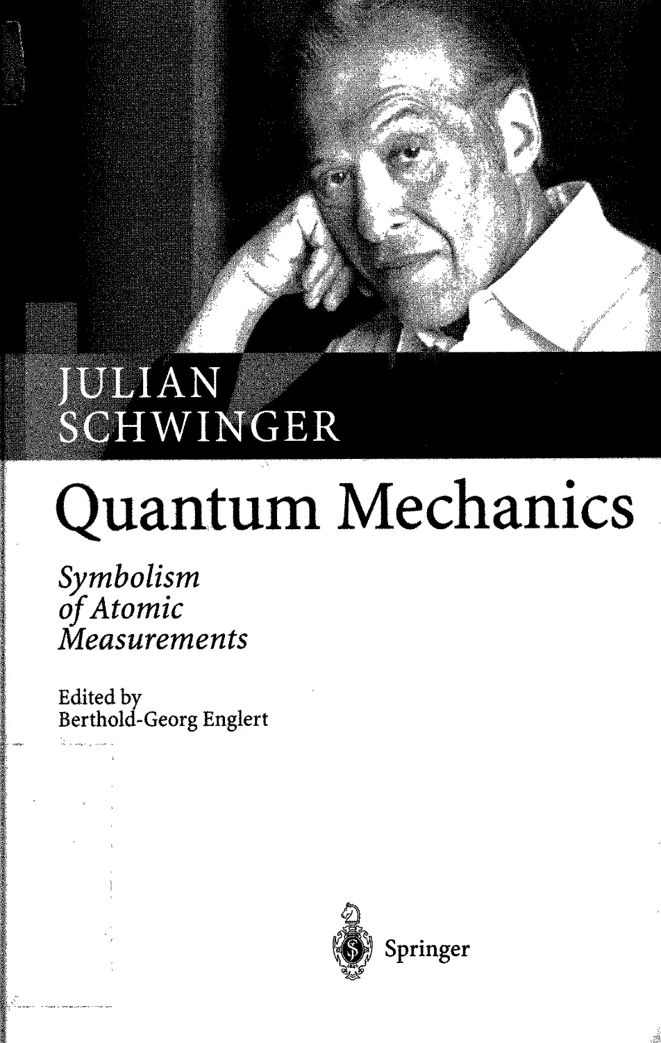
Quantum Mechanics
Symbolism
of Atomic
Measurements
Edited by
Berthold-Georg Englert
Springer

JULIAN SCHWINGER
Quantum Mechanics
Symbolism
of Atomic Measurements
Edited by
Berthold-Georg Englert
« Springer

Julian Schwinger (1918-1994)
Dr. Berthold-Georg Englert Clarice Schwinger
Gleissenweg 23 10727 Stradella Court
85737 Ismaning, Germany Los Angeles, CA 90077, USA
With 78 Drawings and Figures,
and 351 Problems
Library of Congress Cataloging-in-Publication Data.
Die Deutsche Bibliothek - CIP-Einheitsaufnahme
Schwinger, Julian Seymour:
Quantum mechanics : symbolism of atomic measurements /
Julian Schwinger. Ed. by Bertold-Georg Englert. - Berlin; Heidelberg;
New York; Barcelona; Hong Kong; London; Milan; Paris; Singapore;
Tokyo: Springer, 2001
(Physics and astronomy online library)
ISBN 3-540-41408-8
ISBN 3-540-41408-8 Springer-Verlag Berlin Heidelberg New York
This work is subject to copyright. All rights are reserved, whether the whole or part of the material
is concerned, specifically the rights of translation, reprinting, reuse of illustrations, recitation,
broadcasting, reproduction on microfilm or in any other way, and storage in data banks. Duplication of
this publication or parts thereof is permitted only under the provisions of the German Copyright Law
of September 9, 1965, in its current version, and permission for use must always be obtained from
Springer-Verlag. Violations are liable for prosecution under the German Copyright Law.
Springer-Verlag Berlin Heidelberg New York
a member of BertelsmannSpringer Science+Business Media GmbH
© Springer-Verlag Berlin Heidelberg 2001
Printed in Germany
The use of general descriptive names, registered names, trademarks, etc. in this publication does not
imply, even in the absence of a specific statement, that such names are exempt from the relevant
protective laws and regulations and therefore free for general use.
Typesetting: Camera ready copy by the editor using a Springer TgK macropackage
Cover design: Erich Kirchner, Heidelberg
Printed on acid-free paper SPIN 10761836 55/3141/tr 543210

To Clarice and Ola

I I
m%
'* p*
Julian Schwinger (1918-1994)

Preface
Julian Schwinger had plans to write a textbook on quantum mechanics since
the 1950s when he was teaching the subject at Harvard University regularly.*
Roger Newton remembers:"!'
[A] group of us (Stanley Deser, Dick Arnowitt, Chuck Zemach, Paul
Martin and I forgot who else) wrote up lecture notes on his Quantum
Mechanics course but he never wanted them published because he
"had not yet found the perfect way to do quantum mechanics."
The only text of those days that got published eventually - following a
suggestion by, and with the help of, Robert Kohler* - were the notes to the
lectures that, Schwinger presented at Les Houches in 1955. The book was
reissued in 1991, with this Special Preface by Schwinger [3]:
The first two chapters of this book are devoted to Quantum
Kinematics. In 1985 I had the opportunity to review that development in
connection with the celebration of the 100th anniversary of Hermann
Weyl's birthday. [... ] In presenting my lecture [4] I felt the need
to alter only one thing: the notation. Lest one think this rather
trivial, recall that the ultimate abandonment, early in the 19th century,
of Newton's method of fluxions in favor of the Leibnizian calculus,
stemmed from the greater flexibility of the latter's notation.
Instead of the symbol of measurement: M(a',b'), I now write:
\a'b'\, combining reference to what is selected and what is produced,
with an indication that the act of measurement has a beginning and
an end. Then, with the conceptual analysis of \a'b'\ into two stages,
one of annihilation and one of creation, as symbolized by
|o'6'| = |o')(6'|,
the fictitious null state, and the symbols *F and ¢, can be discarded.
As for Quantum Dynamics, I have long regretted that these
chapters did not contain numerous examples of the practical use of the
Quantum Action Principle in solving physical problems. Perhaps that
can be remedied in another book, on Quantum Mechanics. [ ... ]
*See chapter 10 in the recent biography by Mehra and Milton [1]. ^As quoted by
Schweber in section 7.11 of [2]. *See the preface to [3].

VIII Preface
The change in notation mentioned here was systematically incorporated in
the set of lecture notes that Schwinger wrote up for the students of the three-
quarter course on quantum mechanics that he taught twice in the mid-1980s
at the University of California, Los Angeles (UCLA). I had the great luck
to still be at UCLA during much of the first round, taking care, in fact,
of office hours and problem sessions, and I continued to receive Schwinger's
handwritten lecture notes after I had left.
Indeed, these notes were meant to be the basis of the intended book for
which Schwinger had selected the natural title Quantum Mechanics and the
less obvious - to others, that is, not to him - subtitle Symbolism of Atomic
Measurements. This choice is the succinct pronouncement of his philosophy,
which is spelt out in the Prologue. The quote from page 10:
[PJhysics is an experimental science; it is concerned only with those
statements which in some sense can be verified by an experiment.
The purpose of the theory is to provide a unification, a codification,
or however you want to say it, of those results which can be tested by
means of some experiment. Therefore, what is fundamental to any
theory of a specific department of nature is the theory of
measurement within that domain.
is to the point.
Schwinger's continuing interest in frontier physics was a permanent and, in
hindsight, unfortunate distraction from the book-writing enterprise.
Eventually, his untimely death put an end to all plans, and so his quantum mechanics
book is not to be.
Yet there are those UCLA lecture notes. Although they are certainly not
identical to the book Schwinger would have written, they do represent a first
draft and are the closest thing to the unwritten book that is available. Prom
many conversations I had with him, I know that Schwinger was quite happy
with the way he induces the general structure of quantum kinematics and
establishes the dynamical principle, his quantum action principle. I think
that he had finally "found the perfect way to do quantum mechanics."
I always thought that the notes should be put into a form that makes
them accessible to the broad public, but it needed the encouragement of a
few friends to actually go about it. Particularly decisive was the gentle push
by Robert Finkelstein who, in response to my remark - during a lunch session
at the UCLA faculty club (the Chatham had disappeared years earlier) -
that somebody should put the notes into print, just said: " You should do it."
Thank you, Bob.
And then, of course, there was the consistent support by Clarice Schwinger
who gave me the feeling - very calmly and, I'm sure, very consciously - that
she couldn't think of anyone else to do it. Thank you, Clarice.
My dear wife Ola had to be content with a much too small share of my
attention while I was working on this project. Knowing well how much the
book means to me, and why it does, she never complained. Dziekuje, Ci, Olu.

Preface IX
The lecture notes of Schwinger's UCLA course consist of three parts
corresponding to the three quarters of teaching. Here is a brief summary of the
contents.
Part A, the material of the fall quarter, begins with an analysis of
experiments of the Stern-Gerlach type that accomplishes "a self-contained physical
and mathematical development of the general structure of quantum
kinematics" [4]. Much technical material is delivered in passing. In particular, unitary
transformations are studied from various angles, and the algebra of angular
momentum is treated in depth. Then, an analysis of Galilean invariance yields
the non-relativistic Hamilton operator.
The winter quarter, Part B, proceeds from there. The response to
infinitesimal time displacements establishes the equations of motion. Then the
Quantum Action Principle is derived, and accepted as a fundamental
principle. In a sense, the rest of Part B and all of Part C consist of instructive
applications of the action principle - the "numerous examples" referred to
above. Part B contains treatments of, among others, the (driven) harmonic
oscillator, bound-state properties of hydrogenic atoms, and Rutherford
scattering.
Part C (spring quarter) begins with the two-particle Coulomb problem,
including the modifications for two identical particles. The treatment of systems
with many identical particles follows, where the notion of second quantization
eventually leads to the concept of the quantized field. As a first application,
the Hartree-Fock and Thomas-Fermi approaches to many-electron atoms are
presented, the latter in considerable detail.§ The second and final application
is the quantum theory of electromagnetic radiation, which is developed to
the extent necessary for an understanding of (the non-relativistic aspects of)
the Lamb shift.
During his oral lectures, and in the handed-out notes, Schwinger never
took any credit for his own very substantial and highly original contributions.
But, of course, he mentioned the names of others whenever appropriate. I
decided to stick to this practice when preparing the notes for print.
Distributing notes to the students that attend your lectures is one thing,
writing a book for the anonymous reader is quite another. So, some editing
was unavoidable in the course of turning Schwinger's lecture notes into book
form, but I tried to change as little as possible. In addition to the UCLA
notes of the mid-1980s, Chapter 12 contains some material from lectures
that Schwinger gave at the University of New Mexico, Albuquerque in 1987.
The Prologue is based on the transcript of the audio record of a public lecture
that he delivered in the early 1960s.^ Most of the problems are as formulated
by Schwinger; in addition to the ones that came with the lecture notes, I
discovered many good problems in the Schwinger Papers [5] that are archived
at the UCLA Research Library. In fact, all the raw material that I used can
^Tliis is an example that teaching and research were closely related activities for
Schwinger. At the time of these lectures, he was working on refinements of the
Thomas- Fermi method. 'Section 7.10 in [2] comments on this lecture.

X Preface
be found there. Charlotte Brown, Curator of the UCLA Special Collections,
has been very helpful in my search of the Schwinger Papers. I thank her
sincerely.
I wish to thank Herbert Walther for the splendid hospitality extended to
me over the years at the Max-Planck-Institut fur Quantenoptik in Garching;
the institute's infrastructure was of great help while I was working on this
book. During the past year, the crucial stage of this undertaking, I was
supported by the Universitat Ulm; I thank Wolfgang Schleich for the generous
invitation to join his Abteilung Quantenphysik temporarily.
I acknowledge with gratitude the support by the editorial staff of Springer-
Verlag; in particular, the help of Wolf Beiglbock, Christian Caron, and
Brigitte Reichel-Mayer was invaluable. And I thank Jens Schneider, who
turned the handwritten notes into electronic files that I could then work on.
Ismaning, September 2000 BG Englert
References
1. Jagdish Mehra and Kimball A. Milton: Climbing the Mountain. The Scientific-
Biography of Julian Schwinger (Oxford University Press, Oxford and New York
2000)
2. Silvan S. Schweber: QED and the Men Who Made It: Dyson, Feynman,
Schwinger, and Tomonaga (Princeton University Press, Princeton 1994)
3. Julian Schwinger: Quantum Kinematics and Dynamics (W.A. Benjamin, New
York 1970; reprinted by Addison-Wesley, Redwood City 1991)
4. Julian Schwinger: 'Hermann Weyl and Quantum Kinematics'. In: Exact
Sciences and their Philosophical Foundations, Proceedings of the International
Hermann Weyl Congress, Kiel, Germany, 1985, edited by Wolfgang Deppert et al.
(Verlag Peter Lang, Frankfurt/Main and New York 1988) pp. 107-129
5. Julian Schwinger Papers (Collection 371), Department of Special Collections,
University Research Library, University of California, Los Angeles

Contents
Prologue 1
Part A. Fall Quarter: Quantum Kinematics
1. Measurement Algebra 29
1.1 Stern-Gerlach experiment 29
1.2 Measurement symbols 31
1.3 State vectors 36
1.4 Successive measurements. Probabilities 38
1.5 Probability amplitudes. Interference 41
1.6 "Measurement disturbs the system" 46
1.7 Observables 48
1.8 Algebra of Pauli's operators 50
1.9 Adjoint symbols, Hermitian symbols 53
1.10 Matrix representations 56
1.11 Traces 57
1.12 Unitary geometry 59
1.12.1 Column and row vectors, wave functions 59
1.12.2 Two arbitrary components of Pauli's vector operator . 63
1.13 Unitary operators 67
1.14 Unitary operator bases. Complementarity 69
1.15 Quantum degrees of freedom 76
1.16 The continuum limit 82
1.16.1 Heisenberg's commutation relation 82
1.16.2 Schrodinger's differential-operator representation .... 86
Problems 88
2. Continuous q,p Degree of Freedom 101
2.1 Wave functions 101
2.2 Expectation values and their spreads 109
2.3 States of minimal uncertainty Ill
2.4 States of stationary uncertainty 114
2.5 Hermite polynomials 118

XII Contents
2.6 Completeness of stationary-uncertainty states 123
2.7 Eigenvectors of non-Hermitian operators 125
2.8 Classical limit 132
2.9 More about stationary-uncertainty states 135
Problems 136
3. Angular Momentum 149
3.1 Infinitesimal unitary transformations 149
3.2 Infinitesimal rotations 150
3.3 Common eigenvectors of J2 and Jz 152
3.4 Decomposition into spins 155
3.5 Angular momentum of a composite system 158
3.6 Finite rotations. Eulerian angles 162
3.7 Rotated angular-momentum eigenvectors 168
Problems 177
4. Galilean Invariance 183
4.1 Generators of infinitesimal transformations 183
4.2 Hamilton operator for a system of elementary particles 190
Problems 191
Part B. Winter Quarter: Quantum Dynamics
5. Quantum Action Principle 195
5.1 Equations of motion 195
5.2 Conservation laws 197
5.3 Sets of q,p pairs of variables 199
5.4 Wave functions for force-free motion 202
5.5 Quantum action principle 207
5.6 Principle of stationary action 210
5.7 Change of description 213
5.8 Permissible variations 214
Problems 216
6. Elementary Applications 223
6.1 Time transformation functions 223
6.1.1 Free particle 223
6.1.2 Constant force 224
6.1.3 Linear restoring force: Harmonic oscillator 226
6.2 Short times 227
6.3 Harmonic oscillator: Energy eigenvalues 229
6.4 Free particle and constant force: State density 231
6.5 Harmonic oscillator: Energy eigenstates 234
6.6 Free particle and constant force: Energy eigenstates 237

Contents XIII
6.7 Constant force: Asymptotic wave functions 239
6.8 WKB approximation 243
6.9 Zeros and extrema of the Airy function 248
6.10 Constant restoring force 252
6.11 Rayleigh-Ritz variational method 255
Problems 257
7. Harmonic Oscillators 269
7.1 Non-Hermitian operators 269
7.2 Driven oscillator 272
7.2.1 Time-independent drive 274
7.2.2 Slowly varying drive 276
7.2.3 Temporary drive 278
7.3 Remarks on Laguerre polynomials 286
7.4 Two-dimensional oscillator 288
7.5 Three-dimensional oscillator 295
Problems 298
8. Hydrogenic Atoms 303
8.1 Bound states 303
8.2 Parameter dependence of energy eigenvalues 307
8.3 Virial theorem 309
8.4 Parabolic coordinates 313
8.5 Weak external electric field 316
8.6 Weak external magnetic field 319
8.7 Insertion: Charge in a homogeneous magnetic field 324
8.8 Scattering states 328
Problems 333
Part C. Spring Quarter: Interacting Particles
9. Two-Particle Coulomb Problem 343
9.1 Internal and external motion 343
9.2 Rutherford scattering revisited 346
9.3 Additional short-range forces 352
9.4 Scattering of identical particles 355
9.5 Conserved axial vector 358
9.6 Weak external fields 365
Problems 368
10. Identical Particles 375
10.1 Modes. Creation and annihilation operators 375
10.2 One-particle and two-particle operators 381
10.3 Multi-particle states 385

XIV Contents
10.4 Dynamical basics 386
10.5 Example: General spin dynamics 387
10.6 General dynamics 392
10.7 Operator fields 395
10.8 Non-interacting particles 397
Problems 403
11. Many-Electron Atoms 405
11.1 Hartree-Fock method 405
11.2 Semiclassical treatment: Thomas-Fermi model 410
11.3 Correction for strongly bound electrons 420
11.4 Quantum corrections and exchange energy 425
11.5 Energy oscillations 428
Problems 430
12. Electromagnetic Radiation 437
12.1 Lagrangian, modes, equations of motion 437
12.2 Effective action 441
12.3 Consistency check 444
12.4 Free-space photon mode functions 447
12.5 Physical mass 449
12.6 Infrared photons 452
12.7 Effective Hamiltonian 455
12.8 Energy shift 459
12.9 Transition rates 461
12.10 Thomson scattering 465
Problems 467
Index
473

Prologue
It seems to me that there are deep philosophical lessons to be learned in the
way in which the practicing theoretical physicist thinks about the foundations
of the subject, i.e., the manner in which he approaches the problems, the
general criteria he brings to bear on what is a reasonable solution. So, the
important thing then is to display the general world view, the world picture
that the theoretical physicists has.
This is particularly significant in connection with the philosophical
implications of quantum physics, because quantum physics or quantum mechanics
- by which I think we mean finally the rational mode of understanding of
microscopic or atomic phenomena - has perhaps had the greatest impact of
any of the developments of physics upon the mode of thinking or the world
picture of the physicist and thereby, indirectly, of the general citizen.
Now, if we want to understand specifically the origins of quantum physics,
we must go back to see how the stage has been set through the developments
of what is called classical physics, and then compare with quantum physics.
By classical physics, we mean the precise formulation of all of the properties
of matter as they were finally expressed in their essentially perfect form at the
beginning of the 20th century. Classical physics is characterized by the fact
that, whereas the underlying conceptions are idealizations - it was no easy
job to be a Galileo or to be a Newton - nevertheless, these conceptions still
strike very close to common, ordinary everyday affairs. To understand the
principles of physics, as they are expressed within these great generalizations
of classical physics, is not very difficult. Our school children manage it all the
time. But quantum physics is something different. In quantum physics, you
go far beyond the ordinary situations of everyday life. We strike at a level of
idealization that is hard to appreciate until you have seen how this historical
line of development has come about.
The first grand physical theory, of course, was that of Newtonian physics.
This is a theory of massive point particles which interact by means of actions
at a distance. The traditional theory of gravitation is the classic example
of this. And to characterize this theory in a general way in terms of its
philosophical foundations, let me say that Newtonian physics, or Newtonian
mechanics is a causal, deterministic theory.

2 Prologue
By causal, one means essentially that when the state of the system is
given at a particular time - and we must return to precisely what we mean
by "state" - then the state is completely determined at any other time; this
is what we mean by causality. Causality is inference in time: given the state
of affairs at one time, the state of affairs is uniquely determined at another
time. What makes it deterministic is that the knowledge of the state also
determines all possible physical phenomena precisely.
This distinction between causal and deterministic may not seem very
important until we come up to the rather different situation that appears
in quantum mechanics. I have spoken of the state within the framework
of Newtonian physics. It is familiar that when we specify the state of the
system of particles which interact with each other by means of instantaneous
forces as the gravitational force was conceived at that time, that the full
specification of state is the indicating of precisely where the particles are at a
given instant of time and how they are moving. In more technical language,
it is the specification of the positions and the momenta of the particles. If
these are known at a given instant of time, and it is known precisely under
what law of force the particles are moving, such as the grand statement of
the inverse square law of gravitation, then the physical situation is specified
completely. The state at any other time can be predicted and also, since this
is a deterministic theory, the knowledge of the state is the origin of the full
knowledge of the answer to all possible physical questions that can be asked.
Now, to indicate that Newtonian physics is not something that lies
completely behind us in the history of physics, let me perhaps remind you of the
fact that the triumph of Newtonian physics is indicated every time we have
an announcement of a successful space mission. That is, Newtonian physics,
as any general theory of physics must, remains perfectly valid in its own
domain. Here, of course, the domain is the motion of material bodies under the
action of known laws of force which are instantaneous interactions and cover,
therefore, fully the motion of artificial satellites in the perfectly well-known
field of force that is provided by the gravitational attraction of the Earth, or
the Moon, the planets, and so on.
Physics introduces new theories not because the theories in a particular
domain are found to be unsatisfactory, although they may be so also, if the
technique of experiment becomes finer and finer and new phenomena are
found which pass beyond the level of accuracy in the earlier theories, but
primarily because the domains of physics which come into question are ever
extended. To follow the line of historical development: the introduction in
the 17th century of the Newtonian concepts led to a steady development of
these ideas, their applications being primarily to astronomical phenomena,
which lasted for essentially a full 200 years, while the technical means for the
inference, in a precise sense, of the implications of these laws were developed
until one could fully carry out the calculations necessary to follow the paths
of the planets in full detail and so on. It was, however, during the 19th

Prologue 3
century that new areas of physical experience began to be met, in particular
in the domain of electromagnetism. And then we came finally, towards the
second half of the 19th century, to essentially a new physical theory going
beyond anything that had been, so to speak, conceived within the framework
of Newtonian physics. This is Maxwell's field theory of electromagnetism.
As far as the broad categorization of these theories is concerned, this was
also a causal, deterministic theory. But what made it so very different was
what was involved in the specification of state. Recall that the Newtonian
theories were concerned with point particles and the specification of state
was the indication of where these particles were and how they were moving
at any particular time. It is a discrete description: a finite number of particles,
and a finite number of quantities is needed to characterize everything about
this physical system. By contrast, in a field theory - let's continue to have
in mind the very specific example of the electromagnetic field - the
specification of state requires not a finite number of things (where the particles are
and how they are moving) but an infinite number. We must, in principle at
least, specify what the electromagnetic field is doing; how the electric field is
pointed; and how the magnetic field is pointed at every point of space - and
this at a given time. And what makes this a causal theory is that if we know
the state, if we know the distribution throughout space of the electric and
magnetic field at a given time, then we can predict at any later time what the
distribution of the electric and magnetic field will be. Given the state at one
time, the state is uniquely implied at another time. That makes it a causal
theory.
Again, what makes it deterministic is that the knowledge of the state, the
knowledge of the electric and magnetic fields, completely determines the
answers to all questions that can be asked about the electromagnetic field. And,
we should note again that - while we are talking about a domain of classical
physics, with the inference that this is not the final word - nevertheless, the
quantitative success of Maxwell's theory is demonstrated every day. We just
have to look at the ever-expanding development of radio communication
systems, and microwaves of radar or of television, not to mention the ubiquitous
cellular phones. This is not a past history in the development of physics, it
is something whose validity is confirmed all the time. The point, however, is
that it refers to a limited domain of experience. It is not all of the physical
world.
So, here then we have two very different kinds of physical theories, both
causal and both deterministic, but widely different in the nature of what
characterizes the specification of a state. One lies, so to speak, at one
limiting domain of the spectrum, it is a discrete description; a finite number of
quantities is specified. The other, at the other end, is a continuous
description; fields are involved, distributed throughout all space. These then are the
models of the two limits of classical behavior: the discrete, the continuous.
And it is particularly interesting to see how these two entirely different clas-

4 Prologue
sical modes of description have in a sense become unified or, perhaps better,
transcended in the further development of quantum physics.
Still continuing with our historical development, I recall what is all
familiar to you, that at the beginning of the 20th century there were further
very important developments, associated with Einstein's name - the
developments of the special and general theory of relativity. But yet, these were
not radically new developments in the sense that I mean quantum mechanics
to be; they were rounding out the framework of classical physics. They were
the recognition that - once we had placed the field phenomena, the
electromagnetic field specifically, on the same foundation as the theories of particles
- there was a modification in the strict Newtonian point of view. While we
are still dealing, within this framework, with point particles, they no longer
interact via instantaneous forces. We now recognize, as is particularly
emphasized by the relativity theory, that the interactions between particles are
propagated through space by means of the intermediary of the field.
Incidentally, I should also emphasize this difference between the two classical modes:
the strict Newtonian viewpoint is one of the instantaneous interaction at a
distance; the field point of view is one of local interaction propagated from
one point of space to the contiguous points. Within the field concept, there
is no longer any idea of instantaneous propagation. It is propagation through
space and time by means of a mechanism which is, in fact, intrinsically
limited in speed. This is, of course, the famous constancy of the speed of light,
the starting point for all the investigations on the special theory of relativity.
And so, what finally emerges from all of this is a theory with a dualistic
point of view, in which there are particles and fields, standing side by side,
neither explained in terms of the other - a fundamental duality that is the
culmination of classical physics: the strict Newtonian, discrete, point of view
of the particle has been modified because we now recognize that the
interactions between particles are not instantaneous but are propagated through the
mechanism of the field with its continuous point of view. The field is there
to supply the dynamical agency by which particles interact.
It was to be the purpose of further developments of quantum mechanics
that these two distinct classical concepts are merged and become transcended
in something that has no classical counterpart - the quantized field that is
a new conception on its own, a unity that replaces the classical duality. We
must try to trace the development of quantum mechanics, starting from this
classical background, up to this much deeper quantum mechanical foundation
and explanation.
So much then for a summary which can hardly do justice to several
hundred years of hard work by many physicists in attempting to lay the
foundations of these laws of what I will now call macroscopic phenomena because
it was, of course, in the investigation of the microcosmos - of atomic
phenomena - that an entirely new world and a new system of order was opened
up. It was here that it was found that the laws, which served so very well
„. BJrt „ w™s8&>ii^&l

Prologue 5
to range from ordinary experience on the Earth to extraterrestrial
experience in terms of the motions of the planets, are not in accordance with the
observed phenomena. When we turn not outward, but inward, we find new
laws of motions, new laws of physics, new ways of thinking, new philosophical
conceptions.
Now, how did this come about? Of course, in just a few sentences I cannot
give a fair account of the tremendous development of physics which occurred
during the last years of the 19th century and the early years of the 20th,
but let me remind you that these developments began in what may seem
to be a paradox. As pointed out above, we had two distinct laws of
behavior in classical physics, and one never trampled on the other. We either had
particles, and they were discrete objects, or we had fields, and they were
continuous objects distributed throughout space. The fields could be
attenuated as much as you want - a radio wave, as we travel out through space,
becomes weaker and weaker and weaker in a perfectly continuous way. A
particle, on the other hand, has discrete properties which it carries with it.
And so the remarkable thing was the discovery, in investigations of various
atomic phenomena, of an apparent paradox. Light, for example, was known,
from various interference phenomena, to possess properties typical of waves,
which are field phenomena; and light is spread out through space in a
characteristic field way. When performing suitable experiments, one now found that
these light waves appeared to acquire particle-like properties under certain
experimental conditions. Unlike the classical notion of a light wave, which
suggests that its energy is simply distributed continuously throughout the area
that it occupies, light exhibited the ability to transfer definite and discrete
amounts of energy, acting then as if it were a particle - first simply called
light quantum, but now more commonly photon - whose characteristic, of
course, is to have associated with it, in a certain state of motion, a definite
energy, a definite momentum. This was the paradox found in the early days
of these developments: that light waves exhibit, under certain circumstances,
definite particle-like behavior. The two quite distinct classical notions,
mutually exclusive as they are, are nevertheless in some sense realized jointly
within the microscopic domain. An example is the classic experiment of the
photoelectric effect in which light waves, falling upon metals, would transfer
energy to electrons and liberate them, whereby a definite amount of energy
was absorbed every time, despite the picture of a classical field distributed
throughout space in which you might absorb more or less energy, depending
upon the accidental circumstances of that particular electron.
Here then was light, a characteristic example of a wave or a field
phenomenon acting in a particle-like manner. The converse was also true,
although the experimental proof of this would have to wait for some 27 years.
But at this distance in time, I think we can lump all these things together
and say that experimentally, as an important aspect of this same
development, the converse was true. Electrons were the characteristic example of

6 Prologue
microscopic particles. Electron beams could be produced in evacuated tubes
and they would move in straight lines. And when exposed to electric and
magnetic fields, they would change their direction just as material bodies
were supposed to do. But, nevertheless, under appropriate circumstances,
namely when electron beams are scattered from crystalline bodies, one found
interference rings which would be typical for the type of wave phenomena
that is characteristically associated with a distributed field. In other words,
instead of being scattered as material objects would be, electrons moving
through a crystal would be scattered in the way that would produce a
characteristic interference pattern much as light of a certain wavelength would
do. Here then were objects originally thought to be essentially classical
particles which, under new experimental conditions, would exhibit continuum or
wave-like phenomena.
We had then a remarkable duality in which apparently the same objects
could, under some circumstances, act as classical particles; under some other
circumstances, they could act as classical waves. And, of course, this was
something for which there was no preparation in any other phenomena of
physics as they had been known.
Meanwhile, the detailed investigation of the properties of atoms, as they
were revealed by spectroscopic experiments, had proceeded. The possibility of
producing atomic spectra in the suitable circumstances of very thin gases had
made it possible to study the behavior of individual atoms. There were
attempts to understand the observed spectra in terms of the motion of electrons
within the atoms, which ended with a complete failure of classical physics to
account for these phenomena. Indeed, the mere existence of atoms and their
ability to radiate precise spectral lines is a conflict with classical physics. If
we'd accept any picture of an atom as electrons moving around some central
nucleus, as Rutherford discovered to be the situation in 1911, then,
according to the classical laws of electromagnetism, the accelerated charges in their
motions around the nucleus would always continue to radiate until finally
they had exhausted all possible energy and would fall into the nucleus. First
of all, this meant that atoms were not stable, a quite flagrant violation of
simple experience; and more than that, in the course of this process the
electrons would radiate spectral lines whose frequencies would change as they
got closer and closer to the nucleus, and you would have nothing analogous
to the empirical situation of sharp spectral lines, of definite frequencies,
characteristic of individual atoms. Clearly, the laws of macroscopic physics failed
completely within the microscopic world.
In the detailed analysis as it was carried out, primarily in the hands of
Niels Bohr, and others of this important Copenhagen School of Physics, it was
found that the only successful attempt to understand the properties of atomic
spectra consisted of introducing a bold hypothesis: that physical quantities
- such as energy and angular momentum, the two most important examples
- can only have certain definite values. In classical mechanics, they would

Prologue 7
assume any possible values; classically they are continuous objects. A particle
in ordinary life can be given any energy one wishes by simply providing the
appropriate amount of energy; and if you set a body into rotation, the angular
momentum that this will have can be given any value. There is no particular
selected set of values that are natural. But, nevertheless, the analysis of the
facts of atomic spectroscopy indicated that the energy values that atoms,
or electrons in atoms, could have were not continuous but assumed definite
values. This was the only explanation that could be given of the discreteness
of spectral lines. And all of the certain definite values of angular momenta
are simple multiples of a new natural constant, known as Planck's constant
of action, which was first discovered in connection with other attempts to
understand particularly significant characteristics of atomic phenomena.
So here, then, we had first of all the major break with the phenomena of
classical physics: quantities which classically would be given continuous
values, now had discrete values. This, in other words, is the general observation
of the microscopic world: that the phenomenon of atomicity is all-prevailing.
We must account for the very existence of atoms, which after all is not a
classical conception. Classically, there should be no limit to the extent to which
you could subdivide matter. The fact that this subdivision cannot be carried
out indefinitely, but ceases when we reach the atomic scale is, of course, the
most fundamental statement that something new is involved. Here is the
phenomenon of atomicity, not only in the mere existence of atoms but also in the
laws of mechanical motion: an atomicity of angular momentum, an atomicity
of action, to put it in the most general way, was a basic phenomenon of
microscopic physics. And we simply had to accept - I say "we" but, of course,
I was not involved at the time; there is, nevertheless, the feeling of kinship
here - that the physical properties of atoms must be understood in terms of
new laws which transcended anything that was familiar before. This was a
new world.
Beyond this phenomenon of atomicity, which I mark as the one basic fact,
the new fact of microscopic physics, there is another one which appears at
the same time. This is the essential statistical nature of microscopic
phenomena - another fundamental feature which must be accepted as the way that
the microscopic world operates. That the microscopic world is necessarily
statistical can be understood in the example mentioned above of the
diffraction phenomenon that an electron beam, interacting with a crystal, exhibits.
Now, let's think about how this diffraction phenomenon would come about.
A crystal is a regular arrangement of atoms with a characteristic distance
separating them and, by virtue of this characteristic dimension, for any wave
phenomenon that falls upon the crystal, there will be certain preferred
definite directions of scattering, selected by the relation of the wavelength to
the interatomic spacing of the crystal. (This phenomenon is, for example,
well known in the case of X-rays - in fact, its demonstration represented one
of the experimental proofs that X-rays are wave phenomena.) So. when we

8 Prologue
carry out an experiment in which a beam of electrons falls upon this crystal,
and then moves in various directions toward a screen, it will produce a
characteristic interference pattern there; instead of the electrons arriving more
or less at random, with a uniform intensity all over this screen, you will find
preferred places.
Now, if I make the beam so weak that one electron within a perfectly
definite time interval moves through this crystal in some way, it will finally
be detected by landing in a perfectly definite place on this screen. This may be
a scintillation screen, for example, and if you have a weak beam of electrons
and you look at the screen, you'll suddenly see a flash of light, not all over the
screen but in one place. The electron exhibits its particle-like characteristics
when it is finally detected, when it finally exhibits its position by producing
an appropriate chemical process, the result of which is a flash of light. And
we observe that the electron is here. For one electron, there is certainly no
interference pattern. The interference pattern does not appear all at once.
You have simply an individual electron. Now, a second electron arrives in the
course of this very weak beam. What happens to it? Does it land at the same
spot? No, it lands at random, at some other point that has no relation to
the first. But as we continue, and more and more electrons land upon this
scintillation screen - all coming under the same experimental conditions, but
each arriving independently of the others - eventually the pattern of this
interference behavior emerges. Many electrons land here, none land there,
and so on, until the final picture of intensity is one which gives the overall
pattern. But nevertheless, this has come about, as the result of the random
landing of the electrons at various points on the screen.
To emphasize another aspect, now suppose we had carried through such
an experiment and ten billion electrons had finally produced a certain
interference pattern, a picture of intensity of relative number. Then I repeat the
experiment. I prepare exactly the same circumstances, and I turn on the
electron gun and see what happens. Again, the first electron moves through the
crystal. Will it land at the same place as the first electron of the previous run?
Certainly not. We begin all over, but the pattern as a whole repeats itself in a
random way. The first electron of the second experiment will land somewhere;
the second electron of the repeat experiment will land somewhere else - with
no relation between them or the electrons of the first experiment. In other
words, the individual particles arrive in a perfectly random statistical way.
There is no possibility of controlling this. This is, of course, a generalization
from half a century of attempts to do so: the picture which we must accept is
that, within the domain of microscopic phenomena, we are unable to control
how the individual particles will behave. But what is perfectly determined,
and will be reproduced every time you repeat the experiment, is the
interference pattern; the characteristic features of the pattern are predictable and
reproducible. Once we have this apparent duality of entities - electrons that
behave under some circumstances like discrete entities, particles, landing at

Prologue 9
definite places on that screen, but in other respects act as waves, producing
in their overall intensity characteristics the wave phenomenon of interference
- we must accept that the interference pattern is not going to be repeated
in miniature every time an electron lands; and that, therefore, there must be
an aspect of randomness about where the electrons do land. The interference
pattern is merely finally the statement of relative probabilities: with endless
repetitions, you will find many more particles there than here - and this in
a perfectly regular way.
It is then, in a sense, almost an automatic inference of everything that we
have said, but I would prefer to take it as really the more fundamental thing:
it is a basic characteristic of the laws of microscopic phenomena that they are
statistical. It is not possible to predict, in general, the outcome of a specific
event. But what one can predict is the average result, the statistical result,
the net situation for the repetition, a sufficiently large number of times, of the
same experiment - and it is the purpose of microscopic physics or quantum
mechanics to make such predictions.
So here, then, we have the great challenge of microscopic physics - that
there are these two new basic aspects which we must incorporate into a world
picture: the fact that phenomena are atomistic and that they are statistical.
But that the new physics is statistical and therefore fundamentally different
from the fully deterministic classical physics does not mean that we have
failed. We simply recognize what the nature of this new microscopic physics
must be. It is not to predict the outcome of each individual event. It is to
predict rather what the outcome must be on average; what the probable
outcome must be. And as the electron-scattering experiment - or rather this
simple-minded description of the experiment - indicates, this is something
that we necessarily must put up with.
In fact, as we should perhaps mention here, if we attempt in any way
to control precisely where the first electron shall land, we can indeed do
that; we can produce a new experimental situation in which, with essential
certainty, the electrons will land at the pre-assigned spot - all of them. But
then we shall have no interference pattern. In other words, there are now
two situations that we're talking about. The first, in which an interference
pattern does appear, is one definite experimental situation, and in that it is
not possible to predict or control in any way where the individual electrons
will appear. Then there is the second experimental situation, in which we can
control and predict where the electrons will appear in the course of moving
through some apparatus. It will be a different apparatus and that apparatus
could never produce an interference pattern. We are dealing, so to speak,
with two distinct aspects of the microscopic world and it requires a different
experimental situation to display one or the other.
Let's think now of how - once having recognized that we have two basic
features of the microscopic world, the aspects of atomicity and of the statis-

10 Prologue
tical nature of microscopic events - we could proceed to construct a theory
that would incorporate this very bizarre situation.
We must have a mathematical theory which, in some way, will represent
a suitable mathematical model or idealization and enable us to predict in a
coherent way - in much the same manner as physics has always done - what
the outcome of experiments will be if we are given correctly all the conditions
that fully characterize the nature of the experiment. To see what we have to
do, I think we must go back and think a little more consciously of some of the
fundamental principles (call them philosophical, if you like) which underlie
classical physics - or shall I say macroscopic physics, because that's now the
distinction.
I think specifically of the theory of measurement. And here, of course, we
have to recognize the fundamental philosophical conception that physics is
an experimental science; it is concerned only with those statements which in
some sense can be verified by an experiment. The purpose of the theory is to
provide a unification, a codification, or however you want to say it, of those
results which can be tested by means of some experiment. Therefore, what
is fundamental to any theory of a specific department of nature is the theory
of measurement within that domain.
Now, what was characteristic of the theory of measurement in the
macroscopic classical physics? Well, the essential thing that was basic to it was
the conception of a non-disturbing measurement. It is, of course, perfectly
obvious to anyone who has ever come near a physics laboratory that, in the
process of a measurement, aimed at gaining information about a particular
object, we must interact with it physically in some way. But nevertheless we
would like to be able to idealize that interaction in such a way that we could
meaningfully state what that property would be as though the interaction
did not occur. (You may take as the simplest model the insertion of a
thermometer into a body of water with the objective of determining the temperature
of the water - ideally as it would be without any disturbance by means of
the thermometer. Without the presence of the thermometer, however, there
is no means to determine what that temperature is.) As you know, whenever
the interaction occurs there must be some disturbance as a net effect of that
interaction with the object in question. (The insertion of a thermometer into
a pail of water changes the mass of the water. It will change the temperature
that is to be measured in some way.) But what is characteristic of classical
physics is that we can state, and correctly so, that it is meaningful to talk of
an idealization in which that interaction can be made as small as we please
without, however, it becoming zero; because if it is zero, we have no means
of gaining information.
That the interaction is so small that it does not disturb the object of
interest, is in fact not always necessary, nor is it always possible. For example,
some measurements might represent chemical changes, which are large
alterations in the nature of the substance, and these arc certainly not negligible

Prologue 11
disturbances. It is here that a second aspect of macroscopic physics comes
into play. Since classical physics is causal and deterministic, we can
calculate as accurately as we please and correct for the effect of these unavoidable
disturbances. It is indeed familiar that in classical physics any measurement
has a theoretical description associated with it, which represents the
recognition of what the disturbance has been and the calculation of how to correct
for it in order, therefore, to come back to what an idealized non-disturbing
measurement would be. So, for the record: the two basic features of
measurements in classical physics are that we can either make the interaction so
small that there is a negligible disturbance; or, in a particular
experimental circumstance, by the nature of the experiment we wish to perform, if we
cannot make the disturbance arbitrarily small, we can calculate the effect of
that disturbance and compensate for it with arbitrary precision.
This is, simply stated, the theory of classical measurement; and
associated with it is the idea that there is then no limit to the accuracy with
which we could make measurements simultaneously of any number of
physical properties, as in the very statement of the concept of state, for example,
in Newtonian physics. When I assert that the state is the specification of the
positions and the momenta of all the particles in question, then implicit in
that is the assumption, consistent with the whole scheme, that in fact I can
carry out the measurements necessary to give the numerical values that those
quantities have at every time. And similar remarks apply to measuring the
distribution of electromagnetic fields throughout all of space.
In summary then, the classical theory of measurement says that there is
no limit to the accuracy with which we can assign numerical values to all
the quantities that are needed to specify the state, and since all of these are
deterministic theories, that means to all physical properties at once. Since
physical properties can be assigned numerical values consistently, one has
never in classical physics drawn any distinction between the physical
properties and the numerical values which they have at any particular time. In
classical physics, we are always able to assign to the physical properties,
considered as an abstract thing, a very concrete representation by means of
numerical values which a non-disturbing measurement would find for them
at a particular time.
This restates the foundations of classical physics: the idealization of non-
disturbing measurements and the corresponding foundations of the
mathematical representation, the consequent identification of physical properties
with numbers because nothing stands in the way of the continual assignment
of numerical values to these physical properties.
Now, by contrast, what is the situation in microscopic physics? Drawing
upon the vast body of experimental data, accumulated over the course of
several decades, I have summarized above the properties of microscopic physics -
or, if you like, of microscopic measurements - under these two basic headings:
atomicity and the statistical nature of the phenomena.

12 Prologue
What does this mean? First of all, atomicity: atomicity means that the
microscopic entities have many of their properties carried in certain basic
units. There is no half of an electron. The electron has a definite mass; it has
a definite charge. If the interactions that I am concerned with are electrostatic
in nature, I cannot reduce them arbitrarily in strength because there is no
half of a unit of charge. This indicates to you immediately, I think, the basic
difference between the laws of microscopic measurement and macroscopic
measurement. I must take into account the fact that the strength of the
interaction - which must be present if I am to talk of measurement at all
and, therefore, talk meaningfully of physical phenomena - cannot in general
be made arbitrarily small because the physical objects that interact (the
atoms, the electrons) in general have relevant physical properties which come
in certain units - quanta, the origin of the name of the subject that we are
discussing: quantum mechanics.
Now, this might seem as though it were not an unsurmountable difficulty.
We recognized, even in classical physics, that there might be circumstances in
which the act of measurement produced definite disturbances that we could
not minimize because of the particular kind of measurement we carried out.
In classical physics, we said the situation may be such that the
measurement interaction is very strong and cannot be made arbitrarily weak, but
this does not upset the underlying philosophy of measurement because I can
calculate with arbitrary precision what the effect of that interaction was and
compensate for it, correct for it.
Can I still do that now, in the realm of atomic measurements? The
answer is no, because this is where the second fundamental aspect of microscopic
measurement comes into play; namely, the phenomenon of statistics, the fact
that we cannot predict in detail what each individual event will do but only
make predictions on an average or statistical scale. The measurement act
involves a strong interaction - I repeat: on the microscopic scale it is
necessarily strong because we cannot cut the strengths of the charges in half; we
cannot change the properties of these fundamental particles; we must accept
them as they are - and so the measurement unavoidably produces a large
disturbance, which we cannot correct for in each individual instance, for we
cannot control what happens in each individual event in any detail. We can
only predict or control what happens on the average, never in any
individual instance. Therefore, the program of computing what the effect of the
disturbance was and correcting for it is, in general, impossible. Accordingly,
the two basic tenets of the theory of macroscopic measurement are both
violated. Either the interactions cannot be made arbitrarily weak because of
the phenomenon of atomicity, or if we wish to accept this and correct for it,
we cannot do so because we do not have a detailed, deterministic theory of
each individual event; we have only the ability to anticipate or control the
statistical average.

Prologue 13
So, here then is the general implication from the mass of experimental
data that for microscopic physics, if we are to construct a theory, we need
a whole new theory of microscopic measurement, and to go with this we
need a whole new scheme of mathematics, which is to say that we can no
longer speak meaningfully of the numerical values that physical properties
have at a given time. Put differently, I wish to point out that the failure of
these fundamental assumptions means equally well a failure of the ability to
represent physical phenomena in the microscopic realm by numbers which
change in time as we do in the macroscopic or classical domain. Something of
an entirely different mathematical nature is needed, such that it represents,
or mimics, the basic facts of microscopic measurement.
To emphasize the relevant point, I may say this. Macroscopically, we can
measure one physical property; we assign a number to it. We measure a
second physical property; we assign a number to it. We can then speak of
this pair of numbers as the values of this pair of physical properties at a
given time. There is no contradiction here. We can perfectly well go back
and check that the first property has still the same value it had before if we
could, in an idealized way, carry out these measurements rapidly enough (or
regenerate the physical circumstances in such a way that we could repeat the
first measurement).
By contrast, suppose we have indeed succeeded in measuring in some
way one physical property of an atomic system. Now we go on to make a
measurement of the second physical property. That measurement necessarily
will involve an interaction, the strength of which is not arbitrarily weak and
the effect of which is not controllable, in such a way that it will, in general,
produce changes in the physical circumstances that specify the conditions of
the first measurement. In other words, the system that is being measured is
disturbed in an uncontrollable way in such a manner that if we now went
back and asked for the value of the first physical property, checking to see
that it still had the same value as before, we would now find not at all the
same value but a random assortment of all the possible values that it could
assume, with various probabilities that depend in detail upon precisely what
we have done. This is so because the second measurement has introduced a
new physical situation; the interaction of the second measurement has
disturbed the physical system of interest so violently that we have no way of
knowing, except under very special circumstances, whether the system has
been left in precisely the same physical situation that would enable us to
say that the first physical property still has the same value it had before
the second measurement. In other words, once we recognize that the act of
measurement introduces in the object of measurement changes which are not
arbitrarily small, and which cannot be precisely controlled, then we must
acknowledge that every time we make a measurement we introduce a new
physical situation that is essentially different from the situation before the
measurement.

14 Prologue
So, if you measure two physical properties in one order, and then the
other - which classically, of course, would make absolutely no difference -
these are simply two different experiments in the microscopic realm. You
have two different physical situations which come about depending upon
whether you first measure property A and then property B, two successions
of disturbances which have this microscopic character, or do it in the reverse
order, first B and then A, which involves entirely different disturbances. And
since the final physical situation depends crucially upon the order in which the
microscopic measurements are performed, it is, in general, no longer possible
to say that property A and property B have these values. That would only
have meaning if you could get the same numerical values no matter in which
order the measurement was carried out. Exceptional situations aside, in the
"first A then B" order of measurements only B emerges with a known value,
and only A in the "first B then A" order.
Therefore, the mathematical scheme for microscopic measurements can
certainly not be the representation of physical properties by numbers, because
numbers do not have this property of depending upon the order in which the
measurements are carried out. The assignment of a pair of numbers to two
physical properties introduces no sense of order, no sense of sequence. We
must instead look for a new mathematical scheme in which the order of
performing physical operations is represented by an order of performance of
mathematical operations. The mathematical scheme that was finally found
to be necessary and successful is the representation, in a very abstract way,
of physical properties not by numbers but by elements of an algebra for
which the sense of multiplication matters. In other words, the multiplication
of these algebraic symbols was found to be the proper counterpart of the
successive performance of measurements: that the order of measurements is
significant, as a consequence of the unavoidable disturbances, is reflected in
that, correspondingly, the sense of multiplication of these symbols must be
significant.
And so we are led to a much more sophisticated and deep mathematical
scheme in which physical properties are set into correspondence with the non-
commutative elements of an algebra or, as they often are referred to, non-
commutative operators as compared to the very elementary representation of
physical properties by numbers. And with every physical state - the idea of
state reoccurs - we associate a vector in a suitable abstract space on which
these operators act.
As a result of all this, a very beautiful mathematical scheme has emerged
which gives a wonderful account of all of these seemingly bizarre and
incomprehensible facts of microscopic physics. This symbolization of atomic
measurements is quantum mechanics, developed by Heisenberg, Born, Schrodinger
and others, essentially in the years 1925 to 1927, still very distant from our
present point of view.

Prologue 15
Let me now describe, within the same general framework, what the nature
of quantum mechanics is. It is still a causal theory. Given the state at one
time, the state at any other time is uniquely determined, but what makes
it different is that it is not a deterministic theory. It is a causal, statistically
deterministic theory. The knowledge of the state at one time fixes the state
at another time, but what information is obtainable from this knowledge of
the state? Recall that classically, if you knew the state, you knew everything;
if you knew where the particles were and how they were moving, you could
predict any other physical property you happened to be interested in with
arbitrary precision. But, as we have just said, arbitrary precision of individual
predictions cannot exist in the microscopic world. Nevertheless, in a science
of observation we must be able to make precise predictions - and we are,
only that in quantum mechanics these precise predictions are of a statistical
nature. The knowledge of the state enables you to predict the statistical, the
average outcome of the measurement of any physical property, but never the
result of any specific event. In other words, if you know the state, you can
then predict what the result of repeated trials of measurement of a particular
physical property will be. You will have perfectly determinate, statistical
predictions but no longer individual predictions.
I repeat: the causal connections between states at different times is still
present. (This seems to be fundamental in any branch of physics as we know
it.) But what has changed drastically is that the knowledge of the state does
not imply a detailed knowledge of every physical property but merely, in
general, of what the average or statistical behavior of physical properties may
be. This, in a sense, is the final understanding of these remarkable apparent
paradoxes in the earlier developments of the theory. They are now resolved
in terms of this statistical determinate rather than individually determinate
theory.
I have spoken of states but have in no way indicated how a state is to be
defined. The answer to this can be given if we think of a model of a physical
system which still comes very close to classical models. For example, we began
by thinking that atoms were to be understood simply by electrons (small
material bodies, each carrying a unit of negative electric charge) moving
in a certain definite field of force, the Coulomb force field of attraction of
the positively charged nucleus. Here is a situation which seems to fit the
Newtonian mold; a definite law of force, a finite definite number of material
bodies. What failed was not that the dynamical picture was not correct but
that the laws of microscopic physics were different. They were not such as
to permit a detailed, deterministic prediction but they have this character of
the statistically deterministic theory.
We have a physical model which is classical in picture. When we describe
an atom, we say how many electrons there are and what the nuclear charge
is and the picture is still classical, at least as far as our minds are concerned.
What is very different is how we go about calculating. For simplicity, think of

16 Prologue
a hydrogen atom where there is only one electron. So, here is one electron and
the electron has associated with it physical properties of position and
physical properties of momenta, and classically we would say that there is no limit
to the accuracy with which we could measure those positions and momenta
simultaneously. But the distillation of what physicists have learned
throughout this line of development that culminated eventually in the mathematical
scheme of quantum mechanics, is that this is not the proper definition of a
state of an electron in an atom. The best we can do to specify a state is not
to assign numerical values simultaneously to all of these classical properties
of position and momenta but to only half of them.
We can, in fact, produce experimental situations in which we know
precisely where an electron is. It lands on a scintillation screen, and the flash of
light reveals essentially the position of the electron, or we can produce
experimental situations in which we know precisely what the momentum of the
particle is. That, in fact, is what I had in mind when I described this beam
experiment. Here is the particle, moving in a definite direction with a definite
speed. And, having a definite mass, that means I know the momentum; but
when I know the momentum, in a sense I cannot know where the position is,
and the appearance of the interference pattern formed by the random falling
of the particles on the screen is the sign of that fact.
On the other hand, I could produce a very different experimental situation
in which I arrange matters so that the electrons always land at a pre-chosen
site. Then I'd have a position measurement, and I can predict precisely what
the result of such a measurement would be. We will then never have the
interference pattern that is characteristic of the very different physical situation
in which the momenta are perfectly definite.
What has changed basically is the nature of a state. If we have a
certain number of particles - electrons, for example - the specification of the
quantum state amounts to telling where the particles are at a given time or,
alternatively, how they are moving at a given time, but never both together.
So, indeed, by comparison with what would be a full specification of state
in classical physics - where the electrons are and how they are moving - in
quantum mechanics the state is specified by telling, with arbitrary precision,
what the result of the measurement would be of half of those properties. But
then we are completely incapable of predicting the individual values of the
other half. They will then simply have random probability distributions.
If you make measurements again and again on this state, about which you
know precisely the positions, you will always find that position, of course,
comes out precisely as it should. But if, on that state, you make momentum
measurements, you will never find a definite value, you will find a random
statistical distribution. And the more precisely you specify the position, the
wider will be this momentum distribution.
This simple situation is essentially a statement of what is perhaps the
widest philosophical principle that has emerged from these studies of micro-

Prologue 17
scopic physics. This is what is known as Bohr's principle of
complementarity. We have used, and shall continue to use, the example of the so-called
wave- particle duality, tied to the names of Einstein and de Broglie, for the
illustration of complementarity. The general development, however,
establishes that wave-particle duality is just one consequence of the fundamental
complement arity.
So, by the idea of complementarity we mean the final unification, within
these general principles, of what began by seeming to be a paradox.
Electrons, under certain perfectly definite experimental situations, act as
particles would, and under other experimental situations, they act as waves - this
is, so to speak, what we have expressed now in a more precise way using the
insight that the definition of state never refers to all of these physical
properties but to only half of them. You have the privilege of designing experiments
in which different choices are made as to which will be the physical properties
whose values are precisely known. Waves, for instance, represent the option,
the choice on the part of the experimenter, to produce an experimental
situation in which the momenta are selected to have definite values, the positions
can then not be controlled.
Bohr's principle of complementarity is the statement that we have in
microscopic physics first of all a new world (that's the important thing to
recognize), in which classical analogies fail. But, nevertheless, there are
certain situations in which analogies of a classical nature do hold — situations,
for example, in which it is possible to speak meaningfully of particles with
regard to certain circumstances and certain measurements; and other
situations where electrons, or what have you, can be spoken of as waves. Two
distinct classical pictures can hold under different physical situations, never
simultaneously, and the applicability of one picture prevents the applicability
of the other - the two classical analogies are mutually exclusive. But both
pictures are on the same footing. We can produce experimental situations
in which either classical picture can be applied, and the other is then
inapplicable. The idea of complementarity is that a full understanding of this
microscopic world comes only from the possibility of applying both pictures;
neither in itself is complete. Both must be present, but when one is applied,
the other is excluded.
This is, in essence, the entirely new situation which has no counterpart in
any of the classical philosophical modes of thought. It is something that
simply must be accepted. At least all physicists have accepted it - it is essentially
the way in which the laws of microscopic physics have been understood, and
as the result of which the enormously successful development of quantum
mechanics has arisen. Within the space of a few years, the application of these
understandings in microscopic phenomena has completely swept away what
was traditionally regarded as the great classical problems of physics. At least
in principle, if not in practice, a reduction of chemistry to physics has been
brought about. The understanding of all of the various diverse properties of

18 Prologue
matter in all its forms under all ordinary circumstances is reduced to a few
simple facts. The laws of quantum mechanics and the specification of which
particular configuration you happen to be talking about is all you need -
in principle at least, and with great success in practice - to understand the
properties of material bodies, as indicated by the enormous developments of
the underlying theory of the solid state and many other applications.
All of these are in large measure the expression of the understanding of
the laws of atomic physics that have been codified - and unified - in quantum
mechanics.
In a fundamental sense, this was completed in 1927. It is by no means the
end, however, of physicists' investigation of the physical world. The
development has gone on and gone on in the direction of looking for entirely new
realms of physical experience within the domain of higher energies, smaller
distances. We have spoken again and again of the atom, but in the center of
the atom is the nucleus, and within the nucleus are the nucleons, and as we
now understand, the nucleons are made up of other still more fundamental
primordial entities. The search goes on.
To understand a little bit in what language this development is
continued, I must come back to an idea that I mentioned earlier: the notion of the
quantized field, because here we have perhaps the deepest expression of what
has been learned within the framework of these microscopic phenomena. Let
me introduce this in terms of another basic philosophical idea which is given
an entirely new turn within the phenomena of microscopic physics. This is
the concept of identity or indistinguishability. It is, of course, perfectly clear
to you that when we speak even in classical physics of electrons that mere
terminology indicates that we understand that one electron is just like
another. If we measure any of the fundamental non-accidental properties of this
electron, or that electron - its mass, its charge, and whatever more
sophisticated properties you may be concerned with - these are invariably the same.
This is, if you like, the fundamental conception of the uniformity of nature
without which physics could never begin to operate. We must assume that
one sample of a particular substance is like any other sample if no relevant
circumstances are involved.
So, if we take any two electrons, describing them classically as we might
have if we had two beams of electrons moving in some evacuated chamber,
then we understand that one electron is just like another, and in classical
physics there are no particular implications in this, because despite the
identity, the indiscernability in principle of the two electrons, in classical physics
we are never in any difficulty of being able to specifically distinguish them.
We can say this electron originated from this region of space; the second
electron from that region of space. Classically, I am able to follow in detail
the trajectories of these particles, and I can at every instance say precisely
where this particular electron came from and trace its path continuously to
the point of origin. No matter how these electrons may interact in some com-

Prologue 19
plicated way within a vacuum chamber or a radio tube, for example, I could
always identify - in principle at least, thereby using nothing but the classical
laws of physics - at any stage precisely which each electron is which.
Now, I think you may see immediately that the situation must be very
different when we recognize the reality of the microscopic world which is not
governed by those classical laws. Consider, for example, a collision
experiment. Suppose I have two beams of electrons. (You could make them protons
just as well. It is, of course, important to realize that the laws of nature which
I am speaking about govern all of the various manifestations of matter. If I
speak of electrons, that is historical convention. Those could be protons,
neutrons, hyperons, 71 mesons, the laws of physics are the same.) If the electrons
are to collide, they must come into intimate interaction. Of course, what they
do not do now is carry out, as they would do classically, a detailed
trajectory because for that to be meaningful, I must be able to always, without
disturbing the nature of this experiment, check precisely what a particular
electron is doing at every instant of time. That calls for a degree of control,
and thus of determinism, that is impossible in the microscopic world. If I
have produced an experimental situation in which the particles head toward
each other, then they have rather definite momenta. Then, as I have tried to
suggest, the complementary physical measurements no longer can be
specified in detail. I have no way of knowing precisely where these electrons are,
and can give no meaning to such statements about their positions.
And when finally these beams separate, so I no longer have any doubt
about which is which, I have no right or ability to tell whether this electron
is that one - or that one - because I have not been able to follow in detail
precisely what has happened. In other words, these basic physical
phenomena, the atomicity, the statistical nature of things, the inability to control in
detail individual events, imply correspondingly the absence of an ability in
the fundamental experimental sense to tell which particle is which at every
stage of the interaction. This requires, therefore, that my description must
take into account this fundamental failure of being able to place a tag on
every particle. I repeat: there is no experiment I can perform that gives
reality to that label because to do so would represent an intervention into this
experiment, the performance of a detailed microscopic localization
experiment, which would change completely the nature of the collision experiment.
It would no longer be a simple collision, there would be something else there,
equally important, interacting with these particles. It is a different
experiment. And this is the whole point, of course: the recognition that I must
indicate in detail precisely every experiment I have in mind because every
measurement I wish to perform changes the conditions of the experiment,
produces a strong, non-controllable interference in the other things that are
going on. The net result of all of this is the recognition that the description
of the states of several particles necessarily can only be done in a way which
incorporates from the very beginning the fact that they are indistinguishable,

20 Prologue
that particular labels have no significance. This simply means that when we
have several indistinguishable particles, the states can only be described in a
way that is perfectly symmetrical among all the particles that contribute to
it.
Now the word "symmetrical" is to be understood in a more general sense.
The traditional manner in which states are specified is in terms of numerical
quantities that are known as wave functions. I spoke of vectors, state
vectors, which are abstract entities, and wave functions are particular numerical
representations of these abstract vectors. I have several identical particles
and the wave function is a function of their positions, for example. The only
description that is tenable is one in which this wave function is completely
symmetrical among all these positions, so that all the particles are on exactly
the same footing. The arbitrary labels - which could say this particle is the
first, that particle is the second, and so on - must be deprived of any
distinguishing significance by insisting that, no matter how the labels are assigned,
the wave function of the state is the same. The states themselves must
remain unaltered if I decide to distribute the arbitrary labels differently among
the identical particles. But this can be ensured either by making the states
completely symmetrical or completely antisymmetrical - the more general
sense of "symmetrical" referred to above. In this way we recognize the
existence of two very different types of systems of identical particles. In fact,
of the two basic examples we have used, the photon and the electron, the
detailed properties of physical phenomena show that the photon belongs to
this class of symmetrical states, and the electron falls into the framework of
antisymmetrical states.
Let's take a closer look at those wave functions, beginning with just a
single particle. Its wave function is simply a function of its position - or, if
you like, of the three coordinates that specify the position - and of time. Here
you might say that I have, in a sense, a field; a field is after all physically a
distributed object in space and time. This is very much analogous, as far
as this space-time structure is concerned, to the electromagnetic field of
Maxwell's theory; and indeed it might seem that a wave function is just
a field of some other kind. But, as soon as we deal with several particles, the
wave function cannot be a field in the conventional sense, because it is now
the function of two, three, or more positions (and time). In other words, here I
have rather a much more abstract, multidimensional configuration space, and
the multiparticle wave function is a way of indicating what several particles
are doing at once in a highly hypothetical mathematical space, which is very
remote from ordinary three-dimensional space because there are many three-
dimensional spaces now being considered at the same time.
So, we have states of single particles, two particles, three particles, and so
on, and clearly the picture is getting ever more complicated. An enormously
fruitful change of perspective begins by recognizing that there is also a no-
particle state - the vacuum. States with just one particle can then be thought

Prologue 21
of as brought about by creating a particle. First you have the vacuum, then
you create a particle and you have a one-particle state. You create another
particle and have a two-particle state - then a third, a fourth particle, and
so on. At the moment this is nothing but imagination, idealized, abstract
creation processes that, in a sense, just make book-keeping easier. What
makes it useful and important is that I can now deal with experimental
situations with varying numbers of particles - situations in which particles
are physically created and annihilated.
In the mathematical scheme, then, we describe the creation by the
application of a creation operator - apply it, for instance, to a state with five
particles and the result is a state of six particles. It is an operator, rather
than a numerical quantity, because it symbolizes a physical property that is
something beyond what we are accustomed to thinking of, and also because
it acts on a state to produce another one with one more particle.
So, I will imagine, for example, that I apply the creation operator to the
vacuum state and create particle 1 at the time t; I will then create particle 2
at the time t (or any number of additional particles by the repeated action
of this creation operator, but let's have just two right now). In this manner,
I produce something which has, essentially, the nature of a two-particle wave
function which involves both positions and the time t. And the important
thing is that these requirements of symmetry (or antisymmetry) on this wave
function can now be converted into algebraic statements on these operators.
If the situation is one of symmetry, as in the case of photons, then I assert
that whether the creation operators are multiplied in one order or the other,
the result is the same; this independence of the multiplication order produces
symmetry. If it is antisymmetry, as in the case of electrons, I assert that if
they are multiplied in one order, the result is the negative of what occurs
when they are multiplied in the reverse order. In other words, the properties
of these two classes of identical particles - or statistics as it usually is referred
to - becomes replaced by an algebraic property of these operators. In short,
we are led, instead of talking about a system of a definite number of particles,
to think of physical systems with an indefinite number of particles because
we can produce whatever number we are interested in by the application of
this creation operator. We now then, so to speak, transfer our attention to
this operator as the basic physical object. And this is what I mean by the
quantized field: it is on the one hand a field, a mathematical quantity which
varies continuously in time and space; on the other hand, it is certainly not
a classical field because these operators are not physical quantities which
can be measured simultaneously. In the operator character, in the fact that
the sense of multiplication is significant (in a much deeper way than I can
describe it here) we have the elements of discontinuity which is the essence
of the particle concept.
The two entirely unrelated classical conceptions of discreteness of
particles, of continuity of the field, are now unified in this entirely new conception

22 Prologue
of the quantized field - more than unified: transcended because the new
conception is beyond either. The two are, after all, incompatible in the classical
sense because there is nothing that is both discrete and continuous. We have
arrived at something which has neither of those properties but which, in
limited domains, can be characterized in terms of either of these conventional
concepts.
So, here is the fundamental unification, brought about by this idea of the
quantized field. I have emphasized how the quantized field enables us to speak
meaningfully of creation acts, but it should be obvious that, correspondingly,
the inverse processes of annihilation, in which particles get destroyed at
various points in space and time, are equally accounted for by the quantized
field.
As it arose historically, the quantized field was merely a convenient way
of summarizing the mathematical properties of indistinguishable particles,
but soon, through the ever-broadening developments of experimental science,
what was conceived of simply as a mathematical idealization became reality.
I am referring to the ability, as enough energy was available, to supply the
rest energy of particles according to the famous Einstein relation E = mc2:
given the energy E that corresponds to its mass m, a physical particle can
be produced. (It may be necessary for other reasons, such as the
conservation of electric charge, to produce them in pairs, as is in fact the case for
the negatively charged electron and its positively charged counterpart, the
positron.)
By the early 1930s, these experiments had been performed. In later years,
pairs of protons and antiprotons, of neutrons and antineutrons were produced
for which vastly much greater amounts of energy are required, and by now
experiments have created (pairs of) most of the other particles known to be
the building blocks of nature. These experiments alone then give physical
reality to the quantized field, in its interpretation of symbolizing acts of
creation and destruction.
But now, in the course of the development, it soon became realized that
the moment you have introduced the quantized field in direct association
with particles as we know them, inevitably this situation could not persist. A
new level of abstraction had to be reached and was reached. It occurred
essentially during the late 1940s and the 1950s while attempting, as demanded
by the refinement of experimental data, to understand better the properties
of atomic phenomena that were successfully accounted for in the first flush
of the development of quantum mechanics. The experiments went on; more
and more refined properties became known; further and sharper applications
of the theory were required. For example, in the case of electrons in atoms,
from the field point of view, we are really concerned with the dynamics of
two fields. There is the quantized field which is associated with the electrons
and also their counterpart, the positrons; there is the quantized field which is
associated with the electromagnetic field, to use its classical name, the field

Prologue 23
of photons. The photon field and the electron field are in interaction. And
as a consequence, the identification of each field by these physical names is
only an approximate one. Only if the interaction between the two fields is
weak, as to a large extent it is in this example, can we use physical names
in relation to these mathematical objects. But in a more refined theory in
which the interaction between them must now be taken into account, we
have to recognize that what we call physically an electron is only partially
to be associated with that electron field alone. It is also partially to be
associated with the photon field, because the two are in interaction. Physically,
an electron can sometimes radiate a photon; it can then also reabsorb it. In
other words, what we physically call an electron would, at a deeper level,
be described as sometimes the action of the electron field only, but another
fraction of the total history also involves the action of the photon field. And
conversely, what we call a photon, propagating through empty space, is not
merely the result of the creation act of an analogous photon field, because
. the photon can occasionally materialize itself in space and become replaced
by an electron and a positron which then, in the course of time, recombine
to reform the photon.
In other words, the physical object we call the photon is not what is
created all the time by applying the mathematical photon-creation operator
to the vacuum state. The other operators, the quantities that represent the
creation of electrons and positrons, also come into play. Once you recognize
this, we draw a distinction between two levels of physical description. There
is the phenomenological level at which we recognize the properties of
electrons and photons as we see them, out of, of course, the enormously detailed
analysis of microscopic experiments. Then there is the attempt to deepen the
understanding in terms of more primitive objects which are these quantized
fields, which are no longer placed in immediate correspondence with the
phenomenological particles but through a chain of dynamical development. And,
in fact, this program of rcnormalization, to mention the technical term, as
it was applied specifically to the case of electrons and photons, through the
development of what is called quantum electrodynamics, led to a description
on a more fundamental level of some of the finer features of electron and
photon behavior. What were once considered to be anomalies, things that were
unexpected, became the predicted outcome of this deepened understanding.
The lesson was learned that our most profound understanding is not to be
found in terms of what we actually see but at a more fundamental level.
So it has always gone throughout the history of physics. We begin with
atoms as fundamental objects and then we attempt to understand the
properties of atoms in terms of electrons and a nucleus, which is taken as unan-
alyzable. Then we move down to the level of the nucleus, and analyze it in
terms of the properties of nucleons and so on and on. In very simple terms,
this is the conception of how we go about it in terms of smaller and smaller
particles, smaller and smaller regions of space.

24 Prologue
The analysis of particles as we know them and as we associate them
with fields is an attempt at understanding, at a deeper level, that strives
for a simplification in terms of yet more fundamental quantized fields which
have fewer properties, that strives for deeper, more symbolic laws with fewer
arbitrary constants. For example, unlike the experimental situation in which
the charge of the electron, the mass of the electron, the magnetic moment of
the electron, are all unrelated constants, the deeper understanding attempts
to explain one or more of these in terms of a fewer number of fundamental
things.
So it has gone in the case of quantum electrodynamics. This has been a
very successful application of this idea that it is the quantized field conception
which is the statement of our deepest level of understanding of microscopic
phenomena. But as I mentioned, and it must be familiar to you to some
extent, in the course of the development of higher and higher energy machines,
more and more particles have become known and these have appeared in
a bewildering array of properties. Some of them are stable; some of them
are unstable. They decay into each other in all possible conceivable ways.
As sufficient energy is available, they are produced very copiously as the
result of obviously strong interactions. They then proceed very slowly to die
successively, moving down to the final stable particles that we know, which
are still the electrons, protons, plus a few others.
Now, the interactions which are involved here in these basic studies of
nuclear phenomena are of an entirely different kind than the electromagnetic
ones. The electromagnetic forces are essentially rather weak. And on the
basis of this, one has been able to develop technical methods of handling
these interactions. But when one cornea to the very much stronger bonds
that not only hold the nucleus together, but hold together the particles that
compose the nucleons, we are at a much more difficult level in the sense that
not only are the phenomena bewilderingly complicated, but we also lack the
mathematical means to draw the implications of any particular hypothesis
about what is going on. And, as a result of this, there is doubt about what
should be the fundamental nature of an explanation at this level.
Should it be the continuation of this point of view of the searching for
deeper understanding in terms of ideally a very small number of fundamental"
fields, which in their dynamic interplay, and as a result of the complexity of
that dynamics, finally bring about the manifold nature of the world as we
see it? Or must we really abandon this attempt completely, replacing the
difficulties by the anticipation of a fundamental impossibility, and simply
describe nature in terms of what happens when we take various microscopic
particles and perform experiments on them? We send electrons, protons into
the various kinds of nucleons, where we perform experiments in which these
particles enter a certain very small region. We make no attempt to describe
what goes on there and simply try to finally characterize what emerges when
the particles are separated again. Is the purpose of theoretical physics to be

Prologue 25
no more than a cataloging of all the things that can happen when particles
interact with each other and separate? Or is it to be an understanding at a
deeper level in which there are things that are not directly observable (as the
underlying quantized fields are) but in terms of which we shall have a more
fundamental understanding? Well, this question - idealized, frankly, beyond
all recognition - is in a sense the deep philosophical problem that confronts
theoretical physics at the frontier of high-energy physics, where we attempt
to understand the structure of matter as it is revealed to us, in all of its
complexity, using the ever-rising level of energy that has become available to
study the basic building blocks of matter and, in the course of this, to create
new kinds of matter.

Part A
Fall Quarter: Quantum Kinematics

1. Measurement Algebra
1.1 Stern-Gerlach experiment
I presume that all of you have already been exposed to some undergraduate
course in Quantum Mechanics, one that leans heavily on de Broglie* waves
and the Schrodingert equation. I have never thought that this simple wave
approach was acceptable as a general basis for the whole subject, and I intend
to move immediately to replace it in your minds by a foundation that is
perfectly general.
In checking out my impression of undergraduate courses, I happened to
glance through a particular elementary textbook and found this statement:
The laws of quantum mechanics cannot be derived, any more than can
Newton's* laws or Maxwell's^ equations. Ideally, however, one might
hope that these laws could be deduced, more or less directly, as the
simplest logical consequence of some well-selected set of experiments.
Unfortunately, the quantum mechanical description of nature is too
abstract to make this possible.
Despite that last pessimistic assertion, I propose to present just such an
ideal induction (the more accurate term) of the general laws of quantum
mechanics from a well-selected set of experiments - indeed, from a single
type of experiment.
The experiments are atomic beam measurements of magnetic properties,
developments of the original experiment carried out by Stern^ and GerlachU
in 1922. With the exception of ferromagnets, matter in bulk is unmagnetized
in the absence of a magnetic field. A paramagnetic substance acquires a
magnetization proportional to an applied magnetic field, which is understood as
the field lining up the individual atomic magnetic moments against the
disorganizing effect of thermal agitation. This, then, is an indirect measurement
of an atomic magnetic moment. The Stern-Gerlach experiment attempts a
direct measurement of the atomic moment through the mechanical effect of
the field.
*Prince Louis-Victor de Broglie (1892-4987) fErwin Schrodinger (1889-1961)
*Sir Isaac Newton (1643-1727) §James Clerk Maxwell (1831-1879) 'Otto
Stern (1888-1969) !iWalther Gerlach (1889-1979)

30 1. Measurement Algebra
A magnetic dipole moment /z in the magnetic field B has the energy
—/i ■ B, so that the force on it is
F = -V(-n-B{r))=Vn-B{r) . (1.1.1)
In the Stern-Gerlach experiment we meet a situation where, at a particular
point, B has a single component, Bz, which varies strongly in the z direction.
So, the z component of force is
Fz = nz (j^Bz\ . (1.1.2)
Here is the experimental setup:
Ae1 ' •
"g
1 1
1 ^
1 C|
—1 1
1 1
M
jH
Oven Slits Magnet Screen
> 2000°C Frontal view
of magnet
Silver atoms evaporate from the oven and pass through the slits, traversing
the magnet at the center point where there is a strong variation of Bz in the
z direction. Depending on the value of /j,z for a particular atom, the force
on it will deflect the atom up or down and correspondingly deposit it on the
screen. Thanks to the high temperature, the Ag atoms certainly have their
magnetic moments (m.m.) distributed uniformly in all directions, which is to
say that the distribution of \xz should be uniform between the limits /j, and
—(j,. So, after the beam has run for a while, the distribution of atoms on the
screen should be
What did Stern and Gerlach find? This:
The atoms were deflected up or down; nothing in between! It is as though
the atoms emerging from the oven have already sensed the direction of the
field in the magnet and have lined up accordingly. Of course, if you believe
that, there's nothing I can do for you. No, we must accept this outcome as
an irreducible fact of life and learn to live with it!

1.2 Measurement symbols 31
As a first step, we refine the Stern-Gerlach experiment by dealing with
single beams. (In the following we speak of a +m.m. or a —m.m. according
as the atom is deflected up or down.) Suppose we stop the —m.m. beam:
1
or the +m.m. beam:
+m.m. beam
-m.m. beam
(1.1.3)
(1.1.4)
How can we be sure that we have produced a pure +m.m. beam or a pure
—m.m. beam? By repeating these selective measurements:
1)
J I 1 ■' I 1 "
+ selector + selector
+ beam Yes, a + beam.
2)
I I I I
+ selector - selector
Nothing Not a -- beam.
Pure + beam.
(1.1.5)
In sequence 1) we look for a +m.m. beam and find it; in sequence 2) we
look for a —m.m. beam and do not find it. Together that establishes that the
initial +m.m. selection indeed selects +m.m. atoms. Similar pictures apply
to an initial —m.m. selection.
1.2 Measurement symbols
The Stern-Gerlach experiment using silver atoms is the measurement of a
physical quantity, fj,z, that happens to have only two possible values, say +fj,
and — n- We now generalize by regarding \xz as just an example of a physical
quantity A that has the possible values 01,02,. • .on; a typical value will be
designated as a! or a". The specific physical apparatus that measures \xz and
selects a particular outcome (say +m.m.), as suggested by
then becomes an unspecific apparatus, suggested by

32
1. Measurement Algebra
Measure A
Select a'
all of which carries the implication that a measurement is a physical act
occupying a finite region of space (and time).
The above box is awkward as a symbol. We simplify it as follows
Measure A
Select a'
i ' '
a a
(1.2.1)
which retains the implication of a finite region associated with the
measurement act. Physical property A is implicit, adequately implied by a'. But why
the repetition of a'? First, it prepares the way for a generalization; second,
it is a reminder that a selective measurement involves an initial act followed
by its verification, as in the sequence 1) of (1.1.5).
We also introduce symbols for two particularly simple measurement acts:
the unit symbol for the one that does nothing at all - selects everythi
without bias,
Accept
Everything
1
(1.2.2)
and the null symbol for the one that rejects everything, accepts nothing:
(1.2.3)
Accept
Nothing
0.
A first step toward constructing an algebra for these symbols is made
on representing successive acts of measurement - displaced in time - by
sequential multiplication of the respective symbols. Thus the generalization
of 1) in (1.1.5), which says that the repetition of a selective measurement
confirms the measurement is symbolized by
I a'a'I \a'a'\ = \a'a'\
(1.2.4)
The generalization of 2), that two distinct selection acts end up by selecting
nothing, is
a'^a": \a'a'\\a"a"\ = 0.
(1.2.5)
Then, as reasonably obvious statements about multiplication of the
measurement symbols 1 and 0, we have
|a'a'|l = l|a'a'| = |a'a'|
11 = 1 ,
10 = 01 = 0,
(1.2.6)

1.2 Measurement symbols 33
and
|o'o'|0 = 0|o'a'| =0,
00 = 0.
We regress temporarily to note the equivalence
Measure A
Select a'
Measure A — a'
Select 0
What then do we mean by (a' / a")
Measure {A - a!) {A - a")
Select 0
(1.2.7)
(1.2.6
(1.2.9)
This is an A measurement in which either the outcome a', or a", is accepted
without distinction. It is a less selective measurement, which I propose to
represent by the addition of the respective symbols:
a' £ a" :
Measure {A - a') {A - a")
Select 0
= \a'a'\ + \a"a"\
(1.2.10)
which incorporates the complete symmetry between a' and a". Continuing in
this way,
a' / a" / a'" / a' :
Measure (A - a') (A - a") (A - a"')
Select 0
\a'a'\ + \a"a"\ + \a'"a'"\
we end with
Measure {A- a\) ■ ■■{A — an)
Select 0
(1.2.11)
= |oiOi| + ■ ■ ■ + |anan| = 2_Ja'a'l '
a'
(1.2.12)
Just as there are 2 = 2! equivalent sums in (1.2.10), permutations give 3! = 6
equivalent forms in (1.2.11) and n! ones in (1.2.12).
The measurement that accepts all possible outcomes without distinction
is symbolized by 1. So the sum in (1.2.12) must be equal to the unit symbol,
J2\a'a'\ = 1 . (1.2.13)
a'
which states the completeness of the measurement symbols a'o'l.

34 1. Measurement Algebra
Before continuing, notice the simple properties of 0 with respect to
addition. Given the option of accepting either something or nothing one ends up
with something:
\a'a'\+0 = 0+\a'a'\ = \a'a'\ ,
1+0=0+1=1,
0+0=0.
(1.2.14)
Is it consistent with the known properties of the |a'a'| that /J|a'o'| acts
like 1, the unit symbol? If so, we must have o'
(\ ai i it \ i a m 1////1
y Ja a I I \a a | = \a a | .
J
(1.2.15)
This is indeed true if a product with a sum is the sum of the products
(distributive law of multiplication):
(Ela'a'l) |a"a"| = £|a'a'||a"a"|
\ a' / a'
= \a"a"\\a"a"\+ V \a'a'\\a"a"\
i ii i z_/ i ii i
= \a"a"\ +0 + --- + 0= \a"a"\.
(1.2.16)
We therefore accept the distributive law of multiplication.
The notation |a'a'| is an invitation to generalization: |o'o"|, a' ^ a". What
can this mean? Return to the m.m. example and consider arrangement 2) of
(1.1.5):
I 1 '
+ selector
I
selector
As it stands it stops everything. But suppose in the region between the +
selector and the — selector we reversed the direction of the m.m.? A
homogeneous magnetic field can do this; a dipole precesses around the direction of
the field:
B
It is only necessary to control the time in the field. The outcome is a selective
measurement in which only +m.m.'s enter, and only —m.m.'s leave: 1-)— .

1.2 Measurement symbols 35
For successive measurements of this general type we have
(1.2.17)
and
\a'a"\\a'"a'v\ = 0 if a" / a'" . (1.2.18)
Again, we have the proper behavior for the unit symbol 1,
(\ A i / /1 1 i a in i \ A i i 111 a n
y\aa I I |o a | = > |o o ||o a
a' / a'
= |a"a"||a"a'"|+0 + --- = |a"a'"| . (1.2.19)
Now notice this:
\n'n"\\n"n'\ ~ \n'n'\
(1.2.20)
The products on the left side differ only in the order of multiplication; the
right sides are different if a' / a". The order of multiplication can be
significant! This evolving algebra is non-commutative for multiplication. And, as
we could have noticed before, it is not a division algebra,
a'^a": \a'a'\\a"a"\ = 0 (1.2.21)
does not imply that either |o'o'| or |o"o"| is 0; similarly
a'^a": \a'a"\\a'a"\ = 0 (1.2.22)
does not imply |o'o"| = 0.
The commutator
[X,Y]=XY-YX (1.2.23)
of two measurement symbols X and Y vanishes if the order of their
multiplication does not matter; if it does, one has [X, Y] / 0. A related quantity is
the anticommutator {X, Y}, defined by
{X,Y}=XY + YX. (1.2.24)
It equals 2XY or 2YX if [X, Y] = 0; otherwise one can regard \{X, Y} as a
symmetrized product of X and Y. Note the identity
XY =\{X,Y}+\[X,Y], (1.2.25)
an immediate consequence of these definitions.

36 1. Measurement Algebra
The outcome of a measurement is a number. We must have numbers
as well as abstract symbols of measurement in our algebra. The obvious
definitions of the basic numbers one and zero are
1 la'a" = la'a"
0 \a'a"\ = 0.
(1.2.26)
number number symbol
They are convenient in synthesizing the products
(\a'a'v\ = l\a'a'v\ if a" = a'"
0 = 0\a'a'v\ if a" /a'"
!/ // \\ / ,
= o(a ,a )\a a
where
S(a",a'") =
1 if a" = a'" ,
0 if a" / a'" ,
(1.2.27)
(1.2.28)
is Kronecker's* delta symbol.
Notice something else. What meaning shall we give to \a'a"\ + \a'a"\ ?
Well, if we accept the distributive law generally, this is
l\a'a"\ + l\a'a"\ = (l + l)|o'o''
And what is one plus one? Two, naturally!
l\a'a"\ + l\a'a"\ = 2\a'a"\ .
(1.2.29)
(1.2.30)
1.3 State vectors
Let's think a little more about the meaning of |o'o"|. Only an atom having
the value a' of property A, an a' atom for short, can enter (left to right
reading, indicated by L -> R where necessary) and what leaves is an a" atom.
It is as though the entering a' atom is destroyed and in its place an a" atom
is created. This is a mental two-step process that is indistinguishable from
the actual one. We symbolize the composite viewpoint by introducing little
brackets
'Leopold Kronecker (1823-1891)

1.3 State vectors 37
L -> R
\a'a"\ = \a')(a"\ .
a" created
a in
a" out a' destroyed
(1.3.1)
So far this is innocuous. But we take a giant step forward by viewing this
as the product of two symbols of a new type! But is it compatible with the
known algebraic properties of the symbol \a'a"\ ? We must have
I l\ I //H ///\ I lv\ :( II lll\\ l\l lv\
\a ) {a \\a ) {a | = o(a ,a )\a ){a |
% ^ '
= (a la )
(1.3.2)
where we simplify the notation by writing (a"\a'") rather than (a"\ \a'") here
and in all subsequent products of this kind. Observe that (1.3.2) is satisfied
if
(a"\a'"} = S(a",a'") .
Note the consistent physical meaning:
(1.3.3)
[l -> r]
(a" I a'")
a" = a'" : Yes, represented by number 1,
a" / a"' : No, represented by number 0,
destroy a'" atom
create a" atom
(1.3.4)
if this creation-annihilation act is considered in isolation, so that the
destruction of an a'" atom, where only an a" atom, a" / a'", is available, is
not possible.
So now we have n symbols (a'| and n symbols \a') such that the product
( | ) of those with the same label equals one; the product of those with
different labels equals zero.
This has the ring of familiarity, most obviously in the three unit vectors
i, j, k of a spatial coordinate system, or more systematically, e^, k = 1,2,3.
Indeed,
ek -ei =
f 1 if k = l\
{OiikjLlj
6{k,l) =5ki
(1.3.5)
characterizes unit orthogonal vectors. This statement about orthonormality
is supplemented by the completeness relation

38 1. Measurement Algebra
Y^ekek
(1.3.6)
a sum of dyadic products.
Accordingly, we shall speak of these symbols (a'| and |a') as vectors, n
component vectors. But notice that the numerically-valued product
(a'\a")=S{a',a") (1.3.7)
involves two distinct types of vectors; certainly (a'|, symbolizing a creation
act, cannot be equated to |a'), representing an act of destruction (reading
L -> R). The kind of geometrical space in which these vectors lie must be
somewhat more general than a Euclidean* space. We shall speak of (a'| as
a left-vector: and la') as a right-vector:, from the respective positions in the
numerical product. [Dime* calls (a'|a") a bracket, and the vectors: bra and
ket, respectively.]
1.4 Successive measurements. Probabilities
The measurement of the magnetic moment in the z direction, or of property
A, is only one of a myriad of possible measurements, of properties B,C,
This is most obvious in the m.m. example through the possibility of measuring
the m.m. in any other direction:
,ti
//
In the rotated apparatus atoms are also deflected up or down, in the direction
set by the rotated magnetic field. Considered in itself, this experiment is
indistinguishable from the original one. But what happens when a beam
from one apparatus is sent through the other one, as suggest by
V
There are two situations where we already know the answer: When the angle
6 is 0° or 180°.
*Euclid of Alexandria (fl. B.C. 300) fPaul Adrien Maurice Dirac (1902 4984)

1.4 Successive measurements. Probabilities 39
0°
9 = 180°
The atoms in the approaching beam are all
+m.m. The transmitted beam is entirely bent
up.
The atoms in the approaching beam are
--m.m. The transmitted beam is entirely bent
down.
Then, what about
9 = 90°
It helps to think of the first apparatus as being gradually rotated from
9 = 0° to 9 = 180°. As one does so, the initial situation of the transmitted
beam, entirely up, no atoms in the down beam, must change, with fewer up
atoms and more down atoms until one comes to 180°, where there are only
down atoms. It is then clear that, with 9 = 90°, half way between the limits
of 0° and 180°, half of the atoms will be in the up beam (+m.m.'s) and half
will be in the down beam (—m.m.'s).
But what does an individual atom do? It doesn't split in half! This atom
is deflected up and that atom is deflected down. We have no way of predicting
or controlling what an individual atom will do; we can only be sure of what
will happen, on the average, to very many atoms.
Speaking of averages let's list the average m.m. in fi units, for the
transmitted beams of the three arrangements:
= 0°
all +m.m.
Average
+1
9 = 90°
50% +m.m., 50% -m.m.
9 = 180°
all -
m.m.
Can we come up with a reasonable result for any value of 91 The initially
measured m.m. along the 9 direction can be decomposed into the component
along the z direction, and the perpendicular component:

40 1. Measurement Algebra
/F
+ cos8
¥■
It is natural to assume that the average m.m. measured in the z direction is
just the z projection of its known value in the 9 direction; that is, cos 9 which
correctly reproduces the values for 9 = 0°,90°, 180°.
The average m.m. is the weighted average of the two possible outcomes,
+1,-1, the weights being the fraction of a large number of atoms in the up,
or down, beam. When used in this sense (sufficiently large number of atoms),
we speak of the fraction as the probabilities for the respective outcomes.
Thus, for the initial selection of a +m.m. in the 9 direction,
[L -+ R]
and
SO
R]
cos0 = (+l)p(+,+) + (-l)p(+,-)
l=P( + ,+)+P(+,-) :
P( + ,+):
l + cos e
2
1 — cos 9
: COS2 (10) .
:sin2(i0) .
The last versions use the trigonometric identities
cos# = cos (\0 + \6) = cos2(i#) - sin2(i(
:2cos2(i#)-
§0) =cos2(i<
1
l"2sin2(i6>) .
Note
v.2 -,
that the two probabilities in (1.4.3) are really
one:
(1.4.1)
(1.4.2)
(1.4.3)
(1.4.4)
the probabilities of a — outcome is the same as the probability of a + outcome
for the angle n — 9,

the figure
1.5 Probability amplitudes. Interference 41
cos
(i(,r-0))=sin2(i0)
,2/1
(1.4.5)
«*(§(*-0))
sin(|#)
1
reminds us of its geometrical significance. With this in mind, we can
immediately write down the probabilities for an initial choice of — m.m.:
[l -> R]
p(~,+) = cos2(i(7r-^))=sin2(^);
p(-,-) = sin2(i(,r-0)) =cos2(^)
(1.4.6)
The table
P(,)
+
+
cos2(^) sin2(|6>)
sin2(i6>) cos2(i6>)
displays the four probabilities.
1.5 Probability amplitudes. Interference
Now, more generally, we first measure some property A and select the
particular outcome a'; (in L -> R reading) we symbolize that by the creation of
an a' atom: (a'|. Then we make an as yet unspecified type of B measurement
and symbolize it by M(B), so that we now have (a'\M(B). The final step is
the annihilation (detection) of the a' atom, which produces the number
[L
p(a',M(B)) = (o'|M(B)|o'>.
(1.5.1)

42 1. Measurement Algebra
We consider three types of M{B):
1. The B measurement that selects only &':
M(B) = \b')(b'\ ,
[p(a',\b'b'\) =] p{a\b') = (a'\b')(b'\a') . (1.5.2)
2. The B measurement that selects either b' or b", b" ^ b':
M(B) = \b')(b'\ + \b"}(b"\,
p(a',b' or b") = (a'\b')(b'\a'} + (a'\b")(b"\a'}
= p(a',b')+p(a',b"). (1.5.3)
3. The B measurement that selects all b' without bias:
M(B) = 5>'><6'|=1,
b'
p(oM) = J2(a'\b')(b'\a') = (a'\l\a')
b'
= ^p(o',6') = l- (1-5-4)
b'
Here are the properties that qualify p(a',b') to be the probability that a B
measurement performed on an a' atom will have the specific outcome b'■ For,
it should be true that the less specific measurement that selects either b' or
b", that has both b' and b" atoms in the transmitted beam, has an outcome
with the greater probability: p{a!, b') +p{a', &"); and that the outcome of the
least specific measurement has the greatest probability: >Jp(a',&') = 1.
b'
We can also verify the probability formula in one simple situation. That
is when B is just A, as in the two m.m.'s with 9 — 0; or is directly related
to A, as in the two m.m.'s with 9 = 180°. So suppose that b' = a". Then,
surely,
p(a',a") = {j jf£ J°« }=*(«>") (1-5-5)
and indeed
(a'\a")(a"\a') = {S(a',a")}2 = 5{a',a") . (1.5.6)
As we see in the results, and in cos2(|#), a probability is a number in
the range between zero and one. What kind of numbers are the (a'\b') so
that (a'\b')(b'\a') does lie in this range and is not a negative or a complex
number, for example?

1.5 Probability amplitudes. Interference 43
There are two possibilities:
1. (a'\b') is a real number and (b'\a') = (o'|b'). Then
p{a',b')=[(a'\b')]2 >0 (1.5.7)
and automatically p(a',b') < 1, since the sum of all the non-negative
probabilities is equal to one. The objection comes from
(f/lc/HW)
1 ' (1.5.8)
which seems to say that left and right vectors are the same, which they
actually are not, physically. Indeed we shall see explicitly that a scheme
with only real numbers, in which there is no number with a square equal
to —1, does not work.
2. (a'|6') is a complex number and (b'\a') its conjugate, (b'\a') = (a'|&')*.
Then
p(a',&')= |(a'|&')|2>0. (1.5.9)
Now left and right vectors are not the same, but are interconverted by
a process involving complex conjugation (which we shall expand upon
later). We accept complex numbers, because the doubling produced by
the existence of two kinds of vectors fits perfectly with the doubling
provided by the complex numbers.
The construction of probabilities as absolute squares supplies a name for
the complex numbers (a'\b'): probability amplitude. This is a purely functional
description, that real, positive probabilities are derived as absolute squares
of complex valued probability amplitudes. However, this relationship is also
evocative of analogies, which we proceed to develop.
Consider a sequence of measurements on three (in general different)
physical properties : A, B, C. First, perform an A measurement and select the
outcome a'; that is, we create an a' atom: (a'\ (l -> R reading). Then perform
an as yet unspecified B measurement, symbolized by M(B). Finally we select
the outcome c' of the C measurement, symbolized by the annihilation of a
c' atom. The number produced by this sequence is (a'lM(-B)lc'), which is a
probability amplitude from which we derive the probability for the success of
this compound measurement:
[l-»R] p(o',M(B)1c') = \(a'\M{B)\c'}\2 . (1.5.10)
We consider three examples.

44 1. Measurement Algebra
1. M(B) = |&')(&'|, a selective measurement:
[p(o', |6'6'|,c') =] p{a',b',c')= \(a'\b')(b'\c')\'
= p(a',b')p(b',c'). (1.5.11)
This is as it should be. The beam of a' atoms is subjected to a selective
measurement that leaves the fraction of atoms p(a', &'). Then these atoms
are subjected to another selective measurement, of probability p(b',c'),
that gives the net fraction, or probability, as the product: p(a', b')p{b', c').
2. M(B) = Y^bi \b')(b'\ = 1, the measurement that accepts everything
without discrimination; no measurement. For (o'|l|c') we have, equivalently,
<a'|c'> = E<a'l&'><&'lc'>> (1.5.12)
b'
and
p(a, 1,c') = p(a,c) , (1.5.13)
as it should. Incidentally, (1.5.12) is the counterpart of a familiar three-
dimensional vector relation:
A-C = YJAkCk = Y.A-ekek-C ^ (L5-14)
k k
the evaluation of a scalar product in terms of components relative to
some coordinate frame. Note the appearance of the completeness relation
(1.3.6).
3. The non-selective B measurement; the B measuring apparatus functions
but no selection of b' atoms is performed. In the m.m. example, this
means that the up and down beams are physically separated, but then
the two beams are run along together to the next stage.
The result, probability p(a', b, c'), is the sum for each independent choice
of &', which have been physically distinguished by the experiment:
p(a', b, c') = J2P(o\ b')p(b',c') . (1.5.15)
Neither the B measurement that accepts everything, nor the non-selective B
measurement, involves a rejection of atoms at the intermediate stage. So the
total fraction, the total probability, for any outcome equals one, for both:

1.5 Probability amplitudes. Interference 45
5>(a',l,c') = 5>(a')C') = l,
c' c'
5>(a\6,c') = 5>(a',&') £>(&', c') = ! ■ (L5-16)
= 1
= 1
Nevertheless, in general p(a', 1, c') ^ p(a', b, c').
As an example consider A,B,C, the m.m. in three directions:
A
zf
-»B
C
All probabilities for the angle 90° equal |. So (l -> R reading)
a 6 6 c ,
a b be
p{+,b, +) = P{+, +)p{+, +) + p(+,-)p(-, +) = \\ + \\ = | ,
p(+,b,-) =p(+,+)p(+,-) +P(+,-)p(-,-) = H + H = I ■ (!-5-17)
However
p(+,l,+)=p(+,+) = 0
(1.5.18)
since a m.m. that is + in the z direction is certainly not + in the —z direction.
And,
p(+,l,-)=p(+,-) = l
(1.5.19)
since — in the — z direction is the same as + along +z. These probabilities
also add up to one.
To see how this difference must come about, let's look in detail at
p(+,l,±):
[l -> r]
p(+,l,+) =
a c
p(+, 1,-) =
a , b . b . c . a . b . . b , c .
(+1+)(+1+) + (+|-)(-|+)
a . b . . b , c . . a . b . . b . c .
(+1+)(+1-) + <+-><-->
(1.5.20)
Note that the absolute square of each individual term is \\ = |, and keeping
only the absolute squares gives the non-selective measurement. Accordingly,
each product of probability amplitudes is | in magnitude. So it must be (we
show this explicity later) that in p(+, 1, —) the two terms add up:

46 1. Measurement Algebra
p(+,l,-)=|l + I|2 = l, (1.5.21)
whereas in p(+, 1, +) they subtract:
P(+,1,+)=|!-||2 = 0. (1.5.22)
In short, we have situations of constructive or destructive interference, typical
of wave phenomena. On the basis of this analogy, one speaks alternatively of
a probability amplitude as a wave function.
1.6 "Measurement disturbs the system"
Language aside, there is a very important lesson in the fact that p(a!, l,c'),
in which there is no actual B measurement:
p(a',l,c') =
J2(a'\b')(b'\c')
(1.6.1)
is generally different from p(a', b, c'), in which the B measurement takes place,
but all atoms are retained:
p{a',b,c') = Y.\W)(h'V')\2 ■ (L6-2)
That fact is usually expressed as "measurement disturbs the system". This
is very different from the situation in classical physics where it is assumed
that in principle, as an idealized limit, measurement does not disturb the
system. Consider the familiar problem of measuring the electric field at a
point, to which one responds by placing a test charge at that point (itself an
idealization) and measuring the force on it. To the objection that the presence
of the test charge changes the field being measured, one usually says: "yes,
but I can make the magnitude of the test charge arbitrarily small." All very
well, until one reaches the atom and the electron within it and discovers
that (current speculations aside) there are no smaller charges. In short the
atomicity of matter - and of physical properties associated with matter -
sets a fundamental limit to the basic idealization that is implicit in classical
physics. And that's what quantum mechanics is all about.
One gets a quantitative version of "measurement disturbs the system" by
asking for a symbol, M&, of the non-selective B measurement, so that
J2 |(«>')(&'lc')|2 = \(a'\Mb\c'}\2 (1-6.3)
in some sense. It helps to go back to p(a', 1, c') and write it out as

1.6 "Measurement disturbs the system" 47
p(a',l,c') = YtWW EW'X&'V)
V b"
12
= X)Ko'l6'X&'lc'>l + E («'l&')*(&'lc')*(«>")(&"lc') ■
^^
=p(a',6,c')
(1.6.4)
As we have already seen in an example, p(a', b, c') is derived from p(a', 1, c')
by keeping only the absolute squares, by omitting the cross products, b' ^ b"■
We can convey this by choosing
Mb = Y}b')Mh'\b'\, (1.6.5)
b'
where the f(b') are real numbers, phase angles, about which more in a
moment. The effect of this in the above is given by the substitutions:
(a'\b")(b"\c') —► (a'\b")e[^b"\b"\c') ,
(a'|&')*(&'|c')* —► (a'\b'}*e-{rtb'\b'\c')* . (1.6.6)
So there is no change in the terms with b" = &',
e-iv(b')eMb') = \eMb')\2 = iy (1.6.7)
whereas the terms with b" ^ b' are multiplied by
p-i<p(b') MV)
(1.6.5
We succeed in removing these cross products if each <p(b') is not a definite
angle, but rather is a randomly distributed quantity. Then a particular value
p, and p + 7T, are just as likely to occur and the average is zero (e17r = -1).
It is this randomness of the phases that conveys the uncontrollable nature of
the disturbance produced by a measurement. That is important because at a
higher level of classical measurement, disturbances produced by a
measurement can be admitted if they are known and therefore could be compensated
for.
The combination
J2\l/')Mb"\b"\ (1.6.9)
b"
has a wider range of applicability if one allows some of the <p(b") to assume
imaginary values, specifically positive infinite imaginary values, ioo, where
ei(ioo) = e-oo = 0 _ (1 g 1Q)

48 1. Measurement Algebra
If one does this for all b" ^ b', then all those terms disappear and we are left
with [ip(b') is real]
M = Mh">\b'b'\ (1.6.11)
where the remaining phase factor can be ignored in the context of the
probability |(o'|M|c')| . We have returned to the measurement that selects only
b' atoms, all others being discarded, the stopping of those beams now being
represented as a kind of complete absorption (e—°°). The extension of this
viewpoint is immediate. If infinite imaginary phases apply for all but b' and
b" 7^ &', and these two real phases are locked together: <p(b') = <p(b"), we
effectively produced the measurement Ib'b' I + |b"b" |. And finally, if all <p(b') are
real, and locked together as a common phase, we arrive at the measurement
that accepts everything, M(B) = 1.
1.7 Observables
The symbolic representation of measurements and the use of probabilities is
a far cry from classical physics where theory is formulated in terms of the
values of physical properties. But the latter must be latent in the quantum
description. Can we find a symbol that is associated with a physical property
as a whole?
A natural place to start is the average value, or expectation value, of a
physical property B, produced by a measurement on a' atoms. This is
[L H- R] <B> -' = £K££) b' = <°'l (Z»'<*>1 ) 1«') ' (1-7.1)
V ^{a'\b'){b'\a'yb' 7
which exhibits a clear separation between what is measured,
B = J2\b')b'(b'l (1.7.2)
b'
and information about the atoms (a' 1,1 a'), namely
{B)a, = (a'\B\a'). (1.7.3)
We test the suitability of B as the symbol of property B. First, consider
(b'\B = Y, (b'\b") b"(b"\ = b'(b'\ (1.7.4)

1.7 Observables
49
inasmuch as all terms of the b" summation vanish, except b" = b'. The
result can be read (l -> R) as: create a b' atom and measure property B; the
outcome is the number b'. An alternative version is
B\b") - 5»' (b'\b") = \b")b" .
= S(b',b")
(1.7.5)
We might also present these results in another way. Consider B — b'l where
any particular value b' multiplies the unit symbol:
Now, we get
B - b'l = 5»"(&"| - b' $>"}<&" |
b" b"
= $>">(&" -b')(b"\.
b"
(b'\{B-b')=0, {B-b')\b'}=0
(1.7.6)
(1.7.7)
since b" — b' = 0 for b" = b'. We have also suppressed the unit symbol, its
implicit presence being clear in this context.
There is something rather basic we expect of symbol B. If the possible
outcomes of measuring B are &i, &2, ■ ■ ■ ,bn, then the outcomes of measuring
B2 must be (&i)2, (fe)2, ■ ■ ■ , (&n)2> and similarly for higher powers. Well,
B2 = B Y, \b')b'(b' | = 5>')(&')2(&'|
b' b'
and so on, just as it should. In a related way, consider
B^b1=J2\b')(b'^b1)(b'\
and then
(b - &,)(£- fc) = EIW - W - &2)(&'l
b'
terminating with
n
(B-fci)---(B-6n)=n(B-6*)
(1.7.S
(1.7.9)
(1.7.10)
= 5»
n(&'-&*)
fe=i
(&'|=0
(1.7.11)
since any b' is one of the bk's. So B obeys an algebraic equation of degree n.
Accordingly, any function of B expressed by a power series is no more than a
linear combination, with numerical multiples, of 1, B, B2,... Bn_1. As such

50 1. Measurement Algebra
f(B) =. J2 f(b')\b'b'\ = $»/W| ■ (1-7.12)
b' b'
This can be taken as the general definition of the function f(B) of the
measurement symbol B, or of the observable B; any measurement of the physical
property represented by B, measures all functions of B. All that is required
of the numerical function /(&') is that it has a well defined value for each
potential measurement result b' ■
As an illustration of a function of B expressed by a power series of degree
n — 1, consider
w)= n (f^) (!-7-13)
b"&b') y '
a product of n — 1 linear factors. If B happens to have the value &', this
function equals one; if B has a value different from &', the function equals
zero, whence the delta symbol designation. And what is this function in terms
of measurement symbols? It is
6(B,b') = Y^\b"W>b')(b"\ = \b'b'\ > (L7-14)
b"
the symbol of the b' selective measurement. To go along with this, notice that
multiplying 5(B,b') by the factor B — b' produces the polynomial of degree
n that is zero. So
0 = (B-b')S(B,b') = (B-b')\b')(b'\ =0, (1.7.15)
as it should.
Incidentally, the unit symbol 1 is also a function of B, one that has the
value 1 no matter what the value of B:
(&'|1 = (&'| = l(6'| . (1.7.16)
We can exhibit the unit symbol as a power series in B by using the power
series construction of the \b'b'\:
' = £Il(f5£)- <"■">
b' b"&b') y J
Indeed for any value of B, the right side equals 1+0 + 1-0 = 1.
1.8 Algebra of Pauli's operators
In seeking to illustrate this symbolic representation of physical quantities we
naturally turn to Stern-Gerlach experiments and \xzj'\x which has the possible

1.8 Algebra of Pauli's operators 51
values +1, —1. Following Pauli* (1927) we designate this physical quantity as
az, where a'z = +1,-1. Then
(<7z-1)(<7*+1)=<7*-1=0 (1.8.1)
and (a'z and 1 are omitted, the sign suffices)
T"~r —
ct,-1 l-o-2
1 ' -1-1 2
Indeed,
(1.8.2)
|++| + |—1 = 1, |++|-| \=az. (1.8.3)
We also note that, from of = 1, we get
J7* ) =-(l + l+2o2) = —-^- = |++|,
i^y=i(l + l-2o2) = ^ = | —|, (1.8.4)
and
Ml-I = ^^ = ^ = 0. d«)
The totality of measurement symbols \a'za"\,a'z = ±1, o" = ±1, is 4 = 22.
We have displayed I++I and I 1, or, equivalently, 1 and az. Now, in three-
dimensional space there must also be a ax and a ay. And since all directions
in space are equivalent, the outcome of measuring ax and ay must also be
just ±1, so that we must have
02 = 1, 02 = 1 . (1.8.6)
Can we exhibit such physical properties in terms of | + —| and |—|-|?
Let's write out their multiplication properties:
|+-||+-|=0, |-+||-+|=0,
|+~||-+| = |++| , 1- + 11+-1 = 1 — I- (I-8-7)
Since the squares of \-\—| and |—h| are zero, we must have both present if
we are to form an object of unit square. Try
'Wolfgang Pauli (1900-1958)

52 1. Measurement Algebra
-,2
-+I + I+-IJ =
—H —h + H— —H + —^ H— M" H— H— = ' (1-8-8)
= o =1++1 =1 I =°
so we define
** = |-+| + |+-| • (1-8-9)
The only combination left is the difference:
-+1-1+-11 =0-1++1-1 —1+0=-1 ! (1.8.10)
If space where two-dimensional, we could settle for ax and az. But in three-
dimensional space there is no way to get that last square equal to +1, except
by introducing i2 = — 1. Real numbers alone won't work. So az and ax are
joined by
ay =i|- + | ~i|+-| ■ (1-8.11)
Note the converse constructions,
\+-\ = \(?x+iay), \- + \ = \(ox-iay) (1.8.12)
for which we get
0=[|+-|] = \(ax+iayf = \[l-l+i{axay+ayax)] , (1.8.13)
or
axay +ayax = 0; ayax = -axay . (1.8.14)
Then we look at \-\—11—h| = |++|, or
\ (ax +iay)(ax -iffy) = \{l + az) , (1.8.15)
> v '
= 1 + 1 - 2\OX0y
which gives
axay = \az , (1.8.16)
and, in conjunction with (1.8.14), we get
crxcrz + azax = 0, ayaz + azay = 0 . (1.8.17)
Also (by moving the left-hand factor twice):

1.9 Adjoint symbols, Hermitian symbols 53
oxayaz = i = ayazax = azaxay (1.8.18)
which shows that the indices can be cyclically permuted. So axay = \az is
joined by
ayaz = iax, azax = iay . (1.8.19)
This direct conversion of the algebra of the four |±±| into that of the
four l,ax,ay,az is a bit clumsy, but the algebraic properties of Pauli's
vector operator cr are not. One way to express them compactly considers two
numerical vectors, say a and b. Then,
a ■ a a ■ b = (axax + ayay + crzaz)(axbx + ayby + azbz)
(1.8./U)
= axbx + ayby + azbz + iax(aybz - azby) H ,
or
cracrb = ab + icraxb. (1.8.21)
This unifies all the multiplication properties. In particular, let a = b = n,
an arbitrarily directed unit vector. Then
(cr-n)2 = l, (1.8.22)
which shows that a measurement of the component of a in any direction
will have the outcomes +1 and —1. The apparent contradiction between
discrete results of measurements and the possibility of continuous change in
the direction of measurement is resolved by the non-commutativity of the
symbols of different components.
1.9 Adjoint symbols, Hermitian symbols
Now that we have a few more objects to work with, let's develop some more
machinery. First, notice that the symbolization of successive acts of
measurement by multiplication of corresponding symbols has an element of
arbitrariness: we placed them in sequence from left to right (l -> R). But that
is a cultural bias - we can equally well order them from right to left. As
with the freedom of choice of coordinate systems, the validity of a physical
statement cannot depend on which conventions we adopt. So a correct
relation expressed in one convention must also be a correct relation when we
systematically switch to the other convention. We raise this to the status of a
mathematical operation, called the adjoint, or Hermitian* conjugation, and
symbolize it by the dagger: f.
Incidentally, here is another reason that (a'\b') cannot be identified with
a probability, by itself. On reversing the convention, the meaning of (a'\b')
"Charles Hermite (1822-1901)

54 1. Measurement Algebra
is taken over by (&'|a'). The physical probability must be unchanged, which
(a'\b') is not, but, (a'\b')(b'\a') is.
The measurement symbol \a'a"\ has the interpretation of selecting a'
atoms and producing a" atoms, when read from left to right - dextrally. If
we read it from right to left - sinistrally - it means selecting a" atoms and
producing a' atoms. We express this by
\a'a"\* = \a"a'\ , (1.9.1)
which gives the new interpretation in the original convention. Read this: the
adjoint (or Hermitian conjugate) of \a'a"\ is |o"o'|. [Compare with (PAN)* =
NAP, for instance.] Note the particular example
ja'a'jt = \a'a'\ ; (1.9.2)
any such object is said to be self-adjoint or Hermitian. [Compare with
palindromes such as (MOM)t = MOM.]
The left and right vectors (o'|, |o') are read dextrally as the creation
of an a' atom, the destruction of an a' atom, respectively. In the sinistral
convention, (o'l symbolizes the destruction, and la') the creation of the a'
atom. So
(a'\* = \a'), \a'y = (a'\. (1.9.3)
Here, and in general, the repetition of f recovers the original object, as in
(X*)*=X. (1.9.4)
We illustrate another general rule by combining what we have learned:
(\a')(a"\)* = \a")(a'\ = (<o" |)' (|o'>)' (1-9.5)
or
(XY)f = FfXt ; (1.9.6)
the adjoint of a product is the product of the adjoints, in the opposite order.
Here's a more elaborate example:
(ja'&'Hc'd'iy = \d'c'\\b'a'\ = |c/d'|t|a'6'|t . (1.9.7)
We learn something new by rewriting the ingredients of the first equality:
\a'b'\\c'd'\ = \a'}(b'\c')(d'\ = (b'\c'}\a'd'\ ,
\d'c'\\b'a'\ = \d'}(c'\b')(a'\ = (b'\c'y\d'a'\ , (1.9.8)
namely,

1.9 Adjoint symbols, Hermitian symbols 55
(<&'|c'>|a'rf'|)t = <fe'|c'>*|a'rf'|t ; (1.9.9)
in taking adjoints, numbers are replaced by their complex conjugates,
(AX)f = A*Xf , (1.9.10)
where A is any arbitrary complex number.
We must also remark that f reverses sequence, as expressed by
multiplication; it has no effect upon addition:
(X + Y)f = X*+Y* . (1.9.11)
In consequence the unit symbol is Hermitian,
if = (j2\a'a'\) =Ela'a'lt = Ela'a'l= 1- (L9-12)
V a' / a' a'
Indeed, the symbol of any physical property,
B = J2\b')b'(b'\ with b" = bf, (1.9.13)
b'
is Hermitian:
fit = £<&'|t&'*|&')t = 5»'(&'| = B . (1.9.14)
b' b'
Let's try this out on
1 = |++| + | 1 ,
®z = I i r| — | | j
Ox = |—H + JH 1 ,
ay = i|-+| -i|+-| ■ (1.9.15)
Now, 1 and az are examples of what we have just shown; they are Hermitian.
ax and rjy, however, are not presented in the same form. But surely the
adjoint operation is not going to distinguish one direction in space from the
other? Fear not:
4 = |-+|f + l+-|f = |+-| + |-+l = °* >
at - _j|—(_|t +i|_|—|t _ _i|_)—| +j|—h| _ Gy _ (1.9.16)
Let's also notice how the algebra of the ct's behaves under Hermitian
conjugation. The adjoint of (a, b are real)
cracrb = ab + icraxb (1.9.17)
is
cr-bcr-a = a-b — icr-axb
= ba + icrbxa: (1.9.18)
it is the same statement.

56 1. Measurement Algebra
1.10 Matrix representations
The Pauli operators ax and ay are examples of writing one physical quantity,
B, in terms of the measurement symbols of another property, A. We do this
generally by exploiting the structure of the unit symbol 1:
B = IB1 = X>'><0'IBZ>"X°"I
a' a"
= Y,{a'\B\a")\a'a"\. (1.10.1)
a',a"
This exhibits B as a linear combination of the n2 measurement symbols
\a'a"\ as specified by the values of the n x n = n2 numbers (o'|jB|o"). These
numbers can be displayed in an n x n square array, or matrix:
a" -> column
ai /(oi|jB|oi) ••• (oi|jB|o„)\
row V<o„|B|oi>"- (an\B\an)J
(1.10.2)
For example
+-
ax: + (jj).^=(0i~o).^:(j_l)' 1:(oi) ' (L1°-3)
which are known as the Pauli matrices.
The physical property B is determined by its matrix, the a matrix of B.
So all algebraic operations involving B, and other physical properties, can be
expressed in terms of their matrices. Here are the basic algebraic operations:
addition of B and C:
(a'\ (B + C) \a") = (a'\B\a") + (a'\C\a") ; (1.10.4)
multiplication of B and C:
(a'\BC\a'") = (a'\BlC\a'")
= Y,{a'\B\a"){a"\C\a'") ; (1.10.5)
a"
multiplication of B by a number:
(a'\XB\a") = X(a'\B\a") . (1.10.6)

1.11 Traces 57
Notice that the notion of adjoint does not enter here, and B,C can be
replaced by not necessarily Hermitian X, Y, where, say, (the change of labeling
is for convenience)
X = ^2(a"\X\a')\a"a'\ ■ (1.10.7)
a',a"
Then
X* = J2 (a"\X\a')*\a'a"\ , (1.10.8)
a',a"
which is to say
(a'\X*\a") = (a"\X\a'y ; (1.10.9)
the matrix of an adjoint quantity is the complex conjugate, transposed (row
<-> column) matrix of the quantity. If X is the Hermitian B, its matrix is
restricted by
(a'\B\a") = {a"\B\a')* ; (1.10.10)
one can check this for the Pauli matrices.
Notice that complex conjugation is the adjoint for numbers; that is, one
evaluates it by taking the adjoint of its multiplicative components, as in
{a'\b'Y = \by{a\^ = {b'\a') (1.10.11)
and
(a"\X\a'Y = \a'yx*(a"\t = (a'\X*\a") . (1.10.12)
1.11 Traces
Here's another useful concept in which one reverses the order of things. The
measurement symbol \a'a"\ is a product of vectors |o')(o"|. If one reverses
the multiplication order of the vectors, one gets anumber: (o"|o') = 6(a',a").
This operations is called the trace [German: Spur]. So
tr{\a'a"\} =S(a',a") . (1.11.1)
Equally well one should have
tr { \b'b"\} =5{b',b"). (1.11.2)

58 1. Measurement Algebra
But is this consistent with the linear relation between the two types of
symbols, namely
\b'b"\= ^|a')(a'|&')(&"|a")(a"|
a' ,a"
= 5](«>')(&"K>K«"|? (!-U-3)
a' ,a"
Mindful that the trace has no effect upon addition or on numerical multipliers,
we answer this by a symmetric treatment of the first line:
tr {\b'b"\} = ^(&"|a")(a"|a')(a'|&')
a',a"
= (b"\b')=S(b',b") . (1.11.4)
The trace has a simple meaning in terms of matrix elements:
X= J2(a'\X\a")\a'a"\ (1.11.5)
a',a"
gives
tr{X} = J2 (a'\X\a")S{a',a") = ^(a'|X|a') , (1.11.6)
a',a" a'
the so-called diagonal sum of the matrix. A glance at the Pauli matrices
(1.10.3) shows a vanishing trace for each component:
tr{cr} = 0. (1.11.7)
The Pauli matrix for the unit symbol 1 illustrates the general form
(a'\l\a") = 6{a',a") (1.11.8)
from which we get
tr{l} = n, (1,11.9)
the number of different values assumed by property A, or B, or ... .
One can reverse the trace procedure so that any number involving vectors
can be presented as a trace. Thus
(a'\X\a")=tr{X\a"a'\} =tr{\a"a'\X} . (1.11.10)
If one multiplies these equivalent forms by (a"|F|a') and sums over a', a" it
becomes
tr {XY} = tr {YX} ; (1.11.11)

1.12 Unitary geometry 59
the trace of a product of such symbols is independent of the multiplication
order. As an example of that symmetry take the trace of a ■ a cr ■ b =
a ■ b + \cr ■ a x b,
tr{cr-acr-b} = 2a-b, (1.11.12)
which is indeed symmetrical in a and b.
The trace version of a matrix element can be applied to
(B)a, =(a'\B\a') = ti{\a'a'\B} (1.11.13)
in which B can be replaced by any f(B). Consider in particular the function
S(B,b') = \b'b'\- As a quantity that is one, if B is b', and zero otherwise,
(5(B,b'))a, =p(a',b') = tr{\a!a'\\b'b'\} . (1.11.14)
Of course, we check directly that this is (o'|&')(6'|o').
To see the advantages of the trace formula recall that
^ = +l:|++|=—^— ; ^=-l:| —1 = _— (1.11.15)
or
\a'za'z\ = \(l+a'zaz). (1.11.16)
There is nothing special about the z direction. We apply the same formula
to properties A and B, which are cr ■ n\ and cr ■ n2, respectively, where n\ ,2
are unit vectors in two different directions. So
,, f l+g^cr-ni l + a!2cr-n2\
p(a1,a2)=trt[ j
= |tr {1 + a[a ■ n\ + a'2a ■ n2 + o'xa'2a ■ n\a ■ n2\
= 1(1 + a[a!2m ■ n2) = | (1+(7^ cos6>) , (1.11.17)
where 8 is the angle between the two directions. Hence,
1 + cos 9 .->,,
- = CO" 'L'
1 — cos (
p(+,+) =P(- -) = -^- = cos2(i0) ,
p(+, -) = P(-, +) = J = Sin (^) ' (1.11.18)
as we had already surmised.
1.12 Unitary geometry
1.12.1 Column and row vectors, wave functions
It is instructive to look at the az matrix of
l ,/i l+<r'„cr-n
(1.12.1)

60 1. Measurement Algebra
where we use spherical coordinates to parameterize unit vector n:
z
a ■ n = ax sin 1? cos ip
+ay sin 1? sin </3
+az cost? .
Then 0^0(J has the matrix
(1.12.2)
<\<
(a'z\cr • n\a") =
cos 1? sin 1? e lLP
sin 1? e1^ — cos 1?
(1.12.3)
So
(a>\a>n = +1>« = +1|^'> = (^|i±^|ff»)
COS2(|'l?)
cos(|i?)sin(ii?) e
-1(,9
cos(±tf)sin(|tf) elV
ndicat
af a co
cos(itf)
(1.12.4)
which must factor, as indicated by (0^0^ = +l)(a'n = +l|a"). Indeed, this
matrix is the product of a column and a row:
sin(|tf) e1^
(cos(itf) , sin(§#) e_1V)
(1.12.5)
or, alternatively, multiplying the column by e 2^ and the row by e2^, we
get
« = +%") = (cos(i^) e^ , sin(^) e"^) • (1-12-6)
As required by (0^0^ = +1)* = (a'n = +l|o^), the elements of the row are
the complex conjugates of the column elements.
The analogous results for a'n = — 1 are
\Oz\On = -lA°n = -1^/ = (°*| 0 r*/
sin2(Itf)
2„y -sin(|t?)cos(it?)e_iV
-sin(ii?)cos(ii?) e^ cos2(|tf)
-sin(itf) e"2^\ / ; ; s
V2 ; ■ ' (-sin(|i?)e2^ ,cos(|i?)e"2^J
cos(|tf) e&
(1.12.7)

1.12 Unitary geometry 61
The significance of this is expressed generally by writing some vector, say
|&'), as a linear combination of the a vectors:
|6') = l|6'> = ^|o'><o'|6'> (1.12.8)
a'
which exhibits the (a'\b') as components of the vector |&') relative to the
orthonormal system of a vectors - the a coordinate system. An alternative
notation that accompanies the notion of 'wave function' is
(a'\b')=^(a') (1.12.9)
so that
\b') = J2\a')^b-(a') ■ (1.12.10)
a'
The adjoint of this is
<&'|=X>.(a'r<a'|. (1.12.11)
a'
To express the product of the two vectors in terms of their components we
can multiply directly:
(b'\b") = J2^(a'r (a'\a")^(a")
a'a" V " ', „
= 8{a',a")
= X>'(°')V*»(a')> (1.12.12)
or
use 1 = >J|a')(a'|:
a'
(b'\b") =X>'l°'><a'|&"> = 5>fc< (a')*<Ma') • (1.12.13)
a' a'
Notice that the squared length of the b' vector is
(b'\b') = J2 Hv (a') |2 >0. (1.12.14)
a'
Here, for complex-valued components of vectors, is what replaces the sum of
the squares of Euclidean geometry: This kind of geometry is called unitary.
The orthonormality of the b' vectors is conveyed by
a'
b' £ b" : J2 ^' («')>&" («') = ° • (1.12.15)

62 1. Measurement Algebra
Here, then, are two wave functions:
" ^ sin(^) e^ )
, .,. /-sin(itf)e-^
\ cos (|tf) e^
(1.12.16)
Since cos (^) + sin (~d) = 1 it is clear that both of them describe unit
vectors of the unitary geometry. And the two vectors are orthogonal:
(a'n = +l\a'n = -1> = (cos(itf) e^) (-sin(§tf) e"^)
+ (sin(|#) e-^) (cos(itf) e^) = 0 . (1.12.17)
The two wave functions are really the same wave function for, as before,
a'n = —1 is a'n = +1 in the — to direction. According to the side and top views
■K-d
—n
TC + <£,
—n
we get —n by the substitution 1?->7T — $, ip -+ tt + <p, and
</V' =+i -
/cos(f(7r-^e"^^)
= . /-sin^e"""^
1 V cos(|t?) e^
= i^V'=-i •
(1.12.18)
Notice the factor of i. Is that significant? No. The original identification of
V>_i from the product tp-i (a'z)tp^i (ff")* is arbitrary to the extent of a phase
factor ela. Any value of a will do. It has no effect upon orthonormality,
the statement of the unit symbol, or the physical interpretation in terms of
probabilities (see Problem 1-8). The probability amplitude interpretation of
a wave function is expressed by
P{a'nia'z) = k<K)|
(1.12.19)
where the results are, of course (■& here is the angle between the z direction
and to):

1.12 Unitary geometry 63
p(+,+)=pK~) = cos2(itf);
P(+,-)=pK+) = sin2(itf).
(1.12.20)
1.12.2 Two arbitrary components of Pauli's vector operator
It is interesting to use these wave functions to rederive the probabilities
associated with two arbitrary directions n\ and n2 (specified by $i,<£>i and
$2,^2) respectively), according to
(^KHE^kx^khe^ fcr^M)- (1-12-21)
It will suffice to consider
(+, 1|+, 2) = cos {\dx) cos (|tf2) ei^1 - ^
+ sin(|#i) sin(|tf2) e^t^1 _ ^ . (1.12.22)
First note two special situations in which n\ and n2 lie in plane.
1. If both are in the x,y plane, we have fl\ = 1?2 = tt/2 and get
<+,l|+,2> = ie2t' + ie
= cos(i0) ,
i „-£6
(1.12.23)
which is a real number and gives the right probability.
2. If both are in the x,z plane, we have ipi = ip2 = 0 and get
(+,l|+,2) = cos(|i?i)cos(|i?2)
+ sin(|i?i)sin(|i?2)
= cos(i#) ,
which is a real number and gives the right probability.
= 01-02
(1.12.24)

64 1. Measurement Algebra
We see again that we might get by with real numbers in two dimensions. But,
in verifying that we have the right answer in general, we see that complex
numbers are essential. Now
3s(£tfi) cos(itf2) e^1 ~ ^ + sin(itfi) sin(itf2) e"^1 ~ ^
= cos2(ii?i)cos2(|i?2)+sin2(|i?i)sin2(ii?2)
+ sin(^i) cos(itfi) sin(|i?2) cos(±tf2) (V^1 ~ ^ + e-1^1 _ V2A
v v '
= 2cos(i/3] -1/32)
= 1(1 + COS1?i)|(l + costf2) + |(1 - COS1?i)|(l - costf2)
+ |sini?! sini?2cos((/3! - tp-i)
= Hl + cosi?i cos$2 +sim?i sini?2cos((/3i — <p-2)] = cos2(i#) . (1.12.25)
= COS#
There's another way of looking at these matters that is suggested by
writing out a ■ n as
a ■ n = (ax cos ip + ay sin ip) sin 1? + az cos d . (1.12.26)
We begin with
ax cos ip + ay sin <p = ax (cos ip + \az sin <p)
= (cos </3 - \az sin y>) ct^ . (1.12.27)
That directs our attention to
cos ip ± \az sin <p = e±i(T^ , (1.12.28)
where the use of Euler's* identity involves only the fact that (iaz) = —1,
just like i2 = — 1. Another approach starts with the exponentiated function
of crz, and its two possible values:
p±io-z<fi - 1 + az i<p , l^az -i<p
= cos ip ± \oz sin ip . (1.12.29)
So now we have
ax cosy? + ay simp = ax elip<Tz = e"lip<Tzax , (1.12.30)
"Leonhard Euler (1707-1783)

1.12 Unitary geometry 65
where the two forms on the right are connected by the anticommutativity of
ax and az. We again apply this property in getting a more symmetrical form:
e-~{Va>ax = e"^^ e'^f^ax = e-&a*ax e^ff* , (1.12.31)
so that
axcostp + aysiinp = e-%V<T*axe2{Pa* (1.12.32)
and
an= e~~^az (az costf + ax sintf) e^^ (1.12.33)
since
e-iV'Oi e&a* = az e"^"' e&a* = az . (1.12.34)
Notice that we have made free use of exponential properties of the form
eiA, A ei\2A = ei(Ai + \2)A ^ (1.12.35)
which we justify by
eiA, A ei\2A = J2 eiAi«' |o'o'| £ eiA2fl" \a"a"\
a1 a"
= Y, ei(Al + A2>a' \a'a'\ = e1^1 + X^A . (1.12.36)
a'
In a analogous way: <p -+ $, ax -+ az, ay -+ ax, az -+ ay, we have
ff2 costf+ 0-^01^= e^^e^^ (1.12.37)
and
an= e-^^e-^^^e^^e^'^r1^ (1.12.38)
where
U = e^a» e^a' , U^1 = e"^"" e"^^ (1.12.39)
are indeed inverse since
UU'1 = e2§av ekv°* e-fra' e-^ = 1 ,
£/-1 £/ = e~^a" e-^vv e^av e&a* = 1 , (1.12.40)
which illustrates the general statement

so that
66 1. Measurement Algebra
(XY)"1 =1^1^1 . (1.12.41)
Before commenting on this relationship between different physical quantities,
let's supplement it by a connection between vectors. Write
az = Y^H = o'y{< = o'\ (1.12.42)
and get
a n = J2 tf_1K = a')a'(az = a'\U
a'
= £|< = a>'«=a'|, (1.12.43)
a'
(v'n = v'\ = (v'z = v'\U ,
\a'n = a') = U^1 \a'z = a') . (1.12.44)
The necessary adjoint relation between these left and right vectors tells us
that
{ia'z\U)X =V^\a'z) , (1.12.45)
where the left-hand side can equivalently be presented as
[/t(a;|t=[/t|a;>, (1.12.46)
so that
f/t = £/-i , \j\\j = J7f/t = l . (1.12.47)
This one checks directly, first by noting that
(>*')'= (coef+i^sinf)'
f ■ ■ f
= cos \az sin —
2 2
= e~2faz (1.12.48)
which, once worked through, is seen to be just i -> —i. Accordingly,
f/t = (e^av e&a*y = <r^a* e-^°v = J/"1 , (1.12.49)
as required. The same property of U guarantees that, like az,cr-n is Hermitian
(f/tt = U):

1.13 Unitary operators 67
(U*azU)* =U*azU . (1.12.50)
And notice how the requirement (<r • n)2 = 1 is satisfied
(<r ■ nf = U-latUU-lazU = U~1IU = 1. (1.12.51)
1.13 Unitary operators
We express what we have recognized here more generally. Property A has the
possible values 01,02,--- ,on. Property B also has the same possible values
61 = Oi,... , bn = an. Now consider
n
Uab = ^2\ak)(bk\ , Uba = ^2\bk)(ak\ ,
k=\ k
Ul = Uba , Ul = Uab , (1.13.1)
for which
UabUba = ^2\cik) (bk\bi)(ai\ = ^2\ak)(ak\ = 1 ,
k,i *—w—' k
= S(k,l)
UbaUab = Y,\bk)(ak\ai)(bi\ = 1 , (1.13.2)
k,l
so that
Also,
U]ab = Uba = U^, ul = Uab = U£. (1-13-3)
(ak\Uab = (bk\ , Uab\bk) = \ak) ,
(bk\Uba = (ak\ , Uba\ak) = \bk) ■ (1.13.4)
The U symbols act, or operate, on one orthonormal set of vectors to produce
the other orthonormal set. They maintain the metrical relations of the unitary
geometry:
(bk\bi) = (ak\UabUba\ai) = (ak\ai) = 5ki (1.13.5)
and so are called unitary operators. Indeed the term operator is applied,
mathematically, to every element X of the measurement algebra:
X = J2 (a'\X\a")\a'a"\ , (1.13.6)

68 1. Measurement Algebra
which can be thought of as operating on any vector to produce another vector
(of the same kind):
(a'\X = J2(a'\X\a")(a"\,
a"
X\a") = J2\a')(a'\X\a"} ■ (L13-7)
a'
The word 'operator' is frequently used as synonym for 'measurement symbol'
- we have done so above when speaking of Pauli operators, for instance. In
particular the Hermitian operator
A = Y}a')a'{a'\ (1.13.8)
operates on an a vector to produce a multiple of the same vector (as we
know):
(a'\A = a'(a'\ , A\a') = \a')a'; (1.13.9)
such vectors are termed eigenvectors of the operator. The numbers a' are
correspondingly called eigenvalues.
The Hermitian operator B, the symbol of physical property B, is
B = ^2\bk)bk(bk\
k
= 2_^ Uf,a\ak)ak{ak\Uab
k
= UbaAUab (1.13.10)
indicating the manner in which Uab operates on A to produce B.
The totality of b vectors is expressed in terms of the a vectors by, for
example,
h) = Zh)H&') (1.13.11)
k
where the set of n2 numbers, (aJ&/), which are generalizations of direction
cosines, is called the ab transformation function. That is a mathematical
term. Physically these are probability amplitudes or wave functions. They
are also the matrix elements
(^16,) = (¾^¾). (1.13.12)
We illustrate this for the example of a Stern-Gerlach measurement, where
A = ax, B = cr-n, Uba = U^1 = e^*"7* e~^av , (1.13.13)

1.14 Unitary operator bases. Complementarity 69
so that
^e-^-^a^cos^ia.sin^K)
az\an -az
= /cosfe"^-sinfe"^\ 3
V sinf e^ cosf eh<P )
The first column of this matrix is the wave function ipa-n=+i (<r'z), the second
column is tparl=-i(az), consistent with (1.12.6).
1.14 Unitary operator bases. Complementarity
Thus far we have had only one physical example before us - the two-valued
magnetic moment of the Stern-Gerlach experiment. The time has come to
break out of that beachhead. And we shall do it by examining some
apparently innocuous questions.
A unitary operator converts one orthonormal set of vectors into another
such set, or, possibly the same set. Certainly unity is a unitary operator:
ltl = H = l (1.14.1)
and indeed
(a'\l = (a'\, l\a') = \a'). (1.14.2)
Now suppose we consider a unitary operator that produces the same set
of a vectors but in a different order, as produced by numbering them:
01,02,... ,an, and then, for example, cyclically permuting them:
U\ak) = \ak+1)
U\a„) = |oi) .
n-1
(1.14.3)
We have the simplest example of this in ax:
°*h) = l+)> ^1+) = 1-). (1.14.4)
In this example, repetition gives unity, a\ = 1. Now

70 1. Measurement Algebra
U'2\ak) = U\ak+1) = \ak+2) (1.14.5)
and
Un\ak) = \ak+n) = \ak) , (1.14.6)
where the index k is understood modulo n,
n + 1 = n + 1 (mod n) = 1,
n + 2 = n + 2 (mod n) = 2 ,
et cetera. (1.14.7)
We have
Un = 1 ; (1.14.8)
n is called the period of U. Let's think about the numbers u' that satisfy
(1.14.8):
(«')"=!, u'= e2lr[n ; k =1,2,...,n (1.14.9)
so that the various m' are the n different nth roots of unity (for n = 2, e.g.,
the two roots are u' = e 2 = —1, e 2 = 1). What we are saying is that
U obeys the algebraic equation
n
Un-l=J[(U-uk) = 0 with uk = e27Tin . (1.14.10)
The factorization of Un — 1 into a particular m — uk and all the rest is done
this way:
n-l
£/" - 1 = (f//Mfc)n - 1 = (U/uk ~l)J2 ^1^)1 (1.14.11)
/=o
which makes use of the familiar identity
(X - 1) (1 + X + X2 + ... I""1) = Xn - 1 . (1.14.12)
This result (I = n is as good as I = 0)
([/ - ufc) J] (£//«*)' = J2 (U/u*)1 (U -uk)=0 (1.14.13)
/=1 /=1
suggests the symbol for the measurement of U that yields the value uk:
-. n
h«fc| = -^(t/M)' ; (1.14.14)
n ,
/=1
indeed, 1½¾ -> 1 for f/ -> u^., as it should.

1.14 Unitary operator bases. Complementarity 71
It is important to note that this operator is Hermitian:
K«*r = IE (ut/Ol = IE vi"*vl
n
n-\
/=0 / = 1
= \ukuk\ . (1.14.15)
It is clear that the algebra here is quite the same as with a Hermitian operator
and indeed a unitary operator can be considered to be a complex valued
function of a Hermitian operator, as in e^^az.
Now consider
1 n
\uk){uk |o„> = - Y, uk' Ul |o„> (1.14.16)
= 1¾)
with the consequence
1 1
{an\uk){uk\an) = \{uk\an)\ =-u^n = - . (1.14.17)
We choose (uk\an) = \j\fn and get, consistently,
\uk,
/n
/=i
and
for
(uk\=-Lj2e^kl(ai\, (1.14.19)
n ,
/=1
1 MW 1
(wJa,)= ^=e^Tfc'; = -= for I = n . (1.14.20)
1 ' \/n Vn
Now that we have another set of n orthonormal vectors, let's define a
second unitary operator, V, by cyclically permuting them:
(uk\V = (uk+1\ ,
(uk\V2 = (uk+2\ ,
(uk\Vm = (uk+m\ ,
(uk\Vn=(uk\. (1.14.21)

72 1. Measurement Algebra
Again
Vn = l and vi=e2lT'ln, l=l,...n (1.14.22)
so that
\VlVl\
n ,
111'
= \ E (W* , (1-14-23)
leading to
<u„h>H = -Ee^H(«*l . (1.14.24)
and then |(un|uj)| = 1/n. With (un\vi) = 1/\A* we get
|^) = ^V|Mfc)e^W. (1.14.25)
However,
and therefore
\vi
^e^W = (Mfc|a,) (1.14.26)
> = 5Z|«*><«*|ai> = |«i> I (1-14.27)
We are led back to the initial set of vectors.
What we have, then, is the reciprocal definition of two unitary operators,
^h> = |»J+i>, (uk\V = (uk+1\ . (1.14.28)
These unitary operators obey
Un = l, Vn = l, (1.14.29)
and one more relation derived, for example, by considering
(uk\VU = (uk+1\U = e^(fc + 1)(Mfc+1| ,
(uk\UV= e^{uk\V = e^*(ufc+i| , (1.14.30)

1.14 Unitary operator bases. Complementarity 73
namely
We also have
VU= e^UV . (1.14.31)
(^1^,) = 4=6^, (1.14.32)
and the same exponential occurs in
V'Uk = e^fklUkVl , (1.14.33)
which we get, either by repetition, or from the comparison:
(um\VlUk = (um+l\Uk = e™klm + l)(um+l\ ,
(um\UkVl = e^km(um\Vl = e^km(um+l\ . (1.14.34)
For n = 2, we have
[/2 = 1, V2 = 1 , UV = -VU (1.14.35)
which we recognize as the properties of ax and ay (or any other pair); these
Hermitian operators are also unitary: oxax = (crx)'2 = 1. In the progression
from n = 2 to n = oo, we go from anticommuting U and V to commuting U
and V. Commutativity, characteristic of ordinary numbers, is the hall mark
of classical physics. Indeed, from our viewpoint, in which atomic mechanics,
quantum mechanics, is fundamental, we shall derive the characteristics of the
physical properties that are recognized in the classical limit.
The four basic operators of n = 2 are constructed from the fundamental
U,V pairast/fcV', k,l = 1,2:
UlVl = axay = iaz,
U1V2=ax,
U2Vl = ay,
U2V2 = 1 . (1.14.36)
For general n, UkVl with k,l = l...n, gives n2 operators, again just the
number of measurement symbols. Can we exhibit each of the measurement
symbols, say \u'u"\ in terms of the UkVll We do it by beginning with
\uk){uk\ = ¾ (U/uk)1 = - V e-¥klUl . (1.14.37)
Then multiply on the right by Vm k and get

74 1. Measurement Algebra
\ukum\ = ~Y e~2-^klUlVm~k , (1.14.38)
i
which also applies for m < k since V"1 = V™"1, for example. And any
operator, say F, which is a linear combination of the n2 measurement symbols
\u'u"\ is also a linear combination of the n2 unitary operators UkVl:
n
F=Y,hiUkVl = f{U,V), (1.14.39)
it is a function of the fundamental pair U and V.
Although we can think of U and V as complex valued functions of two
physical properties symbolized by Hermitian operators, it is more direct to
work with U and V■ And so we have the probability p(u', v') that the
particular outcome v' will come from a V measurement performed on atoms that
have been selected to have the value u' of U. It is (u' = u^, v' = Vi)
1
(1.14.40)
n
independent of the particular choice of u' and v'. This statistical aspect of
U and V is emphasized by considering a measurement that includes a
nonselective measurement:
p(u',v,u") = X)P(«',«')P(«',«") = Y.\\ = ^ > (L1441)
v' v'
as compared with
p{u', 1, u") = p(u', u") = S(u', u") ; (1.14.42)
the intervening non-selective v measurement has removed all knowledge of
the initial u' value - all outcomes are equally probable.
Physical properties whose measurements interfere are called
incompatible; U and V display optimal incompatibility. That, and the fact that both
U and V are needed in the description of the system is what is meant by
calling U and V complementary properties: Both are required, but the
measurement of one wipes out any prior knowledge of the other. Yes, the essence
of Bohr's* complementarity (1927) is just that: All quantum objects must
possess mutually exclusive properties. That's quantum mechanics.
Here's a nice way to evaluate the trace of an operator F given as a function
of U and V:
F = f(U,V) = J2hiUkVl. (1.14.43)
k,l
p(u',v') =
Jn
P—kl
e n
"Niels Henrik David Bohr (1885-1962)

1.14 Unitary operator bases. Complementarity 75
Take the matrix element with u' row and v' column:
(u'\F\v') = (u'\J2 fkiUkVl\v') = /(«', »')<«'|»') (1.14.44)
k,l
and then
tr {F} = Y,(U'\F\U') = E (u'\F\v')(v'\u')
u' u',v'
or
tr{/(£/,V)} = i £/(«>')• (1-14.46)
n
If F is a physical property, or a function of one, we have
and, since tr {|/'/'|} = 1>
f = EI/')/'(/'l (L14-47)
/'
tr{F} = £/', (1.14.48)
/'
that is
E/' = ^E/(M>')- (L14-49)
/' u'v'
Here, then, the sum of all physical values of f(U, V) is given by a summation
over all the numbers, f(u',«/), that are produced by independent assignment
of values to U and V: an Ergodic Theorem.
As a preliminary to a trace evaluation, note that
E(M*h)HM™) = <^m = -E e^Me"^lffl
/ n /
= -E(e~) (L14-5°)
i
or, equivalently,
1E(-r = (i !or rnz°> (1.14.51)
n, (0 for 0<r<«, v '

— k
76 1. Measurement Algebra
which is just a property of the nth roots of unity, Uk = e^~K. Now consider
tr {UkV1} = -^2 («')*(«')' • (1.14.52)
n
u', V'
Clearly, for k = I = n, we get
tr{l} = n, (1.14.53)
which is (1.11.9), but for any other choice:
k = 1,..., n-1 or I = 1,..., n-1 (1.14.54)
" *■ '
n2 — 1 in number
we have
tr{UkVl}=0. (1.14.55)
This is the generalization of the n = 2 property (1.11.7).
1.15 Quantum degrees of freedom
For each choice of n = 2,3,4,... we get a different pair of complementary
quantities, a different physical system. However, for n = 4 = 2x2, orn =
6=2x3, generally n = nin2, it is possible to consider the system to be
a composite of two simpler ones characterized by n\ and n2. A step in this
direction comes from considering
Ui = Um , U2 = Uni ,
Vi = Vhn2 , V2 = Vhni , (1.15.1)
where l\, l2 are integers such that
U?1 = Un = 1 , f/2n2 = Un = 1 ,
ym _ ylin = j ^ y2«2 = y/2n = j ^ (1.15.2)
as well as, e.g.,
Vi£/2 = vhnaUni = e^LhnU2V1 = U2V-i (1.15.3)
and
Vif/i = y«i"2[/"2 = e^^C/iVi = e^TC/iVi , (1.15.4)
provided Iiri2 = 1 (mod rii). There is a unique choice of l\ and ^) if ni and
ri2 have no common factors - for m = 2, n2 = 3, for instance, one gets l\ = 1,

1.15 Quantum degrees of freedom 77
h = 2. However, this does not cover 4 = 2x2, say. Instead we proceed this
way: replace the linear counting k = 1,... , n by the rectangular counting,
h\k-2
1,1 1,2 ... l,n2
2,1 2,2 ... 2,n2
(1.15.5)
ni,l 1,2 ... ni,n2
where ri] rows and n2 columns account for riin2 = n pairs fcj,fc2. Then we
can introduce operators ¢/1,¼ that permute the rows, and independently,
operators £/2,½ that permute the columns. With
—fci — k-i
uiki = e"i = ulfcl ; u2k2 = e"2 = «;2fc2 (1.15.6)
we get the reciprocal definitions:
(wifci,W2A:2|Vl = («lfci + l,W2fc2| ,
(^1^,^2^1½ = (ulkl,U2k2+l\ , (1.15.7)
Ui\vikx,V2k2) = \vik! + l,V2k2) >
C^2 !«!*!!, «2*!2 ) = |«l*!l,«2*!2 + l) • (1.15.8)
and
Within each set, Ui,Vi and £/2,14, all is as before,
U?1 = V?1 = 1 , f/2n2 = v.p = 1 ,
VlU1 = e^U1V1, V2U2 = e^iU2V2 . (1.15.9)
The operators Ui,Vi act on one index of the vectors; the operators £/2,V2
act on the other index. It does not matter in which order the two different
operator sets act, e.g.,
(uiki, U2k2\UlV2 =^1^(^1^,¾¾]½ = Uik1(uik1,U2k2 + l\ ,
(Mlfci, 1^1½^ = («1*!, «2*2 + 1 1^1 = U1k1{uik1,U2k2 + l\ ■ (1.15.10)
So
UiU2 = U2UX , V1V2 = V2V, ,
UiV2 = V2U! , VlU2 = U2V1 ■ (1.15.11)
Two physical properties such that the measurement of one does not alter
prior knowledge of the other, in which the sequence of measurement does not
matter - as represented by the commutativity of the associated symbols -

78 1. Measurement Algebra
are called compatible. The pair of operators U\,V\ is compatible with the
operator pair ¢/2,½. It's a useful fiction to think of U\,V\ and ¢/2,½ as
describing two independent systems, which can be created individually, in
either order, or individually destroyed:
/' 'I /M/'l /'l/'l
W>M2| = (Ml|\M2| = (M2KMl| )
K,<> = K>K> = K>K>, (1-15-12)
and so
or explicitly,
{u\,u'.2\v'l,v'.;) = (u\\v'l){u'.2\v'l), (1.15.13)
1 1 \ 1 2iiJfci/i 1 — k2l
(uikt, u2k2 fiii, v2i2) = -7= e "i —= e "2
2'2
= _— e27ri(fci/1 /m + ^2/2/^2) _ (1.15.14)
This also emerges directly by writing the (u\ki, M2fc21 in terms of {viit, «2fc21>
which involves (mi^I^i/j); and then writing the (vu1,U2k2\ ^11 terms of the
(«i«i,«2«2|) which introduces (u2k2\v2i2).
These references to compatible and incompatible physical properties
direct attention to something that has remained implicit so far: We began
with the measurement of a single physical property. In general, however, to
such a property A\, we can add another compatible property, A-2. A selective
measurement of both is symbolized by
|a^Oi II02O21 = |«2a2 ||ai°i I • (1.15.15)
We continue in this way until we reach a complete set of compatible
physical properties: Ai,A2, ■ ■ ■ ,^4a'(A), such that any additional property will be
incompatible with at least one member of the complete set. The symbol of
such a complete measurement is
K^'i I • • • \a'K(A)a'K(A) I = |«'a'| with «' = {a[,a2,..., a'K(A) j .
in any order
(1.15.16)
Atoms selected to have the particular set of values a' are said to be in the
state a'.
From this point on, the entire construction of the measurement algebra
and the geometry proceeds as before, the only difference being that the
outcome of a measurement is not a single number but a collection of numbers.
Thus

1.15 Quantum degrees of freedom 79
J2\a'a'\ = l, \a'a'\ = \a')(a'\, (1.15.17)
and
K(A)
(a'\a") = 6{a',a") = ]J Sia'^a'j) ■ (1.15.18)
i=i
Now we reverse things and construct the symbols of measurement of one
quantity from that of complete measurements. Thus
Kai|= £ \a'a'\ ' (1.15.19)
a2>-" <aK(A)
for the measurement that selects atoms with the values a[ of Ai is the less
selective complete measurement that selects a[ and any value of a'2, a'3, ...,
a'KiAy Of course
£|°i°i| = £la'a'l = 1 ' (1.15.20)
a'^ a'
and, e.g.,
Ax = XXK«i| = £|a')ai(«'| • (1.15.21)
a'j a'
Notice that now \a\a\ I is not a simple product of vectors. That is emphasized
by contrasting
tr{|o'o'|} =tr{|a')(a'|} = (a'|a') =1 (1.15.22)
with
trflaXl^trJ ^ la')(a'l \ = £ 1 = m(a[) , (1.15.23)
\a2>-'- >aK(A) J a2'"' 'aK(A)
the multiplicity of a\, the number of a' states that have a'j in common. As a
result, we have, equivalently,
tr
{4i} = 5>im(°i)=£0i- (1.15.24)
Of course, we could start, with any other quantity, £?i, in general
incompatible with the set Ai,A-2,..., and supplement it by compatible properties
to form the complete B set, with its sets of values, &', and vectors (&'|, |&').
What the incompatible A and B sets have in common is the total number

80 1. Measurement Algebra
of states, which is the dimensionality of the geometry. That follows from the
alternative evaluations:
£5>'|&W>=£i=<4)]
a' b' a'
£5>|a'>W>=£l=»(*)
> = n .
(1.15.25)
b' a' b'
We meet these ideas in a more mathematical way in the context of the
eigenvalue problem. Consider an n dimensional space, with a coordinate
system |a'}. Then given a Hermitian operator Bly find its eigenvalues and
eigenvectors, that is, solve
Bi|) = |)&i. (1.15.26)
Introducing the a coordinate, system, we get the system of equations
J2(a'\Bi\a"}iP(a")=iP(a')b\ (1.15.27)
a"
for the components of the eigenvector,
(a'| )='</>(«') • (1.15.28)
When written as
^[(o'|Bi|o") -6i<J(o',o")]^(o") =0, (1.15.29)
a"
it is familiar that the equations have no solution other than tp(a") = 0 unless
det[(o'|Bi \a") - b[6(a',a")] = 0 (1.15.30)
or, more explicitly,
'(oi|jBi|oi) -&i ••• (oi|jBi|o„)
det
= 0
(o„|jBi|oi) ••• (o„|jBi|o„) -&i_
which is an equation of degree n for b[:
{-b[)n + (-b'^-hr {Bx} + ---+detBl=0.
For a simple example, take n = 2, Bx = ax, A = az:
= (-¾)2 + (-¾) tr {<Jx}+detax
(1.15.31)
(1.15.32)
det
-¾ 1
1 -¾
= 0
= -1
= b[2 - 1 = o,
(1.15.33)
implying b[ = ±1.

1.15 Quantum degrees of freedom 81
Given a particular root b[, one returns to the linear equations for the
tp(a"Ys and finds them, to within a constant factor. That is fixed, to within
an arbitrary phase, by normalization,
£|<Ma')|2 = l- (1-15.34)
a'
Two such eigenvectors associated with different roots, or eigenvalues, are
orthogonal. That follows from the alternative evaluation
(b[ \BX \bl) = b[ (b[\b';) = (b[ |&i>'i' (1-15-35)
or
(&i-&i')(&iK>=° (1.15.36)
so that
K / &'/ : (b[\b'0 = J2^(«')>*»(«') = ° • (!-15-37)
a'
Now suppose that not all the n roots are distinct, that some of them are
multiple. For example, suppose that n = 4, and B\ obeys B\ = 1, so that
there are only two eigenvalues: +1, —1. Then one or both must be multiple,
as illustrated by the determinant (&' — 1)2(&' + 1)2. Let the multiplicity of b[
be 771(¾) = 2,3,..., so that there are 771(¾) linearly independent solutions
of (1.15.27). These vectors, \b[, l),... , ^1,771(¾)) are not automatically
orthogonal, but they can be made so, as illustrated in two Euclidean dimensions
by the projection:
-w
So now we have an orthonormal system: \b\,l), I = 1,... ,771(6^). Find a
second Hermitian operator B2 that commutes with Bi, B\B2 = -B2-B1, and
BiB2|&i,Z) =B2B1\b'1,l) -B2|&'i,0&i • (1.15.38)
This says that B-2\b\,l) is a £?i eigenvector with the eigenvalue b\, and must
therefore be an linear combination of the 771(¾) known vectors:
™(6'i)
B2\b[,l}= Y,Kk)(b'i>k\B*K1} (1.15.39)
fc=i
where the appropriateness of the matrix element labeling is checked by
multiplication with (b'},k\.

82 1. Measurement Algebra
Within this m(&'1)-dimensional space we ask for eigenvectors of B?
^1^1,) = 1^,)½ (1.15.40)
or with (&i,l|&i, ) = ipb'.il),
53 <6i,fc|B2|6i,0^i(0 = ^(¾)½ (1.15.41)
/=i
leading to
det [(&i,fc|B2|&l,j) — «J(fc, O62] =°- (1.15.42)
If all the roots of this equation differ, it provides us with the orthoiiormal
vectors 161,62)- ^ not' we nnd a third commuting operator £?3, and so on.
The U, V operators illustrate this discussion. For a system with n states,
the two Hermitian operators implicit in U and V, such that Un = Vn = 1
and Uk = Vk = e27nfc'n for fc = 1,... ,n, each have n distinct eigenvalues, so
the multiplicity of any eigenvector is one. In this situation the single operator
U, or V, is already complete. If n is a prime integer, that's where it rests.
But if n = nin-2, we can introduce U\,V\ of period rii, and the commuting
[/2,½ of period n-2- The eigenvalues of JJ\ or V\ are only rii < n in
number and must be multiple. We can form various complete sets of compatible
properties U\,U2\ U\,V2\ V\,V2\ V\,U2 leading to the orthonormal vectors
1^1^,112^2)) |Mifci,^2/2), etc. If fix and/or n2 is still factorable, this process
can be continued, ultimately ending with the various irreducible systems in
which the number of states is a prime integer: v = 2,3,5, 7,11,13,... . These
we call quantum degrees of freedom.
1.16 The continuum limit
1.16.1 Heisenberg's commutation relation
With the exception of v = 2, all v's are odd. Then it's convenient to choose
the k in uk = vk = e(2m/u)k ag
fc = 0,±l,±2,... ,±^—. (1.16.1)
Now let's exhibit the Hermitian operators in U and V. For
write

1.16 The continuum limit 83
U = eie<? , V = ei€P , q' = qk , p' = pk ,
qk=pk=ek = 0, ±e, ±2e,...,± (n/e - |c) . (1.16.3)
Recall that
V'Uk = e^fklUkVl (1.16.4)
or
y-ljjkyl _ e-^kljjk (1.16.5)
and
Jjkyljj-k _ e-~klyi ^ (1.16.6)
which now appear as
e-ikpeikeq eikp _ p-ifce/e eikeq _ eike(q - h) (1.16.7)
and
eifceg ei/ep e—ikeq _ e-ikelt ^lltp _ eik(p — he) _ (1.16.8)
With le = q', ke = p' they become
e-iq'p jp'q jq'p = jp'(q - q') (1.16.9)
and
ev'qeWPe-ip'q = eiq'(p-p') } (1.16.10)
respectively.
We see here unitary transformations on a function of an operator, a
function that is defined by a power series. So, with U referring to either unitary
operator and A to either q or p, consider
U-1AkU = U~1AAA---U
= U'1 AUU-1 AU ■ ■ ■
= (U^AU)k , (1.16.11)
that is, the unitary transform of the function is the function of the
transformed operator,
U~lf(A)U = f{U~lAU) • (1.16.12)
This is quite generally true - for any operator function f(A) and any unitary
operator U-

84 1. Measurement Algebra
In the examples (1.16.9) and (1.16.10), then
v'b-iq'p^q'p} = jP'(q-q\
eq I pe J = JQ(P-P) . (1.16.13)
It is tempting to identify the respective exponents, but it is not generally
correct because of the periodicity of the exponentials. However, there is a
limit in which this is right: v -> oo, e -> 0, with qualifications. It helps to
first draw the circle of periodicity (¾ = pk = he):
-n/e+ |e n/e— \e
In this limit, as e -> 0,1/e -> oo, any finite portion including 0 is
indistinguishable from a continuous straight line:
0
1
But to avoid the fact that, if the line is continued indefinitely in both
directions, the two ends ultimately meet, one must implicitly restrict all
applications to physical situations where the values of q and p, although possibly
very large, remain finite. Now the periodicity does not come into play, and
the values of q' and p' form a continuum, which permits power by power
identification. So
e-tfP q^P^q-q',
piP 9 „ p-iP
pe-W<l=p-p'. (1.16.14)
Deferring for a moment the interpretation of these equations we again use
the continuous nature of q' and p' permitting a power by power comparison.
We want just the first power:
(1 - iq'p + ■ ■ ■) q (1 + iq'p +•••) = <?-<?' (1.16.15)
*- ^, ^
= q + iq'(qp-pq) + --

and
1.16 The continuum limit 85
(1 + ip'q + ■ ■ ■) p (1 - ip'q + • • •) = p - p' (1.16.16)
v „ '
= P + ip'(qp-pq) + ---
both of which yield the statement of non-commutativity
1
qp — pq = i or T[q,p] = l. (1.16.17)
This is the essence of Heisenberg's* discovery of non-commutativity in
1925. To the compact formulation in the form of the commutation relation
(1.16.17), Born* contributed substantially.
The action of the unitary operators on vectors:
(uk\Vl = (uk+i\ , Uk\vt) = |wfc+«> (1.16.18)
can be relabeled as
(q'\e^P = (q'+q"\ , e^'^p') = \p' + p") , (1.16.19)
after we employ (1.16.2) and (1.16.3) and identify ke = q', le = q" in
uk - eie(fce) = eiel' ,
yi = ei(fe)p = eiq"P ?
uk+l = ex(ke + k) = ek(g' +g") ^ (1.16.20)
and ke = p", le = p' in
jjk _ ei(ke)q _ eip"q
vi = eie(/e) - eieP ,
vk+l = eHl*+ke) = eHP'+p") _ (1.16.21)
We'll find later, in Section 2.1, that (uk\ -> \/e(</|> |^/) -> \p')\ft, but the
additional numerical factors simply cancel here.
Here we see, for example, unitary operator e1^ p acting on a left
eigenvector of q to produce another such eigenvector with a displaced eigenvalue.
The statement that (q'\elcl p is a q eigenvector with the eigenvalue q' + q",
or equivalently that it is an eigenvector of q — q" with the eigenvalue q', is
(q'\eiq"p(q - q") = </(g'|ei<?"P = W\(l^q"P (1.16.22)
*Werner Heisenberg (1901-1976) fMax Born (1882-1970)

86 1. Measurement Algebra
or
eti'p(q-q") = qetf'P, (1.16.23)
which is just the previous operator equation in (1.16.14) (with q" -> q').
As we see, when there is a statement about q, there is an analogous one for
p. That originates in the symmetry (see Problem l-43a) U -> V, V -> J/""1,
or, with U = eie<7, V = ekP,
q-^p, p->-<?. (1.16.24)
Indeed
i = qp~pq —> p(-q) - (-q)p = qp - pq (1.16.25)
and (with q' -> p')
e~'1l'PqeiJP = q~ql ,
I
etfqpe-ip'q=p-p> . (1.16.26)
If we apply this to (q'\eicl"P = (<?' + q"\, we get (p'|e_iP"« = (p' +p"\, the
adjoint of e^'^lp') = \p' +p").
1.16.2 Schrodinger's differential-operator representation
Now let's convert the q vector equation to numerical form by multiplying by
a right vector I ):
(q'\j*"p\) = (q'+q"\). (1-16.27)
We assume I ) to be such that (q' +q"\ ) is a continuous function of q",
permitting expansion of both sides in powers of q":
(q'\{l+iq"p+---)\ ) = (q'\ )+q"^i(q'\ > + '" (1.16.28)
or
^1) = 1^1)- (1-16-29)
This differential-operator representation of the effect of p is the essence of
Schrodinger's discovery of wave mechanics (1926).

1.16 The continuum limit 87
To show the equivalence of this with non-commutativity, consider
1 d
(q'\(qp-pq)\ )=q'(q'\p\)- 7^7(«'M )
,i_d__ i_d_ ,
i dq' i dq'
(q'\ ) = (q'\i\ ) (1.16.30)
as it should.
The substitution q -> p, p -> — q gives us
with the adjoint
MolH^W
< M = 1£< l»'> ■
The relation (1.16.29) and
(q'\f(q)\ ) = f(q')(q'\)
(1.16.31)
(1.16.32)
(1.16.33)
are combined in
W\f(qM\) = f{q\\~)w\) (1-16.34)
provided f(q,p) can be built up from the basic structures by addition and
multiplication. That is, if the differential operator representation is correct
for fi(q,p) and f-i{q,p), as it is for f(q) and p, then it is also correct for
fi(q,P) + f-2(q,p) and A(<7,p)/2(<7,p). Indeed
(q'\ [/i(<Z,p) + f2(q,P)} | ) = (q%(q,p)\ ) + <<z'|/2(<Z,p)| )
and
, , , 1 d \ ,/,19
1 d
(1.16.35)
W\h(q,p)f2(q,p)\ ) - /i (/.7^7) <«'|/2(«.P)| )
The corresponding statements about p eigenvectors,
W(«.p)| ) = /(^)(^1).
(1/(^)1^) = /(7^)(1^.
(1.16.37)
are obvious analogs.

88 1. Measurement Algebra
Problems
1-1 What is the root mean square speed of silver atoms passing through
the slits of the Stern-Gerlach apparatus after evaporating in the oven at
2 227°C?
1-2 The torque /x x B that results from the action of the magnetic field B
on the magnetic moment /x changes the atomic angular momentum vector J
in accordance with
d 7
— J = ijxB.
dt ^
Suppose that /x = jj and let the homogeneous field B point in the z
direction. How do the components of J change in time? Assuming that Jz = 0
initially, after what lapse of time will J reverse direction? Express this as a
distance d traveled in the field at the mean speed v. Take 7 = 1.76 x 107 and
\B\ = Bz = 0.01 [cgs units] and find d.
1-3 On page 30, speaking of the classical anticipation of the outcome of the
Stern-Gerlach experiment, the text says: "the Ag atoms certainly have their
magnetic moments (m.m.) distributed uniformly in all directions, which is to
say that the distribution of /j,z should be uniform between the limits n and
—/x-" Justify the latter conclusion.
1-4 The Stern-Gerlach experiment shows that the possible values of /j,z are
±/x. What then would be measured for /i2z, /^, ^, and
M2 = nl + $ + A ?
How does this compare with the classical picture in which /x should have
some specific direction in space?
1-5 A certain textbook, seeking to define the addition of measurement
symbols, |o'o'| + |o"o"| , a' / a", says: "This is the case of the Stern-Gerlach
experiment followed by a screen with two holes." Comment on this assertion.
1-6 Prove that (a' / a")
[|a'a'| + |a"a"|]2 = |a'a'|+|a"a"|.
1-7 Evaluate the commutator
[|o'o"|,|o'"o"'|] .
Check that your answer has zero trace. Why should that be so?

Problems 89
1-8 Show that the vectors
(af\ = \{a')(a'\ , p) = \a") [Afc")]-1
also satisfy
(a7 p) = <5(a', a")
for arbitrary numerical values of the A (a'), and verify that
IF><*l = i-
a'
Similar statements apply to the vector sets (b'\ and \b"), with numbers A(b').
Find what restrictions on A(o') and A(&') are required so that
Use this arbitrariness - this freedom of definition - to argue that (a'\b'\
cannot itself be a probability, whereas (a'\b')(b'\a') can be, and indeed is.
1-9 Concerning page 43: Show that the apparently more general possibility
for real numbers,
<&>'>= 7<a'|6'>, p(a',&') = 7[(a'|&'>]2
with 7 real and positive, can be reduced to what was considered by an
acceptable redefinition of the a vectors, or the b vectors.
1-10 An initial Stern-Gerlach measurement
selects the + beam. A second + selection is
made on this beam, in a direction differing by
angle e. A third + selection is made on that
beam in a direction again differing by angle e.
This change in direction is repeated n times
in all to produce the final + selection at an
angle 0 = ne relative to the initial direction.
In the limit as e -> 0 and n = 9/e -> oo, what
fraction of the initially chosen beam emerges
from the final selection?
1-11 Write Mb, the symbol of a non-selective B measurement, as a function
of operator B. What kind of operator is this Mj?
1-12 Physical property s has the possible values +1,0, —1. What algebraic
equation does the symbol s obey? Exhibit the measurement symbols | + + |,
|00|, | — | as functions of s.
i
I
s
ne = i

90 1. Measurement Algebra
1-13 Given that
(ax cos <p + ay sin ip) = 1
for all angles ip, and that
az = —\axay ,
deduce all the algebraic properties of ax, ay, az.
1-14 Evaluate
a ■ aa■ba ■ c
in two ways indicated by (cr ■ a a ■ b) a ■ c and a ■ a {a ■ ba ■ c).
1-15 Evaluate the commutator of cr ■ a and cr ■ b, and also their anticom-
mutator.
1-16 The magnetic moment in the Stern-Gerlach experiment is /x = /j,a.
What can you say about the possible outcomes of a measurement of /x2?
Compare with Problem 1-4.
1-17 Use the fact that
ax = e"1iav azei:iay
to find the eigenvectors of ax in terms of the az eigenvectors. What is the
probability interpretation of these ax eigenvectors?
1-18 Exhibit the matrices for cr ■ a and cr ■ b. Then use matrix multiplication
to find the matrix for cr ■ a cr • b, thereby checking the multiplication law for
the ct's.
1-19 The Pauli matrices in (1.10.3) refer to the eigenvectors of az. What
are the equivalent matrices referring to eigenvectors of ax, or of av.
1-20 Stern-Gerlach measurements are made on atoms that are symbolized
by the unit vector I ^, with a'z components i\)(a'z = ±1)- Write the expectation
values of ax, ay, az (comprising the three-dimensional vector (cr)) in terms
of the wave function tp(a'z), which is arbitrary apart from the statement of
normalization. Prove that (cr) is a unit three-dimensional vector.
1-2la Verify the commutator identity
[X,YZ} = Y[X,Z} + [X,Y]Z .

Problems 91
What is the analogous version of [XY, Z] ? What does the phrase "the
commutator [X, Y] is linear in X and in Y" imply about
[X\ + X-2, Y\ + Y-2\ ?
l-21b Check that
[X, [Y, Z]} + [Y, [Z, X]] + [Z, [X, y]] = 0 .
What statement about three-dimensional vectors emerges from the choice
X = a ■ x , Y = cr -y , Z = a ■ z ?
Verify it.
l-22a State the adjoints of the measurement symbols
X*X , X*Y + Y*X, i(X^Y-Y^X),
and of the eigenvector equation (a'\A = a'(a'|.
l-22b X is a non-Hermitian operator. What kind of operators are X^X
and XXt? Verify that
A=$(X + X*) , B = %(X-X*)
are Hermitian, which gives the construction
X = A + \B .
Apply your results concerning X^X and XX^ to learn the adjoint nature of
(l/i)[A,B}.
1-23 Hermitian operator A has eigenvalues a' and eigenvectors |o');
Hermitian operator B is arbitrary. Show that the matrix elements (a'|i?|a") obey
the sum rule
53 (a" - a')\(a'\B\a"}f = |(o'| [B, [A,B]] \a') .
a"
1-24 Use the matrix significance of the trace to prove that
tr {XY} = tr {YX} .
What is tr {[X, Y}\? Evaluate tr {f(A)} in terms of the numbers f(a').

92 1. Measurement Algebra
l-25a Use the construction of the |&'&'| by means of the la'a'l to show that
E!&,&'hEK«'! h1]-
b' a'
l-25b By transforming from b vectors to a vectors prove that
E<W> = E<a'lA1a'> [=trW]-
1-26 The trace has been defined as a numerical property of an operator,
not by any particular matrix realization. As a check of this show that there is
a unitary operator U such that the a matrix of U~~1XU is the b matrix of X.
Conclude from tr {U~~1XU} = tr {X} (why?) that the trace is independent
of the matrix realization used to compute it.
1-27 Show that
tr{XfX} = Y, \(a'\X\a")f >° [=0onlyifX = 0]
a' ,a"
which is the squared length of operator X expressed in terms of components
relative to the orthonormal operator set |o'o"|. Verify the inequality
tr {X*X} tr {yty} > |tr {X^Y} f .
When does the equal sign hold?
l-28a The unit symbol and the three Pauli operators are used to define
another set of four Hermitian operators,
-Boo = |(1 + <?x + <?v + <*z) ,
Bw = o-xB00ax ,
Bqi = <jzB00oz ,
B\\ = OzVxBqqVxVz ■
Verify that they are indeed Hermitian. and find the eigenvalues of Bjt
(j,k = 0,1). Show that
tr {Bjk} = 1 and tr {BjkBj,k,} = 26jj>6kk> .
l-28b The Bjk's are complete, which is to say that any function X of
Pauli's vector operator cr can be written in the form

Problems 93
X = YlxikBik ■
j,k
Justify this statement, and find what is needed in Xjk = tr {(?)Ar}. Are the
coefficients Xjk unique for a given X? Write 1, ax, ay, az as sums of the
Bjk's.
l-28c Operators X and Y are specified by their respective coefficients Xjk
and yjk. Express the traces tr {X}, tr {A^A}, and tr jytA} in terms of
these coefficients.
1-29 Work out the value of
j 1 + {ax + <Ty)/V2 1 + {-ax + ay)/V2 \
{ 2 2 J'
What physical meaning can you give to this number?
l-30a Expectation value is a linear concept:
((X + Y)) = (X)+(Y) , (XX)^X(X),
and the expectation value of the Hermitian operator representing a physical
quantity is real:
{^>* = {^> , (B)* = (B) , ... ,
or, more generally,
({A + iB)) * = ((A - iB)) , that is: (A) * = /x*\ .
Also, (1) = 1. Define the probability operator P (frequently called density
matrix) by
\a'a"\) = (a"\P\a')
(does ( \b'b" | ) have the same form?) so that the expectation value of
X= J2(a'\X\a")\a'a"\
is
(X)= ^(a'|A|a")(a"|F|a') = tr{AF} .
a' ,a"
Prove that P is Hermitian and that tr {P} = 1.

94 1. Measurement Algebra
l-30b Each |o'o'| symbolizes a physical quantity with the non-negative
values 0 and 1. So
(\a'a'\\ = (a'\P\a')>0.
If the Hermitian operator P is regarded as symbolizing some physical
property, conclude that one can write
p=j2p'\p'p'\ with p'>°>xy=i-
p' p'
Recognize that
(X)P = YiP'(X)P'
p'
is a weighted average of the more familiar
(X)p,=tv{X\p'p'\} = (p'\X\p'}.
What happens if P2 = PI
1-31 Property B is measured and atoms selected with B = b'. What is
the corresponding probability operator PI What is it for a non-selective B
measurement?
1-32 Stern-Gerlach measurements are made to determine the expectation
values of ax, ay, az for atoms emerging from a certain source. Show that
P=I(l + <<r)-<r)
is the probability operator characterizing these atoms. Compare with
Problem 1-20.
l-33a The determinant det {X} of operator X can be defined by the
differential statement
,5 log det {X} = tr{X~~lSX}
together with det {1} = 1. If this is to produce a unique det {X} the
differential expression must be integrable, which means that
<M2logdet{X} = <52<5ilogdet{X} ,
where SiX and S2X are independent infinitesimal variations of X. (You will
need an expression for 5X~~l, the variation of the inverse of operator X).

Problems 95
l-33b What is S(XY) in terms of SX and SY? Use this to prove that
det {XY} = det {X} det {Y} .
What is the relation between det {AX} and det {X}, where A is a number?
1-34 In Section 1.5 we anticipated that the probabilities
A
3—>B
a b c a b c
p(+, 1,-) and p(+, 1,+)
C
show constructive and destructive interference, respectively. In Section 1.12
we found the required probability amplitudes. Demonstrate that this works
out as expected. (For simplicity take the three directions to be in the x, z
plane, with azimuthal angles ip = 0.)
1-35 U and V are unitary operators. Show that UV and VU are also
unitary.
l-36a Any member of the 2x2 measurement algebra - any such operator
- is a linear combination of 1 and the three ct's. Consider
U = uo + in • a ,
where the number u$ is real. Under what restrictions on uq and the numerical
vector u is U unitary?
l-36b Unitary operators U and V are given by the numerical parameters
Mo, u and w0, v, respectively. What are the parameters for UV and VU? Verify
that they obey the conditions for a unitary operator.
l-36c Satisfy the unitarity conditions on uo, u in such a way the U is seen
to be an exponential function of i times a Hermitian operator.
l-36d By what simple modification of Uq, u does one remove the restriction
that Mo is real?
1-37 With what restriction on the number A is
1 + iAcr • n
1 — iAcr ■ n
(where n* = n, n ■ n = 1)
a unitary operator? Write it in the form of Problem l-36a; in the form of
Problem l-36c.
1-38 Evaluate e?0* e?°» e?CT~ .

96 1. Measurement Algebra
1-39 Show that the adjoint relation between eigenvectors of unitary
operator U,
<«T = K> >
is consistent with the eigenvector equation
(u'\U = u'(u'\ .
1-40 Operator U permutes vectors 1¾) cyclically [cf. (1.14.3)]. Construct
the eigenvectors
\ui) = ^2\a,k)(ak\ui)
k
by solving the eigenvector equation, thereby determining the eigenvalues ui
and, with the normalization requirement, the (ofcluj).
1-41 Use
Ul\ak) = \ak+,)
to arrive at
U = /J\am)Sm-n,l(an\ ■
Prove (1.14.14) in this way.
1-42 Non-Hermitian A commutes with its adjoint,
AA* = A''A .
(Operators with this property are called normal.) Show that A can be
understood as a (complex) function of a Hermitian operator B,
A = f(B) = MB)+if2(B) , ^ = f*{B) = fx{B)-\f2{B) ,
with real functions /i^. What is the relevance thereof in the context of
(1.14.15)?
l-43a Unitary operators U and V reciprocally defined as in Section 1.14:
Check that the substitution U -> V, V -> U~~l leaves the algebraic properties
of U and V intact. Then find what happens to the reciprocal definitions of
U and V by permutation of eigenvectors.

Problems 97
l-43b Unitary operator W has the defining property
W\vk) = \uk) for k = 1,2,..., n .
Show that
W\uk) = \vn~-k) ,
and then
w~1uw = v, w-lvw = u-1.
l-43c Proceed from
n n -.
W = y^\ukVk\ = y^lukUkl -,—j—r \vkVk\
and find the coefficients Wki in
n
w=J2 wkiUkVl .
k,l=\
1-44 Show the consistency of the uv transformation function (1.14.32) with
the algebraic properties of U and V by evaluating and comparing the matrix
elements
(uk\UV\vi) , (uk\VU\vi) .
1-45 Recall [cf. (1.14.10)]
un-l = JJ(u-u')
u'
with v! = Uk = eS2m'n> for k = 1,... ,n. By taking the logarithm of this
equation and expanding in powers of 1/u, prove that
Y,(U'V =° for 0< r<n.
1-46 Use the cyclic property of the trace,
tr {XYZ} = tr {YZX} = tr {ZXY} ,
for an alternative demonstration of (1.14.55), that is
tr {UkV1} = 0 for 0<k<n or 0<l<n .

98 1. Measurement Algebra
1-47 Evaluate
p(u',v')
by using the construction
I ' 'I
\u u I
and the similar one for |u'u'|.
1-48 Apply the result of Problem 1-45 to prove the completeness of the
\u'u'\ measurement symbols,
\u u I = 1 .
u'
l-49a Consider
F = f(U,V) = J2fkiUkV = Y,lkiVlUk .
k,l k,l
Express the coefficients fkl in terms of the //y's.
l-49b Show that an F which commutes with U, or U~1FU = F, can be
only a function of U, and similarly that an F which commutes with V can
only be a function of V. Conclude that if F commutes with U and V, it must
be just a numerical multiple of the unit symbol 1.
1-50 Prove that
tr {|a'a"|t|a"Vl'|} = S(a',a'")S(a",a'v) ,
an orthonormality statement for the n2 measurement symbols, regarded as
vectors in operator space. Then show the analogous property for the ri2
powers of U and V, that is
^tr {(UkVl)*Uk'v1'} =6kl,6w .
1-51 Demonstrate that
J2\a'a"\*X\a'a"\ = ltr{X}
a' ,a"
and then prove the analog
= tr{|«V||«V|}
i

Problems 99
~ ^2(UkV1)^ X UkVl = 1 tr {X}
by, for example, applying Problem l-49b, or by considering X = UrVs■
1-52 Use both versions of Problem 1-51, for n = 2, to show that
i(X + cr. Xa) =ltr{X} .
Check this for X = 1,(7¾.
1-53 Construct (q'\p'), apart from the numerical factor, by using
1-54 Convert
JP'lpe-'w'l =p-p'
into
[»•
e-ip'q] - l]Le-w'q
i dq
Check the generalization to
ld/(«)
[p,f(q)\
i dq
by introducing the g Schrodinger description. Write the analog with q and p
interchanged.
1-55 Arrange
e-i/(9)eVpei/(9)
in different ways to show that
= ei[/(g + g')-/(g)]eVp
where

100 1. Measurement Algebra
Apply this to f'{q) = —(p'/q')q to recover familiar statements, and find new
ones for f'(q) = nq'2/2.
1-56 Generalize the results of Problem 1-54 to arrive at
d d
Q-f{q,p)=i[p,f{<i,p)], ■^-f(q,p) = ^[f(q,p),o\ ■
Then show that the order of differentiation doesn't matter,
iPlqf{q>P) = lqlpf^P) ■

2. Continuous q, p Degree of Freedom
2.1 Wave functions
The completeness of the U or V vectors is expressed, for example, by the
summation
l = £)|ufc)(ufc|. (2-1-1)
But, in introducing % = ke and proceeding to the limit e -> 0, where q'(= qu)
becomes a continuous variable, the summation must be replaced by an
integration. Accordingly we write
(uk\ = ^(q'\ , \uk) = |g')v/e , (2.1.2)
and
1 = Zy>cfa'l> with e = Qk+i-qk = Aq' , (2.1.3)
and, in the limit, arrive at
1=/ \q')dq'(q'\, (2.1.4)
i-oo
which states the completeness of the q vectors. This symbolic statement
implies the numerical one
/oo
(l\q'} dq' (q'\2) . (2.1.5)
=Mq'Y =M4)
In particular, for a single vector,
/OO /"OO
iPiq'T dq'iP(q') = dq'\iP(q')\2
-oo J — oo
= 1 , (2.1.6)
if it is a unit vector.

102 2. Continuous q, p Degree of Freedom
We get to the same point from the probability interpretation of
\(uk\ )\2 = e\(q'\ > |2-+d</!</,(</) I", (2.1.7)
being the probability dP that a q measurement carried out on the system
represented by the vector I ), or the wave function ij>(q'), shall yield a value in
the range dq' about q'. [We owe this probability interpretation of Schrodinger
wave functions to Born.] The total probability of any outcome must be unity:
//"OO
dP = dq'\iP(q')\2 = 1 . (2.1.
J — oo
The necessary existence of this integral requires that tp(q') -> 0 as \q'\ -> oo.
For a physical system, truly infinite values of q' do not occur.
The qp transformation function is produced by relabeling the uv
transformation function (1.14.32),
H««> = ^W)^= ^==^{kt){h) , (2.1.9)
or
(^) = 4=^, (2.1,10)
What about (utlui) = <5;y? Dividing by e = -Je-Je we get
{q'\q")=5^f1^6{q'-q"), (2.1.11)
which introduces Dirac's delta function, where (e -> 0)
?7«", q'-q" /o: %W) = o,
q< = q" ; q'-q" = 0: S(q' - q") = oo . (2.1.12)
One more property of the delta function comes from
^2 (uk\ui)^(ui) = ip(uk) ,
^eS(q'-q")
f
5{q'-q")dq"^{q")=^{q') (2.1.13)
for arbitrary ^(ut)- Inasmuch as S(q' — q") = 0 if q" / q', only the value of
4>(q") for q" = q' occurs in the integral, and we learn that
/OO /"OO
6(q' - q") dq" = / dq' 8{q' - q") = 1 . (2.1.14)
-OO J — OO

2.1 Wave functions 103
Let's see how all this fits together,
^2 {uk\vi)(vi\um} = (Uk\um) = 5km ~> £<5(</ - q") ,
^(^W\p')^)(^(p'\q")^)
/oo
(q'\p')dp'(p'\q")=6(q'-q"), (2.1.15)
-oo
which is formally correct as a combination of
f\p')dp'(p'\ = l and (q'\q") = 6{q' -q"), (2.1.16)
which state the completeness of the p vectors and the orthonormality of the
q vectors. But how does it work numerically? We have
(q>\p>) = --L jM , (p'\q") = -L e-W (2.1.17)
so that
/>oo
6(q' - q") = i" ^- eW " «") . (2.1.18)
J-oo 27r
But the integral from —oo to oo does not converge!
i^oo 27r Jo ^
dp' d sm(p'(q'-q"))
I
Jo
7T dp' q' — q"
1 sm(P(q'- q"))
= lim l , „ '> = ? . (2.1.19)
P->oo 7T q' — g"
Evidently the difficulty is that we have not made explicit the restriction that
P = oo is not allowed.
To see that this is only an apparent problem, let's restate what has been
done in terms of the individual {q'\p') and (p'\q') transformation functions:
(q'\)= [WW(p'\)i
(p'\} = J(p'\q')dq'(q'\), (2.1.20)
or
/•OO
J '
^(q')= J e^'P^ip'),
:„'„'
¢¢)=1 e^P-1^(q'). (2.1.21)

104 2. Continuous q, p Degree of Freedom
If we eliminate t/>(p')> f°r example, we get
f°° ■ i i <\r>' f°° ■ i a
¢{4) = e^P^ e-V « <tf W') (2.1.22)
J -OO ^ J-oo
which is Fourier's* integral theorem: 'any' function ip(q') can be written as a
linear combination of the functions e15 p , —oo < p' < oo, with the indicated
coefficients. Should we interchange the integration and integrate first overp',
we come to the integral for 6(q' — q"). But what happens if we use it as is?
For example,
^') = ^7le"^'2 (2-L23)
is a normalized wave function since
F
d</ e~q'2 = sfi , (2.1.24)
the basic Gaussian* - integral. Its Fourier transform
^)=/%^^)
J-oo V^Ti"
1 f°° .ii i
T1/4 J-oo
4,/ h e-w ^v')\-w-
71" J-oo
7TV4
is obviously also normalized. And then
1 1 /2
e"P (2.1.25)
1 ] r°° ■ i i i/2
7T1/4 sJllX J-oov v '
1 in'2
= ^Jl^iq > (2-L26)
which is back where we started, without the slightest difficulty. [More about
such Gaussian Fourier integrals later, in particular in Sections 5.4 and 6.5.]
It is clear that, for a physical ip(q'), the actual range of p' is quite finite, so
no harm should be done in leaving P large but finite in (2.1.19). Accordingly,
let's check that, in this sense,
*Jean Baptiste Joseph Fourier (1768-1830) fKarl Friedrich Gauss (1777 1855)

2.1 Wave functions 105
./-00 re q' ~q"
Put q" = q'+X/P, dq" =dX/P:
w)=r——^'+^/p) • (2-l28)
./-00 i" X
We are content here to argue that, because of destructive interference (sin x)
for large x, the relevant x values are limited by |x| ~ 1, and for sufficiently
large P the replacement ip (q'+ ~ 1/P) -> ^{q') is permissible, a statement
of continuity. Then
./-00 1" X
= 1
as it should.
More generally, the restriction to possibly large but finite values of p' is
expressed by the more precise definition
6«-<r) = £%K&)&«-*')
(2.1.30)
e-> 0
where
K(ep') -> 0 as \p'\ -> 00 for given e (i.e., lep'l -> 00) ,
(2.1.31)
K(ep') -> 1 as e -> 0 for given p' (i. e., ep' -> 0) ,
and the eventual limit e -> 0 is reserved until all integrations are performed.
The example just discussed is
(0 for elp'l >l)
K(tf) = { , c ,' } with c= 1/P. (2.1.32)
II for e\p I < 1 J
Another example is
ff(cp') = e"elp'l (2.1.33)
so that (e > 0, eventual limit e -> 0 understood)
W " «") = f ^ e"*' [eW - 5") + e-W - Ol
JO 27T L J
= Reirdp'e-[-itf-?")b'
*" ./0
1 1
= Re
7T e - %' - q")
1 e ,^
-7-; ^ ?• 2.1.34

106 2. Continuous q, p Degree of Freedom
Indeed
JY - q" / 0: 5{q' - q") -> 0
\ q' - q" = 0: 5{q' - q") -> oo
and (substitute q' — q" = ex and x = tan $)
/OO />00 -I
<#*(<?'-<?") = / <V- —
-oo ./-oo ^ (q>
"V J, a2
I r^l2
~ / '
^ J-jr/2
(9' - <?") +
as e -> 0
1 /"c
7T /-<
(2.1.35)
dx
x2 + 1
Yet another,
Now,
K \ep' \ 1 as ep' -> 0 .
(2.1.36)
(2.1.37)
oo j„/ ■„/1 -„/\
dp'sin(^ep')cb/fq/„q//)
2tt |ep'
OO
OO A^' nin f ^ <~vJ
f°° dp' sin(iep')
1
2c
1
1 for q' -q" > -|el
-lforg'-g"< -|ej "
0 for q' - q" > \e ,
1 for -\t<q'-q"<\e
1 for q' - q" > \e
-1 for q' -q" < \e
2^ '
(2.1.38)
0 for q' - q" < -\e ,
which is graphically represented by
6(q' - q")
]
q' - q"

2.1 Wave functions 107
Evidently all conditions are satisfied as e -> 0. What we have here is the
continuum version of the initial introduction of the delta function as the
discrete (l/e)S(q',q"), which is 1/e for q' — q" = 0, and zero for \q' — q"\ =
e,2e,... .
Now notice this:
(q'\q")=S(q'-q")
q'^q" ■■ (q'\q")=0,
states the orthogonality of the q eigenstates, BUT
q' = q" ■■ (q'\q') = ™\
(2.1.39)
(2.1.40)
We have lost the normalization to unity. What we have here is a reminder
that an exact value of q' is an overidealization; any measurement of q, with
its continuous spectrum, will locate it within a certain range, which can be
very small, but never zero. The simplest example of such states is
fq' + h^q
l',Aq') = dq"
Jq'-hAq'
1
tIO
or
^q',Aq'{q")
1 fl for \q" -q'\<\Aq'
VW I 0 for \q"-q'\ > \Aq'
^here
f
d«"K',4,'(g")l =l,
with a graphical representation of the integrand given by
(2.1.41)
(2.1.42)
(2.1.43)
\^AAq") I
1/Aq'
q'-\Aq'l
q' + \Aq'
What is the p description of this state? We evaluate [this is, of course,
essentially the inverse of the Fourier transform in (2.1.38)]

108 2. Continuous q, p Degree of Freedom
-ipq
^q',Aq'{q")
f°° , 1
ll>q',Aq'(p') = / (V'—==■
./-oo V^T
1 fi'+hAi' ■ , //
= -F=F= / dg" e-* «
yJlisAq' Jq>^^Aq>
• s\n(^p' Aq')
1
y/2nAq'
-ip'q'!
and get
I2 = ^
' 2tt
|VV,4?'(p')
which is graphically represented by
}^q\Aq'{p')\2
< uniform for |p'| -C 1/Zig'
sin{±p'Aq')
-1 2
|p'Z\g'
(2.1.44)
(2.1.45)
2tt
'IbW
The total probability is (substitute x = -p'Aq')
f
dp' |</y,zv(p')|
2 /1°° 1
-/ W<fc/
n Jo 2
sin(|p'Z\g')
|p'Z\g'
1 . (2.1.46)
= dx [(sinx)/x]
The q spectrum - that is: the totality of eigenvalues - is sharply
limited, whereas the p spectrum is quite diffuse: for values of \p'\ 3> 1/Aq' the
probability density oscillates about (sin2 -> |, effectively)
\lpq',Aq'(P')\
' 2>
1 1
TiAq' p'
1 „/2 ■
(2.1.47)
The decrease to zero as \p'\ -> 00 is sufficient that the total probability exists
(and equals one), but the average of p' does not,

2.2 Expectation values and their spreads 109
/2
P It
/OO
dp'p'2|^</',/l<7'(P')|2 = OO
(2.1.48)
This unphysical behavior reflects the unnatural nature of the sharply limited
q spectrum. It invites our attention to physical states for which both the q
and p spectra are effectively bounded.
2.2 Expectation values and their spreads
For this purpose we examine the expectation or average values of q and p in
the physical state | ):
<<?> = < M>> <p> = <H>
and the mean square deviation from these averages:
(Sq)2 = (\(q-(q)f\) = (1\1),
(5p)2 = (\(p-(p)f\) = (2\2),
where
<1| = < \(q-(q)), |2>=(p-(p»|>.
Now we consider
(<5g)2(,5p)2 = (l|l)(2|2)>|(l|2)|2.
(2.2.1)
(2.2.2)
(2.2.3)
(2.2.4)
The latter inequality is the unitary counterpart of the 3-dimensional
Euclidean statement a • abb > (a • b) , or cos2 8 < 1. To prove it, think of the
vector
lv> = W-l'>§$
such that
<2|1/2> = <2|1>-<2|2>||^=0.
(2.2.6)

110 2. Continuous 5, p Degree of Freedom
We know that (l/2|l/2) > 0 where the equality holds only if |l/2) = 0, that
is, when |2) is a numerical multiple of |l); when they are parallel. Now, as a
consequence of (2.2.6),
(l/2|l/2) = (l|l/2) = (1|1) - l^L > 0 , (2.2.7)
which is the inequality stated in (2.2.4). So
(6q)2(6p)2>\(\(q-(q))(p-(p))\}\2 (2.2.8)
where the equal sign applies only if (p — (p)) | ) is parallel to (q — (q)) | ),
(P-<P»|>=M<?-(<Z»|>- (2.2.9)
Now for the product of Hermitian operators A and B, one can use identity
(1.2.25),
AB = ±{A,B} + ±\[A,B], (2.2.10)
which is a non-Hermitian combination of the two Hermitian operators {^4, B}
and \[A, B], The diagonal matrix elements of a Hermitian operator -
expectation values - are real. So, with A = q — (q) and B — p— (p), the absolute
square occurring in (2.2.8) is the sum of the squared real and imaginary parts:
(SqSp)2 > [( \±{q-(q),p-(p)}\ )}2 + h( \\{q,p]\ >f (2.2.11)
>0 =1
or
5q8p>-~. (2.2.12)
This is Heisenberg's Uncertainty Principle of 1927 (in Weyl's* form of 1928);
we'll prefer to speak of Heisenberg's uncertainty relation. The equality holds
only if
(p-<P»|> = Ate-<g»|>, < I (P-<P» = A*< I (<?-<<?» (2.2.13)
and
0 = ( \\{q~{q)^-{p)}\) = \(X + \*){5qf , (2.2.14)
so that A = 17 with 7 real. Notice that
(\(p-{p)f\)^l2(\(q-(q)f\),
v v , V v ,
= (Spf ={6qf
*Claus Hugo Hermann Weyl (1885-1955)

2.3 States of minimal uncertainty 111
and therefore
T=sH(sr2*>*- (2-215)
which anticipates that 7 must be positive.
2.3 States of minimal uncertainty
To study the optimal situation, 5q5p = |, let's use (q'\ components:
W\(p-(p))\) = W\(i-(i))\ ) (2-3-1)
or
(~-<P>)W) = i7(3'-te>W)-
Therefore
(2.3.2)
dlogiP=^ = {i(p)-1(q'-(q))]d(q'-(q)) (2.3.3)
and
tP = C e1 <P> («' " <«» e" H (9' " ^)2 . (2.3.4)
After determining the value of the integration constant C from the
normalization of tp,
'P-7(g'-(g»2
/OO /"OO
dq'\^\2 = \C\2 / dg'e
-OO J — OO
|2 /^ ,~,2
= |C|2W-= |C|2\/2^<5g, (2.3.5)
(Note that 7 > 0 is essential here.) we arrive at
^0 = (2jr)-i-i=ei<P>(«'-<«>)e"'4SF"e^><«>, (2.3.6)
Vdq
where the phase constant is introduced in anticipation of a symmetry
property. The substitution q -> p, p -> — q gives us directly
1 (p'-(p>)2
^(p') = (2jt)-4 -i= e1^) (P' " <P» e W e"* <P> <«> , (2.3.7)
V<5p
which should also emerge as

112 2. Continuous q, p Degree of Freedom
dq'
1>iP
"■/
-ipV
-ip
</>(</)
'(«) /■ip-i(p'-(p))(«'-<9'»
/
2tt
1 («'-(9>)2
x (27T)"i-p=e" *(*«>a e2<P)(«)
(2.3.8)
or, after completing a square,
^) = e-i (?) (p' - (p» e^ (p) (q)
1 / d«' _-17^ b' - («) + 2i (p' - (p» (¾)2]2
■/■
: e 4(^9)^
VSq J V2tt
x (27T)"ie"(59)2(p"^2
= (2tt)" i y^ e"1 <g> (P' - <P» ,e- W <? ~ <P»\ e~ * <P> <?> ■
(2.3.9)
Now we can see the precise sense in which wave functions such as (q' \p") —
(2tt)" 2 JQ V and (j\p») = 6(p' -p") are idealizations. First, let's write
¢(01) =
^Ae^{p)(q)(rismf
Sq
1 e^'P" with p" = (p> ,
where
^(p') = [(2tt) i 7^ e" 2 <P> ^ e"1 <«> (p' " p")] <J (p' - p", <5g) , (2.3.10)
tt"! - (p'r/',>2
<J(p'-p"»
2<5p
4(<Sp>2
(2.3.11)
obeys (substitute p' — p" = 2x<5p)
/OO 1 /"OO „
dp' <5 (p' - p", 6p)= -= dx e~x = 1 . (2.3.12)
-oo V71" ./-00
For Sp -> 0, one has S (p' - p", <5p) -> <5 (p' - p") and e"1 <«) (P - P ) -> 1
follows. Also in that limit, Sq = l/Sp -> oo, and then e~(l' ~ (l)f/(26<l)2 -> 1.
This leaves, to within a common (arbitrarily small) factor, just the wave
functions (q'\p") and (p'|p"), respectively.
More practically, suppose Sp is sufficiently small that (q) Sp <C 1, or [since
l/(2«Jp) = Sq]

2.3 States of minimal uncertainty 113
(q) < Sq ,
and that the excursions of q' about (q) are limited by
W ~(q)\<Sq.
(2.3.13)
(2.3.14)
This situation is essentially indiscernible from Sp -> 0, 5q -> oo. Yet the
value of S (p' — p", Sp) for p' —p" — 0 is not infinite (~ l/Sp) and the integral
of |?/>(p')| is one, in contrast to that of [S (p' — p")] . And the Gaussian
function of q' drops below unity for \q' — (q) | ~ Sq, resulting in unit value
for the integral of |?/>(</') I' , in contrast to that of |(g'|p")| , which is infinite.
Let's return to the characterization of the state of minimal uncertainty,
SqSp = |, namely
(p-(p))\) = ifq(l-(l))\}
or, equivalently,
Sq
{q)+iP-
<P>
Sp
) = o
Notice that
(q-(q)\'
(P-(P)\
\V2Sp )
and
(q) p-(p)
1 1
2SqSp i
i L V2Sq ' V2Sp
So there is no loss in generality on redefining q and p
q-(q) , P~ (p)
y^2Sq
V2Sp
so that
(p)
o.
o
(Sqf
(Sp)2
P
1
2
1
2
(2.3.15)
(2.3.16)
(2.3.17)
(2.3.18)
(2.3.19)
(2.3.20)
and also \[q,p] — 1 hold for the redefined variables, and | ) is characterized
by
V2
(q + ip)\)=0.
(2.3.21)

114 2. Continuous q, p Degree of Freedom
So | ) appears as an eigenvector of the non-Hermitian operator y, with
eigenvalue 0. Henceforth we write |0) for this state. But we can also regard |0)
as an eigenvector of the Hermitian operator y^y, with the eigenvalue zero.
Certainly multiplication on the left by the operator
y] = ^{q-ip) (2.3.22)
gives
2/^0) = 0. (2.3.23)
And this is equivalent to the original statement, since the consequence
0 = <0|s/ts/|0> = (l/|0»t (s/|0» (2.3.24)
says that the vector j/|0) is of zero length: j/|0) = 0. The Hermitian operator
introduced here is
I
yfy = 2(«-ip)(« + ip) = |(<?2+p2-t[<7,p])
|(/ +/-1) . (2.3.25)
Notice that
yyf = 5(g + ip)(«-ip) = |(/ +p'2 + yta,/
2
(/+/ + 1) , (2.3.26)
so
vv*-y*v=[v,v*] = i. (2.3.27)
As a reminder, for this state
ip0(q') = n-*e-%q' , ip0{p') = n~* e~&'2 , (2.3.28)
which are (2.3.6) and (2.3.7) for (q) = (p) = 0 and Sq = Sp= l/%/2.
2.4 States of stationary uncertainty
The minimum value of 2SqSp = 1 is attained for the unique state |0). Are
there other states for which 25q5p is neither a maximum nor a minimum, but
is stationary for small changes of the state?

2.4 States of stationary uncertainty 115
2SqSp
If we again use the permissible simplification (q) = (p) = 0, we have
(SqSpf = (\q2\)(\p2\); <|) = 1.
Now consider a small change, Z\( | and A\ ), leading to
(a) Z\(«Mp)2 = (A( I) [g2(«5p)2 + p2(<5g)2] | )
+(|[g2(<5p)2+pW](z\| ))=0
where (b) A{ \ ) = (z\( |) | ) + ( | (z\| )) =
(2.4.1)
0.
(2.4.2)
At this point we adopt (5q)2 = (Sp)2, another permissible simplification.
Then (a) is satisfied in consequence of (b) if
«L±£|> = A|>, <|^^ = <|A.
(2.4.3)
We verify later that (q2) = (p2) follows from this.
Let TV = y*y so that [cf. (2.3.25)]
2 2
Then, with A = n + |, the eigenvector characterization of | ) reads
N\ ) = | )n, ( \N = n( | .
(2.4.4)
(2.4.5)
We know that n = 0 is an eigenvalue. What are the others? First observe
that
yN-Ny= (yy* - y^y) y = y,
(2.4.6)

116 2. Continuous q,p Degree of Freedom
an immediate consequence of the commutation relation (2.3.27), or
y(N -l)=Ny, yN = (N + l)j/, (2.4.7)
of which the adjoints are
{N - l)j/t =y*N, Nyt = j/t (N + 1) . (2.4.8)
What these equations say is that if n is an eigenvalue, then so are n + 1 and
n — 1, in general. Thus
Ny\n) = y{N - l)|n) = y\n){n - 1) (2.4.9)
and
(n\yN = (n\{N + l)y = (n + l)(n\y . (2.4.10)
So
y\n) = \n - l)Cn , (n\y = Cn+l{n + l| , (2.4.11)
where the relationship of the coefficients follows from
(n - l\y\n) = Cn , (n\y\n + l) = Cn+1 . (2.4.12)
Then we have
\Cn\ ={n\y^y\n)—n so that Cn = \/n , (2.4.13)
= N
if we agree on Cn > 0, and therefore
y\n) = \n - l)Vn , (n~l\y = ^fn{n\ (2.4.14)
and
(n|2/f = ^/n(n - l|, yf \n - l) = |n)v/n • (2.4.15)
From the fact that
n=(n\y*y\n)= (y|">)t (»|n>) >0 (2.4.16)
we conclude there must be a non-negative least value no of n, which must
be such that y\rio) = 0. Of course, from the above equations, it follows that
no = 0; the eigenvalue spectrum of TV is n = 0,1, 2,... .

2.4 States of stationary uncertainty 117
The observations that
(n|j/|n) = \/n + l(n + l|n) = 0
(n\y2\n) = (n\yy\n) = Vn+T{n + l\n - 1)^ = 0, (2.4.17)
where
1
lf = ^ + *)a = ^+i^, (2.4.18)
tell us that
(q)n = 0, (P)n=0, ((qp + pq)) n = 0 , {(q2 - P2)) n = 0 ,
(2.4.19)
which imply
(Sqfn = (Sp)l , (2.4.20)
as promised at (2.4.3). From the eigenvalue equation
W2 +P2)\n) = \n)(n+ |) (2.4.21)
we get
(|{q2 +P2))n = (q2) n = (Sq)l = (5qSp)n = n + \ , (2.4.22)
which gives all the stationary values of the uncertainty product 5q5p.
The eigenvectors for eigenvalue n are constructed as
(n\ = (n - 1\4= = /„ _ 2|—L=-^ = • • • = (Ol^L (2.4.23)
and
In) = ^4-10). (2.4.24)
Vn!
These symbolic constructions are realized numerically by the wave functions
1 / rl \ U
(2»n!)-3^__J (,'|0)
-1 / d\" i i„'2
(2nn!) 5/g'___j ,r-4e"29 (2.4.25)

118 2. Continuous q,p Degree of Freedom
and
^(P') = (p'\n) = (p'\^\0)
(_i)»(2»n!)— ^p'-—J <p'|0>
1 / d \™ 1 1 '2
= (-i)n (2n n!)~2 IP' - T7 ) *"" e_fP • (2.4.26)
These wave functions should be connected by
MP') = J <V —j=r- 1>n{q'). (2.4.27)
Note that
/ <tf e-W (V - A) ... = _i (y _ |.) J dq< e-W • • • ; (2.4.28)
the n-fold repetition of the transformation, combined with the truth of this
relation for n = 0 produces the general verification of (2.4.27).
2.5 Hermite polynomials
Now observe that
^£=^(-^)--^ (2-5I)
from which follows
and
^)^(-^-^
7r~"4 l /2 / (i \ n /2
Define the nth Hermite polynomial Hn(g') by
d \n /2 /2
-—J e"« = H„(g')e~g , (2.5.4)
giving

2.5 Hermite polynomials 119
_i
Mq')^-ILl^Rn{q')e-'12l'2 (2.5.5)
\/ L nn\
and
_i
MP') = ("i)n4=Hn(p')e"^'2 • (2.5.6)
V2"n!
The first few polynomials are
Ho(g') = l, E3(q') = (2q')3-Q(2q'),
H, (q') = 2q' , H4 (q1) = (2q')4 - 12(2g')2 + 12 ,
H2(g') = (2g')2 - 2 , H5(g') = (2q'f - 20(2g')3 + 60(2g') , (2.5.7)
the highest power being (2q')n, generally, and
H„(-g') = (-l)"H„(<z')- (2.5.8)
Note the differential recurrence relation
~d7 (Hn(9'}e"9'2) = Hn+1 {q'}e"9'2 (2'5-9)
or
H„+i (<?') = (--^ + 2q'^j Rn(q') (2.5.10)
from which all polynomials can be constructed successively. Another
differential recurrence relation is found by differentiation:
^(H„(,0e-'2)=(-ir(A)n(-V)e-'2
-2g'Hn(g')e"9'2 +2nHn_1(g')e"9'2 (2.5.11)
or
d
d-Rn(q') = 2nRn^(q'). (2.5.12)
The two relations are combined in
d ( d
dq> V dq> + 2<1' I Eniq,) = 2{H + mn{q,) (2'5'13)
which is the differential equation
^-2g'^7+2n)Hn(g') = 0. (2.5.14)

120 2. Continuous q, p Degree of Freedom
Of course, this must be a consequence of the eigenvector equation (2.4.21)
as represented by
\(v''2-^a)M<l') = (n + \)M<l')-
(2.5.15)
i„'2
Indeed the replacement of ipn(Q') by e 2 9 Hn(g') gives, according to
(2.5.16)
just the previous equation (2.5.14).
Here's another way of getting at the structure of the polynomials
n
Hn(g') = 2nn («'-%), (2.5.17)
fc=i
where the % are the n roots of the polynomial of degree n. Write
AH„(g') = 0n(g')H„ (<?'). (2.5.18)
so that
Then, since
M*) = ^8^(^ = £^- (2'5-19)
^Hn(g') = (JjMJ) + lMl')f) Hn(g') (2.5.20)
we get the first-order non-linear differential equation
^Ml') + [Mq')f - 2q'Mq') + 2n = 0 . (2.5.21)
The insertion of the general form of <j>n gives
~ Y, , , 1 V2 + Y, -7^ rl--2V^-+2n = 0. (2.5.22)
The identities
y^--n = yg,',(g,'gfe)=y:-^- (2.5.2¾

2.5 Hermite polynomials 121
and
fjq'-qkq'-qi ^ {q'-%)2 ^«'-«h'-qi
eLj
l \ l
M x<7'~% q' -qi/ Qk -qi
2Y.-r—Y.-^— (2'5'24)
u q ~^i^k)qk-qi
then lead to
% = Y —z~ • (2'5'25)
/(^)qk ~qi
Two general results that follow immediately are
£<?* = £—T-=° (2.5-26)
M< * ~ Ql
and
Yq^Y.^^1^^"^ =V--l>; (2.5.27)
the first is a consequence of the symmetry property (2.5.8): if % is a root, so
is -qk.
Let n be even, n = 2r, so there are r distinct roots in magnitude, both
signs occurring. Then
+ Y + -- (2.5.28)
,, ,,, ,qk-qi ujrf , % + % 2%
l(itk)=\ l(z/tk)=\
or
1 = 2 V -2-^--5+i for ^ = 1,2,..., r (2.5.29)
from which follows
k=\qk
r =-^^- ^5'3°)
The first non-trivial examples are: n = 2, r = 1, where qf = | is immediate
and gives H2 = 22(q'2 - q'2) = (2q')'2 - 2; n = 4, r = 2, where

122 2. Continuous q, p Degree of Freedom
1 1 ..1 1
-q\-qy 2q( ' q\-4 2q\
so that
1 1
(2.5.31)
and
2=2? + 2^ °r ^+^ = 4^¾2 (2.5.32)
h-h or (92-922)2 = 8g2g22. (2.5.33)
q\ - q\ 2¾2 2qx
This gives q\ and q\ as |(1 + x) where (x — 1)2 = 8x, that is
ii = 1-)/1- «i = § + >/§• (2'5'34)
So
= 24 (V4 - 3g'2 + |) = (2</)4 - 12(2g')2 + 12 ■ (2.5.35)
If n is odd, n = 2r + 1, there are r pairs of opposite signed roots, and
zero. Now
qk= JT —L_ + - + JT —L_ + J- (2.5.36)
and
With n = 3, r = 1 we have g2 = § and H3 = 23</ (</ - |) = (2</)3 - 6(2</).
For n = 5, r = 2,
1 = 2^—^ + o^' 1 = -ta + oi. (2-5-38)
1 3 1 _ 1 3 1
-g2^f + 2^' 1~~2qni + 2£
so that here
3 (ft2 + 922) = 4¾2¾2 , 3 (qi - qi)2 = 8¾¾ , (2.5.39)
which gives q\ and gf as |(1 + x) where (x — 1)2 = |x,
<?? = I - \fl - <?2 = § + \/f > (2.5.40)

2.6 Completeness of stationary-uncertainty states 123
and finally
H5 - 2 9 I « -2 + V2J15 ~ 2 _ V 2
= (2</)5 - 20(2</)3 + 60(2</) . (2.5.41)
All polynomials in (2.5.7) are thus written in the form (2.5.17).
2.6 Completeness of stationary-uncertainty states
How do we know that the vectors In), (nl, are complete, that there are no
other eigenvalues of N than n = 0,1, 2,... ? That is asking whether
oo
J2\nn\ = l. (2.6.1)
n=0
To answer, let's begin by exhibiting the \nn\ as algebraic functions of N. The
symbol 1001 should have the value 1 if A^ is 0, and zero otherwise. Notice that
a function of the number n — 0,1,2,... that has this behavior is
^-^0^:::5,2,... ^
Accordingly, replacing n by N and using the binomial expansion:
Similarly,
and
So
2
^-^-MJS^w..., ^-4)
^-^-^={J£;=M,3.... <2-6-5>
00 1 /Vl
fc=o
2kl(N-2-k)l
\nn\=Y(-lf : (2.6.6)
1 ' ^-^v ; nl kUN -n-k)l y '
k=0 v

124 2. Continuous q,p Degree of Freedom
Now try
1 /V! ^ (N-k)\
M =l^y-1) fci(JvTIJ!^n!(iV-fc-n)!
n=0 fc=0 v ' n=0 v '
= (1 + 1)'
k\(N-k)V
E ^(-^2^ = (2 - 1)- = 1- = 1 , (2.6.7)
fc=0
all right.
How is this related to the operator constructions of (2.4.23) and (2.4.24),
where
(!&o><o|J^=Vv.i
mm = ^=-10)(014= = ->(v*)nWvn (2-6-
and
EH = E ^)100^ s exp (^ l00M? (2-6-9)
n=0 n=0
The notation is intended to indicate the insertion of 1001 between the powers
of yt, on the left, and y, on the right. It helps to notice that y^y = TV, and
(j/t) V = V*Ny = yh(N -1)= N(N - 1) (2.6.10)
followed by
(j/t) V = y*N(N - 1)2/ = j/tiVj/(iV - 2) = ^(/V - 1)(/V - 2)
= iV(iV-l)(iV-2); (2.6.11)
in general
<tft)V=(tf^bJ!- (2-6-12)
Then we can write
looi = V(-D* — = Y(-i)k{y ) y
11 ^[ ' k\(N-k)\ ^[ ' k\
= exp (-j/t; J/), (2.6.13)
a basic ordered exponential function. And now
oo
^|nn| = exp(j/f;exp (-yu,y) ;yj = l (2.6.14)
n=0

2.7 Eigenvectors of non-Hermitian operators 125
because the two ordered exponentials are inverses of each other. That would
be obvious if we did not have to worry about the non-commutativity of y^
and y, but in fact, since all j/t's stand on the left, and all j/'s on the right,
that non-commutativity never enters. This is illustrated by the first terms
expMjexp (-y*;y) ;y) = e~~v ;v +y^ e~~v >vy + -y* e~~v >vy2 -\
= (1-2/^+2^^^ + --)
+ yHl~yfy + ---)y + -3/^(1 + • • • )v2 + • • •
= 1 . (2.6.15)
2.7 Eigenvectors of non-Hermitian operators
Nevertheless, things would be more immediately apparent if we could replace
the operators by numbers, by introducing eigenvectors and eigenvalues of y
and j/t:
y\y') = \y')y', (/^ = /(/( (2.7.1)
for then
</|(El""l)b'> = <J/t'|eI'tVe-»tV|j/')
n
= (/|l|2/'). (2.7.2)
We know that there are zero eigenvalues,
2/(0) = 0, (0|j/t = 0. (2.7.3)
So we have only to change the eigenvalues: 0 -> y', 0 -> j/t . That sounds
familiar [we use the adjoints of the relations stated in (1.16.19)]:
\q'+q") = e~-[l"P\q'), (p'+p"\ = (p'\ e^"* , (2.7.4)
illustrating operators that change the eigenvalues of q and p. These relations
are consequences of [q,p] = i. But [?/,«/*] = i. suggesting an analogy: q -> y,
p -> ij/t. Accordingly we expect
q' -> 0 , q" -> y', p -> ij/t: |j/') = e»V |o) ,
' , ', (2.7.5)
p' -> 0 , p" -> iyt , <? -> y: (y* \= (0\eV V .
Unlike |g'), (p'l, these vectors are in adjoint relation.

126 2. Continuous q, p Degree of Freedom
First, notice that the adjoint of
y\y'} = \y')y' (2.7.6)
is
|2/')V=2/'*|2/')t> (2-7.7)
so
|2/')t = (/| « / = y'*- (2-7.8)
Clearly the eigenvalues of non-Hermitian y = 2~ 2 (q + ip) are complex
numbers. Even if we thought they were real, we would see that y = emy,
2/t = e~~lay^, [y,tf] = 1, which are also a perfectly good pair of non-
Hermitian operators, have complex eigenvalues: y' — elay'. So it follows
that
(e»V 10)^ = (01^ ^ / = 2/'*- (2-7.9)
Now let's verify what the analogy suggests:
y \y<) =yeyfy'\0} = e»V ( e~V^ y e»V ) |0). (2.7.10)
Then consider
A fe-yfy'yeyfy'^ = e-v^y (tf^v') + U-^v'{-y^))y^v
= e-yfy'{y,yt}eyfy' = 1, (2.7.11)
= 1
so
e-yfy'yeyfy' =y' + y (2.7.12)
which incorporates the obvious integration constant. Then, since
e»V(y'+y)|0) = e»V |0>j/' = |j/'>J/' , (2.7.13)
I
0
we have checked that y\y') = \y')y'■ The eigenvector is
1 ' *-. -Ja\ %/n! ' ' ^.1 ' %/nT
n=0 v n=0 v

2.7 Eigenvectors of non-Hermitian operators 127
which employs (2.4.24), and taking the adjoint gives (y'* -> y* )
n=0 v
from which we get
Apart from the numerical factor, this is the analog of
^^e-W. (2.7.17)
Notice the special examples
(0\y') = l, </|0> = l. (2.7.18)
The construction of the y, j/t eigenvectors in terms of n states is conveyed
by the components
(n\y') = &¥. , </|n> = i^> . (2.7.19)
Evidently we have arrived at y', and j/t , wave functions that represent the
abstract n vectors of (2.4.23) and (2.4.24). Indeed, from the latter we get
(/|n) = (/|^|0) = ^i(/|0) . (2.7.20)
n\ yn\
= 1
And we can understand the statement (j/t |0) = 1 as the numerical realization
of a vector property, namely
2/(0)=0. (2.7.21)
First, notice that
^7(/1 = ^7(0|e^ = (0|e^S
= W\y, (2.7.22)
the analog of
i±(p>\ = (p>\q. (2.7.23)

128 2. Continuous q, p Degree of Freedom
Then
A(/|0) = (/|2/|0)=0 (2.7.24)
and
(j/t'|0) = (0|0) = l. (2.7.25)
Having recognized these wave functions, note that
n=0 Vn- Vn- n=0
repeats the properties of completeness for the n states.
What is the q' description of the \y') vectors, that is: what is {q'\y')^ We
construct differential operators according to
^W\ = W\n ^,\y') = y'\y') (2.7.27)
the latter being the adjoint of the earlier statement about (j/t I in (2.7.22) or
the analog of {d/dq')\q') = —ip\q'). So
j%W) = U\W)=U\{^V-«)\lt)
= (/2y' -q')(q'\y') (2.7.28)
and
= (V2q'-y')(q'\y'}, (2.7.29)
leading to
(q'\y') = Ce~y +^l'y' - \v'2 . (2.7.30)
The complex conjugate of this is
(/J,/) = C* e"K2 + ^l'yf' ~ Wf . (2.7.31)
We can determine the integration constant C in several ways. First, put
y' = 0, which must give us the known wave function
^0(g') =7r"ie~29' , so that C = tt"4 . (2.7.32)

2.7 Eigenvectors of non-Hermitian operators 129
Or, we can use the completeness of the q' states:
= \c\2 [dq'e-i'2 + ^i'(yf' + y") - ^yf'2 + y"2)
= \C\2Jdq>e^' - (y''+v")/V2f eyV ) (2.7.33)
_I
so that C = 7T 4 again (to within a here undetermined phase).
As an application of the transformation function (q'\y') that touches a
number of bases, introduce the n states via
(q'\y') = J2(q'\n)(n\y')
so that
n=0
1 1 /2 . /K I I 1/2
7T 4 e 2^
T,Mi')
,Ay'Y
n=0
(2.7.34)
(2.7.35)
This appears as a generating function for the jpn, which are selected by the
power of y'. Think of this as a Taylor* series expansion and identify
, t >\ 1 -1 ( d
ipniq)- -7=t 4 —
Vn! \d2/
e 2
d
I(y'-V2^2 ^2
es^
»' = 0
1 _I I„'2
V^! Vd(-\/2g').
7T"4 1/2 / d\" .J!
:e2y I --^ ) e
%/2nn!
d</
n 4 , i/2
(2.7.36)
which agrees with the previous result (2.5.5), indeed.
To say more about the physical interpretation of the states \y'), (j/t |, we
must notice that, with the exception of |0), these vectors are of finite, but
not unit length,
t' /*
yT =y
Thus a normalized vector is
(yl'\y')=e\y'\2>l
(2.7.37)
* Brook Taylor (1685-1731)

130 2. Continuous q, p Degree of Freedom
— II 'I2
\q',p') = \y')e 2 W I with
1
V = ^=(<z' + y/)
(2.7.38)
(frequently called a coherent state, a term coined by Glauber*) and an
expectation value in this state is computed as
,/12
(X)q,tP, = e-\v'\ </|X|2/>.
Since (y — y') \y') = 0, we have
(y)q',P'=y' or (q)(l,tpl=q' and (p) q,y = p' ,
and from
<(2/-2/')2)«',P'=0, ((^-^),^=0,
((y*-yt')(y-y'))q>,p>=o,
we get
(2.7.39)
(2.7.40)
(Sq)2 = (Sp)
2 _ 1
and SqSp= I
(2.7.41)
(2.7.42)
The y eigenvectors are all minimal-uncertainty states, which we have
already discussed in Section 2.3. To see the connection we return to our earlier
results, with just the simplifications 5q = 5p (= l/\/2):
Sp
7=- = 1:
Sq
(p-(p))\) = i(q-(q))\)
or
q + ip (q)+i (p)
) = 0
\/2 %/2
which is (y-y')\ )= 0, with q' = (q), p' = (p). Also [cf. (2.3.6)]
as compared with
1 •-""" -g')e"l(9""9')2eigV
(2.7.43)
(2.7.44)
(2.7.45)
(q"\q',p') = W'\y')e^y'^
^-i e_ ig"2 + q"(q'+ip') - I(g' +ip')'2 - \{q'2 +p'2)
n-Up'tf'-*)etfp'e-W ""2
)2.
(2.7.46)
they are the same.
*Roy Jay Glauber (b. 1925)

2.7 Eigenvectors of non-Hermitian operators 131
Given vectors like the \q',p') and (q',p'\ we naturally ask about
completeness and orthogonality. Let's look first at
(1"\1',P')(<1\P'W") = *-* eW -«"'> e~W ~~l'f e-W" "9')2
(2.7.47)
where
y |„' „'\^<V .r/\n"'\ = 7r~~h(n" - n"M e"^" ~ ?')2
and then
/
(9"k'^')^(9'.P'k'") = ^^(9"-9'")e"(9 ~~q> (2.7.48)
/
<^V>^<9Vk'''> = <%" - 9'") = <«"|1|«'"> (2.7.49)
which is a completeness statement in appearance:
1 = f\q',p')^(q',p'\. (2.7.50)
Indeed, as learned in Problem 2-29, there are many different completeness
statements for the \q',p') vectors: they are over-complete.
But, now consider
(q',p'\q",p") = e~~^y'f (yl'\y") e-Wf
ea*r ^')e-|(9W)V^'-p")\ (2.7.51)
= exp(yf y")
j ii i„n\ 11„i
This equals one for q',p' = q",p", but it is not zero for q',p' / q",p"■ It
only becomes small for appreciable values of \q' ~ q"\ or \p' —p"\. But that
is as it should be; the state (q',p'\ describes a situation in which the average
values of q and p measurements are q' and p' , but the individual results have
spreads of Sq — Sp = \j\pl. A change of q' or p' that is small on this scale
is not a significantly different state. A change that is large, resulting in very
small values of one or both Gaussian functions, produces a different state.
The completeness expression suggests that one can approximately associate
a state with each range Aq', Ap' such that
Aq1An'
-2-Z- = 1 . (2.7.52)
It is not necessary to identify individual states if we ask for probabilities in
a range Aq'Ap'/2n 3> 1. It is in this sense that we assert, from [tp(q',p') =
(q',p'\ ) for unit vector | )]
1 = /^I^V)|2, (2.7.53)

132 2. Continuous q, p Degree of Freedom
that
dg'dp', , , |2
-z—\il>{q,p)\
in
(2.7.54)
is the probability that q and p measurements of minimal uncertainty will
yield values q',p' in the interval dq', dp' .
2.8 Classical limit
As an example, consider
ipn(q',p') = (q',p'\n) = e'2lV I (yt |n)
11 'i2
(2.8.1)
tV aATT
and
\M4M
= (»r)7
n! I 2 / "..I
nl
with 77
/2 . /2
<7 +F
(2.8.2)
We also have (polar coordinates)
q' = sjfr] cos
p' = \/2t7 sin
dg'dp' _ d0
2tt ~ 2tt
dry -> dry ,
(2.8.3)
so one quantum state corresponds approximately to Ar\ = 1 (more about this
in a moment). As it should,
/^!*•"•"!' = / ^---
/*oo n
Also notice that
El^>')|2 = E^ =^ = 1,
(2.8.4)
(2.8.5)
n=0 n=0
which could have been anticipated:

2.8 Classical limit 133
oo
n=0 n=0
= (^,^1^,^) = 1, (2.8.6)
where the completeness of the \nn\ measurement symbols and the
normalization of the \q',p') vectors enter.
For a given n the maximum value of \tpn\ occurs at r\ such that
^log|^„|2 = -^[nbg„-„] = ^-1 = 0, (2.8.7)
or, at r\ = n. The value at the maximum is
According to Stirling's* asymptotic expansion for large n,
n! ~ V2^inne"n (1 + ^- + • • • J , (2.8.9)
[the displayed terms give l! =* 0.9990, 2! ^ 2 x 0.9995, 3! =* 6 x 0.9997] and
l^nl2^ J— * (2.8.10)
V 27rn 1 + i2^
at the maxiimim. The average values of r) and rj2 are
, . f°° A ^ + 1 _„ (n + 1)!
fa = / (fa -i-y- e ^ = ^ r^- = n + 1 ,
^\ = rdritlle-V = t+31 = (n + 2)(n + l)
I J0 n\ n\
= fa)2+fa), (2.8.11)
giving the dispersion
(Sri)'2 = (fa - fa))2) = (??2) - fa) 2 = fa) (2.8.12)
or
Sri = Tfa) . (2.8.13)
So, for very large n, the relative dispersion of r\ approaches zero,
*L = 1 =_1 /s Vv^for n » 1 ,
M \/fa) v/nTI I -> 0 for n -> oo.
"James Stirling (1692-1770)

134 2. Continuous q, p Degree of Freedom
To see what the probability density does, we put r\ = n(l + v), and use the
leading approximation of (2.8.9):
enlog [n(l + v)\ — n— nu
l^nl2^ —
V2nnnn e n
■*- n log (l+i/) — nv
\l2ixn
e"l-2
'2-KTl
(2.8.15)
because log (1 + j/) = j/ — \v'2 for |j/| <C 1 , which is a consistent
approximation. Now,
jdV\^n\2 <* J°° dvy^e->2 = 1 (2.8.16)
and, since
n—>oo
-iw2 |oofori/ = 0
lim W^e""" ^^r1"-"' (2.8.17)
• ■-- »' 27T (0 for j/ / 0 , v ;
we see that
lim dr]\ipn(q',p')\2 ^dv8{p) . (2.8.18)
n->oo
The exact asymptotic correspondence of rj = \(q' + p' ) with n identifies
this as the classical limit, in which the non-commutativity of q and p, and
the equivalent uncertainty 5q5p = |, is unobservable.
Now let's return to (2.8.6) and proceed to integrate over r\ from 0 to rj:
00 .fj
Y\ / dV\<pn(q',p')\2=li. (2.8.19)
n=0J°
Let 77 2> 1. For any n -C rj, the integral covers the entire \i/)n\ distribution
and produces a unit contribution. For large values n, comparable with rj, we
can write, approximately,
dn\il;n\2 ^dv8{v) = dr18{r1-n), (2.8.20)
so those values of n < rj make a unit contribution, whereas those greater than
rj do not contribute. The result is to identify asymptotically the count of the
number of states having n <rj with rj. It is in this sense that increasing rj by
one, Ar] = 1, adds one additional state.

2.9 More about stationary-uncertainty states 135
2.9 More about stationary-uncertainty states
We first found the spectrum of N = y^y, n = 0,1,2 ... and then we
constructed the eigenvectors. Here is a method that gives the eigenvalues and
eigenvectors (expressed by wave functions) together. Consider
(v*'\e~PN\v") with/?>0, (2.9.1)
which we proceed to differentiate with respect to /3:
-~{y''\e-pN\y") = {y''Wy^N\y")- (2.9.2)
Now (see Problem 2-32)
yf(N) = f(N + l)y, (2.9.3)
so
ye-PN=e-PNe-Py {2QA)
and
</\y*V e^N \y"} = <j/t V e"^ e~Py \y")
= yl'e-Py"W\e-PN\y"). (2.9.5)
Now the differentiated equation is (d/3 -> d/3)
^¾ = - W e" V = d[/ e-Py><} (2.9.6)
or
W\e-PN\y")=ye~PS'; (2.9.7)
the constant of integration has already been picked to satisfy
(v*'\e-pN\y") -+ {V]'\y") = eyf'V" for /3 -+ 0. (2.9.8)
Now if we introduce the eigenvalues of TV (temporarily called N') and the
eigenvectors, we get
1^7 fri, Vn! Vn!
from which we learn, once more, that
N' = n = 0,l,... , (2.9.10)
and
<,'»-&£. WO = fiff-
(2.9.11)
n! ' ' \/n\

136 2. Continuous q,p Degree of Freedom
Problems
2-1 It has been stated, at (2.1.28) and (2.1.29), that
lim r^sj^x
Check this by explicitly evaluating the integral for the example
where k is a constant, say positive.
2-2 Show that, for any e,
/oo
dq'6(q'-q") = l
-OO
for 5{q'-q") of the form (2.1.30), provided that K(ep') obeys (2.1.31). Check
this explicitly for the example K(x) = 1/(1 + x2).
2-3 Evaluate
r Veip'(g'-g")e-|(ep')2
7-oo 2?T
and verify that it has the delta function properties in the limit e -> 0.
2-4 Differentiate
x6{x) = 0
to establish
xJx6(yx) = -*(*) '
Find an analogous expression for x2(d/dx)2S(x).
2-5 In a similar way, proceed from
f{x)S{x -a) = f(a)6{x - a)
to show
•^dx^X ~ ^ = -^cT^ ~ a) ~ d^(a^(x ~ ^
and the corresponding expression for f(x)(d/dx)2S(x — a).

Problems 137
2-6 Begin with (1.14.46), that is
tr{/([/,F)} =-£/(«>'),
v
u' ,v'
with the semicolon indicating the UV ordering of (1.14.43), and arrive at
2-7a Consider the normalized matrix elements
f( , ,, (q'\f(g,p)\p') f( , ,, {p'\f(q,p)\q')
(q'\p') {p'\q')
and show that
f(Q,p) = h(q;p) = h{p;q) ■
Given f,(q',p'), what is /2(p',g')?
2-7b Find the qp ordered form of f(q,p) = pq2p by using [q,p] = i, and
also by evaluating fi(q',p'). Repeat for the pq ordered form.
2-8a Evaluate
U(q',p')= e^q e'^e"^'
in various ways to arrive at
U(q',p') = jtfp-P'9) = etfPe-tfQeffl = e-'^9 ^P e~^p'
2-8b Proceed from (cf. Problem 1-51)
hr{(UkV1)* Uk'vl'} = 6kk,6lv
with k,I, k', V = 0, ±1,±2,... , ±\{v - 1)
and derive
tr {U(q',PyU(q",p")} = 2n8{q' - q")S{p'-p") .
2-8c Use Problem 2-6 to prove that
tv{U(q',p')} = 2nS(q')S(p').
Can you produce the result of Problem 2-8b from this?

138 2. Continuous q, p Degree of Freedom
2-9a Verify
qU(q',p') + U(q',p')q = 2i-^U(q',p') ,
and find the analogous statement for pU + Up. Use them to show that the
reflection operator
is such that
Rq — —qR , Rp — —pR .
2-9b Show that R is both Hermitian and unitary. What, then, are the
eigenvalues of R'!
2-9c Use Problems 2-7 to find the qp ordered form of R. Can you then get
the pq ordered version immediately?
2-10a Use the Taylor series expansion of e~"^Me*-" to prove that
e-BAeB = A+[A,B]+±[[A,B],B]+'- .
Note how this simplifies if [A, £?] commutes with B.
2-10b Recognize in the results of Problem 2-8a a realization of the following
statements, which apply when [A, B] commutes with A and B :
eA + B = eAeBe-±[A,B) = eBeAe±[A,B]
2-10c Provide a direct proof of this statement by starting with
*e\(A + B) = {A + B)e\(A + B)
and then writing, for example, e^' +-°) = e*BX(\).
2-11 Extend Problems 2-10b and 2-10c to the situation where [A,B]
commutes with B and [[^4,jB],^4] commutes with A.
2-12a As an alternative to the symmetrical v -> oo limit of Sections 1.16
and 2.1, reconsider

Problems 139
^2(uk\vm){vm\ui) = Ski
m
and define
27rfc ,, 2ttI
9= , <t> = ,
v v
with k,l = 0,±1,±2,... ,±\{v- 1) .
Show that in the limit v -> oo one then gets
oo
J2 ^eim^-^ =8(<t>-((>') with -n<ct>,ct>'<n
m——oo
2-12b Identify thus vectors {<j)\ and \m) such that
(<t>\m)= — ^m
/2tt
with
-ir<(j><ir and m = 0,±1, ±2,... ,
and verify the relations
&(j)(m\4>)(<f)\m') = <5TOiTO, ,
-7T
OO
m=— oo
Explain why these statements express the orthogonality and completeness of
the vector sets.
2-12c Define Hermitian operators # and M in accordance with
&<j>\4>)4>{<j>\ , M= ]P |m)m(m| .
-* m=-oo
State the analogs of (1.14.28) and (1.14.33) in terms of the unitary operators
eim and e1^ . [You will need to introduce the convention that the vectors
(0| and (<j>'\ are identical if <j> — <j)' = 2n. Why?]
2-13 Begin with the inequality
|E l^(«')^(a")-^2(a')^i(a")|2>0
a',a"

140 2. Continuous q,p Degree of Freedom
and arrive at
(l|l)(2|2)> |(l|2)|2
along with the condition for the equal sign to hold.
2-14 Hermitian operators A and B have expectation values (^4), (B) and
spreads 5A, SB, respectively. Define
X = SB(A- (A)) +iSA(B- (B))
and exploit (cf. Problem 1-27)
(x*x\ > 0 , (xxi) > °
to establish
6A6B>^\i[A,B]\
along with the condition for the equal sign to hold. This is Robertson's*
general form (1929) of Heisenberg's uncertainty relation. Apply it to the
pairs (A,B) = (q,p) and (A,B) = {aX)ay).
2-15 The result ^4|l) of applying a Hermitian operator A to a normalized
vector |l) is, quite generally, of the form
A\\)= |l)a+|2)&
where |2) is a normalized vector orthogonal to |l). Show that a and |6| are
the expectation value and the spread of A, respectively, if |l) specifies the
state of the quantum system. What changes if A is non-Hermitian?
2-16 By exponentiating a small multiple of the Hermitian operator A, one
gets a unitary operator exp(ie^4), |e| -C 1, that differs little from the unit
symbol 1. Evaluate the expectation value (exp(ie^4)) to second order in e,
and demonstrate that
|(eieA)|2 = l-£2(M)2+0(£4).
Apply this to the situation of Problem 1-10.
2-17a In Section 2.4, the "permissible simplifications" (q) = (p) = 0 and
Sq = dp are made. As a justification, consider the general situation, in which
the expectation values (q), (p), as well as
'Howard Percy Robertson (1903-1961)

Problems 141
{q2) = (q)'2 + (Sq)'2 ,
{p2) = (p)2 + (Sp)\
(h(qp + pq)) = (q)(p)+A
are arbitrary except for the restriction (why?)
(5qSp)2>\ + A2.
Three consecutive linear transformations,
(i) -► (i)=u.^ (i) u2=(™* sini) (i),
\pj \pj \pj v~sm^cos^/ \pj
(1)-09=^ (I) *=(?/) •
are then chosen such that
<Q>=0, <P>=0, (Q2) = (P2),
(|(QF + FQ)) = 0.
Verify first that each tranformation preserves the fundamental commutation
relation, that is
&P] = [U}=[Q,P} = [q,p}=i-
Then note that
(5) = 0, <p) = 0
by construction, so that
(5) = 0, (p) = 0, (Q) = 0, (P)=0.
Next, determine the angle <f> such that
(liqp + pq)) =0.
Finally, find the value of k that ensures (Q2) = (P2)- Can you thus justify
the simplifications (q) = 0, (p) = 0, (q2) = (p2), and ((qp + pq)) = 0?
2-17b Express (<5g)2, (<5p)2, and A in terms of 0, k, and e = 2(Q2) =
2 (P2) > 1. What do you get for (SqSp)2 - A2? Conclusion?

142 2. Continuous g, p Degree of Freedom
2-17c Verify that the unitary operators U\, U2, U3 are given by
Ui(q,p)= jtoW-vW ,
U2(q,p) = e-Vtf +^2)/2 ,
U3@,P) = ei#c(«P + P«)/2.
Show that
Ui(q,p) = Ux(q,p) , U2(q,p) = U2(5,p) , U3(?,?) =U3(Q,P),
both by an explicit check and by a general argument.
2-17d The total transformation
CM?)-"©-
involves
£/ = £M<z,p)£M5,p)tf3(5,P).
Without invoking the explicit forms of the C/^'s, demonstrate that
[/ = [/3(g,p)t/2(g,p)t/i(g,p).
This expresses U in terms of the original variables g and p. Can you write C/
as a function of the final variables Q and P?
2-17e If the second transformation is left out (cj> = 0), which value of k
ensures (Q2) = (-P2)? Argue that this ¢ = 0 case is sufficient to justify the
simplifications (q) = 0, (p) = 0, <5g = <5p.
2-18 Verify the sum rule of Problem 1-23 for A = y^y and B = ay^ + a*y
with arbitrary complex a,
2-19a Use the definition (2.5.4) to derive
n=0
a generating function for the Hermite polynomials, and recognize it in
(2.7.35).
2-19b Rederive (2.5.8), (2.5.10), and (2.5.12) directly from this generating
function.

Problems 143
2-19c Employ the generating function to prove the orthogonality relation
r°° 2
/ dq e~« Hn (q)Em (q) = 6nm y^2nnl .
J — oo
2-20 Rearrange the binomial expansion (2.6.3) to show that
JV|00| =0,
and, similarly, that
(N ~-n)\nn\ = 0 .
2-21 What are the analogs of Problem 1-54 for the operators y and j/t?
Combine them with 1001 = exp(—y^;y) to prove that
2/|00|=0, \W\y*=Q.
Now check that
|oo| |oo| = |oo|.
2-22a Prove that
e-V;» = (i_A)JV, N = y*y.
For A -> 1 these are expressions for 1001. Put
A = 1 - e-P
and get
use this to identify the eigenvalues and eigenvectors of TV.
2-22b Discuss the interpretation of this relation for /3 <C 1 and for /3 -> oo.
2-23 Here is yet another method for finding the eigenvalues and
eigenvectors of N = y^y. First show that, for any vector | ), the wave function
^{y^ ) — (y^ | ) is an entire function of j/t , that is: ip(y^ ) is analytical
everywhere in the complex y^ plane. Then use this global analyticity to get

144 2. Continuous q, p Degree of Freedom
the eigenvalues and eigenvectors of N. [Dirac calls tp(y^ ) the Fock*
representation of the vector I ). In today's terminology, however, the set of
probability amplitudes tpn = (n| ) constitutes the Fock representation, and the
stationary-uncertainty states |n) are commonly termed Fock states.]
~\yf;y = P-Xyu,y(
2-24 Show that
ye-Av,v= e-*v;y(i-A)j,,
and state the adjoint. Then verify that
r= e-2yu>y = (-i)yfy
is the reflection operator of Problems 2-9.
2-25 Exhibit yky^ for k = 1, 2,... as polynomials in TV. Use them to prove
that
eW = (i _ a)"""1 for |A| < 1 .
Replace the A in Problem 2-22a by —A/(l — A) and conclude that
3Ay;yt = 1 rJ^yf;y
1-A
Check that both sides give the same result when applied to |0).
2-26 By differentiating with respect to j/t, and y, show that Y, the
equivalent ordered operators of Problem 2-25, is such that
y 1-A ' y 1-A
Accordingly, generalize Problem 2-25 to
2-27a In the continuum limit, the analog of operator W in Problems 1-43
W= f dx\q' = x)(p'
*Vladimir Alexandrovich Fock (1898-1974)

Problems 145
Find W|p'), W|g'), and state the analogs of the various forms for W in
Problem l-43c.
2-27b Show that
Wy = iyW , y^W = W%f .
Use them to express W as a function of j/t and y.
2-28a The operator
7=\(Ox + icry)y + yf \(crx - iay)
is a Hermitiaii combination (show this) of y,y^ with the non-Hermitian Pauli
operators \{ax ± ltJy)- Find the eigenvalues of 7. [Hint: What is 72?] Then
express the eigenvectors of 7 in terms of the common eigenvectors In, ±) of
yiy and az.
2-28b Repeat for 7 = \{ax + iay)y + y^\{<Jx — wy) + ^z-
2-29 Verify that
/^k')0)ei(5'2 + 2W+p'2)(0)P'| = l
J 47T ' '
holds for the coherent states of (2.7.38). How does this tell us that the
\q',p' = O) vectors are complete by themselves, and also the \q' = 0,p')
vectors? Can you find more completeness statements for the coherent states?
2-30 Use (2.9.7) and the completeness statement (2.7.50) to get
*{*-0N} = fc^e-^W'le-nv')
yJ -y
1
1- e'
Is this result expected from the spectrum of TV? Employ the completeness
relation of Problem 2-29 for an alternative derivation.
2-31 Use the result of Problem 2-30 to evaluate
(N) = tr {NP} with P =
tr{e-PN}
Does this P obey the general conditions imposed on the probability operator
(cf. Problems 1-30)?

146 2. Continuous q,p Degree of Freedom
2-32 Exploit the completeness of the |nn| measurement symbols to prove
that yf(N) = f(N + 1)2/ and f(N)yt = V*f(N + 1)-
2-33 Evaluate tr { e~P } by differentiating with respect to /?, then
applying the result of Problem 2-32, followed by the use of the cyclic property of
the trace. You will need a boundary condition for /? -> oo. Does your final
result agree with that of Problem 2-30?
2-34 Use the result of Problem 2-30 to find
tr | e-^} with TV = y\yx + y\y.2 ,
where 1 and 2 refer to different degrees of freedom. From your result derive
the eigenvalues of this TV along with their multiplicities. Check the latter by
an elementary argument. Can you supply the corresponding answers for ;/
degrees of freedom,
V
2-35 In view of the cyclic property of the trace (cf. Problems 1-24 and
1-46), is it true that
tr{j/j/t}-tr{j/tj/}=0 ?
In particular, give the explicit numerical forms of the two sides. Then,
compare with the explicit numerical forms of (A > 0)
tr j^e-Ay+jyJ.tr j^e-Ay+yJ
Is this zero? What is the moral?
2-36 Why haven't we talked about a vector obeying
2/t| )=0?
Answer by multiplying on the left by y, and also by using the q' description
to construct the wave function representing the vector. Nevertheless, there is
a sense in which |j/t ^ and (j/'j can be defined. Consider
\y'\>0: (y'\= / d/' e"^ V(yt"\,
Jo
with the integration path extended to oo so as to produce convergence. Then
(check this)

Problems 147
(y'\(y-y')= / ^"£»
Jo owt
/o dyi
= -<tftW = 0|;
t" / //
no£ zero, but a constant vector. So
1
<s/'l = <o|-r—. <s/'|s/"> = -rLi7-
y y y y
As a check of consistency, compare
<2/W> = wv
2/' - 2/"
with
<J/'|j/|j/"> = J/'<J/'|j/">-<0|j/")
1 =
y'-y" y'-y"
Also, from (prove this)
we get
~W = W
Vn! -•—v—' vn!
= W
or
Then
(2/»
(2/0
nn+i '
HO = ^-
n=0
n=0
(2/0*
2/' - 2/"
for \y'\ > |j/ '|.

3. Angular Momentum
3.1 Infinitesimal unitary transformations
Physical properties or combinations of them are symbolized by operators
X, Y,... obeying algebraic relations, X+Y — Z, XY = Z; states are
symbolized by vectors ( |, | ), with algebraic relations, X|l) = |2), |l) + |2) = |3),
all this subject to the adjoint relations, such as A^ = A for a Hennitian
operator and (ll-X't = (2|. There are numbers formed by the vectors and
operators: (l|2), (l|X|2), or equivalent traces, e.g., tr{X|2)(l|}. Suppose
one systematically redefines all vectors and operators:
(1 = (1^, 1) = ^1)
X = U~1XU
(3.1.1)
where W = U' l is a unitary operator. Then all algebraic adjoint and
numerical relations are maintained:
X + Y
XY
|1) + |2) =
X|l) =
-z\
-- z
|3>
|2>
A*=A
( X + Y = Z
XY = ~Z
]iy+|iy=|3>
X\l) = |2)
3f = A
(3.1.2)
and
<lt=T>. (^) = W = 0]x^>. <!|* 12) = (1^12)- (3.1.3)
Thus the symbolic and numerical representations of the atomic
phenomena permit the freedom of unitary transforms, in much the same way as there
is a freedom of coordinate systems. Indeed the two are linked: the change of
description produced by introducing a new coordinate system is represented
by a unitary transformation.
U = 1 is the identity transformation. We are interested in transformations
that differ infinitesimally from the identity:
U = 1 + iG ,
(3.1.4)

150 3. Angular Momentum
where G is an infinitesimal operator of order e; in
f/t = 1 - iGt ,
U*U = (1 - iGf)(l + \G) = 1 + i(G - Gt) + G*G (3.1.5)
the product G^G is of second order, oc e2, and is neglected. Therefore
Gt = G ; (3.1.6)
the generator G is a Hermitian operator.
In what follows we use a notation based on analogy with this familiar
change in coordinate system:
x
0 0
5x x = x — Sx
The displacement of the origin by 8x changes coordinate x into x — 5x. So,
we write
X-l(XG-GX) ,
(3.1.7)
\{X,G\. (3.1.8)
3.2 Infinitesimal rotations
Consider an infinitesimal rotation of the coordinate system, about the z axis
through the angle dtp,
\)-S\) = \)=U-l\) = (l-iG)\),
(\-H\=V\=(\U = (\(l + iG),
X-6X = X = U~lXU = (1 - iG)X(l + iG)
and get
<5|)=iG|), <5(| = -(|iG, SX

3.2 Infinitesimal rotations 151
The components of any vector V are changed to
VX=VX+ SifVy ,
Vy = Vy- 6ipVx ,
VZ=VZ, (3.2.1)
together:
V = V - Su x V , (3.2.2)
where <5o> here is the product of dtp with the unit z vector. Here then
SV = Su x V . (3.2.3)
The infinitesimal nature of G is clearly set by 5<p; we write
G = 6cpJz =6u-J (3.2.4)
for this generator of infinitesimal rotations. What name do we give to the
vector J? How about angular momentum? The appropriateness for this
classical mechanics terminology (which is all that we borrow) will become clear
later.
We have learned that
Su xV = l[V,Su;-J} (3.2.5)
which supplies the commutators relating the components of any vector, with
the components of J. As one way of expressing this, we multiply by numerical
vector a and get (<5a> -> b)
l[aV,bJ]=axbV. (3.2.6)
Thus, parallel components of V and J commute,
[Vk,Jk]=0, (3.2.7)
perpendicular components have commutators proportional to the component
of V in the third direction:
1 rT/ T , _ J +Vi if jkl is a cyclic permutation of xyz, . .
jl j> kl~~y__yl if it's an anticyclic permutation, K ■ ■ )
as illustrated by
\[VX,JV] = Vz , j[Vv,Jx] = -Vz . (3.2.9)

152 3. Angular Momentum
These relations must also apply to vector J:
l[a J,bJ} = axbJ (3.2.10)
thus
•Jx'Jy ~ JyJx = ^'>z , (o.Z.LL)
for example, or
J x J = iJ . (3.2.12)
The answer to Problem l-36a,
[a-cr,b-cr] = 2ia x b a , (3.2.13)
gives us an example of an angular momentum vector J:
J = \o. (3.2.14)
We began with vectors, but even simpler is a scalar: S. It is unchanged
by the rotation, SS = 0, so
0 = 1{S, 5u ■ J) or [5, J) = 0 . (3.2.15)
The scalar product of two vectors is a scalar. Are these characterizations
consistent? We are asking whether it is true that
' 5(VX ■ V2) = SVt -Vi + Vf 6V2 ? (3.2.16)
which amounts to
6u x Vi ■ V2 + V1 ■ 6u x Vg = 0 . (3.2.17)
= Vi x 5u> ■ V-2.
Put more generally: Does
[XY, Z) = X[Y, Z) + [X, Z)Y (3.2.18)
hold? Yes, see Problem l-21a.
3.3 Common eigenvectors of J2 and Jz
The square of the angular momentum vector, J2, is a scalar, so
[J2,J] = 0. (3.3.1)

3.3 Common eigenvectors of J2 and Jz 153
In particular J2 and Jz commute; they are compatible properties. But we
cannot add Jx, or Jy to this list; they commute with J2, but not Jz. We now
ask for the eigenvectors of J2 and Jz:
J2\J2',J'Z) = \J2',J'Z)J2' , JZ\J2', J'z) = |J2', J'Z)J'Z - (3.3.2)
It's convenient, to introduce the non-Hermitian operators (frequently
called ladder operators)
J-\- zr Jx f Wy , J— ™ Jx l^y ™~ J-\- [o.O.O)
such that
[Jz, J+] = lJy + Jx = J+ i
{Jz,J^=iJy-Jx = -J~- (3.3.4)
We also have
J+J- = (Jx + iJy){Jx — iJy) = Jx + Jy — i[Jx, Jy]
= J J z + Jz 1
J^J+ = (Jx - Uy)(Jx + Uy) = fx+Jy+ l[JX, Jy]
= J2-J2~JZ, (3.3.5)
so that
[J+,J_] = 2JZ. (3.3.6)
For simplicity, write J'z — m, and, for reasons we see in a moment we shall
write J2 = j(j + 1) with j > 0 by convention. Then from
JzJ-y — JjrJz ™ J-y Or JzJ-y ™ J-\~yJz + 1) (o.O.Y)
we get
JzJ+\j,m) = J+(JZ + 1)|.7,m) = J+\j,m)(m + 1) . (3.3.8)
Now J2, commuting with J, commutes with J+, so that
J2J+\j,m) = J+J2\j,m) = J+|i,m)j(j + 1) , (3.3.9)
which says that
J+\j,m) = \j,m + l)Ajm (3.3.10)
with a numerical factor Ajm to be found; if j, m are eigenvalues, so, in general,
are j,m + 1. But this increase in rn cannot go on forever. Note that

154 3. Angular Momentum
/• It t I- \ J (J+b''m)) (J+\j'm)) >°. ,,,m
(j,m|J_J+|j.m) = < V ' / \ ' ) (3.3.11)
[j(j + l)-m(m + l) ,
so to (to + 1) cannot exceed j(j + 1). In fact since the largest value m of to is
such that J+1j, m) = 0, we have just
m = j (3.3.12)
(—j — 1 is no£ m). Incidentally, the above relation also tells us that
j(j + 1)- m(m + 1) = (j - m){j + to + 1) = \Ajm\2 (3.3.13)
where
-4jm = {j,m + l\J+\j,m) = (j,m|j_|j,m + l)* . (3.3.14)
Now, starting with
JZJ_ = J_(JZ~1) (3.3.15)
have
and
implying
where
JzJ_|j,m) = J-\j,m)(m - 1) (3.3.16)
J2J„|j,to) = J_|j,m>i(j + 1) (3.3.17)
J-\j,m) = |j',to - l)Bjm (3.3.18)
Sim = (j,m- l\J-\j,m) = A*jm^ . (3.3.19)
This tells us that
\Bjm\2 = {j+m)(j + l-m) . (3.3.20)
So, in general, if j, to are eigenvalues, so are j, to — 1. But the decrease of
to cannot go on forever, or positive \Bjm\ would turn negative. Indeed, the
lowest value to of to is such that J_ | j, to) = 0, or
to = -j . (3.3.21)
The descent from m = j to to = —j occurs in n = 0,1,2,... steps.
Therefore 2j — n,

3.4 Decomposition into spins 155
j = \n =0,|,1, |,2,... . (3.3.22)
For each n, or j, the possible values of m are
m = j,j- 1,..., -{j-l),-j, (3.3.23)
which are n + 1 = 2j + 1 in number,
j 0 £ 1 | 2 ...
2 2 (3.3.24)
2j+ 1
12 3 4 5
In particular j = i 2j + l = 2, m = ±|, is clearly the Stern-Gerlach system:
' =1 = 1(1 + 1)-
arize:
•J2'=i(i + l) , J = \n, J'z=m=j,...,-j,
To summarize:
J+ |j, m) = | j, m + l>\/(j — m)(j + m + 1) ,
J'-li.m) = \j,m-l)y/(j +m)(j -m + 1) , (3.3.25)
where the usual phase convention is adopted, namely that Ajm > 0 and
Bjm > 0-
3.4 Decomposition into spins
The combinations
3 - m = n_ = 0,1,... ,
j+m =n+ =0,1,... , (3.4.1)
direct our attention to another formulation. First note that
j = |(n++n_) = n , m = |(n+— n__) . (3.4.2)
Then, relabeling the states, we get
J+|n+, n_) = |n+ + l,n_ — l) v n_(n+ + 1) ,
X-|7i+,n„) = |n+ - l,n+ +l)i/n+(n_ + 1) . (3.4.3)
Doesn't this set the bells ringing? Recall (2.4.14) and (2.4.15):
j/|n) = |n - l)v/n , y^n) = \n + l)\/n + l \ (3.4.4)
It is as though there are two independent systems, y+,y+, and y_,y_, with
composite states |n+,n_) = |n+)|n_), and

156 3. Angular Momentum
J+ = j/+j/_ , J- = yly+ . (3.4.5)
In addition,
Jz = \{y+V+ ~ V-V-) , J'z=m= \{n+ - n_) , (3.4.6)
and [j = \/j(j +1) +f-i]
\/-/2 + I " | = £(j/+J/+ +J/lj/_) • (3.4.7)
Notice also that
Jx = \{J+ + J-) = | (2/+2/- +2/12/+),
Jy = ±(J+-J^) = i(ij/lj/+ -ij/+J/_) . (3.4.8)
Then, if we introduce the 2-component objects
y=(y+\ «t = r«t „t
we find that
y_ , , 2/ = (2/+,2/1), (3.4.9)
J = y^<ry, y/J2 + \-^ = ^y, (3-4.10)
where the cartesian* components of vector cr are the Pauli matrices of
(1.10.3).
The explicit construction of the eigenvectors that follows from
171) = -^^10) with 2/10) = 0 (3.4.11)
VTl!
is (j ±m = n±)
\j,m) = -^±L= ^-/ |0) with J|0)=0, (3.4.12)
V(j+m)!(j-m)!
where |0) = \j = 0, m = 0) = |n+ = 0, n_ = 0). This state |0), with angular
momentum equal to zero (notice there is no conflict with the commutation
relations if all components of J have the value 0) is unchanged by rotations:
<5|0) =i<5o>-J|0) = 0; (3.4.13)
it is rotationally invariant.
For j = |, to = ±|, we get
|U>=2/+|0), ||,-|) =2/l|0). (3.4.14)
*Rene Descartes (1596-1650)

3.4 Decomposition into spins 157
We can say that, y\,,o = ±1, acts on the |0) state to create a j = | state of
angular momentum, the one with m = |ct. That tells us why the a matrices
appear in the construction of J. For
{\MJ\hm')\m=\a,m-=\a- = <°k£Ws/M°> • (3-4-15)
<t" ,<t"'
Now the commutator properties of y and j/t are summarized by
[y*, vU = &** ; [2/., vA = 0 ; [yl yU = 0 . (3.4.16)
So
ya„,yl\0) = (<W< +^,^,,,)10) = |0>«W , (3.4.17)
the adjoint of which is (a' -> a, a'" -> a")
{Q\yayl,=5aa„(Q\. (3.4.18)
Therefore
(i,ia|j|!,ia'> = <a|i<T|a'> (3.4.19)
which of course says that, for j = |, J = \a.
The basic angular momentum, j = |, is called a spin. The construction
for |j, m) in (3.4.12) can now be described by saying that angular momentum
j, rn is produced by creating n — (j + m) + (j — rn) = 2j spins, where the
combination of j + m +|-spins and j — m —\-spins gives for J'z:
+|(i+m)-|(i-m)=m. (3.4.20)
For thoroughness we ought to verify directly that
J = E^<ffIHff'K' (3-4-21)
<7,<7'
obeys the J x J = iJ commutation relations. Consider then
[vlva-iyl'Va"] = viivl'Va' + ^a'a")ya„, - ^,,(<5<x"'<x + yiya.,,)ya,
= SsvvUa- - Sv'rvl.Vr, , (3-4.22)
where the cancellation occurs because the order of multiplication of y+ and
2/1, or 2/+ and 2/-, does not matter. Notice that this commutation relation has
the same structure as that of the spin measurement symbols (Stern-Gerlach)

158 3. Angular Momentum
[I f\ I I' ///ll C I Hl\ C I II l\ /O A O0\
|ctct|,|(TCT J = Oa>a»\crcr \ — <V"<r' \<r o \ ■ (3.4.23)
Of course, the latter also have the multiplication property
I /11 II ///1 r I ///1 /-q a o/l\
\aa \\(J (J | = Oo-v" |<7<7 | (3.4.24)
whereas [see (3.4.16) above]
yiva-vl'Va- = s*'*"yUai» + yiyl»y„>y„>» ■ (3.4.25)
However, as applied to one spin,
ya,y<T,„\n = 1) = 0 and (n = l|j/tj/t„ = 0 , (3.4.26)
and they are the same. So (cr'\, which, acting to the right, annihilates the
spin of type a' is replaced by ya> which, acting to the right, annihilates a spin
of type a'. Similarly, for |ct) and yl. This kind of extension from one system
to any number of similar systems is usually (somewhat erroneously) called
second quantization. Now, we know that the product of two operators (here,
for one spin) is represented by the product of their matrices, the commutator
of the operators by the commutator of the matrices. So, since the algebra of
the commutators is the same, J commutators are given by
J x J = E V*M 1° x \°\°')V* = iJ . (3-4-27)
= i|<r
indeed.
3.5 Angular momentum of a composite system
In recognizing the significance of J as a collection of n spins we took it as
intuitively obvious that J'z is the sum of the individual ±|'s. Now let's look
more generally at the angular momentum of a composite system. Consider
two parts, with angular momenta J% and J2, which of course commute. An
infinitesimal reference frame rotation acts similarly and independently on the
two parts
U = UiU2 = U2U1 = (1 + W« • Jx)(l + W« • Ja)
= 1 + i6u> ■ (Ji + J2) . (3.5.1)
Thus, the total angular momentum is
J = J1+J2. (3.5.2)
We verify that

3.5 Angular momentum of a composite system 159
J X J = (Ji + J2) X (Jx + J2)
= J\ X J i + Jt X J2 + J2 X Jt + J2 X J2
= iJi =0 =iJ2
= iJ . (3.5.3)
How are the possible values of j [in J2 = j(j + 1)] determined by j\ and
j2? Here's a simple counting argument. The largest value of m = m\ + m2 is
to = ji +j2, which is unique. That is, only (7711,7712) = (./1,./2) will produce
it. Hence the largest value of j is imax = Ji + j-2', it has to = j\ + j2 and
h +h ~ 1. • • •, -(./1 + J2 -1), -(ji + ./2)- Now consider to = ji + j'2 - 1; it can
be produced in two ways: (mi, m2) = (ji - 1,./2), and (toi, to2) = (ji, j'2 - 1)-
One such state is already contained in j = j\ + j'2, m = j\ + ji ~ 1- Hence
there must be another state for which to = j\ + j'2 — 1 is the maximum
value, thus it has j = j\ + J2 — 1. For to = j\ + j2 — 2 there are (in general)
three ways: (mi,m2) = (ji -2,j2),(ji -1,J2 — 1), (j 1, J2 -2). Two of these
accompany j = j\ + j% and j = j\ + j'2 — 1, so there must be a third state
for which m = j\ + j'2 — 2 is maximum; it is j — j\ + j'2 — 2. There are only
a finite number of states; where does this stop? Consider to = j\ + j2 — Ay.
(7711,7712) = (ji - Ay j-2), • • • , (./1,./2 - 4/); 4/ + 1 in number. Suppose that
j2 < j\. Then if 4/ = 2j2, the values of 77½ range over the full gamut,
m-2 = J2, • • • , ~J2- And this means that if we now increase Aj by unity, to
2j*2 + 1, we will not get an additional state; the lowest value of j is jm[n =
j\ +J2 — 2j2 = I Ji — j21, the latter holding generally. We can verify this result,
h +32 >j> |j'i — J2 i ,
3>m>-3 , (3.5.4)
by counting the total number of states. It is (j\ > j2)
31+32
J2 (2j + 1) = (2ji + 1) x (2j2 + 1) , (3.5.5)
7= ji — J2
aver, value no. of terms
as it should.
To illustrate this consider two spins, j\ = j2 = |. Then we start with
m =,/ = 1: |l, 1) = |++) , i.e., mi = 7712 =+| (3.5.6)
which, one should notice, is perfectly symmetrical between the two spins:
1 <r+ 2 leaves this vector intact. Now we use
J-\j,m) = \j,m)^(j +m)(j-m + l)
[cf. (3.3.25)], here for j = 1,
J_|l,l)=|l,0)>/2; J_|l,0)=|l,-l)>/2 (3.5.7)

160 3. Angular Momentum
to construct the other states of j = 1. For this we use the j = | properties
J- \h I) = 12' 2) ' -^~ 12'— 2) = ° - (3-5.8)
So, from |l, l) = 1++)) we get
11,0) = -^(^.+72-)1++)
= ^(1-+) + 1+-)) - (3-5-9)
which is a unit vector, and is symmetrical in 1 and 2. Then
= 1(1-) + 1-)) = 1-), (3.5.10)
which we could have written directly (there is only one way to get m = —1),
although we did have to see how the phase came out. Here are the 2j + 1 = 3
states of j = I +1 = 1. The only other possibility among the 2x2 = 4 states
is the 2j + 1 = 1 state of j = | — | = 0. This m = 0 state is the combination
orthogonal to |l,0), which is (to within a phase factor)
10,0) = -^ (1-+)-1+-)) - (3.5.11)
Under the interchange 1 ■H- 2, this vector turns into its negative - it is anti-
symmetrical.
The symmetry properties of the 3 + 1 states can be expressed by an
operator. First we note that
^=^)=(^:5: (3-5-i2>
or
so the permutation operator P12, which tests symmetry or antisymmetry
under the exchange 1 ■<-» 2 is
-P12 = (!<T! + |cr2)2 - 1 = § + 2<T! - cr2 + I - 1
= £ (1 + <ri • <r2) - (3.5.14)

3.5 Angular momentum of a composite system 161
This operator is such that
p12K,<4') = K>2)- (3-5-15)
For n spins, the state with m = j = |n is
!+ + ■•■+) (3.5.16)
n
which is totally symmetrical in all n spins. All the other m's for j = in,
produced by successive application of J„, which is symmetrical in all the
spins, are also symmetrical. It is that total symmetry that picks out the
maximum value of j. And that is what is displayed by the construction [cf.
(3.4.12)]
\jt m) = -j | y\yl ... ylyl ... |o) , (3.5.17)
V(j +m)l(j -to)! v - v '
j + m j — m
for all these operators are commutative, and have no association with any
individual spin.
The repetition of an infinitesimal rotation, say about the z axis, produces
a finite rotation:
U(<p) = (1 + i6ipjz)(l + i6<pJz) ---(1+ iSipJz)
v '
<fi/5ip S> 1 factors
= litn (l+iS(pJz)'p/Sv = elLpJ* ■ (3.5.18)
Stp->0
The first use we put this to is a more elegant derivation of the addition of
two angular momenta. Begin with the trace
r - t -, _i_ • ei(j + l)¥>_ P-w
sin
((i + |V)
(3.5.19)
sin(j¥>)
and then consider J = Ji + J%, so
eiipJz = eivjlz eivj2z (3.5.20)
This operator has the matrix (diagonal elements)
(ji, mi; j2, to2 | ellfiJz \ji, mi; j2, m2) =(ji, toi | elipJlz \ji, mi)
x(J2,m2|ei(^|i2,m2), (3.5.21)

162 3. Angular Momentum
leading to the trace for given j\,J2, the sum over m,\ and m-i'-
trtAJ^e^'} =tr<j0 {e^-Jtru,) { e1^ }
= J2 e[(mi+m*te. (3.5.22)
Now
*<*) {^j-} *<*> {^-}=sin((V^} sin((V iv)
u; I J u ; I J sin(^) sin(£y>)
_ - COS ((/l + J2 + l)f) + COS ( | J] - j2 | ¥>)
2sin2(|<^)
J1+J2
53 [cos((i + 1)(/5) - cos(j»]
J=Ul-j2|
or
[i + l = (i + |) + i,i = (i + |)-|]
ji+h
^(n){^J^}tHh){e^}= Y,
2 sin2 (iy>)
in((j + |V)
(3.5.23)
sin
sin(iy>)
J1+J2 i
J2 J2 eimv (3-5-24)
i=|ji-J2l m=-]
showing that the totality of m,\, m-2 values can be classified by total angular
momentum eigenvalues:
j>m> -j, ji + j2 >j> \ji — is i ; (3.5.25)
see (3.5.4). Putting ip = 0 repeats the alternative, equivalent, count of states
J1+J2
(2j1 + i)(2j2 + i)= J2 (2i + 1); (3-5-26)
j=\h-h\
see (3.5.5).
3.6 Finite rotations. Eulerian angles
By changing the coordinate system, the rotation around the z axis becomes
the rotation about the direction given by unit vector n. Then if we call

3.6 Finite rotations. Eulerian angles 163
the rotation angle 7 we get the unitary operator representing an arbitrary
rotation
U = el^n • J .
(3.6.1)
Notice that three angles are required to specify this rotation, two to define
n, and 7. Other ways of choosing the three angles can be useful. The one
introduced by Euler uses three successive rotations of the coordinate system.
1. Rotate through angle (f> about original z axis:
z, z
Ux = e^J* , J = UilJUy
2. Rotate through angle 0 about new y axis:
(3.6.2)

164 3. Angular Momentum
U-2 = eWlv = U^1 e[ejv Ui ,
= U2
7 = U.2'llU.2 = U-2~lU{lJUiU2 = U^U^JUM
3. Rotate through angle ip about new z axis:
z,z
(3.6.3)
y,y
U3 = e1^ =^-1^1 e|^£/2£/, = (U^)'1 (U3U2U{) ,
= u3
1 = VZ'11V3 = [(UsU^y1 (u2Ui)] [(£/2^1)-^(^2^1)]
x [(tWr'O/s^t/i)] (3.6.4)
or
J = U'lJU with U = U3U2U1 .
(3.6.5)
We have applied a sequence of transformations, each defined by its action on
the previous coordinate system:
U = UXU2U3
(3.6.6)
and ended with the product of the three transformations defined on the same
system, the original system, applied in the reverse order
U = U3U2Ui .
(3.6.7)
Another way of getting at this begins with a (two-dimensional) Euclidean
analogy:

3.6 Finite rotations. Eulerian angles 165
The final relation between vector and coordinate system is the same whether
the vector is fixed and the coordinate system is rotated (counterclockwise)
or the coordinate system is fixed and the vector is rotated (clockwise). Now
consider, say, (a'| ) where (a'| is a coordinate system for vectors such as | ),
and change the coordinate system (as will be induced by a change of reference
frame)
(a'\->(a'\ = (a'\Ui .
(3.6.8)
Then
(a'| )-> (a'\Ui\ ) (3.6.9)
and we have in effect retained the coordinate system but changed the vector:
\)->Ui\). (3.6.10)
Now make a second change of coordinate system, (a| -> (a'[£/2, so that
(a'\ ) —► (a'\Ui\ ) —► (a'|£/2tfi| ) (3-6.11)
which shows quite clearly that for any number of successive changes, the net
operator is
U = ---U3U2U,
So, for Eulerian angles,
W,M)
eii>jz ei9Jv ei<f>jz
(3.6.12)
(3.6.13)
See Problem 2-17d for another example illustrating these matters.
The dependence on the three angles lets us produce differential-operator
realizations for the three components of J. Consider (w| = ( |f/(w). Then,
since
1 d
U(u) = U{u)Jz ,
(3.6.14)

166 3. Angular Momentum
we get
1 f\
t — (uj\ = (uj\Jz. (3.6.15)
1 d(j) ' '
Next
~U(u) = UWe-W'JyfM3* (3.6.16)
1 Ou
which introduces one of the two statements about a z rotation:
Jx (¢) = e-W* Jx e^J* = Jx cos <f> + Jvsm<f>,
Jy (¢) = e-^J* Jy e^Jz = Jy cos (f)-Jxsm(t). (3.6.17)
Geometry aside, one can check this by producing differential equations:
-Ja(0) = e~^Jn[Jx,Jz] J*J>=Jytt) ,
Jy(cf>) = e-W'iiJy, Jz] J*J' = -Jx{cj>) . (3.6.18)
Define J±((j>) = Jx{<t>) ± iJy{<j)), which obey
^J+(0) = -iJ+(0), ^J_(0)=iJ_(0), (3.6.19)
so
J+(0) = e_i^J+ , J_(0) = e^J_ , (3.6.20)
and Ja(0) = I[J+(0) + J_(0)], J„(0) = ^[J+(0) - J_(0)] give (3.6.17). So
we have learned that
1 d
- —(w| = (oj\ (-^ sin¢ + Jy cos0) . (3.6.21)
Finally,
I Amw) = e^'J* el6Jy j*j' = U(u) e'W' e~idJvJz el6Jy e1^
i dtp
(3.6.22)
or with x —} z, z —} y, y —} x, <j) -> 8 in (3.6.17),
t-^jU(uj) = £/(w) e~^J* (Jz cos6» + Ja sin6») e^J*
= C/(w) (^ sin^cos^ + Jy sin 0 sin (^) + J2 cos#) , (3.6.23)

3.6 Finite rotations. Eulerian angles 167
leading to
ld_
i dip
and then to
1 fl 9
sin 9 \ i dip
(u I = (u) | (Jx sin 0 cos <p + Jy sin 0 sin <p + Jz cos 9)
cos 9
1 9
(w | = (uj I (Jx cos <p + Jy sin 0)
(3.6.24)
(3.6.25)
Equation (3.6.24) could have been anticipated. Angle ip refers to rotations
around the new z axis, which points in the direction given by spherical
coordinates 9, (p. This is just the component of J that appears here.
Now multiply the 9 equation (3.6.21) by ±i and add to the above; the
outcome is
=±i0
9 1/19 ,19
=^ + ~^~e ttt ~ cos^T"^r.
d9 sin 9 \ l dip i dq>
(w| = {uj\J±
We can also construct a differential operator representing J2:
J = J_ J+ -¥ Jz + Jz i
(3.6.26)
(3.6.27)
so
or
(oj\J2
(lo\J2
^1
96>2
x e^
d9 sin9 \i dip i d(j>
d_ _1_
9$ sin (
1_9_
i dip
cos 9
1 9
+ I- —
i d<p
COt0d9
19,,
1 ( 92
sin26> V^2
2cos0 — — —
9(^ 90 dip'2
(3.6.28)
<W|.
(3.6.29)
We make just one application of this differential equation, for which it is
helpful to write
92 9_
d92 +cot0dO ~ ^[0d9
19..9
Sm()d9
(3.6.30)
We are going to integrate over all angles, combining the familiar solid angle
sm9d9d¢ with dip. What is the range of integration? It is 0 —> 7r for 9, set by
the vanishing of sin#. But for </> and ip, appearing in e1^^, e"^, the fact
that J'z can be ±|, ±|,..., in addition to integers, leads us to integrate over

168 3. Angular Momentum
the range <j) : 0 -> An; jp : 0 -> An in order to attain periodicity. So if we
define the normalized "volume"
1 11 f
doj = -sin8d0— dd>—dtp , / duj = 1 ,
2 An vAn ^ J
(3.6.31)
the result of integrating the differential equation obeyed by U(ui) is to remove
all d/d(p, d/dip terms which have no net change, and, as for the 0 derivative
we get
r d ( d
sin0leu
o.
In short, we learn that
which tells us that
/
dujU{uj)J2 =0
/
dujU{uj) = |00|
(3.6.32)
(3.6.33)
(3.6.34)
the symbol of the selection of the j = 0 state, the one with J2 = 0. As for
whether the numerical factor is right, note that
10011001 = |00| I dojU{oj) .
(3.6.35)
But the selection of J2 = 0, for which J = 0, means: U(u) = 1, and
f du) = 1, which shows that the right side is just 1001. More simply put: 1001
has the value one for a state with J2 = 0.
3.7 Rotated angular-momentum eigenvectors
We are given vectors
<J,m|=(0|
y+ yi-
\/{j+m)\(j-m)\
What are these vectors in the rotated frame,
(j,m;u\ =(j,m\U(u) = (0
= (0
—j + m—j — in
\/(j+m)!(j-m)!
1 + m j — m
y+ yt
y/{j + m)\(i-m)\
U(w)
(3.7.1)
(3.7.2)

3.7 Rotated angular-momentum eigenvectors 169
In the last version we have used (o|t/(w) = (0| and defined
y = U~1yU. (3.7.3)
[In the notation of (3.6.2)-(3.6.5) we'd write y, rather than y.} To evaluate
the latter, let's differentiate the form (3.6.1) for U(u),
-&V = * #- e"i7H ' J y ^ -J = U~l[y,n-J]U. (3.7.4)
l 07 107
Now
so
and
a' a" ^
= S(a,a')
= E(CTln • \a\a")ya" = (n ■ \cry)a , (3.7.5)
x^y = n-^y (3-7-6)
y-=<hn-2°y=Uy, (3.7.7)
where £/ is the 2x2 matrix to the j = \ version of U.
When we use Eulerian angles, U is
W= e^5ff*eW5ff»e^ff*, (3.7.8)
which is the matrix
a\a'
I I7/I <\ I e^cosfe^ e^sinfe '2 \
\ - e 2 sin I e 2 e 2 cos f e 2 y
We now see that the (j, m;uj\ are given as a linear combination of the ( j, m' |,
(j,m;w| =V(i,m;wkm')(i,m'| , (3.7.10)
, » v '
= (j,m\U(uj)\j,m')
by expanding

170 3. Angular Momentum
Tl3 +m j -m j + m'j - m!
/+ V~ = = Y(j,m\U{u)\j,m') /+ V~ (3.7.11)
in which
i± I » ,r . </ _,
2/+ = e 2 | cos - e 2 y+ + sin - e '22/,
_ _;i ( 9 \± 9 _\$_ \
2/_ = e '2 I -sin-e'2j/+ + Cos - e Lay„ J . (3.7.12)
We should be able to simplify the jp and <j> dependence, because
(j,m\U(u})\j,m'} = (j,m\e^Jz eWJv e[^J^\j,m')
= eim^(j,m\ eWJy \j, m'} eiro'* . (3.7.13)
Indeed, we see on the left the factor
(e4)J + m(e--4)J-m=^ (3.7.14)
and also just the combinations ^zy+, e l2j/_ occur, as required for
e'-'V^-V:-' = (e'f^)^™' (e-Vr*"' - (3.7.15)
So it suffices to put ip = 0, cj> = 0, and get
/ 9 -9 \3 +m / -s 9 \j — m
(cos 22/++ sin 22/-) (-sin 2?/++ cos|j/-j
\Aj +m)!(j-m)!
j + m' j — m!
^> „ y/(j + m')l(j - m')\
= UU) ,(6)
As an example consider j = 1. Then
1/0 . 9 \2
m = 1 : — I cos-2/+ + sm-2/_ 1
= cos2 °-^ + V2 cos °- sin | y+J/_ + sin2 ^ (3.7.17)
or
^i(,V (0) = cos2 - , E/g (0) = v^ cos - sin | , £/¾ (0) = sin2 |
(3.7.18)

3.7 Rotated angular-momentum eigenvectors 171
and
w = 0 : ( cos - y+ + sin - 2/- 1 I - sin ^2/++ cos o y~
1 y2 1 2/2.
= —jz sin# —!= + cos #2/+2/- H—■= sin# -j= (3.7.19)
v2 v2 v2 v2
or
<V (*) = - ^= sin 0 , £#0> (0) = cos fi , Ui% (9) = -^ sin 9
(3.7.20)
as well as
m = —1 :
1 / . 0 0
— I - sin - 2/+ + cos - 2/-
. 2 9 yi r- . 9 9 ,
= sin - —j= — V 2 sm - cos - 2/+2/- + c°s
2 v 2 2 2
0_2/?l
2V2
(3.7.21)
or
£/1¾ (0) = sin2 0 , £/!V)O(0) = -v^ sin °- cos | , £/¾^ (5) =
cos
(3.7.22)
What we have here is an example of the probabilities relating
measurements of angular momentum, or magnetic moment, in two different directions
related by angle 9:
P
<(m,m';0) = \(j,m;w\j,m')\2 = [u^m,(9)
(3.7.23)
The table
m
7 = 1:
TO
1
0
-1
1
cos4f
1 sin2 9
sin4f
A
0
2 cos2 ! sin2 !
cos2#
2 sin2 ! cos2 §
-1
sin4!
| sin2 0
cos4!
(3.7.24)
summarizes the j = 1 probabilities. Evidently,
p(m,m') =p(m',m) , >Jp(m,m') =1 , Y^p(to,to') = 1 .
m m'
(3.7.25)

172 3. Angular Momentum
For another specialization put m = 0, which requires that j be an integer:
1 = 0,1,2,... . Then (m' -> m)
c°s ~j\)+ + sin -j/_ I I - sin -y+ + cos -y.
V(J+m)!(J-m)!
(3.7.26)
Notice that the left side is multiplied by (—1) when y+ -> j/_, 2/- -> —y+.
So the right side is also equal to
' „1 + m( ., \l - m
y/{l+my.(l-m)l
E (-^r<im(o)
I + m I -m
y/(l + m)\{l-mji
(3.7.27)
m —> -m
and
AD
t0)
KLV) = (-l)mU^m{9) (3.7.28)
follows, for which Uq / = —Uq ij in (3.7.20) is an example. To get an
expression for U^m(6), put
2/+ = sin 0, y^=t-cos0 (3.7.29)
so that
cos w-y+ + sin "-y_ = (t + 1) sin "- ,
0 0 0
sin -2/+ + cos -y_ = (t - 1) cos - ,
and
(-01¾^ = E,*')^^^
V(i + m)!(J-m)!
which has the form of a Taylor series expansion. So
(sm#) — -i—-—'—
V ' \dtj 2lV.
(3.7.30)
(3.7.31)
t(D
U^>m(0) (sin 0)
t = cos (
l + m {l-rn)\
(3.7.32)

3.7 Rotated angular-momentum eigenvectors 173
or
U^(0)-^^^(^0)^(^) ^,, ^ ■ (3.7.33)
(!-m)r ; Vdcos67 2^!
In particular, Uq 0 is given by Legendre's* polynomial,
as illustrated by
U$ (9) = cos 9 = Px (cos 9) . (3.7.35)
Is it accidental that we run into Legendre's polynomial here? Hardly. To
see why this happened, let's restore the angle <j>:
y+ H- y+ A , y_^y_ e-if , yl++ myl~ m -+ e1™^ "V-" m .
(3.7.36)
We now meet the I power of
9 x± . 9 _{± \ f . 0 ii 6» _ii
cos - e 2 y+ + sin - e 2 y_ 1 i — sm - e 2 y+ + cos — e 2 y_
1-1
= - - sin 9 e^y'l + - sin 9 e^yt + cos 9 y+y^
1
= - [ sin^cos^ (y'i - y\) + sin # sin ^ (-ij/'i - \y\) + cos9 2y+y^ ]
— x/r =vx —y/r —vy —z/r =vz
where r,6,(j> are the spherical coordinates of point r [cf. the illustration in
(1.12.2) for unit vector n = r/r], and the cartesian components of vector v
are as indicated,
" = (yl -y+,-iyl-iyl,2y+y-) ■ (3.7.38)
Notice that
v2 = (yl - yl)2 + (iyl + iy2+)2 + (2j/+j/_)2 = 0 , (3.7.39)
f is a complex vector of zero length, a null vector. Its components are
presented, in terms of y = I + j and its transpose yT = (y+,y_), in matrix
form:
*Adrien Marie Legendre (1752-1833)

174 3. Angular Momentum
vx = yT{-Oz)y , vy = yT{-i)y , vz = yTaxy (3.7.40)
or
" = yT -Oycry . (3.7.41)
l
Now we have
(r --)1 _ f jy ,. , /IT A.+ mvL-m ,, 7 42,
where we have written
U(%(0) eim* = JJJL-Ylm{0, ¢). (3.7.43)
Consider the Laplacian* of the left side:
V2(r • v)1 = V • Z(r • i/)' _ lv = 1(1 - l)(r • i/)' _ 2 ^2 = 0 , (3.7-44)
it is a solution of Laplace's equation. Solutions that are homogeneous in r,
of degree I are called solid harmonics; the r Yim(9,(j>) are solid harmonics
[the term spherical harmonics is applied to Yim(6,<j))]. It is familiar that
Legendre's polynomial gives the spherical harmonics that are independent
of <j>; to = 0. Incidentally, the factor introduced in defining Yim(0,4>) by the
generating function (3.7.42) is such that the orthonormality statement
/
&QYlm(0,4>)*YVrn.{0,4>) = 8lv8mm. with dtf = sin0d0(ty (3.7.45)
has a simple appearance. For a proof based on (3.7.42), see Problems 3-14.
The quantity v has been identified as a vector, but is it really? Suppose
one replaces y by y = Uy then
1 1
v = {Uy)TTaycr(Uy) = yTUTTaycrUy . (3.7.46)
Next, the effect of transposition on the Pauli matrices (1.10.3) is given by
°"J = <*x , <?y = -°y , o-J = az (3.7.47)
or
crT = -<Jvcr<Jv . (3.7.48)
*Marquis de Pierre Simon Laplace (1749-1827)

Then, with
we have
or
giving
3.7 Rotated angular-momentum eigenvectors 175
U = e^n ' 2a = cos J + in • <r sin 2 (3.7.49)
t 7 7-i
' ~ - - iffyn • crffy sin - — 7/ -
£/r = cos — — iayn ■ cray sin — = ayU lay (3.7.50)
U1<Ty=<TyU-1 , (3.7.51)
V = yT\ayU'l<rUy. (3.7.52)
We recognize in U~~1aU the transformation that produces er. Specifically, for
infinitesimal transformations, we have
W=l+W«-io-, (3.7.53)
and
yielding
_ 1 1
<T = (1 — iduj ■ —cr)cr(l + iScv ■ -or)
1
= a - —[or, <5o; • or] = a - Su x a , (3.7.54)
17 = v - <5a> x v ; (3.7.55)
f is a vector.
Having seen how things work for m = 0, let's return to the general
situation, using the same substitutions. After using (3.7.29) and (3.7.30) in
(3.7.16),
[(* + 1) sin fH' +"»[(*-!) cos |F
■ m
y/{j + m)\(j -m)7
= E(Bi°*y + "»' ^-""^" ^,,, "£»' W ' (3-7"56)
^—' ./ i +m' ' 1-m/
VX/ + m')!C/-m')!
we get

176 3. Angular Momentum
Uu) , (6) =
77i.m' \ '
(j+m')!(smf) (cos |)
(j -m')\ 2J + m'y/(j + my.{j-m)\
d ^i-m'
[(cos0 + l)'' + m(cos0-l)''-m] . (3.7.57)
^ d cos 6
As we see by writing
-^ (sin|) (cosi) = (tan^j (sine)~m (3-7-58)
we recover the known form for m = 0. Note the simple example
which can be immediately read off from the original expansion.
Given two angular momenta, J\ and J2, what is the state of zero total
angular momentum? As we see from the restriction |ji — j'2 | < j, j — 0 is
only attainable for j\ = j'2 (we have already met j = 0 for ji = j2 = f). So
(omitting jx = j2)
(0| = ^2 (0|mi,TO2)(ml,TO2| , (3.7.60)
7711,7712
which must obey
(0|(Ji+J2)=0. (3.7.61)
The z component of this relation
y^ (0|mi,m2)(mi +m2)(m1,m2| = 0 (3.7.62)
7711,7712
tells us that only values obeying
m — rti\ + m2 = 0 (3.7.63)
occur. Therefore, in a simplified notation,
(°l = ^2 c™(mi "m\ ■ (3.7.64)
m
Now consider
0= (0|(Ji_ + J 2-) = Y^cm{m,-m\(Ji- +J2-)
m
= ^Cmj^/O'i -m){ji +m + l)(m+ 1,-m| (3.7.65)
m
+ VO2 + m)(j2 - m + l)(m, -m + l| | ,

Problems 177
so that (j2 =Ji)
0 = ^2V(Ji ~m)(ji + m + l)(cro+cro+i)(m + l,-m| , (3.7.66)
m
implying cm+i = —cm. Therefore cm alternates in sign as m changes by unity,
or
which already incorporates the normalization factor for a sum of 2jj + 1
orthogonal unit vectors. For the example j\ = |, we get
<0| = -i= [<+,-|-<-+|] , (3.7.68)
which is just the previous result in (3.5.11), apart from a minus sign.
Problems
3-1 Use the y\ , y_ description to find differential operators that represent
the components of J. Apply the latter to the appropriate angular momentum
wave functions to arrive at the known results for J|j,m).
3-2 There are two angular momenta, j\ = 1, J2 = o- Begin with the total
3
2
angular momentum state m = j = § in terms of the individual momenta, and
then construct the other states of j = |. Next find the m = j = | state as
the one orthogonal to the m=\, J = § state. Finally, construct the other
j = | state and verify that it is orthogonal to the m = —|, j = § state.
3-3 What is the j = m = 2 state for the two angular momenta j\ = j-2 = 1?
Find the four other states with j = 2. How would you get the states with
j = 1 and j = 0? Construct all of them.
3-4a Iso (topic) spin T: The nucleon is a particle of isospin T = |; the state
with Tz = \ is the proton (p), the state with T-j = — | is the neutron (n).
Electric charge is given by Q = \ +T3. The n meson, or pion, has isospin
T = 1, and electric charge Q = T3, so there are three kinds of pions with
different electric charge: T3 = 1 (n+), T3 = 0 (n0), T3 = -1 (nr).
Consider the system of a nucleon and a pion. The electric charge of this
system is Q = | + T3. Check that a system of charge 2, T3 = |, is p + 7t+,
according to the isospin assignments. Now, if the system is in the state T = |,
T3 = \, what is the probability of finding a proton? What is the
accompanying n-meson? Answer the same questions for T = |, T3 = — |.

178 3. Angular Momentum
3-4b The unstable particle A, with T = §, decays into T = § states of one
nucleon and one pion. What fraction of such events for A+ produces a 7t+, a
K°, an"?
3-4c Suppose nucleon 1 and nucleon 2 (charge Q = 1 + T% for this system)
are in the T = 0 state. What is the probability that nucleon 1 is a proton?
3-5 The states of angular momentum j = 1 can be constructed from two
J = 2 spins, in a symmetrical state. Use these two-spin states to evaluate the
probabilities p(m,m',0) connecting measurements of components of J in two
directions related by angle 8. Do this for m = m' = ±1 and m = —rn' = ±1.
Then apply probability normalization to find all other probabilities.
Independently evaluate p(Q,0,8). [The question refers specifically to two spins, not
an application of a general result.]
3-6a For j = 1 evaluate
tr {Jk} for k = x,y,z ,
tr {JfcJj} for k,l = x,y,z ,
tr {JlJf} for k,l = x,y,z .
3-6b Use measurement symbols and the trace formula to evaluate the
probability for finding (Jz cosO + Jx sin#)' = 0 if J'z = 0 is prepared.
3-7a For j = |, two orthogonal cartesian components of J, such as Jx and
Jz, are complementary. Show that they are not for j = 1.
3-7b How about two non-orthogonal components, such as Jz and e-J with
some unit vector e?
3-8a Suppose J = |<Ti + \cri-, then what are the associated eigenvalues of
(<Ti ■ a-i) ? Use them to show directly that
(ci -cr-i)2 = 3-<ri a-2
and that the permutation operator Pr2 of (3.5.14) obeys /¾ = 1.
3-8b Use the algebraic properties of CT\ and cr-2 to verify that
C1F12 = -P12C2 or a-2 = Py2 criPu ,
and CT2P12 = -P12C1 or <n = P^1 a2Pi2 ■
How does (3.5.15) follow?

Problems 179
3-9 For J = \<T\ + \<r-2, show that J2, Jy, J2 commute with each other.
Find their common eigenvectors (sometimes call Bell* states), expressed in
terms of the common eigenvectors of (J\z and o-iz- How are they related to
the common eigenvectors of J2 and Jz ?
3-10a System 1 has arbitrary angular momentum J\, system 2 has J2 =
\cr, so that j = j\ ± | for total angular momentum J = 3\ + J2- Show that
the eigenvalues of a ■ J\ are given by
(<T-J,)' =
ji for j = jx + i ,
^-O'l + l) for J=ii-|,
and verify algebraically that
(cr ■ Jxf + cr ■ Jx - J! (ji + 1) = (cr ■ Ji - ii) (cr ■ Ji + ji + 1) = 0 .
Then show that
cr -Ji+ji+1 ji - cr ■ Ji
ancj — —
2ji + 1 2ji + 1
are measurement symbols for j = j\ + \ and j = j\ —\, respectively.
3-10b Employ
cr ■ Ji = az Jlz + \{ax + iay)(Jix - U\y)
+ \{Ox -'U7y)(Jlx +iJlj,)
to show that
cr ■ Ji + ji + 11 ! u I. .rl v h + m + \
2jl+1 lTOi = m-*>m2 = s> = Ij=ji + ^TO)y 2il+1
ii - cr ■ Ji , j u , . . ! , /ii - m + I
2ft+1 lTOl = ™ ~ *'m2 = 2) = b = ^ - g,"»)y 2ii + 1 ■
Use them to check the orthogonality of \j = j\ + \,m) and \j = j\ — \,in).
3-10c Evaluate the expectation values of (az) 1 and show that the
j~ji±^,m
same result is obtained for the z component of the projected operator
J2 J
3-11 Express jn of (3.6.1) in terms of the Eulerian angles <j>, 9, and ip.
*John Stewart Bell (1928-1990)

180 3. Angular Momentum
3-12 Give alternative evaluations for
e^Jy e—inJz e—iirJy emJz
by applying the two different unitary transformations describing finite
rotations that appear here. Repeat with
Conclusion?
3-13 Justify the appearance of [U^m,]2 rather than \U(£m, |2 in (3.7.23)
by showing that these matrix elements are real.
3-14a Use arguments that exploit the vector nature of null vector u to
argue that
i t' t' i i \
where the eventual application to (y'+ ,y_ ... \y'+,y'_) is understood so that
v and ft can be regarded as numerical complex zero-length vectors. Then
find the value of c/ by a special choice for f, such as vx = 1, vy = i, vz = 0.
3-14b Now show that
l i t \l+m i t \l-m
[y u) -2(20-jL {l + m)l (,_m)I
and compare this with what (3.7.42) gives for the integral in Problem 3-14a.
You should arrive at (3.7.45).
3-15 Recognize the orthogonality statement for Legendre polynomials,
\f dxPl(x)Pl,(x)= S"
2 y_! ,w ' w 21 + 1
as a special case of (3.7.45). Use
Po(x) = l, Pi(x)=x, P2(x) = |x2-i
to check this explicitly for 1,1' = 0,1,2.
3-16 Show that
f2
i'Krf*'-).

Problems 181
Which choice for v does then imply the integral representation
P/(cos#) = / —— (cos# + i sin 0 cos </»)
Jo 27T
of Legendre's polynomial? Use it to derive the familiar generating function
^ oo
VI - 2xt + f2 ^ w
which can serve as a convenient alternative definition of the Legendre
polynomials.

4. Galilean Invariance
4.1 Generators of infinitesimal transformations
The freedom of choice for reference frames includes more than rotations:
one can displace the origin, translate it by a constant vector; or one can
let that translation grow proportionally with time; the two frames are in
relative motion at constant velocity. We'll consider only relative speeds that
are small on the scale of the speed of light; see Problems 4-3 and 4-4 for other
circumstances. Then time has an absolute significance (Galilean*-Newtonian
relativity) apart from the freedom of displacing its origin. The infinitesimal
transformations of these types are displayed by the space-time changes
t = t - St ,
r = r — Sr ,
with 6r = Se + Scv x r + 5vt, (4-1-1)
where 6t is a constant, as are the vectors Se, 6u), Sv. The accompanying
unitary operator is
U = \+\G (4.1.2)
where, now
G = 6e-P + 6u-J + 6v-N-8tH + 6<p, (4.1.3)
and we want to recognize that we always have the freedom of a phase
transformation. The names for the generators are derived from classical mechanics:
P: linear momentum vector,
J: (already familiar) angular momentum vector,
H: energy; Hamiltonian (or Hamiltont operator),
JV: no classical name, perhaps booster?
But now we have to notice something. If we write [/ = 1+ iG, it is clear
that G is dimensionless - it is given by pure numbers. But Se-P, the product
*Galileo Galilei (1564-1642) fSir William Rowan Hamilton (1805-1865)

184 4. Galilean Invariance
of length [L] by momentum [ML/T], or [ML2/T] - or equally well -StH:
time [T] times energy [ML2/T'2}, not to mention 5ui-J: angle (dimensionless)
times angular momentum [ML2/T] - has dimensions, those of action. It is
clear that up to now we have been employing natural atomic units, not the
arbitrary units of macroscopic physics. So, if we wish to use the latter, we
must include a conversion factor:
U =l+i^G, G = Se-P + --- + HSip, (4.1.4)
where h, the unit of action, is (27T)"1 times Planck's* constant h. Experiment
tells us that
h= — = 1.05457 x HT27 erg sec = 0.658 212 eV fs (4.1.5)
27T
(leV = 1.602177 x HT12 erg, electron-volt; lfs = HT15s, femto-second).
It is important to recognize that the order in which these transformations,
even infinitesimal ones, are made is important, in general. To use a familiar
situation consider rotations. Compare 1,2:
r -) r — 5\<jO x r -> r — Silj x r — 5-2^ x (r — 5\W x r)
= r - 5\u x r - 6-2w x r + <52o> x (<5iO> x r) (4.1.6)
with 2,1:
r -> r — <52o; x r — S\U} x r + d\U x (<S2u> x r) . (4-1-7)
The result of performing 1,2 and then the inverse of 2,1 is
r -> r + 6210 x (61U) x r) —Siio x (<feo> x r)
= <Siw x (r x 52w)
= r - (6\U) x <S2uj) x r
= r - <5[12]o; x r , (4.1.8)
i.e., another rotation described by
^[12]^ = Siio x <52w = —8-200 x 8\ui . (4.1.9)
From the viewpoint of unitary transformations we are saying that tWi /
U1U2 and
(UiU^UiUi = Um , U^ = (£/2^1)-^1^2 = £/[21] (4-1-10)
which for infinitesimal transformations becomes
*Max Karl Ernst Ludwig Planck (1858-1947)

or
since
4.1 Generators of infinitesimal transformations 185
U[12] = 1 + iG[12] = 1 + ^(G1G2 - G2GX) (4.1.11)
G[i2] = ^[Gi,G2], (4.1.12)
^ = (1 + -^)(1 + 1¾)
1(G2+Gl)-^
= 1 + ^+^)--^¾ (4.1.13)
and
^ = (1 + ^)(1 + 1¾)
l(Gl+G2)-l
= l + ^(Gi+G2)--^GiG2. (4.1.14)
And so we have
1
rz[6\U3 ■ J, <52o> ■ J] = (6\U} x <52o>) ■ J + M[12]y ■ (4.1.15)
Now the only possibility for the scalar 6[r2}<p is a multiple of 61U) ■ <52o>, which
is symmetrical in 1 and 2, not antisymmetrical. Hence S^r2]f = 0. Then,
written as
^[J,6u- J] = Su> x J , (4.1.16)
we recognize the characterization of a vector under rotations.
This immediately tells us that the analogous considerations for the vectors
P, JV, and J will yield
?-[P,6u-J] =Su> xP ,
?-{N,6u>-J}=Su>xN, (4.1.17)
whereas, for the scalar H,
Uh,6cvJ}=0. (4.1.18)
How about translations? As
r -> r -S\e -> r — ^e — <52e (4.1.19)

186 4. Galilean Invariance
indicates, we have
S[V2]e = 0 (4.1.20)
and
^[6ie-P,62e-P] = HS[12]ip, (4.1.21)
where the only possibility of S^2jip oc 6\e ■ S2e shows that
^[6ie-P,62e-P] = 0, (4.1.22)
or
[Pk, Pi] = 0 and P x P = 0 . (4.1.23)
Similarly,
[Nk,Ni]=0, NxN = 0. (4.1.24)
But when we come to
^[Se -P,SvN} = hSip = MSe ■ Sv (4.1.25)
(dimension of M: mass) we can no longer conclude that Sip = 0 since two
different vectors are involved. So
j|[Pfc,JVj] = M<Jw. (4.1.26)
With regard to transformations that include time displacement, consider
t -> t - Sit -> t - Sit - S2t,
r -> r -5xvt-+ r-Sivt-S2v(t-S1t) , (4.1.27)
so that (1, 2) x (2,1)_1 leaves us with a net displacement
S{i2]e = SivS2t - S2vS!t (4.1.28)
which will have no counterpart in displacements or rotations. So
?-[6vN,-6tH\=6v6t-P+h6<p (4.1.29)
or
±[N,H] = -P, (4.1.30)

4.1 Generators of infinitesimal transformations 187
whereas
^[6u-J,-6tH]=Q and hse ■ P, -StH] = 0 (4.1.31)
imply
[J,H] = 0 and [P,H]=0. (4.1.32)
The commutators involving J are the response to rotations, distinguishing
vectors and scalars. Now let's look at the P commutators, the response to
translations. Prom the P equation in (4.1.17) we get
hj,8e-P) =5eJ = 5exP, (4.1.33)
and since
also
and of course
j[P,5e-P} = 5eP = Q, (4.1.34)
I- [N, Se-P]= SeN = -MSe (4.1.35)
^-{H,Se-P} =6eH = 0. (4.1.36)
Both J and JV show a response to translation which can be expressed by
a vector R such that
SeR= ^-{R,5e-P) =6e,
^[Rk,Pl] = 6kl. (4.1.37)
So
6e(J-RxP) = 0, Se{N + MR) = 0 (4.1.38)
and we write
J = RxP + S , (4.1.39)
where the components of S commute with those of P,
[Sk,Pi]=0. (4.1.40)

188 4. Galilean Invariance
Since R is a vector we must have
^z[R,Su- J} = 5u xR
= ^r[R,Su} xR-P + Su -S] (4.1.41)
which is certainly satisfied if
[Rk,Ri]=0 or RxR = 0 and [Rk,St]=Q. (4.1.42)
Also, since JV generates a displacement proportional to t it must contain Pt,
or
N = Pt- MR . (4.1.43)
In particular, for t = 0, N = -MR, and RxR = 0 follows from NxN = 0.
Inasmuch as ii and P are vectors, so is
L = RxP (4.1.44)
and, in view of
}- [L, Su ■ J] = ^- [L, Su-L} = SuxL (4.1.45)
one has
which implies that
We see that
Lx L = ihL (4.1.46)
S x S = ihS . (4.1.47)
J = L + S (4.1.48)
is the decomposition into external or orbital angular momentum L, and
internal or spin angular momentum S.
We have now recognized that the system as a whole is described by
position vector R, momentum vector P, which for each direction in space
constitute a q,p set of operators;
^{Rk,Pl} = Skl, [Rk,Rl} = 0, [Pk,Pl}=0. (4.1.49)
Accordingly all these operators have continuous spectra and have a classical
limit.

4.1 Generators of infinitesimal transformations 189
Notice also that
RL = RRxP = RxRP = 0 (4.1.50)
which means that a rotation about the direction R has no effect, has zero
quantum number,
6{ | =i( |<5o>-£ = 0 if SuxxR. (4.1.51)
But zero is an integer and therefore all possible values of Hn L'2 =1(1 + \)K2
are integers,
/ = 0,1,2,... . (4.1.52)
Now look at the information we have about H:
[J,H}=0, [P,H}=0, ±[N,H] = -P. (4.1.53)
The first says that H is a scalar, the second, according to
(R'\P=^VR,(R'\ (4.1.54)
(R components are compatible) says
[P,H} = jVRH = 0, (4.1.55)
H does not depend on R; the third is
~{Pt-MR,H] = -P (4.1.56)
or
But, according to (P components are compatible, too)
(P'\R = ihVP,(P'\ (4.1.58)
we have
^{R,H}=VPH = ^P (4.1.59)
or
p2
H=2M+ H'mt With VpHint = ° ■ (4.1.60)

190 4. Galilean Invariance
4.2 Hamilton operator for a system
of elementary particles
For us an elementary particle is defined as one without internal energy, or
at least with inaccessible internal energy under the given circumstances. For
atomic structure discussions the elementary particles are electrons and nuclei.
For nuclear physics discussions, they are protons and neutrons, and so on.
Let each elementary particle be described by independent variables ra,
pa, sa and mass ma. Then we construct P,J,N additively
a
a
N = Yi(Pat-mara)=Pt-MR, (4.2.1)
where
and indeed
M = j>a, « = E^p» (4-2-2)
^'^^[E^'Epk
= Ei7-^^ = ^- (4-2-3)
= 1 =Ski
We write
Y,r"x Po = Y, [R+(ra ~ R)]xpa
a a
= RxP + Y,(ra-R)x(Pa- ~P) , (4.2.4)
internal variables
since
Ytma(ra-R)=0 and £(pa - ^P) = 0 , (4.2.5)
a a
and get
S = £ [(^ - fl) x (Po - ^P) + sa] (4.2.6)
for the total internal angular momentum.

Problems 191
If the constituents were isolated from each other we would have
a
More general we write
a
with
^^^{V.-^P)\V, (4.2.9)
where V, the potential interaction energy, is a scalar function of the internal
variables and the sa and possibly others.
Problems
4-1 Verify explicitly that L = Rx P obeys the angular momentum
commutation relations (4.1.46). Can you think of a reason, based on the vector
structure of L, for the fact that any component of L/H has only integer
values?
4-2 Show that L-S commutes with J, X2, and S2. Then find the eigenvalues
of L ■ S.
4-3 Einsteinian* relativity. Replace the first line in (4.1.1) by
t = t <5eo ^Sv ■ r ,
c cl
where c is the speed of light, and the Galilean form is formally recovered in
the limit c -> oo if (l/c)<5eo -> St is understood. Show that the commutators
are the same, with two exceptions:
I- [Se -P,SvN] = (m + \h) Se ■ Sv
and
1 1
— \Sxv ■ N,S2v ■ N] = —-S\v x S2v ■ J .
in J c2
4-4 In consequence of these modified commutation relations, what needs to
be altered in the equations introducing R and S?
'Albert Einstein (1879-1955)

192 4. Galilean Invariance
4-5 Photons have only spin angular momentum +1 or —1 along their
direction of motion. (Incidentally, helicity is a more fitting term than spin under
these circumstances.) A light beam is deflected through the angle 9. To what
extent can you anticipate the dependence of the deflected beam's intensity
on angle from the spin properties of a photon? [Hint: Recall Problem 3-5.]

Part B
Winter Quarter: Quantum Dynamics

5. Quantum Action Principle
5.1 Equations of motion
Consider infinitesimal displacements of the time origin,
t = t-6t, (5.1.1)
and the implied unitary transformation,
U = 1 + ~Gt with Gt = -6tH, (5.1.2)
n
where H, the Hamiltonian operator, depends upon a set of variables for the
system, va(t), and possibly on t itself. When we shift the origin, the variables
are redefined,
va(t)=va{t) (5.1.3)
or
where
so that
va{t) =va(t + St) = va(t) + 6t—va(t)
= va{t)-6va(t), (5.1.4)
Sva(t) = ^[va(t),Gt], (5.1.5)
-Stj-tva(t) = ^[va(t),-6tH]. (5.1.6)
This gives us the equations of motion
^va(t) = ±[va(t),H]. (5.1.7)
More generally, consider any F(v(t),t), where v(t) stands for the
collection of all va(tys. Then

196 5. Quantum Action Principle
U~lFU = F-SF = F(Wlv(t)U, t)
= F(v(t),t) = F(v{t + St),t) . (5.1.8)
We write
F(v(t + St),t) = F(v(t),t) +8t(J-t- ^j F(v(t),t) (5.1.9)
where d/dt is the total time derivative and d/dt refers to the explicit (or
parametric) t dependence, so d/dt — d/dt differentiates the time dependence
implicit in the dynamical variables v(t). This gives
SF = ^-st^ = -st{^-m)F (5-L10)
or
This is Heisenberg's equation of motion. It says that there are two
contributions to the change in time of the arbitrary operator F: its explicit time
dependence - the dF/dt term - and its dynamical time dependence, given
by (i/i)"1 times the commutator of F with the Hamilton operator.
The v equations of motion (5.1.7) are, of course, included since dv/dt = 0.
By their nature, dynamical variables have no explicit time dependence.
For vectors (... ,t\, with the ellipsis indicating a time independent set of
quantum numbers, we have
(■■■,t\ = (...,t\(l + ±Gt) =(...,t\-6(...,t\ (5.1.12)
or
6(...,t\ = ^(.-. ,t\Gt = ^(...,t\StH. (5.1.13)
To be more precise about (... ,t\, from the v(t) select a complete set of
commuting operators, vca{t), so that, at time t, they can all be assigned
numerical values, collectively denoted by v'c:
(v'c, t\vca(t) = v'ca(v'c, t\ . (5.1.14)
The unitary operator (5.1.2) turns these equations into
(v'c,t\ vca(t) =v'ca (v'c,t\ , (5.1.15)
= vca (t + St)
so (v'c,t\ is the left eigenvector of the vca(t + St) with eigenvalues v'ca,

5.2 Conservation laws 197
JrtJ\ = (v'c,t + 6t\=(v'c,t\+6t%-(v'c,t\ . (5.1.16)
dt
Accordingly,
which is
S(v'c,t\
-^^(^1 = ^^(^)^)6^ (5-1-17)
m^(v'c,t\ = (v'c,t\H, (5.1.18)
Schrodinger's differential equation of motion. Its adjoint is
-ih^\v'c,t) = H\v'c>t) . (5.1.19)
These equations of motion come together in
i«,t|F(»(l),t)|<,()
= «• 'I {kHF+!;F+k^-lhFH) !»"•'>
= <«;,*|—(«(*), *)K',*>. (5.1.20)
If F does not depend explicitly on £,
ft(v'c,t\F(v(t))\v'l,t) = 0; (5.1.21)
the number (^,£|jF|w",£) is unchanged by the unitary transformation,
applied to operators and vectors, that represents a change of t.
5.2 Conservation laws
Let's see some general consequences of Heisenberg's operator equation of
motion (5.1.11). First, let F = H:
dH dH 1 rrr rrl dH ,rn_
In particular, if H does not depend explicitly on time, dH/dt = 0, that is, if
H maintains its form under a time displacement, we have
£ = o, (,2.2)
which expresses the conservation of energy: H is a constant of the motion.

198 5. Quantum Action Principle
Next, take F = Se ■ P:
A 1
—Se-P = --[H,Se-P] = -SeH (5.2.3)
where SeH is the change in H produced by a coordinate displacement. If H
is unchanged by such a displacement, if it depends only on relative (internal)
particle coordinates, the ra — R of Section 4.2, then the linear momentum is
conserved,
AP = o. (5.2.4)
Similarly, F = Su: ■ J gives
^-6u ■ J = ~5„H , (5.2.5)
and if H is unchanged by an infinitesimal rotation, if it is a scalar, the angular
momentum is conserved,
1/ = 0. (5.2.6)
Finally, consider F = Sv ■ N = Sv ■ Pt — Sv ■ MR, for which
—Sv -N= ±L(6vPt) + r^lSv ■ N,H]
dt dty ' ihl ' J
= Sv-P-SvH. (5.2.7)
For H = P2/(2M) + H-mt, as in (4.2.8), with an interaction Hamiltonian
Hint that depends only on internal variables and is therefore unaffected by
the transformation, whereas
SVP = It [P, -Sv ■ MR] =SvM , (5.2.8)
as one would expect, one gets
SVH =^-- MSv =Sv-P , (5.2.9)
M
so
-j-N = 0 . (5.2.10)
The interpretation is the obvious one: In conjunction with the momentum
conservation it establishes
±N=±(Pt-MR)=P-M±R = 0, (5.2.11)
and tells us that the system moves with constant velocity P/M.

5.3 Sets of q,p pairs of variables 199
These isolated statements come together in the recognition that they are
all concerned with unitary transformations between equivalent frames of
reference. Given some physical state, | ), it is represented or described by the
wave function (v'c,t\ ). Another description of the same state, in a different
reference frame, is
(v'c,t\) = (v'c,t\U(t)\). (5.2.12)
But this is also the description, in the original frame, of the different physical
state U(t)\ ). Both states must obey the Schrodinger equation of motion
ih^(v'c,t\ ) = (v'c,t\H\ ) (5.2.13)
and
ih^t(v'c,t\U(t)\) = (v'c,t\HU(t)\) (5.2.14)
which, in view of
ihjt ((«;, t\U{t)) = (v'c, t\HU(t) + ih(v'c, t\ jU , (5.2.15)
is only possible if
jtU(t) = 0 , (5.2.16)
so that for U = 1 + \G we get
AG = 0. (5.2.17)
Here is the basis for all the conservation laws, of H, P, J, N-
y ■"■ i " >
5.3 Sets of q, p pairs of variables
In R and P,
[i2*,i%] = 0, [P*,Pj] = 0, ^[Rk,Pi] = Ski (kj = 1,2,3) (5.3.1)
and, more generally, in the ra and pa,
1
[rka,rib] = 0 , \pka,Pib] = 0 , r^[rka,Pib] = Sab6ki , (5.3.2)
we see independent q,p pairs

200 5. Quantum Action Principle
1
[Qa,qp] = 0 , \pa,pp] = 0 , r^[qa,pp] = Sa0 . (5.3.3)
More than this, particle spins sa, as with any angular momentum, can be
represented as [recall (3.4.10), (3.4.21)],
/^j^XXH^kV (5-3-4)
where, for each y, y^ pair,
y 2
a,a'
expresses them in terms of a Hermitian q,p pair; or one can use y, ihy^ as a
non-Hermitian q,p pair,
i
[VoaiVa-b] = ° . [i%L.!%!'(,] = 0 , ^ [yaa,ihylb] = 5ab5aa, . (5.3.6)
So, with great generality, we consider sets of q,p variables, and a Hamilto-
nian operator that is a function of these sets: H(q,p, t). We recall the lessons
of Problems 1-54, 1-55, and 1-56 - which are immediately generalized to sets
of q,p pairs:
[the basic commutation relations (5.3.3) are special cases] - and use them to
get equations of motion for the qa{t), pa(t)-
d 1 dH
-riQa = 7T[qa,H\ = —- ,
at m opa
5* = >..*] = -^- d«)
And now we can understand the origin of the classical Hamilton's equations
of motion; they are already true at the fundamental quantal level!
Next, we give the symbolic Schrodinger equation
^t{v'c,t\) = {v'c,t\H\) (5.3.9)
a more explicit form. As an example (the most usual one) of a complete set of
commuting operators, at time t, we pick the set of qa(t)\ any pp(t) must fail
to commute with one of the operators {qp, of course). So we have an equation
of motion for the wave function
(q',t\ } = ^(q',t). (5.3.10)

5.3 Sets of g, p pairs of variables 201
Again recall that for a single q,p pair (one degree of freedom)
(q'\eliPl" = (q' + q"\ (5.3.11)
[cf. (1.16.19)] which, for q" -> Sq, and extended to any number of pairs, is
d
{q'\\Gq = (q'l^P^a = E^a7<«1 (5-3-12)
rv rv *Qt
or [cf. (1.16.29)]
(l'Apa(t) = j^(q',t\, (5.3.13)
which makes explicit that all operators and vectors here refer to a common
time t. As before, we have the generalization [cf. (1.16.34)]
{q',t\F(q(t),p(t)) = F (V, j^) (q',t\ , (5.3.14)
if F depends algebraically on the p's. So, applied to the Hamiltonian, we get
the numerical differential equation for the wave function:
ififv^',0 = H (V, Y^7»*) M9',t) ■ (5.3.15)
This is Schrodinger's differential equation of motion for q wave functions
(frequently just called the Schrodinger equation).
Equally well (q -> p,p -> —q) we have a Schrodinger equation for p wave
functions,
ih^(p',t) = H Aft A,j/ A ip(p>,t) ; (5.3.16)
as a rule this is useful only if H(q,p,t) depends algebraically on the g's. But
we can always construct one wave function from the other. Recall, for one
degree of freedom, that the qp transformation function is [cf. (2.1.17)]
<gy) = -i=eS«'p\ (5.3.17)
V27rft
where we check the appropriateness of \j\fh by verifying that
J(q'\p')dp'(p'\q") = S(q'-q")
= [~ &j<p'/*)W-<r)t (5.3.18)
which is correct, the previous variable p' being replaced by p'/ft in (2.1.18).

202 5. Quantum Action Principle
For n degrees of freedom,
<«'|p'> = (<«i|-Rl)(|pi>-K>)
= n<«-K> = (2^71 e^E-^-, (5.3.19)
where, indeed, for example,
JW) (dp^ipY) = Hl(q'a\p'a)dp'a(p'a\q'<:) = S(q' -q") . (5.3.20)
= dpi • • • dpn
=*(«;-«;')
So,
or
and
<«',«| >=y<g>'> (dp') <P'»*|>» (5-3-21)
^'' ^ = / (2^7* e* Eq ^ (dp#) ^ ° ' (5-3-22)
^-') = /(2^7^^^ WW.*) ■
(5.3.23)
5.4 Wave functions for force-free motion
As the simplest illustration, consider a single particle of mass M (or system
of particles without reference to internal motion),
P2
H = —r . (5.4.1)
Here
p is constant in time, and it is natural to be interested in the states with
various p values, |p"). In this situation we easily find the p wave functions:
(p',t\p")=iPP„(p',t), (5.4.3)
where |p") refers to t = 0. The Schrodinger equation (5.3.16) reads

5.4 Wave functions for force-free motion 203
i^P" (p', 0 = f^ <V' (p\ *) , (5-4.4)
= E(p')
so
<V' (p,«) = e" W)*,J(p' - p") , (5.4.5)
which incorporates the initial condition
^P»(P',0) = <P'|P"> = «J(P'-P") (5.4.6)
and obviously describes the fact that a p measurement at any time will
certainly yield p", and the particle has the definite energy E(p') = E(p").
Now we construct [three degrees of freedom, n = 3 in (5.3.22)]
*"(r'',)' piW> I e±"r'"' W)W -p")^iEip']t
that's a wave function! Standard notation for plane waves is
j(k-r-wt)^ (548)
and standard terminology calls k the propagation vector or wave vector and
ui the angular frequency, related to the wavelength A and the frequency v by
27T 1
|fe| = — = -, u = 2nv. (5.4.9)
A A
We also note that A = \/(2ir) is the reduced wavelength; the inverse
wavelength A"1 = |fe|/(27r) is called wave number, and \k\ is the reduced wave
number. So (omitting primes) we have Planck's energy-frequency relation,
E = hv = hu , (5.4.10)
and de Broglie's momentum-wavelength relation,
p = hk, |p|=£ = /i. (5.4.11)
Naturally, the wave function (5.4.7) obeys the Schrodinger equation
(5.3.15),
fo§iMr,t) = ^(jVj <</>pM), (5.4.12)
~^E ->p2/(2M)

204 5. Quantum Action Principle
and could have been found in this way also. While we're at it, let's find yet
another kind of wave function for this simple system:
(r',t\r"} = (r',t\r",t = 0), (5.4.13)
which we get as
(r',t\r") = J(r',t\p')(dp')(p'\r")
= f ML e\r' p' e-i[p'2/(2M)]<e-ip' r
(2-Khf <-
-^{W-{r'-r")-i^p'2)
= f ML e'i^W \P' - (M/t)(r' - r")]2 e|f (r' - r")
J (¾¾3 6
= -—— eh2t(r r ) . (5.4.14)
\2mhtJ y '
This time transformation function is conceptually important but, as a
wave function, it is too idealized for direct physical interpretation. For the
following, notice that in all the above, based on
the x, y, and z motions are independent, as in
j=l
for example. So consider just the X\ = x, p\ = px = p motion in one
dimension.
Suppose that, at t = 0, we have a minimum-uncertainty state |<5), with
(x) = xo, (p) = Po, and, of course, SxSp = \h. According to (2.3.6) and
(2.3.7), the initial wave functions are of Gaussian shape,
{x,t = Q\8)=^{x)={L?LjLeiP0{x~x0)eH^)\iK
XoPo
/OO -j
--=,eixP&p^s(p) (5.4.17)
-oo V2nh
and (x -> p, p -> —x)

5.4 Wave functions for force-free motion 205
(p,* = o|«J> = MP) = ^7^- e~rMP~P°) 6-(¾1)
5p
e 2ft
Poxo
= (2/tt)4 ^^(p-^^lKp-^f^lyo _
(5.4.18)
The time dependence of the latter wave function is immediate:
MP,t) = (p,t\5}= e-*EW%(p) . (5.4.19)
In a first step, we then get
tps(x,t) = (x,t\6) = (x\p)dp(p,t\6)
= /^MZe|p(^-^o)e-[i(p-po)^]2e-i^e^oPo
!2nh VSp
(5.4.20)
The exponent in this integrand is quadratic in p, with the p'2 term given by
2
e(t) V h '
where
p5x\ i p2 1 /p5x
(5.4.21)
1 , . ht
The identity
2M(6x)2 MSx hM
(5.4.22)
(5.4.23)
is useful when we complete a square to bring the whole exponent of (5.4.20)
into the form
1
exponent = —
p - e(t)p0 _ i_ x - xp
e(t) [ h/Sx 2£[) Sx
i i p20 fx-xo-pot/MY
+ ^x0P0 .
(5.4.24)
The p integration is now immediate and produces

206 5. Quantum Action Principle
, 2
= (2/tt) t [e(t)«Jp/^] * e^°(K _ x°"> e-* 5&*
(5.4.25)
The corresponding probability distribution
|^(x,0| =^r-e 2l **<*) j (5.4.26)
[make use of Kee(t) = |e(£)l *° Se* it] is a Gaussian at all times and is, of
course, properly normalized,
&x\%l)S{x,t)\=l. (5.4.27)
It exhibits the mean position
(x(t)) =xo + j~t, (5.4.28)
which grows linearly in time and thus confirms that the particle moves with
constant velocity po/M, and the t dependent spread in position,
6x(t) = \e{t)\~~l6x = ^{Sx)2 + (tdp/M)2 , (5.4.29)
which shows that the Gaussian distribution (5.4.26) broadens in time. The
spread in momentum is time independent,
Sp(t) = Sp , (5.4.30)
of course, since
I^(P,*)|2 = I^(P)|2- (5-4.31)
This means that
[Sx(t)Sp(t)]2 = Qfi)2 |£p2 = Qfi)2 + (W*)2 (5.4.32)
so the uncertainty product increases in time, eventually linearly,
6x(t)6p(t)^Ml if ^»fi. (5.4.33)
One should also observe that, at any t > 0, there is a minimum value
possible for 5x(t):

5.5 Quantum action principle 207
2 ,, ,2 I ( fit V
[**(*)] = (Sx)2 + (fe)2 ymJ
= (**-^V + £>£- (5-4-34)
V Sx 2MJ M - M y '
The minimum of Sx(t) occurs at t = T if (Sx)2 = \KI'jM or Sx/6p = T/M] in
this optimal circumstance [<5x(£)] only doubles in time T. Not surprisingly,
this time constant appears in e(t) of (5.4.22),
£=(l+«/rrl with T = M~, (5.4.35)
op
and therefore also in 6x(t),
Sx{t)/5x = y/\ + (t/T)2 > vWr , (5.4.36)
which tells ns that T sets the time scale for the spreading of the Gaussian
probability distribution (5.4.26); the lower bound is the one of (5.4.34), the
equal sign holding for t = T.
Relations such as (5.4.29), (5.4.30), (5.4.33), or (5.4.36) are more generally
true than the particular initial state of minimum uncertainty suggests. This
is the subject of Problem 5-8.
5.5 Quantum action principle
In classical mechanics, Hamilton's equations of motion are deduced from an
action principle. Is there an action principle in quantum mechanics? Yes.
Here is the derivation.
Consider the transformation function relating q states at infinitesimally
different times:
(</, t + dt\q",t) = (q',t\ (l - ±dtH(q(t),p(t), t))\q" ,t) (5.5.1)
and focus, not on what this equals, but how it changes when everything on
which it depends is infinitesimally varied. Recalling
£rW,t\ = j:W,t\pa{t),
§-t(<l\t\ = ~(q',t\H(q(t),p(t),t) = ~(q',t\H(t) , (5.5.2)
we begin with
&q',t+dt(q',t + dt\
= ~(q',t + dt\ (J2pa(t + dt)6qa(t + dt) - H(t + dt)S(t + dt)) (5.5.3)

208 5. Quantum Action Principle
and
Sq»,t\l"> *) = ~ji (£*>«(*)*?<*(*) - H(t)St) \q", t) (5.5.4)
a
which are combined in
S'(q\t + dt\q", t) = i(g', t + dt\ (^ [pa(t + dt)«J<fc(t + dt) - pa{t)Sqa(t)]
- [H(t + dt)6(t + dt)-H(t)6t])\q",t) , (5.5.5)
where 6' - <V,t+dt +<V,*- Using
d 3M
pa(t+dt) =pa(t) + dt—pa(t) = pa(t) - dt— ,
ff (t + dt) = H{i) + d*— = ff (t) + d£— , (5.5.6)
and neglecting consistently all second-order changes, we rewrite (•••) and
get
(■■■) =52pa(t)[6qa(t + dt)-6qa(t)] - di^l^t + dt) —
a a v
- HSdt - dt—5t
dt
=6'{j2Pa(t)[qa(t + dt)-qa(t)]-dtH(t))
dpa
no-
- £ SPa (t) [qa (t + dt) - qa (t)] +dt ^ —- 6pa
= dqa=dt§£
=<*'(£>*(*)[<Za(* + dt)-<fc(t)] -dtff(t)) ■ (5.5.7)
Here, as in (5.5.5), <5' is the injunction to vary everything except the dynamics,
that is: except the form of the Hamilton operator. As for changing the form
of H, symbolized by 6", we have
S"(q', t + dt\q", t) = 6"(q',t\ (l - ±dt H) \q", t)
= -j.(q',t\dt6"H\q",t)
= -Uq',t + dt\dtS"H\q",t) (5.5.5
which fits right into the structure of 8' (■ ■ ■). So, with 6 = 8' + 6",

5.5 Quantum action principle 209
6(q',t + dt\q",t) = i(g',t + dt\6Wt+dt,t\q",t) , (5.5.9)
where
Wt+dt,t = dtL{t) with L = Y,P^-H . (5.5.10)
a
Note that the order in which pa and dqa/dt are written does not matter
after variation, for 5pa and 5qa are numbers (times the unit symbol 1), which
commute with all operators.
Now we consider two consecutive infinitesimal time intervals: t -> t+dt ->
t + 2dt:
and compute S(q',t + 2dt\q",t), using the previous result for each time
interval:
S(q',t + 2dt\q",t)
= J \(q',t + 2dt\SWt+Mt<t+dt |q, t + dt)(dq)(q, t + dt\q", t)
+ [(q',t + 2dt\q,t + dt}(dq)~(q,t + dt\5Wt+dt,t\q",t)
so that
= ±(q',t + 2dt\(6Wt+2dt,t+dt +SWt+dt,t)\q",t) , (5.5.12)
SWt+2dt,t = SWt+2dt,t+dt + SWt+dt,t ■ (5.5.13)
We see that the structure is maintained, with the appropriate W produced
additively from the constituents. The evident generality of this lets us jump
immediately to the statement for any finite time interval, the Quantum Action
Principle:
Siq'Mq"^) = ^(q',h\SW12\q",t2)
with W\2
/"12
= / dtL(t) . (5.5.14)
Jti
W, with the dimension of H - action - is the action operator; L is the La-
grangian, or Lagrange* operator, first met in (5.5.10).
'Joseph Louis de Lagrange (1736-1813)

210 5. Quantum Action Principle
5.6 Principle of stationary action
The time transformation function (g', t\ \q", t2) depends on the choice of final
and initial state, specified by the vectors (q',t\\ and \q",t2), and upon the
form of the Hamiltonian operator that guides the time evolution. For a given
Hamiltonian, the only freedom of change is of initial and final states, for
which we write
(J<g',*i|=^',*i|Gi, 8\q",t2) = ~G2\q",t2), (5.6.1)
where the generators G\ and G2 are infinitesimal Hermitian operators
constructed form the physical variables at the respective times. This gives
5{q'M\q",t2) = ^',*i|(<?i - G2)\q",t2) (5.6.2)
from which we conclude that
SW12 = Gi-G2. (5.6.3)
This is the Principle of Stationary Action. It asserts that the infinitesimal
variation of Wy2 - which, according to (5.5.14) depends upon the variables
at all values of t between t\ and t2 - in fact involves only variations at the
end points, t\ and t2, and so is stationary with respect to variations at any
intermediate time. We now want to recognize that, conversely, the equations
of motion and the commutation relations follow from this single, fundamental
dynamical principle.
In connection with 6t\ and 6t2, it is more convenient to regard t as a
function of a variable r, t = t(r), where r is not varied, but the form of the
function is,
St = St{r) , 6ti = St{n) , St2 = 8t{T2) . (5.6.4)
So, with the reference to r as integration variable left implicit, we have
Wvi = / (5>«dfc - Hdt) . (5.6.5)
Notice that, e. g.,
Sdqa{t) = S[qa(t + dt) - qa{t)]
= 6qa (t + dt) - 6qa (t) = dSqa (t) (5.6.6)
so, symbolically,
<5d = d<5,
(5.6.7)

5.6 Principle of stationary action 211
and
SWvi = / (Z) (SP«d(l« + P^Qc) ~ SHdt - HdSt)
''2 a
= / (Z (^«d«« ~ dP«%*) ~ SHdt + dHSt)
■'2 a
+ / d(j2PaSqa - HSt) . (5.6.8)
^2 a
The last term refers to the end points only,
,.\ i
d{^pa5qa-H8t) = (^pa8qa-H8t) . (5.6.9)
Jin, n, 2
The stationary action principle therefore requires that the first integrand on
the right-hand side of (5.6.8) vanishes at all intermediate times:
The specific nature of the g's and p's is now introduced by asserting that the
8qa and Spa are numerical multiples of the unit operator or, better, that they
commute with all operators q and p. Then we can infer that
dt
and arrive at
where
dH
0pa '
dpa dH dH
dt dqa ' dt
5Wr2 = Gi - G2
G= ^2pa5qa - H5t
dH
dt
(5.6.11)
(5.6.12)
(5.6.13)
at each boundary.
Prom the interpretation of
Gt = ~HSt (5.6.14)
as the generator of infinitesimal time displacements, we infer the Heisenberg
operator equation of motion and the Schrodinger vector equation of motion.
The interpretation of
Gq = ^2paSqa (5.6.15)

212 5. Quantum Action Principle
as the generator of infinitesimal q displacements,
*<F=hF>G<] or jfc = hF^> (5-6-16)
produces the basic commutators
k[9a'Pf,] = % = SaP ' k^M = We = ° • (5'6'17)
We do not, in this way, get [qa, qp] = 0. But, of course, the latter is implicit
in the choice of compatible q states, and the interpretation of the effect of Gq
on these states:
Sq(q',t\ = (q',t\^Gq (5.6.18)
or
~^r(q',t\=(q',t\Pa(t). (5.6.19)
On the other hand, we could have initially chosen as the complete set of
compatible physical properties - commuting operators - the totality of the
p's. Then we would have been led to the action principle
<*<p',*i|p",*2> = ^,^(^ d*£P)|p",*2> (5.6.20)
^here
L. = - V
dt
lp = -J2^t^-h (5-6-21)
is so labeled to distinguish it from
a
the time derivative term of Lp is produced from that of Lq by the substitution
q -* P) P -* ~q, and conversely. And since the operator equations of motion
maintain their form under this substitution,
d* " dPa ^ dt - dqa ' {b-b-26}
they are also produced by the new action principle. What is different is G
now appearing as

5.7 Change of description 213
G = GP + Gt, Gp = -Y, Q°8pa ■ (5-6-24)
The operator significance of Gp,
1 riW 1
^=^,] OT fl^i^' (5-6-25)
gives
^'^] = ff=^ md ^[&'^1 = ^=0' (5-6-26)
Thus, all the fundamental commutators are produced when both Lagrang-
ians, Lq and Lp, are employed.
5.7 Change of description
Although we used the q -> p, p -> —q substitution to recognize that Lp
produces the same equations of motion as Lq, the more fundamental observation
is that
Lq-Lp= —^2paqa, (5.7.1)
for, in general, if
L-L=^-w (5.7.2)
the Lagrangian L produces the same equations of motions as L:
Wl2 - Wl2 =Wl-W2, (5.7.3)
and the stationary action principle applied to W\2 gives the same result as
W\2, since the difference refers to the boundary, not the interior of the time
interval. The remaining boundary terms are
(d - G2) - {Gi - G2) = Swx - 6w2 (5.7.4)
or
G-G = 5w (5.7.5)
at the terminal times t\ and t2.
In the example of Lq and Lp we have
Gq~Gp = ^2pa6qa + ^2QaSPa = s^2qaPa ' (5.7.6)

214 5. Quantum Action Principle
which leads directly to the transformation function connecting the q and p
descriptions:
W> = ^W\(Gq-Gp)\p'} = l(sJ2^P'a)W\p') (5-7-7)
or
(q> \p>) = I ei £« <£p« , (5.7.8)
where the multiplicative constant emerges from the requirement that
l(q'\p,)(dp')(p,\q") = S(q'-q"), (5.7.9)
as in (5.3.20).
5.8 Permissible variations
We began knowing all about p's and g's. Now let's turn it around and take
as our starting point the quantum action principle:
<5(1|2} = ^(1|<W12|2) with W12= f dtL
(5.8.1)
where
a
with no a priori knowledge of operators p and q. For brevity we introduce
the notation
A.B = ]-{A,B} = ^(AB + BA) (5.8.3)
for the symmetrized product of two operators; the symmetrization ensures
that the products pa . dqa are Hermitian. What additional input is required
to infer the specific properties of the operators p and q? And how wide is the
class of permissible variations?
For a given H we have the stationary action principle,
5Wr2 = d - G2
= I (^2 iSP* ■ d<7« ~ dP* • ^«1 ~ SHdt + dHSt)
^2 a
+ I d{^pa . 8qa - H8t) (5.8.4)

5.8 Permissible variations 215
[(5.6.3) and (5.6.8) with symmetrized products] with the inference that
<"'•£(>*■■%-%■«>) + %«■ <«5'
a
To this point the Sqa and Spa are unspecified operators. We now assume
that among the possibilities are operators 6qa, $pa that commute with the
g's and p's. Then all is as before:
dH _ dqa dH _ _ dpa dH _ dH
dpa dt ' dqa dt ' dt dt
and
well
(5.8.6)
Gq = 5>«<%> (5-8-7)
a
GP = -J26paia (5-8-8)
if w = E«fc -Pa in (5.8.2).
Returning to the general expression for SH, we can now write
(5.8.9)
The commutation relations of the g's and p's are maintained if these variations
appear as an infinitesimal unitary transformation,
<%* = rr[qa,G] = j— ,
ifi Opa
$Pa = rz\pa,G] = - — ,
\h dqa
dH 1
5H = ^—5t+r^{H,G] (5.8.10)
or
*™-?(£•£-£• £)-««>• <-"
But we know from Problem 5-10a that this identity of commutator and
symmetrized Poisson* bracket holds, for arbitrary H, only if G is less than
cubic in the g's and p's. Another point to recognize is that one must have
* Simeon Denise Poisson (1781-1840)

216 5. Quantum Action Principle
BC
G = £>*• 5qa = Y.P«- a". (5-8-12)
for instance, which requires that the p dependent part of G - which produces
Sqa - must be linear in the p's; likewise, G must be linear in the q's. Here
we recall that, in general terms, a function / of a number of variables, say
xi,... ,xn, is linear if
/(Axi,... ,Ax„) = A/(xi,... ,x2) ; (5.8.13)
we put A = 1 + SX,
f(xx +6\xx,... ,xn +6\xn) = f(x) + 6\^2xk-—
k
= f(x)+SXf(x), (5.8.14)
and conclude that
5>£- = / (5-8-15)
is characteristic of a linear function. Of course,
Gq = 2_\Pab(la with numbers Sqa (5.8.16)
a
is linear in the p's and q's and thus satisfies the linearity requirements on G.
But now we see an additional possibility: a G that is linear in the p's and
linear in the q's, therefore quadratic in the q's and p's,
G = ^Pa ■ 9apqp ,
Ha = q— = ^Oapqp , %J = -g— = - ^PaOap , (5.8.17)
where the gaps are numbers. We shall make use of this possibility later, in
Section 8.3.
Problems
5-1 Dynamical variables va have a dynamical, but no parametric time
dependence. By contrast, probability operators (see Problems 1-30) do not
change in time at all, P(v(t\),t\) = P{v{t-2),t-2)- Conclude that

Problems 217
which is frequently called the von Neumann* equation. Show that the
dynamical variables can refer to any common time in this equation.
5-2a Descriptions at different times t and t' are related to each other by
the unitary evolution operator U,
(...,t\ = (...,t'\Ut,t,(v(t)),
which has a parametric dependence on both times and a dynamical time
dependence through the dynamical variables v(t) of which it is a function.
Show that U obeys the equations of motion
ih~Ut,P = HU , ih^-Ut,t> = UH ,
at at
where H = H(v{t), t) is the Hamilton operator. Note the fundamental
difference between taking the partial and the total time derivative of the evolution
operator.
5-2b Show first that the replacement v(t) -> v(t') does not change Ut,p as
a whole, that is:
Ut,f(v(t)) =Ut,f(v(f)) ,
and then verify the group property
Ut,f(v(t))=Up,f(v(f))Ut,t.(v(t)) = Ut,f(v(t))Ut.,f(v(t))
or tersely: Ut,t» = Ut,t>Ut>,t>>-
5-3 Show that the spread 8A of observable A and the spread 6H of the
Hamilton operator H obey the inequality
SASH >~
5-4 A slit is opened for the time interval St and an emerging beam of
particles moves along the x axis at the average speed
_ dE
dp
What is the length Sx of the beam? How large is Sp, the unavoidable spread
of momentum in the beam? Show that the related spread of energy, SE, is
such that
SESt>h.
IAA _ 8A\
\dt dt J
*John (Janos) von Neumann (1903-1957)

218 5. Quantum Action Principle
5-5 Stern-Gerlach experiment, spin |fi: z magnetic moment, ±fi; field in-
homogeneity, (d/dz)Bz(z); time in field, t. For the experiment to work, the
positive, or negative, z momentum acquired in time t must be large
compared to (half) the inherent spread of z momenta in the beam, Spz. Write
out this condition. Now, Heisenberg's uncertainty relation requires a
minimum spread of z values, 6z. That implies a corresponding spread in ¢, the
angle of rotation of the angular momentum s in the xy plane, during time t.
Write down <p, according to the torque equation based on /x = 7s [if this
doesn't come to mind, derive it quantum mechanically from the Hamilto-
nian H = —jszB2(z)]. Evaluate dip. What known non-classical property of
Stern-Gerlach measurements follows from the resulting inequality obeyed by
8(j)l
5-6 For the Stern-Gerlach experiment on an atomic doublet, let E be the
energy difference between the two states during the time interval St that the
atoms are in the magnetic field Bz(z). What is the spread, 6E, produced
by the width of the beam, 5z? By using the condition for the experiment to
succeed, show that
6E6t>h.
5-7a One degree of freedom: Hamilton operator H = p2/(2M); minimum
uncertainty state |<5) at time £ = 0. Solve the equations of motion and evaluate
[6x(t)]2 = ([x(t)-(x(t))s]2)g and [6p(t)]2 .
5-7b According to (5.4.34), the inequality [Sx(t)}'2 > Ht/M holds. Give
numerical values to this lower limit of 5x(t) for an electron at the times
t = 10"16s; Is. For an object of mass lg, how large would t have to be in
order that Sx(t) > 1 A ?
5-8a Reconsider the situation of Section 5.4, mass M moving freely along
the x axis. But now do not assume that there is a minimum uncertainty state
at t = 0; rather think of any arbitrary initial state. Solve the Heisenberg
equations of motion to find the expectations values (x(t)), (p(t)), ([x(t)J2),
(\p(t)]2}, and 5 ([x(t)p(t) +p(t)x(t)]) in terms of their initial values. Use
them to show that
6x(t) = Sx ^l~2tt0/T2 + {t/T)2
with T as in (5.4.35) and
*o = ~Zwp [f (W+Px) - (x) (P)] ■
What is the physical significance of £q ?

Problems 219
5-8b How does the restriction in Problem 2-17a follow? [What is 5q dp there
is 5x5p/h here, of course.]
5-9a Recall Problem 2-8a and show that
U(q',p')U(q",p") = e~l^l'p"~l"p'^U(q' + q",p'+p") ,
U(q",p")U(q',pr) = eWp"-4'p')u(q' + <?">P' +p") .
5-9b Any F(q,p) can be written as
F(q,p) = J^-f(q',p')U(q',p')
and similarly
G(q,p) = J ^^9(q",p"W(q",p") ■
To justify this assertion express f{q',p') in terms of the normalized matrix
elements of Problem 2-7a.
5-9c Prove that
e~hDFG= e2DGF
where (introducing H)
^ ». ( d d d d
D = n
dqF dpa dpF dqG J
in which d/dqp, for example, means differentiation with respect to q in F
only.
5-10a Introduce the notation [cf. (5.8.3)]
F.G= 1(FG + GF) = UF>°}
for the symmetrized product of F and G, and use it to rewrite the result of
Problem 5-9c as
where
' ; h dq dp dp dq

220 5. Quantum Action Principle
is the symmetrized Poisson bracket operator. Recognize that
±[F,G] = (F,G)
if either F or G is less than cubic in q or p, or if both F and G are less than
cubic in q, or in p.
5-10b Make a direct evaluation - that is [F1F2,G] = Fx[F2,G] + {Fx, G]F2
et cetera - of (ifi)"1 [g2,p2] and (i/i)"1 [g3,p3]- Compare the results with the
predictions of Problem 5-10a.
5-11 In Section 5.5 we found
S(q',t1\4',t2) = ^,t1\SW^)\q",t2)
with the action operator
4M) = /2(Epa.^-M),
a
and in Section 5.6 we observed that
r-2
wip
= / (- ^2qa ■dpa ~Hdt)'
is needed in
Now consider
and
w*i^M = ^*i|^i(rV>fe>-
8(4,^,^) = ^,^^,12)
Kp'M^" ^) = ^^^^^^)-
Show that the appropriate action operators are
a

Problems 221
and
a
= Wi(2pp)-E^(*2)-««(*2)-
respectively.
5-12 Show that <5o> ■ J, the generator of infinitesimal rotations, is of the
bilinear form in (5.8) if J = r x p + s is constructed from the position vector
r, the momentum vector p, and the spin vector s of the quantum object
considered.

6. Elementary Applications
Let's see the action principle at work solving problems. We'll consider the
one-dimensional motion of a particle (position x, momentum p, mass M)
without any force acting on it, exposed to a constant force, and under the
influence of a linear restoring force.
6.1 Time transformation functions
6.1.1 Free particle
The Hamilton operator
H=^ (6.1.1)
gives
6(x',t\x") = ~(x',t\ [p(t)6x' - pSx" - St^} \x") (6.1.2)
where
p(t)=p, x(t) = x+^t, [x,x(t)]=~ (6.1.3)
are immediate consequences of the Heisenberg equations of motion
dx{t) __ p(t) dp{t)
dt M ' d*
0 ; (6.1.4)
here and below we write \x") = \x",t = 0), p = p(t = 0), and x = x(t = 0)
for brevity. So
S(x', t\x") = ~(x', t\ [y (x(t) - x) (Sx' - Sx") - 6t~ (x(t) - xf] \x")
(6.1.5)
with

224 6. Elementary Applications
,2 , ,.,,2 2
(x(t) - x) = (x(i)) + x - x(t)x - xx(t)
= x(t)x + iht/M
v2 „ ,,, 2 i^
= (x(t)) -2x(t)x + x2- — .
(6.1.6)
Now that [• • •] of (6.1.5) is in a form where x and x(t) stand next to their
respective eigenvectors, we can introduce eigenvalues and get first
S(x',t\x") i \M. , „... , . „, StM. , „.2 ..1 St
-r r—r- = r —(x x )(Sx' - Sx") - ^--(x - x'r + ift- —
(x',t\x") h[t y n ' t2 2 y ' 2 t
and then
Aflx'-x-r + logi + logC
<x',«|*»>=^eiS<«'-*">\
Vt
(6.1.7)
(6.1.S
The value of the multiplicative integration constant C follows from the initial
condition:
(x',t\x")-t(x'\x") = 6(x'-x") for£->0. (6.1.9)
Now
d(x'-x")(x',t\x") = C
2-K\h
(6.1.10)
is actually independent of t so that it must equal unity, and we get
C=\/A, <*', Ax") = J^Md* - *")2 ; (6.1.11)
V 2-K\h ' \ ' I / V 2-kM k '
we have seen this time transformation function before as the factors in
(5.4.16).
6.1.2 Constant force
Next consider the Hamilton operator
P2
H = —r-r — Fx with constant F.
2M
The Heisenberg equations of motion
dx{t) _ p(*) dp(t)
dt ~ ~W ' ~d~T
F,
(6.1.12)
(6.1.13)

6.1 Time transformation functions
225
are, of course, those of motion under the influence of constant force F. They
are solved by
p(t)=p+Ft, x(t)^x+^t+^~t2
with the consequence
[*> *(*)] = ^ •
(6.1.14)
(6.1.15)
Note that this commutator is F independent.
The quantum action principle states here that
6(x',t\x") = -(x',t\
p(t)6x'-p6x"-6t(j£j-Fx
c") . (6.1.16)
We bring it into a more useful form by expressing [• • • ] in terms of x and
x(t), with x(i) to the left of x in products so that they stand next to their
respective eigenvectors. First, we use (6.1.14) to establish
p{t) = ~ [ x{t) - X +
M ( _ Ft2\
(6.1.17)
t V~v/ ~ ' 2MJ '
where we note that initial and final quantities are interchanged,
x(t) <+x , p{t)^p (6.1.18)
on letting t «-» —t. That would be more evident had we continued to label
the two times as ti and t%, with t = t\ — t2- Then we are just talking about
the interchange of labels 1 and 2.
Second, we then use (6.1.15) to get
p2 M
2M
m 1
FH
= W2{W)]2-^)x + x2)-l--~F[xit)^x\+m
Therefore, the [• ■ •] of (6.1.16) turns into
r i M
(6.1.19)
,,Fi2\ M(, „ Ft2\ ,
X H — OX ii -1 1 or.
2MJ
t
x — X
2MJ
St
j M . , 2 ifi 1 , FH2 „\
\W^~X) -2t-~2F{x-x) + jM~Fxj
AM< < ^2 -tl c 1^, , „, F2t3\
[2t
)^^- + -^^)--^
hS{x',t\x") h , , , „,
= --r 1—r- = -ologix ,t\x )
i (x',t\x") i N ' '
(6.1.20)

226 6. Elementary Applications
and the time transformation function
(x',t\x")
M
2n\ht
LM.It,' - r"\2 i pfx'+x" i F^f
e» 2t vx x I eft 2 e ft 24m
(6.1.21)
follows. The value of the integration constant C, as required by (6.1.9), is the
one given in (6.1.11); it is accounted for in (6.1.21).
6.1.3 Linear restoring force: Harmonic oscillator
Now consider the Hamilton operator
H = m + \"^
with constant ui.
The Heisenberg equations of motion
dx(t) p(t) dp(t)
dt
M '
dt
-Moj'2x{t)
(6.1.22)
(6.1.23)
are those of a harmonic oscillator; it's motion under the influence of a linear
restoring force: proportional to the distance x(t) and directed toward the
equilibrium position x = 0. The familiar solutions of (6.1.23) are
1
x(t) = xcos(iot) + -—-ps'm(ujt)
p(t) = pcos(ujt) - Mujxsm{ujt) ,
with the consequence
\x, x(t)] = —-— sin(u)t) .
1 J Muj
Here, the quantum action principle says
6(x' ,t\x") = —(x',t\
1 n '
p(t)Sx' - p5x" - St
(t.
\1M
2 Muj'2
+ ———:
(6.1.24)
(6.1.25)
(6.1.26)
and we express the operators in [• • • ] in terms of x and x(t): First we have
Muj
p
■ \x(t) — xcos{ojt)\
sm(uji)
(6.1.27)
where we again note that t ■<-» —t interchanges initial and final quantities,
and then

6.2 Short times 227
p2 Muj2 /r .^,-,2 .,^ ^ 22/ ^\ ifecos(w^)
£- = ^-—- x £) -2x £)xcosw£ + x2cos2 w£) --^—. ; ' ,
(6.1.28)
so that in (6.1.26)
[... 1 ^ J^L. \x< cos(^) _ x»l fe' + J^_ rx» cos(^) _ a-'] 6x"
l J sm(ut) sin(w£)
\2sin2(w0 v n 2 sin(wt)/
= *L w^ J(x2 + x,2)cosM)"2x,x"]-ifilog./^-l
\2sin(w0 ; v ; J 6VsinM)J
= ~5\og{x',t\x") . (6.1.29)
Accordingly, we get
(x^^'')=C¾/^^e^^¾^'2 + K''2)C0S^-2KV'] . (6.1.30)
For w£ <C 1, this becomes (6.1.8), and therefore the t -> 0 limit of (6.1.9)
requires that the integration constant C has the value given in (6.1.11), and
so we arrive at the time transformation function
(x> t\x") ~ , MU 1 c*™^* + * )cos^) - 2x'x"} (6 1 31)
{X,t\x ;-y27TifisinM)e • ^-^)
We note that the ambiguity of the square root of isin(w£) is only apparent;
see Problem 6-12 for details.
6.2 Short times
We have just seen that we regain the free particle as t -> 0; there is no time
for the force to act. Suppose now that t is small, wt<l, but not approaching
zero. It is helpful to first rewrite the exponent with the aid of the identities
(x'2 + x"'2) cos(ujt) - 2x'x" = {x1 - x")2 cos2{\ut) - {x1 + x")2 sin2(Ac^) ,
sm(iot) = 2sm(^iot)cos(i;U)t) , (6.2.1)
so that
i i i n\ / Mu} LMnL(r'- r"\2 cotl^tot)
(x',dx") = W-——T-7—eft 4 (x x I <™(2wt)
1 Mw-{x' + x"ft:m{\wt)
x e~^~T(x +x > ^(2^) . (6.2.2)

228 6. Elementary Applications
Now we use, for wtCl,
cot(-ojt) = (^ojt)"1 + terms of relative order (ojt)2
tan(~ojt) = \u)t + |(|w£)3 + terms of relative order {ojt)4\ . (6.2.3)
We keep an extra term in the expansion for the tangent because it is
multiplied by (x1 + x")2, which can be large whereas (x' — x")'2 is necessarily small,
of order ht/M = [H/(Muj)]ujt. Indeed, we now shift the origin to a point x,
x'->x + x', x"->x + x" with |x'|,|x"| < \x\ ; (6.2.4)
then
U>t\x") s JL. eif (*' - *"? e-i^C^2 + *(*' + *")](¥ + #) .
N ' ' ' V 2-k'M
(6.2.5)
Recognize that the potential energy and the force at the point x = ~x are
V=\Mu2x2 and F = ~Mu2x , (6.2.6)
respectively, so that the last exponent in (6.2.5) becomes
= 4w +iFt*±£ 4^3 (6.2.7)
and the approximation
i',ii = \hr~r^Tti- ' e^*-^-e nwl1 e nVt 6.2.8)
1 ' V 27rira
obtains. Except for the last factor this is the transformation function (6.1.21)
for constant force F. In the latter discussion the potential energy V = —Fx
is zero at x = 0. Here, at x = 0, which is the physical point x, the potential
energy is V of (6.2.6).
Recall for a moment that the unitary operator for an infinitesimal time
displacement is 1 + j^(-dtH). If the system is conservative, H independent
of t, then the repetition of this a number of times equal to t/dt gives the
unitary operator for a finite displacement of t,
/ • \ t/st
lim [1-UtH) = (TTitH . (6.2.9)
(5(-)-0 \ h J
This means that

6.3 Harmonic oscillator: Energy eigenvalues 229
(x',t\x") = (x'\e-ktH\x") . (6.2.10)
So, if we change H by adding a constant V, the transformation function
changes by the phase factor exp {~j{Vt^ as observed. Incidentally, although
we derived the small-£ approximation (6.2.8) for the oscillator potential, all
that enters is the potential and the force at the reference point x,
V(x) = \Mj2x2 = \Mu2[x~ {x -x)}2
= V-F(x-x) + ±Moj2{x-x)'2 , (6.2.11)
where
V = V(x), F=~^{x), Mu2=~(x). (6.2.12)
ax ax1
Upon using these equations to define V, F,cv2 for an approximate description
of an arbitrary potential energy in the vicinity of position x, we get a "local-
oscillator approximation" for any V{x). Note that we have simplified the
pre-factor in (6.2.2) by putting sin(w£) -> cot. However, the next term in the
expansion sinx = x — |x3 can be included, giving an additional factor of
1 , , t2 d2V
1 + l2^ =1+12Md^-
See Problems 6-16 for some more details.
6.3 Harmonic oscillator: Energy eigenvalues
Let's return to the oscillator result (6.1.31) and set x' = x", and integrate.
This is
/OO l-OO . .
dx'(x',t\x,} = / dx' (x'\e~nm\x') =tv le-km\
-oo J—oo
= r M Li^e-iM^'2tan(!^). (6.3.1)
We have done such Gaussian integrals before, but here we have a
situation in which the integral does not converge if tan(i<x>£) = 0, that is
Lot = 0, ±2n, ±47T,.... Therefore we regard it as a limit in which t -> t — ie,
with e -> +0. Indeed
-to
tan(|w(* - ie)) = tan(|w£) - ie—^—- (6.3.2)
gives the convergence factor

230 6. Elementary Applications
1 Mw2e r / 1 -i\1-2 /2
e-I-8™[COS(2^)] * _ (^33)
Now we get [the identity 2 sin(ujt) tan(-ujt) = (2sin(^w£)) is used]
, ,,, , Muj j nh
tr
y v ' V v z '
1 1
(6.3.4)
V 27Tiftsin(w^) y iMwtan(iw^)
1 _ 1
2isin(|w£) e|w£_e-|urt
At this point we must remember that t is actually t — ie, so | e lw(* le) | =
e—ea; < 1, for which reason we write
— -lot °° °°
tr { e-iHt\ = G 2_[ut = e-2wt J2 e~imJt = E e~ft(n+ ^ ■
e n=0 n=0
(6.3.5)
We know that [designating an eigenvalue of H by E, and its multiplicity by
m(E)}
trle-im\^^m{E)e~iEt (6.3.6)
E
and conclude
E=(n+±)hu, n = 0,1,..., m(£) = 1 . (6.3.7)
Of course, we know all about the n + | part. If we take
//=4 + ^ (6.3.8)
2M 2 v ;
and introduce the dimensionless variables g,p,
—-q, px = Vrnftup, rrfoPz] = T[g,p] = l , (6.3.9)
into the Hamilton operator (6.1.22) we have
H = hu£^-, where (?-±±-\=n+% (6.3.10)
are the eigenvalues found in Section 2.4. Indeed, the stationary-uncertainty
states In) discussed there, then characterized on purely kinematical grounds,
are now recognized to be the energy eigenstates of a harmonic oscillator,
thus acquiring an equivalent dynamical characterization. We'll return to this
in Section 6.5.

6.4 Free particle and constant force: State density 231
6.4 Free particle and constant force: State density
What happens when we carry out the trace calculation for the free particle
and the constant force? If we set x' = x" for the free particle we get from
(6.1.11)
<*'*'> = & <6A1»
which may not seem so informative. It helps to recall that
-i= e^P' dp' e-sfw* ~= e~iP'x" , (6.4.2)
-oo v2nh V2-kH
(x',t\x')= I ^e4fi' (6.4.3)
so that
It1 .t.\x'\ =
/_00 2nh
which, on integration, gives back the stated result. Now (dropping primes)
with
E = If ' (6A5>
which makes evident that the spectrum of H is 0 < E < oo. We also see a
correspondence between quantum states and classical phase space, an integrated
range of dx dp equal to 2nh corresponding to one state. [In three dimensions
it would be an integrated (dr) (dp) equal to (2nH)3.] A more precise way to
put it considers a large finite range of x (J dx -> L). and recognizes that,
counting positive and negative p together,
dp -> 2dV2ME = dE \j~ , (6.4.6)
so
*{'-*"%= L iEtnf-f^m-' <6-«>
evidently,
m^-Lr-f <"-8>
is the number of states per unit energy range over distance L, so

232 6. Elementary Applications
d .,_,. 1 /2M ,„„^
is the state density: the number of states per unit energy range and unit x
range.
Similarly we rewrite the constant-force result (6.1.21),
/ .i \ I M lFxt -i£^
(X, £ a;) = \ 7r-rr-e* e ft 24m
N ' ' ' « 2ttiht
What do we do with
f^e-i(^-4e-ill. (6.4.10)
J_00 2-Kh
i F2t3 i 3 1 / F2 \ 3
e-ftW=e-^, T=_W_J ? (6.4.11)
Write it as a Fourier integral:
e-P
/ —OO
where
/OO
daei(TTAi(a) , (6.4.12)
-00
/00 J . ; 3 1 rOO
— e~laT e~3T =- dr cos (ar + |r3) (6.4.13)
-00 2t tt ./0
is Airy's* function. It obeys a simple differential equation, easily established
by partial integration,
d2 a -r ; f°° dT -utt 2 -ir3
d^Ai^=-.L2^e r e 3
dr _iCTT. 9 _iTs
e ri-^-e sr
.^ 2tt dr
= crAi(cr), (6.4.14)
and is normalized to unit integral,
/00
do-Ai(cr) = l, (6.4.15)
'OO
as we see by potting r = 0 in (6.4.12). Now we find that
tr \e~^Ht} = / dx(x,t\x)
J —OO
(6.4.16)
"Sir George Bidell Airy (1801-1892)

6.4 Free particle and constant force: State density 233
With
and varying p. we get
pdp
E= -£-- Fx- -^r(HMF)i (6.4.17)
2M 2My ' y '
dE , p=±\J2ME + 2MFx + a{hMF)3 . (6.4.18)
So
tr|e~iH*}= fdEe~iEt f daAi(a)
I
dx M
nh
^2ME + 2MFx + a{hMF)\
(6.4.19)
where the integration is over those values of E, a, and x for which the
argument of the square root is positive. The integral (6.4.15) ensures that, for
F = 0, this is the free-particle trace of (6.4.7), as it must be.
Now for F > 0, we take the x integration from where the argument of the
square root vanishes to a large positive value L,
I
L dx M
nH '2ME + 2MFx + a(hMF)i
= f -^=^~d^2ME + 2MFx + a{HMF)i
1 /2ML L E a ( K2 Y
= ^^Y+fl + YlKmf) ■ ^4-20)
With L so large that
l
\E\ ( h2 \ 3
L»y and L»(—J (6.4.21)
and noting that only a values of order unity contribute significantly (see
Problem 6-29 for a refined treatment), this gives
trje-^l =/ dEmL(E)e~JhEt
with mL(E)^^2-^ (6.4.22)
and the state density

234 6. Elementary Applications
lm^^te- (6A23)
where the range of E is -oo < E < oo, for unlike F = 0, where 1/y/E
appears in (6.4.8) to exclude E < 0, there is no restriction on E here.
The nature of the energy spectrum for a constant force is easily
understood. Given the Hamiltonian (6.1.12), one gets an equivalent Hamiltonian
by the displacement x -> x + x$
H=^-Fx-Fx0. (6.4.24)
Clearly the spectrum of p2/(2M) — Fx can have no lower limit, for if it did,
by choosing Fxq > 0 one gets an even lower value. Similarly for an alleged
upper value.
6.5 Harmonic oscillator: Energy eigenstates
The importance of the Hamiltonian in describing time evolution naturally
directs attention not only to the eigenvalues of H but also its eigenvectors.
All that information is in the time transformation function. Let the, possibly
multiple, eigenvectors for energy E be labeled by E, 7, so that
e~iHt = Y,\E^)e~^Et(E^\ ■ (6-5-1)
Then, for example,
(q',t\q")=(q'\e~im\q")
= Yj{q'\E,1)e~iEt{E,1\q") (6.5.2)
B,^ ' " '
= 4>E,7(q') =4>E,',(q")*
identifies their q wave functions. Hence knowledge of a time transformation
function gives one all the eigenvalues and wave functions of H. As we have
seen, the trace is a special application that focuses entirely on eigenvalues:
ti{e~iHt}= Jdq1 (q'\e~iHt\q')
= '£e-TiEt f 6q'\iPeM)
Y^ e~iEt = Y,m(E) e~^Et ■ (6-5-3)
E,j E

6.5 Harmonic oscillator: Energy eigenstates 235
Let's illustrate this first with the discrete spectrum of the oscillator,
starting with [dimensionless variable q = ^/Muj/Hx]
tf.^ys^.'i*")
\/27ri sm(ujt)
3l^][(g'2+g"2)cosM)-2gV']
: ea^
nSe 2- l(q'2 + q"2)
sjl - e~2iujt
x e-(l - e"2^)-1^'2 + q"2 - 2^6-^) _
(6.5.4)
The last factor, a Gaussian in two variables, is usefully presented as a double
Fourier integral.
We stop for a moment to look at this n-dimensional Euclidean Fourier
integral
j(du) e~uTAu + 2iwT^ = f(du) e~uTAu + [uT* + [^u (6.5.5)
where u and <j> are real n-component columns (uk = u*k, 4>k — ¢1), A is a real,
positive, symmetric n x n matrix (Aki = Mh = A*kl), and their products in
the exponent stand for the obvious, namely
uTAu = ^^UkAkiui , ur<j> ~ ^2ui4>i = <j>Tu . (6.5.6)
k i
Complete the square in the exponent, then substitute u -> u + iA~l(f> to turn
the integral into
f(du) e~(w ~ iA-^)TA(u ~ M" V) e-4TA- V
= f(du) e-^Au^A-1^ (657)
Now change the coordinate system to the eigencolumns of matrix A,
f(du) e~uTAu = n (duk e~A^i = r\.rf = _^L. (6.5.8)
J Y J Y V Ak VdetA
The result is
f(du) e-Tiw + 2ittl> = -^L e-<^~ V . (6.5.9)

236 6. Elementary Applications
The two-dimensional Gaussian we are presented with in (6.5.4) is
<TA~\
1 - A2 1 - A2
A 1
V~ 1 - A2 1-A2 J
j n,^ /1 A\ ( q'
W)(xi
with A = e"
-kot
and we note that
det | ^ ] = 1 - A2 .
(6.5.10)
(6.5.11)
Therefore
J^p-(g'2 + 9"2-2AgV')/(l-A2)
yT^A2
= - r dUldu2 e~u* ~ u* ~ 2XuiU'2 + 2i(W]9' + u^") , (6.5.12)
1" J-oo
which we rearrange as
oo l\\\n ,-00
1 A (|A)
dMidw2 (-2iwi)n(-2kt2)
n „—«1 — u2 + 2iuiq' + 2iu2q"
n=0
00 (|A)n ( d \n ( d \nl
n=0
n! \ dq' J \ dq
-) - /°°dMldM2 e"u? - ^ + 2iW + W
/ "" J — oo
J2 J I2
= EAniHn(«')Hn(g")e^'2-5"2,
n=0
(6.5.13)
where we recognize the Hermite polynomials of (2.5.4). In summary,
oo
<«'.%"> = E^(«')e"^n^»(«")* (6-5-14)
n=0
where
£n = tiu (n + |) (6.5.15)
are the energy eigenvalues of (6.3.7), and
Mq,)=J^nn(q,)e-L2l'2
V2nn!
are the wave functions of (2.5.5).
Mx") = (jy) " MQ') (6-5.16)

6.6 Free particle and constant force: Energy eigenstates 237
All this fuss to get back to a known result! Surely there are simpler ways?
Indeed there are, not surprisingly involving non-Hermitian operators. But
before going into that, in Section 7.1, let's look at the wave functions for a
free particle and a particle under constant force.
6.6 Free particle and constant force: Energy eigenstates
For the free particle we know that [this is (6.4,2)]
, , ,, r e*3* i £_* e~ipx'
(x,t\x') = / -== doe »w' =- (6.6.1)
which we now rewrite in terms of E = p2/(2M), dE = (p/M)dp. We have
only to recognize that for a given E, there are two values of p, p = ±\^2ME.
(Henceforth we use p to mean the positive value.) That gives us the form
/•oo
(x,t\x')=y] d£fe,7(i)e""l£tfei7(i')* (6.6,2)
^- + Jo
7=±
where
yj2-Kk V dE
= ^m±e±^v2ME (6.6.3)
V2ttH
represent the two states of the same energy, in which the particle is moving
to the right (+) or the left (-).
Prom Problems 6-6 we know, for constant force F > 0, that
Now
so that
where
(p,t\p') = e n&MF 8(p-p' ~ Ft)eh&MF . (6.6.4)
5{p-p'-Ft) = f" -i^-eiftP-P'-F*) (6.6.5)
/00
dE7pE(p)e~^Et^B(p')* (6.6.6)
-OO
^E(p) = -7=L=eT?F(Ep-6M). (6.6,7)

238 6. Elementary Applications
What happens as F —> 0? Considered as a function of p, iPe(p) oscillates
infinitely rapidly in this limit, except if
which can only occur for £? > 0. This gives us back the free particle
spectrum. We leave to Problem 6-31 the task of verifying that the expected wave
functions emerge.
Given iPe(p), we get iPe(x) as
—4= e*3* dp , e^EP
-oo V^fl V2nhF
1 1
~~ 2-kH^/f
6M )
/ dpeWF(E + Fx^c-i^fM . (6.6.9)
J — oo
The variable change
p=(2MhF)*T , (6.6.10)
gives
V y ' \tfVFj J-oo 2tt
/ 9/l/f \ 3
= (fiVfj HVMF/h2)*{-z-E/F)). (6.6,11)
They are orthonormal and complete, as they should be (see Problem 6-25).
Apart from the normalization constant, we could have recognized the
appearance of the Airy function from the Schrodinger differential equation
for an energy eigenstate,
{q'\H{q,p)\En) = h(<J ^){q'\En) = {<j\En)E (6.6.12)
(frequently called the time-independent Schrodinger equation) or
H 9 il>E,M = 0, (6.6.13)
*-"('■?£)
which here is
E + JMd^ + Fx]lpE{x) = 0- (6'614)
Comparison with [this is (6.4.14)]

6,7 Constant force: Asymptotic wave functions 239
(6.6.15)
indeed shows that
a= {2MF/h2)* (-x-E/F)
should be the argument of the Airy function in (6.6.11).
(6.6.16)
6.7 Constant force: Asymptotic wave functions
It is clear in a general way from the differential equation (6.6.15) that Ai(<r)
will be oscillatory for a negative and sufficiently large, but non-oscillatory
and of exponential behavior if a is positive and sufficiently large. We want
to be a bit more precise about these asymptotic behaviors.
Consider first large negative a values, — a 3> 1- In
Ai(o) = -Re(f drei(Hr-tr3)N) (6.7.1)
there is a stationary value of the phase:
"-U^-r1
W\ — T
so that r =
\a\ =
(6.7.2)
which in fact is a maximum value
1 d'2 (, , 1
2drn|a|T-3r l=-T"
(6.7.3)
Expanding about this value up to quadratic terms, that is:
t —> V—a + t , \a\T
F
= 1(-^
-ar
(6.7.4)
gives
Ai(a) ^ - Re
7T
^ -Re
7T
dre 3
&-*)'<
n &-<?)*
:6 3V
W—a
= 7T 5(-CT) Icosj 3(-^)2 -J
(6.7.5)
which is the leading term in the asymptotic expansion for — a 3> 1.

240 6. Elementary Applications
For a = 0,
1 I /'"" >^3
Ai(0) = -Re( / dTe~sr
(6.7.6)
or, with the substitution t = 3^ e sj/3,
1 / Z*00
Ai(0) = -Re^-ie"""^ / dyy-i e"""2'J
= (-§)! = 2.678 939
EI (-1), = 0,560.
Now we turn to large positive a values, a ^> 1. In
1 / r°° -i l 3^
Ai(a) = -Re I At e-1(ffr + 3CT -
(6.7.7)
(6.7.8)
it's well to notice that, for convergence at r = oo, r should have a negative
imaginary part, i. e., the integration path should run below the real axis, such
as
for example. Next, notice that the exponent still has a stationary point:
d ( 1
, . ar + ~t3 ) = a + t2 = 0 holds for r = —\\fa .
At \ 3
(6.7.9)
So let's choose this contour of integration:
Imr
-Vct
->Rer

6.7 Constant force: Asymptotic wave functions 241
The first part, which we parameterize by r = —iv with v : 0 —> \/a, does not
contribute:
^ Re j J ^(-1)(1^ e~^v " 3«3) )=o. (6.7.10)
The second part, where r = —\\fa + u with u : 0 —> oo, is, for a 3> 1,
Ai(^lRe(£
w Jo
~!ffi P-v^2
dw e 3CT e
3 /»0O
dw e
— \/<TU
= |>A/V^
1 „1 _1 -Vl
(6.7.11)
which is the leading term in the asymptotic expansion for a 3> 1.
Now if we recall (6.6.16) and introduce the meaning of <r, the asymptotic
forms of iPe(x) become
,,. , (2M/H2)
tPE(X) ^7T~5 V >
2\4
(E + Fx)*
for E + Fx > [ti2F2/(2M)]
cos(~(2MlKY~{E + Fx)i-\)
(6.7.12)
and
i/>e{x) =S
l__i (2M/?»y c_f frM/fi^lig + fsl*
2 |£ + Fa;|i
for - (£ + Fx) > [S2F2/(2M)] * .
(6.7.13)
A simpler and more general presentation of these results comes from the
recognition that E+Fx = E—(—Fx) is the classical kinetic energy p2/(2M),
so that
p(x) = y/2M(E + Fx) (6.7.14)
is the classical momentum at position x for energy E, and that
d
da;
3F
{E + Fx) J
= (E + Fx)* =
p(x)
V/2M
(6.7.15)
or
i o rx
2M—{E + Fx)i= dx'p(x'). (6.7.16)
3-^ J-E/F

242 6. Elementary Applications
All this applies for E + Fx > 0, and
E + Fx>0: ipE(x)^ J-^—coa(l [ dx'p(x')-^) (6-7-17)
y irhp(x) ^^ip=o 4/
repeats (6.7.12).
With E + Fx < 0, p(x) is imaginary; this region is classically forbidden.
But the wave function does not vanish, although it decreases rapidly as one
penetrates into the region. With
(6.7.18)
we have
|p(a:)| = ^/2M{-E - Fx)
pX px
/ dx'\p(x')\ =(2M)i / dx'(-E-Fx)k
Jp=0 J-E/F
-(2M)5— {-E-Fx)*
or
E + Fx<0: t/,E{x)*i-. ——e*U
2 l/ nnpyx)
hILodx'\p(x')\
(6.7.19)
(6.7.20)
which repeats (6.7.13).
For the physical interpretation of these asymptotic wave functions, we
first write
2 \irhpj
incident
reflected
for x > -E/F
^if^yeuio^iP(*')i for X<_E/F.
2 \irnpj
(6.7.21)
transmitted
Matters are as sketched in this figure:
ncident
V =
classically
forbidden
classically
allowed

6.8 WKB approximation 243
The incident wave moves to the left in the classically allowed region; it falls
upon the boundary of the region, where E — V(x) = E + Fx = 0. There, a
wave of equal amplitude is generated, moving back into the allowed region:
the reflected wave. And, an exponentially attenuating wave moves on into
the classically forbidden region: the transmitted wave.
The transmitted and reflected wave functions, Vtrans. and Vrefl., are both
obtained from the incident wave function
1 I 2M \* -ifi/JU^pM-i)
*-w = iU*oJ ' K r-° " ("-22)
by simple changes of p(x). The replacement
p(x) -> eJ \p(x)\ = i\p(x)\ (6.7.23)
turns Vine. mtO Vtrans.,
and the replacement
p{x) -> enip{x) = -p{x) (6.7.25)
turns it into i/Vefl.,
^■^H^oJ eV 4J=^-- (6'7-26)
Note that, owing to the phases ±n/4 in the incident and reflected wave
functions, no additional phase factors are needed. These rules for turning
Vine, into '0trans. and -0refl. are known as connection formulas.
6.8 WKB approximation
The remark has been made that these results are more general than the
particular potential V(x) = —Fx. To justify this, consider the Schrodinger
equation
or
^ + |rb(z)]2W*)=0, \p(x)]2=2M(E-V(x)); (6.8.2)

244 6. Elementary Applications
±p{x) being the classical momentum at x. In the light of what we have seen
we look for a solution of the form
ipE(x) = A(x)e
i<j>{x)
(6.8.3)
with real amplitude A(x) and real phase <j>{x). For convenience, we denote
differentiation with respect to x by primes and have
da;
da;2
so that
^E(x) = ^'E = A'e'f + A^'e'f ,
^E(x) = ^ = A" ei(t> + 2A'i# e^ + A\cj>" e^ - Aft2 el
A" - Aft2 + ^p2A = 0 , 2A'<f/ + Acj)" = 0
The second equation, multiplied by A, says that
da;
(A2<j>') = 0 or A
C
(6.8.4)
1.5)
(6.8.6)
with integration constant C [clearly, "constant" means "independent of x"
here; C may (and will) depend on E]. Differentiation of
(6.8.7)
A' 1 <(>"
A 2 (j)'
gives
A" (A'\ (A'V 1 (cj>"\ 1
and then we have that
2 1 2 ldf 1 U"^
9 H2P 2 da; 4>< 4 \<p t
This is useful only as an approximation, beginning
0th order : </>' = ±-p
n
and going on to
1st order : </>' = ±4
^ ±
/(¾ -\as)
1 lKdj/ in
n 4 p da; p %p
)'■
with
1
+ 4
(f)
2
) ■
(p!>C
(?)'
2"
5.8)
(6.8.9)
(6.8.10)
(6.8.11)

6.8 WKB approximation 245
In terms of
\{x) =
p(x)
(6.8.12)
[sometimes called the local (reduced) de Broglie wavelength] this is
2 i / i \ 2"
1 order:
n
1 /\ d Y ! /\dP
(6.8.13)
Thus the leading term is a good approximation wherever the momentum
changes only by a small fraction in a distance of A, that is: where
X(x)
dp(x)
dx
«p(i)
is obeyed. That implies
da;
C IE-VI
(6.8.14)
(6.8.15)
or
H2 {dV/dxf
2M IE-FI3
«1.
(6.
Obviously this fails in the vicinity of any x — Xo for which E — V =
the situation where, for small x — xq,
8.16)
0. In
dV
E-V(x)^F(x-x0) withF=—— (x0)
da;
the approximation is good for
\x - x0\ >
ti
2 \ 3
MF
(F > 0 is assumed) provided of course that
, d2V
\x — Xq\
dx2
«ir,
which requires
d2V
dx'2
0-(^0)
„fMF\
<<F(^)
(6.8.17)
(6.8.18)
(6.8.19)
(6.8.20)

246 6. Elementary Applications
Under these circumstances we have
¢^ JLe±iJxdx'P(x') (6821)
Vp
in the classically allowed region where [p(x)] > 0, and the previous
discussion, with the simple connection formulas among tpinc., "0refl.5 ''/'trans., applies
and gives back just the results found in the special example V(x) = —Fx,
apart from the overall normalization constant.
In the quantum literature this approximation method is identified with
the initials WKB, thereby referring to work of 1926 by Wentzel,* Kramers,*
and Brillouin,* although it had already been given explicitly by Jeffreys5' in
1924, and had a long history stretching back to Green^ and Carliniii (work
of 1837 and 1817, respectively).
The asymptotic forms work only sufficiently far to the left and right of the
point xq where E — V = 0. It would be nice to have a unified approximation
that includes the region of transition between classically allowed [x > xq, p(x)
positive] and forbidden [x < x0, p(x) imaginary] regions. For that, return to
the Schrodinger equation (6.8.2) and define
1 fx , / / /s 2, . 3 ., f a(x) < 0 if x > xq , ,„„„„,
- dx'p(x') = -(-a) 3 with \ (6.8.22)
n JXo 6 yo{x) > 0 it X < Xq ,
so
-dxp = -v^da . (6.8.23)
H
Now, introducing a scaled momentum x(x) m accordance with
„2 _ „„,2
X = pH-o , p1 = -oXl , (6.8.24)
we have
-fi;r = xr > (6-8-25)
da; da
and the Schrodinger equation appears as
:^-X~A ax2)ip = 0 or l j a.,
da da J \\ da da
Xt-XT"-^X2V = 0 or (IAXA_CTU = 0. (6.8.26)
Write
%I> = X~^ (6-8.27)
*Gregor Wentzel (1898-1978) fHendrik Anthony Kramers (1894-1952) ^Leon
Brillouin (1889-1969) §Sir Harold Jeffreys (1891-1989) 'George Green
(1793-1841) l!Prancesco Carlini (1783-1862)

6.8 WKB approximation 247
and use (primes denote differentiation with respect to a)
Ti d ±l d lx'
X daX da 2 x
1 d d
~1~X^~=X 2
X da da
X
d
\c
_I ( d
da^2x)\da 2 X .'*
2VX/ 4Vx
X2
to get
da2 ^ 2 V X
1 /W Ux;
4 U
1/) = 0.
(6.8.28)
(6.8.29)
As before, (x'/x)' and (x'/x)2 wiU be relatively small (compared to ct) in
the asymptotic regions. But now, near xq, where
p{z)*i
^/2MF(x - x0) if x <
xo ,
{ i^2MF(x0 - x) \i x>x0 ,
a{x) = (2MF/S2)5(i0-i),
x(z) = (2ftMFp,
(6.8.30)
the scaled momentum x is a constant and those extra terms are negligible.
Thus, we have an everywhere valid approximation
\da2
-ctW> = 0,
solved by
— C— u
tp oc Ai(er) , -0 oc -—r~ Ai(cr) .
(6.8.31)
(6.8.32)
If, for convenience, we set the proportionality constant to 2^/n, and knowing
the \a\ 3> 1 forms of the Airy function [cf. (6.7.5) and (6.7.11)], we now find
the asymptotic form, for — a > 1,
VP \3 47 Vp(x)
cos
s/>'"M-i) ("■
as expected, and analogously, for a 3> 1,
</> =
1 -*-* l_j/;0^'Ip(^)i
O ?3
— -IT2
6 3° =
y/W)\
33)
(6.8.34)

248 6. Elementary Applications
But now we also know the value of ip at x = xq, for example, to which
the asymptotic forms incorrectly assign oo owing to the diverging 1/ ^y\p(x)\
amplitude factor. For that we need the limit of (—ct)3/p5 = X~~f as a; —> xo,
when a —> 0 and p —> 0. This is available in (6.8.30), and so
1 2585
Mzo) = 2^VxM Ai(0) = -——i- , (6.8.35)
(2fiMF)6
if we again take 2-^7? for the proportionality factor in (6.8.32).
Incidentally, we shouldn't fail to notice the physical significance of the
factor 1/\Jp{x) in the asymptotic form, as given in
l -i(i/!dx'pM-|)
''/'inc. oc —7== e vftJ*o v, (6.8.36)
with its implication
|^nc.|2oc-7-^, (6.8.37)
p(x)
and the associated (relative) probability of finding the incident particle in
the interval da; about x,
|2 ^ da:
darl^incl oc T7^- oc dt . (6.8.38)
dt
Here is the very sensible result that the probability of being found in a given
stretch is proportional to the time that the particle spends in that stretch.
Notice however that we have considered only the incident wave. The same
result would emerge if we had only the reflected wave. But in fact both are
present and in reality
dx\^\2 oc -^-4cos2 Q fdxp-^ . (6.8.39)
So, superimposed on the particle factor \p(x)]~~1dx oc dt, is the wave factor
describing the interference between incident and reflected wave. Indeed, at
certain points, the probability per unit length is zero; at other points it is
four times that of the incident wave alone. On the average it is twice that of
IV'inc. I , representing the additive contribution of I V-'inc. I and |^refl. | .
6.9 Zeros and extrema of the Airy function
The construction of tp from Ai(cr) redirects attention to the latter function
in its finer details. Let us specifically ask where Ai(cr) has zeros:

6.9 Zeros and extrema of the Airy function 249
Ai(an)=0, n = 1,2,3,..., (6.9.1)
and where it has extrema, maxima or minima:
Ai'(ff„)=0, n= 1,2,3,...; (6.9.2)
here and below primes denote differentiation with respect to a, the argument
of the Airy function.
For the purpose of determining the a 's and a 's we return again to the
amplitude-phase construction, this time in real form:
Ai(o-) = Acos^ ,
Ai' = A' cos <p - A<j>' sin <j>,
Ai" = A" cos 4> - 2A'4>' sin 4> - A(f>'2 cos 4> - A4>" sin <j> . (6.9.3)
The differential equation (6.4.14), Ai" = crAi, is satisfied by setting the
coefficients of cos <fr, sin(/> equal to zero,
A" - A0'2 = a A , 2A!(t>' + A'fi' = 0 . (6.9.4)
The integration constant in
A(AV)=0, ^V = ~, (6.9.5)
follows from the asymptotic form (6.7.5), and approximations for <f>(o) are
iteratively found from
^=-a+^L, (6.9.6)
The initial approximation is WKB: ignore A"/A, so that
1st approximation:
0'= ->/=?, <^=|(-a)l-J, A=-^r, (6.9.7)
o 4 (—0)*
where, again, we make use of information available in (6.7.5) about the sign of
<f>' and the behavior of <f> in the WKB regime (—a 3> 1). In this approximation
the zeros a of Ai(cr) are given by
cos (0(a)) = cos (| (-a) f - ^) = 0 , (6.9.8)
so that
2
forn = 1,2,3,... , (6.9.9)
-On ^
37T
T
n —

250 6. Elementary Applications
and the comparison with the exact values,
-cti =* 2.3203 = 2.3381 x 0.9924 ,
-a2 = 4.0818 = 4.0879 x 0.9985 ,
-5¾ = 5.5172 = 5.5205 x 0.9994 ,
(6.9.10)
shows that this simplest approximation is remarkably accurate.
In the approximation where A is slowly varying, the extrema of A cos <
are given by <j>{o) = 0,n,2n ... , so that
3?r
T
n"4
for n = 1,2,3,.
(6.9.11)
Here the comparison with exact values,
-cti =* 1.1155 = 1.0188 x 1.095 ,
-¾ ^ 3.2616 = 3.2482 x 1.0041
-¾ = 4.8263 = 4.8201 x 1.0013
(6.9.12)
reveals very good agreement, except for n = 1.
We improve the approximation for <f>(o) by using the 1st value for A"/A
in (6.9.6),
A^_
A
1
16 (-a)2 '
(6.9.13)
giving
so
and
—a
2 approximation: q
From (j>{a) = 7r/2,37r/2,57r/2,.
of (6.9.9),
1 +
1
16 (-ct)3
1 +
1
32 (-a)3 _
2 3. 7T
= 3(-^-4
48
(-")-
(6.9.14)
(6.9.15)
(6.9.16)
3?r ( 1
T n-4
, we then get a corresponding refinement
3.9.17)
3 5
H
48
[37T ( 1\]
— n
L 2 V 4jj
3
Not surprisingly, the comparison with the exact zeros of Ai(<r),

6.9 Zeros and extrema of the Airy function 251
-cti =* 2.320 251 + 0.019 349 = 2.339 600 = 2.338 107 x 1.000 638 ,
-5¾ = 4.081810 + 0.006 252 = 4.088 062 = 4.087 949 x 1.000 028 ,
-5¾ - 5.517164 + 0.003 422 = 5.520 586 = 5.520 560 x 1.000 005 , (6.9.18)
shows a substantial improvement.
Concerning the zeros of Ai', we note that the extrema of (—0')~2 coscj)
are determined by
H0!
sin 6 + -
2 wy
cose
or. since
is small,
2(</>')2
1 Ai.
1 d 1
= 0
1 1
4 (-a)!
sin
' +
1
2 {4>'Y
With <f>(o) of (6.9.16), the requirement
1
= 0.
> +
2 wy
= 0, 7T,27T, . .
is met by
-on —
pTr
[2
(a 3\]
I" 4J]
3
7
48
"3?r
[2
(a
I"
3"ll
4jj
(6.9.19)
(6.9.20)
(6.9.21)
(6.9.22)
(6.9.23)
and the comparison with the exact zeros of Ai',
-fi =* 1.115460-0.117206 = 0.998255= 1.018 793x0.9980,
-f2 - 3.261626 - 0.013 708 = 3.247 917 = 3.248 198 x 0.999 914 ,
-¾ = 4.826 316 - 0.006 261 = 4.820 055 = 4.820 099 x 0.999 991 , (6.9.24)
shows good agreement for n = 1 and very good agreement for n > 1.
If we now denote the zeros a\, ef2, .. • of the Airy function by a\, 03,
05, ..., and the extrema cti, a2, ■ ■ • by cto, 02, 04, ... , the second-order
approximations (6.9.17) and (6.9.23) are compactly presented as
—o-m. =
r3-rr
—
L 4
( lX
m + -
v 2; J
3
_
fl 1/ ,m\
777+0-1
\48 8V ' )
\3tt ( 1\
— m + -
L 4 V 27]
3
for m = 0,1,2,... (m odd: zeros; m even: extrema).
(6.9.25)

252 6. Elementary Applications
The solid curve in
0.8
displays the function Ai(a) that, for negative a, has these zeros, maxima,
minima, equals 0.3350 at a = 0, and decreases rapidly for a > 0. The dashed
curve shows the leading asymptotic forms (6.7.5) and (6.7.11).
6.10 Constant restoring force
We get a direct application of these results if we ask for the energy values in
the so-called linear potential:
energy
V(x) = F\x\ ,
which corresponds to a constant restoring force,
dV „ ,, i-F forz>0,
—-r— = — b sgn(£) = <
dx B w \+F forz<0.
The Schrodinger equation for an energy state is here
(6.10.1)
(6.10.2)
(6.10.3)

6.10 Constant restoring force 253
This differential operator is even in x; it is unchanged by x —> —x:
ft'2 d2
£+2Md?-f|11
i>(-x) = o.
(6.10.4)
If both tp(x) and ip(—x) are solutions, so also are their even and odd sums
VWen(z) = -j[iAx) +tp(-x)] , 1p0dd(x) = -j[^{x) -1p(-x)] , (6.10.5)
which are characterized by
tpeven(-x) = 1peven(x) , "0odd(~^) = ~1podd(x) , (6.10.6)
so that, taking the continuity of ip and dip/dx for granted,
d
da;
</Wen(0) = 0 , </>odd(0) = 0.
(6.10.7)
For each kind of function it is sufficient to consider only the region x > 0, or
x < 0. We use the latter:
V
•f- boundary condition
>x
which gives us back the situation already studied, V = —Fx, now with a
boundary condition at x = 0, appropriate to even or odd functions.
The solution, with V = —Fx, is
a; s -i [2MFY ( E
x < 0 : ip\x) ^ Ai(ct) Wltn — ct = ( I ( a; + —
Therefore, in accordance with (6.10.6) we have
VW*) <x Ai((2MF/ft2)*(|a:| -F/F)) ,
</>0dd(*) <xsgn(a;)Ai((2MF/ft2)*(|a:| - F/F)) ,
and the boundary conditions (6.10.7) require
(2M_\ 3 f -^ , -<f2 ,
Vn2F2; \-Si, -a2,
for Veven
for Vodd
-<70, -CT2, •■• for Veven
-^i , ~^3 , • • • for Vodd
(6.10.8)
(6.10.9)
(6.10.10)

254 6. Elementary Applications
so that
E™ = ^a™)(r^fX for m = 0,1,2,... (6.10.11)
are the energy eigenvalues for the linear potential (6.10.1). The second-order
approximation for — am in (6.9.25) gives
( 2M V
\h2F2)
H>m —
3?r ( 1
T [m + 2
'W + J
3?r / 1
Tr+2
(6.10.12)
We write fa, fa, fa, ... for the even solutions, and fa, fai, fa, ... for
the odd solutions. The (positive) constants cm in
x>0: faa{x)=cm(2MF/n2Y ki(am + (2MF/h2Yx^ (6.10.13)
are determined by the normalization:
/OO />00
dx\lpm(x)\2 = 2 / dz|V>m(z)|2
-oo ./0
/•OO
/ da[Ai(a)]'
= 2ci
so
C«7. I ^
/>oo
!/ da[Ai(CT)];
J <Tm
(6.10.14)
(6.10.15)
where, as we recall, Ai(<rm) = 0 for m odd, Ai'(<rm) = 0 for m even. Now,
differentiation of the differential equation (6.4.14) obeyed by Ai(<r),
da2
Ai(<r) = a Ai(er) ,
gives
Therefore
da'
Ai'(a) = aAi'{a) + Ai(a) .
(6.10.16)
(6.10.17)
[ Ai(a)]2 = Ai(a)^ Ai'(a) - Ai'(a)^ Ai(a)
^(Ai(a)Ai"(a)-[Ai'(a)]2)
^([Ai'(a)]2-a[Ai(a)]2)
da
i
"da
(6.10.18)

6.11 Rayleigh-Ritz variational method 255
and
A" = /0° d<T [Ai(^)]2 = ([Ai'(am)]2 -am[Ai(am)]2)
(-CTm)[Ai(CTm)l for m even,
2 (6.10.19)
[Ai'(aro)]'
for m odd.
Let's ask how well the leading (WKB) approximations represent the
normalization constants cm. Proceeding from
Ai(a) S 7r-3(-a)-' cos^-(-a)-3 - -J ,
Ai'(a)^7r-J(-a)isin(|(-a)-t-J),
we first get
[Ai»]2-a[Ai(a)]2S V=^
and then with (6.9.25)
On* (!)
3tt / 1
— m+-
4 l 2
= 7r3(6m + 3)'
(6.10.20)
(6.10.21)
(6.10.22)
The comparison with exact values,
co = 1.21954 = 1.30784 x 0.9325 , ci = 1.01549 = 1.00841 x 1.0070 ,
c2 = 0.93261 = 0.93634 x 0.9960 , c3 = 0.88175 = 0.88046 x 1.0015 ,
c4 =* 0.84558 = 0.84666 x 0.9987 , c5 = 0.81777 = 0.81727 x 1.0006 ,
(6.10.23)
shows that the error is well below 1% except for m = 0.
6.11 Rayleigh-Ritz variational method
The one state that did not fare too well with the WKB approximation is,
not surprisingly, the lowest energy state, m = 0, which has a wave function
without oscillations:
Ai(<r0 + \q\
'ipo(x) oc Ai(a0 + \q\)
with q = {2MF/h2)ix .
0 1
(6.11.1)

256 6. Elementary Applications
Here is a method directed specifically at that state. Consider any Hamil-
tonian for which the spectrum is bounded below:
H' = E > E0 ■
(6.11.2)
In the present circumstance, H = p2/(2M) + F\x\, it is clear that H' > 0;
there is a lowest energy state. Generally, we have
(H - E0)' = E - E0 > 0 , (6.11.3)
so that, for any state | ), the expectation value of H — E0 is positive,
((H-~Eo)) = YJ(E-Eo)p(E)>0, (6.11.4)
where the equal sign holds only if | ) = \H' = Eq~). Equivalently,
(H) > E0 , (6.11.5)
so that for any | ), {H) provides an upper limit to Eq. One then tries to
minimize (H) to get a good value. In the quantum literature, this is known
as the Rayleigh*-Ritzt variational method.
It is often convenient to write a normalized (real) wave function as
¢(1)/^// dx'[,«x')]'-
(^ + fW> =
Writing
/
Here then
1
dx
2MV-*fj)(*i^+*FM*
!
dxip2
converts
x -
this
- ( n2 Y
\2MFJ q
into
/d.
and
dV>
£o=,W ^°
>E0.
(6.11.6)
(6.11.7)
dq
+ \q\f
I
>£o
(6.11.8)
dqij}1
where the range of q is, say, 0 —> oo and (dip/dq) (0) = 0.
'John William Strutt, Lord Rayleigh (1842-1919) tWalther Ritz (1878 4909)

Problems 257
Now we must pick a suitable trial wave function ip(q). It should be a
maximum at q = 0, and it must decrease rapidly for large q. Suppose we try
(having some knowledge of its shape)
4>{q) = e"lAg5 , (6.11.9)
where A is an adjustable parameter. Then we get
Jo°° d<? (A2<? + g) e"
4 % a.
3~fAg2
f^~'¥
> £0 (6.11.10)
or, with
(A2 +
¢=(-) **, (6.11.11)
(6.11.12)
where (|)! = 0.892980, (-|)! = 1.354118, and (f)<(-§)! = §7r/sin(|7r) =
271-/35 illustrates a property of the factorial function. We now pick A to
minimize this:
~ (At +\~i) = t\\-1\~\ =0 (6.11.13)
qA *> / o o
or
A2 = J, A3+A^I = 4- (6.11.14)
2 2i
Therefore
3§ (I)! r -,
^0^^--7^^7 = 1^288 | = 10188x 1-0098 I . (6.11.15)
The approximation is correctly in excess and remarkably close considering
the simplicity of the trial wave function. Any more general choice will yield
a lower and better answer.
Problems
6-la One degree of freedom, Hamilton operator H = p2/(2M) + V{x) with
arbitrary V(x). The probability for finding the particle between x' and x'+dx'
is dx' p(x',t) with the probability density

258 6. Elementary Applications
p{x',t) = (6(x{t)-x')) .
Show that the continuity equation
is obeyed by this p and the probability current density
j(x',t) = ±(p(t).5(x(t)-x')) .
Generalize this to motion in three dimensions.
6-lb Now consider the probability density for momentum p,
P(p',t) = (5(p(t)-p'))
and find the associated probability current density needed in
§iPV,t) + ±M,t) = o.
What is the three-dimensional analog?
6-2a One degree of freedom, Hamilton operator H — p2/(2M) — Fx with
constant force F. State and solve the equations of motion. As in Problem
5-7a, again consider the minimum uncertainty state |<5), at t = 0, and evaluate
[Sx(t)}2, [Sp(t)}2.
6-2b Now consider an arbitrary initial state and repeat Problem 5-8a. Why
could you have anticipated that T and to do not depend on F ? What changes
when the force is time dependent, F(t) 1
6-3a One degree of freedom, Hamilton operator H = p2/(2M) + \Mu2x2
with constant frequency u. Same questions as in Problem 6-2a. In addition,
use the solutions to verify that x(t) and p(t) obey the required commutation
relations. Also prove that 5x(t)5p(t) > \h. Under what circumstances does
the equality sign hold for all tl
6-3b Again lift the restriction of an initial minimum uncertainty state.
Follow the strategy of Problem 5-8a and find corresponding expressions for 5x(t)
and Sp(t).
6-4 Three degrees of freedom, Hamilton operator H = p2/(2M). For N =
p(t)t — Mr(t) and constant v, evaluate
(r',t\e*v-N\p')
and interpret the result.

Problems 259
6-5a One degree of freedom: Prove that
dp
[Hint: Recall Problem 1-55.], and illustrate it with
- FX = e""»6MF (-Fx) eh&MF .
2M v '
6-5b Use this to show that
; , 2 . j 3 ; j 3
e~l Um — -^ ^j* = e—ft 6mf eft eft smf
= e ft e s2M'e k m i1 b e ft om
-i^! i-^lFi2 -^^-t i-Fxt
Recognize in these results an example of Problem 2-11.
6-6a Apply a statement of Problem 6-5b to demonstrate that
(p',t\p") = e~I6mf <5(p' -p" -Ft) efi&MF ;
for i? = p2/(2M) — Fx. What does this become in the limit F —> 0?
6-6b Verify that this {p',t\p"} is the solution of the appropriate p Schro-
dinger equation and its initial condition.
6-7 Apply another statement of Problem 6-5b and arrive at
1 i-r'(n1 + Ft~\ —i-2—t -IsLlFt2 — 1
= —■ eft^'e ft2Mle ft m ir b e ft
2,3
(x',t\v') = / enx ^p + ^1) e ft 2M* e ft m 2-^ e » 6«
for H = p2/(2M) — Fa;. Then use the action principle to produce another
derivation of this result.
6-8 Apply the third result in Problem 6-5b to get {p',t\x'). Check that
this is produced from (x',t\p') by complex conjugation combined with the
substitution t —> —t. Why should that be so?
6-9 Use the action principle, for H = p2 j(2M) (one degree of freedom), to
evaluate
SiV.w. £iW.*W). jjsf<*.<i*">-

260 6. Elementary Applications
Are these results correct according to the known forms of the respective time
transformation functions?
6-10 A question analogous to Problem 6-9, with H = p2/(2M) - Fx, and
a;<*',(|j>')=?. ^',(1*")=?.
6-11 One degree of freedom, Hamilton operator
H~2M
d\(x,t)
V
dx
2
d\(x,t)
dt
Does the force M(d/dt)2x depend on the "gauge" \{x,t)l Use the quantum
action principle to find the A dependence of the time transformation function
{x',h\x",t2).
6-12 Concerning the apparent ambiguity of the square root in (6.1.31):
Follow the spirit of the discussion in Section 6.3 and write
' l = e-W (l - e-ee-2i^V
2i sin{ujt) V J
t > 0, e ->• 0
Then show that, for e > 0, the right-hand side is - in a natural way - a
continuous function of ut. Take the limit e —> 0 and state explicitly what you
get for kn < wt < (k + l)n with k integer.
6-13a One degree of freedom, Hamilton operator H = p2/(2M) — F(t)x
with time dependent force F(t) acting between t = 0 and t = T. Consider
variations SF(t) of the force and use the quantum action principle to find
first SF(p',T\x',0) and then (p',T|a;',0).
6-13b Repeat for (x1,T\p',0).
6-13c Finite time transformations are effected by the unitary evolution
operator U,
(..., T\ = (..., 0\U;
see Problems 5-2. Regard U as a function of x = x(t = 0) and p = p(t = 0)
and get the pa>ordered form of U from (p',T|a;',0) and its £p-ordered form
from (x',T|p',0). Show that they can be written as
U = e-ifMTe-bAx^xAp^ijr^dt^dt'm^F^/M
= eft
\xAv e-±PAx ^i^f^T e4 /0T dt /0T dt' f(t)t>F(t')/M

Problems 261
where << and t> are the earlier and later one of the times t and t', respectively,
and
Ap= j dtF(t), Ax = -J AtiiF^)
are convenient abbreviations. What is the physical significance of Ap and
Ax'l
6-13d As a check, use either form for U to verify that x(T) = WxU and
p(T) = UipU.
6-13e Write U as a single exponential of a Hermitian operator, rather than
a product of exponentials. [Hint: Problem 1-55.] Verify that you get the right
answer for time-independent F.
6-14a Consider a Ag atom that passes through a succession of Stern-
Gerlach magnets that are intended to first split a beam of atoms in two
and then reunite it - a Stern-Gerlach interferometer. For simplicity, treat
the longitudinal motion, along the y axis, as classical: y —> vt; ignore the
x motion; and assume that only the z component of the magnetic field is
relevant and that all z values of interest are sufficiently small to justify the
approximation
fj, B = fia B =* n<jzBz(y, z) = /uctz
Bz(y,0) + z-^(y,0)
y~^vt
Show that the Hamilton operator H = p2/(2M) — fj, ■ B is then effectively
reduced to
where the precession frequency Q(t) and the force F(t) vanish before t = 0
and after t = T. Prior to entering the magnets at t = 0 the atom is in
a ax = 1 spin state and its spatial properties are specified by a certain
probability operator P(z,pz). Use the findings of Problems 6-13 to show that
| (<t(T)) |2 = |tr {P(z,pz) e2[(P*Az ~ 2^>*)/fi} |2
where Az and Apz are defined analogously.
6-14b Ideal reunification would be achieved for Az = 0 and Apz = 0.
Supposing now that the experimenter is satisfied by | (<r(T)) | > 0.9, say, how
large are the tolerable uncontrolled errors in Az and Apz1 [Hint: Problem
2-16.1 Conclusion?

262 6. Elementary Applications
6-15 One degree of freedom, Hamilton operator H = p2/(2M) + Vo — Fx +
^Mu2x2 with Vo, F, u2 constant. Use the known transformation function
for Vo = 0, F = 0, u2 / 0 to get
x ' ' ' y 2TTihsm{ujt)
x e-i(Mu3)-' (F - Muj2xf[tM.{\ujt) - iwt]
where 5? = 5(2;' + #"), £ = #' — #". Check the limiting situations of vanishing
F or vanishing uj2 . What happens for uj2 < 0?
6-16a One degree of freedom, Hamilton operator H = p2/(2M) + V(x)
with (rather) arbitrary potential energy V(x). The particle does not travel
far during short time intervals. With this in mind, use the local-oscillator
approximation for V(x), that is
dV 1 .,d2y
V{x) ^ V(x) + (x-x) — (x) + 2^-5)¾-^)
with reference point x = \{x' + x") half-way between the initial and final
positions x" and x', and the result of Problem 6-15 to obtain a short-time
approximation for the time transformation function. You should get
(x',t\x")^ J—j-enn h+±u}2t2) e hUMuj « e *Vt e kum
s v '
free particle
where V = V(x), F = -$£{x), M^S2 = 0(x), and | = x' - x".
6-16b Generalize this to motion in three dimensions with Hamilton
operator H = p2/(2M) + V(r).
6-17a Put x' = x" = x in Problem 6-16a and use the resulting
approximation to (x\ exp(—j^Ht)\x) to show that
tr{/(H)}s /H? JdaM(a)f(^ +7 -^[(H2/M)(F2 -2p2^)}*)
is the corresponding approximation for the trace of a function of H.
6-17b Now use properties of the Airy function and partial integrations
to exhibit the leading quantum correction to the seiniclassical phase space
integral:

Problems 263
tr{/(#)}= /^/(^-+7)- [*£*£#!£/»(*?- +v)
1M " 7 27rft"'V2M / 7 2nh 24 -7 V2M /
semiclassical value leading quantum correction
where primes denote differentiation with respect to the argument of /( ).
6-18 Reconsider the multiplicity of energy states for constant force.
Concerning the phase space integral in (6.4.16): Suppose one integrates first over
x, from -oo to oo, and then limits the p integration to |p| < P.
Demonstrate the equivalence of the resultant spectral density with that displayed in
(6.4.22).
6-19 For function f(H) of Hamilton operator H = p2/(2M) - Fx with
constant force F show that
Why did we not make use of this when evaluating the trace of (6.4.16)?
6-20 Prove that
/oo />oo
daaAi(a) = 0, / da a2 Ai(a) = 0 ,
-OO J —OO
whereas
/>oo
da a3 Ai(a) = 2 .
6-21 Work out Ai'(O) analogously to Ai(0), and conclude that
-Ai(0)Ai'(0) = ^-.
[You will need a fundamental property of the factorial function.]
6-22 We know that
/OO
da Ai(a) = 1 .
-OO
What are the individual values of
^00 pO
/ da Ai(a) and / da Ai(a) ?
JO J-oo

264 6. Elementary Applications
6-23 Here is a theorem about Ai(<r):
1 /1°° 1
[Ai(^)]2 = ^/ drAi(r)
V2~2/3r _ a
2
In what sense does this make a true statement about [Ai(cr)] for — a ^> 1,
if one regards — a as large compared to the significant values of r?
6-24 For a proof of the theorem in Problem 6-23 first show that
0 if a < 0 ,
>0,
r°° ( 0 if a
and use this and (6.4.13) to establish
j_ r
2tt 722/v
dr Ai(r) f°° dx r°° dy_e_j_x3_ixy2_iax
2n i22/v V2-2/3r - a J-oo 2?r J-oo 2?r
Now introduce new integration variables in accordance with x = T\ + T2,
y = |(n — T2) and head home.
6-25 Show that both the orthonormality and the completeness of the iPe(x)
wave functions (6.6.11) imply
/
da Ai(<r — cti) Ai(<r — ct2) = S(ai — a2) ,
which is, therefore, a completeness and orthogonality relation for the Airy
function. Check it directly.
6-26a Use the defining integral representation of Ai(cr) to demonstrate that
/00
da Ai(a)Ai(-a) = 2~5Ai(0) .
-OO
6-26b Extend the argument to establish
/00
dr Ai(a + r) Ai(a - r) e2ifcr = 2~s Ai(2§(a + k2)) .
-00
6-26c As a check of consistency, derive a differential equation for this
integral by first showing that
d2 d2
da2 dr2
[Ai(er + t) Ai(er — r)] = 4crAi(cr + r) Ai(cr — t)

Problems 265
6-27 According to Problem 6-23,
0-2/3 />oo j
Evaluate this integral and arrive at
[Ai(Q)]2 = -^^^6 (-!)«•
Does this check out numerically?
6-28 Verify that another consequence of Problem 6-23 is
-Ai(0)Ai'(0)=--/o -^Ai'(r).
Evaluate this integral to recover the result in Problem 6-21.
6-29 Replace the unbounded x integral in (6.4.19) by the bounded one of
(6.4.20), then perform the a integration and the x integration (in this order)
to arrive at
{ />00
e-iHt\ = / dEmL(E)e~TiEt
' L J~oo
where
mi(E)={§ky oai' w]2-°w<>)]2)^
=(2MF/h2) s (-E/F-L)
Show that (6.4.22) obtains under the circumstances of (6.4.21).
6-30 One degree of freedom, Hamilton operator H = p2/(2M) + ~Moj2x2
with constant frequency w. Use the action principle to find {p',t\x'). Can
you identify the momentum wave functions ipn{p')^ If you find it convenient,
introduce dimensionless variables.
6-31 In order to perform, for E > 0, the limit F —> 0 in (6.6.7) first write
p = ±\/2ME + p, put aside all phase factors that do not depend on p (why
is this allowed?), and get
V^i27rSF
Then show that
* eTiW-E/(2M)p2 ^ (2E/Myh(p) as F -> 0 ,
yf^i2nHF

266 6. Elementary Applications
and note that p3/F ~ y/F in this limit. Verify that your answer agrees with
the ipE,±(p) obtained from (6.6.3).
6-32 The n oscillator state (dimensional variables used) has classical
turning points at q = ±\/2n + 1 (check this). Use the WKB approximation for
the wave function in the classically forbidden region q > \/2n + 1, retaining
the two leading terms in an expansion of the exponent for q ^> \/2n + 1.
How does your result compare with the asymptotic limit of the known wave
function?
6-33 You know the WKB approximation when the classical region is on the
right. Find, in any manner, the WKB wave function for a classical region on
the left. Consider a potential energy V(x) with two classical turning points:
energy
E
x0
Xi
->x
Write the WKB wave function for x > xq, and for x < x\. To within a
possible minus sign these must be the same in the common region xq < x < x±.
Conclude that
\ f ' Ax sj2M{En - V{x)} = n + i for n = 0,1,2,...
™ Jxo
determines the WKB approximations for the energy eigenvalues En.
6-34a Consider the oscillator potential V{x) = \MJ1x1 and use the result
of Problem 6-33 to work out the possible energy values. Compare with the
known result.
6-34b Repeat for the linear potential V{x) = -F|a;|.
6-35a For a very different derivation of the WKB energies of Problem 6-33
return to the approximate trace evaluation in Problem 6-17b. Apply it to
fE(H)
1 if H <E ,
0 if H > E ,
so that tr {/#(#)} is the count of energy eigenstates below energy E. Equate
the semiclassical value of tr {fE„(H)} with n + | (why is that reasonable?)
and show that this reproduces the WKB quantization rule.

Problems 267
6-35b Now use the leading quantum correction of Problem 6-17b to improve
upon the WKB rule. Find the implied corrections for the oscillator potential
V{x) = \Muj2x? and for the linear potential V(x) = F\x\. Compare the
latter with (6.10.12).
6-36 Consider a family ip\(q) = ip{^0) of scaled trial functions in (6.11.8).
Which value of A gives the lowest upper bound for £0? Use this to arrive
at a scale-invariant version of (6.11.8). Try it for tp(q) = exp(—qa) with
a- 2. 1 o
2' 4>

7. Harmonic Oscillators
7.1 Non-Hermitian operators
Now we turn to the treatment of the oscillator using non-Hermitian operators,
with an eye toward more general dynamical circumstances. For simplicity we
use dimensionless variables q,p, and the non-Hermitian variables y, y^ closely
related to them, rather than dimensional x,px:
h 1 , t .
px =VhMujp —> p = --= (yf - y) ,
^[x,Px]=\[q,p]=l, [v,V*]=l, (7.1.1)
and express the energy in frequency units.
^=^ + ^^ = ^(1^ + ^)
= fa(y1y+%)—Kjjy1y, (7.1.2)
where, in addition, the irrelevant constant |fiw = |w is subtracted, so that
the eigenvalues of H are now u, 2w, 3u, ... .
Since [2/,1^] = i analogous to [q,p] = i, it must be possible to use, in
addition to Lagrangian
L=p^-H(q,p,t) (7.1.3)
the Lagrangian
and the generators
L = iy^-H(y,v\t), (7.1.4)
Gy=iyUy, Gy,=-iy5y1 (7.1.5)

270 7. Harmonic Oscillators
as the analogs of Gq = p5q and Gp = —qSp. In accordance with Section 5.7,
the condition is that
L-L=±W, (7.1.6)
with, at any t,
6w = (Gq+Gt)-(Gy+Gt)
= (p5q-H6t)-{iyl8y-H8t). (7.1.7)
The transformation of interest here does not involve t:
H = H, so that Gt = -H5t = -H6t = Gt, (7.1.8)
and we have
p5q - \yHy = 5w(q, y) . (7.1.9)
Now
so
p = i{q-V2y);, y^ = V2q-y, (7.1.10)
Sw = i(q — v2y)Sq — \{y2q — y)Sy
= ^(V+ ^-1^</y) • (7.1.11)
This is used directly in finding the transformation function {q'W),
S(q'\y'} = i(q'\(Gq - Gy)\y') = i(q'\Sw\y'}
= i(q'\y')s(^q'2+1-y'2-iV2q'y^ , (7.1.12)
giving
(q'\y') = n~i e-y2 - \y'2 + ^l'y' (7.1.13)
which is the long known result (2.7.30) including the constant that normalizes
the vector |y' = 0).
With the Hamilton operator of (7.1.2), the non-Hermitian equations of
motion are
ft-w<-^ <»■">
and

7.1 Non-Hermitian operators 271
^ = -- = -^. (7.1.15)
The simplification here is evident, the equations of motion are solved
immediately:
y[t) = e-^ty , y\t) = eiwV . (7.1.16)
Now consider the time transformation function (yt ,t\y"),
<5</, t\y") = 1(/, *| [(G„, + Gt) (*) - G„] |y")
= i<2/+', *| [-tf/y W - <Wv - itfV] \v") , (7.1.17)
where
[•••]= -uS/e^y -<$WW e'iuty - iy1{t) e'[ut6y"
4- 4- 4-4-
V" / V" /
-> <S [-i/e-^V'l , (7.1.18)
so
which satisfies the initial condition
(/, t\y") -> <2/+'|2/"> = e»fV' for t -> 0 . (7.1.20)
Now let's use the time transformation function as
</,*|y") = </|e-itff|y") (7.1.21)
which is immediate from the power series
telling us that
H'=nu with n = 0,1,2,... (7.1.23)
are the energy eigenvalues and
(/^)=1^, (n|y'')=i!LL (7.1.24)

272 7. Harmonic Oscillators
are the wave functions of the energy eigenvectors. This, of course, we already
know. Indeed, we have seen the essential mathematical details in Section 2.9;
that earlier treatment is recovered upon replacing ut by —i/?.
Further, we know that the transformation function (7.1.13),
<«V> = 7T~i e~K2 + V2«V - W2 = £ MD^S- , (7.1.25)
n=0 v
produces the Hermite polynomial form for (q'\n) = ipn(q')- It's also possible
to use this generating function to arrive at asymptotic forms of the r/Vi (<?')•
We leave this matter to Problem 7-3, and turn to a study of more general
dynamics.
7.2 Driven oscillator
Consider the time dependent Hamiltonian
H =ujyly + K(t)*y + K(t)yt . (7.2.1)
It gives the equations of motion
1¾ = ^ = «.+«(«) <™»
and
-i^=<V+„(*)*, (7.2.3)
which describe the system as driven by external forces. Clearly we can solve
these first-order differential equations. But it is important to realize first the
boundary conditions that accompany them. The time development of the
system is given by
(v*',h\y",h)K (7.2.4)
where k is written to recall the presence of the external forces, as distinguished
from (/c = 0)
(vI'M^-y^1-*^. (7.2.5)
Accordingly, it is natural to ask how (l|2)K changes as we turn on the forces,
as given by
6K(1\2)K = i(l\\- f dt (6it*y + 5Ky1)(t)\\2) (7.2.6)

7.2 Driven oscillator 273
where, of course, (l| = (y* , tA and |2) = \y", £2). Now we see that we should
find y(t) in terms of the given y{t2) —> y", and y^ (t) in terms of the given
So, begin with (7.2.2) or, equivalently,
±(eiUy(t))=-ieiUK(t)
(7.2.7)
giving
which is
elujty(t) = elujhy(t2) -i / d*' elujt «(*') , (7.2.8
y(«) = e-^*-*2)^) -i /'d*' e^'-*)K{t')
Jt2
(7.2.9)
For the y\t) equation, it suffices to take the adjoint of the above, while
replacing t2 by t\:
y1(t)=y1{ti)e~iu(-tl ~'} -i f ' M n[l!)* <T™V-*) .
It will be helpful to introduce Heaviside's* unit step function
'l iovt>t',
V(t-t') =
0 for t < t' ,
(7.2.10)
(7.2.11)
so that
f At' e-^-Vittf) = t dt'vit-t'je-^-t'Kit') ,
h2 Jt2
f 1 At' K(t')* e~-'lU){t' ~ *) = J' At1 K{t')*V(t' - t) e-iw(*' ~ *) . (7.2.12)
h Jt2
Thus, the integral in (7.2.6) effectively becomes
/ At (6k*y + 5kiJ) ->
Jt2
f1 Atdn(t)* e-iw(< —<2)y« _i J1 dt> v(t-t!')e-iw(* ""*')«(*')
Jt2 L -^2
/"
+ / At
n2
f g-iwCij -t)_{ Ttf K(t')*ri{t' -1) e_iw(*' - *)
•/*2
<5k(£)
(7.2.13)
'Oliver Heaviside (1850-1925)

274 7. Harmonic Oscillators
or, on exchanging t f* t' in the last (double) integral,
rti
/ At (5K*y + 5Ky1) ->
Jt2
S \f dtK(t)* e~iu}t eiut9-y" + e-^rf' f
At At' K{t)*r]{t - t') e~iw^ ~ *')/e(f)
d* eia;iK(t)
/2
(7.2.14)
This gives immediately the time transformation function
t' i. L" +„\« -»2/T e
{y\h\y"MK =
ew
f -iw(ti -*2)„»
i»t' e-iw*i /^ di eiwiK(t)
x e w J2
x e~' J2
i/21dtK(t)*e-ia;ieia;i22/"
x e- £ At At' K(tyV(t - f) e~™(t - *')«(f) (7 2 15)
We note that the first factor is (yt , £t |j/", £2), the khO time transformation
function of the not-driven oscillator, and the last factor is (0,ti\0,t2)K, the
y" = 0 —> yt — 0 transition amplitude of the driven oscillator. The equivalent
form
</, *i \V", hy = </, tl |,», i2) e-i[/ e"-'>7 + 7* e^V] <0,,, |0, t2>-
(7.2.16)
with
7=/ AteiujtK(t), 1* = I At n{t)* e"'lujt (7.2.17)
reflects these observations.
7.2.1 Time-independent drive
First, let's run a check on this. We wrote n(t), but that includes n independent
oft:
H — ujy^y + K*y + Ky^
I |2
( t K\ ( K\ \k\
= uj(yi + -) ly + -) - L-L-
= cj(yl +X*)(y + X) -u\X\2 with A = k/cj . (7.2.18)

7.2 Driven oscillator 275
The operators in the latter version are mutually adjoint and obey the
commutation relation
[v + \,V* + A*] = 1. (7.2.19)
Therefore we immediately see the spectrum:
I I2
El =nu- — = (n- \X\2)u , (7.2.20)
just lowered by a constant. The eigenvectors are clearly given by
/ I , \*\n
|n,A)= [V ,— ' |0,A) , (y + A)|0,A)=0. (7.2.21)
Vn!
Now
y + A= e-VjeV , (7.2.22)
so that
yeA»f|0,A)=0 (7.2.23)
or
-Ay
0)
|0,A) = ' '=== , (7.2.24)
^(Ole-A^e-A^lo)
where the denominator ensures proper normalization; it's explicit value is
. oo ,,,2n
<0|e~A ye~AyT|0) = J]^r = e ' (7'2-25)
n=0
Accordingly,
|0, A> = e™2 lA'2 e~~A2/t|0> (7.2.26)
which is conveyed, along with |n,A), by the wave functions
|2
(/ln,A)=(l/ +A) e-Ve-||A|-. (7.2.27)
Vn!
Does the time transformation function (7.2.15) produce these results for
K,(t) = k (= wA)? We observe that
7 = / ' At eiu}tK = -iA (eiwil - eiw*2) ,
7* = f ' d^*e~ia;i = iA* (Via;il - e^*2) , (7.2.28)

276 7. Harmonic Oscillators
and
fU dtdt' K*v{t - *') e"^ - *')« = -iu\X\2 p At (l - e^' " *2))
T+ife-^-lV
-'no A
(7.2.29)
where T = t\ — fe- Therefore,
xei|A|2[o;T-i(e--T-l)]
= eio;|A|2Te-»t'A (»f + A*) e"1^^" + A) -A*y" e-|A|
^(/MK^-'MO
(7.2.30)
n=0
is the appropriate time transformation function where, indeed, E* is the
energy of (7.2.20), (y^ \n, A) are the wave functions of (7.2.27), and (n, \\y")
are their adjoints.
7.2.2 Slowly varying drive
Next, suppose that n(t) changes slowly from 0 at t2 to wA at t\,
u(h - h) » 1
1 d2K(t)
w2 dt2
< l«COI
d/c
dT
I >£
= 0 for £ < t2 and t > t± .
(7.2.31)
What happens? We evaluate the integrals needed in (7.2.15) with the aid of
partial integrations. First note that

•K*) = |
d_
dt
' eiu}t
—«(*)
' eiujt
—n{t)
-
+
eiujt dK
(iw)2 dt{t}
ufi dt^\
7.2 Driven oscillator 277
eiujt d2 f ^
+ (iuy dt*K{th
(7.2.32)
so that
and
/'
Jwt
piwti
7 = / dt e1U}ln(t) 2 «(*!) = -iAeia;tl
/ dtK(t)*<
lUJ
—\u>t ~ j \ * e~iujti
(7.2.33)
(7.2.34)
The same approximation is used in
/ dt dt' n(t)*ri(t - t') e"iuj^ " *')/e(f)
■>2
-\w{t-t'\
-K(t) +
^ J' dt [-MK{t)\2 + K{t)*^K{t)] .
e-iw(*-*')dK
Wz
dt
(*)
(7.2.35)
With
i«wi2 = ^[*k*)i2]-*^i««i2 (7-2-36)
and
^0 = 551-^ + 5
•w-lo-^-c)
(7.2.37)
real
imaginary
we write this as
dt dt' n(t)*T){t - £') e"1^* - * )/e(f)
S-i^|K(*i)|2+27^|K(*i)|2-i?
• j. I \ I2 , 1 I \ |2 -,
= —lwi] |A| + -|A| - 10 ,
(7.2.38)
where the real phase 0 is given by

278 7. Harmonic Oscillators
r
At
l ( tAn Ak
[ K — ;—K,
2uj I At At
t ( .Ak Ak*
wl di At
(7.2.39)
Therefore, the time transformation function (7.2.15) is here approximated by
)uh
n=0
x e
= (»t'|„,A>
,ino;i2 w /
Vnl
(7.2.40)
or
= (n|»">
OO
(/,^1^2^= e^ £ (/|n, A) e-1^'1 x eiS«i2(n|;(/") . (7.2.41)
n=0
= <Sft',*i|«,A> =<n|»",*2>
But, in general we can introduce energy states at t2 and different energy
states at t\\
00
WMv"MY= E </.*ihA>(n,A|n'><nV',*2> (7'2'42)
from which we learn that
or
(n,A|n')= e^<J(n,n')
(7.2.43)
|(n,A|n')| =8(n,ri). (7.2.44)
So the system is to be found, with certainty, in the state of the same quantum
number n, although the energy changes by — |/c(£i)| /u) = — uj\\\ in going
slowly from k = 0 at time t2 to k = wA at time £1.
7.2.3 Temporary drive
Now think of a situation in which k is zero before t\ and after t2, being turned
on and then off, as illustrated by

7.2 Driven oscillator 279
where
k = 0 for t < ti and t > t\
(7.2.45)
but otherwise arbitrary. As a first example, put y^ = 0, y" = 0, when (7.2.15)
gives
(0,h\0,t2y= e- £ dtdt' "mi*-*') e~M* ~'V) . (7.2.46)
Then the answer to the question, If the system is in the n = 0 state at £2,
what is the probability that it is still in the n = 0 state at t\, despite the
intervening k disturbance?, is
p(0,0)" =
e J2
/21 dt dt' it(tyr)(t - t') e-iw(* ~ *')«(*')
_ e-2Re/21dtdt' •••
In taking the complex conjugate, also interchange t and £':
(7.2.47)
f dtdt'--- = f dtdt1 K(t)*r](t'-^e-'^-^Ktt1) . (7.2.48)
Then the exponent in (7.2.47) is
2Re(Y d*d*' ..-)= f dtdt'K(t)*[ri(t-t')+r](t'-t^e-^^-t^Kit') .
(7.2.49)
But
jj(* - *') + jj(f - t) =
1 + 0 for £ > £'
0 + 1 for t < t'
: =1.
(7.2.50)
and we get

280 7. Harmonic Oscillators
2 Re (j dtdt' ■■■ J = f dtdt' n(t)* e~[ujt e[ujt'K,(t') = |7|2 (7.2.51)
and
p(0,0)re= e^lTl2 < 1, (7.2.52)
with 7 as in (7.2.17).
Next, only y" = 0; the system starts in n = 0, and we want the probability
p(n,0)K = |(n,£i|0, £2)*! of finding any n at t\:
n=0 v
(7.2.53)
Therefore,
(n,h\0,t2)K = e-'mujt'^T-(0, *! |0, *2 }" (7.2.54)
/n!
and
(l^l2)" l7|2" I I*
p(n, 0)* = -i r^-pfO, 0)" = ii!— e~l7l (7.2.55)
nl nl
where, indeed,
]Tp(n,0)K= e^l e~lTl =1. (7.2.56)
n=0
Also note that |7| is the mean value of n,
00 co 1 |2n
^np(n,0r = (nr = ^-LLe-|Tl = |7|2 , (7.2.57)
n=0 n=l *■ ''
so that one has a Poisson distribution of probabilities:
p(n, 0)K = ^n\ ) e~<n)K . (7.2.58)
n!
Now we turn to the general situation and recall (7.2.16),
00
{vVMv\t2)«= ]T </|n> x(nM\ri,h)" x (n'\y")
= (yfy/Vri. ={y")ni^.
= ye-^ ^Ve-^'e-^^e-ire^V'^^ICt,)- . (7.2.59)

7.2 Driven oscillator 281
First we recognize that if we redefine
/-> eluJhiu, y" -> e-'lujtHv
and at the same time write
k _ 0-'muti / n\ni\K An'ut2
(n,h\n',h)K= e~ma;tl(n|n')
(7.2.60)
(7.2.61)
which is just making explicit the time dependences associated with the
initial and final energies, we get, more simply, the generating function for the
probability amplitudes (n|n')K,
e—uv + u*y + v~/*= ST^ u" -n+ri \n\n / v"
n,n'=0 \ I / v
Then note a symmetry; The replacements
7* 7
u —> —v , i> —> —u
7 7*
leave the left side unchanged. Therefore
(7.2.62)
(7.2.63)
f* ""•„+„< ("I"')" ""' = f* [(7V7H"'.»+»-(n'ln)-[(7/7*H"
„,tl0^ <0|0>- v^7! „tl0 V^T <0|0>- ^
(7.2.64)
or
(n'\n)K = (7*/7)n_n'(«!«')" (7.2.65)
with the consequence
p(n',n)K = |(n'|n)*|2 = p(n,n')K . (7.2.66)
Now return to (7.2.62) and pick out the term proportional to vn /\/n7I:
„^(7*-ti)n = y, ti".n+n,(n|n')"
and, as a Taylor series in u,
(0|0)« %/nTn7! \<W
or (x = |7| - «7; m = 0 : x = I7I )
pw(4^:=_^=(„ir7n^ei7i2fd\
xn e x
x=\j\2
(7.2.67)
(7.2.68)
(7.2.69)

282 7. Harmonic Oscillators
We meet the Laguerre* polynomial of order n (integer), index a (arbitrary)
L<£\x) = —aTa ex ( — ) xn+a e~x (7.2.70)
so that
M^>1 = ./Z(_i7*)»'--»L(n'-n>(|7|2)
(0|0)« Vn'P 7 ; " U71 >
^(-^""-"'l^-^ItI2). (7.2.71)
A convenient way to write the implied probability is by means of the larger
(n>) and smaller (n<) of n and n',
P(n,nT = ^(l7|2)n>~n< [L^>-»<)(|7|2)]2 e~M2 (7.2.72)
J
and, in particular, for n = n1
p(n,n)" =[LW(|7|2)]2e-|Tl2. (7.2.73)
As a polynomial, L„ (x) is
T (a)(-T\ _ _LT-a / _£ 1 ) Tn+a
so
A=0
T («) _ i
Lj = 1 + a — £ ,
E,_ .¾ (n+a)! ,i" ,,
(-1) („._ fcM ffc + „v IT ' (7.2.74)
L2° = ^(1 + a)(2 + a) - (2 + a)z + ^2 , (7.2.75)
for example, and also
(n + a)l Tf_„w, {-x)n
L^=^Kf' ^B)(*) = ^-> (7.2.76)
which exhibit the first and last term of the series.
The situation is particularly simple for
H2 < 1 and Z\n = n-n'/0. (7.2.77)
'Edmond Laguerre (1834-1886)

7.2 Driven oscillator 283
Then the leading factor is (|7| ) and
[L(»>-«<>(0)]2(|7|2)|4n|
| |2|zln|
1/1 if An ¢0, (7.2.78)
p(n,n')"a-
n>
n>
n
(|4r»|!)'
for which
p(n + l,n)*-(n + l)|7|2,
p(n-l,n)*^n|7|2,
p(n + 2,n)"~ i(n + l)(n + 2)|7|4,
p(n-2,n)^-^n(n-l)|7|4 (7.2.79)
are simple examples, for An = ±1 and An = ±2. Note that p(n — l,n) =
p((n — 1) + 1, n — 1) and p(n — 2, n) = p((n — 2) + 2. n — 2) hold, as required
by (7.2.66).
For the probability for An = 0, p(n,n)K, we must use the first terms of
the power series,
l4°)(z) = 1 - nx + ~n(n - l)x2 + ■■■ (7.2.80)
To first order in |7| <C 1, we get
p(n,n)K^ (l-n|7|2) (l - |7|2) =* 1 - (2n + 1)|7|2 , (7.2.81)
and we note that
p(n,n)R +p(n — l,n)K + p(n + l,n)K = 1 + terms of order |7|4 ,
(7.2.82)
a basic check of consistency.
These results for small |7| hold only if n and n' are not compensatingly
large, that is: (7.2.81) assumes that (2n + 1)|7| <S 1, which is not true for
n|7| > 1. Let's return to (7.2.67) in the equivalent form
e"T (l - £)"' = V ^Mu»-»'i»-»'M^ (7.2.83)
V W ^0Vn! <0|0>«
and consider the regime [7] <C 1, n' ^> 1, for which
* \ n'
1 - — ) = en> log (1 ~ 7*/M) S e-n'Y/u _ (7.2.84)

284 7. Harmonic Oscillators
We also concentrate on the situation where we have \An\ <C n'. Then, for
example,
1
n! (n' + An)l (n')An
and
This suggests
we put
a
/n7!
V n!
variable change
«"""' S
e. Indeed,
7= Me
u
f u >
with
,ia
-iat
An
1
v^7
and get
/in \ I I
(7.2.85)
(7.2.86)
(7.2.87)
(7.2.88)
(7.2.89)
We recognize here the generating function of Bessel* coefficients, Bessel
functions of integer order:
oo
e5*(*-l) = Y, tmJm(z), (7.2.90)
m= — oo
so, with account for (0|0)re = 1,
(■ \ An
-ie1QJ JAn(2y/^\j\) (7.2.91)
and
p(n' + An,n'Y S [j^v^M)]' • (7.2.92)
For the essential probability check, we note that [t —> 1/t in (7.2.90)]
OO -j
e-5* (*-«)= J2 ^rn(z) (7.2.93)
m= — oo
and therefore
"Priedrich Wilhelm Bessel (1784-1846)

7.2 Driven oscillator 285
oo
1= Y, tm~m'Jm(z)Jm>(z). (7.2.94)
m,m' = —oo
Picking out the t independent terms establishes the sum rule
oo
l = y, [J»wi2 > (7-2-95)
m=—oo
so that, indeed
00 r i2
5>(n,n')K= £ [Jz\„(2^|7l)j =1- (7-2.96)
n An= — oo
The substitution t -> -tin (7.2.90) tells us that
Jm(z) = (-l)mJ_m(*) (7.2.97)
or
p(n' + An, n'Y = p(n' - An, n')K , (7.2.98)
an approximate version for n' 3> 1 of (7.2.66).
We shall develop further properties of the Jm in Problems 7-11 and 7-12.
For now let's notice that n' 3> 1 is not the classical limit, that requires also
that \An\ 3> 1 and \fn1\^\ > 1. Let's put t = e1^ in the generating function
(7.2.90):
eIz(e*-e-*
= eizsM= g eim*Jm(z) (7.2.99)
or
l which we get
[j4n(2V^M)]'
f2" A(t> izsin
/o 2tt
~ J 2^^TTe
<t> e-i"#
-\An{4>~
— <J<m\Z) •>
<t>') ei2^
|t| (sin 0 -
(7.2
- sin^')
(7.2
.100)
.101)
For \An\ > 1 and y/n/lj] 3> 1, the important region is <j>' — ¢. So write
<f>' = <f> - 'ip, \i/j\ <^1, and <f> - 0' = -0, sin<j> — sin(j>' = ipcos0 to get
ptn' + ^n')^^ / d^e L IM VJ . (7.2.
102)

286 7. Harmonic Oscillators
The tp integration produces a delta function,
1 f2n / \
p(n' + An,n')K £ -/ d<j> 6 hVn* \j\ cos 0 - An) , (7.2.103)
and the remaining <j> integral is non-zero only if \An\ < 2y/ri/\'y\. Substitute
x = cos (fr and arrive at
p(n' + An,n')K * - [ , dx S (2vV|t|z - An)
n J-\ V1 - x2 ^ '
0 if \An\ >2vV|t| ,
-[4n'|7|2-(Z\n)2]~^ if \An\ < 2^71 ■
(7.2.104)
Consistent with the actual approximations, the total probability is unity:
5>(n' + An, n'T = E 1^=.*
An
An n ^4n'\j\2 -(An)2
7Ti-2V^|7l yjAn'^-v2
1 . (7.2.105)
A deeper understanding of this classical statement as the limit of a quantum
statement is gained by solving Problem 7-10.
7.3 Remarks on Laguerre polynomials
A few words about the mathematical properties of L„ '(x) are in order. First,
notice that
\Jg)(x)=l-x-<*(!L-i\ x<*+" = ±x-«(A-i\ xxa~l+n
™ y n! \dx J n! \dx J
= L-M)fA_iyitt-i+n
n! \da; /
+ (^1)1^(^-1) x°+"" (7il)
or
^)(3:)=^-1)^) H-L^Or), (7.3.2)
an algebraic recurrence relation in n and a. Another version IS

and then
14^) = 1^(
in
S-' + iK'M
7.3 Remarks on Laguerre polynomials 287
--1 xaXn = ±(—-l + SL) xn (7.3.3)
dx / n! V da; x /
x / d a
n! I dx x
n+l
I-1!^1
a — 1
n! V dx x
n+l
-n+l
(7.3.4)
or
giving
~ ~ x + a) LW = (n + 1)1,^ = (n + 1) (l^ - L^) (7.3.5)
(7.3.6)
+ i '
x~ - x + n + 1 + a J LW = (n + 1)L^
a differential recurrence relation in n.
The equivalence of the two forms, for integer a,
n\
(n + a)'.
(~-x)aL^(x) = L^(x) =
1
(n +a)V
dx
n+a
i"e *
(7.3.7)
n+a
n+a
tells us that
(—l)a
a integer : h[a) (x) = -—~ ex , ,
™ v ' n! VdaT
= (zl>!fA_i
n! \dx
Prom the latter we learn that
A __ A L(a) = _L(a + l)
dx v n
a differential recurrence relation in a, or with (7.3.2)
d
xne'x
dx
T (a) _ T (a) _ T (a + 1) _ _T (Q + 1)
un ~ Lln un — un~\
(7.3.8)
(7.3.9)
(7.3.10)
which, although proved here for integer a, is generally true. The combination
of the last result with [n —> n — 1 and a —> a + 1 in (7.3.5)]
x~-x + a + l) 14,1+1) = nl4tt)
is the differential equation
d2 . 1 . d
x-r-z + (a + 1 - x)- h n
ax1 dx
Li") = 0
(7.3.11)
(7.3.12)
the Laguerre equation.

288 7. Harmonic Oscillators
7.4 Two-dimensional oscillator
We now turn to the oscillator in two dimensions. The Hamilton operator is
H = u (ip? + \q\) -\u,+u, (\pl + \q\) - \u
= u{y\y1 + yly2) , (7.4.1)
which is specialized in that
oji — 0J2 = oj ; (7.4.2)
that is: this two-dimensional oscillator is isotropic. Clearly the energy
eigenvalues are
Eni,n-2 = n\u + n20J = Noj (7.4.3)
where
N = ni+n2=0,l,... . (7.4.4)
With the exception of N = 0, when ni = n2 = 0, these eigenvalues are
multiple, or degenerate: N is produced by m = N, n2 = 0;nj = N — l,n-2 = 1;
... ; ni =0,n2 = N; there are AT +■ 1 choices in all, so that
m(N) = N+1 (7.4.5)
is the multiplicity of energy Nu.
Closely associated is the freedom to change the variables by a two-
dimensional rotation:
I7i = 2/i cos a + 3/2 sin a , 1/1=2/1 cos a + j/] sin a ,
j/2 = —j/i sin a + y2 cos a , y\ — ~v\ sin a + y\ cos a . (7.4.6)
One checks immediately that the commutation relations are preserved, that,
is
[Vk>Vi] = [vlM] =° and [VkM]=ski for k,l = 1,2, (7.4.7)
or, more fundamentally, that the Lagrangian maintains its form:
£(2/,2/) = i £2/^24 -"Y,VkVk = L = L(v^) ■ (7-4-8)
k k
Two-dimensional rotations are conveniently expressed by
2/+ = -^(2/1-12/2), 2/+ = -^(2/1+12/2).
2/- = -/| (2/1 + 12/2) , yl = -^(2/1 - 12/2) , (7-4.9)

7.4 Two-dimensional oscillator 289
and again the form is maintained
L =i Yl vt~fiV* - u Yl vtv* (7A1°)
cr=± cr=±
and, therefore, so are the commutation relations, as demonstrated by
[2/+,2/+] = \[vi -12/2,2/1 +12/2] = I[2/1-2/1] + I[2/2-2/2] = l,
[2/+,2/1] = |[2/i -12/2,2/1-12/2] = 5 [1/1,1/1] -\[v*,v\] =0, (7.4.11)
for example. The effect of a rotation is simply
y+ = eiUty+ , y+= e iU-y\. ,
y_ = e~iay_ , yl = eia2/l , (7.4.12)
and the maintainance of the commutation relations is transparent:
[1/+,2/+] = [eiay+, e-iayl] = [y+,y\.] = 1 , (7.4.13)
for example.
Consider an infinitesimal rotation,
V±=V±- Sy± = (1 ± i6a y±) (7.4.14)
with
1 1 P\r^
6y± = Ti6ay± = -[y±,G] = - —T (7.4.15)
1 1 9y±
so that the generator is
G = fo L3 where L3 = j/^j/+ - j/Ly_ . (7.4.16)
Alternatively
£3 = 2/1-2/+ ~ 2/I2/- = 1(2/12/2 ~ 2/22/1) = ¢1½ ~ ?2Pi (7.4.17)
as checked, for example, by
Sq1 = T[qi,daL3] = —6aq2 ,
Sq2 = T[q2,SaLz] = 6aqx . (7.4.18)
Evidently, these are infinitesimal two-dimensional rotations indeed, and we
recognize in L3 the two-dimensional version (or third component) of the
three-dimensional orbital angular momentum vector L — q x p.

290 7. Harmonic Oscillators
Using the ya=± variables, the energy is En = En+tU_ = u(n+ +n_), still
with multiplicity m{N) = N + 1, of course. But now the different states of
common N are labeled by the eigenvalue m of the angular momentum L3,
(7.4.19)
L3' =
that is
N = 1
N = 2
N = 3
m
— n+ — n~ = N
m = 1,-1
m = 2,0,-2
m = 3,1,-1,-
-
3
2n_
= N,N-
[m(N)
[m(N)
[m(N)
2,,.. ,-iV,
= JV+1 = 2]
= JV+1 = 3]
= JV+1 = 4]
(7.4.20)
the count of states is correct.
Question: What are the q wave functions for the state of definite energy
and angular momentum? Of course, we know for one degree of freedom that
(q\n)
1
V2nnl
and then for two degrees of freedom:
H„(g)e-592
(7.4.21)
(qi,q2\ni,n2) = (<7i \ni)(q2\n2)
1
V^nini!2"2n2!
Hni(gi)H„2(g2)e-5(9f +«!) , (7.4.22)
which are states of definite energy .Ejv = oj(rii +71-^), but not states of definite
angular momentum L3. For that we go back to the generating function in one
degree of freedom (7.1.25), so for two degrees of freedom (dropping primes)
we have
(qi, <?2 (2/1,2/2)
= it 2 e
Wl + 92) + \/%i2/i + 922/2) - f (2/? + 2/22) ; (7.4.23)
which we proceed to rewrite in terms of y± (numbers!) and also introduce
polar coordinates,
<?i
q-2
q\ ± i<?2
pcos<
psinc;
pe
±\<j>
(7.4.24)
So
<&+<&
P2 , \ (2/1 + 2/1) = 2/+2/- ,
V%l2/1 + q2y2) = p(y+ e1^ + y^ e™1^) ,
(7.4.25)

7.4 Two-dimensional oscillator 291
and
<P,^+,y-)=7r-ie"^-+^+ei0 + y-e i0)e-V
n+,n_-=0
2/+ 2/-
^+! yn-J
(7.4.26)
Now we remember (7.2.62) and (7.2.71), which amount to
-uv + «7 + «7 _
*= £
n,n'=0
Jf__H_in+n' /!Ll^_j^n-n'T.(n-n')
VnlVnJl V n!
(-i7)B-BLjTB'(l7r),
(7.4.27)
a generating function for Laguerre polynomials. So the substitutions
2/+-> w , 2/--> v , 7—>pe
n —> n+ =
A^ + m
N -m
n —> n_ =
(7.4.28)
give us the wave functions
1/^^(/9,0) = -7=(-1) =me1;
/f JV-mM
I 2 /■ mT(m) . 2-, -i/92
(-JV+myl LI(W-m)(P )e 2^
Z7T
(7.4.29)
where the familiar azimuthal wave functions (2w) 2 elmcP are multiplied by
the radial wave functions
PN,m{p) = PN,-m(p)
]V-|m|
= (-1)
>V 2 /■ |m|T(|m|)
>l)
,2^P-^2
(/) e
(7.4.30)
These wave functions are, of course, complete and orthonormal. Expressed
in polar coordinates, the area element is
dqidq2=dppd(j) , (7.4.31)
and orthonormality takes the form
SNN'Srnrn' = / dppd(j)1pNtrn(p, (f>)*1pN>,m> (p, </>)
= ^' dPPPN,m(p)PN>Mp) r^e<m'-m)<l> (7.4.32)
Jo Jo 2n
= S„

292 7. Harmonic Oscillators
which reduces to
/>0O
/ dppPN,m(p)PN',m(p) = $NN' ■ (7.4.33)
JO
To present this most simply as a property of Laguerre polynomials, we write
N =\m\ + 2np , n„ = 0,1,... (7.4.34)
(np is the radial quantum number) and
p2=x, \m\ = a = 0,1,... (7.4.35)
to get (np —> n)
dx xa e~xL^ (x)L^ (x) = 8nn, ^-^ . (7.4.36)
F
Jo
This orthogonality statement about Laguerre polynomials is true for arbitrary
values of a. The simplest example is n = n' = 0 :
f
Jo
dxxae"x = al, (7.4.37)
Euler's familiar integral representation of the factorial function.
What is the form of the Schrodinger equation we have solved? Here, the
Hamilton operator is that in (7.4.1), and so a wave function -0((/1 ,¾) for the
energy E = w(|m| + 2np) obeys
If d' d' \ 1,, 9X
+ 2n> + l + ~2\M + W~*{qi+®
¢ = 0. (7.4.38)
We know, however, that such a wave function appears naturally not in
rectangular but polar coordinates.
That brings up the question of expressing the Laplacian differential
operator in curvilinear coordinates, both in two and three dimensions. Consider
a three-dimensional coordinate system, ui,u2,u3 - that is: a
parameterization of the position vector, r = r(ui,U2,u3). Infinitesimal changes of the
coordinates,
, dr , dr , dr
dr = d«i -— + du2T, h d«3-—
OU\ OU2 ou3
= d«i h\e\ + d«2 h'ie.2 + dw3 /i3e3 , (7.4.39)
define the (local) set of unit vectors e*, k = 1,2,3, and the positive metrical
functions hk(ui,U2,u3), k = 1,2,3. We take for granted that the coordinate
system is orthogonal and right-handed, so that
e.j ■ eu = Sjk for j,k = 1,2,3 and e\ x e-i = e3 . (7.4.40)

7.4 Two-dimensional oscillator
293
Then
ds2 = dx2 + dy'2 + dz2 = h\du\ + h\du\ + h\Au\
is the (squared) distance of neighboring points,
(dr) = da; dy dz = /11¾¾ d«i d«2 d«3
= h
is the volume element, and
(7.4.41)
(7.4.42)
Vr/>
15 15 13,,
h\ OU\ /12 OM2 AI3 OM3/
(7.4.43)
is the gradient of 'tp(r) = tp(ui,U2,u3). To find V2-0, we apply Green's
identity
I
(dr) V ■ Vr/> = / dS ■ Vr/> ,
(7.4.44)
which relates the volume integral (over V) of the divergence of vector Vr/> to
the surface integral (over the boundary 5 of volume V) of this vector field,
to a small volume bounded by two surfaces each of constant u\, constant
«2, and constant «3, and we learn that the Laplacian differential operator is
given by
VV = t
d h d d h d d h d
du\ h\ du\ du2 h\ dui du% h\ du%
= h2h3/hi
ip
(7.4.45)
with its obvious simplification in two dimensions.
For two-dimensional polar coordinates p, <j>, for example, we have
and
hp = 1 , /i0 = p , h = p
d d did
2ji2
dp^dp
> pd<f>
ds1 = dp1 + p'dcj)
d2 Id Id2
dp2 p dp p2 dcp2
(7.4.46)
1
(4)! + ^
\d4>J
(7.4.47)
Then, with
</>
^PN,m{P) , -TT^ = -m2xP
(7.4.48)

294 7. Harmonic Oscillators
we get (JV = \rn\ + 2np)
-,2 J
P(p) = 0 (7.4.49)
Id m
dp2 ' pdp p
^ + ^-^+2^1+^0 + 2^2
in which |m|, freed from the relation to <f>, is arbitrary; np is a non-negative
integer.
The differential equations easily suggest the general character of the wave
function. For large p the dominant terms in (7.4.49) are
$-P2)P = ° (7"4-5°)
and a suitable (bounded) asymptotic solution is
P(p) oc e~~y2 , (7.4.51)
for which
% = -<*■ 0 = ^-^ = ^- <7452»
For small distances the dominant terms are
Kdp2 pdp p
so that
P(p) oc p±m [of which P oc p|ml is bounded] (7.4.54)
since
Then, on writing
P{p)^p\m^-'12p\{p1) (7.4.56)
we get a differential equation for L(x = p2) that is the Laguerre equation
(7.3.12).
Let us also note the form of the differential equation with the first
derivative removed. For that, the identity
d2 „ ( -a& a\ ( d "X 2
,2 +--^-^)^ = ^ (7-453)
P T^P -\P —,P) = I — +
dp2 \ dp J \dp p
d2 2a d a2 - a
dp2 p dp
,2+^+^2- (7A57)

7.5 Three-dimensional oscillator 295
or
+
2a d a — a
+
dp2 p dp p
P =d?
is useful. So, with a = ~ and
P(p) = —u{p)
in (7.4.49) we get,
dp2
m2 - i
^ + 2|m| +4np + 2-p2
u(p) = 0
and (7.4.33) turns into the orthonormality statement
/ &PU\m\,ni,{p)u\mlnli>(p) = £„„„;,
</ 0
for the radial wave functions
«|m|
'"'^ l ' \j (np+\m\)lP n» [P '
(7.4.58)
(7.4.59)
(7.4.60)
(7.4.61)
(7.4.62)
7.5 Three-dimensional oscillator
How about the isotropic oscillator in three dimensions? Its Hamilton operator
is
3
H = X>^* + ql ~ l) = U\{p2 + q2) ~ lU ■ (7-5-1}
k=i
This time, for a change, we begin with the Schrodinger equation,
!+i*-i«"+i)*<«>=o,
(7.5.2)
and, as a convenient way of exploiting the obvious freedom of
three-dimensional rotations, we introduce spherical coordinates:
qi — psine/ cos<
(h—p sin 9 sin (,
fts = p cos 9 ,
(7.5.3)

296 7. Harmonic Oscillators
for which
hp = 1 , he = p , hff, = p sin 0 , ft = p2 sin (
so that
ds'2 = dp2 + p2d92 + p2 sin2 6&<j>2 ,
(dg) = dgi dg2 dg3 = dpp2 A9 sin# &<j>,
(7.5.4)
(7.5.5)
and
-p2 -> V2 =
p2 sin (
9 2 . 9 d p2sin0 d d p2 sin9 d
—p sm#—+ — ^ qq+ T^^r.
ff2
2 5
1
dp2 p dp p2
1 d . .6
:Sin6»— + -T-2
cw sin
/r sin (
1 52
sin e 89
(7.5.6)
Alternatively, it is clear that we must deal with angular momentum, three-
dimensional angular momentum, and its differential-operator' representation,
i=qxp->qx-rV = -tV x q
(primes omitted), and specifically
L2 -> —{q xV)x(qxV) = VxqqxV
= V ■ [q x (q x V)] = V • (q q ■ V - q2 V)
= (9 • V + 3)qf • V - p2 V2 - 2q • V
(7.5.7)
(7.5.8)
or, with q ■ V = /9-^-,
5
rZ , ( d \2 > d 2^,2 2 ^ , o U 2^,2
^ "^ (V +^"^V =Pdp-2+Pdp"PV
so that
52
2 d
/92 0/92 /9 Op
(7.5.9)
(7.5.10)
which identifies the angular derivative term in [— p2x ]V2 of (7.5.6) as the
differential operator representing L2. Symbolically, we write
(L1) = —7—7;— sin
V 'dm 0
1 d2
sin 6» 56»
56» sin2 6» ■
and, in the same vein,
(L) =1^
(7.5.11)
(7.5.12)

7.5 Three-dimensional oscillator 297
In Section 3.7, we have already talked about solid harmonics, plYim(9, ¢),
which satisfy Laplace's equation: V2(p'l/m) = 0. But
so
(L2)d]ffYim = 1(1 + l)Yim I and, of course, (L3)diff y,m = ml|m I
(7.5.14)
and the Yim(6,(j)) are the wave functions of orbital angular momentum with
(as we already know) integral values of I. Accordingly [recall (7.4.58) with
a = 1 here], we write
^(p,M) = -"(p)lWM) (7.5.15)
P
and get the radial differential equation
d2 1(1 + 1) 2E
dp2 p2 u
+ — +3-/9
u(p) = 0 . (7.5.16)
It has exactly the same form as the two-dimensional equation (7.4.60), with
the correspondence
two-dim, oscillator three-dim, oscillator
\m\ 1+ \ (7.5.17)
2|m|+4n„ 2E/u + 1
and, therefore, with \m\ —> I + |, we get
IE
to
or
+ l = 2(Z+|)+4np (7.5.18)
E = Ncj with N = l + 2np = 0,l,... . (7.5.19)
The energy states are degenerate (except for N = 0, where I = np = 0
is unique). The multiplicity is m(N) = \(N + l)(N + 2) since we have for
even N
N I N
1=0,2,... m=-l 1=0,2,...
N -4-2 1
= -f- x(N + l)=~(N + l)(N + 2), (7.5.20)
number average

m(N) = J] (2/ + 1) = ^±i x (N + 2) = ±(JV + 1)(N + 2) . (7.5.21)
1=1,3,...
298 7. Harmonic Oscillators
and for odd N
N* <9i+v = a
2 v ' 2
number average
In Problem 2-34 we got this from the alternative form
— = JV = m +n2 +n3 . (7.5.22)
In view of the orthonormality (3.7.45) of the spherical harmonics, the
orthonormality of the wave functions
/ (d<Z)VVm(<Z)*-0Vm(<Z) = (7.5.23)
where (dg) as in (7.5.5) and
^n„im{q) = -ts,j(p)3MM) , (7.5.24)
reduces to
/>0O
/ &PUnpl{p)U<l{p) = ^nPn' (7.5.25)
•/0
which is automatically satisfied by the two —> three-dimensional construction
«n» = (-l)n'M^f^/+1L^\p)e-hP2 . (7.5.26)
We easily check the normalization for the simple situation np = 0 :
/ ^(^ = -^-/ <W(^)('+*>e
?\('+h) P-p2
1 ^0°
77-^/ <W'+*>e-* = l, (7.5.27)
indeed.
Problems
7-1 Concerning the Lagrange operator (7.1.4): Find the additional term
needed in the action operator
12 =y [ly^dy - H(y,y\t)dt] + (?)
Wl2 =
'2

Problems 299
such that
6W12 = {Gy1+Gt)1-{Gy + Gt)2
as required by the action principle applied to (yt ,t\ \y",t2)- [Hint: Problem
5-11.]
7-2 Dimensionless variables: H = \p2, [q,p] = i. Construct {q',t\y"}, for
which it is sufficient to consider time variations, in conjunction with the
known initial value (q'\y")- Recall that the normalized minimum uncertainty
state is [y" = (q" + ip")/V2]
\q"y)=\y")e-W\\
State {q',t\q",p") and work out the probability density |(g',£|g",p")| ■
Check that it is normalized in q', give its physical meaning, and make contact
with the ips(x,t) of (5.4.25).
7-3 Consider the generating function (7.1.25) for the oscillator wave
functions ij}n(q)- Show first that
i/>n(q) = vn\t
~nl^e-^(q\n)
:i with t > 0 .
y = te1f
Then establish the circumstances under which the <j> integral allows for a
stationary-phase evaluation. Conclude that ipn(q) is exponentially small for
q2 > In and find the corresponding approximation for q2 < 2n. Does the
extreme semiclassical approximation
1^,((/)|2 eJ^2"-*2) for?2<2n>
{ 0 for q2 > 2n ,
emerge in the limit of very large n?
7-4 The driven oscillator: The driving force n(t) can be turned on, and off,
smoothly as in
K(t)=e-ime-^2 ,
or abruptly as in
K(t)= e-'li2tri(±T - \t\) .
Evaluate 7 of (7.2.17) for both choices. Give a rough graphical comparison
of the two 171 , as a function of fl —u, for the situation

300 7. Harmonic Oscillators
\tt — L)\ = — , (J ^> — .
T T
How significant is the change, in these circumstances, if complex e""1 * is
replaced by real 2cos(/?t)?
7-5a Dimensionless variables; Hamilton operator
H = 0J±(p2+q2)-fq,
which describes an oscillator subjected to a constant force. Find the energy
eigenvalues and q wave functions in terms of those for the undisturbed
oscillator (/ = 0). Then find the analogous p wave function relationship.
7-5b Write the ground state q wave function for the disturbed oscillator
(/ 7^ 0). Then apply the (q'\y') generating function of undisturbed oscillator
wave functions to answer this question: If the system is in this //0 ground
state, what is the probability that a measurement of 0J^(p2 + q2) will have
the outcome nw?
7-6 Dimensionless variables; Hamilton operator
with real parameter Q. Apply perturbation theory to get the leading change
in the energy values for small fi. Can you find the exact eigenvalues? [Hint:
Introduce q and p.]
7-7 Write the equations of motion for the Hamilton operator of Problem
7-5a. Evaluate
I dt'q(t')
Jo
in terms of p(t) and p. Then use the action principle to get
TfVWY
thereby obtaining {p',t\p"Y in terms of {p',t\p"\f~°. Recognize here the
same relations found in Problem 7-5a for energies and p wave functions.
7-8a Driven oscillator: The solution (7.2.9) of the equation of motion gives
y(h) in terms of 2/(^2) and k. Construct the operator N\ = 2/(^1)^2/(^1)- What
is its expectation value for a system initially in the nth state? Interpret this
in terms of energy fed into the system by the driving force.

Problems 301
7-8b Evaluate the analogous expression for Nf and interpret the result in
terms of the dispersion of the energy transfer.
7-9 Dimensionless variables; Hamilton operator (7.2.1); minimum
uncertainty states \q',pf) of (2.7.38). Write out (yf = y'*)
(q',p',ti\q",P",t2y = e-H^T (/,^1/,^)^-11^12
and check that
I/ / /,1// II , \k|2 -|u'pia;il - j/'p^*2 +i-Y|2
\(q,p,h\q,P ,h)R\ = e \y e V e +17l
= e_|(/_(,''e-iw(*i-*2)+i7e-iwti|2 _
Why does this combination of y(t\), 2/(^2) values look familiar? Verify the
probability normalization
j^~-\(q',p',h\q",P",t2y\2 = 1.
7-10 Driven oscillator: In the classical limit, the probability distribution
becomes infinitely sharp. What is the final energy of the oscillator, in terms of
the initial energy, I7I, and the phase angle between the initial motion and the
external force? If the phase angle is unknown, what probability distribution
emerges for the final energy?
7-11 Use the generating function of Bessel coefficients to write out the
infinite power series for 3m(z). [Although thus derived for integer m, it holds
generally.] Write the analogous generating function and power series for the
related function
lrn(z) = PmJm(i*) .
Apply both generating function and power series to verify that
J-mCO = (-l)mJm(^) for integer m.
What is the analogous statement for I_m(^)?
7-12 Take the Laguerre polynomial generating function (7.4.27) and, with
the substitutions
u = VX e^ , v = V\ e-1* , H = v^ ,
arrive at the alternative generating function

302 7. Harmonic Oscillators
(As)*° ^ } (n+a)!L" (*j '
which, although thus proved for integer a, is true generally.
7-13a Concerning Laguerre polynomials: Return to Problem 2-26 with
/(2/f) = {v^)a, a arbitrary; f(y) = ya, a = 0,1,2,... . Place / = x,
y = d/dx, and let the equivalent forms operate on e~~x. For arbitrary a,
arrive thereby at yet another generating function:
e~i^ = Y^ A™L(a)M
(1-A)
n=0
with L,W(x) = ^x-aex (-^-) xn+ae-~x
n! \dz,
as in (7.2.70), and, for non-negative integral a, at the same expansion with
the equivalent form
f-na / H \ n+a
Recognize that the latter is equivalent to
■*'<*>-^(e-O
7-13b Derive the recurrence relations (7.3.9) and (7.3.10) directly from the
generating function in Problem 7-13a.
7-13c Use the power series expansion for L„'(x) to prove that (7.3.10) is
true for arbitrary a.

8. Hydrogenic Atoms
8.1 Bound states
Now we are going to do a nice little trick: turn one kind of dynamical system
into another one. Begin with the differential equation (7.4.60) that determines
the energy eigenstates of the two-dimensional isotropic oscillator,
and put
dp2
+ 2|m| +4n„ + 2- p2
u(p) = 0
(8.1.1)
2Ar with A > 0
(8.1.2)
Then
and therefore
d d i—— d i—— d
-1 r— r—-h — l—\
(8.1.3)
d2 j__d_
dr2 2r dr
m2 - ■!■ A
__4+^(H+2Bp + l)_A2
i(p) = 0 . (8.1.4)
Here we have the a = \ case of (7.4.58), and the function change
u(p) = C(\r) *u(r) ,
(8.1.5)
with a (positive) proportionality constant C to be determined later, gives
dr2
m
1 A(|m|+2nr + l)
4r2
+
-A2
u(r) = 0 ,
(8.1.6)
where the radial quantum number np is renamed nr.
Now, for any spherically symmetrical potential V(r), the radial Schrodin-
ger equation for a particle of mass M is

304 8. Hydrogenic Atoms
K2
E~^2MV2 + V^
u(r)Ylm(e,4)=0
or
d2 1(1 + 1) 2Mrr/ , 2ME
v L V(r) A
w(r) = 0 .
(8.1.7)
(8.1.8)
The evident correspondence between the two equations tells us that we're now
dealing with a 1/r potential which we identify with the attractive Coulomb*
potential between the electron charge —e and a nuclear charge Ze
Ze^_
r
V(r) = -— , (8.1.9)
the potential energy of a hydrogenic atom. Then we have the correspondence
two-dim, oscillator three-dim. Coulomb
1(1 + 1)
\{m2 - 1)
A(|m| +2nr + 1)
A2
2M
~w
2M
~W
-Ze2
(-E)
(8.1.10)
and so first
|m|2 -> 41(1 + 1) + 1 = (2/+1)2 , that is |m|-»2J + l
and then
Ze'2M Z
X(2l + 2nr + 2) -> 2—^7— , that is A -> ,
rr noo
where
n = nr + I + 1
is the principal quantum number (or energy quantum number), and
h2
a0 =
Me2
(8.1.11)
(8.1.12)
(8.1.13)
(8.1.14)
is known as the (first) Bohr radius. Therefore
K2 e2ao n2aQ
(8.1.15)
or
* Charles-Augustin de Coulomb (1736-1806)

8.1 Bound states 305
Z2e2
-En =^2^- with n= 1,2,3,...; (8.1.16)
these are the Bohr energies. Except for n = 1, when I = 0 and nr = 0, the
energy states of a hydrogenic atom are degenerate. In general their multiplicity
is
n—1 n—1
m(n) = £(2J + 1) = Y, [(' + I)2 - J2] = «2 = 1,4,9,... . (8.1.17)
1=0 1=0
Here are some numbers pertinent to atomic physics. If M is the electron
mass and e the elementary charge,
M = 9.10939 x 1(T28 g , e = 4.80321 x 10"~10 esu , (8.1.18)
then the Bohr radius is
a0=0.5292 A (8.1.19)
[1 A = 10~~8 cm, Angstrom* unit]; it sets the atomic length scale, and
Me4 e2
^==-- = 13.606 eV , (8.1.20)
Inr 2ao
called Rydbergt energy, sets the energy scale: E„ = — R^Z2/n2.
Corresponding atomic scales for frequency, wave number, time, and velocity are given
by
R00/(2ttH) = 3.2898 x 1015 Hz ,
Roo/(2TThc) = 109 737 cm"1 ,
h/(2ROQ) = hao/e2 = 0.0242fs ,
^/W^JM = e2/h = 2.188 x 108 cm s""1 , (8.1.21)
respectively.
Now, what about the wave functions of the hydrogenic system? We have
the relation (8.1.5) between the oscillator u(p) and the Coulomb u(r), but
need to determine the proportionality constant. Since
/>0O />0O
1=/ dp[u(p)]2=C2 / &y/2Xr{\r)~-*[u(r)f (8.1.22)
Jo Jo " v '
we find
i i
l dr~[U(r)]2] =2* (-) (8.1.23)
* Jonas Anders Angstrom (1814-4874) fJanne Rydberg (1854-1919)

306 8. Hydrogenic Atoms
which gives C in terms of the average value of 1/r in the particular hydrogenic
state, which, at the moment, we don't know. On the other hand, we could
have turned it around:
1 = J™ dr [u(r)}2 = ^ jT ^f^Hpf (8.1.24)
gives
,.1 . . />oo
C = 2^A-i(p2)2 with (p2} = dpp2[u(p)]2 . (8.1.25)
Do we know, or can we easily find, (p2)? Sure! First, for one degree of
freedom: In Section 6.3 we observed that the oscillator energy states are
the stationary-uncertainty states of Section 2.4, and there we had found, in
(2.4.22),
P2) =(q2) =n+|, (8.1.26)
n
giving back
M^H«^+(«V>)
n+|+n+i-l
= 2 2 = n . (8.1.27)
For the two-dimensional oscillator, we have, then,
P2) =(q2i+ql) =ni+Tt2+l=|m|+2np + l (8.1.28)
= N = \m\ + 2np
so that with (8.1.11) and (8.1.13)
//) ->(2/ + l) + (2np +1) = 2(/ +nr+ 1) = 2n. (8.1.29)
/n I
nr
Then, since A = Z/(nao), we have
C = 2i(a0/Z)in, (8.1.30)
giving
I\ =-£-; (8.1.31)
r/„ n2a0
more about this in Section 8.2.

8.2 Parameter dependence of energy eigenvalues 307
So now we are told that (8.1.2) and (8.1.5) with (8.1.12) and (8.1.30) turn
the oscillator u(p) of (7.4.30) into the hydrogenic wave function
/+i /n*-_N Zr
(8.1.32)
or
97.
with x = . (8.1.33)
nao
The simplest example is, of course, nr = 0, n = I + 1,
«—(') = (-)'^(-)"«--. (»■•■")
\nao/ V (2n)! V«ao/
in particular,
Rio(r) = ( — J 2e «o (8.1.35)
for the lowest-energy state, the ground state in which n = 1, I = 0. As a
check of consistency, we evaluate the normalization integral and find, indeed,
/ dr r2 [#„,„_!(r)f= / dxx2-±-x2n~2 e~x = 1 . (8.1.36)
8.2 Parameter dependence of energy eigenvalues
The incidental evaluation
(1) =4- <<"»>
W„ n «0
directs attention to a general question: What information follows by knowing
the dependence of energy eigenvalues E on various parameters A? Consider
the eigenvector equation
[E(A)--ff(A)]|E,7> = 0 (8.2.2)
and its adjoint
(E,-y\[E(\)-H(\)]=0. (8.2.3)

308 8. Hydrogenic Atoms
Differentiate with respect to A:
^m_nm^) + [m.am^)=0, „,4)
and multiply with (E,j\ to get
^ = (^)-
This is frequently called the Hellmann*-Feynmant theorem. We'll reconsider
these matters in somewhat more detail in Section 9.6.
As a first example, consider the one-dimensional oscillator for which
"=& + ¥* = '+*■ <»*»
where T = p2 /(2M) is the kinetic energy and V = \Muj2x2 is the potential
energy. We recall that the dependence of the nth energy eigenvalue upon the
mass M (no dependence) and the frequency u (linear dependence) is given
by
E=(T) + {V) = (n + \)hu> . (8.2.7)
Differentiation with respect to M gives
bh Fit?
MdM = "~T + V ' MdM = ° S° that (T) = {V) ' (8-2-8)
and differentiation with respect to u gives
u = 2V , w- =E so that 2{V)=E. (8.2.9)
OUJ OUJ
Together they say
(T) = (V) = \E , (8.2.10)
which gives the correct sum of (T) and (V), as it should.
Now try three-dimensional hydrogenic atoms,
v2 Ze2
H = T + V withT=-4r, V = , (8.2.11)
2M r
and
Z2e4M
"Hans Hellmann (b. 1903) fRichard Phillips Feynman (1918-1988)

3.3 Virial theorem 309
We differentiate with respect to the mass M,
fij-f be
MdM=~T> MdM=E S°that W = ~E,
and with respect to the nuclear charge Z,
rdH
~dZ
V , Z— = 2E so that (V) = 2E ,
which give the correct sum,
(T) + (V) = -E + 2E = E
The result in (8.2.14), presented as
1\ Z2e2
-Zez
n2ao
is the known
n2ao
(8.2.13)
(8.2.14)
(8.2.15)
(8.2.16)
(8.2.17)
8.3 Virial theorem
There is a related transformation in which we change the scale of the
p's. Consider a three-dimensional system
H = ^ + V(r)=T + V, L=P.^-H
and the infinitesimal transformation
5r = 5X(t)r, 5p = -5X(t)p.
Then the induced change of the Lagrangian is
5L=p- r—6X + 26XT-6Xr-W
at
g's and
(8.3.1)
(8.3.2)
d_
di
(5Xp-r)+Sx\i-^-(p-r)+2T-r- w] , (8.3.3)
and the stationary action principle, 5W\2 =G\ — G2, applied to 5X gives
Gx=5Xpr (8.3.4)
and

310 8. Hydrogenic Atoms
^-lp-r) =2T-r- VV , (8.3.5)
dt v
which is known as the virial theorem. Note that G\ is indeed a generator:
Sr=l[r,Gx} = ^=6\r,
1 BC
Sp=-\p,Gx} = -^ = -5XP. (8.3.6)
The importance of the virial theorem lies in the remark that for a state
of definite energy E, a stationary state, the expectation value of the time
derivative dF/dt of an operator that has no parametric time dependence -
that is F = F(r,p) or dF/dt = 0 - vanishes:
'^ ={E\±(FH-HF)\E)=0. (8.3.7)
E E
When applied to F = p ■ r, this implies
2 (T) = (r ■ W) (8.3.8)
for these expectation values in a stationary state (= eigenstate of the
Hamilton operator). If V(r) is of degree n, that is V oc r™, then
r-VV = r^-V = nV (8.3.9)
dr
and
2(T) = n(V) . (8.3.10)
In conjunction with (T) + (V) = E, then
n 2
(T) = —E , (V) = ^-2E . (8.3.11)
Thus, for the oscillator, n = 2 and
(T) = (V) = \E ; (8.3.12)
and for hydrogenic atoms, where the Coulomb potential has n = —1,
(T) = -E , (V) = IE , (8.3.13)
as seen in Section 8.2.
From the viewpoint of the one-dimensional radial motion described by
u(r), we have Pr — j~§p and

f^t + 'lLtp*
3.3 Virial theorem 311
(8.3.14)
so that effectively
H^Hl = £ + <(< + ^ + y(r).
2M 2Mr2
(8.3.15)
Then, with A = /in (8.2.5),
dl ~ M ^+2J\r2
(8.3.16)
For the Coulomb example, E = — |(Z2e2/a0)(nr +1 + 1) 2, we get
dE Z2e2 1 H2 „ ,,/1
5/
a0 n3 Af
or
(8.3.17)
(8.3.18)
a20 «3 (/ + |)'
whereas, for the three-dimensional isotropic oscillator, .E = fkj(l + 2nr) and
or
dE * ^n i\/1
-=^ = -(/ + 5)(^
Mu 1
ft / +
(8.3.19)
(8.3.20)
A more subtle kind of average occurs when, beginning with the Schrodin-
ger equation (8.1.8),
d2 1(1 +1) 2M
^dr2
we differentiate,
d2 1(1 +1) 2M
+ ^(E-V)
u(r) = 0 ,
dr2
+ -^(E-V)
_2^1)+^
(8.3.21)
u (8.3.22)
(primes denote r derivatives), then cross-multiply both equations to get
d
r3 + ft2
w2 =
dr
(uu" - «'2)
(8.3.23)
leading to

312 8. Hydrogenic Atoms
-21(1 + 1)^ + 2^. (V') = [u'(0)f = [R(0)]2 . (8.3.24)
Here we made use of uu" —> 0 as r —> 0, which is an immediate consequence
of u(r) oc r'+1 for r > 0.
For I / 0, (8.3.24) is
the three-dimensional isotropic oscillator, V = ^Mu}2r2, thus has
and for the Coulomb field we find (I / 0)
1\ - l M7r* /1\ - Z * l (R 1 27)
r3 / 1(1 + 1) ft2 \ r2 / a30 n* 1(1 +1)(/ + 1)- ^^ '>
Now, for I = 0, we have
2M
ft2
For the three-dimensional oscillator thus
2
(V) = [#(0)]2 . (8.3.28)
2(ir) <r> = ^°)r> (8-3-29)
and for the Coulomb potential
The latter is quite simple; does it indeed follow from [1 = 0 and r = 0 in
(8.1.33)]
^0(0) = (-1)-(1)^^(^(0)7 (8.3.31)
Yes, since according to (7.2.76)
4^)(0) = (li±^! so that 4^(0)= (-^.!=n, (8.3.32)
as required. As for the three-dimensional oscillator, relation (8.3.29) says
[dimensionless variables and I = 0 in (7.5.26)]

.4 Parabolic coordinates 313
(P)
x(r)
(r-+0)
1
= t2-
np\
2 K + l)
nj^tH
n„!
K + l)!
("p + I)-'
n„!
Hi
P- 2-
(«p + 5)!
I (l\
m
See Problem 8-16 for an explicit check.
(8.3.33)
8.4 Parabolic coordinates
The wonders of the Coulomb potential do not cease with the connection to
the oscillator. Despite the evident spherical symmetry of the problem, there is
another useful coordinate system, one with a preferred direction - parabolic
coordinates (£ > 0, rj > 0, 0 < 4> < 2n):
x = 2y7;?7 cos <
77 = 4
\/x2 + y2
£ = 4
£ = i 2 3
in terms of which the length r of the position vector r is
= \/x2 +y2 + z2 = Ji&j + (£ - 77)2 = £ + 77
and
£ = 5(7- + 2), r]=\{r-z)
emphasize the privileged role of the z direction. With
H
It + V
(8.4.1)
(8.4.2)
(8.4.3)
^=m/—> h0 = 2V&i, /i = 2(£ + r7) (8.4.4)
£ y v
in (7.4.39) and (7.4.42), we have [cf. (7.4.41)]
ds2 = =^(d£)2 + =^77)2 + 4tv(dcP)2
(8.4.5)
and [cf. (7.4.45)]

314
3. Hydrogenic Atoms
_o 1
2(£ + r7)
1
d „d d d d£+n d
e + r?
d£ ^d£ dr) 'drt dcp 2£v d<p
1 d2
d_ d d_ d_
d£^d£ + d^T1dr]
+
4£Vdcj>-
2 "
Both this Laplacian differential operator and the Coulomb potential
V-- — Ze2
£ + r?
(8.4.6)
(8.4.7)
have £ + rj in the denominator and so, after multiplying with (£ + rj), the
Schrodinger equation
V + £<S-V)
¢ = 0
reads [(2M/H2)Ze2 = 2Z/a0 is used]
d d Id2 2ME d d Id2 2ME 2Z
d£^d£ + 4£d4? + W- ^ + dr]ridr] + 4:qd^ + H2 V + ~^~
(8.4.8)
(8.4.9)
First, it is clear that we can classify states by the eigenvalues L'z = mh of
Lz [factor (2tt)-* eim<t> in the wave function]. Then the differential operator
is additive in £ and rj, so we write
^ = .1^4^)¼
V2?r V£ v^
(8.4.10)
and get the pair <
af equations
" d2 m2 - 1 2ME 2Zi"
[de2 4e ' n2 +a0e.
"d2 m2-l 2MB 2Z2
dry2 4rj2 H2 aorj
«(£)
u{rf)
= 0
= 0
(8.4.11)
with Z\ + Z2 = Z. We set along side these the differential equation for u(r),
that is (8.1.8) with (2M/H2)V = -2Z/(a0r),
dr2 r2
where we know that
2ME (Z/a0)2
1(1 +1) 2ME 2Z
h2
a0r
t(r) = 0
H2 (nr+l + 1)2 '
or, for our immediate purposes
nr,l = 0,1,2,...
(8.4.12)
(8.4.13)

8.4 Parabolic coordinates 315
nr +1 + 1 = -- Z/a° , (8.4.14)
We see the correspondence: \m\ ** 2/ + 1. And so, for the £ and rj equations,
using k\ = 0,1,... and fc2 = 0,1,... as analogs of nr = 0,1,..., we get
1 , in 1 , i\ ^1/ao , ,1/1 1 , -,\ Z2/a0
fci + M m +1) = —7 , . fc2 + 4( TO + 1) = -7 ,,
2VI ' 7 ^-2ME/h2 2V y ^-2ME/h2
(8.4.15)
which, on addition (Zi + Z2 = Z), give
h+h + M + l^-^f^, (84.16,
so that
Zi _ fci+ |(|m|+ 1) Z2 _ fe+ |(|m|+1)
(8.4.17)
and
Z2e2
2n2ao
£ =-^12—' «= 1,2,..., (8.4.18)
the familiar Bohr energies, of course.
What is the multiplicity of states of given n counted this way? Note that
fcj, fc2 = 0,1,..., whereas rri = 0, ±1, ±2,.... From determining the
multiplicities of oscillator energy states in two and three dimensions, we already
know, for non-negative integers that
m + n2 = N : m(N) = N + 1 ,
n1+n2+n3 = N: m(N) = -(N + l)(N + 2) , (8.4.19)
from which, if n3 = 0 is excluded (n'3), we get
m+n-2+r^ = N : m(N) = -{N + 1)(N + 2) - (N + 1)
= -N(N+l). (8.4.20)
So, for
ki+k2 + \m\=n-l (8.4.21)
we have n states for m = 0 and twice \n{n — 1) states for m / 0, giving the
multiplicity
m(n) = n + 2 x -n(n - 1) = n2 , (8.4.22)
which is, of course, the answer we found earlier in (8.1.17).

316 8. Hydrogenic Atoms
8.5 Weak external electric field
The utility of the parabolic coordinate system begins to appear when we ask
for the effect on the energy levels of an applied homogeneous electric field
F, which we take to point along the z axis. Thus the potential energy of an
electron (charge —e) is now
V
Ze2
+ eFz
(?-'*)
(8.5.1)
which, in parabolic coordinates reads
V
+ eF(£ - n)
1
electrostatic potential
[Ze2-eF(e-r,2)]
Thus the factorization of the wave function persists, now with
(8.5.2)
d2 m
1 2ME 2Zi IF
_) 1 £
4£2 h2 ao£ eao
d m
drj'
1 2ME 2ZX IF
~T^>— H P5 1 1 V
'irf- nr aorj eao
«(0 = o,
u{r]) = 0 .
(8.5.3)
Before continuing let's notice what plays the role of the effective potential
yeff for the two motions. Drawn for m = 18, F = \eja\ and Z\ = Z2 = 42
with abscissas linear in £2 and rj2, respectively:
(2Ma2/H2)VeS(Q
>£/ao
{2Ma20/h2)E
we see that
vea(0 -
2M
4C2
2 _ 2Zi 2F
aoC eao
(8.5.4)
binds the electron to the vicinity of the location of its minimum, whereas

1.5 Weak external electric field 317
Vefffa)
2M
m2 - 1 2Zi 2F
47y2
a07? ea0
(8.5.5)
(2Ma2/n2)yeff(r?)
4*
>v/ao
(2Ma20/H2)E
becomes arbitrarily large negative for large 77 values. In the latter situation
there is a certain probability of finding the electron outside the atom, if
ionizing the atom. That, however requires very strong electric fields to be effective,
because one must overcome the exponential attenuation in the classically
forbidden region (recall the discussion in Section 6.7); we are now interested only
in weak fields.
Incidentally, we note that the £ equation in (8.5.3) is known as the
uphill equation, and the 77 equation as the down-hill equation - names that are
obviously suggested by the shapes of the effective potentials.
Think of the F in the u(£) equation as a parameter and differentiate,
anticipating that E and Z\ will change (it is Z that is fixed)
2M dE
~WdF
ea0
(0
2 dZi
a0 dF
Of course, if we only change Z\, we get
2M dE _ 2/1
~WdZl ~ ~a^\i
so that
dE
dE dZx
dZi dF
= e(0 ;
(8.5.6)
(8.5.7)
(8.5.8)
we could have written the left side directly - it is the change of E produced
by the explicit dependence on F. Similarly
dE
dF
dE dZ2
dzVW
-e(ri)
(8.5.9)

318 8. Hydrogenic Atoms
We are going to apply these results for F = 0, to get the linear dependence
of E on F. First, for the £ motion we known that
E = -
Zl
1
with the consequence
and similarly
2«o [fc1 + I(|m|+l)
dE
Z^8Z[ = -2E>
dE
|2 '
(8.5.10)
(8.5.11)
(8.5.12)
Then, multiplying (8.5.8) and (8.5.9) by Z\ and Z2, respectively, and adding
(F = 0):
BF f)
(Zx +Z2) — - 2E—(Z1 + Z2) = eZx <£) - eZ2 (r,) (8.5.13)
= Z
= 0
so
dE
dF
F=0
(8.5.14)
F=0 = z^z^^-Z^)k2
According to Problem 8-ld, for the Coulomb field in spherical coordinates,
<»•>„» = f[3«2-J(J+ 1)] • (8.5.15)
So, with the correspondences
21 + 1 4+ \m\ , Z «-> Zit2 , n «-> fc1>2 + \{\m\ + l) ,
we get
(8.5.16)
a0
Z^v)kl,\m\ - 2
Z2(V)
3 fci +
m\ + 1\ mz — 1
*2»|m| ~~ 2
3 fc2 +
I i 1 \ z 2 1
m + 1 \ mz — 1
and
dE
OF
_ e 3ao
F=0~ Z~2~
(fci -fc2)(fci +^2+ |m| + 1)
(8.5.17)
(8.5.18)
follows.

8.6 Weak external magnetic field 319
This exact statement for F = 0 gives an approximate statement for the
change of energy produced by a weak electric field;
6EnMM = ~-Fn{h - k2) . (8.5.19)
This is an example of first-order perturbation theory, as applied to the linear
Stark* effect.
The quantum numbers k\ and k2 range individually from 0 to n — 1, so
that k\ — k-2 goes from n — 1 to — (n — 1), giving in all 2n — 1 equally spaced
values. For n = 2 with its n2 = 4 states we get
6E
kx = 1, k2 =0, m = 0 : SE = 3ea0F/Z ,
0-- fci =0, k2 = 0, m = ±1 : 6E = 0,
kY = 0 , k2 = 1, m = 0 : 6E = -3ea0F/Z .
F=0 F>0
So the n'2-fold degeneracy is not removed; there are only 2n — 1 different
energy states. What in general is the multiplicity of a given energy, a given
k\ — k2l Suppose k\ > k2. Then we get the same ki — k2 by successively
increasing k\ and k2 by 1, until we reach k\ = n — 1 (n — k\ values including
the original) or by successively decreasing k\ and k2 by 1, until we reach
k2 = 0 (k2 additional values), giving in all
m(n,ki,k2) = n — \ki — k2\ (8.5.20)
for the multiplicity of the Stark-shifted energies. The total number of states
is
n—1 n—1
]T (n-|fc|) =n + 2^(n-fc)=n2 , (8.5.21)
A=-(n-l) k=l
— {n — l)n
the multiplicity we know from (8.1.17) and (8.4.22).
8.6 Weak external magnetic field
This naturally raises a question: What would a homogeneous magnetic field
do to the remaining degeneracy? It is time to appreciate generally how a
charged particle is acted on by electric and magnetic fields that are given.
'Johannes Stark (1874-1957)

320 8. Hydrogenic Atoms
The Lagrangian of a free particle of mass M is
[Here and below we'll always understand products of potentially
non-commuting operators as symmetrized, so p ■ dr should be read as \p ■ dr + \dr ■ p.]
We have already recognized in the context of Coulomb and constant electric
fields that a particle of charge e (now either positive or negative) has the
Lagrangian
dr 1
L =^-2^-^ (8-6-2)
where <t>(r) is the electrostatic or scalar potential representing the electric
field, E = -VO. Now we want to turn on a magnetic field. The important
thing to appreciate is that a magnetic field interacts with motion, as described
by the velocity v. Perhaps you say that you know the velocity: v = pjM'l But
no. Just as the presence of an electric field changes the meaning of energy:
— >— + e$ (8.6.3)
kinetic, potential energy
the presence of a magnetic field changes the meaning of momentum, p is no
longer Mv. For that reason it behooves to introduce v as an independent
variable. Consider this L:
L(r,p,v) =p- \-T7-v) + TjMv2 -e<D(r)
= p- — -H(r,p,v), (8.6.4)
with the Hamiltonian
H = p-v-~Mv2 +e<i>. (8.6.5)
The Hamilton-fleisenberg equations of motions are
dr _dH
dt dp
_^^ = eV(|)=-c£, (8.6.6)
dt or
and, since there is no time derivative of v, simply
BJ-f
0 = — = p - Mv . (8.6.7)
ov

8.6 Weak external magnetic field 321
So we identify v with velocity, dr/dt, learn that momentum p is Mdr/dt
and get the force equation
If we wish we can simply accept that v = p/M and come back to
H=Mt+e®- (8-6'9)
But now we want to add an interaction that depends on v; the simplest
possibility is v multiplied by a new vector. We shall in fact write
1 e
H =pv - -Mv2 + e$(r) - -A(r) ■ v , (8.6.10)
where c = 2.99792 x 1010 cm/s is the speed of light. What are the new
equations of motion? Rather than (8.6.6) and (8.6.7) we get now
dr _dH _
d* " ~dp~~V '
dp dH e ,,,
at or c
f)J-f p
0=-— = p-Mv--A(r). (8.6.11)
ov c
In the second equation, V does, of course, not differentiate the independent
variable v; nevertheless, since we'll shortly accept the third equation as
defining wasa function of p and r, it is expedient to use the vector identity
VA(r) ■ v = v x (V x A) + v ■ VA (8.6.12)
and write the second equation in the equivalent form
~=eV$--t)x(VxA)--wVi4. (8.6.13)
at c v c
So the first equation in (8.6.11) tells us that v is still the velocity dr/dt,
but the third says that p has changed:
dr p
p = M~- + -A(r) . (8.6.14)
kinetic, potential momentum
And the force equation? Differentiate,

322 8. Hydrogenic Atoms
and combine it with (8.6.13) to get
Q 7* 6
M-— = - eV$ + -v x [V x A(r)]
at2 c J
+ - [w • VA - -rMr)] ■ (8.6.16)
To evaluate j^A(r), we need H as a function of p and r, which is
H = (p- -A] -v - -Mv2 + e<I> = -Mv2 + e<I>
v c / 2 2
2M
L(p^£yl)2 + e$. (8.6.17)
Now
^71=^^),^1 = (71,^), (8.6.18)
the symmetrized Poisson bracket, because A is independent of p and H is
less than cubic in p. So
d , dA dH A ,
AtA = l*-lip=V-VA> (8^19)
the term in the second line of (8.6.16) vanishes, and we get
d2v e
M—r = eE+ -v x B
at1 c
with E = -V<J> and B = V x A (8.6.20)
which exhibits the dynamical action of the magnetic field B, as it is
constructed from the vector potential A. The appearance of the Lorentz* force
in (8.6.20) tells us that we have indeed found a way of incorporating
magnetic fields. Thus the Lagrangian (8.6.4) with the Hamilton operator (8.6.10)
is appropriate for a charged particle moving under the influence of both an
electric and a magnetic field.
We are interested now in a homogeneous field B. What is A1 The answer
is not unique. If A is a possible potential, so is A + VA, A arbitrary, for
V x (A + VA) = V x A = B . (8.6.21)
(This is the freedom of gauge transformation.) Suppose for example that B
points in the z direction, so
"Hendrik Antoon Lorentz (1853-1929)

3.6 Weak external magnetic field 323
— A - —
dy dz'
X — ~E^_AZ — Ay — (J ,
One simple solution is
Another is
By = -7T Ax — — j4z = 0 ,
oz ox
Bz = iLAv ^h,Ax = B- (8-6-22)
Ax = Az=0, Ay = Bx. (8.6.23)
Ay = Az = Q, Ax= -By . (8.6.24)
A third is the average of these two
Az = 0 , Ax = -^By , Ay = ^Bx : A = l-B x r ; (8.6.25)
it is the most natural form, being three-dimensional and not singling out
arbitrary x or y directions. The first two appear as
A = ^-Bxr + V (±l-Bxy) . (8.6.26)
If we use the natural form in the Hamiltonian (8.6.17), we get
=Mp-YcBxr)2+e^
H =
2
=£f+e*-^cB-rxp+^Bxr)2- (8-6-27)
Note that the term linear in B is proportional to the orbital angular
momentum L = r x p.
We now apply this to hydrogenic atoms. The charged particle is the
electron, so e —> —e and e > 0 denotes the elementary charge of (8.1.18). Then,
in conjunction with the nuclear Coulomb field and a weak electric field along
the z axis, consider a weak magnetic field along the same z axis. We omit
the quadratic B term and get
H=^-^+eFz + W-cBL" (8-6'28)
This is easy! For any state specified by the magnetic quantum number m,
L'z = mh, we simply get the additional energy (known as the energy shifts of
the normal Zeeman* effect)
'Pieter Zeeman (1865-1943)

324 8. Hydrogenic Atoms
eh
mB = m/j,0B , (8.6.29)
2Mc
where
^ = -^- = 5.788 382 x 1(T9 eV G"1 (8.6.30)
2Mc v ;
is called Bohr magneton. So the energy values in weak parallel electric and
magnetic fields are
E = -^Ar + | ^Fn(h - k2) + miioB . (8.6.31)
Electrically degenerate energy values, those of constant k\ — k-2, have,
according to (8.4.21), here written as
|m| = (n-l + fci-fc2)-2fci , (8.6.32)
■v-
given
different values of \m\, in general, or, for a given value of \m\, opposite values
of m. The degeneracy is completely removed.
8.7 Insertion: Charge in a homogeneous magnetic field
Now consider just the magnetic field B, so that <t> = 0 in (8.6.17), and the
Hamilton operator is
1 1 / P \2
— (p - -A\ with V x A = B = Bez . (8.7.1)
First, look at the commutator relations for v = M_1 {p — |A):
v>(v = w(p-lA)X(p-ecA)
= -Jpl (pxA + Axp)
\H e_ . ihe „ ,0 „ _.
M2 c M2c v ;
That is
1 ell
TEJ-Vx'v^ = ~W~cB ' tf\.v*>v*\ = -tf}.vv>v*\ = 0> (8-7-3)
which shows a (1 + 2)-dimensional split,
H=\Mv2z+\M{vl+i,l) . (8.7.4)
= P2Z/(2M)

8.7 Insertion: Charge in a homogeneous magnetic field 325
For the electron, e = — |e|, the variables q,p introduced by
give
and then
h\e\B k\e\B ,<,„-,
wp' v« = vikq (8-7-5)
}[<Z,P] = 1, (8.7.6)
gives us the energy spectrum
_ p' lei HB . ,,
with - oo <p'z < oo and n = 0,1,2,... . (8.7.8)
Indeed u)\ = \e\B/(Mc), called cyclotron frequency, is the rotation frequency
of v in the x,y plane: the pair
dvx dv.
is just
dt = -uivy , ^- = ulVx (8.7.9)
d? dp
-=ulP, - = -Uiq (8.7.10)
and, of course, we knew this all along since (8.6.20) says
^--^Bx^-^Bxt,. (8.7.11)
dt Mc Mc K '
The energy (omitting the free z motion, or setting p'z = 0) is that of a one-
dimensional oscillator. What is the multiplicity of those energy states? We
get a clear picture by, in contrast with the above, working with a particular
gauge: Ay = Bx,
Note that y does not appear, so

326 8. Hydrogenic Atoms
a state can be specified by an eigenvalue of py, and
H "> m + V (* " il*0 with - °° < 4, < °° (8-7-14)
exhibits the one-dimensional oscillator. Clearly each energy state is infinitely
degenerate, corresponding to the independence of the energy of p'.
How does this work out with A = \B x r? Here
t
,. =UJ2
& + Pi) + ^T,B L* + ^7^ ix' + V2) with ^ = 5wi •
P'z=0
(8.7.15)
We recognize here the two-dimensional oscillator with an extra energy term
u)2Lz. It is convenient to use the quantum numbers (y+y+)' = n+ = 0,1, 2,...
and (y_y_)' = n_ = 0,1,2,..., for then W'2,UZ = hu>2(n+ — nJ) as we've seen
in (7.4.17). So the eigenvalues are
E — hx>2{n+ + n_ + 1) + fk02(n+ - n_)
= hio2(2n+ + 1) = /iwi (n+ + |) . (8.7.16)
This applies for e = —|e| < 0; for e = |e| > 0 we'd have E = fiwi(n_ + |).
The degeneracy comes from the dependence of the energy on only one of the
integers n+,n^.
To describe the degeneracy more physically note that the equation of
motion (8.7.11) is
At At
so
{-WcB*r), (8.7.17)
Av _ A / e
~ A~t\M
e „ e
V+M-cBXr^M-cBXr° (8^18)
obeys Aro/At = 0. Indeed
-^-Bx(r-r0) (8.7.19)
describes the rotational motion around the fixed point ro with frequency uj\.
What are the properties of ro = (#0,2/0)? First n°te
-Bxr0=Mt)+-Bxr=p+-4 (8.7.20)
p-(e/c)A= =2A

8.7 Insertion: Charge in a homogeneous magnetic field 327
so
e eB e eB
—By = vo , p„ H Bx = —
2c y c y ' Fy 2c c
Px~^By = ——ye py + — Bx = —x0 , (8.7.21)
and conclude
eB"2
c
that is
[x0,vo] = [px - YcBy^v + YcBx] = -[nlB ' (8-7-22)
[-o>W,] = -i^ = ^; (8.7.23)
e = — e
it is not possible to specify precisely the center of the motion. The coordinates
xq and j/o are subject to a Heisenberg uncertainty relation,
5x^Aik- (8-7-24)
Also observe that
1 / e ,\2 1 feBx 2
2M
5 Mlo\ =r20
1 lei e2J32
2M (p* +P^ ~^2Mcf Lz + W£
= UJ2
or
so
2JWW2
(8.7.25)
\mu\tI = ^{pI+ P2y) + \Mul {x2 + 2/2) - u2Lz , (8.7.26)
-Mw2ro = f^2(n+ + n_ + 1) - fiw2(n+ - n~)
= hui (n_ + |) . (8.7.27)
Thus the second quantum number, the one that does not appear in the energy
(8.7.16), specifies the required distance of the orbit center from the origin
rt = 2]A- («_ + |) • (8.7.28)

328 8. Hydrogenic Atoms
That, of course, was obvious once we saw (8.7.23); the eigenvalues of x'q + y%
are those of the oscillator, suitably scaled.
Incidentally, one can present E similarly:
H = lMv* = ^[-^-Bx(r- r0)]2 = yw?(r - r0)2 , (8.7.29)
and the comparison with (8.7.16) gives
(r-r-o)2' = 2^(n+ + !) . (8.7.30)
It has now long been clear that the energy degeneracy simply means that
the center of motion can be anywhere, although not precisely specifiable. One
has the option of specifying r^, but the location on that circle is unknown, or
of, for example, specifying Xq (that is the gauge Ay = Bx) but yo is unknown,
or, most physically of using the minimum uncertainty states, the eigenvectors
of Xq + iyo. The latter gives us an easy way to answer the practical question:
If there is only a finite (macroscopic) area A available, how many states are
there of a given energy? We recall that
/
does that counting, where from (8.7.23) we have the correspondence
q -> y/MtJi x0 , p -> y/Muii y0 , (8.7.32)
so
fdg'dp' ^ Mm [,,,, \e\B
J^fT-^^Hjdx^= *^;A (8-7-33)
is the desired number. Another more special way takes the area A to be a
circle. Then the largest radius and the largest n_ are such that
l-A
= 2-|-n_,max. (8.7.34)
Therefore
number of states = n_jmax = —-—-— . (8.7.35)
8.8 Scattering states
Back to the unfinished Coulomb problem - unfinished because we have only
considered the E < 0 states, the bound states. How about the E > 0 states?

8.8 Scattering states 329
They describe an electron, not bound, but coming from far away where it has
positive kinetic energy, ^Mv2 = p2 /(2M), and negligible potential energy,
— Ze2/r —> 0. Such a particle approaching the nucleus will have its direction
changed while receding from the nucleus - it is scattered.
Suppose that the particle, far away, is moving along the z axis with
velocity v = p/M. Its wave function will be essentially the plane wave
en
p • r
en
pz
Akz
.,, p Mv
with k = — — -^-
n n
— . (8.8.1)
The wave approaching the center of force at the origin will produce a new
wave representing the scattered particle which will essentially emanate from
the neighborhood of the origin, seen far away as a spherical wave e .
The two parts of the wave, crudely elkz and e1 , appear in parabolic
coordinates as
Mi - V)
Mt + v)
(8.8.2)
which suggests that the complete wave function may have the form
i/> = eik^G(v) , (8.8.3)
certainly independent of <f> because of the axial symmetry of the physical
situation. Let's try it in (8.4.9) with 2ME/H2 = k2, dip/d<j> = 0:
d_ d_ 2 d_ d_ 2 2Z
d£, d£ drj drj ao
-» -k2(, + ifc
^G(r,) = 0
(8.8.4)
so that
d2 Id ,? 2Z/a0+ik
h \-k + —-—
drj2 j) drj rj
G(v) = 0
(8.8.5)
or, again, with G = \/l/r]u(r])
drf2 Arf
The analogous radial equation,
^2_ _L_
~dr2+ Ar2
d2 1 t ,2 , 2Z/a0 + ik
~\ ;—;r + K H
u{rj) = 0
k2 +
2Z
a0r
t(r) = 0
(8.8.6)
(8.8.7)
is (8.1.8) with I = -\, (2M/H2)V(r) = -2Z/(a0r), and 2ME/H2
k = Z/(nao); it has the bound state solution [cf. (8.1.32)]
u(r) oc r^V- '
Z/(nao)
i{2nr)e~
(8.8.8)

330 8. Hydrogenic Atoms
which indicates the correspondence
r —> 77 , Z —> Z + \ika0 , k —> ik .
So
and
with
/?
«(,)«,*L%(4oo)(2ife7)e-i*'
Gfa) oc L_i/3 (2i/by) e^7?
Z _ Ze2M _ Ze2M _ Ze2 Ze2
ka0 kh2 Hp Mv2 Hv
(8.8.9)
(8.8.10)
(8.8.11)
(8.8.12)
Now notice that the sign of i in k —> ik is chosen so that
G(ri) oc e~ikrl for Z -> 0 [when ^\z/(kao) -> 40) = l] (8.8.13)
as it should. All very well but what is the complex extension of the Laguerre
polynomial that appears here?
Recall that
L(°)(x) = lex (JL\ x»e-x (8.8.14)
is the definition for integer v. But we can extend it by using a contour integral:
L<°>(*) =
At tv%-1
2ri~(t-xy+1
>Ret
(8.8.15)
where a cut must connect t = x and t = 0 for non-integer v values. For
v = —i/3 and x = 2ikr], this gives us
L%(2ikv) = e
2ikri
— e-H^-
1
^,,,,,-.. r2wr . (t-2ikr,y^-
(8.8.16)
A convenient way to take the contour is specified by having the cut extend
from t — 2ikr] to t = 2ikr]+oo and then from t = 00 to t = 0. Then, integrating
along the cut:

8.8 Scattering states 331
>Ret
(8.8.17)
splits the integral into two parts. For part A we write t = 2ikr] + u with
u : oo —> 0 —> oo and evaluate it for krj > 1, giving
lL-%<H.-/l^-"<2*>«r,s^
=* p-i/3 log(2i&77).
2: e
t
fc7?» 1
27Ti
f° e~u f°°
Ldu^+Jo du
2^,^0
(e2mu)
i0[f+log(2kr,)]J_(e-2^_1) [°°duu-i+ye-
2iri V J J0
1 - e-2^
= efe^l0g(2b,)(i/))!;
27T/3
(-l+i/3)!
(8.8.18)
and for part B we find
[L%(2iknj\ z
=,2i/c?? i
szri , x1-'/3 27ri
/ 37T1 \
( e~2kr1\
[/°
y oo
dt e-^r1'3 + e2^ / d* e-^r"3
/
Jo
/^^^.-^^108(2^) e2^-l(_i/?).
2fc?7
■e 2 ^ e'
27T/3
(^-1)(-1/3)1
(8.8.19)
So
L%(2ifc„) = [L(0J3(2ifc7?)]A + [L(0J3(2ifc7?)]B
■i/Jlog(2*,) +/3^ei/Jlog(2*,,)(zl£)
3-,3 e^-l
e 2
27T/3
(i/?)!
2fc?7
(i/?)!
(8.8.20)
If we omit the rj independent pre-factor, we have, for kr) 3> 1,

332
Hydrogenic Atoms
G oc e-ikV e-ifKog(2kr,) +/?^! ei/31og(2^) e-2iarg((i/3)!)
2krj
incident scattered
"^(^lnc+^scatt.)
and, with the scattering angle 9 introduced in accordance with
= e
(8.8.21)
z — r cos (
??= \(r~z)
,2 1/j
2(
= r sin"
2" '
wave vector
I 6 y* Of t/)Scatt.
>X,y
wave vector kez
of V'inc.
(8.8.22)
we write the incident and scattered amplitudes as
T/W = jkze-\f] log (2kr sin*(±e))
e'"" e
„iAx
/?
^scatt. —' ^» . 9/1 ^\
r 2fcsin2(|0)
si/31og(2fcrsin2(|e))e-2iarg((i/3)!) _ (8_823)
Note that although we anticipated that the incident particle is represented
by just e , it actually feels the long-range effect of the slowly decreasing
Coulomb potential; that is equally true of the outgoing spherical wave
representing the scattered particle.
The asymptotic form tp = tp\nc. + ipsc&tt. identifies the respective relative
probability densities for the incident and scattered particles:
\t»
= 1
l<A
l
scatt.
/?
2ksmza0)
(8.8.24)
These are also the relative fluxes - density times speed - because the
asymptotic speed is the same; it is the direction that has changed. One speaks of
the differential cross section per unit solid angle da/dO, where da is the ratio
of the scattered flux into the solid angle dO to the incident flux
da =
l^scatt.lVd/2
I^inc. |
= d/2
0
2fcsin2(|6»)
,8.25)
or, with p/k = Ze2/(Mv2),

Problems 333
a^Gfb) ^¾^ (8-8-26)
It is independent of H and is identical with the classical Rutherford* cross
section.
Problems
8-la One-dimensional oscillator, dimensionless variables: Evaluate
**>.• (**>.■ <«^2
by noting, for example, that (q4) is the squared length of the vector q2\n).
Check these independent calculations by using them to find
q +p
8-lb An example of a more general method for such calculations: Check
that
eiV2A«=eiA»teiAye-lA2.
recall (or, better, show) that
Vk\n) = \n -fc>^—^;
then deduce that
ei^Ag\ =L(0)(A2)e-lA2_
I n
Use the initial terms of the A expansion to recover (g2) „ and (q4) n- Anybody
for(</6>„?
8-lc For the two-dimensional oscillator, using dimensionless variables,
evaluate (p4\ n+)n_ and express it in terms of N and m.
8-ld Use the correspondence between the three-dimensional Coulomb u(r)
and the two-dimensional oscillator u(p) to show that
'Lord Ernest Rutherford, Baron of Nelson (1871-1937)

334 8. Hydrogenic Atoms
na0 \P )n+,n„
(r)n,l =
2Z (p2\
Apply the known oscillator values and the connection between the two
systems to arrive at
^,, = ||[3n2-/(/+ 1)]
8-2 Two-dimensional oscillator: Express p2 = q\ + q\ in terms of y+ and
y_, introduced in accordance with y± = 2^^(yi Tife), and rederive (8.1.28).
8-3 The two-dimensional Coulomb problem is defined by the Hamilton
operator
1 Ze2
2M ^ yy' ^/X2 + yl
What are the energy eigenvalues and their multiplicities?
8-4 The non-relativistic Hamiltonian for a spinning electron (charge e =
— | e |) in a magnetic field is (very nearly)
2M V c J
2Mc
Verify that
■*<,.*.
"^[-(H*)]'-
Consider a homogeneous field along the z axis. What is the energy of the
ground state in the circumstance (pz — §ylz)' = 0? What are, more generally,
the energy eigenvalues for (pz — ^Az)' = Kkl [They are called Landau* levels.]
8-5 For a free particle, the relation between momentum p and the
relativists energy W = Mc2 + E is
W2 = p2c2 - {M(?)2 ,
or
E = W-Mc2 = W^=a-p2MTE^a-p-
[Note the connection with Problem 8-4, in the non-relativistic limit, when
a magnetic field is introduced: p —> p — ~A.] Introduce the electrostatic
'Lev Davidovich Landau (1908-4968)

Problems
335
energy V (replacement E —> E — V) to arrive at this approximate relativistic
correction to the Hamiltonian for a state of energy E:
H = (T-p2M+(E-V)/c^-p + V
What is the resulting energy shift for the ground state of a hydrogenic atom?
8-6a The three-dimensional relativistic Schrodinger equation for a spinless
particle moving in the potential V(r) is
(£_V)2_^(|v) ~-{Mc2)2
r/) = 0.
Insert V = —Ze2/r and find the bound state energy values. [A comparison
method is suggested.]
8-6b An approximate procedure for Problem 8-6a begins
\£\ <C Mc2, and arrives at the modified Schrodinger equation
'-r-mfr
+
2Mc2
r/) = 0.
Use first-order perturbation theory to find the approximate energy shift.
Check that your result is indeed an approximation of what you got in Problem
8-6a.
8-7a Regard p2/(2M) as the leading term in the expansion of
cyV + (Mc)2 - Mr2
in powers of p2. Show that the next term in this expansion gives a correction
of
AH = —a2R0
4
(JL
\(h/a0)
to the Hamilton operator, where a = e2/(Hc) = 1/137 is Sommerfeld's* fine
structure constant.
8-7b Find the resulting shift of the ground-state energy in first-order
perturbation theory. For this purpose evaluate the ground-state expectation
value of p4 = (p2)2 by a variety of methods, indicated by
* Arnold Sommerfeld (1868-1951)

336 8. Hydrogenic Atoms
(p4) = yW)P'4|^(p')|2 = /(dr')^(r')* (W'2)%(r')
= f(dr') |n2V'V(r')|2 = ( [2M (Ze2/r - Z2^)]
Justify these statements.
8-8 State the ground-state eigenvector equation as an integral equation
obeyed by the ip(p') of Problem 8-7b. Then verify that it is obeyed.
8-9a Since r is positive by its nature, one cannot apply the WKB
quantization rule of Problem 6-33 to radial Schrodinger equations of the form (8.1.8)
immediately. A suitable change to unrestricted variables has to be done first.
Show that
r = r0ex/ro, u(r) = e~^x/r°^(x)
(with arbitrary reference length ?*o > 0) turns the normalization integral for
u(r) into the one for tp(x), and that the resulting version of (8.1.8)
corresponds to an effective one-dimensional Hamilton operator given by
^ = 7^7 + ^+^ -.^1=-
As in Problem 6-35a set the semiclassical value of tr {ri(Enrii — Hi)} equal
to nr + | (nr: radial quantum number) and arrive at
«r + \ = ^ /dr ^2MEnr,i - h2(l + \fjr2 - 2MV(r) .
The transition from 1(1 + 1) in (8.1.8) to (I + |)2 here is known as Langer's*
correction.
8-9b Apply this to the three-dimensional oscillator, V(r) — \MiJ1r1. How
do the approximate WKB energy eigenvalues compare with the exact ones?
8-9c Repeat for the three-dimensional Coulomb problem, V(r) = —Ze'2/r.
8-9d These applications are easier if you first verify the integrals
T2 r 1
/ dr === = -7r(n + r2) ,
Jrx v(r-2-r-)(r-n) ^
T2 dr 1 __ 7r
Jri r 7(r2--r)(r-ri) yfnxi '
/
— y[r-2 - r)(r - n) = -7r(n + r2) - 7rv/r7r2~,
ri r ^
for r2 > ri > 0.
*Rudolph Ernest Langer (1894-1968)

Problems 337
8-10 Use arguments analogous to the ones in Problem 8-9a to find the
WKB approximation to the energy eigenvalues for two-dimensional motion
in a rotationally symmetric potential V(x\, x2) = V(p),p = {x\ + x\\) 2. What
do you get for V(p) = \M(J1 p2?
8-11 The triton nucleus of a tritium atom (3H, Z = 1) undergoes a /3 decay
and we assume that the created electron (and also the neutrino) escapes very
quickly. Before the decay, the atom is in its hydrogenic ground state. What is
the probability that, after the decay, the resulting 3He+ ion (Z = 2) is found
in its ground state as well?
8-12 Non-degenerate second-order perturbation theory. We know that
<*-<Mf-£)i*>-°.
from which follows
and
d\ K ' ax' ;
E*E'-> Wikw-Bhtwlw-
It is consistent with
if one chooses
9 (E\E) = 0
dX
Evaluate -ivsE and use it to write out the perturbation expansion for the
eigenvalues of
H = H0 + Hi = H0 + Atfi
A=l
as
— ai
+
ld2E
A = 0 2 dX
A = 0 +
Apply this to the example of Problem 7-6.

338 8. Hydrogenic Atoms
8-13 Can you prove that, in general,
(^)^(7-)-1 ?
When does the equality hold? Is the inequality satisfied for hydrogenic atoms?
Compare the two sides of the inequality for the nr = 0 states, at large n.
Conclusion?
8-14 The generator G\ of (8.3.4) is not Hermitian as it stands. Why is this
irrelevant as long as only infinitesimal scale changes are considered? After
symmetrization we have
Gx = 8\\{p ■ r + r ■ p) = 8\T
which is Hermitian. Find the explicit effect of finite scale transformations
r -> eft re ft ,
i x r —ix r
p-> eft pe ftAi .
How does a scale change affect the orbital angular momentum L = r x p?
8-15 Show that r = \r\ and F constitute a pair of complementary observ-
ables. Which quantum degree of freedom are they associated with? [Hint:
Consider the unitary operator (r/ro)m, where ?*o > 0 is an arbitrary refer-
j_\r
ence length and k is any real number, and compare its product with eft
with their product in reverse order.]
8-16 Three-dimensional oscillator: For nr = 0,1 and arbitrary I, calculate
the expectation values (r-2), (r^3), (r), by direct integration using the radial
wave functions (7.5.26). Compare with what is stated in (8.3.20), (8.3.26),
and (8.3.33).
8-17 Hydrogenic atoms: Use the simple form of the radial function w(r),
nr = 0, to evaluate (rk)n, nr = 0. Check that (r), (r^1), (r-2), (r^3) are
correctly reproduced. For what value of r is [w(r)]2 a maximum? Can you
give an approximate form for [w(r)]2 near the maximum, when n 3> 1?
8-18 Parabolic coordinates:
eim0 i i
^=c7^7f(€);Ar(??)-
With radial normalization:
/>oo />oo
/ d£ [U(0]2 = / d^ [uin)}2 = l,
./0 ./0

Problems 339
and three-dimensional normalization:
|(dr)H2 = l,
what is C'l Use §f = {ez) to rederive (8.5.14).
8-19 In (8.6.10) the scalar potential and the vector potential are assumed
to depend only on position r but not on time t. Now lift this simplifying
restriction and consider <J>(r,£) and A(r,t), so that the Hamilton operator
acquires a parametric time dependence. Show that the Lorentz force (8.6.20)
emerges correctly with electric field E = —dA/dt — V$ and, as before,
magnetic field B = V x A.
8-20 Three-dimensional Coulomb problem. Evaluate the expectation values
(r2)ni. [Hint: Multiply the u differential equation (8.3.21) by 2r3^ - 3r2u
and integrate.] Check your value for the ground state, n = 1, by using its
wave function directly. What is the value of x, the diamagnetic susceptibility
[magnetic energy: — \\B2\ originates in the quadratic B term of (8.6.27)] for
n = 1?
8-21 A particle of charge — |e|, mass M, moves in the homogeneous
magnetic field B, which is directed along the z axis, and also in the electric field
derived from the scalar potential
. = _•„(,._ £^), V^0
where Q > 0. What are the energy values of this system? Their multiplicities
(excluding special relations)? [Hint: Look at Schrodinger's three-dimensional
equation in the natural gauge. Do not take Q to be too large.]
8-22 Concerning the incident wave tpinc. of (8.8.23): The surfaces of constant
phase kz — {3 log(fcr — kz) are not planes of constant z, as for /3 = 0. To get an
impression of the mild distortion caused by the logarithmic term, consider a
distant point on the z axis (r = — z = R, kR 3> 1, Ze2/R <C Mv2) and find
the points in the z = 0 plane of the same phase. How large is their common
r value?

PartC
Spring Quarter: Interacting Particles

9. Two-Particle Coulomb Problem
9.1 Internal and external motion
In Chapter 8 we treated hydrogenic atoms as if their nuclei were infinitely
massive. Let us now refine the analysis and consider two particles with masses
ni\ and m2 and charges Z-^e and Z2e, respectively,
r, ^,m2,Z2e
mi,Zie. /T '
so that
H^f + sL + ^L (,.U)
2l7li 2m2 17"i - V2\
is the Hamilton operator. Introduce the position vector of the center of
gravity, or center of mass:
R = miri+m2r2 , (9.1.2)
mx + m2
the relative position vector:
r = n-r2, (9.1.3)
the total momentum:
P = Pi+P2, (9.1.4)
the relative momentum:
m2Pl - 77liP2
p = . (9.1.5)
mi +m2

344 9. Two-Particle Coulomb Problem
Then
7*i = it -I r , r9 = it r ,
mi + m2 r/it + to2
TOi „ TO9 „
Pi = -*•—P + p, p2 = -2_p_p. 9.1.6
TOi + TO2 TOi + TO2
The reason for the particular factors becomes evident from the Lagrangian
if we introduce the new variables:
dr-i dr2 / To! \ /dil m2 dr
Pi --77- +P2- -rr = P + P) --77- + ; 777
dr at \rrii + to2 J \ at mi+TO2d£
+ ( m2 P p] ■ (** - TOl dr
\mi + to2 / \ dr rn-t + m2 dt
_ dil dr .
=P -^+"-dt- (9-L8)
This tells us immediately that just as r i, pi and r2, p2 describe 3 + 3 = 6
degrees of freedom, so do the pairs R, P and r,p. This says that all
commutators are zero, except
i[i**,P*] = l, i[r*,p*]=l. (9.1.9)
In the Hamiltonian (9.1.1), we have the kinetic energy
where
is the total mass and
2toi 2m2 2M 2\i
M = mi+m2 (9.1.11)
/ 1 1 \ TOiTO2 .
M= —+ — = 3-^- 9.1.12
\TOi TO2/ TOi + TO2
is the reduced mass; and the electrostatic Coulomb potential energy
ZxZ2e2 Z^e2
\r\ -r2\
(9.1.13)
depends only the distance r = \r\ between the particles. So, the Lagrangian
splits in two,

9.1 Internal and external motion 345
L = Lext + Lint , (9.1.14)
where the external part
d 7? P2
Lext = P ■ ^ - ±- (9.1.15)
describes the whole system, which has mass M and moves as a free particle,
and the internal part
dr fp2 , Z1Z2e2\ dr
Lint = p ■ Tt - (- + -^ j = p • - - Hint (9.1.16)
describes the relative motion of the two particles.
For hydrogenic atoms, composed of an electron (particle 1) and the
nucleus (particle 2), one has
mi = mei , m2 = mnuci = M — mei , M, mnuci > mei ;
mei(M-mei)
A* = ^ = md
(l-»SroeI(l-J5sL). (9.1.17)
V M / V mnuci /
Another example is positronium, electron and positron, which have opposite
charge and equal mass, so
M = 2mei , n = |mei • (9.1.18)
The Bohr hydrogenic energy values, for [mnuci =] M = oo, are [put Z —>
~ZXZ2 and M -> mei in (8.1.16)]
^ = -^- <"-19'
We have only to replace the electron mass mei by the reduced mass /j,:
where .Boo is the energy in the limit mnuci —> oo. For positronium, this means
E = |£co (9.1.21)
with Z = 1 in £^.
For scattering we found the cross section (8.8.26), for which the obvious
extension is [Z -> -Z\Z2, M -> /j,, 0 -> 6]

346 9. Two-Particle Coulomb Problem
where v is (still) the relative speed of the two particles when they are far apart.
Because this is the description of the relative motion, it is directly applicable
only when there is no center-of-gravity motion, that is: when the total
momentum vanishes, P = p\ + pi = 0. Under these conditions, p\ = —p2 = p,
the momentum relations of the collision are displayed as (all momentum
vectors are of equal length)
lout
2 out
and 0 is the angle through which p, the relative momentum, is turned.
9.2 Rutherford scattering revisited
The differential cross section involves just the ratio /3/k [recall (8.8.25)],
whereas the asymptotic form of the wave function refers to both [J and k.
Notice that /?, initially Ze2/hv, is
,, = -*£- (9.2.)
with v the asymptotic relative speed, and now
fc = ip = J^v , (9.2.2)
the relative momentum and the relative velocity being related by the reduced
mass. We recall the asymptotic form [cf. (8.8.23)] of the wave function (6 is
still used here)
ip (xe
ifcz -i/31og(2ATsin2(i0))
Akr
+ ll I ei/3 log (2fcr sin2(10)) -2iarg((i/3)!) (g 2 3)
We used parabolic coordinates to get this; now we reexamine it
using spherical coordinates, which are more useful when deviations from the

9.2 Rutherford scattering revisited 347
Coulomb potential come into play as, for example, in proton-proton
scattering where, with increasing energy, nuclear forces begin to play a role.
Let's start by putting
Jkz _ \krcost
(9.2.4)
into spherical coordinates. The azimuthal angle <f> does not occur here, so the
complete set of angle functions are just Legendre's polynomials P/(£ = cos#);
see Section 3.7. Accordingly, we write
Akr cos 6
= J2(2l + l)iljl(kr)Pl (cos 6),
(9.2.5)'
1=0
where the factor i' ensures that ji is real. In fact, if we take the complex
conjugate and at the same time let £ —> —¢, which leaves e C intact, i'P(C)
changes into
(-i)'P;(-C)=i'P/(C)
(9.2.6)
so ji must be real. Upon recalling the orthogonality relation of Problem 3-15,
we note that ji is given explicitly by the integral
= \f dCPtQi&rC. (9.2.7)
i ji(kr) =
For our present purposes, the asymptotic form (i = b » 1) will do:
If1 d elx<^
ilh{x) = ~ / dCP;(C):
d( ix
P;(l)— -P;(-l) —
IX IX
dC^
K d
-i ix d(
S _L[eia; - (-1)' e-[x] = il— (rl eix - i' e~[x)
2\x Tax \ )
p«(0
or
ji{x) =
sin (x — \nl)
(9.2.8
(9.2.9)
So,
AkrcosO ^ g(2/ + jy^LMp^eosj)
;=o
kr
(9.2.10)
is an asymptotic expansion of the plane wave (9.2.4) in terms of Legendre's
polynomials.

348 9. Two-Particle Coulomb Problem
The wave function for the Coulomb potential in this axially symmetric
situation can be expressed as
oo
</>M) = Yl(21 + l)ilRi(r)Pi(cos9)e[Sl , (9.2.11)
where the real radial function Ri obeys the Schrodinger equation
d2 2d /(/ + 1) 2/i ( Z1Z2e2^1
dr2 r dr
,2 + ^
Ri(r) = 0 (9.2.12)
or, with
Ri(r)
_ ui(r)
E-
p2 h2k2
1\i 2\i
ZxZ2e2jx
H2
= Pk
(9.2.13)
more compactly
dr2
1(1 + 1) + fc2 + 2^
«/(r) = 0 .
(9.2.14)
The correspondence with our earlier discussion of hydrogenic bound states
[(8.1.8) with (2M/h2)V(r) = -2Z/{a0r) and 2ME/H2 = -Z2/(na0)2} is
21,2
k2
PZk
2„2
n^a.
(9.2.15)
or
0k
a0
with clq
/iez
and Z
-zxz2
(9.2.16)
so
—i/3 and
ifc
nao
(9.2.17)
where either sign of i would do.
Recalling the bound-state wave functions (8.1.33) we thus note that
\na0 J ™ ' \na0 J
Zr
q nao
-> {2kr)lh^\_l{2ikr)e~'lkr
(9.2.18)
As in Section 8.8 we use a contour integral to generalize
V-\-Qt
x"e'x
(9.2.19)

9.2 Rutherford scattering revisited 349
to non-integer v values,
" [ ' [ ' v\ J 2m (t - x)"+«+i
with the contour as depicted in (8.8.15), so
(9.2.20)
Ri oc eikr(2kr)1 I — r'l0-l-l(t - 2ifcr)
/ 27T1
This looks better with the substitution
t-¥ t + ikr ,
namely
1/3-/-1 e-t
Ri oc (2kr)1 <f> ~{t~ ifcr)i/3_'-1(* + ikr)
-1/3-/-1 e-t
(9.2.21)
(9.2.22)
(9.2.23)
First let's check that we have the physically acceptable solution as r —> 0,
where, of r' and r^'^1, the first is chosen. Look at the integral for r = 0 :
dt A0-1-1.-10-1-1 -t _
. t, i t —
27T1
-t
At e"
2^1^+2
1
(21 + 1)! Vd*
1
2/ + 1
,-*
£ = 0
(2/ + 1)!
(9.2.24)
So indeed Ri behaves correctly, as r', for r —> 0.
Notice the symmetry of the integrand under i —> -i, indicating that it
is intrinsically a real function. Now we want the asymptotic form, kr > 1.
The singularities are at ±ikr, so, with an eye on e , we choose the closed
contour
In
I
ikr (
ikr (
it
<-
part A
-* :
<-
s
->
part B
—> 00
>Ret
(9.2.25)
which is, of course, the contour of (8.8.17) after the shift (9.2.22).

350 9. Two-Particle Coulomb Problem
For part A we write t = ikr + u with u : oo —> 0 —> oo and get, for kr 3> 1,
,—ikr
, „—lfcr r rO
Ri(r)\ =(2Jkr)'(2iJkr)-i/3""'_1 / dww
J A 27T1 /^
.,10-1-1 e-u
e
+ / du(e2'riu)^-'-1e-u
Jo
-*kr. e-i/31og(2fcr) eI^j-« 1 {-2nP _ 1)(i/? _ j _ 1}!
= -2e-7r/3sinh(7r/3)
= J_ e-i[*r + /31og(2fcr) + Inl] fi-I^ 1 ^^ (i/? _ j _ 1}, _
ikr it
(9.2.26)
Let's notice here a property of the factorial function:
z\(-z)\ = -^-r or (* - l)!(-s)! = —f— . (9.2.27)
Then, with z = —i/3 + / + 1, we get
(i/3 - Z - 1)! (-i/3 + /)! = . , ,* t^y = (-1)'+1 . I) -, (9.2.28)
sin
(tt(/ + 1 - i/3)) v y sinh(7r/3)
or
sinh(7r/3) (i/3 - / - 1)! = (-1)'*1 {^+l)l ■ (9.2.29)
This gives
R,(r)] = _A_ e-i[*r + /31og(2fcr) - |tt/ + arg((/ - i/3)!)] e"7^
(9.2.30)
Similarly, we parameterize part B by t = — ikr + u with u : oo —> 0 —> oo and
get
aMl = ^Lei[fcr + /31og(2fcr)-i7rf + arg(q-i/3)!)]_e'27r/3
(9.2.31)
which, as anticipated, is just the complex conjugate of the part-A
contribution, so ,
-f 7T/3 sinfkr + /3 log(2fcr) - W/ + arg((/ - i/3)!))
*<r>aKf=wr— * -• ^
How do we find the factor of proportionality that is independent of r?

9.2 Rutherford scattering revisited 351
Let's return to the expansion (9.2.5) and consider large kr, where (9.2.9)
applies,
1 fCf 1 ft°T*
^ak-^w- (9-2-33)
From the point of view of radial motion, e~ describes a spherical wave
moving in, and e describes a spherical wave moving out. Were it not for
the very long range nature of the Coulomb potential, we could argue that
the effect of the interaction is to produce an additional outgoing wave; the
incoming wave far away is still unaware of the presence of the interaction
potential. While not entirely true, this is still the dominant aspect of the
Coulomb interaction (see Problem 8-22).
For the incoming part of
ijj = 5^(2/ + lJi'e^'i^rJP^cosfl) (9.2.34)
i
to match that of e , where e lRi —> ji(kr), it is clear that the factor in
front of (ifcr)^1 sin(fcr -I ) in (9.2.32) must be unity, so that the looked-for
proportionality factor is
-e**P\(l - i/?)!| . (9.2.35)
Then
ilRi(r)inC, = -(-lj'-^e-^^^e-1^^-^)1) . (9.2.36)
The factor e"1^ g' fcr' is the long-range effect, it is simply a slowly varying
phase that is independent of I. But we must remove e_larg*-' ~~ ^ ''', which
is the purpose of e ':
5t = arg((/ - i/3)!) . (9.2.37)
Now, in fact, the incoming wave of the known solution does have the
factor e-^M2**-). But it also has e_i/31os(sin2(le)). That, however, must be
implicit in our now completely determined wave function:
oo
,/, = ]T(2Z + l)i' e^'Ri(r)Pi(cose) ,
1=0
with Ri = -r- sin(fcr + /3 log(2fcr) - \itl + St) , (9.2.38)
being too subtle to show up in these crude asymptotic expansions.

352 9. Two-Particle Coulomb Problem
Let's use this scattering wave function to answer the following question.
The incident part of the wave is of unit amplitude; or the (relative) probability
density of the incident beam is
|</>inc.|z = e^e-ipiog... 2 = 1_ (9_2.39)
'2 „ifcz -i/3 log...
What is the probability density at the origin, where the particles are in
contact? We know that only I = 0 survives for r —> 0 where Ri our1. So
^(0) = eiSoRo(0) (9.2.40)
where [this is the proportionality factor (9.2.35) with the sign change required
by (9.2.24)]
i?0(0)= e^KZ-i/?)! | (9.2.41)
or
|#))|2 = 6^(-1/3)1(1/3)1 = e^^L • (9.2.42)
There are two situations here,
attractive interaction, ZXZ2 < 0, /3 > 0 : \ip(0)\ = ~—~ > 1 ,
1 — e ZnP
repulsive interaction, ZXZ2 > 0, /3 < 0 : |?/>(0)|2 = ,1, — < 1 •
gZ7T jp j — -J^
(9.2.43)
Not surprising.
Particularly interesting is the situation -/3= Zx Z2e2/(Hv) > 1
(repulsion), or v <C ZiZ2e2/H, where
|^(0)|2S27r|/3|e"27r!^l «1, (9.2.44)
which is a semiclassical situation; the probability of penetrating the classically
forbidden region is small, but not zero. One might wonder to what extent the
semiclassical WKB description can reproduce this result, but we shall not
explore this territory.
9.3 Additional short-range forces
Now suppose that when the colliding particles come quite close, additional
forces come into play; for example, in proton-proton collisions nuclear forces,
which are short range, become important at sufficiently high energies. This

9.3 Additional short-range forces 353
effect first begins with I = 0, where contact is possible. An example of such
a potential is
and, as a preparation, let's begin with a simpler model version that omits
the Coulomb potential:
V(r)
4\
-Vn
ro
->r
so that the Schrodinger equation is [R(r) = (kr) 1u(r)}
/d\2 _ f [ME + V0)/h2]u = k2u for r<r0
\dr) U~\ (2fj,E/K2)u = k2u for r > r0.
So, with attention to w(0) = 0,
C sin(fix) for r < ro ,
u(r) =
sin(fcr + A) for r > ro .
(9.3.1)
(9.3.2)
The real amplitude parameter C and the real phase parameter A are
determined by the continuity condition at r0 of the wave function:
and its derivative:
Csin(/cro) = sin (kro + A)
kC cos(fiTo) = k cos (kro + A)
(9.3.3)
(9.3.4)

354 9. Two-Particle Coulomb Problem
We get
Kcotfixo = kcot(kro + A) (9.3.5)
to determine A,
A = -kr0 + cot-1 f - cot(fcro)) = -kr0 + tan"1 ( - tan(ra*o) I , (9.3.6)
and then C,
C =
k cos(kro + A) sm(kr0 + A)
k cos(kt*o) sin(Kro)
A picture may help to see what's going on here:
V(r),u(r)
>r
(9.3.7)
where the dashes are the extrapolation of the outside wave inside; the
extrapolated wave does not vanish at the origin, which means that the phase
of the outside wave is shifted (this is A, the scattering phase shift) relative
to what it is for Vo = 0.
The same thing happens for the Coulomb potential and short-range force,
that is
flo(r) oc — sin (kr + /3log(2fcr) +S0 + A),
Kr
as compared to pure Coulomb,
1
Ro(r) ~ ^- sin (kr + /?log(2fcr) + 60) ■
(9.3.6
(9.3.9)
So, to keep the given incoming spherical wave, we must delete the I = 0
contribution eiS°Ro(r) and add e{(S° + A">Ro(r) :
<p = Vcoui. + e1^ +^)j?0(r) - eiSoR0(r)
and then, recalling that So = arg((—i/?)!) = — arg((i/3)!),
(9.3.10)

9.4 Scattering of identical particles 355
i(kr + (1\og(2kr) + 250)
Vscatt. = /(0) (9.3.11)
with
/(*)
^_^ei/31og(sin2(Ie)) leiAs[nA (9 3 12)
2fcsin2(|<?) fc V ;
Now the differential cross section in the center-of-mass frame, where © is the
scattering angle, is
^=r2|^cat,|2 = 1/(0)12
/?\2 1 sin2Z\
2k J sin4(i<9) fc2
+ ^8]¾)008^^^10^81112^^) • (9-3-13)
The first term is the Rutherford cross section (9.1.22); the last, interference,
term is purely quantum mechanical. In the classical limit, /3 —> oo, it will
oscillate very rapidly.
9.4 Scattering of identical particles
It is time to point out that the above discussion really applies only to two
distinct particles, the proton and the deuteron, or the deuteron and the tri-
ton, for example, but not to two identical particles: proton and proton, for
example. What's special about identical particles?
Think of the symbolic Schrodinger equation for particles labeled 1 and 2,
with those numbers also used to represent analogous choices of physical
quantities for each particle:
mj^(l,2,*|=(l,2,*|tf(l,2). (9.4.1)
The statement that they are identical particles means that the assignment of
names is purely arbitrary; it makes no difference to the dynamics:
#(1,2) =#(2,1). (9.4.2)
Therefore, interchanging them we also have
mj^(2,l,*| = (2,l,t|tf(l,2). (9.4.3)
The clear inference is that the indistinguishable states (1,2, t\ and (2, \,t\
are really the same states, always remembering the phase freedom:

356 9. Two-Particle Coulomb Problem
(2,1,*|= e^(l,2, t\ (9.4.4)
with if constant. Then interchanging 1 «->■ 2 twice,
<1,2,*| = e^(2,l,t| = (e^)2(l,2,t|, (9.4.5)
tells us that e11*9 = ±1 are the actual possibilities. For e11*9 = +1 we have wave
functions that are symmetrical in the particle labels, (l, 2| = (2, ll, and one
says that such particles obey Bose*-Einstein (BE) statistics; for e11*9 =-1
the situation is that of Fermit-Dirac (FD) statistics with antisymmetrical
wave functions, (l,2| = -(2, ll.
The importance of this for scattering is suggested in the center-of-mass
diagram
1,2 out
2,1 out
illustrating that after the collision there is no way of knowing whether the
particle moving up is particle 1, deflected through angle 0, or particle 2
deflected through angle w — 0; the wave functions for both contingencies
must be used with due attention to the symmetry of the wave function, to
the statistics of the particle. How do we find the statistics of a particular kind
of particle?
Consider the scattering of two 4He nuclei (a particles). The amplitude
/((9) describes the scattering process in which particle 1 is detected moving
up; f(w — 0) describes the process in which it is particle 2 that is detected
moving up. The combination of the two, produced by the interchange of labels
1 and 2 in the final state is f{0) ± f(n - 0), respectively, that is
% = |/(0) ±f(n -0)|2 for /BE statistics,
dO ' J K n \ FD statistics. v '
In the situation of pure Coulomb scattering the amplitudes /(0) and /(^-0)
are available in (9.2.3), where the last factor is a 9 independent, and therefore
now irrelevant, phase factor. Accordingly, the modification of the Rutherford
cross section is given by
"Satyendranath Bose (1894-1974) fEnrico Fermi (1901-1954)

9.4 Scattering of identical particles 357
da _ ( p __ (2e)5
dD \2k 2\m
/3 log (sin2 (|6))) ei/31og(cos2(f6>)) 2
sin2(|<9) cos2(i0)
2e^2
fiv2
1 1 2cos(/?log(tan2(|6)))
sin4(|6>) cos4(|0) sin2(i6>)cos2(|e>)
(9.4.7)
In this so-called Mott* cross section, the first two terms would be the classical
result for identical particles; the third is purely quantum mechanical. Notice
what happens for right-angle scattering, that is: 0 = \k = n — 0, where
f(0) = f(n-0):
(da/d«)quant. _ I/ ± /I2 _ / 2 for BE statistics,
(da/dO)
class.
21/r
2 I 0 for FD statistics.
(9.4.5
In fact, 2 is observed, at low enough energies that nuclear forces are
ineffective: 4He is a BE particle.
It's time to mention something we took for granted about 4He; it has no
spin. But other particles do have spin. And the requirement of symmetry or
antisymmetry refers to all the degrees of freedom of a particle, position and
spin. The spin states of the two particles, each of spin s, can be separated
into symmetrical states and antisymrnetrical states. We already know that for
s = \, the (2s+l) x(2s + l) = 4 states consist of three symmetrical states and
one antisymrnetrical one (see Section 3.5). In general, if you have two
variables, each taking on n values, the number of antisymrnetrical combinations
is |n(n—1), and the number of symmetrical ones is |n(n —l)+n = |n(n + l)
correctly adding to n2. Thus the fraction of spin states that are symmetrical
or antisymrnetrical is (n = 2s + 1)
f s + 1 1
symmetrical fraction 1 _ |ri(n ±l)_n±ll 2s + l>2'
antisymrnetrical fraction \ n2 2n | s 1
2s + l< 2
(9.4.9)
as a check put s = | and get the respective fractions of | and |.
In a collision with all spin states equally probable, the fraction of
symmetrical spin states will have the scattering amplitude f(0) ± f(n — 0), for
the respective BE/pj) statistics, whereas the spin antisymrnetrical fraction
will have the scattering amplitude f(0) T f(n —0). So
-.1/(0)12+ !/(»-6)|'±^-rRe(/(e)-/(T-e)) (9.4.10)
classical
*Sir Nevill Francis Mott (1905-1996)

358 9. Two-Particle Coulomb Problem
and, for 0 = ~n.
(da/d/2)quant.
(da/dO)
class.
1±
1
0 = ln
2s+ 1
s + 1
s +
Y > 1 for BE statistics,
l» + 5
Y < 1 for FD statistics,
(9.4.11)
which shows how, in principle, the statistics and the spin can be determined.
It is an empirical fact, one now understood theoretically, that there is a
connection between spin and statistics:
BE statistics: s = 0,1,2,
FD statistics: s
so, in fact the possibilities are
13 5
2' 2' 2' '
(da/dO)
quant.
(da/d/2)cla88.
e
¥
o 4 6
Z' 3' 5 ■ ■
13 5
2> 4' 6' ' ■
for BE statistics,
for FD statistics.
Note that these are reciprocal sequences.
(9.4.12)
(9.4.13)
9.5 Conserved axial vector
We can't leave the two-body Coulomb problem without presenting it in the
following way, which uses the notation of the hydrogenic atom. We begin
with recalling the basic dynamical properties,
dt
d
—r :
dt
d
dV
H =
1
= -P
xp) =
P2
2(j,
d
dtP
1
= ~p X
Ze2
r
—
P~
-Ze
Ze2
r x r = 0 .
(9.5.1)
We say that L is a constant of the motion. Can we find another vector
constant of the motion? In this, we do not explicitly pay attention to the
order of multiplication of operators, but verify its correctness later. Consider
dt
(p x L) = 7-r x (r x p)
nZe2 ( dr\
-rxfrx^J
\iZe
2 > dr
rr ■
■(,
, dr
dt dt)
- rdr/dt
u
= nZe1
1 dr r dr\
r dt r2 dtJ
= 5 ("z^)
(9.5.2)

9.5 Conserved axial vector 359
Therefore,
(pxL-nZe2-) =0 (9.5.3)
d_
dt
identifies a constant vector; understanding that px L needs symmetrization,
we write it as
A = - - ^^ (pxL-Lxp) . (9.5.4)
[Although the same letter is used, there shouldn't be any danger of confusing
this A with the vector potential of Section 8.6.] Notice that both H and A,
the axial vector, are less than cubic in p. Hence,
dt ~ih[A,Hi~{A,H)~ dr dp dp dr ' { '
where the symmetrization of the Poisson bracket is left implicit. One easily
checks that the individual terms are only linear in p so that the
symmetrization removes any contributions linear in H, and H2 does not occur. Therefore
if it is zero classically, it is zero.
For the next step we need the commutation relations between p and L,
the generator of rotations, for which
Tfi\Px,Ly}=pz, — \py,Lx} = -pz (9.5.6)
are familiar examples. Now look at the z component of p x L + L x p:
(PX L + L XP)Z = PXLy " PyLX + LXPy ~ LyPX
= \Px,Ly}-\py,Lx} = 2ihpz (9.5.7)
so that
px L + Lxp = 2ihp (9.5.8)
summarizes the commutation relations (9.5.6) compactly, and
r 1
r [iZez
--^Hxp + ifip) (9.5.9)
r iiZez
are alternative ways of writing A.

360 9. Two-Particle Coulomb Problem
|2r
What is A ? Use both versions of (9.5.9) and write
1
liZe-
■{—L x p + ihp)
\iZe-
- (p x L - ihp)
1 (t r r r\
=1 =-r I — ■ p x L — ih— p — L x p ■ —h ihp ■ —
uZez \r r r r>
1 \2
—rr ) (-(L xp) ■ (p x L) +ihL xpp+ihpp x L +ti2p2)
^fiZe* J \ ■> ^ ' - *, ' /
+
= 0
= 0
(9.5.10)
and note the identities
ih
2ft2
( r r \ .^h— r in
I p. . p = j/j- v . _ —
\ r r / i r r
(£ x p) ■ (p x L) = L ■ [p x (p x £)]
= L-(pp-L-p2L) = -pzL
= 0
2 r2
(9.5.11)
So
yl2 = l-
2 !-2 ,^ 1
:(£2 + ^) +
/iZe2 r
(pZety
;P2(L2 + h2)
or
#= -
nZ2e4 1 - yl2
(9.5.12)
(9.5.13)
2 i2 + ft2 '
a relation among the constants of the motion, if, Jt, A, which must exist since
there are only six variables (count the components of r and p, for instance).
Notice that bound states (H' < 0) have A2 < 1, whereas scattering states
(H1 > 0) have A > 1. This is consistent with the geometrical significance
of the axial vector A; see Problem 9-14.
What are the commutation relations among the six components of L and
A? We already know that
Tr[Lx,Ly} = Lz ,... and —[Ax,Ly]=Az,.
or, compactly,
L x L = ihL and AxL + LxA = 2iUA
(9.5.14)
(9.5.15)
What is A x A? It is a vector that is a constant of the motion and therefore
it must be a linear combination of L, A, and L x A.

9.5 Conserved axial vector 361
Now consider the transformation
r _> „r ; p _> „p ; (9.5.16)
which leaves the commutation relations and the Hamiltonian intact. (We have
seen the one-dimensional version of this unitary reflection in Problems 2-9
and 2-24). Under this transformation
L-> L , A-+-A, AxA->AxA, (9.5.17)
therefore only L is possible on the right side:
AxA = \hCL , (9.5.18)
where C is a scalar constant of motion. To determine its value, look at
= AyCLz + CLzAy - AzCLy - CLyAz (9.5.19)
or, with (9.5.12),
~ [AX,A2] =(Ax L)XC - C(L x A)x
= ^,^-^]
inhere
tt [Ax, L j — LyAz + AzLy LzAy — AyLz
= (Lx A)x ^{Ax L)x . (9.5.21)
Therefore, C = -2H/(nZ2e4) in (9.5.18) and we have
O TJ
AxA = ih-^—-L . (9.5.22)
fj,Zze*
Let's pretend that we don't know as yet the eigenenergies of H and let's
write
aZ2e4 1
H'= ^^-- with i/>0 (9.5.23)
for the value of H in a subspace of given bound-state energy H' < 0. Then
AxA = ir*\L md A2 = x-h ihL2 + x) > (9-5-24)

362 9. Two-Particle Coulomb Problem
and we define
Jl<2 = \(L±hvA) , (9.5.25)
so that
L = Ji + J2 , HvA = Ji - J2 ■ (9.5.26)
What are the commutation relations for Ji and J2? First,
" 7^ [X, ftlMj,] + — [ftlM,,,, Lj,] J
= - (Lz - Lz - HvAz + TwAz) = 0 , (9.5.27)
so J1 and J2 commute. Then
j^[^,^i»] =4(-¾^1¾] + T^[hvAx,hvAy]
+ -[LxMAy} + -[KvAx,Ly})
= ~(LZ+LZ + %vAz + %vAz) = Jlz , (9.5.28)
so
J1 x J\ = \KJ\ and similarly J2 x J2 = iriJ2 • (9.5.29)
Ji and J2 are two independent angular momenta! There is one constraint,
however. Notice that
r fj,Ze2
A-L = --L -(pxL-iy-I = 0. (9.5.30)
Therefore
= n2v2-L2 ~n2
j2 = j2 = ^(z2+ftW)
= ^2(^-l). (9.5.31)
The eigenvalues of j\ = J\ are j(j + l)H2 where j = 0, |, 1,... or 2j + 1 =
n = 1,2,3 So
v2 = 4j(j + 1) + 1 = (2j + 1)2 = n2 (9.5.32)

9.5 Conserved axial vector 363
and we find, once again, the Bohr energies
It is clear that these energy eigenvalues are degenerate, corresponding to the
2j + 1 = n values for m\ and mi independently: the multiplicity is n2, as we
know. Alternatively we can label the states by the eigenvalues of
L = JX+J2 : \j\ -j2\<l<ji+ h • (9.5.34)
= 0 = 2j = n - 1
n-l
The multiplicity computed this way, Yl (21 + 1) = n2, is, of course, the same.
Notice that n = 1 is j = ji = j2 = 0 so that the ground-state vector I )
obeys
Ji| } = 0 and J2| ) =0 (9.5.35)
or
L\)=0 and A\)=0. (9.5.36)
For the wave function ip(r) representing | ), we have
r x ~V4>(r) = 0 and (-+ -¾^ V ) Mr) = 0 (9.5.37)
l \r fiZe1 J
which say that
and then
</>(r) = m , ( ^ + |- ) V(r) = 0 , (9.5.38)
fc2
</,(r) = ^(0)e~Zr'a° with a0 = — . (9.5.39)
The (positive) value of r/>(0) is, of course, determined by the normalization,
/r°° irn^
(dr)|^|2 = 4tt[^(0)]2 / drr2e~2Zr/ao = ^[iP(0)}2, (9.5.40)
= 2(Ia0/Z)3
and we arrive at the familiar ground-state wave function
3
^n=l{r)=n~i(J-y e-Zr/a0 (95>41)

364 9. Two-Particle Coulomb Problem
What is VVt=i(p)? We can find it by Fourier transformation - indeed, this
is part of Problem 8-7b - but why not directly from
(A + i^'xi;)l>-(7 + ^')l>-0 (95-42)
or
(- + i— J | ) = 0 with p0 = HZ/ao = \iZe2jh , (9.5.43)
using the p description in which r —> ifi^-? The problem is: how to handle
1/r. But | ) is the n = 1 energy eigenstate:
2 n2
(9.5.44)
p2 Ze2
2n r
1 (hZ\\ , p2
> = -£^J !> = -£!>
so
'l> = ^2+«l> = ^+«l>
which gives
[r(p2+p2) + 2inp]| )=0.
And now we see that (r —> iS^fe)
5
dp
(Pz+Po)+2p
1pn=l (p) = 0
or
So,
(p2+pg)-1^(p2+Pg)Vn=l(p)=0.
(9.5.45)
(9.5.46)
(9.5.47)
(9.5.48)
^n=l (p) OC -rj-
ip2 + Po)
,2\2
(9.5.49)
and, as expected for I = 0, the wave function depends only on the length
p of vector p; there is no directional dependence. Normalization determines
the modulus of the proportionality constant, but its phase cannot be chosen
freely anymore because this choice was made earlier when we opted for a
positive ipn=i(r). Therefore, we find the p = 0 value from
♦"•-^/(sSr*'''
(9.5.50)

9.6 Weak external fields 365
here:
i>n=i(p = 0) = 47r(27rft)-2 7r~2 ( — j / drr2e a<>
"">/ Jo
with the consequence
ao,
= 1 f2oo\§ = I /2/ *
■K\hZ) n \p0/
2 /77 1
= 2(a0/Z)3
(9.5.51)
When verifying, as a check, that the normalization is correct,
4 2pl
//>oo ^
(dp)|Vn=j(p)|2 = 47ry dpp2-
r2(p2+pg)4
16 fl
IT
■ [ d**t(1-*)»= — x^, (9.5.53)
P2 + Po = Po/t
= 3(1(
!|!/3!
we meet, in a typical context, Euler's beta function integral
[ At tn(l - t)m = /^ 1M , (9.5.54)
Jo
n!m!
(n + m + 1)!
here for n = §, m = |; and (—|)! = \/n is worth memorizing.
9.6 Weak external fields
Now let's impose a weak electric and a weak magnetic field (homogeneous in
space and time). The small change in the internal Hamiltonian is
8H=-e'r-E- ^'^ LB , e = —lei . (9.6.1)
2c
This is essentially the leading correction of (8.6.27), for e = |e|, except that
effective coupling strengths -- e' for the electric interaction, (e/M)' for the
magnetic interaction - appear; see Problem 9-18 for details.
First we review, in a little more detail than in Section 8.2, the basics of
first-order perturbation theory. We recall that
[E(X)-H(X)]\E, 7)=0, (9.6.2)

366 9. Two-Particle Coulomb Problem
implies
and note that, on multiplication by a small 5\, this becomes
(E, j\SH\E,i) = 5E(E,7')%,7') • (9.6.4)
As told by the appearance of the Kronecker symbol ($(7,7'), the correct choice
of degenerate states is that which diagonalizes the matrix of 5H for these
states. In short, they are the eigenvectors of 6H in this space of degenerate
states.
Finding the eigenvector of L ■ B is easy; what to do about r ■ El Here,
we want to remember something, namely that
, dF, , 1
(F,7| —|F,7') = (E,j\-(FH - HF)\E,j') = 0 (9.6.5)
for any operator F that has no parametric time dependence, dF/dt = 0. Now
look at the axial vector:
r 1
(p x L — L x p)
r 2/iZe2
r d 1
-(rxl-lxr)
r dt 2Ze2
= ^ , (9.6.6)
where the dotted equal sign states equality up to a total time derivative, and
at the unperturbed Hamiltonian:
p2 Ze2
H=£ =T + V (9.6.7)
2/j, r
so that
- = -J^rV • (9.6.8)
r Zez
If we can effectively replace V by H, we shall exhibit r in terms of A/H and
time derivatives that do not contribute. For this we use the virial theorem:
—r ■ p = 2T + V = 2H - V (9.6.9)
where it should be remembered that (although it does not matter) r ■ p is
really \{r -p + p ■ r), and
11 \ 1 f dr dr \ d 1 , ,n „ _.
2(*-P + P-*-)=^(r-dt + dt'rJ=dt2"r ; (9-6-10)

9.6 Weak external fields 367
so
d2 1
V=^2H+^~nr2 . (9.6.11)
Now, then
r 1 , ,rt 2 r d' 1 2
_=_r(_v) = __rH+___^r
2 „ 1 d2r 2
Ze2 2 r
or, in conjuction with (9.6.6),
= Ap = -Ze2r/r3
= -4^rH-\T- (9.6.12)
So
f^^-^rH. (9.6.13)
3 Zp2
r = |^A (9.6.14)
and
SH^.l^A.E.^lMlL.B. (9.6.15)
4 -if 2c
In effect, we have replaced the position vector r in (9.6.1) by a suitable
multiple of the axial vector A. Since A commutes with the unperturbed Ham-
iltonian (9.6.7), this equivalent version of 6H is fit better for a perturbative
evaluation.
For the degenerate states of principal quantum number n, Ze2/(—H') =
2n2ao/Z, this becomes
5H^^n2e'A.E^^BlL.B
Z Zj ZC
3ne' (e/M)' /nfii«x
=---—nnA-E — 1-1- L-B, (9.6.16)
2p0 2c
where we must also observe that, for such states,
nhA=J1-J2, L=J1+J2 (9.6.17)
[v -> n in (9.5.26)]. So

368 9. Two-Particle Coulomb Problem
SH^-^e.^-jj-MMLb-^+J*)
+
2po
3ne'
3ne'
"2p7
2c
is + ^bV*
#■
2c
(e/M)'
2c
B ■ J2
(9.6.18)
We see that the physically significant directions are of these two
combinations of E and B, not of E and B individually. The eigenvalues of Ji and
J2 along these directions are m\h and n^/i, where both m\ and rn-2 range
independently from j = \{n — 1) to —j = —|(n —1), which are (2j + l)2 = n2
states:
<5£L
+
™E+WMYB
E-^^-B
2c
2po
3ne'
2po
fimi
ftm2
(9.6.19)
In general, the degeneracy is removed, the exception occurs where E and
B are perpendicular, when the two combinations have the same length, and
only the difference m\ — 77¾ appears. Note that for B = 0 and F = \E\ we
get
SE = ^^-FUm, - m2) = -^^(^1 ~ ™a) ; (9.6.20)
/po 2 Z
this agrees with the parabolic coordinate result (8.5.19) - there e was |e| -
which was stated in terms of k\p = m-i,2 + |(n — 1) = 0,1,... ,n — 1 .
Problems
9-1 Verify directly from the definition that p = fj,v with v =V\ — V2-
9-2 Verify explicitly the commutation relations between all components of
R, r, P, p.
9-3a The binding potential of some two-atomic molecules may be
approximated by
V(r) = V0
\ r I r
where Vq and 7*0 are phenomenological constants. Find the energy eigenvalues
(relative motion) associated with this potential.

Problems 369
9-3b For many large molecules one has
HV0rl > H2 .
For the corresponding small parameter, give the three leading terms of the
energy eigenvalues.
9-4 Particle 2 is initially at rest. Particle 1, of equal mass, and initial
momentum p'/, collides with it. What are the initial values of P and p? The
collision turns the relative momentum through the angle 0. What is the
angle 6 between the initial momentum p" and the final momentum p[, which
is the scattering angle when particle 2 is initially at rest? Supplement your
analytical derivation by a diagram that makes the result evident.
9-5a Use the construction (3.7.34) of Legendre's polynomials P/(£) to show
that
... xl (. d2 \ sin a;
M = ¥T\{1 + w) "V
for the radial wave function defined in (9.2.5). State, in particular, the explicit
forms of jo (x) and j i (x).
9-5b Note that (why?)
(V2+fc2) e^rcosd =Q
What differential equation does ]i(kr) obey as a function of r; as a function
of x = krl What would you conclude from the differential equation about
the behavior of ]i(x) for small x; for large xl
9-5c Through an appropriate transformation of a differential equation and
comparison of asymptotic forms, recognize that
expresses ]i{x) in terms of a closely related Bessel function. [The j; are known
as spherical Bessel functions.]
9-6a One of the definitions of the factorial function is
n=l
where Euler's constant 7 = 0.5772--- is fixed by 1! = 1. Check that the
relation z\ = z (z — 1)! is obeyed.

370 9. Two-Particle Coulomb Problem
9-6b Use this construction of z\ to prove the relation stated in (9.2.27).
9-7 The spherically symmetrical potential V{r) falls off faster than 1/r for
large r; the radial wave function for positive energy E, Ri(r), is
asymptotically
1
kr
Ri(r) = — sin(fcr — ^nl + 5t) .
Explain why the correct wave function for a particle (relative motion) incident
along the z axis, with wave function e is
oo
il>(r,0) = £(2i + l)i'e^i?,(r)P;(cos^) .
Find the scattering amplitude /(#):
</wt. = -^-/(0) ■
What is the differential scattering cross section per unit solid angle? What is
the total cross section?
9-8a Wave function ip(r,t) obeys the Schrodinger equation
■t,d i
7?2
- — V2 + V(r)
The probability density p and the probability current density j of Problem
6-la are then given by (check this)
p = %!)*%!), j = -RfiffTV^i
They satisfy the continuity equation
which justifies the interpretation of p and j as particle density and particle
flux vector, respectively.
9-8b In a state of definite energy the flux vector of Problem 9-8a obeys
/dS-j = 0,
JS
for any closed surface S. Why? Consider the asymptotic scattering wave
function (time factor omitted)

Problems 371
., eifcr
\l> oc e1KZ + /(0) with z = r cos # .
By integrating over a sphere of large radius (fcr 3> 1), conclude that the total
cross section is given by
Air
a=TIm(/(0 = 7r)) .
Verify this so-called optical theorem for the phase construction of /(0) and a
you found in Problem 9-7.
9-9a Use the operator equation of motion to show, for any operator F not
explicitly dependent on time, that
(£',7'|F(*)|£;",7") = e^E'^E"^(E'n'\F\E",7") .
Is this consistent with the fact that (-B',7'; t\F{t)\E",~f"\ t) is independent
oft?
9-9b Perturbation theory: H = Hq + H\, Hi small. Use the action principle
to show that the small change that Hi produces in the time transformation
function is
<J(l|2) = -i(l|y AtHi{t)\2).
9-9c With Hi not an explicit function of t, and the initial and final states
eigenstates of Ho, that is
{l\2) = {E',i;ti\E",i';t2)
show that the time transformation function in Problem 9-9b produces the
factor
^(E1 - E")U _ ^(E1 - E")t2
-\h
E' - E"
9-9d Demonstrate that in the limit of large T = ti — t2,
i(E' - E")ti _ UE' - E")U
E' - E"
->^T5(E' -E").
At this point you should conclude that the probability per unit time for
E",i' ->£;',7' is

372 9. Two-Particle Coulomb Problem
j-5(E? -E")\(E',7'|^|£;",7")|2.
In the quantum literature this is known as Fermi's golden rule.
9-10a Scattering: Let H0 = p2/(2M), Hx = V(r). The wave function
describing a momentum state [compare with <j)p of (10.8.12) below] is
The average flux of particles in the initial state is
F = v\ipp»\2 with v=\p"\/M.
Introduce momentum-space spherical coordinates to write (dp') in terms of
dE' and the solid angle dO, The differential cross section is defined by
, probability per unit time for all deflections into dO
da — — .
fluxF
You should end up with
This is known as the (first-order) Born approximation.
9-10b Let V be the screened Coulomb potential
V(r) = — e~r/a ;
r
what is d<r/d/2? What do you get in the limit a —> oo?
9-11 The differential cross section (center-of-mass frame) for the scattering
of two particles that are distinguishable in principle, but not in practice, is
|/(0)|2 + \f(n -0)|2 ,
the "classical" part in (9.4.10). Consider the scattering of two spin-| FD
particles. Apply the above to the scattering of particles with opposite spins;
use anti symmetrical wave functions for parallel spins. Compare your result
with that of Section 9.4.
9-12 Carry out the Fourier transformation required to get the hydrogenic
ground-state wave function ipn=i(p) from the known ipn=i(r)-

Problems 373
9-13 Verify the statement about linear p dependence at (9.5.5).
9-14 The polar equation of a conic of eccentricity e is
a(l-e2)
r = —- — .
1 — e cos 6
State the geometrical significance of a and 9. Then use the axial vector A to
arrive at this form of the classical Kepler* orbit. Draw a Kepler ellipse and
indicate A. So, why is A called axial vector?
9-15 Axial vector: Use the result for the time average of r, along with the
structure of A, to rederive the expression for (r)n t given in Problem 8-ld.
9-16 The hydrogenic state mi = rn2 = \(n — 1) obeys (why?)
{Jix+UiV)\ ) = 0, (J2x + iJ2y)| ) = 0 ,
or
(Ax+iA„)\)=Q, (Lx+iLy)\) = 0.
Check that, to within a numerical factor, the solid harmonic with m = I, a
solution of Laplace's equation, is (x + iy)1, so the required wave function is
proportional to (x + iy)n~lf(r). Use the axial vector condition to find f(r).
Exhibit the normalized wave function. [These states are known as circular
Rydberg states, in particular for large principal quantum number n.]
9-17 The n = 2 hydrogenic state, of multiplicity 4, is described by two
spin-Jj's. We know that two spins have three symmetrical states (I = 1)
and one antisymmetrical state (I = 0). Explain why (to within a constant)
Az\n = 2,l = l,m = 0) is \n = 2,1 = 0,m = 0).
9-18 The two-particle system of: (1) charge e, mass m; (2) charge — Ze,
mass M — m; is acted on by weak, homogeneous, electric and magnetic fields.
Consider the internal motion and arrive at the effective electric charge e'
for the electric dipole moment, and the effective ratio (e/M)' for the
magnetic dipole moment. Apply your results to the situations: (a) m/M C 1 (to
first order in m/M) as in a hydrogenic atom; (b) M = 2m, Z = 1, as in
positronium.
9-19a Consider the four degenerate hydrogenic states for n = 2 that are
labeled by angular momentum. Construct the 4x4 matrix of —e'Fz. What
are its eigenvalues and eigencolumns? Compare with the known result for the
linear Stark effect.
"Johannes Kepler (1571-1630)

374 9. Two-Particle Coulomb Problem
9-19b Repeat the above for the matrix of —e'Fx. Were your eigenvalue
answers to be expected?
9-19c Extend the last calculation to the matrix of —e'Fx — j- (e/M)'LzB.
Does it work out correctly?

10. Identical Particles
10.1 Modes. Creation and annihilation operators
We now begin the construction of an algebraic theory of identical particles
known (inaccurately) as second quantization. A brief reference, in the context
of angular momentum, already appears on page 158.
Recall that, for a single system, physical property / is displayed relative
to the complete set of measurements A,
53|o')(o'| = l, (10.1.1)
a'
as
/ = E l«')(«'|/|«")(«"l = E (a'\f\a")\a'a"\ . (10.1.2)
a\a" a',a"
Now consider a collection of identical systems, henceforth called particles,
which are labeled k = 1,2,... , n. Then
/*= E(°*l/*K)lo'o"l*' (1(U-3)
^ _ _ ^
a',a" v , ,
= {a'\f\a")
inasmuch as the relation between / and A is the same for each of the identical
particles. Linear momentum, angular momentum, kinetic energy, are
examples of a one-particle physical property, described by a one-particle operator
that is constructed additively:
n n
^ = E/*= E<a'l/K>EK«"I* • (101-4)
A=l a',a" A=l
* v '
= |a'a"| = |a"a'|t
This generalization of the measurement symbol \a'a"\ is distinguished from
the original by the property

376 10. Identical Particles
Y,\a'a'\ = Yl
\a a I
a' LA—1
= YlY,\a'a'\k =
(10.1.5)
A—1 a'
= 1
We also note the product
n n
I I II I I III lv\ \ ^ \ ^1 I II I I /// /y/l
a a a a = > > \a a U a a b
a=i;=i
El I II I I /// iv\ . V^ 1///11/// /i/|
|aa |A|a a |/ + 2_Jaa 1*1° a |*
a^;
= <S(a",a'")|a'a"'|*
= 5]|a'a"|A|a'"a"/|; + <J(0")0'")|o'a','| (10.1.6)
a^/
and, similarly [a' «->■ a'", a" «->■ a'", &«->■£]
I /// /y/| I I //1 \ N /// /1/11///1 , XI I lv\\ HI "!
|a a ||aa | = >|a a |; |a a |fc+o(a,a )|a a |
a^/
(10.1.7)
The two k / I terms are the same, because operators associated with different
particles, different degrees of freedom, commute. Therefore, on subtracting
the two, we get
[! I II! ! in iv\\ r/ n ni\\ I iv\ r/ I iv\! /// //! /-in 1 c^
I a a |, I a a | = o(a , a )|a a | — 0(a ,a )|a a | . (10.1.8)
Note that on putting a' = a" and summing, we get, consistently;
[_ ! /// /i/!l ! in iv\ ! /// iv\ n dr\ 1 m
n, |a a | = a a — a a | = 0 . (10.1.9)
Also,
!//!!// /Ml £/ / //\! / //! £/ / //\! // /! n /in -i m\
a a , a a | =o(a,a ) a a — o(a , a ) a a| = 0. (J 0.1.10)
In order to distinguish between the states of the n particles, and those of a
single particle, we henceforth call the latter modes. Accordingly, we describe
I i n I \ N i n\
\a a I = 2-j\a a r
(10.1.11)
A=l
as symbolizing a measurement in which one of the n particles is removed
from the a" mode and put into the a' mode (this is sinistral reading - right
to left) or, in factored form:
\a'a"\ = ( Create an 1 x ( annihilate ^ - .,,^W„»
a! particle J I an a" particle
J = </>(a') W) , (10.1.12)

10.1 Modes. Creation and annihilation operators 377
where tp(a')^ and i>{a") are generalizations of |a') and (a"\, respectively, as
introduced in Section 1.3 (reading was dextral then). One calls the -0(a')t's
creation operators, the tp(a")'s annihilation operators, and either kind ladder
operators. Note that the construction (10.1.12) is consistent with the relation
! I II ii I II I I
\a a \' = la a \
(10.1.13)
The meaning we give to ip(a"), that, applied to a state with n particles,
In), it produces a state with n—1 particles, and that ip(a')^, applied to a state
with n—1 particles produces a state with n particles, frees us of the restriction
to a specific number of particles. From now on, n is any non-negative integer,
and
53|o'o'| = n -> 53^(o')V(a') = N (10.1.14)
a' a'
where N is the total number operator, with eigenvalues
N' = n = 0,1,2,... . (10.1.15)
It is natural to extend this to
^(o')V(o') = N(a') , (10.1.16)
the operator for the number of particles of mode a'. That is consistent since
[N(a'),N(a")]=0 (10.1.17)
as a consequence of (10.1.10), so that it is possible to specify simultaneously
all the eigenvalues
N(a')' = n(a') = 0,1,2,... . (10.1.18)
Indeed, a state is characterized by that collection of eigenvalues:
|{n(a')}) = |ni,n2,...) (10.1.19)
where ni, n2,... represent some ordered labeling of the modes and the
number of particles occupying them. Such states with a definite number of
particles in each mode are frequently called Fock states.
The physical meaning of r/>(a') and N(a") is conveyed by
,,,,,,1, u / n(a"Ma')|{n}> for a" / a'1
[[n(a')-l\ip(a)\{n}j for a" = a J
= iP(a')[n(a") - 5(a' ,a")}\{n})
= V(a') [N(a") - 6(a',a")]\{n}) (10.1.20)

378 10. Identical Particles
which is the operator relation
N(a")il>(a!) = il)(a!)[N(a")-6(a',a")] (10.1.21)
or
ty(a'), W(a")] = 6(a',a")7P(a') . (10.1.22)
The analogous treatment of the creation operator %p(a!)^ gives
N(a")iP(a'y = V(a')f [W) + S(a',a")} (10.1.23)
or
[N(a"),iP(a'y] =<J(a',o")^(o')t (10.1.24)
which, as it should be, is the adjoint of the ip relation (10.1.22).
We can check this against the general commutation relation (10-1.8), now
written as
[iP(a')^(a"),^(a'")^(a'v)} =S(a" ,a'")iP(a')^(a'v)
-6(a',a'v)iP(a'")^(a") . (10.1.25)
Putting a'" = a'v specializes it to
[il>(a')^(a"),N(a'")} = <5(a",a">(a')V(a") - <S(a',a"Xa')W)
(10.1.26)
where, indeed,
[^(o0V(o'0.^(o''0]=^(o0U^(o''),^(«"')]+Wo')t»^(o''')]^(o")
= <5(a",a"')V(a') W) - <J(a',a"Xa') W) •
(10.1.27)
For the decisive step consider the creation of two additional particles in
either order
VKaOW^lM); ^(a'OW^IW)- (10.1.28)
The states are physically indistinguishable, the vectors can differ only by a
phase factor,
^(o')V(o")t =C(o',o")^(o")V(o')t (10.1.29)
with
|C(a',a")|2 = l, C(a',a")* = -^-. (10.1.30)

10.1 Modes. Creation and annihilation operators 379
Reversing the order twice is no change at all, so that
C(a',a")C(a",a') = l. (10.1.31)
Then taking the adjoint of (10.1.29) and interchanging a' and a" gives
</,(aXa") = C{a",a'Yil>(a")il>{a') . (10.1.32)
Now look at
[il>(a'),N(a")] = ^(o')^(o")V(o") -^(o")V(o")^(o')
= (iP(a')iP(a"y -C(a",a')^(a")V(o'))^(o")
= 5(a',a")ip(a") (10.1.33)
from which we infer that
*l>(a')il>(ay -C(a",a')il>(a''?il>(a')=8(a',a'') . (10.1.34)
Next, put this in the general commutation relation (10.1.25), requiring
^(o')V(a")^(o"')V(a"0 =V>(a')f [C(a"V>(a"')ty(a")
+ 6(a",a'")}^(a'v)
= <5(a",a">(a')W)
+ C(o',a"')C(o'",o")^(o"')V(o')V(o")^(o"0
(10.1.35)
and likewise
^(a'")^(a'v)iP(a')^(a") =5(a' ,a'v)^(a'")^(a")
+ C(a',a'v)C(a'v,a")^(a'")^(a')^(a")iP(a'v) .
(10.1.36)
So, (10.1.25) is satisfied provided that
C(a',a'")C(a'",a") = C(a',a'v)C(a'v,a") . (10.1.37)
This relation and the ones in (10.1.30) and (10.1.31) can only hold if C(a', a")
is of the form
C(a',a") = ±j<P(.«')-Ma") . (10.1.38)
Only the sign is relevant, however, because, if y(a') is not zero, it can be
made so by a redefinition of the annihilation and creation operators:
V(o') = Mar>Nil>(a') , V(a')f = V(oOf e-^^O^ . (10.1.39)

380 10. Identical Particles
Note the commutation relation expressing the significance of tp, -0*:
e-^Va')' = </<(«')' ^{N + 1} (10.1.40)
which generalize (10.1.22) and (10.1.24). So
V(o') V(o") = el^a')NxP{a')e^a")NxP{a")
= e^(a') + V(a")^e^(a")^(o')^(o")
= ±ei^(a') +V(«")^eiy(a')</,(a»)</,(a')
= ±V(a")V(o') (10.1.41)
and
V(a')W)fT W)fW)
= ei^(a')iV^(0')^(o")te-i^(a")iV
T eM«')^ e-^(a')^(o") V(o') e1^") <rW{*")N (10.1.42)
or
V(a')>(a")t:F V(a")fV(a')
= eW^^a'MQt -C(a",a')V>(a")V(a')j e^"")*
= S(a',a")
= 6(a',a"). (10.1.43)
In summary, there are two types of identical particles: those with BE
statistics (r/>'s commute), called bosons - and those with FD statistics (r/>'s
anticommute), called fermions. The table
BE statistics FD statistics
[l>(a')Ma")]=0 {^(o'),^(o")}=0
[</>(a')f, </>(«") + ] =0 {^(a')t,^(«")+} =0
[^(a'),^")*] =<J(a', a") ty(a'), </>(«")+} = <J(a',a") (10.1.44)
lists corresponding commutation relations. For later use we introduce the
notation
{ \A, B}= AB- BA for BE symbols,
\{A,B}] = { \ \ (10.1.45)
Ll JJ \{A,B} =AB + BA for FD symbols, '
then
[{^(o')^(«")}]=0, [{^)^(0^=0,
[{^(a'),^")*}] =<J(o',o") (10.1.46)
replace the three pairs of (10.1.44).

10.2 One-particle and two-particle operators 381
10.2 One-particle and two-particle operators
The BE system we recognize as the non-Hermitian operator (y, y^) description
of a number of degrees of freedom, and consistently, the eigenvalues of N(a')
are indeed
N(a')' = (V(a')V(a'))' = "(<*') = 0,1,2,... . (10.2.1)
How about the eigenvalues of N(a') for FD statistics? Here
N(a') (1 - N(a')) = ^(a')ty(a') (l - ^(a')ty(a'))
= V(a')f ^(a')V'(a') ^(a'V = 0 , (10.2.2)
= 0
so that
N(a')' =n(a')= 0,1. (10.2.3)
If two particles occupied the same mode, that situation would be symmetrical;
it cannot occur for FD statistics. This is Pauli's Exclusion Principle: one
particle in a mode excludes any additional ones.
A degree of freedom with just two outcomes of measurement? That's also
familiar: spin |. The construction
tl> = |(cti - ia2) , Vf = Wi + i*2) (10.2.4)
gives
O] = tp + ifi , ct2 = ir/> — itp^ , a3 = —<j\Oi = ip^tp — tpip^ , (10.2.5)
for which the basic algebraic relations,
o-j = 1 , cr2 = 1 , er3 = 1 ,
{*i,ct2}=0, {a2,a3}=0, {a3,ai}=0, (10.2.6)
are verified easily, and
N = ^^ = \{^^} + \[^^} =| + |a3 (10.2.7)
has eigenvalues N' = | + | = 1 and N' = \ — \ = 0, indeed.
But what about the fact that FD operators for different modes, which
should be different degrees of freedom, anticommute rather than commute?
This is considered in Problem 10-2, and also here, using the commuting ct's
associated with different degrees of freedom. Let the modes be numbered, so
that a" > a' means that a" is later in the sequence than a'. Consider the
constructions

382 10. Identical Particles
</>(«) =
</>(«')* =
II CT3(a"')
a'"(>a')
II CT3(a"')
a'"(>a')
o (°) .
^1 + i^2 , ,,.
o (°) •
(10.2.8)
Clearly if one multiplies operators for a common mode - that is ip(a')tp(a')
or %j)(a')%l){a'y or ^(a'^^a')* - all is as before, because
II ^(O
a'"(>a')
Now consider a' < a", for instance, and look at
= II Ma'")]2 = l-
o'"(>o')
(10.2.9)
</>(«>(«")
versus
</>(«")</>(«') =
II CT3(a"')
o'"(>o')
II CT3(a'")
a'"(>a")
0\ - 1(72
(«')
CTl — 102
(«")
II CT3(a"')
o'"(>a")
II CT3(a"')
o'"(>o')
<J\ - 102
(«")
(10.2.10)
CTl - 1CT2
(«')
(10.2.11)
where one wants to move the left-hand \{p\ —\oi) over to join its right-hand
partner. In doing so, \{p\ — i02)(a') moves through the product ]fj0-3(0'")
with a!" > a" > a', so that a' is not in this product and nothing happens.
On the other hand \{<J\ — io-2)(a") passes through the product with a'" > a'
which, since a" > a', includes <73(a"), and therefore there is a sign reversal:
^(o")^(o') =-^(a')^(a") or {^(a'), 4>{a")} = 0
(10.2.12)
Similarly, the other anticommutators in (10.1.44) are verified.
All this gives any one-particle operator (10.1.4) the construction
f= Y.^a'y(a'WW)
(10.2.13)
Here is the origin of the term "second quantization". Suppose we consider
a single system (particle) and write down the expectation value of / in the
state described by the wave function ip(a'). It is
(/) = <|/| )= E(l«')(»'l/K)(«"l)
(10.2.14)
= 4,(a'y
= V(a")

10.2 One-particle and two-particle operators 383
F, which refers to any number of particles looks as though it has been
produced by elevating the wave function (first quantization) into an operator
(second quantization).
In Section 3.4, we have already met an example of this construction in
another notation (dimensionless variables):
J = yt 1 = £ y{a')^a'\\a\a")y{a") (10.2.15)
with
[y(a),y(a')}=0, foV^V)] = 0 ,
[y(a),yHa')]=6(a,a'), (10.2.16)
which, we now recognize, says that any angular momentum is a BE
collection of spin-1's. In this connection we noted then that J obeys the proper
commutation relations because \<r does. That is an example of the statement
[F,G] = ]T il>(ay(a'\[f,g]\a")il>(a") , (10.2.17)
which follows from the commutation properties of the ip(a'Y, ip(a"), a
restatement of the commutator
Yjfc>Yl
9i
= ^2[fk,gk] ■
How about the individual product FG? On the one hand,
k I k k^jtl
(10.2.18)
(10.2.19)
a sum of a one-particle operator and a two-particle operator, and, on the
other,
FG=Y,^y(a'\f\a"Ma")
a',a"
x J2 VKOV'Ma'XO.
(10.2.20)
Here we encounter (10.1.35) [with C(a',a'")C(a"',a") = (±1)2 = 1]
^>(o') V(o")^(o'") V(o"0 = S(a",a'")7P(a')^(a'v)
+ ^(a')V(o"')V(o"0^(o") (10.2.21)

384 10. Identical Particles
so
FG= $>(a')V|/0|«'Xo")
a' ,a"
+ E ^{a')^{a'y{aW')^"\g\a'v)^{a'v)^'). (10.2.22)
a',... ,afv
A one-particle operator has a single %[' (and a single ?/>*); only one particle is
required for it to contribute. A two-particle operator has two r/>'s (and two
r/^'s); at least two particles are required for it to function.
More generally, a two-particle operator is
F=lY,f"1 with hi = fik- (10.2.23)
2 z
k^l
Now
so
where
r \ ^ ! I I! ! in ill! £ \ iv iv\ ! // //!
/a; = 2_v |aa|*|a a \ifki\a a \i\a a \k
a',... ,a"
= E fon(0*|/*K)K)J0'01*K'°1' (10.2.24)
= (a ,a \f\a ,a )
= (a'",a'\f\a'v,a")
F=\ E ("'«'"|/|o"o")Elo'o"l*lo'"o'1' (10-2-25)
a',...,a" k^l
=^(o')V(o")^(o"')V(o"0 - <J(o",o"')^(o')V(o"0
=V(a')V(a'")tV'(a"/)V'(a") (10.2.26)
and the general form of a two-particle operator emerges as
F=\ E V'(o')V(a'")t(o'a'"|/|a"a"/)V(a"/)V(a")- (10.2.27)
a',...,a"
Seeing this, it's easy to appreciate that a fc-particle operator is
' 0(^,...,0(2^)
x (o^,...,0^-^1/10^),...,0^))
x^').-^). (10.2.28)

10.3 Multi-particle states 385
10.3 Multi-particle states
What are the eigenvectors (10.1.19) of states with specified numbers in the
various modes? As an obvious generalization of the BE angular momentum
treatment, we have
with
^(o')|0) = 0 for all a'; (10.3.2)
the vector |o) describes the state with no particles, the vacuum. We see that
^(a')f \{n}) = \{n + l(a')})y/n(a') + 1 (10.3.3)
and that ('</> -> d/dtp^)
*l>(a')\{n}) = \{n - l(a')})Vn(arj , (10.3.4)
in words:
{tp(a'y I f increases by one 1
,, ,. 'o {«}) { , , }
r/>(a ) J I decreases by one J
the number of particles in mode a . (10.3.5)
These statements, of course, combine into
tyty)(a')|{"}>=|{n}>n(a'),
{^)(a')\{n}} = |{n})(n(a') + l) . (10.3.6)
The same construction applies to FD statistics, except that - with the
restriction n(a') = 0,1 - the factorial n(a')\ = 1 is always unity. Also the
order of multiplication is significant, some standard order must be adopted.
In effect,
\{n})= Y[ ip(ay\0) with ^(o')|0) = 0 (10.3.7)
(n(a') = l)
is simply a product, over occupied modes. Now one has
<Ka')|{n}> = |{n- l(a')})(-l)n(<a')y^0
_j\{n- l(a')})(-l)n(<a,) for n(a') = 1,
~ 1 0 for n(a') = 0 ;
(10.3.8)

386 10. Identical Particles
and
i/>(ay\{n}) = \{n + l(a')})(-l)"(<a'Vl ~ "(a')
f 0 for n(a') = 1,
= < , , „ (10.3.9)
( |{n + l(a')})(-l)n(<a > for n(a') = 0 .
The sign depends on n(< a'), the number of particles in modes a" < a', that
is: V(a")f stand to the left of </>(«')* in (10.3.1),
n(< a') = 5Z n(a") • (10.3.10)
a"(<a')
10.4 Dynamical basics
So far, this has been kinematics, the study of operators and vectors, without
reference to time. Now to dynamics. The basic variables are ip(a',t) and
ip(a',ty. How do they fit into the action principle? That is quite evident
for the BE situation because the ip(a',t) and ip(a',ty are just examples of
non-Hermitian variables combining q,p type variables. We know that
L = ^2ihi/)(a',t)^il)(a',t)-H (10.4.1)
from which we derive the equations of motion
and
*&«>v = m!h* (10A2)
d BH
V'«' = -siM' (ia4-3)
which are adjoints of each other, and the generators
G = Gi,+Gt=- Y^ityi0'',tf5ip(d\t) - HSt. (10.4.4)
a'
If the Hamiltonian is just a one-particle operator
H= Y,^(a',ty(a'\h\a")ip(a",t) (10.4.5)
we get the equation of motion

10.5 Example: General spin dynamics 387
J,(n' +\ =
ih^-7p(a',t) = ^2{a'\h\a")il)(a",t) , (10.4.6)
compactly written as
ih^-Tp = hip , (10.4.7)
a linear operator equation that is essentially a Schrodinger equation. Let's
illustrate this with the example of angular momentum, considered as a BE
collection of spin-|'s.
10.5 Example: General spin dynamics
As an example we treat the motion of an arbitrary spin S in a time varying
magnetic field B(t) to which the magnetic moment jS couples. The Hamilton
operator
H = -jS-B(t) (10.5.1)
has a parametric time dependence through B(t). Recalling that for any
angular momentum 5J = (iH)~l[J, 5u> ■ J] = 5u> x J, we find the equation of
motion
^ = ±_[S,H]=jSxB; (10.5.2)
the right-hand side is, of course, the torque on the magnetic moment jS in
the magnetic field B.
The conservation of S2 suggests to solve (10.5.2) for the given value of s
[S2 = s(s+l)H2; s = 0, \, 1,... ], but it is much simpler, and more systematic,
to deal with all s values at once. We regard arbitrary 5asa BE collection of
spin-1's,
~S = y^ay, V = (l+_) > V* = (vW-) > (10-5.3)
which uses the notation of Section 3.4. The Hamiltonian (10.5.1) then appears
as
H =-ttyy^a ■ By ; (10.5.4)
it is of the one-particle form (10.4.5) with ip(a', t) —> y±. From the BE
viewpoint, the equations of motion are
d 1 BH
'*»=w=^"-B' (ia5-5)
which are just two (±) linear operator equations.

388 10. Identical Particles
The linearity of the equations of motion says that
y(h)=Uy(t2) (10.5.6)
where U is a 2 x 2 matrix, and therefore
y(*i)f = [Uyfa)]* = y{t^UT* (10.5.7)
which involves the complex conjugate (*) of the transposed (T) matrix.
Explicitly these are
Vafa) = E Ufa'Va'fa) >
cr'=±
v*fa? = E v*>fa)HuTK>* = E w^w<r'(*2)t ■ (10.5.8)
tr'-± a' = ±
The commutation relations require that
[y<rfa),y<r>(tiV] =6,,,,, = [E^^-^.E^^H^X,^]
a" a'"
= E u™>>[y*>>fa),yUfa)W*)„,,,„,
a",a"1 * *~~ '
= Ocr"cr'"
= {UUT*)aa, (10.5.9)
which says that U is a unitary matrix,
UUT* = 1 . (10.5.10)
The dynamical evolution of the system is described by the time
transformation function (yt tt\ \y" ,t2)- It suffices to consider the dependence on y^ ,
for example,
&{v*'M = \{v*'MGv< (10.5.11)
where
Gyt =-ih5yl'y (10.5.12)
[see (7.1.5)], so
6{v*'Mv"M = W'MWy{h)\y",t2) = </,*i|«s/Wy(*2) \y",t2)
I
y"
(10.5.13)
or
<51og(2/t',i1|2/",i2) = (5[2/tW] • (10.5.14)

10.5 Example: General spin dynamics 389
The result,
</,ti|y",t2)=e»'
*'Uy"
(10.5.15)
is correctly normalized because (j/* = 0| is the state of zero angular
momentum, {y* — 0|S = 0, and nothing happens.
All information is contained in the 2x2 matrix U, produced by solving
(10.5.5) and writing the solution in the form (10.5.6). As a specific example
we choose the rotating field
B = Bi (ex cos(ut) + ey sin(wi))
+B0ez
so that
cr ■ B = £?i (ax cos(wi) + ay sin(wi)) + B0az
Accordingly we write
= B1e~i(T"faxeia"f+B0az
and get
or
y(t) = e iSra*y(t)
i-TT + 2CTz) y= -i2^Biax + B°a^y
i-^2/= ~7^[Biax + (Bo +uh)oz]y
Now, with B and 9 defined by
B = JB* + (B0 + oj/j)2 ,
Bsin6 = Bi, Bcos0 = Bo+u/j
(10.5.16)
(10.5.17)
(10.5.18)
(10.5.19)
(10.5.20)
(10.5.21)
we have

390 10. Identical Particles
Biax + (B0 + ujh)az = e~l2avBaz e1^ . (10.5.22)
So with
we get
y= e~{2avy (10.5.23)
i±y = -yB±azy (10.5.24)
and then
%(ti) = e^sM'1 - *2)f(i2) . (10.5.25)
To put it together,
= Uy(t2) (10.5.26)
with
W= e"1 2 CT^(ii -^)61 2 ^ , (10.5.27)
where
Z7(T) = e_i2CT»eiTS2^Tei2CT»
= cos(i7jBT) + isin(i7jBT)(CT2 cos 6» + ctx sin 6») . (10.5.28)
The explicit matrix elements of
(U++ U+^\
"=(»-+»-) (ia5'29)
are
U++ = e-i^T[cos(|7BT) +icos6» sin(|jBT)] ,
U— = ei5a;T[cos(|7JBT) - i cos6» sm(^jBT)] = U*++ ,
W+_ = e_i5w(*» +**)isine sin(|7J3T) ,
W„+ = 6^^(^+^)1^6) sin(|7J3T) = -U%_ (10.5.30)
with T = t\ — <2-

10.5 Example: General spin dynamics 391
Now, applying the lessons of Section 3.4, the expansion
</,ti|y",*2> = e^ uv" = J2 ^(V^V'T (10.5.31)
ra=0
introduces the wave functions for all the spin states
(2/ \s,m)
(yl'r + m(yl)s~m
with
that is
\/(s + m)\(s ~ m)!
(s,m\y") = ^±L (V-> (10.5.32)
X ' ' y/(s + m)l(s-my.
s + m = n+ and s ~m = n_ , (10.5.33)
n = 2s = 0,1,2,... . (10.5.34)
So, for a spin s, we have
m
which gives all the required propability amplitudes in terms of the four matrix
elements of U. For s = |, where
</|U> = 2/!'. (Vr\h,~h) =»!',••• (10.5.36)
we have immediately
(\,\a;h\h\<?';h)B =Uarr, . (10.5.37)
In particular, the probability of the transition \ ++ — \ in time T is
p(|,-I) = |W+^|2= |W_+|2=sin2esin2(i7BT). (10.5.38)
Notice that it oscillates in time, with sin2 (^jBT) ranging between 0 and 1.
The maximum value is given by
2
p(I -1) < sin^ = ( ^ I = ,,, , "~iy, , D,2 (10.5.39)
'I -I) < sin'* = ('^V = ^
which reaches unity for

392 10. Identical Particles
oj = —jBo
(10.5.40)
the condition of resonance between the rotating field and the rotation of
the angular momentum produced by field Bo. Also, at resonance, the time
required to change the probability from 0 to 1 is
AT =
1B1
(10.5.41)
So, the smaller B\, the sharper the resonance, half-width: 7B1 = Aw, but
the longer it takes to build up the transition: AT = n/Au. See Problems
10-4 for s > \.
10.6 General dynamics
For BE systems, with commutation relations
[</>(a'),</>(a")]=0, [^(oO^a'O^O,
(10.6.1)
one uses infinitesimal variations 5ip(a'), 5ip(a'y that commute with all
operators ip, if)1. This maintains the commutation relations, as
[^(00,^(0^=0,
(10.6.2)
for example. Therefore, analogously, for FD systems, with anii-commutation
relations, one uses operator variations that anticommute with all ip, -0*:
{<ty>(oO,^(a'0}=0, {67P(a'),7P(ay}=0, ... . (10.6.3)
Do such completely anticommuting quantities exist? Recall that
n ct3(o"o
a'"(>a')
n ^(o"o
a'"(>a')
(cti - i<72)(a0 ,
(cti +io-2)(aO •
(10.6.4)
What anticommutes with each and every one of these operators? The product
]>3(o'0 (10.6.5)
of all ct3's.

10.6 General dynamics 393
We now want to recognize that dynamics, as described by the Lagrangian
L = J2 'Mia', i)f ^-4>{a', t) - H , (10.6.6)
a'
for BE systems, also includes FD systems. The distinction is implicit in the
nature of the 6ip, 5ip^. Begin with
Wi2= j dtL= [(y^ih^di/t-Hdi) (10.6.7)
and get
6Wi2= f dQri/M/^ - HSt)
^ a'
+ j (JT iH5ip*dip - Y, Vidip*6ip - 5Hdt + dH6t)
•* a' a'
=GX - G2 ■ (10.6.8)
So G = G^ + Gt with
G^=ih^2i>(a',tfSiP(a,t) and Gt = -HSt. (10.6.9)
a'
The significance of G^ as the generator of variations of the tp is conveyed by
61>(a',t) = ^[ip(y%G^\ = Y,W,t),tl>(a",t)^(a",t)] ,
a"
0= i[^(y'^,G^] =5][^(o'»*)t»^(o"»*)t^(o"»*)] ■ (10.6.10)
a"
For BE statistics, the 6ip commute with all ip, ip^, so that
[ip,^Sip] = [ip,ip1]5ip , (10.6.11)
for instance, and we conclude that
ty(a',t), #»",*)*] = S(a',a") , [ip(a',t)l ip(a",tf] = 0 . (10.6.12)
With FD statistics the 6ip anticommute with all ip, ip\ as in
[ip,ip^Sip] = ipip^Stp — ip^Siptp = tptp^Stp + ■tp^tpStp
= {ip,^}Sip, (10.6.13)
for example, and

394 10. Identical Particles
ty(o\t),^(0",t)t}=<S(0',o"),
{V(a',i)t,V(a",i)t} = 0, {ip(a',t),ip(a",t)} = 0 (10.6.14)
follow.
The other inference from the action principle is
a'
(10.6.15)
which is set against the significance of Gt = —H5t in producing the time
derivative of any F(ip,ip\t),
dF dF 1
^ = -3^¾^ <"""•>
Again we get from both
Now let F=G^:
A Fi 1
-Gv, - ^G^ = -[G^, #] = -fytf , (10.6.18)
so
S+H = -\h ]P ma'; ^ S^a', t)-i^4>(a', t)* (± - |) 6^a',t) .
a' a' ^ '
(10.6.19)
Thus consistency requires that
---) <ty(0',i) = - [Sip(a',t),H] = 0 , (10.6.20)
dt dt) ^v ' ' ihl
which is trivial for BE systems, but for FD systems requires that the Hamilton
operator H be an even function of ip and ifi. Of course, that's the kind of
H we've been talking about, made of one-particle operators [?/>*■•• -0] and
two-particle operators [tp^tp^ ■ ■ ■ tptp}.
Using an obvious notation for left and right derivatives, the equations of
motion for both types are
ih-r-ip(a ,t) =
drv ' ' a^(o',t)t '
-^^ = 4¾)5 (la6-21)
which are mutually adjoint.

10.7 Operator fields 395
10.7 Operator fields
Discrete indices are nice, but we want to describe particles that move in three-
dimensional space and are specified by position r (as well as, e. g., spin). So,
understanding the possible presence of, but not writing until needed, discrete
spin indices, we replace ip(a', t) —> ip(r, t). We are now dealing with operator-
valued functions of space and time - operator fields. With
E -> /(dr) t10-7-1)
a1 J
the Lagrangian becomes
L = y(dr) i^(r, i)f J^(r, t) - H , (10.7.2)
leading to the generator
Gv,= ndr)ihil>(r,tf8il>(r,t) , (10.7.3)
and
SiP(r,t) = ity(r,t),G^] = J(dr')[il>(r,t),4(r\t?6il>(r\tj\ ,
0= |^(r,i)t,G^ =|(dr') [iP(r,t)\iP(r',t)UiP(r',t)] , (10.7.4)
or, using the [{ }] notation introduced in (10.1.45), for the two statistics:
H{r, t) = J (dr') [{^(r, t),^(r', i)f}] «ty(r', t) ,
0 = J(dr') [{iP(r,t)\ip(r',tf}]5iP(r',t) , (10.7.5)
which yields the commutation relations
[{^(r,t),ip(r',rf}]=6(r-r'),
[{</>M)t, ^(/,0^=0, [{^(r,i),^(r',t)}]=0, (10.7.6)
the continuous analogs of (10.1.46).
As for the Hamilton operator H, here is a one-particle term:
#(1) = [(dr')(dr")il>(r',tf(r'\h(r,p,t)\r")il>(r",t) , (10.7.7)
or with

/ s ,
396 10. Identical Particles
(r'\h(r,p,t)\r") = h(r', ?V,*)<S(r' - r") , (10.7.8)
somewhat more simply
#(1) = f(dr)ip(r,tfh(r,^V,t}ip(r,t) . (10.7.9)
A two-particle term (the model is potential energy pairs) is
//(2) = I /"(dp') ■ • • (dr") V(r', i)f </>(*•"', i)f
x(r',r'"|t;(ri-r2)|r",r"/)
x 4>{r'v,t)4>(r",t) , (10.7.10)
or with
(r',r'"\v(ri - ^Ir'V} = 5(r' - r")5(r'" - r'v)v(r' - r'") , (10.7.11)
more compactly
Hl2) = i f(dr)(dr') i/>(r, i)f^(r', i)fv(r - rV(r', t)^(r, t) , (10.7.12)
and the symmetry v(r — r') = v(r' - r) replaces /^ = /¾¾ of (10.2.23). The
action principle gives (omitting the 5t contribution)
5H = ih (dr) JVCr, i)T —-^ ^- dip(r, t)
Define, in
6H(ip
',*)=/
(dr)
<5^(r,i)1
<5,i/
+
6rH
8il>(r,t)1 5ip(r,t)
-H(r,t)
(10.7.13)
(10.7.14)
the left functional derivative, with respect to ip\ and the right, functional
derivative, with respect to ip. That gives the equations of motion in the form
.^d t , 8XH
in-—%b(r,t) - -r— -r
-ift^M)'--^-
d_
"at"
(10.7.15)
H{r,t) '
the continuous analogs of (10.6.21). For H - H^ + H^2\ it is a matter of
inspection that
+ f(dr') 7p(r', tfv(r - r')i/>(r', t) ip(r, t) , (10.7.16)

10.8 Non-interacting particles 397
giving the ip equations of motion
h^(r,t) = h(r,jV,t) + f(dr')il>(r',tfv(r-r')il>(r',t)
il>(r,t).
(10.7.17)
10.8 Non-interacting particles
Let's look first at the simplest problem: v = 0, h = p2/(2M), a collection of
non-interacting particles:
d ., , 1 fh. N 2
mat^r'*) = 2M^TvJ ^(r'*}- (10-8-1}
What is the relation between ip(r,ti) and r/>(r',<2)? We know all about that;
the fact that tp is now an operator and not a numerical wave function changes
nothing. So,
''Kr,h) = f(dr') (r,h |r\h)i/>(r',h) , (10.8.2)
where
{-Mr'M) = j ^eiP-^-')e-^^-t,) (10.8.3)
with
„2
EL
2M
EP=~ (10.8.4)
is the time transformation function of (5.4.14).
We want to study the dependence of the time transformation function
(%p^ ,ti\'tp",t2) on the quantum numbers ipi . Recall (10.7.3),
GV = \h f(dr) ip(r, tfSip(r, t) . (10.8.5)
Then G^t is produced as
Gv-t = Gv, - <J (ih f(dr) i/>(r, t)ty(r, t))
= -ih f(dr) 6ip(r, tfip{r, t) . (10.8.6)

398 10. Identical Particles
So
= {^\h\ j{Ar)5^{r)'^{r,h)\^",h) (10.8.7)
where, using (10.8.2),
^(r,ti)|^",t2) -> \4>",h) f(dr') (r,ti\r',h)il>(r')" (10.8.8)
gives
V'log<^'»*ik"»*2)=V f|(dr)(dr')V(r-)t'<r,i1|r',i2)V(r')")
(10.8.9)
and then
<^UK,*2> = e/^X^M'VikW^T . (10.8.10)
Again, this is properly normalized because (0, t\ | is the state of no particles,
the vacuum, which stays the vacuum.
To draw the physical consequences of this expression it helps to exhibit
(r, ti \r', £2) in discrete form, as produced by breaking the /(dp) integral into
a sum over small (dp) cells (we keep the same notation), so now
= 5Z^p(r)e~^p(<1 ~i2VP(r')* (10.8.11)
where
*<" = V<s$*ei,"r- (I0-812)
Then define
|(dr)</>(r)tVP(r)=<, /(dr')^p(OW)" = < (10-8.13)
and get, with T = ti — £2,

10.8 Non-interacting particles 399
= Y[e1'*e~*E*TM
P
CO
= nE^(<^f' dO.8.14)
P np=0
= (^fe4«,VW
u\nv
Consciously thinking of BE statistics, we get
( t^"p
-**-*- ' •* .. /n l .. /n l
p np=0 V P V P
= 5Z(^'|{n})e"^({n})T<{n}^") , (10.8.15)
{«}
where
£(W) = 53^^ ' nP = 0,1,2,... (10.8.16)
p
is the energy of the multi-particle state specified by {n}, and
n\nv
p ■ ,.,. i
<^'iw>=n 4^r. <wr>=n %?r (io-^)
p
/np! " VnP!
are its wave functions. These are the evident energy eigenvalues and the
familiar oscillator wave functions, now for (infinitely) many degrees of freedom.
How does it work out for FD statistics? To this point we have not specified
the statistics and taken for granted that one can work with eigenvectors and
eigenvalues of the tp and tp^ in either situation. But what does, say,
M^^WWr (10.8.18)
mean for FD statistics? We have
wk'> = </<p|</<>;< = !</<»;< (10.8.19)
and therefore the algebraic properties of the tp's must be obeyed by the
eigenvalues ip':
K,</y}=0. (10.8.20)
The ip'p, and the ipP , are a set of totally anticommuting numbers, analogs
of the totally commuting numbers of BE statistics. [Totally anticommuting

400 10. Identical Particles
entities were foreshadowed by Grassmann* about 1840.] It is this total anti-
commutativity, which includes
(^)2 = 0 and (</>P')2 = 0 , (10.8.21)
that assures the FD property: np = 0,1.
Now we return to (10.8.14) and note that, for FD statistics, the expansion
of the exponential terminates with the linear term,
=n[i+<e_i^T<]
p
= E(^t'lW>e~«£;({n})T({n}|</>''> , (10.8.22)
{«}
and we see that
<^'|{n})({n}^")= II K<) • (10-8-23)
(np = l)
As an example take np = 1 for modes 1,3, 7 and np = 0 otherwise, then
(np=1) =(-i)2WVlVi'€T4V'
= (-i)2+V?VjVlVi'^'^'
= (4Vivr)w>3V"). (io-8-24)
which involves an even number of sign changes. In general then, adopting a
standard multiplication order: J7, and its reverse f] , we have
<^'iw>=if OpT ' <{n}i^">=n wt - (io-8-25)
p p
where one could, for uniformity, include 1/' ^np\, which is one.
The consistency of these results with the interpretation of the ip and ip^ as
creation and annihilation operators can be checked. Note that for the vacuum
state
(^t'|0) = i, (0|tf>") = l. (10.8.26)
*Hermann Giinther Grassmann (1809-1877)

10.8 Non-interacting particles 401
So, for both statistics,
/ ,/\nP
<^'iw>=nT%W» - <^'inT^=Ho> (io-8-27)
'n0l
and therefore
i<"»=nT4£io>
(10.8.28)
as required by the creation operators significance of the tp^. Similarly
and
p v p
(wi=(oin
p V P
(</>p)"p
p V P
T '
(10.8.30)
which left vector is indeed the adjoint of the preceding right vector, inasmuch
as f reverses the multiplication order.
The (j>p(r) are the eigenfunctions of h = p2/(2M)
1 fh
2M
V cpp(r) = Eptj>p(r)
(10.8.31)
Equally well, for any single-particle energy h(r,p), say h = p2/(2M) + V(r),
one can introduce eigenfunctions (r| E,... \ = </>a(?*) m accordance with
h(r, y v)^(r) = EaMr) (10.8.32)
such that
(P|e-^1e^|r') = (r,ti|r',t2)
= Y,Mr) e~TiE«(tl -*2) Mr')* (10.8.33)
= (r|a) = (a|r')
and all goes as before. In particular, for FD statistics,
T
(n„=l)
(10.8.34)

402 10. Identical Particles
with
¢1= J(dr')^(r')Ua(r') (10.8.35)
and
ipa |0> = y (dr) Mr')* Mr) |0) = 0 , (10.8.36)
= 0
for which the 1-particle state
|la) = J (dr') ^(r')^a(r') |0> , (10.8.37)
and the 2-particle state
la, lb) = y(dr") WyMr") y(dr') ^(r')Va(r') |0) (10.8.38)
1„
are examples.
What is the effect of ip(r) on these states? First
iP(r)\la) = f (dr')iP(r)iP(r')1 Mr')\0)
= 6(r - r') - iP(r'^ip(r) -> 6{r - r')
= ^o(r)|0) (10.8.39)
which is most reasonable: the wave function (j>a(r) represents ip(r) for a
1-particle state. Next
</>(r) |1Q, 1») = y (dr") ^(r)^(r")f &(r")
^(r-r")-^")1^)
Xy(dr')V(r-')Va(r')|0)
> v ,
= Mr)\la) - J\dr")iP(r")Ub(r")ip(r)\U)
= |0>^(r)
= ^(r)|l0)-^a(r)|li). (10.8.40)
Here are two ways of annihilating one particle, with both sides
antisymmetrical in the a, b labels. Clearly this is general as illustrated by tp(r) | 10,1(,, lc)
which is antisymmetrical in any pair of indices and unchanged by cyclic (even
number) permutations. So

Problems 403
4>{r)\la, U, lc) = Mr)\la, lb) + Mr)\lc, la) + <pa{r)\U, lc) • (10.8.41)
Now try two annihilations:
4>{r)^{r')\la,lb) = 4>{r)[<t>b{r')\la) - Mr')\U)}
= (Mr)Mr') - Mr)Mr')) |0) , (10.8.42)
properly antisymmetrical in a, b and in r,r'. Here we see a 2-particle wave
function. Similarly for three particles, using cyclic symmetry:
</>(r)</>(r')|la, h, lc) = {Mr)Mr') ~ <t>c(r)cj>b{r')) |la)
+ (^(r)</>a(r')-^(r)</»e(r'))|U)
+ {0a(r)Mr') - Mr)0a(r'))\lc} , (10.8.43)
and so forth for states with 4, 5, ... particles.
Problems
10-la BE statistics: Evaluate
W)f\{n}), O/KaOTlW)'
and for a' / a"
tf(aW')|{"}>> 4>(a'Ma.")i\{n}), </>(a')V(a")|W> .
10-lb FD statistics: Same questions (only a' / a", of course).
10-2 FD statistics: Show that, for a' / a", the operators
V(o') = (-!)">"</<(«) , >(a") = (-l)w>-^(a")
are commutative. Here, the operator N>ai, for example, counts the number
of particles in all modes after a' in some standard ordering. What is the
connection with the construction given in lecture?
10-3 Verify (10.3.8) and (10.3.9).
10-4a Spin s in the rotating magnetic field: What is the probability that,
in time T, the transition m = —s —> m = s happens? What is it for m = s —>
m = — s!
10-4b Same set-up, for integer s. What is the probability that m = —s —>
m = 0; that m = s —> m = 0; that m = 0 —> m = ±s?

404 10. Identical Particles
10-4c Again, for s = 1. Use the information available from Problems 10-4a
and 10-4b and find the probability that m = 0 —> m = 0 in time T.
10-5 Concerning the spin dynamics of Section 10.5: Consider a magnetic
field that changes slowly from B(t < 0) = B0ez to B(t > T) = —B0ez. The
initial state of given s has m = s. Find the final state for
T — 2t
B(t) = B0-^r-ez
and for
B(t) = B0(ez cos(irt/T) + ex sm(nt/T)) .
10-6 For both statistics,
Gj, =ih^2^(a',t)H^(a',t) ,
a'
G^ = ihY.Hia',tfil>(a'\t) .
a'
Use the known FD commutation relations to check that G¢t does the
expected things.
10-7 Operator F is of degree n in tp and ifi. Show that
^F=±[F,G^]
for FD systems, implies that
neven: ^^,^ = -^^=--^^,
10-8 Given the Hamiltonian
H=Y, ip(a',tf(a'\h\a")iP(a",t)
a',a"
+ \ E Ha,t)^(a"',ty(a',a"'\v\a",a'v)^(a'v,t)^(a",t),
a',...,a"
what are the equations of motion of a BE system, of a FD system?
10-9 Use (10.8.2) and the equal-time commutation relations (10.7.6) to find,
for non-interacting particles, the commutation relations at unequal times.

11. Many-Electron Atoms
11.1 Hartree-Fock method
We now apply the methods of Chapter 10 to a study of neutral atoms with
Z electrons. As basic physical approximations we take into account only the
electxostatic nucleus-electron interactions, and we treat the nucleus as an
infinitely massive point charge (of strength Ze).
In the Hamilton operator
H = H™ + H^
+ i|(dr)(dr')^(r)V(r')t |^7|^(r')^(*-) (11.1.1)
the one-particle term H^ represents the kinetic energy of the electrons and
the nucleus-electron Coulomb interaction energy, and the two-particle term
H{2) is the energy of the electrostatic electron-electron interaction. They are
of the general forms (10.7.9) and (10.7.12) with
ft(P,?V)=--^-V2- — and v{r-r') = -^-, (11.1.2)
v i ) 2mei r \r — r'\
respectively. All conceivable multi-electron states are described by
eigenvectors of the total number operator with eigenvalue Z,
f(dr)i/>(r?il>(r)\ ) = | )Z . (11.1.3)
We are interested in the ground state, treated approximately, under the
assumption that all electrons are occupying different modes - electrons are
FD particles, fermions. So the approximate ground state is
is)=nT^i°) (n-1-4)
a
where the a's label Z different modes. In general, the expectation value of H
in any state is larger than the true ground-state energy Eg,

406 11. Many-Electron Atoms
|2
( \h\ ) = 53E'\(E'>---\ )1 > E^1(^---1 >l = Ee■ (n-1-5)
£V
So the best choice of approximate state is the one that minimizes (H). We
are, of course, heading toward an application of the Rayleigh-Ritz variational
method of Section 6.11.
To begin, we note that
a
^(0|g> = Els- la>(±)<A(r') (11.1.6)
a
T
with the sign depending on the conventional order implicit in F] . So
<g|^(r)ty(r')|g> = E^(r)*^(r') ' (1LL7)
a
and therefore the expectation value of the one-particle term is
<g|ff (1) |g> = 5] J(dr) Mr)* (-^V2 - ^) &,(r) • (H.1.8)
Similarly we have
^(r>(r)|g> = 53|g - la - lb)(±)ab [Mr')Mr) - <t>a(r')<t>b(r)] (11.1.9)
a<b
and then
(g|</>(r)W)W)</>(r-)|g) = E^»(r)^(r') ~ ^(*-)^(*-')]*
a<b
x [<Pa{r)Mr') - <t>b{r)<Pa(r')} (11.1.10)
or, with £a<6 -> \ J2a^b,
(g|^(r)V(r')V(r')^(r)|g)
= 53[^a(r)^(r')]*[^(r)^(r')-^(r)</»a(r')] (11.1.11)
and so we get
<g|ff(2>|g> = ™E /(dr)(dr')^(r)>6(r'r
a^6 2
x |737m [^(*-)^(*-') - ^W^(r')] •
(11.1.12)

11.1 Hartree-Fock method 407
Since <j>a{r)(j>b{r')-(j>b{r)(t>a{r') = 0 for a = b, the replacement Yla^b ~> Ea,j
is permissible; it does not change the value of (g|ii"(2) |g). Accordingly, the
energy estimate is (remember: it's an upper bound on the true ground-state
energy)
a J
+ ^/(dr)(dr') [MryMr'yv(r-r')Mr')Mr)
-<j>a(ryMr'yv(r-r')cj>a(r')Mr)] (11.1.13)
with h and v of (11.1.2). Of course, the single-electron wave functions are
orthonormal,
/<
(dr)MryMr) = 8ab. (11.1.14)
Now look for the minimum of E by varying the <j)*a and the <j>a:
^ = ^ /(dr) 6Mr)* (hcj>a(r) + £ |(dr') [&(r')*i>(r - r')^(r')^0(r)
-^(r')*v(r-r')^a(p')^(*-)])
+ {its complex conjugate} , (11.1.15)
subject to the constraint (11.1.14), that is
'(dr) [Hlh + KHb] =0, (11.1.16)
from which we conclude that
/<
h + E [(dr')Mr'yv(r ~ r')<t>b{r') &(r)
b J
- Y, /(dr') &(r')Mr - r')<j>a{r') Mr) = £ £a,bMr) (11.1.17)
v „ '
exchange terms
with energy parameters £aj, to be determined self-consistently. These are the
Hartree*-Fock equations.
Things are simpler if, as an approximation, we omit the so-called exchange
terms. Note that, because they involve <j>b{r')*<j>a(r') the a and b wave
functions must overlap which limits their contribution, particularly for Z > 1.
"Douglas Rayner Hartree (1897-1958)

408 11. Many-Electron Atoms
Then the <f>a can be chosen as the eigenfunctions of a single effective potential
V(r):
(~2^V'2 + V) K = £a<f>a (11.1.18)
with
these are called Hartree equations.
Clearly, here we meet the average electron density
«W=El^(r)|2' [(dr)n(r)=Y.l = Z'> (11-1-20)
b J b
the latter statement repeats (11.1.3) in the present context. The total energy
is
2 7e2
r
h2 ^2 Ze
4 Adr)(dr.)=fe>2£> , (11.L21)
or
2n(r)n(r')
£ = J] j(^Wa (-^- V2 + y^a -\ |(dr)(dr')e2
r — r'
(11.1.22)
The first term sums the independent-particle energies £a and counts the
interaction energy twice, and the second, negative, term subtracts the doubly
counted interaction energy once.
Here we have looked for the best choice of the <j>a. Another procedure is
to accept that the <j>a are the wave functions of a common effective potential
and look for the best choice of V. This can be done including exchange, but
we omit it here. So we start with the energy expression (11.1.21) and choose
the (j>a$ such that (11.1.18) holds, which gives
E = E^« - /(dr) (V + ~~) n(r) + y J(Ar)(dr'
n(r)n(r')
(11.1.23)

11.1 Hartree-Fock method 409
To vary V we recall that
so that
6£a = (SV) = J(dr)6V\cj>a\
(11.1.24)
5Y,£* = J(dr)SV Y, l^l2 = f(dr)6Vn . (11.1.25)
Then
SE= [(dr)SVn- f (dr)
+ [(dr)Sne2 f (dr')
Ze2
6Vn+ [V+ )6n
r
n
(r')
or
SE
= |(dr)
5n
T, Z(? 2
-V +ez
r
/(dr')
»(r')
(11.1.26)
(11.1.27)
where we recognize that E is actually a functional of the electron density n.
In view of the constraint
f(dr)6n = 0,
(11.1.28)
6E = 0 then implies that [• • •] in (11.1.27) is constant. Now, since V(r) ->
V(r) + Vq requires £a —> £a + Vq for consistency and does not lead to a
change of the energy (11.1.23), we can agree on the natural convention that
V(r) —> 0 as r —> oo, and then this constant vanishes. Therefore, the best
choice for V is such that
V{r) = -— + e2 j(dr')-^- , (11.1.29)
r J \r — r'\
which is (11.1.19), indeed. The set of equations (11.1.18), (11.1.20), and
(11.1.29) must be solved jointly, and iterative methods suggest themselves
for this purpose.
Before continuing notice the implication of Poisson's equation:
-V2 ( V + ^-) = 47re2n
(11.1.30)
namely that

410 11. Many-Electron Atoms
Ze2
- /"(dr) (.V + ^~\ n + ~ /"(dr) n(r) f (dr'),
n(r')
\r — r"
^V + Ze2/r
Ze2\ 1 , _2. / Ze2
v y +
47re'2
Ze2
(11.1.31)
which is just the negative electrostatic energy of the electrons.
Indeed
*=E&-£?/<*•>
V [V +
Ze1
(11.1.32)
which is a functional of the effective potential V, gives back the condition to
determine V:
= /"(dr) 5Vn- —^ f (dr) VSV ■ V (V +
= J(dr)t
Ze^
r
A-ne2
in the form of Poisson's equation.
n+^V2(V+^
r
(11.1.33)
11.2 Semiclassical treatment: Thomas-Fermi model
Hartree's program involves making an initial choice ofV(r), solving Schrodin-
ger's equation to find the wave functions, then constructing the electron
density, to find a new V(r), and so on. Noting that the effective potential is
spherically symmetric, V(r) = V(r), since nothing distinguishes one spatial
direction from the others, we can give an approximate version of this by using
the WKB approximation of Problem 8-9a
nh Jri
dr\2mel[£~V(r)]
V (I + I)
nr +
1
2 '
(11.2.1)
in which the integration is over the classically allowed region where the square
root has a positive argument. Individual energies are labeled £„r+i j+i and
we get the Z electrons by filling up the energy states from the bottom, up to
the energy —£:
z = 5>(-£„-0
(11.2.2)

11.2 Semiclassical treatment: Thomas-Fermi model 411
with
oo oo
^- = 2^1(21 + 1)- , (11.2.3)
a nr=0 1=0
where 2/+1 is the multiplicity of orbital angular momentum /, and the factor
of 2 is the spin multiplicity. Accordingly, it is convenient to write E as
r
E = Y,(£a + CM-£a-C)-CZ-^J(dr) v(V +
„2m2
(11.2.4)
where Ei — (Z is the sum term of (11.1.32). The purpose of the step function
ri(—£a — 0 is> °f course, to select the occupied states, the ones with £a < — ¢,
the actual value of £ being determined by the count of states (11.2.2).
Inasmuch as we do not know V(r), yet, we can hardly go at this directly,
that is: beginning with V, find the £Ur+i ;+i and work out E. As a step
toward an approximate way of finding V, we replace these summations by
equivalent integrations. First recall that
J_ y eim^-^)=<$(0-^) for -7r<<M'<7r, (11.2.5)
m™ —oo
which is generalized to (<fi — (p* —» 2ttx, — oo < x < oo)
oo oo
£ e2*im*= ]T 5(x-p), (11.2.6)
both sides being periodic in x with period 1. We use two examples of this
so-called Poisson sum formula
oo oo
£ e2,ri*(A-i)= ^(A-I-J), (11.2.7)
&=--00 lz^ — OQ
OO oo
£ ^-1)= Y, &{y-\-nT) . (11.2.8)
j = ~-00 rir^ — OO
Then we can write
nr,l=0
/.oo °°
= / di/dA/(i/,A) £ <J(i/-|-nr)<J(A-|-/)
^° n,.,J=-oo
= j" Avd\f(u,\) V e27ri^-2) + fc(A~5)] . (11.2.9)
j,k= — oo

412 11. Many-Electron Atoms
In particular, for the contribution E\ in (11.2.4),
oo
= 4 /"di/ dA X(£„,x + Ov(-£v,x - C) E e2?d Ci (" ~ 5) + * (A ~ s)] .
Jo ■ j~
(11.2.10)
All the terms here are integrals of oscillatory functions, except j = k — 0.
We pick this out and for historical reasons call this highly semiclassical
approximation the Thomas*-Fermi (TF) approximation,
/>00
E?F = 4 / di/ AdA (£„,A + CM-^,a - 0 (11.2.11)
./0
where, this is (11.2.1),
n Jri
"dr^^-V)-^. (11.2.12)
In essence, the sum over discrete quantum numbers nr,l in (11.2.4) is
approximated by an integral over continuous quantum numbers v, A.
As written, (11.2.12) gives an implicit definition of £„a- It is more
convenient to read it as function v(£, A),
v(f,A) = ijr"dr^(f-V)-^, (11.2.13)
and to switch the integration variable from v to £. This is done with the aid
of a partial integration. Note that
di/ {£ + Qt,(-£ - C) = d[(£ + Qr,(-£ - ¢)1/] - vA[(£ + Qv(-£ - ¢)]
(11.2.14)
vanishes at both
integration limits
and therefore, with d[(£ + Qrj(—£ - Q] = d£rj(-£ — Q,
-C
/•oo [ — (,
/ dv(£ + CM-£-Q = - A£u{£,\), (11.2.15)
./0 ^-00
which uses that v = 0 obtains for £ —> — 00, so that
-C
/.00 /.-i,
EjF =-4 dAA / d£i/(£,A). (11.2.16)
Jo ./-00
'Llewellyn Hilleth Thomas (1903-1992)

11,2 Semiclassical treatment: Thomas-Fermi model 413
In view of
\v{£,\)=\M~J dr ~ — ( — [£- V(r)] --
3 2mei \ ft2
5 5 1
dX d£ 4?r2
/
•(dr;
2\ li2 /2mel
47rdrr2 ( -^ ) ^- ( ^ [£ - V(r)] -
15 J 2mei V h2
^2X2
(11.2.17)
we then get
Eib = ~
157T2
^j^)(2rn4~V(r)-C]f. (11.2.18)
Recalling (11.2.2) and the definition of Ex in (11.2.4), we have
BE,
in general, and in the particular TF context
Z=3^/(dr)[2mel(-y"C)]S-
Next we look at variations of V as in (11.1.25), here:
/"(dr) SVn=SvYJ£a= Sv (E1 - (Z) = SVE1
£ constant
since the induced changes of ( do not contribute,
6C(E1-(Z)=0.
So, the TF approximation for the electron density is
n(r)==3i[2mei(""y(r)""c)]:
which is consistent with (11.2.20),
(dr)n(r) = Z .
/<
Now Poisson's equation (11.1.30) says that
-V2 V +
Ze<
1
= ^e2^2^[2m4~v~0Y
(11.2.19)
(11.2.20)
(11.2.21)
(11.2.22)
(11.2.23)
(11.2.24)
(11.2.25)
a non-linear differential equation to find V(r), subject to the boundary
conditions

414 11. Many-Electron Atoms
rV -> —Ze for r -> 0 and V -> 0 for r -> oo .
We introduce an auxiliary function / by
-v-c
-f with / -> 1 as r -> 0
(11.2.26)
(11.2.27)
and note [recall the Laplacian differential operator in spherical coordinates;
cf. (7.5.6)]
-V-C-
6e-
r
W£„-.,) = ££,
Then (11.2.25) appears as
d2/ 4?r
2me]Ze
2\ 2
/*
3n \ r
dr2 Z 3ir2hz
[a0 — H2/(meie2) is Bohr's radius once more] and with
r = aZ~~zx
this reads
if
d2f(x) _ [f(x)Y
dx2
x?
with /(0) = 1
1 /"?7T \ 3
a=-(—J a0=0.88534a0
(11.2.28)
(11.2.29)
(11.2.30)
(11.2.31)
(11.2.32)
The important point of this TF differential equation is that it is universal,
independent of Z\ its solution is the TF function fix).
The boundary conditions for large x need some discussion (this is for
neutral atoms). At the edge of the atom, the electron density must drop to
zero, so (11.2.23) requires
y + C = o
and the total potential must vanish (no net charge):
V = 0 and therefore ( = 0 .
Also, according to Gauss's theorem,
Z =
1
47r2e2
4irr
_d_
dr
V +
Ze2
edge
rf_dV_
e2 dr
edge
(11.2.33)
(11.2.34)
(11.2.35)

11.2 Semiclassical treatment: Thomas-Fermi model 415
so
av
dr
= 0
edge
All this says that we must have, 'at the edge',
/ = 0 and /'=^=0.
da;
(11.2.36)
(11.2.37)
For neutral atoms then, the edge is at x = oo.
We begin at x = 0, where /(0) = 1, start with some downward slope,
/'(0) < 0 and proceed according to /" = j \fjjx > 0, which says that the
function is always curving upward. There are three qualitative possibilities
according as —/'(0) >,=,< B where B is the correct value of —/'(0). The
plot
/
1 •
0.5-
0-
V
2
6
""-..
,-f'(0)<B
-/'(0) = B
10
r/'(0) > B
shows that /(0) = 0 occurs at finite x, where —/' / 0, if —/(0) > B; and
that /' = 0 occurs at finite x, where / / 0, if —/(0) < B.
Of course, the value of B, the initial slope of the TF function, is found
by numerical integration. But we want to a get a feeling for it, as one can by
seeing its connection with the all important energy, which is
ETF =-
1
1
157T2 me\H3
-^/(dr)
(dr)[2mei(-V -C)]f- CZ
Ze2xl2
VIV+ —
(11.2.38)
in the TF approximation. With ( = 0 and V(r) = ~(Ze2/r)f(Zir/a) =
— (Z3e2/a)f(x)/x this is

416 11. Many-Electron Atoms
Zie2
ETF = -:
2/0
dx(Tx) +5/0 d^"2/2
(11.2.39)
since
7
47re2
j(dr)
v y +
Ze2
./0
f
Jo
dx
dxx
2/d/-1
\dx a;
d/V d (/-1)2
da; / da; a;
da.fyV-^-1)2
da;
s=0
= 0
Clearly, for the correct /,
5 =
^+^
dxf'2 + ^l dxx~ifi=-ETFi
5 in / a
must be stationary. Indeed
/>oo
5S= dx
Jo
r^f+x^fhf
=fsf\7
(11.2.40)
(11.2.41)
J dXdx:f'6f + J dx-J/ [-/" + a:-i/5J=0, (11.2.42)
when /" = j\[JJx and /(0) = 1, so that /(00) = 0, 5f = 0 at x = 0 and
a; = 00.
We learn more by considering a scale change: f(x) —> /(Ax),
5(A) = A- / dxf'2 + X~^ dxx~ifi
1 Jo 3 Jo
(11.2.43)
where we must have
^S<A»
1 f°° 1 2 Z*00
= 0 or -/ da;/'2---/ da;a;^/i=0, (11.2.44)
A=l ^ i0 -^ 0 ,/0
so
/>0O rt />0O
/ da;/'2 = -/ da;a;~2/t for correct / . (11.2.45)
/0 5 io

11.2 Semiclassical treatment: Thomas-Fermi model 417
Also
/>0O />0O J />oo
J dxf = J dar—(//')-y ds//"
/>00
= -/(0) - / dxx~if% for correct / . (11.2.46)
For the correct / then,
/ d^/'2 =
./0
and
This means that
a
2 Z*00
-£ , / dza;-*/*
' ./0
5=(i + |)B = |B.
-ETF=Z$--B
a 7
(11.2.47)
(11.2.48)
(11.2.49)
where jB is the stationary value of S. Before using the latter connection to
get an approximate value for B let's see another way of understanding this
result. We return to (11.2.39) and, inasmuch as we are, in the TF limit, no
longer restricted to integer values of Z, consider d/dZ. Because the functional
(11.2.39) is stationary, induced changes of V and £ do not contribute and only
the explicit dependence on Z counts:
_y(dr)v^ + —)vr-c
OZ 4?r
r
Ze*\ 21
or with
and C = 0
= i/(drHy + rrJv^"c (1L2-50)
V2- = -4n6(r) (11.2.51)
^ = -(^ + ^)(0). (11.2.52)
There is a simple way of understanding this: OE/dZ is the change in E
produced by placing an additional unit positive charge at the nucleus. That
is the negative of the change in E produced by an additional negative unit
charge at the nucleus. But the latter is just the interaction energy of an
electron at r = 0 with the rest of the electrons, which is (V + Ze2/r) (0).

418 11. Many-Electron Atoms
Now (C = 0)
V +
Ze2
r->o a x
= zie-B
from which follows
dETF „4 e2
dZ
= -Z*—B
a
(11.2.53)
(11.2.54)
and then (11.2.49).
Now let's return to the calculation of B according to (11.2.48) and
(11.2.41). In Problem 11-5 we learn that the stationary value of S is a
minimum, so that jB < S and the equal sign holds only if f(x) solves the TF
equation. All trial functions are, of course, subject to the boundary conditions
/(0) = 1 and /(oo) = 0.
As a simple example we consider
/(*) =
1
(1 + Az)
so that, with (11.2.43),
(11.2.55)
;J3<ASi + \~*S2
(11.2.56)
where
* = 2*
7*00
L (T
dx
1 a2
+ x)
2a+2
2 2a + l
(11.2.57)
and [substitute x = 1/t — 1 and recognize Euler's beta function integral
(9.5.54)]
S2 =
CO cy
;V2 2/"
/ dttia-
Jo
j(i-*r
5V (|a-l)!
(11.2.58)
Upon differentiating (11.2.56) we find that the optimal choice for A is A
(|S2/Si)* which gives the estimate
?*<§(2SiSS)*
(11.2.59)
or
**KF'
V2a + 1 (|a-l)!
(11.2.60)

11.2 Semiclassical treatment: Thomas-Fermi model 419
For a = 1,|,|,2 this gives B < 1.5960,1.5908,1.5910,1.5940, respectively.
Certainly, then B < 1.5908. Numerical integration gives
5 = 1.588071 (11.2.61)
for the (negative) initial slope of the TF function. That is: to three significant
figures, B = 1.59 is correct, and the variational estimate for a = | is less
than 0.2% in excess.
Now to the binding energy:
-ETF = ~BZi- = %^-Bzl- = 0.7687Zi- , (11.2.62)
7 a 7 a/ao a® ao
or measuring the energy as a multiple of the atomic energy unit e2/ao,
—ETF
1 = 1.537 Zi (atomic units) . (11.2.63)
2Z
The division by \Z2 is convenient because values then range, over the periodic
table, from 1 to about 6. The points (or rather little circles) in
'o 25 50 75 100 125
Z

420 11. Many-Electron Atoms
report binding energies (in atomic units) as calculated by Hartree-Fock
methods, and in agreement with experiment where that is available (up to about
Z = 20). This collection of points cries out for a smooth connecting curve,
and as a first step toward this goal we have superimposed on the
'experimental' points the smooth curve that corresponds to the TF energy (11.2.63).
The general pattern is right, but one may get the impression that the two
curves are diverging for large Z; in fact they are not, and more important,
the fractional error is decreasing: It begins at about 50% for Z = 1, and has
dropped to about 15% for Z = 100; it is about 25% for Z = 27, Zll'A = 3.
11.3 Correction for strongly bound electrons
Can we improve ETF without getting involved with the oscillating terms
of E\ in (11.2.10) [because there is no sign of oscillations in the data just
plotted]? For that it helps to understand where the TF approximation must
break down. The clue is in the local nature of
nTF(r) = 3i^^2meiy(r)]l (11-3-1}
[( = 0 in (11.2.23)]. The wave functions that actually give n(r) certainly
involve V(r) within a wavelength or so of the given point. This would be
unimportant if the fractional change of V in a wavelength is small:
dr
C IVI with A = - = -==^- (11.3.2)
[the virial theorem (8.3.10) states that kinetic energy j?2/(2mei) and potential
energy V are of the same order of magnitude] or
« ^ = -/½ • (11.3.3)
Observe that at typical TF distances, r and V are of the order Z~3ao
and Zse2/ao, respectively, and this criterion becomes
— (z%—) 2 « (a0e2y* or Z* » 1 . (11.3.4)
Here is the essential parameter of the TF approximation. Now suppose that
r <S Z~~5a0; then V = —Ze2/r and for TF validity we must have
11 o-o ,
~7=T<~r= or r»^, (11.3.5)
that is: r must be much larger than the radius of the first Bohr orbit for the
nucleus with charge Ze. So

11.3 Correction for strongly bound electrons 421
— <r < —r
Z Zi
(11.3.6)
which must be considered satisfied for r as small as Z~2/3ao (assuming
Z* > 1, of course) or energies of the order Ze2/(Z~2/3a0) = Z$e2/a0 but
certainly fails for distances of the order Z~la^ or (binding) energies of the
order Z2e2/ao. Strongly bound electrons, those for which £ ^> Zie2/a0 are
a source of error for the TF approximation.
To correct this we regard Ei as a function of ( and write (( = 0 eventually)
£i(0=[£i(O-£i(Cs)]+£i(Cs)
(11.3.7)
with £s of the order Z^e2 /ao, thereby separating the contribution from the
strongly bound electrons, Ei((s), for which the TF treatment is in error, from
the rest, -Ej(£) - Ei((s), whose TF value can be trusted. Since r C a0/Z~s
for the strongly bound electrons, they move in the potential
V = --
Ze2
(1-*;*')
Ze2 „e2 *
+ B — Z3 ,
r a
(11.3.8)
which is essentially the Coulomb potential of the nuclear charge, and therefore
the calculation of -Ei(Cs) can be done exactly. Of course, for consistency -
contributions of oscillatory terms are omitted from Ex (Q - we want only the
non-oscillatory part of Ei((s).
First, we find the TF value of Ex (Q - Ex (Q as
[£i(( = 0)-£i((s)]TF
1 ^/(dr)[2mel(~y)]§
+
157r2 mei
1
=»/*">
157T2 meih3
The latter integral covers r < rs with
2 17 1
2mei [-(s-B — Zi +
, ^e2 4 Ze2
(s+B-Z* =
a rs
(11.3.9)
(11.3.10)
and has the value
4?r 1
157T2 me\hz
(2melZe2y
f
Jo
dr r2 [
r rs
32 Z2e2 fmele
157T ao
K2
-a0
Zrs
2a0
f
Jo
dtr*(i-ty-
= 1
2Z
2^,2
a0
Zrs
2a0
2Z
2JI
a0
= 5tt/16
(11.3.11)

422 11. Many-Electron Atoms
where we introduce an effective continuous quantum number ns
rs = —nt or (S + B — Z> = 5.
Z a ZaoUg
(11.3.12)
Then, summing the Bohr energies with multiplicities 2n2, £q(£s) is
2a0n
^,^ v^„?/ Z2e2 „e2 4 \ /1 1
Z2e2 / 1 , 1 \
"n I 2* ~T ~^ 1
2 2 LnsJ
a0
£ -i +
(11.3.13)
where [«sj is the largest integer that does not exceed ns. So, the correction
for the strongly bound electrons adds
2 „2
a0
L«sJ
+ E
-1
(11.3.14)
to the energy, but this still contains oscillatory contributions which we must
identify and then discard.
The challenge here is to separate the summations into smooth and
oscillatory parts. Begin with the Poisson sum formula (11.2.6) in the form
E 8(x — n) = 1 + 2 2_, cos(2irmx)
(11.3.15)
and integrate x from e to ns with 0 < e < 1,
»ns 00 LwsJ
/ da; E S(x ~ n) = £ l = LnJ
= ns + - ]T
sin(27rmns)
1
m
sin(27rme)
m
(11.3.16)
The left-hand side does not depend on e, and so the e terms on the right-hand
side must be constant. Putting e = 5 gives the value stated. But, wouldn't
we get zero for e = +0? No; it is essential to realize that the summation is not

11.3 Correction for strongly bound electrons 423
zero for infinitesimal positive e. Indeed, it has contributions for sufficiently
large m that an integration can be used:
I f H2-(+°» . I f ^sin(2™(+0)) = 1 f
m= 1
dt . 1
7sm*=2-
(11.3.17)
So
|_nsJ = tis — |
smooth
1 ^-^ s'm(2irmns)
oscillatory
(11.3.18)
»ns
0 12 3 4 5
identifies the smooth and oscillatory parts of \ns\.
More generally, we multiply (11.3.15) by xk, k = 1,2,... and use
successive partial integrations to get
LnsJ „Ms oo
^2 nk = / dxxk ^2 S(x - n)
rk+l
n~~ oo
k
AI'Kmx
, '- + 2Re"T(-l)A^f-^ V * ."",, .
fc + 1 ^-^v y fc! ^-^ (i27rm) !+*-•»
' " m=lv ' J
j=0
With
2E
COs(7Tto)
E
(-i)r
^ (2?rm)2 2?r2 ^ m2
m=l v ' m=l
this gives for k = 1
1
"24
LnsJ oo
E« = o^2-^+2E
sin(27rmns) cos(27rmns)
ns—^ i +
2nm
(27rm)2
(11.3.19)
(11.3.20)
(11.3.21)
smooth
and for k = 2
[ns\
J2 n2 = -ns3 +2 ^
n=l m=l
smooth
oscillatory
, sin(27rmns) cos(27rmns) sin(27rmns)
27rm
+ 2ns
(2?rm)2
(2?rm)3
oscillatory
(11.3.22)

424 11. Many-Electron Atoms
Accordingly, the smooth part of (11.3.14) is
2 „2
Z2e
a0
;ns +
3"s
^z2
a0
(11.3.23)
The net result is independent of ns, as it should be, and tells us that the
correction for strongly bound electrons adds |Z2 atomic units to the energy.
Therefore (11.2.63) is changed to
-E
\z2
1.537Zs -1
The second curve in
(atomic units) .
(11.3.24)
-E
\2?
shows the remarkable improvement that these corrections for the innermost
electrons bring about.

11.4 Quantum corrections and exchange energy 425
11.4 Quantum corrections and exchange energy
How about the remaining discrepancies? Where to look? Problem 11-3 shows
that TF is a classical limit, with ETF given by a classical phase space integral
(including the spin multiplicity of 2),
E™(O = 2J^0j^(H(rtp) + C)v(-H(r,p)-C) , (11-4.1)
the leading semiclassical approximation to
E^tiiiH + CH-H-O] (11-4-2)
with the single-particle Hamilton operator
E(r,p)=4+v(r)' (ii'43)
That suggests looking at the first quantum corrections to EjF.
All we need is the three-dimensional generalization of the one-dimensional
result of Problem 6-17b, which requires that we recognize
as the essential ingredient. So, the leading quantum correction to EjF is
hn(-h)
h = H(r,p) + C
E*» --2 f ldr) (dp) -^- V2V —hn(-h)
1 ~ J (2nh)3 24me. dh* V[ '
= 2/MM_^v2yif-^-y(r)-() (11.4.5)
./ (27rft)3 24mei V 2mei w V v ;
or, after evaluating the momentum integral,
Er = 24^h /(dr) VV \-2m^-V - 0] h ■ (11-4-6)
Notice the appearance of V2y, not V2(y + Ze2/r) where
V2V{r) = A-KZe25(r) - 47re2n(r) . (11.4.7)
But we must not forget the special treatment of strongly bound electrons.
What we want is
[£i(0-£i(Cs)]qm (11-4.8)
where E\{C,S) is computed from the potential Vs — —Ze2/r + (B/a)Zs such
that V2T4 = 4:nZe25(r). So, the necessary correction for the strongly bound

426 11. Many-Electron Atoms
electrons removes the virtual 6(r) contribution, and we get the quantum
correction
A«mE = dk /(dr) v' (y + T~) \-2m^-v -0V- (n-4-9)
Since this is a small correction to the TF energy, we evaluate it consistently
for the TF potential that obeys the differential equation (11.2.25),
A^E = - J-^ /(dr) [2mel(-y - ¢)]2
^pr/(dr-)[-V(r)-(]2. (11.4.10)
2
"9^
With the TF parameterization r — Z ^ax, V + ( = —Zs (e2/a)f(x)/x this
becomes
^qm-B — - —2
-Zi— r dx[f(x)]2 . (11.4.11)
^0 «0 Jo
MfP
4
For the neutral-atom TF function f(x), the integral is 0.615 435, and
.Se2
Z\qmJB = -0.04907^3 — . (11.4.12)
a0
Next we look at exchange, for which purpose we return to (11.1.13), pick
out the exchange term, and make the spin summation explicit:
£ex = ~\ E /(dr)(dr') E Mr, *)*&(»", a')*v(r - r')^(r', a')Ur, a) .
a,b <r,<r'
(11.4.13)
Since, for example,
2_,(t>a{i',a)*(j)b(r\<j) = 0 if modes a,b have different spin (11.4.14)
a
only the a, b pairs of the same spin (net factor of 2) contribute, so that
Eex = -^1^)^)1:.^(^)^(^^(^)^^) (n.4.15)
with the Coulomb interaction potential v(r — r') of (11.1.2). In the semiclas-
sical TF limit the wave functions are those of (10.8.12),

11.4 Quantum corrections and exchange energy 427
Mr) = J^^eJP-r with \p\ < y/2ma(-V - Q = P (11.4.16)
and we have
, f , (dp) (dp') e~i(P-P') -(r-r')
Eex = -e2 / (dr)(dr')7^¥?^4 = r. . (11.4.17)
y (2nn)J (^irh)6 \r — r'\
We first integrate over r', where only the H/P vicinity of r contributes, and
meet the Fourier transform of the Coulomb potential,
|(dr')-
-jr(p-p')-(r-r')
(P ~p) J \r — r'\ \ J
(p-p1)2 J K ' V / |r-r'|
v v '
= 47T(5(r' — r
4irH2
{p-p'f '
Then (11.4.17) becomes
(11.4.18)
F - 4?re f(dr) f (dp)(dp,) ni4 1Q^
E---(W¥j{dr)J Jp-^W (11A19)
where |p|, |p'| < P(r) = i/2mei(—V(r) — Q specifies the range covered by
the two momentum integrations, so that [see Problem 11-11]
_ 4?r e
±Jp.v —
(2.)4^/^)^(-^)-0]2
i^l/(dr)hy(r)_c]2 (1L420)
and, recalling (11.4.10), we have
Therefore
-Eex + AqmE =
9
11 „ „ 11 /3ttV
(11.4.21)
~3 Z"00 9 s P2
/ ds [/(^)]2 Zf -,
Jo ao
= 0.2699
(11.4.22)

428 11. Many-Electron Atoms
and together with the terms of (11.3.24) we arrive at
rp
—*mooth = 1.537Zs - 1 + 0.540Z~i (atomic units) . (11.4.23)
2Z
Now we have a third curve in the comparison with the 'experimental' data,
0I 1 1 1 u_ J
0 25 50 75 100 125
Z
a curve that runs right through the little circles! (Except that it stops 7.7%
above Z = 1.) That the third curve be visible at all, two thirds of the circles
are removed, only those for Z = 1,2,3,6,9,... ,120 are displayed, with a
larger diameter than in the figures on pages 419 and 424. In three steps
we've reached the goal of understanding the smooth Z dependence of the
Hartree-Fock energies, first seen in the figure on page 419.
11.5 Energy oscillations
Do we stop with this success? Not quite. We have got to see the contributions
of oscillatory terms. When should they show up? They are there to enforce the

11.5 Energy oscillations 429
integer nature of nr and I, or if you like, the discreteness of the individual
electron. In contrast, the TF treatment regards the electrons as infinitely
divisible, as if their total number were continuous. The implied error must
be roughly the ratio of the actual unit of charge, e, relative to the total
charge (for neutral atoms) Ze: 1/Z. Relative to the TF energy (11.2.62),
ET* oc Z7/3, this is Zs, one order below where we are.
Can we anticipate anything about the structure of these oscillatory terms?
Recall (11.2.10),
E,=AJdvA\\ {Sv,x + CM-^,a - OE e2?d [j{V~ *} + k(X~ ^ •
(11.5.1)
j,k
We might expect that a dominant contribution comes from regions where A
approaches its maximum value (= A), a region of constructive interference.
Now, in (11.2.12),
* = !/*:
it J r
dr /2mP
h2
r2{£ -V)-\2 ,
we have
v > 0 and £ < -Q ,
(11.5.2)
(11.5.3)
so that the largest A occurs for the smallest ^, that is: v ~ 0, and the largest
£, that is: £ = 0 for neutral atoms (( = 0). In fact
A2 = Max
2mei
-w1
'■[-V(r)]
,2a
ZV3—Max{xf(x)}
a0
z1/a (—) yxma.^f(xma.x)
(11.5.4)
From the numerically known f(x) it turns out that xf(x) is maximum at
a^max = 2.104, and from the value of / there, /(xmax) = 0.2312, one gets
A = 0.928Z3 .
This suggests looking at
— Eos
i~E) ~ ("-^smooth)
Zf
(11.5.5)
(11.5.6)
as a function of Z s. That is done in this figure (atomic energy units used
once more):

430 11. Many-Electron Atoms
-En
Zi
0.08
0.04
0.00
0.04
-
-
-
" e/
<*b
A° ° '* '
/ V ° /\
/ 1 "J \
/ 1*7 1
rA
';^l'S
:
/
/
\ /
jvi
)
p*/^i -
•'A A "
/
-
3 zi 4
where Hartree-Fock data is marked by little circles, and the larger circles
display real experimental data (including a smooth relativistic contribution).
There are the oscillations! And their period is indeed close to Zs. The result
of calculation, with leading terms only, is the continuous curve. It refers only
to oscillatory terms - a smooth term of order Zs in the energy is not included
[nor is the relativistic contribution whose dominant term is ~Z2(Za)2, a =
1/137 being Sommerfeld's fine structure constant]. With that in mind, the
agreement in magnitude and structure is impressive.
Problems
11-la For a variational estimate of the ground-state energy of two-electron
atoms, Hamiltonian:
2 2
2mei
3=1
i=i
■r2\
Sffkin.
: Hn-i
iHe.
consider states with zero total angular momentum (antisymmetric spin state)
and symmetric spatial wave functions of the form
^(ri >ri\ _ q fe-Z(ar[ + (3r2)/a0 + e-Z(f3r[ + ar'2)/a0\
with r[ = \r[\, r'2 — \r'^\ and a,/3 > 0. Determine the (positive)
normalization constant C. Then verify that the expectation values of the three pieces
of H are given by

Problems 431
(Hi
kin.
'*- = U2
fflo 2
a2+P2 , 0 „/ 2
(apy
+
a + /?,
{Hn.e)/-=-Z2(a + P)
I fflo
{He-e) /v0 = lz(^h
— —+—
1
+
Why could you have anticipated that a«j9 changes nothing?
11-lb Now, for simplicity, put a = /3 and find the a value for which (H) is
minimal. Is this estimate good enough to explain the existence of the stable
negative hydrogen ion H-?
11-lc To facilitate the optimization of both a and /?, introduce new
parameters x, y in accordance with
\{a + P)
y = Va/3
You should find that (H) is a quadratic function of y, so that - for any given
x > 1 (why this restriction?) - the optimal y can be found immediately. Then
optimize x. Is the estimate now good enough?
11-ld Compare both estimates with experimental values:
-£ = 0.52776, 2.9038, 7.2804, 13.657,22.036 xe2/a0 for Z = 1,...,5.
ll-2a Non-interacting electrons filling v closed Bohr shells. Energy:
Z2
2 ' 2 ) = ~^V (atomic energy units).
E = V In ,
^ \ 2n
Show that, for N electrons,
n=i
Verify that, for sufficiently large N,

432 11. Many-Electron Atoms
and
-£ = Z2[(§A0M + IL(iA^+...]
= (§)*S*-^ + &(f)*S*+--
t
N = Z
ll-2b The asymptotic expansion of v as a function of N obviously holds
only for large N. Nevertheless, put N = 2 (!) and compare the numerical
value produced by the first three terms with the actual value of v. Similarly
for JV = 10.
11-3 The classical limit of tr {f(q,p)}, n degrees of freedom, is
/ »/fe p)
J (27Tft)" J{q,P)
Consider / = (H(r,p) + ()r](-H(r,p) - £) so that
tr {/} = X>« + Ov(-£a - 0 = ^1 ■
a
Then (n — 3 plus spin--)
£i,cias, =2/^2^ (H(r,p) + C)v(-H(r,p)-C) ■
Verify, for H = p2/(2mel) + V(r), that
E1M = /(dr) (-JL) -L, [W-V - 0] § = E7 -
ll-4a Show that a solution of the TF differential equation (it is the
asymptotic form for x ^> 1) is
(Ax)'
Then demonstrate that if f(x) is any solution of the diffei'ential equation,
so also is X3f(Xx). [Of course, the boundary condition /(0) = 1 cannot be
maintained.!

Problems 433
ll-4b Prove that 5f, a small difference between two solutions, obeys
d2 stt ^ 3 ff(xV l
Show that this 6f equation is satisfied by 3/ + #gj. How could you have
anticipated that?
11-5 With the convention that /2 = 0 for / < 0 show that
If*
i! = fi + yhh -h)+ f'df (^ - /)^/¾.
J h
Use this to prove that the stationary value of the / functional S of (11.2.41)
is a global minimum.
ll-6a The variational estimate (11.2.60) is an upper bound on B, the initial
slope of the TF function. To get a lower bound, take
as the looked-for function. Then show that
S=--y dxx^[g,(x)y-g(0)--j dx[g(x)]2
equals |i? for the correct g(x); that S is stationary at the correct g, if trial
functions are restricted by g'(x) > 0 and g(x —> co) = 0; and that the
stationary value is a global maximum.
ll-6b Now try, for example,
g(x) = -Ai e"^^ with A1?2 > 0 ,
and optimize Ai and A2- Compare the resulting lower bound on B with the
actual value (11.2.61).
11-7 Use the asymptotic form given in Problem ll-4a to test for the failure
of the TF approximation at large r.
ll-8a Positive TF ions: N < Z. Modify the arguments presented for the
neutral atom to show that f(x) still obeys the TF differential equation but
with the following boundary conditions at 7*0 = aZ^sx0, the edge of the
atom:
f(xo)=0, ^0^^°) = l ~ ~z ■

434 11. Many-Electron Atoms
Of course, /(0) = 1, as for N = Z. What can you say qualitatively about
—/'(0) in relation to B = 1.588, the value for neutral atoms?
ll-8b Show that
N = f(dr) n = Z f ° dx x* [f(xj\
Then use the differential equation and boundary conditions to prove that the
last form is indeed equal to N.
ll-9a TF atoms: energy and scaling. Consider E = E\ - C,N + E-2 with
1 1
and
^ = -1^^^/^^,(-^-0]
and recall the physical boundary condition
lim rV(r) = -Ze2 .
Use the scaling transformation
V{r) -> XV(Xr) , ( -> AC, Z -> Z
to show that
-i£i-CiV + £2 =0 or £:=1¾.
Then use the different transformation
V(r) -> A4y(Ar) , £ -> A4( , Z -> A3Z
to prove that
7(E1 + E2) - 4(N = 3Z-^E(Z, N)
or
3r„ d
E=l[ZQZE(Z>N)-CN]
ll-9b Prove that
d
dNE(Z,N) = -C,

Problems 435
and so arrive at
(z^ + nm)e(~z>n) = Ie(~z>n)-
First consider neutral atoms, N = Z, and use the above to prove again that
E(Z,Z) <x Zs. Then demonstrate that, in general,
E(Z,N) = zie
What can you say about the function e(N/Z) forN = Z and for N <C Z1
11-10 The TF density is proportional to r_5 for very small r. With the
method that is used in Section 11.3 derive n(r = 0), the electron density
at the site of the nucleus, with corrections for the strongly bound electrons
taken into account. You will need the density of a closed Bohr shell at r = 0.
How do you get this from (8.3.30)?
11-11 In the following integral, p and p' range over the interior of a sphere
with radius P. Prove that
/(dp) (dp'), l /|2=(27T)2P4.
J \P—P\

12. Electromagnetic Radiation
12.1 Lagrangian, modes, equations of motion
We now turn to another application of the methods of Chapter 10: the
electromagnetic field interacting with charged particles. Aiming at applications
in atomic physics, where particle dynamics is predominantly non-relativistic,
we continue to use the non-relativistic description of the particles developed
in Chapters 4-11.
The Lagrangian consists of a sum over the particles (masses ma, charges
ea, positions ra, momenta pa, velocities va) and an integral over the
Lagrangian density of the field:
* = £
P
v I + ~mv2 - e$(r, t) + -v ■ Air, t)
at I 2 c
+
/<*>£
-E- 1-—A + V®) -B-VxA+~(B2-E2)
cdt
(12.1.1)
(symmetrized products understood). For a single particle, we have already
seen the particle part in Section 8.6. We check the field part from its
consequences: varying the electric field E and the vector potential A, which are
paired in the time-derivative term, gives two equations of motion,
SE: E = --^-A-V®,
c at
8A: V xB-- — E= — > eava5(r-ra) = — j
cot c t—' c
(12.1.2)
where j is the electric current density of the moving charges; whereas
varying the magnetic field B and the scalar potential ¢, which have no time-
derivative terms in the Lagrangian, gives two constraints,
5B :
<5<J>:
B = V xA,
V ■ E = 4?r Y^ eaS(r - ra) = 4irp ,
(12.1.3)
where p is the electric charge density.

438 12. Electromagnetic Radiation
Using these constraints, we can eliminate the fields B, <t> that do not obey
equations of motion. For B, this is easy, accept B = V x A as a definition.
For ¢, we turn to the 5<£> equation in (12.1.3) and split E into a longitudinal
and a transverse part,
E = E\\+ E± with V x E\\ = 0 and V ■ E± = 0
where we might as well write
E\\ = -V$ , ensuring Vx£|=0,
and get Poisson's equation for ¢,
,, P(r',t)
-V2<1>
Similarly
A = A,, +A±
4irp, <f>(r,t) = /(dr')
with V x Tin = 0 and V ■ A± = 0
(12.1.4)
(12.1.5)
(12.1.6)
(12.1.7)
but here the freedom of gauge transformations, A —> A + VA (see Section
8.6 and Problem 12-1), says that the longitudinal part A^ is arbitrary and
can be chosen to vanish:
-Am =0
= a± ,
V -A = 0 .
(12.1.8)
This is the radiation gauge. It retains only the gauge-invariant transverse part
of A. Incidentally, (12.1.5) in the E equation of (12.1.2) requires dA^/dt = 0
for consistency.
In the radiation gauge then, note that the time-derivative term involves
transverse fields only,
/
(dr)
1
47T
,-, is;
^E----A
c at
I
= (dr)
1
47T
c at
(12.1.9)
because a partial integration removes the virtual E\\ contribution; that the
integral of E2 splits in two,
that this longitudinal contribution is the electrostatic interaction energy of
the charges,
E?
/(*)»|f-/W')^- = 5/(*)^
eae&
2 J V A ' r-r' 2^\ra-rb\
a.b
(12.1.11)

12.1 Lagrangian, modes, equations of motion 439
where the a = b term will be omitted; and that
_eaeb
It
a, b
5><&(r,*)]a = /(dr)p<I> = £!-r
J „t Ir«
-n\
(12.1.12)
is twice this interaction energy.
So the Lagrangian reduces to
^ = E
(17* \ 1 P
^E
eae&
2 *-? |ra-r6|
+
/(dr)
_J_£ ^ j (V x A)" + jgj
4?rc X dt 8?r
In addition to terms that refer solely to the particles,
p.{--v +-mv
i'part. — 2_j
a
or solely to the radiation field
Afield = / (dr)
dr \ . 1 2
-\Y.-
eae&
2 "~7l \ra-n\
^J^E d A (V X A)2 + E2±
4ttc X <% 8?r
(12.1.13)
(12.1.14)
(12.1.15)
there is a single interaction term,
Lmt. = E -»<•(*) • ^(*•<•(*)» *) = /(dr) -j(r, *) • A(r, t) . (12.1.16)
a ° J C
The two equivalent ways of writing L-mt. emphasize the particles or the
radiation, respectively.
Now note that, owing to Stokes's* theorem and the transverse nature
of A,
0 < /(dr) (V x A)2 = /(dr) [4-(Vx(Vx A))]
= f(dr)A- (-V2)j4, (12.1.17)
so that the negative Laplacian —V2 is a positive differential operator. It is
expedient to introduce transverse vector eigenfunctions of —V2:
r2
c
2Aa(r)=(^-)2Aa(r), V • Aa(r) = 0
(12.1.18)
(with ua > 0 by convention) that are complete (as transverse functions, see
Problem 12-3 for details), and orthonormal:
'Sir George Gabriel Stokes (1819-1903)

/<
440 12. Electromagnetic Radiation
(dr) Aa(r)* ■ Ap(r) = 8afl . (12.1.19)
Another important property is
(dr) Aa(r) ■ A0(r) = 0 if uia ? uip , (12.1.20)
/<
which holds since A*a obeys the eigenfunction equation (12.1.18) with the
same u value as Aa.
To handle the infinitely many degrees of freedom of the radiation field,
we express the transverse fields E± and A in terms of these mode functions
as Hermitian operators,
-A(r, t) = Y, \— (M*)^a(r) + ya(t)lAa(ry) ,
C *—* w ^j \ /
a "
^±(r, *) = J] >/27r«wa (iya(*)Aa(r) - ifcWU^r) j . (12.1.21)
Then, to within additional time derivatives,
and, to within an additive constant,
/
(dr) (V x Af + E\ _^ ^ ^^ _ (12_L23)
So we arrive at
^i^+EN^-^J ■ (12-L24>
2 ^ |ra -r6
= £fle
From the structure of this Lagrangian one reads off the commutation
relations and equations of motion. Of course, operators referring to different
degrees of freedom commute, and within each degree of freedom, the only
non-vanishing ones are
jjjhfc.P*] = 1 , h\V,{Hy^ = [y'y*] = l ■ (12.1.25)
Varying the y^'s produces the equations of motion of the j/Q's,

12.2 Effective action 441
{di ~ W<* ) Va = V fioT 5Z eaVa ' Aa(ra)* ' (12.1.26)
and variation of the j/Q's gives the adjoint equations,
~{dt ~ Wa) V« = ~V fo7 ^ eot,° ' ^°^ " (12-1-27)
' a
Upon introducing current components,
ja(t) = $>at;a(*) "^a (*•<•(*))* = f(dr)j(r,t).Aa(r)* ,
ja(ty = Y,e*v*® '^"M*)) = f(dr)j(r,t)-Aa(r) , (12.1.28)
a "^
(remember: products are symmetrized if necessary), the interaction Lagrang-
ian has the compact appearance,
/2irh
W = E^fc+4) , (12-1.29)
a
and the equations of motion read
The electromagnetic modes are described by driven oscillators - driven by
the electric current of the charges.
12.2 Effective action
First consider the situation in which the radiation field is not driven
because no charges are present. Then we just have a collection of independent
oscillators, and from Section 10.8 we know that
</,*l|y",*2) = n<Wa'»*l|Wa»*2)
E</lw>e^(M)(il~i2)<wh/'>> a2'2-1)
{«}

442 12. Electromagnetic Radiation
where \{n}) is the vector describing the state in which there are na light
quanta - photons - in each mode a, with the multi-photon energy
E({n}) = Y^f^ana
(12.2.2)
and the multi-photon wave functions
(VT
a«}i»">=n
n\na
iv'i)
(12.2.3)
When the charged particles are present we examine the transformation
function
(/,...,^,...,^) = (112)
(12.2.4)
where the dots represent some choice of description for the particles. Keeping
in mind the structure of the Lagrangian
L — Lpart. + Lint. + Lfleld
(12.2.5)
we see that, if we vary particle variables only, which appear in Lpart. and
Lint.;
<5part.(l|2) — -r(l|<5part. / dt (Lpart. + Lint.J
|2) (12.2.6)
where
<W.Lint. = J2 \ TT [Wia Va + vt <Wt JJ ■ (12.2.7)
V LUrv L J
Now, the solution of the driven oscillator equations of motion (12.1.30) are
[compare with (7.2.9) and (7.2.10)]
Va(t) = e-^V-^vM + i\[^-a[M V(t- ne-^-^Ut') ,
fc(<)f = yQ(*i)t e-^^*1 - *) + i^-j\t'ja^ e^C ~ %{t' - t) .
(12.2.8)
As a consequence of the initial specification of the ya, ya{ti>) —> y"a, and the
final specification of the y^a, ya(hV —> yt > one piece of the action variation
^part. Lint. IS

12.2 Effective action 443
J-2 ~~ V WQ L
+ v,
He-^ofr-'U^Mt)]
Jpart.
fldt y]^va-A'(ra(t),t)
J2 „ C
(12.2.9)
where
-a1 (r,t) = Y,\^\A^^iUa{t^t2)y^+yi'^1Ua{tl^t)A»(ry} ■
C V b^a L -»
(12.2.10)
The second piece of <5part. /2 dt L;nt. is
I'dtdt'iT— \6paxt.ja(t)Ht - *')e_iWa(* -*')ja(*)
./2 „ wa L
= 6,
part.
(12.2.11)
f At dt> i y; ^ja(t)^(t -11) e-^t* - *')ja(t')
So, for a given effective field A'(r,t), we have an effective particle action
dt[Lpart. + Y,~va ■ A'(ra(t),t)]
a
+ ['todt'iY^—j^vit-Ve-^-^Mt), (12.2.12)
which determines the particle part of the time transformation function,
W*
5(...,h\...,t2)A =-(...,^1^11...,*2>
(12.2.13)
where A', that is: y"a and y]^ , held fixed. The complete time transformation
function is given just by
„t'
- /„t' i, \„"
(yl ,...,h\y",... ,t2) = (y1 ,h\y" ,t2) (... ,h\... ,t2)A . (12.2.14)
v v ' v v '
photons particles under
only the influence
of photons

444 12. Electromagnetic Radiation
12.3 Consistency check
Of course we should check what must be true: that this also contains the
influence of the charged particles on the photons. So consider
^(1(2) = (11^(^)12)
dyl
= (1| [e-*"<*(*i - ^ ya(h) + i^^fdt e"^^ ~ *)ja(*)] |2)
I V —a J2
y'L
(12.3.1)
and compare it with
d
dyl
^[(/,^,^)(...,*i|...,*2>A']
d-rr{y^My",t2)){...M\...M)A'
'it I
\dyk
+ W,h \v"M)-?-j{... ,h I-.-, h)A' . (12.3.2)
dyl
As for the first part, we have
—7{y1 , h\y",h) = -—eWf> y?
dyl dyl
= e
-iua(t! -t2)„»/„.t'
v'L{v] M\y",h) ■ (12.3.3)
For the second part we use the action principle to vary A'(r,t), specifically
by an infinitesimal change of yl :
5A, (...,h\...,t2)A' = U...,h\ f dt^2^va-6A'{ra(t),t)\... ,t2)A' ,
^2 a C
(12.3.4)
where, for the present purposes,
c \ u
5A> = £™ Syf e-'^(tl ~ *)Aa(r)*. (12.3.5)

12.3 Consistency check 445
So,
^ [l dte-™*^-*)(... ^¢)1... ,t2)A' , (12.3.6)
and the two versions are the same, according to the clearly consistent
interpretation of a particle matrix element,
(l\ja(t)\2) = (y^,tl\y",t2)(...,t1\ja(t)\...,t2}A' . (12.3.7)
We have carried out variations of particle variables and photon variables.
But what about t\ and t21 Consider, for example, the t\ Schrodinger equation
m^-(l|2) = (l|#|2). (12.3.8)
Is this exactly reproduced by
— {...,tl\...,t2) +W,h\y ,t2)~ ^ ?
(12.3.9)
It simplifies our task here to adopt the Lagrangian viewpoint, in which
va = -~, (12.3.10)
so that
and [recall the definition of ja in (12.1.28)]
dtLint. = ]T\/ ^jT [yaeadra ■ Aa(ra) + y\,eadra ■ Aa(ra)*] ,
a V Wa a
(12.3.12)
along with
dt Lfieid = Yl [ihy* dy<* ~~ dt ^JaUcJ . (12.3.13)
a
We identify H as the coefficient of — d5t in 5 [dt L]. Thus, we see that

446 12. Electromagnetic Radiation
a v 7 a^b ' a 0[ a
s v /
— ilpart.
The ti Schrodinger equation now reads more explicitly
^-(/,...,*i|y",...,*2>
(12.3.15)
where we can introduce y,y^ eigenvalues:
+ivlrIdte~~'luJa{tl~*)iaw' (12-3-16)
and recognize immediately that the purely photonic part,
^J2^y»e~~iuJa{tl~~t2)y«(l\2) > (12-3-17)
a
is just what emerges from the t\ derivative of
(/,^1^,¾) =eSa^'e"6',a('I"'2)^. (12.3.18)
The only question is whether
-^<y'>--- ,*l|[-Hpart.
+ i]T y/torfk^yi' j'dt e-™°(tl ~ *)ja(*)] |</",... ,*2)
(12.3.19)
equals
(2/^,^1^,^)-(... ,*i |— ,*2>A' - (12.3.20)
This is also the question: Is the t\ Hamiltonian associated with the particle
function (... ,^ |... ,t2)A given by
Hf = tfpart. + iTV^^ayi' f dt e-M*» - *)ja(t) ? (12.3.21)
•/2

12.4 Pree-space photon mode functions 447
To answer this, we look back at the effective action W^ in (12.2.12)
where
At
E>-^-E^^EV^-hw^
,(1-¾)^
(12.3.22)
and, for example,
Atii = Yleadra ' Aa{ra)
(12.3.23)
Observe first that the t variation of the p ■ ■ ■ j term in W^ contains overt
references to St but not to ^St; no contribution to H^ here. Of course,
£part. gives if part., as before. That leaves the terms of (12.3.22). Again there
is St, but not ^St. Problem? No. There is explicit dependence on the final
time t\ in the effective field A'. The relevant part of W{% is
[dt Yjeava-YJ\f^H^St1)yi'e-i^^-t)Aa(rar
■Sh
(12.3.24)
A'
which displays just the required contribution to ii\ .
12.4 Free-space photon mode functions
Let's be more explicit about the Aa(r), the photon mode functions, for the
situation of unbounded space. Then, there are no boundary conditions to
watch in addition to the defining properties stated in (12.1.18) and (12.1.19).
The basic solutions are plane waves,
sifc'r with \k\ =
(12.4.1)
which are given a trans verse-vector character by polarization vectors e^x
(with A = 1.2 for linear polarization or A = ± for circular polarization, for
instance) subject to
k ■ ek\ = 0 and e^A* ■ ek\>
U,\> ,
(12.4.2)
and are normalized by reference to small wave number cells,

448 12. Electromagnetic Radiation
AkX{r) = ekX I I {Ak) eik'r. (12.4.3)
a/(27t)3 (<5fc) J 5k)
Indeed, in view of
[ {6k) ( {dk') [{dr)e-^k"k,^r = {2n)a{6k)6k.k, (12.4.4)
J{5k) J{5k') I ,
= (27r)35(fc-fc')
their orthonormality is easily verified,
/(dr) Ahx{rT ■ Ak'Ar) =e- ■ ek'x W7PTWT
x / (dfc) / (dfc') f{dr)e-[(k"k'yr
J{Sk) J{5kl) J
= Sk,k>S\,\> ■ (12.4.5)
As long as the range of r is restricted,
|Z\fc-r|<l, (12.4.6)
where Ak measures the size of a {5k) cell, it suffices to write [now using (dfc)
rather than {Sk)}
AkX{r)=ekJ^eik-r. (12.4.7)
This is, of course, just the trans verse-vector analog of the scalar mode
function (10.8.12).
With this choice we have {u = c|fc|)
+ e%xe-ilk-r-u(t-t^vQ, (12.4.8)
where it might be clearer to associate the explicit il512 dependence with the
corresponding eigenvalues, that is
^[fc-r-wf^giwfc. e~-i[k-r-ut]y^er-iuh ^ (1249)
As for the non-local in time interaction term,
WW-ioc = f dtdt'lT— Utfrt-^e-^-^U*), (12.4.10)

12.5 Physical mass 449
we have
;«(*)*->$>«„(*) W|^eifc -MO,
JaW^e'MV'elJ^e-*-^) , (12.4.11)
so that
W12>n.loc = ^ d* d*' J] I j^ (J2 eava(t) - ekX eifc " MO)
x ir,(t - *') e~ia;(* ~ *') (J2 e»»»(*') ' 4a e"ifc ' r6(i'}) ■
(12.4.12)
12.5 Physical mass
To begin our applications, let all y" = 0 (no photons initially) and all y^ = 0
(nor finally), so that the effective field vanishes: A'(r,t) = 0, and consider
just one particle (mass m0, charge e, position r, momentum p, velocity v).
Then
x ir,(t - *') e-iw(* ™ e)v(t) ■ e*kX e-ifc " r(*') ,
(12.5.1)
where the time-non-local term accounts for the net effect that results from the
emission of a photon (at the earlier times t') and its subsequent reabsorption
(at the later times t).
In this situation we can well anticipate that the whole system moves with
constant velocity, and constant momentum, as described non-relativistically
by an effective Hamiltonian
* = £' d^=°< (12-5-2)
so that [r = r(t = 0)]
v = — , r(t)=r+~t = r + vt . (12.5.3)
mm

450 12. Electromagnetic Radiation
Then we encounter the operator product
v ■ ekX eifc ■ (r + vt) e~ik " (r + vt'^v ■ e*kX , (12.5.4)
where, for example, v ■ eu\ and elk\r +vt) commute because ek\ and k are
perpendicular [k -ek\=0, cf. (12.4.2)]. Now, one knows, in various ways, that
eAeB ^eA + B+\[A,B] + --- ? (12_5>5)
where (recall Problem 2-10b) the series terminates if, as here, [A,B]
commutes with A and B:
A = ik ■ (r + vt) , B = -ifc ■ (r + «*') ,
U,i3l = [fc-r,fc--^*'l + [*:• — t,k-r] = -ih—(t-t') . (12.5.6)
1 J L m m m
v v • v v •
So
_ifc ■ (r + vt) .-ifc ■ (r + vt') = „ifc ■ w(i - t') P-»fi£(* - «')
= eifc.t,(i-Oe-"^(*-*'), (12.5.7)
which presents us with the time integral
f1 At At' e-i["-k-v + fw2/(2mc2)] (t - t')irj(t _ f!) (12 5 8)
If we restrict attention to photons of non-relativistic energy,
Hio^mc2 , (12.5.9)
the ratio of the third to the first two terms is
Two
2mc2
« 1 , (12.5.10)
and we neglect the third term (while noting the potential for a relativistic
treatment). For the second term we have
\k-v\ < -\v\ =u^A , (12.5.11)
c c
which is neglected relative to uj for non-relativistic motion, |v| Cc.
So, the exponent in the integrand of (12.5.8) is effectively equal to — icj(t —
t'), and we are left with

12.5 Physical mass 451
f dt dt' e_iw(* ~ *')iJ?(* -t')= f At f dt' i e^* ~ *')
= [tldt±(l-e-i»(t-t*))
'*2
fii
(12.5.12)
Concentrate first on the secular term, the one growing linearly with the
duration T — ti — t2- That contribution to W\i is
/ d^2 E / j£^jv ■ e*^ ■ eix ■ (12.5.13)
Inasmuch as there is no explicit dependence on k, the polarization sum is
over two of three orthogonal directions, so on the average
Ylv-e^v-e*^->h2 ' (12.5.14)
and
(dfc) -> 4?rfc2dfc = 4?r^dfc . (12.5.15)
This gives for the additional action term
[ dte2~v2-^rdk= [ dt-Smv2 (12.5.16)
J'2 3 -K& J2 2
where
so that
4 P2 /•27r/Amin 8 p2 /A ■
37T i
2 /•27r/Amin Rp2/\ ■
■~ dk = |li^H£l (12.5.17)
■ c2 y0 3 c2
e2
<5m < m if Amin > —5- , (12.5.18)
requiring a restriction to the non-relativistic situation to stop the linearly
divergent integral [which, as Weisskopf* and Furryt noticed, is only
logarithmic, relativistically, when w gets replaced by u + hk2/(2m)}. This piece of
the action adds directly to f2 dt ^m0v2 to effectively change m0 into
m = m0 + 5m, (12.5.19)
the "renormalized mass".
'Victor Frederick Weisskopf (b. 1908) fWendell Hinkle Furry (1907-1984)

452 12. Electromagnetic Radiation
12.6 Infrared photons
Now we turn to the non-secular, transient term of (12.5.12), which is produced
from (12.5.13) by the substitution
I
'^[..•l->[•••! (-^) (e-iwT-l) , (12.6.1)
/2 V ^
so, with (12.5.14) and (12.5.15)
„2
Wta../d*|^.'(-±)(.-^-l)
£f ^(o— -1). <!«,)
_13 7TC3
For a state of definite momentum (velocity), this is a numerical addition to
the action, one that produces a change in the time transformation function
by the multiplicative factor
2eV fdu / -iwT_1\
jrWi2,„-sec = e3 ntlc3 J u) V 7
dw . „ „
2eV /"dw
3 Tr/kr / w
(12.6.3)
The factors e"""^ , e""1^ +a; )T, ... clearly indicate the presence of one
or more photons. What's going on?
The initial choice y'^ = 0, "setting the initial field equal to zero",
denies the existence of the magnetic field associated with the uniformly moving
charge. In effect, we have set v = 0 at time t-2. Then at time t2 + 0, the
magnetic field springs into being, as though the velocity v comes into
being instantaneously. That, as we know, produces radiation. Indeed, for long
wavelength, 'infrared' photons, it is known that the relative probability of
emitting a photon in the range duj is
as one sees above. In fact
2t?V^ (12.6.4)
2 e2v2
e 3?r he3 , e 3tt he3 -—, ... (12.6.5)
are the absolute probabilities for emitting no photons, one photon, ... ; that
these probabilities add to unity is immediately apparent:

12.6 Infrared photons 453
nac6 J u V ' = 1
lim e37rfic3 i w V J =1 . (12.6.6)
One may wonder why these factors are probabilities, rather than probability
amplitudes. That is because they contain both the probability amplitude for
emission (at time t%) and the complex conjugate probability amplitude for
absorption (at time tx). The absolute squared amplitude is the probability.
One can live with this description, but it would be more physical to make
the magnetic field explicit from the beginning. For that purpose, go back to
the Lagrangian (12.1.24), with L-mt. in the form (12.1.29), and the ya
equations of motion (12.1.30). If there were no time dependences in the current
components ja, the steady-state solution for ya would be
Accordingly, let us, more generally, redefine ya, y'a
Va -> — J^-Ja ■ (12.6.7)
ua y nu>a
U!a V tV-da
Then, for example,
— — V CJa
whereas L-mt. becomes
Ei%4^ -> 5>»«^« + E iv irAiv«
(12.6.1
e&-e§^. <"*.)
E JW «»■ + S»J»! + 2 E ,¾. i (12-6-10)
a a a
the sum of the two is just
- Y, ^c,yiya + Yl -2&ia ■ (12.6.11)
a a a
No interaction between photons and charges? It is there, in
^v^dt'«+£^dt'°- (2-6-12)

454 12. Electromagnetic Radiation
Thus, we now have a new interaction Lagrangian L;nt. (shift the time
derivative to p),
and a new particle Lagrangian Lpart,,
w -> E [p ■ (S -«) - \^2} „ - 5 E ^¾ + E 5^«.
(12.6.14)
setting aside, as of only marginal interest at the moment, the particle
contribution involving the i{P f^j — 4^ p j) terms of the last sum in (12.6.12);
we'll remember about them later, on page 458.
What is the additional particle term, for just a single particle? It is, with
the single-particle versions of (12.4.11),
f (dfc) e2 2 2 2 e2 f2*/x™« i
(12.6.15)
producing, for each particle, the mass renormalization (12.5.19).
How about the interaction between different particles? That is contained
in
/ S ^ E E e«e*eA ■ "a elk ■r" e~ik ■ r»ebe*kX ■ vb
A a, b
-> E ^ j ^wVa ■ e*A ■Vb eik'{ra ~rb) • (12-6-16)
where, with 1 denoting the unit dyadic,
E e<^A = 1 - I? , (12-6.17)
A=l,2
which, of course, states the geometrical fact, exploited already in (12.5.14),
that this dyadic sum is the projector to the plane perpendicular to k. This
then gives
1 v-^ eae& 1 f (dfc) r 1 I i/(
a^b J
r = ra -rb
(12.6.18)

12.7 Effective Hamiltonian 455
where
/Me*., = 4 r~dfc^ = ^ (mU9)
J k1 J0 kr r
[note that this is essentially the inverse Fourier transform of the Coulomb
potential that we've seen in (11.4.18)], and
/>0O
/ dk [sin(fcr) — kr]
Jo
f/;-M-)-H^(-i
=2l,rAk'j^pi = ^r< (12.6.20)
Jo K
where the equivalent replacement in the first step subtracts an r independent
term, which is spurious, since this is differentiated eventually,
_ _ T-rvb-r va-vb va-rvb-r no«oi\
va-Vvb-Vr = va-V = 3 . (12.6.21)
V|eifc-r
Thus,
1 /,(dfe)r 1 _
_ Vg -Vb _ 1 TVg -Vb _ Vg ■ T V b " T1 _ 1 fttg 'Vj Vg ■ V V b " 7» 1
r 21 r r3 J ~ 21 r r3 J '
(12.6.22)
which gives us the magnetic-energy interaction contribution to Lpart.,
1 V^ eaeb va ■ Vb + Va ■ ~ Vb ■ ~
4x:
known as Darwin* term.
12.7 Effective Hamiltonian
(12.6.23)
r = ra -rb
The new form of the interaction Lagrangian L;nt. in (12.6.13) is obtained
from the old one in (12.1.29) by the substitution
*Charles Galton Darwin (1887-1962)

456 12. Electromagnetic Radiation
_L_d_'
Ja ~? ~T,Ja >
ua At
.t i d ,t
-7° wa dr a
(12.7.1)
This implies no essential change in the A' term because, for example,
eluJatja and e
\UJat
j_A_
ua At
Ja
(12.7.2)
differ by a time derivative. But there is a significant change in the
time-nonlocal interaction term of the effective action (12.2.12), which now reads
wWic
dtdt'i^^V-O^^-^^
•u% At
i'^'E/||5[sX>-<"--
d*'
jk -ra(t)
Note here that, for instance,
At At
(12.7.3)
(12.7.4)
so that the magnitude of the second term, compared to the first, is of the
order
I ^-1
I M I
\V\ U)\V\
V
I di
<1
(12.7.5)
because one expects the important values of u to be of the order of j ^ j /1 v \.
For the simplicity of writing in what follows let the system be a hydrogenic
atom, so there is effectively only one moving charge. Then the non-local in
time supplement to the particle action becomes
Wl2,n-loc —
h ^ J (2tt)2w3 At
xi^-Oe-^-O^l.e^e-1*-^).
(12.7.6)
We should try to find an effective Hamiltonian H in a self-consistent way. It
begins by writing
fottl e-ifc • r(t') = e-jrH(t - 0 SM*) e-ifc • r(t) ejrH(t - t') {u ? ?)
At' At

12.7 Effective Hamiltonian 457
and by supposing that the system is initially in the E0 eigenstate of H, so
that on the right side, H —> -Bo- Then the essential terms of the t' integral
are
fAt'ie-Ln^ + H-E0)(t-t') = f^2 dr{fi-i(J*, + H - E0)r
Ji-2 JO
(12.7.8)
h
hu + H -E0
which has the form
l-ie-'1XT (12.7.9)
x x
with x = u + (H — E0)/H and r = t — t2, and equals ir for x = 0.
Now we must recognize that r, which is of the order of the total
measurement time T = t\ — t2, is a very long time on the atomic scale, particularly
if we are interested in energy measurements or the details of transition
processes. This means that the rapidly oscillating x function e~~1XT will
generally not contribute to x integrals, except in the neighborhood of x = 0. Now,
breaking (12.7.9) into real and imaginary parts,
1 - cob(st) + . sin^r) ^^
/:
we observe that
f\^,rd^=I for XoT>1> (12.7.n)
' ~xo ^ J—oo y
so that
^^ -> nS(x) , (12.7.12)
x
whereas [l — cos(xt)]/x, which vanishes at x = 0, is l/x with the singularity
at x = 0 removed: the principal value (V). In summary then,
1 _ e-ixr 1
► V- + mS{x) , (12.7.13)
x x
effectively.
With only a single integral left, we can present the change 6Wi2 in the
action in terms of an addition 5H to the Hamiltonian,
dv
~dt
'" = -•* £/£$;?««
x ej» — . (12.7.14)

458 12. Electromagnetic Radiation
Now, for any function of p and r,
eife ' r/(p, r) e_ifc - r = f(p - hk, r) . (12.7.15)
Is this change of the electron momentum p by a photon momentum hk
relevant in the non-relativistic regime we are considering? No, it isn't because
the important photon energies Two are of the order of atomic energies, so that
\hk\ = hu/c is very small compared to \p\ ~ (atomic energy)/?;. Thus, the
exponential factors can be discarded in (12.7.14), and then the polarization
sum can be done once more,
drc**[-te*-dF->3dr[-Jdt' (12-7-16)
A=l,2
and we arrive at
2 e2H f du dv r 1 xt i dv
/du dv r 1 ._ tt „,ii
^■hjTir^ + ^ + ^4
(12.7.17)
This addition to H from Wi2,n-ioc is not the whole story, however,
because the terms put aside on page 454 must be added. They give an energy
contribution
^ul{Jadt dt3a)
-ft(vekXeik-r)e'ik-re*kX-v]
/du . / dv dv \ /.„ „ .„x
^ <*■*-*■*)> (12-7-18)
~* 3?r c3
where the intermediate steps are analogous to those between (12.7.3) and
(12.7.6) as well as (12.7.16).
Putting the pieces together, the first-order correction in the effective
Hamilton operator,
8Hi-iSH2, (12.7.19)
is not a Hermitian operator but has an imaginary part,
CTT 2e2H f du dv TT , dv ,-,n~nn\
5H2 = -— I — — ■ 8{hu) + H-Eo)—, 12.7.20
3 c3 J u dt dt

12.8 Energy shift 459
in addition to its real part
2 e2
6Hi =-
3?r
cA J u [dt \ fkJ +
H \ dv
H -E(J~dt
1 / dv dv \
2 V dt d£ )
(12.7.21)
12.8 Energy shift
Let's first look at the energy change (E0\5Hi\Eo) induced by this real part.
A simplification is achieved by using
1 [v, H] = ^ [v, hu + H - E0] = I [v, 0} = i[0, v] (12.8.1)
dv
dt ihL ' J ihu l
to rewrite the integrand (principal values understood):
dv 1 dv 1./ dv dv \ , v ^,-1/^, ^, \
+ \v ■ [yfl - fiv) + \ (fiv - vfi)
= nvn~lvQ -\v2n -\nv2.
4-
4-
(12.8.2)
As indicated, the fi's to the very left and the very right will stand next
to (Eq\ and \E0), respectively, and therefore they can be replaced by their
eigenvalue u. So
dv 1 dv
dt' n~dl +
and we have
2 e2
1./ dv dv \ , / 1 1 \
-it)-- --v)->w2v (— v (12.8.3)
2 V dt dt J \fi ujJ v '
6Hi =-
37TC3
2 e2fi
: p_
Two + H — E0 uj
i).
37r m2,e
with p = meiv.
Owing to the occurring subtraction, 8H\ contains no contribution
proportional to v2; and, indeed, it shouldn't since mass renormalization is already
taken care of by the extra term in (12.6.14), as we've seen at (12.6.15). And
so the mass appearing in (12.8.4) is the physical mass of the electron.
Mindful of the (E0\ ■ ■ -\E0) context, we note that (principal value
understood),

460 12. Electromagnetic Radiation
5Hi = — - ^-^7 I Auiui
37r m^c3
2 e2H
37r m2x6
f
- / dojup-
1
H + Hiu--Eo
1
p
are equally good, and so is half their sum. Now
for any operator A, and
L J l
for H = p2/(2me]) + V(r), so that
,P
1
P,
H + tkj-E0
and (take the adjoint)
1
■p->--l?W
1
fai H + ho: — Eq
V
P _H + hu-E0
This gives
e2ft
P
-> -p
<Jffi -» -
iirm\xc?
Jo
dwi VV
1
37rmg,c3
VV ■ log
p
fiio„
H + Hui- E0
1
H + hw- E0
P
vv\
H-En
p - p ■ log
filOr,
\H-Eo\
(12.8.5)
(12.8.6)
(12.8.7)
(12.8.:
(12.8.9)
VV
(12.8.10)
which stops the non-relativistic integration where it certainly breaks down,
at /wmai of the order of meic2, the relativistic energy associated with the
electron mass me\.
Suppose we replace the logarithmic operator \og(hwmax/\H — Eq\) by
some effective numerical value log(meic2/AE) . Then we get
^^log(^)(-i)(VV.p-p.Vv) (12.8.
11)
=\hV2v
and, with
-Zp2
v2v = v2- - ^-^2^
= 4irZez6{r),
(12.8.12)

12.9 Transition rates 461
we have
'^sss?1* Oaf) ***'<'>
t \ 2 / 2
" \ ry 2,... (melC
3 he \me\c) \ AE
Ze'log -nH<S(r), (12-8-13)
so that
which involves the wave function ^/¾ (r) at r = 0, that is: at the site of the
nucleus.
We know that, for I = 0 and principal quantum number n,
hK(0)|2 = -(—V (12.8.15)
[(8.3.30) in conjunction with |loo| = (47r)-1]) and with the recognition that
the ratio of the electron's Compton* wavelength h/(me\c) and the Bohr radius
ao = h2/(meie2) is Sommerfeld's fine structure constant a,
H ^0=^ = 7^ (12-8-16)
meic/ 137.036
we get Bethe'st result
8Enfi = („,01^1«, 0) = ^^ log (¾) - - (12.8.17)
This upward displacement of the I = 0 states is known as the Lamb* shift.
Together with relativistic effects of order a2 it gives a complete account of
hydrogenic fine structure.
12.9 Transition rates
Having dealt with the real part 8H\ of (12.7.21) we now turn to the imaginary
part SH2 of (12.7-20). What is its significance? Look at the (Eo,ti\E0,t2)
probability amplitude. The "energy shift" —i {5H2) contributes to the time
factor e ft the real factor
e~\{5H2)T (12.9.1)
'Arthur Holly Compton (1982-1962) fHans Albrecht Bethe (b. 1906) *Willis
Eugene Lamb (b. 1913)

462 12. Electromagnetic Radiation
implying that the probability for persistence of the state after the elapse of
time T = t\ — t2 is
-l(5H2)T _ -7T
e ft
= e
(12.9.2)
so that 7 is the probability per unit time for the system to leave the state. In
other words, 7 is the decay constant of the unstable system associated with
spontaneous emission.
We have thus
2.,,. 4e2 ,dt; fm dw ... TT dv , _, .
7=-(^^0) = 3^01^ -S^ + H-E0)-\E0)
(12.9.3)
with
/>00 J 1
/ ^S(hiu + H-E0) = - wv(Eo-H)
J0 U) tjQ— ii
E(<E0)
(12.9.4)
where the ellipsis indicates further quantum numbers in case of energetic
degeneracy. So
_ fV y^ i_
3 c3 ^ E0-E
E(<E0)
<*.-\%W
(12.9.5)
which is a sum over all states of energy below Eq. Alternative versions are
obtained from
3^ = 5^ = (*)>.*],"] (12'9-6)
and v = p/mei; they read
4 e2 y^ Eq-E
1' ~ 3hc *-*> h
E(<E0)
4 e2 y^ E0-E
~ 3 he 2-*> h
E«E0)
_4 /e2\3 Y- ^o
3 \hc) f-"
(E,-
(E,-
-E
H
\V\F \
1 cl /
2
1 p If \
]meic<
fEo-E^
\ e2/«o ,
r
(£,..-1-1¾)
ao
(12.9.7)
and illustrate that one can equally well use transition matrix elements of r
or p for the evaluation of 7.

12.9 Transition rates 463
The individual terms in (12.9.5) obviously represent the rate at which
transitions are made with the emission of a photon of (angular) frequency
u = Ue0 - E) . (12.9.8)
This is the quantum analog of the classical Larmor* formula for the rate of
radiation of energy.
£(£)' = '■
In fact, the quantum rate of radiation of energy is obtained by multiplying
each transition rate by the appropriate Two = Eq — E, giving
4e
P ^ 3c3
E(<E0)
dv i
(E,...\^\Eo)
dt
2
(12.9.10)
For sufficiently excited states, the sum of matrix elements to lower energies
becomes equal to the sum to higher energies, so that the replacement
£ -+5 E <■"■»>
2
E(<E0) all E
is permissible, and
-!£<*-i(S),w-£((S)')ik. «—»
This recovery of the classical Larmor rate is an example of how classical
physics is contained in quantum mechanics as a limit.
How about a direct derivation of the transition rate? Return to (12.2.14),
{^\...,h\^,...,t2) = {y1'My',t2){---M---^)A' ■ (12-9.13)
If we want the probability amplitude for one photon finally, given none
initially, we are looking for a term with but a single y^a = (y^ jlQ)- That can
only come from (■■■)■■ -)A since (yt ; ^ jo, t2) = 1 ■ So we want
9 ' ■ ' ■ \A'\ _ A/ . I 9 urA'\ *\A'=o
-7(... M\.--M)A U=0 = jj<- .tilT-pWtf |... ,fc>'
oy'a n dyhc
(12.9.14)
where [cf. (12.3.1); here one particle only, for simplicity]
*Sir Joseph Larmor (1857-1942)

464 12. Electromagnetic Radiation
d
4< = f
dvt h
= J dtev(t)
2-kH
dyl J2 V w,
where the so-called dipole approximation,
e-'*>*(ti -1) Aa(ry
A (rY-Ji^le e"ifc'r
a[ ' ~ V (2?r)3 a
(dfc)
(27T)
3 °a '
(12.9.15)
(12.9.16)
is applicable since typical photon wavelengths A = |fe \ ~ are much larger than
internal atomic distances r, so that |fe ■ r\ < r/X <C 1- Then the probability
of the transition Eq —> E,... is
2
dt(E,...\ea-v(t)\E0)e[u}t
1 (dfe) 2irh 2
h2 (2?r)3
(12.9.17)
where
iHt\
(E,...\v(t)\E0} = (E,...\enmve~nHt\E0)
= (E,...\v\E0)e^E"E^
which gives, see Problem 9-9d,
r
dtei(E-E0 + hu)t
= T2nH6(E - Eo + hu)
(12.9.18)
(12.9.19)
This is proportional to the duration T = t\ - t2, and so the probability per
unit time is
1 (dfe) 2^e22nh6{E^Eo + nio)^ea.v^Eo^
/z2(2?r)3 u, " ""'""v" ~u ' ~~>i\-r<« "i~u/i ■ (12.9.20)
We sum over the two polarizations and integrate over fe, and get the rate for
transitions E0 —> E,
,2
-^- <J(«w + E - £0) e2 - \(E,. ..\v\Eo)\
4 e2 Eq-E
3 fie ft
(E,...\-\Eo) v(Eo-E)
(12.9.21)
The sum of these partial rates is the total rate 7 of (12.9.7), which shows the
consistency of the two ways of calculating 7.
If there had been n photons of this kind present initially, and we ask
for the probability of one more, the additional y^ factor multiplying ('</ jn)
gives \/n + l(yt jn _|_ 1^ so that the probability (per unit time) has the factor
n+ 1:
(n + lfoE<-E0 = njE^E0 + 1e<~e0 ■ (12.9.22)
In addition to spontaneous emission (rate ^e<~e0) there is stimulated
emission (rate wye<~e0), stimulated by the n photons already present. A similar
discussion for absorption gives a rate proportional to n, the number of
photons available.

12.10 Thomson scattering 465
12.10 Thomson scattering
As the last application, we consider a situation in which one photon (wave
vector k', polarization A') is present initially, another photon (fc, A) finally,
and there is a single charge (electron) that is at rest, p = 0, initially and
finally: scattering of a photon by a charge at rest. To extract the amplitude
V'scatt. = (Ua,P = (Mi|lfe'v,P = 0,t2)
we differentiate twice
d d
(12.10.1)
tps,
dyl dy'i
(y* ,p = 0,h\y",p = 0,t2)
,r -n ,,"-
= 0, y" = 0
So,
where
with a = kX , /3 = fc'A' , a ^ /3
^scatt. = <0,p = 0,^(^(0,^ = 0,*2>
\ oya
/=0, y" = 0
or, equivalently,
*= L(*,)w(t2r+^|^
,f
(12.10.2)
(12.10.3)
(12.10.4)
(12.10.5)
■■ o, »" = o
corresponding to the choice of order in which we differentiate.
In the long-wavelength limit we have in mind, the dipole approximation
(12.9.16) is appropriate. Then (T = t\ —12 again)
ya(h) = ya(t2)e-'luJ*T + iJ^J1 dt e^'1 -*)et,(t) - Aa(r(t))*
^-T^Mr'
(12.10.6)
and with
„,,„ = , - ^ -, £ ^1^ [* e-i-« - «,,
ua> V (27T)3
2V
+ ^;e-i^(ti-t)e*,]
(12.10.7)

466 12. Electromagnetic Radiation
we get
dy'p V ^a y (2tt)3 y w0 y (2tt)j V "ie] /
a e/3 ■
(12.10.:
So the transition probability is
i/ i2- fe2 V ^2?r (dfe«)i^M ^ * v
Vmel/ u«w,i (2irY (27r)J " p/
/" dte^"
2
(12.10.9)
= 27rT5(o;a — up)
and
is the transition rate (now writing ka,oja = k,u and kp,ujp = k',u'). The
5 function states the expected: the scattering is elastic, the scattered photon
has the frequency of the incident one.
We are interested in the differential cross section da for scattering into
solid angle dO, so we put
2 i
(dfc)=^-^d/2, (12.10.11)
integrate over the frequency uj of the scattered photon, and divide by the
incident flux c(dfe')/(27r)3, giving
(2 \ ^
^J (eJ-ev)2d/2. (12.10.12)
If we have no knowledge of the polarization of the incident photon, we must
take the average of the two A' possibilities,
(el ■ ex,f - \ £ K ■ evf = \ - ^^ , (12.10.13)
A' = l,2 l l k
and if we don't discriminate between the two polarizations of the scattered
photon, we must sum over the two possible A values,

Problems 467
K ■ ex,f -> £ (cj ■ ev)2 = 1 - ^¾^ • (12.10.14)
k2
A=l,2
Taken together, they amount to
where 0 is the scattering angle, k ■ k' = kk' cos0. So the polarization-
insensitive version of (12.10.12) is
da 1 ( e2 x 2
) (1 + -
cos2 6») . (12.10.16)
d/2 2 \meic2
The total cross section,
-/^^-f^V^fl+iU^f^V, (12.10.17)
is the classical Thomson* cross section for light scattering by small obstacles.
The remark made above about the Larmor formula applies here too: classical
physics is contained in quantum mechanics as a limit.
Problems
12-1 That there are not equations of motion for all field variables of La-
grangian (12.1.1) is implied by the ambiguity, or freedom, associated with
gauge transformations,
1 d
A -» A + VX , <!>->$ —A,
cot
E-+E , B->B ,
where X(r,t) is arbitrary. Show that an infinitesimal gauge transformation
gives
SXL = / (dr)
/<
1 . _r. 1 d '
-J-VSX + p-jr-SX
c cot
Then apply the principle of stationary action to obtain the continuity
equation
Explain why this states the local conservation of electric charge.
*Sir John Joseph Thomson (1856-1940)

468 12. Electromagnetic Radiation
12-2 Use vector identities to show that
F±(r) = |(dr') 47r|r^r/|V' x [V x F(r')}
are the longitudinal and transverse parts of vector field F(r).
12-3 The completeness relation of the transverse mode functions Aa of
(12.1.18),
Y,Aa(r)Aa(rr=5±(r,r'),
a
is in terms of the transverse delta function, a dyadic with the properties
V-8±(r,r')=0, V • 8±(r,r') = 0 ,
and
|(dr')8±(r,r')-F(r')=Fx(r)
for any F = Fy + Fx- Show that
/ (dfc) Pifc • (r - r') (■, _ tf.
J (2tt)3 V k<
where 1 is the unit dyadic, has these properties.
12-4 The mode expansion (12.1.21) constructs the transverse fields A and
E± from the mode functions Aa and the non-Hermitian variables 2/a,;y„.
Reverse it and express ya, j/£ in terms of A and E±.
12-5 Justify (12.1.22) and (12.1.23).
12-6a Given a set of orthonormal transverse mode functions AQ(r), show
that the set of functions defined by
B„(r) = -Vxia(r)
are mode functions that could be used equally well. Can you express the
Aa(r)'s in terms of the BQ(r)'s?
12-6b Recognize that
B(r, i) = Vx A(r,t) = ^ V^tkua (ya(t)Ba(r) + ya(t^Ba(r)*) .

Problems 469
Then verify that the radiation-energy-density operator is
U^~ (E\ + B2) = ^X>£SJ[ (A*a -A0 + B*a- Bp) yiy0
~ 2 iAa ' A0 ~ B» • Bp) VcVp
-\(K'A0-B*a-B*0)yivl],
where the same terms are omitted as in (12.1.23), the terms that would give
rise to a non-zero energy density of the vacuum. Check that
I (dr) u = Yl ^ocviva
12-6c The energy-flux-density operator, the analog of the classical Poynt-
ing* vector, is
S = ~E± xB .
Air
Give its mode expansion (usual omissions). Use it to prove that
^U + V-S=-j±-E±;
this is the quantum analog of Poynting's theorem.
12-7a Apply the principle of stationary action to the Lagrangian (12.1.13)
and find the fundamental field commutation relations
[a-A(r,t),b-E±(r',t)] ,
where a and b are arbitrary numerical vectors. Then verify that the mode
expansion (12.1.21) is consistent, provided that y,y^ have their usual
commutation relations.
12-7b State the commutation relations
[a-B(r,t),b-E±(r',t)} .
12-8a Suppose the current components ja(t) in (12.1.30) derive from a
classical electric current j, so that they are numerical quantities, not operators.
Assume further that j = 0 for t < fe and t > t\, and find the vacuum
persistence amplitude (0,t\ |0,£2)J-
"John Henry Poynting (1852-1914)

470 12. Electromagnetic Radiation
12-8b Now consider j = j< + j> with j< = 0 for t > T and j> = 0 for
t < T, where T is an intermediate instant, t\ > T > t2- Use the identity
<0,*i|0,*2>J"<+J'> =^(0^i|{«},T)J'>({n},T|0,t2)J'<
{«}
to find ({n},ti\0,t2)j and (0,*i \{n},t2)j.
12-8c Give an independent derivation by first constructing (y* ,tx 10,^2)J
and (0,ti ly",t2)-'; then compare.
12-9a For given wave vector k, adopt a coordinate system in which k = ke^.
Then the real unit vectors
specify linear polarization, and
ek+ = 2"2 (ei + ie2) = i 1 efc„ = 2"2 (iei + e2) = -j=\ 1
specify circular polarization (or, better, helicity). Verify explicitly that
E exA = E ek\elx = 1 - TT = [ 0 1 0
A=l,2 A=± ^ V0 0 0,
12-9b Repeat for the pair of polarization vectors
Ska = ei cos # + e2 e11*5 sin $ , e^b = ^2 cos •& — e\ e~11? sin •& .
How are they related to the ek± pair? Polarization of which kind is specified
by eka,ekb?
12-10 Charged particle in an isotropic three-dimensional oscillator
potential; initial state \n'x,n'y,nz) = |2); final state (nx,ny,nz\ = (l|. Find the
transition rate 714-2 ■ Then sum over all possible transitions to get the decay
rate of the initial state.
12-11 Hydrogenic atoms: Concerning matrix elements of the type
In, l,m\r\n',1',m') ,

Problems 471
find a selection rule that states which elements are not automatically zero.
[Hint: Consider r —> —r.]
12-12a Hydrogenic atoms: Find the decay rate of the states with principal
quantum number n = 2, angular quantum number 1 = 1, magnetic quantum
number m = 1 or m = 0 or m = -1. Why is it sufficient to consider one m
value?
12-12b Repeat for n = 3, I = 0,1,2.
12-12c Repeat for arbitrary n,l = n—l,m = I, the circular Rydberg states
of Problem 9-16.
12-13 The Thomson cross section (12.10.17), an area, is a multiple of a
squared length, e2/'(me\(?), the so-called classical electron radius. What is its
relation to the electron's Compton wavelength and to the Bohr radius?

Index
Angstrom unit 305
Angstrom, Jonas Anders
305
absorption 464
action operator 209
action principle (see also quantum
action principle) 209
adjoint (see also measurement
symbol, adjoint ~s) 54, 91
- matrix representation of an ~ 57
-- of a measurement symbol 54
- of a number 55
- of a product 54
- of a unitary operator 67
- of right and left vectors 54, 66
Ag atom see silver atom
Airy, Sir George Bidell 232
Airy function 238
asymptotic form 239, 241
- completeness of ~s 264
- differential equation 232
- extrema 248-252
- Fourier integral 232
- integrated ~ 232, 255, 263-265
- orthonormality of ~s 264
- plot 252, 255
- value at 0 240, 263, 265
- zeros 248-252
a particle 356
angular frequency 203
angular momentum 151,183,200
- as a BE collection of spins 383, 387
- commutator with scalar operator
152
- commutator with vector operator
151
- conservation of ~ 198
- decomposition into spins 155-158
- differential-operator representation
165-167, 296
- eigenvectors 152-155
- rotated s 168-177
- external ~ 188
- for the Stern-Gerlach system 155
- internal ~ 188, 190
- of composite systems 158-162
- orbital ~ 188, 289, 297
- spin ~ 188
annihilation (see also destruction)
37,41,43
annihilation operators 377, 400
anticommutator 35
anticommuting numbers 399
anticommuting quantities 392
atomic energy unit 419
atomic scales 305
atomicity 7,12,46
axial vector 359
- geometrical significance 360
BE (Bose-Einstein) 356
BE statistics 356
- and spin 358
- commutation relations 380
Bell, John Stewart 179
Bell states 179
Bessel, Friedrich Wilhelm 284
Bessel coefficients 284, 301
Bessel functions 284
- generating function 284, 285, 301
- power series 301
- spherical ~ 369
- sum rule 285
/3 decay 337
Bethe, Hans Albrecht 461
Bethe's Lamb shift result 461
binomial expansion 123,143
Bohr, Niels Henrik David 6,17, 74
Bohr energies 305, 363, 422
Bohr magneton 324
Bohr orbit 420
Bohr radius 304, 414, 461, 471
Bohr shells 431,435
Bohr's complementarity 17, 74

474 Index
booster 183
Born, Max 14, 85
- and Heisenberg's non-commutativity
85
Born approximation 372
Born's probability interpretation 102
Bose, Satyendranath 356
Bose-Einstein see BE
boson 380
boundary condition 253
bra 38
Brillouin, Leon 246
Carlini, Francesco 246
causal theory 1-3,15
causality 2
center of gravity 343
center of mass 343
- cross section in ~ frame 355
- position vector 343
change of description 213-214
charge in electric and magnetic field
- Hamilton operator 321
- Lorentz force on ~ 322
charge in homogeneous magnetic field
- commutation relations 324
- count of states 328
- energy eigenvalues 325
- Hamilton operator 324
classical analogies 17
classical electron radius 471
classical kinetic energy 241
classical limit 73,132-134,188, 285,
432,463,467
classical momentum 241, 244
classically allowed region 243, 246,
410
classically forbidden region 242, 243,
246,317
coherent state 130
- (over-)completeness of ~s 131
column (see also column vector) 59,
60
column vector 59-63
commutator 35
- identities 90, 91
- trace of a ~ 91
complementarity 17,69-76
complementary properties 74
complementary quantities 76
completeness
- of p vectors 103
- of q vectors 101
- of U and V vectors 101
- of Airy functions 264
- of coherent states 131
- of measurement symbols 33, 98
- of minimal-uncertainty states 131
- of radiation field mode functions
439
- of stationary-uncertainty states
123-125,128
composite system 76
Compton, Arthur Holly 461
Compt on wavelength 461,471
connection formulas 243, 246
conservation
- local ~ of electric charge 467
- of angular in omentum 198
- of energy 197
- of linear momentum 198
conservation laws 197-199
constant force
- asymptotic wave functions 239-243
- energy eigenstates 237, 238
- their completeness 264
- their orthonormality 264
- equations of motion 224
- Hamilton operator 224
- state density 233
- time transformation function 226
constant restoring force 252
continuity equation 258, 467
continuum limit 82-87
Copenhagen school of physics 6
correspondence
- between hydrogenic bound states and
scattering states 330
- between two-dimensional oscillator
and three-dimensional Coulomb
problem 304,333
- between two and three-dimensional
oscillator 297
Coulomb, Charles-Augustin de 15,
304
Coulomb force field 15
Coulomb potential 304
- Fourier transform 427, 455
- in parabolic coordinates 314
- long-range effect of ~ 332
- virial theorem 310
Coulomb problem see hydrogenic
atoms
creation 41,43,54
- as though ~ of an atom 36
- symbolic act of ~ 38

Index 475
creation operators 377, 400
cross section
- differential ~ 332, 372
- in center-of-mass frame 355
- Mott ~ 357
- Rutherford ~ 333, 355
- Thomson ~ 467, 471
current components 441
curvilinear coordinates 292-293
- distance 293
- gradient 293
- Laplacian 293
- volume element 293
cyclotron frequency 325
Darwin, Charles Galton 455
Darwin term 455
de Broglie, Prince Louis-Victor 17, 29
de Broglie wave 29
de Broglie wavelength 245
- local ~ 245
de Broglie's momentum-wavelength
relation 203
degenerate states
- in perturbation theory 366
degree of freedom
- quantum ~ 76 --82
delta function 102,136
- as a limit 105
- identities 136,264
- transverse ~ 468
delta symbol 36, 50
density matrix 93
Descartes, Rene 156
destruction (see also annihilation)
36,54
- as though ~ of an atom 36
- symbolic act of ~ 38
determinant
- of an operator 94
- of an operator product 95
deterministic theory 1-3,15
- statistically ~ 15
deuteron 355
diarnagnetic susceptibility 339
dipole approximation 464, 465
Dirac, Paul Adrien Maurice 38
Dirac's delta function see delta
function
division algebra 35
down-hill equation 317
driven oscillator
- boundary conditions 272
- constant drive 274-276
-- energy eigenstates 275
- energy eigenvalues 275
-- time transformation function 276,
278
- wave functions 275
- equations of motion 272
- Hamilton operator 272
- slowly varying drive 276-278
- temporary drive 278-286
- time transformation function 274
dyadic product 38
dynamical principle 210
dynamical variables 196
- time dependence of ~ 196
effective Hamiltonian 449, 456
- first-order correction 458
effective potential 316, 408
eigenvalue 68
- multiplicity of an ~ 79, 81
- of non-Hermitian operator 125-132
- problem 80
eigenvector 68
- common ~s of J2 and Jz 152-155
- equation 96
- of non-Hermitian operator 125-132
- orthogonality of ~s 81
Einstein, Albert 4,17,191
Einstein relation 22
Einsteinian relativity 191
electric charge density 437
electric current density 437
electric field 46, 437
- force on test charge in ~ 46
- hydrogenic atoms in ~ 316-319
- longitudinal part 438
- transverse part 438
electromagnetic field 437
electromagnetic radiation
- absorption 464
- commutation relations 440, 469
- constraints 437
- current components 441
- effective field 443
- effective Hamiltonian 449, 456
- first-order correction 458
- effective particle action 443
- energy density 469
- energy flux density 469
- equations of motion 437, 440
- field Lagrangian 439
- infrared photons 452

476 Index
- interaction Lagrangian 439, 441,
454
- Lagrangian 437,439
- longitudinal fields 438-439
- mass renormalization 451,454,459
- mode expansion 440, 469
- multi-photon energy 442
- multi-photon wave functions 442
- orthonormality of modes 448
- particle Lagrangian 439, 454
- photon mode functions 447
- spontaneous emission 462, 464
- stimulated emission 464
- time-non-local effective action 448,
449, 456
- transverse fields 438-439
electron 20
electron charge 304
electron density 408
electron-electron interaction 405
electron-volt 184
electrostatic interaction energy 438
electrostatic potential 316
elementary particle 190
emission
- spontaneous ~ 464
- stimulated ~ 464
end-point variation 210
energy 183
- conservation of ~ 197
- potential ~ 191
energy eigenstates
- constant force 237, 238
- free particle 237
- harmonic oscillator 230
- linear potential 253
energy eigenvalues
- charge in homogeneous magnetic
field 325
- from time transformation function
230, 234
- harmonic oscillator 230, 271
- hydrogenic atoms 305
- linear potential 254
- parameter dependence of ~
307-309
- two-dimensional oscillator 288
energy quantum number 304
equations of motion 195-197
- constant force 224
- driven oscillator 272
- electromagnetic radiation 437, 440
- for identical particles 386, 394
- for operator fields 396
- for the evolution operator 217
- free particle 223
- Hamilton's ~ 200, 207
- harmonic oscillator 226
- Heisenberg's ~ 196, 211
- non-Hermitian variables 270
- probability operator 217
- Schrodinger's ~ 197,211
ergodic theorem 75
Euclid of Alexandria 38
Euclidean geometry 61
Euclidean space 38
Euler, Leonhard 64
Euler's beta function integral 365
Euler's constant 369
Euler's factorial function integral 292
Euler's identity 64
Eulerian angles 162-169, 179
evolution operator 217
- equations of motion 217
- group property 217
exchange terms 407
exclusion principle 381
expectation value 48, 93,109-111,140
- of a unitary operator 140
factorial function 292, 350, 369
- Euler's integral 292
FD (Fermi-Dirac) 356
FD statistics 356
- and spin 358
- commutation relations 380
Fermi, Enrico 356
Fermi's golden rule 372
Fermi-Dirac see FD
fermion 380
Feynman, Richard Phillips 308
fine structure constant 335, 430, 461
first quantization 383
flux
- incident ~ 332, 466
- scattered ~ 332
Fock, Vladimir Alexandrovich 144
Fock representation 144
Fock states (see also stationary-
uncertainty states) 144,377
force-free motion see free particle
Fourier, Jean Baptiste Joseph 104
Fourier's integral theorem 104
free particle 202-207
- energy eigenstates 237
- equations of motion 223

Index 477
- Hamilton operator 223
- state density 232
- time transformation function 224
frequency 203
function
- of a measurement symbol 50
- of an observable 50
functional derivative 396
Furry, Wendell Hinkle 451
Galilean invariance 183-191
Galilean-Newtonian relativity 183
Galilei, Galileo 1,183
gauge transformation 322, 438, 467
- infinitesimal ~ 467
Gauss, Karl Friedrich 104
Gauss's theorem 414
Gaussian Fourier integral 104, 235
generating function 129
- for Hermite polynomials 142
- for Laguerre polynomials 291,301,
302
- for Legendre polynomials 181
- for probability amplitudes 281
- for spherical harmonics 174
generator 150
- for operator fields 395
Gerlach, Walther 29
Glauber, Roy Jay 130
Grassmann, Hermann Giinther 400
Green, George 246
Green's identity 293
half-width 392
Hamilton, Sir William Rowan 183
Hamilton operator (see also Hamilto-
nian) 183
- charge in electric and magnetic field
321
- charge in homogeneous magnetic
field 324
- constant force 224
- driven oscillator 272
- for FD systems 394
- for many-electron atoms 405
- for operator fields 395
- for system of particles 190-191
- free particle 223
- harmonic oscillator 226
- identical particles 386
- three-dimensional oscillator 295
- two-dimensional oscillator 288
Hamilton's equations of motion 200,
207
Hamiltonian (see also Hamilton
operator) 183
harmonic oscillator
- dimensionless variables 230, 235,
269
-- driven ~ see driven oscillator
- energy eigenstates 230
- energy eigenvalues 230, 271
- their multiplicity 230
- equations of motion 226
- Hamilton operator 226
- non-Hermitian variables 269
- three-dimensional isotropic ~ see
three-dimensional oscillator
- time transformation function 227,
271
- two-dimensional isotropic ~ see
two-dimensional oscillator
- virial theorem 310
-- wave functions 236, 271
- - asymptotic form 272, 299
Hartree, Douglas Rayner 407
Hartree equations 408
Hartree-Fock equations 407
- exchange terms 407
Harvard University VII
Heaviside, Oliver 273
Heaviside's unit step function 273
Heisenberg, Werner 14, 85
Heisenberg's equation of motion 196
Heisenberg's non-commutativity 85
- and Max Born 85
- and Schrodinger's wave mechanics
87
Heisenberg's uncertainty principle
110
Heisenberg's uncertainty relation 110
- Robertson's general form of ~ 140
helicity 192,470
helium (4He) nucleus 356
helium (3He+) ion 337
Hellmann, Hans 308
Hellmann-Feynman theorem 308
Hermite, Charles 53
Hermite polynomials 118-123, 236
- differential equation 119
- generating function 142
- of low order 119
- orthogonality 143
- recurrence relations 119
- roots of the ~ 120

478 Index
Hermitian conjugation see adjoint
hydrogen ion (H~~) 431
hydrogenic atoms
- axial vector 358-365
- geometrical significance 360
- circular Rydberg states 373, 471
- decay rate 471
- energy eigenvalues 305
- their multiplicity 305,315,319,
363
- fine structure 461
- ground-state wave function 363,
365
- in external electric field 316-319
- in external fields 365-368
- effective coupling strength 365
- in parallel electric and magnetic field
323
- radial expectation values 306,311,
312,318,333,338,339,373
- scattering states 328-333
- Schrodinger equation 314
- - in parabolic coordinates 314
- Stark-shifted energies 319
- their multiplicity 319
- virial theorem 310
- wave functions 307
hyperon 19
identical particles
- annihilation operators 377
- commutation relations 380
- creation operators 377
- dynamics 386-387,392-394
- equations of motion 386, 394
- Hamilton operator 386, 394
- ladder operators 377
- Lagrangian 393
- measurement symbol 375
- modes 376
- occupied ~ 385
- multi-particle operators 384
- multi-particle states 385-386
- wave functions 399
- non-interacting ~ 397-403
- number operator of a mode 377
- one-particle operators 375, 381-384
- scattering of ~ 355-358
- Schrodinger equation 387
- single-particle energy 401
- time transformation function 397
- total number operator 377, 405
- two-particle operators 381-384
incident wave 243
(in)compatible properties 74, 78
independent systems 78
independent-particle energies 408
interference 41-46
- between incident and reflected wave
248
- constructive ~ 46
- destructive ~ 46
internal energy 190
internal variables 190,191
inverse
- of a product 65
- of a unitary operator 65, 67
- of an ordered exponential 125
isospin 177
Jeffreys, Sir Harold 246
Kepler, Johannes 373
ket 38
kinetic energy 320
- of two-body system 344
kinetic momentum 321
Kramers, Hendrik Anthony 246
Kronecker, Leopold 36
Kronecker's delta symbol see delta
symbol
L —> r see left to right reading
ladder operators 153, 377
Lagrange, Joseph Louis de 209
Lagrange operator see Lagrangian
Lagrangian 209
- for BE systems 393
- for charge in electric and magnetic
field 322
- for charge in electric field 320
- for FD systems 393
- for identical particles 393
- for operator fields 395
- with velocity dependence 320
Lagrangian density 437
Laguerre, Edmond 282
Laguerre equation 287, 294
Laguerre polynomials 282
- contour integral representation 330,
349
- differential equation 287
- first and last series terms 282
- generating function 291, 301, 302
- in hydrogenic wave functions 307
- of complex degree 330, 349

Index 479
- of low order 282
- orthogonality 292
- power series 282
- initial terms 283
- recurrence relations 286, 287
Lamb, Willis Eugene 461
Lamb shift 461
- Bethe's result 461
Landau, Lev Davidovich 334
Landau levels 334
Langer, Rudolph Ernest 336
Langer's correction 336
Laplace, Marquis de Pierre Simon 174
Laplace's equation 174, 297, 373
Laplacian differential operator
- in curvilinear coordinates 293
- in parabolic coordinates 314
- in polar coordinates 293
- in spherical coordinates 296
- vector eigenfunctions 439
Larmor, Sir Joseph 463
Larmor formula 463, 467
left to right reading 36, 38, 41, 53
Legendre, Adrien Marie 173
Legendre's polynomial 173, 174, 347,
369
- expansion of plane wave 347
- generating function 181
- integral representation 181
- of low order 180
- orthogonality 180
light quantum 5
linear momentum (see also
momentum) 183
- conservation of ~ 198
linear potential 252
- energy eigenstates 253
- energy eigenvalues 254
- WKB approximation 255
linear restoring force see harmonic
oscillator
local-oscillator approximation 229,
262
long-wavelength limit 465
Lord Rayleigh see Strutt, J. W.
Lorentz, Hendrik Antoon 322
Lorentz force 322, 339
m.m. see magnetic moment
magnetic dipole (see also magnetic
moment) 30
- precession of ~ in magnetic field 34
magnetic field 30, 322, 387, 437
- energy of magnetic dipole in ~ 30
- force on magnetic dipole in ~ 30
- of uniformly moving charge 452
- precession of magnetic dipole in ~
34
- rotating ~ 389
- torque on magnetic dipole in ~ 88,
387
magnetic moment (see also magnetic
dipole) 29, 30, 38, 69, 387
- average ~ measured 40
- energy of ~ in magnetic field 30
- force on ~ in magnetic field 30
- torque on ~ in magnetic field 88,
387
many-electron atoms
- binding energy 419, 424, 428
- exchange energy contribution
426-427
-- innermost electrons 424
-- oscillatory terms 428-430
- quantum corrections 425-426
- relativistic contribution 430
-- smooth part 428
- TF approximation 419
- effective potential 408
- electron density 408
- energy
- as a functional of the density 409
-- as a functional of the effective
potential 410
- Hamilton operator 405
- independent-particle energies 408
- strongly bound electrons 420-425
- total number operator 405
mass 186,190
- reduced ~ 344
- total ~ 344
mass renormalization 451, 454, 459
matrix representation 56-57
- of an adjoint 57
Maxwell, James Clerk 3, 29
Maxwell's equations 29
measurement
- disturbance by ~ 46-48
- less selective ~ 33, 42
- non-selective ~ 44-46, 74
- selective ~ 31, 32, 34, 42, 44, 50, 78
- successive ~s 32,35,38-41,53
- that accepts everything 32, 42, 44,
48
- that rejects everything 32

480 Index
measurement symbol (see also
operator) 32-36,73
- addition of ~s 33, 88
- adjoint ~s 53-55
- as product of right and left vectors
37
- completeness of ~s 33, 98
- distributive law of multiplication of
~s 34,36
- for identical particles 375
- for physical property 48-50
- algebraic equation obeyed by ~~
49
- function of a ~ 50
- Hermitian ~s 53-55
- multiplication of ~s 32
- non-commutativity of ~s 53
- order of multiplication of ~s 35
- self-adjoint ~s 54
- trace of a ~ 57
minimum-uncertainty state (see also
uncertainty, states of minimal ~)
204
modes and particles 376
momentum (see also linear
momentum) 188
- relative ~ 343
- total ~ 343
- vector 188
Mott, Sir Nevill Francis 357
Mott cross section 357
neutrino 337
neutron 177
Newton, Sir Isaac 1, 29
Newton's laws 29
non-Hermitian variables
- equations of motion 270
- generators 269
- Lagrangian 269
nuclear charge 304
nuclear forces 347, 352, 357
nucleon 177
nucleus-electron interaction 405
null symbol 32
number operator 377, 405
observable 48-50
- function of an ~ 50
operator (see also measurement
symbol) 67
- acting on vector 68
- compatible ~ pairs 78
- determinant of an ~ 94
- eigenvalue of an ~ 68
- eigenvector of an ~ 68
- fundamental pair of ~s 74
- inverse of an ~ 65, 94
- matrix representation of an ~
56-57
- non-Hermitian ~s y, y^ 114
- normal ~s 96
- period of an ~ 70
- represented by differential ~ 87
- symmetrized product of two ~s
214,219
- that permutes cyclically 69, 71
- unitary ~ bases 69-76
- unitary ~s 67-76
- as function of Hermitian ~s 71
- reciprocal definition of two ~~s
72,77
-- that differ little from 1 140
-- that permute rows or columns 77
operator fields 395-397
- commutation relations 395
- equations of motion 396
- generator 395
- Hamilton operator 395
- Lagrangian 395
operator space 98
optical theorem 371
ordered exponential function 124-125
orthogonality
- of eigenvectors 81
- of Hermite polynomials 143
- of Laguerre polynomials 292
- of Legendre polynomials 180
- of minimal-uncertainty states 131
- of the q eigenstates 107
orthonormality
- of Airy functions 264
- of measurement symbols 98
- of radial oscillator wave functions
291, 295, 298
- of radiation field mode functions
439
- of spherical harmonics 174
parabolic coordinates 313, 316, 329
particle 375
- identical ~s see identical particles
particles and modes 376
Pauli, Wolfgang 51
Pauli matrices 56, 58,156
Pauli operators 50-53, 56

Index 481
- Hermitian property of ~ 55
Pauli vector operator 53
- two arbitrary components 63-67
Pauli's exclusion principle 381
period
- of an operator 70
periodic table 419
permutation operator 160, 178
perturbation theory 319,337,365
- for degenerate states 366
phase angle
- imaginary ~ 47
- random ~ 47
phase space 231, 262
photoelectric effect 5
photon 5, 20,192, 442
7C meson 19,177
pion 177
Planck, Max Karl Ernst Ludwig 7,
184
Planck's constant 7,184
Planck's energy-frequency relation
203
plane waves 203
- as photon mode functions 447
- expansion in Legendre polynomials
347
Poisson, Simeon Denise 215
Poisson bracket 215, 220
Poisson distribution 280
Poisson sum formula 411, 422
Poisson's equation 409, 413, 438
polar coordinates 132, 290, 293
polarization
- circular ~ 447, 470
- linear ~ 447, 470
polarization sum 451, 454, 458, 464
polarization vector 447
position vector 188
- of the center of mass 343
- relative ~ 343
positron 22
positronium 345,373
potential energy 191,320
potential momentum 321
Poynting, John Henry 469
Poynting vector 469
Poynting's theorem 469
principal quantum number 304
principle of stationary action (see also
stationary action principle) 210
- as fundamental dynamical principle
210
probability 38-41,53
- as a fraction of possible outcomes
40
- as absolute square of a ~ amplitude
43
- for compound measurement 43
probability amplitude (see also wave
function) 41-46, 62, 68
probability current density 258
probability density 257, 258
probability operator 93,145
-- equations of motion 217
- for non-selective measurement 94
- for selective measurement 94
propagation vector 203
proton 177,355
quanta 12
quantized field 18-22
quantum action principle (see also
action principle) 209, 214
- permissible variations 214-216
quantum electrodynamics 23
quantum number
- energy ~ 304
- magnetic ~ 323
- principal ~ 304
- radial ~ 292
radial quantum number 292, 336
radiation gauge 438
Rayleigh-Ritz method 255-257, 406
reading dextrally see left to right
reading
reading sinistrally see right to left
reading
reduced mass 344
reduced wave number 203
reduced wavelength 203
reflected wave 243
reflection operator 138,144
relative momentum 343
relative motion 345
relative position vector 343
relative speed 346
relative velocity 346
renormalization 23
renormalized mass 451
resonance 392
right to left reading 53
Ritz, Walther 256
Robertson, Howard Percy 140
rotation 183,187

482 Index
- finite ~ 161-168
- infinitesimal ~ 150-152,158,184
row (see also row vector) 59, 60
row vector 59-63
Rutherford, Lord Ernest 6, 333
Rutherford cross section 333, 355, 356
Rydberg, Janne 305
Rydberg energy 305
scalar potential 437
scale change
- infinitesimal ~ 309
- - generator of —* 309
scattering
- elastic ~ 466
- of identical particles 355-358
- of photon by charge at rest 465
- of two BE particles 356
- of two FD particles 356
- proton-proton ~ 347
- Rutherford ~ 328-333, 346-352
- Thomson ~ 465-467
scattering amplitude 370
scattering angle 332
scattering phase shift 354
Schrodinger, Erwin 14, 29
Schrodinger equation 29, 201
- differential ~ for p wave functions
201
- differential ~ for q wave functions
201
- differential ~ of motion 197
- for identical particles 387
- radial ~ 303
- relativistic ~ 335
- symbolic ~ 200
- time-independent ~ 238
Schrodinger's differential equation
of motion (see also Schrodinger
equation) 197
Schrodinger's wave mechanics 86
- and Heisenberg's non-commutativity
87
second quantization 158, 375, 382, 383
short-range forces 352-355
silver atom 30, 31
solid harmonics 174, 297, 373
Sommerfeld, Arnold 335
Sommerfeld's fine structure constant
335, 430, 461
spectrum 108
speed of light 183,191,321
spherical Bessel functions 369
spherical coordinates 60,173, 295
spherical harmonics 174
- generating function 174
- orthonormality 174
spherical wave 351
spin 157,188
- general ~ dynamics 387-392
- wave functions for ~ states 391
spin and statistics 358
spontaneous emission 462, 464
spread 109-111,140
Spur see trace
Stark, Johannes 319
Stark effect 373
- linear ~ 319
state density
- constant force 233
- free particle 232
state specification 2-17
state vectors 36-38
stationary action principle (see also
principle of stationary action) 210,
214
stationary-uncertainty state 144, (see
also uncertainty, states of stationary
~) 230,306
statistics and spin 358
step function 273
Stern, Otto 29
Stern-Gerlach apparatus 88
- rotated ~ 38
Stern-Gerlach experiment 29-31, 50,
69, 88, 218
Stern-Gerlach interferometer 261
Stern-Gerlach measurement 68
- successive ~s 38-41,89,95
stimulated emission 464
Stirling, James 133
Stirling's asymptotic expansion 133
Stokes, Sir George Gabriel 439
Stokes's theorem 439
strongly bound electrons 420-424
- and break-down of TF approximation
421
- energy correction due to ~ 424
Strutt, John William 256
sum rule
- for Bessel functions 285
- for matrix elements 91
symmetrized product 214
Taylor, Brook 129
Taylor series 129,138,172,281

Index 483
test charge 46
- force on ~ in electric field 46
TF (Thomas-Fermi) 412
TF approximation 412
- binding energy 419
- corrected for strongly bound
electrons 424
- exchange energy correction
426-427
- quantum corrections 425-426
- break-down of ~ 420
- electron density 413, 435
- at the site of the nucleus 435
- energy 415,435
- scaling transformations 434
strongly bound electrons 420-424
TF differential equation 414
- boundary conditions for ions 433
TF function 414
- asymptotic form 432
- initial slope 415,419,433
- integrated ~ 426
- plot 415
theory
- causal ~ 1-3,15
- deterministic ~ 1-3,15
- statistically deterministic ~ 15
Thomas, Llewellyn Hilleth 412
Thomas-Fermi see TF
Thomson, Sir John Joseph 467
Thomson cross section 467, 471
Thomson scattering 465-467
three-dimensional oscillator
- decay rate 470
- energy eigenvalues 297
- their multiplicity 298
- Hamilton operator 295
- orthonormality of radial wave
functions 298
- radial expectation values 311-313
- transition rates 470
time 183
time dependence
- explicit ~ 196
- implicit ~ 196
- of dynamical variables 196
- of probability operator 217
- parametric ~ 196
time displacement 186,195
time transformation function 204
- and energy eigenvalues 230, 234
- and wave functions 234
- constant force 226
- driven oscillator 274, 276, 278
- free particle 224
- harmonic oscillator 227, 271
- identical particles 397
- short times 227-229
total mass 344
total momentum 343
trace 57-59,74
- cyclic property of the ~ 97
- in terms of matrix elements 58
- of a commutator 91
- of a product 59
- of the unit symbol 58
transformation function 68
- as generating function 272
- between Hermitian and non-
Hermitian variables 270
transition matrix elements 462
translation 183,187
- infinitesimal ~ 185
transmitted wave 243
transverse delta function 468
trial wave function 257
tritium 337
triton 337,355
two-body system
- center-of-mass position 343
- Hamilton operator 343
- kinetic energy of ~ 344
- Lagrangian 344
- external part 345
-- internal part 345
- reduced mass 344
- relative momentum 343
- relative motion 345
- relative position 343
- relative speed 346
- relative velocity 346
- scattering 346-358
- total mass 344
- total momentum 343
two-dimensional oscillator
- energy eigenvalues 288
- - their multiplicity 288
- generating function for wave
functions 290
- Hamilton operator 288
- orthonormality of radial wave
functions 291,295
- radial expectation values 306, 333
two-dimensional rotation 288
- generator of infinitesimal ~ 289

484 Index
UCLA VIII
uncertainty
- Heisenberg's ~ principle 110
- Heisenberg's ~ relation 110
- states of minimal ~ 111-114
- states of stationary ~ 114-118, 135
uncertainty principle 110
uncertainty relation 110, 140, 218, 327
unit symbol 32-35, 50
- trace of ~ 58
unitary geometry 59-67
- dimensionality of a ~ 80
- metrical relations of a ~ 67
- unit vectors of a ~ 62
unitary transformation 67-69
- infinitesimal ~ 140, 149-150
- generator of ~~ 150,183
- order of ~~s 184
- of an operator function 83
- of operators 149
- of vectors 149
- sequence of ~s 140-142, 164
up-hill equation 317
vacuum 20,385,398,400
vacuum persistence amplitude 469
vector
- adjoint ~s 54
- completeness relation for ~s 37, 44
- left ~ 38, 43
- orthonormal ~ set 69, 71
- right ~ 38, 43
- state ~s 36-38
- unit orthogonal ~s 37
vector potential 322, 437
- for homogeneous magnetic field
322-323
- longitudinal part 438
- transverse part 438
virial theorem 310, 366
- Coulomb potential 310
- harmonic oscillator 310
- hydrogenic atoms 310
volume element 293
- in curvilinear coordinates 293
- in spherical coordinates 296
von Neumann, John 217
von Neumann equation 217
wave
- incident ~ 243, 332
- plane ~ 329
- photon mode function 447
- reflected ~ 243
- scattered ~ 332
- spherical ~ 329
- transmitted ~ 243
wave function (see also probability
amplitude) 46,59-63,68,69
- azimuthal ~ 291
- even ~ 253
- for spin state 391
- hydrogenic ~ 307
- odd ~ 253
- radial ~ 291
- trial ~ 257
wave number 203
- reduced ~ 203
wave number cells 447
wave vector 203
wave-particle duality 17
wavelength 203
- Compton ~ 461, 471
- de Broglie ~ 245
- reduced ~ 203
Weisskopf, Victor Frederick 451
Wentzel, Gregor 246
Wentzel-Kramers- Brillouin see WKB
Weyl, Claus Hugo Hermann 110
WKB (Wentzel-Kramers-Brillouin)
246
WKB approximation 243-248, 266
- for energy eigenvalues 266,410
- - Langer's correction 336
- linear potential 255
- scaled momentum in ~ 246
- unified ~ 246
Zeeman, Pieter 323
Zeeman effect
- normal ~ 323

T^mf^
JULIAN SCHWINGER
Quantum Mechanics
ulian Schwinger, who shared the 1965 Nobel Prize for physics
with Richard Feynman and Sin-Itiro Tomonaga for his
pioneering work on quantum electrodynamics, had a considerable
influence on the conceptual development of modern quantum
field theory.
In addition to being an extremely productive researcher he
was also a brilliant teacher, and this book demonstrates his
outstanding ability to expose a difficult subject in a clear and
concise style. In marked contrast to many textbooks on quantum
physics, his approach is inductive rather than deductive. The
I SUN ^-s to ti U'.S 8
, "V ,,,'
ft / //): /Av inv. 5/) r /»g e r. de