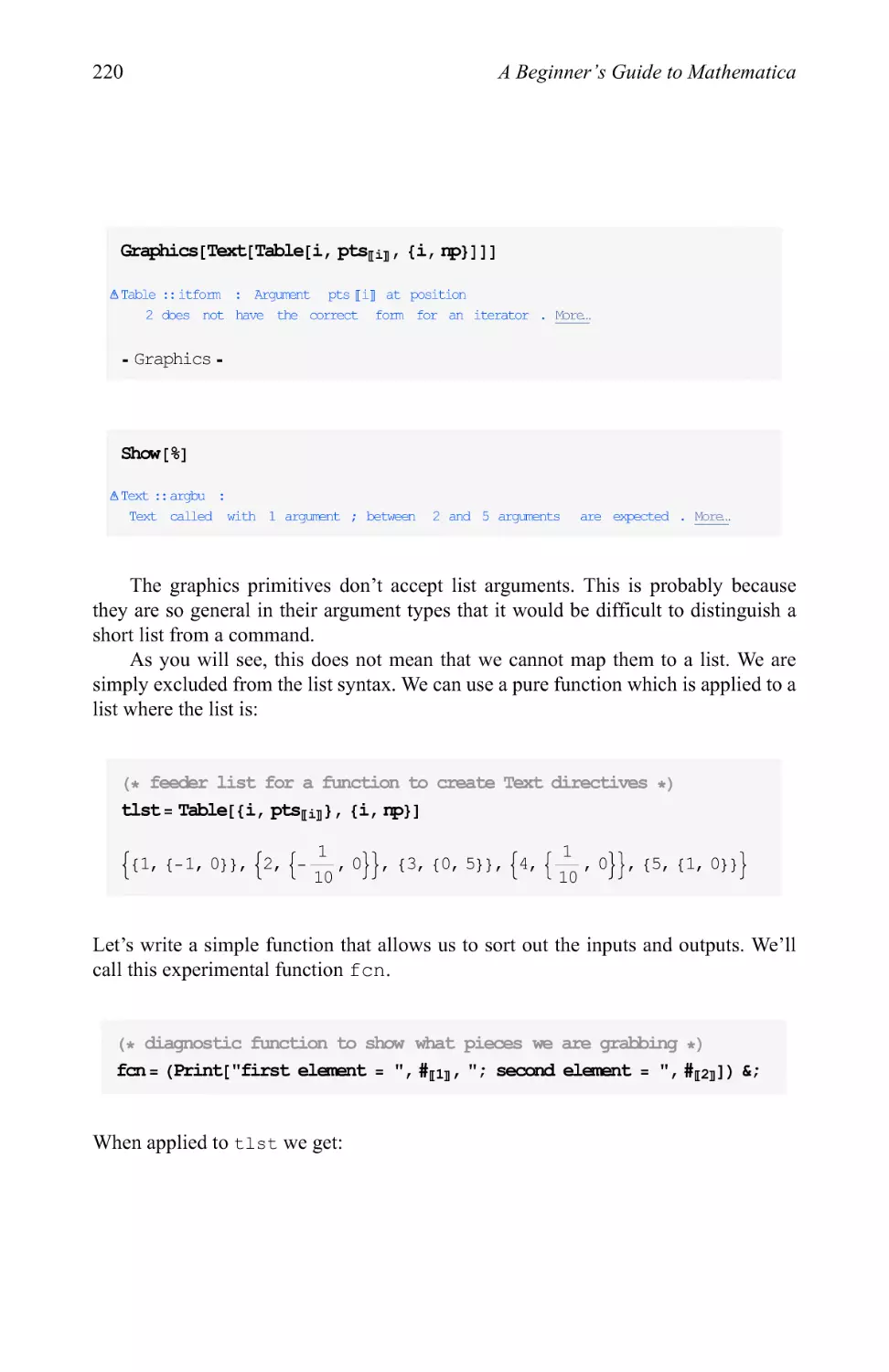
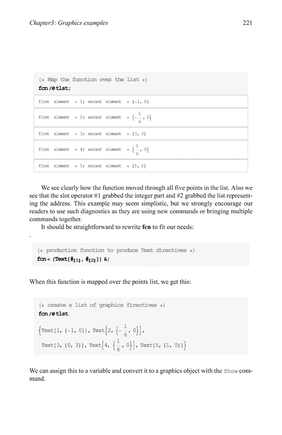
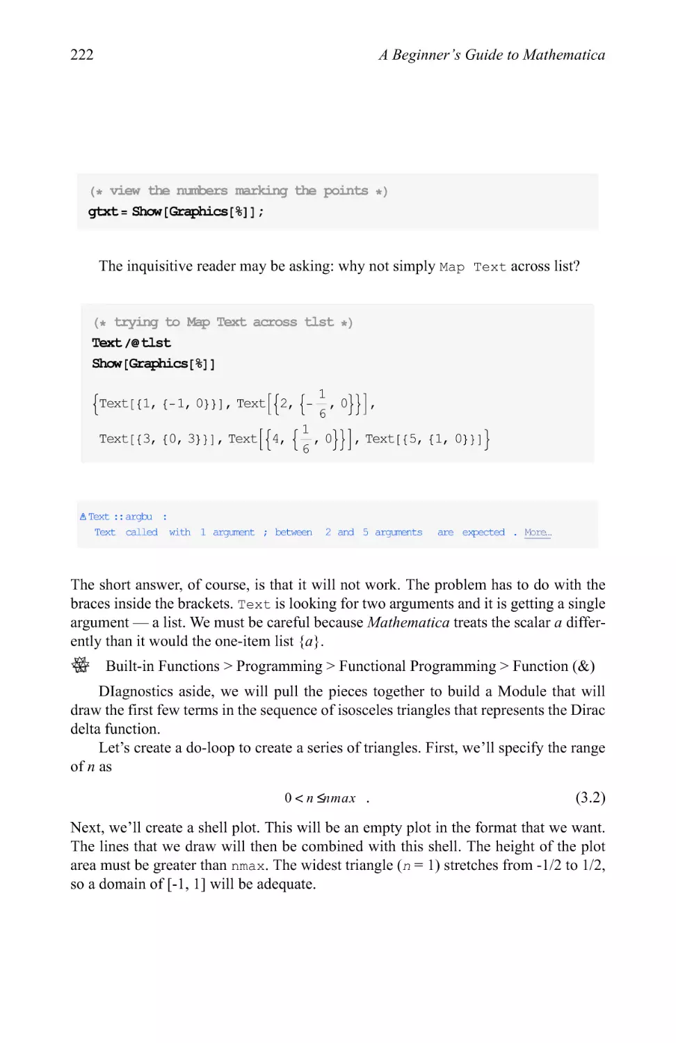
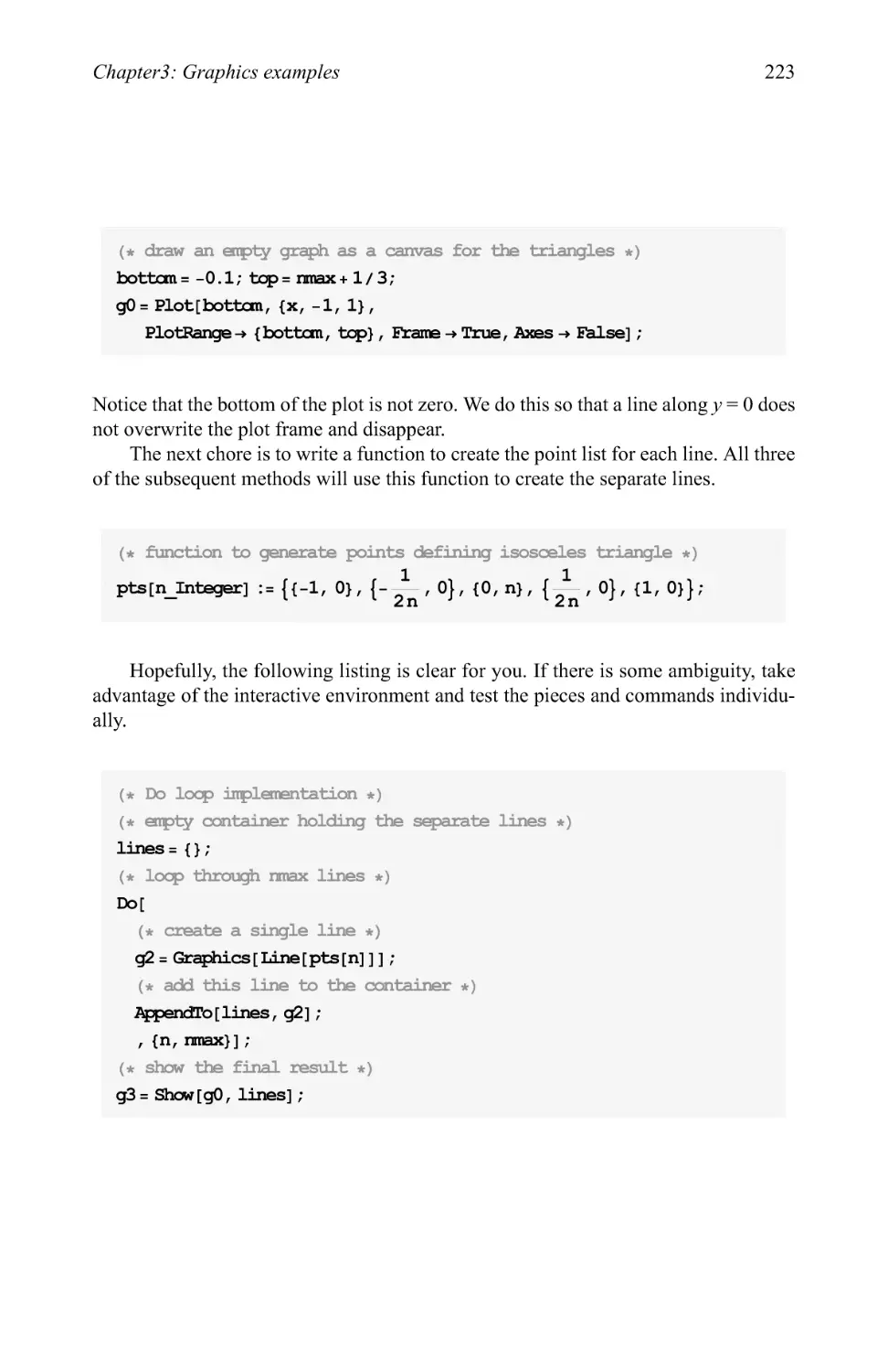
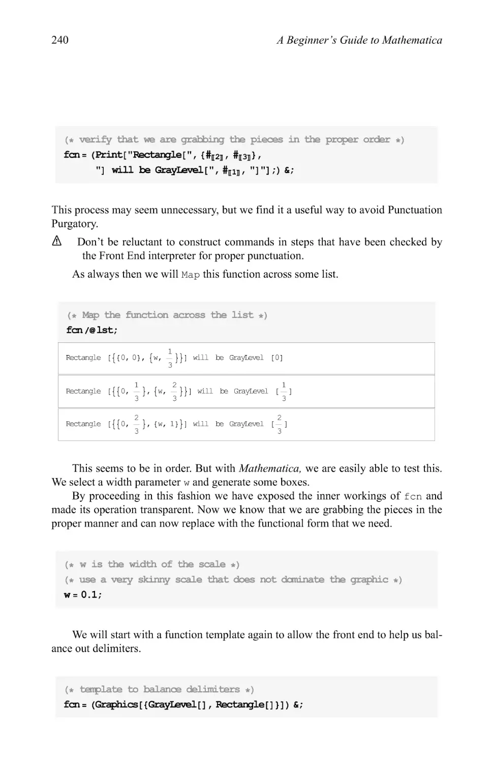
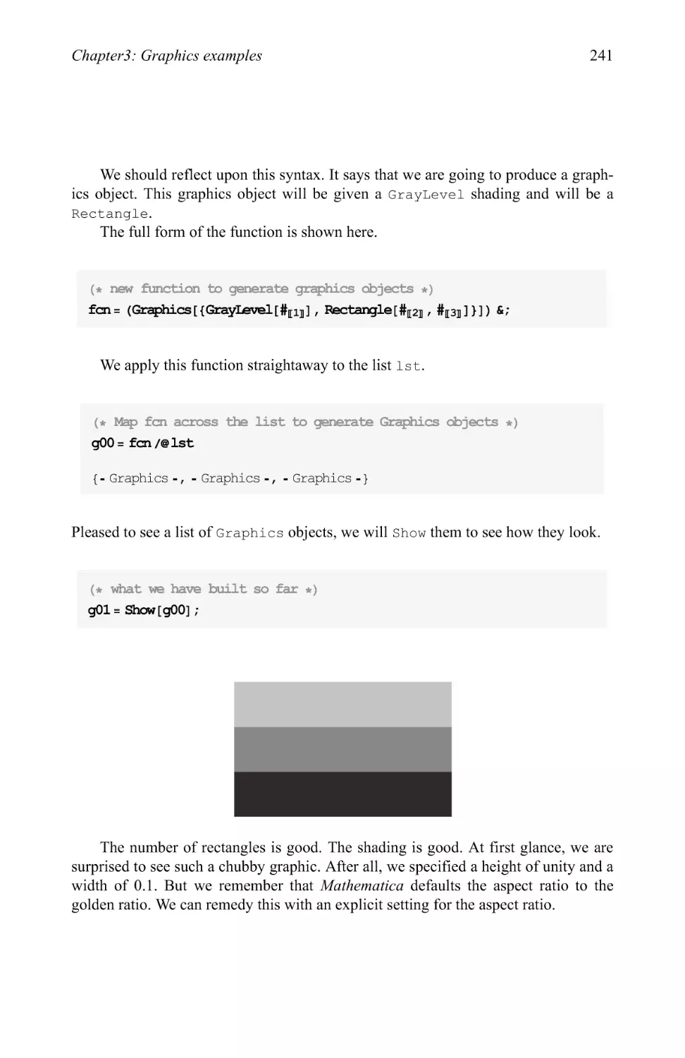
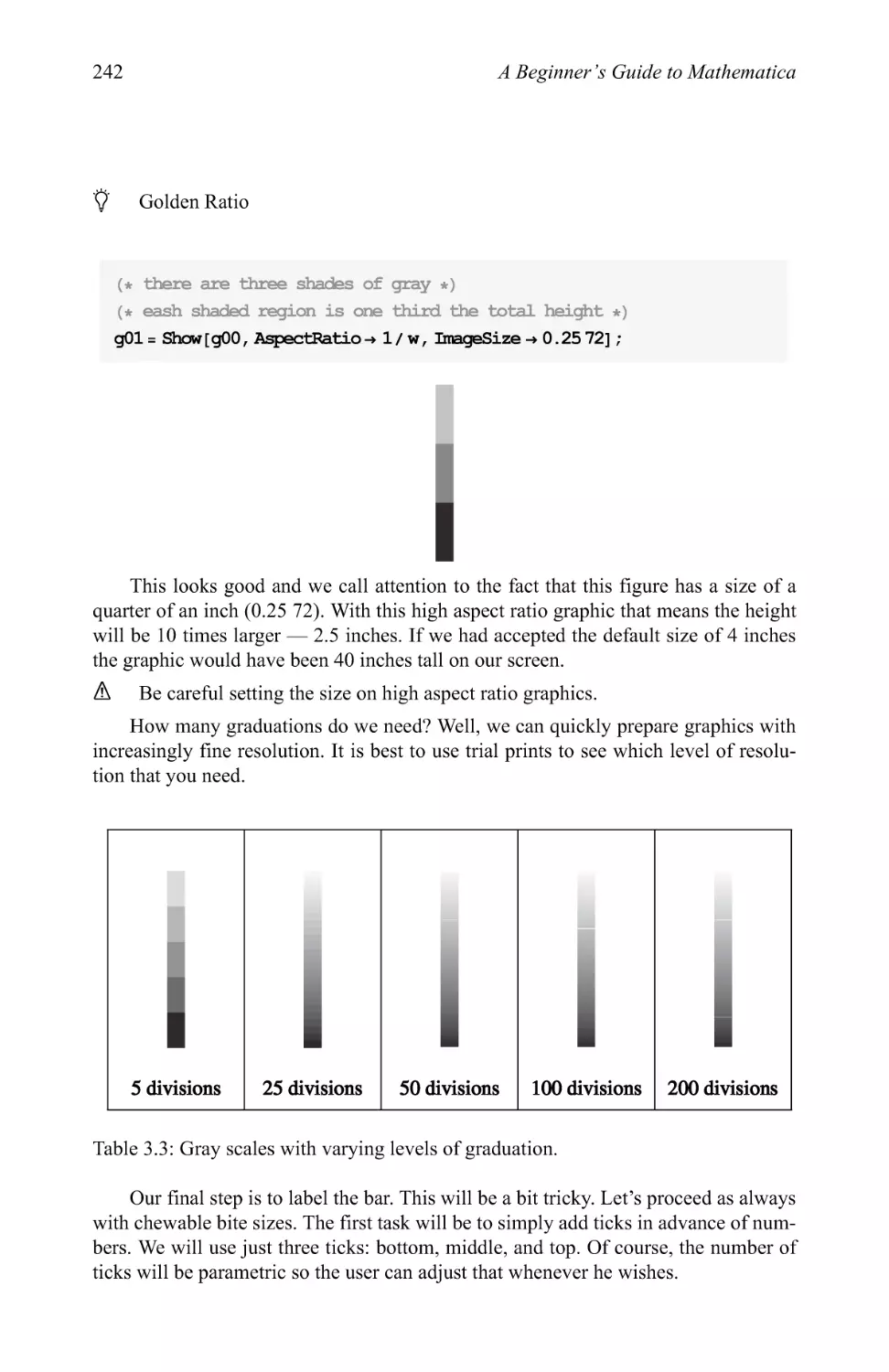
/


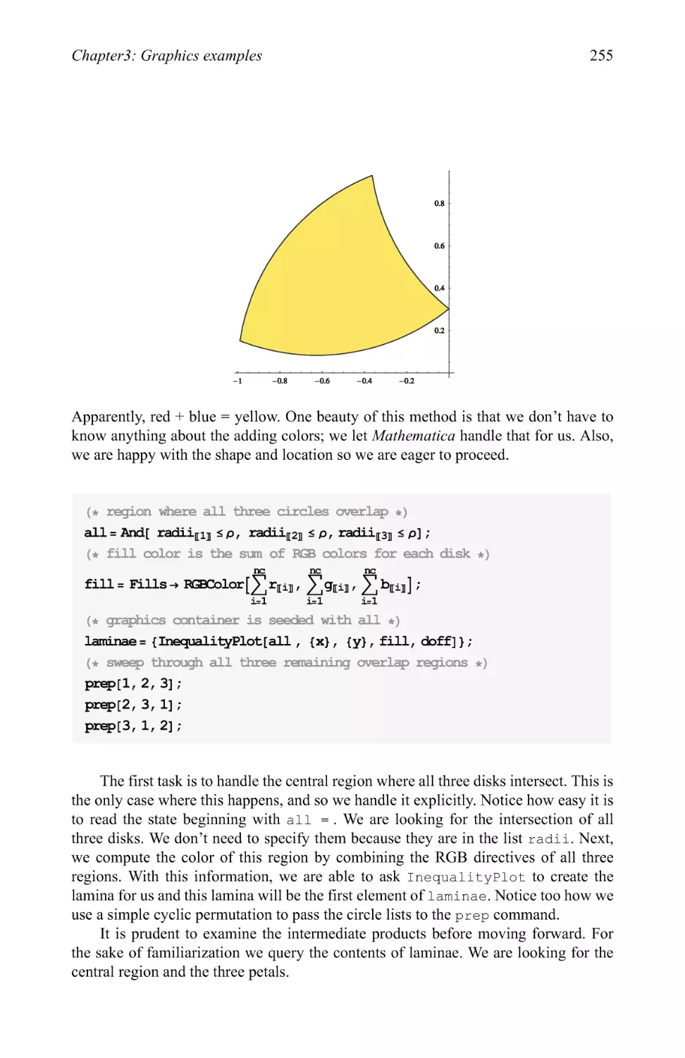
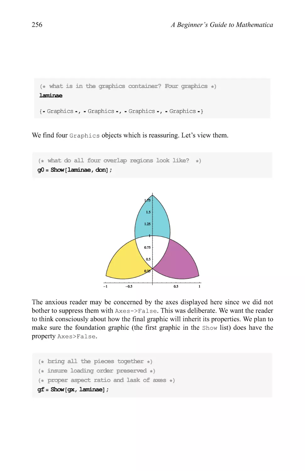


Text
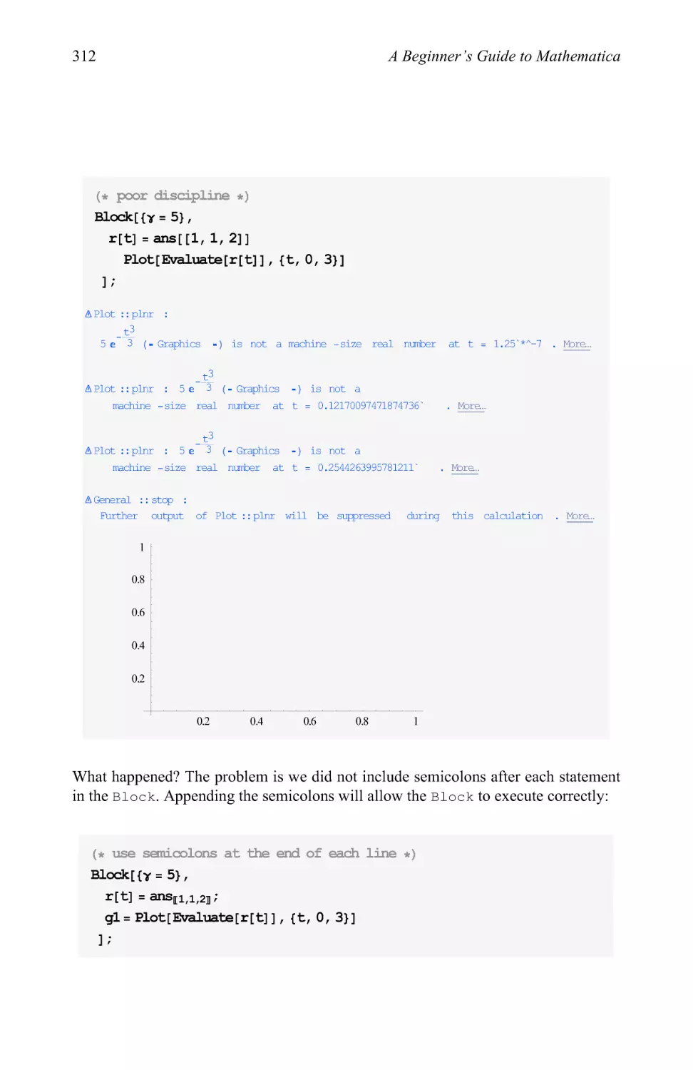
A Beginner's Guide to
Mathematica
David McMahon
Daniel M. Topa
mlM Chapman &.
_M J Taylor & Francis Croup
Hall/CRC
A Beginner's Guide to
Mathematica
A Beginner's Guide to
Mathematica
David McMahon
Daniel M. Topa
+LM Chapman & Hall/CRC
^^ | Taylor & Francis Group
Boca Raton London New York
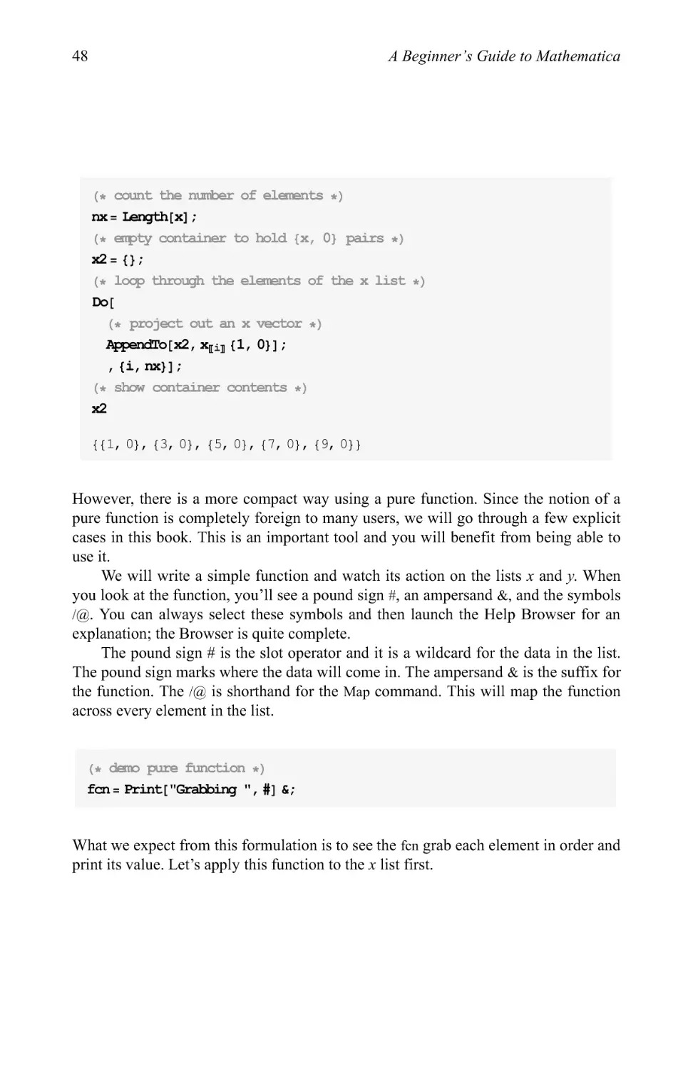
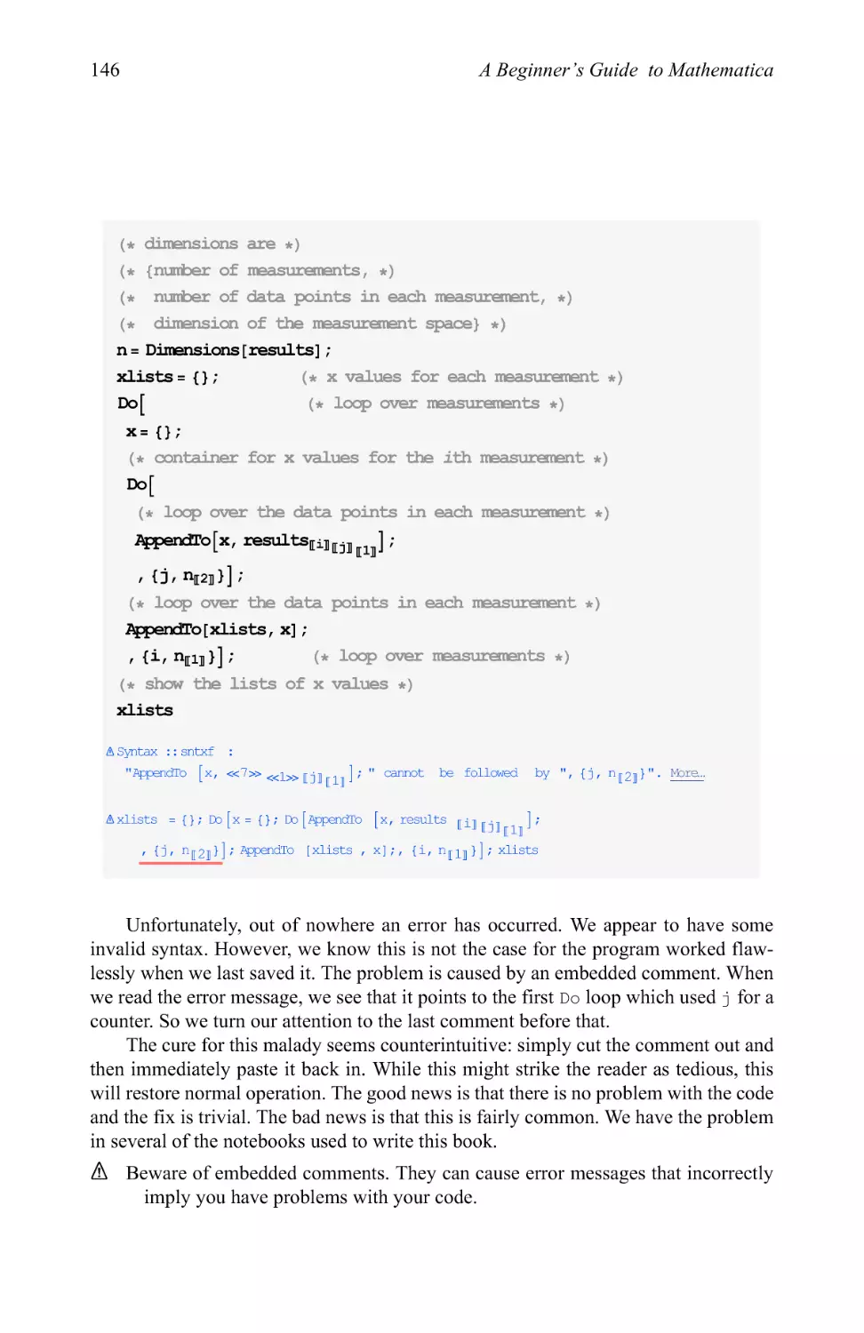
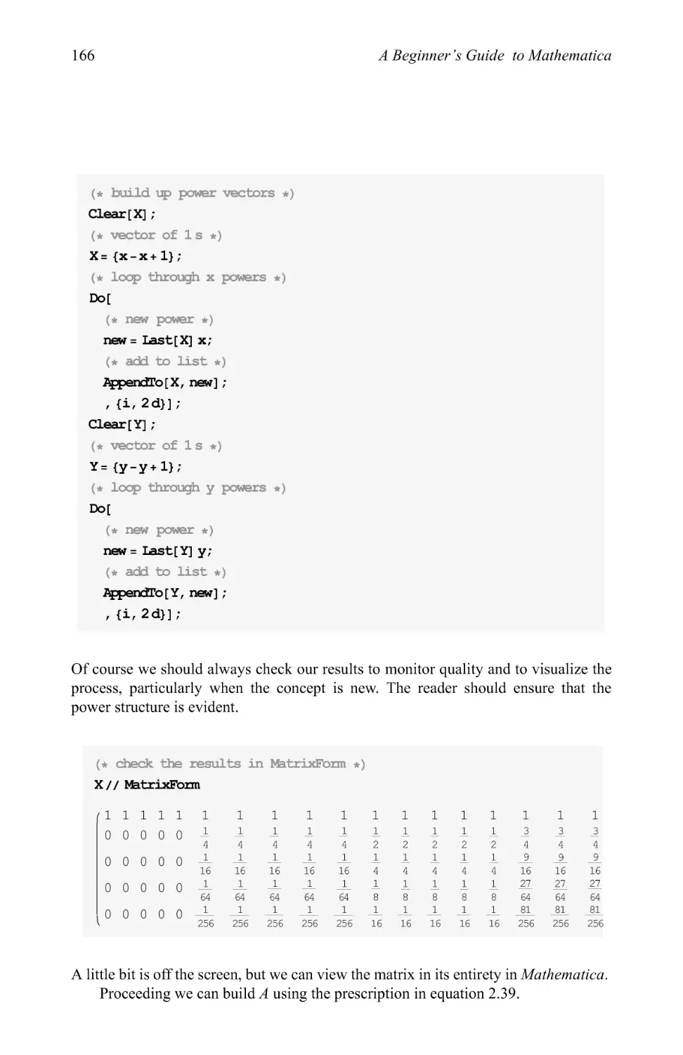
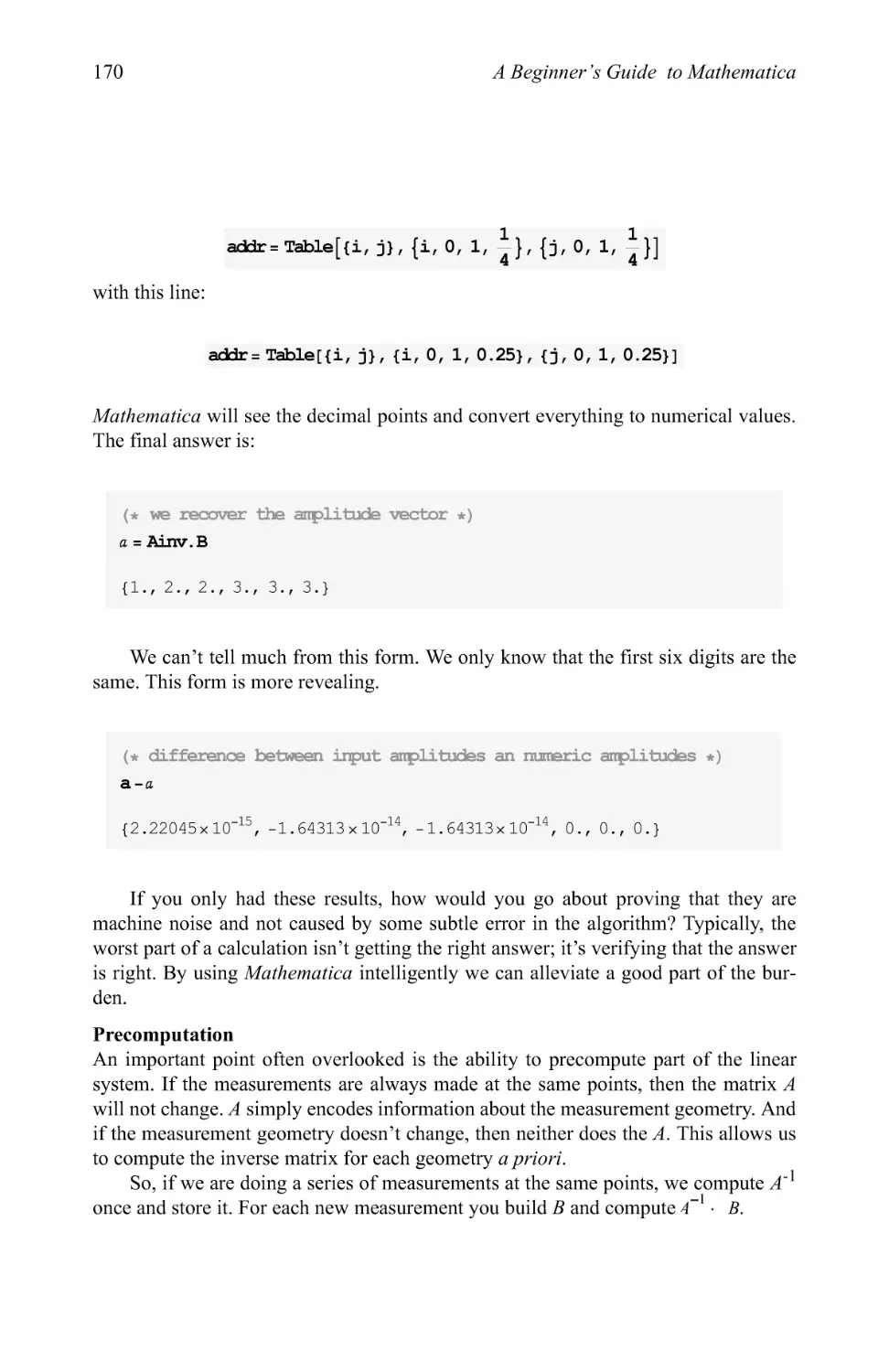
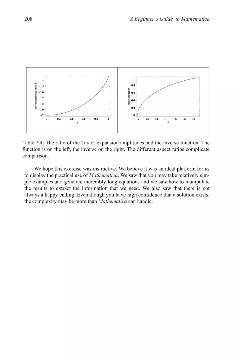
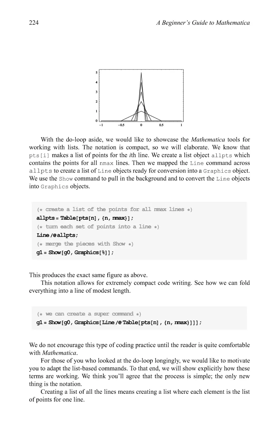
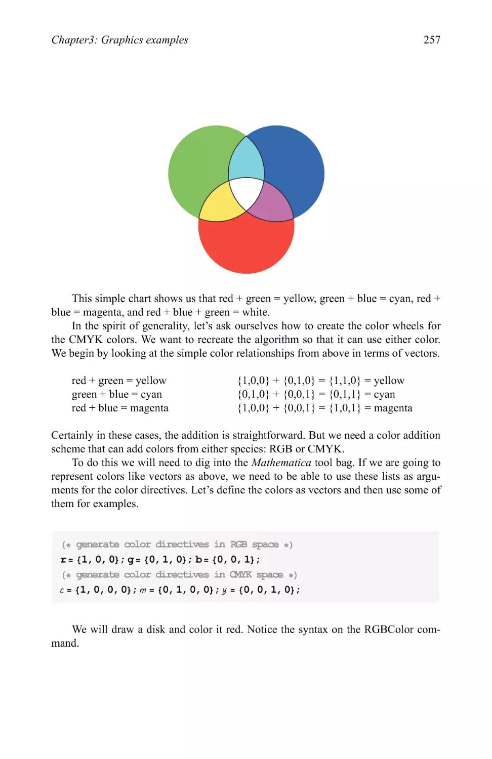
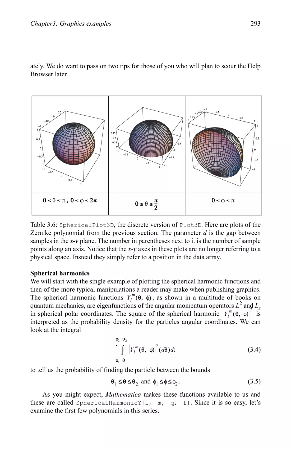
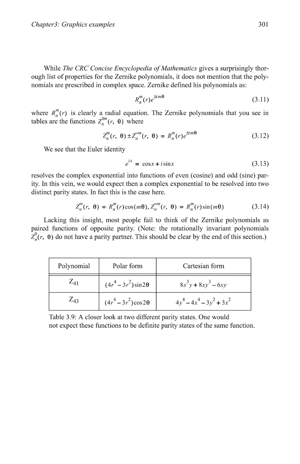
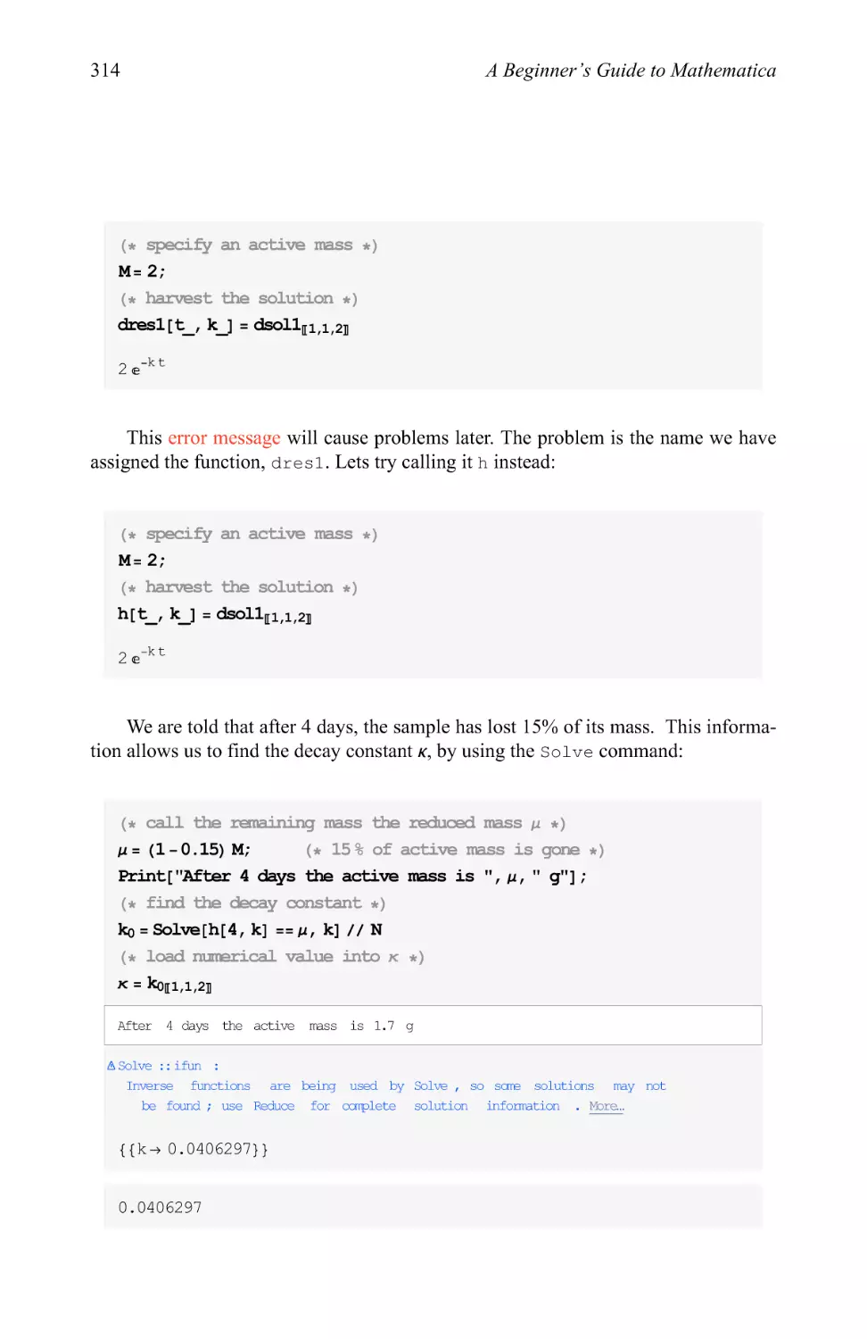
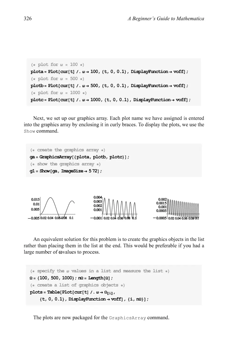
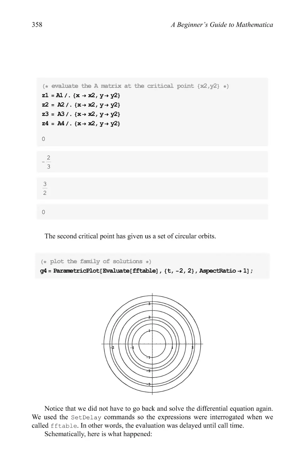
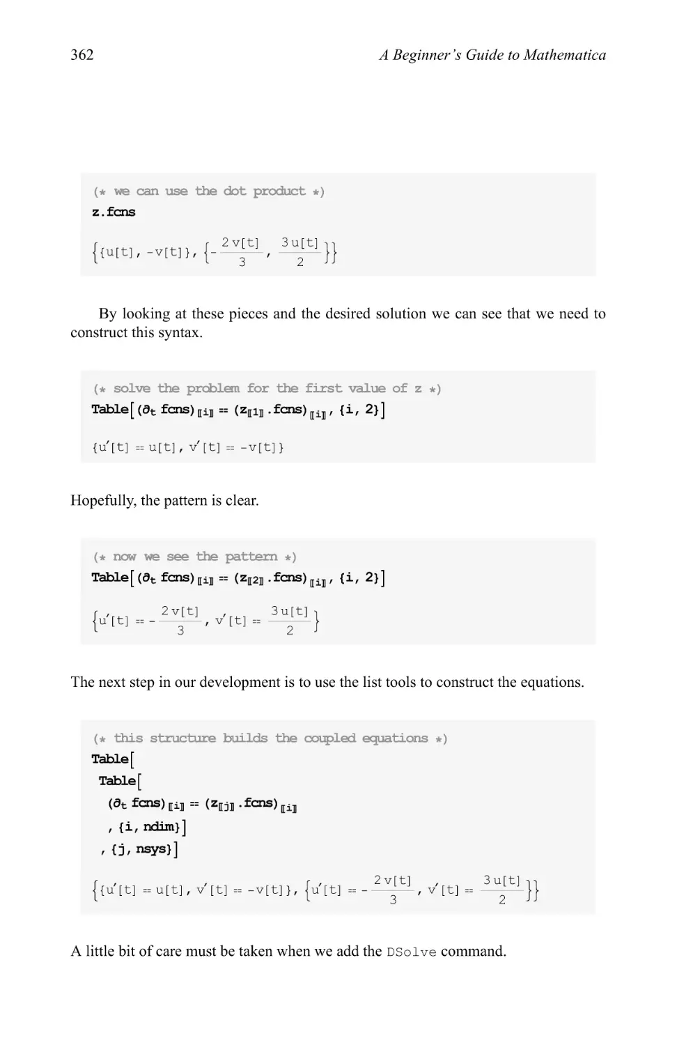
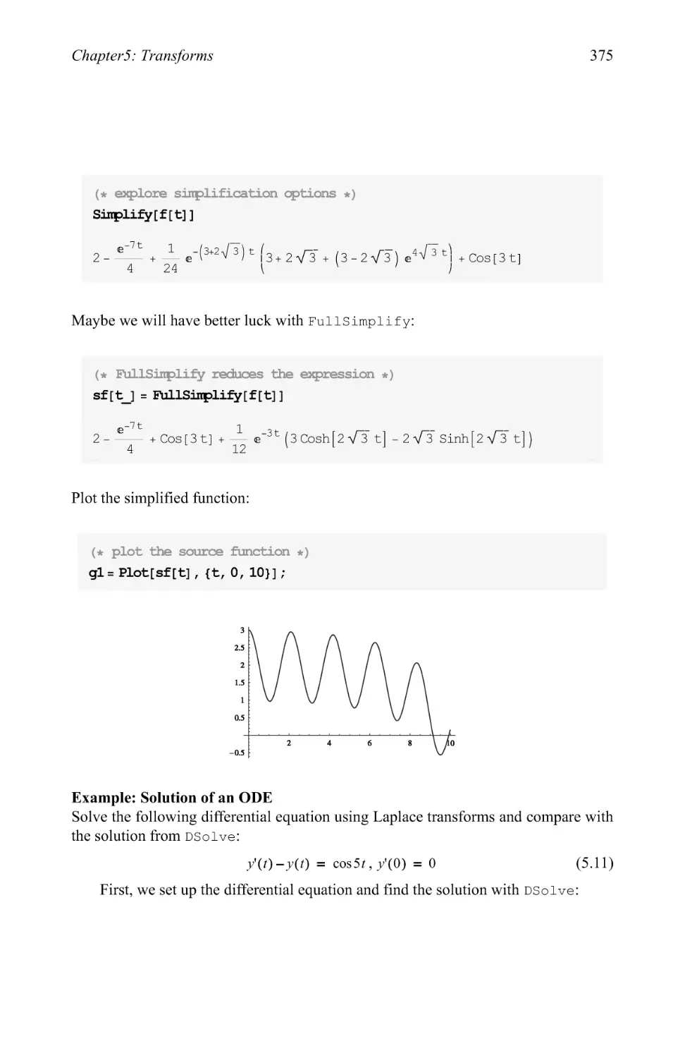
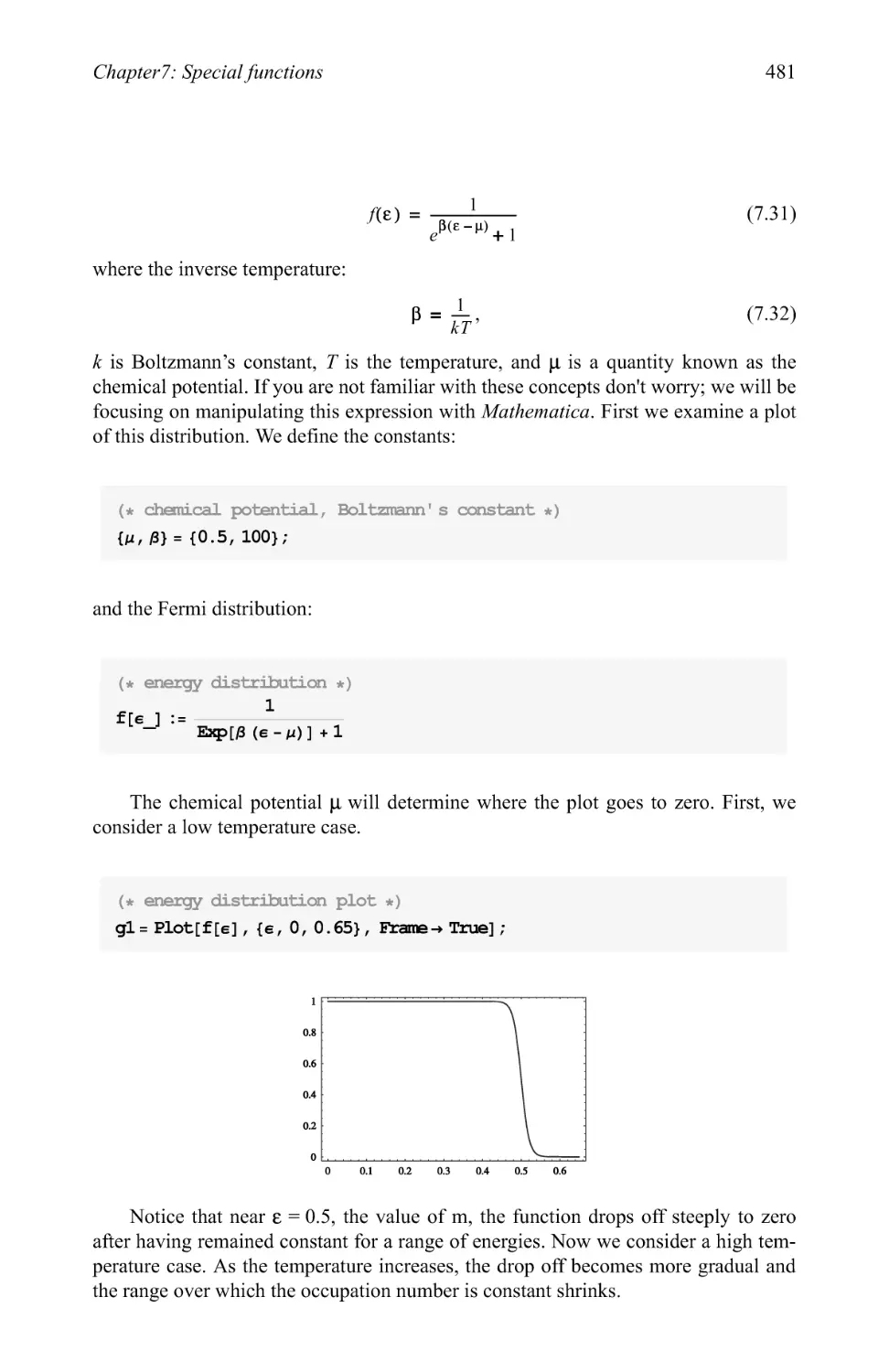
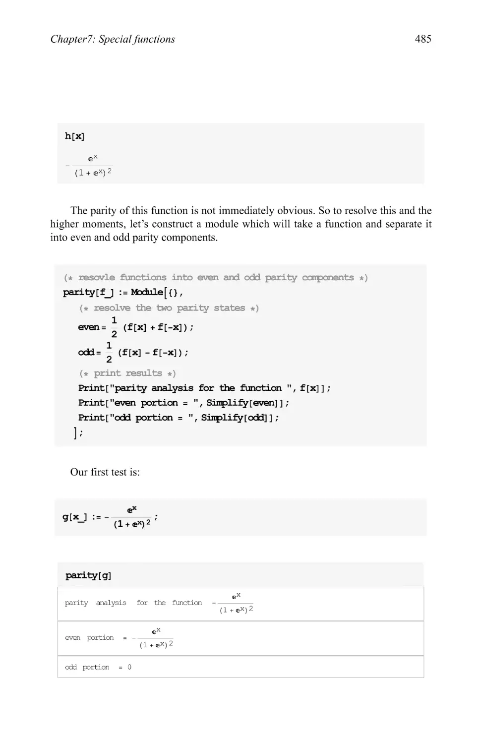
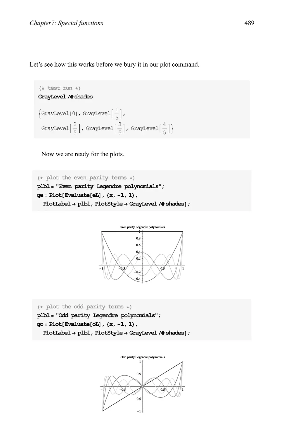
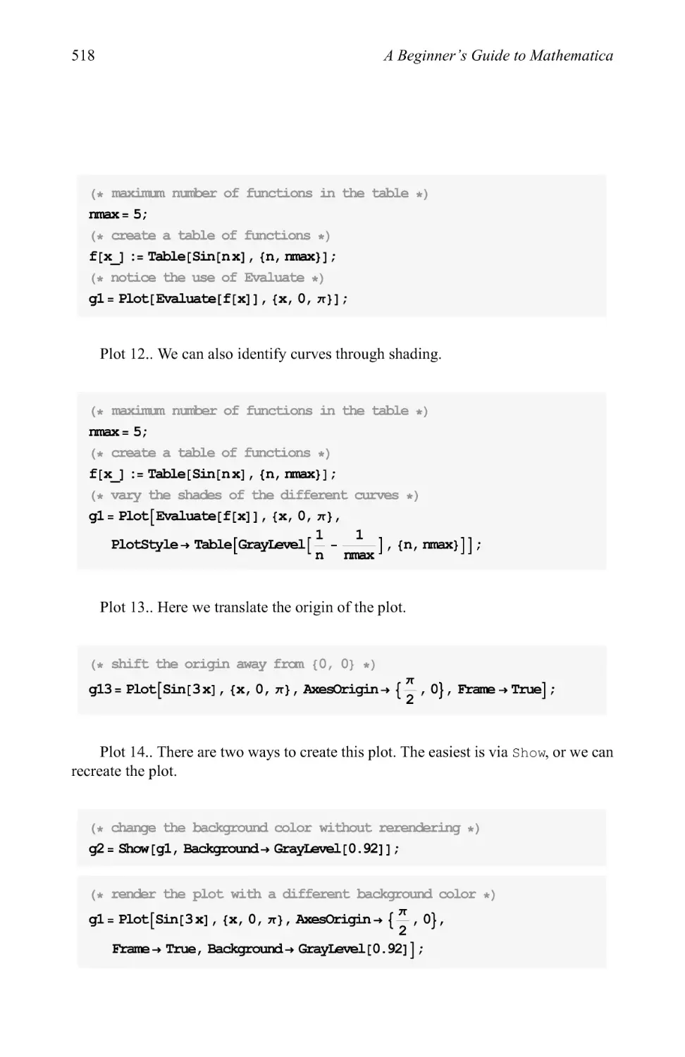
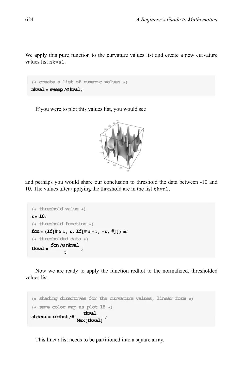
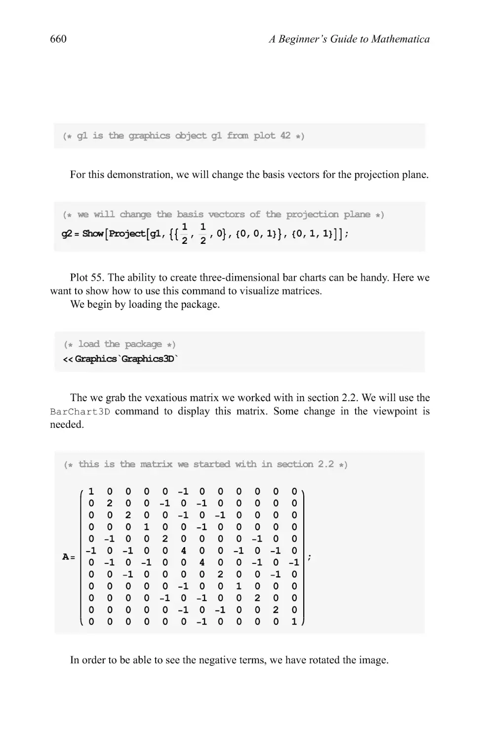
Cover image: This polynomial is an extension of the Legendre polynomial defined on a square instead of a
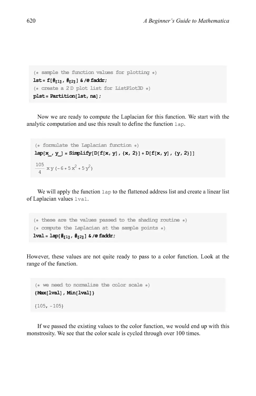
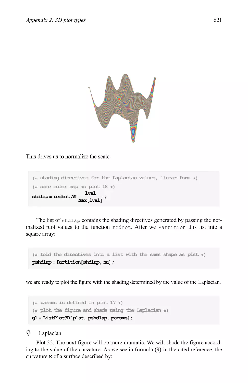
one-dimensional interval. The color scheme is determined by the value of the Laplacian of the polynomial.
Published in 2006 by
Chapman & Hall/CRC
Taylor & Francis Group
6000 Broken Sound Parkway NW, Suite 300
Boca Raton, FL 33487-2742
© 2006 by Taylor & Francis Group, LLC
Chapman & Hall/CRC is an imprint of Taylor & Francis Group
No claim to original U.S. Government works
Printed in the United States of America on acid-free paper
10 987654321
International Standard Book Number-10: 1-58488-467-3 (Softcover)
International Standard Book Number-13: 978-1-58488-467-5 (Softcover)
Library of Congress Card Number 2005051949
This book contains information obtained from authentic and highly regarded sources. Reprinted material is
quoted with permission, and sources are indicated. A wide variety of references are listed. Reasonable efforts
have been made to publish reliable data and information, but the author and the publisher cannot assume
responsibility for the validity of all materials or for the consequences of their use.
No part of this book may be reprinted, reproduced, transmitted, or utilized in any form by any electronic,
mechanical, or other means, now known or hereafter invented, including photocopying, microfilming, and
recording, or in any information storage or retrieval system, without written permission from the publishers.
For permission to photocopy or use material electronically from this work, please access www.copyright.com
(http://www.copyright.com/) or contact the Copyright Clearance Center, Inc. (CCC) 222 Rosewood Drive,
Danvers, MA 01923, 978-750-8400. CCC is a not-for-profit organization that provides licenses and registration
for a variety of users. For organizations that have been granted a photocopy license by the CCC, a separate
system of payment has been arranged.
Trademark Notice: Product or corporate names may be trademarks or registered trademarks, and are used only
for identification and explanation without intent to infringe.
Library of Congress Catalogmg-in-Publication Data
McMahon, David.
A beginners guide to Mathematica I David McMahon, Dan Topa.
p. cm.
Includes bibliographical references and index.
ISBN 1-58488-467-3 (alk. paper)
1. Mathematica (Computer file) 2. Mathematics-Data processing. I. Topa, Dan. n. Title.
QA76.95.M44 2005
510'.285'536--dc22 2005051949
Visit the Taylor & Francis Web site at
http://www.taylorandfrancis.com
Taylor & Francis Group and the CRC Press Web site at
is the Academic Division of Informa pic. http://www.crcpress.com
informa
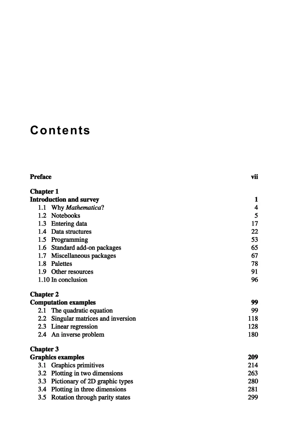
Contents
Preface vii
1
4
5
17
22
53
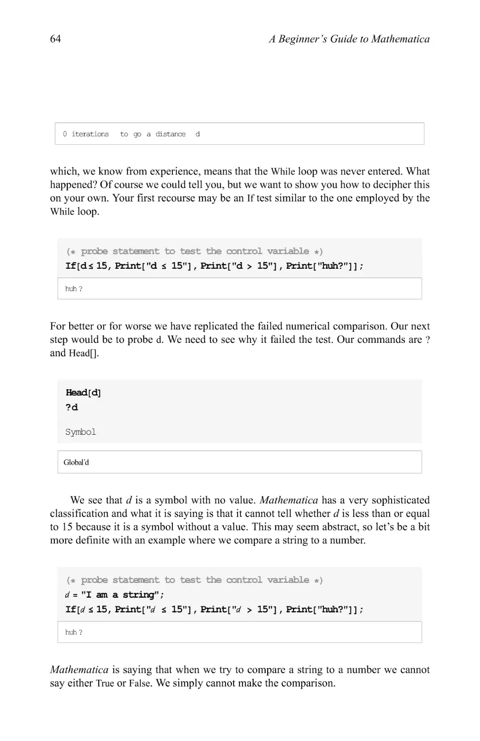
65
67
78
91
96
99
99
118
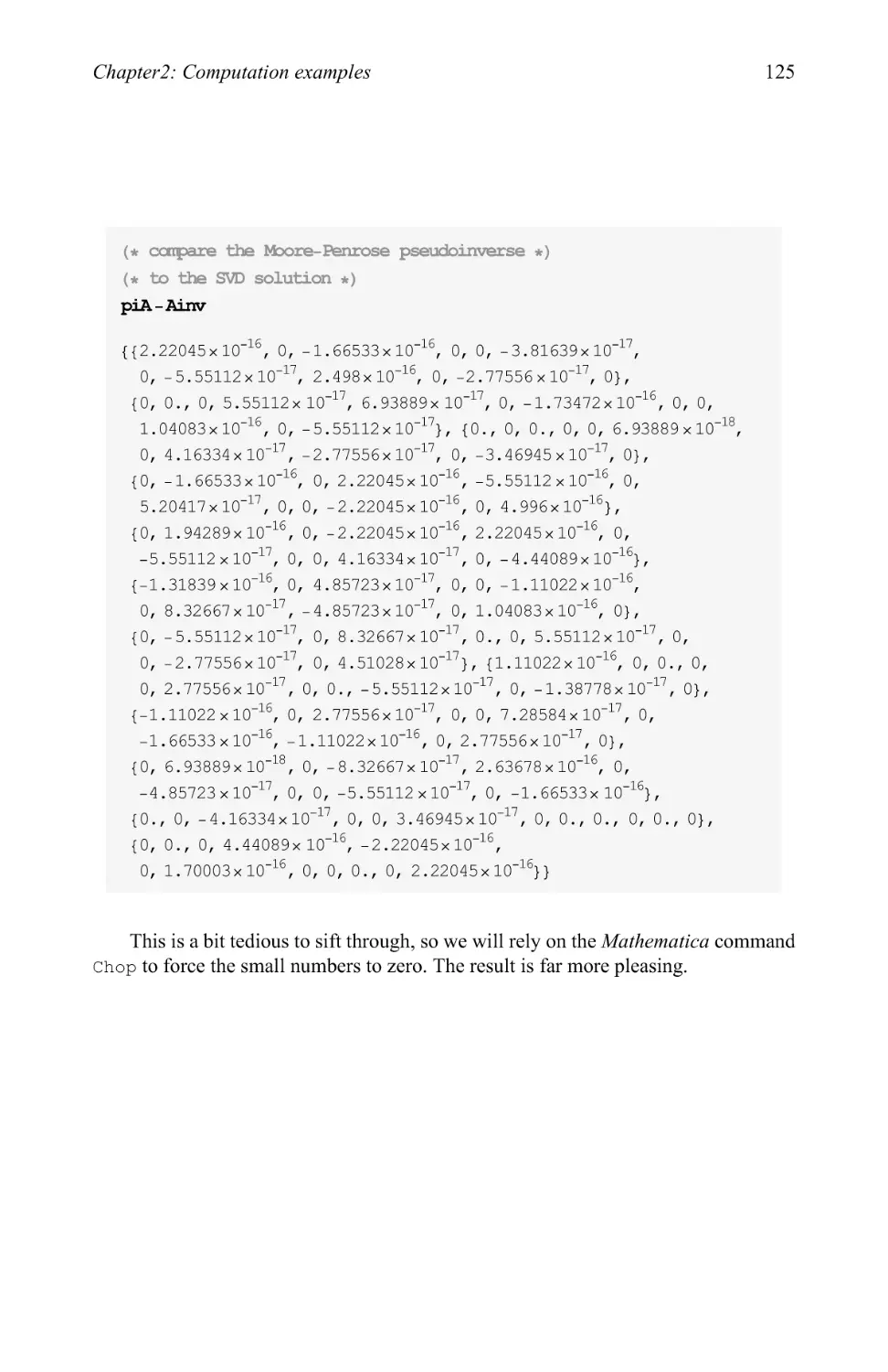
128
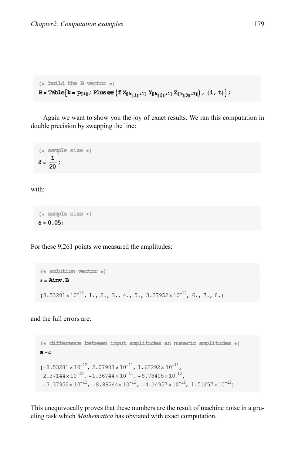
180
Chapter 3
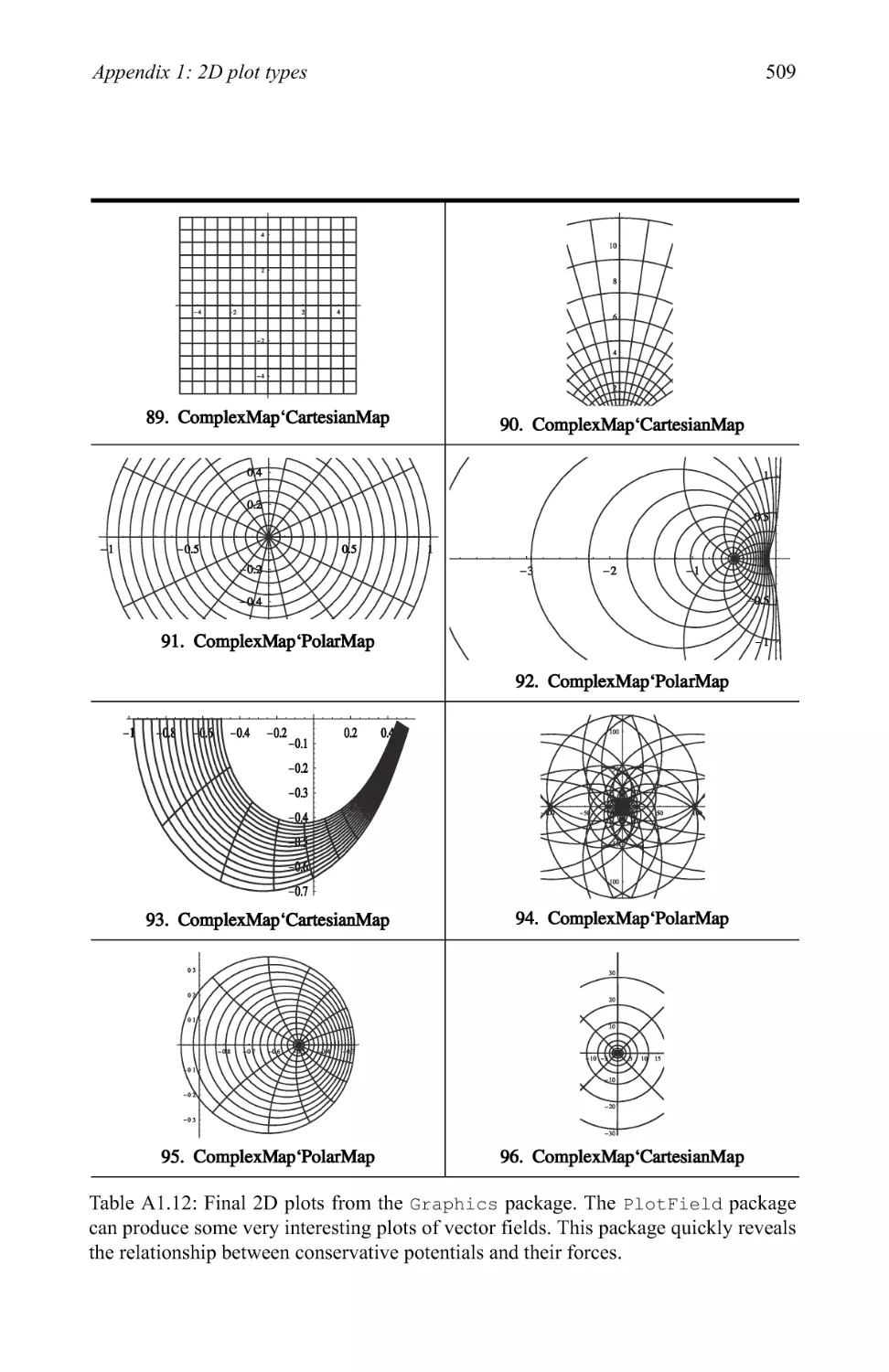
Graphics examples 209
3.1 Graphics primitives 214
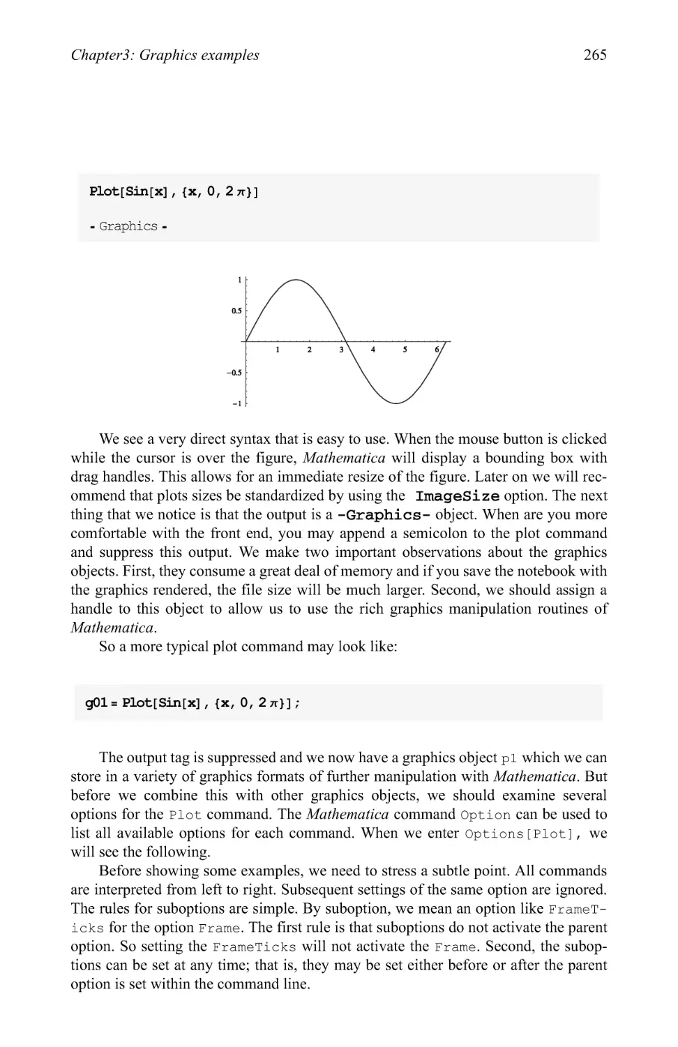
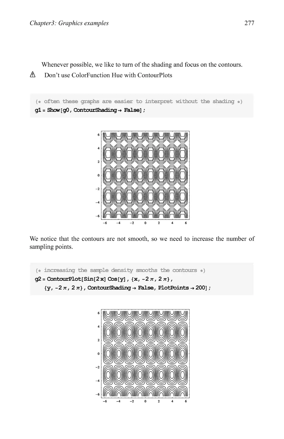
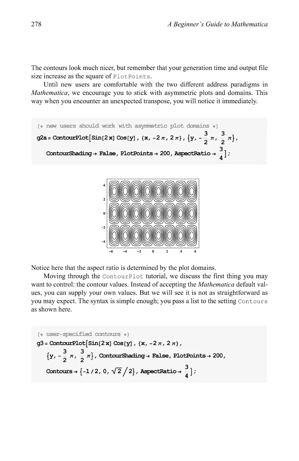
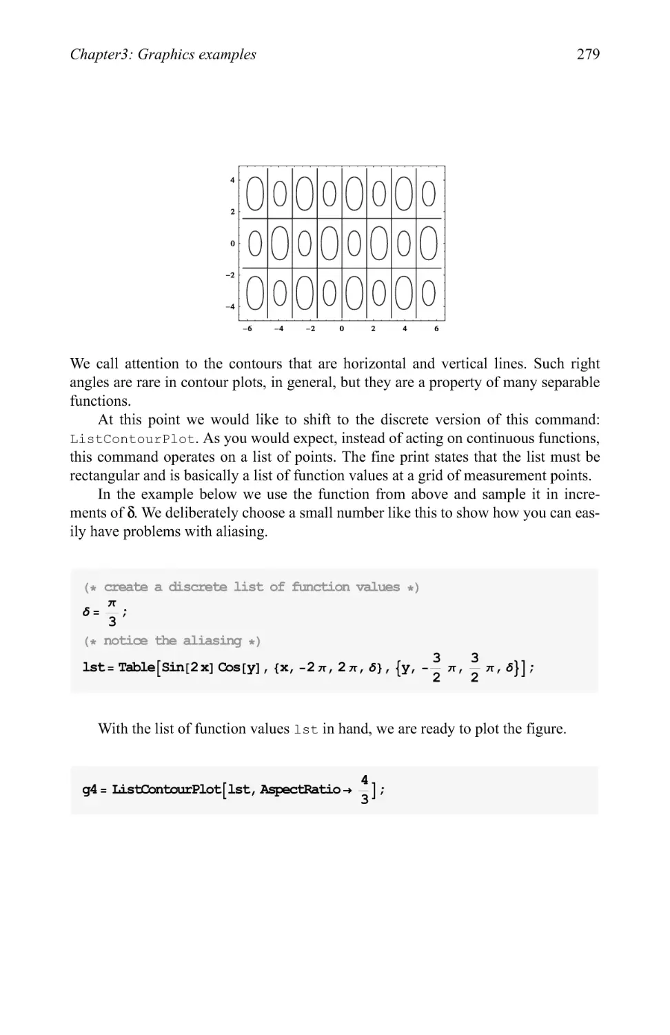
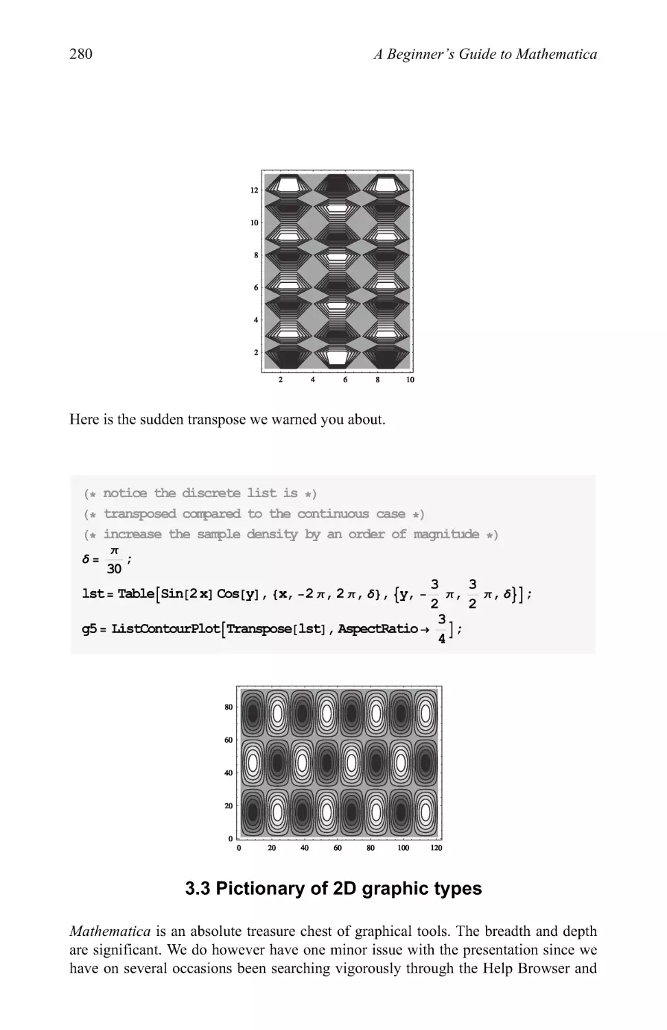
3.2 Plotting in two dimensions 263
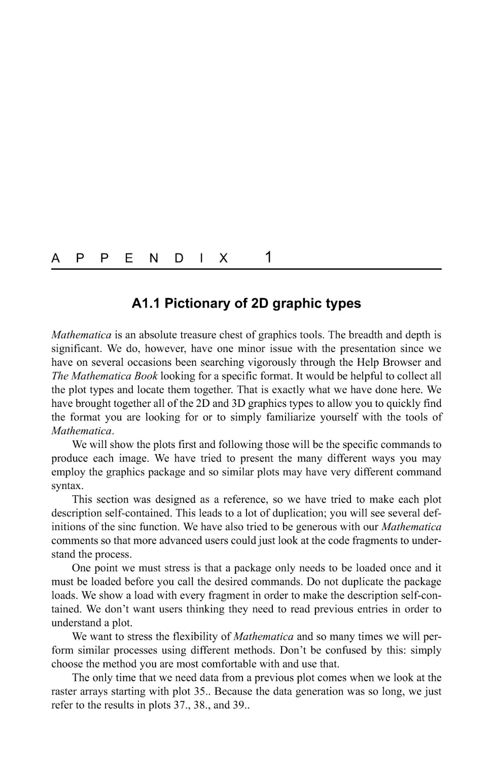
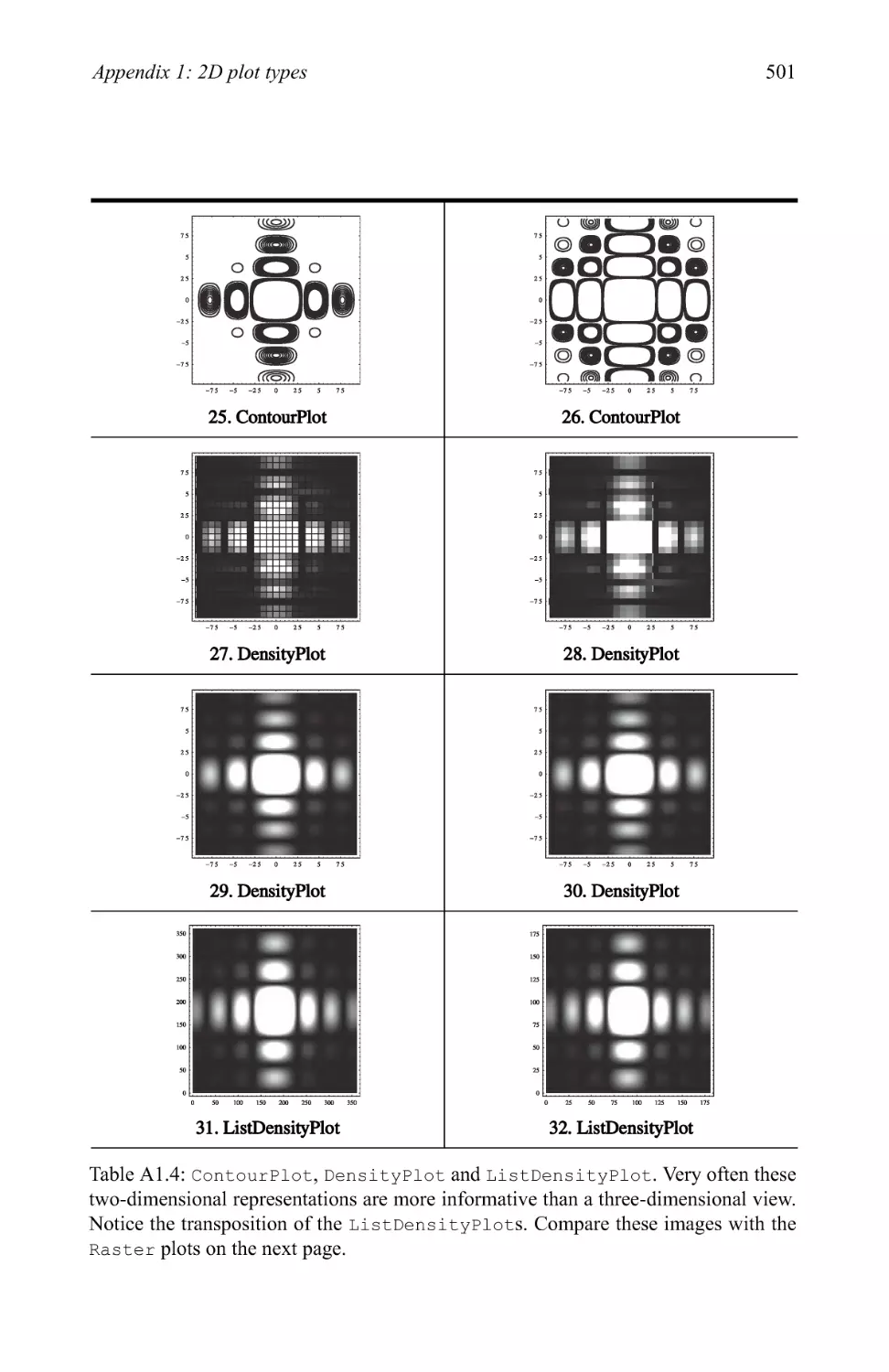
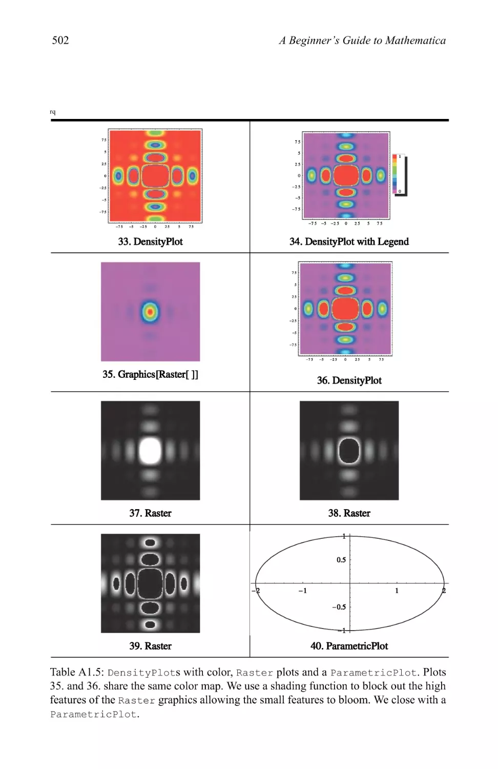
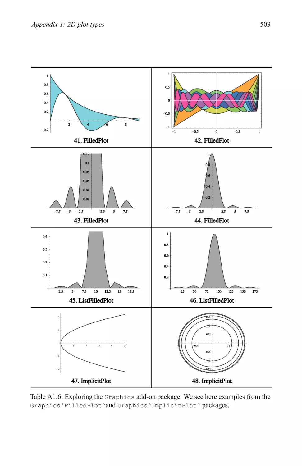
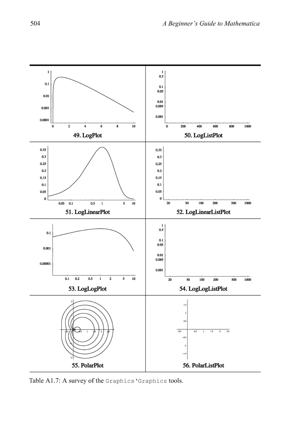
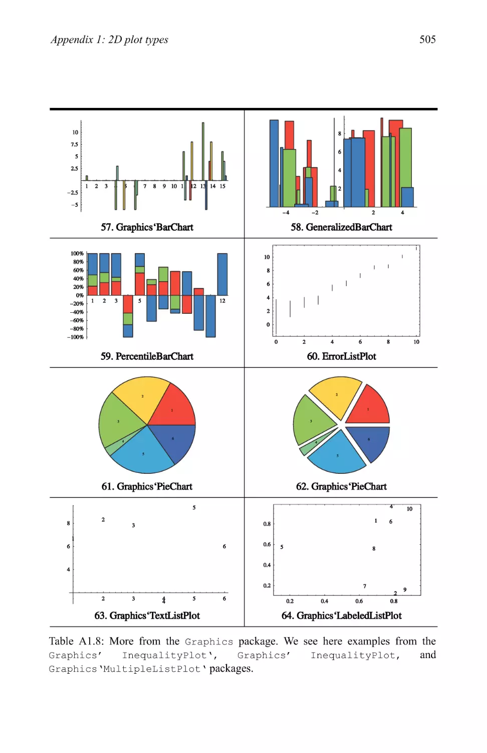
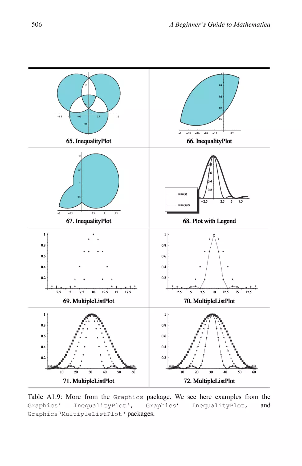
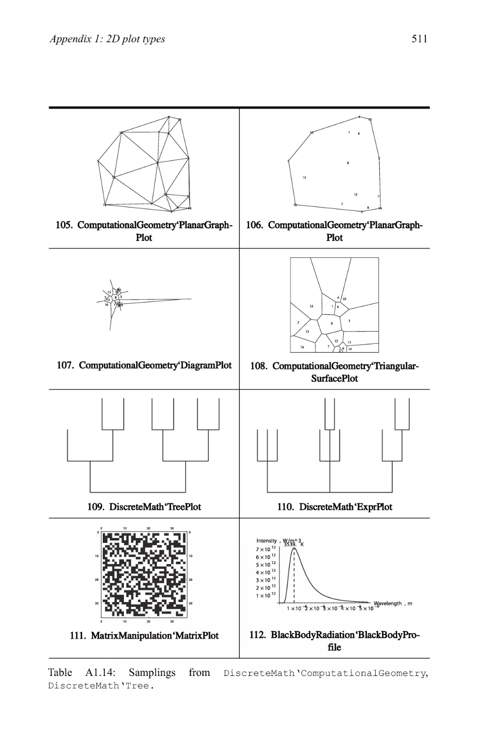
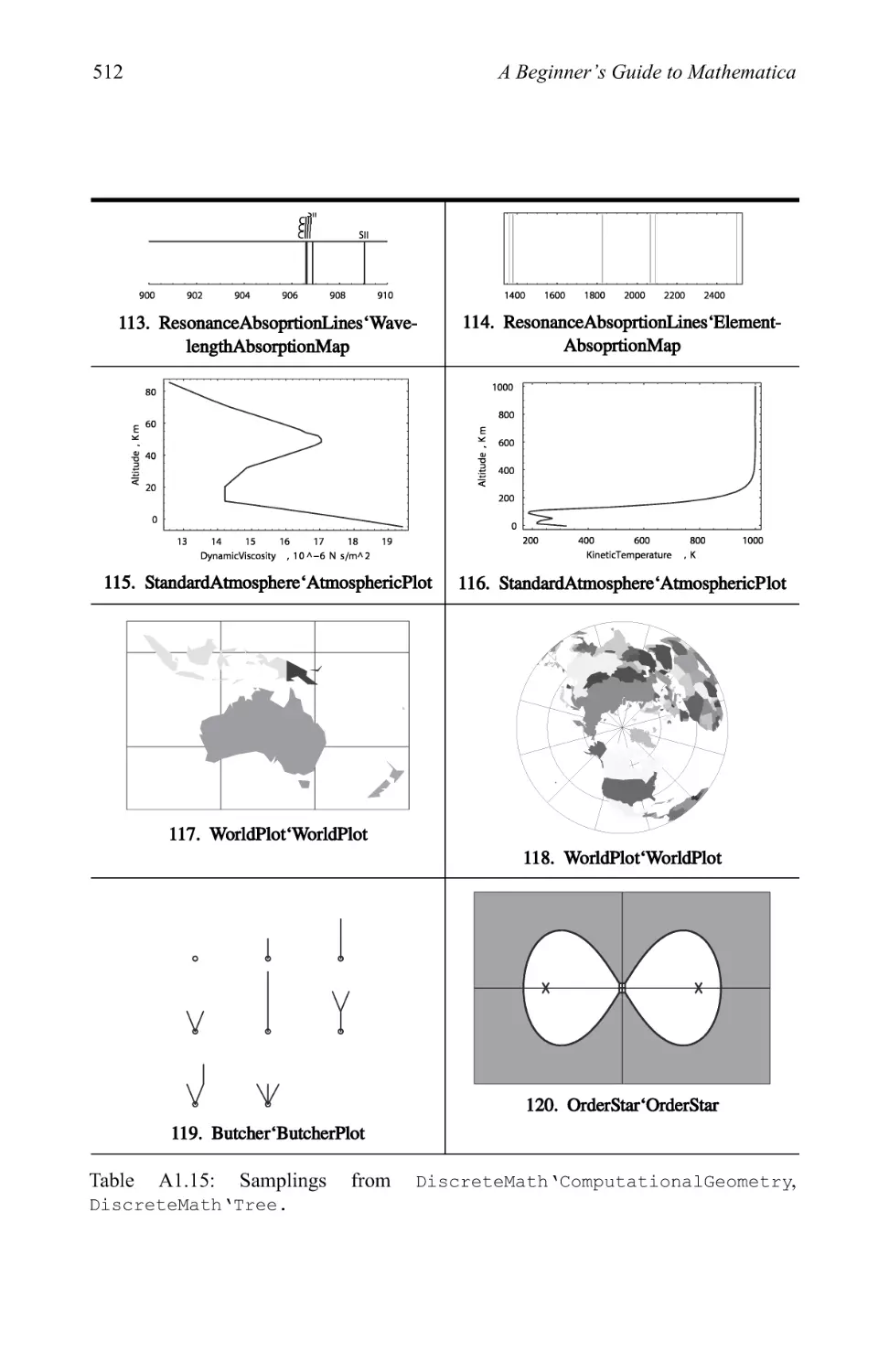
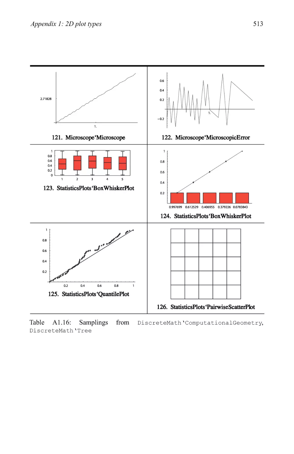
3.3 Pictionary of 2D graphic types 280
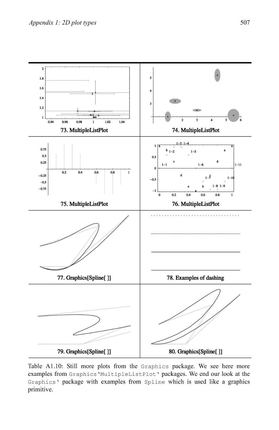
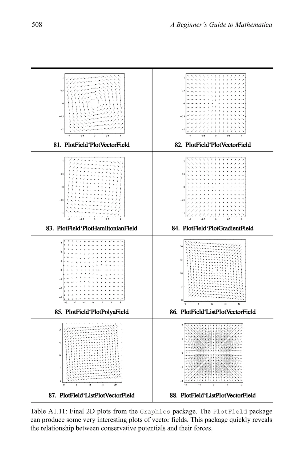
3.4 Plotting in three dimensions 281
3.5 Rotation through parity states 299
Chapter 1
Introduction and survey
1.1
1.2
1.3
1.4
1.5
1.6
1.7
1.8
1.9
Why Mathematical
Notebooks
Entering data
Data structures
Programming
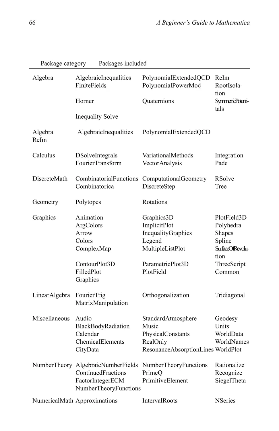
Standard add-on packages
Miscellaneous packages
Palettes
Other resources
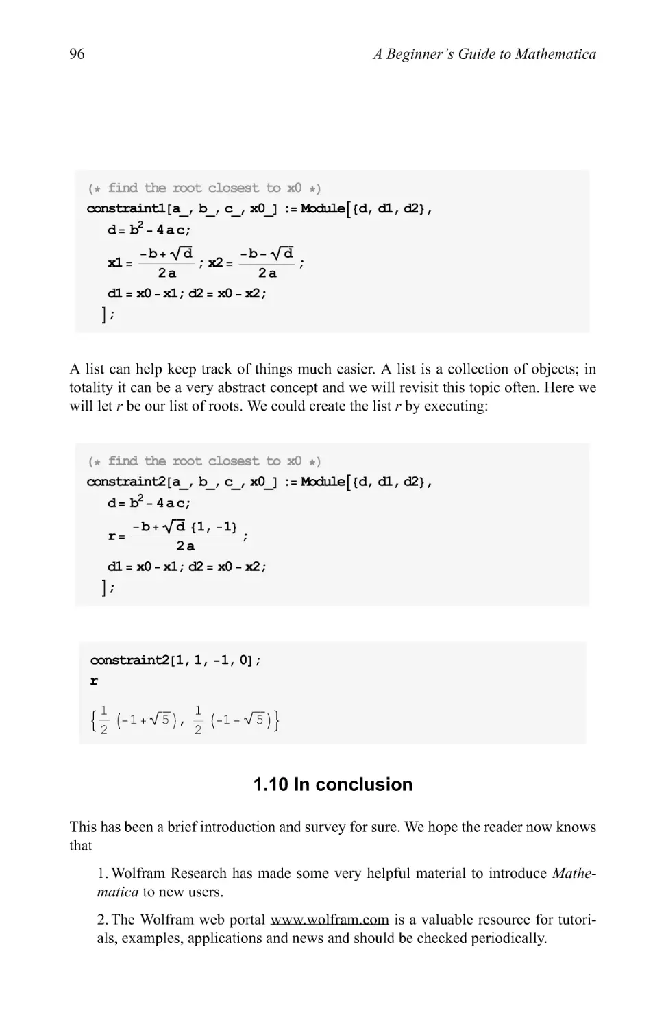
1.10 In conclusion
Chapter 2
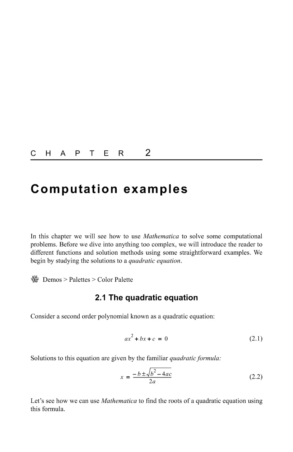
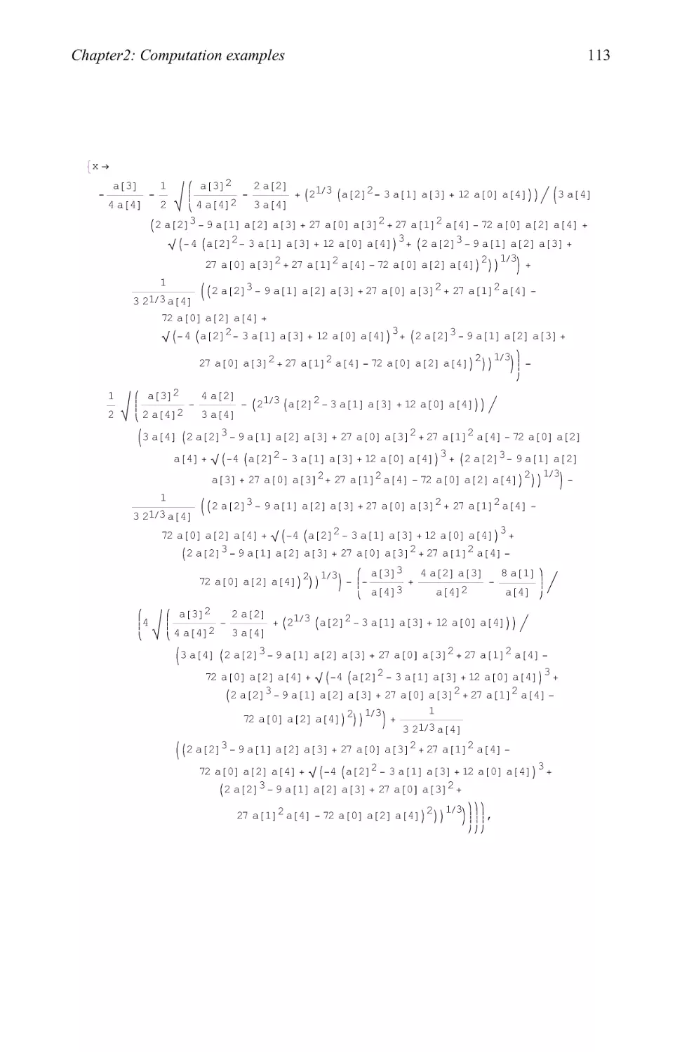
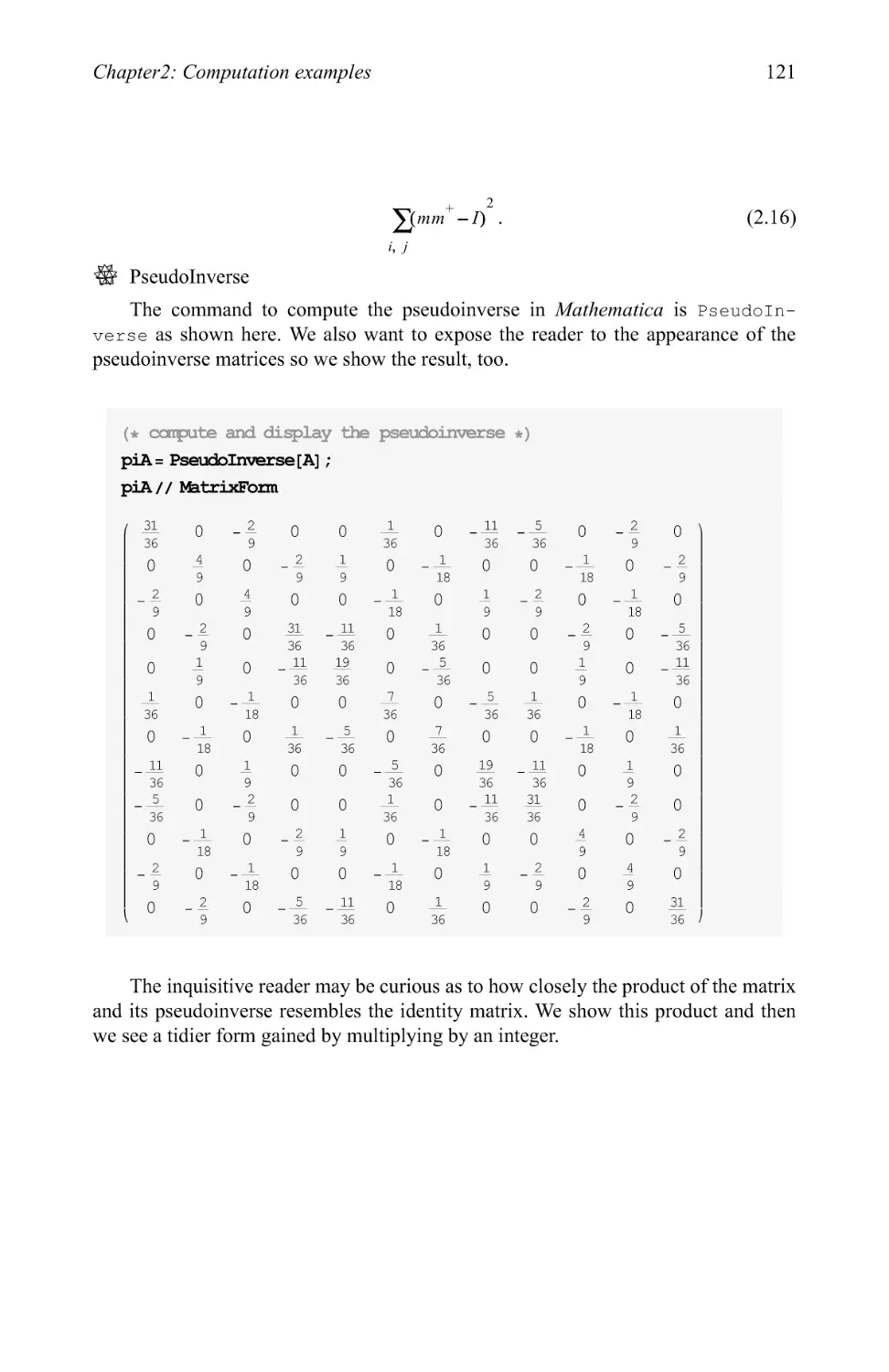
Computation examples
2.1
2.2
2.3
2.4
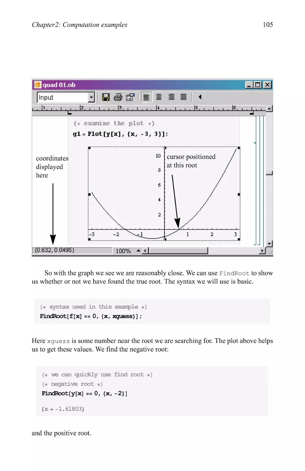
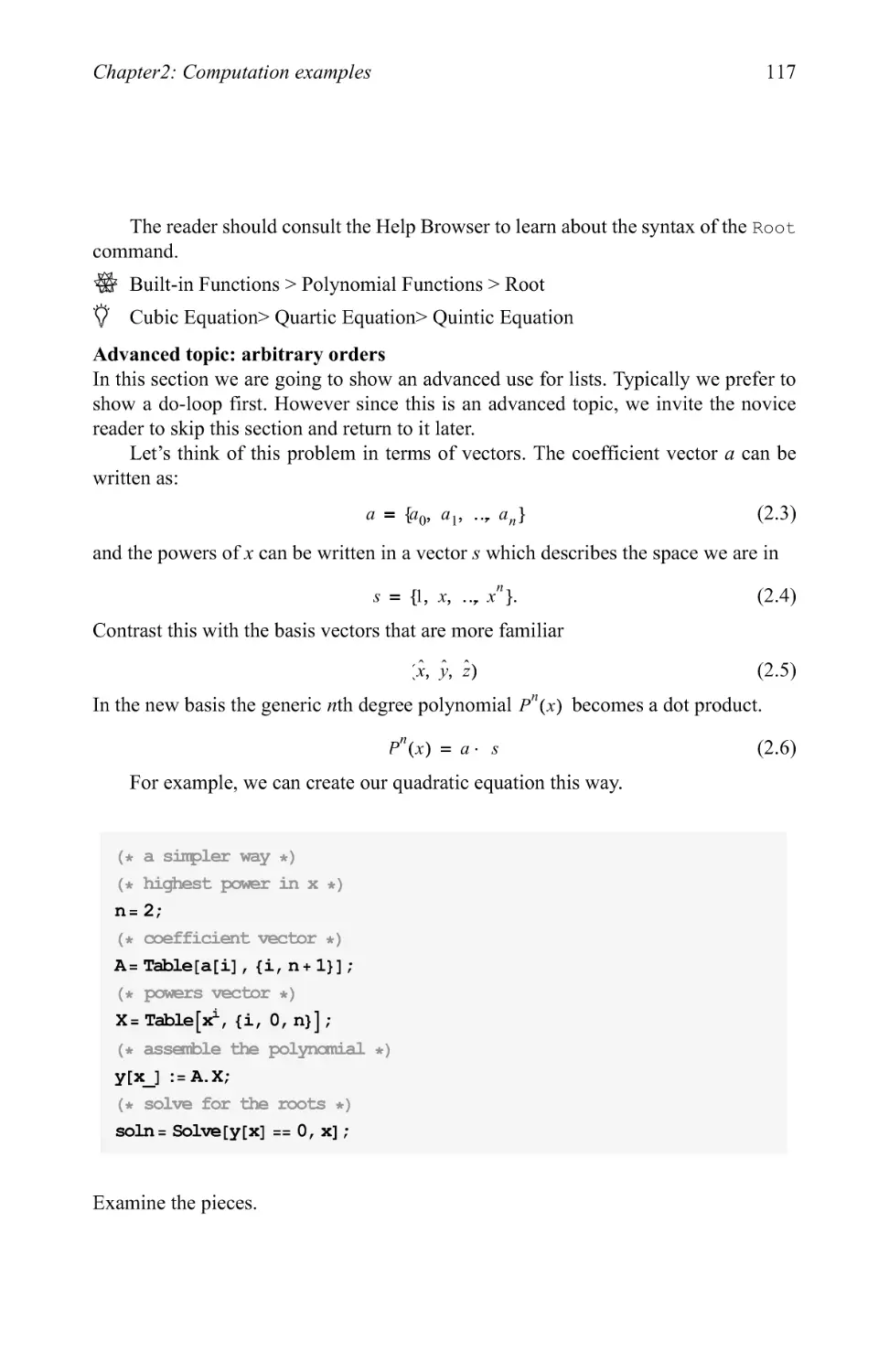
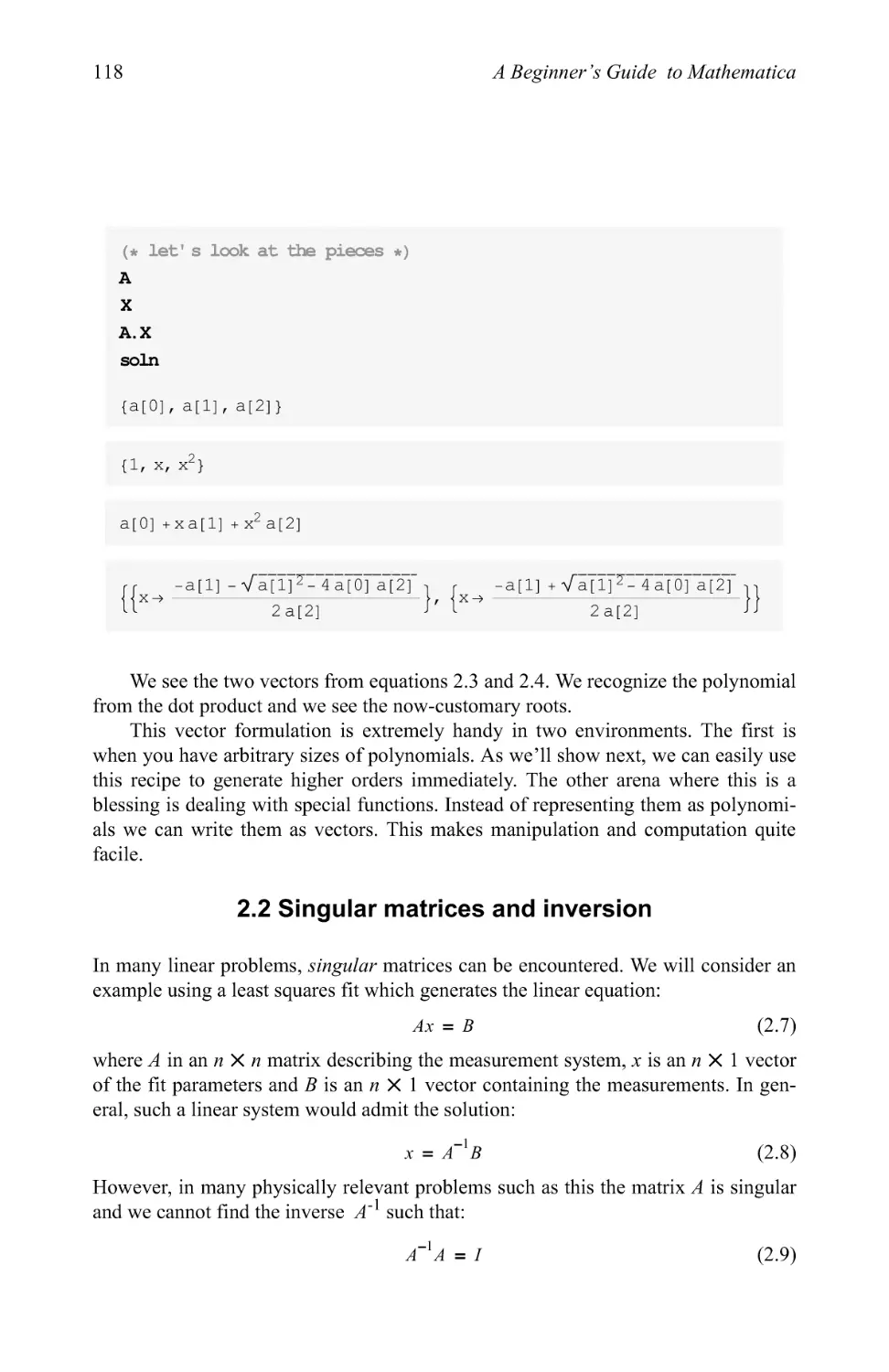
The quadratic equation
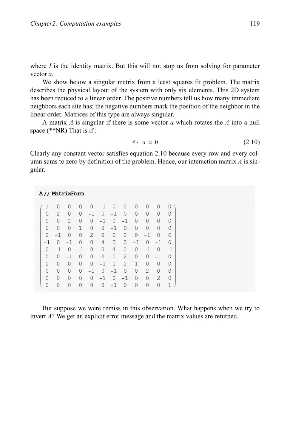
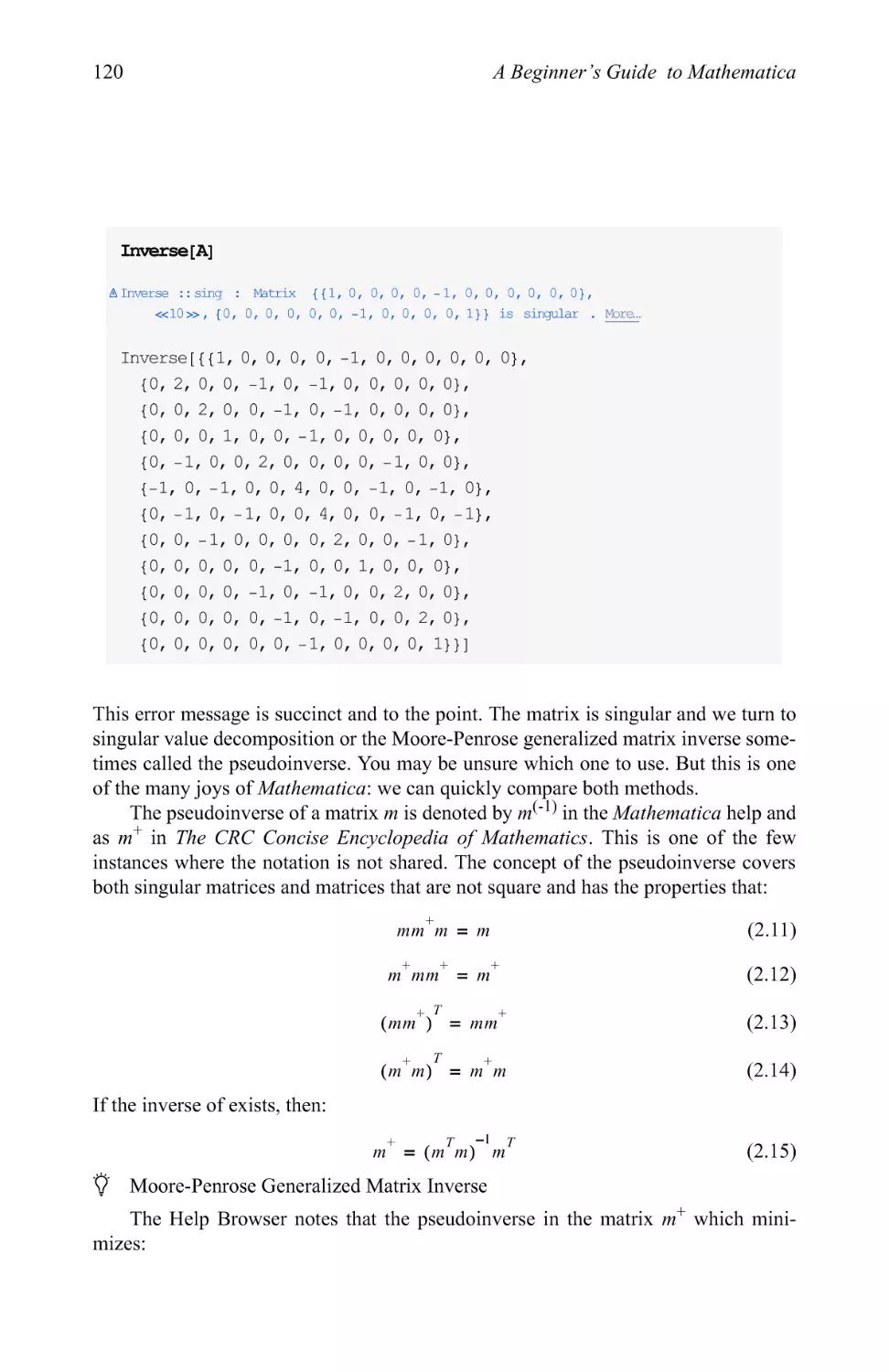
Singular matrices and inversion
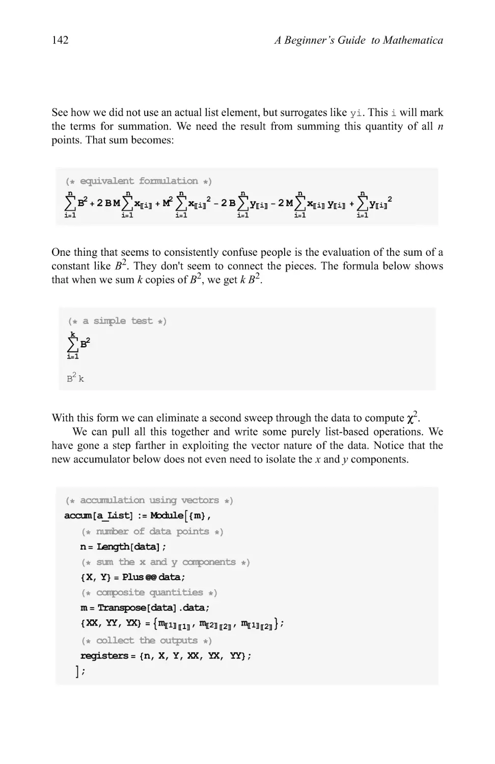
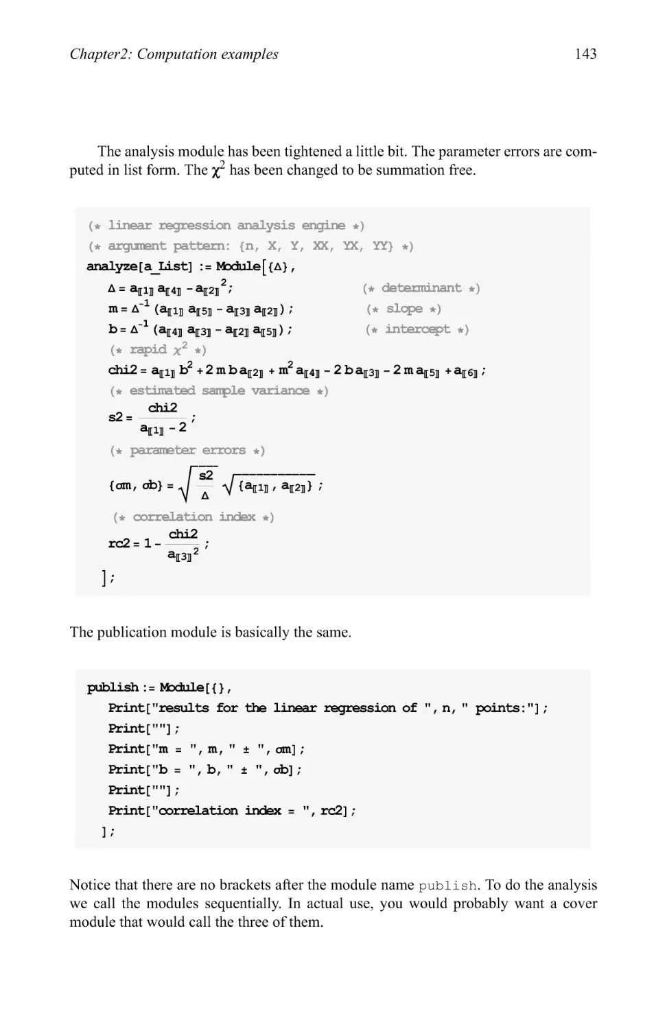
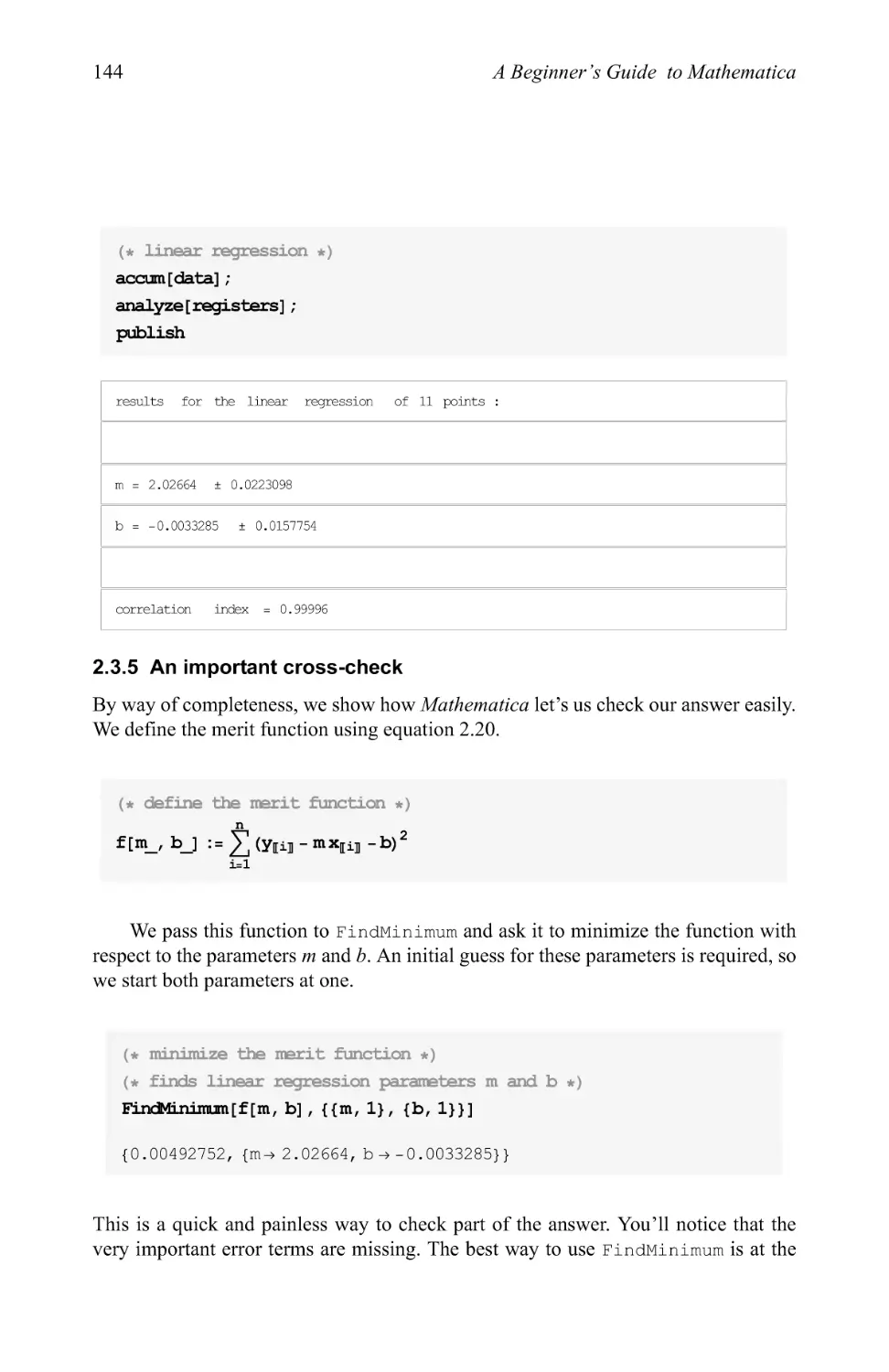
Linear regression
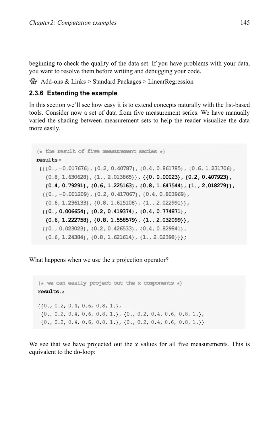
An inverse problem
VI
A Beginner's Guide to Mathematica
Chapter 4
Ordinary differential equations 303
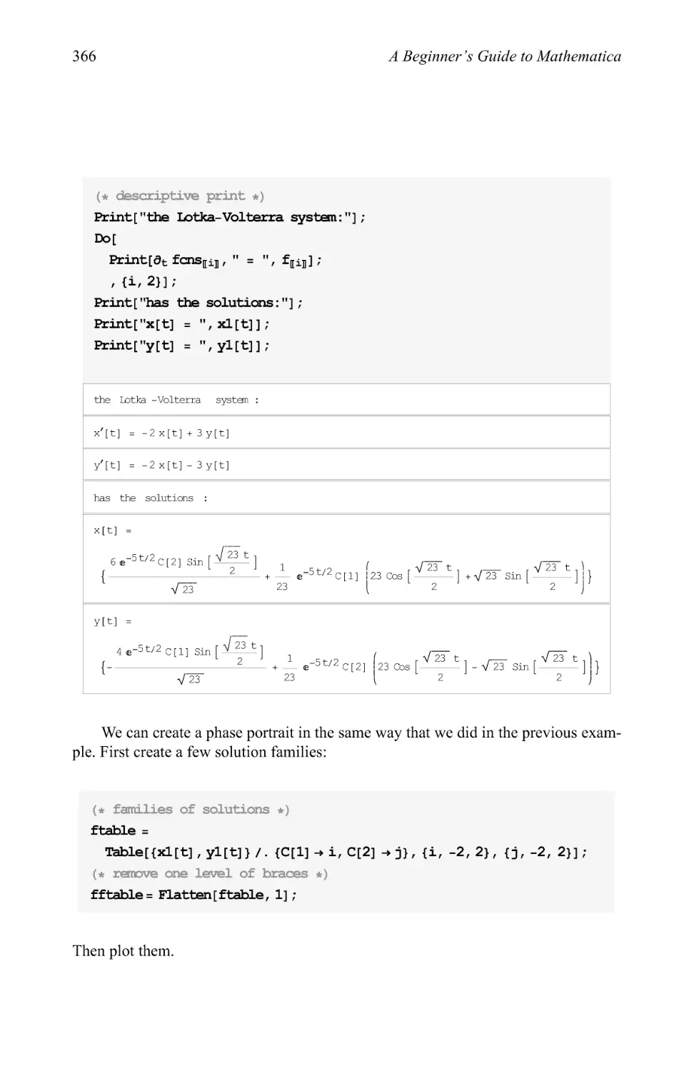
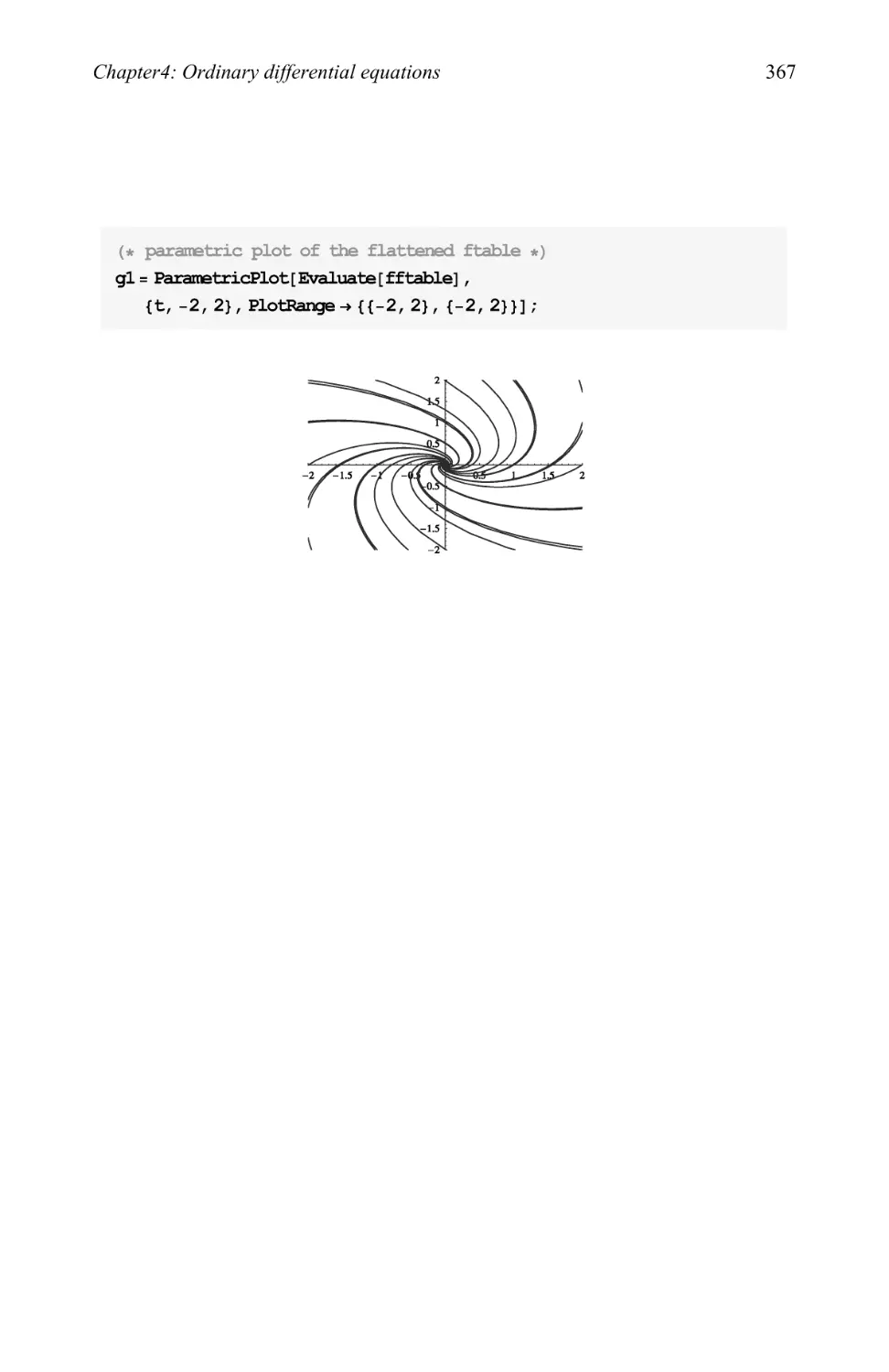
4.1 Defining, entering and solving differential equations 303
Chapter 5
Transforms 369
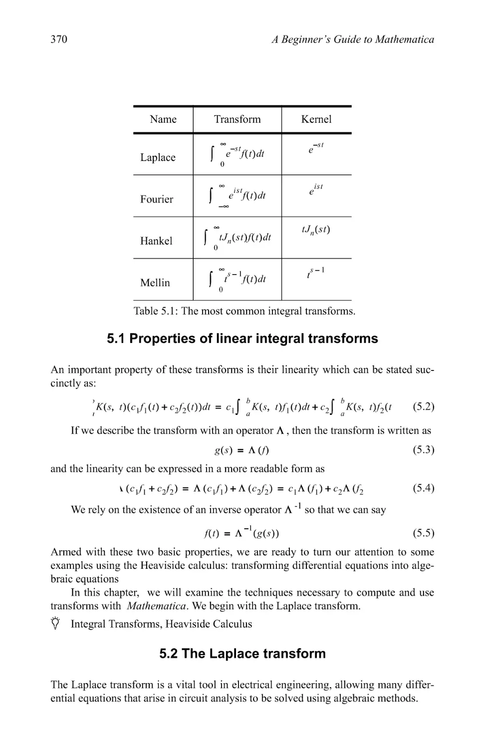
5.1 Properties of linear integral transforms 370
5.2 The Laplace transform 370
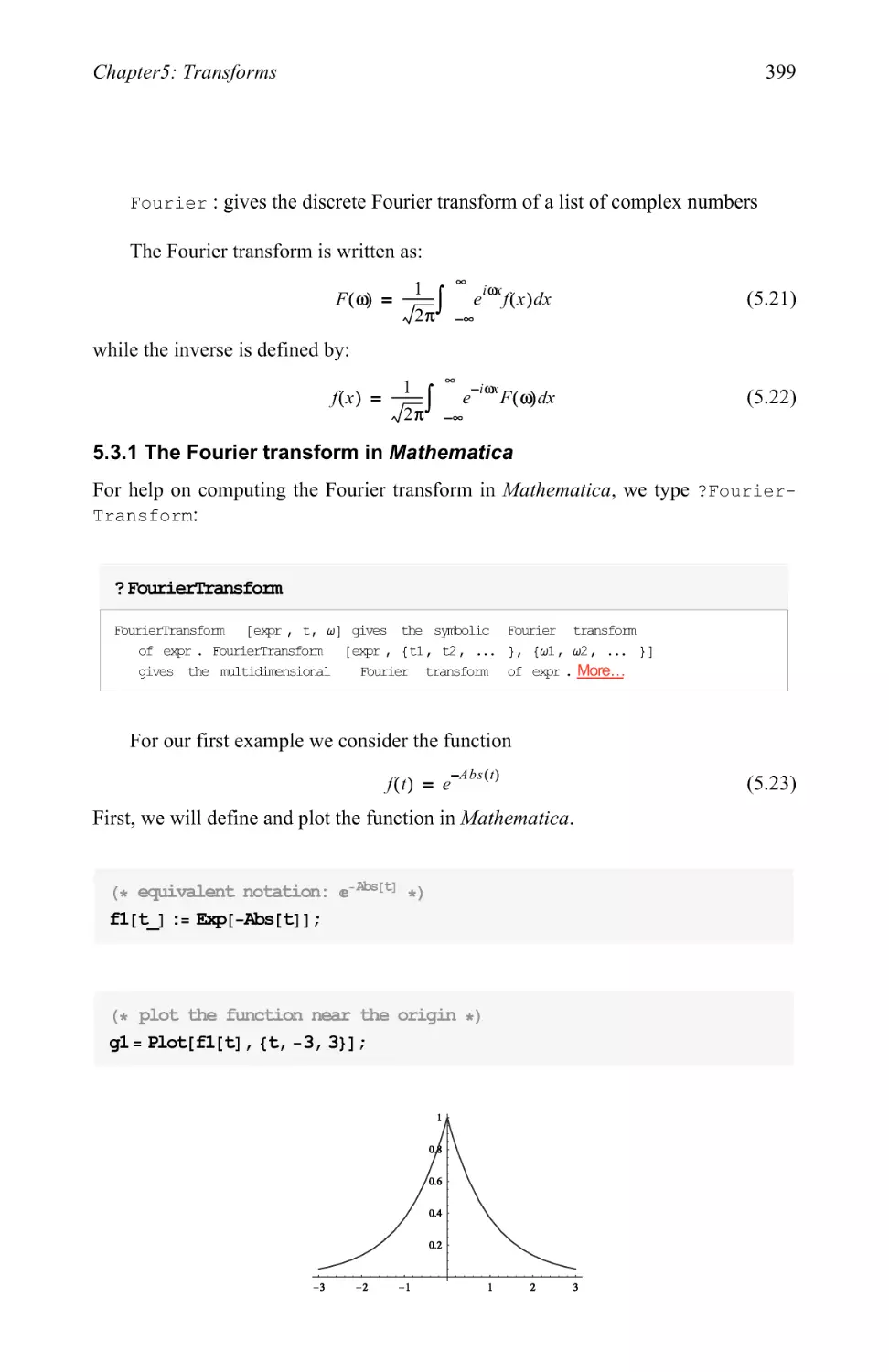
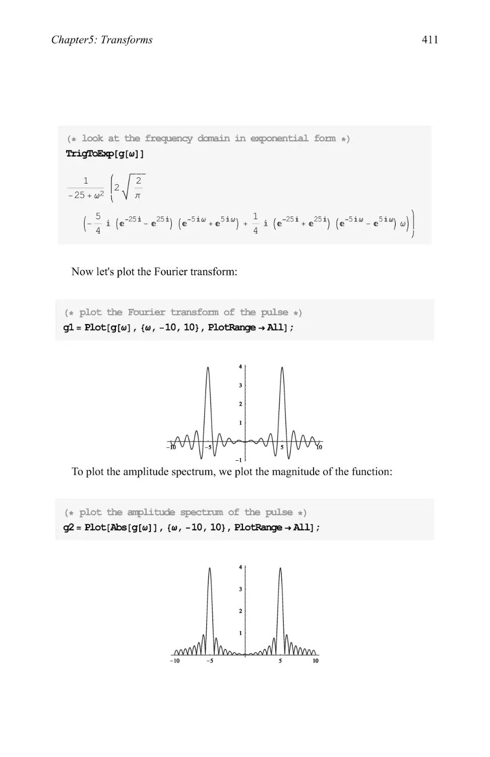
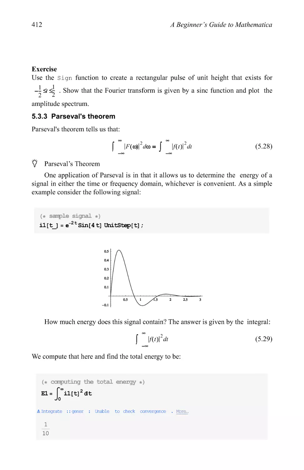
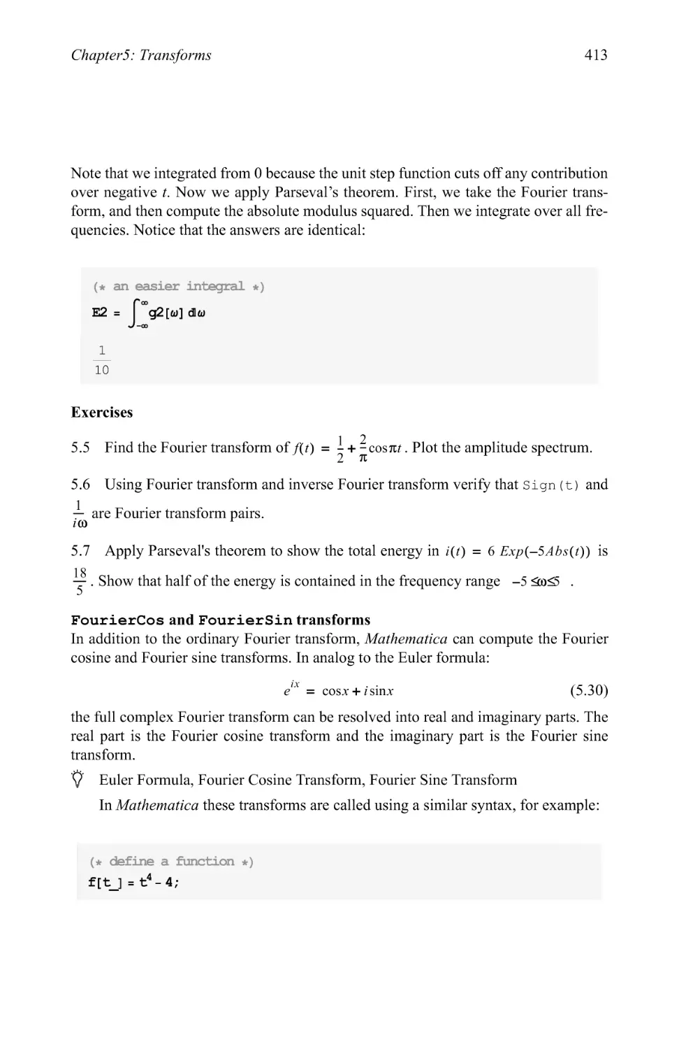
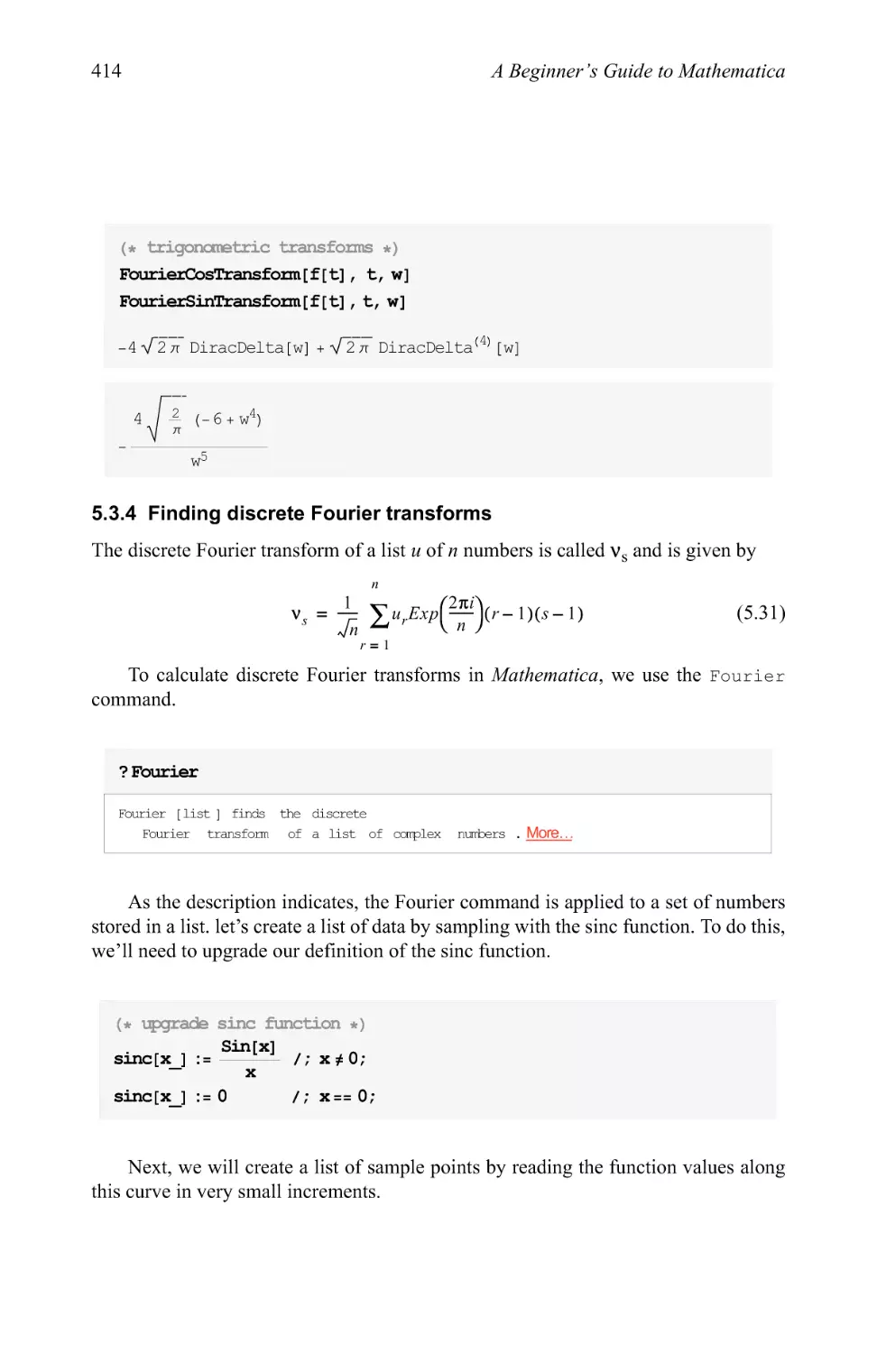
5.3 The Fourier transform 398
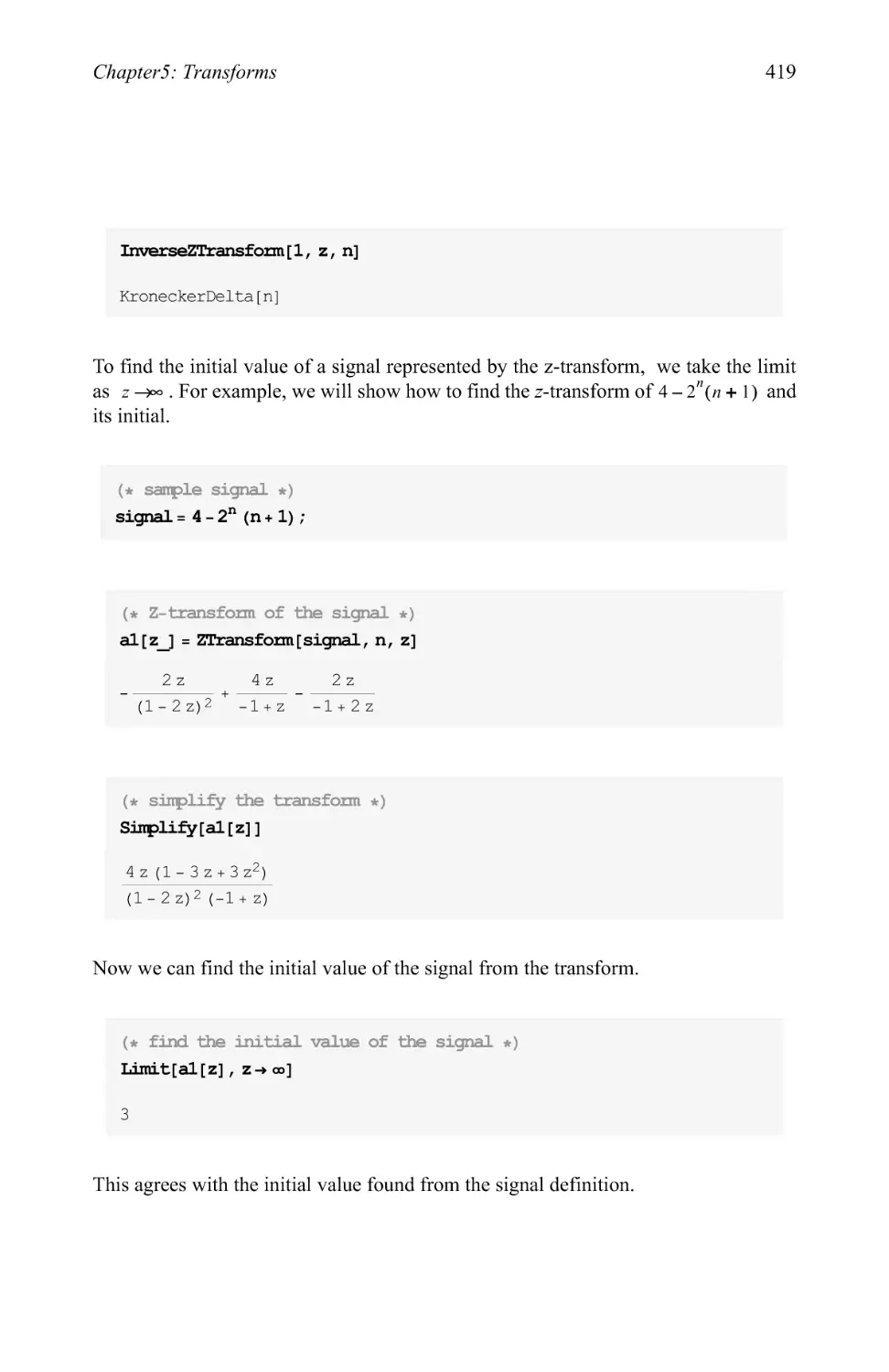
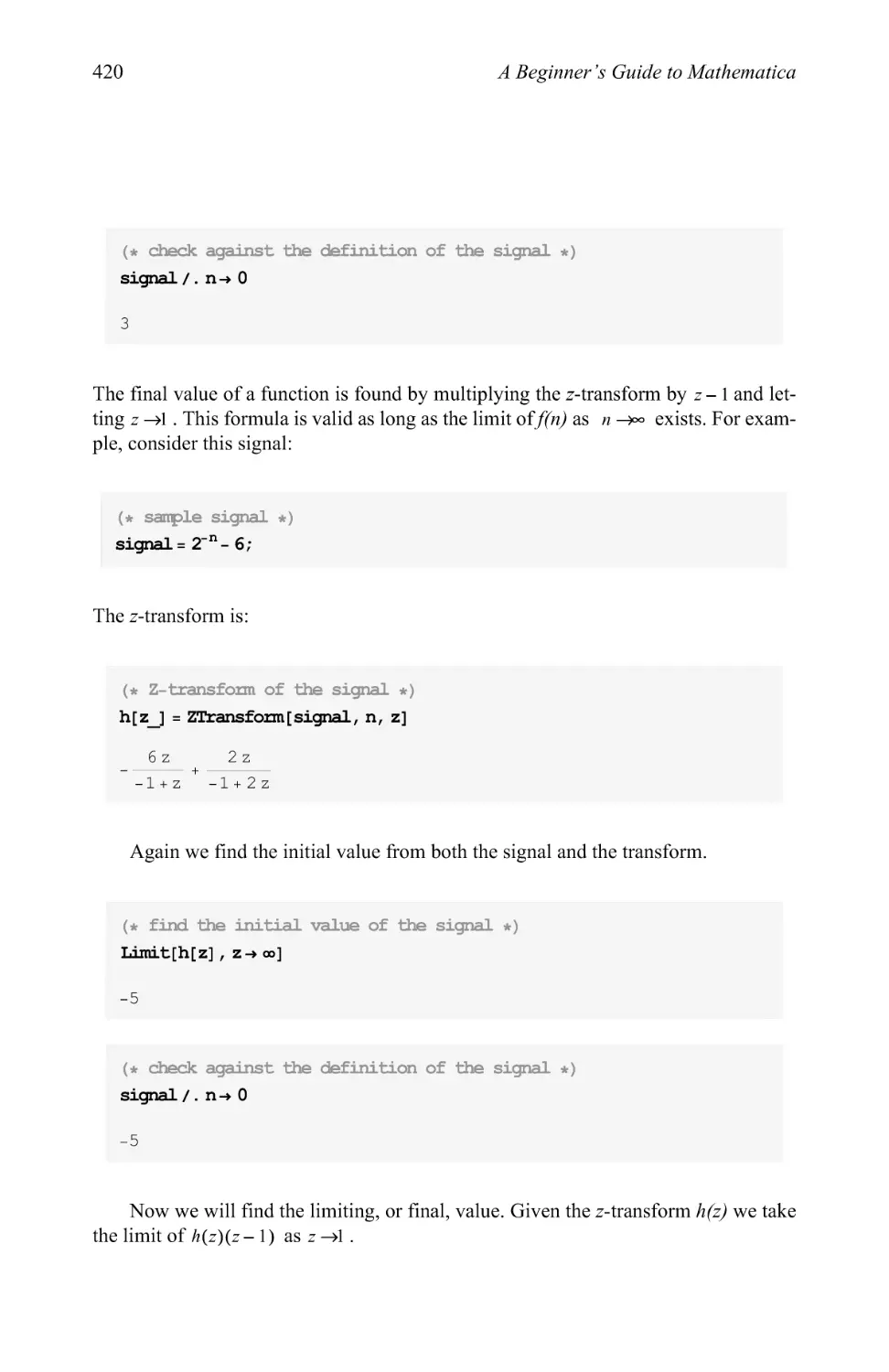
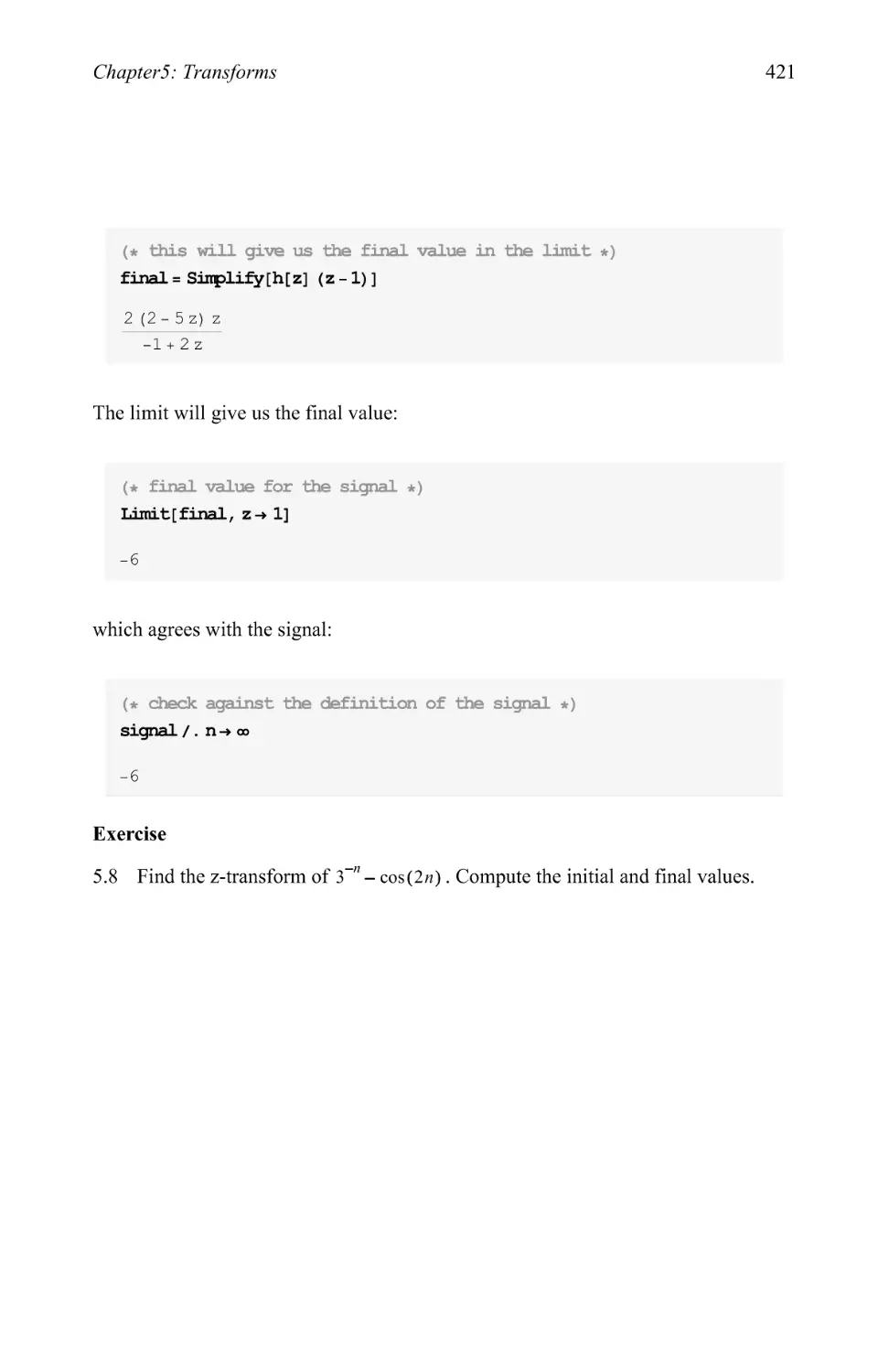
5.4 The z-transform 417
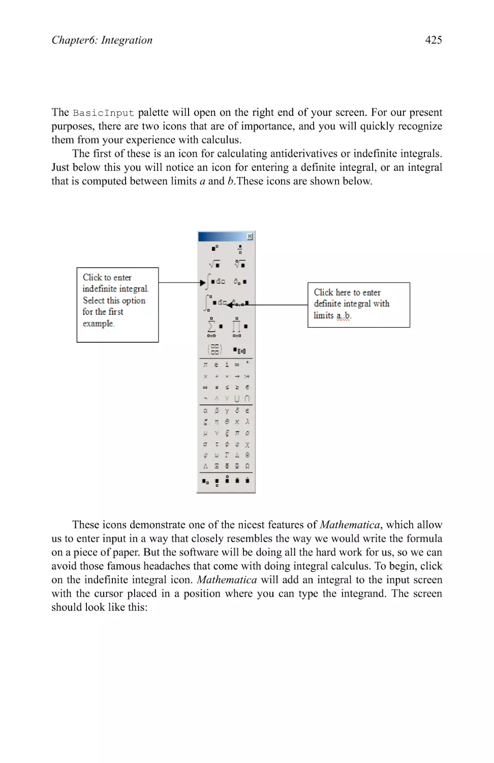
Chapter 6
Integration 423
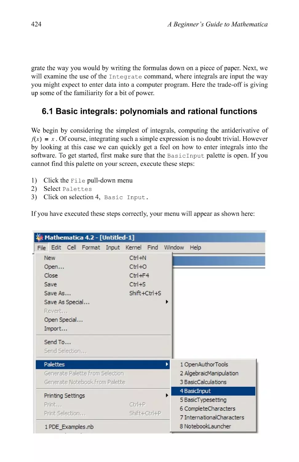
6.1 Basic integrals: polynomials and rational functions 424
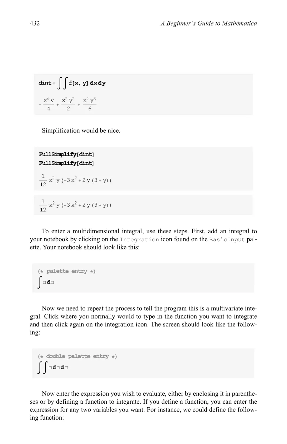
6.2 Multivariate expressions 430
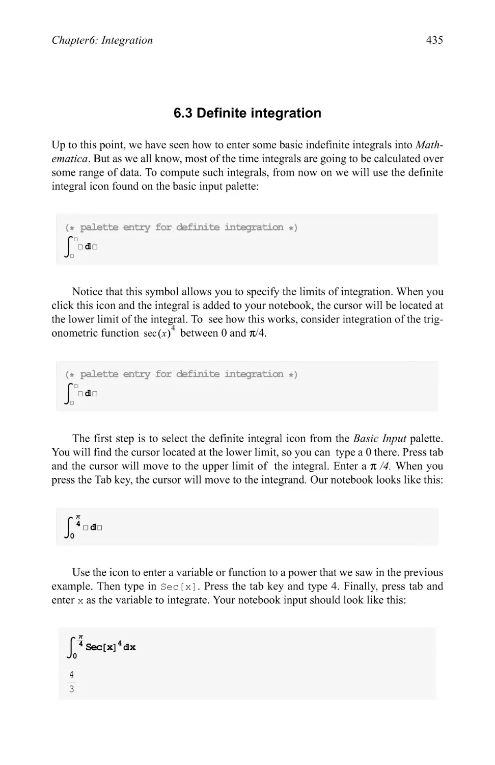
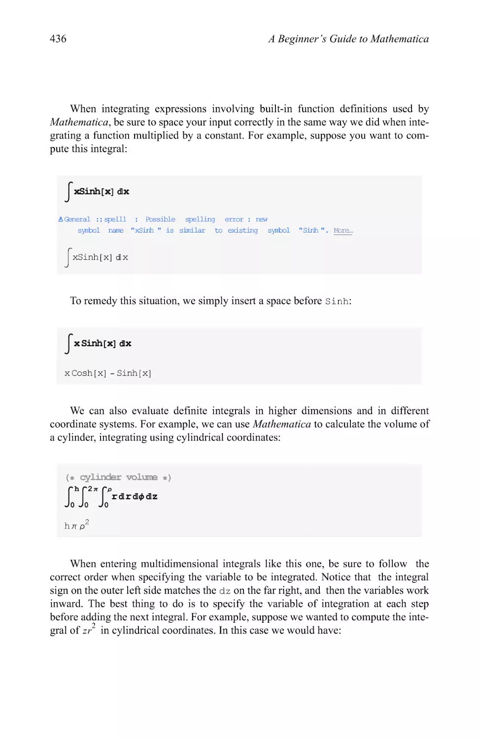
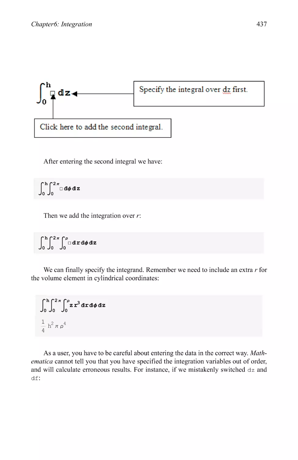
6.3 Definite integration 435
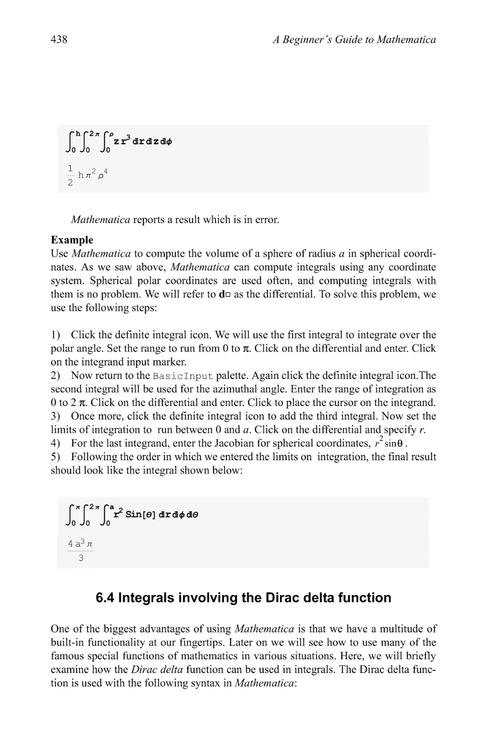
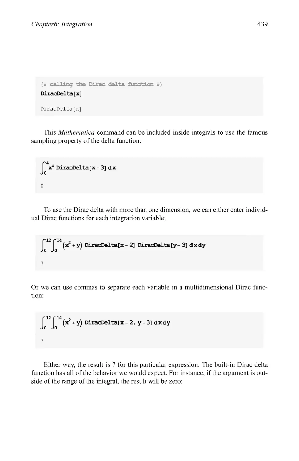
6.4 Integrals involving the Dirac delta function 438
6.5 Using the Integrate command 440
6.6 Monte Carlo integration 442
Chapter 7
Special functions 451
7.1 The Gamma function 451
7.2 The Bessel functions 465
7.3 The Riemann zeta function 478
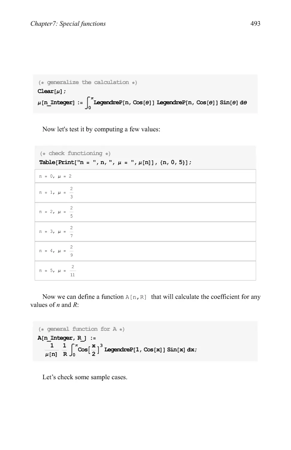
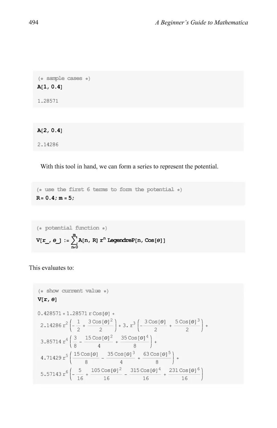
7.4 Working with Legendre and other polynomials 487
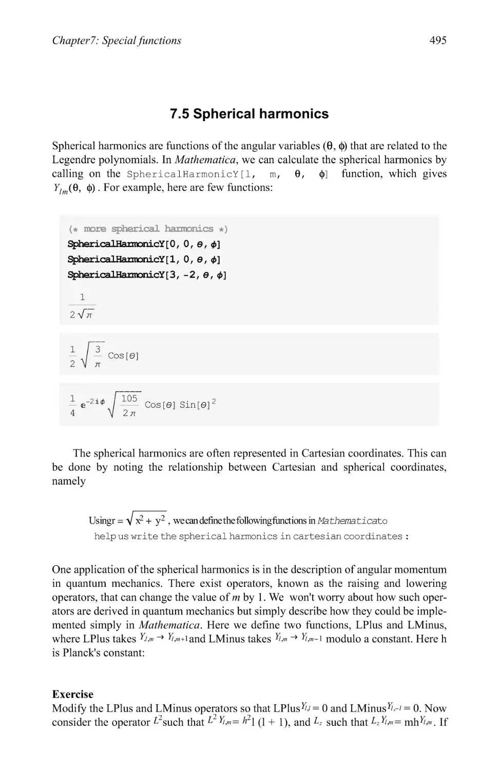
7.5 Spherical harmonics 495
Appendix 1 497
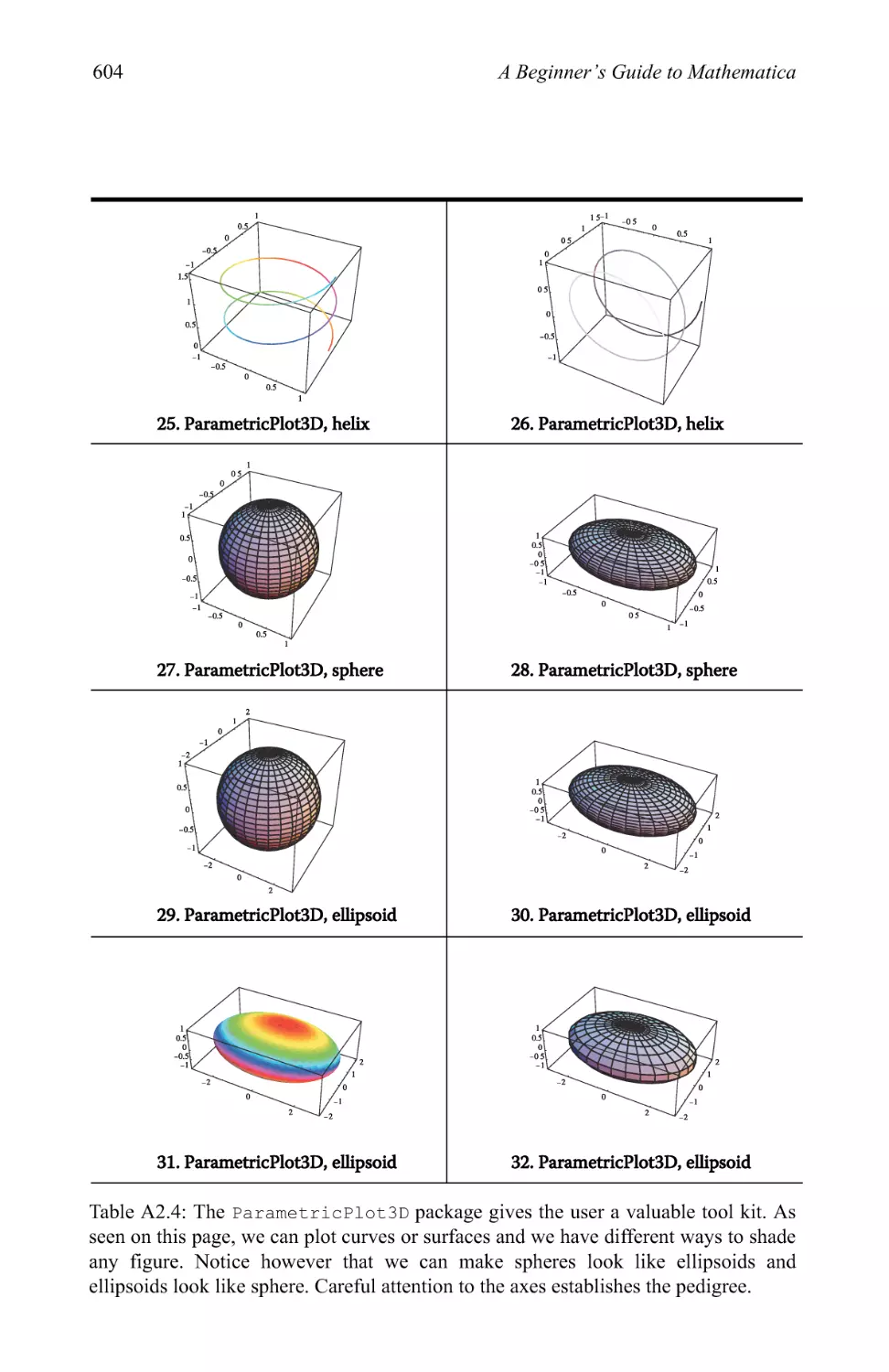
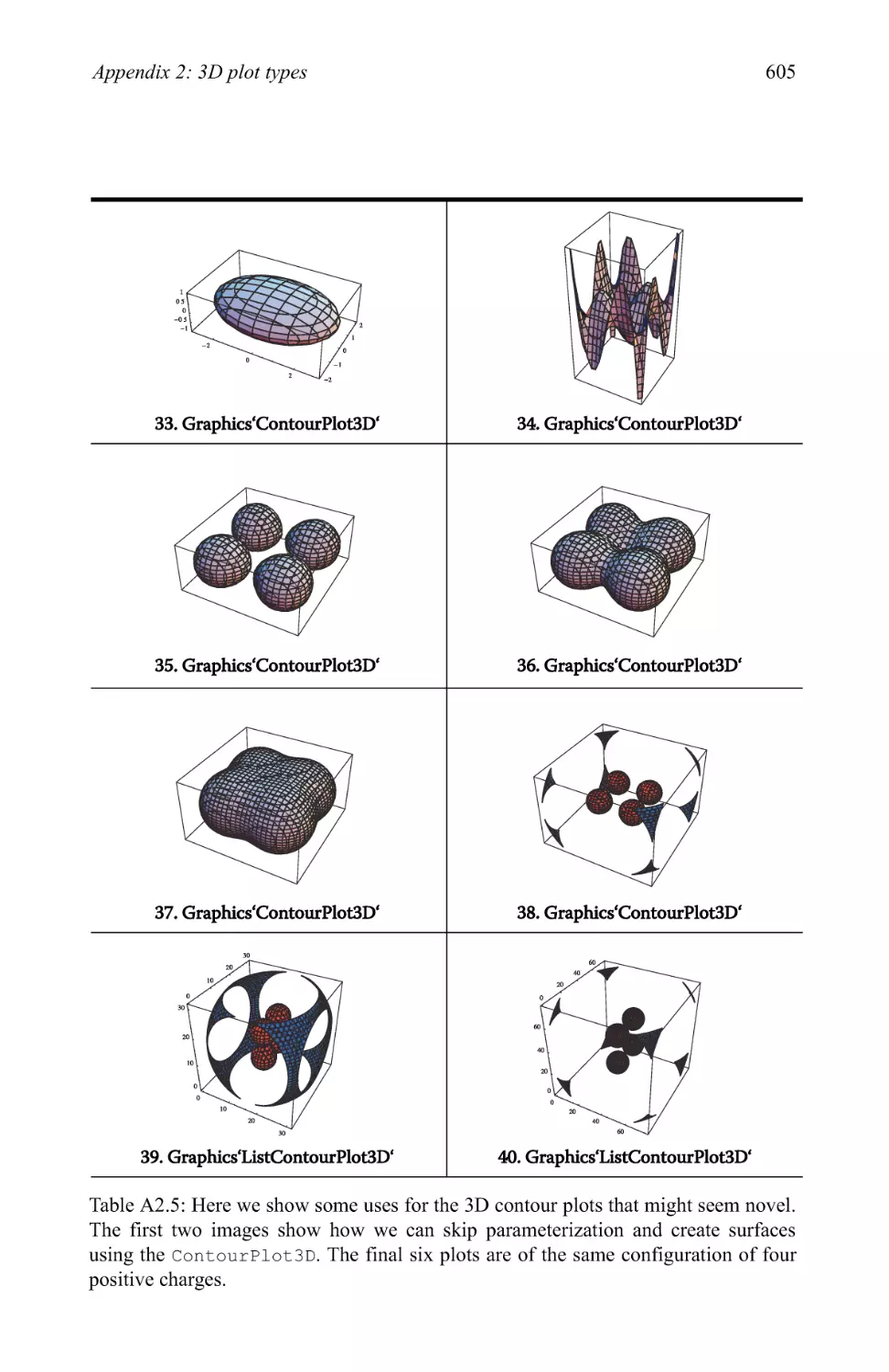
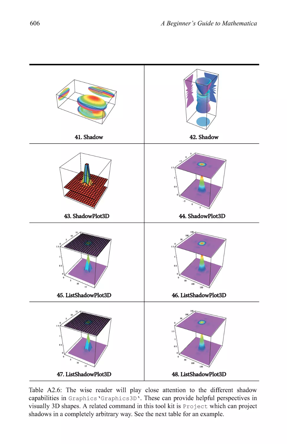
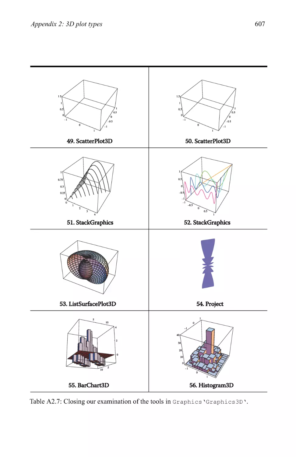
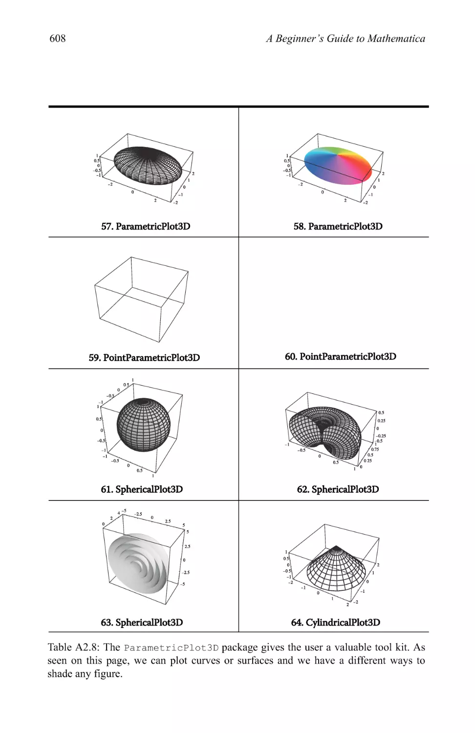
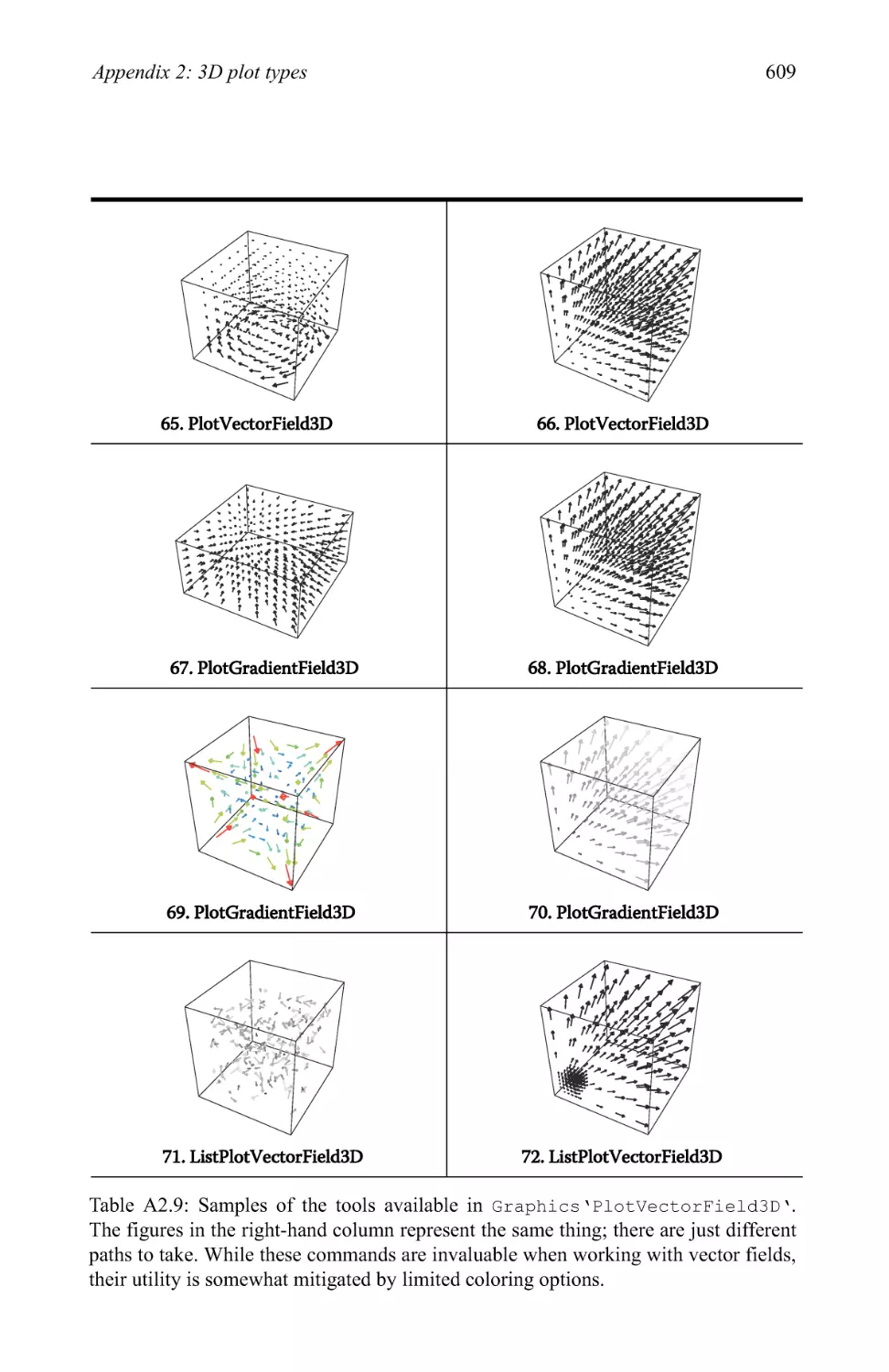
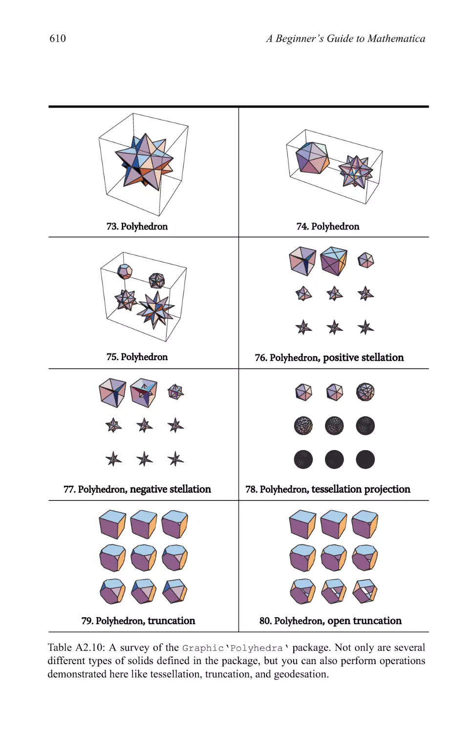
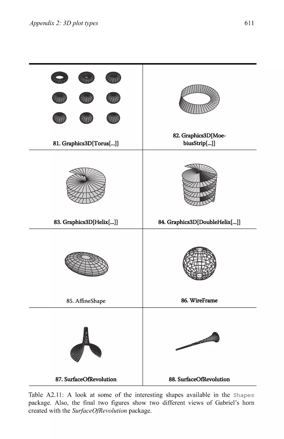
Appendix 2 599
References 693
Index
695
Preface
Mathematica is an incredibly powerful and useful environment for symbolic
computing, numerical computing and data visualization. To us, it is the flagship product that
gave the personal computing revolution its biggest boost. Some may counter that
spreadsheet programs or databases were more significant. For sure these products
have great relevance. But in those cases the application migrated from mainframe
computers to personal computers (PCs) and hence became more accessible.
Considering computing languages like FORTRAN we were so vexed by the low compiler
qualities for the PCs that we found them of little utility. Mathematica, on the other
hand, gave people a whole new power that had heretofore been unrealized. It
extended capabilities far beyond mainframes. Certainly other applications attempted
to claim the scientific computing market such as Theorist and Math Cad. But our
experiences with them made us feel we could do the symbolic computations and
integrations faster without the computer.
Admittedly, in prerelease 3.0 the user interface was not very appealing. Yet it was
impossible to argue that you were working with a brand new set of capabilities. The
sophistication of the symbolic capabilities has gone unmatched for decades. We can
think of no truer testament to the breakthrough that Mathematica represents than this.
There have been a few feigned attempts at duplication, but nothing has come very
close. The architecture of Mathematica was ahead of its time. When you look at the
transition from FORTRAN 77 to C you see a true modernization of the computing
language. After mastering C, one looks at FORTRAN as a bit confining. For instance,
C was capable of making a list of arbitrarily sized lists and FORTRAN was not.
Mathematica came and delivered the best part of FORTRAN — the rigorous, robust
computation — with the wonderful, modern features of C. On top of that we got stun-
Vlll
A Beginner's Guide to Mathematica
ning symbolic capabilities and superlative graphical capabilities. The only significant
downside we are faced with is that unlike IDL, we cannot compile our Mathematica
code into machine language files. However, it would be irresponsible to characterize
such a miraculous tool as incomplete. We think even critics of Mathematica would
have to agree either that it is the gold standard for PC software or that it has at least
greatly elevated the standards. Its customers are served very well, the releases are
virtually bug-free, the documentation is excellent and available on paper too! The
online help is state-of-the-art and the Wolfram website is a door to a vast amount of
examples and tutorials.
One particularly frustrating problem we have with other PC applications is how
often the paradigms shift. New releases mean legacy code is now broken. This really
frustrates someone who basked in the interrelease years between FORTRAN 77 and
FORTRAN 90. Over the years one thing that has impressed us with Mathematica is
the stability of the design. To be sure, a program with such far-reaching scope and
power will have changes, but they are so few as to border on the inconsequential.
Perhaps because of a brilliant design, or perhaps because of good stewardship,
Mathematica has been a friendly monolith over the years.
One goal of this volume is to start new users on a voyage of discovery and take
previous users a bit farther along. The subject matter is so rich that it cannot be done
justice in a single volume. We have tried to sift through a lot of the material and to
introduce you to those items that are the most useful to practical applications.
To be sure, we will document cases of bugs, but these bugs are mostly in the front
end. Wolfram Research seems to guard its computational kernel most jealously. We
suppose that because there are so few bugs it is easy to delineate them. Given their
appearance we feel some discussion is warranted because they could easily bedevil
users. We hope that this volume — accompanied by the copious Wolfram material —
will help you see how helpful Mathematica can be in everyday use.
Another goal of this book is to help you learn the aspects of Mathematica needed
for many practical applications. The publisher has chartered us to come up with a
distinct approach that separates this book from so many other good ones. So we place a
high value on notebook and file system organization, cross-platform capabilities, data
reading and writing. We also want to help you write notebooks that are easy to read
and to debug. We work with new users, and a great deal of their trouble comes from
lack of discipline. Mathematica has a wonderful flexibility; it is not a rigid program.
Some users view the absence of rigidity as a problem. They seem to yearn for single
path to master. We want to show that there are often multiple ways to solve a problem
and you should choose the one most comfortable for you. The publisher has tasked us
to include the error messages users are likely to encounter and to assist in their
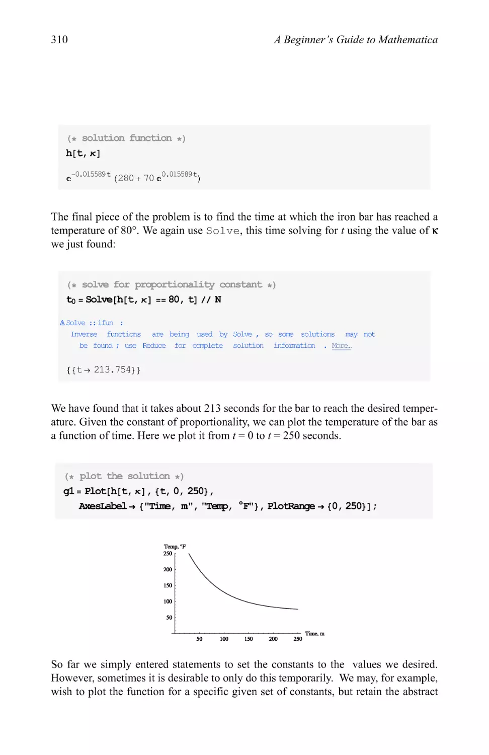
interpretation.
We have been working with numerous associates over the years helping them to
understand and to learn Mathematica. In some sense this book documents what we
have learned from our talented colleagues as they endeavoured to conquer
Mathematica. Perhaps our deep appreciation for Mathematica stems from our reliance upon it.
We are certain that this application can be a boon to most people.
Preface
IX
Some of our peers have been quite vocal and challenged us to write a book that will
help them solve significant problems in their laboratories and universities. The
attempt to do so has been quite daunting. One complaint we heard over and over is
that many books help you solve problems that they don't need Mathematica for. They
can look at a wave equation and tell you what the answer is; they don't need
Mathematica for that. We wanted a readable book and we felt strongly that to be useful we
would need to keep it brief. We didn't want to present a compendium of arcane
problems and esoteric solutions. But we did want to present a hierarchy. We want to start
with problems that are simple and present multiple solution paths. Solutions ranging
from basic to elegant to gradually introduce the user to the Mathematica toolkit. And
then we wanted to introduce challenging problems and eventually cutting-edge
problems.
We want to build an intuition and that takes time and repetition. Fortunately we are
dealing with an extremely well-designed and documented product and ultimately the
diligent will be rewarded. We also want this book to be useful to people of different
skill levels. We do not pretend that you will master the application after one reading.
We count on readers to revisit sections of interest and sections that were challenging,
so that they can continue to refine their skills.
To write this book we used Mathematica 5.1 for the Macintosh and for the PC.
We feel quite strongly that the cross-platform capabilities of Mathematica enhance its
value. In general if you are using 5.0 or even 4.x, we would expect that almost all of
the code fragments presented here will run in your environment.
Finally, the publisher will set up a website where you can download the code
fragments you see in this book. We encourage you to download these scripts and run
them on your own machine to experiment and to reinforce the lessons. Also, you will
be able to see the figures in full color. The URL is http://www.crcpress.com/.
CHAPTER 1
Introduction and survey
We use Mathematica every day and have helped many other users to learn
Mathematica. We have listened to advanced users and heard their comments and protestations.
This book is a product that we have crafted to address the issues that we have
frequently confronted. As we mentioned in the preface, Mathematica is too broad to
conquer quickly. But you can rapidly learn what you need to become functional and to
begin exploring.
We have written a book that will take multiple readings. We have tried to present
tiered solutions: solutions you can grasp immediately, solutions that require a bit more
experience but simplify the problem, and elegant solutions showing the core of
Mathematical power. On first exposure one should be content to glean the rudiments. As
you revisit the material it will become clear, and hopefully you can progress to the
more powerful Mathematica structures.
We start out with familiar mathematics to reduce confusion. We show different
ways to solve the same problem. Hopefully as you reread sections, you will become
more familiar with the more sophisticated formulations. We also show common user
mistakes and error messages. The point of this volume is not to show that the authors
can solve problems with Mathematica, it is instead to show the reader that he can
solve problems with Mathematica and a little help.
1.0.1 Augmenting Wolfram material
Before starting with this book, you need to take a few minutes to go through the
Mathematica tutorials we list here and to explore the on-line help (available though
the Fl key on Windows platforms or help on the Macintosh).
2
A Beginner's Guide to Mathematica
First, the later versions of Mathematica (4.2 and beyond) come with quick
tutorials which are of high quality and will help quickly introduce you to features and
capabilities of Mathematica. In version 5 and later, the tutorial is accessed through the
menu bar under the Help command. We cannot think of a better introduction than this
tutorial. You can see the commands and output together. You can copy the commands
from the tutorial into your own notebook and experiment with them. At the end of the
tutorial you are presented with a host of hyperlinks to take you to topics for further
scrutiny. We encourage users to view the tutorial and we will assume that you have
done so before reading this book. We intend to elaborate topics outside of the tutorial.
Second, you can use the vast resources at the Wolfram web portal www.wol-
fram.com. You can find all manner of materials to help you master Mathematica:
presentations, papers, notebooks, etc. The sophistication ranges from elementary to
advanced. In the last few years Wolfram Research has put a great deal of effort into
their Internet sites and you should periodically check them. Three superb Internet
tutorials for new users can be found at:
http;//documents.wolfram.com/v5/Tour/
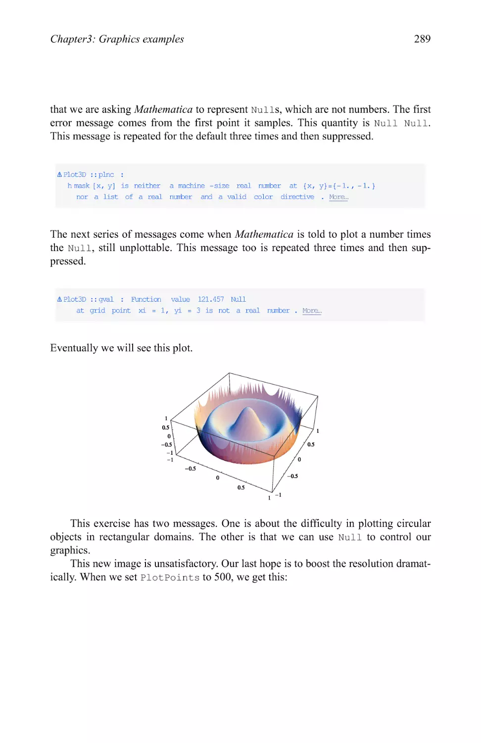
http;//documents.wolframxom/v5/TheMathematicaBook/A?racticalTntroducti-
onToMathematica/
http;//www. wolfram.com/products/mathematica/tour/
These materials should be appreciated for their brevity, their accuracy, and their
utility. The goal of this book is to expand beyond these tutorials. In other words, we are
operating under the assumption that you have reviewed the on-line tutorial and the
Internet tutorials.
Mathematica includes a book called Getting Started. It is a superlative way to
introduce users to Mathematica. If you can find this book, read it first and then turn to
the Help Browser and Internet materials.
The on-line help is superlative and you should make use of it early and often. You
will find a clear and succinct summary for each command and usually several
examples. These examples are invaluable to mastering Mathematica for they show the
basics and often very sophisticated examples. To access the on-line help, double click
on a command word to highlight it and then press the Fl (or help) key. This will
launch the Help Browser. The references are thoroughly cross-referenced and hyper-
linked. For example, if you are manipulating the structure of a list and you launch the
help browser on the command Take you see a clear and concise statement of what the
command does. As you read down the bullet list, you will find hyperlinks to the
relevant sections in The Mathematica Book (sections 1.8.4 and 2.4.2). There is a Back
button to return you to this page if you wander off using the hyperlinks. You will also
notice a list of commands related to this one. In this instance we find Part, Drop,
StringTake, Select, Cases, Partition and PadLeft. Typically these commands have
similar or opposite functionality.
Every user who has access to Mathematica has access to the on-line help, the
tutorial, and (if Internet connected) the websites. Some users may have other, more
expensive options. You should also consider subscribing to the Mathematica Journal
to learn cutting-edge techniques and the latest applications. They may seem
overwhelming at first, but eventually you will appreciate the beauty and power of Mathe-
Chapter 1: Introduction and survey
3
matica. Also, you should consider upgrading your Mathematica subscription to the
Premier package which supplies you with all the current releases and provides for
telephone support from the staff at Wolfram Research.
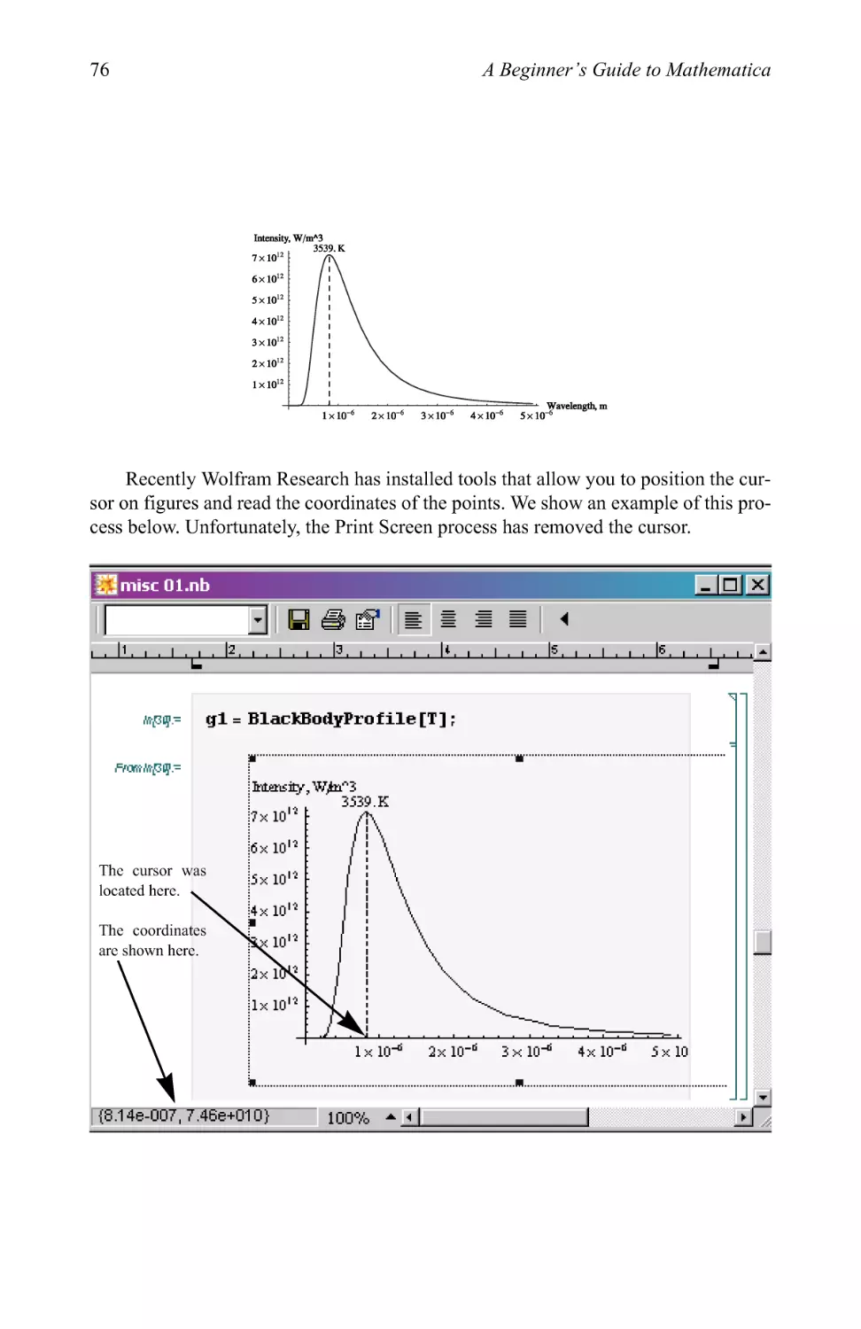
Special characters make things easier to read.
1.0.2 Using this book
We believe very much in reinforcement. By reinforcement we mean repetition and
repetition in different contexts. We do think it realistic that you can read the excellent
on-line help and master Mathematica. We think that material and complexity should
be introduced gradually and that the contexts should be varied. Most of all, we believe
the reader needs to be exposed to realistic problems that show the subtleties and
nuances of Mathematica. The reason we have titled this book Practical Mathematica
is because we want to prepare the reader to use Mathematica on his own in the
laboratory, the office or at home. This means acquainting you with common problems,
errors and their messages and practical tools like data I/O. We have specifically
chosen exercises that require attention to details. We want to convince the readers that
they can use Mathematica to successfully solve problems on their own.
To reinforce the importance of the on-line help we will often refer to relevant sections
for further reading. Such entries will be preceded by the Mathematica spikey ¢.
Also due to the fantastically rich mathematical concepts used it is invaluable to
have a single reference which spans the panorama of mathematics used. The second
edition of The CRC Concise Encyclopedia of Mathematics is a priceless reference to
keep nearby. It does a good job of unifying notation amongst hundreds of sources and
relies heavily upon Mathematica for either demonstration or comparison. The on-line
help is excellent and the Encyclopedia augments these explanations admirably. The
second edition has a much stronger tie-in with the Mathematica. References to The
CRC Encyclopedia of Mathematics will be annotated with y.
The World Wide Web hosts a variety of useful information pertaining to
Mathematica. Most of the information is available through the Wolfram Research website.
Any references to the web will be marked with ^*£.
Finally, we note a curious silence over a few of the bugs in Mathematica. To be
sure the functionality is quite robust, but there are a few minor glitches with the front
end. However, these minor problems may be enough to completely derail the new
user and as such we show how to diagnose, how to correct, and how to avoid. In this
same category of advice we will include comments to guide users past some common
errors new users make. Such comments will be marked with A.
W These statements refer to entries in the Help Browser.
V The statements refer to entries in The CRC Concise Encyclopedia of
Mathematics.
^*£ These statements refer to material on the World Wide Web.
A These statements refer to common pitfalls of the new user as well as
Mathematica bugs. This is information you will typically find nowhere else.
4
A Beginner's Guide to Mathematica
1.1 Why Mathematical
A common question we ask our colleagues is why they chose a particular product.
Oftentimes the answer has to do with legacy code. The organization has accumulated
a great deal of coding in one particular application. The cases of interest are when the
laboratory or office has no legacy code and may have users familiar with packages
such as Matlab and IDL. What drove them to select the product that they did?
We appreciate that there are other valuable products out there that will serve the
users admirably and we think they serve their market segment in good stead. If you
say you want to produce machine language executables from your code, then IDL is a
great choice. If you want a Matlab package that is exactly tailored to your job, then
Matlab is an excellent choice. If you want to do problems in the Feynman calculus,
relativistic tensor calculus, nonlinear differential equations, number theory or plow
through the integrals in Gradshteyn and Ryzhik then Mathematica is an excellent
choice.
At one point we too were trying to find the best application to serve our needs.
We explored a variety of packages and found many, many useful features across all of
the products. We would like to clear up some of the Mathematica myths that seem to
be immortal.
1. Mathematica is hard to learn.
This is frustrating to hear. From what we can discern, it seems that other
packages with far-reduced capabilities are "quick" to learn. But as we will show, the
rudiments of Mathematica can be grasped in as brief a period. Of course with
Mathematica there still remains a significant tool kit to be explored. For example, say
you want to program a linear regression using Mathematica and application X. We
will show that the basics of Mathematica can be conquered in a comparable period of
time. Except with application X there is not much more to assimilate and with
Mathematica you have only scratched the surface. So your choice could be to use
application X until you are faced with more daunting problems and then start all over again
with Mathematica, or you can start and grow with Mathematica. In summary,
Mathematica has a comparable learning rate. Mastering the complete application will take
far more time due to the extensive capabilities of this tool kit.
In this book we attempt to show a tiered approach to problem solving. We show
how to use elementary techniques in a transparent fashion and then introduce
refinements. We think you will see in almost all cases the more advanced features — which
may seem foreign — greatly simplify coding.
2. Mathematica is slower than other similar applications.
This is remarkable because in many cases the opposite is true: Mathematica
frequently has a significant speed advantage over other applications. Whenever possible
Mathematica will do calculations in arbitrary precision by using a rational number
representation and symbolic methods. Two comments: this can give you exact
answers free of numerical errors — a real benefit — and it can be extremely slow. But
Chapter 1: Introduction and survey
5
the other packages don't have an arbitrary precision mode, so in this sense Mathemat-
ica is infinitely faster. Now if you want to run Mathematica in a double precision
mode (by using the numeric operator N[] or simply typing 3. in lieu of 3), then
Mathematica runs with comparable speed and precision.
In general, we are very impressed by the careful attention Wolfram Research
gives to its releases. Perhaps because of the program's enormous scope we should
expect an occasional glitch. We encountered a rather severe problem when
transitioning from 4.0 to 4.2. An entire class of singular value decomposition (SVD) problems
would no longer evaluate. Out of thousands of notebooks this was the only problem
discovered. Unfortunately, it did cause quite a dilemma for us.
We are not criticizing Wolfram Research. They usually do a superb job with
upgrades. The more usual case is for an application upgrade to be tantamount to a bug
swap. Old bugs are exchanged for new bugs. Also, there are annoying changes in
command paradigms and syntax that require extensive modification to interface codes
or documentation.
So in regard to stability, Wolfram Research provides a shining example of how to
make an application grow and evolve. Perhaps we are showing our age and our
fondness for the Pax FORTRANA, the 13 years between FORTRAN 77 and FORTRAN
90. We are 10 years into the second period of stability ushered in by FORTRAN 95.
^ If possible, do not delete old versions of Mathematica when you upgrade. There
is a minute chance that the upgrade may contain a bug that may impact
previously developed calculations.
1.2 Notebooks
At this point we consider that you have gone through the tutorials and are familiar
with basic operations. After working with Mathematica for awhile, you will probably
find yourself using multiple notebooks at once and moving notebooks between
different machines, maybe even different platforms. It is always important to ensure that
your notebooks execute linearly, that is, from top to bottom. Requiring commands to
be executed out of order is a very poor coding practice. Also, you should ensure that
your notebook can run independently and does not require unreferenced notebooks to
be open. Perhaps you are familiar with using modules; they are a great way to give
notebooks a clean, readable appearance. They are an example of a referenced file
since they are loaded by reference. One should use modules and one must avoid
unreferenced data. For example, suppose on one notebook you do a long computation
for some variable q. This variable is needed by yet another notebook, yet there is no
referencing; the second notebook uses q as a global variable. This is a terrible
programming practice that many users run into at first. The target notebook should be
able to run on its own. You can test this by launching Mathematica and immediately
running the target notebook. If the run is successful, you have avoided unreferenced
data.
6
A Beginner's Guide to Mathematica
1.2.1 A seed notebook
To help us with these housekeeping details, we maintain a read-only notebook called
seed.nb. As the name implies this is a file that all notebooks will grow from. To create
a new notebook we open seed.nb and save it under a different name. We are then
ready to begin coding. Before we start however we will discuss the overhead of the
template file seed.nb
The first command is an important one because this cleans out the memory. This
will ensure that we are not relying upon unreferenced data, a very important
consideration. It also precludes a problem new users often create: using the same variable
names in different notebooks. For example, if we have two notebooks open and they
both use a variable x, the value of x is the value from the most recent execution. This
can create an extremely difficult debugging environment. In fact, when we assist new
users who present us with problematic notebooks, we first run the Clear command to
prevent any ambiguities from manifesting. At first glance, this command has a simple
syntax. For example, to clear the variables x and name you would write:
Clear[x, name]
Let's look at some examples of clearing variables. First, we will show how to
clear numeric values.
x=2;
Print ["x = ", x] ;
x = . ;
Print ["x = ", x] ;
x = 2
X = X
The last statement simply tells us that x is a variable with no assigned value. As
you might suspect, we can clear string values in the same manner.
Chapter 1: Introduction and survey
x = "bcc";
Print["x = ", x] ;
Clear[x]
Print ["x = ", x] ;
x = bcc
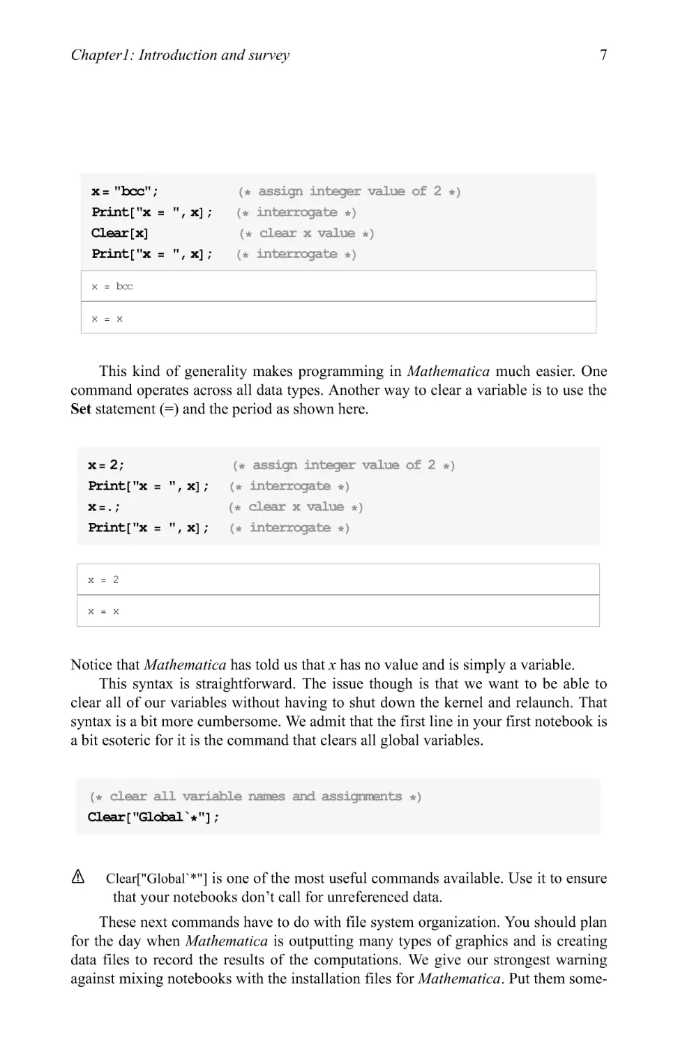
This kind of generality makes programming in Mathematica much easier. One
command operates across all data types. Another way to clear a variable is to use the
Set statement (=) and the period as shown here.
x=2;
Print["x = ", x] ;
x = . ;
Print["x = ", x] ;
x = 2
X = X
Notice that Mathematica has told us that x has no value and is simply a variable.
This syntax is straightforward. The issue though is that we want to be able to
clear all of our variables without having to shut down the kernel and relaunch. That
syntax is a bit more cumbersome. We admit that the first line in your first notebook is
a bit esoteric for it is the command that clears all global variables.
caear["Glbbar*"] ;
A Clear["Globar*"] is one of the most useful commands available. Use it to ensure
that your notebooks don't call for unreferenced data.
These next commands have to do with file system organization. You should plan
for the day when Mathematica is outputting many types of graphics and is creating
data files to record the results of the computations. We give our strongest warning
against mixing notebooks with the installation files fox Mathematica. Put them some-
8
A Beginner's Guide to Mathematica
where else; a little organization up front allows for a graceful expansion later. In the
seed notebook we define a variable dirnb which points to a highest level of the
notebook file system structure. All file system references are then relative to dirnb. If you
work on different computers and platforms, a good idea is to maintain duplicate files
structures. If you work on different platforms, you would only then need to change
the definition of dirnb.
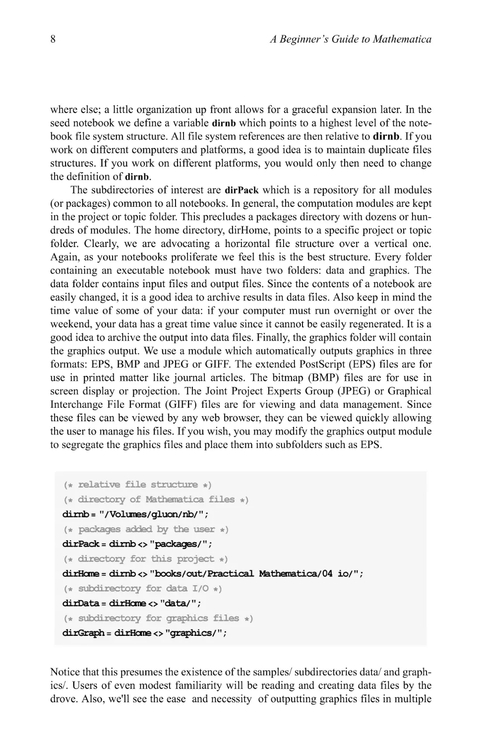
The subdirectories of interest are dirPack which is a repository for all modules
(or packages) common to all notebooks. In general, the computation modules are kept
in the project or topic folder. This precludes a packages directory with dozens or
hundreds of modules. The home directory, dirHome, points to a specific project or topic
folder. Clearly, we are advocating a horizontal file structure over a vertical one.
Again, as your notebooks proliferate we feel this is the best structure. Every folder
containing an executable notebook must have two folders: data and graphics. The
data folder contains input files and output files. Since the contents of a notebook are
easily changed, it is a good idea to archive results in data files. Also keep in mind the
time value of some of your data: if your computer must run overnight or over the
weekend, your data has a great time value since it cannot be easily regenerated. It is a
good idea to archive the output into data files. Finally, the graphics folder will contain
the graphics output. We use a module which automatically outputs graphics in three
formats: EPS, BMP and JPEG or GIFF. The extended PostScript (EPS) files are for
use in printed matter like journal articles. The bitmap (BMP) files are for use in
screen display or projection. The Joint Project Experts Group (JPEG) or Graphical
Interchange File Format (GIFF) files are for viewing and data management. Since
these files can be viewed by any web browser, they can be viewed quickly allowing
the user to manage his files. If you wish, you may modify the graphics output module
to segregate the graphics files and place them into subfolders such as EPS.
dirnb = "/Volumes/gluon/rib/ " ;
dirPack = dirnb <> "packages/" ;
dirHome = dirnb <> "books/out/Practical Mathematica/04 io/";
dirData = dirHome <> "data/ " ;
dirGraph = dirHome <> "graphics/ " ;
Notice that this presumes the existence of the samples/ subdirectories data/ and
graphics/. Users of even modest familiarity will be reading and creating data files by the
drove. Also, we'll see the ease and necessity of outputting graphics files in multiple
Chapter 1: Introduction and survey
9
formats. For these reasons it is best to create subdirectories separate from your
notebooks.
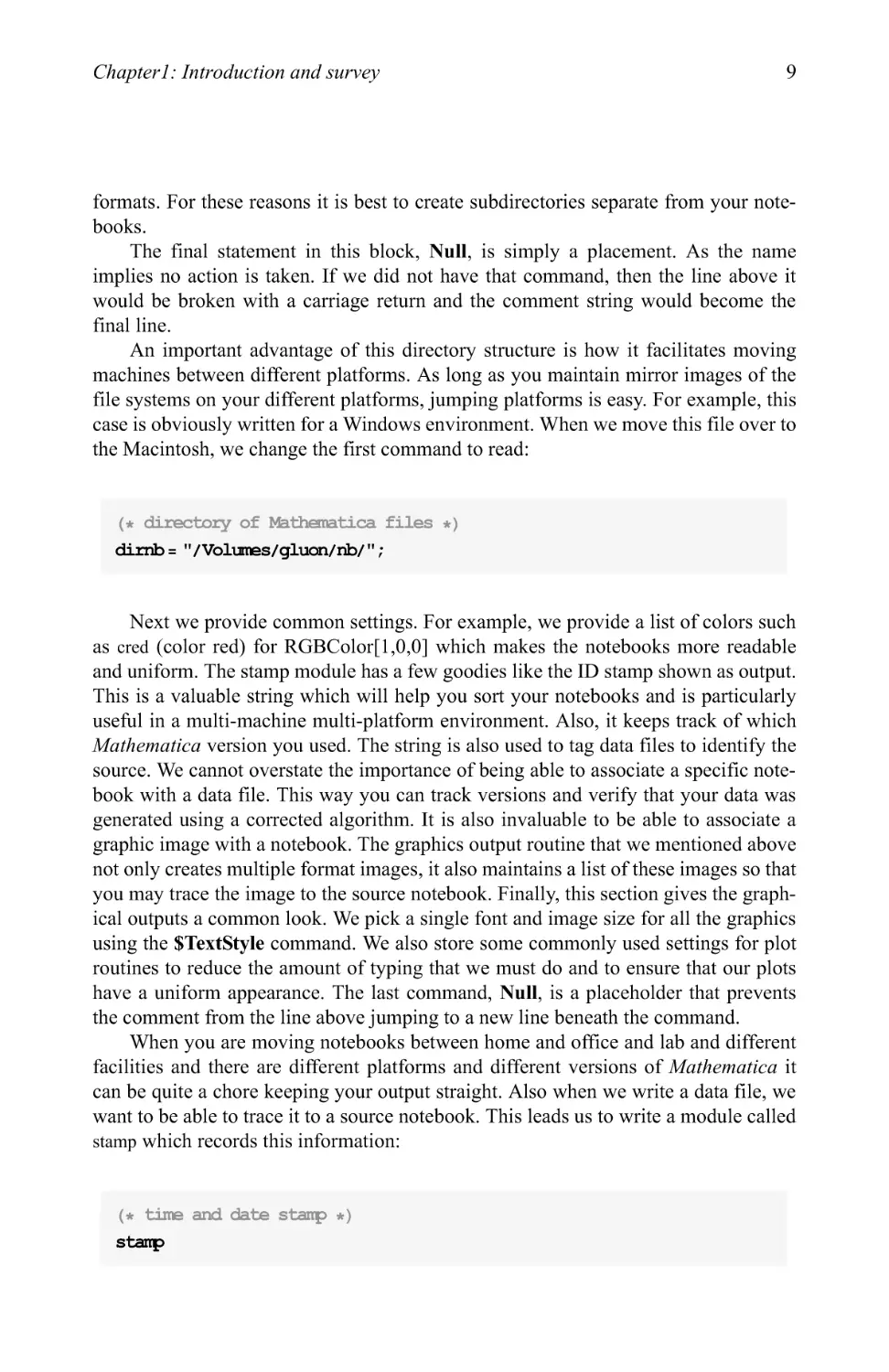
The final statement in this block, Null, is simply a placement. As the name
implies no action is taken. If we did not have that command, then the line above it
would be broken with a carriage return and the comment string would become the
final line.
An important advantage of this directory structure is how it facilitates moving
machines between different platforms. As long as you maintain mirror images of the
file systems on your different platforms, jumping platforms is easy. For example, this
case is obviously written for a Windows environment. When we move this file over to
the Macintosh, we change the first command to read:
dirrib = "/Volumes/gluon/rib/ " ;
Next we provide common settings. For example, we provide a list of colors such
as cred (color red) for RGBColor[ 1,0,0] which makes the notebooks more readable
and uniform. The stamp module has a few goodies like the ID stamp shown as output.
This is a valuable string which will help you sort your notebooks and is particularly
useful in a multi-machine multi-platform environment. Also, it keeps track of which
Mathematica version you used. The string is also used to tag data files to identify the
source. We cannot overstate the importance of being able to associate a specific
notebook with a data file. This way you can track versions and verify that your data was
generated using a corrected algorithm. It is also invaluable to be able to associate a
graphic image with a notebook. The graphics output routine that we mentioned above
not only creates multiple format images, it also maintains a list of these images so that
you may trace the image to the source notebook. Finally, this section gives the
graphical outputs a common look. We pick a single font and image size for all the graphics
using the STextStyle command. We also store some commonly used settings for plot
routines to reduce the amount of typing that we must do and to ensure that our plots
have a uniform appearance. The last command, Null, is a placeholder that prevents
the comment from the line above jumping to a new line beneath the command.
When you are moving notebooks between home and office and lab and different
facilities and there are different platforms and different versions of Mathematica it
can be quite a chore keeping your output straight. Also when we write a data file, we
want to be able to trace it to a source notebook. This leads us to write a module called
stamp which records this information:
stanp
10
A Beginner's Guide to Mathematica
prepared
Volumes
by
dantopa
on quark
using v 5
/ gluon / rib / books / out / Practical
.0 on
3/1/05
Mathematica
at
/04
22
io
:48
:25
/import
in /
xls
01.
nb
Finally, we include a statement at the end of the notebook which will save the
notebook. This is advantageous if you are doing an extended run. In the Windows
environment you can open a notebook and execute all the commands, including the
terminal save command which will record all of your data. We call your attention to
cases where you are generating megabytes of graphical data in the front end. In this
case an automatic save may not be beneficial. We urge users to store graphical output
in one or a few of the data formats mentioned above and keep your notebooks free of
graphics when practicable.
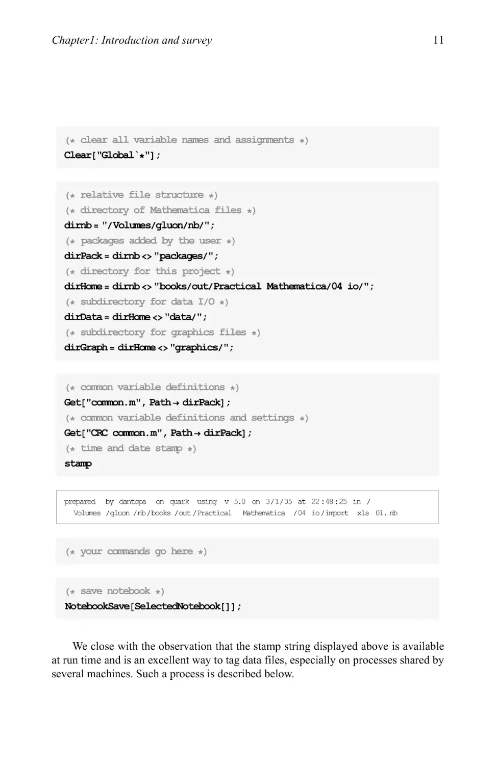
When you put it all together, the seed notebook looks like this
Chapter 1: Introduction and survey
11
caear["GlabalV'] ;
dirrib = "/Volumes/gluon/nb/ " ;
dirPack = dirrib <> "packages/" ;
dirHome = dirrib <> "books/out/Practical Mathematica/04 io/";
dirData = dirHome <> "data/ " ;
dirGraph = dirHome <> "graphics/ " ;
Gtet["ccmmon.m", Path-> dirPack] ;
Get["CKC common, m", Path-> dirPack] ;
stamp
prepared
Volumes
by
dantopa
on quark
using v 5
/ gluon / nb / books / out / Practical
.0 on
3/1/05
Mathematica
at
/04
22
io
:48
:25
/import
in /
xls
01.
nb
NotebcokSave [ SelectedNotebook [ ] ] ;
We close with the observation that the stamp string displayed above is available
at run time and is an excellent way to tag data files, especially on processes shared by
several machines. Such a process is described below.
12
A Beginner's Guide to Mathematica
1.2.2 Distributed computing
Here we present a toy model for using several machines to complete a task. In our
example, we used half a dozen machines to generate high-density plots of
two-dimensional functions we were generating. We have one machine which is the controller.
The controller has two special files: the task assignment file and the Mathematica plot
module. The task assignment problem can be an ASCII file. It is simply the number of
the next plot to evaluate (the plot were numbered linearly).
Distribution is simple. In our case, all servant machines had mapped their B:
drive to the controller directory. In this way every servant is running the exact same
code. This is imperative. Different code on different machines creates headaches.
When the servant machine is ready, it first gets a task assignment. For example, if plot
15 is the next plot to do out of 100 plots, then the task assignment file contains two
lines: the value 15 and the value 100. To get an assignment, a servant machine opens
the file, reads 15, checks that this is less than or equal to the termination value 100,
writes 16 and closes the file. The plot module is loaded from the controller machine
which ensures that the plots are identical.
Distributed processing is a great way to use computing power normally unused
overnight or during the weekends. As a courtesy to those affected, they should be
reminded to reboot their machines since Mathematica may have saturated their
physical memory and may push applications to virtual memory on the hard drive which is
much slower.
Note that Wolfram Research has a parallel processing add-on package to turn
multiple CPUs into a true parallel processing computer. You can read about it at
www, wol fram. com /produ cts/appl i cati on s/paral 1 el /.
1.2.3 Minor bugs in the front end
There are some minor bugs in the front end that have persisted through a few releases.
Fortunately, they do not affect the quality of the kernel computations. However, one
class of error will prevent the kernel from seeing your code.
Leading spaces
At times the front end will introduce leading spaces. Suppose, for example, that you
have created and saved the directory structure above. It executes fine and when you
close the notebook, the code block looks exactly as it does above. But when you open
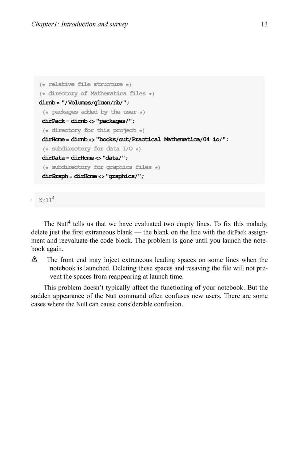
it, spaces have been prepended. When you execute the code block, you will see
Chapter 1: Introduction and survey
13
dirrib = "/Volumes/gluon/rib/ " ;
dirPack = dirrib <> "packages/" ;
dirHcme = dirrib <> "books/out/Practical Mathematica/04 io/";
dirData = dirHcme <> "data/ " ;
dirGraph = dirHcme <> "graphics/" ;
= Null4
The Null4 tells us that we have evaluated two empty lines. To fix this malady,
delete just the first extraneous blank — the blank on the line with the dirPack
assignment and reevaluate the code block. The problem is gone until you launch the
notebook again.
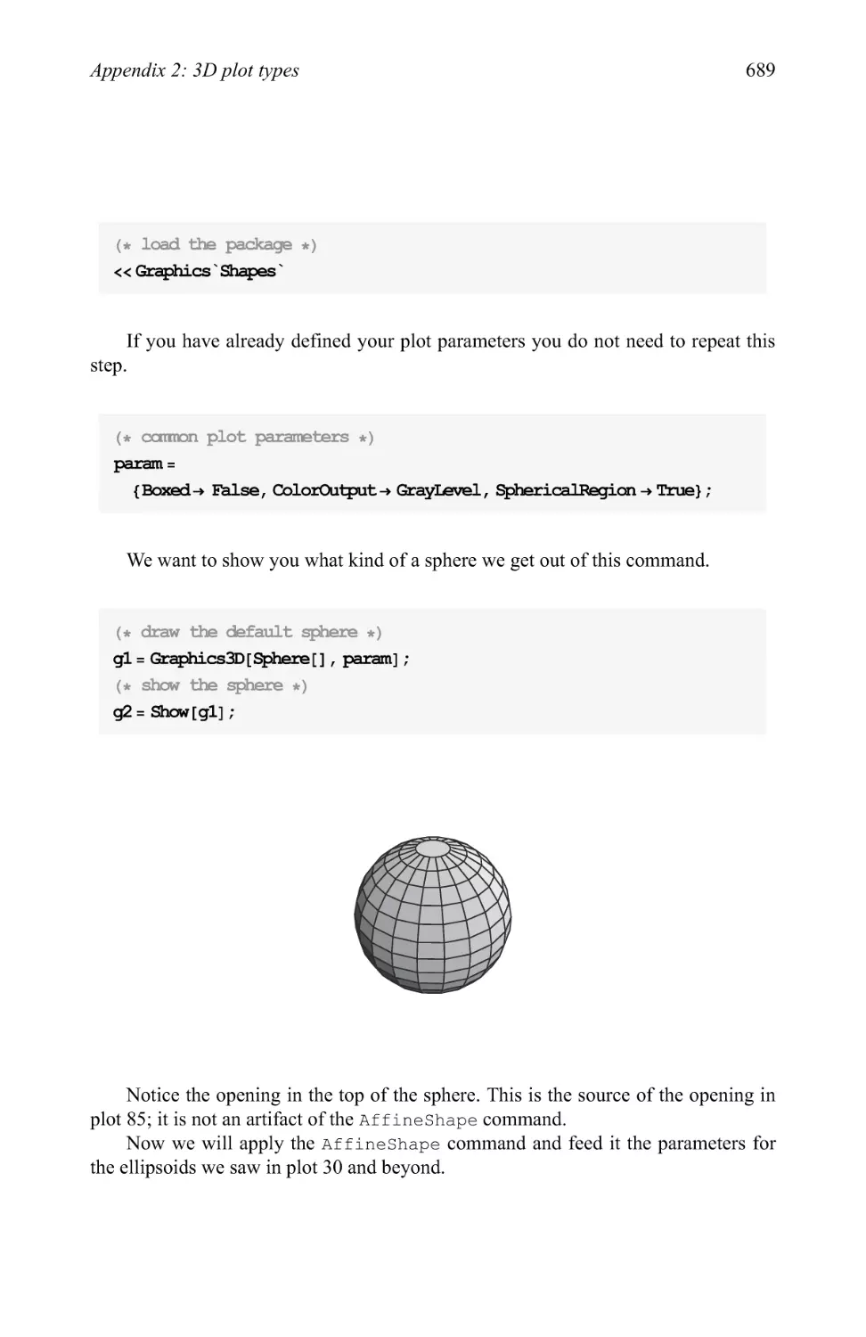
A The front end may inject extraneous leading spaces on some lines when the
notebook is launched. Deleting these spaces and resaving the file will not
prevent the spaces from reappearing at launch time.
This problem doesn't typically affect the functioning of your notebook. But the
sudden appearance of the Null command often confuses new users. There are some
cases where the Null can cause considerable confusion.
14
A Beginner's Guide to Mathematica
pgen[l_Integer, mJEnteger] := Module[{g},
g= Spherica 1 HarmonicY[ 1, m, e, <p] ;
g2 = Simplify[gConjugate[g] , Ge Reals A^ie Reals] ;
];
{1, m} = {5,3};
pgen[l, m]
g2
385 Null3 (7 + 9Cos[2e])2Sin[e]6
4096/r
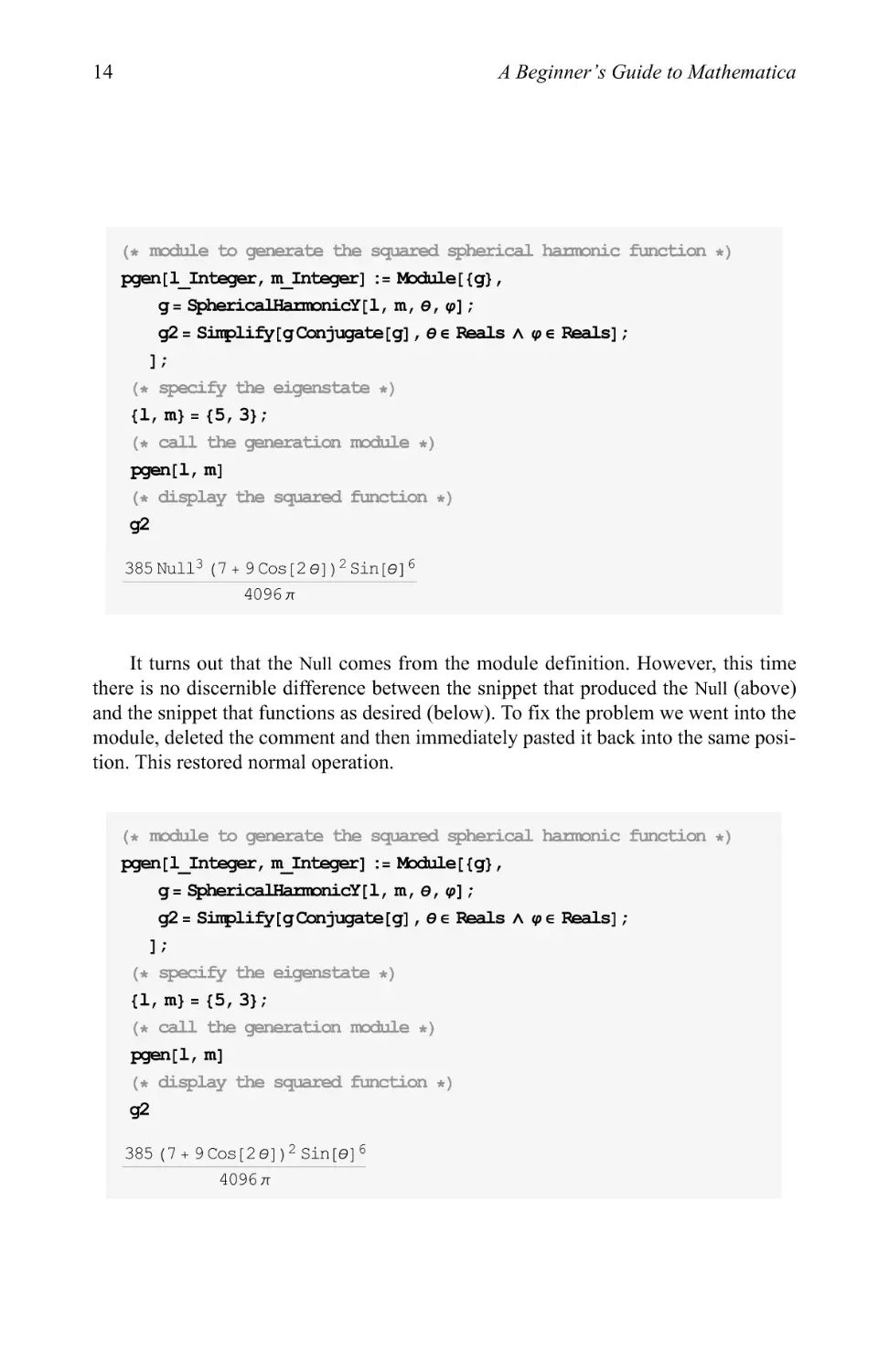
It turns out that the Null comes from the module definition. However, this time
there is no discernible difference between the snippet that produced the Null (above)
and the snippet that functions as desired (below). To fix the problem we went into the
module, deleted the comment and then immediately pasted it back into the same
position. This restored normal operation.
pgen[l_Integer, mJEnteger] := Module[{g},
g= Spherica 1 Ha rmonicY [ 1, m, e, q>] ;
g2 = Simplify[gConjugate[g] , 06 Reals A^ie Reals] ;
];
{1, m} = {5,3};
pgen[l, m]
g2
385 (7 + 9 Cos [2 G])2 Sin[e]6
4096/r
Chapter 1: Introduction and survey
15
A The Mathematica front end may react unfavorably to comments and cause
extraneous Nulls to appear. Deleting the comments and repasting them will
restore normal operation for the remainder of the session.
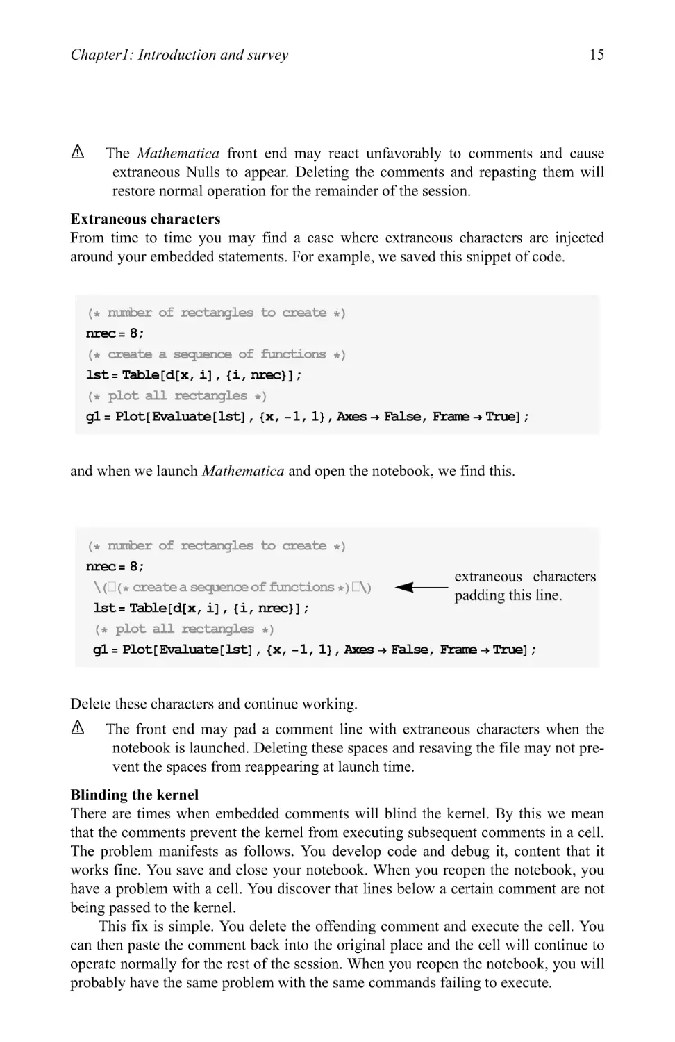
Extraneous characters
From time to time you may find a case where extraneous characters are injected
around your embedded statements. For example, we saved this snippet of code.
nrec= 8;
lst= Table[d[x, i] , {i, nrec}] ;
gl = Plot [Evaluate [1st] , {x, -1, 1}, Axes -> False, Frame -> True] ,
and when we launch Mathematica and open the notebook, we find this.
nrec= 8;
extraneous characters
padding this line.
lst= Table[d[x, i] , {i, nrec}] ;
gl = Plot [Evaluate [1st] , {x, -1, 1}, Axes -> False, Frame -> True] ;
Delete these characters and continue working.
A The front end may pad a comment line with extraneous characters when the
notebook is launched. Deleting these spaces and resaving the file may not
prevent the spaces from reappearing at launch time.
Blinding the kernel
There are times when embedded comments will blind the kernel. By this we mean
that the comments prevent the kernel from executing subsequent comments in a cell.
The problem manifests as follows. You develop code and debug it, content that it
works fine. You save and close your notebook. When you reopen the notebook, you
have a problem with a cell. You discover that lines below a certain comment are not
being passed to the kernel.
This fix is simple. You delete the offending comment and execute the cell. You
can then paste the comment back into the original place and the cell will continue to
operate normally for the rest of the session. When you reopen the notebook, you will
probably have the same problem with the same commands failing to execute.
16
A Beginner's Guide to Mathematica
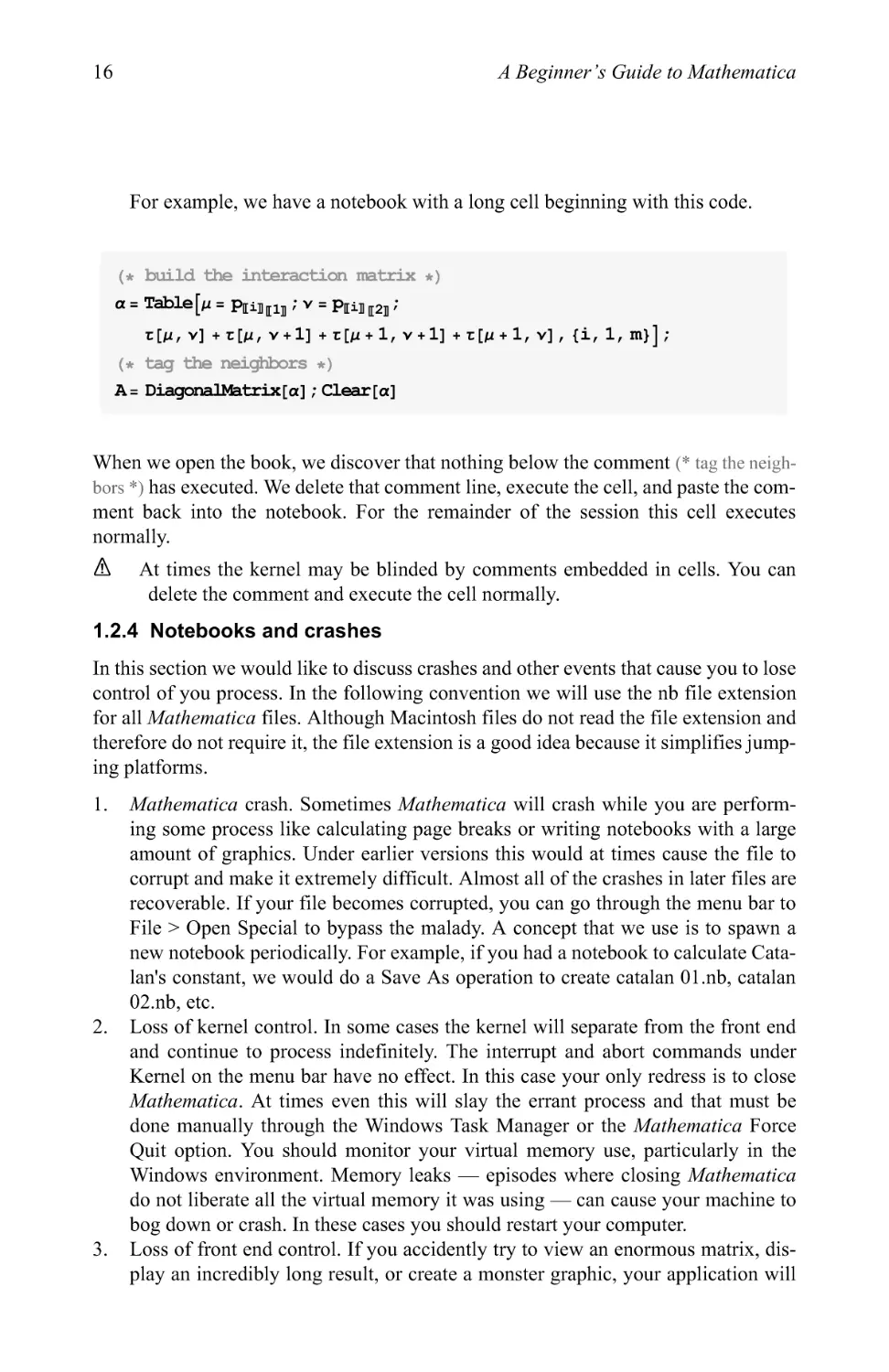
For example, we have a notebook with a long cell beginning with this code.
a = Table[ji = V>uHll; v = p^ l2]] ;
r[ju, v] + r[ju, v + 1] + r[ju + l, v + 1] + r[ju + l, v] , {i, 1, m}] ;
A= DiagonalMatrix[o] ; Clear [o]
When we open the book, we discover that nothing below the comment (* tag the
neighbors *) has executed. We delete that comment line, execute the cell, and paste the
comment back into the notebook. For the remainder of the session this cell executes
normally.
A At times the kernel may be blinded by comments embedded in cells. You can
delete the comment and execute the cell normally.
1.2.4 Notebooks and crashes
In this section we would like to discuss crashes and other events that cause you to lose
control of you process. In the following convention we will use the nb file extension
for all Mathematica files. Although Macintosh files do not read the file extension and
therefore do not require it, the file extension is a good idea because it simplifies
jumping platforms.
1. Mathematica crash. Sometimes Mathematica will crash while you are
performing some process like calculating page breaks or writing notebooks with a large
amount of graphics. Under earlier versions this would at times cause the file to
corrupt and make it extremely difficult. Almost all of the crashes in later files are
recoverable. If your file becomes corrupted, you can go through the menu bar to
File > Open Special to bypass the malady. A concept that we use is to spawn a
new notebook periodically. For example, if you had a notebook to calculate
Catalan's constant, we would do a Save As operation to create Catalan 01.nb, Catalan
02.nb, etc.
2. Loss of kernel control. In some cases the kernel will separate from the front end
and continue to process indefinitely. The interrupt and abort commands under
Kernel on the menu bar have no effect. In this case your only redress is to close
Mathematica. At times even this will slay the errant process and that must be
done manually through the Windows Task Manager or the Mathematica Force
Quit option. You should monitor your virtual memory use, particularly in the
Windows environment. Memory leaks — episodes where closing Mathematica
do not liberate all the virtual memory it was using — can cause your machine to
bog down or crash. In these cases you should restart your computer.
3. Loss of front end control. If you accidently try to view an enormous matrix,
display an incredibly long result, or create a monster graphic, your application will
Chapter 1: Introduction and survey
17
appear to stall. It is just the front end working busily for you. But if completion of
the task will take days, weeks, or years, waiting may not be an option. Your only
recourse is to close Mathematica and to relaunch. When you get back into your
notebook, divert your output to a file. Also as in the second case, check for
memory leaks and restart if warranted.
4. Mathematica has very strong capabilities and can easily generate problems that
gobble up gigabytes of memory. We have noticed on Windows machines that
saturating the memory can lead to erratic behavior. Other applications may exhibit
unusual symptoms and Mathematica may act strangely and give the wrong
answer. Although quite rare, the user should be aware. The prescribed cure is to
reboot. Although many people do not believe us, we have demonstrated problems
with virtual memory in the Windows environment. We had notebooks that would
not work when using virtual memory. As soon as we boosted physical memory
the notebooks could work. Yes, we know the official story is that virtual and
physical memory have the same functionality (albeit different speeds), but the
empirical data clearly shows that physical memory is best. In a Windows
environment Mathematica will take less than 2 GB, so if you are wondering how
much RAM to install make sure that Mathematica will have its 2 GB.
1.3 Entering data
Are you a keyboard person or a mouse person? Either way your preferences are
satisfied with Mathematica. Mouse users can pick and choose from the well-organized
palettes available from the menu bar. These palettes will be presented next. Keyboard
users will be happy to find a rather extensive set of keyboard shortcuts. These
shortcuts are nice and we show an example below.
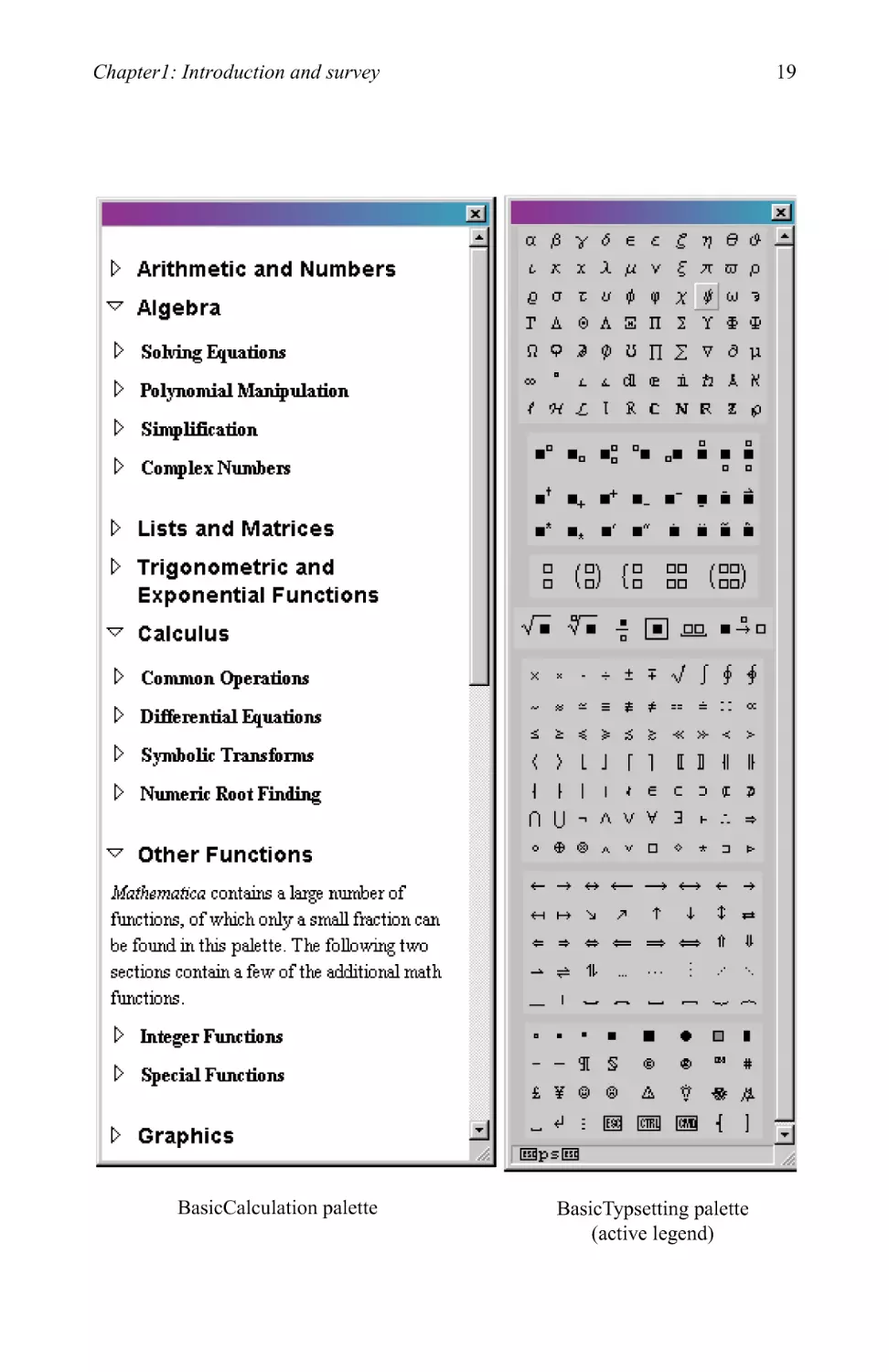
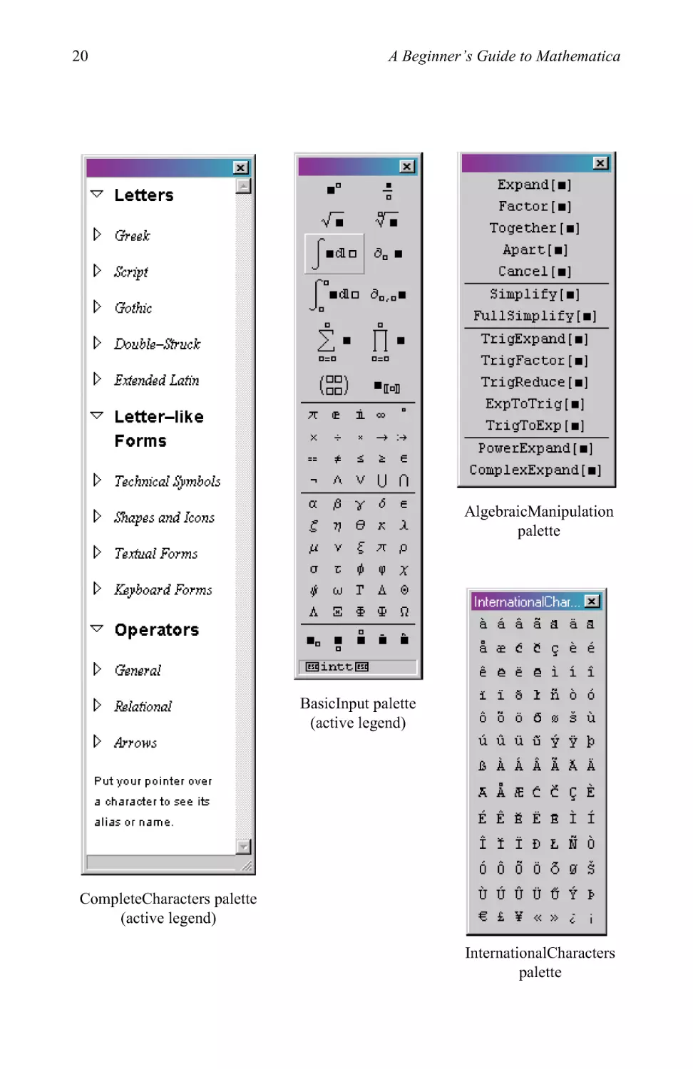
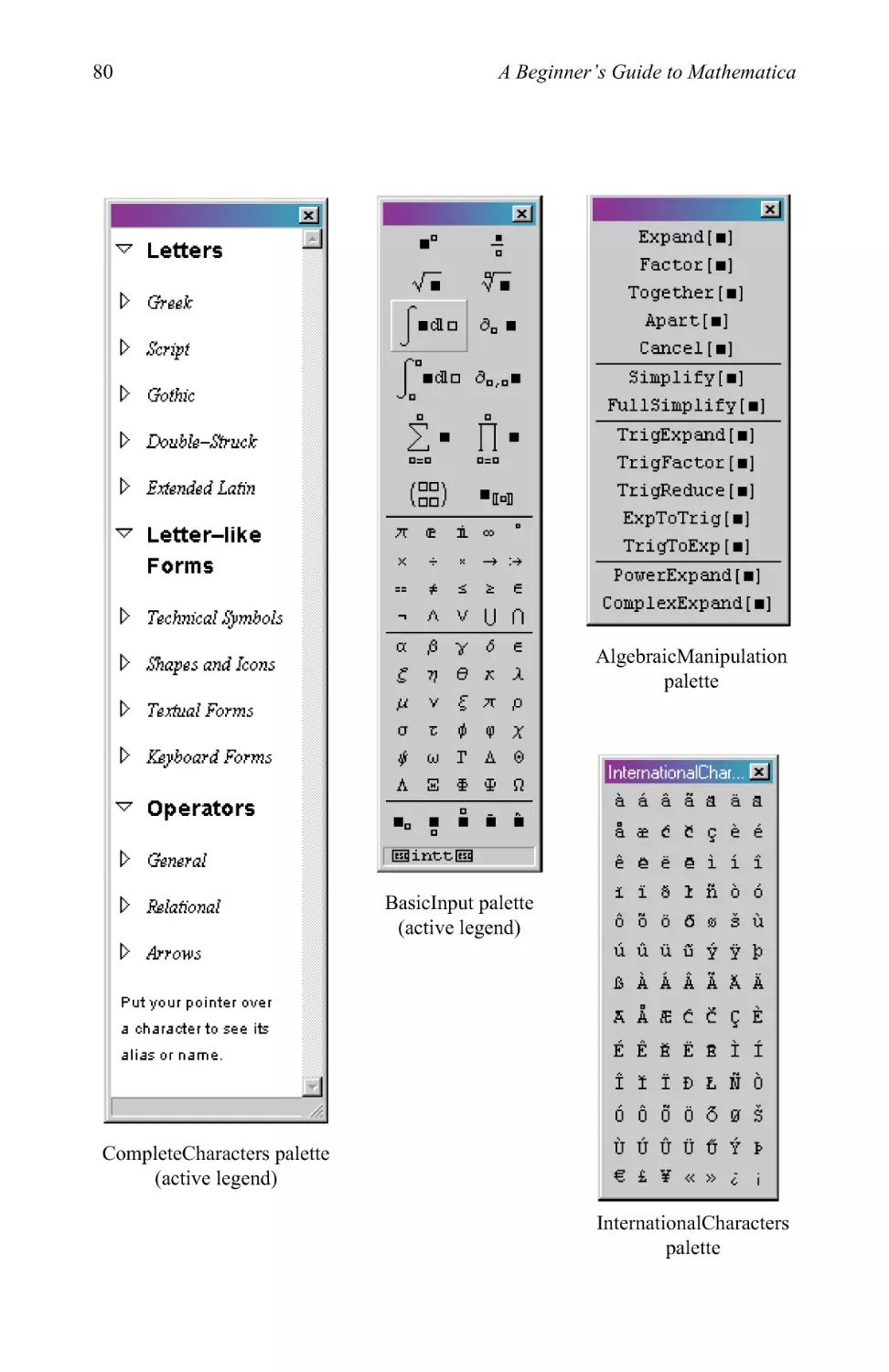
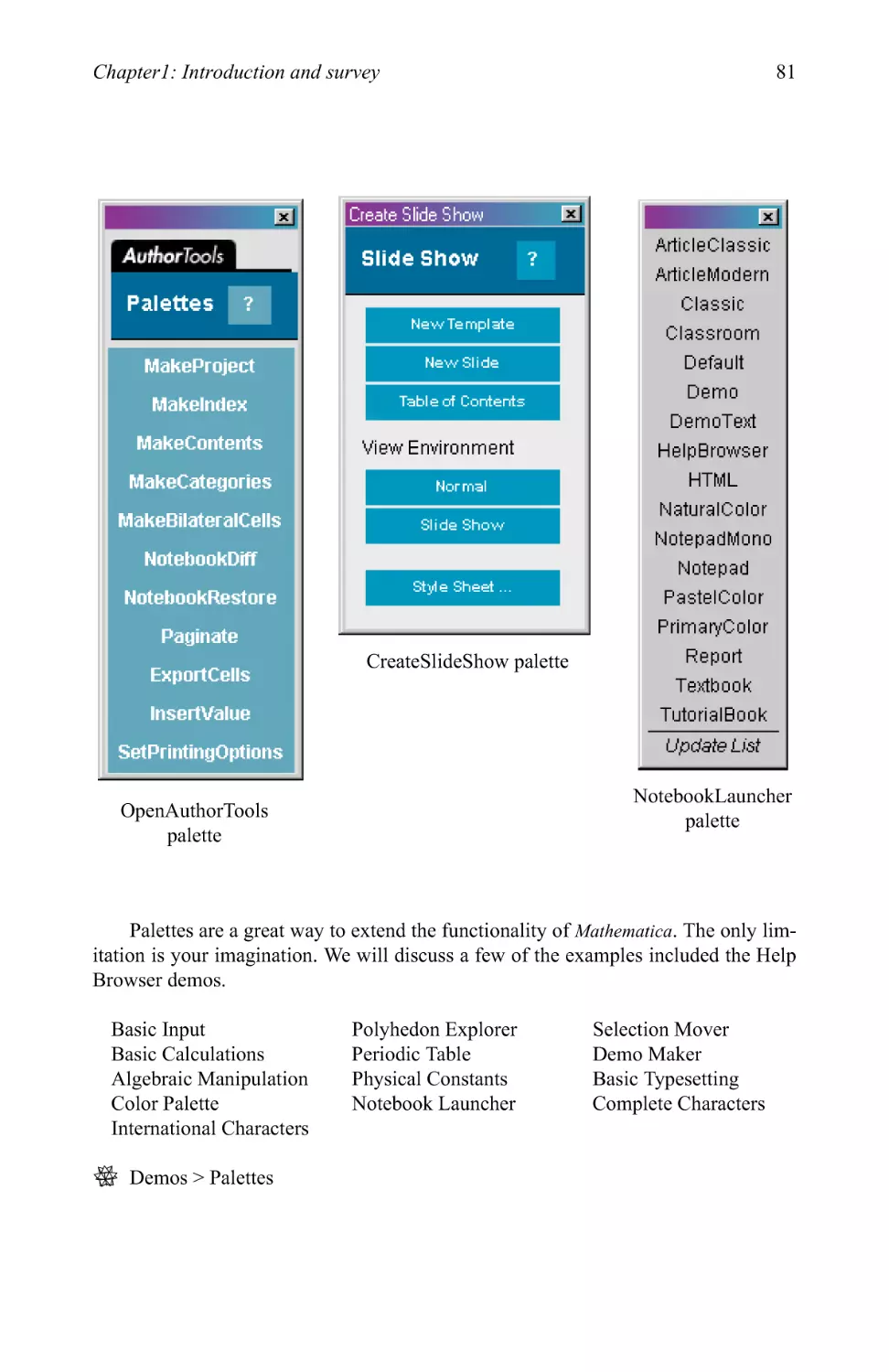
1.3.1 Standard palettes
Mathematica has many useful palettes to simplify our lives. To access the palettes, go
through the menu bar File > Palettes and you will see the following list of nine
palettes:
OpenAuthorTools Basiclnput CreateSlideShow
AlgebraicManipulation BasicTypesetting InternationalCharacters
BasicCalculations CompleteCharacters NotebookLauncher
Unfortunately, not all of these palettes display their titles. For this reason, and to
acquaint the reader with their functional capability we will show all the palettes
below.
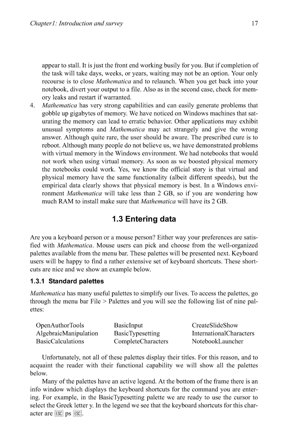
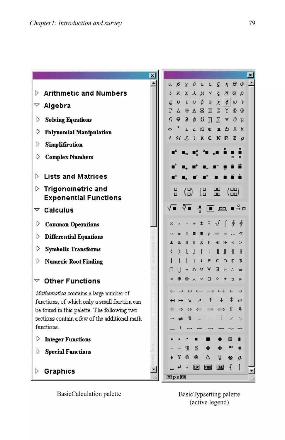
Many of the palettes have an active legend. At the bottom of the frame there is an
info window which displays the keyboard shortcuts for the command you are
entering. For example, in the BasicTypesetting palette we are ready to use the cursor to
select the Greek letter y. In the legend we see that the keyboard shortcuts for this
character are [esc] ps [escI.
18
A Beginner's Guide to Mathematica
These palettes are "sticky" in the sense that their state is recorded when
Mathematica closes and the environment is recreated when Mathematica is launched. In
other words if you have three palettes open when you close Mathematica, the same
three, and only these three will be opened when Mathematica is launched. The demo
palettes listed below are not sticky and they need to be opened each time you use
them.
1.3.2 Keyboard shortcuts
Over time people tend to gravitate toward the keyboard shortcuts because they are so
much faster. We will show two examples in this section. Also, for the remainder of the
chapter we will display the keyboard shortcuts that we used to create the Mathematica
code. At the end of the chapter we point you to an extensive list of the keyboard
shortcuts in the Help Browser.
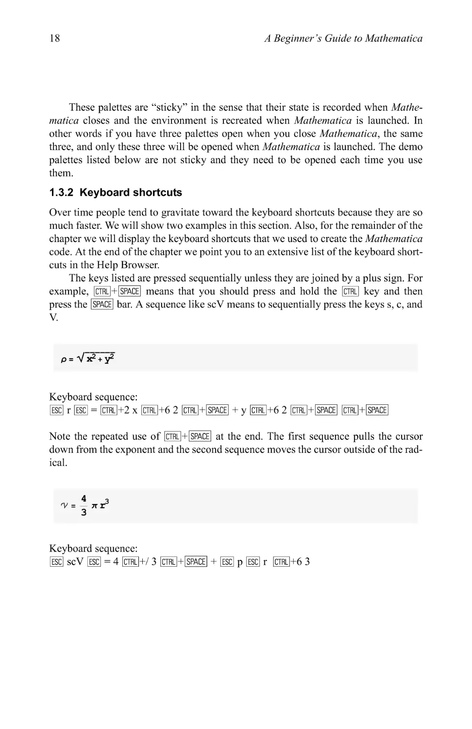
The keys listed are pressed sequentially unless they are joined by a plus sign. For
example, | CTRL |+| SPACE] means that you should press and hold the | CTRL | key and then
press the | SPACE | bar. A sequence like scV means to sequentially press the keys s, c, and
V.
p= V^ + y2
Keyboard sequence:
[esc] r [esc] = [cTrD+2 x [ctrO+6 2 [ctr^+I space | + y [ctrO+6 2 [ctrl1+|space| [ctrl1+|space|
Note the repeated use of | CTRL |+| SPACE] at the end. The first sequence pulls the cursor
down from the exponent and the second sequence moves the cursor outside of the
radical.
^ 3
'V = 7r r
Keyboard sequence:
[esc! scV [esc] = 4 [ctrO+/ 3 [ctrlI+Ispace| + [esc] p [esc] r [ctrO+6 3
Chapter 1: Introduction and survey
19
>
^7
>
>
>
>
>
>
^7
>
>
>
>
^7
^^^^^^^M *\\
■*■ i
Arithmetic and Numbers
Algebra
Solving Equations
Polynomial Manipulation
Simplification
Complex Numbers
Lists and Matrices
Trigonometric and
Exponential Functions
Calculus
Common Operations 1
Differential Equations
Symbolic Transforms
Numeric Root Finding
Other Functions
MflfAemflft'cfl contains a large number of
functions, of which only a small fraction can
be found in this palette. The following two
sections contain a few of the additional math
functions.
>
>
>
Integer Functions
Special Functions
Graphics -^J
t K X JJ. ^ V £ 7T GJ p
TAGAEIISYS*
» n LidlE i f] A K
■+ «+ -+
n tnJ In nn InnJ
Vi^^H
.DP. ■ ■
X
"
±
<
\
n
o
«-
*H
^
_*
x - + ±
h s = £
£ 3 5= £
> l j r
Mm
[J - A V
* ® A V
-> *+ *—
H* ^ 7"
^ o ^
^ U ...
* V J *
* == = ::
&■«»■<
1 I J \\
e c d i
V 3 h .".
n * * n
—* «—> «-
t I t
=* » ft
*
oc
>-
If
5
^
fe-
->
1=±
4
n - ■ ■ ■ * D I
£ ¥ © © a t * A
_ ^J E [Eg S 1^ ■[ ] "J,
EOpsEO
BasicCalculation palette
BasicTypsetting palette
(active legend)
20
A Beginner's Guide to Mathematica
^^^^^m
^ Letters
I> Greek
I> Script
I> Gothic
[> Double-Struck
[> Extended Latin
^ Letter-like
Forms
[> Technical Symbols
[> Shapes and Icons
[> Textual Forms
[> Keyboard Forms
^ Operators
I> General
[> Relational
[> ^rou^
Put your pointer over
a character to see its
alias or name.
xj
J
J
■"
«/i
h
[■dl
Jn
D
z-
D = D
7T <E
X +
== *
-. A
a p
£ V
V v
a r
^ 0J
A E
□
n
i
X
£
V
y
e
C
*
r
*
D
■o ■ ■
■
D
*]
^W
5n
^n„
D
n
D = D
■
:■
■
■m
00
-*
1
U
<5
K
7T
<P
A
*
D
""*
e
n
e
A
P
*
0
n
Basiclnput palette
(active legend)
Expand[■]
Factor[■]
Together[■
Apart[■]
Cancel[■]
Simplify[■]
FullSimplifyla:
TrigExpand[«]
TrigFactor[■]
TrigReduce[«]
ExpToTrig[«]
TrigToExp[«]
PowerExpand[«]
ComplexExpand[i
AlgebraicManipulation
palette
CompleteCharacters palette
(active legend)
1 Internatio
a a
a ae
e e
i i
6 o
u u
& A
D
A A
E E
I 1
6 6
u u
€ £
a
d
e
S
0
ii
A
E
fi
I
0
U
¥
nalChar.
a
e
n
1
e
u
A
C
E
D
0
U
«
a e
? e
i :
fi c
s £
Y i
A 2
e c
E ]
z. i
i e
. i
j 6
J u
' 1?
t A
; e
: i
J 6
S Of 5
e i
» ^
r t
i
InternationalCharacters
palette
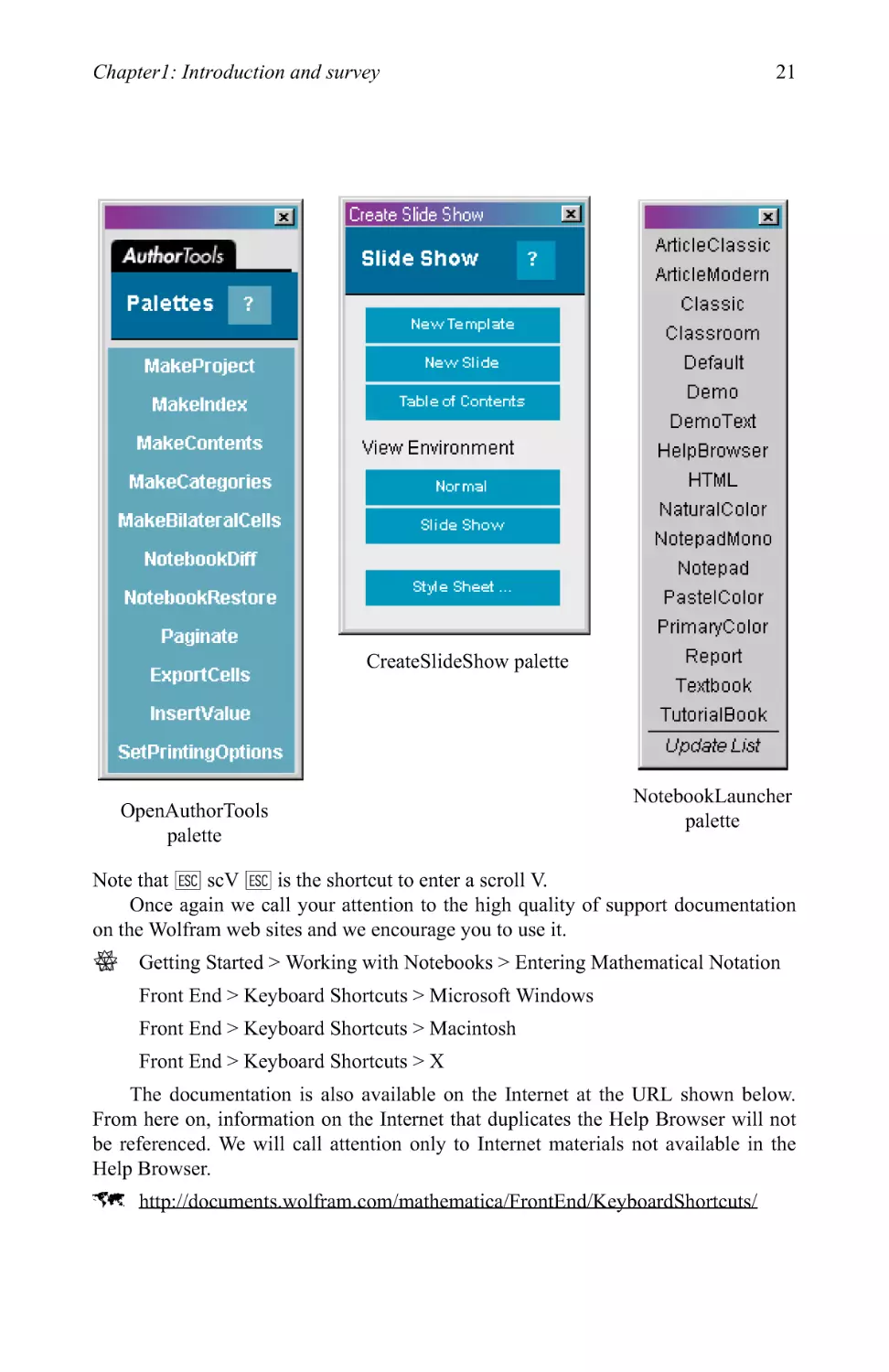
Chapter!: Introduction and survey
21
*]
■SJ
Slide Show
Table of Contents
View Environment
CreateSlideShow palette
OpenAuthorTools
palette
ArticleClassic
ArticleModern
Classic
Classroom
Default
Demo
DernoTetft
HelpBrowser
HTML
NaturalColor
NotepadMono
Notepad
PastelColor
PrimaiyColor
Report
Textbook
TutorialBook
Update List
NotebookLauncher
palette
Note that [esc] scV [esc] is the shortcut to enter a scroll V.
Once again we call your attention to the high quality of support documentation
on the Wolfram web sites and we encourage you to use it.
^ Getting Started > Working with Notebooks > Entering Mathematical Notation
Front End > Keyboard Shortcuts > Microsoft Windows
Front End > Keyboard Shortcuts > Macintosh
Front End > Keyboard Shortcuts > X
The documentation is also available on the Internet at the URL shown below.
From here on, information on the Internet that duplicates the Help Browser will not
be referenced. We will call attention only to Internet materials not available in the
Help Browser.
"T*£ http://documents.wo1fram.com/mathematica/FrontEnd/KeyboardShortcuts/
22
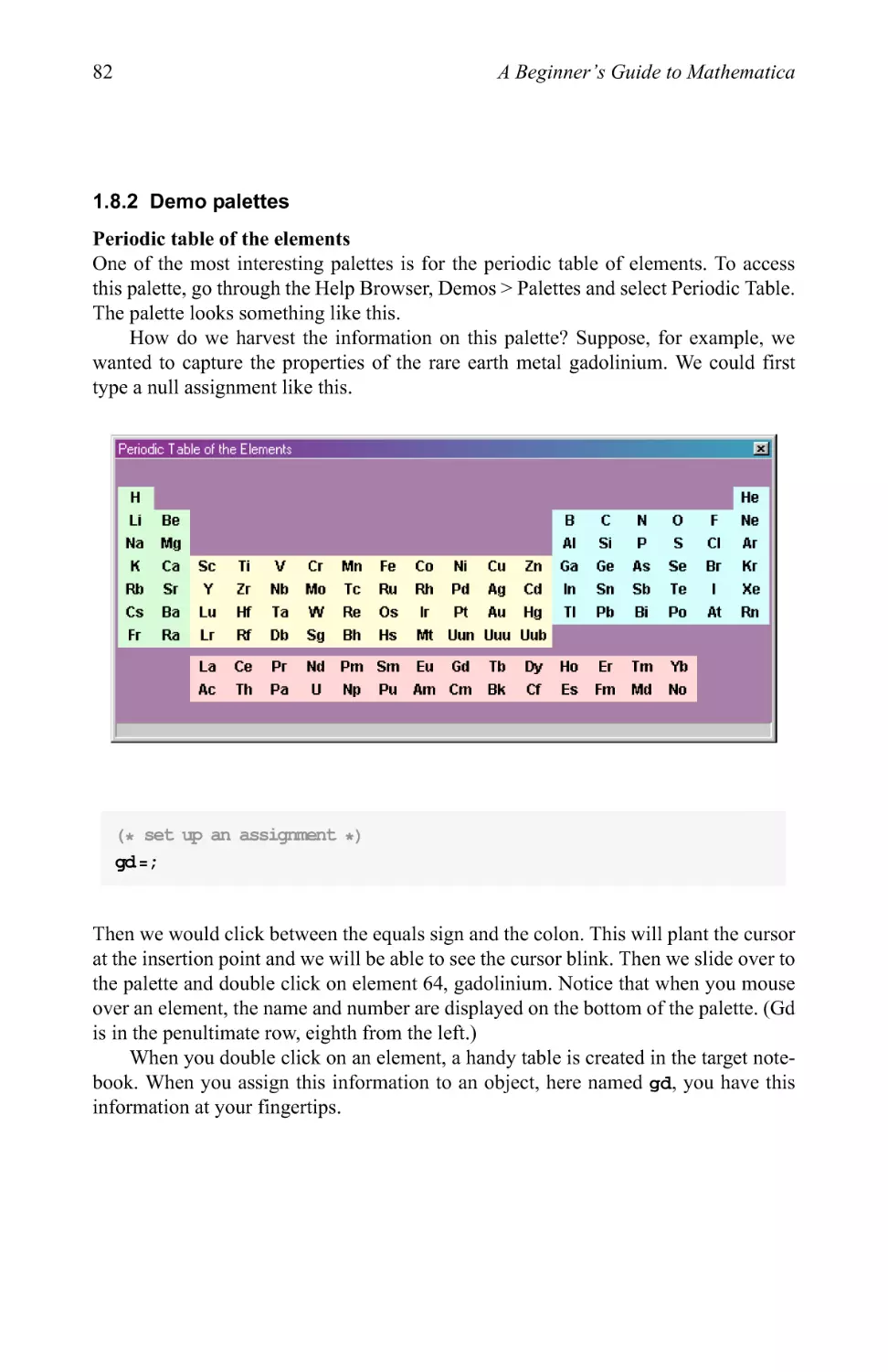
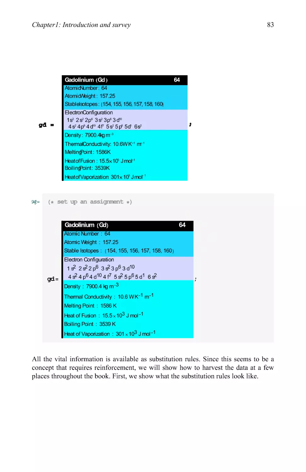
A Beginner's Guide to Mathematica
1.4 Data structures
Many of us are familiar with the representation of numbers in modern computer
languages. We expect to find integers of different sizes (say 4 or 8 bytes), real numbers in
single and double precision, and complex numbers composed of pairs of real numbers
and strings. Mathematica gives us a far richer set of tools:
1. Integers of arbitrary size
2. Rational numbers of arbitrary size
3. Symbols such a p
4. Real numbers of double precision
5. Complex numbers and quaternions
6. Lists
Our experience from learning Mathematica and from aiding others to learn
Mathematica has shown us that it is difficult to look at the list of data structures and realize
how very different Mathematica is. Perhaps this is because we have used the
conventional data structures to explore our world for so long that we are now accustomed to
formulating problems in terms of the tools we are familiar with.
For example, the arbitrary sized integers and rational number representation
allow us to compute some answers to arbitrary precision. In other words, we can get
as much precision as we want. It becomes a question of computer time. This is a great
boon. Perhaps some users will think of arbitrary precision and an extension of double
precision — but it is far more than that as we shall see. We are now able to do
computations far closer to singularities. Matrix inversions can now dance within a razors
edge of singularity. It truly empowers us for we are now no longer limited by the
computer.
Also, the symbolic capability allows us to do incredibly long calculations and
recover exact answers or answers of arbitrary precision. This is a most welcome gift.
Consider the case of using Mathematica to develop an algorithm. Typically we test
the algorithm by looking for a difference from zero in some special cases. In
FORTRAN we get an answer like machine noise and must decide whether or not is it truly
machine noise or some algorithmic imprecision.
Do not think that because Mathematica allows completely arbitrary list structures
that it is list-friendly. Mathematica is the ultimate list-processing platform and is
designed around this concept. So many of our examples will show that Mathematica
was designed around the list concept. When you see the performance improvements
from using lists, you will realize Mathematical true pedigree.
1.4.1 Representations
There are many ways to represent data with Mathematica. We shall explore some of
the most popular types using the sample list shown here that allows you to see how
different types of data are represented.
Chapter 1: Introduction and survey
23
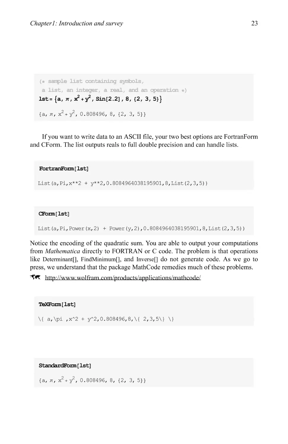
lst= {a, 7T, x^ + y2, Sin[2.2] , 8, {2, 3, 5}}
{a, 7T, x2+y2, 0.808496, 8, {2, 3, 5}}
If you want to write data to an ASCII file, your two best options are FortranForm
and CForm. The list outputs reals to full double precision and can handle lists.
FortranForm [ 1st]
List(a,Pi,x**2 + y**2,0.8084964038195901,8,List (2,3,5))
CForm [1st]
List(a,Pi,Power(x,2) + Power(y,2),0.8084964038195901,8,List(2,3,5))
Notice the encoding of the quadratic sum. You are able to output your computations
from Mathematica directly to FORTRAN or C code. The problem is that operations
like Determinant], FindMinimum[], and Inverse[] do not generate code. As we go to
press, we understand that the package MathCode remedies much of these problems.
"T*£ h ttp;//www.wolfram.com/products/applications/mathcode/
TfeXForm[lst]
\{ a,\pi ,xA2 + yA2,0.808496,8,\{ 2,3,5\} \}
StandardForm [ 1st]
{a, 7T, x2+y2, 0.808496, 8, {2, 3, 5}}
24
A Beginner's Guide to Mathematica
TraditionalForm [ 1st]
j?+ /, 0.808496, 8, {2, 3, 5}}
InputForm [ 1st]
{a, Pi, xA2 + yA2, 0.8084964038195901, 8, {2, 3, 5}}
OutputForm [ 1st]
2 2
{a, Pi, x + y , 0.808496, 8, {2, 3, 5}}
1.4.2 Queries
A wonderful feature of the interactive Mathematica environment is being able to
query our computations in real times. The user should immediately etch into memory
two very important commands: Head[] and ?.
The Head of a number describes its type. The question mark operator shows us all
definitions of the symbol. This is most helpful for new users who have accidently
created multiple definitions of a variable or module. We will frequently show how to call
these commands and interpret their meaning because we think this should be the first
step in constructing larger code blocks and debugging.
Chapter 1: Introduction and survey
25
1.4.3 Entering data
Mathematica Help Browser
Jn]_xj
_J | M>
Front End | Getting Started | Tour
Built-in Functions I Add-ons fc Links
Go n
Demos | Master Index
The Mathematica Book
Numerical Comp ► _tj
Algebraic Compi ►
Mathematical Fu ►
Lists and Matrici ►
Graphics and S< ►
Programming
*%• A k. __J
(Alphabetical Listii*|
List Constructior ►
Element Extractii ►
List Testing ►
List Operations ►
Structure Manipi ►
d
Part
First
Head
Extract
Take
.*.
—]
d
Last
■ LastO^?-] gives the last element inexpr.
■ L&3t[expr ] is equivalent to expr [ [ -1 ] ].
■ See Section 1.2.4.
■ See also: Part, First, Take, Most,
■ Mh> 2>J f^rSlOH I.
Further Examples
This returns the last element from the list.
in[1]:= Last [{a, h, c, d}]
uijt[i]= d
100% ^ <l
J
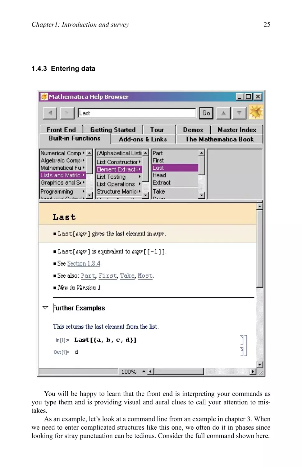
You will be happy to learn that the front end is interpreting your commands as
you type them and is providing visual and aural clues to call your attention to
mistakes.
As an example, let's look at a command line from an example in chapter 3. When
we need to enter complicated structures like this one, we often do it in phases since
looking for stray punctuation can be tedious. Consider the full command shown here.
26
A Beginner's Guide to Mathematica
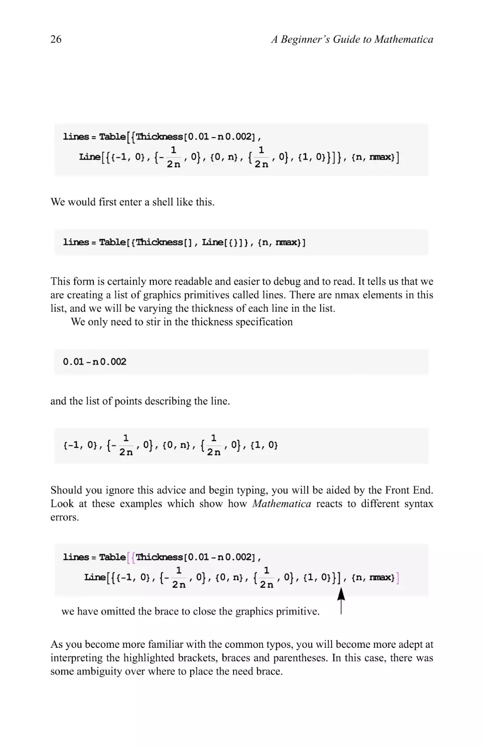
lines = Table[{Thickness[0.01 -n0.002] ,
Line[{{-1, 0}, {-^, °}' <0' n>' ij^' °}' t1' °>}]}' (n, nmax}]
We would first enter a shell like this.
lines = Table[{Thickness[] , Line[{}]}, {n, nmax}]
This form is certainly more readable and easier to debug and to read. It tells us that we
are creating a list of graphics primitives called lines. There are nmax elements in this
list, and we will be varying the thickness of each line in the list.
We only need to stir in the thickness specification
0.01-n0.002
and the list of points describing the line.
{_1' °}' t'2n'°^ {0'n}' (^ ' °1' {1' 0}
Should you ignore this advice and begin typing, you will be aided by the Front End.
Look at these examples which show how Mathematica reacts to different syntax
errors.
lines = Table Thickness[0.01 -n0.002] ,
Line[{{-1, 0}, {-t—, 0}, {0,n}, {— , 0}, {1, 0}}], {n, nmax}
l l i 2 n J L 2 n J J J
we have omitted the brace to close the graphics primitive. I
As you become more familiar with the common typos, you will become more adept at
interpreting the highlighted brackets, braces and parentheses. In this case, there was
some ambiguity over where to place the need brace.
Chapter 1: Introduction and survey
27
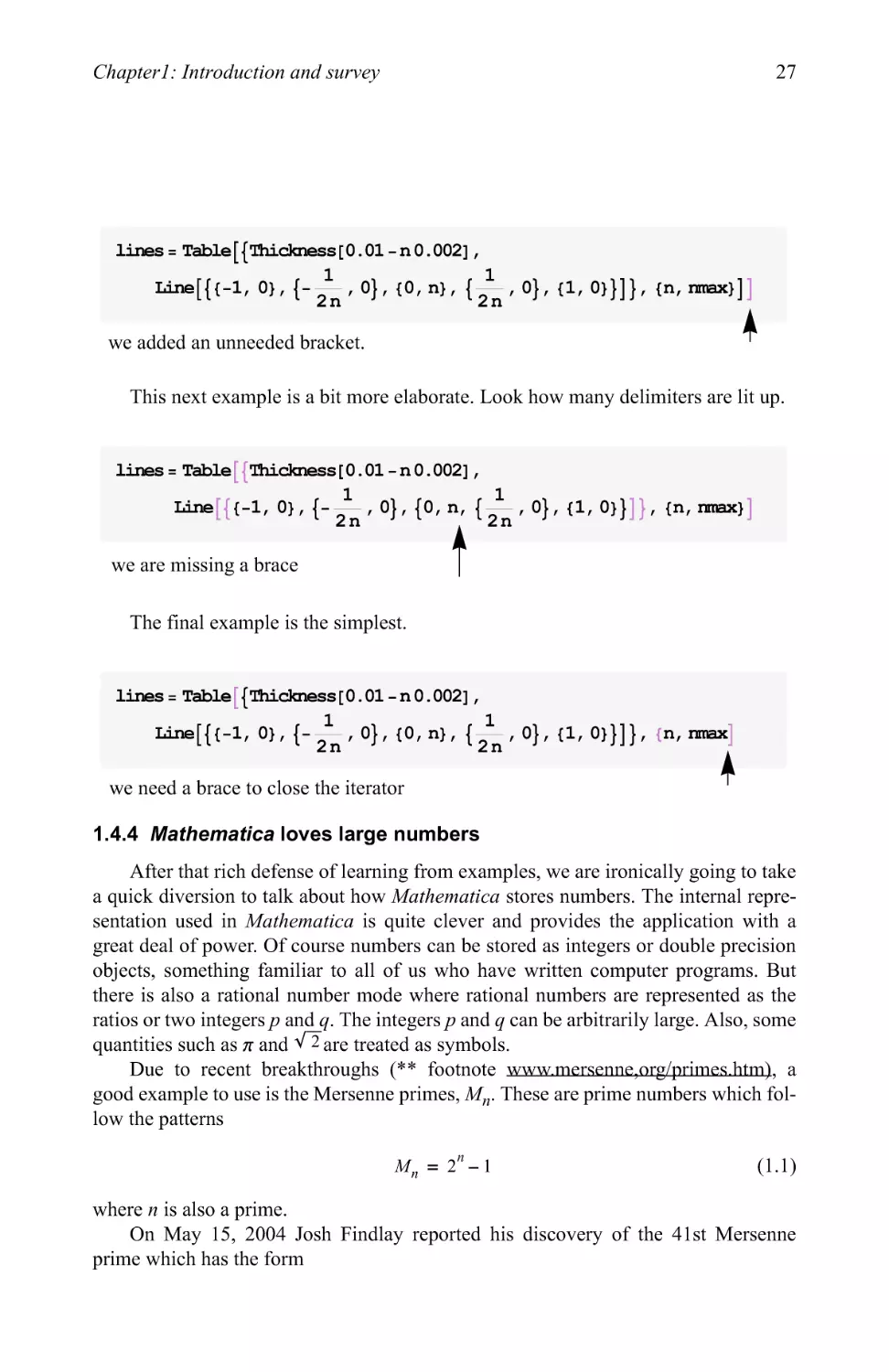
lines = Table[{Thickness[0.01 -n0.002] ,
Line[{{-1, 0}, {-^, 0} , {0,n}, {—, 0}, {1, 0}}]}, {n, nmax}]
A
we added an unneeded bracket. '
This next example is a bit more elaborate. Look how many delimiters are lit up.
lines = Table Thickness[0.01 -n0.002] ,
Line {-1, 0}, {~Yn' °}' {°'n' ij^' °}' &' °>1 ' O^™")
we are missing a brace |
The final example is the simplest.
lines= Table {Thickness[0.01-n0.002] ,
Line[{{-1, 0}, {-—, 0}, {0,n}, {—, 0} , {1, 0}}]},
we need a brace to close the iterator
1.4.4 Mathematica loves large numbers
After that rich defense of learning from examples, we are ironically going to take
a quick diversion to talk about how Mathematica stores numbers. The internal
representation used in Mathematica is quite clever and provides the application with a
great deal of power. Of course numbers can be stored as integers or double precision
objects, something familiar to all of us who have written computer programs. But
there is also a rational number mode where rational numbers are represented as the
ratios or two integers/? andg. The integers/? and q can be arbitrarily large. Also, some
quantities such as n and V 2 are treated as symbols.
Due to recent breakthroughs (** footnote www.mersenne;org/prirneshtrn); a
good example to use is the Mersenne primes, Mn. These are prime numbers which
follow the patterns
Mn = 2"-\ (1.1)
where n is also a prime.
On May 15, 2004 Josh Findlay reported his discovery of the 41st Mersenne
prime which has the form
n, nmax
28
A Beginner's Guide to Mathematica
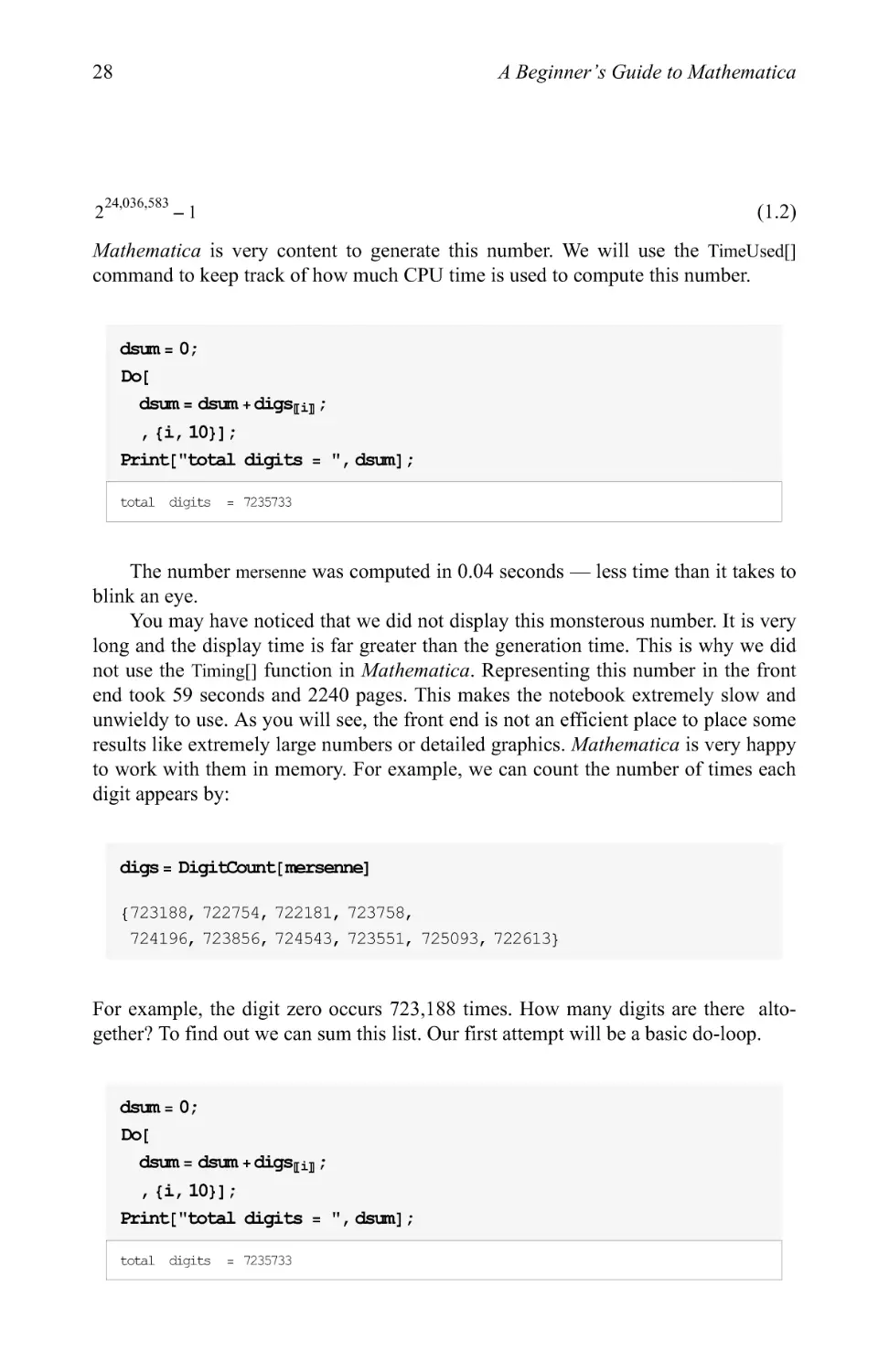
Mathematica is very content to generate this number. We will use the TimeUsed[]
command to keep track of how much CPU time is used to compute this number.
dsum= 0;
Do[
dsum = dsum + digsjij;
, {i, 10}];
Print ["total digits = ", dsum] ;
total digits = 7235733
The number mersenne was computed in 0.04 seconds — less time than it takes to
blink an eye.
You may have noticed that we did not display this monsterous number. It is very
long and the display time is far greater than the generation time. This is why we did
not use the Timing[] function in Mathematica. Representing this number in the front
end took 59 seconds and 2240 pages. This makes the notebook extremely slow and
unwieldy to use. As you will see, the front end is not an efficient place to place some
results like extremely large numbers or detailed graphics. Mathematica is very happy
to work with them in memory. For example, we can count the number of times each
digit appears by:
digs= DigitCount[ mersenne]
{723188, 722754, 722181, 723758,
724196, 723856, 724543, 723551, 725093, 722613}
For example, the digit zero occurs 723,188 times. How many digits are there
altogether? To find out we can sum this list. Our first attempt will be a basic do-loop.
dsum= 0;
Do[
dsum = dsum + digs^ij;
, {i, 10}];
Print ["total digits = ", dsum] ;
total digits = 7235733
Chapter 1: Introduction and survey
29
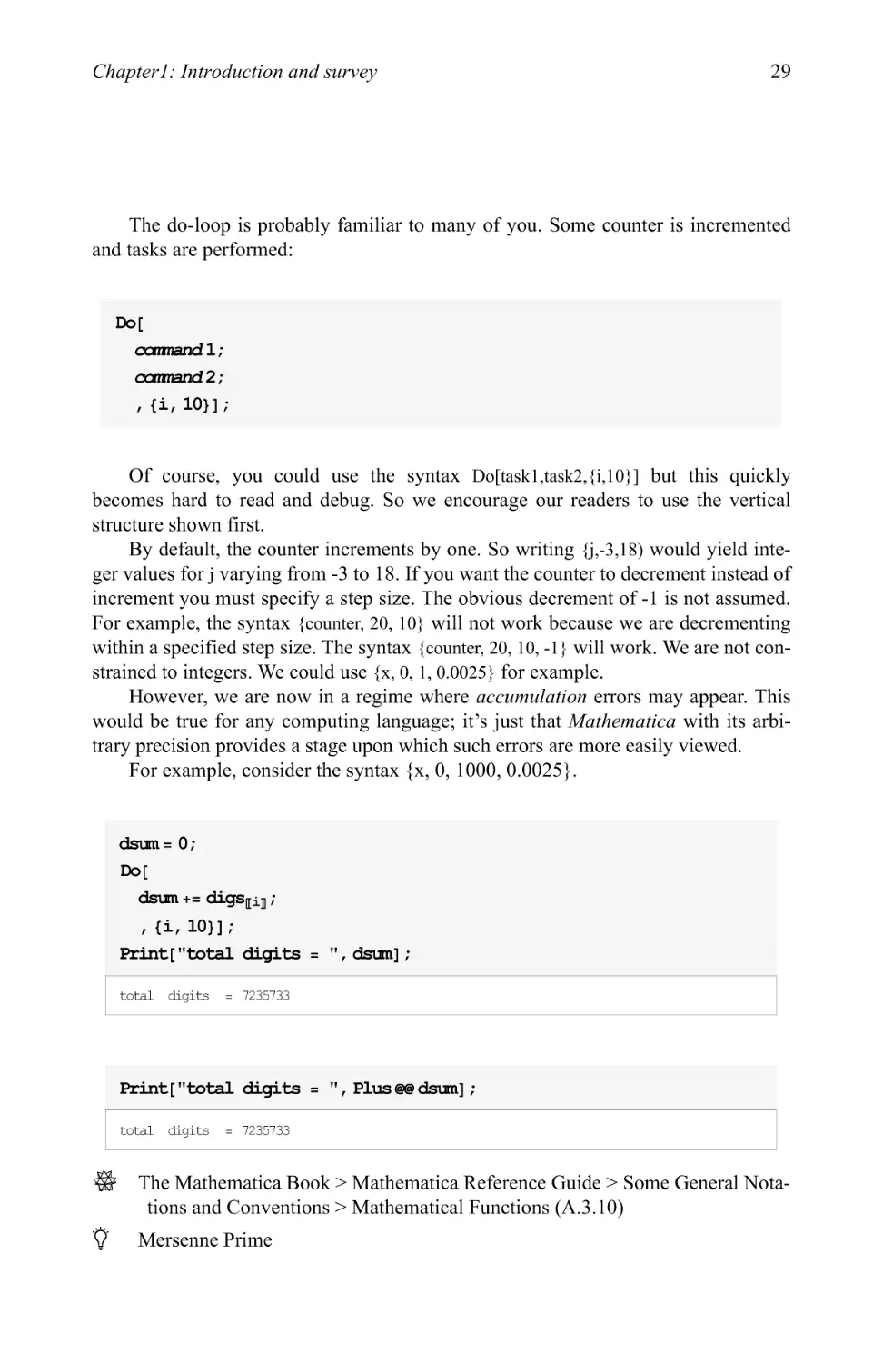
The do-loop is probably familiar to many of you. Some counter is incremented
and tasks are performed:
Do[
command 1;
command 2;
, {i, 10}];
Of course, you could use the syntax Do[taskl,task2,{i,10}] but this quickly
becomes hard to read and debug. So we encourage our readers to use the vertical
structure shown first.
By default, the counter increments by one. So writing {j,-3,18) would yield
integer values for j varying from -3 to 18. If you want the counter to decrement instead of
increment you must specify a step size. The obvious decrement of-1 is not assumed.
For example, the syntax {counter, 20, 10} will not work because we are decrementing
within a specified step size. The syntax {counter, 20, 10,-1} will work. We are not
constrained to integers. We could use {x, 0, 1, 0.0025} for example.
However, we are now in a regime where accumulation errors may appear. This
would be true for any computing language; it's just that Mathematica with its
arbitrary precision provides a stage upon which such errors are more easily viewed.
For example, consider the syntax {x, 0, 1000, 0.0025}.
dsum= 0;
Do[
dsum += digsjij;
, {i, 10}];
Print ["total digits = ", dsum] ;
total digits = 7235733
Print ["total digits = ", Plus @@ dsum] ;
total digits = 7235733
^ The Mathematica Book > Mathematica Reference Guide > Some General
Notations and Conventions > Mathematical Functions (A.3.10)
V Mersenne Prime
30
A Beginner's Guide to Mathematica
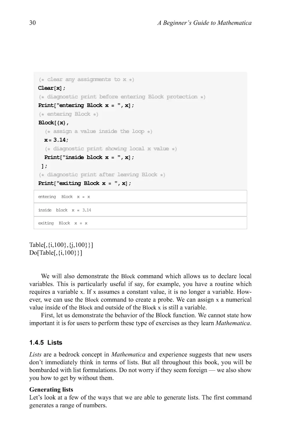
Clear[x] ;
Print ["entering Block x = ", x] ;
Block[{x},
x=3.14;
Print ["inside block x = ", x] ;
];
Print ["exiting Block x = ", x] ;
entering
inside
exiting
Block x
block x =
Block x :
= X
3.14
= X
Table[,{i,100},{j,100}}]
Do[Table[,{i,100}}]
We will also demonstrate the Block command which allows us to declare local
variables. This is particularly useful if say, for example, you have a routine which
requires a variable x. If x assumes a constant value, it is no longer a variable.
However, we can use the Block command to create a probe. We can assign x a numerical
value inside of the Block and outside of the Block x is still a variable.
First, let us demonstrate the behavior of the Block function. We cannot state how
important it is for users to perform these type of exercises as they learn Mathematica.
1.4.5 Lists
Lists are a bedrock concept in Mathematica and experience suggests that new users
don't immediately think in terms of lists. But all throughout this book, you will be
bombarded with list formulations. Do not worry if they seem foreign — we also show
you how to get by without them.
Generating lists
Let's look at a few of the ways that we are able to generate lists. The first command
generates a range of numbers.
Chapter 1: Introduction and survey
31
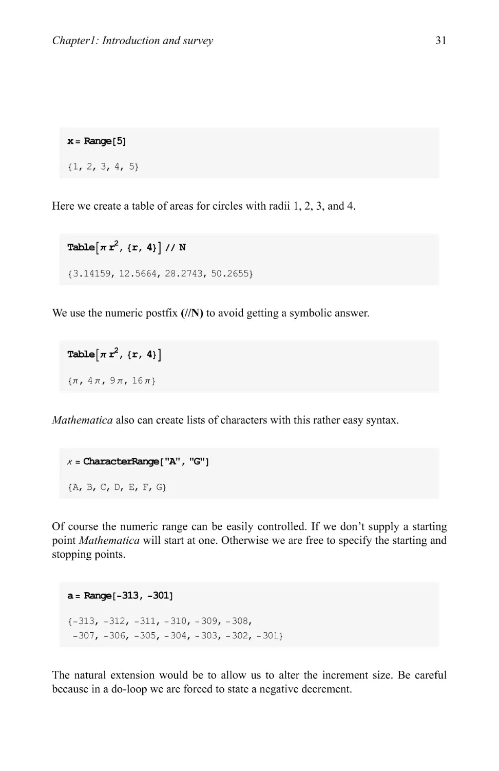
x= Range[5]
{1, 2, 3, 4, 5}
Here we create a table of areas for circles with radii 1, 2, 3, and 4.
Table[7rr2, {r, 4}] II N
{3.14159, 12.5664, 28.2743, 50.2655}
We use the numeric postfix (//N) to avoid getting a symbolic answer.
Table[7rr?, {r, 4}]
{/T, 4/T, 9/T, 16/T}
Mathematica also can create lists of characters with this rather easy syntax.
x = C3iaracterRange["A", "G"]
{A, B, C, D, E, F, G}
Of course the numeric range can be easily controlled. If we don't supply a starting
point Mathematica will start at one. Otherwise we are free to specify the starting and
stopping points.
a= Range [-313, -301]
{-313, -312, -311, -310, -309, -308,
-307, -306, -305, -304, -303, -302, -301}
The natural extension would be to allow us to alter the increment size. Be careful
because in a do-loop we are forced to state a negative decrement.
32
A Beginner's Guide to Mathematica
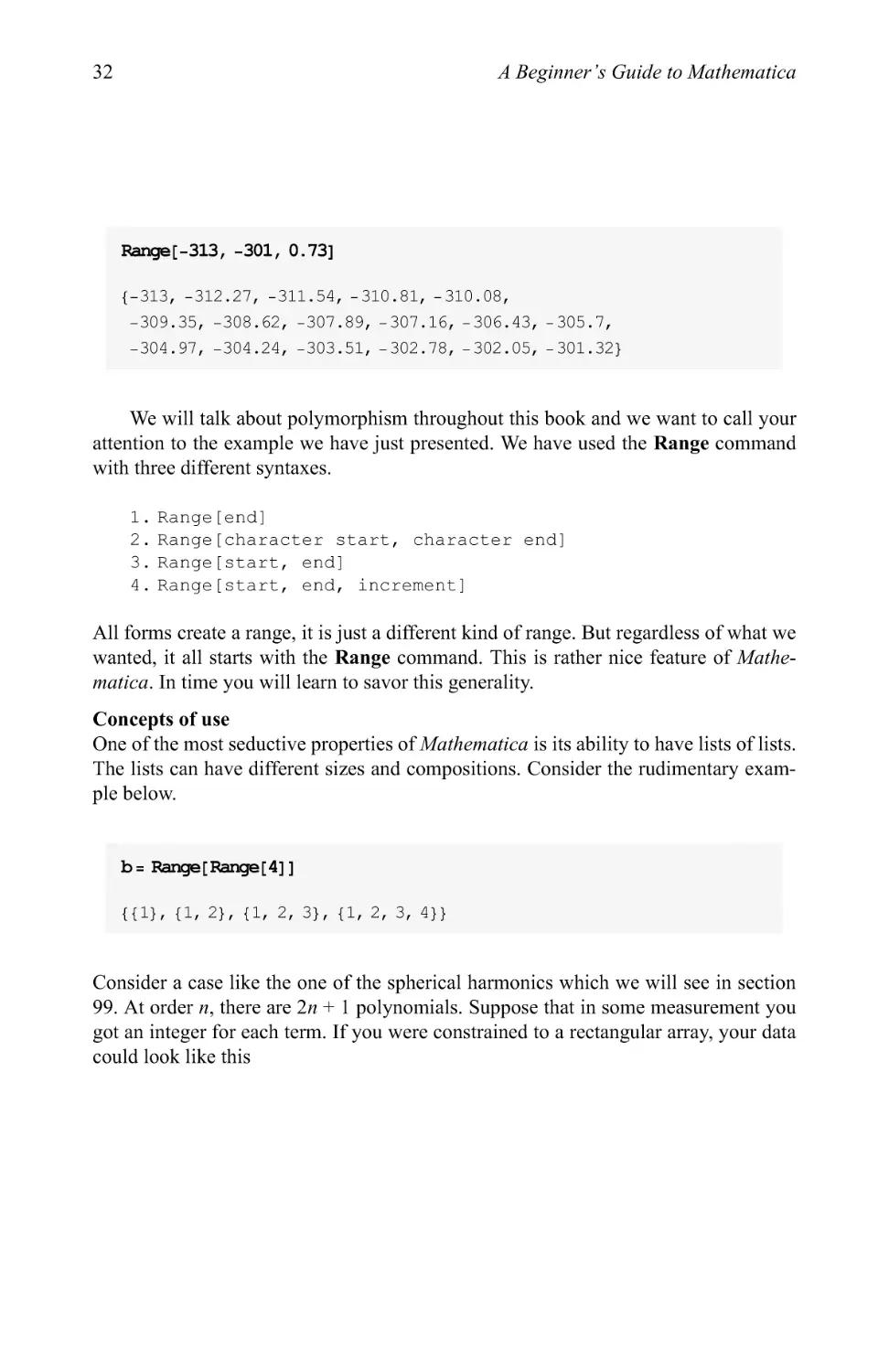
Range[-313, -301, 0.73]
{-313, -312.27, -311.54, -310.81, -310.08,
-309.35, -308.62, -307.89, -307.16, -306.43, -305.7,
-304.97, -304.24, -303.51, -302.78, -302.05, -301.32}
We will talk about polymorphism throughout this book and we want to call your
attention to the example we have just presented. We have used the Range command
with three different syntaxes.
1. Range[end]
2. Range[character start, character end]
3. Range[start, end]
4. Range[start, end, increment]
All forms create a range, it is just a different kind of range. But regardless of what we
wanted, it all starts with the Range command. This is rather nice feature of
Mathematica. In time you will learn to savor this generality.
Concepts of use
One of the most seductive properties of Mathematica is its ability to have lists of lists.
The lists can have different sizes and compositions. Consider the rudimentary
example below.
b= Range[Range[4] ]
{{1}, {1, 2}, {1, 2, 3}, {1, 2, 3, 4}}
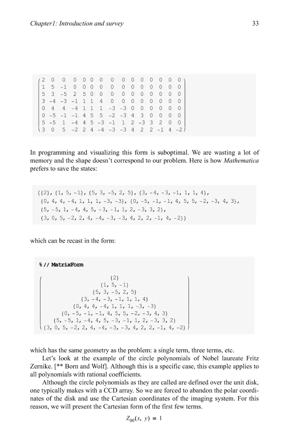
Consider a case like the one of the spherical harmonics which we will see in section
99. At order n, there are 2n + 1 polynomials. Suppose that in some measurement you
got an integer for each term. If you were constrained to a rectangular array, your data
could look like this
Chapter 1: Introduction and survey
33
2
1
5
3
0
0
0
5
3
-4
4
-5
0
-1
-5
-3
4
-1
0
0
2
-1
-4
-1
0
0
5
1
1
4
0
0
0
1
1
5
0
0
0
4
1
5
0
0
0
0
-3
-2
0
0
0
0
-3
-3
0
0
0
0
0
4
0
0
0
0
0
3
0
0
0
0
0
0
0
0
0
0
0
0
0
0
0
0
0
0
0
0
0
0
0
0
5-51-445
3 0
-2 2 4
12-33200
-3 4 2 2-14-2
In programming and visualizing this form is suboptimal. We are wasting a lot of
memory and the shape doesn't correspond to our problem. Here is how Mathematica
prefers to save the states:
{{2}, {1, 5, -1}, {5, 3, -5, 2, 5}, {3, -4, -3, -1, 1, 1, 4},
{0, 4, 4, -4, 1, 1, 1, -3, -3}, {0, -5, -1, -1, 4, 5, 5, -2, -3, 4, 3},
{5, -5, I, -4, 4, 5, -3, -I, I, 2, -3, 3, 2),
{3, 0, 5, -2, 2, 4, -4, -3, -3, 4, 2, 2, -I, 4, -2}}
which can be recast in the form:
% // MatrixForm
{2}
{1, 5, -1}
{5, 3, -5, 2, 5}
{3, -4, -3, -1, 1, 1, 4}
{0, 4, 4, -4, 1, 1, 1, -3, -3}
{0, -5, -I, -I, 4, 5, 5, -2, -3, 4, 3}
{5, -5, 1, -4, 4, 5, -3, -1, 1, 2, -3, 3, 2}
\ {3, 0, 5, -2, 2, 4, -4, -3, -3, 4, 2, 2, -1, 4, -2} )
which has the same geometry as the problem: a single term, three terms, etc.
Let's look at the example of the circle polynomials of Nobel laureate Fritz
Zernike. [** Born and Wolf]. Although this is a specific case, this example applies to
all polynomials with rational coefficients.
Although the circle polynomials as they are called are defined over the unit disk,
one typically makes with a CCD array. So we are forced to abandon the polar
coordinates of the disk and use the Cartesian coordinates of the imaging system. For this
reason, we will present the Cartesian form of the first few terms.
zoo(x' y) = l
34
A Beginner's Guide to Mathematica
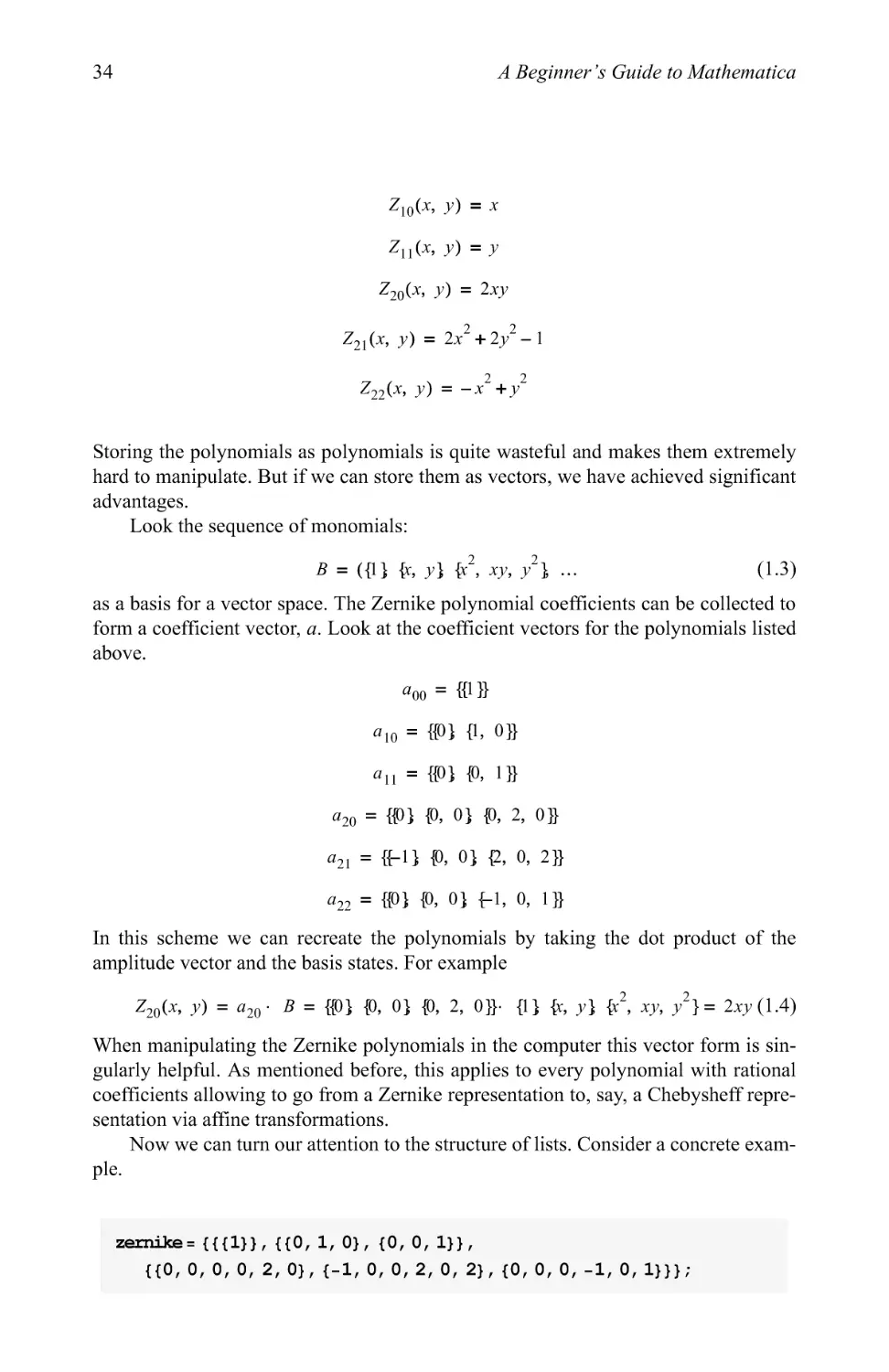
z10C*, y) = x
Zn(x, y) = y
z2o(x' y) = 2xy
2 2
Z21(x, y) = 2x + 2y -1
2 2
Z22(x, y) = -x + y
Storing the polynomials as polynomials is quite wasteful and makes them extremely
hard to manipulate. But if we can store them as vectors, we have achieved significant
advantages.
Look the sequence of monomials:
B = ({1} fc y} {c\ xy, y2\ ... (1.3)
as a basis for a vector space. The Zernike polynomial coefficients can be collected to
form a coefficient vector, a. Look at the coefficient vectors for the polynomials listed
above.
«10 = {{0} {1, 0}}
«n = {{0} {0, 1}}
«20 = (PI ft °1 ft 2> 0»
«21 = {HI ft 0} {2, 0, 2}}
«22 = m ft 0} H, 0, 1}}
In this scheme we can recreate the polynomials by taking the dot product of the
amplitude vector and the basis states. For example
Z20(x, y) = a20- B = {{0} {0, 0} {0, 2, 0}}- {1} fc y} {c\ xy, y2}= 2xy(\A)
When manipulating the Zernike polynomials in the computer this vector form is
singularly helpful. As mentioned before, this applies to every polynomial with rational
coefficients allowing to go from a Zernike representation to, say, a Chebysheff
representation via affine transformations.
Now we can turn our attention to the structure of lists. Consider a concrete
example.
zernike= {{{1}}, {{0, 1, 0}, {0, 0, 1}},
{{0, 0, 0, 0, 2, 0}, {-1, 0, 0, 2, 0, 2}, {0, 0, 0, -1, 0, 1}}};
Chapter 1: Introduction and survey
35
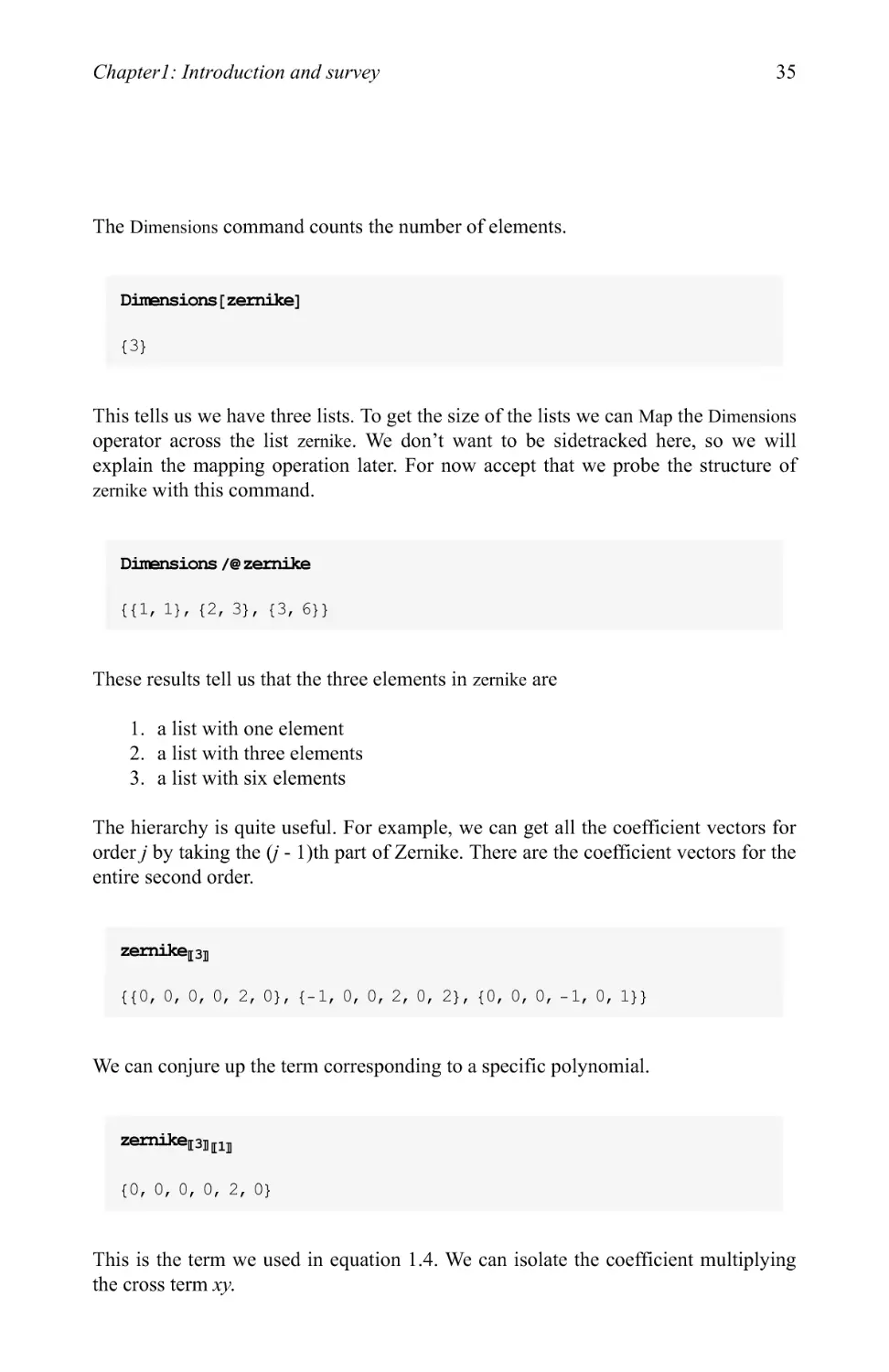
The Dimensions command counts the number of elements.
Dimensions [ zernike]
This tells us we have three lists. To get the size of the lists we can Map the Dimensions
operator across the list zernike. We don't want to be sidetracked here, so we will
explain the mapping operation later. For now accept that we probe the structure of
zernike with this command.
Dimensions /@ zernike
{{1, 1), {2, 3}, {3, 6}}
These results tell us that the three elements in zernike are
1. a list with one element
2. a list with three elements
3. a list with six elements
The hierarchy is quite useful. For example, we can get all the coefficient vectors for
order j by taking the (J - l)th part of Zernike. There are the coefficient vectors for the
entire second order.
zernikepj
{{0, 0, 0, 0, 2, 0}, {-1, 0, 0, 2, 0, 2}, {0, 0, 0, -1, 0, 1}}
We can conjure up the term corresponding to a specific polynomial.
zernikepjmj
{0, 0, 0, 0, 2, 0}
This is the term we used in equation 1.4. We can isolate the coefficient multiplying
the cross term xy.
36
A Beginner's Guide to Mathematica
2
Manipulating lists
Mathematica has been designed around the concept of lists and you will find a natural
comfort using the application to manipulate lists. Look how simple it is to subtract
one list from another.
x= Range[5] ;
y= Range[ll, 15] ;
x-y
{-10, -10, -10, -10, -10}
We can easily create a table of the first six odd numbers:
x=Table[2n + l, {n, 0, 5}]
{1, 3, 5, 7, 9, 11}
or the first six prime numbers:
Prime [Range [6]]
{2, 3, 5, 7, 11, 13}
There is even a facility to generate lists using functions:
z = Array [Sin, 3]
{Sin[l], Sin[2], Sin[3]}
Chapter 1: Introduction and survey
37
Mathematica is faithfully holding these symbolic forms until we request numerical
evaluation which we can do in prefix:
N[z]
{0.841471, 0.909297, 0.14112}
or postfix form:
z//N
{0.841471, 0.909297, 0.14112}
Of course, we are only shown the first six digits of an answer unless we request more.
N[z, 20]
{0.84147098480789650665,
0.90929742682568169540, 0.14112000805986722210}
All Mathematica functions operate on lists seamlessly:
Sin[Range[4]]
{Sin[l], Sin[2], Sin[3], Sin[4]}
These lists can have any structure and dimension:
Sin [Range [Range [4] ] ]
{{Sin[l]}, {Sin[l], Sin[2]},
{Sin[l], Sin[2], Sin[3]}, {Sin[l], Sin[2], Sin[3], Sin[4]}}
Notice that the answer has the same structure as the argument. We can force
numerical evaluation at any time.
38
A Beginner's Guide to Mathematica
%//N
{{0.841471}, {0.841471, 0.909297}, {0.841471, 0.909297, 0.14112},
{0.841471, 0.909297, 0.14112, -0.756802}}
We can use the command Flatten to force all the numbers into a linear order. You can
see that Flatten will remove all the internal braces.
Flatten[%]
{0.841471, 0.841471, 0.909297, 0.841471, 0.909297,
0.14112, 0.841471, 0.909297, 0.14112, -0.756802}
All Mathematica operators are content to operate upon lists.
%//N
{0.841471, 0.909297, 0.14112, -0.756802}
The lists can have any form of content.
Sin[{l, 7T, 3.1415926, Dan}]
{Sin[l], 0, 5.35898xl0"8, Sin[Dan]}
The Head command is an extremely useful command for the beginner. It
specifically identifies the data type. This is of vital importance because you will discover
that Mathematica is extremely disciplined about how it handles different data types.
This may surprise the new user who has just seen evidence that we can apply virtually
any operator to any data type, but as we go along you will see the precision with
which Mathematica distinguishes data types.
Head[l]
Integer
Chapter 1: Introduction and survey
39
Notice that n is not a number — it is a symbol representing a number. This subtlety is
required for an arbitrary precision computation engine.
Head[7r]
Symbol
When we take the Head of the numerical value of 71, we see that we have a Real
number.
Head[ 3.1415926]
Real
We see that the variable Dan is a symbol now.
Head [Dan]
Symbol
Again for arbitrary precision, we see that Mathematica is keeping this as a
functional value, not a number.
Head[Sin[l]]
Sin
Mathematica looks at this statement and recognizes the sine function has produced an
integer. Since integers are an exact data type in Mathematica, this expression is
evaluated as -1.
Head[ Sin [tt]]
Integer
40
A Beginner's Guide to Mathematica
Let's explore how these data types help Mathematica maintain arbitrary
precision. Consider the statement below where we know the answer from basic algebra.
1024-Sin[l] -1024
-Sin[l]
However, in a double precision world we will not get this answer. We will use the
numeric operator N to show us what a double precision computation of this
expression would yield:
N[1024-Sin[l]] -N[1024]
0.
This is a nuance and we want to clarify the concept. Consider the example below.
You could not form this number using a computer language based on IEEE double
precision variables.
z= 1024 + Sin[l]
1000000000000000000000000 + Sin[l]
However, because Mathematica can handle arbitrarily large integers and symbols, we
can compute this answer to arbitrary precision.
N[z, 50]
1.0000000000000000000000008414709848078965066525023x 1024
Over time you will see that this capability exposes us to entirely new vistas.
Chapter 1: Introduction and survey
Clear[x] ;
fl= Exp[xRange[4] ]
f2= Sin[Range[4] x]
r x 2x 3x 4x,
{e , e , e , e }
{Sin[x], Sin[2x], Sin[3x], Sin[4x]}
flf2
{<exSin[x], <e2xSin[2x], <e3xSin[3x], <e4xSin[4x]}
fl.f2
<exSin[x] + <e2xSin[2x] + <e3xSin[3x] + <e4x Sin[4x]
?x
Globalx
x = {1, 2, 3, 4, 5}
SeedRandom[l] ;
x=Table[2Randon[] , {2}, {4}, {3}]
{{{1.33739, 1.6624, 1.56361}, {0.249268, 1.86907, 1.2005},
{1.51671, 1.93818, 0.251398}, {1.15127, 1.5101, 1.64288}},
{{1.2092, 0.388929, 1.31461}, {1.11912, 1.67346, 0.321073},
{1.70887, 1.89087, 1.87436}, {0.521834, 1.45458, 0.558263}}}
42
A Beginner's Guide to Mathematica
SeedRandom[l] ;
x= Table[2Randcm[] , {2}, {4}, {3}]
{{{1.33739, 1.6624, 1.56361}, {0.249268, 1.86907, 1.2005},
{1.51671, 1.93818, 0.251398}, {1.15127, 1.5101, 1.64288}},
{{1.2092, 0.388929, 1.31461}, {1.11912, 1.67346, 0.321073},
{1.70887, 1.89087, 1.87436}, {0.521834, 1.45458, 0.558263}}}
V:
{{{1.15645, 1.28934}, {1.25045, 0.499268}, {1.36714, 1.09568}},
{{1.23155, 1.39218}, {0.501396, 1.07297}, {1.22886, 1.28175}},
{{1.09964, 0.623642}, {1.14657, 1.05788}, {1.29362, 0.566633}}}
matrix = Table[{r, c}, {r, 3}, {c, 3}]
{{{1, 1}, {1, 2}, {1, 3}},
{{2, 1}, {2, 2}, {2, 3}}, {{3, 1}, {3, 2}, {3, 3}}}
matrix// MatrixForm
1\
l)
2\
l)
3\
l)
(I)
(I)
(I)
/i
(3
/2
(3
I3
(3
Chapter 1: Introduction and survey
43
matrix = Table[ToString[{r, c}] , {r, 3}, {c, 3}] ;
matrix// MatrixForm
[ U, 1} {1, 2} {1, 3}\
I {2, 1} {2, 2} {2, 3} |
I {3, 1} {3, 2} {3, 3} )
There is even a facility to generate lists using functions:
array[sin]
Note that these values are held as symbols; they are not evaluated. To do that we need
to use the numeric operator N in prefix or postfix notation.
If we want to see the first 20 digits, we can use the prefix form as shown here:
N[z,20]
Functions in Mathematica are polymorphic — they perform the same function
for different inputs. Consider the sine functioning on this list.
Let's correlate the outputs to the inputs. The output Sin[l] is a symbol right now. We
could force numeric evaluation, but a secret to arbitrary precision is to evaluate all
symbols at the end of a calculation. Sin[pi] gives the expected exact answer of 0, not
o., a zero with a period signalling a zero to 16 or 17 digits. We see that the sign of p to
single precision gives us a zero to single precision. Finally the Sin[Dan] is being held
as just that until we can specify how to interpret Dan.
Notice what happens when we omit the brackets around the list. Mathematica
will repeat the input as a signal that it doesn't know how to interpret these
instructions.
As always we encourage the reader to experiment and probe with the tools at
hand. Let's examine the pedigrees of the inputs to the sine function.
Head
We see an Integer, a Symbol, a Real and another Symbol. The first Symbol is p
and can be evaluated by Mathematica at the end of the computation. The second
symbol Dan will be carried along too just like pi until the end. Hopefully by that time the
user will have supplied some definition.
Now let's look at the output types. The Head command tells us what data type
Mathematica "sees" when it encounters an expression like this. This reveals a little bit
about how Mathematica works. Let's discuss these results out of order. Head[Sin[p]]
is an Integer. This means that Mathematica has immediately evaluated this special
case to an integer zero. The Head[Sin[3.1415926]] is a real, telling us that Mathemat-
44
A Beginner's Guide to Mathematica
ica has substituted the single precision zero answer. Head[Sin[l]] is a Symbol telling
us that Mathematica will hold the symbolic value until tasked by the numeric
operator. Similarly, the Head query tells us that Sin[Dan]] is a symbol and there will be no
attempt at evaluation until by the N[].
Let's build up some functions using lists. We'll build a list fl which will be
Exp[n x] and a list f2 which will be Cos[n x]. This is the height of simplicity,
fl
f2
Now let's manipulate these lists. Notice the difference between the multiplication and
the dot product.
You may think the difference between a multiplication and a dot product is manifest,
but confusing these quantities is not uncommon for new users. Note that the list
argument is not restricted to one-dimensional lists.
1.4.6 The square root operator sweeps through them all.
We call your attention to the SeedRandom[] command. This very important
command allows you to start a particular string of random numbers. This is very
important when debugging your code and verifying your results. For example, say you have
a computationally intensive code that suddenly yields an unexpected answer. Is it an
algorithm problem or a data problem? If you have seeded your random number
generator, then you have the ability to trace through the code.
The subtlety missed is that while you want random numbers to simulate real
measurements, you want your computer code to be exactly repeatable. Consider that
you have verified and validated your code. Later circumstances compel you to make
minor changes which should not affect the operation of the code. How could you
prove that the code is unchanged if you are unable to reproduce your previous
answers?
As you might imagine, matrices are particularly simple to represent with lists. Let's
create a matrix that shows us the row and column address for each entry.
flat matrix
This is how Mathematica "sees" the matrix. But we want it in a more familiar form.
vector
What we see is a list of vectors since the {r,c} list is actually a vector itself presented
in proper form. However, to force the form into a {row, column} form, we will use
the ToString[] operator as shown here.
A At small dimensions Mathematica automatically handles vectors and covectors.
Chapter 1: Introduction and survey
45
List gymnastics
One of the great joys about working with Mathematica is the tool kit for list
operations. We can natively perform all the important operations that we learned in linear
algebra. Experience shows that the list gymnastics are often the most unfamiliar
exercises in Mathematica. We'll work through a few examples to clarify this. If you are
still uncertain about how to use lists, keep reading because we will show how to do
most operations without the list tools.
Let's begin with two short sample lists which we will call x and};.
x=Table[2n + l, {n, 0, 4}]
y=CharacterRange["a", "e"]
{1, 3, 5, 1, 9}
{a, /3, y, 5, e}
Very often we will need to take these two lists and merge them into a single list of
points {x, y}. A do-loop can do this for us easily enough. Schematically the process
looks like this.
count the number of terms (nx) ;
create a container to hold the {x, y} data (z) ;
loop through the data and create an {x, y} pair;
add the {x, y} pair to the container z ;
display container contents;
A Mathematica implementation of this process is this.
46
A Beginner's Guide to Mathematica
nx = Length[x] ;
z= {};
Do[
AppendTo[z, {Km, ym}] ;
, {i, nx}];
z
{{1, a}, {3, /3}, {5, y}, (7, 6}, {9, e}}
A better way to construct this process is to use the Table command. This involves
replacing the code:
z={};
Do[
AppendTo[z, {Km, y^}] t
, {i, nx}];
with the more succinct:
z=Table[{x[[i]],y[[i]]}, {i, nx}];
This streamlines and clarifies the process.
Chapter 1: Introduction and survey
41
nx= Length[x] ;
z = Table[{x[[i]], ym}, {i, nx}] ;
z
{{1, a), {3, /3}, {5, Y}, {1, 6}, {9, £}}
By way of demonstration we want to show yet another way to fold the data
together. We are not recommending this method; we present it to teach the user about
a different set of tools.
These tools will be discussed a few more times and for now we simply want to
expose the reader to their existence.
The first thing we'll do is multiply a scalar times a vector. How does this process
work in Mathematical We encourage the reader to write simple fragments of code
whenever in doubt.
a{l, 1}
{a, a}
a{l, 0}
{a, 0}
a{0, 1}
{0, a}
We can use this knowledge then to take a scalar and make a vector. So for the x list we
just multiply every member of the list by the vector {1,0}.
Again, we could rely upon the do-loop.
48
A Beginner's Guide to Mathematica
nx= Length[x] ;
x2= {};
Do[
AppendTo[x2, xm {1, 0}] ;
, {i, nx}];
x2
{{1, 0}, {3, 0}, {5, 0}, {1, 0}, {9, 0}}
However, there is a more compact way using a pure function. Since the notion of a
pure function is completely foreign to many users, we will go through a few explicit
cases in this book. This is an important tool and you will benefit from being able to
use it.
We will write a simple function and watch its action on the lists x and y. When
you look at the function, you'll see a pound sign #, an ampersand &, and the symbols
/@. You can always select these symbols and then launch the Help Browser for an
explanation; the Browser is quite complete.
The pound sign # is the slot operator and it is a wildcard for the data in the list.
The pound sign marks where the data will come in. The ampersand & is the suffix for
the function. The /@ is shorthand for the Map command. This will map the function
across every element in the list.
fcn= Print ["Grabbing ", #] &;
What we expect from this formulation is to see the fen grab each element in order and
print its value. Let's apply this function to the x list first.
Chapter 1: Introduction and survey
49
fcn/@x;
Grabbing
Grabbing
Grabbing
Grabbing
Grabbing
1
3
5
7
9
Now the y list.
fcn/@y;
Grabbing
Grabbing
Grabbing
Grabbing
Grabbing
a
/3
Y
6
£
Hopefully at this point you have a grasp of how to apply a pure function to a list. If
not, don't worry because we will be addressing this important concept repeatedly.
Let's take all that we have discussed and put it together. We will write two
functions: one to inflate x values and one to inflate y values. We will then be able to add
the inflated lists. Here is the composition and operation of the first function.
x2 = (#{1, 0}) &/@x
{{1, 0}, {3, 0}, {5, 0}, [1, 0}, {9, 0}}
50
A Beginner's Guide to Mathematica
The x values are now embedded in a two-dimensional list. This the first part of an
address.
y2 = (#{0, 1}) &/@y
{{0, a}, {0, /3}, {0, y}, {0, 6}, {0, s}}
Now the y values are embedded allowing us to add the lists.
z = x2+y2
{{1, a}, {3, /3}, {5, y}, (7, 6}, {9, £}}
This is the answer that we want, but the purpose of this last exercise was to
acclimate the reader a little more to functions, slot operators, and mapping. The proper
way to solve the problem is incredibly simple.
The first thing that we will do is create a list using x and y. We do this in the
simplest fashion: with two braces and a comma.
zt= {x, y}
{{1, 3, 5, 1, 9}, {a, (3, Yr 5, £}}
We could simply state the answer, but we want to show you how to resolve
problems, not encourage rote memorization. Let's examine our new list zt in MatrixForm
to visualize its shape.
zt// MatrixForm
1 3 5 7 9\
a /3 y 5 £ /
Our problem would be solved if the first row was the first column and the second row
was the second column. In other words, if we just had the transpose.
Chapter 1: Introduction and survey
51
z = Transpose [zt]
{{1, a}, {3, (3), {5, y}, {1, 6}, {9, s}}
That was remarkably easy. To encourage list-based thinking by the reader we will
show the solution in MatrixForm. To reinforce the elegant simplicity, we will show
all the steps needed to take a list of x values and a list of y values and create a list of
{x, y} points.
Transpose[{x, y}]
{{1, a}, {3, /3}, {5, y}, {7, 6}, {9, £}}
Generating constant vectors
We can count on Mathematica to do the right thing. Consider the interactions of
vectors and scalars. When we add a scalar to a vector, Mathematica adds the scalar to
every term.
y + l
{1+a, 1 + /3, 1 + Yf 1 + 6, 1 + e}
Multiplication by a scalar gives the expected result.
2y
{2a, 2(3, 2Y, 25, 2 £}
We view Mathematical generality as a blessing. At times though it can hinder the
new user because for example Mathematica is content to add numbers and string and
symbols and may not send a error message when there is a problem. This requires a
little more attention to programming.
52
A Beginner's Guide to Mathematica
For instance, we have seen codes where the product of vectors was used in lieu of
the dot product. They are quite different as you would expect.
{a, b} {c, d}
{ac, bd}
)
{a, b} .{c, d}
ac + bd
The relationship that seems most confusing however is this one.
{a, b}
{c, d}
We hope that these rules are clear. However, if you are debugging your code and
are unsure, just do what we did: compose simple lists and manipulate them and see
whether you find the expected results.
So what happens when we subtract an /7-dimensional vector from itself? We get
an /7-dimensional zero.
x-x
{0, 0, 0, 0, 0}
This identity is essential if you want to have true vector arithmetic. It is also a quick
way to generate zero vectors if you need them for accumulators. Another popular use
comes from least squares problems when you need a one vector of the proper
dimension as we shall see in chapter 2.
Chapter 1: Introduction and survey
53
x-x+ 1
{1, 1, 1, 1, 1}
A You can use simple vector arithmetic to create constant vectors.
1.5 Programming
Mathematica has a unique and powerful programming language associated with it.
Many comment on the similarity with the program languages C++ and Scheme. We
think that the interactive environment is an excellent one to learn in because you can
view variable states, display intermediate steps, and perform all manner of diagnostic
and probe sequences.
Throughout the volume we will stress learning by doing. Sit down at a computer
and perform small, quick experiments to teach yourself how the programming
language works. We are far, far away from the day when you had to punch computer
cards, read them in, and then wait for the line printer to output your job. This is a new
paradigm; you have an excellent Help Browser and an interactive environment and
you should feel compelled to investigate.
A goal for us is to teach the reader how to perform little tests needed to help sort
out functionality and proper syntax. We aren't trying to show you how to solve a
problem per se, but trying to show you how you should approach problems in
Mathematica.
^ Built-in Functions > Programming
1.5.1 Flow control
There are a rich variety of flow control commands in Mathematica. Some are quite
simple, some are nuanced. Our tour will be quite brief and will cover the most basic
tools needed to get started.
^ Built-in Functions > Programming > Flow Control
The Do loop
We think that the do-loop is one of the most basic commands and hope that all users
can grasp its functioning directly.
Here is a prototype do-loop that will have ten steps as i ranges from 1 to 10.
54
A Beginner's Guide to Mathematica
Do[
, {i, 10}];
The counter syntax is fairly simply. You can start at zero.
Do[
, {i, 0, 10}];
Or start at a negative number.
Do[
, {i,-20, 10}];
You can use any numeric variable for the counter, the maximum value and the
increment.
Do[
, {i, 0.32565, 11.4567, 0.998}] ;
We can step backwards with a decrement. But there is some fine print. For while
an omitted increment causes Mathematica to use unity, an omitted decrement of -1
will not be assumed. The loop will not execute. Perhaps this sounds like minutiae to
you. The point we sound often is not to strain your memory, but to investigate. Try
this sample loop.
Do[
Print ["inside the Do loop"] ;
, {i, 0, -2}]
Chapter 1: Introduction and survey
55
There was no output statement so we never made it into the loop. Once we explicitly
show the decrement the loop will work as shown here.
Do[
Print ["inside the Do loop"] ;
, {i, 0, -2, -1}]
inside the Do loop
inside the Do loop
inside the Do loop
We can nest our do-loops — that is, place one inside another.
Do[
Do[
Do[
, {i,n}];
, {j,n}];
, {k, n}];
This is the more general form for nesting Do loops. You can nest as many levels as
you wish. If your process allows it, you may be able to use a more compact statement
such as this.
Do[
, {i, n}, {j, n}, {k, n}] ;
56
A Beginner's Guide to Mathematica
Something about the latter form tends to confuse the new user. Whereas in the
former instance the index incrementing in clear, it is not so clear here. In the former
case what we expect is that k increments from 1 to n, and then j increments. After k
has incremented n times, j has incremented n times and i finally increments. In other
words, k is changing the fastest and i is changing the slowest.
When some people see the counters together on one line, they do not always
realize which counter is going faster. Here is how someone could sort this out for
themselves. Just count the steps and print out the indices.
n=2;
m=l;
Do[
Print[m++, ". indices are {i,j,k} = ", {i, j, k}] ;
, {i, n}, {j, n}, {k, n}] ;
1.
2.
3.
4.
5.
6.
7.
8.
indices
indices
indices
indices
indices
indices
indices
indices
are
are
are
are
are
are
are
are
{irjrk} =
{irjrk} =
{irjrk} =
{irjrk} =
{irjrk} =
{irjrk} =
{irjrk} =
{irjrk} =
{1,
{1,
{1,
{1,
{2,
{2,
{2,
{2,
1,
1,
2,
2,
1,
1,
2,
2,
1}
2}
1}
2}
1}
2}
1}
2}
The inquisitive reader may be wondering if one method offers a time advantage
over the other. Well, we could state the answer, but we are not writing a collection of
facts for memorization. We are writing a manual on how to explore and use Math-
emtica.
We will compose do-loop in both formats and have them perform a simple task
so that we can ensure both loops have performed the same amount of work.
Our next step will be to turn on a timer.
Chapter 1: Introduction and survey
57
« Ut±lit±esNShowTimeN ;
Now we will compose and run the competing loops.
n=100;
p=0;
Do[
p+= 7r;
, {i, n}, {j, n}, {k, n}] ;
P
0. Second
10.595 Second
0. Second
1000000/t
The more explicit method is seen on the next page. The significant results are these.
First, both methods successfully return 10 n. This assures us we successfully
coded both loops. (Well, actually it says we similarly coded both loops.) The first
method to 10.595 seconds and the second method to 10.465 seconds. This is basically
a dead heat. If you run these loops yourself several times, you will see timing
differences within each example that suggest 0.13 second difference is not meaningful.
An extension of the multiple counter scenario is to have one counter depend upon
another. We'll run into this case later on and for now we will study the basic
functioning of the nested do-loop. The prototype form is this.
Do[
, {i, 0,n}, {j, 0, i}]
58
A Beginner's Guide to Mathematica
Are you able to write on a piece of paper, in the proper order, what the values of i
and j will be? Can you predict how many steps there will be as a function of nl The
first question is one you should be able to answer. If not, you should experiment much
more with do-loops before leaving this section. This is a bedrock concept for the rest
of this book.
n=100;
p=0;
Do[
Do[
Do[
p+= 7r;
, {i,n}];
, {j,n}];
, {k,n}];
P
0. Second
10.465 Second
0. Second
1000000/t
The trial do-loop is seen atop the next page. We have introduced other elements to.
First, you noticed that we have counted the number of steps with the variable
steps. Perhaps you know that the sum of the integers from 1 to n is:
n
^i = \n(n-\) (1.5)
i= 1
V Arithmetic Series (formula 3)
In general we find that formulae such as this are a great error source. The starting
index may get changed as in this case from one to zero and the summation value is
overlooked, or you mistyped the formula, or maybe you never knew the formula.
Regardless, your CPU is doing over a billion operations a second and is more than
Chapter 1: Introduction and survey
59
happy to count them up for you. When Mathematica sees the command step++ , it
returns the value of step and then adds one to it. If you wished to increment before
querying step, then you would type ++step.
Also, we call your attention to the fact that we can put output variables.
step= 1;
n=2;
Do[
Print[step++, ". {i,j} = ", {i, j}] ;
, {i, 0, n}, {j, 0, i}]
1.
2.
3.
4.
5.
6.
U,j} =
U,j} =
{irj} =
{irj} =
U,j} =
{irj} =
= {0, 0}
= U, 0}
= U, 1}
= {2, 0}
= {2, 1}
= {2, 2}
A successful execution is easy to recognize, but we want to expose the nascent
user to error messages most likely to appear. For this case, we will swap the order of
the indices.
step= 1;
n=2;
Do[
Print[step++, ". {i,j} = ", {i, j}] ;
, {j, 0, i}, {i, 0,n}]
A Do :: iterb : Iterator {j, 0, i} does not have appropriate bounds . More..
Do[Print[step++, . {i,j} = , {if j}];, {j, 0, i}, {if 0, n} ]
60
A Beginner's Guide to Mathematica
What the error message is saying is that it cannot set up a loop for j to go from 0 to i
because i has no value. We know what we meant but Mathematica can only search
inside the counter (to the left) and not outside (to the right).
As always, Mathematica repeats commands it cannot execute. This is a handy
way to differentiate between a bad algorithm and a bad command.
We close the section on do-loops with an observation by our colleague P. Riera.
Oftentimes people use do-loops to step through some space and make measurements.
Say you are moving in small steps 8. You have two choices for keeping track of the
measurement position: x+= 8 and x = i 8. Do not accumulate! The first form is a
nursery for machine noise as we show here.
5=0.31415926;
sum= 0;
D»[
product = i 5 ;
sum+= 5;
, {±, io5}]
Print ["the error = ", product- sum] ;
the error = -3.92174 xlO"8
After only 10 steps we are already down to single precision.
/k Do not accumulate in your loops. This is an efficient way to erode precision.
If this is your first exposure to numerical computing, this may surprise you. It is
due to the fact that we are trying to represent base 10 numbers in base 2 (binary). To
demonstrate this, we can make the problem go away when our increment has an exact
binary representation.
5=0.125;
sum= 0;
D0[
product = i 5 ;
sum+= 5;
, {I, 105}];
Print ["the error = ", product- sum] ;
the error = 0.
Chapter 1: Introduction and survey
61
Don't flirt with the special cases. Make it a practice to avoid accumulation.
W Built-in Functions > Programming > Flow Control > Do
The For loop
While we believe the do-loop is the workhorse for flow control, we do want to expose
readers to the For loop. We show here an equivalent formulation for the triple index
do-loops we presented.
n=100;
p=0;
For[i= 1, i< n,
For[j = 1, jsn,
For[k= 1, k^ n,
P+= 7T
,k++]
, j++]
, i++]
P
0. Second
13.59 Second
0. Second
1000000/t
We see that this form is appreciably slower (about 3 seconds) and is a bit harder to
read. But if you are comfortable with this syntax, you should use it.
^ Built-in Functions > Programming > Flow Control > For
While
The While command has some interesting uses and we encourage readers to ponder
ways to integrate this command into their programs. The syntax is the height of
simplicity.
62
A Beginner's Guide to Mathematica
While [test,
];
An excellent case for this problem is the random walk. Our variant of the
problem is this. We start at the origin and take a series of unit steps, each in a random
direction. We stop when we have reached some predetermined distance from the
origin.
Say that we want to keep going until we have traveled the distance 15. Our basic
structure would look like this.
While [distances 15,
increment step counter;
create a random angle;
take the step;
compute the distance;
];
We are trying to encourage users to reduce the processes to separate and simple
statements that can be tested before putting the whole statement together. Far too often
have we been asked to unravel some Gordian knot of code suffering from a host of
maladies, all of which would have been exposed had the pieces been tested
independently.
Chapter 1: Introduction and survey
63
d= -oo;
k=0;
SeedRandom[l] ;
P= {0, 0};
While[d< 15,
k++;
0= Random[Real, {0, 2 7r}] ;
p+= {Cos[0] , Sin[0]};
d= VS-usOOp2 ;
]-■
Print[k, " iterations to go a distance ", d] ;
93 iterations to go a distance 15.0538
In the interest of expediency we present the While loop after assembling tested
components. We call your attention to the following features.
First, we were careful to give d a numeric value before we started. One thing we
love about Mathematica are the values ipo. They make comparisons so easy and they
prevent annoying bugs. We have seen users use what they consider to be a large
number to control feedback loops but they have found out the hard way that there are
legitimate values in excess of their bound.
/k Take advantage of the infinities in Mathematica (ipo) to ensure that your
comparison functions as desired.
When we replace the statement
d= -oo;
with the statement:
Clear[d] ;
this simulates what would happen if you forgot to assign a value to the test variable.
This produces the output:
64
A Beginner's Guide to Mathematica
0 iterations to go a distance d
which, we know from experience, means that the While loop was never entered. What
happened? Of course we could tell you, but we want to show you how to decipher this
on your own. Your first recourse may be an If test similar to the one employed by the
While loop.
If[d^ 15, Print["d <, 15"] , Print["d > 15"] , Print["huh?"] ] ;
huh?
For better or for worse we have replicated the failed numerical comparison. Our next
step would be to probe d. We need to see why it failed the test. Our commands are ?
andHead[].
Head[d]
?d
Symbol
GlobaTd
We see that d is a symbol with no value. Mathematica has a very sophisticated
classification and what it is saying is that it cannot tell whether d is less than or equal
to 15 because it is a symbol without a value. This may seem abstract, so let's be a bit
more definite with an example where we compare a string to a number.
d - "I am a string" ;
If [d <, 15, Print [V <, 15"] , Print [V > 15"] , Print["huh?"] ] ;
huh?
Mathematica is saying that when we try to compare a string to a number we cannot
say either True or False. We simply cannot make the comparison.
Chapter 1: Introduction and survey
65
< Make sure that your test variable has a value when you first enter the While
loop.
The final thing we call your attention to is something that we will state often.
Whenever you use a random series of numbers in your code, seed the random number
generator with SeedRandom[]. This may seem counterintuitive, but remember, the
random number generator simulates random conditions. You don't want your algorithm
to behave randomly, you want your data to behave randomly. If you have not seeded
your sequence, your validation may be impossible. For example, suppose you
changed your code in a way that should not have altered the computations. How
would you show that your code behaves the same? If you have seeded your data, you
can run the same sequences again and look for the same results.
Another reason is that many times we have watched users look at their output and
get unexpected or "impossible" answers. How can you know if the problem is your
code or if your problem is the data or if the problem is your understanding of the
algorithm? If you have seeded your data you can repeat the sequence.
Also, we are very pleased to note that different platforms will supply the same
sequence of random numbers if you seed with a definite value. That means that you
can continue testing and development on different platforms.
< Make sure you always seed the random number generator with a definite value.
With these points said, we will close our discussion on flow control. We do want
to state that we will be visiting the random walk problem again in this chapter to
develop a graphical output form.
Y Built-in Functions > Programming > Flow Control > Which
1.6 Standard add-on packages
Mathematica offers a large number of standard add-on packages to extend its
capabilities. This is a buffet style structure — you can take whatever you want. You
should take a few minutes to examine this list. Many users ignore this list and end up
attempting to duplicate the function found in these packages.
In addition to providing a comprehensive environment for calculations and a
programming language, Mathematica is also a system for representing and presenting
scientific and technical knowledge. Certain packages are included with Mathematica
to provide easy access to commonly used scientific data, such as the value of physical
constants and conversion factors for various systems of units
So how do we access packages?
66
A Beginner's Guide to Mathematica
Package category Packages included
Algebra Algebraiclnequalities PolynomialExtendedQCD Relm
FiniteFields PolynomialPowerMod Rootlsola-
tion
Horner Quaternions %mmsbicPotenti-
tals
Inequality Solve
Algebra
Relm
Calculus
DiscreteMath
Geometry
Graphics
LinearAlgebra
Miscellaneous
NumberTheory
Algebraiclnequalities
DSolvelntegrals
FourierTransform
CombinatorialFunctions
Combinatorica
Polytopes
Animation
ArgColors
Arrow
Colors
ComplexMap
ContourPlot3D
FilledPlot
Graphics
FourierTrig
MatrixManipulation
Audio
BlackBodyRadiation
Calendar
ChemicalElements
CityData
AlgebraicNumberFields
ContinuedFractions
FactorlntegerECM
PolynomialExtendedQCD
VariationalMethods
VectorAnalysis
ComputationalGeometry
DiscreteStep
Rotations
Graphics3D
ImplicitPlot
InequalityGraphics
Legend
MultipleListPlot
ParametricPlot3D
PlotField
Orthogonalization
StandardAtmosphere
Music
PhysicalConstants
RealOnly
Integration
Pade
RSolve
Tree
PlotField3D
Polyhedra
Shapes
Spline
SurfceQfftevdu-
tion
ThreeScript
Common
Tridiagonal
Geodesy
Units
WorldData
WorldNames
ResonanceAbsorptionLines WorldPlot
NumberTheoryFunctions
PrimeQ
PrimitiveElement
Rationalize
Recognize
SiegelTheta
NumberTheoryFunctions
NumericalMath Approximations IntervalRoots
NSeries
Chapter 1: Introduction and survey
67
Statistics
Utilities
BesselZeros
Butcher
CauchyPrincipalValue
ComputerArithmetic
Gaus sianQuadrature
InterpolateRoot
ANOVA
Confidencelntervals
ContinuousDistributions
DataManipulation
DataSmoothing
DescriptiveStatistics
BinaryFiles
FilterOptions
Listlntegrate
Microscope
Newton-
Cotes
OrderStar
NlntegratelnterpolatingFunctPolynomi-
NLimit
NResidue
DiscreteDistributions
HypothesisTests
i LinearRegression
MultiDescriptiveStatistics
MultiDiscreteDistributions
MemoryConserve
Package
alFit
SplineFit
TrigFit
MuWrorrain)^
bution
NonlinearFit
NormalDistrfou-
tion
Statistics-
Plots
: Common
ShowTime
W Add-ons & Links > Standard Packages
An important point to remember is that this list is growing. If you have a Premier
subscription, then you will automatically receive the distributed packages. Other
packages are available through the Mathematica Information Center at
library.wolfram, com.
Because of the diversity of the packages in the Miscellaneous category, we would
like to spend some time to familiarize the reader with the sundry functions.
1.7 Miscellaneous packages
Most users are surprised at the depth and scope of the add-on packages to
Mathematica. For example, it is not uncommon for people to write code to perform vector
operations even though the Calculus'Vector Analysis package has a rather formidable tool
kit. Hopefully the list above will prevent someone from writing code for routines they
already have.
The catchall category, Miscellaneous, has some intriguing packages and we want
to take some time to scan through some of them. Again the hope is that this will
preclude readers from trying to replicate this work themselves. We will separate the
packages with the command needed to load them.
68
A Beginner's Guide to Mathematica
1.7.1 Miscellaneous'Audio
« Miscellaneous AudioN
The Audio package provides the user with a tool kit to create standard and custom
wave forms. The command below will create a sawtooth form with a fundamental
frequency of 700 Hz lasting for 3 seconds. Notice that the command creates a sound
object, but does not generate the sound.
noise = Waveform [Sawtooth, 700, 3]
- Sound -
To hear this rather annoying sound we use the Show command as shown here.
You may have expected a command like Hear, but keeping in the spirit of generality,
Mathematica has a rather universal Show command.
si = Show [noise] ;
The Help Browser has some excellent background material which we show
below. Also, there are some very interesting sound demos in the Demos, including the
tones for the touch tone phones.
^ Add-on & Links > Standard Packages > Miscellaneous > Audio
Add-on & Links > Standard Packages > Miscellaneous > Music
The Mathematica Book > A Practical Introduction to Mathematica > Graphics
and Sound > Sound
Demos > Sound Gallery > Touch Tones
Chapter 1: Introduction and survey
69
We have calculated peak wavelength above and we can check it somewhat
crudely on the chart. Select the graphic object above by clicking on it. Your cursor
will then take on the appearance of four arrows. Then hold down the Alt key (3=§ or
command key on the Macintosh) and you will be able to read the coordinates in the
lower left-hand corner of the notebook window. The result will be in the coordinates
of the plot. This is an extremely useful feature for all two-dimensional plots that many
users seem to miss.
In this particular case the measurement seems quite crude. We placed the cursor
on the spot where the dotted line intercepted the wavelength axis and the coordinate
as 8.06x 10"7. However, we understand that cursor movement is quantized by the
pixels, so we shifted the cursor one pixel to the right and the crosshairs were clearly
beside the dotted line and the value was 8.18x 10"7, a noticeable discrepancy from the
valueof8.19xl0"7.
^ Add-on & Links > Standard Packages > Miscellaneous > BlackBodyRadiation
/k Be somewhat wary of using the cursor to measure graphics coordinates. There
seem to be some small errors.
1.7.2 Miscellaneous'Calendar'
<< MiscellaneousNCalendarN
It is somewhat surprising to see how complete a tool kit Wolfram provides for calen-
drical calculations. However, we must surmise that users doing financial calculations
and users doing celestial mechanics are quite pleased with the capabilities. For
example, we can find out what day of the week it was on July 4, 1776;
DayOfWfeek[{1776, 7, 4}]
Thursday
On May 25, 1961 President Kennedy addressed a joint session of Congress and
promised to send a man to the moon and return him safely. We can count the number
of days between this speech and Neil Armstrong's famous moonwalk easily
DaysBetween[{1961, 5, 25}, {1970, 7, 20}]
3343
70
A Beginner's Guide to Mathematica
The Mars Polar Lander was launched on January 1, 1999. Its voyage lasted 334
days. What day was it due to land on Mars?
DaysPlus[{1999, 1, 3}, 334]
{1999, 12, 3}
There are tools to convert between Gregorian and Julian calendars as well as the
Islamic calendar. You can also compute special days.
In 325 A.D. the Roman emperor Constantine convened the Council of Nicea and
established that Easter will be the first Sunday that occurs after the first full moon on
or after the vernal equinox. However, this mandated an ecclesiastical full moon and
equinox which differ from their astronomical counterparts used today. The
ecclesiastical computations don't account for the full complexity of lunar motion which is
defined as the 14th day of tabular lunation. The net effect is to constrain Easter to fall
between March 22 and April 25. These Gregorian tables are used by the Roman
Catholic Church and the Protestants. The Eastern or Orthodox Christian Church uses the
Julian tables.
It may sound confusing, but it is all sorted out in Mathematica. Also, the Naval
Observatory gives the day of Easter close attention. You can check the listing at the
URL below.
"f*£ http;//aa.usno.navy.mil/faq/docs/easter.html
We can generate our own table easily.
es= Table[EasterSunday[d] , {d, 1980, 2024}]
{{1980, 4, 6}, {1981, 4, 19}, {1982, 4, 11}, {1983, 4, 3}, {1984, 4, 22},
{1985, 4, 7}, {1986, 3, 30}, {1987, 4, 19}, {1988, 4, 3}, {1989, 3, 26},
{1990, 4, 15}, {1991, 3, 31}, {1992, 4, 19}, {1993, 4, 11}, {1994, 4, 3},
{1995, 4, 16}, {1996, 4, 7}, {1997, 3, 30}, {1998, 4, 12}, {1999, 4, 4},
{2000, 4, 23}, {2001, 4, 15}, {2002, 3, 31}, {2003, 4, 20}, {2004, 4, 11},
{2005, 3, 27}, {2006, 4, 16}, {2007, 4, 8}, {2008, 3, 23}, {2009, 4, 12},
{2010, 4, 4}, {2011, 4, 24}, {2012, 4, 8}, {2013, 3, 31}, {2014, 4, 20},
{2015, 4, 5}, {2016, 3, 27}, {2017, 4, 16}, {2018, 4, 1}, {2019, 4, 21},
{2020, 4, 12}, {2021, 4, 4}, {2022, 4, 17}, {2023, 4, 9}, {2024, 3, 31}}
In this form comparison with the website is quite tedious. This gives us a good reason
to demonstrate the benefits of TableForm as you see below.
Chapter 1: Introduction and survey
TableForm[Table[EasterSunday[d] , {d, 1980, 2024}]]
1980
1981
1982
1983
1984
1985
1986
1987
1988
1989
1990
1991
1992
1993
1994
1995
1996
1997
1998
1999
2000
2001
2002
2003
2004
2005
2006
2007
2008
2009
2010
2011
2012
2013
2014
2015
2016
2017
2018
2019
2020
2021
2022
2023
2024
4
4
4
4
4
4
3
4
4
3
4
3
4
4
4
4
4
3
4
4
4
4
3
4
4
3
4
4
3
4
4
4
4
3
4
4
3
4
4
4
4
4
4
4
3
6
19
11
3
22
7
30
19
3
26
15
31
19
11
3
16
7
30
12
4
23
15
31
20
11
27
16
8
23
12
4
24
8
31
20
5
27
16
1
21
12
4
17
9
31
72
A Beginner's Guide to Mathematica
^ Add-on & Links > Standard Packages > Miscellaneous > Calendar
1.7.3 Miscellaneous'ChemicalElements'
« MiscellaneousN Chemica 1 ElementsN
Here we find the chemical elements and their properties in a form more amenable to
programming. We can query the atomic weight using either the full element name
Atomicflfeight [ Gadolinium]
157.25
or the abbreviation:
AtomicWeight[Gd]
157.25
As we will do in the section on palettes, we can find the boiling point in degrees
Kelvin.
fcp= BoilingPoint[Gd]
3539. Kelvin
Let's suppose that we want the value but not the units. In other words, we want the
pure number 3539. How would we isolate that? Our first step is to look at the
dimension of the number:
Dimensions[fcp]
{2}
Chapter 1: Introduction and survey
73
We see that we have two items, a value and a unit.
fcPiii]]
fcP|[2]]
3539.
Kelvin
We can use the Part command in shorthand as shown above or in command form
Part[fcp, 1]
3539.
We can use a zero index with the Part command to find the Head of the expression.
Part[fcp, 0]
Times
As always, it is good practice to check our results.
Head[bp]
Times
This leads us to wonder what is the exact form of a number with dimensions?
74
A Beginner's Guide to Mathematica
RillForm[fcp]
Times[3539. \ Kelvin]
So given a list we can always Take and element or range of elements. An
example is shown here.
Take[fcp, 1]
3539.
Equivalently we can Extract elements from the list.
Extract[fcp, 1]
3539.
Yet another syntax would be to Drop elements from the list.
Drop[fcp, -1]
3539.
Here we used a negative index to count from the end, not the beginning.
Y Built-in Functions > Lists and Matrices > Element Extraction
Chapter 1: Introduction and survey
75
1.7.4 Miscellaneous'BlackBodyRadiation'
< < MiscellaneousN BlaclcBodyRadiationN
Plank's postulation of quantized oscillators successfully explained the energy
spectrum of blackbody radiation and its variation with temperature. The Black Body
Radiation tool kit computes properties and displays spectral distributions for black bodies
whose temperatures are given in Kelvin. Consider a blackbody at the temperature of
boiling gadolinium shown below.
T = BoilingPoint /. gd
3539. Kelvin
The wavelength at the peak of the spectral distribution is:
PeakWavelength [ T]
8.19441xl0"7 Meter
In a moment we will actually plot this distribution and use Mathematica cursor tools
to measure the peak. First though we will compute the total power emitted
TotalPower[T]
8.89479xl06Watt
Meter2
Routines in this package will automatically generate the spectral distribution,
gl = BlackBocfyProfile[T, IinageSize-► 5 72] ;
76
A Beginner's Guide to Mathematica
lxHT6 2xl(T6 3xl(T6 4xl(T6 5xlO-6
Wavelength, m
Recently Wolfram Research has installed tools that allow you to position the
cursor on figures and read the coordinates of the points. We show an example of this
process below. Unfortunately, the Print Screen process has removed the cursor.
misc 01.nb
-|D| x|
i ■ M ■ i ■ I ■ i ■ IA i ■ I ■ i ■ lJ. i ■ I ■ i ■ I*, i ■ I ■ i ■ l&. i ■ I ■ i ■ lb. i ■ I ■ i
ntpq.-= gl = BlackBodyPro file [T ] ;
The cursor was
located here.
The coordinates
are shown here.
lxlO"15 2xl0-d 3^10-15 4xl0-d 5x10
J
{3.14e-007, 7.46e+010} 100% * jj
Chapter 1: Introduction and survey
11
« MiscellaneousN EhysicalConstantsN
This package has a nice assortment of physical constants in SI units. To save you the
trouble of determining how current they are, we show their values.
AccelerationDueToGravity
AgeOfUniverse
AvogadroCons tant
BohrRadius
Bolt zmannCons tant
ClassicalElectronRadius
CosmicBackgroundTemperature
DeuteronMagneticMoment
DeuteronMass
EarthMass
EarthRadius
ElectronCharge
ElectronComptonWavelength
ElectronGFactor
ElectronMagneticMoment
ElectronMass
FaradayCons tant
FineStructureConstant
GalacticUnit
GravitationalConstant
HubbleConstant
IcePoint
MagneticFluxQuantum
MolarGasConstant
MolarVolume
MuonGFactor
MuonMagne t i cMoment
MuonMass
NeutronComptonWavelength
NeutronMagneticMoment
NeutronMass
PlanckConstant
PlanckConstantReduced
PlanckMass
ProtonComptonWavelength
ProtonMagneticMoment
ProtonMass
QuantizedHallConductance
9.80665 Meter/Second^
4.7X10¹⁷ Second
6.02214X10²³ /Mole
5.29177X10"11 Meter
1.38065X10"23 Joule/Mole
2.81794X10"15 Meter
2.726 Kelvin
4.33073X10"27 Joule/Tesla
3.34358X10"27 Kilogram
5.9742X1024 Kilogram
6378140 Meter
1.60218X10"19 Coulomb
2.42631X10"12 Meter
-2.00232
-9.28476X10⁻²⁴ Joule/Tesla
9.10938X10"31 Kilogram
96485.3 Coulomb/Mole
0.00729735
2.6X10²⁰ Meter
6.673X10"11 Meter2 Newton/
Kilogram2
3.2X10"18 /Second
273.15 Kelvin
2.06783X10"15 Kilogram
8.31447 Joule/Kelvin Mole
0.022414 Meter2/Mole
-2.00233
-4.4905X10"26 Joule/Tesla
1.88353X10"28 Kilogram
1.31959X10"12 Meter
-9.66236X10⁻²⁷ Joule/Tesla
1.67493X10"27 Kilogram
6.62607xl0"34Joule Second
1.05457xl0"34Joule Second
2.1767X10"8 Kilogram
1.32141X10"15 Meter
1.41061X10"26 Joule/Tesla
1.67262X10"27 Kilogram
0.0000387405 Ampere/Volt
78
A Beginner's Guide to Mathematica
RydbergCons tant
SackurTetrodeCons tant
SolarConstant
SolarLuminosity
SolarRadius
SolarSchwarzschildRadius
SpeedOfLight
SpeedOfSound
StefanConstant
ThomsonCrossSection
VacuumPermeabi1i ty
VacuumPermi 11 ivi ty
WeakMixingAngle
1.09737x10' /Meter
-1.1517
1373. Watt/Meter2
3.86x1026 Watt
6.9599x10s Meter
2953.25 Meter
299792458 Meter/Second
340.292 Meter/Second
5.6704X10"8 Watt/Kelvin4 Meter2
6.65246X10"29 Meter
n Second Volt/(2, 500, 000 Ampere
Meter)
8.85419xl0~12Ampere Second/Meter
Volt
0.2224
A greatly expanded package is available from a Wolfram website as 'StandardPhysi-
calConstants'. We show the web address below.
^WE http://1ibrary.wo1fram.com/infocenter/Conferences/4QQ^/
1.8 Palettes
Palettes are a great way to extend the functionality of Mathematica. We will not spend
a lot of time on this but we will refer to some innovative examples available to you.
1.8.1 Standard palettes
Mathematica has many useful palettes to simplify our lives. To access the palettes, go
through the menu bar File > Palettes and you will see the following list of nine
palettes:
OpenAuthorTools
AlgebraicManipulation
BasicCalculations
Basiclnput
BasicTypesetting
CompleteCharacters
CreateSlideShow
InternationalCharacters
NotebookLauncher
Unfortunately, not all of these palettes display their titles. For this reason, and to
acquaint the reader with their functional capability we will show all the palettes
below.
These palettes are "sticky" in the sense that their state is recorded when
Mathematica closes and the environment is recreated when Mathematica is launched. In
other words if you have three palettes open when you close Mathematica, the same
three, and only these three will be opened when Mathematica is launched. The demo
palettes listed below are not sticky and they need to be opened each time you use
them.
Chapter 1: Introduction and survey
79
>
■^7
I>
I>
I>
I>
>
>
\r
I>
>
>
>
\7
^^^^^^^^1 -
—J
Arithmetic and Numbers
Algebra
Solving Equations
Polynomial Manipulation
Simplification
Complex Numbers
Lists and Matrices
Trigonometric and
Exponential Functions
Calculus
Common Operations 1
Differential Equations
Symbolic Transforms
Numeric Root Finding
Other Functions
Mrffcemflfrca contains a laige number of
functions, of which only a small fraction can
be found in this palette. The following two
sections contain a few of the additional math
functions.
I>
I>
I>
Integer Functions
Special Functions
Graphics -^J
g ^ y *5 ^ n e^ q
L K X 1 tf V £ 7T GI p
o.aru0<p;r^cj-3
co " L i CU E ± ft A ft
■+ ^ ^
a fn\ rn an fnn\
d \d) Id an Inni
v^ ^ i H
.DP.
X
"
-1
<
\
n
o
«-
«H
^
^
* - -=- ±
» = = S
* 3 5= £
> l j r
Mi'
U - a v
* ® A V
-> ++ *
1-+ ^ 71
^ # ^
^ 11- ...
* V J *
# == = ::
£■«»-<
1 1 111
e c d i
V 3 n .-.
□ * * H
■> «—> «-
to,*
=> « ft
*
oc
>
If
5
^
t-
->
i=±
4
° - - ■ ■ * □ I
£ ¥ <S> © i $ * A
„ *J e Hi H E*S ■[ ] "Ti
EOpsEO
BasicCalculation palette
BasicTypsetting palette
(active legend)
80
A Beginner's Guide to Mathematica
^^^^^m
^ Letters
I> Greek
I> Script
I> Gothic
[> Double-Struck
I> Extended Latin
^ Letter-like
Forms
I> Technical Symbols
[> Shapes and Icons
[> Textual Forms
I> Keyboard Forms
^ Operators
I> General
[> Relational
I> ^rou^
Put your pointer over
a character to see its
alias or name.
xj
J
J
■"
«/i
h
[■cfl
□
Z-
7T <E
X +
== #
-. A
a /3
£ V
V v
a r
^ CJ
A E
□
a
i
K
1
V
y
e
£
*
r
§
□
■o ■ ■
EOintt[II3
■
□
*]
Ti
an
«-,.
□
n
■
:■
■
■m
00
-*
£
u
<5
^
7T
<P
A
*
D
""*
e
n
e
JL
P
*
©
n
Basiclnput palette
(active legend)
Expand[■]
Factor[■]
Together[■
Apart[■]
Cancel[■]
Simplify[■]
FullSimplifyla:
TrigExpand[«]
TrigFactor[■]
TrigReduce[«]
ExpToTrig[«]
TrigToExp[«]
PowerExpand[«]
ComplexExpand[i
AlgebraicManipulation
palette
CompleteCharacters palette
(active legend)
1 Internatio
a a
D
a ae
e e
i i
6 o
u u
& A
D
A A
E E
I 1
6 0
U U
€ £
a
d
e
S
0
ii
A
E
fi
I
0
U
¥
nalChar.
a
e
£
1
e
u
A
C
E
D
0
U
«
a e
? e
i :
fi c
0 2
Y i
A 2
e c
E ]
z. i
i e
. i
j 6
J u
' 1?
t A
; e
: i
J 6
S Of 5
e i
» t
r t
i
InternationalCharacters
palette
Chapter 1: Introduction and survey
81
*]
Create Slide SI
Slide Show
View Environment
CreateSlideShow palette
OpenAuthorTools
palette
ArticleClassic
ArticleModern
Classic
Classroom
Default
Demo
DernoText
HelpBrowser
HTML
NaturalColor
NotepadMono
Notepad
PastelColor
PrimaiyColor
Report
Textbook
TutorialBook
Update List
NotebookLauncher
palette
Palettes are a great way to extend the functionality of Mathematica. The only
limitation is your imagination. We will discuss a few of the examples included the Help
Browser demos.
Basic Input
Basic Calculations
Algebraic Manipulation
Color Palette
International Characters
Polyhedon Explorer
Periodic Table
Physical Constants
Notebook Launcher
Selection Mover
Demo Maker
Basic Typesetting
Complete Characters
^ Demos > Palettes
82
A Beginner's Guide to Mathematica
1.8.2 Demo palettes
Periodic table of the elements
One of the most interesting palettes is for the periodic table of elements. To access
this palette, go through the Help Browser, Demos > Palettes and select Periodic Table.
The palette looks something like this.
How do we harvest the information on this palette? Suppose, for example, we
wanted to capture the properties of the rare earth metal gadolinium. We could first
type a null assignment like this.
H
Li
Na
K
Rb
Cs
Fr
Be
Mg
Ca
Sr
Ba
Ra
Sc
Y
Lu
Lr
La
Ac
Ti
Zr
Hf
Rf
Ce
Th
V
Nb
Ta
Db
Pr
Pa
Cr
Mo
W
Sg
Nd
U
Mn
Tc
Re
Bh
Pm
Np
Fe
Ru
Os
Hs
Sm
Pu
Co
Rb
lr
Mt
Eu
Am
Ni
Pd
Pt
Uun
Gd
Cm
Cu
Ag
Au
Uuu
Tb
Bk
Zn
Cd
Hg
Uub
Dy
a
B
Al
Ga
In
TI
Ho
Es
C
Si
Ge
Sn
Pb
Er
Fm
N
P
As
Sb
Bi
Tm
Md
0
S
Se
Te
Po
Yb
No
F
CI
Br
I
At
He
Ne
Ar
Kr
Xe
Rti
gd =
Then we would click between the equals sign and the colon. This will plant the cursor
at the insertion point and we will be able to see the cursor blink. Then we slide over to
the palette and double click on element 64, gadolinium. Notice that when you mouse
over an element, the name and number are displayed on the bottom of the palette. (Gd
is in the penultimate row, eighth from the left.)
When you double click on an element, a handy table is created in the target
notebook. When you assign this information to an object, here named gd, you have this
information at your fingertips.
Chapter 1: Introduction and survey
83
Gadolinium (Gd)
AtomidMumber: 64
AtomicVteight: 157.25
Stablelsotopes: {154,155,156,157,158,160}
El ectronConf i gurati on
1s2 2s22p6 3s23p63cr°
4s24p64cro4F 5s25pP5d1 6s2
Density: 7900.41¾ nrr3
ThennalConductivity: 10.6WK"1 nrr1
Meltin^oint: 1586K
HeatofFusion : 15.5x1c3 J moM
Boilin^oint: 3539K
HeatofVaporization 301 x 103 J mol"1
Gadolinium (Gd)
Atomic Number : 64
AtomicVteight : 157.25
Stable Isotopes : {154, 155, 156, 157, 158, 160}
Electron Configuration
1s2 2s22p6 3s23p63d10
4s24p64d104f7 5s25p65d1 6s2
Density : 7900.4 Vq nrr3
Thermal Conductivity : 10.6 WK"1 nrr1
Melting Point : 1586 K
Heat of Fusion : 15.5 x 10³ J mol"1
Boiling Point : 3539 K
HeatofVaporization : 301 x 103 J mol"1
All the vital information is available as substitution rules. Since this seems to be a
concept that requires reinforcement, we will show how to harvest the data at a few
places throughout the book. First, we show what the substitution rules look like.
84
A Beginner's Guide to Mathematica
gd
J Abbreviation -^ GcL, AtomicNumber -^ 64, AtomicWeight -> 157.25,
Stablelsotopes^ {154, 155, 156, 157, 158, 160},
ElectronConf iguration -»
{{2}r {2, 6}, {2, 6, 10}, {2, 6, 10, 7}, {2, 6, 1}, {2}},
MeltingPoint-» 1586. Kelvin, BoilingPoint^ 3539. Kelvin,
15.5 Joule Kilo 301. Joule Kilo
HeatOfFusion -» , HeatOfVaporization -» ,
Mole Mole
7900.4 Kilogram 10. 6 Watt 1
Density^ , ThermalConductivity -»
Meter3 Kelvin Meter J
Suppose we want to extract the boiling point. We know from the substitution rule
above:
BoilingPoint-> 3539. Kelvin
that a variable called BoilingPoint will be replaced with the list {3539.,
Kelvin}. We just need to apply the rule using /. the ReplaceAll operator as
shown here.
BoilingPoint / . gd
3539. Kelvin
If you are not comfortable with the shorthand yet, you can use an explicit form:
ReplaceAll [BoilingPoint, gd]
3539. Kelvin
You should use whichever convention you find easiest to work with.
We close with the observation that one of the standard add-on packages under
Miscellaneous, ChemicalElements, also contains the same information.
Chapter 1: Introduction and survey
85
^ Demos > Palettes > Periodic Table
Add-on & Links > Standard Packages > Miscellaneous > Chemical Elements
RGB color selector
Another very useful palette helps us select RGB colors visually. The palette, part of
which is shown here, allows us to click on a color and get the RGB directives. The
palette is quite large and we show only the left-most portion here.
Suppose we want to use a particular purple. We might assign this color the
variable name cpur. As before, we enter an assignment shell.
cpur = ;
As before, we plant the cursor between the equals sign and the colon. Then we
move the cursor over to the palette and click on the square that is third from the left
and third from the bottom. We find the color assignment done for us.
cpur = RGBColor[0.4, 0, 0.6];
This palette is quite useful since many of us who use Mathematica are mathematically
oriented but not overly familiar with the RGB color scheme.
Also Wolfram Research has imbued Mathematica with significant color
capabilities and interested readers can check out the following items in the Help Browser.
# Demos > Palettes > Color Palette
Add-ons & Links > Standard Packages > Graphics > Colors
Built-in Functions > Graphics and Sound > Graphics Primitives > GrayLevel
Built-in Functions > Graphics and Sound > Graphics Primitives > RGBColor
Built-in Functions > Graphics and Sound > Graphics Primitives > Hue
86
A Beginner's Guide to Mathematica
Built-in Functions > Graphics and Sound > Graphics Primitives > CMYKColor
Fundamental Constants
The fundamental constants warrant their own palette and Miscellaneous package. The
palette takes the form
c
3)
NA
a
m*
S
*
£G
R
ao
mp
m#
b1
k
vm
R*
amu
r*
Paste Form
Paste
Symbol
• Paste Value
1 *J
G
cr
c£
re
£B
*b
Foreshadowing events to come, we are going to check and see which packages
are loaded right now.
$Packages
{Globals, Systems}
We have a clean slate. Let's explore the three different paste options using the
velocity of light. Paste Form inserts the symbol.
299792458 Meter
Second
We see that by using the palette we have loaded a few packages.
Chapter 1: Introduction and survey
87
$Packages
{MiscellaneoussUnitss, Miscellaneouss SlUnitss,
Miscellaneouss PhysicalConstantss, Globals, Systems}
Paste Symbol shows use of the variable name from the add-on package:
SpeedQfLi^it
299792458 Meter
Second
Paste Value gives us the magnitude and units.
Meter
299792458
Second
299792458 Meter
Second
The speed of light is defined in terms of even more fundamental units, the
vacuum permittivity and the vacuum permeability.
_i
c = (£o^o) 2 0-1)
The Mathematica environment makes such comparisons facile. The least
desirable way is to inspect the two values. As we shall see, this inspection will fail to find
a small discrepancy. Pressing forth, we use Paste Form to input:
A Beginner's Guide to Mathematica
c= (eoMo)"1/2
2.99792x10⁸
Second2
Meter2
They appear to be equal, but are they exactly equal as required? The best way to
answer this question is to take the difference of the two quantities and look for a zero.
However, this example is a special case showing a subtle problem. So before we
difference the two forms, we'll reluctantly show a way to visually compare the two
numbers.
FortranForm [ % ]
2.997924580105029e8/Sqrt(Second**2/Meter**2)
FortranForm [ c]
(299792458*Meter)/Second
So we uncover a problem beyond the 9th decimal. Let's quantify the difference.
<5= c-c
299792458 Meter 2 . 99792 x 108
Second
Second2
Meter2
When we look at the expression, we see that the unit on both sides of the minus
sign are equivalent. The natural response is to hope that Simplify will resolve the
units problem.
Chapter 1: Introduction and survey 89
Sirrplify[%]
Meter |2.99792 x10⁸ Second
I
Second2
That didn't work and we reflexively try FullSimplify.
RillSirrplify[%%]
Meter |2.99792 x10⁸ Second
I
Second2
When all else fails, try the Help Browser. When we go to the browser entry for
^S* Add-ons & Links > Miscellaneous > Units
(there is no help for SlUnits) we find the Convert command and try it immediately.
Convert[<5, Meter/Second]
0.0105029 Meter
Second
The difference is now quantified and we will now check the values for the
constants in the composite formula.
■2. 99792x10° Meter /Second^
Meter2
■2. 99792x10° Meter / Seconf
Meter2
90
A Beginner's Guide to Mathematica
VacuuiriPerneability
7\ Second Volt
2500000 Ampere Meter
VacuuiriPermitt±vity
8 .85419 x 10"12 Ampere Second
Meter Volt
Turning to [13], we see that the velocity of light in vacua is defined to be an exact
quantity at 299,792,458 m/s. So the source of the problem is not with the speed of
light. Also, the vacuum permeability (here magnetic constant) is defined exactly as:
\Lq = 4tcx 10"7NA"2 .
We notice the speed of light and vacuum permeability as defined in Mathematica are
exact. The speed of light is an integer and the vacuum permeability is defined
symbolically using 71. This focuses our attention upon the vacuum permittivity (electric
constant) which is defined now in terms of the previous two fundamental constants.
e0 = (\i0c2)~ (1.6)
The value of e0 then should be by definition.
def =
VacuuiriPerneability SpeedOfLight2
625000 Ampere Second
22468879468420441 Meter/T Volt
which works out to:
Chapter 1: Introduction and survey
91
FortranForm [def ]
(625000*Ampere*Second)/(2.246887946842044el6*Meter*Pin/olt)
It would be nice to force a numerical valuation to remove the symbol n and to collect
the units.
FortranForm [def// N]
(8.85418781762039e-12*Ampere*Second)/(Meter*Volt)
We are able to contrast this with the value stored in the PhysicalConstants
package.
FortranForm [ VaaiumPermittivity ]
(8.854187817e-12*Ampere*Second)/(Meter*Volt)
^ Add-ons & Links > Standard Packages > Miscellaneous > PhysicalConstants
"f*£ http://1ibrary.wo1fram.com/infocenter/MathSource/55111 (a much larger set of
units)
1.9 Other resources
1.9.1 The Mathematica Journal
This quarterly journal is a useful collection of articles and quick answers that address
common Mathematica questions and present cutting-edge applications.
Articles
There are some very interesting articles that teach us a little science and a lot of
Mathematica. They make for very enjoyable reading. But there are articles which are quite
useful. For instance, there was a 51 page article entitled "What's New in Mathematica
5?". This article, written by the Mathematica 5 Product Team at Wolfram Research
presents a detailed discussion and examples of the new features and capabilities of
Mathematica 5. The same issue also had a 40 page article by Wolfram Research staff
member Lars Homuth called "Mathematica 4.2: A Technical Review."
92
A Beginner's Guide to Mathematica
Demystifying Rules 8:4, Nancy Blackman
In and Out
The column edited by Paul Abbot has several short answers to reader questions.
Q: Normally, when creating a recursive function, I use the name of the
function to perform the recursive call.
Q: I am computing the singular values of a matrix consisting of physical
data. If I have some estimate of the error in each matrix element, is there a
simple way to compute the error in the singular values?
Q: How can I compute the limit of as through integer values?
Q: Is there a way to produce 2D text for inclusion within 3D graphics?
Q: How can I play a sound to alert me regarding my program's progress
during a long looping procedure?
Given that it is a matrix that varies with time, define its Moore-Penrose
pseudoinverse. How can I find a simplified expression for in terms of?
Is it possible to have Mathematica interpret space not as multiplication but
instead as noncommutative multiplication?
Q: Given a numeric data set, how does one go about finding a reasonable
fitting function when you have no underlying theoretical equation to work
with?
Q: Is there any way to separate input and output? I want to input code in one
window and show the results in another.
Tricks of the trade
Construction of Matrix Differential Operators
Solving integral equations
Trott's corner
1.9.2 Other Mathematica books
The are dozens of quality Mathematica books in print and more are added every
month.
1.9.3 Boneyard
There are some very important features to note in this module we will address
individually. The first thing to note is that the comments are all outside of the module.
Comments inside the module can cause erratic behavior. This is one of the few quirks
in Mathematica, but it can be a vexing one. With internal comments you may have a
situation where a module suddenly ceases to perform. You use it one day and on the
next the module will not execute even though you have made no changes to the
module whatsoever. The maladies of comments internal to module fall into two basic
categories:
Chapter 1: Introduction and survey
93
1. The module will not execute. The observed cure is to remove the internal
comments. The problem is that this is not repeatable; the manifestation is sporadic.
2. The module declares that some valid line has improper syntax. A practical
solution is to delete a carriage return and re-insert it. Unfortunately when you have
thousands of line of code the message is often hard to associate with the specific line.
Removal of internal comments also clears this up.
Developing long modules without comments is onerous for sure, but you may
end up feeling that debugging a sporadic problem is a bigger burden. Now in the
examples that follow we have included internal comments because we want the
coding to be as clear as possible. But we often had problems with some of these modules
and on the website we have the purged versions which we encourage you to harvest as
needed.
The next thing we notice is the form of the arguments: the accompanying
underscores e.g. a_. The underscore structure is used to specify a Head or variable type. We
could restrict a to be an integer with the assignment a_integer. Similarly, we could
write a_Real or a_Complex. If we don't specify a type, that is if we simply use a_,
then there is no restriction up the variable a. We'll do some experiments with headers
in a moment.
But first we will discuss the SetDelayed command embodied in the symbol: =.
The Set command that we are all familiar with, =, does an immediate assignment to
the variable qSolve. With the delayed statement the assignment is not evaluated until
the qSolve is actually used. Later on after we have learned a bit more you will see
example where SetDelayed is absolutely essential. For now, let us simply state that
it is the proper form to use.
Now for some simple experiments. Let's just look at calling different variable
types. The only action we'll perform is to print the value of the variable passed. First
we create the module
printlntegers [xJEnteger] : = Module [ {},
Print["x is an ", Head[x] , " and has the value ", x] ;
];
and then we call it:
x=2;
printlntegers [x]
x is a Integer and has the value 2
94
A Beginner's Guide to Mathematica
Now we'll force x to be a real number by appending a period.
x=3.;
Head[x]
printlntegers [x]
Real
printlntegers[3.]
Mathematica has just told us there was no action taken. It simply repeats the call. No
action was taken. This is your clue that the module was not called. The three most
common reasons that modules fail to execute are these:
1. The module has not yet been defined. Either the definition has been cleared or
the definition has been overwritten.
2. The argument lists do not match. In the case immediately preceding we tried to
pass a real as an argument and there is no definition of printlntegers that accepts a real
number.
3. You have comments embedded in you module.
4. The name has multiple definitions and a non-functioning version takes
precedence over your version.
This is an important topic and we shall dwell on it a bit longer. First we call your
attention to something that comes as a surprise to many: Real numbers are considered
distinct from Integer numbers in Mathematica. Here the distinction between real and
integer should not be pondered in the mathematical sense, but instead in the sense of
computer languages.
Let's return to the failure cases listed above and show how they could be
debugged. In the first case let's call a non-existent module:
ghost[l, 2]
ghost[1, 2]
Our first step is to see what Mathematica thinks the module ghost is:
?ghost
Global ghost
Chapter 1: Introduction and survey
95
We see that there is no definition yet and nothing for the kernel to do. Another
common malady is to make a mistake in typing the module. Some people like to turn off
the spelling checker. This can cause the novice some heartache. Watch what happens
where we accidently type Reals in lieu of Real:
ghost[x_Reals, y_Reals] := V"^ + ? ;
ghost[2., 3.]
ghost[2., 3.]
?ghost
Global ghost
ghost [x_Reals , y_Reals ] := sj xz + y
Why allow this? Why allow Reals? It is to allow us users to define our own types.
This is a feature, not a bug.
A failure mechanism that can be quite vexing is when internal comments cause
your modules to fail. The symptoms are perplexing. Modules that worked yesterday
do not work today even though they have not been modified. An unstated assumption
of debugging is a trust in the compiler or interpreter, so typically your investigations
will delve elsewhere. But for this reason we strongly encourage users to avoid
comments inside of modules. It is tempting to add them back later and you will probably
be able to do so and you may think the malady has disappeared. Be fearful for the
problem will probably return.
The final primary failure mechanism, precedence problems, will be explored
later. We will continue with refining our example of the quadratic equation.
While it is easy to find the roots, in general we want these numbers so that we
might use them in subsequent computations. Or perhaps we want the root closest to
some value or we want the only real value. We will begin with finding the root closest
to an input value.
96
A Beginner's Guide to Mathematica
constraintl[a_, b_, c_, xO_] := Module [{d, dl, d2},
d=b2-4ac;
-b + V"d ^ -b-Vcl
xl = - ; x2 = -
2a 2a
dl = xO-xl; d2 = x0-x2;
A list can help keep track of things much easier. A list is a collection of objects; in
totality it can be a very abstract concept and we will revisit this topic often. Here we
will let r be our list of roots. We could create the list r by executing:
constraint2[a_, b_, c_, x0_] := Module[{d, dl, d2},
>2-4ac;
-b + VH{l,-1} .
d=b2-4ac;
r =
2a
dl = xO-xl; d2 = x0-x2;
constraint2[l, 1, -1, 0] ;
r
{^(-1^5) f |(-l-V5)}
1.10 In conclusion
This has been a brief introduction and survey for sure. We hope the reader now knows
that
1. Wolfram Research has made some very helpful material to introduce
Mathematica to new users.
2. The Wolfram web portal www.wol fram.com is a valuable resource for
tutorials, examples, applications and news and should be checked periodically.
Chapter 1: Introduction and survey
97
3. Mathematica is much more than a set of symbolic, numeric and graphic
engines. There are many diverse packages to perform specialized tasks.
A.Mathematica has many other capabilities, such as the ability to make palettes,
demos, and slide shows. Don't let your imagination limit how you use this
application.
5. We are ready to begin learning through example.
CHAPTER 2
Computation examples
In this chapter we will see how to use Mathematica to solve some computational
problems. Before we dive into anything too complex, we will introduce the reader to
different functions and solution methods using some straightforward examples. We
begin by studying the solutions to a quadratic equation.
^ Demos > Palettes > Color Palette
2.1 The quadratic equation
Consider a second order polynomial known as a quadratic equation:
ax +bx + c = 0 (2.1)
Solutions to this equation are given by the familiar quadratic formula:
>±Jb2-4ac
2a
(2.2)
Let's see how we can use Mathematica to find the roots of a quadratic equation using
this formula.
100
A Beginner's Guide to Mathematica
V Quadratic Equation
Given the coefficients of a quadratic equation, find solutions given by the
quadratic formula
The first thing that we note is that there are two solutions indicated by the plus or
minus symbol, ±. The most basic approach would be a sequence like:
a=l;b =2; c= 3;
-b+V"^2-4ac
xl=
2a
„ -b-V"^~~4ac
x2 =
2a
| (-2+2iV"2")
- (-2-2i VV
This certainly works, and we are happy to see that Mathematica is perfectly
content to return complex numbers. But such unlabeled output is a bad habit to fall into.
We should include some explanatory text:
-b + V"^2-4ac
xl= ;
2a
„ -b-V"^~~4ac
x2 =
2a
Print ["positive root = xl = ", xl] ,
Print ["negative root = x2 = ", x2];
positive
negative
root
root
= xl =
= x2 =
1
—
2
1
—
2
(-2 + 2
(-2-
-2
iV2")
iVT)
The output now not only identifies the roots, but also tells us that these values are
in the data variables xl and x2 which can be used in subsequent computations.
Naturally we would like to turn these instructions into an object like a subroutine which we
Chapter2: Computation examples
101
could use whenever we encounter a quadratic polynomial. We will use the Module
structure which has the syntax:
Module [ {local variable list},
instruction;
instruction;
];
The braces inside the module surround the local variable list. Over time, you will
appreciate that your module variables can be local. As local variables, they will have
no values outside of the module. Consider this example.
We have defined a module to solve for the two roots of a quadratic equation. In
the module we call the roots xl and x2. External to the module, however, we define a
global variable xl. Once we enter the module and Mathematica sees a request for a
local variable xl, the global value will be ignored. So we will see that we enter the
module with xl having a global value; then inside the loop xl will have a local value.
When we exit the module, the global value of xl is restored.
102
A Beginner's Guide to Mathematica
xl=l;
Print ["the value of xl outside of the module = ", xl] ;
Module[{discximinant, xl, x2},
discximinant = b2 - 4 a c;
Print ["inside; discximinant = ", discximinant] ;
- b + ydiscximinant
2a
- bl V dScxiiiEnant
x2 = Y
2a
Print [
"the value of xl inside of the module = ", xl] ;
]-•
Print ["the value of xl outside of the module = ", xl] ,
Print ["outside: discximinant = ", discximinant];
the value of xl outside of the module
= 1
inside ; discriminant = -8
the value of xl inside of the module
the value of xl outside of the module
■!<
= 1
-2 + 2 i V2~)
outside : discriminant = discriminant
So we see that a module can maintain its own local variable list. The method used
here is pedagogical. In practice we would want to maintain the values of the roots and
assign the module a name so that we could call it when needed. Such a module to
solve the quadratic equation might look like this.
Chapter2: Computation examples
103
qSolve[a_, b_, c_] := Module[{d},
d=b2-4ac;
„ -b + V"3
xl =
2a
x2 = y
2a
h
Testing the code we find the following:
qSolve[l, 1, -1] ;
xl
x2
|(-^V"5)
| (-1-V5)
We have an answer, so the Mathematica coding is adequate. Do we have the right
answer? Our first cross-check will be to see whether we have recovered the input
coefficients.
Sirrplify[(x-xl) (x-x2)]
-1 + X+ X
We can quickly create a plot to verify that we have in fact a quadratic polynomial.
104
A Beginner's Guide to Mathematica
y[x_] := (x-xl) (x-x2)
gl=Plot[y[x], {x, -3, 3}];
In our analysis, if possible exact comparisons are preferred. However, approximate
checks are acceptable if they are not the final step in our analysis. In this vein, we
present a Mathematica feature that allows us to make measurements directly on it
plots.
Select the plot graphic by clicking on it. You'll see a bounding box with nine
handles like the one in the picture below. Move your mouse inside of the box and hold
down the |CTRL| key (§=§ or command on the Macintosh). Your cursor will turn into a set
of crosshairs and the location of the center will be displayed in the lower left-hand
corner of you notebook.
The graduations on the plot are abrupt. For example, in this case the x values
jumped from 0.61 to 0.632 when the cursor jumped pixels. That was as close as we
could come to the expected value 0.618. (You'll notice that the Print Screen
command removes the cursor.)
Chapter2: Computation examples
105
quad 01.nb
Input
3 0
i ■ P. i ■ i .,1 ■ I2, i ■ i ■ i ■ P. i ■ i ■ i ■ l*. i ■ i ■ i ■ p. i ■ i ■ i ■ P.
coordinates
displayed
here
{0.632,0.0495}
-|D| X|
■ jj. ■ -d
tfl =
}
Plot[y[x], {x
m
■ V
-3
m
-2 \
100%
, -3,
3}]
10
s
6
4
2
~rr^.
T
M
; cursor positioned
: at this root
i /
/
\/
^^ 1 2
p
1
■"■£
■
3
*
So with the graph we see we are reasonably close. We can use FindRoot to show
us whether or not we have found the true root. The syntax we will use is basic.
FindRoot[f [x] == 0, {x, xguess}] ;
Here xguess is some number near the root we are searching for. The plot above helps
us to get these values. We find the negative root:
FindRoot[y[x] == 0, {x, -2}]
{x^ -1.61803}
and the positive root.
106
A Beginner's Guide to Mathematica
FindRoot[y[x] == 0, {x, 1}]
{x^ 0.618034}
A somewhat crude test is to check the first six digits.
{xl, x2} ll N
{0.618034, -1.61803}
But we prefer a precise test, checking all digits.
xl - x / . root2
x2 - x / . rootl
0.
0.
An important lesson to remember is that when you are looking for an equality,
check for a zero; don't try to verify the digits yourself.
Symbolic solution
In the last example, while we looked up the solution for the quadratic equation, the
full power of Mathematica can be exploited by using its symbolic computation
engine.
Let's see how to solve the problem symbolically. The first step is to define a
quadratic polynomial. Obviously we don't want to waste time naming coefficients. We
want a labeling scheme that allows us to deal with the coefficients as if they were a
list.
Chapter2: Computation examples
107
y[xj : = a^ij + a^j x + aP]] x2
New users would probably select a list form. A format like this allows us to
immediately recognize that the /?th term would be:
a[[n]] X
The problem is that the we cannot have an empty list. If we reference the third term in
a list a, then there must be a list called a with at least three terms. Watch what
happens when we violate this rule.
Solve[y[x] == 0, x]
A Part :: partd : Part specification a[l] is longer than depth of object . More...
A Part :: partd : Part specification a [2] is longer than depth of object . More...
A Part :: partd : Part specification a [3] is longer than depth of object . More...
A General :: stop : Further output of
Part :: partd will be suppressed during this calculation . More..
^X_> 2a[3] J' ^ 2a[3] ^
We did get an answer, but Mathematica is unhappy. The error message
Part specification a[l]] is longer than depth of object
tells us that we are looking for the first part in a list called a. There is no list called a.
So even though we have an answer, the error is nudging us to use a different method.
This compels us to use a different syntax: a [ i ]. This stands for a dummy list of
objects called a. The size need not be specified and we can use zero for an index.
Now when we define the polynomial:
108
A Beginner's Guide to Mathematica
y[x_] := a[0] +a[l] x+a[2] x2
we are able to solve for the roots without complaint.
soln= Solve[y[x] == 0, x]
rf^ -a[l] -Va[l]2-4a[Q] a[2]" | r -a[l] + Va[l] 2 - 4 a[0] a[2]" ^
UX_> 2a[2] J' 1X^ 2a[2] JJ
Again we see our two roots in a list. But this is a 2D list (i.e. a list indexed by two
parameters). New users can be confused by this. Let's look at the components.
solrii
m
-a[l] -/a[l]2-4a[Q] a[2]~
2a[2]
You can clearly see the root, but it is inside braces. This tells us that we have another
level. In fact, we can display the first element in solnt[1]] which is a list itself.
-a[l] - V"aTlj2lTaToJT[2l
2a[2]
This is what we want: a naked substitution rule. To emphasize the structure of soln,
we show the direct access method to this root.
Chapter2: Computation examples
109
soln[ri]][[i]]
-a[l] - /allT^-TaToJT[2T
x^
2a[2]
The universal tool to reduce the dimensions of a list is Flatten. The form we
will use will flatten any structure down to a simple list. So a 2 X 2 matrix would
become a list of four elements; a 3 X 3 X 3 tensor would become a list of 27
elements. In our case, rts will become a list with two elements.
rts= Flatten [soln]
r - a[ 1 ] - VaJI72 -Taj0] T[2] - a[ 1 ] + VaJIT2"-TajOjT[2]~ 1
x^ , x^
L 2a[2] 2a[2] J
With the dimension fixed, we want to convert the roots from rules to values. This
leaves us with the familiar positive and negative roots.
roots = {x/. rtsnij, x/. rts^j}
I - a [ 1 ] - /aTIT2"-TaToT a"2" - a [ 1 ] + ^a[l]^ -Ta[0T ~a[2] }
L 2a[2] ' 2a[2] J
The reason to find this form was to allow us to symbolically solve for the roots of
a quadratic polynomial and then compute the roots. We will posit some vector of
coefficients b.
b={l, 1, -1};
Digression: What is the zeroth element of a list? We cannot store data in this
element because Mathematica stores the Head there.
110
A Beginner's Guide to Mathematica
b[[0]]
List
Returning to the problem at hand, how do we put the b values in place of the a's?
We could show the method directly, but it's more instructive to show the readers how
they might develop the solution.
Let's see how to swap just one element. We pick the second set and try to write a
rule.
roots/. a[l] -► b|[2]|
r -1 - V"l~~4"a-T0T~a[Tf -1 + ^T-~4~K[0]^[2] .
L 2a[2] ' 2a[2] J
Bolstered by our success, we will now have Mathematica create a list of rules for us.
rules = Table[a[i-1] -+ 1¾¾, {i, 3}]
{a[0] ^ 1, a[l] ^ 1, a[2] -+-1}
We can apply these roots altogether:
newroots = roots /. rules
{|(1 + V5),|(1-V5)}
recovering the familiar result from the previous section.
We close this section with a look at polynomials through order five. Notice that
Mathematica is content to solve even the most difficult of systems. This is why it is a
good idea to use smaller systems when developing code. This generates a great deal
of output and produces some powerful results.
Chapter2: Computation examples 111
Do[
A= Table[a[i] , {i, 0, n}] ;
X= Tablefx4", {i, 0, n}] ;
y[x_] :=A.X;
soln= Solve[y[x] == 0, x] ;
Print[""] ;
Print ["roots for polynomial of order ", n]
Print [ Flatten [ soln] ] ;
, {n, 5}];
roots for polynomial of order 1
r a[0]
a[l]
roots for polyncmial of order 2
-a[l] -Va[l]2-4a[0] a[2]
(x > ,
2a[2]
x ^
-a[l] + V a[l]2- 4 a[0] a[2]
2a[2]
-}
112
A Beginner's Guide to Mathematica
roots for polynomial of order 3
r a[2]
lx >
3a[3]
(21/3 (-a[2]2 + 3a[l] a[3] ) ) / |3 a[3] -2 a[2]3 + 9a[l] a [2] a [3] -27 a[0] a [3]
V 4 (-a[2]2+3a[l] a[3])3+(-2a[2]3+9a[l] a [2] a[3] - 27 a[0] a[3]2)2
^ 1 (( <3 9
! + ! -2a[2]3+9a[l] a [2] a [3] -27 a[0] a[3]2 +
J 32!/3a[3] [\
V 4 (-a[2]2+3a[l] a[3])3+ (-2 a [2] 3+ 9 a[l] a [2] a [3] -27 a[0] a[3]2)2
, x->- a[ ] + ((1+iVT) (-a[2]2+3a[l] a[3]))/
3a[3] 1
j3 22/3a[3] -2a[2]3 + 9a[l] a [2] a [3] -27 a [0] a[3]2 +
1 I
V 4 (-a[2]2+3a[l] a[3])3+ (-2a[2]3+ 9a[l] a [2] a[3] - 27 a[0] a[3]2)2
\ x f(i i VT)
j 62l/3a[3] \K * " "'
-2a[2]3+ 9 a[l] a[2] a[3] -27 a[0] a[3]2 +
V 4 (-a[2]2+3a[l] a[3])3+ (-2 a[2]3+ 9a[l] a [2] a[3] - 27 a[0] a[3]2)2
' v -» + ( h i -\/~T ^ f a[9i2+ -5arii a r 31 U /
J 3a[3] /
|3 22/3a[3] -2a[2]3 + 9a[l] a [2] a [3] -27 a [0] a[3]2 +
[ [
V 4 (-a[2]2+3a[l] a[3])3+ (-2 a[2]3+ 9a[l] a [2] a[3] - 27 a[0] a[3]2)2
) 1 ! (1 1 i ^T)
j 621/3a[3] [^ * V ~ '
[-2 a[2]3+ 9 a[l] a[2] a[3] -27 a[0] a[3]2 +
V 4 (-a[2]2+3a[l] a[3])3+ (-2 a[2]3+ 9a[l] a [2] a[3] - 27 a[0] a[3]2)2
)'
2 +
^1/3
1/31
j
^1/3
J
^1/3
J
^1/3
J
^1/3
J
Chapter2: Computation examples
113
a[3]2 .H!2] ,9l/3,ar912
+ (21/3 (a[2]2-3a[l] a[3] +12 a[0] a[4] ) ) / (3 a[4]
a[3] _^
4 a[4] 2 "\/ [ 4 a[4]2 3 a[4]
(2a[2]3-9a[l] a[2] a[3] +27 a[0] a[3]2 + 27 a[l]2a[4] -72 a[0] a[2] a[4]
V(-4 (a[2]2-3a[l] a[3] +12 a[0] a[4])3+ J2a[2]3-9a[l] a[2] a[3] +
27 a[0] a[3]2 + 27 a[l]2a[4] -72 a[0] a [2] a[4])2) ) 1/3) +
f(2a[2]3-9a[l] a[2] a[3] +27 a[0] a[3]2+27 a[l]2a[4] -
3 2l/3a[4] W
72 a[0] a[2] a[4] +
V(-4 (a[2]2-3a[l] a[3] + 12 a[0] a[4])3+ (2a[2]3-9a[l] a[2] a[3] +
27 a[0] a[3]2 + 27 a[l]2a[4] -72 a[0] a [2] a[4])2)) 1/3) ! -
J
1_ j( a[3]2 4a[2]
2 V [2a[4]2 3a[4]
(3 a [ 4 ] (2a[2]3-9a[l] a [ 2 ] a [ 3 ] +27 a [ 0 ] a[3]2 + 27 a[l]2a[4] -72 a [ 0 ] a [ 2 ]
a[4]+V(-4 (a[2]2-3a[l] a[3] +12 a[0] a[4])3+ (2a[2]3- 9a[l] a [2]
(21/3 (a[2]2-3a[l] a [3] + 12 a[0] a[4] ) ) /
a [3] +27 a[0] a[3]2+27 a[l]2a[4] -72 a[0] a [2] a[4])2)) )
f(2a[2]3-9a[l] a[2] a[3]+27a[0] a[3]2+27a[l]2a[4] -
32l/3a[4] ^
72 a[0] a [2] a [4] +V(~4 (a[2]2-3a[l] a [3] +12 a[0] a[4])3 +
(2a[2]3-9a[l] a[2] a[3] +27 a[0] a[3]2 + 27 a[l]2a[4] -
x2\xl/3\ ( a[3]3 4a[2]a[3] 8a[l]l /
72a[0] a[2] a[4] 2 j l-^- + „ - — | /
1 y a[4]3 a[4]2 a[4] /
[ j ( a[3]2 2 a[2] ,1/-5,9 xx /
4 + 21/3 a[2]2-3a[l] a [3] + 12 a [ 0] a [4] /
{ V i4a[4]2 3a[4] '
(3 a [4] (2a[2]3-9a[l] a [2] a [3] +27 a[0] a[3]2 + 27 a[l]2a[4] -
t2
72 a[0] a [2] a [4] +V("4 (a[2] -3a[l] a [3] +12 a[0] a[4]) +
a[3] + :
\2\\l/3\
(2a[2]3-9a[l] a[2] a[3] +27 a[0] a[3]2 + 27 a[l]2a[4] ■
72 a[0] a[2] a[4]
I 32l/3a[4]
((2a[2]3-9a[l] a[2] a[3] +27 a[0] a[3]2 + 27 a[l]2a[4] -
72 a[0] a [2] a [4] +V(~4 (a[2]2-3a[l] a [3] +12 a[0] a[4])3 +
(2a[2]3-9a[l] a[2] a[3] +27 a[0] a[3]2 +
27 a[l]2a[4] -72 a[0] a[2] a[4])2))1/3) | | |f
)))
114
A Beginner's Guide to Mathematica
i[3]2 2a[2]
a[3]
4 a[4] 2 ^ [ 4a[4]2 3 a[4]
+ (21/3 (a[2]2-3a[l] a[3] + 12 a[0] a [4] ) ) / (3 a [4]
(2a[2]3-9a[l] a[2] a[3] +27 a[0] a[3]2 + 27 a[l]2 a[4] -72 a[0] a[2] a[4] +
V(-4 (a[2]2-3a[l] a[3] + 12 a[0] a[4])3+ (2a[2]3-9a[l] a[2] a[3] +
27 a[0] a[3]2 + 27 a[l]2a[4] -72 a[0] a [2] a[4])2) ) 1/3) +
f(2a[2]3-9a[l] a[2] a[3]+27a[0] a[3]2+27a[l]2a[4] -
3 2l/3a[4]
72 a[0] a[2] a[4] +
V(-4 (a[2]2-3a[l] a[3] + 12 a[0] a[4])3+ (2a[2]3-9a[l] a[2] a[3] +
27 a[0] a[3]2 + 27 a[l]2a[4] -72 a[0] a [2] a [4] )2))1/3) I +
>
( a[3]2 4 a[2] ,1/-3,0 x x /
- 21/3 a[2]2-3a[l] a[3] + 12 a[0] a[4] /
[ 2 a[4]2 3 a[4] '
(3 a [4] (2a[2]3-9a[l] a [2] a [3] +27 a[0] a[3]2 + 27 a[l]2a[4] -72 a[0] a [2]
a[4]+V(-4 (a[2]2-3a[l] a[3] + 12 a[0] a[4])3+ (2a[2]3-9a[l] a[2]
a [3] +27 a[0] a[3]2+27 a[l]2a[4] -72 a[0] a [2] a[4])2) ) 1/3) -
f(2a[2]3- 9 a[l] a [2] a [3] +27 a[0] a[3]2+27 a[l]2a[4] -
32l/3a[4] P
72 a[0] a [2] a [4] +V(~4 (a[2]2- 3 a[l] a[3] +12 a[°] a[4])3 +
(2a[2]3-9a[l] a[2] a[3] +27 a[0] a[3]2 + 27 a[l]2a[4] -
x2wl/3\ ( a[3]3 4 a[2] a[3] 8a[l] ) I
72 a[0] a[2] a [4] 2 ^ + L — /
1 { a[4]3 a[4]2 a[4] j/
( /f a[3]2 2a[2]
(21/3 (a[2]2-3a[l] a[3] + 12 a[0] a[4]))/
[ 4 a[4]2 3 a[4]
(3 a [4] (2a[2]3-9a[l] a [2] a [3] +27 a[0] a[3]2 + 27 a[l]2a[4] -
72 a[0] a[2] a[4] +V("4 (a[2]2-3a[l] a[3] +12 a[0] a[4])3 +
(2a[2]3-9a[l] a [ 2 ] a [ 3 ] +27 a [ 0 ] a[3]2 +
27 a[l]2a[4] -72 a[0] a[2] a[4])2))1/3) +
f(2a[2]3- 9a[l] a [2] a [3] +27 a[0] a[3]2+27 a[l]2
3 2l/3a[4]
a[4] - 72 a[0] a[2] a[4]+V(-4 (a[2]2-3a[l] a[3] + 12 a[0] a[4])3 +
(2a[2]
) a[l] a[2] a[3] + 27 a[0] a[3]
27 a[l]2a[4] -72 a[0] a[2] a [4] ) 2) ) 1/3) | | | ,
)))
Chapter2: Computation examples
115
i[3]2 2a[2]
a[3]
4 a[4] 2 \j [ 4 a[4]2 3 a[4]
+ (21/3 (a[2]2-3a[l] a[3] + 12 a[0] a [4] ) ) / (3 a [4]
(2a[2]3-9a[l] a[2] a[3] +27 a[0] a[3]2 + 27 a[l]2 a[4] -72 a[0] a[2] a[4] +
V(-4 (a[2]2-3a[l] a[3] + 12 a[0] a[4])3+ (2a[2]3-9a[l] a[2] a[3] +
27 a[0] a[3]2 + 27 a[l]2a[4] -72 a[0] a [2] a[4])2) ) 1/3) +
f(2a[2]3-9a[l] a[2] a[3]+27a[0] a[3]2+27a[l]2a[4] -
3 2l/3a[4]
72 a[0] a[2] a[4] +
i2
V(-4 (a[2]2-3a[l] a [3] + 12 a[0] a[4]) + (2a[2] j-9a[l] a [2] a [3] +
27 a[0] a[3]2 + 27 a[l]2a[4] -72 a[0] a [2] a [4] )2))1/3) j -
a[3]<
4a[2]
(21/3 (a[2]2-3a[l] a[3] +12 a[0] a[4]))/
[ 2 a[4]2 3 a[4]
(3 a [4] (2a[2]3-9a[l] a [2] a [3] +27 a[0] a[3]2 + 27 a[l]2a[4] -72 a[0] a [2]
a[4]+V(-4 (a[2]2-3a[l] a[3] + 12 a[0] a[4])3+ (2a[2]3-9a[l] a[2]
a [3] +27 a[0] a[3]2+27 a[l]2a[4] -72 a[0] a [2] a[4])2) ) 1/3) -
f(2a[2]3- 9 a[l] a [2] a [3] +27 a[0] a[3]2+27 a[l]2a[4] -
32l/3a[4] P
72 a[0] a [2] a [4] +V(~4 (a[2]2- 3 a[l] a[3] +12 a[°] a[4])3 +
(2a[2]3-9a[l] a[2] a[3] +27 a[0] a[3]2 + 27 a[l]2a[4] -
x2wl/3\ ( a[3]3 4 a[2] a[3] 8a[l] ) I
72 a[0] a[2] a [4] 2 + ^ + L — /
1 { a[4]3 a[4]2 a[4] j/
( l< a[3]2 2a[2]
(21/3 (a[2]2-3a[l] a[3] + 12 a[0] a[4])) /
[ 4 a[4]2 3 a[4] '
(3 a [4] (2a[2]3-9a[l] a [2] a [3] +27 a[0] a[3]2 + 27 a[l]2a[4] -
72 a[0] a[2] a[4] +V("4 (a[2]2-3a[l] a[3] +12 a[0] a[4])3 +
(2a[2]3-9a[l] a [ 2 ] a [ 3 ] +27 a [ 0 ] a[3]2 +
27 a[l]2a[4] -72 a[0] a[2] a[4])2))1/3) +
f(2a[2]3- 9a[l] a [2] a [3] +27 a[0] a[3]2+27 a[l]2
3 2l/3a[4]
a[4] - 72 a[0] a[2] a[4]+V(-4 (a[2]2-3a[l] a[3] + 12 a[0] a[4])3 +
(2a[2]
) a[l] a[2] a[3] + 27 a[0] a[3]
27 a[l]2a[4] -72 a[0] a[2] a [4] ) 2) ) 1/3) | | | ,
)))
116
A Beginner's Guide to Mathematica
a[3]
a[3]2 -^..1/3(,^
(21/3 (a[2]2-3a[l] a[3] +12 a[0] a[4] ) ) / (3 a[4]
4 a[4] 2 V I 4 a[4]2 3 a[4] ' y
(2a[2]3-9a[l] a[2] a[3] +27 a[0] a[3]2 + 27 a[l]2a[4] -72 a[0] a[2] a[4] +
V(-4 (a[2]2-3a[l] a[3] +12 a[0] a[4])3+ (2a[2]3-9a[l] a[2] a[3] +
27 a[0] a[3]2 + 27 a[l]2a[4] -72 a[0] a [2] a[4])2) ) 1/3) +
f(2a[2]3-9a[l] a[2] a[3] +27 a[0] a[3]2+27 a[l]2a[4] -
3 = r /ii \
3 2l/3a[4]
72 a[0] a[2] a[4] +
V(-4 (a[2]2-3a[l] a[3] + 12 a[0] a[4])3+ (2a[2]3-9a[l] a[2] a[3] +
27 a[0] a[3]2 + 27 a[l]2a[4] -72 a[0] a [2] a[4])2)) 1/3) ! +
1 j ( a[3]2 4 a[2] , 1/3 , ? xx /
21/3 a[2]2-3a[l] a [3] + 12 a[0] a[4] /
2 V ( 2a[4]2 3a[4] '
(3 a [ 4 ] (2a[2]3-9a[l] a [ 2 ] a [ 3 ] +27 a [ 0 ] a[3]2 + 27 a[l]2a[4] -72 a [ 0 ] a [ 2 ]
a[4]+V(-4 (a[2]2-3a[l] a[3] + 12 a[0] a[4])3+ (2a[2]3- 9a[l] a [2]
a [3] +27 a[0] a[3]2+27 a[l]2a[4] -72 a[0] a [2] a[4])2) ) 1/3) -
f(2a[2]3-9a[l] a[2] a[3]+27a[0] a[3]2+27a[l]2a[4] -
32l/3a[4] ^
72 a[0] a [2] a [4] +V(~4 (a[2]2-3a[1] a[3l +12 a[°] a[4] )3 +
(2a[2]3-9a[l] a[2] a[3] +27 a[0] a[3]2 + 27 a[l]2a[4] -
,2\ vl/3\ ( a[3]3 4 a[2] a[3] 8 a[l] \ I
72a[0] a[2] a[4] 2 | l-^- + „ — /
; [ a[4]3 a[4]2 a[4] )'
( I ( a[3]2 2 a[2] , m-\ , -> ,, 1
I 4 /1^ + 21/3 a[2]2-3a[l] a [3] + 12 a [ 0] a [4] /
^ V ^4a[4]2 3a[4] 7//
(3 a [4] (2a[2]3-9a[l] a [2] a [3] +27 a[0] a[3]2 + 27 a[l]2a[4] -
72 a[0] a [2] a [4] +V("4 (a[2]2"3a[1] at3] +12 a[°] a[4])3 +
(2a[2]3-9a[l] a[2] a[3] +27 a[0] a[3]2 + 27 a[l]2a[4] -
2\\l/3\
72 a[0] a[2] a[4])2)) '6) +
3 2l/3a[4]
f(2a[2]3-9a[l] a[2] a[3] +27 a[0] a[3]2 + 27 a[l]2a[4] -
72 a[0] a [2] a [4] +V("4 (a[2]2-3a[l] a [3] +12 a[0] a[4])3 +
(2a[2]3-9a[l] a[2] a[3] +27 a[0] a[3]2 +
27 a[l]2a[4] -72 a[0] a[2] a[4])2))1/3) j j j
roots for polynomial of order 5
{x^Root [a[0]+a[l] #l+a[2] #l2+a[3] #l3+a[4] #l4 + a[5] #15&, l] ,
x^Root [a[0]+a[l] #l+a[2] #l2+a[3] #l3+a[4] #l4 + a[5] #15&, 2],
x^Root [a[0]+a[l] #l+a[2] #l2+a[3] #l3+a[4] #l4 + a[5] #15&, 3],
x^Root [a[0]+a[l] #l+a[2] #l2+a[3] #l3+a[4] #l4 + a[5] #15&, 4],
x^Root [a[0]+a[l] #l+a[2] #l2+a[3] #l3+a[4] #l4 + a[5] #15&, 5]}
Chapter2: Computation examples
111
The reader should consult the Help Browser to learn about the syntax of the Root
command.
W Built-in Functions > Polynomial Functions > Root
V Cubic Equation> Quartic Equation> Quintic Equation
Advanced topic: arbitrary orders
In this section we are going to show an advanced use for lists. Typically we prefer to
show a do-loop first. However since this is an advanced topic, we invite the novice
reader to skip this section and return to it later.
Let's think of this problem in terms of vectors. The coefficient vector a can be
written as:
a = {aQ, al9 ..T an} (2.3)
and the powers of x can be written in a vector s which describes the space we are in
s = {1, x, ..„ /}. (2.4)
Contrast this with the basis vectors that are more familiar
[x, y, z) (2.5)
In the new basis the generic nth degree polynomial Pn(x) becomes a dot product.
Pn(x) = a- s (2.6)
For example, we can create our quadratic equation this way.
n=2;
A= Table[a[i] , {i, n+ 1}] ;
X= Table^, {i, 0, n}] ;
y[x_] :=A.X;
soln= Solve[y[x] == 0, x] ;
Examine the pieces.
118
A Beginner's Guide to Mathematica
A
X
A.X
soln
{a[0], a[l], a[2]}
{1, x, x2}
a[0] +xa[l] +x2 a[2]
rr^ -a[l] -/a[l]2-4a[Q] a[2]" | r -a[l] + Va[l] 2 - 4 a[0] a[2]" ^
Ll*^ 2a[2] Jf ^^ 2a[2] JJ
We see the two vectors from equations 2.3 and 2.4. We recognize the polynomial
from the dot product and we see the now-customary roots.
This vector formulation is extremely handy in two environments. The first is
when you have arbitrary sizes of polynomials. As we'll show next, we can easily use
this recipe to generate higher orders immediately. The other arena where this is a
blessing is dealing with special functions. Instead of representing them as
polynomials we can write them as vectors. This makes manipulation and computation quite
facile.
2.2 Singular matrices and inversion
In many linear problems, singular matrices can be encountered. We will consider an
example using a least squares fit which generates the linear equation:
Ax = B (2.7)
where A in mm X n matrix describing the measurement system, x is an n X 1 vector
of the fit parameters and B is an n X 1 vector containing the measurements. In
general, such a linear system would admit the solution:
x = A~lB (2.8)
However, in many physically relevant problems such as this the matrix A is singular
and we cannot find the inverse A~ such that:
A~lA = I (2.9)
Chapter2: Computation examples
119
where I is the identity matrix. But this will not stop us from solving for parameter
vector x.
We show below a singular matrix from a least squares fit problem. The matrix
describes the physical layout of the system with only six elements. This 2D system
has been reduced to a linear order. The positive numbers tell us how many immediate
neighbors each site has; the negative numbers mark the position of the neighbor in the
linear order. Matrices of this type are always singular.
A matrix A is singular if there is some vector a which rotates the A into a null
space.(**NR) That is if:
4- a = 0 (2.10)
Clearly any constant vector satisfies equation 2.10 because every row and every
column sums to zero by definition of the problem. Hence, our interaction matrix^ is
singular.
A// MatrixForm
f 1
0
0
0
0
-1
0
0
0
0
0
, 0
0
2
0
0
-1
0
-1
0
0
0
0
0
0
0
2
0
0
-1
0
-1
0
0
0
0
0
0
0
1
0
0
-1
0
0
0
0
0
0
-1
0
0
2
0
0
0
0
-1
0
0
-1
0
-1
0
0
4
0
0
-1
0
-1
0
0
-1
0
-1
0
0
4
0
0
-1
0
-1
0
0
-1
0
0
0
0
2
0
0
-1
0
0
0
0
0
0
-1
0
0
1
0
0
0
0
0
0
0
-1
0
-1
0
0
2
0
0
0
0
0
0
0
-1
0
-1
0
0
2
0
0 \
0
0
0
0
0
-1
0
0
0
0
1 ,
But suppose we were remiss in this observation. What happens when we try to
invert^? We get an explicit error message and the matrix values are returned.
120
A Beginner's Guide to Mathematica
Inverse [A]
A Inverse :: sing : Matrix {{1, 0, 0, 0, 0, -1, 0, 0, 0, 0, 0, 0},
«10», {0, 0, 0, 0, 0, 0, -1, 0, 0, 0, 0, 1}} is singular . More...
Inverse[{{l, 0, 0, 0, 0, -1, 0, 0, 0, 0, 0, 0},
(0, 2, 0, 0, -1, 0, -1, 0, 0, 0, 0, 0},
0, 0, 2, 0, 0, -1, 0, -1, 0, 0, 0, 0},
0, 0, 0, 1, 0, 0, -1, 0, 0, 0, 0, 0},
0, -1, 0, 0, 2, 0, 0, 0, 0, -1, 0, 0},
-1, 0, -1, 0, 0, 4, 0, 0, -1, 0, -1, 0},
0, -1, 0, -1, 0, 0, 4, 0, 0, -1, 0, -1},
0, 0, -1, 0, 0, 0, 0, 2, 0, 0, -1, 0},
0, 0, 0, 0, 0, -1, 0, 0, 1, 0, 0, 0},
0, 0, 0, 0, -1, 0, -1, 0, 0, 2, 0, 0},
0, 0, 0, 0, 0, -1, 0, -1, 0, 0, 2, 0},
0, 0, 0, 0, 0, 0, -1, 0, 0, 0, 0, 1}}]
This error message is succinct and to the point. The matrix is singular and we turn to
singular value decomposition or the Moore-Penrose generalized matrix inverse
sometimes called the pseudoinverse. You may be unsure which one to use. But this is one
of the many joys of Mathematica: we can quickly compare both methods.
The pseudoinverse of a matrix m is denoted by mS > in the Mathematica help and
as m+ in The CRC Concise Encyclopedia of Mathematics. This is one of the few
instances where the notation is not shared. The concept of the pseudoinverse covers
both singular matrices and matrices that are not square and has the properties that:
mm m = m (2.11)
m mm = m (2.12)
If the inverse of exists, then:
{mm ) = mm (2.13)
{mm) = m m (2.14)
m = {m m) m (2.15)
V Moore-Penrose Generalized Matrix Inverse
The Help Browser notes that the pseudoinverse in the matrix m+ which
minimizes:
Chapter2: Computation examples
121
5jj>m -I) . (2.16)
U j
^ Pseudoinverse
The command to compute the pseudoinverse in Mathematica is
Pseudoinverse as shown here. We also want to expose the reader to the appearance of the
pseudoinverse matrices so we show the result, too.
piA= Pseudoinverse [A] ;
piA//
( —
36
0
1 _1
9
0
0
—
36
0
_JJk
36
1 - —
36
0
_2
9
o
V
MatrixForm
0
_4
9
0
_^
9
J,
9
0
_x_
18
0
0
1
18
0
_ _2
9
_ _2
9
0
_4
9
0
0 -
_J^
18
0
1
9
_^
9
0
_J^
18
0 -
0
_2
9
0
31
36
_JLL
36
0
X
36
0
0
_2
9
0
_ J^
36
0
A
9
0
11
36
JL9
36
0
_^_
36
0
0
1
9
0
_JJk
36
_1_
36
0
1
18
0
0
7
36
0
_ Jl
36
1
36
0
_J^
18
0
0
1
18
0
1
36
_ J^
36
0
7
36
0
0
1
18
0
JL
36
_li
36
0
1
9
0
0
_ J^
36
0
JL9
36
_ JJk
36
0
J,
9
0
_ J^
36
0
_^
9
0
0
_1_
36
0
_JJk
36
31
36
0
_ _2
9
0
0
_^
18
0
_^
9
J,
9
0
_^
18
0
0
A
9
0
_ _2
9
_ _2
9
0
1
18
0
0
_J^
18
0
1
9
_^
9
0
_4
9
0
0 '
_^
9
0
_ JL
36
_JLL
36
0
JL
36
0
0
_2
9
0
31
36 1
The inquisitive reader may be curious as to how closely the product of the matrix
and its pseudoinverse resembles the identity matrix. We show this product and then
we see a tidier form gained by multiplying by an integer.
122
A Beginner's Guide to Mathematica
A.piA// MatrixForm
5_
6
0
1
6
0
0
1
6
0
1
6
1
6
0
1
6
0
0
5_
6
0
_1
6
_1
6
0
_1
6
0
0
_1
6
0
_^
6
_1
6
0
5_
6
0
0
_1
6
0
_1
6
_^
6
0
_1
6
0
0
_A
6
0
5_
6
_^
6
0
_^
6
0
0
_1
6
0
_^
6
0
_A
6
0
_1
6
5_
6
0
_1
6
0
0
_^
6
0
_^
6
_^
6
0
_A
6
0
0
5_
6
0
_^
6
_^
6
0
_^
6
0
0
_^
6
0
_1
6
_A
6
0
b_
6
0
0
_1
6
0
_^
6
_1
6
0
_^
6
0
0
_1
6
0
b_
6
_^
6
0
_1
6
0
_A
6
0
_1
6
0
0
_1
6
0
_^
6
5_
6
0
_2
6
0
0
_1
6
0
_1
6
_^
6
0
_1
6
0
0
5_
6
0
_^
6
_^
6
0
_A
6
0
0
_1
6
0
_^
6
_^
6
0
5_
6
0
0
_A
6
0
_1
6
_^
6
0
_1
6
0
0
_1
6
0
A
6
If we multiply by six, the pattern is a bit more obvious.
1
6
f 5
0
-1
0
0
-1
0
-1
-1
0
-1
, 0
0
5
0
-1
-1
0
-1
0
0
-1
0
-1
-1
0
5
0
0
-1
0
-1
-1
0
-1
0
0
-1
0
5
-1
0
-1
0
0
-1
0
-1
0
-1
0
-1
5
0
-1
0
0
-1
0
-1
-1
0
-1
0
0
5
0
-1
-1
0
-1
0
0
-1
0
-1
-1
0
5
0
0
-1
0
-1
-1
0
-1
0
0
-1
0
5
-1
0
-1
0
-1
0
-1
0
0
-1
0
-1
5
0
-1
0
0
-1
0
-1
-1
0
-1
0
0
5
0
-1
-1
0
-1
0
0
-1
0
-1
-1
0
5
0
0
-1
0
-1
-1
0
-1
0
0
-1
0
5
The pseudoinverse is a great tool that returns an exact result. The problem is that
the calculation is so long that we are excluded from studying many physically
relevant systems. In optics applications, for example, it is common to encounter systems
with sizes like 48 X 48 and 64 x 64. In the following table, we show some computa-
Chapter2: Computation examples
123
tional times for small systems, indicating that real physical applications can be
problematic.
System size
2x2
2x3
3x2
3x3
3x4
4x3
4x4
5x5
Computation time, s
0.11
0.361
0.43
91.192
1218
1416
31,891
Kernel crash
No more memory available.
IVMhermtica kernel has shut down.
Try quitting other applications and then retry.
In short, in the time it takes to run a singular value decomposition on a 64 X 64
system, the pseudoinverse has completed only a 5 X 5 system. This suggests to us that
when dealing with most applications, the singular values decomposition is a better
choice. However, there is now a problem. In version 5.0 the command used to
perform the SVD, SingularValues Decomposition, was declared obsolete. Given
the magnitude of the impending disaster, we want to show the exact wording used to
explain this predicament.
SingularValues has been superseded by SingularValueList and Sin-
gularValueDecomposition. SingularValueDecomposition uses a
different and more complete definition.
W Built-in Functions > New in Version 5.0 > Obsolete in Version 5 >
SingularValues.
Unfortunately, The CRC Concise Encyclopedia of Mathematics also references the
obsolete command.
V Singular Value Decomposition
Though the future of this vital tool seems uncertain, we shall press forth with the
demonstration.
Let's pass A to the routine SingularValues. The attempt fails.
124
A Beginner's Guide to Mathematica
{u, md, v} = Singular-Values [A] ;
A SingularValues :: svdf :
SingularValues has received a matrix with infinite precision . More...
A Set :: shape :
Lists {u, md, v} and SingularValues [{{1, 0, 0, 0, 0, -1, 0, 0, 0, 0, 0, 0},
«10», {0, 0, 0, 0, «4», 0, 0, 0, 1}}] are not the same shape . More...
The comment displayed tells us that A has infinite precision. This means that A is
composed of integers. We can easily remedy this problem by instead passing N [A].
{u, md, v} = SingularValues [N[A] ] ;
Ainv= Chop [Transpose [v] . Diagona 1 Matrix [ — 1 .ul ,
Ainv// MatrixForm
0.861111
0
-0.222222
0
0
0.0277778
0
-0.305556
0
0.222222
0
0.
-0
0.
-0.
-0.
-0
0
.444444
0
.222222
.111111
0
.0555556
0
0
.0555556
0
.222222
-0
0.
-0
0.
-0
0
.222222
0
.444444
0
0
.0555556
0
.111111
.222222
0
.0555556
0
0
-0.222222
0
0.861111 -
-0.305556
0
0.0277778 -
0
0
-0.222222
0
-0.138889 -
0
0.111111
0
■0.305556
0.527778
0
-0.138889
0
0
0.111111
0
-0.305556
0.0277778
0
-0.0555556
0
0
0.194444
0
-0.138889
0.0277778
0
0.0555556
0
0
-0.0555556
0
0.0277778
-0.138889
0
0.194444
0
0
-0.0555556
0
0.0277778
-0
0.
-0
0.
-0
0.
.305556 -
0
.111111 -
0
0
.138889 (
0
.527778 -
.305556
0
.111111
0
0
-0.222222
0
0
3.0277778
0
-0.305556
0.861111
0
0.222222
0
-0.
-0
0.
-0.
0.
-0
0
.0555556
0
.222222
.111111
0
.0555556
0
0
.444444
0
.222222
-0
-0
-0
0.
-0
0.
.222222
0
.0555556
0
0
.0555556
0
.111111
.222222
0
.444444
0
0
-0.222222
0
-0.138889
-0.305556
0
0.0277778
0
0
-0.222222
0
0.861111
This form worked. What we have just done is to decompose the matrix A into
three separate matrices:
A = JJLVT (2.17)
where U and V have special properties and X is a diagonal matrix composed of the
singular values. The surrogate inverse is then composed using this recipe:
A(~l) = vhf (2.18)
In our Mathematica notebook we call the matrix resulting from equation 2.18 Ainv.
The obvious question is how does Ainv compare to pi A? When we difference the
two matrices, we see this:
Chapter2: Computation examples
125
piA-Ainv
:10"16, 0, -2.77556 x 10"17, 0},
{{2.22045xl0~16, 0, -1. 66533 x 10~16, 0, 0, -3.81639x10'
0, -5.55112xl0"17, 2.4
{0, 0., 0, 5.55112x 10"17, 6.93889x 10"17, 0,
1.04083xl0"16, 0, -5.55112xl0"17}, {0., 0, 0., 0, 0, 6. 93889 x 10"18,
-1.73472x10 , 0, 0,
-2.77556xl0"17, 0
0, 4.16334xl0"17,
{0, - 1. 66533xlO"16, 0, 2 .22045x 10"16
5.20417xl0"17, 0, 0, -2.22045xl0"16
{0, 1.94289xl0"16, 0, -2 .22045x 10"16
:10"17, 0, 0, 4.16334xl0"17
{-1.31839xl0"16, 0, 4.85723xl0"17, 0
-5.55112
0, 8.32667x10"
-4.85723x10, 0
-3.46945 xlO"17, 0},
-5.55112 xlO"16, 0,
0, 4.996xl0"16},
-16
, 0,
16,
4.44089x10"^},
16
2.22045x10'
0,
0, -1.11022x10'
1.04083xl0"16, 0},
0., 0, 5.55112xl0_±/, 0,
17
{0, -5.55112xl0"17, 0, 8.32667xl0"17
0, -2.77556xl0"17, 0, 4 .51028x 10"17}, {1.11022x 10"16, 0, 0., 0,
0, 2.77556xl0"17, 0, 0., -5.55112x 10"17, 0, -1.38778x 10"17, 0},
{-1.11022 xlO"16, 0, 2.77556xl0"17, 0, 0, 7.28584x 10"17, 0,
-1.66533x10"
-1.11022x10"
], 2.77556xl0_1/, 0},
{0, 6.93889xl0"18, 0, - 8.32667x 10"17, 2 . 63678x 10"16, 0,
-4.85723 xlO"17, 0, 0, -5.55112 x 10"17, 0, -1. 66533x 10"16},
{0., 0, -4.16334xl0"17, 0, 0, 3.46945x 10"17, 0, 0., 0., 0, 0., 0},
{0, 0., 0, 4.44089x 10"
-2.22045x10"
0, 1.70003xl0"16, 0, 0, 0., 0, 2.22045x 10"16}}
This is a bit tedious to sift through, so we will rely on the Mathematica command
Chop to force the small numbers to zero. The result is far more pleasing.
126
A Beginner's Guide to Mathematica
Chop[%] // MatrixForm
000000000000
000000000000
000000000000
000000000000
000000000000
000000000000
000000000000
000000000000
000000000000
000000000000
000000000000
1000000000000
We see that the Moore-Penrose pseudo-inverse is an algorithm that gives exact
answers equivalent to the obsolete Singula rvalues. A serious downside is that the
staggering time penalty of the pseudoinverse drives us to use the obsolete command.
Unfortunately, this command is slated to disappear shortly and the replacement
command SingularValuesDecomposition does not yield the result we need.
A Wolfram Research is planning to abandon SingularValues, an important tool for
solving singular linear systems.
Symbolic exploration
We want to demonstrate how easy it is to check the identities from The CRC Concise
Encyclopedia of Mathematics, equations 2.11-2.14. We'll use the matrix A and its
pseudoinverse piA from the previous example. Notice how the use of Equal test (==)
gives us a wonderful result.
mm m = m
(2.11)
A. piA. A== A
True
+ + +
m mm = m
(2.12)
piA.A.piA== piA
True
Chapter2: Computation examples
111
(mm ) = mm (2.13)
Transpose [A. piA] = = A. piA
True
(mm) = m m (2.14)
Transpose [piA. A] == piA. A
True
Equation 2.16 tells us that the pseudoinverse minimizes the squared difference
between the product of the matrix and its pseudoinverse and the identity matrix. In
this case the difference is 2.
diff= (A.piA-Identiti*fetrix[Length[A]])2;
diff// MatrixForm
Plus @@ Plus @@ diff
1 J^
36
0
_1_
36
0
0
1
36
0
_1_
36
_1_
36
0
1
36
I °
0
1
36
0
_1_
36
1
36
0
1
36
0
0
1
36
0
1
36
1
36
0
JL
36
0
0
l
36
0
JL
36
JL
36
0
1
36
0
0
1
36
0
JL
36
1
36
0
1
36
0
0
1
36
0
1
36
0
1
36
0
JL
36
1
36
0
1
36
0
0
1
36
0
1
36
1
36
0
_1_
36
0
0
1
36
0
_1_
36
J^
36
0
1
36
0
0
1
36
0
JL
36
1
36
0
1
36
0
0
1
36
0
1
36
1
36
0
JL
36
0
0
l
36
0
J^
36
JL
36
0
1
36
0
1
36
0
J^
36
0
0
1
36
0
_1_
36
J^
36
0
1
36
0
0
JL
36
0
l
36
_!_
36
0
J^
36
0
0
1
36
0
1
36
JL
36
0
1
36
0
0
J^
36
0
1
36
X
36
0
1
36
0
0
JL
36
0
l
36
_!_
36
0
J^
36
0
0
1
36
0
1
36
2
128
A Beginner's Guide to Mathematica
2.3 Linear regression
Now let's move onto to the archetypical example linear regression, a least squares fit
to a straight line. There is a standard package, referenced below, that will do linear
regression for us. But the point of this section is not to perform the regression, but to
learn Mathematica by seeing how it is employed to solve familiar problems.
2.3.1 Derivation
Consider a set on n measurements of the form (x, y). The goal of a linear regression is
to find the slope m and intercept b for line which minimizes a merit function. In
general, the merit function for a least squares fit is of the form:
i= 1
{measurement•-prediction^)
(2.19)
Here the prediction will be (m ±om, b ±ob) . For the case of equal measurement
uncertainties at each point we can write the merit function % as
X = ^(yt-mxi-b)
(2.20)
Canonical minimization finds the zeros of the derivatives in parameter space:
dmX2 = 0 and db%2 = 0
These simultaneous equations lead to the direct solution
(2.21)
m±a = A
n n
n SX^- 5/i ^Jt^sJ^n
V i= l
:1 i=\
and
(2.22)
/ n n
>±ob = A
^
where the determinant A is computed as
n ( n \
A = n V;*
I-
V* = l J
(2.23)
(2.24)
and the square of the estimated variance is:
Chapter2: Computation examples
129
n
^(j.-wx.-Z?)
/ = ^i . (2.25)
n-2
An effective quality metric is the correlation index:
n
^(y.-mxt-b)
t*l-,mir Y - <2-26>
v = l /
V Correlation Index, Least Squares Fitting
2.3.2 Basic implementation
We begin with a list of measurements.
data= {{0, 0.002164}, {0.1, 0.184447}, {0.2, 0.386971},
{0.3, 0.582324}, {0.4, 0.80787}, {0.5, 1.061785}, {0.6, 1.231706},
{0.7, 1.430628}, {0.8, 1.613865}, {0.9, 1.80023}, {1, 2.007923}};
We need to write modules to perform the regression and output the results. The
functionality will be split like this
Read in the data
Build the accumulators
Accumulate
Compute fit parameters
and quality measures
Analyze
Print the results
Present
Table 2.1: Dividing the function for a linear regression.
Dividing the modules up like this makes the code much easier to read and to debug
and allows you to swap components between other routines.
The first module operates on a list data in memory:
130
A Beginner's Guide to Mathematica
Module[{x, y},
n= Length [data] ;
{X, XX, Y, YX, X2} = {0, 0, 0, 0, 0} ;
Do[
x = dataM[[1]] ; y = data^j m ;
X+=x;
XX+=x2;
Y+=y;
YX+=yx;
, {i,n}];
]•>
To make the code easier to read and to understand we extract the quantities x and y
from the list data. Then we loop through the data set and augment the accumulators
in what we hope is an explicit manner.
The outputs of this module are the accumulators x, xx, Y, yx and the number of
points n. These are passed to the analysis module.
Chapter2: Computation examples
131
Module[{},
A=nXX-X2;
m= A
b=A
Do[
x= <
X2*
,-1 (nYX- Y
_1 (XXY-X
datamij^^j;
-= (y-mx-
, {i,n}];
s2 =
om =
ob=.
rc2 =
*2
n-2 '
V?'
^-
-1^
Y2
X);
:yx) ;
y = data^
b)2;
^12]]
]'•
Now we have completed the computations and are ready to print the data.
132
A Beginner's Guide to Mathematica
Module[{},
Print ["results for the linear regression of ", n, " points:"] ;
Print[""] ;
Print["m = ", m, " ± ", om] ;
Print["b = ", b, " ± ", ob] ;
Print[""] ;
Print [ "oorrelation index = ", rc2] ;
];
results for the linear regression of 11 points :
m = 2.02664 ± 0.0223098
b = -0.0033285 ± 0.0157754
correlation index = 0.99996
One of the most common problems seen when a least squares fit is not done
properly is that there is no computation for the error in the fit parameters. This tells us
how well the data matched the model and how well we know the slope and intercept.
We must always show the data against the fit. This allows for a qualitative
evaluation. We have seen far too many cases where people debugged valid code. This is
because they have not viewed their data and they have assumed the program must be
wrong. Also, we must plot the solution in parameter space when possible. After
viewing this plot you will instantly accept its utility. The final part is to plot the residuals
and see whether they are uncorrelated.
The next chapter presents the basics of Mathematica s prodigious graphics
routines and we will defer detailed explanation of the plots till then. For now we will
simply present them.
First, we show the parameter space plot which reveals the accuracy and precision
of the plot.
Chapter2: Computation examples
133
0.075
0.05
0.025
0
-0.025
-0.05
-0.075
Parameter space
/^ N
( )
V J
'
2 2.05
slope
In this plot we are no longer in a physical space where x and y were measured.
Instead, this is a parameter space plot. The parameter space is the abstract space
where the problem was minimized. The horizontal axis represents slope and the
vertical axis represents intercept. We can see the iso% contours as a faint background and
it appears that the solution point is at the minimum. The crosshairs mark the "true
solution." By this we mean the values of slope and intercept that we put into the
module that generated the data points.
The distance between the intersection of the crosshairs (the ideal result) and the
single point (the measured result) represents our accuracy. This tells us how close we
came to the true answer. The ellipse centered about the single point is an error ellipse.
This ellipse has radii {c^, (¾} and it represents the precision with which the result is
known.
The last two plots are shown together.
2
1.5
1
0.5
0
0
0.2
Data vs. fit
0.4 0.6
0.8 1
0.05
0.04
0.03
0.02
0.01
0
-0.01
-0.02
Linear regression errors
2 4 6 8
10
Table 2.2: Plots from the linear regression. The plot on the left displays the data
superimposed over the solution curve. The plot on the right shows the
regression errors at each point. Ideal residuals are uncorrelated.
2.3.3 List-based tools
At this point we see that Mathematica has a basic yet powerful tool kit which is quite
intuitive. If this is your initial introduction, then we suggest that you spend some time
to familiarize yourself with the basics as you become comfortable in the interactive
environment. As you work with Mathematica you will interact with the on-line help
134
A Beginner's Guide to Mathematica
and hopefully begin to broaden your knowledge and increase your understanding of
the language. You will learn how the interpreter helps you to make sure that you have
closed all your parentheses, how to interact with the operating system, how to read the
error messages, etc.
Advanced users or users familiar with programming languages like Scheme may
wish to immediately begin with the more sophisticated features. We will use the linear
regression example to explore vector operations. We begin some List exercises.
Consider the data set above in the variable data. How would we take this list and
generate a list of x values and a list of y values? A simple approach is to consider a
single element, say {0,0.002164}. How would we project out the x value? If we are in
a basis with unit vectors x and y, we can use the dot product with the basis vectors to
project out the amplitudes. Mathematically the operation can be expressed as:
[ax + by)- x = a (2.27)
where the basis vectors are orthonormal. That is,
x • x = 0, y • y = 0, and x • y = 0 (2.28)
We can isolate the x midy values with this simple prescription based on equation 2.28.
x= {1, 0};
y= {0, 1};
x= {0, 0.002164} .x
y= {0, 0.002164}.y
0.
0.002164
We can see how to project out terms for a single measurement, but how would we do
it for the entire list? The answer is very simple: apply the projection operator to the
entire list.
Chapter2: Computation examples
135
x= data.x
y= data.y
{{0, 0.002164}, {0.1, 0.184447}, {0.2, 0.386971},
{0.3, 0.582324}, {0.4, 0.80787}, {0.5, 1.06179}, {0.6, 1.23171},
{0.7, 1.43063}, {0.8, 1.61387}, {0.9, 1.80023}, {1, 2.00792}}.(f.
{{0, 0.002164}, {0.1, 0.184447}, {0.2, 0.386971}, {0.3, 0.582324},
{0.4, 0.80787}, {0.5, 1.06179}, {0.6, 1.23171}, {0.7, 1.43063},
{0.8, 1.61387}, {0.9, 1.80023}, {1, 2 .00792}}.0.002164
Unfortunately, we have a major problem here. The dot product failed and as a
diagnostic Mathematica has demonstrated the operation it was trying to perform. The gist
of the problem is that the vector x has been overwritten; it is no longer {1,0}. Instead
it has taken on the components of the x vector that we found previously. The
fundamental problem is that x and x are not separate variables. A trivial fix is to use the
script character set as shown here.
{x, y} = IdentityMatrix[2] ;
x= data.at
y= data.^
{0., 0.1, 0.2, 0.3, 0.4, 0.5, 0.6, 0.7, 0.8, 0.9, 1.}
{0.002164, 0.184447, 0.386971, 0.582324, 0.80787,
1.06179, 1.23171, 1.43063, 1.61387, 1.80023, 2.00792}
We should explore the statement assigning the basis vectors their values. We
could have written:
136
A Beginner's Guide to Mathematica
x= {1, 0};
y= {0, 1};
But we realize the values on the right-hand side form an identity matrix. In the spirit
of foreshadowing we choose to use the identity matrix since this will scale with the
dimension of the problem. More on this later. By now it should be clear that the list
assignment:
{listajij, listal2], listal3], ...} = {listb^i],, listbl2j, listbpj, ...}
is shorthand for:
listaEij = listbjij
lista[2] = listbl2]
listapj = listbpj
We hope that you can appreciate the ease and elegance of these vector operations.
Another exercise we can consider is to take the two lists we have above and blend
them into the original form of data. This is a wise thing to do because if you have
made a series of y measurements at a series of x values, these two sets should be
combined into one object, a data object. Divorcing the x and}; values and maintaining
separate lists are common mistakes of the novitiate and should be avoided. They can lead
to confusion and data corruption. The only time you may wish to consider divorcing
the lists is if you have made a large number of measurements with one x set. Here it
would be wasteful to store the x values millions of times and in this case, you would
want to use the first value of your y list to indicate which x set is applicable.
We will take these two lists and create a measurement object which we will call
seriesl. We have covered this basic method in the last chapter, so we hope this
concrete example is quite clear. Observe how simple this is.
seriesl = {x, y}
{{0., 0.1, 0.2, 0.3, 0.4, 0.5, 0.6, 0.7, 0.8, 0.9, 1.},
{0.002164, 0.184447, 0.386971, 0.582324, 0.80787,
1.06179, 1.23171, 1.43063, 1.61387, 1.80023, 2.00792}}
Chapter2: Computation examples
137
When we do, we realize that we can transpose the matrix:
MatrixForm[ seriesl = Transpose [seriesl] ]
I °
0.1
0
0
0
0
0
0
0
0
I 1
2
3
4
5
6
7
8
9
0.002164\
0.184447
0.386971
0.582324
0.80787
1.06179
1.23171
1.43063
1.61387
1.80023
2.00792 ,
and recover a measurement object:
seriesl
{{0., 0.002164}, {0.1, 0.184447}, {0.2, 0.386971},
{0.3, 0.582324}, {0.4, 0.80787}, {0.5, 1.06179}, {0.6, 1.23171},
{0.7, 1.43063}, {0.8, 1.61387}, {0.9, 1.80023}, {1., 2.00792}}
2.3.4 A more elegant implementation
Before we return to the linear regression problem we want to explore the vector
operations a bit more. We begin with the case of multiple measurements shown here. We
have performed five sets of measurements shown below. We have varied the shadings
to simplify the content of the results object.
Let's go back to the point where we separate the x and}; vectors.
138
A Beginner's Guide to Mathematica
{x, y} = IdentityMatrix[2] ;
x= data.at
y= data.^
{0., 0.1, 0.2, 0.3, 0.4, 0.5, 0.6, 0.7, 0.8, 0.9, 1.}
{0.002164, 0.184447, 0.386971, 0.582324, 0.80787,
1.06179, 1.23171, 1.43063, 1.61387, 1.80023, 2.00792}
We can use Mathematica s impressive assortment of commands to prepare our sums
without writing a Do loop.
n= Length [data] ;
X= Plus@@x;
XX= Plus®®*2;
Y= Plus@@y;
YX=x.y;
One thing is certain: you learn by doing a lot faster than you learn by reading.
We encourage you to experiment with the code fragments on your own. Try to write
quick diagnostics when in doubt. You can study the function of the MapAll operator
(@@) with a few lines of code.
After you read the Help Browser entries, you should experiment for yourself and
see how the commands work. The first step is to build a small list.
r= Range[5]
{1, 2, 3, 4, 5}
We expect the Plus operator to sum this list, so we will use the Sum command to first
calculate the sum.
Chapter2: Computation examples
139
SumCr^j, {i, 5}]
15
Now we can compare this result to mapping the Plus operator across the list.
Plus@@r
15
Another presentation which explicitly shows the action uses characters in lieu of
numbers.
r= CharacterRange["a", "e"]
{a, b, c, d, e}
Mathematica is perfectly happy to add symbols.
Sumtr^ij, {i, 5}]
a+b+c+d+e
The internal representation is revealing for it shows us that Mathematica is using a
Plus operator as the foundation for the sum.
RillForm[%]
Plus ["a", "b", "c", "d", "e"]
140
A Beginner's Guide to Mathematica
Now we can compare this result to mapping the Plus operator across the list.
Plus@@r
a+b+c+d+e
We see that the results for the Sum and the Plus operators are identical because
Mathematica resolves them into the same internal representation.
RillForm[%]
Plus ["a", "b", "c", "d", "e"]
Hopefully, this is all quite clear, and the extension to summing %2 is transparent.
But since we have encountered users confused as to whether we are computing the
sum of the squares or the square of the sums, we will show how to resolve this
question. Look at the values for the list r and the list r2.
r
r2
{a,
{a2,
b, c
b2
, d,
c2,
e}
d2,
e2}
Mapping the Plus operator across the list of squared elements provides us with the
sum of squared elements.
Plus@@r^
a2 + b2 + c2 + d2 + e2
Chapter2: Computation examples
141
Mapping the Plus operator across the list of squared elements provides us with the
sum of squared elements.
Notice that we can compute the sum of the squares with the dot product.
r .r
a2 + b2 + c2 + d2 + e2
Those were different ways to compute the sum of the squares. The square of the sum
can be computed using:
(Plus@@r)2
(a + b+ c+ d+ e)
Again the point of these exercises is not so much to resolve questions about mapping
but to demonstrate to the reader how to explore these issues.
Having clarified the methods of summation we are ready to compute our results.
We are able to use the same code from the module.
A=nXX-X2;
m= A-1 (nYX-YX) ;
b= A"1 (XXY-XYX) ;
Can we eliminate the do-loop used to compute the residuals? Yes and we will use
Mathematica to show us how. We expand a symbolic form of the merit function being
careful not to use the variables m and b since they have numerical values from the
computation above.
Expand[ (yi - Mxi -B)2]
B + 2BMxi + M xi - 2 B yi - 2Mxiyi + yi
142
A Beginner's Guide to Mathematica
See how we did not use an actual list element, but surrogates like yi. This i will mark
the terms for summation. We need the result from summing this quantity of all n
points. That sum becomes:
n n n n n n
^B2 + 2 BM^x^j + Np ^x^j2 - 2 B^y^j - 2 M^x^j ym + J^y^2
i=l i=l i=l i=l i=l i=l
One thing that seems to consistently confuse people is the evaluation of the sum of a
constant like B2. They don't seem to connect the pieces. The formula below shows
that when we sum k copies of B2, we get kB2.
k
I*
i=l
B2k
With this form we can eliminate a second sweep through the data to compute %2.
We can pull all this together and write some purely list-based operations. We
have gone a step farther in exploiting the vector nature of the data. Notice that the
new accumulator below does not even need to isolate the x and}; components.
accum [ a_List] : = Module [ {m},
n= Length [data] ;
{X, Y} = Plus@@data;
m = Transpose [ data] . data ;
{XX, YY, YX} = {l^ljj!],, 1^2^2^ ^1112]] }'"
registers = {n, X, Y, XX, YX, YY};
Chapter2: Computation examples
143
The analysis module has been tightened a little bit. The parameter errors are
computed in list form. The % has been changed to be summation free.
analyze[a_List] : = Module[ {A},
2
a= a^ij a^j -a^j ;
m = A" (a^ij a^j - apj a^j) ;
b = A" (a^j apj - a^j a^j) ;
Ghi2=a[[i]]b +2mba|2j+m a[4]-2ba131-2maj51+aj6]j
chi2
s2 = ;
aIill - 2
»,*i-^f V
{om, c±>} = .J — ^ {a^ij, a^j}
rc2 = 1 ;
al3]]2
]-•
The publication module is basically the same.
publish : = Module[{},
Print ["results for the linear regression of ", n, " points:"]
Print[""] ;
Print["m = ", m, " ± ", om] ;
Print["b = ", b, " ± ", ob] ;
Print[""] ;
Print ["correlation index = ", rc2] ;
];
Notice that there are no brackets after the module name publish. To do the analysis
we call the modules sequentially. In actual use, you would probably want a cover
module that would call the three of them.
144
A Beginner's Guide to Mathematica
accum[data] ;
analyze [registers] ;
publish
results for the linear regression
of 11 points :
m = 2.02664 ± 0.0223098
b = -0.0033285 ± 0.0157754
correlation index = 0.99996
2.3.5 An important cross-check
By way of completeness, we show how Mathematica let's us check our answer easily.
We define the merit function using equation 2.20.
f [m_, bj :=2 (y^ij - mx^ -h):
i=l
We pass this function to FindMinimum and ask it to minimize the function with
respect to the parameters m and b. An initial guess for these parameters is required, so
we start both parameters at one.
FindMinimum [f[m, b] , {{m, 1}, {b, 1}}]
{0.00492752, {m^ 2.02664, b -> -0 .0033285}}
This is a quick and painless way to check part of the answer. You'll notice that the
very important error terms are missing. The best way to use FindMinimum is at the
Chapter2: Computation examples
145
beginning to check the quality of the data set. If you have problems with your data,
you want to resolve them before writing and debugging your code.
^ Add-ons & Links > Standard Packages > LinearRegression
2.3.6 Extending the example
In this section we'll see how easy it is to extend concepts naturally with the list-based
tools. Consider now a set of data from five measurement series. We have manually
varied the shading between measurement sets to help the reader visualize the data
more easily.
results =
{{{0., -0.017676}, {0.2, 0.40787}, {0.4, 0.861785}, {0.6, 1.231706},
{0.8,1.630628}, {1., 2.013865}}, {{0,0.00023}, {0.2,0.407923},
{0.4,0.79291}, {0.6,1.225163}, {0.8,1.647544}, {1., 2.018279}},
{{0., -0.001209}, {0.2, 0.417067}, {0.4, 0.803969},
{0.6,1.236133}, {0.8,1.615108}, {1., 2.022991}},
{{0., 0.006654}, {0.2, 0.419374}, {0.4, 0.774871},
{0.6,1.222758}, {0.8,1.558579}, {1., 2.032099}},
{{0., 0.023023}, {0.2, 0.426533}, {0.4, 0.829841},
{0.6, 1.24384}, {0.8, 1.621614}, {1., 2.02398}}};
What happens when we use the x projection operator?
results, at
{{0., 0.2, 0.4, 0.6, 0.8, 1.},
{0., 0.2, 0.4, 0.6, 0.8, 1.}, {0., 0.2, 0.4, 0.6, 0.8, 1.},
{0., 0.2, 0.4, 0.6, 0.8, 1.}, {0., 0.2, 0.4, 0.6, 0.8, 1.}}
We see that we have projected out the x values for all five measurements. This is
equivalent to the do-loop:
146
A Beginner's Guide to Mathematica
n = Dimensions [results] ;
xlists = {};
Do[
x= {};
Do[
appendix, resultsMljl|li] ;
f ijr n[[2]]}] /
AppendTo[ xlists, x] ;
f {i, n^ij}] ;
xlists
A Syntax :: sntxf :
"£ppendTo [x, «7» «1» ^ jj -, ] ; " cannot be followed by ", {j, n^j}". More...
A xlists = {}; Do [x = {}; Do [AppendTo [x, results n- -j_-n . ] ;
' ^' n[r2]]}]; ^PPendTo [xlists , x] ; , {i, n[[ l]i } ] ^ xlists
Unfortunately, out of nowhere an error has occurred. We appear to have some
invalid syntax. However, we know this is not the case for the program worked
flawlessly when we last saved it. The problem is caused by an embedded comment. When
we read the error message, we see that it points to the first Do loop which used j for a
counter. So we turn our attention to the last comment before that.
The cure for this malady seems counterintuitive: simply cut the comment out and
then immediately paste it back in. While this might strike the reader as tedious, this
will restore normal operation. The good news is that there is no problem with the code
and the fix is trivial. The bad news is that this is fairly common. We have the problem
in several of the notebooks used to write this book.
A Beware of embedded comments. They can cause error messages that incorrectly
imply you have problems with your code.
Chapter2: Computation examples
147
This kind of behavior can absolutely vex new users. For this reason we caution the
user to avoid in-line comments and internal comments. Comments are most safely
relegated to their own lines outside of the functional code as shown below.
You'll notice that we lighten the comments. This is not required and is simply a
personal preference that allows the code to stand out more. It is also possible to use
colors in your text and comments.
The dot product formulation is far simpler to read and to implement. Some may
counter that learning the vector notation takes more time. However, the cumbersome
nature of the do-loop actually impedes progress and dissuades one from attempting
more complex problems. In the end, the pain required to learn the new paradigm will
make using the program far easier.
Suppose, for example, you wanted a list of the form {{x values at first data
point}, {x values at second data point},...}. We could create a do-loop like we did
above, or we could simply write:
Transpose [results] .x
{{0., 0., 0., 0., 0.}, {0.2, 0.2, 0.2, 0.2, 0.2},
{0.4, 0.4, 0.4, 0.4, 0.4}, {0.6, 0.6, 0.6, 0.6, 0.6},
{0.8, 0.8, 0.8, 0.8, 0.8}, {1., 1., 1., 1., 1.}}
We can now compare the y values at each data point.
yvalues = Transpose [results] .y
{{-0.017676, 0.00023, -0.001209, 0.006654, 0.023023},
{0.40787, 0.407923, 0.417067, 0.419374, 0.426533},
{0.861785, 0.79291, 0.803969, 0.774871, 0.829841},
{1.23171, 1.22516, 1.23613, 1.22276, 1.24384},
{1.63063, 1.64754, 1.61511, 1.55858, 1.62161},
{2.01387, 2.01828, 2.02299, 2.0321, 2.02398}}
148
A Beginner's Guide to Mathematica
A data analyst would look at these measurements at the same position (the same x
value) and immediately want to see the average and standard deviation. We will
explore the hierarchy of ways to compute these quantities.
average[a_List] := Module[{n, X, X2},
n= Length[a] ;
{X, X2} = {0, 0};
Do[
X+= a^ij;
X2 += a^ij ;
, {i,n}];
X/=n; X2 /= n;
{a,o} = {X, V"^"~x2"};
Print ["average = ", a, " ± ", a] ;
At this point we can apply this module to the data, looking at the y values of the first
data point in each measurement.
average [ yvalues^ ij ]
average = 0.0022044 ± 0.0131453
How would we evaluate the average for every data point? Here is a simplistic way.
Chapter2: Computation examples
149
n= Length [yvalues] ;
Do[
average [yvalues^ ]
, {i, n}]
average
average
average
average
average
average
=
=
=
=
=
=
0.0022044 ± 0.0131453
0.415753 ± 0.00713438
0.812675 ± 0.0303383
1.23192 ± 0.00760895
1.61469 ± 0.0300997
2.02224 ± 0.00610936
Notice that in this fragment we use n to count the number of measurements (5). Inside
the module average n is used to count the number of data points in each measurement
(6). Because we made n a local variable, in average it does not conflict with the global
n.
As usual, there are many different ways to do the same thing in Mathematica.
Let's look at a vector operation to perform the same operation. We will use the Apply
operator @@ that we saw previously. This operator applies a function across an array.
This time we will study how functions are applied across arrays. Look at the example
below
Clear[a, b, c, d, e, f] ;
Plus@@{a, b, c}
a + b + c
If you are confused by the shorthand notation, we show the command form too.
150
A Beginner's Guide to Mathematica
Apply[Plus, {a, b, c}]
a + b + c
The inquiring reader will wonder how this operation acts on multidimensional lists.
As always, the example tells the story.
Plus@@{{a, b, c}, {d, e, f}}
{a + d, b+ e, c + f}
Remember that in MatrixForm the operand looks like:
{{a, b, c}, {d, e, f}} // MatrixForm
/ a b c\
I d e f J
So we see that the Apply operator is summing columns. But what if we want it to sum
rows? Then we just operate on the transpose.
Plus@@Transpose[{{a, b, c}, {d, e, f}}]
{a + b + c, d+ e + f}
Let's end this topic with a look at ways to sum the entire array. When we apply the
Plus operator to the array, we get the expected:
Plus@@{{a, b, c}, {d, e, f}}
{a + d, b+ e, c + f}
Chapter2: Computation examples
151
This array can then be summed using the Apply operator:
Plus@@%
a+b+c+d+e+f
We could also have written:
Plus@@Plus@@{{a, b, c}, {d, e, f}}
a+b+c+d+e+f
The drawback with this method is that an /7-dimensional array has n - 1 occurrences
and who wants to write all of that? After all, a great beauty of Mathematica code is
how closely it resembles the mathematical equations that we write on paper. For
example, if we write a-b we understand that a and b can have any common
dimension. In many computing languages we would have to construct subroutines for every
dimension the problem might have. Modern languages allow us to conceal these
separate operations with polymorphism, but we still are spending our time writing
computer code to handle the different cases. One quick remedy is to remove the structure
from the contents with the Flatten command:
Flatten[{{a, b, c}, {d, e, f}}]
{a, b, c, d, e, f}
There are no longer any rows or columns, just the data. We only need a single
application of Plus @@ now:
Plus@@%
a+b+c+d+e+f
To close this discussion we show how to take our flattened array and recreate the
matrix using the Partition command.
152
A Beginner's Guide to Mathematica
Partition[{a, b, c, d, e, f}, 3]
{{a, b, c}, {d, e, f}}
At last we return to the averaging exercise. The following steps should be clear:
tyvalues = Transpose [yvalues] ;
tyvalues II MatrixForm
n= Length [tyvalues] ;
X= Plus @@Transpose [yvalues] /n
X2 = Plus @@ Transpose [yvalues2 ] / n
(-0.011616 0.40787 0.861785 1.23171 1.63063 2.01387\
0.00023 0.407923 0.79291 1.22516 1.64754 2.01828
1-0.001209 0.417067 0.803969 1.23613 1.61511 2.02299 |
0.006654 0.419374 0.774871 1.22276 1.55858 2.0321
I 0.023023 0.426533 0.829841 1.24384 1.62161 2.02398J
{0.0022044, 0.415753, 0.812675, 1.23192, 1.61469, 2.02224}
{0.000177658, 0.172902, 0.661361, 1.51768, 2.60814, 4.0895}
It makes sense now to take the transpose of the two output vectors to again cluster the
data measurement series instead of measurement points.
Chapter2: Computation examples
153
averages = Transpose[ {X, X2} ]
{{0.0022044, 0.000177658}, {0.415753, 0.172902}, {0.812675, 0.661361},
{1.23192, 1.51768}, {1.61469, 2.60814}, {2.02224, 4.0895}}
Now we need to operate on the second number in each pair to convert it from the
average of the squares to the standard deviation. In other words, we want some
process that will take a data pair and perform this operation.
second number —^second number - (first number) (2.29)
One way to implement such an operation is to define a function like this.
sdev[a_List] := {a^j, ^a^j - a^j2 } ;
We could then apply this across the data pairs to yield the final result.
sdev /@ averages
{{0.0022044, 0.0131453}, {0.415753, 0.00713438},
{0.812675, 0.0303383}, {1.23192, 0.00760895},
{1.61469, 0.0300997}, {2.02224, 0.00610936}}
Yet another approach would be to write a function using the slot operator #. To
illustrate how the slot operator works we'll compose a short function fen and apply it to
the argument [a, b, c].
fcn =
(Print["slot 1 = ", #1, "; slot 2 = ", #2, "; slot 3 = ", #3]) &;
fcn[a, b, c] ;
slot 1 = a; slot 2 = b; slot 3 = c
Of course, the slot operator can reference inside of lists.
154
A Beginner's Guide to Mathematica
fcn =
(Print["first element = ", t^ij, "; second element = ", #¢25]) &;
array = {{a, b}, {c, d}};
array// MatrixForm
fcn[{{a, b}, {c,d}}];
first element = {a, b}; second element = {c, d}
We can reference into lists at any level:
fcn= (Print["first sub element = ",
#111111 * "; second sub element = ", #111^]) &;
fcn[{{a, b}, {c,d}}];
first sub element = a; second sub element = b
Buoyed by this knowledge we can write a new standard deviation function using
the slot operator:
sd= ({#[[11, -y #i2]] -#ii]]2}) &;
and apply it to the list averages to obtain the final result:
Chapter2: Computation examples
155
sd/@ averages
{{0.0022044, 0.0131453}, {0.415753, 0.00713438},
{0.812675, 0.0303383}, {1.23192, 0.00760895},
{1.61469, 0.0300997}, {2.02224, 0.00610936}}
Of course, the advantage of having repeated measurements comes from
analyzing the aggregate data. How do we take the five data sets and put them in the proper
format? We will use one Flatten statement.
data= Flatten [results, 1]
{{0., -0.017676}, {0.2, 0.40787}, {0.4, 0.861785},
{0.6, 1.23171}, {0.8, 1.63063}, {1., 2.01387}, {0, 0.00023},
{0.2, 0.407923}, {0.4, 0.79291}, {0.6, 1.22516}, {0.8, 1.64754},
{1., 2.01828}, {0., -0.001209}, {0.2, 0.417067}, {0.4, 0.803969},
{0.6, 1.23613}, {0.8, 1.61511}, {1., 2.02299}, {0., 0.006654},
{0.2, 0.419374}, {0.4, 0.774871}, {0.6, 1.22276},
{0.8, 1.55858}, {1., 2.0321}, {0., 0.023023}, {0.2, 0.426533},
{0.4, 0.829841}, {0.6, 1.24384}, {0.8, 1.62161}, {1., 2.02398}}
All the previous routines for analysis and plotting will operate on this list. The
analysis results are these.
results for the linear regression of 30 points :
m = 2.01661 ± 0.0591095
b = 0.00827742 ± 0.0417968
correlation index = 0.999987
Here is the plot showing the result in parameter space.
156
A Beginner's Guide to Mathematica
0.075
0.05
0.025
0
-0.025
-0.05
-0.075
Finally, we conclude the analysis presentation with a look at the solution line and
the residuals.
2
1.5
1
0.5
0
0
0.2
Data vs. fit
0.4 0.6
0.8 1
0.04
0.02
0
-0.02
-0.04
-0.06
5
Linearregression errors
10 15 20
25
30
Table 2.3: Plots from the linear regression of five data sets. The plot on the left
displays the data superimposed over the solution curve. The plot on the right
shows the regression errors at each point. Ideal residuals are uncorrelated.
Perhaps at this point the reader is expecting us to demonstrate how to bring
Mathematical impressive symbolic powers to bear on the mathematics demonstrated
in equations 2.21-2.25. Certainly these problems are intricate. However, we will use
Mathematica to perform an even better trick: we will demonstrate a way to set up and
solve polynomials least squares fits that does not require us to solve the equations.
These solutions are most easily visualized.
W The Mathematica Book > Principles of Mathematica > Functional Operators >
Pure Function
Built-in Functions > Programming > Functional Programming > Function (&)
V Function
2.3.7 Higher powers
Mathematica really shines when it comes to vector operations which comprise the
preferred method for handling higher dimensions problems. We'll start with a simple
Chapter2: Computation examples
157
problem handled explicitly and from that we'll generalize the order of the polynomial
and the dimension of the fit.
Readers with a background in linear algebra know that we can think of
polynomials as comprising a vector space. We'll use an example of a quadratic polynomial
in a 2D space. If the polynomial is:
2 2 2
p (x, y) = «oo+ aiox + ao\y + a2ox + ao2y +anxy (2.30)
we can write the components as:
= (<z0Q, alQ, aQl, a2Q, aQ2, ci\\ (2.31)
We call a the amplitude vector. We define a space vector s by:
= (1, x, y, x , xy, y (232)
and define the polynomial to be:
°2(x, y) = a- & (2.33)
Look closely at the space vector. We can define a power vector p which holds the
powers for the terms in the space vector as
((0, 0), ((1, 0), (0, 1)), ((2, 0), (1, 1), (0, : (2.34)
Notice that the indexing on the a vector matches the values of the p vector. So we
know for example that the coefficient atj multiplies the term xiy.
This is pleasant, but when we do the matrices, we will be forced to use a linear
ordering scheme. Think of the result of flattening/?. We would find that px = (0, 0),
p2 = (l, 0) and so on until p6 = (0, 2).
We define the merit function as
n
X2= JjLPt-a- sf (2.35)
1= 1
where st represents the space vector evaluated with the values {xt, yt}. We minimize
this function in the canonical fashion by simultaneously setting all derivatives with
respect to the fit parameters equal to zero.
Consider the derivative with respect to a„ where we use Greek letters to denote
the position in the vectors a, s, and/?. Roman letters are used to mark data points.
n
\* = S^-«- ^=0- (2-36)
i= 1
This generates a series of CD equations linear in the fitting parameters. Here CD
represents the length of the a, s, and p vectors. The solution to the linear system is the a
vector which minimizes equation 2.35.
The linear system that we will set up is:
Aa = B
(2.37)
158
A Beginner's Guide to Mathematica
We want to show the current case specifically and then show how to handle the
general case.
Proceeding, our six linear equations have the forms:
n n
«00 X,1+«10 5/<' + a01 5> + «20 £^ +«11 5>^ +«02 ^/i = ^ZPi
i=\ i=\ i=\ i=\ i=\ i=\ i=\
«00 5><' + a10 ^Xi+a0\ SX^ + «20 2/i+*ll SX^/ + «02 SX^ = £Pi*i
i=\ i=\ i=\ i=\ i=\ i=\ i=\
n n n n n n n
«00 5> + a10 SX^ + «01 Y/i+a20 5>^' + aH SX^ + «02 Y/i = SP^
i=\ i=\ i=\ i=\ i=\ i=\ i=\
n n n n n n n
7 'J 0 4 i. 9 9 7
«00 5><'+a10 5/<'+a01 £^ +«20 ^xi+a\\ SX^/ + «02 J/iJ'i = ^PiXi
i=\ i=\ i=\ i=\ i=\ i=\ i=\
7 7 ^9 9 9 ^
«00 SX^ + «10 5/^/+ «01 SX^+«20 S^^+«H SX^/+«02 SX^
i=\ i=\ i=\ i=\ i=\ i=\
= ^PWi
i = 1
9 9 ^ 99 ^ 4 9
«00 5> +«10 5//^ +«01 5> +^20 5//^ +aH 5/^' +^02 5> = Y.Piyi
i=\ i=\ i=\ i=\ i=\ i=\ i=\
Consider the first equation closely and see how the subsequent equations relate to it.
You will see that the |Uth equation is formed by multiplying the first equation by s„-
This is, of course, the prescription in equation 2.36 where we have moved the
measured values, the Pt terms, to the right-hand side of the equation.
This problem represents a very simple system: a quadratic equation in two
dimensions. But already any attempt to manipulate this and larger systems seems to
invite ennui. Clearly, any desire to solve more realistic systems compels one to
explore other avenues of solution. We will discuss more elegant resolutions in later
sections.
Continuing with the solution, these equations form the linear system:
Chapter2: Computation examples
159
n Si Si' S? S^i S?
Si S? S^i S* S^i S^
Si S^i S? S^i S^ S*
2 2
x-^ x-^ 3 x^ 2 x^ 4 x-"' 3 x^ 2
Si Si Si'^i Si S^i' S^
x^ x^ 2 x^ 2 x""13 x^ 2 2 x^ 3
25^,- 2^ em Etyt 2J.-^ 25^
x^ 2 x^ 2 x^ 3 x-^ 2 2 x^ 3 x^ 4
Si Si'^i Si Si'^i S^' Si
'00
MO
*01
'20
'02
Si
Si^i
Si-^i-
Si-'
S^
(2.38)
represented as:
4- a = B (2.37)
We apologize to readers who find this level of detail tedious and unnecessary, but
experience has proven over and over that this kind of definition is needed to connect
people to a process that many find overly abstract.
Two observations should come from looking at equation 2.38. Look at the A
matrix on the left-hand side. The term in the |Uth column and vth row is:
^v
-%
y\
also, the term in the jith column of the B matrix is
B» = Sixi yt
(2.39)
(2.40)
From equation 2.39 it is now clear that the A matrix must be symmetric. This is
expressed by the arithmetic fact that
P\l+Pv = Pv+P\i
(2.41)
Before moving forward the reader must be convinced that the properties in equations
2.39-2.41 are reflected in equation 2.38.
With the A and B components in hand, the amplitude vector, the solution, is
a = A
(2A2)
Bypassing the algebra
By using the p vector we have shown how to generalize these polynomial regression
problems. We no longer need to even bother with the derivatives and the linear
equations. We can boost the degree of fit d and increase the dimension of the space D. We
have a prescription in equations 2.39 and 2.40 that tells us how to build the entire
linear system.
Now we will use Mathematical vector nature to further simplify matters; we
will not use the Length command for any computation. Notice how a fit of degree d
needs to sum the spatial variables through order 2d. Think of q as the list of {x, y)
160
A Beginner's Guide to Mathematica
points where the measurement was made. As we have shown, it is a trivial matter to
separate the list into component lists X and Y If we maintain this list structure, we see
that we need lists like {X,X2,X*, ...} and {Y, Y2, 73, ...}. We can use Plus@@ to
easily build the needed sums on these lists, and we can use the dot product to build the
mixed sums like ^x^ .
Consider the construction of the list:
X= {Y°, x\ J?, ..T^d\ (2.43)
The first component is the list of x values to the zeroth power. This requires some
reflection because we must allow for measurements at the origin which means that we
will have zeros in our lists and 0 is an ambiguous quantity which can be either zero
or one. We show the two limiting conditions below.
Limits, x-»0]
1
Limit[x2, x->0]
0
In this case we will interpret 0 as unity. This means that Jr will be a list of n
ones. The good news is that we can then build successive powers of Xby simply
multiplying by x. A demonstration of building the X list should clarify the process. First,
we identify a rather typical set of measurement locations on a grid.
Chapter!: Computation examples
161
addr=Table[{i, j}, {i, 0, 1, -}, {j, 0, 1, -}]
{{{0,0), {o,i},(o,j},{o, {},{0, 1}},
Hf °}'{f f}'{f |}'{f |}'{f *
{{f °Mf iMf fMf |Mf ^
{{1,0),(1, |},{i, j},{i, f}, {i,i}}}
This has more structure than we want. If you look, each address has an {i,j} address.
We want a simple list of points which is addressed linearly.
addr= Flatten [aririr, 1]
{{0, 0),(0, |}, {o, j}, (0, |}, {0,1), {I,o},
r 1 li r1 li r1 3^ r1 l r1 l r1 li
{T'll'd'il'd'il'h'1}'^'0}'^'!}'
{?-!}'{?'Il'd'1!'!!'0}'If'-il'd'1)-
{f-ll'd'1}^1'01^1'!-}^1'!}'!1'!}' {1'1}1
We will now compute the value of the polynomial at each of these addresses.
Let's create the overhead to describe our 2D space.
d=2;
t=- (d+1) (d+2);
162
A Beginner's Guide to Mathematica
Next comes the table of powers for the x and y components of each monomial in the
space vector. When we create the vector, it will have a superfluous level of internal
structure that we need to remove. This is how we created the vector shown in
equation 2.34.
Table[{i-j, j}, {i, 0,d}, {j, 0, i}]
p= Elatben[%, 1]
{{{0, 0}}, {{1, 0}, {0, 1}}, {{2, 0}, {1, 1}, {0, 2}}}
{{0, 0}, {1, 0}, {0, 1}, {2, 0}, {1, 1}, {0, 2}}
With these exponents we can build the space vector as shown in equation 2.32.
s= Table[xPWHl yPl^M , {i, t}]
{1, x, y, x2, xy, y2}
We are ready to specify an amplitude vector a. If this code is confusing, just type
the list in yourself. We wanted to create a list of amplitudes that we could easily
associate with each order. For example, the amplitude for order zero is one; for order one,
it is two, etc.
a= (#[[i]] + ½]] + 1) &/@p
{1, 2, 2, 3, 3, 3}
When we follow the prescription of equation 2.33, we get the desired result shown in
equation 2.30.
f = a.s
l+2x+3x +2y+3xy+3y
Chapter2: Computation examples
163
Our next action is to construct a list of measurements. This represents the type of
data we might take in the laboratory. The most basic strategy is to use the Table
command.
nd= Length [addr] ;
data= Table [
{addrjij^, addr^^ , f I. x->addr^m /.y->addrmm]
, {i, nd}]
r r 1 27, r 1 11, f 3 67,
{(0, 0, 1}, {o, -, _}, {0, -, T}f {o, -, -}, {0, 1, 6),
rl 27, rl 1 41, rl 1 61, rl 3 87,
U ' °' "16 J f U ' 7' 16Jf U' 2"' "16 J f U ' 7' "16 J f
rl 119, rl 11, rl 1 61, rl 1 21,
U ' lf ~Te r \2' °' TJ' t~2' 7' TeJ' t~2' 7' Ti'
rl 3 113, rl 37, r3 67, r3 1 87,
17' 7' l6"Jf t"2' lf TJ' W' °' 16 J' U ' 7' "16 J f
r 3 1 113 , r 3 3 145, r 3 183,
However, as evidenced by the Length command, we are not exploiting
Mathematical vector powers. Here is a form that does, using a pure function.
data= ({#[[11, #[[21, f/.x-> #¢13, /. y->#[[2]]}) &/@addr
r r 1 27, r 1 11, f 3 67,
{(0, 0, 1}, {0, -, _}, {0, -, T}, {0, -, -}, {0, 1, 6},
rl 27 , r 1 1 41 , r 1 1 61 , r 1 3 87,
U ' °' "16 J f U ' 7' 16Jf U' 7' "16 J f U ' 7' "16 J f
rl 119, rl 11 , r 1 1 61 , r 1 1 21,
U ' lf "16" J' 12 f °' TJf ^7' 7' 16Jf ^7' 7' TJ'
rl 3 113 , r 1 37 , r 3 67 , r 3 1 87,
12 ' 7' l6"Jf ^7' lf TJ' U' °' 16 J' U ' 7' "16 J f
r3 1 113 , r 3 3 145, r 3 183,
(I'l'T^'h'T'T^'h'1'^}'11'0'6*'
r 1 119 , r 1 37 , r 3 183 , ,
{^'^M^'tM1'?^'11'1'141}
164
A Beginner's Guide to Mathematica
With data in hand we are ready to begin the computation of the amplitudes. Our
first step is to resolve the components of the measurement object. When you look at
the following dot products, the identity matrix should be manifest.
x=data.{l, 0, 0}
y=data.{0, 1, 0}
F=data.{0, 0, 1}
r 111111
0, 0, 0, 0, 0, -,
I- 4
4 4 4 4 4 2
2' 2' 2 ' 2'
111133333 ,
222244444 J
[o, -, -, -, 1, 0, -, -, -, 1, 0,
1 4 2 4 4 2 4
113113113i
r r r ± r U, , , , 1, U, , , , 1>
424 424 424J
r 27 11 67 27 41 61 87 119 11 61 21
L 16 4 16 16 16 16 16 16 4 16 4
113 37 67 87 113 145 183 119 37 183
r r r r r r r ®r , , , 1
16 4 16 16 16 16 16 16 4 16
We will use these lists to build the computation quantities symbolized in list 2.43. The
strategy for all components is the same. For clarity, we will choose the specific
example of X. We lay the foundation first.
X= {x-x+1}
{{1, 1, 1, 1, 1, 1, 1, 1, 1, 1, 1, 1, 1, 1, 1, 1, 1, 1, 1, 1, 1, 1, 1, 1, 1}}
The next term is gained by multiplying the last term in X by x. This rule is true not
only for this term, but also for all subsequent terms.
Chapter2: Computation examples
165
Last[X] x
r 111111
0, 0, 0, 0, 0, , , , , , -,
L 4 4 4 4 4 2
111133333 ,
t t t t t t t t t ^-1 ^-1 ^-1 ^-1 -J-1
222244444 J
The new term is appended to the X list.
^>pendTo[X, %]
{{1, 1, 1, 1, 1, 1, 1, 1, 1, 1, 1, 1, 1, 1, 1, 1, 1, 1, 1, 1, 1, 1, 1, 1, 1),
r 1111111
0, 0, 0, 0, 0, -, -, -, -, -, -, -,
L 4 4 4 4 4 2 2
11133333 ,,
22244444 JJ
This recipe is easy. In this fashion we never manually compute things like x . Instead
we gradually build up x • x- x • x- x • x , quite an efficient use of CPU time. Here
is what the loops are to compute X and Y:
166
A Beginner's Guide to Mathematica
Clear[X] ;
X= {x-x+1};
Do[
new = Last[X] x;
AppendTo[X, new]
, {i, 2d}];
Clear[Y] ;
Y={y-y+i};
Do[
new = Last[Y] y;
AppendTo[Y, new]
, {i, 2d}];
Of course we should always check our results to monitor quality and to visualize the
process, particularly when the concept is new. The reader should ensure that the
power structure is evident.
X// MatrixForm
111111 1 1 1 1111111 1 1
4 4 4 4 4222224 4 4
16 16 16 16 16 4 4 4 4 4 16 16 16
64 64 64 64 64 8 8 8 8 8 64 64 64
0 0 0 0 0 — — — — — — — — — — — — —-
l 256 256 256 256 256 16 16 16 16 16 256 256 256
A little bit is off the screen, but we can view the matrix in its entirety in Mathematica.
Proceeding we can builds using the prescription in equation 2.39.
Chapter2: Computation examples
167
A= Table[k= pm + p^; X^m+n .Y^m+11, {i, t}, {j, t}] ;
Notice that because Mathematica forces us to use one-based arrays (i.e., the first
index is always one), we can't have a zero-based array. This forces us to shift the
index k up by one. Similar action is required for the B vector.
B= Table[k= pM; Plus@@ (FX^^ij Y^^u) , {i, t}] ,
You'll notice in the case of the A matrix there is no multiplication or summation.
We express the matrix elements as a dot product. This is an elegant way to view the
problem. To reinforce this point, we will consider a specific case.
X[[2]]
YP]|
r 111111
0, 0, 0, 0, 0, -, -, , , , -,
L 4 4 4 4 4 2
111133333 ,
222244444 J
r 1 1 9 119 1
0, , -, , 1, 0, , -, , 1, 0, ,
1 16 4 16 16 4 16 16
1 91 1 91 1 9-,1
4 16 16 4 16 16 4 16 J
The dot product is trivial to write.
X[[2]] • Ypj
75
16
168
A Beginner's Guide to Mathematica
Compare this formulation to the equivalent Do loop.
n= length [X^j] ;
term= 0;
Do[
tern+= Xm^j ^3^±]]
, {i,n}];
term
75
16
We encourage our readers to set a personal goal of eventually learning how to use the
vector tools.
Returning to the calculation, we always find it helpful to look at the terms in
equation 2.38.
A// MatrixForm
25
25
2
25
2
15
8
25
4
75
8
25
2
J5
8
25
4
125
16
75
16
75
16
25
2
25
4
J5
8
J5
16
75
16
125
16
75
8
125
16
J5
16
885
128
125
32
225
64
25
4
J5
16
J5
16
125
32
225
64
125
32
75
8
J5
16
125
16
225
64
125
32
885
128
This matrix comes in two flavors. The number of data points is either in the upper
left-hand corner as shown here or in the lower right-hand corner. Notice that in true
vector form, we never measured n; it comes naturally from the vector formulation.
The B vector shows the effect of the bottom terms being multiplied by powers of
x and y. These terms are smaller. This is the ideal case. One should always endeavor
to reduce the magnitude of the problem to improve precision.
Chapter2: Computation examples
169
B// MatrixForm
I 150 )
1525
16
I 1525 I
I 16 I
9905
128
3775
64
I 9905 I
I 128 I
We need to invert A to solve the linear system.
Ainv = Inverse [A] ;
Ainv// MatrixForm
/ 83
175
164
175
164
175
16
35
16
25
16
I ~35
164
175
808
175
16
25
128
35
_^2
25
0
164
175
16
25
808
175
0
_^2
25
128
35
^6
35
128
35
0
128
35
0
0
One multiplication solves the problem.
a - Ainv.B
{1, 2, 2, 3, 3, 3}
This is an exact answer, something extremely useful to those who carefully validate
their codes.
Let's look at a numeric version of this computation. The only change we have to
make is to replace this line
JL6
25
' 25
_J32
25
0
6±
25
0
^6
35
0
128
35
0
0
128
170
A Beginner's Guide to Mathematica
addr=Table[{i, j}, {i, 0, 1, -}, {j, 0, 1, -}]
with this line:
addr= Table[{i, j}, {i, 0, 1, 0.25}, {j, 0, 1, 0.25}]
Mathematica will see the decimal points and convert everything to numerical values.
The final answer is:
a = Ainv.B
{1., 2., 2., 3., 3., 3.}
We can't tell much from this form. We only know that the first six digits are the
same. This form is more revealing.
{2.22045xl0~15, -1. 64313 xlO"14, - 1. 64313x 10"14, 0., 0., 0.}
If you only had these results, how would you go about proving that they are
machine noise and not caused by some subtle error in the algorithm? Typically, the
worst part of a calculation isn't getting the right answer; it's verifying that the answer
is right. By using Mathematica intelligently we can alleviate a good part of the
burden.
Precomputation
An important point often overlooked is the ability to precompute part of the linear
system. If the measurements are always made at the same points, then the matrix A
will not change. A simply encodes information about the measurement geometry. And
if the measurement geometry doesn't change, then neither does the A. This allows us
to compute the inverse matrix for each geometry a priori.
So, if we are doing a series of measurements at the same points, we compute A
once and store it. For each new measurement you build B and compute A • B.
Chapter2: Computation examples
111
2.3.8 Higher dimensions
The next step is to extend this method to spaces of higher dimension D. There is one
small detail which we must attend: the dot product turns into a vector multiplication.
Also, experience shows that many people are a little confused by how to formulate
the p vector in higher dimension. Finally, we will speed the process up a bit by using
recursion.
We shall address the generalizations as we encounter them. First, we will pose a
3-space polynomial for study.
2 2 2
r(x, y, z) = x + 2y + 3z + 4x + 5xy + 6y + lyz + 8z (2.44)
This has the amplitude vector:
a= {0, 1,2, 3, 4, 5, 0, 6, 7, 8} ;
We are still looking at a quadratic form, just in a space of higher dimension.
d=2;
How does one generalize the vector of exponents pi Quite easily.
p= Elatten[Table[{i-j, j-k, k}, {i, 0, d}, {j, 0, i}, {k, 0, j}] , 2]
t= Length[p] ;
{{0, 0, 0}, {1, 0, 0}, {0, 1, 0}, {0, 0, 1}, {2, 0, 0},
{1, 1, 0}, {1, 0, 1}, {0, 2, 0}, {0, 1, 1}, {0, 0, 2}}
For a space of D dimensions the components of the/? vector will each have D terms as
shown here for D = 3.
We need to build vectors of the components. Posit a list data which is a list of
measurements in the form {x, y z, f(x, y, z)}. We can extract component lists as before
using:
172
A Beginner's Guide to Mathematica
\y\
\z\
= data • 1
(2.45)
where I is the identity matrix of appropriate dimension. This has the Mathematica
manifestation of:
x= data.{l, 0, 0, 0}
y=data.{0, 1, 0, 0}
z= data.{0, 0, 1, 0}
f =data.{0, 0, 0, 1}
Here we would like to improve on the do-loops which built the X and 7 vectors.
We wrote two different loops for a single process applied to two different data sets.
This is poor programming practice. We should encode the single procedure in such a
form that it can be applied to variables easily. In other words, we don't want to hard-
code or process.
We turn once again to a pure function.
build= (Last[#l] #2) &;
Here is how the command is used.
X= {x-x+1},
Do[
AFpendTo[X, build[X, x] ];
, {i, 2d}]
This is correct, but we still have to manually apply our data to it. This may not be a
burden at D = 3, but if you are a chemist or a physicist working in dozens or hundreds
or thousands of dimensions, this approach is out of the question.
Chapter2: Computation examples
173
We won't handle the arbitrarily large spaces because we think a specific example
is more helpful to the novitiate. Hopefully, advanced users will be able to modify this
code as needed.
First, we need to specify our space.
d=2;
2) = 3;
big= Table[l, {2)}] ,
little = {x, y, z} ;
Now we have a module to do the buildup for us.
assenble[i_Integer, dJEnteger] := Module[{X, x},
x = little^ij;
X= {x-x+1};
Do[
AFpendTo[X, build[X, x] ] ;
, {j,2d}];
big= ReplaaePart[big, X, i] ;
];
This structure can now be used to sweep through the entire space, one dimension
at a time.
174
A Beginner's Guide to Mathematica
Do[
asseirble[i, d] ;
, {i,z>}]
Now we need to again generalize the method we used in the last section. As you
can see, our computation was accomplished by a dot product.
A= Table[k= p^ + p^; X^^ij .Y^m+Il, {i, t}, {j, t}] ;
Yet now we have three terms X, Y, and Z. There is no dot product for three vectors,
the analog of the vector triple product. The scalar triple product involves a dot
product and a cross product. Clearly, this part needs to be fixed.
V Dot Product, Vector Triple Product, Scalar Triple Product
What we asked the dot product to do was multiply the first components, then
multiply the second components, etc. Then we wanted these products summed. We
need to same action, except for an arbitrary number of components. Once again,
Mathematica has the perfect tool. We simply need to multiply the lists and then sum
the resultant lists. It is a difficult process to describe with words, but the mathematical
formulation is unambiguous. We are going to replace the form that only works in two
dimensions:
xirk[[i]]+l11 -^^21+111
with:
Plus@@ (Xji+ij Yjj+ij Zjk+ij)
a form that scales to arbitrary dimension. We are not done yet.
The observant reader may have looked at the formulation in the previous section
and noted somewhat of an inefficiency. Here is the offending line.
A= Table[k= p^ + p^; X^^ij .Y^^i],, {i, t}, {j, t}] ;
The problem is that while we are using Mathematical highly optimized vector tool,
the dot product, we are still recomputing redundant terms. For example, the matrix is
Chapter2: Computation examples
175
symmetric, yet we just go ahead and recompute Ajt even though we have the
equivalent^/,- in hand.
Even worse are some cases like ^-^- which appear four times, and each time it
is computed anew. Certainly, the effect is imperceptible for the data set that we
presented. But if we have large numbers of dimensions and large numbers of
measurements, it behooves us to use Mathematical tools that help us prevent such waste.
This is a case that clearly calls for recursion. When we formulate the problem
recursively, Mathematica remembers all previous results. So if a new result is called
for, Mathematica checks for the value and recomputes it only if needed. We will build
a recursive function called el em to build the elements of the A matrix. To make the
function recursive, we will just combine the SetDelayed (: =) operator and the Set
(=) operator like so.
elem[i_Integer, j_Integer, kJEnteger] : =
elem[i, j, k] = Plus@@ (Xj^ij Yjj+ij Z^ij)
Let's dissect this syntax. This is a basic function defined with the SetDelayed
operator.
elem[i_Integer, j_Integer, kJEnteger] := Plus@@ (Xj^ij Y^ij Zlk+Il)
This is a set operation which we are all intimately familiar with. The value of the
computation on the right-hand side of the equality is assigned to the variable on the
left-hand side. Again, the wording is awkward and the formulation is simple.
elem[i, j, k] = Plus@@ (Xj^ij Yttj+ij Z^u)
When we combine these two statements, we form a function that stores all its values.
So if we call elem[l,2,3]. Mathematica will first check to see whether
el em [ 1, 2, 3 ] is a stored value. If not, it will use the functional definition to compute
it.
If this seems a bit nebulous, do not worry. Recursion is an important topic and we
will be reinforcing this lesson.
176
A Beginner's Guide to Mathematica
V Recursion
We think looking at the before and after values for this function should make the
process clear. We need to move the results from the big list to the X, Y, and Z lists.
This is simply to make the matrix element computation more concrete. Then we will
define the recursive function el em.
{X, Y, Z} =big;
elem[i_Integer, j_Integer, kJEnteger] : =
elem[i, j, k] = Plus@@ (Xj^ij Y^+Il Z^+Il) ;
At this point the function maintains a simple definition.
?elem
Global elem
elem [i_Integer , j_Integer , kJEnteger ] : =
elem [i, j , k] = Plus @@ (X[i + 1] Y[j + 1] Z[k + 1] )
Then we proceed to build the A matrix.
A=Table[n=p[[iI] + p[[j]]; elemCn^, n^j, nP]]] , {i, t}, {j, t}] ;
Now elem has the value shown here. The stored values are evident and they are first.
?elem
Global elem
Chapter2: Computation examples
elem[0, 0, 4] = 159347853
80000
elem[0, 3, 1] =194481
160
elem [3, 0, 1] =194481
160
elem [2, 1, 1] = I26567
160
elem [2, 0, 1] = I26567
80
elem [1, 1, 1] = ^Q
8
elem [0, 2, 1] = I26567
80
elem [1, 0, 1] = ^2^
elem[l, 0, 3] =194481
160
elem [0, 1, 1] = -^1
elem[0, 1, 3] =194481
160
elem [4, 0, 0] = 159347853
80000
elem [0, 0, 1] = -^1
2
elem [3, 1, 0] =194481
160
elem[0, 0, 3] =194481
80
elem [2, 2, 0] =1229749
1600
elem [3, 0, 0] =194481
80
elem[l, 3, 0] =194481
160
elem [2, 1, 0] = I26567
80
elem[0, 4, 0] = 159347853
80000
elem [1, 2, 0] = I26567
80
178
A Beginner's Guide to Mathematica
elem [2, 0, 0] = 126567
40
elem [2, 0, 2] = 1^29749
1600
elem[0, 3, 0] =194481
80
elem [1, 1, 0] = ^61
4
elem [1, 1, 2] = 126567
160
elem [0, 2, 0] = I26567
40
elem [1, 0, 0] = -^1
2
elem [0,2, 2] =1^29749
1600
elem [1, 0, 2] = 126567
80
elem [0, 1, 0] = -^1
2
elem [0, 1, 2] = 126567
80
elem [0, 0, 0] = 9261
elem [0, 0, 2] = 126567
40
elem [1, 2, 1] = 126567
160
elem [i_Integer , j_Integer , k_Integer ] : =
elem [i, j, k] = Plus @@ (X[i + 1] Y[j + 1] Z[k + 1] )
The last detail is the B vector. Here no change is required; we already have used
the list multiplication tools. Here is the code for the previous case:
B= Table[k= p^; Plus@@ (FXj^,!] Y^^u), {i, t}] ;
and for the current case.
Chapter2: Computation examples
179
B= Table[k= pm; Plus@@ (f 3¾^¾ Y^+u Zttkpru) , {i, t}] ;
Again we want to show you the joy of exact results. We ran this computation in
double precision by swapping the line:
with:
6=0.05;
For these 9,261 points we measured the amplitudes:
a = Ainv.B
{8.53281xl0~12, 1., 2., 3., 4., 5., 3.37952 x 10~12, 6., 7., 8.}
and the full errors are:
a-a
{-8.53281 xlO-12,
2.37144xl0~12,
-3.37952 xlO"12,
2.07983 xlO , 1. 62292 x 10 ,
1.36744 xlO"11, -8.78408xl0~12,
-8.89244xl0~12, -4 .14957 x 10~12, 1.51257 x 10"12}
This unequivocally proves that these numbers are the result of machine noise in a
grueling task which Mathematica has obviated with exact computation.
180
A Beginner's Guide to Mathematica
In closing we want to again remind the reader that the A matrix describes the
measurement geometry. This allows one to precompute A and hence A for every
geometry used.
Error propagation
As we have stated emphatically, computation of the errors associated with the
amplitudes is absolutely essential. However, this is a book to help one learn about
Mathematica and so we are forced to exclude these intricate calculations. Fortunately for us,
we have been able to teach Mathematica how to compute them for us. If you need to
see how to compute these terms, you can e-mail the author.
2.4 An inverse problem
This is a very interesting case taken from a laboratory problem. We will see how
Mathematica can put incredible power at your fingertips and on rare occasions, taunt
us. This was a problem originally solved in version 4.2. But when switched over to
version 5.0, the notebook no longer calculated as desired. We want to address this and
also use the example to demonstrate real world problem solving. This is a good
teaching exercise because this is a real problem of significance and it exemplifies the types
of issues you are likely to encounter.
2.4.1 Measuring curvature
Consider an ideal point source of light with a wavefront emitted at a time t$. The
source will produce a spherical wavefront with a radius r increasing at a constant rate
in the same way ripples in a pond spread after you drop in a stone. A very important
and fundamental measurement involves determining the radius of the wavefront from
the measurement of relative height variation over a small patch.
We will consider one measurement type called a modal fit. This method relies on
describing the wavefront using a series of basis functions. We will consider the basis
set of minimal complexity, the Taylor monomials:
, x, y, x , xy, y , (2.46)
The computational problem is immediately apparent. We are attempting to use
rational functions to describe a surface with irrational form.
z = 7r2-x2-/ (2.47)
For centuries a simple formula has been used. One resolves the measured patch
into a quadratic function. Without loss of generality, we can discuss this problem in
one dimension since the sphere is rotationally invariant. If we call A the amplitude of
the quadratic term, the curvature can be expressed as
k = 4A . (2.48)
1 .dantopa@gmail.com
Chapter2: Computation examples
181
Certainly paraboloids do not resemble spheres. So how well does equation 2.48
do in describing the relationship between the measured paraboloid and the ideal
sphere?
Let's step back for a moment and talk about the issue of curvature. How does one
compute the curvature K at the point p of some curve? We call up the formula we
learned in first semester calculus.
k = *!! (2.49)
2 3/ 2 v J
(1+/)
V Curvature
We can apply this formula to the curve of the upper half of a circle.
y(x) = Jr2-x2 (2.50)
We will see that Mathematica can at times exhibit vexatious behavior. We start by
creating a curvature operator.
r. . f"[x]
K[f ]
- (1+f [X]2)3/2
Then we define a function using equation 2.50.
f[x ] = V^-x2 ;
Notice that we are not computing the curvature at a point. We are going to return a
function that will describe the curvature at all points.
sphere = x:[f]
X2 1
/r2_x2\3/2
(1+^2
V~r2~-~x2
2 ^3/2
Some simplification is in order.
182
A Beginner's Guide to Mathematica
Simplify [ sphere]
1
Clearly, we need to try Full Simplify.
EUllSiraplify [ sphere]
1
We are stymied that Mathematica has factored r - x in one case, but not the other.
Let's backtrack and consider simplification with a simple example.
SiraplifyfVx2]
This may not be what you expected, but it is correct. After all, x may be complex.
Specifying that x is real helps.
Simplify [V x2 , x e Reals]
Abs[x]
This still may not be what you expected, but it is correct because x may be negative.
When we limit x to be non-negative we get:
Chapter2: Computation examples
183
Simplify [V x2 , x e Reals A x £ 0]
x
There is another tool we can use called Refine. In this case, it functions in the
same manner as Simplify.
Refine [Vx2]
Here it has similar limitations.
Refine[V x2 , x e Reals A x £ 0]
X
So we go back to the original problem and hope that by restricting r and x we can
simplify the result.
E\illSiraplify[ sphere, re Reals Axe Reals A r > 0ax> 0]
r
Such is not the case. We will then try Refine.
184
A Beginner's Guide to Mathematica
Refine [sphere, re Reals Axe Reals A r > Oax> 0]
x^T^2
1 +
r2_x2 ,
After considerable effort we finally managed to sidestep the problem with this
equivalent definition for the curvature.
f"[x]2 m
K[ ~~i (l + f [x]2)3 '
You'll notice that we squared the numerator and brought it under the radical. The
curvature function takes the initial form:
JC[f]
I (r2-X2)3/2 ^
This allows for simplification.
Simplify [x:[f] , re RealsAr> 0]
1
r
This leads us to the spectacular result that a sphere is a surface of constant
curvature. Also, we see that the curvature is the reciprocal of the radius. This convention
Chapter2: Computation examples
185
allows us to say that planes have no curvature. Pressing forth, how can we use a
quadratic function to describe the curvature.
Remembering back to freshman calculus when we learned about curvature; we
were told about the osculating circle. When we computed the curvature at some point
p, the osculating circle touched the curve at that one point. The radius of the
osculating circle was the reciprocal of the computed curvature.
V Osculating Circle
Instead of looking at the apex of the parabola and asking about the radius of the
osculating circle there, we should think of the wavefront as an osculating circle and
ask what value A for the amplitude of the quadratic monomial is needed to match the
parabola to the circle. Consider that now the circle is fixed and we are varying the
parabola. Figure 2.1 helps visualize the problem and define key parameters.
Approximation error vs. angle
marginal ray angle
Figure 2.1: The geometry of the circle and its parabolic approximation. The figure on the left shows a
slice of the hemispherical wave (black) and the parabola (gray) which matches the curvature at the
apex. The black ray extending from the origin is the chief ray; the gray ray represents the marginal
ray. These two rays define the marginal ray angle 0 which describes how much of the circle we are
looking at. The figure on the right shows the difference between the circle and the parabola measured
along the normal rays. The blue tick marks on the left identify specific marginal ray angles which
correspond to the blue dots on the right.
What we find is that the formula 2.48 is exact only at the apex of the parabola.
When you look at the curve on the left, you may at first consider the match to be quite
good. But in optical experiments one can measure deviations of the order of fractions
of the wavelength of the light used in the measurement. The figure on the right shows
what the error is between the ideal surface and the measured surface.
Again, we must pay attention to units. As an example, consider a sphere with
radius 9 mm being examined over an angle of re/ 16 (roughly 11°). At the edge of the
measurement, the discrepancy is 0.0016 mm. For a 635 nm laser this corresponds to
over 2.5 waves, an enormous difference.
How can we use a modal expansion to measure a sphere over some appreciable
angle 0?
The same second order expansion that was used to find the amplitude A in
equation can be employed in a different fashion to yield an exact result. We will use two
amplitudes this time: the amplitude for the constant term, a0o and the amplitude for
the xy cross term a^.
186
A Beginner's Guide to Mathematica
Examine figure 2.2 below which shows the ratio of the amplitudes for the
constant terms (a0o) and the x y term (an). The dependent variable is a dimensionless
quantity r defined as:
r = sine. (2.51)
By looking at figure 2.2 we see that r varies from zero at the apex to unity for a full
90° sample.
Figure 2.2: An absolute measurement of the radius for the sphere requires knowledge from two
different amplitudes. The two lowest nonzero amplitudes are a0o an<^ a\\- The variation of these terms with
respect to r is shown here.
These quantities take the functional forms:
4 2 ? 3/ 2 4 ?
2(20r - 21 r +12 + (1-/) (- 2r + 9r -
1* 6
15r
2(- 5r2 + 4 + J\-r2(r4 + 3r2 - 4))
a^^ =
-12))
5r
(2.52)
(2.53)
As alluded to earlier, the ratio of these two amplitudes can tell us exactly what the
curvature is over a large r.
Figure 2.3: The ratio of the constant amplitude over the cross amplitude can tell us what the value of r
is.
The problem now is that we have the ratio £ as a function of r, £ (r). We need to invert
this to find r as a function of £ since £ is what we measured. For this task, we turn to
Mathematica. We start with computing the ratio. We found that while v. 4.2 could
fully simplify this equation, version 5.0 could not. This can be particularly
problematic.
Chapter2: Computation examples
187
... ■ ..^ r8 (-3 + Sr2) +4Vl-r2 (6-7^ + ^) /
£42 = RillSiirplify—- - - - /
L 15 r4 /
4 (4-5r2 + VT-r2 (-4 + 3^ + ^))
5r6
15- 15 r2- 5r4+ r6 + 15 (1- r2)3/2
]
3 (-5+ 5r2+ r4)
Considerable effort was made to coax the proper answer from version 5.0, but to no
avail.
„ . ,.^ r8 (-3 + 5Z2) +4Vl-r2 (6-7^ + ^) /
£50 = RillSiirplify —- - - - - /
L 15 r4 /
4 (4-5r2 + VT-P" (-4 + 3^ + ^))
5r6
]
-3+ 5r2) +4 V"l- r2 (6-7:
12 (4-5r2+V"l-r2 (-4 + 3r2+r4))
At least it is trivial to show that the two answers are equivalent.
diff =£42 -£50
0
The form of the amplitude ratio that we will use is the version 4.2 form:
■;(r) = r6-5r4-15r2+15 + 15(l-r2)3/ '_ (2M)
3(r4 + 5r2-5)
188
A Beginner's Guide to Mathematica
15 - 15 r2 - 5 r4 + r6 +15 (1 - r2)
3(-5 + 5r2 + r4)
3/2
Before we perform the analytic inversion, let's exploit the ImplicitPlot
command to look at the inverse function.
« GraphicsN ImplicitPlotN
gl =
.. . . r 15-15^-5^ + ^ + 15(1-^)372 r „ 4in
anpUdtPlot^^ 3(_5 + 5r2 + r4; — , {*, -2, -3}].
A Solve :: verif :
Potential solution {r->-«69»} (possibly discarded by verifier )
should be checked by hand . May require use of limits . More...
A Solve :: verif :
Potential solution {r->-«69» i} (possibly discarded by verifier )
should be checked by hand . May require use of limits . More...
A Solve :: verif :
Potential solution {r^«69» i} (possibly discarded by verifier )
should be checked by hand . May require use of limits . More...
A General :: stop : Further output of
Solve :: verif will be suppressed during this calculation . More..
Chapter2: Computation examples 189
This method does not work and now we rely exclusively on the analytic inverse.
Mathematica inverts this function in an instant.
soln= Solve[f == £, r] ; II Timing
ns= Length[soln]
{0.181 Second, Null}
8
We see there are eight solutions for us to evaluate, each quite lengthy. We'll show
the first solution here; the other seven solutions are comparable in length.
First [soln]
A Beginner's Guide to Mathematica
15 3f 1 ,, 2 9 2
- / 25 + 10 f + 3 f + — (5 + 2 f) 2
(442800 + 1279800 f + 1601775 f2 + 962820 f3 + 296460
4 2 2 V ^ 4
3 (25 + 10 f + 3f2) + (3 21/3 (400+ 740 f + 595 f2 + 150 f3 + 9f4)) /
00 + 1279800
f4+ 36450 f5+ 1458 f6 + V (9447840000+ 97627680000 f +
307448460000 f2 + 479595978000 f3 + 414147542625 f4 +
193975965000 f5 + 42249559500 f6 + 2391484500 f7) )1/3 +
( (442800+ 1279800 f + 1601775 f2 + 962820 f3 +
32i/3 \\
296460 f4 + 36450 f5 + 1458 f6 +
V(9447840000+ 97627680000 f + 307448460000 f2 +
479595978000 f3 + 414147542625 f4 +193975965000 f5 +
42249559500 f6 + 2391484500 f7) )1/3)) -
/(-25- 10 f -3 f2 + — (5 + 2f)2 -3 (25+ 10 f + 3 f2) -
(3 21/3 (400+ 740 f + 595 f2 + 150 f3 + 9 f4) ) /
(442800 + 1279800 f + 1601775 f2 + 962820 f3 + 296460
f4+ 36450 f5+ 1458 f6 + V (9447840000+ 97627680000 f +
307448460000 f2 + 479595978000 f3 + 414147542625 f4 +
193975965000 f5 + 42249559500 f6 + 2391484500 f7) )1/3 -
(442800+ 1279800 f + 1601775 f2 + 962820 f3 + 296460 f4 +
32i/3
36450 f5+ 1458 f6 + V (9447840000 + 97627680000 f +
307448460000 f2 + 479595978000 f3 + 414147542625 f4 +
193975965000 f5 + 42249559500 f6 + 2391484500 f7) )1/3)
(27 (5 + 2 f)3- 360 (-1 + 2 f + f2) - 36 (5+ 2 f) (25+ 10 f+ 3f2))
(4 /(25+ 10 f + 3f2 + — (5 + 2 f)2- 3 (25+ 10 f + 3 f2) +
(3 21/3 (400 + 740 f + 595 f2 + 150 f3 + 9 f4) ) /
(442800 + 1279800 f + 1601775 f2 + 962820 f3 +
296460 f4 + 36450 f5 + 1458 f6 +
V(9447840000 + 97627680000 f + 307448460000 f2 +
f5 + 42249559500 f6 + 2391484500 f7) )1/3 +
1// ?
442800+ 1279800 f + 1601775 f+ 962820
3 21/3 ^
f3 + 296460 f4 + 36450 f5 + 1458 f6 +
V(9447840000 + 97627680000 f + 307448460000 f2 +
479595978000 f3 + 414147542625 f4 +193975965000
f5 + 42249559500 f6 + 2391484500 f7) )1/3)
Chapter2: Computation examples
191
As you can see, we are overwhelmed by the voluminous output. How are we to
decide which of these eight solutions is the one that we need? We will develop the
evaluation process using just the first element from the solution. First, you may want
to simplify the expressions since we know the range £ is a real number We will see
that simplification at this point does not seem to help. But first examine the
simplification.
192
A Beginner's Guide to Mathematica
ssoln= Simplify [ First [soln] , f e Reals]
Jil5+ 6f - I 1100 +40 f + 12 f2 + 9 (5+ 2 f) - 12 (25+ 10 f + 3 f2) + (42
(400 +740 f + 595 f2 + 150 f3 + 9 f4) ) I 16400 + 47400 f + 5932^
f2 + 35660 f3 + 10980 f4 + 1350 f5 + 54 f6 + 15 V"l5
U6
V (4 + 3 f)3 (60+ 485 f + 760 f2 + 492 f3 + 36f4) +
1/3 2/3
2 2^
16400 + 47400 f + 59325 f2 + 35660 f3 + 10980 f4 + 1350 f5 + 54 f6 +
15 V~15 V (4 + 3f)3 (60 + 485 f + 760 f2 + 492 f3 + 36f4)
11/3^
I I
A
I-
(2 2±/J (400+ 740 f + 595 fz + 150 f° + 9 f*
V~2 /l-50-20f- 6f2+ 9 (5 + 2f)2- 6 (25+ 10 f+ 3 f2
[l6400 + 47400 f + 59325 f2 + 35660 f3 + 10980 f4 + 1350 f5 + 54 f6 +
, r \ i/ 3
15^15 V (4 + 3f)3 (60+ 485 f + 760 f2 + 492 f3 + 36f4)
22/3 116400 + 47400 f + 59325 f2 + 35660 f3 + 10980
f4 + 1350 f5 + 54 f6 + 15 V~15
y 3
V (4 + 3f)3 (60+ 485 f + 760 f2 + 492 f3 + 36f4) +
(45 (17 + 6f)) I I /1100+ 40 f + 12 f2 + 9 (5 + 2 f) 2 - 12
(25 + 10f + 3f2) + (4 21/3 (400+ 740 f + 595 f2 +
150 f3 + 9 f4) ) I 16400 + 47400 f + 59325 f2 +
35660 f3 + 10980 f4 + 1350 f5 + 54 f6 + 15 V~15
1/3
V (4 + 3 f)3 (60 + 485 f + 760 f2 + 492 f3 + 36f4) +
2 22/3 116400 + 47400 f + 59325 f2 + 35660 f3 +
10980 f4 + 1350 f5 + 54 f6 + 15 VI5
V (4 + 3 f)3 (60 + 485 f + 760 f2 + 492 f3 + 36f4)
III
J )))
Chapter2: Computation examples
193
How will we use these substitution rules? The basic strategy is this. We will
sample equation 2.54 uniformly as r varies from zero to unit and develop a list of points
of the form {r, ^ (r)}. Then we will feed these points to the inverse function and look
for agreement.
pts=Table[{r, £}, {r, 0, 1, 0.1}]
{{0, -2}, {0.1, -1.99499}, {0.2, -1.9799}, {0.3, -1.95451},
{0.4, -1.91837}, {0.5, -1.87082}, {0.6, -1.81069},
{0.7, -1.73606}, {0.8, -1.64321}, {0.9, -1.52345}, {1., -1.33333}}
We need to extract the list or r values and ^ values separately. We will feed the x
values into the inverse function and see if it returns the ^ values.
x=pts.{l, 0};
y=pts.{0,l}
ny= Length [y]
{-2., -1.99499, -1.9799, -1.95451, -1.91837, -1.87082,
-1.81069, -1.73606, -1.64321, -1.52345, -1.33333}
11
Since we are dealing with such a long and complex solution, we really don't want
to be tinkering with the entire list. So let's take one piece of it and develop our
methodology. The first piece is as good as any at this point.
test= First [soln] ;
As usual, we will show the process first as a Do loop. But before showing the
entire loop, we want to present the key steps. This will help you to visualize the
machinations of the do-loop. As you recall, the variable test is a giant substitution rule of
this form:
194
A Beginner's Guide to Mathematica
subrule = {r-> function[f]}
We will give/a numerical value from the list of y's.
siibrule = {r-> number}
To convert from a substitution rule to a number we simply apply the substitution rule.
X = r /. subrule
This is the process. Let's watch this process in action. We pick one of the y values and
substitute for/
R= test/, f+yni]]
{r^ 0. - 4.02331 xl0"7i}
Apply the substitution rule to extract the numerical value.
x= r/. R
0. - 4.02331 xl0"7i
These two steps immediately above are the engine in the do-loop that will be
collecting the values for us.
Chapter2: Computation examples
195
X={};
Do[
R= test/, f^ynij;
AppendTo[X, r/. R]
, {i,ny}];
X
{0. - 4.02331 xl0~7i, -0.1, -0.2, -0.3, -0.4,
-0.5, -0.6, -0.7, -0.8, -0.9, -1. + 1. 97686 x 10~7 i }
Following established procedure, we show how to implement this process using a
better tool: the Table command.
R=Table[test/. f^y^, {i, ny}]
{{r^ 0. -4.02331xl0~7i}, {r-»-0.1}, {r^-0.2},
{r^-0.3}, {r^-0.4}, {r^-0.5}, {r^-0.6}, {r^-0.7},
{r^-0.8}, {r^-0.9}, {r -» -1. + 1. 97686x 10"7 i }}
We will apply these rules together to get the X list.
X= r/. R
{0. - 4.02331 xl0"7i, -0.1, -0.2, -0.3, -0.4,
-0.5, -0.6, -0.7, -0.8, -0.9, -1. + 1. 97686 x 10"7 i }
The advanced reader may be wondering why we used two separate commands.
After all we could accomplish the process using:
196
A Beginner's Guide to Mathematica
X= r/. Table[test/. f->ytti]], {i, ny}]
{0. - 4.02331 xl0~7i, -0.1, -0.2, -0.3, -0.4,
-0.5, -0.6, -0.7, -0.8, -0.9, -1. + 1. 97686 x 10~7 i }
Certainly, one must agree that this form has limited pedagogic value. But we present
it for the mid-level users who wish to improve their Mathematica skills.
Now we ask that you pay close attention. We are going to show why the arbitrary
precision is such a blessing and why simplification can be such a chore.
Look at our output. First of all, we see complex numbers that are small. While
they may be close to a single precision zero value, they appear to have substantial
values in a double precision calculation. Also, when we examine the real values, we see
significant errors. You should always view your results at full precision. This is
because the screen display only shows six digits. In a double precision calculation
you are able to hide all manner of errors past the sixth decimal.
A Always check the full precision of your output. Remember, the screen display
defaults to six characters.
FortranForm [ X]
List( (0.,-4.023313522338867e-7),-0.09999999999483113,
-0.19999999999911372,-0.2999999999979378,-0.3999999999990377,
- -0.4999999999996558,-0.6000000000007402,-0.7000000000008683,
- -0.7999999999997527,-0.9000000000004127,
- (-1.0000000000000162,1.9768624248238478e-7))
Are these errors in the algorithm or are they errors in computation? We certainly
cannot tell by inspection and hunches don't count. If we had a double precision tool
we would be doomed to some serious evaluation to establish the fidelity of the
algorithm. This process can most charitably be described as tedious and more accurately
characterized as ghastly. But we have Mathematica and we can exploit infinite
precision here.
Why did Mathematica give us numerical values anyway? The answer is because
we feed numeric values into the computation. It all boils down to the increment on the
iterator. We used a numeric value 0.1.
Chapter2: Computation examples
197
pts= Tablet {r, £}, {r, 0, ljo.ltl
{{0, -2}, {0.1, -1.99499}, {0.2, -1.9799}, {0.3, -1.95451},
{0.4, -1.91837}, {0.5, -1.87082}, {0.6, -1.81069},
{0.7, -1.73606}, {0.8, -1.64321}, {0.9, -1.52345}, {1., -1.33333}}
If we use a rational value, we get exact answers.
pts=Table[{r, f}, {r, 0, 1,
}]
10000
[ 14849501 891^/11
1000000 200
148497
}'
625
625
3 4572
5 ' 2525
4 9736
5 ' ~ 5925
224876 144V 6 j
15625 + 25
8997
10000
'-)•{+«■
13610229 273^/ 91 j
1000000 200
136257
■}'
194939
63^21 ]
7827
Ml5'
}■&
L)-a-
16
177
701 45^3 )
64 8
}'
loooo I 6567149 + -153^51 '
1000000 200
10000
69297
100941 + 57V 19
1000000 200
L}>
8817
J'^-4}}
We'll show this process in more detail with the solution. But first, we must find
the solution.
198
A Beginner's Guide to Mathematica
tO= TimeUsed[] ;
norms = {};
Do[
Print ["testing root ", i] ;
solni= Simplify [soln^ij] ;
X= r/. Table[Simplify[solni/. f-> y^] , {i, ny}] ;
quality = Plus @@ Simplify [ X - x]2 ;
^>pendTo[norms, quality] ;
If [quality == 0, Print ["Solution = root ", i] ] ; -^
, {i, ns}] ;
time = TimeUsed[ ] - tO ;
As you can see from the statement marked with the arrowed line the loop will
announce all roots that meet the solution criteria. That criteria being a zero norm for
the difference vector between input and output. When we run this loop, however, we
are surprised: no solution is found.
Chapter2: Computation examples
199
testing root 1
testing root 2
AN:: meprec : Internal precision limit
$MaxExtraPrecision
50.s reached while evaluating
3- V"«l>
-254
«1»«1»
4 «1»<<1>>H
-127
+ 4 «1»
«1»
«8» + «1» . More..
testing
testing
testing
testing
testing
testing
root 3
root 4
root 5
root 6
root 7
root 8
With curiosity piqued, we check results to see what values are there.
norms// N
{15.4, -2.77001x10 , 24.824, 3.42412, 42.5182 - 89. 9i ,
-2.53428-55.45311, 42.5182 + 89.9 1, -2.53428 + 55.45311}
We see large real numbers, large complex numbers, and the second entry which is
quite small, but not zero. Then we notice the blue error message telling us that we
exceeded the limit for extra precision. So while the second solution is the most likely
candidate, we are very uncomfortable with the nonzero answer. A close inspection of
the difference vector is warranted.
We can recycle the code from the Do loop quickly to capture the difference
vector.
200
A Beginner's Guide to Mathematica
i=2;
solni= Simplify [solrijij] t
X = r/. Table[Simplify[solni/. f-> y^] , {i, ny}]
diff = X-x;
The difference vector is too large to display here. We see that only one term — the
final term — is actually zero. We begin our exploration with a peek at the first element.
First[X]
-127-
488 22/3
(2389+ 225^41
, 1/3
+ 4 (4778+ 450 ^~41
, 1/3
-254-
488 22/3
(2389 + 225^41
, 1/3
-4 (4778 + 450 ^~41
, 1/3
450
-127-
488 22/3
(2389+225^/
41
,1/3
+ 4 (4778+ 450^41
1/3
We suspect that this simplifies to zero. So we apply Simplify only to find:
Chapter2: Computation examples
201
Simplify[%]
3- -127-
488 22/3
(2389+225^41
T^\ 1/3
+ 4 (4778+ 450 ^~41
{ 1/3
-254-
488 22/3
(2389 + 225^41)173
-4 (4778 + 450 ^~41
1/3
450
-127-
322/3 +4 (4778+450^41)173
(2389+225^/
41
a/3
that there is no change. We then try FullSimplif y with success.
RillSimplify[%%]
Bolstered we move to the next term which proves resilient against both Simplify
and FullSimplif y.
X[[2]]
A Beginner's Guide to Mathematica
-14849501 - 4455000 VI1 1
a/ 3
2474950 2474950 v
-223882517493857901377160419034974146242757434963155495459
133922765856805223525427994546567249839170471567963760000
VlT - 558972325862906899407255000000000
V(247495 (508721731160524385776588082404608337271423 +
68532908907834108568690240121030139255000 VTl)) +
3492420714637870405451401508687267336249869
(3492420714637870405451401508687267336249869-
274623785676540442505591699984073779130000 VlT +
1091542270945500000 ^(2722445
(508721731160524385776588082404608337271423+
68532908907834108568690240121030139255000
^-1-)))--
274623785676540442505591699984073779130000Vll
(3492420714637870405451401508687267336249869-
274623785676540442505591699984073779130000 VTl +
1091542270945500000 ^(2722445
(508721731160524385776588082404608337271423+
68532908907834108568690240121030139255000
VTl) ) )1/3 + 21334422657915014376374467321
(3492420714637870405451401508687267336249869-
274623785676540442505591699984073779130000 VTl +
1091542270945500000 ^(2722445
(508721731160524385776588082404608337271423+
68532908907834108568690240121030139255000
VTl ) ) ) 2/3 - 1538268685707063441504780000 VlT
(3492420714637870405451401508687267336249869-
274623785676540442505591699984073779130000 VTl +
1091542270945500000 ^(2722445
(508721731160524385776588082404608337271423+
68532908907834108568690240121030139255000
VTl ) ) ) 2/3 + 1091542270945500000
^(2722445 (508721731160524385776588082404608337271423 +
68532908907834108568690240121030139255000
Vll) ) -104373373040111 +
3492420714637870405451401508687267336249869-
Chapter2: Computation examples
203
(3492420714637870405451401508687267336249869-
274623785676540442505591699984073779130000 VTl +
1091542270945500000
^(2722445 (508721731160524385776588082404608337271423 -
68532908907834108568690240121030139255000
^)))w /
(3492420714637870405451401508687267336249869-
274623785676540442505591699984073779130000
VTT + 1091542270945500000
^1 (2722445 (508721731160524385776588082404608337271423 +
68532908907834108568690240121030139255000 VTT) ) ) -
1 , 1
2474950
/ 4 -12923643035700006+529253946540000 Vll +
12 (22274749 - 4455000 V"ll ) 2 +
98998000 (14849501 + 4455000 V"ll) - 2 (14849501+ 4455000/IT ) 2 +
(18 (-21334422657915014376374467321+
1538268685707063441504780000 VTl ) ) /
(3492420714637870405451401508687267336249869-
274623785676540442505591699984073779130000 VTl +
1091542270945500000
^(2722445 (508721731160524385776588082404608337271423 +
68532908907834108568690240121030139255000
^1-1-)))--
18 (3492420714637870405451401508687267336249869 -
274623785676540442505591699984073779130000 VTl +
1091542270945500000
^(2722445 (508721731160524385776588082404608337271423 +
68532908907834108568690240121030139255000
^-1-)))--
(9923111554050000 (-3024961+ 495000 VI1)) /
^ -22388251749385790137716041903497414624275743496315549--.
5459-
133922765856805223525427994546567249839170471567963760--.
000 V1T -
558972325862906899407255000000000
^(247495 (508721731160524385776588082404608337271423 +
68532908907834108568690240121030139255000 VTT) ) +
3492420714637870405451401508687267336249869
3492420714637870405451401508687267336249869-
204
A Beginner's Guide to Mathematica
(3492420714637870405451401508687267336249869-
274623785676540442505591699984073779130000 ^Tll +
1091542270945500000
^(2722445 (508721731160524385776588082404608337271423 +
68532908907834108568690240121030139255000 yfll) ) ) V3-
274623785676540442505591699984073779130000 V~lT
(3492420714637870405451401508687267336249869-
274623785676540442505591699984073779130000 V~lT +
1091542270945500000
^(2722445 (508721731160524385776588082404608337271423 +
68532908907834108568690240121030139255000 VTT) ) ) V3 +
21334422657915014376374467321
(3492420714637870405451401508687267336249869-
274623785676540442505591699984073779130000 VTT +
1091542270945500000
^(2722445 (508721731160524385776588082404608337271423 +
68532908907834108568690240121030139255000 VTT) ) ) 2/3 -
1538268685707063441504780000 V~lT
(3492420714637870405451401508687267336249869-
274623785676540442505591699984073779130000 V~lT +
1091542270945500000
^(2722445 (508721731160524385776588082404608337271423 +
68532908907834108568690240121030139255000 yfll) ) ) 2/3 +
1091542270945500000 ^(2722445
(508721731160524385776588082404608337271423+
68532908907834108568690240121030139255000 VTT) )
(-104373373040111+ (3492420714637870405451401508687267336249869 -
274623785676540442505591699984073779130000 V~ll +
1091542270945500000
^(2722445 (508721731160524385776588082404608337271423 +
68532908907834108568690240121030139255000
^)))1 /
10477262143913611216354204526061802008749607-
823871357029621327516775099952221337390000
VTT +
3274626812836500000
V 2722445 508721731160524385776588082404608337271423+
68532908907834108568690240121030139255000 VTT
Chapter2: Computation examples
205
What is the point of showing all this? This is to show that Mathematica can take
you to new places outside the reach of other packages. The measurement of curvature
is one of optics oldest problems and is today one of its most fundamental tasks. For
example, the exercise of measuring your eyes for glasses and contacts is about finding
the right curvature for the spherical and cylindrical terms. By knowing the curvature
of light from distant stars, radio telescopes are able to watch the North American
continental plate bulge and sag by inches with changes in atmospheric pressure.
So the problem is fundamental and Mathematica has opened a new doorway. We
have eight other terms of comparable complexity to deal with, and in practical
applications, you'll need to be able to manipulate such terms. We will see not only that
they require special treatment, but also that they will drive you to change some
practices. This much output can drive the size of the file up quickly and can quickly
saturate your virtual memory. When you have saturated your virtual memory, we urge
you, when possible, to leave Mathematica and reboot. Your platform will slow to a
crawl if the virtual memory is saturated.
Also, exercises like this will make clear distinctions between physical and virtual
memory. You expect an enormous speed difference. But we found that some
notebooks would not run under virtual memory but worked fine with physical memory.
Our IT person swore that this was impossible, but the demonstration showed
otherwise.
We also want to make the point that some of these results which may take
minutes or hours to compute should be stored as output in modules. Suppose we did a
calculation which takes 8 hours and outputs 100 pages. Obviously, you don't have time
to compute this anew each day and the best thing is to store the output. Here are the
steps to take to preserve the answer. First, create the output. (We will use the factorial
function as a surrogate here.)
100!
9332621544394415268169923885626670049071596826438162146859296389521-,
759999322991560894146397615651828625369792082722375825118521091686--.
4000000000000000000000000
Next, we will open a new notebook which we call results.nb. We will paste this output
into the input field of a variable called out. You will notice that the face of the print
goes from regular to bold.
206
A Beginner's Guide to Mathematica
out =
933262154439441526816992388562667004907159682643816214685929638952-,
17599993229915608941463976156518286253697920827223758251185210916-
864000000000000000000000000;
We need to turn this into an evaluation cell. We select the cell and go through the
menu bar Cell > Cell Properties > Initialization Cell. When we save the notebook into
the packages directory (dirPack) as long result. nb, we will be prompted to
create an autosave package. Click the left button (the default) to create the *.m file which
Mathematica needs.
Auto Save Package
2£j
The notebook you asked to save contains Initialization cells.
If you want to be able to load this notebook into the kernel directly using
the Get or Needs functions, you should click Create Auto Save Package.
This will cause the front end to automatically maintain a package (.m)
the same directory as the notebook. The package will contain all the
initialization cells from the notebook; it will be updated each time the
notebook is saved.
He in
Create Auto Save Package
Don't Create Auto Save Package
Finally, we need to load this module. In the notebooks where you need this result you
can add this line to the header.
Get ["long result, m", Path-> dirPack] ;
Every time you open your other notebooks, this statement will execute. Mathematica
will go to the *.m file. Then it will automatically load the variable out.
So, manipulation of large files is an integral part of the Mathematica curriculum.
Now the question is how do we resolve these enormous equations? Full
Simplify ran on one term for over 12 hours without finishing. Earlier we saw an error
message like this.
N:: meprec :
Internal precision limit $MaxExtraPrecision
50." reached while evaluating
Chapter2: Computation examples
207
When we click on this error, we get some advice on adjusting the numerical precision.
The entry suggests using a Block function:
prec= 107 ;
k=0;
Block [{$MaxExtraPrecision = prec},
result = (If[#== 0, k++; #, #]) &/@diff;
];
Print[k, " zeros found"] ;
Even a million digits were not enough. We promptly tried 10 million only to have the
kernel crash after some hours.
(Notice that the Block statement prevents the precision from being adjusted on
all computations.)
$ Built-in Functions > Warning Messages > Numerical Computation > Numerical
Evaluation > General: :meprec
We then tried to FullSimplify this term and aborted the calculation after 12 CPU
hours. After all, there are nine terms to evaluate and we are looking at over 120 CPU
hours to resolve this problem.
We then went inside the expression and tried all manners of substitutions and
tried to extract pieces that would simplify, all without success. So we are forced
finally to admit defeat after resolving only the two end points exactly and take
comfort from the numerical and graphical evaluation. While we prefer an exact
evaluation, in this case there was no other inverse solution which even came close. The
original function and its inverse are plotted in table 2.4.
208
A Beginner's Guide to Mathematica
-1.4
I "L5
2
■8 -1.6
I _1*7
o -1.8
^ -1.9
-2 L . . . . _
0 0.2 0.4 0.6 0.8 1 I -2 -1.9 -1.8 -1.7 -1.6 -1.5 -1.4
Table 2.4: The ratio of the Taylor expansion amplitudes and the inverse function. The
function is on the left, the inverse on the right. The different aspect ratios complicate
comparison.
We hope this exercise was instructive. We believe it was an ideal platform for us
to display the practical use of Mathematica. We saw that you may take relatively
simple examples and generate incredibly long equations and we saw how to manipulate
the results to extract the information that we need. We also saw that there is not
always a happy ending. Even though you have high confidence that a solution exists,
the complexity may be more than Mathematica can handle.
CHAPTER 3
Graphics examples
Mathematica is the preeminent symbolic computation package whose utility is
greatly enhanced by an extensive set of visualization tools suitable for scientific
visualization. There is a basic set of graphics routines which will quickly allow the user to
plot functions and data easily in several formats. Mathematica presents a tool kit of
graphics primitives enabling users to significantly extend graphics capabilities
beyond the basic routines. We will see how easy it is to create animation sequences
which considerably augment interpretation as we will see. Because of the power and
facility of the graphics routines, we will devote a significant portion of our time to
explaining them.
The online help for the mathematical functions is superlative. The help for the
graphics functions is more Spartan; however, version 5 has significant improvements
in this area. With the online help and this book, the user should be able to create
complicated graphics objects. We will explicitly demonstrate capabilities that are not
shown by example in the help files. For example, we will show how to create surface
color maps and how to remove mesh lines from parametric curves.
In tribute, the burgeoning types of output Mathematica makes available, we close
this chapter with a pictionary which allows the reader to find the output type he likes
by inspection.
3.0.1 Color options
The graphics tools are complemented by professional-strength output utilities. The
user can choose the color representations schemes of red, green, and blue (RGB) or
cyan, magenta, yellow, and black (CMYK). And of course a monochrome pattern
varying from black to white is available. In a moment we will start with the graphics
210
A Beginner's Guide to Mathematica
primitives and show how the various color palettes can be used. But first we want to
discuss the color schemes.
Of course, the gray level (monochrome) maps are best when the image will be
presented in monochrome; like a black and white document, you will get better
results by rendering the graphic in gray level. Using a black and white copier to
reproduce a color figure needlessly reduces the quality of the image. The distinction
between RGB and CMYK is a distinction between the output methods. The RGB
palette is designed for display on monitors; the actual pixels in the screen are either red,
white or blue. However, most printing processes use a CMYK palette reflecting the
four inks that are used. Translating between the two palettes has some ambiguity
because the color spaces have different sizes.
Mathematica also presents a hue scheme which allows for variation of hue,
saturation, and brightness. Much of the time we will simply want to vary colors and in this
case there is a mechanism for a variation in hue only. We will treat the hue methods as
a shortcut enabling us to quickly and simply color our figures.
In the common file loaded with the seed notebooks we have a list of predefined
colors using a rustic shorthand. This precludes us having to type out the full color
name and having to remember the combinations.
{cred, cblu, ogni, cwht, cblk, cpur}
{RGBColor[l, 0, 0] , RGBColor[0, 0, 1] , RGBColor[0, 1, 0] ,
RGBColor[l, 1, 1] , RGBColor[0, 0, 0] , RGBColor [ 0 . 4, 0, 0.8]}
^ Demos > Palettes > Color Palette
Add-ons & Links > Standard Packages > Graphics > Colors
Built-in Functions > Graphics and Sound > Graphics Primitives > GrayLevel
Built-in Functions > Graphics and Sound > Graphics Primitives > RGBColor
Built-in Functions > Graphics and Sound > Graphics Primitives > Hue
Built-in Functions > Graphics and Sound > Graphics Primitives > CMYKColor
3.0.2 Output file types
After we have created the graphics we will want to store them. Mathematica 5
allows for a wide variety of outputs: a complete list is given in the help for the
Export command. We will discuss three formats which are quite useful regardless
of whether the host platform is using Linux, Mac OS or Windows. The three formats
are EPS (enhanced PostScript), BMP (bitmap) and JPEG (joint project experts
group). (We note that GIF, graphics interchange file format, can be used
interchangeably with JPEG in the following discussion). The PostScript files are in a vector form,
and these can scale to different sizes without compromising resolution. So the size of
the graphic does not have much of an effect on the file size. In our examples we will
Chapter3: Graphics examples
211
be very specific about the graphic size but is to allow the user to perform uniform
scaling when the images are inserted into documents. When we create a PostScript
image, we will include a TIFF (***) preview. The PostScript figure will be rendered
when the document is printed, and the TIFF preview gives a rough representation on
the screen. In general, a computer may not have a utility that allows the user to view
the PostScript file. In these cases the TIFF preview is essential. (EPS files can be
opened by applications like PhotoShop and Illustrator.)
The other formats yield best results when they are rendered in the desired size, or
some factor of 2n larger n e Integers . The bitmap format works best for screen
displays, for example, when using PowerPoint. The bitmap file is not as large as the
PostScript file, but it is still of considerable size. The bitmap files shrink gracefully
only when the reduction is some power of 2. So reducing by 50% will result in a
faithful rendition, but reduction by 65% will distort details and text.
The final format to consider is JPEG (or GIFF). These files are very small and
can be viewed in a web browser. Because of the small size, we are able to view
dozens of images at a time, which is very handy for sorting through a collection of
hundreds of images. The formats are well matched for a screen resolution of 72 dots per
inch (dpi). Naturally when printed at 1200 dpi or 2400 dpi, the quality will be awful:
details and sharp edges will be lost. For example, text may be unreadable. So these
formats are primarily to display on web pages and aid in controlling your image
library.
Table 3.1 below summarizes the three graphics formats of interest and their
properties as discussed.
File size
Resolution
Application
Viewed with
EPS
Very large
Excellent
Print
-
BMP
Large
Marginal
Display
Paint
JPG
Small
Marginal
View
Browser
Table 3.1: Graphics output formats.
A useful trick is to use a single routine to simultaneously render images in all
three formats. We include such a prototype here. This can be very handy when it
precludes the need to replicate graphics settings and reproduce a figure.
^ Built-in Functions > Graphics and Sound > Import and Export > Display (will
refer to Export)
Built-in Functions > Graphics and Sound > Import and Export > Export
Built-in Functions > Graphics and Sound > Import and Export > Import
3.0.3 Displaying graphics
Some of the common variables that load when we execute a notebook control the
display of graphics. The Mathematica command DisplayFunction is well documented
212
A Beginner's Guide to Mathematica
and the command is simple to use. We have found though that these surrogates are
even easier to use.
The surrogates come in two flavors: a rule and an option. This is because some
graphics commands accept the rule and some do not. We will clarify this through
example. First, we will show the variables in rule form.
don
doff
DisplayFunction -> (Display[$Display, #1] &)
Display Function -> Identity
This is the preferred usage. However, at times, we are limited to these.
von
voff
Display[$Display, #1] &
Identity
One word on entering these values. To turn the display on we actually enter $Dis-
playFunction, not ($Display, #1] &). That is how the entry is interpreted. You
can see this clearly below.
$DisplayRanction
Display[$Display, #1] &
Let's demonstrate the two different environments. The Plot command is
restrictive and will not accept a rule.
Chapter3: Graphics examples
213
Plot[Sin[x] , {x, -7r, 7r}, doff] ;
A Plot :: nonopt :
Cptions expected (instead of doff ) beyond position 2 in Plot [Sin [x] ,
{x, -7T, 71}, doff ] . An option must be a rule or a list of rules . More...
But when we switch to the option form, all is well.
gl= Plot[Sin[x] , {x, -7r, 7r}, DisplayRanction -> voff ] ;
The plot is not displayed as requested. The plot was generated and we can view it
with Show.
Show[gl, don] ;
Let's look at a plot command that does accept rules. To do this, we will create a
list often random {x,y} pairs and use ListPlotto display them.
SeedRandom[l] ;
a= Table[{Random[] , Random[]}, {10}] ;
Now we shall plot them.
214
A Beginner's Guide to Mathematica
gl = ListPlot[a, doff] ;
The lack of output tells us that we have been successful. As always though, we should
verify the result.
Show[gl, don] ;
| 0.4 0.6 0.8
0.8 [
0.6 f
0.4 [
0.2 [
^ Built-in Functions > Graphics and Sound > Advanced Options > DisplayFunc-
tion
3.1 Graphics primitives
We will begin our exploration with the graphics primitives. As we go along we will
also learn a bit more about the mathematical capabilities of Mathematica. The online
help now lists the collection of all graphics primitives together, greatly expediting the
learning process. We will concentrate on members from the subset
Point Rectangle Circle Raster
Line Cuboid Disk RasterArray
While we are exploring these primitives, we hope to give the reader a view from
the bottom up. The goal is to use these primitives to also teach you the basics about
plots: aspect ratios, object properties, etc.
^ Built-in Functions > Graphics and Sound > Graphics Primitives >
3.1.1 Examples using graphics primitives: the Dirac delta distribution
We are all familiar with functions. They are maps that relate an x value to a y value.
Typically functions have derivatives and we can use them to compute areas via
integration. But consider a generalization of this concept: we are unable to specify the
Chapter3: Graphics examples
215
value of the function, but we may be able to specify its derivative or its enclosed area.
Such a function would be called a generalized function, or in the earlier literature, an
ideal function.
The noted physicist P.A.M. Dirac posited the general function that bears his name
— the Dirac delta function. He developed this linear functional to perform theoretical
calculations in quantum mechanics. It has some interesting properties that are
summarized in [19]. For our display purposes, we will define the delta function as the
limit of a sequence having unit area. The distribution is zero everywhere except at the
origin where the value is not bounded.
Many people like to dispel the ambiguity of a generalized function by showing a
sequence that will reach the delta function in the limit. We will show two such
sequences here.
0' Delta function, Distribution (Generalized Function)
Isosceles triangles
We begin using isosceles triangles. As shown in [**], the area A under the triangle is
given by
A = bh (3.1)
where b is the base width and h is the height. Using integer values n for the height at
the origin, we see that the base will extend from -1/ In to \/ In. We will use this to
enter points in on the Line command which has the syntax:
Line[{pt[[i]], pttt2]], ..., pt^}]
So to create a Graphics object for an arbitrary height we would use
pts= {{-1, 0}, {-2^°}' {0,n}, {—, 0}, {1, 0}};
gl = Graphics[ Line[pts] ] ;
Notice that we have formed a list of points pts external to the Line primitive.
This makes the code more explicit and more readable. Mathematica allows users to
concoct lines of arbitrary length but we urge users to avoid the temptation to
conglomerate everything.
A common problem that new users have is that they assemble large chunks or
code and create something that won't work. We encourage a more deliberate
216
A Beginner's Guide to Mathematica
approach where the pieces are tested individually. In this light we want to test our line
command to see if it performs as expected.
Block[{n= 3},
pts={{-l, 0}, {-j^, 0}, {0,n}, {^,0}, {1,0}};
gl = Graphics[Line[pts] ] ;
Show[gl] ;
Print ["connect the points ", pts] ;
]-•
connect
the
points
u-
-1,
0},
{-
1
6 '
0},
{0,
3},
r 1
<!'
0},
{1,
0}}
JL
The witch's hat looks fine and the points are correct. While this exercise was
simple, we want to use it to demonstrate a good method to debug more complicated
figures.
The structure of Mathematica allows us to quickly label the points. This can be a
lifesaver when you are using two different addressing schemes. A standard {x, y}
address is measured from the lower left-hand corner and both variables increase as
you move up and right. Matrices, however, have their origin in the upper left-hand
corner and the row index increases as you move down; the column index increases as
you move to the right.
Visualizing and ordering your points can make a tremendous difference. While
we do this, we will learn a little bit about the flexibility Mathematica provides us. Our
Chapter3: Graphics examples
111
first approach will be the ever-reliable Do loop. First, we present the basic syntax for
the Text command.
Text [text, address]
The basic command to label a point with the number i and the location ptsl is:
Text[i, ptsjij]
We will use this basic structure to build a table of graphics objects that labels the
points on the line.
np = Length[pts] ;
gtxt= Table [Graphics [ Text [i, ptsjij] ] , {i, np}] ;
g2= Show[gtxt] ;
g3 = Show[gl, gtxt] ;
The output from this code is shown in table 3.2. Notice how we have used the Show
command to combine graphics objects.
carbinedgraphics = Show [graphicsl, graphics2, ... ] ;
218
A Beginner's Guide to Mathematica
Table 3.2: The assembly sequence for the line with labeled points.
¢. Built-in Functions > Graphics and Sound > Graphics Primitives > Text
In general, we consider the Table command to be comparable to the Do
command in terms of ease of use. Therefore, we will not show how to use both structures
after this example. In this case, we will show how to employ a do-loop.
Our first step is to measure the length of the point list to find out how many lines
we are drawing. The function of the do-loop should be transparent.
np = Length[pts] ;
gtxt= gl;
Do[
gtxt= Show[gtxt, Graphics[Text[i, ptsjij] ] ] t
, {i, rp}];
Show[gtxt] ;
This sequence produces the exact same figure as the example based on the Table
command. This method certainly works, and you should use this structure as long as
you are comfortable. However, Mathematica has a great faculty for lists. Because of
this, we want to emphasize how to use the lists.
Let's examine the functioning of the Table command a bit more closely. We
start by showing the output to help the reader visualize the operation. In this case, we
are building a table of graphics objects.
Chapter3: Graphics examples
219
Table [Graphics [Text[i, ptsjij]] , {i, np}]
{- Graphics - , - Graphics -, - Graphics - , - Graphics - , - Graphics -}
The next option is to move the Table command inside the Graphics command
and create a table of Text objects as shown below. We can do this because Graphics,
like almost all Mathematica commands, works as well on lists as it does on single
arguments.
Table[Text[i, pts^j] , {i, np}]
{Text[l, {-1, 0}], Text[2, {--, o}] ,
Text[3, {0, 3}], Text[4, {-, o}] , Text[5, {1, 0}]}
This code produces the exact same figure as before.
A natural consideration would be to consider putting the Table command inside
of the Text command. This will fail.
Text[Table[i, pts^ij, {i, rp}]]
A Table :: itform : Argument pts [i] at position
2 does not have the correct form for an iterator . More..
Text[Table[i, pts[i], {i, np} ]]
Text[Table[{i, pts^ij}, {i, np}]]
Text[
{{1, {-1, 0}}, [2, {-1, 0}}, {3, {0, 3}}, {4, {1, 0}}, {5, {1, 0}}]
220
A Beginner's Guide to Mathematica
Graphics[Text[Table[i, ptsjij, {i, np}] ] ]
A Table :: itform : Argument pts [i] at position
2 does not have the correct form for an iterator . More..
- Graphics -
Show[%]
A Text :: argbu :
Text called with 1 argument ; between 2 and 5 arguments are expected . More..
The graphics primitives don't accept list arguments. This is probably because
they are so general in their argument types that it would be difficult to distinguish a
short list from a command.
As you will see, this does not mean that we cannot map them to a list. We are
simply excluded from the list syntax. We can use a pure function which is applied to a
list where the list is:
tlst= Table[{i, pts^ij}, {i, np}]
i i
{{1, {-1, 0}}, [2, {- —, 0}}, {3, {0, 5}}, {4, {—, 0}}, {5, {1, 0}}}
Let's write a simple function that allows us to sort out the inputs and outputs. We'll
call this experimental function fen.
fcn= (Print["first element = ", #¢1^, "; second element = ", #¢21]) &;
When applied to tlst we get:
Chapter3: Graphics examples
221
fcn/@tlst;
first
first
first
first
first
element
element
element
element
element
= 1;
= 2;
= 3;
= 4;
= 5;
second
second
second
second
second
element
element
element
element
element
= {-1, 0}
.(.1..,
= {0, 3}
.,1,.,
= {1, 0}
We see clearly how the function moved through all five points in the list. Also we
see that the slot operator #1 grabbed the integer part and #2 grabbed the list
representing the address. This example may seem simplistic, but we strongly encourage our
readers to use such diagnostics as they are using new commands or bringing multiple
commands together.
It should be straightforward to rewrite fen to fit our needs:
fcn= (Ttattfmj,^],]) &;
When this function is mapped over the points list, we get this:
fen /@ tlst
JText[l, {-1, 0}], Text[2, {--, o}] ,
Text[3, {0, 3}], Text[4, [ —, 0J] , Text[5, {1, 0}]j
We can assign this to a variable and convert it to a graphics object with the Show
command.
222
A Beginner's Guide to Mathematica
gtxt = Show [Graphics [ %] ] ;
The inquisitive reader may be asking: why not simply Map Text across list?
Text/@tlst
Show [Graphics [%] ]
JText[{l, {-1, 0}}], Text[{2, {--, o}}] ,
Text[{3, {0, 3}}], Text[{4, {-, o}}], Text[{5, {1, 0}}]}
A Text :: argbu :
Text called with 1 argument ; between 2 and 5 arguments are expected . More..
The short answer, of course, is that it will not work. The problem has to do with the
braces inside the brackets. Text is looking for two arguments and it is getting a single
argument — a list. We must be careful because Mathematica treats the scalar a
differently than it would the one-item list {a}.
W Built-in Functions > Programming > Functional Programming > Function (&)
Diagnostics aside, we will pull the pieces together to build a Module that will
draw the first few terms in the sequence of isosceles triangles that represents the Dirac
delta function.
Let's create a do-loop to create a series of triangles. First, we'll specify the range
of n as
0 <n<nmax . (3.2)
Next, we'll create a shell plot. This will be an empty plot in the format that we want.
The lines that we draw will then be combined with this shell. The height of the plot
area must be greater than nmax. The widest triangle (n= 1) stretches from -1/2 to 1/2,
so a domain of [-1, 1] will be adequate.
Chapter3: Graphics examples
223
bottom= -0.1; tcp = nmax+ 1/3;
g0= Plot[bottcm, {x, -1, 1},
PlotRange-> {bottom, top}, Frame -> True, Axes -> False] ;
Notice that the bottom of the plot is not zero. We do this so that a line along y = 0 does
not overwrite the plot frame and disappear.
The next chore is to write a function to create the point list for each line. All three
of the subsequent methods will use this function to create the separate lines.
pts[n_lnteger] := {{-1, 0}, {-j^, 0} , {0,n}, {—, 0}, {1, 0}};
Hopefully, the following listing is clear for you. If there is some ambiguity, take
advantage of the interactive environment and test the pieces and commands
individually.
lines = {};
Do[
g2 = Graphics [ Line [pts[n] ] ] ;
7^pendTo[lines, g2] ;
, {n, nmax}];
g3= Shew[g0, lines] ;
224
A Beginner's Guide to Mathematica
-1 -0.5 0 0.5 1
With the do-loop aside, we would like to showcase the Mathematica tools for
working with lists. The notation is compact, so we will elaborate. We know that
pts [i] makes a list of points for the /th line. We create a list object allpts which
contains the points for all nmax lines. Then we mapped the Line command across
allpts to create a list of Line objects ready for conversion into a Graphics object.
We use the Show command to pull in the background and to convert the Line objects
into Graphics objects.
allpts = Table [pts [n] , {n, nmax}] ;
Line/©allpts;
gl= Shcw[g0, Graphics[%]] ;
This produces the exact same figure as above.
This notation allows for extremely compact code writing. See how we can fold
everything into a line of modest length.
gl= Show[g0, Graphics [Line/® Table [ pts [n] , {n, nmax}]]] ;
We do not encourage this type of coding practice until the reader is quite comfortable
with Mathematica.
For those of you who looked at the do-loop longingly, we would like to motivate
you to adapt the list-based commands. To that end, we will show explicitly how these
terms are working. We think you'll agree that the process is simple; the only new
thing is the notation.
Creating a list of all the lines means creating a list where each element is the list
of points for one line.
Chapter3: Graphics examples
225
allpts= Table[pts[n] , {n, nmax}]
-, O}, {0, 1}, {-, o}, {1, 0}},
7'°}'{0'2}'{^
7'°}'{0'3}'{i
{{-
{{-
{{-
{{-
{{-
-1,
-1,
-1,
-1,
-1,
0},
0},
0},
0},
0},
-, 0}, {0, 2}, {-, o}, {1, 0}},
--, 0}, {0, 3}, {-, o}, {1, 0}},
--, o}, {0, 4}, {-, o}, {1, 0}},
-^0},{0,5}f{i,0},{lf0}}}
The equivalent do-loop for is shown below.
allpts = {} ;
Do[
AppendTo[ allpts, pts[n] ] ;
, {n, nmax}]
allpts
{{-
{{-
{{-
{{-
{{-
-1,
-1,
-1,
-1,
-1,
0},
0},
0},
0},
0},
--, 0}, {0, 1}, {-, o}, {1, 0}},
--, o}, {0, 2}, {-, o}, {1, 0}},
--, o}, {0, 3}, {-, 0}, {1, 0}},
--, o}, {0, 4}, {-, o}, {1, 0}},
-^0},{0,5}f{i,0},{lf0}}}
You must agree that the Table command has a simple syntax and has the
advantage of creating the container for us.
226
A Beginner's Guide to Mathematica
The next step involves mapping the Line operator across each element in the list
of lines. This simply means that we take each element from the list allpts and Maps
the Line operator to it.
Line/® allpts
Line
Line
Line
Line
Line
{{-1, 0}, {
{{-1, 0}, {
{{-1, 0}, {
{{-1, 0}, {
{{-1, 0}, {
^, 0}, {0, 1}, ||, 0}, {1, 0}}],
\, 0}, {0, 2}, {i, 0}, {1, 0}}],
-, 0}, {0, 3}, {-, 0}, {1, 0}}],
\, 0}, {0, 4}, {1, o}, {1, 0}}],
^, o}, (0, 5},{' 0}, {1,0}}]}
If the growing list of Mathematica commands and syntax structures is taxing your
memory and you have forgotten what it means to Map a function to an argument, just
remembers that when we apply the sine function to a list of numbers we get a list of
sine values. You are quite comfortable with the concept; it is just the appellation that
seems new.
The astute reader may ask if we could also create this sequence using the List-
Plot command. This will involve a bit of manipulation, so we would like to discuss
this approach.
We will discuss ListPlot more in a later sections, but for now we are content
with the fact that it will plot a list of points, which is exactly what we have. We can
Map ListPlot to the entire points list allpts which is still in memory.
g4= ListPlot/©allpts
Chapter3: Graphics examples
227
This isn't quite what we need since the points are unconnected. After checking
the Help Browser we see that we can modify ListPlot to join the plot points. We
test this syntax like so.
n=2;
g4 = ListPlot [pts[n] , PlotJoined-> True] ,
The attentive reader is not alarmed by the presence of the x and y axes because he
remembers that we can load the graphic gO first and our final graphic will inherit the
property:
Axes-> False
The question now is how does one map ListPlot with options changed? We
again will create a function and the function will be the ListPlot command with the
options that we need.
fcn= (ListPlot[#, PlotJoined-> True, doff]) &;
Creating the plot is trivial now.
g4 = fen /@allpts;
This produces the exact same plot as the other two methods.
To complete the discussion we bring up an important topic that causes new users
some consternation. We have just drawn five lines on one plot. How can we distin-
228
A Beginner's Guide to Mathematica
guish them? You, the reader, may wish to use different colors, or dashing or some
other method. We will show how to vary the line thickness. We are not suggesting that
the thickness variation is a good way to distinguish lines, but the method serves as a
template for other schemes the reader may have.
The application syntax is shown here.
Graphics [ {Thickness [th] , Line [pts]} ] ;
Going back to the example using the Line operator we see that we need to make
a change where we have:
Line/@allpts;
Of course if we wanted to apply a single option to all the Lines, we could simply
modify the Graphics command at the end.
gl= Show[gO, Graphics[%] ] ;
But we need to have a different directive for each line. This is the same type of
problem that we just solved for the ListPlot problem. We need to write a function
so that we can pass the options. First, we will decide what directive to apply and then
show the function we will use to map the directive across the lines.
After a brief experimentation we have decided a good choice will be:
Thickness[0.0085- n0.001]
where n is the number of the element in allpts. An attempt using this syntax will
fail.
fcn= (Graphics[{Thickness[0.0085-n0.001] , Line[#]}]) &;
Chapter3: Graphics examples
229
This is because we are not inside a loop with a counter n. The resourceful reader may
try set n = 0 before calling the function and replacing n with n++. This will not work
because there will be no incrementing during the mapping.
Fortunately, we see that the basic entity here, the list of points for the isosceles
triangle, contains an n.
pts= {{-1, 0}, {»2^, °}' {°'n>' (2^'°}' {1' °}J;
We turn our attention to the third element.
{0, n}
The third element is a list. We want the second element from this list.
n
So the syntax we will use is:
n
The function we will use takes the form:
fcn= (Gt^shicsflThicknessfO.OOSS-tpj^j 0.001] , Line[#]}]) &;
230
A Beginner's Guide to Mathematica
Again we caution the new user to start with a template command like this:
fcn= (Graphics[{Thickness[] , Line[]}]) &;
to balance delimiters and avoid punctuation purgatory.
When we bring the pieces together we see this.
allpts= Table[pts[n] , {n, nmax}] ;
fcn= (Graphics [{Thickness [0.0085- #131 ^j °. 001] , Line[#]}]) &;
fcn/@allpts;
g5= Show[g0, %] ;
-1 -0.5
Here the list-based commands allow for extremely compact notation.
g5= (Graphics[{Thickness[0.0085- ftpi^j 0.001] , Line[#]}]) &/@
Table[pts[n] , {n, nmax}] ;
g5= Show[g0, g5] ;
In closing we have looked at three different paradigms to create the delta function
sequence with isosceles triangles. One should not be confused by this multiplicity. If
you are overwhelmed, pick the paradigm that you are most comfortable with and
move forward.
Chapter3: Graphics examples
231
Tophats
Let us take a brief detour out of graphics primitives to look at yet another sequence
for representing the delta function. We can construct a sequence similar to the one
above using rectangles of unit area. If the rectangle height is n, the width must be \ln.
This may sound like a job for the Rectangle command, but the problem there is that
a rectangle is not a function: it is dual valued. Instead we will build a tophat function
using the Unit Step function.
Of course, we could show how to use the Unit Step function directly, but a
major thrust of this book is to teach the reader how to explore on his own. So if a
professor told you that you could build a tophat using the unit step function, what would
you do? The first task would be to consult the Help Browser and then plot the
function.
gO = Plot[UnitStep[x] , {x, -1, 1}, Axes -► False, Frame -► True] ;
i r ■ j - n
0.8 ]
0.6 ]
0.4 j
0.2 j
0 I -! \
-1 -0.5 0 0.5 1
The Help Browser has an example showing how to construct crenellations. This
shows us the basic pattern that we will use. Following their example we construct a
more advanced function with the Unit Step command.
gl =
Plot[UnitStep[(x-l) (x+2)] , {x, -3, 3}, Axes-► False, Frame-* True] ;
l r j " " j =■
0.8 t I
0.6
0.4
0.2
o i ! ! ■
-3-2-10 1 2 3
232
A Beginner's Guide to Mathematica
We show that we have created a negative tophat. We need to flip it over and fix
the boundaries and amplitude.
n=2;
g2= Plot[nUnitStep[-(x ) (x + )],
{x, -2, 2}, Axes -► False, Frame -► True] ;
2
1.5
0.5
0
Now that we have identified the core process for building a tophat we can
encapsulate the functionality.
d[x_, n_Integer] := nUnitStep[- fx j fx+ j ]
In this function, x is a plot variable and we will use an integer sequence to supply
values for n. The code below will create the first eight rectangles in the sequence.
nrec= 8;
lst= Table[d[x, i] , {i, nrec}] ;
gl = Plot [Evaluate [1st] , {x, -1, 1}, Axes -► False, Frame -► True] ,
Chapter3: Graphics examples
233
-1 -0.5 0 0.5 1
This is certainly an interesting sequence and we now want to show how to make
the older (wider) figures disappear as we build up the sequence. The best choice for
this is to use the GrayLevel command.
Mathematica provides you with a helpful chart of the gray levels and new users
will be surprised to find it with the Color Graphics. More seasoned veterans realize
this is because GrayLevel is a coloring option.
^ Demos > Graphics Gallery > Color Charts > GrayLevel
Since our tophats are in a table, we will construct a table of GrayLevel directives
to map to the tophats. Again we will do this in steps. Too many times we have been
asked to debug huge conglomerations of undebugged fragments. We often find it
more expedient to start fresh from the beginning than to unravel kludge code.
For our static example here, we will not want the gray level to fade out
completely, so there is a minimum fade we will tolerate. The term grf marks this value as
0.9. Just to keep things parametric we also define a maximum darkness of gri being
0 (completely black). After fixing the scale we will decide how many steps we will
allow across the scale and from this compute the fundamental change A in Gray-
Level space.
With these values in hand we are able to build a table for GrayLevel directives
which we will show here.
gri= 0.9; grf = 0;
grf- gri
A= -
nrec- 1
stlst= Table[GrayLevel[gri + (i- 1) A] , {i, nrec}]
{GrayLevel[0.9], GrayLevel[0.771429], GrayLevel[0.642857],
GrayLevel[0.514286], GrayLevel[0.385714], GrayLevel[0.257143],
GrayLevel[0.128571], GrayLevel[1.11022x 10~16] }
234
A Beginner's Guide to Mathematica
Look at how trivial it is to map this table. We just needed to append:
PlotStyle-* stlst
g2 = Plot [Evaluate [1st] , {x, -1, 1},
Axes-> False, Frames True, PlotStyle -> stlst] ;
8
6
4
2
0
-1 -0.5 0 0.5 1
If you are comfortable with the Table command, you could fall back on the reliable
Do loop. You can replace
stlst = Table[GrayLevel[gri+ (i- 1) A] , {i, nrec}]
with the equivalent
stlst= {};
Do[
Arpendro[ stlst, GrayLevel[gri + (i- 1) A] ] ;
, {i, nrec}] ;
stlst
{GrayLevel[0.9], GrayLevel[0.771429], GrayLevel[0.642857],
GrayLevel[0.514286], GrayLevel[0.385714], GrayLevel[0.257143],
GrayLevel[0.128571], GrayLevel[1.11022x 10"16] }
Chapter3: Graphics examples
235
3.1.2 Examples using graphics primitives: Lattice field theory
In an influential 1983 article [15], Claudio Rebbi brought the mysteries of lattice
gauge field theory to a popular audience. His ambitious undertaking managed to
explain how a quantum field theory formulated for a discrete world was able to
explain the fundamental phenomenon of quark confinement.
As the quark model of hadron structure gained credence in the 1960's and 1970's,
considerable experimental efforts were undertaken to find or create isolated quarks.
The belief was that if all baryons were composed of quarks, we should be able to find
or isolate naked quarks. A broad range of determined efforts failed to find any
evidence for isolated quarks.
Perhaps the theory of the color force, quantum chromodynamics (QCD) was a
victim of the success of the theory of the electromagnetic force (QED) which is the
most precise theory ever formulated. The important distinction between the two
quantum field theories of QCD and QED is that QED is perturbative and this allows
calculations to approach finite values because successive terms in an approximation are
considerably smaller.
^TflT http;//scienceworld.wolfram.com/physics/QuantumElectrodynamics.html
^TWT http://sciencewor1d.wo1fram.com/physics/GyromagneticRatio.htm1
QCD is non-perturbative and will not yield to the theoretic methods of its
predecessor QED. Hence, the development of the lattice, a discrete version of the
continuous world that we live in. A basic lattice may have dimensions of xxyxzxt of 10x10
x 10x 10. Time and space are no longer continuous: they exist only at the lattice
vertices and fields can exist only on the links connecting two vertices.
This all sounds a bit abstract and is difficult for many people to visualize. But
Rebbi's article contains what we call Rebbi diagrams which give this process a simple
form that fosters intuition.
Let us proceed to create a Rebbi diagram for QED. We start with some
fundamental parameters. We will study a two-dimensional slice of 5x4 vertices {^ /r}. We
want the vertices to have some spatial extent since points are so hard to see, so each
one will be represented by a small disk of radius 0.075 (p) with a light gray shading
(vgry).
{€,n} = {5,4};
p= 0.075;
vgry= GrayLevel[0.5] ;
r=2p;
12 = Identit^fetrix[2] ;
As you can see, construction of the graphics primitives is a simple task. (For this
display we used a much smaller 3x2 grid.)
236
A Beginner's Guide to Mathematica
verts = Table [{vgry, Disk[{/i, v}, p]}, {/i, f}, {v, 77}]
{{{GrayLevel[0.5], Disk[{l, 1}, 0.075]},
{GrayLevel[0.5], Disk[{l, 2}, 0.075]}},
{{GrayLevel[0.5], Disk[{2, 1}, 0.075]},
{GrayLevel[0.5], Disk[{2, 2}, 0.075]}},
{{GrayLevel[0.5], Disk[{3, 1}, 0.075]},
{GrayLevel[0.5], Disk[{3, 2}, 0.075]}}}
Now that we have commands for the vertices, we will process them through the
Graphics command.
pv= Show [Graphics [verts] , AspectRatio-> — ] ;
Next, we will add some charges.
clist= {{{3, 3}, »+»}, {{4, 3}, "-"}};
nc= Length [clist] ;
Chapter3: Graphics examples
237
As always, we are counting the number of charges rather than entering nc = 2. It is
difficult to estimate how many bugs would be eliminated if this simple procedure
were followed. So many times programmers make changes and forget to update
variables like nc. Let the computer do what it does so well: counting.
3.1.3 Examples using graphics primitives: Gray scales
While there is a Legend package available (as shown in 2D graphics pictionary, plots
34 and 68), you may find the tool a tad rustic. Regardless, it is instructive to see how
to assemble one on your own.
This endeavor is simple enough and we shall construct a simplistic color scale
using the gray levels. During this process we will discover an important problem and
present its solution.
Again we caution the reader about the problems of stringing together untested
code fragments. A more deliberate approach is almost always faster. Too many users
want to learn to swim by jumping into the deep end of the pool. In this case we will
see that a graduated approach allows us to quickly identify a potential problem.
For this problem we will use the graphics primitive Rectangle. We will use the
syntax:
Rectangle[{xmin, ymin}, \xmax, ymax}, graphics]
where {xmin, ymin) and {xmax, ymax} are the coordinates of the lower left-hand
corner and the upper right-hand corner, respectively. The final argument represents
the shading directives we will map.
Our first decision is how many graduations do we want in our scale? It would be
nice to give the scale a smooth look with imperceptible graduations, so we will
choose a large number. However, we will use a small number in development to
accelerate the process.
ns= 3; A = 1/ ns;
Next, we will build a list of the corners needed for Rectangle. The Table
command is the ideal choice. Note that w is the width which we have not supplied yet.
238
A Beginner's Guide to Mathematica
lst= Table[{{0, iA}, {w, (i + 1) A}}, {i, 0, ns- 1}]
{{{0, 0},{w, |}}, {{0, |},{w, f}}, {{0, f}, {w, 1}}}
If you are uncomfortable with the Table command, you can use this Do loop. You
should study the two methods used together here to see how they work.
lst= {};
Do[
AppendTo[lst, {{0, iA}, {w, (i+l)A}}];
, {i, 0,ns-l}];
1st
{{(0, 0), {w,|}},{{0,|}, {w, |}},{{o, j}, {w, 1}}}
On a minor stylistic point we want to state that the Do loop iterator could have
been over the range 1 to ns + 1. Readers should use whichever convention they are
most comfortable with.
Do[
AppendTo[lst, {{0, (i-1) a}, {w, iA}}];
, {i, ns + 1}] ;
Now that we have specified the location and size of the rectangles we need to supply
a shade. Note that we are not going to supply a graphics directive. There is no need to.
When we sweep through 1st to convert the points into Rectangles, we will also
convert the shades into GrayLevel commands. What shade will each box have? It
will be shaded with GrayLevel [iA]. Therefore, we need to include the quantity iA
with each pair of corners.
Chapter3: Graphics examples
239
Now we need to turn our numerical corners list into a list of graphics. First, we
will just isolate the components and state how they will be used. This should make the
subsequent function definition more clear.
nbox= Length[lst] ;
Do[
shade = lst^j m;
llhc=lstIill2lili;
inhcslst^ij^j^;
Print[i, ". Rectangle[",
{llhc, urhc}, "] will be GrayLevel[", shade, "]"] ;
, {i, nbox}] ;
1. Rectangle [{0, 0}] will be GrayLevel [0]
2 . Rectangle [ {0, — } ] will be GrayLevel [ — ]
3 . Rectangle [ f 0, — } ] will be GrayLevel [ — ]
Let's replicate this functionality in a function. Our first step is to write a shell for
the command since we are going to end up with a lot of punctuation.
fcn= (Print[]) &;
Then we write out the Print statement on a separate line and see that we have
balanced the quotes and braces.
Print["Rectangle[", {#m, #i3]|}, "] will be GtoayLevel[", #¢13,, "]"];
Now we paste this Print command inside of fen.
240
A Beginner's Guide to Mathematica
fcn = (Print["Rectangle[", {#^, #^),
"] will be GrayLevel[", #^, »]»] ;) &;
This process may seem unnecessary, but we find it a useful way to avoid Punctuation
Purgatory.
A Don't be reluctant to construct commands in steps that have been checked by
the Front End interpreter for proper punctuation.
As always then we will Map this function across some list.
fen/@ 1st;
Rectangle
Rectangle
Rectangle
[{{0,
[{{o.
[{{o.
1 ii
0}, {w, — }}] will be GrayLevel [0]
1 i r 2 ii !
— \r \™r — \\] wil1 be GrayLevel [ — ]
3 3 3
2 2
— If lw' !})] wil1 be GrayLevel [—]
3 3
This seems to be in order. But with Mathematica, we are easily able to test this.
We select a width parameter w and generate some boxes.
By proceeding in this fashion we have exposed the inner workings of fen and
made its operation transparent. Now we know that we are grabbing the pieces in the
proper manner and can now replace with the functional form that we need.
w= 0.1;
We will start with a function template again to allow the front end to help us
balance out delimiters.
fcn= (Graphics[{GrayLevel[] , Rectangle[]}]) &;
Chapter3: Graphics examples
241
We should reflect upon this syntax. It says that we are going to produce a
graphics object. This graphics object will be given a GrayLevel shading and will be a
Rectangle.
The full form of the function is shown here.
fcn= (Gr^>hics[{GrayLevel[#[[i]]] , Rectangle[%l2j , ftpj]}]) &;
We apply this function straightaway to the list 1st.
g00= fen/@ 1st
{- Graphics - , - Graphics - , - Graphics -}
Pleased to see a list of Graphics objects, we will Show them to see how they look.
g01= Show[g00] ;
The number of rectangles is good. The shading is good. At first glance, we are
surprised to see such a chubby graphic. After all, we specified a height of unity and a
width of 0.1. But we remember that Mathematica defaults the aspect ratio to the
golden ratio. We can remedy this with an explicit setting for the aspect ratio.
242
A Beginner's Guide to Mathematica
V Golden Ratio
g01= Show[g00, AspectRatio-► 1/w, ImageSize -+ 0.25 72] ;
i
This looks good and we call attention to the fact that this figure has a size of a
quarter of an inch (0.25 72). With this high aspect ratio graphic that means the height
will be 10 times larger — 2.5 inches. If we had accepted the default size of 4 inches
the graphic would have been 40 inches tall on our screen.
A Be careful setting the size on high aspect ratio graphics.
How many graduations do we need? Well, we can quickly prepare graphics with
increasingly fine resolution. It is best to use trial prints to see which level of
resolution that you need.
1
5 divisions
1
25 divisions
1
50 divisions
1
100 divisions
1
200 divisions
Table 3.3: Gray scales with varying levels of graduation.
Our final step is to label the bar. This will be a bit tricky. Let's proceed as always
with chewable bite sizes. The first task will be to simply add ticks in advance of
numbers. We will use just three ticks: bottom, middle, and top. Of course, the number of
ticks will be parametric so the user can adjust that whenever he wishes.
Chapter3: Graphics examples
243
nt=3;A = ,
nt-1
w
<5 =
8
We will use the graphics primitive Line to draw the tick marks. The ticks marks
will be drawn at a height h and have a width w being drawn from w - 6 to w + 6,
hence the reason for 8 being a half-width. We are going to encounter our first problem
and it is easier to see against the simplest scale.
g01= gOO;
Do[
h= (j-1) a;
gl= Graphics[Line[{{w-<5, h}, {w + <5, h}}]] ;
gOl = Show[g01, gl, doff] ;
, {j,nt}];
g02= Show[g01, AspectRatio^ 1/w, ImageSize ^ 0.25 72, don] ,
244
A Beginner's Guide to Mathematica
i
We present this graphic in a larger size to show an issue with the tick marks
whose finite thickness extends beyond the border of the graphic. This is because, as
stated, the lines have finite width. We need to outline the bar and the discontinuity
will vanish.
verts = {{0, 0}, {w, 0}, {w, 1}, {0, 1}, {0, 0}};
fix= Graphics[ Line [verts] ] ;
Now we blend the bar and the box and ticks into a single graphics object.
g03= Show[g02, fix] ;
Chapter3: Graphics examples
245
i
So far, so good. We will attempt to finish the job by labeling the ticks, herewith
{0, 1/2, 1}. This will require some effort. Reusing the same do-loop we used to draw
the tick marks, we will add the numbers.
g04= g03;
Do[
h= (j-l)A;
gt= Gtophics[Text[h, {w + 2<5, h}, {-1, 0}]] ;
gOl = Show[g01, gt, doff] ;
, {j,nt}];
g04= Show[g04, AspectRatio^ 1/w, ImageSize ^ 0.25 72, don] ;
246
A Beginner's Guide to Mathematica
grays 03.nb *
- □ x
3 H
I
■ I ■ I ■ Pi I ■ I ■ I ■ !*■ I ■ I ■ I ■ Pi I ■ I ■ I ■ Pi I ■ ,1
Pull this handle out to view the
hidden text. Beware: the height
grows tens times faster than the
width.
100% ^jl
J
A Adding text to a graphic will not increase the graphic size. You must somehow
expand the figure if you plan to add text.
3.1.4 Examples using graphics primitives: disks
First, we make a comment on the precision of the Mathematica syntax. A circle is a
one dimensional object that lives in a two-dimensional space. We say one
dimensional in the usual context: the locus of points is mapped using a single parameter, in
this case an angle. The disk is solid and all points can be mapped using the two
parameters of radial distance and angle. More simplistically, a circle is like a hoop
and a disk is like a coin. Of course in general usage, the word circle is often used
where the word disk should be. With that resolved, we will now draw a disk.
The basic syntax isDisk[{x,y},r] where the italicized characters are the input
values for the origin and radius. Let's draw a unit disk.
Graphics[Disk[{0, 0}, 1] ] ;
So where is the disk? It has been rendered, but not displayed; it is in memory. The tag
-Graphics- tells us that a graphics object has been created. To view a graphics
object, we use the Show command and the % operator to point to the previous result.
Chapter3: Graphics examples
247
Show[%]
- Graphics -
This certainly doesn't look like a circular object; the aspect ratio is wrong. The aspect
ratio for a graphic is the ratio of the height to the width. As explained in the help for
the option AspectRatio, the default setting for the aspect ratio is Golden Ratio
¢= (1 + 75)/ 2. In general, there is evidence of considerable ingenuity in the
presentation of graphics in Mathematica. There are some excellent algorithms to decide
how to label axes, for instance. But while these routines are quite good, in general, we
will occasionally need to make adjustments. In this case we will simply let
Mathematica determine a better aspect ratio by setting the option AspectRatioiEAu-
tomatic. Also, at this time we will assign a pointer to the graphics object by
naming it gOl for "graphics object 01". Finally, we will suppress the tag by using a
semicolon suffix.
248
A Beginner's Guide to Mathematica
g01= Graphics [Disk[{0, 0}, 1] ] ;
Show[g01, AspectRatio -> Automatic] ;
You will notice that the output tag is suppressed. We now have a graphic object in
gOl which we can modify, combine with other graphics objects, or write to a file.
Let's consider creating an EPS file. There are two command options available, Export
and Display. For now we will chose the Display command which has the basic
syntax Display [filename, handle, format]. This is a little different format
from what you will see in the help file; the syntax we are using is a bit more specific
and we hope simpler.
Display[dirGrapho "disk.eps", gOl, "EPSI"] ;
This creates an EPS file named disk. eps in the directory dirGraph. The <>
operator is used to concatenate two string variables. If you don't specify a directory, your
graphic will be created in the default directory.
Display ["disk, eps", gOl, "EPSI"] ;
Chapter3: Graphics examples
249
This creates an EPS file named disk.eps in the current directory. (To see which
directory you are pointed to use the Mathematica command Directory^].) We
discourage this process because mixing notebooks, graphics files, and data files is a
poor practice.
We could have changed the aspect ratio when we generated the graphic. That is
we could have used:
gOl = Graphics[Disk[ {0, 0}, 1] , AspectRatio -> Automatic] ;
Show[%] ;
and produced the exact same image on the screen. However, we note a significant
difference. In the initial case, the graphics object we generated was stretched after
creation by changing the aspect ratio. The output file for this graphic contains the elliptic
object we first generated. This means that when the object is embedded in a
text-processing application, it must be scaled in that application. This is undesirable; we
should create graphics that are ready for immediate use. We should embed the
command for the desired aspect ratio in the command which generates the graphics.
So why present an example of something to avoid? It is to make the point that we
have a rich tool kit available to us which allows us to manipulate graphics objects
after they have been created. If we are working with extremely intricate objects, we
may save time by not rerendering them and using the Show command to do the
manipulation.
W The Mathematica Book > Principles of Mathematica > The Structure of
Graphics and Sound > Advanced Topic: Low Level Graphics Rendering
3.1.5 Examples using graphics primitives: color wheels
Let's return to the discussion of color palettes and show how the RGB and CMYK
palettes combine. We will start by overlapping three circles, each shaded with a
primary color from the RGB palette. For visual appeal, we want the origins of the three
circles to form an isosceles triangle. So by definition the offset angle will be k/ 3 and
we need only to choose the size of the offset. We arbitrarily chose a value of 125% of
the circle radius. We will choose one circle to be the anchor and define the other two
circle locations relative to the anchor. A natural selection would be to put the anchor
circle origin at {0, 0} and assign unit radius.
The other two circles are then offset from the anchor origin by a distance of
6 9 I
±sin-, cos- >. We will attempt to draw these circles.
250
A Beginner's Guide to Mathematica
p=1;
1=1.25;
o= {0, 0};
7T
e=3''
We have now specified the origins for all three circles. Even better, we have
expressed them in terms of an offset from the anchor circle. These parameters specify
the system completely and all other information will be derived from this set of
numbers.
Down below, we take the above numbers and use them to locate the circles in
space and to define the circles algebraically.
v=l{Sin[J],0>s[|]};
c= {o, o+ {-1, 1} v, o+ {1, 1} v};
nc= Length[c] ;
radii= Table[ (x-c^^)2 + (y- q^^)2, {i, nc}] ;
r = {1, 0, 0};g= {0, 1, 0};b= {0, 0, 1} ;
c= {1, 0, 0, 0}; m= {0, 1, 0, 0}; y = {0, 0, 1, 0} ;
2p + Cos[|]l
aspct = AspectRatio -> ;
2p+ 1
Let's look at equations which will be used to define the circles.
radii
{x2+y2, (0.625+x)2+ (-1.08253 + y) 2, (-0 . 625 + x) 2 + (-1.08253 + y) 2}
Chapter3: Graphics examples
251
For example, let's take the case of the second element and show how this is used to
define a lamina.
eql = radii^j ^ P
(0.625+x)2+ (-1.08253 + y)2< 1
For now we are able to draw the circles because they have an origin and a radius.
The algebraic forms will be needed to determine overlap regions.
prim =
Table[{RGBColor[r[[i]], g^ , hm ] , Disk^ij, p]}, {i, nc}] ;
gc = Graphics [ prim] ;
gx= Show[gc, aspct] ;
When working problems like this one it is always wise to be explicit. Let's
number the circles so that we can print the graphic to have in front of us for debugging.
We see after producing the plot that the numbers were almost too small to read,
so we went to the Help Browser to read about Text and that referred us to an example
inListPlot (under Further Examples) which showed us the format we needed.
^ Built-in Functions > Graphics and Sound > Graphics Primitives > Text
^ Built-in Functions > Graphics and Sound > 2D Plots > ListPlot
252
A Beginner's Guide to Mathematica
txt = Table [Text [i, c^, TextStyle-> {FontSize-> 24}] , {i, nc}] ;
gtOl = Graphics[txt] ;
g00= Show[gt01, gx] ;
Our aspect ratio is wrong even though we clearly specified it in the command
gx = Show[gc,aspct]. The problem is the order that we combine the graphics.
The first graphic we pull in sets the properties for the composite object. You can say
that the properties for the composite object are inherited from the first object. The
correction for this is quite simple: we just have to load the graphics object gx first.
This will also bring the numbers to the top of the graphic.
g00= Show[gx, gtOl] ;
Chapter3: Graphics examples
253
You could have specified the aspect ratio in the graphics object for the text
characters, gt. We prefer to keep the aspect ratio in the assignment gx which is the source
of the aspect information.
Notice how we created a list of graphics objects; the circles were created in a list.
First, we drew three circles in a simple fashion. Then we numbered the circles with a
list of text graphics objects. We used the simplest form of the Text command:
Text [value, location}. Now that we have the diagram, we can see how to shade
the overlap regions.
Mathematica will not combine colors for us; this is a simple operation we must
do ourselves. Look at what happens when we draw the disks. Each disk can be
considered opaque; you can tell which order they were drawn by looking at the exposed
colors.
So the graphics engine will not combine colors for us, but it allows us to deal
with color algebraically. This will be extremely helpful when we want to color our 3D
plots. In this case, we note that there are four overlap regions: three "petals" and a
central spot. The three petals are defined by the following unions:
add colors 1 and 2 1^2^3 intersect 1 and 2, exclude 3
add colors 1 and 3 1^3^2 intersect 1 and 3, exclude 2
add colors 2 and 3 2^3^ 1 intersect 2 and 3, exclude 1
The central spot is the intersection of all three sections, 1^2^3 , and combines
all three colors. Notice that we are not defining colors in the overlap regions; we are
adding colors. This methodology will allow us to easily switch over to another color
scheme like CMYK.
First, we need to define the overlap regions. While Mathematica is well suited to
solve for these laminae algebraically, it allows an easier method using the inequalities
package. The template for the command we will use is:
InequalityPlot[And[oondtionl, condition2, oondition3] ,
{x}, {y}, Fills -> RGBColor[r, g, b] ]
We see that we generate some logical conditions for the Inequality plot.
These will closely match the intersections listed above. Fortunately, we do not need to
specify ranges for x and}; so we can syntax {x} and {y}. Finally, the option Fills
defines what color the lamina will be. This is where we will add colors in accordance
with logical conditions. Our first step is to load InequalityGraphics package
and then create each overlap region.
« GraphicsN InequalityGraphicsN;
254
A Beginner's Guide to Mathematica
Keeping in Mathematica s spirit of generality, we will write a module that looks
at the three "petals" and determines what color they should be.
prep[i_Integer, j_Integer, k_Integer] : = Module [{},
ineq= And[ radii^ <>pr radii^ <> p, radii^ * p] ;
fill = {Fills-* RGBColortr^ij + rm, gl±1 + gm, hm + hm] , doff} ;
gO = InequalityPlot[ineq, {x} f {y} f fill] ;
7^>pendTo[laminae, gO] ;
];
The premise of this routine is that we look at the intersection of two regions and
exclude the third. This is a very basic routine. When we call the routine, we will cycle
through the three circles to call this routine properly. The fill color is determined by
adding the colors of the two overlap zones. With the petal shape and location
determined by the algebraic equations and the color determined by summing the RGB
directives, we are ready to call the InequalityPlot routine. As we create a shaded
petal, we add it to the container lamina. Later on we see that we will be able to use
this list object as if it were a single graphic and this will relieve us the burden of
having to specify the names of the objects.
We never think it is a good idea to write a bunch of code and then see whether it
works. You should test as you go and exploit one of the great features of the
interactive Mathematica environment. In this vein, we will generate a test petal.
laminae = {};
prep[l,2,3];
gO = Show [laminae, don] ;
Chapter3: Graphics examples
255
Apparently, red + blue = yellow. One beauty of this method is that we don't have to
know anything about the adding colors; we let Mathematica handle that for us. Also,
we are happy with the shape and location so we are eager to proceed.
all = And[ radiijij < p, radii^j ^ P, radiipj < p] ;
nc nc nc
fill= Fills-* KSBColor^r^, ^g^, ^b^] ;
i=l i=l i=l
laminae = {InequalityPlot[all , {x} , {y} , fill, doff]} ;
prep[l,2,3];
prep[2, 3, 1] ;
prep[3, 1, 2] ;
The first task is to handle the central region where all three disks intersect. This is
the only case where this happens, and so we handle it explicitly. Notice how easy it is
to read the state beginning with all = . We are looking for the intersection of all
three disks. We don't need to specify them because they are in the list radii. Next,
we compute the color of this region by combining the RGB directives of all three
regions. With this information, we are able to ask inequalityPlot to create the
lamina for us and this lamina will be the first element of laminae. Notice too how we
use a simple cyclic permutation to pass the circle lists to the prep command.
It is prudent to examine the intermediate products before moving forward. For
the sake of familiarization we query the contents of laminae. We are looking for the
central region and the three petals.
256
A Beginner's Guide to Mathematica
laminae
{- Graphics - , - Graphics - , - Graphics -, - Graphics -}
We find four Graphics objects which is reassuring. Let's view them.
gO = Show [laminae, don] ;
The anxious reader may be concerned by the axes displayed here since we did not
bother to suppress them with Axes->False. This was deliberate. We want the reader
to think consciously about how the final graphic will inherit its properties. We plan to
make sure the foundation graphic (the first graphic in the Show list) does have the
property Axes>False.
gf = Show[gx, laminae] ;
Chapter3: Graphics examples
257
9
This simple chart shows us that red + green = yellow, green + blue = cyan, red +
blue = magenta, and red + blue + green = white.
In the spirit of generality, let's ask ourselves how to create the color wheels for
the CMYK colors. We want to recreate the algorithm so that it can use either color.
We begin by looking at the simple color relationships from above in terms of vectors.
red + green = yellow {1,0,0} + {0,1,0} = {1,1,0} = yellow
green + blue = cyan {0,1,0} + {0,0,1} = {0,1,1} = cyan
red + blue = magenta {1,0,0} + {0,0,1} = {1,0,1} = magenta
Certainly in these cases, the addition is straightforward. But we need a color addition
scheme that can add colors from either species: RGB or CMYK.
To do this we will need to dig into the Mathematica tool bag. If we are going to
represent colors like vectors as above, we need to be able to use these lists as
arguments for the color directives. Let's define the colors as vectors and then use some of
them for examples.
r= {1, 0,0}; g= {0,1, 0};b= {0,0, 1} ;
c= {1, 0, 0, 0};m= {0, 1, 0, 0}; y = {0, 0, 1, 0} ;
We will draw a disk and color it red. Notice the syntax on the RGBColor
command.
258
A Beginner's Guide to Mathematica
gOO= Disk[{0, 0}, 1] ;
g01= Graphics [{RGBColor [1, 0, 0] , g00}] ;
Show[g01] ;
Watch what happened when we pass the vector r to RGBColor. We get a succinct
error message and the disk is not colored.
g00= Disk[{0, 0}, 1] ;
g01= Graphics[{RGBColor[r] , g00}] ;
Show[g01] ;
A RGBColor :: argr :
RGBColor called with 1 argument ; 3 arguments are expected . More..
What we are being told is this: we are using the wrong syntax.
RGBColor [1, 0, 0] good
RGBColor [{1, 0, 0}] bad
How do we tell Mathematica to interpret the list as the arguments? We use the
Sequence command which will splice the list into a sequence of arguments using the
Apply operator @@. More examples with Sequence will be shown later. For now, we
will see that:
RGBColor[Sequence@@{1, 0, 0}] => RGBColor[1, 0, 0]
This simple statement will allow us to pass color vectors to both the RGB and CMYK
directives.
Chapter3: Graphics examples
259
gOO= Disk[{0, 0}, 1] ;
g01= Graphics [{R3BColor[Sequence@@r] , g00}]
Show[g01] ;
The next step in our generalization process is to create a command that can look
at a list and turn it into either an RGB or CMYK directive based upon the length. We
wrote a function to make a directive from a list.
makedir[a_List] := Module[{n},
n= Length[a] ;
If [n== 3, Return [R3BColor[ Sequence @@ a] ] ,
Return [CMXKColor[ Sequence @@ a] ] ]
L
Let's go back to the command that drew the three colored circles and show how
makedir has liberated us from specifying the color species. First, we define the
colors for the circles.
color = {c, m, y) ;
Next, we will apply the colors in this list to the three circles.
260
A Beginner's Guide to Mathematica
prim =
Table[{makedir[color[[ij] , DisktCjij, p]}, {i, nc}] ,
gc= Graphics [prim] ;
gx= Show[gc, aspct] ;
The next component is a module to add colors. This is quite simple because of
the vector form of the colors. The module addcolor will take a list, add the vectors,
and return the appropriate color directive. A key element of this process is creating a
zero vector to act as an accumulator. We covered this in the first chapter, and we will
emphasize it here again.
The point is to create a zero vector of length three or length four. This is trivial in
Mathematica: we simply subtract a vector from itself. Look at these examples.
r - r = {1, 0, 0} - {1, 0, 0} = {0, 0, 0}
c - c = {1, 0, 0, 0} - {1, 0, 0, 0} = {0, 0, 0, 0}
This is needed because we will use a do-loop to add the color values and we need to
start with a zero of proper dimension, three or four.
Chapter3: Graphics examples
261
addcolor [a_List] := Module [{n, m, scolor},
n= Length[a] ;
scolor = atti]| - a^ij ;
Do[
scolor+= a^ij;
, {i,n}];
m = Length [ scolor] ;
coldir= If [m== 3,
RGBColor[ Sequence @@ scolor] , CMXKColor [ Sequence @@ scolor] ] ;
Return[coldir];
];
As we have said often and will continue to say, it is better to take advantage of
Mathematical extensive list tools. For example, we can replace the code:
n= Length[a] ;
scolor = atti]| - a^ij ;
Do[
scolor+= a^ij;
, {i,n}];
with
scolor = Plus@@a;
262
A Beginner's Guide to Mathematica
But as always, we encourage the reader to use the paradigm that is the easiest for him.
The module prep needs updated too. Specifically the lines:
fill = {Fills -+ RGBColor [r^j + rm, g^ + qm, b^ + 1¾^ ] , doff} ;
must be replaced with:
fill = {Fills -► addcolor [ {color^j, color^ jj} ] , doff} ;
Finally, in the code that orchestrates the assembly process of the disks and the
laminae, we must replace the line:
fill= Fills-* RGBColorf^r^ij, j]gm, ^¾¾];
i=l i=l i=l
with:
fill= Fills ^ makedir[ Plus @@ color] ;
With these changes we can draw either the RGB or CMYK color wheels simply
by changing the contents of the list color. When we look at the CMYK wheels, we
see:
Chapter3: Graphics examples
263
In Mathematica we find the relationships cyan + magenta = blue, cyan + yellow
= red, and yellow + cyan = green. We also see that the RGB colors are additive since
they sum to white, and the CMYK colors are subtractive because they sum to black.
3.1.6 Lessons learned from the primitives
We started with the graphics primitives because we felt such a simplified environment
would foster a feeling of relaxation when dealing with Mathematical graphics tools.
We have learned how to combine graphics objects, how to manipulate color and
shading, how to suppress displays, how to adjust aspect ratios and how to use a few more
commands like Sequence and Apply.
Our goal is to make the user eager to use the more general tools like Plot.
Already the reader should have a feeling of comfort when learning the more general
commands.
3.2 Plotting in two dimensions
The plotting capabilities of Mathematica are prodigious and we receive a great deal of
attention in this book. We will start with the Plot command since it is the most
intuitive. As mentioned before, one should always check the Mathematica book for a clear
and succinct summary of the command. In the case of the Plot command, there are
some particularly subtle demonstrations.
3.2.1 The Plot command
The Plot command is an excellent construct that has a good balance between
simplicity and flexibility. As always, your first recourse to investigate a command should
be the Help Browser.
264
A Beginner's Guide to Mathematica
Cations [Plot]
r 1
^ AspectRatio-> , Axes -> Automatic, AxesLabel -> None,
L GoldenRatio
AxesOrigin -> Automatic, AxesStyle-> Automatic, Background -> Automatic,
ColorOutput-> Automatic, Compiled-> True, DefaultColor -» Automatic,
Def aultFont :-> $DefaultFont, Display Function :-» $DisplayFunction,
Epilogs {}, FormatType :-> $FormatType, Frame -> False, FrameLabel -> None,
FrameStyle-> Automatic, FrameTicks -> Automatic, GridLines -> None,
ImageSize-> Automatic, MaxBend-> 10., PlotDivision -» 30.,
PlotLabel -» None, PlotPoints -» 25, PlotRange -» Automatic,
PlotRegion -» Automatic, Plotstyle -» Automatic, Prolog -» {},
RotateLabel^ True, TextStyle:^ $TextStyle, Ticks ^Automatic!
This represents a very powerful tool kit. We will detail the basic settings you are
likely to need.
AspectRatio: this is the height divided by the width. For example, the sinx plot is 2
units tall and 2tt units wide.
Axes: True (default) to display axes, False to suppress them.
DisplayFunction: can suppress the display of a graphic. Very helpful if you are
creating complex graphics.
Frame: True to display a frame, False (default) to suppress a frame.
FrameLabel: when Frame is True this option controls the display of the labels
for all four edges of the frame.
FrameTicks: controls labeling of the ticks on the frame.
ImageSize: controls the size of the graphic, measured in print points. Using x 72
will create a graphic with a width of x inches.
PlotLabel: labels the plot if Frame is False.
PlotPoints: controls the sampling density. Rapidly varying functions will demand
a higher value for PlotPoints.
PlotRange: Mathematica has a very intelligent method of scaling plots, but at times
you may want to override it.
Ticks: controls labeling of the ticks on the axes.
Again, the hypertext help is extremely helpful, especially for the basic commands
above. We always prefer to print the Help Browser entries so that we may annotate
them and refer to them while entering command syntax.
Let's start by plotting a complete period of the function sinx.
Chapter3: Graphics examples
265
Plot[Sin[x] , {x, 0, 2tt}]
- Graphics -
We see a very direct syntax that is easy to use. When the mouse button is clicked
while the cursor is over the figure, Mathematica will display a bounding box with
drag handles. This allows for an immediate resize of the figure. Later on we will
recommend that plots sizes be standardized by using the ImageSize option. The next
thing that we notice is that the output is a -Graphics- object. When are you more
comfortable with the front end, you may append a semicolon to the plot command
and suppress this output. We make two important observations about the graphics
objects. First, they consume a great deal of memory and if you save the notebook with
the graphics rendered, the file size will be much larger. Second, we should assign a
handle to this object to allow us to use the rich graphics manipulation routines of
Mathematica.
So a more typical plot command may look like:
g01= Plot[Sin[x] , {x, 0, 2tt}] ;
The output tag is suppressed and we now have a graphics object pi which we can
store in a variety of graphics formats of further manipulation with Mathematica. But
before we combine this with other graphics objects, we should examine several
options for the Plot command. The Mathematica command Option can be used to
list all available options for each command. When we enter Options [Plot] , we
will see the following.
Before showing some examples, we need to stress a subtle point. All commands
are interpreted from left to right. Subsequent settings of the same option are ignored.
The rules for suboptions are simple. By suboption, we mean an option like FrameT-
icks for the option Frame. The first rule is that suboptions do not activate the parent
option. So setting the FrameTicks will not activate the Frame. Second, the
suboptions can be set at any time; that is, they may be set either before or after the parent
option is set within the command line.
266
A Beginner's Guide to Mathematica
3.2.2 List plots
Mathematica comes with a very effective offering of list plots: they correspond to all
the continuum plot features.
Random walk
Let's revisit the random walk problem from chapter 1; this is a great example for the
ListPlot. We will modify the While loop to capture the steps in a list we shall call
q. Here is the modified loop.
d= -oo;
max= 5;
k=0;
SeedRandom[l] ;
P={0, 0};
|q={p};
While [d< max,
k++;
e= Randcm[Real, {0, 2tt}] ;
|s= {Cos[6] , Sin[e]};
p+=s;
^^pencCoC^ Pi;
d= VpIus®®?2 ;
]-•
Print[k, " iterations to go a distance ", d] ;
11 iterations to go a distance 5.2976
The gray sidebars on the left mark the modifications needed to get the loop to
store the history of its steps which we show below.
Chapter3: Graphics examples
267
((0, 0}, (-0.488935, -0.87232}, (-0.000589038, -1.74497},
(0.197935, -2.72507}, (0.906666, -2.01959}, (1.82326, -2.4194},
(1.01518, -3.00847}, (1.06765, -4.00709}, (2.04884, -4.20009},
(2.75284, -3.48988}, (1.86365, -3.94743}, (1.89539, -4.94693}}
Our first task will be to draw the steps. ListPlotisan ideal command for this
when we realize that we can connect the plot points.
gl = ListPlot[q, PlotJoined-> True, Frame -> True] ;
-0.5 0 0.5 1 1.5 2 2.5
Pay close attention to how we draw the circle.
g2= Circle[{0, 0}, max] ,
It is not a graphic yet until converted from a primitive using the Graphics command
which we shall do when we combine the objects using Show.
g3 = Show[gl, Graphics[g2] ] ;
268
A Beginner's Guide to Mathematica
4
2
0
-2
-4
-4-2 0 2 4
That was really quite simple. When we look at this plot, some improvements
immediately spring to mind. First, we should lighten the axes. They are a nice
reference, but they draw the eye away from the trajectory.
gl= ListPlot[q, PlotJoined-> True,
Frame-> True, AxesStyle-> GrayLevel[0.8] ] ;
Next, we'll give the threshold circle a blue color to separate it more. Also, we
will build a descriptive title telling how many steps were taken. Observe how we
folded the step counter k into the title so that the plot label is automatic. Too often
have we seen people manually label charts and then change the data making the title
incorrect. Let Mathematica take care of that for us. Finally, we want an aspect ratio
that makes the circle look round and Mathematica is happy to do that also.
g4 = Show[gl, Graphics[ {cblu, g2} ] , AspectRatio -> Automatic,
PlotLabel-> "Random walk for " <>ToString[k] <> " unit steps"] ;
Random walk for 11 unit steps
4
2
0
-2
-4
-4-2 0 2 4
Chapter3: Graphics examples
269
Plotting imaginary roots
Consider the equation:
/+1=0 (3.1)
which we realize will have eight imaginary roots. How might we find these roots and
the plot them?
The solution is easy with Mathematical Solve. First, we define the equation.
eq=x8+l== 0
1 + x° == 0
Then we Solve it.
soln= Solve [eq, x]
{{x^ -(-1)1/8}, {x^ (-1)178}, {x^-(-l)3/8}, {x^ (-1)378},
{x^ -(-l)578}, {x^ (-1)578}, {x^-(-l)778}, {x^ (-1)778}}
To be sure, each of these roots is complex and we can make the complex form
manifest with ComplexExpand.
CoirplexExpand[ (-1)1/8]
Cos[ —1 + i Sin[ —
So how do we apply this command to all of the roots? Let's try a substitution rule
that we will apply to the substitution rules for the roots. In other words, we want to
cast a substitution rule to apply to all the substitution rules like x—> (-1) 3/8.
The naive attempt fails.
270
A Beginner's Guide to Mathematica
subrule = {(x_-> y_) -> (x-> CtonplexExpand[y])}
{(x_^ y_) -> x^ y}
We need to use the RuleDelayed operator. This will hold the evaluation of the
right-hand side until after the rule is applied. This fixes the substitution rule subrule.
W Built-in Functions > Programming > Rule Application > Rule Delayed (: >)
subrule = {(x_-> y_) :-» (x-> CtonplexExpand[y])}
{ (x_ -» y_) :-> x -» ComplexExpand [ y] }
Now we can apply subrule to soln which is itself a collection of substitution rules.
csoln = soln / . subrule
{{x.-Cos[^]-iSin[|]}, {x.Cos[^]+iSin[^]},
{x. -i Cos[^] -Sin[|]}, {x^ i Cos[^] + Sin[^]},
{x. -i Cos[^] +Sin[^]}, {x. i Cos[^] - Sin[^]},
{x.Cos[^]-iSin[^]}, {x.-Cos[^]+iSin[^]}}
At last, all the roots can be viewed. We need to take these roots and turn them into
plottable coordinates.
^ Built-in Functions > Algebraic Computation > Equation Solving > Solve >
Further Examples > Polynomial Equations in One Variable
We will treat these roots just as we did in school and plot them in the imaginary
plane with coordinates {Re [ z] , im [z] }. Three paths will be shown to collect the
plot data that we need.
The most basic way to recover these points is with a Do loop. If that is what you
are comfortable with, we encourage you to keep using it. Over time, you should accli-
Chapter3: Graphics examples
111
mate to the more powerful tools. When we use a do-loop to build a list, we are using
this basic structure.
n= Length [list] ;
container = {};
Do[
calculations
Appendro[container, results] ;
, {i,n}];
Now let's fill out the template.
nr= Length[csoln] ;
pts={};
Do[
z = x / . csolnjij ;
plotpt = {Re[z] , Im[z]};
AppendTo[pts, plotpt] ;
, {i, nr}];
pts
{{-Cos[^],-Sin[|]},{cos[|],Sin[^]},
{-Sin[^], -Cos[|]}, {sin[|], Cos[^]}, {sin[^], -Cos[^]},
{-Sin[^], Cos[|]}, {cos[|], -Sin[^]}, {-Cos[^], Sin[|]}}
If you are brand-new to Mathematica, then you should study these pieces
carefully. When in doubt, take advantage of the interactive environment and study the
individual commands you are using. Let's start with the root extraction substitution
rule.
272
A Beginner's Guide to Mathematica
csolrijij
Z= X/. CSOlllji]]
{x.-Cos[^]-iSin[^]}
-Cos[|]-iSin[^]
This is the core process and if you are not comfortable with what is happening, you
should grab the Mathematica code and experiment all the while consulting with the
Help Browser.
How is this root converted into plottable coordinates? Using the Real and
Imaginary operators.
plotpt= {Re[z] , Im[z]}
{-Cos[^],-Sin[^]}
The next step is to add this list of plot points. We choose the AppendTo because
it is more compact than Append.
Appenctro[pts, plotpt]
{{-Cos[^],Sin[^]}}
As we alluded to, we could use the Append command. Notice that this requires the
use of the Set command — an equals sign.
Chapter3: Graphics examples
273
pts = Append [pts, plotpt]
{{-Cos[^],Sin[|]}}
With either syntax we see that we have added a list of two elements to the list of plot
points.
A better way to build the list of plot points is to use the Table command which
automatically constructs a list for us, relieving us from the need to create an empty list
and having to manually add each element. Notice how compact this fragment is.
nr= Length [csoln] ;
pts= Table[z= x/. csolnjij; {Re[z] , Im[z]}, {i, nr}]
{{-Cos[^],-Sin[^]},{cos[^],Sin[^]},
{-Sin[^], -Cos[^]}, {Sin[|], Cos[^]}, {sin[^], -Cos[|]},
{-Sin[^], Cos[|]}, {cos[|], -Sin[^]}, {-Cos[^], Sin[|]}}
Notice that in the Table command we are generating the complex number z. This z is
not displayed because the substitution rule is terminated with a colon. So we have z in
memory for the Real and Imaginary commands to process. This is a very nice syntax.
But we look at the Length command and we can tell that we are not thinking in
vector terms yet. After all, when you compute a dot product, do you first have to
specify the size of the vectors? Of course not; you realize that the answer will have the
same dimension as the input vectors. Let us work towards a vector paradigm that
liberates us of this elephantine measuring.
We turn to the pure function. When we map a pure function across an array, it
processes every element. Instead of saying "perform this process n times" we merely
say "perform this process on every member". Here is the candidate function to
compute the address of a plot point.
addr= (z= x/. #; {Re[z] , Im[z]}) &;
274
A Beginner's Guide to Mathematica
The slot operator # marks the position that the array elements will come through.
Compare this function to the Table command.
We can apply this function to every element in the list using the Map command (/
pts = addr /@ csoln
{{-Cos[^],-Sin[^]},{cos[^],Sin[^]},
{-Sin[^], -Cos[^]}, {Sin[|], Cos[^]}, {sin[^], -Cos[|]},
{-Sin[^], Cos[^]}, {cos[^], -Sin[^]}, {-Cos[^], Sin[^]}}
We understand that many users need to see concepts like pure functions and
mapping in a few different contexts before they can assimilate them. So do not worry if
this seems a bit nebulous. We will revisit these important concepts several more
times.
In closing, we address the concerns of the serious reader who is wondering why
we call the pure function method the most compact since it and the Table method
required two separate lines of code. The truth is that we can collapse everything into
one line.
pts= (z= x/. #; {Re[z] , Im[z]}) &/@csoln
{{-Cos[^],-Sin[^]},{cos[^],Sin[^]},
{-Sin[^], -Cos[^]}, {Sin[|], Cos[^]}, {sin[^], -Cos[|]},
{-Sin[^], Cos[^]}, {cos[^], -Sin[^]}, {-Cos[^], Sin[^]}}
But we cannot stress enough how important it is for people learning Mathematica to
avoid such high-density coding and use simpler fragments more amenable to
debugging.
Now that we have the plot points we will use ListPlot to display them.
gl = ListPlot [pts] ;
Chapter3: Graphics examples
275
-0.75
-0.5
0.75
0.5
0.25
-0.25
-0.25
-0.5
-0.75
0.25
0.5
0.75
The point of this chapter is to familiarize you with the graphics tools available to
you. We have made several changes to this plot. They are:
popts= {PlotRange-> {{-1.01, 1}, {-1.01, 1}},
AxesStyle-> GrayLevel[0.8] ,
AspectRatio -> Automatic,
PlotStyle-* {cblu, PointSize[0.015]},
Frame-* True,
FrameTicks-> {{-1, 0, 1}, {-1, 0, 1}, None, None},
FrameLabel^ {"x", "i", "Roots of x8-l", ""}};
Notice how clean and readable our plotting command is now.
g2 = ListPlot[pts, popts] ;
276
A Beginner's Guide to Mathematica
We will discuss the plot options individually and we encourage the reader to get
the code from the website and experiment by removing and changing parameters.
That is the fastest way to learn.
Here are the plot options that we chose.
PlotRange: both axes from {-1.01,1}. If you use {-1,1} you will lose the
labelling on the points -1 for both axes.
AxesStyle: we want to mute the axes so it does not draw attention away from
the symmetric presentation of the points.
AspectRatio: Abandon the GoldenRule for Automatic.
PlotStyle: we made the points blue and a little bigger than default so they
would be more apparent.
Frame: turn on the frame.
FrameTicks: simplify the ticks to reduce visual clutter.
FrameLabel: add descriptive labels to the axes and add a title.
3.2.3 Contour plots
Contour plots are extremely useful plots that are too often ignored because people
want the eye candy of a 3D plot.
Let's start immediately with a basic contour plot. We are deliberately using an
asymmetric function because later on you will see a transpose of this function when
you are not expecting it.
g0 = ContourPlot[Sin[2x] Cos[y] , {x, -2tt, 2 n}, {y, -2n, 2 7r}] ;
We think the GrayLevel shading is the best because you can readily tell that white is
high and black is low. The hue color scheme is a poor choice here because of the
periodic boundary conditions. Red is high and it is also low.
Chapter3: Graphics examples 277
Whenever possible, we like to turn of the shading and focus on the contours.
A Don't use ColorFunction Hue with ContourPlots
gl = Show[gO, ContourShading^ False] ;
We notice that the contours are not smooth, so we need to increase the number of
sampling points.
g2 = ContourPlot[Sin[2x] Cos[y] , {x, -2 tx , 2 tx} ,
{y, -2 tx, 2 7t} , ContourShading -> False, PlotPoints ^ 200] ;
6
4
2
0
-2
-4
-6
-6-4-2 0 2 4 6
278
A Beginner's Guide to Mathematica
The contours look much nicer, but remember that your generation time and output file
size increase as the square of PlotPoints.
Until new users are comfortable with the two different address paradigms in
Mathematica, we encourage you to stick with asymmetric plots and domains. This
way when you encounter an unexpected transpose, you will notice it immediately.
g2a= CantourPlot[Sin[2x] Cos[y] , {x, -2tx, 2 7r}, {y, — tx, n] ,
3
ContourShading-> False, PlotPoints-> 200, AspectRatio-> — ] ;
Notice here that the aspect ratio is determined by the plot domains.
Moving through the ContourPlot tutorial, we discuss the first thing you may
want to control: the contour values. Instead of accepting the Mathematica default
values, you can supply your own values. But we will see it is not as straightforward as
you may expect. The syntax is simple enough; you pass a list to the setting Contours
as shown here.
g3= ContourPlot [Sin [2 x] Cos [y] , {x, -2 tx , 2 tx) ,
3 3
{y, — 7i, 7x] , ContourShadi ng-> False, PlotPoints-> 200,
Contours-* {-1/2, 0, ^j~2 /2) r AspectRatio-► —] ;
Chapter3: Graphics examples
279
0
0
0
0
0
0
0
0
0
0
0
0
0
0
0
0
0
0
0
0
0
0
0
0
-6-4-2 0 2 4 6
We call attention to the contours that are horizontal and vertical lines. Such right
angles are rare in contour plots, in general, but they are a property of many separable
functions.
At this point we would like to shift to the discrete version of this command:
ListContourPlot. As you would expect, instead of acting on continuous functions,
this command operates on a list of points. The fine print states that the list must be
rectangular and is basically a list of function values at a grid of measurement points.
In the example below we use the function from above and sample it in
increments of 8. We deliberately choose a small number like this to show how you can
easily have problems with aliasing.
7T
<5= — ;
3
3 3
lst= Table[Sin[2x] Cos[y] , {x, -2tt, 2tt, 6}, {y, — tx, tx, 6\\ ;
With the list of function values 1st in hand, we are ready to plot the figure.
g4 = ListContx>urPlot[lst, AspectRatio -> — ] ;
280
A Beginner's Guide to Mathematica
Here is the sudden transpose we warned you about.
30
3 3
lst= Table[Sin[2x] Cos[y] , {x, -2tt, 2tt, 6}, [y, — ti, ti, 6}] ,
3
g5= ListContx>urPlot[ Transpose [1st] , AspectRatio -> — ] ;
0 20 40 60
3.3 Pictionary of 2D graphic types
Mathematica is an absolute treasure chest of graphical tools. The breadth and depth
are significant. We do however have one minor issue with the presentation since we
have on several occasions been searching vigorously through the Help Browser and
Chapter3: Graphics examples
281
The Mathematica Book looking for a specific format. It would be helpful to collect all
the plot types and locate them together. That is exactly what we have done here. We
have brought together all the 2D and 3D graphics types to allow you to quickly find
the format you are looking for or to simply familiarize yourself with the tools of
Mathematica.
We will show the plots first and following those will be the specific commands to
produce each image. We have tried to present the many different ways you may
employ the graphics package and so similar plots may have very different command
syntax.
3.4 Plotting in three dimensions
Mathematica has a powerful and diverse tool kit for three-dimensional graphics. The
Help Browser entry shows a smattering of what is possible with the tool kit.
^ Built-in Functions > Graphics and Sound > Graphics Primitives > Graphics3D
3.4.1 Plot3D
No more memory available.
MatherrBtica kernel has shut down.
Try quitting other applications and then retry.
W Demos > Graphics > 3D Graphics
The tool kits for the three-dimensional plots are a little richer and artistry is a bit
more important.
First of all, when doing a series of plots or comparing plots, it is important to use
Spherical Re gion^T rue. This will make sure that the unit vectors have the same
size in both plots.
Second, to orient your figures, use the 3D VewPoint Selector under the Input
entry on your menu bar. This is far more convenient than varying numbers in a list.
/k Be prudent and set SphericalRegion—>True
/k To orient your figures use the menu bar entry Input > 3D VewPoint Selector
3.4.2 The sampling function
We begin with a simple example using the sampling function, also known as the sine
(pronounced "sink") function which is defined as
. t . sin(x) ,~ 0>.
smc(x) = —— (3.2)
When a plane wave irradiates a rectangular aperture the spatial irradiance
distribution in the Fourier plane has the form sine (x)sine (y). Let's plot the profile. The
282
A Beginner's Guide to Mathematica
units on the x and y axes will be in units where the aperture size is unity. Note the
trademark simplicity of the plot syntax.
Sin[x]
sinc[x ] := ;
— x
Plot3D[sinc[x]2sinc[y]2, {x, -10, 10}, {y, -10, 10}] ;
We will study the resultant graph in detail.
Notice that Mathematica has greatly truncated the height scale in order to fully
resolve the fine structure at the base of the peak. Notice too that we automatically get
a bounding box and that the default aspect ratio, described by BoxRatios is:
Cations[%, BoxRatios]
{BoxRatios^ {1, 1, 0.4}}
Let's change the aspect ratios and a few other parameters. Observe that there is
no need to rerender the graphic to make these changes. Suppose we are preparing this
graphic for a technical journal and we need to render a crisp black and white image.
We will then turn off the shading and boost the sampling density. We will also turn off
the axes because the vertical units are arbitrary and the x, y units are scaled to the
aperture. Also, we will turn on the SphericalRegion bounding feature.
gg2= Show[ggl, Shading-> False, PlotRange -> All, BoxRatios-► {1, 1, 1},
Boxed-> False, Axes-> False, SphericalRegion -> True] ;
Our graph now appears as:
Chapter3: Graphics examples
283
You will notice that the figure seems to be off-center and closer to the bottom. This is
because of the SphericalRegion bounds. One advantage of this option is that all of
your common figures will import into documents with exactly the same size.
We would like to boost the sampling density and this will require the figure to be
rendered again. We will try a PlotPoints value of {65, 65}.
gg3 =
Plot3D[sinc[x]2sinc[y]2, {x, -10, 10}, {y, -10, 10}, Shading-* False,
PlotRange-> All, BoxRatios-> {1, 1, 1}, Boxed-> False,
Axes-> False, PlotPoints-► {65, 65}, SphericalRegion -> True] ;
Disaster ensues. We show an abridged list of the errors.
l
A Power :: infy : Infinite expression encountered . More..
0.
A oo:: indet : Indeterminate expression 0. Ccmplexlnfinity encountered . More..
A General :: stop :
Further output of Power :: infy will be suppressed during this calculation
284
A Beginner's Guide to Mathematica
APlot3D :: pine :
9 9
sine [x] sine [y] is neither a machine -size real number at {x, y}={0., -10. }
nor a list of a real number and a valid color directive . More..
A General :: stop : Further output of
Plot3D :: pine will be suppressed during this calculation . More..
A Plot3D :: gval : Function value Indeterminate
at grid point xi = 1, yi = 33 is not a real number . More..
A General :: stop : Further output of
Plot3D :: gval will be suppressed during this calculation . More..
Fortunately for us, Mathematica will only repeat an error message three times per
command and then it will suppress further instances. We will show the plot generated
in a moment. For now, we call your attention to the error messages.
Look at the message APlot#d: :pine:(fourth entry). It tells us that at the
address {x, y} = { 0, 10 } the plot function had an indeterminate value. This is a
very helpful piece of information that allows us to begin probing directly. Let's
reproduce this error.
sinc[0] sine [-10]
l
A Power :: infy : Infinite expression — encountered . More..
0
A oo:: indet : Indeterminate expression 0 Complexlnfinity encountered . More..
Indeterminate
There is a problem with the product of these two numbers. We will look at them
individually.
Chapter3: Graphics examples
285
sinc[0]
sinc[-10]
l
A Power :: infy : Infinite expression — encountered . More..
0
A oo:: indet : Indeterminate expression 0 Corrplexlnfinity encountered . More..
Indeterminate
Sin[10]
10
The problem is that we did not follow the prescription in [19]. We need to fix the
definition of the function at zero. The graph makes this fairly clear. The plot routine
chooses x and}; sample values of exactly zero.
We'll cover limits in chapter 5. For now, we think it should be fairly clear how this
command operates.
Limit[ sine[x] , x-> 0]
1
With a corrected definition we are done.
286
A Beginner's Guide to Mathematica
gg4 =
Plot3D[sinc[x]2sinc[y]2, {x, -10, 10}, {y, -10, 10}, Shading-* False,
PlotRange-> All, BoxRatios-> {1, 1, 1}, Boxed-> False,
Axes-> False, PlotPoints-> {65, 65}, Spherical Region -> True] ;
V Sine function
The switch from Plot3D
Let's return to another example with the now-familiar Zernike polynomials.
ZSt 4(r, 6) = 70r8 - 140r6 + 90r4-20r2 + 1 (3.3)
For years, these decades were plotted on a rectangular domain looking like the
proverbial round peg forced into the square hole. For demonstration purposes, we will
reproduce the result here.
The functional definition for the Zernike polynomials we will use is:
g[r_] :=70^-140^+90^-20^ + 1/
However, we need to put this into Cartesian coordinates. Mathematica will do this
nicely for us.
Chapter3: Graphics examples
287
h= Siraplify[g[r] /. r-> V^ + y2]
1-20 (x2 + y2) + 90 (x2+y2)2-140 (x2 + y2) 3 + 70 (x2+ y2)4
Accepting the defaults we produce this frightful rendition.
gl=Plot3D[h, {x, -1, 1}, {y, -1,1}];
From experience we know that the polynomials are bound on the range [-1, 1]. This
figure has the scale dominated by height values outside of the unit circle. So we need
to input the range manually. Also, we want to increase the resolution which will
require us to suppress the mesh.
gl = Plot3D[h, {x, -1, 1}, {y, -1, 1},
Mesh-> False, PlotPoints-* 100, PlotRange-* {-1, 1}] ;
The result, while not pleasing, is not as horrific.
288
A Beginner's Guide to Mathematica
We could try to plot this function on a rectangular domain using Plot3D and a
masking function which will suppress any part of the function outside of the unit disk. A
sample masking function is given here.
niask[x_, y_] : = Null /; x2 + y2 > 1;
mask[x_, y_] :=1 /; x2 + y2 ^ 1;
We can pull the conditionals inside of the argument list as shown below. The choice is
a matter of style, not function.
mask[x_, y_ /; x2 + y2>l;] := Null
mask[x_, y_ /; x2 + y2^l;] :=1
Pressing forth we will use the masking function and see what kind of relief we are
afforded.
ppts= 100;
g2 = Plot3D[hmsk[x, y] , {x, -1, 1}, {y, -1, 1},
Mesh-> False, PlotPoints-► ppts, PlotRange^ {-1, 1}] ;
which produces the subsequent plot. We will talk about the errors generated during
the screen rendering and the EPS file rendering. What the messages are telling us is
Chapter3: Graphics examples
289
that we are asking Mathematica to represent Nulls, which are not numbers. The first
error message comes from the first point it samples. This quantity is Null Null.
This message is repeated for the default three times and then suppressed.
APlot3D :: pine :
h mask [x, y] is neither a machine -size real number at {x, y} = {-l. , -1.}
nor a list of a real number and a valid color directive . More..
The next series of messages come when Mathematica is told to plot a number times
the Null, still unplottable. This message too is repeated three times and then
suppressed.
APlot3D ::gval : Eunction value 121.457 Null
at grid point xi = 1, yi = 3 is not a real number . More..
Eventually we will see this plot.
This exercise has two messages. One is about the difficulty in plotting circular
objects in rectangular domains. The other is that we can use Null to control our
graphics.
This new image is unsatisfactory. Our last hope is to boost the resolution
dramatically. When we set Plot Points to 500, we get this:
290
A Beginner's Guide to Mathematica
We have paid a grievous price to get to this point. Look at the time and file size
penalties shown below in table 3.4. The generation time is short, but the time to
render into an EPS file is several minutes. Also the graphic size is so huge that we are in
danger of creating a document that cannot be printed.
PlotPoints
40
100
500
time, s
0.06
0.95
21.17
file size, KB
148
685
14,839
Table 3.4: Creation times and file sizes for plots of
different resolutions. Notice the time and file sizes
increase as the square of PlotPoints.
ListPlot3D
Before we turn to nonrectangular plot strategies, we will examine discrete forms of
plotting. The first is ListPlot3D which takes an ordered list of height values and
plots them on a 2D array.
We will keep using the same sample function from the previous section and
generate a list of points. The sample spacing is d = 0.2 units telling us that we will have
11 sample points. This is far less than the default value of 25 points used in Plot3D.
Chapter3: Graphics examples
291
5=0.2;
pts =
Table[r=Vl?~+~^2;If[r^l,g[r],Null], {x, -1, 1,5}, {y, -1, 1,5}];
The plot syntax is elementary.
g3 = ListPlot3D[pts] ;
We ran different resolutions to show what would happen and we present the results in
table 3.5. For the plots at higher density we have suppressed the surface mesh. As
with all list-type plots we lose information about the coordinate system the samples
were made in. In this case we varied the coordinates x and y inside the domain [-1, 1 ]
and created a list of points devoid of spatial location information. For example, in the
rightmost figure the point at the x = 750, y = 500 means this is the height value from
the 750th row and the 500th column.
As before if you wish to preserve the spatial information of the plot positions, we
will need to turn to a scatter-type plot.
ScatterPlot3D
Before we turn to non-rectangular plot strategies, we will examine discrete forms of
plotting. The first isListPlot3D which takes an ordered list of height values and
plots them on a 2D array.
292
A Beginner's Guide to Mathematica
Table 3.5:ListPlot3D, the discrete version of Plot 3D. Here are plots of the Zernike
polynomial from the previous section. The parameter d is the gap between samples in
the x-y plane. The number in parentheses next to it is the number of sample points
along an axis. Notice that the x-y axes in these plots are no longer referring to a
physical space. Instead they simple refer to a position in the data array.
3.4.3 SphericalPlot3D
Options[SphericalPlot3D]
{AmbientLight -> GrayLevel [ 0 . ] , AspectRatio -> Automatic,
Axes -> True, AxesEdges Automatic, AxesLabel -> None,
AxesStyle-> Automatic, Background-> Automatic,
Boxed-+ True, BoxRatios -+ Automatic, BoxStyle -+ Automatic,
ColorOutput-> Automatic, Compiled-> True, DefaultColor -+ Automatic,
Def aultFont :-> $DefaultFont, DisplayFunction :-> $DisplayFunction,
Epilogs {}, FaceGrids -+ None, FormatType :-+ $FormatType,
ImageSize-> Automatic, Lightings True, LightSources -+
{{{1., 0., 1.}, RGBColor[l, 0, 0]}, {{1., 1., 1.}, RGBColor[0, 1, 0]},
{{0., 1., 1.}, RGBColor[0, 0, 1]}}, Plot3Matrixs Automatic,
PlotLabel-> None, PlotPoints -+ Automatic, PlotRange -+ Automatic,
PlotRegions Automatic, Polygonlntersections -+ True, Prologs {},
RenderAll-> True, Shadings True, SphericalRegion -+ False,
TextStyle:-> $TextStyle, Ticks -+ Automatic, ViewCenter -+ Automatic,
Viewpoints {1.3, -2.4, 2.}, ViewVertical -+ {0., 0., 1.}}
Each of these entries has a description within the Help Browser and over time you can
assimilate the nuances. We want to demonstrate that you can begin plotting immedi-
Chapter3: Graphics examples
293
ately. We do want to pass on two tips for those of you who will plan to scour the Help
Browser later.
Table 3.6: SphericalPlot3D, the discrete version of Plot3D. Here are plots of the
Zernike polynomial from the previous section. The parameter d is the gap between
samples in the x-y plane. The number in parentheses next to it is the number of sample
points along an axis. Notice that the x-y axes in these plots are no longer referring to a
physical space. Instead they simply refer to a position in the data array.
Spherical harmonics
We will start with the single example of plotting the spherical harmonic functions and
then of the more typical manipulations a reader may make when publishing graphics.
The spherical harmonic functions 7zm(8, (])), as shown in a multitude of books on
quantum mechanics, are eigenfunctions of the angular momentum operators L2 andZz
in spherical polar coordinates. The square of the spherical harmonic 7^(8, ¢) is
interpreted as the probability density for the particles angular coordinates. We can
look at the integral
h »2
' J |7zm(8, ®\2(dB)di (3.4)
to tell us the probability of finding the particle between the bounds
Q{ <8 <82 and ^ <(t><(^2 . (3.5)
As you might expect, Mathematica makes these functions available to us and
these are called SphericalHarmonicY[l, m, q, f]. Since it is so easy, let's
examine the first few polynomials in this series.
294
A Beginner's Guide to Mathematica
Do[
Do[
Print[{l, m}, ": ", Spherica 1 Ha rmonicY [ 1, m, G, <p]] >
, {m, -1,1}];
, {1, 0,2}];
{0, 0}: ^-
2 Vtt
{1,-1}: - e~i(f) J Sin [9]
2 7T
1 3
{1, 0} : - /- Cos [9]
2 V 71
{1, 1} : -- ei(p Sin [9]
* 2tt
{2,-2}: _ e_2i<p Sin [9]"
2tt
{2,-1}: - e"i(p Cos [9] Sin [9]
2 A 2tt
1 / 5 / ?x
{2,0}: — / — -1 + 3 Cos [G]z)
4 V 7T
{2,1}: --ei(p Cos [9] Sin [9]
2 \ 2/r
2tt
do loop
paste from sh 5 3 01
results
Chapter3: Graphics examples
295
Let's pick the specific example computing the square of the magnitude of
5
Y5 (6, ¢). As we can see, the function is complex, so we will use the identity:
\z\2 = zz (3.6)
where z is the complex conjugate of z. When we perform this process we find:
{1, m} = {5,3};
g2 = Spherica 1 HarmonicY[ 1, m, e, q>]
Conjugate [Spherical HarmonicY[ 1, m, e, q>] ]
^^ (385 e3icp-3iConjugate[cp] ± + g Conjugate [Cos [0] ] 2)
1024 7X X
Conjugate [Sin [e] ] 3 (-1 + 9 Cos [e] 2) Sin[e]3)
Mathematica has returned the most general form which tells us that it allows for the
possibility that the angles 6 and (p may be complex. We will use Simplify with the
assumption that these angles are real.
Simplify[%, Oe Reals A q>e Reals]
385 (7 + 9 Cos [2 e])2 Sin[e]6
4096/r
Now we are ready to write a module to generate the square of the eigenfunctions.
296
A Beginner's Guide to Mathematica
pgen[l_Integer, mJEnteger] := Module[{g},
g= Spherica 1 HarmonicY[ 1, m, e, <p] ;
g2 = Simplify[gConjugate[g] , e e Reals A q> e Reals] ;
];
{1, m} = {5,3};
pgen[l, m]
g2
385 (7 + 9 Cos [2 G])2 Sin[e]6
4096/r
With the computation in hand we are now ready to plot the functions. First, we
will accept all the default values.
g00= SphericalPlot3D[g2, {e, 0, 7r}, {<p, 0, 2 7r}] ;
Next we suppress the labeling of the axis since we have the luxury of only being
concerned with qualitative information.
gOl = Show[g00, Axes-* False] ;
Notice that we do not have to rerender the graphic. We can use the Show command to
display the existing graphic with the new option. For detail-intensive figures this can
be a tremendous time savings.
What remains behind in the bounding box we will now dispose of.
g02= Show[g01, Boxed-► False] ;
It is always prudent to bundle your plot options. Assigning them a variable name not
only helps keep your plot command free from clutter but also allows you to easily
standardize your figures. We will bundle our options here in the variable opts.
Chapter3: Graphics examples
297
Since we have made all the simple changes, we now want to increase the
sampling density to make the figure look smoother.
opts= {Axes-* False, Boxed-> False, PlotPoints -> {150, 50}};
g03= SphericalPlot3D[g2, {e, 0, 7r}, {<p, 0, 2 7r}, opts] ;
At this higher sampling density the mesh lines are running together. They need to be
removed using the Edge Form [ ] command.
g04= SphericalPlot3D[{g2, EdgeForm[]}, {e, 0, 7r}, {<p, 0, 2 7r}, opts] ;
At this juncture we can talk about shading and illumination. Experience tells us
that the quickest way to understand the effects of illumination and shading are to look
at examples. As you might suspect, the Help Browser has some very brief and
informative examples showing variation of these parameters. We will use a light source
from one of these examples.
Is = LightSources ->
{{{0, 0, 1}, RGBColor[0, 0, 1]}, {{1, 0, 0.4}, RGBColor[l, 0, 0]},
{{0, 1, 0.4}, RGBColor[0, 1, 0]}};
Notice how easy it is to see and manipulate the light sources when they are separated
like this. See how compact the plot command can be.
g05 =
SphericalPlot3D[{g2, EdgeForm[]}, {e, 0, 7r}, {<p, 0, 2 7r}, opts, Is] ;
^ Demos > Graphic Gallery > Color Charts > Light Source Variation
Demos > Graphic Gallery > Color Charts > Surface Color Variation
V Spherical Harmonic
For example, see McGervey, J.D., Introduction to Modern Physics, Academic Press,
1971.
298
A Beginner's Guide to Mathematica
1. gO
2. gl
3. g2
4. g3
5. g4
Table 3.7: A typical evolution for a 3D plot.
6. g5
Chapter3: Graphics examples
299
3.5 Rotation through parity states
We would like to use this section as an opportunity to discuss a little-known property
of the Zernike polynomials. After you are done here, you'll see how this applies to
more common special functions like the polynomials of Legendre.
We are going to discuss the parity properties of these polynomials. In physics, we
classify the functions according to a parity operator P which acts upon a function/ If
the function/has a definite state of parity then we can write:
f(±x) = P[f(x)] (3.7)
and P has a multiplicative action of either 1 or -1. In other words, if:
f(-x) =f(x) (3.8)
the function is even, and if:
f(-x) = -fix) (3.9)
the function is odd. Look at the two graphs below.
Table 3.8: Two possible types of definite parity for functions.
Of course, any function g(x) can be resolved into two parity components, even
g (x) and odd g~(x), using this prescription.
/W = \igM + g(-x)], g(x) = \[g(x)-g(x)] (3.10)
To bolster this concept, let's have Mathematica do an example for us. We'll use the
trial function g(x) = x + x .
g[x_] := x + x2;
300
A Beginner's Guide to Mathematica
Now we define the operators (modules) to extract the even and odd components of a
given function.
even[f_] := Sirrplify[f [x] + f [-x] ] ;
odd[f_] := Sirrplify[f [x] - f [-x] ] ;
Hopefully, we are able to compute the answers already. Here is what Mathematica
says.
even[g]
2
X
odd[g]
X
As always we perform some form of check. Here we will ensure that the sum of
the even and odd components restores the original components.
odd[g] +even[g]
V Zernike Polynomials
Parity
Chapter3: Graphics examples
301
While The CRC Concise Encyclopedia of Mathematics gives a surprisingly
thorough list of properties for the Zernike polynomials, it does not mention that the
polynomials are prescribed in complex space. Zernike defined his polynomials as:
jjn( . ±zm0 /^2 1 1 \
Rn(r)e (3.11)
where R™(r) is clearly a radial equation. The Zernike polynomials that you see in
tables are the functions Zn (r, 6) where
Z>, 9)±Ctoe)=<(r)e*me (3.12)
We see that the Euler identity
e = cosx + zsinx (3.13)
resolves the complex exponential into functions of even (cosine) and odd (sine)
parity. In this vein, we would expect then a complex exponential to be resolved into two
distinct parity states. In fact this is the case here.
Z>, 9) = <(r)cos(roe),Z^V, 9) = <(r)sin(me) (3.14)
Lacking this insight, most people fail to think of the Zernike polynomials as
paired functions of opposite parity. (Note: the rotationally invariant polynomials
Zn(r, 9) do not have a parity partner. This should be clear by the end of this section.)
Polynomial
z41
Z43
Polar form
(4r4-3r2)sin29
(4r4-3r2)cos29
Cartesian form
3 3
8x y + 8xj/ - 6xy
4 4 2 2
Ay -Ax -3y +3x
Table 3.9: A closer look at two different parity states. One would
not expect these functions to be definite parity states of the same function.
CHAPTER 4
Ordinary differential equations
An equation involving one or more derivatives is known as a differential equation.
There are two basic tools that can be used to solve differential equations using
Mathematical the DSolve and NDSolve commands. DSolve can be used to arrive at
symbolic solutions, while we can use NDSolve to find numerical solutions to differential
equations. In this chapter we will explore the use of DSolve.
4.1 Defining, entering and solving differential equations
Let's begin by considering a very simple differential equation. Let y(x) be a function
such that its derivative with respect to x is a constant:
^ = A (4.1)
dx
Multiplying both sides by dx we have:
dy = Adx (4.2)
We can then integrate both sides:
304
A Beginner's Guide to Mathematica
dy = AJ d. (4.3)
Giving the solution:
y=Ax + C (4.4)
To solve a problem like this using Mathematica, we use the DSolve command. First,
let's ask Mathematica to tell us something about DSolve by typing ?DSolve:
? DSolve
DSolve [eqn, y, x] solves a differential equation for the function
y, with independent variable x. DSolve [{eqnl , eqn2 , ... }, {yl,
y2, ... }, x ] solves a list of differential equations . DSolve [ eqn ,
y, {xl, x2, ... }] solves a partial differential equation . More...
Now let's use DSolve to obtain the solution we just found analytically. First, we
define the equation. Equations that will be used with the DSolve command need to
have two equal signs. Writing -L as D [ y [ x ] , x ], we have:
ecyi = D[y[x] , x] == A
y'[x] == A
Next, we use this expression as input to the DSolve command. To get a solution to
the equation, we need to tell Mathematica three things. The first is the equation we
want to solve, which we have just defined using the variable eqn. Next, we need to
tell Mathematica the function we are solving for. In this case, we are solving for
y [x]. Finally, we have to specify the independent variable, x. These pieces of data are
passed to DSolve and separated by commas. Let's store the solution returned by
DSolve in a variable called result:
result = DSolve [eqn, y[x] , x]
{{y[x] ^Ax + C[l]}}
Mathematica correctly reports the result including the constant of integration, which
serves as the initial condition. But, as things currently stand, the form of the solution
Chapter4: Ordinary differential equations
305
is not of much use. For example, suppose we wanted to display y(7). If we simply
type this into Mathematica, it just repeats what we typed:
y[7]
y[7]
To see how to extract the solution, notice that the solution is enclosed in double
braces. This tells us that the DSolve command returns the solutions it finds in a list. In
this case, with a simple first order differential equation, there is only one solution. We
can use the list manipulation techniques we learned in chapter 1 to extract the
contents of this list. For this example, let's define a new function of x and extract the
solution the way we would extract an element of an ordinary list. This is done by writing
listname [ [i, j ,...] ], and in this case, the list name is simply the name we have
given to the returned solution, result. So we write:
f[x_] := resultji,!^]]
Ax + C[l]
Now we have the solution in a format that we can use. Suppose that we are told that
f(0) = 2 and A = l. We can type these values into Mathematica and then obtain a plot
of the function/(¾), say for 0 <r <10 :
306
A Beginner's Guide to Mathematica
C[l] =2;
A=7;
gl=Plot[f[x], {x, 0, 10}];
A Set :: write : Tag C in C [ 1 ] is Protected . More...
A Plot :: plnr :
f [x] is not a machine -size real number at x = 4.1666666666666667s*A-7 . More...
A Plot :: plnr :
f [x] is not a machine -size real number at x = 0.40566991572915795s . More..
A Plot :: plnr :
f [x] is not a machine -size real number at x = 0.8480879985937368s . More...
A General :: stop :
Further output of Plot :: plnr will be suppressed during this calculation . More..
Unfortunately, this doesn't seem to have worked. It turns out that Mathematica
allows us to specify initial conditions using the DSolve command. This can be done
by enclosing the equation you want to solve together with the initial condition in
braces. The two must be separated by a comma. So let's try again, this time telling
DSolve that y[0] = 2:
Chapter4: Ordinary differential equations
307
result = DSolve[{eqn, y[0] == 2}, y[x] , x]
g[x_] := result^i,!^]]
A=7;
gl = Plot[g[x] , {x, 0, 10}];
{{y[x] ^2 + 7x}}
70
60
50
40
30
20
10
2 4 6 8 10
This time Mathematica has given us exactly what we wanted. After some
exercises, let's move on and try a more realistic example.
Exercises
Use Mathematica to obtain general solutions to the following equations:
4.1 <^-6x = 0
dt
dx 2x + y
4.3 *? = jcln(0,*(0) = 1
ot
AAA Example: Newton's law of convective cooling
A metal bar is heated to 350°F. In 20 seconds, the temperature of the bar has dropped
to 275°. Find the amount of time required for the bar to drop to a temperature of 80°.
The temperature of the surrounding environment is 70°.
Let's quickly review Newton's law of cooling, or introduce it for readers not
familiar with this equation. Newton's law of cooling relates the temperature change
of a heated object to the temperature of the surrounding environment in the following
308
A Beginner's Guide to Mathematica
way. If we call the temperature of the object T(t) and the temperature of the
surrounding environment^, we find that:
<W = -k(T-A) (4.5)
dt
Note that we are assuming that the temperature of the environment is a constant.
If we call the initial temperature B, we can obtain a solution to this simple differential
equation using the same techniques discussed in the previous section. First, we use
DSolve to find the solution:
result = DSolve[{at T[t] == -k (T[t] -A) , T[0] == B}, T[t] , t]
{{T[t] -» <e~kt (-A+B+ A<ekt) }}
This time we've placed the equation directly into DSolve without first defining a
variable to store it. Remember, use two equal signs in defining the equation:
atT[t] ==-k(T[t] -A)
Also recall that the equation and the initial condition are enclosed in braces {} and
separated by a comma:
{dt T[t] == -k (T[t] -A) , T[0] == B}
Finally, we again told Mathematica two more pieces of information. The first is the
function we are solving for, which in this case is T(t). The second is the independent
variable, which is t. These have been placed after the definition of the equation and
the initial condition and separated by commas.
The solution is once again returned in the form of a list. The first item of business
is to extract that solution from the list so we can use it. Note that as the problem
currently stands, there are really two variables in the problem, the time t and the constant
of proportionality k. We will be able to use the problem data to solve for k, but with
two variables, we need to define the solution as a function of t and k. Following the
same procedure we used above, we write:
h[t_, kj = result^,!^]]
<e"kt (-A+B+ A<ekt)
Chapter4: Ordinary differential equations
309
Now that we have the solution in a form that we can use, let's put in some specific
values for the constants. First consider the value off(t) att= 0:
h[0, k]
B
We see that B gives us the initial temperature of the object. In the statement of the
problem, we are told that the bar is initially at 350°. So we need to set B = 350. What
about the other constant in the solution, Al A represents the temperature of the
surrounding environment, which is 70°. To find the constant of proportionality k, we use
the given data that the temperature of the bar is 275° after 20 seconds. We do this by
setting f(20) = 275 and using the Solve command:
A=70;B = 350;
ko = Solve[h[20, k] == 275, k] II N
A Solve :: ifun :
Inverse functions are being used by Solve , so some solutions may not
be found ; use Reduce for complete solution information . More...
{{k^ 0.015589}}
Again, we have the solution in a list. We extract it using the same notation that we
have used to extract the solutions to the differential equations. We use the Greek
symbol K to store the proportionality constant just found:
K = k<)|[l,l,2]]
0.015589
Now we can see what h(t,K) looks like for the given initial condition, environmental
temperature, and proportionality constant:
310
A Beginner's Guide to Mathematica
h[t,ic]
-0.015589t
(280+ 70 e
0.0155891,
The final piece of the problem is to find the time at which the iron bar has reached a
temperature of 80°. We again use Solve, this time solving for fusing the value of K
we just found:
to = Solve[h[t, k] == 80, t] II N
A Solve :: ifun :
Inverse functions are being used by Solve , so some solutions may not
be found ; use Reduce for complete solution information . More...
{{t^ 213.754}}
We have found that it takes about 213 seconds for the bar to reach the desired
temperature. Given the constant of proportionality, we can plot the temperature of the bar as
a function of time. Here we plot it from t = 0 to t = 250 seconds.
gl= Plot[h[t, k] , {t, 0, 250},
AxesLabel-» {"Time, m", "Temp, °F"}, PlotRange-
■{0,250}];
Time, m
So far we simply entered statements to set the constants to the values we desired.
However, sometimes it is desirable to only do this temporarily. We may, for example,
wish to plot the function for a specific given set of constants, but retain the abstract
Chapter4: Ordinary differential equations
311
form of the function for later use. We can do this by using the Block command. Let's
askMathematica for some details about Block:
?Block
Block [{x, Yr ••• }r expr ] specifies that expr is to be
evaluated with local values for the symbols x, y, ... . Block [{x =
xO, ... }, expr ] defines initial local values for x, ... . More...
So we see that Block allows us to specify temporary or local values for the
constants. Outside of the Block, the constants will revert back to their original values. To
see how a Block could be used, consider the following equation:
|+'2/=0 (4.6)
The solution of this equation is:
ans= DSolve[{at f[t] + t2 f [t] == 0, f[0] == y} , f[t] , t]
t3
{{f[t] ^<e"3 y}}
There is one undetermined constant, the initial condition y. To see how the
Block command can be used, we consider the case where f(0) = 5, and plot the
resulting solution.
312
A Beginner's Guide to Mathematica
Block[{Y=5},
r[t] = ans[[l, 1,2]]
Plot[Evaluate[r[t]] , {t, 0, 3}]
];
A Plot :: plnr :
_t3
5 e 3 (- Graphics -) is not a machine -size real number at t = 1.25s*A-7 . More...
A Plot :: plnr : 5 e 3 (. Graphics -) is not a
machine -size real number at t = 0.12170097471874736s . More...
_t3
A Plot :: plnr : 5 e 3 (. Graphics -) is not a
machine -size real number at t = 0.2544263995781211s . More..
A General :: stop :
Further output of Plot :: plnr will be suppressed during this calculation . More..
1 [
0.8
0.6
0.4
0.2
0.2 0.4 0.6 0.8 1
What happened? The problem is we did not include semicolons after each statement
in the Block. Appending the semicolons will allow the Block to execute correctly:
Block[{Y=5},
r[t] =ans|[i,i,2]];
gl= Plot[Evaluate[r[t]] , {t, 0, 3}]
];
Chapter4: Ordinary differential equations
313
4.1.2 Example: radioactive decay
Consider a 2 gram amount of a certain radioactive material. After 4 days, the material
has lost 15% of its active mass. Radioactive materials decay at a rate that is
proportional to the amount present in the sample. Find an expression that gives the amount
of material present in the sample at time t, find the mass of the material after 1 day has
passed, and find the material's half-life.
Radioactive decay is governed by the simple equation:
% - -*"
We use DSolve to find a solution to this equation, calling the initial mass M:
(4.7)
dsoll=DSolve[{y'[t] == -ky[t], y[0] =M},y[t], t]
A DSolve :: deqn : Equation or list of equations expected
instead of M in the first argument {y'[t] =-ky[t],M}. More...
A DSolve :: deqn : Equation or list of equations expected
instead of M in the first argument {/[t] =-ky[t],M}. More...
DSolve [{y'[t] ==-ky[t] , M}, y[t] , t]
The source of this error is the fact that we only used a single equal sign when
specifying the initial condition, M. Lets try again with the correct syntax:
dsoll= DSolve[{y'[t] ==-ky[t] , y[0] ==M},y[t], t]
{{y[t] ^<e-ktM}}
Again, we can extract the solution of the equation by writing dsoll[[l,l,2]] and
set the initial mass Mto 2 grams:
314
A Beginner's Guide to Mathematica
M=2;
dresl[t_, k_] = dsollllflf2l
o -kt
2 e
This error message will cause problems later. The problem is the name we have
assigned the function, dresl. Lets try calling it h instead:
M=2;
h[t_, k_] = dsollllflf2l
o -kt
z e
We are told that after 4 days, the sample has lost 15% of its mass. This
information allows us to find the decay constant k, by using the Solve command:
ix= (1-0.15) M;
Print ["After 4 days the active mass is ", [i, " g"] ;
ko = Solve[h[4, k] == [i, k] II N
K = ko[[l,l,2]]
After 4 days the active mass is 1.7 g
A Solve :: ifun :
Inverse functions are being used by Solve , so some solutions may not
be found ; use Reduce for complete solution information . More...
{{k^ 0.0406297}}
0.0406297
Chapter4: Ordinary differential equations
315
With the decay constant in hand, we can find the amount of the substance present
at any time t. We substitute t=\ day and the value of k found above for the decay
constant to report the result:
Print ["After 1 day the active mass is ", h[l, k] , " g"] ;
After 1 day the active mass is 1.92037 g
In a decay problem it can be useful to display the amount of the active substance
remaining after a given number of days in a table. Let's say we want to display the
amount of the substance in grams on each day for 20 days.
T= Table[h[i, k] , {i, 20}]
{1.92037, 1.84391, 1.77049, 1.7, 1.63231, 1.56732, 1.50492,
1.445, 1.38747, 1.33222, 1.27918, 1.22825, 1.17935, 1.13239,
1.0873, 1.04401, 1.00244, 0.962532, 0.924208, 0.887411}
The current format of the table isn't very professional. The Table Form
command allows us to put the table in a presentable format. First, we change the table so
that it prints the day and amount of the substance remaining on that day together as a
pair:
316
A Beginner's Guide to Mathematica
T=Table[{i, h[i,K]}, {i, 20}]
TableForm[Prepend[T, {"t, days", " active mass, g"}]]
{{1, 1.92037}, {2, 1.84391}, {3, 1.77049}, {4, 1.7},
{5, 1.63231}, {6, 1.56732}, {7, 1.50492}, {8, 1.445},
{9, 1.38747}, {10, 1.33222}, {11, 1.27918}, {12, 1.22825},
{13, 1.17935}, {14, 1.13239}, {15, 1.0873}, {16, 1.04401},
{17, 1.00244}, {18, 0.962532}, {19, 0.924208}, {20, 0.887411}}
t, days
1
2
3
4
5
6
7
8
9
10
11
12
13
14
15
16
17
18
19
20
active i
1.92037
1.84391
1.77049
1.7
1.63231
1.56732
1.50492
1.445
1.38747
1.33222
1.27918
1.22825
1.17935
1.13239
1.0873
1.04401
1.00244
0.962532
0.924208
0.887411
4.1.3 Higher order differential equations
Mathematica can also be used to solve differential equations involving second order
and higher derivatives. As a simple example, consider:
2
*L+f{x) = 0 (4.8)
dx
The solution to this equation is found in the same way as the solution to a first order
equation by using DSolve:
Chapter4: Ordinary differential equations
317
DSolve[f' ' [x] + f [x] == 0, f [x] , x]
{{f [x] -» C[l] Cos[x] +C[2] Sin[x] }}
Second order equations, which will have two undetermined constants, require
that the initial condition be specified for both the function and its derivative. The
initial condition for the derivative of the function can be added immediately after the
initial condition for the function, usually enclosed in curly braces {} with the equation.
For our example, let's suppose that/(0) = 1 and/'fO) = 1. We can enter the equation in
the following way:
soll= DSolve[{f'' [x] +f[x] == 0, f[0] == 1, f' [0] == 1}, f[x] , x]
{{f [x] -» Cos[x] +Sin[x] }}
The solution is extracted in exactly the same way as we have been doing with
first order equations. Here we try to plot, but get an error.
fl[X] = SOll|[i,i,2]]
gl= Plot[fl[x] , {x, 0, 2tt}] ;
Cos[x] + Sin[x]
A Plot :: plnr :
fl [x] is not a machine -size real number at x = 2.617993877991494s*A-7 . More...
A Plot :: plnr :
fl [x] is not a machine -size real number at x = 0.25488992540742256s . More...
A Plot :: plnr :
fl [x] is not a machine -size real number at x = 0.5328694051959509s . More...
A General :: stop :
Further output of Plot :: plnr will be suppressed during this calculation . More...
318 A Beginner's Guide to Mathematica
11-
0.8
0.6
0.4
0.2
0.2 0.4 0.6 0.8 1
One way to get around the error is to use Evaluate:
gl= Plot[Evaluate[fl[x]] , {x, 0, 2tt}] ;
Another way is to use the fact that the solution is stated as a substitution rule.
gl= Plot[f[x] /. Flatten[soll] , {x, 0, 2tt}] ;
where we have used Flatten to remove a superfluous level of structure.
Example: Using different coefficients
Find the solution of:
Chapter4: Ordinary differential equations
319
Q- + Ky = cosx. (4.9)
dx
Plot the result setting the arbitrary constant C = 0, 2, and 4.
First, let's solve the equation. Since it is a second order equation, there will be
one undetermined constant.
soln= DSolve[y' [x] + 7ry[x] == Cos[x] , y[x] , x] ;
80111^1,1,2]]
-7rxnM1 /rCos[x] + Sin[x]
e C[l] + —
1+7T2
To evaluate the solution for different values of the constant, we can use the
ReplaceAll command (/.). For example, to set the constant to C = -4, we write:
8011^1,1,2]] /.C[l] -»-4
_nx /rCos[x] + Sin[x]
-4e
1 + /t2
We can create separate plots for each value of the constant by using a While
loop:
i=0;
While[i< 5,
gl=Plot[soln[[i,i,2]] /.C[l] ->i, {x, 0, 2tt}],
i=i + 2;
];
320
A Beginner's Guide to Mathematica
To plot the results together on the same graphic, we create a table and then plot the
table. Be sure to use Evaluate when plotting with the Table command.
T=Table[soln[[i,i,2]] /.C[l] ->i, {i, 0, 4, 2}];
gl= Plot[Evaluate[T] , {x, 0, 2tt}] ;
Chapter4: Ordinary differential equations
321
Often when solving differential equations, the equation at hand is nonhomoge-
neous. In these cases, it is sometimes desired to obtain the homogeneous and
particular solutions. As an example, consider the equation:
u" + 5u = te'1 (4.10)
To find the homogeneous equation, we set it equal to zero. The homogeneous
equation in this case is:
u" + 5u = 0 (4.11)
One way to separate out the two solutions is to find the solution to the homogeneous
equation and subtract that from the general solution to obtain the particular solution.
Let's try that in this case.
ugen = DSolve[u' ' [t] + 5u[t] == te_t, u[t] , t] ;
uhom = DSolve[u' ' [t] + 5u[t] == 0, u[t] , t] ;
UG[t_] := ugenm,!^]];
UH[t_] := uhoridi,!^]] ;
UP[t ] := UG[t] -UH[t] ,
Print ["general solution: ", UG[t]] ;
Print [ "homogenous solution: ", UH [ t] ] ;
Print ["particular solution: ", UP[t]] ;
general solution :
te"t (cos [V~ t] 2 + Sin [V~ t] 2)
C[l] Cos [V 5 t] + C[2] Sin [VT t] +
5 + Log [ te ]
homogenous solution : C [ 1] Cos [V 5 t] + C [2] Sin [V~5 t]
te_t Cos [V"5 t] + Sin [VT t]
particular solution :
5 + Log [ te ] 2
322
A Beginner's Guide to Mathematica
The form of the particular solution can obviously be simplified since:
2 2
sin x + cos x = 1 (4.12)
We can then check to see that it does give us back te~ and plot the solution.
UPl[t_] = Simplify[UP[t] ]
te_t
5 + Log[t<e]2
A descriptive print and a plot will help clarify the problem and solution.
Print "^- + 5up = ", Simplify[dt tUPl[t] + 5 UPl[t] ] 1;
l dt2 *- ' J
d2up
+ 5uD = te_T:
dt2 P
We are having trouble with the plot.
gl= Plot[UPl[t] , {t, 0, 1}] ;
A Plot :: plnr :
UP1 [t] is not a machine -size real number at t = 4.166666666666666s*A-8 . More...
A Plot :: plnr :
UP1 [t] is not a machine -size real number at t = 0.04056699157291579s . More..
A Plot :: plnr :
UP1 [t] is not a machine -size real number at t = 0.08480879985937367s . More..
A General :: stop :
Further output of Plot :: plnr will be suppressed during this calculation . More...
Chapter4: Ordinary differential equations
323
11-
0.8
0.6
0.4
0.2
0.2 0.4 0.6 0.8 1
What is the problem? The error message is quite helpful. It says that we are not
returning numerical values from our function. So we will test a case.
UP1[0]
1
5 + Log[te]2
The value of 0 was clearly not substituted for t. After all, we see t explicitly. The
problem is that we made a typo early on. Instead of typing the desired:
te-fc
we instead missed the space and create a variable te
The good news is that the fix is trivial because we used the SetDelay operator,
: =. Once we fix the source statement, the other definitions will perform the
assignments when they are called, and this is after we have fixed things.
ugen = DSolve[u' ' [t] + 5u[t] == t<e_t, u[t] , t] ;
With the patch made, we immediately find correct answers throughout the calculation
chain.
324
A Beginner's Guide to Mathematica
Print ["general solution: ", UG[t]] ;
Print ["homogenous solution: ", UH[t]];
Print ["particular solution: ", UP[t]] ;
general solution :
C[l] Cos [V~ t] + C[2] Sin [V^_ t] + e_t (1+ 3 t) (cos [VT t] 2 + Sin [V~5~ t]z
solution : C [ 1] Cos [V 5 t] + C [2] Sin [V~5 t]
particular solution
e_t (1 + 3 t) (cos [V 5 t] 2 + Sin [V_5 t] 2)
With a little polish we will be ready to plot the particular solution.
UPl[t_] = Simplify[UP[t] ]
18
e (1+ 3t)
We are ready for plotting.
gl= Plot[UPl[t] , {t, 0, 1}] t
Exercises:
Solve the following differential equation:
Chapter4: Ordinary differential equations
325
^ + 83/ = sin; (4.13)
dt
for three different cases:
4.4 y(n) = 0
4.5 y(n)=-l
4.6 ^; = 2
Electrical circuit problem
Consider an inductor resistor (L-R) circuit driven by an AC source. The equation
describing the time behavior of the current i(t) is:
R /(0+^ = esin(crf) (4.14)
Solve this equation for R = 100 ohms, L = 10 H, and £ = 10. Plot the results on
separate graphs for co = 100, 500, 1000 Hz. Assume that i(0) = 0.
First, we solve the differential equation with the given initial condition:
si = DSolve[{Ri[t] +Li' [t] == eSin[wt] , i[0] == 0}, i[t] , t]
rf <e-10t (-0J + <E10tojCos[taj] - 10<e10t Sin[toj]) ..
Ui[t] KW }}
Next, we define the constants specified in the problem and define the function
cur [t] that we will use to store the solution:
e= 10;R=100; L= 10;
cur[tj = sl|[i,i,2]]
e-l0t (_aj + (E10tajCos[taj] - 10 <e10t Sin[tc
100 + oj2
To plot the solution for three given frequencies, we will form a Graphics Array
object using the ReplaceAll operator / . to specify the frequency coin each case.
Each plot can be set up in the usual way with the additional requirement that we add
the replacement operator to the input slot where we specify the function to plot. The
plots are created in this manner:
326
A Beginner's Guide to Mathematica
plota= Plot[cur[t] /. o)-> 100, {t, 0, 0.1}, DisplayFunction-► voff ] ;
plotb= Plot[cur[t] /. (o-> 500, {t, 0, 0.1}, DisplayFunction^ voff] ;
plotc= Plot[cur[t] I. u)^ 1000, {t, 0, 0.1}, DisplayFunction-► voff] t
Next, we set up our graphics array. Each plot name we have assigned is entered
into the graphics array by enclosing it in curly braces. To display the plots, we use the
Show command.
ga= GraphicsArray[{plota, plotb, plotc}]
gl = Show[ga, ImageSize-* 5 72] ;
-0.005
-0.0005
An equivalent solution for this problem is to create the graphics objects in the list
rather than placing them in the list at the end. This would be preferable if you had a
large number of covalues to process.
Q = {100, 500, 1000}; nfi = Length[Q] ;
plots = Table [ Plot [ cur [t] /. <o -> Q^,
{t, 0, 0.1}, DisplayFunction-> voff] , {i, no.}] t
The plots are now packaged for the Graphics Array command.
Chapter4: Ordinary differential equations
327
gl= Show [GraphicsArray[plots] , ImageSize-* 5 72] ;
-0.005
-o.ooi
-0.0005
Second order equation ay" + by' + cy = F
As an example of this class of equation, consider the following problem:
y"{t) + 2y\t)-y{t) = cos4t (4.15)
with the initial conditions j/(0) = 1 and /(0) = 0 .
We obtain a solution and plot for 0 ^ <1 . The solution returned by DSolve is
quite messy:
soil = DSolve [
{y"[t] + 2y'[t] -y[t] == Cos[41] , y[0] ==l,y'[0] == 0}, y[t] , t]
{{y[t].L-^t
-740 J2 t+(~^2 ) t + 338 yf2 J2 M"1"/2 ) t- 740 J2 t+("1+^2 ) fc-
338 V"2" J2 t+(-1+^2_) t + 34 et+2V"2" H-1^2) fc Cos [ 4 t] +
15 V"2" et+2^2 t+(-W2) tCQS[4 t] + 34 et+(-W2) tCos[4 t] _
15V2et+(-1+V2)tCos[4t] _i6et+2V2t+(-l-V2)tsin[4t] +
76VTet+2V"2_t+(-W"2>sin[4t] _16et+(^T)ts.n[4t] _
76V"2"et+(-1+^2)tSin[4t] ! \ / (4 (-19+2^2) (19 + 2^2-))}}
Let's examine our simplification options.
328
A Beginner's Guide to Mathematica
SiiipliifytsollKi,!^]]]
^^ l<e~^2 t f-68 e^2 tCos[4t] +
1412 11
<e_t 1740- 338aA2"+ (740+ 338^") <e2^2 t+ 32 <et+^ 2 t Sin[4t] I I I
RillSimplify [ soll^ 1,1,21]
706
I370-169V"2 + (370 + 169 V"2) <e2^2 t - 2 <et+^ 2 fc (17 Cos [4 t] - 8 Sin[4 t] )1
s[t_] = %;
Now we can plot the result.
gl=Plot[s[t], {t, 0, 1}];
Mass in a gravitational field
A 2 kg mass is thrown upward with an initial velocity of 100 m/s. Find out how long
it takes to hit the ground and plot the position and velocity as functions of time up to
the time the object hits the ground. Find the magnitude of the velocity at impact.
Chapter4: Ordinary differential equations
329
This problem gives us a chance to solve a second order equation. From Newton's
laws, the equation of motion is:
dx2
m—- = —mg (4.16)
dt
As the mass terms cancel, the equation can be set up as follows:
g = 9.81;
eql = x" [t] +g== 0;
Next, we define the initial condition, which states that the velocity is 100 m/s, and
solve the equation.
v0 = 100;
sl= DSolve[{eql, x[0] == 0, x' [0] == v0}, x[t] , t]
{{x[t] -» 100t-4.905t2}}
The specification of the problem requires us to obtain the velocity as a function
of time. Velocity v(t) is defined as the first derivative of the position:
v(0 = ^ (4.17)
at
First, we extract the solution and then create a new function for the velocity by
taking its derivative. Notice that we use the underscore character in the function
definition to ensure that we are defining functions:
v0 = 100;
sl= DSolve[{eql, x[0] == 0, x' [0] == v0}, x[t] , t]
{{x[t] -» 100t-4.905t2}}
330
A Beginner's Guide to Mathematica
The object is at ground level when the position x = 0. To find the time when this
occurs, we need to solve 100^-4.905^ = 0 . Since this is a quadratic, there will be
two solutions:
tf = Solve[pos[t] == 0, t]
{{t^ 0.}, {t-» 20.3874}}
The first solution, t = 0, naturally tells us that at the initial time the object was at
ground level. The second time is more interesting and tells us that the object falls
back to ground in about 20 seconds. We can extract these two solutions and store
them in numerical variables which we call t\ and t2. From what we've seen so far
about extracting solutions, we make a guess as to how to obtain the first solution:
tl = tf ¢1,1,2]]
0.
How do we obtain the second solution? A guess might betf[l,2,2]]:
t2 = tf ¢1,2,2]]
A Part :: partw : Part 2 of {t -» 0. } does not exist . More...
{{t^ 0.}, {t-> 20.3874}}[1, 2, 2]
Unfortunately this just gives us an error telling us we have referenced a nonexistent
part, sort of like trying to take the elevator to the tenth floor of a an eight-story
building. In fact the correct syntax is given as follows:
t2 = tf ¢2,1,21
20.3874
Chapter4: Ordinary differential equations
331
Now we have all the information we need to finish the problem. First, let's report
the magnitude of the velocity when the object hits the ground. To report the
magnitude, we use the Abs function to report the absolute value (the velocity, which will
be in a direction such that it points toward the ground, will actually be negative).
Print ["Velocity when ball hits the ground = ", vel[t-2] , " m/sec"]
Velocity when ball hits the ground = -100. m/sec
Finally, we create a plot of the position and velocity. We will include both on the
same graph, so we will distinguish between the curves by using the PlotStyle
option. We will plot the velocity with a dashed line:
gl = Plot[{pos[t] , vel[t]}, {t, ti, t2},
PlotStyle^ {GrayLevel[0] , Dashing[{0.01}]}] ,
Another mass in a gravitational field: a parachute jumper with air resistance
A 150 pound man jumps out of an airplane at 10,000 feet and immediately opens his
parachute. How long does it take him to reach the ground? Consider the problem with
air resistance proportional to the velocity squared.
Let x(t) represent the altitude of the man above ground as a function of time. The
equation we need to solve is a modified form of equation 4.16:
2
dx (dx\
(4.18)
where m is the mass of the parachutist, g is the acceleration due to gravity, and or is a
constant of proportionality. Let us do some dimensional analysis for a. On the right-
hand side, we have a mass times an acceleration, so the units are:
332
A Beginner's Guide to Mathematica
mg = [kg]
m
2
length
time
(4.19)
The air resistance term must have these same units. We have a multiplied by
velocity squared, which gives us:
= a
length
,. 2
time
Comparison with the above leads to the conclusion that:
f mass 1
a = I 7 I
(4.20)
(4.21)
[length}
We can divide through the equation by the mass and consider the ratio p = — .
For this example, we take t/ m = 0.2/ n.
First, we define some constants. We call the initial altitude of the parachutist h$.
g= 9.81;
m= 150;
/3=0.09;
ho = 10000 ;
One important note is to remember when entering constants, do not insert
commas. In other words, it would be incorrect to define h0 = 10, 000. Instead we enter
hQ = 10000 .
With the appropriate constant definitions completed, we use DSolve to obtain a
solution of the equation. Let's restate the equation here:
dx
m—- +
dt
ag) = -mg
(4.18)
Following the previous example, we use prime notation to indicate the
derivatives. The first and second derivatives can be correctly entered into Mathematica with
the following notation:
x'[t]
x"[t]
Remember, in DSolve, we must use two consecutive equal signs (==) to specify the
equation. So the correct syntax for the entire equation is:
Chapter4: Ordinary differential equations
333
x"[t] + /3x'[t] ==-g
/3x'[t] + x"[t] == 0
Remember, always make sure that there is a space between individually defined
symbols. For example, for the first derivative term, make sure to include a space after the
ft character. Otherwise, this would confuse Mathematica and cause the program to
arrive at erroneous results. Examine the differences below.
x"[t] +jBxf [t] ==0
x"[t] +/3x' [t] ==0
Now that we understand the correct format for the equation, we can enter it into
the program. As we have seen this is done by placing the equation inside curly braces,
separated by commas from the initial conditions. As this is a second order equation,
there will be two initial conditions, one for the function h(t) and one for the first
derivative K(t). We assume that the plane is flying at a constant height when the
parachutist jumps out of the aircraft, and so we set K(0) = 0. If we ask Mathematica to
store the solutions in a list called sol, the correct syntax to enter all the data as given
is:
sol= DSolve[{x' '[t] +/3x' [t] == -g, x[0] == ho, x' [0] ==0}, x[t] , t]
{{x[t] ->
2.71828"°-09t (-1211.11+ 11211.12.71828°-09t- 109. 2 .71828°-09t t) }}
You may consider this form more heuristic.
334
A Beginner's Guide to Mathematica
diffeq=x' ' [t] + /3x' [t] ==-g;
system = {diffeq, x[0] == ho, x' [0] == 0};
soll= DSolve[system, x[t] , t]
{{x[t] ->
2.71828"°-09t (-1211.11+ 11211.1 2.71828°-09t- 109. 2 .71828°-09t t) }}
Let's do two things with this information. The specification of the problem asked us to
find out how long it will take the parachutist to reach the ground. We can find this out
by solving for x = 0. Finally, lets make a plot ofx(t).
First, we need to get the solution out and assign it to a function that we can use.
This is done in the standard way:
A[t_] = 8011^1,1,2]]
2.71828"°-09t (-1211.11+ 11211.12.71828°-09t- 109. 2 .71828°-09t t)
Another way to load the function is longer, but it specifically shows us that we
are harvesting a solution for x [ t ].
A[t_] =x[t] /. Flatten[soln]
2.71828"°-09t (-1211.11+ 11211.12.71828°-09t- 109. 2 .71828°-09t t)
Notice that the arrow x [ t ] —> is no longer included in the representation of the
function. This means that we now have a function that we can use to do things like plot
the results. Now we can ask Mathematica to give us the jumper's altitude at any given
time such as when the parachute is first opened:
Chapter4: Ordinary differential equations
335
A[0]
10000.
To find the time that the parachutist will reach the ground, which is located at
height h = 0, we can use Solve to find a solution for A [t ] = 0. We store the result
in a variable called tf inal:
tfinal= Solve[A[t] == 0, t]
AInverseFunction :: ifun : Inverse functions are
being used . Values may be lost for multivalued inverses . More...
A Solve :: ifun :
Inverse functions are being used by Solve , so some solutions may not
be found ; use Reduce for complete solution information . More...
{{t^-27.3459}, {t-> 102.853}}
As we found in the previous example, the result is returned as a list. The first
time listed is negative, and so is discarded as physically meaningless. Knowing that
the time to reach ground is about 100 seconds, we can use a [t] to create a plot of
height as a function of time in seconds:
gl=Plot[A[t], {t, 0, 103}];
20 40 60
336
A Beginner's Guide to Mathematica
Suppose that we wanted to access the solutions returned by Solve directly. How
can we do it? Solve has returned a nested list with two entries. Seeing that the entry
of interest is located in the second position, we might try this:
total_time= tfinal^ 1,1,21
-27.3459
Changing the index used allows us to access the other solution, the total time
required to reach the ground:
Exercise: A mass-spring system
4.7 Use Mathematica to obtain a solution to the following problem. Find the
displacement y(t) for a mass m hanging from a spring of length / is described by the
following equation:
2
miZ + ky(t) = 0 (4.22)
df
The constant k is determined from the relation k = ^, where A/ is the extension
A/
of the spring when attaching the mass m to its bottom. The initial position is given as
y(0) = 5 cm and we take the initial velocity -j- at time t = 0 to be -j- = 0. Use SI units
where g = 9.81 m/s .
4.1.4 The Dirac delta function
For our next few examples, we consider differential equations involving the Dirac
delta function. Suppose that we have:
^+sinx = 5(x) (4.23)
dx
where 6(x) is the Dirac delta function we saw in chapter 3. To enter the Dirac delta,
we simply type DiracDelta[x]. The equation is easily solved:
dsol = DSolve[ax f [x] + Sin[x] == DiracDelta[x] , f [x] , x]
{{f [x] -» C[l] +Cos[x] +UnitStep[x] }}
Chapter4: Ordinary differential equations
337
sol = 6solllflf2i I. C[l] -+ 2
2 + Cos[x] +UnitStep[x]
Now suppose that we want to evaluate the solution at a particular value of x, say
x = 0. If we try to write sol [ 0 ], we get nonsensical output:
sol[0]
(2 + Cos[x] +UnitStep[x]) [0]
The correct way to extract a functional evaluation is to apply the ReplaceAll
operator:
sol /. x -> 0
4
V Delta Function
Example: Solve y"(t) - 2y(t) = 8(x-3)
We begin by defining the function:
deql=y' ' [t] -2y[t] == DiracDelta[t-3] ;
Next, we use DSolve to get the solution:
2^2
}}
338
A Beginner's Guide to Mathematica
Now we need to get the solution into a form that we can use to generate the plot.
Up until now we have been using the notation sol [ [1,1,2] ]. Alternatively, we can
use the icon found in the Basic Input palette which you saw in chapter 1. To do
this correctly, we need to add three levels. This is done by clicking on the icon three
times, without moving your cursor. When this is done correctly, your screen should
look like this:
For the current example, we create a function g:
)
g[t] =sdLl|illlli2i/.C[l] -0/.C[2] -1
,__ e-3^2-/2 t f_e6^2 + e2V_2_ t) UnitStep[-3 + t]
W2 t+ \ ^J
2 V"2
We didn't specify any initial conditions in the problem, but let's suppose that
C [ 1 ] = 0 and C [ 2 ] = 1. These constants can be specified after the solution to the
differential equation has been obtained by using the ReplaceAll operator (/ .).
)
g[t] =s6HllIllJi2i/.C[l] -0/.C[2] -1
(E"3^2-^2 t (-<e6^2 +<e2V2t) UnitStep[-3 + t]
- J 2 t I )
e v + —
2 V"2
Now we can plot the solution.
Chapter4: Ordinary differential equations
339
gl=Plot[g[t], {t, 0,10}];
A Plot :: plnr :
g[t] is not a machine -size real number at t = 4.1666666666666667s*A-7 . More...
A Plot :: plnr :
g[t] is not a machine -size real number at t = 0.40566991572915795s . More...
A Plot :: plnr :
g[t] is not a machine -size real number at t = 0.8480879985937368s . More...
A General :: stop :
Further output of Plot :: plnr will be suppressed during this calculation . More...
l I-
0.8 [
0.6 [
0.4 [
0.2 [
0.2 0.4 0.6 0.8 1
The plot did not work. We look at the error message and see that we are not
generating numbers so we try an experiment.
g[0]
g[0]
Will Evaluate help us again?
Evaluate[g[t] /. t-» 0]
1
So we need to wrap our function with an Evaluate wrapper.
340
A Beginner's Guide to Mathematica
gl= Plot[Evaluate[g[t]] , {t, 0, 10}] ;
1200
1000
800
600
400
200
Another way to get around the problem that we had with the plot is to define
g (t) as a function, by including the underscore character after t, that is, write g [t_]
instead of g [ t ]. We illustrate this here:
g[tj =801^1^, . /.C[l] -0/.C[2] -1
nnm
-V"2-t +
3/2-/2 t f_e6^2 +e2V_2_t) UnitStep[-3+t]
2 V~2
By way of demonstration, we will use this to zoom in on the behavior of function
near t = 0.
gl = Plot[g[t] , {t, 0, 6}, Frame-* True, Axes-* True,
AxesStyle^GrayLevel[0.8] , PlotRange-* {-1, 10}] ,
Exercise: The Dirac delta function in a differential equation
4.8 Solve the following equation:
Chapter4: Ordinary differential equations
341
/W + W = s(*-±) (4.24)
with the initial conditions j/(0) = 0 and /(0) = 0 . Plot the solution for 0 <r <ln .
Example: Boundary value problems
The student is often confronted by boundary value problems, or problems that involve
conditions on the solution or the derivative at two or more points. In this section we
will try several examples, beginning with the following simple problem. Find u(x)
given that:
u"(x) + u(x) = 0 (4.25)
where u(0) = u(n) = 0 .
To solve the equation, we simply add the second boundary condition to DSolve:
soln= DSolve[{u'' [x] +u[x] == 0, u[0] == 0, u|>] ==0}, u[x] , x]
{{u[x] ->C[2] Sin[x]}}
The constant in this equation is completely arbitrary.
Example: Heat conduction in a cylinder
In this example we take our first look at Laplace's equation. Here we consider heat
conduction through a cylinder such that there is no variation of temperature in either
the z or angular directions. Letting T(r) represent the temperature which varies with
radius, in cylindrical coordinates, Laplace's equation for T is given by (noting that
there is no (z, ¢) dependence:
V2r = -^-( r^f] = 0 (4.26)
Suppose that the cylinder has inner radius a and outer radius b, and that it is subject to
the boundary conditions T(a) = A and T(b) = B .
Find the solution for T(r) and plot this solution for the following scenario:
inner radius a = 2 m
outer radius b = 4 m
inner temperature A = 50°K
outer temperature B=\ 00°K
We begin by obtaining the solution with DSolve:
342
A Beginner's Guide to Mathematica
soln= DSolve[{ ar (rar T[r]) == 0, T[a] == A, T[b] == B} , T[r] , r]
UT ^ BLog[a] -ALog[b] + ALog[r] - B Log[r] ^
U Loaf^l - T,narhl J J
The result is a doubly nested list. As a tip, you can remove one level of the list by
applying the Flatten command. In that case we would have written:
soln= soln// Flatten
BLog[a] -ALog[b] +ALog[r] -BLog[r]
T[r]
Log[a] - Log[b]
or equivalently:
soln= Flatten [soln]
r BLog[a] -ALog[b] +ALog[r] -BLog[r]
T[r] -»
L Log[a] - Log[b]
Notice that there is only one set of braces in the answer returned, while before the
answer was returned with two sets of braces. We can create a function, which we will
call H [ r ], to access this solution in the following way:
H[r_] = soln^j
-200Log[4] + 200Log[r]
T[r] -> ^ ^-^-
Log[2] - Log[4]
Now we set the parameters a, b, A, and B to the values specified in the problem
description and plot.
Chapter4: Ordinary differential equations
343
a = 2; b = 4; A = 200; B =100;
gl=Plot[H[r], {r, 2, 4}];
A Plot :: plnr :
H[r] is not a machine -size real number at r = 2.000000083333333s . More...
A Plot :: plnr :
H[r] is not a machine -size real number at r = 2.0811339831458313s . More...
A Plot :: plnr :
H[r] is not a machine -size real number at r = 2.1696175997187472s . More...
A General :: stop :
Further output of Plot :: plnr will be suppressed during this calculation . More...
l
0.8
0.6 I-
0.4
0.2
0.2 0.4 0.6 0.8
Why didn't this work? We look at the error message and then check the function.
H[2]
T[2] ->
200Log[2] - 200Log[4]
Log[2] -Log[4]
While we can see a number on the right-hand side, we do not have a number. We
have a rule.
344
A Beginner's Guide to Mathematica
H[2]
200Log[2] - 200Log[4]
T[2]
Log[2] -Log[4]
We have not correctly accessed the solution. This time we will use the Part icon
from the Basic input palette as before. First, we click the icon once to place it in the
notebook:
J|[n]|
We select the icon a second time, allowing us to access two levels:
DIMI|[n]]
Now we can use this to create a function in Mathematica:
H[r_] = solnmj^j
-200Log[4] + 200Log[r]
Log[2] - Log[4]
Now that we have H [ r ] in hand, we can generate the plot:
gl=Plot[H[r], {r, 2, 4}];
Chapter4: Ordinary differential equations
345
Example: Critically damped system
Next we consider the following damped mass-spring system:
y+ 3/ + 737 = 0 where % = a(t)
at
(4.27)
with two sets of initial conditions. The first set is 37(0) = 1 , a(0) = /(0) = 2 . The
second set is 37(0) = 1, a(0) = /(0) = 3 . Let's make a phase plot for the system.
We begin by using DSolve to obtain a solution for the first set of initial
conditions:
diffeq=y"[t] + 3y'[t] + 7y[t]
mssoll = DSolve[{diffeq, y[0] == 1, y' [0] == 2}, y[t] , t]
{{^^ Ys
e-3t/2 |19Cos ^ j +7^i9 sin - ' '
}}
Now we extract the solution, which we call spl (t):
spl[t_] = mssoHmjmj
M
-3t/2
19 Cos
VI9 t
+ 7^19 Sin[
VI9 t 1)
Next, we obtain the solution based on the second set of initial conditions:
346
A Beginner's Guide to Mathematica
mssol2 = DSolve[{diffeq, y[0] == 0, y' [0] == 3}, y[t] , t]
6 e-3t/2sin[Vjp-
{{y[t]
V"is
-}}
and harvest the solution.
sp2[t_] =mssdL2ttijW|[2]|
6e-3t/2sin[^]
V"l9
Let's plot these two functions to examine their behavior. We include both
functions on the same graph.
gl=Plot[{spl[t], sp2[t]}, {t, 0, 2},
PlotStyle-» {Dashing[{0.01, 0}] , Dashing[{0.01, 0.01}]}] t
Notice how easy it easy to use the graphics primitive text to label these curves.
Chapter4: Ordinary differential equations
347
gtl = Graphics [Text ["ic 1", {0.6,1}]];
gt2 = Graphics [Text ["ic 2", {0.2, 0.6}]] ;
g2= Show[gl, gtl, gt2] ;
Example: Systems of equations and phase plots
A frequent task that is encountered when solving differential equations is the
construction of a phase plot. In this section we will demonstrate a way to do this in Math-
ematica by solving the following set of equations:
y = 4x+y
(4.28)
(4.29)
We begin in the usual way by generating the solution with DSolve. To include
multiple equations, you put the equations inside one set of curly braces as before, and
separate with commas. So we would write the current set of equations that we are
interested in the following manner:
{x'[t] == -x[t],y'[t] ==4x[t] +y[t]}
Perhaps you will find this form easier to read:
sysl=x' [t] == -x[t]
sys2 = y'[t] ==4x[t] + y[t] ,
fcns= {x[t],y[t]};
348
A Beginner's Guide to Mathematica
Admittedly, we lose real estate, but we gain clarity. You must also tell Mathematica
that you are solving for two functions; this is also done by enclosing them inside curly
braces, separated by commas and assigning them to the list fens.
The solution statement takes this form:
msl = DSolve[{sysl, sys2}, fens, t]
{{x[t] ->e-tC[l], y[t] ->2e-t (-l+<e2t) C[l] + efc C[2] }}
Mathematica has provided us with two solutions inside a nested list. As before,
the first solution is indexed by [ 1,1, 2 ] and the second solution is indexed by
[1,2,2].
xl[t_] = mslnumj^
yl[t_] = mBliiil2Il21
<E_tC[l]
2e_t (-l + <e2t) C[l] +<etC[2]
As expected from the definition of the problem, we have two undetermined
constants. It is often desirable to examine a phase plot of the solution for different values
of the constants. We will do that here examining the constants over the range {-2, -1,
0, 1, 2}. It is helpful to store the results in a table, so we will generate a table and use
the ReplaceAll operator /. to substitute the appropriate values for the constants:
ftable =
Table[{xl[t],yl[t]}/. {C[l]-> i, C[2] -> j}, {i, -1, 1}, {j, -1, 1}]
{{{-e~ , -e - 2 e" (-1 + e ) },
{-e~ , -2e~ (-1 + e )}, {-<e~ , e - 2 e~ (-1 + e )}}r
{{0, -^), {0, 0}, {0, ^)), {{e-t, -et+2e_t (-l + <e2t)},
{<e~ , 2 <e~ (-1+e )}, {e~ , e + 2 e~ (-1 + e )}}}
Chapter4: Ordinary differential equations
349
Immediately we notice an extra level of braces that need to be removed since the list
of functions needs to be linear, (i.e. indexed by a single parameter. Flatten does the
job once more).
fftable = Flatten [ftable, 1]
{{-e~ r -e - 2 e~ (-1 + e )},
{-e" r -2e" (-1 + e )}, {-e~ , e - 2 e" (-1 + e )},
{0, -^), {0, 0}, {0, ^), {e_t, -et+2e"t (-l + e2t)},
{e~ , 2e~ (-1+e )}, {e" , e +2e" (-1 + e )}}
A parametric plot can now be created showing the integral curves of the solution.
gl= parplot = EarametricPlot[Evaluate[fftable] ,
{t, -2,2},PlotRange->{{-5, 5}, {-5,5}}];
In most cases it is desired to show the vector field associated with the integral
curves of a given solution. To do this you will need the PlotField graphics package
that you saw in chapter 3. It can be loaded using the following statement:
« GraphicsN PlotFieldN
A minor but important fact to notice when loading packages with this type of
statement is that the tick marks used here are the apostrophe character found in the
upper left of most keyboards ('), and not a single quote (').
The goal is to plot the functions against the derivatives telling us where the
function is headed. The vector field that we will be plotting is the derivative which is
resolved into the components {*', /}. These derivatives are given in equation 4.28.
350
A Beginner's Guide to Mathematica
Here is what the vector plot looks like.
g2 = PlotVectorField[{-x, 4x + y}, {x, -5, 5}, {y, -5, 5}] ;
The final step is to combine the two plots which can be done with the Show
command.
g3= Show[gl, g2] ;
Exercise: Phase plots
4.9 Find the solution of y + 9/ + 2y = 0 and create a vector field and parametric
plot.
Finding critical points
Consider the problem defined by these two equations:
^ = x(2x-73/ + 22),and^ = y(x + 9y-2)
at at
(4.30)
what are the equilibrium points of the system? To find these stationary points we need
to solve:
Chapter4: Ordinary differential equations
351
x(2x-ly + 22) = 0, and y(x + 9y-2) = 0. (4.31)
eql = x (2 x - 7 y + 22) ;
eq2 = y (x + 9y-2) ;
This can be done simultaneously by using Solve, enclosing both equations inside
curly braces. We begin with two equation definitions:
V Stationary Point
We find these equilibrium points by invoking Solve, setting each equation equal
to zero:
spoints = Solve[{eql== 0, eq2 == 0}, {x, y}]
r r 184 26^ r 2^^
|{x-> -11, y-> 0}, |x-> ~^-r Y^ —\r {x^0, y^ 0}, |x-> 0f Y^ — \\
Now how do we make use of the equilibrium points? We can access the points
using the same notation that we have been using to extract solutions of differential
equations. Let's extract the first point and label it by (xl, yl):
xl= spointsttilttllM
-11
To get the value of y in the first pair, we extract [1,2,2]:
yl= spointsttlltt2li2j
0
A similar procedure can be used to access the other points. The notation works
as follows: the first index selects the address of an equilibrium point from the solution
352
A Beginner's Guide to Mathematica
list. The second index specifies either x or y. The final index marks the object on
either side of the arrow in the substitution rule.
Let's go through this process explicitly. We'll approach this like we are peeling
an onion. We'll remove a layer, remove another layer, and then remove the final layer
using the Out operator %.
spointS|[2]|
r 184 261
x-> , y-> \
L 25 25 J
184
x^
25
%[[2]]
184
25
List manipulation is a topic that one needs to master to be comfortable with
Mathematica. We have multiple tools to do the same thing. Let's look at five other
different ways to get the x value we have shown above.
Chapter4: Ordinary differential equations
353
{i, j,k} ={2, 1, 2};
Eart[spoints, i, j, k]
spointsji^j^k]]
spoints[[i, j, k]]
spoints[[i]][[j]][[k]]
184
^5
184
25
184
25
184
25
As we have seen in chapters 1 and 2, Mathematica can quickly generate
enormous numbers and lists and navigating these full screens demands more than using
Page Up and Page Down. You should spend time practicing accessing lists so you are
comfortable with being able to grab or find the exact part that you want.
As we have said many times before, do not try to commit these to memory. Pick
the one that you are most comfortable with and use that. The one thing you should
take away from this list is the Part command. That's where you need to look in the
Help Browser for more information.
# Part
0 Critical Point
Exercises
Find the critical points for the following equations.
4.10 *a = x-8j/ + 2 and* = 5x+y-9
dt dt
354
A Beginner's Guide to Mathematica
4.11 *!: = 2x + 2y-5 and* = x+y+\
dt ' dt
Example: The Lotka-Volterra equations
In this example we will find the critical points of the following system and evaluate
their stability.
x' = x - 2xy , y = —y + 3xy
(4.32)
We begin by defining two functions f 1 and f 2 that are given in terms of the
definitions of x' and y':
fl = x-2xy;
f2= -y+3xy;
Notice that we chose the Set command (=) over the SetDelayed (:=). This is
because these values of f define the problem and hence will not change during
evaluation.
Next, we use Solve to find the critical points of the system. Since we are solving
a system of equations and not a system of differential equations, we use Solve
instead of DSolve.
cpts= Solve[{fl== 0, f2== 0}, {x, y}]
[{x^ 0, y^ 0}, |x-> — r y^ —}}
We have two critical points. Let's investigate the stability of each in turn and create
phase plots. The procedure used is to solve A = ?, where A is a matrix given by:
A =
V2 V2
A\ A2
A3 AA
(4.33)
where we have used the labels A\ through AA for later convenience. Although we
have already shown some details of matrix manipulation, we want to show how to
compute this answer outside of matrix formalism for readers not yet comfortable with
linear algebra. Since the system is small, this should not cause too much difficulty. At
the end we'll show how to use linear algebra to solve this problem.
First, we compute each of the derivatives found in the matrix:
Chapter4: Ordinary differential equations
355
ai = ax f l
A2 = ay fl
A3 = ax f 2
A4 = ay f 2
l-2y
-2x
3y
-1 + 3x
Next, we will need the critical points. There are only two, so lets extract each of
them individually as was done in the previous section. We label the first critical point
by (xl, yl) and the second critical point by (x2, y2).
Xl = CptS[[i,i,2]|
yl = CptS^i f2,2]|
X2 = CptS|[2,l,2]|
y2 = cptsl2r2r2j
0
0
1
3
1
2
To gain an understanding of the system, we can study a linearized form of the
equations. We seek solutions u(t) and v(t) that satisfy the given equations at each of
the critical points:
356
A Beginner's Guide to Mathematica
^ = Alu(t)+A2v(t) (4.34)
at
^ = A3u(t)+A4v(t). (4.35)
dt
where Al through AA are the components of the matrix defined above. First, let's
define new quantities { z 1, z 2, z 3, z4} that are defined in terms of {Al, A2,
A3, A4 } at the critical points. This can be done easily by using the ReplaceAll
operator:
zl = Al / . {x -> xl, y-> yl}
z2 = A2/. {x->xl, y->yl}
z3 = A3/. {x-> xl, y^ yl}
z4 = A4/. {x->xl,y-> yl}
Next, we define the equations with the Set Delayed operator:
uecyi := atu[t] == zlu[t] + z2v[t] ;
veqn := at v[t] == z3u[t] + z4v[t] ;
This is done so that when we pick a new critical point, we don't have to solve the
differential equations anew. The same reasoning applies to the DSolve command:
lvsols := DSolve[{ueqn, veqn}, {u[t] , v[t]}, t]
Chapter4: Ordinary differential equations
357
To examine stability, we make a phase plot. First let's make a table of solutions
for various values of the parameters c [ 1 ] and C [ 2 ].
ftable: =
Tablet {ul[t],u2[t]}/. {C[l] -> i, C[2] -> j}, {i, -2,2}, {j, -2, 2}];
fftable := Flatten[ftable, 1]
All we have to do now is to make a parametric plot in the same way we did in the
previous section:
g2 = EarametricPlot [ Evaluate [ fftable] ,
{t, -2,2},PlotRange->{{-5,5}, {-5,5}}];
The result obtained is a familiar one. The critical point (0,0) is a saddle point,
which is unstable. We now duplicate the procedure for the second critical point,
which has been stored in the variables (x2, y2).
358
A Beginner's Guide to Mathematica
zl = Al / . {x -> x2, y-> y2}
z2 = A2 / . {x-> x2, y-> y2}
z3 = A3 / . {x-> x2, y-> y2}
z4 = A4 / . {x-> x2, y-> y2}
0
2
3
3_
2
0
The second critical point has given us a set of circular orbits.
g4 = EaranetricPlot[Evaluate[fftable] , {t, -2,2}, AspectRatio-> 1] ;
Notice that we did not have to go back and solve the differential equation again.
We used the Set Delay commands so the expressions were interrogated when we
called ff table. In other words, the evaluation was delayed until call time.
Schematically, here is what happened:
Chapter4: Ordinary differential equations
359
Request for ff table: no value stored, compute from f table.
Request for ff table: no value stored, compute from ul and u2
Request for ul and u2: no values stored, compute from lvsols
Request for lvsols: no value stored, compute from ueqn and veqn
Request for ueqn and veqn: no value stored, using zl through z4
V Critical Point, Lotka-Voltera Equations
Now let's see how we would approach this problem using the vector tool kit in
Mathematica. This formulation will allow us to handle problems of arbitrary
dimensions and coupled systems of arbitrary size.
We proceed as before by defining the derivative functions.
fl = x-2xy;
f2= -y+3xy;
Except now we are going to combine these entries into a list. The size of this list is the
size of our system.
f={fl, £2};
nsys = Length[f] ;
Now we need to specify our coordinate system. We will call the number of
spatial dimensions ndim.
var= {x, y};
ndim = Length[var] ,
We are now able to have Mathematica construct the A matrix for us using the
recipe in equation 4.33.
360
A Beginner's Guide to Mathematica
A=Table[D[f[[j]], varm] , {j,nsys}, {i, ndim}];
A// MatrixForm
We can now solve for all the critical points at once.
cpts = Solve[f == 0, {x, y}]
|{x^ 0, y^ 0}, |x-> —, y^ —}}
What we really need is not the substitution rules above, but the addresses.
addr= {x, y} /. cpts
nc = Length [addr] ;
{{0,0}, {|, |}}
We are able to evaluate the A matrix for every set of critical points.
A=Table[D[f[[j]], var^j] , {j, nsys}, {i, ndim}] ;
A// MatrixForm
/ 1 - 2 y -2 x \
I 3y -l+3x)
Now we need to make preparations for DSolve to solve the system of equations
4.34 and 4.35, the first of which is to describe the solution functions.
fcns= {u[t] , v[t]};
Chapter4: Ordinary differential equations
361
What happens now is that we need to express the DSolve arguments in terms of
the lists that we have created. The index gymnastics can be a bit tedious, but when
you see the indices in action it becomes more clear.
Let's build the first set of coupled equations. Our goal is to produce an analog to
these two statements:
DSolve[{u [t] == u[t] , v [t] == -v[t]}, fens, t]
{{u[t] -^etC[l]f v[t] ^e-tC[2]}}
-2 3
DSolve[{u [t] == — v[t] , v [t] == u[t]}, fens, t]
|[u[t] -» C[l] Cos[t] C[2] Sin[t] ,
v[t]"C[2]Cos[t]+lC[1]Sin[t]}}
The pieces that we have are:
at fens
{u'[t], v'[t]}
and A and z which we have already seen. We show z again to emphasize that we are
setting up a system whose solutions will have the same length as z.
{{{1, 0}, {0, -1}}, {{o, -1}, {|, o}}}
Formally, we will be needing the dot product.
362
A Beginner's Guide to Mathematica
z.fcns
r r 2v[t] 3u[t] ^
{{u[t], -v[t]}, { ^-, -^}}
By looking at these pieces and the desired solution we can see that we need to
construct this syntax.
Table^atfcns)^ == (z^j .fens) m , {i, 2}]
{u [t] ==u[t], v [t] == -v[t]}
Hopefully, the pattern is clear.
Table[ (dt fens) l±1 == (zm .fens) m , {i, 2}]
r ,r.n 2v[t] 3u[t] 1
[u [t] == , v [t] == ]
The next step in our development is to use the list tools to construct the equations.
Table [
Table [
(dt fens) tti]l == (zttj]] .fens) tti]|
, {i, ndim}]
, {j, nsys}]
{{u'[t] ==u[t], v [t] == -v[t]}, |u'[t]
A little bit of care must be taken when we add the DSolve command.
2v[t]
, v [t]
3u[t]
}}
Chapter4: Ordinary differential equations
363
solns= Table [
DSolve[
Table [
(at fens) nij == (z^jj .fens) l±l
, {i, ndim}]
, fens, t]
, {j, nsys}]
O
|{{u[t] -» etC[l] , v[t] -^e_tC[2] }}, [ju[t] -»C[1] Cos[t] C[2] Sin[t],
o
v[t] -» C[2] Cos[t] + — C[l] Sin[t] }}}
We need to collapse this list.
fsolns= Flatten [solns, 1] ;
To finish the problem we will add a descriptive output.
Table [
Print[i, ". critical point = ",
addr^jj, "; solution = ", fsolns^j] ;
, {i, nsys}] ;
1. critical point = {0,0}; solution = {u [t] -> efc C [ 1] , v[t] -> e_t C [2] }
r 1 1 .
2. critical point = \ —, — ; solution
3 2
2 3
{u[t] -»C[1] Cos [t] C[2] Sin [t] , v[t] -» C[2] Cos [t] + — C[l] Sin [t] }
Most of the problem that people have with lists is that they don't take the
systematic approach shown above. Instead they try to write everything at once like this.
364
A Beginner's Guide to Mathematica
solns =
Table [DSolvef Table [ (at fens) tti]l == (Zjjj .fens) ^, {i, ndim}] , fens, t]
Flatten[, {j, nsys}] , 1]
Clearly, the better approach is to solve the problem incrementally as done earlier.
The concerned reader may wonder how this approach would work if the problem
was in, say, six dimensions. Would we be able to build the solution so easily? The
answer is of course not. You would take a two-dimensional problem and generalize it
like we have done here.
Exercise:
4.12 Investigate the critical points and create phase plots for the following Lotka-Vol-
terra system:
x' = x-xy (4.36)
y = -y + xy (4.37)
Phase plane portrait
As another example that will illustrate the creation of a phase plane portrait, consider
the system:
jc' = -2x + 3y (4.38)
y = -2x-3y (4.39)
We load these equations into the list f as before.
f= {-2x[t] +3y[t], -2x[t] -3y[t]}
{-2x[t] + 3y[t], -2x[t] -3y[t]}
Next, update the solutions list.
fcns=: {x[t],y[t]};
This step creates the equations to feed into DSolve.
Chapter4: Ordinary differential equations 365
sys := Table[ (dt fens) m == fm , {i, 2}]
This solves the coupled system. Note the economical expression is very readable.
stl := DSolve[sys, fens, t]
Here is a way to harvest the solutions without worrying about indices.
xl[t_] = fcns^ij /. stl;
yl[t_] =fcns[[2]] /. stl;
A descriptive summary is always helpful. Notice here that we have replaced a
Table with a Do loop.
366
A Beginner's Guide to Mathematica
Print ["the Lotka-Volterra system:"];
Do[
Print[dt fcnsm, " = ", £m] ;
, {i, 2}];
Print ["has the solutions:"] ;
Print["x[t] = ", xl[t]] ;
Print["y[t] = ",yl[t]];
the Lotka -Volterra system :
x'[t] = -2 x[t] + 3 y[t]
y'[t] = -2x[t] - 3y[t]
has the solutions :
x[t] =
6e-5t/2C[2]Sln[i^] 1 ( v-f3- rV"2Tt1]1
f z + e~bt/ZC[l] 123 Cos +V23 Sin !}
V1T 23 ( 2 2 JjJ
y[t] =
We can create a phase portrait in the same way that we did in the previous
example. First create a few solution families:
ftable =
Table[{xl[t],yl[t]}/. {C[l]-> i, C[2] -> j}, {i, -2,2}, {j, -2, 2}];
fftable = Flatten[ftable, 1] ;
Then plot them.
Chapter4: Ordinary differential equations 367
gl = ParametricPlot [ Evaluate [ ff table] ,
{t, -2,2}, PlotRange->{{-2,2}, {-2,2}}];
CHAPTER 5
Transforms
As we see in The CRC Concise Encyclopedia of Mathematics, a general integral
transform g(s) of the function f(t) is given by:
r(cc) = f bK(s, t)f(t)d (5.1)
where K(s, t) is called the kernel of the transform. Table 5.1 below shows the most
popular transforms and their kernels. In general, these transforms are used to solve
problems for which a more conventional approach is difficult or impossible. The
transform takes the problem into a space where the solution is relatively easy. Then a
reverse transform brings us to the solution to the original problem. We will show
several examples of this process using differential equations.
When we get to the Fourier transform, we will start with the continuum transform
and then look at discrete cases of the Fourier transform. From here, we will look at
another discrete transform, the Z-transform. First, we want to discuss two important
properties.
370
A Beginner's Guide to Mathematica
Name
Laplace
Fourier
Hankel
Mellin
Transform
[ e~stf(t)dt
0
[ °° eistf{t)dt
[ Un{st)f(t)dt
0
[ ts~lf(t)dt
0
Kernel
-St
e
ist
e
tJn(st)
rl
Table 5.1: The most common integral transforms.
5.1 Properties of linear integral transforms
An important property of these transforms is their linearity which can be stated
succinctly as:
JK(s, t)(cxfx(t) + c2f2(t))dt = cj fa, t)fx(t)dt + c2\ bK(s, t)f2(t (5.2)
If we describe the transform with an operator A, then the transform is written as
g(s) = A (/) (5.3)
and the linearity can be expressed in a more readable form as
i(cxfx + c2f2) = A(c1/1) + A(c/2) = ClA(/i) + c2A(/2 (5.4)
We rely on the existence of an inverse operator A" so that we can say
/(0 = A-\g(s)) (5.5)
Armed with these two basic properties, we are ready to turn our attention to some
examples using the Heaviside calculus: transforming differential equations into
algebraic equations
In this chapter, we will examine the techniques necessary to compute and use
transforms with Mathematica. We begin with the Laplace transform.
V Integral Transforms, Heaviside Calculus
5.2 The Laplace transform
The Laplace transform is a vital tool in electrical engineering, allowing many
differential equations that arise in circuit analysis to be solved using algebraic methods.
Chapter5: Transforms
371
5.2.1 Computation of Laplace transforms
The Laplace transform is defined by:
F(s) = J ystf(t)dt (5.6)
In Mathematica, we can obtain the Laplace transform of any function by simply
typing LaplaceTransf orm. To find out more about the LaplaceTransf orm
command, we type:
? LaplaceTransform
LaplaceTransf orm [expr , t, s] gives the Laplace transform of
expr . LaplaceTransform [ expr , {tl, t2 , ... }, {si, s2 , ... } ]
gives the multidimensional Laplace transform of expr . More...
V Laplace Transform
We begin by computing the Laplace transform of some elementary functions.
We designate the Laplace transform of f symbolically by L[f]. For example, it is
known that:
£[<"] = ^ (5.7)
s
where n\ is the factorial function, given by n\ = n(n-1)(/7-2)....(2)(1). Note that the
factorial can be written in terms of the Gamma function:
n\ = r(»+l) (5.8)
^ Factorial, Gamma
V Factorial, Gamma Function
We can show this result using Mathematica:
LaplaceTransform [tn, t, s]
s~ _n Gamma [ 1 + n]
Here we show some more standard examples by finding the Laplace transforms
of the functions cos (cor), cosh(2t), and e x :
372
A Beginner's Guide to Mathematica
LaplaceTransform[Cos[aj t] , t, s]
s
S2 + 6J2
LaplaceTransform[Cosh[21] , t, s]
s
-4 + s2
LaplaceTransform[<B6x, x, s]
1
-6 + s
As mentioned above, the Laplace transform is a linear operator. This implies:
L[af(t) + bg(t)] = aL[f(t)] + bL[g(t)] = aF(s) + bG(s) (5.9)
where the functions with capital letters represent the transform of the functions
written in lowercase.
We can show this linearity with Mathematica by demonstrating that the
transform of the sum is equal to the sum of the transforms. For example:
lhs= LaplaceTransform[5Cos[8t] +3<e2t, t, s]
3 5s
-2 + s 64 + s2
rhsl= LaplaceTransform [ 5 Cos [ 8 t] , t, s]
rhs2 = LaplaceTransf orm [ 3 <e21, t, s]
5s
64 + s2
3
-2 + s
Chapter5: Transforms
373
As mentioned before, we don't put much faith in the "optical inspection
technique." Let Mathematica do the checking for us.
lhs == rhsl + rhs2
True
Here is a more symbolic representation:
fcnl= 5Cos[8t] ;
fcn2=3<e2t;
Does the transform of the sum equal the sum of the transforms?
LaplaceTransform[fcnl + fcn2, t, s] ==
LaplaceTransform [ f cnl, t, s] + LaplaceTransform[fcn2, t, s]
True
To put the Laplace transform to use in a practical setting, it will be necessary to
also calculate the inverse Laplace transform. This is done in Mathematica by typing
InverseLaplaceTransform:
? InverseLaplaceTransf orm
InverseLaplaceTransf orm [expr , s, t] gives the inverse Laplace transform of
expr . InverseLaplaceTransform [ expr , {si, s2 , ... }, {tl, t2 , ... } ]
gives the multidimensional inverse Laplace transform of expr . More...
We demonstrate with a few examples:
374
A Beginner's Guide to Mathematica
2
InverseLaplaceTransform [ , s, t]
s+9
0 -9t
z e
4
InverseLaplaceTransform [ — , s, t]
s2 + 6 s
1 e"6t
4 1 I
16 6 )
3 i
InverseLaplaoeTransf orm [ —-'- , s, t]
t3
Example: Inverse Laplace transforms
Find and plot the function/(%) that corresponds to the Laplace transform given by:
F(s) = l l- + -^- (5.10)
2 (s+ 7)(/ +6s-3) / + 9
2 1 s
- s (s + 7) (s2+6s-3) s2+9
f [t_] = InverseLaplaceTransf orm [ g [ s ] , s, t]
2-— + — e-(3+2^3>(3+2^3 ,(3-2^3) e4V"3t]+Cos[3t]
4 24 I l ; ;
Can this be simplified?
Chapter5: Transforms
375
Simplify [f[t]]
4 24 I l ; )
Maybe we will have better luck with FullSimplif y:
sf[t_] = FullSirrplify[f[t]]
2-- + Cos[3t] + — e"3t (3Cosh[2AA3_ t] - 2 V~3 Sinh[2AA3~ t]
Plot the simplified function:
gl=Plot[sf[t], {t, 0,10}];
Example: Solution of an ODE
Solve the following differential equation using Laplace transforms and compare with
the solution from DSolve:
y\t)-y(t) = cos5t,y\0) = 0 (5.11)
First, we set up the differential equation and find the solution with DSolve:
376
A Beginner's Guide to Mathematica
diffecyi=y' [t] -y[t] == Cos[51] ;
soln= DSolve[{ecyi, y[0] == 0}, y[t] , t]
[|y[t] -> — (et-Cos[5t] + 5Sin[5t] )}}
Now let's take the Laplace transform of the equation:
lapl= LaplaceTransform[y' [t] -y[t] -Cos[5t] , t, s]
s
LaplaceTransform[y[t] , t, s] +
s LaplaceTransform[y[t] , t, s] -y[0]
This procedure has turned a differential equation in t into an algebraic equation
ins. All we need to do now is solve for LaplaceTransform[y [t] , t, s] and invert
the result.
soln2 = Solve[lapl == 0, LaplaceTransform[y[t] , t, s] ]
ff s + 25y[0] + s2y[0] ^
\ LaplaceTransform[y[t] , t, s] -> — \ \
U ^ L^L (-1+s) (25+S2) JJ
Here we extract the solution subject to the given initial condition:
F[sj = solrtfji,!^]] I. y[0] -► 0
s
(-1+ s) (25 + s2)
Now we use InverseLaplaceTransf orm to write the solution in terms oft.
Chapter5: Transforms
311
soln3[t_] = InverseLaplaceTransform[F[s] , s, t]
1 t
— (e -Cos[5t] +5Sin[5t])
26
Comparison with the solution obtained with DSolve shows that they are
identical, as expected. To have Mathematica do the work for us, we grab the DSolve
solution:
solnl[t_] =y[t] /. Flatten[soln]
1 t
— (e -Cos[5t] +5Sin[5t])
26
and compare it with the solution we just found. They agree, as expected.
solnl[t] == soln3[t]
True
Often it is important to write a Laplace transform in terms of a partial fraction
decomposition. This is helpful for the inversion process, especially when the
inversion is done by hand. An expression can be split into partial fractions using the
Mathematica command Apart.
Using the previous example, we find that:
Apart[F[s]]
1 25-s
26 (-1+ s) 26 (25+ s2
V Partial Fraction Decomposition
378
A Beginner's Guide to Mathematica
Further simplification can be obtained by using FactorTerms. If we apply Fac-
torTerms and Apart together on F(s), we get an expression whose elements enjoy a
one-to-one correspondence with the elements in the equation in t:
FactorTerms [%]
1/1 25 s
26 ' -1 + s + 25 + s2 ~ 25 + s2
To see the one-to-one correspondence, note the following inverse transforms:
InverseLaplaceTransf orm [ , s, t]
25
InverseLaplaceTransf orm [ - , s, t]
5Sin[5t]
2
InverseLaplaceTransf orm [ - , s, t]
Cos[5 t]
This is a great opportunity to explore the list features of Mathematica. We begin
by bundling our s space components into a list.
r 1 25 s i
fen = { , - , - \ ;
1 s - 1 25 + s2 25 + s2 J
Naturally, Mathematica is content to apply the inverse Laplace transform to a list.
Chapter5: Transforms
379
soln= InverseLaplaceTransform [ fen, s, t]
{eS 5Sin[5t] , Cos[5t] }
Now we are ready to begin working with the composite functions. We will form
the composite function from the s space components:
cfcn= Plus @@ fen
1 25 s
-1+ s + 25+ s2 + 25+ s2
and the composite solution using the inverse transform.
csoln = Plus @@ InverseLaplaceTransf orm [ fen, s,t]
et+ Cos[5t] + 5Sin[5t]
We see that the sum of the inverse transforms is the inverse transform of the
sums.
Plus @@ InverseLaplaceTransf orm [fen, s, t] ==
InverseLaplaceTransf orm [ Plus @@ fen, s, t]
True
Example: Solving a circuit problem
One of the most useful applications of the Laplace transform is in the algebraic
solution of a differential equation. Let's reconsider the electrical circuit problem worked
in the last chapter. The governing equation is:
R /(0+^-4 = esin(crf)
380
A Beginner's Guide to Mathematica
We will study the case where R= 100 ohms, L= 10 H, and e= 10. We also set
i(0) = 0. First, let's define the constants and the equation:
{R, L, e} = {100, 10, 10};
ecyil = Ri[t] +Lati[t] -eSin[«t]
100 i[t] -10 Sin[tw] + 10i'[t]
Next, we compute the Laplace transform of the equation:
ltl= LaplaceTransform[eqnl, t, s]
100 LaplaceTransform[i[t] , t, s] +
10 Va? Sign [a;]
10 (-i[0] + sLaplaceTransform[i[t] , t, s])
s2 + u2
To find the solution i(t), we need to compute the inverse Laplace transform. First, we
need to obtain the Laplace transform of i in terms of the other variables:
solnl = Solve[ltl == 0, LaplaceTransform[i[t] , t, s] ]
rr s2i[0] +oj2i[0] + V^~ Sign[oj] ^
\ \ LaplaceTransform[i[t] , t, s] -> > >
U (10+s) (s2 + oj2) H
Now lets define a new function in terms of this result:
Chapter5: Transforms
InvCur[s] = solnlji,!^]]
s2i[0] +oj2i[0] + ^aj2 Sign[oj]
(10 + s) (s2 + oj2)
To find the current, we compute the inverse transform of InvCur:
Cur[t_] = InverseLetplaceTransf orm [ InvCur [ s] , s, t]
1 ie"10t L (100 + (/) i[0] -
u (100 + u2) \ \
V^2 Sign[oj] {-u + e10toj Cos [tu] - 10 e10t Sin[t u] )
Now we apply the initial condition i(0) = 0 and let CD—>100 Hz.
pCur[t_] =Cur[t] /. {±[0] -► 0, <o^> 100}
e-l0t (_ioo+ 100e10tCos[100t] - 10 e10t Sin[100 t] )
10100
With the solution function defined, we can create a plot.
gl= Plot[pCur[t] , {t, 0, 1}] ;
382
A Beginner's Guide to Mathematica
Example: Coupled circuits
Two coupled L-R circuits are described by the following two equations:
diA di1
ldt dt
Lx— +M— +Rxix = cos(5t)H(t) (5.12)
dir, di ■
L2—+M—l+R2i2 = 0 (5.13)
where H(t) is the Heaviside step function, implemented in Mathematica as Unit-
Step. Also, Mis the mutual inductance, Lx andLx are the inductance in circuit 1 and
2, and R^ and R2 are the resistance in circuit 1 and 2. The initial conditions are known
to be /j(0) = i2(0) = 0. Solve for the currents ^(0) and z2(0) and plot them.
V Heaviside Step Function
First, we define our constants:
{LI, L2, M, Rl, R2} = {10, 5, 6, 100, 90} ;
Next, we define a function to represent the source
V[t_] = Cos[5t] UnitStep[t] ;
and the equations in the problem.
diffeql = LI dt il [t] + Mdt ±2 [t] + Rl il [t] == V[t] ,
diffeq2= L2at i2[t] +Mat il[t] +R2i2[t] == 0;
Finally, we encode the initial conditions.
icrules= {il[0] ^ 0, i2[0] ^ 0} ;
Now we compute the Laplace transforms of these quantities, subject to the initial
conditions:
Chapter5: Transforms
383
ltl= LaplaceTransfom[diffeql, t, s] /. icrules
lt2= LaplaceTransfom[diffeq2, t, s] /. icxules
100 LaplaceTransform[il[t] , t, s] + 10 s LaplaceTransform[il [t] , t, s]
s
6 s LaplaceTransform[i2 [t] , t, s] == -
25 + s2
6 s LaplaceTransform[il[t] , t, s] + 90 LaplaceTransform[i2 [t] , t, s] +
5 s LaplaceTransform[i2 [t] , t, s] == 0
We have a system of equations with two unknowns, the Laplace transforms of the
currents. To arrive at a solution to this system, we will use Cramer's rule which tells
us how to solve a system of equations like this:
ax + by = c
dx + ey = f
(5.14)
(5.15)
To compute the solution, first we form the determinant of the matrix formed by
the coefficients in the equations on the left:
A = Det
Then the solutions for x and}; are given by:
a b
d e
(5.16)
Det
c b
\fe_
Det
, x
a c
A 7 A
V Cramer's Rule
Returning to our example, first we form the determinant A of the system:
(5.17)
_ 1100 +10 s 6 s \
a" I 6s 90 + 5sJ;
A = Det[o]
9000 +1400 s + 14 s
2
Let us now label the Laplace transforms of the current by 11 [ s ] and 12 [ s ].
384
A Beginner's Guide to Mathematica
Let's form the matrices for each that will go in the numerators of equations 5.17 as
specified Cramer's rule:
We are now able to pose solutions for the currents.
Tirsi -
J.J.[£>j -
12[s] =
Det[Bl[s]]
A
Det[B2[s]]
A
90s + 5 s2
25+s2 25+s2
9000+ 1400 s + 14 s2
(25+s2) (9000 +1400 s +14 s2)
These solutions can now be inverted to get each of the currents as a function of
time:
Chapter5: Transforms
currl[t_] = InverseLaplaceTransform [ II [ s] , s, t]
curr2[t_] = InverseLaplaceTransf orm [ 12 [ s] , s, t]
45071390
-10 (35+V_9io") 1
-173537 + 773 -/910 - (173537 + 773 -/910 ) e
20
91 (3814Cos[5t] +1655Sin[5t];
45071390
^ (35+/9_10 )
12740 + 2047 ^910 + (12740 - 2047 /910 ) e V 7
20 iW t
182 (140 Cos [5 t] -173Sin[5t];
A plot is much more helpful here.
Plot[{currl[t] , curr2[t]}, {t, 0, 2},
PlotStyle-* {Dashing[{0.01, 0}] , Dashing[{0.01, 0.01}]}] t
386
A Beginner's Guide to Mathematica
Now we shall go back and repeat this process, this time taking advantage of
Mathematical vector tools.
Our thinking shifts here. Instead of thinking of two circuits, we need to think of a
list of circuits. Although we have but two here, we won't see a tremendous gain from
the vector treatment. On the other hand, the reduced number makes this a great
teaching tool.
L={10,5};
R= {100, 90};
M= 6;
We put items in a list and let Mathematica handle the operations across the list. In the
case above we had constants to assign. Here we will bundle our current variables
together for solution.
i[t_] = {il[t],i2[t]};
The initial conditions are now expressed as a substitution rule in this form.
icrules= {il[0] -► 0, i2[0] -► 0} ;
The applied voltage is still the same:
V[t_] = Cos[5t] UnitStep[t] ;
except that know we want to group the voltages applied to both circuits.
Chapter5: Transforms
387
rhs[t_] := {V[t], 0};
nrhs= LaplaceTransform[rhs[t] , t, s]
This has all been very straightforward. Now, how do we generalize the
differential equations? Let's study one equation.
eql = Ll at il [t] + Mdt i2 [t] + Rl il [t] == V[t] ;
This is the first differential equation and we have underlined all the terms that use
elements that would be the first in their list: the first current, the first resistance, the
first inductance, and the first applied voltage. The term that is boxed is the only term
that breaks the pattern of using first entries. It uses the second current in the list.
We are going to build the differential equations in a table with an index |Ll. We see
that the underlined terms will have the same index |Ll as the table index. The current
term will have another index which we will call v.
What is v? Typically in these problems of multiple dimensions, v is the next
term. We treat the indices as though they are cyclic. So when |Ll = 1, v = 2. When |Ll =
2, the next coordinate will be 1 because we cycled through the list.
Sometimes these generalization problems become more clear in higher
dimensions. Suppose we had three equations. Let's show the values of the three indices as
we loop through the cases.
1. fc v, k}= {1, 2, 3}
2. fc v, k}= {2, 3, 1}
3. {u, v, k}= {3, 1, 2}
The easiest way to represent such cyclical boundary conditions is to double the list.
That is, define:
n = {1, 2, 3, 1, 2, 3 (5.18)
Then when (LX has an arbitrary value, the other indices are always v = (i + 1 and
k = v + 1 . We see now how quickly this approach generalizes to arbitrary dimension.
However, in three dimensions or more we no longer use indices like jll and v. Instead
we use m and mv .
388
A Beginner's Guide to Mathematica
Also in two dimensions we will not set up a list like 5.18. We will use the simple
fact that
v = 3-ji (5.19)
Here is what the generalized differential equation looks like. Compared to the
prototype equation the generalization is straightforward.
Llatil[t] +Mati2[t] +Rlil[t] == V[t] ;
LM dti[t] ttM]l + Mat i[t] M + R^j i[t] M == rhs[t] M
So now instead of building equations for circuit 1 and circuit 2, we follow a
generic prescription and build as many equations as needed. As stated earlier, we
won't see a great convenience with only two cases; but if you had three or several
cases, then you would need to use the list-based approach.
Here is what the loop looks like.
eqns= Table [
v = 3 - [x;
Lm dti[t] M + Mat i[t] M + R^j i[t] lVLj == rhs[t] M
, {n,2}]
{100il[t] +10 11'[t] + 6i2'[t] == 0,
90i2[t] + 6il'[t] + 5i2'[t] == Cos[5t] UnitStep[t] }
Mathematica will find the Laplace transform of all items in the list.
lt= LaplaceTransform[eqns, t, s] /. icrules
1100 LaplaceTransform[il[t] , t, s] + 10 s LaplaceTransform[il [t] , t, s]
6 s LaplaceTransform[i2 [t] , t, s] == 0,
6 s LaplaceTransform[il[t] , t, s] + 90 LaplaceTransform[i2 [t] , t, s] +
s
s i
5 s LaplaceTransform[i2 [t] r t, s] == \
25 + s2 J
Chapter5: Transforms
389
Now comes the most challenging part: isolating the terms for Cramer's rule.
Certainly while you are learning Mathematica, it is a good practice to copy and paste to
move output into input. But in general, we want to get the human out of the loop: we
are so slow and so error prone.
This is what we have:
{100 LaplaceTransform[il[t] , t, s] + 10 s LaplaceTransform[il[t] , t, s] +
6 s LaplaceTransf orm [ 12 [ t] , t, s] == 0,
6 s LaplaceTransform [il [ t] , t, s] + 90 LaplaceTransform[i2[t] , t, s] +
s ,
5 s LaplaceTransform[i2[t] , t, s] == - }
25 + s2
and we need to take this and create a system like this
(100 +10 s) LPil + 6 s LPi2 = 0
6 s LPil +(90 + 5 s) LPi2 = ?—-
25+s2
This will be an interesting task that will teach us a little about the internal workings of
Mathematica.
The initial step is to isolate the terms on the left-hand side of the equations. We
already have the right-hand side values in the list nrhs. We know from previous
experience that the function First will do the trick. Look at the example action
below.
First [
100 LaplaceTransform[il[t] , t, s] + 10 s LaplaceTransf orm [ il [ t] , t, s] +
6 s LaplaceTransform[i2[t] , t, s] == 0]
100 LaplaceTransf orm [il [t] , t, s] +
10 s LaplaceTransf orm [il[t] , t, s] + 6 s LaplaceTransf orm [i2 [t] , t, s]
We took one of the output equations and applied First. This gives us the left-
hand side of the equation. Now we need to Apply First across the equations list. If
we simply tryFirst[lt] , we will get the first differential equation. Instead we want
the first part of each equation, so we need to enter First/@lt.
390
A Beginner's Guide to Mathematica
eqns = First/® It
{100 LaplaceTransform[il[t] , t, s] + 10 s LaplaceTransform[il [t] , t, s] +
6 s LaplaceTransform[i2 [t] , t, s] , 6 s LaplaceTransform[il [t] , t, s] +
90 LaplaceTransform[i2 [t] , t, s] + 5 s LaplaceTransform[i2 [t] , t, s] }
Next, we need to convert these sums into a list. This is easy to do once you see
how Mathematica handles these quantities. Let's work with a small sum.
test = a + b + c
a + b + c
How does Mathematica represent this expression?
FullForm[test]
Plus [a, b, c]
We see the Plus operator applied to the argument list. This implies that we can just
swap the operator.
test I. Plus -> List
{a, b, c}
The Full Form highlights the change.
Chapter5: Transforms
391
FullForm[%]
List [a, b, c]
We are now ready to operate on the extracts from the Laplace transforms.
neqns = eqns /. Plus -> List
{{100 LaplaceTransform[il[t] , t, s] , 10 s LaplaceTransform[il [t] , t, s] ,
6 s LaplaceTransform[i2 [t] , t, s]},
{6 s LaplaceTransform[il[t] , t, s] , 90 LaplaceTransform[i2 [t] , t, s] ,
5 s LaplaceTransform[i2 [t] , t, s]}}
The ensuing challenge is to remove the Laplace transform terms. As usual, we
encourage the reader to investigate things in the interactive environment. We will
experiment with a single term.
xx = 100 LaplaceTransform[il[t] , t, s]
100 LaplaceTransform[il [t] , t, s]
The Full Form is most helpful.
FullForm[xx]
Times[100, LaplaceTransform[il[t], t, s]]
We need to know what kind of object the transform term is so that we may address it.
The Head operator will reveal the type.
392
A Beginner's Guide to Mathematica
Head[ LaplaceTransform[il [t] , t, s] ]
LaplaceTrans form
For comparison we show a more familiar example.
Head [3]
Integer
The point that we need to demonstrate is that the Head of a term is always the Oth
element. You may be surprised to see that the integer 3 has a Oth element.
3[[0]]
Integer
Besides being very interesting, the discussion on the Oth element is highly
relevant. For when we look for the transform terms, we will see the Oth element listed.
spot= Position [xx, LaplaceTransf orm]
{{2, 0}}
Since we don't want to replace the Head, we only want to replace the term and we
need to ignore the 0 reference in the position list.
ReplacePart[xx, 1, 2]
100
Chapter5: Transforms
393
If we use the full position {2,0}, we replace the Head with undesirable results.
ReplacePart[xx, 1, {2, 0}]
100 l[il[t] , t, s]
We want, for example, to go from an expression that is 100*LaplaceTransform to a
the expression 100*1 which is of course 100.
With the details resolved, we will find all the locations of transform.
lst= Position [eqns, LaplaceTransform]
{{1, 1, 2, 0}, {1, 2, 3, 0}, {1, 3, 3, 0},
{2, 1, 3, 0}, [2, 2, 2, 0}, [2, 3, 3, 0}}
We need to sweep through this list and drop the 0 terms. We can use the Drop
command. Specifying a negative location number tells Mathematica to count from the
end, not the beginning.
Drop[{l, 1,2, 0}, -1]
U, 1, 2}
We can easily bundle this action into a pure function and act on the entire list.
lsta= (Drop[#, -1]) &/@lst
We know what we are looking for: Laplace transforms. We know where they are:
the positions are in the list lsta. Now we need to replace the transforms with the
number one. We work on the details on a smaller fragment.
394
A Beginner's Guide to Mathematica
ReplacePart[ neqns, 1, {1, 1, 2}]
{{100, 10 sLaplaceTransform[il[t] , t, s] ,
6 s LaplaceTransform[i2 [t] , t, s]},
{6 s LaplaceTransform[il [t] , t, s] , 90 LaplaceTransform[i2 [t] , t, s] ,
5 s LaplaceTransform[i2 [t] , t, s]}}
We need to place this action into a pure function.
fcn= (neqns= ReplacePart[neqns, 1, #]) &;
This function can be applied to the Laplace transform of the differential equations,
providing us at last with a list of coefficients.
fcn/@lsta;
neqns
{{100, 10s, 6s}, {6s, 90, 5s}}
We aren't quite ready to tackle Cramer's rule. The data that we have is an array
that is 2 x 3 and we need a 2 x 2 array.
neqns II MatrixForm
/100 10 s 6s\
I 6s 90 5s)
We need this form:
Chapter5: Transforms
395
/a b\ _ /100 + 10s 6s \
Id ei " I 6s 90 + 5si
The most expedient thing to do at this point is to simply build the coefficients to
pass into the module we will build to implement Cramer's rule. We will rely heavily
upon the dot product with unit vectors to project out the value that we need.
a= First[neqns.{l, 1, 0}]
100 +10 s
The second term comes with a superfluous element:
b= necyis.{0, 0, 1}
{6s, 5s}
which we will discard.
b= First[b]
6s
The next term is easy because it is the redundant term: the coupling common to
both currents.
d=b;
The last term is harvested is a way similar to the way we solved for the first term
a.
396
A Beginner's Guide to Mathematica
e = Total [Last[necyis.{l, 1, 0}]] ;
With the terms in hand we will put Cramer's rule into a module.
cramer[A_List, BJList] := Module [{det, a, b, c, d, e, f},
{c, f} = Flatten[B] ;
det= Det [A] ;
{x,y} = 3^11^^-1^ (J J)],i«:[(; J)]}];
We have kept the same {x, y} notation for the output as used in equation 5.17.
Finally, after all these machinations, we are ready to use the Heaviside calculus.
«—[(;J),«h
{x, y}
{
s (15 + s)
2(25+s2) (750+ s (125+ 2 s) ) 2 (25 + s2) (750 + s (125+ 2 s)
Our coupled differential equations have been reduced to algebraic expressions. Notice
the slight difference between this output and the output we initially saw. This is
because we have built the Simplify command into the module cramer. This will be
why the solution function looks slightly different also.
We are now ready to take the inverse transforms to recover the solution.
Chapter5: Transforms
397
current [t_] := InverseLaplaceTransf orm [ {x, y}, s, t]
Here is the functional form.
current [t]
■2169860
-4 25-K/385 t
5^3!
8393 - 19 V~385 + (8393 + 19 ^385 ) e 2
I
154 (109Cos[5t] + 47Sin[5t])
2169860
-|(25+V_385)-
5^385 t )
1925 + 461 ^385 + (1925 - 461 /385 ) e 2
154 (25 Cos [5 t] -28Sin[5t];
I
We will plot this result to demonstrate that the two solutions are equivalent.
frmlbl= {"tine, s", "current, A", "Coupled circuits", ""};
pstyle= {Dashing[{0.01, 0}] , Dashing[{0.01, 0.01}]};
gl = Plot[Evaluate[current[t] ] , {t, 0, 2}, PlotStyle-> pstyle,
Frames True, FrameLabel-> frmlbl, DisplayFunction-> voff] ;
tl=Text["Il", {1.6, 0.006}] ;
t2=Text["!2", {0.6,0.0035}];
gt= Graphics[{tl, t2}] ,
g2 = Show[gl, gt, don];
398
A Beginner's Guide to Mathematica
0.0075
0.005
< 0.0025
f 0
3 -0.0025
-0.005
-0.0075
Exercises
5.1 Compute the Laplace transforms of the following functions. Verify the result by
using the InverseLaplaceTransf orm command:
a) f(t) = -£-
cost
b) f(0 = e~7t+sin(2t)
c) g(x) = x e
5.2 Use Laplace transform methods to find a solution of the following two
equations:
a) x\t)+x(t) = te~ +cosh5£
b)/(0 + 8/{t)-2y{t) = 4cosh2;, j/(0) = 1,/(0) = 0
5.3 A mass-spring system with a resistive force proportional to the velocity is
described by the equation:
mx"(t) + ax\t) + kx(t) = F(t) (5.20)
Solve this equation using Laplace transforms for m = 2 kg, a = 0.1, k = 1, x(0) =
x'(0) = 0 for the following driving forces:
a) F(t) = cost
b) F(t) = ^sint
5.4 Find the partial fraction decomposition of .
(^ + 3)(/ + 7^ + 2)
5.3 The Fourier transform
The next transform we will examine is the Fourier transform. In Mathematica, there
are four commands that are of interest:
FourierTransform : returns the Fourier transform of a function
FourierCosTransf orm : returns the Fourier cosine transform of a function
FourierSinTransf rom : returns the Fourier sin transform of a function
Coupled circuits
Chapter5: Transforms
399
Fourier : gives the discrete Fourier transform of a list of complex numbers
The Fourier transform is written as:
F(co) = -L f °° eimf(x)dx
J2nj -co
(5.21)
while the inverse is defined by:
f(x) = -p= \ e imF((o)dx (5.22)
j2nJ -co
5.3.1 The Fourier transform in Mathematica
For help on computing the Fourier transform in Mathematica, we type ?Fourier-
Transform:
? FourierTransform
FourierTransform [expr , t, w] gives the symbolic Fourier transform
of expr . FourierTransform [ expr , {tl, t2 , ... }, {wl, w2 , ... } ]
gives the multidimensional Fourier transform of expr . More...
For our first example we consider the function
f(t) = e~Abs(t)
First, we will define and plot the function in Mathematica.
(5.23)
fl[t_] := Exp[-Abs[t]] ;
gl=Plot[fl[t], {t, -3,3}];
400
A Beginner's Guide to Mathematica
Now let's compute the Fourier transform.
g[o)_] = FourierTransform[fl[t] , t, o>]
1 + OJ2
We can plot the Fourier transform against the frequency CO
g2= Pl0t[g[G>] , {6), -7T, 7T}] ,
1 2 3
Next, we revisit the sine function, an important function in communications theory.
The definition is given in equation 3.2. First, here is a plot.
gl= Plot[sinc[t] , {t, -8 7r, 8 7r}, PlotRange -> All] ,
1 2 3
Then we have the Fourier transform.
Chapter5: Transforms
401
g[o>_] = FourierTransform[sinc[t] , t, o>]
i r~rr
- A - (Sign[l-w] +Sign[l+oj])
We will plot the transform in a frame since much of the function is zero-valued.
gl = Plot[g[o>] , {6), -5, 5}, Frame -> True] ,
1.2
0.8
0.6
0.4
0.2
0
In section 3.1.4 we used the UnitStep function to build tophat functions to
represent a sequence of functions approaching the Dirac delta function. We can also use
the Sign function. You can see from the previous plot how to build a tophat function
with the Sign function, also known as the signum function.
?Sign
Sign [x] gives -1, 0 or 1 depending on whether x is negative , zero , or positive
More...
0' Sign
Here are some commonly used Fourier transforms. The first is the shifted Dirac
delta function.
402
A Beginner's Guide to Mathematica
FourierTransform [ DiracDelta [ t - 6] , t, u]
e6iw
The Fourier transform of a Gaussian function is another Gaussian function.
FourierTransform[<e 4 , t, w]
V2 eV
The FourierParameters option
There are many conventions for the definition of the Fourier transform that involve
constants multiplying the defining integral. Mathematica allows you to select the
convention you would like to use by specifying an option called FourierParameters.
The FourierParameters {a, b} are used in the following way:
V Fourier Transform, equations 9-10.
Chapter5: Transforms
403
Fourier Transform
F((o) = —^—[ Exp(ib(X)f(t)dt (5.24)
^/(271)1 ~aJ -~
f(t) = j—1^1—f Exp(-ib(a)F((o)d(o (5.25)
V(2te) —
By default, Mathematica uses {a, Z?}^{0, 1} . You can change the convention
used by specifying the FourierParameters option as an additional argument in the
FourierTransform command by typing FourierParameters—>{a,b}. For
example, some engineering texts define:
g(t) = J" Exp(-i2nf)F((0)d(0 (5.26)
G(t) = J" Exp(i2nf)f(t)dt (5.27)
In this case, comparison with the above shows that {a, b} = {0, 2tt}. Therefore
we would add the argument FourierParameters—>{0, 2n} to the Fourier
transform command. To see an example of how to compute a Fourier Transform
of a signal using this convention, we again compute the transform of e~ f*:
FourierTransform[Exp[-Abs[t] ] , t, f, FourierParameters-> {0, 2 7r}]
2
1 + 4 f2 /t2
Now that we've seen how to compute the Fourier transform, we can now explore
how to compute the inverse. This is easily done by typing inverseFourierTrans-
f orm. For example, we compute the Fourier transform of an exponential pulse. A
decaying exponential pulse starts at f(t) = I for t = 0 and decays exponentially as t
increases. We can define compose this as:
f4[t_] = ©_tUnitStep[t] ;
The plot shows the simple behavior.
404
A Beginner's Guide to Mathematica
gl = Plot[f4[t] , {t, -1, 1}, Frame -> True, Axes -> False] ,
1
0.8
0.6
0.4
0.2
0
-1 -0.5
0.5 1
To check, we compute the inverse Fourier transform:
x[t_] =
InverseFourierTransform[g4[f] , f, t, FourierParameters -> {0, 2 7r}]
e tUnitStep[2/r t]
The result doesn't quite look right, but when we plot, we see that it's the same:
gl= Plot[x[t] , {t, -1, 1}, Frame-> True, Axes -> False] ;
1
0.8
0.6
0.4
0.2
0
\
\.
^^
-1 -0.5
0.5 1
5.3.2 Applications of the Fourier transform
The Fourier transform is used extensively in science and engineering. Even a
dedicated volume could not do the topic justice. Our hope here is to provide a few
examples as a laboratory for the reader to experiment in.
Chapter5: Transforms
405
Example: Signal modulation
As an example application of the Fourier transform, we consider a model of
amplitude modulation and filtering. For a message signal m(t) amplitude modulation is
implemented by multiplication with a carrier wave c(t). As an example, we consider
a message signal m(t) that is a Gaussian pulse centered at the origin:
ml[t_] = Exp[-t2] ;
gl=Plot[ml[t], {t, -3,3}];
1 2 3
For the carrier wave, we choose a cosine function:
cl[t_] = COS[4 7Tt] ,
gl=Plot[cl[t], {t, -3, 3}];
406
A Beginner's Guide to Mathematica
The modulated signal is formed by simple multiplication:
x[t ] = cl[t] ml[t] ;
To demodulate the signal, we begin by computing the Fourier transform:
fx[6)_] = FourierTransform[x[t] , t, to]
Coshp (-4/t + oj)2] Coshp (4/t + oj)2]
2 V~2
2 V"2
Sinhp (-4/t + oj)2] Sinhp (4/r + aj)2]
2^2
2/2
This form looks ripe for simplification.
fx[u] = Simplify [fx. [o>] ]
e Cos [4 71 u]
Let's see how the amplitude spectrum of the modulated function looks:
g2= Plot[fx[o>] , {6), -3, 3}];
Chapter5: Transforms
407
Often, a signal must be passed through a filter. For example a low pass filter will
only allow frequencies that fall within a certain range about the origin in the
frequency domain. To construct a low pass filter that lets only frequencies |ce| <10 |, we
can use the Sign function:
filter[w_] = (Sign[6)-1.5]-Sign[6) + 1.5]) ;
We will call the filtered function pass, since this is the part of the signal which passes
through.
pass[6)_] = filter[u] fx[aj] ,
Notice how closely the Fourier transform resembles the input function.
gl= Plot[pass[6)] , {<o, -3, 3}, PlotRange-> All] ;
408
A Beginner's Guide to Mathematica
We could invert this function to obtain the original signal, unfortunately
Mathematica has problems with this.
new = InverseFourier Transform^ filter[oj] fx[aj] , w, t]
InverseFourier
1 9
Transform — e"w Cos[4/t6j] (Sign [- 1.5 +oj] - Sign[1.5 + oj] ) , w, t
Example: An RF pulse
Find the Fourier transform of a radio frequency (RF) pulse with amplitude A = 2 and
frequency 2nf = 5, that exists from -5 ^<5 . Plot it, and plot the amplitude
spectrum.
The RF pulse is a sinusoidal wave defined only over a short period of time, as
shown in the following plot:
III
' ill
-3
1 1 1 1 1 II I5 10
Aside: Representing a filter in Mathematica
A low pass filter selects frequencies over a given range -a <co<a . Such a selection
function can be represented as a step centered at the origin. For example, for a = 3, we
can construct a low pass filter by using unit step functions as in section 3.1.4:
gl= Plot[UnitStep[t + 3] - UhitStep[t- 3] , {t, -5, 5},
PlotLabel -> "Sample Low Pass Filter", Frame -> True] ;
Sample Low Pass Filter
1 F ■ 1 I ' =j ■ 1
0.8 [ I
0.6 I I
0.4
0.2 [ I
ni . I . I I . J
Chapter5: Transforms
409
Another way to construct this function in Mathematica is to use Sign to create a
rectangular pulse, which we can then multiply by the appropriate trigonometric function.
To see how this works, we plot Sign [t]:
gl = Plot[Sign[t] , {t, -10, 10}, Axes -> False, Frame -> True] ;
0.5
0
-0.5
-10 -5 0
By changing the argument to t = -5, we can shift the function five units to the right:
gl= Plot[Sign[t-5] , {t, -10, 10}, Axes-> False, Frame->True];
0.5
0
0.5
Following a different path from section 3.1.4, we can create the desired tophat
function.
gl=Plot[ (Sign[t+5]-Sign[t-5]) ,
{t, -10, 10}, Axes -> False, Frame -> True] ;
410
A Beginner's Guide to Mathematica
1
0.8
0.6
0.4
0.2
0
With our rectangular pulse in hand, we can define the appropriate RF pulse and
plot. Since the problem specifies that the amplitude of the sinusoidal function is A =
2, it will cancel the - in the definition of the rectangular function. We use a sine
function for our pulse:
f3[t_] =Cos[5t] (Sign[5-t] +Sign[5 + t]);
gl= Plot[f3[t] , {t, -10, 10}, PlotRange-» {-3, 3}] ;
The Fourier transform of this pulse is:
g[w_] = FourierTransform[f3[t] , t, to]
2/- (-5Cos[5w] Sin[25] +wCos[25] Sin[5w] ;
-25 + oj2
Sometimes it is more useful to examine the frequency domain function in
exponential form. We can do this with the TrigToExp function:
Chapter5: Transforms
411
TrigToExp[g|>] ]
1 k/i
-25 + (x)2 i v ^
° . I -25i 25i\ / -5iw 5iw\ -1 . / -25i 25i\ / -5iw 5iw\ \
— i(e - e j(e + e J + — i(e + e j(e - e jo;
Now let's plot the Fourier transform:
gl= Plot[g[w] , {oj, -10, 10}, PlotRange -+ All] ,
To plot the amplitude spectrum, we plot the magnitude of the function:
g2= Plot[Abs[g[aj]] , {a>, -10, 10}, PlotRange -+ All]
-10 -5
5 10
412
A Beginner's Guide to Mathematica
Exercise
Use the sign function to create a rectangular pulse of unit height that exists for
— <i <- . Show that the Fourier transform is given by a sine function and plot the
amplitude spectrum.
5.3.3 Parseval's theorem
Parseval's theorem tells us that:
[ |F(co)|2</cg= J W)\2dt
(5.28)
v Parseval's Theorem
One application of Parseval is in that it allows us to determine the energy of a
signal in either the time or frequency domain, whichever is convenient. As a simple
example consider the following signal:
-2t
il[t_] = e"ztSin[4t] UnitStep[t] ;
How much energy does this signal contain? The answer is given by the integral:
[ °° Wfdt (5.29)
We compute that here and find the total energy to be:
-j:
El= il[trdlt
Jo
A Integrate :: gener : Unable to check convergence . More...
1
10
Chapter5: Transforms
413
Note that we integrated from 0 because the unit step function cuts off any contribution
over negative t. Now we apply Parseval's theorem. First, we take the Fourier
transform, and then compute the absolute modulus squared. Then we integrate over all
frequencies. Notice that the answers are identical:
■ J**
£2 = | g2[a] da
1
10
Exercises
1 2
5.5 Find the Fourier transform of/(0 = - + -cos7tt. Plot the amplitude spectrum.
5.6 Using Fourier transform and inverse Fourier transform verify that Sign (t) and
— are Fourier transform pairs.
1(0
5.7 Apply Parseval's theorem to show the total energy in i(t) = 6 Exp(-5Abs(t)) is
1 8
— . Show that half of the energy is contained in the frequency range -5 ^co<5 .
FourierCos and FourierSin transforms
In addition to the ordinary Fourier transform, Mathematica can compute the Fourier
cosine and Fourier sine transforms. In analog to the Euler formula:
e = cosx + zsinx (5.30)
the full complex Fourier transform can be resolved into real and imaginary parts. The
real part is the Fourier cosine transform and the imaginary part is the Fourier sine
transform.
V Euler Formula, Fourier Cosine Transform, Fourier Sine Transform
In Mathematica these transforms are called using a similar syntax, for example:
f[t ] = t4-4;
414
A Beginner's Guide to Mathematica
FourierCosTransform[f [t] , t, w]
FourierSinTransform[f [t] , t, w]
-4 V"2 tt~ DiracDelta[w] + ^~2n DiracDelta(4) [w]
4 / -2 (-6 + w4)
5.3.4 Finding discrete Fourier transforms
The discrete Fourier transform of a list u of n numbers is called vs and is given by
n
v* = jfn 5>^(v)(r~ X)(s~1} (531)
r= 1
To calculate discrete Fourier transforms in Mathematica, we use the Fourier
command.
? Fourier
Fourier [list ] finds the discrete
Fourier transform of a list of complex numbers . More..
As the description indicates, the Fourier command is applied to a set of numbers
stored in a list, let's create a list of data by sampling with the sine function. To do this,
we'll need to upgrade our definition of the sine function.
Sin[x]
sinc[x ] := ^^ /; x^O;
— x
sinc[x ] := 0 /; x== 0;
Next, we will create a list of sample points by reading the function values along
this curve in very small increments.
Chapter5: Transforms
415
lst= Table[sinc[x] , {x, -8 7r, Bn, }] ;
We compute the discrete Fourier transform of this data as follows:
flst= Fourier [1st] ;
It would be nice to plot this data in the complex plane. To facilitate this, we will
write a quick function to convert complex numbers into a format for plotting as we
did in section 3.2.2.
fcn= ({Re[#], Im[#]}) &;
We just apply this function to the data to create a list which we can ListPlot.
plst= fen/@ fist;
It is interesting to compare the continuous and discrete transformations together
and we have done this is table 5.2 below. This table makes the point that the process is
very different in the continuum than it is from the discrete case.
To demonstrate the normalization of the discrete transform we apply the inverse
operation:
ilst= InverseFourier[flst] ;
and compare it to the original data set. We will not even bother to print the list for
inspection. Instead, we sum the squares of the errors.
416
A Beginner's Guide to Mathematica
Continuous
Discrete
250 500 750 1000 1250 1500
1.2
0.8
0.6
0.4
0.2
0
0.03
0.02
0.01
0
-0.01
-0.02
-0.03
-0.075 -0.05 -0.025 0 0.025 0.05 0.075
Table 5.2: Comparing the continuous and discrete Fourier transforms. The top row
shows the original data. The bottom row shows the results of the transforms.
diff = (lst-ilst) ;
Total [diff2]
2.35299x10'
-29
To get some idea of the error at each point, we compute the RMS of the errors.
Chapter5: Transforms
All
nl= Length[lst] ;
rTotal[diff2"]
rmserr = A /
V nl
1.21231xl0"16
The last thing to check is the extremal values to see if all our errors were localized.
Max[diff]
Min[diff]
6.66134xl0~16
-6. 66134 x 10-16
5.4 The z-transform
The z-transform is defined for a function f(n) by the series
Z[f(n)] = ^f(n)z-n . (5.32)
n = 0
The z-transform finds its application primarily in electrical engineering and in the
frequency responses of circuits. To calculate a z-transform in Mathematica we use the
ZTransform command. We can learn about this command by using the Help
Browser:
? ZTransform
ZTransform [expr , n, z] gives the Z transform of expr . MOPB..
V Z-Transform
Here are some examples of z-transforms and their inverses.
418
A Beginner's Guide to Mathematica
ZTransform[l, n, z]
z
-1+ z
InverseZTransform[%, z, n]
1
ZTransf orm [ 0. 8n UnitStep [n] , n, z]
z
-0.8+ z
InverseZTransform[%, z, n]
0.8n
ZTransf orm [Cos [n] , n, z]
z (-l-e2i+2eiz)
2 (z + e^z-e1 (1+ z2) )
InverseZTransform[%, z, n]
-*- -in / -, 2 in\
-e (1+e )
ExpToTrig[%]
1
— (Cos[n] - i Sin[n]) (1+ Cos[2n] + i Sin[2n])
Here is an interesting inverse transformation.
Chapter5: Transforms
419
InverseZTransform[l, z, n]
KroneckerDelta[n]
To find the initial value of a signal represented by the z-transform, we take the limit
as z —*» . For example, we will show how to find the z-transform of 4 - 2n(n + 1) and
its initial.
signal = 4 - 2n (n + 1) ;
al[z_] = ZTransform[signal, n, z]
2 z 4 z 2 z
(1- 2 z)2 + -1 + z -1 + 2 z
Simplify [al[z]]
4 z (1- 3 z + 3z2)
(1- 2 z)2 (-1+ z)
Now we can find the initial value of the signal from the transform.
Limit[al[z] , z-> oo]
3
This agrees with the initial value found from the signal definition.
420
A Beginner's Guide to Mathematica
signal/. n-> 0
3
The final value of a function is found by multiplying the z-transform by z - 1 and
letting z -^1 . This formula is valid as long as the limit off(n) as n -*» exists. For
example, consider this signal:
signal = 2"n- 6;
The z-transform is:
h[z_] = ZTransform[signal, n, z]
6 z 2 z
+
-1 + z -1 + 2 z
Again we find the initial value from both the signal and the transform.
Limit[h[z] , z-> oo]
-5
signal/. n-> 0
-5
Now we will find the limiting, or final, value. Given the z-transform h(z) we take
the limit of h(z)(z- 1) as z ^1 .
Chapter5: Transforms
All
final = Siraplify[h[z] (z-1)]
2 (2 - 5 z) z
-1 + 2 z
The limit will give us the final value:
Limit[final, z-> 1]
-6
which agrees with the signal:
signal/. n-> oo
-6
Exercise
5.8 Find the z-transform of 3~n - cos(2n). Compute the initial and final values.
CHAPTER 6
Integration
Integration is one of the most important and frequently used tools of calculus, finding
its way into many applications of science and engineering. Unfortunately, it's often
the case where only the simplest of expressions are easy to integrate by hand. In the
past this could mean that if you came across an expression that could not be integrated
using the elementary methods and tricks taught in calculus, you would have to dig out
some heavy book and search endless tables to find the answer. If you were lucky
some 19th century mathematician had done the hard work for you and you would find
what you were looking for. Luckily for us, Mathematica shines when computing
integrals of all kinds, and can be used to quickly determine the answer whether the
problem at hand involves a definite or indefinite integral. Answers to indefinite integrals
are reported symbolically in functional form just like you would write them on a piece
of paper. Integrals can be computed using any coordinate system you desire. So
instead of taking a trip to the library or bookstore to leaf through a heavy table of
integrals, you can simply type in the integral you are trying to compute and let
Mathematica do the hard work. In this chapter we will consider how to use Mathematica to
integrate several well-known functions. This will be done in two ways. First we
investigate the use of symbolic input that lets you enter the functions you want to inte-
424
A Beginner's Guide to Mathematica
grate the way you would by writing the formulas down on a piece of paper. Next, we
will examine the use of the integrate command, where integrals are input the way
you might expect to enter data into a computer program. Here the trade-off is giving
up some of the familiarity for a bit of power.
6.1 Basic integrals: polynomials and rational functions
We begin by considering the simplest of integrals, computing the antiderivative of
f(x) = x . Of course, integrating such a simple expression is no doubt trivial. However
by looking at this case we can quickly get a feel on how to enter integrals into the
software. To get started, first make sure that the Basiclnput palette is open. If you
cannot find this palette on your screen, execute these steps:
1) Click the File pull-down menu
2) Select Palettes
3) Click on selection 4, Basic Input.
If you have executed these steps correctly, your menu will appear as shown here:
& Mathematica 4.2 - [Untitied-1]
File Edit
New
Open...
Close
Save
Save As
Cell Format
Save As Special...
Open Special...
Import..
Input
Kernel Find
Ctrl+N
Ctrl+O
Ctrl+F4
Ctrl+S
Shift+Ctrl+S
Vindow
Send To.
Printing Settings
1 PDE_Examples .nb
1 OpenAuthorTools
2 AlgebraicManipulation
3 BasicCalculations
4 Basiclnput
5 BasicTypesetting
6 CompleteCharacters
7 InternationalCharacters
3 NotebookLauncher
Chapter6: Integration
425
The Basiclnput palette will open on the right end of your screen. For our present
purposes, there are two icons that are of importance, and you will quickly recognize
them from your experience with calculus.
The first of these is an icon for calculating antiderivatives or indefinite integrals.
Just below this you will notice an icon for entering a definite integral, or an integral
that is computed between limits a and b.These icons are shown below.
ma ■
Click to enter
indefinite integral.
Select this option
for the first
example.
=^«T«J
Click here to enter
definite integral ^vith
limits a..b.
□=□ □=□
mM
These icons demonstrate one of the nicest features of Mathematica, which allow
us to enter input in a way that closely resembles the way we would write the formula
on a piece of paper. But the software will be doing all the hard work for us, so we can
avoid those famous headaches that come with doing integral calculus. To begin, click
on the indefinite integral icon. Mathematica will add an integral to the input screen
with the cursor placed in a position where you can type the integrand. The screen
should look like this:
426
A Beginner's Guide to Mathematica
JntrtJedl
11=.
- □
Enter function to be
integrated here.
After entering function, click
tab= then specify integration
variable here.
100% * <
Begin by typing an x for our integrand. Next, we have to tell Mathematica what
the integration variable is. To do this, press the Tab key. This will move the cursor to
the right where you can simply type another x. To display the result, follow these
steps:
1) Click the Kernel pull down menu.
2) Select Evaluation.
3) Click Evaluate Notebook.
After a quick computation Mathematica will display the result we all know from cal-
1 2
cuius, -x .Your screen should look like this:
j
xdx
This first example wasn't very complicated. In fact, most of us could recite the
answer automatically. To see the value of using Mathematica, let's gradually build up
to integrating more complicated functions. The first we will consider are functions
involving various powers of x. Mathematica can handle such functions completely
Chapter6: Integration
All
symbolically or numerically. For example, we can compute the integral of xr without
specifying the value of r. If we enter this expression:
j
x^dlx
1 + r
We can also include constants in our integrals. Suppose, for example, we wanted
to calculate the integral of ex , where c is a constant:
j
cx2^
This probably isn't what you expected. So what happened? We confused the software
by entering our data incorrectly. Mathematica isn't sure whether we are considering x
as a single variable, or we really want c to be a multiplicative constant. If you run into
this problem, simply add a space between the c and x in your integrand:
cx2dlx
c XJ
3
Another, less pretty way to ensure Mathematica understands what you mean is to
use the multiplication symbol * :
;<
tx^x
The next step is to integrate more complicated expressions like square roots or
rational functions. For example, suppose we wish to integrate the following
expression:
428
A Beginner's Guide to Mathematica
f[x_] = VX2-2X3 ;
int= f [x] dx
(-1 - x + 6 x2) V^~~2^3
15 x
Can the quadratic term be factored?
Simplify [int]
FullSiroplify [ int]
(-1 - x + 6 x2) Vx2~~2l?
15 x
(-l + 2x) (1+ 3x) V"x2~-2x:
15 x
Remember that the semicolon tells Mathematica to suppress any output of the
expression just entered. If you want to use the result of an integral later, you can
define a function in terms of that integral. This can be done by simply entering an
expression like this:
f[x_] := |x3dl>
Later, we might want to do different things with f [ x ]. As a simple example, we
can then include/in a new expression and calculate the derivative, or plot the
function:
g[x_] = axf[x]
„3
Chapter6: Integration
429
gl=Plot[f[x], {x, 0,2}];
Sometimes the expressions you enter can give the software a headache. For
instance, if we try to evaluate the following:
r[x] = + x2dlx
A Syntax :: sntxb : Expression cannot begin with
x ?
— + x dx" . More..
5
Ar[x] = | — + xzdx
To avoid this kind of problem, we can enclose the integrand in parentheses:
:[x_] = J(* + x2)^
10 3
Notice that since we have defined the integral as a new function r [ x ], we can
use the Simplify command we met in chapter 1 to put both terms over a common
denominator:
Simplify[r[x] ]
1 ?
— xz (3+ 10 x)
30
430
A Beginner's Guide to Mathematica
Example
Find[
1
-dx and plot the result over the domain x= {0,1}.
/2x^ + 11
The steps required to solve this problem using Mathematica are the following:
1) Type f[x] = Jlx + 11 and then click on the integral icon of the Basiclnput
palette.
2) Next click on the fraction icon, also found on the Basiclnput palette.
3) Enter a "1" for the numerator, and press the Tab key to move the cursor to the
denominator and enter f [x].
4) Press Tab and enter x for the integration variable. The input should look like
this:
f[x_] = V2x? +ii ;
g[x ] = dx
- J f[x]
ArcSinhL/ -^- xj
42
Now tell Mathematica to plot by typing the following command:
gl = Plot[g[x] , {x, 0,1}];
6.2 Multivariate expressions
We now move on to consider the integration of expressions in more than one
dimension. For our first example, we consider the integration of a function f(x,y) given by
the following:
Chapter6: Integration
431
2 x y + y2 x - x ;
Our natural inclination is to simply enter this into the program the way we
might write it on a piece of paper:
2xy + y2x-x3dxdly
A Integrate :: nodiffd :
2 xy cannot be interpreted . Integrals are entered in the
form f dx, where d is entered as [Escdcpsc] . More...
2xy+y x-x^dxdy
It appears that the software has had trouble interpreting this expression. There are
two ways to get around this problem. The first is to enclose the expression to be
integrated in parentheses:
(2xy + y^x-x3) dxdly
x4 y x2 y2 x2 y3
Another way to avoid this error is by defining the function ahead of time, in the
same way that we did with the previous example when integrating the square root of
the function. If instead we first enter this statement:
f[x_, y ] =2xy + y2x-x3
3 2
-x + 2 xy+ xy
432
A Beginner's Guide to Mathematica
dint= f [x, y] dlxdly
x4 y x2 y2 x2 y3
Simplification would be nice.
FullSiraplify[dint]
FullSiraplify[dint]
1
12
1
12
x2y (-3x2+2y (3 + y))
x2y (-3x2+2y (3 + y))
To enter a multidimensional integral, use these steps. First, add an integral to
your notebook by clicking on the Integration icon found on the Basiclnput
palette. Your notebook should look like this:
/
Ddn
Now we need to repeat the process to tell the program this is a multivariate
integral. Click where you normally would to type in the function you want to integrate
and then click again on the integration icon. The screen should look like the
following:
H°
din din
Now enter the expression you wish to evaluate, either by enclosing it in
parentheses or by defining a function to integrate. If you define a function, you can enter the
expression for any two variables you want. For instance, we could define the
following function:
Chapter6: Integration
433
g[x_, y_] = x2 -2yx3;
Recall that an expression like this simply defines x and}; as placeholders. We can
now use this as a general function definition and if for some reason we want to use
other variables in the expression, we can do so. Suppose, for example, we wish to use
variables s and t. To do this we enter the following:
dint= q[s, t] dsdlt
:= JJg[s, t]
s3t s4t2
3 ~ 4
What kind of simplification can we use?
Simplify [ dint]
FullSiroplify[dint]
1
12
1
12
s3 t (4- 3s t)
s3 t (4- 3s t)
We can extend the process to compute triple integrals or for string theory fans,
integrals in any number of dimensions. For example, Mathematica quickly calculates
the integral:
434
A Beginner's Guide to Mathematica
uv + u2 x-2xy + u4 x^vdudlvdlxdly
Integrate
JTJ>
A Integrate :: nodiffd :
uv cannot be interpreted . Integrals are entered in the
form f dx, where d is entered as [Escdcpsc] . More...
A uvtu x-2xytu x vdudvdxdy
Again, recall we can fix this problem by enclosing the integrand in parentheses:
(uv + u2 x-2xy + u4 x2v) dudlvdlxdly
2 4 2
— u vxy (15 u v+ 10 u x+2u vx -30xy)
60
Example
One of our favorite exercises in calculus is integration by parts. Use Mathematica to
integrate the function e sinx.
To integrate the sin function, we will use the built-in Mathematica function
Sin[] that we met in chapter 1. When you add the integral to your notebook, it
should look like this:
JVsi
Sin[x] dx
1 X
— e (-Cos[x] + Sin[x] ;
Notice, however, that Mathematica does not include the integration constant.
Keep this in mind when performing indefinite integrals.
Chapter6: Integration
435
6.3 Definite integration
Up to this point, we have seen how to enter some basic indefinite integrals into Math-
ematica. But as we all know, most of the time integrals are going to be calculated over
some range of data. To compute such integrals, from now on we will use the definite
integral icon found on the basic input palette:
r
□ din
Notice that this symbol allows you to specify the limits of integration. When you
click this icon and the integral is added to your notebook, the cursor will be located at
the lower limit of the integral. To see how this works, consider integration of the
trigonometric function sec(x) between 0 and n/4.
r
Jn
□ din
The first step is to select the definite integral icon from the Basic Input palette.
You will find the cursor located at the lower limit, so you can type a 0 there. Press tab
and the cursor will move to the upper limit of the integral. Enter a n /4. When you
press the Tab key, the cursor will move to the integrand. Our notebook looks like this:
Jo
Use the icon to enter a variable or function to a power that we saw in the previous
example. Then type in Sec [x]. Press the tab key and type 4. Finally, press tab and
enter x as the variable to integrate. Your notebook input should look like this:
i
4
3
4Sec[x]4dlx
436
A Beginner's Guide to Mathematica
When integrating expressions involving built-in function definitions used by
Mathematica, be sure to space your input correctly in the same way we did when
integrating a function multiplied by a constant. For example, suppose you want to
compute this integral:
j
xSinh[x] dlx
A General :: spelll : Possible spelling error : new
symbol name "xSirih " is similar to existing symbol "Sinh". More...
J
xSinh[x] dx
To remedy this situation, we simply insert a space before Sinh:
j
xSinh[x] dlx
x Cosh[x] -Sinh[x]
We can also evaluate definite integrals in higher dimensions and in different
coordinate systems. For example, we can use Mathematica to calculate the volume of
a cylinder, integrating using cylindrical coordinates:
rhr27r rP
Jo Jo Jo
"h f 2tt fp
rcUrdl0dlz
Jo
hjx p2
When entering multidimensional integrals like this one, be sure to follow the
correct order when specifying the variable to be integrated. Notice that the integral
sign on the outer left side matches the dz on the far right, and then the variables work
inward. The best thing to do is to specify the variable of integration at each step
before adding the next integral. For example, suppose we wanted to compute the
integral of zr in cylindrical coordinates. In this case we would have:
Chapter6: Integration
All
XV
Z^
Click here to add the second integral.
After entering the second integral we have:
rhr2*
Jo Jo
zd0dlz
Then we add the integration over r:
Jo Jo Jo
□ dlrdl0dlz
We can finally specify the integrand. Remember we need to include an extra r for
the volume element in cylindrical coordinates:
zr3drdl0dlz
Jo Jo Jo
1 v.2 4
— h 71 p
4
As a user, you have to be careful about entering the data in the correct way. Math-
ematica cannot tell you that you have specified the integration variables out of order,
and will calculate erroneous results. For instance, if we mistakenly switched dz and
df:
438
A Beginner's Guide to Mathematica
"h ^2 7T fp o
fT2T
Jo Jo Jo
zr drdlzdl0
o
1 v. 2 4
— h/r p
2
Mathematica reports a result which is in error.
Example
Use Mathematica to compute the volume of a sphere of radius a in spherical
coordinates. As we saw above, Mathematica can compute integrals using any coordinate
system. Spherical polar coordinates are used often, and computing integrals with
them is no problem. We will refer to dn as the differential. To solve this problem, we
use the following steps:
1) Click the definite integral icon. We will use the first integral to integrate over the
polar angle. Set the range to run from 0 to n. Click on the differential and enter. Click
on the integrand input marker.
2) Now return to the Basicinput palette. Again click the definite integral icon.The
second integral will be used for the azimuthal angle. Enter the range of integration as
0 to 2 71. Click on the differential and enter. Click to place the cursor on the integrand.
3) Once more, click the definite integral icon to add the third integral. Now set the
limits of integration to run between 0 and a. Click on the differential and specify r.
4) For the last integrand, enter the Jacobian for spherical coordinates, r sin0 .
5) Following the order in which we entered the limits on integration, the final result
should look like the integral shown below:
r^Sinte] drdl0dl0
Jo Jo Jo
4 a3/I
3
6.4 Integrals involving the Dirac delta function
One of the biggest advantages of using Mathematica is that we have a multitude of
built-in functionality at our fingertips. Later on we will see how to use many of the
famous special functions of mathematics in various situations. Here, we will briefly
examine how the Dirac delta function can be used in integrals. The Dirac delta
function is used with the following syntax in Mathematica:
Chapter6: Integration
439
DiracDelta[x]
DiracDelta[x]
This Mathematica command can be included inside integrals to use the famous
sampling property of the delta function:
x2 DiracDelta[x- 3] dx
Jo
To use the Dirac delta with more than one dimension, we can either enter
individual Dirac functions for each integration variable:
I I (x2 + y) DiracDelta[x- 2] DiracDelta[y- 3] dxdly
Or we can use commas to separate each variable in a multidimensional Dirac
function:
I I (x2 + y) DiracDelta[x-2, y-3] dxdy
Either way, the result is 7 for this particular expression. The built-in Dirac delta
function has all of the behavior we would expect. For instance, if the argument is
outside of the range of the integral, the result will be zero:
440
A Beginner's Guide to Mathematica
r
Jo
27
Cos[x] DiracDelta[x- 7r] dx
x
2tt
Cos[x] DiracDelta[x- 9] dlx
o
6.5 Using the Integrate command
In this chapter we have been doing all of our integrals using symbolic input that lets
us view the input in much the same way we would do our math by hand on a piece of
paper. This is one of the nicest features of the recent versions of Mathematica. But for
those who want more direct access, it is possible to use the integrate command
instead, integrate can be used to compute both definite and indefinite integrals, in
one or more dimensions.The syntax for computing an indefinite integral is:
Integrate[f [x] , x]
For example, if we want to compute the integral of the tangent function, we can
use the following commands:
f[x_] := Tan[x] ;
Integrate [f [x] , x]
-Log[Cos[x]]
Chapter6: Integration
441
To integrate in more than one dimension, simply input your variables in a comma
separated list. For example:
Integrate[xy2, x, y]
x2y3
6
While this input produces:
Integrate[Cos[x] +Sin[y] , x, y, z]
-xzCos[y] +yzSin[x]
Integrate[x/, {x, -4, 4}, {y, 0, 2}]
Follow the same input conventions used with the graphical integrals. Here
we need to make sure there is a space, *: or enclose one of the expressions
in parentheses so that the software can correctly interpret all the variables.
To calculate a definite integral, enclose each integration variable in curly braces
along with the integration limits. The general syntax is:
Integrate[f, {x, min, max}]
2 2
For example, to calculate xy d we write:
o
Integratefx2, {x, 0, 2}]
8
3~
442
A Beginner's Guide to Mathematica
Exercises
6.1 Show that i d-x is the inverse sine function.
a/1 — x
6.2 Define a function in terms of the following integral. Compute the integral and
plot the result for x ranging over [-1,1]- Then calculate the derivative of the function
to make sure you get the integrand back.
[ l—5dx (6.1)
(5*+14)*
2
6.3 Show that the integral of Yx" between x= {0,2} is —- .
x= 1
6.4 Use Mathematica to find the volume of a right circular cone. Integrate in
cylindrical coordinates.
6.6 Monte Carlo integration
Mathematica is a very potent tool for symbolic integration and Wolfram states that it
is able to compute 95% of the integrals in the classic volume by Gradshteyn and
Ryzhik [9]. This is very impressive. Even more impressive, Mathematica is also an
extremely powerful tool for numerical integration.
V Monte Carlo Integration, Monte Carlo Method, Buffon Needle Problem, Buffon-
Laplace Needle Problem
A Note: Unfortunately the Metropolis method, an important aspect of Monte Carlo
integration refers to the nonexistent entry for Simmulated Annealing in [19].
We simply cannot do justice to the integration capabilities built into
Mathematica. But we would at least like to discuss one topic, Monte Carlo integration. The gist
of this technique is that you randomly sample data points and count the ones that are
inside the integration domain. Our example should clarify the simplicity of the
technique.
Unfortunately Monte Carlo integration is a low-precision technique, so we do not
wish to use it in general. However, with the low precision comes a faster execution, so
it is a good technique for some problems. Where do you need Monte Carlo
integration? If you have a problem that falls into one of these categories:
1. Vast number of integration variables
Example: quantum theories
2. Highly oscillatory integrals
Example: sin(x~ ) near the origin
3. Cases where the integration domain is difficult to formulate
Example: a three-dimensional torus
Chapter6: Integration
443
Here is an extremely simple exercise into the topic. We have a square inscribed
with a circle and we are throwing darts at the square. All of the darts land within the
square and the darts are distributed randomly and uniformly. By simply counting the
darts inside and outside of the circle we are able to estimate the ratio of the areas of
the two figures. If we consider a circle with origin r centered at the origin, we can
write:
271
2
j j pdQdp
umber inside the circle _ o o _ nr1 _ , f6 2^
total number r r r r 4r2
dxdy
in the continuum. For our discrete measurement we will count the number of darts
that are in the circle (in) and the number outside of the circle (out). We will use the
ratio:
area ratio = —-— (6.3)
in + out
So the integration is reduced to a counting exercise. Notice too that the area ratio is
what is computed, not an area. To get an area we would multiply the area of the
square by the ratio above.
These are the details. We will build the target first. For convenience we'll
collocate the origins of the circle and the coordinate system. Also, the radius n will be one.
We'll draw a black square and overlay that with the white circle.
o= {0, 0};p = l;
g01 = Graphics[Rectangle[{-p, -p}, {p,p}]];
g02 = Graphics[{GrayLevel[l] , Disk[o, p]}] ;
We combine these objects to form a target so that the circle is on top.
gtarget = Show [gOl, g02, AspectRatio -> Automatic] ;
444
A Beginner's Guide to Mathematica
n
How do we simulate the impact points for the darts? We will need a continuous,
uniform distribution. When we want an impact point, we execute DistRU [ -p, p ]. As
always, we have seeded our random number generator. This will allow readers to
duplicate the example exactly.
Needs [ "StatisticsNCtontinuousDistributionsN" ] ;
DistRU [mn_, inx_] := Rarxiom[lJiifornDistribution[nin, mx] ] ;
SeedRandcm[l] ;
We are almost ready to begin the simulation. There are some overhead tasks to
establish. We need to mark the CPU time so that we are able to measure the time used
by this method. To measure the accuracy, we will define a variable with the
continuum answer k/ 4. We need to specify the number of darts we want to throw and
arrange for counters and collectors, counters for the analysis and collectors for the
display. Our overhead tasks look like this.
Chapter6: Integration
445
tO= TimaUsed[] ;
ar = 7r 14 ;
n= 1000;
{in, out} = {0, 0};
ptsin = {}; ptsout = {};
We are now ready to begin throwing the darts. The loop is rather simple. We
generate an address pair {x, y}; this is the dart impact point. Then we measure to see if
the point is inside the circle. Once we know that, we increment the proper counter and
add the point to the proper list.
Do[
{x, y} = {DistEU[-l, 1] , DistEU[-l, 1]} ;
If [y + y^l,
in+= 1; AppendTo[ptsin, {x, y}] ,
out+= 1; AppendTo[ptsout, {x, y}] ;
, "Error" Null result"] ;
, {i, n}];
The analysis of the data is almost anticlimactic. We just need to compute the ratio
shown in equation 6.3. For comparison, we show the exact result and then quantify
the accuracy.
446
A Beginner's Guide to Mathematica
in
ratio =
in + out
Print[" measured ratio = ", ratio// N] ;
Print[" analytic ratio = ", ar// N] ;
ar- ratio
Printf" accuracy error = ", 100// N, "%"1 ;
L ar
Print["time for ", n, " darts = ", TirreUsed[] - tO, " s"],
measured
analytic
accuracy
1000 darts
ratio = 0.767
ratio = 0.785398
error = 2.34253 %
: 0.07 sec
We would be negligent if we did not take advantage of the visualization tool kit
to see what the data look like.
gOl = ListPlot[ptsin, PlotStyle-» GrayLevel[0.1] , doff] ;
g02 = ListPlot[ptsout, PlotStyle-» GrayLevel[0.9] , doff] ,
g03= Show[gtarget, gOl, g02, don] ;
Chapter6: Integration
AA1
When you look at this figure, keep in mind that the process of measuring the area
of the circle was reduced to counting the number of darts that landed inside and the
total number of darts thrown.
Let's call this the explicit method. If you are new to Mathematica, this is easy to
follow. User's should strive to use the full power of Mathematica and the next
example exploits functions to simplify the coding. Specifically, we will replace the loop
where we throw darts one at a time:
{x, y} = {DistEU[-l, 1] , DistEU[-l, 1]} ;
with a command that throws all 1000 at once:
pts= Table[{DistEU[-l, 1] , DistEU[-l, 1]}, {n}];
In the former method we had a do-loop that gave us the address of impact point
for each dart. As we generated them, we were able to sort them. In the latter method,
the impact points are bundled together and handed to us. How do we sort them?
By this juncture the reader probably suspects we will use a pure function. Indeed
we will. With the do-loop structure abandoned, the pure function will do our sorting.
Compare this sorting procedure to the previous sort. The process is the same; we just
have a different syntax.
448
A Beginner's Guide to Mathematica
score = (
If[#M +#|[2]| *1#-
in+= 1; AppendTo[ptsin, {x, y}] ,
out+= l;AppendTo[ ptsout, {x, y}] ,
"Error! Null result"
]
What's happening is that an {x, y} address is grabbed and checked to see whether it is
within the circle. If it is, the in counter is incremented and the point is added to the
list of points inside the circle, ptsin. If outside of the circle, the counter out is
incremented and the point is added to the list of points outside of the circle, ptsout. The
third condition should never be reached. A point is either inside or on the circle or
outside of it. However, good programming discipline drives us to include the Null
case condition as a useful debugging tool.
To use this function score, we simply Apply the function across the points list
as shown here:
score/@pts;
This new formulation produces the same results in about a third less time.
One practice that is far too often ignored is measuring the accuracy of the
computation. We cringe when people take two uncertain tools and compare their results trying
to make statements about accuracy. One of the great advantages of modeling physical
systems is that you are able to measure the accuracy of the computation. We will
demonstrate using this case.
For this problem we know that the circle covers k/ 4 of the area of a square. That
is the exact answer that we are seeking. As you can see in the printed summary, we do
provide a quantified accuracy number. But we are curious about how the number of
points improves the accuracy.
To study the simulations march toward the continuum solution, we analyzed
large numbers of points and we probed the results periodically. The results are charted
in table 6.1 below. For the first run represented by the top row, we used a million darts
and we interrogated the system every 1,000 throws to see what the area value was.
The left-hand side of the first row is the best presentation for we did not specify
PlotRange and we relied upon Mathematica to crop the plot for us. In the second
graph, on the right, we forced the PlotRange to All and lost some detail.
Chapter6: Integration
449
default plot range
0.7875
0.787
o 0.7865
■-E3
0.786
0.7855
Arearatio v. numberof samples
0 200000 400000 600000 800000 lxl
06
numberof darts
1000 runs of 1000 points
0.786
0.7858
| 0.7856
,.
Arearatio v. numberof samples
0 2xl06 4xl06 6xl06 8xl06 lxl
07
numberof darts
10,000 runs of 1000 points
PlotRange —>AI 1
0.8025
0.8
0.7975
o 0.795
* 0.7925
0.79
0.7875
0.785
Arearatio v. numberof samples
0 200000 400000 600000 800000 lxlO6
numberof darts
1000 runs of 1000 points
0.8025
0.8
0.7975
o 0.795
2 0.7925
0.79
0.7875
0.785
Arearatio v. numberof samples
0 2xl06 4xl06 6xl06 8xl06 lxlO7
numberof darts
10,000 runs of 1000 points
Table 6.1: Using Monte Carlo integration to measure the area of a circle. Notice the
difference the PlotRange setting makes. Also notice the lack of precision
improvement with more data points
We find an expected behavior. As we increase the number of samples the
accuracy improves: the points march toward the line representing the exact answer.
Then we considered the same string of numbers but this time going up to 10
million samples. These data are shown on the bottom row of table 6.1. These data show
that the additional measurements are wasted because they do not translate into an
better computation.
CHAPTER 7
Special functions
Bessel functions, Gamma functions, and other named mathematical objects
frequently find their way into many applications in mathematical physics and
engineering. Fortunately, Mathematica is well suited to handling special functions. In this
chapter we will introduce the reader to the use of a few special functions within the
Mathematica environment. We begin by considering the Gamma or Factorial
function.
7.1 The Gamma function
The factorial function n! is given by the following definition:
>! = n- (^-1)- (n-l).2- ] (7.1)
We assume most readers are familiar with this concept. In Mathematica, the factorial
of any integer can be computed using the Factorial function. For example, we can
construct a table that lists the factorial of the integers from 1 to 20:
452
A Beginner's Guide to Mathematica
Table[Factorial[i] , {i, 1, 20}] //TableForm
1
2
6
24
120
720
5040
40320
362880
3628800
39916800
479001600
6227020800
87178291200
1307674368000
20922789888000
355687428096000
6402373705728000
121645100408832000
2432902008176640000
It turns out that the factorial can be generalized by introducing the Gamma
function. This is typically written as a function of z, T(z), and it also gives us the factorial
of any integer. In fact we have:
T(z) = (W-1)! (7.2)
In Mathematica, we can compute the value of the Gamma function for any z by
writing Gamma [ z ]. Here we build the previous table using Gamma instead of factorial:
Chapter 7: Special functions
453
Table [Ganma[i] , {i, 1, 20}] //TableForm
1
1
2
6
24
120
720
5040
40320
362880
3628800
39916800
479001600
6227020800
87178291200
1307674368000
20922789888000
355687428096000
6402373705728000
121645100408832000
As we stated earlier, however, the Gamma function allows us to generalize the
Gamma function to any z. For example we can compute the Gamma function for real
numbers, even if they are negative:
Erint["r(-) = ",Gamma[-]];
Print["r(5.6) = ", Ganma[5.6] ] ;
Print["r(-3.4) = ", Ganma[-3.4] ] t
Print["r(-2) = ", Gamma[-2]];
r
r
r
3
(-) =
2
(5.6)
(-3.4)
2
= 61.
= 0
5539
325891
r (- 2) = Corrplexlnf inity
It can also be used with complex numbers:
454
A Beginner's Guide to Mathematica
Gamra[2. + 7. i]
-0.000648833+ 0.0004448651
Note, however, that the values specified as the real and imaginary parts must be
entered as reals. If you type the input as 2 + 7/, Mathematica is not able to calculate
the result:
Ganma[2 + 71]
-0.000648833+ 0.0004448651
The Gamma function is defined via the Euler integral, which is written as:
r(z) = J e^t^di (7.3)
o
As we so often see Mathematica reflects mathematics:
Gamma[-] == e_tt2~ at
True
It's easy to plot the Gamma function in Mathematica. For example:
gl = Plot[Gamra[x] , {x, -4, 4}, PlotPoints -> 200] ;
I J
-4
n
J
2
20
10
-201
I _^
2 4
Chapter 7: Special functions
455
Example
The function:
/M = —?—. (7.4)
can be written in terms of Gamma functions. We can do this by considering Y(x) in
combination with T(l-x). The defining function is:
71
f [x ] = ;
— Sin[7rx]
g[x_] = Gamra[x] Gamra[l-x] ;
This allows us to strictly test the equivalence of the answers.
f[1.6] ==g[1.6]
True
Now let's look at a graphical comparison. Here we form a difference function. If
the two formulations are identical, the difference will be zero at all points.
diff[x_] := g[x] -f[x]
The plot is quite interesting:
g3= Plot[diff[x] , {x, 0, 2tt}] ;
456
A Beginner's Guide to Mathematica
1.5x10"
1x10"
5x10"
-5x10
-1x10"
-1.5x10
14 t 1 |
:H
1
14 [
1
h
What we are seeing here is double precision machine noise. As we see,
Mathematica accounts for that in the comparison:
f[1.6] -g[1.6]
4.44089x10"
There are several other functions of interest that are related to the Gamma
function. One of these is the Euler Beta function, B(x,y). It is related to the Gamma
function via the relationship:
B(x, y) = U&M
T(x+y)
(7.5)
In Mathematica, you can obtain values of this function by entering Beta [a, b].
Here we verify the relationship between the Gamma and Beta functions:
Ganma[3] Ganma[4]
Gamra[7]
b= Beta[3, 4]
1
60
1
60
We see that the answers are expressed in rational numbers, so this equivalence is
exact.
Exercise
Products of even or odd numbers are represented by the double factorial function. For
example:
Chapter 7: Special functions
457
[2w + l)I! = (2w + l)- (2^-1)..3- 1 (7.6)
[2«)!! = In- (2^-2)..4- 2 (7.7)
7.1 Using the Factorial2 function in Mathematica show that:
f °° 14 -x2 , 13!! r rn 0.
x e ax = —^"Vft \'-°)
1 0 2
One interesting application of the Gamma function is that it can be used to calculate
the surface area and volume of a sphere in any number of dimensions. If we call the
number of dimensions n, the surface area of a sphere is found from the formula:
9 n/ 2
V = R— (7.9)
T{n/ 2) v }
where R is the radius of the sphere. Let's compute a few examples:
3
2tt2
Ganma[|]
4/rR2
2tt
Ganma[l]
2/rR
2tt5
Ganma[5]
7T5R9
12
Now to find the volume of a sphere in n dimensions, we use the formula:
458
A Beginner's Guide to Mathematica
2 7tlw*
Vol[n Integer, R ] := IT
- - Gaima[l + n/2]
The trial case is well-known.
Vol[3, R]
4/rR2
Example: Polynomial approximation to a sphere
The following example is borrowed from an optics application as was discussed in
section 2.4. We consider a Taylor expansion in two dimensions for a hemisphere. The
expansion through order d is:
d i
i = q/ = o
Our goal is to find the amplitudes a which best describe the hemisphere:
\|j(jt, y) = J\-x -y . (7.11)
The least squares fit requires us to evaluate integrals of the form:
( d v \
IIV»,/"Vp2 = 0 (7.12)
Vn=0v = 0 J
where the domain D is the unit disk; D2 and the exponents £ and T|are integers. An
interesting aspect about this problem is that the general case is easier to solve than the
specific case. We proceed with generalization directly.
Let/? be a vector containing the exponents of the monomials in the Taylor
expansion. As an example, the vector for a second order expansion is:
((0, 0), (1, 0), (0, 1), (2, 0), (1, 1), (0, (7.13)
The integral in equation (7.14) represents the matrix A in the linear equations Aa = B
where a is the solution: the amplitude vector we are solving for. Using the p vector the
matrix elements are expressed simply as:
Chapter 7: Special functions
459
4tj = J x 1 ly 2 2dx2 (7.14)
D
As you might imagine, these integrals require some time; a great deal of time in
fact. Let's look at the direct attack and compare that to using special functions. First,
we need to specify the system we are in.
d=3;
p= Flatten[Table[{i-j, j}, {i, 0, d}, {j, 0,1}], 1] ;
n = Dimensions [p] jij ;
Print [
"the powers for the xy monomials through degree ", d, " are ", p] ,
the powers for the xy monomials through degree 3 are
{{0, 0}, {1, 0}, {0, 1}, {2, 0}, {1, 1}, {0, 2), {3, 0}, {2, 1}, {1, 2}, {0, 3}}
Now we will follow the recipe in equation 7.14.
460
A Beginner's Guide to Mathematica
t0= TimeUsed[] ;
Al = Table [ Simplify [
fr y *~*^im**tt*m ypi^m+pi^m aYa*r r> o]
,{i,n}, {j,n}];
tl= TimeUsed[] ;
Print["Total tine to execute ", tl - tO// N, " s"]
Al // MatrixForm
Total
' nr2
0
0
7rr4
4
0
7rr4
4
0
0
0
0
time to
0
7rr4
4
0
0
0
0
Trr6
8
0
Trr6
24
0
execute
0
0
7rr4
4
0
0
0
0
Trr6
24
0
Trr6
8
23
7rr4
4
0
0
Trr6
8
0
Trr6
24
0
0
0
0
934 s
0
0
0
0
Trr6
24
0
0
0
0
0
7rr4
4
0
0
Trr6
24
0
Trr6
8
0
0
0
0
0
Trr6
8
0
0
0
0
5 Trr8
64
0
Trr8
64
0
0
0
Trr6
24
0
0
0
0
Trr8
64
0
7rr8
64
0
Trr6
24
0
0
0
0
Trr8
64
0
Trr8
64
0
0
0
Trr6
8
0
0
0
0
7ir8
64
0
5 7rr8
64
The point of this exercise is to demonstrate why the direct approach is
undesirable. Instead, let's take advantage of Mathematical symbolic tool kit and evaluate the
result analytically.
Chapter 7: Special functions
461
WX^dydX
If [r > 0 &&Re[m] > -3 &&Re[n] > -1,
(1+ (-l)m) (1+ (-l)n) r2+m+n Gamma[^] Gamma[^]
4 Gamma[- (4 + m + n) ]
2
m
xn{rz-xz) 2 (-l)mxn (rz- xz) 2
l+m 1+m
■n / T-2 _ v2 \ 9 /_1\mYn /r2_ Y2\
Integrate
L l+m l+m
{x, -r, r}, Assumptions -> ! (r > 0 &&Re[m] > -3 && Re[n] > -1)
After a little time pondering the parity of the problem, the solution can be
extracted. The germane parity considerations are these. We are integrating over two
symmetric domains. We may, for example, consider the y domain to be from {-a> a}.
The only thing that will survive this integration is an even function. (Recall equations
3.8 and 3.9.) Also, the x domain is similarly even and will filter out even functions or
the even components of functions. The perplexed reader is encouraged to use the
interactive environment to investigate.
What you will eventually come to is that
2 + n + m^fn + 1^-p fmj±T\
r nmAA _j_ y 2 ) y 2 j
| x y ay ax = V'-iJ)
m+\
2TiU4 + n + m)\
and the only nonzero answers are when the powers of x and};, n and m, are both even.
So we are looking at a function definition like this:
4 r^^Gamraf^1] Gamraf^11]
integral[n, m] 22
m+1 2Gamra[^ (4 + m + n)]
to load the A matrix. Except that we want to do so more efficiently. If we look at the A
matrix, it is obviously symmetric since
462
A Beginner's Guide to Mathematica
What is less apparent but still true is that besides this symmetry, many terms are
repeated. We are loathe to waste computation time.
Fortunately, the sophisticated design of Mathematica allows us to write a
function that guarantees that each unique matrix element will be computed once and only
once. The basic syntax is
integral[n_?EvenQ, m_?EvenQ] := integral[n, m] =.
integral[n_Integer, mJEnteger] := integral[n, m] = 0;
where the ellipsis represents the formula in equation 7.15. Notice that we have
combined the SetDelay operator (: =) with the Set operator (=). This will cause
Mathematica to first inspect the functional definition and see if the requested problem has
been solved yet. If the value has been computed, the kernel returns that value. If the
value has not been computed, then the kernel will evaluate the function in the place of
the ellipsis. Note too that we have bypassed evaluation of the terms with improper
parity and have forced them to zero. The following example should clarify the
process.
First, we load the function definition:
integral [n_?EvenQ, m_?EvenQ] : =
4 r^^Gamraf^1] Gainraf^11]
integral[n, m] = —^ 2
m+1 2Ganma[^ (4 + m + n)]
integral[n_Integer, mJEnteger] := integral[n, m] = 0;
Let's check the definition.
? integral
GlobaTintegral
4 (r2+mfnGarmaf 3+m] Gamraf^11
integral [n_?EvenQ , m_?EvenQ ] := integral [n, m] = —* L—j-^ l—f—-
(m+1) 12Gamma[-^ (4+m+n)
integral [n_Integer , m_Integer ] := integral [n, m] = 0
Chapter!: Special functions 463
Now let's compute the A matrix.
t0= TimeUsed[] ;
A2= Table [n = W.jm + Pi jl m ; m= Pm^i + P|[j]||[2]|;
integral [n, m]
,{i,n},{j,n}];
tl= TimeUsed[] ;
Print ["Time required using Gamma functions ", tl - tO]
A2 // MatrixForm
Time required using Gamma functions 0.01
nr2
0
0
7rr4
4
0
7rr4
4
0
0
0
0
0
7rr4
4
0
0
0
0
Trr6
8
0
Trr6
24
0
0
0
7rr4
4
0
0
0
0
Trr6
24
0
Trr6
8
7rr4
4
0
0
Trr6
8
0
Trr6
24
0
0
0
0
0
0
0
0
Trr6
24
0
0
0
0
0
4
0
0
Trr6
24
0
Trr6
8
0
0
0
0
0
Trr6
8
0
0
0
0
5 Trr8
64
0
Trr8
64
0
0
0
Trr6
24
0
0
0
0
7rr8
64
0
7rr8
64
0
Trr6
24
0
0
0
0
Trr8
64
0
Trr8
64
0
0
0
Trr6
8
0
0
0
0
7rr8
64
0
5 Trr8
64
Compare the times: the first method took 23.93 seconds; this method took 0.01
seconds. Are the answers the same?
A1==A2
True
So the answer is the same, and it is a much faster way. Let's look at how
recursion prevented redundant computations. Look at the function integral now:
464
A Beginner's Guide to Mathematica
? integral
GlobaTintegral
integral [3, 2] = 0
4
integral [2, 0] = -^-
integral [2, 2] = *^-
24
integral [ 1, 0]
integral [2, 4] = -^-
64
integral [1, 2] = 0
integral [ 0, 0 ] = n r2
integral [1, 4] = 0
4
integral [0, 2] = -^-
integral [0, 4] = -^-
integral [0, 61 = 5/Tr
64
integral [5, 1] = 0
integral [4, 1] = 0
integral [3, 1] = 0
integral [3, 3] = 0
integral [2, 1] = 0
integral [2, 3] = 0
integral [1, 1] = 0
integral [1, 3] = 0
integral [6, 0] = 5/Tr
64
integral [5, 0] = 0
integral [4, 0] = -^-
integral [0, 1] = 0
integral [ 1, 5] = 0
Chapter 7: Special functions
465
integral [4, 2] = ^-
64
integral [0, 3] = 0
integral [3, 0] = 0
integral [0, 5] = 0
4 (r2+m+nGanira[ 3+ml Gamm^l)
integral [n_?EvenQ , m_?EvenQ ] := integral [n, m] = —y L z J L z J/
(m+1) (2Gamma[^ (4+m+n) )
integral [n_Integer , m_Integer ] := integral [n, m] = 0
As a value is computed, it is stored at the top of the definition and these already
computed cases are what the kernel looks for first.
The clever reader is wondering why we haven't taken notice of the symmetry
relation
integral[n, m] = integral[m, n] . (7.17)
We leave it as an exercise.
7.2 The Bessel functions
A frequently encountered beast that often shows up in applications of electromagne-
tism is the Bessel function. There are actually several "kinds" of Bessel functions and
we refer the reader to The CRC Concise Encyclopedia of Mathematics.
V Bessel Differential Equation, Bessel Function of the First Kind, Bessel Function
of the Second Kind, Hankel Function.
We begin with Jv(x), which Mathematica refers to as the Bessel J function.
This function represents the solutions to Bessel's differential equation
xy" + xy' + (x -v )y = 0 (7.18)
which are not singular at the origin.
In Mathematica we define this equation in the following manner:
bdiffeq=x2y" [x] +xy'[x] + (x2 -v2) y[x] == 0;
When we apply DSolve to the equation, we get:
466
A Beginner's Guide to Mathematica
DSolve[bdiffeq, y[x] , x]
{{y[x] -» BesselJ[v, x] C[l] + BesselY[v, x] C[2] }}
a superposition of Bessel functions of the first and second kind. Plots of the Bessel
functions of the first kind show that they are oscillating, but nonperiodic:
gl= Plot[BesselJ[2, x] , {x, 0, 20}] ;
Let's examine the first few together. We will plot the odd parity functions, and
then the even parity functions. The plots are quite interesting. (We only show the code
to produce the odd parity functions. The even parity case is a trivial change.)
btable= Table[BesselJ[i, x] , {i, 1, 5, 2}] ;
gtable= Table[GrayLevelf^1 -] , {i, 1, 5, 2}] ;
gl = Plot[Evaluate[btable] , {x, -15, 15}, PlotStyle -+ gtable]
Chapter 7: Special functions
467
Table 7.1: The first few odd and even parity Bessel functions of the first kind.
Near the origin the Bessel J function is related to the Gamma function. The
limiting form is given by:
For example, we have the limiting form of J2(x) •
fl[x_] = BesselJ[2, x];
f2[x ] 1 ( X)2;
- Gamra[3] V 2'
Let's use Mathematica to compare these two forms: f 1 the exact, and f 2 the
approximate.
fl[x_] = BesselJ[2, x] ;
£2[> ] = 1 (X)2;
- Gainra[3] V 2/
As usual we will not compare the two numbers; we will check the difference between
them.
468
A Beginner's Guide to Mathematica
x = 0.025;
diff = fl[x] -f2[x] ;
Print ["at x = ", x, " exact - approximate = ",
fl[x]-f2[x] ,
fl[x] J
at x = 0.025 exact - approxiirate = -4.06893 xl0"y (-0.0052085 %)
Similarly, for the plot, the two curves are not distinguishable, so we will plot the
difference between them:
g2= Plot[fl[x] -f2[x] , {x, -0.1, 0.1}, Axes^ False, Frame-► True] ;
0
-2xl(T8
-4xl0-8
-6xl<r8
-8xl0"8
-lxlO-7
-0.1 -0.05 0 0.05 0.1
The derivatives of Bessel functions satisfy several recursive relations, which can
be verified using Mathematica. For example:
ax BesseU[n, x]
1
— (BesselJ[-l + n, x] - BesselJ[l + n, x] )
Example: Simple model of a nuclear reactor
An important quantity is the study of a reactor design in the neutron flux given in
neutrons per square centimeter per second. In this example we consider a simple model
of a reactor given by an infinite cylinder. The flux (|) obeys the homogeneous reactor
equation:
Chapter 7: Special functions
469
ii+I^ + S24)=0 (7.20)
dr2 rdr
B is a constant, known as the Buckling constant. Its meaning won't concern us
here, so we will just note that it is a constant we will find using the boundary
conditions of the problem. This equation is known as the reactor equation. Solve the
equation and plot the solutions. We begin by defining the equation and solving with
DSolve:
f[r_] :=0"[r] + 0' [r] + B20[r] ==0
soln= DSolve[f [r] , 0[r] , r]
{{0[r] -> BesselJ[0, Br] C[l] + BesselY[0, Br] C[2] }}
The solution is given in terms of two Bessel functions. Since this is a second
order equation, there are two undetermined constants. We will use some physical
intuition and examine the limiting behavior of the Bessel functions. Let's compute the
limits as r^O and r-*» before we plot the functions. First, we will put the
equations in a list.
fens = {BesseU[0, r] , BesselY[0, r]} ;
Then we will examine behavior near the origin:
Print["limit as r-*0 for ", fens, ":"] ;
Limit[#, r-> 0] &/@fcns
limit as r->0 for {BesselJ [0, r] , BesselY [0, r] } :
{1, -oo}
470
A Beginner's Guide to Mathematica
and finally as the radius increases without bound
Print ["limit as r-*» for ", fens, ":"] ;
Limit[#, r-> oo] & /@ fens
limit as r->oo for {BesselJ [0, r] , BesselY [0, r] } :
{0, 0}
Both functions go to zero as r ->°o ? which is physically reasonable. We expect
that as you move far from the reactor the neutron flux will drop to zero. However, we
notice that the BesselY function in not finite at the origin. This is not physically
reasonable, because the neutron flux must remain finite at the core. Let's plot the two
functions, using a dashed line for the BesselY function:
dash= {Dashing[{0.01, 0}] , Dashing[{0.01, 0.01}]};
gl = Plot[{BesselJ[0, r] , BesselY[0, r]}, {r, 0, 5}, PlotStyle -+ dash] ;
The plot clearly shows that the BesselY function is not physically reasonable,
and therefore cannot represent the neutron flux. Therefore the constant C [ 2 ] in the
solution must be set to zero. We extract the solution into a function variable, applying
the condition that C [ 2 ] is zero.
Chapter 7: Special functions
All
g[r_] = solnji,!^]] /• C[2] -+0
BesselJ[0, Br] C[l]
To determine the Buckling constant 5 we apply a boundary condition which is
based on the zeros of the Bessel function. Suppose that we want the flux to vanish at
the outer radius a of the reactor. Then we have:
<K<i) = C[\]J0(Br) (7.21)
By determining the zeros of the Bessel function, we can find B in terms of the radius
a of the reactor. We will investigate several methods to find the zeros of the Bessel
function. To find the first zero, lets expand the Bessel function in a series, taking only
a few terms:
order = 8;
seriesl= Series[BesseU[0, r] , {r, 0, order}]
r^ r^ ru ru <
1 + + +0[rr
4 64 2304 147456
We can solve this eighth order polynomial for r = 0. First, we need to eliminate
the big O terms on the end using the Normal command.
Normal[series1]
r4 r6 r8
64 2304 + 147456
Now we ask for the roots.
472
A Beginner's Guide to Mathematica
rootl= Solve[Normal[seriesl] == 0, r] II N
{{r^ -4.65672}, {r -> -2 . 40564}, {r^ 2.40564}, {r^ 4.65672},
{r^ -5.12554- 2.8297 1}, {r ^5.12554- 2.8297 1},
{r^ -5.12554 + 2.8297 1}, {r ^5.12554 + 2.8297 1}}
There are several roots here, but only the real roots are significant, and
furthermore only positive roots have any meaning. We can find the roots of interest by
looping through each case:
n= Length [rootl] ;
froot= {};
Do[
x = r / . rootl^ij ;
If [NoriNegative[*] , ArpendTo[ froot, x] ] ;
, {i,n}];
Print ["roots of interest: ", froot] ;
roots of interest : {2.40564 , 4.65672 }
Another way to accomplish this task is to write a function that sweeps through
the roots and extracts nonnegative real values. We call this function sweep:
sweep = (x = r/. #; If [NoriNegative[*] , ArpendTo[ froot, x]]) &;
froot= {};
sweep/® rootl;
Print ["roots of interest: ", froot] ;
roots of interest : {2.40564 , 4.65672 }
Chapter 7: Special functions
473
But as is so often the case, we find the exact tools we need are available to us.
First, we create a list of numerical values, not substitution rules. Notice how we can
take care of the entire list as easily as we would convert one element in the list.
nroot = r / . rootl
{-4.65672, -2.40564, 2.40564, 4.65672, -5.12554-2.8297 1,
5.12554-2.8297 1, -5.12554 + 2.8297 1, 5.12554 + 2.8297 1}
The Select command will do the rest of the work for us.
froot= Select [nroot, NonNegative]
{2.40564, 4.65672}
There is, however, an even better way to accomplish this task when working with
Bessel functions. We can use the BesseUZeros function that is built into Mathe-
matica. Let's find the roots one more time. The root of interest is the smallest root, so
after finding the roots we will apply the Min function to the list to extract it. This
approach works like this:
« Numerica 1 MathN BesselZerosN
roots2= BesseUZeros[0, 5]
{2.40483, 5.52008, 8.65373, 11.7915, 14.9309}
The Min function returns the root of interest.
Fn= Min[roots2]
2.40483
474
A Beginner's Guide to Mathematica
The constant B is then determined by:
B = ^ (7.22)
a
where a is the outer radius of the reactor.
a=2;
Pn
g[rj =g[r] /. B->—
BesselJ[0, 1.20241 r] C[l]
There is one final constant left in the problem, C [ 1 ]. We don't want to dive too
far into nuclear engineering here, but we will simply note that this constant can be
found in relation to the power P of the reactor via the relation:
P = aC[l]f §dr (7.23)
J o
where a is a collection of constants that don't concern us here. This involves
integrating the Bessel function. For the case at hand we find that:
int= g[r] dlr
Jo
1.22279C[1]
and C [ 1 ] can then be determined from:
Solve[P== aint, C[l]]
rr 0.81780lPn
{{c^ a }}
Example: TEZ modes in a cylindrical cavity
Consider an electromagnetic waveguide with a cylindrical shape. Given a vector
potential function Fz which satisfies the wave equation, for frequency CQ find the
electric and magnetic fields and calculate the impedance for the waveguide.
We are concerned in this case with transverse-electric modes for a wave traveling
in the z-direction. This means that the electric field will be zero in the direction of z.
The function:
Chapter 7: Special functions
475
Fz = Fz(r, (ft z)
must satisfy the wave equation:
vVz + pVz = 0 (7.24)
where the Laplacian is computed in cylindrical coordinates and P is a constant. For
simplicity, we also take |l = £ = 1. If we consider outward traveling waves only, then
the function Fz is given by:
Fz(r, (ft z) = AmnHl^r)cos(m^sm^fh"j (7.25)
These are called Hankel functions of the second kind. They can be written in terms of
Bessel functions that we have already met via the relation:
Hm$r) =Jm(M-iYm(M (7.26)
Hankel functions are not defined in Mathematica, so we will construct a function
called H2 to represent it. Let's suppose that we are considering the (1,0) mode only
and for convenience set A10 = 1, P = 1 and h=\.
H2[B_, r_, n_] := (BesselJ[n, Br] -i BesselY[n, Br]) ;
The force is then given by:
Fz[r_, 0_, G_] := H2[l, r, 1] Cos[0] Sin[7r z] ;
Now we can calculate the elements of the electric and magnetic forces. We start
with the electric forces.
1
Er[r , 0 , z ] := — a0Fz[r, 0, z] ;
— — — r
E^[r_, 0_, z_] := arFz[r, 0, z] ;
Ez[r_, 0_, z_] := 0;
and follow up with the magnetic forces:
476
A Beginner's Guide to Mathematica
Hr[r_, 0_, z_] := FullSirrplifyf dzdr Fz[r, 0, z] ] ;
fy[r , 0 , z ] := FullSiirplifyf- — dzd4> Fz[r, 0, z]l ;
— — — L wr J
Hz[r_, 0_, z_] : =
FullSiirplifyf- — (az,z- — dzdr Fz[r, 0, z] + /32- — dz dr Fz[r, 0, z]]l ;
Since this is a bit cumbersome, we will generate some useful Print statements.
Print ["electric field components:"] ;
Printf'Er = ", Er[r, 0, z] ] ;
Print['% = ",S,[r, 0, z] ] ;
Print["Ez = ", Ez[r, 0, z] ];
electric field ccnponents :
(BesselJ [1, r] - i BesselY [1, r] ) Sin [tt z] Sin [0]
Er =
I1 1 \
E* = [— (BesselJ [0, r] - BesselJ [2, r] ) i (BesselY [0, r] - BesselY [2, r] )
* X 2 2 '
Cos [0] Sin [7T z]
Ez = 0
Chapter 7: Special functions
All
Print ["magnetic field components:"] ;
Print["Hr = ", Hr[r, 0, z] ] ;
Print["fy = ", ^[r, 0, z] ] ;
Print["Hz = ", Hz[r, 0, z] ] ;
magnetic field components :
Hr =
1
(7T (-iBesselJ [0, r] +
Cos [0])
i BesselJ
7T (i BesselJ [1, r] + BesselY
H0
1
Hz = -
2 oj2
(-2 i/32 w +tt (-BesselJ [0,
Cos [7T z] Cos [0] )
r a)
r] +
[1,
[2,
r])
BesselJ
r] -
Cos
[2,
BesselY [0, r]
[tt z] Sin [0]
r] + i (BesselY
+ BesselY [2, r] )
[0,
r] -BesselY
Cos
2, r
[7TZ]
]))
Notice that Mathematica has applied the familiar relationships between
derivatives of the Bessel functions to obtain the form of the electric field. Specifically:
ar BesseU[l, r]
1
— (BesselJ[0, r] -BesselJ[2, r])
Finally, we determine the functional form of the impedance. The impedance in
this case is given by the electric field in the (|) direction divided by the magnetic field
in the z-direction:
478
A Beginner's Guide to Mathematica
iirped= ^[r' *' Z] II FullSiirplify
Hz[r, 0, z]
(</ (i BesselJ[0, r] - i BesselJ[2, r] + BesselY[0, r] - BesselY[2, r] )
Cos[0] Sin[/r z] ) / (2fS2u +
it (-i BesselJ[0, r] + i BesselJ[2, r] - BesselY[0, r] + BesselY[2, r])
Cos [tt z] Cos[0] )
Exercises
7.2 Consider the use of other types of Bessel functions in Mathematica, specifically
the BesselK and Bessel I functions. Compute the derivatives of functions of
different orders and see if you can determine recursion relations that exist for these
derivatives. Examine plots of the functions.
7.3 Consider the case of TM waves in a cylindrical resonant cavity. The electric and
magnetic fields are represented in terms of a separable function
\|<r, ¢) = ^{r)eiM {121)
where m = 0, 1, 2, ... The function obeys a two-dimensional wave equation given by:
or V r )
Solve this equation and investigate various cases of m.
7.3 The Riemann zeta function
The Riemann zeta function is defined by the series:
«0= XT- (7.29)
7=1
It has wide application in many areas of physics. In Mathematica, we can use
Zeta [ r ] to calculate tj(r). The Zeta function is defined over the complex plane, and
is usually written as ^(s) (instead of using the conventional variable z to represent a
complex number). For a real variable x> 1, this function is closely related to the
Gamma function, and can be defined with the integral:
;« = f^J *& (7.30)
Chapter 7: Special functions
479
Let's verify this in Mathematica. We use the integrate command so that we
can specify that the real part of x > 1:
f [xj =
1 tx_1
Integratef , {t, 0, oo}, Assumptions -> Re[x] > ll
Gamma[x] let-l J
PolyLog[x, 1]
Pick a sample value:
f[4]
Zeta[4]
^4
90
As usual, let Mathematica handle the comparison, no matter how obvious it seems.
True
When we plot these functions, we see that the curves are indistinguishable and
that the difference is exactly zero over the plot domain:
gl = Plot[{f [x] , Zeta[x]}, {x, 2, 10}, PlotStyle-> dash] ;
g2= Plot[f[x] -Zeta[x] , {x, 2, 10}] ;
480
A Beginner's Guide to Mathematica
C,(s) plays an interesting role in many series. For example, consider:
1-2^4-2iZeta[2i] // Siirplify
Another interesting series result is:
Zeta[i] - 1
2^
- + - (-l+Log[4];
Example: The Fermi-Distribution
We now consider the distribution of particles in a gas consisting of fermions. Fermi-
ons are particles like electrons and protons that obey the Pauli exclusion principle.
This basically says that no two fermions can exist in the same identical energy state.
Here we will investigate the occupation number of the energy states, which is
described by a probability distribution known as the Fermi distribution. If we call this
distribution/^ where e is the energy, then:
Chapter 7: Special functions
481
/(e) =
e0M+1
where the inverse temperature:
P =
kT'
(7.31)
(7.32)
k is Boltzmann's constant, T is the temperature, and |l is a quantity known as the
chemical potential. If you are not familiar with these concepts don't worry; we will be
focusing on manipulating this expression with Mathematica. First we examine a plot
of this distribution. We define the constants:
{Ai,/3}= {0.5, 100};
and the Fermi distribution:
f[e ] :=
Exp[/3 (e-ji)] +1
The chemical potential \i will determine where the plot goes to zero. First, we
consider a low temperature case.
gl= Plot[f[e] , {e, 0, 0.65}, Frama-> True] ;
0.1 0.2 0.3 0.4 0.5 0.6
Notice that near e = 0.5, the value of m, the function drops off steeply to zero
after having remained constant for a range of energies. Now we consider a high
temperature case. As the temperature increases, the drop off becomes more gradual and
the range over which the occupation number is constant shrinks.
482
A Beginner's Guide to Mathematica
/3=12;
gl= Plot[f[e] , {e, 0, 0.65}, Frames True] t
0 0.1 0.2 0.3 0.4 0.5 0.6
To obtain the actual distribution of particles in the gas, we need to know the
distribution of energy states. This distribution is given the label g(e). Two common
forms of this function are:
g(e) = Ve,andg(e) = e2
Let's examine the first case. Let's plot g over the same range of energy:
(7.33)
g[ej := V<
gl= Plot[g[e] , {e, 0, 0.65}, Frame-* True] ;
0 0.1 0.2 0.3 0.4 0.5 0.6
The actual distribution of particles is found by forming the product of these two
quantities. We compare the low and high temperature cases:
Chapter 7: Special functions
483
/3=100;
gl = Plot[g[e] f[e] , {e,0,l}, PlotRange-* {0, 1}] ,
0.2 0.4 0.6 0.8
/3 = 12;
g2= Plot[g[e] f[e] , {e, 0, 1}, PlotRange^ {0, 1}] t
0.2 0.4 0.6 0.8
Now consider the derivative of the occupation number function, which will tell
us how occupation number changes with energy and examine a plot (recall |l = 0.5 for
our example):
Clear[/3] ,
h[ej = ae f [e]
e/3(-0.5+e) £
(1 + e/3 (-0.5+e))2
484
A Beginner's Guide to Mathematica
/3=1;
Plot[-h[e] , {e, -10, 10}] ;
When working with probability, it is often of interest to compute the moments of
a given distribution. Let's calculate a few of these for h(e,). For the rest of the example
we set x = 8-(i and (3 = 1 .
f[x ] :=
— Exp[x] + 1
h[x ] :=axf[x];
Table[Print["the ", i, "th ircmsnt = ", ["ac^hM dx] , {i, 0, 4}] ;
J-CD
the Oth moment
the 1th moment
the 2 th moment
the 3 th moment
the 4 th moment
= -1
= 0
tt2
3
= 0
7tt4
15
We see that odd moments seem to be zero. Even moments are taking on powers
of 71. Let's look at the parity states of these moments. We will rely upon equations 3.8
and 3.9 to guide us. First, we examine h:
Chapter 7: Special functions
485
h[x]
(1 + ex) 2
The parity of this function is not immediately obvious. So to resolve this and the
higher moments, let's construct a module which will take a function and separate it
into even and odd parity components.
parity[fj :=Module[{},
even = (f [x] + f [-x]) ;
odd= - (f[x] -f[-x]);
Print ["parity analysis for the function ", f [x] ] t
Print ["even portion = ", Simplify [even] ] ;
Print["odd portion = ", Simplify[odd] ] ;
]-•
Our first test is:
g[XJ:=-(i^
parity[g]
parity analysis for the function
(1 +ex)2
even portion
(1 +ex)2
odd portion = 0
486
A Beginner's Guide to Mathematica
This is good news. We have all even functions. The multiplier function xn has the
same parity as the power n. We just need these simple rules for multiplying functions:
even x even = even (7.34)
even x odd = odd (7.35)
oddx odd = even (7.36)
For this application we only need the first two cases since at least one function is
always even.
Since we are integrating over a symmetric domain, the integral of an odd
function will be zero. This leaves us to consider the even cases.
Backtracking a little bit, the results computed by Mathematica should hint that
the moments of the distribution can be represented by Riemann zeta functions. In
fact, there is a result which states that we can write these integrals in terms of zeta
functions:
r xnex = „!(1_2i-^w (737)
0(/+1)2
In the current example the nth moment (n even) of the derivative of the Fermi
distribution is given by:
f °°xn^.(dx) = -2«!(1-21_W)C(«) (7.38)
' o dx
Let's verify this with Mathematica.
moments [nJEnteger] : = 0 /; OddQ[n]
moments[n_Integer] :=-2n! (l-21_n) Zeta[n] /; EvenQ[n]
Now for the comparison:
Chapter 7: Special functions
487
ocmpare =
Table[{a, b) = { r°xj h[x] dx, ncmsnts[ j] } ; {a, b, a ==b}, {j, 10}] ;
J-GO
TableFom[Prepend[ compare, {"integral", "formula", "equivalent?"}]]
integral
0
_*2
3
0
15
0
31 7T6
21
0
127 ttS
15
0
2555 7^0
33
formula
0
3
0
15
0
31 7T6
21
0
127 ttS
15
0
2555 7T10
33
equivalent?
True
True
True
True
True
True
True
True
True
True
7.4 Working with Legendre and other polynomials
Consider Laplace's equation which gives the potential V for a charge free region of
space. In spherical coordinates, assuming azimuthal symmetry, Fthen satisfies:
m^u*o=°
This equation can be solved by separation of variables, assuming that
V(r, 6) = f(r)g(Q). Without exploring the details here, which can be found in any text
on partial differential equations, we find that the equations/and g must satisfy the
following, with each equation in (r, 0) separately equal to a constant that we call k:
1
{sinef) . -k (7.41)
gsinG^e
It is the second of these equations, the equation in 0, that is of interest here.
Solutions of this equation are given in terms of the Legendre polynomials. If we let
k = m(m + 1), then the solutions are:
488
A Beginner's Guide to Mathematica
g(Q) = PJcosQ) (7.42)
where Pm is the Legendre polynomial. In Mathematica, the Legendre polynomials are
implemented by the function LegendreP[n,x]. Legendre polynomials are indexed
from n= 0. Here we construct a table of the first ten Legendre polynomials:
Table[LegendreP[n, x] , {n, 0, 9}] II TableForm
1
X
_1 + ^x2
2 2
__3x J^x3
2 2
1 _ 15 x2 + 35 x4
8 4 8
15x _ 35x3 J^x5
8 4 8
_ J^ + 105 x2 _ 315 x4 + 231 x6
16 16 16 16
35 x 315 x3 _ 693 x5 + 429 x7
16 16 16 16
35 _ 315 x2 + 3465 x4 _ 3003 x6 +
128 32 64 32
315 x _ 1155 x3 9009 x5 _ 6435 x7
128 32 64 32
6435 x8
128
+ 12155 x9
128
The graphs are interesting. We begin by separating the parity states.
eL= Table[LegendreP[n, x] , {n, 0, 8, 2}] ;
oL= Table[LegendreP[n, x] , {n, 1, 9, 2}] ;
As before, we will use shading differences to distinguish the polynomials. We
will build a list named shades of GrayLevel settings for this purpose.
shacfes= Tablet^1 - , {i, 5}]
r 12 3 4*,
{O'J'l'l'l}
Chapter 7: Special functions
Let's see how this works before we bury it in our plot command.
GrayLevel /@ shades
[GrayLevel[0], GrayLevel[ — 1,
GrayLevel — L GrayLevel — L GrayLevel — j
Now we are ready for the plots.
plbl= "Even parity Legendre polynomials";
ge= Plot[Evaluate[eL] , {x, -1, 1},
PlotLabel -► plbl, PlotStyle ^ GrayLevel /@ shades];
Even parity Legendre polynomials
plbl= "Odd parity Legendre polynomials";
go= Plot[Evaluate[oL] , {x, -1, 1},
PlotLabel -► plbl, PlotStyle -► GrayLevel /@ shades];
Odd parity Legendre polynomials
/
0.5 /
490
A Beginner's Guide to Mathematica
Returning to the original problem, in the case of electrostatics, a general solution
of the potential Vis found to be:
V(r,Q)= x[v" + ^Vm(«>se) (7.43)
n = 0
Here An and Bn are constants that are determined from the boundary conditions of the
problem. We now consider an example.
Example: A hollow sphere
The potential on the surface of a hollow sphere of radius R = 0.4 m is found to be
cosf - j . What is the potential inside the sphere?
Examining the general series solution above, we note that as r -*0 , if the constants
Bn are not zero, the potential will go to infinity. This is a nonphysical result: we
require that the potential remain finite. Therefore, we can immediately set Bn = 0 for
all n. We are then left with:
V(r, 6) = ^AnrnPJcosQ) (7.44)
n = 0
Atr = R (0.4 m), we have the condition that
V = cos(|)3. (7.45)
Therefore, we know that
J^AnrnPm(cosQ) = cos(|)3 (7.46)
n = 0
To solve for the An, we use the fact that the Legendre polynomials form a
complete set of orthogonal functions. We can show this by integrating them in
Mathematica:
ortho[n_Integer, mJEnteger] : =
LegendreP[n, Cos[0]] LegendreP[m, Cos[0]] Sin[e] die
Jo
Chapter 7: Special functions
491
mat = Table[ortho[i, j] , {i, 0, 3}, {j, 0, 3}] ;
mat// MatrixForm
t 2 0 0 0\
0^ 0 0
3
I o o I o I
1° ° ° -l\
Given the importance of the concept of orthogonality in special functions, we
would be wise to ponder it a bit more. Let's look at another one to evaluate the
orthogonality relationship.
results = Table[{i, j, ortho[i, j]}, {i, 0, 3}, {j, 0, 3}]
[{{0, 0, 2), {0, 1, 0}, {0, 2, 0}, {0, 3, 0}},
{{1, 0, 0}, [l, 1, -}, {1, 2, 0}, {1, 3, 0}},
{{2, 0, 0}, {2, 1, 0}, [2, 2, -}, {2, 3, 0}},
{{3, 0, 0}, {3, 1, 0}, {3, 2, 0}, [3, 3, -}}}
If you encountered such a list, how would you determine whether there was an
orthogonal function involved? First, we Flatten the list to remove unneeded
substructure.
fresults = Flatten [results, 1]
{{0, 0, 2}r {0, 1, 0}, {0, 2, 0}, {0, 3, 0}, {1, 0, 0},
{l, 1, -}, {1, 2, 0}, {1, 3, 0}, {2, 0, 0}, {2, I, 0},
p p
[2, 2, -}, {2, 3, 0}, {3, 0, 0}, {3, 1, 0}, {3, 2, 0}, J3, 3, -}}
We will compose an inspector function to go through the list and tell us whether
the datum supports orthogonality ("good") or does not support orthogonality ("bad").
492
A Beginner's Guide to Mathematica
fcn= ({1, r, i} =#;
If[l==r, If[i,s 0, "good", "bad"], If[i +0, "bad", "good"]]) &;
When we apply this function to f results we see:
fen /@ fresults
{good, good, good, good, good, good, good,
good, good, good, good, good, good, good, good, good}
Returning to the computation, we find that in general, the integral
f \(cose)P„(cose)rfe = ^8m„. (7.47)
Using this property we can solve for each of the An constants by using the
orthogonality relationship to project out individual components. In other words, we can solve for
the constants by multiplying each side of the equation above by ^(cosG^inG and
integrating. This allows us to specify each constant as:
2n+ 1
4M =
v\ C0S(T) Pm(cose)sin6Je (7-48)
2R" * o
Mathematica computes the first constant as about 1.2:
R= 0.4;
\x = LegendreP[l, Cos[0] ] LegendreP[l, Cos[0] ] Sin[0] die;
Jo
1 1 C* rx,3
Ai = Cos LegendreP[l, Cos[x]] Sin[x] dx
[x R Jo 2
1.28571
To make this more general, we can define a function to calculate these terms. For
example, let's define |l as a function of n that will let us calculate the inner product of
any order of Legendre polynomials, where n = m.
Chapter 7: Special functions 493
Clear[ju] ;
ji[n Integer] := LegendreP[n, Cos[0]] LegendreP[n, Cos[0]] Sin[0] d0
~~ Jo
Now let's test it by computing a few values:
Table [ Print ["n =
n = 0,
n = 1,
n = 2,
n = 3,
n = 4,
n = 5,
V =
V- =
V- =
V- =
V- =
V- =
2
2
3
2
5
2
7
2
9
2
11
",n, ", ji =
",fi[n]], {n,
0,5}];
Now we can define a function A [n, R] that will calculate the coefficient for any
values of n and R:
A[n_Integer, R_] : =
1 If* rx,3
Cosf —1 LegendreP[l, Cos[x]] Sin[x] dx;
V[ri\ RJo L2J
Let's check some sample cases.
494
A Beginner's Guide to Mathematica
A[l, 0.4]
1.28571
A[2, 0.4]
2.14286
With this tool in hand, we can form a series to represent the potential.
R= 0.4; m = 5;
V[r_, 0_] := 2AEn' Rl rTl LegendreP[n, Cos[0] ]
n=0
This evaluates to:
V[r, 0]
0.428571 + 1.28571rCos[0] +
2( 1 3Cos[6]2) 3( 3Cos[6] 5Cos[e]3>l
2.14286 r 1-- + l-^— I + 3. r3 I — + l-^- I
12 2 ) 12 2 )
4 ( 3 15 Cos [6]2 35 Cos [6]4 ]
3.85714 r I l-^- + l-^— I +
18 4 8 J
s(15Cos[e] 35 Cos [e]3 63Cos[e]5>l
4.71429 r5 I — l-^- + l-^— I +
I
(
I-
\ 16 16 16 16
c( 5 105 Cos [6]2 315 Cos [6]4 231Cos[e]6>l
5.57143 r I + — -^- + -^- I
Chapter 7: Special functions
495
7.5 Spherical harmonics
Spherical harmonics are functions of the angular variables (0, ¢) that are related to the
Legendre polynomials. In Mathematica, we can calculate the spherical harmonics by
calling on the SphericalHarmonicY [1, m, 6, ty] function, which gives
7/m(6, ¢). For example, here are few functions:
Spherica 1 HarmonicY[0, 0,0,0
Spherica 1 HarmonicY[ 1, 0,0,0
Spherica 1 Ha rmonicY [ 3, -2, 0,
2 V/r
1 3
-- Cos[e]
2 V 71
1 ■ /IDS
— e~2i0 / Cos re] sinrei2
4 V 2/r
The spherical harmonics are often represented in Cartesian coordinates. This can
be done by noting the relationship between Cartesian and spherical coordinates,
namely
Usingr = V x2 + y2 , we can define the foUowingfunctions in Mathematicato
help us write the spherical harmonics in cartesian coordinates :
One application of the spherical harmonics is in the description of angular momentum
in quantum mechanics. There exist operators, known as the raising and lowering
operators, that can change the value of m by 1. We won't worry about how such
operators are derived in quantum mechanics but simply describe how they could be
implemented simply in Mathematica. Here we define two functions, LPlus and LMinus,
where LPlus takes ^ ~> ^Wiand LMinus takes ^ ~> Yi,m-i modulo a constant. Here h
is Planck's constant:
Exercise
Modify the LPlus and LMinus operators so that LPlus^ = 0 and LMinus^ -i = 0. Now
consider the operator £2such that L Yhm= h2\ (\+ i)? anc[ Lz sucn that ^^= mh^. If
496
A Beginner's Guide to Mathematica
L = (Lx) + (Ly) + (Lz) ? and LPlus = Lx+ &Ly, LMinus = Lx- a^, construct functions in
Mathematica to implement L and ^, where L is constructed out of LPlus, LMinus,
and Lz.
APPENDIX 1
A1.1 Pictionary of 2D graphic types
Mathematica is an absolute treasure chest of graphics tools. The breadth and depth is
significant. We do, however, have one minor issue with the presentation since we
have on several occasions been searching vigorously through the Help Browser and
The Mathematica Book looking for a specific format. It would be helpful to collect all
the plot types and locate them together. That is exactly what we have done here. We
have brought together all of the 2D and 3D graphics types to allow you to quickly find
the format you are looking for or to simply familiarize yourself with the tools of
Mathematica.
We will show the plots first and following those will be the specific commands to
produce each image. We have tried to present the many different ways you may
employ the graphics package and so similar plots may have very different command
syntax.
This section was designed as a reference, so we have tried to make each plot
description self-contained. This leads to a lot of duplication; you will see several
definitions of the sine function. We have also tried to be generous with our Mathematica
comments so that more advanced users could just look at the code fragments to
understand the process.
One point we must stress is that a package only needs to be loaded once and it
must be loaded before you call the desired commands. Do not duplicate the package
loads. We show a load with every fragment in order to make the description
self-contained. We don't want users thinking they need to read previous entries in order to
understand a plot.
We want to stress the flexibility of Mathematica and so many times we will
perform similar processes using different methods. Don't be confused by this: simply
choose the method you are most comfortable with and use that.
The only time that we need data from a previous plot comes when we look at the
raster arrays starting with plot 35.. Because the data generation was so long, we just
refer to the results in plots 37., 38., and 39..
498
A Beginner's Guide to Mathematica
1. Point
2. Rectangle
3. Line
4. Line
5. Circle
6. Disk
7. Cuboid
8. Cuboid
Table Al. 1: Graphics primitives. The commands give the user a wide range of control.
The Raster graphics primitive will be presented with the DensityPlot commands.
Note the Cuboid commands create Graphics3D objects.
Appendix 1: 2D plot types
499
9. Plot
11. Plot
0.5 1 1.5 V
\ 2 25 /
10. Plot
12. Plot
0 0.5 1 1.5 2 2.5 3
14. Plot
15. Plot
16. Plot
Table A 1.2: Exploring the basics of Plot. The top four graphs show different ways to
plot multiple curves. The bottom four graphs display different strategies to refine the
appearance of a plot.
500
A Beginner's Guide to Mathematica
5 10 15 20
17. ListPlot
0.5 1 1.5 2
18. ListPlot
0.5 1 1.5 2
19. ListPlot
21. ContourPlot
-75 -5 -25 0 25 5
22. ContourPlot
25 5 75 10 125 15 175
23. ListContourPlot
25 50 75 100 125 150 175
24. ListContourPlot
Table A1.3: Looking at ListPlot, ContourPlot and ListContourPlot. The top
four figures all show List Plots. Plot 20. shows a Plot overlaid on a ListPlot.
There are two formats for the points in ListPlot. Figures 17. and 18. show the
differences; look at the x axes. The bottom four graphics compare ContourPlot to
ListContourPlot. Note the lower figures are transposed.
Appendix 1: 2D plot types
501
25. ContourPlot
oor
•or
•or
OOL
o «r
DO©
Do©
26. ContourPlot
-75 -5 -25 0 25 5 75
27. DensityPlot
-75 -5 -25 0 25 5 75
28. DensityPlot
-75 -5 -25 0 25 5 75
29. DensityPlot
-75 -5 -25 0 25 5 75
30. DensityPlot
31. ListDensityPlot
25 50 75 100 125 150 175
32. ListDensityPlot
Table A1.4: ContourPlot, DensityPlot and ListDensityPlot. Very often these
two-dimensional representations are more informative than a three-dimensional view.
Notice the transposition of the ListDensityPlots. Compare these images with the
Raster plots on the next page.
502
A Beginner's Guide to Mathematica
oonoo
-75 -5 -25 0 25 5 75
33. DensityPlot
-7 5 -5 -2 5 0 2 5 5 7 5
34. DensityPlot with Legend
.Q.
35. Graphics[Raster[ ]]
-75 -5 -25 0 25 5 75
36. DensityPlot
37. Raster
38. Raster
00U00
39. Raster
40. ParametricPlot
Table A1.5: DensityPlots with color, Raster plots and a ParametricPlot. Plots
35. and 36. share the same color map. We use a shading function to block out the high
features of the Raster graphics allowing the small features to bloom. We close with a
ParametricPlot.
Appendix 1: 2D plot types
503
41. FilledPlot
-0.5 0 0.5 1
42. FilledPlot
-ZXi
^
-7.5 -5 -2.5 2.5 5 7.5
43. FilledPlot
-7.5 -5 -2.5 2.5 5 7.5
44. FilledHot
2.5 5 7.5 10 12.5 15 17.5
25 50 75 100 125 150 175
45. ListFilledPlot
46. ListFilledPlot
47. ImplicitPlot
48. ImplicitPlot
Table A1.6: Exploring the Graphics add-on package. We see here examples from the
Graphics "FilledPlot "and Graphics "ImplicitPlot" packages.
504
A Beginner's Guide to Mathematica
0.01
0.005
200 400 600 800 1000
50. LogListPlot
0.35
0.3
0.25
0.2
0.15
0.1
0.05
0
50 100 200 500 1000
51. LogLinearPlot
52. LogLinearListPlot
0.1
0.05
0.01
0.005
0.1 0.2 0.5 1 2 5 10
53. LogLogPlot
50 100 200
54. LogLogListPlot
15 2 25
55. PolarPlot
56. PolarListPlot
Table A1.7: A survey of the Graphics "Graphics tools.
Appendix 1: 2D plot types
505
57. Graphics 'BarChart
58. GeneralizedBarChart
59. PercentileBarChart
2 4 6 8 10
60. ErrorListPlot
61. Graphics'PieChart
62. Graphics'PieChart
2 3 4_ 5 6
63. Graphics'TextListPlot
0.8
0.6
0.4
0.2
5
7
1
8
4'
6
. 2
10
9
64. Graphics'LabeledListPlot
Table A1.8: More from the Graphics package. We see here examples from the
Graphics' InequalityPlot \ Graphics' InequalityPlot, and
Graphics "MultipleListPlot' packages.
506
A Beginner's Guide to Mathematica
65. InequalityPlot
-1 -08 -06 -04 -02 02
66. InequalityPlot
67. InequalityPlot
68. Plot with Legend
1
0.8
0.6
0.4
0.2
,?,$■♦,,
*
• •
• ♦ ♦ •
*
• ♦ ♦ •
>■*■!., >■■■♦.,
,>,♦,♦ , t
2.5 5 7.5 10 12.5 15 17.5
69. MultipleListPlot
2.5 5 7.5 10 12.5 15 17.5
70. MultipleListPlot
/T\
,+t»"S
*i..AM>C
10 20 30 40 50 60
71. MultipleListPlot
10 20 30 40 50 60
72. MultipleListPlot
Table A1.9: More from the Graphics package. We see here examples from the
Graphics' InequalityPlot \ Graphics' InequalityPlot, and
Graphics "MultipleListPlot' packages.
Appendix 1: 2D plot types
507
' 4-
,1 I
'1 , \J „
. ' . '. ' "U11—: '.
0.94 0.96 0.98 1 1.02 1.04
73. MultipleListPlot
2 3 4 5 6
74. MultipleListPlot
-0.25
-0.5
-0.75
0.2 0.4 0
1
0.5
0
0.5
-1
a
1
b
-1
-2
c
-3
d
-4
e
-5
"
, a
1-6
b
c
-7
A
d
-8
*
e
-9
aj
"
L-1C
75. MultipleListPlot
0.2 0.4 0.6 0.8 1
76. MultipleListPlot
77. Graphics[Spline[ ]]
78. Examples of dashing
79. Graphics[Spline[ ]]
80. Graphics[Spline[ ]]
Table ALIO: Still more plots from the Graphics package. We see here more
examples from Graphics "MultipleListPlot' packages. We end our look at the
Graphics' package with examples from Spline which is used like a graphics
primitive.
508
A Beginner's Guide to Mathematica
81. PlotField'PlotVectorField
\\\\\\ \ t i t t f / //
\\\\\U M //////
/ / / J J i i I \ \ \\\\X
/ / / / W I I \ \ \ WW
-05 0 05
82. PlotField'PlotVectorField
/
t
1 t
\N
/
t
v
^
-
^
-
;;---
'' - *■
:::::
-^
>:;
ly
^x\
r r
W
-05 0 05
83. PlotField'PlotHamiltonianField
w\\\\ \ t f tff///
// / / / * t i \ \ \ \ w^
///// /MM \ WW
84. PlotField'PlotGradientField
85. PlotField'PlotPolyaField
. } \ v
t
f
>//
J;/
IS
m!!
z^zzwz^
->'';
it:::::;;;
^^z^t^c^
:/'/
' > >
* ' \ \
||
5 10 15 20
86. PlotField'ListPlotVectorField
10 15 20
87. PlotField'ListPlotVectorField
88. PlotField'ListPlotVectorField
Table ALU: Final 2D plots from the Graphics package. The PlotField package
can produce some very interesting plots of vector fields. This package quickly reveals
the relationship between conservative potentials and their forces.
Appendix 1: 2D plot types
509
| | | 2|
-4
89. ComplexMap'CartesianMap
90. ComplexMap'CartesianMap
91. ComplexMap'PolarMap
92. ComplexMap'PolarMap
93. ComplexMap'CartesianMap
94. ComplexMap'PolarMap
95. ComplexMap'PolarMap
96. ComplexMap'CartesianMap
Table A 1.12: Final 2D plots from the Graphics package. The PlotField package
can produce some very interesting plots of vector fields. This package quickly reveals
the relationship between conservative potentials and their forces.
510
A Beginner's Guide to Mathematica
97. Combinatorica'FerrersDiagram
99. Combinatorica'ShowGraph
101. Combinatorica'ShowGraph
103. Combinatorica'ShowGraph
Table A 1.13: Samplings from Discre
98. Combinatorica'ShowGraph
100. Combinatorica'ShowGraph
102. Combinatorica'ShowGraph
104. Combinatorica'ShowGraphArray
^Combinatorica.
Appendix 1: 2D plot types
511
105. ComputationalGeometry'PlanarGraph-
Plot
106. ComputationalGeometry'PlanarGraph-
Plot
\
>v 15
/ 13 \
M6 n^^-——""""""^
7n^
107. ComputationalGeometry'DiagramPlot
108. ComputationalGeometry'Triangular-
SurfacePlot
109. DiscreteMathTreePlot
110. DiscreteMath'ExprPlot
Wavelength ,
111. MatrixManipulation 'MatrixPlot
1 Xl0"lx10"lx10^x10"lx10
112. BlackBodyRadiation'BlackBodyPro-
file
Table A1.14: Samplings from DiscreteMath "ComputationalGeometry,
DiscreteMath"Tree .
512
A Beginner's Guide to Mathematica
900 902 904 906 908 910
113. ResonanceAbsoprtionLines' Wave-
lengthAbsorptionMap
1400 1600 1800 2000 2200 2400
114. ResonanceAbsoprtionLines 'Element-
AbsoprtionMap
13 14 15 16 17 18 19
DynamicViscosity , 10A-6 N s/mA2
115. StandardAtmosphere'AtmosphericPlot
1000
800
E
* 600
Ol
.g 400
200
0
200
400 600
KineticTemperature
800 100C
, K
116. StandardAtmosphere'AtmosphericPlot
r i Kt
V-
f^r
>*
117. WorldPlot'WorldPlot
118. WorldPlot'WorldPlot
Y
Y
Y
ee
120. QrderStar'QrderStar
119. Butcher'ButcherPlot
Table A1.15: Samplings from DiscreteMath'ComputationalGeometry,
DiscreteMath ATree.
Appendix 1: 2D plot types
513
121. Microscope'Microscope
122. Microscope'MicroscopicError
12 3 4 5
123. StatisticsPlots'BoxWhiskerHot
0.997699 0.612529 0.406955 0.379226 0.0783843
124. StatisticsPlots'BoxWhiskerPlot
0.2 0.4 0.6 0.8
125. StatisticsPlots'QuantilePlot
126. StatisticsPlots'PairwiseScatterPfot
Table A1.16: Samplings from DiscreteMath'ComputationalGeometry,
DiscreteMath ATree
514
A Beginner's Guide to Mathematica
A1.2 Graphics primitives
We begin our survey with the graphics primitives. This is a good laboratory to start
with. The commands are very simple and they introduce the user to basic concepts
like the coordinate system and dimension of the plot. Also we learn about shading,
coloring and concepts like aspect ratio.
Plot 1.. We can easily plot a list of points. First, we create a list of points by
sampling a function.
pts=Table[{x, Sin[x]}, {x, 0, 2tt, -£-}];
Next, we create a list of graphics primitives by applying Point across the list of
points.
prim = Point /@ pts;
You can see what the list is like by examining the first element.
First [prim]
Point[{0, 0}]
We need to convert these commands into a Graphics object and display it with
the Show command.
gl = Show [Graphics [prim] ] ;
Plot 2.. Notice how we avoided a white rectangle (GrayLevel [1]) since it
would be invisible.
Appendix 1: 2D plot types
515
6=0.1;
nr= 9;
recs= Table[Rectangle[1= i (1 + 6) ; r = 1 + 1; {1, 0}, {r, 1}] , {i, 0, nr}] ;
shades = Table [{GrayLevelf — ] , recs^i]]}, {i, nr}] ;
gl = Show [Graphics /@ shades] ;
Plot 3.. We can draw disconnected lines...
pts=Table[{{0, i}, {5-i, i}}, {i, 4}];
prim= Line/@pts;
gl = Show [Graphics [prim] ] ;
Plot 4.. Or connected lines.
p={-i, -i};
pts=Table[p+= {1, 1}; {p, p+{1, 0}, p+{1, 1}}, {i, 0, 4}];
Elatten[pts, 1] ;
prim= Line/@pts;
gl = Show [Graphics [prim] ] ;
Plot 5.. There is a command for circles...
516
A Beginner's Guide to Mathematica
cirl = Circle[{0, 0}, 1] ;
cir2 = Circle[{0, 0}r-r {0, -^}];
cir3=Circle[{0, 0}, {1.2, 1}] ;
gl = Show [Graphics /@ {cirl, cir2, cir3}, AspectRatio -> Automatic] ;
Plot 6.. and a separate one for disks.
diskl= {GrayLevel[0.1] , Disk[{0, 0}, 1]} ;
disk2= {GrayLevel[0.5] , Disk[{0, 0}, , {0, — }]};
disk3= {GrayLevel[0.6] , Disk[{0, 0}, {1.2, 1}]};
gl = Show[Graphics /@ {%, %%%, %%}, AspectRatio-> Automatic] ;
Plot 7.. This is the monolith from 2001: A Space Odyssey. The aspect ratios were
given by the squares of the first three integers.
o= {0, 0,0};
prim= Cuboid[o, {1, 4, 9}] ;
gl = Show [GraphicsSD[prim] ] ;
Plot 8.. Notice that these are Graphics 3D object.
Appendix 1: 2D plot types
517
o= {0, 0,0};
cubes= Table[o + i{l, 1, 1}, {i, 4}] ;
gl = Show [GraphicsSD[Cuboid /@cubes] ] ;
A1.3 Kernel commands
We now will explore the plot commands available to users in the standard kernel.
These commands are available in the Mathematica kernel and do not require us to
load any packages to access them. (The exception is plot 34. where you must load a
package to create the plot legend.)
Plot 9.. We begin a look at the work horse command, Plot.
gl= Plot[{Sin[2x] , Exp[x] , }, {x, 0, tt} , PlotRange-» {-1.01, 3}] ;
Plot 10.. We can identify the curves by dashing.
dashes= {{0.15, 0.05}, {1, 0}, {0.05, 0.15}};
gl= Plot[{Sin[2x] , Exp[x] , }, {x, 0, 7r},
PlotRange-> {-1.01, 3}, PlotStyle-> Dashing /©dashes] ;
Plot 11.. We can plot lists of functions.
518
A Beginner's Guide to Mathematica
nmax= 5;
f [x_] := Table[Sin[nx] , {n, nmax}] ;
gl = Plot[Evaluate[f[x]] , {x, 0, tt}] ;
Plot 12.. We can also identify curves through shading.
nmax= 5;
f [x_] := Table[Sin[nx] , {n, nmax}] ;
gl = Plot[Evaluate[f [x] ] , {x, 0, 7r},
PlotStyle-> Table [GrayLevel [ 1 , {n, nmax} 11 ;
L Ln nmaxJ J J
Plot 13.. Here we translate the origin of the plot.
gl3= Plot[Sin[3x] , {x, 0, 7r}, AxesOrigin-> {— , 0} , Frame-> True] ;
Plot 14.. There are two ways to create this plot. The easiest is via Show, or we can
recreate the plot.
g2 = Show [gl, Backgrounds GrayLevel [0.92] ] ;
gl = Plot[Sin[3x] , {x, 0, 7r}, AxesOrigins { — , 0} ,
Frame-> True, Backgrounds GrayLevel[0.92] ] ;
Appendix 1: 2D plot types
519
Plot 15.. Here the default plot sample density struggles with this wildly
oscillating function. Notice that the maximum and minimum values near the origin no longer
appear to be ±1, which we know they should be.
gl= Plot[Sin[ ] , {x, 0, tx}] ;
Plot 16.. Boosting the sample density by a factor of 20 fixes the amplitude
problem.
gl= Plot[Sin[ ] , {x, 0, 7r}, PlotPoints-* 500] ;
Plot 17.. We begin our examination ofListPlot. First, we need to create some
lists using two different syntaxes. Study them closely. The first format is simply a list
of values. The first value will be plotted at position 1, the second at position 2, etc.
The x axis is now a counter and no longer has physical relevance.
listl= Table [Sin [ — ] , {i, 20}] ;
list2=Table[{^,Sin[^]}, {i, 20}],
Plot 18.. The second is a list of x and}; values together and the x axis now has
physical dimension.
gl= ListPlot[listl] ;
Plot 19.. You may wish to connect the points to make a form more distinct.
520
A Beginner's Guide to Mathematica
gl = ListPlot[list2, PlotJoined-> True] ;
Plot 20.. It's easy to combine Graphics objects.
gl= Show[gl3, gl8] ;
Plot 21.. For the next several plots, we will be using an asymmetric function built
from the sampling function, also called the sine function. We start with the default
contour plot.
V Sine Function
Sin[x]
sinc[x /; x± 0] := ^^
~~ x
sinc[x_/; x== 0] := 1;
gl= ContourPlot[sine[x]2sine[1.2y]2, {x, -3 7r, 3 7r}, {y, -3 7r, 3 7r}];
Plot 22.. Turning off the shading can be done without regenerating the plot.
g2 = Show[gl, ContourShading^ False] ;
Plot 23.. To explore the list version of this command, ListContourPlot, we
will need to create a list of points. These points will be evaluated and then contours
will be drawn. The first list will be rather coarse, consisting of just 19 points.
Appendix 1: 2D plot types
521
6= tt/3;
pts= Table[sinc[x]2sinc[1.2y]2, {x, -37r, 3 7r, 6}, {y, -3 7r, 3 7r, 6}] ;
Length [pts]
19
gl= ListContourPlot[pts, ContourShadi ng -> False] ;
Plot 24.. We increase the resolution substantially, by almost an order of
magnitude.
6= tt/30;
pts =
Table[sinc[x]2sinc[1.2y]2, {x, -37r, 3 7r, 6}, {y, -3 7r, 3 7r, 6}] ;
Length [pts]
181
gl= ListContourPlot[pts, ContourShadi ng -> False] ;
Plot 25.. We begin a series of improvements to the basic contour plot. The first
being resolution.
gl= ContourPlotfsine[x]2 sine[1.2y]2, {x, -3 7r, 3 7r},
{y, -3 7r, 3 7r}, ContourShadi ng -> False, PlotPoints -> 150] ;
522
A Beginner's Guide to Mathematica
Plot 26.. By limiting the PlotRange, we can zoom in on interesting features.
gl= ContourPlot[sinc[x]2sinc[1.2y]2, {x, -37r, 37r}, {y, -37r, 37r},
ContourShading^ False, PlotRange-* {0, 0.001}, PlotPoints -► 150] ;
Plot 27.. Compare the Contour Plots with the DensityPlots.
gl= DensityPlot[sinc[x]2sinc[1.2y]2, {x, -3 7r, 3 7r}, {y, -3 7r, 3 7r}] ;
Plot 28.. Turning of the mesh can be very helpful.
gl = DensityPlot[sinc[x]2 sinc[l .2 y]2,
{x, -3 7r, 3 7r}, {y, -3 7r, 3 7r}, Mash-> False] ;
Plot 29.. Eliminating the mesh is essential at higher plot density.
gl = DensityPlot[sinc[x]2 sinc[l .2 y]2,
{x, -3 7r, 3 7r}, {y, -3 7r, 3 7r}, Mash-► False, PlotPoints-► 150]
Plot 30.. If we increase the resolution enough, we can make the effects of
discretization disappear.
gl = DensityPlot[sinc[x]2 sinc[l .2 y]2,
{x, -3 7r, 3 7r}, {y, -3 7r, 3 7r}, Mash-> False, PlotPoints-> 250] ;
Plot 31.. The next few images we made with the list version, ListDensity-
Plot. This required us to create two lists: a coarse sampling list and a fine sampling
list. First, we give the coarse list.
Appendix 1: 2D plot types
523
6= 7T /15;
pts =
Table[sinc[x]2sinc[1.2y]2, {x, -3tt, 3tt, 6}, {y, -3tt, 3tt, 6}] ;
Length [pts]
91
gl= ListDensityPlot[pts, Mash-> False] ;
Plot 32.. Now we give the fine list.
6= 7T /60;
pts =
Table[sinc[x]2sinc[1.2y]2, {x, -37r, 3 7r, 6}, {y, -3 7r, 37r, 6}] ;
Length [pts]
361
gl= ListDensityPlot[pts, Mash-> False] ;
Plot 33.. We begin a quick look at color scales. The Hue scale is convenient, but it
wraps. That means that red is high and red is low, highly undesirable.
gl= DensityPlot[sine[x]2sine[1.2y]2, {x, -3 7r, 3 7r}, {y, -3 7r, 3 7r},
Mash-> False, ColorFunction-> Hue, PlotPoints -> 150] ;
524
A Beginner's Guide to Mathematica
Plot 34.. This is a color scale based upon Hue which is called hot. It only uses
part of the Hue map and this precludes the wrapping problem.
hot[x_] :=Hue[(l-x) -^ ] ,
This plot shows the intrinsic tool Mathematica provides for adding legends. As
you can see, the legend is added to the completed plot.
In order to optimize the arrangement on the page, this explanatory sequence is
out of order. Hence, we are grabbing the plot from figure 36. and adding the legend to
that.
« Graphics NLegencT ;
6 6
g2=ShcwLegend[gl, {Hue[#^] &, 10, " 1",
" 0", LegendPosition^ {1.05, -0.3}}, PlotPoints -+ 150] ,
Plot 35.. We could use the Raster command just like the DensityPlot
command, but we wanted to try something different. We wanted the raster regions (each
rectangle) to represent a pixel on a charge-coupled device (CCD) camera. What does
this mean? Instead of treating the raster region like a point sample we instead treat it
as a tiny integrator giving it a finite extent. The bounds of integration corresponding
to the physical edge of the light-collecting region. More precisely, the pixel measures
the total amount of light received which has the effect of averaging the light over the
collection region. Remember, we just know the total number of photons collected
over the region, we do not know their distribution. In essence, we really have the
average value of the distribution function over the collection region.
In one dimension, consider a distribution function f(x). What we collect over the
domain {a,b} in one dimension is:
r b
f(x)dx
and of course, the average value of the function is
Appendix 1: 2D plot types
525
\x) = (b-a) J f(x)dx (Al.l)
While the measured quantity is the integral off(x), the usable quantity is the average
off(x). So if you are told that the integral has a certain value, that information cannot
be used until you know the size of the domain.
While we will continue to work with same basic function, now we need an
integrated form. We show the simplest definition of the sine function here so that we may
integrate analytically.
Sin[x]
sinc[x ] := ;
— x
Integrate[sine[x]2, {x, a, b}, Assumptions ->{ae Reals, b e Reals}]
lf[b==0||b>0&&a>0||b<0&&a<0,
Sin[a]2 Sin[b]2
Sinlntegral[2 a] + Sinlntegral[2 b] ,
a b
rSin[x]2
Integrate , {x, a, b},
L XZ
Assumptions -» ae Reals &&b e Reals &&(a>0&&b<0|| a < 0 &&b> 0)
(If you are evaluating symbolic manipulation packages, a good test is this
integral.) The basic integral is:
sine (x)dx = Si(2x)-xsinc (x) (A1.2)
where Si(x) is the sine integral function.
V Sine Integral
There is a scale factor to account for (the 1.2 in sinc(1.2y)), but we wanted to
show this form to establish a more clear functional relationship. Since the irradiance
profile is separable, we only need to worry about a one-dimensional representation
because we can multiply the results together as shown here.
526
A Beginner's Guide to Mathematica
Integrate[sine[wx]2, {x, a, b}, Assumptions -> {a, b} e Reals]
sill[aw]2 - sin[bw]2 - w Sinlntegral [ 2 a w] + w Sinlntegral [2bw]
So we see that:
[ sinc2(wx)dx = Si(2wx^-xsmc2(wx) (A1.3)
Notice the suppression of conditions in the second integrate command when we
introduced the scale parameter w.
By looking at the two integrate commands we see the basic integration and a
reminder to check for the special cases where the boundary is zero. However, if we
use the full form of the sine function, this problem is taken care of for us.
Sin[x]
sinc[x ] := ^^ /; x^O
— x
sinc[x ] := 1 /; x== 0
Now we are ready to define the indefinite integral of the square of this function.
IIsinc2[w_, x_] : = w"1 Sinlntegral[2 wx] - xsinc[wx]2
IIsinc2[x_] := IIsinc2[l, x]
With the indefinite integrals we can build the results for definite integrals.
IDsinc2[w , a , b ] := IIsinc2[w, b] - IIsinc2[w, a]
At last we are ready to define a function pixel which integrates the light over
the domains {a, b} and {c, d} with scale factors {wl, w2 }.
Appendix 1: 2D plot types
527
pixel[wl_, a_, b_, w2_, c , &_] := IDsinc2[wl, a, b] IDsinc2[w2, c, d]
To create the CCD array, we call pixel and pass the integration domains and the
scale factors of 1 and 1.2.
6= tt/30;
12
ccd= Table [pixel [1, x, x+ 6, — , y, y+ <5] ,
{x, -3tt, 3tt-<5, 6}, {y, -3tt, 3tt-<5, 6}] ;
Some attention is required because we used the scale factor 12/10 in lieu of 1.2,
Mathematica has generated an enormous table of expressions which looks like this
one.
(30 Sinful2
I
25(5 + /5) 125Sin[^]2
864/I + 534/I
r 89tt ]
Sinlntegral + Sinlntegral[6/r]
15
5 r 178 71 ] 5 r 36 7T ]
— Sinlntegral + — Sinlntegral
Manipulation will be much faster if we convert to numeric values at this point. Also
we need to scale by 8-2 to finish the calculation of the average as shown in equation
(Al.l).
528
A Beginner's Guide to Mathematica
cod
ccdn= —— II N;
<52
A useful and helpful test is to inspect the maximum value and ensure that it is
close to one. Physically, we expect the maximum value of the irradiance to be unity,
but because the pixel averages over some small area near the peak, we expect an
answer less than one. As we increase the sample density, this maximum value will get
closer to unity.
Max[ccdn]
0.997032
The same color map will be used.
hot[x_] :=Hue[(l-x) -^ ] ,
We create a graphics object gl from the raster array and the graphics object g2
shows the CCD array with the proper aspect ratio.
gl = Graphics [ Raster [ccdn, ColorFuncticn -> hot] ] ;
g2 = Show[gl, AspectRatio -> Automatic] ;
Plot 36.. Here we generate the basic DensityPlot that was used with the
Legend in figure 34.. We use the color map that does not wrap:
Appendix 1: 2D plot types
529
hot[x_] :=Hue[(l-x) -^ ] ;
and the basic plot command is:
gl= DensityPlot[sine[x]2sine[1.2y]2, {x, -37r, 37r}, {y, -37r, 37r},
Mash-> False, CblorFunction-> hot, PlotPoints -> 150] ;
Plot 37.. We are back to the Raster primitive. We will use the same functions to
irradiate the CCD, but we will explore black and white shading options. The large
central peak completely dominates the graphic and the default shading shows us this
large peak and only hints that there may be side lobes. One standard practice to
correct for this would be to apply a threshold in a gain function.
For example, suppose the threshold was 0.1. What we would want then is for the
GrayLevel shading to vary from 0 to 1 and the function varies from 0 to 0.1. Of
course we could use a Color Function to handle this for us, but we want to
demonstrate the gain. The ensuing two plots use modified Color Functions.
The first step is to sweep through the pixels and replace any value over 0.1 with
the threshold value 0.1. Then when we divide by the threshold value, we will end up
with pixel values that vary from 0 to 1 and we can use the default Color Function.
Here is the process in application.
thresh = 0.1;
gain= (If[#> thresh, thresh, #]) &;
Now we have some details to sort out. We need to apply the gain to the entire
array. One way to do this is to linearize (Flatten) the array, apply the gain, and
Partition the result back into a matrix.
530
A Beginner's Guide to Mathematica
fccdn= Flatten [ccdn] ;
tccd = gain /@ fccdn;
n = V Dimensions [ tccd] ;
r tccd n
ccdnl = Partitionl , n^ij I t
thresh
We are now ready to generate the graphics.
gl = Graphics [Raster [ccdnl] ] ;
g2 = Show[gl, AspectRatio-► Automatic] ;
Plot 38.. Now we will use a modified ColorFunction to accentuate the side
lobes. This ColorFunction will also black out an pixels above the threshold. This
makes the side lobes seem more apparent.
thresh= 0.1;
shade = (GrayLevel[lf [#< thresh, , 0]]) &;
We could always use one command to generate the graphic, but two steps help
the user follow the process better.
gl = Graphics [Raster [ccdnl, ColorRanction -► shade] ] ;
g2 = Show[gl, AspectRatio-► Automatic] ;
Appendix 1: 2D plot types
531
Plot 39.. We use a much lower threshold going from 0.1 in the previous graph to
0.005 here. The side lobes are quite apparent.
thresh = 0.005;
We use the same plot commands.
gl = Graphics [ Raster [ccdnl, ColorRanction -> shade] ] ;
g2 = Show[gl, AspectRatio-> Automatic] ;
Plot 40.. We use ParametricPlot to draw an ellipse. This is not something we
could do with a single command in Plot since the command Plot works with
functions.
gl = ParametricPlot [
{2Cos[t] , Sin[t]}, {t, 0, 2 7r}, AspectRatio-> Automatic] ;
A1.4 Add-on package: graphics
There are a vast number of packages within the add-on package Graphics \ In the
examples we will show how to load the specific package that you need. Another
strategy is to simply load all of the packages at once like this:
« GraphicsN
The disadvantage of this method is that you greatly increase the amount of
named variables which increases chances for a shadowing conflict.
532
A Beginner's Guide to Mathematica
A1.4.1 Graphics'FilledPlot'
The first subpackage we will look at includes the commands to create filled plots.
These can quickly show complicated laminae or highlight differences between
functions.
Plot 41.. We begin a detailed survey of the add-on package Graphics. We will
first examine theFilledPlot package. First, we load the package.
« GraphicsN FilledPlotN
For demonstration purposes, we look at a damped sine wave. Mathematica will
color in the gap between the sine wave and the damping function.
f[x_] :=Exp[-3]
gl = FilledPlot[{f [x] Sin[x] , f [x]}, {x, 0, 3 tt} , PlotRange-> All] ;
Plot 42.. What happens when we have several functions?
« GraphicsN FilledPlotN
fcns= Table[LegendreP[i, x] , {i, 8}] ;
gl= FilledPlot [Evaluate [fens] , {x, -1, 1}, PlotRange -> All] ;
Plot 43.. We turn our attention to filled plots of a single function which will
subsequently be compared to discretely sampled versions of the same curve. As always,
the first step is to load the package.
Appendix 1: 2D plot types
533
« GraphicsN FilledPlotN
Next, we define the curve of interest.
Sin[x]
sinc[x ] := ^^ /; x + 0
— x
sinc[x ] := 1 /; x== 0
When we plot this curve, we see that Mathematica has applied a threshold in
order to allow the smaller features to be more visible.
gl= FilledPlot[sinc[x]2, {x, -3 7r, 3 7r}] t
Plot 44.. We will now redo the previous figure forcing the plot range to show the
entire function. We will also add a frame and suppress the axes to improve the
appearance. Observe that we do not have to rerender the curve.
g2 = Show[gl, PlotRange-> All, Frame -> True, Axes -> False] ;
Plot 45.. The next two plots are discrete versions of the previous two plots. This
; is a
package.
plot is a coarsely sampled sine function. The first step is to load the appropriate
« GraphicsN FilledPlotN
We define the function of interest.
534
A Beginner's Guide to Mathematica
Sin[x]
sinc[x ] := ^^ /; x^O
— x
sinc[x_] :=1 /; x== 0
Now we sample the function and put these values into a list called pts.
7T
<5 =
3
pts= Table [sine [x]2, {x, -3 7r, 3 7r, <5}] ,
When we plot the function, notice that the discrete version also is thresholded to
make the smaller features more apparent. Also, notice the change in the values along
the x axis.
7T
<5 =
3
pts= Table [sine [x]2, {x, -3 7r, 3 7r, <5}] ,
Plot 46.. This plot will be a more finely sampled version of the previous plot and
we will also add a frame and suppress the axes in order to facilitate comparison to plot
44.. We begin by loading the package:
« GraphicsN FilledPlotN
We define the function we are sampling.
Appendix 1: 2D plot types
535
Sin[x]
sinc[x ] := ^^ /; x^O
— x
sinc[x_] :=1 /; x== 0
The list of sampled values is called pts.
7T
<5 = —
30
pts= Table [sine [x]2, {x, -3 7r, 3 7r, <5}] ;
Compare this to plot 44.. Notice the dramatic change in the x values.
gl = FilleriListPlot[pts, Frames True, Axes -> False] ;
A1.4.2 Graphics'lmplicitPlot'
The implicit plot functions are real time-savers. They allow you to plot curves that are
not functions and allow for instant plotting of inverse functions without having to
define them.
Plot 47.. Implicit plots are a valuable feature that alleviates the task of inverting
functions. It also allows us to plot curves that are not functions. We will first load the
package:
« GraphicsN Implied tPlotN
and then plot a curve which is not a function:
gl= IraplicitPlotfy2 == x, {x, -1, 5}] ;
536
A Beginner's Guide to Mathematica
Plot 48.. Now we will plot a family of curves. We will look at an ellipsoid
defined by
2 2 2
-+y- + - = \ (A1.4)
2 72 2 v y
a b c
This is of course a three-dimensionsal surface and we have a two-dimensional tool.
So what we will do is plot slices of the ellipsoid and these slices will act like the
contours in a topological map. The first step is to load the needed package.
« GraphicsN Implied tPlotN
Then we define the general ellipsoid.
■*-(!)'* (iMS)'-*
? ? ?
xz yz zz
— + — + — ----1
a2 b2 C2
For the plot we are forced to select a specific ellipsoid.
{a, b, c} = {1, 0.85, 0.5};
fcns= Table[eql, {z, 0, c, 0.1}]
Note that we are able to plot the curves without having to use Evaluate.
gl= ImplicitPlot[fcns, {x, -a, a}] ,
V Ellipsoid
Appendix 1: 2D plot types
537
A1.4.3 Graphics'Graphics'
The doubly named graphics package is a catchall of many useful routines. The
logarithmic plots are in here. The polar plots are in here. Business-like routines for bar
charts, pies charts and text listed charts are in here. The most overlooked category is
the error charts.
Plot 49.. The next six plots demonstrate Mathematical three basic logarithmic
plots in both continuous and discrete form. We start with the basic logarithmic curve.
First, we load the package.
< < GraphicsN GraphicsN
Then we specify a function and an upper limit.
(o= 10;
fcn[x_] := xExp[-x] ;
Now we plot the function with a logarithmic scale (x linear, y logarithmic).
gl= LogPlot[fcn[x] , {x, 0, a}] ;
Plot 50.. Here we will create a discrete version of the previous plot. First we load
the package.
< < GraphicsN GraphicsN
Then we specify the same function and upper limit.
538
A Beginner's Guide to Mathematica
o)= 10;
fcn[x_] := xExp[-x] ;
Now we will discretely sample the function and store the values in the list pts.
pts= Table[fcn[x] , {x, 0, u, —}] ;
Plotting is simple. Notice the change in the x axis values.
gl = LogListPlot[pts] ;
Plot 51.. The last two graphs had a linear x scale and a logarithmic y scale. In
these next two plots we will switch the scale. The x scale will be logarithmic and thej^
scale will be linear.
We load the package:
< < GraphicsN GraphicsN
and specify the same function as in the preceding two graphs.
w= 10;
fcn[x_] := xExp[-x] ;
The format we want is the LogLinearPlot (x logarithmic,^ linear).
Appendix 1: 2D plot types
539
gl = LogLinearPlot[fcn[x] , {x, 0, o>}] ;
Plot 52.. Next is the discrete version of the same graph. As before we will sample
the function and collect the values in a list called pts. We begin by loading the
package.
< < GraphicsN GraphicsN
We define the same function and upper bound as the other graphs in this series.
w= 10;
fcn[x_] := xExp[-x] ;
The function is sampled discretely
pts= Table[fcn[x] , {x, 0, u, —}] ;
Notice the change in the x axes values between this plot and plot 51..
gl = LogLinearListPlot[pts] ;
Plot 53.. The final format has logarithmic scales for both axes. We proceed as
usual by loading the package:
540
A Beginner's Guide to Mathematica
< < GraphicsN GraphicsN
and specify the same function as in the preceding four graphs.
w= 10;
fcn[x_] := xExp[-x] ;
The format we want is the LogLogPlot (x logarithmic,^ logarithmic).
gl= LogLogPlot[fcn[x] , {x, 0, a)}] ;
Plot 54.. To prepare the discretely sampled version of the previous plot we first
load the package.
< < GraphicsN GraphicsN
We specify the same function and domain as plots 49.-53..
o)= 10;
fcn[x_] := xExp[-x] ;
Next, we collect sample values in the list pts.
Appendix 1: 2D plot types
541
pts= Table[fcn[x] , {x, 0, u, —}] ;
The plot command has the expected syntax where the word List is inserted
before Plot.
gl = LogLogListPlot[pts] ;
Plot 55.. The next two plots show different versions of the Limacon of Pascal
(not the famous Blaise Pascal whose name appears so frequently in mathematics;
instead his father Etienne).
The general form for the limacon is:
r =
Special cases for this curve are these:
1. b>2a
2. 2a>b>a
3. b = a
4. b<a
5. b = a/ 2
b + acosQ. (A1.5)
convex limacon
dimpled limacon
cardioid
limacon with an inner loop
trisectrix (limacon with an inner loop)
We will prepare a list of functions that has examples of every case listed above.
To do this we first load the package.
< < GraphicsN GraphicsN
We set a = 1 . The parameter b will vary from 1/2 to 2 in increments of 1/4. This
will create cases of each type of limacon mentioned above. Specifically the cases will
be:
1. b = 1 / 2 trisectrix (limacon with an inner loop)
2. b = 3/ 4 limacon with an inner loop
3. b = 1 cardioid
4. b = 5/ 4 dimpled limacon
5. b = 3/ 2 dimpled limacon
542
A Beginner's Guide to Mathematica
6. b = 7/ 4 dimpled limacon
7. b = 2 convex limacon
fcns= Table[b + Cos[6] , {b, , 2, }] ;
We will create an interesting graphic by plotting all these sections together.
gl = PolarPlot[ Evaluate [fens] , {6, 0, 2 7r}] ;
V Limacon
Plot 56.. The Polar Plot has a discrete version: PolarListPlot. We will plot
a discretely sampled trisectrix. We load the package first.
< < GraphicsN GraphicsN
curve.
2
The values of {a, b}= <{ 1, - i> specify the trisectrix. We discretely sample this
pts= Table[b+ Cos[e] , {e, 0, 2n, ^^}]
The plot syntax is simple. Notice this List plot command does not change the
values in either axes.
gl = FolarListPlot[pts] ;
Appendix 1: 2D plot types
543
Plot 57.. Mathematica has some very flexible commands for creating bar charts
which we will explore. As always, we start by loading the package.
< < GraphicsN GraphicsN
For a subject to plot, we will return to the Zernike polynomials that we saw in
section 1.4.5. We will consider the following polynomials:
ZA 0(x1? -¾) = 4x^2-4x^2 (A1.6)
3 3
Ca 1 (ll , Xry ) = OX1X2 + OX1X2 — OX1X2 V^T*'/
£4 2^xi' -¾) = 6xj + 12xjX2 + 6X2-6XJ-6x2 + 1 (A1.8)
^4, 2vAl' A2/ — ^iti^jA2Tua2-ua|-ua2
^4, 3^X1' X2
^4 3(-^15 -¾) = — 4xj+4x2 + 3xj-3x2 (A1.9)
Z4 4(x1? x2) = Xj — 6xjX2 + x2 (ALIO)
In our codes we do not represent these polynomials as functions. Instead they are
vectors of coefficients in a Cartesian basis space. The Cartesian basis that we are
using is the set monomials
2 2 3 2 2 3 4 3 2 2 3 fA^ ^^\
Xij at I) IXij XiXoj at I) IX1 j XiXoj XiXoj at I) IX1 j XiXoj XiXoj XiXoj . 11\. 1,11)
The relationship between the polynomials and the coefficient vectors cnm is the
following:
A 3.3
T'X 1 X2 — tX 1 X2 ?
= ((0), (0, 0), (0, 0, 0), (0, 0, 0, 0), (0, -4, 0, 4 (A1.12)
OX1X0 T OX1X0 OX1X0 7
= ((0), (0, 0), (0, -6, 0), (0, 0, 0, 0), (0, 8, 0, 8: (A1.13)
4 2 2 4 2 2
6xl + 12xjX2 + 6x2 — 6xj — 6x2 + 1 =>
= ((1), (0, 0), (-6, 0, -6), (0, 0, 0, 0), (6, 0, 12, 0, (A1.14)
A 4 44 1 2 1 2 =^>
= ((0), (0, 0), (3, 0, -3), (0, 0, 0, 0), (-4, 0, 0, 0S (A1.15)
4 ,22 4 %
Xi ~- OX i Xo T Xo 7
544
A Beginner's Guide to Mathematica
= ((0), (0, 0), (0, 0, 0), (0, 0, 0, 0), (1, 0, -6, 0S (A1.16)
So in Mathematica the quantity we store is the coefficient vectors.
c= {{0, 0, 0, 0, 0, 0, 0, 0, 0, 0, 0, -4, 0, 4, 0},
{0, 0, 0, 0, -6, 0, 0, 0, 0, 0, 0, 8, 0, 8, 0},
{1, 0, 0, -6, 0, -6, 0, 0, 0, 0, 6, 0, 12, 0, 6},
{0, 0, 0, 3, 0, -3, 0, 0, 0, 0, -4, 0, 0, 0, 4},
{0, 0, 0, 0, 0, 0, 0, 0, 0, 0, 1, 0, -6, 0, 1}};
We can use a bar chart to represent these coefficient vectors. However, the Bar-
Chart command does not work with lists. So we cannot plot c immediately.
gl = BarChart[c] ;
Two choices are apparent. The simplest method would be to specify the list
members.
gl = BarChartliCji]], cl2j, c^ , c^j, c^] ;
The more elegant solution is to use the Sequence command to splice in the list
members. Both methods produce the result in plot 57..
gl = BarChart[ Sequence @@c] ;
Plot 58.. There is a very general bar chart tool that allows the user to specify not
only the heights, but also the widths and locations. We will create three data lists
corresponding to the red, blue and green shaded bars in the plot. Each data set will have
ten points in the format {position, height, width}.
First, we load the package.
Appendix 1: 2D plot types
545
< < GraphicsN GraphicsN
Since we are going to generate random data for plotting, it is best to seed the random
number generator. This will allow the user to reproduce these results exactly.
SeedRandcm[l] ;
The GeneralizedBarChart command plots a list of points in the form
{position, height, width} and interprets them as describing a single bar on the chart. We
will create expressions to generate the parameters individually and then bundle them
into a point.
pos := 10 [Random[] ) ;
hgt := 5 (Random[] - —) ;
wid := Random[] ;
datum := {pos, hgt, wid} ;
For clarity, we will create three different data sets, each with a unique number of
bars. The names of the sets are tied to the color Mathematica will use to display them.
datared = Table[datum, {10}] ;
datablue= Table[datum, {9}] ;
datagreen= Table [datum, {8}] ;
This command also will not accept lists. So as in the previous case we may either
specify the list members individually
546
A Beginner's Guide to Mathematica
gl = GeneralizedBarChart [ da tared, datablue, datagreen] ;
or we may use the Sequence command.
alldata= {datared, datablue, datagreen} ;
gl = GeneralizedBarChart [ Sequence @@alldata] ;
Both commands produce the plot shown. We encourage users to acquaint
themselves with the Sequence command.
Plot 59.. There are two similar commands, StackedBarChart and Percen-
tileBarChart that have a similar usage and output. We will use an example of a
PercentileBarChart. After we load the package we will create the data.
< < GraphicsN GraphicsN
We start by creating three lists, each with a different number of elements. Since
we will use random data, we need to seed the sequence.
SeedRandcm[l] ;
We also will ensure that the random sequences vary in amplitude and mean.
Appendix 1: 2D plot types
547
lsta := 10 (Random[] - ) ;
lstb:= 8 (Random[] - ) ;
lstc := 11 (Random[] - ) ;
lstA= Table [lsta, {11}] ;
lstB= Table [lsta, {9}] ;
lstC= Table[lstc, {12}] ;
We are now ready to plot the data.
gl= FercentileBarChart[lstA, IstB, IstC] ,
You'll notice that this plot command will not accept a list of lists as its argument.
If you wanted to plot such a list, you would use the Sequence command.
alldata= {IstA, IstB, IstC};
gl = PeroentileBarChart[ Sequence @@alldata] ;
This produces the exact same plot.
Plot 60.. The ErrorListPlotis our nominee for the most valuable overlooked
feature in Mathematica. This is a wonderful command that seems absent from the
collective consciousness of the user community.
Our first step is to load the package.
548
A Beginner's Guide to Mathematica
< < GraphicsN GraphicsN
We will generate a curve with random noise and since we will be calling random
numbers we need to seed the generator.
SeedRandom[l] ;
The format for the points passed to the plot command is
plot point format: {x, y, ay}
where Oy is the error in the y measurement. In a real measurement this error would be
computed or estimated. For the sake of expediency, in this case we have created a
somewhat arbitrary function to generate the errors.
pts= Table[y= l + x+Random[] ; {x, y, 3 (x2 +y2)-172} , {x, 0, 10}] ;
The plot syntax is quite simple.
gl = ErrorListPlot[pts, Axes-> False, Frame -> True] ;
Plot 61.. The next two plots show basics examples of the intrinsic tool for making
pie charts. The initial step is to load the package.
< < GraphicsN GraphicsN
Appendix 1: 2D plot types
549
Since we are going to use random data to create table values, we need to seed the
random number generator.
SeedRandcm[l] ;
Now we can create a short list of plot values.
lst= Table[Random[] , {6}] ;
Here too the plot syntax is straightforward.
gl = PieChart[lst] ;
Plot 62.. We return to the same data and chart in the previous plot. The tool Pie-
Chart allows us to accent an element by separating it from the pie. This will draw
attention to the specific datum. Here we will show how to separate all the pieces.
First, we load the package.
< < GraphicsN GraphicsN
As before we will seed the random number generator.
SeedRandcm[l] ;
and create a short data list.
lst= Table[Random[] , {6}] ;
550
A Beginner's Guide to Mathematica
The option to explode all the pieces is straightforward.
gl = PieChart[lst, PieExploded-> All] ;
Plot 63.. The next two charts show options for labeling data points in much the
same manner as we did in section 3.**. In this first example we will plot a list of
random points but instead of plotting dots for the points we will plot the address of the
point in the list. The addresses here run from one to six.
We begin with the package load.
< < GraphicsN GraphicsN
As always, we seed the random number generator.
SeedRandcm[l] ;
Next, we create a list of six points in the form {x, y}.
lst= Table [{Random [] , Randcm[]}, {6}] ;
The TextListPlot command will automatically plot the point number in lieu
of a dot.
gl = TextListPlot [1st, Axes -> False, Frame -> True] ;
Plot 64.. If you feel the presentation in the previous plot is deficient because it
does not show any dots, then you should use instead LabeledListPlot. This will
produce both the dots and the text labeling.
We begin with the package load.
Appendix 1: 2D plot types
551
< < GraphicsN GraphicsN
Of course, we need to seed the random number generator before we request any
random numbers.
SeedRandcm[l] ;
We generate the same table of points as in plot 63..
lst= Table[{Randcm[] , Randcm[]}, {6}] ;
The plot command here follows the same syntax as the previous plot.
gl = LabeleriTn stPlot[Ist, Axes-> False, Frame -> True] ;
A1.4.4 Graphics'lnequalityGraphics'
This tool kit allows us to handle inequalities, which extends us beyond the equalities
that we have been using so far. This package was used extensively to prepare the
color wheels we created in section 3.1.5. We will in fact use the same three circles
from that example and show how to create different laminae using logical operators.
Plot 65.. We will study the important inequalityGraphics package with three
more plots. Section 3.1.5 also used this package and so curious readers may go there
for more examples.
Being able to plot inequalities is certainly a great strength. We feel however, that
the greatest leverage from this package comes from being able to solve multiple
systems not constrained to functions. Also, the ability to create domains with logical
functions is a boon. We will demonstrate these features through example using the
same three circles from section 3.1.5.
First, we must load the package.
552
A Beginner's Guide to Mathematica
« GraphicsN InequalityGraphicsN
We have manually extracted the circles from the example.
circles = {x2 + y2, [ — + x]
f 5V"3 r ( 5 .'<
+ y r —+X
8 * V 8 I
5V3
Of course, these do not yet describe the disks until we turn them into inequalities.
lam= (#< 1) &/@ circles
/22,/5 ,2( 5V"3"
{x +y <_l, ( +x)
\2
!' h- +x
2 f 5V"3" ]
I
2
Yj ,1}
These overlapping circles are made of three types of regions:
1. naked disk: involves just one disk
2. two disk overlap: involves two disks
3. three disk overlap: involves all three disks.
We will use logical operators to look at combinations of these regions.
First we apply the XOR operator to these three domains. This is a very interesting
condition. We see from the Help Browser that the XOR operator will be True if an
odd number of conditions are True and the rest are False.
When will these conditions be satisfied? In two places: the conditions 1 and three
from the list above. These are the cases that have an odd number of Trues.
We see that the XOR command cannot operate on a list.
gl = InequalityPlot[ Xbrtlamp]], lam^i, lamp], ] , {x}, {y} ] ,
Of course, we could use the special character for XOR generated by [esc] xor [esc]
Appendix 1: 2D plot types
553
gl = InequalityPlot[ lamp]] V7 lam^i V lampi, W , iY) ] ;
We encourage user's to learn how to apply the Sequence command.
gl = InequalityPlot[ Xor[ Sequence@@lam] , {x}, {y} ] ;
Plot 66.. We will revisit the previous plot and this time apply the Or function
instead of the Xor function. We proceed with the same steps to set up the problem.
« GraphicsN InequalityGraphicsN
circles = {x2 + y2, ( + x] +
lam= (#^ 1) &/@ circles
jx + ^r < 1, I — + x) +
This time we use the logical Or function. We notice that the Sequence command
will not work here.
gl = InequalityPlotCQrClamjij, lam^i, lamp] ] , {x}, {y} ] ;
The special character representation is:
5V3
8
-(-*•■)
2
XI +
5V3
5V3
i.f-1
5V3
si
554
A Beginner's Guide to Mathematica
gl = InequalityPlotCQrClamdi]], lam^i, lan^n ] , {x}, {y} ] ;
Plot 67.. This is the final entry in our three-plot look at the inequalityGraph-
ics command. The previous two plots used the Xor and Or logical commands and
here will use the And operator. This will select the third region in the list presented
with plot 65.. The initial steps are the same for all three plots.
« GraphicsN InequalityGraphicsN
circles = {x2 + y2, ( + x)
f 5V3 J2 ( 5 _^2 [ 5y3- ^2
y '(-8+X)
+ y
lam= (#^ 1) &/@ circles
k2 + y2 < 1, (— +x) -
I 5V~3
1,(---)2.
5aT3
The And operator also does not allow sequencing.
gl = InequalityPlot[ Andtlamdij, lan^n, lampi ] , W, {y} ] .
The special character presentation looks like this.
gl = InequalityPlot[ 131¾¾ A lan^j A lan^a, W , {y} ] .
Plot 68.. We feel the Legend package deserves one more look in addition to plot
34.. We first load the package:
Appendix 1: 2D plot types
555
« Graphics' LegendN
and define the sine function.
Sin[x]
sinc[x /; x* 0] := ^^
~~ x
sinc[x /;x==0] := 1;
In order to simplify the plot command, we will use variables for two plot options.
The first option supplies us with different line thicknesses to separate our curves. The
second option is the text for the legend.
pst= {Thickness[0.0075] , Thickness[0.015]};
plg= {"sinc[x]2", "sinc[ X]2"};
We call your attention to one problem: in the legend, the lines have the same
thickness.
x 2
gl= Plot [{sine [x]2, sine [ —] }, {x, -3 7r,3 7r},
PlotRange-> All, PlotStyle-> pst, PlotLegend-> pig] ;
A1.4.5 Graphics'MultipleListPlot'
Here we will briefly discuss how to combine and view different discrete data sets. We
did not touch on the topic very much, but you have a wide selection of plot symbols
as well as the capability to create your own symbols. Also in plot 78. we show how to
use defined variables to create dashed lines.
556
A Beginner's Guide to Mathematica
Plot 69.. The next eight plots will demonstrate different aspects of the command
MultipleListPlot. Pay attention to how different lists automatically get different
symbols and note the different options for connecting the symbols.
The first step is to load the package.
« Graphics NMultipleLi stPlotN
We will be sampling the sine function.
Sin[x]
sinc[x /; x* 0] := ^^
~~ x
sinc[x /;x==0] := 1;
We will create two different lists by discretely sampling two different functions.
7T
5=3
lstl= Table [sine [x]2, {x, -3 7r, 3 7r,<5}];
X 2
lst2 = Table[sine[ —] , {x, -3 7r, 3 7r, <5}] ,
Plotting these two lists is simple.
gl= MultipleListPlot[Istl, lst2] ;
Plot 70.. We will use the same data set as in the previous example and this time
we will show how to connect the symbols on a selected set. The initial steps are the
same.
Appendix 1: 2D plot types
557
« Graphics NMultipleListPlotN
sinc[x /,^^0] := Sin[XL;
X
sinc[x_/; x== 0] := 1;
7T
lstl= Table [sine [x]2, {x, -3 7r, 3 7r,<5}];
X 2
lst2 = Table[sine[ —] , {x, -3tt, 3tt, 6}] ;
We use a list of logical variables to dictate which set of points is connected.
gl= MultipleListPlot[lstl, lst2, PlobJoined^ {True, False}] ;
Plot 71.. We will proceed as before in the two previous plots, then add a third list
of sample points.
« Graphics NMultipleListPlotN
sinc[x /,^^0] := SintXL;
X
sinc[x_/; x== 0] := 1;
This time we add a third list of points.
558
A Beginner's Guide to Mathematica
7T
5=3
lstl= Table [sine [x]2, {x, -3 7r, 3 7r,<5}];
X 2
lst2 = Table[sine[ —] , {x, -3tt, 3tt, 6}] t
X 2
lst3= Table[sine[ —] , {x, -3 7r, 3 7r, 6}] t
The additional curve is easy to add.
gl= MultipleListPlot [ Istl, lst2, lst3] ;
Plot 72.. Our final look at the basic MultipleListPlot takes the previous
example and makes two changes. First, the creation of the data sets is simplified.
Second, we use one command to specify that all lists should have the points joined.
We begin with the same initial steps.
« Graphics NMultipleListPlotN
sinc[x /;x,0]:r Sin[X]
X
sinc[x /;x==0] := 1;
Rather than specifying the lists individually, we create a list of lists.
Appendix 1: 2D plot types
559
7T
X 2
lst= Table [Table [ sine [ —] , {x, -3tt, 3tt, 6}] , {i, 3}] ;
Next, we plot the list and specify that each sublist has the consecutive elements
connected.
gl = MultipleListPlot[lst, PlotJoined-> True] ;
Plot 73.. The next two plots show different strategies for displaying data with the
concomitant errors.
For the first series we will perform a series of linear regressions. We will vary the
quality of the regression using two mechanisms: the sample density and the simulated
noise. The input parameters for the fit were {slope, intercept} = {1,2}.
We begin by loading the package.
« GraphicsN MultipleT ii s tPlotN
Next, we define the parameters for our fit. We vary the sample density from low
to high and we vary the noise from high to low. This will give us a mix of results. We
expect to see fit results of distinctly different accuracy and precision.
<5= {0.25, 0.1, 0.01, 0.001};
nd= Length[<5] ;
noise= {1, 0.25, 0.1, 0.01};
nn= Length [noise] ;
560
A Beginner's Guide to Mathematica
We take a linear regression module from chapter 2.
lr[a_List] := Module[{n, x, y, X, XX, Y, YX, x, y),
{x, y) = IdentityMatrix[2] ;
x= a.at;
y=a.j^;
n= Length[a] ;
X= Total [x] ;
XX = Total [x2] ;
Y= Total [y] ;
YY= Total [y2] ;
YX=x.y;
A=nXX-X2;
m= A"1 (nYX-YX) ;
b=A_1 (XXY-XYX) ;
x2 = nb2 + 2bmX+m2XX-2bY-2mYX+YY;
s2 =
om:
ob =
rc2
*2
' n-2 '
■V^'
■V^«
x2
Y2
Return[{{m, b}, ErrorBar[om, ob]}] ,
Then we seed our random number generator and create the sixteen different raw
data sets to feed to the linear regression module.
Appendix 1: 2D plot types
561
SeedRandcm[l] ;
data= Table[
Table [Table [{x, 2 + x+ noise^ Random[]}, {x, 0, 1, 6^}] , {i, nd}] ,
{j, nn}];
However, in this form the data needs to be restructured. The sixteen cases are packed
into a four by four array and we want a linear array with a single index. This is a
simple use of the Flatten command.
After flattening the array, we apply the linear regression module to it.
fdata= Flatten[data, 1] ;
pts = lr /@ fdata;
The plot is easy to create.
gl= MultipleListPlot [pts, Frame-> True,
FrameLabel-> {"slope", "itercept", "Regression results", ""}] ;
Plot 74.. For this plot we relied exclusively upon material in the Help Browser.
First we load the package.
« Graphics'MultipleListPlotN
Then we go into the Help Browser and execute in [11 ] which defines myfunc.
Then we prepend gl= to In [12 ] which is the MultipleListPlot command. When
we execute these two steps, the variable gl will contain the graphic.
562
A Beginner's Guide to Mathematica
Show[gl] ;
^ Add-ons & Links > Standard Packages > Graphics > MultipleListPlot
Plot 75.. This use of the MultipleListPlot may seem counterintuitive. For
instead of passing multiple lists, we will pass a single list. This duplicates the example
in the Help Browser showing a typical stem plot, a format useful in signal processing.
The first step is to load the package.
< < GraphicsN MultipleListPlotN
Next, we create a table of plot points. Here we followed the example in Help
Browser and used the sine function.
lst= Table[{x, Sin[x]} II N, {x, 0, 2tt, — }] ;
The plot command is quite simple.
gl = MultipleListPlot [1st, SymbolShape -> Stem] ;
Plot 76.. In this final MultipleListPlot we wanted to accentuate different
ways to identify points through symbols and labels.
Our first step is to load the package.
« GraphicsN MultipleT ii s tPlotN
Following the example in the Help Browser we discretely sample two different
curves.
Appendix 1: 2D plot types
563
lstl= Table[{x, Sin[x]} II N, {x, 0, 2tt, — }] ;
6
lst2= Table[{x, Cos[x]} II N, {x, 0, 2tt, — }] ;
These are the data to be plotted. Now we will specify plot symbols and labels.
syms= {PlotSyrribol[Diamond, Filled-* False] , Label};
syml= {Automatic, CharacterRange[ "a", "e"]} ;
These options are invoked in the plot command.
gl = MultipleListPlot[lstl, lst2, SymbolShape -> syms,
Symbol Tabel -> syml, Frame -> True, PlotRange -> All] ;
A1.4.6 Graphics'Spline'
In this section we will use one data set to demonstrate the three splines available in
Mathematica: cubic, Bezier and composite Bezier. The attentive reader will notice
that the spline routines behave like a graphics primitive in that they need a Graphics
wrapper to create a visual output. Mathematical details are found in the Help Browser
entry from NumericalMath "SplineFit \
Plot 78. is not part of this sequence; it is positioned here so that it would appear at
the end of the MultipleListPlot package.
Plot 77.. We wanted to take a common list of points and show three different
splines through them. Plots 77., 79. and 80. all use the same data. The splines will be
very different.
First we load the package.
« GraphicsN SplineN
564
A Beginner's Guide to Mathematica
Then we create an arbitrary list of points. For comparison, we connect these
points with a gray line and the spline fit will overlay this.
pts= {{0, 0}, {1, 1}, {2, 2}, {1, -2), {0, -2), {1, -2), {3, 3}};
gpts= Graphics[{GrayLevel[0.5] , Line[pts]}] ;
We fit the data set with a cubic spline. Notice that Spline is not a graphics
command. It functions like a graphics primitive.
gl = Show[gpts, Graphics[Spline[pts, Cubic] ] ] ;
V Spline, Cubic Spline
Plot 78.. Due to clustering constraints, the desire to keep like figures together, we
end up with seemingly misplaced cases like this one. Here we want to show the user
different options available for using dashed lines.
We will use the ListPlot command to draw four separated lines of the same
length. Each of these lines will have a different dashing pattern. The first step is to
build a table of these endpoints.
endpts= Table[{{0, i}, {l,i}}, {i, 4}];
Next we build a table of dashing options.
dsh= {Dashing[{Dot}] , Dashing[{Dot, Dash}] ,
Dashing[{Dot, Dash, Dot, LongDash}] , Dashing[{Dot, Dot, Dash}]};
Now we need to combine these two lists into a single list of points of the form
{endpoints, style}. This will allow us to create a function to build the plots. We will
use the process described in section 1.4.5 as well as section 2.3.3.
Appendix 1: 2D plot types
565
lst= {endpts, dsh} ;
nlst= Transpose [1st] ,
With the list in hand, we can now compose a function to create the ListPlots in
the desired format.
fcn= (ListPlottttnij, Axes -> False,
PlotJoined-> True, PlotStyle-> tt^j, doff]) &;
We can simply Apply this function to nlst to create our plots. Notice that the
display has been turned off.
Now we can display this list of graphics objects being careful to turn the display
back on.
g2 = Show[gl, don] ;
Plot 79.. The cubic spline and the Bezier spline are two of the most used spline
fits. The previous plot showed an example of the cubic fit; this plot shows an example
of the Bezier fit.
The first step is to load the package.
« GraphicsN SplineN
Then we create an arbitrary list of points. For comparison, we connect these
points with a gray line and the spline fit will overlay this.
566
A Beginner's Guide to Mathematica
pts= {{0, 0}, {1, 1}, {2, 2}, {1, -2), {0, -2}, {1, -2}, {3, 3}};
gpts= Graphics [{GrayLevel[ 0.5] , Line[pts]}] ;
We fit the data set with a Bezier spline. Notice that Spline is not a graphics
command. It functions like a graphics primitive.
gl = Shcw[gpts, Graphics[Spline[pts, Bezier] ] ] ;
V Bezier Spline
Plot 80.. Our final spline is the composite Bezier. The mathematical details of
these spline fits can be found in NumericalMath "SplineFit \
We proceed by loading the package.
< < GraphicsN SplineN
Then we create an arbitrary list of points. For comparison, we connect these
points with a gray line and the spline fit will overlay this.
pts= {{0, 0}, {1, 1}, {2, 2}, {1, -2}, {0, -2}, {1, -2}, {3, 3}};
gpts= Graphics [{GrayLevel[ 0.5] , Line [pts]}] ;
We fit the data set with a composite Bezier spline. Notice that Spline is not a
graphics command. It functions like a graphics primitive.
gl = Shew [ gpts, Graphics [ Spline [ pts, CorrpositeBezier] ] ] ;
Appendix 1: 2D plot types
567
A1.4.7 Graphics'PlotField'
This is a rich toolkit for plotting vector fields. Also, we can input scalar fields and
Mathematica will perform vector operations like taking the gradient and plotting the
vector output. The visualization of these fields is one of the most rewarding uses of
the two-dimensional plot routines.
Plot 81.. We begin a entire page dedicated to the Graphics "PlotFielcT
package. This is package is interesting and fun to use. We will start with the basic
commands first.
To begin, we load the package.
« Graphics NPlotFielcT
Then we define a vector-valued force field.
fi= {-y'x}
V x2 + y2
Plotting is easy.
gl= PlotVectorField[fl, {x, -1, 1}, {y, -1, 1}, Frame-> True] ;
Plot 82.. We have just plotted a nonconservative force and we would like to
examine a conservative force. We load the package:
« Graphics NPlotFielcT
and define the force.
568
A Beginner's Guide to Mathematica
£2 = {x, y} ;
We plot the field values:
gl= PlotVectorField[f2, {x, -1, 1}, {y, -1, 1}, Frama-> True] ;
and ask if this is a conservative force. Equivalently, can we integrate the force to find
a potential?
x^y2
i p p
^ (* +Y )
We will test this potential:
F= {Sx 0, 5y 0}
{x, y}
We ask Mathematica to do the comparison for us.
F===f2
True
V Conservative Field
Appendix 1: 2D plot types
569
Plot 83.. The command PlotHamiltonianField is named descriptively for it
plots the Hamiltonian vector field of a scalar function. We load the package:
« Graphics NPlotFielcT
define the usual scalar potential:
and plot the Hamiltonian vector field.
gl= PlotHamiltonianField[0, {x, -1, 1}, {y, -1, 1}, Frame-> True] ;
Since we are in the plane, this plot will be orthogonal to the gradient field, the
subject of the next plot
Plot 84.. There is a command that accepts scalar potentials and plots the force,
the gradient field: PlotGradientField.
We start with the loading of the package.
« Graphics NPlotFielcT
We stick with the same scalar potential.
We ask Mathematica to form the derivatives and plot them for us in one step.
570
A Beginner's Guide to Mathematica
gl= PlotGradientField[0, {x, -1, 1}, {y, -1, 1}, Frame-> True] ;
Careful inspection of this plot and its predecessor can convince that in the plane,
these two vector fields are orthogonal.
Plot 85.. Now we will demonstrate how to plot a Poly a field. Since the argument
accepts complex functions, we will use the Riemann zeta function.
First we load the package.
« Graphics NPlotFielcT
There isn't anything else to do except to plot.
P5 =
PlotPolyaField[Zeta[x + i y] , {x, -tk, 7r}, {y, -tk, 7r}, Frame-> True] ;
V Zeta Function
Plot 86.. The last three plots will deal with the discrete versions of the PlotVec-
tor command.
First, we load the package.
« Graphics NPlotFielcT
Now we are ready to discuss the specifics of our problem. We start by defining a
sample density, 8. The sample points will be separated by the distance 8.
6=0.1;
Next, we define and discretely sample a vector field.
Appendix 1: 2D plot types
571
F[x_, y_] := {x, -y};
vec= Table[F[x, y] , {x, -1, 1, 6}, {y, -1, 1, <5}] ;
When we plot the vector field notice that the axes now count points: they do not
correspond to the physical space of measurements.
gl = ListPlotVectorField[vec, Frame-> True] ;
Plot 87.. For the next plot, we will simply change the sign on one of the
arguments of the vector field.
But first we need to load the package.
« GraphicsNPlotFielcT
We want to keep the sample density the same.
6=0.1;
Notice that we have only changed the sign of y.
F[x_, y_] := {x, y} ;
vec= Table[F[x, y] , {x, -1, 1, 6}, {y, -1, 1, <5}] ;
The plot is very different. But we have the same scaling malady: the axes count
points; they do not correspond to the space of measurements.
572
A Beginner's Guide to Mathematica
gl= ListPlotVectorField[vec, Frames True] ;
Plot 88.. For the final list plot, we will create the data in a different format that
allows us to display the data in the same space the measurements were made in.
First, we load the package.
« Graphics NPlotFielcT
We keep the same sample density.
<5=0.1;
Now we define a vector function and this time when we sample, we record the
sample address {x, y} and save it in the data array.
F[x_, yj := {x, y};
vec= Table[{{x, y}, F[x, y]}, {x, -1, 1,6}, {y, -1, 1,6}];
fvec= Flatten [vec, 1] ;
Now when we plot, our axes correspond to the measurement space.
gl= ListPlotVectorField[fvec, Frame-> True] ;
Appendix 1: 2D plot types
573
A1.4.8 Graphics'ComplexMap'
As explained so well in the Help Browser, any attempt to plot a complex valued
function/of a complex variable z requires four dimensions: two for the input and two for
the output.
If you have had a course in complex variables, then you remember how we
studied mapping sets of lines in the complex plane. This package does these mappings for
us.
Plot 89.. Now we start a full page of plots dedicated to the ComplexMap package.
We begin with a display of the Cartesian coordinate system. Below this plot is a
display of the polar coordinate system.
First, however, we need to load the package.
« GraphicsN CcmplexMapN
Then we plot the coordinate system using the identity operator.
gl=CartesiariMap[Identity, {-5, 5}, {-5, 5}] ;
This is an excellent reminder of the domain used here. The twin domains {-5, 5}
here specify {xmin,xmax} and {ymimymax}.
Plot 90.. This plot shows what the sine function looks like in a Cartesian map.
After loading the package:
« GraphicsN CcmplexMapN
we can plot the function immediately.
gl= CartesianMap[Sin, {-1, 1}, {0, 7r}] ;
574
A Beginner's Guide to Mathematica
The domains here are for the polar variables r and 9. The first domain specifies
that -1^<1 and 0^9 <27i .
Plot 91.. Compare this plot coordinate presentation to the one above it, plot 89..
To create this plot we first load the package:
« GraphicsN CcmplexMapN
Next, display the coordinate system using the identity operator.
gl= PolarMap[Identity, {0, 1}, {0, 2tt}] ;
Plot 92.. Naturally since we are have the capability to plot complex functions we
would want to look at the Riemann zeta function. But first, we need to load the
package.
< < GraphicsN CcmplexMapN
Then we specify the function and a domain. Notice that the function Zeta is
specified without arguments.
gl= PolarMap[Zeta, {0, 1}, {0, 2 7r}] ;
Plot 93.. This first look at the zeta function has merely whetted the appetite. We
now want to look at this function in a Cartesian map.
We load the package.
« GraphicsN CcmplexMapN
Appendix 1: 2D plot types
575
Then issue a simple plot command. Notice the restricted domain. We will see this
domain again in plot 95.. The profoundly different results will be a graphic reminder
that the similar domains are for different coordinates.
gl= CartesiariMap[Zeta, {0, — }, {0, 2 7r}] ;
Plot 94.. Let's look at the sine function in both coordinate systems. We'll start
with the polar plot. Compare this with the Cartesian presentation in the plot below it,
plot 96..
We begin with the package load.
« GraphicsN CcmplexMapN
Now we plot the sine function. We will be careful to use the same domain with
the polar coordinates. As noted earlier, we will get a profoundly different set of lines
because the similar domains are for differing coordinates.
gl= PolarMap[Sin, {0, 11}, {0, 2tt}] ;
Plot 95.. We return to the zeta function first shown in plots 92. and 93.
We load the package first.
< < GraphicsN CcmplexMapN
Then we plot with the restricted domain.
gl= PolarMap[Zeta, {0, }, {0, 2tt}] ;
576
A Beginner's Guide to Mathematica
Plot 96.. Our final entry in the ComplexMap series is another look at the sine
function in Cartesian coordinates.
We start by loading the package.
« GraphicsN CcmplexMapN
Then we plot in Cartesian coordinates. We used the same domain in plot 94.,
except now the domain is for different coordinates. The plots are very different.
gl= C£rtesiariMap[Sin, {0, 11}, {0, 2 7r}] ;
A1.5DiscreteMath'
We now begin a survey of some very powerful visualization tools for discrete math.
The tools are quite diverse and we will discuss three subpackages for combinatorics,
computational geometry, and tree.
A1.5.1 DiscreteMath'Combinatorica'
The visualization tools for the combinatorics are extremely useful in trying to learn
the subject. The best documentation available is in the Help Browser, and we refer the
readers there. The dual entries correspond to the redundant ways to get to the Com-
binatorica package in the Help Browser.
Plot 97.. We now begin a page dedicated to the package Combinatorica
package and its tools for building graphs. Our first example is a Ferrers diagram (notice
the absence of an apostrophe). This type of figure is sometimes referred to as a Young
diagram.
First, we load the package.
« DiscreteMattf CombinatoricaN
The plot syntax is elementary:
Appendix 1: 2D plot types
577
gl = Perrer^iagram[RanckxriPartition[500] ] ;
^ Add-ons & Links > Standard Packages > DiscreteMath > Combinatorica
W Add-ons & Links > Combinatorica
V Ferrers Diagram
Plot 98.. The next seven plots will all deal with graphs in one fashion or another.
Our first task is to load the package.
« DiscreteMathN CombinatoricaN
Here we show the complete graph on seven vertices, K7.
gl = Shc^X5raph[CcxrpleteGraph[7] ] ;
^ Add-ons & Links > Standard Packages > DiscreteMath > Combinatorica
^ Add-ons & Links > Combinatorica
V Graph
Plot 99.. We see in the Help Browser that "A star is a tree with one vertex of
degree n-1. Adding any new edge to a star produces a cycle of length 3."
To show an example, we first load the package.
« DiscxeteMathNCcmbinatoricaN
We will show a star with 18 vertices and we will connect point 1 to point 3.
gl= ShowGraph[A±JEdge[Star[18] , {1, 3}]] ;
^ Add-ons & Links > Standard Packages > DiscreteMath > Combinatorica
578
A Beginner's Guide to Mathematica
^ Add-ons & Links > Combinatorica
V Graph
Plot 100.. What happens when we combine two copies of each edge of a star? We
will perform this combination using the previous plot as a test case.
First we load the package.
« DiscreteMathN CombinatoricaN
Combining the copies is easy.
gl = ShowGraph[GraphS\jm[Star[18] , Star[18] ] ] ;
^ Add-ons & Links > Standard Packages > DiscreteMath > Combinatorica
^ Add-ons & Links > Combinatorica
V Graph, Tree
Plot 101.. You can read about trees in the Help Browser entry listed below and in
the CRC Concise Encyclopedia of Mathematics entry for Tree. Here we will create a
random tree
« DiscreteMathN CombinatoricaN
If you wish to duplicate this result, you will need to duplicate the seeding of the
random number generator.
SeedRandcm[l] ;
The display syntax is simple.
Appendix 1: 2D plot types
579
gl = Sho&X^aph[RandomTree[15] ] ;
^ Add-ons & Links > Standard Packages > DiscreteMath > Combinatorica
W Add-ons & Links > Combinatorica
V Graph, Tree
Plot 102.. We next demonstrate how Mathematica allows you to contract graphs.
First, we load the package.
« DiscreteMathN CombinatoricaN
Then we show the contraction.
gl= ShowGraph[Contract[CcxrpleteGraph[5, 5] , {2, 7}] ] ;
^ Add-ons & Links > Standard Packages > DiscreteMath > Combinatorica
^ Add-ons & Links > Combinatorica
V Graph
Plot 103.. Different embeddings can reveal different aspects of a graph's
structure. We will show one embedding and we encourage the inquisitive reader to
experiment with the specified graph.
First, we load the package.
« DiscxeteMathNConbinatoricaN
Somewhat arbitrarily we select the 30th embedding.
gl= Shc*X^aph[RankedBiibe^ 6] , {30}]] ;
^ Add-ons & Links > Standard Packages > DiscreteMath > Combinatorica
580
A Beginner's Guide to Mathematica
^ Add-ons & Links > Combinatorica
V Graph, Embedding
Plot 104.. For the final plot in the DiscreteMath 'Combinatorica' package,
we show a feature that allows the user to view several interesting graphs. As
explained in the Help Browser, this options allows one to see several related graphs.
First we load the package.
« DiscreteMathN CombinatoricaN
Then we plot the graphs in one fell swoop.
gl = Shov»GraphArray[Partition[FiniteGraphs, 3, 5] ] ;
^ Add-ons & Links > Standard Packages > DiscreteMath > Combinatorica
^ Add-ons & Links > Combinatorica
V Graph
A1.5.2 DiscreteMath'ComputationalGeometry'
This is a potent and well-documented package. Also The CRC Concise Encyclopedia
of Mathematics has many useful entries to augment the Help Browser.
Plot 105.. The next four plots give us a feel for the tools available in the Compu-
tationalGeometry package within the DiscreteMath package.
We start by loading the package.
« DiscxeteMathNCorrputationalGeonietryN
Now we need a list of random points which will serve as the basis for triangula-
tion. Of course we will seed the random number generator to allow the reader to
exactly duplicate these results.
Appendix 1: 2D plot types
SeedRandcm[l] ;
data2D= Flatten [Table [10 {Random [] , Randcm[]}, {4}, {4}] , 1]
{{6.68693, 8.312}, {7.81807, 1.24634},
9.34537, 6.00252}, {7.58355, 9.69089},
1.25699, 5.75636}, {7.55052, 8.21438}, {6.04601, 1.94465},
6.57307, 5.59559}, {8.36731, 1.60536}, {8.54436, 9.45436},
9.37182, 2.60917}, {7.27288, 2.79132}, {2.68489, 4.29717},
9.4548, 1.54498}, {3.33952, 8.29465}, {1.87126, 1.85409}}
We will display the Delaunay triangulation of these points.
gl = PlanarGraphPlot[data2D] ;
V Triangulation, Delaunay Triangulation
Plot 106.. A very important process is finding the convex hull, the
forming a bounding perimeter for the data set.
We start by loading the package.
« DiscreteMathNComputationalGeometryN
We will use the same data set as the previous example.
582
A Beginner's Guide to Mathematica
SeedRandcm[l] ;
data2D= Flatten [Table [10 {Random [] , Randcm[]}, {4}, {4}] , 1]
{{6.68693, 8.312}, {7.81807, 1.24634},
9.34537, 6.00252}, {7.58355, 9.69089},
1.25699, 5.75636}, {7.55052, 8.21438}, {6.04601, 1.94465},
6.57307, 5.59559}, {8.36731, 1.60536}, {8.54436, 9.45436},
9.37182, 2.60917}, {7.27288, 2.79132}, {2.68489, 4.29717},
9.4548, 1.54498}, {3.33952, 8.29465}, {1.87126, 1.85409}}
Next, we find the convex hull.
chull = ConvexHull [data?P] ;
We want to plot the convex hull against the data points.
gl = PlanarGraphPlot[data?D, chull] ;
*§' Convex Hull
Plot 107.. Mathematica allows us to plot a diagram from a vertex list. First we
load the package.
« DiscreteMathNCorrputationalGeometryN
Now we will use the same data set as in the previous two examples. Thanks to the
benefit of seeding, we can recreate this string of random numbers simply by using the
same seed.
Appendix 1: 2D plot types
583
SeedRandcm[l] ;
data2D= Flatten [Table [10 {Random [] , Randcm[]}, {4}, {4}] , 1]
{{6.68693, 8.312}, {7.81807, 1.24634},
9.34537, 6.00252}, {7.58355, 9.69089},
1.25699, 5.75636}, {7.55052, 8.21438}, {6.04601, 1.94465},
6.57307, 5.59559}, {8.36731, 1.60536}, {8.54436, 9.45436},
9.37182, 2.60917}, {7.27288, 2.79132}, {2.68489, 4.29717},
9.4548, 1.54498}, {3.33952, 8.29465}, {1.87126, 1.85409}}
Plotting the diagram is easy.
gl = DiagramPlot[data2D] ;
Plot 108.. This next example requires a bit more work than the others in this
group. We want to plot a bounded diagram of the data set that we have been using,
data2D. Mathematica will need to compute the convex hull, the bounded diagram
vertices, and the bounded diagram adjacency list. We will need to compute the
coordinates of a rectangular bounding box; a simple task with the vector tools available to
us.
We begin by loading the package.
« DiscreteMathNCorrputationalGeometryN
We will use the same data set as the previous three examples.
584
A Beginner's Guide to Mathematica
SeedRandom[l] ;
data2D= Flatten [Table [10 {Random [] , Randcm[]}, {4}, {4}] , 1]
{{6.68693, 8.312}, {7.81807, 1.24634},
9.34537, 6.00252}, {7.58355, 9.69089},
1.25699, 5.75636}, {7.55052, 8.21438}, {6.04601, 1.94465},
6.57307, 5.59559}, {8.36731, 1.60536}, {8.54436, 9.45436},
9.37182, 2.60917}, {7.27288, 2.79132}, {2.68489, 4.29717},
9.4548, 1.54498}, {3.33952, 8.29465}, {1.87126, 1.85409}}
We find the convex hull as we did in plot 106..
chull = ConvexHull [data?P] ;
We compute the Delaunay triangulation displayed in plot 105.
delval = DelaunayTriangulation [ data?D],
Now we need to find the bounding coordinates for data2D. This entails
separating out the x and}; coordinates into individual lists and applying the commands Min
and Max.
x=data2D.{l, 0};
y=data2D.{0, 1};
{left, right} = {Floor[Min[x] ] , Ceiling[Max[x] ]} ;
{bottom, top} = {Floor[Min[y] ] , Ceiling[Max[y] ]};
We can now assemble a list of the bounding coordinates.
Appendix 1: 2D plot types
585
bl = {{left, bottom}, {right, bottom}, {right, top}, {left, top}} ;
We now rely upon Mathematica to compute the bounded diagram vertices and
the bounded diagram adjacency list.
{diagvertl, diagvall} = BoundedDiagram[bl, data2D, delval, chull] ;
Now we can plot the results.
gl = DiagramPlot[data?D, diagvertl, diagvall] ;
V Adjacency List, Vertex (Graph), Voronoi Diagram
A1.5.3 DiscreteMathTree'
It is difficult to imagine learning about trees and graphs without a visualization tool
such as this one. Compare the arguments to the plots. The arguments are arcane, while
the plots are almost intuitive.
Plot 109.. We want to show to quick examples of the tools available for tree plots
in the package DiscreteMath "Tree \
First, we load the package.
« DiscreteMathN TreeN
Then we will create a simple list using the range command and use this list to
make a tree.
586
A Beginner's Guide to Mathematica
tree= MakeTree[Range[6] ]
{{3, 3}, {{1, 1}, {}, {{2, 2}, {}, {}}},
{{5, 5}, {{4, 4}, {}, {}}, {{6, 6}, {}, {}}}}
Now we can plot the tree.
gl = TreePlot[tree] ;
V Tree
Plot 110.. In this example we will view an expression as a tree. We will just
create a randomly complicated expression for study.
We first load the package.
« DiscreteMathNTreeN
The we create a tree for the input expression.
gl = ExprPlot[f [g[x, y, z] , g[x, h[x, y] , z] , g[x, j [x, y] ] ] ] ;
V Tree
A1.6 LinearAlgebra'MatrixManipulation'
This is an extremely useful, and often overlooked, standard package. We will only see
a single example here because there is but one plot command within it. We hope that
users will rely upon this tool to visualize large matrices.
Plot 111.. There is a handy tool for viewing sparse matrices and large matrices.
The MatrixPlot command presents an array. Zero elements are shown in white;
nonzero elements are shown in black.
To see an example, we first load the package.
Appendix 1: 2D plot types
587
« Linear Algebra NMatrixManipulationN
Then we create a large random matrix for display. Of course, we need to seed the
random number sequence.
SeedRandcm[l] ;
Now we are ready to view this large matrix.
gl = l^trixPlot[Table[Random[Integer] , {35}, {35}] ] ;
A1.7 Miscellaneous
The rich and diverse packages within the Miscellaneous add-on package are reflected
in the varied and diverse plots here. Since many subpackages have but one or two
plots we will not bother to separate them topically in a subsection of text.
Plot 112.. In the first chapter we found the boiling point of gadolinium was
3539°K. What does the intensity spectrum look like for a blackbody at this
temperature?
To find out we first must load the package.
« Miscellaneous NBlacfcBcdyRadiationN ;
The plot is generated for us.
gl = BlackBodyProfile[3539 Kelvin] ;
588
A Beginner's Guide to Mathematica
Plot 113.. The ResonanceAbsorptionLines package has very interesting
capabilities which we will sample with two plots. For the first plot, we will present an
absorption spectrum for the elements over a specified range of wavelengths.
First we load the package.
« Miscellaneous NItesonanceAbsorpt±onLinesN ;
Then we plot the absorption lines over the range 900-910 angstroms.
gl= fevelengt±iAbsorpt±onMap[900Angstrom, 910Angstrom] ;
Plot 114.. We can also plot absorption spectra for each element.
Of course, we first need to load the package.
« Miscellaneous ResonanceAbsorptionLinesN ;
In this example we will look at boron.
gl = ElementAbsorpt±onMap[ Boron] ;
Plot 115.. There is a handy package that describes the standard atmosphere. We
will show two examples here.
First, we load the package.
« MiscellaneousN StandarxJAtmosphereN ;
Then we plot the dynamic viscosity as a function of altitude.
Appendix 1: 2D plot types
589
gl = AtmosphericPlot[pynamicViscosity] ;
Plot 116.. The previous plot showed the dynamic viscosity of the atmosphere as a
function of altitude. Let's also look at the kinetic temperature.
First, we load the package.
« MiscellaneousN StandardAtnosphereN ;
Then we request a plot of the kinetic temperature.
gl = AtnosphericPlot[KineticTenperature] ;
Plot 117.. The WorldPlot package is an extremely interesting package and we
encourage the reader to explore this in the Help Browser. We shall limit ourselves to
two examples.
First, we load the package.
« MiscellaneousN WorldPlotN ;
We decide to focus on Oceania. We want to use RandomGrays and after brief
experimentation we decide to change our random number seed to create a shading
scheme we like.
SeedRandcm[2] ;
Before we plot this region of the globe, we call your attention to an unpleasant
detail. The output from these routines is not a -Graphics- object, but is instead a -
WorldGraphics- object. The need to have a different graphics object is not clear to
590
A Beginner's Guide to Mathematica
us and the problem is that you cannot use the standard tools Export and Display to
send the results to a file.
Certainly, the Help Browser sets a high standard for technical documentation, but
this is a minor blemish. The Help Browser specifies two remedies; unfortunately, it
does not specify them together. You have to do a lot of reading to secure this basic
fact. An example would be most appreciated.
The two choices that you have to remedy this are:
1. Set the option WorldToGraphics—>True
2. Convert the to a standard graphics object using the Graphics command.
Look at Oceania and generate a -Graphics- object in lieu of the default
-WorldGraphics- object.
gl = WorldPlot[ {Oceania, RandcmGrays}, WDrldToGraphics -> True] ;
If you use the default settings, you will create a -WorldGraphics- object.
g2 = WorldPlot[ {Oceania, RandcmGrays}, doff] ;
Head[g2]
WorldGraphics
The conversion is easy.
g3 = Graphics [g2]
- Graphics -
Plot 118.. For the next plot we wanted to show a specific world view.
First we need to load the package.
« Miscellaneous NWorldPlotN;
Appendix 1: 2D plot types
591
Since we are using RandomGrays we need to seed the random number sequence.
We choose a seed that produces a favorable shading pattern.
SeedRandcm[2] ;
To keep the plot command clean we will use variables to encode our choice for
some options.
wrot= {90, 0, 105};
wran= {{0, 90}, {-180, 180}};
Here is the plot command.
gl = WDrldPlot[ {WDrld, RandcmGrays},
WDrldRotation-> wrot, WDrldRange-> wran,
WDrldProjection^ LanibertAzirauthal, WDrldToGraphics -> True] ;
See the previous example (117.) for comments on outputting -WorldGraphics-
output to files.
A1.8 NumericalMath'
This is a rich assortment of utilities to perform some numerical work and to evaluate
numerical results. We will constrain ourselves here to the plotting routines.
A1.8.1 NumericalMath'Butcher'
Extending Runge-Kutta fits to higher methods can be extremely difficult. The
package is designed to relieve much of the computational burden. Interested readers
should be sure to check the MathSource web address at the end of this section.
592
A Beginner's Guide to Mathematica
Plot 119.. The NumericalMath "Butcher ' package is designed to help
formulate higher-order Runge-Kutta methods. Much more specific information is found in
the Help Browser and the references at the end of this example.
First, we load the package.
« NumericalMathN ButcherN ;
Then we create a list of the trees for a Runge-Kutta method of order four. This list
is partitioned by order.
gl= ButcherTrees[4]
{{f}, {f[f]>, {f[f[f]], f[f2]},
{f[f[f[f]]], f[f[f2]], f[f f[f]], f[f3]}}
It is helpful to view these trees as a plot.
g2 = ButcherPlot[gl] ;
This is one of the rare times that The CRC Concise Encyclopedia of Mathematics
does not have a direct entry for a topic. While the Help Browser explanation is very
good, there are some useful augmentations of this esoteric topic, the first of which is
in Wolfram's Mathsource.
^^ Runge-Kutta Order Conditions Package: http://1ibrary.wo1fram.com/infocenter/
MathSource/1524/
^*£ Symbolic Derivation of Runge-Kutta Conditions: http://www. 1 acim uqam.ca/
-plouffe/OEISarchive/SDRKOCfi.pdf
A1.8.2 NumericalMath'OrderStar'
Plot 120.. In numerical work we sometimes benefit from being able to describe a
function with a rational function approximation. This package performs Pade
approximations. The package NumericalMaths Approximations s has functions that
perform minimax and general rational approximations.
We begin by loading the package.
Appendix 1: 2D plot types
593
« Numerica 1 MathN QrderStarN
We now specify a function, an expansion point and an order and generate the
approximation function.
approx = Pade[Tan[z] , {z, 0, 1, 0}]
z
Plot the convergence region.
gl = QrderStar[approx, Tan[z] ] ;
V Pade Approximant
^*£ A very helpful explanation and Mathematica demonstration can be found at
http://math.fii11erton.edu/mathews/n2003/Web/PadeApproximationMod/Pade-
ApproximationMod.html
A1.8.3 NumericalMath'Microscope'
Plot 121.. While arbitrary precision arithmetic is an enormous boon, it is unique
to Mathematica. Because of this ability, Mathematica is able to quantify the errors in
fixed precision computations.
Let's load the package and do some basic computations.
« Numerica 1 Math "MicroscopeN;
As explained in the Help Browser, numbers represented in a computer are a
discrete set due to their binary representation in memory. This means that there will be
gaps in the representation of non-integer numbers. The machine error is the difference
between the computed number and its representation on the host machine.
594
A Beginner's Guide to Mathematica
For example, consider the function e* atx= 1. We can compute the error with a
simple command.
gl = MachineError [ Exp [ x] , x-> 1]
-0.325531 Ulps
The answer is measured in terms of Ulps: unit in the last place. This is just one digit
in the least significant place. On this machine an Ulp is
Ulp[l]
1.11022 xlO"16
Fortunately we are given the ability to plot these errors over an extended range.
gl= Microscope[Exp[x] , {x, 1}] ;
Plot 122.. A more revealing version of the information in the previous plot is to
look not at the computed value of the function, but at the error in the representation.
The first step is to load the package.
« Numerica 1 Math "MicroscopeN;
Now we are able to display the error in Ulps as a function of x.
gl= MicroscopicError[Exp[x] , {x, 1, 20}] ;
Appendix 1: 2D plot types
595
A1.9 Statistics'StatisticsPlots'
We end our whirlwind tour with a set of four plots from the package
Statistics ^StatisticPlots \
Plot 123.. The first example is the box-and-whisker plot.
First we load the package.
« StatisticsNStatisticsPlotsN;
Since we are using random data, we need to seed the random number generator.
SeedRandom[l] ;
We are now able to create a reproducible sequence of random numbers.
data= Table[Random[] , {100}, {5}];
This random array is the argument for the BoxWhiskerPlot command. Each
column is summarized by one figure in the plot.
gl = BoxWhiskerPlot [data] ;
§' Box-and-Whisker Plot
^ Add-ons & Links > Standard Packages > Statistics > Statistics Plots
Plot 124.. Next we will show an example of a quality control plot using the
Pareto format.
First, we open the package.
« StatisticsNStatisticsPlotsN;
Since we will be using random numbers, we will seed them for repeatability.
596
A Beginner's Guide to Mathematica
SeedRandcm[l] ;
We will now create some random data.
data= Table[Randcm[] , {5}]
{0.600252, 0.758355, 0.969089, 0.125699, 0.575636}
As stated in the Help Browser the Pareto format combines a bar chart showing
percentages of each category with a line plot showing the cumulative percentage.
gl = ParetoPlot[data] ;
^ Add-ons & Links > Standard Packages > Statistics > Statistics Plots
Plot 125.. Here we will present a sample quantile-quantile plot using random
data.
First, we load the package.
« StatisticsNStatisticsPlotsN;
We seed the random number sequence so that readers may exactly duplicate this
result.
SeedRandcm[l] ;
Next, we create a list from two random data sets.
Appendix 1: 2D plot types
597
data= {Tablet Random [] , {100}] , Table[Randan[] , {300}]};
Then we are able to plot the data.
gl = QoantilePlottdatanij, data^j ];
^ Add-ons & Links > Standard Packages > Statistics > Statistics Plots
V Quantile
Plot 126.. The final example from this package is a pairs scatter plot from
multivariate data.
We load the package.
« StatisticsNStatisticsPlotsN;
Then we seed the random number generator.
SeedRandcm[l] ;
We create five sets of data of 100 points.
data= Table [Randcm[] , {100}, {5}];
The plot syntax is quite simple.
gl = PairwiseScatterPlot[data] ;
^ Add-ons & Links > Standard Packages > Statistics > Statistics Plots
APPENDIX 2
A2.1 Pictionary of 3D graphic types
We hope that readers find the pictionary format a convenient way to explore the 3D
graphics routines in Mathematica. The new user can be overwhelmed by the number
of different options available and we hope it will be convenient to look for a format
on these pages.
As we point out in the ensuing Mathematica code, there are some things that
might confuse users. The ParametricPlot3D command is in the kernel, which
means that it is available without loading any packages. However, there are versions
of the same command that run only after you load Graphics Pa rametricPlot 3D \
Also, you will see commands for SphericalPlot3D and Cylindrical-
Plot3D. While these commands can produce distinctly different kinds of plots, they
can also produce the same kinds of plot.
We have designed this section so that you can flip through the plots and see
which format you want to learn about. Then you can turn to the Mathematica code
that produced that example. In general we tried to make the Mathematica code self-
contained so that you could just run a few commands to create your own
reproduction. In some cases this was not possible and we used code from other examples.
However, these fragments are clearly marked and will explicitly tell you what is
needed and where it is located.
Since we want the code fragments to be independent, we have duplicated some
code: most notably the package loads. You only need to load a package once during
your Mathematica session. It will then be available until you close the application.
We have tried to use the space as economically as possible. This means that in
general we used the more powerful tools available and we also used differing
approaches for the same procedure. So do not be alarmed if you see that same process
performed different ways.
We have gone to great lengths to ensure that these examples are useful and
interesting. We have included references to other works as well as to this book. We have
600 A Beginner's Guide to Mathematica
commented on the work heavily and we hope you are able to learn from these
examples.
Appendix 2: 3D plot types
601
1. Plot3D default
2. BoxRatios—»{1,1,1}
3. Axes —>False
4. Boxed—>False
5. Shading—>False
6. Mesh—>False
s
/
V^
7. SphericalRegion—>True
■'. /
r
*4U\V
7'1
8. MeshStyle—>GrayLevel[0.6]
Table A2.1: The most basic adjustments with the Plot3D command. For this series
only plot 1 was created by plotting a function. All other plots were operations on the
graphics object in plot 1.
602
A Beginner's Guide to Mathematica
9. startingplot
11. ColorFunction—>GrayLevel
13. ColorOutput—>CMYKColor
15. ColorFunction—>redcold
10. ColorFunction—>Hue
12. ColorOutput—>RGBColor
14. ColorFunction—>redhot
16. LightSources—>lsrc
Table A2.2: Once more we start with a single rendering, this time in higher resolution.
We then demonstrate some basic options for coloring, starting with the same graphic
object.
Appendix 2: 3D plot types
603
r
i
1 7. canvas to he painted
N. altitude shading with ir.oreblue
21. Laplacian shading with redhot
23. a gradient shading with redhot
i
IS. altitude shading with redhot
20. altitude shading with morered
22. curvature shading with redhot
24. v gradient shading with redhot
Table A2.3: Interesting shading options. We started with the figure in plot 17 and then
used different shading schemes. Figures 18-20 use altitude shading with different
color schemes. The remaining figures shade according to values for the Laplacian, the
curvature and the gradient.
604
A Beginner's Guide to Mathematica
25. ParametricPlot3D, helix
26. ParametricPlot3D, helix
27. ParametricPlot3D, sphere
28. ParametricPlot3D, sphere
29. ParametricPlot3D, ellipsoid
30. ParametricPlot3D, ellipsoid
31. ParametricPlot3D, ellipsoid
32. ParametricPlot3D, ellipsoid
Table A2.4: The ParametricPlot3D package gives the user a valuable tool kit. As
seen on this page, we can plot curves or surfaces and we have different ways to shade
any figure. Notice however that we can make spheres look like ellipsoids and
ellipsoids look like sphere. Careful attention to the axes establishes the pedigree.
Appendix 2: 3D plot types
605
33. GrapMcs'ContourPlot3D'
34. GrapMcs'ContourPlot3D'
35. GrapMcs'ContourPlot3D'
36. GrapMcs'ContourPlot3D'
37. GrapMcs'ContourPlot3D'
38. GrapMcs'ContourPlot3D'
39. GrapMcslistContourPlot3D'
40. GrapMcs'ListContourPlot3D'
Table A2.5: Here we show some uses for the 3D contour plots that might seem novel.
The first two images show how we can skip parameterization and create surfaces
using the ContourPlot3D. The final six plots are of the same configuration of four
positive charges.
606
A Beginner's Guide to Mathematica
41. Shadow
42. Shadow
43. ShadowPlot3D
44. ShadowPlot3D
45. ListShadowPlot3D
46. ListShadowPlot3D
47. ListShadowPlot3D
48. ListShadowPlot3D
Table A2.6: The wise reader will play close attention to the different shadow
capabilities in Graphics "Graphics3D\ These can provide helpful perspectives in
visually 3D shapes. A related command in this tool kit is Pro j ect which can project
shadows in a completely arbitrary way. See the next table for an example.
Appendix 2: 3D plot types
607
49. ScatterPlot3D
51. StackGraphics
53. ListSurfacePlot3D
55. BarChart3D
50. ScatterPlot3D
52. StackGraphics
54. Project
56. Histogram3D
Table A2.7: Closing our examination of the tools in Graphics ' Graphics 3D \
608
A Beginner's Guide to Mathematica
57. ParametricPlot3D
58. ParametricPlot3D
59. PointParametricPlot3D
60. PointParametricPlot3D
61. SphericalPlot3D
62. SphericalPlot3D
63. SphericalPlot3D
64. CylindricalPlot3D
Table A2.8: The ParametricPlot3D package gives the user a valuable tool kit. As
seen on this page, we can plot curves or surfaces and we have a different ways to
shade any figure.
Appendix 2: 3D plot types
609
65. PlotVectorField3D
66. PlotVectorFiekBD
67. PlotGradientField3D
68. PlotGradientField3D
69. PlotGradientField3D
70. PlotGradientField3D
71. ListPlotVectorField3D
72. ListPlotVectorFiekBD
Table A2.9: Samples of the tools available in Graphics 'PlotVectorField3D\
The figures in the right-hand column represent the same thing; there are just different
paths to take. While these commands are invaluable when working with vector fields,
their utility is somewhat mitigated by limited coloring options.
610
A Beginner's Guide to Mathematica
73. Polyhedrc
>n
75. Polyhedron
& ^ ^
ih ih Jh
77. Polyhedron, negative stellation
79. Polyhedron, truncation
74. Polyhedron
tJl t$l -jJl
76. Polyhedron, positive stellation
@ @ @
Www
• • •
78. Polyhedron, tessellation projection
***
80. Polyhedron, open truncation
Table A2.10: A survey of the Graphic "Polyhedra' package. Not only are several
different types of solids defined in the package, but you can also perform operations
demonstrated here like tessellation, truncation, and geodesation.
Appendix 2: 3D plot types
611
81. Graphics3D[Torus[..J]
82. Graphics3D[Moe-
biusStrip[...]]
83. Graphics3D[Helix[..J]
84. Graphics3D[DoubleHelix[..J]
85. AffineShape
86. WireFrame
87. SurfaceOfRevolution
88. SurfaceOfRevolution
Table A2.ll: A look at some of the interesting shapes available in the Shapes
package. Also, the final two figures show two different views of Gabriel's horn
created with the SurfaceOfRevolution package.
612
A Beginner's Guide to Mathematica
A2.2 Kernel commands
We begin our survey with the 3D graphics routines available in the kernel. Because
these commands are in the kernel, there is no need to load a package before we can
use them.
Plot 1: To study the 3D plot routines, we created a series of orthogonal functions
over the unit square by applying the Gram-Schmidt orthogonalization process to the
2 2
series 1, x, y, x , xy, y , ... Out of this series of functions we have selected:
f [x_, y_] := (9xy-15x3y-15xy3 + 25x3y3)
We present the default plot.
gl=Plot3D[f[x, y], {x, -1,1}, {y, -1, 1}] ;
V Gram-Schmidt Orthonormalization
Plot 2: Here we give the figure more realistic proportioning and extend the plot
range to show the sharply pointed extrema.
g2= Show[gl, BoxRatios-> {1, 1, 1}, PlotRange-> All] ;
Plot 3. Now we suppress the axes. Notice the numbering is on the axes; the frame
still is present.
g3= Show[g2, Axes-> False] ;
Plot 4. Here we turn off the frame which is controlled through the Boxed
parameter.
Appendix 2: 3D plot types
613
g4 = Show[g3, Boxed-> False] ;
Plot 5. Turn of the shading and only show the mesh. This is good for black and
white publication.
g5= Show[g4, Shading-> False] ;
Plot 6. Let's go back to plot 4 and turn off the mesh.
g6= Show[g4, Mash-> False] ;
Plot 7. This is how you change the viewpoint. If you want all your figures to
appear to be the same size, then you need to use SphericalRegion—>True as done
here.
gv =
Show [g6, Viewpoint-> {0.070, -2.400, 2.000}, Spherical Region -> True] ;
Plot 8. Instead of turning the mesh off, you may wish to mute the appearance.
g8= Show[g4, MashStyle-> GrayLevel[0.6] ] ;
Plot 9. We begin a look at plot options in higher resolution. We begin with the
same function we used on the previous page.
614
A Beginner's Guide to Mathematica
f [x_, y_] := (9xy-15x3y-15xy3 + 25x3y3)
We have brought over our favorite options from the preceding page.
ga =
Plot3D[f [x, y] , {x, -1, 1}, {y, -1, 1}, PlotPoints-> 150, Axes-> False,
BoxRatios-> {1, 1, 1}, Mash-> False, Spherica 1 Region-> True] ;
Plot 10. The Hue coloring option is convenient since it can take a single
parameter, but it has a fatal flaw in that it wraps. That is, red is high and red is low.
gb= Show[ga, ColorFunction -> Hue] ;
Plot 11. GrayLevel is a good option for black and white printing.
gc= Show[ga, ColorFunction^ GrayLevel] ;
Plot 12. For color output there are two basic choices: RGB and CMYK. Use
RGBColor if your plots are for display on a monitor or screen. Since most laser
printers use CMYK toners, any printed output should be rendered in CMYKColor.
This is the familiar (and default) RGBColor.
gd= Show[ga, ColorOutput-> RGBColor] ;
Plot 13. This is the CMYKColor option.
Appendix 2: 3D plot types
615
ge= Show[ga, ColorOutput-> CMYKColor] ;
Plot 14. While hue does suffer from the malady of wrapping, it can be remedied
easily. Here we will only use 80% of the scale. This will make red hot (high) and blue
cold (low). Here is a simple function definition
Clear [redhot] ;
redhot[x_] := Hue[ (1-x) 0.8] ;
Here is an equivalent form as a pure function.
Clear [redhot] ;
redhot := Hue[(l-#) 0.8] &;
This is what plot 9 looks like with altitude shading using the redhot color
scheme.
gf = Show[ga, ColorFunction -> redhot] ;
V Gram-Schmidt Orthonormalization
Plot 15. It is a simple matter to reverse this color scale and make red be the low
color.
redoold:= Hue[0.8#] &;
This becomes the new color function.
616
A Beginner's Guide to Mathematica
gg= Show[ga, ColorFunction -> redoold] ;
Plot 16. Finally, we want to simply point out that you can vary the position and
the color of the three virtual lights used to illuminate graphics objects. We will show
one example here and we encourage the reader to look at the cited material at the end
of this chapter for a more thorough presentation.
First, we define three different colors for the lights.
cpur = FGBColor[0.4, 0, 0.8] ;
cblu = FGBColor[0, 0, 1] ;
cred= FGBColor[l, 0, 0] ;
We plug these colors into the light source list. We do not change the positions of
the lights.
lsrc= {{{1, 0, l},cpur}, {{1, 1, 1}, cred}, {{0, 1, l},cblu}}
{{{1, 0, 1}, RGBColor[0.4, 0, 0.8] },
{{1, 1, 1}, RGBColor[l, 0, 0]}, {{0, 1, 1}, RGBColor [ 0, 0, 1]}}
Notice that we do not have to redraw the figure. We can change the illumination
using the Show command.
¢1 = Show[ga, IAghtSouroes -> lsrc] ;
^ Demos > Graphics Galleries > Color Charts > Light Source Variations
Demos > Graphics Galleries > Color Charts > Surface Color Variations
Plot 17. For the plots on this page we will exploit the ListPlot3D command.
While this may seem a trivial extension of the Plot 3D command, we will discover that
it offers an easy way to color a diagram using a parameter other than the plot value.
We will start with the same 2D function that we have been using so far.
Appendix 2: 3D plot types
617
f [x_, y_] := (9xy-15x3y-15xy3 + 25x3y3)
Except that now we wish to sample the function over regular intervals to form a
grid of plot values. The list 1st will contain the function values for plotting for all
figures on the page.
1
<5= ;
200
lst= Table[f [x, y] , {x, -1, 1, 6}, {y, -1, 1, <5}] ;
We will use the variable pa rams to contain the common plot parameters which
we want to use for the plot page. The variable allows us to ensure that all plots have
the same appearance and it simplifies the plot command syntax.
params = {Mash-> False, Axes-> False, Boxed-> False,
BoxRatios -> {1, 1, 1}, Spherica 1 Region -> True} ;
gl= ListPlot3D[lst, params] ;
Plot 18. One of the easiest chores is to shade the figure by altitude. This means
that the plot value is what is used to determine the color. The slot operator # in the
function redhot is where the plot value will come in. If we were plotting z = f(x, y),
then the slot operator will be where the z values are passed in.
redhot= Hue[(l-#) 0.8] &;
Notice that we do not need to redraw the figure with ListPlot3D. We can simply
call the graphic and apply the new color scheme.
618
A Beginner's Guide to Mathematica
g2 = Show[gl, ColorFunction -> redhot] ;
Plot 19. The next two plots will experiment with variations of the previous color
schemes. What we wanted to do was to reduce the amount of green near the zero
values of the function to help us see the smaller features better.
To do this we are just take the square root of the function value that we pass to
the Hue command. The Norm command produces the desired answer when we take
the square root of a negative number. This slows the transition from blue to green
noreblue = Hue[Nbrm[V (l-#) ] 0.8] &;
There is no need to render the figure again; we can recolor the figure in the Show
command.
g2 = Show[gl, ColorFunction^ moreblue, don] ;
Plot 20. Next, we will boost the red colors by squaring the function value passed
to the hue command. This will accelerate the transition to red colors.
morered= Hue[ (l-#)2 0.8] &;
When you look at this color scheme you will see why we call it more red.
g2 = Show[gl, ColorFunction^ morered, don] ;
Appendix 2: 3D plot types
619
Plot 21. Now we want to shift paradigms and create some shadings that depend
on parameters other than the altitude. As we create the plot values list we can now
create a list of shading directives to pass to ListPlot3D. The new syntax is
gl= ListPlot3D [plotvalves, shading commands]
This is entirely different. Before we only had access to the z or altitude values.
Now we have access to the two parameters: x and}; or 9 and ¢. This allows to
compute a value for, say, the Laplacian. And that is precisely what we shall do in this plot.
We will stick with the same basic function.
f [x_, y_] := (9xy-15x3y-15xy3 + 25x3y3)
And we shall sample the function as before. In addition, we will need to keep a
list of the sample addresses in addr. Tending to the details, you will see that we
measure the two-dimensional array. This is because we need to flatten the arrays to
simplify our functions. The size of the square array, na, will be used to fold or
Partition the linear arrays back into two-dimensionsal form.
1
6 = ;
200
addr= Table[{x, y}, {x, -1, 1,6}, {y, -1, 1,6}];
na= Length [addr] ;
faddr = Flatten[addr, 1] ;
The linear list faddr is the flattened address list. We will now create the list of
function values in a linear list 1st since we acted on the linear list faddr. We will
Partition the function values into the square array plst.
620
A Beginner's Guide to Mathematica
lst= f[$m, #¢2]]] &/@faddr;
plst= Partition [1st, na] ;
Now we are ready to compute the Laplacian for this function. We start with the
analytic computation and use this result to define the function lap.
lap[x_, yj = Siirplify[D[f [x, y] , {x, 2}] + D[f [x, y] , {y, 2}] ]
105 2 2
xy (-6 + 5xz + 5y )
We will apply the function lap to the flattened address list and create a linear list
of Laplacian values lval.
lval= laprfnij, #¢2]]] &/@faddr;
However, these values are not quite ready to pass to a color function. Look at the
range of the function.
{Max[lval] , MLn[lval]}
{105, -105}
If we passed the existing values to the color function, we would end up with this
monstrosity. We see that the color scale is cycled through over 100 times.
Appendix 2: 3D plot types
621
0
This drives us to normalize the scale.
lval
shdlap = redhot /@
Max[lval]
The list of shdlap contains the shading directives generated by passing the
normalized plot values to the function redhot. After we Partition this list into a
square array:
pshdlap= Partition [shdlap, na] ;
we are ready to plot the figure with the shading determined by the value of the Laplacian.
gl= ListPlot3D[plst, pshdlap, params]
V Laplacian
Plot 22. The next figure will be more dramatic. We will shade the figure
according to the value of the curvature. As we see in formula (9) in the cited reference, the
curvature K of a surface described by:
622
A Beginner's Guide to Mathematica
g(x, y) = 0 (A2.1)
is given by
_ °xwy ~ &xy&x&y &yy&x /AO 0^
" 2 2^71 ^Z'Z)
(Sx+Sy)
where the subscripts denote differentiation.
We will, of course, ask Mathematica to compute the derivatives for us, starting
with the x derivatives.
gx= ax f[x, y]
gxx=ax,xf[x, y]
n
(9y- 45x2y- 15 y3 + 75x2y3)
7 -3
— (-90xy+150xy3)
Next are the y derivatives.
gy=ay f[x, y]
gyy=ay,yf[x, y]
n
(9x- 15 x3- 45xy2+ 75x3y2)
n
(-90xy+150x3y)
Finally, we have the mixed derivative.
Appendix 2: 3D plot types
623
gxy=ax,yf[x, y]
n
(9- 45 x2- 45y2+ 225 x2y2)
We can combine these results to create a curvature function.
gxxgy2- 2gxygxgy + gyygx? .
(gx2 + gy2)-
x[x_, yj = EMllSixrpUfyt ™* ,S ZV2 ]
-(2x (-3+ 5x2) y (-3 + 5 y2)
(3-15y2 + 50 y4- 5 x2 (3 + 25 y4) + 25 x4 (2- 5 y2 + 25 y4))) /
(25 x6 (1- 5y2)2 + y2 (3- 5 y2) 2 + x2 (9-180y2 + 525 y4 - 250 y6) +
5x4 (-6+ 5y2 (21- 60 y2 + 25 y4) ) ) 3/2
When we apply the curvature function to the address list, we encounter some
trouble.
kval = k [#m, #¢2]] ] & /@ faddr II N;
l
A Power :: infy : Infinite expression encountered . More..
03/2
A oo:: indet : Indeterminate expression 0 Corrplexlnfinity encountered . More...
For now we will simply force the nonnumerical values to be zero. This is
certainly not rigorous; it is merely expeditious.
sweep = If [NumaricQ[#] , #, 0] &;
624
A Beginner's Guide to Mathematica
We apply this pure function to the curvature values list and create a new curvature
values list nkval.
nkval= sweep/@kval;
If you were to plot this values list, you would see
and perhaps you would share our conclusion to threshold the data between -10 and
10. The values after applying the threshold are in the list tkval.
r=10;
fcn= (If[#* z, z, If[#£-t, -z, #]]) &;
fen /@ nkval
tkval = ;
Now we are ready to apply the function redhot to the normalized, thresholded
values list.
, , „ tkval
shdeur = redhot /@
Max[tkval]
This linear list needs to be partitioned into a square array.
Appendix 2: 3D plot types
625
pshdcur= Partition [shdcur, na] ;
At last we are able to plot. Notice that we are using the list of function values
pist from plot 21 and the plot parameters from plot 17.
gl= ListPlot3D[plst, pshdcur, params] ;
V Curvature
Plot 23. In the next two plots we will shade the figure according to the value of
the gradient. In general for a two-dimensional function in Cartesian space the gradient
is given by
Wx, y) = V* fy) (A2.3)
This is a vector quantity and we will use two plots. The first plot will be shaded
according to the x value of the gradient and the second plot will be shaded using the y
value of the gradient.
Both graphs will use the redhot color map. The first step is to compute the x
component of the gradient and for that we will turn to Mathematica.
gradx[x_, yj = Simplify[ax f [x, y] ]
21 o o
-— (-l + 5x^) y (-3+5y^)
We will apply this function to the address list and create a list of values of the x
gradient at each address, dval.
gval = gradxtttjij, #^ ] & /@ faddr;
626
A Beginner's Guide to Mathematica
We will need to normalize this list so that the color function will create reasonable
results.
{Max[gval] , MLn[gval]}
{21, -21}
The maximum values are the same magnitude. This makes it easier to normalize the
data. The list shddiv is the list of color directives based upon the value of the x
derivative.
aval
shdgrd = redhot /@
Max[gval]
As before, this linear list needs to be partitioned into a square array.
pshdgrd= Partition [shdgrd, na] ;
We will not plot the figure. Notice that we are using the list of function values
pist from plot 21 and the plot parameters from plot 17.
gl= ListPlot3D[plst, pshdgrd, params] ;
V Gradient
Plot 24. This is a complement to the preceding plot. We will shade this figure
using the y value of the gradient and the same redhot color map.
We create a function that gives us the y value of the gradient.
Appendix 2: 3D plot types
627
gracfy[x_, yj = Siraplify[ay f [x, y] ]
— x (-3 + 5x^) (-1+ 5y )
8
We apply this function to the address list.
gval = gracfytttjij, %l2j ] & /@ faddr;
We need to normalize the values, so we need to find the extrema.
{Max[gval] , MLn[gval]}
{21, -21}
The normalized values are passed to the function redhot.
gval
shdgrd = redhot /@ ;
Max[gval]
After partitioning the data:
pshdgrd= Partition [shdgrd, na] ;
we are ready to plot the figure with the shading.
628
A Beginner's Guide to Mathematica
gl= ListPlot3D[plst, pshdgrd, params] ;
v Gradient
Plot 25. This page is devoted to parametric plots in three dimensions. We will see
that ParametericPlot3D can plot either a curve or a surface. The first two figures
are curves.
This is a simple helix. Rendering the curve in black leads to a confusing drawing
so we applied a simple coloration scheme. While we have faulted Hue for color
wrapping problems, in this case we do not care. The natural variation allows the eye to
follow the curve as sketched.
gl= BaranetricPlot3D[{Cos[8t] , Sin[8t] , t, Hue[t]}, {t, 0, — }] ;
§' Helix
Plot 26. Notice how we have simply changed the order of the arguments to
generate this helix. We also wanted to demonstrate a GrayLevel shading scheme. We have
normalized the function values so that the shading value varies from one (white) and
the start and gradually goes to zero (black) at the terminus. We hope you agree this
aids the eye in following the curve.
gl= ParametricPlot3D[
{Cos[8t] , t, Sin[8t] , GrayLevel[l ]}, {t, 0, — }] ;
§' Helix
Plot 27. We will begin a look at parametric plots using the spherical coordinates.
As you will see in the citation at the end of this section, the relationship between the
Cartesian parameters x, y, and z and the spherical polar parameters r, 9, and (|) is
according to equations 4-6:
x = r cos 6 sin ty (A2.4)
y = rsin6sin(|) (A2.5)
Appendix 2: 3D plot types
629
z = rcos(|> (A2.6)
On this page we shall deal with spheres and their generalizations, the ellipsoids.
gl= ParametricPlot3D[{Cos[e] Sin[#] , Sin[e] Sin[#] , Cos[#]},
{6, 0, 2 7r}, {¢, 0, 7r}, Spherica 1 Region-> True] ;
V Spherical Coordinates
Plot 28. Now looking ahead to the following examples, we want to show how to
make a sphere look like an ellipsoid by adjusting the BoxRatios.
{a, b, c} ={3,2, 1};
Notice that we are not drawing a sphere: we are taken a sphere that is already
drawn and stretching the box it is in.
g2= Show[gl, BoxRatios-> {a, b, c}] ;
Plot 29. Now we will plot an ellipsoid but stretch the bounding box so that the
figure looks like a sphere. In the reference cited below, we learn that an ellipsoid is a
quadratic surface defined as
2 2 2
^+^ + - = 1. (A2.7)
2 72 2 v y
a b c
In spherical coordinates the definition becomes
2 2^ . 2X 2 . 2^ . 2X 2 2
r
cos 8sin (b r sin 8sin (b r cos (|) _ , TA? R"!
2 72 2 ~ V • J
fl DC
The parametric equations are then
x = rcos8sin(|) (A2.9)
j/ = rsin8sin(|) (A2.10)
z = rcos(|) (A2.ll)
where
630
A Beginner's Guide to Mathematica
0^9<27i and 0^>^c . (A2.12)
These equations are passed directly to the plot command.
{a, b, c} ={3,2, 1};
gl = ParametricPlot3D[{aCos[e] Sin[#] , bSin[e] Sin[#] , cCos[0]},
{e, 0, 2n), {#, 0, 7r} , Spherica 1 Region-> True, BoxRatios-> {1, 1, 1}] ;
V Ellipsoid
Plot 30. Now we will plot the ellipsoid with the default box ratios and we will
find the ellipsoid that we expected.
{a, b, c} ={3,2, 1};
gl= ParametricPlot3D[{aCos[e] Sin[#] , bSin[e] Sin[#] , cCos[#]},
{6, 0, 2 7r}, {0, 0, 7r}, Spherica 1 Region-> True] ;
When we look at plots 27-30, we see two sphere and two ellipsoids. The
arrangement of the figures shows that we can make spheres look like ellipsoids and ellipsoids
look like spheres. How can we tell them apart? Just look at the axis.
Look at figure 28, the squashed sphere. The x axis varies from {-1,1) as do thej^
and z axes. Yet these axes of the same dimension have different lengths on the plot, a
sure sign of distortion.
Similarly, when you look at figure 29 you will see that the plot lengths of the axes
are the same yet the dimensions are very different: x varies from {-3,3}, y from {-2,2}
and z from {-1,1}. This figure too has been distorted.
V Ellipsoid
Plot 31. The ability to shade a figure using the basic parameters is extremely
useful. Here we will show how to color our ellipsoid according to the divergence. In the
case of a three-dimensional Cartesian space the divergence of a scalar function § is
given in equation.
V<> =^ + (^ + ^ (A2.13)
which, in Mathematica, takes the form
Appendix 2: 3D plot types
631
div3c[0_] := D[0, x] + D[0, y] +D[0, z] ;
Our scalar function comes from the functional definition of the ellipsoid in
Cartesian coordinates as described in reference 7. We apply the divergence function in
Mathematica.
X2 v2 z2
fcn= div3c[— + — + ll
La2 b2 c2 J
2 x 2 y 2 z
"a2" + "b2" + "^2"
Now we will convert this function to spherical coordinates.
sfcn[e_, 0_] : =
FullSiraplify[fcn/ . x-> Cos[6] Sin[#] / . y-> Sin[e] Sin[#] / . z-> Cos[#] ]
Out of curiosity we examine this functional form.
sfcn[e, 0]
/Cos[0] /Cos [6] Sin[6] x ,
As in the other examples (37-40), we will need to normalize the source function
so that it is restricted to the domain (-1,1). To do that, we need to find the extrema of
this function and that requires us to specify an ellipsoid.
{a, b, c} ={3,2, 1};
632
A Beginner's Guide to Mathematica
Finc*feximim[sfcn[e, 0] , {e, 0}, {0, 0}]
FirxMjiimum[sfcn[e, 0] , {e, 0}, {0, 0}]
{2.0735, {e^ 1.15257, 0^ 0.267045}}
{-2.0735, {e^ 1.15257, ¢^ -9.15773}}
We capture the normalization factor in the variable normfac.
normfac = %\ij
2.0735
The function we will be using to generate the scaled inputs for the shading
directive is
,. i/~/Cos[0] /Cosrei Sinrei \ %%
ndiv[e_, 0_] := normfac x (2 ( ^+( ^ + ^ ) Sin[0]))
This is the same redhot color map that we used on the plots of the previous page.
redhot= Hue[(l-#) 0.8] &;
The syntax used for coloring surface graphics is not documented very well in the
Help Browser. We will be using:
{SurfaoeCtolor[redhot[ndiv[e, 0] ] ] , EdgeForm[]}
which colors the surface and turns off the mesh with the EdgeForm [ ] call.
Appendix 2: 3D plot types
633
You will also have noticed by now that we cannot pass plot parameters in a
variable which leads to the rather cluttered call
gl= ParametricPlot3D[{aCos[e] Sin[0] , bSin[e] Sin[0] ,
cCos[0] , {S\irfaoeColor[redhot[ndiv[e, 0] ] ] , EdgeForm[]}},
{G, 0, 2 7r}, {0, 0, 7r}, Spherica 1 Region-> True,
PlotPoints-> {50, 50}, ArbientLio^it^GrayLevel[0.45] ] ;
V Divergence, Ellipsoid
Plot 32. Closing our look at the ParametricPlot3D command, we will turn to
the Mercator parameterization of the ellipsoid using trigonometric and hyperbolic
functions. According to the reference, equations 15-17, the Mercator parameterization
of the ellipsoid is given by
x(u, v) = asQchvcosu (A2.14)
y(u, v) = Z?sechvsinw (A2.15)
z(u, v) = ctanhv (A2.16)
You will find that the top of the figure is hard to close. You will see that there is a
small opening in the top of the ellipsoid. This is due to the asymptotic behavior of the
hyperbolic tangent which we plot below.
0.5
-0.5
-10 -5 0 5 10
v
The curve approaches the asymptotic values of ± 1 almost reluctantly. It appears
the figure in the reference used the domain {-1,1} for v, leaving the small hole in the
top. We used the v domain {-5,5} which closed the hole, but at the default setting of
PlotPointsthe edge is less rounded.
634
A Beginner's Guide to Mathematica
{a, b, c} ={3,2, 1};
gl= ParametricPlot3D[{aSech[v] Cos[u] , bSech[v] Sin[u] , cTanh[v]},
{v, -5, 5}, {u, 0, 2 7r}, Spherica 1 Region-> True] ;
v Ellipsoid
A2.3 Add-on package: Graphics
As we will see, there currently is a single add-on package that has commands to
generate three-dimensional graphics objects. This certainly simplifies our classification
efforts.
A2.3.1 Graphics'ContourPlot3D'
The three-dimensional extension to the contour plotting capability may seem
straightforward. However, we will see that there is some subtlety involved since it is usually
difficult to view more than one three-dimensional contour. On the other hand, this is
not a great limitation; in fact shall see that we can render shapes without knowing the
parametric representation by plotting a zero contour value.
Plot 33. We will show how to plot an ellipsoid without having to know the
parameterization. The key is to realize that the equation for an ellipsoid in Cartesian
coordinates,
2 2 2
^+^ + ^ = 1 A2.7
2 72 2
a b c
can be written as r(x, y, z) = 0 allowing us to plot the ellipsoid surface as the zero
contour value.
We start by loading the package.
« GraphicsN ContourPlotSDN
Now we specify the same ellipsoid that we have been using
Appendix 2: 3D plot types
635
{a, b, c} ={3,2, 1};
x2 V2 z2
gl=CantourPlot3D[— + *- + — -1, {x, -a, a},
l a2 fc2 c2
{y, -b, b}, {z, -c, c}, Axes -> True, Spherical Region -> True] t
The alert reader probably suspects that we do not have to create a plot function
such that r(x, y, z) = 0; we should be able to use the equation more directly. And in fact
we can. We can exactly duplicate this chart by plotting the contour of value one using
{a, b, c} ={3,2, 1};
x2 y2 z2
gl=ContourPlot3D[— + — + -—, {x, -a, a}, {y, -b, b},
L a2 b2 c2
{z, -c, c}, Axes -> True, Spherica 1 Region -> True, Contours -> {1}] ;
A You must pass a list to the Contours option. Remember, a list with one element
is different from an integer.
V Ellipsoid
Plot 34 This feature is so valuable that we want to demonstrate it one more time.
Here we will use the function that was plotted in table A2.5.
Of course we need to load the package first.
< < GraphicsN ContourPlo t3DN
Then we can define the function.
f[x_, yj :=- (9xy-15x3y-15xy3 + 25x3y3)
8
636
A Beginner's Guide to Mathematica
The only subtlety here is going from a 2D function of x and}; to a 3D function of
x, y, and z. However, this is cured by casting a plot function of the form %x, y, z) = 0.
So if we write the equality:
:(x,y) =f(x,y) (A2.17)
then the plot function:
:(x,y)-f(x,y) = 0 (A2.18)
is apparent.
gl = ContourPlot3D[z - f [x, y] ,
{x, -1, 1}, {y, -1, 1}, {z, -2, 2}, PlotPDints-> {5, 5}]
Plot 35. For the remainder of the plots in the table, we will be looking at four
positive charges placed at the vertices of the unit square in the plane z = 0. We will probe
the high-field and weak-field equipotentials and will even be able to simultaneously
display equipotentials from both regimes.
We proceed with the obligatory package load.
< < GraphicsN ContourPlo t3DN
The we locate the positive charges at the vertices of the unit square.
p= {{0, 0, 0}, {1, 0, 0}, {1, 1, 0}, {0, 1, 0}};
np= Length[p] ;
Now we can create a function to compute the field value at any location due to
the four charges.
0=Sum[ ^ — - — - — , {i, rp}] ;
(x"P[[i]l[[l]]) + (y-P|[i]||[2]|) + (Z_PlIi]l[[3]])'
First, we will look at a high-field value of 10 which is found only in the
immediate region of the charges.
Appendix 2: 3D plot types
637
gl = ContourPlot3D[0, {x, -1, 2}, {y, -1, 2}, {z, -1, 1},
Contours -> {10}, PlotPoints -> {7, 7}, Spherica 1 Region -> True] ;
The observant reader will realize that the equipotential surfaces are not ideal
spheres. We can see a nipple-like structure point to nearest neighbors.
Plot 36. Proceeding from the previous plot, we now want to find a transition
surface: this is the surface with the smallest field value that unites all four charges.
Of course, we need to load the package first.
« GraphicsN ContourPlotSDN
As before, we locate the four positive charges:
p= {{0, 0, 0}, {1, 0, 0}, {1, 1, 0}, {0, 1, 0}};
np= Length[p] ;
and write a function to compute the value of the field at any point.
(x"P[[i]l[[l]]) + (y-P|[i]||[2]|) + (Z_PlIi]l[[3]])
We are looking for the equipotential with the smallest value that covers all four
charges. This value is:
0/.x->l/2/.y->l/2/.z->O
8
638
A Beginner's Guide to Mathematica
So we plot the contour for a field strength of eight.
gl = CtantourPlot3D[0, {x, -1, 2}, {y, -1, 2}, {z, -1, 1},
Contours -> {8}, PlotPoints -> {7, 7}, Spherica 1 Region -> True] ;
Plot 37. We continue to explore even weaker field values which correspond to
longer distances. We will see that the equipotential surface begins to mask the
structure of the charge distribution.
As usual, we start by loading the package.
« GraphicsN ContourPlotSDN
Then we position the four charges at the vertices of the unit square.
p= {{0, 0, 0}, {1, 0, 0}, {1, 1, 0}, {0, 1, 0}};
np= Length[p] ;
Then we cast a function that can compute the field strength at any point.
0=Sum[ ^ — - — - — , {i, np}] t
(x"P[[i]l[[l]]) + (y-P|[i]||[2]|) + (Z_PlIi]l[[3]])'
The contour for field value five is created like this.
gl = CtontourPlot3D[0, {x, -1, 2}, {y, -1, 2}, {z, -1, 1},
Contours-> {5}, PlotPoints-> {7, 7}, Spherical Region -> True] ,
Plot 38. This is that last of four plots looking at four charges in the continuum.
We will be able to plot two equipotential surfaces here if we choose them judiciously.
Appendix 2: 3D plot types
639
We begin by loading the package.
« GraphicsN ContourPlotSDN
We place the positive charges as in the previous three plots:
p= {{0, 0, 0}, {1, 0, 0}, {1, 1, 0}, {0, 1, 0}};
np = Length[p] ;
and we create the same equation that describes the field strength at any point.
0=Sum[ ^ — - — - — , {i, rp}] ;
(X-P[[i]l[[l]l)2+ (y-Ptti]l[[2]l)2+ (z"P|[i]]|[3]]):
For this example, we will show two equipotential surfaces and we will want to
color them to increase contrast. We established some color definitions in the header
when we loaded the notebook CRC common. m. The colors we will use are these.
cblu
cred
RGBColor[0, 0, 1]
RGBColor[l, 0, 0]
The field values that we will plot are 1 and 12. The low field value one is not
contained by the bounding box and we will see only fragments of it. The high field value
of 12 will take the guise of spheres around each of the charges.
640
A Beginner's Guide to Mathematica
gl = ContourPlot3D[0, {x, -1, 2}, {y, -1, 2}, {z, -1, 1},
Contours^ {1, 12}, CbntourStyle-> {{cblu}, {cred}},
Limiting-> False, PlotPoints-> {7, 7} , Spherical Region -> True] ;
Plot 39. For the final two plots in the table we will look at the discrete form of the
three-dimensional contour plotting package ListContourPlot3D. As usual, when
we switch to a list plot, the axes no longer measure physical distances or units; instead
they count points. We will also see the orientation change.
To start, we must load the package.
« GraphicsN ContourPlotSDN
We will use the same charge distribution:
p= {{0, 0, 0}, {1, 0, 0}, {1, 1, 0}, {0, 1, 0}};
np= Length[p] ;
and potential function as in the preceding four plots:
0=Sum[ ^ — - — - — , {i, np}] t
(X-P[[i]][[l]l)2+ (y-Ptti]l[[2]l)2+ (z"PlIi]l|[3]|):
The difference comes when we discretely sample the field by creating a table of
field values. Here we will use a coarser sample than in the following plot:
Appendix 2: 3D plot types
641
1
<5= —;
10
fieldval= Table[0, {x, -1, 2, 6}, {y, -1, 2, 6}, {z, -1.5, 1.5, <5}] ;
Mathematica will examine these field values and draw the equipotentials for use.
gl= ListCbntourPlot3D[fieldval,
Contours^ {1, 9}, *feshRange-> {{-1, 1}, {-1, 1}},
lighting-> False, ContourStyle-> {{cblu}, {cred}},
Spherica 1 Region-> True, Axes^ True] ;
Plot 40. Now we want to increase the resolution from the previous plot because
we want to look at higher values for the field.
We start by loading the package.
< < GraphicsN ContourPlo t3DN
All plots in this table has the same charge distribution
p= {{0, 0, 0}, {1, 0, 0}, {1, 1, 0}, {0, 1, 0}};
np= Length[p] ;
and therefore the same function describing the field values at arbitrary points.
(X-P[[i]][[l]])2+ (y-P[[i]][[2]])2+ (Z-Ptti]]p]])2
642
A Beginner's Guide to Mathematica
Here is where we will improve the resolution by shrinking the distance between
sample points.
1
<5 = —
25
fieldval= Table[0, {x, -1, 2, 6}, {y, -1, 2, 6}, {z, -1.5, 1.5, <5}],
This 3D array is passed directly to the plot routine. Notice the change in orientation
between this plot and plot 38.
gl= ListContourPlot3D[fieldval,
Contours^ {0.75, 12}, *feshRange-> {{-1, 1}, {-1, 1}},
lighting-> False, CtontourStyle-> {{cblu}, {cred}},
Spherica 1 Region-> True, Axes^ True] ;
Appendix 2: 3D plot types
643
A2.4 Graphics'Graphics3D'
This package is another catchall with various and diverse functions. We will explore
these functions individually.
Plot 41. As we mentioned in chapter 3, three-dimensional graphics are at times
hard to read. To mitigate this problem, Mathematica provides a Shadow routine that
will project shadows onto the walls helping us to more quickly visualize the shape.
Unfortunately, we will see that our careful shading is corrupted in the shadows.
We start by loading the package.
< < GraphicsN GraphicsSDN
If you are trying to reproduce this figure you will first have to regenerate the
figure displayed in plot 31. We will start with this figure and then use the Shadow
routine to cast shadows from it.
g2 =
Shadow [gl, AnbientLight -> GrayLevel [0.6] , Spherica 1 Region -> True] ;
A The Shadow routine does not always project shading schemes correctly.
Plot 42. We do not wish to discourage the reader because of the problems with
projecting the shading. This is a valuable tool and we want to show an example that
works as desired.
We need to load the package first.
< < GraphicsN GraphicsSDN
We are going to recreate the spherical harmonic we studied in chapter 3. We will
use the same module to create the plot function from the square of the spherical
harmonic. Except this time, because we have the shadow projection, we can study a more
foliated function since we will be able to see how the sheaves are shaped.
644
A Beginner's Guide to Mathematica
pgen[l_Integer, mJEnteger] := Module[{g},
g= Spherica 1 HarmonicY[ 1 , m, e, <p] ;
sh= Simplify [g Conjugate [g] , Ge Reals A q>e Reals] ;
];
{1, m} = {7,2};
pgen[l, m]
sh
315 Cos [6]2 (15- 110Cos[e]2+ 143 Cos [e]4)2 Sin[e]4
4096/r
As before, we will change the light source to something we find a bit more
appealing. We will bundle all these options into a single list opts allowing us to
maintain a very simple plot syntax.
ls= LightScurces ->
{{{0, 0, 1}, RGBColor[0, 0, 1]}, {{1, 0, 0.4}, RGBColor[l, 0, 0]},
{{0, 1, 0.4}, RGBColor[0, 1, 0]}};
cpts= {Axes-> False, Boxed-> False,
PlotPoints-> {150, 50}, Mash-> False, Spherica 1 Region -> True, Is} ;
gl= SphericalPlot3D[{sh, EdgeForm[]}, {e, 0, n}, {q>, 0, 2 7r}, opts] ;
We will use this plot, graphics object gl, in the Shadow plot command. We will
also use the same light source to use the same coloration.
g2 = Shadow [gl, Is, Spherica 1 Region -> True] ;
Appendix 2: 3D plot types
645
The inquisitive reader may wish to compare how the shadows reveal structure to
a cutaway shown here, created by restricting the domain of ¢.
gl = SphericalPlot3D[{sh, EdgeForm[]}, {B, 0, 7r}, {q>, 0, 7r}, opts] ;
Plot 43. A related plot command is ShadowPlot3D. This will render the figure in
three-dimensions and project a contour-like shadow plot either above or below the
bounding box. We'll show the default plot first; then we'll adjust the plot parameters
to improve the appearance.
But first, we need to load the package.
< < GraphicsN GraphicsSDN
Then we define the sine function which we have been relying upon quite often.
Sin[x]
sinc[x /; X5* 0] : =
x
sinc[x /;x==0] := 1;
We'll use the same plot function as numerous other plots in this book.
646
A Beginner's Guide to Mathematica
fcn[x_, y_] := sinc[x]2sinc[1.2y]2
This is the default plot. It is a bit coarse and we can't see the shadow.
gl= ShadowPlot3D[fcn[x, y] ,
{x, -3 7r, 3 7r}, {y, -3 7r, 3 7r}, Spherica 1 Region-> True] ;
Plot 44. Let's improve the appearance of the previous plot. Let's keep everything
the exact same until we get to the plot command. In lieu of the old plot command
we'll substitute the color map that doesn't wrap:
redhot := Hue[(l-#) 0.8] &;
and a new plot command, rich with settings.
gl =
ShadowPlot3D[fcn[x, y] , {x, -3 7r, 3 7r}, {y, -3 7r, 3 7r}, PlotPoints-> 200,
SurfaoeMash-> False, SfoadowMash-> False, ShadowPosition -> 1,
Axes^ True, ColorFunction -> redhot, Spherical Region -> True] ;
We have increased the resolution by increasing PlotPoints. This drives us to
turn the two meshes off: the surface mesh on the three-dimensional figure and the
shadow mesh. We will use ShadowPosition to move the shadow to the top of the
figure. Notice that we have to turn Axes on. In most plots, Axes defaults to True.
The color map is the same we have used dozens of times by now.
Plot 45. The next four charts will use the discrete form of the ShadowPlot3D
command. This may seem to be overzealous, but we want to make two points. First,
the discrete command works the same as the continuum command with the usual
caveat that the discrete axes now count points instead of marking some physical
distance. Second, this command is an extremely powerful data visualization tool.
Appendix 2: 3D plot types
647
To begin, we load the package.
< < GraphicsN GraphicsSDN
Then we define the sine function.
Sin[x]
sinc[x /;x5*0] := ^^ ;
~~ x
sinc[x_/; x== 0] := 1;
We use the sine function to build a plot function.
fcn[x_, y_] := sinc[x]2sinc[1.2y]2
Now we need to create a rectangular table of function values. We have done this
many times before in the text.
7T
<5= — ;
3
z = Table[fcn[x, y] , {x, -3n, 3 7r, 6}, {y, -3 7r, 3n, 6}] II N;
Before we plot the height values in the array z, we want to use the color map that
doesn't wrap. We rely upon the same color map we have used dozens of times by
now.
redhot := Hue[(l-#) 0.8] &;
Now we are ready to plot the data. We will find the display to be rather coarse.
648
A Beginner's Guide to Mathematica
gl = ListShadowPlot3D[z, SurfaceMash-> False,
SfoadawMash-> True, ShadowPosition-> 1, Axes -> True,
ColorFunction -> redhot, Spherica 1 Region -> True] ;
Plot 46. We want to repeat the previous exercise, except this time at a much
higher resolution.
We first load the package.
< < GraphicsN GraphicsSDN
Then we define the sine function
Sin[x]
sinc[x //x^O] := ^^ ;
— x
sinc[x_/; x== 0] := 1;
which is used to build the plot function.
fcn[x_, y_] := sinc[x]2sinc[1.2y]2
We will discretely sample the plot function with a sample density that is 10 times
higher than the previous example. (This will generate 100 times more points.)
7T
<5= —;
30
z= Table[fcn[x, y] , {x, -3n, 3 7r, 6}, {y, -3 7r, 3n, 6}] II N;
We will, of course, use the same color map.
Appendix 2: 3D plot types
649
redhot := Hue[(l-#) 0.8] &;
Finally, we present the plot. Compare this plot to plot 44.
gl = ListShadowPlot3D[z, SurfaceMash-> False,
SfoadowMash-> False, ShadowPosition-> 1, Axes -> True,
ColorFunction^ redhot, Spherica 1 Region-> True] ;
Plot 47. We have demonstrated the expected result that we can make the discrete
plots look like the continuum plots by simply driving the sample density higher.
There is the usual tell-tale trace, however, of axes with different scales and a
transposition.
One story not yet told is what a great tool this command is for visualizing data.
Real data have finite errors associated with them. We will demonstrate how strongly
the signal survives in a high noise environment.
We start with the obligatory package load.
< < GraphicsN GraphicsSDN
Once more we define the sine function.
Sin[x]
sinc[x /; X5* 0] : =
x
sinc[x /;x==0] := 1;
The sine function is used to create the plot function fen.
fcn[x_, y_] := sinc[x]2sinc[1.2y]2
650
A Beginner's Guide to Mathematica
This time when we sample the data, we will introduce some random noise. In this
case, the noise will be 10% of the signal. Note that we have seeded the random
number sequence. This will allow you to exactly replicate these results.
7T
6= — ;
3
SeedRandcm[l] ;
e=0.1;
nz= Table[fcn[x, y] (1 + e Random [Real, {-1, 1}]) ,
{x, -3tt, 3tt, 6}, {y, -3tt, 3tt, <5}] //N;
The array nz contains the noisy data, the measurement surrogate. We will also
create the ideal signal for comparison later.
z= Table[fcn[x, y] , {x, -3tt, 3tt, 6}, {y, -3tt, 3tt, 6}] II N;
This is the common color map for all of these plots.
redhot := Hue[(l-#) 0.8] &;
Now we are ready to plot the noisy data.
gl = ListShadowPlot3D[nz, SurfaoeMash-► False,
ShadowMssh-> True, ShadowPosition-> 1, Axes -> True,
ColorEunction-> redhot, Spherica 1 Region-> True] ;
These data are virtually indistinguishable from the pure signal in plot 45. Let's
quantify the differences now.
Appendix 2: 3D plot types
651
We start by picking the middle row. Picking a single row allows us to compare
data in one dimension. What we want is a difference vector which computes the
difference between the signal and the measurement.
diff = zjioj -nzjioj
{-0.000239859, 0.000125101, 0.0000505524, 0.00107762,
3.25637xl0~35, -0.00164128, -0.0014477, 0.00184026, 0.0404135,
-0.00479161, 0.0565682, -0.000267032, 0.00221527, 0.000612281,
2.17626xl0"35, 0.00108673, 0.000443597, 0.000175955, 0.0000283661}
These numbers are a bit hard to decipher, so we will compute them to a relative
percentage of the signal. Notice how Mathematical vector division makes this easy.
err= diff/zjioj
{-0.0339194, 0.036595, 0.0113219, 0.0677292,
0.0214309, -0.0458469, -0.059553, 0.033645, 0.070556,
-0.00479161, 0.0987596, -0.00488208, 0.091128, 0.0171032,
0.0143224, 0.0683016, 0.0993497, 0.0514713, 0.00401136}
These percentages are more meaningful, and a plot will really tell the story.
gl= ListPlot[err, PlotStyle-> cblu,
PlotRange-> All, Axes -> False, Frame -> True] ;
0.1 F
0.075
0.05
0.025
0
-0.025
-0.05
7.5 10 12.5 15 17.5
652
A Beginner's Guide to Mathematica
We are looking at some rather large errors of up to 10% in the data, yet the plot
representations between ideal and measured are virtually identical.
Plot 48. We want to repeat the previous exercise and this time we will more than
double the error and see if this erodes our ability to see the side lobes.
As before, we first load the package.
< < GraphicsN GraphicsSDN
Our plot function is based upon the sine function.
Sin[x]
sinc[x /;x±0] := ^^ ;
~~ x
sinc[x_/; x== 0] := 1;
The plot function is separable in Cartesian coordinates.
fcn[x_, y_] := sinc[x]2sinc[1.2y]2
As in the previous example, we will discretely sample the plot function and add a
random amount of noise. The noisy data simulating a measurement is in the list nz.
7T
<5 = —;
30
SeedRandcm[l] ;
e=0.25;
nz= Table[fcn[x, y] (1 +e Random [Peal, {-1, 1}]) ,
{x, -3tt, 3tt, 6}, {y, -3tt, 3tt, 6}] //N;
Appendix 2: 3D plot types
653
When we want to measure the noise in each point, we will need to know the exact
value of the input function.
z= Table[fcn[x, y] , {x, -3tt, 3tt, 8} r {y, -3tt, 3tt, 6}] II N;
We continue to use the redhot color map.
redhot : = Hue[(l-#) 0.8] &;
When we plot the data, we see that the plot is virtually indistinguishable from the
ideal data displayed in plot 46.
gl = ListShadowPlotSD [nz, SurfaoeMash -> False,
Sha<±MM=sh-> False, ShadowPosition^ 1, Axes -^ True,
ColorEunction-> redhot, Spherica 1 Region-> True] ;
Once again we want to precisely measure the amount of noise present in the
signal and we will use the middle row as an example. First, we compute the difference
between the ideal value and the surrogate measurement.
diff = zjioj - nzjioj ;
Then we convert these errors in to percentages.
err= diff / zll0l ;
When we plot these values, we see some breath-stealing errors over 20%. Yet the
plot remains faithful to the signal.
654
A Beginner's Guide to Mathematica
gl= ListPlot[err, PlotStyle-> cblu,
PlotRange-> All, Axes-> False, Frame -> True] ;
0 25 50 75 100 125 150 175
Plot 49. The next two plots will examine the ListScatterPlot3D command
which is very useful. We will show a basic plot and then a strategy for shading the
individual points.
We begin with a package load of course.
< < GraphicsN GraphicsSDN
These points represent a descent trajectory where the speed and circle radius are
gradually reduced.
pts=Table[{tCos[8t] , tSin[8t] , t}, {t, 0, 1.5, 0.005}] ;
The plot syntax is quite simple. We are using the SphericalRegion option to
force our plots to be the same size.
gl = ScatterPlotSD [ pts, SphericalRegion -> True] ;
Plot 50. This is easy to use, but we are limited in our coloring options. The
problem is that the PlotStyle option applies to all of the points. In other words, we can
Appendix 2: 3D plot types
655
change the color for all of them. We would really like to have a discrete version of the
plot generated here.
gl= ParanetricPlot3D[{tCos[8t] , tSin[8t] , t, Hue[t]},
{t, 0, —} , Spherica 1 Region-> True] ;
So how can we get around this syntax limitation? The answer is simple. We
create a series of plots, each plot having a single point. When we plot a single point, we
can use the Plot Style to provide a unique color directive for that point. This is all
trivial with Mathematical list-based architecture.
As usual, we first load the package.
< < GraphicsN GraphicsSDN
Now we will create a table of plots. Each plot shall have but one point. We have
to be careful here to use the single point, which is ScatterPlot3D [ {pt} ]. Also,
since we don't want to see a series of hundreds of single point plots, we will suppress
the display.
plots = Table[ScatterPlot3D[{{tCos[81] , tSin[8t], t}},
PlotStyle-* Hue[t] , doff] , {t, 0, 1.5, 0.005}] ;
656
A Beginner's Guide to Mathematica
We now have a table of Graphics 3D objects. The Show command will
automatically unite them into a single plot. We have to be careful to turn the display on since
the graphics objects all have the display turned off.
gl = Show [plots, don, Spherica 1 Region -> True] ;
Plot 51. These next two plots use the stackGraphics command to combine
two-dimensional graphics. This is an interesting alternative to putting all of the curves
on one plot.
For this example, we will plot the trajectories of a cannonball shot out of a
cannon at a 45° to ensure maximum range. We will vary the energy of the propellant in
two Joule increments.
The fine print is as follows: all of the propellant energy is converted into kinetic
energy. There is no atmosphere and Earth is not spinning. These corrections would
have a negligible effect upon the result and a deleterious effect on the transparency of
the calculation.
The basic strategy is to build a table of plots where each plot is a single trajectory.
Notice that in this format we could apply an arbitrary shading.
{g, m} = {9.8, 1} ;
b=l;
plots = Table [a = - —
Plot [ax2 + bx, {x, 0, } , Frame-> True, DisplayEunction -> voff]
, {6,2,20, 2}];
Now we are ready to present the data. First, we load the package.
< < GraphicsN GraphicsSDN
The plot syntax is quite simple.
Appendix 2: 3D plot types
657
gl = Show [StackGraphics [plots] , Spherica 1 Region -> True] ;
Plot 52. Let's revisit the same parity plots of the Legendre plots we showed in
section A1.4. Recall how we combined all of those curves onto a single Plot. Here
we will use the StackGraphics option to combine them.
We will create a table of plots and each plot displays a single polynomial. Notice
how this allows us to color the individual curves.
plotso= Table [
Plot[LegendreP[n, x] , {x, -1, 1},
PlotStyle -> Hue [ — ] , DisplayEunction -> vof f ]
, {n, 9,1, -2}];
Then we load the package:
< < GraphicsN GraphicsSDN
and display them with StackGraphics.
gl = Show [ StackGraphics [plotso] , Spherica 1 Region -> True] ;
Plot 53. For this plot we were a little aggressive. We wanted to show how the
ListSurfacePlot3D command works and we chose a spindle torus for the test. As
we see from our ever ready reference (equations 2-4), the general parameterization for
a torus is given by:
x = (c + acosv)cosu (A2.19)
y = (c + a cos v) sin w (A2.20)
x = asinv (A2.21)
658
A Beginner's Guide to Mathematica
where the parameters u and v are bound by the domain [0, In). (We have corrected an
obvious typo in the reference equation 3.)
When c < a, we have a spindle torus. Let's show a cutaway view of one by
restricting the domain of the parameter u.
{a, c} = {2,1};
gl = BarametricPlot3D [
{(c + aCos[v]) Cos[u] , (c+aCos[v]) Sin[u] , aSin[v]},
{u, 0, 7r}, {v, 0, 2 7r}, Spherica 1 Region-> True] ;
Certainly, this looks like a stressful case for a routine which will use the points to
create vertices in a polygon mesh. After all, we have two distinct surfaces here. Let's
see how well we do.
We will create the list of points first. This requires us encode equations 19-21
above.
x:= (c + aCos[v]) Cos[u]
y:= (c + aCos[v]) Sin[u]
z := aSin[v]
Now we need to specify the same torus.
Appendix 2: 3D plot types
659
{a, c} = {2,1};
We are now able to build a list of sample points.
7T
<5 = —;
20
pts= Table[{x, y, z}
, {u, 0, tt, 6}, {v, 0,2tt,<5}];
We are now ready to plot, so we need to load the package.
< < GraphicsN GraphicsSDN
The plot syntax is quite simple.
< < GraphicsN GraphicsSDN
The results are amazing. Compare the plot immediately above with plot 53.
V Torus
A Watch out for the typo in equation 3, p. 2,991 in the previous reference.
Plot 54. The Project command allows us to take our graphics to the carnival
House of Mirrors and change (distort) the figures in an arbitrary manner.
First, we load the package.
< < GraphicsN GraphicsSDN
We will use the figure to generate for plot 41.
660
A Beginner's Guide to Mathematica
For this demonstration, we will change the basis vectors for the projection plane.
1 1
g2= Show [Project [gl, {{-, -, 0}, {0,0, 1}}, {0,1, 1}]],
2' 2
Plot 55. The ability to create three-dimensional bar charts can be handy. Here we
want to show how to use this command to visualize matrices.
We begin by loading the package.
< < GraphicsN GraphicsSDN
The we grab the vexatious matrix we worked with in section 2.2. We will use the
BarChart3D command to display this matrix. Some change in the viewpoint is
needed.
10000-1000000
0200-10-100000
00200-10-10000
000100-100000
0-10020000-100
■10-10 0 4 0 0-10-10
0-10-10 0 4 0 0-10-1
00-10000200-10
00000-1001000
0000-10-100200
00000-10-10020
000000-100001
In order to be able to see the negative terms, we have rotated the image.
Appendix 2: 3D plot types
661
gl = BarChart3D[A,
Viewpoints {-1.579, -3.559, -1.211}, Spherical Region -> True] ;
Plot 56. Complementing the three-dimensional bar chart is a three-dimensional
histogram. Here too we will use this command in an different manner. Let's go back
to the points shown in plot 49. We will make a histogram of the x and}; values for the
points in that list.
This drives us to some brief list gymnastics. We need to go from a list in the
format {x, y z) to a list in the form {x, y). This is fairly simple. We can project out the x
values into a list using the dot product. A similar operation works to create a y list.
These lists are then merged and the resultant list transposed giving us the data and the
format that we needed. (This process was detailed at the end of section 2.2.)
First, we create the points used in plot 49.
pts= Table[{tCos[8t] , tSin[8t] , t}, {t, 0, 1.5, 0.005}] ;
Clearly we could have manufactured the list in the proper format, but we wanted
to answer the question of how to analyze the data used in that plot. Proceeding, we
create our {x, y} list.
x= pts.{l, 0, 0};
y=pts.{0, 1, 0};
z = {x, y} ;
data= Transpose [z] ;
This list is summarily plotted.
662
A Beginner's Guide to Mathematica
gl = Histogram3D[data, Spherica 1 Region -> True] ;
A2.5 Graphics ParametricPlot3D^
We believe that there is a nomenclature conflict. There is a ParametricPlot3D
command in the kernel which means it is available as soon as Mathematica is
launched. Then there is a package Graphics 'ParametricPlot3D\ Certainly the
former is a package and the latter is a command, so they are different types of things.
It is just that the types of plots they produce are so similar. We can only hope that one
day Wolfram Research can change one of the names.
Of course we can expect that the Help Browser has a succinct explanation:
This package extends ParametricPlot3D by providing an alternative to
the PlotPoints option where the sampling may be specified by giving a
step size in each coordinate.
Pressing forth, we shall examine the different kinds of plots this package can
produce.
Plot 57. Remember the problematic Mercator parameterization in plot 32?
Specifically the problem was that by the time we closed the hole in the top of the figure
the ellipsoid was no longer smooth, having taken an angular appearance. This is
precisely the type of reason that you would use the extended form of the
ParametricPlot3D command.
We first load the package.
« GraphicsN ParametricPlot3DN
Then as before, we specify an ellipse and plot the figure using the Mercator
projection. This time however you will note the subtle change in the plot syntax: we have
specified the increments in the plot parameters. We have drawn boxes around these
increments.
Appendix 2: 3D plot types
663
{a, b, c} ={3,2, 1};
gl = ParametricPlot3D[
{aSech[v] Cos[u] , bSech[v] Sin[u] , cTanh[v]}, {v, -5, 5,
{u, 0,2tt,
h
} , Shading-> False, Spherica 1 Region-> True] ;
Compare this plot to 32.
Plot 58. One oversight in the documentation for these commands was that there
were no examples where the edge lines were removed and the figure was colored.
This is the problem that made us wish we could search the entire Mathematica Book
to find example.
Here we will demonstrate how to turn off the edge lines and apply a color
scheme. We have drawn a box around the list that makes these changes.
Of course, to duplicate this plot, you need to load the package
« GraphicsN BarametricPlot3DN
You'll notice that we essentially recycled the code from the previous example,
making only the change that we have outlined.
{a, b, c} ={3,2, 1};
gl= ParametricPlot3D[{aSech[v] Cos[u] , bSech[v] Sin[u] ,
cTanh[v] ,
{Hue[ —],EdgeForm[]B, {v,-5, 5, —},
2tt
10
{u, 0, 2 7r, } , lighting-► False, Spherica 1 Region-> True]
Plot 59. We will now present two examples using PointParametricPlot3D,
the discrete version of the continuum command we have explored. We will replicate
the braking trajectory presented in plot 49.
First, we load the package
664
A Beginner's Guide to Mathematica
« GraphicsN ParametricPlot3DN
Then we pass the parametric equations and a sampling recipe.
gl= PointEaranetricPlot3D[{tCos[8t] , tSin[8t] , t},
3 5
{t, 0,-, } , Spherica 1 Region -► True] ;
The plots are the same. Compare the code with the commands used in plot 49:
pts= Table[{tCos[8t] , tSin[8t] , t}, {t, 0, 1.5, 0.005}] ;
gl = ScatterPlot3D[pts, Spherica 1 Region -> True] ;
Plot 60. In this plot we will return to the horn torus; this is the case where the two
characteristic radii are the same.
We start by loading the package.
« GraphicsN BarametricPlot3DN
Then following the parameterization in the cited reference we plot the sample
points.
Appendix 2: 3D plot types
665
{a, c} = {1,1};
gl = PointEarametricPlot3D [ {(c + a Cos [ v]) Cos [u] ,
(c + aCos[v]) Sin[u] , aSin[v]} , {u, 0, 2 7r, — },
16
{v, 0, 7r, — } , Boxed-► False, Spherica 1 Region-> True] ;
V Torus
Plot 61. The next three examples will demonstrate the Spherical Plot 3D
command.
We start by loading the package.
« GraphicsN BarametricPlot3DN
Notice how trivial it is to plot a sphere: we plot the constant radius.
gl= SphericalPlot3D[l, {6, 0, 7r}, {0, 0, 2 7r},
CtolorOutput-> GrayLevel, Spherica 1 Region -> True] ,
Typically, the plot function (here the constant one) is some function of the
parameters 0 and ¢. We will show more general cases next.
Plot 62. The horn torus from plot 60 is back. We will create this version using
SphericalPlot3D.
First, we load the package.
« GraphicsN BarametricPlot3DN
Then we plot the function. We truncated the domain of (|) to provide the reader
with a cutaway view.
666
A Beginner's Guide to Mathematica
gl= SphericalPlot3D[Sin[e] , {6, 0, 7r}, {0, 0, 7r},
CtolorOutput-> GrayLevel, Spherica 1 Region -> True] ;
Notice that the horn tours is created by two different parameterizations: sin0 in
SphericalPlot3D and equations A2.19-21 with a = c in ParametricPlot3D.
Plot 63. In our final look at SphericalPlot3D we will show how to combine
three-dimensional graphics objects.
First we load the package.
« GraphicsN BarametricPlot3DN
Then we will build a table of Graphics 3D objects. Notice that we have turned
the display off while building the table as we do not want our screen to fill with so
many images.
gl= Table[
SphericalPlot3D[{r, EdgeForm[]}, {e, 0, n), {¢, 0, n), ColorOutput^
GrayLevel, Spherica 1 Region -> True, DisplayRjnction -> vof f ]
, {r, 1,5, 1}];
We will use the Show command to combine the graphics and bring them to life.
Since these figures all had the display turned off the final graphics object g2 will also
have that property, forcing us to turn the display on in the last step.
g2= Show[gl, don] ;
Plot 64. We will close this subsection by creating a cone with Cylindri-
calPlot3D. In these coordinates, the cone has a simple description. For this example
we choose 1 - r.
First, of course, we must load the package.
Appendix 2: 3D plot types
667
« GraphicsN ParametricPlot3DN
Look at the simplicity of the plot syntax. (Ignore the optional parameter settings.)
This is a very simple description.
gl= CyiindricalPlot3D[l- r, {r, 0, 2}, {0, 0, 2n},
PlotPoints-> {10, 25}, Shading-> False, Spherical Region -> True] ,
Observe we can create an identical figure with ParametricPlot3D:
h=2;r = 2;
gl= ParametricPlot3D[
rh-z „ h-
{ —— rCos[9], —-
n n
PlotPoints-> {10, 25}, Shadings False, Spherical Region -> True] ,
{^2 rCos[9], ^2 rSin[9], z-1}, {z, 0,h}, {e, 0, 2tt},
The moral of this story is that the proper choice of coordinate systems can greatly
simplify plotting.
668 A Beginner's Guide to Mathematica
A2.5.1 Graphics PlotField3D^
This package is the natural extension of the two-dimensional plot commands we saw
in Appendix 1, plots 81-88. We will see that the visualization in three-dimensions is a
bit more complicated.
Plot 65. As you might expect, this command will plot vector fields of three
dimensions. In our first example however, we will force all the vectors to lie within
planes of constant z.
First we load the package.
« GraphicsN PlotFieldSDN
The we define the vector field.
2= {y, -x, 0} .
Z2
Then we plot the field.
gl= PlotVectorField3D[f2, {x, -1, 1}, {y, -1, 1},
{z, 1, 3}, VectorHeads -► True, Spherica 1 Region-> True] ;
Compare this figure to plot 81 which used this vector field.
£1, {-y'X> ;
V x2 + y2"
Plot 66. Here we will extend the potential used in Appendix 1, plot 82 to three
dimensions.
Before we start we will load the package.
Appendix 2: 3D plot types
669
« GraphicsN PlotFieldSDN
Here is the obvious extension to the scalar potential.
0 = x2 + y2 + z2 ;
In the first appendix, we had two dimensions and we just built a gradient function
manually. In this case, we would like to build a gradient function which handles
arbitrary dimensions. This is useful not only for higher dimensions, but also for extracts
of higher dimensions.
The basic process is to define a list of your dimensions here called £. As usual we
will count these dimensions rather than hard-coding the number. This is one less thing
to debug if we change the dimensions. Now our gradient becomes a list object
assembled with the Table command.
£= {x, y, z};
n£ = Length[£];
field = Table[D[0, gm], {i, n£}] ;
In this case we build the scalar field into the gradient definition field. The plot
syntax is then
gl= PlotVectorField3D[field, {x, 0, 1}, {y, 0, 1},
{z, 0, 1}, VectorHeads -> True, Spherics 1 Region-> True] ;
Plot 67. For the next case we want to present a more interesting potential.
But first we load the package.
670
A Beginner's Guide to Mathematica
« GraphicsN PlotFieldSDN
We will just add some terms to the potential used in the previous plot.
*=*W + z2_2((x+!)2+(y_!)2+z2);
Here we will ask Mathematica to compute the gradient for us.
gl= PlotGradientFieldSD[0, {x, -1, 1}, {y, -1, 1},
{z, 0, 1}, VectorHeads -> True, Spherica 1 Region-> True] ;
Plot 68. Now we want to return to the potential in plot 66. In that plot we
computed the gradient and plotted the vectors. Now we will ask Mathematica to compute
the gradient for us. Compare this plot to the one above it.
Loading the package is our first step.
« GraphicsN PlotFieldSDN
Then we rely upon the plot command to do the work for us.
gl= PlotGradientFielcBD[0, {x, 0, 1}, {y, 0, 1},
{z, 0, 1}, VectorHeads -► True, Spherica 1 Region-> True] ;
Plot 69. In this example we will show a separable potential and we will do some
shading.
We begin by loading the package.
Appendix 2: 3D plot types
671
« GraphicsN PlotFieldSDN
We will use the redhot color map as in so many previous examples.
redhot := Hue[(l-#) 0.8] &;
The scalar potential is separable.
0 = xyz;
We can now plot the color shaded gradient field.
gl = PlotGradientFieldSD [0,
{x, -1, 1}, {y, -1, 1}, {z, -1, 1}, VectorHeads-> True,
ColorEunction^ redhot, PlotPoints-> 5, Spherica 1 Region -> True] ;
Plot 70. Let's return to the potential used in plot 66. This time we will adjust the
plot domains and vary the gray shading.
We load the package.
« GraphicsN PlotFieldSDN
Then we define the scalar potential.
0 = x2 + y2 + z2;
672
A Beginner's Guide to Mathematica
We leave computation of the gradient to Mathematica.
gl= PlotGradientFielcBD[0, {x, 0, 1},
iY, 0, 1}^ {*, 0, 1}, PlotPoints-> 5, VectorHeads -> True,
ColorRjnction -> GrayLevel, Spherica 1 Region -> True] ;
Plot 71. We will present two examples of the discrete version of PlotVector-
Field3D. The first plot will explore a gas of noninteracting particles.
We start by loading the package.
« GraphicsN PlotFieldSDN
Now we create a random gas. Here we use 200 particles. Notice how we have
avoided a syntax like:
vel= Tablet {Random[Real, 0.075(-1, 1}] ,
Random [Real, 0.075 {-1, 1}] , Random [Real, 0.075 {-1, 1}]}, {i, np}] ;
Also, notice that we are using a GrayLevel shading.
Appendix 2: 3D plot types
673
np = 200;
SeedRandcm[l] ;
x := Random[]
v:= Random [Real, 0.075(-1, 1}]
pos= Table[{x, x, x}, {i, np}];
vel= Table [{v, v, v}, {i, np}];
The curious reader may wonder why we created data in this format since we
cannot use these lists directly in the plot command. We think that your code should match
the physics of the problem. So we separate out the velocities which are temperature
dependent.
We do this because it is so simple to put the data into the desired format.
data= Transpose[{pos, vel}] ;
gl = ListPlotVectorField3D[data, ColorFunction -► GrayLevel,
VectorHeads-> True, Spherica 1 Region-> True] ;
Plot 72. We return to the potential of problems 66, 68, and 70. This plot will be a
discrete version. If you look at the plot figures, you will notice that these four plots
form the right-hand column of the page.
We load the package.
« GraphicsN PlotFieldSDN
We define the same potential.
674
A Beginner's Guide to Mathematica
0 = x2 + y2 + z2 ;
We steal the gradient function from plot 66.
£= {x, y, z};
n£= Length[£] ;
field = Table[D[0, sm], {if n£}] ;
Then we build a table of sample points. Here the samples are 0.25 units apart.
The list of sample values is datal.
6=0.25;
pts= Table [
{{x, y, z}, field}
, {x, 0, 1, 6}, {y, 0, 1, 6}, {z, 0, 1, 6}] ;
datal = Flatten[pts, 2] ;
Instead of plotting these points we want to zoom in on a specific region. We will
sample this region at higher density and then combine the high and low resolution
data for a single plot.
Appendix 2: 3D plot types
675
6=0.05;
pts= Table [
{{x, y, z}, field}
, {x, 0, 0.2, 6}, {y, 0, 0.2, 6}, {z, 0, 0.2, 6}] ;
data2 = Flatten[pts, 2] ;
The data at finer resolution is data2 and we need to join that to datal.
data= Join[datal, data2] ;
We can now plot both sets at once.
gl= ListPlotVectorField3D[data, VectorHeads -> True,
ScaleEactor-> 0.25, Spherica 1 Region-> True] ;
A2.5.2 Graphics Polyhedra^
While these package may seem esoteric to many users, their output is probably the
most recognizable symbol of Mathematica: the Mathematica spikey. This will be the
first of eight samples drawn from this package.
The ten solids covered in this package are these:
Tetrahedron Cube
Octahedron Dodecahedron
Icosahedron Hexahedron
GreatDodecahedron SmallStellatedDodecahedron
GreatStellatedDodecahedron Greatlcosahedron
V Platonic Solid, Uniform Polyhedron
Plot 73. Let's draw the Mathematica spikey.
We start by loading the package.
676
A Beginner's Guide to Mathematica
< < GraphicsN PolyhedraN
This step is not necessary, but it is convenient. We collected all the recognized
solids into a single list. This enables us to do things like loop through the solids and it
keeps us from having to continually type these long names.
lst= {Cube, Tetrahedron, Octahedron, Icosahedron,
GreatDodecahedron, GreatStellatedDodecahedron, Dodecahedron,
Hexahedron, SmallStellatedDodecahedron, Greatlcosahedron} ;
nl= Length[lst] ;
Don't forget that a negative list index counts from the end backwards.
lstj.2]]
SmallStellatedDodecahedron
Here we will separate the steps to clarify the process. The Polyhedron
command creates a graphics object, not as plot.
gl = Polyhedron [lst[[_2]]];
g2 = Show [gl, Axes -> True] ;
We could have combined the steps in this manner.
Appendix 2: 3D plot types
677
g2 = Show [ Polyhedron [lst^j] , Axes -> True] ;
And we could have skipped the 1st reference and typed in the name.
g2 = Show [ Polyhedron [SnallStellatedDodecahedron] , Axes-> True] ;
Plot 74. What is the difference between an icosahedron and a great icosahedron?
We load the package first.
< < GraphicsN PolyhedraN
Again, the list is not necessary; it is just nice.
lst= {Cube, Tetrahedron, Octahedron, Icosahedron,
GreatDodecahedron, GreatStellatedDodecahedron, Dodecahedron,
Hexahedron, StaallStellatedDodecahedron, Greatlcosahedron} ;
nl= Length[lst] ;
Here we show positive (forward) and negative (backward) referencing.
lst^j
lst^ij
Icosahedron
Greatlcosahedron
678
A Beginner's Guide to Mathematica
We'll create two graphics objects and combine them with show.
gl= Polyhedron[lstj4]l, {0, 0, 0}] ;
g2= Polyhedron [lstj.ij, {3, 0, 0}] ;
gg = Show [gl, g2, Spherica 1 Region -> True] ;
We could have used a list to hold the graphics objects.
gl= {Polyhedron[lst^j, {0, 0, 0}] , Polyhedron[lstj_ij, {3, 0, 0}]};
gg= Show[gl, Spherica 1 Region-> True] ;
Here is the gumbo version: everything is thrown into one pot (or command).
gg= Show[{Polyhedron[lst^j, {0, 0, 0}] ,
Polyhedron[lst^ij, {3, 0, 0}]}, Spherica 1 Region -> True] ;
When you try to read this command you'll see why we eschew such compact
code writing.
gg= Show[{Polyhedron[Icosahedron, {0, 0, 0}] ,
Polyhedron[Greatlcosahedrcn, {3, 0, 0}]}, Spherica 1 Region-> True] ;
V Icosahedron
Plot 75. We notice that we have four flavors of dodecahedron. It would be nice to
view them all together in one plot.
We load the package to start.
< < GraphicsN PolyhedraN
Appendix 2: 3D plot types
679
We show the list of recognized solids one last time.
lst= {Cube, Tetrahedron, Octahedron, Icosahedron,
GreatDodecahedron, GreatStellatedDodecahedron, Dodecahedron,
Hexahedron, SmallStellatedDodecahedron, Greatlcosahedron} ;
nl= Length[lst] ;
These are the four dodecahedra.
lstpj
lst^j
lstjgj
lst^j
Dodecahedron
GreatDodecahedron
SmallStellatedDodecahedron
GreatStellatedDodecahedron
We follow the previous prescription by creating a graphics object for each
dodecahedron. We use Show to combine them.
gl= Polyhedron[lstpj, {0, 0, A}] ;
g2= Polyhedron[lstj5]], {A, 0, A}];
g3= Polyhedron[lst^gj, {0, 0, 0}] ;
g4= Polyhedron[lst^si, {A, 0, 0}] ;
gg= Show[gl, g2, g3, g4, Spherica 1 Region-> True] ;
680
A Beginner's Guide to Mathematica
The engaged reader may ask if there isn't some way to use Mathematica s list-
based tools. Here is one such implementation.
elem= {7, 5, 9, 6} ;
ne= Length [elem] ;
A=5;
^ere= {{0, 0, A}, {A, 0, A}, {0, 0, 0}, {A, 0, 0}};
ge= Table [
Polyhedronflstnei^^j, wherenij]
, {i, ne}];
gg= Show[ge, Spherica 1 Region^ True] ;
V Dodecahedron
Plot 76. The next two plots explore stellation. The first shows positive stellation,
the second negative stellation. However, we discovered a bug in the package and we
will see that stellation and translation don't mix. This precludes us from having
stellated graphics anywhere but at the origin. To circumvent this problem we will use the
Graphics Array command.
A Stellated objects must be plotted at the origin.
We load the package to begin.
< < GraphicsN PolyhedraN
First we will show a stellated cube, then we will show what happens when we
translate that cube.
Appendix 2: 3D plot types
681
gO = Polyhedron [Cube] ;
gl = Show [ Stellate [gO, 4] , Axes -> True, Spherica 1 Region -> True] ;
Look what happens when we translate the stellated figure.
gl= Polyhedron [Cube, {1, 0, 0}] ;
g2 = Show [ Stellate [gl, 4] , Axes -> True, Spherica 1 Region -> True] ;
It appears as though the cube has translated but the points of stellation have not.
Because of this we cannot combine stellated figures into one plot object like gg in the
previous plot. This is not a great hardship; we point it out so that the new user would
not look for a syntax error.
The plan is as follows. We create a graphics object gO which is the basic cube.
We will stellate this object in a table.
682
A Beginner's Guide to Mathematica
gO = Polyhedron [Cube, Boxed -> False] ;
gl= Table[
Stellate [gO, i]
, {i, 0, 8}];
We have to repack the array. We have a linear array and we want a
two-dimensional square array. The Partition command handles this nicely.
g2 = Bartition[gl, 3] ;
g3= Show[GraphicsArray[g2] , Spherica 1 Region -> True] ;
§' Stellation
Plot 77. The previous plot displayed the cases of positive stellation. We now wish
to explore negative stellation. We refer the reader to the caution sounded in the last
example which showed us that we can't move a stellated object from the origin.
As always, we first load the package.
< < GraphicsN PolyhedraN
We create a base graphic object gO for the cube. Next, we apply negative
stellation indices to the base object.
gO = Polyhedron [Cube, Boxed ^ False] ;
gl= Table[
Stellate [gO, -i]
, {i, 0,8}];
Appendix 2: 3D plot types
683
Then we fold the linear array in a square matrix and display the graphics array.
g2 = Bartition[gl, 3] ;
g3= Show[GraphicsArray[g2] , Spherica 1 Region -> True] ;
0 Stellation
Plot 78. The next command is the Geodesate command. As described in the
Help Browser this command displays the projection of the order n regular tessellation
of each face of the polyhedron onto the circumscribed sphere.
We start by loading the package.
< < GraphicsN PolyhedraN
We will start with a basic cube. With this basic object, we will create a table of
graphics object created by a tesselation of order i.
gO = Polyhedron [Cube, Boxed -> False] ;
gl= Table[
Geodesate[gO, i]
, {i, 9}];
We will continue using the Graphics Array command to display the images.
g2 = Bartition[gl, 3] ;
g3= Show[GraphicsArray[g2] , Spherica 1 Region -> True] ;
V Geodesic Dome
684
A Beginner's Guide to Mathematica
Plot 79. The final two plots in this series deal with truncation. The first series will
present the default truncation, the second plot presents figures using the open
truncation.
We load the package.
< < GraphicsN PolyhedraN
We will stick with the established pattern. We will create a graphics object gO
which is the basic cube. We will then use the Table command to create a list of
graphics objects, each representing a successively higher degree of truncation. The
highest truncation parameter is one-half.
gO = Polyhedron [Cube, Boxed -> False] ;
gl= Table[
Truncate [gO, i]
, {i, 0, 0.5, 0.0625}] ;
We use Graphics Array to display the results.
g2 = Partition[gl, 3] ;
g3= Show[GraphicsArray[g2] , Spherica 1 Region -> True] ;
Plot 80. In the previous plot we looked at truncation of the cube. Now we will
look at open truncation of the cube. The difference between truncation and open
truncation is quite clear once you compare the figures.
Load the package.
< < GraphicsN PolyhedraN
Appendix 2: 3D plot types
685
Create the base graphics object gO which will be passed to the OpenTruncate
command.
gO = Polyhedron [Cube, Boxed ^ False] ;
gl= Table[
OpenTruncate [gO, i]
, {i, 0, 0.5, 0.0625}] ;
We rely upon Graphics Array to display the figures.
g2 = Bartition[gl, 3] ;
g3= Show[GraphicsArray[g2] , Spherica 1 Region -> True] ;
V Truncated Cube
A2.5.3 Graphics Shapes'
Mathematica has a package to draw and manipulate these six basic shapes.
Cylinder Sphere
Cone Helix
Torus Double Helix
We will plot some of these figures and demonstrate the manipulation commands.
Plot 81. In the previous plot we looked at truncation of the cube. Now we will
look at open truncation of the cube. The difference between truncation and open
truncation is quite clear once you compare the figures.
Load the package.
« GraphicsN ShapesN
This plot command allows us to collect our plot parameters into a list which
makes the plot commands much easier to read. This also helps us to standardize the
appearance of our plots.
686
A Beginner's Guide to Mathematica
param =
{Boxed-> False, CtolorOutput-> GrayLevel, Spherica 1 Region -> True} ;
In the cited reference we see there are three different types of torus. The most
common form looks like a donut and is called a ring torus. If we shrink the donut hole
to zero we have a horn torus. And if we keep shrinking the internal radius we get a
spindle torus.
We will build a table of tori and you will be able to see the transition from ring
through horn to spindle. We will build a table of graphics objects.
gl=Table[
i + 1
r=
3
Graphics3D[Torus[2, r, 20, 30] , param]
, {i, 9}];
g2 = Bartition[gl, 3] ;
We display these graphics objects using the Graphics Array command.
g3= Show[GraphicsArray[g2] , Spherica 1 Region -> True] ;
The horn torus is in the middle of the figure: second row, second column. The
table starts in the upper left-hand corner and goes across and then down. Every torus
before the horn torus is a ring torus; every figure after the horn torus is a spindle torus.
V Torus
Plot 82. We can quickly plot a Mobius strip.
Load the package first.
Appendix 2: 3D plot types
687
« GraphicsN ShapesN
If you have already defined your plot parameters, you may skip this step.
param= {Boxed-> False, ColorOutput-> GrayLevel} ;
Then specify the parameters of the Mobius strip.
gl= Graphics3D[MoebiusStrip[2, 0.5, 50] , param] ;
g2 = Show[gl, Spherica 1 Region-> True] ;
0 Mobius Strip
Plot 83. Next we will look at the Helix. This is another of the rare cases where
the CRC Concise Encyclopedia of Mathematics differs from Mathematica. The CRC
Concise Encyclopedia of Mathematics distinguishes between the wire like helix and
the helicoid which is a form of surface. A helix is addressed by one parameter and a
helicoid is addressed by two. Mathematica calls both objects a helix. Intrigued
readers are directed to the entries for Helix and Helicoid.
Load the package.
« GraphicsN ShapesN
We have consolidated our favorite plot parameter settings.
param =
{Boxed-> False, CtolorOutput-> GrayLevel, Spherica 1 Region -> True};
688 A Beginner's Guide to Mathematica
We create the Graphics 3D object and then use Show to display it. These steps
can be combined.
gl= Gfraphics3D[Helix[2, 1, 3, 30] , param] ;
g2= Show[gl] ;
V Helicoid
Plot 84. This is an example of a double helix. We refer the reader to the
discussion in the previous entry for the helix.
Load the package.
« GraphicsN ShapesN
If you have already defined these parameters you do not need to repeat this step.
param =
{Boxed -> False, ColorOutput -> GrayLevel, Spherica 1 Region -> True} ;
Again we have used two steps in the interest of clarity. These commands can be
merged into a single line.
gl= Graphics3D[DoubleHelix[l, 1, 3, 30] , param] ;
g2= Show[gl] ;
V Helicoid
Plot 85. Now we would like to demonstrate the image manipulation tools in this
package. The AffineShape command will be applied to a sphere.
Load the package to begin.
Appendix 2: 3D plot types
689
« GraphicsN ShapesN
If you have already defined your plot parameters you do not need to repeat this
step.
param =
{Boxed-> False, CtolorOutput-> GrayLevel, Spherica 1 Region -> True} ;
We want to show you what kind of a sphere we get out of this command.
gl = Graphics3D[ Sphere [] , param] ;
g2= Show[gl] ;
Notice the opening in the top of the sphere. This is the source of the opening in
plot 85; it is not an artifact of the Af fine Shape command.
Now we will apply the Af fine Shape command and feed it the parameters for
the ellipsoids we saw in plot 30 and beyond.
690
A Beginner's Guide to Mathematica
g2 = MfineShape[gl, {3, 2, 1}] ;
g3= Show[g2] ;
V Affine Transformation
Plot 86. In our final plot we will show how to apply the Wire Frame command.
As expected, this will reduce a plot to a series of polygons without shading or color.
Load the package.
« GraphicsN ShapesN
Here are the plot parameters that we will use.
param= {Boxed-> False, ColorOutput-> GrayLevel} ;
We will use the same sphere from the previous example. Notice that we apply the
Wire Frame command to the Graphics 3D object.
gl = Graphics3D[ Sphere [] , param] ;
g2 = Show[WireFrame[gl] , Spherica 1 Region -> True] ;
A2.5.4 Graphics SurfaceOfRevolution
The package for studying surfaces of revolution is quite simple conceptually. You
specify a curve and a revolution axis. We will look at Gabriel's Horn, a special case
generated by rotating the curve v{x) = 1/ x about the x axis (x > 1). As pointed out in
the reference this curve has the unusual property that it has finite volume and infinite
surface area. The analog is that you can fill it with paint, but there can never be
enough paint to cover the outside.
Plot 87. For our first encounter we will present a cutaway view.
Load the package.
Appendix 2: 3D plot types
691
« GraphicsN Surf aceOfRevolutionN
Collect the plot parameters.
param= {Boxed-► False, ColorOutput-> GrayLevel, BoxRatios -► {1, 1, 1},
Shading-> False, Axes-> False, Spherical Region -> True} ;
Plot the cutaway.
gl = SurfaceOfRevolution [ , {x, 1, 10}, (e, 0, 7r|, paraml ;
L x L 2 J J
0' Gabriel's Horn
Plot 88. Here we will present a more typical view of this figure.
Load the package first.
« GraphicsN SurfaceOfRevolutionN
Here are the plot parameters
param =
{VieWVertical-* {1, 0, 0}, Ticks -+ {Automatic, Automatic, {-1, 0, 1}},
Shading-> False, Boxed-► False, Axes -> False,
PlotPoints -> {20, 15}, Spherica 1 Region -> True} ;
This greatly simplifies the plot command.
gl= SurfaceOfRevolution[x_1, {x, 0.1, 1}, param] ;
References
1. Abell, M. and Braselton, J., Mathematica by Example, 2e, Academic Press, San
Diego, 1997.
2. Arfken, G. and Weber, H., Mathematical Methods for Physicists, 5e, Harcourt
Academic Press, New York, 2000.
3. Bevington, P.R. and Robinson, D.K., Data Reduction and Error Analysis for the
Physical Sciences, 2e, McGraw-Hill, New York, 1992.
4. Cap, R, Mathematical Methods in Physics and Engineering with Mathematica,
CRC Press, Boca Raton, FL, 2003.
5. Folland, G.B., Introduction to Partial Differential Equations, 2e, Princeton,
1995.
6. Garcia, A.L., Numerical Methods for Physicists, 2e, Prentice Hall, 2000.
7. Ganzha, V. and Evgenii V., Numerical Solutions for Partial Differential
Equations: Problem Solving Using Mathematica, CRC Press, Boca Raton, FL, 1996.
8. Glynn, J. and Gray, T., The Beginners Guide to Mathematica Version 4,
Cambridge University Press, New York, 2000.
9. Gradshteyn, I.S. and Ryzhik, I.M., Tables of Integrals, Series and Products, 6e,
Academic Press, 2000.
10. Griffiths, D., Introduction to Electrodynamics, Prentice Hall, 1998.
11. Magnusson, P. et al., Transmission Lines and Wave Propagation, 4e, CRC Press,
Boca Raton, FL, 2001.
12. McGervey, J.D., Introduction to Modern Physics, Academic Press, 1971.
13. Mohr, P.J. and Taylor, B.N., The Fundamental Physical Constants, Physics
Today, 56:8, p. BG6, August 2003.
14. Press, W.H., Teukolsky, S.A., Vetterling, W.T., Flannery, B.P., Numerical
Recipes in FORTRAN, 2e, Prentice Hall, 2000.
15. Rebbi, C, The Lattice Theory of Quark Confinement, Scientific American,
p. 54, 1983.
694
A Beginner's Guide to Mathematica
16. Rebbi, C, The lattice theory of quark confinement, in Particles and Forces at the
Heart of the Matter, eds. Carrigan, Jr., R.A. and Trower, R, p. 36, Freman, 1990.
17. Sanchez, D., Allen, R. and Kyner, W., Differential Equations, 2e,
Addison-Wesley, New York, 1988.
18. Stowe, K., Introduction to Statistical Mechanics and Thermodynamics, John
Wiley & Sons, New York, 1984.
19. Weisstein, E., CRC Concise Encyclopedia of Mathematics, 2e, CRC Press, Boca
Raton, FL, 2004.
20. Wolfram, S., The Mathematica Book, 4e, Cambridge University Press, 1999.
Index
A
Abbot, Paul, 92
AccelerationDueToGravity, 77
Accum Module, 142
Accumulation errors, 29, 60
Addcolor Module, 260-262
AddEdge command, 577
Add-on packages, see also specific package
DiscreteMath', 576-586
Graphics', 503, 503-509, 531-576, 634-
642
Graphics'ContourPlot3D', 634-642
Graphics'Graphics3D', 643-662
Graphics'Legend', 524
Graphics'ParametricPlot3D', 662-691
Graphics'PlotField3D', 668-675
Graphics'Polyhedra', 675-685
Graphics'Shapes', 685-690
Graphics'SurfaceOfRevolution', 690-691
LinearAlgebra'MatrixManipulation',
586-587
Miscellaneous'Audio', 68-69
Miscellaneous'BlackBodyRadiation', 75-
78, 587
Miscellaneous'Calendar', 69-72
Miscellaneous'ChemicalElements', 72-74
Miscellaneous'ResonanceAbsorption-
Lines', 588
Miscellaneous'StandardAtmosphere',
588-589
Miscellaneous'WorldPlot', 589-591
NumericalMath', 591-594
parallel processing, 12
standard, 65-67
Statistics'StatisticsPlot', 595-597
Adjacency List, 585
Affine Shape, 611
AffineShape command, 688-690
Affine Transformation, 690
Affine transformations, 34-36
AgeOfUniverse, 77
Air resistance, 331-336
Algebra, linear, see LinearAlgebra'Matrix-
Manipulation' add-on package
Algebra bypass, 159-170
AlgebraicManipulation palette, 20, 80
Algebra package, 66
Algebra Relm package, 66
Altitude
shading by, 603, 617-618
viscosity, 588-589
AmbientLight option, 633, 643
Ampersand sign (&), 48
Amplitude spectrum, 406, 411
Analyze Module, 143
AND operator, 254-255, 554
Apart command, 377-378
AppendTo command
Bessel functions, 472
696
A Beginner's Guide to Mathematica
bypassing algebra, 165-166
color wheels, 254
cross-check, 146
curvature measurements, 195, 198
Dirac delta function, 223, 234
grayscales, 238
higher dimensions, 172-173
imaginary roots, 271-273
lists, 46
Monte Carlo Integration, 445
random walk, 266
Apply operator
coupled circuits, 389
cross-check, 149-151
Graphics'Spline', 565
Monte Carlo Integration, 448
Arbitrary orders, 117-118
Arithmetic Series (formula 3), 58
Armstrong, Neil, 69
Array function, 36, 43
Articles, resources, 91-92
Aspect ratio
color wheels, 252-253
gray scales, 241-242
AspectRatio option
basics, 264
color wheels, 250
contour plots, 278
disks, 247-249
graphics primitives, 516
gray scales, 242
imaginary roots, 275-276
kernel commands, 528, 530-531
Lattice field theory, 236
ListContourPlot, 280
Lotka-Volterra equations, 358
Monte Carlo Integration, 443
random walk, 268
tick marks, 243, 245
Assemble, higher dimensions, 173-174
Assumptions option, 479, 525-526
Asymmetric function, 520
Atmosphere, 588-589
AtmosphericPlot command, 589
Atomic Weight command, 72
Audio, 68
Average Module, 148
AvogardroConstant, 77
AxesLabel option, 310
Axes option
basics, 264
Bessel functions, 468
color wheels, 256
Dirac delta function, 231-232, 340
extraneous characters, 15
Fourier Transform, 404
Graphics'ContourPlot3D', 635, 641
Graphics'FilledPlot', 533, 535
Graphics'Graphics', 548, 550
Graphics'Graphics3D', 644, 646, 649-
651,653-654
Graphics'PlotField', 571-572
Graphics'Polyhedra', 676-677, 681
Graphics'SurfaceOfRevolution', 691
kernel commands, 612, 614, 617
pictionary, 601
radio frequency pulse, 409
sampling function, 282-283, 286
spherical harmonics, 296-297
AxesOrigin option, 518
Axes Style option
Dirac delta function, 340
imaginary roots, 275-276
random walk, 268
Axes suppression, 612
B
Background option, 518
Backward referencing, 677
BarChart command, 544
BarChart3D, pictionary, 607
BarChart3D command, 660-661
BasicCalculation palette, 19, 79
Basiclnput palette
basics, 20, 80
definite integration, 435, 438
Dirac delta function, 338
multivariate expressions, 432
polynomials and rational functions, 424-
425
BasicTypesetting palette, 19, 79
Bessel Differential Equation, 465
Bessel Function of the First Kind, 465
Bessel Function of the Second Kind, 465
Index
697
Bessel functions, 465^78, 467
Beta function, 456
Bezier Spline, 563, 565-566
Bitmap (BMP) files, 8, 210-211
BlackBodyProfile command, 75, 587
Blackbody radiation, 69, see also Miscella-
neous'BlackBodyRadiation'
BlackBodyRadiation'BlackBodyProfile, 577
Blackman, Nancy, 92
Blinding the kernel, 15-16
Block command
differential equations, 311-312
Dirac delta function, 216
large numbers, 30
Block function, enormous equations, 207
BMP, see Bitmap (BMP) files
BohrRadius, 77
BoilingPoint command
Miscellaneous'BlackBodyRadiation', 75
Miscellaneous'ChemicalElements', 72
periodic table of the elements, 84
Boltzmann constant, 481
BoltzmannConstant command, 77
Boneyard, resources, 92-96
Born and Wolf studies, 33
Boundary values, Dirac delta function, 341
Bounded diagram, 583-585
BoundedDiagram command, 585
Box-and-Whisker Plot, 595
Boxed option
Graphics'Graphics3D', 644
Graphics'Polyhedra', 682-685
Graphics'Shapes', 686
Graphics'SurfaceOfRevolution', 691
helicoids, 689-690
helix, 687-688
kernel commands, 612-613, 617
Mobius Strip, 687
pictionary, 601
PointParametricPlot3D, 665
sampling function, 282-283, 286
spherical harmonics, 296
BoxRatios option
Graphics'SurfaceOfRevolution', 691
kernel commands, 614, 617, 629-630
pictionary, 601
sampling function, 282-283, 286
BoxWhiskerPlot command, 595
Braking trajectory, 654, 663-665
Buckling constant, 469
Buffon-Laplace Needle Problem, 442
Buffon Needle Problem, 442
Bugs, 12-15, see also Cautions; Debugging
code
Butcher'ButcherPlot, pictionary, 572
ButcherPlot command, 592
ButcherTrees command, 592
C
Calculus package, 66
Calendar, Help Browser resource, 72
Cartesian coordinates
basics, 33
Graphics'Graphics3D', 652
sampling function, 286-287
spherical harmonics, 495
CartesianMap command, 573, 575-576
Cartesian space, kernel commands, 625-628
Cautions
accumulation, loops, 60
characters, extraneous, 15
characters, number of, 196
Clear["Global'*], 7
code problems, 15-16, 146
ColorFunction Hue, 277
comments, 15-16, 146
common typos, 26
comparison functions, 63
constant vectors, 53
ContourPlots, 277
Contours option, 635
covectors, 44
cursor, graphic coordinates, 69
elements, 635
embedded comments, 15-16, 146
error in equation, 659
figure orientation, 281
graphic coordinates, measuring, 69
graphics, size, 242, 246
high aspect ratio graphics, 242
Hue, 277
icon, 3
infinities, 63
integers, 635
698
A Beginner's Guide to Mathematica
kernel blinding, 16
leading spaces, 13
lists, 635
loops, accumulation, 60
Metropolis, 442
Monte Carlo integration, 442
Nulls, extraneous, 15
orientation of figures, 281
output precision, 196
precision erosion, 60
punctuation, 240
screen display default, 196
shading schemes, 643
Shadow routine, 643
Simulated Annealing, 442
singular elements, 635
Singular Values, 126
small dimensions, 44
SphericalRegion, 281
stellated objects, 680
text, 246
typos, common, 26
unreferenced data, 3
vector arithmetic, 53
vectors, 44
Which function, 65
CCD, see Charge-coupled devices (CCD)
C code, representations, 23
Ceiling, 584
CForm command, 23
CharacterRange command
generating lists, 31
Graphics'MultipleListPlot, 563
linear regression, 139
lists, 45
Characters, 15, 196
Charge-coupled devices (CCD), 33, 524,
527-530
Chebysheff representation, 34
Chemical elements, 85
Chop command, 124-126
Circle command
Graphics'InequalityGraphics', 552-554
graphics primitives, 498, 515-516
random walk, 267
Circle polynomials, 33
Circuits
higher order differential equations, 325-
327
Laplace transforms, 379-398
ClassicalElectronRadius, 77
Clear command
bypassing algebra, 166
cross-check, 149
kernel commands, 615
large numbers, 30
Legendre polynomials, 493
manipulating lists, 41
Riemann zeta function, 483
seed notebooks, 6-7
While loop, 63
Clear["Global'*"] command, 7, 11
CMYK color
basics, 209-210
color wheels, 257-259
Help Browser resource, 86, 210
kernel commands, 614-615
pictionary, 602
sum, 263
CMYKColor command, 261, 614-615
Code problems, 15-16, 146
Coefficients, 318-324
ColorFunction option
cautions, 277
Graphics'Graphics3D', 646, 648-650,
653
Graphics'PlotField3D', 671-672
kernel commands, 523, 528-531, 614-
616,618,620-621,626
ListPlotVectorField3D, 673
pictionary, 602
PlotVectorField3D, 673
Coloring surface graphics, 632
Color options, graphics primitives, 209-210
ColorOutput option
Graphics'Shapes', 686
Graphics'SurfaceOfRevolution', 691
helicoids, 689-690
helix, 687-688
Mobius Strip, 687
PointParametricPlot3D, 665
SphericalPlot3D, 666
Color palette, 85, 99,210
Colors, 85,210
Color scales, 523-524
Color scheme variations, 618
Color wheels, 249-263
Combinatorica, 577-579
Index
699
Combinatorica'FerrersDiagram, 510
Combinatories ShowGraph, 510
Combinatories ShowGraphArray, 510
Combining three-dimensional graphics
objects, 666
Comments, cautions, 15-16, 146
Common settings, 9,11
Compare function, 487
Comparison functions, 63
CompleteCharacters palette, 20, 80
CompleteGraph command, 577, 579
ComplexExpand command, 269-270
ComplexMap, see Graphics'ComplexMap'
Complexmap'CartesianMap, 509
ComplexMap'PolarMap, 509
Composite Bezier command, 566
Composite Bezier splines, 563
Computation, Laplace transforms, 371-398
ComputationalGeometry'DiagramPlot, 511
ComputationalGeometry'PlanarGraphPlot,
511
ComputationalGeometryTriangularSurface-
Plot, 511
Computation examples
algebra bypass, 159-170
arbitrary orders, 117-118
basics, 99
cross-check, 144-145
curvature measurement, 180-208,185-
186, 208
derivation, 128-129
error propagation, 180
higher dimensions, 171-180
higher powers, 156-170
inverse problem, 180-208
linear regression, 128-180
list-based tools, 133-137
precomputation, 170
quadratic equation, 99-118
singular matrices and inversion, 118-127
symbolic explorations, 126-127
symbolic solution, 106-117
Conjugate command
Graphics'Graphics3D', 644
leading spaces, 14
spherical harmonics, 295-296
Connected lines, 515
Connecting points, 519-520
Conservative Field, 568
Conservative forces, 567-568
Constantine (Roman emperor), 70
Constants, palettes, 86-91
Constant vectors, 51-53
Constraint Module, 96
ContourPlot command, 500-501, 520-522
ContourPlot3D command, 635-636, 638
ContourPlots, cautions, 277
Contour plots, 2D plotting, 276-280
ContourShading option, 277-278, 520-522
Contours option
cautions, 635
contour plots, 278-279
Graphics'ContourPlot3D', 635, 637-638,
640-642
ContourStyle option, 640-642
Contract command, 579
Convective cooling, 307-313
Convert command, 89
Convex hull, 581-582, 584
Coordinate systems, choice, 666-661
Corners, rectangles, 237-239
Correlation Index, 129
Cos[] function
Bessel functions, 475
color wheels, 250
contour plots, 278
Dirac delta function, 440
Fourier Transform, 405
Graphics'Graphics3D', 655
Graphics'MultipleListPlot, 563
Integrate command, 441
kernel commands, 531, 629-631, 634
Laplace Transform, 372
Legendre polynomials, 490, 492^94
radio frequency pulse, 410
z-transform, 418
Cosh function, 372-373
CosmicBackgroundTemperature, 77
Coupled circuits, 382-398
Covectors, cautions, 44
Cramer Module, 396
Cramer's Rule
coupled circuits, 389, 395-396
Laplace transforms, 383-384
The CRC Encyclopedia of Mathematics,
383
Crashes, notebooks, 16-17
CRC common.m notebook, 639
700
A Beginner's Guide to Mathematica
The CRC Encyclopedia of Mathematics
Adjacency List, 585
Affine Transformation, 690
Arithmetic Series (formula 3), 58
Bessel Differential Equation, 465
Bessel Function of the First Kind, 465
Bessel Function of the Second Kind, 465
Bezier Spline, 566
Box-and-Whisker Plot, 595
Buffon-Laplace Needle Problem, 442
Buffon Needle Problem, 442
Conservative Field, 568
Convex Hull, 582
Correlation Index, 129
Cramer's Rule, 383
Critical Point, 353, 359
Cubic Spline, 564
Curvature, 181,625
Delaunay Triangulation, 581
Delta Function, 215, 337
Distribution (Generalized Function), 215
Divergence, 633
Dodecahedron, 680
Dot Product, 174
Ellipsoid, 536, 630, 633-635
Embedding, 580
Euler Formula, 413
Factorial, 371
Ferrers Diagram, 577
Fourier Cosine Transform, 413
Fourier Sine Transform, 413
Fourier Transform, 402^03
Function, 156
Gabriel's Horn, 691
Gamma Function, 371
Geodesic Dome, 683
Golden Ratio, 242
Gradient, 626, 628
Gram-Schmidt Orthonormalization, 612,
615
Graph, 577-580
Hankel Function, 465
Heaviside Calculus, 370
Heaviside Step Function, 382
Helicoid, 687-688
Helix, 628, 687
high-order Runge-Kutta methods, 592
icon, 3
Icosahedron, 678
Integral Transforms, 370
Laplace Transform, 371
Laplacian, 621
Least Squares Fitting, 129
Limacon, 542
Lotka-Volterra Equations, 359
Mersenne Prime, 29
Mobius Strip, 687
Monte Carlo Integration, 442
Monte Carlo Method, 442
Moore-Penrose Generalized Matrix
Inverse, 120, 126
Osculating Circle, 185
Pade Approximant, 593
Parity, 300
Parseval's Theorem, 412
Partial Fraction Decomposition, 377
Platonic Solid, 675
Pseudoinverse, 120
Quadratic Equation, 690
Quantile, 597
Quintic Equation, 117
Recursion, 176
Runge-Kutta methods, higher-order, 592
Scalar Triple Product, 174
Sign, 401
Sine Function, 286, 520
Sine Integral, 525
Singular Value Decomposition, 123
Spherical Coordinates, 629
Spherical Harmonic, 297
Spline, 564
Stationary Point, 351
Stellation, 682-683
Torus, 659, 665, 686
Tree, 578-579, 586
Triangulation, 581
Truncated Cube, 685
Uniform Polyhedron, 675
Vector Triple Product, 174
Vertex (Graph), 585
Voronoi Diagram, 585
Zernike Polynomials, 300-301
Zeta Function, 570
Z-transform, 417
CreateSlideShow palette, 21, 81
Creating plots, 518
Critically damped system, 345-347
Critical points, 350-359
Index
701
Cross-check, 144-145
Cross product, 174
Cube, 676-677, 679, 681-685
Cubic spline, 563-566
Cuboid command, 498, 516
Cursor, graphic coordinates, 69
Curvature function, 621-625
Curvature measurement, 180-208,185-186,
208
Curvature shading, 603
Curves identification, 518
Cylinders, 341-345
Cylindrical cavity, 474^78
Cylindrical coordinates, 437
CylindricalPlot3D, 599, 608
CylindricalPlot3D command, 666-661
D
Damped mass-spring system, 345-347
Darts, throwing, 443^49
Dashing, pictionary, 507
Dashing command
Bessel functions, 470
coupled circuits, 385, 397
damped mass-spring system, 346
Graphics'Spline', 564
kernel commands, 517
Data
entering, 17, 25-27
keyboard shortcuts, 18-21
standard palettes, 17-18,19-21
Data structures
basics, 22
concepts of lists, 32-36
constant vectors, 51-53
entering data, 25-27
generating lists, 30-32
large numbers, 27-30
lists, 30-51
manipulating lists, 36-44
queries, 24
representations, 22-24
square root operator, 44-53
Datestamp, see Stamp
DayOfWeek command, 69
DaysBetween command, 69
DaysPlus command, 70
Debugging code, 52, 144-145
Defining differential equations, 303-367
Delaunay Triangulation, 581, 584
Delta Function, 215, 337
Demo palettes, 82-91
Density, kernel commands, 519
DensityPlot command
kernel commands, 522, 524-529
pictionary, 501-502
Derivation, 128-129
Determinant^ operations, 23
DeutreronMagneticMoment, 77
DeutreronMass, 77
DiagonalMatrix command, 16, 124
Diagram color, 616-617
DiagramPlot command, 583, 585
Differential equations
air resistance, 331-336
basics, 303
boundary values, 341
coefficients, 318-324
convective cooling, 307-313
critically damped system, 345-347
critical points, 350-353
cylinders, 341-345
defining, 303-367
different coefficients, 318-324
Dirac delta function, 336-367
electrical circuits, 325-327
entering, 303-367
gravitational field, 328-336
heat conduction, 341-345
higher order, 316-336
Lotka-Volterra equations, 354-364
mass, 328-336
mass-spring system, 336
Newton's law, convective cooling, 307-
313
parachute jumper exercise, 331-336
phase plane portrait, 364-367
phase plots, 347-350
radioactive decay, 313-316
second order equations, 327-328
solving, 303-367
systems of equations, 347-350
Digits, number shown, 37
Dimensions command
702
A Beginner's Guide to Mathematica
basics, 35
Gamma function, 459
kernel commands, 530
Miscellaneous'ChemicalElements', 72
Dirac, P.A.M., 215
Dirac delta distribution, 214-234
Dirac delta function
boundary values, 341
critically damped system, 345-347
critical points, 350-353
cylinders, 341-345
differential equations, 336-367
Fourier Transform, 401^02
heat conduction, 341-345
integration, 438^40
Lotka-Volterra equations, 354-364
phase plane portrait, 364-367
phase plots, 347-350
systems of equations, 347-350
DirData, 8, 11, 13
Directory structure, 7-9, 11, 249
DirGraph
directory structure, 8
disks, 248
leading spaces, 13
notebooks, 11
DirHome, 8, 13
DirPack
curvature measurements, 206
directory structure, 8
leading spaces, 13
notebooks, 11
Disconnected lines, 515
Discrete Fourier transforms, 414-417, 416
DiscreteMath'Combinatorica, 510
DiscreteMath'Combinatorica', 576-580
DiscreteMath'ComputationalGeometry, 511-
513
DiscreteMath'ComputationalGeometry',
580-585
DiscreteMath'ExprPlot, 511
DiscreteMath package, 66
DiscreteMathTree, 511-513
DiscreteMathTree', 585-586
DiscreteMathTreePlot, 511
Discrete versions
Fourier transforms, 414^17, 416
ListContourPlot, 279-280
ListPlot3D, 290-291, 292
ListPlotVectorField3D, 672-675
LogLinearListPlot command, 539
LogLogListPlot command, 540-541
PointParametricPlot3D, 663-665
Discretization, 522
Discriminant function, 102
Disk command
color wheels, 251, 258-260
Lattice field theory, 236
Monte Carlo Integration, 443
Disks, graphics primitives, 246-249, 498,
516
Display, graphics primitives, 211-214
Display command, 248
Display (export), 211
$DisplayFunction command, 212
DisplayFunction option
basics, 264
coupled circuits, 397
displaying graphics, 211
electrical circuit problem, 326
Graphics'Graphics3D', 657
Help Browser resource, 214
SphericalPlot3D, 666
Distributed computing, 12
Distribution (Generalized Function), 215
DistRU function, 444, 447
Divergence, 633
Do command, 218
Dodecahedron, 676-680
Do loop
Bessel functions, 472
bypassing algebra, 166, 168
color wheels, 260-261
cross-check, 146
curvature measurements, 194-195, 198—
199
Dirac delta function, 218, 222-225, 234
generating lists, 31-32
gray scales, 238-239
Help Browser resource, 61
higher dimensions, 172-174
imaginary roots, 270-271
large numbers, 28-29
linear regression, 130-131, 141
lists, 46-48
Monte Carlo Integration, 445
phase plane portrait, 365-366
programming, 53-61
Index
703
spherical harmonics, 294
tick marks, 243, 245
Dot product, 167, 174
Double helix, 611, 688
Double helix command, 688
Double precision, 179
Drop command, 74, 393
DSolve command, see also Differential
Equations
Bessel functions, 465-466, 469
Laplace Transform, 375-376
DynamicViscoity command, 589
E
EarthMass, 77
Easter table, 70
EdgeForm command
Graphics'Graphics3D', 644-645
Graphics'ParametricPlot3D', 663
kernel commands, 632-633
spherical harmonics, 297
SphericalPlot3D, 666
Electrical circuits, 325-327, 379-381
ElectronCharge, 77
ElectronComptonWavelength, 77
ElectronFactor, 77
ElectronMagneticMoment, 77
ElectronMass, 77
ElementAbsorptionMap command, 588
Element extraction, 74
Elements, 82, 635
Elem recursive function, 175-178
Ellipsoids
helicoids, 689-690
kernel commands, 629-633
pictionary, 604
The CRC Encyclopedia of Mathematics,
536, 630, 633-635
Embedded comments, 15-16, 146
Embedding, 579-580
Enormous equations, 206-208
Entering differential equations, 303-367
EPS, see Extended PostScript (EPS) files
Equation of motion, 329
Equations, see Differential equations
Equations, enormous, 206-208
Equipotential surfaces, 637-639
ErrorBar command, 560
ErrorListPlot, 505
ErrorListPlot command, 547-548
Errors
computation examples, 180
discrete Fourier transforms, 4X6-4X1
equation, caution, 659
formulae, 58-60
linear regression, 180
relative, 653-654
sampling function, 284
singular matrices and inversion, 120
spelling checker, 95
Euler Beta function, 456
Euler formula, 413
Evaluate command
Bessel functions, 466
coupled circuits, 397
differential equations, 312
Dirac delta function, 232, 234, 339-340
extraneous characters, 15
Graphics'FilledPlot', 532
higher order differential equations, 318,
320
kernel commands, 518
Legendre polynomials, 489
Lotka-Volterra equations, 357-358
phase plane portrait, 367
systems of equations and phase plots, 349
Expand command, 141 Even function, 300,
485-186
Exp command
Fourier Transform, 399, 403, 405
Graphics'FilledPlot', 532
Graphics'Graphics', 537-540
Microscope'Microscope, 594
Riemann zeta function, 481
Exploding pie charts, 550
Export, 211
Export command, 210, 248
ExprPlot command, 586
ExpToTrig command, 418
Extended PostScript (EPS) files, 8, 210-211,
248, 288-289
Extract command, 74
Extraneous characters, 15
704
A Beginner's Guide to Mathematica
F
Factorial function
curvature measurements, 205
Gamma function, 451
Help Browser resource, 371
The CRC Encyclopedia of Mathematics,
371
Factorial function, 457
FactorTerms command, 378
FaradayConstant, 77
Fermi-Distribution, 480-487
Ferrers Diagram command, 577
Figure orientation, cautions, 281
File system organization, 7-9, 11, 249
FilledPlot, 503, see also Graphics'FilledPlot'
FilledPlot command, 532-533
Fills command, 253, 255, 262
Filter representation, 407^11
Findlay, Josh, 27
FindMaximum command, 632
FindMinimum command, 23, 144, 632
FindRoot command, 105-106
Fine list, kernel commands, 523
FiniteGraphs command, 580
First function
coupled circuits, 389-390, 395
curvature measurements, 189, 192-193,
200
graphics primitives, 514
Flat matrix, 44
Flatten command
bypassing algebra, 161-162
cross-check, 151, 155
DiscreteMath'ComputationalGeometry',
581-584
Gamma function, 459
Graphics'MultipleListPlot, 561
Graphics'PlotField', 572
graphics primitives, 515
heat conduction, cylinder, 342
higher dimensions, 171
higher order differential equations, 318
inverse Laplace transform, 377
kernel commands, 529-530, 619
Legendre polynomials, 491
ListPlotVectorField3D, 674-675
Lotka-Volterra equations, 363-364
manipulating lists, 38
mass in gravitational field, 334
phase plane portrait, 366
quadratic equation, 109, 111
systems of equations and phase plots, 349
Floor command, 584
Flow control, 53-65
Fonts, common settings, 9
For loop, 61
FORTRAN, 22-23
FortranForm command
curvature measurements, 196
fundamental constants, 88, 91
representations, 23
Forward referencing, 677
Fourier command, 399
Fourier Cosine Transform, 413
FourierCosTransform command, 398
FourierCos transforms, 413-414
FourierParameters option, 402-404
Fourier Sine Transform, 413
FourierSinTransform command, 398
FourierSin transforms, 413^14
Fourier Transform, 402^03
FourierTransform command, 398^04
Fourier transforms
basics, 398-399
discrete Fourier transforms, 414-417,
416
filter representation, 408^411
FourierCos transforms, 413^414
FourierParameters option, 402-404
FourierSin transforms, 413^14
Parseval's theorem, A\2-A\A
radio frequency pulse, 408
signal modulation, 405-408
FrameLabel option
basics, 264
coupled circuits, 397
Graphics'MultipleListPlot, 561
imaginary roots, 275-276
radio frequency pulse, 408
Frame option
Bessel functions, 468
coupled circuits, 397
Dirac delta function, 231-232, 340
extraneous characters, 15
Fourier Transform, 401, 404
Graphics'FilledPlot', 533, 535
Index
705
Graphics'Graphics', 548, 550
Graphics'Graphics3D', 651, 654, 657
Graphics'PlotField', 567-572
imaginary roots, 275-276
kernel commands, 518
Plot command, 265
radio frequency pulse, 409
random walk, 267-268
Riemann zeta function, 481-482
FrameTicks option, 264-265, 275-276
FullForm command
coupled circuits, 390-391
linear regression, 139-140
Miscellaneous'ChemicalElements', 74
FullSimplify command
Bessel functions, 476, 478
curvature measurements, 182-183, 187,
201
enormous equations, 206
fundamental constants, 89
Inverse Laplace Transform, 375
kernel commands, 623, 631
multivariate expressions, 432-433
polynomials and rational functions, 428
second order equation, 328
Function (&), 156,222
Functions
mathematical, 29
polymorphism, 43
The CRC Encyclopedia of Mathematics,
156
G
Gabriel's Horn, 611, 691
Gain function, kernel commands, 529-530
GalacticUnit, 77
Gamma function
basics, 451^65
Bessel functions, 467
Help Browser resource, 371
Laplace Transform, 371
Riemann zeta function, 479
The CRC Encyclopedia of Mathematics,
371
Gas, noninteracting particles, 672-673
Gaussian function, 402
GeneralizedBarChart, 505
GeneralizedBarChart command, 544-546
General: imeprec, 207
Geodesate command, 683
Geodesic Dome, 683
Geometry package, 66
Get command, 206
Ghost module, 94-95
GIFF, see Graphical Interchange File Format
(GIFF)
Glitches, see Bugs; Cautions
Global variables, clearing, 7,11
Golden Ratio, 241-242, 247
Gradient, 626, 628
Gradient function, 625
Gradient shading, 603, 625
Gradshteyn and Ryzhik studies, 4, 442
Gram-Schmidt orthogonalization, 612
Gram-Schmidt Orthonormalization, 612, 615
Graph, 577-580
Graphical Interchange File Format (GIFF),
8,210
Graphic coordinates, measuring, 69
Graphics
basics, 209
color options, 209-210
contour plots, 276-280
harmonics, spherical, 293-297, 298
imaginary roots, plotting, 269-276
ListPlot3D, 290-291, 202
list plots, 266-276
output file types, 210-211, 211
parity states, rotation, 299, 299-301, 301
pictionary, 280-281
Plot command, 263-265
Plot3D, 281, 286-290, 290
random walk, 266-268
rotation, parity states, 299, 299-301, 301
sampling function, 281-292
ScatterPlot3D, 291-292
SphericalPlot3D, 292-298, 293, 599
three-dimensional plotting, 281-298
two-dimensional graphic types,
pictionary, 280-281
Graphics, size, 242, 246
GraphicsArray command
electrical circuit problem, 326-327
Graphics'Polyhedra', 680-685
706
A Beginner's Guide to Mathematica
Graphics'Shapes', 686
Graphics Array object, 325
Graphics'BarChart, 505
Graphics command
color wheels, 251-252, 258-260
coupled circuits, 397
damped mass-spring system, 347
Dirac delta function, 215-217, 219, 223,
228-230
disks, 246, 248-249
graphics primitives, 514-516
Graphics'Spline', 564, 566
gray scales, 240
kernel commands, 528, 530
Lattice field theory, 236
Miscellaneous'WorldPlot', 590
Monte Carlo Integration, 443
tick marks, 243-245
Graphics'ComplexMap', 573-576
Graphics'ContourPlot3D', 605
Graphics'ContourPlot3D' package, 634-642
Graphics3D, 281
Graphics3D command
graphics primitives, 516-517
Graphics'Shapes', 686
helicoid, 689
helix, 688
Mobius Strip, 687
Graphics3D objects
graphics primitives, 516-517
helicoids, 690
helix, 688
Graphics3D[Torus], 611
Graphics'FilledPlot', 503, 532-535
Graphics'Graphics', 537-551
Graphics'Graphics3D' package, 643-662
Graphics'Graphics tools, 504
Graphics'ImplicitPlot'
basics, 535-536
curvature measurements, 188
pictionary, 503
Graphics'InequalityGraphics', 253, 551-555
Graphics'InequalityPlot', 505-506
Graphics'LabeledListPlot, 505
Graphics'Legend', 524, 554-555, see also
Legend
Graphics'ListContourPlot3D', 605
Graphics'MultipleListPlot', 505-507, 555-
563
-Graphics- objects
disks, 246-247
Miscellaneous'WorldPlot', 590
Plot command, 265
Graphics objects, kernel commands, 520
Graphics package, 66
Graphics'ParametricPlot3D' package, 662-
691
Graphics'PieChart, 505
GraphicsTlotField', 349, 567-572, see also
PlotField
Graphics'PlotField3D' package, 668-675
Graphics'Polyhedra' package, 675-685
Graphics primitives
basics, 514-517
circles, 515-516
color wheels, 249-263
connected lines, 515
Dirac delta distribution, 214-234
disconnected lines, 515
disks, 246-249, 516
Graphics3D objects, 516-517
gray scales, 237-246, 242, 514-515
Help Browser resource, 214
isosceles triangles, 215-230, 218
lattice field theory, 235-237
lessons learned, 263
monolith, 516
pictionary, 280-281, 498
points, 514
three-dimensional plotting, 281-298
tophats, 231-234
two-dimensional plotting, 263-280
Graphics rendering, 249
Graphics'Shapes' package, 685-690
Graphics'Spline', 563-566, see also Spline
Graphics[Spline[]], 507
Graphics'SurfaceOfRevolution'package,
690-691
Graphics'TextListPlot, 505
GraphSum command, 578
GravitationalConstant, 77
Gravitational field, 328-336
GrayLevel command
Bessel functions, 466
contour plots, 276
Dirac delta function, 233-234
graphics primitives, 514, 516
Graphics'Spline', 564, 566
Index
707
kernel commands, 518, 530, 614, 628
Lattice field theory, 235
Legendre polynomials, 488^89
Monte Carlo Integration, 443
PlotVectorField3D, 672
GrayLevel option
kernel commands, 529, 614, 628
pictionary, 602
SphericalPlot3D, 666
Gray levels, 85,210,233
Gray scales, graphics primitives, 237-246,
242, 514-515
GreatDodecahedron, 676-677, 679
Greatlcosahedron, 676-679
GreatStellatedDodecahedron, 676-677, 679
GridGraph command, 579
Gyromagnetic ratio, 235
H
Hankel Function, 465, 475
Head command
basics, 94
coupled circuits, 391-393
manipulating lists, 38-40, 43
Miscellaneous'ChemicalElements', 73
Miscellaneous'WorldPlot', 590
queries, 24
While loop, 64
Heat conduction, 341-345
Heaviside Calculus, 370
Heaviside Step Function, 382
Helicoid, 687-689
Helix
Graphics'Shapes', 687-688
kernel commands, 628
pictionary, 604, 611
The CRC Encyclopedia of Mathematics,
628, 687
Help Browser
audio, 68
basics, 2
blackbody radiation, 69
calendar, 72
chemical elements, 85
CMYK color, 86,210
color palette, 85, 99, 210
colors, 85, 210
Combinatorica, 577-579
display (export), 211
Display Function, 214
do loop, 61
element extraction, 74
export, 211
factorial function, 371
flow control, 53
Function (&), 156,222
functions, mathematical, 29
Gamma function, 371
General: imeprec, 207
Graphics3D, 281
graphics primitives, 214
graphics rendering, 249
gray levels, 85, 210,233
hue, 85,210
icon, 3
import, 211
keyboard shortcuts, 21
light source variation, 297, 616
linear regression, 145
ListPlot, 251
for loop, 61
low level graphics rendering, 249
Macintosh, 21
mathematical functions, 29
mathematical notation, entering, 21
Microsoft Windows, 21
MultipleListPlot, 562
music, 68
NumericalMath'SplineFit', 563
older Mathematica versions, 5
palettes, 81
Part command, 353
periodic table, 85
physical constants, 91
polynomial equations, 270
programming, 53
pseudoinverse, 120-121
Pure Function, 156
Quintic equation, 117
rendering, graphics, 249
RGB color, 85,210
Root command, 117
Rule Delayed operator, 270
SingularValues, 123
708
A Beginner's Guide to Mathematica
sound, 68
standard packages, 67
statistics plots, 595-597
surface color variation, 297, 616
text, 218, 251
3D Graphics, 281
touch tones, 68
units, 89
variables, 270
Hexahedron, 676-677, 679
High aspect ratio graphics, 242
Higher dimensions, 171-180
Higher order differential equations
air resistance, 331-336
basics, 316-318
coefficients, 318-324
electrical circuits, 325-327
gravitational field, 328-336
mass, 328-336
mass-spring system, 336
parachute jumper exercise, 331-336
radioactive decay, 313-316
second order equations, 327-328
Higher powers, 156-170
High-order Runge-Kutta methods, 592
Histogram3D, 607
Histogram3D command, 661-662
Homuth, Lars, 91
Horn torus, 686, see also Torus
Hot function, kernel commands, 524
HubbleConstant, 77
Hue option
cautions, 277
Graphics'Graphics3D', 646-647, 650,
655
Graphics'ParametricPlot3D', 663
Graphics'PlotField3D', 671
Help Browser resource, 85, 210
kernel commands, 524, 528-529, 614-
615,617-618
pictionary, 602
I
IcePoint, 77
Icons (in book), 3
Icosahedron, 676-679
Identity command, 573-574
IdentityMatrix command
Graphics'MultipleListPlot, 560
Lattice field theory, 235
linear regression, 138
list-based tools, 135
singular matrices and inversion, 127
If statement
Bessel functions, 472
curvature measurements, 198
kernel commands, 624
Monte Carlo Integration, 448
While loop, 64
Illumination, kernel commands, 616
Image size, common settings, 9
ImageSize option
basics, 264
electrical circuit problem, 326
gray scales, 242
Miscellaneous'BlackBodyRadiation', 75
tick marks, 243,245
Imaginary command, 273
Imaginary operator, 272
Imaginary roots, plotting, 269-276
ImplicitPlot, 503
ImplicitPlot command, 188, 535-536, see
also Graphics'ImplicitPlot'
Import, 211
In and Out column, 92
InequalityGraphics, see Graphics'lnequality-
Graphics'
InequalityPlot, 506
InequalityPlot command
color wheels, 253-255
Graphics'InequalityGraphics', 552-554
Infinities, cautions, 63
Inflating values, 49-51
InputForm command, 24
Inputs, sorting, 220
Integer command, 587
Integers, 14, 635
Integer variables
color wheels, 254
Gamma function, 458, 462
Graphics'Graphics3D', 644
higher dimensions, 173, 175-176
Legendre polynomials, 490, 493
Riemann zeta function, 486
Index
709
Integral function, 461^65
Integral Transforms, 370
Integrate command
integration, 440^42
kernel commands, 525-526
Riemann zeta function, 479
Integration
basics, 423^24
defined, 435^38
Dirac delta function, 438^40
Integrate command, 440-442
Monte Carlo integration, 442^49, 449
multivariate expressions, 430-434
polynomials, 424-430
rational functions, 424-430
Integration icon, 432
InternationalCharacters palette, 20, 80
Internet tutorials, 2, see also World Wide
Web
InverseFourier operation, 415
InverseFourierTransform option, 404, 408
Inverse functions, curvature measurements,
188-189
InverseLaplaceTransform command
circuit problem, 381
coupled circuits, 385, 397
Laplace Transform, 373-375
ODE solution, 376-377
Inverse[] operations
bypassing algebra, 169
representations, 23
singular matrices and inversion, 120
Inverse problem, 180-208
InverseZTransform, 418-4 19
Inversion, see Singular matrices and
inversion
Isosceles triangles, 215-230, 218
J
Join command, 675
Joint Project Experts Group (JPEG) files, 8,
210-211
JPEG, see Joint Project Experts Group
(JPEG) files
K
Kennedy, John (former President), 69
Kernel, blinding, 15-16
Kernel commands, 2D plot types
basics, 517
charge-coupled devices, 524, 527-530
ColorFunction, 529-531
color scales, 523-524
connecting points, 519-520
ContourPlot, 522
creating plots, 518
curves identification, 518
density, 519
DensityPlot, 522, 524-529
discretization, 522
fine list, 523
Flatten, 529-530
Graphics objects, 520
GrayLevel option, 529
hot, 524
Hue option, 524
Integrate command, 526
Legend, 528
ListContourPlot, 520-521
ListDensityPlot, 522-523
ListPlot, 519
mesh, 522
origin of plot, 518
Parametric Plot, 531
Partition, 529-530
Plot command, 517, 531
plot improvements, 521
PlotRange, 522
plotting lists of functions, 517-518
Raster command, 524, 529
resolution, 521-522
sampling function, 520
shading, 518, 520
sine function, 520, 525-526
Kernel commands, 3D plot types
altitude, shading by, 617-618
axes suppression, 612
Boxed parameter, 612-613
BoxRatios, 629
CMYK, 614-615
color function, 620-621, 626
coloring surface graphics, 632
710
A Beginner's Guide to Mathematica
color scheme variations, 618
curvatures and curvature function, 621—
625
diagram color, 616-617
EdgeForm, 632
ellipsoids, 629-633
gradient, shading, 625
Gram-Schmidt orthogonalization, 612
GrayLevel option, 614, 628
helix, 628
Hue option, 614-615
illumination, 616
lap function, 620
ListPlot3D command, 616-617, 619
Mercator parameterization, 633
mesh, 613, 632
morered, 618
Norm command, 618
normfac variable, 632
orthogonal functions, 612
ParametricPlot3D, 628, 633-634
params variable, 617
Partition, 619-621
PlotPoints, 633-634
position of lights, 616
proportioning, 612
redcold function, 615-616
redhot function, 615, 621, 625-627, 632
resolution, 613-614
RGBColor, 614
scalar function, 631
shading, 613, 617-622, 625-628
Show command, 616
spherical coordinates, 628-629, 631
SphericalRegion, 613
viewpoint, 613
Keyboard shortcuts, 18-21
KineticTtemperature command, 589
KroneckerDelta, 419
L
LabeledListPlot command, 550-551
Labeling points, 216-217
Lamina, 251-263
Lap function, 620
Laplace's equation, 487
Laplace transforms
basics, 370
circuits, 379-398
computation, 371-398
coupled circuits, 382-398
The CRC Encyclopedia of Mathematics,
371
electrical circuits, 379-381
inverse Laplace transforms, 374-375
linear integral transform properties, 370
ODE solution, 375-379
transforms, 370-398
Laplacian, 621
Laplacian shading, 603
Large numbers, data structures, 27-30
Last function, 165-166, 172
Lattice field theory, 235-237
Leading spaces, 12-15
Learning curve, 4
Least square problems, 52
Least Squares Fitting, 129
Legend, see also Graphics'Legend'
kernel commands, 528
plot with, pictionary, 506
Legend package, 237
LegendPosition option, 524
Legendre command, 532, 657
Legendre polynomials, 487^94
Length command
Bessel functions, 472
bypassing algebra, 159, 163, 168
color wheels, 250, 259, 261
cross-check, 149, 152
curvature measurements, 189, 193
Dirac delta function, 217-218
discrete Fourier transforms, 417
electrical circuit problem, 326
Graphics'ContourPlot3D', 636-641
Graphics'MultipleListPlot, 559-560
Graphics'PlotField3D', 669
Graphics'Polyhedra', 680
gray scales, 239
higher dimensions, 171
imaginary roots, 271, 273
kernel commands, 521, 523, 619
Lattice field theory, 236
linear regression, 130, 142
ListPlotVectorField3D, 674
Index
111
lists, 46-48
Lotka-Volterra equations, 359-360
Lessons learned, graphics primitives, 263
Lighting option, 640-642, 663
LightSources option
Graphics'Graphics3D', 644
kernel commands, 616
spherical harmonics, 297
Light source variation, 297, 616
Limacon, 541-542
Limit command
Bessel functions, A69-A10
bypassing algebra, 160
sampling function, 285
z-transform, 419^421
LinearAlgebra'MatrixManipulation' add-on
package, 586-587
LinearAlgebra package, 66
Linear integral transform properties, 370
Linear regression
algebra bypass, 159-170
cross-check, 144-145
derivation, 128-129
error propagation, 180
higher dimensions, 171-180
higher powers, 156-170
list-based tools, 133-137
precomputation, 170
Line command
Dirac delta function, 215, 224
entering data, 26
graphics primitives, 515
tick marks, 243
Line operator, 226, 228, 244
Lines, graphics primitives, 498
List-based tools, 133-137
ListContourPlot command
contour plots, 279-280
kernel commands, 520-521
pictionary, 500
ListContourPlot3D package, 640
ListDensityPlot command, 501, 522-523
ListFilledPlot, 503
ListPlot command
color wheels, 251
Dirac delta function, 226-227
discrete Fourier transforms, 415
displaying graphics, 213-214
Graphics'Graphics3D', 651, 654
Graphics'Spline', 564
Help Browser resource, 251
imaginary roots, 274-275
kernel commands, 519-520
Monte Carlo Integration, 446
pictionary, 500
ListPlot3D command
kernel commands, 616-621, 626
three-dimensional plotting, 290-291, 292
List plots, 2D plotting, 266-276
ListPlotVectorField command, 571-572
ListPlotVectorField3D, 609
Lists
basics, 30
cautions, 635
concepts, 32-36
data structures, 22
generating, 30-32
manipulating, 36-AA
merging, 45^6
operations, 45-51
usage, 32-36
ListScatterPlot3D command, 654-656
ListShadowPlot3D, 606
ListShadowPlot3D command, 648-650, 653
ListSurfacePlot3D, 607
ListSurfacePlot3D command, 657-659
LogLinearListPlot, 504
LogLinearListPlot command, 539
LogLinearPlot, 504
LogLinearPlot command, 538-539
LogListPlot, 504
LogListPlot command, 538
LogLogListPlot, 504
LogLogListPlot command, 540-541
LogLogPlot, 504
LogLogPlot command, 540
LogPlot, 504
LogPlot command, 537
Loops, accumulation, 60
Lotka-Volterra Equations, 354-364
Low level graphics rendering, 249
Lr Module, 560
Lsrc option, 602
712
A Beginner's Guide to Mathematica
M
MachineError command, 594
Machine noise, 22, 179
Macintosh computer, 21
MagneticFluxQuantum, 77
Makedir Module, 259
MakeTree command, 586
Manipulation, lists, 36-AA
Map command
Dirac delta function, 226
gray scales, 240
imaginary roots, 274
shorthand, 48
Masking function, 288
Mass, higher order differential equations,
328-336
Mass-spring system, 336
Mat function, 491
MathCode, 23
Mathematica
add-on packages, 65-78
augmentation, Wolfram material, 1-3
basics, 1,4-5,96-97
boneyard, 92-96
control loss, 16-17
crashes, 16
data structures, 22-53
front end control loss, 16
function polymorphism, 43
kernel control loss, 16
learning curve, 4
Mathematica Journal, 91-92
memory usage, 17
notebooks, 5-17
older versions, 5
packages included, 66-67
palettes, 78-91
previous versions, 5
programming, 53-65
resources, 91-96
speed, 4-5
upgrading, 5
Mathematica Journal, 2, 91-92
Mathematical functions, 29
Mathematical notation, entering, 21
Matrices, see LinearAlgebra'MatrixManipu-
lation' add-on package
basics, 33MatrixForm command
bypassing algebra, 166, 168-169
coupled circuits, 394
cross-check, 150, 152, 154
Gamma function, 460, 463
Legendre polynomials, 491
list-based tools, 137
lists, 50
Lotka-Volterra equations, 360
manipulating lists, 42-43
singular matrices and inversion, 119,
121-122, 124, 126-127
MatrixManipulation'MatrixPlot, 511
MatrixPlot command, 586-587
Max function
DiscreteMath'ComputationalGeometry',
584
kernel commands, 528, 620, 626-627
random walk, 266
McGervey, J.D., 297
Memory, curvature measurements, 205
Mercator parameterization, 633, 662-663
Mersenne Prime, 27-29
Mesh option
Graphics'Graphics3D', 644
kernel commands, 522-523, 529, 613,
617,632
masking function, 288
pictionary, 601
sampling function, 287
MeshRange option, 641-642
MeshStyle option, 601, 613
Metropolis, 442
Microscope command, 594
Microscope'Microscope, 513
Microscope'MicroscopeError, 513
MicroscopicError command, 594
Microsoft Windows, 21
Min function
Bessel functions, 473
DiscreteMath'ComputationalGeometry',
584
kernel commands, 620, 626-627
Miscellaneous'Audio', 68-69
Miscellaneous'BlackBodyRadiation', 75-78,
587
Miscellaneous'Calendar', 69-72
Miscellaneous'ChemicalElements', 72-74,
84
Index
713
Miscellaneous package, graphic primitives,
66
Miscellaneous'PhysicalConstants', 77-78
Miscellaneous'ResonanceAbsorptionLines',
588
Miscellaneous'StandardAtmosphere', 588-
589
Miscellaneous'WorldPlot', 589-591
Mobius Strip, 611, 686-687
Modal fit, 180
Modules
accum, 142
analyze, 143
average, 148
color wheels, 259, 261
constraint, 96
cramer, 396
cross-check, 148
ghost, 94-95
Graphics'MultipleListPlot, 560
higher dimensions, 173
leading spaces, 14
linear regression, 130-132, 142-143
makedir, 259
nonexistent, 94-95
parity, 485
publish, 143
quadratic equation, 101-103
regression, 129-132
syntax, 101-102
MolarGasConstant, 77
MolarVolume, 77
Moments function, 486-487
Monolith, 516
Monomials, 180
Monte Carlo integration, 442^49, 449
Monte Carlo Method, 442
Moore-Penrose Generalized Matrix Inverse,
120, 126
Moreblue option, 603, 618
Morered option, 603, 618
Multidimensional integrals, 432
MultipleListPlot, 506-507, 562, see also
Graphics'MultipleListPlot'
MultipleListPlot command, 556-558, 561-
562
Multivariate expressions, 430^34
MuonGFactor, 77
MuonMagneticMoment, 77
MuonMass, 77
Music, 68
Myths, 4-5
N
Needs command, 444
Negative decrement, 31-32
Negative index, 74, 676
Negative referencing, 677
Nesting, 55-56, 342
NeutronComptonWavelength, 77
NeutronMagneticMoment, 77
NeutronMass, 77
Newton's law, convective cooling, 307-313
Noise environment, 649-651
Nonconservative forces, 567
Non-existant modules, 94-95
Normal command, 471-472
Norm command, 618
Normfac variable, 632
NotebookLauncher palette, 21, 81
Notebooks
basics, 5
bugs, front end, 12-16
crashes, 16-17
curvature measurements, 205
distributed computing, 12
extraneous characters, 15
kernel, blinding, 15-16
leading spaces, 12-15
seed, 6-11
NotebookSave command, 11
Nuclear reactor, Bessel functions, 468-474
Null
common settings, 9
directory structure, 9
extraneous, cautions, 15
leading spaces, 13-16
ListPlot3D,291
masking function, 288-289
ScatterPlot3D, 291
NumberTheory package, 66
NumericalMath'Approximations, 592-593
NumericalMath'BesselZeros', 473
NumericalMath'Butcher', 591-592
714
A Beginner's Guide to Mathematica
NumericalMath'Microscope', 593-594
NumericalMath'OrderStar', 592-593
NumericalMath package, 66-67
NumericalMath'SplineFit', 563, 566
O
Oceania, 589-590
Octahedron, 676-677, 679
Odd function, 300, 485^86
ODE solution, 375-379
On-line Help Browser, see Help Browser
On-line Web sites, see World Wide Web
OpenAuthorTools palette, 21, 81
Open truncation, 610, 684-686
% operator, 246-247
Options
Plot command, 264
SphericalPlot3D, 292
Order Star command, 593
OrderStar'OrderStar', 512
Orientation of figures, 281
Origin of plot, 518
OR operator, 553-554
Orthogonal functions, 490-491, 612
Osculating Circle, 185
Out operator, 352
OutputForm command, 24
Outputs
file types, 210-211, 211
precision, cautions, 196
sorting, Dirac delta function, 220
storing, curvature measurements, 205-
206
P
$Packages, 86-87
Packages, currently loaded, 86
Pade Approximant, 593
Pade approximation, 592-593
PairwiseScatterPlot command, 597
Palettes, see also specific palette
constants, 86-91
Demo palettes, 82-91
Help Browser resource, 81
periodic table of the elements, 82, 82-85
RGB color selector, 85-86
standard, 17-18,19-21, 78-81, 79-81
stickiness, 18, 78
Parachute jumper exercise, 331-336
Parallel processing add-on package, 12
Parameter space, 132-133
ParametricPlot command
kernel commands, 531
Lotka-Volterra equations, 357-358
phase plane portrait, 367
pictionary, 502
systems of equations and phase plots, 349
ParametricPlot3D, 599, 628, 633-634
ParametricPlot3D command
Graphics'Graphics3D', 655, 658
Graphics'ParametricPlot3D', 663
kernel commands, 628-630, 633-634
Params variable, 617
Pareto format, 595
Parity, 300
Parity Module, 485
Parity states, rotation, 299, 299-301, 301
Parseval's Theorem, 412^414
Part command, 73, 353
Partial Fraction Decomposition, 377
Partition command
cross-check, 151-152
DiscreteMath'Combinatorica', 580
Graphics'Polyhedra', 682-685
Graphics'Shapes', 686
kernel commands, 529-530, 619-621,
625-627
Pascal, Blaise, 541
Pascal, Etienne, 541
PasteForm, 87-88
Paste Symbol, 87
Paste Value, 87
PeakWavelength command, 75
PercentileBarChart, 505
PercentileBarChart command, 546-547
% operator, 246-247
Periodic table of the elements, 82, 82-85
Phase plane portrait, 364-367
Phase plots, 347-350
Physical constants, 78, 91
Physical memory, 205
Index
715
Pictionary, 2D plot types
basics, 497
ContourPlot, 500-501
DensityPlot, 501-502
DiscreteMath'Combinatorica, 510
DiscreteMath'ComputationalGeometry,
511-513
DiscreteMathTree, 511-513
Graphics add-on package, 503, 503-509
Graphics'FilledPlof, 503
Graphics'Graphics tools, 504
Graphics'ImplicitPlot', 503
Graphics'InequalityPlot', 505-506
Graphics'MultipleListPlot', 505, 505-507
graphics primitives, 280-281, 498
ListContourPlot, 500
ListDensityPlot, 501
ListPlot, 500
ParametricPlot, 502
Plot, 499
PlotField, 508-509
Raster, 502
Spline, 507
Pictionary, 3D plot types
basics, 599, 601-611
coloring options, 602
ContourPlot3D, 605
Graphics'Grahics3D', 606-607
Graphics'PlotVectorField3D', 609
Graphics'Polyhedra' package, 610
ParametricPlot3D package, 604, 608
Plot3D, 601
Project command, 606
resolution, 602
shading options, 603
Shapes package, 611
PieChart command, 548-549
PieExploded option, 550
Pitfalls, see Cautions
PlanarGraphPlot command, 581-582
PlanckConstant, 77
PlanckConstantReduced, 77
PlanckMass, 77
Planck's constant, 495
Platonic Solid, 675
Plot command
Bessel functions, 466, 468, 470
circuit problem, 381
coupled circuits, 385, 397
damped mass-spring system, 346
differential equations, 306-307, 310, 312
Dirac delta function, 223, 231-232, 234,
339-340
displaying graphics, 212-213
electrical circuit problem, 326
extraneous characters, 15
Fourier Transform, 399-401, 404^07
Gamma function, 454^55
Graphics'Graphics3D', 657
Graphics'InequalityGraphics', 555
heat conduction, cylinder, 343-344
higher order differential equations, 317—
320, 322, 324
Inverse Laplace Transform, 375
kernel commands, 517-519,531
Legendre polynomials, 489
mass in gravitational field, 331, 335
pictionary, 499
polynomials and rational functions, 429-
430
quadratic equation, 104
radio frequency pulse, 408-411
Riemann zeta function, 479, 481^84
second order equation, 328
two-dimensional plotting, 263-265
Plot3D command
kernel commands, 612, 614
sampling function, 282-283, 286
three-dimensional plotting, 281, 286-
290, 290
PlotField, 508-509, see also Graphics'Plot-
Field'
PlotField'ListPlotVectorField, 508
PlotField'PlotGradientField, 508
PlotField'PlotHamiltonianField, 508
PlotField'PlotPolyaField, 508
PlotField'PlotVectorField, 508
PlotGradientField, 609
PlotGradientField command, 569-570
PlotGradientField3D command, 670-672
PlotHamiltonianField command, 569
Plot improvements, 521
PlotJoined option, 267, 557, 565
PlotLabel option
basics, 264
Legendre polynomials, 489
radio frequency pulse, 408
random walk, 268
716
A Beginner's Guide to Mathematica
PlotLegend option, 555
Plotpoint format command, 548
PlotPoints option
basics, 264
contour plots, 277-278
CylindricalPlot3D, 667
Gamma function, 454
Graphics'ContourPlot3D', 636-638, 640
Graphics'Graphics3D', 644, 646
Graphics'PlotField3D', 671-672
Graphics'SurfaceOfRevolution', 691
kernel commands, 519, 521-524, 529,
614, 633-634
masking function, 288
resolution, 289-290
sampling function, 283-284, 286-287
spherical harmonics, 297
PlotRange option
basics, 264
differential equations, 310
Dirac delta function, 223, 340
Fourier Transform, 400, 407
Graphics'FilledPlot', 532-533
Graphics'Graphics3D', 651, 654
Graphics'InequalityGraphics', 555
Graphics'MultipleListPlot, 563
imaginary roots, 275-276
kernel commands, 517, 522
Lotka-Volterra equations, 357
masking function, 288
Monte Carlo Integration, 448
phase plane portrait, 367
radio frequency pulse, 410^411
Riemann zeta function, 483
sampling function, 282-283, 286-287
systems of equations and phase plots, 349
PlotStyle option
Bessel functions, 466, 470
coupled circuits, 385, 397
damped mass-spring system, 346
Dirac delta function, 234
Graphics'Graphics3D', 654-655, 657
Graphics'Spline', 565
imaginary roots, 275-276
kernel commands, 517-518
Legendre polynomials, 489
mass in gravitational field, 331
Monte Carlo Integration, 446
Riemann zeta function, 479
PlotSymbol command, 563
Plotting
function lists, 517-518
graphics primitives, 263-298
PlotVector command, 570-572
PlotVectorField command, 350, 567-568
PlotVectorField3D, 609, 672-675
PlotVectorField3D command, 668-669
Plot with legend, 506
Plus operator
bypassing algebra, 167
color wheels, 262
cross-check, 149-152
curvature measurements, 198
higher dimensions, 174-175
inverse Laplace transform, 379
linear regression, 138-141
singular matrices and inversion, 127
Point function, 514
PointParametricPlot3D, 608, 663-665
Points
graphics primitives, 498
labeling, 216-217
plotting, 514
PolarListPlot, 504
PolarListPlot command, 542
PolarMap command, 574-575
PolarPlot, 504
PolarPlot command, 542
Polya fields, 570
Polyhedron, 610
Polyhedron command, 676-685
Polymorphism, 32
Polynomials
basics, 33-36
Gamma function, 458^65
Help Browser resource, 270
integration, 424-430
Legendre type, 487^94
Position command, 392-393
Position of lights, 616
Positive referencing, 677
Positive stellation, 610
Potentials, 670-671, 673-675
Pound sign (#), 48
Precision
data structures, 22
erosion, cautions, 60
recursion, 179
Index
111
reducing magnitude, problems, 168
Precomputation, 170
Prepend command, 487
Prep module, 262
Prime command, 36
Print command
Bessel functions, 468^70, 472, 476-477
cross-check, 148, 153-154
curvature measurements, 198
differential equations, 314-315
Dirac delta function, 216, 220
Do loop, 54-56, 59-60
enormous equations, 207
Gamma function, 453, 459^60, 463
gray scales, 239-240
higher order differential equations, 321,
324
large numbers, 28-30
Legendre polynomials, 493
linear regression, 132
Lotka-Volterra equations, 363
mass in gravitational field, 331
Monte Carlo Integration, 446
phase plane portrait, 366
pure function, 48
quadratic equation, 100, 102, 111
random walk, 266
Riemann zeta function, 484-485
seed notebooks, 6-7
spherical harmonics, 294
While loop, 63-64
Printlntegers command, 94
Print Screen command, 104
Programming
basics, 53
Do loop, 53-61
flow control, 53-65
Help Browser resource, 53
For loop, 61
While loop, 61-65
Project, 607
Project command, 659
Proportioning, 612
ProtonComptonWavelength, 77
ProtonMagneticMoment, 77
ProtonMass, 77
Pseudoin verse, 120-121
Pseudolnverse command, 121
Publish Module, 143
Punctuation, 239-240
Pure functions
bypassing algebra, 163
Dirac delta function, 220-221
Help Browser resource, 156
higher dimensions, 172
imaginary roots, 273-274
lists, 48
Q
QSolve variable, 93, 103
Quadratic equation
arbitrary orders, 117-118
basics, 99-106
symbolic solution, 106-117
The CRC Encyclopedia of Mathematics,
690
Quantile, 597
QuantilePlot command, 597
QuantizedHallConductance, 77
Quantum electrodynamics, 235
Queries, 24
Quintic equation, 117
R
Radioactive decay, 313-316
Radio frequency pulse, 408
Random command
DiscreteMath'ComputationalGeometry',
581-584
Graphics'Graphics', 545, 548, 550
Graphics'Graphics3D', 650, 652
Graphics'MultipleListPlot, 561
Linear Algebra'MatrixManipulation', 587
manipulating lists, 41-42
Monte Carlo Integration, 444
PlotVectorField3D, 672-673
random walk, 266
Statistics'StatisticsPlot', 595-597
While loop, 63
RandomGrays command, 590-591
RandomPartition command, 577
718
A Beginner's Guide to Mathematica
RandomTree command, 579
Random walk, 266-268
Range command
DiscreteMathTree', 586
generating lists, 31-32
linear regression, 138
manipulating lists, 36
RankedEmbedding command, 579
Raster, pictionary, 502
Raster command, 524, 528-530
Rational functions, 424^30
Real command, 273
Real operator, 272
Reals
curvature measurements, 183-184, 192
Graphics'Graphics3D', 644
leading spaces, 14
spelling checker, 95
spherical harmonics, 295-296
Rebbi, Claudio, 235
Rebooting computer, 12
Rectangle command, 237-241, 443
Rectangles, graphics primitives, 498
Recursion, 176
Recursive function, 175-178
Redcold option, 602, 615-616
Redhot option
Graphics'Graphics3D', 646-650, 653
Graphics'PlotField3D', 671
kernel commands, 615-618, 621, 624-
627, 632-633
pictionary, 602-603
Refine command, 183-184
Relative errors, 653-654
Rendering, graphics, 249, 288
ReplaceAll operator
Dirac delta function, 337-338
electrical circuit problem, 325
Lotka-Volterra equations, 356
periodic table of the elements, 84
systems of equations and phase plots, 348
ReplacePart command
coupled circuits, 392, 394
higher dimensions, 173
Representations, data structures, 22-24
Resolution, kernel commands, 521-522,
613-614
Resonance absorption lines, 588
ResonanceAbsorptionLines'ElementAbsorp-
tionMap, 512
ResonanceAbsorptionLines'WavelengthAb-
sorptionMap, 512
Resources
articles, 91-92
boneyard, 92-96
Mathematica Journal, 91-92
In and Out column, 92
Tricks of the Trade column, 92
Result variable, 304-305, 307-308
Return command, 259, 560
RGB color
basics, 209-210
Help Browser resource, 85, 210
palettes, 85-86
sum, 263
RGBColor command
color wheels, 257-259, 261
Graphics'Graphics3D', 644
kernel commands, 614-616
pictionary, 602
spherical harmonics, 297
Riemann zeta function, 485
basics, 478-487
Graphics'ComplexMap', 574-575
Graphics'PlotField', 570
Riera, P., 60
Ring torus, 686, see also Torus
RMS, errors, 416^17
Root command, 117
Roots, quadratic equation, 106-111
Rotation, parity states, 299, 299-301, 301
Rule Delayed operator, 270
Runge-Kutta methods, 592
RydbergConstant, 77
Ryzhik, Gradshteyn and, studies, 4, 442
S
SackurTetrodeConstant, 77
Sampling function, 281-292, 520
Save statement, 10-11
Scalar function, kernel commands, 631
Scalar Triple Product, 174
ScaleFactor option, 675
Index
719
ScatterPlot3D, 291-292, 607
ScatterPlot3D command, 654-655, 664
Score function, 448
Screen display default, 196
Sec[] function, 435
Second order equations, 327-328
Seed notebooks, 6-11
SeedRandom[] command
DiscreteMath'Combinatorica', 578
DiscreteMath'ComputationalGeometry',
581-584
displaying graphics, 213
Graphics'Graphics', 545-546, 548-551
Graphics'Graphics3D', 650, 652
Graphics'MultipleListPlot, 560-561
Linear Algebra'MatrixManipulation', 587
manipulating lists, 41-42
Miscellaneous'WorldPlot', 589-590
Monte Carlo Integration, 444
PlotVectorField3D, 673
random walk, 266
square root operator, 44
Statistics'StatisticsPlot', 595-597
While loop, 63, 65
Select command, 473
Separable potential, 670-671
Sequence command
color wheels, 258-259, 261
Graphics'Graphics', 544, 546-547
Graphics'InequalityGraphics', 553
Series command, 471
Set command
basics, 93
higher dimensions, 175
imaginary roots, 272
Lotka-Volterra equations, 354
seed notebooks, 7
SetDelayed command
basics, 93
higher dimensions, 175
Lotka-Volterra equations, 356, 358
Shading function
curvature, 603
kernel commands, 518-520, 530, 613,
617-622, 625-628
Legendre polynomials, 488^89
Shading option
altitude, 617-618
cautions, 643
CylindricalPlot3D, 667
Graphics'ParametricPlot3D', 663
Graphics'SurfaceOfRevolution', 691
gray scales, 239
kernel commands, 613
pictionary, 601
sampling function, 282-283, 286
Shadow, pictionary, 606
Shadow command, 643-644
ShadowMesh option, 646, 648-650, 653
ShadowPlot3D, 606
ShadowPlot3D command, 645-646
ShadowPosition option, 646, 648-650, 653
Shadow routine, 643
Shell plot, 222-223
Show command
color wheels, 251-252, 254, 256, 258,
260
contour plots, 277
coupled circuits, 397
damped mass-spring system, 347
Dirac delta function, 216-218, 220-224,
228, 230
disks, 246-249
displaying graphics, 213-214
electrical circuit problem, 326
Graphics'FilledPlot', 533
Graphics'Graphics3D', 656-657, 660
Graphics'MultipleListPlot, 562
Graphics'Polyhedra', 676-682, 684-685
graphics primitives, 514-516
Graphics'Shapes', 686
Graphics'Spline', 565-566
gray scales, 241-242
helicoids, 689-690
helix, 688
kernel commands, 517, 520, 528, 530,
612-616,618,629
Lattice field theory, 236
Miscellaneous'Audio', 68
Mobius Strip, 687
Monte Carlo Integration, 443, 446
random walk, 267-268
sampling function, 282
spherical harmonics, 296
SphericalPlot3D, 666
systems of equations and phase plots, 350
tick marks, 243-245
ShowGraphArray command, 580
720
A Beginner's Guide to Mathematica
ShowGraph command, 577-579
ShowLegend command, 524
Signal function, 419^20
Signal modulation, transforms, 405-408
Sign function, 401, 409-410
Simplify command
coupled circuits, 396
curvature measurements, 182-184, 192,
198,200-201
Fourier Transform, 406
fundamental constants, 88-89
Gamma function, 460
Graphics'Graphics3D', 644
higher order differential equations, 322,
324
Inverse Laplace Transform, 375
kernel commands, 625, 627
leading spaces, 14
multivariate expressions, 433
polynomials and rational functions, 428-
429
quadratic equation, 103
Riemann zeta function, 480, 485
rotation, parity states, 300
sampling function, 287
second order equation, 328
spherical harmonics, 295-296
z-transform, 419, 421
Simulated Annealing, 442
Sine function
discrete Fourier transforms, 414-415
Fourier Transform, 400
Graphics'FilledPlot', 533-535
Graphics'Graphics3D', 645-649, 652
Graphics'InequalityGraphics', 555
Graphics'MultipleListPlot, 556-558
kernel commands, 520-523, 525-526,
529
sampling function, 281-282, 284-285
The CRC Encyclopedia of Mathematics,
286, 520
Sine Integral, 525
Sin[] function
color wheels, 250
contour plots, 278
Dirac delta function, 336
Gamma function, 455
Graphics'ComplexMap', 573
Graphics'FilledPlot', 532, 535
Graphics'Graphics3D', 646, 649, 655
Graphics'MultipleListPlot, 556-558, 563
Integrate command, 441
kernel commands, 517-520, 525, 531,
629-631,634
Legendre polynomials, 490, 492^93
manipulating lists, 36, 40
multivariate expressions, 434
radio frequency pulse, 412
Singular elements, cautions, 635
Singular matrices and inversion, 118-127
Singular Value Decomposition, 123
Singular Values, 123, 126
Singular Values command, 124
SingularValuesDecomposition command,
126
Sinh[] function, 436
Slot operators, 48, 617
Small dimensions, 44
SmallStellatedDodecahedron, 676-677, 679
SolarConstant, 77
SolarLuminosity, 77
SolarRadius, 77
SolarSchwarzschildRadius, 77
Solve command
arbitrary orders, 117
Bessel functions, 472, 474
critical points, 351-352
curvature measurements, 189
differential equations, 309-310, 314
imaginary roots, 269
Laplace Transform, 376, 380
Lotka-Volterra equations, 354-358, 360
mass in gravitational field, 330, 335
quadratic equation, 107-108, 111
Solving differential equations, 303-367
Sound, 68
Spaces, leading, 12-15
Special functions
basics, 451
cylindrical cavity, 474^78Bessel
functions, 465^78, 467
Fermi-Distribution, 480-487
Gamma function, 451^65
harmonics, spherical, 495
Legendre polynomials, 487^94
nuclear reactor, 468-474
polynomials, 458-465, 487^94
Riemann zeta function, 478^87
Index
111
spheres, 458^65, 490^94
TE2 modes, 474-478
Speed, software, 4-5
SpeedOfLight, 77, 87, 90
SpeedOfSound, 77
Spelling checker, 95
Sphere
curvature measurements, 181-182
Gamma function, 458-465
Legendre polynomials, 490^94
pictionary, 604
Sphere command, 689-690
Spherical coordinates, 628-629, 631
Spherical Harmonic, 297
SphericalHarmonicY, 14, 294-296, 644
SphericalPlot3D, 292-298, 293, 608
SphericalPlot3D command, 644-645, 665-
666
SphericalRegion option
cautions, 281
CylindricalPlot3D, 667
Graphics'ContourPlot3D', 635, 637-638,
640-642
Graphics'Graphics3D', 643-644, 646,
648-650, 653, 655-658, 661
Graphics'ParametricPlot3D', 663
Graphics'PlotField3D', 668-672
Graphics'Polyhedra', 678-685
Graphics'Shapes', 686
Graphics'SurfaceOfRevolution', 691
helicoids, 689-690
helix, 687-688
kernel commands, 613-614, 617, 629-
630, 633-634
ListPlotVectorField3D, 673, 675
Mobius Strip, 687
pictionary, 601
PointParametricPlot3D, 664-665
sampling function, 282-283, 286
SphericalPlot3D, 666
Spindle torus, 658-659, 686
Spline, 507, 564, see also Graphics'Spline'
Square root operator, 44-53
StackedBarChart command, 546
StackGraphics, 607
StackGraphics command, 656-657
Stamp, 9-11
StandardAtmosphere'AtmosphericPlot, 512
StandardForm command, 23
Standard packages, 67
Standard palettes, 17-18,19-21, 78-81, 79-
81, see also Palettes
Stationary Point, 351
Statistics'ContinuousDistributions', 444
Statistics package, 67
Statistics plots, 595-597
StatisticsPlots'BoxWhiskerPlot, 513
StatisticsPlots'PairwiseScatterPlot, 513
StatisticsPlots'QuantilePlot, 513
Statistics'StatisticsPlot', 595-597
StefanConstant, 77
Stellate command, 682
Stellated objects, 680
Stellation, 680-683
Step++ command, 59
Subrule, 194,270
Substitution rules, 108-109, 193-194
Sum command, 138-139, 636-641
Sum of squares, 141
SurfaceColor command, 632-633
Surface color variation, 297, 616
SurfaceMesh option, 646, 648-650, 653
Sweep function, 472, 623-624
Symbolic explorations, 126-127
Symbolic solution, 106-117
SymbolLabel option, 563
SymbolShape option, 562-563
Symbols (in book), 3
Systems of equations, 347-350
Table command
arbitrary orders, 117
Bessel functions, 466
blinding the kernel, 16
bypassing algebra, 161-163, 167, 170
color wheels, 250-252, 260
coupled circuits, 388
curvature measurements, 193, 195-198,
200
differential equations, 315-316
Dirac delta function, 217-220, 224-225,
230, 232-234
discrete Fourier transforms, 415
722
A Beginner's Guide to Mathematica
DiscreteMath'ComputationalGeometry',
581-584
displaying graphics, 213
electrical circuit problem, 326
entering data, 26
extraneous characters, 15
Gamma function, 452^53, 460, 463
generating lists, 31
Graphics'ContourPlot3D', 641-642
Graphics'FilledPlot', 532, 534-535
Graphics'Graphics', 538-542, 545, 548-
551
Graphics'Graphics3D', 647-657, 659,
661
Graphics'ImplicitPlot', 536
Graphics'MultipleListPlot, 556-559,
561-563
Graphics'PlotFiekT, 571-572
Graphics'PlotField3D', 669
Graphics'Polyhedra', 680, 682-685
graphics primitives, 514-515, 517
gray scales, 237-238
higher dimensions, 173-174, 176
higher order differential equations, 320
imaginary roots, 273-274
kernel commands, 518-523, 527, 617,
619
Lattice field theory, 236
Legendre polynomials, 488, 491, 493
LinearAlgebra'MatrixManipulation', 587
ListContourPlot, 280
ListPlot3D, 291
ListPlotVectorField3D, 674-675
lists, 45-47
Lotka-Volterra equations, 357, 360, 362-
364
manipulating lists, 36, 41^3
Monte Carlo Integration, 447
phase plane portrait, 365-366
PlotVectorField3D, 672-673
quadratic equation, 110-111
Riemann zeta function, 484, 487
SphericalPlot3D, 666
Statistics'StatisticsPlot', 595-597
systems of equations and phase plots, 348
TableForm command
differential equations, 315-316
Gamma function, 452-453
Legendre polynomials, 488
Miscellaneous'Calendar', 70
Riemann zeta function, 487
Take command, 74
Tan function, 440
Taylor expansion, 458
Taylor monomials, 180
TE2 modes, 474-478
Tesselation projection, 610
Test function, 194-196
Tetrahedron, 676-677, 679
TeXForm command, 23
Text, 218, 246, 251
Text command
color wheels, 251-253
coupled circuits, 397
Dirac delta function, 217, 219-222
tick marks, 245
TextListPlot command, 550
TextStyle command, 252
$TextStyle command, 9
The CRC Encyclopedia of Mathematics
Adjacency List, 585
Affine Transformation, 690
Arithmetic Series (formula 3), 58
Bessel Differential Equation, 465
Bessel Function of the First Kind, 465
Bessel Function of the Second Kind, 465
Bezier Spline, 566
Box-and-Whisker Plot, 595
Buffon-Laplace Needle Problem, 442
Buffon Needle Problem, 442
Conservative Field, 568
Convex Hull, 582
Correlation Index, 129
Cramer's Rule, 383
Critical Point, 353, 359
Cubic Spline, 564
Curvature, 181,625
Delaunay Triangulation, 581
Delta Function, 215, 337
Distribution (Generalized Function), 215
Divergence, 633
Dodecahedron, 680
Dot Product, 174
Ellipsoid, 536, 630, 633-635
Embedding, 580
Euler Formula, 413
Factorial, 371
Ferrers Diagram, 577
Index
723
Fourier Cosine Transform, 413
Fourier Sine Transform, 413
Fourier Transform, 402^03
Function, 156
Gabriel's Horn, 691
Gamma Function, 371
Geodesic Dome, 683
Golden Ratio, 242
Gradient, 626, 628
Gram-Schmidt Orthonormahzation, 612,
615
Graph, 577-580
Hankel Function, 465
Heaviside Calculus, 370
Heaviside Step Function, 382
Helicoid, 687-688
Helix, 628, 687
high-order Runge-Kutta methods, 592
icon, 3
Icosahedron, 678
Integral Transforms, 370
Laplacian, 621
Least Squares Fitting, 129
Limacon, 542
Lotka-Volterra Equations, 359
Mersenne Prime, 29
Mobius Strip, 687
Monte Carlo Integration, 442
Monte Carlo Method, 442
Moore-Penrose Generalized Matrix
Inverse, 120, 126
Osculating Circle, 185
Pade Approximant, 593
Parity, 300
Parseval's Theorem, 412
Partial Fraction Decomposition, 377
Platonic Solid, 675
Pseudoinverse, 120
Quadratic Equation, 690
Quantile, 597
Quintic Equation, 117
Recursion, 176
Runge-Kutta methods, higher-order, 592
Scalar Triple Product, 174
Sign, 401
Sine Function, 286, 520
Sine Integral, 525
Singular Value Decomposition, 123
Spherical Coordinates, 629
Spherical Harmonic, 297
Spline, 564
Stationary Point, 351
Stellation, 682-683
Torus, 659, 665, 686
Tree, 578-579, 586
Triangulation, 581
Truncated Cube, 685
Uniform Polyhedron, 675
Vector Triple Product, 174
Vertex (Graph), 585
Voronoi Diagram, 585
Zernike Polynomials, 300-301
Zeta Function, 570
Z-transform, 417
Thickness, 26, 228-230, 555
ThomsonCrossSection, 77
3D Graphics, 281
Three-dimensional plotting
basics, 281
graphics primitives, 281-298
harmonics, spherical, 293-297, 298
ListPlot3D, 290-291, 202
Plot3D, 281, 286-290, 290
sampling function, 281-292
ScatterPlot3D, 291-292
SphericalPlot3D, 292-298, 293
Thresh function, 529-531
Tick marks, 242-245
Ticks option, 264, 691
TIFF files, 211
Timer, Do loops, 56-57
Timestamp, see Stamp
TimeUsed[] command
curvature measurements, 198
Gamma function, 460, 463
large numbers, 28
Monte Carlo Integration, AA5-AA6
Timing[] function, 28, 189
Tophats
Dirac delta function, 233
graphics primitives, 231-234
radio frequency pulse, 409
Torus
Graphics'Graphics3D', 658-659
Graphics'Shapes', 686
pictionary, 611
SphericalPlot3D, 665-666
724
A Beginner's Guide to Mathematica
The CRC Encyclopedia of Mathematics,
659, 665, 686
Torus command, 686
ToString[] operator, 43-44, 268
Total command, 416, 560
TotalPower command, 75
Touch tones, 68
TraditionalForm command, 24
Transforms
basics, 369, 370
circuits, 379-397
coupled circuits, 382-397
discrete Fourier transforms, 414^17,
416
electrical circuits, 379-381
filter representation, 408^411
FourierCos transforms, 413-414
FourierParameters option, 402^04
FourierSin transforms, 413-414
Fourier transforms, 398^17
inverse Laplace transforms, 374-375
Laplace transforms, 370-398
linear integral transform properties, 370
ODE solution, 375-379
Parseval's theorem, A\2-A\A
radio frequency pulse, 408
signal modulation, 405-408
z-transform, 417^421
Transpose, lists, 50-51
Transpose command
cross-check, 147, 150, 152-153
Graphics'Graphics3D', 661
Graphics'Spline', 565
linear regression, 142
ListContourPlot, 280
ListPlotVectorField3D, 673
singular matrices and inversion, 124, 127
Tree, 578-579, 586
TreePlot command, 586
Triangles, series, 222-223
Triangulation, 581
Tricks of the Trade column, 92
TrigToExp function, 410-411
Truncated Cube, 685
Truncation, 684-685, see also Open
truncation
Two-dimensional graphic types, pictionary,
280-281
Two-dimensional plotting
basics, 263
contour plots, 276-280
graphics primitives, 263-280
imaginary roots, plotting, 269-276
list plots, 266-276
Plot command, 263-265
random walk, 266-268
2001: A Space Odyssey, 516
Typos, common, 26
U
Ulp, see Units in last place (Ulp)
Underscore structure, 93
Uniform Polyhedron, 675
Units, 89, 91
Units in last place (Ulp), 594
UnitStep function
coupled circuits, 386
Dirac delta function, 231-232
Fourier Transform, 403
radio frequency pulse, 408, 412
z-transform, 418
Unit steps, random walk, 268
Unreferenced data, 3
Upgrading Mathematica versions, 5
URLs, see World Wide Web
User warnings, see Bugs; Cautions
Utilities package, 67
Utilities'ShowTime', 56-57
V
VacuumPermeability, 77, 87-91
VacuumPermittivity, 77, 87-91
Variables
Help Browser resource, 270
Miscellaneous'WorldPlot', 591
underscore structure, 93
Vector arithmetic, 53
VectorHeads option, 668-673, 675
Vectors, 44, 52
Vector Triple Product, 174
Velocity, 328-336
Index
725
Vertex (Graph), 585
Vertex list, 582-583
Viewpoint, kernel commands, 613
ViewPoint option, 613, 661
View Vertical option, 691
Virtual memory, 205
Viscosity, function of altitude, 588-589
Voronoi Diagram, 585
W
Warnings, see Bugs; Cautions
Waveform command, 68
WavelengthAbsorptionMap command, 588
WeakMixingAngle, 77
Web, see World Wide Web
Which function, 65
While loop
higher order differential equations, 319
programming, 61-65
random walk, 266
Wildcards, lists, 48
WireFrame, 611
WireFrame command, 690
Wolf, Born and, studies, 33
Wolfram Research, 1-3, 592, see also World
Wide Web
-WorldGraphics- object, 589-590
WorldPlot, see Miscellaneous'WorldPlot'
WorldPlot command, 590
WorldPlot'WorldPlot, 512
WorldProjection option, 591
WorldRange option, 591
WorldRotation option, 591
WorldToGraphics option, 590-591
World Wide Web
Easter table, 70
gyromagnetic ratio, 235
icon, 3
keyboard shortcut, 21
MathCode, 23
packages included, 67
Pade approximation, 593
parallel processing add-in package, 12
physical constants, 78
quantum electrodynamics, 235
Runge-Kutta methods, 592
tutorials, 2
units, 91
X
X gradient shading, 603
XOR operator, 552-553
Y
7 gradient shading, 603
Z
Zernike Polynomials
basics, 33-36
sampling function, 286-287
ScatterPlot3D, 292
SphericalPlot3D, 293
The CRC Encyclopedia of Mathematics,
300-301
Zernike studies, 33, 301
Zeta function, 570, see also Riemann zeta
function
Z-transform, 417-421