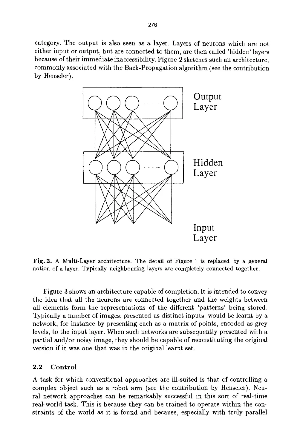
/


Author: Braspenning P.J. Thuijsman F. Weijters A.J.M.M.
Tags: artificial intelligence
ISBN: 3-540-59488-4
Year: 1991


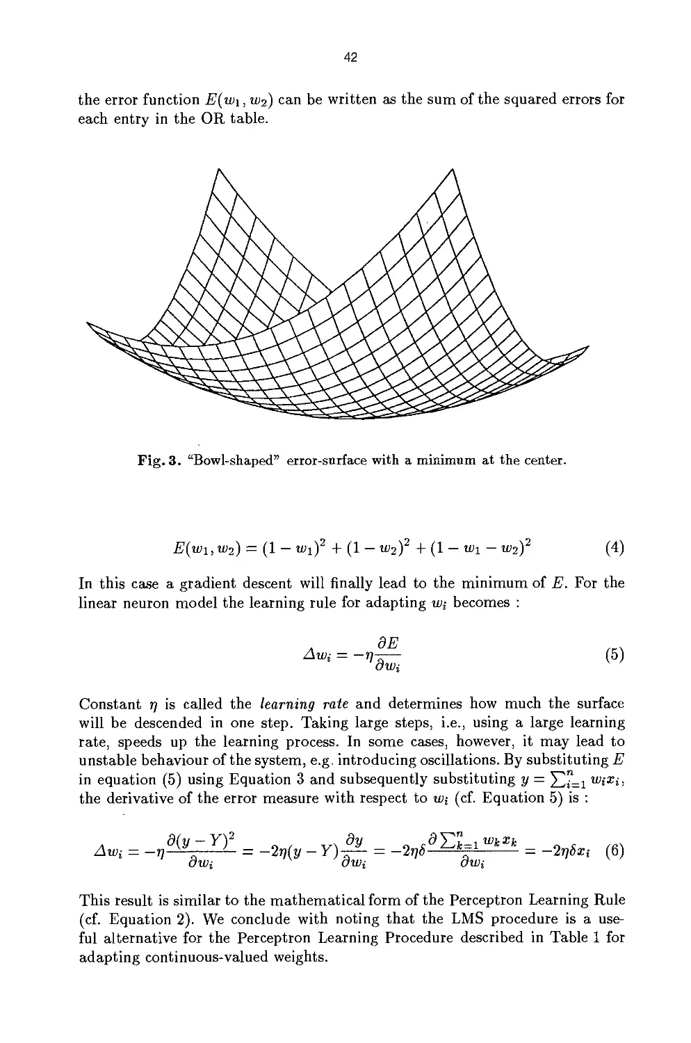
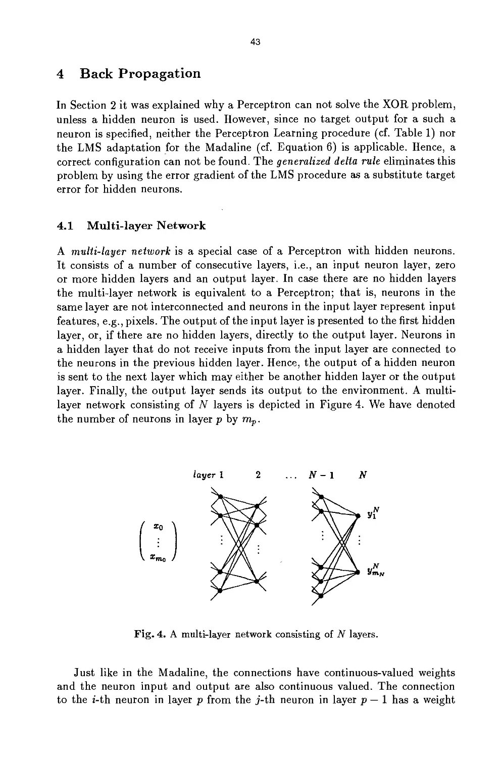
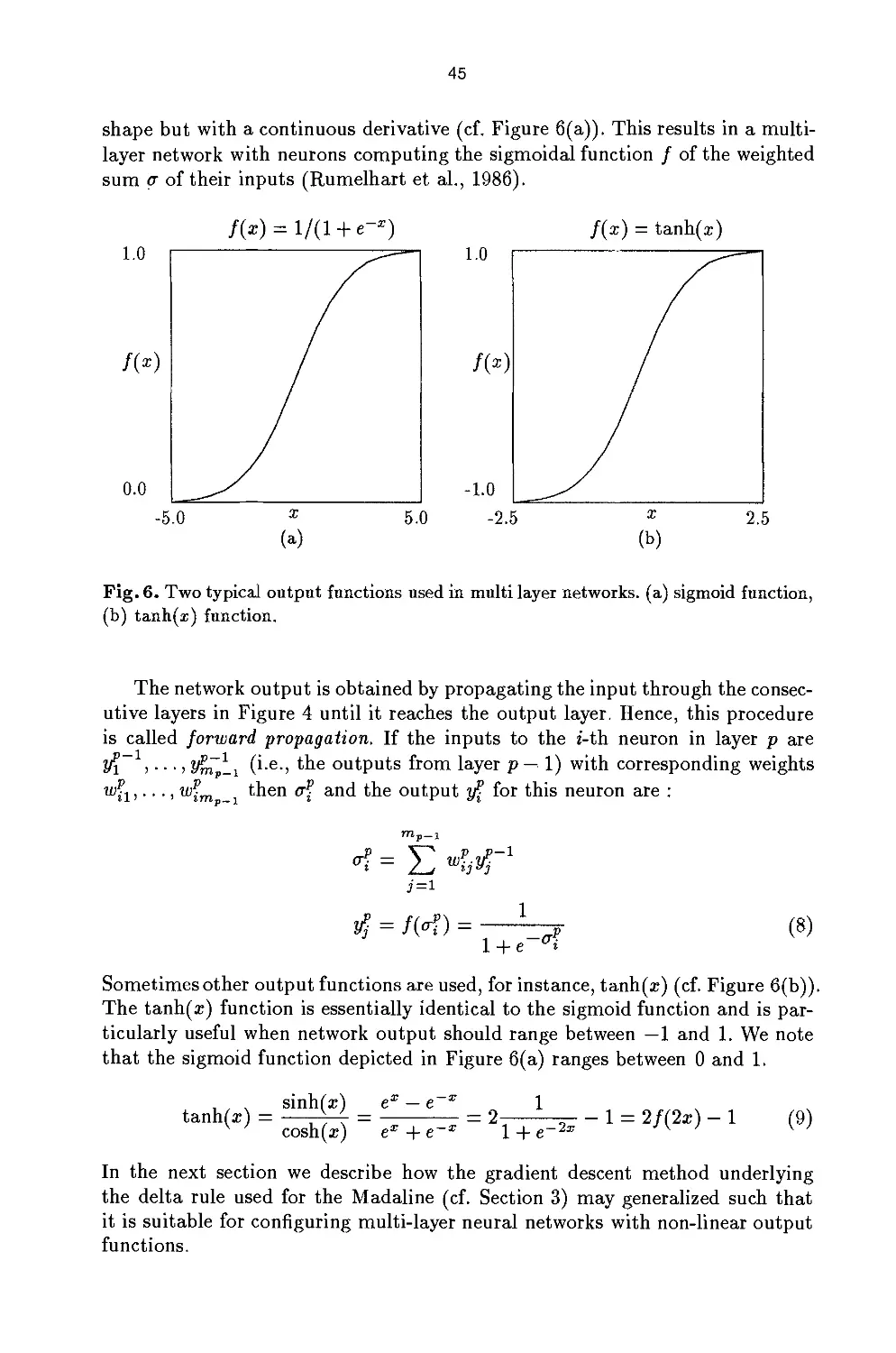
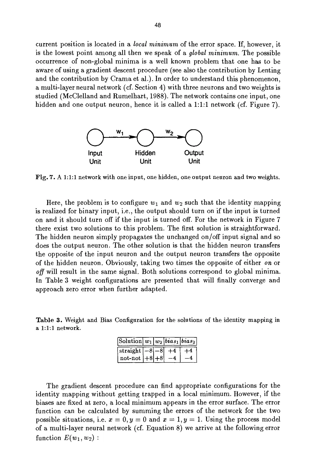
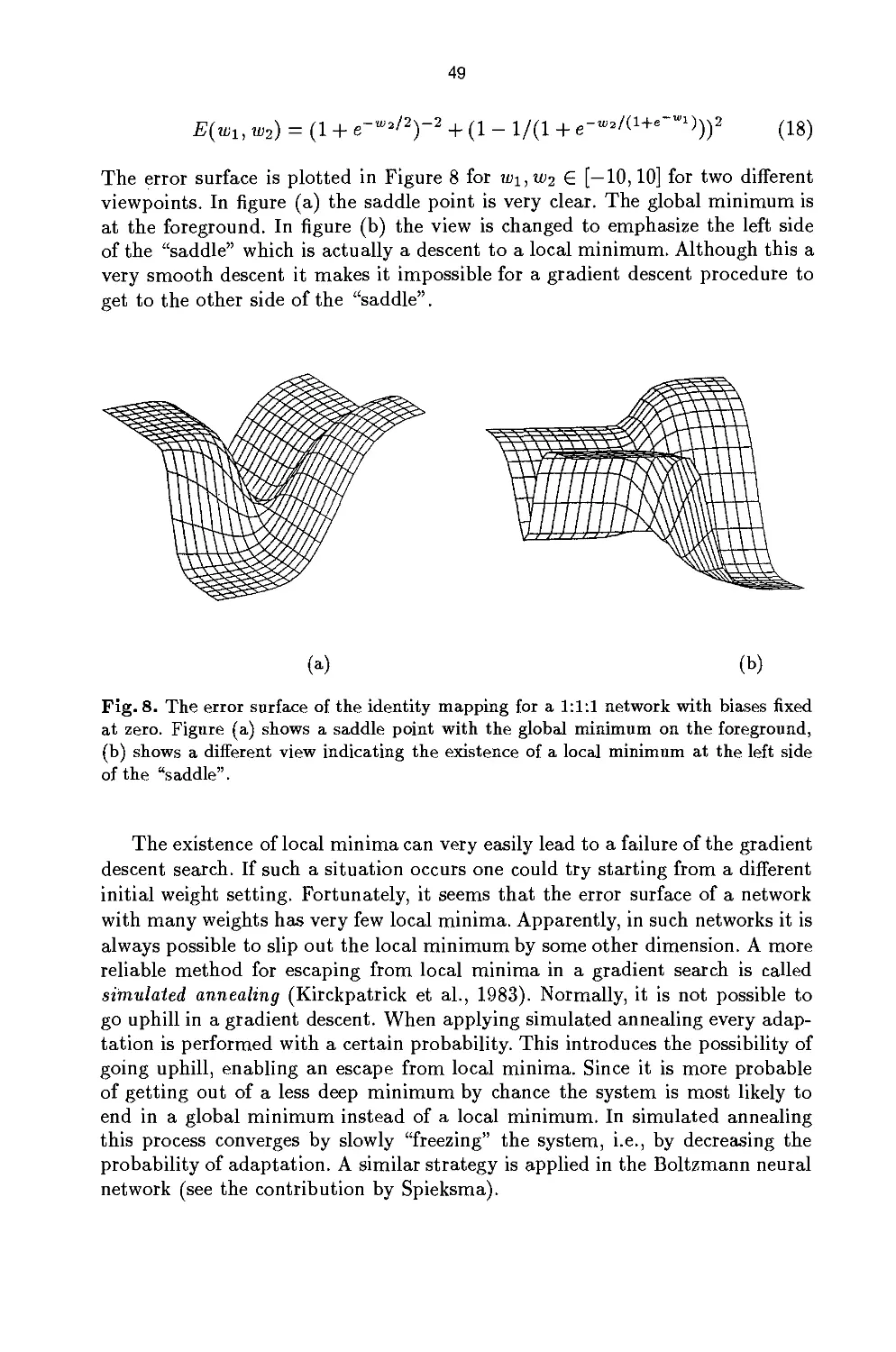
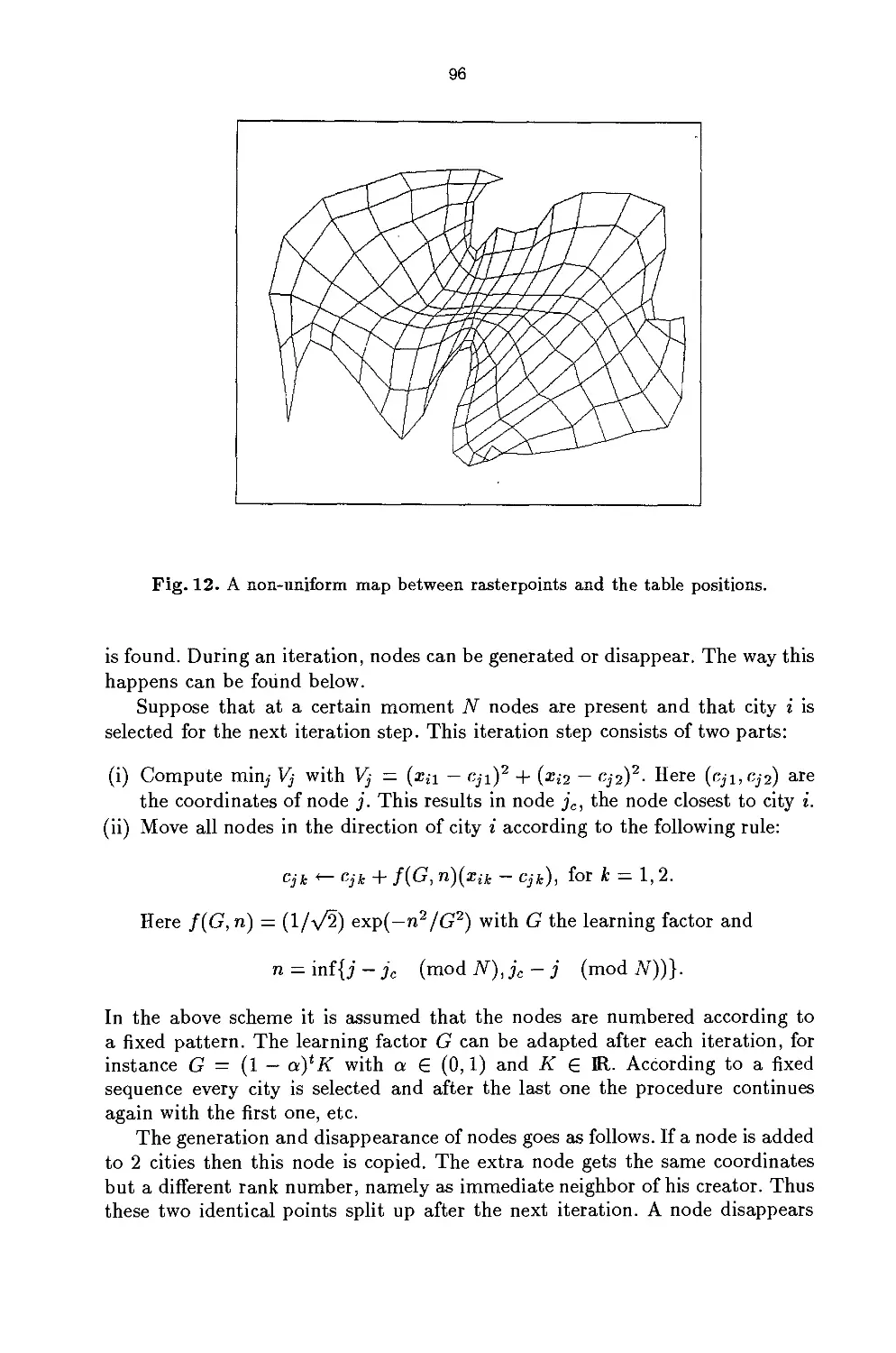
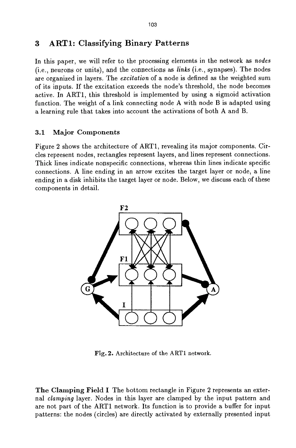
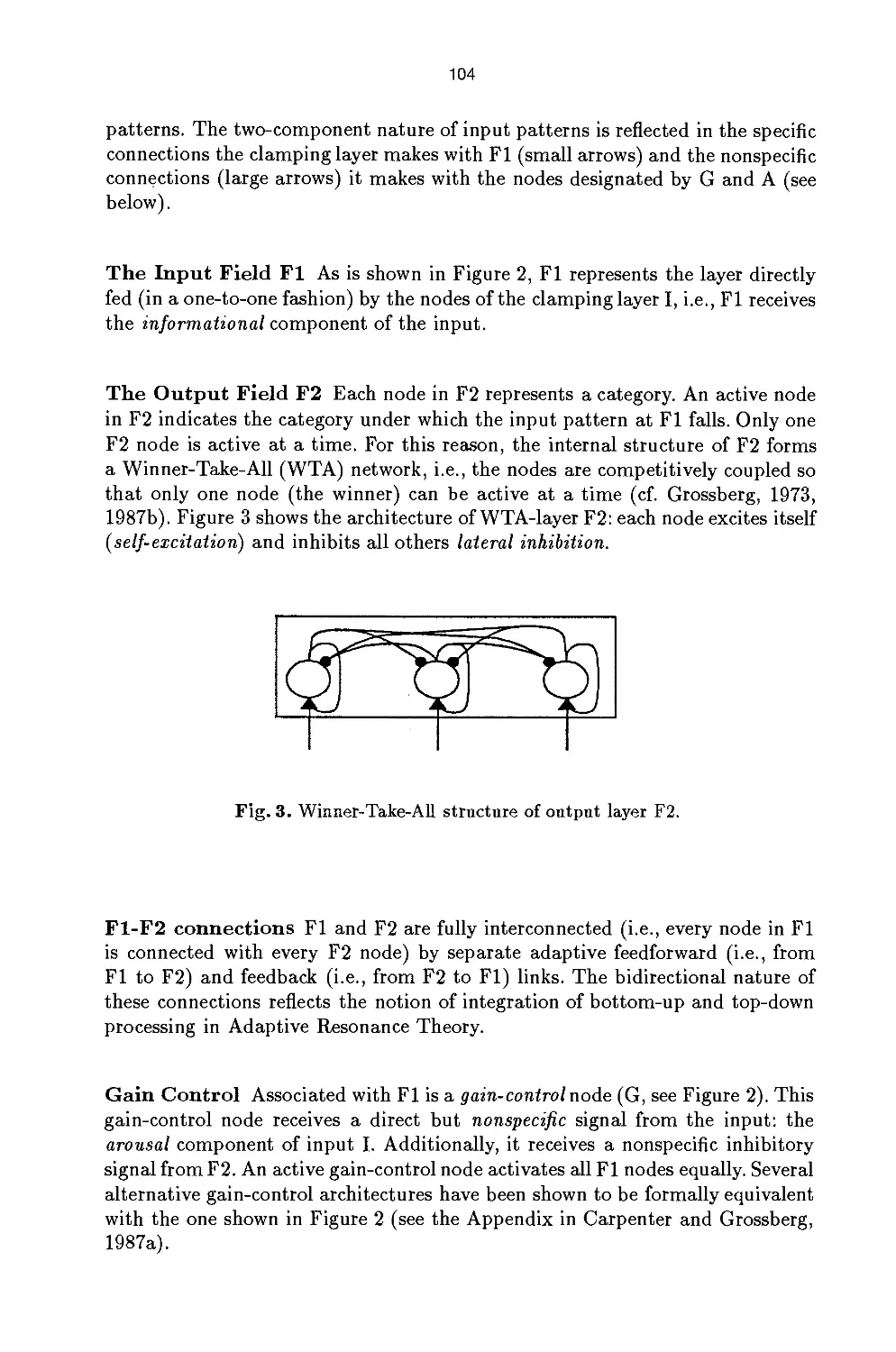
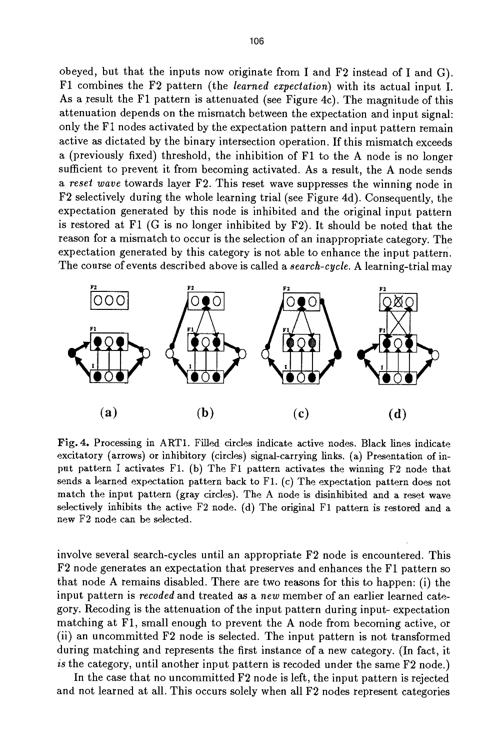
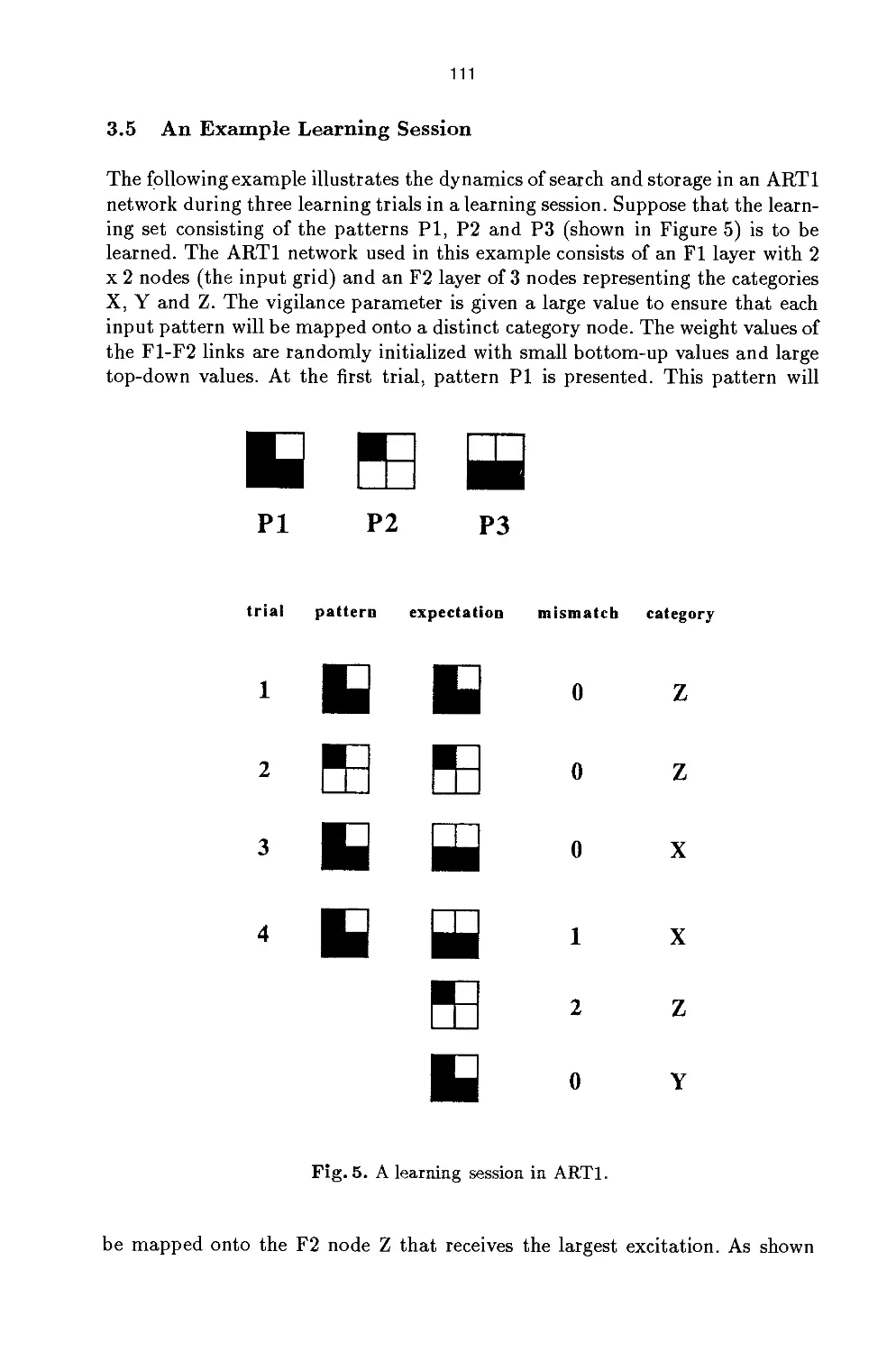
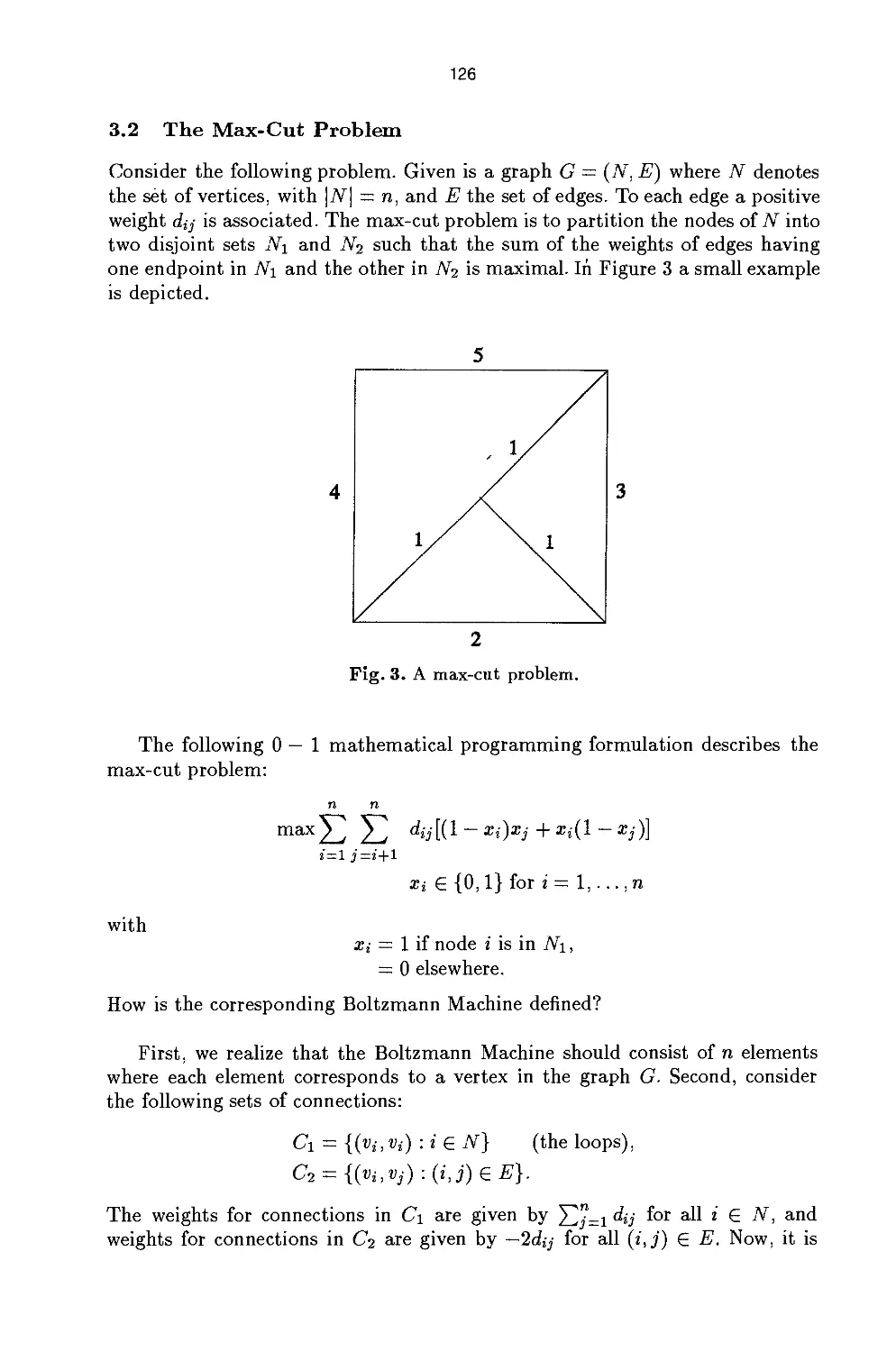
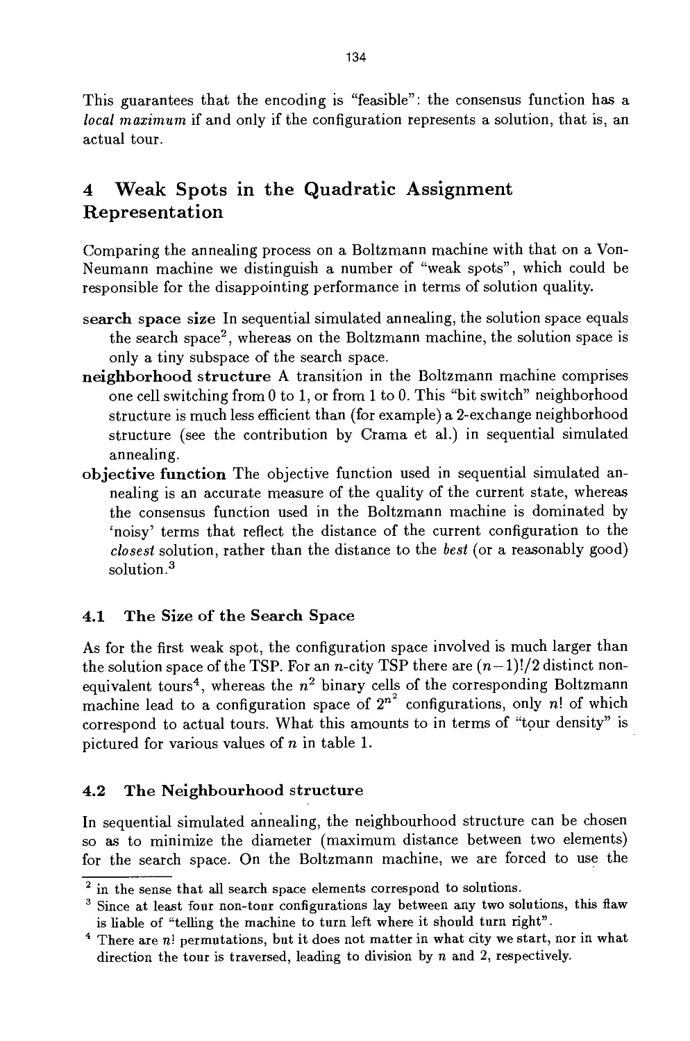
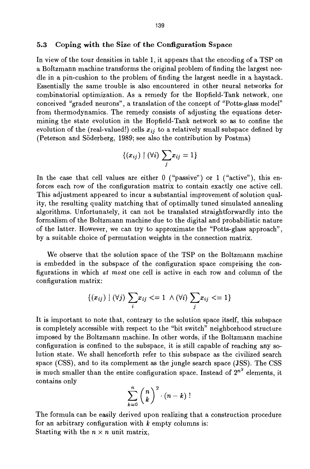
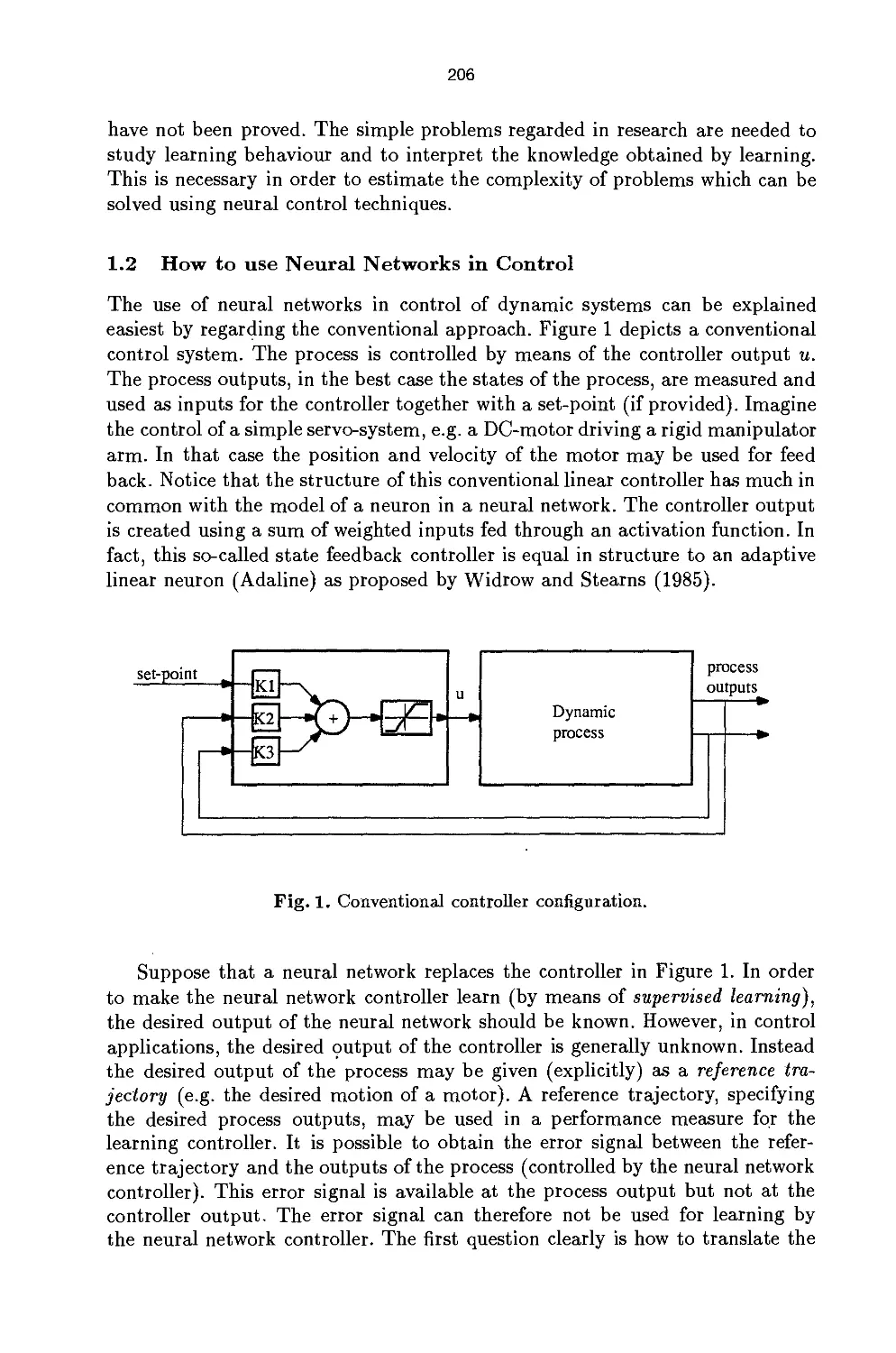
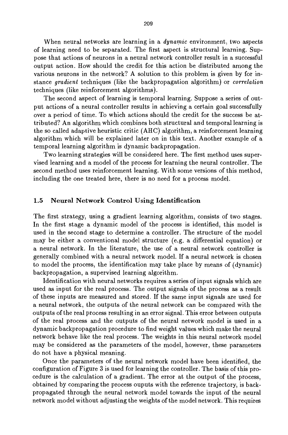
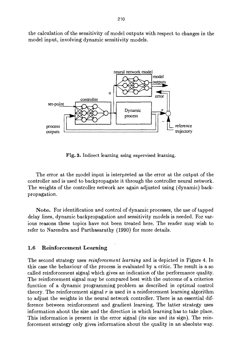
Text
Lecture Notes in Computer Science 931
Edited by G. Goos, J. Hartmanis and J. van Leeuwen
Advisory Board: W. Brauer D. Gries J. Stoer
P.J. Braspenning F. Thuijsman
A.J.M.M. Weijters (Eds.)
Artificial
Neural Networks
An Introduction to
ANN Theory and Practice
fflj) Springer
Series Editors
Gerhard Goos
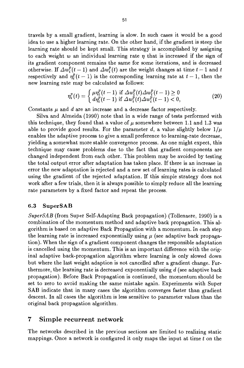
Universitat Karlsruhe
Vincenz-Priessnitz-StraBe 3, D-76128 Karlsruhe, Germany
Juris Hartmanis
Department of Computer Science, Cornell University
4130 Upson Hall, Ithaca, NY 14853, USA
Jan van Leeuwen
Department of Computer Science, Utrecht University
Padualaan 14, 3584 CH Utrecht,The Netherlands
Volume Editors
P.J. Braspenning, Department of Computer Science
F. Thuijsman, Department of Mathematics
A.J.M.M. Weijters, Department of Computer Science
University of Limburg, P.O. Box 616
6200 MD Maastricht, The Netherlands
CR Subject Classification (1991): El.l, 1.2.6, G.1.6,1.5.1, J.l, J.2, J.6
1991 Mathematics Subject Classification: 92B20, 94C15, 68T05, 90C90
ISBN 3-540-59488-4 Springer-Verlag Berlin Heidelberg New York
CIP data applied for
This work is subject to copyright. All rights are reserved, whether the whole or
part of the material is concerned, specifically the rights of translation, reprinting,
re-use of illustrations, recitation, broadcasting, reproduction on microfilms or in
any other way, and storage in data banks. Duplication of this publication or parts
thereof is permitted only under the provisions of the German Copyright Law of
September 9,1965, in its current version, and permission for use must always be
obtained from Springer-Verlag. Violations are liable for prosecution under the
German Copyright Law.
© Springer-Verlag Berlin Heidelberg 1995
Printed in Germany
Typesetting: Camera-ready by author
SPIN: 10486258 06/3142-543210 - Printed on acid-free paper
Preface
This book is the result of a concerted action by the departments of Computer
Science and Mathematics of the University of Limburg (Maastricht, The
Netherlands) to develop a collection of lectures, specifically dedicated to informing the
industrial world about the potential of using neural networks. For this reason,
both departments had worked together within an NN working group to set up
an Autumn School for Neural Networks, which was held in 1990 in Maastricht.
Participants came from different quarters within government, industry and small
and medium-sized companies, and insurance and banking institutes. However,
the participants were not arbitrarily chosen workers within those quarters.
The target group of people addressed by the Neural Network School were
technical managers, consultants, research associates, and software developers at
the high end of the spectrum whose employers expected innovative applications
of new technologies within their own (industrial) setting. Hence, in our view
the target group consisted of people with a reasonable level of formal education
and, specifically, some basic background in mathematics and computer science.
Having this group in mind, the contributions of this book were set. Hence the
prerequisites for a fruitful understanding of the material are set. Nevertheless,
some more specific knowledge of mathematics and/or computer science may be
required at a few places.
The aim of this book is not to offer a systematic exposition of all kinds of
neural networks or a bunch of most often used networks. Rather, the idea was to
focus on two generic application domains, namely control and optimization, and
use these application domains to illustrate the concrete use of different kinds of
neural networks. Put otherwise, these application domains were used to cluster
and direct the NN School lectures to be particularly illustrative for how to apply
different kinds of neural network architecture. In this way, we hoped to serve the
needs of the participants, both regarding their need to (theoretically) understand
the functioning of any particular network and regarding their need to really see
a demonstrative example application.
After the NN School was held we used the feedback from the participants
to update and elaborate the course materials into a set of papers which together
comprise this book. That is, the book is a compilation, not of the original course
materials, but of carefully re-worked original papers. However, it should not be
seen as detailing the newest developments within the rapidly evolving scientific
discipline of neural networks. As explained already, this was not the goal of our
efforts.
What can the reader expect of this book? First, it gives a representative
bunch of neural network architectures which have found widespread application.
The level of exposition is such that the functioning of these neural networks can
be understood, and many times their functioning is also dealt with in a more
analytical fashion. Secondly, quite a few applications are described for which a
particular neural network architecture has been chosen. This choice is not always
VI
based on purely objective criteria, because the field of neural networks is still of
a rather experimental nature. However, where possible the actual choice of
architecture is reasoned. In fact, one contributing paper in this book is exclusively
dedicated to making a choice about the neural network architecture to use for a
particular task within an actual application domain. Thirdly, reading the book
as a whole certainly stimulates one's curiosity (and therefore one's innovative-
ness) about the applicability of neural networks within one's own field of work.
Therefore, the team of authors considers itself to have been successful if many
readers, after reading this book, seriously consider applying some neural network
technology to the problem at hand, whether it is for a classification/recognition
task, a control task, or a complex multiple constraint satisfaction task.
Of course, the ordering of the papers in this book is not arbitrary. It
constitutes the route which we think to be most profitable for the serious reader.
However, depending on the reader's pre-existing background knowledge about
neural networks, we do not object at all to a reader who wants to dive into
particular papers, especially because all papers are sufficiently self-contained.
Nevertheless, we would like to finish this introduction with an outline of the
route of papers in this book.
The first paper, by Braspenning, gives a general chararcterization of neural
networks and puts the contributions to the book in perspective. In the
contribution by Weijters and Hoppenbrouwers the back-propagation network is discussed.
This is probably the most widespread and most popular architecture. The paper
by Henseler addresses this architecture again, but in a more formal way and
applied to a robot control task. The paper by Peters treats the forerunner of
back-propagation networks, namely perceptrons, and analyzes mathematically
their advantages/disadvantages. The contribution by Vrieze gives a basic
treatment of another architecture, the Kohonen network, and analyzes basic
expectations of what it does and can do for a number of application tasks. The paper by
Postma and Hudson again introduces an architecture, namely adaptive resonance
networks, and discusses a number of variants. The paper by Spieksma treats a
neural network architecture which is inspired by physical phenomena treated by
statistical mechanics, namely the Boltzmann machine architecture, and applies
it to a combinatorial optimization problem. The contribution by Lenting
discusses the same architecture, but now from the perspective of how to map (or
represent) a particular problem on (with) such an architecture; a topic which,
in fact, deserves careful attention with any of the architectures. The paper by
Postma introduces another architecture inspired by a physical theory, namely
the Hopfield-Tank network, but its main gist is to show how neural networks
can help in solving optimization problems. The contribution by Crama, Kolen,
and Pesch addresses a wide range of combinatorial optimization approaches
including a neural network approach like the Boltzmann machine and a genetic
algorithm inspired by a Darwinian framework. The paper by Boekhoudt turns
to process identification and control, which is another important generic
application domain of neural networks, and some already introduced NN architectures
are evaluated regarding their promising use. The paper by Van Luenen again
VII
deals with control tasks and discusses the neural network design and learning
strategies appropriate for these tasks with a quite illustrative example
application: the inverted pendulum. The paper by Cardon and Hoogstraten is written
from the perspective of a large industry (Shell) and deals with practical
criteria for choosing a neural network solution illustrated by an application for an
industrial classification task. The next paper by Braspenning discusses the
relationship between NNs and Artificial Intelligence (with its strong emphasis on
symbolic processing) and focuses on a high-level map of the many types of neural
networks and their dynamics, thereby sketching a landscape wherein all treated
architectures may be placed. Finally, the contribution by Hudson and Postma
addresses the topic of choosing and using a neural net, providing suitable criteria
in the context of different types of problems, outlining a general categorization
of neural network architectures, and finally summing up the considerations that
may matter in making a choice.
We would like to finish with a somewhat cautious remark. Although this
book is critical at some points about the appropriateness or usefulness of neural
network technology, it includes among its purposes that of saving this technology
from the sometimes inordinate claims that its enthusiasts are making for it. In
a sense, the neural network hype is over! Dressed in more modest but palpable
working clothes, neural network technology may yet become a reasonably
valuable collection of tools for addressing practical problems.
Finally, we wish to acknowledge those who assisted in making this volume
possible. We thank all participants of the NN School and all contributors to this
volume. We are grateful to P. Schoo for the computer assistance at the NN School
and to J.J.M. Derks and E.J. Pesch for their assistance at various stages of this
project. We are especially indebted to Mrs. M. Verheij and Mrs. M. Haenen for
preparing this document in BTjjX.
P.J. Braspenning
F. Thuijsman
A.J.M.M. Weijters
Contents
P.J. Braspenning
Introduction: Neural Networks as Associative Devices 1
A.J.M.M. Weijters and G.A.J. Hoppenbrouwers
Backpropagation Networks for Grapheme-Phoneme
Conversion: a Non-Technical Introduction 11
J. Henseler
Back Propagation 37
H.J.M. Peters
Perceptrons 67
O.J. Vrieze
Kohonen Network 83
E.O. Postma and P.T.W. Hudson
Adaptive Resonance Theory 101
F.C.R.. Spieksma
Boltzmann Machines 119
J.H.J. Lenting
Representation Issues in Boltzmann Machines 131
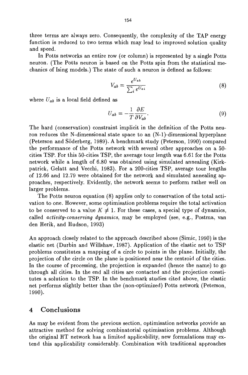
E.O, Postma
Optimization Networks 145
Y. Crama, A.W.J. Kolen and E.J. Pesch
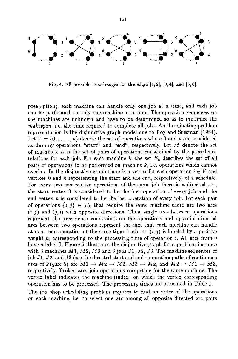
Local Search in Combinatorial Optimization 157
P. Boekhoudt
Process Identification and Control 175
W.T.C. van Luenen
Learning Controllers Using Neural Networks 205
H.R..A. Cardon and R. Hoogstraten
Key Issues for Succesful Industrial Neural-Network
Applications: an Application in Geology 235
P.J. Braspenning
Neural Cognodynamics 247
P.T.W. Hudson and E.O. Postma
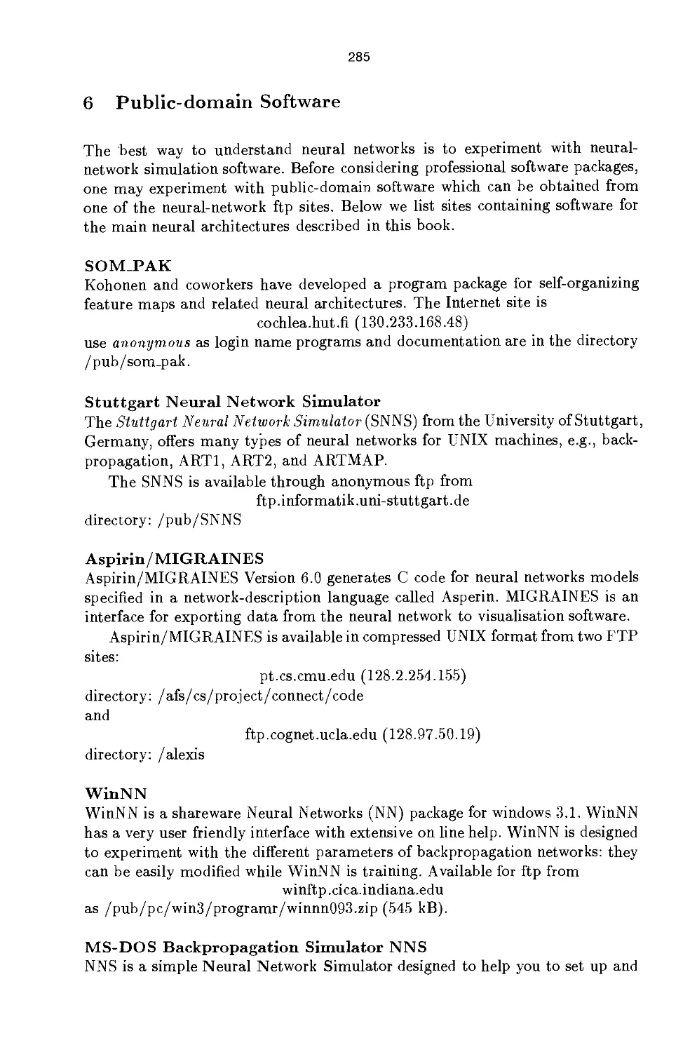
Choosing and Using a Neural Net 273
Supporting General Literature 289
Addresses of the Authors 295
Introduction: Neural Networks
as Associative Devices
P.J. Braspenning
Department of Computer Science, University of Limburg, Maastricht
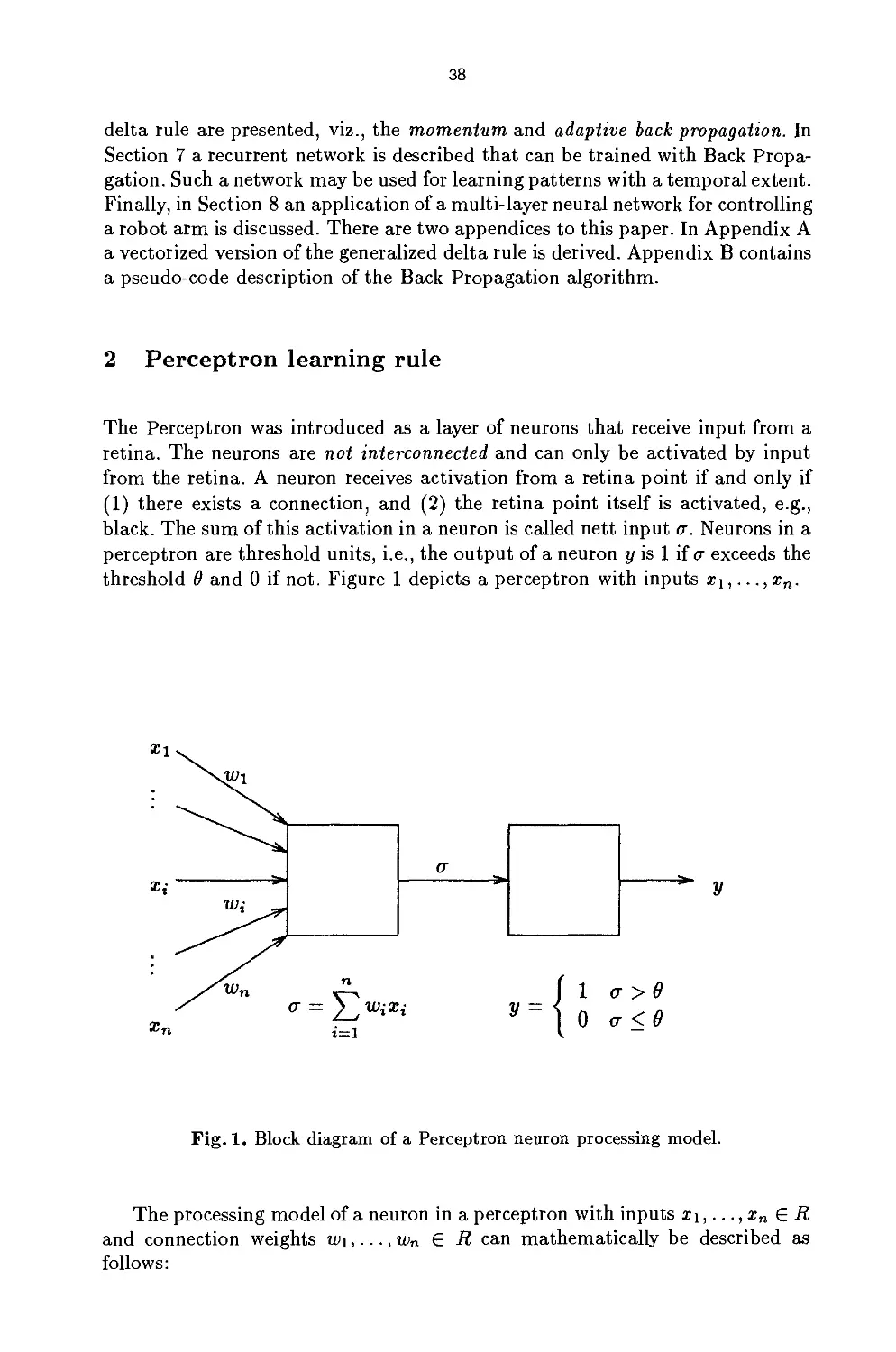
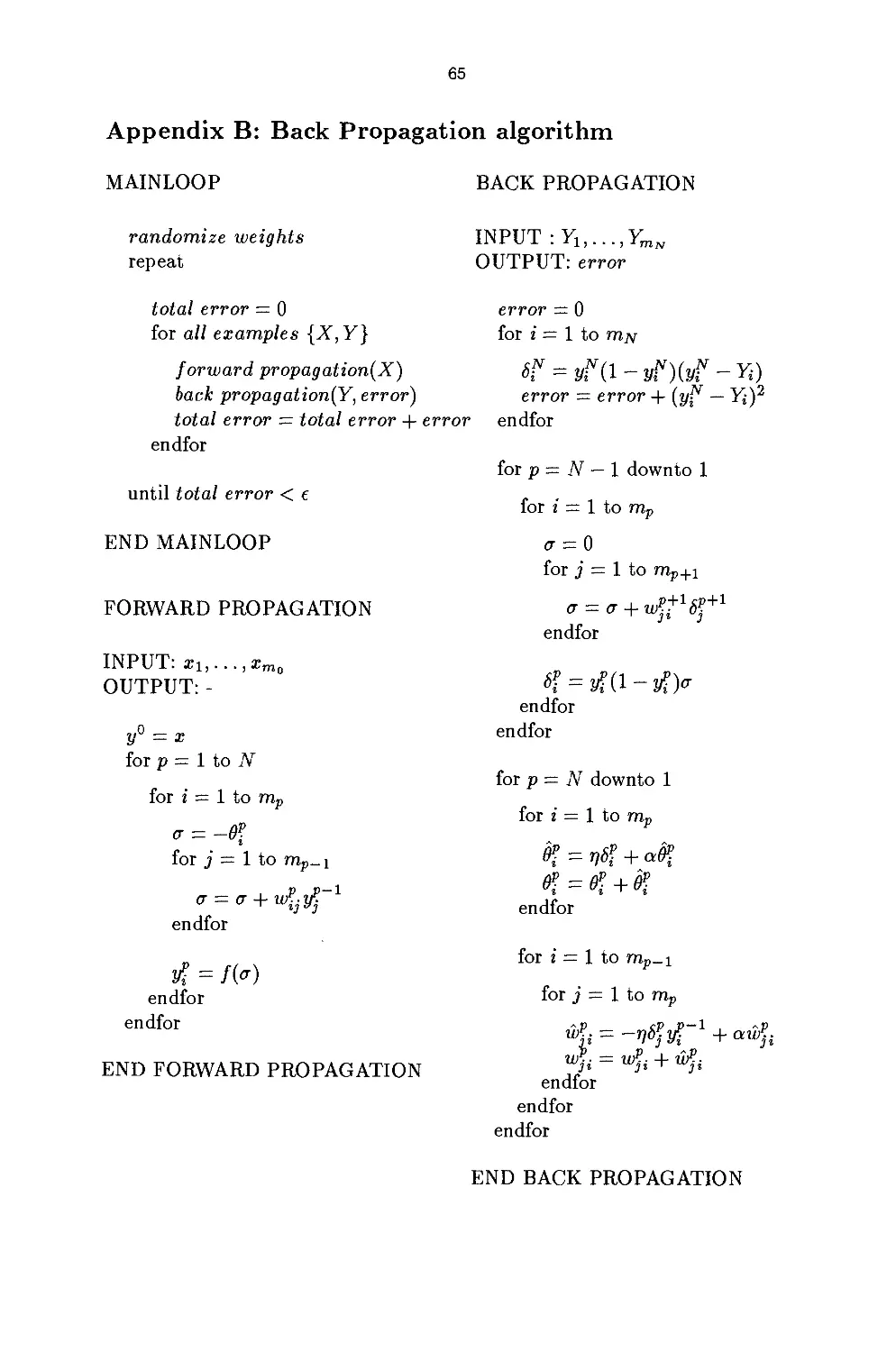
1 Introduction
This introductory paper provides a short overview of the many contributions to
this book. It may help in better finding your way through the following papers,
while also providing the many-faceted reasons for putting them together in the
first place. As stated already in the Preface, this book results from a concerted
action by the departments of Computer Science and Mathematics of the
University of Limburg (Maastricht, The Netherlands) to develop a collection of lectures,
specifically dedicated to informing the industrial world about the potential of
using neural networks. These lectures were thoroughly updated and elaborated
and finalized in the collection of papers which together comprise this book. The
target group concerned technical managers and consultants, research associates
and software developers at the high end of the spectrum. Their employers should
have an active interest in innovative applications of new technologies within their
own (industrial) setting. Therefore, the target group consists of people from such
diverse environments as government, industry and small and medium-sized
companies, insurance and banking etc..
The idea was to focus on two generic application domains, namely control
and optimization, and use these application domains to illustrate the concrete
use of different kinds of neural networks. Although these application domains
were used to cluster the diverse contributions, they were in no way meant to be
exhaustive for the application domains where neural networks may profitably be
used. In fact, we were (and are) sure that neural networks can also be applied
with success in many other domains. Nevertheless, focussing on a rather small
set of (generic) application domains has the advantage that the reader gets a
more lively picture of how to involve neural networks for a problem at hand.
Most contributions to this book try to serve the reader in a two-fold way,
namely to help in understanding the functioning of any particular (type of)
network and to illustrate its use with an application which acts as a demonstrative
example. Further, some contributions are possibly helpful in providing more
context, practical industrial experience or concrete advice about neural networks. In
the following paragraphs we will detail these contributions somewhat more.
2 Associative Devices and Heuristic Devices
First, however, we like to state that the basic interest in neural networks comes
from the fact that they may be considered as very flexible, associative devices.
2
Basically, they are devices able to perform pattern-recognition, -construction
and -retention, but in a way which is both more flexible, and often less well
theoretically understood than more classical pattern-recognition techniques.
Sometimes they may be applied where older techniques just fail since these techniques
require more strict boundary conditions to be fulfilled for their proper use.
However, the results of applying neural networks may be less theoretically justified,
although, of course, still of considerable practical relevance.
To give an example: being able with the help of a neural network to find a
pattern in stock market dynamics may appal the theoretician (when the pattern
is not well-founded enough to predict stock prices), and yet delight the invester
which might use it (additionally) for his nearby decisions and apparently wins
money! The point here is, of course, that practical relevance never coincides with
theoretical well-foundedness. Still, our picture would be too rosy if we would not
add that practical results also don't coincide with practical relevance, since the
latter concept only hints at the possibility of useful, practical results] Hence,
neural networks may be seen as a particular class of heuristic devices. .
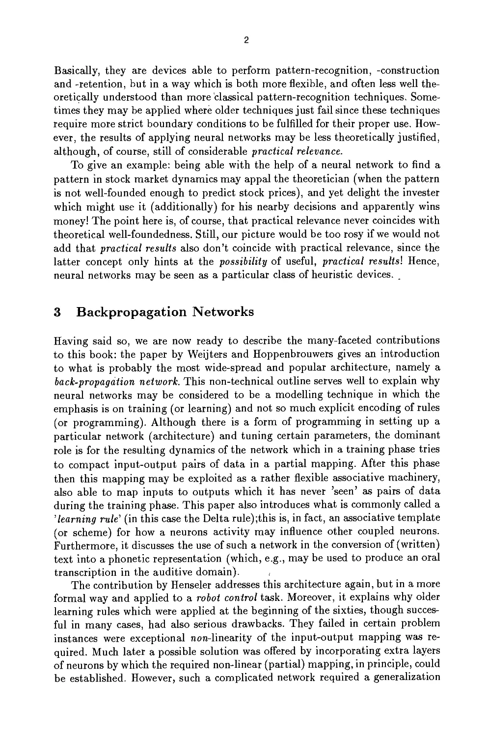
3 Backpropagation Networks
Having said so, we are now ready to describe the many-faceted contributions
to this book: the paper by Weijters and Hoppenbrouwers gives an introduction
to what is probably the most wide-spread and popular architecture, namely a
back-propagation network. This non-technical outline serves well to explain why
neural networks may be considered to be a modelling technique in which the
emphasis is on training (or learning) and not so much explicit encoding of rules
(or programming). Although there is a form of programming in setting up a
particular network (architecture) and tuning certain parameters, the dominant
role is for the resulting dynamics of the network which in a training phase tries
to compact input-output pairs of data in a partial mapping. After this phase
then this mapping may be exploited as a rather flexible associative machinery,
also able to map inputs to outputs which it has never 'seen' as pairs of data
during the training phase. This paper also introduces what is commonly called a
'learning rule' (in this case the Delta rule);this is, in fact, an associative template
(or scheme) for how a neurons activity may influence other coupled neurons.
Furthermore, it discusses the use of such a network in the conversion of (written)
text into a phonetic representation (which, e.g., may be used to produce an oral
transcription in the auditive domain). ,
The contribution by Henseler addresses this architecture again, but in a more
formal way and applied to a robot control task. Moreover, it explains why older
learning rules which were applied at the beginning of the sixties, though succes-
ful in many cases, had also serious drawbacks. They failed in certain problem
instances were exceptional non-linearity of the input-output mapping was
required. Much later a possible solution was offered by incorporating extra layers
of neurons by which the required non-linear (partial) mapping, in principle, could
be established. However, such a complicated network required a generalization
3
of older associative schemata (or learning rules), and only after finding the
generalized delta rule an upsurge in interest for such networks re-appeared. This
paper also addresses some difficulties with this generalized learning rule, and
shows some ways to improve the performance of such networks. Moreover, it
introduces recurrent networks, i.e. networks in which neurons may (indirectly)
feed back their output to neurons from which they previously received inputs.
It seems that such type of networks may be required to find patterns in time
(besides space). Finally, the back-propagation network is applied to the problem
of robot arm movement control, whereas an appendix contains the code for the
basic algorithm. The robot arm requires also discussion of the representation of
the problem for a particular network; a topic which is often undervalued, but
remains of utmost importance for succesfully using any neural network.
4 Some Other Classical Networks
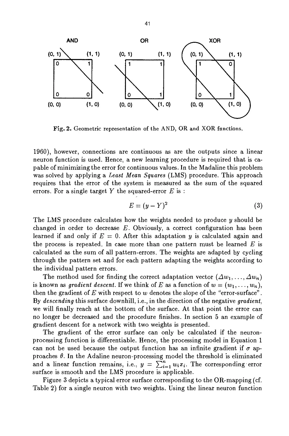
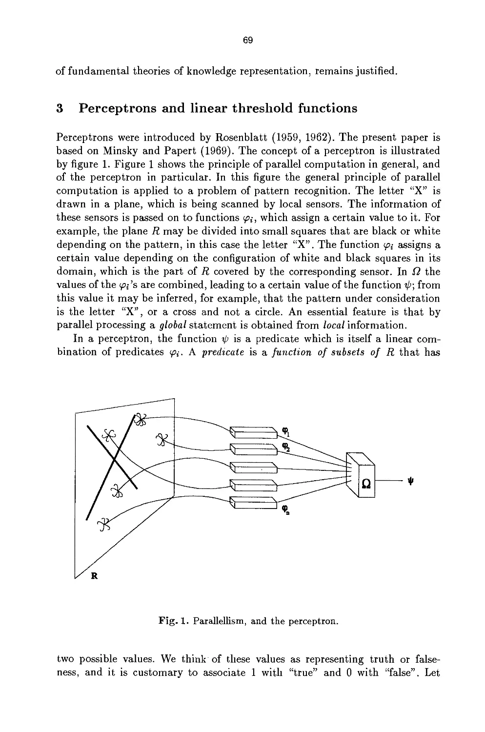
The paper by Peters treats the forerunner of backpropagation networks, namely
perceptrons, and analyzes mathematically their advantages and disadvantages.
Although this type of network is no longer really used the analysis is still of
great interest for a number of reasons. First, perceptrons may be considered to
be building blocks for understanding the functioning of more intricate networks.
As such getting a clear picture of their properties helps in knowing globally what
can (and cannot) be expected of neural networks. Secondly, this paper discusses
also a dynamical building block (of perceptrons and also of many present-day
neural networks), namely the activity of neurons as a linear threshold function.
Although this dynamical property of neuron activity is not used everywhere, it
acts as some sort of yardstick to assess the basic operation of a neurons
processing. Moreover, it is the easiest way to visualize the characteristic non-linear
mapping of a sequence of neurons, dependent on each others output to build up
their own activity, and only producing their own output after reaching a certain
threshold for their activity. Thirdly, this paper addresses the very important
topic of which (complicated) predicates (build out of templates or masks, which
are basic sub-patterns) can be computed (i.e., assessed to be true or false!) by
a certain network type. Again, the perceptron network acts here as some sort of
yardstick against which other network architectures can be measured. Finally,
the topic of training (or 'learning') is treated again, but now in a way which
allows to remove the 'magic' of neural network learning by showing that the
heart of the matter is convergence of the dynamics of the network to a stable
state.
The contribution by Vrieze gives a basic treatment of another architecture,
the Kohonen network, and analyzes basic expectations of what it does and can
do for a sample of application tasks. Since this type of network has quite some
other form and resulting dynamics than the previous perceptron-based family of
treated architectures, the reader is slowly, yet thoroughly introduced to this kind
of neural network. Formal neurons are introduced with a certain basic
mathematical behaviour, and then their interaction within a lattice-like field of such
4
neurons is discussed. Since this interaction, depending on the distance to other
neurons may be exhibitory or inhibitory for the other neurons activity, the
associative scheme (or learning rule) is much more intricate than in the case of the
Delta rule. Still, the basic functioning of the network is as an associative device,
but now in a 'self-organizing' (or unsupervised) way. Stripped from 'magic', this
term means only that the associations found by the neural network of Kohonen
type result from inherent dynamical adaptation of the network to the data set.
Depending on the complexity of the network and corresponding inherent
dynamics the Kohonen type network generally projects a collection of input-output
vector pairs onto a space of lower dimensionality while preserving as much as
possible the topology of the original set of vector pairs in this lower dimensional
space. The network 'incorporates' this nearby topology in its collective neuronal
interaction. After appropriate proofs of basic properties this paper also discusses
some applications, and provides the code of the basic algorithm in the appendix.
5 Stability versus Plasticity
The paper by Postma and Hudson again introduces an architecture, namely
adaptive resonance networks, and discusses a number of variants. The
theoretical background (Adaptive Resonance Theory) of these ART-networks are to
be found in numerous publications by Grossberg and co-workers. However, this
contribution focusses on more practical aspects of this family of neuronal
networks. Just like the previous type of networks, the ART-networks operate in an
unsupervised way. However, their basic functioning is quite different: they learn
input patterns by trying to classify them under the heading of a most similar
class pattern. If such a class pattern can not be found then the input pattern
may be the seed of a new class pattern. The theoretical framework (ART) is a
thoroughly worked out answer to what is called the stability-plasticity dilemma.
This dilemma is faced by any neural network, but Grossberg and co- workers
were particularly concerned about it, because their basic purpose was to mimick
as far as possible the way in which our brain has solved that dilemma. It comes
down to being plastic enough to be able to store new input patterns, yet stable
enough to be able to maintain already properly stored (or classified) patterns.
The family of ART-networks (ART1, ART2 and ART3 etc.) is treated in just
enough detail to get a basic understanding of their functioning and the kinds
of input patterns (binary, analog) to which they can be applied. Finally, an
evaluation of the whole family of networks is provided.
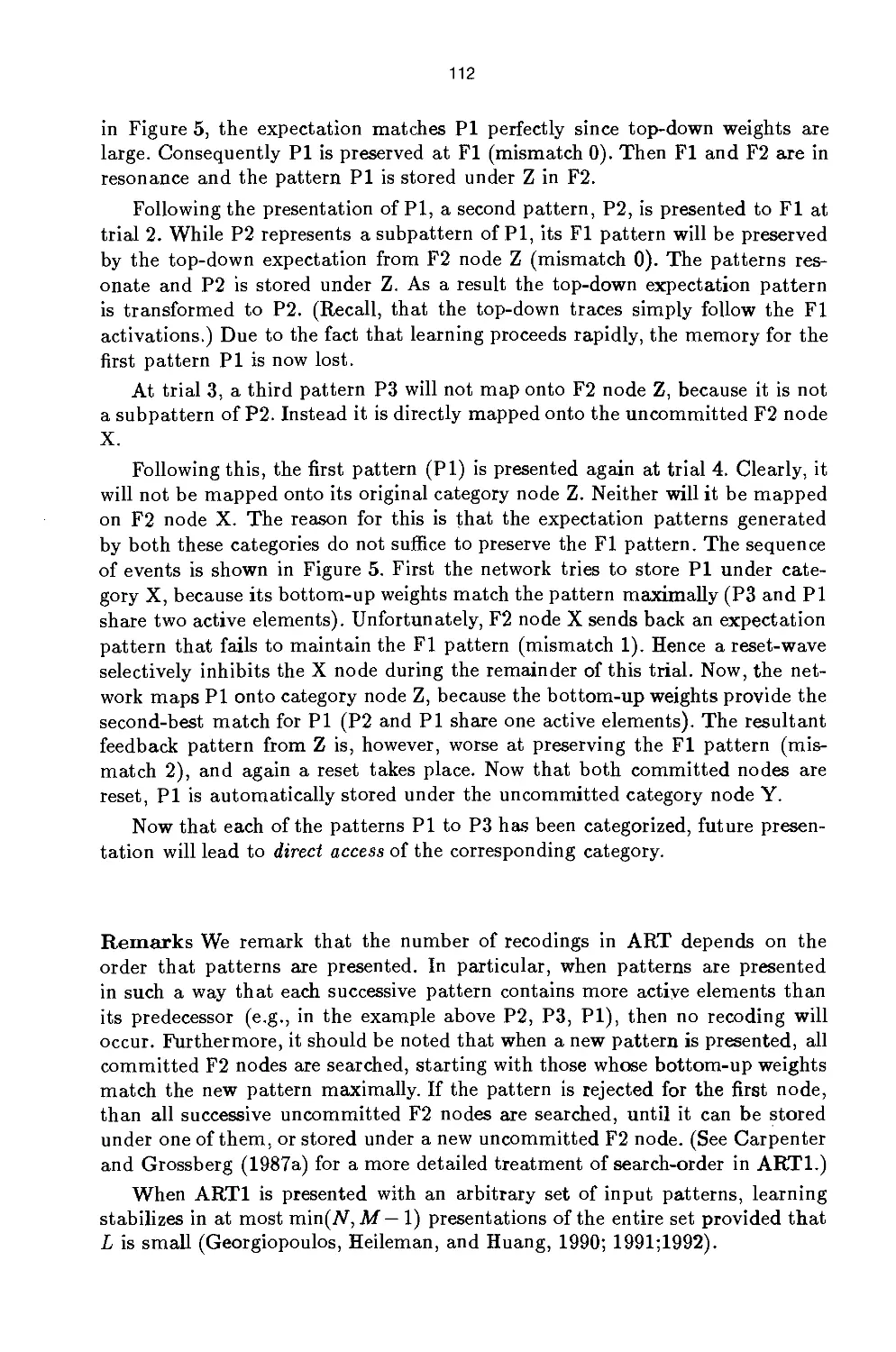
The contribution by Spieksma treats a neural network architecture which
is inspired by physical phenomena treated by statistical mechanics, namely the
Boltzmann machine architecture, and applies it to a combinatorial optimization
problem. However, the Boltzmann machine may also be applied to problems from
all areas of pattern recognition and pattern learning. The most basic properties
of such machines, i.e. when they are implemented in the most proper way, are
massive parallelism (any neuron calculates its activity and output irrespective of
the calculations of any other neurons) and simulated annealing (collectively and
5
in time, the neurons slowly 'freeze' their acquired, yet plastic patterns into more
stable patterns). Though a very promising type of network, the reader should
keep in mind that most of the implementations until now are not full
implementations, but mostly simulations of the massive parallelism attributed to Boltzmann
machines. Still, even those simulations may provide useful results, although the
user should be careful (see Lenting's contribution). This paper provides a
detailed description of the Boltmann machine and its variants. Moreover, it treats
some combinatorial optimization problems (max-cut, Travelling Salesman) and
how the Boltmann machine may handle them. A summary and description of
some possible future developments close this paper. It is to be mentioned that
the Boltmann machine model is not only widely used in theoretical physics, but
is also one of the most well-understood and analyzeable models in the field of
neural networks.
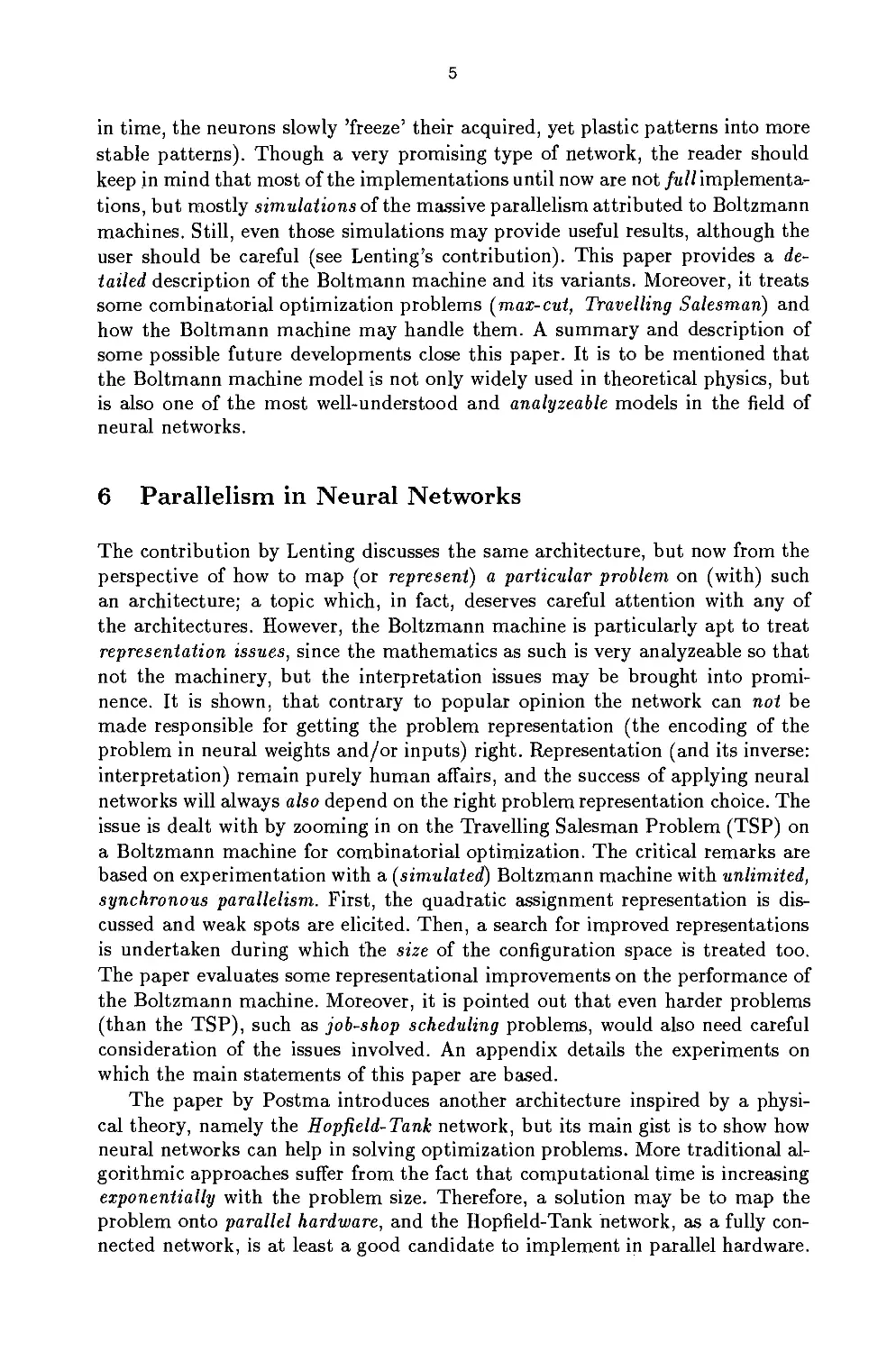
6 Parallelism in Neural Networks
The contribution by Lenting discusses the same architecture, but now from the
perspective of how to map (or represent) a particular problem on (with) such
an architecture; a topic which, in fact, deserves careful attention with any of
the architectures. However, the Boltzmann machine is particularly apt to treat
representation issues, since the mathematics as such is very analyzeable so that
not the machinery, but the interpretation issues may be brought into
prominence. It is shown, that contrary to popular opinion the network can not be
made responsible for getting the problem representation (the encoding of the
problem in neural weights and/or inputs) right. Representation (and its inverse:
interpretation) remain purely human affairs, and the success of applying neural
networks will always also depend on the right problem representation choice. The
issue is dealt with by zooming in on the Travelling Salesman Problem (TSP) on
a Boltzmann machine for combinatorial optimization. The critical remarks are
based on experimentation with a (simulated) Boltzmann machine with unlimited,
synchronous parallelism. First, the quadratic assignment representation is
discussed and weak spots are elicited. Then, a search for improved representations
is undertaken during which the size of the configuration space is treated too.
The paper evaluates some representational improvements on the performance of
the Boltzmann machine. Moreover, it is pointed out that even harder problems
(than the TSP), such as job-shop scheduling problems, would also need careful
consideration of the issues involved. An appendix details the experiments on
which the main statements of this paper are based.
The paper by Postma introduces another architecture inspired by a
physical theory, namely the Hopfield-Tank network, but its main gist is to show how
neural networks can help in solving optimization problems. More traditional
algorithmic approaches suffer from the fact that computational time is increasing
exponentially with the problem size. Therefore, a solution may be to map the
problem onto parallel hardware, and the Hopfield-Tank network, as a fully
connected network, is at least a good candidate to implement in parallel hardware.
6
The theoretical framework comes from the area of spin-glasses within Solid State
Theory (one of the Theoretical Physics sub-disciplines). As the mathematical
model is well-known in those circles, and full connectivity of neurons often
simplifies the analysis of the network, traditional statistical-mechanics techniques
could be applied to Hopfield-Tank (HT) networks. In fact, being able to handle
such networks within a well-understood theoretical framework caused a
widespread and ever Increasing interest to re-appear in those 'good old' neural nets.
This contribution treats the structure and dynamics of HT- networks in enough
detail to understand their basic functioning. Further, it shows how the task
assignment problem (as an example of an optimization problem) can be mapped
onto this type of network. Furthermore, the performance of HT-networks and
the special role of continuous activation functions together with the use of a
sigmoid non-linearity to produce neural outputs is treated. A final discussion
explains the shortcomings and current research alternatives.
7 Neural Networks versus Other Approaches
The contribution by Crama, Kolen and Pesch addresses the full range of
combinatorial optimization approaches including a neural network approach like the
Boltzmann machine and a genetic algorithm inspired by a Darwinian
framework. However, the real topic concerns the local search in combinatorial
optimization since the local search is the basic principle underlying many classical
optimization methods. Connected with local search is a neighbourhood around
every feasible solution of a (combinatorial optimization) problem. This again is
an operationalization of the basic idea that slight perturbation of known feasible
solutions may render the final solution by looking simultaneously for minima in
the objective function which reflects the constraints (the function is defined over
the space of feasible solutions). Hence, local search is crucial and, moreover, also
well-suited to explain the dynamics of many types of neuTal networks (see also
the contribution by Hudson and Postma). This paper is illuminating on many
topics such as: how to pick an initial solution, how to define neighbourhoods
and how to select (search) a neighbour of a given solution. Obviously, both the
starting solutions and the choice for the size of the neighbourhoods are
important for any local search procedure. There is a trade-off between quality of the
solution and complexity of the algorithm. In addition, there is always a problem
with local search, namely the existence of local optima (which are not global).
This paper describes very well how recent extensions of local search with more
possibilities to escape local optima (e.g., Boltzmann machine, Tabu search) come
down to allowing for occasional degradations of the objective function. Moreover,
it shows clearly why, in this context, genetic algorithms are also an
interesting technique, because here the computation starts with a population of feasible
solutions instead of a single one (as in more traditional approaches).
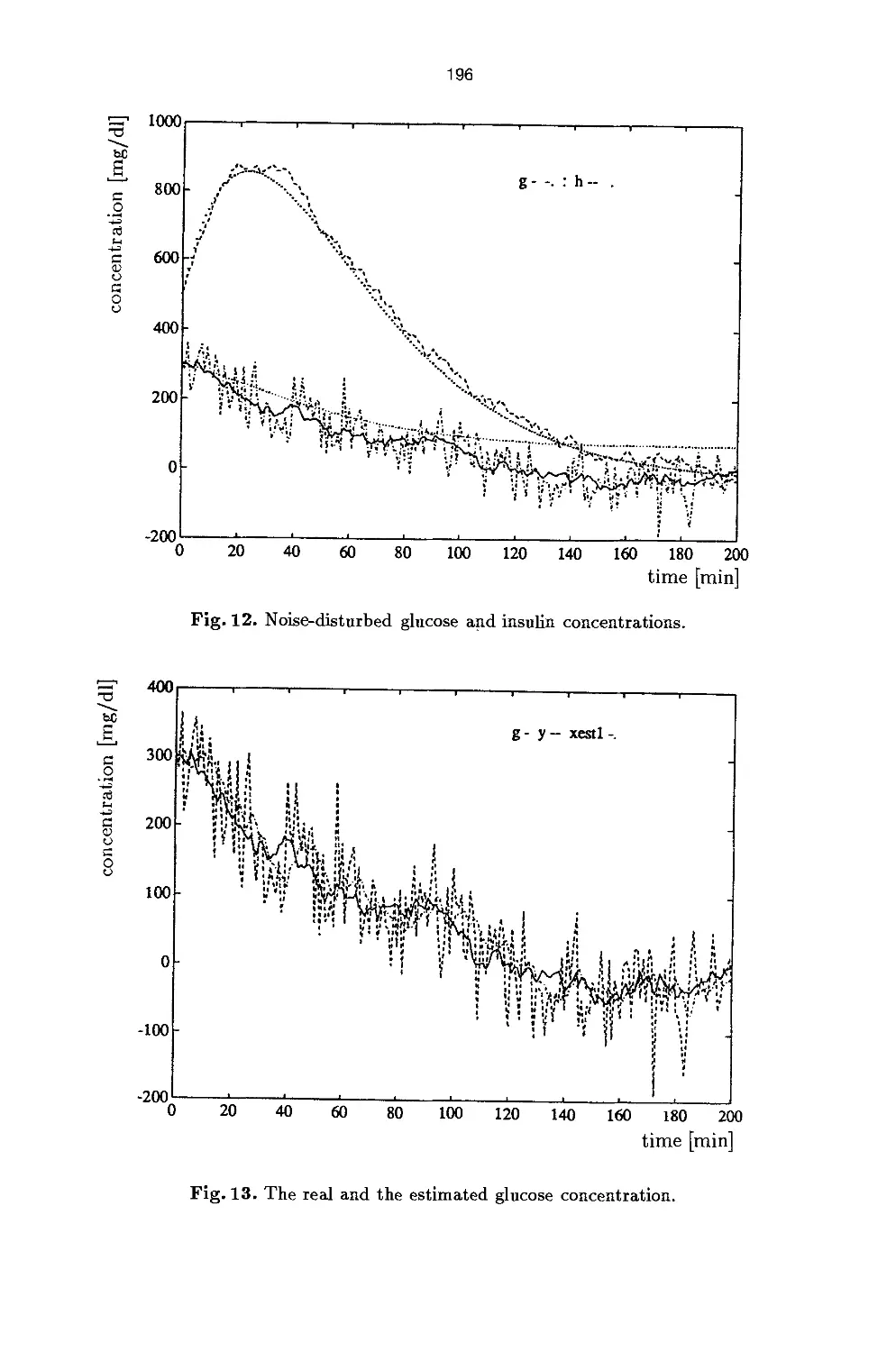
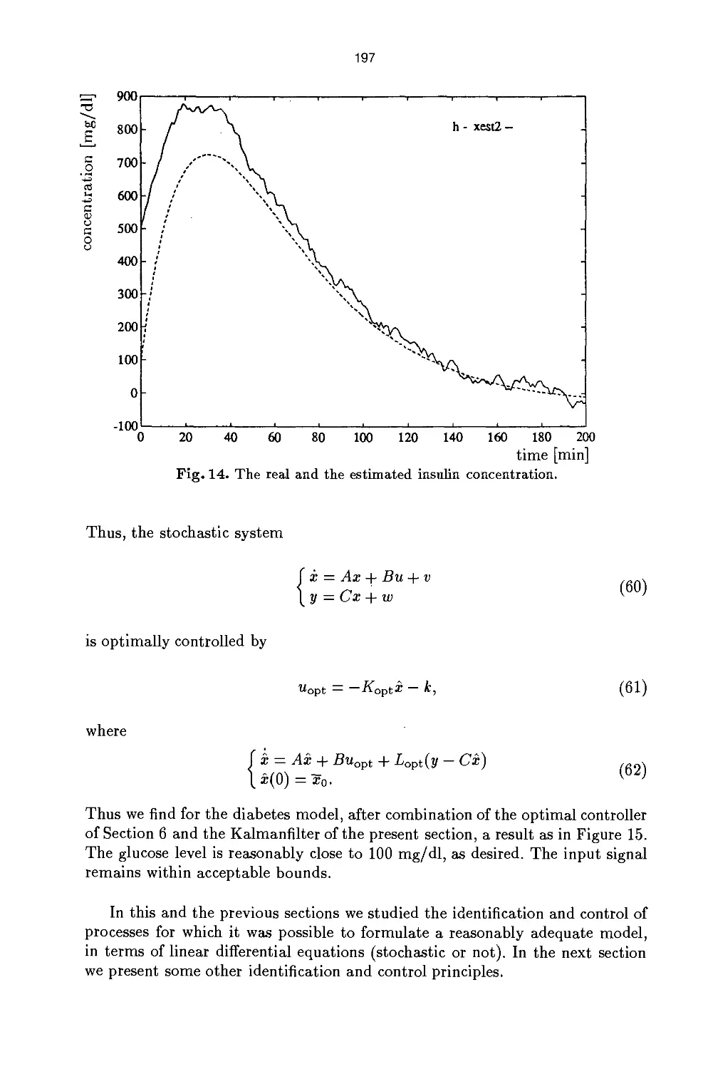
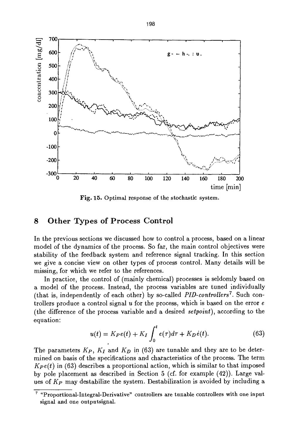
The contribution by Boekhoudt turns to process identification and control,
which is another important generic application domain of neural networks, and
some already introduced NN-architectures are evaluated regarding their promis-
7
ing use. The issues of control can not be tackled before the process to be con-
troled is understood. Therefore, the topic of process identification should be
addressed first. Process identification consists of a number of steps to come to
a mathematical model formulation of the process to be studied. This paper
surveys "traditional" methods of identification and control (in the sense that they
make no use of neural networks). After that, it discusses where neural networks
may profitably be used. The basic ideas of process identification and control are
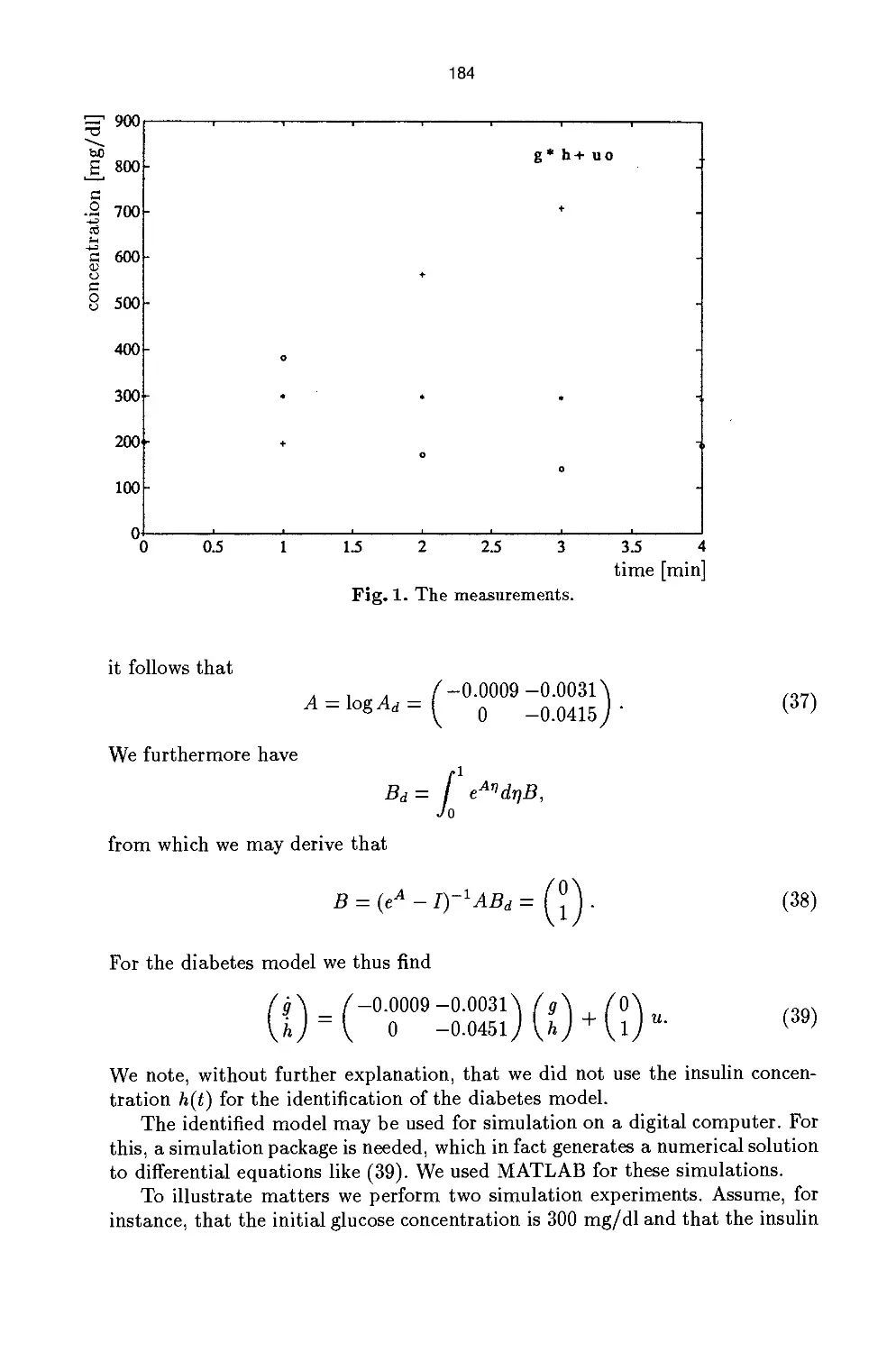
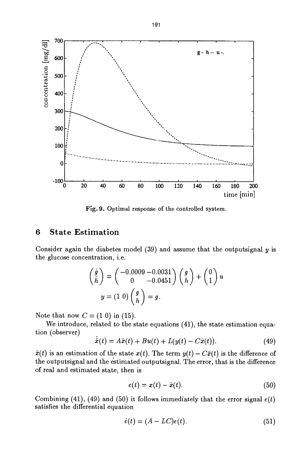
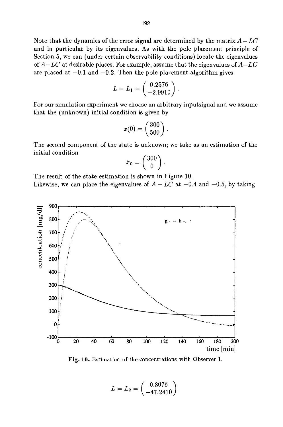
treated with the help of a particular model of the diabetes mellitus process. It
serves well to understand the basic issues, such as the parameter-identification
problem, process control by pole placement, state estimation etc.. These basics
are then extended with a discussion of stochastic systems, which may be applied
to account for differences between model results and reality. Differences which
may results from such diverse sources as 1) changing process characteristics, 2)
unmodelled non-linearities, 3) changing process parameters, and 4) sensor (mea-
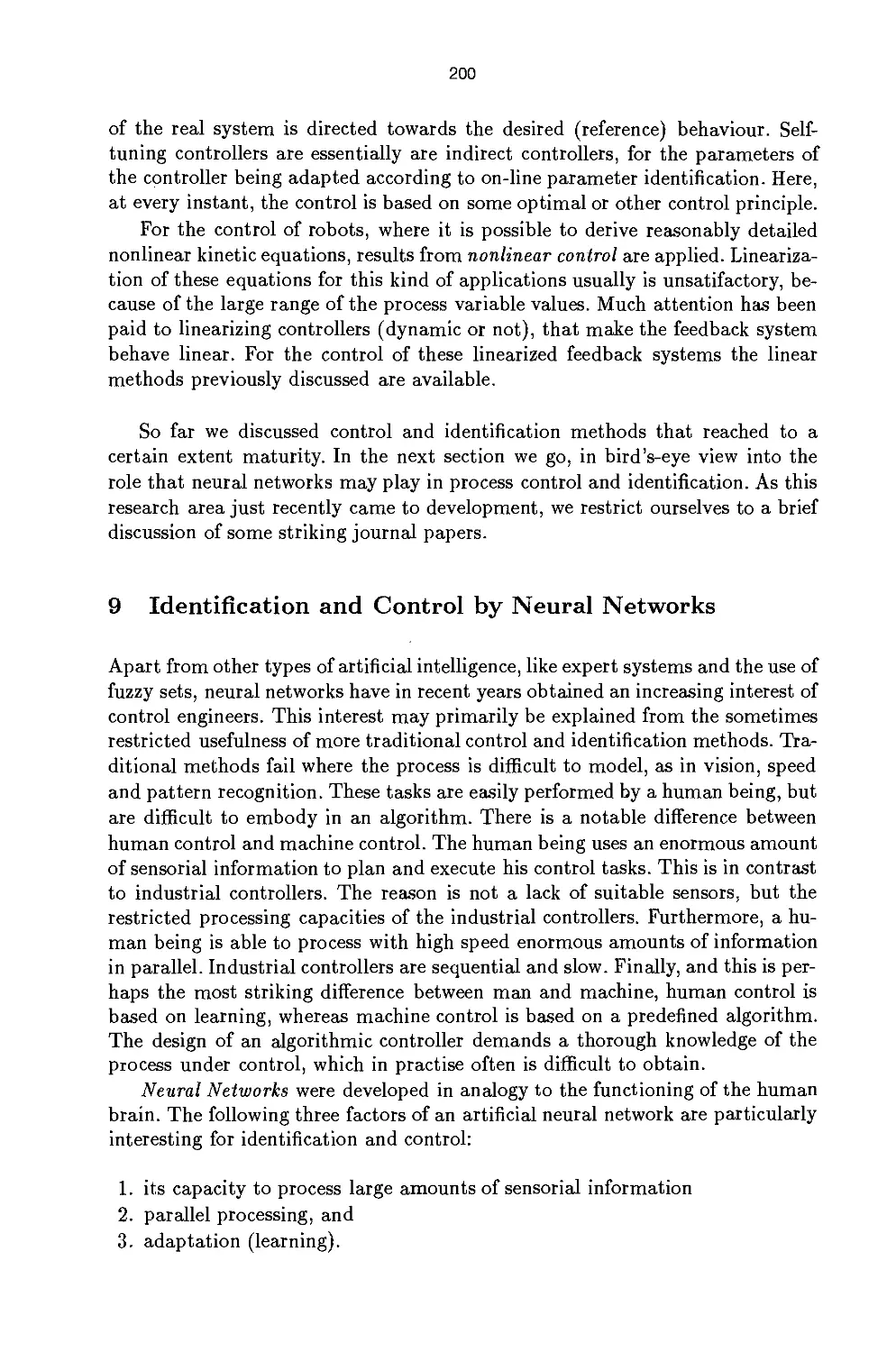
surement)errors and other disturbances. Moreover, control of processes, based
on a linear model of the dynamics, sometimes requires other types of process
control. Also, the fact that a model is not always completely given (i.e., lack
of knowledge) requires other types of control. It is in these cases that neural
networks may profitably be used, but more mathematical rigor in applying them
is certainly needed.
8 Applying Neural Networks
The paper by Van Luenen again deals with control tasks and discusses the
neural network design and learning strategies appropriate for these tasks with a
quite illustrative example application: the inverted pendulum. Again, the
emphasis is on preliminary results, although quite interesting results are claimed
in the literature. However, the author quite rightly warns that all present-day
work is experimental in nature and mostly conducted in research laboratories.
Still, one may expect that in future more and more control tasks will be solved
with the help of (particular types of) neural networks, and major problems (e.g.,
long learning times, computational capabilities, proofs of convergence and proofs
of stability) will (at least partially) be solved. After an extended introduction
which explains how neural networks may be applied to control problems, what
kind of learning strategies may be used, how process identification (sometimes
also in the form of a neural network model) is done, and how a priori knowledge
may be embodied, the learning strategy of reinforcement learning is treated in
more detail. In particular, the adaptive heuristic critic (AHC) algorithm can be
used to learn the control of a process, and this algorithm is treated in quite some
detail. An example application of this algorithm is with the inverted pendulum; a
very nice application since this process is notoriously instable and allows to show
the real power of this learning strategy. Experimental results are provided and
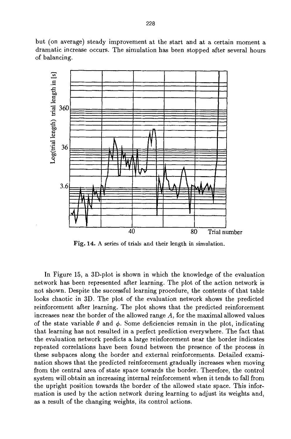
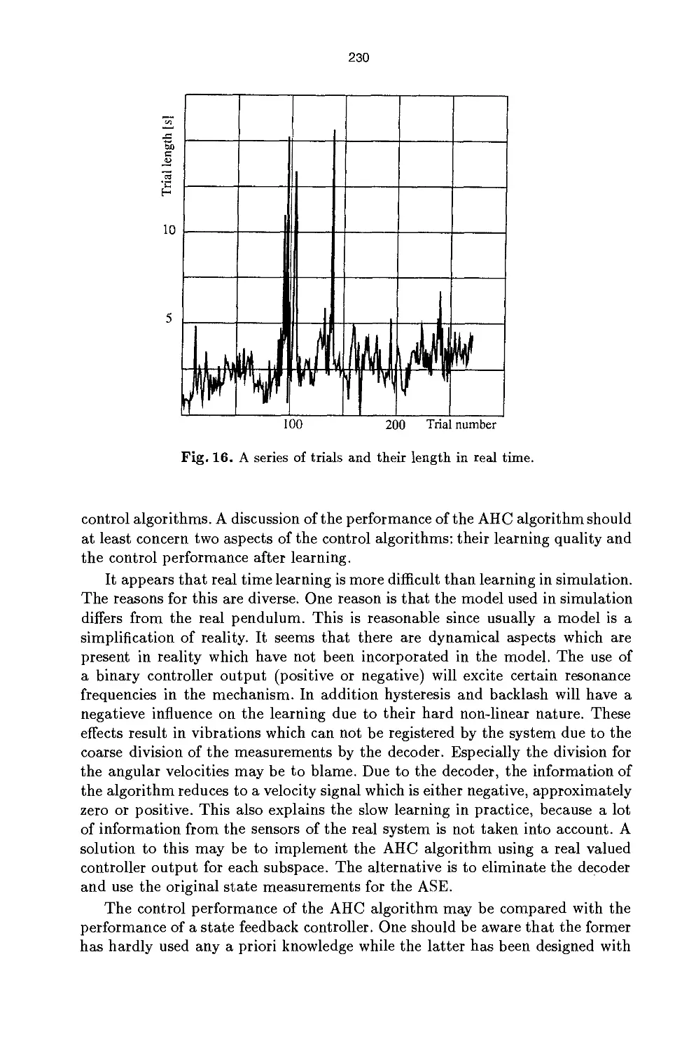
discussed, also with respect to the real time behaviour of the pendulum.
Interestingly, an integration of Artificial Intelligence and neural networks is foreseen
to be needed for practical use of neural controllers.
8
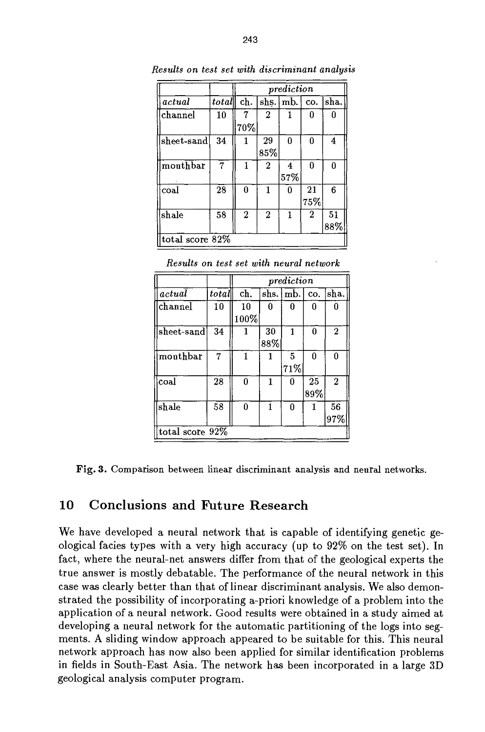
The contribution by Cardon and Hoogstraten is written from the
perspective of a large industry (Shell) and deals with practical criteria for choosing a
neural network solution illustrated by an application for an industrial
classification task. The experience reported here goes back to developments within the
Shell Research laboratory in Rijswijk (The Netherlands), where already from the
mid eighties neural network explorations were performed. Shell Research was
a forerunner in applying neural networks to concrete practical problems, and
people in the laboratory became used to considering the use of Expert Systems,
Standard Statistics, Genetic Algorithms on Rule Induction besides the possible
application of neural networks to their problems. Therefore, this paper reports
in a condensed way about their experiences, mostly in the form of answers to
key questions, such as: When do you consider to use a neural network?, What
are the critical isssues when introducing a neural network in an operational
environment?, What are the most important stages in the development cycle?
Subsequently, a practical application developed within the laboratory will be
discussed. In this context, also a comparison with a well-known statistical technique
(Linear Discriminant Analysis) is given. Moreover, some improvements to the
algorithm (Back-Propagation) used in the application, are treated. The neural
network developed for the identification of genetic geological fades types proved
quite succesful in practical terms. For example, when the neural network answer
differs from the answers provided by the geological experts, the answer is mostly
debatable in the first place.
9 Context, Choice and Use of Neural Networks
The next paper by Braspenning discusses the relationship between NNs and
Artificial Intelligence (with its emphasis on symbolic processing) and focuses on
a high-level map of the many types of neural networks and their dynamics, thus
sketching a landscape wherein (nearly) all architectures may be placed. After
an introduction about the relationship between (and corresponding critics of)
Artificial Intelligence and Artificial Neural Networks, showing the many sources
of renewed interest in ANNs, and a very short summary of ANN-basics, a general
dynamical systems framework for ANNs is expounded. This framework may help
in viewing all neural network architectures (i.e. those discussed in the book and
many others) from a general vantage point. It functions as some sort of cognitive
map on which the many architectures may be placed, and some 'white spots'
located. Basically, the reader is introduced to two complementary spaces, namely
activation dynamics and weight dynamics. The latter is only used during the
training (or learning) phase of a neural network, but is otherwise absent when
the weights are kept fixed. However, even then the activation dynamics may
be of a convergent, oscillatory or even chaotic nature. The latter two are not
further discussed, although one may expect that in the near future also these
forms of dynamics will be used for information-processing. Convergent dynamics
(i.e., converging to a stable state of the network) has however a quite natural
interpretation from the perspective of information-processing. Accordingly, the
9
class of convergent dynamics is described under which most neural networks fall,
and criteria for convergence are given that may be applied to actual nets. The
topic of Liapunov functions is treated together with an equality that allows to
find criteria for global asymptotic stability. Finally layered networks and cascades
are discussed, because they form a natural way to build more complex networks.
At the end of the book, the contribution by Hudson and Postma addresses
the topic of choosing and using a neural net, providing suitable criteria in the
context of different types of problems, outlining a general categorization of
neural network architectures, and finally summing up the considerations that may
matter in making a choice. The tone set by this contribution is that neural
networks provide very powerful ways of solving certain sorts of problems, yet they
do not, nevertheless, provide a panacea. Therefore, it makes sense to detail some
very general features of neural networks, and to categorize them on the basis of
these (operational) features. First, however, some types of problems for which a
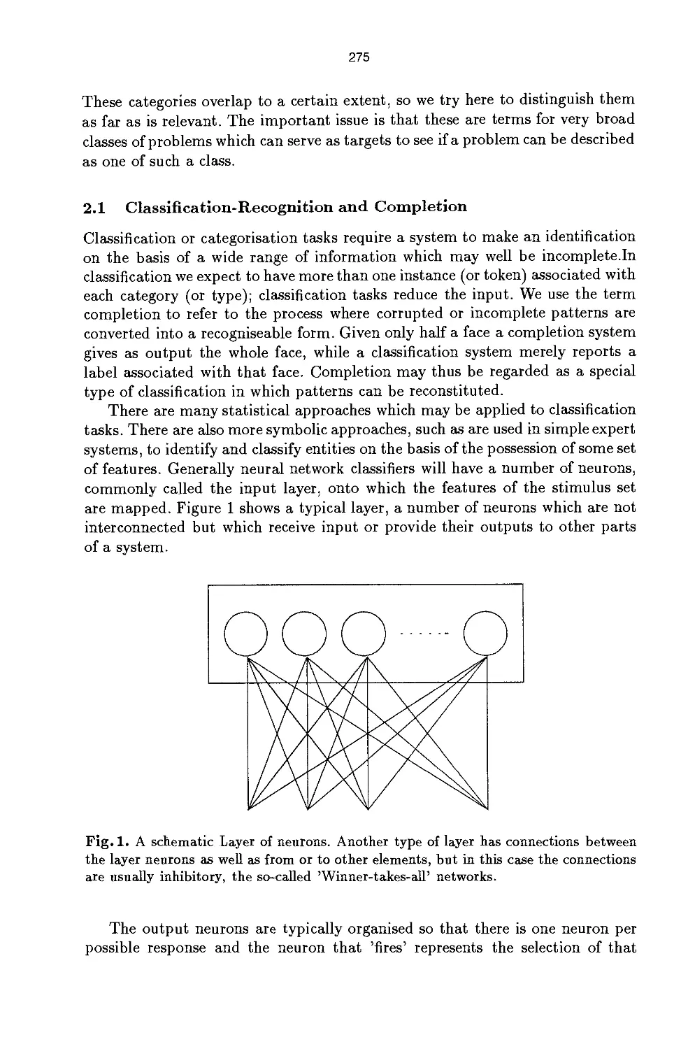
neural network may be useful should be distinguished and described. Then a
general classification of architectures is provided (moreover, a particularly helpful
table of common neural networks and several references to public domain neural
network simulators are provided). This classification aids enormously in treating
subsequently considerations for choosing a network architecture and
considerations for using a network. The first class of considerations addresses features like
learning or non-learning, generalization, input type, output, stability, scalability
and execution speed. The second class of considerations treats, mostly from a
user perspective, issues like learning speed, learning algorithm, learning
parameters, number of layers, connectivity, distributed or localized representations and
locality of algorithm. The conclusions of this paper emphasize again that careful
analysis of the problem at hand in terms of the features discussed are necessary
to make a reasoned choice for either a particular network architecture or not
using a neural network at all.
10 Concluding Remarks
In conclusion, the papers in this book provide together a broad and often deep-
going survey of Artificial Neural Network land; a land which is as exciting as
unexplored. Many more theoretical contributions are needed (and, in fact, also
more and more theory is developed). However, for the time being we also need
brave adventurers who are willing to experiment with particular network
architectures and dynamics within concrete practical problems. It is our hope that
this book stimulates those "adventurers" outside academia to explore the use
of Artificial Neural Networks to solve their concrete problems for the benefit of
their companies. Moreover, any feed-back of readers is welcomed for the benefit
of the ANN-science.
Backpropagation Networks for
Grapheme-Phoneme Conversion:
a Non-Technical Introduction
A.J.M.M. Weijters1 and G.A.J. Hoppenbrouwers2
1 Department of Computer Science, University of Limburg, Maastricht
2 Dutch State School of Translation and Interpreting, Maastricht
1 Introduction
Until very recently, cognitive processes typically have been modelled by means
of rule based-models. It appears, however, to be possible to model these
processes by means of neural networks3. This modelling technique, inspired by the
workings of the human brain, is distinguished from approaches based on symbol
manipulation by the fact that the rules are not incorporated in the model
explicitly: a neural network is not programmed for a particular task but is trained
for it. Presenting it with examples enables it to acquire the skill which is to be
modelled.
Our contribution to the present volume is meant as a non-technical
introduction to this modelling technique. It consists of three parts. In section 2 we
discuss (in general terms) various modelling techniques in which neural networks
play a major role. Section 3 discusses NETspraak, a neural network that can be
trained to convert Dutch texts into a phonetic representation, thus providing a
practical example of the approach. After a brief discussion of the model used
for NETspraak, we deal with the learning material and the test material
presented to NETspraak. Closer examination of the results at various stages of the
learning process, gives an indication of the results that can be achieved. Both in
the choice of the name and in the technical realisation of NETspraak (Dutch for
NETtalk) we have been inspired by the article "NETtalk: A Parallel Network
That Learns to Read Aloud" (Sejnowski and Rosenberg, 1987). NETtalk can
be trained to convert English texts into a phonetic representation. We conclude
section 3 with a comparison of the results of NETtalk and NETspraak. In
section 4 we attend to the question of whether the modelling technique using neural
networks is really as promising as the results achieved so far might suggest.
3 The terminology in this field is still unsettled. In the literature on the subject the
following terms can be found, all referring to the same thing: Neural Networks (NN),
Artificial Neural Networks, Parallel Distributed Processing Networks (often referred
to as PDP-networks), Connectionist Networks, Neural Circuits, Dynamical
Computation Systems, etc. In this paper we will stick to the term "neural network".
12
2 Neural Networks: An Introduction
Modelling of cognitive processes by means of neural networks differs greatly from
classical approaches. In this section, we will introduce a number of important
notions such as that of a processing unit, threshold values, weights, a learning
rule, and local and distributed representation. It aims to offer the reader a
nontechnical introduction. A more technical introduction is to be found in (Rumel-
hart and McClelland (eds.), 1986) and the paper by Henseler in the present
volume. Readers interested in the application of neural networks in modelling
linguistic cognitive processes are referred to chapters 18 (On Learning the Past
Tenses of English Verbs) and 19 (Mechanisms of Sentence Processing) of the
former publication.
In subsection 2.1 we will present some back-ground information on the
cognitive process to be modelled: the conversion of (written) texts into a phonetic
representation. The rest of the section will be devoted to a discussion of the
classical method of modelling this process. In subsection 2.2 we will briefly
discuss the neuro-physiological structure of the brain, since this formed the primary
inspiration for the architecture of neural networks. In subsection 2.3 we will
illustrate the workings of a very simple network, showing how this can be trained
to perform various tasks. This training process uses a particular kind of learning
rule: the Delta rule, which will also be discussed.
We will end section 2 by presenting, in 2.4, the main characteristics of the so-
called back-propagation networks, which have been used extensively in practical
applications. This type of network was also used for NETspraak.
2.1 The Main Features of Classical Methods of Modelling
At the basis of classical methods of modelling, there is always a system of explicit
rules according to which symbolic expressions are manipulated. This can be
illustrated by taking a closer look at traditional approaches to the problem of
grapheme-to-phoneme conversion. Let us begin by presenting some back-ground
information on this problem.
It is a well known fact that the spelling systems for natural languages such
as English and Dutch are far from providing one-to-one correspondences with
the sounds they are supposed to represent. One letter may be used to represent
several different sounds. Thus the e's in the word eleven [ile.v'n] all represent
different sounds4. The opposite situation also occurs: the letters c and k in scorn
and skip represent an identical sound. Often a combination of letters is used to
represent a single sound, as in knight where the sound corresponding to kn is
identical to the n in night. Sometimes letters are used that are not pronounced
at all as in bomb, where the second b is not realized.
If we do not restrict our attention to isolated words, but take them in their
natural context we should take into account all kinds of sandhi phenomena, as
in bread and butter, where and is pronounced ['n],
4 We follow the convention used in linquistics of placing texts in phonetic script
between square brackets.
13
An instance of sandhi that is very common in Dutch is the assimilation of
voice as in is de [iz de] (English: is the) versus is ie [is te] (English: is too).
Similar examples in Dutch can be given for all the above examples, although
the frequency with which these phenomena occur in each language may differ.
English and Dutch do differ in the following respect (Bloomfield, 1933:114).
In Dutch, a single consonant before the vowel of a stressed syllable, always shares
in the loudness, regardless of word-division or other factors of meaning: een aam
(measure of forty gallons) and een naam (a name) are both [e'na:m]. In English
we have an aim [en 'ejm] versus a name [e 'nejm].
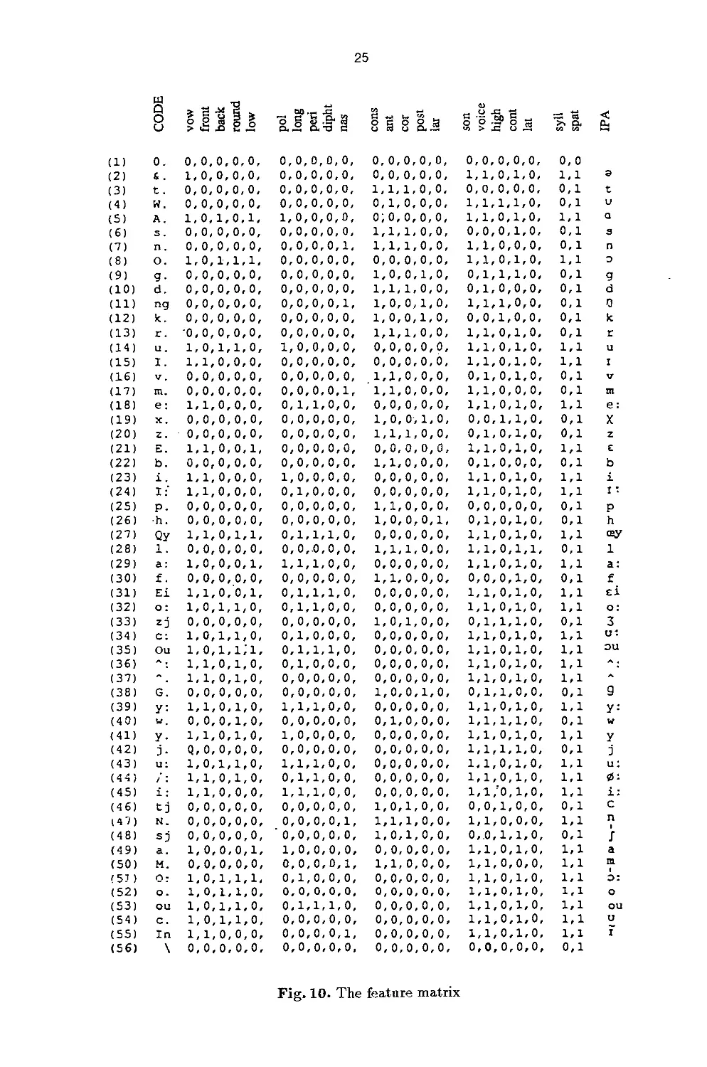
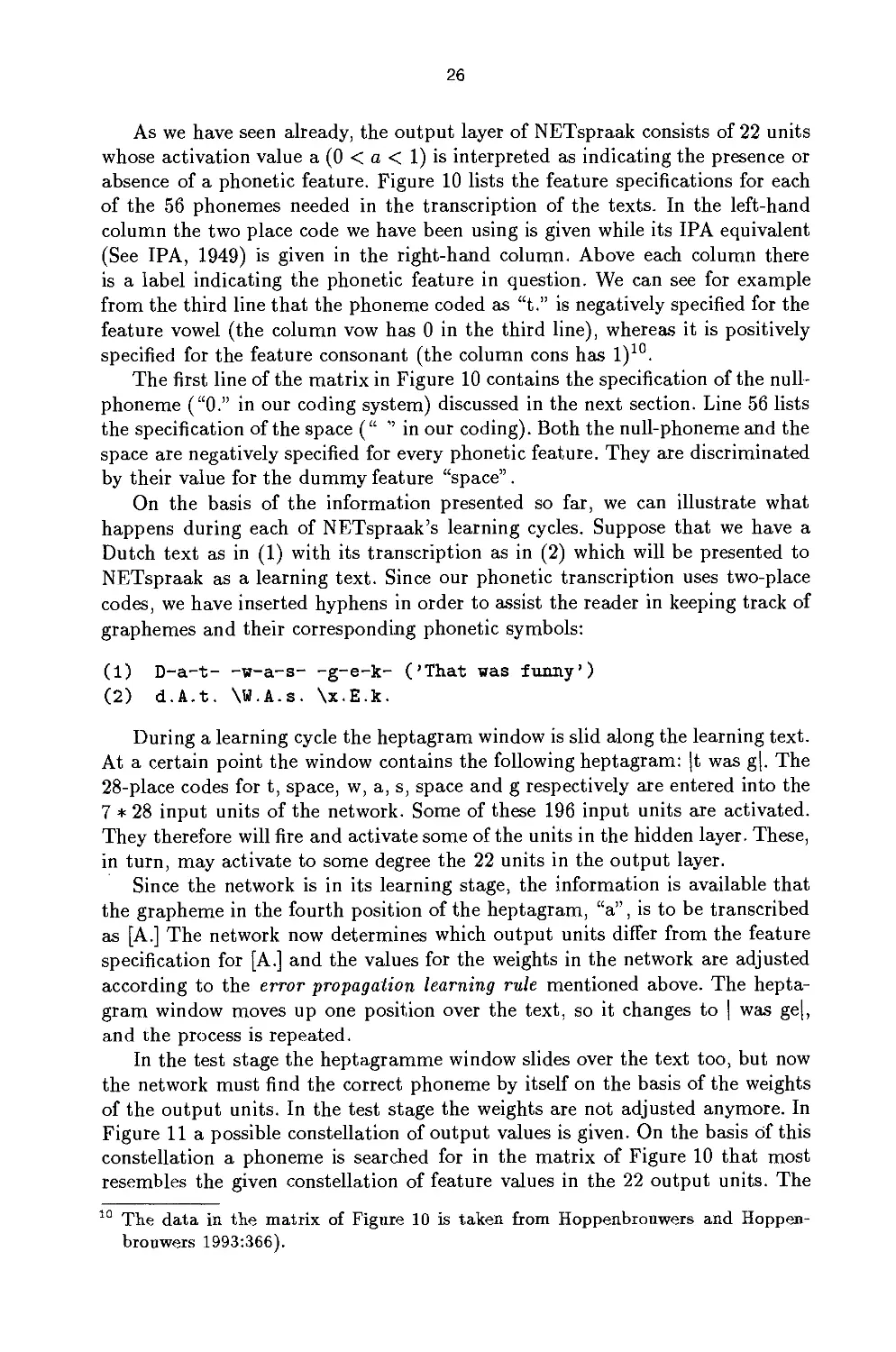
In order to indicate how a text is pronounced we make use of the phonetic
alphabet presented in (Figure 10). Every phoneme is represented in our notation
by means of two characters. How these codes relate to the International Phonetic
Alphabet (IPA, 1949) can be seen from the same matrix in Figure 10: in the left-
hand column of the matrix one finds the two-place code we have been using, while
in the right-hand column its IPA equivalent is given.
Using this phonetic alphabet, we can indicate that the name of the Dutch
town of Enschede is pronounced as [E.n.s.x.&.d.e:].
In classical approaches, symbolic rule systems are used, with rules such as
that in (1):
(a) n(p,b,m) -► [m.]
(b)n(k,g) -[ng] (1)
(c) n -+ [n.]
This rule for converting the grapheme n is to be interpreted as follows. The
grapheme n is pronounced as [m.] if followed by one of the graphemes p, b or
m, and as [ng] if followed by one of the graphemes k or g. In all other cases it is
pronounced [n.].
Here, our interest is not primarily whether (1) provides an adequate and
correct account of the facts, but in illustrating the fact that modelling the skill
in question consists of defining an adequate set of rules of the type given in (1).
Such a rule system is considered to be an adequate one, if it enables us to convert
any Dutch text into its correct phonetic representation mechanically5, that is to
say without having to depend on (implicit) knowledge on our part. If the rules
are formulated in terms of a computer programme that is able to convert texts
into their phonetic representation, we have a handy means to check whether,
in converting a text, we are making use exclusively of the rule proposed. Such
an approach would moreover, provide us with a useful product, which could be
used, for example, for automatically producing spoken newspapers for the blind.
Providing such a system of adequate and explicit rules, however, is by no
means a trivial matter. It would be very convenient indeed if a system were
available that could learn the skill involved purely on the basis of an example
consisting of a text and its correct phonetic transcription. Neural networks do
in fact seem to provide us with the means to achieve this: they are capable of
Rule systems in which reference is made to phonetic features to express various kinds
of linguistic generalization, such as the rule in Dutch phonology known as Final
Devoicing, are instances of symbol manipulating rules: [-son] —► [- voice] / #
14
grasping the underlying rule system on the basis of examples given to them. In
section 3 we present a neural network which can be trained to convert written
text into a phonetic representation on the basis of a few pages of sample texts.
2.2 Some Neuro-Physiological Facts about the Brain
As we have already said, the architecture of neural networks resembles in some
respects that of the human brain, which was the original inspiration for them,
although it should be stressed from the outset that neural networks are not
meant to constitute a model for the workings of the human brain.
Fig. 1. The structure of a neuron
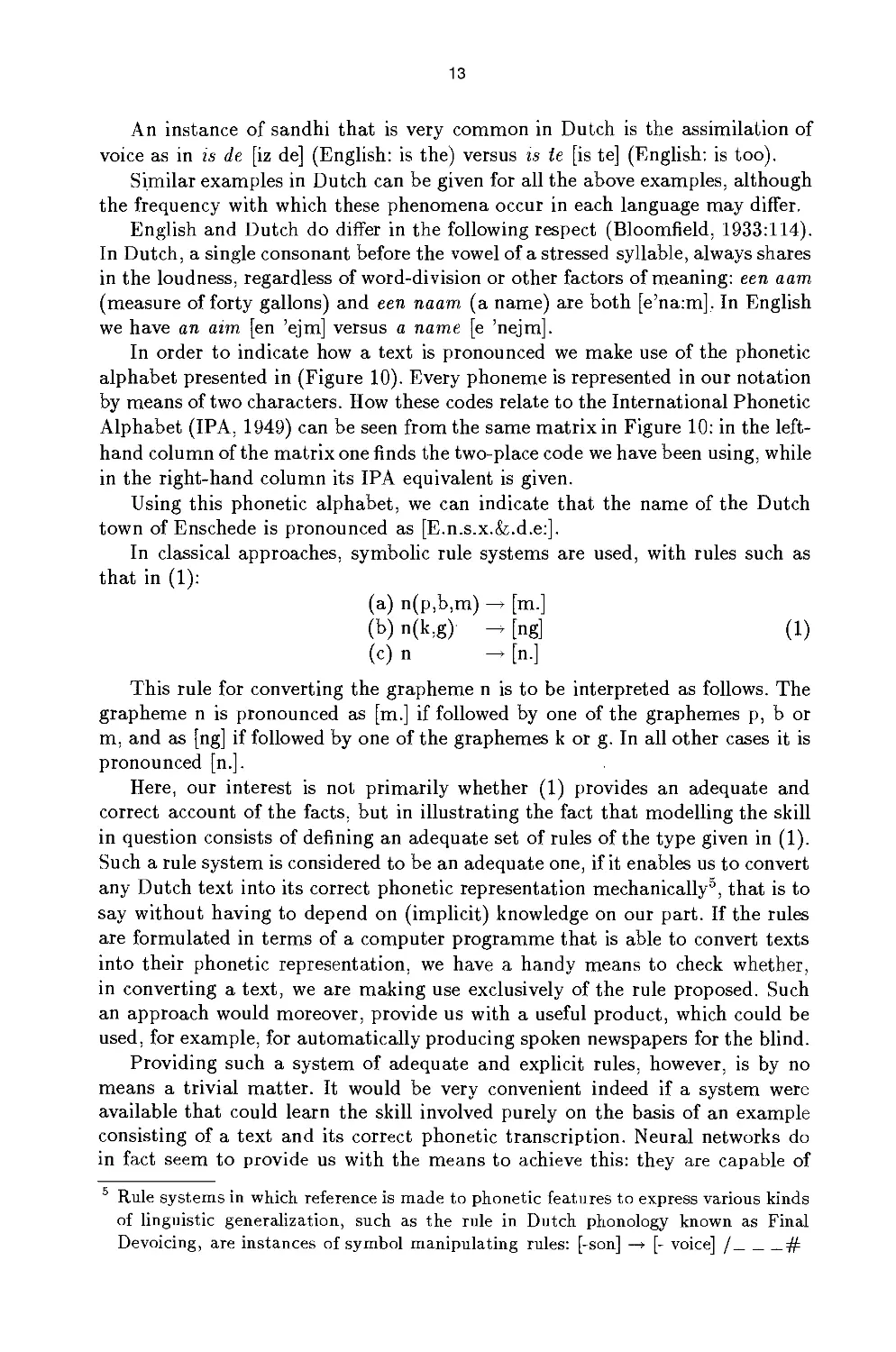
The human brain forms a massive communications network, consisting of
billions of nerve cells, also known as neurons. Many different types of neurons are
known. The structure of the individual neuron is rather simple. As can be seen
from Figure 1, we can distinguish three main elements: the cell body, a (large)
number of dendrites, and an axon. The offshoots of an axon are connected by
so-called synapses to the dendrites of many other neurons.
In functional terms a neuron can be seen as a processing unit receiving
incoming impulses via the dendrites. These impulses or electrical currents may vary
in frequency, but not in intensity. If the number of incoming impulses within a
certain period of time exceeds a certain threshold value, the neuron will fire off
an impulse via its axon. Both activating and inhibiting impulses can be fired.
Since incoming signals are added together, activating and inhibiting impulses
can cancel out one another partially or completely.
When a neuron fires, it transmits its impulse via the axon and synapses
to other neurons. The frequency and the nature of the impulse transmitted
(activating or inhibiting) is largely determined by the synapses.
The various individual building blocks of the brain are relatively simple units
that decide, on the basis of incoming signals, whether or not to transmit a signal.
Whereas these building blocks are relatively simple, the system as a whole is
15
incredibly complex, due to the enormous number of neurons, the number of
interconnections between them (the number of dendrites for a single neuron
may amount to 200,000) and the fact that all the neurons function autonomously
and in parallel6. This great number of connections is essential, since the learning
process in the brain depends on the growth of new connections or the breaking
up of existing ones. In this process the synapses play an important role.
2.3 The Basic Architecture of a Neural Network
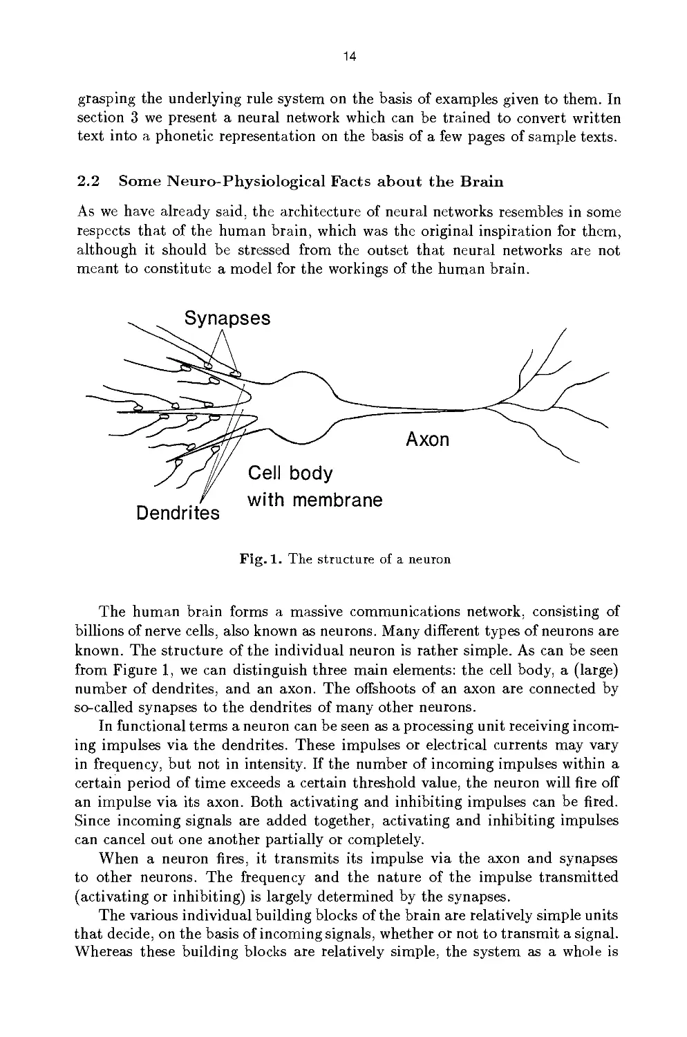
Many mathematical models for the (human) brain have been developed.
Although they may differ considerably from one another in detail, they have the
following minimum characteristics in common. The basic unit of a neural network
is the processing unit. Below we give a brief description of the basic elements
of the processing unit (cf. Figure 2). Between brackets we will, where possible,
mention the analogous structure in the human brain.
i1
o1
Summation Threshold
value
Input Weights
Output
Fig. 2. The components of a processing unit
A number of input values coming from another processing unit or from
outside (dendrites);
So-called weights indicating the degree of influence of the input value on
the processing unit in question (the frequency and the nature of the signal
transmitted via the synapses);
In this paper we will pay very little attention to the parallel aspect of neural
networks. In many cases, including NETspraak, parallellism is simulated in non-parallel
systems. In principle, parallel systems can be developed that can perform the same
functions as NETspraak, but many times faster.
16
- A summation function, usually the weighted sum of the input values, here:
w\ * i\ +W-2* «2 + W3 * *3 (the summation of incoming values in the neuron);
- A threshold value: if the resulting sum reaches this threshold value, the
signal will be transmitted, otherwise it will not (the threshold value that the
summation of the incoming signals must exceed if the neuron is to fire);
- An output signal (the signal exiting via the axon);
Let us illustrate this to the workings of a very simple neural network for
modelling the logical connective AND. From classical predicate calculus we know
that the conjunction of two propositions PI and P2 by means of the logical
connective AND yields a true proposition if and only if both PI and P2 are
true. If we represent TRUE by 1 and FALSE by 0, then only the input (1 1) to
the neural network should result in a value of 1 for the output signal, the input
pairs (1 0), (0 1), and (0 0) would have to result in an output signal with the
value 0. The simple network in Figure 3 appears to be adequate for modelling
the logical connective AND. This network consists of three processing units Ul,
U2 and U3. Ul and U2 are so-called input units, U3 is an output unit. The
interconnections are indicated by lines connecting the units. The weight of the
connection between Ul and U3 is 0.7, in other words W\3 = 0.7; furthermore we
have W23 = 0.7.
Threshold value = 1
w23 = 0.7
Input Output
Fig. 3. A neural network for the logical connective AND
In all the networks in Figures 3-6, the threshold value in the processing units
is equal to 1, as is the strength of the signals transmitted. Transmitting no signal
at all can be regarded as sending a signal of strength 0. If, and only if, the sum
of the weighted input signals is greater than or equal to 1, a signal (of strength
17
1) is transmitted.
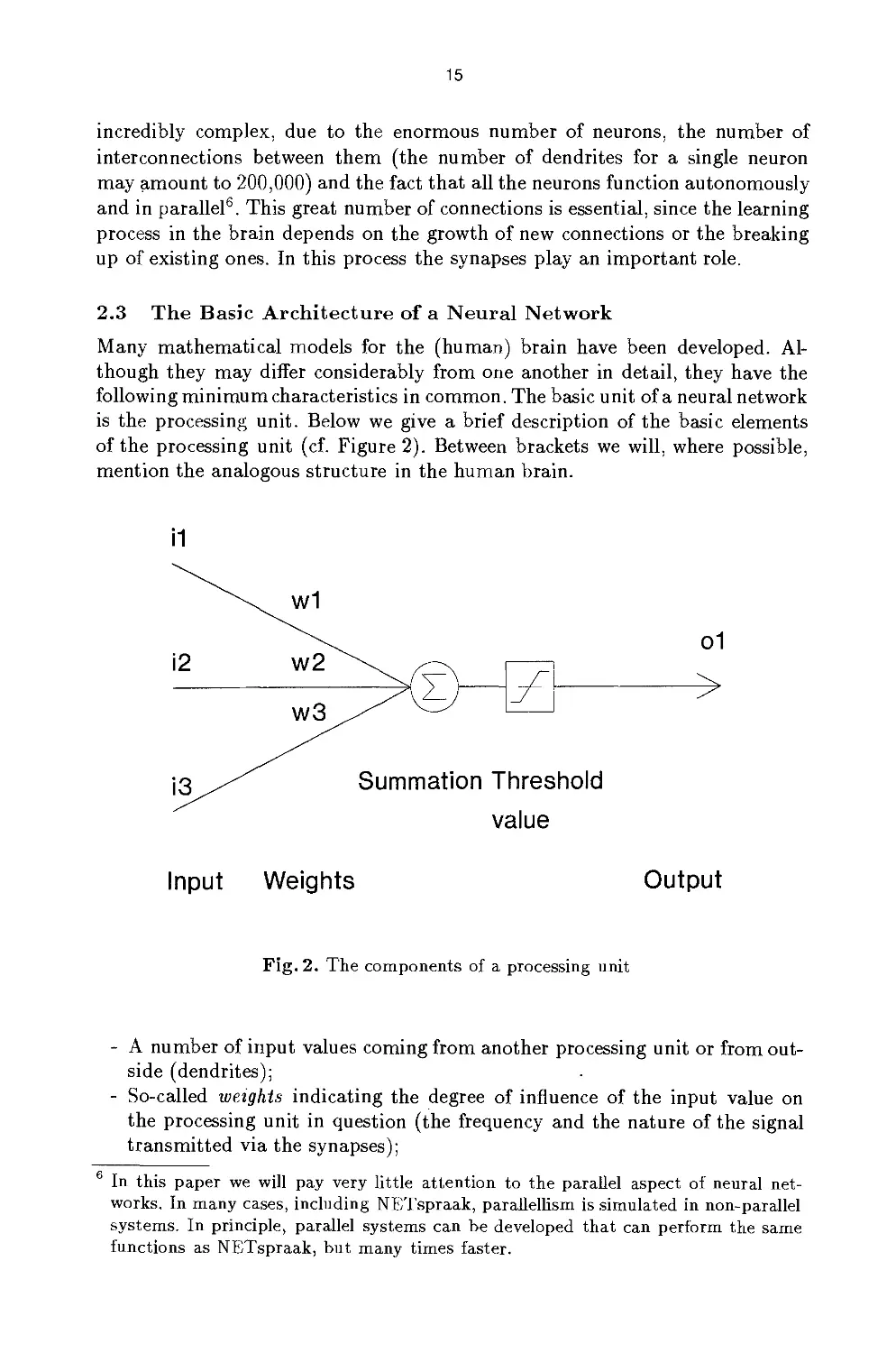
Let us examine what happens in case of an input pair ii = 1 and 2*2 = 1
(that is to say, both PI and P2 are TRUE). In this case unit 1 receives a signal
of strength 1; since the threshold value is 1, a signal of strength 1 is transmitted
to unit 3. In a similar way, unit 2 will transmit a signal of strength 1 to unit
3. In order to determine whether or not unit 3 will transmit a signal, we must
calculate the weighted sum of the input signals to unit 3:
w\ * i\ + W2 * i-z = 0.7 * 1 + 0.7 * 1 = 1.4
We see that the weighted sum exceeds the threshold value 1 and so unit 3
will transmit a signal of strength 1.
In case i\ = 1 and i2 = 0 the result will be 0 because the weighted sum of
the input signals for unit 3 is
0.7*1 + 0.7*0 = 0.7
The weighted sum is smaller than the threshold value and therefore unit 3 will
not fire, resulting in an output value for unit 3 of 0. The reader may easily verify
that the network yields correct results for the other possible input combinations
(0 1) and (0 0).
By merely adjusting the weights in the network in Figure 3, we can easily
adapt the network for another logical connective such as the inclusive OR.
Threshold value = 1
Input Output
Fig. 4. A neural network for inclusive OR
The proposition PI OR P2 is FALSE if, and only if, both PI and P2 are
FALSE. The network in Figure 4 which models the inclusive OR, differs only
18
from the one in Figure 3 in that the weights W13 and W23 have been adjusted
(they have both been set to the value 1.4).
Determining the adequate value for the weights in order to make the network
suitable for a specific task, is not difficult in the case of such simple networks,
but for more complex cases it is far from easy. We have already alluded to
the possibility of training a network for a particular task. This would free us
from the task of determining the correct weights "manually". In order to train
a network, so-called learning rules are used. By using such a rule, it becomes
possible to transform the AND network of Figure 3 into the OR-network of
Figure 4 automatically.
Training a network really amounts to adjusting the weights in response to
incorrect results. At the basis of all this is the following principle: the degree
to which a connection has contributed to a particular error determines to what
degree the weight associated with the connection in question will be adjusted.
The so-called Delta rule is one of the learning rules based on this principle. It
can be formulated as follows:
AWij = c * (gj — dj) * a;
where
AWij '■ the change in the weight associated with the
connection between the processing units i and j;
c : a so-called learning constant (for this a value
of 0.35 has proved adequate in practice);
gj : the activity desired for unit j [goal];
dj : the current activity of output element [=unit] j;
a; : the current activity of input element [=unit] i
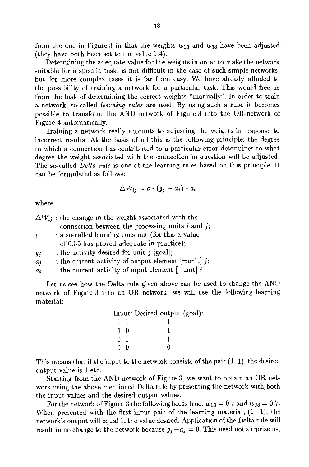
Let us see how the Delta rule given above can be used to change the AND
network of Figure 3 into an OR network; we will use the following learning
material:
Input: Desired output (goal):
1 1 1
1 0 1
0 1 1
0 0 0
This means that if the input to the network consists of the pair (1 1), the desired
output value is 1 etc.
Starting from the AND network of Figure 3, we want to obtain an OR
network using the above mentioned Delta rule by presenting the network with both
the input values and the desired output values.
For the network of Figure 3 the following holds true: W13 = 0.7 and W23 — 0.7.
When presented with the first input pair of the learning material, (1 1), the
network's output will equal 1: the value desired. Application of the Delta rule will
result in no change to the network because gj —aj = 0. This need not surprise us,
19
since in the case of both propositions being true, there is no difference between
the logical connectives AND and OR. As far as the input pair (1 1) is concerned,
the network is correct and no weights need to be adjusted.
In the case of the input pair (1 0) matters are different: the output value
desired is 1, whereas the network will yield an output value of 0 (it is after all
still an AND network!). Application of the Delta rule yields:
Aw13 = 0.35 * (1 - 0) * 1 = 0.35
Aw23 = 0.35*(l-0)*0 = 0
This will give us the following values: w13 = 0.7+0.35 = 1.05 and w23 = 0.7+0 =
0.7.
Application of the Delta rule to the input pair (0 1) yields:
Aw13 = 0.35*(l-0)*0 = 0
Aw23 = 0.35 * (1 - 0) * 1 = 0.35
This will give us the weights w±3 = 1.05 + 0 = 1.05 and w23 = 0.7 + 0.35 = 1.05.
The result of presenting the input pair (0 0) is 0. In this case the weights are
not adjusted since a8- equals 0 in the expression:
c*(gj - aj)*a,i
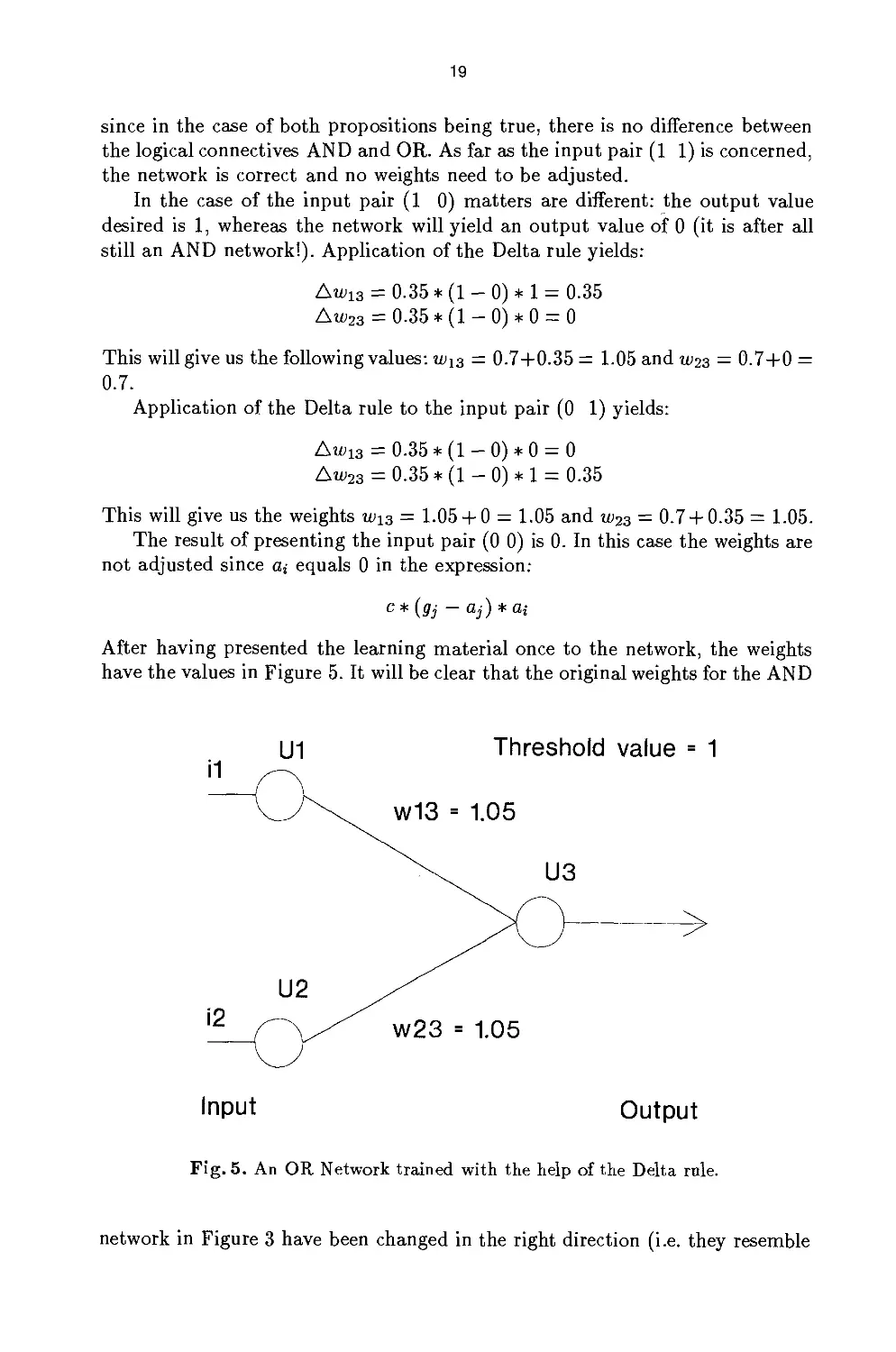
After having presented the learning material once to the network, the weights
have the values in Figure 5. It will be clear that the original weights for the AND
U1 Threshold value = 1
i1 ^-n
Input Output
Fig. 5. An OR Network trained with the help of the Delta rule,
network in Figure 3 have been changed in the right direction (i.e. they resemble
20
more the weights in Figure 4), but one may ask whether we are already dealing
with a real OR network? The reader may easily verify that this is indeed the
case. Presenting the learning material to the network once again, will no longer
affect the weights of the network.
From a comparison of the networks in Figure 4 and Figure 5, we conclude that
the same functionality may be achieved by assigning different weights. This holds
even more true for more complicated networks.
In the above example, training the network was a very simple matter. We
will see later that more learning material is often required and the same learning
material may have to be presented many times in succesion.
Using the Delta rule we have been training a network in correctly performing
a particular task. It is not possible, however, to adapt the network in Figure 3 so
as to make it fit for modelling exclusive OR (henceforth XOR). The proposition
PI XOR P2 is true if, and only if, exactly one of its constituent parts is true. It
can be shown that networks consisting solely of input units and output units are
inadequate for the modelling of non-linearly classifiable problems7. If we do not
restrict ourselves to the use of input and output units, and introduce one or more
so-called "hidden layers", defining an XOR network no longer presents a problem.
The processing units in the hidden layer perform the role of recognizing the
relevant abstract characteristics. In the XOR network in Figure 6, U3 functions
as the recognizer of a situation in which only i\ = 1, and in which therefore
i2 = 0. The reader may easily verify that the network in Figure 6 correctly
models the XOR connective.
In defining the XOR network of Figure 6 the problem has been solved,
however, only in part: we will also have to define a new learning rule. In 1986
(Rumelhart, Hinton and Williams, 1986) and (Parker 1986) independently
formulated an extension of the Delta rule, the socalled error propagation learning
rule8, which plays an essential role in back-propagation networks.
2.4 Back-Propagation Networks
The error propagation learning rule can be applied in networks having the
following characteristics: the network has one or more hidden layers; all units within
a layer are connected to all units of the next layer; there are no connections
between non-successive layers. These restrictions result in a network architecture
as shown in Figure 7.
An important feature of back-propagation networks is furthermore that
signals of arbitrary strength between 0 and 1 can be fired; one is no longer restricted
to integer values 0 and 1. In modelling the logical connectives, the continuity
of the input and output signals is not generally used: signals with a value less
than 0.5 are interpreted as negative values, signals with a value greater than 0.5
as positive. Thus, if the pair (1 1) is presented as input to an adequate XOR
7 See (Minsky and Papert, 1969)
8 For details on the error propagation learning rule see the paper by Henseler in the
present volume.
21
Threshold value = 1
Input Hidden layer Output
Fig. 6. An XOR network with one hidden layer
Input Hidden layer Output
Fig. 7. Back-propagation network with one hidden layer
22
back-propagation network the output value must be less than 0.5; a value of 0.61
would indicate that the network does not perform adequately.
In back-propagation networks, also, the value of the output signal is
calculated by taking the weighted sum of the values of the input signals for all units
in each of the layers. During the training stage, the result thus achieved can be
compared to the result desired, after which the weights of the connections can
be adjusted if necessary in accordance with the error propagation learning rule.
Although there is no upper limit to the number of hidden layers, in practice
a single hidden layer will usually suffice. This is also true of the skill we wish
to model by means of a neural network: grapheme-phoneme conversion. As we
will see later, a back-propagation network with a single layer appeared to be
adequate.
The architecture eventually used for the network (the number of input and
output units, and the number of units in the hidden layer) depends to a large
extent on the choice of "translation" of the skill to be modelled, in terms of
input and output signals.
In the following section we will elaborate on the problem to be modelled, and
we will discuss the architecture of the grapheme-phoneme network designed for
this task.
3 NETspraak
Our attempt to use the computer for automatic grapheme-phoneme conversion is
by no means new. Wester and Kerkhoff from the research-group "Language and
Speech" at Nijmegen University have developed a conversion system for Dutch.
An evaluation of this system, in which its performance was tested by presenting
it with words in isolation, is given in (Willemse, 1987). An evaluation with the
explicit aim of assessing the usefulness of this system in producing a spoken
journal for the blind, is to be found in (Bezooijen, 1989). From this source it
is possible to gain a clear impression of the performance of this system when
applied to running text.
For the conversion of English texts into a phonetic representation, the rule-
based expert system DECtalk, developed by Digital Equipment Corporation, is
available commercially.
As we saw before, NETtalk and NETspraak differ crucially from these
traditional approaches in that no explicit rule system is used. The knowledge
possessed by someone who can read a Dutch or English text aloud is not stated
explicitly and cannot be traced to any unambiguously identifiable part of the
network. In the learning stage, the network is presented with a text a number of
times and during each cycle of this process it makes guesses as to the best way
to represent any given grapheme of the text by a phonetic symbol: The result
predicted by the network is then compared to the result desired, and the weights
are adjusted if necessary.
The type of back-propagation network discussed in subsection 2.4 can be
made fit for grapheme-phoneme conversion by formulating the problem in terms
23
of input to and output from the network. How this can be done is discussed in
subsection 3.1. As we have already mentioned, training a network takes place
by means of a learning text. It is important that, after the training stage, the
performance of the network is measured by testing it using text material other
than that used in the learning stage, for we are not primarily interested in
finding out whether the network is able to learn the peculiarities of the learning
text. What we really want to know is whether the network is able to make
significant generalizations. The choice of learning text and test text, the problems
we encountered in transcribing the material, and the solutions we have chosen
are the subject of subsection 3.2.
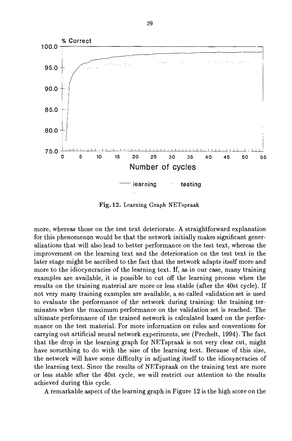
It usually makes sense to present a particular learning text to a network
many times in succession. NETspraak went through the learning text 55 times.
In subsection 3.3 we discuss the learning path that NETspraak follows and we
compare the results with those achieved by NETtalk and by two traditional
systems: the INF-KUN-system and GRAFON (Daelemans, 1985, 1988).
3.1 Input and Output for NETspraak
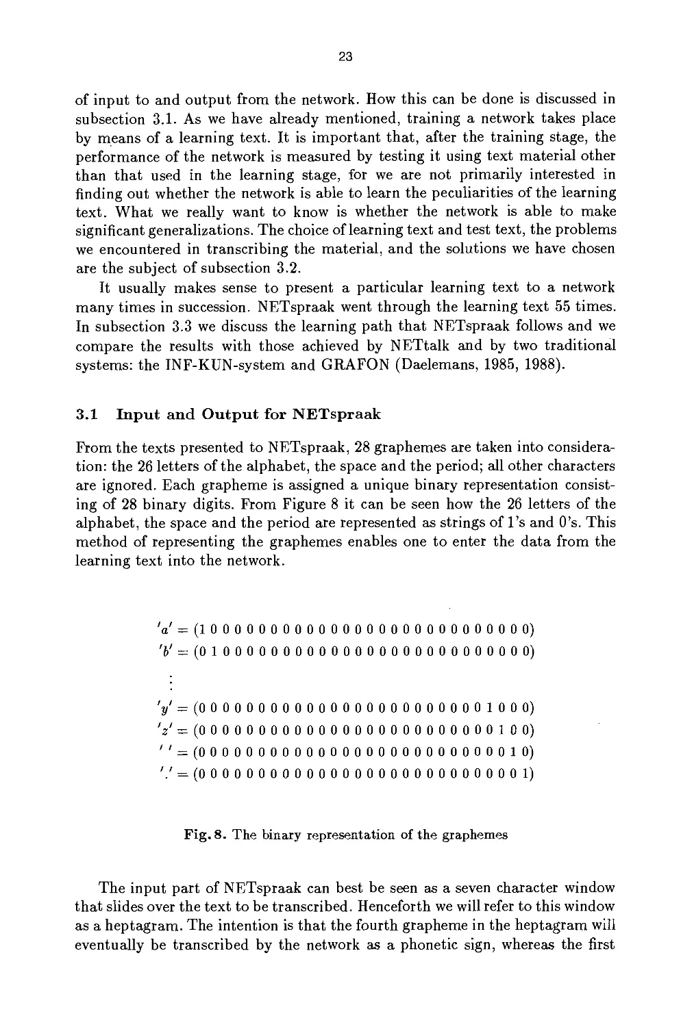
From the texts presented to NETspraak, 28 graphemes are taken into
consideration: the 26 letters of the alphabet, the space and the period; all other characters
are ignored. Each grapheme is assigned a unique binary representation
consisting of 28 binary digits. From Figure 8 it can be seen how the 26 letters of the
alphabet, the space and the period are represented as strings of l's and O's. This
method of representing the graphemes enables one to enter the data from the
learning text into the network.
V = (100000000000000000000000000 0)
'«.' = (0 10000000000000000000000000 0)
V= (0 00000000000000000000000100 0)
V = (0 00000000000000000000000010 0)
'' = (0 000000000000000000000000010)
'.' = (0 00000000000000000000000000 1)
Fig. 8. The binary representation of the graphemes
The input part of NETspraak can best be seen as a seven character window
that slides over the text to be transcribed. Henceforth we will refer to this window
as a heptagram. The intention is that the fourth grapheme in the heptagram will
eventually be transcribed by the network as a phonetic sign, whereas the first
24
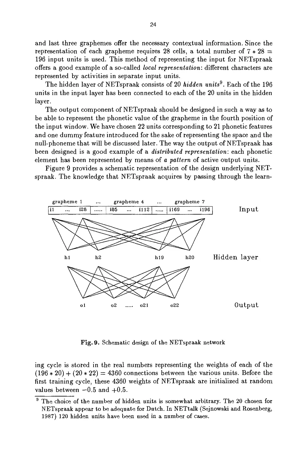
and last three graphemes offer the necessary contextual information. Since the
representation of each grapheme requires 28 cells, a total number of 7 * 28 =
196 input units is used. This method of representing the input for NETspraak
offers a good example of a so-called local representation: different characters are
represented by activities in separate input units.
The hidden layer of NETspraak consists of 20 hidden units9. Each of the 196
units in the input layer has been connected to each of the 20 units in the hidden
layer.
The output component of NETspraak should be designed in such a way as to
be able to represent the phonetic value of the grapheme in the fourth position of
the input window. We have chosen 22 units corresponding to 21 phonetic features
and one dummy feature introduced for the sake of representing the space and the
null-phoneme that will be discussed later. The way the output of NETspraak has
been designed is a good example of a distributed representation: each phonetic
element has been represented by means of a pattern of active output units.
Figure 9 provides a schematic representation of the design underlying
NETspraak. The knowledge that NETspraak acquires by passing through the learn-
grapheme 1 ... grapheme 4 ... grapheme 7
il ... i28
185 ... 1112
H69 ... U96
hi h2 hi9 h20 Hidden layer
ol o2 o21 o22 Output
Fig. 9. Schematic design of the NETspraak network
ing cycle is stored in the real numbers representing the weights of each of the
(196 * 20) + (20 * 22) = 4360 connections between the various units. Before the
first training cycle, these 4360 weights of NETspraak are initialized at random
values between —0.5 and +0.5.
9 The choice of the number of hidden units is somewhat arbitrary. The 20 chosen for
NETspraak appear to be adequate for Dutch, In NETtalk (Sejnowski and Rosenberg,
1987) 120 hidden units have been used in a number of cases.
25
1 Hill aftfl
(1)
(2)
(3)
(4)
(5)
(6)
(7)
(8)
(9)
(10)
(11)
(12)
(13)
(14)
(IS)
(16)
(17)
(18)
(19)
(20)
(21)
(22)
(23)
(24)
(25)
(26)
(27)
(28)
(29)
(30)
(31)
(32)
(33)
(34)
(35)
(36)
(37)
(38)
(39)
(40)
(41)
(42)
(43)
(44)
(45)
(46)
(4 7)
(48)
(49)
(50)
(53)
(52)
(53)
(54)
(55)
(56)
0.
£.
t.
w.
A.
s .
n .
O.
g-
d.
ng
k.
r.
u.
I.
V .
m.
e:
X.
z.
E.
b.
i .
I:'
P.
■h.
Qy
l.
a:
f.
Ei
o:
zj
c:
Ou
"• •
G.
y:
w .
y.
j.
u:
/ :
i :
tj
N.
Sj
a.
M.
0:
o.
ou
c.
In
\
0,0,0,0,0,
1,0,0,0,0,
0,0,0,0,0,
0,0,0,0,0,
1,0,1,0,1,
0,0, 0,0,0,
0,0,0,0,0,
1,0,1,1,1,
0,0,0,0,0,
0,0,0,0,0,
0,0,0,0,0,
0,0,0,0,0,
0,0,0,0,0,
1,0,1,1,0,
1,1,0,0,0,
0,0,0,0,0,
0,0,0,0,0,
1,1,0,0,0,
0,0,0,0,0,
0,0,0,0,0,
1,1,0,0,1,
0,0,0,0,0,
1,1, 0,0,0,
1,1,0,0,0,
0, 0, 0, 0,0,
0,0,0,0,0,
1,1,0,1,1,
0,0,0,0,0,
1,0,0,0,1,
0,0,0,0,0,
1,1,0,0,1,
1,0,1,1,0,
0,0,0,0,0,
1,0,1,1,0,
1,0,1,1,"1,
1,1,0,1,0,
1,1,0,1,0,
0,0,0,0,0,
1,1,0,1,0,
0,0,0,1,0,
1,1,0,1,0,
Q, 0,0, 0,0,
1,0,1,1,0,
1,1,0,1,0,
1,1,0,0,0,
0,0,0,0,0,
0, 0,0,0,0,
0,0,0,0,0,
1,0,0,0,1,
0,0,0,0,0,
1, 0,1,1,1,
1, 0,1, 1,0,
1,0,1,1,0,
1,0,1,1,0,
1,1,0,0,0,
0,0,0,0,0,
0,0,0,0,0,
0,0,0,0,0,
0,0,0,0,0,
0,0,0,0,0,
1,0,0,0,0,
0,0,0,0,0,
0,0,0,0,1,
0,0,0,0,0,
0,0,0,0,0,
0,0,0,0,0,
0,0,0,0,1,
0,0,0,0,0,
0,0,0,0,0,
1,0,0,0,0,
0,0,0, 0, 0,
0,0,0,0,0,
0,0,0,0,1,
0, 1,1,0,0,
0,0,0,0,0,
0,0,0,0,0,
0,0,0,0,0,
0,0,0,0,0,
1,0,0,0,0,
0,1,0,0,0,
0,0,0,0,0,
0,0,0,0,0,
0,1,1,1,0,
0,0,0,0,0,
1,1,1,0,0,
0,0,0,0,0,
0,1,1,1,0,
0,1,1,0,0,
0,0,0,0,0,
0,1,0,0,0,
0,1,1,1,0,
0,1,0,0,0,
0,0,0,0,0,
0,0,0, 0,0,
1,1,1,0,0,
0, 0,0,0,0,
1,0,0,0,0,
0,0,0,0,0,
1,1,1,0,0,
0,1,1,0,0,
1,1,1,0,0,
0,0,0,0,0,
0,0,0,0,1,
' 0,0,0,0,0,
1,0,0,0,0,
0,0,0,0,1,
0,1,0,0,0,
0,0, 0,0,0,
0,1,1,1,0,
0,0,0,0,0,
0,0,0,0,1,
0,0,0,0,0,
c *- »- sa l- c -s m S ^ =« <
0,0,0,0,0,
0,0,0,0,0,
1,1,1,0,0,
0,1,0,0,0,
o;o,0,0,0,
1,1,1,0,0,
1,1,1,0,0,
0,0,0,0,0,
1,0,0,1,0,
1,1,1,0,0,
1,0,0,1,0,
1,0,0,1,0,
1,1,1,0,0,
0,0,0,0,0,
0,0,0,0,0,
1,1,0,0,0,
1,1,0,0,0,
0,0,0,0,0,
1,0,0,1,0,
1,1,1,0,0,
0,0,0,0,0,
1,1,0,0,0,
0,0,0,0,0,
0,0,0,0,0,
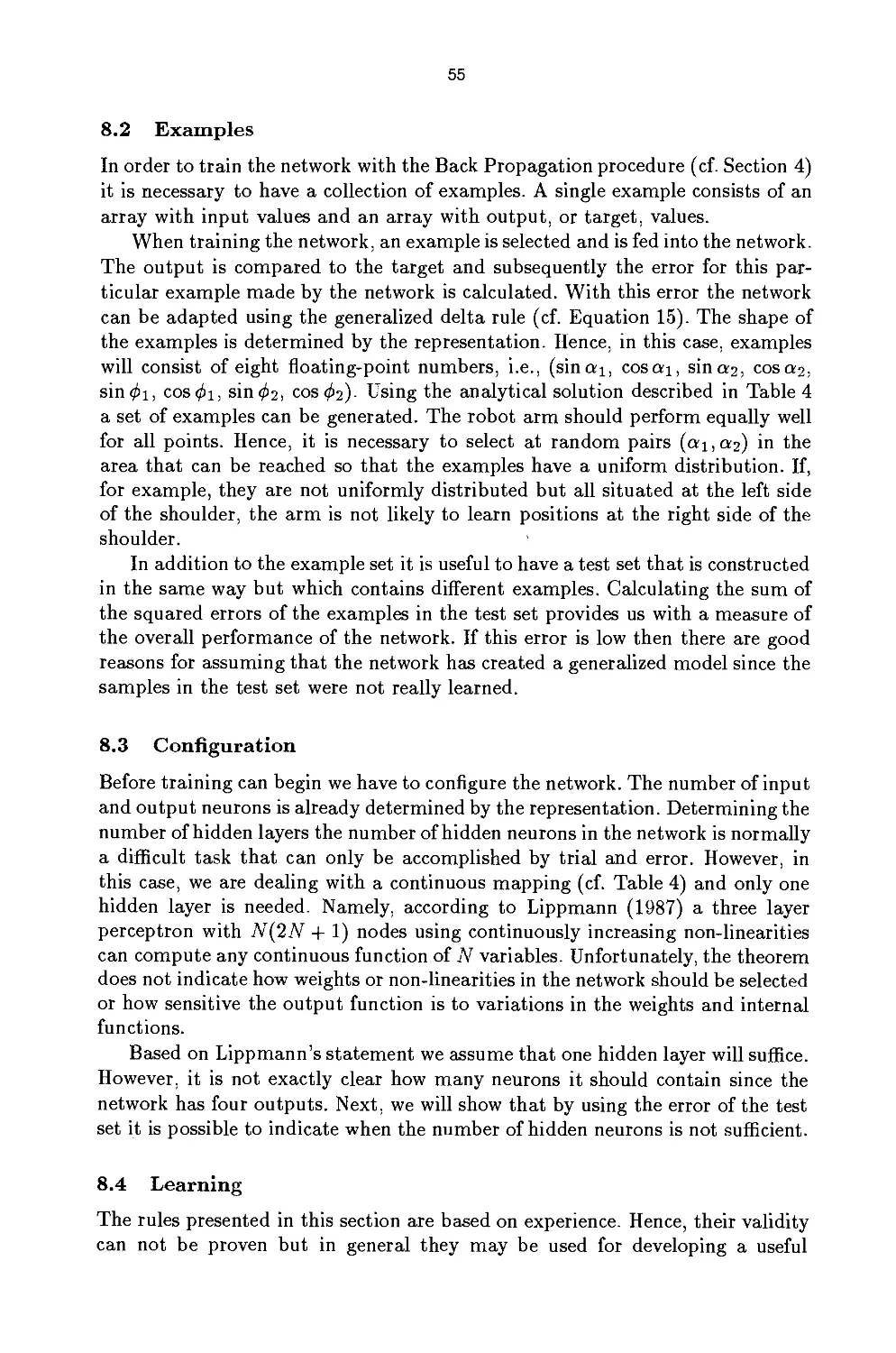
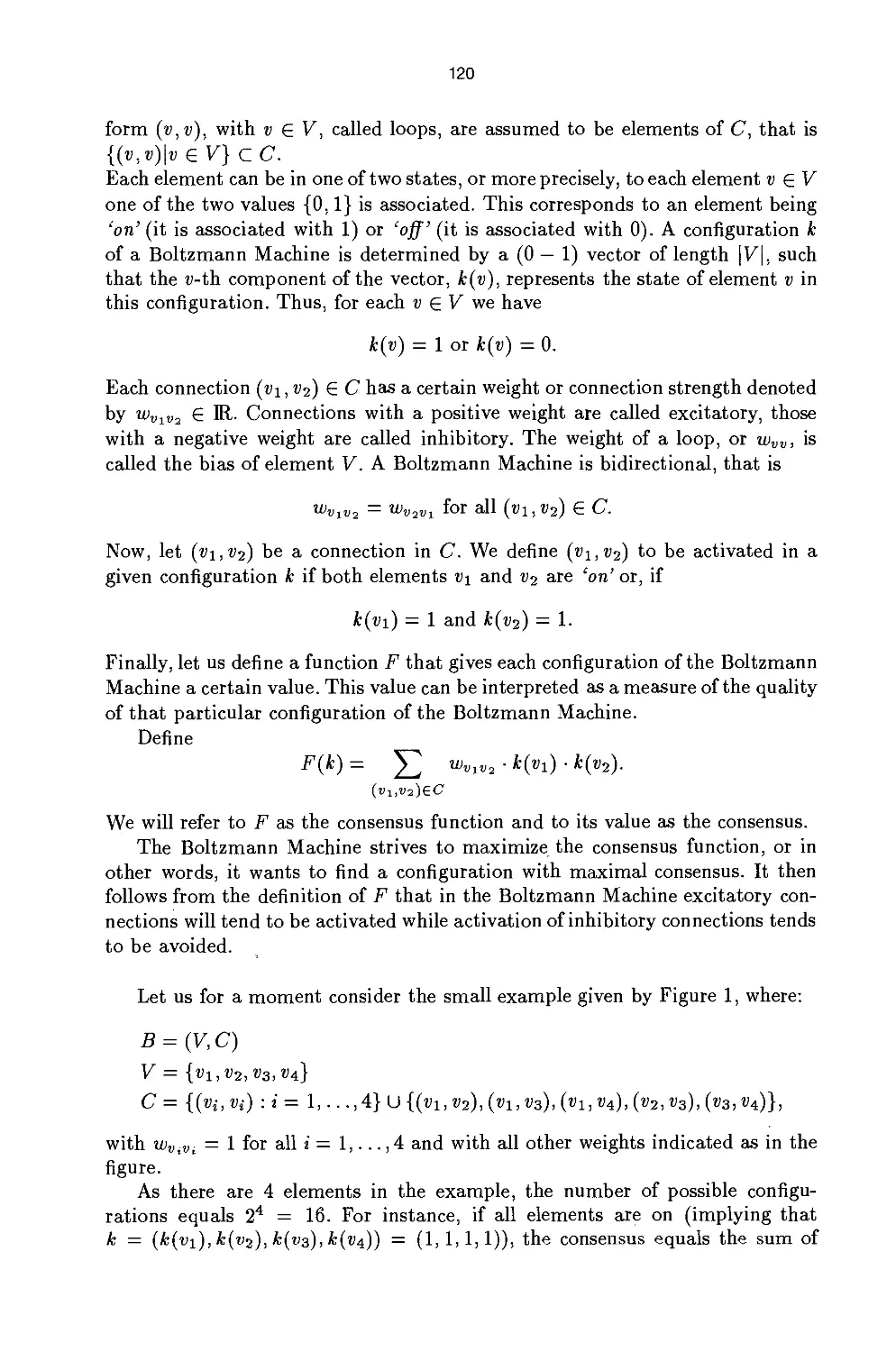
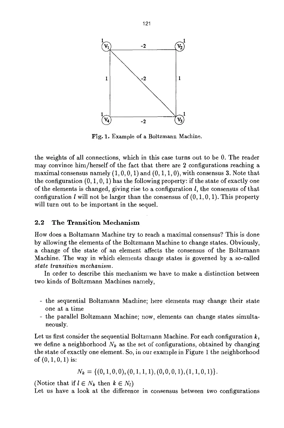
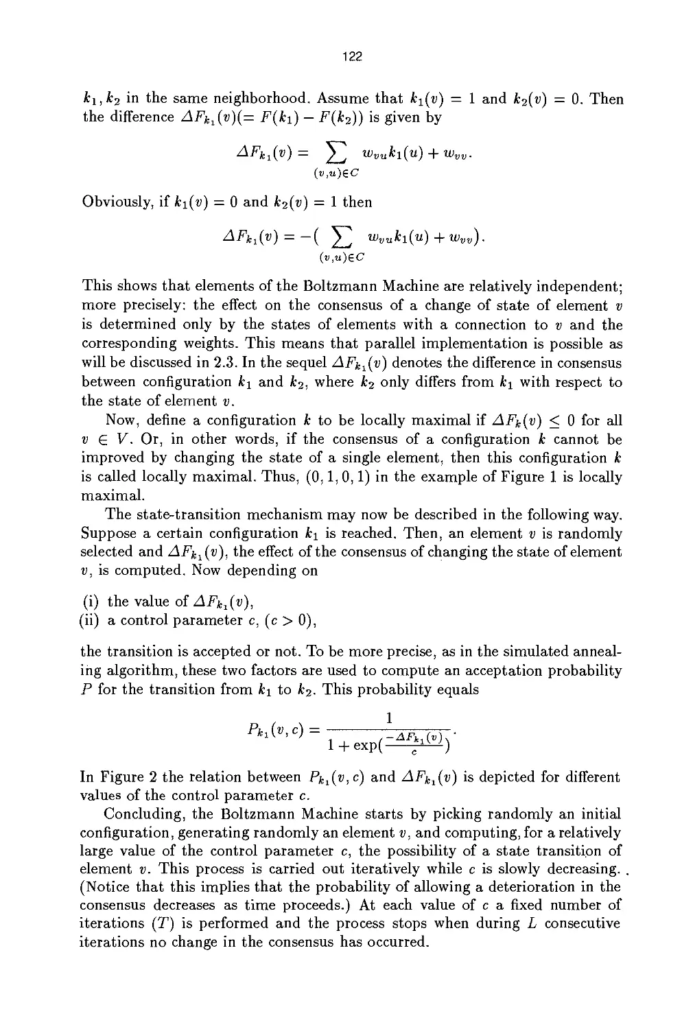
1,1,0,0,0,
1,0,0,0,1,
0,0,0,0,0,
1,1,1,0,0,
0,0,0,0,0,
1,1,0,0,0,
0,0,0,0,0,
0,0,0,0,0,
1,0,1,0,0,
0,0,0,0,0,
0,0,0, 0,0,
0,0,0,0,0,
0,0,0,0,0,
1,0,0,1,0,
0,0,0,0,0,
0,1,0,0,0,
0,0,0,0,0,
0,0,0,0,0,
0,0,0,0,0,
0,0,0,0,0,
0,0,0,0,0,
1,0,1,0,0,
1,1,1,0,0,
1,0,1,0,0,
0,0,0,0,0,
1,1,0,0,0,
0,0,0,0,0,
0,0,0, 0,0,
0,0,0,0,0,
0,0,0,0,0,
0,0,0,0,0,
0,0,0,0,0,
0,0,0,0,0,
1,1,0,1,0,
0,0,0,0,0,
1,1,1,1,0,
1,1,0,1,0,
0,0,0,1,0,
1,1,0,0,0,
1,1,0,1,0,
0,1,1,1,0,
0,1,0,0,0,
1,1,1,0,0,
0,0,1,0,0,
1,1,0,1,0,
1,1,0,1,0,
1,1,0,1,0,
0,1,0,1,0,
1,1,0,0,0,
1,1,0,1,0,
0,0,1,1,0,
0,1,0,1,0,
1,1,0,1,0,
0,1, 0,0,0,
1,1,0,1,0,
1,1,0,1,0,
0,0,0,0,0,
0,1,0,1,0,
1,1,0,1,0,
1,1,0,1,1,
1,1,0,1,0,
0,0,0,1,0,
1,1,0,1,0,
1,1,0,1,0,
0,1,1,1,0,
1,1,0,1,0,
1,1,0,1,0,
1,1,0,1,0,
1,1,0,1,0,
0,1,1,0,0,
1,1,0,1,0,
1,1,1,1,0,
1,1,0,1,0,
1,1,1,1,0,
1,1,0,1,0,
1,1,0,1,0,
1,1/0,1,0,
0,0,1,0,0,
1,1,0,0,0,
0,0,1,1,0,
1,1,0,1,0,
1,1,0,0,0,
1,1,0,1,0,
1,1, 0,1,0,
1,1,0,1,0,
1,1,0,1,0,
1,1,0,1,0,
0,0,0,0,0,
0,0
1,1
0,1
0,1
1,1
0,1
0,1
1,1
0,1
0,1
0,1
0,1
0,1
1,1
1,1
0,1
0,1
1,1
0,1
0,1
1,1
0,1
1,1
1,1
0,1
0,1
1,1
0,1
1,1
0,1
1,1
1,1
0,1
1,1
1,1
1,1
1,1
0,1
1,1
0,1
1,1
0,1
1,1
1,1
1,1
0,1
1,1
0,1
1,1
1,1
1,1
1,1
1,1
1,1
1,1
0,1
3
t
V
a
3
n
D
g
d
Q
k
r
u
I
V
m
e:
X
z
c
b
i
I:
p
h
<sy
1
a:
f
ei
o:
3
O".
ou
":
*
g
y;
w
y
j
u:
0:
i:
C
n
;
a
m
o:
o
ou
o
I
Fig. 10. The feature matrix
26
As we have seen already, the output layer of NETspraak consists of 22 units
whose activation value a (0 < a < 1) is interpreted as indicating the presence or
absence of a phonetic feature. Figure 10 lists the feature specifications for each
of the 56 phonemes needed in the transcription of the texts. In the left-hand
column the two place code we have been using is given while its IPA equivalent
(See IPA, 1949) is given in the right-hand column. Above each column there
is a label indicating the phonetic feature in question. We can see for example
from the third line that the phoneme coded as "t." is negatively specified for the
feature vowel (the column vow has 0 in the third line), whereas it is positively
specified for the feature consonant (the column cons has 1)10.
The first line of the matrix in Figure 10 contains the specification of the null-
phoneme ("0." in our coding system) discussed in the next section. Line 56 lists
the specification of the space (" '' in our coding). Both the null-phoneme and the
space are negatively specified for every phonetic feature. They are discriminated
by their value for the dummy feature "space".
On the basis of the information presented so far, we can illustrate what
happens during each of NETspraak's learning cycles. Suppose that we have a
Dutch text as in (1) with its transcription as in (2) which will be presented to
NETspraak as a learning text. Since our phonetic transcription uses two-place
codes, we have inserted hyphens in order to assist the reader in keeping track of
graphemes and their corresponding phonetic symbols:
(1) D-a-t- -w-a-s- -g-e-k- ('That was funny')
(2) d.A.t. \W.A.s. \x.E.k.
During a learning cycle the heptagram window is slid along the learning text.
At a certain point the window contains the following heptagram: |t was g|. The
28-place codes for t, space, w, a, s, space and g respectively are entered into the
7 * 28 input units of the network. Some of these 196 input units are activated.
They therefore will fire and activate some of the units in the hidden layer. These,
in turn, may activate to some degree the 22 units in the output layer.
Since the network is in its learning stage, the information is available that
the grapheme in the fourth position of the heptagram, "a", is to be transcribed
as [A.] The network now determines which output units differ from the feature
specification for [A.] and the values for the weights in the network are adjusted
according to the error propagation learning rule mentioned above. The
heptagram window moves up one position over the text, so it changes to | was ge|,
and the process is repeated.
In the test stage the heptagramme window slides over the text too, but now
the network must find the correct phoneme by itself on the basis of the weights
of the output units. In the test stage the weights are not adjusted anymore. In
Figure 11 a possible constellation of output values is given. On the basis of this
constellation a phoneme is searched for in the matrix of Figure 10 that most
resembles the given constellation of feature values in the 22 output units. The
10 The data in the matrix of Figure 10 is taken from Hoppenbrouwers and Hoppen-
brouwers 1993:366).
27
.00 .00 .01 .00 .00 .00 .01 .00 .01 .00 .94 .23 .00 .01 .00 .00 .00 .02 .00 .00 .00 1.00
Fig. 11. A possible constellation of output values
sum of squares of the differences between the values in the output units and
those in the corresponding columns of the feature matrix is used as a similarity
measure. Using this measure will yield [p.] in line 25 of the feature matrix as
resembling most the constellation in Figure 11.
3.2 The Learning Text and the Test Text
Both theoretical considerations and the possible practical applications make
clear that the use of plain running text is to be preferred to the use of
isolated words, since only in the former case can assimilation phenomena such as
those discussed in subsection 2.1 be taken into consideration.
For this reason, we have chosen to present NETspraak with a learning text
consisting of the first ten pages of De Avonden, a famous Dutch novel by Gerard
Reve (1987), and its phonetic transcription (22071 graphemes, 4040 words). As
a test text we have chosen the eleventh page of that novel (2355 graphemes,
457 words). Of course a transcription of the latter page had to be available in
order to make an assessment of the performance of the network possible. The
testing of NETspraak's results by presenting it with a test text was motivated
by our wish to gain some insight into NETspraak's ability to reach significant
generalizations. In this context it is useful to note that 32% of the heptagrams
in the test text occurred in the learning text at least once, whereas 68% were
new.
The period was the only punctuation mark that was taken into account: it
was included in the contextual information, but the network did not have to
assign it a phonetic interpretation.
A minor difficulty we encountered was posed by the necessity to enforce a
one-to-one correspondence between the graphemes of a text and the phonetic
symbols in the transcription: as in most orthographies, a cluster of graphemes
in Dutch is often used to represent a single phoneme. We solved this problem
by introducing a null phoneme, indicated as [0.] As can be seen from Figure 10,
this symbol is negatively specified for all features. Thus the word wekker (alarm
clock) is transcribed as in (4).
(3) W-e-k-k-e-r- ('alarm clock')
(4) W.E.k.O.&.r.
In order to avoid inconsistencies in the transcription process11, we have ad-
11 It must be said however, that one of the reasons that neural networks appear to be
so promising has to do precisely with the fact that they are not very sensitive to
exceptions, inconsistencies and errors.
28
hered to the following rule: if a sound is represented by a cluster of graphemes,
the symbol representing that sound has been assigned to the first grapheme in
the cluster, the other graphemes being assigned the null phoneme. In (3) and
(4) we find an application of this rule12.
The opposite situation, one grapheme that is to be represented by two
phonemes, is rare. The example in (5)-(6) illustrates this:
(5) m-e-1- k- ('milk')
(6) m.E.l.&.k.
In our texts no such cases actually happened to occur. In (Sejnowski and
Rosenberg 1987) such cases were dealt with by adding a new symbol to the set of
phonemes so as to represent the combination of signs. For the case illustrated
in (5) and (6), therefore, the symbol [L.] could be introduced to represent the
combination [I.&.].
3.3 The Learning Path
The learning text discussed in the previous section was presented to the network
many times in succession. During each learning cycle, the heptagram window
slid successively over the 22071 graphemes, calculated at each step the assumed
phoneme specification for the fourth grapheme in the window, compared this
specification with the specification of the correct phoneme provided by us and
adjusted the weights if neccessary according to the error propagation rule.
At the end of each cycle, the percentage of correct grapheme-phoneme
assignments was calculated both for the learning text and for the test text. In
Figure 12 the learning graph is shown for 55 cycles. The graph in Figure 12 is
typical of backpropagation networks. One often finds that after a starting period
with rapid improvement, a stage of stabilization sets in, in which the distance
between the results of the test text and those of the learning text remain the
same. At the latest stage, the results on the learning text may improve a little
12 In some cases application of this rule led to solutions that are hardly plausible if one
wishes to take into account information on syEabic structure. In the foEowing
example, assigning the phoneme [t.] to the grapheme d of the word dat ('that') appears
to be more natural than assigning it to the grapheme d of the word vindt ('finds')
as we now do by adhering to the rule given above.
H-i-j- -v-i-n-d-t- -d-a-t- -n-i-k-s- ('He does not like it')
h.EiO. v.I.n.t.O. O.A.t. n.I.k.s.
Two remarks are relevant here. Since neither the null phoneme nor the space are
realized phonetically, the above transcription is equivalent to the transcription given
below, which can be produced simply by leaving out the nuE phoneme and the space:
h.Eiv.I.n.t.A.t.n.I.k.s.
Furthermore, nothing indicates that the network would behave differently if a
different transcription convention were adhered to. The network also learns the
transcription conventions from its example.
29
100.0
95.0
% Correct
90.0 +
85.0
80.0
75.0
i i i i i i i i i i i i i i i i i i
0 5 10 15 20 25 30 35 40 45 50 55
Number of cycles
learning
testing
Fig. 12. Learning Graph NETspraak
more, whereas those on the test text deteriorate. A straightforward explanation
for this phenomenon would be that the network initially makes significant
generalizations that will also lead to better performance on the test text, whereas the
improvement on the learning text and the deterioration on the test text in the
later stage might be ascribed to the fact that the network adapts itself more and
more to the idiocyncracies of the learning text. If, as in our case, many training
examples are available, it is possible to cut off the learning process when the
results on the training material are more or less stable (after the 40st cycle). If
not very many training examples are available, a so called validation set is used
to evaluate the performance of the network during training: the training
terminates when the maximum performance on the validation set is reached. The
ultimate performance of the trained network is calculated based on the
performance on the test material. For more information on rules and conventions for
carrying out artificial neural network experiments, see (Prechelt, 1994). The fact
that the drop in the learning graph for NETspraak is not very clear cut, might
have something to do with the size of the learning text. Because of this size,
the network will have some difficulty in adjusting itself to the idiosyncracies of
the learning text. Since the results of NETspraak on the training text are more
or less stable after the 40st cycle, we will restrict our attention to the results
achieved during this cycle.
A remarkable aspect of the learning graph in Figure 12 is the high score on the
30
test text: 96.7%, where (Sejnowski and Rosenberg, 1987) reported a score of 80%
on similar material in English. Apart from the nature of English orthography
and the fact that NETtalk also takes account of stress assignment, the fact that
our learning text was four times larger, may well play a role.
The performance of NETspraak is the more remarkable since in the learning
text a number of French words occur that initially confused the network, but
which it could eventually deal with very well: La favorite van Couperin (Reve,
1987 page 16).
In order to enable the reader to gain an impression of the performance of
NETspraak, we have provided a representative sample of the test text in
Figure 13 together with the transcription provided by us and that provided by
NETspraak (after 41 cycles through the learning text). Where the transcription
produced by NETspraak differs from ours, it is printed in bold face. Note that
NETspraak appears to know whether the word hij is to be transcribed as [h.Ei]
or as [i.]13! The personal pronoun hij ('he') can be reduced to —i.— only if it is
directly preceded by the finite verb.
The mistakes that NETspraak makes are not usually very serious ones. None
of the four mistakes shown in 13 is wildly out. In three cases we are dealing
with a difference of only one phonetic feature (s-z., z-s., g-x.), in the other case
the grapheem d is transcribed as [t.] where the null phoneme should have been
chosen. Once in a while, however, NETspraak really makes a blunder. In a part
of the text not reproduced here, for example, the personal pronoun JJ (You) is
transcribed as [&.] instead of [y.]. In defence of NETspraak we note that the
word JJ (You) appears only once in the learning text.
We were surprised to observe that the space was transcribed once as [p.]. The
reason for this has to do with the fact that no other phoneme in Figure 10 has
been negatively specified for so many features, whereas the space is negatively
specified for all phonetic features. Closer inspection reveals that the value of the
output unit corresponding to the feature consonant was high; a moderate value
for the feature anterior proved sufficient to choose [p.].
4 Evaluation
In subsection 4.1 we discuss briefly a number of ways to further improve NET-
spraak's performance. In subsection 4.2 we address the question of whether the
modelling approach using neural networks is indeed as promising as we may be
inclined to believe on the basis of the results achieved so far.
4.1 Ways to Improve the Performance of NETspraak
As can be seen from the learning graph in Figure 12, NETspraak achieved its
best score on the test text after 41 cycles: 96.7% of the graphemes in the test
13 We should take into account that the distinction between upper case and lower case
has not been allowed for. It is, therefore, not on the basis of such information that
NETspraak is able to distinguish between the two uses of the word hip.
31
... H-O-E- -Z-A-L- -H-E-T- -G-A-A-N- -D-A-C-H-T- -F-R-I-T-S-.-
... h.u.O. Xz.A.l. \0.ft.t. \x.a:0.n. Xd.A.x.O.t. \f.r.I.t.s.2.
... h.u.O. Xz.A.l. XO.ft.t. \x.a:0.n. Xd.A.x.O.t. \f.r.I.t.s.2.
H-O-E- -Z-A-L- -H-E-T- -G-A-A-N- -Z-E-I- -H-I-J-.- -E-R-
h.u.O. Xz.A.l. XO.ft.t. \x.a:0.n. Xz.EiO. \0.i.0.2. \ft.r.
h.u.O. Xz.A.l. XO.ft.t. \x.a:0.n. Xz.EiO. \0.i.0.2. \ft.r.
W-A-S- -E-V-E-N- -E-E-N- -S-T-I-L-T-E-.- -S-I-H-D-S- -J-O-O-P-
W.A.z. \e:v.ft.O. \&.O.n. \s.t.I.l.t.ft.2. Xs.I.n.O.s. \j.o:0.p.
W.A.z. \e:v.ft.O. \&.O.n. \s.t.I.l.t.ft.2. Xz.I.n.t.s. \j.o:0.p.
U-I-T- -H-U-I-S- -I-S- -V-A-D-E-R- -V-E-R-V-O-L-G-D-E-
QyO.t. \h.Qy0.z. \I.s. \f.a:d.ft.r. \v.ft.r.v.0.1.g.d.&.
QyO.t. Xh.QyO.s. \I.s. \f.a:d.ft.r. \v.ft.r.v.0.1.g.d.&.
H-I-J- -O-P- -E-E-N- -L-U-C-H-T-I-G-E- -T-O-O-N- -K-A-N-
O.i.O. \0.p. \&.O.n. \l.".x.0.t.ft.g.&. \t.o:0.ng \k.A.n.
O.i.O. \0.p. \&.O.n. \l.-.x.0.t.ft.x.&. \t.o:0.ng \k.A.n.
I-K- -U-I-T-S-T-E-K-E-N-D- -M-E-T- -H-E-M-
I.k. \Qy0.t.s.t.e:k.ft.n.t. Xm.E.t. \0.ft.m.
I.k. \Qy0.t.s.t.e:k.ft.n.t. Xm.E.t. \0.ft.m.
O-P-S-C-H-I-E-T-E-N-.- -J-O-O-P- -G-L-I-M-L-A-C-H-T-E-.-
O.p.s.x.O.i.O.t.ft.0.2. \j.o:0.p. Xx.l.I.m.l.A.x.O.t.&.2.
O.p.s.x.O.i.O.t.ft.0.2. \j.o:0.p. Xx.l.I.m.l.A.x.O.t.ft.2.
Z-I-J-N- -V-A-D-E-R- -S-C-H-A-K-E-L-D-E- -D-E- -R-A-D-I-O- -I-N-
z.&.O.m. \v.a:d.ft.r. \s.x.0.a:k.ft.l.d.&. \d.ft. \r.a:d.i.o: \I.n.
z.&.O.m. \v.a:d.ft.r. \s.x.0.a:k.ft.l.d.&. \d.ft. \r.a:d.i.o: \I.n.
E-N- -V-O-N-D- -E-E-N- -W-A-L-S-.- -H-I-J- -T-I-K-T-E- -I-N-
E.m. Xv.O.n.t. \&.O.m. \W.A.l.s.2. \h.EiO. Xt.I.k.t.ft. \I.n.
E.m. Xv.O.n.t. Xft.O.m. \W.A.l.s.2. \h.EiO. Xt.I.k.t.ft. \I.n.
D-E- -M-A-A-T- -M-E-T- -Z-I-J-N- -H-A-N-D- ...
d.ft. \m.a:0.t. Xm.E.t. Xs.&.O.n. Xh.A.n.t. ...
d.ft. \m.a:0.t. Xm.E.t. Xs.&.O.n. Xh.A.n.t. ...
Fig. 13. A sample of the test text with the transcriptions provided by us and by NET-
spraak. The first line of each triple contains the text to be transcribed. The second line
contains the transcription provided by us, and the third line contains the transcription
provided by NETspraak.
32
text were transcribed correctly. This high score, together with the fact referred
to earlier that 68% of the heptagrams occurring in this text do not occur in the
learning text, appears to support the conclusion that during the learning phase
significant generalizations are reached.
As we have already seen in subsection 3.3, the score achieved by NETspraak
is better than the score of 80% reported for NETtalk when applied to running
text. As a possible explanation we suggested (apart from the more problematic
nature of English orthography, and the fact that NETtalk can deal with stress
phenomena) the fact that our learning text is approximately four times as large
as that used to train NETtalk. It is possible that an even better result can be
achieved by increasing the size of the learning text. Some indication of the
relevance of this remark is provided by Rosenberg (1987), who in a later experiment
achieved a much better score by using a set of 16,000 dictionary words to train
NETtalk. On a set of 1000 words different from those in the learning material a
score of 90% was achieved.
A comparison of NETspraak's performance with that of its German
counterpart NetzSprech (Dorffner, 1989) does not make very much sense. Dorffner
not only restricts himself to the conversion of words in isolation, but, what is
worse, he makes no distinction between learning text and test text. As regards
the learning text Dorffner reports an "error rate going down to less than 3% for
features and less than 10% for letters".
A problem that we encountered in comparing the performance of NETspraak
with that of traditional systems such as the INF-KUN system (Kerkhoff et ah,
1984) and the GRAFON system (Daelemans, 1988) was that available
quantitative data on the performance of these systems are not easy to compare. In
principle such a comparison would be possible and very interesting. In entering
upon such a comparison not only the number of errors should be taken into
account, but also the nature of the errors.
In (Daelemans, 1988 page 13) a score of 99.26% is reported for a text
comparable to the test text used by us. One difficulty in comparing the results of
the various systems is a direct consequence of the fact that in the case of
NETspraak, the correct transcription was provided beforehand, whereas in the other
approaches the transcription provided by the system was evaluated afterwards.
Both W. Daelemans (GRAFON) and W. Senders and J. Kerkhoff (INF-KUN
system) have been kind enough to present the text we used in testing NETspraak
to the systems developed by them. Using the transcription of this text provided
by us beforehand, both traditional systems achieved a score of approximately
96%. The fact that this score is lower than that achieved by NETspraak (96.7%)
need not surprise us: The learning text and the test text that we used for
NETspraak have been transcribed by the same person, giving NETspraak a definite
advantage over the other systems.
Apart from the possibility, indicated above, of improving NETspraak's
performance by increasing the size of the learning text, the following suggestions
for further research may prove useful.
For NETspraak we have chosen a 7-grapheme window. Although this choice
33
is not free from arbitrariness, it was partly motivated by the fact that context
in most phonological rules is usually restricted to three segments or less in both
directions. A seven-character window for NETspraak therefore appears to be
sufficient to enable it to make significant generalizations. It is to be expected,
however, that NETspraak's ability to master exceptions will improve if the size
of the window is increased.
Another approach that one could choose to improve the performance of the
network, may require some explanation. The hidden layer used in NETspraak
consists of 20 processing units. It is worthwhile experimenting with this number,
although such an approach would not be entirely unproblematical. Increasing the
number of units in the hidden layer will have a positive effect on the learning
capacity, especially as regards the learning text. There is however the danger
of the weights being adjusted too specifically to the learning text, which would
have a deteriorating effect on the performance of the network on the test text.
Using a smaller number of units in the hidden layer has a negative influence
on the ability of the network to make significant generalizations, whereas using
too many hidden units increases the danger of the system's becoming fixated on
idiosyncracies of the learning text. Since a sound theoretical basis for deciding
on the optimum number of hidden units is not yet available, finding the best
constellation will remain a matter of trial and error. This trial and error approach
is not restricted to this particular aspect of neural networking: the choice of the
value for the learning constant (see subsection 2.3) is a case in point. We found
that a maximum score of 97.5% could be achieved using 80 units in the hidden
layer. Adding more hidden units did not result in any further improvement.
Further improvement can be achieved by changing NETspraak's input in
the following way: instead of restricting oneself to a representation of the 7
graphemes in the heptagram window as described in subsection 3.1, the feature
specifications of the grapheme transcribed last could be added to the input to
the network. The input would then consist of 196 input units for^he heptagram
window and 22 input units representing the phonetic features of the grapheme
processed last, making a total of 196 + 22 = 218 input units. This would result
in an overall network architecture as given in Figure 14. Experiments with a
network built according to this scheme with 100 units in the hidden layer resulted
after 28 learning cycles in a score of 98% on the test text (see Weijters, 1990).
Of course this feedback approach need not be restricted to the grapheme
processed last, but may be extended to any number of graphemes already
processed.
In contrast with NETtalk, NETspraak does not pay attention to stress
assignment. On the basis of the results reported for NETtalk, an extension of
NETspraak in this sense would seem very promising, especially if combined with
a feedback approach as discussed above.
4.2 The Usefulness of Neural Networks
The practical usefulness of systems such as NETspraak seems beyond doubt.
One great advantage of such systems as opposed to symbolic approaches lies in
34
Grapheme 1 ... Grapheme 4
Grapheme 7 Feedback
il ... i20 i85 ... il 12 i 169 ... il96 i 197 ... i218 Input
hi ha
h99 hlOO
Hidden layer
Output
Transcription of grapheme
preceding grapheme 4
Fig. 14. Network architecture for a neural network with feedback
the fact that we can train the same network for another language in a short time
without having to change the system. Whereas the implementation of a classical
symbol-oriented system for grapheme-phoneme-conversion takes years, training
a neural network is a matter of days. It is moreover very well conceivable that
a neural network which is already operational keeps on learning on the basis of
feedback on errors made.
The fact that we have been able to model the conversion of graphemes to
phonemes rather succesfully using a neural network, may come as a surprise.
However, linguistics is more than phonology, and phonology is more than just
the problem of grapheme-phoneme conversion. The question remains whether it
is possible to model other linguistic processes with the help of neural networks.
For an interesting discussion of these and related questions the reader is referred
to (Rummelhart and McClelland, 1986), (Pinker and Prince, 1988) and (Reilly
and Sharkey, 1992).
As far as the theoretical usefulness of the modelling technique using neural
networks is concerned, various positions can be taken.
One view holds that this approach, although it might result in systems that
may be of some practical use, is of no use whatsoever from a theoretical point
of view, since it does not increase in any way our understanding of the cognitive
process being modelled.
The opposite view would hold that it is apparently possible to model cognitive
processes adequately without relying on a system of explicit rules. It may well
be that linguists (and scientists in other fields of research) have been looking for
35
rule systems that have no basis in psychological reality. In cognitive processes
no use is made of symbolic representations, nor of rules to manipulate these.
Linguistic abilities do not depend on a knowledge of rules (either explicit ones
or implicit ones), but result from an intricate network of weight assignments.
One might wonder whether this modelling technique is not just another
variation on existing statistical approaches. We will not enter that discussion here.
For an extensive and critical discussion we refer to (Fodor and Pylyshyn, 1988).
References
R. van Bezooijen (1989) Evaluation of the suitability of Dutch Text-to-Speech conversion
for application in a spoken daily newspaper for the blind. Spinn/ASSP-Report 15,
Institute of Phonetic Sciences, University of Amsterdam.
L. Bloomfield (1933) Language. George AEen and Unwin Ltd. London.
W. Daelemans (1985) GRAFON: a system for automatic grapheme to phoneme
transliteration and phonological rule testing. Internal report, University of Nijmegen.
W. Daelemans (1988) GRAFON-D: A grapheme-to-phoneme conversion system for
Dutch. Proceedings Twelfth International Conference on Computational Linguistics
(COLING-88). Budapest, 133-138.
G. Dorffner (1989) Replacing symbolic rule systems with PDP networks. Netzsprech:
a German example. Applied Artificial Intelligence, Vol. 3: 45-67.
J.A. Fodor and Z.W. Pylyshyn (1988) Connectionism and cognitive architecture: A
critical analysis, in: Cognition 28, 3-71.
C. Hoppenbrouwers and G. Hoppenbrouwers (1993) Feature frequencies and the
classification of Dutch dialects. Verhandlungen des Internationalen Dialektologenkon-
gresses Bamberg 1990. Band 1. Wolfgang Viereck (ed.). Franz Steiner Verlag
Stuttgart.
IPA, International Phonetic Association (1949) The Principles of the International
Phonetic Association. London, (repr. 1978).
J. Kerkhoff, J. Wester and L. Boves (1984) A compiler for implementing the linguistic
phase of a text-to-speech conversion system, in: H. Bennis and W.U.S. van Lessen
Kloeke (eds.). Linguistics in the Netherlands. Foris Publications, Dordrecht.
M. Minsky, and S. Papert (1969) Perceptrons. Cambridge, Mass, MIT-Press.
D. Parker (1986) Comparison of algorithms for neuronlike ceEs, in: Denker (ed.). Neural
Networks for Computing. AIP Proceedings 151, New York.
S. Pinker and A. Prince (1988) On language and connectionism: Analysis of parallel
distributed processing of language acquisition, in: Cognition 28, 73-193.
L. Prechelt (1994) Probenl - a set of neural network benchmark problems and
benchmarking rules. Technical report 21/94, Fakultat fur Informatik, Universitat
Karlsruhe.
G. Reve (1987) De Avonden, Een winterverhaal. (34-th edition). Bezige Bij.
Amsterdam, originally published 1947.
R.G. Reilley &; N.E. Sharkey (1992) Connectionist Approaches to Natural Language
Processing. Lawrence Erlbaum Associates, Hillsdale, N.J.
C.R. Rosenberg (1987) Analysis of NETtalk's internal structure. Proceedings of the
Ninth Annual Cognitive Science Conference. Seattle, WA.
D. Rumelhart, G. Hinton and R. Williams (1986) Learning internal representations
by error propagation. In: Rumelhart and McCleEand (eds.). Parallel distributed
Processing: Foundations. 1. MIT-Press, Cambridge, MA, 318-362.
36
D.E. Rumelhart, J.L. McClelland and the PDP Research Group (eds.) (1986) Parallel
Distributed Processing. MIT-Press, Cambridge, MA.
T.J. Sejnowski and C.R. Rosenberg (1987) Parallel networks that learn to pronounce
English text. Complex Systems, Vol. 1: 145-168.
A.J.M.M. Weijters (1990) NETspraak: a grapheme-to-phoneme conversion network for
Dutch. Proceedings of the IEEE symposium on neural networks. IEEE Student
Branch, Delft: 59-68.
R. Willemse (1987) Performance assessment of the dutch grapheme-to-phoneme module
Esprit-project 860, Report nr. NU-GRPHASS-0509.
Back Propagation
J. Henseler*
Forensic Science Laboratory of the Ministry of Justice, Rijswijk
1 Introduction
In the late 1950's two artificial neural networks were introduced that have had
a great impact on current neural network models. The first one is known as
the Perceptron (cf. Rosenblatt, 1958, 1962) and contains linear threshold units,
i.e., outputs are either zero or one. The second network model is constructed
from Adaline (Adaptive Linear) units which have a linear output, i.e., without a
threshold. This network is known as the Madaline (cf. Widrow and Hoff, 1960).
Both networks use a learning rule that is a variant of what is now called the
delta rule (Rumelhart et al., 1986).
The main drawback of these two neural network models is their restriction to
one layer of adaptive connections. In their famous book Perceptrons, Minsky and
Papert (1969) showed that such networks are only capable of associating linearly
separable input classes. This means, for example, that neither the Perceptron
nor the Madaline would ever be able to learn the exclusive-or (XOR) problem
(cf. Section 2). Minsky and Papert also noted that these limitations could be
overcome if an intermediate layer of adaptive connections is introduced. At that
time, however, no efficient learning rule for networks with intermediate layers
was known.
In 1985 several learning schemes for adapting intermediate connections were
reported (Parker, 1985; Le Cun, 1985). However, in this paper we will focus
entirely on the generalized delta rule that was introduced in 1986 by Rumelhart
et al. (1986). The application of the generalized delta rule requires two phases.
In the first phase, input is propagated forward to the output units where the
error of the network is measured. In the second phase, the error is propagated
backward through the network and is used for adapting connections. Owing to
the second phase this procedure is also known as Back Propagation of error.
We note that this procedure is similar to an algorithm descibed much earlier by
Werbos (1974).
Section 2 describes the Perceptron learning rule. It also shows why a
perceptron can not solve the exclusive-or problem. In Section 3 the Madaline learning
rule is described and its relation to the Perceptron learning rule. In Section 4
the architecture of multi-layer neural networks is introduced. It describes how
these networks may be adapted using the generalized delta rule. Section 5 pays
attention to a serious drawback of this learning rule, viz., the existence of
local minima. In Section 6 some second-order improvements on the generalized
* We thank IBM for their hardware support under the Joint Study Agreement
DAEDALOS
38
delta rule are presented, viz., the momentum and adaptive back propagation. In
Section 7 a recurrent network is described that can be trained with Back
Propagation. Such a network may be used for learning patterns with a temporal extent.
Finally, in Section 8 an application of a multi-layer neural network for controlling
a robot arm is discussed. There are two appendices to this paper. In Appendix A
a vectorized version of the generalized delta rule is derived. Appendix B contains
a pseudo-code description of the Back Propagation algorithm.
2 Perceptron learning rule
The Perceptron was introduced as a layer of neurons that receive input from a
retina. The neurons are not interconnected and can only be activated by input
from the retina. A neuron receives activation from a retina point if and only if
(1) there exists a connection, and (2) the retina point itself is activated, e.g.,
black. The sum of this activation in a neuron is called nett input a. Neurons in a
perceptron are threshold units, i.e., the output of a neuron y is 1 if a exceeds the
threshold 6 and 0 if not. Figure 1 depicts a perceptron with inputs Xi,...,x„.
0 a <e
Fig. 1. Block diagram of a Perceptron neuron processing model.
The processing model of a neuron in a perceptron with inputs x\,..., xn 6 R
and connection weights wi,...,wn € R can mathematically be described as
follows:
39
n
a = YlwiXi
_ (la>9
y~ \0<t<9
Here Wi ^ 0 means a connection to the f-th input exists and W{ = 0 means it does
not exist. If Wi > 0 the input contributes to the activation sum a in a positive
way, i.e., it excites the neuron. If Wi < 0 the input decreases the activation sum,
i.e., it inhibits the neuron. A neuron will only turn on in case the excitatory input
is more than 9 units stronger than the inhibitory input. Hence, a neuron, or a
number of neurons, establishes a mapping from input activity on the output. The
nature of this mapping is entirely determined by the perceptron configuration,
i.e., by connections and thresholds.
In terms of a Perceptron, pattern recognition may be interpreted as a mapping
of retina images onto a number of categories. A perceptron can perform this task
if it has an appropriate configuration. If such a configuration exists then it can be
obtained by adapting the perceptron using the procedure presented in Table 1.
According to this procedure the connections and thresholds are adapted, based
on the actual output of a neuron y (cf. Equation 1) and its desired output, or
target, Y.
Table 1. Perceptron Learning Procedure
INPUT: 1:,...,¾
TARGET: Y
Calculate y according to Equation 1
if y ^ Y then
if y = 1 then
9 = 9 + 1
for i = 1 to n do
if xi = 1 then Wi = Wi — 1
endfor
else
9 = 9-1
for % = 1 to n do
if Xi = 1 then Wi = Wi + 1
endfor
endif
endif
The perceptron learning procedure can be described as a delta rule in math-
(1)
40
ematical form. Let the threshold change and the weight change be denoted by
AS and Aw{, respectively. It is easy to see that the delta rule presented in (2)
corresponds to the procedure described in Table 1 :
A6 = y - Y = 6
Awi = -(2/- Y)xt = -6x{ (2)
For some mappings, however, an appropriate configuration does not exist. As
was pointed out by Minsky and Papert (1969) no perceptron configuration can
be found for the XOR-function in Table 2. This configuration is known as the
exclusive-or problem since either the first input or the second input must be
activated but not both in order to turn on the output. In the XOR case this
Table 2. Mappings of the OR, AND and XOR function, respectively.
Input
Xl
0
0
1
1
X2
0
1
0
1
Output
OR
0
1
1
1
AND
0
0
0
1
XOR
0
1
1
0
problem can be analyzed as follows. A single neuron can only categorize inputs
Xi and x-z in two classes, viz., Class 0 containing inputs for which W\X\-\-u>iXi < 0
and Class 1 containing inputs for which w\X\ + Wix-x > 6. For any value of w\,
w-z and 0 this separation has the shape of a line meaning that Class 0 and 1
have to be linearly separable. From Figure 2 it follows that the AND and OR
functions are linearly separable but that the XOR function requires a non-linear
separation.
If, on the other hand, we were allowed to add another input feature X3 to
the perceptron that is the logical-and function of X\ and x-z it would be possible
to solve the XOR problem. This input feature could be calculated by a second,
intermediate, neuron. In that case, however, the perceptron learning procedure
does not tell us how to configure this neuron since no target for its output is
known since it is hidden from the network output. In Section 4 a generalization
of the delta-rule will be presented that is capable of configuring intermediate, or
hidden, neurons. First, we will deal with adapting continuous-valued weights in
the next section.
3 Gradient descent
The Perceptron Learning Procedure described in Table 1 only works with discrete-
valued connections, inputs and outputs. In the Madaline (Widrow and Hoff,
41
Fig. 2. Geometric representation of the AND, OR and XOR functions.
1960), however, connections are continuous as are the outputs since a linear
neuron function is used. Hence, a new learning procedure is required that is
capable of minimizing the error for continuous values. In the Madaline this problem
was solved by applying a Least Mean Squares (LMS) procedure. This approach
requires that the error of the system is measured as the sum of the squared
errors. For a single target Y the squared-error E is :
E=(y-Yf
(3)
The LMS procedure calculates how the weights needed to produce y should be
changed in order to decrease E. Obviously, a correct configuration has been
learned if and only if E = 0. After this adaptation y is calculated again and
the process is repeated. In case more than one pattern must be learned E is
calculated as the sum of all pattern-errors. The weights are adapted by cycling
through the pattern set and for each pattern adapting the weights according to
the individual pattern errors.
The method used for finding the correct adaptation vector {Aw\,..., Awn)
is known as gradient descent. If we think of E as a function of w = (w\, ...,wn),
then the gradient of E with respect to w denotes the slope of the "error-surface".
By descending this surface downhill, i.e., in the direction of the negative gradient,
we will finally reach at the bottom of the surface. At that point the error can
no longer be decreased and the procedure finishes. In section 5 an example of
gradient descent for a network with two weights is presented.
The gradient of the error surface can only be calculated if the neuron-
processing function is differentiable. Hence, the processing model in Equation 1
can not be used because the output function has an infinite gradient if a
approaches 6. In the Adaline neuron-processing model the threshold is eliminated
and a linear function remains, i.e., y = Y^i=iwixi- The corresponding error
surface is smooth and the LMS procedure is applicable.
Figure 3 depicts a typical error surface corresponding to the O It-mapping (cf.
Table 2) for a single neuron with two weights. Using the linear neuron function
42
the error function E{w\, W2) can be written as the sum of the squared errors for
each entry in the OR table.
Fig. 3. "Bowl-shaped" error-surface with a minimum at the center.
E(wuw2) = (1- Wi)2 + (1- w2f + (l-u>i- w2f
(4)
In this case a gradient descent will finally lead to the minimum of E. For the
linear neuron model the learning rule for adapting u>i becomes :
Aw{ = -rj
dE
dwi
(5)
Constant r\ is called the learning rate and determines how much the surface
will be descended in one step. Taking large steps, i.e., using a large learning
rate, speeds up the learning process. In some cases, however, it may lead to
unstable behaviour of the system, e.g. introducing oscillations. By substituting E
in equation (5) using Equation 3 and subsequently substituting y = Ya=i wixi>
the derivative of the error measure with respect to Wi (cf. Equation 5) is :
Awi = _„fcZ£ = -2,(, - Y)%L = -2r]Sd^WkXk = -2^,- (6)
OWi OWi OWi
This result is similar to the mathematical form of the Perceptron Learning Rule
(cf. Equation 2). We conclude with noting that the LMS procedure is a
useful alternative for the Perceptron Learning Procedure described in Table 1 for
adapting continuous-valued weights.
43
4 Back Propagation
In Section 2 it was explained why a Perceptron can not solve the XOR, problem,
unless a hidden neuron is used. However, since no target output for a such a
neuron is specified, neither the Perceptron Learning procedure (cf. Table 1) nor
the LMS adaptation for the Madaline (cf. Equation 6) is applicable. Hence, a
correct configuration can not be found. The generalized delta rule eliminates this
problem by using the error gradient of the LMS procedure as a substitute target
error for hidden neurons.
4.1 Multi-layer Network
A multi-layer network is a special case of a Perceptron with hidden neurons.
It consists of a number of consecutive layers, i.e., an input neuron layer, zero
or more hidden layers and an output layer. In case there are no hidden layers
the multi-layer network is equivalent to a Perceptron; that is, neurons in the
same layer are not interconnected and neurons in the input layer represent input
features, e.g., pixels. The output of the input layer is presented to the first hidden
layer, or, if there are no hidden layers, directly to the output layer. Neurons in
a hidden layer that do not receive inputs from the input layer are connected to
the neurons in the previous hidden layer. Hence, the output of a hidden neuron
is sent to the next layer which may either be another hidden layer or the output
layer. Finally, the output layer sends its output to the environment. A
multilayer network consisting of N layers is depicted in Figure 4. We have denoted
the number of neurons in layer p by mp.
layer I 2 ... N-l N
Fig. 4. A multi-layer network consisting of N layers.
Just like in the Madaline, the connections have continuous-valued weights
and the neuron input and output are also continuous valued. The connection
to the f-th neuron in layer p from the jf-th neuron in layer p — 1 has a weight
44
denoted by w\-. Two connected layers p — 1 and p with their connections and
corresponding weights are shown in Figure 5.
layer p — 1 layer p
y0
„.p— 1 *"i7 "~~S;>^ P V""* P P —1
O ^=1
Fig. 5. Organization of connection weights corresponding to a neuron.
We note that if a multi-layer network would be constructed from Adalines it
is essentially equivalent to a Madaline, i.e., a single-layer network. This is caused
by the linearity of the neuron transfer function in the Adaline implying that j/f =
of. This can be shown by introducing w?- as the n-th order weight connecting
2/?_n~ to j/f. We note that wf- ' — wjf-.. A multi-layer network consisting of
Adalines collapses into a single layer having weights w^ ,..., w^Nmo . We
illustrate this by showing that y? is directly expressible as a linear summation
of j/^- ,..., t#7^2 using first-order weights between layer p — 2 and p.
p v—i
3 = 1 3=1
^ = E wij-yj * = E wija*l
= E < E ™r C2 = E E <-r J *
3 = 1 k=l k=l \ 3 = 1
-2
„" (1)
mp_2
= E <(1^"2 a)
ib = l
The multi-layer structure does not collapse into a single layer if a non-linear
output function is used, for instance, the hard-limiting threshold function used
in the Perceptron neuron processing model (cf. Equation 1). However, as we
indicated in the previous section, this step function is not differentiable and,
hence, it does not allow the adaptation of weights using a gradient descent.
Therefore, the step function is substituted by a sigmoid function having a similar
45
shape but with a continuous derivative (cf. Figure 6(a)). This results in a
multilayer network with neurons computing the sigmoidal function / of the weighted
sum a of their inputs (Rumelhart et al., 1986).
/(*) = 1/(1+ e"*)
f(x) = tanh(:r)
5.0 -2.5
Fig. 6. Two typical output functions used in multi layer networks, (a) sigmoid function,
(b) tanh(x) function.
The network output is obtained by propagating the input through the
consecutive layers in Figure 4 until it reaches the output layer. Hence, this procedure
is called forward propagation. If the inputs to the f'-th neuron in layer p are
V\~ > ■ ■ • > S^r!.! ('-e-> the outputs from layer p —■ 1) with corresponding weights
w:
n> ■
then a? and the output j/f f°r this neuron are :
l
l + e
~(T;
(8)
Sometimes other output functions are used, for instance, tanh(«) (cf. Figure 6(b)).
The tanh(«) function is essentially identical to the sigmoid function and is
particularly useful when network output should range between —1 and 1. We note
that the sigmoid function depicted in Figure 6(a) ranges between 0 and 1.
tanh(«) =
sinh(«) ex — e"
cosh(«) ex + e~
= 2-
1
l + e
--1 = 2/(2^)-1
(9)
In the next section we describe how the gradient descent method underlying
the delta rule used for the Madaline (cf. Section 3) may generalized such that
it is suitable for configuring multi-layer neural networks with non-linear output
functions.
46
4.2 Generalized Delta Rule
The back-propagation procedure (Rumelhart et al., 1986) is essentially a gradient-
descent method which minimizes an error E by adapting weights (cf. Section 3).
The error is measured as the sum of the squared errors of the actual response
yf* and the desired (target) responses Y{ of the neurons in the output layer. For
a single example E becomes:
£ = E(^-y>)2 (1°)
j=i
Although somewhat more complicated, this error function is essentially the same
as the one presented in Equation 3 in Section 3. The error surface is defined as
a function of the network parameters, i.e., the weights. Error E is minimized
by a change (A) in the weights in the direction of the gradient descent, i.e.,
proportional to the negative gradient of E :
A< = -¾ (11)
Constant r/ is called the learning rate, and is a positive real number. Increasing
the learning rate on the one hand speeds up the adaptation process but on the
other hand may cause the system to become unstable.
The derivative of E with respect to weights belonging to hidden layers is
more difficult to determine because E is defined in terms of the error made by
the output layer. However, it can be shown that the error in layer p can be
expressed in terms of the errors occurring in the next layer p-\-1 and so on. The
full derivation of the generalized delta rule is presented in Appendix A. This
derivation introduces a delta error <5f for all neurons in the network which is
used to calculate the components of the error gradient.
If = *T <12>
The delta error <5f is defined as the partial derivative of E with respect to the
net input <5f of neuron i in layer p.
* = wi (13)
The partial derivative dE/dcr? is in fact a measure for the desired change in
the output of the specific neuron j in order to minimize E. The delta error is
spread through the network back from the last layer towards the first hidden
layer directly following the input layer by a back-propagation process.
The derivation of the procedure for calculating 8? in Equation 13 is described
in Appendix A. It results in the generalized delta rule that can be used for
47
calculating weights w\-(t) based on their value at previous iteration t — 1 and
the error:
5-1
<•(*) = <■(*-1)-^-1 (14)
rf(l-rf)E<1^+ll<"<JV (15)
Ufa-^)(^-^) p=^v
We note that the factor j/f (1 —j/f) in the calculation of the delta error corresponds
to the derivative of the sigmoid function (cf. Equation 8). Namely, it can be
shown that for the derivative of a sigmoid function f(x) with respect to x,
f'(x) = f(x)(l — f(x)) holds. In case the tanh(«) function (cf. Equation 9) is
used, the factor yf(1 — yf) should be substitued by 1 — yf since tanh'(«) =
l-tanh2(z).
The Perceptron Learning procedure does not only adapt weights but also
thresholds. It can be shown that the threshold adaptation rule in Equation 2 still
applies when a threshold is entered in the sigmoidal function / (cf. Equation 8).
Introducing a threshold avoids the situation where training is not very successful
when \\a\\ >■ 0. In that case / is almost horizontal and /' approaches 0. Hence,
the weight change will also be close to zero. Moreover, a threshold may also avoid
the emergence of local minima in the error surface (cf. Section 5). A threshold
parameter 0 is introduced for each neuron by using g(cr, 0) = f(a — 6) instead of
just / in the processing model:
g(a, 6) = f(a -6) = \—^ (16)
l + e~\a ~a>
As in Equation 11 the error E may be minimized by adapting 0. From
Equations 8 and 16 it follows that the derivative of g(cr, &) with respect to 6 equals
— f'{cr — 0). In Appendix A it is shown that the mathematical form of the
Perceptron Learning rule for adapting the threshold (cf. Equation 2) still holds,
viz.:
A6 = rjS (17)
In many implementations of the Back Propagation procedure, neurons have no
explicit thresholds. Instead, a so-called bias neuron is added to the network. The
bias neuron receives no input and constantly has output —1. Each neuron has
a connection to the bias neuron. The adaptation (cf. Equation 12) of the
corresponding connection weight reduces to the threshold adaptation in Equation 17.
Hence, the weight to the bias neuron has the same functionality as the threshold.
5 Local minima
A gradient descent procedure searches for a minimal error on the error surface
(cf. Figure 3). Once a minimum is reached there is no way out regardless of
the fact that other, better, minima may exist. If a better minimum exists the
48
current position is located in a local minimum of the error space. If, however, it
is the lowest point among all then we speak of a global minimum. The possible
occurrence of non-global minima is a well known problem that one has to be
aware of using a gradient descent procedure (see also the contribution by Lenting
and the contribution by Crama et al.). In order to understand this phenomenon,
a multi-layer neural network (cf. Section 4) with three neurons and two weights is
studied (McClelland and Rumelhart, 1988). The network contains one input, one
hidden and one output neuron, hence it is called a 1:1:1 network (cf. Figure 7).
Input Hidden Output
Unit Unit Unit
Fig. 7. A 1:1:1 network with one input, one hidden, one output neuron and two weights.
Here, the problem is to configure Wi and w? such that the identity mapping
is realized for binary input, i.e., the output should turn on if the input is turned
on and it should turn off if the input is turned off. For the network in Figure 7
there exist two solutions to this problem. The first solution is straightforward.
The hidden neuron simply propagates the unchanged on/off input signal and so
does the output neuron. The other solution is that the hidden neuron transfers
the opposite of the input neuron and the output neuron transfers the opposite
of the hidden neuron. Obviously, taking two times the opposite of either on or
off will result in the same signal. Both solutions correspond to global minima.
In Table 3 weight configurations are presented that will finally converge and
approach zero error when further adapted.
Table 3. Weight and Bias Configuration for the solutions of the identity mapping in
a 1:1:1 network.
Solution
straight
not-not
W\
-8
+8
U>2
-8
+8
bias i
+4
-4
bias2
+4
-4
The gradient descent procedure can find appropriate configurations for the
identity mapping without getting trapped in a local minimum. However, if the
biases are fixed at zero, a local minimum appears in the error surface. The error
function can be calculated by summing the errors of the network for the two
possible situations, i.e. x = 0,y = 0 and x = l,y = 1. Using the process model
of a multi-layer neural network (cf. Equation 8) we arrive at the following error
function E(wi, w2) :
49
E(Wl, w2) = (1 + e~w2'2)-2 + (1- 1/(1 + e-^/C^8""1)))2 (18)
The error surface is plotted in Figure 8 for w\,W2 € [—10,10] for two different
viewpoints. In figure (a) the saddle point is very clear. The global minimum is
at the foreground. In figure (b) the view is changed to emphasize the left side
of the "saddle" which is actually a descent to a local minimum. Although this a
very smooth descent it makes it impossible for a gradient descent procedure to
get to the other side of the "saddle".
(a) (b)
Fig. 8. The error surface of the identity mapping for a 1:1:1 network with biases fixed
at zero. Figure (a) shows a saddle point with the global minimum on the foreground,
(b) shows a different view indicating the existence of a local minimum at the left side
of the "saddle".
The existence of local minima can very easily lead to a failure of the gradient
descent search. If such a situation occurs one could try starting from a different
initial weight setting. Fortunately, it seems that the error surface of a network
with many weights has very few local minima. Apparently, in such networks it is
always possible to slip out the local minimum by some other dimension. A more
reliable method for escaping from local minima in a gradient search is called
simulated annealing (Kirckpatrick et al., 1983). Normally, it is not possible to
go uphill in a gradient descent. When applying simulated annealing every
adaptation is performed with a certain probability. This introduces the possibility of
going uphill, enabling an escape from local minima. Since it is more probable
of getting out of a less deep minimum by chance the system is most likely to
end in a global minimum instead of a local minimum. In simulated annealing
this process converges by slowly "freezing" the system, i.e., by decreasing the
probability of adaptation. A similar strategy is applied in the Boltzmann neural
network (see the contribution by Spieksma).
50
6 Enhancements
The Back Propagation procedure converges very slowly, which is typical for many
gradient descent procedures. Moreover, when the number of neurons increases
linearly, the speed decreases more than linear. This is caused by the fact that
the dimension of the gradient equals the number of weights in the network. In a
multi-layer network the number of weights is roughly equal to the square of the
number of neurons in the largest layer. On the other hand, however, we saw that
if the dimension of the error space increases there seems to be a smaller chance
of getting trapped in a local minimum. If we were able to speed up the learning
process, Back Propagation would be very useful for configuring large networks as
well. Increasing the learning rate does not always speed up the learning process.
As a matter of fact, if the learning rate becomes too large, the system will
certainly begin to oscillate and the learning process halts. In this section we will
describe three alternative methods for speeding up the learning process. The
first method uses a so-called momentum (Rumelhart et al., 1986), the second
is called the adaptive back-propagation algorithm (Silva and Almeida, 1990),
and the third is called Super SAB, a self-adapting Back Propagation Algorithm
(Tollenaere, 1990).
6.1 Momentum
The weight adaptation described in Equation 15 is very sensitive to small
disturbances. Suppose the direction of the gradient changes due to, for example, a
bump in the error surface. In that case the back propagation procedure may just
as well continue by going straight over the bump since it will vanish quickly. If,
however, the gradient change is persistent, the adaptation will take notice of it.
This strategy is accomplished by taking into account the previous adaptations
in the learning process so that it gets a momentum. In practice this means that
the weight adaptation calculated at step t (cf. Equation 15) is combined with
the adaptation from step t — 1 multiplied with a so-called momentum parameter
a. The adaptation process then becomes :
Aw^t) = -^f+1y? + aAw%{t - 1) (19)
The momentum parameter a has to be in [0,1) otherwise the contribution of
each Aw\- grows infinitely. On the other hand, if a is too small the momentum
becomes insignificant. One should therefore set the value of a close to one, e.g.,
0.9. A basic problem with the momentum method is that it assumes the gradient
slowly decreases when arriving close to the minimum. If, however, this is not the
case the adaptation process will go through the minimum at high speed due to
its momentum.
6.2 Adaptive Back-Propagation algorithm
When looking at an error surface, see, for example, Figure 8, we see that slopes
may be gentle in one direction but steep in another. If the gradient descent
51
travels by a small gradient, learning is slow. In such cases it would be a good
idea to use a higher learning rate. On the other hand, if the gradient is steep the
learning rate should be kept small. This strategy is accomplished by assigning
to each weight w an individual learning rate r\ that is increased if the sign of
its gradient component remains the same for some iterations, and is decreased
otherwise. If Aw\(t — 1) and Aw?(t) are the weight changes at time t — I and t
respectively and jjf (t — 1) is the corresponding learning rate at t — 1, then the
new learning rate may be calculated as follows:
„pm _ / rfS - 1) if AutWAutit - 1) > 0
'( ' ~ I Wit - l) if Ax^{t)AvJl{t - 1) < 0, (2U)
Constants /i and d are an increase and a decrease factor respectively.
Silva and Almeida (1990) note that in a wide range of tests performed with
this technique, they found that a value of p somewhere between 1.1 and 1.3 was
able to provide good results. For the parameter d, a value slightly below 1/p
enables the adaptive process to give a small preference to learning-rate decrease,
yielding a somewhat more stable convergence process. As one might expect, this
technique may cause problems due to the fact that gradient components are
changed independent from each other. This problem may be avoided by testing
the total output error after adaptation has taken place. If there is an increase in
error the new adaptation is rejected and a new set of learning rates is calculated
using the gradient of the rejected adaptation. If this simple strategy does not
work after a few trials, then it is always possible to simply reduce all the learning
rate parameters by a fixed factor and repeat the process.
6.3 SuperSAB
SuperSAB (from Super Self-Adapting Back propagation) (Tollenaere, 1990) is a
combination of the momentum method and adaptive back propagation. This
algorithm is based on adaptive Back Propagation with a momentum. In each step
the learning rate is increased exponentially using /i (see adaptive back
propagation). When the sign of a gradient component changes the responsible adaptation
is cancelled using the momentum. This is an important difference with the
original adaptive back-propagation algorithm where learning is only slowed down
but where the last weight adaption is not cancelled after a gradient change.
Furthermore, the learning rate is decreased exponentially using d (see adaptive back
propagation). Before Back Propagation is continued, the momentum should be
set to zero to avoid making the same mistake again. Experiments with Super
SAB indicate that in many cases the algorithm converges faster than gradient
descent. In all cases the algorithm is less sensitive to parameter values than the
original back propagation algorithm.
7 Simple recurrent network
The networks described in the previous sections are limited to realizing static
mappings. Once a network is configured it only maps the input at time t on the
52
output according to some learned mapping. Hence, the network is not capable of
taking into account inputs that it processed earlier unless they were presented
during the learning period.
One way to eliminate this restriction is to use a shift register that consists
of N buffers, each capable of storing a single value. Each time a new input
sample arrives the buffers are shifted, i.e., buffer N becomes N — I, N — 1
becomes N — 2 etcetera. The contents of buffer N are forgotten and the new
sample is stored in buffer 1. A network with N buffers as input neurons is
capable of processing temporal information restricted to the last N samples.
First of all this solution is very awkward since it requires shift registers that
are physically limited, meaning that only a limited number of samples can be
retained. Secondly, this solution introduces a translation problem since a pattern
can begin at N different positions.
Another way to eliminate this restriction without using buffers is to use
outputs at time t — 1 as input at time t (see also the contribution by Weijters
and Hoppenbrouwers). These may either be outputs from neurons in the output
layer but can just as well be taken from any other neuron in the network. Such
a network is called a recurrent network and since its structure has remained
the same it can still be trained using the Back Propagation procedure. One
particular kind is called Simple Recurrent Network (SRN) and has been studied
by Elman (1988). This network contains an input layer, a hidden layer and an
output layer. The input layer is divided into input neurons that actually serve
as the network input and so-called context neurons that are connected to the
hidden neurons. For each hidden neuron there exists exactly one context neuron
and after each iteration the output of a hidden neuron is copied to the output
of its corresponding context neuron. The structure of this recurrent network is
depicted in Figure 11.
8 Robot Arm
In this section the Back Propagation procedure is used to configure a
multilayer network for controlling a robot-arm system. After the network is adapted,
or trained, it has an internal model enabling it to control the system. The robot-
arm setup is drawn in Figure 9. It depicts a robot arm that is bent at the shoulder
over <j)i, and at the elbow over <f>2 degrees. Hence, the robot-arm is said to have
two degrees of freedom. The problem is to find 4>\ and ¢2 such that the hand of
the arm reaches at a point that coincides with the crossing point of the looking
directions a\ and (¾ of the left and right eye respectively.
In a real situation the examples, needed for training the system, may be
obtained by taking measurements. In the case of Figure 9 this could, for example,
be accomplished by using a mechanical model. After having placed the arm
.and eyes such that the eyes are looking at the hand, the corresponding angles
can be measured. By repeating this procedure a collection of examples may be
obtained. The advantage of this approach is that it is very straightforward to
obtain examples for, e.g., a robot arm with five degrees of freedom. Deriving an
53
analytical model for such an arm is still feasible although it is very difficult and
certainly not cheap. We have chosen a robot arm with two degrees of freedom
because it is relatively easy to derive an analytical solution. Looking at the
complexity of the solution for this simple robot arm (cf. Table 4) gives a good
idea of how complicated solutions for industrial robot arms may get.
Fig. 9. Two eyes are rotated over a\ and 02 degrees respectively, looking at the hand
of a robot arm with two freedoms <j>\ and <f>2 respectively.
The distance between hand and shoulder is denoted A. The length of the
lower arm is B and of the upper arm is C. They determine the reach of the
hand. We will use some addtitional variables enabling us to partition the
transformation in 3 steps. In the first step the coordinates (x, y) of the hand are
calculated relative to the shoulder. In the second step, angles 71 and 72 inside
the "arm-triangle" are calculated. Finally, in the third step, the shoulder and
elbow angles ¢1 and ¢2 are calculated.
Table 4. Analytical form of transformation for the robot arm.
I x = w — dtanoi/(tanor2 — tanoi)
y = h — rftanori tana2/(tana2 — tanori)
II A1 = x2, + y2
cos 71 = (A2 + C2 - B2)/2CA
cos 72 = (A2 - C2 + B2)/2BA
III (j>\ = 180 — axcta,ny/x — 71
¢2 = 7i + 72
54
A multi-layer neural network can perform this mapping with reasonable
accuracy after having learned a set of examples. In this case one may think of
the network as an automatic interpolator. The development of this network may
be divided in four phases that may be considered as a simple methodology for
designing a multi-layer neural network that controls a robot arm.
8.1 Representation
A neural network may be thought of as a computer that programs itself
according to a set of examples. This is not as good as it sounds. A neural network
will only be capable of solving a problem if it gets all the information that is
required. This means that, most of all, a neural network engineer must analyze
the problem and determine what information is relevant and how it should be
fed into the network. Moreover, he or she should also decide what kind of
information is delivered by the network. This is a representation problem. Essentially,
the representation problem in neural networks is caused by the large variety of
possible representations. Choosing a correct representation does not only depend
on the problem domain, it also depends on the physical capabilities of the neural
network. For example, a multi-layer neural network will never be able to reach 1
as output owing to the sigmoidal function. If binary examples should be learned,
it is wise to take, e.g., 0.1 instead of 0 and 0.9 instead of 1. In the robot-arm
system there are two problems. The first problem is that angles range between
0 and 360 degrees. This can simply be solved by scaling the angles to the range
[0,1], dividing the angles by 360. The second, more serious problem, is that
angles are periodic, i.e. 0 equals 360, or, after scaling, 0 is 1. This makes it very
difficult, if not impossible, for a network to learn a proper model, because 0 and
1 have opposite meanings by their very nature. There are two ways to deal with
this problem:
1. The first solution is that by making sure that the hand can only reach in front
of the eyes, (A < h, cf. Figure 9), we ensure that ai,a2 € [0°,180°]. After
scaling we obtain a representation in which 0 and 1 actually, and literally,
have an opposite interpretation. However, when using this solution, it would
mean that the angles of the arm are also restricted to this range unless other
output features are added that, for example, represent the sign of ^i and <f>2-
2. The second solution is to represent angles as a sine, cosine pair. This means,
however, that instead of two there are four inputs and four outputs. Due
to this solution the scaling problem has slightly changed since the values of
sine and cosine range between —1 and 1. This can be solved by adding 1
and dividing the result by 2. Using this representation 0 and 1 have opposite
interpretations. We note that the linear scaling to [0,1] is not necessary if
the tanh(«) function is used instead of the sigmoid function.
We have chosen for the second solution since it is straightforward and the sine
and cosine of the viewing directions can be measured directly when obtaining
examples from a mechanical model. Now that we have established the
representation we can proceed by generating a collection of examples.
55
8.2 Examples
In order to train the network with the Back Propagation procedure (cf. Section 4)
it is necessary to have a collection of examples. A single example consists of an
array with input values and an array with output, or target, values.
When training the network, an example is selected and is fed into the network.
The output is compared to the target and subsequently the error for this
particular example made by the network is calculated. With this error the network
can be adapted using the generalized delta rule (cf. Equation 15). The shape of
the examples is determined by the representation. Hence, in this case, examples
will consist of eight floating-point numbers, i.e., (sinai, cosai, sina2, cosa2,
sin ^i, cos ^i, sin ^2, cos ¢2)- Using the analytical solution described in Table 4
a set of examples can be generated. The robot arm should perform equally well
for all points. Hence, it is necessary to select at random pairs («1,02) in the
area that can be reached so that the examples have a uniform distribution. If,
for example, they are not uniformly distributed but all situated at the left side
of the shoulder, the arm is not likely to learn positions at the right side of the
shoulder.
In addition to the example set it is useful to have a test set that is constructed
in the same way but which contains different examples. Calculating the sum of
the squared errors of the examples in the test set provides us with a measure of
the overall performance of the network. If this error is low then there are good
reasons for assuming that the network has created a generalized model since the
samples in the test set were not really learned.
8.3 Configuration
Before training can begin we have to configure the network. The number of input
and output neurons is already determined by the representation. Determining the
number of hidden layers the number of hidden neurons in the network is normally
a difficult task that can only be accomplished by trial and error. However, in
this case, we are dealing with a continuous mapping (cf. Table 4) and only one
hidden layer is needed. Namely, according to Lippmann (1987) a three layer
perceptron with N(2N + 1) nodes using continuously increasing non-linearities
can compute any continuous function of N variables. Unfortunately, the theorem
does not indicate how weights or non-linearities in the network should be selected
or how sensitive the output function is to variations in the weights and internal
functions.
Based on Lippmann's statement we assume that one hidden layer will suffice.
However, it is not exactly clear how many neurons it should contain since the
network has four outputs. Next, we will show that by using the error of the test
set it is possible to indicate when the number of hidden neurons is not sufficient.
8.4 Learning
The rules presented in this section are based on experience. Hence, their validity
can not be proven but in general they may be used for developing a useful
56
learning strategy.
During the learning phase it is important to monitor the error of the example
set and of the test set. Learning should always proceed if there is still a
considerable reduction of the error. Only when the changes get very small, i.e., learning
becomes tediously slow, one should start wondering if the learning goal has been
achieved or if a problem has come up. We will discuss a number of situations
that may occur.
1. Normally, the errors on both the example and the test set should decrease
continuously with small disturbances. If, however, these disturbances are
large and very frequent this probably means that the system is unstable. In
that case the learning-rate parameter should be decreased.
2- If the error of the example set has become, or is almost zero, then the learning
phase should be halted because no more can bejearned from the current
examples. In this case there are two possibilities: (1) the error on the test
set is also zero or almost zero, and (2) the error on the test set is still
considerable. In the first situation the network has successfully completed
the learning task- In the second situation there is a good indication that
there are not enough examples or that they are not representative for the
problem domain. It is advisable to review the examples and try again.
3. If shortly after the beginning the error on the example set is decreasing very
slowly but is still considerable there may be a problem. First of all it may be
that the learning rate is too small. A typical learning rate is 0.3. By increasing
the learning rate the error should decrease more rapidly. However, if this
leads to unstable behaviour, it may be that the examples are inconsistent or
that an inefficient representation was chosen. For instance, mapping 0° on 0
and 360° on 1 is inefficient because 0 and 1 are opposite neuron activity levels
while 0° and 360° represent the same angle. Inconsistencies in the example
set may be found by examining if there are contradictions. In that case an
alternative representation should be considered. Another explanation for not
being able to learn the examples may be that the network has not enough
hidden neurons. Hence, if the representation seems correct and the error is
really not going to become zero, then it is advisable to try again with more
hidden neurons.
4. If the errors are non zero and do not change, this could mean the learning
process is trapped in a local minimum (cf. Section 3) or it could indicate that
there is no solution. One way to deal with this problem is to use another
initial set of weights and start all over again hoping that a local minimum
will be avoided.
5. It may be possible that both the example error and test error are decreasing
smoothly but that suddenly the learning rate drops drastically. After a while
the example error decreases again but the test error only increases. A possible
explanation is that until the moment the learning rate dropped the network
was perfectly well capable of creating a model. Then, suddenly, the network
is not able to gain more accuracy and learning stops. Apparently the network
tries to achieve the desired accuracy by learning a perfect mapping without
57
generalizing. Hence, the error of the test set increases. By adding more hidden
neurons this problem may be avoided.
8.5 Simulation Results
The following simulation results were obtained with a Back Propagation training
procedure using only the momentum ehancement. Using the analytical solutions
stated in Table 4 a learning set and a test set were constructed. Both consist of
100 randomly generated arm-eye orientations. The mean error on the examples of
learning set and the test set during 1,000 training cycles are shown in Figure 10
(a) to (f) below.
earmng=0.3 momentum=0.0
learn
. learn
learn
earning=s4.0 momentum=0.7
earning=0.9 momentum=0.0 Ieamings0.3 momentum=0~
_ £ , . £L
learn
learn
learn
earnings0.9 momentum=0.7
0-
eaming-0.3 momentum-0.7 ieaming=0.3 momentum=077 learmng=0.3 momentum=0.
Fig. 10. Simulation results obtained by exucting 1,000 cycles over a randomly
generated learning and test set. Figures (a)-(g) to the robot-arm application: (a), (b), (c) and
(d) correspond to a 4:4:4 network, (e) shows instable behavior because a is too large;
(f) and (g) correspond to a 4:8:4 and a 4:16:4 network respectively. Figure (h) shows
the curves for 2:1 network trained with 'or' and 'and' problem, for a 2:2:1 network for
the 'xor' problem.
Figures (a) to (e) were obtained from a 4:4:4 network. First of all it should be
noticed that the error on the test set reduces quickly meaning that apparently
58
there is a strong correlation between the examples in the learning set and those in
the test set. Figures (a) and (b) were obtained without a momentum. Compared
to (c) and (d), where the momentum is 0.9, the curves in (a) and (b) are initially
less steep. The best results after 1,000 cycles were obtained in case (d) due to the
higher learning rate. However, in figure (e) the learning rate is set to 4.0 which
is too large. The result is that the curves start oscillating and that the learning
rate is very slow or sometimes even negative. An adaptive Back Propagation
algorithm like SuperSAB would detect the oscillations and immediately reduce
the learning rate parameter. However, when the curve is smooth (e.g. figure (a))
SuperSAB increases the learning rate (cf. figure (b)). Figure (f) shows learning
results for a 4:8:4 network and (g) for a 4:16:4 network. Although the learning
rate parameter is set to 0.3 learning is even more quickly then in (d). It must be
realized, however, that training a 4:16:4 network requires much more effort then
training a 4:4:4 network, i.e., the true learning rate in (e) and (f) may actually be
slower. It should be clear from these simulation results that in order to achieve a
high learning rate it is important to tune the learning parameters. When looking
at the performance of the robot arm when it is controlled by the network it is
clear that the network can only interpolate from the examples it has learned.
In Figure 10(h) the simulation results for the 'or','and' and 'xor' problems are
shown. The 'or' and 'and' problem were trained on a 2:1 network and converged
very quickly. The 'xor' problem was trained on a 2:2:1 network and required
considerable longer time to converge compared to the 'or' and 'and'. Very typical
for the 'xor' problem is that it seems initially as if the network has got stuck in
a local minimum but that after a few hundred cycles the error reduces quickly.
9 Conclusions
The most important conclusion to this paper is that multi-layer neural networks
in combination with Back Propagation have a very wide area of application.
Adaptive multi-layer neural networks form a useful technique for categorizing,
recognizing and modeling data distributions. In such applications this technique
must be considered as a serious competitor of classical (statistical) methods. One
of the major advantages that makes this technique so desirable is that no a priori
assumptions have to be made concerning the nature of the input distribution.
However, in this paper it is also pointed out that some serious drawbacks exist.
First of all, Back Propagation is a gradient descent in network weight space.
Consequently, the search for solutions in this space may be hindered by local
minima. Moreover, a good representation of the input and output of the network
is essential. This usually involves a thorough analysis of the problem domain
that may be just as difficult as designing an algorithmic solution. Furthermore,
examples needed for training the network may not always be available. Another
issue that has not yet been mentioned is that Back Propagation is rather difficult
to realize in hardware compared to other network paradigms that rely on local
adaptation rules. This means that when using Back Propagation, learning has to
be done in advance and the resulting weights can be stored in a physical target
59
neural network machine. For Back Propagation this is the only way to benefit
from the virtue of neural networks, i.e., their ability to process large numbers of
input in parallel.
Input
Pattern
Output
Pattern
Context
Pattern
Hidden
Pattern
Fig. 11. A Simple Recurrent Network (Elman, 1988).
60
Appendix A: Derivation of the Generalized Delta Rule
In this Appendix a vectorized version of the generalized delta rule is derived.
A vector notation is used because it enables us to exploit the regular structure
of the network which will finally result in simpler rules. Moreover, Henseler and
Braspenning (1990) use this result to prove that the generalized delta rule can
also adapt multi-layered neural networks with complex-valued weights.
Consequently, the net inputs to and the outputs from the neurons in layer p are denoted
by vectors crp and yP respectively:
tP -
y= \ . (21)
The lower indices in Equation 20 run over the neurons in larger p. Appropriately,
the weights between layers p — 1 and p in a multi-layer network can be written
in a weight matrix Wp:
v v
-i \
wp
(22)
^mpl • • • *^mpmp_i /
Let vector y°(t) be the input in the network at time t. Generally we shall leave
out the (t) index. The j-th component of?/0 denotes the activity of input neuron i.
With y° the input in the network, the output y1* may be obtained by iteratively
calculating y1,..., yN, i.e. the output of layers 1,..., N respectively. This process
is called forward propagation of the network input. Equation 8 may be rewritten
as follows:
<?p = WPf-1 (23)
y" - /K) (24)
The generalized-delta rule is based on a gradient-descent method which
minimizes a total error E by adapting weights in the opposite direction of the
gradient of the error surface in weight space. The error is measured as the sum of
the squared errors of the actual responses y\ , ■ ■ ■, j/mN and the desired (target)
responses Y\,... ,YmN of the neurons in the output layer. In vector notation, the
error function is equal to the squared length of the error vector, Y — yN.
mN
£ = B*-^)2 = iiY-^n2 (25)
»=i
Since the network output yN is determined by the connection weights, the error
E is a function of the connection weights and will therefore be represented by
E(Wl,..., WN) which we will denote E(W) for short. The objective is to find a
network weight configuration W1,..., WN such that the error E{w) is minimal.
61
A very simple method that may be used to approximate this minimum is to adapt
W1,..., WN in the direction of the negative gradient. This method is called
gradient descent. The error gradient contains components for each weight w\'• in
the network. In a gradient descent, each weight wp; is adapted .proportionally
(a) to the negative partial derivative of E(w) with respect to u&:
We note, however, that gradient descent does not guarantee a global minimum to
be found. It is only guaranteed that a local minimum is found. The generalized
delta rule may be derived by rewriting Equation 26. Firstly, the chain rule is
used to rewrite the partial derivative in the right-hand side:
d«£ aof 5«,?. J dut, k=i
(27)
= 0Mi
The factor Sf introduced in Equation 27 is called the delta error of the i-th
neuron in layer p. The change for an entire weight matrix Wp is obtained by
removing the indices i and j from Equation 27. This means that the weight
change equals the product of 6 in layer p and the output yT of the previous layer
p— 1. The superscript T denotes the transpose of a vector, i.e., yT is a row vector
and the product of S and yT is a matrix.
AWP = -r)6pyr-1T (28)
Constant r/ is called the learning rate, and is a positive real number. Increasing
the learning rate on the one hand speeds up the adaptation process but on the
other hand may introduce oscillations in the learning process meaning that the
descent along the error surface is not effective. One method that is often used
to speed up the adaptation process without introducing oscillations is to
modify Equation 28 by including a second-order term which is called a momentum
(Rumelhart et al., 1986). The momentum represents a fraction of the
previous weight adaptation. Let AWp(n) denote the weight adaptation at the n-th
iteration, then Equation 28 is modified as follows:
AWp(n + 1) = _,,#y~1T + aAWp(n) (29)
The momentum coefficient a € [0,1) is a constant which determines the effect of
past weight changes on current direction of the gradient descent. The momentum
term filters high-frequency oscillations, i.e., it suppresses oscillations allowing the
learning rate to be larger.
The derivative of the error E(w) with respect to the net input of in a neuron
may be calculated by applying the chain rule again. Namely, we calculate the
62
derivative of E(w) with respect to j/? and multiply this with the derivative of yfc
with respect to the net input <j\ of neuron j in layer p:
#
dEjw)
8<rf
^ 3E{w) d$
h W d*
(30)
Allthough the partial derivative of j/? to ap is zero if i ^ j the summation over
j = 1,..., mp in Equation 30 is entered to formulate Sf as the inner product of
two vectors:
6! =
dE(w) dE{w)
(31)
WmJdaf)
This equation can be extended to a matrix multiplication resulting in SpT =
(«?>■■■>%,):
T _ (dEjw) 8E(w)
(32)
!? p
Matrix #* is called the layer differential matrix and the delta error 8P in layer p
is calculated as follows:
p = ^pt9E(w)
dyP
(33)
Neurons in a multi-layer network that are located in the same layer are not
interconnected; hence, matrix #* is diagonal since the i-th component of if
depends on <j\ only, i.e., 8$/da\ = 0 if f ^ j. It can be shown from the
definition of / in Equation 8 that if y = f(a) then j/ = /'(^) = 2/(1 — J/)- Hence,
#* can be presented as :
/rf(l-rf)
#-P =
0
\
(34)
V 0 ...14,(1-!«,,)/
The derivative of E(w) with respect to j/? in Equation 30 can only be calculated
directly for p = N, i.e., for the output layer. This was expected since the error
is measured in the output layer for which the target values Y are specified by
the example. According to the definition of E{w) in Equation 25, the derivative
for the output layer is :
8E(w)
dyN
-2(y-i^) = 2(i^-y)
(35)
The factor 2 will be left out by entering it in the learning rate i) (cf. Equation 29).
The delta error in layer N can be calculated using Equation 33. The error Sp in
63
hidden layer p is calculated in terms of the error made by the subsequent layer
p + 1 (up to N) as follows :
m») _ "v ^w wp _ r? ,P+1 j_ ^ -+v
**+1 =o if i?i
mp+1
= E ^+1<' (36)
This result enables the formulation of the generalized delta rule for 8f in its usual
form by substituting Equation 36 into Equation 30 and denoting dy? /dap =
mp+1
«r = /vn E <?+H+1 (37)
i=i
Apparently, the error propagation according to Equation (37) looks like forward
propagation (cf. Equation 24) except that it is in the opposite direction, hence
called back propagation. We will rewrite Equation 36 as a matrix multiplication
resulting in (dE(xv)/djf)T = (dE(w)/dyp1,.. .,dE(w)/dyPm):
V wmp+il ■ wmp+1mp
which reduces further to,
(38)
5|W = ^p+i v+1 (39)
Combining the results found in Equations 33, 35 and 39 the following equations
can be formulated for calculating the delta error vector Sp :
#PTWP+lT8P+1 1< p < N
&NT(yN - Y) P = N
^ix :;, Lrv" m
Equation 40 is also referred to as the generalized delta rule and is used when
calculating the weight change AW defined in Equation 29. This rule is a
generalized version of the delta rule (cf. Equation 2) used for adapting weights in
layered networks without hidden layers, i.e., Perceptrons (Rosenblatt 1958).
It can be shown that the generalized delta rule also applies to threshold
adaptation when a threshold parameter is added to the sigmoidal function (cf.
Equation 16), i.e., Equation 24 becomes if = f(ap — 0P). If the j-th neuron in
64
layer p has threshold 6? then the threshold change (A) to minimize the error
E(w) is given by:
n"' V 86? V dy? 86? n dy? 8a? ^ ( l)
We note that the final transition is accomplished by substituting Equation 30
taking into account that 8y? /dcr? = 0 if i ^ j. Using a vector notation and
adding a momentum (cf. Equation 29) the following threshold adaptation rule
is used:
A6p(n +1) = V8P + aA6p(n) (42)
65
Appendix B: Back Propagation algorithm
MAINLOOP BACK PROPAGATION
randomize weights
repeat
INPUT :Yu...,YmN
OUTPUT: error
total error = 0
for all examples {X,Y}
forward propagation(X)
back propagation(Y, error)
total error = total error + error endfor
endfor
error = 0
for i = 1 to m,N
^ = 1^(1-1^)(1^-¾)
error = error + (yf* — Y;)2
until total error < e
END MAINLOOP
FORWARD PROPAGATION
INPUT: xu...,xmo
OUTPUT: -
y° = x
for p = 1 to TV
for i = 1 to mp
for j = 1 to rop_i
a = a + ti^-if1
endfor
tf = /(*)
endfor
endfor
END FORWARD PROPAGATION
for p = N — 1 downto 1
for i = 1 to mp
a = 0
for j = 1 to mp+i
a^a + w^S^1
endfor
«r = »?(i-»ry
endfor
endfor
for p = ./V downto 1
for i = 1 to mp
endfor
for i = 1 to mp_i
for j = 1 to mp
endfor
endfor
endfor
I = -^Wf-1 +
a«r
J«
END BACK PROPAGATION
66
References
J.L. McCleEand and D.E. Rumelhart (1988) Training hidden units: the Generalized
Delta Rule. Chapter 5 in Explorations in Parallel Distributed Processing: A
Handbook of Models, Programs, and Exercises. MIT Press, Cambridge, MA.
J.L. Elman (1988) Finding structure in time. CRL Technical Report 8801. Center for
research in Language, University of California, San Diego.
J. Henseler and P.J. Braspenning (1990) Training complex multi-layer neural networks,
Proceedings of the Latvian Signal Processing International Conference, Vol. 2, Riga,
301-305.
S. Kirckpatrick, CD. Gelatt and V. Torre (1983) Optimization by simulated annealing.
Science 220, 671-680.
Y. Le Cun (1985) A Learning Procedure for Assymetric Threshold Network.
Proceedings of Cognitiva '85. (In French), Paris. 599-604.
R.P. Lippmann (1987) An introduction to computing with neural nets. IEEE ASSP
Magazine 3 (4), 4-22.
M.L. Minsky en S.A. Papert (1969, 1988) Perceptrons: An Introduction to
Computational Geometry. The MIT Press, Cambridge, MA.
D.B. Parker (1985) Learning-Logic. TR-47, MIT, Center for Computational Research
in Economics and Management Science. Cambridge, MA.
F. Rosenblatt (1958) The Perceptron: a probabilistic model for information storage
and organization in the brain. Psychological Review 65, 386-408.
F. Rosenblatt (1962) Principles of Neurodynamics. Spartan, New York.
D.E. Rumelhart, G.E. Hinton and R.J. Williams (1986) Learning internal
representations by error propagation. Chapter 8 in Parallel Distributed Processing :
Foundations. Vol. 1, MIT Press, Cambridge, MA, 318-362.
F.M. Silva and L.B. Almeida (1990) Acceleration techniques for the Backpropagation
algorithm. Lecture Notes in Computer Science: Neural Networks 412 (Eds. L.B.
Almeida and C.J. WeEekens), 110-119.
T. ToEenaere (1990) SuperSAB, fast adaptive Back Propagation with good scaling
properties. Neural Networks 3 (5), 561-573, Pergamon-Press.
P. Werbos (1974) Beyond Regressions New Tools for Prediction and Analysis in the
Behavioral Sciences. M. Sc. thesis, Applied Mathematics, Harvard University, Boston,
MA.
B. Widrow and M.E. Hoff (1960) Adaptive switching circuits. Record of the 1960 IRE
WESCON Convention, New York, IRE, 96-104.
Perceptrons
H.J.M. Peters
Department of Quantitative Economics, University of Limburg, Maastricht
1 Introduction
A perceptron is a neural network that is trained under supervision. This means
that the perceptron's decisions during training are compared with the desired
decisions; based on this comparison the internal weights of the network are
adjusted until a satisfactory result is reached. Not only the (rate of) convergence of
this learning process is important, but also the problem of representation: Which
(practical) problems can be written in a form suited to apply the perceptron;
that is, which problems can be written as a linear threshold function? What are
the implications of such representations for the efficiency and the rate of
convergence of the learning process, and the necessary storage capacity? The by now
classical work of Minsky and Papert (1969,1988), Perceptrons, An Introduction
to Computational Geometry, on which this paper is based, in particular provides
a detailed study of representation problems in connection with the perceptron.
The organization of this paper is as follows. Section 2 gives a brief
historical account of the development of perceptron theory. In section 3 definitions
and a few preliminary results are presented. Section 4 develops some theoretical
results which can be seen as exemplary for what perceptrons can and cannot
do. Section 5 is on training and convergence; in particular, the basic perceptron
convergence theorem is stated and proved. Section 6 contains a few concluding
remarks.
2 Historical overview
Perceptrons were introduced by Rosenblatt (1959). In his Principles of Neuro-
dynamics (1962) Rosenblatt writes:
Perceptrons ... are simplified networks, designed to permit the study
of lawful relationships between the organization of a nerve net, the
organization of its environment, and the "psychological" performances of
which it is capable. Perceptrons might actually correspond to parts of
more extended networks and biological systems; in this case, the results
obtained will be directly applicable. More likely they represent extreme
simplifications of the central nervous system, in which some properties
are exaggerated and others suppressed. In this case, successive
perturbations and refinements of the system may yield a closer approximation.
Thus, the perceptron can be regarded as a highly simplified model of the
human brain or at least part of it. Rosenblatt's book revived interest in neural
68
"connectionistic" networks, but was not the first work in this area.
Neurological networks had been introduced and discussed earlier by McCulloch and Pitts
in their articles A Logical Calculus of the Ideas Immanent in Nervous Activity
(1943) and How We Know Universals (1947). In these articles network
architectures were described which in principle were capable of recognizing spatial
patterns in a way invariant under certain groups of geometric transformations.
Further, Hebb's book The Organization of Behavior (1949) must be mentioned
within this development.
Although, in the fifties, some further developments of neural networks
occurred, things became quiet by the end of this decade. To a considerable extent,
this was due to the success of the serial von Neumann computer. As an aside,
note that neural networks were first developed in the forties, at a time when
computers hardly existed, and programming languages above a minimal
standard did not exist at all; in spite of this, neural networks are now often being
offered as an alternative to "old fashioned" programming.
Rosenblatt's perception brought new life to an almost extinct area; this per-
ceptron, in all its simplicity, appeared to be capable of "learning" certain things.
On the other hand, it turned out that perceptrons were not able to learn
certain other things, in spite of all the effort put into extending and refining the
training process, and building bigger machines. Namely, most researchers in the
field were looking for more general methods which should make the perceptron
capable of handling a large(r) class of problems.
This is not true as far as Minsky en Papert in their book Perceptrons: An
Introduction to Computational Geometry (1969) are concerned. Instead of
looking for a method which would work in every possible situation, they provided a
mathematical analysis and explanation of the fact that the particular method
used by the perceptron performs well in some cases and badly in other cases.
Consequently, the book reveals not only the possibilities but also the
restrictions of the perceptron; for this reason, the limited interest in neural networks
during the seventies has often been ascribed to the publication of this book. In
the republication of the book in 1988, Minsky and Papert remark that research
in the area of neural networks had come to a halt already at an earlier stage,
due mainly to a lack of fundamental theories. Too much (vain) effort had been
invested in the simple and somewhat ad hoc training process, at the expense of
the more important problem of representation of knowledge. Indeed, during the
seventies research in this last area has expanded enormously.
The present revival in the field of neural networks and, more generally, of par-
allellism (or "connectionism") is, among other things, perhaps due to the further
development of multilayered perceptrons; these perceptrons will not be discussed
in this paper (see, however, the contributions by Henseler and by Weijters and
Hoppenbrouwers). It should be mentioned that Minsky and Papert have been
rather sceptical concerning the possibilities of multilayered perceptrons, which
makes the above reproach understandable. At this moment it is not yet clear
whether multilayered perceptrons will lead to a breakthrough in parallel
computing. The emphasis, however, tha.t Minsky and Papert give to the importance
69
of fundamental theories of knowledge representation, remains justified.
3 Perceptrons and linear threshold functions
Perceptrons were introduced by Rosenblatt (1959, 1962). The present paper is
based on Minsky and Papert (1969). The concept of a perceptron is illustrated
by figure 1. Figure 1 shows the principle of parallel computation in general, and
of the perceptron in particular. In this figure the general principle of parallel
computation is applied to a problem of pattern recognition. The letter "X" is
drawn in a plane, which is being scanned by local sensors. The information of
these sensors is passed on to functions y>,-, which assign a certain value to it. For
example, the plane R may be divided into small squares that are black or white
depending on the pattern, in this case the letter "X". The function <pi assigns a
certain value depending on the configuration of white and black squares in its
domain, which is the part of R covered by the corresponding sensor. In Q the
values of the (pi's are combined, leading to a certain value of the function tp', from
this value it may be inferred, for example, that the pattern under consideration
is the letter "X", or a cross and not a circle. An essential feature is that by
parallel processing a global statement is obtained from local information.
In a perceptron, the function -ip is a predicate which is itself a linear
combination of predicates y>,-. A predicate is a function of subsets of R that has
Fig. 1. Parallellism, and the perceptron.
two possible values. We think of these values as representing truth or
falseness, and it is customary to associate 1 with "true" and 0 with "false". Let
70
# = {^i, ^2; ■ ■ ■»f>n\ be a set of predicates. The predicate ip is called linear with
respect to # if there exist a number 6 and numbers «i, «2, ..-,¾ such that, for
every X C R, ip{X) = 1 if and only if a±ip±(X) + .. . + an<pn(X) > 0. The
number 0 is the threshold and the a,-'s are the coefficients or weights. The predicate
ip is called a linear threshold function. More compactly, ip can be written as
iP(X) = [£ a^(X) > (?].
Here, [...] is a predicate assigning to the expression between the brackets the
value 0 if the expression is false, and 1 if the expression is true.
A perceptron is a device capable of computing all predicates which are linear
with respect to some given set # of partial predicates. For instance, suppose the
retina R is divided into a (finite) number of squares, and associate with each
square i the predicate y>,-: "The square is black". Thus, the predicate (ft has
value 1 if and only if the corresponding square is black. By taking all weights a;
equal to 1, and 0 equal to 25, the linear threshold function ip assigns value 1 to
a pattern X in R if and only if X occupies more than 25 squares. Furthermore,
in a perceptron the weights are adjustable by a learning process; see section 5.
In what follows, a special kind of predicate called "mask" plays an important
role. Suppose, as above, that the (bounded) retina R is divided into a finite
number of squares. We identify these squares with points. With each point p of
R the predicate ipp is associated, defined by <pp(X) :=[p£l] for every X C R.
More generally, with each subset A of R a predicate <p^ : X >—► [A C X], the
mask of A, is associated. These masks can be used in definitions of predicates.
For instance:
[X contains at least M points] = Epefl VpPO > M — 1],
[X contains more points than Y] = [J2P£R VpPO ~ <Pp(Y) > 0]>
[X is for the larger part located in the right half of R] =
EPe^shl^(*)-£Pe*leflM*)>0]-
Suppose R contains n points. Then each predicate, being a function that assigns
0 or 1 to every subset of R, can be identified with a vector in 2"-dimensional
Euclidean space (with coordinates in {0,1}). It is easy to verify that the 2"
masks form a basis of this space; consequently, each predicate can be written as
a unique linear combination of masks. In particular, this implies the following
theorem.
Theorem 1 If the retina R zs finite, then each predicate is a linear threshold
function with respect to the set of all masks.
Consequently, if R is finite, each predicate can be computed by a perceptron;
therefore, problems that can be represented as a predicate can be computed by
a perceptron. The performance of a perceptron mainly depends on the following
two factors:
- How "local" are the predicates <fi?
71
- How many predicates are needed, and what are the proportions of their
weights?
Minsky and Papert (1969) distinguish between several measures of "localness"
of a predicate. The most important of these are the maximal diameter of the
area of R to which the predicate is restricted, and the maximal number of points
determining the value of the predicate. We will confine our attention to the
latter measure. In order to give a formal definition, let the support S(<p) of an
arbitrary predicate <p be the smallest subset S of R with f{X) = f{X D S) for
every subset X of R. It is not hard to show that, if the support exists, then it
is unique. The cardinality 1^(^)1 of S((p) is called the degree of <p. Predicates
with small supports are, generally speaking, too local to be interesting. We are,
however, interested in predicates which have R as support, but can be expressed
as a combination of predicates with small supports. The order of a predicate ip
is the smallest number k such that there is a collection of predicates # = {f}
with repect to which ip is a linear threshold function and with
\S(<p)\< k for allp €#.
Observe that the order of a predicate rp does not depend on its specific
representation.
Masks have order 1, because for each subset A of R
^po = [X>*(*)>i^i-i]>
i.e., <pa is a linear threshold function with respect to predicates of degree 1. Note,
however, that the degree of ^ is equal to \A\.
An example of a predicate of order 2 is the "counting predicate"
rPM(X):=[\X\=M],
where M is a nonnegative integer at most |i?|. This can be seen as follows.
Assume the points of R are numbered, with masks y>,- for points i and ^¾ for
two-point sets consisting of points i and j (i,j = 1,2,...). Then
VM(X) = [(2M- 1)£ <pi{X) + (-2) Y, VH(x) >M2- 1].
For the right hand side of this equality yields
[(2M - 1)\X\ - \X\(\X\ -1)- M2 > -1] = [(|X| - Mf < 1],
which has value 1 if and only if \X\ — M. This shows that the order is at
most 2. That the order is exactly 2 follows from corollary 3 in the next section.
The counting predicate is an example of a predicate where a perceptron would
perform quite well. The number of local predicates is relatively small, namely
|i?| + ||i?|(|i?| — 1), and the weights are not too large so that we can expect a
reasonable rate of convergence during the training phase.
72
4 Easy and difficult predicates
Some predicates are "difficult" in the sense that they are of high order and that
the weights in a representation are large. It is consequence of theorem 1 that if
the order of a predicate is equal to k then the predicate can be written as a linear
threshold function with respect to the set of masks of maximal degree k; namely,
a predicate of order k can be written as a linear threshold function of predicates
of degree at most k, and these can be written as linear threshold functions of
masks of degree at most k. Consequently, to find the order of a predicate one
only needs to consider representations in terms of masks.
It is not always clear at first sight whether the order of a predicate is small
or big. For example, the interesting predicate which tells us whether a certain
pattern in R is convex turns out to be of order at most 3, whereas the predicate
which recognizes connected patterns is of order |i?|. In this section, among other
things, these statements will be proved together with a more general result, the
group invariance theorem. This theorem applies to predicates which are
invariant under certain permutations of the retina (for instance, the exact location
of a pattern on the retina does not influence its convexity or connectedness),
and states that the weights in a linear threshold function representation are
independent of such permutations.
Throughout it is assumed that the retina R is a finite approximation of a
(bounded) subset of the Euclidean plane—for instance, think of the page in front
of you as being divided into a finite number of small squares. A subset X of R
is convex if with each pair of points in X also all points on the connecting line
segment are in X. (Of course, some caution is in order here because R is finite,
but this caution is presumed from now on.) Figure 2 shows some examples of
nonconvex sets. Observe that in a nonconvex set X there is always a pair of
points a, 6 of which the midpoint is not in X. Based on this observation, we can
define
V'CONVEX(X) = [^2<P{xi,Xj,Xk}(X) -ip{Xi,Xk}(X) > -1]
as the predicate recognizing convexity of X. Here, summation is over all triples
Xi, Xj, Xk with xj the midpoint of the other two points. Obviously, the order of
V'convbx is at most three.
Before continuing with more "difficult" predicates we first formulate and
prove the group invariance theorem. By way of an illustration, suppose we wish
a predicate to recognize the letter "A" no matter where it is located on the
retina. Then this predicate should not depend on certain permutations of the
retina, e.g., certain translations. In order to formalize this notion, the concept
of a group is important. Suppose G is a set with an operation under which that
set is closed. Thus, denoting the operation by juxtaposition, we have gh € G for
all g, h 6 G. Now G is called a group if, additionally, the following conditions are
satisfied:
(i) There is an element of unity, e € G, with eg — ge — g for all g G.G.
(ii) Each element g £G has an inverse element g-1 £ G with gg_1 = g~lg = e.
(iii) The group operation is associative: (gh)i = g(hi) for all g, h, i € G.
73
Fig. 2. Nonconvex sets.
In the present context the group of all permutations P of the finite retina R
is of interest. For a subgroup G of P, we say that two subsets X and Y of R
are G-equivalent, denoted by X =q Y, if there is an element g in G for which
X = g(Y). For instance, if G consists of all horizontal translations of R (think
of R as transformed to a cylinder by gluing the left and right ends together, for
instance), then the letter "A" somewhere on R is equivalent to the letter "A"
shifted over any distance to the left or right. It is easy to verify that =g is indeed
an equivalence relation in the usual mathematical meaning of the word. We
further say that two predicates <p and f' are G-equivalent, denoted by <p =g <p',
if there is an element g in G for which <p(g(X)) = <f'(X) for every X c R.
Also this defines an equivalence relation in the usual sense. In the example
above, the predicate recognizing an "A" located at certain fixed coordinates is
equivalent under the group G of horizontal translations to predicates recognizing
the "A" located at different horizontal coordinates. Finally, we say that the set
of predicates # is closed under the group G if for every <p in # and g in G the
predicate <pg is also in #. For instance, the set of predicates such that each one
recognizes the "A" at a different horizontal location is closed under the group
of all horizontal translations. Now the group invariance theorem can be stated.
Theorem 2 Let G be a subgroup of the group P of permutations of the finite
retina R, and let # be a set of predicates closed under G. Let the predicate ip
be a linear threshold function with respect to # that is invariant under G. Then
there exists a linear representation of ip,
for which the coefficients depend only on the equivalence classes of the predicates
in #, that is, P(<p) = P(<p') whenever <p =g <p'■
Proof Let ip have a linear representation [X^e^ a{f)f{^) > 0]- (This is
without loss of generality, for if the threshold is unequal to 0 we can always
74
normalize by adding the predicate <pq, with constant value 1 to #. At the end of
the proof we can drop this additional predicate again.) For any g € G, the map
<p i-^ tpg is & bijection on #, so that,
£ a(<p)<p(X) = ]T a(<pg)<pg(X)
<p£4> <?€$
for all X, because the same numbers are added in both sums. Let X be a subset
of R with tp(X) = 1. Then, for each g € G, by G-invariance of ip,
YJ»{f9)^9{g-l{X))>Q,
and therefore
]T a{<pg)<p(X) > 0.
Summing over all g in G and interchanging summation signs, we obtain
]T(]Ta(W)MX)>0
which can be written as
J2 P(<pMX) > o,
with (3(<p) := Ylg€G a(V9) f°r aU V € ^- The same argument for an X with
ip(X) = 0 will show that
J2 PfrMX) < 0.
Combining the two inequalities yields
V(X) = [£)%>M*)>()].
Finally, suppose that ^ =g ^', and let h € G with ip — <p'h. Then
/?(*>) = ]T a(^) = J] atfhg) = ]T a(^) = ftp1)
scg sgG 3eG
where the third equality derives from the fact that the bijection g i—► hg simply
permutes the order of adding the same numbers. This concludes the proof. □
A first consequence of theorem 2 is the following corollary.
Corollary 3 Let G be a group of permutations of R with the property that for
any pair of points p,q of R there is a g € G with g(p) = q. Then the only first-
order predicates invariant under G are ip(X) = [\X\ > m], *P(X) = [\X\ > m],
tp(X) = [|X| < m], and ip(X) = [\X\ < m], for some m.
75
Proof Let p,q £ R, X C R, and let g € G with g(p) = q. Then fp{X) =
<pq(g(X)), so ipp =a <pq. Therefore, in view of theorems 1 and 2 we may assume
V(X) = []Ta^(X)>0],
P€X
for a first-order predicate ip invariant under G. For a > 0 this is equivalent to
rP(X) = [\X\ > 9/a].
The other predicates are obtained for a < 0 or a = 0 and by rewriting. □
Another consequence of the group invariance theorem concerns the following
predicate
V'odd(^) = [|^| is an odd number].
We consider this predicate because it illustrates the mathematical methods used
and the kind of questions they enable to discuss. It turns out that this predicate
is of maximal order:
Theorem 4 V'odd is of order \R\.
Proof Obviously, V'odd is invariant under the group of all permutations.
Suppose the order of V'odd is equal to m. By theorems 1 and 2 it can be written
as
m
3=0 ip£$j
where #y contains all masks of degree j. (The threshold can be taken equal to 0
without loss of generality.) Observe that, for every j
\X\\ |X|(|X|-l)...(|X|-j + l)
3 ) j\
which is a polynomial of degree j in \X\. It follows that
?n
X>;(X>(*))
j=o i^e^
is a polynomial of degree at most m in \X\, say P(|X|).
Consider a sequence Xo,X\,... ,X\R\ of subsets of R with |XS| = i. Since
P(\X\) > 0 if and only if \X\ is odd,
P(\Xo\)<0, PflA-iUX), P(\X2\)<0,...
which is only possible if the degree of the polynomial P(|X|) is at least |i?|. But
this implies m > \R\. n
The following theorem implies that the number of predicates needed in a
representation of V'odd is large.
E ?(*) = (
76
Theorem 5 Suppose ipODD is represented as a linear threshold function with
respect to a set of predicates # containing only masks. Then <P contains all masks.
Proof Suppose, to the contrary, that the mask <pa (A c R) is not an element
of #, and that V'odd = Eve$ a(^)>' > ^1- For anv predicate ip define tpA by
X i-> tp(XnA). Then, for every <p € #, <pA = <p if S(<p) C A and tpA is identically
zero otherwise. Let <f>A be the set of masks in # whose supports are subsets of
A. Then V^DD = [E„e<M <*{<p)<p > &], and |S(y>)| < \A\ for all y> € <^. This
contradicts theorem 4 because it implies that the order of 4>ADD, viewed as a
predicate on A, is less than \A\. □
Summarizing, the predicate V'odd has order equal to the cardinality of the retina,
and in a linear threshold function representation with masks all masks are
needed. Furthermore, by a combinatorial argument it can be shown that in such
a representation the weights grow at least as fast as 2's^^_1 (see theorem 10.1
in Minsky and Papert). Such a representation is given by
Vw(X) = [-£(-2)|5(v)lP(*) > 1]
where summation is over all masks. Consequently, a perceptron not only has to
compute a large number of predicates, but also the weights of these predicates
increase exponentially. For instance, for a relatively small retina of 5 x 5 squares
the number of masks is 225 and, in absolute value, the largest weight is 225; thus,
the internal proportions of the weights grow exponentially large.
As a final example* the predicate V'connected will be considered. Call two
points of the finite retina R adjacent if they correspond to squares with a common
edge. A subset X of R is connected if for any two points p, q in X there is a path
of adjacent points in X through p and q. Connectedness is an important feature
in pattern recognition. It will be shown that V'connected has arbitrarily large
orders as R grows in size. We first prove the following theorem.
Theorem 6 Let A\,. .., Am be disjoint subsets of R with equal cardinalities
4m2, and define the predicate
ip(X) = [\X fl A{\ > 0 for every i].
Then the order of ip is at least m.
Proof Let G be the group of all permutations of R with g(Ai) = A{ and
g(p) = p for every g € G, i = 1,..., m, and p € R\ U/ Aj. Clearly, ip is invariant
with respect to G. Let # be the set of masks of degree k or less, where k is
some number at most \R\. Note that, for <p, <p' £ <P, <p =q ip' if and only if
\S(<p) fl A{\ = \S(<p') fl Ai\ f°r every i. Let #i,#2, ■ • ■ denote the corresponding
equivalence classes. For every equivalence class #y and every subset X of R let
Nj(X) := \{ip € #y : S(sp) C X}\. By a simple combinatorial argument,
/ pfnAil \( \xnA2\ \ ( \xnAm\ \
i( >- Vls^nAii; {\S(<p)nA2\J ■■■{\S(<p)nAm\)'
77
where <p is an arbitrary element of #j. This implies that Nj(X) is a polynomial
of the form Nj{x\,. ..,xm) of degree at most k by taking X{ = \XP\Ai\. Suppose
E a<plP > 0] is a representation of ip as a linear threshold function with respect to
the set of masks of degree at most k; for what follows we can take the threshold
equal to zero without loss of generality. By theorem 2, the group invariance
theorem, we can write
which is itself a polynomial of degree at most k. Thus, we can write
xl>(X) = [Q(xlt...,xm)>0]
where Q := J2PjNj is a polynomial of degree at most k. Consequently, by
definition of ip and x{, Q(xi,..., xm) > 0 if and only if X{ > 0 for all f. By making
the substitution Xi = (t — (2i — 1))2 in Q{x\,..., xm), Q becomes a
polynomial of degree at most Ik in t. Let t take on the values t = 0,1,..., 2m. Then
0 < x, < Am2 for all Xi. Observe that one of the Xi's equals zero for t odd, and
all Xi's are positive lit is even. So Q is positive for even t and nonpositive for
odd t. By counting the number of sign changes we obtain 2k > 2m, so k > m,
which concludes the proof. □
Minsky and Papert call theorem 6 the "one-in-a-box" theorem since the
predicate investigated in this theorem is true for those patterns which have a nonempty
intersection with each member of a given collection of disjoint subsets of R.
Theorem 6 will be used to prove the announced result concerning V'connected- Call
a predicate, defined for differently sized retinas, of finite order if there is a
number k such that the order of the predicate is at most k whatever the size of the
(finite) retina.
Theorem 7 The predicate V'connected is not of finite order.
Proof Suppose the order of V'connected is uniformly bounded by k, and let
m > k. Consider an array of 2m + 1 rows each containing 4m2 squares, see
figure 3. For each i = 1,..., m let Ai be the set of points (squares) of the 2f th
row. Let R be the union of the even rows, i.e., of the Ai, and R of the odd rows.
Define the predicate ip on R by ip(X) = 1 if and only if V'connected(^U.R) = 1.
Let V'connected have a representation [J2a(f)'P > ^] where the <p's are masks
of degree at most k. Define, for a mask y> = <pA (A C (R U R)), <p' by X i—►
<Pac<r{X) (X C R). Then <p'(X) = 1 if and only if <p(X U R) = 1; consequently,
\^2loc{f)f' > 0] is a representation for ip, of order at most k. Because k < m,
this contradicts theorem 6 applied to ip. D
5 Learning and convergence
As is apparent from the preceding sections, the usefulness of perceptrons and of
neural networks in general is intimately related to representation of knowledge.
78
A1
A2
Am
\„
Fig. 3. Proof of theorem 7.
An essential feature of the perceptron is, however, that it can be trained. Because
it is able to learn, one does not have to know the exact representation of a
particular predicate in order to apply a perceptron.
Recall that a perceptron computes predicates of the form
V>(X) = [][>^(x) > 0].
This is an exact representation of the predicate. For many complex problems,
however, we do not know this exact representation; in particular, we do not know
the weights av. A perceptron is programmed—parallel, or by simulation—in such
a way that these weights can be adapted. The learning process starts with a more
or less arbitrary set of weights. Next, the perceptron is "fed" some examples—for
instance the complete set of objects to be classified, or a representative subset.
For each example the output of the perceptron is compared with the desired
output, and if necessary the weights are adapted. This process is repeated until
a reasonable result is obtained. For an example, see the contribution by Weijters
and Hoppenbrouwers in this book.
The algorithm to adapt the weights {av \ <p € #} may be as follows. Suppose
we have a collection of patterns F = F+ U F~ we wish to classify and—for
convenience—assume 0 = 0. We will denote a set of weights {av \ <p £ $} as
a vector A in |#|-dimensional space. Further, for X € F the vector with the
values <p(X) as coordinates is denoted by 4>(X). The predicate ip classifying the
patterns in F can be written as
xl>{X) = [A-0(X) >0]
for some weight vector A, where we assume that A ■ $(X) > 0 if X € F^ and
A -#(X) < 0 if X € F~. Consider the following "learning algorithm":
Start Choose an arbitrary vector A.
Test Choose an X G F.
79
If X € F+ and A - &(X) > 0: go to Test.
If X <E F+ and A - &(X) < 0: go to Add.
IfX€F~ and A - &(X) < 0: go to Test.
If X € F~ and A ■ &(X) > 0: go to Subtract.
Add Replace A by A + &(X). Go to Test.
Subtract Replace A by A - &(X). Go to Test.
Summarizing, if a pattern X is classified in the right way, then the next test
pattern is chosen; if a pattern X is wrongly classified as belonging to F~, then
the corresponding #-vector is added to A; if a pattern X is wrongly classified as
belonging to F+, then the corresponding #-vector is subtracted from A.
Surprisingly enough, it turns out that this simple algorithm works. We prove this result
for a simpler formulation of the learning algorithm. Instead of distinguishing
between vectors <P(X) for patterns X, we will simply distinguish between vectors
<f in a collection F of zero-one vectors.
Consider the following program.
Start Set A to an arbitrary # of F.
Test Choose an arbitrary # £ F.
If A #>0 go to Test; (P)
otherwise go to Add.
Add Replace A by A + #. Go to Test.
Observe that this program can indeed replace the previous one by taking for F
in (P) the set {$(X) : X € F+} U {-$(X) : X € F~}.
The following theorem is known as the perceptron convergence theorem.
Theorem 8 Assume there exists a vector A* for which A* ■ # > 0 for all # in
F', then program (P) will go to Add only a finite number of times.
Proof Let || ■ || denote the Euclidean norm, and let m be the number of
predicates <p, which is equal to the squared maximal length of a vector # in
F. Since F is a finite set, there is a number 8 > 0 with A* ■ <t> > 8 for all #
in F. Define the map C : A i-> [A* ■ A)/\\A\\. The Cauchy-Schwarz inequality,
\A* ■ A\ < \\A*\\ \\A\\, implies C(A) < \\A*\\ for all vectors A. We consider the
behavior of C(A) on successive passes of the program through Add. Then
A*-At+1=A*-(At+$)
- A* -At+A* $
> A* -At+8
so that, after the n th application of Add we obtain
A*-An>n5. (1)
Because At ■# must be nonpositive (or the program would not have gone through
Add), we further have
pi+i||2 = Ai+i -At+i
80
= (At+0)-(At+0)
= 11^ + 2^.0+11^112
<\\At\\2 + m
so that, after the n th application of Add we obtain
pn||2 <nm. (2)
Combining equations refeql and 2 yields
C(An) = ^r>-^L.
\\An\\ Vnm
Because C(A) < \\A*\\ the program can pass through Add only so long as
n < m||A*||2/<52. This completes the proof. □
Remark It is easy to verify that theorem 8 still holds if F is a compact set
instead of a collection of zero-one vectors.
The algorithm in theorem 8 will after finitely many times result in a vector
A0 which has the property that A0 ■ 0 > 0 for all 0 in F—the proof of the
theorem actually gives an indication of the rate of convergence. In terms of the
original problem, the predicate ip = [A0 ■ 0 > 0] will have the following (desired)
property:
X eF~ => t/>(X) = 0, X £F+ => t/>(X) = 1.
This is often expressed as "the predicate ip separates the sets F+ and F~~." Of
course, the vector A0 does not have to be equal to A*.
There exist some variations on this algorithm, for which variations of the
perceptron convergence theorem hold. An important variation is classification in
more than two classes. We conclude this section by formulating the corresponding
algorithm. Let F\, F^, ■ ■ ■ be classes of patterns and assume that there exist a
number 8 > 0 and vectors A* for which, for all j ^ i
XeFi=>A*f 0(X) > A* ■ 0(X) + 6.
The corresponding training program is as follows.
Start Choose A\, Ai,... (=£ 0) arbitrary.
Test Choose i,j and X £ F{.
If M ■ 0(X) > Aj ■ 0(X), go to Test;
otherwise go to Change.
Change Replace A{ by Ai +0(X), Aj by Aj -0(X);
go to Test.
Under the mentioned conditions, this program will go to Change only a finite
number of times.
81
6 Concluding remarks
The main conclusion of the preceding sections is that the usefulness of the
simplest of neural networks, the perceptron, depends essentially on the
representation of the problem to be handled. If many masks are needed or the internal
proportions of the weights in an exact representation are large, then the
perceptron might not perform very well. Examples were given in section 4. For instance,
for the predicate V'odd it can be shown that the number of "learning" examples
must grow exponentially with the number of squares, i.e., the size of the
problem. On the other hand, Minsky and Papert present some examples where the
perceptron could perform well, such as recognition of convexity, of recognition
of hollow or solid squares, and some others.
More complex problems may sometimes be solved by so-called multilayered
perceptrons—an example is the exclusive or (XOR) predicate, see the
contribution by Weijters and Hoppenbrouwers. These neural networks are also trained
under supervision, according to the so called generalized Deltarule, which is an
extension of the perceptron learning algorithm. Both are based on the
"steepest descent" optimization principle. See the contribution by Henseler on Back
Propagation.
References
D.O. Hebb (1949) The Organization of Behavior. Wiley, New York.
W.S. McCuEoch and W. Pitts (1943) A logical calculus of the ideas immanent in neural
nets. Bulletin of Mathematical Biophysics, 5, 115-137.
M.L. Minsky and S.A. Papert (1969, 1988) Perceptrons: An Introduction to
Computational Geometry. The MIT Press, Cambridge, MA.
W. Pitts and W.S. McCulloch (1947) How we know universals. Bulletin of Mathematical
Biophysics, 9, 127-147.
F. Rosenblatt (1959) Two theorems of statistical separability in the perceptron.
Proceedings of a Symposium on the Mechanization of Thought Processes, Her Majesty's
Stationary Office, London, 421-456.
F. Rosenblatt (1962) Principles of Neurodynamics. Spartan Books, New York.
Kohonen Network
O.J. Vrieze
Department of Mathematics, University of Limburg, Maastricht
1 Introduction
One of the main problems in informatics concerns the representation of data
including their mutual relations. The more economically such a representation
occurs, the more "intelligent" the resulting knowledge system can be made.
Mutatis mutandis this holds for the human brain system. In thinking processes
and in information handling processes in the unconscious parts of the brains
there is an urge to represent knowledge in reduced form, leaving the overall
picture. The goal of human intelligent information handling is generally aimed
at the construction of simplified maps of the observable world. Dependent on the
way real world data presents itself, different abstraction levels may be discerned.
It is already known for a long time that the various parts of the brain are
ordered with respect to sensitivity to modalities. This especially holds for the
cortex cerebralis. Further there are areas that perform special tasks like speach
control or the analysis of sensory perceptions like sight, hearing, sense, etc. More
recently it appeared that within these specialized areas a next hierarchical
structure exists. A striking observation was that for visual and for somato-sensory
response-signals typographically the same ordering was found at the cortex as
holds for the associated sense itself. In such a case one speaks of a somato-topic
map. This feature forms the starting point of a Kohonen network. Though the
main structure of the human brain network are genetically determined,
experiments show that this sensory projection can also be learned by experience. For
instance the loss of some sense or of brain tissue or the suppression of sensory
stimulation during youth may result in a complete leave out of the above
mentioned projection. In such cases it appears that the corresponding areas of the
brains are used for other projections.
A Kohonen network can be interpreted as a mechanism to simulate the
learning process that enables certain areas of the brains to handle in an orderly
manner the sensory perceptions. Notice, that a Kohonen network is not a physical
analogy of an expected or registered neuronal configuration, but merely a system
that functionally simulates the learning processing functions of certain areas of
the cortex.
In Section 2 the principles of the Kohonen network will be outlined. Next,
in Section 3 the use of Kohonen networks will be treated. For instance, for the
one-dimensional case it will be proved how Kohonen networks can represent a
probability distribution of one variable.
In Section 4 two application are worked out, one concerning the control of a
robot and one concerning a "heuristic for the travelling salesman problem.
84
This paper will be concluded with a few remarks. Finally, in the Appendix
we give an application on ordering of color signals, which is meant as an intuitive
adstruction of the operation and the principles of the self-organizing property of
the Kohonen mechanism.
2 The Principle of the Kohonen Network
Usually the input-output relation of a model of a neuron is given by a threshold
function.
Input
12 ._
S3 _
Sn
M-3
On
Output T)
Fig. 1. The formal neuron.
In Figure 1, £j, j = 1,2,..., n, are the inputsignals and r\ represents the
outputsignal. Further, fii, fi2, . .., fin, can be interpreted as synaptic efficiency-
coefficients, also called the weights. Using a threshold function, the relation
between the input signals and the output signals can be expressed as:
r) = kx 6(%2t*&-8),
(1)
t=i
In expression (1), 6 represents the Dirac or Heaviside function, i.e., S(x) = 1
when x > 0 and 6(x) = 0 when x < 0. Hence the neuron is firing at level k
whenever
In practice a neuron often behaves as a leaking integrator. So a representation
as a dynamical system leads to the following state equation:
-^=Yl^i-l(v) ifr?>0
85
and
^ = max jf>& - 7(1?), 0} if i? = 0, (2)
where 7 is a loss term, which is generally nonlinear.
The unsupervised learning behavior of an artificial neuron as described above
can be represented by defining the efficiency-coefficients fij, j = 1,.. .,n, time
independent. Already in 1949 Hebb postulated the hypothesis that the first
derivative of fij is proportional to both the incoming and the outgoing signal.
Besides, it is likely that a kind of forgetfulness will take place or some other
effect that reduces the learning quality. Usually in a Kohonen network the rate
of forgetting is taken proportional to fij and also to some function 0 of the
outputsignal 77.
*&- = ar£,--0(r,)H. (3)
In the Taylor expansion of j3(rj), normally the constant term equals 0. a is called
the adaption parameter or learning parameter.
Equation (3) forms the base of a Kohonen network. The asymptotic behavior
of the vector fi = (fii ,fi2, ■ ■ ■, fin) associated with a stochastic input £1,...,£n
determine the properties of the network.
The next proposition, that holds under quite general conditions, can be found
in Kohonen (1988).
Proposition 1: Let £1,^2, ■ ■ ■ ,£n be time invariant stochastic variables and let
C be the associated (n x n) correlation matrix. Then, the dynamical system (1),
(2) and (3) will converge to the asymptotic value fi*, where fi* is the eigenvector
corresponding to the biggest eigenvalue of C.
In other words, the neuron becomes specific sensitive to a special form of the
statistical input data. Namely a form that represents a fundamental property of
the statistic input £1,.. ., £„.
We will now consider a neural network as described in Figure 2.
Two basic properties are essential. In the first place, every neuron receives the
same input. In the second place lateral feedback is included, i.e., every neuron
receives as additional input the output of all neurons including itself. In practice,
the functional interaction levels of the lateral feedback signals often are "Mexican
hat" shaped, cf. Figure 3
A "Mexican hat" interaction behaves as follows. When a neuron is firing,
near by situated neurons are stimulated,- diminishing with increasing distance
to the firing neuron. From a certain distance on inhibition will take place that
gradually vanishes when the distance becomes very large.
In Kohonen networks usually only the inner stimulation area is used, i.e.,
when a neuron i fires, a positive feedback takes places for all neurons i', whose
distance to i is smaller than some given number p. When iVj = {i'\d(i,i') < p},
the stimulus pattern over iV,- will have the form of the inner area of the "Mexican
hat". Such an artificial neural network can be used as a learning mechanism
to quantify vectors by approximation. The way this can be done will now be
described.
86
Input x
fe-
e-
■-e-
-e-
-e-
-e-
-e-
-e-
-e-
-e-
-e-
-e-
~e~
-e-
■-e-
-e-
-e-
-e-
p
-e-
-e-
-e-
-e-.
Output y
Fig. 2. Operational module for neural systems.
Interaction
Fig. 3. The "Mexican-hat" function of lateral interaction.
Let I be a raster of points, indicating neurons. The learning process proceeds
along discrete time moments t = 1, 2,.. .. To every point i € I, at every time
moment t, a vector mu = (m«i, «Jt»2i ■ ■ ■, "i*in) is associated. Here, mtij can be
interpreted as the updated efficiency-coefficient of neuron i for input channel j.
The learning process is fed with inputdata x% = (xti,xt2, ■ ■ ■, xtn), * = 1,2,....
Let X be the set of all possible inputs x. At every time moment t an x € X
is being selected according to a specified chance experiment. This results in
training series xt, t = 1, 2,.... Next fix a p > 0 and a row at, t — 1, 2,... with
lirrii_>oo at — 0. At every time moments the vectors mi are adapted along the
following scheme:
(i) Select ie such that \\xt - rnnc\\ = min,-e/ \\xt - m«||
(ii) LetNt:={i\ \\ie-i\\<p]
(iii) Set rrii+u = mu + athnc(xt - mti) for i € Nt. Set mt+li = mu for i ¢ Nt.
Initially mu can be arbitrarily chosen.
The interpretation of the above scheme is as follows. In step (i) the neuron ic
87
is selected that fits the input at best. This neuron fires. Next those neurons are
selected whose distance to ic is at most p and those neurons are stimulated by the
lateral feedback mechanism. This results in an update of the efficiency-coefficient.
The constants huc determine the magnitude of this lateral stimulation. In
concordance to the "Mexican hat" one could take /j88-c = ik ^.,-11 ■ However easier to
handle is the choice huc = 1 which is just as effective and sometimes even better.
Tacitly, in the above procedure, we have assumed that both I and X are metric
spaces. Observe that the scheme (i)-(iii) can be considered to be the discrete
version of the dynamical system (1)-(3).
Fig. 4. Illustration of "projection" and dimension reduction.
Repeatedly application of the procedure (i)-(iii) results in a map of I into
X. This map is determined by the probabilities with which the different points
of X appear in the series. For example, in Figure 4, X is a distorted block
and I is a rectangular raster of points. If we take the uniform distribution on
X then the mi8's, i € I will asymptotically approach the values as indicated
in Figure 4. In fact to every i <E I a segment of X can be associated. Notice
that the shape of X and the shape of the image of I coincide but differ in
dimension. This phenomenon turns out to be a general property. In literature
on Kohonen networks this property is often called "self-organizing feature map"
or "topology- conserving learning maps". Two other examples that show the
topology preserving property can be found in Figure 5 and Figure 6.
In Figure 5 X is a square and the training series xt is again selected according
to the uniform distribution. I is a square raster of points with starting vectors
mti concentrated around the center of X. The image of/ into X becomes more
and more representative for X with increasing number of iterations.
In Figure 6 X is a triangle. Again the uniform distribution is used. Here the
points of I are located at a line, so one dimensionally. Also in this case the image
of I tries to copy X as close as possible. Thus, Figure 6 shows an example of a
learning process in which the representation of the object under study occurs in
a lower dimension than the dimension of the object itself.
500 cycfes
2000 cycies
(a)
<»)
Fig. 5. Weight vectors during the ordering process of a uniform distributed square into
a. lattice.
3 Mathematical Aspects of the Kohonen Network
The proof that the above procedure (i)-(iii) has the mentioned asymptotic
property will only be given in case that X is a linesegment endowed with the uniform
distribution and where / = {l,2,...,n}is linearly ordered.
The neighborhood Nt of a point ic £ I that is "hit" at time point t is chosen
as follows:
If tc € {2,3, ...,71- 1} then Nt = {i&- 1,^,^ + 1)-
If ic = I, then Nt = {1,2}.
If ic = n, then Nt = {n - 1, n}.
Now, if we apply the procedure (i)-(iii) with hiic = 1 and lim^oo at = 0, the
next theorem, can he proved.
89
0 20 100
1000 10000 25000
Fig. 6. Weight vectors during the ordering process of a uniform distributed triangle
into a curve.
Proposition 2: With probability 1 the series mn, mi2, ..., mtn is either
monotone decreasing or monotone increasing for all t sufficiently large.
Whether the sequence mn, mti, ... mtn is ordered can be measured by the
expression
n
D = ]jP|m« -m«_i| - \mtn - mn\.
»=2
According to the triangle inequality we have D > 0 and D = 0 if and only if
the sequence mn, mti, ■ - •, mtn is monotone. The self-organizing effect of the
algorithm follows by the fact that at each stage the probability that D decreases
is larger than the probability that D increases. At every stage at most 4 terms of
D will change, in which ic — 1, ic, and ic + l are involved. For every configuration
of the points ic—2, ic— 1, iC} ic + l, ic+2 it can easily be shown that the probability
of a reduction of D is larger than the probability of an increase. For instance
with at = \ the result of an iteration based on Xt can be found below:
go
Before the iteration.
After the iteration.
The following assertion can easily be verified:
Assertion 1: Once the sequence mn, m<?7 , .., min is monotone for a ctttam
t, then it is also monotone for all larger t.
Namely, if \mti — xt\ is minimal for i = ic, then the images of ie — 1, ic
and ic + 1 slide a bit into each other while the other images remain unchanged.
Hence the ordering will not be disturbed. So the proposition is proved if with
probability 1 the sequence mn, rri\i, -., mtn is monotone for certain t.
Assertion 2: When the sequence <xt, ( = 1, 2,... is appropriately chosen, the
sequence mn, mn, - ■ -, mtn becomes monotone with probability 1 for certain t.
91
This assertion can be proved using Markov chain theory., A specific ordering
ro*i, ro*2> - •-) w*n represents a state of the system. States may or may not
change after each iteration. It can be proved that all non-monotone states are
transient states and that exactly one of the both monotone states (decreasing or
increasing) will be reached with probability 1 and that these states are absorbing.
In Figure 7 the asymptotic result of an application of the procedure on a
uniform distribution on [0,1] is shown. Figure 8 shows an application on a normal
distribution on [0,1].
1.00
0.75-
0.5
0.25 -
0.00
rD
10
20 25
Neuron Number
Fig. 7. Kohonen self organizing map of a uniform distribution.
Both figures indicate that the limit values of the images mu have to do with
the original distribution. This relation can be stated as follows. Let m* be the
limit values in case of a uniform distribution. In the limit mu does not change
anymore in expectation, hence:
E{x\x &Si}- m* = 0, for each ie I, (4)
where Si C X is such that if x <E Si,then i is selected. It can straightforwardly
be verified that
for 3 < i < n - 2
for i = 1
for i = 2
for i ~ n — 1
for i~n
[\(™*i-2 + n»?-i), i«+i + ™*+2)l
St
S = flU(m$ + m$)]
S = [0,|(rn5 + rnS)]
-¾ = [h«-3 + m*n_2), 1]
Si = [|(mn-2 + »"*_!), 1]
The set of functional equations (4) thus reduces to a matrix equation with two
solutions, which are symmetric to each other. In Table 3 and Figure 9 the
solutions are numerically and graphically presented for different values of |/|.
92
1.00 -i
0.75-
0.5 -
0.25 -
0.00
10
20 25
Neuron Number
Fig. 8. Kohonen self-organizing map of a normal distribution.
Table 1. Asymptotic values of m* for the cases \I\ = 5, 6, 7, 8, 9 and 10.
Length of
array (I) m* mi, m^ m± m^ m6 rrij mg m$ m^o
5 0.2 0.3 0.5 0.7 0.8 - - - - -
6 0.17 0.25 0.43 0.56 0.75 0.83 ----
7 0.15 0.22 0.37 0.5 0.63 0.78 0.85 ---
8 0.13 0.19 0.33 0.44 0.56 0.67 0.810.87- -
9 0.12 0.17 0.29 0.39 0.5 0.61 0.7 0.83 0.88 -
10 0.11 0.16 0.27 0.36 0.45 0.55 0.64 0.73 0.84 0.89
1 = 5
J l_
| ! I I I I l_
»1 L.
-I 1 I I I ! .1
>0| ■ ■ ' ' ' ' ' l_
J \
Fig. 9. Asymptotic values of m* for different values of |/|.
93
It appears that, with the exception of the borderpoints, the points m* are
symmetrically divided along [0,1]. To every i € I an interval of X can be associated,
consisting of those points x for which \x — m*\ < \x — m*,\, each i' € I. Let
X{ = {x € X; \x — m*\ < \x — m*,|, each i' € I}, then m* is the relative
center of gravity of X(, weighted according to the used probability mechanism.
Furthermore the probabilities p(Xi) are equal for each i with a small deviation
at the endpoints. This deviation decreases both relatively and absolutely with
increasing n. That all probabilities p(Xi) are equal is reflected in Figure 9 by
the phenomenon that around the average, where the most probability mass is
concentrated, the intervals Xi are smaller. Hence, in order to represent such a
probability distribution relatively more points out of I are used to represent the
area around the average when compared to the extreme ends.
In Figure 10 the asymptotic values for a broken ring are depicted. Further
the so-called Voronoi mosaic is given, being the subdivision of X in the areas
Xi- Notice that the areas Xi are separated by hyperplanes that are orthogonal
to the connecting lines between the points m*.
Infuence region
of unit i
Support of
P(x)
Fig. 10. Equilibrium state in self-organization.
4 Practical Applications
In this Section we discuss two practical applications. The first one concerns an
application of Ritter, Martinetz and Schulten (1989) to a learning process with
respect to the kinetics of a robot arm. The second one concerns an application
of Angeniol, De la Croix Vanbois and Le Texier (1988) on the traveling salesman
problem.
4.1 Control of a robot arm
Two cameras observe a point object at a table as well as the position of the grab
of the robot. The cameras can only "see" two-dimensionally, resulting in the two
94
coordinates (xu, «12) and (#21; #22)- The goal of the learning process is to learn
the robot to move his grab to the right position when he observes an object. The
grab can be positioned by tuning three angles: (?i, (?2 and 63 as indicated in figure
11. Hence the learning process aims at approximating the map fi : ((#11,^12),
(^21,^22)) '—> (01)02,¾) such that fJ-((x 11,x 12), (#21,^22)) does the grab move
to the desired position at the table.
Fig. 11. The camera positions and the grab of the robot.
We consider the discretized version of the problem. To that purpose, imagine
a raster at the table and if the grab is positioned in such a way that he can
pick up a certain raster point then we suppose that all positions at the table for
which this point is closest can also be picked up. The network I consist of as
many points as the points of the raster and the points of I are logically arranged
similar to the raster points. To every network point i £ I, at every time point t,
two vectors are added: mu and Vu- The vector d,- consist of 15 components. The
first three concern the angles (9ui,0u2, and 0ti3), being the temporarily tuning
choices associated to table rasterpoint i. This tuning prescription results in a
certain position of the grab which is observed by the two cameras: mu = ((mun,
m«i2), ("it»2ij mn'22))- The other 12 components of d,- concern the 12 elements of
an adapter matrix of size (3x4). This matrix is used when the angles associated
to this rasterpoint have to be adapted. This matrix will be denoted by Au- The
adaption process goes as follows:
Randomly a table rasterpoint is chosen, say i, with coordinates X{ = ((arm, Xiu),
95
(^21,^-22))- Next
Gt+ii = Qu + atAti(xi - mu) (5)
and
At+u = Ati + Ati(xi - mt+ii) x (mt+u - rnu)T\\mt+u - rnti\\~2 (6)
Here at £ [0,1] is the learning factor at iteration t, while the components of
mt+u correspond to the position of the grab as seen by the cameras, when the
grab is tuned according to Ot+u-
Equation (5) can be interpreted as the combination of a rough tuning 0ti and
a fine correction tuning atAti(x{ — ran)- Equation (6) can be rewritten as
At+u = Ati + {A*; - Ati)AmiAmJ\\Ami\\-2, (7)
where
Arm = mt+u — mu
A*i = -Ati(xi - mti){AmJl)T
A -1 - (( 1 1 ) ( X ! xA
1 y-Amm' Amn2 ^Ami2i' Ami22 J
When in equation (7) A* is considered to be the true A{, then we derive the
usual adaption scheme for Kohonen networks.
Based on the general theory of Kohonen networks it can be stated that the
above scheme converges to an optimal control of the grab. As lateral feedback
mechanism one could take for instance a Gaussian function as discussed in
Section 2.
The model presented here concerns the most simple version of a grab control.
The next step is of course to treat the situation for which as X the total surface
of the table is included. We will not elaborate this problem here, but indicate
that when a certain area of the table asks for a greater precision, this can be
reached by putting more probability weight on such an area. In figure 12 an
illustration can be found.
4.2 Self-organizing Maps and the Travelling Salesman Problem
Angeniol et al. (1988) applied the idea of a self-organizing map in the form of
a heuristic to the traveling salesman problem (TSP). They confined themselves
to TSP's in a plane surface.
We consider M cities with coordinates (xn, «8-2) for city i. The distance from
city i to j equals ^(xn — Xji)2 + (xi2 — #j2)2- The network is of the Hamilto-
nian type: each city is connected to all other cities.
The application of the idea of a self-organizing map goes via the construction
of certain curve. This is formed by nodes that move each iteration towards the
cities. If the nodes and the cities coincide or if the distances between the nodes
and the cities are small enough, the iteration stops and an approximating solution
96
Fig. 12. A non-uniform map between rasterpoints and the table positions.
is found. During an iteration, nodes can be generated or disappear. The way this
happens can be found below.
Suppose that at a certain moment N nodes are present and that city i is
selected for the next iteration step. This iteration step consists of two parts:
(i) Compute mio,- Vj with Vj - (xn - Cj{f + (xi2 - cj2)2- Here (cji,cj2) are
the coordinates of node j. This results in node jc, the node closest to city i.
(ii) Move all nodes in the direction of city i according to the following rule:
cjk <- cjk + f(G, n)(xik - cjk), for k - 1,2.
Here f(G, n) = (1/V2) exp(-n2/G2) with G the learning factor and
n - ini{j - jc (mod N),jc - j (mod N))}.
In the above scheme it is assumed that the nodes are numbered according to
a fixed pattern. The learning factor G can be adapted after each iteration, for
instance G = (1 - afK with a € (0,1) and K € K. According to a fixed
sequence every city is selected and after the last one the procedure continues
again with the first one, etc.
The generation and disappearance of nodes goes as follows. If a node is added
to 2 cities then this node is copied. The extra node gets the same coordinates
but a different rank number, namely as immediate neighbor of his creator. Thus
these two identical points split up after the next iteration. A node disappears
97
if after 3 consecutive rounds along all cities this node is not selected at all as
closest node.
Again using the general theory of Kohonen networks it can be shown that
if after a certain iteration the nodes are close enough to the cities then the
allocation will not change anymore. In order to check whether this situation is
reached an arithmetic criterion can be build in.
The diagram below serves as an example.
Fig. 13. Application of a Kohonen network to a TSP with 1000 cities.
5 Conclusions
A Kohonen network as a self-organizing mechanism supplies an important
contribution in the development of neural networks. The learning aspect is mainly
aimed at the quantification of vectors,which can be accompanied by a reduction
of the dimension. Further, the property that "shapes" remain kept with self-
organizing feature maps, makes the Kohonen network a very strong instrument.
A striking fact is that both anatomically and functionally certain cortex areas
can be discerned that have similar properties as Kohonen networks. Examples
are the processing of sound and light stimuli.
With respect to the theoretical properties of Kohonen networks little is
known. Especially the rate of convergence related to the time-dependent
learning factor is an uncertain aspect. For the application to the TSP no theoretical
foundation is present indicating the quality of the heuristic. In conclusion, a
98
Kohonen network appears to be a promising technique for which coming
mathematical foundations have to show the quality as well as future directions of
development.
In the appendix a further application of the self-organizing property of a
Kohonen network is worked out. This example is given by Henseler and Postma
(1990).
Appendix
Recently Henseler and Postma reported an application of the self- organizing
principle of Kohonen networks. A screen, subdivided in grids or squares is casted
with paint daubs of different colors. A square is selected randomly. Next, with
the aid of the basic colors yellow, blue and red a color is mixed that fits the color
of the selected square at best. Such a color can be represented by a vector (y, b, r)
representing the proportions of the three consisting colors. Now, a daub of this
color is thrown to the screen, aiming at hitting the selected square. However
not only this square will be hit, but also neighbors with decreasing intensity for
squares further away. Subsequently, a next random square is chosen, etc.
Using a computer program Henseler and Postma show that this procedure
orders colors at the screen. Figure 14 gives an example. The left figure is the
starting position. The figure to the right gives the ordering after the self-organizing
process.
Ill Blue
Fig. 14. The self-organizing process of ordering colors.
Below a pseudo-code list is given of the computer program that enables
experimenting with the above described phenomenon.
99
THE ALGORITHM
Program SOFM
{Input}
m, n : natural number {dimension map}
B : natural number {dimension neighborhood}
a : rational number {adaption rate}
{Output}
V(l..m, l..n, 1..3) : rational number
{Local}
i, j, k : natural number
W{,Wj : natural number
if (1..3) : rational number
d, minimum : rational number
b : natural number
begin
{random initialization of V}
for (i,j,k) in [1..n] x [1..m] x [1..3] do
V(i,j, k) = random number in [3/8..5/8]
end for
{self-organization}
repeat till V nearly does not change any more
{take a daub K of arbitrary color}
for Jb in [1..3] do
K(k) = random number in [0,1]
end for
{determine square V(wi,Wj) closest to K}
minimum = infinity
for (i,j) in [1..m] x [1..n] do
{compute distance between V and K}
d = 0
for Jb in [1..3] do
d = d + (V(i, j, k) - K{k) * (V(i, j, k) - K(k))
end for
{save (i, j) if d has smallest distance so far}
if d < minimum then
minimum = d
W{ = i
Wj = j
end if
100
end for
{adapt V(wi,Wj,k) and its neighbors}
for (a, j) in [w{ — B, W{ + B] x [wj — B, wj + B] do
{do not surpass the defined screen!}
if (a, j) in [l,m] x [l,n] then
{6 in (0,5] indicates in which
neighborhood (i,j) can be found}
b - MAX(ABS(a - un), ABS(j - Wj))
{adapt color V(i,j,k) dependent on
the distance to V(wi, Wj, k) and on a]
for k in [1..3] do
V(i,j,k) = V(i,j,k)+
+a*(K(k)-V(i,j,k))/(2*b+l)
end for
end if
end for
end repeat
end program
References
B. Angeniol, G. de la Croix Vaubois and J.Y. le Texier (1988) Self-organizing feature
maps and the Travelling Salesman problem. Neural Networks 1, 289-293
D.O. Hebb (1949) The Organization of Behavior. Wiley, New York.
H. Henseler and E. Postma (1990) Self-organization as computational principle (in
Dutch). Convex 6, 16-19.
T. Kohonen (1988) An introduction to neural computing. Neural Networks 1, 3-16.
T. Kohonen (1988) Self-Organization and Associative Memory. (2nd ed.), Springer-
Verlag, Berlin.
H.J. Ritter, T.M. Martinetz and K.J. Schulten (1989) Topology-conserving maps for
learning risoco-motor-coordination. Neural Networks 2, 159-168.
Adaptive Resonance Theory
E.O. Postma and P.T.W. Hudson
Department of Computer Science, University of Limburg, Maastricht
1 Introduction
This paper provides an overview of the family of ART (Adaptive Resonance
Theory) neural networks. Theoretical backgrounds of these networks can be found
in the numerous publications by Grossberg and his coworkers (see Grossberg,
1982; 1986; 1987a and Grossberg 1987c for some summarizing overviews). In
this contribution, we focus on the practical aspects of ART to help the reader
to grasp the approach without being bothered too much by theoretical details.
ART networks learn input patterns by classifying them in an unsupervised way:
there is no external teacher telling the network under which category an input
pattern should be stored. The fact that learning proceeds unsupervised imposes
restrictions on the way input patterns are treated in ART networks. These
restrictions follow from consideration of the stability-plasticity dilemma. According
to this dilemma, a neural network should be plastic, in order to store novel input
patterns; however, it should also be stable, in order to protect stored patterns
from being erased (cf. Grossberg, 1987b). ART networks cope with the stability-
plasticity dilemma by treating novel input patterns differently from old (earlier
learned) input patterns.
Section 2 provides a concise introduction to the Adaptive Resonance
Theory that helps the reader to understand certain design choices in the networks.
Section 3 treats the ART1 network in detail. This network classifies binary
patterns in arbitrarily fine categories without the need for an external teacher (i.e.,
learning is unsupervised). In addition, a variant of ART1 is outlined that
simplifies the architecture considerably. Section 4 discusses the modifications needed
to extend the network to classify analog patterns (ART2) and Section 5
discusses supervised learning in ART networks. Finally, Section 6 evaluates ART
networks.
2 Adaptive Resonance Theory
The formulation of the Adaptive Resonance Theory goes back to the first
publications of Grossberg (compiled in Grossberg, 1982). It is based on many
notions drawn from biology, psychology, and mathematics. Below we shortly
describe three central notions: (a) the notion of two stages, (b) the notion of two-
component input, and (c) the notion of integration of bottom-up and top-down
processes.
102
(a) Two Stages The theory pertains to networks of two interconnected layers,
designated Fl and F2 in Figure la. Fl is an input layer and F2 is an output layer.
A pattern in F2 represents a categorization of a pattern at Fl. The connections
between Fl to F2 (represented by the arrows in Figure la) enable both layers
to communicate.
(b) Two-Component Input In ART, input signals are composed of two
components: a specific informational and a nonspecific arousal component (see
Figure lb). The informational component contains the patterned information or
content embodied in the input ("what is it?"). The arousal component
represents the general activation that is generated by the presence of the input alone,
irrespective of its content ("there is something!").
(c) Integration of Bottom-up and Top-down Processes The integration
of input from the environment and internally generated expectations based on
knowledge of the environment is an important notion in ART (see Figure lc).
The integration of the processing of bottom-up input signals with the knowledge-
based (top-down) signals, provides a key to the stability-plasticity dilemma. It
enables ART networks to differentiate between novel and old patterns: a novel
pattern does not match expectation whereas an old one does.
output
F2
Fl
input
(a)
knowledge
w
input
environment
(b)
(c)
Fig. 1. Basic notions of the Adaptive Resonance Theory, (a) Network consist of an
input layer Fl and an output layer F2. (b) Input consists of two components: one
component contains the patterned information, the other signals the presence of input, (c)
Pattern processing comes about by the integration of what comes in (the environmental
input) and what is known about it (the knowledge about the environment).
103
3 ART1: Classifying Binary Patterns
In this paper, we will refer to the processing elements in the network as nodes
(i.e., neurons or units), and the connections as links (i.e., synapses). The nodes
are organized in layers. The excitation of a node is defined as the weighted sum
of its inputs. If the excitation exceeds the node's threshold, the node becomes
active. In ART1, this threshold is implemented by using a sigmoid activation
function. The weight of a link connecting node A with node B is adapted using
a learning rule that takes into account the activations of both A and B.
3.1 Major Components
Figure 2 shows the architecture of ART1, revealing its major components.
Circles represent nodes, rectangles represent layers, and lines represent connections.
Thick lines indicate nonspecific connections, whereas thin lines indicate specific
connections. A line ending in an arrow excites the target layer or node, a line
ending in a disk inhibits the target layer or node. Below, we discuss each of these
components in detail.
Fig. 2. Architecture of the ART1 network.
The Clamping Field I The bottom rectangle in Figure 2 represents an
external clamping layer. Nodes in this layer are clamped by the input pattern and
are not part of the ART1 network. Its function is to provide a buffer for input
patterns: the nodes (circles) are directly activated by externally presented input
104
patterns. The two-component nature of input patterns is reflected in the specific
connections the clamping layer makes with Fl (small arrows) and the nonspecific
connections (large arrows) it makes with the nodes designated by G and A (see
below).
The Input Field Fl As is shown in Figure 2, Fl represents the layer directly
fed (in a one-to-one fashion) by the nodes of the clamping layer I, i.e., Fl receives
the informational component of the input.
The Output Field F2 Each node in F2 represents a category. An active node
in F2 indicates the category under which the input pattern at Fl falls. Only one
F2 node is active at a time. For this reason, the internal structure of F2 forms
a Winner-Take-All (WTA) network, i.e., the nodes are competitively coupled so
that only one node (the winner) can be active at a time (cf. Grossberg, 1973,
1987b). Figure 3 shows the architecture of WTA-layer F2: each node excites itself
(self-excitation) and inhibits all others lateral inhibition.
Fig. 3. Winner-Take-AE structure of output layer F2.
F1-F2 connections Fl and F2 are fully interconnected (i.e., every node in Fl
is connected with every F2 node) by separate adaptive feedforward (i.e., from
Fl to F2) and feedback (i.e., from F2 to Fl) links. The bidirectional nature of
these connections reflects the notion of integration of bottom-up and top-down
processing in Adaptive Resonance Theory.
Gain Control Associated with Fl is a gain-control node (G, see Figure 2). This
gain-control node receives a direct but nonspecific signal from the input: the
arousal component of input I. Additionally, it receives a nonspecific inhibitory
signal from F2. An active gain-control node activates all Fl nodes equally. Several
alternative gain-control architectures have been shown to be formally equivalent
with the one shown in Figure 2 (see the Appendix in Carpenter and Grossberg,
1987a).
105
Attentional Subsystem An attentional subsystem A receives nonspecific
signals from two layers: nonspecific excitation from I and nonspecific inhibition
from Fl (large filled circle in Figure 2). The A node compares the size of the
Fl activations with the size of the input I. If the Fl activations are (to some
degree) smaller than the input activations, the A node is activated. It then
affects the nodes in F2 in a state-dependent manner: only the winning F2 node is
suppressed by an active A node, leaving the other F2 nodes unaffected.
3.2 Matching at Fl with the ^-Rule
The integration of top-down expectation and bottom-up data in Adaptive
Resonance Theory is implemented in ART1 by matching a weighted F2 pattern with
an I pattern at layer Fl. For such a matching, a special rule is introduced. Fl
nodes obey the |-rw/e: "two out of three signal sources must activate an Fl node
in order for that node to generate suprathreshold output signals" (Carpenter and
Grossberg, 1987a, p. 65). As evident in Figure 2, Fl receives its three signals
from: (1) the input; (2) the gain-control node G, and (3) the feedback
connections from F2. According to the |-rule, Fl is able to send its pattern to F2 only
when it is simultaneously activated either by I and G, or by I and F2
(simultaneous activation by F2 and G cannot occur because F2 inhibits G). Whenever
there is activation at F2 each node in Fl becomes active whenever the it receives
simultaneous activity from F2 and its node in I. This matching operation at Fl,
essentially implements the binary intersection of the transformed F2 pattern and
the input pattern I.
3.3 Processing Patterns in ART1
The aim of the ART1 network is to classify input patterns, made of binary data,
into one of the categories formed by the nodes in F2. This comes down to the
mapping of a set of similar input patterns (i.e., instances of a category) onto
the same node (i.e., category). As an illustration of processing in ART1, the
course of events after presentation of an input pattern I (i.e., a learning trial),
is described in a qualitative way.
The Search for a Category Suppose that the binary input pattern (1,0,1)
is presented to a network that has already learned (and classified) some binary
patterns of length 3. As shown in Figure 4a, this pattern feeds into Fl.
Simultaneously, node G activates all nodes in Fl, ensuring that the |-rule is obeyed
(i.e., Fl activations exceed their thresholds). Node A receives a nonspecific
excitatory signal from the input, but is not activated because it receives a nonspecific
inhibitory signal from Fl that is stronger by definition. The suprathreshold Fl
pattern excites the competitively interacting nodes in F2. Which node is the
winner depends on the amount of excitation it receives from Fl. When the
winner is determined (being the middle F2 node in Figure 4b), its activation results
in a feedback pattern to Fl and inhibition of G. (We note that the |-rule is still
106
obeyed, but that the inputs now originate from I and F2 instead of I and G).
Fl combines the F2 pattern (the learned expectation) with its actual input I.
As a result the Fl pattern is attenuated (see Figure 4c). The magnitude of this
attenuation depends on the mismatch between the expectation and input signal:
only the Fl nodes activated by the expectation pattern and input pattern remain
active as dictated by the binary intersection operation. If this mismatch exceeds
a (previously fixed) threshold, the inhibition of Fl to the A node is no longer
sufficient to prevent it from becoming activated. As a result, the A node sends
a reset wave towards layer F2. This reset wave suppresses the winning node in
F2 selectively during the whole learning trial (see Figure 4d). Consequently, the
expectation generated by this node is inhibited and the original input pattern
is restored at Fl (G is no longer inhibited by F2). It should be noted that the
reason for a mismatch to occur is the selection of an inappropriate category. The
expectation generated by this category is not able to enhance the input pattern.
The course of events described above is called a search-cycle. A learning-trial may
F2 F2 F2 FJ
(a) (b) (c) (d)
Fig. 4. Processing in ART1. Filled circles indicate active nodes. Black lines indicate
excitatory (arrows) or inhibitory (circles) signal-carrying links, (a) Presentation of
input pattern I activates Fl. (b) The Fl pattern activates the winning F2 node that
sends a learned expectation pattern back to Fl. (c) The expectation pattern does not
match the input pattern (gray circles). The A node is disinhibited and a reset wave
selectively inhibits the active F2 node, (d) The original Fl pattern is restored and a
new F2 node can be selected.
involve several search-cycles until an appropriate F2 node is encountered. This
F2 node generates an expectation that preserves and enhances the Fl pattern so
that node A remains disabled. There are two reasons for this to happen: (i) the
input pattern is recoded and treated as a new member of an earlier learned
category. Recoding is the attenuation of the input pattern during input- expectation
matching at Fl, small enough to prevent the A node from becoming active, or
(ii) an uncommitted F2 node is selected. The input pattern is not transformed
during matching and represents the first instance of a new category. (In fact, it
is the category, until another input pattern is recoded under the same F2 node.)
In the case that no uncommitted F2 node is left, the input pattern is rejected
and not learned at all. This occurs solely when all F2 nodes represent categories
107
that are incompatible with the input pattern. In this case encoding the input
pattern would exceed the storage capacity of the network and, therefore, erase
memory of earlier learned patterns. This illustrates the important feature of
protection of earlier learned information, providing a solution to the stability-
plasticity dilemma.
The Storage of Information It is assumed that the consecutive search-cycles
proceed very rapidly. During the search, the weights of the connections
(operating on a much slower time scale than the activations) are not changed. When
the search stops, the activations at Fl and F2 are stabilized. If a category is
found (the input is not rejected) both the Fl and F2 patterns are stable and in
a state called resonance. The feedforward links are then adapted with a special
learning rule.
In order to appreciate the need for this learning rule, the following example
illustrates what would happen if a simple Hebb rule (i.e., incrementing weights
of links connecting active nodes) were to be used. Suppose that an Fl pattern
consists of solely active nodes and that all (bottom-up) weights have small
random values. When a category is found, then, according to the Hebb-rule, the
weights of the links from all Fl nodes to the F2 node are increased, elevating
them above the other random low-valued weights. Suppose now that, following
this, another Fl pattern is presented, containing a few active nodes. Obviously,
this pattern is part of the first pattern, or a subpattern. This subpattern will be
projected onto the same F2 node as the first Fl pattern, because all the weights
of the links from the active nodes (constituting the subpattern) were increased
during presentation of the first pattern. Generally this means that each pattern
that represents a subpattern of an earlier pattern will be mapped onto the
category associated with that earlier pattern (e.g., after classifying pattern 'E', the
patterns T and 'F' will inevitably be classified onto the same F2 node). In the
extreme case of a pattern with only active elements, all succeeding patterns will
be lumped into the same category. It is obvious that this has to be prevented. For
this reason, in ART, a special non-Hebbian learning rule is introduced. Without
going into much detail here (see section 3.4), this special rule ensures that Fl
patterns with a large number of active elements lead to smaller weight
increments than Fl patterns with a small number of active elements. This can be
achieved by letting the links that converge onto the F2 node compete for a
limited amount of "total weight". When there are many competitors (converging
links) each one receives only a small increment, whereas when there are only a
few competitors a larger increment per link is allowed.
Vigilance: the Coarseness of Categories In ART, learning proceeds
without supervision. Which F2 node will be selected for the first pattern in a category
is, therefore, arbitrary. This is not, however, true for the size of the categories.
Whether the patterns of an APPLE and an APE are to be classified into the
same category, depends on the size of the category (e.g., the categories FRUIT
and ANIMAL vs. the category TO BE FOUND IN TREES). Therefore, in ART,
108
a special vigilance parameter is introduced. This parameter determines the
magnitude of Fl-activity attenuation that is allowed before the A node is activated.
A small vigilance value allows large mismatches between expectation and
input, while a large vigilance value tolerates only small mismatches. The size of
the categories after learning are, therefore, inversely related to the value of the
vigilance parameter.
3.4 Formal Description of ART1
This section treats ART1 in a formal way. The following table summarises the
notations for easy reference.
symbol
N
M
rii
Tlj
li
f 0,9()
Wij
Wji
description
number of nodes in Fl
number of nodes in F2
node inFl (i£ {1, ..,#})
node in F2 (j € {1,.., M})
activation value of node i, node j respectively
external input feeding into node i
sigmoid function
weight value of a link from Fl to F2 (bottom-up)
weight value of a link from F2 to Fl (top-down)
rate parameter for activation dynamics
rate parameter for weight dynamics
Activation Dynamics The network dynamics are described by differential
equations in "dimensionless form" (cf. Carpenter and Grossberg, 1987a). The variable
a2- represents node i's (intrinsic) activation value, whereas its output (as "seen"
by other nodes) is given by /(a;) (i.e., the sigmoid of the intrinsic activation).
The activation change of node n; in Fl obeys the equation
dt
M
M
- a,- + (1- Aa.i)(Ii + D^2 f(aj)wji)~(B + Cat)^/(¾)
.decay
excitation
inhibition
(i)
with A,B,C,D constant parameter values (A > Q;max(l,D) < B < l + D;C >
0). This equation consists of three parts: (1) an autonomous decay term; (2) an
excitation term, and (3) an inhibition term. These three terms are treated in
detail below.
(1) The decay is proportional to the activation of n2-. Hence a node receiving
no input will decay exponentially towards its minimum value; (2) The excitation
of rii, is gained by term (1 — Aa,-). According to this term, no matter how large
109
the excitation, a; saturates at its maximum value l/A. (When a; becomes larger
than l/A the excitation gain term becomes negative.)
The second term (Ii+D J2j f(aj)wji) accounts for the two excitatory inputs
of rii, the external input J; and the weighted top-down input from F2; (3) The
inhibition of rij is gained by term (B + Cat), keeping the minimum activation
value at —B/C. The second term ^\- f(o,j) represents the lumped inhibitory
input from F2 (acting via the gain-control node G). We note that this equation
represents a shortcut with respect to the wiring of the gain-control node. It is,
however, formally equivalent with the architecture as shown in Figure 2 (see
Carpenter and Grossberg, 1987a).
The activation change of node rij in F2 obeys an analogous equation
± -\
N M
-aj +(1- Aaj)(f(aj) + Dy£jf(ai)wij) - (B + Caj)^ /(¾)
i k&
(2)
with A, B, C, D constant parameter values (for valid values see Grossberg, 1973).
The excitation term in this equation implements the self-excitation of F2 nodes
(needed for competitive interactions) and the weighted input from Fl. The
inhibition term represents the lateral inhibition each F2 node receives from all other
F2 nodes. As said before, the self-excitation and lateral inhibition endow F2 with
the Winner-Take-All property (see Grossberg, 1973). When Aa is large the F2
layer behaves approximately like a choice circuit (cf. Carpenter and Grossberg,
1987a). At every time instance in a choice circuit, the node with the largest
excitation has an activation value that equals 1.0, while the rest of the nodes
have activation value 0.0.
Weight Dynamics Variable Wij represents the weight value of the bottom-up
link connecting n; (in Fl) with rij (in F2). This link is adapted according to
Wij = Kf(aj)
dt
N
L(l - Wij)h(a,i) — wij ]P h(ak)
(3)
with L a constant parameter value (see below), and h() a "binary switch"
function:
,, N f 1 if a > 0 ,.,
A<a>= \0if a.^n (4)
<0.
The learning-rate parameter Xw is small compared to Aa (i.e., weights vary slowly
with respect to activation changes).
The first (excitatory) term between the brackets, L(l — Wij)h(a,i), describes
the weight increase when <n > 0. Term (1 — wij) ensures that Wij saturates at
(maximum) value 1. The second (inhibitory) term, WijJ2k&h(ak), represents
the negative effect of the summed "other" Fl nodes, gained by the magnitude of
Wij. (Larger weights receive more inhibition.) The initial term, f(a,j), indicates
that learning (weight change) takes place at a rate proportional to the output
110
of the F2 node. Weights of connections that feed into an inactive F2 node are,
therefore, not changed.
A simple differential equation describes the dynamics of the top-down weights
d
dl
-W;
'ji
K f(aj) [~Wji + h(ai)]. (5)
In this equation, the decay of weight Wji is gained by the output of the F2 node.
The joint activation of the Fl and F2 node, n2- and rij, represented by the product
f(aj)h(ai) may compensate this decay. It can be easily seen from this equation
that the top-down weights diverging from an active F2 node simply follow the
Fl activations: at equilibrium the above equation reduces to Wji = h(a{).
Fast Learning ART1 can operate in two learning modes: fast learning (i.e.,
patterns are directly encoded at their first presentation) or slow learning
(patterns are gradually encoded over several presentations). Here the fast learning
case will be discussed, allowing considerable simplification of the learning
equations. Fast learning (large Xw) implies even faster activation dynamics. Therefore,
the outputs of Fl and F2 nodes can be considered as rapidly switching binary
variables (as described by the binary switching function AQ).
In the fast learning case, weights are changed in a single time step. The
bottom-up weights change according to (cf. Simpson, 1989)
Wij = l^h^'dh{ai) = h{aj) = l (6)
I 0 otherwise
The top-down weights are adapted by
_ J 1 if h(a,i
ji ~ \0 othen
) = h(aj)=l .
rwise ^ '
Initially, the bottom-up weights should obey the following inequality: 0.0 <
'ij < l-1+n ' anc^ ^e top-down weights: 0.5 < Wji < 1.0, to ensure that initial
w;
input patterns are mapped onto uncommitted F2 nodes.
Vigilance The A node compares the full inhibitory signal from Fl with the full
excitatory signal it receives from the input. When the difference between these
signals exceeds a certain threshold, the A node becomes active. The vigilance
parameter p is inversely related to this threshold. Whenever the ratio KjJ- of the
size of Fl activations |i^l| and the size of I activations |/| becomes smaller than
p € [0,1], the A node is activated and the active F2 node reset.
111
3.5 An Example Learning Session
The following example illustrates the dynamics of search and storage in an ART1
network during three learning trials in a learning session. Suppose that the
learning set consisting of the patterns PI, P2 and P3 (shown in Figure 5) is to be
learned. The ART1 network used in this example consists of an Fl layer with 2
x 2 nodes (the input grid) and an F2 layer of 3 nodes representing the categories
X, Y and Z. The vigilance parameter is given a large value to ensure that each
input pattern will be mapped onto a distinct category node. The weight values of
the F1-F2 links are randomly initialized with small bottom-up values and large
top-down values. At the first trial, pattern PI is presented. This pattern will
" .
PI P2 P3
trial pattern expectation mismatch category
E3 B
U B
L B
E
x
z
Fig. 5. A learning session in ART1.
be mapped onto the F2 node Z that receives the largest excitation. As shown
112
in Figure 5, the expectation matches PI perfectly since top-down weights are
large. Consequently PI is preserved at Fl (mismatch 0). Then Fl and F2 are in
resonance and the pattern PI is stored under Z in F2.
Following the presentation of PI, a second pattern, P2, is presented to Fl at
trial 2. While P2 represents a subpattern of PI, its Fl pattern will be preserved
by the top-down expectation from F2 node Z (mismatch 0). The patterns
resonate and P2 is stored under Z. As a result the top-down expectation pattern
is transformed to P2. (Recall, that the top-down traces simply follow the Fl
activations.) Due to the fact that learning proceeds rapidly, the memory for the
first pattern PI is now lost.
At trial 3, a third pattern P3 will not map onto F2 node Z, because it is not
a subpattern of P2. Instead it is directly mapped onto the uncommitted F2 node
X.
Following this, the first pattern (PI) is presented again at trial 4. Clearly, it
will not be mapped onto its original category node Z. Neither will it be mapped
on F2 node X. The reason for this is that the expectation patterns generated
by both these categories do not suffice to preserve the Fl pattern. The sequence
of events is shown in Figure 5. First the network tries to store PI under
category X, because its bottom-up weights match the pattern maximally (P3 and PI
share two active elements). Unfortunately, F2 node X sends back an expectation
pattern that fails to maintain the Fl pattern (mismatch 1). Hence a reset-wave
selectively inhibits the X node during the remainder of this trial. Now, the
network maps PI onto category node Z, because the bottom-up weights provide the
second-best match for PI (P2 and PI share one active elements). The resultant
feedback pattern from Z is, however, worse at preserving the Fl pattern
(mismatch 2), and again a reset takes place. Now that both committed nodes are
reset, PI is automatically stored under the uncommitted category node Y.
Now that each of the patterns PI to P3 has been categorized, future
presentation will lead to direct access of the corresponding category.
Remarks We remark that the number of recodings in ART depends on the
order that patterns are presented. In particular, when patterns are presented
in such a way that each successive pattern contains more active elements than
its predecessor (e.g., in the example above P2, P3, PI), then no recoding will
occur. Furthermore, it should be noted that when a new pattern is presented, all
committed F2 nodes are searched, starting with those whose bottom-up weights
match the new pattern maximally. If the pattern is rejected for the first node,
than all successive uncommitted F2 nodes are searched, until it can be stored
under one of them, or stored under a new uncommitted F2 node. (See Carpenter
and Grossberg (1987a) for a more detailed treatment of search-order in ART1.)
When ARTl is presented with an arbitrary set of input patterns, learning
stabilizes in at most m'm(N,M— 1) presentations of the entire set provided that
L is small (Georgiopoulos, Heileman, and Huang, 1990; 1991;1992).
113
3.6 Simplifying ART: SMART
Tapang (1989) proposed a Simplified/Modified ARTl (SMARTl) network. The
structure of SMART is shown in Figure 6. In SMARTl, the gain control node
and the f-rule are omitted without losing ARTl's functionality. In ARTl, the
matching operation at Fl entails a binary intersection of the top-down
expectation pattern and input pattern. Only Fl nodes that receive simultaneous
activation from F2 and I remain activated. Alternatively, in SMARTl the binary
union of these patterns represents the matching. When this union results in an
activation that is larger than the activation at input I, Fl sends a nonspecific
excitation signal to the A node that exceeds the nonspecific inhibition it receives
from the input I. Consequently, a reset wave is released and the active F2 node
is inhibited. The initial weight values in SMARTl differ from those in ARTl.
ART
SMART
F2
u
Fl
I
J
Fig. 6. Comparison of ART and the Simplified/Modified ART network (SMART).
Specifically, the initial top-down weights should all be zero. When they would
have large values (like in ARTl) the union of the expectation and input would
be the same irrespective of the input pattern. Zero-valued weights will preserve
initially presented input patterns.
A functional difference between ART and SMART concerns the preferable
order of pattern presentation preventing their recoding. As discussed in the
"Remarks" section, the preferred presentation order for ART is from small-sized to
large-sized patterns. In SMART it is just the reverse, from large- to small-sized
patterns. In SMART a large-sized pattern, encoded under an F2 node, yields a
large feedback expectation. This expectation prevents small-sized patterns from
being mapped under the same F2 node, because it will raise the Fl activation
above the vigilance threshold causing a reset wave. Consequently, after a large
pattern has been stored under one F2 node, a subsequent smaller pattern will
be stored under another F2 node in SMART.
114
4 ART2: Classifying Analog Patterns
In ARTl, the matching of a top-down expectation pattern and an input pattern
occurs by comparing the total activation of Fl with the total activation of input
I. Obviously, the method is possible only because in ARTl input patterns are
binary. Therefore, Carpenter and Grossberg (1987b) extended their original
network to ART2 in order to enable classification of analog (i.e., continuous-valued)
patterns. Below, a qualitative description is given of the necessary modifications.
In ART2, the matching of categories against analog input patterns require a
rather complicated circuitry of three Fl- sublayers (see Figure 7). For each Fl
node in ARTl, seven nodes are needed in ART2. Moreover, in order to normalize
the activation of four of these nodes, five nonspecific inhibitory interneurons are
needed (not shown in Figure 7). Figure 7 shows the architecture for one Fl
node. The aim of this circuit is to compare the normalized input value I with
the normalized top-down expectation. The circuit contains a lower loop k-l-m-
n that circulates a single input value, and an interacting upper loop o-p-m-n
that circulates a single expectation value. Input value J; feeds into k. Node k
feeds this value into node 1, simultaneously being normalized (indicated by the
gray arrow) with respect to the total pattern I. The corresponding Fl value
feeds into node o. This node sends a normalized value to node p. The outputs
of nodes p and 1 feed into node m. The normalized value of m is fed into node
n. Node n, in turn feeds the result back to nodes o and k. In addition, n and
o feed into node q constituting the normalized mismatch between input and
expectation. The resultant functional behaviour of this intricate circuitry is that
Fig. 7. Modified Fl structure in ART2. The figure shows the ART2 equivalent of one
ARTl Fl node. Redrawn after Simpson (1989).
input and expectation are simultaneously normalized and matched. In ART2,
115
both bottom-up and top-down weights are changed according to the ART1 top-
down equation. Competitive interactions between the bottom-up weights are not
necessary in ART2, due to the normalization of patterns at Fl.
5 Supervised Learning with ARTMAP
ART networks form categories in an unsupervised way. There is no teacher
telling the network to which class a particular instance belongs. Some tasks
require, however, the explicit linkage of examples to classes. ARTMAP (Carpenter,
Grossberg, and Reynolds, 1991), a model incorporating two ART networks
coupled by an associative network, extends adaptive resonance theory to supervised
learning. In ARTMAP, one ART network (ARTa) is presented with an input
pattern (example) and the other (ARTb) is presented with the associated
output pattern (teaching pattern). Both the input and output patterns are classified
by the respective F2 fields of ARTa and ARTb, yielding active F2 nodes in both
modules. A so-called MAP field contains nodes that receive inputs from the F2
fields. The F2 field of ARTa is connected by unidirectional adaptive links to the
MAP nodes, while the F2 field of ARTb connects bidirectionally in a one-to-one
fashion with the MAP nodes. An internal control system conjointly maximizes
predictive generalization and minimizes predictive error by adjusting the
category size (vigilance) autonomously. ARTMAP selforganizes its weights in real
time and stabilizes its weights after learning. Previously learned classes are not
overwritten by new patterns. Consequently, unlike backpropagation, ARTMAP
does not exhibit catastrophic forgetting.
6 Evaluation
The main feature of the ART networks described in this paper is that they
provide a solution to the stability-plasticity dilemma. Learned information is
automatically protected and ART shuts off its learning when its capacity is used
(i.e., no uncommitted F2 nodes are left). For this reason the networks can be
readily applied to problems such as pattern recognition without the danger of
previously learned information being overwritten.
Clearly, ART1 provides an architecture that is more attractive and
probably better realizable than ART2. In computer simulations, ART1 (or SMART)
can be implemented using the simple learning equation given in this paper. For
ART2, a major simplification for the simulations might be the (algorithmic)
normalization and matching of patterns at Fl, avoiding the complications
involved with implementing the computationally expensive circuitry of Figure 7.
An updated version of ART2, called ART2-A (Carpenter, Grossberg, and Rosen,
1991a), incorporates some computational shortcuts leading to an improved
learning speed. An extension of adaptive resonance theory to hierarchical networks
has also been proposed (Carpenter and Grossberg , 1990). Also, "fuzzy"
reformulations of ART1 (Carpenter, Grossberg, and Rosen, 1991b) and ARTMAP
116
(Carpenter et al., 1992) have been proposed using concepts from fuzzy-set
theory.
ART networks have some limitations that should be taken into account when
considering their application. One such limitation is that ART is not capable of
translation-, scale- and rotation-invariant pattern processing. The matching
operation employed in ART is a first-order measure and, therefore, not capable
of detecting the higher-order relations in the input necessary for such invariant
processing (cf. Moore, 1989). A second limitation of ARTl networks is that they
are sensitive to noise in their input patterns. As remarked by Hertz, Krogh and
Palmer (1989), when random bits are missing from input patterns the recod-
ing operation may degrade the category representations significantly. A third
limitation of ART is that its category representations are localised (i.e.,
represented by a single F2 node) instead of being distributed over multiple nodes.
As a result, damage to a single F2 node leads to the loss of an entire category.
Although, F2 may be redefined to hold distributed representations of categories,
an entirely different learning scheme would be needed to preserve the properties
of the original architecture.
Although application of ART networks may require one or more alterations of
the standard algorithm, its self-stabilizing property makes it an attractive
candidate for application to real-world problems (see, e.g., Caudell, Smith, Escobedo,
and Anderson, 1994).
References
G.A. Carpenter and S. Grossberg (1987a) A massively parallel architecture for a self-
organizing neural pattern recognition machine. Computer vision, graphics, and
image processing, Vol. 37, 54-115.
G.A. Carpenter and S. Grossberg (1987b) ART 2: self-organization of stable category
recognition codes for analog input patterns. Applied Optics, Vol. 26, 4919-4930.
G.A. Carpenter and S. Grossberg (1990) ART 3: Hierarchical search using chemical
transmitters in self-organizing pattern recognition architectures. Neural Networks,
Vol. 3, 129-152.
G.A. Carpenter, S. Grossberg and J.H. Reynolds (1991) ARTMAP: Supervised
realtime learning and classification of nonstationary data by a self-organizing neural
network. Neural Networks, Vol. 4, 565-588.
G.A. Carpenter, S. Grossberg and D.B. Rosen (1991a) ART2-A: An adaptive resonance
algorithm for rapid category learning and recognition. Neural Networks, Vol. 4,
493-504.
G.A. Carpenter, S. Grossberg and D.B. Rosen (1991b) Fuzzy ART: Fast stable learning
and categorization of analog patterns by an adaptive resonance system. Neural
Networks, Vol. 4, 759-771.
G.A. Carpenter, S. Grossberg, N. Markuzon, J.H. Reynolds and D.B. Rosen(1992)
Fuzzy ARTMAP: A neural network architecture for incremental supervised learning
of analog multidimensional maps. IEEE Transactions on Neural Networks, Vol. 3,
698-713.
T.P CaudeE, S.D.G. Smith, R. Escobedo and M. Anderson (1994) NIRS: Large scale
ART-1 neural architectures for engineering design retrieval. Neural Networks, Vol.
7, 1339-1350.
117
M. Georgiopoulos, G.L. Heileman and J. Huang (1990) Convergence properties of
learning in ART1. Neural Computation, Vol. 2, 502-509.
M. Georgiopoulos, G.L. Heileman and J. Huang (1991) Properties of learning in ART1.
Neural Networks, Vol. 4, 751-757.
M. Georgiopoulos, G.L. Heileman and J. Huang (1992) The N-N-N Conjecture in
ART1. Neural Networks, Vol. 5, 745-753.
M. Georgiopoulos, J. Huang and G.L. Heileman (1994) Properties of learning in
ARTMAP. Neural Networks, Vol. 7, 495-506.
S. Grossberg (1973) Contour enhancement, short term memory, and constancies in
reverberating neural networks. Studies in Applied Mathematics, Vol. LII, 213-257.
S. Grossberg (ed.) (1982) Studies of mind and brain: neural principles of learning,
perception, development, cognition, and motor control. Boston: Reidel Press.
S. Grossberg (ed.) (1986) The adaptive brain I: Cognition, learning, reinforcement, and
rhythm. Elsevier/North-HoEand, Amsterdam.
S. Grossberg (ed.) (1987a) The adaptive brain II: Vision, speech, language, and motor
control. Elsevier/North-HoEand, Amsterdam.
S. Grossberg (1987b) Competitive learning: From interactive activation to adaptive
resonance. Cognitive Science, Vol. 11, 23-63.
S. Grossberg (1987c) Nonlinear neural networks: principles, mechanisms, and
architectures. Neural Networks, Vol. 1, 17-61.
B. Moore (1989) ART1 and pattern clustering. In D.S. Touretzky, G. Hinton and T.
Sejnowski (Eds.), Proceedings of the 1988 Connectionist Models Summer School
Morgan Kaufmann, San Mateo, CA, 174-185.
P.K. Simpson (1989) Artificial Neural Systems: Foundations, Paradigms, Applications,
and Implementations. Pergamon Press, New York, NY.
C.C. Tapang (1989) An alternative matching mechanism: Getting rid of attentionaJ
gain control and its consequent 2/3 rule in ART-1. Technical Report, Syntonic
Systems, Inc.
Boltzmann Machines
F.C.R. Spieksma
Department of Mathematics, University of Limburg, Maastricht
1 Introduction
The purpose of this paper is to introduce the reader to a specific type of
neural networks called Boltzmann Machines. The Boltzmann Machine is a model
originally proposed in a paper of Hinton and Sejnowski (1983) (see also Ack-
ley, Hinton and Sejnowski (1985)), and it possesses attractive properties for
solving problems from such diverse areas as: pattern recognition, combinatorial
optimization and learning. The combination of massive parallelism from neural
computing and simulated annealing is the characteristic feature of Boltzmann
Machines and results in a promising computational tool.
Potential benefits of the Boltzmann Machine entail among others:
- the model can be used in different problem areas; it is generally applicable.
- there is a sound mathematical background available which facilitates the
analysis of the model.
- it is relatively easy to implement.
This paper is organized as follows. The next section is devoted to a detailed
description of Boltzmann Machines. Different types of Boltzmann Machines are
reviewed and some examples are given. Also, that section briefly addresses
theoretical aspects of Boltzmann Machines. Section 3 deals with applications. First,
we describe in a general way how problems from combinatorial optimization may
be solved using Boltzmann Machines; then this is illustrated by two examples.
This paper concludes with Section 4 where a brief summary is given and some
possible future developments are stated.
Let us close this introduction by mentioning that this paper is based on the
book of Aarts and Korst (1989) in which a rigorous treatment/on the subject of
Boltzmann Machines is presented.
2 The Boltzmann Machine
This section describes how Boltzmann Machines work (Subsection 2.1), the state
transition mechanism (2.2) and different types of Boltzmann Machines (2.3).
2.1 Description
A Boltzmann Machine B can be seen as a set of elements V (the neurons)
and a set C of pairs of elements of V (the connections). All connections of the
120
form (v,v), with v £ V, called loops, are assumed to be elements of C, that is
{(v,v)\v£V}cC.
Each element can be in one of two states, or more precisely, to each element v £ V
one of the two values {0,1} is associated. This corresponds to an element being
'on' (it is associated with 1) or 'off' (it is associated with 0). A configuration k
of a Boltzmann Machine is determined by a (0 — 1) vector of length |V|, such
that the 0-th component of the vector, k(v), represents the state of element v in
this configuration. Thus, for each v £ V we have
k(v) = 1 or k(v) = 0.
Each connection (v\,v2) £ C has a certain weight or connection strength denoted
by u,viv2 € IR" Connections with a positive weight are called excitatory, those
with a negative weight are called inhibitory. The weight of a loop, or wvv, is
called the bias of element V. A Boltzmann Machine is bidirectional, that is
w»i»2 = w»2»i for all (01,02) G C.
Now, let (01,02) be a connection in C. We define (1*1,02) to be activated in a
given configuration k if both elements vi and v2 are 'on' or, if
k(v\) = 1 and k(v2) = 1.
Finally, let us define a function F that gives each configuration of the Boltzmann
Machine a certain value. This value can be interpreted as a measure of the quality
of that particular configuration of the Boltzmann Machine.
Define
(»i,»s)ec
We will refer to F as the consensus function and to its value as the consensus.
The Boltzmann Machine strives to maximize the consensus function, or in
other words, it wants to find a configuration with maximal consensus. It then
follows from the definition of F that in the Boltzmann Machine excitatory
connections will tend to be activated while activation of inhibitory connections tends
to be avoided.
Let us for a moment consider the small example given by Figure 1, where:
B = (V,C)
V = {vi,V2,V3,V4}
C = {(vi,Vi) : i= 1,..., 4} U {(01,02), (01,03),(^1, «4), («2, «3), («3, «4)},
with wViVi = 1 for all 2 = 1,..., 4 and with all other weights indicated as in the
figure.
As there are 4 elements in the example, the number of possible
configurations equals 24 = 16. For instance, if all elements are on (implying that
k = (k(vi), k(v2), k(v3), k(Vi)) = (1,1,1,1)), the consensus equals the sum of
121
Fig. 1. Example of a Boltzmann Machine.
the weights of all connections, which in this case turns out to be 0. The reader
may convince him/herself of the fact that there are 2 configurations reaching a
maximal consensus namely (1,0,0,1) and (0,1,1, 0), with consensus 3. Note that
the configuration (0,1, 0,1) has the following property: if the state of exactly one
of the elements is changed, giving rise to a configuration I, the consensus of that
configuration I will not be larger than the consensus of (0,1,0,1). This property
will turn out to be important in the sequel.
2.2 The Transition Mechanism
How does a Boltzmann Machine try to reach a maximal consensus? This is done
by allowing the elements of the Boltzmann Machine to change states. Obviously,
a change of the state of an element affects the consensus of the Boltzmann
Machine. The way in which elements change states is governed by a so-called
state transition mechanism.
In order to describe this mechanism we have to make a distinction between
two kinds of Boltzmann Machines namely,
- the sequential Boltzmann Machine; here elements may change their state
one at a time
- the parallel Boltzmann Machine; now, elements can change states
simultaneously.
Let us first consider the sequential Boltzmann Machine. For each configuration jb,
we define a neighborhood JV* as the set of configurations, obtained by changing
the state of exactly one element. So, in our example in Figure 1 the neighborhood
of (0,1,0,1) is:
iVA = {(0,1,0,0),(0,1,1,1),(0,0,0,1),(1,1,0,1)}.
(Notice that if I € Nk then k € N,)
Let us have a look at the difference in consensus between two configurations
122
ki,k2 in the same neighborhood. Assume that ki(v) = 1 and k2(v) = 0. Then
the difference AFk1(v)(= F(k\) — F(k2)) is given by
AFkl(v) = ]P wvuki(u) + wvv.
{v,u)£C
Obviously, if k\(v) = 0 and k2(v) = 1 then
AFkl(v) = -( ]P 1^,^1(14)+^,,).
{v,u)£C
This shows that elements of the Boltzmann Machine are relatively independent;
more precisely: the effect on the consensus of a change of state of element v
is determined only by the states of elements with a connection to v and the
corresponding weights. This means that parallel implementation is possible as
will be discussed in 2.3. In the sequel AFkl(v) denotes the difference in consensus
between configuration ki and k2, where k2 only differs from k\ with respect to
the state of element v.
Now, define a configuration k to be locally maximal if AFk{v) < 0 for all
v £ V. Or, in other words, if the consensus of a configuration k cannot be
improved by changing the state of a single element, then this configuration k
is called locally maximal. Thus, (0,1, 0,1) in the example of Figure 1 is locally
maximal.
The state-transition mechanism may now be described in the following way.
Suppose a certain configuration k\ is reached. Then, an element v is randomly
selected and AFkl(v), the effect of the consensus of changing the state of element
v, is computed. Now depending on
(i) the value of AFkl(v),
(ii) a control parameter c, (c > 0),
the transition is accepted or not. To be more precise, as in the simulated
annealing algorithm, these two factors are used to compute an acceptation probability
P for the transition from k\ to k2. This probability equals
PkAv,c) = — (.AFkAvW
l + exp( ^)
In Figure 2 the relation between Pkl(v,c) and AFkl(v) is depicted for different
values of the control parameter c.
Concluding, the Boltzmann Machine starts by picking randomly an initial
configuration, generating randomly an element v, and computing, for a relatively
large value of the control parameter c, the possibility of a state transition of
element v. This process is carried out iteratively while c is slowly decreasing. .
(Notice that this implies that the probability of allowing a deterioration in the
consensus decreases as time proceeds.) At each value of c a fixed number of
iterations (T) is performed and the process stops when during L consecutive
iterations no change in the consensus has occurred.
123
Fig. 2. Threshold functions of acceptation probabilities.
Obviously, the values T, L and, more importantly, the way in which c is
decreased (the so-called cooling schedule) determine the outcome of this process.
More in particular, there are different ways of prescribing such cooling
schedules. Usually, a cooling schedule is specified beforehand, (for different variants,
see Aarts and Korst (1989)), but it is also possible to design cooling schedules
which depend on the behavior of the process itself (see Andresen (1991)). In any
case, when specifying T, L and the cooling schedule, one has to find a balance
between on the one hand cooling too fast (i.e. choosing T too small or letting
c decrease too fast; this may cause the Boltzmann Machine to get stuck in a
local maximum of poor quality), and on the other hand cooling too slow, which
results in excessive computation times (for more comments along this line we
refer to the contribution by Crama et al.).
Mathematically it can be proved that given enough time the Boltzmann
Machine stabilizes in a global maximum. More practically, when less time is
available, it is easy to see that the Boltzmann Machine at least always
stabilizes in a local maximum, since as c approaches zero, only transitions with an
improvement in consensus are accepted.
2.3 Different Types of Boltzmann Machines
In the previous subsection we described the state transition mechanism for a
sequential Boltzmann Machine. However, we noted there that, due to the relative
independence of the elements, parallelism is possible. Here, we will explore this
subject deeper.
124
In a parallel Boltzmann Machine elements are allowed to change states
simultaneously. To give an exact description we should distinguish between so-called
synchronous and asynchronous parallelism. In synchronous parallelism sets of
state transitions are evaluated consecutively, while the state transitions in one
set are evaluated simultaneously. Then, the accepted state transitions of a
particular set are communicated through the Boltzmann Machine. This implies that
for the next set of state transitions, the exact configuration of the Boltzmann
Machine is known. To use synchronous parallelism implies the availability of a
global clocking scheme, which is not required in asynchronous parallelism. Here,
elements continously generate state transitions which are evaluated on the basis
of not necessarily up-to-date information as the state of connected elements may
have changed meanwhile.
Another important characteristic of a parallel Boltzmann Machine is whether
there is limited or unlimited parallelism. In limited parallelism only not
connected elements may change states in parallel. This restriction does not apply
to unlimited parallelism.
Let us consider a synchronous Boltzmann Machine with limited parallelism.
Then we may want to partition the elements of the Boltzmann Machine in sets
of maximal size, such that no two connected elements belong to the same set. In
this way the greatest speed-up is achieved, since all elements of one set can
simultaneously propose a state transition. For instance, consider again our example
in Figure 1. There we may partition the elements as follows:
{{M,{*>3},{*>2,M}.
Now, elements v2 and v4 may change their states simultaneously, realizing an
increase in the number of state transitions per time unit.
In the unlimited case, the following may happen. Suppose two connected
elements Vi and v% are off and they both switch to on. Then, the connection {y\, v2)
is activated, although wVlV2 was not considered in the calculation of AFk^v).
In principle, this could make the Boltzmann Machine accept unwanted state-
transitions; however, the probability of a transition based on an erroneously
calculated AFk1(v) decreases as the control parameter c decreases. This so
happens, because the probability of a transition decreases as c decreases. This may
explain the fact that in practice, unlimited parallelism does not seem to affect
the quality of configurations obtained by the Boltzmann Machines.
However, for Boltzmann Machines with limited parallelism it can be proved
(under some minor assumptions) that the final configuration converges to the
optimal configuration, whereas this statement is not (yet) proved for Boltzmann
Machines with unlimited parallelism, due to the fact that state transitions based
on erroneously calculated AFk^v) may occur.
125
3 Solving Combinatorial Optimization Problems with
Boltzmann Machines
In this section we describe how Boltzmann Machines can be used to solve
problems from combinatorial optimization. A general explanation is given in (3.1)
while (3.2) and (3.3) focuss on specific combinatorial optimization problems,
namely the max-cut problem and the traveling salesman problem respectively.
Some familiarity with problems from combinatorial optimization is assumed.
3.1 General Description
An instance of a combinatorial optimization problem can be viewed as a finite
set of feasible solutions, with a certain cost associated to each feasible solution,
represented in a concise manner. Of course, the problem is to find a feasible
solution with minimal cost. Usually, due to the enormous number of feasible
solutions, complete enumeration to find a best solution is impractible. How can a
Boltzmann Machine be used to solve problems from combinatorial optimization?
Obviously, we have to design our Boltzmann Machine in such a way that it
represents the problem we want to solve. This can be achieved in the following
way.
A combinatorial optimization problem can be formulated with binary
variables, that is with variables Xi belonging to {0,1} for all i. Let us now define
a Boltzmann Machine such that each binary variable is represented by exactly
one element. In this way, a configuration of the Boltzmann Machine defines a
(not-necessarily feasible) solution of the combinatorial optimization problem; we
simply set X{ = k(v{) for all i.
Now, the set of connections C and the corresponding weights w should be
designed in such a way that the consensus function is feasible and order
preserving.
Feasibility of the consensus function is achieved when each local optimum of
the Boltzmann Machine corresponds to a feasible solution of the combinatorial
optimization problem. Thus, when the consensus function is feasible, a feasible
solution is guaranteed to be found by the Boltzmann Machine.
An order preserving consensus function is a consensus function such that
the quality of local optima of the Boltzmann Machine reflects the quality of
the solutions of the combinatorial optimization problem. More precisely, if
solution a is better then solution 6, then for the corresponding local maxima the
same relation should hold. This implies that for an order preserving consensus
function a best solution of the combinatorial optimization problem corresponds
with a global optimum in the Boltzmann Machine. As the Boltzmann Machine
maximizes its consensus function, it looks for a configuration corresponding to
an optimal solution of the combinatorial optimization problem. In the following
we discuss two kinds of combinatorial optimization problems with a feasible and
order-preserving consensus function.
126
3.2 The Max-Cut Problem
Consider the following problem. Given is a graph G = (N, E) where N denotes
the set of vertices, with \N\ ~ n, and E the set of edges. To each edge a positive
weight dij is associated. The max-cut problem is to partition the nodes of N into
two disjoint sets iVi and N2 such that the sum of the weights of edges having
one endpoint in iVi and the other in N2 is maximal. In Figure 3 a small example
is depicted.
Fig. 3. A max-cut problem.
The following 0-1 mathematical programming formulation describes the
max-cut problem:
n n
max]P ]P dij[(1 - Xi)xj + ar,-(l — Xj)]
Xi € {0,1} for i = 1,..., n
with
Xi = 1 if node i is in iVi,
= 0 elsewhere.
How is the corresponding Boltzmann Machine defined?
First, we realize that the Boltzmann Machine should consist of n elements
where each element corresponds to a vertex in the graph G- Second, consider
the following sets of connections:
Ci = {(vitVi) :i€N} (the loops),
C2 = {(Vi, Vj):(i, j)€E}.
The weights for connections in C\ are given by YTj^i dij for all i £ N, and
weights for connections in C2 are given by —2dij for all (i,j) G E. Now, it is
127
not hard to prove that the resulting consensus function is feasible and order
preserving; consider the consensus of a configuration k:
n
F(k)z= E (EdtfX*M)2+ E -2<m(»o*(«v)
n ti n n
= E E %(^ + ^) + E E -2rfvz=zJ
i=i y=z+i f=i j—i-\-i
which is equivalent to the original formulation. Hence, it follows that the Boltz-
mann Machine for the max-cut problem with the connections and corresponding
weights as defined earlier, has a feasible and order-preserving consensus function.
The Boltzmann Machine belonging to the example of Figure 3 is given in
Figure 4.
Fig. 4. A Boltzmann Machine for the max-cut example.
Unfortunately, the problem of choosing the connections and their weights in
order to have a feasible and order-preserving consensus function is not always as
easy as for the max-cut problem For the following combinatorial optimization
problem, this becomes mote difficult.
3.3 The Traveling Salesman Problem (TSP)
Consider the following problem. Given n vertices (or cities) and a distance ctj
for each pair of vertices (i, j), i = 1, . .., n, j = 1,..., n, determine the minimal
length of a tour visiting each city precisely once. Problems of this type may
occur as subproblems in the area of scheduling.
A 0 — 1 mathematical programming formulation for this problem is given by
128
with variables
and with parameters
min Y, d»;
subject to V^ xtp ~ 1 for all p
Xip ~- <
« = 1
y X{p = 1 for all i
x,p G {0,1} for all i,p
1 if the trip visits city i
at the p-th position
0 otherwise
Hjpq
Cij if q = (p + 1) mod n
0 otherwise.
So for any round tour along the cities as determined by the variables X{p, we
have that dijpqXipXjq = (¾ if and only if city i immediately precedes city j on
this trip. Moreover, dijpq = 0 otherwise. Thus J2i j v q ^ijpqxipxjq ls the total
length of the tour given by x.
In order to use a Boltzmann Machine to solve the TSP we need an element Vip for
each variable X{p. Furthermore, we choose the set of connections as C\ UC2UC3
where C\, C? and C3 are as follows:
Ci = {(%>,%>)} (the loops),
C-z - {(vip,Vjq)\i ¢. j A q = (p + 1) mod n} and
C3 = {(i>ip,Vjq)\(i = jAp^q)V(i^jAp= q)}-
If we choose the weights of the connections in the following way:
for all (Vip,Vip) G Ci, we take wVipVip > maxAi;) k?i(cik + c,-j) to avoid loops,
for all (v,p,Vjq) G C2, we take wVipVjq — ~ctj and
for all (vip,Vjq) G C3, we take w„ipVjq < ~m\n{wVipVip,wVjqVjq} to get a tour,
then it can be proved that the consensus function is feasible and order preserving.
We shall omit this proof; for details see Aarts and Korst (1989).
129
4 Conclusions
In this paper we have described the Boltzmann Machine and its potential use for
problems from combinatorial optimization. Two remarks are worth mentioning
here.
Firstly, the traveling salesman problem shows that it is not always easy to
find a consensus function that is feasible and order preserving. In other words,
the translation of the problem formulation into a provably equivalent Boltzmann
Machine is generally nontrivial. In fact, for more complicated combinatorial
optimization problems (e.g. job shop scheduling), one has not yet succeeded in
designing a satisfactory Boltzmann Machine.
Secondly, the "cooling down scheme", i.e. the way in which the control
parameter c is decreased appears to be critical; to find a satisfactory cooling down
scheme is a problem in itself.
In the past years however, a number of applications has appeared in
literature, for which Boltzmann Machines were succesfully used. For an overview
of these applications we refer to Aarts and Korst (1989). It is to be expected
that Boltzmann Machines or similar approaches will play a major role in solving
problems from combinatorial optimization. In fact, also due to the increasing
availability of special purpose hardware, especially designed for Boltzmann
Machines, its general importance will become more significant.
References
E.H.L. Aarts and J. Korst (1989) Simulated Annealing and Boltzmann Machines. John
Wiley and Sons, Chichester, England.
D.H. Acjkley, G.E. Hinton and T.J. Sejnowski (1985) A learning algorithm for
Boltzmann machines. Cognitive Science 9, 147-169.
B. Andresen (1991) Parallel implementation of simulated annealing using an optimal
adaptive schedule. Proc. European Simulation Multi-conference, 296-300.
G.E. Hinton and T.J. Sejnowski (1983) Optimal perceptual inference. Proc. IEEE Conf.
on Computer Vision and Pattern Recognition, Washington DC, 448-453.
Representation Issues in Boltzmann Machines
J.H.J. Lenting*
Department of Computer Science, University of Limburg, Maastricht
1 Introduction
Finding a suitable representation for a problem in the context of specific
hardware and software environments is commonly acknowledged to be an important
— and far from easy — area of research. Whereas most traditional approaches
within the field of symbolical AI explicitly address this issue, it is sometimes
suggested in neural network research that the task of getting the
representation right can be left to the network. This is untrue. For some problems, neural
networks get along with remarkable success. For others, however, results are
rather disappointing. Both in learning and non-learning networks, the problem
representation (the encoding of the problem in neural weights or inputs) often
appears to be instrumental in this respect.
As an example, we shall look at the representation of a Traveling
Salesman Problem (TSP) on a Boltzmann machine for combinatorial optimization.
Boltzmann machines generally perform well on many graph problems (e.g., the
max-cut problem described in the contribution by Spieksma), but rather
disappointingly on other combinatorial optimization problems, like the Traveling
Salesman Problem, which has occurred a number of times in earlier chapters
(viz., the contributions by Vrieze, Crama et al., Postma and Spieksma). In this
paper, we investigate the role of the TSP representation in this matter.
Statements on the effect of representational variations are based on experimentation,
using a (simulated) Boltzmann machine with unlimited, synchronous parallelism
(see the contribution by Spieksma). An account of the experiments is presented
in the appendix.
2 Performance Evaluation of the Boltzmann Machine
2.1 Performance Criteria
Important promises of neural networks lie in the area of computation speed
and robustness. As for the usefulness of Boltzmann machines for combinatorial
optimization, we consider computation speed to be by far the most important
criterion. Robustness is less of an issue, at least if we use the performance of
* Research was supported by the Netherlands Foundation for Scientific Research NWO
under grant number 612-322-014
132
simulated annealing as our point of reference. No major difference is to be
expected in robustness between sequential simulated annealing on a Von-Neumann
computer, and parallel simulated annealing on a Boltzmann machine, since
simulated annealing itself is relatively insensitive to problem changes due to its
probabilistic nature.
Summarizing, apart from solution quality, we shall use but one criterion for
the performance of the Boltzmann machine on TSPs: computation time.
2.2 Boundary Conditions for Representation Research
Whereas the performance of Boltzmann machines on many graph problems
compares favorably with both simulated annealing and tailored algorithms, the
results of Boltzmann machine simulations on TSPs have been much less impressive
(Aarts and Korst, 1989a;b). One has tried to improve on this in many ways,
trying out adaptive cooldown schedules (Andresen, 1991), non-digital Boltzmann
machines with continuous cell values (Gutzmann, 1987), and machines with
additional, weightless connections (Aarts and Korst, 1989a). In this paper we shall
concentrate on alternative problem representations that do not require
adaptation of the Boltzmann machine architecture. The motivation for this restriction
is twofold. Firstly, the impact of problem representation on performance, which
we are currently focusing on, can not be properly determined if we use different
architectures. Secondly, the (commercial) feasibility of producing Boltzmann
machine hardware is endangered if different problems require different architectures.
Consequently, we simply stick to the conceptual description of the Boltzmann
machines that was provided in the contribution by Spieksma. Encoding a TSP
on the Boltzmann machine is thus tantamount to determining the connection
matrix. Of course, this can only be done properly, after one has decided how to
map the solution space of the TSP on the configuration space of the Boltzmann
machine.
3 The Quadratic Assignment Representation
3.1 Mapping the Solution Space onto the Configuration Space
We recall the TSP encoding as a quadratic assignment problem from the
contribution by Spieksma. A TSP solution (cyclic permutation of cities to be visited)
is mapped onto the cells 2¾ of the Boltzmann machine by defining
X{j = 1 if city i is at position j in the tour, and
X{j ~ 0 otherwise.
We remark that this mapping is all but surjective: only a small fraction of the
configurations corresponds to an actual tour. More precisely, picturing the
configuration (xij) as a matrix, the configuration represents an actual tour if and
133
only if each row and each column contains exactly one nonzero element. A row
full of zero's would imply the associated city to be skipped, a zero column
indicates an empty position in the tour, and more than one nonzero element in
a row or column corresponds to a city occurring at different positions, or more
than one city at one position, respectively.
3.2 Mapping the Objective Function onto the Connection Matrix
In the following, we describe how the objective function (minimal tour length) is
translated into a definition for the connection matrix of the Boltzmann machine.
We shall refer to connection strengths as "weights", using Wijki to denote the
weight between cells 2¾ and Xki. The non-zero entries of the connection matrix
(wijki) are divided in three categories:
city weights the entries connecting cells with themselves;
distance weights the entries connected to pairs of cells denoting adjacent cities
in the tour;
permutation weights the entries connected to pairs of cells that must not be
both "on" if the configuration of the machine is to represent a solution (i.e.,
pairs of cells denoting different cities at the same position, or the same city
at different positions).
Denoting these categories with d, C2, and C3, respectively, and the distance
between cities i and j with d(i,j), the weight matrix (wijki) is defined by:
Wijki - -d{i, k) if Wijki G C2
wijij > max (<f(i, A) + <f(i, to)) if w%jij
ktm] k^m
Wijki < - min(wijij, wuki) if Wijki G C3
Wijki — 0 otherwise
This assignment of the weight matrix can be understood as follows. First of all,
the Boltzmann machine strives for maximal consensus, so we need to ensure
that high consensus values correspond to short tours. This is achieved by the
assignments to ^-category weights. If we would leave it at that, consensus would
be maximal if all cells of the machine were set to zero, representing a "tour"
visiting no cities at all. To counteract this, cities are stimulated to embark on
the tour by assigning the bias connection weights in class C\. The stimulation
of each city is chosen sufficiently high to compensate for the associated distance
weights in the worst possible situation (in which a city's neighbors (in the tour)
are exactly those cities which are most distant to it). If we would leave it at
that, consensus would be maximal if all cells were set to one, that is, if each
city occurs at all positions. To counteract this, the "permutation weights" (C3)
are chosen sufficiently high to guarantee that any configuration with more than
one nonzero cell in some row or column will lead to a lower consensus value
then a neighboring configuration with one nonzero cell in that row or column.
134
This guarantees that the encoding is "feasible": the consensus function has a
local maximum if and only if the configuration represents a solution, that is, an
actual tour.
4 Weak Spots in the Quadratic Assignment
Representation
Comparing the annealing process on a Boltzmann machine with that on a Von-
Neumann machine we distinguish a number of "weak spots", which could be
responsible for the disappointing performance in terms of solution quality.
search space size In sequential simulated annealing, the solution space equals
the search space2, whereas on the Boltzmann machine, the solution space is
only a tiny subspace of the search space.
neighborhood structure A transition in the Boltzmann machine comprises
one cell switching from 0 to 1, or from 1 to 0. This "bit switch" neighborhood
structure is much less efficient than (for example) a 2-exchange neighborhood
structure (see the contribution by Crama et al.) in sequential simulated
annealing.
objective function The objective function used in sequential simulated
annealing is an accurate measure of the quality of the current state, whereas
the consensus function used in the Boltzmann machine is dominated by
'noisy' terms that reflect the distance of the current configuration to the
closest solution, rather than the distance to the best (or a reasonably good)
solution.3
4.1 The Size of the Search Space
As for the first weak spot, the configuration space involved is much larger than
the solution space of the TSP. For an n-city TSP there are (n —1)!/2 distinct non-
equivalent tours4, whereas the n2 binary cells of the corresponding Boltzmann
machine lead to a configuration space of 2" configurations, only n\ of which
correspond to actual tours. What this amounts to in terms of "tour density" is
pictured for various values of n in table 1.
4.2 The Neighbourhood structure
In sequential simulated annealing, the neighbourhood structure can be chosen
so as to minimize the diameter (maximum distance between two elements)
for the search space. On the Boltzmann machine, we are forced to use the
2 in the sense that all search space elements correspond to solutions.
3 Since at least four non-tour configurations lay between any two solutions, this flaw
is liable of "telling the machine to turn left where it should turn right".
4 There are n\ permutations, but it does not matter in what city we start, nor in what
direction the tour is traversed, leading to division by n and 2, respectively.
135
Table 1. The density of tours in the Boltzmann configuration space
n
6
10
12
20
100
n!
720
3.6 X10⁶
4.8 X 10*
2.4 x 1018
0.9 x 10158
2^
68 x I0a
1.27 x 1030
2.2 x 1043
2.6 x 10120
2.0 x 103010
tour density
1 x 10⁻⁸
2 x 10-24
2 x 10-35
1 x 10-102
5 x iQ-2853
rather unattractive neighborhood structure of bitwise switches. Consequently,
a 2-exchange, which requires one step on a Von-Neumann machine with the
appropriate neighbourhood structure, will at best require 4 steps and at worst a
number close to the dimension of the problem (the number of cities) on a
Boltzmann machine. The probabilistic nature of state space transitions implies that
these numbers are lower-bound estimates of the efficiency decrease incurred.
4.3 The Combined Effects of the Weak Spots
Summarizing, the quadratic assignment encoding of a TSP is 'unfortunate' as
a consequence of three interacting aspects: the low density of solutions in the
state space, the primitive neighborhood structure, and the low distinctive ability
of the consensus function. Apart from these representation problems, there are
also architectural ones (e.g., involving errors due to unlimited parallelism and
difficulties in determining an appropriate cooldown schedule) which can interact
with the representation problems. In view of our focus on representation, we
choose not to discuss these additional problems here.
5 Searching for Improved Representations
In this section we explore potential remedies against each of the
representational flaws postulated in the previous section. It will appear that none of these
"remedies" render truly adequate improvements. The representational flaws thus
appear to constitute a serious problem.
5.1 Adjusting the Objective Function
To counteract the 'noisy' influence of terms unrelated to solution quality in
the consensus function, Aarts and Korst (1989a;b) suggest to decrease the city
weights, thus egalizing the "consensus surface" defined by the weight matrix.
They propose to define the entries u^-y equal to the mean value of the sum
of distances from two different cities to city i, instead of the maximum value.
This would result in diminishing the difference in magnitude between the
distance weights on one hand and city and permutation weights on the other, thus
reducing the dominance of the latter two in the consensus function.
136
However, this adjustment does imply that one gives up on feasibility. It is no
longer guaranteed that the consensus is locally maximal in each configuration
which denotes a solution. Consequently, the Boltzmann machine is not
guaranteed to settle down in a configuration representing a TSP solution. For some
TSPs, the machine is even bound to end up in non-tour configurations. As an
<KH.K)
Fig. 1. The Korean-Dutch connection: a difficult case for the egalized TSP
representation
example, an "eccentric" TSP involving ten cities in Holland and two in Korea
(see figure 1) will most likely result in two Dutch cities being left out of the tour
altogether in the final solution. The consensus change incurred by excluding a
Dutch city adjacent to a Korean one from the tour equals the city weight of the
Dutch city minus the sum of the distances to its neighbors. The latter sum will
approximate d(H,K), because the distances between Dutch cities are negliga-
ble in comparison with the distance d(H, K) between the two countries. In the
egalized representation of an n-city TSP, the city weight of city i equals
j
For Dutch cities, the sum in the above expression will approximately equal
2 • d(H,K).5 Consequently, the city weights of Dutch cities approximate ^-j- •
d(H, K), in this case ^- • d{H, K). It appears that the city weight is dominated
by the distance weights. In other words, the consensus will increase if the Dutch
"border" city is removed from the tour. As a consequence, feeding the Boltzmann
machine with an "eccentric" TSP like the Korean-Dutch connection will render
an incomplete configuration with a probability that approaches 1 if cooldown
speed approaches zero.
5 We assume that the sum of distances to cities within Holland is negligible with
respect to twice the distance between the two countries.
137
This is hardly a reason to reject the representation, however. The number of
cities left out is likely to be sufficiently low to easily add them to the tour
afterwards, either by greedy heuristics or, as we did in our experiments, by switching
to a feasible connection matrix (while retaining the configuration) and
performing a quench6. Our experiments confirm the results mentioned in (Aarts and
Korst, 1989a), indicating that the mean quality of solutions found is indeed
improved. Cooldown did end up in non-tours much more often than they reported,
however7. We attribute this discrepancy to the difference in degree of extremity
(resemblance to the Korean-Dutch TSP) between our respective test problems.
In any case, their "try-again" strategy in case of non-tour final configurations
will perform very badly on TSPs like the Korean-Dutch connection, which is why
we prefer our own, safe strategy of "postmortem quenching". In addition, the
non-feasibility of the consensus function requires adaptation of the stop criterion
to prevent persistent oscillatory behavior in cases where the consensus of some
configuration equals that of a neighboring configuration8. This can — and, in
several of our experiments, indeed did — occur if the feasibility of the consensus
function is no longer guaranteed, as in the case of the "egalized" representation.
The criterion advocated by Aarts and Korst, "stop if no cell switch has occurred
during a certain number of sweeps", should be changed into "stop if no consensus
change has occurred during a certain number of sweeps".
5.2 Counteracting the Inefficiency of the Neighbourhood Structure
Though the neighbourhood structure itself can not be tampered with, its
adequacy can be enhanced by encoding the problem as a linear assignment problem,
Xij = 1 denoting that city i follows city j (immediately) in the tour. The weight
matrix elements Wijij now refer directly to the cost of traveling from city i to
city j, obviating the need to separate the city weight from the distance weight.
We may simply define the bias connections to,j,j by
w^ij > max{<f(i, &), d(j, k)} - d(i, j)
k
The first term in this expression represents the largest distance from either of
the two cities i and j to a third city, the second denotes the distance between
the two cities. The permutation weights are defined, analogously to those in the
quadratic assignment encoding, to compensate for any of the associated bias
connection weights in case of "conflicting adjacency9":
mjki < - m\n{wijij, wkiki}
The efficiency of solution space traversal is greatly enhanced when using
the linear assignment representation instead of the quadratic assignment
representation. While four cell switches are needed in the quadratic assignment
A quench is a cooldown starting at a very low temperature.
7 viz., in 96% of all cases, instead of the 20% implied by their account,
implying a transition probability of 0.5 irrespective of temperature.
that is, in case i = j xor k = I.
138
representation to exchange two cities in a tour, four cell switches in the linear
assignment representation are sufficient to "cut loose" a city from the tour, and
insert it elsewhere at any desired position. In the quadratic assignment
representation, such an operation would require a number of cell switches between
four and about half the total number of cities, due to the fact that each of the
cities between the old and the new position has to shift one position to the left.
Other rearrangement operations, like 2-exchanges, also require less cell switches
in the linear assignment representation. Therefore, it is not too surprising that
the representational shift appeared to be very proficient to the performance of
Hopfield-Tank networks on the TSP (Joppe et al., 1990). Unfortunately, the
improvement is not nearly as impressive for the Boltzmann machine (Aarts and
Korst, 1989a). As for the reason why, we can only guess. The small difference
between the representation on the Hopfield-Tank network and that on the
Boltzmann machine10 may be responsible for the discrepancy. Alternatively, the cell
switch neighbourhood structure, which we remain condemned to, may, in
combination with the probabilistic nature of the search, prohibit any representational
shift to render more than marginal improvement.
A linear assignment representation for TSPs on the Boltzmann machine is
less attractive for other reasons than lack of impact on performance. Like the
quadratic assignment representation, the linear assignment representation does
not provide a surjective mapping onto the configuration space. Again, many
configurations do not correspond to solutions, in this case because of the fact that
closed subtours may occur. Unlike the non-solutions in the quadratic assignment
representation, however, these subtour-configurations can not be suppressed by
adjusting the weight matrix. Information on the presence of subtours is
essentially non-local. Aarts and Korst appear to be rather lighthearted with respect
to this disadvantage. To cope with subtours, they simply propose the addition of
a second network of connections to the Boltzmann machine. The added
connections do not contribute to the consensus function like the "normal" connections
do. They only serve as communication channels for subtour detection. Once
detected, subtours are combined (and thus resolved) by tampering directly with
transition probabilities, that is, circumventing the consensus function. In our
view, this amounts to proposing a special purpose Boltzmann-like machine for
TSPs. We feel that such a Boltzmann machine variant is bound to be
commercially unattractive, unless it is shown to perform well on a much larger class of
problems than TSP. In any case, the fact that architectural changes are required
in shifting from a quadratic to a linear assignment representation implies that
performance comparisons between the quadratic and linear assignment
representations are not suited to investigate the impact of representation on performance.
The Hopfield-Tank representation involves adjacency, whereas the Boltzmann
representation involves successorship.
139
5.3 Coping with the Size of the Configuration Sspace
In view of the tour densities in table 1, it appears that the encoding of a TSP on
a Boltzmann machine transforms the original problem of finding the largest
needle in a pin-cushion to the problem of finding the largest needle in a haystack.
Essentially the same trouble is also encountered in other neural networks for
combinatorial optimization. As a remedy for the Hopfield-Tank network, one
conceived "graded neurons", a translation of the concept of "Potts-glass model"
from thermodynamics. The remedy consists of adjusting the equations
determining the state evolution in the Hopfield-Tank network so as to confine the
evolution of the (real-valued!) cells 2¾ to a relatively small subspace defined by
(Peterson and Soderberg, 1989; see also the contribution by Postma)
{(*tf) I (VO J>; = 1}
3
In the case that cell values are either 0 ("passive") or 1 ("active"), this
enforces each row of the configuration matrix to contain exactly one active cell.
This adjustment appeared to incur a substantial improvement of solution
quality, the resulting quality matching that of optimally tuned simulated annealing
algorithms. Unfortunately, it can not be translated straightforwardly into the
formalism of the Boltzmann machine due to the digital and probabilistic nature
of the latter. However, we can try to approximate the "Potts-glass approach",
by a suitable choice of permutation weights in the connection matrix.
We observe that the solution space of the TSP on the Boltzmann machine
is embedded in the subspace of the configuration space comprising the
configurations in which at most one cell is active in each row and column of the
configuration matrix:
{(*«) I (Vj) 2>; <= 1 A (Vi) $>,• <= 1}
i 3
It is important to note that, contrary to the solution space itself, this subspace
is completely accessible with respect to the "bit switch" neighborhood structure
imposed by the Boltzmann machine. In other words, if the Boltzmann machine
configuration is confined to the subspace, it is still capable of reaching any
solution state. We shall henceforth refer to this subspace as the civilized search
space (CSS), and to its complement as the jungle search space (JSS). The CSS
is much smaller than the entire configuration space. Instead of 2" elements, it
contains only
" / \ 2
The formula can be easily derived upon realizing that a construction procedure
for an arbitrary configuration with k empty columns is:
Starting with the n x n unit matrix,
140
1. remove k unit vectors (( , I possibilities)
2. permute the remaining n — k unit vectors ((n — k) ! possibilities)
3. insert k zero vectors (again I , 1 possibilities)
For n = 10, this comes down to 9,864,101 configurations instead of 1.27 x 1030,
corresponding with a solution density in the CSS of about 0.36.
It would be somewhat misleading to estimate the relative efficiency of CSS-
restricted search by bluntly comparing the CSS solution density with the overall
solution density 2 x 10-24 in table 1, because of the fact that the permutation
weights will push the Boltzmann machine configuration towards the solution
subspace in any case, as the temperature decreases. Monitoring the consensus
during cooldown, however, has demonstrated to us that, in the usual11 quadratic
assignment encoding, highly negative consensus values dominate during a
substantial part of the cooldown, indicating that the machine is wandering around
elaborately into the JSS12.
In view of the above, it may prove worthwhile to restrict the evolution of the
Boltzmann machine to the CSS. The question, of course, is "how?". Whereas
a strict confinement is hard to conceive within the probabilistic context of the
Boltzmann machine, an approximate one can be achieved by enlarging the
permutation weights. This will speed up convergence from a random initial
configuration towards the solution space at high temperatures. Furthermore, it will
suppress excursions into the JSS at lower temperatures. Unlike the Potts- glass
confinement in the Hopfield-Tank network, however, the adjustment applies to
the "test" part of a generate-and-test cycle. It suppresses excursions into the
JSS by stiffening the criteria for transition acceptance, rather than by actively
proposing more promising transitions. Consequently, the weight adjustment in
the Boltzmann machine is bound to be less effective than the shift to a Potts-glass
model in the Hopfield-Tank architecture. This was confirmed by our experiments.
6 Summary and Conclusions
We have postulated three major causes for the disappointing performance of
the Boltzmann machine on a TSP in comparison with sequential simulated
annealing. For each of these, we proposed, analyzed, and tested representational
variations that could be expected to lead to some improvement. Whereas the
experiments indeed indicate some improvement, the outcome is not overwhelming.
Changes to the representation seem to sort much less effect on the Boltzmann
machine than they do on the Hopfield-Tank network. Nevertheless, a conclusion
11 Usually, the city- and permutation weights are chosen as low as possible under the
inequality constraints imposed by the feasibility condition.
12 It can be inferred that consensus is definitely non-negative in the CSS.
141
that the Hopfield-Tank network is better suited to deal with combinatorial
optimization problems than the Boltzmann machine would be premature. Firstly,
Boltzmann machine simulations did perform well on other combinatorial
optimization problems than the TSP. Secondly, there is, as yet, considerable
uncertainty with respect to the speed and construction cost that can be expected
of different kinds of neural network hardware in the future. At present, it is
expected (Aarts and Korst, 1989b) that Boltzmann machines will be easier to
implement in hardware than Hopfield-Tank networks.
We hope to have shown that massive parallelism in neural networks,
promising as it may be, is not guaranteed to solve computational problems, that
representation does matter in neural networks, and that finding a better
representation is difficult. In this respect, we remark that the TSP should be qualified as
a relatively easy problem in comparison with, for instance, job-shop scheduling
problems. Attempts to solve nontrivial scheduling problems on the Boltzmann
machine would stumble upon the same representation problem we encountered
with the TSP, only (much) more vehemently (c/., Sadeh, 1991; p. 8).
Appendix: Experimental results
The TSP that was used in the experiments involved 10 cities in Holland. The
associated distance matrix is shown in table 2.
All of the experimental results pertain to a Boltzmann machine featuring
unlimited synchronous parallelism. This was simulated by allowing the cells of the
Table 2. The distance matrix of the 10-city TSP
/ 0 19 57 186 87 215 38 99 111 184 \
19 0 42 182 103 231 54 115 136 209
57 42 0 134 104 221 61 116 156 229
186 182 134 0 145 244 170 207 261 334
87 103 104 145 0 125 53 62 131 204
215 231 221 244 125 0 181 153 221 294
38 54 61 170 53 181 0 62 93 166
99 115 116 207 62 153 62 0 67 140
111136 156 261131221 93 67 0 74
\ 184 209 229 334 204 294 166 140 74 0/
machine to attempt a state transition in sweeps. In each sweep, each individual
cell is selected with probability 2/3 to attempt a transition. The transition
probabilities of selected cells are computed on the basis of the configuration prior to
the sweep. This simulation practice was derived from (Aarts and Korst, 1989b).
142
The probability of 2/3 was chosen in view of the fact that the machine tends
to get stuck in "blinking" (alternation between "all cells on" and "all cells off'
states) for (substantially) higher values (Aarts, 1992). The corollary for the
information backlog incurred by this value is that at high temperatures13 two third
of the information on cell values is presumed "potentially outdated".
The results of the experiments which we performed with the three
representations for TSPs on the Boltzmann machine are summarized in figure 2.
tour length («1000)
1.563 - -
1.363 - -
1.163--
0.963 -I 1 I I I Mill 1 I I I IIIH 1 I I I III!1
100 1000 10000 100000
#sweeps
representation
~^~ normal I egalized ~~*~ Potts
Fig. 2. Solution quality of a 10-city TSP for various representations
Each (marked) data point in figure 2 represents the outcome of a "sample" of
50 computations on the Boltzmann machine. The mean number of sweeps in
the sample is indicated (logarithmically) along the horizontal axis, whereas the
mean tour length of the final solutions are indicated along the vertical axis. The
range of the vertical axis corresponds with the actual range of tour lengths in
the entire "population" of tours in the TSP that was used in the experiment,
that is, the best (shortest) tour has length 963 and the worst one has length
1734. The data points of the three curves do not have common "mean-sweeps"
values, since it is not possible to preset the number of sweeps in advance: The
Boltzmann machine must be allowed to settle down in a final state in its own
13 At low temperatures, the expected number of sweeps between consecutive switches
of an individual cell is much higher than one, diminishing the probability that other
cells switch erroneously.
143
time. In our experiments, we used "no consensus change during 100 sweeps" as
a criterion for quiescence.
As for the conclusions we can draw from the three curves in figure 2, it seems
warranted to state that the normal (quadratic assignment) representation
performs worst, the Poiis-glass representation somewhat better, and the egalized
representation performs best. However, in view of the fact that all three curves
lie well above the best tour level (963), it seems questionable whether the
improvement induced by replacing the normal by the egalized representation is
worth the trouble. After all, the problem is so small (ten cities) that we would
expect the result to be near-optimal. This is hardly true, at least not with
respect to the mean value of the solution lengths. In most cases, the best solution
in a sample of 50 computations is near-optimal. The resulting impression that
performance is poor with each of the three representations is strengthened if
we compare the frequency distribution of tour length in a sample of Boltzmann
solutions to that in the entire population of tours.
is
16
14
12 -
10
8
6 -
4
2 A
(•1000) frequency(population) frequency(sample)
0 EP A ESI El [J3 CD 03
[]
□ a
ls>
- 2
fy 0
0.95 1.05 1.15 1.25 1.35 1.45 1.55 1.65 1.75
tour length (*1000)
population ' sample
Fig. 3. Distribution of tour length in the TSP and a Boltzmann solution sample thereof
Figure 3 shows the distribution of tour length in the sample associated with
144
data point (5928,1226) in figure 2 (the fifth data point of the normal
representation) in comparison with the distribution of tour length in the total
population of tours. Frequency data of the Boltzmann solution sample are marked with
small, solid dots. The corresponding frequency values are indicated at the
rightmost vertical axis. Frequency data of the total population are marked with open
squares, with associated frequency values at the leftmost vertical axis. Though
the figure shows the number of near-optimal tours to be low, there appear to be
thousands of tours with a length below 1200, whereas more than half of the
solutions resulting from Boltzmann machine simulation are longer tours. In other
words, the performance of the Boltzmann machine on this 10-city TSP is rather
disappointing.
References
E. Aarts and J. Korst (1989a) Boltzmann Machines for Traveling Salesman Problems.
European Journal of Operational Research 39, 79-95.
E. Aarts and J. Korst (l989b) Simulated Annealing and Boltzmann Machines. John
Wiley and Sons.
E. Aarts (1992) personal communication
B. Andresen (1991) Parallel Implementation of Simulated Annealing Using an
Optimal Adaptive Annealing Schedule. Proceedings of the European 1991 Simulation
Multiconference, 296-300.
K.M. Gutzmann (1987) Combinatorial Optimization Using a Continuous State
Boltzmann Machine. Proceedings of the IEEE First International Conference on Neural
Networks, Vol. Ill, 721-734.
A. Joppe, H.R.A. Cardon and J.C. Bioch (1990) A Neural Network for Solving the
Traveling Salesman Problem on the Basis of City Adjacency in the Tour. In:
Proceedings of the International Neural Network Conference, Paris, Vol. 1, 254-257.
C. Peterson and B. Soderberg (1989) A New Method for Mapping Optimization
Problems onto Neural Networks. International Journal of Neural Systems, Vol. 1, No.
1, 3-22, World Scientific Publishing Company.
N. Sadeh (1991) Look-Ahead Techniques for Micro-Opportunistic Job Shop Scheduling,
Report CMU-CS-91-02, Carnegie-Mellon University.
Optimisation Networks
E.O. Postma
Department of Computer Science, University of Limburg, Maastricht
1 Introduction
A particular class of optimisation problems has a solution time that grows
exponentially with the problem size. For large problems within this class, exhaustive
search for the optimal solution becomes infeasible. Therefore, knowledge
concerning the structure of these problems is often exploited to perform an
intelligent search for a solution. Nevertheless, computation time may still grow out of
bounds for sufficiently large problems. For these cases, a method yielding good
solutions (not necessarily the best) within a limited time may provide an
attractive alternative. In this paper a neural-network approach initiated by Hopfield
and Tank (1985) is discussed that does just this.
Hopfield and Tank's (1985) network is a fixed-weights version of the adaptive-
weights network proposed earlier by Hopfield (1982, 1984). Although Hopfield
was not the first to study such a network (see Cohen and Grossberg, 1983, and
Grossberg, 1982; 1988, for an overview), his papers initiated a widespread
interest in fully-connected networks, especially in the physics community. Hopfield
pointed out that fully-connected networks can be analysed with mean-field
theory, a standard statistical-mechanics technique. With the application of mean-
field theory many properties of fully-connected networks have been established
(see, e.g., Amit, 1989; Hertz, Krogh, and Palmer, 1991).
In section 2 the structure and dynamics of the Hopfield-Tank network are
outlined. Section 3 discusses the main shortcomings of the network and provides
an overview of some recent approaches that try to deal with these shortcomings
mostly by applying ideas from statistical mechanics. Finally, Section 4 concludes
with some remarks.
2 The Hopfield-Tank Network: Structure and Dynamics
In this section, we start with a description of the architecture of the Hopfield-
Tank network. Then, the relation of network dynamics and a global energy
function is pointed out. Subsequently, an example of how a specific optimisation
problem can be mapped onto a fully-connected network is described. Finally, the
performance and nature of computation in Hopfield-Tank networks is discussed.
2.1 Basic Structure
The Hopfield-Tank (HT) network consists of a certain number of elements or
neurons. This network is fully connected: each neuron is connected by links with
146
all other neurons in the network. These links subserve the signal transmission
in the network. Associated with each link is a connection strength called the
weight. Weights can be set to zero to limit the connectivity of the network.
2.2 Activation Dynamics
At each moment in time, the state of a neuron is characterised by an activation
value. The following differential equation describes the activation dynamics of a
single neuron i:
d N
C-Vi(t) = -vi(t) + £>;,- /(¾(0) + Ih (1)
i
with / representing a sigmoid function (see below), Vi the activation of the i-th
neuron, wji the weight of the link from neuron j to neuron i, N the number
of neurons in the network and I{ an externally applied input to neuron i. C is
a positive constant. As is evident from this equation, at each point in time the
activation value of a neuron is determined by its autonomous decay term —v{(t),
the weighted sum of the output signals of all neurons V- Wji f(vj(t)), and an
externally applied input I{. Take note of the constant C mediating the velocity
by which the input signals affect the activation value. For small values of C this
effect is (almost) instantaneous, whereas for larger values the "charging time"
of the neuron increases.
2.3 The Sigmoid Function
A crucial feature of the HT network is the function / in equation (1). This
function describes the neurons' mapping of input signals onto its output. It
appears (see Section 2.7) that a good choice for / is a sigmoid function
/(*) = t~^- (2)
Here, A £ (0, oo) is a parameter controlling the "steepness" (or gain, cf. Hop-
field and Tank, 1985) of the sigmoid function. For small values of A, function /
approximates a step function (high gain: abrupt transition from 0 to 1) whereas
for large values of A it approaches a linear function (low gain: smooth transition
from 0 to 1).
Figure 1 shows the decreasing steepness of the 0-to-l transition
accompanying an increasing value of the parameter A in (2). For small values (A —► 0) of
this parameter (2) approaches a step function (left). For large values (A —► oo)
it approaches a linear function (right).
147
X
Fig. 1. The decreasing steepness of the 0-to-l transition.
2.4 Energy Function
The states Vi = f(vi) of the neurons in a fully-connected network can be
expressed in a state vector V. (V = {Vi, V2,..., Vjv}.) An energy (or cost) function
can be defined that specifies a scalar energy value E(V) for each possible
network state V (Amari, 1977). The energy function can be thought of as spanning
a curved surface (in N dimensions). The shape of this surface is determined by
the energy values specifying the height at any point in the landscape. Valleys
and hills represent minima and maxima of the energy function. Like physical
systems, properly-defined network dynamics follow the negative energy
gradient to end up in a (local) minimum of the energy function. In the landscape
metaphor these network dynamics can be thought of as a ball that is subject to
gravitational force and rolls downhill into a valley.
Hopfield (1984) showed that in the high-gain limit, i.e., A —► 0, the stable
states of a network with dynamics (1) are the minima of
N N N
^(V) = -2 EE^^ - E^ (3)
i j i
provided that Wij = Wji for all i, j and wa = 0 for all f. (It should be remarked
that in the high-gain limit, the Vi can be interpreted as binary variables, i.e.,
Vi = 0 or V{ — 1. For other gain values (1) leads to stable states that are minima
of an energy function with an additional term. )
To solve an optimisation problem with a fully-connected network of neurons
with dynamics (1) an appropriate energy function has to be defined and cast
into the form (3).
2.5 The Task Assignment Problem
The mapping of an optimisation problem onto a fully-connected network is best
explained by considering a specific example. We take the problem of assigning
148
six assistants to the task of shelving six collections of books as an example
(cf. Tank and Hopfield, 1987). Each assistant differs in the rate at which he
or she can shelve books of a particular collection. For instance, as can be seen
in Figure 2a (showing the shelving rates per minute for each assistant on a
particular collection), Sarah is superior in shelving geology books (shelving rate
10 per minute) while she performs badly on art books (shelving rate 1 per
minute). The problem is to find the highest shelving rate by assigning each
assistant to a single collection. The total number of solutions to this problem is
720 (6 factorial).
Hopfield and Tank proposed using a network in which neurons were organized
in a square. In this square the rows represent the assistants and the columns
Sarah
Jessica
George
Karen
Sam
Tim
Geology
10
6
1
5
3
7
Physics
5
4
8
3
2
6
Chemistry
4
9
3
7
5
4
History
6
7
6
2
6
1
Poetry
5
3
4
1
8
3
Art
1
2
6
4
7
2
rate = 40
rate = 44
a
Fig. 2. The task assignment problem, (a) Shelving rates per minute for each
assistant-task combination, (b) Two solutions found by the network.
represent the collections. An active neuron in this square network indicates the
assignment of an assistant to a particular collection. The basic idea is that the
constraints of the problem are encoded in the inputs and the weights of the links
connecting the neurons. We now proceed by defining an appropriate energy
function for the task assignment problem. Subsequently, by defining the inputs
and weights in a particular way, we show that this energy function can be written
in the form (3). Consequently, a network with these inputs and weights and
149
neuron dynamics (1) evolves towards minima of the task assignment energy
function.
We define nat as the neuron that represents the assignment of the a-th
assistant to the 6-th book collection (a, 6 € {1,2,...,K}). The shelving rate of
the a-th assistant on the 6-th collection is denoted as raj. Solutions of the task
assignment problem obey the following hard constraints:
— a single assistant should be assigned to each book collection, and
— a single book collection should be assigned to each assistant.
The hard constraints ensure that a valid solution is obtained. To get good
solutions the additional soft constraint
— assistants should be assigned to tasks they perform well
has to be imposed. The following energy function incorporates the hard and soft
constraints:
a b e^a a b d^a
+lfe^Vai~K) ~pEEV^- (4)
\ a b / a b
The first two right-hand terms represent the hard constraints. The first right-
hand term of (4) becomes positive if and only if more than one assistant is
assigned to each book collection. The second right-hand term becomes positive
if and only if more than one book collection is assigned to each assistant. Because
the first two terms do not ensure that there is any assignment at all, the
conservation term \ (J2a J2b ^b ~ -^-) 's added that becomes positive if the number of
assignments is not exactly K. The last term represents the soft constraint (p > 0
is a parameter that balances the soft constraint against the hard constraints).
Combined, these terms ensure that minima of Etap(V) correspond to states V
that represent (good) solutions to the task assignment problem.
As a first step to bring (4) in the form (3) we rewrite it as
w(v) = I e e e vaiVct + \ e y, E y«y«+\ (e E ^)
a b c^a a b d^b \ a b /
+Ik2-kEEv^-pEI1v^^ (5)
a b a b
The basic idea is to incorporate all quadratic terms in (5) in the weights and all
linear terms in the external inputs. To do this we define wab,cd, the weight of the
link connecting neuron nab with neuron nca- (nab ^ ncd), as
Wab,cd = —^Jd(l — &ac) ~ 8ae(l — Sbd) ~ 1,
150
where Sxy — 1 if x = y and 8xy = 0 otherwise. The three right-hand terms
defining each weight account for the three respective quadratic right-hand terms
in (5). In the network, the three terms represent inhibition between neurons
within each row (i.e., assistants), inhibition between neurons within each column
(i.e., collections), and a global inhibition for each pair of neurons, respectively.
The external inputs Iat incorporate the last two (Jinear) terms of (5):
lab = K + prab ■
In the network, the right-hand terms represent, for each neuron, an excitatory
bias and a "data" term (i.e., shelving rates), respectively.
With these definitions, (5) can be written as
etAP(v) = -^ EE E E ^,^,1¾ - e E ^.» + \R2- (6)
abed a b
Except for the constant term and a change in indices, this energy function has
the same form as (3). Remark that minimizing (6) corresponds to minimizing
(3), since the constant term does not change the energy gradients. Therefore the
activation dynamics forcing the network to minima of Etap(V), i-e., to valid
solutions of the task assignment problem, is given by
C—vah(t) = -vab(t) + Y^YlWah-ed^VedW> + Iab' (7)
c d
which is (1) with new (double) indices.
The above analysis indicates that a HT network with the activation dynamics
of (7), moves towards a state that represents a solution to the task assignment
problem. Figure 2b shows two solutions that were found by such a network. Filled
squares represent activated neurons. The left panel shows a good solution with
a total shelving rate of 40 (obtained by adding the individual rates in (a) that
correspond to the filled squares). The right panel shows the optimal solution that
was also found by the network: total shelving rate of 44 (cf. Tank and Hopfield,
1987).
2.6 Performance
The appealing feature of the HT network is its speed. After initializing the
network (by applying the input activations to the neurons) it settles very quickly
into a stable state. But what about the quality of solutions found by the network?
Hopfield and Tank (1985) mapped the Travelling Salesman Problem (TSP, i.e.
the problem of finding the shortest tour which visits each of a given number of
cities once, and ends at the starting point) onto their network. They employed a
representation similar to the one used for the task assignment problem. Instead of
assigning each assistant to a task, in their TSP network each city was assigned to
a position in the tour. In contrast to the task assignment problem, the distances
between cities (the constraints) were encoded in the weights and not in the initial
151
activations. Twenty simulation runs on a 10 x 10 HT network were performed by
Hopfield and Tank. In 16 runs, tours within about the 500 best (shortest) ones
were found. One of the two best tours (the shortest and next to shortest tour)
was found in about half of the simulations. Given the total number of 181,440
valid tours for the 10 cities TSP, the network seems to have a strong tendency
to select one of the best ones. For 4 simulation runs,, the HT network did not
converge to a valid solution (see below).
2.7 Analogue computation of discrete problems
Below we discuss three features of the HT network that elucidate how it performs
its computations: the continuous activation values, the sigmoid nonlinearities,
and the interpretation of network states.
Continuous activations
The state space of the HT network is formed by an ./V-dimensional hypercube.
For small values of A in (2), individual neurons behave approximately like
binary elements. As a result, possible network states are on the (2-^) corners of the
hypercube. In the task-assignment problem, valid solutions are binary vectors.
Why, then, not use truly binary neurons? The main point is that the actual
computation occurs within the continuous 0 to 1 range. Neurons connect to other
neurons in effect to communicate their probability of being part of the final
solution. This probability is expressed in their activation value (cf. Hopfield and
Tank, 1985). Restricting activation values to binary values seriously hampers
the possibility of neuron-to-neuron communication. In fact, Hopfield and Tank
(1985) found a network that operated only on the corners of the hypercube
(binary activation values) to perform little better than random. In contrast, when
network dynamics are stochastic instead of deterministic, binary neurons are
able to communicate intermediate values by their time-averaged state. In fact,
the HT network may be cast in such a stochastic form by using Glauber
dynamics (see, e.g., Hertz, Krogh, and Palmer, 1991).
Sigmoid nonlinearity
In addition to graded output values, in the HT network, a sigmoid (nonlinear)
output function is employed. The reason for using such a function can be
intuitively understood as follows. On the one hand each neuron has to decide whether
it will be "on" or "off" in the final solution. This requirement suggests a step
function. On the other hand, however, neurons need to communicate with each
other about their activation value within the 0 to 1 range. This requirement
suggests a continuous increasing function. Both requirements can be dealt with
by using a sigmoid function for the input-output mapping of neurons. (For a
formal treatment of sigmoid functions in WTA networks, the interested reader
is referred to Grossberg (1973; 1982).)
Interpretation of network states
Although stable states of the HT network can be readily identified with solutions
152
of the task assignment problem (or TSP), the interpretation of the relaxation
towards these states is not that apparent. As suggested in our discussion of
continuous activations, intermediate activation values might be loosely interpreted
as representing probabilities. For instance, an activation value of 0.5 for a neuron
coding the assignment of assistant X to task Y corresponds to the fifty percent
probability that this assignment is part of the final solution. The winner-take-
all interactions within the network tend to normalize the total activation within
rows and columns to 1.0, as is required for the probability interpretation to hold.
3 Limitations and Alternative Approaches
There are two major obstacles for serious application of the HT network. One
concerns the validity of solutions obtained. The other occurs when applying the
network to problems of a large size.
The HT network has no means of avoiding local minima (i.e., apparently good
solutions) that are not global minima (i.e., optimal solutions). In the landscape
analogy, a local minimum represents a hanging valley while a global mimimum
is the lowest point in the landscape. The network dynamics in principle always
leads to a minimum. However, there is no guarantee that the minimum found
is also a global minimum. This entails that the HT network does not yield the
optimal solution in all cases. More importantly, due to practical constraints on
implementation, it might end up in a situation that does not represent a solution
at all. The finding that four of the twenty simulations performed by Hopfield
and Tank (1985) represented invalid solutions is a case in point.
While the HT network can yield solutions very quickly for problems of a
moderate size (e.g., TSP up to 30 cities), its applicability to larger problems
has been questioned (Wilson and Pawley, 1988). With larger problems the HT
network often does not converge to a valid solution of the optimisation problem.
This failure to scale up well is due to the practical problems associated with the
number of comparisons each neuron must participate in. This represents a serious
problem, because it is in conflict with the main advantage of the HT network
(i.e. processing speed). When the network performs badly at larger problems
this advantage becomes valueless.
3.1 Current Research
Given the serious limitations of the HT-approach, many researchers have
attempted to modify and improve upon the original approach. In the following
several current lines of research are discussed.
Simulated annealing
In order to deal with the problem of local minima, a technique called simulated
annealing (Kirkpatrick, Gelatt and Vecchi, 1983) can be employed. This
optimisation technique entails the use of a global "temperature" that is gradually
lowered (see the contribution by Crama et al.). In Hopfield and Tank (1985) the
153
slope of the sigmoid function / is argued to represent the deterministic analogue
of the temperature. Hopfield and Tank (1985) reported that their interpretation
of simulated annealing, i.e., slowly increasing the steepness of the sigmoid during
relaxation, yields better results. Representing the temperature by a noise-level is
more appropriate in stochastic networks. Akiyama, Yamashita, Kajiura and Aiso
(1989) proposed the Gaussian machine. This network combines graded output
responses of the neurons in the HT network with stochastic properties of the
Boltzmann machine (see the contribution by Spieksma). By introducing random
(Gaussian) noise superimposed on the input of individual neurons in
combination with an annealing procedure, the Gaussian machine performs better than
either the Boltzmann machine or the HT network. Several similar approaches
have been proposed, e.g. the Cauchy Machine (Takefuji and Szu, 1989) and
Annealing networks (Van den Bout and Miller III, 1989).
Alternative mapping
The way in which an optimisation problem is mapped onto a network may affect
its efficiency to a large extent. An interesting example is the mapping proposed
by Joppe, Cardon and Bioch (1990). These researchers employed an alternative
mapping of the TSP problem onto the IIT network. Instead of representing a
city-position combination, in their network each neuron denotes the adjacency
of two cities. In each row of their network the number of active neurons equals
two when a solution is found (each city in a closed tour has two neighbouring
cities). This alternative mapping is based on the observation that insertion of a
city between two adjacent cities in a partially established tour might result in a
shorter tour-length. In terms of the original mapping, insertion of a city requires
a rather large increase in energy because all cities in the partially established
tour have to be shifted one position. When mapping in terms of adjacency only
the three involved cities have to change positions. To cope with the occurrence
of a solution involving closed subtours, Joppe et al., (1990) added a second layer
to the network that detects such invalid solutions. This approach has several
advantages when compared to the original approach of Hopfield and Tank. Firstly,
the energy function is simplified. Secondly, convergence towards a solution turns
out to be faster. Thirdly, larger problems can be solved. Finally, in contrast to
the original TSP implementation, the distances do not have to be represented
in weights but can be externally applied as inputs.
Potts networks
Probably the most promising line of research in applying neural networks to
optimisation problems is based on "Potts" networks. The basic notion underlying
these (and related) networks is that in many optimisation problems the hard
constraints can be translated into a conservation of the total activity of a subset
of neurons in the network to one. For example, in the TAP energy function (4),
the first three right-hand terms conserve the total activity in the network. If the
network dynamics are defined in such a way that the total activation within each
row (or column) is always equal to one, one of the first two and the last of these
154
three terms are always zero. Consequently, the complexity of the TAP energy
function is reduced to two terms which may lead to improved solution quality
and speed.
In Potts networks an entire row (or column) is represented by a single Potts
neuron. (The Potts neuron is based on the Potts spin from the statistical
mechanics of Ising models.) The state of such a neuron is defined as follows:
gUab
v°> = ^7J- (g)
where Uai is a local field defined as
^ = -^- (9)
The hard (conservation) constraint implicit in the definition of the Potts
neuron reduces the N-dimensional state space to an (N-l)-dimensional hyperplane
(Peterson and Soderberg, 1989). A benchmark study (Peterson, 1990) compared
the performance of the Potts network with several other approaches on a 50-
cities TSP. For this 50-cities TSP, the average tour length was 6.61 for the Potts
network while a length of 6.80 was obtained using simulated annealing (Kirk-
patrick, Gelatt and Vecchi, 1983). For a 200-cities TSP, average tour lengths
of 12.66 and 12.79 were obtained for the network and simulated annealing
approaches, respectively. Evidently, the network seems to perform rather well on
larger problems.
The Potts neuron equation (8) applies only to conservation of the total
activation to one. However, some optimisation problems require the total activation
to be conserved to a value K ^ 1. For these cases, a special type of dynamics,
called activity-conserving dynamics, may be employed (see, e.g., Postma, van
den Herik, and Hudson, 1993)
An approach closely related to the approach described above (Simic, 1990) is the
elastic net (Durbin and Willshaw, 1987). Application of the elastic net to TSP
problems constitutes a mapping of a circle to points in the plane. Initially, the
projection of the circle on the plane is positioned near the centroid of the cities.
In the course of processing, the projection is expanded (hence the name) to go
through all cities. In the end all cities are contacted and the projection
constitutes a solution to the TSP. In the benchmark studies cited above, the elastic
net performs slightly better than the (non-optimized) Potts network (Peterson,
1990).
4 Conclusions
As may be evident from the previous section, optimisation networks provide an
attractive method for solving combinatorial optimisation problems. Although
the original HT network has a limited applicability, new formulations may
extend this applicability considerably. Combination with traditional approaches
155
(e.g., Burke, 1994) may also improve solution quality and speed. The
combination of the Potts networks with simulated annealing seems to provide the best
of both worlds: improved speed over the HT network and the performance
(ability to escape from local minima) of simulated annealing techniques (e.g., as in
Boltzmann Machines). The Potts network and elastic net approaches show good
performance up to large-sized problems. In addition they can be treated formally
in terms of statistical mechanics (Peterson and Soderberg, 1989; Simic, 1990).
Further improvements of these optimisation networks are to be expected in the
near future. Additionally, the availability of parallel hardware may facilitate
real-time application of optimisation networks (e.g., Wang, 1994).
References
Y. Akiyama, A. Yamashita, M. Kajiura and H. Aiso (1989) Combinatorial optimization
with Gaussian Machines. In: Proceedings of the International Joint Conference on
Neural Networks, Vol. I, San Diego, CA, 533-540.
S-I. Amari (1977) A neural theory of association and concept formation. Biological
Cybernetics 26, 175-185.
D.J. Amit (1989) Modeling brain function: The world of attractor neural networks.
Cambridge University Press, Cambridge.
L.I. Burke (1994) Neural methods for the traveling salesman problem: insights from
operations research. Neural Networks 7, 681-690.
M.A. Cohen and S. Grossberg (1983) Absolute stability of global pattern formation
and parallel memory storage by competitive neural networks. IEEE Transaction
on Signals, Machines and Cybernetics 13, 815-826.
R. Durbin and D. Willshaw (1987) An analogue approach to the travelling salesman
problem using an elastic net method. Nature 326, 689-691.
S. Grossberg (1973) Contour enhancement, short term memory, and constancies in
reverberating neural networks. Studies in Applied Mathematics LII, 213-257.
S. Grossberg (Ed.) (1982) Studies of mind and brain: neural principles of learning,
perception, development, cognition, and motor control, Boston, Reidel Press.
S. Grossberg (1988) Nonlinear neural networks: principles, mechanisms, and
architectures. Neural Networks 1, 17-61.
J. Hertz, A. Krogh, and R.G. Palmer (1991) Introduction to the theory of neural
computation. Redwood City CA: Addison-Wesley Publishing Company.
J.J. Hopfield (1982) Neural networks and physical systems with emergent collective
computational properties. Proceedings of the National Academy of Sciences U.S.A.
79, 2554-2558.
J.J. Hopfield (1984) Neurons with graded response have collective computational
properties like those of two-s'tate neurons. Proceedings of the National Academy of
Sciences U.S.A. 81, 3088-3092.
J.J. Hopfield and D.W. Tank (1985) "Neural" computation of decisions in optimization
problems. Biological Cybernetics 52, 141-152.
A. Joppe, H.R.A. Cardon and J.C. Bioch (1990) A neural network for solving the
travelling salesman problem on the basis of city adjacency in the tour. In: Proceedings
of the International Neural Network Conference, Paris, Vol. 1, 254-257.
S. Kirkpatrick, CD. Gelatt and M.P. Vecchi (1983) Optimization by simulated
annealing. Science 220, 671-680.
156
C. Peterson (1990) Parallel distributed approaches to combinatorial optimization:
Benchmark studies on Traveling Salesman Problem. Neural Computation 2, 261-
269.
C. Peterson and B. Soderberg (1989) A new method for mapping optimization problems
onto neural networks. International Journal of Neural Systems 1, 3-22.
E.O. Postma, H.J. Van den Herik, and P.T.W. Hudson (1993) Activity-conserving
dynamics for neural networks. In S. Gielen and B. Kappen (Eds.), Proceedings of
the International Conference on Artificial Neural Networks, ICANN'93 Springer-
Verlag, London, 539-544.
P. D. Simic (1990) Statistical mechanics as the underlying theory of'elastic' and 'neural'
optimisations. Network 1, 89-103.
Y. Takefuji and H. Szu (1989) Design of parallel distributed Cauchy Machines. In:
Proceedings of the International Joint Conference on Neural Networks, Vol. I, San
Diego, CA, 529-532.
D.W. Tank and J.J. Hopfield (1987) Collective computation in neuronlike circuits.
Scientific American 257 (6), 62-70.
D.E. Van den Bout and T.K. Miller III (1989) Graph partitioning using annealing
neural networks. In: Proceedings of the International Joint Conference on Neural
Networks, Vol. I, San Diego, CA, 521-528.
J. Wang (1994) A deterministic annealing neural network for convex programming.
Neural Networks 7, 629-641.
G.V. Wilson and G.S. Pawley (1988) On the stability of the traveling salesman problem
algorithm of Hopfield and Tank. Biological Cybernetics 58, 63-70.
Local Search in Combinatorial Optimization
Y. Crama1, A.W.J. Kolen2, E.J. Pesch3
1 Department of Economics and Business Administration, University of Liege
2 Department of Quantitative Economics, University of Limburg, Maastricht
3 Department of Economics and Business Administration, University of Bonn
1 Introduction
Consider the minimization problem min{f(x)\x G S} where / is the objective
function and S is the set of feasible solutions of the problem. One of the most
intuitive solution approaches to this optimization problem is to start with a
known feasible solution and slightly perturb it while decreasing the value of the
objective function. In order to operationalize the concept of slight perturbation
let us associate with every x G S a subset N(x) of S, called neighbourhood oix.
The solutions in N(x), or neighbours of x, are viewed as perturbations of x. Now
the idea of a local search algorithm is to start with some initial solution and move
from neighbour to neighbour as long as possible while decreasing the objective
value. This local search approach can be seen as the basic principle underlying
many classical optimization methods, like the gradient method for continuous
nonlinear optimization or the simplex method for linear programming. More
importantly, maybe, in connection with the main topic of this book, it also best
explains the dynamics of many classes of neural networks, like e.g. the sequential
iterations of Hopfield nets. In this framework, the objective function corresponds
to the energy (Lyapunov) function of the network, the feasible solutions are the
different configurations, and two configurations are neighbours if they differ in
the state of exactly one neuron (that is, the neuron is excited in one of the
configurations and inhibited in the other).
Some of the important issues that have to be dealt with when
implementing a local search procedure are how to pick the initial solution, how to define
neighbourhoods and how to select a neighbour of a given solution. In many
cases of interest, finding an initial solution creates no difficulty. But obviously,
the choice of this starting solution may greatly influence the quality of the
final outcome. Therefore local search algorithms are usually run several times on
the same problem instance, using different (e.g. randomly generated) initial
solutions. Whether or not the procedure will be able to significantly ameliorate
a poor solution often depends on the size of the neighbourhoods. Small
neighbourhoods (in the limit, empty ones) are easy to search, but offer little room for
improvement. Large neighbourhoods (in the limit; encompassing all solutions)
raise the odds of reaching an optimal solution, but may be very tedious to
explore. The choice of neighbourhoods for a given problem is conditioned by this
trade-off between quality of the solution and complexity of the algorithm, and is
generally to be resolved by experimentation. Another crucial issue in the design
of a local search algorithm is the selection of a neighbour which improves the
158
value of the objective function. What neighbour should be picked? The best one
(greedy strategy)? Or the first one found in the search of the neighbourhood
and improving upon the current solution? Or still some other candidate? This
question is rarely to be answered through theoretical considerations. In
particular, the effect of the selection criterion on the quality of the final solution, or on
the number of iterations of the procedure is often hard to predict (although, in
some cases, the number of neighbours can rule out an exhaustive search of the
neighbourhood, and hence, the selection of the best neighbour). Here again
experimentation with various strategies is required in order to make a decision (see
the vast literature on the selection of entering variables in the simplex method).
The attractiveness of local search procedures stems from their wide
applicability and (usually) low empirical complexity (see Johnson et al. (1988) and
Yannakakis (1990) for more information on the theoretical complexity of
local search). Indeed, local search can be used for highly intricate problems, for
which analytical models would involve astronomical numbers of variables and
constraints, or about which little theoretical knowledge is available. All that
is needed here is a reasonable definition of neighbourhoods, and an efficient
way of searching them. When these conditions are satisfied, local search can
be implemented to quickly produce good solutions for large scale instances of
the problem. Running the procedure many times, with various initial solutions,
adds to its quality and flexibility. These features of local search explain that
the approach has been applied to a wide diversity of situations (see Pesch and
Vo8(1995) for applications to real world problems). This will be illustrated, in
the next section, on combinatorial optimization problems arising in the area of
scheduling.
Nevertheless, local search also knows its drawbacks. Most notably, the
procedure stops as soon as it encounters a local optimum, i.e., a solution x such
that f(x) < f(y) for all y in N(x). In general, such a local optimum is not
a global optimum. Even worse, there is usually no guarantee that the value of
the objective function at an arbitrary local optimum comes close to the optimal
value. This inherent shortcoming of local search can be palliated in some cases
by the use of multiple starts. But, because NP-hard problems often possess many
local optima, even this remedy may not be potent enough to yield satisfactory
solutions. In view of this difficulty, several extensions of local search have been
recently proposed, which offer the possibility to escape local optima by
accepting occasional degradations of the objective function. This is the case for certain
types of neural networks, e.g. of Boltzmann machines with probabilistic update
rules. In Sections 3 and 4, we discuss two other successful approaches based on
related ideas, namely simulated annealing and tabu search. Another interesting
extension of local search works with a population of feasible solutions (instead
of a single one) and tries to detect properties which distinguish good from bad
solutions. These properties are then used to construct a new population which
hopefully contains a better solution than the previous one. This technique, known
under the name of genetic algorithm will be discussed in Section 5. But before
this, we will first illustrate the concepts introduced above for a few well-known
combinatorial optimization problems.
159
2 Combinatorial Optimization Problems
In combinatorial optimization problems the set S of feasible solutions is finite.
The problem is to find an element s in S of minimum objective function value,
i.e. f(s) = min{/(«)| £ S}. Usually the number of elements in S (the
cardinality of S) is extremely large so that complete enumeration is computationally
impossible.
Combinatorial Optimization is the field of mathematics which tries to solve
combinatorial optimization problems by exploiting their structure as much as
possible in order to make them computationally tractable.
Example 1. The Traveling Salesman Problem
Consider n jobs which have to be processed on one machine which can handle
only one job at a time. Let pj denote the processing time of job j, j = 1,..., n.
Furthermore, assume there is a switch-over time (¾ required between jobs i and
j, f, j = 0,1,..., n, where 0 corresponds to the rest state of the machine. The
objective is to complete all jobs as soon as possible. An instance with n = 4 jobs
is presented in Figure 1.
C02 \V2 C21 pi Cli pi Ci3 p3 C30
Fig. 1. A one machine schedule for 4 jobs.
Since the sum of the processing times J2j=iPj ls always included in the
total processing time, the latter is determined by the switch-over time.
Therefore the problem can be viewed as the problem of finding a permutation 7r :
{0, 1,..., n} —> {0,1, ..., n) which minimizes
n-l
f(n) = 2-j C<i)<i+1) + cir(n>r(0)
over the set S of all permutations. The latter combinatorial optimization problem
is called the (symmetric) traveling salesman problem; when caj(= Cj,-) is viewed
as the distance between two cities i and j the problem translates into finding
the shortest tour which visits each city exactly once.
The tour correspondirig to the schedule in Figure 1 can be represented by
the edges [0, 2], [2,1], [1, 4], [4, 3], and [3, 0], as is illustrated in Figure 2.
Probably the best known neighbourhood structure for the symmetric traveling
salesman problem is determined by the concept of r-exchange. Two tours are
neighbours with respect to an r-exchange if they differ in exactly r edges.
Figure 3 describes a 2-exchange where the edges [1,2] and [3,4] are replaced by
160
2 C21 1
C02/ \ C14
o/ \ 4
C3b\ /C43
3
Fig. 2. The tour corresponding to the schedule of Figure 1.
the new edges [1, 3] and [2, 4]. The change in the length of the tour is easy to
calculate as C13 + C24 — C12 — C34. The deletion of three edges does not uniquely
determine three new edges which have to be inserted in order to get a feasible
tour. In Figure 4 four possible 3-exchanges result when the edges [1, 2], [3,4], and
[5,6] are replaced by three new ones. Newly introduced edges are either [1,3],
[2,5], [4,6], or [1,4], [2,5], [3,6], or [1,4], [2,6], [3,5], or [1,5], [2,4], [3,6]
Example 2. Job Shop Scheduling
A job shop consists of a set of different machines that perform operations on
jobs.
Fig. 3. A 2-exchange of edges [1,2], [3,4] by [1,3], [2,4].
Each job has a specified processing order through the machines; that is a
job is an ordered list of operations, each of which is determined by the machine
it requires and by its processing time. Operations cannot be interrupted (non-
161
11111
Fig. 4. All possible 3-exchanges for the edges [1,2], [3,4], and [5,6].
preemption), each machine can handle only one job at a time, and each job
can be performed on only one machine at a time. The operation sequences on
the machines are unknown and have to be determined so as to minimize the
makespan, i.e. the time required to complete all jobs. An illuminating problem
representation is the disjunctive graph model due to Roy and Sussman (1964).
Let V = {0,1,..., n} denote the set of operations where 0 and n are considered
as dummy operations "start" and "end", respectively. Let M denote the set
of machines; A is the set of pairs of operations constrained by the precedence
relations for each job. For each machine k, the set £& describes the set of all
pairs of operations to be performed on machine k, i.e. operations which cannot
overlap. In the disjunctive graph there is a vertex for each operation i £ V and
vertices 0 and n representing the start and the end, respectively, of a schedule.
For every two consecutive operations of the same job there is a directed arc;
the start vertex 0 is considered to be the first operation of every job and the
end vertex n is considered to be the last operation of every job. For each pair
of operations {i,j} € Ek that require the same machine there are two arcs
(i,j) and (j,i) with opposite directions. Thus, single arcs between operations
represent the precedence constraints on the operations and opposite directed
arcs between two operations represent the fact that each machine can handle
at most one operation at the same time. Each arc (i, j) is labeled by a positive
weight pi corresponding to the processing time of operation i. All arcs from 0
have a label 0. Figure 5 illustrates the disjunctive graph for a problem instance
with 3 machines Ml, M2, M3 and 3 jobs Jl, J2, J3. The machine sequences of
job Jl, J2, and J3 (see the directed start and end connecting paths of continuous
arcs of Figure 5) are Ml -+ Ml -+ M3, M3 -+ M2, and M2 -+ Ml -+ M3,
respectively. Broken arcs join operations competing for the same machine. The
vertex label indicates the machine (index) on which the vertex corresponding
operation has to be processed. The processing times are presented in Table 1.
The job shop scheduling problem requires to find an order of the operations
on each machine, i.e. to select one arc among all opposite directed arc pairs
162
such that the resulting graph is acyclic (i.e. there are no precedence conflicts
between operations) and the length of the maximum weight path between the
start and end vertex is minimal. The length of a maximum weight (or longest)
Table 1. Processing times of a 3 job 3 machine instance.
Ml
M2
MS
3
2
3
/1
-
4
3
/2
3
6
2
/3
Fig. 5. The disjunctive graph for the problem instance of Table 1.
path determines the makespan.
In order to improve a current schedule, we have to modify the machine order
of jobs (i.e. the sequence of operations) on longest paths. Therefore a
neighbourhood structure can be defined by (i) reversing an edge (between operations on
the same machine) on a longest path in the graph, and (ii) reversing an edge
on a longest path in the graph such that this edge is incident to an edge of the
arc set A. For details we refer to Matsuo et al. (1988), Aarts et al. (1994), van
Laarhoven et al. (1992), Dell'Amico and Trubian (1993).
For the problem instance of Figure 5 let us consider the schedule defined by
the jobs processing sequence J\ —> J3 on machine Ml, and Jl —> 31 —> J3 on
machine Ml and M3, see the arc selection in Figure 6. Hence all jobs are lying
on a longest path of length 26. Reversing the processing order of jobs J2 and J3
on machine Ml yields a reduced makespan of 16 for the new schedule.
163
Fig. 6. A schedule with makespan 26.
Example 3. Minimizing the Sum of Weighted Completion Times
Consider n jobs which have to be processed on one machine. Each job has a
processing time pj and a weight (e.g., a cost factor) Wj, j = 1,...,n. All jobs
are available at the start of the planning period, say at time 0. The completion
time Cj of job j, j — 1,..., n, is defined as the time at which the processing of
job j is finished. The objective is to find a sequence of the jobs which minimizes
the weighted sum of completion times ^27=1 Wj ■ Cj.
Consider an instance involving 5 jobs, the processing times and weights of
which are presented in Table 2. A schedule with job sequence 1,2,3,4,5 is
represented in the Gantt-chart of Figure 7. Its objective function value is 2 ■ 8 + 3 ■
2 + 6-9 + 10-10 + 13-5 = 241.
Two job sequences are defined to be neighbours if one can be obtained from the
other by interchanging two consecutive jobs. If job i is an immediate predecessor
Table 2. Processing times and weights of a 5 job problem instance.
job
Pj
Wj
1
2
8
2
1
2
3
3
9
4
4
10
5
3
5
of job j then interchanging i and j does not affect the completion time of the
other jobs. Therefore the new schedule, where j precedes i, is an improvement
if Wi ■ (T + p^ + Wj ■ (T + pi + pj) > wj ■ (T + pj) + Wi ■ (T + pj + pi), where
T is the starting time of job i in the first schedule. Thus the interchange gives
an improvement if Wj/pj > Wi/pi. For instance, interchanging jobs 2 and 3 in
the schedule of Figure 7 leads to an improvement since 9/3 > 2/1 (the schedule
1,3,2,4,5 has an objective function value of 238). As a matter of fact, an optimal
solution can always be found by ordering the jobs in non-increasing order of
164
1
2
3
4
5
job
—t
0 2 3 6 10 13 time
Fig. 7. A schedule for the problem instance of Table 2.
Wj/pj (this is Smith's ratio rule (1956)). Hence, in contrast with the preceding
examples, the neighbourhood structure defined above guarantees that every local
minimum is a global minimum, and that local search always leads to an optimal
solution.
3 Simulated Annealing
Simulated annealing was proposed as a framework for the solution of
combinatorial optimization problems by Kirkpatrick, Gelatt and Vecchi (1983) and,
independently, by Cerny (1985). It is based on a procedure originally devised
by Metropolis et al. (1953) to simulate the annealing (or slow cooling) of solids,
after they have been heated to their melting point.
In simulated annealing procedures, the sequence of solutions does not roll
monotonically down towards a local optimum, as was the case with local search.
Rather, the solutions trace an up-and-down random walk through the feasible set
S, and this walk is loosely guided in a "favourable" direction. To be more specific,
let us now describe the ib-th iteration of a typical simulated annealing procedure,
starting from a current solution x £ S. First, a neighbour of x, say y £ N(x), is
selected (usually, but not necessarily, at random). Then, based on the amplitude
of A = f(x) - f(y), a transition from x to y (i.e., an update of x by y) is either
accepted or rejected. This decision is made nondeterministically: the transition is
accepted with probability pk(A), where pk is a probability distribution depending
on the iteration count k. The intuitive justification for this rule is as follows. In
order to avoid getting trapped early in a local optimum, transitions implying a
deterioration of the objective function (i.e., with A < 0) should be occasionally
accepted, but the probability of acceptance should nevertheless increase with
A. Moreover, the probability distributions are chosen so that pk+i(A) < pk{A).
In this way, escaping local optima is relatively easy during the first iterations,
and the procedure explores the set S freely. But, as the iteration count increases,
only improving transitions tend to be accepted, and the solution path is likely to
terminate in a local optimum. The procedure stops if the value of the objective
function remains constant in L (a termination parameter) consecutive iterations,
or if the number of iterations becomes too large.
165
In most implementations, and by analogy with the original procedure of
Metropolis et al. (1953), the probability distributions p& take the form:
,„ (I if Zi > 0
where c&+i > c& > 0 for all k, and c& —> oo when k —> oo. A popular choice
for the parameter c& is to hold it constant for a fixed number (T) of consecutive
iterations, and then to increase it by a constant factor:
Ci-T+t = a* ■ Co for t = 1, 2,..., T and 2 = 0,1,2,...
Here, Co is a small positive number, and a is slightly larger than 1. It is clear that
the choice of the termination parameter and of the distributions Pk(k = 1,2,...)
(the so-called cooling schedule) strongly influences the performance of the
procedure. If the cooling is too rapid (e.g. if T is small and a is large), then simulated
annealing tends to behave like local search, and gets trapped in local optima
of poor quality. If the cooling is too slow, then the running time becomes
prohibitive. Under some reasonable assumptions on the cooling schedule, theoretical
results can be established concerning convergence to a global optimum or the
complexity of the procedure (see van Laarhoven and Aarts (1987), Aarts and
Korst (1989)). In practice, determining appropriate values for the parameters is
part of the fine tuning of the implementation, and still relies on experimentation.
We refer to the extensive computational studies by Johnson et al. (1989, 1991)
for the wealth of details on this topic.
Simulated annealing has been applied to several types of combinatorial
optimization problems, with various degrees of success (see van Laarhoven and Aarts
(1987), Aarts and Korst (1989), and Johnson et al. (1989, 1991)). In particular,
many researchers tested the performance of simulated annealing approaches to
the traveling salesman problem (the seminal papers by Kirkpatrick et al. (1983)
and Cerny (1985) already handled this problem; see van Laarhoven and Aarts
(1987) and Johnson (1990) for an overview of the literature). The neighbourhood
structure used in these implementations is generally based on 2- or 3-exchanges
(see Section 2). This seems to lead to algorithms which are more effective than
repeated applications of simple local search, but less than the Lin-Kernighan
heuristic (1973). Simulated annealing has also been applied to job shop
scheduling, with neighbourhood structures of the type described in Section 2 (Matsuo et
al (1988), Aarts et al. (1994), and van Laarhoven et al. (1992)). The resulting
algorithms perform again better than multiple-start local search or simple-minded
heuristics. Given sufficient (very high) running time, they can produce better
solutions than the efficient bottleneck procedure due to Adams et al. (1988).
As a general rule, one may say that simulated annealing is a reliable procedure
to use in situations where theoretical knowledge is scarce or appears difficult
to apply algorithmically. Even for the solution of complex problems, simulated
annealing is relatively easy to implement, and usually outperforms a local search
procedure with multiple starts.
166
4 Tabu Search
Tabu search is a general framework for the solution of discrete optimization
problems, which was originally proposed by Glover, and subsequently expanded in a
series of papers (Glover (1977, 1986, 1989, 1990), Glover and McMillan (1986),
etc.) One of the central ideas in this proposal is to guide deterministically the
local search process out of local optima (in contrast with the non-deterministic
approach of simulated annealing). This can be done using different criteria, which
ensure that the loss incurred in the value of the objective function in such an
"escaping" step is not too important, or is somehow compensated for.
For instance, assume that several numerical criteria, say /i,..., /m are
relevant to evaluate the quality of candidate solutions. A weighted combination of
these criteria, f = J2wi • fi> can then be used as objective function in a classical
local search procedure to produce a local optimum x with respect to /. If the
weights Wi are now modified, another combination of the criteria, say /', is
obtained, for which x is (in general) no longer a local optimum. Local search can
then proceed with this new objective function, to generate alternative solutions
to the problem. This type of approach was used by Glover and McMillan (1986)
in their solution of very large employee scheduling problems.
Another, more straightforward criterion for leaving local optima is to replace
the improvement step in the local search procedure by a "least deteriorating"
step. One version of this principle was proposed by Hansen (independently of
Glovers's work on tabu search), under the name steepest descent mildest ascent
(see Hansen and Jaumard (1990), as well as Glover (1989)). In its simplest
form, the resulting procedure replaces the current solution a; by a solution y £
N(x) which maximizes A = f(x) — f(y). If during L (a termination parameter)
iterations no improvements are found, the procedure stops. Notice that A may
be negative, thus resulting in a deterioration of the objective function. Now, the
major defect of this simple tabu search procedure is readily apparent. If A is
negative in some transition from x to y, then there will be a tendency in the
next iteration of the procedure to reverse the transition, and go back to the local
optimum x (since x improves on y). Such a reversal would cause the procedure
to oscillate endlessly between x and y. To prevent this phenomenon (which is
likely to occur in every version of tabu search), Glover and Hansen propose to
maintain throughout the search a (dynamic) list of forbidden transitions, called
tabu list (hence the name of the procedure). The purpose of this list is not to
rule out cycling completely (this would in general result in heavy bookkeeping
and loss of flexibility), bu,t at least to make it improbable.
In the framework of the steepest descent mildest ascent procedure, we may
for instance implement this idea by placing a solution a; in a tabu list T after
every transition away from x. In effect, this amounts to deleting x from 5, But,
for reasons of flexibility, a solution would only remain in the tabu list for a
limited number of iterations, and then should be freed again.
Another possible implementation would be to create a tabu list T(y) for
every solution y £ 5. After a transition from x to y, x would be placed in the
list T(y), meaning that further transitions from y to x are forbidden (in effect,
167
this amounts to deleting x from N(y)). Here again, x should be dropped from
T(y) after a number of transitions. For still other possible definitions of tabu
lists, see e.g. Glover (1986, 1989), Glover and Greenberg (1989), Hansen and
Jaumard (1990), Hertz and de Werra (1990).
Tabu search encompasses many features beyond the possibility to avoid the
trap of local optimality and the use of tabu lists. Even though we cannot
discuss them all in the limited framework of this survey, we would like to mention
two of them, which provide interesting links with artificial intelligence and with
genetic algorithms (to be discussed in the next section). In order to guide the
search, Glover suggests to record some of the salient characteristics of the best
solutions found in some phase of the procedure (e.g., fixed values of the
variables in all, or in a majority of those solutions, recurring relations between the
values of the variables, etc.). In a subsequent phase, tabu search can then be
restricted to the subset of feasible solutions presenting these characteristics. This
enforces what Glover calls a "regional intensification" of the search in promising
"regions" of the feasible set. An opposite idea may also be used to "diversify"
the search. Namely, if all solutions discovered in an initial phase of the search
procedure share some common features, this may indicate that other regions of
the solution space have not been sufficiently explored. Identifying these
unexplored regions may be helpful in providing new starting solutions for the search.
Both ideas, of search intensification or diversification, require the capability of
recognizing recurrent patterns within subsets of solutions. Techniques developed
in the fields of pattern recognition or learning may clearly be relevant for this
purpose (Glover (1986, 1989, 1990)). Variants of tabu search have been sucess-
fully applied to a large diversity of optimization problems: scheduling, clustering,
generalized bin packing (see Glover (1986, 1990), Glover and McMillan (1986)),
graph coloring (Hertz and de Werra (1987)), maximum satisfiability (Hansen and
Jaumard (1990)), etc.. Sophisticated neighbourhood structures for some
scheduling problems are proposed by Brucker et al (1993, 1994) and Glass et al (1992).
Applications to the traveling salesman problem are reported in Malek et al.
(1989); various neighbourhood structures are presented by Glover (1991, 1992).
Taillard (1994) has implemented a parallel tabu search approach for the job shop
scheduling problem, while Widmer (1991) applied tabu search to a generalized
version of the same problem. Taillard uses a neighbourhood structure defined by
reversing an edge between operations on the same machine on the longest path
in the disjunctive graph, see Section 2. Such a reversed edge becomes tabu for
a certain number of iterations. Widmer, on the other hand, defines a neighbour
of the current schedule by selecting a machine M and an operation J, and by
shifting the position of J in the operations sequence of machine M. If J is shifted
from position i to position k in the sequence, then the couple (J, i) is included
in the tabu list, meaning that operation .7 may not return to position i in the
operations sequence for machine M (until (J, i) is removed from the tabu list).
Ever more powerful methods are described by DelPAmico and Trubian (1993)
as well as Nowicki and Smutnicki (1993).
Like simulated annealing (or, maybe, more than it), tabu search has estab-
168
lished itself as a successful general-purpose heuristic for combinatorial
optimization problems. But the full potential of the method, as well as its theoretical
properties, largely remain to be understood.
5 Genetic Algorithms
As the name suggests, genetic algorithms are motivated by the theory of
evolution; they date back to the early work of Rechenberg (1973), Holland (1975), and
Schwefel (1977), see also Goldberg (1989a,b), Michalewicz (1992) and Liepins
and Hilliard (1989). They have been designed as general search strategies and
optimization methods working on populations of feasible solutions. Working with
populations permits to identify and explore properties which good solutions have
in common (this is similar to the regional intensification idea mentioned in our
discussion of tabu search). Solutions are encoded as strings consisting of
elements chosen from a finite alphabet. Roughly speaking, a genetic algorithm
aims at producing near-optimal solutions by letting a set of strings,
representing random solutions, undergo a sequence of unary and binary transformations
governed by a selection scheme biased towards high-quality solutions. Therefore
the quality or fitness value of an individual in the population, i.e. a string, has
to be defined. Usually it is the value of the objective function or some scaled
version of it. The transformations on the individuals of a population constitute
the recombination steps of a genetic algorithm and are performed by three
simple operators. The effect of the operators is that implicitly good properties are
identified and combined into a new population which hopefully has the
property that the value of the best individual (representing the best solution in the
population) and the average value of the individuals are better than in previous
populations. The process is then repeated until some stopping criteria are met. It
can be shown that the process converges to an optimal solution with probability
one (cf. Eiben et al. (1991)). The three basic operators of a genetic algorithm
when a new population is constructed are reproduction, crossover and mutation.
Via reproduction a new temporary population is generated where each
member is a replica of a member of the old population. A copy of an individual is
produced with probability proportional to its fitness value, i.e. better strings
probably get more copies. The intended effect of this operation is to improve the
quality of the population as a whole. However, no genuinely new solutions and
hence no new information are created in the process. The generation of such new
strings is handled by the crossover operator.
In order to apply the crossover operator the population is randomly
partitioned into pairs. Next, for each pair, the crossover operator is applied with a
certain probability by choosing a position randomly in the string and
exchanging the tails (defined as the substring starting at the chosen position) of the two
strings (this is the simplest version of a crossover). The effect of the crossover
is that certain properties of the individuals are combined to new ones or other
properties are destroyed. The mutation operator which makes random changes
to single elements of the string only plays a secondary role in genetic algorithms.
169
Mutation serves to maintain diversity in the population (see the previous section
on tabu search).
Besides unary and binary recombination operators, one may also introduce
operators of higher arities such as consensus operators, that fix variable values
common to most solutions represented in the current population. Selection of
individuals during the reproduction step can be realized in a number of ways:
one could adopt the scenario of Goldberg (1989a) or use deterministic ranking.
Further it matters whether the newly recombined offspring compete with the
parent solutions or simply replace them.
The traditional genetic algorithm, based on a binary string representation of
solutions, is often unsuitable for combinatorial optimization problems because it
is very difficult to represent a solution in such a way that substrings have a
meaningful interpretation. So it is no surprise that the first attempt by Grefenstette
et al. (1985) (and Grefenstette (1987)) to solve the traveling salesman problem
by a traditional genetic algorithm based on a so-called ordinal representation
of solutions led to solutions as far as 25% above the optimum, even for small
problem sizes. However, choosing a more natural representation of solutions, for
instance, a permutation of the cities for the traveling salesman problem or a
list of operations sequences per machine for job shop scheduling, involves more
intricate recombination operators, in particular crossover operators, in order to
get feasible offspring; this tradeoff has been, for instance, noticed by Aarts et
al. (1994) for the job shop scheduling problem and by Miihlenbein et al. (1987,
1988), Gorges-Schleuter (1989), or Kolen and Pesch (1994) for the traveling
salesman problem. The construction of a crossover operator should also take
into consideration that fitness values of offspring are not too far from those of
their parents, and that offspring should be closely genetically related to their
parents. Let us illustrate this discussion on some examples.
For the traveling salesman problem, the Grefenstette-crossover (Grefenstette
(1987)) constructs one new tour from two parent tours as follows, (i) Randomly
choose a city as the current city of the tour and label it "visited". (ii) Consider
all the edges incident to the current city in both parents and choose among these
edges a shortest one leading to an unvisited city. If all edges lead to an already
visited city, randomly choose an edge (which is not in one of the parents) to
one of the unvisited cities. Say j is the unvisited endpoint of this edge. Label
j "visited", and repeat (ii) with j as the new current city, until all cities have
been visited.
The procedure can be repeated to generate two offspring from the two
parents. Variations are possible, for instance in step (ii) we may select edges at
random or with a probability inversely proportional to their length.
The Miihlenbein-Gorges-Schleuter-crossover (Miihlenbein et al. (1988) and
Gorges-Schleuter (1989)) chooses a path in one of the parents and incorporates
this path in the other parent while leaving as many as possible of the edges
undisturbed. The length of the path is randomly chosen within the interval
[n/3, n/2]; the first vertex of the path is also randomly chosen. We illustrate the
Miihlenbein-Gorges-Schleuter-crossover by an example. Assume that we wish to
170
implant the path (1,2,3) from parent (1,2,3,4,5,6,7,8) into parent (1,8,4,6,3,5,2,7),
called the receiving parent. The first step to perform is to create a new tour
such that both endpoints of the path, city 1 and city 3 in our case, are adjacent.
Adjacency can be reached by either of two 2-exchanges (see Figure 3). In the first
one, edges [1, 8] and [3, 5] are replaced by the new edges [1, 3] and [5, 8], while in
the other 2-exchange the edges [1, 7] and [3, 6] are replaced by the new edges [1, 3]
and [6,7]. Thus two tours are obtained where cities 1 and 3 are adjacent. In both
of them all cities of the path that has to be implanted are removed from their
positions while the order of all other cities remains untouched. In our case city 2
will be dropped from both tours and an edge [5, 7] is introduced in both. Finally
the path is implanted between the two endpoints, i.e. city 2 becomes adjacent
to cities 1 and 3 in both tours. Hence, we get two new tours (1,2,3,6,4,8,5,7) and
(1,2,3,5,7,6,4,8), the best of which is chosen as a result of the crossover. Similarly
we get the second offspring when we start choosing a path in the other parent.
The crossover operator used by Aarts et al (1994) in case of job shop
scheduling is also based on a natural solution representation. The idea is to implant a
subset of edges from one parent into the receiving parent. More specifically, an
arc (i, j) sequencing two jobs on the same machine in the first parent is
randomly chosen. If this arc occurs on a longest path in the receiving parent, then
it is reversed in the latter and the longest paths are recomputed. This process is
repeated k times where k is at most the number of operations in the underlying
job shop scheduling problem. A second offspring is obtained by interchanging
the roles of the parents.
Problems from combinatorial optimization are well within the scope of
genetic algorithms and early attempts closely followed the scheme of what
Goldberg (1989a) calls a simple genetic algorithm. Compared to standard
heuristics, for instance for the traveling salesman (cf. Lawler et al. (1985), Grotschel
and Holland (1991)) or the job shop scheduling problem (cf. Baker (1974),
French (1982), Adams et al. (1988)), "genetic algorithms are not well suited for
fine-tuning structures which are very close to optimal solutions" (Grefenstette
(1987)). Therefore it is essential, if a competitive genetic algorithm is desired,
to compensate for this drawback by incorporating (local search) improvement
operators into the basic scheme; see Miihlenbein et al. (1987, 1988), Miihlenbein
(1989), Jog et al. (1989) and Suh and Van Gucht (1987). The resulting
algorithm has then been called genetic local search heuristic or genetic enumeration;
for the traveling salesman we refer to the papers of Ulder et al. (1991),
Johnson (1990), and Kolen and Pesch (1994); for the job shop scheduling problem
we refer to Dorndorf and Pesch (1994). For instance, local search improvement
algorithms that were used for the traveling salesman problem and applied to
some or all of the individuals in the population are 2-opt, i.e. repeated most
improving 2-exchanges, tabu search, and the varying r-exchange algorithm of
Lin and Kernighan (1973). Each individual of the population is then replaced by
a locally improved one or an individual representing a locally optimal solution,
i.e. an improvement procedure is applied to each individual either partially (to
a certain number of iterations) or completely.
171
Some type of improvement heuristic may also be incorporated into the crossover
operator (see Kolen and Pesch (1994)).
In any case the improvement step as well as the crossover operator heavily
depend on the representation of the solution. Usually a simple representation
requires more sophisticated recombination operators and vice versa. To overcome
these difficulties Dorndorf and Pesch (1995) proposed a completely different
encoding scheme for the job shop scheduling problem. In this scheme, each
individual of the population is a string of n — 1 entries (pi,P2, ■ ■ -,Pn-i) where
n — 1 is the number of operations in the underlying problem instance. The
entry pi represents a rule from a set of priority rules (see Panwalkar and Iskander
(1977)); this rule is then used to determine the 2-th operation to be processed.
Such a solution representation enables to use the simplest type of crossover as
well as to incorporate problem specific knowledge, i. e. as Davis (1985) claimed
"to examine the workings of a good deterministic program in that domain"; the
resulting algorithm is competitive with special purpose heuristics. Putting things
in a more general framework, a genetic meta-strategy controls a sequence of
local decisions (such as priority rules or even more complicated ones, see Dorndorf
and Pesch (1995)) in order to find best combinations.
References
E.H.L. Aarts and J. Korst (1989) Simulated Annealing and Boltzmann Machines. John
Wiley and Sons, Chichester.
E.H.L. Aarts, P.J.M. van Laarhoven, J.K. Lenstra and N.L.J. Ulder (1994) A
computational study of local search algorithms for job shop scheduling. ORSA Journal
on Computing 6, 118-125.
J. Adams, E. Balas, and D. Zawack (1988) The shifting bottleneck procedure for job
shop scheduling. Management Science 34, 391-401.
K.R. Baker (1974) Introduction to Sequencing and Scheduling. Wiley, New York.
P. Brucker, J. Hurink and F. Werner (1993) Improving local search heuristics for some
scheduling problems. Working paper, University of Osnabrflck, Discrete Applied
Meth. (to appear).
P. Brucker, J. Hurink and F. Werner (1994) Improving local search heuristics for some
scheduling problems, Part II. Working paper, University Osnabriick.
V. Cerny (1985) Thermodynamic^ approach to the traveling salesman problem; an
efficient simulation algorithm. Journal of Optimization Theory and Application 45,
41-51.
L. Davis (1985) Job shop scheduling with genetic algorithms. Proc. an Int. Conf.
Genetic Algorithms and Their Applications (J.J. Grefenstette, ed.), Lawrence Erlbaum
Ass., 136-140.
M. DeE'Amico and M. Trubian (1993) Applying tabu-search to the job shop scheduling
problem. Annals of Operations Research 41, 231-252.
U. Dorndorf and E. Pesch (1995) Evolution based learning in a job shop scheduling
environment. Computers & Operations Research 22, 25-40.
A.E. Eiben, E.H.L. Aarts and K.H. van Hee (1991) Global convergence of genetic
algorithms: a Markov Chain analysis. Proc. 1st. Int. Workshop on ParaEel
Problem Solving from Nature (H.-P. Schwefel and R. Manner, eds.), Lecture Notes in
Computer Science 496, 4-9.
172
S. French (1982) Sequencing and Sheduling: An Introduction to the Mathematics of the
Job Shop. Wiley, New York.
C.A. Glass, C.N. Potts and P. Shade (1992) Genetic algorithms and neighbouhood
search for scheduling unrelated paraEel machines. Working paper, University of
Southampton.
F. Glover (1977) Heuristic for integer programming using surrogate constraints.
Decision Sciences 8, 156-160.
F. Glover (1986) Future paths for integer programming and links to artificial
intelligence. Computers and Operations Research 13, 533-549.
F. Glover (1989) Tabu Search-Part I. ORSA Journal on Computing 1, 190-206,
F. Glover (1990) Tabu Search-Part II. ORSA Journal on Computing 2, 4-32.
F. Glover (1991) Multilevel tabu search and embedded search neighbourhoods for the
traveling salesman problem. Working paper, University of Colorado, Boulder.
F. Glover (1992) Ejection chains, reference structures and alternating path methods
for traveling salesman problems. Working paper, University of Colorado, Boulder.
F. Glover and H.J. Greenberg (1989) New approaches for heuristic search: A bilateral
linkage with artificial intelligence. European Journal of Operational Research 13,
119-130.
F. Glover and C. McMillan (1986) The general employee scheduling problem: an
integration of MS and AI. Computers and Operations Research 13, 563-573.
D.E. Goldberg (1989a) Genetic Algorithms in Search, Optimization and Machine
Learning. Addison-Wesley, Reading.
D.E. Goldberg (1989b) Zen and the art of genetic algorithms. Proc. 3rd Int. Conf.
Genetic Algorithms (J.D. Schaffer, ed.), Morgan Kaufmann Publ. 80-85.
M. Gorges-Schleuter (1989) ASPARAGOS, a paraEel genetic algorithm and
population genetics. Proc. 3rd Int. Conf. Genetic Algorithms (J.D. Schaffer, ed.), Morgan
Kaufmann Publ., 422-427.
J.J. Grefenstette (1987) Incorporating problem specific knowledge into genetic
algorithms. Genetic algorithms and simulated annealing (L. Davis, ed.), Pitman, 42-60.
J.J. Grefenstette, R. Gopal, B. Rosmaita, and D. van Gucht (1985) Genetic algorithms
for the traveling salesman problem. Proc. 1st. Int. Conf. Genetic Algorithms and
their Applications (J.J. Grefenstette, ed.), Lawrence Erlbaum Ass., 160-168.
M. Grotschel and O. Holland (1991) Solution of large-scale symmetric travelling
salesman problems. Math. Programming 51, 141-202.
P. Hansen, and B. Jaumard (1990) Algorithms for the maximum satisfiability problem,
Computing 44, 279-303.
A. Hertz and D. de Werra (1987) Using tabu search techniques for graph coloring.
Computing 39, 345-351.
A. Hertz and D. de Werra (1990) The tabu search metaheuristic: How we use it. Annals
of Math, and Artificial Intelligence 1, 111-121.
J.H. HoEand (1975) Adaptation in Natural and Artificial Systems. The University of
Michigan Press, Ann Arbor.
P. Jog, J.Y. Suh, and D. van Gucht (1989) The effects of population size, heuristic
crossover and local improvement on a genetic algorithm for the traveling salesman
problem. Proc. 3rd. Int. Conf. Genetic Algorithms (J.D. Schaffer, ed.), Morgan
Kaufmann Publ., 110-115.
D.S. Johnson (1990) Local optimization and the traveling salesman problem. Proc.
17th Colloq. Automata, Languages, and Programming, Springer-Verlag, 446-461.
173
D.S. Johnson, C.R. Aragon, L.A. McGeoch, and C. Schevon (1989) Optimization by
simulated annealing: An experimental evaluation; Part I, Graph partitioning.
Operations Research 37, 865-892.
D.S. Johnson, C.R. Aragon, L.A. McGeoch and C. Schevon (1989) Optimization by
simulated annealing: An experimental evaluation; Part II, Graph coloring and
number partitioning. Operations Research 39, 378-406.
D.S. Johnson, C.H. Papadimitriou, and M. Yannakakis (1988) How easy is local search?
J. Computer System Sci. 37, 79-100.
S. Kirkpatrick, CD. Gelatt Jr., and M.P. Vecchi (1983) Optimization by simulated
annealing. Science 220, 671-680.
A. Kolen and E. Pesch (1994) Genetic local search in combinatorial optimization.
Discrete Applied Mathematics 48, 273-284.
P.J.M. van Laarhoven and E.H.L. Aarts (1987) Simulated Annealing: Theory and
Applications. Reider, Dordrecht.
P.J.M. van Laarhoven, E.H.L. Aarts, and J.K. Lenstra (1992) Job shop scheduling by
simulated annealing. Operations Research 40, 113-125.
E.L. Lawler, J.K. Lenstra, A.H.G. Rinnooy Kan, and D.B. Shoys (eds.) (1985) The
Traveling Salesman Problem. John Wiley and Sons.
G.E. Liepins and M.R. Hilliard (1989) Genetic Algorithms: foundations and
applications. Annals of Operations Research 21, 31-57.
S. Lin and B.W. Kernighan (1973) An effective heuristic algorithm for the Traveling
Salesman Problem. Operations Research 21, 498-516.
Z. Michalewitcz (1992) Genetic Algorithms -f- Data Structures = Evolution Programs.
Springer, Berlin.
M. Malek, M. Guruswamy, M. Pandya, and H. Owens (1989) Serial and parallel
simulated annealing and tabu search algorithms for the traveling salesman problem.
Linkages with Artificial Intelligence (F. Glover and H.J. Greenberg, eds.) Annals
of Operations Research 21, 59-84.
H. Matsuo, C.J. Suh, and R.S. Sullivan (1988) A controEed search simulated
annealing method for the general jobshop scheduling problem. Working paper 03-04-88,
Department of Management, University of Texas, Austin.
N. Metropolis, A. Rosenbluth, M. Rosenbluth, A. TeEer, and E. TeEer (1953) Equation
of state calculations by fast computing machines. Journal of Chemical Physics 21,
1087-1092.
H. Muhlenbein (1989) Parallel genetic algorithms, population genetics and
combinatorial optimization. Proc. 3rd Conf. Genetic Algorithms (J.D. Schaffer, ed.), Morgan
Kaufmann Publ., 416-421.
H. Muhlenbein, M. Gorges-Schleuter, and O. Kramer (1987) New solutions to the
mapping problem of paraEel systems: the evolution approach. Parallel Computing
4, 269-279.
H. Muhlenbein, M. Gorges-Schleuter, and O. Kramer (1988) Evolution algorithms in
combinatorial optimization. Parallel Computing. 7, 65-85.
E. Nowicki and C. Smutnicki (1993) A fast taboo search algorithm for the job shop
problem. Working paper, Technical University of Wroclaw.
S.S. Panwalkar and W. Iskander (1977) A survey of scheduling rules. Operations
Research 25, 45-61.
E. Pesch and S. Vofi, eds. (1995) Applied Local Search. OR Spektrum (special issue,
to appear).
I. Rechenberg (1973) Optimierung technischer Systeme nach Prinzipien der biologis-
chen Evolution. Problemata, Frommann-Holzboog.
174
B. Roy and B. Sussman (1964) Les problemes d'ordonnancement avec contraintes dis-
jonctives. SEMA, Note D.S. No. 9., Paris.
H.-P. Schwefel (1977) Numerische Optimierung von Computer-Modellen mittels der
Evolutionsstrategie. Birkhauser Basel.
W.E. Smith (1956) Various optimizers for single-stage production. Naval Research
Logistics Quarterly 3, 59-66.
J.Y. Suh and D. van Gucht (1987) Incorporating heuristic information into genetic
search. Proc. 2nd Int. Conf Genetic Algorithms (J.J. Grefenstette, ed.), Lawrence
Erlbaum Ass. 100-107.
E. TaiUard (1994) Parallel taboo search technique for the job shop scheduling problem.
ORSA Journal On Computing 6, 108-117.
N.L.J. Ulder, E.L. Aarts, H.-J. Bandelt, P.J.M. van Laarhoven, and E. Pesch (1991)
Genetic local search algorithms for the traveling salesman problem. Proc. 1st. Int.
Workshop on Parallel Problem Solving from Nature (H.-P. Schwefel and R. Manner,
eds.), Lecture Notes in Computer Science 496, 109-116.
M. Widmer (1991) Job shop scheduling with tooling constraints: a tabu search
approach. J. Operational Research Society 42, 75-82.
M. YannakaMs (1990) The analysis of local search problems and their heuristics. Proc.
7th. Annual Symposium on Theoretical Aspects of Computer Science (C. Choffrut
and T. Lengauer, eds.). Lecture Notes in Computer Science 415, 298-311.
Process Identification and Control
P. Boekhoudt
Department of Mathematics, University of Limburg, Maastricht, The Netherlands
1 Introduction
The control of processes is common in nature and technology. In the human body
for example the blood pressure, the diameter of the eye pupil, the blood glucose
level, the pH, etc. are controlled by biological mechanisms. Technological
examples of control are the regulation of the room temperature and the automatic
flight control of an airplane.
Natural processes usually (but not necessarily) are autonomously controlled,
i.e., without human interference. Technological processes often are directly or
indirectly affected by human action. For example the flight of an airplane may
be controlled by the pilot (direct control) or the autopilot (indirect control).
Man has an irresistible need to understand and to control natural and
technological processes. He is searching uncessantly for more or less automated means
of control. The automatic control of the just forementioned processes usually
needs a model. This model may either be physical (a scale model) or
mathematical, i.e., a description of the process variables in terms of mathematical
expressions; we will focus on the latter in the sequel. Before stating a model
formulation, a profound study of the process usually needs to be performed. This
study consists of collecting physical data of the process and measurements of
the process variables. The first step in model formulation is the determination
of the different process variables and their mutual interactions. The next step is
to establish the extent to which the process variables interact, such that model
and reality fit as much as possible. These steps towards a mathematical model
formulation of the process are part of what is called process identification.
In this treatise many aspects of identification and control of processes pass in
review. The aim of this paper is firstly to give a survey of "traditional" methods
of identification and control and secondly to point out where neural networks
might prove useful. In order to avoid a high degree of abstraction, we illustrate
the different features for an interesting application. The application concerns
the modelling, simulation and regulation of the disease diabetes mellitus. Before
discussing the identification and control aspects, we first give a concise view of
the process (diabetes) under study.
2 A Simple Diabetes Model
The disease diabetes mellitus is characterized by a disturbed regulation of the
blood glucose level. The hormone insulin, which is secreted by the pancreas,
plays a major role in the control of the blood glucose level. One of the functions
176
of insulin is influencing the entry of glucose into cells. When there is a shortage
of insulin, glucose is unable to enter the cells and cannot be utilized. This leads
to an excess of sugar in the blood (hyperglycemia) with a consequent excretion
of large volumes of urine, which leads to dehydration and intense thurst. Even
though the blood glucose level is elevated, glucose is unable to enter the
appetite regulating cells of the hypothalamus. A diabetic person therefore tends
to be eating constantly. The deficiency of the insulin response function of the
pancreas is nowadays considered as the main contributor to diabetes. There are
two major forms of diabetes:
juvenile-onset diabetes (I)
This form of diabetes is estimated to afflict 1 in every 600 children, and appears
mostly before age 20. The cells of the pancreas that manufacture insulin are
destroyed.
maturity-onset diabetes (II)
This form of diabetes usually arises in adults and is frequently related to the
obesity of the individual. It is the most common form of diabetes.
The cause of type I diabetes is unknown; a viral infection or an auto immune
reaction are considered to be possible. Type II diabetes manifests itself by normal
(or even high) insulin concentrations. The surface membranes of the cells are,
however, less sensitive to insulin.
A therapy for individuals with type I diabetes is to provide them with insulin,
extracted from cattle and pig pancreatric tissue. The use of nonhuman insulin
may cause allergic reactions. Promising results are reported on gene splicing
(recombinant DNA) for the production of human insulin. Of the type II diabetes
patients, 90% of those who lose weight do not require any medication to control
their disease.
In the sequel we focus on type I diabetes and in particular on the regulation of
the blood glucose level. Knowledge of the process that controls the blood glucose
level already contributed to establishing dose strategies for portable insuline
pumps and the development of an artificial pancreas.
We will first present a simple mathematical model, which describes the
relations between the insulin and glucose concentrations. This model is the starting
point for a guided tour through the field of process identification and control.
The mathematical model describes the time courses of the insulin and blood
glucose concentrations. The aim of the model is to learn the dynamics of the
process and to get to suitable model-based insulin injection strategies.
Define the time dependent variables
G(t) = blood glucose concentration at time t
H(t) = insulin concentration at time t.
Assume, without precisely specifying how, that we know a relation which
describes the changes in time of the glucose and insulin concentrations. That is,
177
assume that the change of the glucose concentration depends on the glucose
concentration and the insulin concentration:
G(t) = /i(G(t),ff(0)- (1)
Analogously, the change of the insulin concentration depends on the glucose
concentration, on the insulin concentration, and on the rate u(t) of insulin that
is administrated, i.e.,
H(t) = f2(G(t),H(t)) + u(t). (2)
Although we have no precise description of /i and /2, at this point we assume
this to be the case. Later we will see that a precise description of /1 and /2 is
irrelevant for the formulation of a useful model.
We first define the level at which no change in the glucose and insulin
concentrations Go and Ho occurs (fasting levels). Then apparently
fi(G0,H0) = f2(G0,Ha) = 0. (3)
The concentrations Go and Ho are equilibrium concentrations. The difference
g(t) between G(t) and the equilibrium level Go we define as
g(t) = G(t) - Go. (4)
The difference h(t) between H(t) and the equilibrium level H0 we define as
h(t) = H(t) - H0. (5)
As long as g(t) and h(t) are small enough, that is, as long as G(t) and H(t) are
close to their equilibrium values, it follows from (1) and (2) after linearization
that
g(t) = -mig(t)-m2h(t) (6)
h(t) = -m3h(t) + mAg(t) + u(t)» (7)
where
ml = ^-(G0,H0) , m2 = -||(Go,#o)
m3 = -||(Go, H0) , m4 = ||(Go, H0). (8)
The constants mi, m^, m3 and 7714 are all positive. The system of linear
differential equations (6), (7) (which we will refer to as "the model") may be interpreted
as follows:
178
the change of the glucose concentration is proportional to the glucose
concentration. Or, in other words, the more glucose there is in the blood
the more glucose will be metabolized. This explains the term —mi g(t) in
(6). Similarly, glucose metabolization is proportional to insulin
concentration, i.e., the higher the insulin concentration, the faster the glucose
concentration decreases. This explains the term —m,2h(t) in (6).
A high insulin concentration implies a faster metabolism of the insulin,
explaining the term —rri3h(t) in (7). A normal functioning of the blood
glucose and insulin regulation implies that an increase in the glucose
concentration is followed by a higher insulin production, explaining the
term mAg(t) in (7).
Finally the term u(t) is, as defined before, the amount of insulin that is
injected per time unit.
For diabetic individuals there is an impaired ability to produce endogenous
insulin and in this situation the parameter 7714 is usually assumed to have the value
zero.
An alternative representation of the model (6), (7) is
or more compactly
where
9 \ _ I -mi -m2
h J I m4 -m3
+
x = Ax + Bu
y =Cx
x(0) = x0
(9)
(10)
u(t)
x(t)
X0
*i(t)\ - (9(t)
*2(0
h(t)
*i(on /*(on
x2(0)J \h(0)J
the "input signal"
the "state" (11)
the "output signal" (12)
the "initial state". (13)
The set of differential equations (10) is called a linear system (referring to the
proportionalities in the differential equations).
The matrices A, B and C in (10) are, as is easily verified, given by:
A =
—mi — rri2
0 -m3
,B =
,C =
10
0 1
(14)
where we assumed 7714 = 0. Note that the state x(t) and the output y(t) are
identical here. This needs not always to be the case, as we will see later when
we discuss the state estimation problem.
179
At this point the model (6), (7), or equivalently (10), only gives a global
relationship between the process variables g(t) and h(t). Not before the parameters
mi, m2 and m$ are known, the model may be used for simulation and for
determining an input signal u(t) (the insulin injection rate) which effects a desired
time-course of the output signals (the insulin and glucose concentrations). For
more detailed information on the model we refer to Swan (1984).
In the next section we discuss how to determine the unknown parameters in
the model.
3 The Parameter-Identification Problem
The starting point is the model
x — Ax + Bu
y =Cx (15)
Xq - x(0),
where the matrix A contains the unknown parameters mi, m2 and m3. It is
common sense to choose the parameters such that the difference between model
and reality is as small as possible.
Let the real (measured) glucose- and insulin concentration be
»<*> = (£[?))' (16)
where the subscript r refers to the real process. Let the model outcome be
where the subscript m refers to the model. We define an error function
e(t)=yr(t)-ym(t), (18)
which is the difference at time t of reality and model outcome. The "total error"
is the sum of errors at all time instants. To avoid annihilation of positive and
negative errors, we usually sum squares of errors. As the time t is a continuous
variable, we do not compute a sum but an integral, viz1.
J* CO
E= eT(t)e(t)dt, (19)
Jo
which seems to be a reasonable measure of error. The problem of determining
the parameters mi, m2 and m3 now is one of determining mi, m2 and m3 such
that E in (19) is minimized.
1 T denotes transpose.
180
A method that may be used, is to keep all parameters but one constant and
to vary the remaining parameter such that the minimum of (19) is found with
respect to this parameter. This process may be repeated for all parameters, until
E is minimal with respect to all parameters. This method is computationally
extremely demanding, rather unsystematically and not guaranteed to converge
to the optimal parameter values (due to so-called local minima). More advanced
methods for minimizing (19) turn out to be even more demanding. To solve the
minimization of (19), we choose to use a discretized version of (15).
Assume that u(t) in (15) is an arbitrary input signal, then (cf. Friedland (1986))
x(t) = eAtx0 + I eA^-T^Bu(T)dT
Jo
y(t) = CeAtx0 + C [ eA^-T^Bu(T)dT, (20)
Jo
where the time dependent matrix eAt is defined as
A2f2 A3f3
eAt = I + At + ^- + ^± + .... (21)
Assume furthermore, that u(t) is "piecewise" constant, i.e.,
ud(t) = u(kT) kT<t<kT + T. (22)
In other words, the signal u(t) is considered at discrete time points (lying T time
units apart). At intermediate time points the signal is assumed to be constant.
As the sampling time T is chosen smaller, the original signal u(t) is better
approximated by the discrete time signal ud(t). In other words: as the sampling
frequency (= 1/T) is higher, the signal ud(t) more closely follows the original
signal u(t). Sampling of electrical signals in practise is accomplished by zero-
order-hold devices.
From (20) it follows, after applications of (22), that
f x(kT + T) = eATx(kT) + /QT eAr>dr)Bu(kT) m)
\y(kT) =Cx(kT). { >
Now define2
Ad = eAT,Bd= / e^drjB, (24)
Jo
then from (23) (after omitting T), we have
/ x(k + 1) = Adx(k) + Bdu(k) . .
\y(k) =Cx(k). W
The model (25) is a discrete time ("sampled data") system, in contrast with the
continuous time system (15).
the subscript d refers to discrete time.
181
For the diabetes model (9), the discretized version is of the form (25), where
lU(*)J"w)J"lw
(26)
with
From (14), and from
Ad = eAT=(<hlt2
\021 ^22
it follows that 0n > 0, 022 > 0 and 02i = 0.
For the moment the problem seems to be extended, since now we have 5
unknown parameters (0n, 0i2, 022, 7i and j2) instead of the original 3 unknown
parameters mi, m2 and m^ to be determined. The reason, however, to rewrite
the model is that the parameter estimation problem may be converted to a
standard "least squares problem", as will be explained next.
We note that from (26) it follows that
xx(k + 2) = «Jiizi(* + 1) + <^i2*2(* + 1) + Jiu(k + !)
= 011^1 (* + 1) + 012(02lZl(*) + <t>22X2{k) + 72«(*)) + liu(k + 1),
but also
ru\ - gi(* + l) _ 011^(^) - liu(k)
x2{K) - ,
012
so that, since x\(k) = yi(k), it is easily seen that
yi(k + 1)- am(k + 1)- a2yi(k) - blU(k + 1)- b2u(k) = 0, (27)
with
«1 = 011 + 022
«2 = —011022 + 012021
h = Ti
h = 01272 -02271, (28)
and 0ii > 0, 022 > 0, 02i = 0.
The parameter identification problem now is transformed to the identification
of (27). The model (27) is of the so-called ARM A-type3, which is also widely
used for economical time-series analysis.
3 ARMA=autoregressive moving average.
182
Define the parameter vector
01 = (a1,a2,b1,b2)T,
(T denotes transpose)
then (27) reads as
2/i(*) = V>iT(*)0i+ei(Mi),'
where the entries of the vector
V>iT(*) = (yi(k - 1), yi(k - 2), ui(* - 1), ui(fc - 2))
(29)
are the observations (measurements).
For a certain choice of the parameter vector 0i, there is a difference between
the real yi(k) and #^(£)0^ this difference defines the error ei(k; 0i). Taking the
process variable j/i, at a number of (discrete) time points, it follows immediately
from (29) that
J/i(n) = 1>i(n)6i + ei(n; 0i)
yi(n + 1) = ipj(n + l)0i + ei(n + 1; 0i)
or (more concisely)
with
yi(N) = xl>?(N)$1+e1(N;61)i
yi=!?i£i+£i(^;ffi),
/ yi(") \
,#i
/ V-iT(") \
MN\0) =
WW/
We now want to minimize the error
AT
Jx(0!) = J] c2(fc; 0i) = eJ(N; 0i)£i(^; 0i)
k=n
/ci(n)\
(30)
(31)
with respect to the parameter vector 0i. This is a standard least squares
minimization problem, where the optimal parameter vector 0, is found from the
so-called normal equation
jpTjM^jpTy^ (32)
Provided the matrix #^#1 is non-singular (i.e., has an inverse), the optimal
parameter vector 0i follows from
0i = (^r^Yi. (33)
For determining the optimal parameter vector, measurements of the real process
need to be available. These data are collected in the matrix #i and the vector
183
For the diabetes model the measurements are related to the inputsignal u
(insulin injection rate) and the signal y\ (the glucose concentration). Not every
choice of the input signal, however, is guaranteeing the matrix #^#1 'n (32)
to have an inverse. In literature this problem is related to so-called "persistant
excitation", which means that the system has to be activated at a sufficiently
high level in order to learn its characteristics. For this, sinusoid inputsignals are
usually taken.
More details on the system identification problem may be found in Franklin
and Powell (1980). In the next section we return, after this more or less general
discussion of the identification of models of the type (15), to the diabetes model.
4 Parameter Identification and Simulation
For the parameter identification of the diabetesmodel (9) we apply a rather
arbitrary inputsignal
27T 27T
u(i) = 200+ 100(sin— i + sin— t), t>0, [mg/dl per minute] (34)
3 5
which excites the system sufficiently. The sampling time is chosen T = 1 minute.
The signals g and u, are measured for four minutes, giving
g(0) = 300, g(l) = 299.4245, g{2) = 297.9771, g(3) = 295.7406
g(4) = 293.1109 [mg/dl]
u(0) = 200, u(l) = 381.7082, u(2) = 172.1760, u(3) = 141.2215
«(4) = 191.4969 [mg/dl per minute].
The measurements are depicted in Figure 1.
Using the method in Section 3, we find
0-2
k
( 1.9584\
-0.9585
-0.0015
\-0.0015/
(35)
From (28) it follows, that
^u = 0.9991, ^i2 = -0.0030, ^2i = 0, <f>22 = 0.9593
Ti = -0.0015, 72 = 0.9795,
so that
For
0.9991 -0.0030\ _ /-0.0015\
0 0.9593 J ' d ~ \ 0.9795 ) '
Ad = eAT = eA
(36)
184
1.5 2 2.5 3
Fig. 1. The measurements.
3.5 4
time [min]
it follows that
, , , , -0.0009-0.003l\
A = \ogAd=[ Q _0Q415j
We furthermore have
Bd= I eA"dr]B,
Jo
from which we may derive that
B = (eA-I)-1ABd=(0\
For the diabetes model we thus find
-0.0009 -0.0031
0 -0.0451
+
(37)
u.
(38)
(39)
We note, without further explanation, that we did not use the insulin
concentration h(t) for the identification of the diabetes model.
The identified model may be used for simulation on a digital computer. For
this, a simulation package is needed, which in fact generates a numerical solution
to differential equations like (39). We used MATLAB for these simulations.
To illustrate matters we perform two simulation experiments. Assume, for
instance, that the initial glucose concentration is 300 mg/dl and that the insulin
185
concentration is 0 mg/dl (note: these concentrations are with respect to fasting
levels). At this moment we relinquish from insulin injection, so that
g(0) = 300, /»(0) = 0, u(t) = 0.
Figure 2 shows that the glucose concentration slowly decreases. Next we study
the effect of a constant insulin injection rate of 100 mg/dl per minute, or u(t) =
100. We take g(0) = 300 and fc(0) = 0. The result of simulation of (39) is shown
in Figure 3.
The validity of the model is limited and, as always, one needs to be careful
with the interpretation of simulation results.
tT 300i ~~~---l—~—*—■ ■ ■ ■ ' ■ ■ '
^250- ~ ■
.o
c-i
1 200-
o
C
o
o
150-
100-
50-
0 20 40 60 80 100 120 140 160 180 200
time [min]
Fig. 2. The glucose concentration for u(t) = 0.
In the next section we address the problem of determining an input signal
u(i) which effects a desirable system response.
5 Process Control by Pole Placement
In nature and in technology the control of processes is usually based on feedback.
The feedback principle is easily explained by means of a blockdiagram as in
Figure 4.
In this blockdiagram u is the input signal and y the output signal. The dynamic
behaviour of the system (the plant P) is for example described by a set of
differential equations like (39)- We pose the question how to choose u, such that
186
-1000
0 20 40 60 80 100 120 140 160 180 200
time [min]
Fig. 3. The insulin and glucose concentrations for u(t) = 100.
U
Fig. 4. A blockdiagram of the system.
the output signal y has a desired shape, say r(i). It seems reasonable to adjust
the input signal on basis of the error e(t) — y{t) — r(t). Now consider Figure 5.
Here the input signal y is compared with the (reference) signal r. The difference
e is an input signal for the so-called controller K (this is also a system!), which
generates an input signal u for the plant P. In Figure 5 we see that the output
signal y is used to establish the input signal u, which explains the feedback
principle (in fact, the output is fed back to the input). The problem of determining
a suitable input signal u now boils down to the design of a controller K.
We return to the diabetes model (39):
-0.0009 -0.0031 \
0 -0.0451 j
+
(40)
187
-3M>
-,1
K
U
Fig. 5. The feedback system.
or (cf. (15))
x — Ax + Bu
y = Cx.
(41)
The "speed" (bandwidth) of the output signal y depends on the eigenvalues of
the matrix A. For the diabetes model these eigenvalues are Ai = —0.0009 and
A2 = —0.0451, implying that the outputsignal y consists of terms e~0-0009* and
e-0.0451*
These terms decrease very slowly for increasing values of t, so that the
uncontrolled system has a slow response (cf. Figure 2). Now assume that in Figure 5
the reference signal is taken r(t) = 0, the outputsignal is the state x (i.e., y = x,
or C = I in (41)) and the controller K is a constant matrix (to be determined).
It follows from
u = Ke= -Ky = -Kx, (42)
and (41), that
x = (A
y
BK)i
x
(43)
The speed of the outputsignal y is now determined by the eigenvalues of the
matrix A — BK. By making an appropriate choice for K, we can (under some
additional controllability conditions) locate the eigenvalues of the feedback
system at desirable places. Algorithms for determining the control matrix K, given
the desired eigenvalues of A — BK, are found in the literature (cf. Friedland
(1986)). This method of changing the eigenvalues of the open loop system
matrix A via feedback is called pole placement.
By taking K = (0 0), the eigenvalues of A — BK just equal those of A, i.e.,
for the diabetes model Ai, = —0.0009 and A2 = —0.0451. If we decide to choose
the eigenvalues of A — BK equal to Ai = —1 and A2 = —2, it follows (by use of
a pole placement algorithm), that
K = Ki = (-664.2906, 2.9576).
If we take, as before, for the initial conditions g(0) = 300 and h(0) = 0, we find
(cf. Figure 6), that g and h rapidly decrease to a constant zero level.
188
xlO3
0 20 40 60 80 100 120 140 160 180 200
time [min]
Fig. 6. Response of the feedback system with controEer K\.
In other words the reference signal r = 0 is tracked rapidly by the closed-loop
system. There is however a price: the inputsignal (the insulin injection rate)
takes excessive large values, up to about 2 • 105 mg/dl insulin per minute! This
does not seem to be a very realistic choice for the inputsignal.
It is even possible to destabilize the diabetes model (note that the diabetes
model by itself has negative eigenvalues and, hence, is stable). If we choose K
such that the eigenvalues of A - BK, are Ai = 0.01 and A2 = -0.01, then the
outputsignal will have terms e001* and e-001*; the first term will grow
without bound. For this choice of K, the system is unstable. The pole placement
algorithm yields
K = K2 = (0.0320, -0.0424).
The result is plotted in Figure 7, which shows the instability of g and ft. This
design clearly is not a realistic control for the feedback system.
The first design (Ki) resulted in a stable, fast feedback system, but the excessive
inputsignal values made the design useless. We now try to design a slower (stable)
feedback system, by choosing the eigenvalues smaller in magnitude, for instance
Ai = -0.05 and A2 = -0.1. The pole placement algorithm gives
K = K3 = (-1.5696, 0.1076).
The simulation result is given in Figure 8; the maximum value of the inputsignal
is about 471 mg/dl per minute, which is a much better result than for the first
controller design. The question arises whether it is possible to choose K in some
sense optimally. Of course, what is optimal needs to be defined. To this end, we
189
define a performance criterion, which measures the performance of the system.
The aim is to choose a controller K which accomplishes an optimal (usually:
minimal) performance.
For the diabetes model, assume that we want to keep the glucose
concentration close to a constant level (say gd,), without administering excessive quantities
of insulin. The criterion could take the following form
-a
c
.2
'-+J
03
C
<u
o
5
o
1UUU
500
0
-500
■1000
-1500
-2000
-9<;nn
-
-
-
-
i 1 1 1 1 1 1 1
g - h - u -. _____
""-..„.
"■-..„.
*--.._
"■*.„
--^
""X
\
1 1 1 1 I 1 1 '
-
-
-
-
-
N
0 20 40 60 80 100 120 140 160 180 200
time [min]
Fig. 7. Response of the feedback system with controller K2
-f
Jo
[(9 ~ 9df + pu2]dt,
(44)
where the weighting factor p determines the extent to which large volumes of
insulin are penalized. We want to determine the inputsignal u such that the
criterion c in (44) is minimal.
More generally, the problem of determining an optimal control law for a
system as in (41) is formulated as
/•00
min/ [(x — Xd)TQ(x — Xd) + uT Ru]dt,
u Jo
(45)
where Q and R are suitably chosen weighting matrices and x^ is the desired level
of the state variable x. The solution of this so-called linear quadratic optimal
control problem (the regulator problem), turns out to be a feedback control law:
«oPt(<) = -Kx(t) -k,
(46)
190
0 20 40 60 80 100 120 140 160 180 200
time [min]
Fig. 8. Response of the feedback system with controller K3-
where
K = R~1BTP, k = R-1BT(AT - PBR~1BT)xd,
and P a positive definite solution of the algebraic Riccati equation:
PA + ATP - PBR~1BTP + Q = 0.
(47)
(48)
As an example we take in (44) p = 10 and gd = 100 mg/dl. From (47) and (48)
it follows that
'58.5694 -2.9909 \
-2.9909 0.1830 )
Kopt - (-0.2991 0.0183) k = 31.5998.
0, we find a result as given in Figure 9. This
100 for large values of t and u(t) remains
Starting with g(0) = 300 and h(0)
result is highly satisfactory: g(t) :
within reasonable bounds.
The control law we used in (46) is of a feedback type, which presumes the
availability of measurements of all the state variables. In practise this is hardly
ever the case. For the diabetes model it is conceivable that g(t) is available
for measurement but h(t) is not. The question is how to control the process
(optimally) under this restriction. An answer to this question is given in the
next section, where we deal with state estimators (observers).
191
r^i
-a
60
e
c
o
-^
est
C-i
-^
C
<u
700
600
500
400
.1001 ■-
g - h - u -.
_i i_
0 20 40 60 80 100 120 140 160 180 200
time [min]
Fig. 9. Optimal response of the controEed system.
6 State Estimation
Consider again the diabetes model (39) and assume that the outputsignal y is
the glucose concentration, i.e.
-0.0009 -0.0031 \ g\ /0'
0 -0.0451 U + l'U
y = d 0)(1)
9-
Note that now C = (1 0) in (15).
We introduce, related to the state equations (41), the state estimation
equation (observer)
£(t) = Ax(t) + Bu{t) + L(y(t) - Cx(t)). (49)
x(t) is an estimation of the state x(t). The term y(t) — Cx(t) is the difference of
the outputsignal and the estimated outputsignal. The error, that is the difference
of real and estimated state, then is
e(t) = x(t) - x(t).
(50)
Combining (41), (49) and (50) it follows immediately that the error signal e(t)
satisfies the differential equation
i{t) = (A-LC)e(t).
(51)
192
Note that the dynamics of the error signal are determined by the matrix A — LC
and in particular by its eigenvalues. As with the pole placement principle of
Section 5, we can (under certain observability conditions) locate the eigenvalues
of A—LC at desirable places. For example, assume that the eigenvalues of A—LC
are placed at —0.1 and —0.2. Then the pole placement algorithm gives
r-r -( °'2576 ^
For our simulation experiment we choose an arbitrary inputsignal and we assume
that the (unknown) initial condition is given by
,.(0) =
300
500/ '
The second component of the state is unknown; we take as an estimation of the
initial condition
/300
Xo={ 0
The result of the state estimation is shown in Figure 10.
Likewise, we can place the eigenvalues of A — LC at —0.4 and —0.5, by taking
20 40 60 80 100 120 140 160 180 200
time [min]
Fig. 10. Estimation of the concentrations with Observer 1.
T - T - f 0'8076 ^
L ~ L* ~ I -47.2410 ) ■
193
With the same inputsignal, the same initial conditions and the same initial
estimate as in the previous design, we find what is plotted in Figure 11.
Observe that the second observer is faster than the first. This is obvious, since the
r^i
-a
C
o
-^
«3
C-i
C
<u
C
o
<J
900
800
700
600
500
400
300
200
100
0
-100
-t r-
i ■ i
g--h-. :
20 40 60 80 100 120 140 160 180 200
time [min]
Fig. 11. Estimation of the concentrations with Observer 2.
second observer has "faster" eigenvalues. It is therefore natural to ask whether
we can design an arbitrarily fast observer (by choosing negative eigenvalues with
sufficiently large magnitude). The answer is for at least two reasons negative:
1. a fast observer requires sampling of the signals at a high rate, which is
practically limited (hardware limitations).
2. a fast observer amplifies model and measurement errors (noise).
For these reasons a limited speed (bandwidth) of the estimator is required.
In the next section we consider the modelling of error sources and their
implications on the design of an optimal state estimator.
7 Stochastic Systems
This section deals with modelling of possible differences between model results
and reality. These differences may be caused by the following error sources:
- changing process characteristics
194
- unmodelled non-linearities
- changing process parameters
- sensor (measurement)errors and other disturbances.
We expand the linear model
x = Ax + Bu
y = Cx • (52)
by adding noise terms, v and w, to the state differential equation and the output
equation, respectively, so that
{
x = Ax + Bu + v .
y=Cx + w ' {06)
where v and w are stochastic processes .
Though mathematically far from trivial, it is assumed for computability
reasons that the processes v and w are stationary, gaussian distributed and mutually
uncorrelated white noise processes. The statistical properties of these processes
are assumed to have zero mean and intensities (say, variances) Qv and Qw.
Furthermore the initial state x0 of the stochastic system has a mean ~Xq and a
variance P0, and the initial state is uncorrelated with v and w. Summarizing
these assumptions we have5 6
E{v(t)} = 0, E{w(t)} = 0,
Rv(t) = E{v(t)vT(r -1)} = QvS(t) ,
Rw(t) = E{w(T)wf(T -1)} = Qw6(t) {0V
E{x(0)} = xo, E{(x(0) -xo)(x(0) -x0)T} = P0.
A further explanation of the characteristics of the stochastic processes v and w
is beyond the scope of this treatise; we refer for more details to Kwakernaak and
Sivan (1972).
For the diabetes model we choose
^^(Tioo) en£» = 2500>
which gives a time course of the glucose and insulin concentrations as in
Figure 12. The state x and the outputsignal y are disturbed under the influence of
The main characteristic of a stochastic process is that the present knowledge of the
state of the process is not enough to predict the future evolution of the process
in time. For lack of better, stochastic processes are often modelled by statistical
parameters such as the mean and the variance (or better: the mean vector and the
covariance matrix). The reason is that it is not possible to obtain the probability
densities or distributions in practice. Often, "gaussian" processes are assumed, for
which the above mentioned parameters apply.
E{v(t)} denotes the expected value of the process v at time t. If pv(t)(v) is the
probability density function of the stochastic process v, then E{v(t)} = J^° vpv^(v)dv.
6(-) is the Dirac-delta function. For more details we refer to Kailath (1980).
195
the noise terms, which impedes adequate estimation with an estimator as
described in Section 6. The disturbed state now is to be estimated on basis of a
disturbed outputsignal y, which is available for measurement. Actually, we are
searching for an estimator x(t) of the state that minimizes the difference between
the real state x(t) and x(t). Since x and y are stochastic processes, it is the
minimization of the expectation of the difference, given the measured outputsignal.
Apparantly, the problem is the minimization of the conditional variance of the
estimation error
E{(x(t) - £(*))(*(*) - x(t))T \y(r),r < t}. (55)
R.E. Kalman, one of the founders of modern control theory, found in the early
60's, that under certain conditions (not explicitly stated here), the state
estimator is of an observer type as discussed in Section 6. This state estimator, which
is called the Kalman filter, is described by
( x ~ Ax + Bu + Lopt(y - Cx) „„,
l*(0)=5o, ( j
where
Lopt = PCTQ-\ (57)
and where P is the non-negative definite solution of the Riccati equation
0 = AP + PAT-PCTQ-1CP + Qv. (58)
We apply this result to the process as plotted in Figure 11. From (57) and
(58) we find
_ ( 0.1992 \
ivopt - ^_0.0062j '
In Figure 13 and 14 the effect of the Kalmanfilter is clear: noise influences are
strongly filtered.
The next question is, whether it is possible to control a system, which is afflicted
by noise, optimally. In analogy with (45) we define a stochastic optimal control
problem
min^i J [(x~xd)TQ(x-xd) + uTRu]dt\. (59)
The solution to this problem is surprisingly simple. This is due to the so-called
separation principle:
1. compute an optimal control law for the system while neglecting the noise
terms. Differently stated: determine an optimal control law based on (52)
instead of (53). The optimal control law with respect to (59) is given by
(46), (47) and (48). Note that we use state feedback in (46) .
2. estimate the state x with the Kalmanfilter and use the estimation x for the
optimal control law in 1.
196
£^
-a
W)
s
c
o
-^
«)
14
c
<u
1000
800
600
400
200
-200
%--. : h- .
w&i& II TRr^sxr
0 20 40 60 80 100 120 140 160 180 200
time [min]
Fig. 12. Noise-disturbed glucose and insulin concentrations.
5" 400
c
o
c
-200
20 40 60 80 100 120 140 160 180 200
time [mini
Fig. 13. The real and the estimated glucose concentration.
197
-a
C
o
c
o
20 40 60 80 100 120 140 160 180 200
time [min]
Fig. 14. The real and the estimated insulin concentration.
Thus, the stochastic system
x = Ax + Bu + v
y = Cx + w
(60)
is optimally controlled by
^opt
= -Koptx - k
(61)
where
x = Ax + Buopt + Lopt(y - Cx)
x(0) = x0.
(62)
Thus we find for the diabetes model, after combination of the optimal controller
of Section 6 and the Kalmanfilter of the present section, a result as in Figure 15.
The glucose level is reasonably close to 100 mg/dl, as desired. The input signal
remains within acceptable bounds.
In this and the previous sections we studied the identification and control of
processes for which it was possible to formulate a reasonably adequate model,
in terms of linear differential equations (stochastic or not). In the next section
we present some other identification and control principles.
198
-a
C
o
c
<u
o
a
o
o
0 20 40 60 80 100 120 140 160 180 200
time [min]
Fig. 15. Optimal response of the stochastic system.
8 Other Types of Process Control
In the previous sections we discussed how to control a process, based on a linear
model of the dynamics of the process. So far, the main control objectives were
stability of the feedback system and reference signal tracking. In this section
we give a concise view on other types of process control. Many details will be
missing, for which we refer to the references.
In practice, the control of (mainly chemical) processes is seldomly based on
a model of the process. Instead, the process variables are tuned individually
(that is, independently of each other) by so-called PID-controllers"''. Such
controllers produce a control signal u for the process, which is based on the error e
(the difference of the process variable and a desired setpoint), according to the
equation:
u(<) = KPe{i) + Ki j e(T)dT + KDe(i). (63)
Jo
The parameters KP, Ki and Kd in (63) are tunable and they are to be
determined on basis of the specifications and characteristics of the process. The term
Kpe(i) in (63) describes a proportional action, which is similar to that imposed
by pole placement as described in Section 5 (cf. for example (42)). Large
values of KP may destabilize the system. Destabilization is avoided by including a
"Proportional-Integral-Derivative" controllers are tunable controllers with one input
signal and one outputsignal.
199
derivative action, which is the term Kue{t) in (63). The derivative action might
prevent the error to become zero, which would cause a permanent difference
between setpoint and process variable. This effect is controlled by adding an
integral action, represented by the term Kj JQ e(r)di in (63). The parameters of
the PID-controller are such that the specifications as, for example, the set time
(time to reach the setpoint) overshoot (largest error) and stability margins (how
far is the system from instability?) are met. Industrial PID-controllers usually
apply the Ziegler-Nichols procedure for tuning the parameters Kp, Kj and Kq.
PID-controllers are commercially available in digital form.
Often, systems specifications are easier to state in terms of the frequency
response function of the feedback system. The frequency response function of
a (linear!) system can be obtained, for example, by measuring the response
of the system to different sinusoid like signals. The input-output behaviour of
the system then is not described by a model like (10), but by its frequency
response function. Based on the frequency response of the open loop system
many (mainly graphical) tools exist to design stabilizing controllers. Also other
specifications, like the bandwidth (speed) of the feedback system, are easily
translated to specifications for the open loop frequency response. For "shaping"
a frequency response, simple tunable dynamic controllers such as "lead" and
"lag" controllers are commonly used.
The frequency response techniques belong to the domain of "classical
control" , since these techniques were used on a large scale far before the advent of
"modern control", as described partly in the previous sections. The design of
so-called robust controllers renewed the interest in modern control for classical
techniques. A robust controller is a controller which is based on a nominal model
of the system to be controlled. This controller stabilizes the system even
under significant model uncertainties. These model uncertainties are usually easier
modelled in terms of frequency response functions. The field which is concerned
with the development of robust controllers is denoted by "Woo optimal control".
It is in fact a symbiosis of classical and modern control: "neoclassical control".
Another branch of control technology deals with the design of adaptive
controllers. These controllers act on (linear) systems that operate in a large
uncertainty band (caused by, for example, changing parameters). For this type of
system a unique parameter identification is insufficient for obtaining satisfactory
controllers. In adaptive control one distinguishes two approaches to the control
problems:
1. Indirect control: the parameters of the system are estimated on line, and
control parameters are tuned accordingly.
2. Direct control: there is no parameter identification. The parameters of the
controller are adapted according to a criterion.
Widely used adaptive control systems are so-called model reference adaptive
control systems (MRAS) and self-tuning controllers. Model reference adaptive
control systems are based on a mathematical model of the desired systems
behaviour. The parameters of the controller are adapted such that the behaviour
200
of the real system is directed towards the desired (reference) behaviour. Self-
tuning controllers are essentially are indirect controllers, for the parameters of
the controller being adapted according to on-line parameter identification. Here,
at every instant, the control is based on some optimal or other control principle.
For the control of robots, where it is possible to derive reasonably detailed
nonlinear kinetic equations, results from nonlinear control are applied.
Linearization of these equations for this kind of applications usually is unsatifactory,
because of the large range of the process variable values. Much attention has been
paid to linearizing controllers (dynamic or not), that make the feedback system
behave linear. For the control of these linearized feedback systems the linear
methods previously discussed are available.
So far we discussed control and identification methods that reached to a
certain extent maturity. In the next section we go, in bird's-eye view into the
role that neural networks may play in process control and identification. As this
research area just recently came to development, we restrict ourselves to a brief
discussion of some striking journal papers.
9 Identification and Control by Neural Networks
Apart from other types of artificial intelligence, like expert systems and the use of
fuzzy sets, neural networks have in recent years obtained an increasing interest of
control engineers. This interest may primarily be explained from the sometimes
restricted usefulness of more traditional control and identification methods.
Traditional methods fail where the process is difficult to model, as in vision, speed
and pattern recognition. These tasks are easily performed by a human being, but
are difficult to embody in an algorithm. There is a notable difference between
human control and machine control. The human being uses an enormous amount
of sensorial information to plan and execute his control tasks. This is in contrast
to industrial controllers. The reason is not a lack of suitable sensors, but the
restricted processing capacities of the industrial controllers. Furthermore, a
human being is able to process with high speed enormous amounts of information
in parallel. Industrial controllers are sequential and slow. Finally, and this is
perhaps the most striking difference between man and machine, human control is
based on learning, whereas machine control is based on a predefined algorithm.
The design of an algorithmic controller demands a thorough knowledge of the
process under control, which in practise often is difficult to obtain.
Neural Networks were developed in analogy to the functioning of the human
brain. The following three factors of an artificial neural network are particularly
interesting for identification and control:
1. its capacity to process large amounts of sensorial information
2. parallel processing, and
3. adaptation (learning).
201
In the previous section we gave a brief discussion of adaptive controllers. These
adaptive controllers usually assume that the system to be controlled and the
controller are linear. A neural controller, as a matter of fact, is a nonlinear adaptive
controller. It is nonlinear for being built up in layers of nonlinear elements
(neurons). It is adaptive, for the parameters (the weights of the interconnects) being
adapted according to a learning rule.
In order to give a flavour of the applications of neural networks for
identification and control, we give a concise view on a number of recent publications in
this field. Of special interest are those in the special issues of the IEEE Control
Systems Magazine, April 1988, 1989, 1990 and 1992.
In Kraft and Campagna (1990) a comparison is made of a special type neural
network (cerebellar model articulation controller, CMAC), a selftuning adaptive
controller and a model reference adaptive controller (MRAC). A superior
controller is not found in this comparitive study. A positive characteristic of the
neural controller is its robustness in the presence of model errors (like nonlin-
earities). A negative characteristic of the neural controller, in comparison with
the other adaptive controller, is its slow learning of the systems behaviour.
In Chu et al. (1990) examples of system identification are given for the Hop-
fieldmodel. In Bavarian (1988) also a Hopfield network is applied for
implementation of analog to digital signal conversion (this A/D-conversion is very common
in control technology). Most publications on applications of neural networks for
identification and control are based on the backpropagation algorithm. An
extremely illuminative presentation of the algorithm may be found in Narendra and
Parthasarathy (1990), where many simple non-linear identification and control
problems are solved with neural networks. In Li et al. (1989) a neural network
is learned how to control the shape of a robothand for grasping an object. The
learning is based on objects characteristics like width and diameter.
In Passino et al. (1989) the significance of neural networks for discrete-event
systems is discussed, stressing the conversion of numeric to symbolic data. In
Nguyen and Widrow (1990) the backing of a trailer truck is investigated. First,
the dynamics of the truck and the trailer are learned by the neural network
(identification). Next a neural controller is learned to back up the truck and
trailer correctly. In Bhat et al. (1990) some nonlinear static and dynamic
chemical processes are modelled with neural networks.
The book "Neural Networks for Control" by Miller et al. (1990) is a collection
of papers that are organized in three major sections: General Principles, Motion
Control and Application Domains. The emphasis of the book is on artificial
neural network methods for optimization over time and on reinforcement, with
applications to control. The focus is mainly on robotic control, however, other
domains are covered as well.
Very recently, a special issue of the IEEE Control Systems Magazine (1992),
appeared consisting of papers that present as varied and current as possible
a picture of the research in the field. The papers are introduced by Antsaklis
(1992).
202
In all the publications just mentioned the benefits of the neural networks
became apparent, viz., their robustness against model uncertainties, their ability
to generalize and their speed (provided they are implemented on parallel
hardware). As a serious objection against neural networks, many publications stress
the lacking theoretical grounds. As a matter of fact a guarantee that the network
does what it should do is generally missing. This is a consequence of the
complicated analysis of nonlinear dynamic systems. Furthermore, the convergence
of the weights in the network is usually slow and often cannot be guaranteed
in advance. The optimization of the weights often stops in a non-global minimum.
So far, the use of neural networks for process identification and control is
rather arbitrary; a general concept does not exist (yet). It is too early to estimate
the significance of neural networks for process identification and control. They
however are very challenging for researchers, laying the message of Antsaklis
(1990) to heart:
"Neural networks in control must be studied by using mathematical rigor
in the tradition of our discipline [control theory]. Only in this way can
we harvest the full benifits of these powerful new tools. Only in this way
can we create something lasting and useful for the years to come."
10 Conclusion
In this treatise we considered many aspects of process identification and control.
The identification problem is one of determining an appropriate
mathematical model of the process under study and of determining the parameters of the
model. Often, one assumes that the process (which generally may be modelled as
a set of nonlinear differential equations) operates in the neighbourhood of an
operating (equilibrium) point. In this neighbourhood the process behaves linearly.
By linearization about an operating point, the nonlinear differential equations
convert to linear differential equations: a linear system. The identification and
control of linear systems is well-understood. The parameter identification often
follows from a signal discretization and the solution of a least squares problem-
An identified model (linear or not) may serve as a basis for simulation.
Furthermore, linear system control laws may be designed to influence the systems
behaviour. Feedback is a widely used principle, to control the system behaviour.
Under certain conditions, pole placement might prove useful for achieving
desirable stability, bandwidth and response properties of the feedback system. A
feedback system with a favourable response (for instance high speed reference
tracking) has, however, its price: the control action may cause unacceptably
high control signal values. This leads to the formulation of a mathematical
optimization problem which is related to the underlying optimal control problem.
In this mathematical optimization problem, the performance criterion consists
of weighted control variables and controlled variables. This criterion is to be
minimized with respect to the control variables. Optimal control is based on
203
availability of all state variables, which condition is not always met in practice.
In this case observers are applied to estimate the state variables. The speed of an
observer is limited by possible amplification of model and measurement errors.
This necessitates the modelling of these errors, by using white noise processes
with specific stochastic properties. The control of linear stochastic systems turns
out to be surprisingly simple as a consequence of the. separation principle. The
system is controlled by a "non stochastic" optimal controller which uses optimal
state estimation from the KaimanfUter.
We mentioned different types of control, like PID control, frequency
response control, robust control, adaptive control and nonlinear control. Finally,
we glanced at the use of neural networks for process identification and control.
Many professional journals have neural networks in their focus. Some promising
results have been reported already. It is, however, too early to give a final
judgement of the impact that neural networks may have on process identification and
control.
References
P.J. Antsaklis (1990) Neural Networks in Control Systems. IEEE Control Systems
Magazine 10 (3), 3-5.
P.J. Antsaklis (1992) Neural Networks in Control Systems. IEEE Control Systems
Magazine 12(2), 8-10.
B. Bavarian (1988) Introduction to Neural Networks for Intelligent Control. IEEE
Control Systems Magazine 8 (2), 3-7.
N.V. Bhat, P.A. Minderman, Jr., T. McAvoy and N.S. Wang (1990) Modeling Chemical
Process Systems via Neural Computation. IEEE Control Systems Magazine 10 (3),
24-30.
S.R. Chu, R. Shoureshi and M. Tenorio (1990) Neural Networks for System
Identification. IEEE Control Systems Magazine 10 (3), 31-35.
G.F. Franklin and J.D. Powell (1980) Digital Control of Dynamic Systems. Addison-
Wesley, Reading etc.
B. Friedland (1986) Control System Design: an Introduction to State-Space Methods.
McGraw-Hill, New York etc.
T. Kailath (1980) Linear Systems. Prentice-Hall, Englewood Cliffs, N.J.
L.G. Kraft and D.P. Campagna (1990) A Comparison Between CMAC Neural Network
Control and Two Traditional Adaptive Control Systems. IEEE Control Systems
Magazine 10 (3), 36-43.
H. Kwakernaak and R. Sivan (1972) Linear Optimal Control Systems. Wiley-
Interscience, New York etc.
H. Li, T. Iberall and G.A. Bekey (1989) Neural Network Architecture for Robot Hand
Control. IEEE Control Systems Magazine 9 (3), 38-43.
W.T. Miller, R.S. Sutton, and P.J. Werbos (eds.) (1990) Neural Networks for Control.
MIT Press, Cambridge, MA.
K.S. Narendra and K. Parthasarathy (1990) Identification and Control of Dynamical
Systems Using Neural Networks. IEEE Trans. Neural Networks 1 (1), 4-27.
D.H. Nguyen and B. Widrow (1990) Neural Networks for Self-Learning Control
Systems. IEEE Control Systems Magazine 10 (3), 18-23.
204
K.M. Passino, M.A. Sartori and P.J. Antsaklis (1989) Neural Computing for Numeric-
to-Symbolic Conversion in Control Systems. IEEE Control Systems Magazine 9 (3),
44-52.
G.W. Swan (1984) Applications of Optimal Control Theory in Biomedicine. Marcel
Dekker, Inc., New York etc.
D.A. White and D.A. Sofge (eds.)(1992) Handbook of Intelligent Control: Neural, Fuzzy,
amd Adaptive Approaches. Van Nostrand, New York.
Learning Controllers Using Neural Networks
W.T.C. van Luenen
Unilever Research Laboratorium Vlaardingen
1 Introduction
In the following sections the applicability of neural networks for control of
dynamic systems is considered. It should be clear to the reader that neural networks
are one of the research topics in which a large interest exists at this moment.
However, despite the fact that promising results are claimed, most of them are
preliminary. The methods and algorithms presented here are not (yet) ready for
practical applications in industry. All work is experimental and conducted in
research laboratories. It will still take a lot of research on both theoretical and
practical topics to solve major problems in this field. Such problems are long
learning times, computational capabilities, proofs of convergence and proofs of
stability. However, the following sections give an introduction to an interesting
new research area with possibly great aspirations in the future.
1.1 Motivation
Conventional control algorithms are based on the use of mathematical models of
the process which needs to be controlled (see the contribution by Boekhoudt).
Creating such a model for a complex system takes time. Conventional control
theory also puts restrictions on the models used in controller design. The model
should for instance be linear, contain gaussian noise and quadratic performance
criteria should be used. However, often processes are non-linear and the
parameters may even not be time invariant. As a result of this, for some processes, only
ill-defined models are available to the control engineer.
Despite such problems, these processes need to be controlled in some way.
Neural networks have learning capabilities and they can be used to realize
nonlinear mappings. These are attractive features which could make them useful
building blocks for non-linear adaptive controllers. Neural networks may be
useful here because they are able to learn a non-linear control law. They do not
require us to fully define the structure of the process or the structure of the
controller on beforehand. However, some amount of a priori knowledge is required
to design a neural network controller. After learning, the controller structure is
represented by the structure, the non-linearities and the weights of the neural
network. The weights of the neural network may be considered as the parameters
of the controller.
Until now, only well-known processes have been used in research to test
learning controllers. The reason for this is that much of the behaviour of neural
networks is unknown. Convergence and stability of network learning algorithms
206
have not been proved. The simple problems regarded in research are needed to
study learning behaviour and to interpret the knowledge obtained by learning.
This is necessary in order to estimate the complexity of problems which can be
solved using neural control techniques.
1.2 How to use Neural Networks in Control
The use of neural networks in control of dynamic systems can be explained
easiest by regarding the conventional approach. Figure 1 depicts a conventional
control system. The process is controlled by means of the controller output u.
The process outputs, in the best case the states of the process, are measured and
used as inputs for the controller together with a set-point (if provided). Imagine
the control of a simple servo-system, e.g. a DC-motor driving a rigid manipulator
arm. In that case the position and velocity of the motor may be used for feed
back. Notice that the structure of this conventional linear controller has much in
common with the model of a neuron in a neural network. The controller output
is created using a sum of weighted inputs fed through an activation function. In
fact, this so-called state feedback controller is equal in structure to an adaptive
linear neuron (Adaline) as proposed by Widrow and Stearns (1985).
set-point
"
^
Kl
fcsl
"X
-£>-"EE
_A
r
u
Dynamic
process
process
outputs
Fig. 1. Conventional controller configuration.
Suppose that a neural network replaces the controller in Figure 1. In order
to make the neural network controller learn (by means of supervised learning),
the desired output of the neural network should be known. However, in control
applications, the desired output of the controller is generally unknown. Instead
the desired output of the process may be given (explicitly) as a reference
trajectory (e.g. the desired motion of a motor). A reference trajectory, specifying
the desired process outputs, may be used in a performance measure for the
learning controller. It is possible to obtain the error signal between the
reference trajectory and the outputs of the process (controlled by the neural network
controller). This error signal is available at the process output but not at the
controller output. The error signal can therefore not be used for learning by
the neural network controller. The first question clearly is how to translate the
207
output error into a controller error. This is shown in Figure 2. If this can be
achieved, the next question is how to design a proper neural network controller.
These two questions will be treated separately in the next sections.
set-point
reference
trajectory
process
outputs
Fig. 2. The learning problem for neural controllers.
1.3 Neural Network Design
The design of a neural network controller is a topic of current research. So far
there is no design strategy, just some rules of thumb. The choice of the
appropriate neural network structure heavily depends on available a priori knowledge
about the process. Notice that the structure of a neural network is determined
a priori, while learning concerns the adjustment of the weights in the network.
In the most simple case the process which needs to be controlled is linear
and all its states are available for the controller. In that case a linear controller
will be able to solve the problem. A single linear neuron may be used which
generates a controller output signal out of a linear combination of its inputs.
It does not make sense to build networks of linear neurons because the overall
network output would still remain a linear combination of its inputs. The number
of weights in the linear neuron is equal to the number of controller inputs (states
and reference value).
A more complex case appears when the process is known to be linear but
not all the states are available to the controller. In that case extra information
should be made available. In such a case conventional control algorithms use
observers to estimate the unmeasured states. These observers use the known
states and (in digital implementations) the time delayed values of these known
208
states to estimate the unknown states. Therefore it seems reasonable to use time
delayed values of the measured states as inputs of the neural network controller.
In this way the neural network receives data in which information about the
unmeasured states is contained.
If the process regarded is non-linear (or it is not known to be linear), the use
of a non-linear neural network for the controller could be considered. In the case
that all states of the process are measured, they can be used as inputs of the
neural network. If not all states are measured, time delayed values may be used
as inputs. The type of network could be a single- or a multi-layer feed forward
network with neurons containing differentiable activation functions. The latter
type is often used in combination with backpropagation. The multi-layer network
may be taught a non-linear mapping between state space and controller output
space. According to Kolmogorov's theorem (Kolmogorov, 1957), this network
needs two layers of non-linear neurons. The number of neurons in the output
layer is determined by the number of controller outputs. The (single) hidden
layer should be sufficiently large, but there are no practical rules saying how
large.
The use of single layer networks using for instance non-linear Gaussian or
polynomial functions has the advantage of fast learning algorithms while
requiring more neurons. The proper size of a non-linear neural network is hard to
determine a priori. A network which is too small for its task will not be able to
learn the task properly. If the network is too large, its learning speed will slow
down and the learning procedure may not converge. Results of trial and error
experiments show that the performance of neural networks in learning a
mapping show a graceful degradation of performance if an initially large network is
made smaller. Therefore, it is wise to choose the network a little oversized and
try smaller and larger versions to see whether this results in convergence and
faster learning behaviour.
Note. Neural network learning algorithms are used today with roughly two
different approaches, either considering them as an associative memory, or as a
function approximation. The first approach is common in pattern recognition,
where networks should recognize a restricted number of patterns. The second
is common in system identification and control. There, networks are used to
approximate a particular function or process. In the memory approach, each
pattern is learned separately, and there is a serious demand that the network
should remember all prelearned patterns after learning a new one. In the
approximation approach, a series of data comes in, (sometimes in real time), which
is used for approximation, in which interpolation is important.
1.4 Learning Strategies
Once the neural network structure has been chosen, the next step is to find a
strategy for learning the correct weight values in the network. Since this problem
has been investigated intensively, it deserves considerable attention.
209
When neural networks are learning in a dynamic environment, two aspects
of learning need to be separated. The first aspect is structural learning.
Suppose that actions of neurons in a neural network controller result in a successful
output action. How should the credit for this action be distributed among the
various neurons in the network? A solution to this problem is given by for
instance gradient techniques (like the backpropagation algorithm) or correlation
techniques (like reinforcement algorithms).
The second aspect of learning is temporal learning. Suppose a series of
output actions of a neural controller results in achieving a certain goal successfully
over a period of time. To which actions should the credit for the success be
attributed? An algorithm which combines both structural and temporal learning is
the so called adaptive heuristic critic (AHC) algorithm, a reinforcement learning
algorithm which will be explained later on in this text. Another example of a
temporal learning algorithm is dynamic backpropagation.
Two learning strategies will be considered here. The first method uses
supervised learning and a model of the process for learning the neural controller. The
second method uses reinforcement learning. With some versions of this method,
including the one treated here, there is no need for a process model.
1.5 Neural Network Control Using Identification
The first strategy, using a gradient learning algorithm, consists of two stages.
In the first stage a dynamic model of the process is identified, this model is
used in the second stage to determine a controller. The structure of the model
may be either a conventional model structure (e.g. a differential equation) or
a neural network. In the literature, the use of a neural network controller is
generally combined with a neural network model. If a neural network is chosen
to model the process, the identification may take place by means of (dynamic)
backpropagation, a supervised learning algorithm.
Identification with neural networks requires a series of input signals which are
used as input for the real process. The output signals of the process as a result
of these inputs are measured and stored. If the same input signals are used for
a neural network, the outputs of the neural network can be compared with the
outputs of the real process resulting in an error signal. This error between outputs
of the real process and the outputs of the neural network model is used in a
dynamic backpropagation procedure to find weight values which make the neural
network behave like the real process. The weights in this neural network model
may be considered as the parameters of the model, however, these parameters
do not have a physical meaning.
Once the parameters of the neural network model have been identified, the
configuration of Figure 3 is used for learning the controller. The basis of this
procedure is the calculation of a gradient. The error at the output of the process,
obtained by comparing the process ouputs with the reference trajectory, is back-
propagated through the neural network model towards the input of the neural
network model without adjusting the weights of the model network. This requires
210
the calculation of the sensitivity of model outputs with respect to changes in the
model input, involving dynamic sensitivity models.
neural network model
set-point
process
outputs
reference
trajectory
Fig. 3. Indirect learning using supervised learning.
The error at the model input is interpreted as the error at the output of the
controller and is used to backpropagate it through the controller neural network.
The weights of the controller network are again adjusted using (dynamic) back-
propagation.
Note. For identification and control of dynamic processes, the use of tapped
delay lines, dynamic backpropagation and sensitivity models is needed. For
various reasons these topics have not been treated here. The reader may wish to
refer to Narendra and Parthasarathy (1990) for more details.
1.6 Reinforcement Learning
The second strategy uses reinforcement learning and is depicted in Figure 4. In
this case the behaviour of the process is evaluated by a critic. The result is a so
called reinforcement signal which gives an indication of the performance quality.
The reinforcement signal may be compared best with the outcome of a criterion
function of a dynamic programming problem as described in optimal control
theory. The reinforcement signal r is used in a reinforcement learning algorithm
to adjust the weights in the neural network controller. There is an essential
difference between reinforcement and gradient learning. The latter strategy uses
information about the size and the direction in which learning has to take place.
This information is present in the error signal (its size and its sign). The
reinforcement strategy only gives information about the quality in an absolute way.
211
The algorithm has to find out for itself (by trial and error) in what direction the
learning should go.
The critic may have various shapes. Essential parts within the critic are an
evaluation of the current state of the process and a predictor of future
evaluations. The evaluation may be carried out by means of a traditional (differ-
entiable!) criterion as it is used for optimal control. However, it may also be a
(non-differentiable!) range detector, as will be treated later. The predictor within
the critic is often implemented by a neural network, just like the controller.
However, other representations like tables and fuzzy logic have been used as well. It
learns by the method of temporal differences (Sutton, 1988) as will be treated
later.
set-point
process
outputs
Fig. 4. Reinforcement learning control.
1.7 A Priori Knowledge
At this stage it is important to notice that learning and a priori knowledge are
strongly connected. Learning controllers can not be designed without a priori
knowledge of the process. A priori knowledge is for instance the assumption
that a process model is linear or that its structure is known. A more advanced
type of a priori knowledge is a process model, used in the controller design. An
important piece of a priori knowledge is the structure of the controller. This
may be a linear structure, a table or a neural network. The choice of a particular
controller structure determines in a major sense the type of learning which is
possible. If for instance our controller allows gradient calculation (that is it
contains differentiable elements) the backpropagation algorithm may be used.
If, however, the controller contains a hard limiter, this is not possible.
If knowledge of the process is available, this knowledge may be used to speed
up learning. One possibility is to use the a priori knowledge in the structure of a
212
model or in the structure of the controller. The presence of all the process states
or a set of incomplete states is a simple example of a variation of such knowledge.
It is possible that the structure of the model is known but the parameters are
not. In that case it is preferable to use this model and identify its parameters
instead of trying to identify a neural network model which does not use the
available model structure at all. Another example is that a non-linear part of a
model, e.g. a fiction curve, is not well known or time varying.
In all cases, the introduction of a priori knowledge reduces the complexity of
the learning problem a great deal. Therefore, it will also help in obtaining faster
learning and convergence to the appropriate solution.
If we consider the two approaches to neural network control, differences
appear in the requirements for using them. The identification approach requires us
to create a model of the process by means of experiments with the real process.
Usualy, extensive sets of measurements are required for this purpose. Therefore,
this approach will not always be flexible in practice. The reinforcement learning
approach does not need a model. However, trial and error learning can be even
more troublesome in practice. The motivation for using reinforcement learning
may be found in the fact that human learning is like trial and error learning.
Humans do not learn a model from which they derive a control strategy. By
subsequently trying something and observing the effects, they learn a direct
relation between control actions and process outputs. This is what reinforcement
learning approach does, and why it is under investigation in the remainder of
this paper.
2 Reinforcement Learning
Reinforcement learning is a technique which is well known in the field of learning
automata (Narendra and Thathachar, 1989). It also appears in some early papers
on learning control (Mendel and McLaren, 1970). This type is called nonassocia-
tive reinforcement learning (NRL). In later literature (e.g. Barto and Anandan,
1985) different approaches to reinforcement learning appear in the context of
neural networks. These are denoted as associative reinforcement learning
algorithms (ARL).
Figure 5 shows a block diagram for nonassociative reinforcement learning.
The objective in this scheme is to let the automaton select a single action u
which optimizes a reinforcement signal r generated by a critic.
The reinforcement signal is generated after evaluation of the response x of
the environment. As a result of this learning procedure, the automaton learns
a single action or probability distribution which results in an optimal
reinforcement. If the environment is deterministic, its output depends on the action of
the automaton only. In that case the learning procedure is in fact a function
optimization problem. It may be compared with hill climbing. If the environment
is not deterministic but stochastic, the learning procedure becomes a stochastic
optimization problem in which the expectation of r or the success probability is
to be maximized.
213
critic
r
Learning
automaton
u
—»
environment
Fig. 5. Nonassociative reinforcement learning.
The second type of algorithm, associative reinforcement learning as proposed
by Barto et al. (1981), is shown in Figure 6. The essential difference with the
nonassociative version is that the automaton receives both a reinforcement
signal and a so called context input. The context input is in general equal to the
response of the environment. The automaton has to learn to associate between
the response of the environment and the reinforcement signal which it obtains.
The objective here is to learn a mapping from the response space to the space
of actions while optimizing the reinforcement signal. As a result of this learning
procedure an optimal action u8- is learned for each response X{. The ARL
automaton can therefore be regarded as a set of NRL automata, each learning an
optimal action Ui for a particular response X{.
critic
Learning
automaton
environment
Fig. 6. Associative reinforcement learning.
ARL algorithms exist in two versions. The first type maximizes the
expectation of the reinforcement signal at each time step. In this case each time step, an
214
evaluation of the current state of the process is generated by the critic by means
of a criterion or range detector. This evaluation is only meaningful in a static
sense (the current state). The second version maximizes the cumulative value of
the reinforcement over time. In this case the critic is provided with a
predictor which forecasts future evaluations. This type of evaluation is meaningful in
a dynamic sense. In the next section this will be shqwn by an ARL algorithm
which maximizes the cumulative reinforcement over time.
Reinforcement algorithms originally were developed and used in problems
where the response space consisted of a finite number of elements (responses)
Xi. Therefore these learning algorithms were first used together with
table-lookup type of data storage (Barto et al., 1983). This has been called the memory
approach of knowledge storage in Section 1.3. The AHC algorithm described in
Section 3 is an example of such a case using a so called state space decoder which
divides state space in a finite number of subspaces. Later versions of these ARL
algorithms use continuous mappings (Anderson, 1987) in which case multi-layer
feed forward networks and backpropagation are used.
The underlying need of the learning algorithm, approximation of the control
or critic function, makes it possible to use various types of structures. It may for
instance use single layer neural networks or even fuzzy logic based structures.
3 The Adaptive Heuristic Critic (AHC) Algorithm
The AHC learning algorithm has been proposed by Barto et al. (1983). The
algorithm presented by Barto et al. had not been developed primarily for use in
the control of dynamic systems under the conditions usually assumed by control
engineers. However, it indicated the capabilities of reinforcement learning neural
networks for such control tasks using a minimum amount of a priori knowledge.
The article by Barto was one in a series of publications in which several
similar approaches towards "learning control" were described. The most well known
of these papers are the "boxes approach" (Michie and Chambers, 1968) and the
continuous multi layer neural network approach of the cart-pole balancing
problem by Anderson (1987). The first one presented a pattern recognition approach
to the cart-pole balancing problem, the latter described the implementation of
the AHC algorithm by means of multi layer feed forward networks and back-
propagation. It was Werbos (1990) who made the connection to the classical
optimal control problem (see also the contribution by Boekhoudt).
In this section the AHC algorithm will be described and analyzed. This is
done using the table-look-up (memory approach) version of the algorithm, but
it is similar for versions using a neural network. The reason for using the table-
look-up version is the real time constraint, which had to be satisfied when the
algorithm was tested on an experimental setup.
3.1 Global Description
A block diagram of the AHC algorithm as originally proposed and used for pole
balancing is outlined in Figure 7. The process is controlled by the AHC output
215
u while the state vector of the process, x_, is measured and used as input for
the AHC. The AHC algorithm itself can be divided into three parts: the action
network (called Adaptive Search Element or ASE by Barto), the evaluation
network (Adaptive Critic Element or ACE) and a range detector. Finally, in
the original publication a state space decoder has been added. The state space
decoder is typical for the table-look-up version. The parts of the block diagram
will be described below.
Sofar the AHC algorithm has been shown to work for the inverted pendulum
(Barto et al., 1983). Other applications are under investigation. There are a few
restrictions when applying the AHC algorithm. First of all, the process should
contain a single input signal. This demand is caused by the relation between the
reinforcement r and the AHC output u (as will be explained). If more output
signals are to be generated, by the action network, its structure needs to be
changed. The number of process outputs is not limited. However, it is known
from classical control theory that the process should satisfy certain demands
in order to be controllable. An important demand, if the control law should
determine the process behaviour, is that all states of the process need to be
available to the controller. It requires some a priori knowledge of the process to
determine the states and to include them in the vector x_.
frH
as
w
8
o
w
Q
1 f
Network
A
r
Action
Network
r
u
Range detector
PROCESS
i—
%—
X
Fig. 7. Block diagram of the AHC controEer algorithm.
As stated, the decoder is not a part which is required by the AHC algorithm
However, there are advantages in using it. The decoder divides the range of each
of the measured state variables in a number of intervals. In this way the state
space is effectively divided into a number of non-overlapping subspaces. The
process state can therefore only be in one subspace at the same time. As a result
216
of this, the vector of measured state variables is converted into one binary valued
vector indicating which subspace is currently visited. The determination of the
correct subspace takes time. However, the binary character of the converted
state vector simplifies the calculations in the remainder of the algorithm. The
algorithm learns an action u for each subspace. The division into subspaces can
be made arbitrary fine, approximating the continuous case (without decoder) to
an arbitrary degree of accuracy. However, due to computational limits, the size
of the decoder and therefore its accuracy is limited in practice.
The action network (ASE) in the AHC algorithm calculates the control
action u. Its inputs are the state vector a; and a scalar reinforcement signal r.
The reinforcement is an externally provided signal which criticizes the systems
performance in order to optimize the ASE's actions. A detailed analysis of its
working will be given later. Because the aim is to build a learning system using
a minimum amount of a priori knowledge, a simple and intuitive reinforcement
signal is used. The reinforcement is generated by means of a range detector. The
process should remain in a certain part of the state space, say A, and as long
as the process remains within A, r is zero. Upon failure, caused by the process
leaving A, a reinforcement is given and r becomes unequal to zero as in relation
(1). The value —1 is due to Barto et al. (1983), its choice is arbitary.
Reinforcement r : < ~ _ (1)
Failure happens after a number of actions generated by the action network. The
goal of the action network is to generate output signals u in such a way that a
reinforcement (failure) is reprieved more and more. In the end this should result
in an optimally controlled behaviour, optimal according to the reinforcement
signal. The algorithm can thus be regarded as a heuristic optimization algorithm.
Barto et al. (1983) first tried to reach this goal with a single action network and
the external reinforcement of relation (1). However, this did not result in good
learning behaviour. This can be explained with reference to Section 2. This
evaluation is only meaningful in the static sense, while the system which we
like to control is a dynamic system. For this reason we need to maximize the
cumulative reinforcement over time.
The evaluation network (ACE) has been introduced in the algorithm to
improve the learning behaviour. It acts as a predictor for the cumulative
reinforcement. The idea is to let the ACE use the external reinforcement r to calculate
an improved internal reinforcement r. This signal r is a prediction of cumulative
reinforcements r. The ACE uses a Temporal Difference (TD) method (Sutton,
1988) to learn from its own predictions. A detailed analysis will be given later.
Briefly, the ACE should learn to predict the value of r that will eventually be
received, if the action of that subspace is carried out. The difference between
successive predictions is used to calculate f.
The ACE in fact learns to generate an improved reinforcement which is no
longer incidental (present just in case of a failure) but continuously present. This
gives the ASE better information on how to learn. Because of the predictive
217
meaning of f, the AHC algorithm is able to optimize its actions from the start of
a trial until failure. Therefore, exchanging the ACE with a reinforcement signal
containing more information than (1) (using for instance an optimal control
criterion) is not equivalent. Barto et al. (1983) reported that the use of the ACE
significantly improved the learning behaviour of the system.
In the next sections the details of the AHC algorithm will be described. At
first reading, the rather technical Sections 3.2 to 3.4 may be skipped and the
reader may continue with Section 4.
3.2 Action Network
The structure of the action network (ASE) is given by equations (2) through
(5) which will be explained below. The equations have been transformed into
block diagrams as well, because this provides a better visual understanding of
the algorithm.
Action network eligibility:
ei(k + 1) = 6ei(k) + (1- 6)u(k)xi(k) (2)
Action network weight factors:
Wi(k+ 1) = Wi(k) + ar(k)ei(k) (3)
Action network output:
n
u(k) = F{^2Wi(k)xi(k) + noise (Jb)} (4)
j=i
Threshold function:
w( , J +1 if x > 0 , .
*W = \-lif*<0 (5)
Where:
a learning factor
8 determines the decay rate of the eligibility
The meaning of the parameters will be explained with reference to the block
diagram in Figure 8 which gives the information flow of the action network.
Because of the discrete time character of the algorithm, a special notation has
been used in which the forward-shift operator is denoted as q. Its inverse is called
the backward-shift operator denoted by q'1. This operator has the following
properties:
«/(*) = /(* + l)^-1/^) = /(* - 1)
The operator is related to the complex variable z in the z-transform, well known
from digital control theory (e.g. Franklin and Powell, 1980).
In the action network the controller output u is calculated by taking the dot
product of the input state vector x and the weight factor vector w of the network.
[fHEh
q - 8
40)
218
=MxHN3=*~
q - 1
S(0)
=^0-^6-
Fig. 8. Block diagram of the action network.
The result, to which noise is added, is fed through a threshold function F which
results in either a positive or a negative output u. The noise term has been
added for probing. It helps to explore state space while searching for the correct
weights. Notice that the controller lacks a reference signal which could be used
as a learning stimulus. At the start of the learning procedure, the initial weights
are zero valued and the noise results in random actions. These actions lead to
failure, a reinforcement is given and the weights are adjusted. As the weight
values grow, the actions related to the weights become more likely. In this way
the influence of the probing signal is large at start and becomes less during
learning as the weights become larger in magnitude and more deterministic.
The learning procedure of the algorithm should lead to an optimal set of
weight values. The reinforcement signal r determines when the weights are
optimal. The problem of finding the optimal control law can thus be formulated
as the problem of finding an optimal set of weights which implements the
desired controller, i.e. when f is zero. The quality of the learning procedure, and
thus the quality of f, determines the usefulness of the control law after learning.
Learning takes place by means of periodic updates. A general learning rule, for
the equation of a weight update procedure, is given by relation (6).
Vi(k + 1) = Wi(k) + a Aw
(6)
Here, the learning factor a plays a role in the adjustment speed of the weights
and the convergence of adjustment. In supervised learning (e.g. the delta-rule
by Widrow and Stearns (1985) or backpropagation) usually a steepest descent
approach is used, in which Aw stands for the gradient. In the case of
reinforcement learning a gradient can not be calculated. Therefore a correlation technique
is used. In the action network Aw is equal to the product of the input vector
x, the (controller) output u (this product is filtered) and the reinforcement r
(see relation (2) and (3)). If none of these signals is equal to zero, a nonzero
correlation is obtained. Because of the threshold F, the output u just influences
the sign of Aw. The usual expression for the gradient Aw in the delta rule is
219
Aw — (d — u)x, where (d — u) is the error between the desired and the actual
output and x is the input. We see that in the reinforcement algorithm the error
is replaced by the reinforcement signal r while the proper sign of Aw is obtained
by multiplication with u.
The block diagram of Figure 8 and relations (2) and (3) show that the
product of a and u is filtered before it is used for the calculation of Aw. This filtering
element (l—6)/(q — S) delivers an output e which is called an eligibility by Barto
(1983). The reason for the introduction of the eligibility will not be treated here
but has been extensively motivated in its originally biological context (Sutton
and Barto, 1981; Klopf, 1988). Here we shall concern ourselves with its
functionality. This filter can be interpreted as a low pass filter. Its use can be motivated
by the use of the non-overlapping subspaces and the reinforcement learning rule
which is based on correlations.
In the AHC algorithm with decoder, the process state follows a certain path
in state space visiting several subspaces after one another. Each subspace
corresponds to an input of the action network. A visit to a subspace therefore
corresponds to a pulse on the corresponding input of the ASE (xi and xi in
Figure 9). However, at the same time all other inputs X{ are zero. Therefore,
without the filter, the correlation product Aw — xuf would be zero for all sub-
spaces, except the one where the process is in at that time. As a result of this,
only the weight belonging to the current subspace would be adjusted. This is
precisely what we do not want to happen. Because due to the dynamic
character of the process, actions in the past were (each for some part) responsible for
the presence of the process in the current subspace. And therefore the current
reinforcement f is an evaluation of these actions in the past.
By low pass filtering the product of x^ and u, an output e8- results which
remains non-zero for a while and non-zero correlations become possible, even
when the process is not in the related subspace. This eligibility e8- exponentially
builds up when a subspace is entered and decays after the subspace has been
left. The building and decay rates depend on the parameter S of the filter. The
effect of the filter is shown in Figure 9.
Here xi and £2 indicate subsequent visits of two mutually disjoint subspaces,
as a function of time. The reinforcement signal r becomes active after £2 has
become zero. It should be clear that the correlations between X\ and r and
between z2 and r are zero (the control signal u is not shown for simplicity). On
the right hand side of Figure 9, the eligibilities e\ and e2 are shown. Note that
ei is the output resulting from filtering the prouct of Xi and u. The correlations
between t\ and r and between e2 and r are non-zero (indicated by the black
area). The area t\ ■ r is smaller compared with the area e2 • r. This indicates a
weaker correlation. This is intuitively pleasing because x\ happened longer ago
than X2 and therefore x\ is held less responsible for causing the reinforcement
signal to occur.
One should be aware that the presence of the filters is connected to the use of
a discrete state space. If the decoder is not used, and the measured states x_ are
directly used as input for the ASE, the filters are not necessary (see Anderson
220
]
!
e\r
\e2-r
1
time —► time
Fig. 9. Correlation as a result of eligibilities.
(1987)).
Regarding the eligibility as the result of a low pass filter results in an
important conclusion about the parameter 8 which determines its cut-off frequency.
The cut-off frequency should not be chosen lower than the bandwidth of the
incoming signals because this would result in a loss of information. If the cut-off
frequency is chosen too high, the effects of discontinuities due to the division of
the state space may become too strong.
As can be seen in relation (6), the weight factors are calculated from a
periodical update and an old value. At the start of the learning procedure an initial
value needs to be chosen. This is a problem on its own. In neural networks
usually the weights are initiated at a zero value or a small random value. For the
AHC algorithm the zero value is used. In the context of neural control a more
appropriate choice would be to use a priori knowledge of the process (if
available) to initiate the weights. For some subspaces the sign of the correct action is
not hard to determine. This is possible only because the weights of the one layer
architecture allow interpretation. The integration of a priori knowledge in neural
networks is much more difficult in practical engineering environments, especially
when complex multi layer networks are used.
For the interpretation of the knowledge in the single layer AHC algorithm,
relation (4) should be regarded. Suppose the decoder and the threshold device
are not used and the inputs and output are continuous real valued variables (see
Anderson, 1987). In that case the input vector x of the algorithm is the real
valued vector of the state variables. In the dot product of the state vector and
the weight vector, the weight vector can just as well be interpreted as the vector
of state feedback controller parameters. This implies that if the state vector
221
contains all state variables and if correct values of the weight factors are found,
the classical state feedback control law may be realized with a linear action
network.
If a decoder is used in the algorithm, a controller output is learned for each
of the subspaces. In the case of a differentiable function F, a real valued output
is learned for each subspace. Because the AHC algorithm uses a threshold
function for F, it just learns to take a decision on steering plus or minus for each
subspace. Assuming that the weight factor of a particular subspace has a large
enough value (either positive or negative), the noise term in the action network
can be neglected. In that case the decision taken in this subspace has become
deterministic and only depends on the sign of the weight and not on its absolute
value. This has important consequences for the learning behavior.
Because the algorithm only uses the sign of the weights, the factor a may be
chosen relatively large. This will, after a few updates, result in a large value of
the weight and thus a deterministic action u.
3.3 Evaluation Network
The structure of the evaluation network (ACE) is given by equations (7) through
(10). The block diagram of the evaluation network is shown in Figure 10. It can
be seen that both action (Figure 7) and evaluation networks are conceptually
equal.
Evaluation network eligibility:
Xi(k + 1) = Xxi(k) + (1 - \)xi(k) (7)
Evaluation network weight factors:
vi(k + 1) = »{(*) + (3f(k)xi(k) (8)
Evaluation network product:
n
p{k) =Y,n{k)xi{k) (9)
! = 1
Evaluation network output:
r(k + 1) = r(k) + 1P(k) - p(k - 1) (10)
Where:
0 learning factor
A determines the decay rate of the eligibility
7 determines the prediction horizon
The dot product of the state vector x_ and the weight vector v is determined
in order to calculate a prediction p of the cumulative external reinforcement r
over time. Since the external reinforcement r is always zero except on failure,
the extreme values of this prediction are zero and the value of r on failure.
222
The adaptation of v happens in a way similar to the action network. Here the
filter has only x as input. Comparing the functionalityof Figure 7 and Figure 10,
6, e, a, and w in Figure 7 correspond to X,x_,0 and v respectively in Figure 10.
Because the absolute magnitude of the external reinforcement is bounded,
the magnitude of its prediction p should also be bounded. Therefore the learning
factor 0 should be chosen small compared to the magnitude of r.
As stated before, the evaluation network uses a Temporal Difference (TD)
method (Sutton, 1988) to calculate an internal reinforcement f. An extensive
explanation of TD methods is beyond the scope of this paper. In short, the TD
method uses an infinite horizon prediction in which predictions are calculated of
the reinforcement r in the future. With the parameter 7 a form of exponential
discounting is realized. The value of this parameter, 0 < 7 < 1, determines the
effective length of the prediction horizon that is used. The algorithm calculates
the weights in such a way that p(t) approximates r(t+l)+jp(t+l). In this way it
produces an early internal indication of the chance that an external reinforcement
(equivalent to failure) is to be expected in the future. If it has a positive value the
system performs better than it expected and gives a reward. A negative result
means the system performs worse than expected. With 7, the prediction method
prevents the extinction of the internal reinforcement in case of prolonged correct
behaviour of the system.
q-X
m
Mxj=Ni]=
q-1
T
m
&^
P(0)
w-1
-6
Fig. 10. Block diagram of the evaluation network.
3.4 Implementation Dependent Timing
The weight factors in the algorithm are obtained by correlating various signals.
In order to obtain correct weights, the timing of the signals is important as
will be explained. Suppose the AHC algorithm is implemented in a computer
controlled system. On a certain moment in time the process is sampled and the
state vector #(fc) is obtained. The presence of a decoder does not matter here.
In the ideal case the computer outputs the calculated action u(k) at the same
instant while the evaluation r(k + 1) of this action is calculated one time step
later. As a result of this, the multiplication of x_(k), u(k) and r(k) in Figure 7
223
and Figure 8 is not correct. The correct implementation is to multiply x(k) and
u(jb) with r(k + 1) and therefore x and u(k) should be delayed by one time step.
In practical implementations the computer takes almost the entire sample time
to calculate its response. In that case a sample x(k) results in an action u(k+ 1)
one time step later and its evaluation r(k + 2) two time steps later. Hence, it is
important to account for the corresponding time delays.
3.5 Cooperation in Learning of Action and Evaluation Network
Within the AHC algorithm, action and evaluation network cooperate in learning.
In fact these two networks each have a separate learning mechanism, but there
is mutual interference. Starting the learning (with no a priori knowledge), the
action network will try to control the process. At the start, bad actions will
cause repeated external reinforcements. These will not result in major changes
in the action network. However, the evaluation network will learn to predict the
external reinforcements. Only as a result of the improvement of these predictions,
the action network is able to improve its actions. The action network will be able
to keep the process within the allowed range A longer and longer.
Suppose the process has remained within the allowable range A of state
space and there has not been an external reinforcement for a while. For that
part of the state space the weights of the evaluation network will exponentially
decay and become zero. This only happens if the actions performed by the action
network result in optimal behavior according to the external reinforcement r. For
if they are optimal, r will remain zero and consequently the prediction of the
ACE should also be zero. As a result of this, f will become zero and the action
network will stop learning. This ends the learning procedure, until a disturbance
or change in the process makes additional learning necessary. In that case the
algorithm continues the described procedure.
4 Application: the Inverted Pendulum
Various papers have been published in which the AHC algorithm has been
demonstrated in a simulation applied to a cart pole system. The beauty of this
type of process is its instability on which a learning control algorithm can be
demonstrated nicely. Therefore, in the research presented here, a similar
process has been used. Because of practical reasons, the actual device has been
constructed slightly different.
The device used in the experiments is shown in Figure 11. It consists of two
connected links of which one is driven on a rotating shaft by a motor and the
second one is able to rotate freely. The aim is to drive the first link in such a
way as to balance the second link. A special construction is used to pick up the
second link if the controller fails to balance the second link. In that way the
pendulum can be used in learning experiments as will be described later.
224
Fig. 11. The inverted pendulum.
4.1 System Architecture
A system has been built that enables both simulation and practical experiments.
It is shown in Figure 12. A PC~AT is provided with a number of transputers
(Bakkers and Van Amerongen, 1990) in order to provide sufficient
computational resources. Both the simulation of the pendulum and the calculations for
the controller are performed on separate transputers. The PC acts as a user
interface and as a timer. The PC, the simulation transputer and the controller
transputer communicate by means of a third transputer, the guard, which
performs signal scaling, error checking and data routing. In real time operation, the
PC communicates between the pendulum and the guard transputer by means
of interrupts. Both in simulation and in real time, the pendulum state variables
and trial length statistics are visualized on the PC screen. For the controller a
special monitor and transputer graphics card have been added to visualize the
weight factors and eligibilities. The system is able to perform real time
simulations. It can also execute the AHC algorithm for the practical pendulum in real
time.
5 Experimental Results
A number of experiments have been carried out to investigate the capabilities
of the AHC algorithm. In order to test the algorithm in simulations, a model
of the pendulum has been made (Oosterveen, 1990). Based on this model, a
state feedback controller has been realized to investigate the possibilities for the
control of the pendulum. This state feedback controller required the nonlinear
model of the pendulum to be linearized.
225
--
graphlcal
monitor
T4
T1
TO guard (T800) '
T1 controller (T800) 1
T2 simulation (TBOO)
T4 graphics (T414)
PC/AT
T2
Inverted
Pendulum
Fig. 12. Hardware system architecture.
This first step was useful because the complexity of the control problem
became clear: the pendulum contains a number of non linearities. The state
feedback controller showed that stabilization and control of the pendulum was
possible using this model and the pole placement technique (see the chapter by
Boekhoudt). When the AHC algorithm is used in combination with a state space
decoder, it is always a question whether the accuracy of the state space division
is enough to enable stabilization.
The reason for the development of a detailed model is that little is known
about the capabilities of neural networks and learning algorithms. Since
convergence and stability of these algorithms have not been proved, experiments are
needed to study learning behaviour and to interpret the control results obtained
by learning. This is necessary in order to estimate the complexity of problems
which can be solved using neural control techniques.
226
5.1 Experiment Design
The basic experiment which has been carried out is directed towards the learning
behavior of the system. It is identical to the experiment presented by others for
pole balancing. The weights and eligibilities of the controller are initiated at
zero values. The inverted pendulum is put in the upright position. The system
is started by setting free the second link of the pendulum. The link starts to fall
and the controller performs (initially random) actions. At the start this leads to
an early failure. The link is considered to be fallen when either the driving link
or the second link has moved out of the allowable range A. This is the end of a
learning trial and a reinforcement is given upon this failure to enable learning.
The fallen link is picked up again and the second trial starts. As the system
proceeds and learns the trials should last longer and longer until, eventually, the
link is balanced.
The experiment described above has been carried out in simulation as well
as in practice. During these experiments the influence of several parameters of
the AHC algorithm has been investigated. Because the experiments contain a
certain randomness (due to noise added to the output of the controller) a single
experiment is not representative for the average behavior. Therefore series of
experiments had to be carried out in order to obtain reliable data.
5.2 Simulation
The first goal of the simulations was to investigate the effect of the parameters in
the AHC algorithm on the learning behaviour. The second aim was to obtain a
set of parameters which would yield successful learning sequences in simulation,
before starting the experiments on the experimental setup. An important aspect
of the algorithm is the decoder, especially the way in which the state space is
divided into subspaces. In Section 3.1 some (dis-)advantages of the decoder have
been enumerated. Simulations show that the learning behaviour of the algorithm
is sensitive towards the choice of subspaces. This can be expected because a
coarse division of state space was used in order to limit the computational effort
required for the algorithm. A division which resulted in appropriate learning is
shown in Figure 13. This division was found with the help of the monitor on
which the weights of the network were displayed.
The cut-off frequencies of the low pass filters needed to be tuned by means
of the parameters 6 and A. Experiments showed that the choice of these
parameters is important to obtain the required learning behavior. Having obtained a
correct value, however, a 10% change did not dramatically effect the results. The
parameters were tuned by regarding the values of the eligibilities on the screen
during operation. If the pendulum starts in the upright position and falls out of
the range A, the eligibilities of the subspaces the pendulum has passed should
show an exponential decay from the border of the allowed range A to the upright
position point.
The second investigation concerned the learning factors a and 0. Here it
should be taken into consideration that the maximal weight magnitude is un-
227
1—1 III I '-—h-4-
-12 -6 -10 1 6 12 -°° -5 5
t—*+H J-—1-4
-60 -15 -5 5 15 60 ^=^ -8 8
Fig. 13. The decoder boundaries.
bounded for the action network and bounded for the evaluation network (see
Section 3).
An important parameter related to a is the noise variance a. The probing
function of the noise at the start should decrease as the weights become more
deterministic (larger). Therefore the value of the noise variance should be such
that the learned weight value becomes noticeable in the performed action within
a few updates of a weight. The relation between the two has not been studied in
experiments so far. It appeared that for the action network a could be chosen
between 102 and 104 with a value for a equal to 0.01.
For the evaluation network the value of 0 could be chosen between 1% and
10% of the reinforcement magnitude. If the learning factors were chosen too
small, little or no learning took place. If they were chosen too large, the weights
became too large and their values showed oscillating behavior.
In order to improve learning, a number of experiments with minor
modifications of the algorithm have been carried out. One considered the problem of the
extinction of the internal reinforcement in case of prolonged correct behavior
followed by a failure (see Section 3). Experiments have shown that this extinction
causes problems in the adaptation procedure if the actions are not yet optimal
in all subspaces (Potma, 1990).
One solution would be to scale down the learning factor (for the weight
adaptation of the action network) proportional with time. This was not successful.
A successful solution is to make the weight update proportional with the
evaluation weight v( by multiplication of this weight with the second part of relation
(3).
Finally, the correction of the relation in time between the signals (Section 3.4)
has been implemented. This did not result in significant changes. Perhaps this
is due to the relatively slow speed of the pendulum compared with a relatively
high sample rate.
Figure 14 shows a typical sequence of trials illustrating the learning behavior
of the system. This life time plot on logarithmic scale shows that there is a slow
228
but (on average) steady improvement at the start and at a certain moment a
dramatic increase occurs. The simulation has been stopped after several hours
of balancing.
60
s
1>
-3 360
•fi
OJO
s
1>
15
£ 36
3
3.6
=ktk
w
mm
m
i
^
Hi
4#=
.... _| ..,
40 80 Trial number
Fig. 14. A series of trials and their length in simulation.
In Figure 15, a 3D-plot is shown in which the knowledge of the evaluation
network has been represented after learning. The plot of the action network is
not shown. Despite the successful learning procedure, the contents of that table
looks chaotic in 3D. The plot of the evaluation network shows the predicted
reinforcement after learning. The plot shows that the predicted reinforcement
increases near the border of the allowed range A, for the maximal allowed values
of the state variable 0 and ¢. Some deficiencies remain in the plot, indicating
that learning has not resulted in a perfect prediction everywhere. The fact that
the evaluation network predicts a large reinforcement near the border indicates
repeated correlations have been found between the presence of the process in
these subpaces along the border and external reinforcements. Detailed
examination shows that the predicted reinforcement gradually increases when moving
from the central area of state space towards the border. Therefore, the control
system will obtain an increasing internal reinforcement when it tends to fall from
the upright position towards the border of the allowed state space. This
information is used by the action network during learning to adjust its weights and,
as a result of the changing weights, its control actions.
229
Fig. 15. The knowledge in the evaluation network.
5.3 Real Time Behaviour
The real time behaviour of the controller has been tested in two ways. In the
first way, the system is learning in simulation using the detailed model of the
pendulum. After learning, the knowledge obtained can be used to control the
real system. This method has been shown to work reasonably well. However, the
length of a trial in practice is not as long as in simulation (a few minutes against
hours).
The most illustrative experiment has been to let the controller learn using
the real system. This is of course the ultimate goal of the research. Until now the
algorithm is not able to balance the link for longer than about 15 seconds (peak
value). It also takes more time to learn this trial length on the real system than
in simulation. The life time plot for a real time learning experiment is given
in Figure 16. It shows an increasing trial length in the beginning, indicating
the system has been learning in real time. However, in the experiments the
increase in trial length could not be maintained. Performance peaks occur now
and then, but the behaviour of the controlled system was not as smooth on the
real system as it was in simulation. The real time system was also sensitive to
external disturbances on the links of the inverted pendulum.
5.4 Discussion
The experiments show that the AHC algorithm can be used as a learning control
algorithm, for the inverted pendulum both in simulation and in practice. It is
hard to compare the algorithm with other algorithms at this time since the way
in which the control problem is formulated here is difficult to compare to classical
230
il M
w
1
U J
1
I
V"'
\ki
N' ^iy
1
\m
i/1'1
w
100 200 Trial number
Fig. 16. A series of trials and their length in real time.
control algorithms. A discussion of the performance of the AHC algorithm should
at least concern two aspects of the control algorithms: their learning quality and
the control performance after learning.
It appears that real time learning is more difficult than learning in simulation.
The reasons for this are diverse. One reason is that the model used in simulation
differs from the real pendulum. This is reasonable since usually a model is a
simplification of reality. It seems that there are dynamical aspects which are
present in reality which have not been incorporated in the model. The use of
a binary controller output (positive or negative) will excite certain resonance
frequencies in the mechanism. In addition hysteresis and backlash will have a
negatieve influence on the learning due to their hard non-linear nature. These
effects result in vibrations which can not be registered by the system due to the
coarse division of the measurements by the decoder. Especially the division for
the angular velocities may be to blame. Due to the decoder, the information of
the algorithm reduces to a velocity signal which is either negative, approximately
zero or positive. This also explains the slow learning in practice, because a lot
of information from the sensors of the real system is not taken into account. A
solution to this may be to implement the AHC algorithm using a real valued
controller output for each subspace. The alternative is to eliminate the decoder
and use the original state measurements for the ASE.
The control performance of the AHC algorithm may be compared with the
performance of a state feedback controller. One should be aware that the former
has hardly used any a priori knowledge while the latter has been designed with
231
all the knowledge available about the process. The neural controller has shown
to be able to stabilize the inverted pendulum both in simulation and in practice.
However, in contrast with the state feedback controller, its sensitivity to noise
and disturbances is considerable and the variance in the stick position is also
larger. Regarding the algorithm this can be explained using the same arguments
as used before: the binary controller output in combination with poor
velocity feedback. The relatively coarse state space division allows the pendulum to
move freely within a subspace without the controller noticing this. Therefore,
stabilization of the pendulum requires the system to create a kind of limit cycle
in which it will continue to move around. Due to the possibility of free motion
within a subspace a certain randomness will remain. In practice disturbances,
noise and higher order dynamics will eventually cause the system to fail.
6 Relations to Other Work and Conclusions
The results described sofar are influenced by the use of the state by the state
space decoder in the controller. The AHC algorithm needs to be evaluated
in combination with feed forward networks containing differentiable activation
functions and a continuous real valued output. Such results have been published
by Van Luenen et al (1993). Evidence is provided in this paper that from a
classical control point of view, the adaptive critic algorithm suffers from a number
of limitations. The algorithm was not able to balance a second order system,
consisting of a single link inverted pendulum, with an erro converging to zero.
In addition, the meaning of the AHC algorithm in relation to optimal
control and, more specifically, dynamic programming will have to be studied. More
details can be found in Van Luenen (1994), where various approaches for using
neural networks in control are evaluated. There, the idea is posed that the critic
network can in fact be considered as a substitute for a process model. Learning
to predict the reinforcement is comparable to learning (or identifying) a process
model in real time in the sense that both require trials or experiments on the real
setup in order to improve the quality of the controller. However, classical control
engineers will prefer the process model as a representation of the knowledge to
be learned rather than the criterion predictor.
The two approaches mentioned at the beginning of this chapter,
reinforcement learning control and indirect learning control using identification both have
their limitations, especially when considered from a practical point of view (Van
Luenen, 1994). For the latter case, the identification of non-linear processes is
a computational problem as well as an algorithmic one. For non-linear
optimisations which multi layer neural networks require, it will be very hard to proof
convergence. In the case of reinforcement algorithms, most successes have, been
achieved on higher level control tasks such as navigation and strategies for peg
in hole insertion with inaccurate robots.
In classical feedback control, neural networks are to be considered as
structures with distributed parameters which can be used to approximate a control
function, a process model or a criterion prediction. Other structures, like tables,
232
splines and fuzzy logic may be used for similar purposes. The challenge is to
explore this property, for instance by using it for non-linear systems in which
the function to be approximated (or learned) is not known a priori. An
example is a learning feed forward controller implemented for tracking control of an
autonomous vehicle (Van Luenen, 1994). The learning controller uses a neural
network beased on spline functions and is capable to correct for parameter errors
and errors in the friction model. Another example is the use of neural networks
when controller outputs are hard to calculate in real time. An example is the
optimal control problem defined for the inverted pendulum by Van Luenen (1994).
Here, the controller has to bring the second link of the pendulum to the upright
position from any initial position Q. The results show that this is feasible in
simulation as well as on the experimental setup.
References
C.W. Anderson (1987) Strategy learning with multilayer connectionist representations.
Proc. 4th Int. Workshop Machine Learning, Univ. California, Irvine, 103-114.
A.W.P. Bakkers and J. van Amerongen (1990) Transputer based control of mechatronic
systems. Control, Systems and Computer Engineering Group (BSC), University
of Twente, Enschede, Netherlands, Proc. of the 11th World Congress of IFAC in
Tallinn, USSR.
A.G. Barto and P. Anandan (1985) Pattern recognizing stochastic learning automata.
IEEE Trans. Syst. Man Cybern. 15 (3), 360-375.
A.G. Barto, R.S. Sutton and P.S. Brouwer (1981) Associative search network: a
reinforcement associative memory. Biol. Cybern. 40, 201-211.
A.G. Barto, R.S. Sutton and C.W. Anderson (1983) Neuronlike adaptive elements
that can solve learning control problems. IEEE Trans. Systems, Man Cybern. Vol.
SMC-13, No. 5, 834-846.
G.F. Franklin and J.D. Powell (1980) Digital control of dynamic systems, Addisson-
Wesley Publishing company, Reading, Massachusetts.
A.H. Klopf (1988) A neuronal model of classical conditioning. Psychobiology 16 (2),
85-125.
A.N. Kolmogorov (1957) On the representation of continuous functions of many
variables by superposition of continuous functions of one variable and addition [in
russian]. Dokl. Akad. Nauk USSR 114, 953-956.
W.T.C. van Luenen, P.J. de Jager, J. van Amerongen and H.M. Franken (1993)
Limitations of adaptive critic control schemes. Proc. of the Int. Conference on Artificial
Neural Networks, Amsterdam, The Netherlands.
W.T.C. van Luenen (1994) Neural networks for control, on knowledge representation
and learning. PhD thesis, Control Laboraty, Dept. of Electrical Engineering,
University of Twente, The Netherlands.
J.M. Mendel and R.W. McClaren (1970) Reinforcement learning control and pattern
recognition systems. In Adaptive learning and pattern recognition systems: theory
and applications, Mendel, J.M. and Fu, K.S. (eds.), 287-318, New York, Academic
Press.
D. Michie and R.A. Chambers (1968) 'Boxes' as a model of pattern-formation. Towards
a theoretical Biology, Vol. 1, Prolegomena, C.H. Waddington, Ed., Edinburgh: Ed-
ingburgh Univ. Press, 206-215.
233
K.S. Narendra and M.A.L. Thathachar (1989) Learning Automata, an introduction.
Prentice Hall, Englewood CliiFs NJ.
K.S. Narendra and K. Parthasarathy (1990) Identification and control of dynamical
systems using neural networks. IEEE Trans. Neural Networks 1 (l).
H. Oosterveen (1990) Design and implementation of a state feedback and a neural
controller for inverted pendulum. Master thesis, Control, Systems and Computer
Engineering Group (BSC), Reporter. 89R140, University of Twente, Enschede, The
Netherlands.
H.T.A. Potma (1990) Analysis of the adaptive heuristic critic algorithm applied to
pole balancing. Master thesis, Control, Systems and Computer Engineering Group
(BSC), Reportnr. 90R068, University of Twente, Enschede, The Netherlands.
R.S. Sutton (1988) Learning to predict by the methods of temporal diiFerences. Machine
Learning 3, 9-44.
R.S. Sutton and A.G. Barto (1981) Towards a modern theory of adaptive networks:
Expectation and prediction. Psychol. Rev. 88, 135-171.
B. Widrow and S.D. Stearns (1985) Adaptive signal processing. Prentice Hall,
Englewood CliiFs NJ.
Key Issues for Successful Industrial
Neural-Network Applications:
an Application in Geology
H.R.A. Cardon and R. van Hoogstraten
Shell Internationale Petroleum Mij. B.V., The Hague
1 Introduction
Neural networks are starting to find their way towards practical applications.
Although the number of actual, fully operative neural networks is still relatively
small, more and more successful applications have been reported over the past
few years. In this article we will discuss the issues that are critical for developing
successful, applicable neural networks. These issues are based on experience with
practical applications developed at the Shell Research laboratorium in Rijswijk,
The Netherlands. We will discuss these key issues in a chronological sequence:
When do you consider using a neural network? What are the critical issues
when introducing a neural network in an operational environment? What are
the most important stages in the development cycle? Subsequently, these issues
will be illustrated with a practical application. This example concerns a neural
network developed to perform a pattern-recognition task in geology.
2 Criteria in Choosing for a Neural-Network Solution
When one is confronted with a problem, there are usually a couple of solution
possibilities to choose from. If a neural network is considered, often techniques
such as Expert Systems, Standard Statistics, Genetic Algorithms on Rule
Induction are also considered. Each technique has its advantages and disadvantages.
This also applies to neural networks. Some specific advantages of neural networks
are:
- automated learning from examples;
- no need to make assumptions about the form of the relationship between
input and output;
- fast learning (if networks have less than 50 neurons).
Some specific disadvantages are:
- a neural network behaves as a "black box", i.e. it is hard to interpret the
neural network solution;
- it is difficult to incorporate knowledge of a given problem.
236
This combination of advantages and disadvantages makes neural networks
particularly useful in situations with (ample) training examples but no clear
relationship between input and output. Expert systems are likely to be more successful
in situations where an expert is able to give a set of clear rules and criteria for
solving a problem. Standard Statistics are more applicable when a clear model
for the problem exists. Then, only a best fit to this model has to be made.
Genetic Algorithms seem to have their strongest capability in solving optimisation
problems with non-linear constraints. Of course, it should be mentioned that
for many problems a hybrid approach is optimal. Because of complexity most
problems need to be split up into modular parts, and each module will need its
own solution method.
3 Cooperation of Problem-Area and Neural-Network
Experts
Industrial neural-network applications are aimed at solving or automating a
problem occurring in a specific area. Often experts from this specific area —
in our example geology — ask the help of neural-network experts because they
have heard or read about the capabilities neural networks can offer. After the
problem-area expert has explained his problem to the neural-network expert, and
they have agreed that it is interesting to try to solve the problem with neural
networks, it is highly essential that problem-area and neural-network experts
cooperate closely together.
Many neural network applications have failed in the past because a problem was
explained and some data were solely given to the neural-network expert who then
worked unattended for the rest of the project. This easily can lead to neural
networks that minimise all kinds of criteria, have good scores on (artificial) test sets
but are simply not fit for their purpose. Therefore, it is absolutely crucial that
there is frequent communication between the neural-network and the problem-
area expert. This cooperation will encourage the generation of more data , will
lead to better ideas about what criteria the neural network should optimise and
will make it much easier to incorporate knowledge about the problem. This
incorporation of knowledge is very important: often knowledge built up by experts
is simply discarded when constructing a neural network. This makes the task
of a neural network even harder. The knowledge can be incorporated by e.g.
constructing a good training and testing set, selection and inclusion of relevant
input parameters, and appropriate pre-processing. The selection of input
parameters can well be an iterative process: input parameters are proposed, validated
and then discarded or accepted, and sometimes, at a later stage, replaced by
new parameters.
4 Development Stages
The first step in the- development of a neural network is the gathering and
selection of proper training and testing data. The data should be representative
237
of the problem. The data also have to cover the application space in order to
avoid a high degree of extrapolation. It is difficult to verify these conditions but,
again, good frequent contact with the problem-area expert can be very helpful.
In cases where the neural network produces mistakes, it can be useful to try to
find out why this happens. For example, by looking at examples in the training
set most similar (e.g. according to Euclidean distance) to the pattern for which
the networks fails.
Once a good data set has been constructed, the prototyping phase can start.
In this prototyping phase the feasibility of a neural-network solution to the
problem is investigated. The most adequate pre-processing of the data and the most
relevant input parameters and good optimisation criteria (usually the number of
correct classifications) are determined. It is very important to spend a significant
effort on a good visualisation of the results. Figures indicating, for example, a
low root-mean-squared error of 0.02 are often.less meaningful than a graphical
overview of the neural net's response to the various patterns. In our example at
the end of this article, geologists were well-pleased to see the neural-net
identification of the geological layers (visualised by the use of different colours). This
enabled them to interpret the results in a way they were used to, and they were
also more able to indicate errors which definitely had to be corrected.
Sometimes, however, they also adjusted their own responses because of the answers
produced by the neural net!
After this extensive investigation it needs to be decided whether the neural
network will be made operational. It should be realised that usually a neural
network is not used as an autonomously operating part, but that in most cases
it is used as an assistant. This assistant can verify the expert's answers, can
indicate difficult patterns, or can do a lot of "boring" work, leaving the hard
problems to the expert. Only after extensive testing in practice, the network
could eventually take over and operate autonomously. When a network has to
be installed in an operational environment, one has to consider whether it is going
to be installed as a fixed network, a network that allows or needs finetuning, or
as a network with on-site learning capabilities. A fixed network, i.e. a network
with a fixed architecture and frozen weights, has the advantage that the neural-
network expert can monitor all the training in the laboratory and that the user
can use the network as a black box. The user does not need to know anything
about the operation of the neural net. A disadvantage, however, is that in the
operational environment conditions often appear (slightly) different from the
operational operations as assumed during the development of the neural net. If
the differences are small enough (for instance, in the case of the same problem,
but in different countries), some finetuning will solve the problem. This, however,
puts some extra demands on the flexibility of the exported network. When the
differences between the conditions assumed in the laboratory and the operational
ones are expected to be large, a very flexible network with learning capabilities
is necessary. This will allow, for instance, the inclusion of new input parameters.
In this case, far more complex neural network software is needed as well as
some neural-network knowledge at the location where the neural network is
implemented.
238
As an example in which all of the above-mentioned considerations played a
role we give a more technical description of a project in which neural networks
have been used for performing a task in the area of geology. The description of
this project was given in a slightly modified version in Cardon et al. (1991).
5 Problem Description
The properties that determine the flow of oil and gas in subsurface reservoirs
can vary over short distances, and yet they can usually be measured on actual
rock samples only from a limited number of locations (wells). Geologists
therefore model the distribution of these reservoir properties in the region between
the wells by relating the properties to genetic characteristics of rocks. For this
purpose, five rock classes (facies) were distinguished in a group of North Sea
reservoirs that originated in a coastal plane environment during Jurassic times:
(1) channel-fill, (2) sheet-sand, (3) coarsening-upwards sand (mouthbar), (4)
coal and (5) shale (see Figure 1). This classification was based on the
characteristics observed on continuous rock samples from the reservoir interval (cores).
For economic reasons, however, cores are only available for a limited number of
wells. Information from other wells must therefore be restricted to wireline logs.
Wireline logs are produced by tools which are lowered in an exploration well
to obtain information about the formation. The identification process of genetic
facies relies on the recognition of characteristic log signatures, which are typified
by shape, vertical trend and value. A neural-network approach seems well suited
to this intuitive type of pattern recognition.
In this study, a neural network has been trained to recognise the five
genetic facies types mentioned above. Implementation of this and other similar
networks in an existing knowledge-based log subdivision and correlation system
would significantly add to the system's capabilities, since the interpretation of
genetic facies types is presently carried out by the system user. Consistent and
correct identification of genetic facies types is crucial for a 3-D reservoir
geological modelling system (Davies, 1990) in which genetic units must be properly
identified in order to be modelled correctly.
6 Extraction of Features and Training of the Neural
Network
A schematic representation of our back-propagation network is given in Figure 2,
and further details on the subject are found in (Lippman, 1987; Rumeihart, 1987;
Stinchcombe, 1987).
It was decided not to let the neural network operate on the raw data, but to apply
some pre-processing first. For each segment, the following 13 features, which are
considered relevant by geologists were extracted : thickness, average values and
trends of the gamma ray log (GR), formation density log (FDC), compensated
239
Fig. 1. An example of wireline log responses in an exploration well.
neutron log (CNL) and borehole compensated sonic log (BCSL), plus the positive
and negative separations between the FDC and CNL and between the GR, and
BCSL. Standardised values of these parameters were fed into a neural network
with 13 input units. Since we fed the aforementioned parameters instead of
the raw log values into the neural network, we were thus able to exploit a-
priori knowledge and the experience of geologists and obtained a significant
data reduction. Several network configurations were tried to find the topology
for optimal performance. A back-propagation network with 13 input neurons,
5 hidden neurons and 5 output neurons appeared optimal. The network was
trained with 334 examples. It reached a root-mean-squarred error (rms) of 0.16
and a correctness ratio of about 96% on the training set within 1000 cycles. The
generalisation capability of the network was tested on 137 other examples. On
this test set the network performed very well: a rms of 0.2 and a correctness
ratio of about 92% . (See the table below in Figure 3.) It should also be kept in
mind that in many cases where the neural-net answer differs from that provided
by its trainer, the network is not necessarily wrong!
7 Operation of the Neural Network
A standard back-propagation network with three layers is used. The layers are
connected by feedforward, weighted connections; no feedback or communication
240
av. CNL
Input layer
Hidden layer
Output layer
FDC
CNL
Preprocessing
\
av. FDC trend FDC J(FDC-CNL) Thickness
A^ _L _L J
Channel Sheet-sand Mouthbar
Shale
Fig. 2. Schematic representation of a back-propagation network. For each subdivision a
number of features are extracted from the wireline logs. Only five such possible features
are drawn. These features are fed into the input layer. The output layer indicates the
calculated genetic facies type.
within a layer takes place. The function of the input layer is merely to distribute
the values of the input parameters to the next layer, which consists of the hidden
neurons. The input layer of the network does not perform any transformation
on the inputs; i.e. output o is equal to input x for each neuron i in this layer:
o»
£%
(i)
In contrast, the hidden and output neurons compute a weighted sum of their
inputs, biased by a threshold:
Ui = ]Pu;,-j0j-0,-,
(2)
where wy denotes the connection weight from neuron j to neuron i and 0,- is the
threshold of neuron i. The output of hidden and output neurons is a non-linear
241
function of the summed input. In our models we used
/(«) = [! + ^]-1 (3)
During the learning process, the network tries to minimise an error function E.
Errors are defined per training pattern p:
Ep = h(tp,op) (4)
with t the "target" vector (the vector of desired output values given by the
supervisor). For most purposes, the sum squared error
Ep = 0.5]T>pj -optf (5)
3
is used. Here opj is the value of the jth neuron of the output layer when pattern
p is presented to the network as input and tpj denotes the jth component of
the ideal target output of example p. The overall measure of error for the set of
training patterns is:
Etotal = 2_^ -¾ (6)
P
The objective of the training phase is to find an optimal set of weights and
thresholds such that Etotai 1S minimised. In the following, we will treat the threshold
of a neuron as the weighted connection from a neuron j with (constant) output
oj = 1. After presentation of a pattern p, the weights are updated according to
u^ = wf + Apw?;w (7)
and
\™?fw = -»|§: + «*»tf, (8)
where i) > 0, the learning rate, gives the rate of weight change and the term
with a > 0 can be added to introduce momentum. The learning and momentum
parameters i) and a had to be chosen. Often values for i) of about 0.1 and for a
close to 0.6 were used. Also an initial choice for the weights had to be made. We
initialised the weights by choosing them randomly from a uniform distribution
between -0.5 and 0.5. It was found, however, that in most cases the choice of
parameters did not have much influence on the network's performance. To be
precise, this was definitely not always so. To test the training accuracy of a
network, the root-mean-squared error
/ ^total /n\
rmS=ijp~dj ^
is commonly used, with d the dimension of the output (i.e. the number of neurons
in the output layer) and p the number of examples in the training set.
242
8 Comparison with Linear Discriminant Analysis
A standard statistical technique for classification problems is discriminant
analysis (Duda and Hart, 1973; Norusis, 1985). In this analysis, linear combinations
D of the input variables X are formed:
Di = Boi + BliX1 + .... + BniXn (10)
where the B's are coefficients estimated from data. The B's are chosen so that
the classes (of examples) are separated as well as possible, while at the same time
the volume of the clusters (or classes) is kept to a minimum. The discriminant
functions describe the hyperplanes that separate the groups. If the distribution
of features is normal and the covariance matrices per group are identical, it can
be proven that the discriminant analysis technique is Bayes optimal.
Although the conditions required to guarantee Bayes optimality do not hold
in general, one can nonetheless perform a discriminant analysis. For our problem,
the discriminant analysis gave a performance of 82% for the correctness ratio.
This is clearly worse than the score of the neural network (cf. Figure 3). The
reason seems to be the capability of a neural net to model non-linear relationships
in the data.
9 Improvements on the Back-Propagation Algorithm
A number of ideas to improve both the speed of training and the
generalisation capability of the neural net were also investigated. The training procedure
aims at obtaining an optimal set of weights wij such that an error criterion E,
representing a distance measure between answers calculated by the neural net
and target answers, is minimised. In standard back-propagation, (5) and (6) are
used.
Two ideas for improving on standard back-propagation training were tried.
First, a comparison was made between two strategies for changing weights in
the learning procedure. One method is to calculate the weight change ApWij
for every pattern and then to change the weights so that Awij = ]T\ Apwij
(batch learning). The other method is to immediately change a weight by ApWij
after each presentation of a pattern (on-line learning). Simulations consistently
indicated a clearly faster convergence for on-line learning. The performance on
the test data was comparable (see Figure 4).
Secondly, closer attention was paid to the training set. Traditionally, training
patterns are selected randomly from the set, so that each pattern has a 1/p
chance of being chosen. In error-dependent training, the patterns (examples)
with a larger error are given a greater chance of being selected as training
patterns. They are chosen with a chance proportional to Ep. This leads to a
training procedure in which more attention is paid to patterns which have not been
learned very well, rather than fine-tuning the network with patterns that are
already well classified. Applied to this problem, simulations of error-dependent
training indicated a slightly faster convergence and a slightly improved
generalisation.
243
Results on test set with discriminant analysis
actual
channel
sheet-sand
mouthbar
coal
shale
total
10
34
7
28
58
prediction
ch.
7
70%
1
1
0
2
shs.
2
29
85%
2
1
2
mb.
1
0
4
57%
0
1
CO.
0
0
0
21
75%
2
sha.
0
4
0
6
51
88%
total score 82%
Results on test set with neural network
actual
channel
sheet-sand
mouthbar
coal
shale
total
10
34
7
28
58
prediction
ch.
10
100%
1
1
0
0
shs.
0
30
88%
1
1
1
mb.
0
1
5
71%
0
0
CO.
0
0
0
25
89%
1
sha.
0
2
0
2
56
97%
total score 92%
Fig. 3. Comparison between linear discriminant analysis and neural networks.
10 Conclusions and Future Research
We have developed a neural network that is capable of identifying genetic
geological facies types with a very high accuracy (up to 92% on the test set). In
fact, where the neural-net answers differ from that of the geological experts the
true answer is mostly debatable. The performance of the neural network in this
case was clearly better than that of linear discriminant analysis. We also
demonstrated the possibility of incorporating a-priori knowledge of a problem into the
application of a neural network. Good results were obtained in a study aimed at
developing a neural network for the automatic partitioning of the logs into
segments. A sliding window approach appeared to be suitable for this. This neural
network approach has now also been applied for similar identification problems
in fields in South-East Asia. The network has been incorporated in a large 3D
geological analysis computer program.
244
Training
0.40
T—|—i—i—r
200.0 400.0 600.0
Number of cycles
' ' l ' ' ' ' l
800.0 1000.0
Generalisation
100.0
80.0
$60.0-
§40.0-
£
o
O
20.0-
0.0
on-line
i—i—i—i—i—i—i—i—i—i—i—i—i—i—i—i—i—i—i—i—i—i—i—i—|
0.0 200.0 400.0 600.0 800.0 1000.0
Number of cycles
Fig. 4. Comparison of on-line versus batch learning. In the upper plot the convergence
during training is compared; in the lower plot the classification performance on the
test set is monitored during training.
245
Acknowledgements
The authors wish to thank Mark Hooijkaas (University of Eindhoven) and
Sandra Oudshoff (University of Utrecht) for their large contribution to this project
and Willem Epping, Harry Joosten and Hans Rieuwerts of KSEPL for their
valuable discussions. Furthermore, the authors wish to thank Paul Davies, Frances
Abbots, Mark Budding, and Harry Soek of KSEPL for their cooperation on the
geological aspects of this project.
References
P. Davies (1990) Integrated reservoir characterisation of Cycle III, Brent Group, Brent
Field, U.K. North Sea. In Proceedings of Archie Conference.
R.O. Duda and P.E. Hart (1973) Pattern classification and scene analysis. Wiley, New
York.
M. Stinchcombe, K. Hornik and H. White (1989) Multilayer feedforward networks are
universal approximators. Neural Networks, 2.
R.P. Lippman (1987) An introduction to computing with neural nets. IEEE ASSP
magazine, April, 4-22.
M.J. Norusis (1985) SPSS-X Advanced Statistics Guide. SPSS-X Inc, Chicago.
D.E. Rumelhart and J.L. McClelland (1987) Parallel Distributed Processing:
Explorations in the micro-structure of cognition. Volume 1,2, MIT Press, Cambridge
MA.
H.R.A. Cardon, R. van Hoogstraten and P. Davies (1991) A neural network application
in geology: identification of genetic fades. Artificial neural networks: Proceedings
of the ICANN 1991, Espoo, Finland. Volume 1, North Holland, 809-814.
Neural Cognodynamics
P.J. Braspenning
Department of Computer Science, University of Limburg, Maastricht
1 Introduction
The main title of this paper is a paraphrase on the term 'quantum cognodynam-
ics', which was humorously used by Feigenbaum to denote the field of
classical Artificial Intelligence (AI). Although Feigenbaum's nickname should not be
taken very seriously, the title of this paper is apt to denote a frontier of
exploration, which is regarded by many as essentially the final one: the brain. The
idea of emulating the brain by means of models of its neural network(s) and
corresponding implementations (in software or in hardware) revives in fact age
old dreams about building artificial brains. In this sense the field of Artificial
Neural Networks (ANNs) shares a large part of its impetus with the field of
classical Artificial Intelligence.
There are, however, also significant differences in emphasis. Many of these
differences remind us of a similar clash of opinions about the way human cognition
should be studied by the discipline of Psychology. For example, there are (and
have been) many behaviourial analysts, which try to explore cognition by
studying human behaviour in a variety of problem-solving tasks. Methodologically,
they presume that in the scientific enterprise only intersubjective observables
(i.e., behaviourial data) are allowed, and usually they strongly oppose
psychologists of a more speculative bend. At the other side of the road, so to speak,
are psychologists proclaiming that introspection is not the same as just
speculating. They view introspection as a quite peculiar source of knowledge also
to be tapped when it comes to understanding the phenomena of cognition. In
their opinion cognition can not be understood by studying solely the (outside)
behaviour of human beings.
Classical AI versus Artificial Neural Networks
The introductory remarks help in characterizing the difference in emphasis
between classical AI and the field of ANNs. The power of the breed of systems build
within AI is viewed as residing in the (amount of) explicit knowledge contained
by the system. Furthermore, the unit of knowledge is commonly considered to
be the rule, i.e. a conceptual unit expressing a kind of regularity or law-like
connection between states (or events, processes etc.) of the world. In contrast, in the
field of ANNs the power of neural networks is attributed to their complex, yet
highly flexible behaviour. Moreover, there is no real unit of knowledge, because
the behaviour is generated by the collective interaction of a huge amount of
neurons. In fact, in so far as any generative mechanism (including the behaviour
generated by a ANN) is brought about by knowledge one is forced to say that
248
the 'knowledge' of the network is distributed. Be that as it may, if one wants to
speak about knowledge represented by the network it should still be quite clear
that ANNs contain no rule-like knowledge. It makes much more sense to view
them as highly complex, associative devices.
Such an associative device uses a web of associations between data of the
outside world; a web that is dynamically built in interaction with the outside world.
Therefore, it comes as no surprise that one of the most well-known applications
of ANNs is as associative memory of world data. Metaphorically, picking up one
part of such a web triggers all other content-related data to appear too. A first
way of thinking about such devices is as systems moving along an (abstract)
trajectory in the space defined by the representation chosen for the underlying
dynamical system and in a direction given by some optimality criterion for
associative linkage.
Renewed Interest in ANNs
The main purpose of our introduction is to state clearly and succinctly that the
many over-enthusiastic claims in regard of the field of ANNs together with a
corresponding difficulty in distinguishing between genuine results and wishful
thinking should be seen as indicating a shift in scientific attention.
For example, in many cases the knowledge that should be captured for
building a classical AI system appears as yet too difficult to articulate. Associative
devices such as ANNs seem to promise easier ways for capturing the necessary
knowledge. However, one often forgets that the knowledge to be articulated in
order to build a classical knowledge-based system may be (and indeed is
often) quite something else than the web of associations generated by an ANN.
The shift in scientific attention from knowledge-based towards behaviour-based
systems reflects mainly increased technological possibilities for computing with
ANNs. However, the quality of the (partial) solutions towards real artificial-
intelligent systems (based on these different kinds of systems) is presently not
very different, and is anyway still a subject of many discussions.
The resurgence of interest in neural networks has been fuelled by several
factors. We mention here only a few:
a) New search techniques such as simulated annealing and its deterministic
approximation can be embodied very naturally by these networks. Thus parallel
hardware implementations promise to be extremely fast at performing the
best-fit searches required for associative (content-addressable) memory and
real-world perception.
b) New learning procedures have been developed which allow networks to learn
from examples. The learning procedures automatically construct the
internal representations that the networks require to be effective in particular
domains. Hence, they m&y remove the need for explicit programming in
ill-structured tasks which contain a mixture of regular structure, partial
regularities, and exceptions.
c) There has also been considerable progress in developing ways of representing
complex, articulated structures in neural networks. The style of representa-
249
tion is tailored to the computational abilities of the networks and differs in
important ways from the style of representation that is natural in serial von
Neumann machines. It allows networks to be damage resistant which makes
it much easier to build massively parallel networks.
Still, with respect to each of these factors some critical remarks are in order.
First, the possibilities for parallelism are the subject of many grandiose claims.
Yet, generally due to the huge amount of neurons needed only hardware
implementations might fulfil the many claims. Although substantial progress in
hardware implementations are indeed reported, it is only fair to say that these
constitute only the most primitive (i.e., unstructured) networks.
Secondly, the internal representations constructed automatically by new
learning procedures need not at all represent humanly accessible knowledge. Many
useful associations may be generated by the network for ill-structured tasks,
but it is fair again to say that ill-structured essentially means 'lacking sufficient
knowledge'. Therefore, although any useful web of associations is better than
nothing at all, one should keep in mind that regularities as discovered by human
beings are outside the scope of ANNs (except for some accidental
commonalities). Besides, the (meaning of the) term 'partial regularities' is exemplary for
the many misnomers appearing in ANN-terminology. In fact, good old
'correlations' are meant. None the less, for a domain containing mainly such 'partial
regularities' it is rather obvious that ANNs could indeed be helpful in building
internal representations of its correlational structure.
Thirdly, there is a difference between using neural networks to implement
complex, articulated structures and claiming that the network may represent such
structures. The latter requires that the network has identifiable means to
compose these structures from their constitutive relations. The first, however, only
requires a mapping of the relational structure on the units and links of the
network. This is quite similar to the usual distinction between a physical database
(being an implementation of a database) and a logical database (representing the
information contained in the database). As a matter of fact, a new
implementation style is often confused with new ways of representing knowledge. Clearly,
a damage resistance of the network can in this context be an asset, which may
profitably be used in implementing such high-level structures.
The Purposes of this Contribution
The previous remarks provide the context for what this paper is aiming at.
First of all, we shall not deal any further with questions regarding the
knowledge contained by the network. We hope that our cautionary remarks will
prevent any superficial and unwarranted comparison between knowledge-based and
behaviour-based systems. In any case, one should first try to understand their
behaviour. After that, a systematic comparison between knowledge-based and
behaviour-based systems might show much more complementary features than
are usually advertised.
Secondly, due to the customary emphasis on the behaviour (thus dynamics) of
these systems our main topic will be a high-level map of the many types of neural
250
networks and their dynamics.
Thirdly, by providing a framework to locate particular types of neural dynamical
systems such a map could support the reader in assimilating other papers in this
book. What's more, it is a cognitive map outlining also types of systems, which
are not treated at all within the present book. Areas on the map corresponding
to such types still have a function in reminding us of very interesting systems
indeed. Notwithstanding the fact that these systems are not yet technologically
feasible and belong to relatively unexplored domains of research, they deserve
much more attention because of their presumably quite unexpected, even
unforeseeable behaviour.
Fourthly, overseeing our high-level map of 'neural cognodynamics' some types of
systems will be named in particular. These names should be used as 'anchors',
i.e., as providing a point of reference, while we treat some general knowledge
concerning these types of systems.
Finally, we like to suggest that re-reading the paper after understanding some
particular types of neural dynamics (as presented in the different contributions
of this book) in more detail may prove to be fruitful indeed.
2 Artificial Neural Networks Revisited
As this paper is placed to the end of the book and since so many different
networks have been described in previous contributions it maybe useful to review
the basics of ANNs before we sketch the promised high-level map of such network
systems.
The generic ANN or connectionist architecture is a network of very large
numbers of simple but highly interconnected active nodes. Each node is assumed
to receive real-valued activity (either excitory or inhibitory or both) along its
input lines. Typically (but not necessarily), the processing of the nodes consists
of summing this activity and changing the state of the node as a function of
this sum. The connections are modulating the activity that they transmit as a
function of an intrinsic (but modifiable) property called its weight. The weighted
sum of the activity along the input lines is then fed into a mostly non-linear
output function, which usually includes some threshold for the total activation
of any node.
In general there is a non-linear functional relation between the activity on an
input line and the state of activity of its sources. The behaviour of the network
as a whole is a function of the initial state of activation of the nodes and of
the weights associated with its connections, which constitute the (only form of)
memory of the architecture.
This generic architecture can be specialized in quite a number of ways, e.g.
by
1) introducing stochastic mechanisms, which determine the level of activity or
the state of a node,
251
2) connecting nodes to outside environments, in which case they are sometimes
assumed to have a certain receptive field in parameter space (a narrow range
of combinations of parameters values).
3) encoding environmental properties by the pattern of states of entire
populations of nodes, called distributed representation, instead of in terms of a
single node state (local representation).
4) building networks in terms of modules that are themselves connectionist
networks functioning as (swper-)nodes (i.e., so-called cascade systems).
Thus an ANN denotes a family of mechanisms which are similar regarding a
number of architectural and dynamical commitments.
The networks may exhibit interesting collective properties such as pattern
recognition, the appearance of rule-like behaviourial regularities, and the
realization of many desired multi-parameter, multi-valued (input-output) mappings.
Moreover, such networks can be made to learn by modifying the weights on
the connections as a function of certain kinds of feedback. This is usually done
in a way that reduces the discrepancy between an actual output (in response
to some input) and a pre-determined output contained in an independent set of
input-output pairs, the so-called learning set.
In learning mode the networks can be seen as servo-mechanisms trying to realize
optimal memory traces for the collection of input-output pairs to be learned.
The feedback mechanism of, e.g., "back propagation" is well-known.
Many people are initially surprised how much computing with even a uniform
network of simple interconnected nodes can be accomplished in order to realize
the aforementioned aggregate, or, as they are mostly called, emergent
properties. Yet, physicists, chemists and even population biologists would be able to
tell an interesting story about the way natural 'many-body' systems establish
('compute') aggregate properties. Quite another factor is, in fact, contributing
to the fascination for the amazing networks, i.e. their superficial analogy to the
neural system. Presumed, neural plausibility has been the initial driving force
behind claims about ANNs as models of mental processes and connectionist
(distributed) representations as mental representations. We will not discuss these
issues, but explain why ANNs are very interesting systems, even without any
claims in respect of their neural plausibility. Therefore, we discuss now the
activation dynamics and possible trajectories of dynamical systems, such as ANNs,
to draw the contours of a high-level map of such systems.
3 Activation Dynamics
The term activation dynamics refers here to the dynamics of a dynamical system
(e.g., an ANN) with fixed weights for which, given initial values of the activations
of all the nodes, all future activations of the nodes can be computed. Parameters
of the activation dynamics are weights, activation thresholds (or biases), and
actually used input vectors.
A complementary view is based on weight dynamics referring to adaptive
schemes for realizing a particular form of activation dynamics. For example,
252
establishing an activation dynamics for classifying input patterns according to
some classification scheme requires finding a weight dynamics of a mapping of
input onto output vectors constrained by some partial specification. Such a partial
specification is the so-called learning set, ideally consisting of the most
prototypical examples of input vector classifications. Finding a trajectory through weight
space such that every initial weight distribution converges to an equilibrium is
what generally has been called learning in neural network literature.
The utmost generality is reached by allowing dynamics in both activation and
weight spaces. This would define an dynamical system in the Cartesian product
of the weight space and the activation space. However, this generality is mostly
too difficult to be treated rigorously.
Our consideration of activation dynamics assumes continuous time. The
reason for that is two-fold. First, dynamical systems running in continuous time can
in general be described by sets of differential equations. Secondly, these equations
function as a mnemonic to categorize the different types of activation dynamics
and thus aid in maintaining a high-level map of such dynamics. On the other
hand, systems running in discrete time are certainly no less useful so that our
choice for continuous time should not be seen as a particular bias, but only as a
particular heuristic approach.
Convergent, Oscillatory, and Chaotic Dynamics
An ANN may be identified with a dynamical system described by a set of
ordinary differential equations based on a continuously differentiable vector field.
The activation dynamics of such a system (assuming weights and external inputs
are clamped) may be categorized in three broad categories:
a) convergent: every trajectory of the activation vector (vector of activations
of all nodes) moves finally (maybe after a very long time!) towards some
equilibrium or stationary state.
b) oscillatory: every trajectory (of the activation vector) moves asymptotically
towards a periodic succession of states (or 'periodic orbit'), which could be
stationary.
c) chaotic: very many trajectories are not reaching some periodic (though not
necessarily stationary) orbit. What is generally called the 'butterfly effect'
refers to extreme sensitivity of long-term behaviour of trajectories to starting
values.
Most theoretically treated or practically realized ANNs have convergent
activation dynamics (see Section 4). From the standpoint of biology such behaviour
is highly implausible for natural networks, especially if the nodes are identified
with nerve cells. Yet, in such networks coherently acting collections of cells have
been found for which the convergent behaviour is less unlikely. In that case, such
collections are taken as nodes of a network.
Types of dynamics: an information-processing view
Equally important, convergent activation dynamics is conceptually the easiest
253
way to understand the information-processing capabilities of such systems.
Indeed, if activation dynamics means e.g. retrieving some (cluster of) information
then the end of the trajectory (the stationary state) can be taken to refer to
that particular (cluster of) information. However, it is much more difficult to
understand conceptually how by using an oscillatory network the asymptotically
reached cycle (non-constant periodic orbit) may stand for some (cluster of)
information.
Moreover, how should one retrieve that information? Should we think of a global
invariant like the cycle's period, or its amplitude or the average of some function
defined over the orbit (e.g. the activation vector velocity)?
In fact, a stationary state (or equilibrium) is a point in the activation state
space. If this state space is finite dimensional then there are as much stationary
states belonging to particular activation dynamics as there are points within
the state space. Formulated differently, any state may be reached by finding an
appropriate activation dynamics. On the other hand, the set of possible cycles
is an infinite dimensional space, while also time is needed for determining the
eventual information-reference function of the cycle (besides of the infinite set of
points making up the cycle). Yet, from the standpoint of information processing
oscillatory activation dynamics is of much interest, though not very well explored.
It is even more difficult to think about information-processing possibilities of
chaotic networks. However, as stated earlier the assumed neural plausibility of
ANNs has been a strong driving force for neural net research. It is therefore quite
amazing that as a matter of experimental fact brain dynamics seems to be more
of an oscillatory and/or chaotic flavour than a convergent one (Freeman and
Viana Di Prisco, 1986a). Thus, the question arises how a limit cycle of a chaotic
orbit (often some sort of fractal) may be used to represent information These
very interesting, but also rather difficult questions concerning chaotic networks
will not be treated here. However, the interested reader may expect to hear much
more about such chaotic systems in the near future.
Our main concern in the rest of this paper will be systems with convergent
activation dynamics.
4 The Class of Convergent Dynamics
Although in the course of time many ANNs have been implemented, meanwhile
not always very well understanding their activation dynamics, the neural network
research has now reached a state in which networks can be constructed, that have
known theoretical properties. A bunch of mathematical methods, like gradient
descent, Liapunov functions, probability theory, linear algebra, group theory,
dynamical systems theory, differential equations and combinatorics, have been
proven to be useful in analyzing the dynamics. However, this holds mostly for
convergent dynamics, whereas the analysis of oscillatory networks is somewhat
underdeveloped or too complex to be used. An example is given by the so-
called Liapunov function, whose existence is a criterion for every trajectory to
254
converge to a stationary state. A comparable criterion for convergence to a cycle
is, however, unknown.
Before delving into more details it is useful to treat ANNs within a more
formal framework. The formal framework here is inspired by Hirsch (1989), though
our treatment is necessarily shorter and not nearly as rich as his paper.
However, our goal is somewhat different since we don't strive for completeness, but
for some handy theoretical background so as to be able to assess what can be
expected from particular types of networks.
4.1 Mathematical Models for ANNs
First, we give two basic equations which cover many of the actually used AN-
Nmodels. Of course, these equations are rather general and therefore somewhat
abstract. However, carefully elaborating them provides precisely the kind of
insights that we are aiming at.
Think of a network of n nodes, where each node has its activation a8- = a;(i)
at time t, output function o;, activation threshold S{ and output signal O; =
Oi{o-i + S;). Moreover, the weight on the link from node j to node i is generally
a real number Wij. We use the convention that a value of zero means that
there is no link between i and j. The incoming signal from node j to node i is
S{j — WijOj. Moreover, a vector I can be introduced denoting a vector of any
number of external inputs feeding into some or all nodes. As we treat activation
dynamics the weights and thresholds are fixed.
Now, the future activation states are assumed to be determined by a system
of n differential equations (one for each node i) of the form:
dai/dt = Gi(ai,Sii,...,Sin,I) i = 1, ...,n and I — (Ij,...,Im) (1)
where the independent variable t represents time.
As the weights Wij, thresholds «,• and external inputs /¾ are assumed to be
known we may write
da,i/dt = Fi(a1,...,an) i= 1,..., n (2)
T output functions oj are taken to be continuously differentiable and nonde-
creasing: o'- > 0. Further, the state transition functions G; are assumed to satisfy
6Gi/8Sij > 0; i.e., an increase in the weighted signal WijOj(aj) from node j to
node i tends to increase the activation of node i. In many cases one can assume
non-negative outputs: oj > 0. In this case the condition Wij > 0 can be
interpreted as "node j excites node i", since an increase in the output Oj will cause the
activation a; to rise if other outputs are held constant; similarly, Wij < 0 means
"node j inhibits node i" .It is important to distinguish a dynamica 1 system and
the way it is represented in particular coordinates. Equation (2) represents the
network in so- called network coordinates, which are convenient because a; is
the activation of node i of the network. However, if we choose the outputs o,- as
coordinates then the underlying dynamical system may be represented by other
differential equations. In practice, only mathematical convenience determines the
255
choice of coordinates, whilst any invertible function of the activation states may
be chosen. The usual dynamical features of solutions to (2) like convergence of
the dynamics, attractors (ends of trajectories), periodic orbits, limit cycles, etc.,
are invariant under coordinate transformations since they are properties of the
underlying dynamical system.
Not all systems that are models for ANNs are included in (2) (see further
on), but since the equations are rather general one can use them to illustrate
the mathematics involved.
Of special significance is the fact, that inputs are often held constant
('clamped') during a particular run of the activation dynamics. That means that the
inputs are parameters determining the activation dynamics. As such they should
be specified before one can legitimately speak of stationary states, attractors,
and so on.
In vector notation we write (2) as da/dt = F(a), where F is the vector field on
Euclidian space Rn whose f'-th component is Fi. F is always held continuously
differentiable. The underlying dynamical system can be characterized as the
collection of mappings {Ct}teR defined as follows. For each b £ Rn there is a
unique solution a to (2) with a(0) = b; we set (t(b) = a(t).
A special case of (2) and a class of network dynamics which is much studied,
are the additive networks:
da,i/dt = — Cjdj + "^WijO^aj +Sj) + It i = 1,..., n (3)
J
with constant decay rates C{ > 0 and external inputs J; (Amari, 1972, 1982;
Aplevich, 1968; Cowan, 1967; Grossberg, 1969; Hopfield, 1984; Malsburg, 1973;
Sejnowski, 1977).
A closely related type of network (which is, however, not covered in general
by (3)) is composed of nodes, which are differentiable analogs of linear threshold
elements with a dynamics given by:
dbi/dt = -c,-6,- + 6i ]T Wijbj +si\ i= 1,..., n (4)
where each #,• is a sigmoid function. Just in case all c; are equal one may
substitute a; = J2j Wijbj by which a system of type (3) with o; = #,• is obtained.
Sometimes the weight matrix is invertible in which case the inverse
transformation is also possible. Note, however, that if one of these equations represents a
physical network, then the other one is indeed only conceptual showing that the
underlying dynamics is not dependent on the representation as such. Moreover,
it suggests that studying network-type equations in different representations may
provide additional insights.
Equations (2) (special case equation 3) and (4) cover many of the actual
ANN-models introduced in this book.
256
4.2 Input-Output Behaviour for ANN-Models
Now what is the role of network input and output in establishing a particular
activation dynamics? If we take a network described by (1) it is clear that one
must specify the initial activation vector a(0) and the external input vector I.
However, although both provide ways of feeding data into the network, their
dynamical role is different. In fact, the external input vector I determines a
particular dynamical system, whereas, a different a(0), assuming I fixed, determines
another trajectory of the same dynamical system. This is precisely the reason
that one can view a particular dynamical system determined by an external
input vector I as reflecting the outside world described by I.
Within a particular network architecture (in which no feedback lines
appear and with a process model using discrete time, i.e., so-called feed-forward
ANNs) by definition only initial values of input nodes are required since future
activation values of any other nodes are determined solely by functions of the
input values. In contrast, a process model using continuous time and based on
differential equations, even with a feed-forward architecture, requires all
activations to have an initial value. Of course, this results from the fact that differential
equations are not determined with some initial values missing. Even so, the
initial values of non-input nodes may be reset to zero or some other conventional
value each time the network is run. However, resetting is not very plausible from
a biological viewpoint, though mathematical analysis becomes much easier with
such a conventional procedure.
To imagine the dynamics suppose that (almost) every initial value lies in
the basin of some point attractor. Suppose further that one wants to establish
a mapping from inputs to attractors. Moreover, suppose that resetting of initial
values is not done. Then the following scenario may happen:
- After the first input vector is fed in, the activation is in some initial state. If
this state is in the basin of some stationary state p = (pi,..., pn) the initial
dynamics (based on the input vector) leads to a trajectory (starting from
the initial state) that will approach p.
- Feeding a second input vector (unequal to the first one) disturbs the
activation dynamics such that p is generally no longer a stationary state of the
new dynamics. Assume that q is a (new) attractor corresponding to the new
dynamics, while p is still close enough to lie in the basin of q. Then the
activation vector moves along a trajectory leading towards q.
- Suppose that a third input vector is injected which is equal to the very first
one. In that case the system jumps back to the initial activation dynamics.
However, the system still tends to move along a trajectory based on q, rather
than a trajectory based on the initial activation state.
- Now while there is in general no reason to suppose that the initial activation
state and q are lying within the same basin of the attractor p for the initial
dynamics, the activation state will evolve to some new attractor r ^ p.
It is clear that in this way no required mapping will be established. Obviously,
such a network cannot be used as a classifier for the input vectors /;, or as an as-
257
sociative content-addressable memory from which stored items can be retrieved
by injecting a (maybe partially given) input vector used previously. Instead it
behaves like a drunkard attracted by any newly appearing stationary state.
In passing we mention only a less widespread used alternative for clamped
external inputs. The alternative is to give I(t) a single pulse character, i.e.,
specified during a particular time interval and clamped afterwards to some
conventional value. In that case the dynamics during the time interval is different
from the dynamics afterwards. Although we don't treat such networks in any
detail, it may be of interest to know that they may be used to mould a
particular dynamics by shooting the system during a particular time interval towards a
particular region of activation space (say a basin of an attractor) using suitable
input vectors. When the input pulse is shut off, the location of the activation
vector a(t) in activation space guarantees a 'free-wheeling' movement towards
the nearest attractor. Such networks do not depend on initial activation vectors
provided the 'guns' of external input vectors do their work properly. That is,
resetting activation values is no issue here.
In the next section some convergence issues will be dealt with and the
importance of so-called Liapunov functions will be explained. In connection with
these issues the main types of ANN-models will be characterized.
5 Convergence and Liapunov Functions
Nearly all networks used as models for ANNs are convergent (or, if not really
known, assumed to be so). Especially, the frequently used feed-forward networks
are convergent. As said earlier, this holds in particular for networks running in
discrete time. However, networks running in continuous time corresponding to
equation (1) require the condition: SGi/Sai = 0, i.e., G; is purely longitudinal
along surfaces in activation space.
The class of additive nets (equation (3)) are known to be convergent in certain
cases, namely:
1) if the weight matrix W = [Wij] is symmetric,
2) if the state transition functions G; are of a special algebraic form,
3) if the derivatives o'j and the weights fulfil certain inequalities, and
4) finally, compositions (or networks) of convergent networks (so-called
cascades; see Section 6) are sometimes provable convergent.
Each of these cases will be discussed in somewhat more detail. In view of the
particular information-processing role of convergent networks these cases are of
major practical interest too.
5.1 Robust and Simple Stationary States
Convergence of activation dynamics is not always easy to prove. However, in
practice somewhat weaker conditions are useful too and frequently less difficult
to verify. These conditions often guarantee at least that no cycles or recurrent
258
trajectories will be found or that such nonconvergent orbits are not stable enough
to be observed.
Bounded Dynamics
Without going into much details some of the conditions relevant for dynamical
systems (appearing as models for ANNs) will be outlined. For any of the systems
considered below it is assumed that there is a bounded set F attracting all
trajectories. Essentially, it means that after a specific time point in their evolution
all states of all trajectories can be proven to be an element of this set.
Another way of expressing is that every trajectory a(t) approaches a
nonempty, closed, bounded, connected set of limit points (roughly the end-points of
all trajectories). If a(0) = q the set of limit points is, by definition, contained
in O(q), the so-called limit set of the point q. Clearly, all points on the orbit
of q (i.e., the trajectory starting at the point q) share the same limit set. The
limit set is an invariant under the activation dynamics meaning that if b(t) is a
trajectory starting at a point 6(0) € 0(q), then b(t) £ O(q) for all t for which
b(t) is defined. Now, convergence of a trajectory is equivalent to a singleton limit
set (one stationary state).
Stability
Of particular importance are stable stationary states. Stationary states p for a
vector field H are characterized by H(jp) = 0, i.e. the states p are eigenvectors
of the field H. However, stable stationary states require additionally that every
eigenvalue of the linearized field DH(p) has a negative real part.
When p is stable the basin of p is the union of all trajectories tending to p.
Furthermore, all trajectories lying in the basin approach p at an exponential
rate. Moreover, when p is stable then it is also robust meaning that for small
perturbations of H the corresponding stable states are near p. Such robustness
is especially valued in physical models, because it means that experimental
measurement uncertainty is bounded by a region around p. In fact, the absence of
robustness is seen in physics as giving rise to spurious results, which are either
not observable or not meaningful at all.
A more generic type of stationary state is a hyperbolic one for which the
eigenvalues of DH{p) have at least nonzero real parts. Sufficiently small
perturbations of H lead to hyperbolic stationary states if and only if H itself has only
hyperbolic equilibria. As a consequence when p is a hyperbolic stationary state
then either p is a stable equilibrium, or else the set of trajectories tending to p
forms a smooth manifold of lower dimension than the state space. A physical
example of the latter case are the so- called scattering states within metals (or
metallic alloys) giving rise to energy bands (i.e., smooth manifolds of energy
states) through which electrons may move rather freely, thus explaining their
low electrical resistance. In a sense, one can still use the concept of robustness
as shown by for instance shifts of these bands by the presence of one or more
(metallic) impurities (as a consequence of small perturbations of the original
Hamiltonian of the system). That is, a vector field close enough to H must have
259
a hyperbolic stationary state rather near the hyperbolic equilibrium p of H.
It is of some interest that the symmetric weight matrix W = [Wij] in
equation (3) renders the corresponding vector field to be Hermitian meaning that its
stationary states are at least hyperbolic.
Simplicity
A stationary state is simple if and only if the linearized field DF(p) of F can be
inverted. This is equivalent to proving that an eigenvalue equal to zero cannot
appear. Indeed, hyperbolic stationary states are simple besides robust. Being
simple is the key to getting segregated equilibria so that simpleness is a generic
condition for all stationary states. Assuming bounded dynamics, the end result
is a finite set of stationary states. In practice, however, vector fields may be
used for which it is not quite certain that the set of stationary states is finite.
However, lacking any indication to the contrary, one may often assume that the
particular vector field used has a finite equilibrium set.
The aforementioned dynamical concepts are quite general, though not so well-
known within the community of ANN-users. The same holds for a particular type
of function, the Liapunov function, which plays a peculiar role in determining
the convergence of trajectories of particular activation dynamics.
5.2 Liapunov Functions
A Liapunov function (henceforth denoted by L-function) is a continuous function
V on the state space with the property not to increase along trajectories. For
the set of limit points of a trajectory the function equals a constant. A strict L-
function strictly decreases along nonstationary trajectories. If V is strict then the
limit set contains only stationary states (see e.g. Hirsch and Smale, 1974).
Furthermore, one should know that any strictly increasing function of a L-function
V is a function of the same signature. Moreover, because of the assumption of
bounded dynamics for systems, any L-function is bounded from below, whilst
the foregoing function composition (any function of a L-function V) guarantees
boundedness again for, e.g., ev. What's more, addition of a sufficiently large
positive constant to a bounded L-function leads to a bounded positive L-function
(which is strict if V is strict).
Assuming a vector field F on Rn (see equation 2) and V to be a continuously
differentiate real valued function on Rn one can show (using the chain rule)
that if a(t) is a trajectory then
d/dt{V(a(t))} = VV(a(t))-F(a(t))
where W is the gradient vector field of V and the dot means the usual inner
product. The equality allows to state that V is a L-function if and only if W-F <
0 everywhere, while V is strict if and only if \/V ■ F < 0 at every point z such
that F(z) ^ 0. Suppose F(z) ^. 0 and set V(z) = c. In that case the vector
F(z) is transverse to the level surface V~l{c) at z, whilst pointing toward the
set where V < c.
260
Because of the boundedness (from below) of L-functions one can conclude
that a strict L-function directs every trajectory to approach asymptotically a set
of stationary states. Technically, the system is quasiconvergent meaning that the
velocity of (or tangent vector to) every trajectory tends to zero: the trajectory
appears to converge. A strict L-function excludes cycles (or recurrent
trajectories). If the set of equilibria is finite or countable infinite then a strict Liapunov
function guarantees every trajectory to have a unique equilibrium so that the
system is also convergent indeed.
Even if strictness of a L-function is not given it may be possible to prove
quasiconvergence. Using the fact that the limit set of a trajectory must be
contained in the largest invariant set in which the L-function is constant over orbits
one may be able to demonstrate by LaSalle's invariance principle (LaSalle, 1968)
that this invariant set consists purely of stationary states. Hence, the system will
be quasiconvergent. Again, if this set is discrete then the system is convergent.
In this way Golden (1986) was able to prove convergence of Anderson's Brain-
State-In-A-Box ANN-model (a well-known model which is, however, not treated
in this book).
Although there is no general method for finding L-functions the following
findings may prove useful in constructing one.
A. Usual Physical Systems and Gradient Systems
Liapunov functions are sometimes called energy functions, because for dissipative
mechanical systems energy is a strict L-function. However, also entropy (used in
classical thermodynamic systems) is a strict L-function.
For a gradient system dai/dt = —SU/da, the real valued function U on the
state space is a strict L-function. For this reason adaptive learning systems use
an error function, which behaves as a L-function for the weight dynamics. By
minimizing the error function one is searching for a (local) minimum in the error
surface (or error landscape). In learning algorithms for adapting weights many
approximations to gradient descent on the error function have already been used.
In case a vector field F can be written as the product of a positive continuous
function on the state space and another vector field G, for which a L-function
V(a) exists, one can show that V(a) acts also as a L-function for F. In this case
the trajectories of F are re-parametrizations of those of G, i.e. the trajectories
are only scaled.
B. Survival-of-the-Competitively-Fittest Systems
For systems of the form
dxi/di = ai(x)[bi(xi) - ^cikdk(xk)] = Ft(x) (5)
k
where the factor a,{ > 0, the constant matrix [c;&] is symmetric, and d'k > 0,
Cohen and Grossberg (1983) have constructed Liapunov functions. Here, the
matrix element cu can be taken to be equal to zero since the term cudi(xi) can
be hosted by bi{xi). Interestingly, these systems are a generalization of ecological
261
systems describing interacting species having symmetric community matrices
(Gause-Lotka-Volterra systems).
Many specializations of (5) have been used for particular ANN-models with
Xi the activity level of node i, dj.{xk) the output of node k, c;& the weight (or
strength) of the connection from node k to node i and a((x) an amplification
factor. If all Xj and dj have positive values, then the connection from node k to
node i is inhibitory if en- > 0, while being excitatory if c;& < 0. The summation
in (5) represents the net input to node i. Assuming the amplification factor to
have a positive value, the activity of node i decreases if and only if the net input
to node i exceeds a certain intrinsic function bi of the nodes activation.
One may think about the nodes as competing among themselves in case that
all connections between different nodes are inhibitory. The competition is, then,
modulated by the state-dependent amplification factors a;, the self-excitement
rates bi, and the inhibitory interactions Ci^dj..
Cohen and Grossberg discovered the following L-function for system (5)
V(x) = ~Ys / H»)di(L1W + hT,jkcJkdj(xj)Mxk) (6)
i J°
Moreover, they showed that if aj > 0 and derivative d'k > 0, then V is a strict
Liapunov function so that the system is quasiconvergent. In some general
circumstances quasiconvergence could also be proved for particular cases by means
of LaSalle's invariance principle.
C. Hopfield's Neural System with Graded Response
Hopfield (1984) has provided, quite independently, the same Liapunov function
for a special case of (2) with
Fi(x) = -CiXi + J2 Tij9(xj) (7)
3
where [T(j] is a constant symmetric matrix and derivative g' > 0.
In that case the L-function is
-5 £,-^+¾¾¾)^) (8)
which in Hopfield's electrical circuit interpretation is precisely the energy.
On the whole, all these findings suggest a deep analogy between the concept
of energy in physics and strict Liapunov functions forcing every trajectory in
activation space to approach asymptotically a set of equilibria so that the
dynamics is at least quasi convergent. In fact, there is every reason to suspect that
the special algebraic form required of the state transition functions may profit
from quite general considerations about Hamiltonians in physics. Also
noteworthy, it has been shown (Golden, 1988] that a broad class of networks with strict
L-functions can be interpreted to maximize a posteriori estimates of the
probability distribution of the input-output pairs representing the actual environment
of the system. This lends even somewhat more credibility to our earlier
statement that ANNs are to be seen as associative devices optimally closing the
environmental loop.
262
5.3 A Remarkable Inequality
The introduction to Section 4 mentioned a quite peculiar circumstance in which
certain types of additive networks can be shown to be convergent, namely in
case that the derivatives of the output functions and the weights satisfy certain
inequalities.
These types of additive networks are of the form
dxi/dt = a,i(x)\bi(xi) - C(x1,..., xn)] (9)
with dj > 0 and 6C/8xi > 0 for all i (or 8C/8xi < 0 for all i).
One should observe that b{ is a function of Xi only. Equally important, the
function C, which maps from Rn to R is independent from i. For 8C/8xi > 0
these systems are competitive systems in which the competition between the X{
is mediated by the scalar field-like quantity C(x) based on the interaction of all
Xi.
Although no L-functions are known for systems like (9), Grossberg (1978,
1982) has shown that piecewise monotonicity of the bi renders equation (9)
convergent. Furthermore, without such monotonicity the system can still be
shown to be quasi convergent.
A specialization of (9) and a nice example is given by
dxi/dt = nxi[Bi — X{ — K 2_)°j(xj)] 0 < a;; < Bi
3
where o'j > 0, while n, Bi and K are positive constants.
In this special type of network the summation of the neural outputs uses
no weighting (there is a uniform weight of — K for all interconnections between
nodes) to provide the net input to any node i from all nodes of the network
(including i itself). Due to the sign all connections are inhibitory (i.e., including
the self-excitations).
Breaking all interconnections (and thus competitive, inhibitory interactions) by
putting K = 0 reduces the equation to
dxi/dt — riXi[Bi — Xi] 0 < Xi < Bi
That is, by shutting off the inhibitory field any activation Xi is now allowed to
reach its upper bound Bi.
Interestingly enough, systems of type (9) are well-known in physics, e.g. as
multiple-scattering type equations where the scalar field consists of linear
combinations of weighted products of regular functions (like e.g. spherical Bessel
functions) plus a product (representing the self-excitation) of a regular and. non-
regular function (like e.g. an outgoing, spherical Hankel function). As multiple-
scattering equations (see e.g. Braspenning and Lodder, 1994; Braspenning et al.,
1982, 1984) presumably represent cooperative systems we have an active interest
in exploring their connection to Grossberg's results. Moreover, such a connection
may give a Liapunov function that is up till now considered to be unknown.
263
5.4 A Criterium for Global Asymptotic Stability
Returning again to the shorthand equation (2), but writing it now with its
explicit dependency on clamped external inputs as:
dxi/dt = F{(xi, ...,xm,h,...,In) i =1,...,n
one can consider the issue of global asymptotic stability.
This system is globally convergent if there is a unique stationary state to
which it converges for I = (Ji,..., Jn). Moreover, if this equilibrium is stable
then the system is called globally asymptotically stable. In case that the system is
globally convergent for any input vector I one is not bound to specify the initial
values of the X{, since all trajectories approach the same unique stationary state
only depending on the particular I injected. It is clear that such a system has
the ability to map the space of input vectors to the space of activation vectors.
Additionally, for e.g. systems running in real-time it is no longer necessary to
reset the activations when input vectors are changing2.
A quite simple condition for global asymptotic stability of the dynamical
system dx/dt = F(x) is given by the following inequality:
(Af\f) < -//(/1/} for all / € Rn
for each Jacobian A = DF(x), constant fi with — fi < 0, where (|) denotes inner
product and (/|/) is the squared Euclidian norm. The inequality can be proved
by a Taylor expansion of F, while estimating the distance between two solutions
x(t) and y(t) assuming sufficient closeness of x(0) and y(0) (Hirsch, 1989).
Without explicit proof it is still useful to know that this condition is
equivalent to the largest eigenvalue of the Hermitian matrix (or symmetrized matrix in
case of real values) ^(A + AT) being < — fi, where AT is the transposed matrix.
This condition guarantees that x(t) converges to a stationary state, which is
asymptotically stable.
Systems, which are globally asymptotically stable have a strict L-function.
However, to construct this function one should first know about its global
asymptotic stability so that this function is not helpful in determining such a system.
Yet, it may prove useful in determining convergence of layered or cascaded
networks (see Section 6) in which this type of network appears as a subnetwork or
component (i.e., node) respectively.
The condition for global asymptotic stability can be applied to the general form
for additive networks
dxi/dt =z -CiXi + ^2WijOj(xj) + Ii = Ffoi,.. .,xn)
3
Qualitatively it is not difficult to understand that the aforementioned condition
for global asymptotic stability can be ensured by using output or transfer
functions 0{ with gains o\ which are relatively small compared to the self-inhibitions
2 see e.g. Kelly, D.G., Stability in contractive nonlinear neural networks. IEEE
Transactions on Biomedical Engineering
264
C{. An alternative formulation can be given in terms of the weight matrix W:
ensure that each diagonal element Wu (self-weight) is much more negative than
the absolute values of the other weights (i.e., non-diagonal elements W{j) on
input lines connected to node i.
Although such a condition may be in conflict with other, possibly
architectural constraints, or with a concrete algorithm used for calculating the weights,
it is at least helpful in knowing what to expect. Moreover, assuming uniformly
bounded weights and gains
0 < o'i < 0, Wa < /?, \Wij\<6, 0<a<a
and accounting for the fact that the connectivity m, i.e. maximum number of
other nodes any node is connected to, determines also the relative strength of
the net input compared to the self-inhibiting contribution (depending on c,-) the
aforementioned condition can be used to infer that
0(P + m6) <a
guarantees global asymptotic stability for general additive networks.
Interestingly, this reformulated condition is independent of the number of nodes actually
used for the ANN, while depending only on local properties of the network.
Hirsch remarks that Kelly (see previous footnote) gives a different
criterion for global asymptotic stability of a somewhat less general additive network,
namely specialized to c,- = 1 for all i. However, he also notes that as every
eigenvalue of \{W + WT) has absolute value < (W^)* one can infer again that
the (upper) boundedness of the gains o\ and matrix elements Wij (as mentioned
before) ensures a particular balance between the self-inhibitory and other
inhibitory contributions to the node's activation. This balance then secures that
e.g. the square of the trajectory length {(x — p)\(x — p)) is a strict L-function
for additive networks, since it decreases strictly on the nonstationary trajectory
x(t) towards the unique stationary state p.
In the next section some convergence issues will be globally treated for
networks consisting of sub-networks (thus acting as layers) and those consisting
of super-nodes, which are ANNs too (thus establishing cascades). Interestingly,
these convergence issues can often be dealt with by using only the results
previously mentioned for simple networks.
6 Layered Networks and Cascades
Layered networks appear very often within the field of ANNs, since they allow
in general to retain a particular functionality without being forced to full
connectivity of all nodes. A particular class of so-called feed-forward networks is,
in fact, quite popular because they are conceptually rather simple; that is, each
sub-network is feeding its output to (the nodes of) a subsequent sub-network
or layer. Obviously, it would be nice if one could analyze the dynamics of the
network in terms of the dynamics of the sub-networks. Although such analysis
265
is possible in many cases, the results are not always as intelligible as one would
expect and sometimes even counter-intuitive. Therefore, emphasizing only the
basic concepts the next account gives some results without going into much
technical detail.
A network with a layered structure consists of sub-networks ttj each of which
is feeding its output only to the next 7^+1. A generalization of such a structure
is a cascaded network. When ttq and 7T] are separate networks and some nodes
of 7T0 feed their outputs to nodes of tr\ by means of new connections, one gets
a larger network A (a cascade of 7To and K\). When again outputs from A are
fed into a third separate network ito, one gets A (a cascade of A into 7^). It is
clear that a cascade can be seen as a feed-forward (super-)network consisting of
supernodes, which are themselves networks.
An important concept is the rcducibility of a network. A network is called
irreducible if any two distinct nodes take part in a loop of (directed) connections
such that every node can influence the output, of every other node (directly
or indirectly). Absence of irreducibility means a reducible network (for example
feed-forward networks or cascades, which are reducible to one-node networks). A
maximal irreducible sub-network of a given network is called a basic sub-network.
Even without proof it is not very difficult to see that, any reducible network
can be partitioned in a way such that the network is a cascade with components
being basic sub-networks of the reducible network. Furthermore, the possible
irreducibility of a network represented by equation (1) can be expressed in terms
of the irreducibility of the weight matrix W. Irreducibility of a square matrix
means that one can construct for any pair of distinct labels a path of successive
labels in between such a pair such that along this path there will always be a
pair of subsequent labels denoting a matrix element unequal to zero. Formulated
differently, the linear mapping expressed by the matrix has no invariant sub-
space, which is proper and nontrivial. Another useful formulation is: there is no
similarity transformation (based on permutations of coordinates) that will bring
the matrix in one-upper-block quasi-diagonal form.
Testing a weight matrix for irreducibility may be done by constructing the
flow chart of the network, and searching for loops of directed edges between any
two distinct nodes i and j. A consequence of reducibility is that the matrix can be
brought in block triangular form with square matrices along the main diagonal
and only zeros at some upper or lower part of the diagonal. As a matter of
convention, often the lower block triangular form is chosen such that the upper
right part of the matrix above the block diagonal contains only zeroes.
In the following we will treat .some pertinent results of studies about
convergence of cascades and layered networks. Although no proofs are given (however,
see (Hirsch, 1989)), these results are presented as some guidelines that may help
in constructing actual models of ANNs with particular dynamical properties.
6.1 Globally Stable Cascade Network
A cascade is globally asymptotically stable if each network in the cascade has
this dynamical property. Formulated in terms of vector fields with parameters
266
(modelling systems with inputs) one may introduce F as a vector field on Rm
and the vector field G on Rn with input parameter from Rm (G a mapping
Rm x Rn —> Rn) to obtain the dynamical system
dx/dt = F(x) dy/dt = G(x, y)
which is a cascade of the two systems dx/dt = F(x) and dz/dt = G(p, z) with p
being a parameter for the latter system representing the input from the former
system. Iteration, of course, leads to more complex cascades. Even so, based on
the sketched procedure one can formulate a dynamical system on the Cartesian
product state space E° x ... x E3 , with Ek an Euclidian space of arbitrary
dimension, x* a vector in Ek, and a vector field Fk on Ek with inputs from
E° x ... x Ek~l as the mapping Fk : E° x ... x Ek -► Ek by
(dx/dt)° = F°(x°),
(dx/dty =i^(x°,...,xJ'), with j= l,...,max(j)
This system is globally asymptotically stable if for every parameter value any
of the components is globally asymptotically stable. Furthermore, if any of the
lower level cascades can only be proven to be convergent, whilst a higher level
is globally asymptotically stable then the resulting cascade of systems is also
convergent (a similar result holds for almost convergence, meaning that it is
very unlikely to observe a nonconvergent trajectory). These results appear to
hold for discrete systems too.
6.2 Liapunov and Cascade Convergence
Not every cascade of convergent systems is also convergent. To get an idea of
what would be required to make the cascade convergent: if the initial component
or super-node (see e.g. F above) would be convergent and for successive vector
fields (like G above) a strict L(iapunov)-function would be given for each of its
stationary states, while it is known that these vector fields have only a finite
number of stationary states then the cascade can be proven to be convergent.
Similar conditions lead to almost convergence of the cascade.
6.3 Additive Cascades
Of special interest are additive cascades of networks in which functions of the
outputs of component networks are added to the input nodes of subsequent
networks in the cascade.
If we take a collection of networks wj each of the Cohen-Grossberg form of
equation (5) (see subSection 5.2) then we can build a cascade of such systems as
follows: fix j and let y denote the activation vector of wj so that the dynamics
must be of the form
dyi/dt = a,-(y,-) [6,-(1/,-) - ^T cikdk(yk)} + h^z1) (10)
k
267
Here, z3 is a vector whose components are the activations of the nodes in the
(lower-level) networks 7Ti,..., Wj-i-
We remark explicitly that a; is a function of ?/;, while we assume as before
that a; > 0, d'k > 0 and [c{k] is a symmetrical matrix. Giving hj(zJ) explicitly
the status of a parameter r equation (10) can be reformulated as
dyi/dt = ai(yi)[Bi(yi) - ]T cikdk(yk)] = Gi(r, y) (11)
k
with Bi(yi) = bi(yi) + r/a;(?/i). Consequently, as this equation is in the form of
equation (5) for each fixed r the Liapunov function of equation (6) can be applied
to give a function V(t, y). This is for each fixed r a strict Liapunov function for
Gi(r, y). As a result, it can be proved that if the vector fields Gi and L-functions
V happen to be continuously differentiate functions in both variables then the
cascade has a strict L-function. Practically, this means that the functions a;, &;,
di and hj should be continuously differentiable to three variables.
In fact, there is an important generalization with the usual conditions except
that [cij] is merely required to be in block triangular form, while the blocks down
the diagonal should still be symmetric. Even then the activation dynamics can
be shown to have a strict continuously differentiable L-function.
6.4 An Extra Useful Ordering Condition
Without Liapunov functions or the use of global asymptotic stability it is much
more difficult to prove that a cascade of convergent networks is convergent itself.
A way in which one may proceed is building cascade systems in which the stable
stationary states in basins of lower-level networks (i.e., in earlier stages in the
cascade) are approached at much faster convergence rates than stationary states'
in the higher-level networks (i.e., in later stages). Technically, it can be arranged
by ensuring that at the earlier stages the eigenvalues of the linearized vector
fields for particular stable stationary states (say x — p for DF(x)) have a more
negative real part than the eigenvalues at particular stable states (say y = q
for DG(p, y)) of later stages. We remark only that with this additional condition
nearly any initial state of the cascade network of type (11) can be shown to
belong to a basin of a stable stationary state.
A useful example is given by a two layer network 7r. Each layer is assumed to
be a recurrent additive network, whilst the second layer 7r2 is not sending inputs
to the first network tt\ . The dynamics of the cascade of tt\ into 7T2 can be written
as
dxi/dt = -CiXi + ^T WijOj(xj +Sj) + Ii = Fi(x) (12)
3
dyk/dt = -ckyk + ^Ukiri(yi + st)
i
+ ^2vkmom(ym + sm) = Gk(x,y) (13)
m
268
with weights W{j in the first layer, {/&; in the second layer, and weights Vkm
for connections from the first to the second layer. In the first layer the
activation functions are oj(xj), and in the second layer r;(?/;). Now, by invoking the
additional condition about the ordering of (the real parts of) the eigenvalues
belonging to a stationary state of the x-dynamics with respect to those of the y-
dynamics one can show that almost every initial value of the activation dynamics
of the network x will be located in the basin of a stable stationary state. Clearly,
the additional ordering condition can be used in constructing a particular type
of additive network.
Here, we finish our overview of models for ANNs (as typified by
particular general formulae). However, the reader interested in more detailed
treatments of cooperative and competitive systems should consult the recent work
of Hirsch and others providing a wealth of theoretical findings, which are not
very well known in the broader community of ANN-users. Especially,
cooperative irreducible systems show almost quasiconvergent dynamics (Hirsch, 1984,
1985, 1988), meaning that trajectories appearing not to converge are seldom
observed, whilst cycles or any other kinds of nonconvergent orbits are unstable.
This also means that cooperative systems tend to have less exotic dynamics,
which is clearly advantageous in the present state of modelling ANNs.
7 Resume and Some Conclusions
After expressing the difference between classical AI systems and Artificial
Neural Networks as the difference between knowledge-based and behaviour-based
systems, we have stated that ANNs should not be seen as systems based on
explicitly acquired (human) knowledge, but instead as complex associative devices
trying to optimally close the environmental loop.
For this reason they can be a very valuable addition to the range of
instruments for building a knowledge-based system, though there are domains (at
present unsatisfactorily covered by classical AI) in which ANNs are clearly
superior to any human knowledge acquired till now. Yet, one should actively resist
any kind of superficial comparison between classical AI systems and ANNs, since
the power of the former systems clearly depends on the amount of explicit
knowledge supplied to it. And who knows what better ways of knowledge acquisition
will be found? The power of ANNs together with new computational
possibilities explains, of course, the renewed interest in building such devices and the
exploration of their manyfaceted behaviours. We referred to their powerful
ability to search in parallel, to learn from examples, even in so-called ill-structured
domains, and to become much more structured so that also inherently complex
concepts can possibly be represented by the network. However, we were also
rather critical of many of such ready-made claims since there are still too many
unsolved problems, which should not be skipped lightmindedly. Having said so,
the purpose of this contribution was explained to focus more on the general be-
haviourial side of ANNs then on the knowledge, which they are said to embody
(however, see e.g. Braspenning P.J., 1989).
269
After outlining a basic generic architecture of ANNs we have explored mainly
the activation dynamics of quite general models of ANNs. The idea was that
these generic models may help in assimilating the rather diversified literature,
which is also scattered over many reports, journals and books.
Introducing the convergent, oscillatory and chaotic dynamics which may be
shown by these generic models we have stressed the fact that presently convergent
dynamics seems to provide the easiest picture of how information-processing by
these systems is possible. However, we have also pointed at future discoveries
about how oscillatory dynamics might be used in information processing. The
reader was hinted not forget that in principle such dynamics provides much
richer possibilities for representing information, though we still don't know very
well how to use these representations. Also in view of the fact that our brain
has been shown to favour more oscillatory and chaotic types of behaviour, very
exciting results about these kinds of activation dynamics may be expected in
the near future.
Focusing on the class of convergent dynamics and introducing quite general
mathematical descriptions of ANN-models we emphasized that there probably
exist findings of deep analogies between many network-type equations still
waiting to be discovered. A heuristic guide to such findings may involve using at least
some different representations of the same underlying dynamical system.
As far as the external inputs is concerned we have introduced the idea that
the dynamics of a system becomes fixed by clamping the external input. Only
when the external input has a burst-like character aimed at locating the initial
dynamics in the neighbourhood of a basin (with an attractor, of course) are these
systems not dependent on the initial activation vectors. In most cases, however,
initial activation vectors are to be reset if a new external input vector is injected.
Next, we have treated (in some depth) a number of convergence issues
related to special circumstances in which convergence of activation dynamics can
be proven or even established by constructive methods. Many methods make
use of so-called Liapunov functions being at least non-increasing functions of the
state vector along a trajectory through activation state space. We paid relatively
much attention to so-called additive networks, since this type of network is
conceptually rather easy, and in practice very often used. It is useful to distinguish
categorial cases in which additive networks may be proven to be convergent.
These were enumerated in the introduction of Section 5, whereas the rest of the
paper aimed at providing a working knowledge of necessary concepts and ideas
for treating these different cases.
After dealing with a number of weaker conditions, like those for stable and
simple stationary states in the context of bounded dynamics", the concept and
use of Liapunov functions has been sketched. Furthermore, a number of ways of
constructing L-functions have been outlined. Moreover, a remarkable inequality
(due to Grossberg) guaranteeing convergent or quasi convergent dynamics for
a quite general class of systems was introduced. These systems can act in a
competitive or cooperative mode depending on the sign of the partial derivatives
of a scalar field term.
270
Globally convergent dynamics has been introduced, whilst showing its
importance for mapping input vectors to activation vectors. Although these systems
have a Liapunov function, this function can be constructed only after one knows
already that the system is globally asymptotically stable. None the less, such
constructed Liapunov functions may prove useful in determining the
dynamics of layered networks or, even more generally, cascade systems. With respect
to these cascade systems only the most basic issues were treated. We provided
(without any proofs) some guidelines to know better what to expect of particular
types of cascade systems. Again, additive cascades allowed to formulate simple
convergence conditions. Besides, their explicitness may help the reader in
conceptualizing how these cascade systems operate. Finally, we have hinted at the
fact that, if necessary, the addition of a quite intelligible condition (which
enforces certain convergence rates towards stable stationary states) renders nearly
all additive cascade systems convergent (or at least quasiconvergent) for nearly
all initial states of the cascade. This is a rather hopeful result as long as one is
able to apply the condition in the construction of a cascade network.
As a matter of fact, in practice one often constructs networks with too many
degrees of freedom so that the dynamics of the resulting network is completely
unpredictable, even categorically unknown. We have come to believe that this
situation will hamper real progress in finding reliable, and applicable models for
ANNs. Even in a field with such a strong experimental flavour one should know
that experiment alone can not provide the general knowledge that one is looking
for. The researcher and ANN-engineer has to bifurcate his activities related to
ANNs in such a way that the "chaos" of possible findings is "solved" through the
combination of experiment and theoretically sound knowledge of ANN-models.
The suggested literature hereafter helps in getting more knowledge about the
many models.
References
S.-I. Amari (1972) Characteristics of random nets of analog neuron-like elements. IEEE
Transactions on Systems, Man and Cybernetics. SMC-s, 643-653.
S.-I. Amari (1982) Competitive and cooperative aspects in dynamics of neural
excitation and self-organization. In S. Amari and M. Arbib (Eds.) Competition and
cooperation in neural nets. Springer Lecture Notes in Biomath. 45. New York,
Springer.
J.D. Aplevich (1968) Models of certain nonlinear systems. In: E.R. Caianiello (Ed.),
Neural Networks, 110-115. Berlin, Springer-Verlag.
P.J. Braspenning (1989) 'Out of Sight, Out of Mind' -► 'Blind Idiot': A Review of
Connectionism in the Courtroom. AI Communications, Vol. 2, Nos. 3/4, 168-176.
P.J. Braspenning and A. Lodder (1994) Generalized multiple-scattering theory. Phys.
Review B49, 10222-10230.
P.J. Braspenning, R. ZeEer, P.H. Dederichs and A. Lodder (1982) Electronic Structure
of Nonmagnetic Impurities in Cu, J. Phys. F12, 105.
P.J. Braspenning, R. Zeller, A. Lodder and P.H. Dederichs (1984) Selfconsistent
Cluster Calculations with Correct Embedding for 3d-, 4d- and some sp-Impurities in
Copper, Phys. Review B29, 703.
271
M.A. Cohen and S. Grossberg (1983) Absolute stability of global pattern formation
and parallel memory storage by competitive neural networks. IEEE Transaction
on Systems, Man, and Cybernetics 13, 815-826.
J.D. Cowan (1967) A mathematical theory of central nervous activity, Unpublished
dissertation, Imperial CoEege, University of London.
W.J. Freeman (1991) The Physiology of Perceptron, Scientific American, V264, nr. 2,
34-41.
R.M. Golden (1986) The 'brain-state-in-a box' neural model is a gradient descent
algorithm. Journal of Mathematical Psychology, 30, 73-80.
R.M. Golden (1988) A unified framework for connectionist systems. Biological
Cybernetics, 59, 109-120.
S. Grossberg (1969) On learning and energy-entropy dependence in recurrent and
nonrecurrent signed networks. Journal of Statistical Physics, 1, 319-350.
S. Grossberg (1978a) A Theory of Human Memory: Self-Organization and Performance
of Sensory-Motor Codes, Maps and Plans, Prog. Theor. Biol. 5, 233.
S. Grossberg (1978b) Competition, decision, and concensus. Journal of Mathematical
Analysis and Applications, 66, 470-493.
S. Grossberg (Ed.) (1982) Studies of Mind and Brain: Neural Principles of Learning,
Perception, Development, Cognition, and Motor Control. Reidel Press, Boston.
M.W. Hirsch and C. Pugh (1970) Stable manifolds and hyperbolic sets. Proceedings of
Symposia in Pure Mathematics, 14, 133-164.
M.W. Hirsch and S. Smale (1974) Differential equations, dynamical systems, and linear
algebra. New York, Academic Press.
M.W. Hirsch (1984) The dynamical systems approach to differential equations. Bulletin
of the American Mathematical Society, 11, 1-64.
M.W. Hirsch (1985) Systems of differential equations that are competitive or
cooperative. II: Convergence almost everywhere. SIAM Journal of Mathematical Analysis,
16, 423-439.
M.W. Hirsch (1988) Systems of differential equations that are competitive or
cooperative. III. Competing species. Nonlinearity, 1, 51-71.
M.W. Hirsch (1989) Convergent Activation Dynamics in Continuous Time Networks,
Neural Network, Vol. 2, 331-349.
J.J. Hopfield (1984) Neurons with graded response have coEective comptutational
properties like those of two-state neurons. Proceedings of the National Academy Academy
of Sciences U.S.A. 81, 3088-3092.
J.P. LaSalle (1968) Stability theory for ordinary differential equations. Journal of
Differential Equations, 4, 57-65.
Ch. v.d. Malsburg (1973) Self-organization of Orientation Sensitive Cells in the Striate
Cortex, Kybernetik 14, 85-100.
T.J. Sejnowski (1977) Storing covariance with nonlinearly interacting neurons. Journal
of Mathematical Biology, 4, 303-321.
Choosing and Using a Neural Net
P.T.W. Hudson and E.O. Postma
Department of Computer Sciences, University of Limburg, Maastricht
1 Introduction
The range of available types of neural networks is considerable, and increasing.
To those who are not immediately involved with such objects (and even to those
who are) the picture is one of 'blooming, buzzing confusion' (James, 1890).- The
potential user needs help to decide whether neural networks can help with solving
problems and, if so, which network approach is most appropriate. In this paper
we have no pretensions to academic depth of coverage. Instead, we have gone for
breadth, selecting some of the better known neural network architectures and
ordering them in terms of dimensions we have found useful in practice.
Most researchers are, not surprisingly, interested in the behaviour and
advantages of their own chosen network. They are not, therefore, always the best
suited to provide an objective evaluation of the whole field to a potential
customer. This paper is intended to provide a very brief set of guidelines for choosing
a network architecture and then for using it appropriately; we have tried to
provide a 'consumer's guide' to help those whose interest is primarily as a user of
neural networks rather than as one driven by scientific curiosity. Our
comparisons are done by analysing some very general features of neural networks and
by categorising different types of network. By concentrating upon certain widely
applicable features it is to be hoped that the same approach can be generalised
to new network architectures or those which have been excluded here should a
user wish to know more.
This book, as a whole, provides some rigorous introductions to a wide range of
different networks1. We also use the term architecture to emphasise the variations
in structure as well as the differences in dynamic behaviour. Neural networks
provide very powerful ways of solving certain sorts of problems. They do not,
nevertheless, provide a panacea, as one might imagine when reading certain
types of more popular literature. Anyone who considers that applying a neural
network approach might be an interesting or effective way of solving a problem
needs to be helped in knowing where to look and what to select for.
It is certainly not the case that a neural network technique will ever
represent the only possible way of solving a problem. Marr (1982) distinguished very
clearly between three levels of analysis; the computational, algorithmic and im-
plementational levels. The first (the problem of what is being computed and why)
is independent of the algorithm chosen to tackle a computational problem (how
to compute it). The third level is implementational, how is the algorithm actually
1 Because of our wish for breadth of coverage we have included some architectures not
discussed in this book
274
carried out. Neural networks are, in the first instance, algorithmic approaches.
This said, nevertheless, there are clear interrelations between the algorithmic
and implementation levels. In particular, it may well be the case that a real-
life problem, even if capable of elegant and even slightly superior solution by a
conventional algorithm, is still best tackled by a hardware implementation using
a neural network algorithm because that is the only effective way we have of
ever reaching the desired speed with a parallel approach. Likewise, we may be
interested in types of solutions that we ourselves produce and approaches we use
- biology has had a long time to reach certain solutions and to define what is
computable and worth computing.
There are a number of reasons why you might consider using a neural
network to help solve one or more specific problems. First one should consider
whether there is a well defined alternative technique. If so it may be necessary
to evaluate the different approaches to see which offers the most advantages.
Typically many neural network architectures offer a functionality similar to
statistical approaches and it is important to recognise this. If there is a well-defined
alternative it is questionable whether neural networks offer any added benefit,
although there are situations where they are still attractive. In particular the
neural network approach is interesting when either the input data is not as
clean as many statistical approaches, or even the algorithms implementing such
techniques, require. A special case of this is when the total expected range of
input data exceeds allowable variation, even though most of the time the data
is within limits. Technically, statistical techniques may require exclusion of such
non-standard data; a neural network may well be more forgiving. Another
interesting possibility arises when the underlying model is not even clear, which
implies that conventional statistical approaches will be suspect. A final possible
reason for choosing a neural network, albeit more speculative, is the possibility of
implementing a system in parallel hardware. In this latter case general purpose
neural network hardware may soon be more accessible than hardware
implementations of specific statistical approaches and for certain classes of problem may
represent the only feasible way of computing results in any reasonable time.
In general it is possible to summarise the choice of a neural network approach
as follows: If you know what to do or how to do it, choose a conventional
approach. If, on the other hand, you need a solution but do not know exactly what
to do, or the data is a mess, then a neural network becomes an, and possibly
the only, available solution. While this may seem a rather extreme position, it
is one guaranteed not to miss effective solutions, if they exist at all.
2 Types of Problem
We can distinguish three basic types of problem for which neural networks are
appropriate:
1. Classification-Recognition and Completion;
2. Control;
3. Constraint Satisfaction.
275
These categories overlap to a certain extent, so we try here to distinguish them
as far as is relevant. The important issue is that these are terms for very broad
classes of problems which can serve as targets to see if a problem can be described
as one of such a class.
2.1 Classification-Recognition and Completion
Classification or categorisation tasks require a system to make an identification
on the basis of a wide range of information which may well be incomplete.In
classification we expect to have more than one instance (or token) associated with
each category (or type); classification tasks reduce the input. We use the term
completion to refer to the process where corrupted or incomplete patterns are
converted into a recogniseable form. Given only half a face a completion system
gives as output the whole face, while a classification system merely reports a
label associated with that face. Completion may thus be regarded as a special
type of classification in which patterns can be reconstituted.
There are many statistical approaches which may be applied to classification
tasks. There are also more symbolic approaches, such as are used in simple expert
systems, to identify and classify entities on the basis of the possession of some set
of features. Generally neural network classifiers will have a number of neurons,
commonly called the input layer, onto which the features of the stimulus set
are mapped. Figure 1 shows a typical layer, a number of neurons which are not
interconnected but which receive input or provide their outputs to other parts
of a system.
Fig.l. A schematic Layer of neurons. Another type of layer has connections between
the layer neurons as weE as from or to other elements, but in this case the connections
are usually inhibitory, the so-called 'Winner-takes-aU' networks.
The output neurons are typically organised so that there is one neuron per
possible response and the neuron that 'fires' represents the selection of that
276
category. The output is also seen as a layer. Layers of neurons which are not
either input or output, but are connected to them, are then called 'hidden' layers
because of their immediate inaccessibility. Figure 2 sketches such an architecture,
commonly associated with the Back-Propagation algorithm (see the contribution
by Henseler).
000
Output
Layer
¢^¾¾ g
Hidden
Layer
Input
Layer
Fig. 2. A Multi-Layer architecture. The detail of Figure 1 is replaced by a general
notion of a layer. Typically neighbouring layers are completely connected together.
Figure 3 shows an architecture capable of completion. It is intended to convey
the idea that all the neurons are connected together and the weights between
all elements form the representations of the different 'patterns' being stored.
Typically a number of images, presented as distinct inputs, would be learnt by a
network, for instance by presenting each as a matrix of points, encoded as grey
levels, to the input layer. When such networks are subsequently presented with a
partial and/or noisy image, they should be capable of reconstituting the original
version if it was one that was in the original learnt set.
2.2 Control
A task for which conventional approaches are ill-suited is that of controlling a
complex object such as a robot arm (see the contribution by Henseler).
Neural network approaches can be remarkably successful in this sort of real-time
real-world task. This is because they can be trained to operate within the
constraints of the world as it is found and because, especially with truly parallel
277
outputs
c
/
^ A
inputs
Fig. 3. An interconnected network. The inputs are mapped onto all of the neurons, as
are the outputs. It is possible to see such a structure as a layer, but one in which there
are interconnections which are not necessarily inhibitory.
implementations, they exploit the inherent parallelism of solutions which rely
upon rapid progressive approximation to the solution. Whereas a conventional
approach may require an analysis of trajectories and the computation of an
optimal path (well known to be difficult when there are many dimensions, such as in
multiply-jointed arms) a neural network approach may rely upon successive
approximations employing relaxation-type techniques for which they are eminently
well suited.
Another advantage is the response to change in certain aspects of the task.
For instance, if a robot arm is bent, or the hand is replaced by a larger grip-
per, then many (learning) neural network approaches can adapt quite quickly,
whereas many conventional approaches have to start again from scratch.
2.3 Constraint Satisfaction
These are problems in which a great many different factors all apply in defining
solutions. For instance, a school timetable is dependent upon the presence of
teachers, rooms, class sizes; making a good timetable requires balancing all these
different constraints at the same time. Another example might involve the setting
up of a flight schedule for an airline: routes, expected numbers of passengers,
types and sizes of aircraft all play a role in what can be made available at what
places and at what times.
While there exist many different approaches to constraint satisfaction (e.g.,
linear programming, heuristic search) the great advantage of neural networks
lies in their ability rapidly to come to an acceptable solution that compares
278
favourably with traditional methods (Peterson, 1990). The major difficulty with
using neural networks to solve constraint-satisfaction problems lies in the
selection of a good mapping between the problem and the network architecture.
Connection weights between neurons can be used to encode constraints while the
neurons themselves must also have an interpretation. For instance, the travelling
salesman problem is a classic constraint-satisfaction task which may be solved
using a neural network (Hopfield and Tank, 1985; Soderberg and Peterson, 1989).
In such a network, however, the neurons and connections do not have an
immediately obvious interpretation. Unfortunately, mapping problems onto networks
still appears to be highly task-specific. Clever problem representation can
enhance the performance (quality and speed of solution) significantly (Soderberg
and Peterson, 1989; see our contribution Solving Optimisation Problems with
Neural Networks).
These three characteristic problem areas, taken together, suggest where the
power of neural networks is to be sought and what it is exactly which gives them
such power and advantages over more conventional approaches. Table 1 gives an
overview of a number of neural network architectures rated in terms of a range
of relevant parameters. These are subdivided in five main types. Given the many
architectures now available, the list is by no means exhaustive, only the better
known are reported here. Hertz, Krogh, and Palmer (1989) and Simpson (1990)
provide more detailed overviews of the networks summarized here as well as
some others. The table is organized in terms of five different architectures and a
number of features forming dimensions along which networks can be evaluated.
3 General Classification of Architectures
We can distinguish a number of distinct types of neural network architecture. The
first, Type I, comprises those that come to mind first for many people; the Per-
ceptron and multi-layer perceptrons such as the Madaline and Back-Propagation
networks. Such architectures are exemplified by Figure 1 and by Figure 2, All
these are characterised by a fairly straightforward feedforward operation. They
all learn, under supervision, and usually form quite simple representations of
their inputs, although the existence of a hidden layer will often complicate
matters. All such 'Perceptron-like' systems can be seen as representing weighted
decisions about whether to proceed (i.e. fire) or not. Feedforward systems, such
as these, rely upon learning in a different mode from actual operation, such as
classification or recognition (see the contributions by Peters and by Henseler).
Type II are the associative memories. These architectures store many
different patterns, which can be released upon presentation of limited input data,
i.e., completion tasks. Some of the systems reported here such as the Boltz-
mann (see the contribution by Spieksma) and Cauchy machines (Takefuji and
Szu, 1989) can also be used as non-learning optimization systems, as defined for
Type V, the constraint-satisfaction networks. Type II systems can also be seen
as non-linear energy-minimizing networks. These systems search in a complex
state-space, defined by their connection strengths, for good solutions (i.e., local
minima).
279
Table 1. Overview of common neural networks. Abbreviations and core references:
Perc: Perceptron (Rosenblatt, 1958); BP: Back-Propagation Network (Rumelhart,
Hinton, and Williams, 1986); Hop: Hopfield Network (Hopfield, 1982; 1984); Boltz:
Boltzmann Machine (Ackley, Hinton, and Sejnowski, 1985); BAM: Bidirectional
Associative Memory (Kosko, 1988); AHC: Adaptive Heuristic Critic (Barto, Sutton,
Anderson, 1983); SOFM: Self-Organizing Feature Map (Kohonen, 1984); ARTl/2:
Adaptive Resonance Theory Network (Carpenter and Grossberg, 1987a, 1987b); ARTMAP:
Adaptive Resonance Theory Mapping Network (Carpenter, Grossberg, and Reynolds,
1991); CALM: CAtegorizing and Learning Module (Murre and Phaf, 1992); HT: Hop-
field-Tank optimisation network (Hopfield and Tank, 1985); Potts: Potts optimisation
network (Peterson and Soderberg, 1989). Partly based on Simpson (1990).
Supervised Learning
Type
Network
input type
output type
stability-novelty
representations
connectivity
scalability
locality alg.
learning speed
execution speed
transfer
function
learning type
main learning
parameters
Network
Perc
analog
binary
-
local
fuE
-
+
+
+
step
function
error
learning
rate
Perc
I
BP
analog
analog
-
distr.
high
-
-
-
+
sigmoid
function
error
l.rate
momentum
BP
Hop
binary
binary
-
distr.
fuE
-
+
-
+
probab.
sigmoid
hebb
temp
l.rate
Hop
Boltz
binary
binary
-
distr.
high
-
-
-
-
probab.
sigmoid
hebb
temp
anneal
Boltz
II
(A)BAM
analog
analog
-
distr.
fuE
-
+
+
+
ramp/sigmoid
function
hebb
~
(A)BAM
III
AHC
analog
binary
-
distr.
high
-
+
+/-
+
step
function
reinforcement
l.rate
internal reinf.
AHC
Type
Network
input type
output type
stability-novelty
representations
connectivity
scalability
locality alg.
learning speed
execution speed
transfer
function
learning type
main learning
parameters
Network
Unsupervised Learning
IV
SOFM
a
b
-
local
full
-
-
-
+
n.a.
competitive
l.rate
neighbourh.
SOFM
V
ARTl/2
b/a
b
+
local
high
modular
+
+
+
sigmoid
function
competitive
1, rate
vigilance
ARTl/2
ARTMAP
a
a
+
local
high
modular
+
+
+
sigmoid
function
competitive
1. rates
vigilances
ARTMAP
CALM
a
a
+
local
high
modular
+
+
+
sigmoid
function
competitive
1. rate
noise
CALM
Non-learning
VI
HT
b
b
n.a.
distr.
high
-
+
n.a.
+
sigmoid
function
n.a.
slope of
sigmoid
HT
Potts
b
b
n.a.
distr.
high
+
+
n.a.
+
generalized
sigmoid
n.a.
critical
temperature
Potts
280
Type III are reinforcement-learning networks. These systems learn in a
supervised way but do not receive the detailed feedback characteristic of Type
I systems. Rather, the feedback acts as a critic that responds to network
output with right (reward) or wrong (punishment) reinforcement signal, (see the
contribution by Van Luenen).
Type IV are the feature-mapping systems such as the Self-Organising
Feature Maps (SOFMs) of Kohonen (1984). The inputs are typically mapped onto
a two-dimensional surface formed by neurons. The output represents a
classification. The statistical properties of the input patterns are reflected in the two-
dimensional spatial organisation of neuronal activity. Distance between common
components in the input (conceptual relatedness) becomes mapped onto two-
dimensional distances in the output. Similarity between input patterns becomes
represented as spatial proximity in the sense that adjacent nodes tend to develop
similar weight patterns. The SOFM is a sort of competitive-learning network
with learning characteristics (see the contribution by Vrieze).
Type V systems are much more complex architectures, they involve a number
of distinct parts, both functionally and architecturally. Typically there are a
number of layers of different functional properties combined together to form a
single, albeit complex, processing unit. These systems are inherently modular
and are capable of acting as classification, recognition and memory building
blocks. Figure 4 shows an example of such a building block, the CALM module
which can be combined to form complex, highly specific processing systems.
Grossberg's ART architectures form other examples of such detailed and highly
modular architectures (see our contribution on Adaptive Resonance Theory).
Finally, Type VI systems involve combinatorial approaches to problems
without the ability to learn. Examples are the fully-connected energy-minimizing
networks of Hopfield and Tank (1985) and Peterson and Soderberg (1989) (see our
contribution on Optimisation Networks). In Type VI systems, solving constraint-
satisfaction problems, the connections represent the constraints and the system
iterates until relaxing to a solution (i.e., pattern of activation). Such architectures
may have problems with local minima and much research work has concentrated
upon ensuring that they do not.
4 Considerations for Choosing a Network Architecture
Here follows a list of the features we feel important to consider if one wishes to
use a neural network approach to a specific problem. What we have done here
is just to annotate those features which appear in the comparison Table.
Learning or non-learning
Although learning is often regarded as the most important defining feature of
neural networks, there are situations in which learning is less important. The
other interesting ability, to provide reasonable and satisfactory (but not
necessarily optimal) solutions to complex problems, may be sufficient reason to choose
281
Fig. 4. The CALM module, with distinct layers arranged in a particular way. The
bottom layer forms the Representation (R-nodes) with the connection weights from
the input to the R-nodes being adjusted in the learning process. The top layer are
'Veto' nodes, controlling the R nodes and providing inputs to a 'newness detector',
the E-node. Finally, external to the module, there is an excitatory random node, the
Arousal or A-node, which perturbs the incoming information. This module can then
provide input to other CALM modules.
a network. Type VI systems offer powerful optimisation abilities which may
compete with other forms of algorithm and implementations.
Generalisation
Does a system provide solutions which are appropriate only to inputs already
known, or can it associate good answers to previously tmencountered situations
that are somewhat similar to encountered ones? If the full range of possible
input situations is known, generalisation may not be an issue. Generalisation
is an ability associated with neural networks which many consider important,
but may lead to confusion. One should distinguish between expecting existing
answers to be attached to new input data (categorisation) and the alternative,
generating new answers (extrapolation and interpolation). It should be noted
that interpolation will probably be effective but that neural networks provide no
guarantee when it comes to extrapolation.
Input type
Inputs can be either boolean (yes/no or present/absent) or continuous
(numerical). A pattern can be presented as a number of simultaneous inputs of either
sort. For instance a temporal pattern may be represented as a vector of values
(generally continuous but not necessarily) with sequential elements in the
original pattern mapping quite directly onto the network input vector. A picture
becomes a 2-dimensional vector of the same sort, but now the vector may be
made up of first the sequence of the top row, followed by subsequent rows in
order. Another example is encoding letters. There are two obvious possibilities,
8 binary nodes representing the ascii codes, or 26 binary nodes, one node for
282
each letter. The former is highly encoded, the latter sparsely, both are vector
representations. Sparse representations make the interpretation of the network's
behaviour much simpler, but at the cost of more nodes.
The trick is understanding how best to convert one's input into a vector
format. The only advice we can give here is that this translation to a vector is
crucial because finding a good representation is at least half of the solution.
Output Type
A network can provide a single output, which can serve as a classification
judgement, when boolean, or a real, continuous output. The alternative is a number of
outputs firing simultaneously, which represents a pattern as output in the same
way as a pattern can be presented as input. Basically the vector rules for the
input apply to the output as well. A picture can be output as easily as it can be
input.
Stability-Novelty
One crucial issue, often overlooked by protagonists, is what happens to learning
when novel stimuli are presented. Some systems can suffer seriously from
disruption of the original learning set (e.g., Back-Propagation networks). This need
not be a problem when the totality of the learning set is known in advance and
a reasonable sample is selected. It is important to see stability in the context
of generalisation; highly stable systems are unlikely to generalise well and vice-
versa. This is because they preserve the original memory of the learning set and
have a considerable degree of inertia (e.g., ART networks).
Scalability
The issue of scalability is of whether the system suffers a penalty when it grows.
Many systems operate effectively in small-scale or demonstration applications,
but suffer badly when scaled up. This may be due to the number of connections
or their required precision. Penalties are incurred in serial implementations when
the growing number of connections slows down solution time considerably. They
may also, and probably more critically, be induced by the size of the problem
faced; relaxation approaches in which n potential solutions compete will
generally show exponential time complexity behaviour with increasing n (Minsky and
Papert, 1969; 1988).
Execution Speed
It is necessary to consider whether the execution speed is determined by running
the implementation on serial hardware (which is usually the case) or whether
there are inherent limitations because of the nature of the algorithm. The latter
problems may be found when there are, for instance, a large number of iterations
required to arrive at a solution (as in the Boltzmann machine). In general globally
determined approaches to problems, where everything can influence everything
else, will be inherently slow as everything has to wait for everything else. The
more of everything there is, the worse it gets.
283
5 Considerations for Using a Network
The considerations above were concerned mainly with the choice of a network
architecture although even there useability issues arise. The features discussed
here are more, but again not necessarily exclusively, related to issues of use rather
than initial choice.
Learning Speed
If a system is to learn, it is important to know how rapidly the learning takes
place. Questions which may be asked refer to such issues as the effect of the size
of the learning set, the nature of examples which are to be presented, and the
ease of discrimination between examples. Rapid learning may result in lowered
discrimination in the final system. What is important to consider is whether all
the learning can be performed in advance or whether the ability to learn should
remain. Back propagation, for instance, is a slow learner but allows very rapid
performance once learning has been completed and turned off.
Learning Algorithm
The exact nature of the learning algorithm can be very important. Some systems,
such as back-propagation, take a large number of trials to learn and can suffer
catastrophic failure when exposed to new information. Back propagation
actually learns a whole learning set, so adding new information essentially involves
providing a whole new set and destroying the old. For back-propagation this
implies that the only way to have incremental learning is to present the union
of the two sets, old and new, for learning and start over again. Other algorithms
suffer less from this but may not carry the guarantee that an exhaustive
algorithm like back-propagation possesses (Hornik, Stinchcombe and White, 1989).
Learning Parameters
Some systems have more than one parameter which can be varied to affect
either the speed or the accuracy of learning. Using a system with several learning
parameters may require the user to understand sufficient about those
parameters to be able to manipulate them with a view to maximising return on the
learning set. For instance, Back Propagation is one of a number of techniques
with a learning-speed parameter (learning rate) which can significantly affect
the quality of what is learnt. The Vigilance parameter in ART determines the
coarseness of the categories learned while the Temperature in the Boltzmann
machine specifically trades off solution speed against quality. Generally the
different parameters allow one to trade off solution or learning speed against some
other quality, such as discrimination power of the final system.
Transfer Function
The transfer function determines the relationship between inputs and output.
In general the function introduces a degree of non-linearity that functions as a
(graded) threshold mechanism. Each form of transfer function effectively forces
the neuron to represent a decision (yes/no or 1/0) but may allow, with the ex-
284
ception of the step function, a degree of fudge in the middle of the range. The
ramp function is sometimes described as semi-linear. The step function is a
limiting case of the sigmoid function (see our contribution on Optimisation Networks).
Number of Layers
Many systems are layered, which represents an initial structure and have
nonlinear behaviour through the use of transfer functions such as the sigmoid. In
general there is a clear advantage to using a single hidden layer of non-linear
neurons between the input and output layers, but having more than two
hidden layers in a system with non-linearity does not increase their computational
power (Cybenko, 1988; 1989; Hornik et al., 1989). This benefit accrues to the
user who wishes to understand the internals of the system. The disadvantages lie
in areas such as speed of learning and execution because there are more nodes
and connections to be computed.
Connectivity-
Is it necessary to have all elements connected to all others? Fully interconnected
networks produce considerable computational overheads. Types I, II, III, IV and
VI are all either highly or fully interconnected. Type V, in contrast, have high
local interconnection (within modules) and full interconnectivity only between
separate modules. Reduced interconnectivity may be very advantageous in both
learning and execution (Murre, 1992). Fully interconnected systems are,
however, more amenable to analytical solutions. What this means is that you may
be able to understand, mathematically, why the system is working badly, as
opposed to having an effective but analytically intractable system.
Distributed and Localised Representations
This issue arises when one wishes to interpret what a network is doing. Much
of the discussion around this area centres upon theoretical issues. In practice it
may be easier to start with localised representation (e.g. 26 nodes for 26 letters)
but more complex applications are best served by distributed representation.
The modular approach tends to combine the two with localised representation
within modules, distributed between. The damage resistance of networks is due,
in considerable part, to distribution of information across large portions of
networks.
Locality of Algorithm
Some algorithms require that knowledge about the whole of the network be made
available to any one part. Others, in contrast, require input from only a small
number of neighbouring elements. These considerations are probably of little
importance in small implementations, but become increasingly important when
considering hardware-specific implementations with large numbers of processors.
285
6 Public-domain Software
The best way to understand neural networks is to experiment with neural-
network simulation software. Before considering professional software packages,
one may experiment with public-domain software which can be obtained from
one of the neural-network ftp sites. Below we list sites containing software for
the main neural architectures described in this book.
SOM_PAK
Kohonen and coworkers have developed a program package for self-organizing
feature maps and related neural architectures. The Internet site is
cochlea.hut.fi (130.233.168.48)
use anonymous as login name programs and documentation are in the directory
/pub/som-pak.
Stuttgart Neural Network Simulator
The Stuttgart Neural Network Simulator (SNNS) from the University of Stuttgart,
Germany, offers many types of neural networks for UNIX machines, e.g., back-
propagation, ART1, ART2, and ARTMAP.
The SNNS is available through anonymous ftp from
ftp.informatik.uni-stuttgart.de
directory: /pub/SNNS
Aspirin/ MIGRAINES
Aspirin/MIGRAINES Version 6.0 generates C code for neural networks models
specified in a network-description language called Asperin. MIGRAINES is an
interface for exporting data from the neural network to visualisation software.
Aspirin/MIGRAINES is available in compressed UNIX format from two FTP
sites:
pt.cs.cmu.edu (128.2.254.155)
directory: /afs/cs/project/connect/code
and
ftp.cognet.ucla.edu (128.97.50.19)
directory, /alexis
WinNN
WinNN is a shareware Neural Networks (NN) package for windows 3.1. WinNN
has a very user friendly interface with extensive on line help. WinNN is designed
to experiment with the different parameters of backpropagation networks: they
can be easily modified while WinNN is training. Available for ftp from
winftp.cica.indiana.edu
as /pub/pc/win3/programr/winnn093.zip (545 kB).
MS-DOS Backpropagation Simulator NNS
NNS is a simple Neural Network Simulator designed to help you to set up and
286
train a backpropagation network with one or more hidden layers. Conducting
experiments with setting up and training simple Artificial Neural Networks (ANN)
will improve your understanding of the basic principles underlying
backpropagation networks and more general ANNs. The program is written in ANSI C and
can be used on any MSDOS-PC with 256Kb RAM.
ftp.cs.rulimburg.nl (137.120.13.8)
program and documentation are in the directory: /pub/software/ANN
People without ftp-facilities can ask for a copy of the NNS-software by
sending a request to Ton Weijters, University of Limburg, Faculty of General
Sciences, Department of Computer Science, P.O. Box 616, 6200 MD Maastricht,
The Netherlands.
7 Conclusions
To recapitulate, there are a great many ways of solving particular problems, a
neural network is only one of them. We should stress that the approach is
essentially one at the algorithmic level, together with possible implementational
consequences in the future. For someone with a specific problem it is first
necessary to analyse that problem in terms of the features discussed here, such as
whether learning is necessary, generalisation, type of input etc. Such an analysis
can provide a pattern against which it should be possible to see if there is a
match with one of the architectures in Table 1. If so, that provides a strong
suggestion that the matching architecture may prove useful and useable. If no such
match exists, it is then possible to ask whether neural networks really are the
appropriate tool at all or, alternatively, either to search for the nearest network
architecture or for one not mentioned in our scheme.
References
D, Ackley, G. Hinton, and T, Sejnowski (1985) A learning algorithm for Boltzmann
machines, Cognitive Science, 9, 147-169.
J.A. Anderson, J.W, Silverstein, S.A. Ritz, and R.S. Jones (1977) Distinctive
features, categorical perception, and probability learning: Some applications of a
neural model. Psychological Review, 84, 413-451.
A. Barto, R. Sutton and C. Anderson (1983) Neuron-like adaptive elements that can
solve difficult learning control problems. IEEE Transactions on Systems, Man, and
Cybernetics, SMC-13, 834-846.
G.A. Carpenter and S. Grossberg (1987a) A massively parallel architecture for a self-
organizing neural pattern recognition machine. Computer vision, graphics, and
image processing, Vol. 37, 54-115.
G.A. Carpenter and S. Grossberg (1987b) ART 2: self-organization of stable category
recognition codes for analog input patterns. Applied Optics, Vol. 26, 4919-4930.
G.A. Carpenter, S. Grossberg and J.H. Reynolds (1991) ARTMAP: Supervised
realtime learning and classification of nonstationary data by a self-organizing neural
network. Neural Networks, Vol. 4, 565-588.
287
G. Cybenko (1988) Continuous valued neural networks with two hidden layers are
sufficient. Technical Report, Department of Computer Science, Tufts University,
Medford, MA.
G. Cybenko (1989) Approximation by superpositions of a sigmoidal function.
Mathematics of Control, Signals, and Systems, Vol. 2, 303-314.
J.J. Hopfield (1982) Neural networks and physical systems with emergent collective
computational properties. Proceedings of the National Academy of Sciences U.S.A.,
79, 2554-2558.
J.J. Hopfield and D.W. Tank (1985) "Neural" computation of decisions in optimization
problems. Biological Cybernetics, 52, 141-152.
K. Hornik, M. Stinchcombe and H. White (1989) Multilayer feedforward networks are
universal approximators. Neural Networks, 2, 359-366.
W. James (1890) Principles of Psychology, New York: Holt.
T. Kohonen (1984) Self-organization and associative memory, Berlin: Springer-Verlag.
B. Kosko (1988) Bidirectional associative memories. IEEE Transactions on Systems,
Man, and Cybernetics, SMC-18, 42-60.
Marr (1982) Vision. Freeman, San Francisco.
J.M.J. Murre (1992) Categorization and Learning in Modular Neural Networks. Hemel
Hempstead: Harvester Wheatsheaf
J.M.J. Murre, R.H. Phaf and G. Wolters (1992) CALM: Categorizing and Learning
Module. Neural Networks, 5, 55-82.
C. Peterson (1990) Parallel distributed approaches to combinatorial optimization:
Benchmark studies on Traveling Salesman Problem. Neural Computation 2, 261-
269.
C. Peterson and B. Soderberg (1989) A new method for mapping optimization problems
onto neural networks. International Journal of Neural Systems 1, 3-22.
F. Rosenblatt (1958) The perceptron: A probabilistic model for information storage
and organization in the brain. Psychological Review, 56, 386-408.
D.E. Rumelhart, G.E. Hinton and R.J. Williams (1986) Learning representations by
back-propagating errors. Nature, 323, 533-536.
P.K. Simpson (1990) Artificial Neural Systems: Foundations, Paradigms, Applications,
and Implementations. Pergamon Press, New York, NY.
H. Szu (1986) Fast simulated annealing. In J. Denker (Ed.), AIP Conference
Proceedings 151: Neural Networks for Computing, 420-425. New York: American Institute
of Physics.
Y. Takefuji and H. Szu (1989) Design of parallel distributed Cauchy Machines. In:
Proceedings of the International Joint Conference on Neural Networks, San Diego,
CA. Vol. I, 529-532.
B. Widrow (1962) Generalization and information storage in networks of adaline
"neurons". In M. Yovits, G. Jacoby, and G. Goldstein (Eds.), Self-Organizing Systems
1962, 435-461. Washington: Spartan Books.
Supporting General Literature
H. Adeli and S.-L. Hung (1995) Machine Learning: Neural Networks, Genetic
Algorithms and Fuzzy Systems. Wiley, New York.
S.-I. Amari (1977) A neural theory of association and concept formation. Biological
Cybernetics 26, 175-185.
S.-I. Amari (1983) Field Theory of Self-Organizing Neural Networks, IEEE Trans. Syst.
Man Cybern. SMC-13, 741.
D.J. Amit (1989) Modeling Brain Function. Cambridge University Press, Cambridge,
MA.
D.Z. Anderson (ed.) (1988) Neural Information Processing Systems - Natural and
Synthetic. American Institute of Physics, New York, NY.
J.A. Anderson, A. Pellionisz and E. Rosenfeld (eds.) (1990) Neurocomputing 2,
Directions for Research. MIT Press, Cambridge, MA.
J.A. Anderson and E. Rosenfeld (eds.) (1988) Neurocomputing, Foundations of
Research. MIT Press, Cambridge, MA.
A. Barr, and E.A. Feigenbaum {1981) The Handbook of Artificial Intelligence. Kauf-
mann, Los Altos, CA.
A.G. Barto, R.S. Sutton and C.W. Anderson (1983) Neuronlike adaptive elements that
can solve difficult learning control problems. IEEE Transactions on Systems, Man,
and Cybernetics 13, 834-846.
H.D. Block (1962) The perceptron: a model for brain functioning. I. Review of Modern
Physics 34, 123-135.
A. Blum (1992) Neural Networks in C+ + : an Object-Oriented Framework for Building
Connectionist Systems. Wiley, New York.
E.R. Caianiello (1961) Outline of Theory of Thought Processes and Thinking Machines,
J. Theoret. Biol. 2, 204.
G.A. Carpenter (1989) Neural network models for pattern recognition and associative
memory. Neural Networks 2, 243-257.
G.A. Carpenter and S. Grossberg (1987a) A massively parallel architecture for a self-
organizing neural pattern recognition machine. Computer vision, graphics, and
image processing 37, 54-115.
G.A. Carpenter and S. Grossberg (1987b) ART 2: self-organization of stable category
recognition codes for analog input patterns. Applied Optics 26, 4919-4930.
G.A. Carpenter , and S. Grossberg (1987) Neural Dynamics of Category Learning and
Recognition: Structural Invariants, Reinforcement, and Evoked Potentials. In
Pattern Recognition and Concepts in Animals, people and Machines. M.L. Commons,
S.M. Kosslyn and R.J. Herrnstein, Eds. Erlbaum, Hillsdale, NJ.
G.A. Carpenter, and S. Grossberg (1988) The ART of adaptive pattern recognition by
a self-organizing neural network, IEEE Computer. Special issue on Artificial Neural
Systems 21, 77-88.
G.A. Carpenter and S. Grossberg (1990) ART 3: Hierarchical search using chemical
transmitters in self- organizing pattern recognition architectures. Neural Networks
3, 129-152.
M. Caudill and C. Butler (1990) Naturally Intelligent Systems. MIT Press, Cambridge,
MA.
J. Denker (ed.) (1986) Neural Networks for Computing. AIP Conference proceedings
151. American Institute of Physics, New York, NY.
R.M. Durbin and D. Willshaw (1987) An analogue approach to the travelling salesman
problem using an elastic net approach. Nature 326, 689-691.
290
R. Eckmiller and C. von der Malsburg (eds.) (1988) Neural Computers. NATO ASI
Series, Series F Computers and Systems Sciences, Vol. 41. Springer-Verlag, Berlin.
G.M. Edelman (1989) Neural Darwinism. The Theory of Neuronal Group Selection.
Oxford University Press, Oxford.
J.A. Feldman and D.H. Ballard (1982) Connectionist models and their properties.
Cognitive Science 6, 205-254.
W.J. Freeman (1991) The Physiology of Perceptron, Scientific American V264, nr. 2,
34-41.
K. Fukushima (1975) Cognitron: A self-organizing multilayered neural network.
Biological Cybernetics 20, 121-136.
K. Fukushima (1988) A neural network for visual pattern recognition. Computer 21,
65-74.
D. Gabor (1969) Associative Holographic Memories, IBM J. Res. Dev. 13, 156.
R.P. Gorman and T.J. Sejnowski (1988) Analysis of hidden units in a layered network
trained to classify sonar targets. Neural Networks 1, 75-89.
S. Grossberg (Ed.) (1982) Studies of Mind and Brain: Neural Principles of Learning,
Perception, Development, Cognition, and Motor Control. Reidel Press, Boston.
S. Grossberg (1987) Competitive learning: From interactive activation to adaptive
resonance. Cognitive Science 11, 23-63.
S. Grossberg (1986) The Adaptive Brain I: Cognition, Learning, Reinforcement, and
Rhythm. Elsevier/North-Holland, Amsterdam.
S. Grossberg (1987) The Adaptive Brain II: Vision, Speech, Language, and Motor
Control. Elsevier/North-Holland, Amsterdam.
S. Grossberg (1987) Nonlinear neural networks: principles, mechanisms, and
architectures. Neural Networks 1, 17-61.
S. Grossberg (Ed.) (1988) Neural Networks and Natural Intelligence. Bradford Books,
Cambridge, MA.
D.O. Hebb (1949) The Organization of Behavior. Wiley, New York, NY.
R. Hecht-Nielsen (1990) Neurocomputing. Addison-Wesley, Reading, MA.
P.J. van Heerden (1963) Theory of Optical Information Storage in Solids, Appl. Opt.
2, 393.
G.E. Hinton and J.A. Anderson (eds.) (1981) Parallel models of associative memory.
Erlbaum, Hillsdale, NJ.
J.J. Hopfield (1982) Neural networks and physical systems with emergent collective
computational properties. Proceedings of the National Academy of Sciences U.S.A.,
Vol. 79, 2554-2558.
J.J. Hopfield and D.W. Tank (1985) Neural computation of decisions in optimization
problems. Biological Cybernetics 52, 141-152.
J.J. Hopfield and D.W. Tank (1986) Computing with neural circuits: A model. Science
233, 625-633.
E.R. Kandel and J.H. Schwartz (1989) Principles of neural science, Second Edition.
New York, Springer-Verlag.
T. Khanna (1990) Foundations of Neural Networks. Addison-Wesley, Reading, MA.
T. Kohonen (1977) Associative Memory: A System Theoretical Approach. Springer-
Verlag, Berlin.
T. Kohonen (1982) Self-organized Formation of Topologically Correct Feature Maps,
Biol. Cybern, 43, 59.
T. Kohonen (1987) Adaptive, associative, and self-organizing functions in neural
computing. Applied Optics 26, 4910-4918.
T. Kohonen (1988) An introduction to neural computing. Neural Networks 1, 3-16.
291
T. Kohonen (1989) Self-organization and associative memory, Third Edition, New
York, Springer-Verlag.
B. Kosko (1987) Adaptive bidirectional associative memories. Applied Optics 26, 4947-
4960.
A. Lapedes and R. Farber (1988) How neural nets work. In: Neural Information
Processing Systems, (ed. D.Z. Anderson) American Institute of Physics, New York,
NY.
R.P. Lippman (1987) An introduction to computing with neural nets. IEEE ASSP
Magazine 3 (4), 4-22.
J.L. McClelland and D.E. Rumelhart (1988) Explorations in Parallel Distributed
Processing, a Handbook of Models, Programs, and Exercises. MIT Press, Cambridge,
MA.
J.L. McClelland, D.E. Rumelhart and the PDP Research Group (eds.) (1986) Parallel
Distributed Processing: Explorations in the Microstructure of Cognition. Vol. 2.
Psychological and Biological Models. MIT Press, Cambridge, MA.
W.S. McCulloch (1988) Embodiments of Mind, (new edition). MIT Press, Cambridge,
MA.
W.S. McCulloch and W.A. Pitts (1943) A logical calculus of the ideas immanent in
nervous activity. Bulletin of Mathematics and Biophysics 5, 115-133.
C. Mead (1989) Analog VLSI and Neural Systems. Addison-Wesley, Reading, MA.
T.M. Miller, R.S. Sutton and P.J, Werbos (1990) Neural Networks for Control. MIT
Press, Cambridge, MA.
M.L. Minsky (1985) The Society of Mind. Simon and Schuster, New York, NY.
M.L. Minsky and S.A. Papert (1988) Perceptrons: An Introduction to Computational
Geometry, expanded edition. MIT Press, Cambridge, MA.
L. Nadel, L.A. Cooper, P. Culicover and R.M. Harnish (eds.) (1989) Neural
Connections, Mental Computation. MIT Press, Cambridge, MA.
K. Nakano (1972) Associatron- a model of associative memory, IEEE Trans. Syst. Man.
Cybern.SMC-2, 380.
N.J.Nilson (1990) The Mathematical Foundations of Learning Machines, (new edition).
Morgan Kaufmann Publishers, San Mateo, CA.
Y.-H. Pao (1989) Adaptive Pattern Recognition and Neural Networks. Addison-Wesley,
Reading, MA.
C. Parten, C. Harston, A. Maren and R. Pap (1990) Handbook of Neural Computing
Applications. Academic Press, San Diego, CA.
R. Pfeifer, Z. Schreter, F. Fogelman-Soulie and L. Steels (eds) (1989) Connectionism
in perspective, North Holland.
K.H. Pribram (ed) (1991) Brain and Perception: Holonomy and Structure in Figural
Processing. Lawrence Erlbaum Associates, Hillsdale, NJ.
F. Rosenblatt (1958) The perceptron: A probabilistic model for information storage
and organization in the brain. Psychological Review 56, 386-408.
F. Rosenblatt (1962) Principles of Neurodynamics. Spartan, New York, NY.
D.E. Rumelhart, J.L. McClellandand the PDP Research Group (eds.) (1986)
Parallel Distributed Processing: Explorations in the Microstructure of Cognition Vol. 1.
Foundations. MIT Press, Cambridge, MA.
D.E. Rumelhart, G.E. Hinton and R.J. Williams (1986) Learning representations by
back-propagating errors. Nature 323, 533-536.
D.E. Rumelhart and D. Zipser (1986) Feature discovery by competitive learning. In:
Parallel Distributed Processing: Explorations in the Microstructure of Cognition,
292
Vol. 1. Foundations, (eds. J.L. McClelland, D.E. Rumelhart, and the PDP research
group), MIT Press, Cambridge, MA.
T.J. Sejnowski and C.R. Rosenberg (1988) NETtalk: a parallel network that learns to
read aloud. In: Neurocomputing, Foundations of Research, (eds. J. A. Anderson and
E. Rosenfeld) MIT Press, Cambridge, MA.
P.K. Simpson (1990) Artificial Neural Systems. Foundations, Paradigms, Applications,
and Implementations. Pergamon Press, New York, NY
D.W. Tank and J.J. Hopfield (1987) Collective computation in neuronlike circuits.
Scientific American 257 (6), 62-70.
D.S. Touretzky (ed.) (1989) Advances in Neural Information Processing Systems, 1.
Morgan Kaufman Publishers, San Mateo, CA.
D.S. Touretzky (ed.) (1990) Advances in Neural Information Processing Systems, 2.
Morgan Kaufman Publishers, San Mateo, CA.
D.S. Touretzky, G. Hinton and T. Sejnowski (ed.) (1989) Proceedings of the Connec-
tionist Models Summer School. Morgan Kaufmanii Publishers, San Mateo, CA.
R.R. Trippi and E. Turban (eds.) (1993) Neural Networks in Finance and Investment:
Using Artificial Intelligence to Improve Real World Performance. Probus, Chicago,
IL.
C. von der Malsburg (1973) Self-organization of orientation sensitive cells in the striate
cortex. Kybernetik 14, 85-100.
C. von der Malsburg and E. Bienenstock (1986) Statistical coding and short-term
synaptic plasticity: A scheme for knowledge representation in the brain. In:
Disordered systems and biological organization, NATO ASI Series, Vol. F20. (eds. E.
Bienenstock, F. Fogelman-Soulie, and G. Weisbuch), Springer-Verlag, Berlin.
B. Widrow and M.E. Hoff (1960) Adaptive switching circuits. 1960 IRE WESCON
Convention Record, Part 4, 96-104.
B. Widrow and M.E. Hoff (1985) Adaptative Switching Circuits. In 1960 WESCON
Convention, Record Part 4, 96-104; Human NeurobioL, 4, 229.
D.J. Willshaw and H.C. Longuet-Higgens (1970) Associative Memory Models, Machine
Intelligence, B. Meltzer and O. Michie, Eds. Edinburgh U.P.
G.V. Wilson and G.S. Pawley (1988) On the stability of the traveling salesman problem
algorithm of Hopfield and Tank. Biological Cybernetics 58, 63-70.
M. Zeidenberg (1990) Neural Networks in Artificial Intelligence. Simon and Schuster,
New York, NY.
S.F. Zornetzer, J.L. Davis and C. Lau (eds.) (1990) An Introduction to Neural and
Electronic Networks. Academic Press, San Diego, CA.
J.M. Zurada (1992) Introduction to Artificial Neural Systems. West Publishing
Company, St. Paul, USA.
Journals:
Applied intelligence : the international journal of artificial intelligence, neural networks,
and complex problem-solving technologies. Kluwer Academic Publishers, Dordrecht.
First issue: July 1991.
Connection Science. Journal of Neural Computing, Artificial Intelligence and Cognitive
Research. Carfax Publishing Company, Abingdon, United Kingdom. First issue:
January 1989.
IEEE Transactions on Neural Networks. IEEE, New York, NY. First issue: March 1990.
293
The International Journal of Neural Networks. Research and Applications. Learned
Information (Europe) Ltd., Oxford United Kingdom. First issue: January 1989.
International Journal of Neural Systems. World Scientific Publishing Co. Pte. Ltd.,
London, United Kingdom. First issue: 1989.
Journal of Neural Network Computing. Auerbach Publishers, Warren Gorham and
Lamont Co., Boston, MA. First issue: 1989.
Machine learning : neural networks, genetic algorithms, and fuzzy systems Wiley, New
York. First issue: 1995.
Neural networks in finance and investment: using artificial intelligence to improve real
world performance Probus, Chicago, IL. First issue: 1993.
Network. Computation in Neural Systems. IOP Publishing Ltd., Bristol, UK. First
issue: January 1990.
Neural Computation. MIT Press, Cambridge, MA. First issue: Spring 1989.
Neural Network News. AlWeek Inc., Atlanta, CA. First issue: January 1989.
Neural Network Review. The critical review journal for the neural network community.
Lawrence Erlbaum Associates Inc., Hillsdale, NJ. First issue: 1987.
Neural Networks. The official journal of the International Neural Network Society
(INNS). Pergamon Journals Ltd., Oxford, United Kingdom. First issue: January
1988.
Neurocomputing. North-Holland/Elsevier Science Publishers, Amsterdam, The
Netherlands. First issue: January 1989.
Neural Processing Letters. D Facto Publications, Brussel. First issue: September 1994.
Special Issues:
Applied Optics (1986) Vol. 25, No. 18. Special issue on Neural Computation.
Applied Optics (1987) Vol. 26. No. 10. Special issue on Neural Computation.
Byte (1987) Vol. 12, No. 11. Special issue on heuristic algorithms.
Byte (1989) Vol. 14, No. 8. Special issues on neural networks.
Dr. Dobb's Journal (1990) April. Special issue on neural networks.
IEEE Computer (1988) Vol. 21, No. 3. Special issue on Artificial Neural Systems.
IEEE Transactions on Systems, Man, and Cybernetics (1983) Vol. 13, No. 5. Special
issue on Neural and Sensory Information Processing.
Addresses of the Authors
P. Boekhoudt, Department of Mathematics, University of Limburg, P.O. Box 616, 6200
MD Maastricht, The Netherlands.
P.J. Braspenning, Department of Computer Science, University of Limburg, P.O. Box
616, 6200 MD Maastricht, The Netherlands.
H.R.A. Cardon, Shell Internationale Petroleum Mij. B.B., EPD/22, P.O. Box 162, 2501
AN The Hague, The Netherlands.
Y. Crama, Department of Economics and Business Administration, University of Liege,
Boulevard du Rectorat 7 (B31), 4000 Liege, Belgium.
J. Henseler, Section of Forensic Computerscience, Forensic Science Laboratory of the
Ministry of Justice, Volmerlaan 17, 2288 GD Rijswijk, The Netherlands.
R.J.W. van Hoogstraten, Shell Internationale Petroleum Mij. B.V., EPD/22, P.O. Box
162, 2501 AN The Hague, The Netherlands.
G.A.J. Hoppenbrouwers, Dutch State School of Interpreting, P.O. Box 964, 6200 AZ
Maastricht, The Netherlands.
P.T.W. Hudson, Department of Computer Science, University of Limburg, P.O. Box
616, 6200 MD Maastricht, The Netherlands.
A,W.J. Kolen, Department of Quantitative Economics, University of Limburg, P.O.
Box 616, 6200 MD Maastricht, The Netherlands.
J.H.J. Lenting, Department of Computer Science, University of Limburg, P.O. Box
616, 6200 MD Maastricht, The Netherlands.
W.T.C. van Luenen, Unilever Research Laboratorium Vlaardingen, P.O. Box 114, 3130
AC Vlaardingen, The Netherlands.
E.J. Pesch, Department of Economics and Business Administration, University of
Bonn, Adenauerallee 24-42, D-53113 Bonn, Germany.
H.J.M. Peters, Department of Quantitative Economics, University of Limburg, P.O.
Box 616, 6200 MD Maastricht, The Netherlands.
E.O. Postma, Department of Computer Science, University of Limburg, P.O. Box 616,
6200 MD Maastricht, The Netherlands.
F.C.R. Spieksma, Department of Mathematics, University of Limburg, P.O. Box 616,
6200 MD Maastricht, The Netherlands.
F. Thuijsman, Department of Mathematics, University of Limburg, P.O. Box 616, 6200
MD Maastricht, The Netherlands.
O.J. Vrieze, Department of Mathematics, University of Limburg, P.O. Box 616, 6200
MD Maastricht, The Netherlands.
A.J.M.M. Weijters, Department of Computer Science, University of Limburg, P.O. Box
616, 6200 MD Maastricht, The Netherlands.
Lecture Notes in Computer Science
For information about Vols. 1-857
please contact your bookseller or Springer-Verlag
Vol. 858: E. Bertino, S. Urban (Eds.), Object-Oriented
Methodologies and Systems. Proceedings, 1994. X, 386
pages. 1994.
Vol. 859: T. F. Melham, J. Camilleri (Eds.), Higher
Order Logic Theorem Proving and Its Applications.
Proceedings, 1994. IX, 470 pages. 1994.
Vol. 860: W. L. Zagler, G. Busby, R. R. Wagner (Eds.),
Computers for Handicapped Persons. Proceedings, 1994.
XX, 625 pages. 1994.
Vol: 861: B. Nebel, L. Dreschler-Fischer (Eds.), KI-94:
Advances in Artificial Intelligence. Proceedings, 1994.
IX, 401 pages. 1994. (Subseries LNAI).
Vol. 862: R. C. Carrasco, J. Oncina (Eds.), Grammatical
Inference and Applications. Proceedings, 1994. VIII, 290
pages. 1994. (Subseries LNAI).
Vol. 863: H. Langmaack, W.-P. de Roever, J. Vytopil
(Eds.), Formal Techniques in Real-Time and
Fault-Tolerant Systems. Proceedings, 1994. XIV, 787 pages. 1994.
Vol. 864: B. Le Charlier (Ed.), Static Analysis.
Proceedings, 1994. XII, 465 pages. 1994.
Vol. 865: T. C. Fogarty (Ed.), Evolutionary Computing.
Proceedings, 1994. XII, 332 pages. 1994.
Vol. 866: Y. Davidor, H.-P. Schwefel, R. Manner (Eds.),
Parallel Problem Solving from Nature - PPSN III.
Proceedings, 1994. XV, 642 pages. 1994.
Vol 867: L. Steels, G. Schreiber, W. Van de Velde (Eds.),
A Future for Knowledge Acquisition. Proceedings, 1994.
XII, 414 pages. 1994. (Subseries LNAI).
Vol. 868: R. Steinmetz (Ed.), Multimedia: Advanced
Teleservices and High-Speed Communication
Architectures. Proceedings, 1994. IX, 451 pages. 1994.
Vol. 869: Z. W. Ras', Zemankova (Eds.), Methodologies
for Intelligent Systems. Proceedings, 1994. X, 613 pages.
1994. (Subseries LNAI).
Vol. 870: J. S. Greenfield, Distributed Programming
Paradigms with Cryptography Applications. XI, 182 pages.
1994.
Vol. 871: J. P. Lee, G. G. Grinstein (Eds.), Database
Issues for Data Visualization. Proceedings, 1993. XIV, 229
pages. 1994.
Vol. 872: S Arikawa, K. P. Jantke (Eds.), Algorithmic
Learning Theory. Proceedings, 1994. XIV, 575 pages.
1994.
Vol. 873: M. Naftalin, T. Denvir, M. Bertran (Eds.), FME
'94: Industrial Benefit of Formal Methods. Proceedings,
1994. XI, 723 pages. 1994.
Vol. 874: A. Borning (Ed.), Principles and Practice of
Constraint Programming. Proceedings, 1994. IX, 361
pages. 1994.
Vol. 875: D. Gollmann (Ed.), Computer Security -
ESORICS 94. Proceedings, 1994. XI, 469 pages. 1994.
Vol. 876: B. Blumenthal, J. Gornostaev, C. Unger (Eds.),
Human-Computer Interaction. Proceedings, 1994. IX, 239
pages. 1994.
Vol. 877: L. M. Adleman, M.-D. Huang (Eds.),
Algorithmic Number Theory. Proceedings, 1994. IX, 323 pages.
1994.
Vol. 878: T. Ishida; Parallel, Distributed and Multiagent
Production Systems. XVII, 166 pages. 1994. (Subseries
LNAI).
Vol. 879: J. Dongarra, J. Wagniewski (Eds.), Parallel
Scientific Computing. Proceedings, 1994. XI, 566 pages.
1994.
Vol. 880: P. S. Thiagarajan (Ed.), Foundations of
Software Technology and Theoretical Computer Science.
Proceedings, 1994. XI, 451 pages. 1994.
Vol. 881: P. Loucopoulos (Ed.), Entity-Relationship Ap-
proach-ER'94. Proceedings, 1994. XIII, 579 pages. 1994.
Vol. 882: D. Hutchison, A. Danthine, H. Leopold, G.
Coulson (Eds.), Multimedia Transport and Teleservices.
Proceedings, 1994. XI, 380 pages. 1994.
Vol. 883: L. Fribourg, F. Turini (Eds.), Logic Program
Synthesis and Transformation - Meta-Programming in
Logic. Proceedings, 1994. IX, 451 pages. 1994.
Vol. 884: J. Nievergelt, T. Roos, H.-J. Schek, P. Widmayer
(Eds.), IGIS '94: Geographic Information Systems.
Proceedings, 1994. VIII, 292 pages. 19944.
Vol. 885: R. C. Veltkamp, Closed Objects Boundaries
from Scattered Points. VIII, 144 pages. 1994.
Vol. 886: M. M. Veloso, Planning and Learning by
Analogical Reasoning. XIII, 181 pages. 1994. (Subseries
LNAI).
Vol. 887: M. Toussaint (Ed.), Ada in Europe.
Proceedings, 1994. XII, 521 pages. 1994.
Vol. 888: S. A. Andersson (Ed.), Analysis of Dynamical
and Cognitive Systems. Proceedings, 1993. VII, 260
pages. 1995.
Vol. 889: H. P. Lubich, Towards a CSCW Framework for
Scientific Cooperation in Europe. X, 268 pages. 1995.
Vol. 890: M. J. Wooldridge, N. R. Jennings (Eds.),
Intelligent Agents. Proceedings, 1994. VIII, 407 pages. 1995.
(Subseries LNAI).
Vol. 891: C. Lewerentz, T. Lindner (Eds.), Formal
Development of Reactive Systems. XI, 394 pages. 1995.
Vol. 892: K. Pingali, U. Banerjee, D. Gelernter, A.
Nicolau, D. Padua (Eds.), Languages and Compilers for
Parallel Computing. Proceedings, 1994. XI, 496 pages.
1995.
Vol. 893: G. Gottlob, M. Y. Vardi (Eds.), Database
Theory- ICDT '95. Proceedings, 1995. XI, 454 pages.
1995.
Vol. 894: R. Tamassia, I. G. Tollis (Eds.), Graph
Drawing, Proceedings, 1994. X, 471 pages. 1995.
Vol. 895: R. L. Ibrahim (Ed.), Software Engineering
Education. Proceedings, 1995. XII, 449 pages. 1995.
Vol. 896: R. N. Taylor, J. Coutaz (Eds.), Software
Engineering and Human-Computer Interaction. Proceedings,
1994. X, 281 pages. 1995.
Vol. 897: M. Fisher, R. Owens (Eds.), Executable Modal
and Temporal Logics. Proceedings, 1993. VII, 180 pages.
1995. (Subseries LNAI).
Vol. 898: P. Steffens (Ed.), Machine Translation and the
Lexicon. Proceedings, 1993. X, 251 pages. 1995.
(Subseries LNAI).
Vol. 899: W. Banzhaf, F. H. Eeckman (Eds.), Evolution
and Biocomputation. VII, 277 pages. 1995.
Vol. 900: E. W. Mayr, C. Puech (Eds.), STACS 95.
Proceedings, 1995. XIII, 654 pages. 1995.
Vol, 901: R. Kumar, T. Kropf (Eds.), Theorem Provers in
Circuit Design. Proceedings, 1994. VIII, 303 pages. 1995.
Vol. 902: M. Dezani-Ciancaglini, G. Plotkin (Eds.), Typed
Lambda Calculi and Applications. Proceedings, 1995.
VIII, 443 pages. 1995.
Vol. 903: E. W. Mayr, G. Schmidt, G. Tinhofer (Eds.),
Graph-Theoretic Concepts in Computer Science.
Proceedings, 1994. IX, 414 pages. 1995.
Vol. 904: P. Vitanyi (Ed.), Computational Learning
Theory. EuroCOLT'95. Proceedings, 1995. XVII, 415
pages. 1995. (Subseries LNAI).
Vol. 905: N. Ayache (Ed.), Computer Vision, Virtual
Reality and Robotics in Medicine. Proceedings, 1995. XIV,
567 pages. 1995.
Vol. 906: E. Astesiano, G. Reggio, A. Tarlecki (Eds.),
Recent Trends in Data Type Specification. Proceedings,
1995. VIII, 523 pages. 1995.
Vol. 907: T. Ito, A. Yonezawa (Eds.), Theory and
Practice of Parallel Programming. Proceedings, 1995. VIII,
485 pages. 1995.
Vol. 908: J. R. Rao Extensions of the UNITY
Methodology: Compositionality, Fairness and Probability in
Parallelism. XI, 178 pages. 1995.
Vol. 909: H. Comon, J.-P. Jouannaud (Eds.), Term
Rewriting. Proceedings, 1993. VIII, 221 pages. 1995.
Vol. 910: A. Podelski (Ed.), Constraint Programming:
Basics and Trends. Proceedings, 1995. XI, 315 pages.
1995.
Vol. 911: R. Baeza-Yates, E. Goles, P. V. Poblete (Eds.),
LATIN '95: Theoretical Informatics. Proceedings, 1995.
IX, 525 pages. 1995.
Vol. 912: N. Lavrac, S. Wrobel (Eds.), Machine
Learning: ECML - 95. Proceedings, 1995. XI, 370 pages. 1995.
(Subseries LNAI).
Vol. 913: W. Schafer (Ed.), Software Process
Technology. Proceedings, 1995. IX, 261 pages. 1995.
Vol. 914:1. Hsiang (Ed.), Rewriting Techniques and
Applications. Proceedings, 1995. XII, 473 pages. 1995.
Vol. 915: P. D. Mosses, M. Nielsen, M. I. Schwartzbach
(Eds.), TAPSOFT '95: Theory and Practice of Software
Development. Proceedings, 1995. XV, 810 pages. 1995.
Vol. 916: N. R. Adam, B. K. Bhargava, Y. Yesha (Eds.),
Digital Libraries. Proceedings, 1994. XIII, 321 pages.
1995.
Vol. 917: J. Pieprzyk, R. Safavi-Naini (Eds.), Advances
in Cryptology - ASIACRYPT '94. Proceedings, 1994. XII,
431 pages. 1995.
Vol. 918: P. Baumgartner, R. Hahnle, J. Posegga (Eds.),
Theorem Proving with Analytic Tableaux and Related
Methods. Proceedings, 1995. X, 352 pages. 1995.
(Subseries LNAI).
Vol. 919: B. Hertzberger, G. Serazzi (Eds.), High-Per-
formance Computing and Networking. Proceedings, 1995.
XXIV, 957 pages. 1995.
Vol. 920: E. Balas, J. Clausen (Eds.), Integer
Programming and Combinatorial Optimization. Proceedings, 1995.
IX, 436 pages. 1995.
Vol. 921: L. C. Guillou, J.-J. Quisquater (Eds.), Advances
in Cryptology - EUROCRYPT '95. Proceedings, 1995.
XIV, 417 pages. 1995.
Vol. 923: M. Meyer (Ed.), Constraint Processing. IV, 289
pages. 1995.
Vol. 924: P. Ciancarini, O. Nierstrasz, A. Yonezawa
(Eds.), Object-Based Models and Languages for
Concurrent Systems. Proceedings, 1994. VII, 193 pages. 1995.
Vol. 925: J. Jeuring, E. Meijer (Eds.), Advanced
Functional Programming. Proceedings, 1995. VII, 331 pages.
1995.
Vol. 926: P. Nesi (Ed.), Objective Software Quality.
Proceedings, 1995. VIII, 249 pages. 1995.
Vol. 927: J. Dix, L. Moniz Pereira, T. C. Przymusinski
(Eds.), Non-Monotonic Extensions of Logic
Programming. Proceedings, 1994. IX, 229 pages. 1995. (Subseries
LNAI).
Vol. 928: V.W. Marek, A. Nerode, M. Truszczynski
(Eds.), Logic Programming and Nonmonotonic
Reasoning. Proceedings, 1995. VIII, 417 pages. 1995. (Subseries
LNAI).
Vol. 929: F. Moran, A. Moreno, J.J. Merelo, P. Chacon
(Eds.), Advances in Artificial Life. Proceedings, 1995.
XIII, 960 pages. 1995 (Subseries LNAI).
Vol. 930: J. Mira, F. Sandoval (Eds.), From Natural to
Artificial Neural Computation. Proceedings, 1995. XVIII,
1150 pages. 1995.
Vol. 931: P.J. Braspenning, F. Thuijsman, A.J.M.M.
Weijters (Eds.), Artificial Neural Networks. IX, 295
pages. 1995.
Vol. 932: J. Iivari, K. Lyytinen, M. Rossi (Eds.), Advanced
Information Systems Engineering. Proceedings, 1995. XI,
388 pages. 1995.
Vol. 933: L. Pacholski, J. Tiuryn (Eds.), Computer
Science Logic. Proceedings, 1994. IX, 543 pages. 1995.
Vol. 934: P. Barahona, M. Stefanelli, J. Wyatt (Eds.),
Artificial Intelligence in Medicine. Proceedings, 1995. XI,
449 pages. 1995. (Subseries LNAI).
Vol. 935: G. De Michelis, M. Diaz (Eds.), Application
and Theory of Petri Nets 1995. Proceedings, 1995. VIII,
511 pages. 1995.