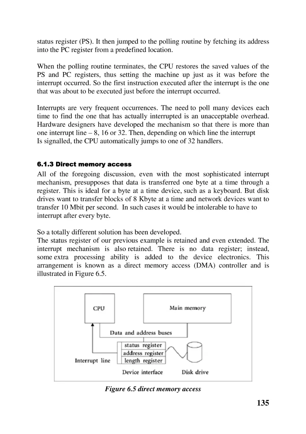
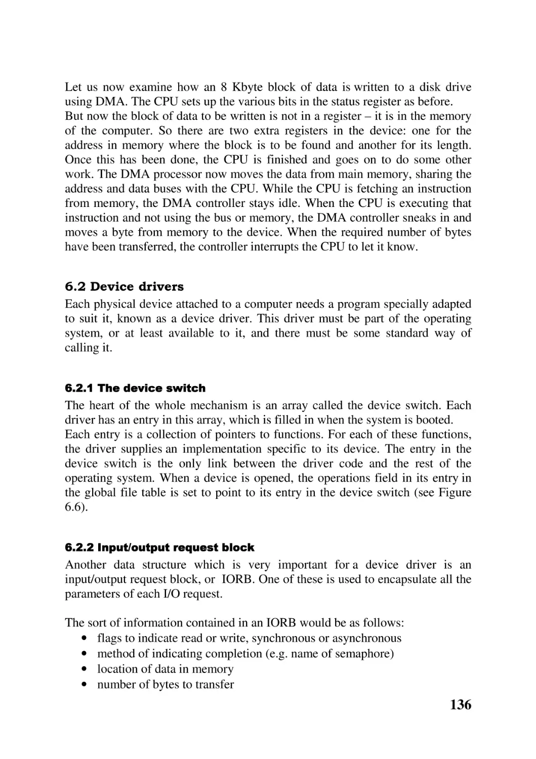
/


Text
1
Operating Systems
John O’Gorman
2
© John O’Gorman 2000
All rights reserved. No reproduction, copy or transmission of this
publication may be made without written permission. No paragraph of
this publication may be reproduced, copied or transmitted save with
written permission or in accordance with the provisions of the Copyright,
Designs and Patents Act 1988, or under the terms of any licence permitting
limited copying issued by the Copyright Licensing Agency, 90 Tottenham
Court Road, London W1P 0LP.
Any person who does any unauthorised act in relation to this publication
may be liable to criminal prosecution and civil claims for damages.
3
The author has asserted his right to be identified as the author of this work
in accordance with the Copyright, Designs and Patents Act 1988.
First published 2000 by MACMILLAN PRESS LTD
Houndmills, Basingstoke, Hampshire RG21 6XS and London Companies
and representatives throughout the world ISBN 0–333–80288–8 paperback
A catalogue record for this book is available from the British Library.
This book is printed on paper suitable for recycling and made from fully
managed and sustained forest sources.
10 9 8 7 6 5 4 3 2 1
09 08 07 06 05 04 03 02 01 00
Typeset by Ian Kingston Editorial Services, Nottingham, UK
Printed in Great Britain by Antony Rowe Ltd, Chippenham, Wiltshire
Page v
4
Contents
Preface
Chapter 1 Introduction
9
12
Chapter overview 12
1.1 What is an operating system? 12
1.2 What does an operating system do? 13
1.3 Interfaces to operating systems 15
1.4 Study of operating systems 18
1.5 Historical development of operating systems 20
1.6 Types of operating system 21
1.7 Design of operating systems 24
Chapter summary 26
Further reading 28
Self-test questions 28
Discussion questions 29
Chapter 2 Process manager
30
Chapter overview 30
2.1 The concept of a process 30
2.2 Processors and processes 32
2.3 Multi-threading 33
2.4 Representing processes, tasks and threads 36
2.5 Process creation and termination 38
2.6 Thread creation and termination 39
2.7 Thread state 41
2.8 Context switching 42
2.9 Scheduling 43
Chapter summary 46
Further reading 47
Self-test questions 48
Discussion questions 49
Chapter 3 Concurrency
51
Chapter overview 51
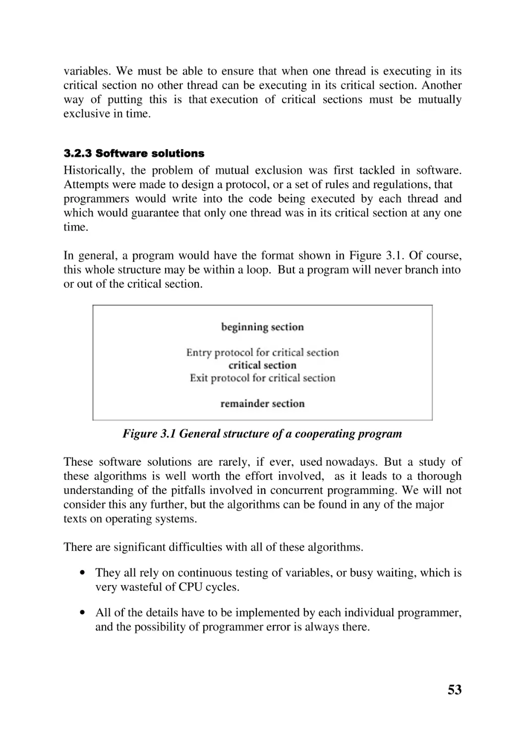
3.1 Introduction 51
3.2 Interaction between threads 52
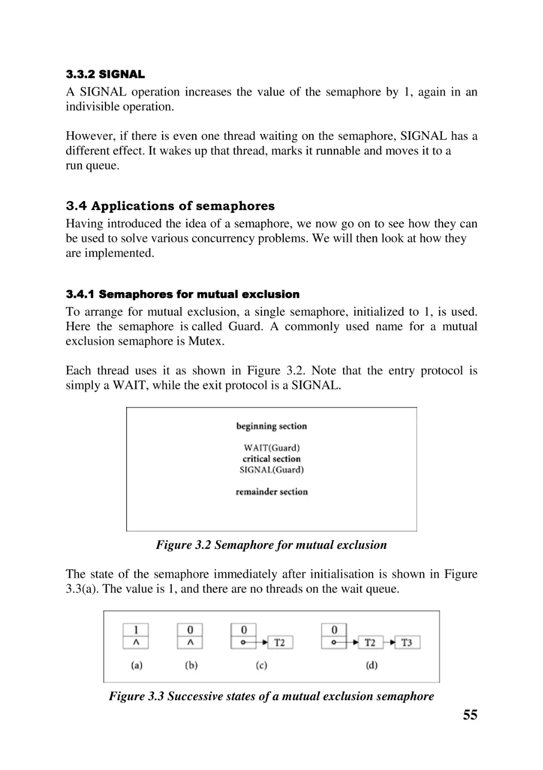
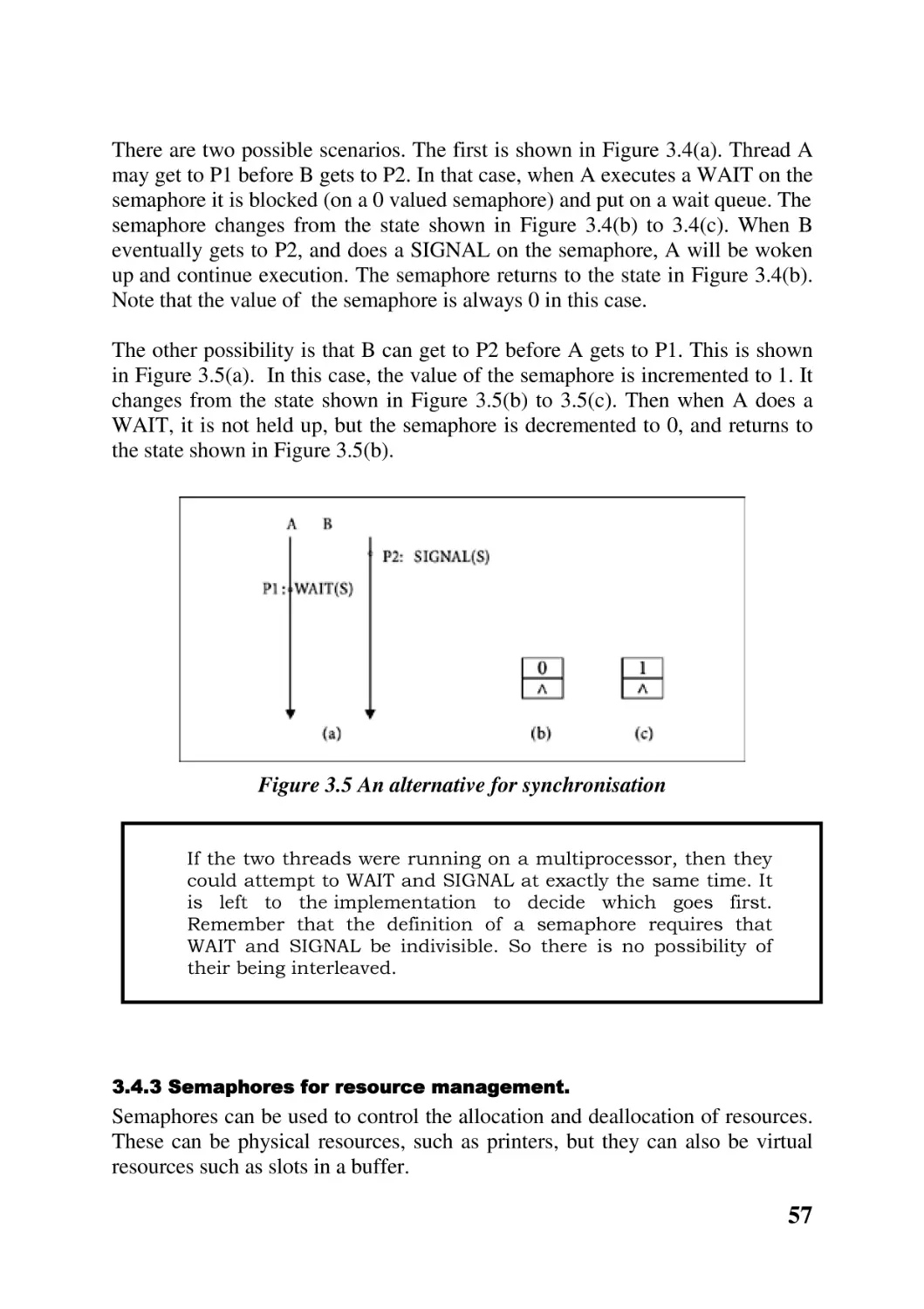
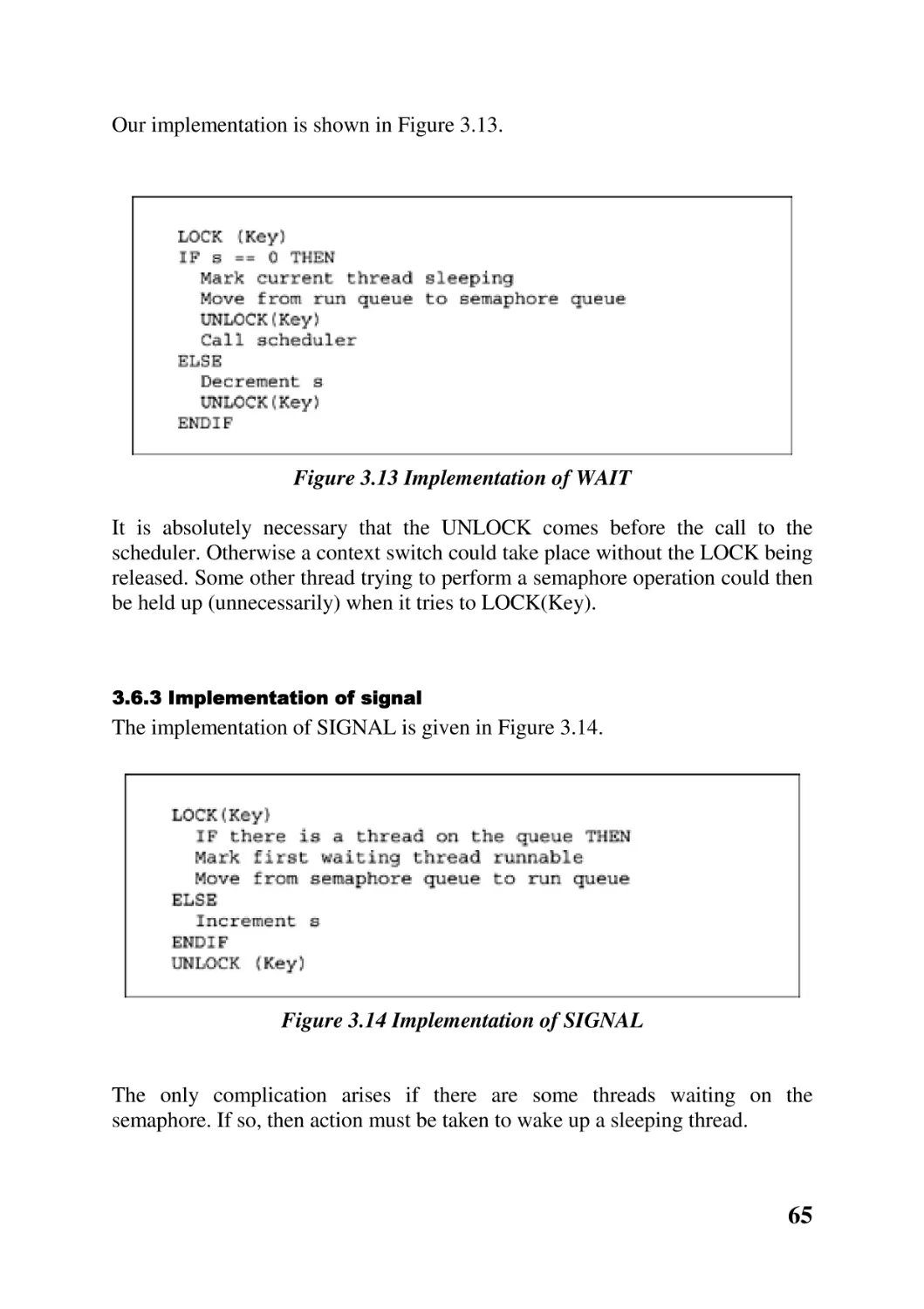
3.3 Semaphores 54
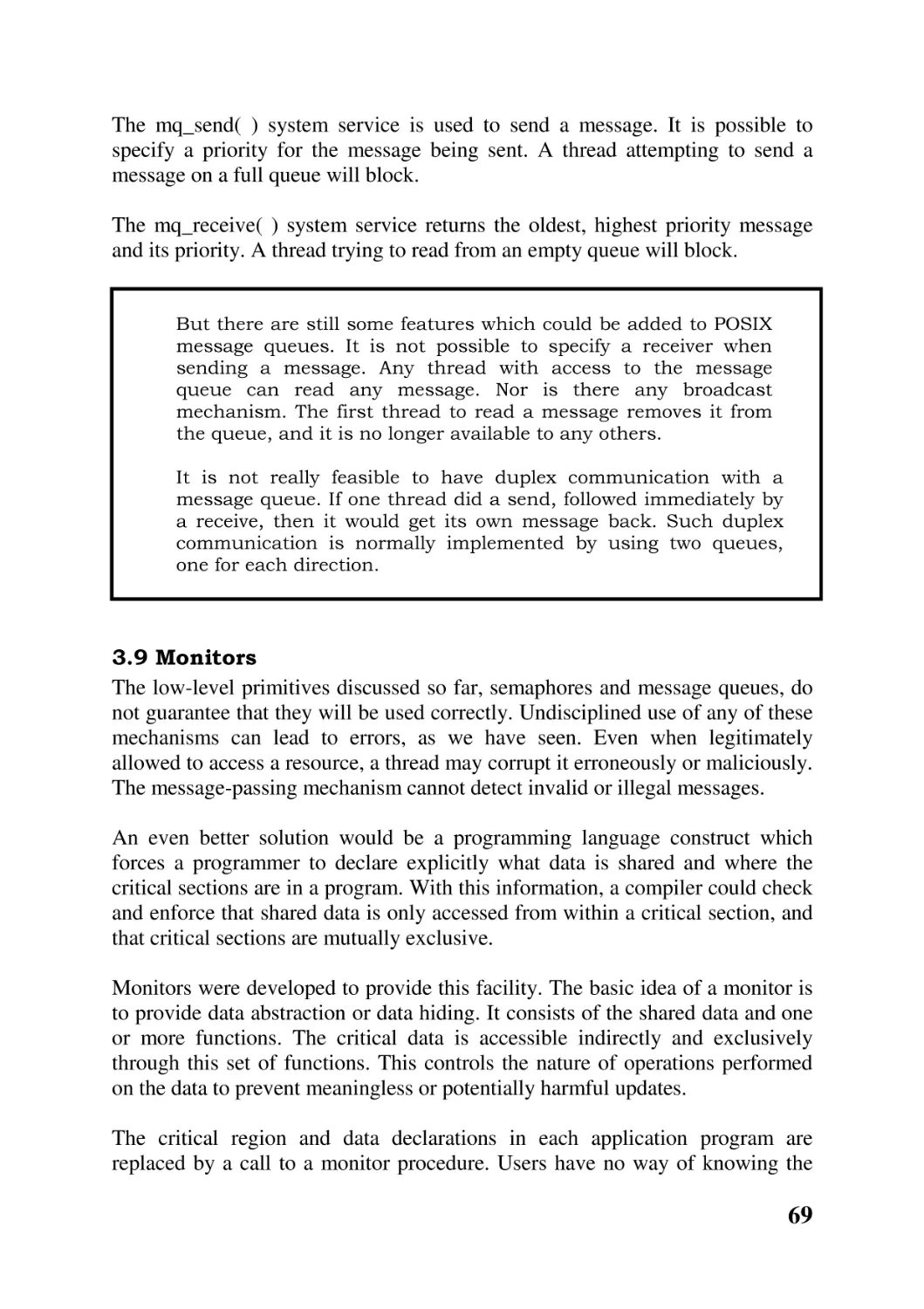
3.4 Applications of semaphores 55
5
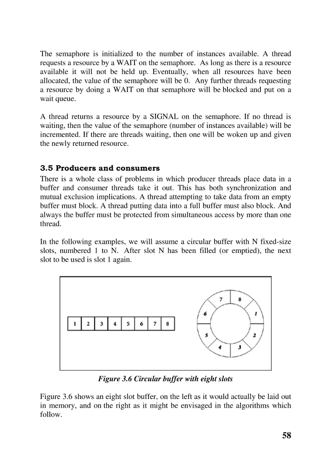
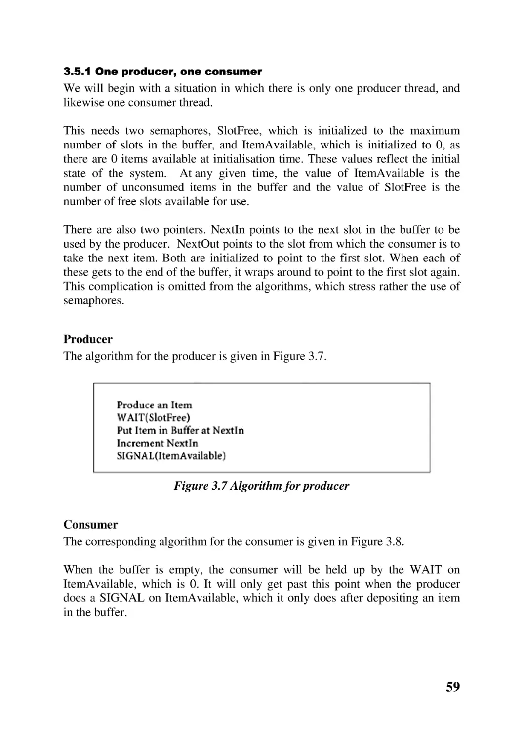
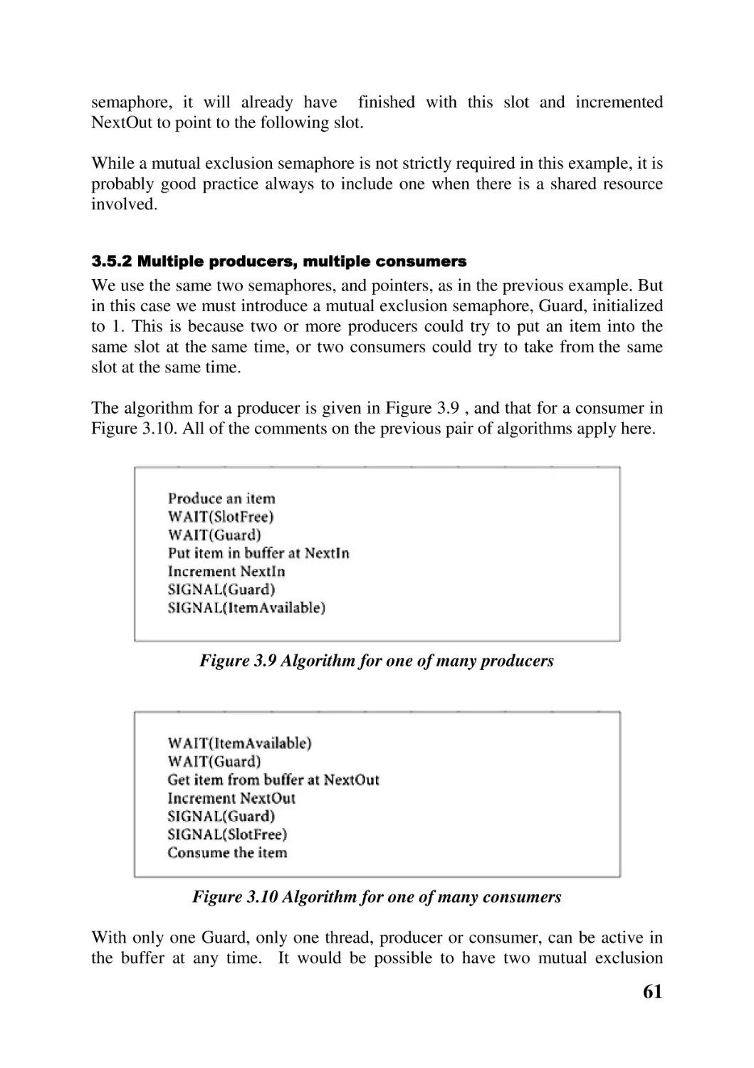
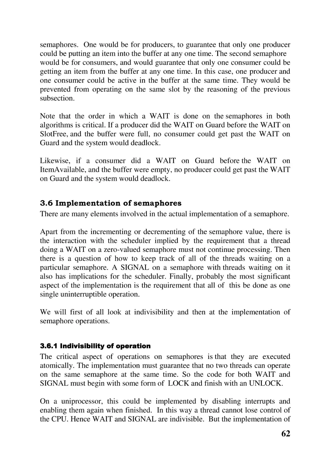
3.5 Producers and consumers 58
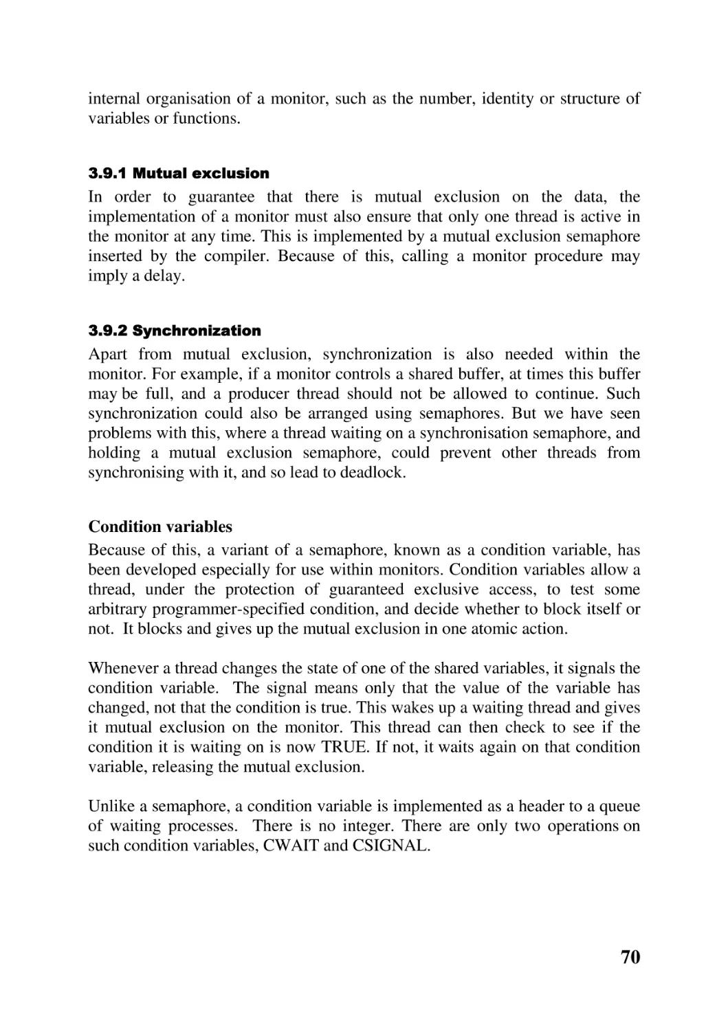
3.6 Implementation of semaphores 62
3.7 Limitations of semaphores 66
3.8 Message passing 67
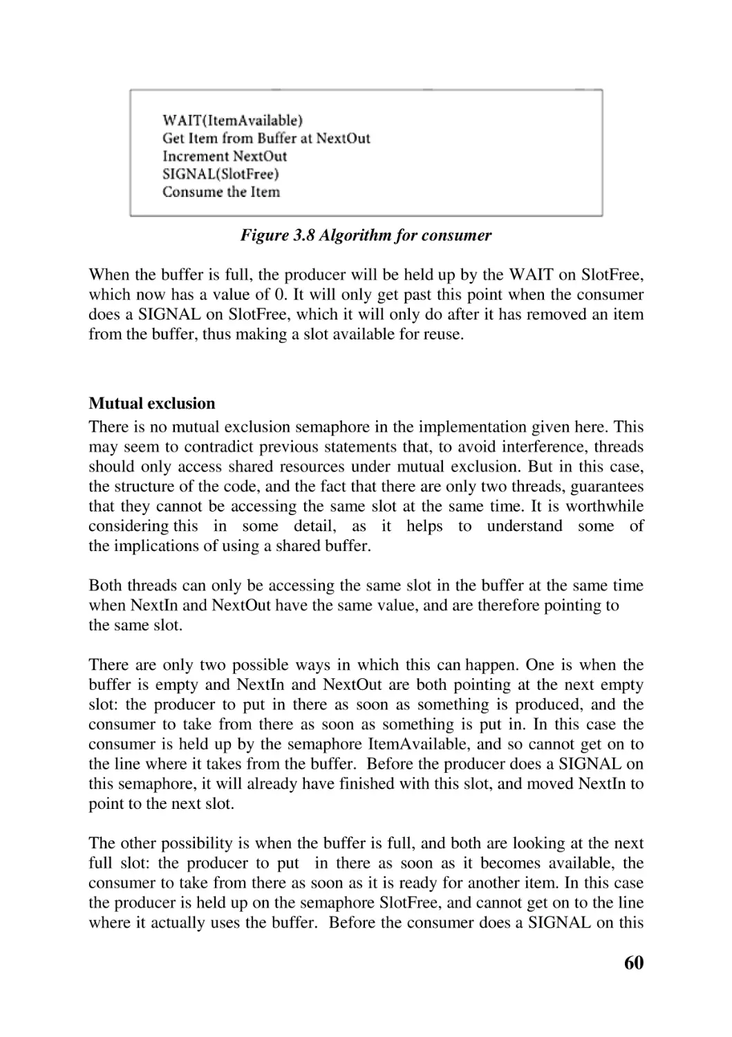
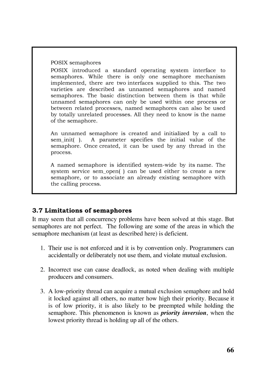
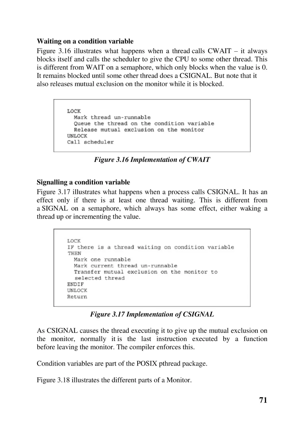
3.9 Monitors 69
3.10 Deadlock 74
Chapter summary 77
Further reading 79
Self-test questions 80
Discussion questions 81
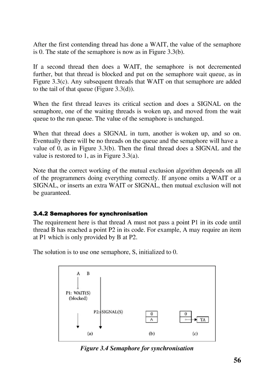
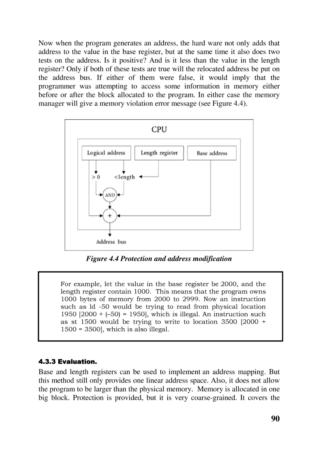
Chapter 4 Memory manager
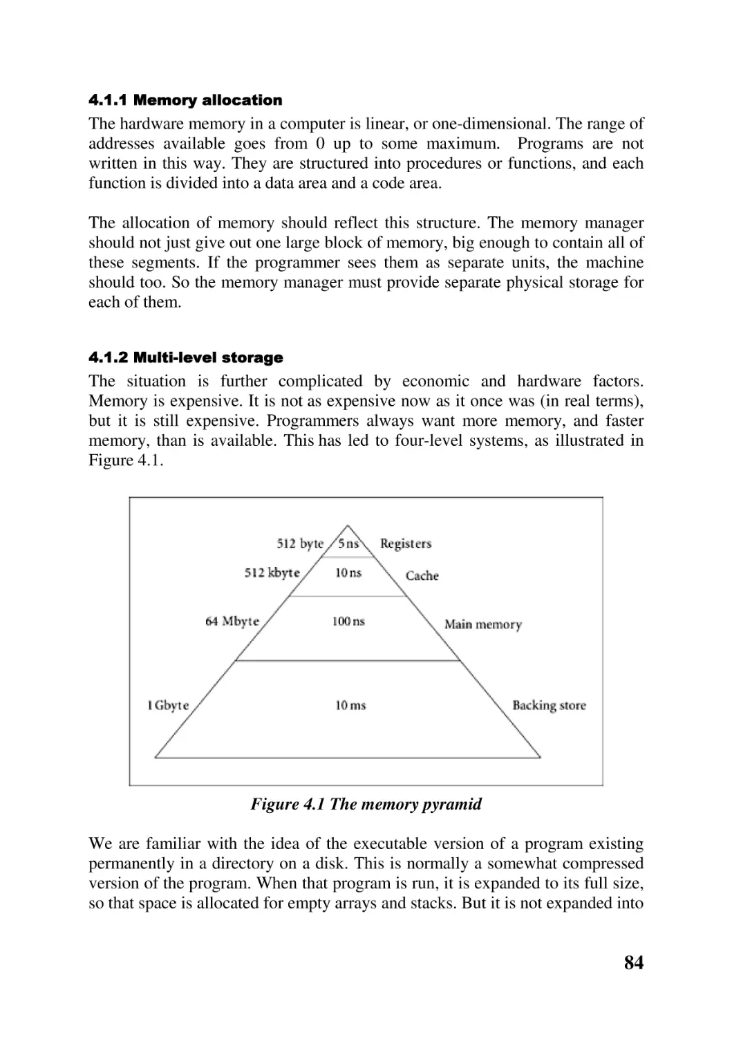
83
Chapter overview 83
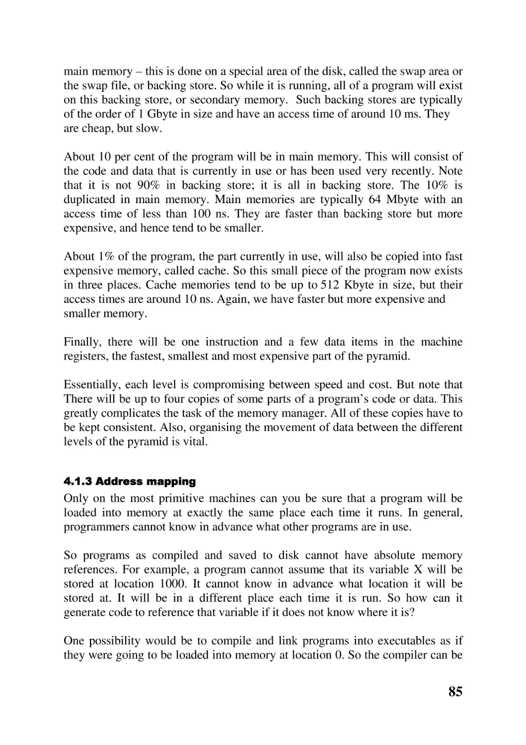
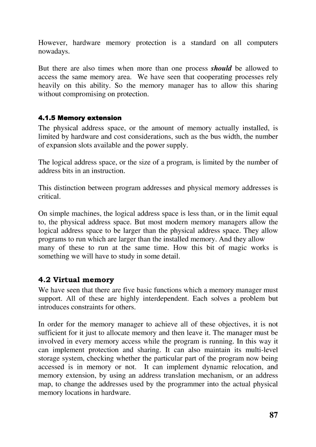
4.1 Objectives of a memory manager 83
4.2 Virtual memory 87
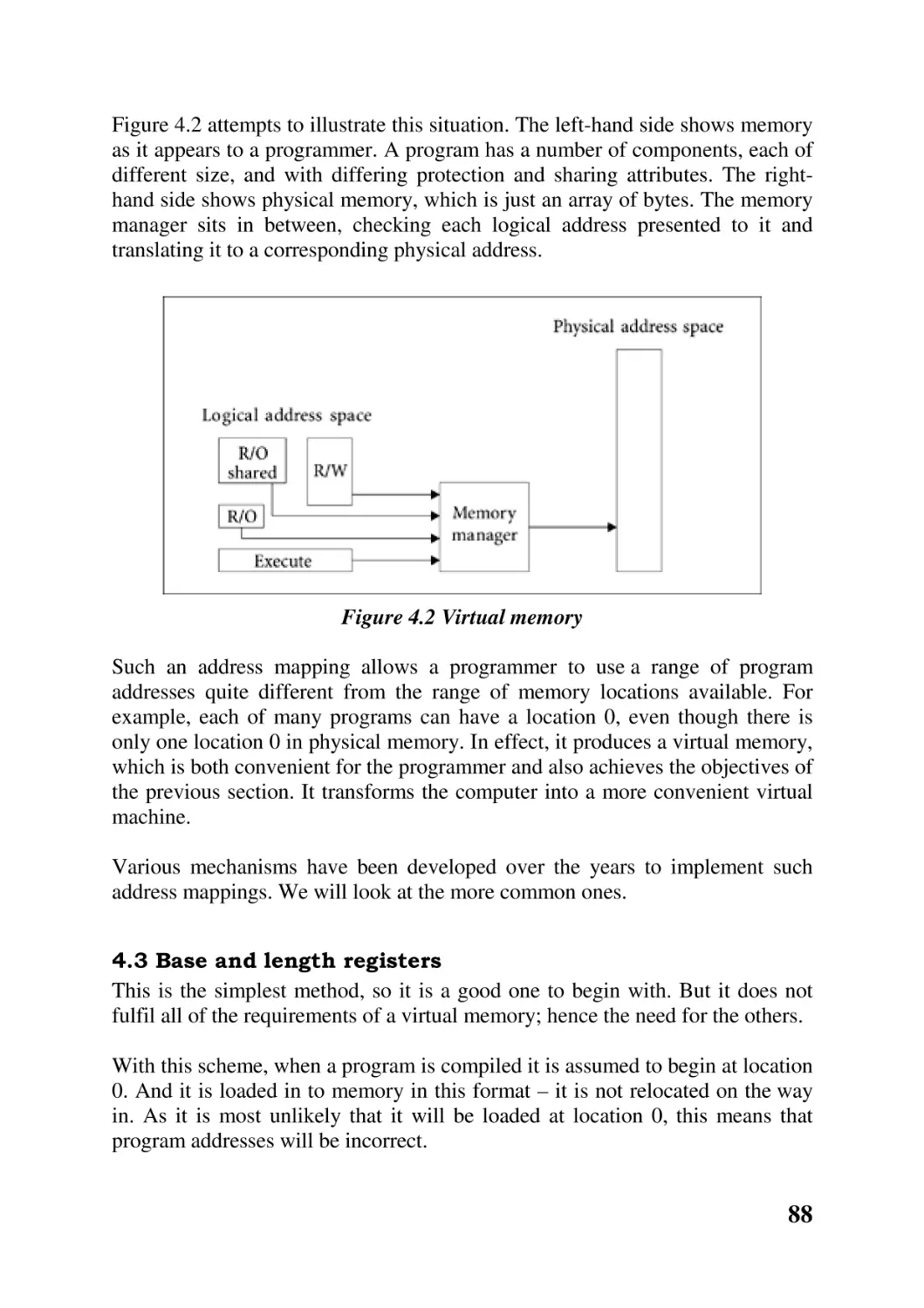
4.3 Base and length registers 88
4.4 Segmentation 91
4.5 Paging 98
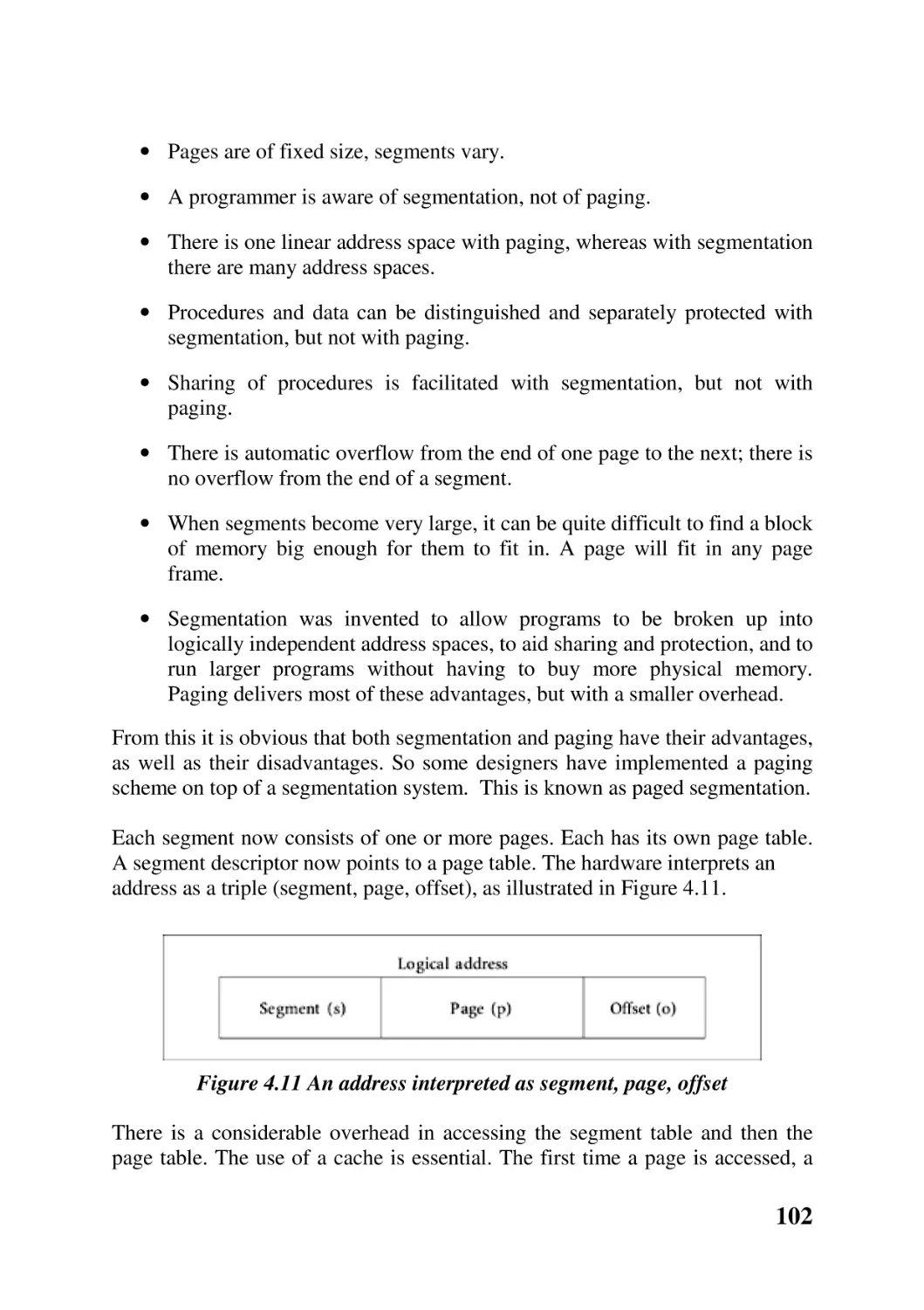
4.6 Paged segmentation 101
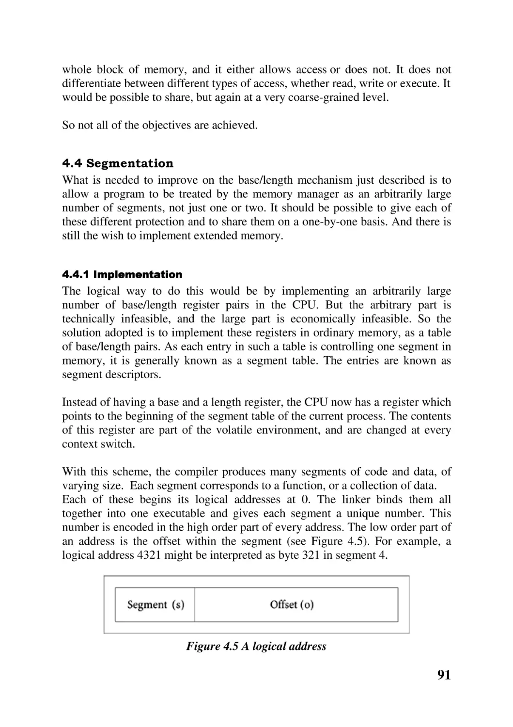
4.7 System services for memory management 103
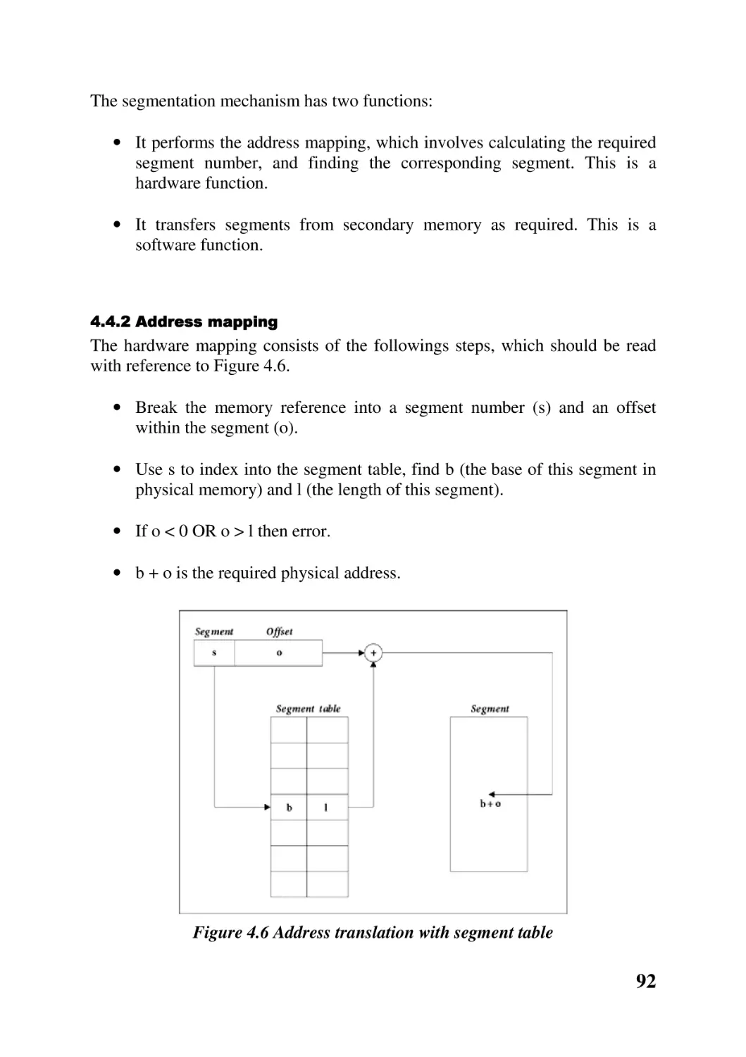
Chapter summary 103
Further reading 105
Self-test questions 105
Discussion questions 106
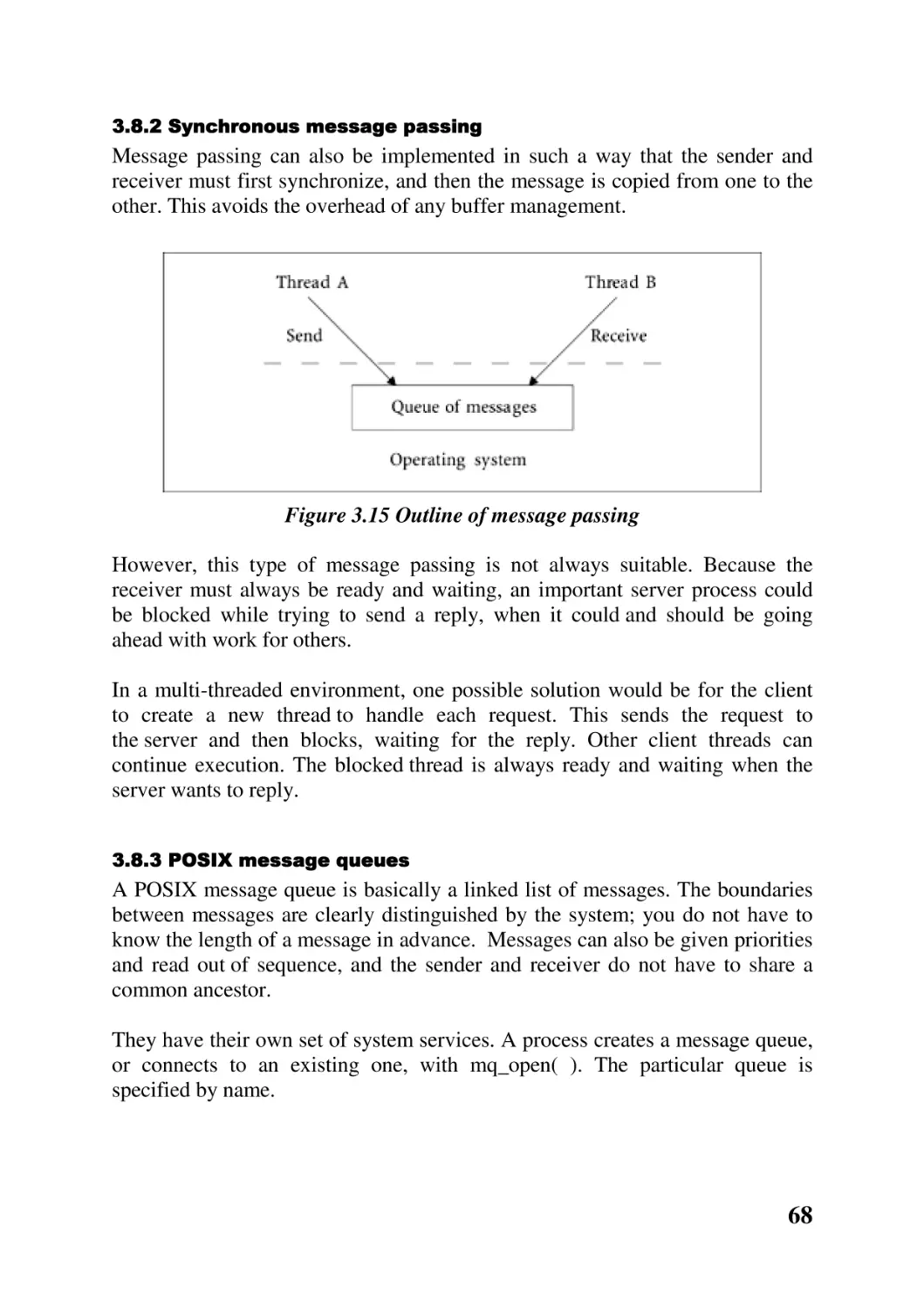
Chapter 5 Input and output
109
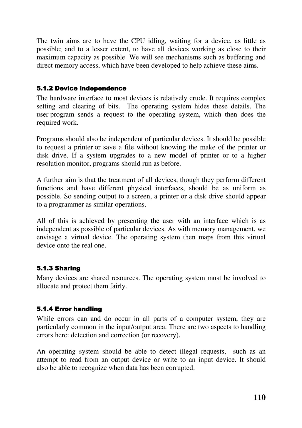
Chapter overview 109
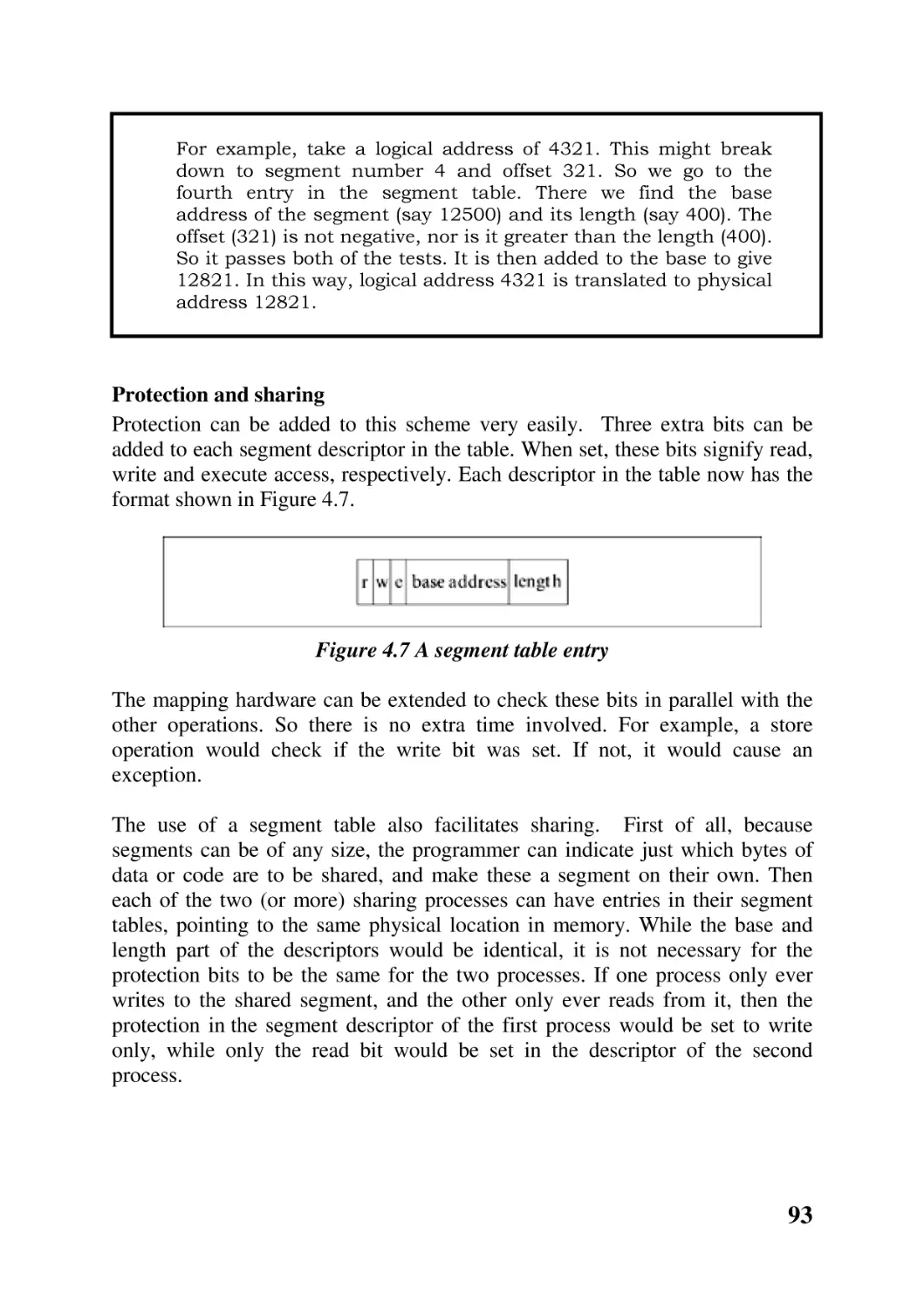
5.1 Design objectives 109
5.2 I/O subsystem 111
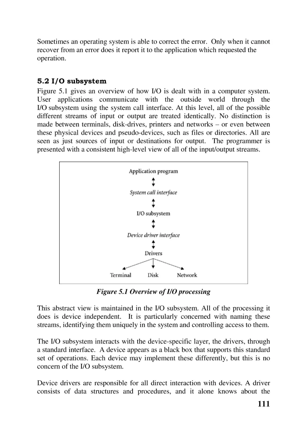
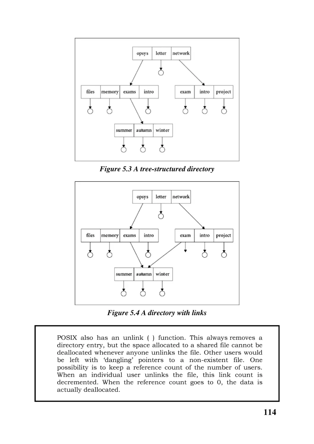
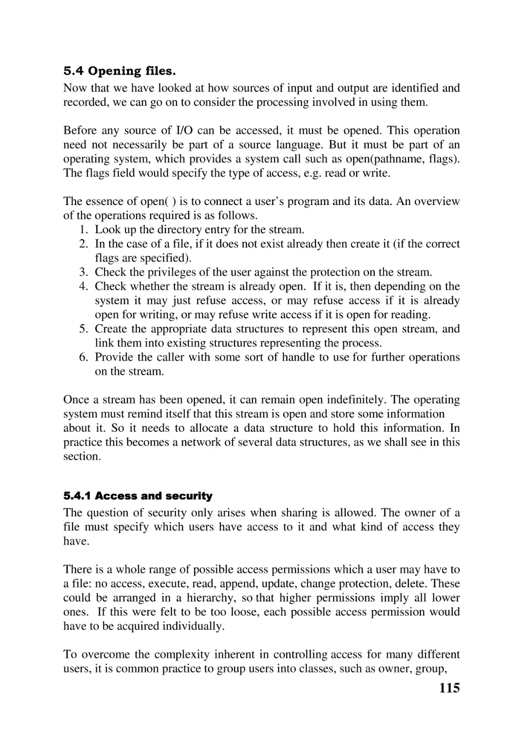
5.3 Directory name space 112
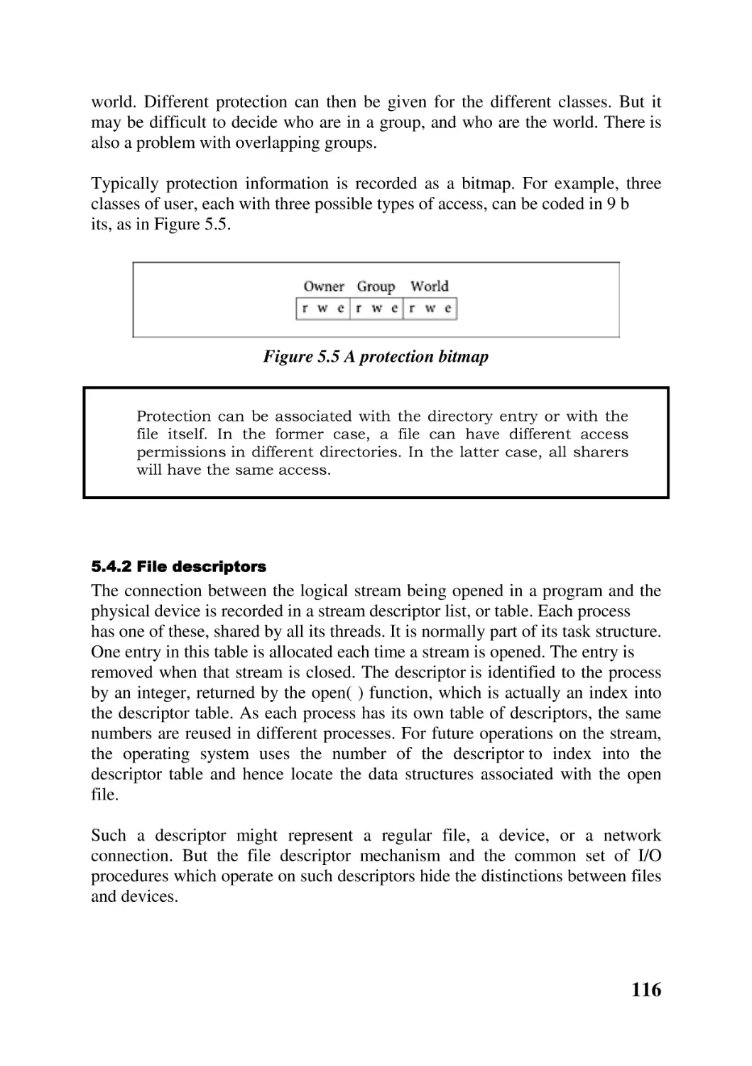
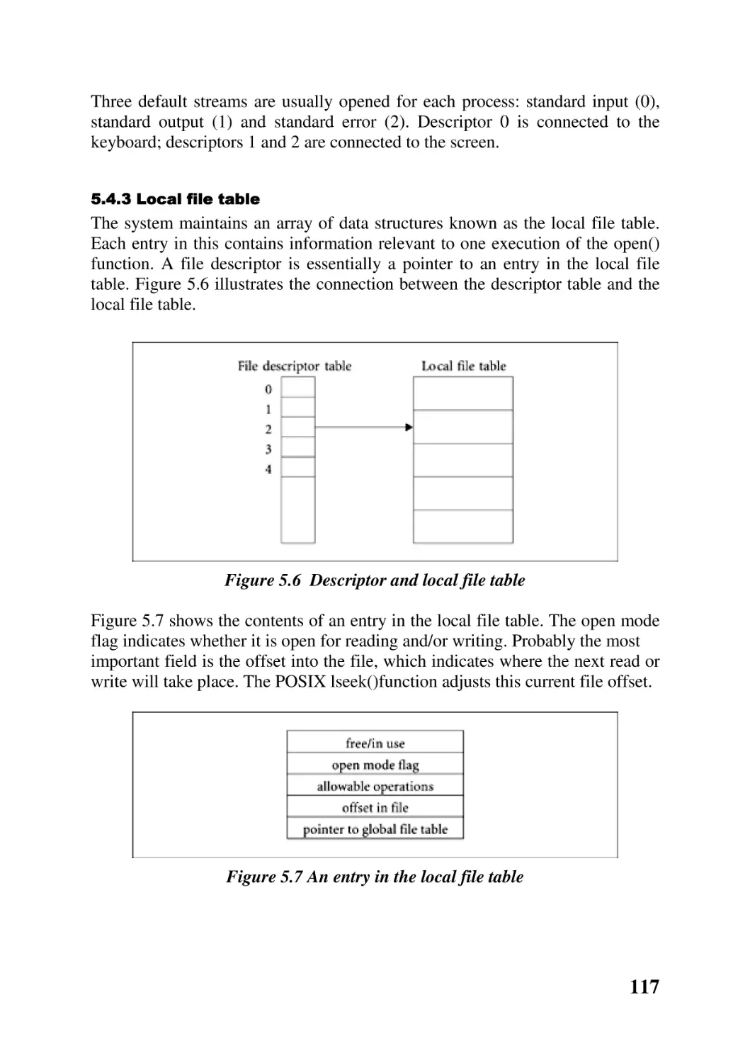
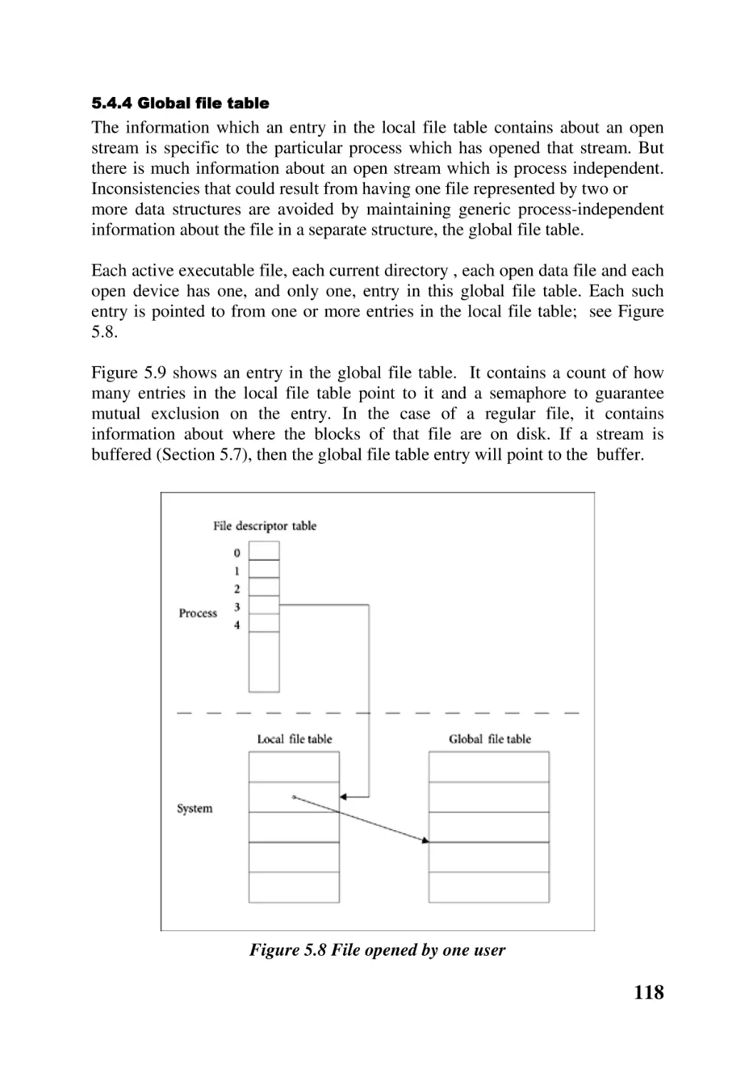
5.4 Opening files 115
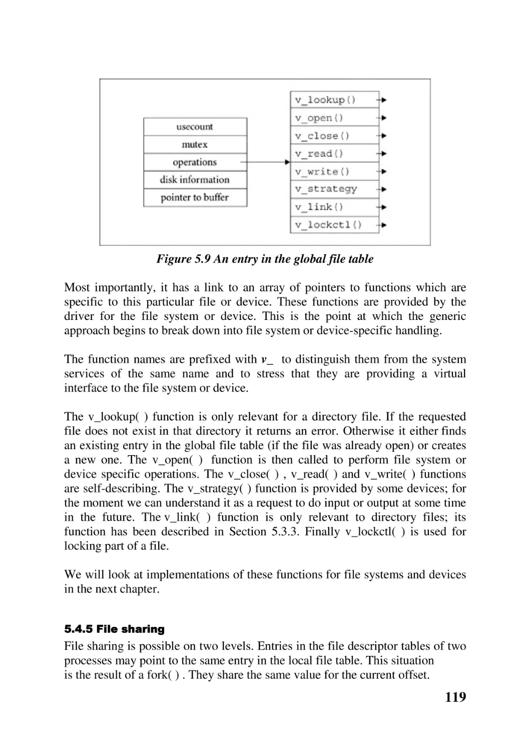
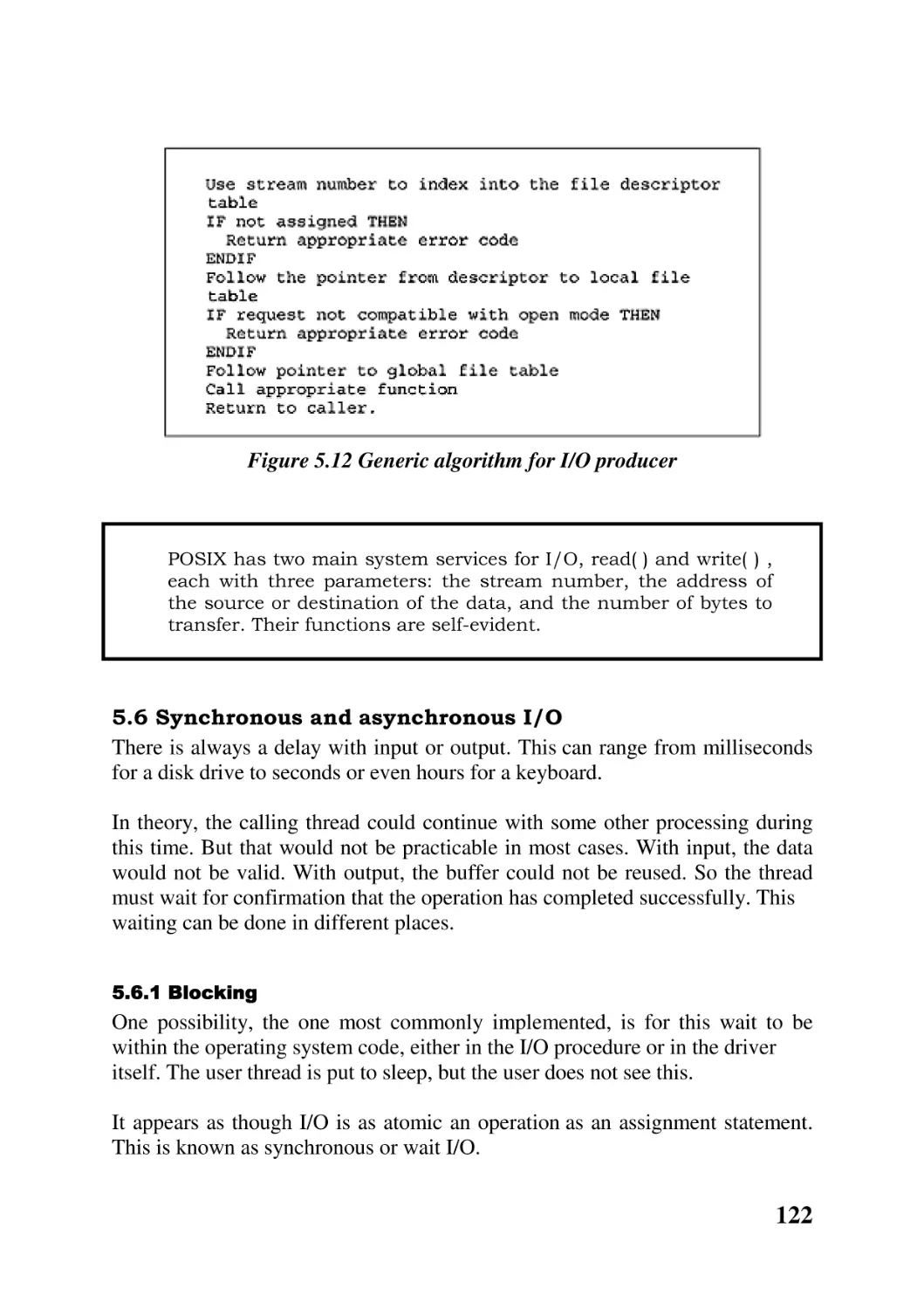
5.5 Input/output procedures 120
5.6 Synchronous and asynchronous I/O 122
5.7 Buffering 123
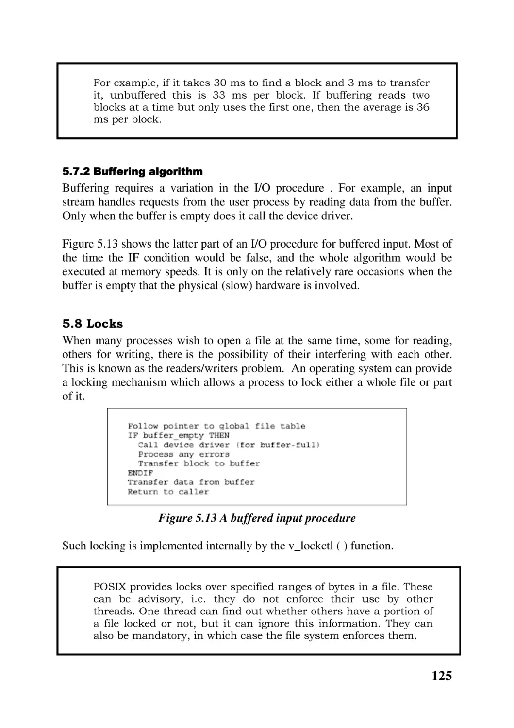
5.8 Locks 125
5.9 Close 126
Chapter summary 126
Further reading 127
Self-test questions 128
Discussion questions 128
6
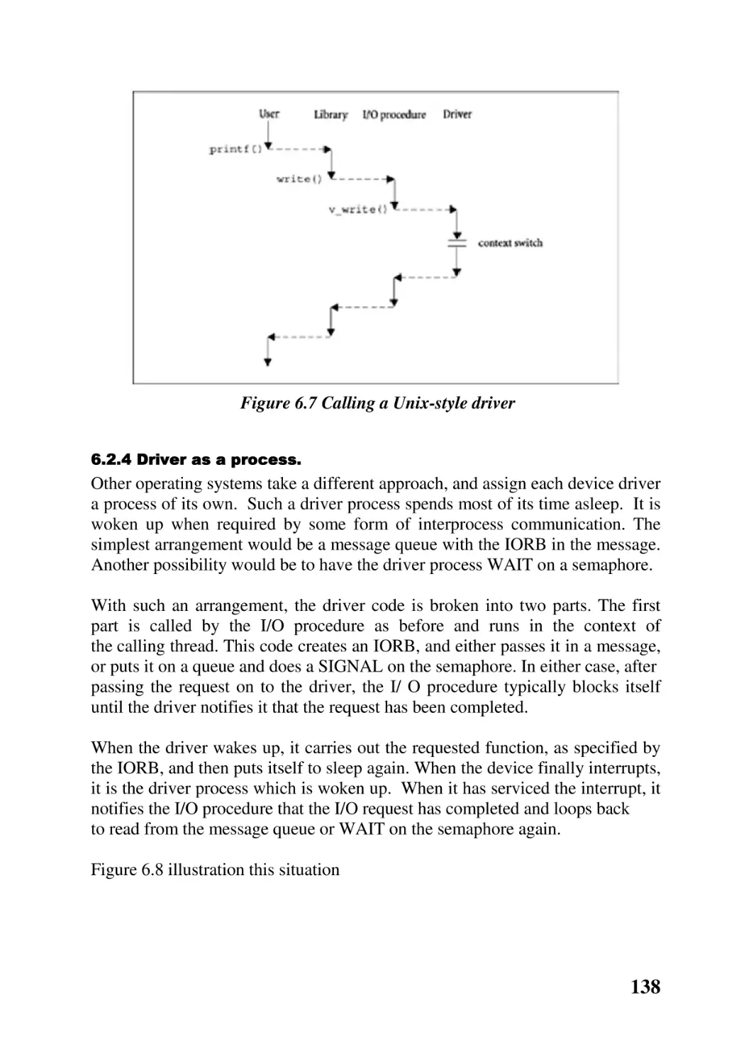
Chapter 6 Low-level I/O processing
131
Chapter overview 131
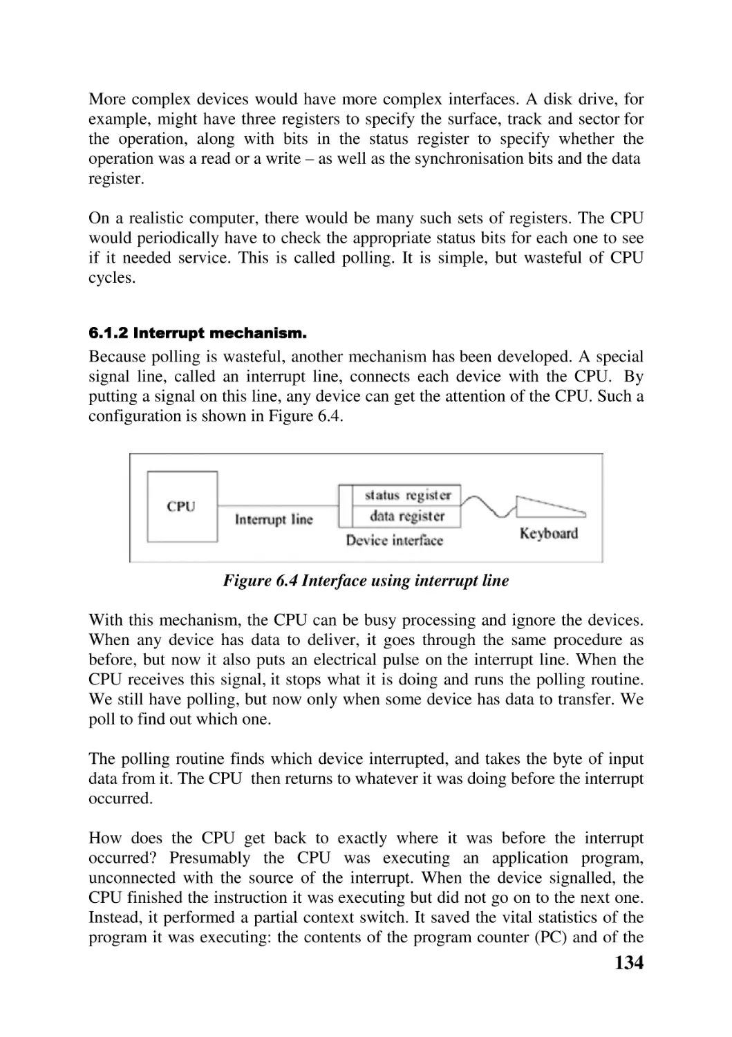
6.1 Interface with the hardware 131
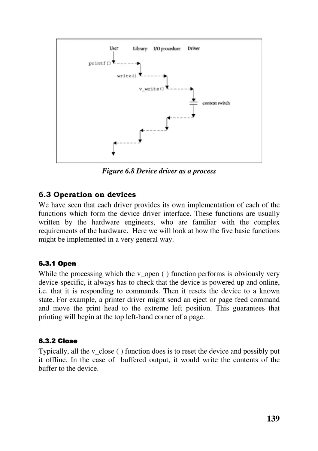
6.2 Device drivers 136
6.3 Operations on devices 139
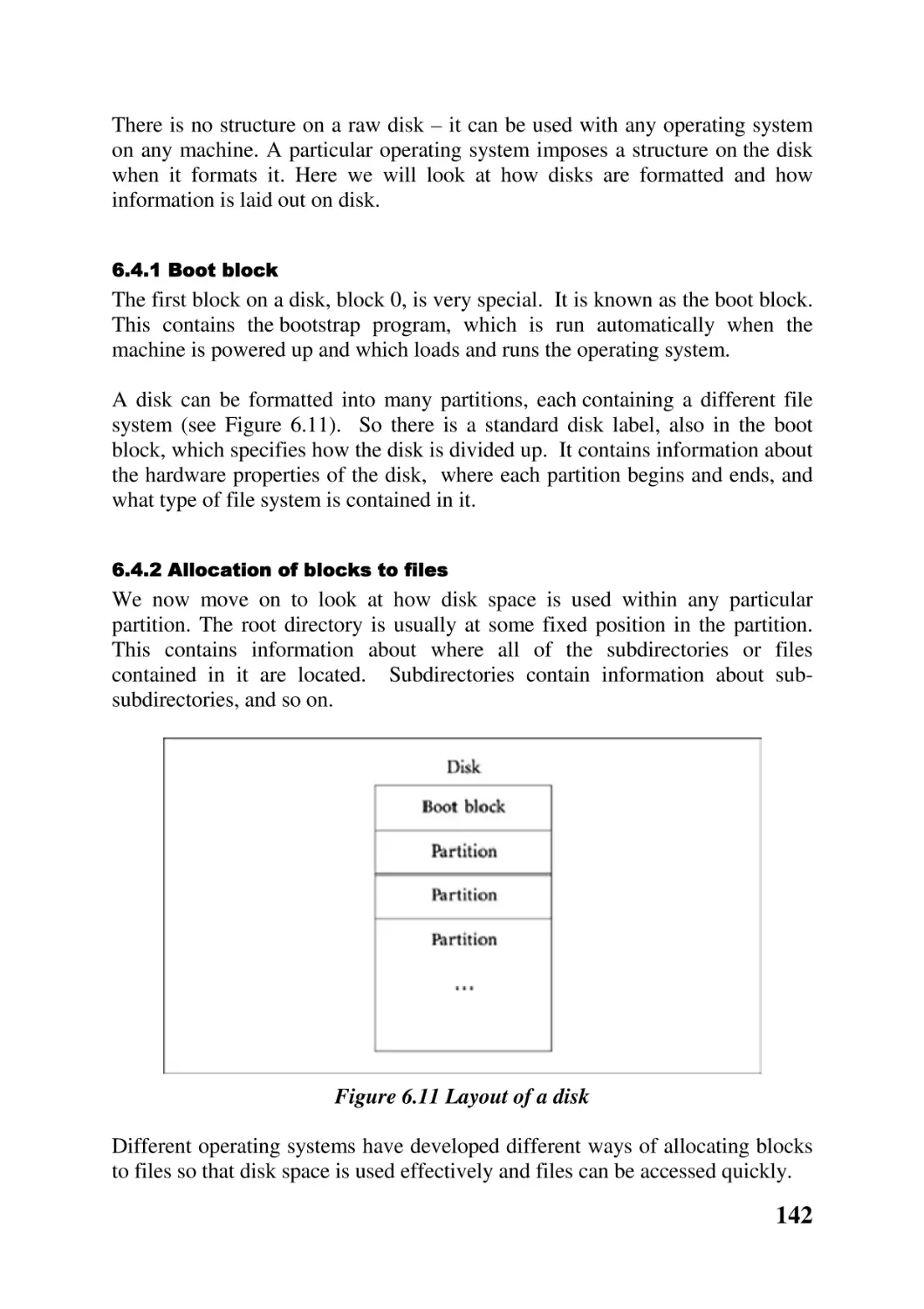
6.4 Disk organisation 141
6.5 The file manager 146
Chapter summary 148
Further reading 149
Self-test questions 149
Discussion questions 150
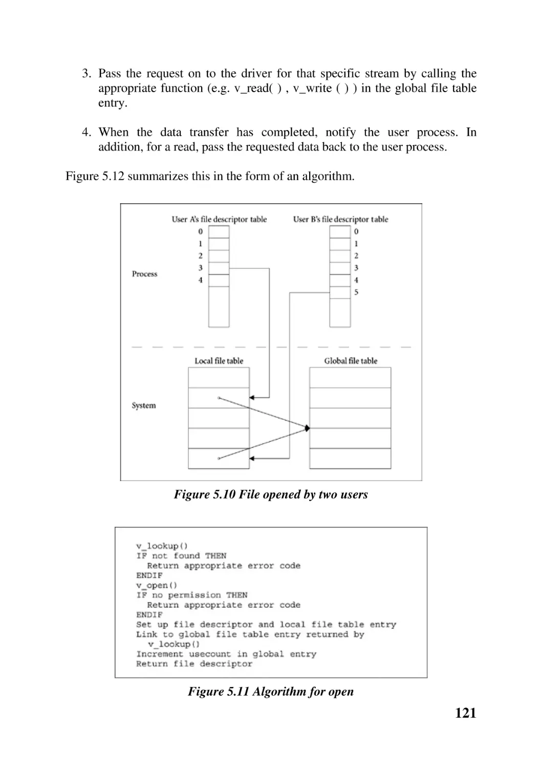
Chapter 7 Distributed systems
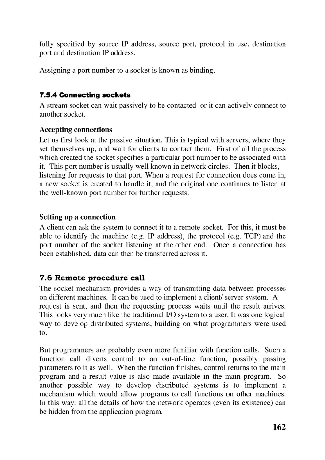
152
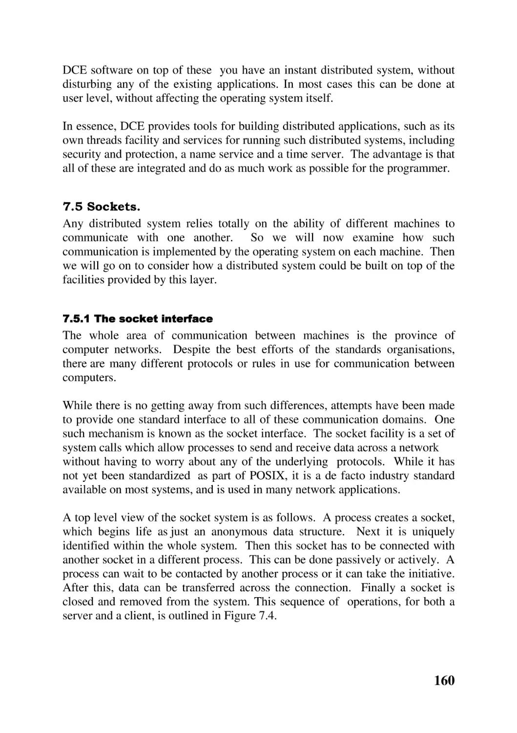
Chapter overview 152
7.1 Introduction 152
7.2 Features of distributed systems 153
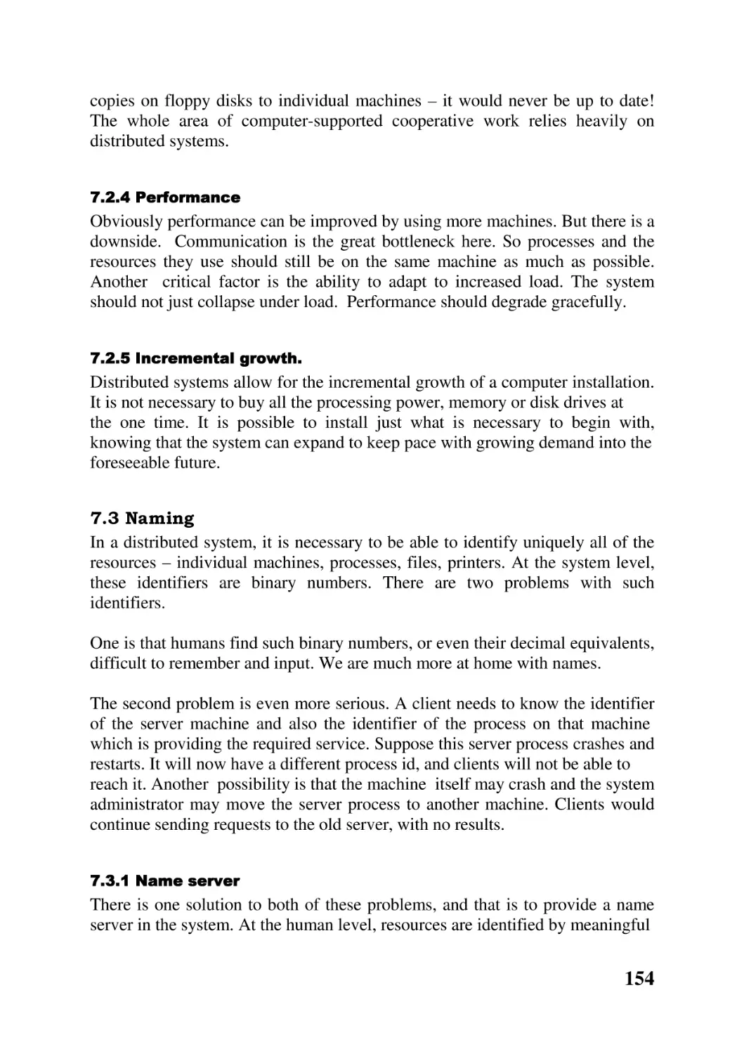
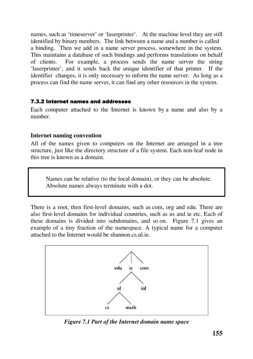
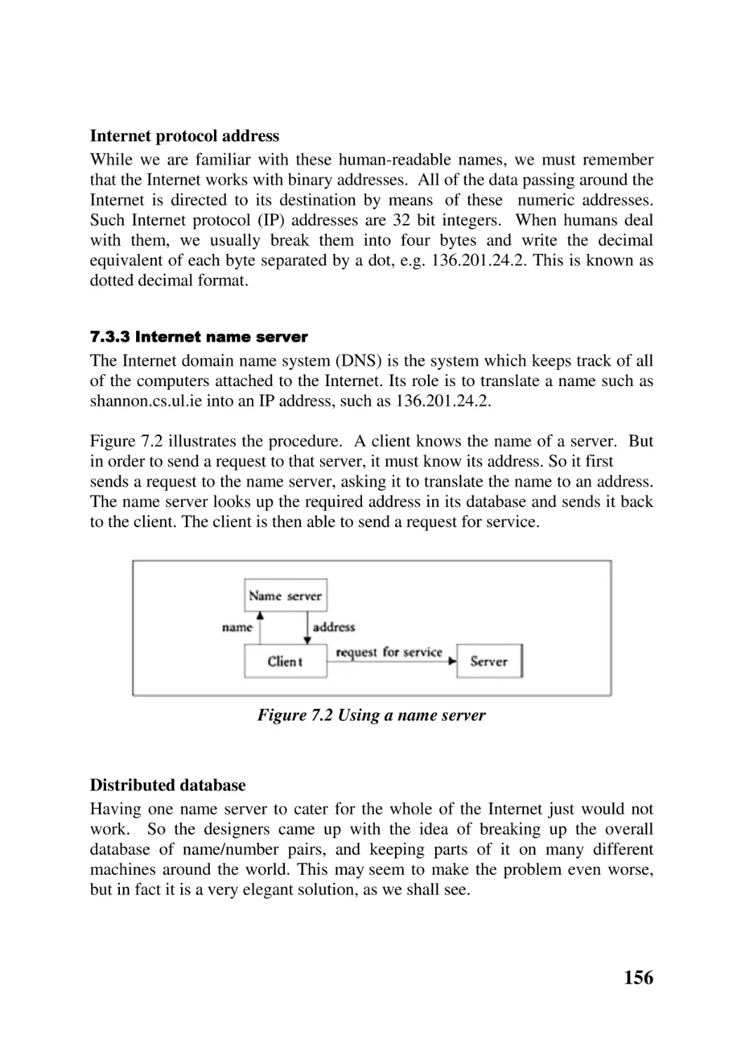
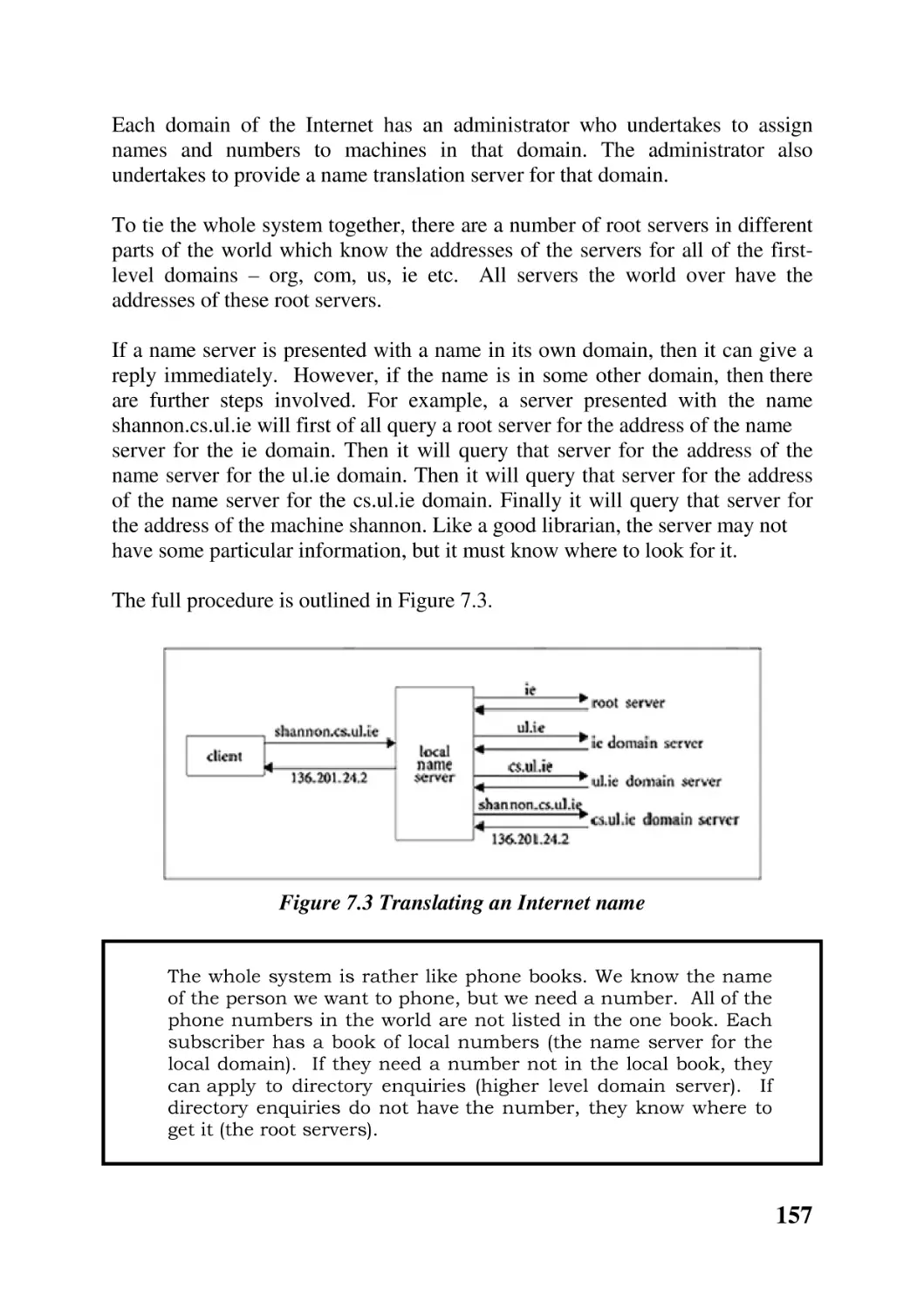
7.3 Naming 154
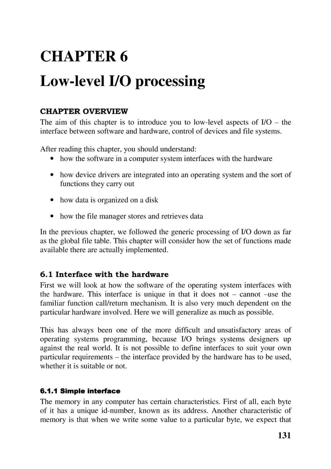
7.4 Operating systems 158
7.5 Sockets 160
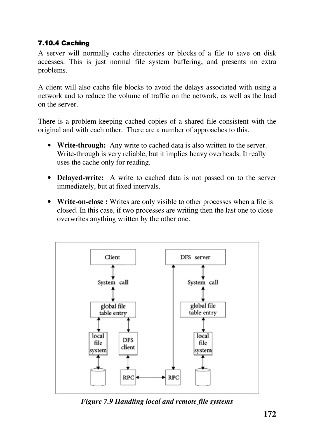
7.6 Remote procedure call 162
7.7 Distributed mutual exclusion 164
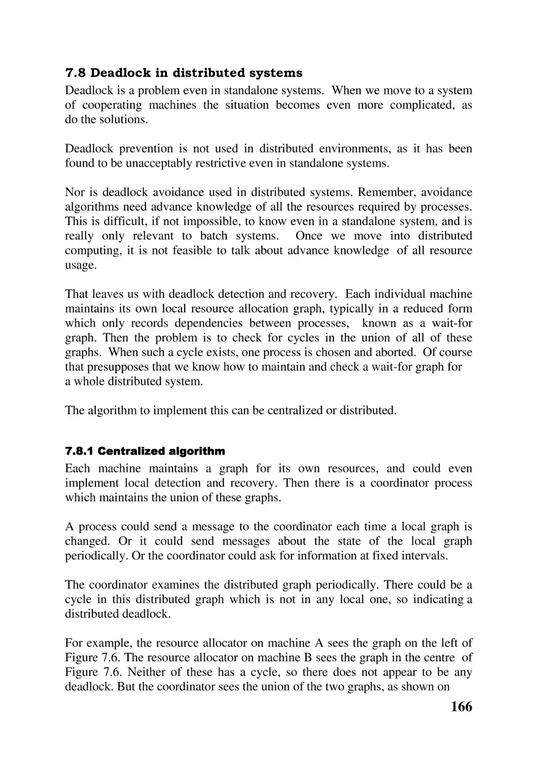
7.8 Deadlock in distributed systems 166
7.9 Distributed shared memory 167
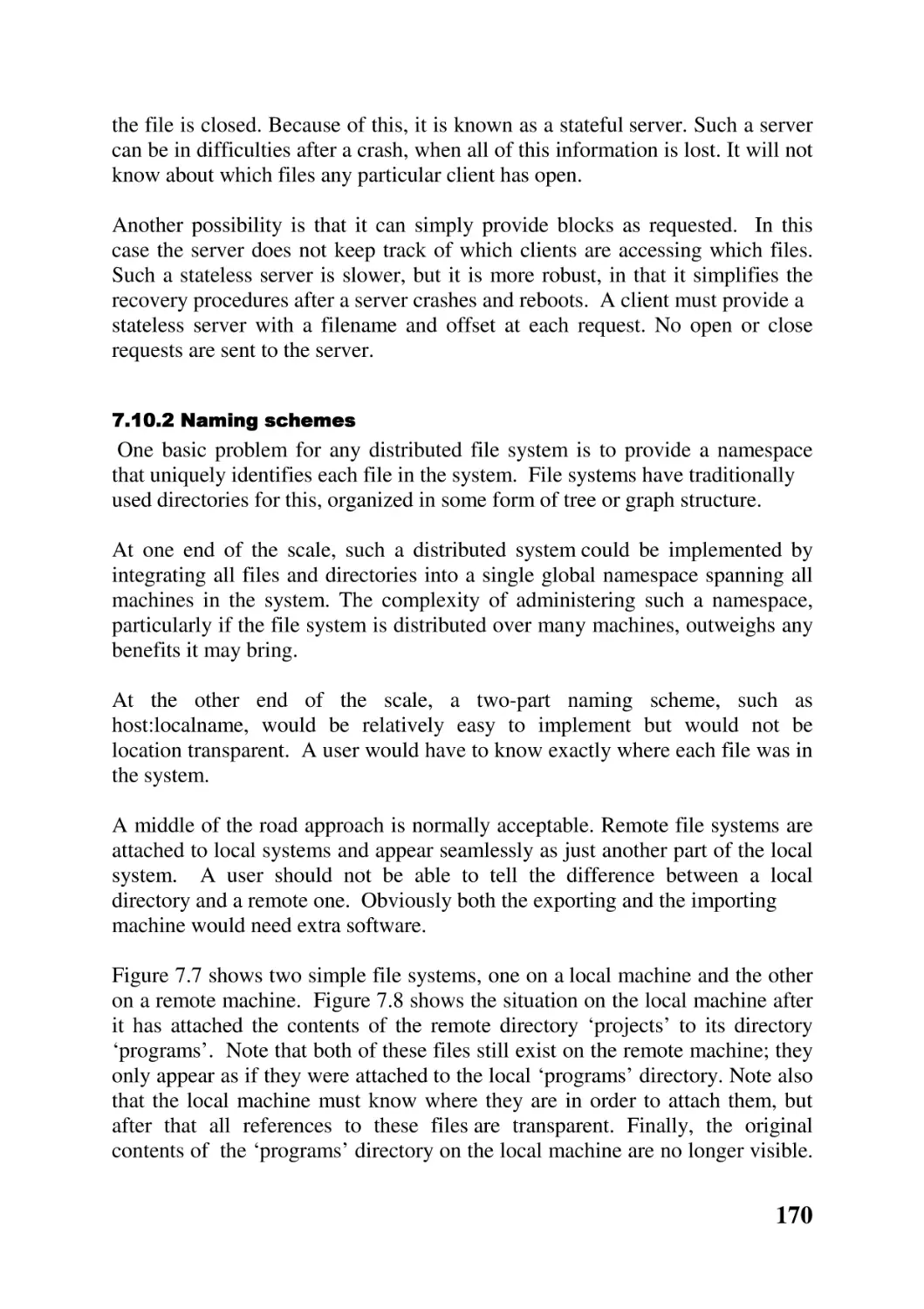
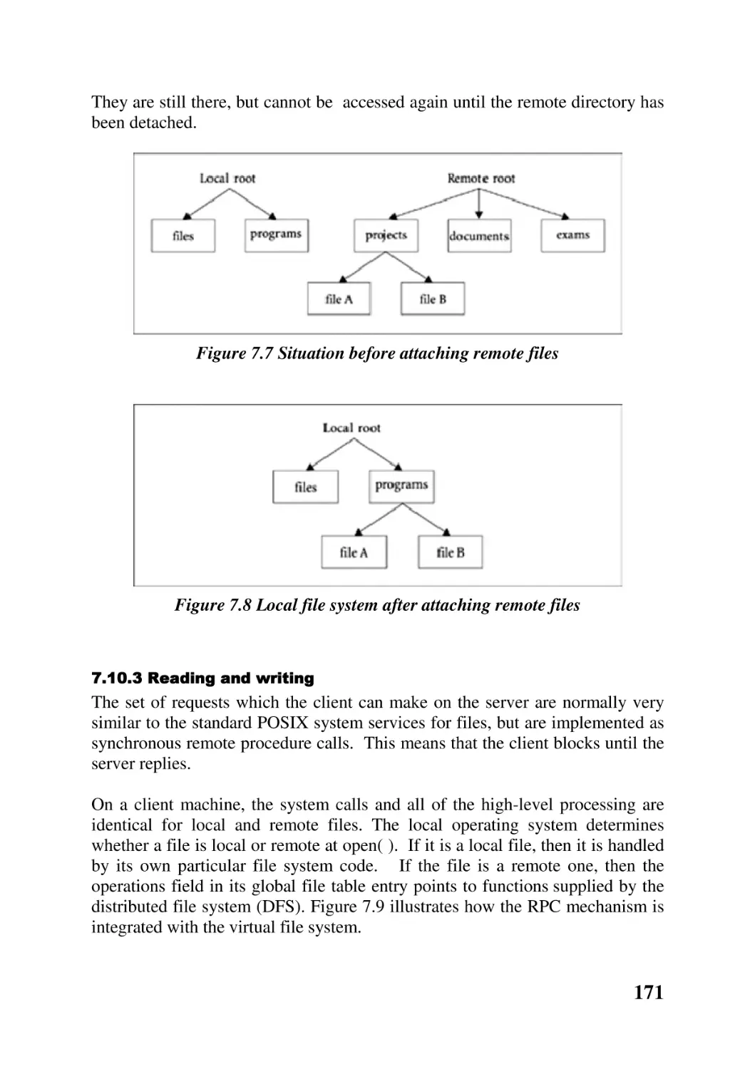
7.10 Distributed file systems 169
Chapter summary 174
Further reading 175
Self-test questions 176
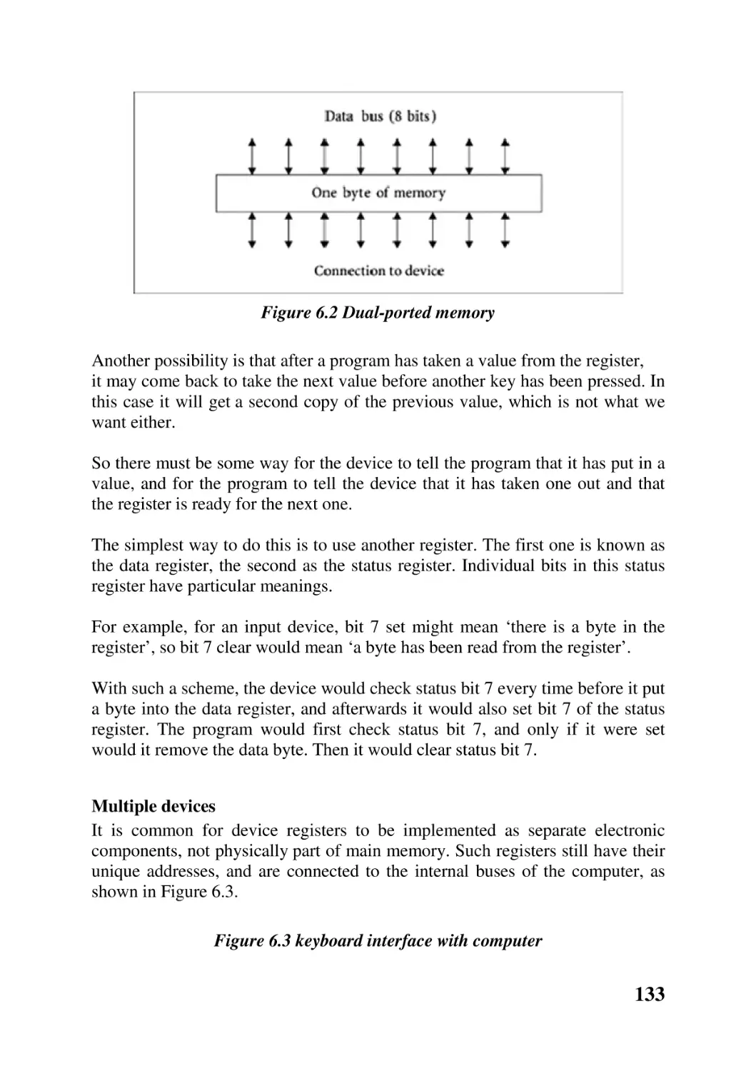
Discussion questions 177
Chapter 8 Fault tolerance and security
180
Chapter overview 180
8.1 Fault tolerance 180
8.2 Security 183
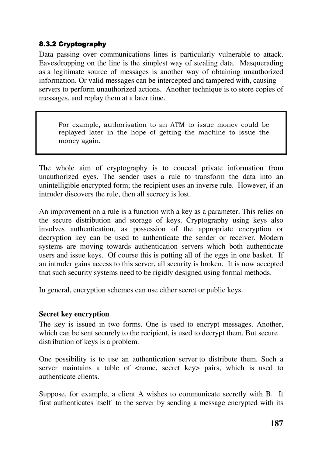
8.3 Security in distributed systems 186
Chapter summary 189
Further reading 190
Self-test questions 190
Discussion questions 191
Reading List
192
7
Preface.
There are many excellent textbooks available on operating systems. While they
take different approaches to the subject, they all have some features in common.
Most are large books, up to 700 pages in length, and priced in proportion, aimed
at students taking operating systems modules in specialist computer science
courses, or computer science majors in general science courses, or even
postgraduate students.
But apart from these, operating systems are also taught in a large number of
other courses, although in nothing like the same detail. Almost every certificate
or diploma course that has anything to do with computing contains a module on
operating systems.
Students on such courses are unlikely to buy large, costly textbooks, containing
more material than is required for short modules.
Consequently, there is a discrepancy between what is being offered by
publishers, and what is needed in the academic market.
This book is intended to fill that gap, as a text for a one term or one semester
introductory course on operating systems. It contains material for roughly 25–
30 lectures. The main feature which distinguishes it from other books on the
market is its size. Students should, in their short course, make use of all of it,
and so feel they are getting their money’s worth.
Approach to the subject
Apart from the size of the book, there is also the question of the approach taken
to the subject. An operating system can be understood as including everything
that comes on the distribution disk. Items such as libraries, a GUI, command
shells, and utility programs are frequently considered to be part of the operating
system. Many books on operating systems have this underlying view, and they
study them from the outside, looking at such matters as system management,
use of a GUI, shell programming.
An operating system can also be taken to mean just the kernel. This is the view
taken in this book. So the approach it takes is an investigation of the internals of
operating systems, of how they are designed and built. There is nothing here
about GUIs or shells.
8
The interface to the kernel is the set of system services provided by the
particular operating system. There is a passing reference to the POSIX interface
in relevant places throughout the text. As more and more operating systems are
now providing a POSIX compliant interface, this seems reasonable.
Features
In common with other books in the Grassroots series, this text has the following
features:
• Chapter objectives, which clearly define what students should learn in
each chapter
• Chapter summaries, for quick revision
• References to further reading in a small set of classic textbooks, for those
who want more information
• Self-test questions at the end of each chapter, so that students can assess
whether they have achieved the objectives of the chapter
• Discussion questions, which take students into areas beyond those
covered in the book.
Omissions
One feature which is commonly found in larger textbooks is an introduction to
real operating systems, such as Windows NT or Unix, either as running
examples, or as appended case studies. Such examples are not included in this
book, because of the size of this book and their availability elsewhere. This
book aims at presenting as much of the basic theory as is possible in a short
course. A longer, or more intensive, course would be better served by one of
the larger textbooks.
There are no quantitative examples given in areas such as scheduling, memory
management, or input/output, as some textbooks do. This is not to play down
their importance; the omission is due both to the size of the book and to the
intended audience.
For the same reason, there are no examples of system programming in the text.
While the POSIX interface is mentioned, this text does not set out to teach
system programming. References to textbooks on POSIX programming are
included in each chapter.
9
Required background
This book is not for an absolute beginner. It is assumed that a student would
already have some knowledge of how a computer system works, i.e. have
completed a module in computer organisation, or computer architecture, or an
introduction to computing. In places, an elementary knowledge of programming
is assumed, while Chapter 7 (Distributed systems) assumes an introductory
knowledge of networks.
Further reading
While this text covers all of the fundamentals, because of its size this coverage
is necessarily limited. It does, however, provide pointers to other material.
Students taking the sort of short course that this is intended for are unlikely to
get around to very extensive reading. Consequently it does not provide
exhaustive references to the secondary, and even less the primary, literature in
the subject.
A reference collection of about ten volumes is assumed. Between them they
contain all of the background reading that might ever be needed for such a
course. It is expected that all of these would be available to a student, either in a
reference collection or on short-term loan. For anybody who wishes to go even
further into a particular topic, the reading lists in these books will provide
anything they desire.
Overview
The arrangement of the material is traditional. Chapter 1 introduces the reader
to operating systems, and gives an overview of the rest of the book. Chapter
2 covers the traditional material on processes, but with more emphasis than
usual on threads. Chapter 3 considers interactions between concurrent threads,
including semaphores, message queues, and monitors. On the assumption that
this is the only place where a student will meet concurrency, it goes into the
topic in some detail. Memory management is covered in Chapter 4, including
segmentation and paging. Input /output is dealt with over two chapters: Chapter
5 concentrates on the high-level device-independent aspects, while Chapter 6
looks at low-level aspects such as the interface with the hardware, control of
devices, and file organisation on disk. Chapter 7 introduces the reader to
distributed computer systems, and goes into some detail on communication
mechanisms, and various distributed services which can be built on top of these.
10
Finally, Chapter 8 looks briefly at fault handling and security issues, in both
stand-alone and distributed systems.
John O’Gorman
11
CHAPTER 1 Introduction
CHAPTER OVERVIEW
This chapter aims to introduce you to operating systems, and give an overview
of the material which will be covered in the remainder of the book.
After reading this chapter, you should understand:
• where an operating system fits into a computer system, and what it does
• the different interfaces to an operating system
• why a student of computing needs to know about operating systems
• how different types of operating systems have developed
• the main modules which go to make up an operating system
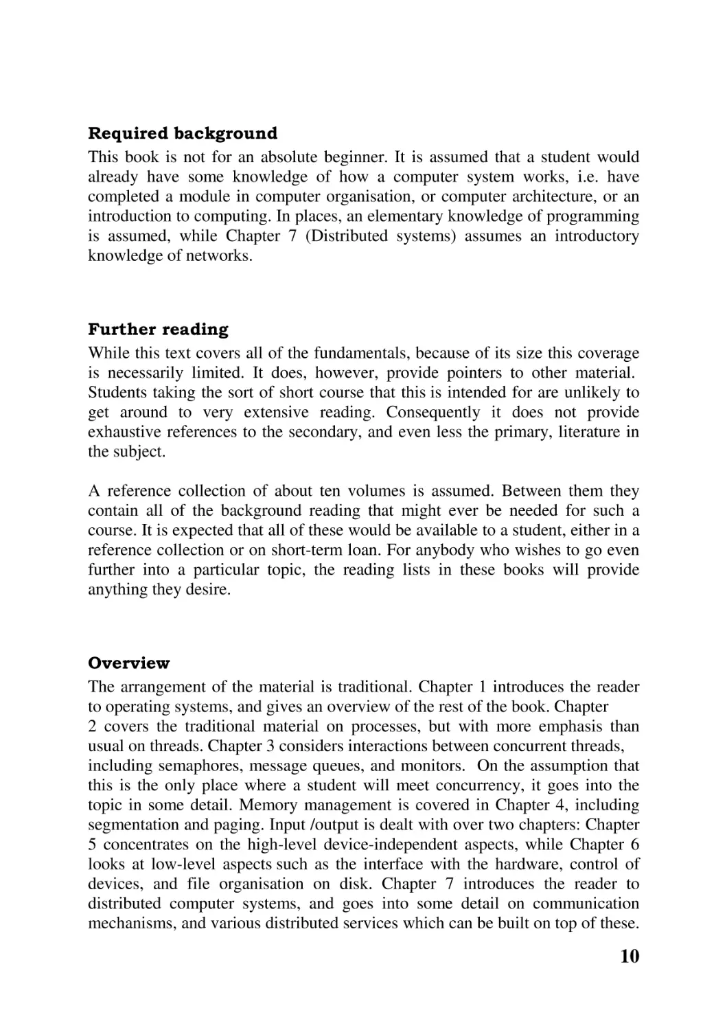
1.1 What is an operating system?
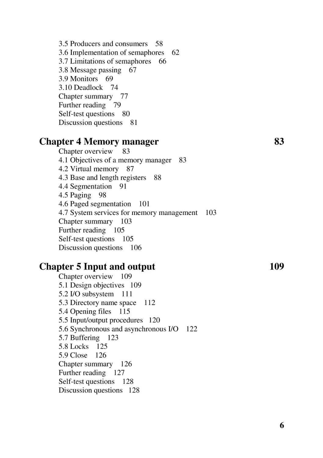
An operating system is the most fundamental piece of software running on any
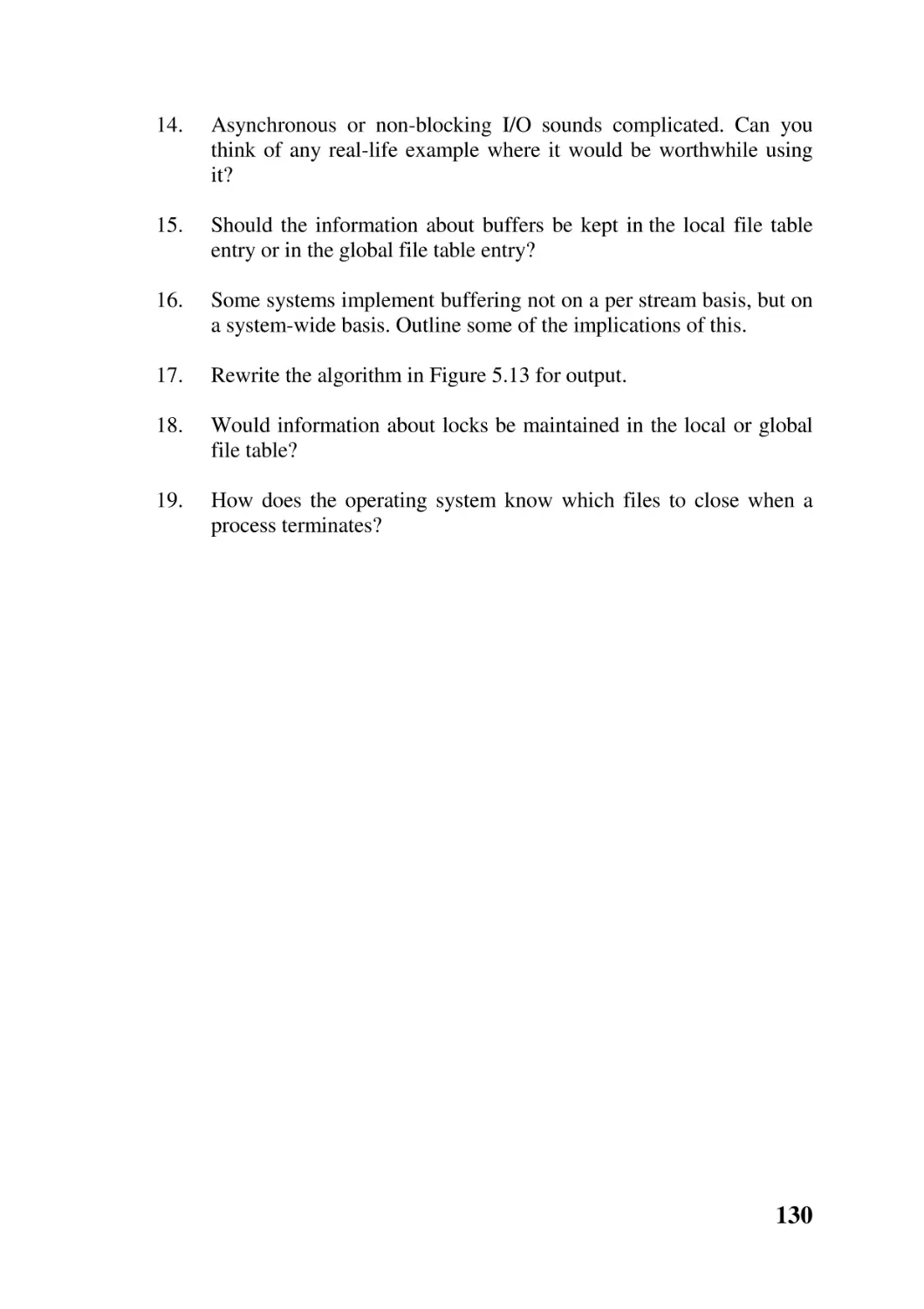
computer. Figure 1.1 shows in a very simplified way the basic components of a
computer system. But while simple, it is important for understanding just where
an operating system fits in.
Everybody has been a user. All have used a word processor, a spreadsheet,
maybe even an accounting package. These are all application programs. Figure
1.1 shows the application program interacting with the operating system.
Now the operating system is itself a program, which is written, compiled, tested
and debugged just like any other program. This program is run whenever a
computer is switched on. It is almost always done automatically – no special
command is required – so users may not be aware that it happens every time
they switch on a machine. It stays running all the time until the machine is
switched off.
12
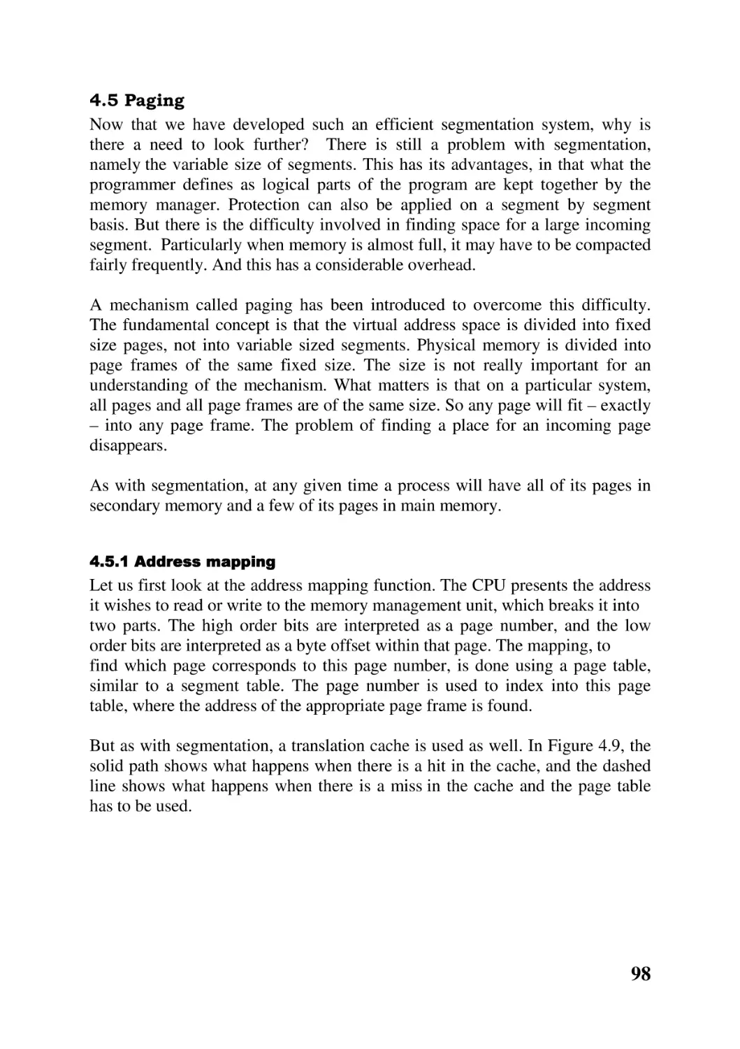
Figure 1.1 Overview of a computer system
Operating systems have been given a high profile lately. Both
OS/2 and Microsoft Windows have been advertised on prime
time television. But while the term is now in common use, not
many understand exactly what an operating system is, and
certainly not how it works.
This book sets out to remedy that lack.
But that still leaves the question: why do we need it?
A ‘raw’ machine, bare hardware, is very inhospitable. It needs programming in
its own binary machine code. Remember – we are dealing with digital
computers. Everything is represented by numbers. English text, pictures,
programs, whether in C or assembler – all are represented in the machine by
numbers in binary format. Programming at this level is definitely not userfriendly.
Very simply, operating systems were invented to take some of the pain out of
dealing with the raw hardware. This leads us on neatly to a discussion of what
they do.
1.2 What does an operating system do?
An operating system has been likened to a government. It does no productive
work itself, but provides an environment which helps others to do productive
work.
So an operating system helps a user to develop and run programs, by providing
a convenient environment. In the jargon that has come into use, it provides a
13
virtual machine in place of the real machine. It does this by supplying simple
functions that carry out the most commonly required operations, particularly in
the following areas:
• Starting and stopping programs, and sharing the CPU between them.
• Managing memory. This involves keeping track of which parts of
memory are in use and which are free. It also keeps track of which
programs the memory in use has been allocated to, and provides
mechanisms by which programs can ask for more memory or give back
memory they no longer need.
• Input and output. Operating systems cover up the differences between
alternative makes and models of devices. For example, the dozens of
different makes and models of PC all run the Windows operating system.
So all application programs run on any of them, despite the fact that no
two machines are the same. In fact, when a program will not run on a
particular machine, it is almost always because the programmer jumped
over the operating system and contacted the hardware directly.
Programmers do this sometimes to make things run faster (e.g. games),
but at the cost of compatibility.
Referring to Figure 1.1 again, the operating system can be slightly different at
the bottom, to suit different hardware, but must be strictly identical on all
machines at the top.
• Another service that operating systems provide in this area is the
techniques to overlap input and output with processing. While one
program is taking input from the keyboard, another can be writing to a
file, while a third is doing some processing. This means that the overall
efficiency of the machine is improved.
• File systems. Every computer user takes filing systems for granted.
Information is saved in a file. It can be a word processor document, a
program, a spreadsheet – the user thinks up a name for it, and it is saved
somewhere. Next time it is required, as long as the name can be
remembered, that data is there ready for use, just as it was left. All of that
work is done by the operating system.
• Protection. It is common nowadays to have many different programs
running on the one machine at the same time, whether for different users,
or for just one user. As there is only one memory, and one CPU, it is easy
14
for them to interfere with one another. The operating system sees to it that
each separate program is protected from all the others.
• Networking. The operating system covers up the differences between
machines, so that any model of computer can communicate seamlessly
with any other.
• Error handling and recovery. What can go wrong will go wrong. The
operating system must be able to detect errors, and either recover from
them or warn the user.
Finally, it is important that the operating system does all of this efficiently and
economically. Resource use by the system, in terms of CPU time, memory and
use of the disk, must be reasonable.
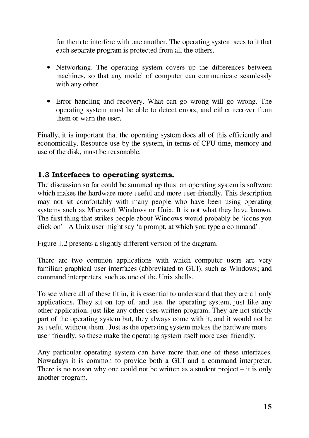
1.3 Interfaces to operating systems.
The discussion so far could be summed up thus: an operating system is software
which makes the hardware more useful and more user-friendly. This description
may not sit comfortably with many people who have been using operating
systems such as Microsoft Windows or Unix. It is not what they have known.
The first thing that strikes people about Windows would probably be ‘icons you
click on’. A Unix user might say ‘a prompt, at which you type a command’.
Figure 1.2 presents a slightly different version of the diagram.
There are two common applications with which computer users are very
familiar: graphical user interfaces (abbreviated to GUI), such as Windows; and
command interpreters, such as one of the Unix shells.
To see where all of these fit in, it is essential to understand that they are all only
applications. They sit on top of, and use, the operating system, just like any
other application, just like any other user-written program. They are not strictly
part of the operating system but, they always come with it, and it would not be
as useful without them . Just as the operating system makes the hardware more
user-friendly, so these make the operating system itself more user-friendly.
Any particular operating system can have more than one of these interfaces.
Nowadays it is common to provide both a GUI and a command interpreter.
There is no reason why one could not be written as a student project – it is only
another program.
15
Figure 1.2 Interfaces to an operating system
1.3.1 The system service interface
Note that in Figure 1.2 these user interfaces, indeed all application programs,
call system services. These are the real interface to the operating system.
‘System services’ is the name used to describe the set of functions provided by
an operating system to enable a user to request service from it.
Just like any functions you have written yourself, they are passed parameters,
they perform some operations, and return a value. The difference is that these
functions have been written by the operating system designers, and are available
in a library for your use.
Typically there would be hundreds of these functions. As well as the more
obvious ones, such as handling disks and other peripherals, there will also be
services which allow values inside the operating system itself to be queried and
set.
Compilers for high-level languages use these system services all the time. For
example, output commands like printf() are translated by the C compiler to calls
on the appropriate system service for the underlying operating system.
This book will be dealing with the lower half of Figure 1.2, with the operating
system itself, and an introduction to system services. We will not be dealing
with command interpreters, shells or GUIs.
Until very recently, each operating system had its own set of system services.
This made programs which used such system services very difficult to port to
16
another system. Consequently, attempts are currently under way to establish a
standard. The main thrust of this is POSIX – the POS standing for Portable
Operating System. This is being encouraged by the IEEE.
Note that POSIX is not an operating system – it is a standard for operating
system designers.
The POSIX interface is now available, to a greater or lesser degree, on almost
all operating systems. Unix, Windows NT, OS/2 and OpenVMS are some
examples. Because POSIX is becoming a standard, we will refer to it at
appropriate places, but we are not really dealing with system programming in
this book – the interested reader is referred to the reading list.
1.3.2 System services from the outside
The POSIX programming interface is relatively simple. System services are all
described fully in the appropriate manuals, as supplied with each operating
system. These give the order, type and meaning of each parameter, as well as
explaining what aspect of the function each parameter controls.
All system services are defined as C functions. This means that they return a
value. This return value is not just to be discarded. System programming is
different from application programming, when it can normally be seen from the
screen whether the program worked correctly or not. When a system service is
called, say to change some attribute of the operating system, or write to a disk,
there is no visible indication of whether the operation was successful or not. The
only indication is the value returned.
The specific meaning of this value in each case is defined in the
appropriate manual page. But in most cases, if the call did not
work for some reason or other, the return value is -1. If the call
did work, some other value is returned. This success value
should be checked to see that it is correct. It is not sufficient just
to check that a call did not fail. It may have succeeded, but not
done what was intended.
Normally a program should not continue after a system call fails – presumably
it was called for some purpose, which has not now been achieved. However,
the reason why it failed is probably more important.
17
Information about why a system call failed can be obtained using
the C library function perror( ).
1.3.3
1.3.3 System services from the inside
The actual C library function which the application calls does very little work. It
puts the parameters on the stack and then executes a special machine instruction
which causes the CPU to change to kernel mode.
At this stage we need a little detour into the hard ware. All
modern CPUs operate in at least two different modes. In one of
these, called user mode, the CPU can only execute a subset of its
instructions – the more common ones, like add, subtract, load
and store, etc. In the other mode, called kernel mode, the CPU
can execute all of its instructions, including extra privileged
instructions. These typically access special registers which
control protection on the machine. Normally the machine runs in
user mode. When it wants to do something special, it has to
change into kernel mode.
As well as setting the CPU into kernel mode, the C function also transfers
control to the appropriate place in the operating system. This executes the
requested service, running in kernel mode. When finished, it uses another
special machine instruction to change the mode back to user. Finally it returns
control to its caller, the application program.
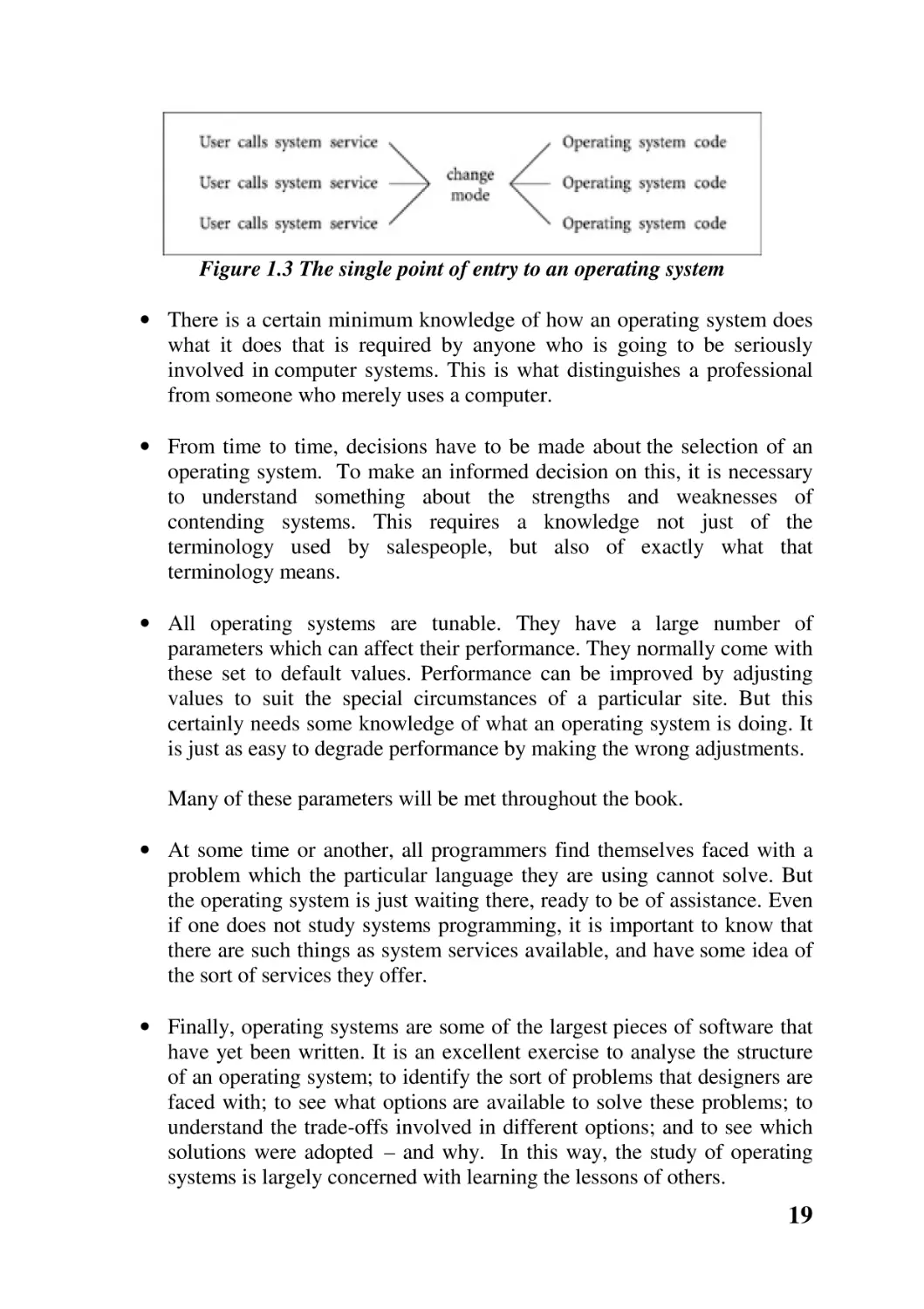
Figure 1.3 shows that no matter which system service the user calls, they all
pass through the one entry point into the operating system, and then go on to
execute the part of the operating system code specific to each.
1.4 Study of operating systems
There may be a feeling at this stage that a GUI is good enough for anything we
may want to do with computer operating systems – now that we have Windows,
there is no need for the remainder of the book. It is certainly true that most
computer users, even some computer professionals, will rarely need any more
than the facilities provided by the user interface. But there are a number of very
good reasons for going a little deeper than that into an operating system.
18
Figure 1.3 The single point of entry to an operating system
• There is a certain minimum knowledge of how an operating system does
what it does that is required by anyone who is going to be seriously
involved in computer systems. This is what distinguishes a professional
from someone who merely uses a computer.
• From time to time, decisions have to be made about the selection of an
operating system. To make an informed decision on this, it is necessary
to understand something about the strengths and weaknesses of
contending systems. This requires a knowledge not just of the
terminology used by salespeople, but also of exactly what that
terminology means.
• All operating systems are tunable. They have a large number of
parameters which can affect their performance. They normally come with
these set to default values. Performance can be improved by adjusting
values to suit the special circumstances of a particular site. But this
certainly needs some knowledge of what an operating system is doing. It
is just as easy to degrade performance by making the wrong adjustments.
Many of these parameters will be met throughout the book.
• At some time or another, all programmers find themselves faced with a
problem which the particular language they are using cannot solve. But
the operating system is just waiting there, ready to be of assistance. Even
if one does not study systems programming, it is important to know that
there are such things as system services available, and have some idea of
the sort of services they offer.
• Finally, operating systems are some of the largest pieces of software that
have yet been written. It is an excellent exercise to analyse the structure
of an operating system; to identify the sort of problems that designers are
faced with; to see what options are available to solve these problems; to
understand the trade-offs involved in different options; and to see which
solutions were adopted – and why. In this way, the study of operating
systems is largely concerned with learning the lessons of others.
19
Many of the ideas and techniques used by system designers are of general use
over the whole field of software development. So the study of operating systems
complements other courses on software design and development.
1.5 Historical development of operating systems
Operating systems did not just appear fully formed on the computer scene. As
with anything else, a knowledge of where we have come from always helps in
the understanding of where we are at.
Initially, in the late 1940s, there was only hardware. There was no operating
system. The programmer was also the user, and in many cases the designer and
builder as well. Programs and data were entered in binary by means of switches
on the front of the machine. Each switch represented one bit. Output was by
means of lights, with each light representing one bit. The programmer did
everything that an operating system does today.
The 1950s saw the introduction of specialist operators, who were not
programmers themselves, but who tended the machine, fed the programs to the
machine, and delivered back the output.
The programmers no longer interacted directly with the computer. They used
punch machines to encode their programs as a series of holes in stiff cards,
which the computer could read and interpret. The operators acted as a human
interface between the programmer and the hardware.
By the 1960s, human intervention was a serious source of delay in the system.
Loading and unloading punched cards, starting and stopping devices – all of
this slowed things down.
So instead of giving verbal commands to a human operator, the programmer
punched instructions on control cards, which were inserted at the appropriate
places before and after the program cards and the data cards. These commands
were written in specially developed job control languages. The other side of the
coin was the development of the command interface. This was a program which
read, interpreted and executed the command cards. Such command interpreters
are still with us today, in the form of the Unix or DOS shells. So here we have
the beginning of operating systems as we now know them.
In the late 1960s we had the first attempts to provide interactive use of a
computer, at a reasonable cost. The basic idea was to timeshare the computer.
As the name implies, each user gets a share of the computer’s time. But each
user’s turn comes around so fast that the system can give the impression that
20
each one has a machine of their own. The operating system, which replaced the
human operator, had to ensure that all of this worked.
In the 1970s, computer users found that programs were growing in size and
required more memory than users could afford. The initial solution was to break
programs up into little chunks, each of which would fit in the available memory
at any one time. These were then swapped in and out as required – a timeconsuming task.
Eventually operating systems came to the rescue and made memory look much
larger than it really was. This virtual memory allowed larger programs to run
at no extra financial cost, but it slowed machines down. So effectively we were
trading speed against cost.
With timesharing, and multi-user systems of all sorts, the issue of protecting
one program from another became more and more important. Once again,
operating systems took on the responsibility.
One of the significant developments of the 1980s was networking. The
hardware ability to link machines together led to demands on operating systems
to control this communication. There was a certain fusing of the fields of
operating systems and computer networks.
Networking has grown from merely connecting machines to providing shared
resources such as file systems or printers. Network operating systems were
developed to control this (Windows for Workgroups, Novell NetWare etc.). By
the end of the 1990s things had reached a stage where groups of machines acted
as one, collaborating on some task. We talk about distributed systems, and of
course they call for distributed operating systems to control this sort of
interaction.
Another feature of operating systems in the 1990s was the move to open
systems. Previously, operating systems had been developed specifically for
particular hardware platforms, e.g. MS-DOS for the PC or VMS for the VAX.
Now there is a move to build generic operating systems (e.g. Linux) which will
run on any hardware.
1.6 Types of operating system
From the overview given in the previous section, it is not surprising that many
different types of operating system have grown up over the 50 year history of
computing. This diversity is due to attempts by designers to meet particular
requirements and to write specialist systems dedicated to specific purposes.
21
The most important distinction that has arisen historically is between batch and
interactive systems. Then there is the combination of these in the generalpurpose system. Of late, network and distributed systems have become
important. There are also some very specialized systems, which we will not
study. It will suffice to mention them in passing.
1.6.1 Batch systems
Historically, these were the earliest systems developed, so we will look at them
first.
In such a system, the program, the data and the commands to manipulate the
program and data are all submitted together to the computer in the form of a
‘job’. There is little or no interaction between users and an executing program.
Obviously this is not very suitable for program development, even though it
was once used for this.
There is still a niche market for batch systems today. In any situation where the
data is all available and there is no need for interaction with a running program,
a batch system is quite adequate. One classic example of this is payroll
processing, where all of the information on hours worked, rates of pay, tax
allowances etc. is available beforehand, and the computer can be allowed to run
on its own, printing payslips. Another example is printing account statements,
such as bank or credit card statements. There is no need for any operator
interaction once the job has been started.
The advantage of a batch environment is that it can provide a wide variety of
different devices and software, which it would not be cost-effective for an
individual user to purchase.
1.6.2 Interactive
This is the most common mode of computing today, using keyboard, mouse and
screen. It is what most people think of when they say computing. For a
programmer, it is a significant improvement on batch systems, as it is now
possible to intervene directly while a program is being developed, or as it is
running.
Single user
Some systems provide interactive computing on a single-user basis. Examples
would be Windows NT and OS/2.
22
The present state of the art is a single-user machine which is multitasking. It
does more than one thing at the same time, for the one user. The motivation
behind this is to improve productivity, but it brings up the whole question of
protection. One job must not have free access to files, data, or programs
belonging to another. On the other hand, there may be times when you want to
share data between programs – so the protection has to be selective. A
significant proportion of operating system code is involved with dealing with
this.
Terminology in this area is very confusing (and confused). Different companies
and authors use the same words with different meanings, and different words to
mean the same thing. In general, we can take process to mean the same as task,
so multiprocessing is the same as multitasking. But be warned that this is not
universally true. Some authors reserve multiprocessing for computers with
more than one CPU.
Multi-user
Other systems provide interactive computing on a multi-access or Multi-user
basis. We will take that to mean simultaneous access to a computer system
through two or more terminals. Unix is an example of this.
The motivation behind this is the sharing of resources and information.
1.6.3 General purpose.
In practice, a given environment may want a bit of everything. For example, a
timesharing system may support interactive users, but also include the ability to
run programs in batch mode. So we speak of general-purpose systems.
1.6.4 Network operating systems
It is a common practice today to share resources such as printers and databases
across a network. Network operating systems handle the underlying processes
required for such sharing.
A further development in this area is the integration of NOS with the generalpurpose operating system already found on desktop workstations. Windows NT
Server is an example, and Unix can also be configured this way.
23
1.6.5 Distributed systems
This is the most recent development in operating systems, meeting the
requirements of a multi-user system in a new way. Essentially, it consists of a
group of machines acting together as one.
Thus when a user starts a program, it may actually run on the local machine.
But if that computer is heavily loaded, and the operating system knows that
another machine is idle, then the job may be transferred to that idle machine.
All this migration of data or of programs from one machine to another is totally
under the control of the distributed operating system, and the user is not aware
of it.
1.6.6 Specialist systems
Some specialized operating systems have also been developed, each with its
own particular application area. For example, a real-time operating system
would be used in situations such as chemical plants, life support systems, or flyby-wire aeroplanes. Such a system guarantees that it will respond within a fixed
time.
Specially designed operating systems would be in order when the computer
system is dedicated to processing large volumes of data, which are maintained
in an organized way. Examples would be a student record system or a library
database. The operating system must hide the organisation and structure of the
data from the user and optimise it for fast response to requests.
If there are frequent changes to the data, such as in airline seat reservation
systems or banking systems, then we speak of transaction processing systems.
1.7 Design of operating systems
An operating system is a large – very large – piece of software. To design, build
and maintain large software systems requires a high-level view of how the
system is structured and how its different components work together. So we can
start with a top-level break down of an operating system.
At this level of detail, an operating system can be decomposed into modules
which would provide the following functions:
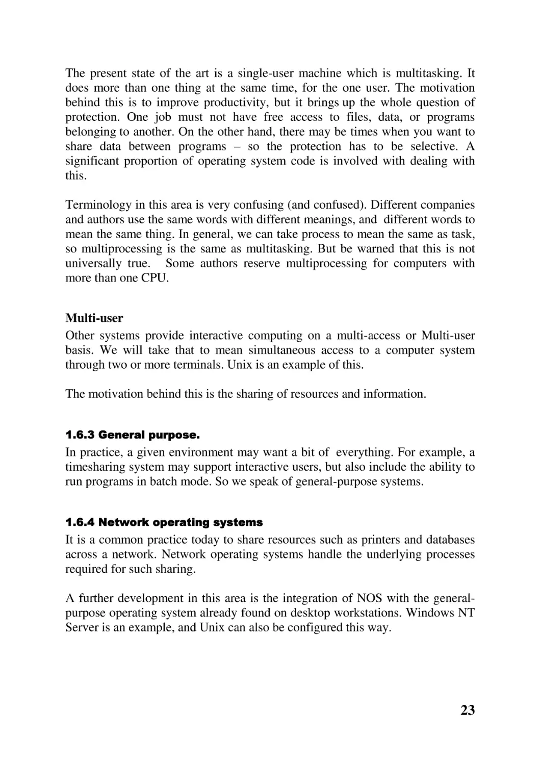
• Process management
• Memory management
• I/O management
24
• File storage, which uses I/O and adds protection and security
• Network management
Such an operating system is illustrated in Figure 1.4. Subsequent chapters will
look at each of these modules, one by one.
Figure 1.4 Modular operating system
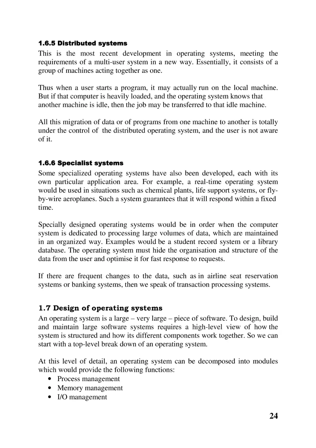
Operating systems have tended to grow larger and more complex. A relatively
new proposal is to restructure the operating system into two layers. The lower
layer is the microkernel, which provides the absolutely minimum facilities. For
example, at the hardware level, complicated setting and testing of bits in
registers may be needed to get a character to a printer. The I/O management
layer in the microkernel provides a function to do this which hides all the details
of hardware, not to mention the complication of different models of hardware.
Above this microkernel is a layer which provides optional extra services, as
well as emulating a particular system service interface. The microkernel
provides its own private interface, which is used by any emulation layer built
above it.
It could even be possible to emulate more than one system service interface at
the same time. Figure 1.5 shows a microkernel with both a POSIX interface,
and a Microsoft Win32 application programming interface layered above it.
Sometimes these are referred to as different ‘personalities’. The NT operating
system is built like this.
25
Figure 1.5 Microkernel with two personalities
CHAPTER SUMMARY
• An operating system is a program which sits between the raw hardware
and applications. It provides a user-friendly interface to applications
programmers, hiding the complexity and diversity of the hardware.
• It provides an environment which makes it easier for applications
programmers to do productive work. It:
- supplies simple functions that carry out the most commonly
required operations
- manages and shares the resources of the computer system, such as
CPU, memory, disks and printers
- hides some differences in the hardware. It does all of this as
efficiently and economically as possible.
• Most users are familiar with graphical user interfaces and command
interpreters. These are just applications which sit on top of the operating
system and make it more user-friendly. Like all applications, they in turn
make use of system services. These are the real interface to an operating
system.
• Systems services are the functions which the operating system offers to
perform on behalf of applications programs.
Internally, each system service is only a wrapper which switches the CPU
into kernel mode and calls the appropriate kernel function. Afterwards it
switches back to user mode and returns to the caller.
26
• A certain minimum knowledge of how an operating system does what it
does is required by anyone seriously involved in computer systems. A
user may be required to choose, or tune, an operating system. Many of the
techniques used by system designers are relevant in the wider field of
software development.
• The earliest computers had no operating systems, with the programmer
operating directly on the hardware. The first operating systems were
human operators.
• In the 1960s, verbal commands to operators were replaced with machinereadable commands written in job control languages. In the late 1960s,
timesharing led to operating systems taking over the scheduling of
machines.
• The 1970s was the era of virtual memory. Then in the 1980s, networking
and the GUI were the development areas. Distributed systems and open
systems were at the forefront of operating systems research in the 1990s.
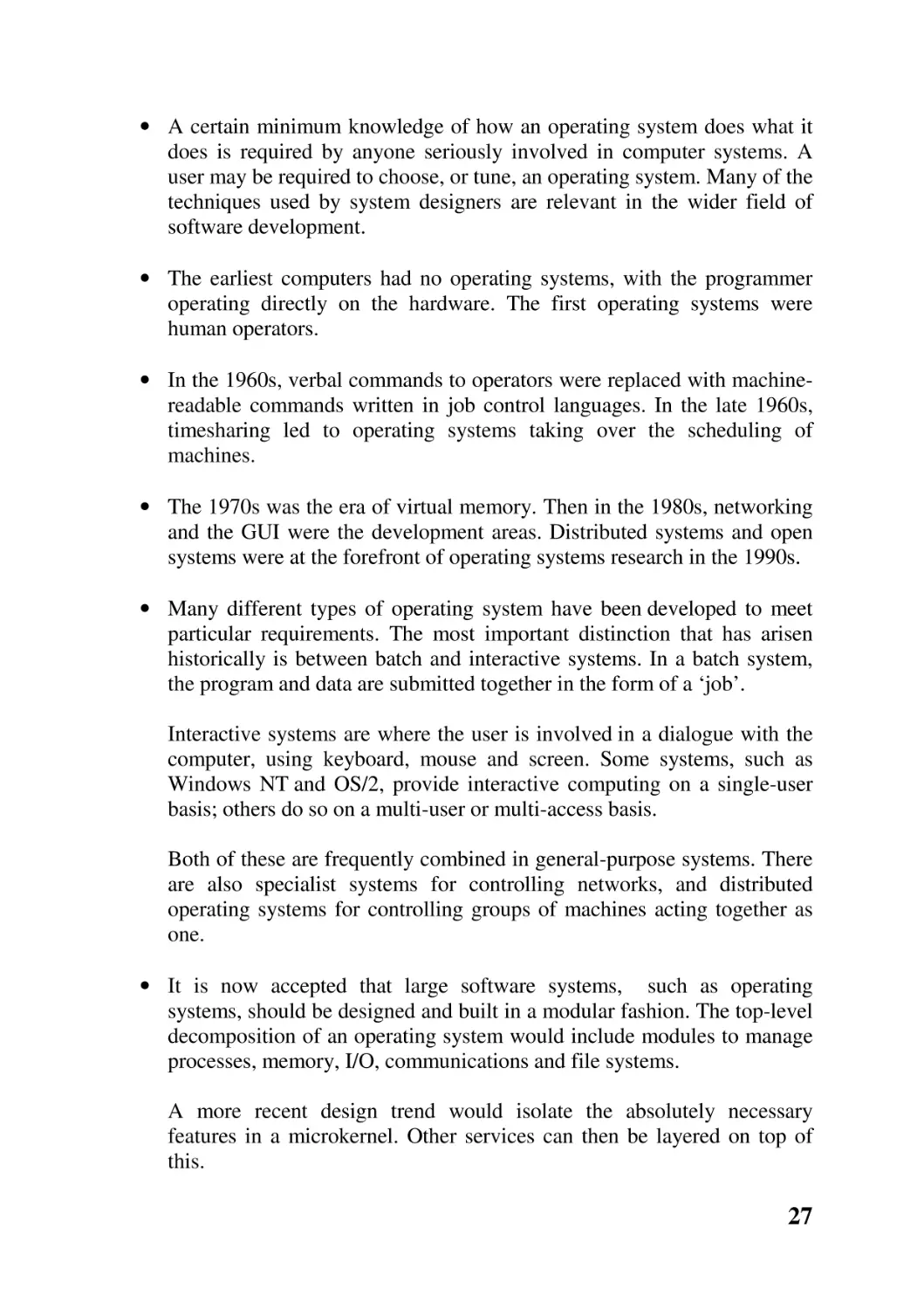
• Many different types of operating system have been developed to meet
particular requirements. The most important distinction that has arisen
historically is between batch and interactive systems. In a batch system,
the program and data are submitted together in the form of a ‘job’.
Interactive systems are where the user is involved in a dialogue with the
computer, using keyboard, mouse and screen. Some systems, such as
Windows NT and OS/2, provide interactive computing on a single-user
basis; others do so on a multi-user or multi-access basis.
Both of these are frequently combined in general-purpose systems. There
are also specialist systems for controlling networks, and distributed
operating systems for controlling groups of machines acting together as
one.
• It is now accepted that large software systems, such as operating
systems, should be designed and built in a modular fashion. The top-level
decomposition of an operating system would include modules to manage
processes, memory, I/O, communications and file systems.
A more recent design trend would isolate the absolutely necessary
features in a microkernel. Other services can then be layered on top of
this.
27
FURTHER READING
All books on operating systems cover this introductory material. For example,
Silberschatz and Galvin Chapter 1; Nutt Sections 1.1, 3.2; Tanenbaum and
Woodhull Section 1.1; Stallings Chapter 2; Tanenbaum (1992) Chapter 1. For
more on the system service interface see Silberschatz and Galvin Sections 2.6,
3.2, 3.3, 21.3; Nutt Section 3.3.3; Tanenbaum and Woodhull Sections 3.1, 3.2;
Stallings Section 1.7. The historical introduction is also covered in Tanenbaum
and Woodhull Section 1.2. Nutt Section 1.2 deals with the different types of
operating system. Material on operating system design can be found in
Silberschatz and Galvin Sections 3.1, 3.5, 3.7; Nutt Section 3.1; Tanenbaum
and Woodhull Section 1.5.
SELF-TEST QUESTIONS
1. Explain where an operating system fits into a computer system.
2. List and explain the most important functions of an operating system.
3. Explain the difference between a GUI, a command interpreter and the
system service interface to an operating system.
4. Outline how a programmer uses the POSIX interface to an operating
system.
5. How does system service code get to change the CPU to run in kernel
mode?
6. Justify why the study of operating systems is relevant to a student of
computing.
7. Outline the historical development of operating systems.
8. Distinguish the different types of operating system which have
developed.
9. Briefly describe the main modules which go to make up an operating
system.
28
DISCUSSION QUESTIONS
1. An operating system is an extra layer of software in a computer, extra
instructions to be executed, which slows an application program down.
Discuss the advantages and disadvantages of removing operating systems
altogether.
2. Many of the things an operating system does seem to be relevant to large
multi-user systems – overlapping input and output, communicating with
other machines and providing virtual memory. Is such an operating
system really needed on a single-user personal computer?
3. Is Windows NT an operating system? Or a GUI? Or both?
4. Check the manual page for the read ( ) system service. Describe all of the
checks you would have to perform on the value returned by this function
to be sure that you had covered every possibility.
5. All system services call a special machine instruction which causes the
CPU to change to kernel mode. It seems that you could write your own
assembler program, using this instruction, and hence take over the
machine yourself. Investigate the special instruction on the hardware you
are using, and find out why it is not as easy as it seems.
6. Do you find the arguments given in Section 1.4 convincing? Why? Or do
you think operating system courses should be abolished? Can you think
of any other reasons why they should be part of a computer systems
course?
7. Early computer systems got on without operating systems. What has
changed that we need them today?
8. What might be the next big breakthrough in operating systems?
9. What use is a multitasking operating system on a single-user machine?
Surely one user can only do one thing at a time?
10. Distributed systems certainly seem to have great advantages. List some
aspects which might make you slow to move from standalone systems.
11. An operating system designed with either of the methods we have
discussed would require significant rewriting if moved to a machine with
different hardware. Discuss how an operating system might be designed
to minimize this.
29
CHAPTER 2 Process manager.
CHAPTER OVERVIEW
In the previous chapter, the modules which go to make up an operating system
were identified. This chapter aims to introduce you to the first of these, the
process manager.
After reading this chapter, you should:
• be familiar with both the static and dynamic aspects of a process
• understand the relationship between processes and processors
• be familiar with the concept of multiple threads of control in a process
• understand how processes and threads are represented within an operating
system
• understand how processes and threads are created and terminated
• be familiar with the life cycle of a thread
• understand the mechanics of context switching, and of scheduling
2.1 The concept of a process
A process is the unit of work in a computer system. There are two aspects to
any process, a static part and a dynamic part.
The static part, which we will refer to as a task, involves the resources allocated
to the process. This includes a certain amount of space in memory, a current
working directory, sources of input and output such as a keyboard, screen and
open files, and maybe a connection with another process over a network. The
most important resource which any process has, though, is a program. A
program is a sequence of instructions. On its own, a program does nothing. It is
inert.
The dynamic part of a process can be described as ‘a program in action’. When
the instructions that make up a program are actually being carried out, the CPU
30
works its way through the program in a particular pattern. A program typically
involves branches and loops, so this pattern may be the same each time the
program is run, or it may be different. This dynamic part of a process is known
as a ‘thread of execution’, or a ‘thread of control’, or just a thread. A thread has
access to all of the resources assigned to the task.
There is some similarity between an operating system process,
and baking a cake. The task corresponds to the ingredients
(resources), including the recipe (program). The thread is the
actual sequence of operations carried out, as directed by the
recipe, for example mixing, baking, and maybe even eating. The
process is the whole job of work, which we might describe as
‘make a cake’.
A very formal definition of a process would be ‘a sequence of states, resulting
from the action of a set of instructions on the states as they develop’. At first
sight this does not seem to be the same thing. It seems to be a purely static
concept, with no dynamic aspect at all. So it is necessary to explain what is
meant by a computational state in this context. It is like a photograph of the
internals of the computer, taken at a particular instant. It includes the values of
the CPU registers, the values in each byte of memory and the values in each of
the special registers associated with hardware devices.
At any given time, the computer is in a particular state. Then an instruction is
executed. This changes at least one value somewhere in the machine, and moves
it to a (very slightly) different state.
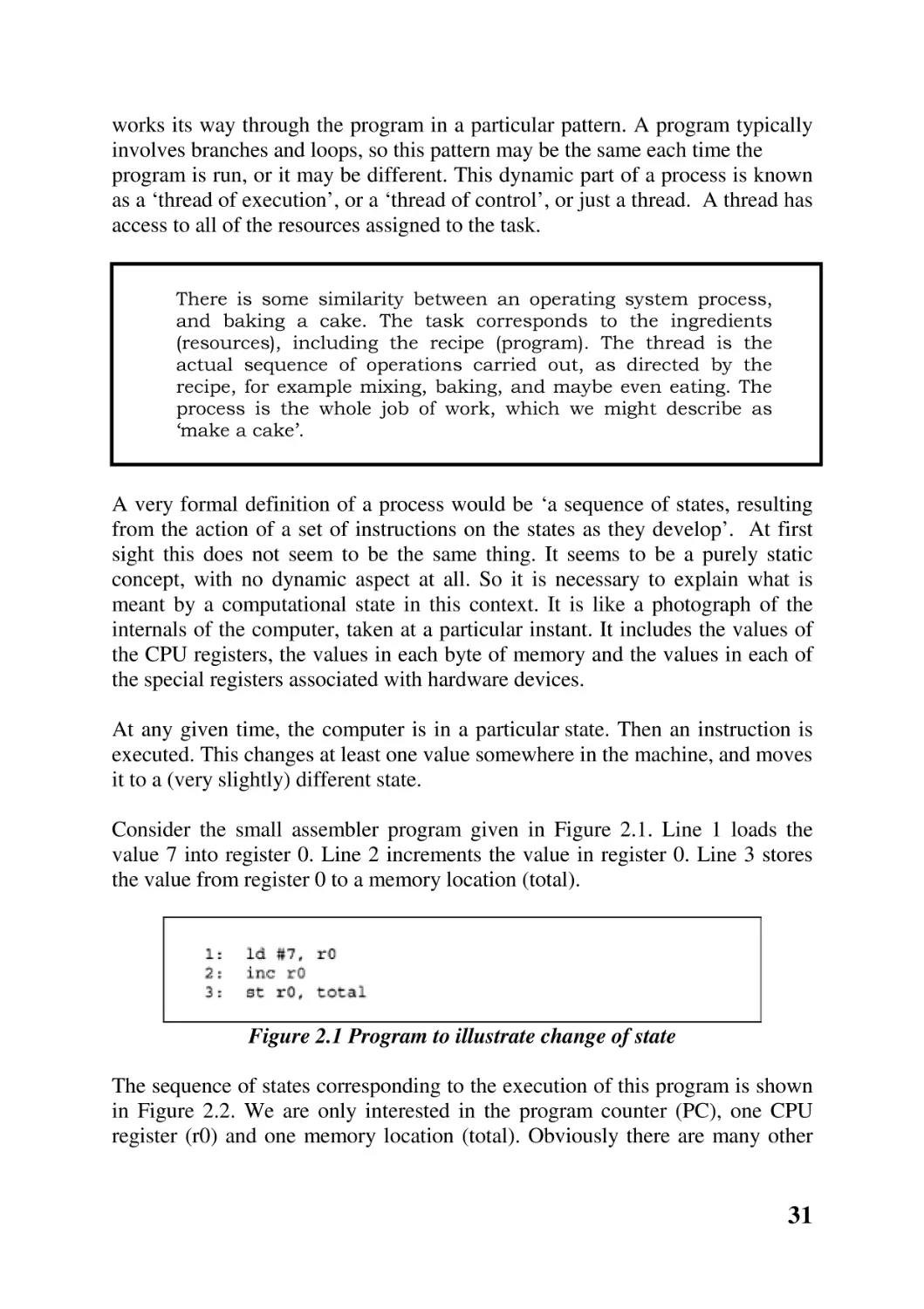
Consider the small assembler program given in Figure 2.1. Line 1 loads the
value 7 into register 0. Line 2 increments the value in register 0. Line 3 stores
the value from register 0 to a memory location (total).
Figure 2.1 Program to illustrate change of state
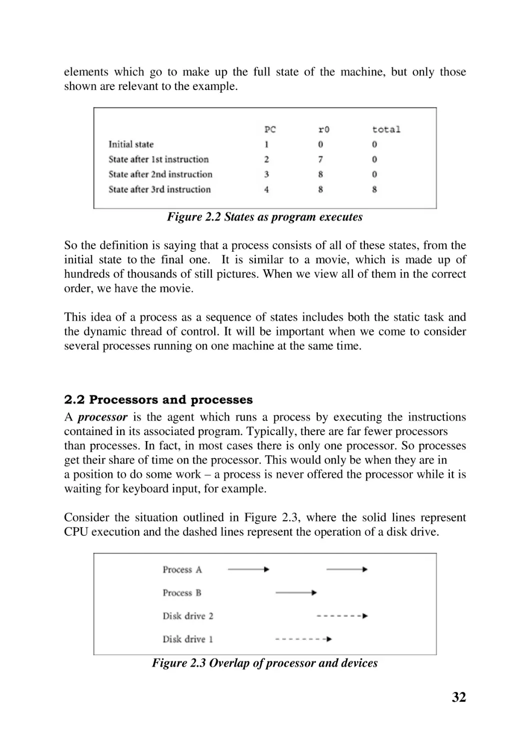
The sequence of states corresponding to the execution of this program is shown
in Figure 2.2. We are only interested in the program counter (PC), one CPU
register (r0) and one memory location (total). Obviously there are many other
31
elements which go to make up the full state of the machine, but only those
shown are relevant to the example.
Figure 2.2 States as program executes
So the definition is saying that a process consists of all of these states, from the
initial state to the final one. It is similar to a movie, which is made up of
hundreds of thousands of still pictures. When we view all of them in the correct
order, we have the movie.
This idea of a process as a sequence of states includes both the static task and
the dynamic thread of control. It will be important when we come to consider
several processes running on one machine at the same time.
2.2 Processors and processes
A processor is the agent which runs a process by executing the instructions
contained in its associated program. Typically, there are far fewer processors
than processes. In fact, in most cases there is only one processor. So processes
get their share of time on the processor. This would only be when they are in
a position to do some work – a process is never offered the processor while it is
waiting for keyboard input, for example.
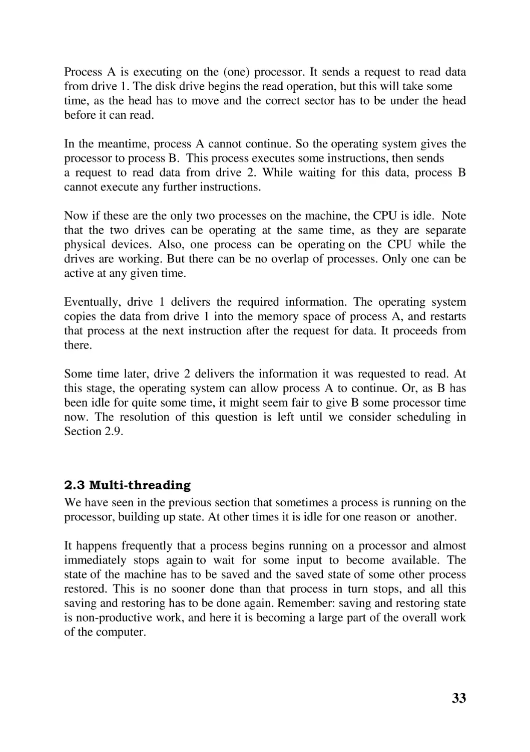
Consider the situation outlined in Figure 2.3, where the solid lines represent
CPU execution and the dashed lines represent the operation of a disk drive.
Figure 2.3 Overlap of processor and devices
32
Process A is executing on the (one) processor. It sends a request to read data
from drive 1. The disk drive begins the read operation, but this will take some
time, as the head has to move and the correct sector has to be under the head
before it can read.
In the meantime, process A cannot continue. So the operating system gives the
processor to process B. This process executes some instructions, then sends
a request to read data from drive 2. While waiting for this data, process B
cannot execute any further instructions.
Now if these are the only two processes on the machine, the CPU is idle. Note
that the two drives can be operating at the same time, as they are separate
physical devices. Also, one process can be operating on the CPU while the
drives are working. But there can be no overlap of processes. Only one can be
active at any given time.
Eventually, drive 1 delivers the required information. The operating system
copies the data from drive 1 into the memory space of process A, and restarts
that process at the next instruction after the request for data. It proceeds from
there.
Some time later, drive 2 delivers the information it was requested to read. At
this stage, the operating system can allow process A to continue. Or, as B has
been idle for quite some time, it might seem fair to give B some processor time
now. The resolution of this question is left until we consider scheduling in
Section 2.9.
2.3 Multi-threading
We have seen in the previous section that sometimes a process is running on the
processor, building up state. At other times it is idle for one reason or another.
It happens frequently that a process begins running on a processor and almost
immediately stops again to wait for some input to become available. The
state of the machine has to be saved and the saved state of some other process
restored. This is no sooner done than that process in turn stops, and all this
saving and restoring has to be done again. Remember: saving and restoring state
is non-productive work, and here it is becoming a large part of the overall work
of the computer.
33
The overhead involved in moving from running to idle, or vice
versa, can be considerable. The operating system has to save
the whole state of the machine as it was at the moment when the
process stopped running. There is a similar overhead involved
when a process begins running again. All of the saved state has
to be restored and the machine set up exactly as it was when the
process last ran. And this overhead is on the increase as the
number and size of CPU registers grows and as operating system
s become more complex, so requiring ever more state to be
remembered.
This has led to the idea of having a number of paths of execution (threads)
through the program at the same time. With such an arrangement, if one thread
is blocked another can execute. It is not necessary to save and restore the full
state of the machine for this, as it is using the same memory, files and devices –
it is just jumping to another location in the program code. But each thread must
maintain some state information of its own, for example the program counter,
stack pointer and general-purpose registers. This is so that when it regains
control it may continue from the point it was at before it lost control.
So now a task can be viewed as an environment in which one or more threads
can execute. A standard process consists of a task with a single thread; but
processes may have more than one thread.
The example we used earlier, of baking a cake, can be extended
to baking several cakes. We still have only one process. There is
one task, or set of resources, though there may be more of them.
There is only one recipe. But while one cake is in the oven, we
may be mixing the ingredients for another. We are following the
recipe at two different places at the same time. Instead of idly
waiting for the first cake to be baked, we are using that time
productively.
2.3.1 Example
A file server is a good example of the usefulness of multi-threading. If there is
only one thread, then it can only handle one request at a time. As it will spend
quite a proportion of its time waiting for the disk drive, the total amount of work
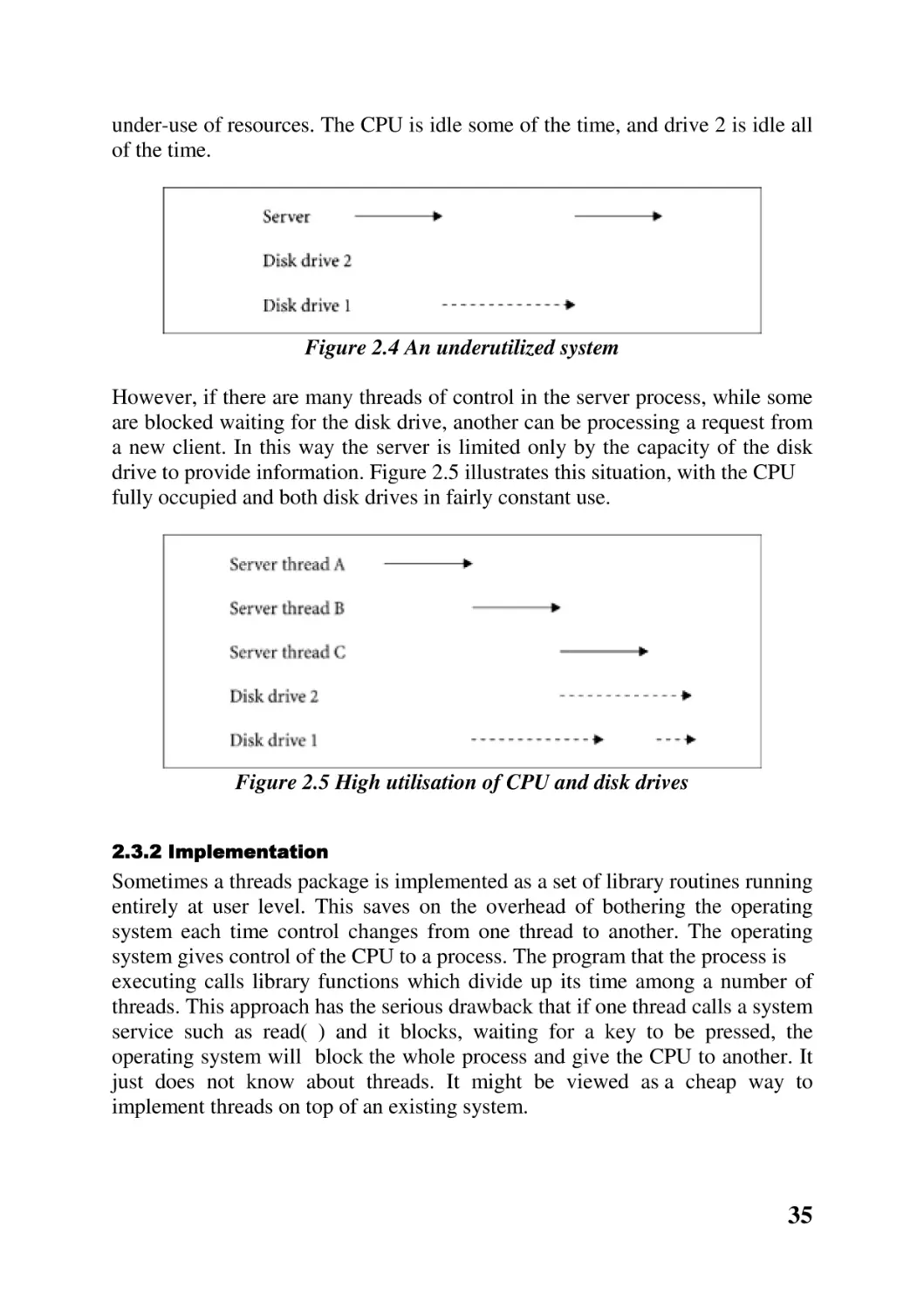
it does for its clients will be nothing near its capacity. Figure 2.4 illustrates this
34
under-use of resources. The CPU is idle some of the time, and drive 2 is idle all
of the time.
Figure 2.4 An underutilized system
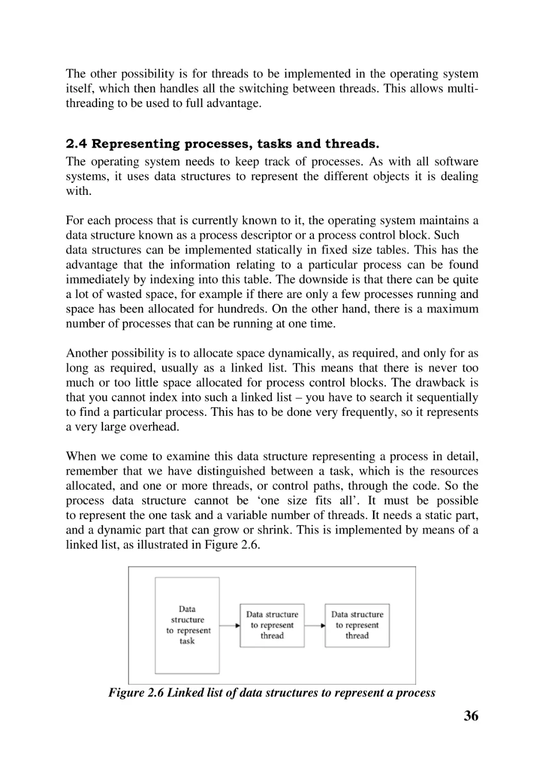
However, if there are many threads of control in the server process, while some
are blocked waiting for the disk drive, another can be processing a request from
a new client. In this way the server is limited only by the capacity of the disk
drive to provide information. Figure 2.5 illustrates this situation, with the CPU
fully occupied and both disk drives in fairly constant use.
Figure 2.5 High utilisation of CPU and disk drives
2.3.2 Implementation
Sometimes a threads package is implemented as a set of library routines running
entirely at user level. This saves on the overhead of bothering the operating
system each time control changes from one thread to another. The operating
system gives control of the CPU to a process. The program that the process is
executing calls library functions which divide up its time among a number of
threads. This approach has the serious drawback that if one thread calls a system
service such as read( ) and it blocks, waiting for a key to be pressed, the
operating system will block the whole process and give the CPU to another. It
just does not know about threads. It might be viewed as a cheap way to
implement threads on top of an existing system.
35
The other possibility is for threads to be implemented in the operating system
itself, which then handles all the switching between threads. This allows multithreading to be used to full advantage.
2.4 Representing processes, tasks and threads.
The operating system needs to keep track of processes. As with all software
systems, it uses data structures to represent the different objects it is dealing
with.
For each process that is currently known to it, the operating system maintains a
data structure known as a process descriptor or a process control block. Such
data structures can be implemented statically in fixed size tables. This has the
advantage that the information relating to a particular process can be found
immediately by indexing into this table. The downside is that there can be quite
a lot of wasted space, for example if there are only a few processes running and
space has been allocated for hundreds. On the other hand, there is a maximum
number of processes that can be running at one time.
Another possibility is to allocate space dynamically, as required, and only for as
long as required, usually as a linked list. This means that there is never too
much or too little space allocated for process control blocks. The drawback is
that you cannot index into such a linked list – you have to search it sequentially
to find a particular process. This has to be done very frequently, so it represents
a very large overhead.
When we come to examine this data structure representing a process in detail,
remember that we have distinguished between a task, which is the resources
allocated, and one or more threads, or control paths, through the code. So the
process data structure cannot be ‘one size fits all’. It must be possible
to represent the one task and a variable number of threads. It needs a static part,
and a dynamic part that can grow or shrink. This is implemented by means of a
linked list, as illustrated in Figure 2.6.
Figure 2.6 Linked list of data structures to represent a process
36
2.4.1 Task
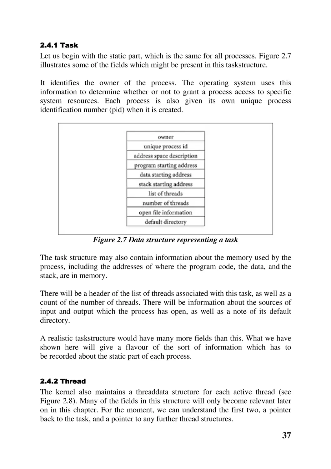
Let us begin with the static part, which is the same for all processes. Figure 2.7
illustrates some of the fields which might be present in this taskstructure.
It identifies the owner of the process. The operating system uses this
information to determine whether or not to grant a process access to specific
system resources. Each process is also given its own unique process
identification number (pid) when it is created.
Figure 2.7 Data structure representing a task
The task structure may also contain information about the memory used by the
process, including the addresses of where the program code, the data, and the
stack, are in memory.
There will be a header of the list of threads associated with this task, as well as a
count of the number of threads. There will be information about the sources of
input and output which the process has open, as well as a note of its default
directory.
A realistic taskstructure would have many more fields than this. What we have
shown here will give a flavour of the sort of information which has to
be recorded about the static part of each process.
2.4.2 Thread
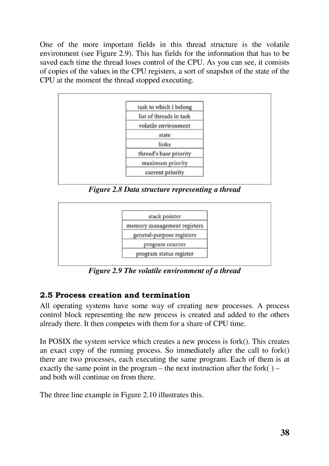
The kernel also maintains a threaddata structure for each active thread (see
Figure 2.8). Many of the fields in this structure will only become relevant later
on in this chapter. For the moment, we can understand the first two, a pointer
back to the task, and a pointer to any further thread structures.
37
One of the more important fields in this thread structure is the volatile
environment (see Figure 2.9). This has fields for the information that has to be
saved each time the thread loses control of the CPU. As you can see, it consists
of copies of the values in the CPU registers, a sort of snapshot of the state of the
CPU at the moment the thread stopped executing.
Figure 2.8 Data structure representing a thread
Figure 2.9 The volatile environment of a thread
2.5 Process creation and termination
All operating systems have some way of creating new processes. A process
control block representing the new process is created and added to the others
already there. It then competes with them for a share of CPU time.
In POSIX the system service which creates a new process is fork(). This creates
an exact copy of the running process. So immediately after the call to fork()
there are two processes, each executing the same program. Each of them is at
exactly the same point in the program – the next instruction after the fork( ) –
and both will continue on from there.
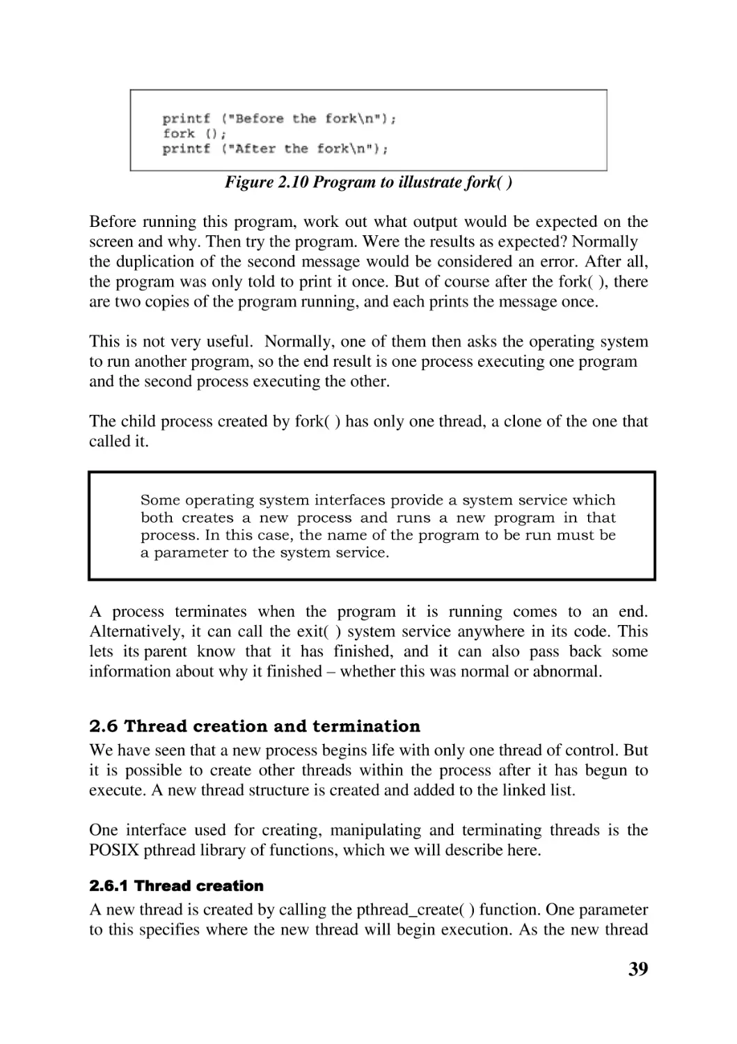
The three line example in Figure 2.10 illustrates this.
38
Figure 2.10 Program to illustrate fork( )
Before running this program, work out what output would be expected on the
screen and why. Then try the program. Were the results as expected? Normally
the duplication of the second message would be considered an error. After all,
the program was only told to print it once. But of course after the fork( ), there
are two copies of the program running, and each prints the message once.
This is not very useful. Normally, one of them then asks the operating system
to run another program, so the end result is one process executing one program
and the second process executing the other.
The child process created by fork( ) has only one thread, a clone of the one that
called it.
Some operating system interfaces provide a system service which
both creates a new process and runs a new program in that
process. In this case, the name of the program to be run must be
a parameter to the system service.
A process terminates when the program it is running comes to an end.
Alternatively, it can call the exit( ) system service anywhere in its code. This
lets its parent know that it has finished, and it can also pass back some
information about why it finished – whether this was normal or abnormal.
2.6 Thread creation and termination
We have seen that a new process begins life with only one thread of control. But
it is possible to create other threads within the process after it has begun to
execute. A new thread structure is created and added to the linked list.
One interface used for creating, manipulating and terminating threads is the
POSIX pthread library of functions, which we will describe here.
2.6.1 Thread creation
A new thread is created by calling the pthread_create( ) function. One parameter
to this specifies where the new thread will begin execution. As the new thread
39
belongs to the same process, it must execute code from within the same
program. But it cannot start just anywhere. Each thread starts at the beginning
of some function, known as its start routine.
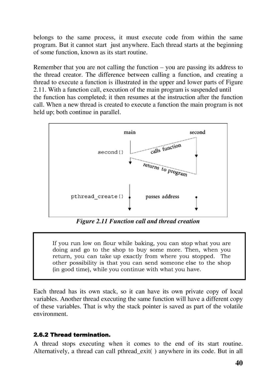
Remember that you are not calling the function – you are passing its address to
the thread creator. The difference between calling a function, and creating a
thread to execute a function is illustrated in the upper and lower parts of Figure
2.11. With a function call, execution of the main program is suspended until
the function has completed; it then resumes at the instruction after the function
call. When a new thread is created to execute a function the main program is not
held up; both continue in parallel.
Figure 2.11 Function call and thread creation
If you run low on flour while baking, you can stop what you are
doing and go to the shop to buy some more. Then, when you
return, you can take up exactly from where you stopped. The
other possibility is that you can send someone else to the shop
(in good time), while you continue with what you have.
Each thread has its own stack, so it can have its own private copy of local
variables. Another thread executing the same function will have a different copy
of these variables. That is why the stack pointer is saved as part of the volatile
environment.
2.6.2 Thread termination.
A thread stops executing when it comes to the end of its start routine.
Alternatively, a thread can call pthread_exit( ) anywhere in its code. But in all
40
cases the data structure representing the thread remains in the system. It is
finally removed when some other thread calls pthread_detach( ) .
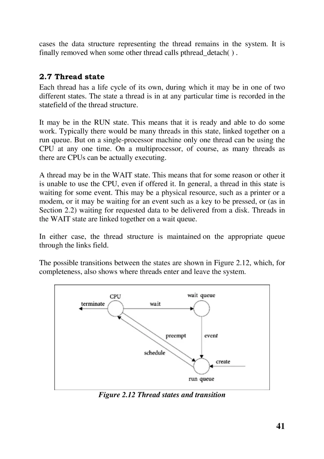
2.7 Thread state
Each thread has a life cycle of its own, during which it may be in one of two
different states. The state a thread is in at any particular time is recorded in the
statefield of the thread structure.
It may be in the RUN state. This means that it is ready and able to do some
work. Typically there would be many threads in this state, linked together on a
run queue. But on a single-processor machine only one thread can be using the
CPU at any one time. On a multiprocessor, of course, as many threads as
there are CPUs can be actually executing.
A thread may be in the WAIT state. This means that for some reason or other it
is unable to use the CPU, even if offered it. In general, a thread in this state is
waiting for some event. This may be a physical resource, such as a printer or a
modem, or it may be waiting for an event such as a key to be pressed, or (as in
Section 2.2) waiting for requested data to be delivered from a disk. Threads in
the WAIT state are linked together on a wait queue.
In either case, the thread structure is maintained on the appropriate queue
through the links field.
The possible transitions between the states are shown in Figure 2.12, which, for
completeness, also shows where threads enter and leave the system.
Figure 2.12 Thread states and transition
41
When a new thread is created, it always begins in the RUN state on the run
queue. Eventually it will be given a time slice on the CPU. When this transition
takes place is the responsibility of the scheduler.
A thread may stop using the CPU for three reasons. It may do so voluntarily,
while it is waiting for a resource, in which case it moves to the WAIT state. It
may decide to terminate itself or the whole process. Or the operating system
may take the processor from it, even though it has further instructions to
execute. This is called preemption. The operating system does this when a
thread has used up its share of time, or when the CPU is needed to handle some
more urgent work. In either case, when a thread is preempted it moves back to
the run queue.
A thread leaves the WAIT state when the event it is waiting for occurs. The
only way it can move is to the RUN state, where it will take its turn and
eventually move back to the CPU.
2.8 Context switching
This is the name given to the whole procedure of reallocating a processor from
one thread to another. As we have seen in the last section, apart from
terminating, a thread loses control of the processor for one of two reasons.
Either it moves into the WAIT state to wait for a resource to become available,
or a timer interrupts to tell it that it has used up its time slice. In both cases the
context switcher is called.
It is absolutely essential that the current state of the machine be saved when a
thread loses control of the CPU. This state includes the values in the generalpurpose registers, stack pointer, memory management registers, and most
especially the processor status register and the program counter. When, at some
time in the future, the thread now being switched out becomes eligible to run
again, it will then be possible to set up the machine exactly as it was after the
last instruction was executed. So the next instruction will operate on the correct
state, and the thread (sequence of states) will continue properly.
This state, or volatile environment as it is sometimes called, is saved in the
thread structure of its own thread. Presumably the state of the new thread to be
run is available in its thread structure. It was saved there when it was contextswitched out some time previously. This state is now copied from the volatile
environment field to the appropriate registers.
42
The order in which the various items of information are copied
from the thread structure to the registers is not important,
except that it is essential that the value of the PC be the last item
moved. Remember that there must be some program giving
instructions for all of this moving. It is in fact the context
switcher. While it is running, the PC is pointing to context
switcher code. If the PC were the first register restored, then the
next instruction would not be taken from context switcher code,
but from wherever the PC is now pointing – into the middle of the
new program. So that program would be started up without all of
its state. This would lead to chaos.
The sequence of operations involved in context switching is shown in Figure
2.13, with time running down the page.
Figure 2.13 Context switching
2.9 Scheduling
The previous section examined how a thread is given a chance to run on a
processor. Scheduling determines which thread will be next.
The main objective of the scheduler is to see that the CPU is shared among all
contending threads as fairly as possible. But fairness can mean different things
in different situations. In an interactive system, the scheduler tries to make the
response time as short as possible. A typical target would be 50–150 ms. Users
can find it quite off-putting if the response time varies wildly, say from 10–1000
ms. If one keystroke is echoed immediately, and the next is not echoed for a
second, a user is inclined to press the key again, with all the consequent errors.
43
A batch system will not be concerned with response time but with maximising
the use of expensive peripherals. Many different scheduling algorithms have
been developed for such systems.
In real-time systems, the scheduler will have to be able to guarantee that
response time will never exceed a certain maximum. For example, a multimedia
system handling video and audio must have access to the processor at
predefined intervals.
One very simple scheduling arrangement would be static fixed
ordering. This would be suitable in a process control situation.
The function and duration of all threads would be known in
advance at design time. So a decision can be made once and for
all on who goes next.
For example, a thread controlling a sensor may be run, followed
by a thread which does some calculations on the input data,
followed by a thread which controls a valve. Then the sensor
thread runs again.
2.9.1 Priority
In an interactive system there is no way to predict in advance how many threads
will be running, or how long they will want to run for. They could be scheduled
on a first come, first served basis. But this way some unimportant threads could
monopolize the system, while urgent threads languish on a queue.
So a common practice is to order all of the runnable or ready threads by some
priority criterion. There could be any number of priorities, typically 8, 16 or 32.
The simplest way to think about it is that this priority is allocated to the thread
when it is created. The descriptors of all runnable threads are linked into the run
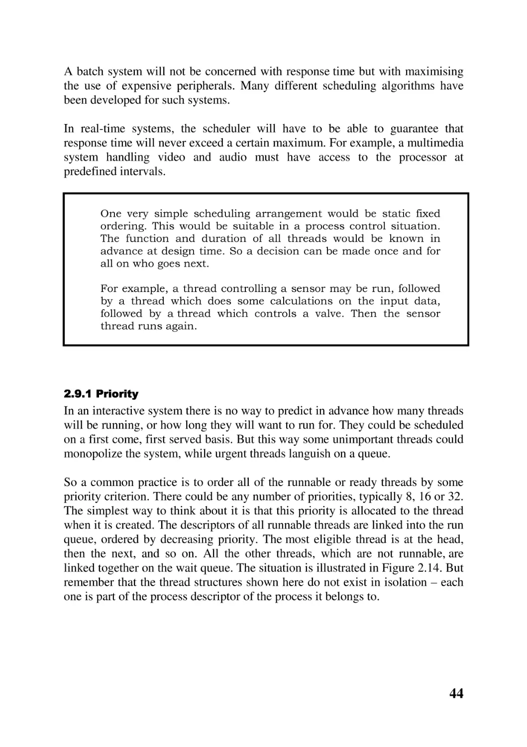
queue, ordered by decreasing priority. The most eligible thread is at the head,
then the next, and so on. All the other threads, which are not runnable, are
linked together on the wait queue. The situation is illustrated in Figure 2.14. But
remember that the thread structures shown here do not exist in isolation – each
one is part of the process descriptor of the process it belongs to.
44
Figure 2.14 Threads on the ready and wait queues
Modern CPUs tend to have a special privileged register which
points to the data structure representing the current running
thread.
Each thread gets a certain time slice on the processor. This is called the
quantum. Each time the hardware timer interrupts, the scheduler decrements the
quantum. When it gets to zero, it is time to context switch. If a thread is still
runnable when its time is up, the context switcher moves it to the appropriate
position in the queue, depending on its priority.
Most systems now use separate queues for each priority. The
thread at the head of the highest priority non-empty queue will
always be the next to run. When a thread is preempted, it is
moved to the tail of its queue. This is known as round robin
scheduling.
2.9.2 Multilevel priority queues
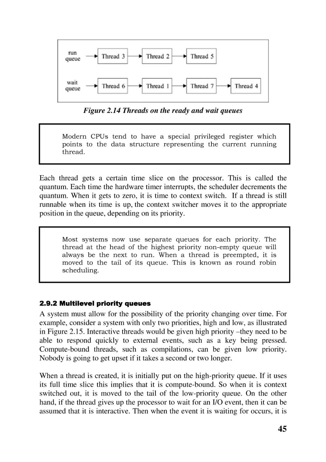
A system must allow for the possibility of the priority changing over time. For
example, consider a system with only two priorities, high and low, as illustrated
in Figure 2.15. Interactive threads would be given high priority –they need to be
able to respond quickly to external events, such as a key being pressed.
Compute-bound threads, such as compilations, can be given low priority.
Nobody is going to get upset if it takes a second or two longer.
When a thread is created, it is initially put on the high-priority queue. If it uses
its full time slice this implies that it is compute-bound. So when it is context
switched out, it is moved to the tail of the low-priority queue. On the other
hand, if the thread gives up the processor to wait for an I/O event, then it can be
assumed that it is interactive. Then when the event it is waiting for occurs, it is
45
moved from the wait queue to the high-priority queue. Threads on this queue
are always offered the processor before the low-priority queue, but are expected
to keep it for a shorter time.
Figure 2.15 Two different priority queues
The situation described can be generalized to any number of priorities, with a
thread migrating between them. Typically, different queues would have
different time slices. I/O bound threads would have high priority, and hence
receive rapid service. But they would have short time slices, because it is
unlikely that they will do much processing before giving up the processor and
waiting for more I/O.
On the other hand, CPU-bound threads have lower priorities; hence they have to
wait longer between turns on the CPU. But they would have longer time slices,
so when they do get the processor they can make significant use of it.
The information needed to manage this is kept in the thread structure. The base
priority and maximum priority are decided when it is created. This would
probably depend on the importance of the owner of the process. The final field
in the thread structure of Figure 2.8 always contains the current priority of the
thread.
CHAPTER SUMMARY
• A process is the unit of work in a computer system. It consists of a task,
or set of system resources, such as a program and memory space, and a
thread, or control path through the program.
• As there is normally only one processor, it is shared among all processes.
• It is becoming common to allow more than one control path, or thread,
through the one program. This reduces the non-productive overhead
involved in frequently saving and restoring the state of the machine.
46
• The system keeps track of each process by means of a data structure
called a process descriptor. In practice this can be a collection of
structures, each representing one aspect of the process.
• In POSIX, new processes are created as almost exact clones of their
parents. The main differences are that they have an identification number
of their own, and have only one thread. When a process terminates, it can
send status information back to its parent.
• Further threads can then be created to run within that process.
• At any given time, a thread will either be runnable or waiting.
• When a processor is being reallocated from one thread to another, it is
necessary to save the current state of the machine and restore the
previously saved state.
• The decision as to which thread to run next is known as scheduling. This
could be on a first come, first served, run to completion basis. More
commonly, a variation of this is used, where each thread gets a maximum
amount of time, the quantum. If it does not finish within the quantum, it
is context switched out and put at the back of the queue.
Even more typically, priority schemes are used, with a different queue of
ready threads for each priority. The priority of a thread can be
dynamically adjusted to reflect its historical use of the CPU.
FURTHER READING.
General background on process management can be found in Silberschatz and
Galvin Section 4.1; Nutt Chapter 6; Tanenbaum and Woodhull Section 2.1;
Stallings Chapter 3; Tanenbaum (1992) Section 2.1. For more on process
creation see Silberschatz and Galvin Section 4.3. Rago Chapter 2 is a very good
introduction to POSIX system programming; Robbins and Robbins Appendix
A, and Gray Chapter 1 also cover the same material, and Gray introduces
manual pages in Appendix A. The fork()system call is described in Robbins and
Robbins Chapter 2; Grey Chapter 3; Stevens Chapter 8. For more information
on threads see Silberschatz and Galvin Section 4.5; Tanenbaum (1992) Section
12.1. For threads programming see Robbins and Robbins Chapter 9. Scheduling
is dealt with in Silberschatz and Galvin Section 4.2 and Chapter 5; Nutt Chapter
7; Tanenbaum and Woodhull Section 2.4; Stallings Chapter 8; Tanenbaum
(1992) Section 2.4.
47
SELF-TEST QUESTIONS
1. Distinguish between the static part of a process (the task) and the
dynamic part (the thread).
2. How can more than one thread be executing at the same time on a
machine with only one CPU?
3. What is the motivation behind introducing multiple threads of control in
the one process?
4. Outline the fields in the data structures used to represent a process, a task
and a thread within an operating system.
5. Explain how the POSIX fork( ) function creates a new process.
6. Explain the difference between calling a function and creating a new
thread to execute that function.
7. Outline the life cycle of a thread.
8. Explain how context switching works.
9. Describe the different objectives of a scheduler in interactive, batch and
real-time systems.
10. Explain what is meant by priority scheduling.
11. Explain how multilevel priority feedback queues work.
DISCUSSION QUESTIONS
1. Figure 2.3 is an oversimplification.
representing the operating system itself.
Redraw it to include a row
2. When a process moves from running to idle, the state of the machine has
to be saved. Obviously this cannot mean the whole state, as there would
be no place to save it. Does the task have to be saved? Would it be
sufficient just to save information about the thread?
3. One way of implementing a multi-threaded server would be to have a
boss thread, which gives out jobs to a number of worker threads. Discuss
the trade-offs involved in having a fixed number of these, as opposed to
creating a new one for each job and terminating it when finished.
48
4. Process descriptors could be kept on hash queues. How would this
compare for efficiency with static tables and linked lists?
5. The information about open files is kept in the task structure. What would
be the effect of putting this in the thread structure instead?
6. Some operating systems create a new process as a clone of the existing
one; others create a new process with a new program. Discuss the
advantages and disadvantages of both systems.
7. What would happen if the fork( ) system call were inside a loop?
8. Investigate the wait( ) and exit( ) system services. What happens if a child
calls exit( ), but the parent never calls wait ( ) ?
9. Investigate the getpid( ) and getppid( ) system services. Why do you think
there is no system service which returns the id of a child process?
10. Investigate the different versions of the exec( ) system service, and
distinguish between them.
11. The perror ( ) library function should never be used with thread functions.
Why not?
12. What is the difference between a function recursively calling itself and a
function creating a new thread to run another copy of itself?
13. Investigate how to pass parameters to a thread when creating it.
14. List all the possible combinations of terminating and detaching which
result in the thread structure being removed.
15. What would happen to a process if all of its threads terminate and are
detached?
16. When the context switcher is running, the PC holds an address within
context switcher code, so it would not be correct to save the actual
contents of the PC. What is really required is to save the contents of the
PC as it was just before the context switcher ran. How can this be done?
17. Modern CPUs have special instructions to do all of the copying of
registers required at a context switch. Investigate these instructions for a
machine of your choice.
49
18. What happens if a thread uses up its quantum but is still the highest
priority thread in the whole system? How is this situation avoided with
multilevel feedback queues?
50
CHAPTER 3 Concurrency
CHAPTER OVERVIEW
The aim of this chapter is to consider the implications of having more than one
thread executing at the same time, and to examine some of the solutions which
have been developed to control interaction between threads.
After reading this chapter, you should:
• be familiar with the implications of cooperation and competition between
concurrent threads
• understand the semaphore mechanism and its associated operations
WAIT and SIGNAL
• be able to apply semaphores in the standard situations: mutual exclusion,
synchronization, resource management, bounded buffer
• understand how semaphores might be implemented within an operating
system
• be familiar with the message-passing mechanism
• be familiar with monitors
• understand the deadlock implications of concurrent threads
3.1 Introduction
The previous chapter introduced the concept of a process as the unit of work
within a computer system. It has also introduced the concept of one or more
threads of control in each process. We have seen that it is possible, even likely,
that many threads will be in existence at the same time, belonging to different
processes. Each will be somewhere between its initial state and its final state.
Such threads are said to be concurrent, running at the same time. As there is
typically only one processor, we only have apparent concurrency, with the
operating system switching between whichever thread has control at any one
time.
If the threads are unrelated, and never need to interact in any way, then there
should be no problem. But frequently they do need to work together to achieve
51
the goal of the concurrent system. For example, many threads may each
generate part of a solution; these parts then need to be combined.
So, the operating system must be able to provide for, and control, interaction
between concurrent threads.
3.2 Interaction between threads.
Let us begin by looking at why threads may need to interact with each other.
3.2.1 Cooperation
Threads may need to cooperate to carry out some particular job. For example,
one thread may make a request for service on some other thread. It then has to
wait for the service to be done. A user thread may request an operating system
thread to read from a disk drive. It has to wait for the data to be available in
memory before proceeding.
In cases like this, there is a general requirement for some mechanism by which
a thread can wait to synchronize with another thread, or with the hardware. The
other side of this is that one thread must be able to signal to another thread that
some point is reached, or that some particular piece of work has been carried
out.
3.2.2 Competition
Concurrent threads may compete for exclusive use of resources. They may
make simultaneous requests for the same resource or the same service.
As an example to illustrate the basic problem, consider a producer thread which
puts items onto a linked list and a consumer thread which takes them off.
Several pointers have to be changed when inserting or removing an item on a
linked list. They cannot all be changed simultaneously, so there is always a
short time when the links are inconsistent.
Now suppose that the producer is context-switched out at just that inconsistent
point, and the consumer context switched in. At best, an item will be lost or an
item will be read twice. At worst, the consumer may hang, or it may even crash
the operating system.
The problem can be summarized as follows. We have a number of concurrent
threads. Each has a segment of code, called its critical section, in which it is
executing instructions which may affect other threads, e.g. updating common
52
variables. We must be able to ensure that when one thread is executing in its
critical section no other thread can be executing in its critical section. Another
way of putting this is that execution of critical sections must be mutually
exclusive in time.
3.2.3 Software solutions
Historically, the problem of mutual exclusion was first tackled in software.
Attempts were made to design a protocol, or a set of rules and regulations, that
programmers would write into the code being executed by each thread and
which would guarantee that only one thread was in its critical section at any one
time.
In general, a program would have the format shown in Figure 3.1. Of course,
this whole structure may be within a loop. But a program will never branch into
or out of the critical section.
Figure 3.1 General structure of a cooperating program
These software solutions are rarely, if ever, used nowadays. But a study of
these algorithms is well worth the effort involved, as it leads to a thorough
understanding of the pitfalls involved in concurrent programming. We will not
consider this any further, but the algorithms can be found in any of the major
texts on operating systems.
There are significant difficulties with all of these algorithms.
• They all rely on continuous testing of variables, or busy waiting, which is
very wasteful of CPU cycles.
• All of the details have to be implemented by each individual programmer,
and the possibility of programmer error is always there.
53
• More seriously, there is no way to enforce the protocol. It depends on
cooperation. A programmer may omit part of it, or leave it out altogether
and just go directly to the critical section.
• Apart from all of that, these protocols are just too complicated.
So programmers began to demand that the operating system help with
concurrency problems. One of the reasons why operating systems exist at all is
to provide a more user-friendly environment for a programmer.
In the following sections we will examine several mechanisms which operating
system designers have provided to help with these problems.
3.3 Semaphores
The first such general solution was a mechanism called a semaphore. This can
be described as:
a non-negative integer, which apart from initialisation, can be acted on
only by two standard, atomic, un-interruptible operations, WAIT (which
decrements the value of the semaphore) and SIGNAL (which increments
the value).
Instead of users trying to devise their own synchronization protocols,
semaphores are provided as a tool by the system implementor.
Using semaphores, competing or collaborating thread s do not have to know
even the number of contenders, much less their identities or
internal implementation details. All they have to know is the name of the
semaphore.
3.3.1 WAIT
A WAIT operation decreases the value of the semaphore by 1 in one indivisible
operation. But it can only do that if the result would be nonnegative. If the value
of the semaphore before the WAIT is 0, then the thread cannot continue and is
moved to a wait queue.
Note that it is not possible to read the value of the semaphore (although some
implementations have provided for this).
54
3.3.2 SIGNAL
A SIGNAL operation increases the value of the semaphore by 1, again in an
indivisible operation.
However, if there is even one thread waiting on the semaphore, SIGNAL has a
different effect. It wakes up that thread, marks it runnable and moves it to a
run queue.
3.4 Applications of semaphores
Having introduced the idea of a semaphore, we now go on to see how they can
be used to solve various concurrency problems. We will then look at how they
are implemented.
3.4.1 Semaphores for mutual exclusion
To arrange for mutual exclusion, a single semaphore, initialized to 1, is used.
Here the semaphore is called Guard. A commonly used name for a mutual
exclusion semaphore is Mutex.
Each thread uses it as shown in Figure 3.2. Note that the entry protocol is
simply a WAIT, while the exit protocol is a SIGNAL.
Figure 3.2 Semaphore for mutual exclusion
The state of the semaphore immediately after initialisation is shown in Figure
3.3(a). The value is 1, and there are no threads on the wait queue.
Figure 3.3 Successive states of a mutual exclusion semaphore
55
After the first contending thread has done a WAIT, the value of the semaphore
is 0. The state of the semaphore is now as in Figure 3.3(b).
If a second thread then does a WAIT, the semaphore is not decremented
further, but that thread is blocked and put on the semaphore wait queue, as in
Figure 3.3(c). Any subsequent threads that WAIT on that semaphore are added
to the tail of that queue (Figure 3.3(d)).
When the first thread leaves its critical section and does a SIGNAL on the
semaphore, one of the waiting threads is woken up, and moved from the wait
queue to the run queue. The value of the semaphore is unchanged.
When that thread does a SIGNAL in turn, another is woken up, and so on.
Eventually there will be no threads on the queue and the semaphore will have a
value of 0, as in Figure 3.3(b). Then the final thread does a SIGNAL and the
value is restored to 1, as in Figure 3.3(a).
Note that the correct working of the mutual exclusion algorithm depends on all
of the programmers doing everything correctly. If anyone omits a WAIT or a
SIGNAL, or inserts an extra WAIT or SIGNAL, then mutual exclusion will not
be guaranteed.
3.4.2 Semaphores for synchronisation
synchronisation
The requirement here is that thread A must not pass a point P1 in its code until
thread B has reached a point P2 in its code. For example, A may require an item
at P1 which is only provided by B at P2.
The solution is to use one semaphore, S, initialized to 0.
Figure 3.4 Semaphore for synchronisation
56
There are two possible scenarios. The first is shown in Figure 3.4(a). Thread A
may get to P1 before B gets to P2. In that case, when A executes a WAIT on the
semaphore it is blocked (on a 0 valued semaphore) and put on a wait queue. The
semaphore changes from the state shown in Figure 3.4(b) to 3.4(c). When B
eventually gets to P2, and does a SIGNAL on the semaphore, A will be woken
up and continue execution. The semaphore returns to the state in Figure 3.4(b).
Note that the value of the semaphore is always 0 in this case.
The other possibility is that B can get to P2 before A gets to P1. This is shown
in Figure 3.5(a). In this case, the value of the semaphore is incremented to 1. It
changes from the state shown in Figure 3.5(b) to 3.5(c). Then when A does a
WAIT, it is not held up, but the semaphore is decremented to 0, and returns to
the state shown in Figure 3.5(b).
Figure 3.5 An alternative for synchronisation
If the two threads were running on a multiprocessor, then they
could attempt to WAIT and SIGNAL at exactly the same time. It
is left to the implementation to decide which goes first.
Remember that the definition of a semaphore requires that
WAIT and SIGNAL be indivisible. So there is no possibility of
their being interleaved.
3.4.3 Semaphores for resource management.
Semaphores can be used to control the allocation and deallocation of resources.
These can be physical resources, such as printers, but they can also be virtual
resources such as slots in a buffer.
57
The semaphore is initialized to the number of instances available. A thread
requests a resource by a WAIT on the semaphore. As long as there is a resource
available it will not be held up. Eventually, when all resources have been
allocated, the value of the semaphore will be 0. Any further threads requesting
a resource by doing a WAIT on that semaphore will be blocked and put on a
wait queue.
A thread returns a resource by a SIGNAL on the semaphore. If no thread is
waiting, then the value of the semaphore (number of instances available) will be
incremented. If there are threads waiting, then one will be woken up and given
the newly returned resource.
3.5 Producers and consumers
There is a whole class of problems in which producer threads place data in a
buffer and consumer threads take it out. This has both synchronization and
mutual exclusion implications. A thread attempting to take data from an empty
buffer must block. A thread putting data into a full buffer must also block. And
always the buffer must be protected from simultaneous access by more than one
thread.
In the following examples, we will assume a circular buffer with N fixed-size
slots, numbered 1 to N. After slot N has been filled (or emptied), the next
slot to be used is slot 1 again.
Figure 3.6 Circular buffer with eight slots
Figure 3.6 shows an eight slot buffer, on the left as it would actually be laid out
in memory, and on the right as it might be envisaged in the algorithms which
follow.
58
3.5.1 One producer, one consumer
We will begin with a situation in which there is only one producer thread, and
likewise one consumer thread.
This needs two semaphores, SlotFree, which is initialized to the maximum
number of slots in the buffer, and ItemAvailable, which is initialized to 0, as
there are 0 items available at initialisation time. These values reflect the initial
state of the system. At any given time, the value of ItemAvailable is the
number of unconsumed items in the buffer and the value of SlotFree is the
number of free slots available for use.
There are also two pointers. NextIn points to the next slot in the buffer to be
used by the producer. NextOut points to the slot from which the consumer is to
take the next item. Both are initialized to point to the first slot. When each of
these gets to the end of the buffer, it wraps around to point to the first slot again.
This complication is omitted from the algorithms, which stress rather the use of
semaphores.
Producer
The algorithm for the producer is given in Figure 3.7.
Figure 3.7 Algorithm for producer
Consumer
The corresponding algorithm for the consumer is given in Figure 3.8.
When the buffer is empty, the consumer will be held up by the WAIT on
ItemAvailable, which is 0. It will only get past this point when the producer
does a SIGNAL on ItemAvailable, which it only does after depositing an item
in the buffer.
59
Figure 3.8 Algorithm for consumer
When the buffer is full, the producer will be held up by the WAIT on SlotFree,
which now has a value of 0. It will only get past this point when the consumer
does a SIGNAL on SlotFree, which it will only do after it has removed an item
from the buffer, thus making a slot available for reuse.
Mutual exclusion
There is no mutual exclusion semaphore in the implementation given here. This
may seem to contradict previous statements that, to avoid interference, threads
should only access shared resources under mutual exclusion. But in this case,
the structure of the code, and the fact that there are only two threads, guarantees
that they cannot be accessing the same slot at the same time. It is worthwhile
considering this in some detail, as it helps to understand some of
the implications of using a shared buffer.
Both threads can only be accessing the same slot in the buffer at the same time
when NextIn and NextOut have the same value, and are therefore pointing to
the same slot.
There are only two possible ways in which this can happen. One is when the
buffer is empty and NextIn and NextOut are both pointing at the next empty
slot: the producer to put in there as soon as something is produced, and the
consumer to take from there as soon as something is put in. In this case the
consumer is held up by the semaphore ItemAvailable, and so cannot get on to
the line where it takes from the buffer. Before the producer does a SIGNAL on
this semaphore, it will already have finished with this slot, and moved NextIn to
point to the next slot.
The other possibility is when the buffer is full, and both are looking at the next
full slot: the producer to put in there as soon as it becomes available, the
consumer to take from there as soon as it is ready for another item. In this case
the producer is held up on the semaphore SlotFree, and cannot get on to the line
where it actually uses the buffer. Before the consumer does a SIGNAL on this
60
semaphore, it will already have finished with this slot and incremented
NextOut to point to the following slot.
While a mutual exclusion semaphore is not strictly required in this example, it is
probably good practice always to include one when there is a shared resource
involved.
3.5.2 Multiple producers, multiple consumers
We use the same two semaphores, and pointers, as in the previous example. But
in this case we must introduce a mutual exclusion semaphore, Guard, initialized
to 1. This is because two or more producers could try to put an item into the
same slot at the same time, or two consumers could try to take from the same
slot at the same time.
The algorithm for a producer is given in Figure 3.9 , and that for a consumer in
Figure 3.10. All of the comments on the previous pair of algorithms apply here.
Figure 3.9 Algorithm for one of many producers
Figure 3.10 Algorithm for one of many consumers
With only one Guard, only one thread, producer or consumer, can be active in
the buffer at any time. It would be possible to have two mutual exclusion
61
semaphores. One would be for producers, to guarantee that only one producer
could be putting an item into the buffer at any one time. The second semaphore
would be for consumers, and would guarantee that only one consumer could be
getting an item from the buffer at any one time. In this case, one producer and
one consumer could be active in the buffer at the same time. They would be
prevented from operating on the same slot by the reasoning of the previous
subsection.
Note that the order in which a WAIT is done on the semaphores in both
algorithms is critical. If a producer did the WAIT on Guard before the WAIT on
SlotFree, and the buffer were full, no consumer could get past the WAIT on
Guard and the system would deadlock.
Likewise, if a consumer did a WAIT on Guard before the WAIT on
ItemAvailable, and the buffer were empty, no producer could get past the WAIT
on Guard and the system would deadlock.
3.6 Implementation of semaphores
There are many elements involved in the actual implementation of a semaphore.
Apart from the incrementing or decrementing of the semaphore value, there is
the interaction with the scheduler implied by the requirement that a thread
doing a WAIT on a zero-valued semaphore must not continue processing. Then
there is a question of how to keep track of all of the threads waiting on a
particular semaphore. A SIGNAL on a semaphore with threads waiting on it
also has implications for the scheduler. Finally, probably the most significant
aspect of the implementation is the requirement that all of this be done as one
single uninterruptible operation.
We will first of all look at indivisibility and then at the implementation of
semaphore operations.
3.6.1 Indivisibility of operation
The critical aspect of operations on semaphores is that they are executed
atomically. The implementation must guarantee that no two threads can operate
on the same semaphore at the same time. So the code for both WAIT and
SIGNAL must begin with some form of LOCK and finish with an UNLOCK.
On a uniprocessor, this could be implemented by disabling interrupts and
enabling them again when finished. In this way a thread cannot lose control of
the CPU. Hence WAIT and SIGNAL are indivisible. But the implementation of
62
WAIT or SIGNAL might run to 20 or 30 machine instructions. It is not really
acceptable to have the machine running with interrupts disabled for such a long
time.
So some other solution has to be found. Just as previously the application
programmers threw the problem back at the operating system designers, so now
these latter throw the problem back at the hardware designers. We ask them to
include some mechanism in the hardware specifically for this purpose.
Different hardware designers have come up with different ways to implement
such a lock.
One possibility is a machine-level instruction which, in one operation,
exchanges the contents of two locations. With this, LOCK is implemented as
shown in Figure 3.11. Key is a global variable; each thread would have its own
copy of Local. If the value in Key is 1, this means that another thread is holding
the lock and the current one cannot proceed. If the value of Key is 0, then the
semaphore is free and the current thread can proceed. If there is a value of 1 in
Local after the Exchange, this means that the Key was 1 beforehand. Only when
there is a value of 0 in Local after the Exchange can you be sure that Key was 0
beforehand.
Figure 3.11 Lock using exchange
The UNLOCK routine is a simple assignment, Key = 0. Any compiler will
produce one uninterruptible machine-level instruction for this.
Intel microprocessors have an XCHG instruction which exchanges
the contents of a register with a memory location. So Key would
be in memory, while Local would be in a register.
This LOCK mechanism goes around the REPEAT loop continually until it finds
a value of 0 in Key. This is known as busy waiting. But as long as the
implementation of WAIT and SIGNAL are simple, the time spent busy waiting
63
should be reasonably short. Any contending threads should execute the code for
WAIT and SIGNAL and release the lock in a very short space of time, so there
should be virtually no busy waiting.
On the other hand, application programs may have very long critical sections,
which are almost always occupied. Figure 3.12 tries to illustrate the timing
relationship of LOCK and UNLOCK to WAIT and SIGNAL.
It is not possible to use LOCK and UNLOCK in place of WAIT and SIGNAL.
Busy waiting is not acceptable over the time-scale involved.
Figure 3.12 Timing relationship of locks and semaphores
3.6.2 Implementation of WAIT
Decrementing the semaphore value is trivial. When a thread does a WAIT on a
zero-valued semaphore it must be blocked and moved from the run queue to a
semaphore queue. This means that, as well as a value, the semaphore data
structure must also contain a pointer to the head of a queue. The queue itself is
implemented by a link field in each thread descriptor. This could possibly be
the same field as used for the run queue, as a thread can never be waiting on a
semaphore and runnable at the same time.
64
Our implementation is shown in Figure 3.13.
Figure 3.13 Implementation of WAIT
It is absolutely necessary that the UNLOCK comes before the call to the
scheduler. Otherwise a context switch could take place without the LOCK being
released. Some other thread trying to perform a semaphore operation could then
be held up (unnecessarily) when it tries to LOCK(Key).
3.6.3 Implementation of signal
The implementation of SIGNAL is given in Figure 3.14.
Figure 3.14 Implementation of SIGNAL
The only complication arises if there are some threads waiting on the
semaphore. If so, then action must be taken to wake up a sleeping thread.
65
POSIX semaphores
POSIX introduced a standard operating system interface to
semaphores. While there is only one semaphore mechanism
implemented, there are two interfaces supplied to this. The two
varieties are described as unnamed semaphores and named
semaphores. The basic distinction between them is that while
unnamed semaphores can only be used within one process or
between related processes, named semaphores can also be used
by totally unrelated processes. All they need to know is the name
of the semaphore.
An unnamed semaphore is created and initialized by a call to
sem_init( ).
A parameter specifies the initial value of the
semaphore. Once created, it can be used by any thread in the
process.
A named semaphore is identified system-wide by its name. The
system service sem_open( ) can be used either to create a new
semaphore, or to associate an already existing semaphore with
the calling process.
3.7 Limitations of semaphores
It may seem that all concurrency problems have been solved at this stage. But
semaphores are not perfect. The following are some of the areas in which the
semaphore mechanism (at least as described here) is deficient.
1. Their use is not enforced and it is by convention only. Programmers can
accidentally or deliberately not use them, and violate mutual exclusion.
2. Incorrect use can cause deadlock, as noted when dealing with multiple
producers and consumers.
3. A low-priority thread can acquire a mutual exclusion semaphore and hold
it locked against all others, no matter how high their priority. Because it
is of low priority, it is also likely to be preempted while holding the
semaphore. This phenomenon is known as priority inversion, when the
lowest priority thread is holding up all of the others.
66
4. The semaphore mechanism does not actually pass any data. This has to be
arranged separately, e.g. using a shared buffer.
5. Blocking is indefinite; it is not possible to specify a timeout.
6. It is not possible to specify waiting on two or more semaphores with
AND/OR conditions.
The semaphore mechanism can be improved (at the cost of extra complexity),
particularly to cater for points 5 and 6. But in general, we have to continue our
search for other mechanisms.
3.8 Message passing.
Semaphores only dealt with the mutual exclusion and synchronization aspects
of interprocess communication. Any data transferred between threads had to be
catered for separately from this, typically by using buffers in shared memory.
One possible development to take from these low-level primitives is to make
them more powerful by combining data transfer with mutual exclusion and
synchronization. This can be implemented by some form of structured message
passing. The system would arrange for both the transfer of such messages
between threads (as well as synchronization between sender and receiver) and
the queueing of messages where required.
Some argue that message passing should always be used, as it is a mechanism
which extends neatly to distributed systems.
Such a message-passing system can be asynchronous or synchronous.
3.8.1 Asynchronous message passing
With this type of message passing, a sending thread is never delayed. Sending a
message need not be immediately followed by receiving – the operating system
can maintain a queue of waiting messages.
Figure 3.15 gives the outline of a message passing system. Note that the
operating system is involved in all data passing between the two threads. They
never communicate directly with each other, only with the operating system.
But both threads take the initiative; the operating system does not force
messages on the receiver.
67
3.8.2 Synchronous
Synchronous message passing
Message passing can also be implemented in such a way that the sender and
receiver must first synchronize, and then the message is copied from one to the
other. This avoids the overhead of any buffer management.
Figure 3.15 Outline of message passing
However, this type of message passing is not always suitable. Because the
receiver must always be ready and waiting, an important server process could
be blocked while trying to send a reply, when it could and should be going
ahead with work for others.
In a multi-threaded environment, one possible solution would be for the client
to create a new thread to handle each request. This sends the request to
the server and then blocks, waiting for the reply. Other client threads can
continue execution. The blocked thread is always ready and waiting when the
server wants to reply.
3.8.3 POSIX message queues
A POSIX message queue is basically a linked list of messages. The boundaries
between messages are clearly distinguished by the system; you do not have to
know the length of a message in advance. Messages can also be given priorities
and read out of sequence, and the sender and receiver do not have to share a
common ancestor.
They have their own set of system services. A process creates a message queue,
or connects to an existing one, with mq_open( ). The particular queue is
specified by name.
68
The mq_send( ) system service is used to send a message. It is possible to
specify a priority for the message being sent. A thread attempting to send a
message on a full queue will block.
The mq_receive( ) system service returns the oldest, highest priority message
and its priority. A thread trying to read from an empty queue will block.
But there are still some features which could be added to POSIX
message queues. It is not possible to specify a receiver when
sending a message. Any thread with access to the message
queue can read any message. Nor is there any broadcast
mechanism. The first thread to read a message removes it from
the queue, and it is no longer available to any others.
It is not really feasible to have duplex communication with a
message queue. If one thread did a send, followed immediately by
a receive, then it would get its own message back. Such duplex
communication is normally implemented by using two queues,
one for each direction.
3.9 Monitors
The low-level primitives discussed so far, semaphores and message queues, do
not guarantee that they will be used correctly. Undisciplined use of any of these
mechanisms can lead to errors, as we have seen. Even when legitimately
allowed to access a resource, a thread may corrupt it erroneously or maliciously.
The message-passing mechanism cannot detect invalid or illegal messages.
An even better solution would be a programming language construct which
forces a programmer to declare explicitly what data is shared and where the
critical sections are in a program. With this information, a compiler could check
and enforce that shared data is only accessed from within a critical section, and
that critical sections are mutually exclusive.
Monitors were developed to provide this facility. The basic idea of a monitor is
to provide data abstraction or data hiding. It consists of the shared data and one
or more functions. The critical data is accessible indirectly and exclusively
through this set of functions. This controls the nature of operations performed
on the data to prevent meaningless or potentially harmful updates.
The critical region and data declarations in each application program are
replaced by a call to a monitor procedure. Users have no way of knowing the
69
internal organisation of a monitor, such as the number, identity or structure of
variables or functions.
3.9.1 Mutual exclusion
In order to guarantee that there is mutual exclusion on the data, the
implementation of a monitor must also ensure that only one thread is active in
the monitor at any time. This is implemented by a mutual exclusion semaphore
inserted by the compiler. Because of this, calling a monitor procedure may
imply a delay.
3.9.2 Synchronization
Apart from mutual exclusion, synchronization is also needed within the
monitor. For example, if a monitor controls a shared buffer, at times this buffer
may be full, and a producer thread should not be allowed to continue. Such
synchronization could also be arranged using semaphores. But we have seen
problems with this, where a thread waiting on a synchronisation semaphore, and
holding a mutual exclusion semaphore, could prevent other threads from
synchronising with it, and so lead to deadlock.
Condition variables
Because of this, a variant of a semaphore, known as a condition variable, has
been developed especially for use within monitors. Condition variables allow a
thread, under the protection of guaranteed exclusive access, to test some
arbitrary programmer-specified condition, and decide whether to block itself or
not. It blocks and gives up the mutual exclusion in one atomic action.
Whenever a thread changes the state of one of the shared variables, it signals the
condition variable. The signal means only that the value of the variable has
changed, not that the condition is true. This wakes up a waiting thread and gives
it mutual exclusion on the monitor. This thread can then check to see if the
condition it is waiting on is now TRUE. If not, it waits again on that condition
variable, releasing the mutual exclusion.
Unlike a semaphore, a condition variable is implemented as a header to a queue
of waiting processes. There is no integer. There are only two operations on
such condition variables, CWAIT and CSIGNAL.
70
Waiting on a condition variable
Figure 3.16 illustrates what happens when a thread calls CWAIT – it always
blocks itself and calls the scheduler to give the CPU to some other thread. This
is different from WAIT on a semaphore, which only blocks when the value is 0.
It remains blocked until some other thread does a CSIGNAL. But note that it
also releases mutual exclusion on the monitor while it is blocked.
Figure 3.16 Implementation of CWAIT
Signalling a condition variable
Figure 3.17 illustrates what happens when a process calls CSIGNAL. It has an
effect only if there is at least one thread waiting. This is different from
a SIGNAL on a semaphore, which always has some effect, either waking a
thread up or incrementing the value.
Figure 3.17 Implementation of CSIGNAL
As CSIGNAL causes the thread executing it to give up the mutual exclusion on
the monitor, normally it is the last instruction executed by a function
before leaving the monitor. The compiler enforces this.
Condition variables are part of the POSIX pthread package.
Figure 3.18 illustrates the different parts of a Monitor.
71
Figure 3.18 An illustration of a monitor
The programming of monitor procedures still needs great care.
But it is only done once, hopefully by a specialist and competent
programmer. Ordinary programmers only have to call procedures
and pass parameters. They have no need to worry about mutual
exclusion or synchronization.
3.9.3 Example using a monitor
We will now look at how an allocator for a single resource could be
implemented using a monitor (see Figure 3.19). This simple monitor could be
used to control allocation of a printer, for example. We have already seen this
implemented with a semaphore. Note that there is no express mention of mutual
exclusion. This is all taken care of by the compiler once it sees the keyword
MONITOR.
The use of a while in reserve ( ) means that when the thread is woken up after
the CWAIT it will test the condition one more time before going on and
claiming the resource.
Remember that no part of the implementation shown here would be visible to a
user. All the user would know would be the names of the two functions,
reserve( ) and release( ) , and the effect of calling them. When control returns
from a call to reserve( ) , the thread has exclusive rights to the resource. When
control returns from a call to release ( ) , the thread no longer has any rights to
the resource.
72
Figure 3.19 Monitor to allocate a single resource
Note that the actual resource is not in the monitor; there is
nothing in this implementation to prevent an unscrupulous
programmer from accessing the resource without permission.
Other problems, such as the bounded buffer manager and readers/ writers, can
also be solved using monitors. Examples can be found in the standard operating
systems textbooks.
3.9.4 Disadvantages of monitors.
The advantages of monitors have been outlined already, but there is also a
downside.
1. The fact that only one thread can be active in the monitor at any one time
can be restrictive. One solution is for the shared resources to be
outside the monitor, which controls only the granting and taking back of
permissions to access the resource, as in Figure 3.19. But this does not
enforce mutual exclusion.
2. As with semaphores, a thread calling a monitor is committed to wait if the
monitor is in use, and again if the resource is not available. One possible
solution to this is to create a child thread which calls the monitor, while
the parent thread proceeds in parallel. Of course at some stage the parent
73
has to be assured that the work has been done, so there is a need for
synchronization between them.
3.10 Deadlock
Before leaving the subject of concurrency, we must give some consideration to
the problem of deadlock between threads in concurrent processes. While
resources are always requested by some particular thread, they are held by the
process and are available to all threads in that process. So it would be very
unusual for threads in the same process to deadlock among themselves. This
normally occurs between threads in different processes.
The simplest possible example of deadlock would involve two threads and two
files. Each thread has one of the files open for exclusive writing, and each wants
to open the other. They will both wait forever.
A more formal definition would be:
A set of threads is in a deadlock state when every thread in the set is
waiting on a resource which is being held by another thread in the set.
Note first of all that every thread is waiting; if even one of them was runnable,
then the set would not be deadlocked. Note also that all of the resources being
waited on are held by a thread or threads within the set. If even one of the
resources was held by some thread outside the set, then they would not be
deadlocked.
3.10.1 Resource types and instances
Resources are divided into different types. There can be any number of identical
instances of a particular type. If a thread requests an instance of a resource type,
the request can be satisfied by allocating any instance of that type.
Normally, the following sequence must be followed: request, which may result
in a wait; followed eventually by allocation; followed by use; followed by
release. It is taken for granted that a thread may not use a resource without first
requesting and being granted it, and that a thread will always return a resource
after use.
3.10.2 Resource allocation graphs
The state of a system can be represented by means of a system resource
allocation graph. This represents threads and resource types as vertices. The
edges represent requests and allocations. An example of such a graph for a
74
system with three threads and three resource types, one of which has two
instances, is given in Figure 3.20.
In this example, resource types are represented by rectangles, with individual
instances shown by dots within the rectangle. Arrows from an instance of
a resource to a thread indicate an allocation to that thread; arrows from a thread
to a resource type represent a request. When the request is granted, the
direction of the arrow is reversed.
If such a resource allocation graph does not have a cycle, then the system is not
deadlocked.
Figure 3.20 A deadlock-free resource allocation graph
If there is a cycle, then it may be deadlocked, depending on the number of
instances of the resources involved in the cycle.
For example, the graph shown in Figure 3.20 does not have a cycle. So the
system it represents is not deadlocked.
If T2 were to request an instance of R2 then there would be two cycles, and the
system would be well and truly deadlocked, as shown in Figure 3.21.
But note the version of the graph shown in Figure 3.22. There is certainly a
cycle in the graph, but T3 is not involved in it. T3 is not waiting on any
resource, so it is runnable. It is at least possible that it will return its instance of
R2, which could then be given to T2 , thus breaking the cycle. So we cannot say
that the system is deadlocked. It may be; we just don’t know.
75
Figure 3.21 A deadlocked resource allocation graph
Figure 3.22 A resource allocation graph for four threads
3.10.3 Necessary and sufficient conditions
There are four conditions which must be true before a system is deadlocked.
These are also sufficient conditions – once all four of them are true, the system
is deadlocked, no ifs or buts about it.
These conditions are:
1. Mutual exclusion - the resources involved must be unshareable.
Obviously if they are shareable they cannot cause deadlock, as a thread
will never have to wait on such a resource.
76
2. Hold and wait - the system works in such a way that threads hold the
resources they have while waiting for others.
3. No preemption - resources can only be released voluntarily by a thread:
they cannot be taken back by the system.
4. Circular wait and the waiting threads can be arranged in order T0, T1,
...,Tn, such that Tx is waiting for the resource held by Tx+1, and Tn is
waiting for the resource held by T0. This is a generalized way of saying
that there is a cycle in the resource allocation graph.
There are three possible approaches to the problem:
• Prevent deadlock by arranging that at least one of the conditions given
above is not true. But this can be very restrictive.
• Avoid deadlock by checking each request for a resource, only granting it
if there is no possibility of it causing deadlock. The overhead involved in
this
• is so great that it is rarely used.
• Allow deadlock to occur, but be sure that it is detected as soon as it
happens, and then try to recover from it. This is a suitable strategy when
deadlock is very unlikely.
CHAPTER SUMMARY
• Operating system intervention is needed to control interactions between
different threads running at the same time.
• Threads may need to cooperate to carry out some particular job. But they
also may compete for exclusive use of resources. Both situations require a
mechanism for threads to communicate between themselves.
Competition between threads can be summarized as the critical section
problem. Each thread has a section of code, its critical section, and a
solution must guarantee that only one thread can be executing code from
its critical section at any given time.
Historically, solutions to the critical section problem were first
implemented in software. But these algorithms all have the drawback
that they rely on cooperation between programmers. There is no way to
77
enforce them. So there is a need for operating system intervention in this
area.
• A semaphore is a non-negative integer which can only be acted on by two
uninterruptible operations.
WAIT decrements the value; if it is already 0, the calling thread is
blocked.
SIGNAL wakes up a thread if there is one waiting; otherwise it
increments the value.
• Semaphores can be used to control mutual exclusion (initialized to 1),
synchronization (initialized to 0), and resource allocation (initialized to
the number of instances available).
• A classic use of semaphores is to control producer and consumer threads,
communicating through a shared buffer.
• Making WAIT and SIGNAL be uninterruptible requires some sort of
locking mechanism in hardware, for example an exchange instruction.
While this uses busy waiting, it is acceptable over the time-scale
involved.
The implementation of semaphores also involves interacting with the
scheduler, for blocking and unblocking threads, and managing the queue
of waiting threads.
POSIX provides semaphores, which can be named or unnamed.
• Semaphores are not the ultimate solution to concurrency problems. They
can be improved on, and there is also room for other mechanisms.
• Message passing mechanisms add features such as distinguishing
between message boundaries and priority between messages. Such a
mechanism can be synchronous or asynchronous.
POSIX provides a set of system calls for implementing message queues.
• A monitor consists of the data representing a share d object, which is
accessible indirectly and exclusively through a set of publicly available
78
procedures. The implementation ensures that only one thread is active in
the monitor at any one time.
For synchronization, a mechanism known as a condition variable is
provided. This allows a thread, under the protection of guaranteed
exclusive access, to test some condition and to decide whether to block
itself or not.
Monitors can be used to solve all of the classic concurrency problems,
such as resource allocators, bounded buffer management and the
readers/writers problem.
• The state of a system can be represented by a resource allocation graph. If
there is a cycle in this graph, then the system is deadlocked.
There are three possible strategies which can be adopted in relation to
deadlock: prevention, avoidance or detection and recovery.
FURTHER READING.
Further material on interprocess communication is available in Silberschatz and
Galvin Section 4.4; Nutt Sections 8.1, 8.2; Tanenbaum and Woodhull Section
2.2; Stallings Section 4.1; Tanenbaum (1992) Sections 2.2.1–2.2.4. The
software algorithms referred to in this chapter can be found in Silberschatz and
Galvin Sections 6.1–6.2 or Stallings Section 4.2.
All textbooks cover semaphores. See Silberschatz and Galvin Sections 6.4, 6.5;
Nutt Section 8.3; Tanenbaum and Woodhull Section 2.2.5; Stallings Section
4.4; Tanenbaum (1992) Section 2.2.5. For more on hardware locks see
Silberschatz and Galvin Section 6.3 or Stallings Section 4.3. Programming with
semaphores is covered in Robbins and Robbins Chapter 8, Sections 10.1, 10.2;
and in Gray Chapter 7.
For message passing, the theory can be found in Silberschatz and Galvin
Section 4.6; Nutt Section 9.3; Tanenbaum and Woodhull Section 2.2.7;
Stallings Section 4.6; Tanenbaum (1992) Section 2.2.8. Gray Chapter 6 covers
the programming aspects.
Monitors are described in Silberschatz and Galvin Section 6.7; Nutt Section 9.2;
Tanenbaum and Woodhull Section 2.2.6; Stallings Section 4.5; Tanenbaum
(1992) Section 2.2.7. Robbins and Robbins Section 10.3 covers programming
with condition variables.
79
For further reading on deadlock, see Silberschatz and Galvin Chapter 7; Nutt
Chapter 10; Tanenbaum and Woodhull Section 3.3; Stallings Chapter 5;
Tanenbaum (1992) Chapter 6.
SELF-TEST QUESTIONS
1. Give examples of situations in which threads may need to cooperate or
compete.
2. Explain the semaphore mechanism and the WAIT and SIGNAL
operations.
3. Give an example of how you would use a semaphore to ensure mutual
exclusion, including the initial value.
4. Give an example of how you would use a semaphore to synchronize two
threads, including the initial value.
5. Give an example of how you would use a semaphore to manage a set of
resources, including the initial value.
6. Give an example of how you would use a semaphore to manage a
bounded buffer.
7. Discuss ways to implement the indivisibility requirement of a semaphore.
8. Explain how the WAIT operation might be implemented within an
operating system.
9. Explain how the SIGNAL operation might be implemented within an
operating system.
10. Explain the difference between the POSIX named and unnamed
semaphores.
11. List some reasons why semaphores are not the ultimate solution to
concurrency problems.
12. Explain the message-passing mechanism, distinguishing between
asynchronous and synchronous messaging.
80
13. Explain the basic idea of a monitor and how it is an improvement over
other forms of concurrency control.
14. Explain the condition variable mechanism and the CWAIT and
CSIGNAL operations.
15. Outline the structure of a monitor used for resource allocation.
16. Define deadlock.
17. Present the four necessary and sufficient conditions for deadlock to occur.
18. Outline the three possible approaches to the problem of deadlock.
DISCUSSION QUESTIONS
1. To insert an item into a singly linked list requires two pointers to be
changed. Suppose a thread is context-switched out after changing the
first but not the second. Draw a diagram of this situation. If the next
thread to run now tries to traverse this same list, what will happen?
2. The C instruction items-- compiles to the following code
ld items, r0
dec r0
st r0, items
The second instruction decrements register 0. What happens if a thread
is context-switched out after the first instruction and another thread
executes items-- on the same variable? What happens if the context
switch takes place after the second instruction?
3. One solution to the critical section problem would be to use a global
variable. When set to 1, this means the critical section is occupied and
no other thread can enter. When set to 0, it means the critical section is
free. Each thread checks this in its prologue code; only if it is 0 does it
set it to 1 and enter the critical section. The epilogue code clears it
back to 0.
Why will this not work?
4. Simulate the use of semaphores for one producer and one consumer
with two people sitting across a table. A card with 0 on one side and 1
on the other can represent a semaphore. An enlarged copy of Figure 3.6
81
can represent the buffer. NextIn and NextOut can be simulated by
index fingers.
You should find that no matter how the two threads interleave their
actions, they cannot be putting into and taking out of the same slot in
the buffer at the same time.
5. Reverse the order of the WAITs on SlotFree and Guard in the
algorithm shown in Figure 3.9. Now run the two algorithms and see
what happens.
Reverse the WAITs in Figure 3.10 and see what happens.
What effect does reversing the SIGNALs in either of these have?
6. How does the disabling of interrupts guarantee that a thread will not be
context-switched out in the middle of a WAIT?
Why is it not an acceptable mechanism?
7. The provision of sem_trywait( ) in POSIX seems to be a great
improvement and a thread need never block if it does not want to.
Outline a situation in which a thread might still find itself blocked
unwillingly.
8. POSIX message queues are asynchronous. Propose a set of system
calls (including parameters) which would implement synchronous
messaging. Add a broadcast facility to this.
9. Instead of blocking, a monitor could return a message saying “Busy”
and try again later. Discuss the implementation of this.
10. Design an algorithm which checks for cycles in a resource allocation
graph. What would decide when this algorithm is to run?
11. Suggest methods for preventing deadlock by negating one of the
necessary conditions at a time.
12. Investigate the banker’s algorithm for deadlock avoidance.
13. If a detection algorithm finds a system to be deadlocked, suggest some
strategies for breaking that deadlock.
82
CHAPTER 4 Memory Manager
CHAPTER OVERVIEW
The aim of this chapter is to introduce you to the part of the operating system
which manages memory.
After reading this chapter, you should:
• understand why a memory manager is needed, and what it is attempting
to do
• understand the concept of virtual memory
• understand the four main mechanisms used to implement virtual memory
– base/length registers, segmentation, paging, paged segmentation
• understand how memory extension works
• understand the reason for CPU caches, and how they work
• have been introduced to some of the classic memory management
algorithms
4.1 Objectives of a memory manager
We will first of all look at the requirements of a memory manager – what it is
all about and what it should do. When a C programmer thinks of a memory
manager, the first thing that comes to mind is the malloc( ) library function.
When some bytes of memory are required, it provides them; when no longer
required, free( ) takes them back. We might appreciate that there is some
bookkeeping involved in such a service, but not much.
This, however, is only one aspect of what a memory manager does – if the most
obvious. There are other areas of equal, if not greater, importance. We will now
look at each of these in turn.
83
4.1.1 Memory allocation
The hardware memory in a computer is linear, or one-dimensional. The range of
addresses available goes from 0 up to some maximum. Programs are not
written in this way. They are structured into procedures or functions, and each
function is divided into a data area and a code area.
The allocation of memory should reflect this structure. The memory manager
should not just give out one large block of memory, big enough to contain all of
these segments. If the programmer sees them as separate units, the machine
should too. So the memory manager must provide separate physical storage for
each of them.
4.1.2 MultiMulti-level storage
The situation is further complicated by economic and hardware factors.
Memory is expensive. It is not as expensive now as it once was (in real terms),
but it is still expensive. Programmers always want more memory, and faster
memory, than is available. This has led to four-level systems, as illustrated in
Figure 4.1.
Figure 4.1 The memory pyramid
We are familiar with the idea of the executable version of a program existing
permanently in a directory on a disk. This is normally a somewhat compressed
version of the program. When that program is run, it is expanded to its full size,
so that space is allocated for empty arrays and stacks. But it is not expanded into
84
main memory – this is done on a special area of the disk, called the swap area or
the swap file, or backing store. So while it is running, all of a program will exist
on this backing store, or secondary memory. Such backing stores are typically
of the order of 1 Gbyte in size and have an access time of around 10 ms. They
are cheap, but slow.
About 10 per cent of the program will be in main memory. This will consist of
the code and data that is currently in use or has been used very recently. Note
that it is not 90% in backing store; it is all in backing store. The 10% is
duplicated in main memory. Main memories are typically 64 Mbyte with an
access time of less than 100 ns. They are faster than backing store but more
expensive, and hence tend to be smaller.
About 1% of the program, the part currently in use, will also be copied into fast
expensive memory, called cache. So this small piece of the program now exists
in three places. Cache memories tend to be up to 512 Kbyte in size, but their
access times are around 10 ns. Again, we have faster but more expensive and
smaller memory.
Finally, there will be one instruction and a few data items in the machine
registers, the fastest, smallest and most expensive part of the pyramid.
Essentially, each level is compromising between speed and cost. But note that
There will be up to four copies of some parts of a program’s code or data. This
greatly complicates the task of the memory manager. All of these copies have to
be kept consistent. Also, organising the movement of data between the different
levels of the pyramid is vital.
4.1.3 Address mapping
Only on the most primitive machines can you be sure that a program will be
loaded into memory at exactly the same place each time it runs. In general,
programmers cannot know in advance what other programs are in use.
So programs as compiled and saved to disk cannot have absolute memory
references. For example, a program cannot assume that its variable X will be
stored at location 1000. It cannot know in advance what location it will be
stored at. It will be in a different place each time it is run. So how can it
generate code to reference that variable if it does not know where it is?
One possibility would be to compile and link programs into executables as if
they were going to be loaded into memory at location 0. So the compiler can be
85
quite sure that its variable X is 1000 bytes (for example) from the beginning of
the program. And it will always be exactly that far from the beginning. When a
program is loaded into memory, a part of the operating system known as a
relocating loader could adjust each memory reference to suit the particular
location where it is loaded this time.
For example, if variable X is 1000 bytes into the program, then an
instruction to read X might be compiled as ld 1000. If at load time
the memory manager finds a suitable free space at 2500, then the
relocating loader will change that instruction to read ld 3500. And
that is exactly where the variable X now is –1000 bytes on from
location 2500.
Such static relocation, which is done once each time a program is loaded, is fine
for a single-user machine. But in a multi-user environment it begins to fray at
the edges. Programs terminate, returning pieces of memory to the manager. So
the manager finds itself owning many small segments, scattered around
memory. There may be 1 Mbyte of memory free, but if it is in 100 blocks of 10
Kbyte each it is not of much use. The solution is to compact memory, gathering
the small unused bits together.
That means moving a program around in memory after its addresses have been
adjusted by the loader. But it will not work in its new location. If the program
from the example above is later moved to begin at 1200, the ld 3500 instruction
will now be looking at someone else’s program. It certainly will not be looking
at the variable X.
Because we have to accept that the region of memory allocated to a process may
change during its lifetime, the memory manager must be able to change an
address each time it is used, and in a way that is transparent to the process. This
is called dynamic relocation, as opposed to static relocation.
4.1.4 Memory protection and sharing.
At its simplest, this means that one user must not be able to trample on the
space of another, or of the operating system. This interference can be accidental
or it can be malicious. Protection involves both prevention and, when that fails,
at least detection of the intrusion.
Every memory reference generated by a program must be checked at run time
by the memory manager. This is almost impossible without hardware help.
86
However, hardware memory protection is a standard on all computers
nowadays.
But there are also times when more than one process should be allowed to
access the same memory area. We have seen that cooperating processes rely
heavily on this ability. So the memory manager has to allow this sharing
without compromising on protection.
4.1.5 Memory extension
The physical address space, or the amount of memory actually installed, is
limited by hardware and cost considerations, such as the bus width, the number
of expansion slots available and the power supply.
The logical address space, or the size of a program, is limited by the number of
address bits in an instruction.
This distinction between program addresses and physical memory addresses is
critical.
On simple machines, the logical address space is less than, or in the limit equal
to, the physical address space. But most modern memory managers allow the
logical address space to be larger than the physical address space. They allow
programs to run which are larger than the installed memory. And they allow
many of these to run at the same time. How this bit of magic works is
something we will have to study in some detail.
4.2 Virtual memory
We have seen that there are five basic functions which a memory manager must
support. All of these are highly interdependent. Each solves a problem but
introduces constraints for others.
In order for the memory manager to achieve all of these objectives, it is not
sufficient for it just to allocate memory and then leave it. The manager must be
involved in every memory access while the program is running. In this way it
can implement protection and sharing. It can also maintain its multi-level
storage system, checking whether the particular part of the program now being
accessed is in memory or not. It can implement dynamic relocation, and
memory extension, by using an address translation mechanism, or an address
map, to change the addresses used by the programmer into the actual physical
memory locations in hardware.
87
Figure 4.2 attempts to illustrate this situation. The left-hand side shows memory
as it appears to a programmer. A program has a number of components, each of
different size, and with differing protection and sharing attributes. The righthand side shows physical memory, which is just an array of bytes. The memory
manager sits in between, checking each logical address presented to it and
translating it to a corresponding physical address.
Figure 4.2 Virtual memory
Such an address mapping allows a programmer to use a range of program
addresses quite different from the range of memory locations available. For
example, each of many programs can have a location 0, even though there is
only one location 0 in physical memory. In effect, it produces a virtual memory,
which is both convenient for the programmer and also achieves the objectives of
the previous section. It transforms the computer into a more convenient virtual
machine.
Various mechanisms have been developed over the years to implement such
address mappings. We will look at the more common ones.
4.3 Base and length registers
This is the simplest method, so it is a good one to begin with. But it does not
fulfil all of the requirements of a virtual memory; hence the need for the others.
With this scheme, when a program is compiled it is assumed to begin at location
0. And it is loaded in to memory in this format – it is not relocated on the way
in. As it is most unlikely that it will be loaded at location 0, this means that
program addresses will be incorrect.
88
4.3.1 Relocation
When it is loaded, the address of where the beginning of the program is in
memory is saved in a special CPU register, called the base register. On every
memory access, the logical address provided by the program is added to the
value in the base register to produce the correct memory address, which is then
put out on the address bus (see Figure 4.3).
This has the advantage that, during execution, a program can be moved to a new
location if required. For example, this may be needed for compaction. All that
has to be done is to change the value in the base register. This movement is
fully transparent to the user, who is totally unaware of it.
Figure 4.3 Address modification in CPU
It is not economically feasible to have a base register for each thread in a multithreaded system. So in practice the CPU has only one, which is loaded with the
information for the current thread. When a thread is context-switched out, this
value is saved as part of the volatile environment; the corresponding value for
the incoming thread is restored to the hardware base register. This is the reason
for a field entitled ‘memory management registers’ in the volatile environment
of the thread structure.
4.3.2 Protection
With the scheme as outlined so far, a programmer could generate an address of
any value. Hence a program could access memory way outside its own space. In
order to protect memory, a second register is needed. This is called a limit
register, or more commonly a length register. At load time, the number of
bytes of memory allocated to the program is stored here.
89
Now when the program generates an address, the hard ware not only adds that
address to the value in the base register, but at the same time it also does two
tests on the address. Is it positive? And is it less than the value in the length
register? Only if both of these tests are true will the relocated address be put on
the address bus. If either of them were false, it would imply that the
programmer was attempting to access some information in memory either
before or after the block allocated to the program. In either case the memory
manager will give a memory violation error message (see Figure 4.4).
Figure 4.4 Protection and address modification
For example, let the value in the base register be 2000, and the
length register contain 1000. This means that the program owns
1000 bytes of memory from 2000 to 2999. Now an instruction
such as ld -50 would be trying to read from physical location
1950 [2000 + (–50) = 1950], which is illegal. An instruction such
as st 1500 would be trying to write to location 3500 [2000 +
1500 = 3500], which is also illegal.
4.3.3 Evaluation.
Base and length registers can be used to implement an address mapping. But
this method still only provides one linear address space. Also, it does not allow
the program to be larger than the physical memory. Memory is allocated in one
big block. Protection is provided, but it is very coarse-grained. It covers the
90
whole block of memory, and it either allows access or does not. It does not
differentiate between different types of access, whether read, write or execute. It
would be possible to share, but again at a very coarse-grained level.
So not all of the objectives are achieved.
4.4 Segmentation
What is needed to improve on the base/length mechanism just described is to
allow a program to be treated by the memory manager as an arbitrarily large
number of segments, not just one or two. It should be possible to give each of
these different protection and to share them on a one-by-one basis. And there is
still the wish to implement extended memory.
4.4.1 Implementation
The logical way to do this would be by implementing an arbitrarily large
number of base/length register pairs in the CPU. But the arbitrary part is
technically infeasible, and the large part is economically infeasible. So the
solution adopted is to implement these registers in ordinary memory, as a table
of base/length pairs. As each entry in such a table is controlling one segment in
memory, it is generally known as a segment table. The entries are known as
segment descriptors.
Instead of having a base and a length register, the CPU now has a register which
points to the beginning of the segment table of the current process. The contents
of this register are part of the volatile environment, and are changed at every
context switch.
With this scheme, the compiler produces many segments of code and data, of
varying size. Each segment corresponds to a function, or a collection of data.
Each of these begins its logical addresses at 0. The linker binds them all
together into one executable and gives each segment a unique number. This
number is encoded in the high order part of every address. The low order part of
an address is the offset within the segment (see Figure 4.5). For example, a
logical address 4321 might be interpreted as byte 321 in segment 4.
Figure 4.5 A logical address
91
The segmentation mechanism has two functions:
• It performs the address mapping, which involves calculating the required
segment number, and finding the corresponding segment. This is a
hardware function.
• It transfers segments from secondary memory as required. This is a
software function.
4.4.2 Address mapping
The hardware mapping consists of the followings steps, which should be read
with reference to Figure 4.6.
• Break the memory reference into a segment number (s) and an offset
within the segment (o).
• Use s to index into the segment table, find b (the base of this segment in
physical memory) and l (the length of this segment).
• If o < 0 OR o > l then error.
• b + o is the required physical address.
Figure 4.6 Address translation with segment table
92
For example, take a logical address of 4321. This might break
down to segment number 4 and offset 321. So we go to the
fourth entry in the segment table. There we find the base
address of the segment (say 12500) and its length (say 400). The
offset (321) is not negative, nor is it greater than the length (400).
So it passes both of the tests. It is then added to the base to give
12821. In this way, logical address 4321 is translated to physical
address 12821.
Protection and sharing
Protection can be added to this scheme very easily. Three extra bits can be
added to each segment descriptor in the table. When set, these bits signify read,
write and execute access, respectively. Each descriptor in the table now has the
format shown in Figure 4.7.
Figure 4.7 A segment table entry
The mapping hardware can be extended to check these bits in parallel with the
other operations. So there is no extra time involved. For example, a store
operation would check if the write bit was set. If not, it would cause an
exception.
The use of a segment table also facilitates sharing. First of all, because
segments can be of any size, the programmer can indicate just which bytes of
data or code are to be shared, and make these a segment on their own. Then
each of the two (or more) sharing processes can have entries in their segment
tables, pointing to the same physical location in memory. While the base and
length part of the descriptors would be identical, it is not necessary for the
protection bits to be the same for the two processes. If one process only ever
writes to the shared segment, and the other only ever reads from it, then the
protection in the segment descriptor of the first process would be set to write
only, while only the read bit would be set in the descriptor of the second
process.
93
4.4.3 Extending memory
Segmentation allows us to achieve another objective of good memory
management – it allows us to extend memory. That is, the logical address space
can be greater than the physical memory. We can write programs larger than the
installed physical memory on the machine.
The essential point is that all the segments of the program are on backing store,
on a part of the disk reserved for this called swap space. No matter how many
segments there are in a program, at any given time it can be executing an
instruction or using data from only one of them. So while in theory it may be
sufficient to have only one segment in memory at a time, in practice it is
certainly sufficient to have only a small number of segments in memory at any
given time. Most commercial programs have large amounts of error-handling
code, which may seldom or never be used. There is no point having this taking
up valuable space in memory. Because only a fraction of the segments need be
in memory at any time, the total size of the program can be much larger than the
installed physical memory, and it can still run perfectly well.
To handle the mechanics of this, we need to add yet another bit to the segment
descriptor, known as the presence (or valid) bit. This is set to 1 when
the segment is in memory and the data in the base and limit fields is valid.
When the corresponding segment is not in memory, this bit is cleared to 0. The
hardware recognizes this bit and understands whether a segment is currently in
memory or not.
Segment fault
When a program address refers to a segment not currently in main memory, as
indicated by the presence bit being cleared to 0, a segment fault interrupt is
generated. The current thread cannot continue, so it is marked blocked and put
on a wait queue. The missing segment is loaded into memory and the
corresponding segment descriptor is updated.
How does the operating system know where to find the missing
segment? When the segment table is first set up, at run time, it
contains descriptors for all of the segments of the program, even if
none of them is in memory. The presence bits are cleared to 0.
The fields for base addresses and lengths are unused, so the
operating system reuses them to contain the disk addresses of
the respective segments. Then, when a segment fault occurs it
knows where to find the appropriate segment on disk. It can load
it in and then use the base and length fields for their proper
purpose.
94
Placement policies
How does the operating system know where to put any incoming segment? It
links together all of the free areas into what is commonly called a free list, or, as
it contains all of the holes in memory, a hole list. Then bringing in a segment
involves scanning this list for a hole large enough to hold the incoming
segment. If no hole large enough exists it may be necessary to compact
memory.
There are three principal algorithms.
Best fit The hole list is maintained in increasing order of size. The incoming
segment is placed in the smallest hole in which it will fit. The idea here is that
the unused fragment is kept as small as possible, thus reducing waste. But it is
unlikely that it will be of use for anything else.
Worst fit The incoming segment, irrespective of its size, is placed in the largest
available hole. The idea behind this strategy is that the resulting fragment will
be as large as possible and will be useful for something else.
First fit The list is not maintained in order of size. It may be in address order or
creation order, usually as a circular linked list, with a circulating pointer. The
first area large enough is allocated. The next search begins where the last one
finished. The idea behind this is that when the pointer eventually circulates back
to the beginning so many segments will have been deallocated in the meantime
that large free regions will have grown up there again.
4.4.4 Cache memory
The foregoing description of segmentation will work, and will achieve the
objectives set out for memory managers. But it will be unacceptably slow. The
time required for each memory reference is effectively doubled. The CPU has to
read the segment descriptor, then calculate the real address, then read from that
address. Even worse than that, segment faults slow the machine down by a
factor of thousands. If they are frequent, even the fastest CPU will be dragged to
a crawl.
We saw earlier in this section that it is not economically feasible to hold the
whole of a segment table in fast CPU registers. But it is possible to hold some
descriptors in the CPU at any time. So hardware designers generally provide a
special small hardware memory, called by various names. It is most commonly
called cache memory, but it is also known as associative memory or associative
registers, content addressable memory, or a translation look-aside buffer. The
basic idea is that the descriptors of the most recently accessed segments are
95
saved, or cached, in the CPU, where they can be accessed almost
instantaneously – certainly in less than 10 ns.
Associative registers
There is one fundamental problem with finding items in a cache. Because they
are a random selection, they cannot be in sequential order. When looking for the
descriptor for segment 4, for example, the CPU knows that it will always be at
position 4 in the segment table. It is sufficient to use a construct such as
segment_table[4] to refer to it.
Now the CPU cannot be sure that descriptor 1 will be at position 1 in the cache.
And it certainly cannot presume that when it has found descriptor 1 in the cache
descriptor 2 will be immediately after it. Descriptor 2 may be anywhere else in
the cache. Or it may not be there at all. So addressing, or finding items in, a
cache has to be done on a different basis from main memory. We have to store
the number of each descriptor, as well as its contents. This is not necessary for a
table, as it is implied by the position in the table.
Each cache register consists of two parts, a key and a value, as shown in Figure
4.8. The key is the number of the descriptor, e.g. 1, 4, 7. The value part is the
actual contents of the segment descriptor.
Figure 4.8 Searching a segmentation cache
96
When associative registers are presented with an item, it is compared with all
keys simultaneously. So if a reference is made to segment 4, all of the cache
registers are checked in parallel to see if any of them has the key 4. If one has,
then the CPU has access to the descriptor for segment 4. If none of them has
a key of 4, this implies that segment 4 was not referenced recently. The CPU
must then go to the segment table in main memory for the required information.
When it is bringing it from memory it drops a copy in the cache, on the
assumption that the program will probably reference segment 4 again soon. This
adding an entry to the cache implies that some other entry must be discarded.
For the sake of simplicity and speed, this is normally done FIFO.
It must be stressed that this is a very fast search , done in parallel on all cache
registers at the same time. This makes for expensive hardware, and keeps
cache size small. Translation buffers are typically around 8 Kbytes.
The cache is normally cleared on each context switch. The new
thread will have segment numbers similar to the old thread, so
unless it belongs to the same process it is necessary to clear the
old entries to avoid confusion.
Instruction and data caches
There is a further complication, introduced to speed things up even more. Most
modern machines have three different caches. One is the translation buffer we
have just examined in some detail. Another one caches recent instructions that
have been read in and executed. The third caches recent data items that have
been accessed.
So after finding a translation cached in the translation buffer, the CPU does not
always go immediately to main memory for the instruction or data. It first of all
looks in the instruction or data cache. If it finds the item it is looking for, it does
not have to go to main memory at all.
For example, assuming a hit in both the translation and
instruction cache, the effective time to read an instruction can be
as low as 20 ns – much faster than direct memory access. But
note that this speedup is due to caching – not to segmentation.
97
4.5 Paging
Now that we have developed such an efficient segmentation system, why is
there a need to look further? There is still a problem with segmentation,
namely the variable size of segments. This has its advantages, in that what the
programmer defines as logical parts of the program are kept together by the
memory manager. Protection can also be applied on a segment by segment
basis. But there is the difficulty involved in finding space for a large incoming
segment. Particularly when memory is almost full, it may have to be compacted
fairly frequently. And this has a considerable overhead.
A mechanism called paging has been introduced to overcome this difficulty.
The fundamental concept is that the virtual address space is divided into fixed
size pages, not into variable sized segments. Physical memory is divided into
page frames of the same fixed size. The size is not really important for an
understanding of the mechanism. What matters is that on a particular system,
all pages and all page frames are of the same size. So any page will fit – exactly
– into any page frame. The problem of finding a place for an incoming page
disappears.
As with segmentation, at any given time a process will have all of its pages in
secondary memory and a few of its pages in main memory.
4.5.1 Address mapping
Let us first look at the address mapping function. The CPU presents the address
it wishes to read or write to the memory management unit, which breaks it into
two parts. The high order bits are interpreted as a page number, and the low
order bits are interpreted as a byte offset within that page. The mapping, to
find which page corresponds to this page number, is done using a page table,
similar to a segment table. The page number is used to index into this page
table, where the address of the appropriate page frame is found.
But as with segmentation, a translation cache is used as well. In Figure 4.9, the
solid path shows what happens when there is a hit in the cache, and the dashed
line shows what happens when there is a miss in the cache and the page table
has to be used.
98
Figure 4.9 Address translation with cache and page table
4.5.2 Page fault
When a program address refers to a page not currently in main memory, as
indicated by the presence bit in the page table entry being cleared to 0, a page
fault interrupt is generated. This is handled just like a segment fault, except that
there is no problem deciding which page frame to use –any empty one will do.
If a free page frame is not available, then some pages must be removed to make
space. The system would not wait until it had no page frames available – it
would always keep a minimum number of free page frames.
Otherwise it might have no space in which to run the replacement algorithm,
leading to deadlock.
4.5.3 Removal policies
The basic question here is: which page to remove? The ideal is to keep the page
fault rate as low as possible, so the page should be chosen with this in mind. A
number of different algorithms have been developed.
99
Optimal
This algorithm can be stated very simply – replace the page which will not be
used for the longest period of time. The problem with it is that it is impossible
to implement, as it requires knowledge of the future.
But it is the best algorithm, hence the name optimal. It can be used as a
standard against which to compare all others. We can rank an algorithm in terms
of how close it comes to the optimal.
FIFO
This is the simplest page replacement algorithm. It can be implemented by
allocating page frames sequentially and replacing pages in the same order. The
problem with this algorithm is that it ignores the possibility that the oldest page
may be the one most heavily referenced and be the one needed immediately.
A modified form of the FIFO algorithm is not to write the removed page out
immediately, but to keep it on a temporary list which is written out en bloc at
intervals. When a page fault occurs, the system searches this list before going to
disk. This method provides protection against the relatively poor, but simple,
FIFO algorithm. It gives a second chance.
Least Recently Used (LRU)
This algorithm uses the recent past as an approximation of the near future. It
arranges all pages in order of use, and removes the one that was not used for
the longest time. As an algorithm it is quite good. The major problem is how to
implement it efficiently.
Not Recently Used (NRU)
Few machines provide the hardware necessary to implement LRU, but many
provide some help in the form of a reference bit. At any time, the system can
determine which pages have been used recently and which have not. We cannot
know the order of use. Still, this allows the use of an algorithm which tries to
approximate LRU, known as Not Recently Used, as given in Figure 4.10. The
search is circular, and wraps around at the end of the page table. If a page
has been referenced since the last time around, then it is not removed
immediately. Instead, its reference bit is cleared and it is given another chance.
Only if its reference bit is still clear when the algorithm has circled all the way
around the page table will it be removed.
100
Figure 4.10 Algorithm for second chance replacement
Dirty pages
One other factor which influences page replacement algorithms is
that there is a big difference between replacing a page that has
been written to since it was brought in and one that has not. The
former has to be copied out to disk, a time-consuming operation.
The latter can just be discarded, written over, as the copy on disk
is exactly the same as the copy in memory.
If we include yet another bit in the page table entry, the written
bit, or the dirty bit, then any algorithm can tell these apart.
4.5.4 Page table organisation.
Page tables can take up a large amount of main memory. Because the page table
has to map the whole of the virtual address space, there could be very many
empty entries. However, they have to be there as placeholders in the array of
page descriptors. Techniques have been developed for handling such sparse
arrays. One typical method is not to keep them in indexed order, but to access
them by a hash function.
There is a trade-off here between the size of the table and the time taken to
access it. If indexed, the time taken to access any entry is fixed. If hashed, larger
tables take longer. Another possibility is to page the page tables themselves.
4.6 Paged segmentation
Now that we have seen both segmentation and paging, a comparison of the two
mechanisms should help in understanding both of them.
101
• Pages are of fixed size, segments vary.
• A programmer is aware of segmentation, not of paging.
• There is one linear address space with paging, whereas with segmentation
there are many address spaces.
• Procedures and data can be distinguished and separately protected with
segmentation, but not with paging.
• Sharing of procedures is facilitated with segmentation, but not with
paging.
• There is automatic overflow from the end of one page to the next; there is
no overflow from the end of a segment.
• When segments become very large, it can be quite difficult to find a block
of memory big enough for them to fit in. A page will fit in any page
frame.
• Segmentation was invented to allow programs to be broken up into
logically independent address spaces, to aid sharing and protection, and to
run larger programs without having to buy more physical memory.
Paging delivers most of these advantages, but with a smaller overhead.
From this it is obvious that both segmentation and paging have their advantages,
as well as their disadvantages. So some designers have implemented a paging
scheme on top of a segmentation system. This is known as paged segmentation.
Each segment now consists of one or more pages. Each has its own page table.
A segment descriptor now points to a page table. The hardware interprets an
address as a triple (segment, page, offset), as illustrated in Figure 4.11.
Figure 4.11 An address interpreted as segment, page, offset
There is a considerable overhead in accessing the segment table and then the
page table. The use of a cache is essential. The first time a page is accessed, a
102
long and time-consuming address conversion is necessary, but subsequent
accesses to the same page can be very rapid. The conversion of a virtual to a
physical address is almost instantaneous if the page has been recently accessed.
Paged segmentation fulfils all the requirements of memory management. The
only drawback is the complexity of the address map and the space overhead of
the tables. But dedicated hardware, especially associative memory, can greatly
reduce this.
4.7 System services for memory management
There are a number of POSIX system services which allow the user to interact
with the memory manager.
It is possible to create a new segment in the virtual memory map and associate
this area with a file on disk. So the file appears to be in memory, and is
accessed using pointers, but in fact it is paged in and out by the memory
manager, as required.
This has the advantage that it reduces the number of system calls which have to
be made. With traditional file I/O, the operating system has to be called for
every read or write to a file; this way there is only one system call to set up the
new segment.
It also has the advantage that it unifies the data space of a program.
Traditionally, a programmer has some data in variables in memory and some in
files, with two totally different ways of accessing them. Mapping a file into
virtual memory means that all the data is now accessed in the same way by a
program.
The system service which does all of this is mmap( ). It is also possible to lock
a segment into memory and, of course, to unmap it.
POSIX also provides an shm_open( ) system service, which creates a segment
of sharable memory. This can then be mapped into the address space of
different processes, just like a file.
CHAPTER SUMMARY
• A memory manager has to do much more than just keep track of which
bytes are in use, and which are free.
It must be able to divide up and manage memory in sections which
correspond exactly to the divisions and sizes of any particular program.
103
And it must be able to handle a three- or four-level hardware memory,
maintain consistency, and organize the movement of data between
different levels.
It is most unlikely that a program will be in the same physical location in
memory each time it runs. Yet the memory manager must ensure that no
matter where it is, all loads or stores in the program refer to the correct
items of data.
It must protect one user from another, and yet at the same time allow
them to share data and procedures when required.
Most modern memory managers cater for programs which are larger than
the installed physical memory.
• All of these objectives can be met by making a sharp distinction between
program addresses as seen by the programmer and the actual hardware
memory locations in which the program is loaded. The memory manager
uses a translation mechanism, or a mapping, to convert from one to the
other, and so is said to implement a virtual memory system.
• The simplest way to implement a virtual memory is to use base and limit
registers. The base register allows the program addresses to be adjusted
on each memory reference, and the limit register implements protection.
• Segmentation provides an arbitrarily large number o f base/limit pairs,
but using a table in main memory rather than dedicated registers.
Different types of protection (e.g. read, write, execute) can be provided.
Sharing is possible by having a single segment referred to in the tables of
two different processes.
Not all segments of a program need be in memory at a given time, so the
total of the program can be much larger than installed physical memory.
The memory manager needs to be able to recognize when a segment is
not in memory and bring it in from backing store if required. Placement
algorithms decide which free space to pick for an incoming segment.
Common ones are best fit, worst fit or first fit. But fragmentation is
always a problem.
• Segmentation as described doubles the time required for each memory
reference. It is made practicable by holding the most recently looked up
descriptors in the CPU itself – in what is called a cache.
104
• The variable size of segments causes difficulties, which can be solved by
paging. Programs are divided into fixed size pages, not into variable sized
segments. Physical memory is divided into page frames, of the same size.
So any page will fit – exactly – into any page frame.
Removal algorithms decide which page to remove in order to make room
in main memory. Common policies are FIFO, least recently used and not
recently used.
• Both segmentation and paging have their advantages and disadvantages.
The best aspects of both systems can be combined by paging each
segment.
• There are system services provided for mapping file s into regions of
virtual memory and for sharing regions of memory between processes.
FURTHER READING
The hardware aspects of memory management are dealt with by Silberschatz
and Galvin Sections 2.3, 2.4; Nutt Section 4.3; Stallings Sections 1.5, 1.6.
Silberschatz and Galvin have a section on protection, Section 2.5. All textbooks
devote a chapter to memory management: Silberschatz and Galvin Chapter 8;
Nutt Chapter 11; Tanenbaum and Woodhull Chapter 11; Stallings Chapter 6;
Tanenbaum (1992) Chapter 3. For further information on the concept of Virtual
Memory, see Silberschatz and Galvin Chapter 9, Section 21.6; Tanenbaum
(1992) Section 7.3.2. Gray Chapter 8 deals with programming for shared
memory.
SELF-TEST QUESTIONS
1. Explain why a memory manager is needed as part of an operating system
and what it is attempting to do.
2. Explain what is meant by the term ‘virtual memory’.
3. Explain how the base/length register mechanism implements the
relocation and protection aspects of virtual memory.
4. Explain how address mapping is performed in a segmented memory
management system.
5. Explain how memory extension is performed in a segmented memory
management system.
105
6. Explain why cache memory is necessary with a segmented memory
management system.
7. Explain how paging differs from segmentation.
8. Outline some of the policies which may be adopted when removing a
page from memory.
9. Show how paged segmentation is an attempt to combine the best points of
both segmentation and paging.
DISCUSSION QUESTIONS
1. If a program used only relative addressing, it would seem that it could
be relocated without any difficulty. Why is this not a general solution
to the address mapping problem?
2.
On a particular architecture, the logical address is limited to 16 bits.
This would seem to limit programs to 64 Kbyte. Could you devise
some way of writing larger programs, still with 16 bit addresses?
3.
Do ‘virtual memory’ and ‘extended memory’ mean the same thing?
4.
Without progressing to a full-blown segmentation system, could you
suggest ways in which the base/limit mechanism could be improved?
Consider areas such as more than one linear address space,
finegrained protection and sharing. How about extending memory?
5.
The standard implementation of segmentation uses a segment table
which is created by the compiler, so it is not possible to map extra
segments in at run time. Could it be adapted for this?
6.
A program generates an address 0xFDE9. The high-order 5 bits
represent the segment number. Convert the address to binary and find
the segment number.
The segment table entry for that segment says that the high-order bits
of the base address for that segment are 0x213. Perform the address
mapping and find the physical address.
106
7.
When a process terminates, both its segment table and all of its
segments actually in memory are released. Discuss the implications of
this for a shared segment.
8.
With memory extension schemes we can run programs larger than the
installed physical memory. Is there any limit to this?
9.
The memory manager can use a segment table entry for two purposes
and sometimes it contains a segment descriptor, other times a disk
address. But when it contains a segment descriptor the disk address is
overwritten. How then does it know where to write the contents of
the segment to when it has to swap it out?
Suggest an extension to the mechanism to cater for this.
10. When compacting memory, the simplest algorithm is to move
everything to one end. But this may not be the most efficient way of
doing it. Can you suggest something better?
11. As caches becomes larger, invalidating the cache on each context
switch becomes more and more wasteful. Suggest an extension to the
mechanism which would enable entries to be kept in the cache across
context switches.
12. With a virtual memory system, two programs can have the same
virtual address. Could they have the same physical address?
13. A FIFO page replacement algorithm can keep a temporary list of
pages which are about to be swapped out, just in case one of them
may be needed again almost immediately.
Should a page on such a list have its presence bit set or not?
14. Investigate ways of implementing the LRU page removal algorithm
and comment on their efficiency.
15. What is the essential difference between the second chance FIFO and
the NRU page replacement algorithms? Both give a second chance.
16. It is far quicker to remove a clean page, as opposed to a dirty one.
Evaluate a strategy which attempts to keep the maximum number of
pages clean by writing back dirty pages when there is no other traffic
on the disk channel.
107
17. If a page table is implemented as an array, it takes exactly one
memory reference to access any element in it. If it is implemented as
a hash table, what is the minimum number of memory references
required to access an element? How large could this grow?
18. If a program is reading sequentially through data stored in a paged
system, when it reaches the end of one page it automatically goes to
the start of the next page.
What happens when it reaches the end of the last page?
If the data actually finishes half-way through the last page, what will
happen if the program tries to read beyond the end of the data?
19. Could a page table be implemented as a tree structure? Discuss the
implications.
20. Regions of the virtual address space mapped by mmap( ) are inherited
across a fork( ), but not an exec( ). Why?
108
CHAPTER 5 Input and output.
CHAPTER OVERVIEW
The aim of this chapter is to introduce you to input and output in an operating
system. It concentrates on the high-level generic aspects, leaving the low-level
details to the next chapter.
After reading this chapter, you should understand:
• the objectives of an I/O manager
• the distinction between the generic I/O subsystem and the device-specific
drivers
• how I/O streams are recorded using human meaningful names, and how
these are mapped onto physical devices or files
• the processing and data structures involved in opening a stream
• the high-level processing involved in reading or writing a stream and the
differences between synchronous and asynchronous I/O, and their
respective advantages and disadvantages
• the concept of buffering and its advantages and disadvantages
5.1 Design objectives
Before getting into the fine details, it is a good idea to take a broad look at the
area and lay out some of the objectives which should underlie the design of an
input/output system.
5.1.1 Efficiency
Input/output is the classic bottleneck in computing, due to the enormous
difference in speed between the CPU and memory on the one hand and the
devices attached to the computer, such as a keyboard or printer. So there is great
scope here for improving efficiency.
109
The twin aims are to have the CPU idling, waiting for a device, as little as
possible; and to a lesser extent, to have all devices working as close to their
maximum capacity as possible. We will see mechanisms such as buffering and
direct memory access, which have been developed to help achieve these aims.
5.1.2 Device independence
The hardware interface to most devices is relatively crude. It requires complex
setting and clearing of bits. The operating system hides these details. The
user program sends a request to the operating system, which then does the
required work.
Programs should also be independent of particular devices. It should be possible
to request a printer or save a file without knowing the make of the printer or
disk drive. If a system upgrades to a new model of printer or to a higher
resolution monitor, programs should run as before.
A further aim is that the treatment of all devices, though they perform different
functions and have different physical interfaces, should be as uniform as
possible. So sending output to a screen, a printer or a disk drive should appear
to a programmer as similar operations.
All of this is achieved by presenting the user with an interface which is as
independent as possible of particular devices. As with memory management, we
envisage a virtual device. The operating system then maps from this virtual
device onto the real one.
5.1.3 Sharing
Many devices are shared resources. The operating system must be involved to
allocate and protect them fairly.
5.1.4 Error handling
While errors can and do occur in all parts of a computer system, they are
particularly common in the input/output area. There are two aspects to handling
errors here: detection and correction (or recovery).
An operating system should be able to detect illegal requests, such as an
attempt to read from an output device or write to an input device. It should
also be able to recognize when data has been corrupted.
110
Sometimes an operating system is able to correct the error. Only when it cannot
recover from an error does it report it to the application which requested the
operation.
5.2 I/O subsystem
Figure 5.1 gives an overview of how I/O is dealt with in a computer system.
User applications communicate with the outside world through the
I/O subsystem using the system call interface. At this level, all of the possible
different streams of input or output are treated identically. No distinction is
made between terminals, disk-drives, printers and networks – or even between
these physical devices and pseudo-devices, such as files or directories. All are
seen as just sources of input or destinations for output. The programmer is
presented with a consistent high-level view of all of the input/output streams.
Figure 5.1 Overview of I/O processing
This abstract view is maintained in the I/O subsystem. All of the processing it
does is device independent. It is particularly concerned with naming these
streams, identifying them uniquely in the system and controlling access to them.
The I/O subsystem interacts with the device-specific layer, the drivers, through
a standard interface. A device appears as a black box that supports this standard
set of operations. Each device may implement these differently, but this is no
concern of the I/O subsystem.
Device drivers are responsible for all direct interaction with devices. A driver
consists of data structures and procedures, and it alone knows about the
111
hardware characteristics of a device, such as the number of heads on a disk
drive.
The remainder of this chapter will deal with the high-level I/O subsystem; the
next chapter will deal with the low-level drivers.
5.3 Directory name space
I/O streams are almost always identified by human readable names. In many
systems, a filename and a device name are very different things. Filenames are
kept in file directories; device names are maintained in separate listings. Other
systems make no distinction between the names of devices and the names of
files; both are kept in the directory structure.
Unifying the file and device name-spaces has many advantages. Users are
presented with a consistent view of the system. They can use their own
descriptive names to refer to devices. The access control and protection
mechanisms developed for the file system extend seamlessly to cover devices as
well. For the remainder of this chapter, we will use the term ‘file’ to refer to any
I/O stream.
To enable users to organize and keep track of all of their files, the file namespace is organized into a logical directory structure. A typical directory entry is
shown in Figure 5.2. The type field specifies whether it is a regular file, a
directory or a device. The location field contains information about the physical
location of the file on disk or where the device is connected to the computer. It
must be stressed that directories only contain information about files,
particularly their names –directories do not contain the files themselves.
Figure 5.2 A typical directory entry
Such directories can be organized in various ways. The functionality provided
by different directory systems is proportional to their complexity.
112
5.3.1 SingleSingle-level directory
This is the simplest possible organisation. All of the filenames are contained in
the one directory. It would generally be implemented as a table, so there is a
limit to the number of entries it can contain.
5.3.2 TreeTree-structured directories
This is a natural generalisation of the single-level directory and is illustrated in
Figure 5.3. In this system, a directory (or subdirectory) contains filenames
and/or subdirectories.
There is also a notion of a current or default directory. Users think of
themselves as being ‘in’ a particular directory. It is better to think of it as
shorthand – the system puts the default directory name before all filenames
passed to it.
Most systems now treat directories as variable length files, each record being a
directory entry. Information about a file, such as the name and where it is on
disk, is kept in the actual directory itself. One field defines the entry as a
subdirectory, a regular file or a device name.
The POSIX stat( ) system service can be used to read the information which the
operating system maintains about a file.
5.3.3 Acyclic graph directories
directories
The system shown in Figure 5.4 allows directories or files to be shared. We are
not talking here about two copies of a single file. Rather, we have separate
entries in two different directories, each pointing to the same file. This can be
useful, for example, to two programmers working on the same project. All of
the project work can be in one directory, which is a subdirectory of both of their
home directories.
The POSIX link( ) system call creates an additional directory entry for an
existing file. There is no way to tell which is the original one. Remember that
the name of the file is kept in the directory entry, not in the file itself. This
means that a file with two links can have a different name in each of the
directories.
113
Figure 5.3 A tree-structured directory
Figure 5.4 A directory with links
POSIX also has an unlink ( ) function. This always removes a
directory entry, but the space allocated to a shared file cannot be
deallocated whenever anyone unlinks the file. Other users would
be left with ‘dangling’ pointers to a non-existent file. One
possibility is to keep a reference count of the number of users.
When an individual user unlinks the file, this link count is
decremented. When the reference count goes to 0, the data is
actually deallocated.
114
5.4 Opening files.
Now that we have looked at how sources of input and output are identified and
recorded, we can go on to consider the processing involved in using them.
Before any source of I/O can be accessed, it must be opened. This operation
need not necessarily be part of a source language. But it must be part of an
operating system, which provides a system call such as open(pathname, flags).
The flags field would specify the type of access, e.g. read or write.
The essence of open( ) is to connect a user’s program and its data. An overview
of the operations required is as follows.
1. Look up the directory entry for the stream.
2. In the case of a file, if it does not exist already then create it (if the correct
flags are specified).
3. Check the privileges of the user against the protection on the stream.
4. Check whether the stream is already open. If it is, then depending on the
system it may just refuse access, or may refuse access if it is already
open for writing, or may refuse write access if it is open for reading.
5. Create the appropriate data structures to represent this open stream, and
link them into existing structures representing the process.
6. Provide the caller with some sort of handle to use for further operations
on the stream.
Once a stream has been opened, it can remain open indefinitely. The operating
system must remind itself that this stream is open and store some information
about it. So it needs to allocate a data structure to hold this information. In
practice this becomes a network of several data structures, as we shall see in this
section.
5.4.1 Access and security
The question of security only arises when sharing is allowed. The owner of a
file must specify which users have access to it and what kind of access they
have.
There is a whole range of possible access permissions which a user may have to
a file: no access, execute, read, append, update, change protection, delete. These
could be arranged in a hierarchy, so that higher permissions imply all lower
ones. If this were felt to be too loose, each possible access permission would
have to be acquired individually.
To overcome the complexity inherent in controlling access for many different
users, it is common practice to group users into classes, such as owner, group,
115
world. Different protection can then be given for the different classes. But it
may be difficult to decide who are in a group, and who are the world. There is
also a problem with overlapping groups.
Typically protection information is recorded as a bitmap. For example, three
classes of user, each with three possible types of access, can be coded in 9 b
its, as in Figure 5.5.
Figure 5.5 A protection bitmap
Protection can be associated with the directory entry or with the
file itself. In the former case, a file can have different access
permissions in different directories. In the latter case, all sharers
will have the same access.
5.4.2 File descriptors
The connection between the logical stream being opened in a program and the
physical device is recorded in a stream descriptor list, or table. Each process
has one of these, shared by all its threads. It is normally part of its task structure.
One entry in this table is allocated each time a stream is opened. The entry is
removed when that stream is closed. The descriptor is identified to the process
by an integer, returned by the open( ) function, which is actually an index into
the descriptor table. As each process has its own table of descriptors, the same
numbers are reused in different processes. For future operations on the stream,
the operating system uses the number of the descriptor to index into the
descriptor table and hence locate the data structures associated with the open
file.
Such a descriptor might represent a regular file, a device, or a network
connection. But the file descriptor mechanism and the common set of I/O
procedures which operate on such descriptors hide the distinctions between files
and devices.
116
Three default streams are usually opened for each process: standard input (0),
standard output (1) and standard error (2). Descriptor 0 is connected to the
keyboard; descriptors 1 and 2 are connected to the screen.
5.4.3 Local file table
The system maintains an array of data structures known as the local file table.
Each entry in this contains information relevant to one execution of the open()
function. A file descriptor is essentially a pointer to an entry in the local file
table. Figure 5.6 illustrates the connection between the descriptor table and the
local file table.
Figure 5.6 Descriptor and local file table
Figure 5.7 shows the contents of an entry in the local file table. The open mode
flag indicates whether it is open for reading and/or writing. Probably the most
important field is the offset into the file, which indicates where the next read or
write will take place. The POSIX lseek()function adjusts this current file offset.
Figure 5.7 An entry in the local file table
117
5.4.4 Global file table
The information which an entry in the local file table contains about an open
stream is specific to the particular process which has opened that stream. But
there is much information about an open stream which is process independent.
Inconsistencies that could result from having one file represented by two or
more data structures are avoided by maintaining generic process-independent
information about the file in a separate structure, the global file table.
Each active executable file, each current directory , each open data file and each
open device has one, and only one, entry in this global file table. Each such
entry is pointed to from one or more entries in the local file table; see Figure
5.8.
Figure 5.9 shows an entry in the global file table. It contains a count of how
many entries in the local file table point to it and a semaphore to guarantee
mutual exclusion on the entry. In the case of a regular file, it contains
information about where the blocks of that file are on disk. If a stream is
buffered (Section 5.7), then the global file table entry will point to the buffer.
Figure 5.8 File opened by one user
118
Figure 5.9 An entry in the global file table
Most importantly, it has a link to an array of pointers to functions which are
specific to this particular file or device. These functions are provided by the
driver for the file system or device. This is the point at which the generic
approach begins to break down into file system or device-specific handling.
The function names are prefixed with v_ to distinguish them from the system
services of the same name and to stress that they are providing a virtual
interface to the file system or device.
The v_lookup( ) function is only relevant for a directory file. If the requested
file does not exist in that directory it returns an error. Otherwise it either finds
an existing entry in the global file table (if the file was already open) or creates
a new one. The v_open( ) function is then called to perform file system or
device specific operations. The v_close( ) , v_read( ) and v_write( ) functions
are self-describing. The v_strategy( ) function is provided by some devices; for
the moment we can understand it as a request to do input or output at some time
in the future. The v_link( ) function is only relevant to directory files; its
function has been described in Section 5.3.3. Finally v_lockctl( ) is used for
locking part of a file.
We will look at implementations of these functions for file systems and devices
in the next chapter.
5.4.5 File sharing
File sharing is possible on two levels. Entries in the file descriptor tables of two
processes may point to the same entry in the local file table. This situation
is the result of a fork( ) . They share the same value for the current offset.
119
Another possibility is that two file descriptors, in the same or different
processes, each point to their own local file table entries. This is a result of two
independent processes performing an open( ) on the same file. Because there are
two entries in the local file table, each process can have its own different offset
within the file. But there is only one entry in the global file table. Figure 5.10
illustrates this situation.
With POSIX, system calls refer to files by giving a position in the
file descriptor table. When two users share a file they both have
their own file descriptor table. So one may refer to it by file-id 3,
while another refers to it by file-id 5. They both have separate
entries in the local file table, in which process-specific
information is held, but there is only one entry in the global file
table.
5.4.6 Summary
The whole procedure of opening a file is summarized in the form of an
algorithm in Figure 5.11.
5.5 Input/output procedures
Opening a file is not an end in itself. It is done so that the file may then be used
for input or for output. The subset of the system calls which perform these
functions is known as the I/O procedures. These are the externally visible
interface to the input/output manager, called by the user process. They sit
between the user and the kernel, checking and translating.
The following is an overview of what such an I/O procedure has to do.
1. Use the file descriptor number which was returned by open( ) to index
into the file descriptor table of the calling process. If the descriptor is
valid, the corresponding entry will contain a pointer to a local file table
entry; otherwise it contains a NULL pointer and the request is invalid.
2. Examine the corresponding entry in the local file table and compare the
parameters supplied by the user with those required or permissible for the
device. Is this operation legitimate for this device? For example, a read
operation on a printer is normally considered illegal. If the operation is
not legal, return an error.
120
3. Pass the request on to the driver for that specific stream by calling the
appropriate function (e.g. v_read( ) , v_write ( ) ) in the global file table
entry.
4. When the data transfer has completed, notify the user process. In
addition, for a read, pass the requested data back to the user process.
Figure 5.12 summarizes this in the form of an algorithm.
Figure 5.10 File opened by two users
Figure 5.11 Algorithm for open
121
Figure 5.12 Generic algorithm for I/O producer
POSIX has two main system services for I/O, read( ) and write( ) ,
each with three parameters: the stream number, the address of
the source or destination of the data, and the number of bytes to
transfer. Their functions are self-evident.
5.6 Synchronous and asynchronous I/O
There is always a delay with input or output. This can range from milliseconds
for a disk drive to seconds or even hours for a keyboard.
In theory, the calling thread could continue with some other processing during
this time. But that would not be practicable in most cases. With input, the data
would not be valid. With output, the buffer could not be reused. So the thread
must wait for confirmation that the operation has completed successfully. This
waiting can be done in different places.
5.6.1 Blocking
One possibility, the one most commonly implemented, is for this wait to be
within the operating system code, either in the I/O procedure or in the driver
itself. The user thread is put to sleep, but the user does not see this.
It appears as though I/O is as atomic an operation as an assignment statement.
This is known as synchronous or wait I/O.
122
This is the situation in a high-level language such as C. When a programmer
writes a printf( ) or a scanf( ), it is expected that when the program goes on to
execute the next instruction, the I/O will have completed.
It is also the default situation with system services such as read( ) or write( ) .
5.6.2 NonNon-blocking.
blocking.
This default can be changed to non-blocking I/O, for example by calling open()
with the O_NONBLOCK flag. In this case, the v_strategy( ) function is called
instead of v_read ( ) or v_write ( ) and all I/O requests will return immediately,
whether they have been carried out or not. The actual read or write will be done
by the driver in its own time. This is known as asynchronous or nowait I/O. The
user must be aware that I/O is not instantaneous, and must not attempt to use
data which has not yet been provided.
This introduces a requirement for synchronisation, and the responsibility for this
rests completely with the programmer. For example, the thread could WAIT on
a semaphore which the driver will SIGNAL.
Where the user thread does the synchronisation is important. It can come
immediately after the call to read( ) or write( ) . This means that the user
thread is suspended until the I/O completes. The effect is exactly the same as
with blocking I/O.
It is also possible for the programmer to put the synchronisation further on in
the code. In this case the program can perform other computations, even make
other I/O requests, while the original request is being serviced. This method has
the advantage that it leads to better overall utilisation of the computer system.
5.7 Buffering
The foregoing discussion of I/O procedures assumed that each I/O request from
a thread caused a physical transfer to or from a peripheral. A thread which does
a series of I/O operations on the same file, such as sequential writes, will be
blocked each time it calls the I/O procedure. This means a context switch each
time, which is a heavy overhead.
One solution is to perform input ahead of requests and to batch several output
requests together into one physical transfer. This technique is known as
buffering.
Data for output are accepted into a buffer at the request of a user program, e.g.
a write( ). The operating system then releases the data from the buffer to the
123
device when the buffer is full or the device is able to accept it. The user has to
wait only if the buffer is full.
Input data is accepted into the buffer from the device as rapidly as it can supply
it. It is then provided to the user program on request. The user has to wait only
if the buffer is empty.
Space for the buffer is allocated by the operating system when the file is
opened. The buffer is pointed to from the entry in the global file table.
Typically the open() command would fill the buffer. When the stream is closed,
the buffer would be written out, if necessary, and the space returned.
5.7.1 Motivation
There is only one real advantage – improved performance. It reduces the
elapsed time for a user’s program by reducing the number of waits. This frees
resources faster, so speeding up the whole system.
For example, if it takes 30 ms to find a block on a disk and 3 ms
to transfer it, that is an average transfer time of 33 ms per block.
With buffering, two blocks can be transferred in 36 ms, or 18 ms
per block.
But buffering cannot perform miracles. If the user’s program supplies or needs
more data than a device can handle over an extended period, then buffers are of
no use.
For example, if a data processing program is producing on
average more than 100 characters per second and the printer is
rated at 100 characters per second, then the only solution is to
buy a faster printer.
When reading or writing random records, buffering can actually be detrimental
to performance. Buffering would read in several consecutive records. It is most
unlikely that any of these, other than the first, will be used.
124
For example, if it takes 30 ms to find a block and 3 ms to transfer
it, unbuffered this is 33 ms per block. If buffering reads two
blocks at a time but only uses the first one, then the average is 36
ms per block.
5.7.2 Buffering algorithm
Buffering requires a variation in the I/O procedure . For example, an input
stream handles requests from the user process by reading data from the buffer.
Only when the buffer is empty does it call the device driver.
Figure 5.13 shows the latter part of an I/O procedure for buffered input. Most of
the time the IF condition would be false, and the whole algorithm would be
executed at memory speeds. It is only on the relatively rare occasions when the
buffer is empty that the physical (slow) hardware is involved.
5.8 Locks
When many processes wish to open a file at the same time, some for reading,
others for writing, there is the possibility of their interfering with each other.
This is known as the readers/writers problem. An operating system can provide
a locking mechanism which allows a process to lock either a whole file or part
of it.
Figure 5.13 A buffered input procedure
Such locking is implemented internally by the v_lockctl ( ) function.
POSIX provides locks over specified ranges of bytes in a file. These
can be advisory, i.e. they do not enforce their use by other
threads. One thread can find out whether others have a portion of
a file locked or not, but it can ignore this information. They can
also be mandatory, in which case the file system enforces them.
125
It is possible to take out a read, write or read/write lock. Read locks can be
shared, but write locks are exclusive.
5.9 Close
This function has to clean up after I/O operations. It calls the v_close( )
function in the global file table to do any file system or device-specific
operations. For example, if opened for writing, a filled or partially filled buffer
must be written out to the disk. If opened for read only, data buffers can be
discarded.
It then deallocates the entry in the local file table and the file descriptor, and
decrements the reference count in the global file table. If this is zero, then the
entry can be released as well at this stage.
The operating system automatically closes all files when a process terminates.
CHAPTER SUMMARY
• Input/output is the classic bottleneck in computing, so an operating
system tries to be as efficient as possible in this area. Because each piece
of hardware is unique, the operating system presents the user with a
consistent virtual device interface. It should also provide a comprehensive
set of error routines.
• The set of system services that handle I/O make up the I/O subsystem,
which takes care of device naming, access control, buffering and locking.
It passes the request on to a device-specific driver which knows about the
hardware characteristics of a device.
• Operating systems generally allow all sources of input and output to be
referenced by user-defined names, so making the interface more user
friendly.
• Such filenames are stored in some form of directory structure. This may
be as simple as one single table, but typically it has some form of tree
structure, and may allow sharing, even under different names.
• The open( ) system call first checks if the file is already open; if not, it
searches the directory structure. If the file does not exist, it may create it.
It then checks the privileges of the user against the protection on the file.
126
When a file is opened, the system sets up a network of data structures in
memory which are used for all further accesses to the file. Each process
has a file descriptor table, which keeps track of all its open streams. Then
there is a system-wide local file table which has one entry per open file
per process. Finally, there is a system-wide global file table which has
one entry per open file, no matter how many processes have it open.
• Input/output procedures sit between the user and the device drivers. In
general, they check that the particular stream is open, and that the
requested operation is legitimate for that stream. Then the request is
passed on to a driver program for a specific device.
• There is always some delay with I/O, and there are two possible ways of
dealing with this. The calling thread can be blocked, and the CPU given
to another thread. This is the simplest approach, known as synchronous or
wait I/O.
Another possibility is that the calling thread can continue with other
work, but it has to detect when the I/O completes. This is known as
asynchronous or nowait I/O.
• Buffering is a technique which attempts to batch together many small
reads (or writes) into one larger physical transfer of data. It adds
complexity, but is acceptable because of improved efficiency.
• POSIX provides locks over specified ranges of bytes in a file. These can
be advisory or mandatory.
• When a stream is closed, the file descriptor entry is invalidated and the
entry in the local file table released. If not shared, the global file table
entry can also be freed.
FURTHER READING
General background on input and output can be found in Silberschatz and
Galvin Sections 10.1, 12.3–12.5; Nutt Chapter 13; Tanenbaum (1992) Section
4.1. Directories are covered in Silberschatz and Galvin Section 10.3;
Tanenbaum and Woodhull Sections 5.1, 5.2; Tanenbaum (1992) 4.2. On the
programming side, Stevens Section 12.6 deals with file I/O.
127
SELF-TEST QUESTIONS.
1. List, and briefly comment on, the objectives of an I/O manager.
2. Outline how the I/O subsystem fits into the overall view of a computer
system, from the user to the hardware.
3. Explain how I/O streams can be kept track of using a directory structure.
How is sharing implemented in this system?
4. Give an overview of the operations involved in opening an I/O stream.
5. An operating system keeps track of open I/O streams using three different
data structures. Explain the reason for such a complex arrangement.
6. Two different processes are holding the same I/O stream open: one for
reading at byte 100, another for writing at byte 200. Explain, with the aid
of a diagram, how the operating system records this situation.
7. Explain the difference between synchronous and asynchronous I/O and
their respective advantages and disadvantages.
8. Explain what is meant by buffering and its advantages and disadvantages.
DISCUSSION QUESTIONS
1.
It is important to distinguish between information about a file
(metadata), and the information in the file. One possibility is to keep
the meta-data in the directory entry. What other possibilities are
there?
2.
Could each thread in a process have a different default directory, or
do they all have to share the same one?
3.
An acyclic graph directory cannot have backward-pointing links. If
this restriction is removed we have a general graph directory.
Discuss the advantages and disadvantages of this.
4.
How does the unlink( ) function know whether there is more than
one link pointing to a file?
5.
Read the manual page for stat( ) and outline how you would use it to
build a directory listing program. There is one vital piece of
128
information not given by stat( ). What is it? Where would you get
this?
6.
Could each thread in a process have a different set of open files?
What changes in the task and thread data structures would be
required? What would be the advantages and disadvantages of this?
7.
Instead of putting a pointer to the local file table entry in the file
descriptor table and passing back an index into this table, it would
be possible to pass back the pointer directly to the calling thread.
Why do you think it is not done this way?
8.
Suppose a program opens a file for writing and returns file
descriptor 5. Investigate how you would use the POSIX dup2( )
system call to arrange that all output from the program now goes to
the file and not to the screen.
9.
The v_lookup ( ) function searches a directory for a given filename
and, if found, it creates an entry in the global file table for that file.
This entry contains a pointer to the v_lookup( ) function. Do we
have a chicken and egg situation here? How did the system know
how to call v_lookup ( ) before v_lookup( ) created the entry with its
own address in it?
10.
With the mechanisms as described, could two threads in the same
process open the same file twice?
Would there be one or two file descriptors? Would there be one or
two entries in the local file table?
Would there be one or two entries in the global file table?
11.
In the algorithm in Figure 5.11, would it not seem more logical to
check permissions before bothering about whether the file exists or
not?
12.
Distinguish between the POSIX open( ) system service and the
internal function v_open( ) .
13.
What is the meaning of the value returned by the POSIX write ( )
function?
129
14.
Asynchronous or non-blocking I/O sounds complicated. Can you
think of any real-life example where it would be worthwhile using
it?
15.
Should the information about buffers be kept in the local file table
entry or in the global file table entry?
16.
Some systems implement buffering not on a per stream basis, but on
a system-wide basis. Outline some of the implications of this.
17.
Rewrite the algorithm in Figure 5.13 for output.
18.
Would information about locks be maintained in the local or global
file table?
19.
How does the operating system know which files to close when a
process terminates?
130
CHAPTER 6
Low-level I/O processing
CHAPTER OVERVIEW
The aim of this chapter is to introduce you to low-level aspects of I/O – the
interface between software and hardware, control of devices and file systems.
After reading this chapter, you should understand:
• how the software in a computer system interfaces with the hardware
• how device drivers are integrated into an operating system and the sort of
functions they carry out
• how data is organized on a disk
• how the file manager stores and retrieves data
In the previous chapter, we followed the generic processing of I/O down as far
as the global file table. This chapter will consider how the set of functions made
available there are actually implemented.
6.1 Interface with the hardware
First we will look at how the software of the operating system interfaces with
the hardware. This interface is unique in that it does not – cannot –use the
familiar function call/return mechanism. It is also very much dependent on the
particular hardware involved. Here we will generalize as much as possible.
This has always been one of the more difficult and unsatisfactory areas of
operating systems programming, because I/O brings systems designers up
against the real world. It is not possible to define interfaces to suit your own
particular requirements – the interface provided by the hardware has to be used,
whether it is suitable or not.
6.1.1 Simple interface
The memory in any computer has certain characteristics. First of all, each byte
of it has a unique id-number, known as its address. Another characteristic of
memory is that when we write some value to a particular byte, we expect that
131
same value to be there when we read from that byte in the future. We expect it
to remember that value – hence the name memory.
Memory may be visualized as dead-ended. When a CPU puts a value into a
particular byte along the data bus, the only way that value can be read is along
the same data bus, in the opposite direction. This is illustrated in Figure 6.1.
Figure 6.1 Computer memory
Device registers
It is possible to build memory so that it is dual ported. This means that there are
two paths into and out of a particular byte. In such a situation, if a value is put
into a particular byte there is no guarantee that it will be there at a later time. It
may have been removed on the other path or rewritten over the other path.
This is the mechanism that is used to get bytes of information into and out of a
computer. One particular location in the address space is chosen for a particular
device, and instead of ordinary memory it is implemented with this dual-ported
memory, more frequently referred to as a device register. One side of it is
connected to the data bus of the computer, as usual. The other side is connected
directly to the device.
This is illustrated in Figure 6.2. Now the device can put data into that register,
and the program can retrieve that data, as if reading it from memory.
Conversely, the program can put data into the register, just as if writing to
memory. The device can then read that data directly.
Synchronisation
But we have a problem with synchronisation. When a key is pressed on a
keyboard, the keyboard hardware puts the value of the code corresponding to
that key in the appropriate register. If the program does not remove that value
before the next key is pressed, the previous value will be overwritten and lost.
132
Figure 6.2 Dual-ported memory
Another possibility is that after a program has taken a value from the register,
it may come back to take the next value before another key has been pressed. In
this case it will get a second copy of the previous value, which is not what we
want either.
So there must be some way for the device to tell the program that it has put in a
value, and for the program to tell the device that it has taken one out and that
the register is ready for the next one.
The simplest way to do this is to use another register. The first one is known as
the data register, the second as the status register. Individual bits in this status
register have particular meanings.
For example, for an input device, bit 7 set might mean ‘there is a byte in the
register’, so bit 7 clear would mean ‘a byte has been read from the register’.
With such a scheme, the device would check status bit 7 every time before it put
a byte into the data register, and afterwards it would also set bit 7 of the status
register. The program would first check status bit 7, and only if it were set
would it remove the data byte. Then it would clear status bit 7.
Multiple devices
It is common for device registers to be implemented as separate electronic
components, not physically part of main memory. Such registers still have their
unique addresses, and are connected to the internal buses of the computer, as
shown in Figure 6.3.
Figure 6.3 keyboard interface with computer
133
More complex devices would have more complex interfaces. A disk drive, for
example, might have three registers to specify the surface, track and sector for
the operation, along with bits in the status register to specify whether the
operation was a read or a write – as well as the synchronisation bits and the data
register.
On a realistic computer, there would be many such sets of registers. The CPU
would periodically have to check the appropriate status bits for each one to see
if it needed service. This is called polling. It is simple, but wasteful of CPU
cycles.
6.1.2 Interrupt mechanism.
Because polling is wasteful, another mechanism has been developed. A special
signal line, called an interrupt line, connects each device with the CPU. By
putting a signal on this line, any device can get the attention of the CPU. Such a
configuration is shown in Figure 6.4.
Figure 6.4 Interface using interrupt line
With this mechanism, the CPU can be busy processing and ignore the devices.
When any device has data to deliver, it goes through the same procedure as
before, but now it also puts an electrical pulse on the interrupt line. When the
CPU receives this signal, it stops what it is doing and runs the polling routine.
We still have polling, but now only when some device has data to transfer. We
poll to find out which one.
The polling routine finds which device interrupted, and takes the byte of input
data from it. The CPU then returns to whatever it was doing before the interrupt
occurred.
How does the CPU get back to exactly where it was before the interrupt
occurred? Presumably the CPU was executing an application program,
unconnected with the source of the interrupt. When the device signalled, the
CPU finished the instruction it was executing but did not go on to the next one.
Instead, it performed a partial context switch. It saved the vital statistics of the
program it was executing: the contents of the program counter (PC) and of the
134
status register (PS). It then jumped to the polling routine by fetching its address
into the PC register from a predefined location.
When the polling routine terminates, the CPU restores the saved values of the
PS and PC registers, thus setting the machine up just as it was before the
interrupt occurred. So the first instruction executed after the interrupt is the one
that was about to be executed just before the interrupt occurred.
Interrupts are very frequent occurrences. The need to poll many devices each
time to find the one that has actually interrupted is an unacceptable overhead.
Hardware designers have developed the mechanism so that there is more than
one interrupt line – 8, 16 or 32. Then, depending on which line the interrupt
Is signalled, the CPU automatically jumps to one of 32 handlers.
6.1.3 Direct memory access
All of the foregoing discussion, even with the most sophisticated interrupt
mechanism, presupposes that data is transferred one byte at a time through a
register. This is ideal for a byte at a time device, such as a keyboard. But disk
drives want to transfer blocks of 8 Kbyte at a time and network devices want to
transfer 10 Mbit per second. In such cases it would be intolerable to have to
interrupt after every byte.
So a totally different solution has been developed.
The status register of our previous example is retained and even extended. The
interrupt mechanism is also retained. There is no data register; instead,
some extra processing ability is added to the device electronics. This
arrangement is known as a direct memory access (DMA) controller and is
illustrated in Figure 6.5.
Figure 6.5 direct memory access
135
Let us now examine how an 8 Kbyte block of data is written to a disk drive
using DMA. The CPU sets up the various bits in the status register as before.
But now the block of data to be written is not in a register – it is in the memory
of the computer. So there are two extra registers in the device: one for the
address in memory where the block is to be found and another for its length.
Once this has been done, the CPU is finished and goes on to do some other
work. The DMA processor now moves the data from main memory, sharing the
address and data buses with the CPU. While the CPU is fetching an instruction
from memory, the DMA controller stays idle. When the CPU is executing that
instruction and not using the bus or memory, the DMA controller sneaks in and
moves a byte from memory to the device. When the required number of bytes
have been transferred, the controller interrupts the CPU to let it know.
6.2 Device drivers
Each physical device attached to a computer needs a program specially adapted
to suit it, known as a device driver. This driver must be part of the operating
system, or at least available to it, and there must be some standard way of
calling it.
6.2.1 The device switch
The heart of the whole mechanism is an array called the device switch. Each
driver has an entry in this array, which is filled in when the system is booted.
Each entry is a collection of pointers to functions. For each of these functions,
the driver supplies an implementation specific to its device. The entry in the
device switch is the only link between the driver code and the rest of the
operating system. When a device is opened, the operations field in its entry in
the global file table is set to point to its entry in the device switch (see Figure
6.6).
6.2.2 Input/output request block
Another data structure which is very important for a device driver is an
input/output request block, or IORB. One of these is used to encapsulate all the
parameters of each I/O request.
The sort of information contained in an IORB would be as follows:
• flags to indicate read or write, synchronous or asynchronous
• method of indicating completion (e.g. name of semaphore)
• location of data in memory
• number of bytes to transfer
136
• device number
• starting block number on device
Figure 6.6 Global file table and device switch
6.2.3
6.2.3 Driver as a function
In some operating systems, such as Unix, when the currently executing thread
wishes to do I/O it executes library code and then I/O procedure code, which
calls device driver code, passing an IORB as a parameter. It is blocked
somewhere in the driver, waiting on the device, and so is context-switched out.
The processor is given to some other thread.
When the device is ready, it interrupts. The interrupt routine, running in
interrupt context (stolen from the current thread), services the device. This part
of a device driver is never called directly by a user, and usually has no relation
to the currently running thread. It is not possible to predict when it will run; this
depends on the device. It identifies which thread was waiting for this device,
and moves it from the wait queue to the run queue. Eventually its turn will
come, and it will wake up at exactly the point where it was blocked in the
driver. It will return to the I/O procedure, to the system service, and ultimately
to the user.
Figure 6.7 illustrates this situation.
137
Figure 6.7 Calling a Unix-style driver
6.2.4 Driver as a process.
Other operating systems take a different approach, and assign each device driver
a process of its own. Such a driver process spends most of its time asleep. It is
woken up when required by some form of interprocess communication. The
simplest arrangement would be a message queue with the IORB in the message.
Another possibility would be to have the driver process WAIT on a semaphore.
With such an arrangement, the driver code is broken into two parts. The first
part is called by the I/O procedure as before and runs in the context of
the calling thread. This code creates an IORB, and either passes it in a message,
or puts it on a queue and does a SIGNAL on the semaphore. In either case, after
passing the request on to the driver, the I/ O procedure typically blocks itself
until the driver notifies it that the request has been completed.
When the driver wakes up, it carries out the requested function, as specified by
the IORB, and then puts itself to sleep again. When the device finally interrupts,
it is the driver process which is woken up. When it has serviced the interrupt, it
notifies the I/O procedure that the I/O request has completed and loops back
to read from the message queue or WAIT on the semaphore again.
Figure 6.8 illustration this situation
138
Figure 6.8 Device driver as a process
6.3 Operation on devices
We have seen that each driver provides its own implementation of each of the
functions which form the device driver interface. These functions are usually
written by the hardware engineers, who are familiar with the complex
requirements of the hardware. Here we will look at how the five basic functions
might be implemented in a very general way.
6.3.1 Open
While the processing which the v_open ( ) function performs is obviously very
device-specific, it always has to check that the device is powered up and online,
i.e. that it is responding to commands. Then it resets the device to a known
state. For example, a printer driver might send an eject or page feed command
and move the print head to the extreme left position. This guarantees that
printing will begin at the top left-hand corner of a page.
6.3.2 Close
Typically, all the v_close ( ) function does is to reset the device and possibly put
it offline. In the case of buffered output, it would write the contents of the
buffer to the device.
139
6.3.3 Read
The v_read( ) function implements synchronous read requests. All the
information relevant to the request is built into an IORB, which is one of the
parameters to v_read( ) .
The algorithm for a driver which runs in user context is given in Figure 6.9.
Figure 6.9 Algorithm for reading from a character device
The following comments refer to this algorithm.
1. Normally a device can perform only one operation at a time. So there
must be some way of ensuring mutual exclusion on the device. This
could, for example, be a semaphore. Whatever mechanism is used, it
must ensure that while a device is working for one thread any other
thread that calls it will be blocked.
2. Setting up the operation involves writing to the control registers of the
particular device.
3. The driver then has to wait, even if there are other requests pending, as
the device can do only one thing at a time. So the calling thread is put
to sleep. When the device has finished and generated a hardware
interrupt, the interrupt routine will locate the waiting thread and mark it
runnable. When it eventually runs, it will take up at the next
instruction.
4. The test for error involves checking the status register of the device.
The error number relevant to the condition is returned.
5. The data is read from the data register of the device.
6.3.4 Write
The processing for v_write ( ) , which implements synchronous write requests,
is very similar. An IORB is filled in, as before, pointing to the data to be
written.
140
The algorithm for a driver which runs in user context is given in Figure 6.10.
The comments made about the previous algorithm are also relevant here.
6.3.5 Strategy
The v_strategy ( ) routine is a common entry point for asynchronous read and
write requests. One of its parameters is an IORB.
If the driver code is executed in the context of the calling process, once the
operation is set up, v_strategy( ) returns and the I/O procedure can decide what
to do next – either block or return to the user. Any other driver work is done by
the interrupt routine.
Figure 6.10 Algorithm for writing to a character device
If the driver itself is a process in its own right, then v_strategy( ) merely queues
the request and returns. Typically the I/O procedure puts the calling thread to
sleep at this stage; it is woken up by the driver when the operation has
completed. The request is carried out by the driver in its own time.
6.4 Disk organisation.
One device needs to be examined in greater detail – the disk drive. A disk is a
collection of fixed size blocks. The block size is decided by the hardware
designer. Current sizes are 2 Kbyte to 8 Kbyte. Blocks are numbered
sequentially from 0 upwards and are always referenced by the driver in terms of
this physical block number. Most of these blocks are used to hold directories
and files. But there are also blocks used by the file manager itself.
141
There is no structure on a raw disk – it can be used with any operating system
on any machine. A particular operating system imposes a structure on the disk
when it formats it. Here we will look at how disks are formatted and how
information is laid out on disk.
6.4.1 Boot block
The first block on a disk, block 0, is very special. It is known as the boot block.
This contains the bootstrap program, which is run automatically when the
machine is powered up and which loads and runs the operating system.
A disk can be formatted into many partitions, each containing a different file
system (see Figure 6.11). So there is a standard disk label, also in the boot
block, which specifies how the disk is divided up. It contains information about
the hardware properties of the disk, where each partition begins and ends, and
what type of file system is contained in it.
6.4.2 Allocation of blocks to files
We now move on to look at how disk space is used within any particular
partition. The root directory is usually at some fixed position in the partition.
This contains information about where all of the subdirectories or files
contained in it are located. Subdirectories contain information about subsubdirectories, and so on.
Figure 6.11 Layout of a disk
Different operating systems have developed different ways of allocating blocks
to files so that disk space is used effectively and files can be accessed quickly.
142
Contiguous allocation
This requires each file to occupy a set of blocks that come one after the other on
the disk. The directory entry holds the start address and the number of blocks.
This method supports both sequential and direct access.
For example, with contiguous allocation you know that block 7
will always be immediately after block 6 on the disk. Also, you
can always calculate where block 7 is – it is always 7 blocks from
the beginning of the file on the disk.
The difficulties are with finding space for a new file and with extending a file,
as well as the need to compact the disk. Similar problems, and suggested
solutions, have been seen when dealing with segmented memory management.
A variation on this used by most systems nowadays is to allocate disk space not
in individual blocks, but a number of contiguous blocks at a time, known as
extents or clusters.
Block linkage
Essentially the file is kept as a linked list. The directory entry points to the first
block. Each block has a pointer to the next block. The last block allocated has a
NULL pointer.
This form of organisation may be suitable for small files or for sequential files
which are always read from beginning to end. But for relative files, to read
block 17, for example, it would also be necessary to read each of the 16 blocks
before it.
Even more seriously, if a block, or even a pointer, is lost or damaged, then the
remainder of the list is lost. Not only that, but it may be linked into another file,
or even into the list of free blocks.
File map
This is an attempt to improve on the foregoing, by bringing all the pointers for
the whole disk together in one place. A map of the whole disk is maintained,
with one entry for each block on the disk. So the seventh entry, for example,
represents block 7. If the block is free, then this entry contains 0. Initially, on a
143
newly formatted disk, all entries are 0. This map, or at least some portion of it,
could be copied into main memory at boot time.
The directory points to the location in the file map representing the first block in
the file. That entry contains either a pointer to the file map entry for the next
block, or a NULL entry.
Figure 6.12 illustrates this. The only information about File A in the directory is
the filename and the fact that it begins at block 1. This entry in the file map
points to block 6, which points to block 9, which has a NULL pointer,
signifying that it is the last block in the file. Similarly it can be seen that File B
consists of blocks 2, 5, 7 and 11.
Figure 6.12 Example of a file map
This has the same problems as the previous method, in that it is essentially
sequential. But at least the sequential search is done in memory, at memory
speed.
Indexed allocation
This improves on linked allocation by bringing all of the pointers for a file
together into one location on the disk, the index block. Thus it makes the
pointers contiguous. The directory points to the index block, which in turn
points to a large number of data blocks, depending on the size of a block and the
size of a pointer (see Figure 6.13).
This method supports direct access. For example, to find the seventh block you
go directly to the seventh pointer. It also allows non-consecutive blocks to be
144
written to a file without the need for dummy blocks in between as placeholders.
The NULL entries in the index block are the placeholders.
Figure 6.13 Indexed allocation
A disadvantage is the small time overhead in reading the index block. Of
course it puts all of the eggs in the one basket. If the index block is damaged,
the whole file may become unreadable.
Evaluation
All of the methods described here have their advantages and disadvantages. It
is possible to use more than one form of allocation. Unix, for example, uses a
form of indexed allocation which is biased in favour of smaller files. For
security, both index blocks and links could be used. As the directory is such an
important feature in the whole structure this could be duplicated.
6.4.3 Management of free space
There are two possible approaches to this. All of the free blocks can be regarded
as one large file. Or the free space can be tracked using a bitmap.
Free space as a file
One of the methods described earlier can be used to keep track of free blocks.
Contiguous
A directory of free blocks is maintained. Generally, several contiguous blocks
are allocated or freed at the same time. So free blocks are not tracked
individually, but as clusters of free blocks. This directory would be maintained
in size order. When allocating, policies such as best fit and worst fit
Are relevant. If a sufficiently large contiguous area of disk is not available
compaction is necessary.
145
Links
All of the free blocks on a disk are maintained as one linked list. Blocks can be
added to or taken from either end of the chain.
File map
Zero-valued entries in the file map indicate free blocks.
Indexed
All of the free blocks are linked from one or more index blocks. The overhead
involved in allocating or deallocating space is proportional to the number of
blocks affected. But the addresses of a large number of free blocks can be found
quickly.
Free space bitmap
Free space can be tracked by means of a bitmap, with one bit representing each
block on the disk. The position of the bit within the map corresponds to the
position of the block on the disk. If the bit has a value of 0 this means that it is
free; 1 implies that it is in use. This bitmap is held on disk and loaded into main
memory at boot time.
A bitmap has the advantage that it uses the minimum amount of space.
Disk space allocation strategies
The simplest approach to this is to use the first block on the free chain or in the
bitmap. But a somewhat more sophisticated approach would be to use the block
which will minimize the amount of disk head movement. In general, disk
allocation policies tend to depend on the way in which free space is maintained.
There is some advantage in keeping all the blocks of a file on the same part of a
disk. When allocating on a new disk, each file could be given a track of its own.
Blocks scattered all over the disk can greatly decrease performance. The
solution is a periodic rebuild of the disk. This involves copying all of the data
to another disk or to tape and reformatting the original disk. The data is then
copied back in such a way that each file is contiguous on disk.
6.5 The file manager
The memory manager deals with storage, but only for the duration of a running
process. At most it maintains information for as long as the machine is powered
up. The file manager provides a facility for long-term storage, and is responsible
for organising this data in such a way that the user can access it quickly and
easily.
146
A file system is concerned with the physical properties of each file, such as
where it is, and how long it is. Most files do not exist in their entirety in one
place on the disk. Rather, they are scattered more or less at random among the
blocks which make up the disk space. There is a parallel with the way pages are
allocated at random to page frames. The allocation of files to blocks is a major
function of the filing system.
The function pointers in a global file table entry representing a regular file do
not point to the device switch entry for the driver of the disk drive on which the
file is stored. Rather, they point to the code of the file manager. We will now
look at how these functions are implemented within the file manager.
6.5.1 Open
By the time the v_open( ) function is called, the open( ) I/O procedure has
already set up an entry in the global file table. This function is mainly
concerned with access checks. The rights of a process have to be compared with
the protection attributes of the file.
If this test is passed, the function reads information from the disk about the
allocation of the file. This might be as simple as a pointer, either to the first
disk block or to the first entry in the file map, or it might be a whole index
block. This information is then saved in the global file table entry.
6.5.2 Close
The v_close( ) function merely flushes any dirty pages it may have buffered,
and updates the information in the directory entry, e.g. the date field and
possibly the length field.
6.5.3 Read
The v_read( ) function uses the information from the global file table about
where the file is on disk, to calculate a physical block number for the section of
the file it is requested to read. It then passes a request for that block on to the
device driver for the disk on which the file is stored.
For reasons of efficiency, it will keep a copy of this block, as some other part of
it is likely to be needed again in the near future. This is known as buffering or
147
caching disk blocks. It is similar in intention to the CPU cache, but should not
be confused with it. For one thing, it is not associative.
For example, suppose v_read ( ) is asked for 100 bytes, beginning
at offset 1400. If the page size is 512 bytes, then dividing 1400 by
512 gives 2, with a remainder of 376. So it wants 100 bytes from
block 2 of the file, beginning at byte 376 in that block.
It uses the information in the global file table to convert logical
block 2 in this file to a physical block number on the disk, and
then asks the disk driver for that block.
It extracts the required sequence of bytes from that block and
sends them back to the I/O procedure for eventual transmission
to the user.
6.5.4 Write
The v_write ( ) function is very similar in operation to v_read( ) . If the block is
already buffered in memory it will make the changes there. Otherwise it will
first read in the whole block, then change the specified bytes. In any case, it
will wait until it has a full block written in memory; then it will call the disk
driver to copy it back to the disk.
CHAPTER SUMMARY
• The interface between the operating system and the hardware is
implemented by means of dual-ported memory known as device registers.
Data can be moved in or out through such registers one byte at a time.
• To avoid the CPU wasting time repeatedly checking to see if there is new
data available, an interrupt mechanism can be added.
• Finally, peripheral processing units known as DMA controllers can be
used to handle all the work of moving data between memory and a
device, leaving the CPU free for more productive processing.
• Each configured device has an entry in the device switch containing
pointers to device-specific functions. These are implemented by a device
148
driver, a part of the operating system that is specially tailored to each
individual piece of hardware.
• Each driver provides its own implementation of the functions which form
the device driver interface. The v_read( ) and v_write( ) functions are
synchronous, while v_strategy( ) is asynchronous.
• Some of the space on each disk is used for administrative purposes. This
includes the disk label and the boot block.
Various schemes are used for allocating blocks to files. One possibility is
that a file is kept in contiguous blocks. Another possibility is that
the blocks of a given file are linked together by pointers, much like a
linked list. Two improvements on that are to bring all the pointers for the
whole disk together in a file map, or to bring all the pointers for a
particular file together in an index block.
All free blocks on a disk can be treated as one large file. Another
possibility is to track blocks as free or in use by means of a bitmap.
• The file manager provides a facility for long-term storage. The virtual
interface in the global file table specifies a standard set of operations on
files, and each file system type is expected to provide its own
implementation of these.
FURTHER READING.
General background on devices can be found in Silberschatz and Galvin
Sections 2.2, 12.2; Nutt Chapter 5; Stallings Chapter 10; Tanenbaum (1992)
Chapter 5. Nutt Section 4.4 introduces device hardware. Interrupt handling is
described in Nutt Section 4.5; Stallings Section 1.4.
Disk organisation is described in Silberschatz and Galvin Chapter 13; Stallings
Section 11.6. File organisation is covered by Silberschatz and Galvin Chapter
11; Tanenbaum and Woodhull Section 5.3; Tanenbaum (1992) Section 4.3.
Robbins and Robbins covers file-related system services in Chapter 3.
SELF-TEST QUESTIONS
1. Explain how data is moved in and out of a computer using device
registers.
2. Explain how interrupt-driven I/O works and the advantage of it.
149
3. Explain what is meant by DMA and the advantage of it.
4. Device drivers can be implemented as functions which run in the context
of the calling thread, or they can be implemented as operating system
threads in their own right. Explain the two arrangements and mention
advantages and disadvantages.
5. Give an overview of how a device driver might implement the five major
functions open, close, read, write, strategy.
6. Outline four methods of allocating disk blocks to files, comparing the
advantages and disadvantages.
7. Give an overview of how a file manager might implement the four major
operations open, close, read, write.
DISCUSSION QUESTIONS
1. When a device interrupts, the PC and PS of the running thread are
stored automatically and the PC and PS of the interrupt handler
loaded into the hardware registers. But the general-purpose registers
still contain values belonging to the running thread and there has not
been a full context switch. The interrupt handler cannot run without
using some general- purpose registers. How can it do this without
overwriting values belonging to the running thread?
2.
When a device is opened, the operations field in its entry in the global
file table is set to point to its entry in the device switch. How can the
system know which entry in the device switch corresponds to the
device it is opening?
3.
Compare the advantages and disadvantages of running a device driver
in the context of the calling thread or making it a process in its own
right.
4.
Rewrite the algorithms in Figure 6.9 and 6.10 for a driver which is
implemented as a process in its own right.
5.
It is a common problem that disks formatted by one operating system
cannot be read by any other. Would a common disk label (across all
operating systems) help?
150
6.
In a system using contiguous allocation, a file contains 10 blocks.
Explain what is involved in adding a block (a) at the beginning, (b) in
the middle and (c) at the end.
7.
Repeat Question 6 for block linkage, file map and indexed allocation.
8.
Block linkage is very susceptible to damaged pointers. Could you
suggest any extensions which would make it possible to reconstruct
files, even if one or more pointers were lost?
9.
Explain how indexed allocation allows for holes in files, e.g. it is
possible to have record 1 and record 10,000 without allocating space
for the intervening records.
10. When compaction is required in a contiguous allocation scheme, is it
necessary to compact the whole disk, or would it be sufficient to
compact each track? Is there any time difference?
11. Both a bitmap and a file map use a map of the disk. What is the
essential difference between them?
12. When using a bitmap to keep track of free space, it is important to
maintain consistency between the directory and the bitmap. Which
should be updated first?
13. When the file manager has calculated a physical block number, how
does it ask the disk driver to read that block?
151
CHAPTER 7 Distributed systems.
CHAPTER OVERVIEW
The aim of this chapter is to introduce you to distributed computer systems,
including communication mechanisms and various services which can be built
on top of these.
Having read this chapter, you should understand:
• the features specific to distributed systems
• the mechanism used for naming resources in such systems
• different paradigms used in designing and building such systems,
including CORBA and DCE
• the communication mechanisms upon which distributed systems can be
built, particularly sockets and RPC
• distributed services, such as mutual exclusion, deadlock detection, shared
memory and file systems
7.1 Introduction
Computer systems have developed from standalone machines, to direct
connections between two machines, to networks where one machine can
communicate with any other networked machine. But even with this, the user is
always aware of the connection and has to issue explicit commands for the
movement of data.
Now we are on the verge of the next development, building on networking. This
involves groups of machines acting together as one. A distributed system is a
collection of individual computers which are networked together not just to
share data, but to cooperate, to distribute computation among several physical
machines.
Distribution must be transparent, both to the user and to programs at the system
call interface. This means that the user or programmer should not be able to tell
that a remote machine is involved. Ideally, a distributed system should look like
a conventional system to users. Software for this is just emerging.
The simplest possible architecture used to structure a distributed system is to
arrange for some processes to provide services to others. Those which provide
services are known as servers, naturally enough. Those which use these
152
services are known as clients. The whole arrangement is known as a
client/server system. What the server does, and what it sends back to the client
(if anything) can vary enormously. But all of the different models of distributed
computing can be reduced to this.
7.2 Features of distributed systems
Distributed systems have some features not found in standalone systems, and
these are influencing the pace of development.
7.2.1 Economy
Probably the single most important argument for the move towards distributing
computing resources is the economic one. At present the ratio between price an
d performance is in favour of multiple small machines. A microcomputer can
only provide limited performance; but if microcomputers can be added together
to provide a cumulative performance, they will do so at a fraction of the cost of
a mainframe.
Sharing the workload over idle workstations is one of the long-term goals of
distributed systems. The ideal here is that when a personal workstation is idle, it
would make itself available and undertake work for other, busier, machines. But
it would always be fully available for its owner when required.
7.2.2 Reliability
Distributed systems can offer the high reliability and fault tolerance needed by
critical applications. This is achieved by redundancy in processing power, other
hardware and storage of data. If one machine in a group of 10 crashes, 90% of
the processing power is still available. One copy of a database may be
destroyed, but with proper systems in place it can be ensured that other up-todate copies exist and are immediately available. The user need not even be
aware that there was a problem.
7.2.3 Resource sharing
This is another factor driving the development of distributed systems. Such
sharing can be for purely economic reasons, for example to use an expensive
printer or other specialized hardware. A multi-user licence for one shared copy
of a piece of software is cheaper than many single-user licences.
Apart from economic reasons, it can often be very convenient to share
resources. It is not really feasible to share a company’s database by distributing
153
copies on floppy disks to individual machines – it would never be up to date!
The whole area of computer-supported cooperative work relies heavily on
distributed systems.
7.2.4 Performance
Obviously performance can be improved by using more machines. But there is a
downside. Communication is the great bottleneck here. So processes and the
resources they use should still be on the same machine as much as possible.
Another critical factor is the ability to adapt to increased load. The system
should not just collapse under load. Performance should degrade gracefully.
7.2.5 Incremental growth.
Distributed systems allow for the incremental growth of a computer installation.
It is not necessary to buy all the processing power, memory or disk drives at
the one time. It is possible to install just what is necessary to begin with,
knowing that the system can expand to keep pace with growing demand into the
foreseeable future.
7.3 Naming
In a distributed system, it is necessary to be able to identify uniquely all of the
resources – individual machines, processes, files, printers. At the system level,
these identifiers are binary numbers. There are two problems with such
identifiers.
One is that humans find such binary numbers, or even their decimal equivalents,
difficult to remember and input. We are much more at home with names.
The second problem is even more serious. A client needs to know the identifier
of the server machine and also the identifier of the process on that machine
which is providing the required service. Suppose this server process crashes and
restarts. It will now have a different process id, and clients will not be able to
reach it. Another possibility is that the machine itself may crash and the system
administrator may move the server process to another machine. Clients would
continue sending requests to the old server, with no results.
7.3.1 Name server
There is one solution to both of these problems, and that is to provide a name
server in the system. At the human level, resources are identified by meaningful
154
names, such as ‘timeserver’ or ‘laserprinter’. At the machine level they are still
identified by binary numbers. The link between a name and a number is called
a binding. Then we add in a name server process, somewhere in the system.
This maintains a database of such bindings and performs translations on behalf
of clients. For example, a process sends the name server the string
‘laserprinter’, and it sends back the unique identifier of that printer. If the
identifier changes, it is only necessary to inform the name server. As long as a
process can find the name server, it can find any other resources in the system.
7.3.2 Internet names and addresses
Each computer attached to the Internet is known by a name and also by a
number.
Internet naming convention
All of the names given to computers on the Internet are arranged in a tree
structure, just like the directory structure of a file system. Each non-leaf node in
this tree is known as a domain.
Names can be relative (to the local domain), or they can be absolute.
Absolute names always terminate with a dot.
There is a root, then first-level domains, such as com, org and edu. There are
also first-level domains for individual countries, such as us and ie etc. Each of
these domains is divided into subdomains, and so on. Figure 7.1 gives an
example of a tiny fraction of the namespace. A typical name for a computer
attached to the Internet would be shannon.cs.ul.ie.
Figure 7.1 Part of the Internet domain name space
155
Internet protocol address
While we are familiar with these human-readable names, we must remember
that the Internet works with binary addresses. All of the data passing around the
Internet is directed to its destination by means of these numeric addresses.
Such Internet protocol (IP) addresses are 32 bit integers. When humans deal
with them, we usually break them into four bytes and write the decimal
equivalent of each byte separated by a dot, e.g. 136.201.24.2. This is known as
dotted decimal format.
7.3.3 Internet name server
The Internet domain name system (DNS) is the system which keeps track of all
of the computers attached to the Internet. Its role is to translate a name such as
shannon.cs.ul.ie into an IP address, such as 136.201.24.2.
Figure 7.2 illustrates the procedure. A client knows the name of a server. But
in order to send a request to that server, it must know its address. So it first
sends a request to the name server, asking it to translate the name to an address.
The name server looks up the required address in its database and sends it back
to the client. The client is then able to send a request for service.
Figure 7.2 Using a name server
Distributed database
Having one name server to cater for the whole of the Internet just would not
work. So the designers came up with the idea of breaking up the overall
database of name/number pairs, and keeping parts of it on many different
machines around the world. This may seem to make the problem even worse,
but in fact it is a very elegant solution, as we shall see.
156
Each domain of the Internet has an administrator who undertakes to assign
names and numbers to machines in that domain. The administrator also
undertakes to provide a name translation server for that domain.
To tie the whole system together, there are a number of root servers in different
parts of the world which know the addresses of the servers for all of the firstlevel domains – org, com, us, ie etc. All servers the world over have the
addresses of these root servers.
If a name server is presented with a name in its own domain, then it can give a
reply immediately. However, if the name is in some other domain, then there
are further steps involved. For example, a server presented with the name
shannon.cs.ul.ie will first of all query a root server for the address of the name
server for the ie domain. Then it will query that server for the address of the
name server for the ul.ie domain. Then it will query that server for the address
of the name server for the cs.ul.ie domain. Finally it will query that server for
the address of the machine shannon. Like a good librarian, the server may not
have some particular information, but it must know where to look for it.
The full procedure is outlined in Figure 7.3.
Figure 7.3 Translating an Internet name
The whole system is rather like phone books. We know the name
of the person we want to phone, but we need a number. All of the
phone numbers in the world are not listed in the one book. Each
subscriber has a book of local numbers (the name server for the
local domain). If they need a number not in the local book, they
can apply to directory enquiries (higher level domain server). If
directory enquiries do not have the number, they know where to
get it (the root servers).
157
Caching
The system as it has just been described would work, but there would be an
unacceptable number of queries travelling around the world. Instead, it relies
heavily on caching. Every time a server sends a query for the address of another
machine, it saves the name/address combination in memory. It always tries to
satisfy a request from this cache before sending a query to another machine.
When a server has been running for a while it will have all of the most
frequently used addresses cached, and only rarely will it have to send queries
over the network.
7.4 Operating systems
Two different types of underlying operating system have developed for use in
distributed environments.
7.4.1 Network operating system
The most common use of a NOS is to attach file systems from a remote server
on to a local machine, where they appear as part of the local directory structure.
The user sees no difference between local and remote files. All of this is run on
the server side by a network operating system, which is really just a generalpurpose operating system with enhancements. It only transfers those portions
of a file which are actually in use. If the file is modified, then the changes are
written back to the server. There is a similarity between this and paging. Unix
provides all of these services, as does Windows NT Server.
Such a NOS also allows other remote resources, such as a printer, to appear as if
they were actually attached to the local machine.
7.4.2 Distributed operating system
A true distributed operating system must, at the very least, begin to blur the
boundaries between machines.
Obviously it will be responsible for managing all local resources, such as the
CPU and peripheral devices, including network interfaces. As well as this, it is
responsible for advertising resources which are free and available, as well as
exporting and importing processes to and from other machines. And it should
do all of this transparently.
158
7.4.3 Hybrid systems
Fully distributed operating systems are not yet in widespread use. The current
state of the art is to use specially adapted single-machine operating systems.
These communicate among themselves, advertising resources which are free. So
they are not fully transparent.
At present, the way forward is not clear. Several different alternatives have been
proposed as the basis for the distributed systems of the future. We will consider
two of these, but only time will tell exactly how the whole area will develop.
CORBA
The most important aspect of distributed design is the interface between the
different components. Object orientation has been proposed as the best
technique for defining such interfaces.
The Object Management Group has published a specification for a Common
Object Request Broker Architecture. As its name implies, CORBA provides
access to objects distributed across a system by matching up requests with
objects. It is envisaged that CORBA would be used both for building
distributed systems and for integrating existing and new applications.
In a distributed system, a server typically manages resources on behalf of
clients. Like all object-oriented systems, CORBA encapsulates these resources
in modules and makes them available only through interface procedures. This
allows an application to be broken into components which can communicate
with each other very easily, no matter where they are in the distributed system.
CORBA has been described as acting like a software bus. Just as hardware
components all communicate with each other over the system bus, so software
components communicate with each other through CORBA.
Within the Microsoft Windows environment, the Distributed Component Object
Model (DCOM) performs a role similar to that of CORBA. Objects have
DCOM interfaces which can be exported.
Distributed Computing Environment
The Open Software Foundation has developed DCE, which is an attempt to
build a distributed computing environment on top of existing operating systems.
It has been ported for example to Windows, OS/2, Tru64 Unix, and OpenVMS.
So in theory you can take a number of existing machines, of different
architectures, each running its own operating system, and just by putting the
159
DCE software on top of these you have an instant distributed system, without
disturbing any of the existing applications. In most cases this can be done at
user level, without affecting the operating system itself.
In essence, DCE provides tools for building distributed applications, such as its
own threads facility and services for running such distributed systems, including
security and protection, a name service and a time server. The advantage is that
all of these are integrated and do as much work as possible for the programmer.
7.5 Sockets.
Any distributed system relies totally on the ability of different machines to
communicate with one another. So we will now examine how such
communication is implemented by the operating system on each machine. Then
we will go on to consider how a distributed system could be built on top of the
facilities provided by this layer.
7.5.1 The socket interface
The whole area of communication between machines is the province of
computer networks. Despite the best efforts of the standards organisations,
there are many different protocols or rules in use for communication between
computers.
While there is no getting away from such differences, attempts have been made
to provide one standard interface to all of these communication domains. One
such mechanism is known as the socket interface. The socket facility is a set of
system calls which allow processes to send and receive data across a network
without having to worry about any of the underlying protocols. While it has
not yet been standardized as part of POSIX, it is a de facto industry standard
available on most systems, and is used in many network applications.
A top level view of the socket system is as follows. A process creates a socket,
which begins life as just an anonymous data structure. Next it is uniquely
identified within the whole system. Then this socket has to be connected with
another socket in a different process. This can be done passively or actively. A
process can wait to be contacted by another process or it can take the initiative.
After this, data can be transferred across the connection. Finally a socket is
closed and removed from the system. This sequence of operations, for both a
server and a client, is outlined in Figure 7.4.
160
Figure 7.4 Communication using Sockets
7.5.2 Creating a socket
While sockets can be created in several different flavours, there are two really
important types. The first is connection-oriented, where it is assumed that a
stream of data is going to flow between the sender and receiver. This is similar
to the telephone service, where a connection is first set up, and after that you
just talk. In the Internet domain these sockets are implemented by the
Transmission Control Protocol (TCP).
The other type of socket is connectionless, or datagram, where the
communication is going to be one or more individual messages. This is similar
to the postal service, where each letter must be individually addressed. In the
Internet domain these sockets are first of all query a root Datagram Protocol
(UDP).
A socket is normally created as part of the I/O subsystem. It has a file descriptor
and an entry in both the local and global file tables. It may or may not have a
directory entry.
7.5.3 Binding an address
In the Internet domain, messages are sent over a network to a destination
machine which is identified by an IP address. But each message also has an
identifier for the protocol which should receive it, such as UDP or TCP. Then
within the particular Internet protocol, a 16 bit number, called a port number, is
used to identify the specific socket. So a connection between two sockets is
161
fully specified by source IP address, source port, protocol in use, destination
port and destination IP address.
Assigning a port number to a socket is known as binding.
7.5.4 Connecting sockets
A stream socket can wait passively to be contacted or it can actively connect to
another socket.
Accepting connections
Let us first look at the passive situation. This is typical with servers, where they
set themselves up, and wait for clients to contact them. First of all the process
which created the socket specifies a particular port number to be associated with
it. This port number is usually well known in network circles. Then it blocks,
listening for requests to that port. When a request for connection does come in,
a new socket is created to handle it, and the original one continues to listen at
the well-known port number for further requests.
Setting up a connection
A client can ask the system to connect it to a remote socket. For this, it must be
able to identify the machine (e.g. IP address), the protocol (e.g. TCP) and the
port number of the socket listening at the other end. Once a connection has
been established, data can then be transferred across it.
7.6 Remote procedure call
The socket mechanism provides a way of transmitting data between processes
on different machines. It can be used to implement a client/ server system. A
request is sent, and then the requesting process waits until the result arrives.
This looks very much like the traditional I/O system to a user. It was one logical
way to develop distributed systems, building on what programmers were used
to.
But programmers are probably even more familiar with function calls. Such a
function call diverts control to an out-of-line function, possibly passing
parameters to it as well. When the function finishes, control returns to the main
program and a result value is also made available in the main program. So
another possible way to develop distributed systems is to implement a
mechanism which would allow programs to call functions on other machines.
In this way, all the details of how the network operates (even its existence) can
be hidden from the application program.
162
7.6.1 Overview
The remote machine has a module containing one or more procedures. This
gives the mechanism its name – remote procedure call, or RPC. We try to make
it look like a normal function call as far as possible – input and output
parameters, and a return value. This is achieved by the client having a dummy
procedure in a library on its own machine, known as a stub. The client calls this
in the usual way, just like any other local procedure. As far as the client knows,
this is the procedure which is doing the work. But it is not. All it does is to
format the parameters into a message, add some identification of the procedure
it wants executed on the remote machine, and send the message off to that
machine using an interface such as a socket. The client stub then blocks,
waiting for a reply.
When the message arrives at the remote machine, the RPC server process there
unpacks the message, and identifies which procedure is being requested. It then
calls that procedure in the normal way and the procedure returns as normal,
passing back a return value to the RPC server process. This in turn packages
the result as a message, and sends it to the communication layer for
transmission back to the waiting stub on the requesting machine. This stub is
then woken up, unpacks the message and passes back the result to the client
process in the normal way. Figure 7.5 illustrates the flow of control in this
case.
7.6.2 Generating stubs
All of this could be done by hand, in a conventional programming language, but
it would be very prone to error. The order and type of the parameters must be
the same in all four modules that deal with them. If all four are coded
independently, there is certainly room for inconsistencies to creep in,
particularly over time, as changes are made in one place but not in all.
The ideal is to automate as much of this as possible. The programmer only
writes the client program and the server procedure. Tools have been developed
which generate C code to implement RPC. They are supplied with the
characteristics of remote procedures that are visible to clients, such as the name
of the procedure and the number and types of the parameters. From this
specification they generate a server stub and a client stub, which make the
network calls. These are then compiled and linked in with the code written by
the programmer.
163
Figure 7.5 Call/return with RPC
7.7 Distributed mutual exclusion.
Now that we have developed interfaces for communication between machines,
such as sockets and RPC, we can go on to consider how these can be used to
implement distributed versions of the services that a standalone operating
system provides for its local processes.
We have looked at the problems connected with concurrent systems on a single
machine in some detail. When studying mutual exclusion on standalone
machines, we based our solutions on the idea of critical sections within
programs. Then, once we had guaranteed that at most one process could be
executing a critical section at any time, we could guarantee mutual exclusion.
Mechanisms such as semaphores were introduced to control this. Now we turn
to the extra complications introduced when concurrent processes are running on
different machines.
The concept of critical sections will extend to cover mutual exclusion in
distributed systems. But mechanisms such as semaphores are difficult to
distribute. They rely on shared variables, which by definition exist in one place.
It is difficult to guarantee indivisible uninterruptible access to them over a
network.
So other algorithms have been developed to control mutual exclusion in
distributed systems. These fall into two classes.
164
7.7.1 Centralized
Centralized algorithm
With this arrangement, there is one dedicated coordinator process somewhere in
the system. Such a process could control one critical section or many. When a
process wishes to enter its critical section, it asks permission from this
coordinator, waits until it gets it, enters the critical section, and then informs the
coordinator when it leaves its critical section. The coordinator must ensure that
only one process has permission to be in its critical section at any time.
Such a system will work if there are no failures or lost messages. One problem
with it, as with all centralized algorithms, is that it introduces a communications
bottleneck. Also the whole system will deadlock if a process crashes while in
its critical section. But the main problem with any centralized algorithm is that
the coordinator process may crash. Such systems are usually built so that any
process can act as coordinator, but only one does so at a time. So when the
current coordinator crashes, it is necessary to ensure that another one takes over
– but only one other.
There must be some way of recognising that the coordinator is no longer
functioning.
This can usually be detected by failure to receive an
acknowledgement after a timeout period. The process which detects the lack of
a coordinator identifies a successor from among all of the others based on the
combination of process id and IP address, which we assume is globally unique.
Generally, the process with the highest id is selected as coordinator. Two
processes can discover a dead coordinator at the same time, but both will
identify the one new coordinator.
7.7.2 A distributed algorithm
Because of the drawbacks associated with centralized algorithms, fully
distributed algorithms have been developed. With these, each process takes its
share of the responsibility for arranging mutual exclusion on a critical section.
Such an algorithm assumes that all processes know each other.
When a process wants to enter its critical section, it multicasts a request to all of
the others. A process will only reply to this request if it is not in, or wanting to
go into, its critical section. The requesting process waits until it has got
permission from all of the others, then enters its critical section.
One of the drawbacks of this algorithm is the large number of messages it
requires. Another problem is the need to know all the processes involved. But it
is suitable for small, stable sets of cooperating processes.
165
7.8 Deadlock in distributed systems
Deadlock is a problem even in standalone systems. When we move to a system
of cooperating machines the situation becomes even more complicated, as
do the solutions.
Deadlock prevention is not used in distributed environments, as it has been
found to be unacceptably restrictive even in standalone systems.
Nor is deadlock avoidance used in distributed systems. Remember, avoidance
algorithms need advance knowledge of all the resources required by processes.
This is difficult, if not impossible, to know even in a standalone system, and is
really only relevant to batch systems. Once we move into distributed
computing, it is not feasible to talk about advance knowledge of all resource
usage.
That leaves us with deadlock detection and recovery. Each individual machine
maintains its own local resource allocation graph, typically in a reduced form
which only records dependencies between processes, known as a wait-for
graph. Then the problem is to check for cycles in the union of all of these
graphs. When such a cycle exists, one process is chosen and aborted. Of course
that presupposes that we know how to maintain and check a wait-for graph for
a whole distributed system.
The algorithm to implement this can be centralized or distributed.
7.8.1 Centralized algorithm
Each machine maintains a graph for its own resources, and could even
implement local detection and recovery. Then there is a coordinator process
which maintains the union of these graphs.
A process could send a message to the coordinator each time a local graph is
changed. Or it could send messages about the state of the local graph
periodically. Or the coordinator could ask for information at fixed intervals.
The coordinator examines the distributed graph periodically. There could be a
cycle in this distributed graph which is not in any local one, so indicating a
distributed deadlock.
For example, the resource allocator on machine A sees the graph on the left of
Figure 7.6. The resource allocator on machine B sees the graph in the centre of
Figure 7.6. Neither of these has a cycle, so there does not appear to be any
deadlock. But the coordinator sees the union of the two graphs, as shown on
166
the right of Figure 7.6. Clearly there is a system-wide cycle, and these four
processes are deadlocked.
Figure 7.6 Local and global wait for graphs
7.8.2 Distributed algorithm
Every time a transaction has to wait for a resource, it sends a message to the
process holding it. This message contains the id of the blocked process. If the
recipient is waiting on something, it updates the message with its own id and
forwards it to the process holding that resource. If the message ever comes back
to the original sender, then there is a cycle.
This scheme is attractive, but sending a message when you are blocked is not
exactly trivial.
7.8.3 Recovery
Discovering a cycle in a distributed system is one thing. But then there is the
question of how to break a cycle when one is discovered. There are two options
available: either kill one or more processes or preempt some resources from one
or more processes.
One possibility is for the blocked process to terminate itself. But this could be
overkill if more than one process discovers the cycle at about the same time.
With the distributed algorithm, each blocked process could add its id number to
the message instead of replacing it. This way the ids of all processes involved
in the cycle would be known to all of the others. The highest or lowest could
then choose itself as victim.
7.9 Distributed shared memory
We have seen how shared memory is implemented for processes running on the
same machine. And we have seen how this is the basic mechanism
underpinning all interprocess communication on standalone machines. Data is
167
passed between cooperating processes through shared buffers. Synchronisation
and mutual exclusion are implemented using semaphores, which are basically
shared variables.
Effort is now being directed towards allowing memory to be shared by
processes on different machines. This would allow a shared memory
programming model to be used by cooperating processes in a distributed
system. With such a scheme, a standalone system could be distributed with
minimum effort.
7.9.1 Implementation
To a programmer, there should be no difference between distributed shared
memory and shared memory on a standalone machine. Each process has its
own virtual address space. Some of the physical memory backing this address
space is also mapped into the address space of other processes. Whether these
processes are on the same machine or on remote machines should not really be
relevant to a programmer.
On a standalone machine there is no question about where the shared memory
will be physically located – it will have to be somewhere in the physical
memory of that machine. But with a distributed system, it could physically exist
on any of the machines.
The simplest way to implement distributed shared memory is to have one server
machine which manages the shared memory on behalf of client processes
on remote machines. These communicate with the server by means of RPC.
The initial mapping of a range of such distributed shared memory into the
address space of a process can be handled in a manner very similar to POSIX
shared memory. An initial RPC identifies the block of shared memory which is
being requested. The server checks permissions and access mode etc., and then
returns a handle. This is a unique identifier which is used to identify and
authenticate all further accesses to that block of distributed shared memory.
The server exports two further procedures, one for reading, and one for writing.
Finally there is a procedure which lets the server know that the client has no
further use for this block of shared memory.
7.9.2 Local runrun-time support.
While easy to understand, the foregoing scheme is very inefficient and can be
improved on in a number of ways. So far, the local memory manager is not
168
involved at all – the client process has to make an RPC for every read and write.
Ideally, distributed shared memory should be transparent to a process.
Assignment to variables in distributed shared memory should be identical to
assignment to variables in local memory –the memory manager should take care
of all of the necessary overhead.
This can be accomplished by a slight extension to the local memory manager
and to the mmap( ) system service so that it can map this shared memory into
the address map of the process, possibly setting it up as a segment in its own
right. Then it returns a pointer to this segment. From here on the process
accesses the distributed shared memory using standard local pointers.
The first time a program references an address which is not local a remote page
fault occurs, and the distributed shared memory run-time fetches the appropriate
page. To a user, this looks exactly like the traditional system. The main
difference is that the backing store is a remote server, not a local disk.
7.10 Distributed file systems
We have already studied file systems in a previous chapter. A first step up from
such a standalone system is the ability to copy files between different machines,
such as is provided by the file transfer protocol, ftp. This makes a second copy
of the file on the local machine. A distributed file system is much more than
that. There is only one copy of the file, but it appears as if it exists on any of the
machines in the system. Such a file system can be part of a distributed
operating system, but this is not necessary. A distributed file system should
look like a conventional file system, including its performance.
7.10.1 Client/server systems
The simplest way to implement a distributed file system is to have the files on
one machine (the server) and the user on another machine (the client). In
a realistic system there will be many clients, and possibly more than one server.
Servers can run on dedicated machines, or a machine can be both server and
client.
Typically, a user would make normal system calls which the client software
translates to RPC calls to the server.
A server can track each file being accessed by each client. It can implement
locks and perform read-ahead for sequential reads, just like a standalone file
system. All of this implies that it must maintain information about every file
that each client has opened, and that this information must be maintained until
169
the file is closed. Because of this, it is known as a stateful server. Such a server
can be in difficulties after a crash, when all of this information is lost. It will not
know about which files any particular client has open.
Another possibility is that it can simply provide blocks as requested. In this
case the server does not keep track of which clients are accessing which files.
Such a stateless server is slower, but it is more robust, in that it simplifies the
recovery procedures after a server crashes and reboots. A client must provide a
stateless server with a filename and offset at each request. No open or close
requests are sent to the server.
7.10.2 Naming schemes
One basic problem for any distributed file system is to provide a namespace
that uniquely identifies each file in the system. File systems have traditionally
used directories for this, organized in some form of tree or graph structure.
At one end of the scale, such a distributed system could be implemented by
integrating all files and directories into a single global namespace spanning all
machines in the system. The complexity of administering such a namespace,
particularly if the file system is distributed over many machines, outweighs any
benefits it may bring.
At the other end of the scale, a two-part naming scheme, such as
host:localname, would be relatively easy to implement but would not be
location transparent. A user would have to know exactly where each file was in
the system.
A middle of the road approach is normally acceptable. Remote file systems are
attached to local systems and appear seamlessly as just another part of the local
system. A user should not be able to tell the difference between a local
directory and a remote one. Obviously both the exporting and the importing
machine would need extra software.
Figure 7.7 shows two simple file systems, one on a local machine and the other
on a remote machine. Figure 7.8 shows the situation on the local machine after
it has attached the contents of the remote directory ‘projects’ to its directory
‘programs’. Note that both of these files still exist on the remote machine; they
only appear as if they were attached to the local ‘programs’ directory. Note also
that the local machine must know where they are in order to attach them, but
after that all references to these files are transparent. Finally, the original
contents of the ‘programs’ directory on the local machine are no longer visible.
170
They are still there, but cannot be accessed again until the remote directory has
been detached.
Figure 7.7 Situation before attaching remote files
Figure 7.8 Local file system after attaching remote files
7.10.3 Reading and writing
writing
The set of requests which the client can make on the server are normally very
similar to the standard POSIX system services for files, but are implemented as
synchronous remote procedure calls. This means that the client blocks until the
server replies.
On a client machine, the system calls and all of the high-level processing are
identical for local and remote files. The local operating system determines
whether a file is local or remote at open( ). If it is a local file, then it is handled
by its own particular file system code. If the file is a remote one, then the
operations field in its global file table entry points to functions supplied by the
distributed file system (DFS). Figure 7.9 illustrates how the RPC mechanism is
integrated with the virtual file system.
171
7.10.4 Caching
A server will normally cache directories or blocks of a file to save on disk
accesses. This is just normal file system buffering, and presents no extra
problems.
A client will also cache file blocks to avoid the delays associated with using a
network and to reduce the volume of traffic on the network, as well as the load
on the server.
There is a problem keeping cached copies of a shared file consistent with the
original and with each other. There are a number of approaches to this.
• Write-through: Any write to cached data is also written to the server.
Write-through is very reliable, but it implies heavy overheads. It really
uses the cache only for reading.
• Delayed-write: A write to cached data is not passed on to the server
immediately, but at fixed intervals.
• Write-on-close : Writes are only visible to other processes when a file is
closed. In this case, if two processes are writing then the last one to close
overwrites anything written by the other one.
Figure 7.9 Handling local and remote file systems
172
7.10.5 Replication
Replication
Multiple copies of the same file may be kept on different servers to increase
reliability and to distribute the workload over the system. This is not just
caching, but permanently replicating resources in their entirety.
Replication should be transparent to the user, implemented by the system. Each
replica manager retains a physical copy of some or all files. These replica
managers can periodically swap updates.
Replication of read only files is trivial, but it does ensure availability when one
of the servers is down. If requests are processed in parallel by all of the replica
servers, then it is even fault-tolerant. But once writable files are replicated there
are questions of consistency if some are updated and others not.
7.10.6 Sun Network File System
One of the most commonly used file systems is NFS. It was originally designed
as part of SunOS, the operating system for Sun workstations. The definitions of
its protocols are in the public domain, which led to its widespread adoption so
that it has become a de facto standard. It has been implemented on top of a
range of different hardware and operating systems.
NFS maintains only one copy of a file, and the most recent update is the version
visible to the system. Any replication or caching is extra, not part of NFS. As
several clients can import the same directory, sharing is implicit in the system.
This sharing is controlled by the access permission mechanism on the server.
Implementations of distributed file systems will be required to
scale well to the very large systems of the future, possibly even
worldwide systems. This rules out any mechanisms which rely
on centralisation. Broadcasting, or sending a message to all
machines on the network, is another mechanism which does not
scale well to larger systems. So there will be more emphasis
placed on fully distributed algorithms.
173
CHAPTER SUMMARY
• A distributed system is a collection of networked computers which
cooperate to distribute computation among themselves.
• There are a number of reasons leading to the development of distributed
systems. There are economic reasons, as a network of small machines is
cheaper than the equivalent large machine. Also, they can offer greater
reliability. The ability to share resources is another factor, as well as their
ability to grow little by little.
• We prefer to identify machines and resources by human-readable names.
At the systems level this is more conveniently done by numeric
identifiers. A name server maps between the two.
DNS is the name server used for the Internet. It is a distributed database
which makes heavy use of caching.
• Network operating systems provide some distributed applications, such as
remote directory and printer sharing. A true distributed operating system
must go further than this, and at least begin to blur the boundaries
between machines.
CORBA provides access to distributed objects. It can be used both for
building new systems and for distributing legacy systems. The interface
definition is at the heart of the CORBA system.
OSF DCE is a similar proposal which also runs on top of existing
operating systems. It provides tools for building distributed applications
as well as run-time services to support them.
• Interprocess communication between different machines is an essential
prerequisite for any distributed system. The socket facility allows
processes to send and receive data across a network without having to
worry about any of the underlying mechanisms.
After a socket is created, it can then be assigned a unique system-wide id
number. A user may passively accept connections or may actually take
the initiative and establish a link with a remote socket which is listening.
After that, data can be passed between the two ends.
• Remote procedure call is a mechanism which allows programs to call
functions on remote machines in a transparent manner. The caller has a
stub procedure to marshal the arguments into a message and send it to the
server. The server has a stub which unmarshals the arguments and calls
the actual worker procedure.
Some of the work involved in writing RPC programs can be automated.
174
• The algorithms which have been developed to control mutual exclusion in
distributed systems fall into two classes. Some are centralized, with one
controller which handles all requests. If this controller crashes, a new one
has to be elected.
Another possibility is to control mutual exclusion using a fully distributed
algorithm. For example, a process could request permission from all of
the others before entering its critical section.
• Deadlock prevention and avoidance are not used in distributed systems.
Detection and recovery can be implemented with either a centralized or a
distributed algorithm.
• A server manages distributed shared memory for a group of clients. These
send requests to the server using RPC. On a local machine, the onus
could be put on the memory manager to mask any difference between
local and remote memory.
• A distributed file system allows a file on one machine to appear as if it
actually existed on another machine. The system consists of a file server
and a client. A user makes normal system calls, which are translated to
RPC calls to a server. Such a distributed file system can provide stateful
or stateless service.
It must be possible to identify each file in the system in a way that is
location-independent. A typical solution is to allow remote directories to
be mounted as part of a local directory tree.
Caching of files on the client is used to reduce network traffic, and
improve performance. The major drawback with it is the problem of
cache consistency.
Multiple copies of the same file may be kept on different servers to
increase reliability and to distribute the workload over the system. With
writable files, such replication introduces problems of transparency and
consistency.
• The Sun Network File System is a commonly used distributed file
system.
FURTHER READING.
A general introduction to distributed systems and the design issues involved can
be found in Silberschatz and Galvin Sections 15.1, 15.2 and 16.5; Tanenbaum
175
(1992) Chapter 9; Tanenbaum (1995) Chapter 1. Client/ server architecture is
dealt with in Stallings Section 12.3; Tanenbaum (1992) Section 10.2;
Tanenbaum (1995) Section 2.3. Tanenbaum deals with system models in (1992)
Section 12.2 and (1995) Section 4.2; and processor allocation in (1992) Section
12.3 and (1995) Section 4.3. Stallings Section 13.1 covers process migration.
Silberschatz and Galvin deal with network operating systems in Section 16.1
and distributed operating systems in Section 16.2. Tanenbaum (1995)
introduces DCE in Chapter 10.
An introduction to communication in distributed systems is given in Stallings
Section 12.1. Sockets are introduced by Silberschatz and Galvin Section 21.9.1.
Socket programming is covered by Robbins and Robbins Section 12.4; Gray
Chapter 10; Rago Chapter 7.
For an overview of RPC see Silberschatz and Galvin Section 16.3.1; Nutt
Section 17.3; Stallings Section 12.5; Tanenbaum (1992) Section 10.3;
Tanenbaum (1995) Section 2.4. RPC programming is covered by Robbins and
Robbins Chapter 14; Gray Chapter 9; Rago Chapter 8.
Silberschatz and Galvin deal with distributed services in Chapter 18, as does
Tanenbaum (1995) in Chapter 3 and Tanenbaum (1992) in Chapter 11.
Stallings deals specifically with distributed deadlocks in Section 13.4. For
further reading on distributed shared memory, see Tanenbaum (1995) Chapter 6
or Nutt Section 17.4. For a general introduction to distributed file systems, see
Silberschatz and Galvin Chapter 17; Nutt Chapter 16; Tanenbaum (1992)
Chapter 13; Tanenbaum (1995) Chapter 5. Material specific to NFS can be
found in Silberschatz and Galvin Section 17.6.2.
SELF-TEST QUESTIONS
1. Outline five features which are specific to distributed systems and are
influencing the pace of their development.
2. Explain the role of a nameserver in a distributed system
3. Explain how the Internet DNS translates a name to an address.
4. Distinguish between a network operating system and a fully distributed
operating system.
5. Outline the approach to building distributed systems taken by CORBA
and by DCE.
176
6. Outline the steps involved in setting up communication using a stream
socket, both on the server side and on the client side.
7. Give an overview of the RPC mechanism.
8. Explain both the centralized and distributed approach to mutual
exclusion in a distributed system.
9. Explain both the centralized and distributed approaches to deadlock in
a distributed system.
10. Describe how distributed shared memory could be implemented.
11. Explain the difference between stateful and stateless distributed file
systems.
12. Explain how a remote file system can be integrated into the directory
structure of a local machine.
13. Outline some different approaches to keeping cached copies of shared
files consistent with the original and with each other.
DISCUSSION QUESTIONS
1. A distributed system can be built to be so reliable and fault-tolerant
that a user need not even be aware that a fault has occurred. Is this a
good thing?
2. Investigate the nslookup program and use it to obtain information
about different subdomains of the Internet.
3. When you present a name to your browser or mailer, how does it find
out the address of the machine it has to communicate with? Work out
all of the steps involved.
4. Which communication protocols are in use on the machine you use?
5. The socket facility can be built on top of many different
communication domains. Why does this not allow a machine using
DECNET to communicate with a machine using AppleTalk? What
extra arrangements would have to be made to allow this?
177
6. Consult the manual page for socket ( ) (or a textbook) to find out more
about the differences between stream and datagram sockets, as well as
any other types which might be available.
7. The same system service, bind( ) , is used to associate an address with
a socket, no matter which address domain is in use. How can one
function be so universal?
8. When a request comes in to a socket awaiting connections, a new
socket is created to handle it and the original socket continues to listen
for further requests. What address does the new socket have, how does
it get it, and how does the requesting socket get to know it?
9. For a conventional function call (e.g. a user-defined function or a client
stub), how are the parameters actually passed? How is the return value
passed back?
10. An RPC server could have one general-purpose module which receives
all requests and then passes them on to the appropriate local procedure.
Or it may have a separate stub for each procedure. What are the
advantages and disadvantages of each method?
11. Investigate some algorithms for electing a new coordinator when a
centralized algorithm is used for mutual exclusion.
12. What happens if a centralized coordinator crashes, is replaced, and
then starts up again, acting as if it were still the coordinator?
13. Is the distributed algorithm for mutual exclusion fair?
14. Develop a distributed algorithm for mutual exclusion based on token
passing.
15. Discuss how each of the four necessary conditions for deadlock might
be negated in a distributed system.
16. Outline the requirements of a distributed shared memory system in
which different parts of the memory are owned by different machines.
17. Could the local run-time support for distributed shared memory be
extended so that a program could actually declare a distributed shared
variable and refer to it by name?
178
18. If two clients have the same file cached using write-through caching,
can they interfere with each other? What solutions are available for this
problem?
19. Suggest a protocol which replica managers could use among
themselves to keep their copies of a file consistent.
20. With NFS, could a client mount the same remote directory at two
different points in its own directory tree?
179
CHAPTER 8 Fault tolerance and
security.
CHAPTER OVERVIEW
This final chapter introduces you to how operating systems deal with threats to
their correct functioning, including fault handling and security issues, in both
standalone and distributed systems.
Having read this chapter, you should understand:
• the issues involved in handling faults in computer systems
• the mechanisms used to implement security policies on standalone
systems
• the extra implications of security in distributed systems, including
authentication and cryptography
8.1 Fault tolerance
How well a system can deal with faults is the area of fault tolerance.
8.1.1 Types of fault
A fault is a malfunction, the cause of an error. It can be a hardware or a
software fault. It can be transient, intermittent, or permanent.
A transient fault occurs once only. It is usually a hardware fault, such as a
random cosmic ray flipping a bit in memory. There is not much that can be
done about identifying the fault and repairing it, as it does not occur again. The
emphasis is on detecting it and recovering from it.
An intermittent fault occurs again and again, at unpredictable intervals. It is the
most difficult type of fault to diagnose, as you never know when it will occur a
gain. It can be a failing hardware component or a bug in software.
A permanent fault is just that – something is broken and must be replaced. This
can be a hardware component or a piece of code which is not doing what it is
supposed to do.
180
8.1.2 Detecting faults
The first requirement for a fault-tolerant system is that it be able to detect a
fault. This should be done as soon as possible, as the longer it goes undetected
the more errors will be caused, reducing the chance of identifying the
underlying fault.
The general approach to this is to use redundancy. Data faults can be detected
by using information redundancy, such as check-bits or checksums. They can
indicate that a data item has been corrupted. A step up from this is to use errorcorrecting codes. There is a greater overhead involved here, but they make
it possible to recreate the correct value.
Another possibility is to use time redundancy by repeating the operation. For
example, two different copies of a file can be read and compared. If they do
not match exactly, we know that an error has occurred. This more than doubles
the time involved. Sometimes it is possible to use physical redundancy by
installing extra equipment, e.g. duplicate processing on two different CPUs.
8.1.3 Recovering from faults
When a fault-tolerant system detects a fault, it either fails gracefully or masks it.
Graceful failure means that it informs the user, notifies any other processes it is
communicating with, closes all I/O streams it has open, returns memory, and
stops the process. Masking a fault would include retrying an operation on a
different CPU, attempting to contact a different server on a network, using a
different software routine, or using an alternative source for data.
At the very least, faults should be confined to the process in which they occur.
They must not spread to other processes or to the operating system itself.
8.1.4 Faults in file systems
The following are some common faults which are specific to file systems.
• Bad read: One or more sectors of a disk cannot be read. At best, the user
loses part of a file. At worst, a whole directory, an index block or a
bitmap can be lost.
• Bad write: Information is written to the wrong sector. Chains of pointers
can be corrupted. One file can be linked into another or, even worse, into
the free list, resulting in chaos.
• When a system uses a disk buffer cache, a power failure can leave the
disk in an inconsistent state.
• Viruses can cause corruption or even total loss of data.
181
• There are always faults attributable to humans, whether intentional or not.
Precautions
In designing safeguards against these faults, the following factors have to be
balanced.
• What is the mean time between failure (MTBF) for the hardware? In
other words, what are the odds against the system crashing?
• What is the operational cost of making backup copies? If it only requires
a click on an icon or can be done automatically, then why not do it? But
in some systems it may mean shutting the computer down.
• What is the cost of loss of information? The loss of the latest version of a
student program is very different from the loss of banking information.
One hundred per cent protection requires that everything be recorded in
duplicate or triplicate. This involves two or three similar drives, all writing in
unison. Reads are also duplicated and compared.
Another security feature is to read after every write to check that the data has
been properly written. This involves a heavy time overhead.
Backups and recovery
Generally some degree of loss can be tolerated, and the policy adopted is
regular backups.
One approach to this is to do a total backup at fixed intervals. The entire file
system is copied to tape or to another disk. Recovery from a crash is easy when
using a total backup. The disk is reformatted or replaced, and the backup tape is
copied to the disk. We then have a copy of the file system as it was a day,
a week or a month ago.
8.1.5 Faults in distributed systems.
Distributed systems involve a number of machines and a communications
infrastructure which can be spread over quite a wide area. Hence by their nature
such systems are more prone to faults than standalone machines. But these
same characteristics can be used to ensure that the system as a whole can
survive faults. With a multiplicity of machines, a distributed system can be
designed so that faulty or nonfunctioning elements of the system, whether
processors, disk storage or communications, can be replaced by other fully
functioning elements.
182
8.2 Security
There may also be deliberate attempts to cause the system to malfunction, and
this is the area of security.
Threats to security come at different levels. Leakage happens when confidential
information is accidentally made available to an unauthorized agent. Stealing is
when such an agent takes positive action to access the information. Tampering
is when data in the system is changed in such a way that it still appears to be
valid. Vandalism is when data is changed so as to be meaningless.
Once there is more than one user, or even more than one process, on a machine,
it becomes necessary to provide some security protection.
8.2.1 Security policy
A security policy is a statement of the rules and practices that regulate how a
computer system manages, protects and distributes sensitive information. The
security policy decides whether a given subject (user, process etc.) can be
permitted to gain access to a specific object (resource, data, file etc.). A
computer system should have sufficient hardware and software to enforce such
a security policy.
Each user has a set of privileges which give rights to access certain objects
through operating system functions. These privileges are acquired when a use
r logs on to the system, and are normally inherited by each new process that the
user creates.
8.2.2 Protection mechanisms
Protection can be implemented in many different ways, from an all-or-nothing
level down to a very fine granularity. Generally there is a tradeoff between the
granularity of the protection and the overhead of implementing it.
Physical exclusion
If the system can only be accessed from specific terminals in a designated area,
then traditional security methods such as locks or identity checks can be used to
control access to those terminals. This level of protection is normally only used
in the highest security sites.
183
Exclusion of unauthorized users
The traditional approach to this is to issue each user with an account name and a
password. The problems with passwords are well known. Many systems will
not allow a user to set a password which is easily cracked. It is common
practice that only encrypted versions of passwords are stored, and the
encryption algorithm cannot be reversed.
Distinguishing between users
We do not, however, want even authorized users to have access to everything.
So we must make some further distinctions after access. The system maintains
a list of the privileges granted to each user and checks every request for
resources against this.
This is certainly an improvement, but it still has the weakness that access rights
remain unchanged during the lifetime of a process. A process may need access
to a particular resource just once, for example at initialisation. But it retains that
right, even though it is unneeded. This is a potential security hole.
Access for current activity only
The most fine-grained protection is based on the idea of need-to-know, or
access rights for the current activity only.
For example, consider two processes performing two-way communication
through a shared buffer. Access privileges for the buffer segment should be
dependent on whether a process is currently engaged in reading or writing. So
we need mechanisms for granting and revoking privileges while a process is
running.
8.2.3 Access matrix
The most general way of tracking who can access what, and how, in a system is
to use an access matrix.
The rows of the matrix represent processes, also known as subjects or domains.
This is the ‘who’ part. The columns represent the resources, or objects. This is
the ‘what’. The entries in the array represent the ‘how’ part. Figure 8.1 shows
an example of a simple access matrix.
The information in the access matrix should not be accessible to user-level
processes. It itself is highly protected by the operating system.
184
Figure 8.1 Example access matrix
An access matrix for even a small system can grow quite large. Most of the
entries will be empty. Such a sparse matrix is very wasteful of space. So they
are rarely implemented as actual matrices. Other methods are used, purely to
pack the relevant data in more concisely. We will now consider some of these.
Global table
Each entry in such a table is a set of ordered triples <Domain, Object,
RightsSet>. For example, the information from the first row of Figure 8.1
would be encapsulated as <Domain1, File1, Read>, <Domain1, File3, Read>.
If the triple corresponding to a particular operation exists, then that operation is
valid. Otherwise it is invalid.
Even though it does not take up as much space as a full access matrix, such a
table can be quite large. Also, if a particular object can be accessed by every
subject, then it must have a separate entry corresponding to each domain. This
tends to inflate the size of the table.
Capability lists
One way of slicing the access matrix is to have a separate list for each domain.
This would consist of the couples <Object, RightsSet>. As such a list specifies
what a subject operating in that domain can do, not surprisingly it is known as a
capability list. The capability list for Domain1 in Figure 8.1 would be
<File1, Read>, <File3, Read>.
Access control lists
Another way of compacting an access matrix is to store each column in the
matrix as a separate list of ordered pairs <Domain, RightsSet>. With this
scheme, each object has its own access control list. For example, the access list
for File1 in Figure 8.1 would be <Domain1, Read>, <Domain4, Read/Write>.
185
If there are any default access rights, these could be put at the head of the list,
e.g. <AllDomains, RightsSet>. So the defaults would be checked first before
going on to scan the remainder of the list.
8.3 Security in distributed systems
Security in a distributed system involves two further aspects: authentication of
the different machines and users in the system and the protection of
messages passing between them.
8.3.1 Authentication
This involves the set of techniques whereby a server can identify a remote user
or a client can verify that it is dealing with a legitimate server.
Servers themselves are always in danger of being infiltrated. The best known
method is still password cracking. Viruses are another way to get control of
a server. A virus (in this context) is a program which can modify another
program, such as the part of the operating system implementing the security
policy.
One-way authentication
The classic mechanism for a user to authenticate itself to a server has been
passwords. An improvement for standalone machines would be non-forgeable
identifiers, such as fingerprints or voice patterns. These are difficult to transmit
over a network, and so are of less value in a distributed system.
Two-way authentication
It is not sufficient for a machine to authenticate a user; the user must also be
able to authenticate the machine. It is important to know that it is the legitimate
server and not a fake. A common method is to have one trusted authentication
server in the system. Each machine can agree a password with this server.
For example, a user wishing to log on to a file server would send its request
through the authentication server. This can verify the user and authenticate the
request to the file server. It can also verify the file server and assure the user
that it is dealing with the authorized server.
186
8.3.2 Cryptography
Data passing over communications lines is particularly vulnerable to attack.
Eavesdropping on the line is the simplest way of stealing data. Masquerading
as a legitimate source of messages is another way of obtaining unauthorized
information. Or valid messages can be intercepted and tampered with, causing
servers to perform unauthorized actions. Another technique is to store copies of
messages, and replay them at a later time.
For example, authorisation to an ATM to issue money could be
replayed later in the hope of getting the machine to issue the
money again.
The whole aim of cryptography is to conceal private information from
unauthorized eyes. The sender uses a rule to transform the data into an
unintelligible encrypted form; the recipient uses an inverse rule. However, if an
intruder discovers the rule, then all secrecy is lost.
An improvement on a rule is a function with a key as a parameter. This relies on
the secure distribution and storage of keys. Cryptography using keys also
involves authentication, as possession of the appropriate encryption or
decryption key can be used to authenticate the sender or receiver. Modern
systems are moving towards authentication servers which both authenticate
users and issue keys. Of course this is putting all of the eggs in one basket. If
an intruder gains access to this server, all security is broken. It is now accepted
that such security systems need to be rigidly designed using formal methods.
In general, encryption schemes can use either secret or public keys.
Secret key encryption
The key is issued in two forms. One is used to encrypt messages. Another,
which can be sent securely to the recipient, is used to decrypt them. But secure
distribution of keys is a problem.
One possibility is to use an authentication server to distribute them. Such a
server maintains a table of <name, secret key> pairs, which is used to
authenticate clients.
Suppose, for example, a client A wishes to communicate secretly with B. It
first authenticates itself to the server by sending a message encrypted with its
187
secret key. This message asks for a key to communicate with its destination B.
This is the first of the sequence of messages illustrated in Figure 8.2.
The server uses A’s secret key to decrypt this message, so proving that it must
have come from A. It then generates a one-off key for this communication
between A and B, and sends this key, as well as a copy of this key encrypted
with B’s secret key, back to A. This whole message is encrypted with A’s
secret key, so A can decrypt it. This is the second message in Figure 8.2.
A then sends the encrypted version of the one-off key to B. As the server
originally encrypted this with B’s secret key, B is able to decrypt it and extract
the one-off key. A never learns B’s secret key.
Then A encrypts its message using the one-off key, and sends this encrypted
message to B. B uses the one-off key to decrypt it, thus proving that it must
have come from A.
Public key encryption
Each recipient has two keys, such that either can be used to decrypt a message
encrypted with the other. One, the private key, is kept very secret. The other,
the public key, is freely available, e.g. on the Web. Anyone can encrypt a
message with the public key, but only the recipient can decrypt it, using the
private key.
Figure 8.2 Sequence of messages with secret keys
188
8.3.3 Digital signatures
With the growth in the number of computer documents, we need to be able to
authenticate such documents. Again, either public or secret keys can be used
for this.
Public keys
The document is encrypted with the private key. Anyone can decrypt it using
the public key, but only the originator could have encrypted it. So its
authenticity is guaranteed.
Secret keys
This requires the use of an authentication server. The source process sends the
message, encrypted with its secret key, to this server, which verifies the sender.
The server then adds a certificate of authenticity, and encrypts the message with
the secret key of the destination process. The receiver has the assurance of the
server it trusts that the message is authentic. Figure 8.3 shows the sequence of
operations in this case.
Figure 8.3 Digital signature with secret key
CHAPTER SUMMARY
• Computer systems are particularly prone to faults. The first step is to
detect them. Then a system can try to mask them in some way, such as
reconfiguring
• the system to work around the faulty element. Users must have
confidence that their files will be there when required. Disks do fail, so
operating systems have procedures built into them to recover from such
failures. The simplest method is frequent backups.
189
Distributed systems are more prone to faults, but faulty components can
easily be masked by functioning ones.
• Threats to security do not just come from malicious outsiders, but can
also result from faults within the system itself.
Modern computer systems are expected to have a formal description of
just how secure they are. Protection mechanisms can range from physical
exclusion, through exclusion of unauthorized users, then distinguishing
between users, to fine-grained protection domains.
The most general way of tracking who can access what, and how, in a
system, is to use an access matrix. This can be implemented as a global
table, capability lists, or access control lists.
• Distributed systems are very open to threats to security. There are two
aspects to this: mutual authentication of servers and clients and protection
of messages passing between them. There is also a need for
authentication of machine-readable documents.
FURTHER READING.
Fault tolerance in distributed systems is covered by Silberschatz and Galvin
Section 16.4; Tanenbaum (1995) Section 4.5. Protection mechanisms are dealt
with in Silberschatz and Galvin Chapter 19; Tanenbaum and Woodhull Section
5.5; Tanenbaum (1992) 4.5. For further information on security, see
Silberschatz and Galvin Chapter 20; Tanenbaum and Woodhull Section 5.4;
Tanenbaum (1992) 4.4; Stallings Chapter 14.
SELF-TEST QUESTIONS
1. Discuss the issues involved in handling faults in a computer system.
2. Discuss the mechanisms which could be used to implement security
policies in a computer system.
3. Explain the problem of mutual authentication in a distributed system, and
some of the approaches taken.
4. Outline how secret keys and public keys can be used to encrypt data
passing over communication lines.
5. Explain how digital signatures work.
190
DISCUSSION QUESTIONS
1. Investigate the procedure known as ‘incremental backup’.
2. When a password is typed at the keyboard, even though not echoed on
the screen, it is still stored somewhere in memory. Would it be
possible to find this part of memory and thus discover another user’s
password?
3. We have seen that the memory manager implements a reasonably strict
protection regime. Would it be possible to make this the basis for all
protection in a system?
4. Suggest ways in which the system could enforce protection on two
processes performing two-way communication through a shared buffer
so that a process has read access only when it should be reading and
write access only when it should be writing.
5. If a particular security domain had read access to every object, then a
capability list for that domain would have to have an entry for every
object. Can you suggest some way of abbreviating this?
6. Suggest a safeguard against attempts to intercept and store messages on
a network and replaying them later.
7. Does the use of an authentication server really solve the problem of
authentication, or does it just open up the possibility of one really huge
hole in security?
8. With reference to the sequence of messages in Figure 8.2, could an
imposter masquerade as B and be able to decrypt the message?
9. With public key encryption, how can you be sure that the public key
you are using is really that of your intended recipient, and not that of an
imposter who intercepts the message and decrypts it?
10. Using the private key to encrypt the document guarantees that only the
claimed originator could have encrypted it. But it also means that
anyone can read it. Is it possible to have both a digital signature, and an
encrypted document?
191
Appendix A
Reading List
Gray, J. (1997) Interprocess Communications in Unix.
Upper Saddle River, NJ: Prentice Hall.
Nutt, G. (1997) Operating Systems: a Modern Perspective.
Reading, MA: Addison-Wesley.
Rago, S. (1993) Unix System V Network Programming.
Reading, MA: Addison-Wesley.
Robbins, K. and Robbins, S. (1996) Practical Unix Programming.
Upper Saddle River, NJ: Prentice Hall.
Silberschatz, A. and Galvin, P. (1998) Operating System Concepts, 5th edn.
Reading, MA: Addison-Wesley.
Stallings, W. (1995) Operating Systems, 2nd edn. Englewood Cliffs, NJ:
Prentice Hall. Stevens, W. R.
(1992) Advanced Programming in the Unix Environment.
Reading, MA: Addison-Wesley.
Tanenbaum, A. (1992) Modern Operating Systems.
Englewood Cliffs, NJ: Prentice Hall.
Tanenbaum, A. (1995) Distributed Operating Systems.
Englewood Cliffs, NJ: Prentice Hall.
Tanenbaum, A. and Woodhull, A. (1997) Operating Systems: Design and
Implementation, 2nd edition.
Upper Saddle River, NJ: Prentice Hall.
192