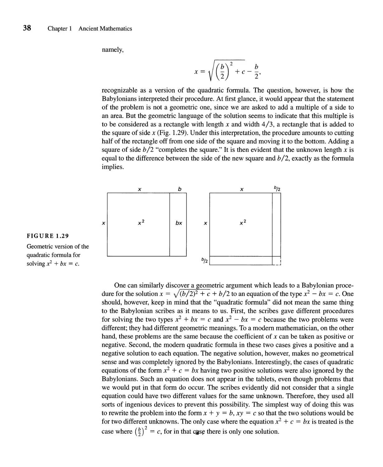
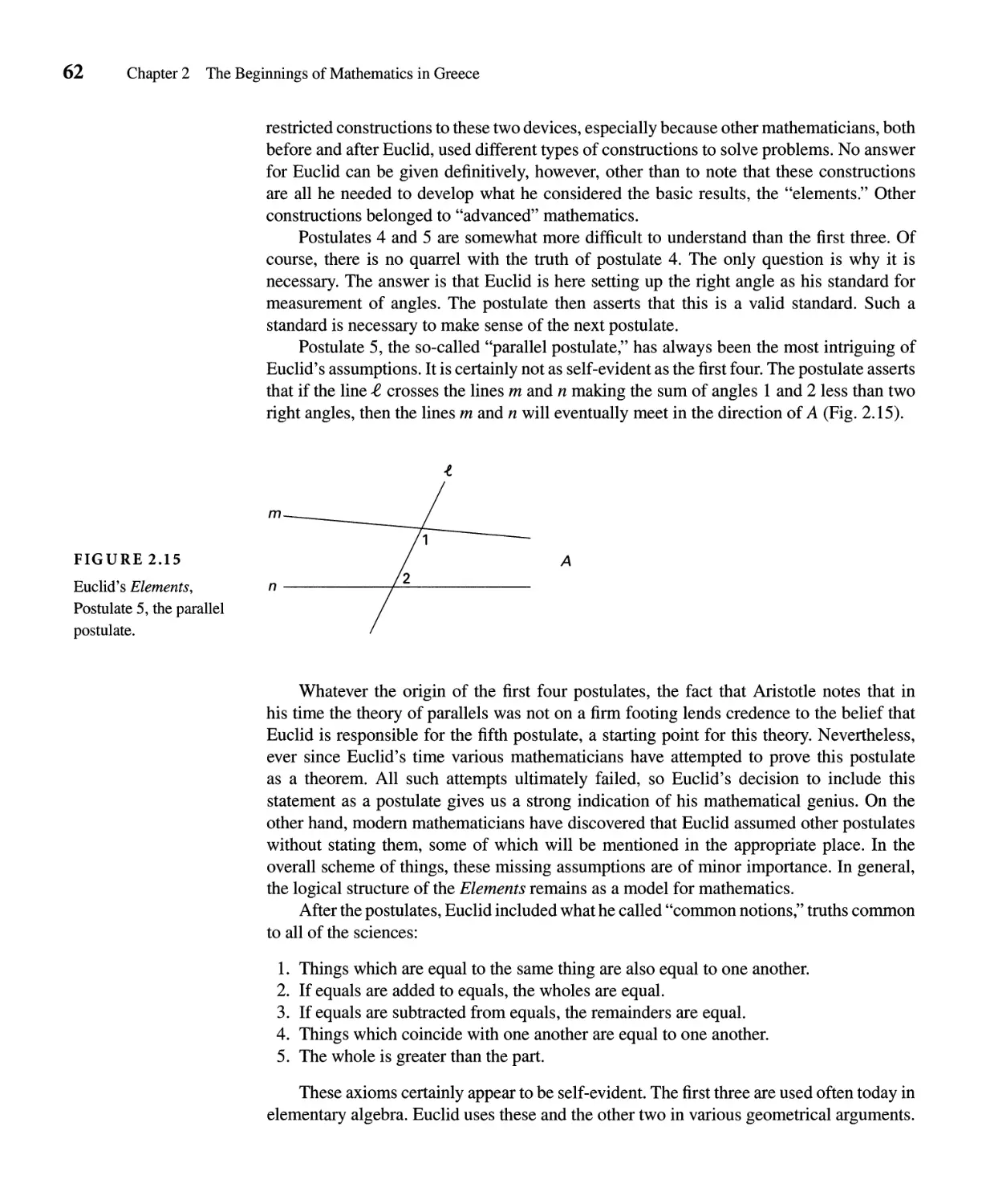
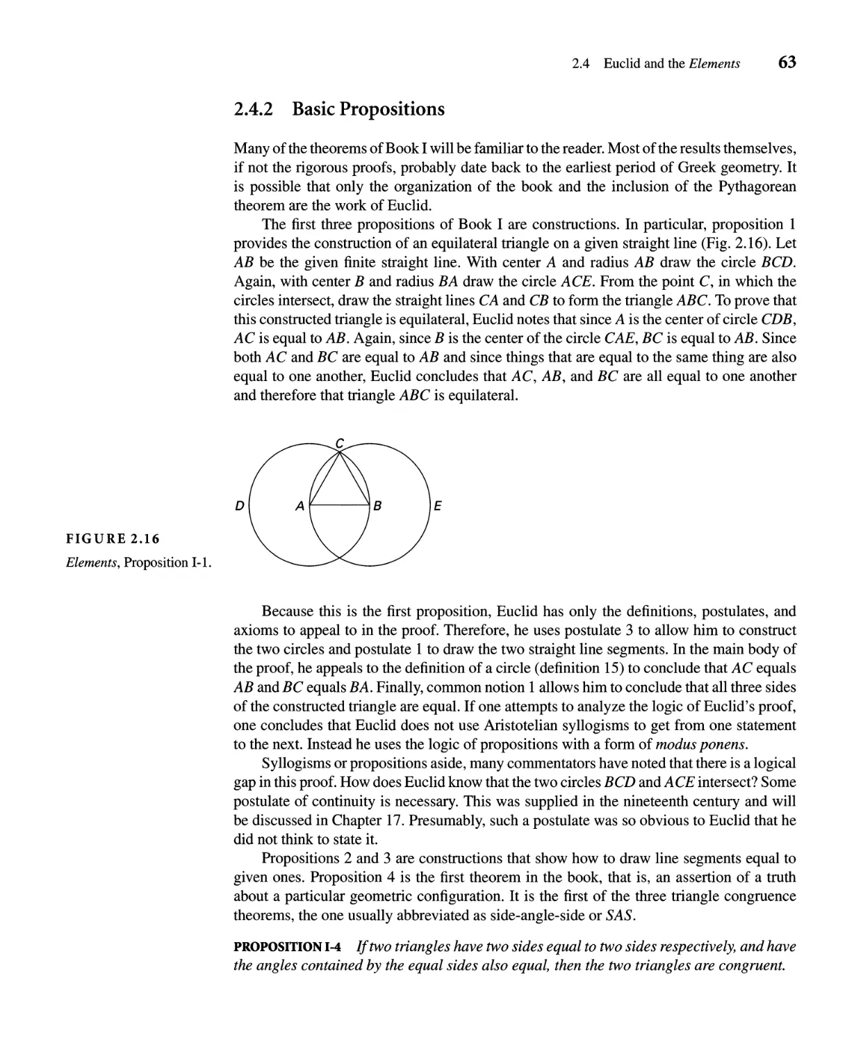
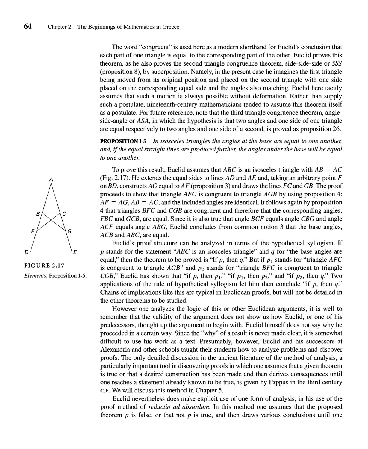
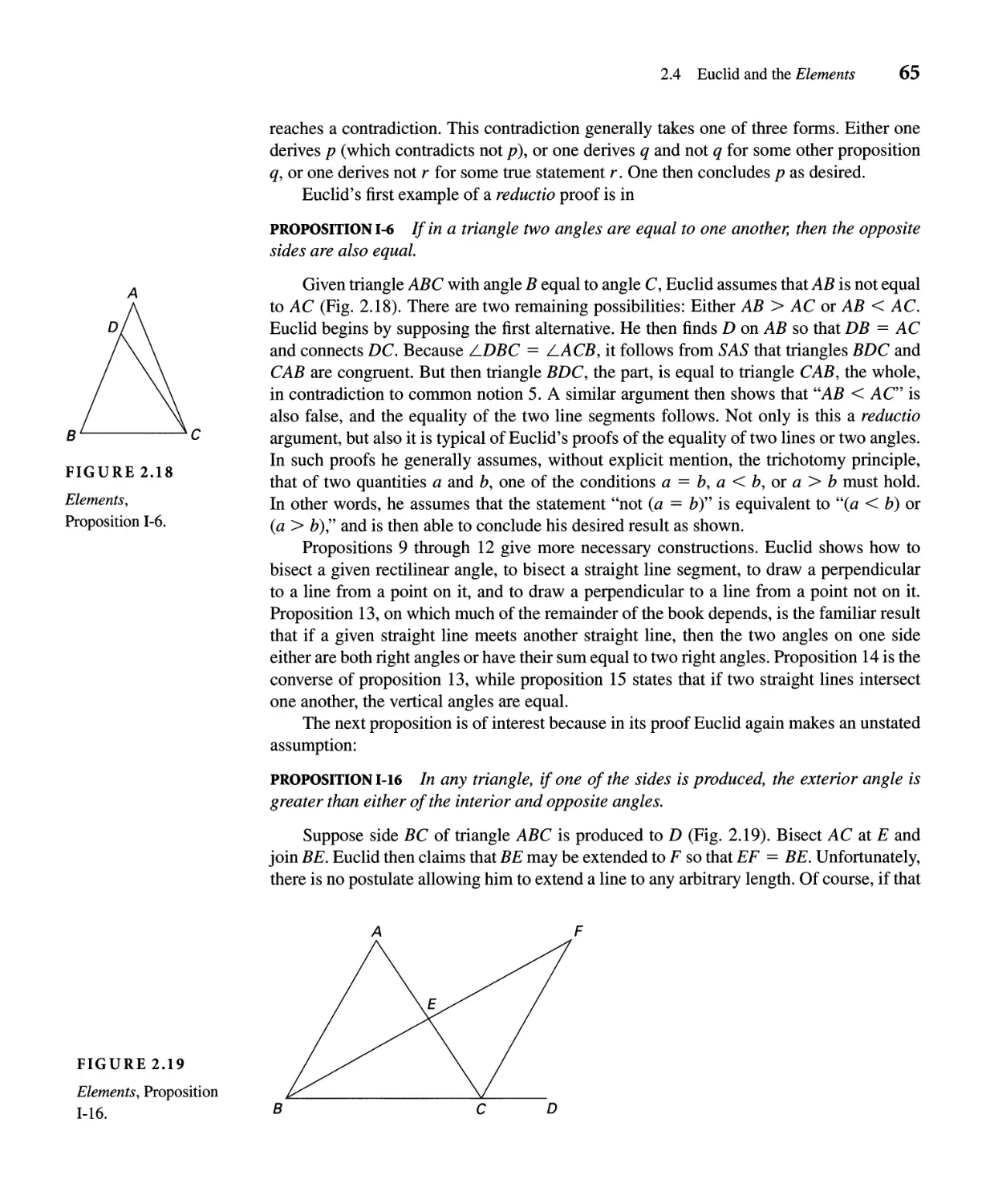
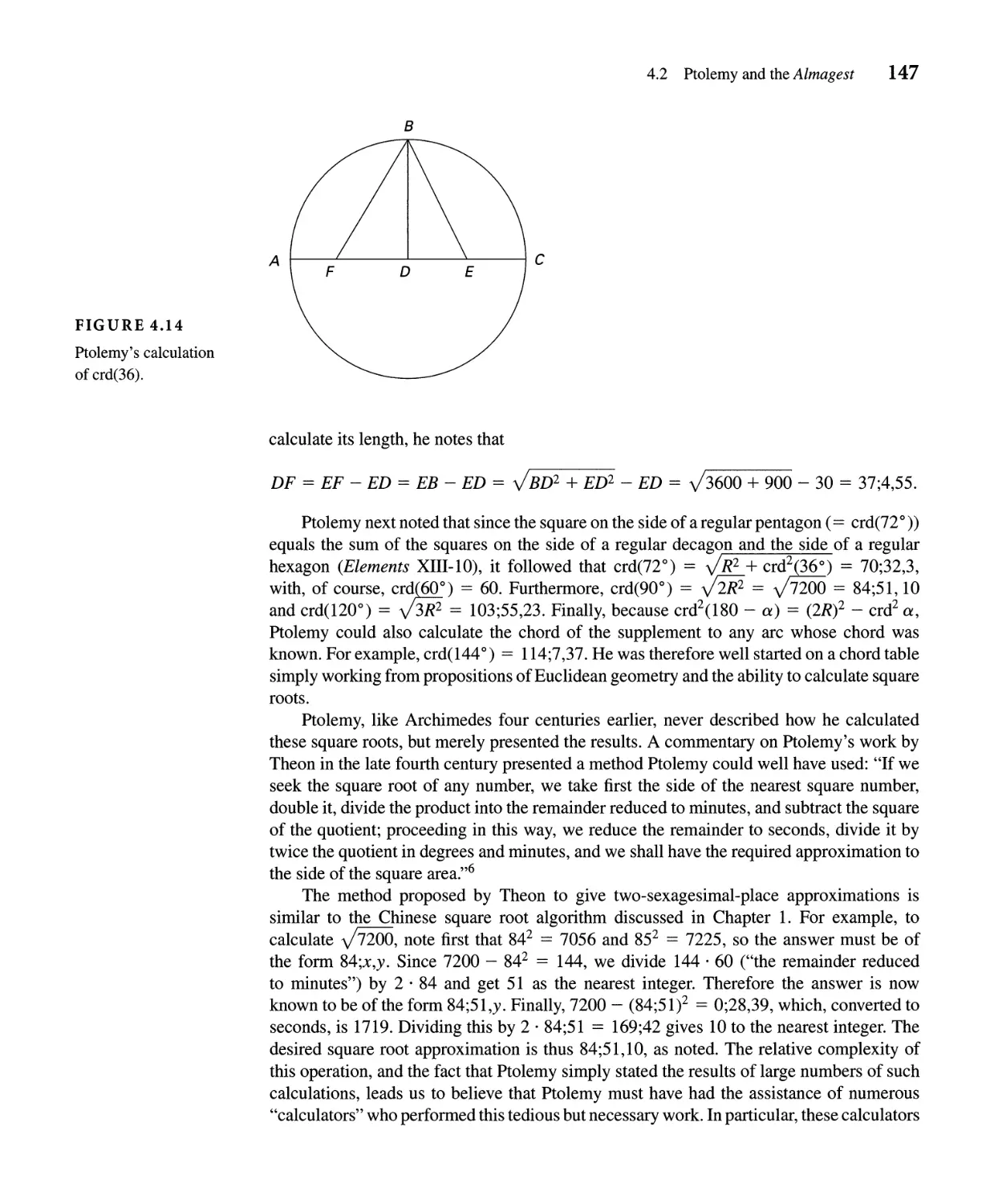
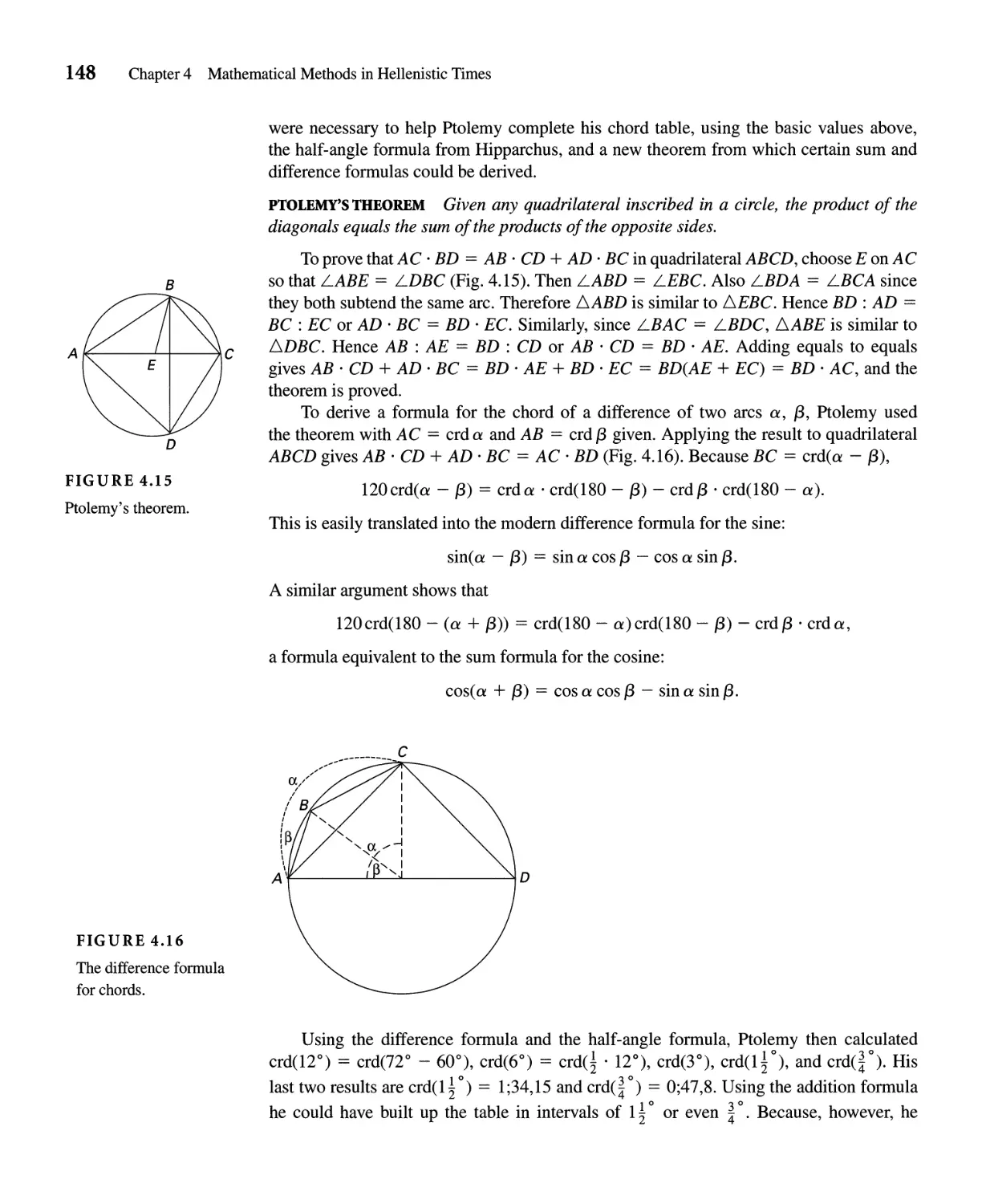
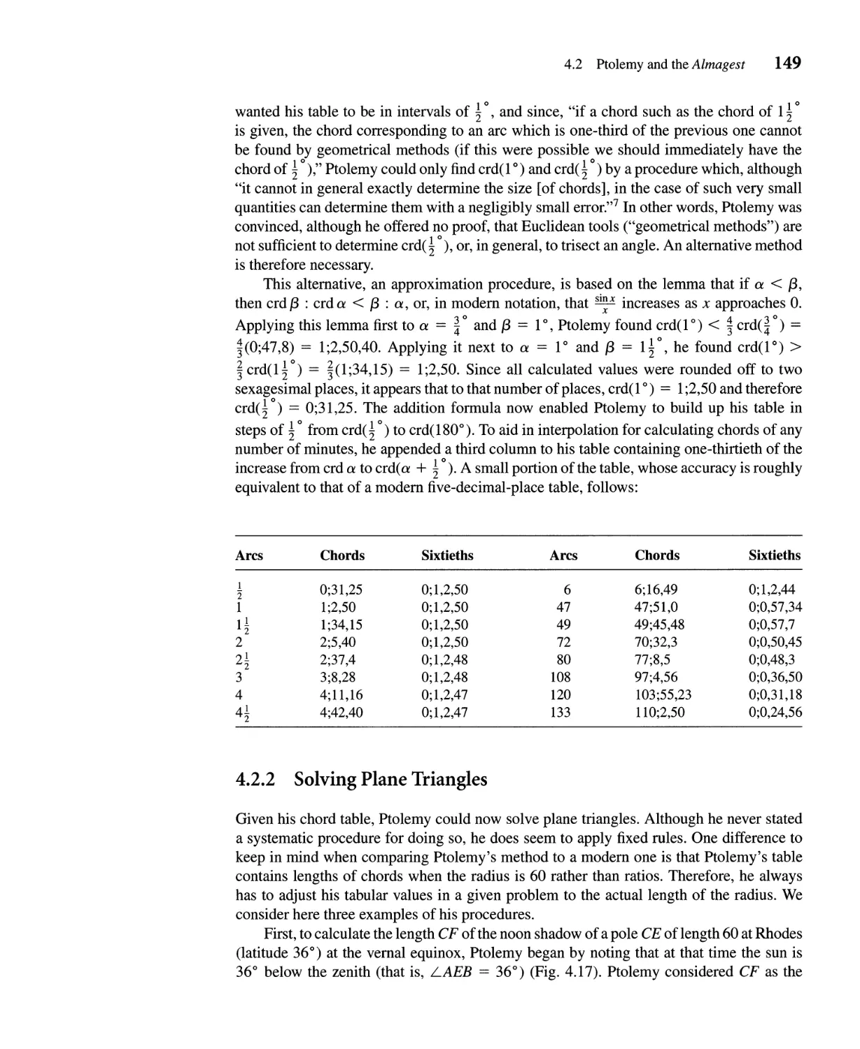
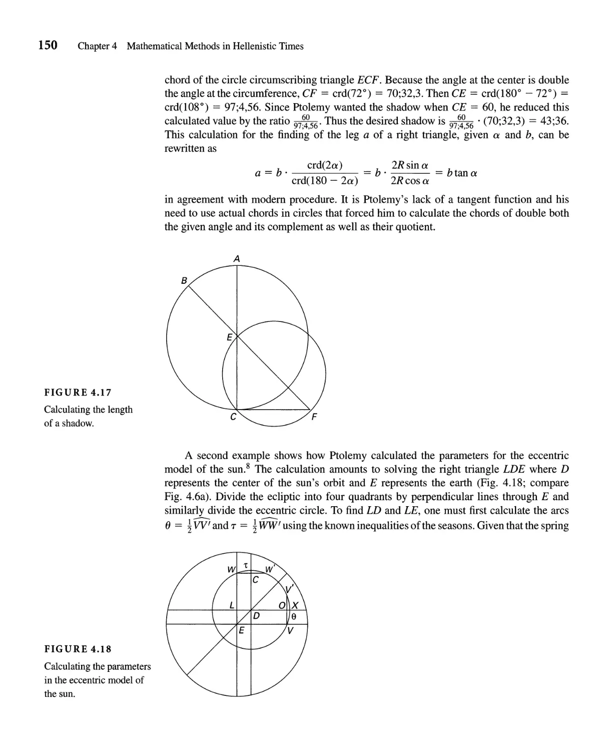
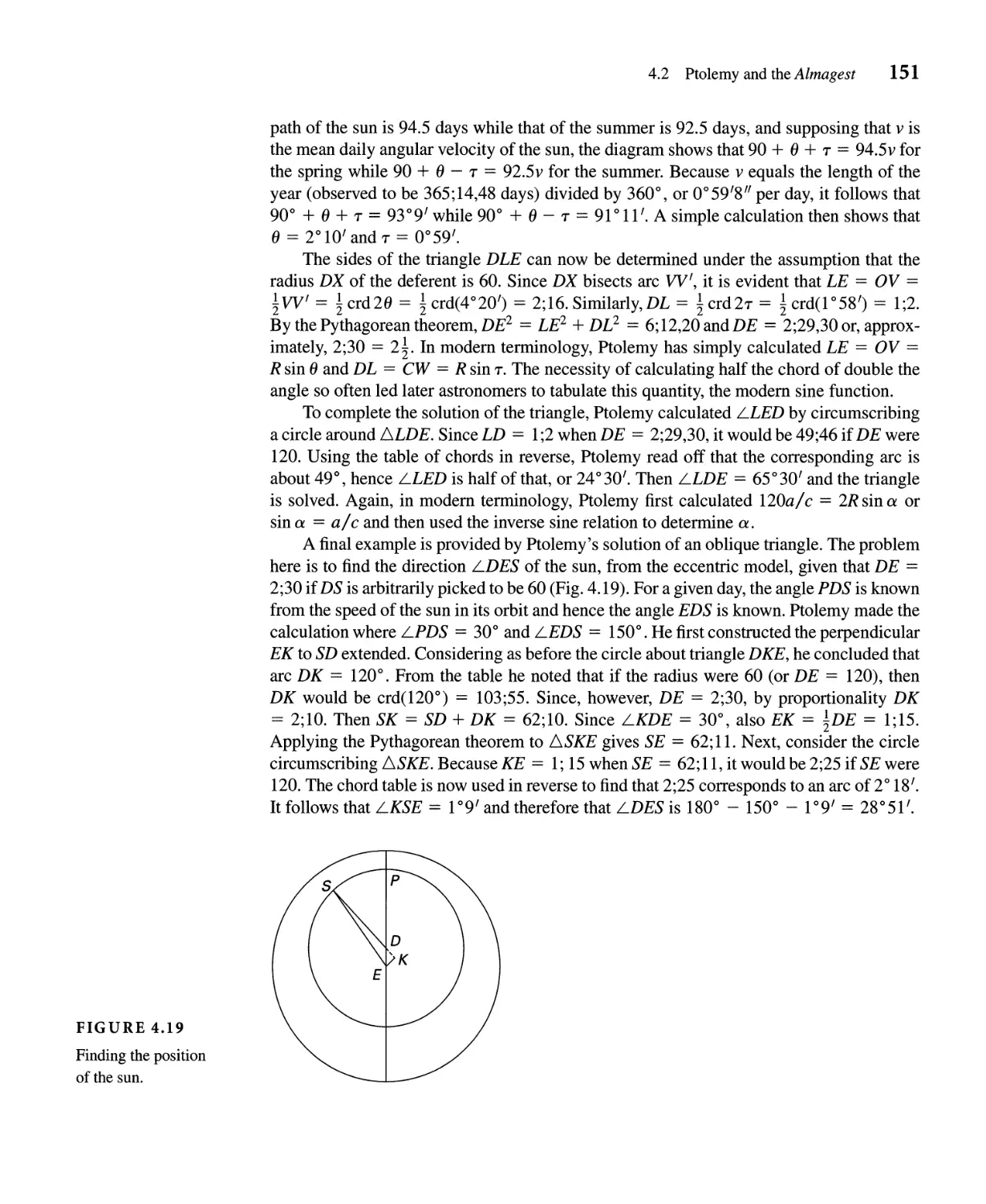
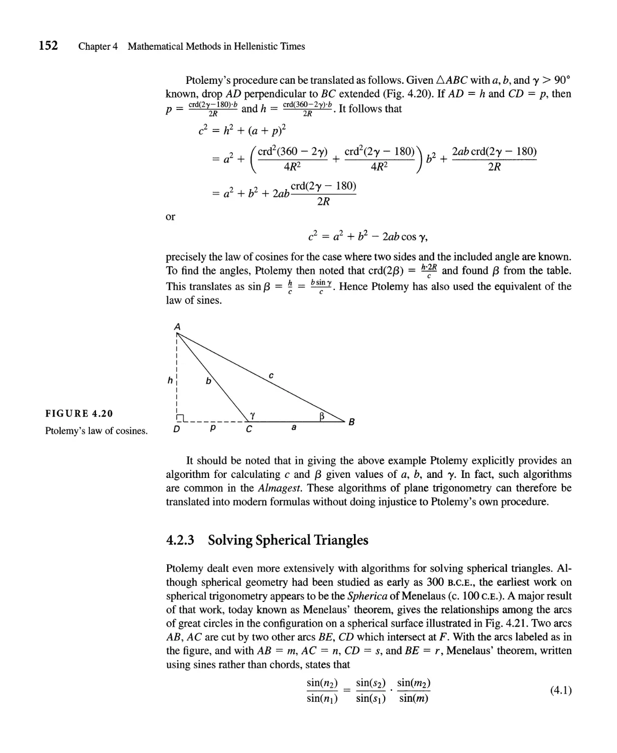
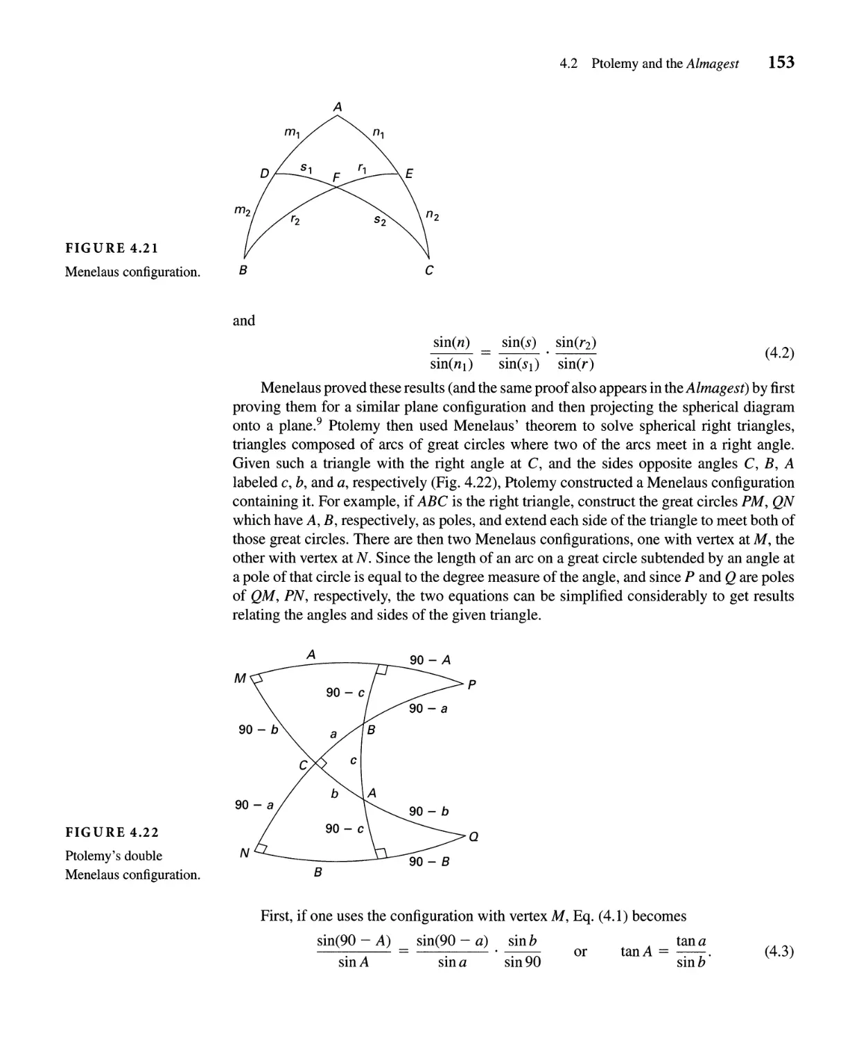
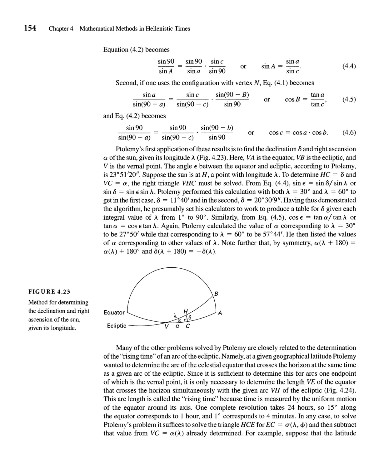
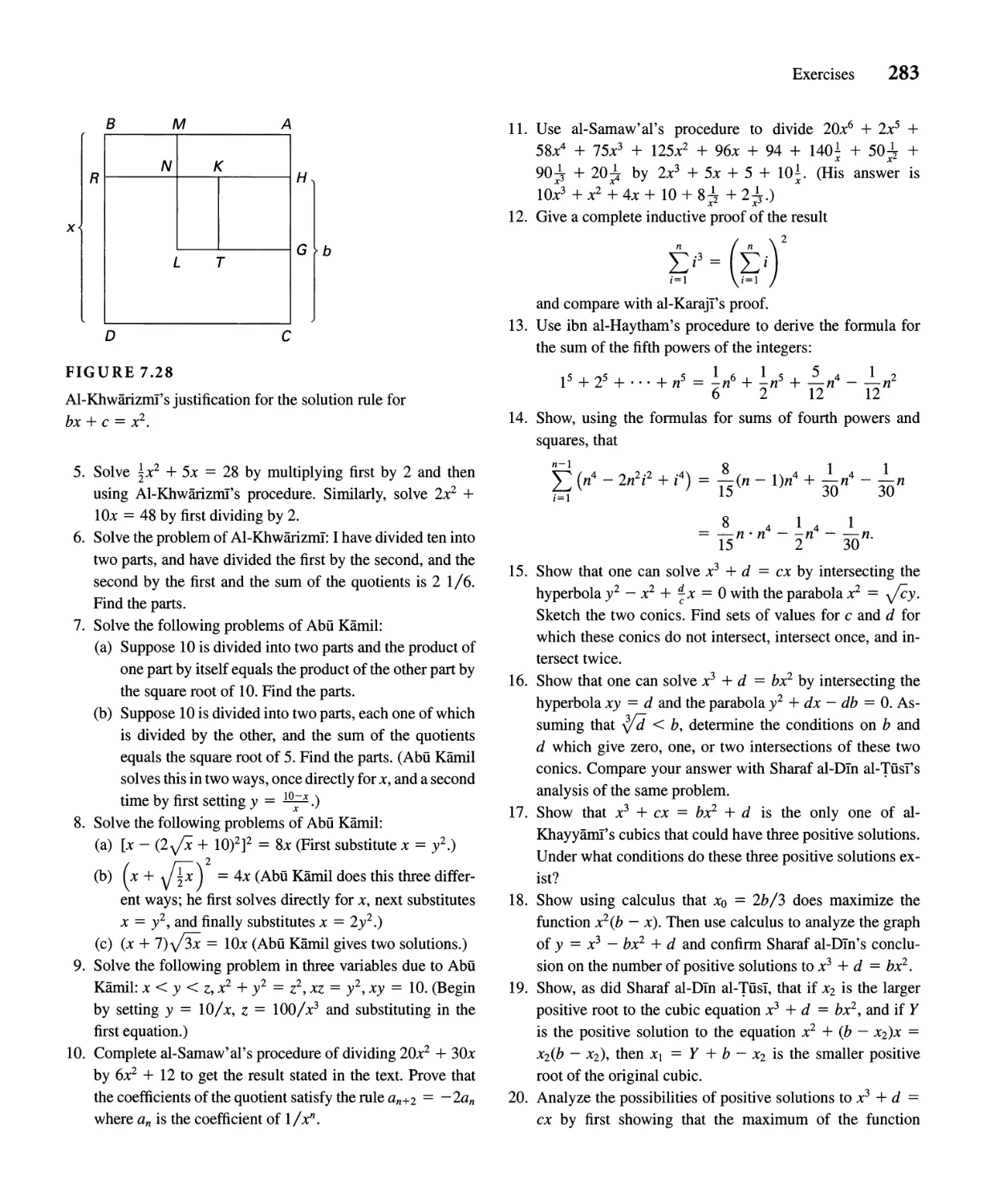
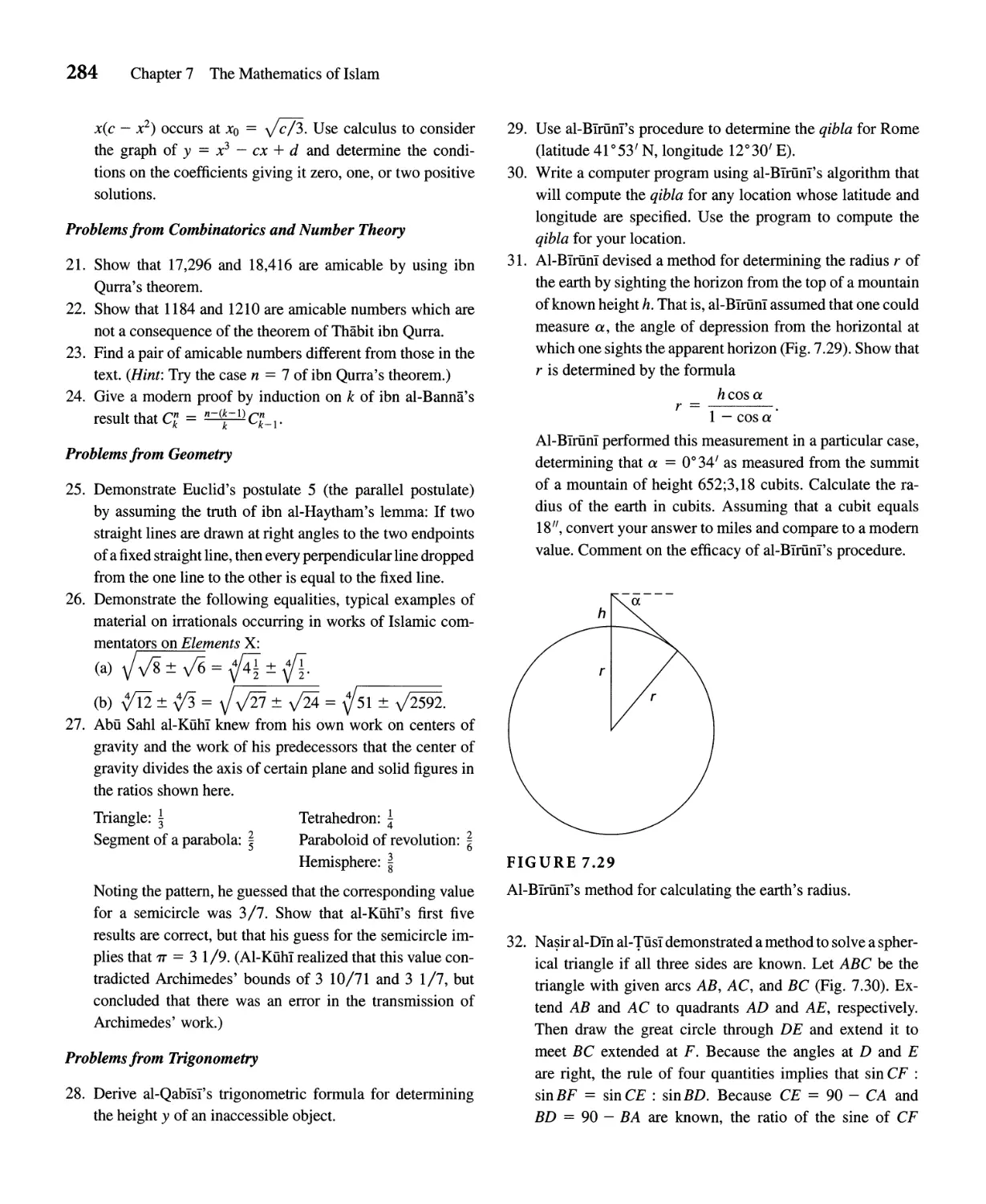
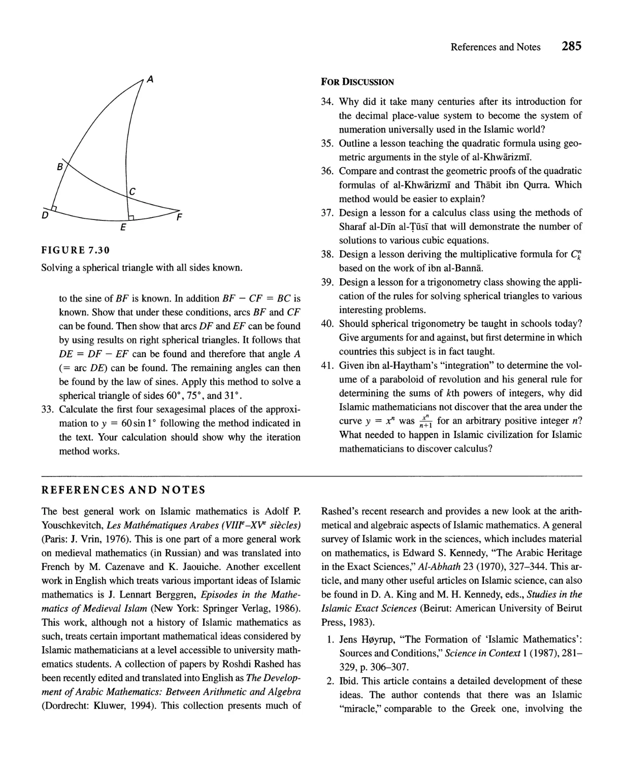
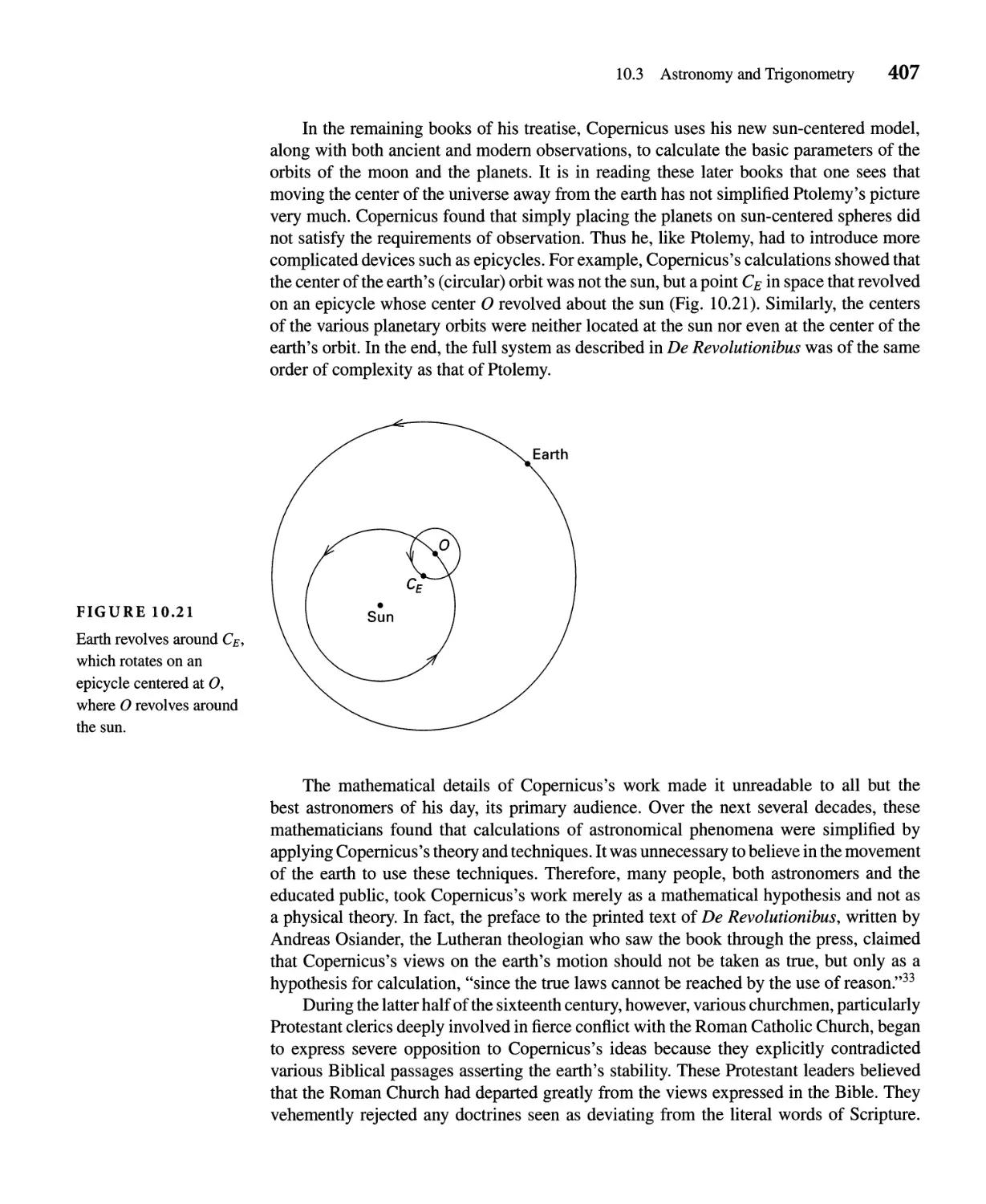
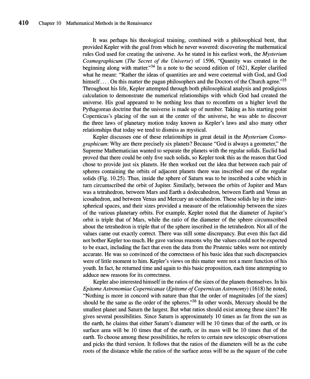
/


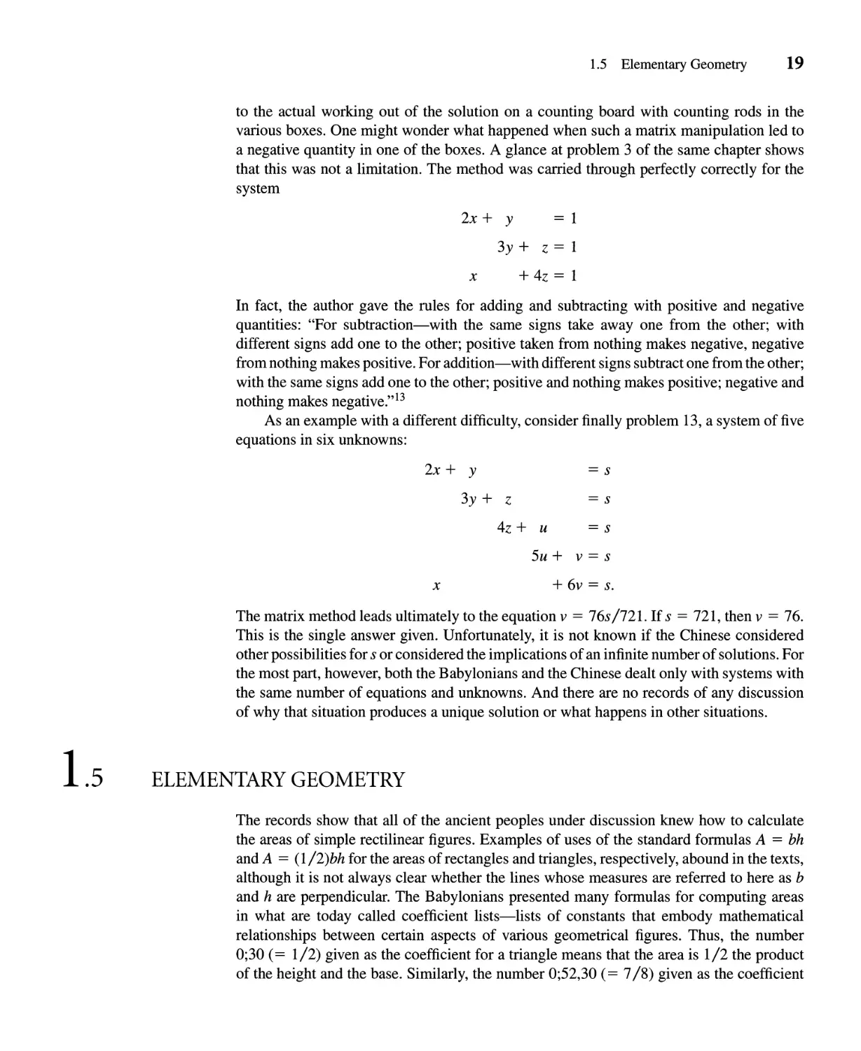
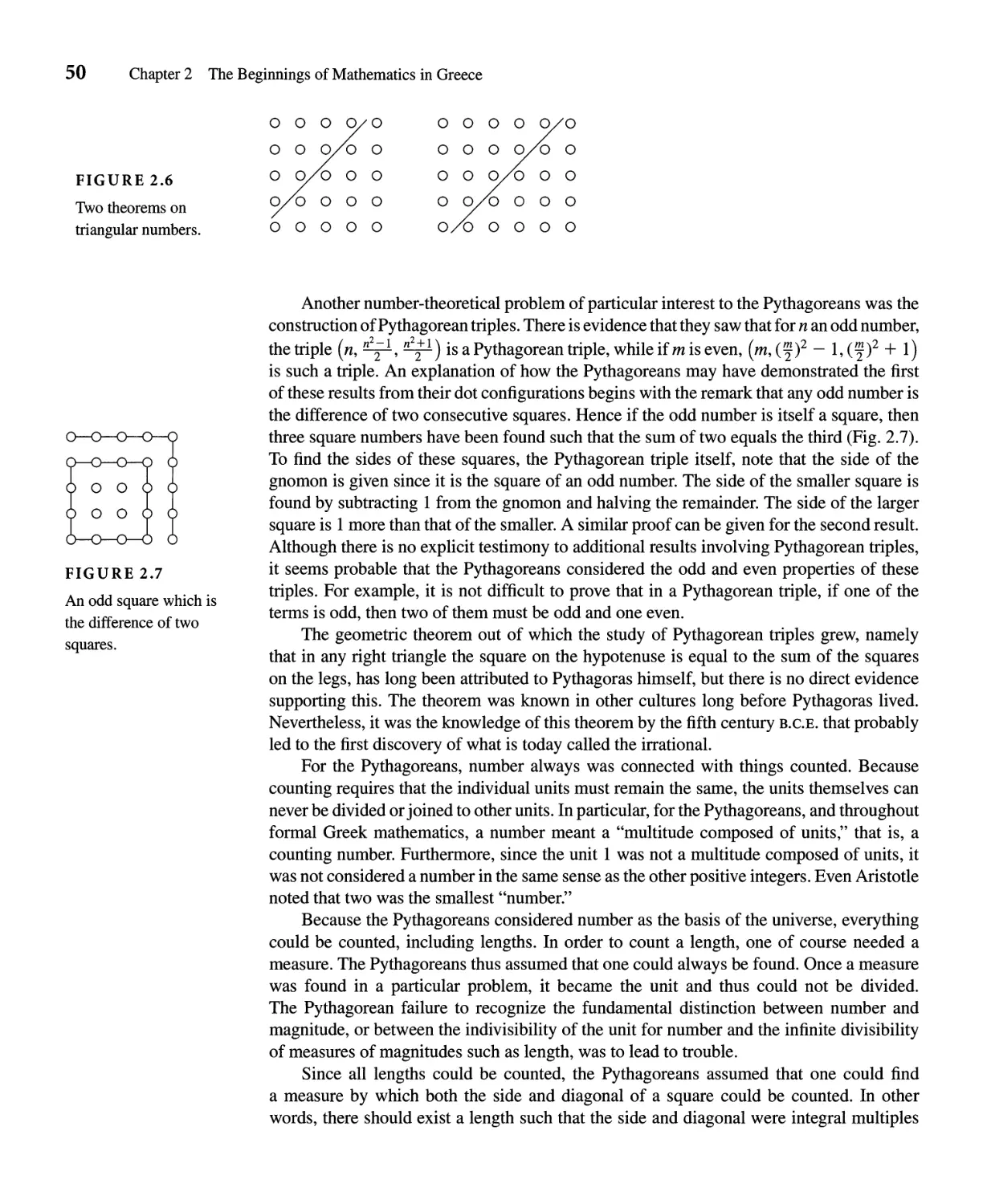
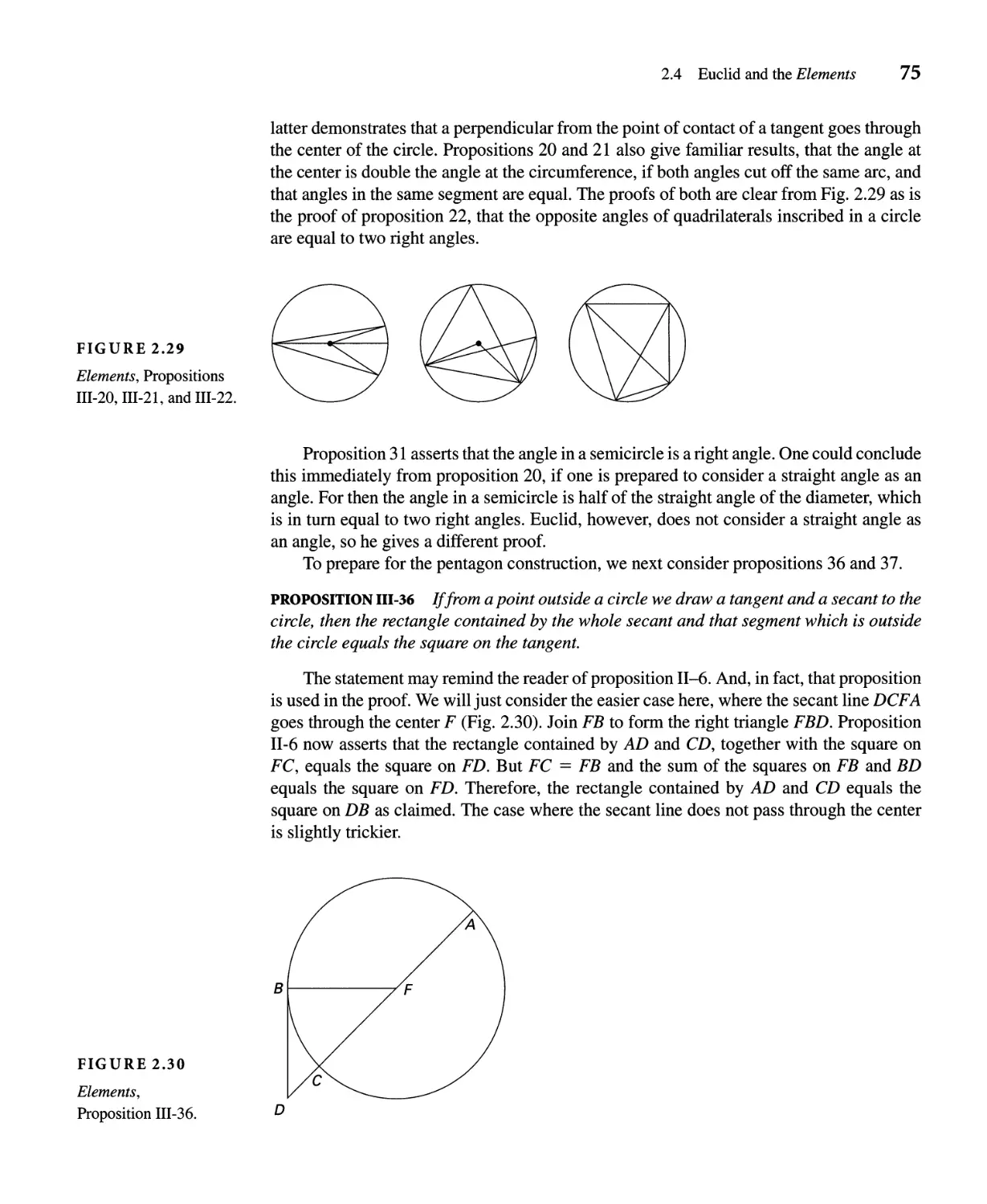
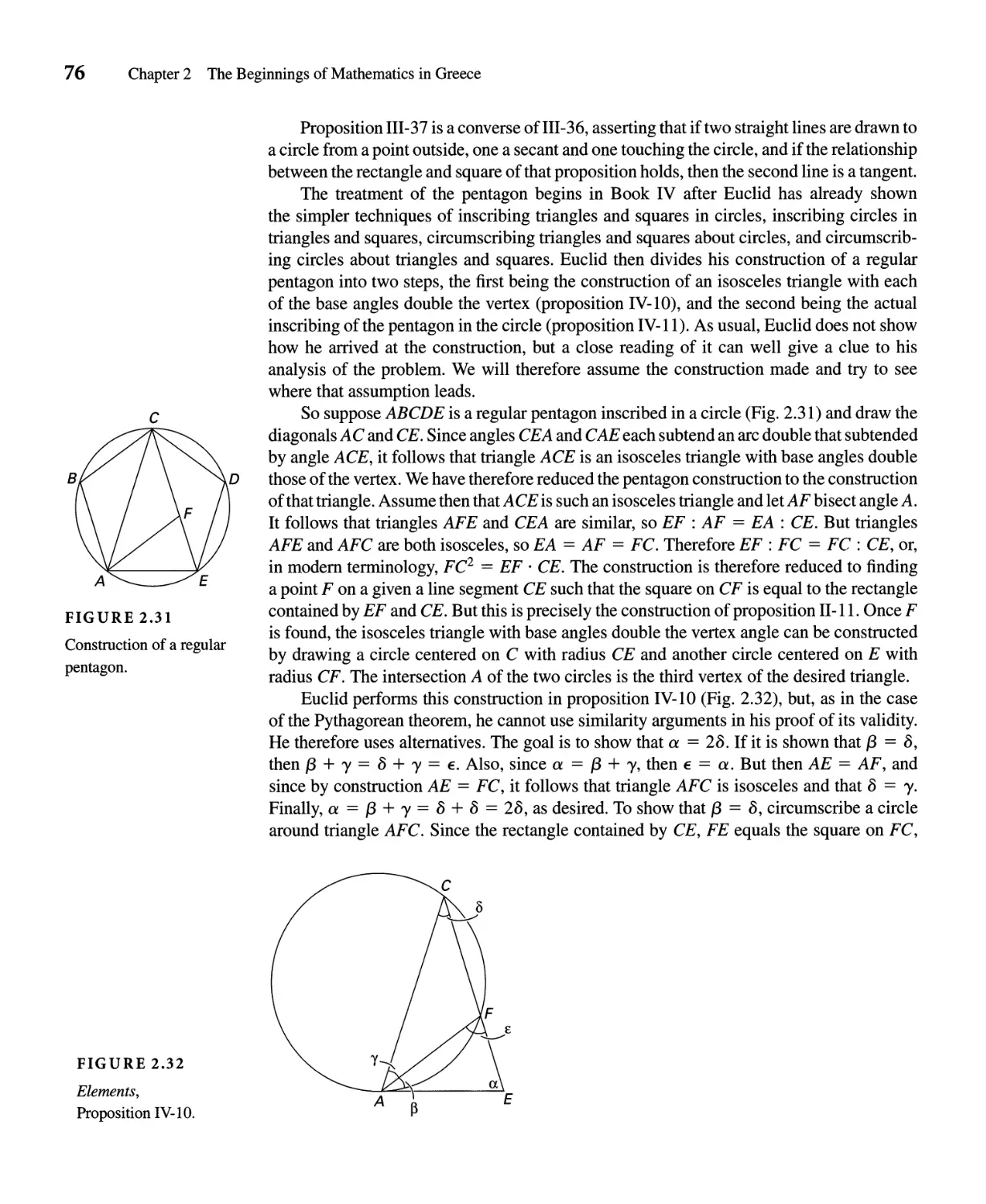
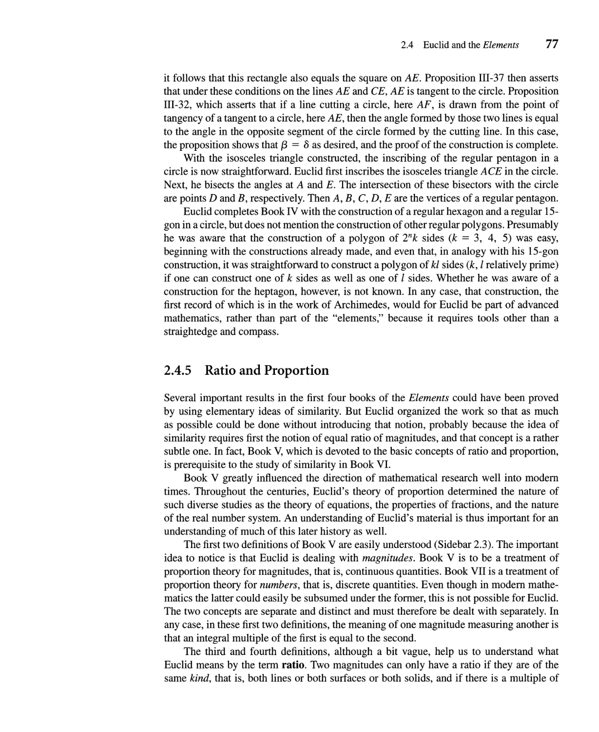

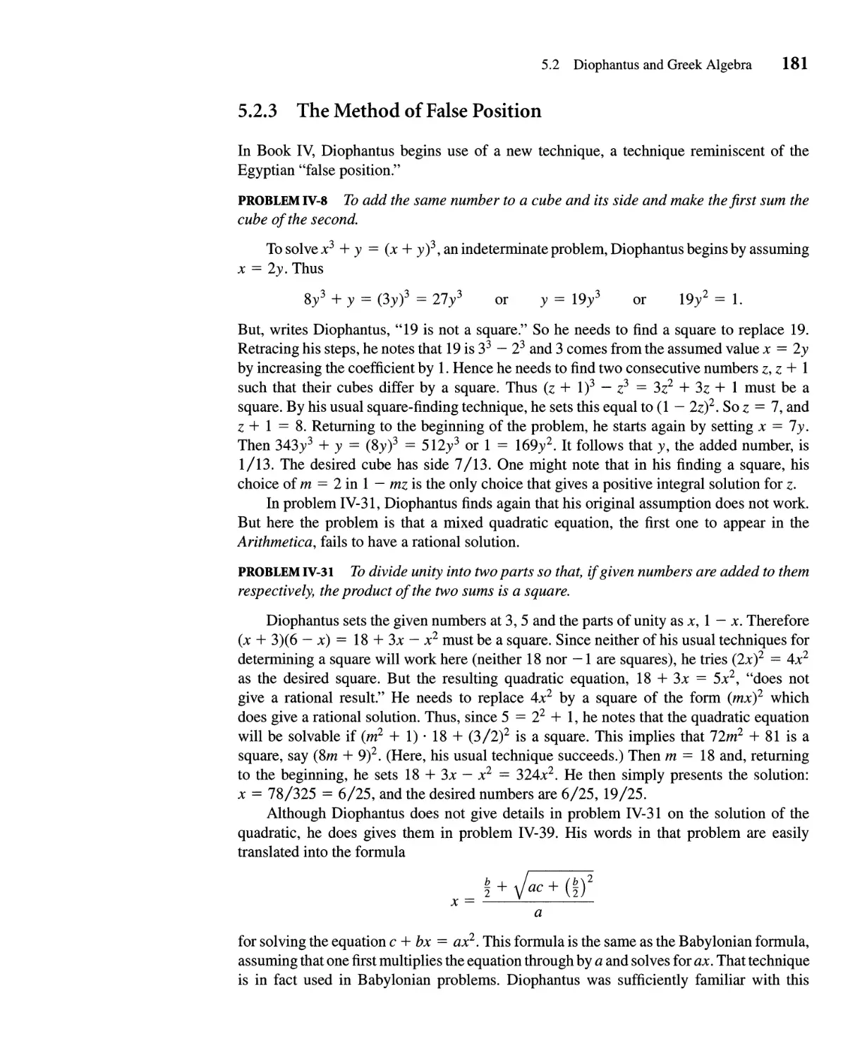
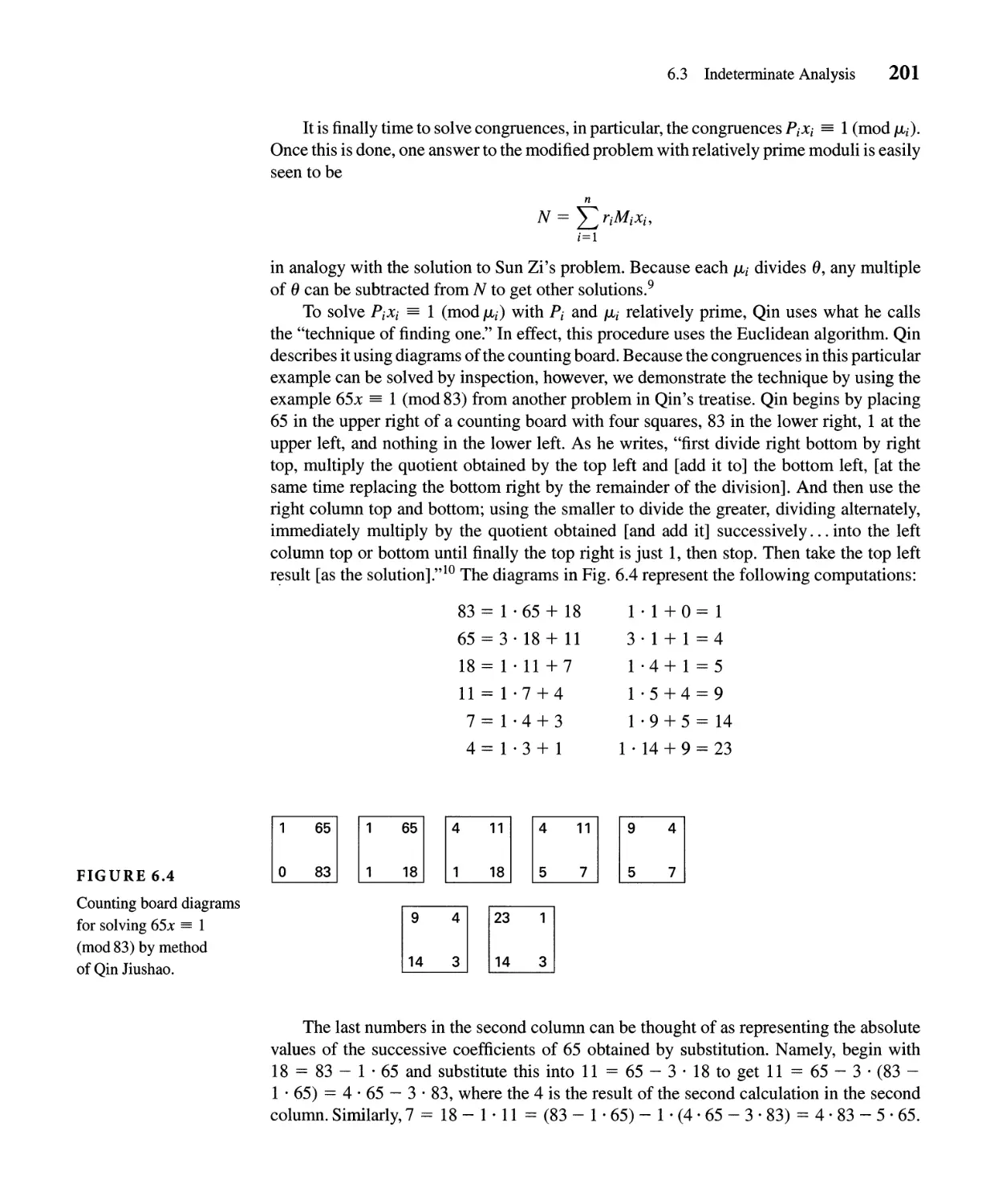
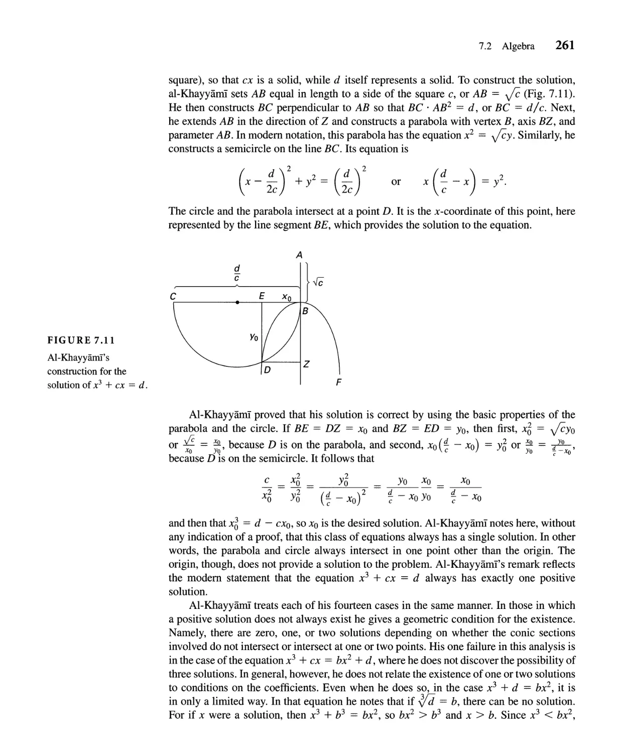
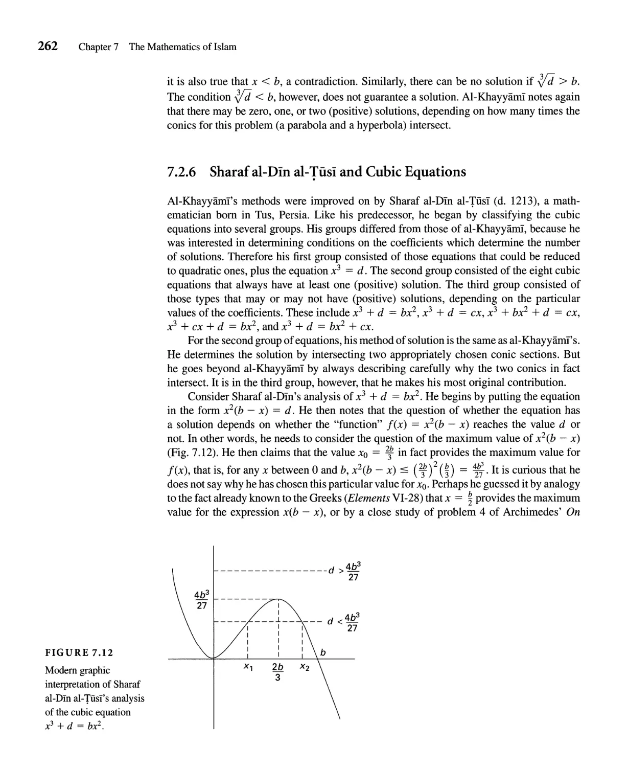

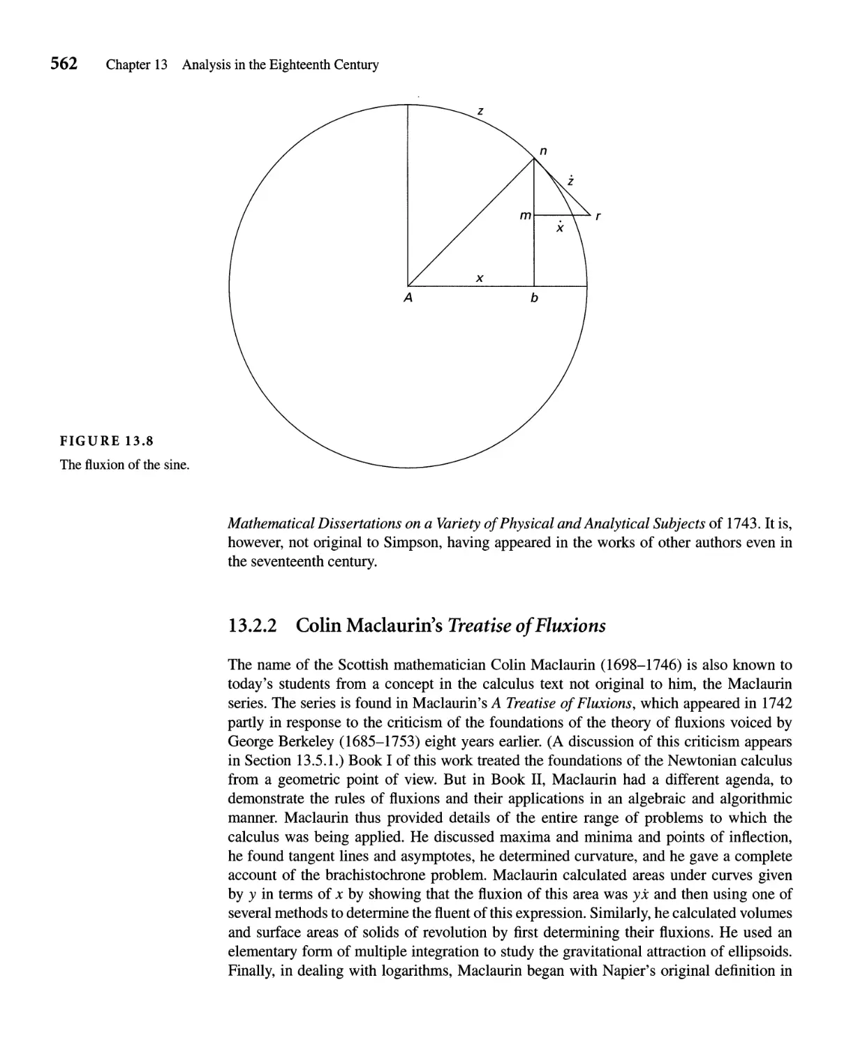


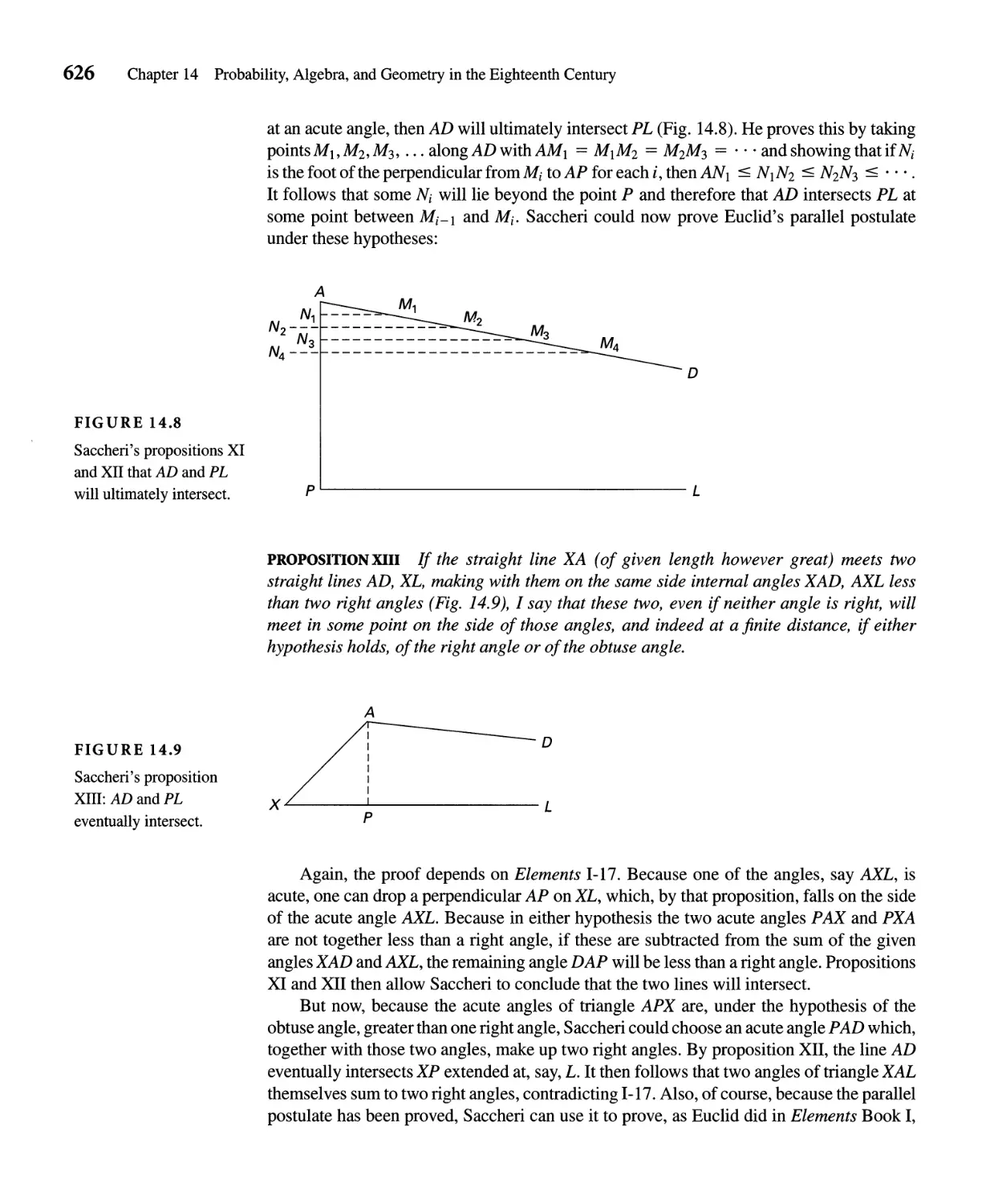


Text
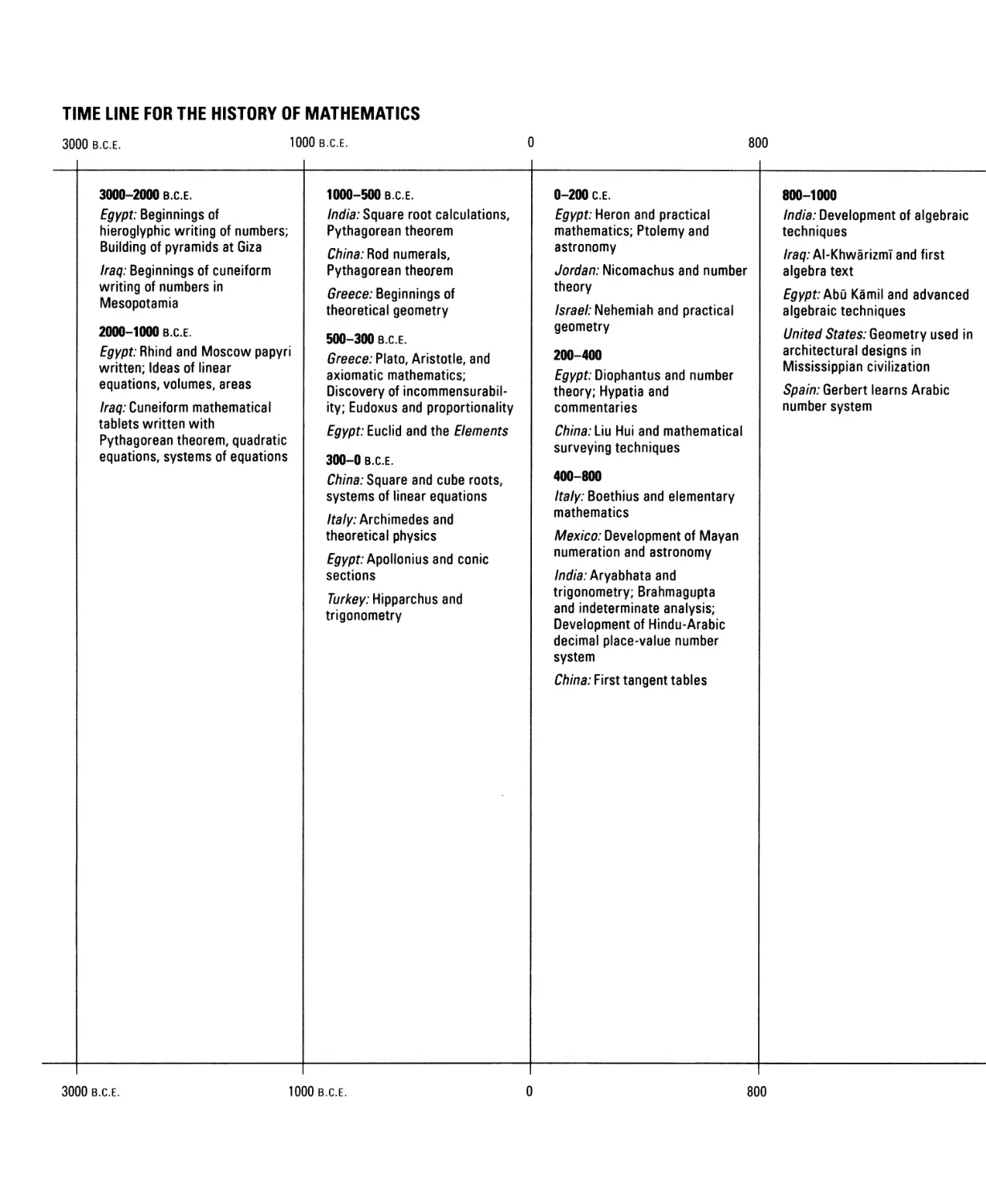
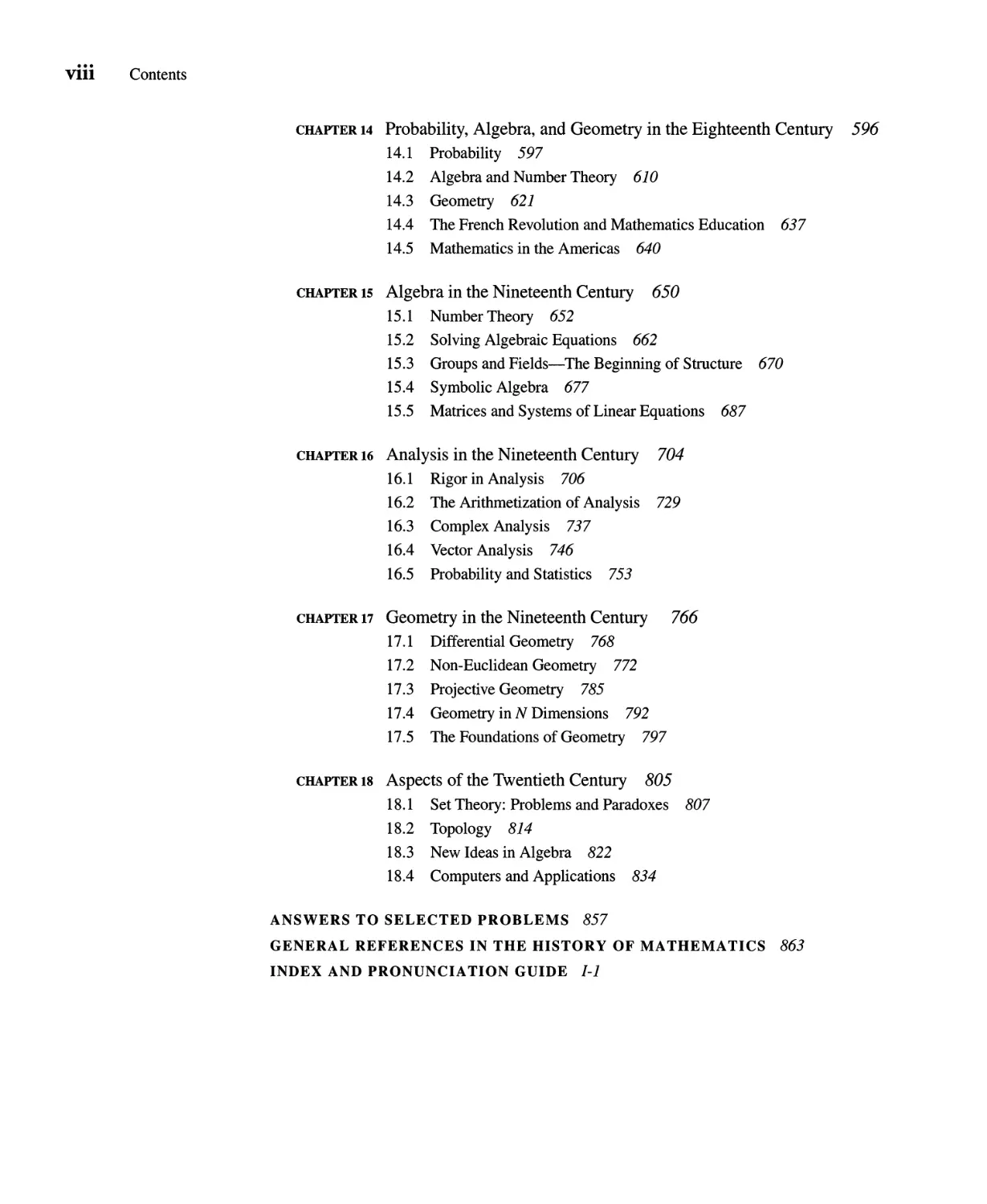
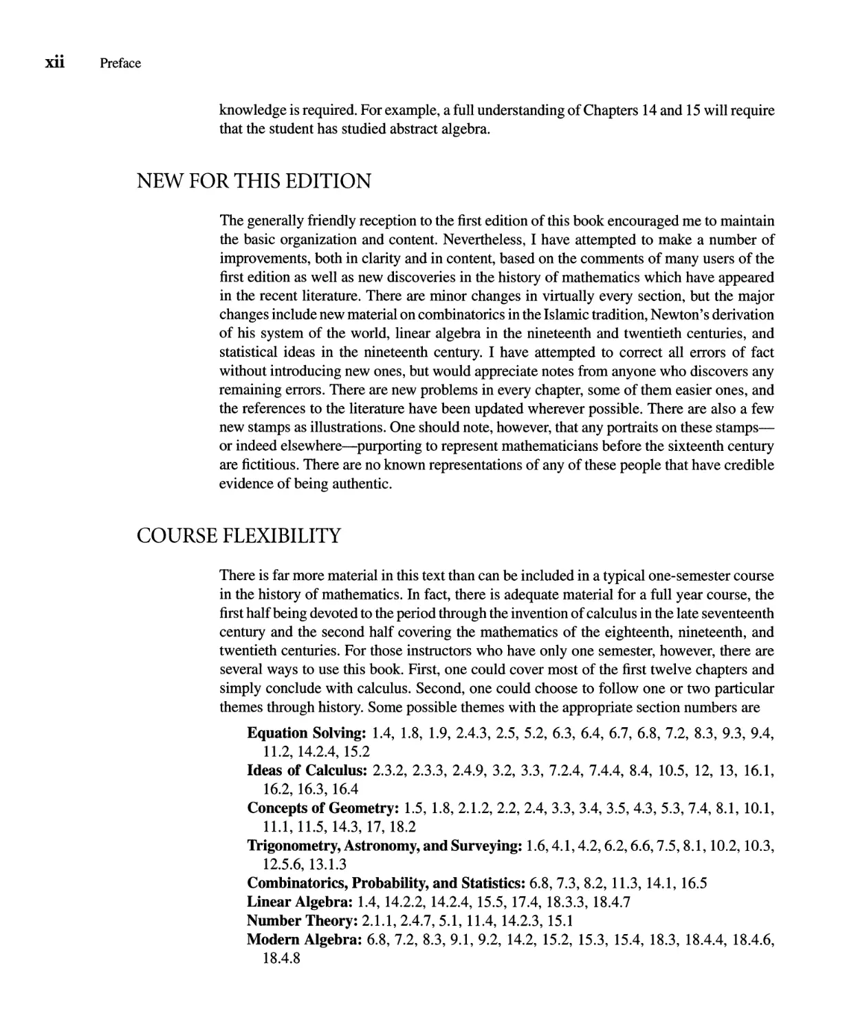
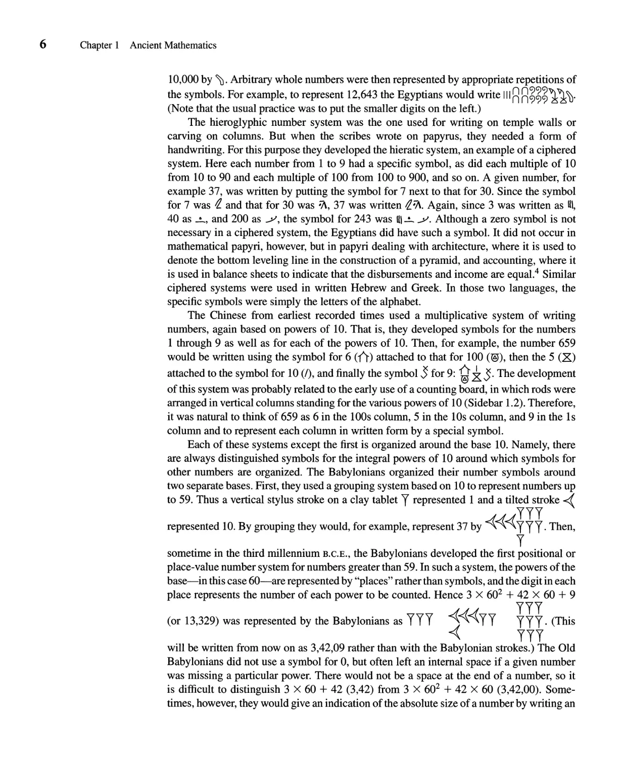
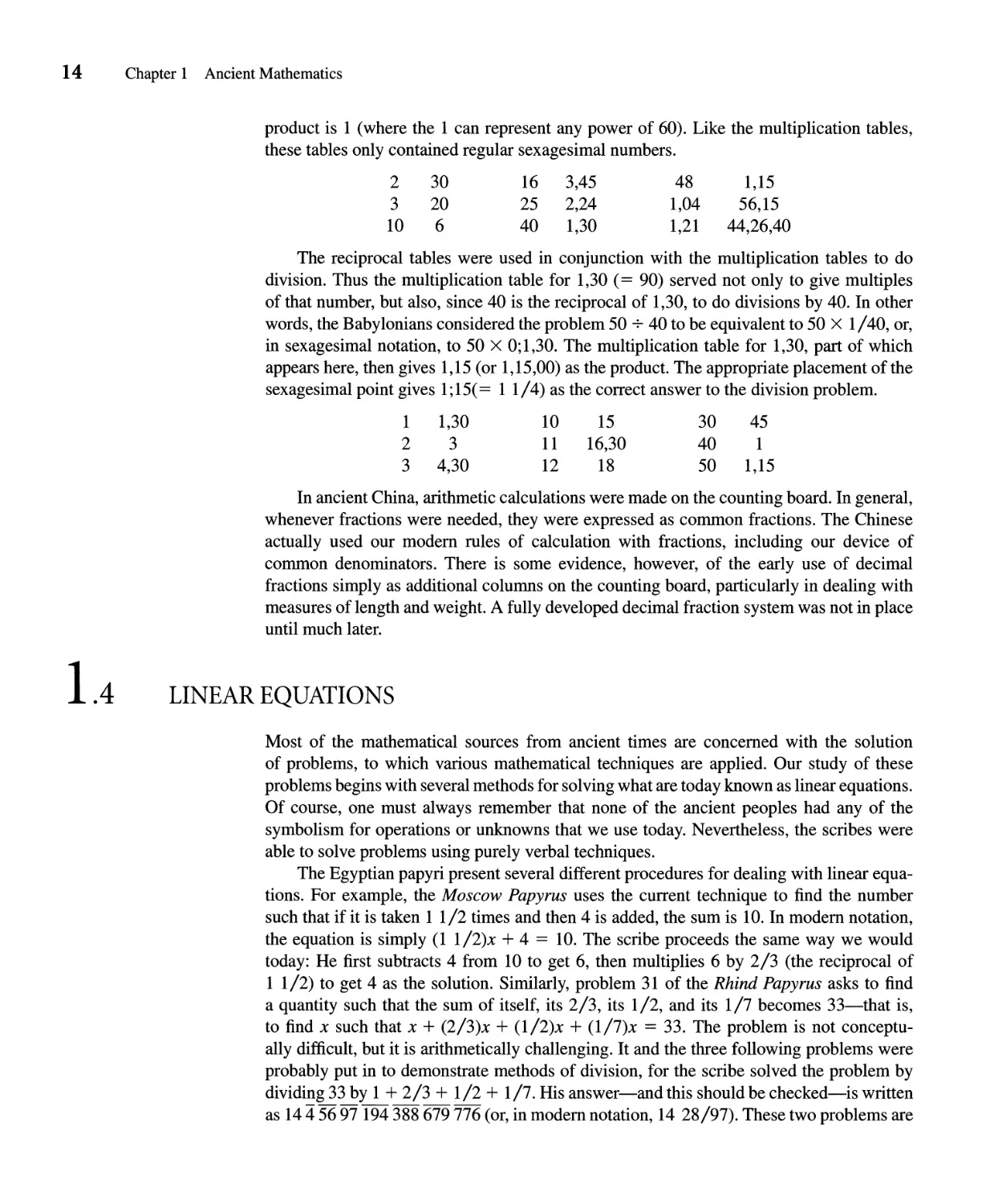
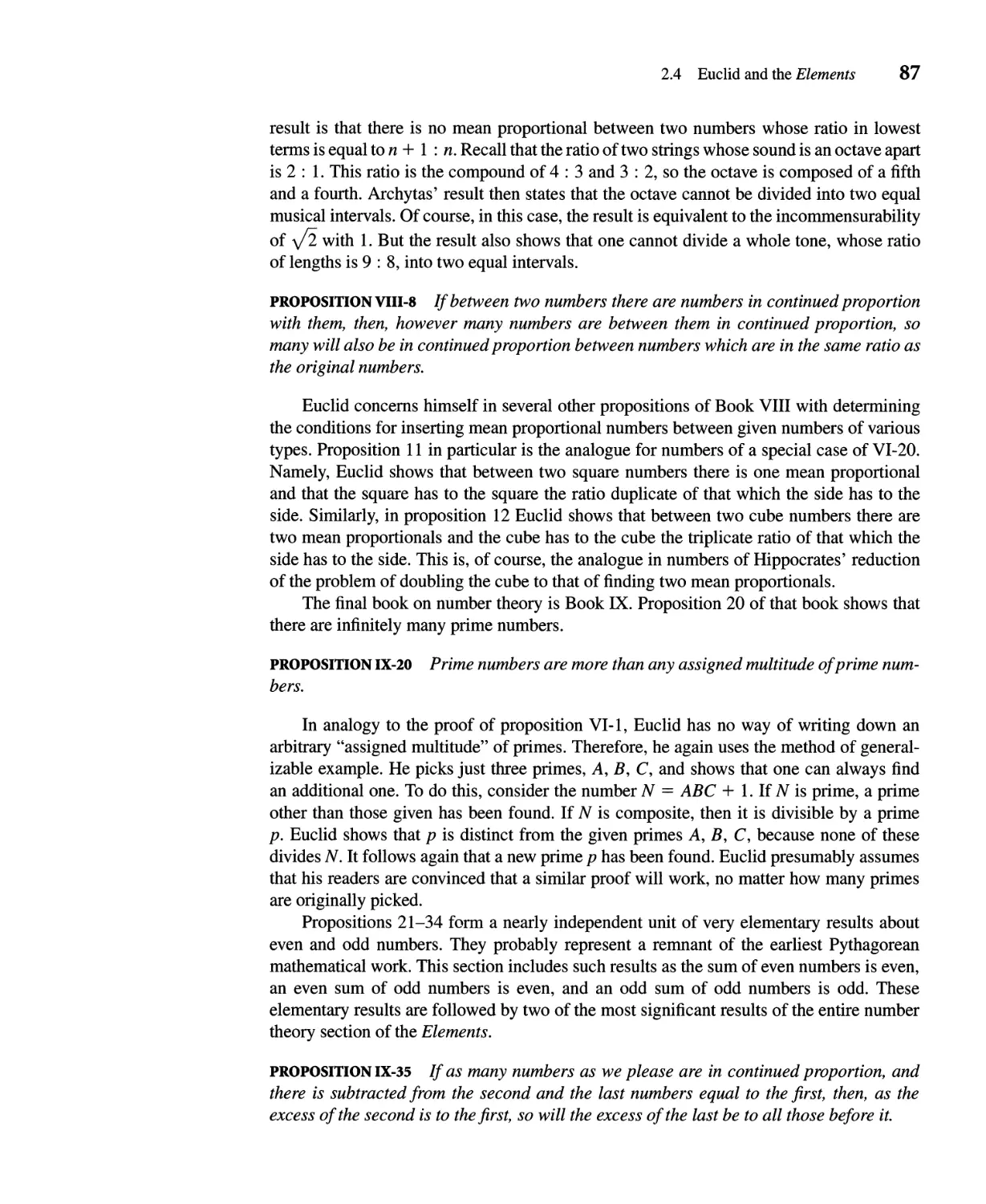
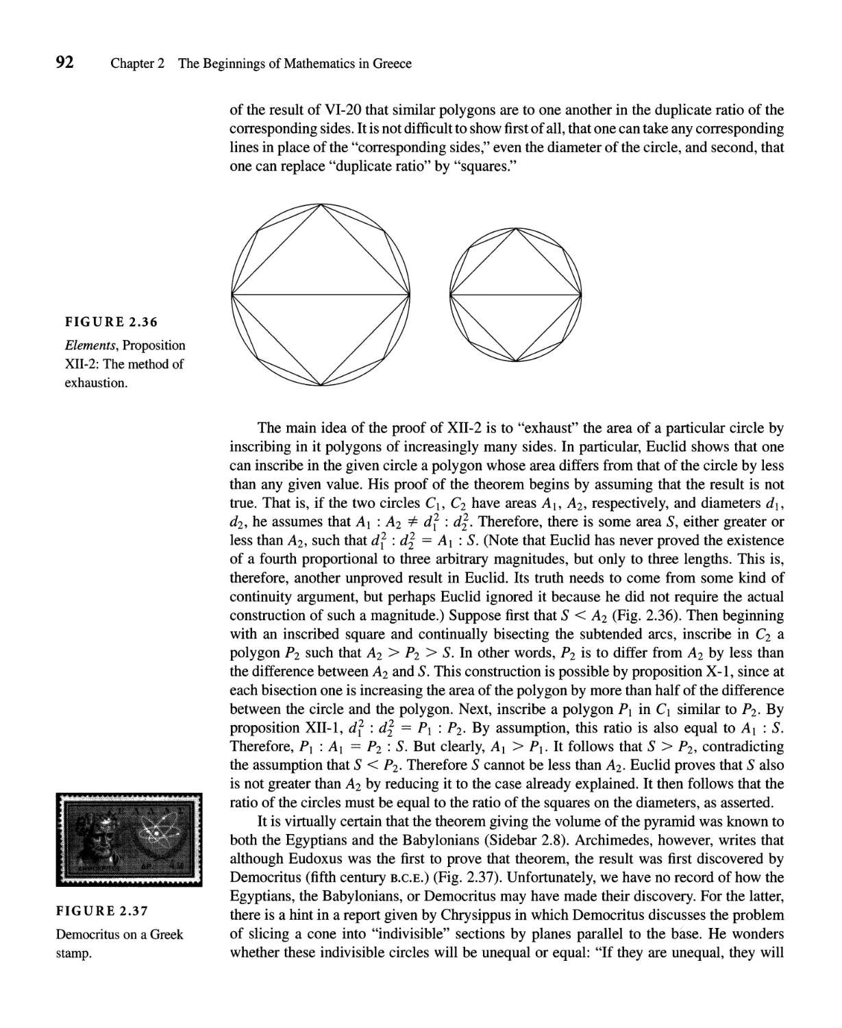
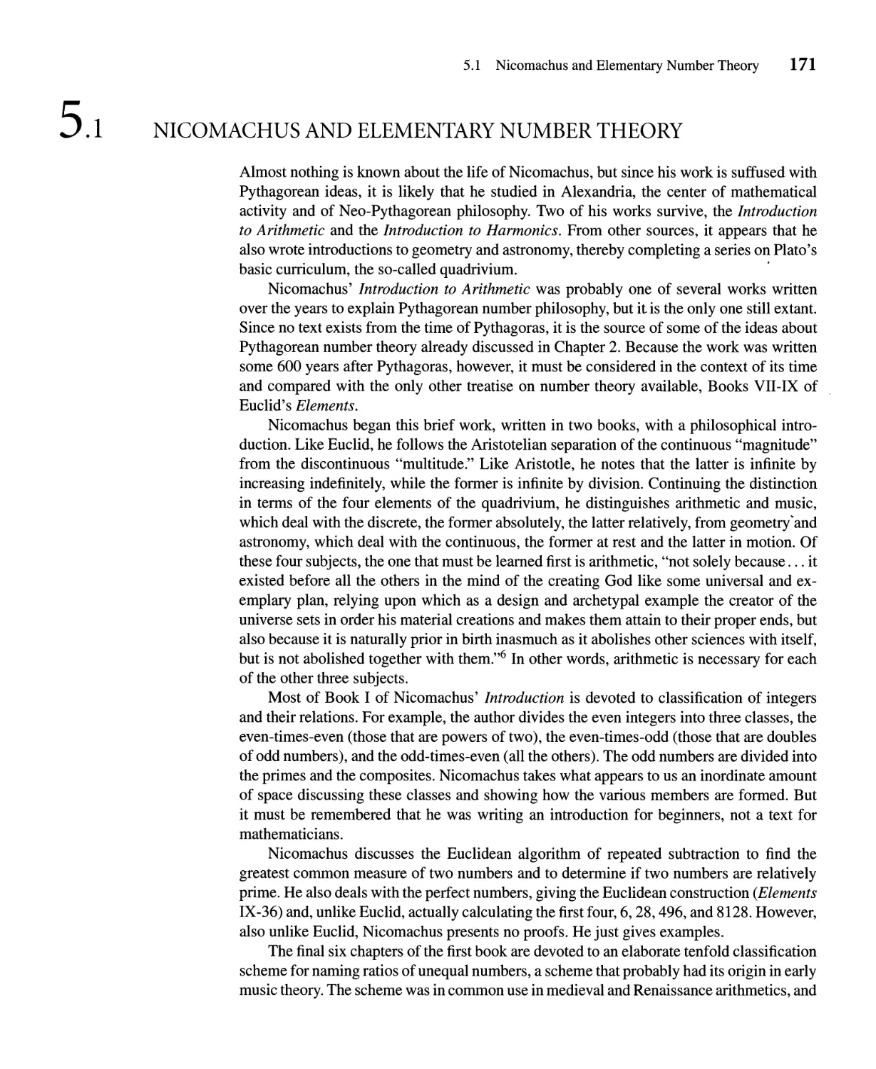
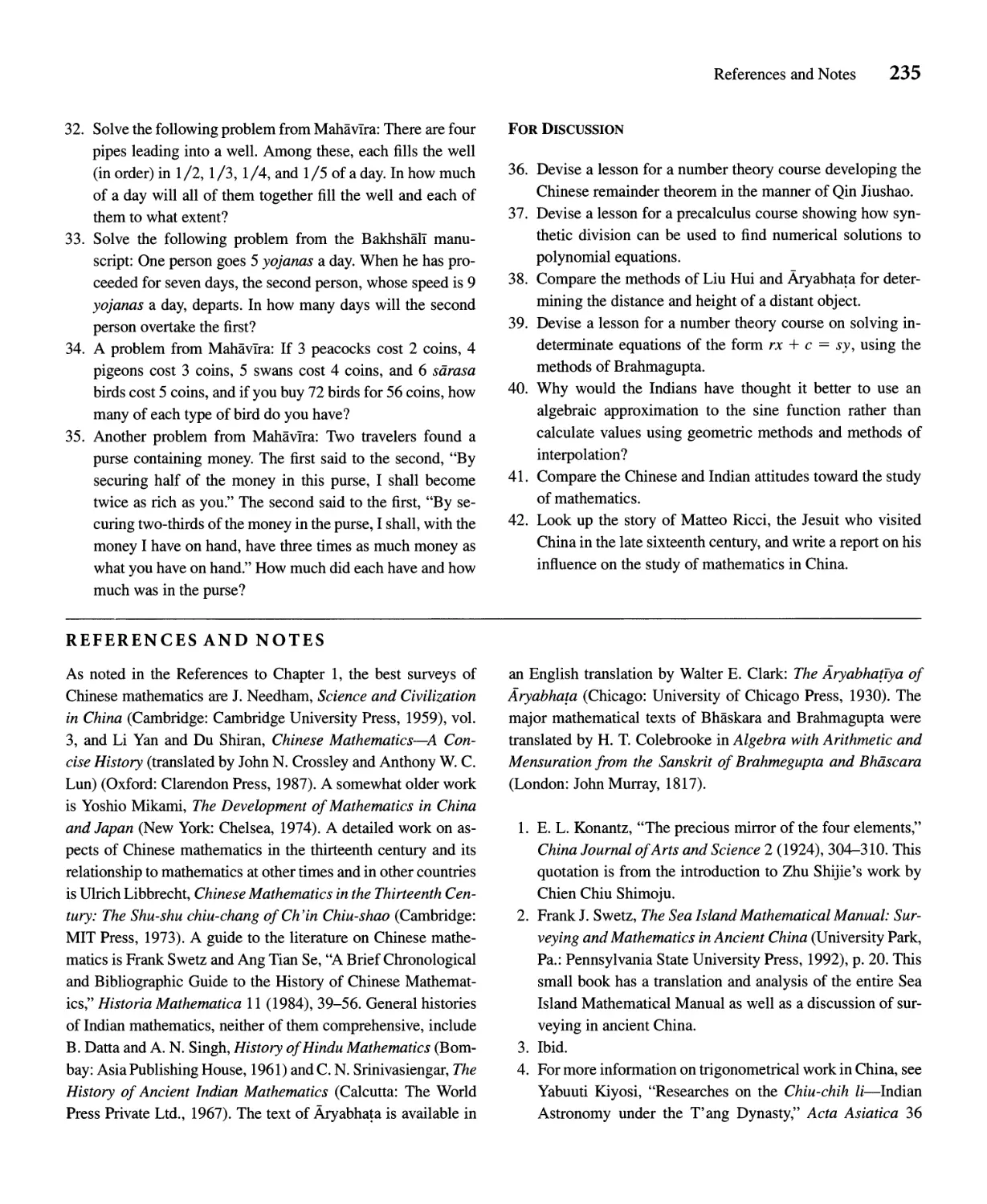
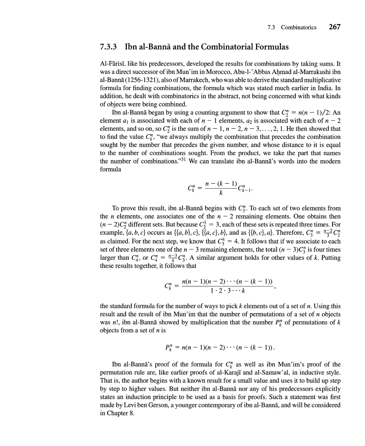
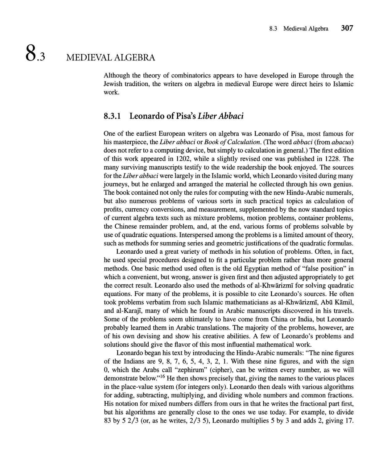
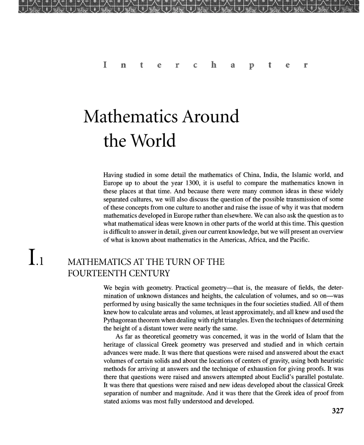
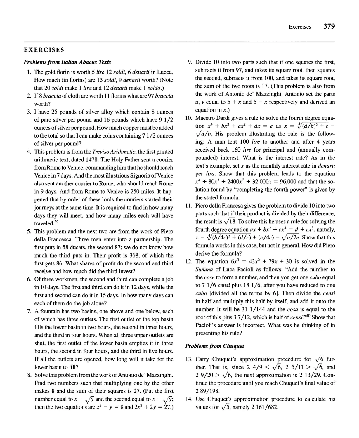
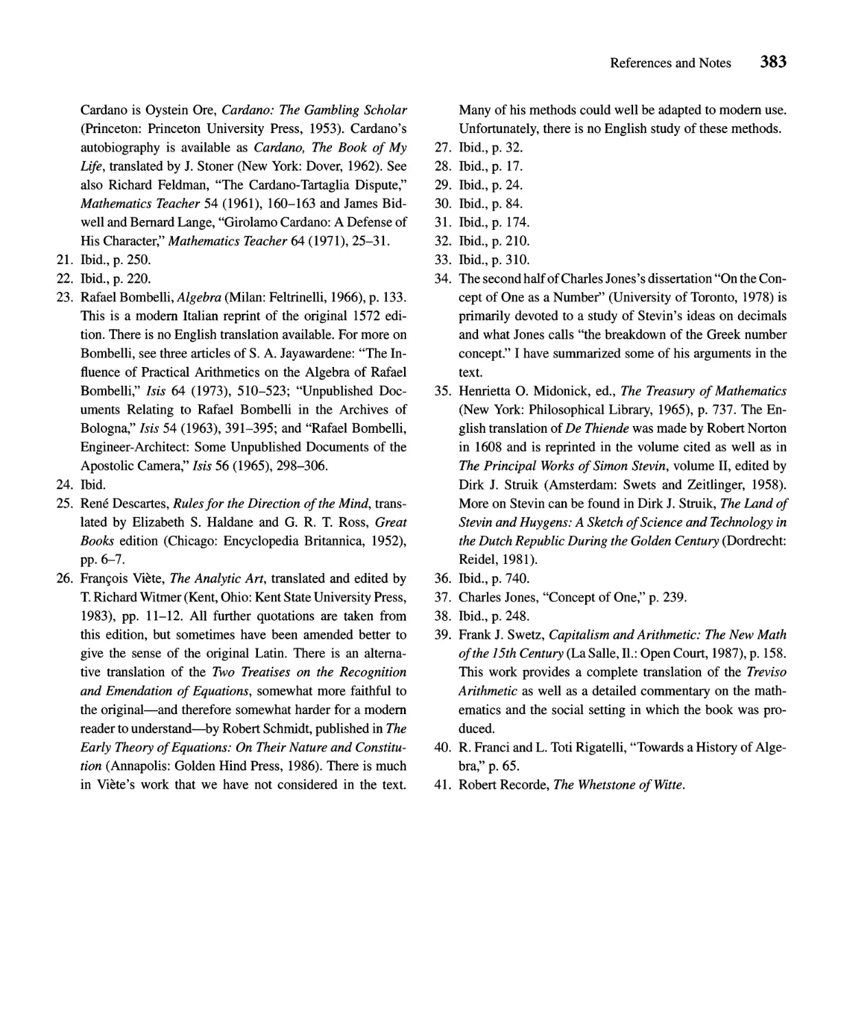
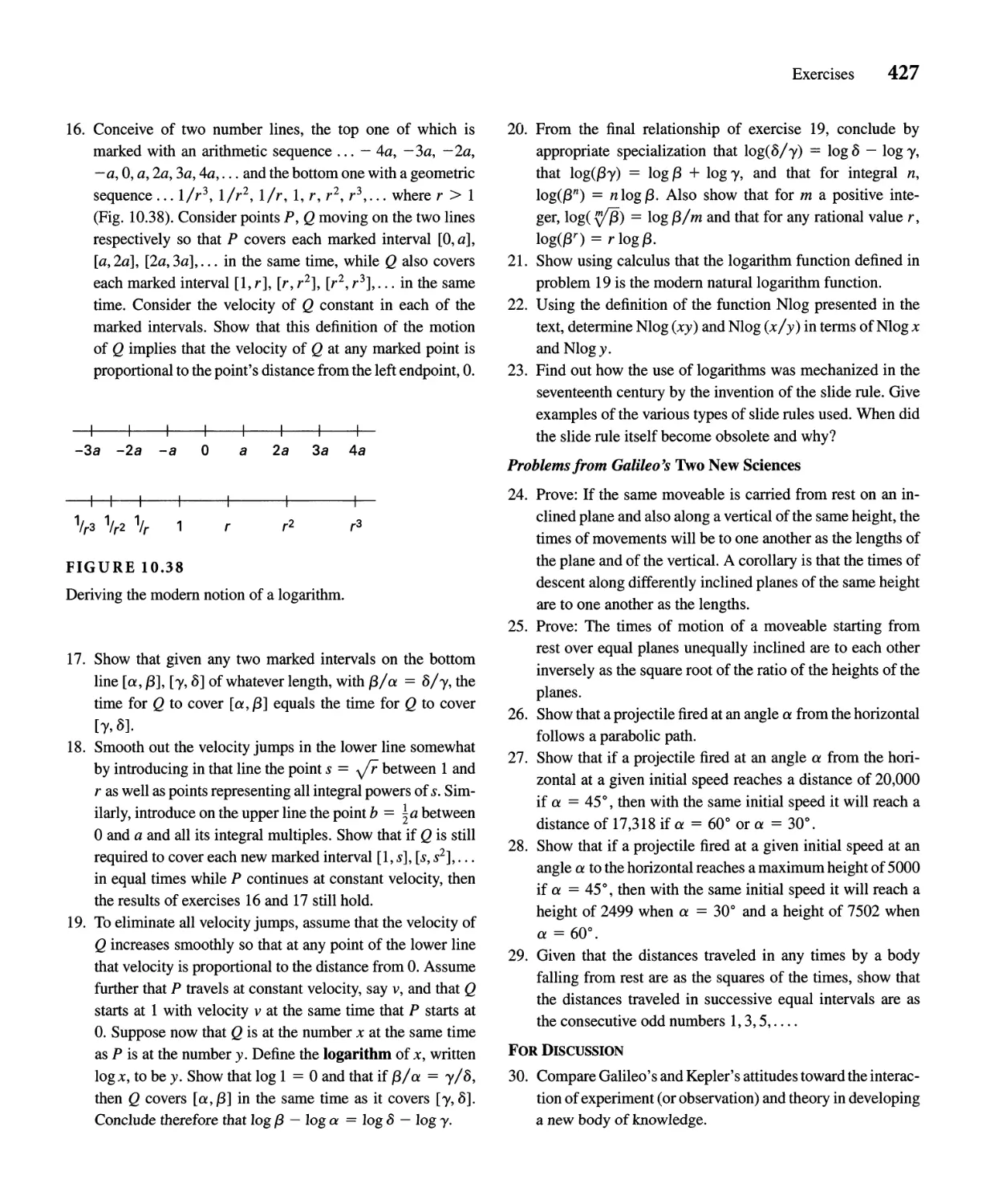
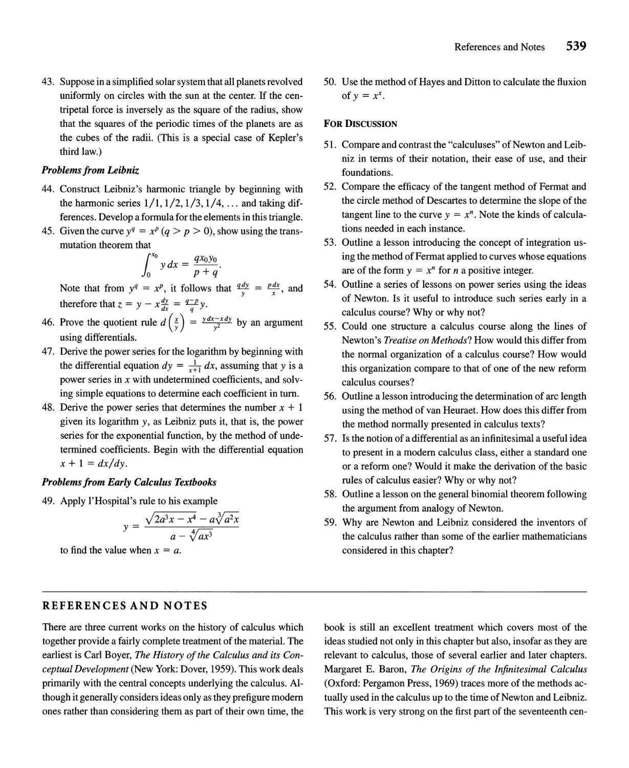
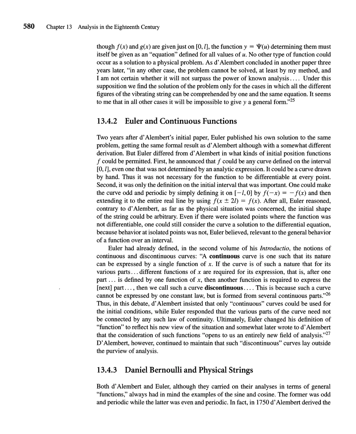
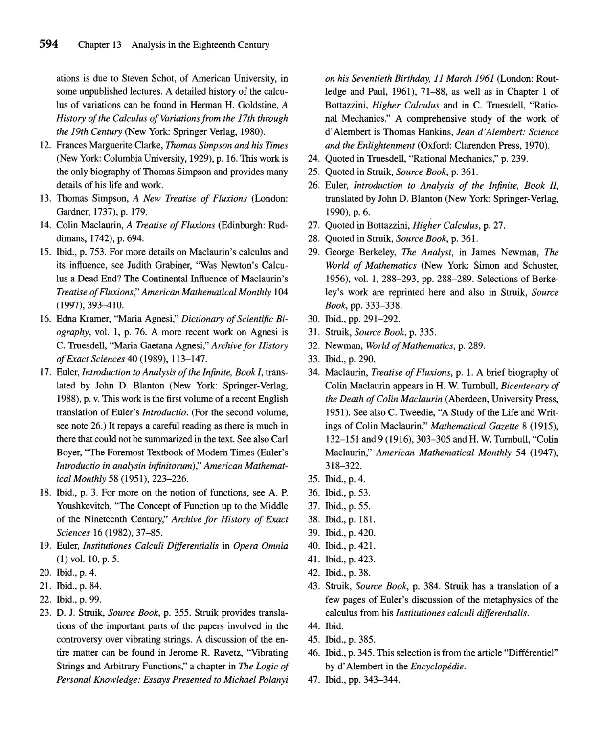
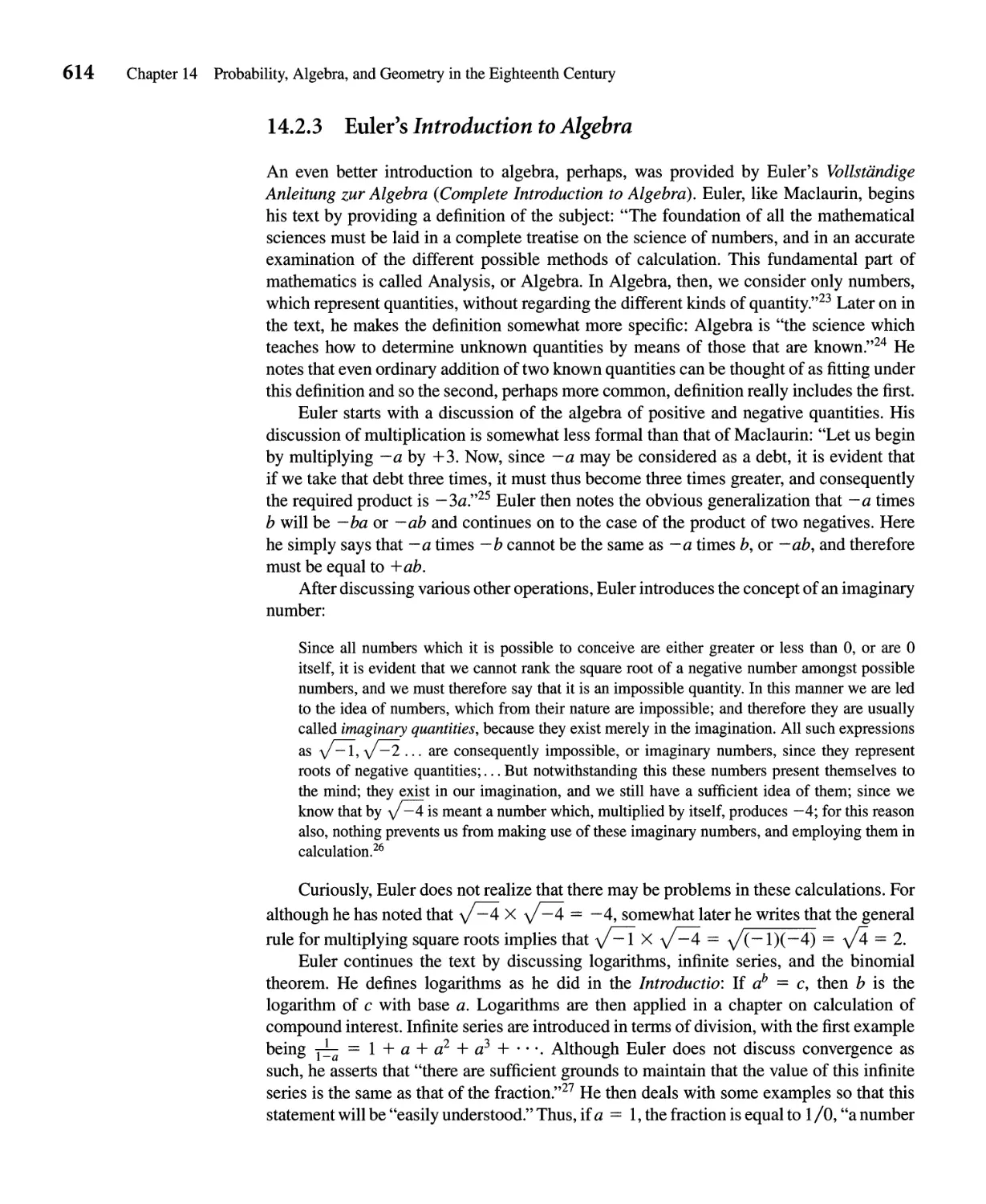
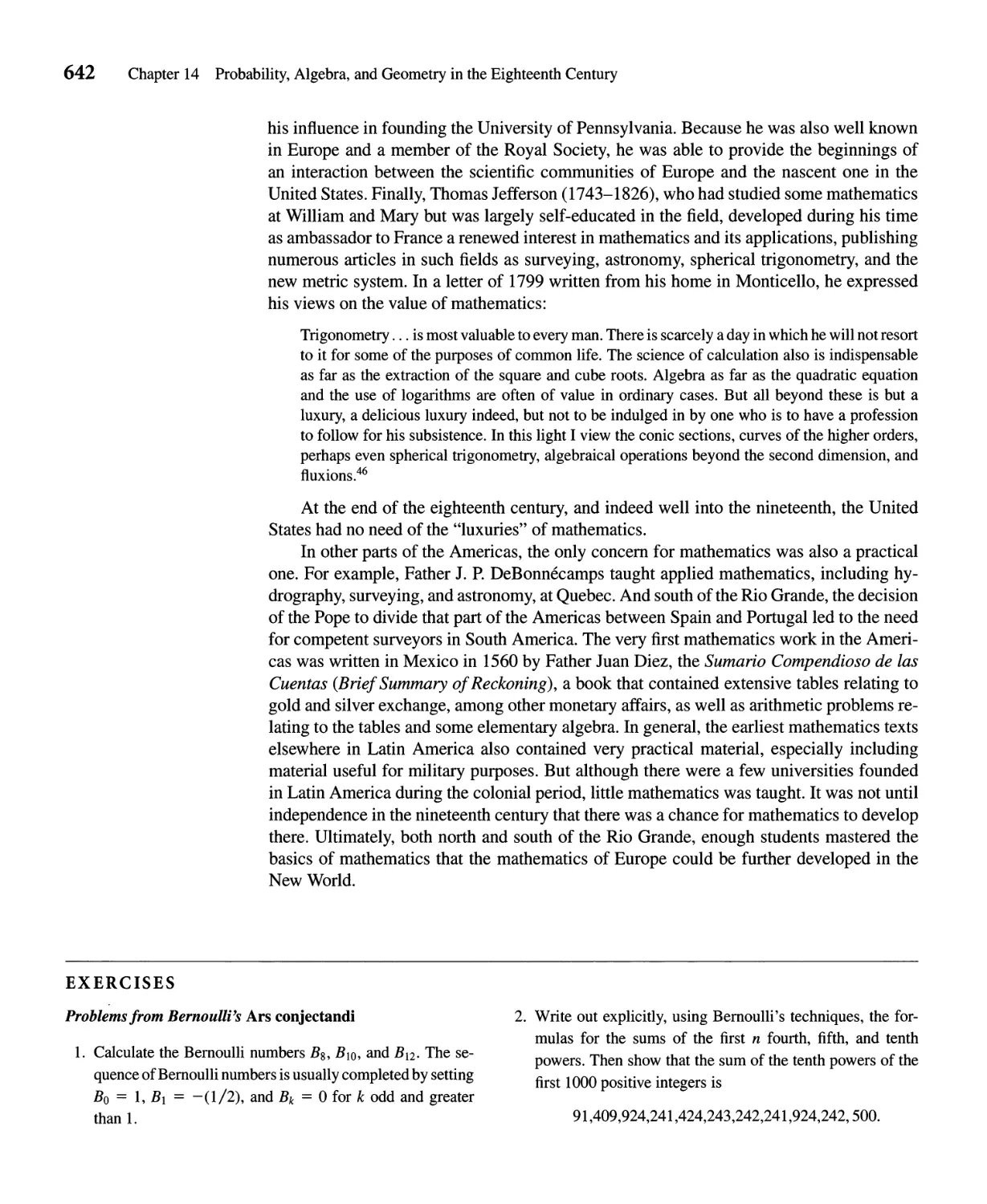
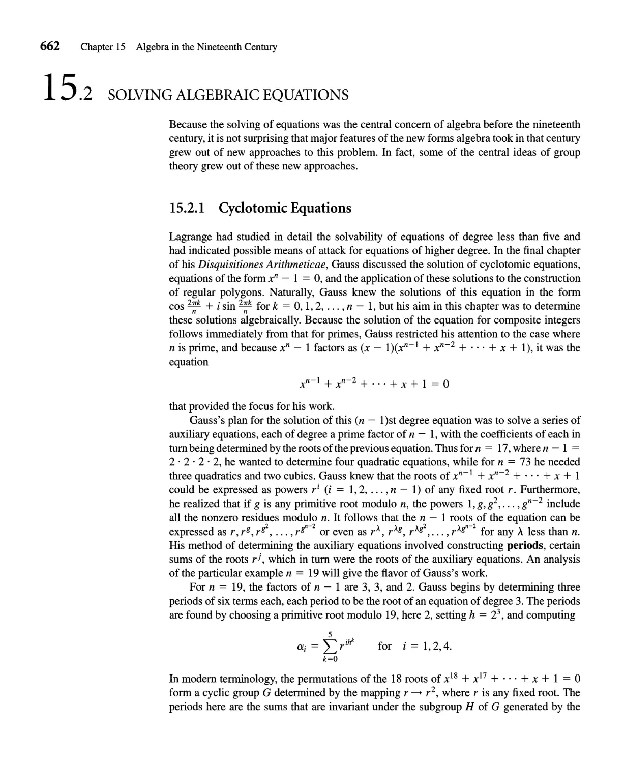
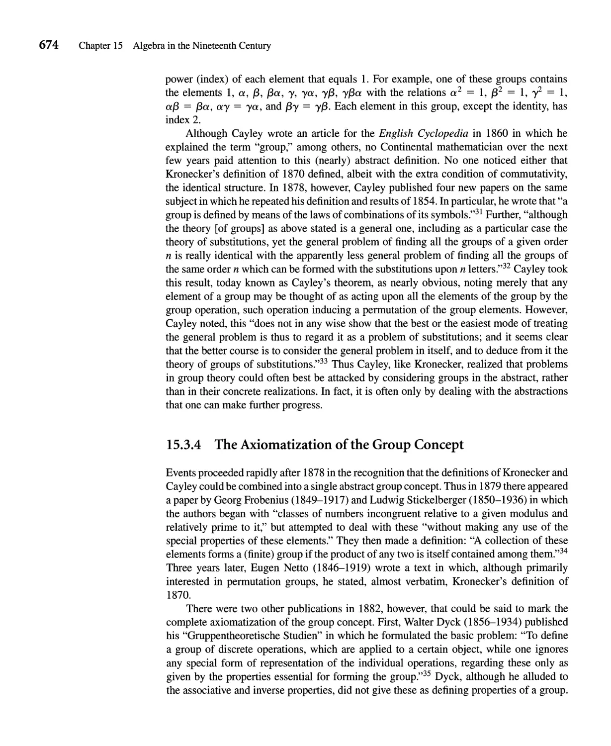
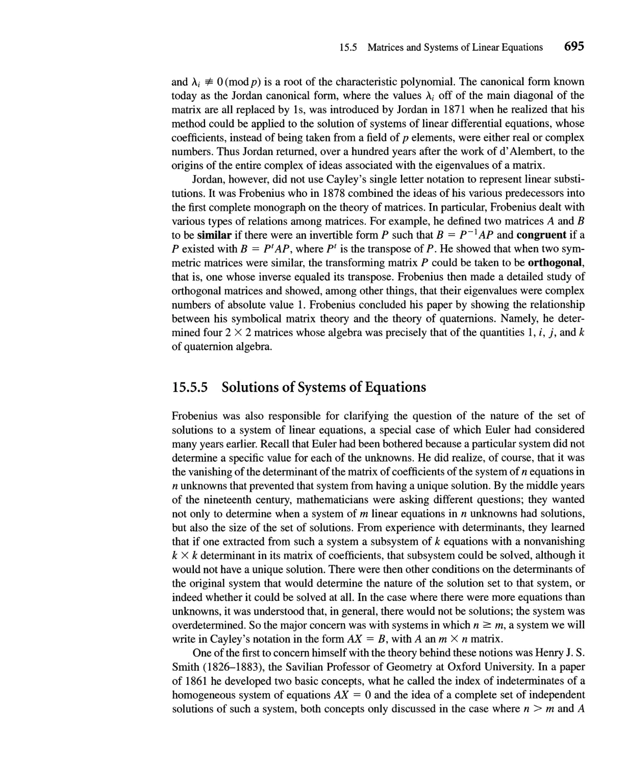
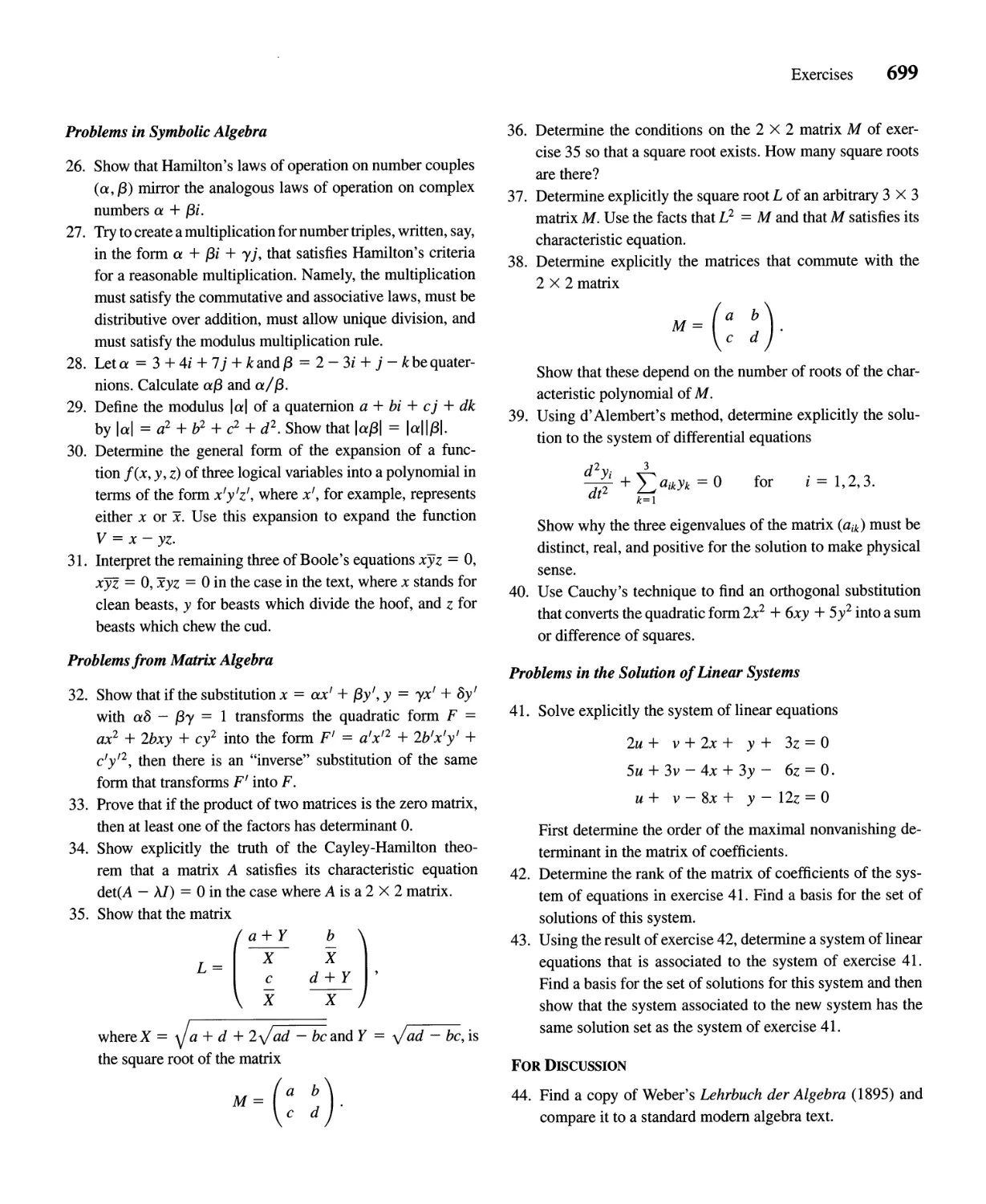
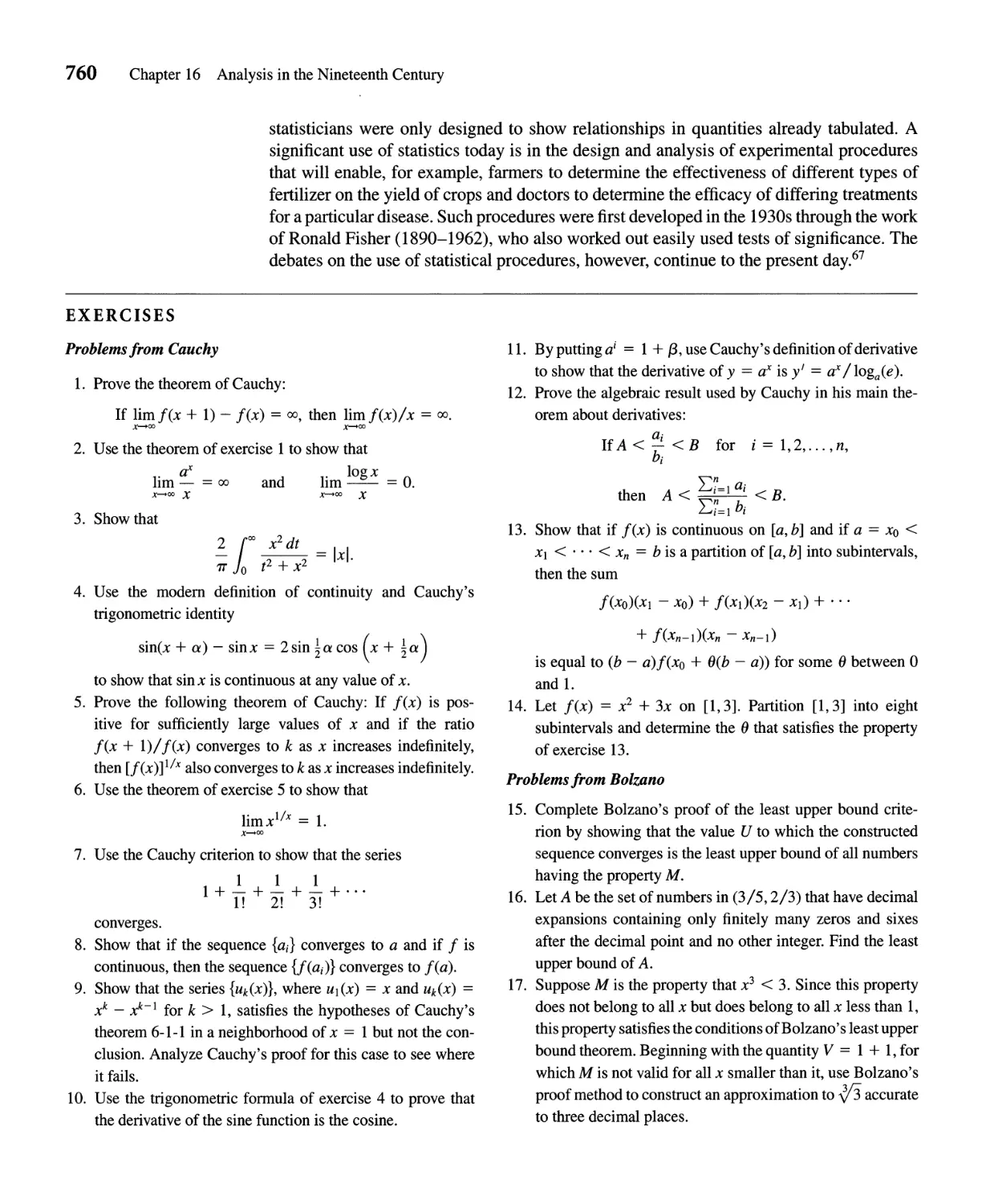
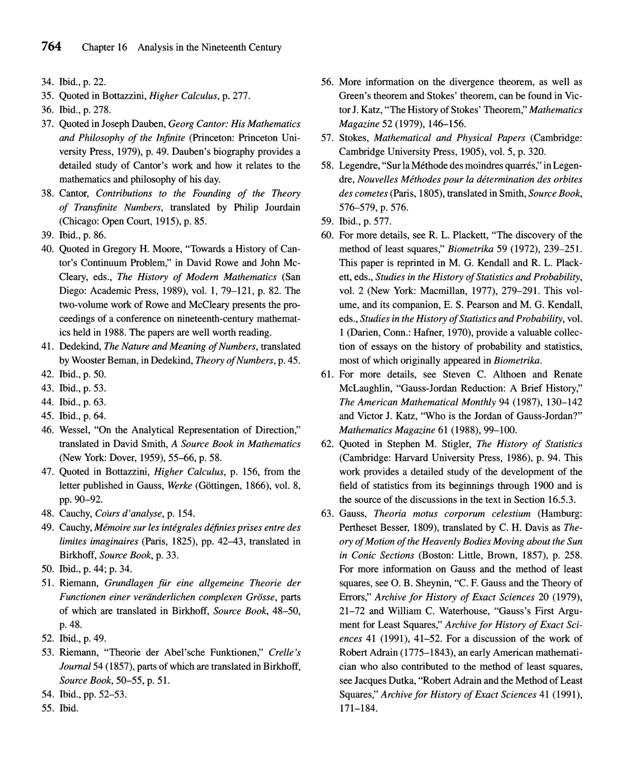
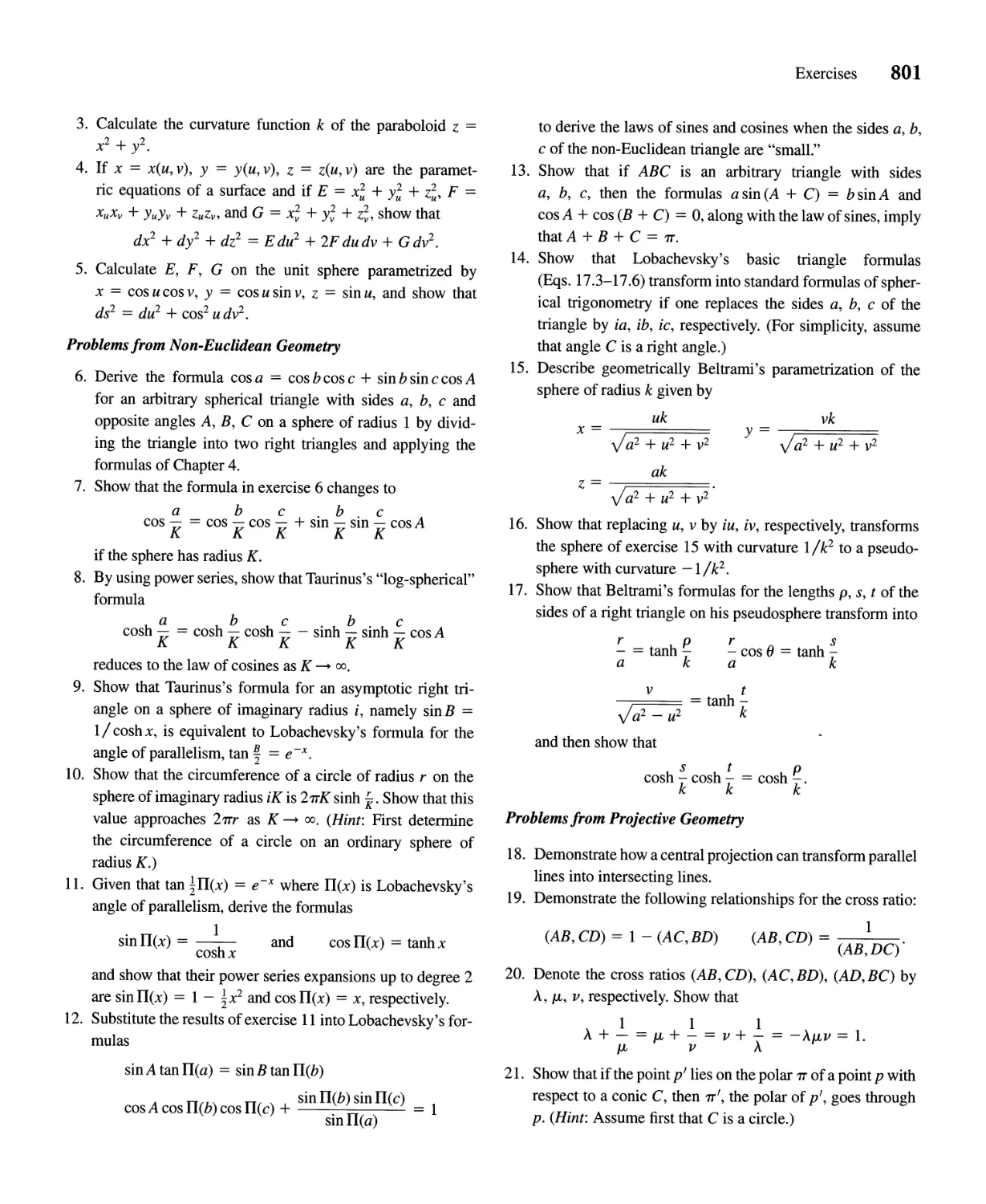
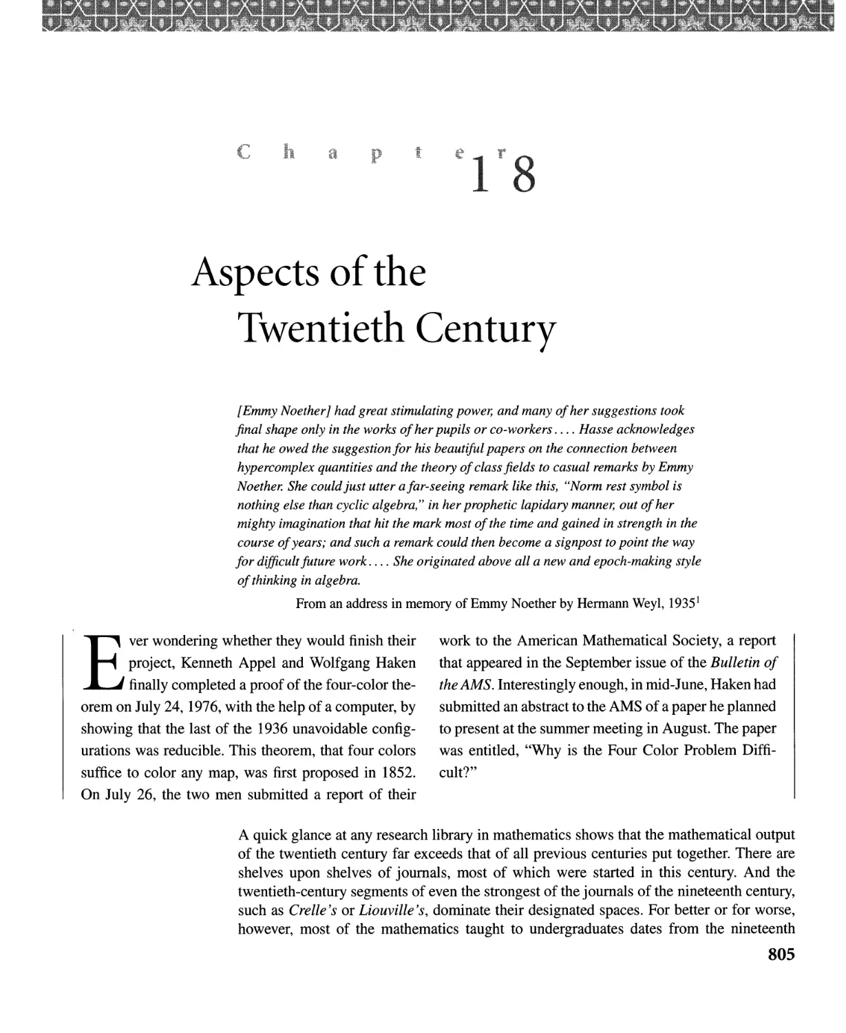
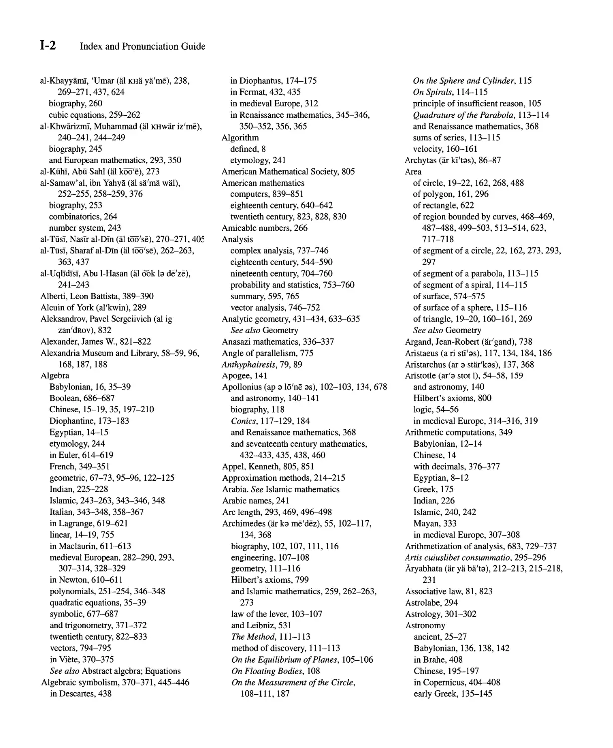
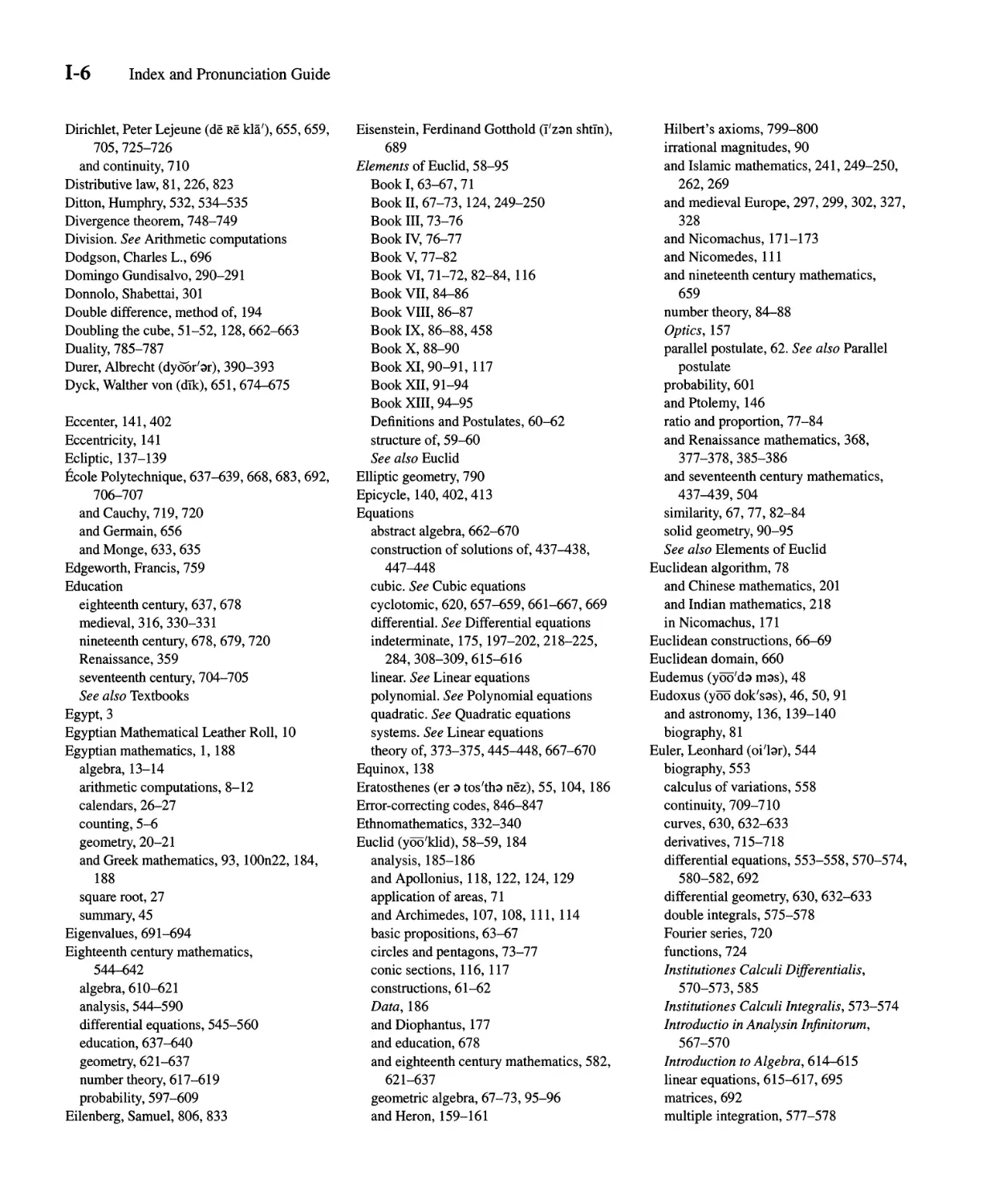
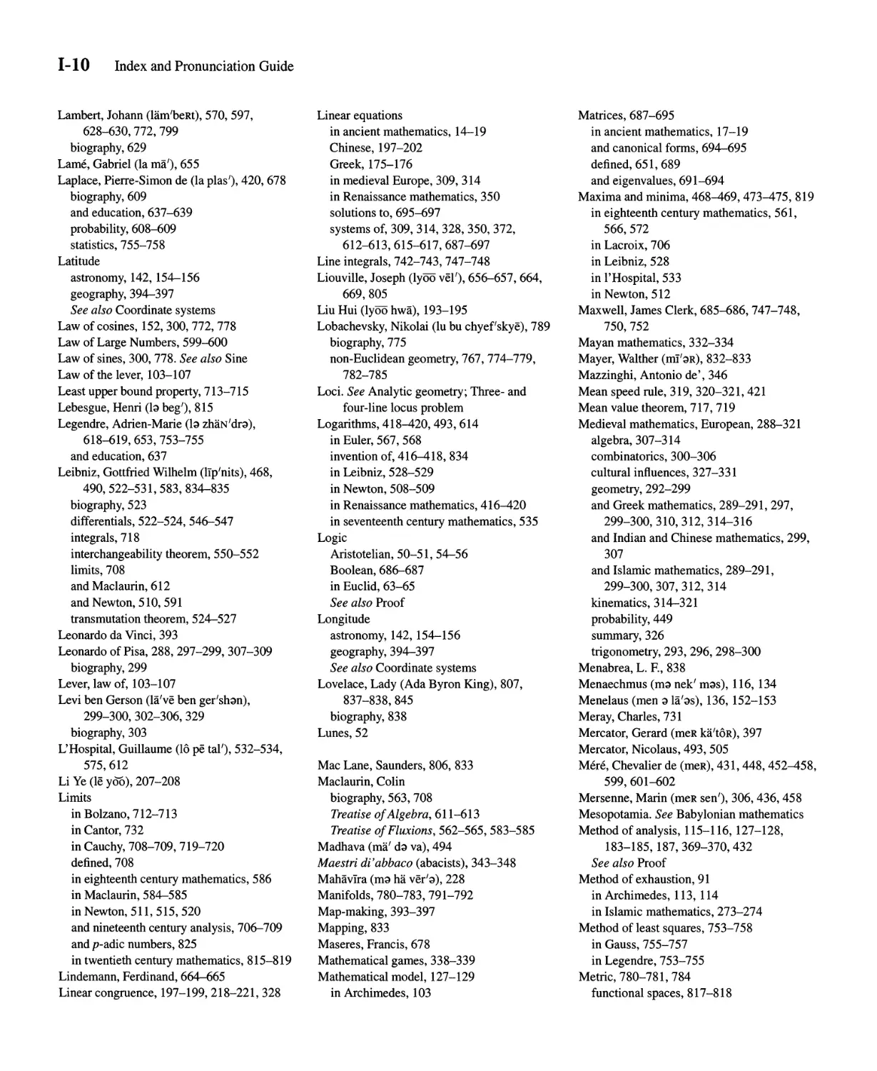
TIME LINE FOR THE HISTORY OF MATHEMATICS
3000 B.G.E.
1000 B.G.E.
o
800
3000-2000 B.C.E. 1000-500 B.C.E. 0-200 C.E. 800-1000
Egypt: Beginnings of India: Square root calculations, Egypt: Heron and practical India: Development of algebraic
hieroglyphic writing of numbers; Pythagorean theorem mathematics; Ptolemy and techniques
Building of pyramids at Giza China: Rod numerals, astronomy Iraq: AI-Khwarizmi and first
Iraq: Beginnings of cuneiform Pythagorean theorem Jordan: Nicomachus and number algebra text
writing of numbers in Greece: Beginnings of theory Egypt: Abu Kamil and advanced
Mesopotamia theoretical geometry Israel: Nehemiah and practical algebraic techniques
2000-1000 B.C.E. 500-300 B.C.E. geometry United States: Geometry used in
Egypt: Rhind and Moscow papyri Greece: Plato, Aristotle, and 200-400 architectural designs in
written; Ideas of linear axiomatic mathematics; Egypt: Diophantus and number Mississippian civilization
equations, volumes, areas Discovery of incommensurabil- theory; Hypatia and Spain: Gerbert learns Arabic
Iraq: Cuneiform mathematical ity; Eudoxus and proportionality commentaries number system
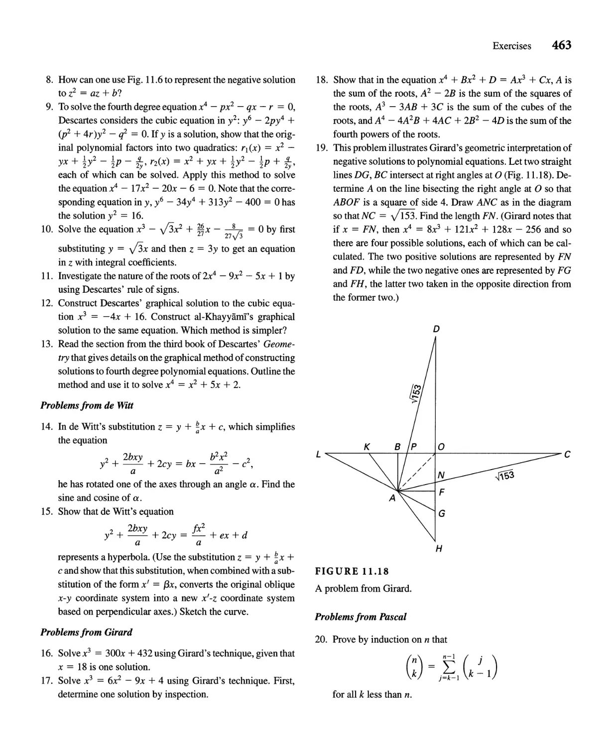
tablets written with Egypt: Euclid and the Elements China: Liu Hui and mathematical
Pythagorean theorem, quadratic surveying techniques
equations, systems of equations 300-0 B.C.E.
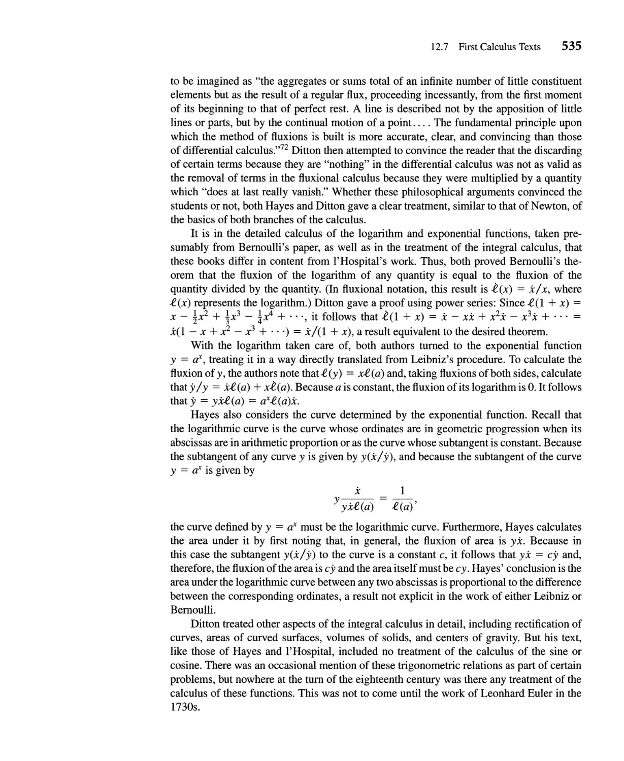
China: Square and cube roots, 4OO-BOO
systems of linear equations Italy: Boethius and elementary
Italy: Archimedes and mathematics
theoretical physics Mexico: Development of Mayan
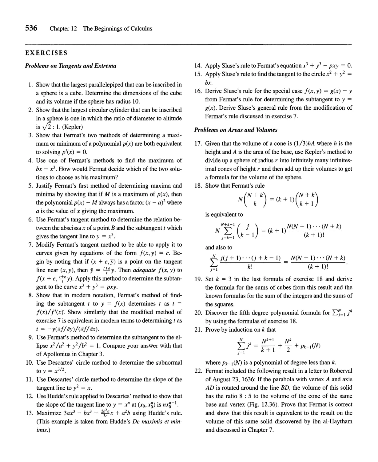
Egypt: Apollonius and conic numeration and astronomy
sections India: Aryabhata and
Turkey: Hipparchus and trigonometry; Brahmagupta
trigonometry and indeterminate analysis;
Development of Hindu-Arabic
decimal place-value number
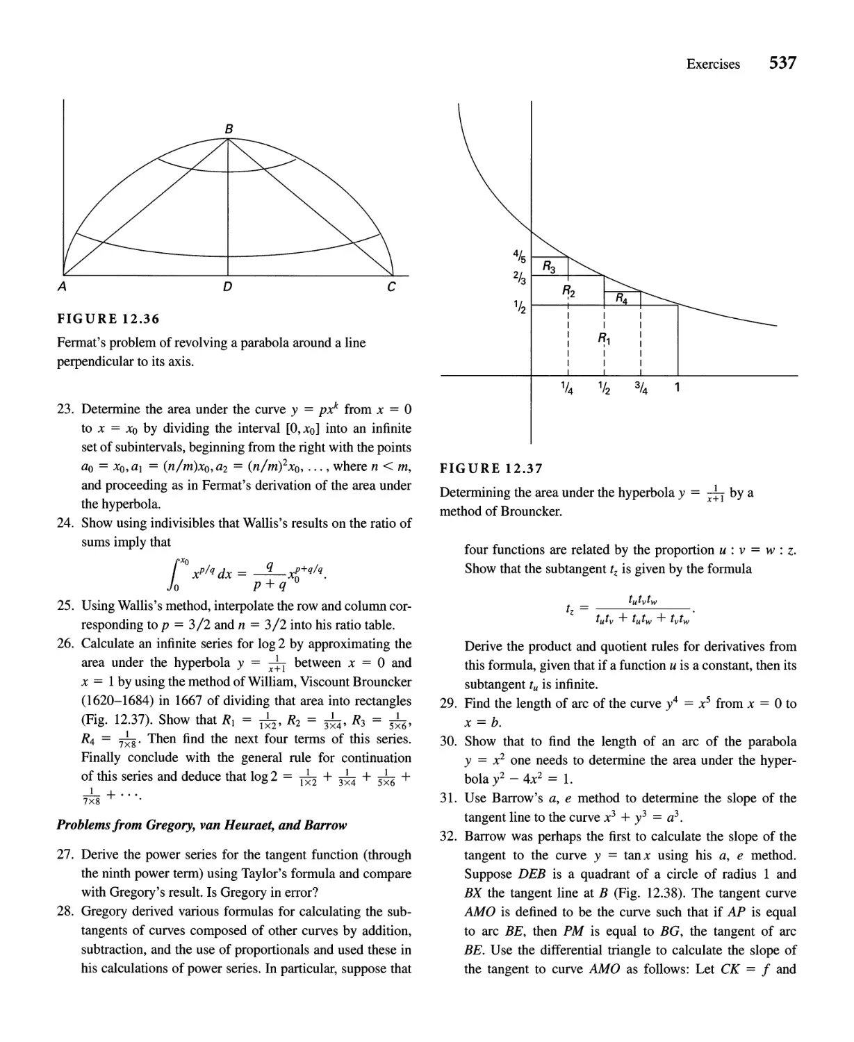
system
China: First tangent tables
3000 B.G.E.
1000 B.G.E.
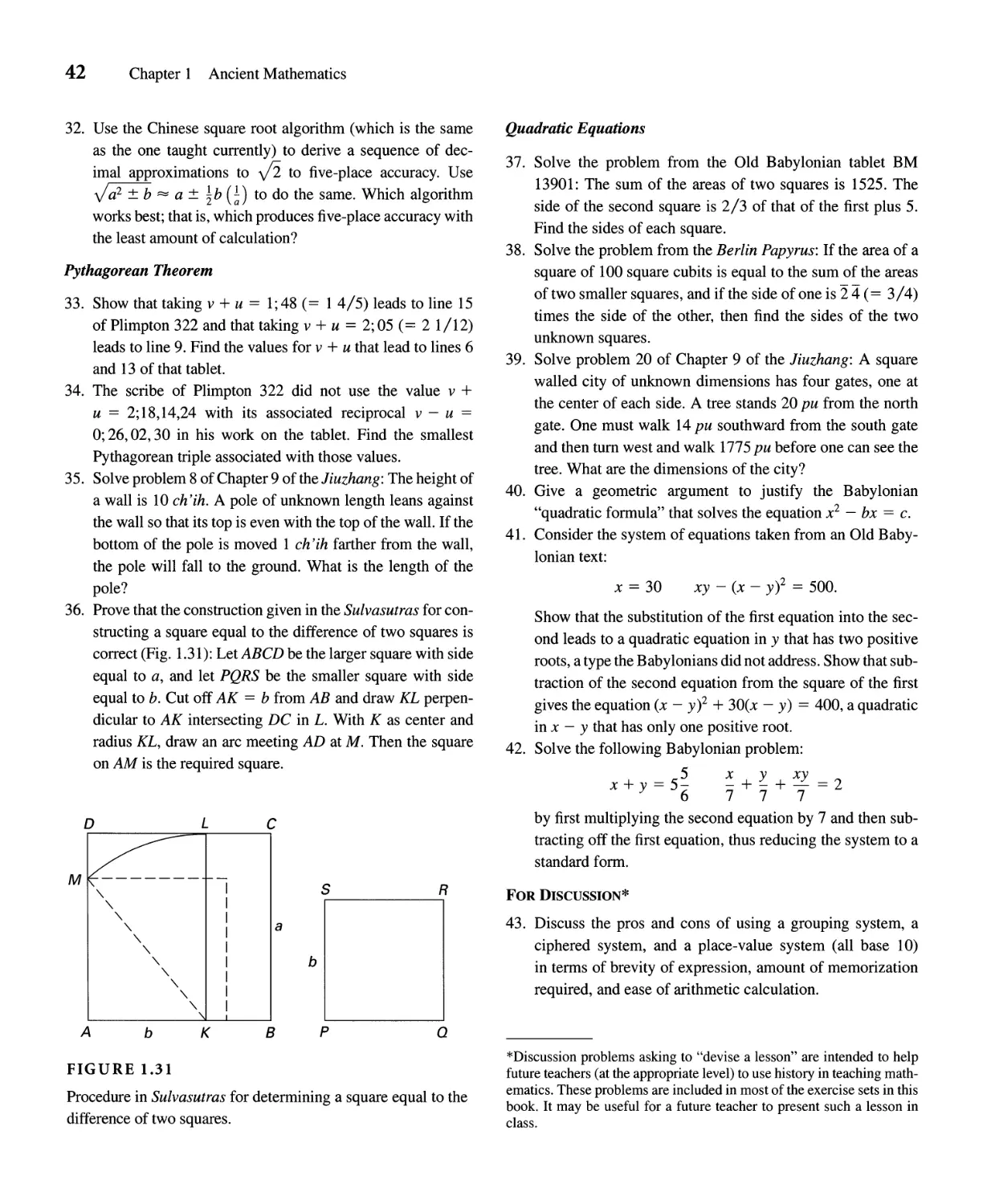
o
800
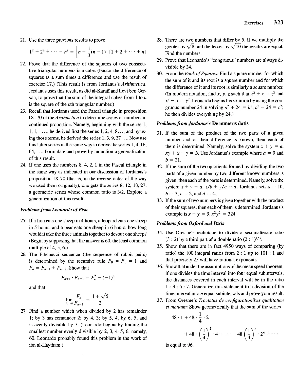
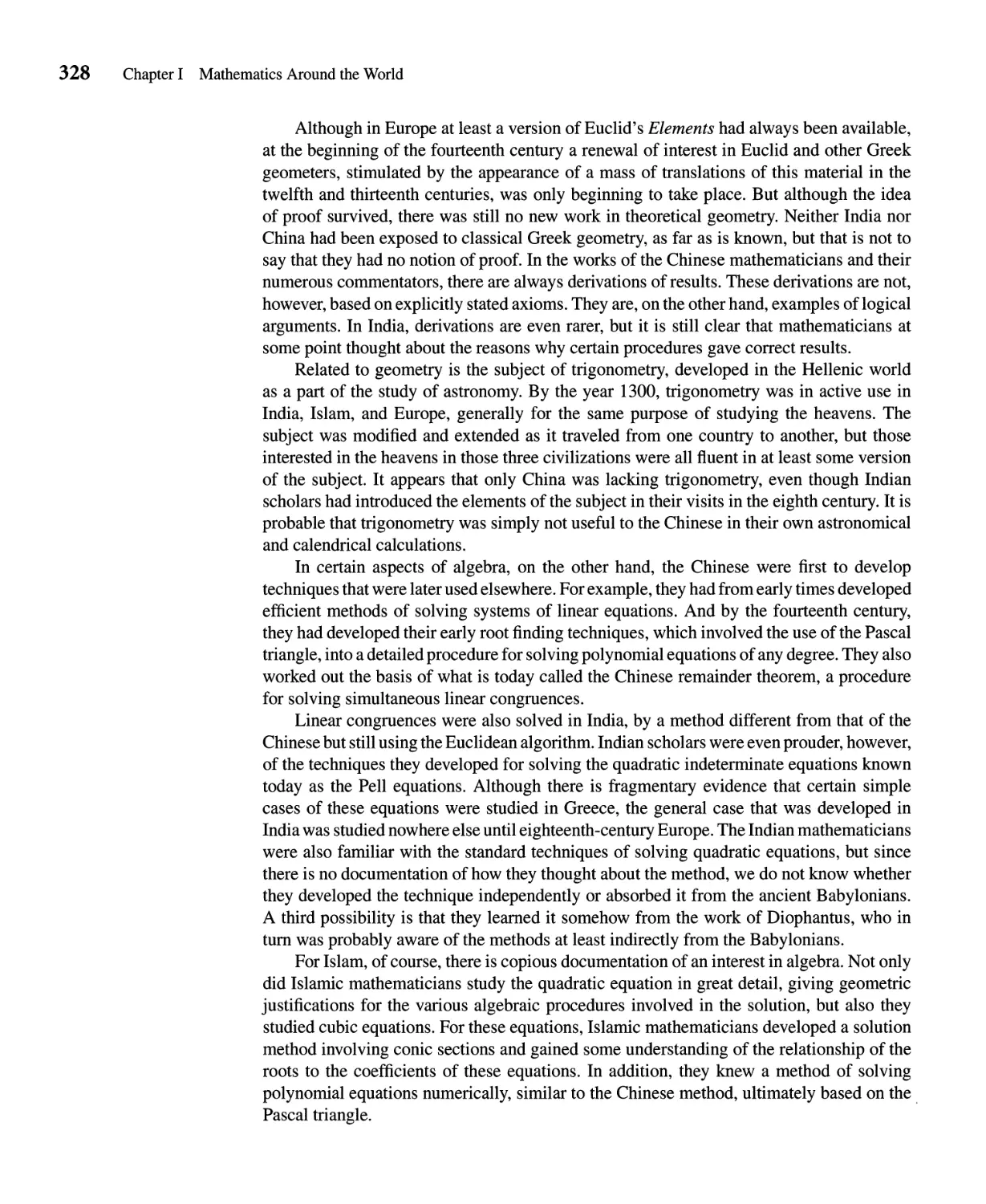
1000
1200
1600
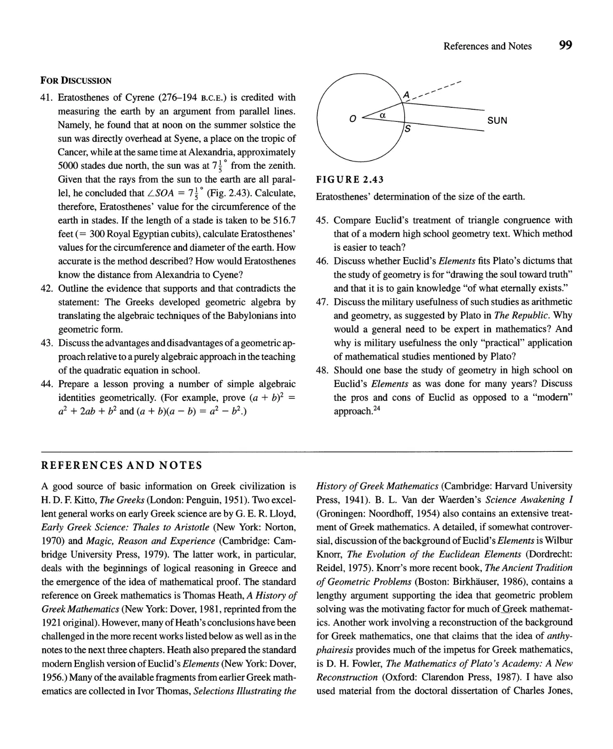
1800
1000-1200 1200-1400 1600-1700 1800-1900
Iraq: AI Karaji, induction, and Iran: Nasir ai-Din al-lUsi and Kepler, Newton, and celestial Algebraic number theory
Pascal triangle trigonometry physics Galois theory
Egypt: Ibn al Haytham, sums France: Jordanus and advanced Descartes, Fermat, and analytic Groups and fields
of powers, and volumes of algebra; Levi ben Gerson and geometry
paraboloids induction; Oresme and Napier, Briggs, and logarithms Quaternions and the discovery
kinematics of noncom mutative algebra
Iran: Omar Khayyam and the Girard, Descartes, and the
geometric solution of cubic England: Velocity, acceleration, theory of equations Theory of matrices
equations and the mean speed theorem The arithmetization of analysis
Pascal, Fermat, and elementary
India: AI BirOni and spherical China: Chinese remainder probability Development of complex
trigonometry; Bhaskara and the theorem; Solution of polynomial analysis
Pell equation equations Pascal, Desargues, and
China: Pascal triangle used to Peru: Quipus used for record projective geometry Vector analysis
solve equations keeping Newton, Leibniz, and the Differential geometry
Spain: Arabic works translated invention of calculus Non Euclidean geometry
1400-1600
in Latin; Abraham ibn Ezra and India: Discovery of power series 1700-1800 Projective geometry
combinatorics
for sine, cosine, and arctangent Development of techniques for Foundations of geometry
Italy: Leonardo of Pisa and Italy: Algebraic solution of the solving ordinary and partial
introduction of Islamic differential equations 1900-2000
mathematics cubic equation Set theory
Germany: Perspective and Development of the calculus of
United States: Astronomical functions of several variables Growth of topology
alignments in Anasazi buildings geometry
Attempts to give logically Algebraization of mathematics
in the Southwest England: New algebra and correct foundations to the
Zimbabwe: Construction of trigonometry texts calculus Influence of computers
Great Zimbabwe structures Poland: Copernicus and the Lagrange and the analysis of the
heliocentric system solution of polynomial equations
France: Viete and algebraic
symbolism
1000
1200
1600
1800
A HISTORY OF
MATHEMATICS
Al
Introduction
A HISTORY OF
MATHEMATICS
Al
Introduction
5;eC()fld Editi()n
VICTORJ. KATZ
University of the District of Columbia
T£.T ADDISON-WESLEY
An imprint of Addison Wesley Longman, Inc.
Reading, Massachusetts · Menlo Park, California · New York · Harlow, England
Don Mills, Ontario · Sydney · Mexico City · Madrid · Amsterdam
To Phyllis,
for long talks,
long walks,
and afternoon naps
Reprinted with corrections, November 1998
Sponsoring Editor: Jennifer Albanese
Production Supervisor: Rebecca Malone
Project Manager: Barbara Pendergast
Prepress Services Buyer: Caroline Fell
Manufacturing Supervisor: Ralph Mattivello
Design Direction: Susan Carsten
Text and Cover Design: Rebecca Lloyd Lemna
Cover Photo: @ SuperStock
Art Editor: Sarah E. Mendelsohn
Composition and Prepress Services: Integre Technical Publishing Co., Inc.
Library of Congress Cataloging-in-Publication Data
Katz, Victor J.
A history of mathematics: an introduction / Victor J. Katz.
2nd ed.
p. cm.
Includes bibliographical references and index.
ISBN 0-321-01618-1
1. Mathematics-History. I. Title.
QA21.K33 1998
510'.9-dc21
98-9273
CIP
Copyright @ 1998 by Addison-Wesley Educational Publishers, Inc.
All rights reserved. No part of this publication may be reproduced, stored in a retrieval system, or transmitted,
in any form or by any means, electronic, mechanical, photocopying, recording, or otherwise, without the prior
written permission of the publisher. Printed in the United States of America.
3 4 5 6 7 8 9 10-MA-0099
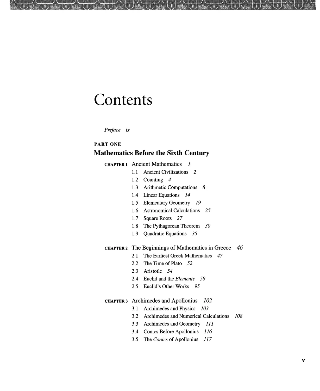
Contents
Preface lX
PART ONE
Mathematics Before the Sixth Century
CHAPTER 1 Ancient Mathematics 1
1.1 Ancient Civilizations 2
1.2 Counting 4
1.3 Arithmetic Computations 8
1.4 Linear Equations 14
1.5 Elementary Geometry 19
1.6 Astronomical Calculations 25
1.7 Square Roots 27
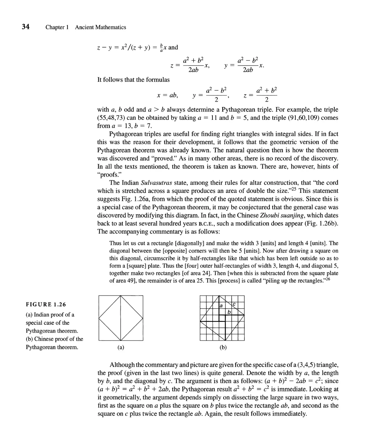
1.8 The Pythagorean Theorem 30
1.9 Quadratic Equations 35
CHAPTER 2 The Beginnings of Mathematics in Greece 46
2.1 The Earliest Greek Mathematics 47
2.2 The Time of Plato 52
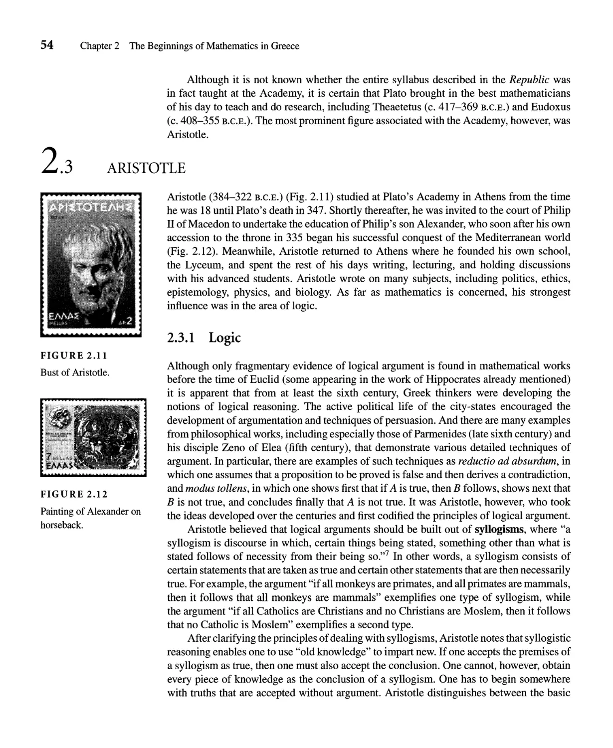
2.3 Aristotle 54
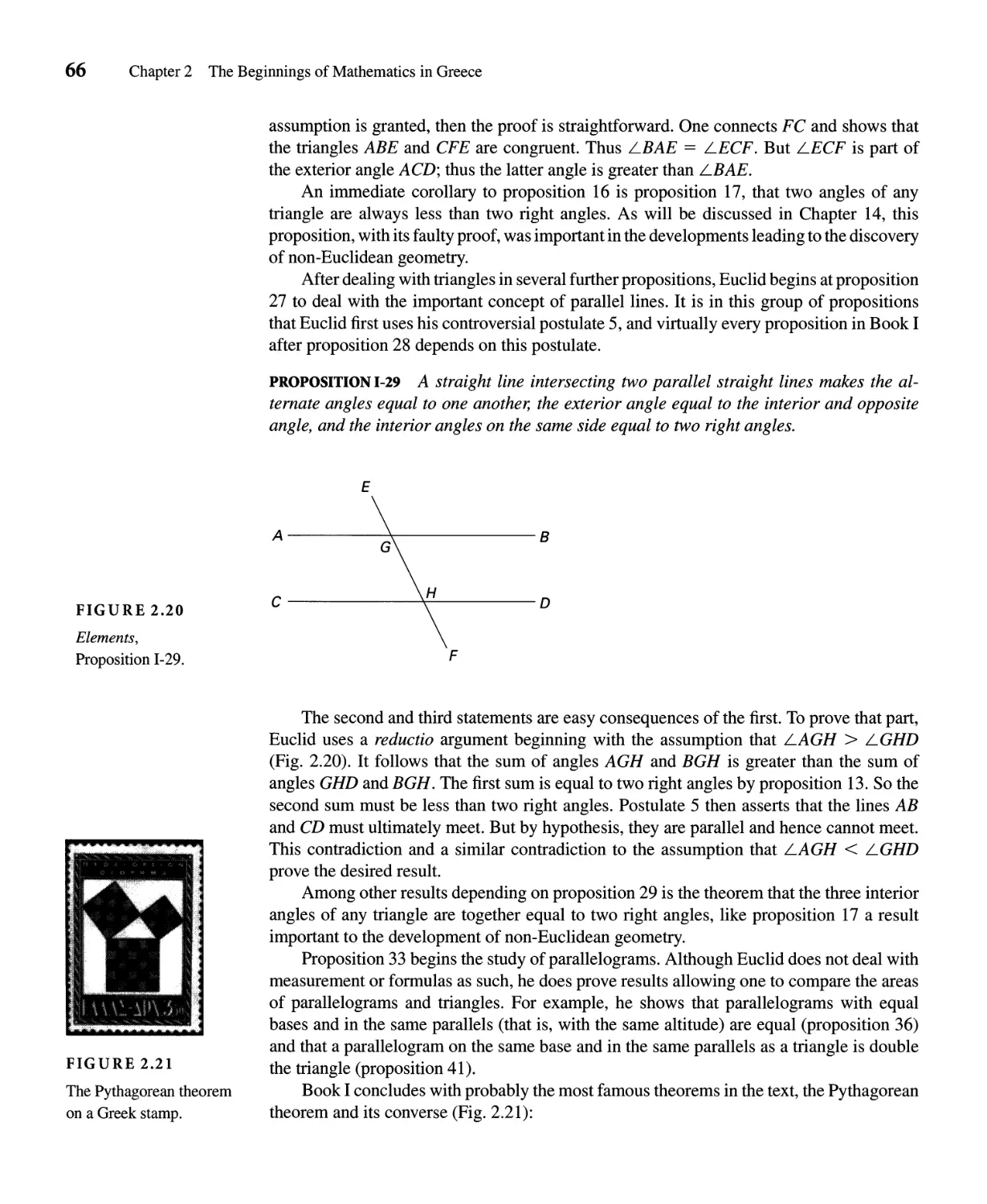
2.4 Euclid and the Elements 58
2.5 Euclid's Other Works 95
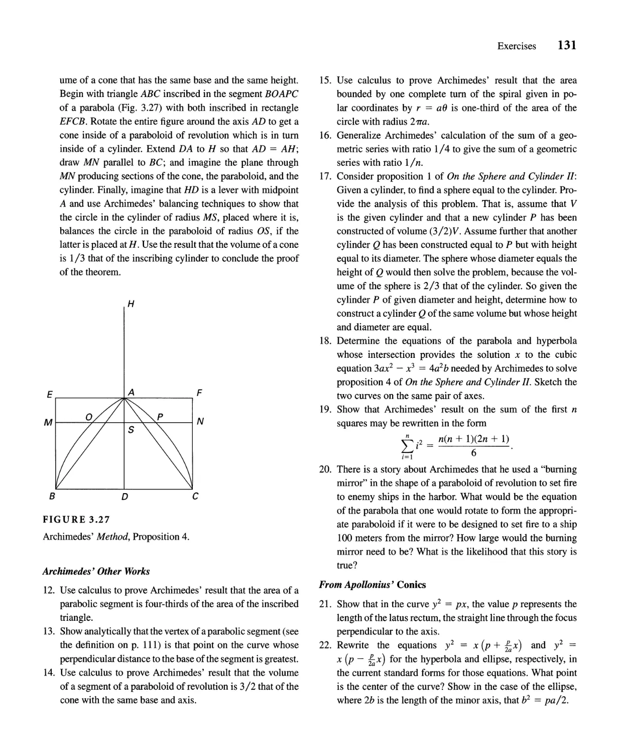
CHAPTER 3 Archimedes and Apollonius 102
3.1 Archimedes and Physics 103
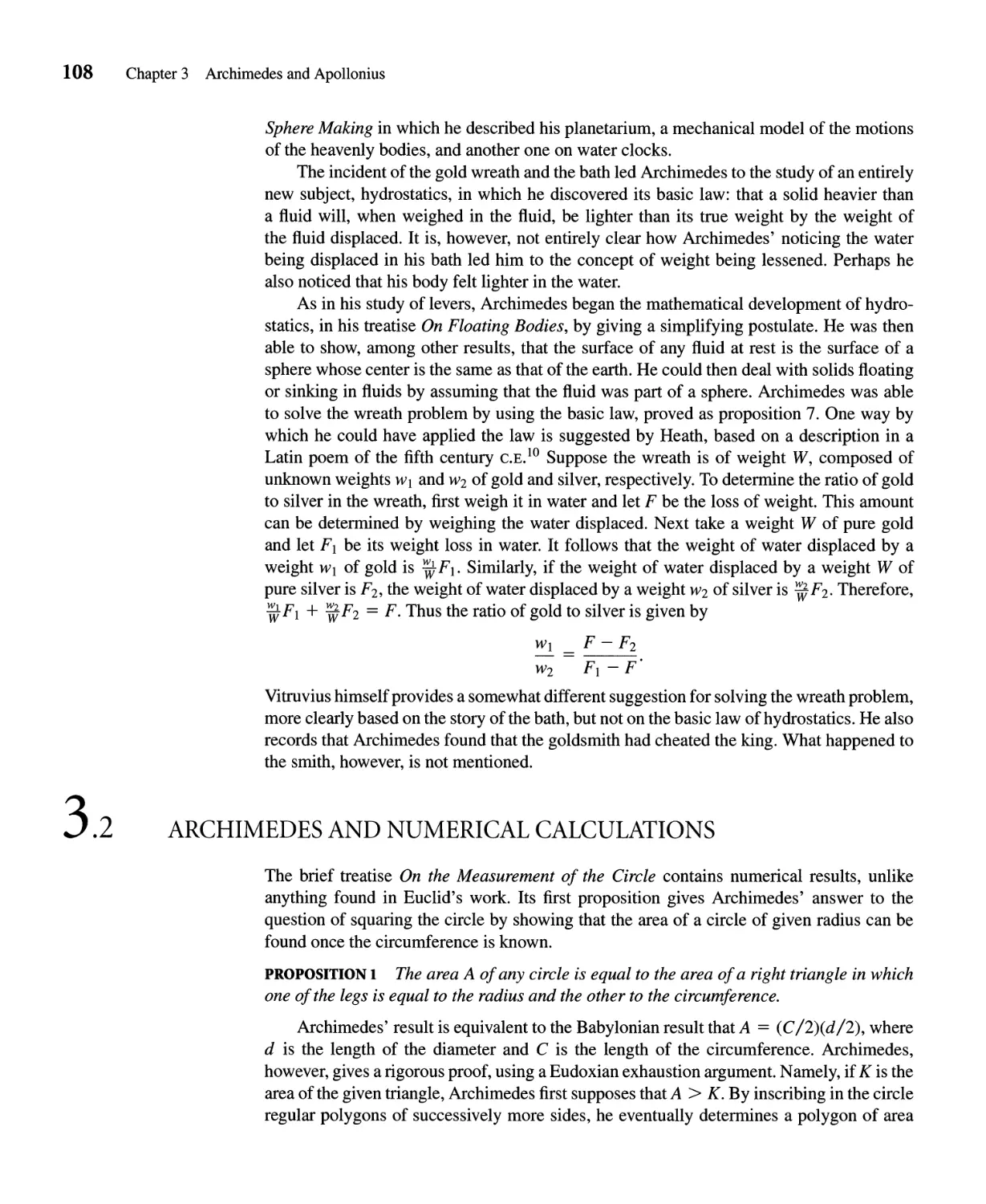
3.2 Archimedes and Numerical Calculations 108
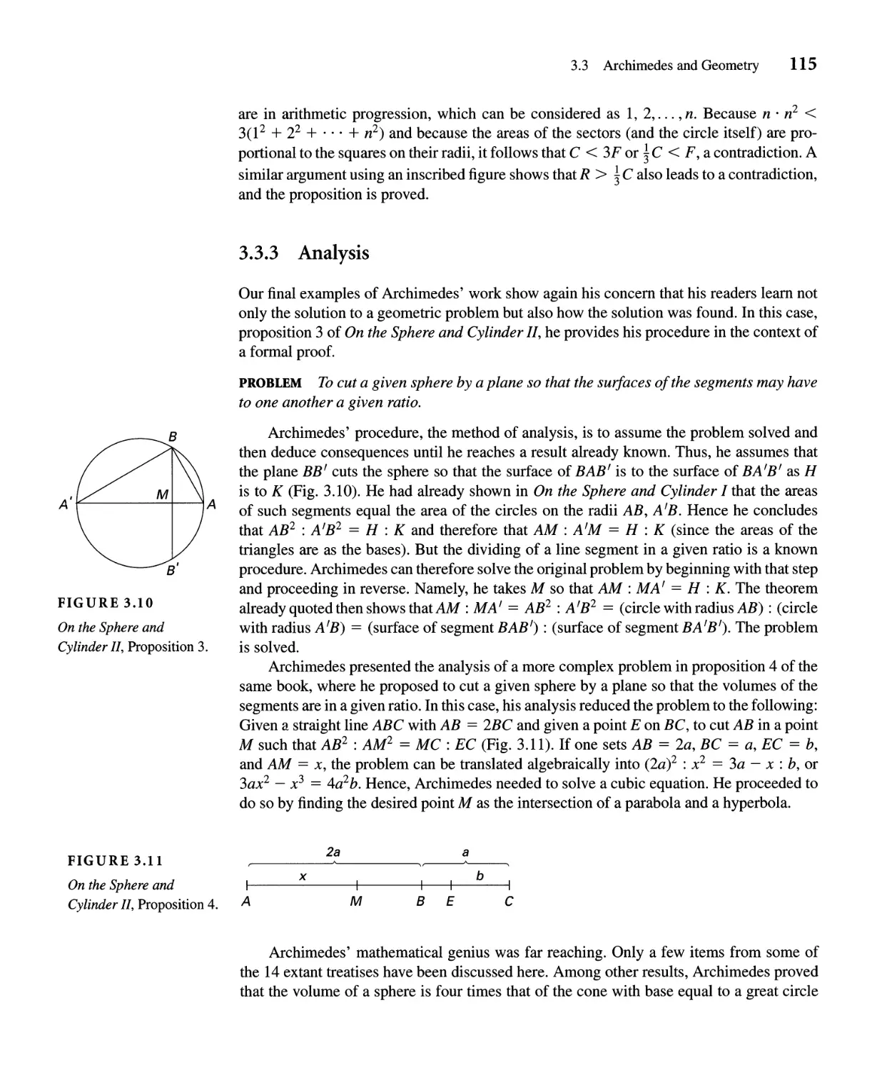
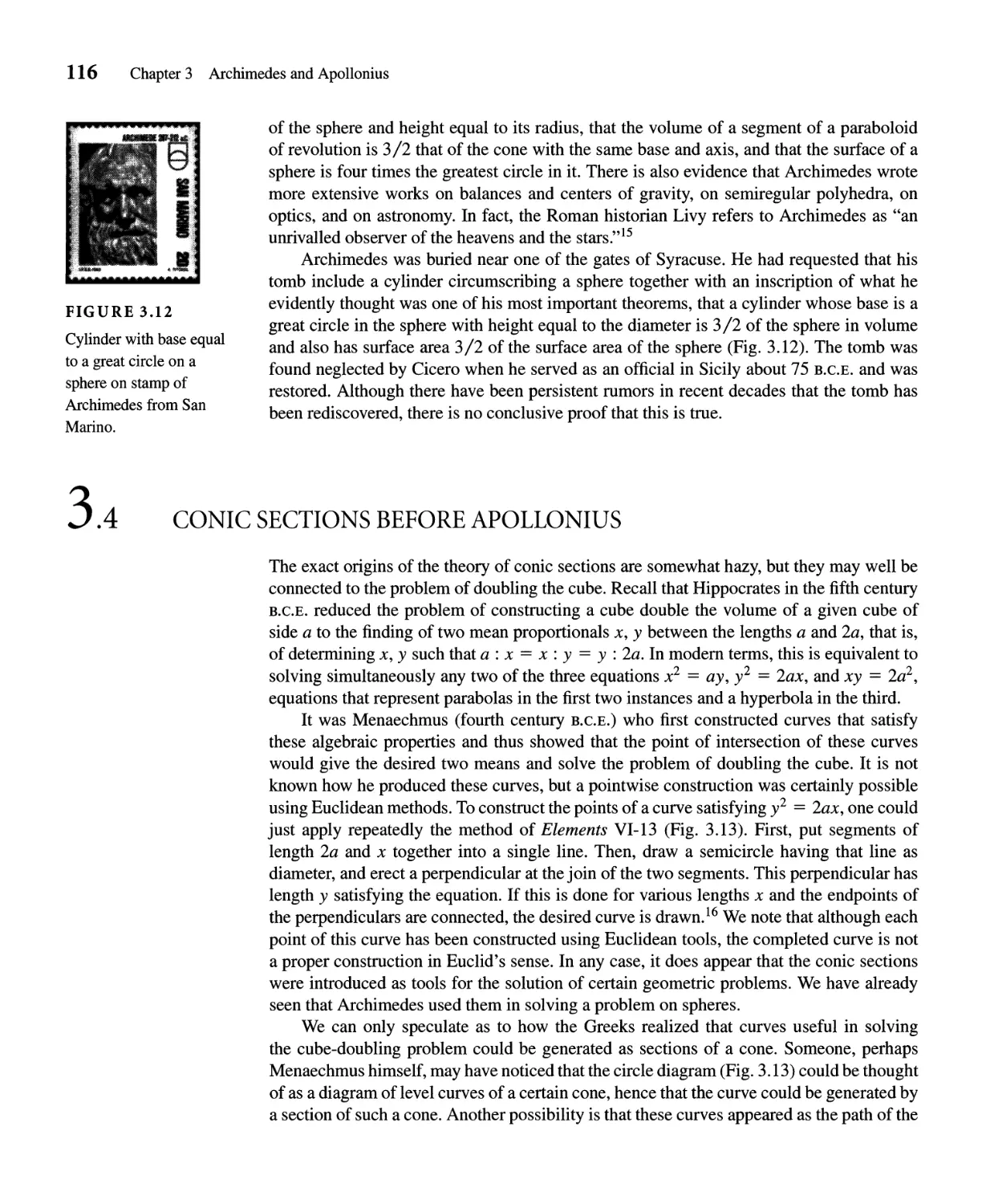
3.3 Archimedes and Geometry 111
3.4 Conics Before Apollonius 116
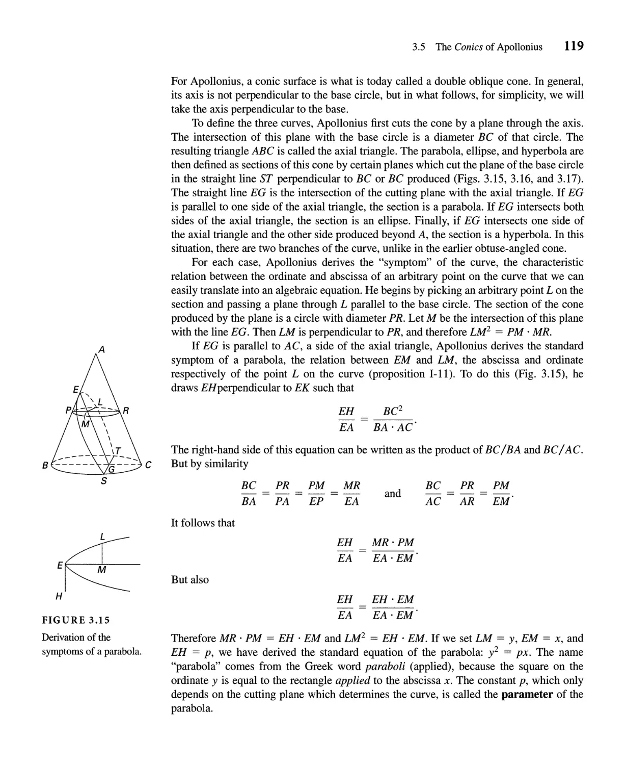
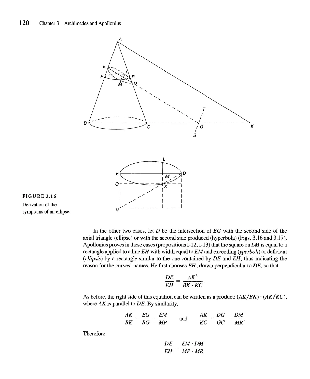
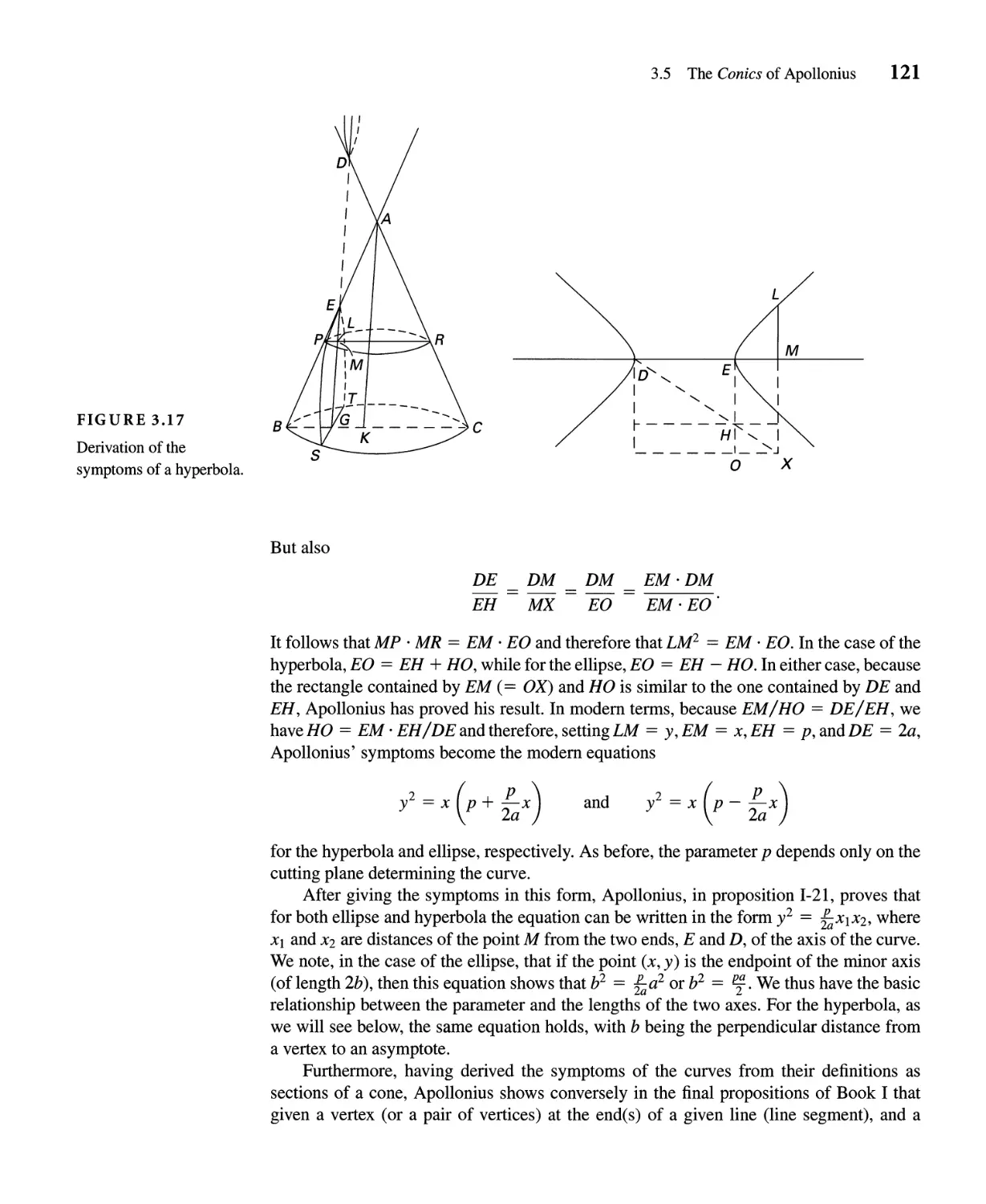
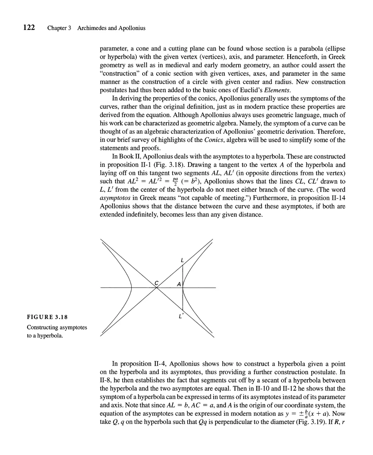
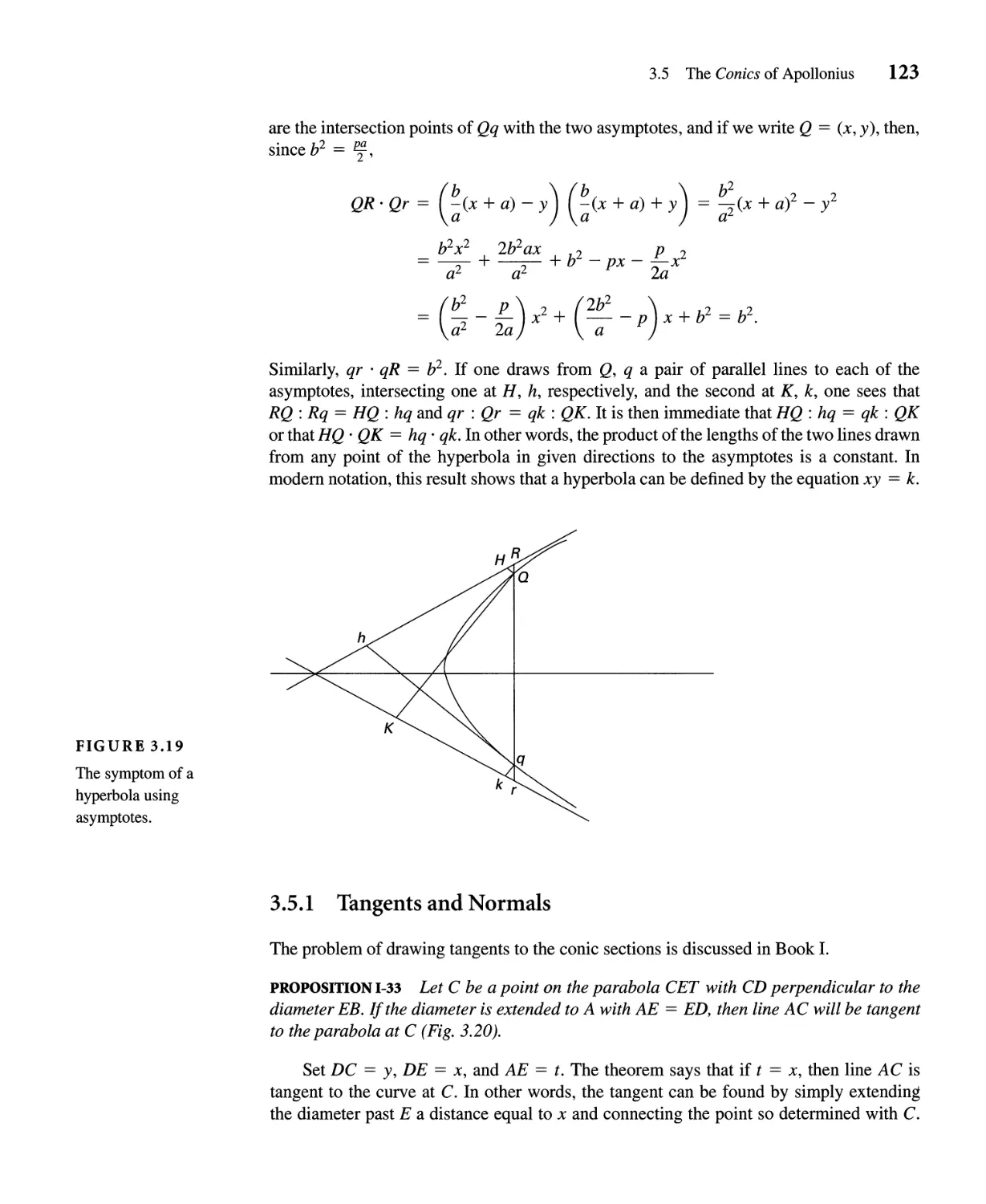
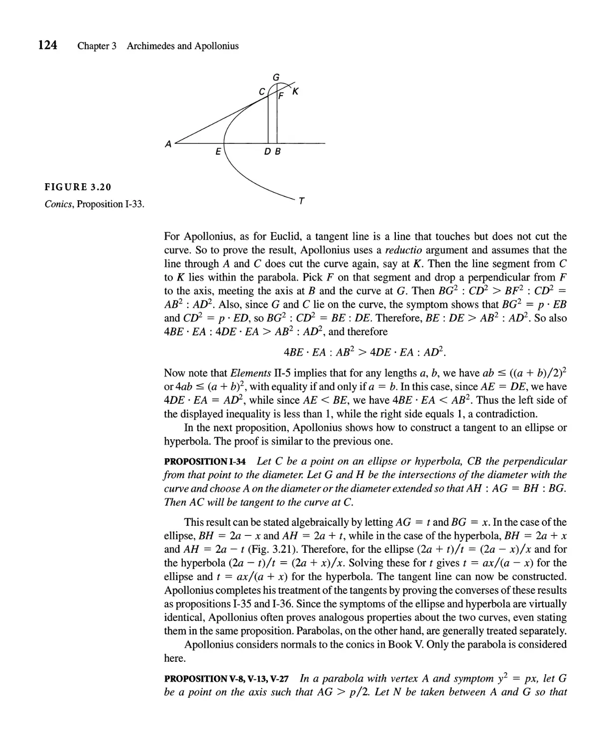
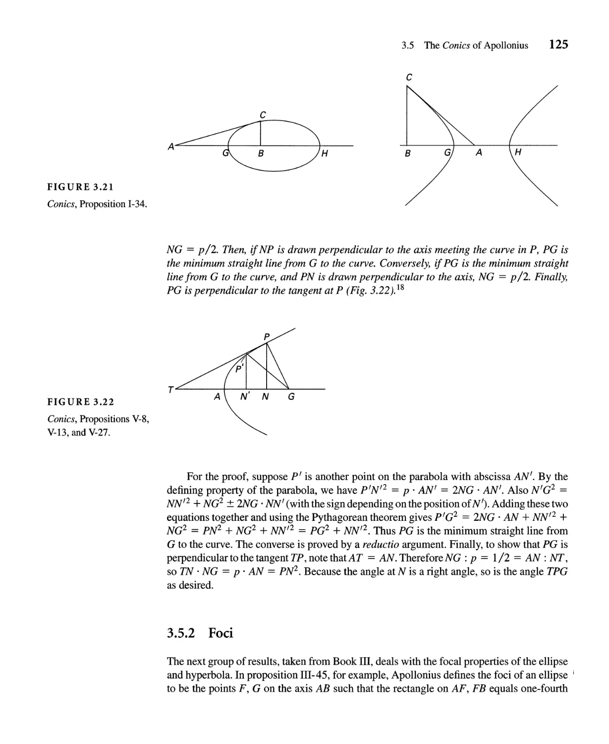
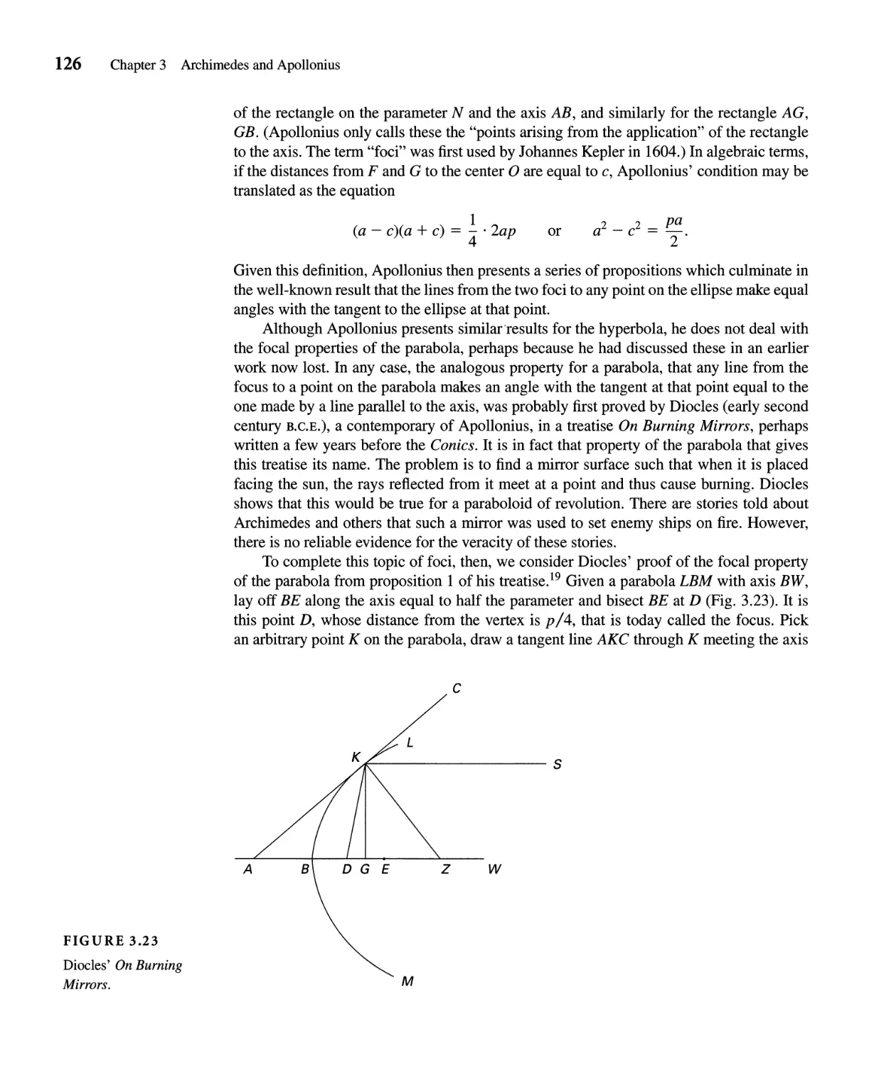
3.5 The Conics of Apollonius 117
v
.
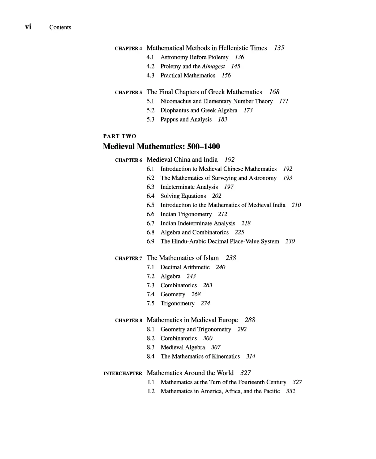
VI Contents
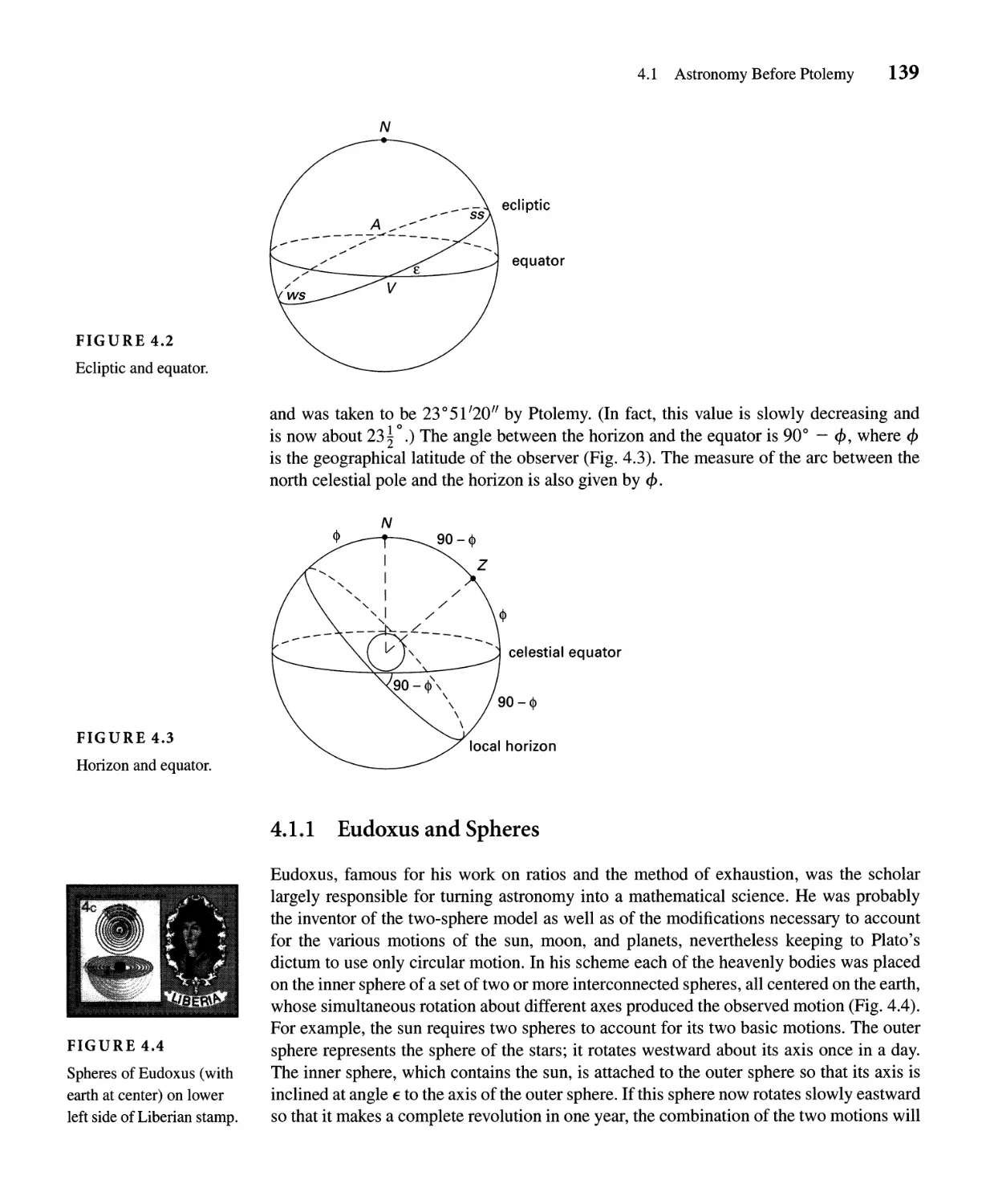
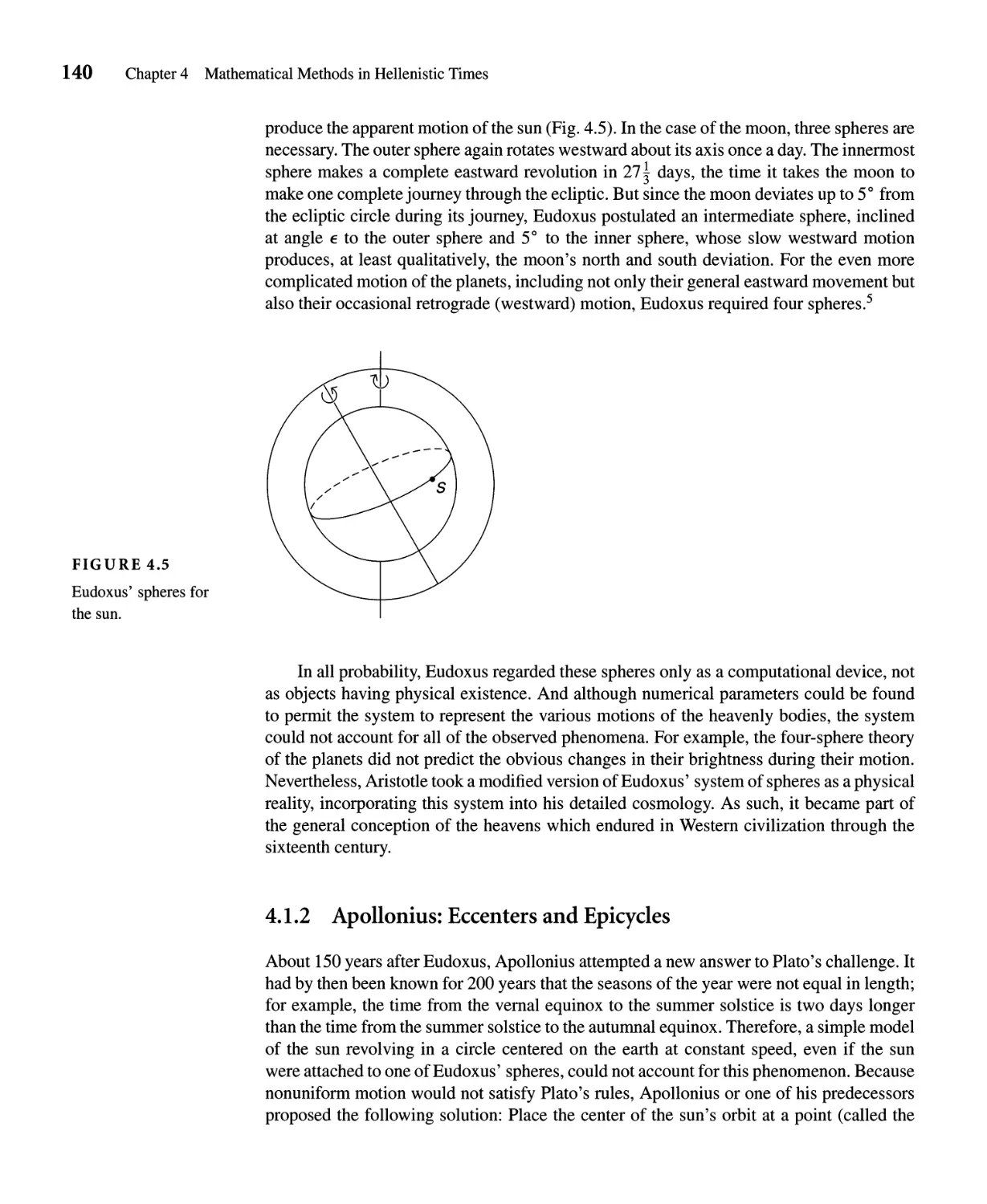
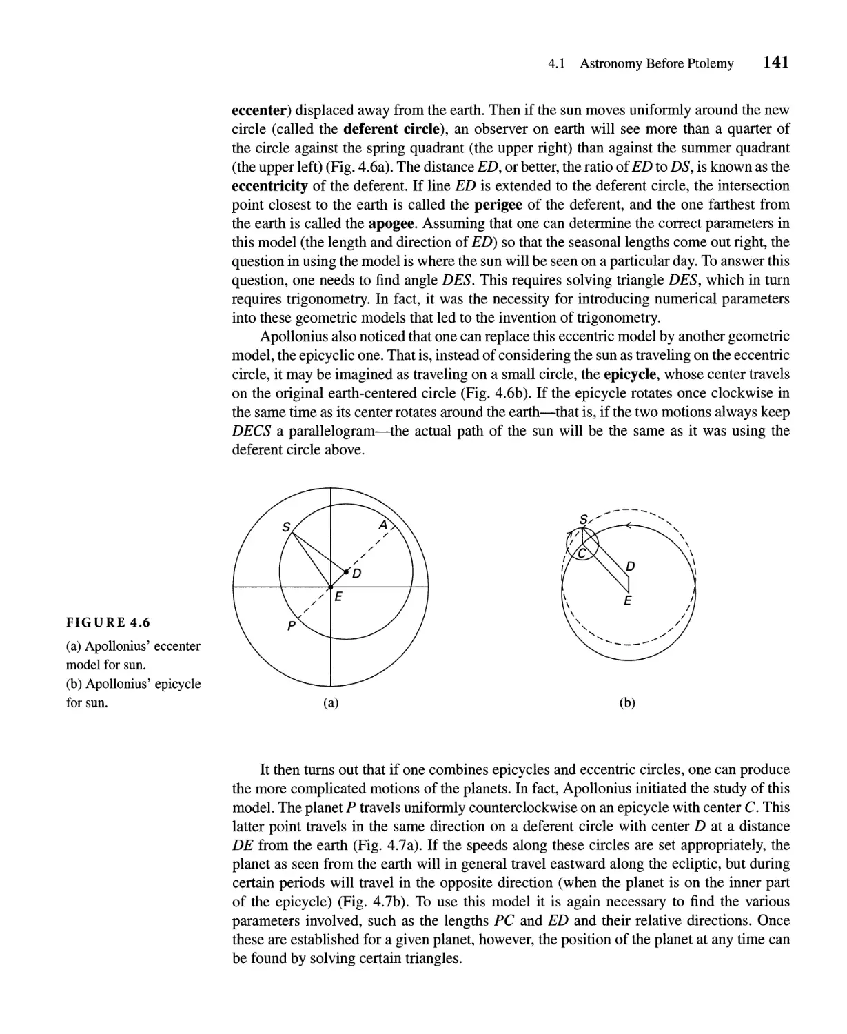
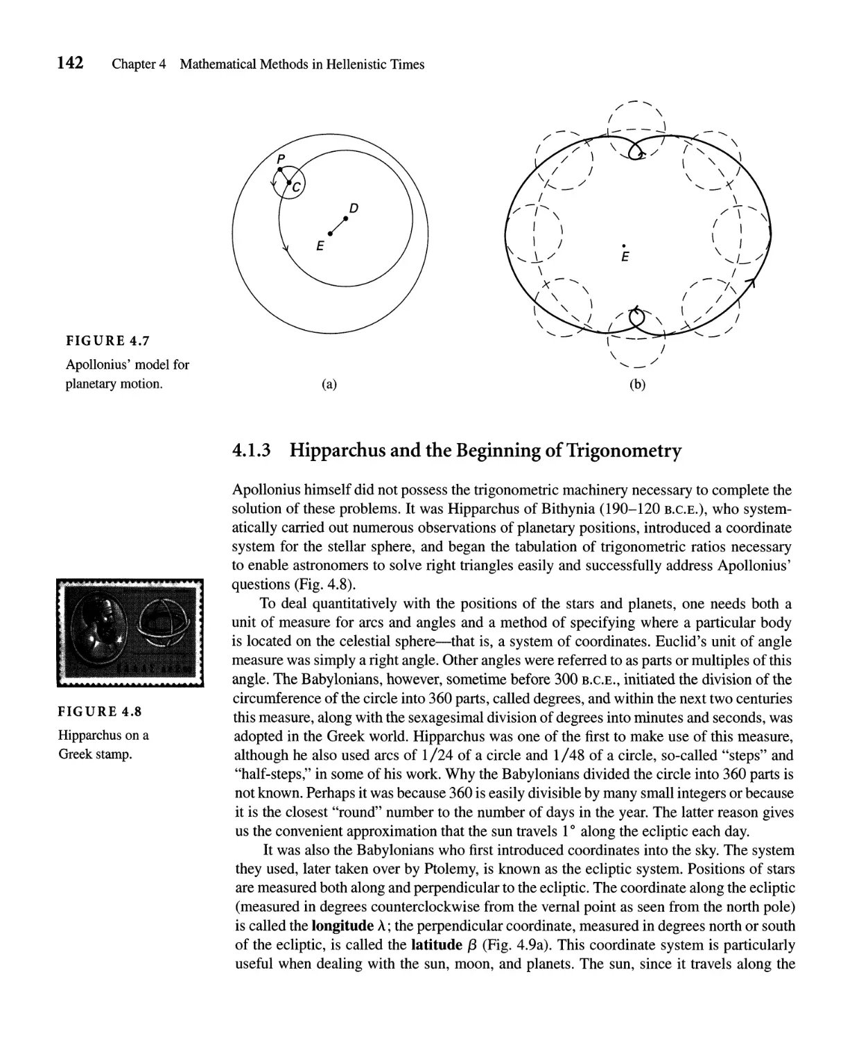
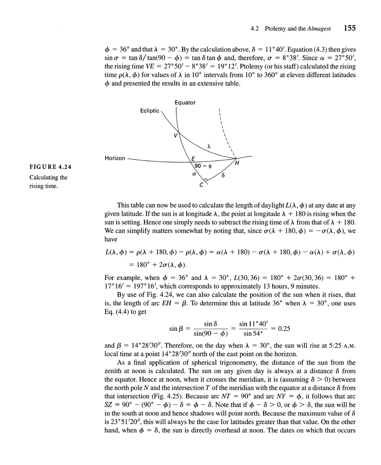
CHAPTER4 Mathematical Methods in Hellenistic Times 135
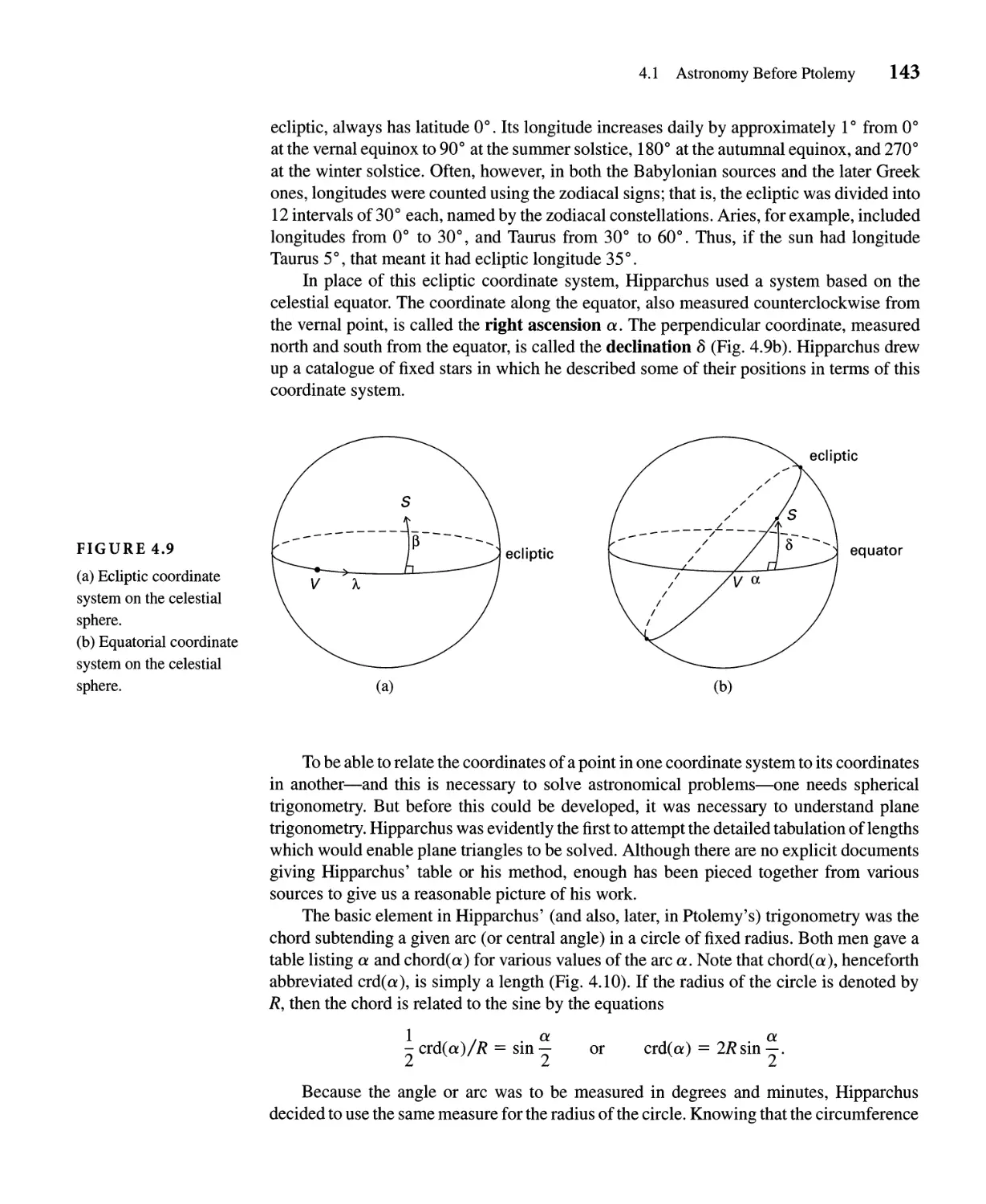
4.1 Astronomy Before Ptolemy 136
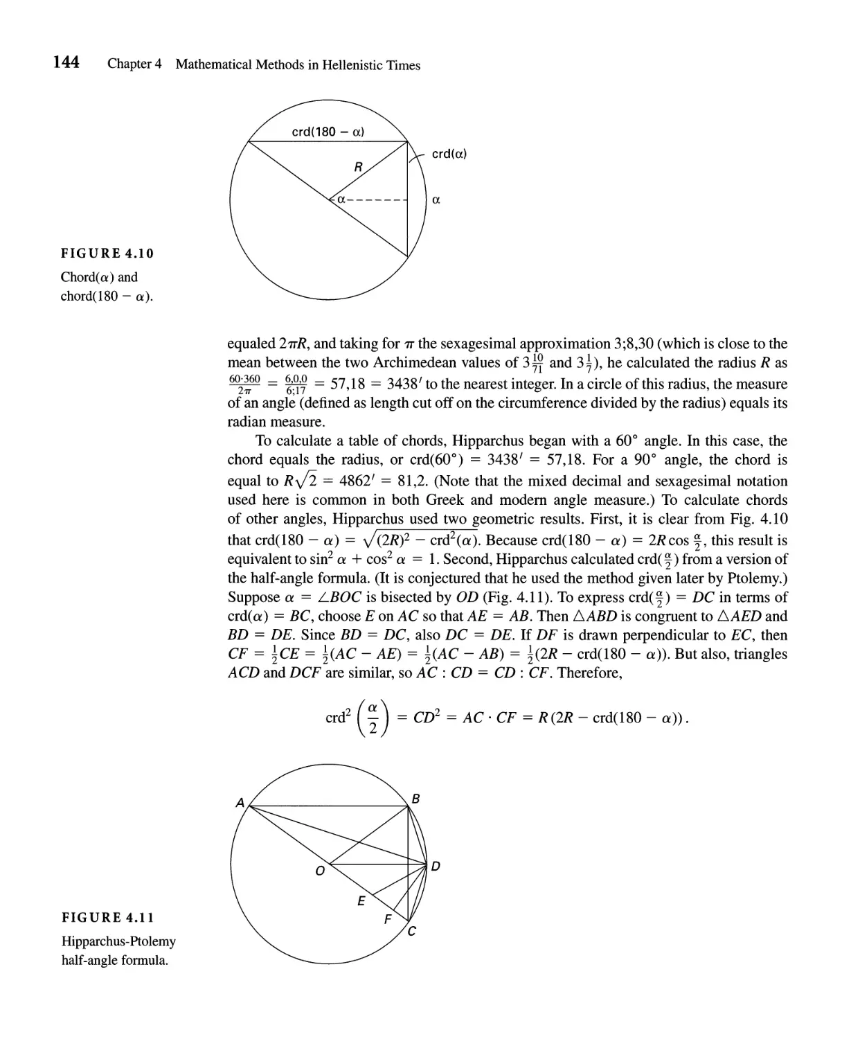
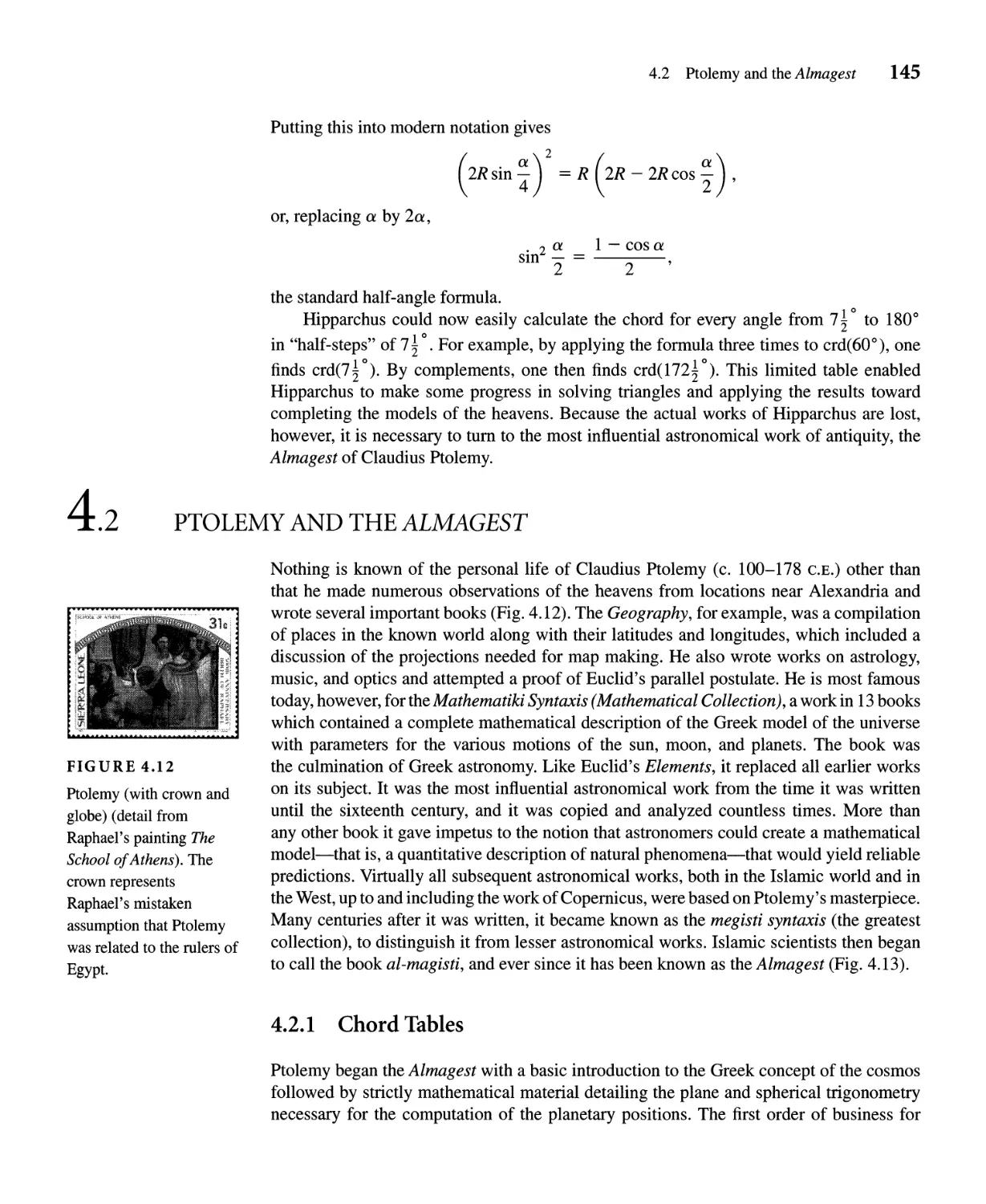
4.2 Ptolemy and the Almagest 145
4.3 Practical Mathematics 156
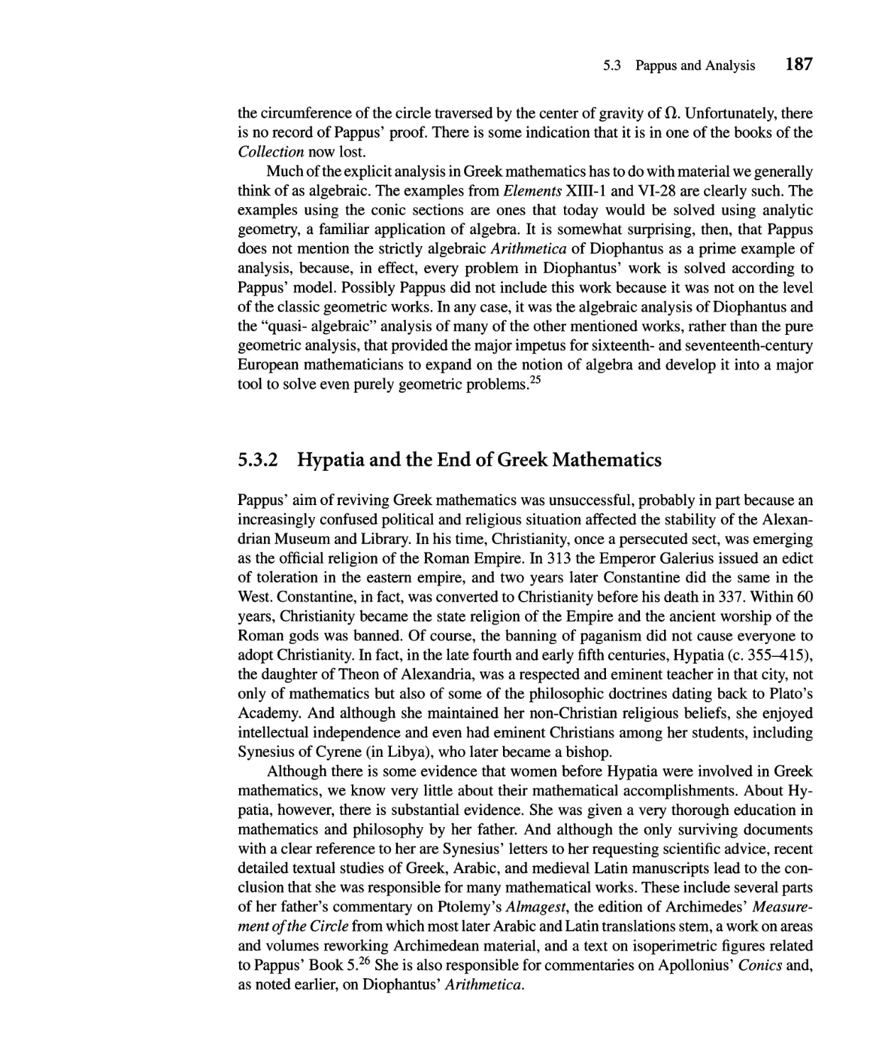
CHAPTER 5 The Final Chapters of Greek Mathematics 168
5.1 Nicomachus and Elementary Number Theory 171
5.2 Diophantus and Greek Algebra 173
5.3 Pappus and Analysis 183
PART TWO
Medieval Mathematics: 500-1400
CHAPTER 6 Medieval China and India 192
6.1 Introduction to Medieval Chinese Mathematics 192
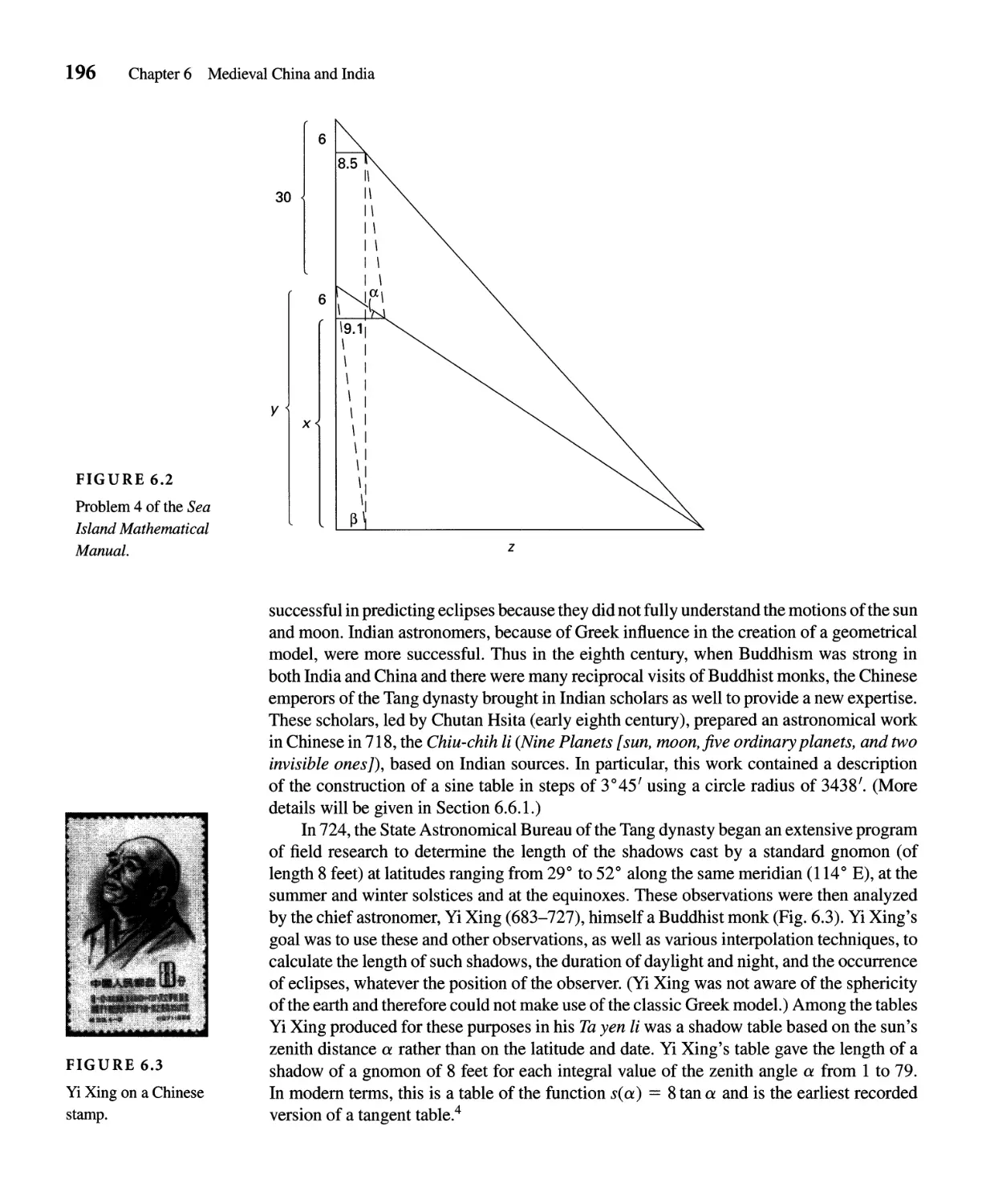
6.2 The Mathematics of Surveying and Astronomy 193
6.3 Indeterminate Analysis 197
6.4 Solving Equations 202
6.5 Introduction to the Mathematics of Medieval India 210
6.6 Indian Trigonometry 212
6.7 Indian Indeterminate Analysis 218
6.8 Algebra and Combinatorics 225
6.9 The Hindu-Arabic Decimal PI ace- Value System 230
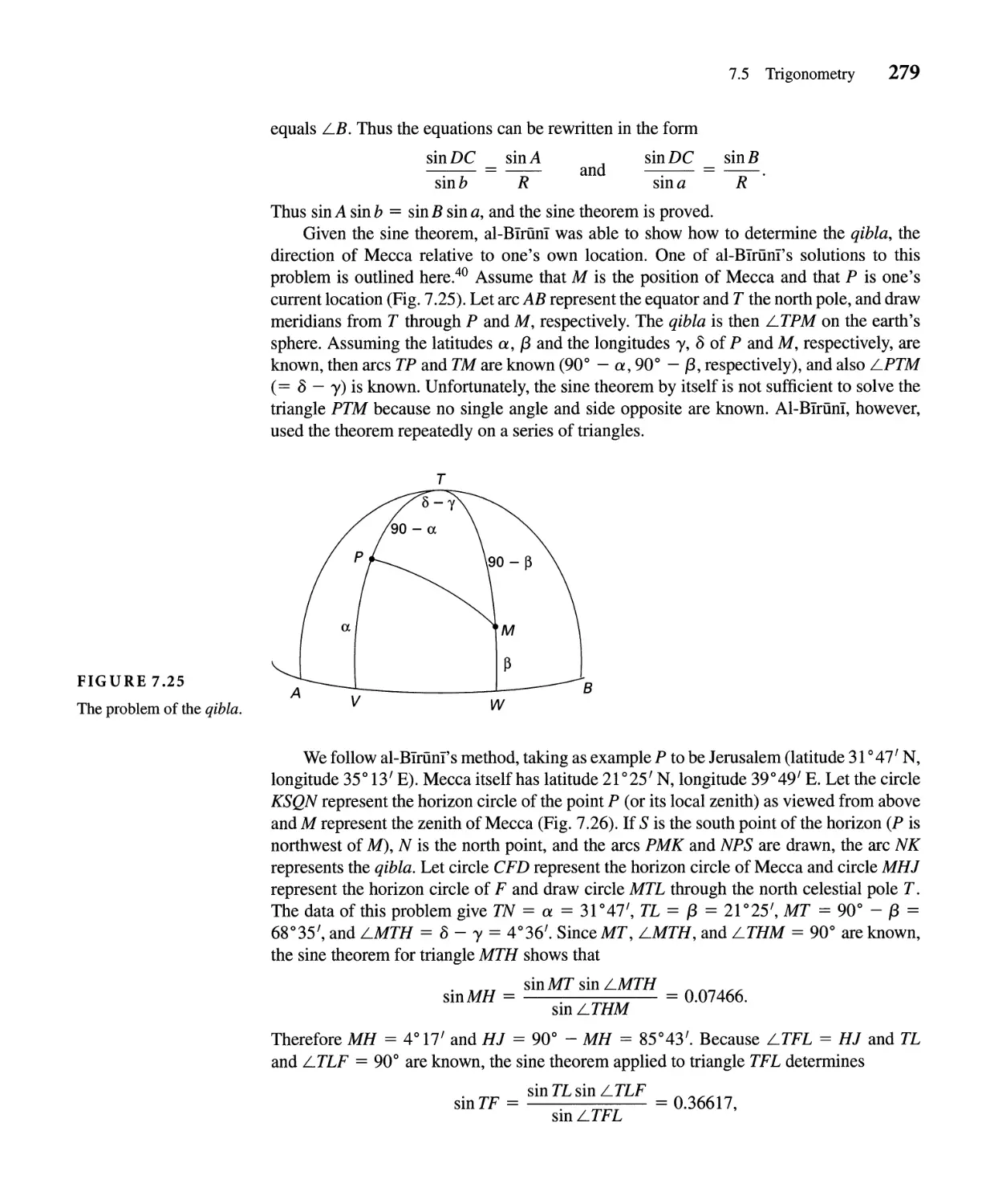
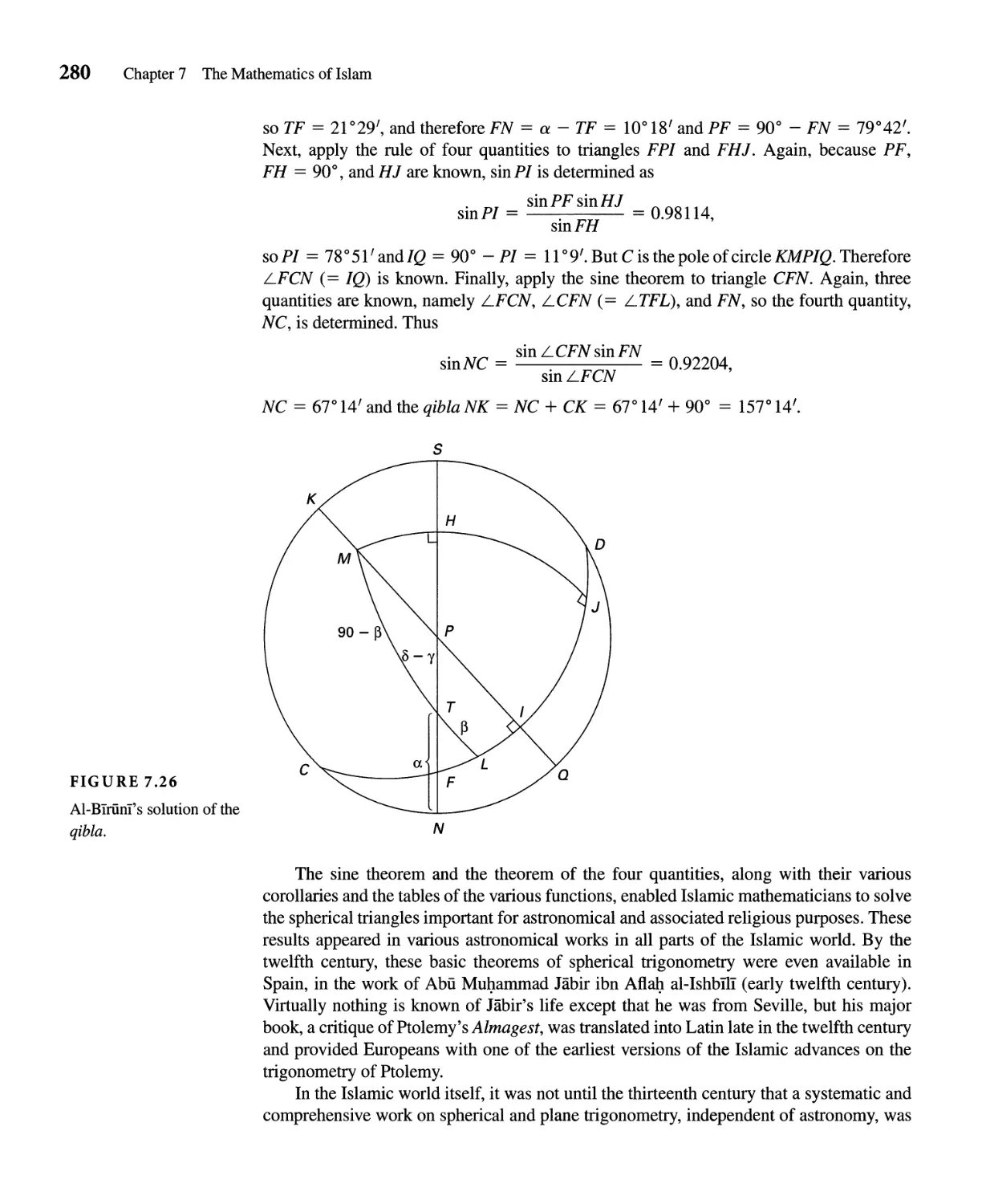
CHAPTER 7 The Mathematics of Islam 238
7.1 Decimal Arithmetic 240
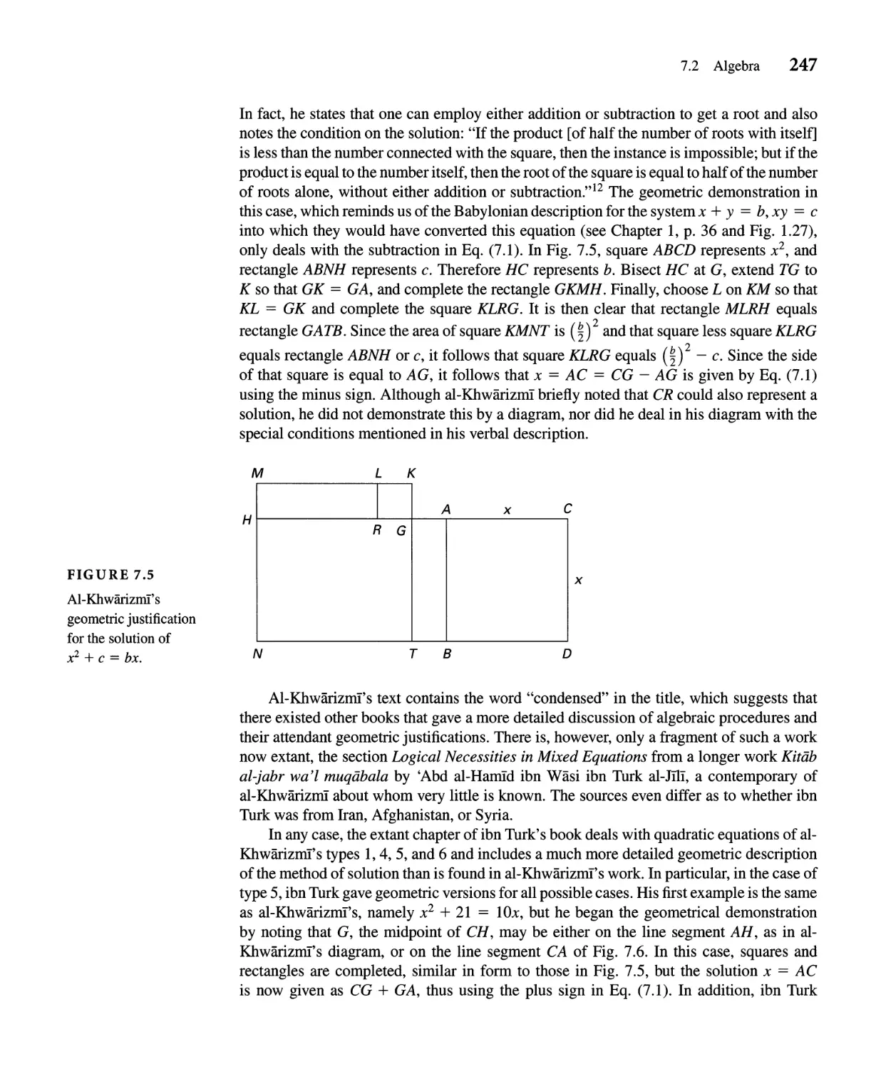
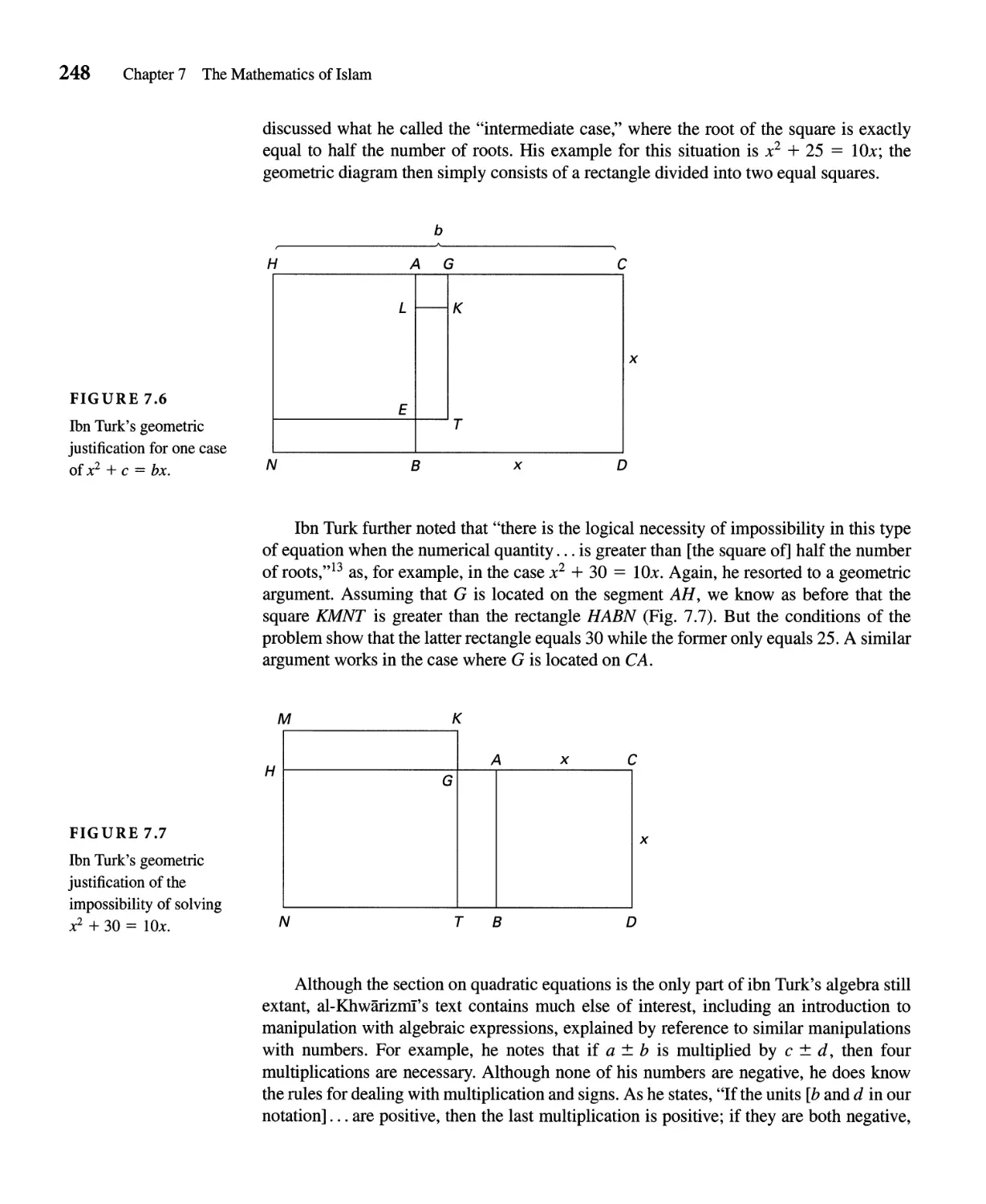
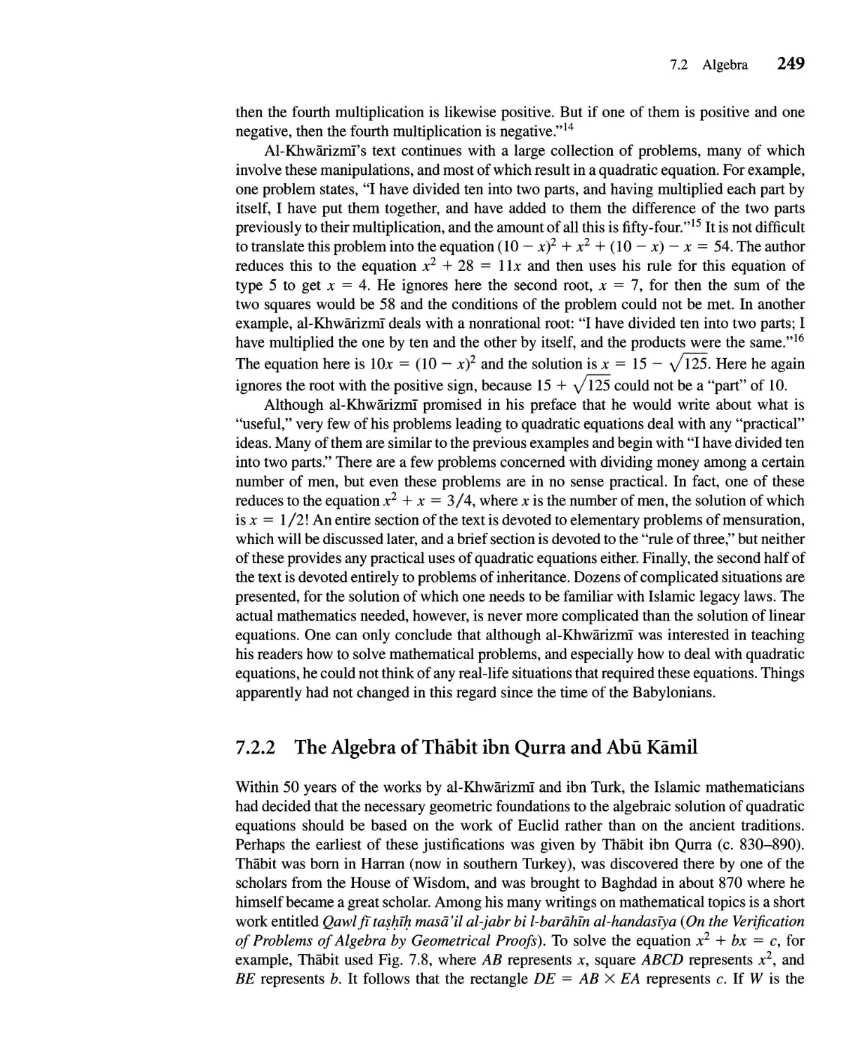
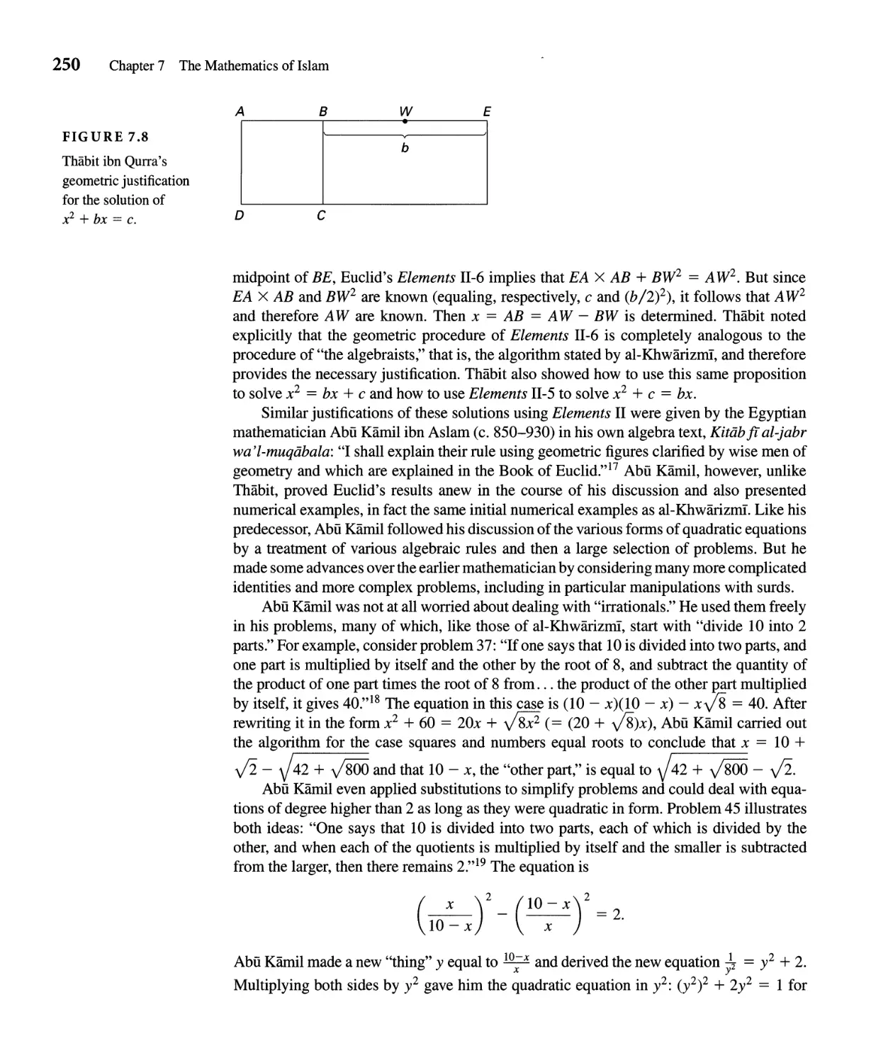
7.2 Algebra 243
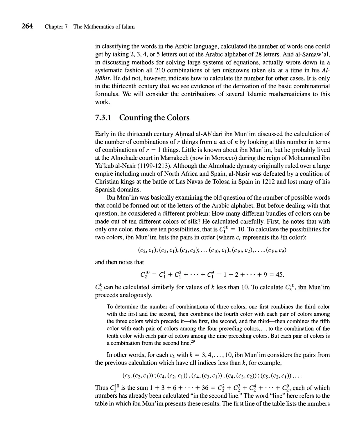
7.3 Combinatorics 263
7.4 Geometry 268
7.5 Trigonometry 274
CHAPTER 8 Mathematics in Medieval Europe 288
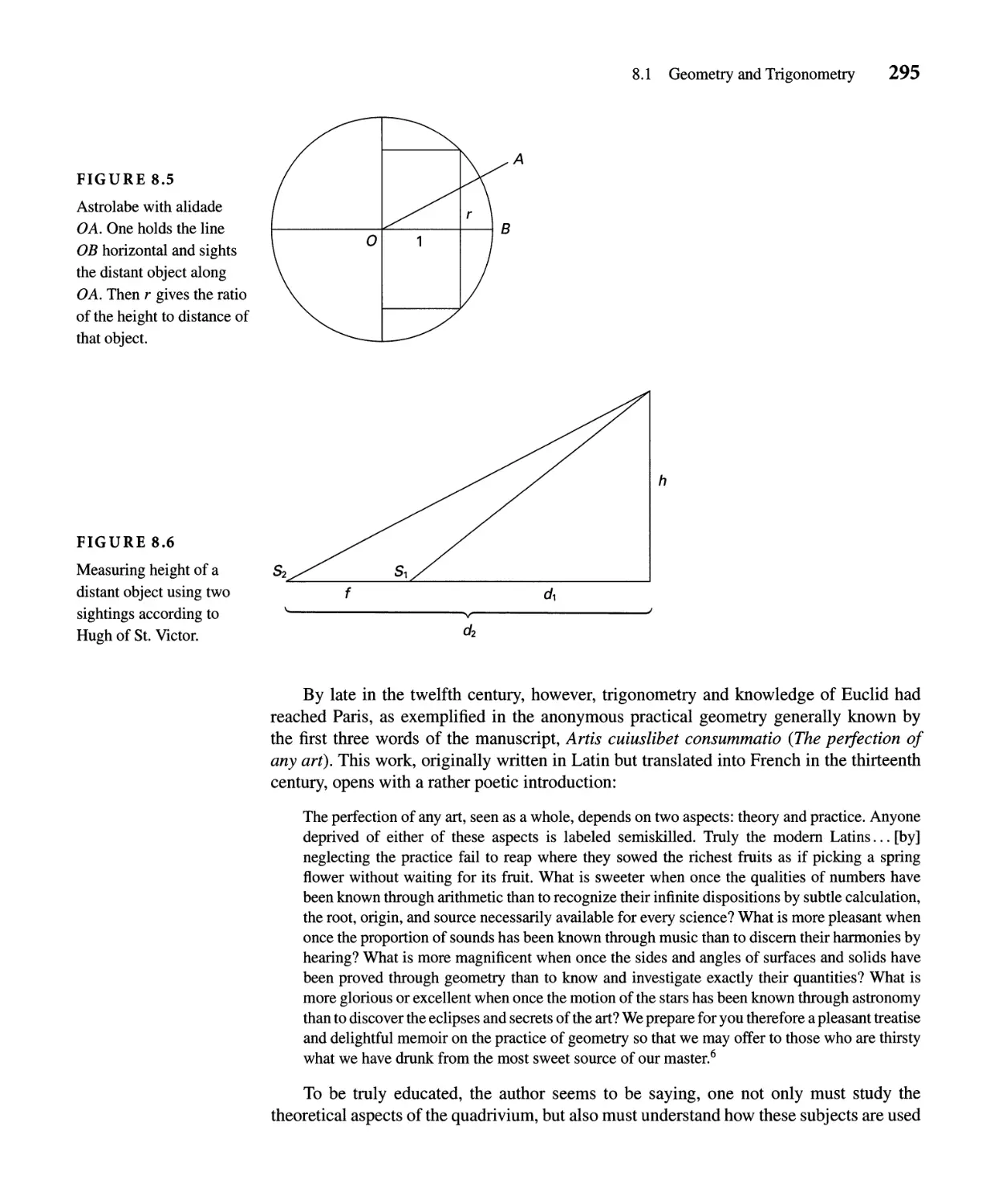
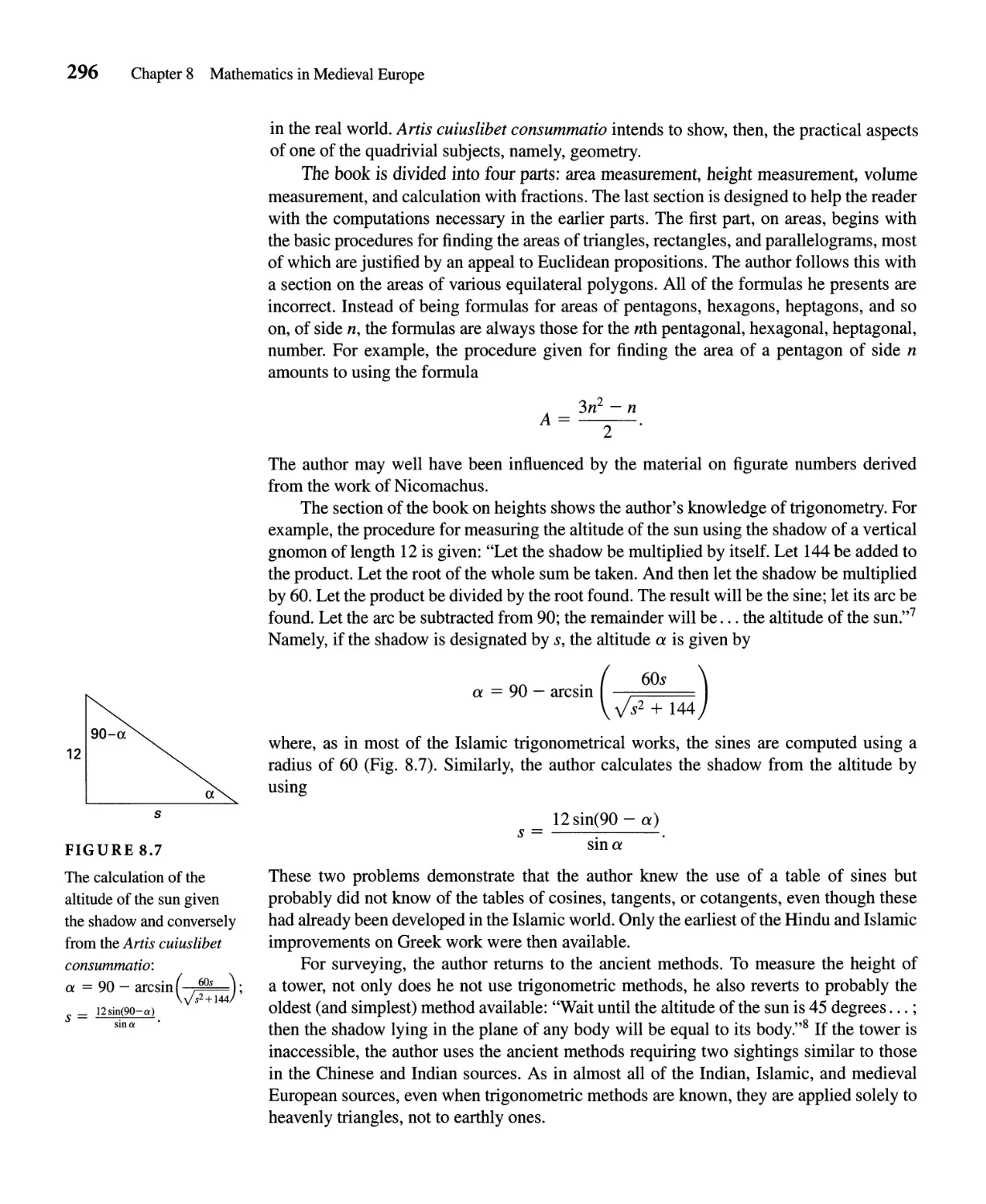
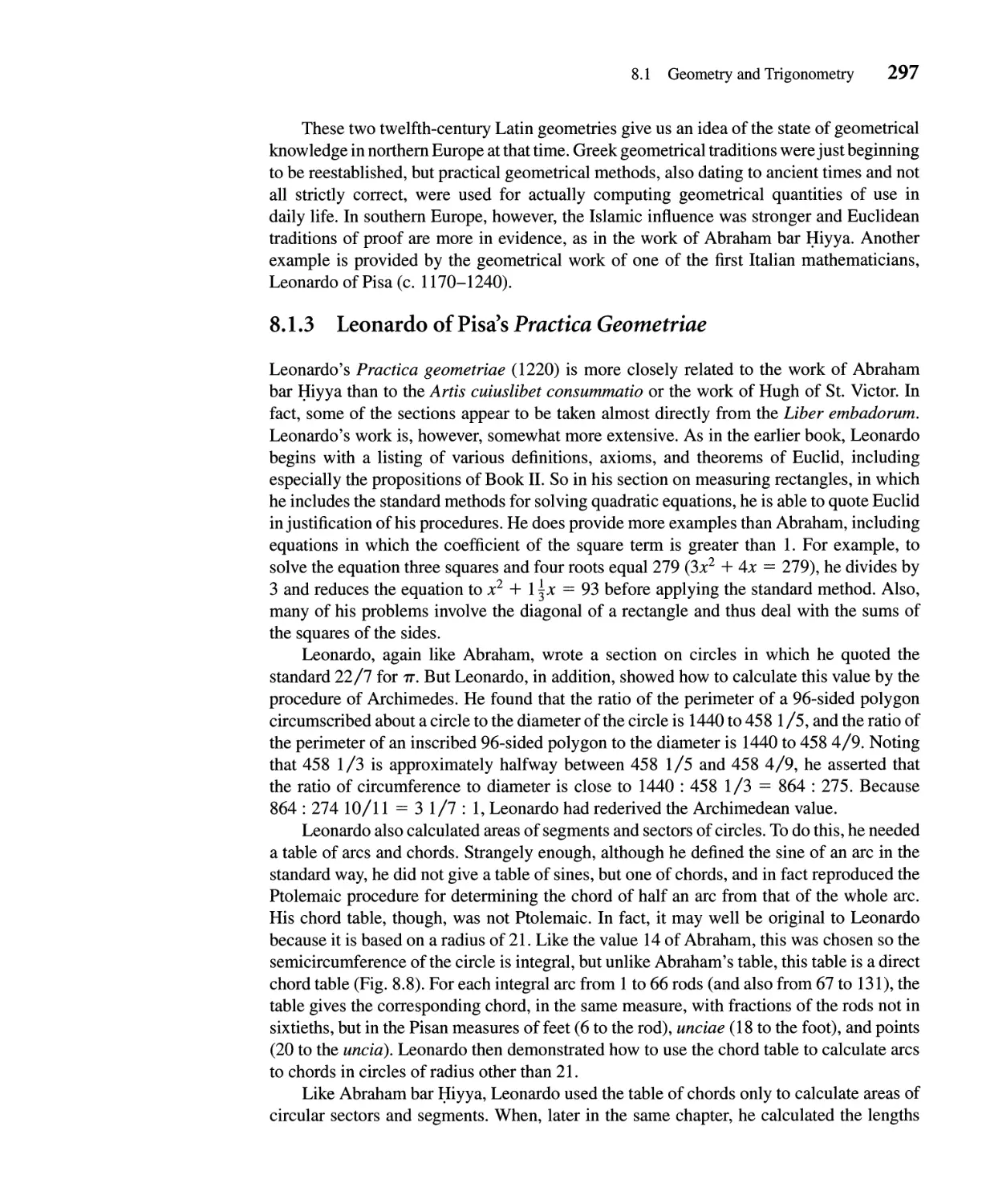
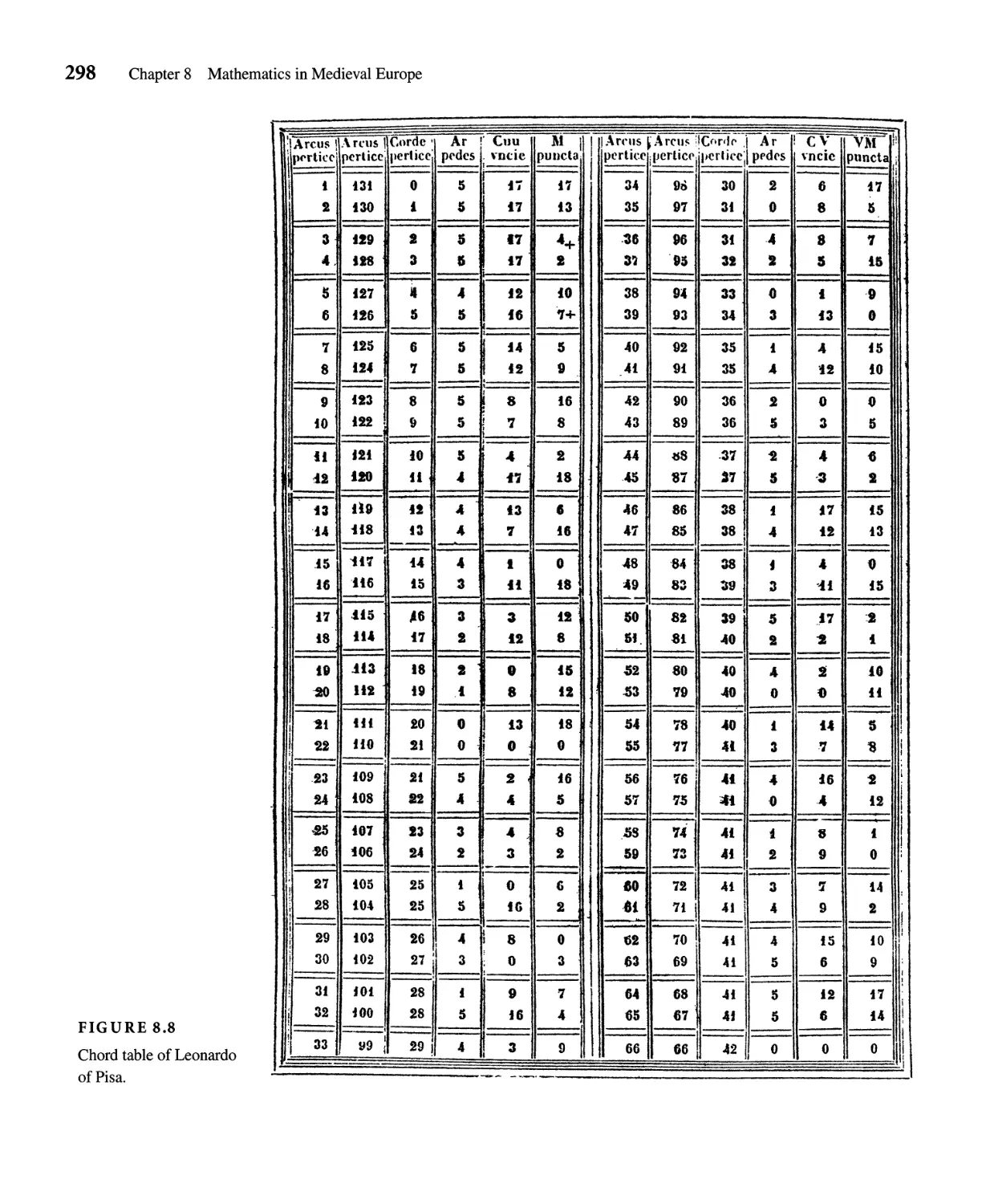
8.1 Geometry and Trigonometry 292
8.2 Combinatorics 300
8.3 Medieval Algebra 307
8.4 The Mathematics of Kinematics 314
INTERCHAPTER Mathematics Around the World 327
1.1 Mathematics at the Turn of the Fourteenth Century 327
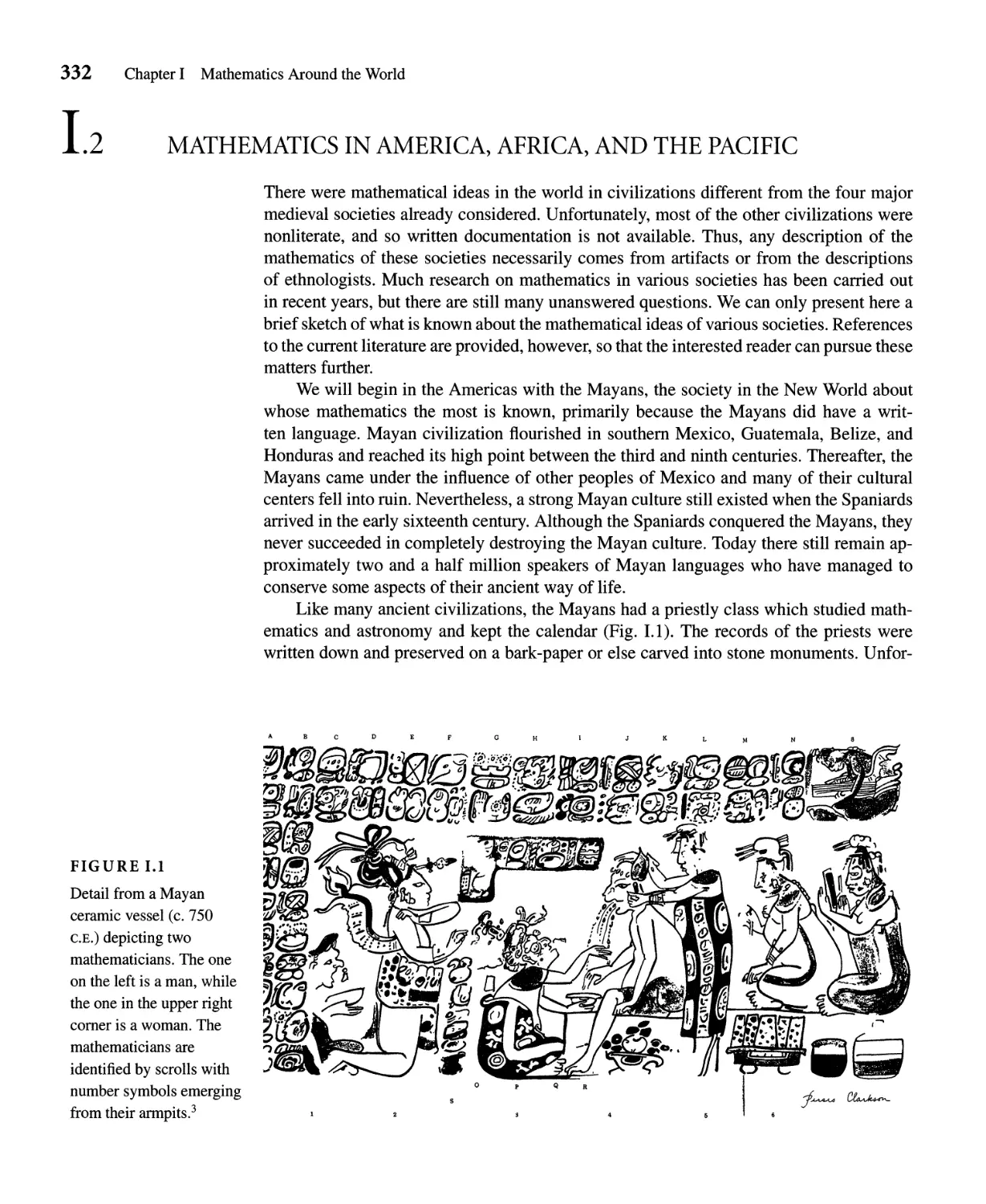
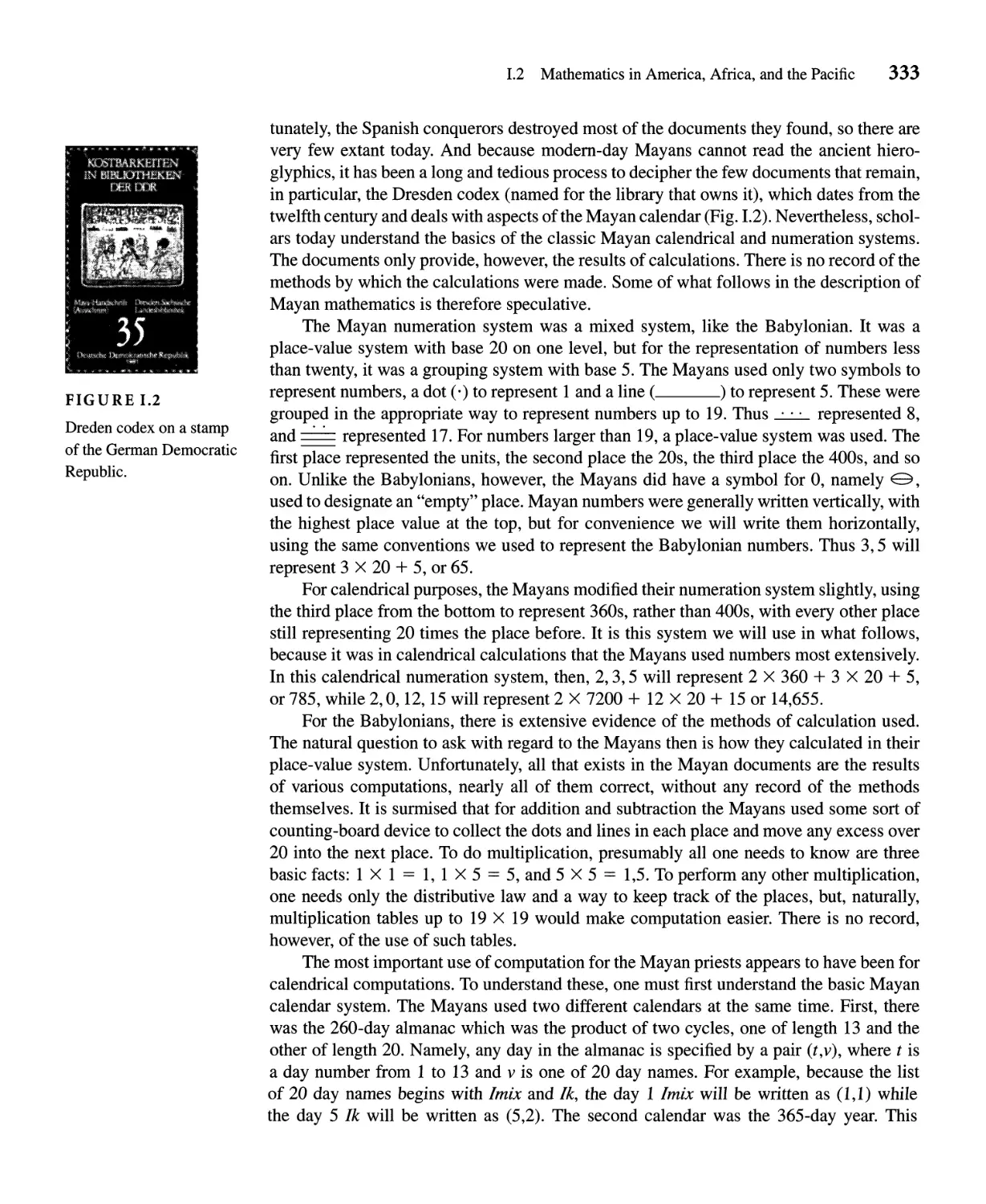
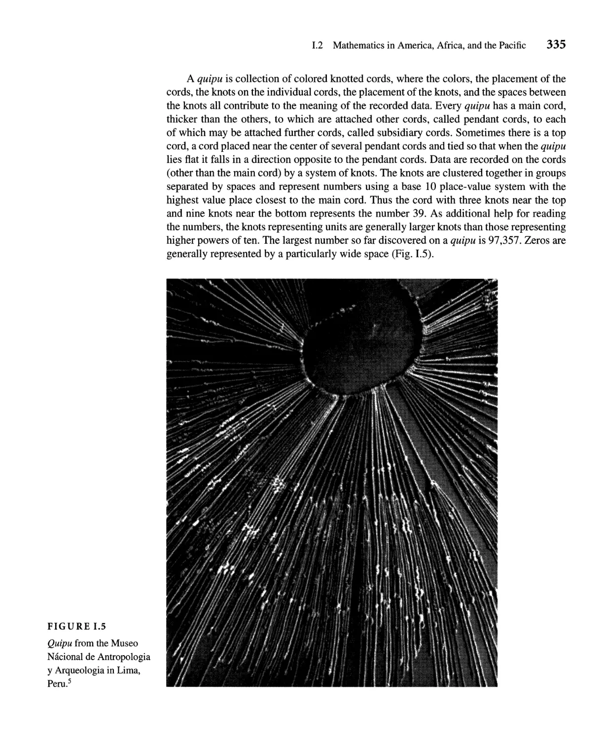
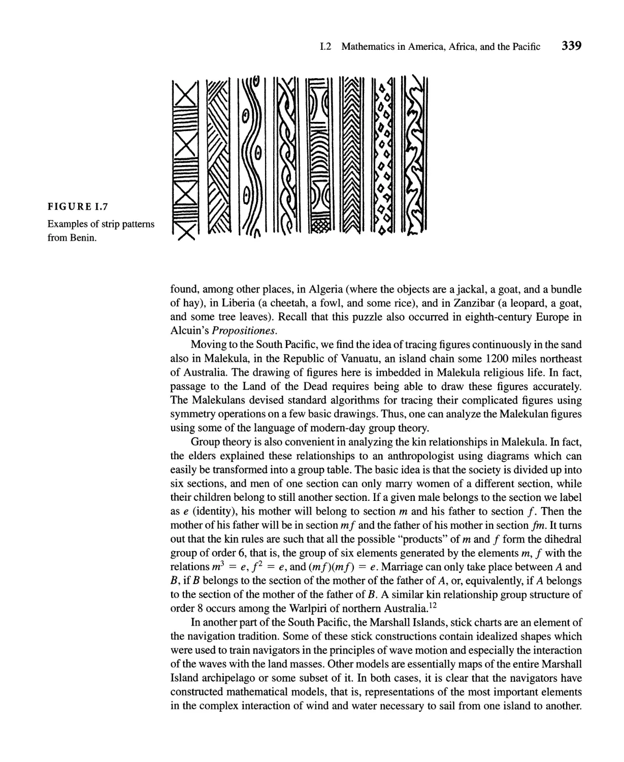
1.2 Mathematics in America, Africa, and the Pacific 332
..
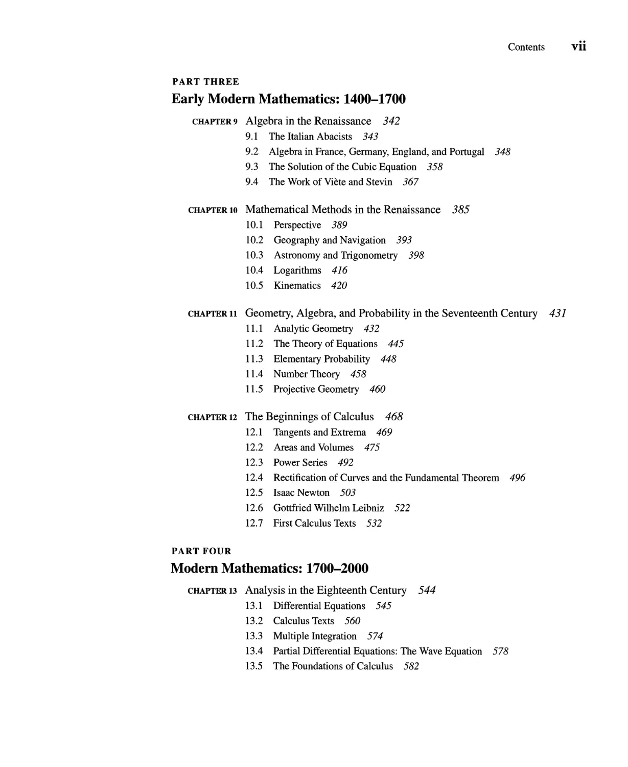
Contents VII
PART THREE
Early Modern Mathematics: 1400-1700
CHAPTER 9 Algebra in the Renaissance 342
9.1 The Italian Abacists 343
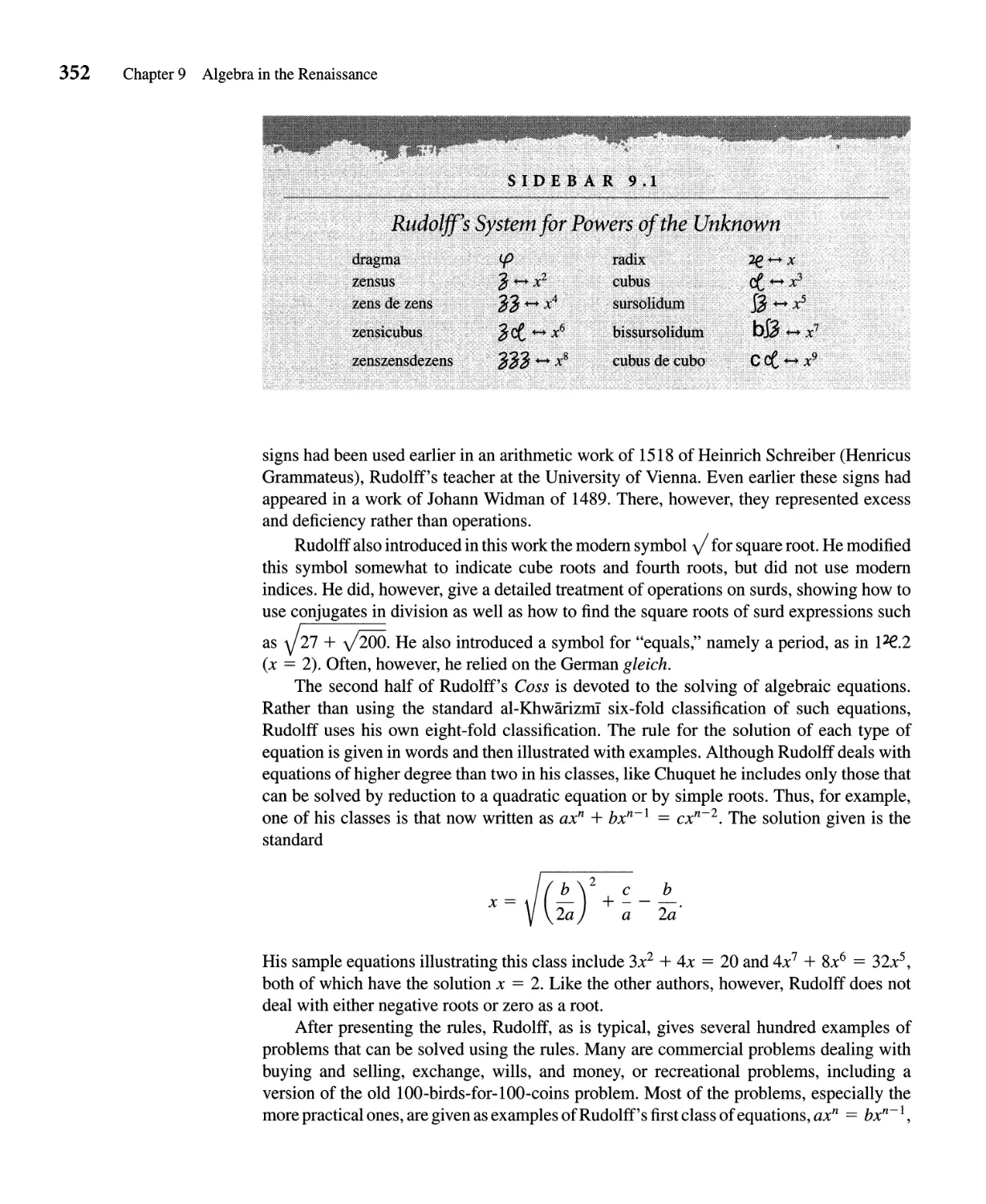
9.2 Algebra in France, Germany, England, and Portugal 348
9.3 The Solution of the Cubic Equation 358
9.4 The Work of Viete and Stevin 367
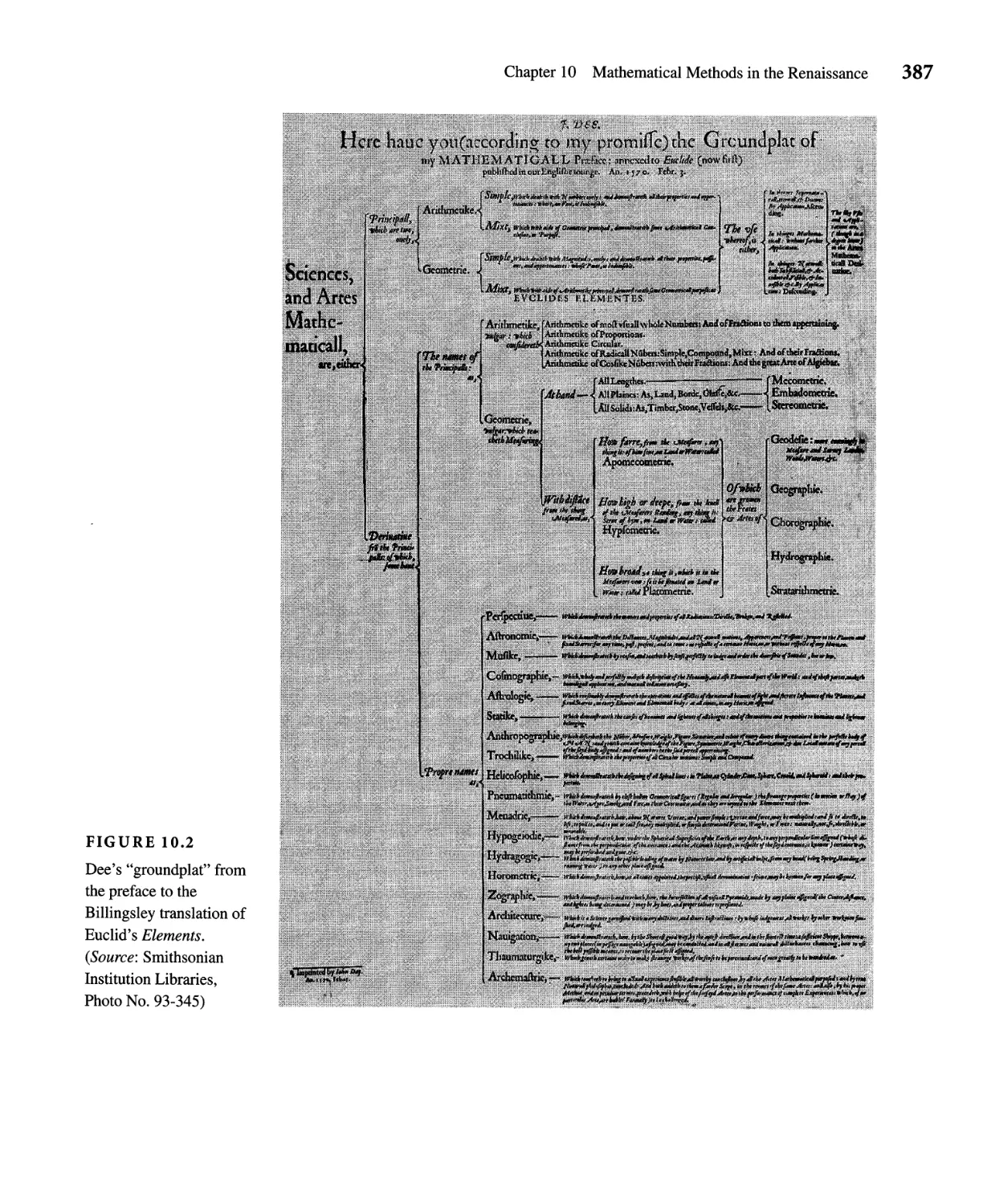
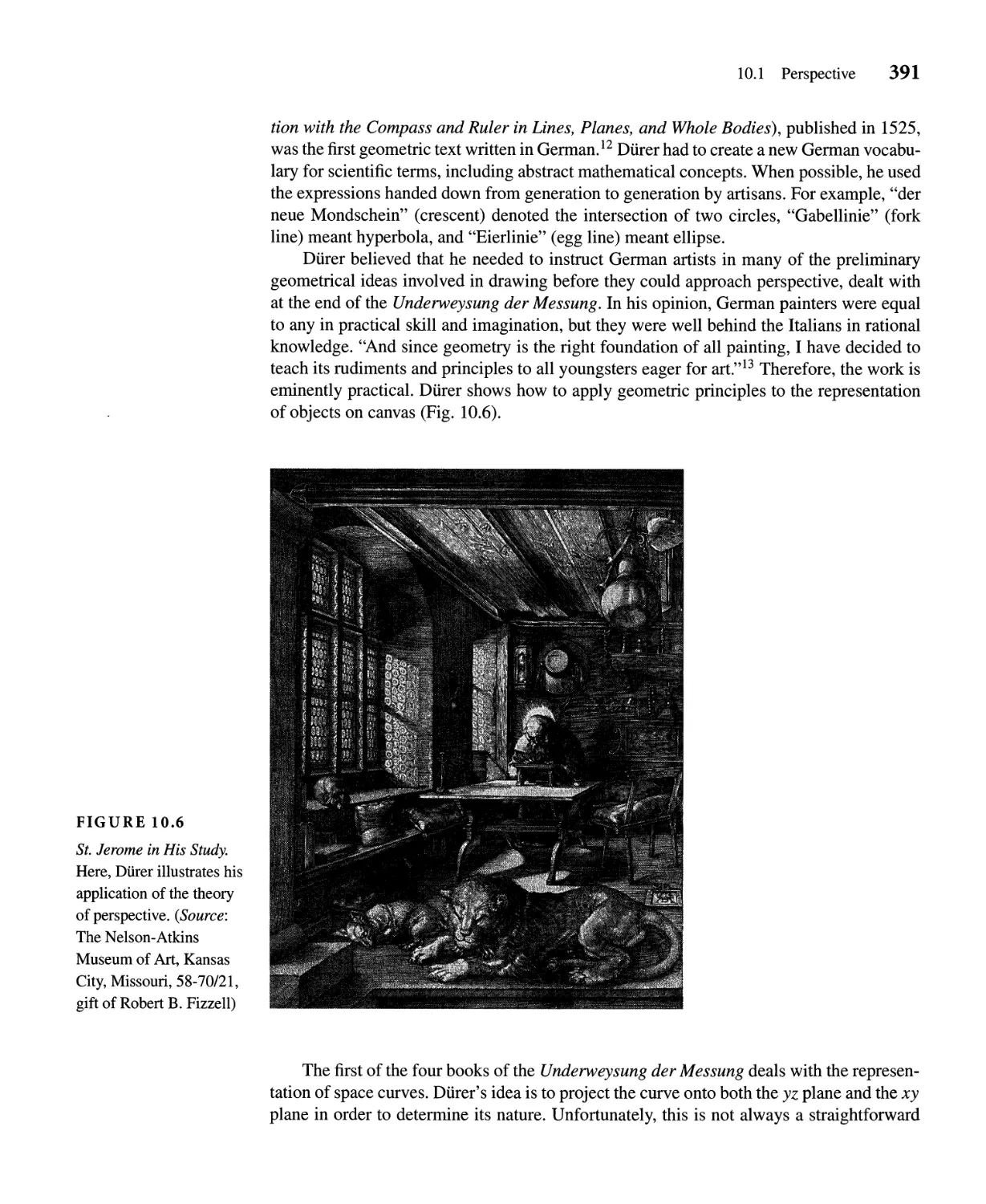
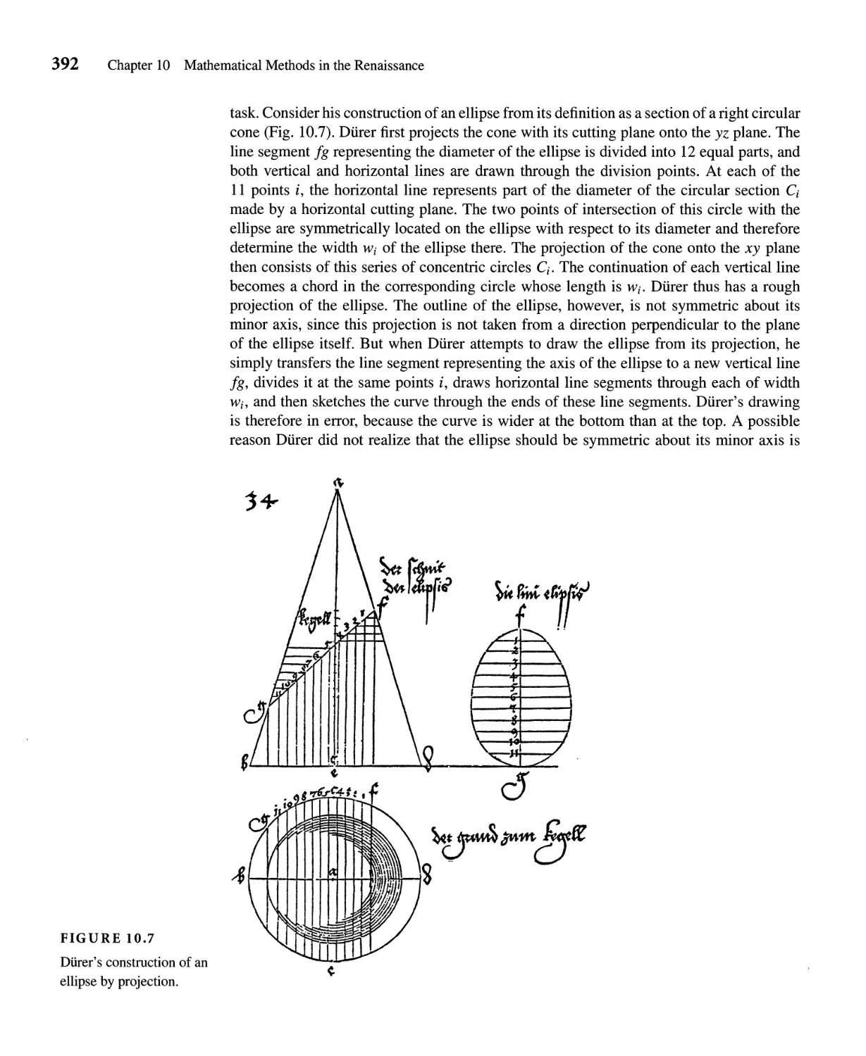
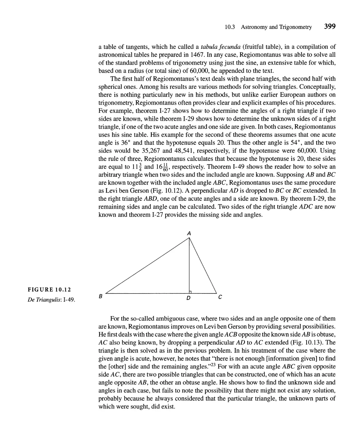
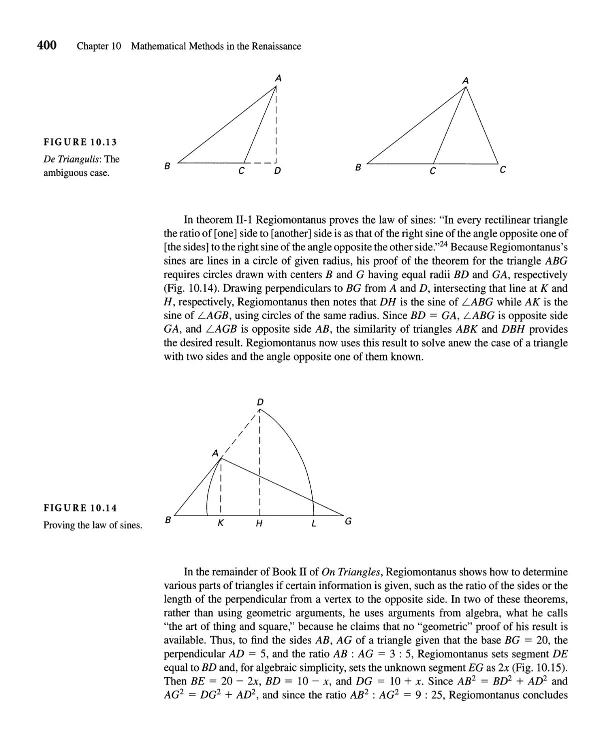
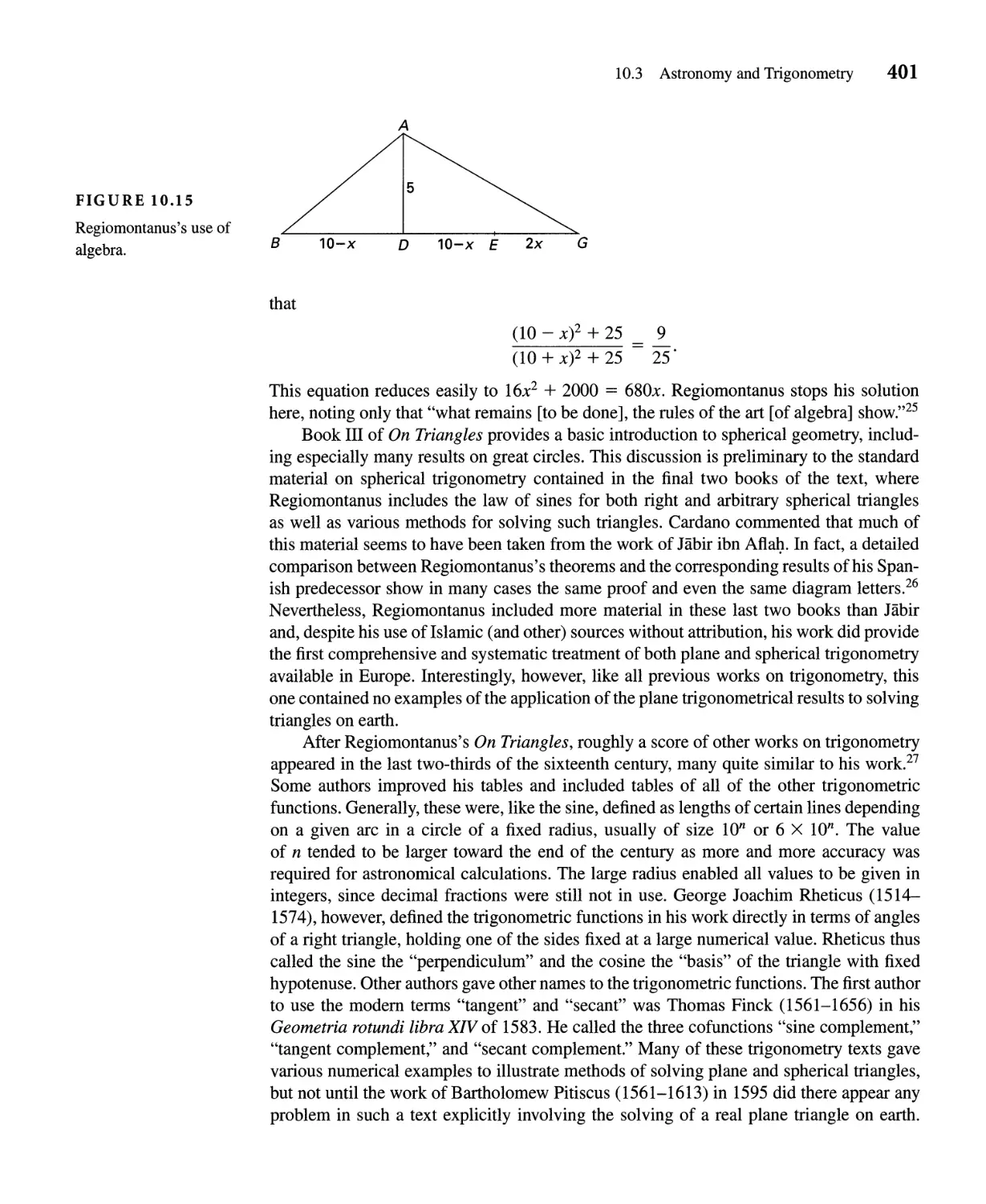
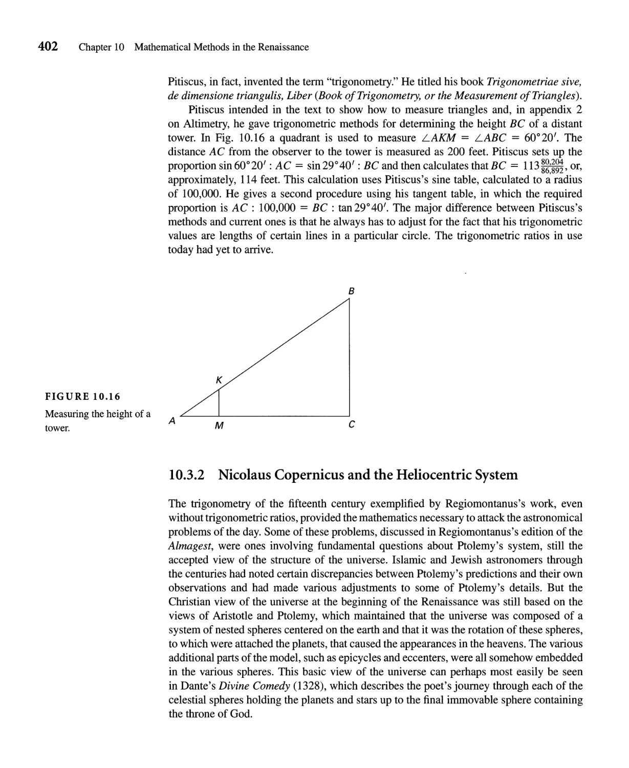
CHAPTER 10 Mathematical Methods in the Renaissance 385
10.1 Perspective 389
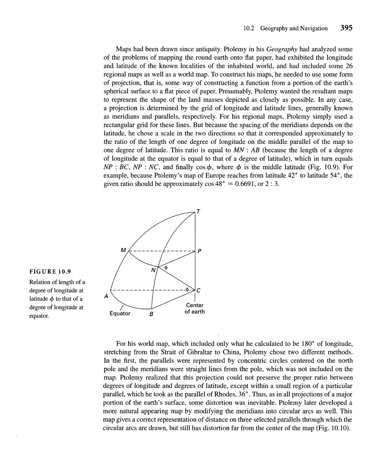
10.2 Geography and Navigation 393
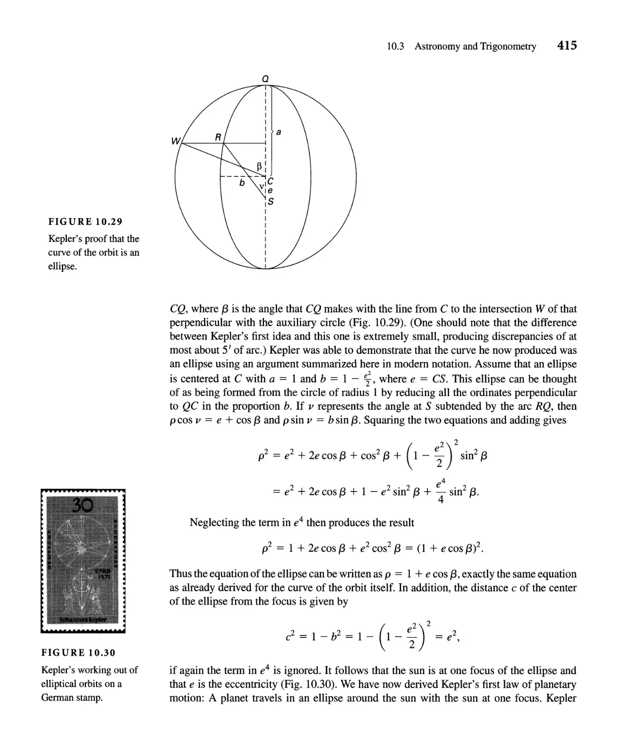
10.3 Astronomy and Trigonometry 398
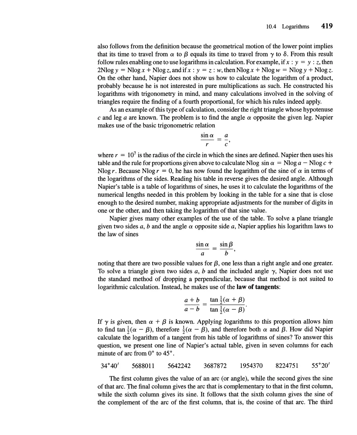
10.4 Logarithms 416
10.5 Kinematics 420
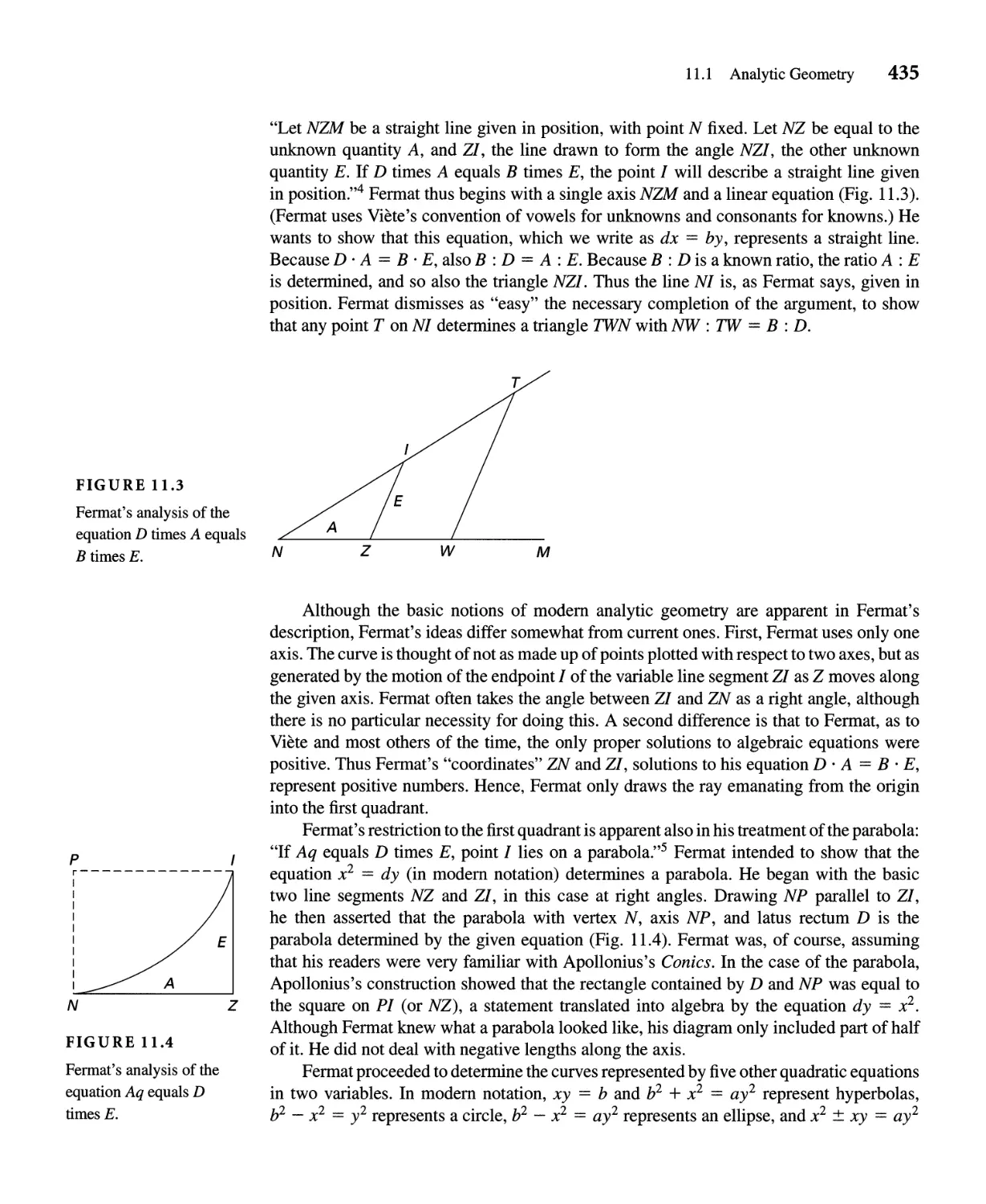
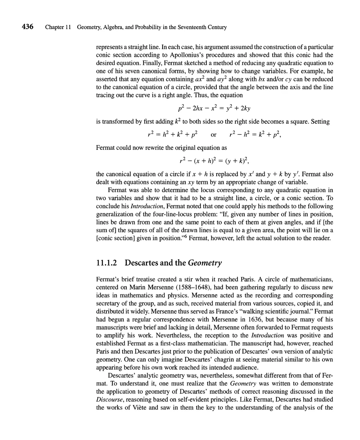
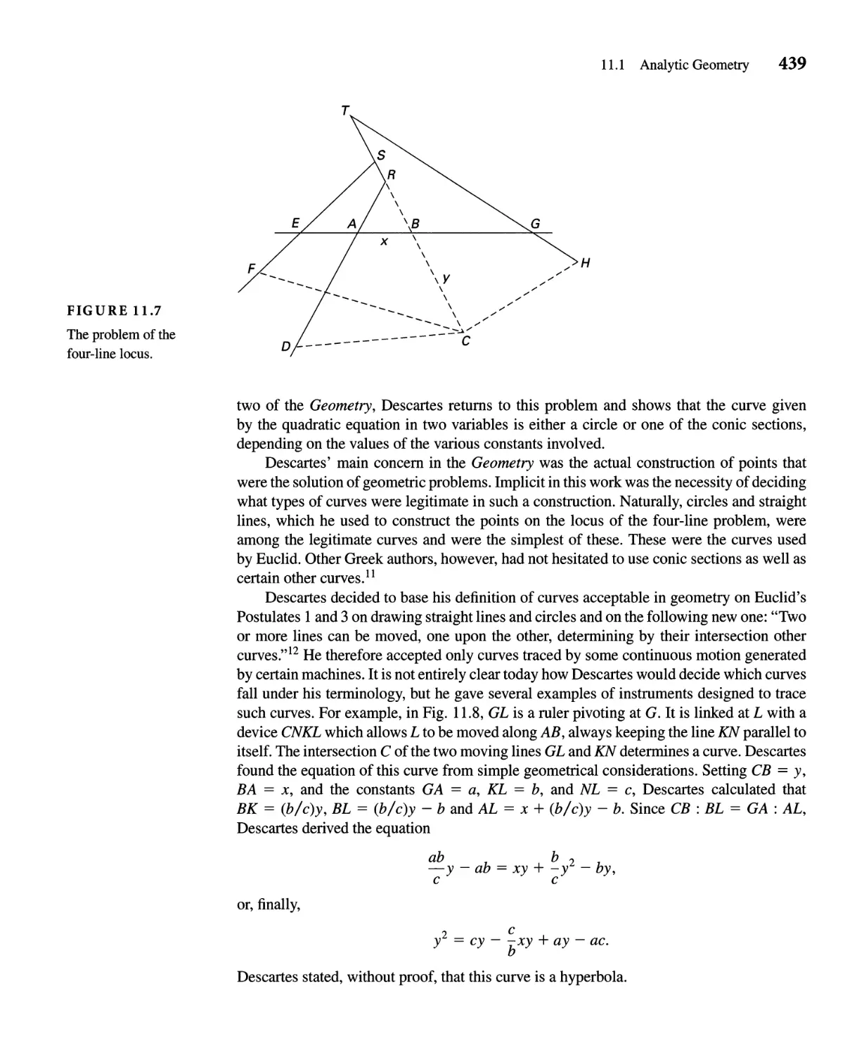
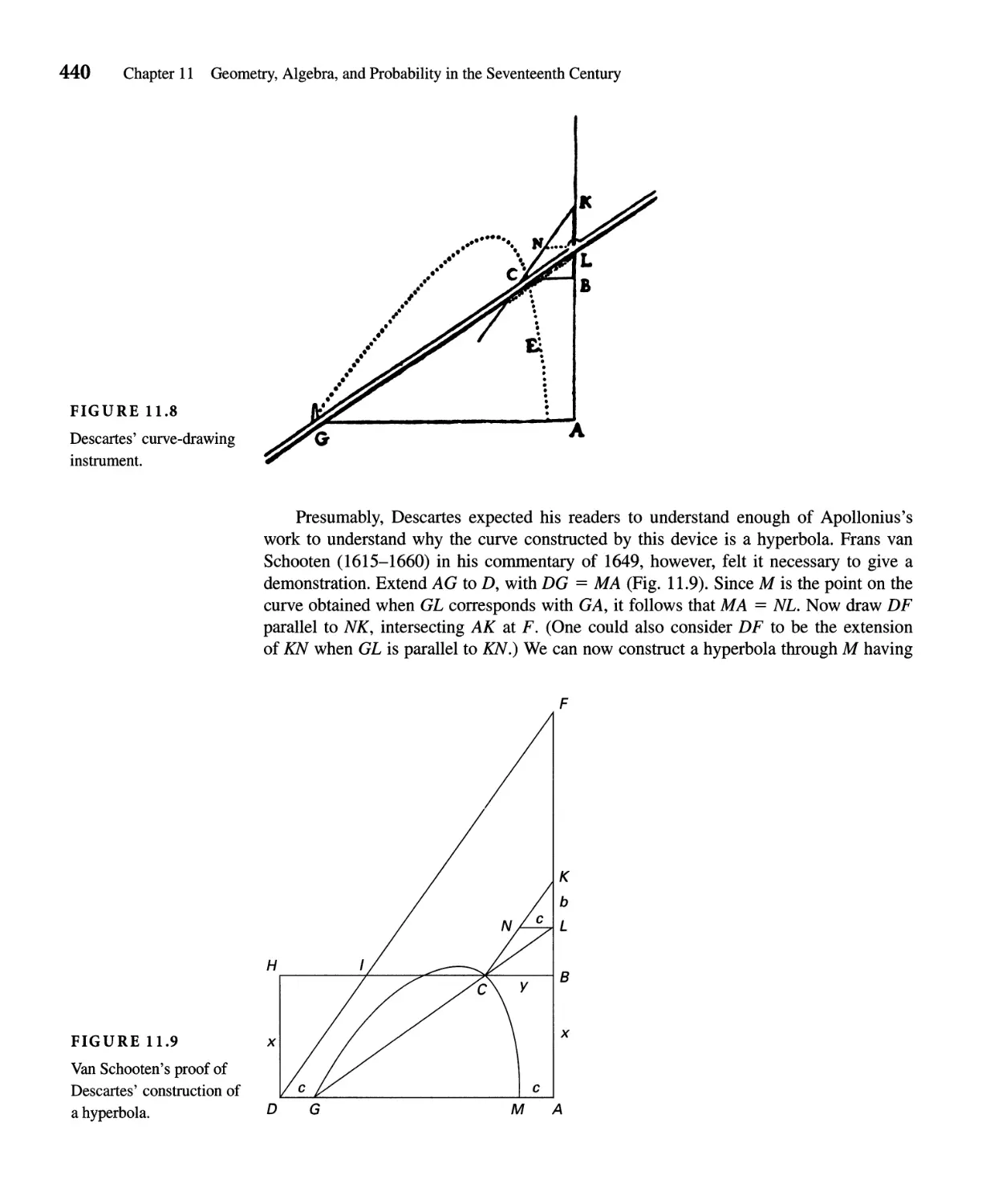
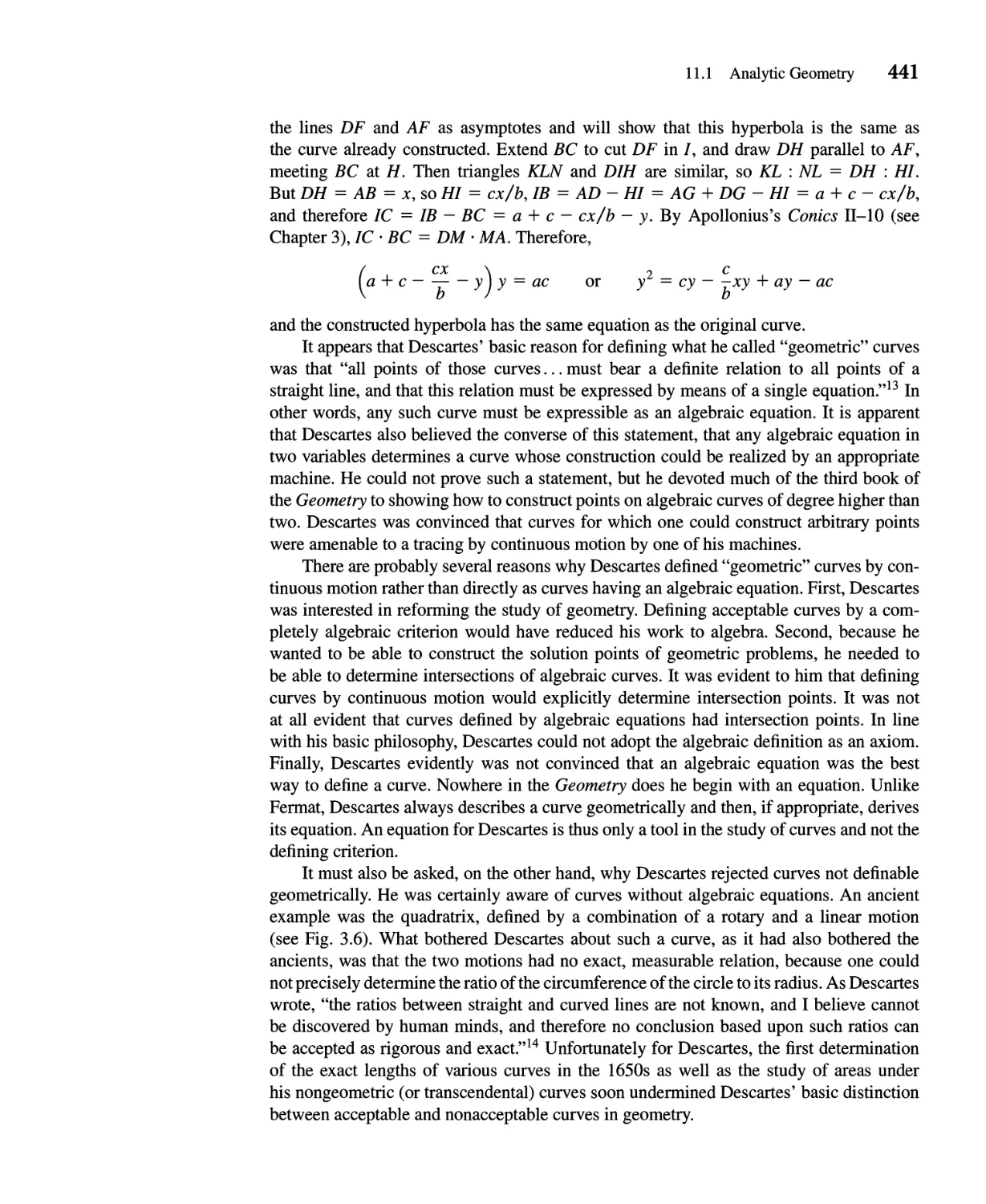
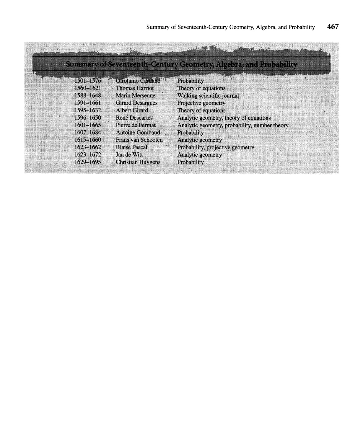
CHAPTER 11 Geometry, Algebra, and Probability in the Seventeenth Century 431
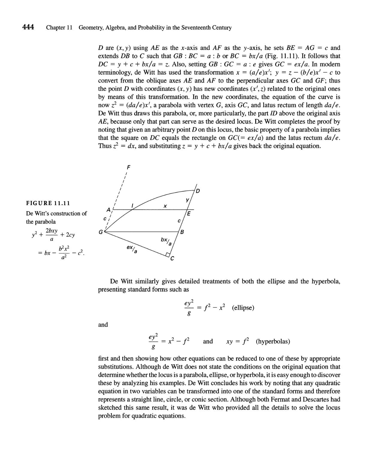
11.1 Analytic Geometry 432
11.2 The Theory of Equations 445
11.3 Elementary Probability 448
11.4 Number Theory 458
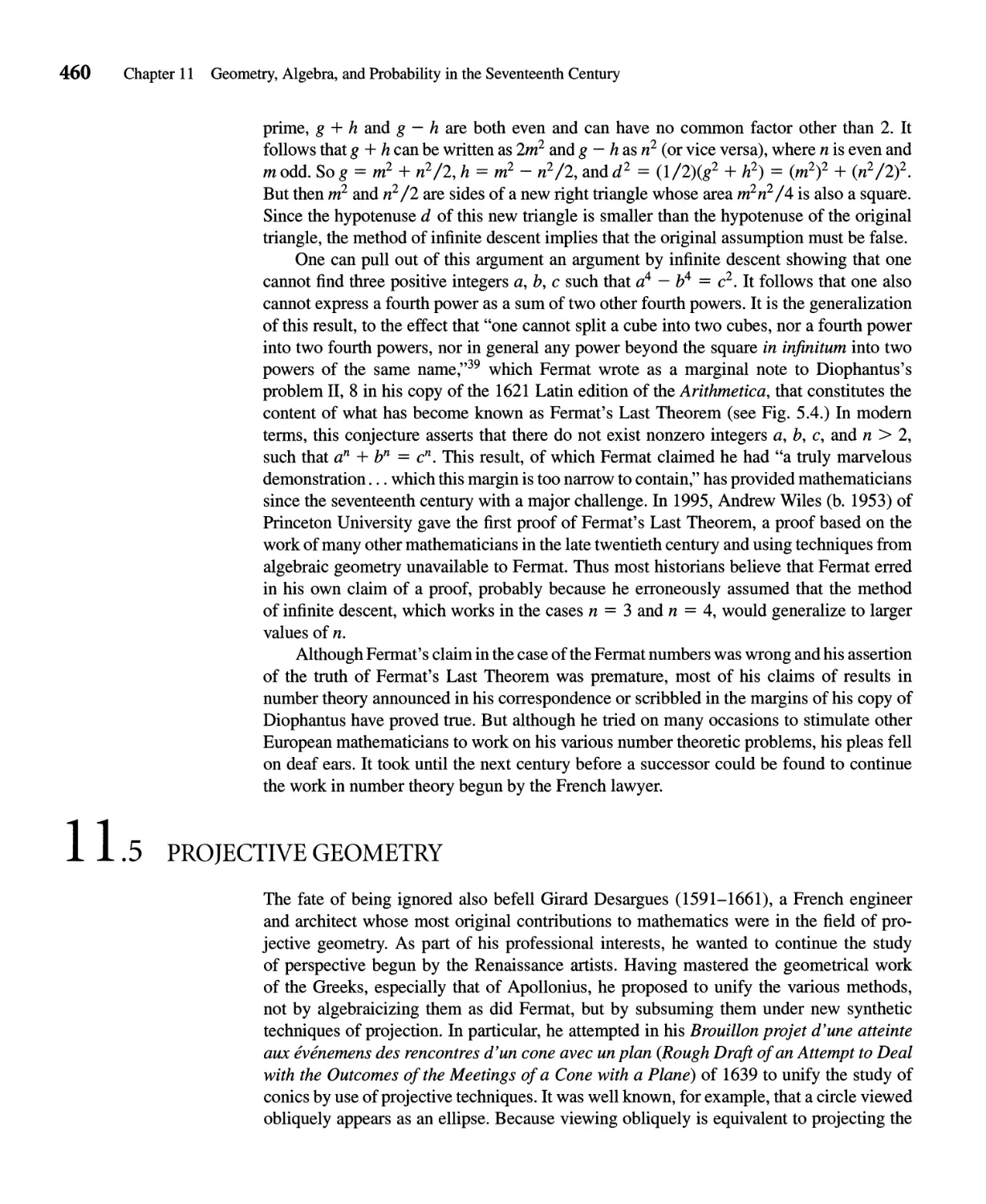
11.5 Projective Geometry 460
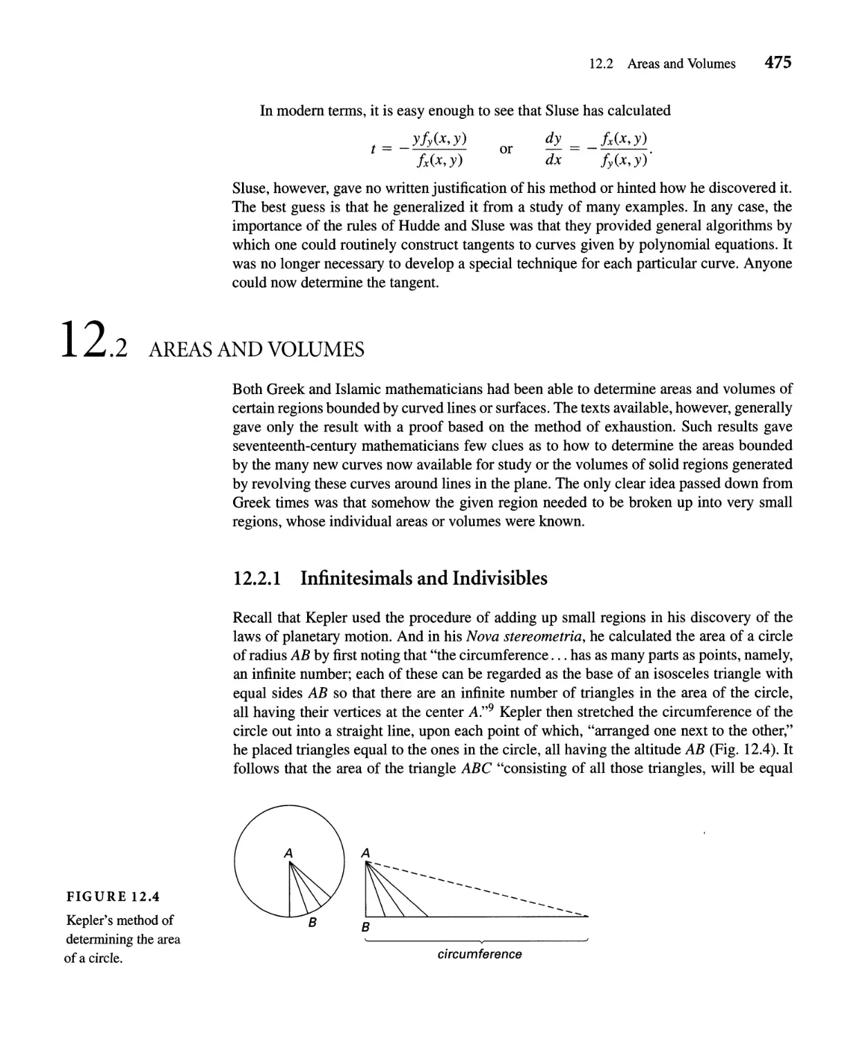
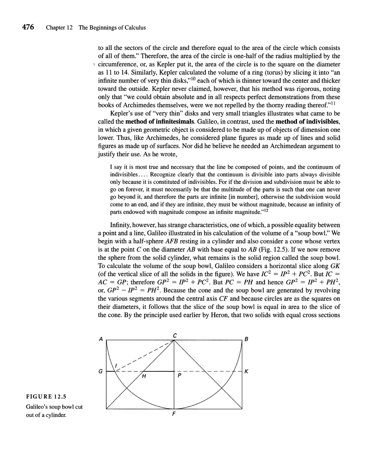
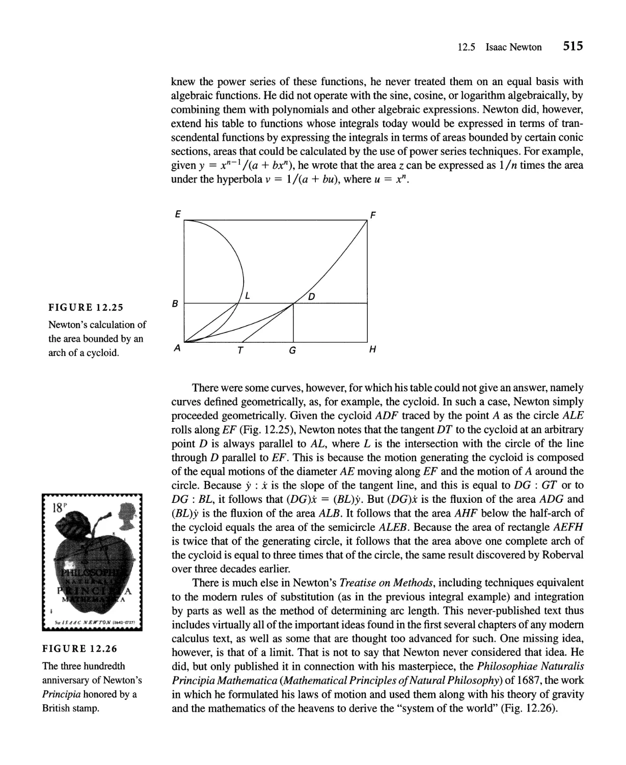
CHAPTER 12 The Beginnings of Calculus 468
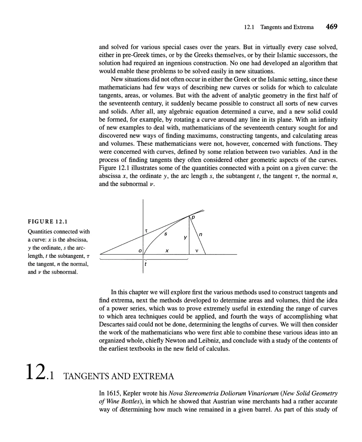
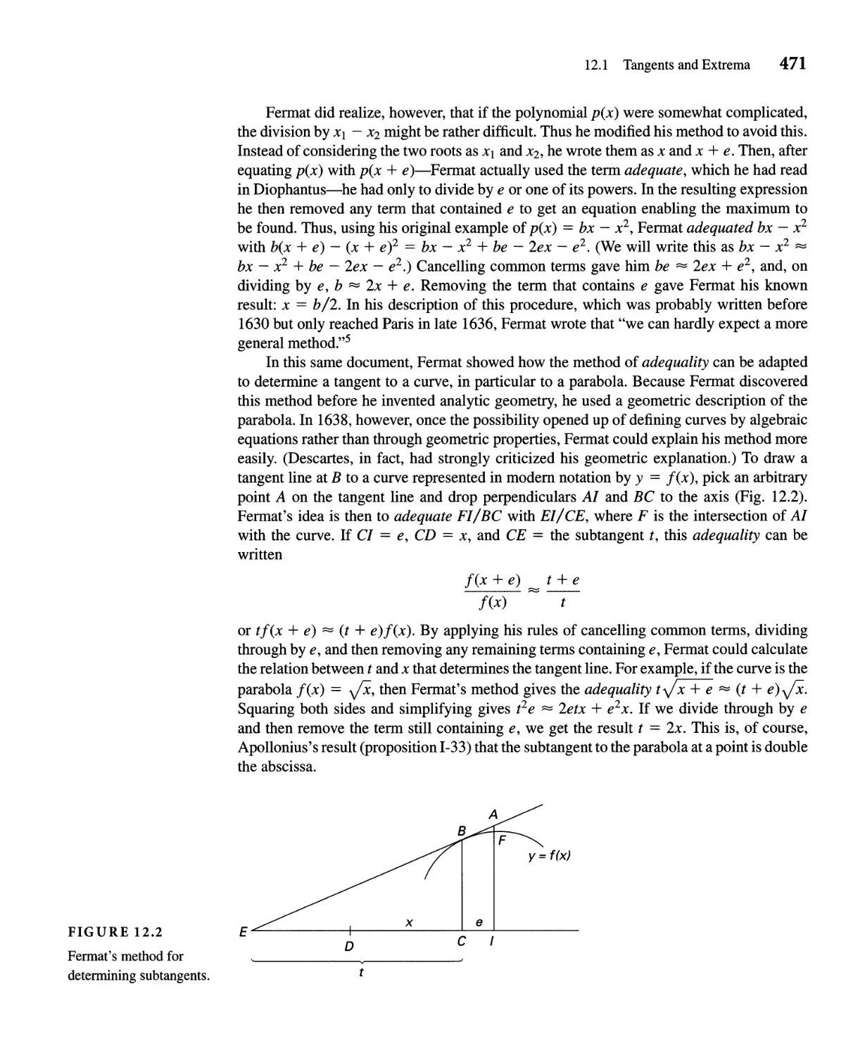
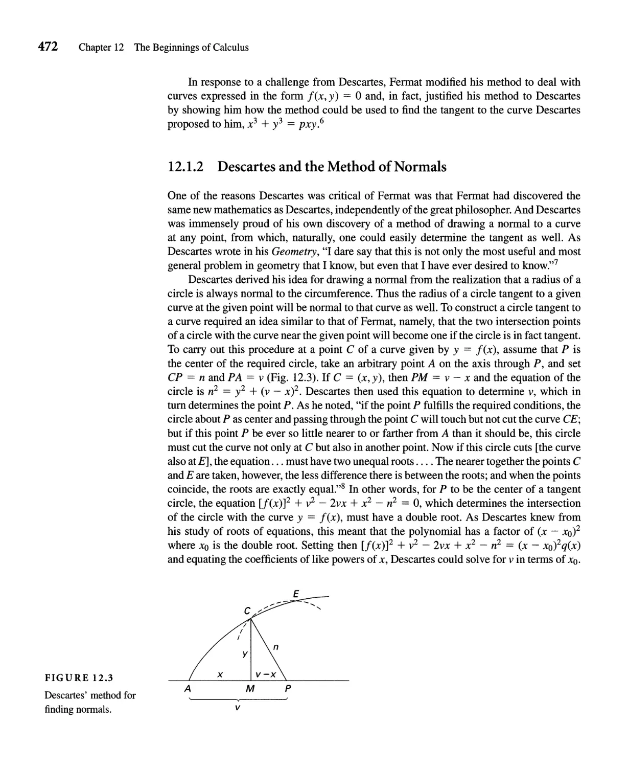
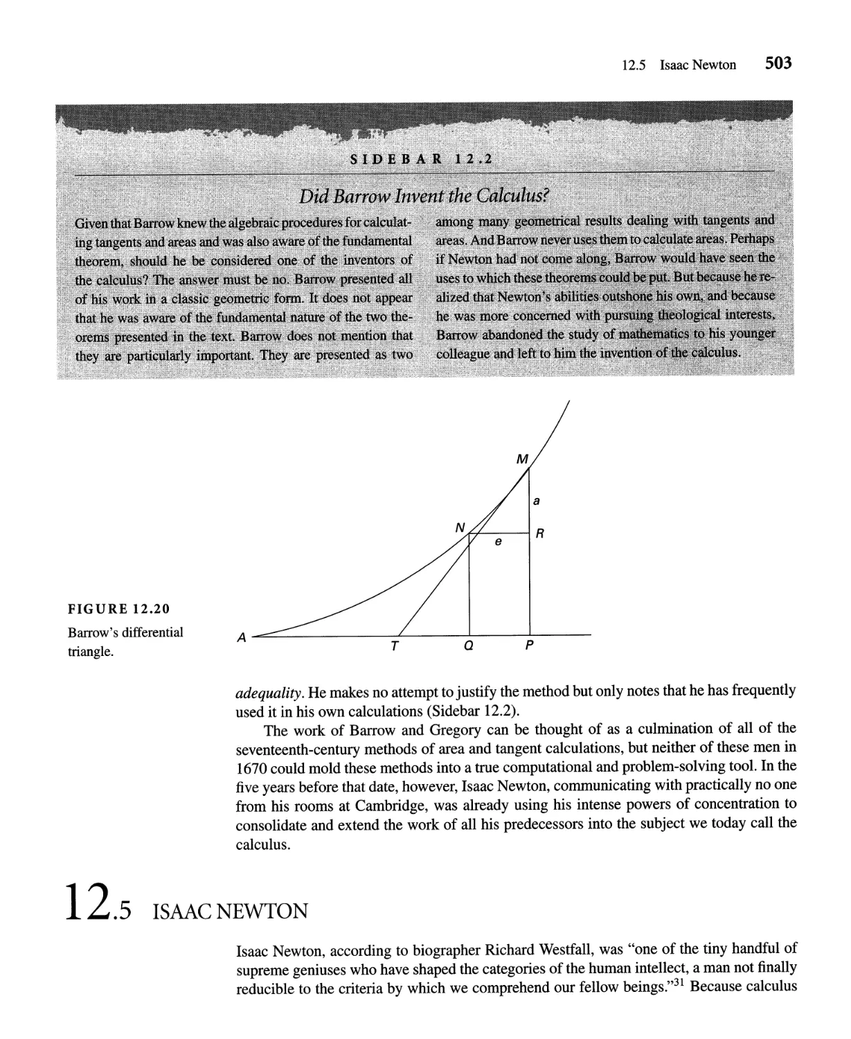
12.1 Tangents and Extrema 469
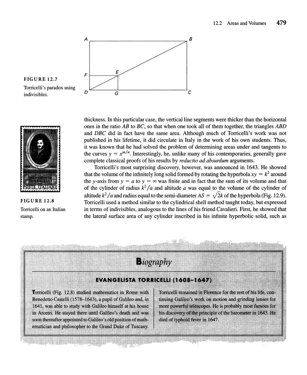
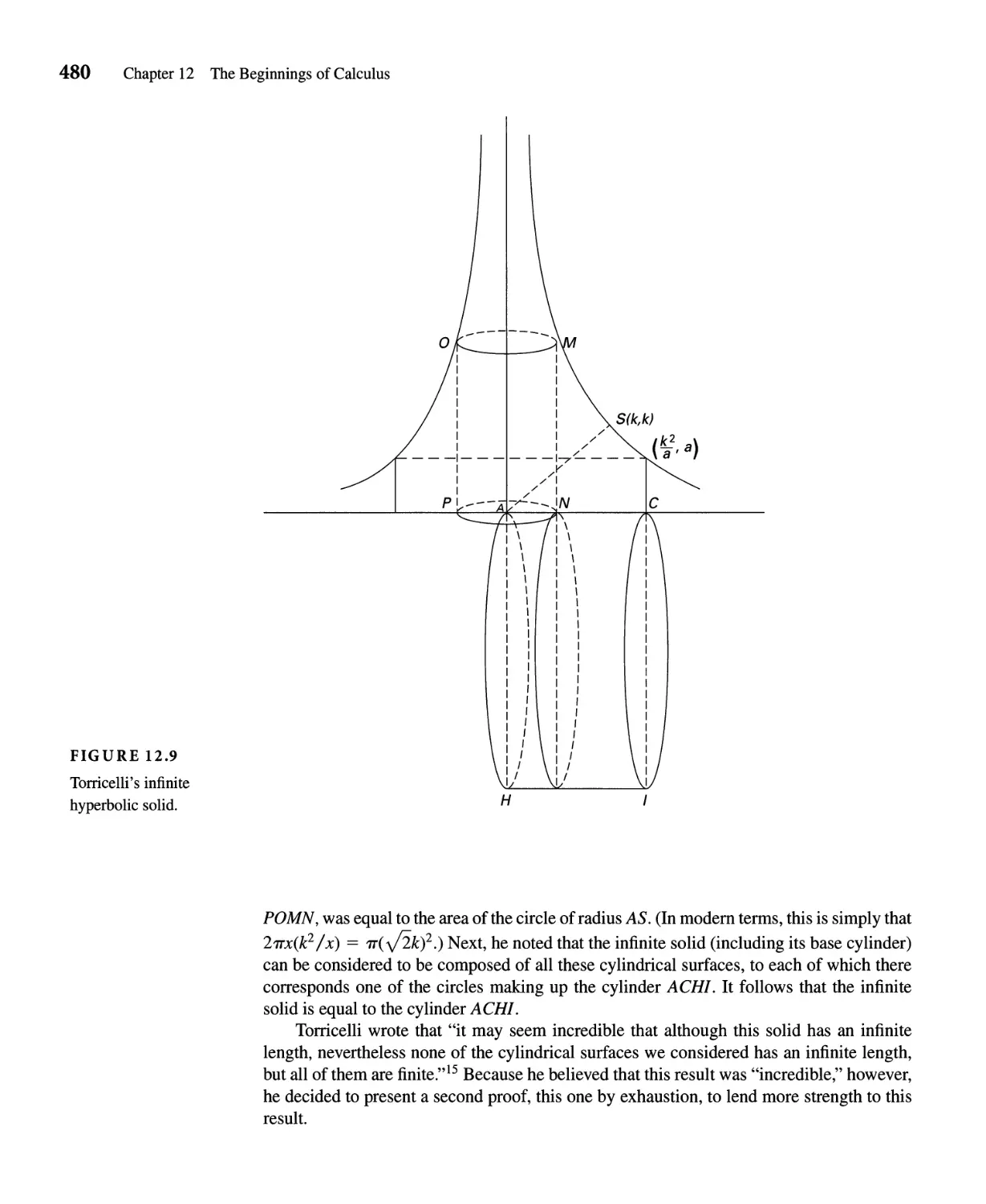
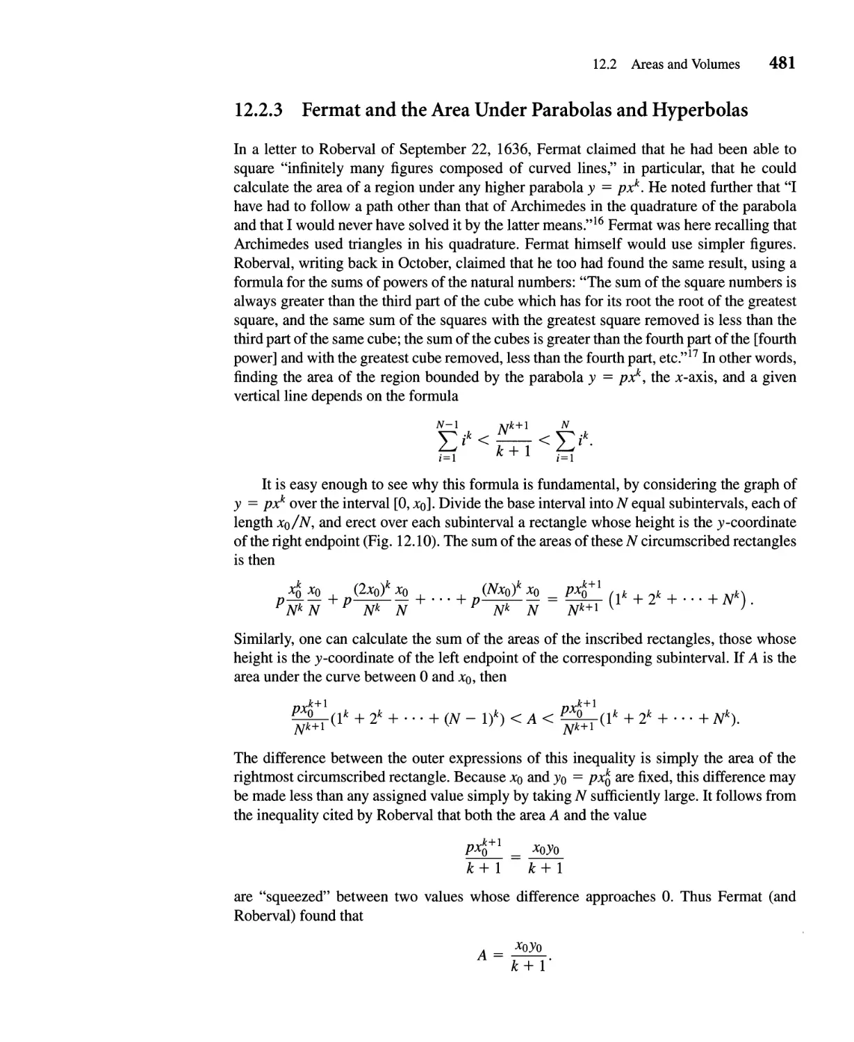
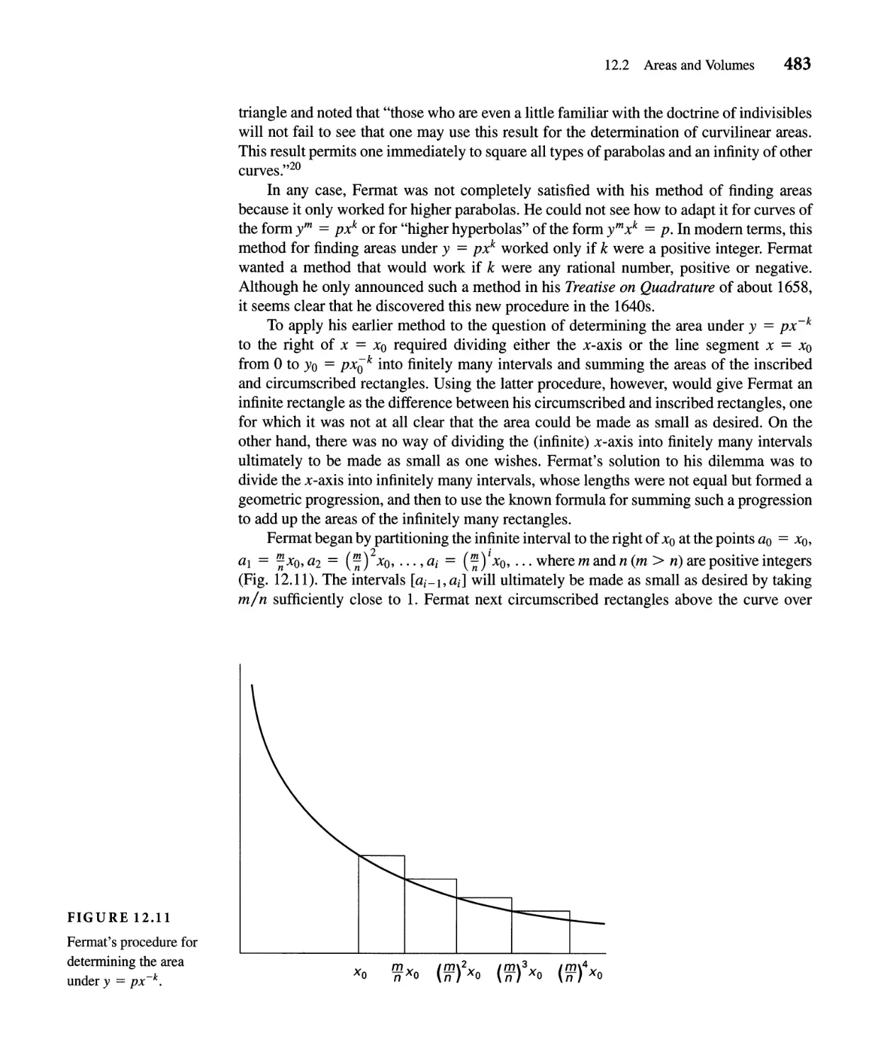
12.2 Areas and Volumes 475
12.3 Power Series 492
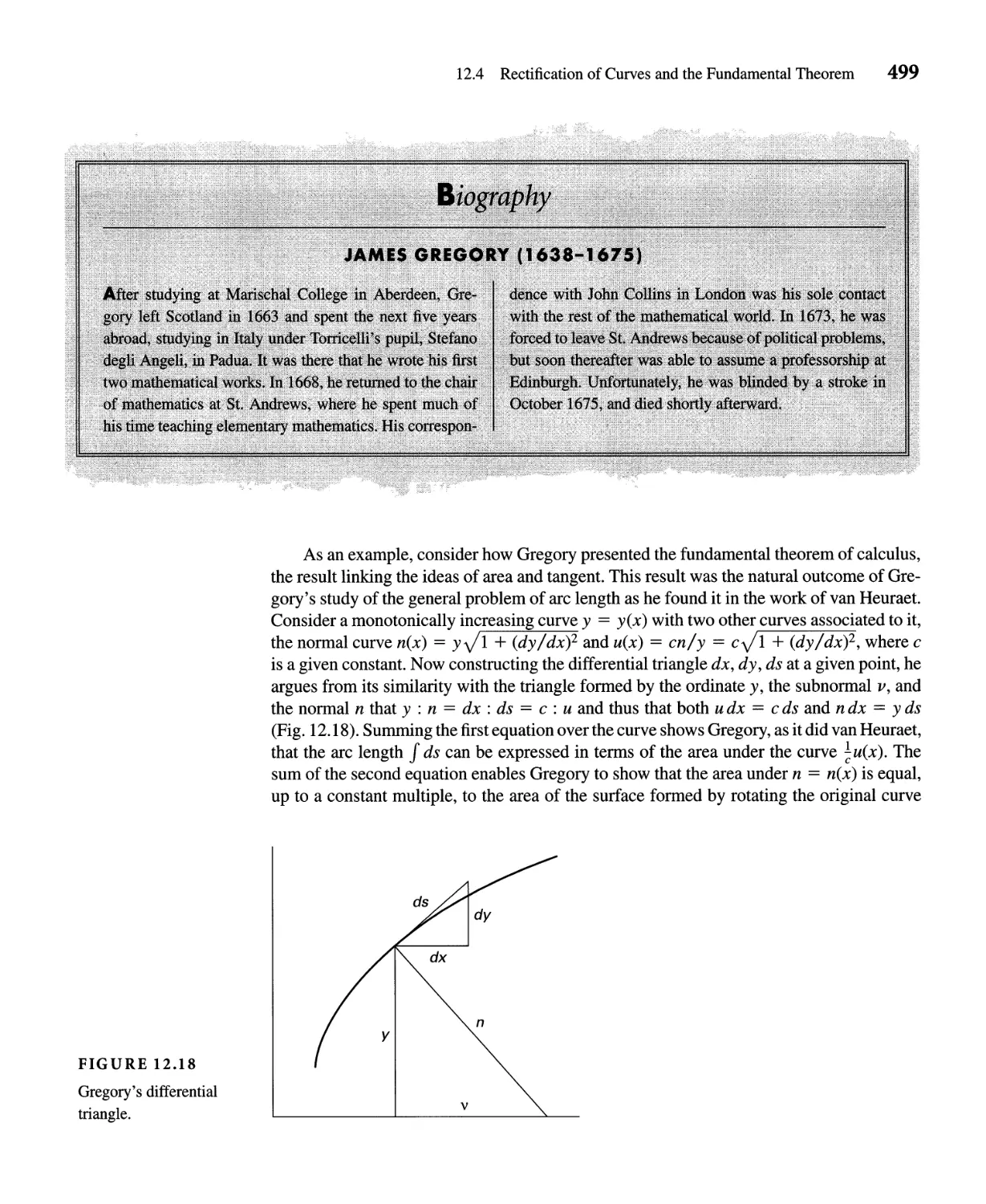
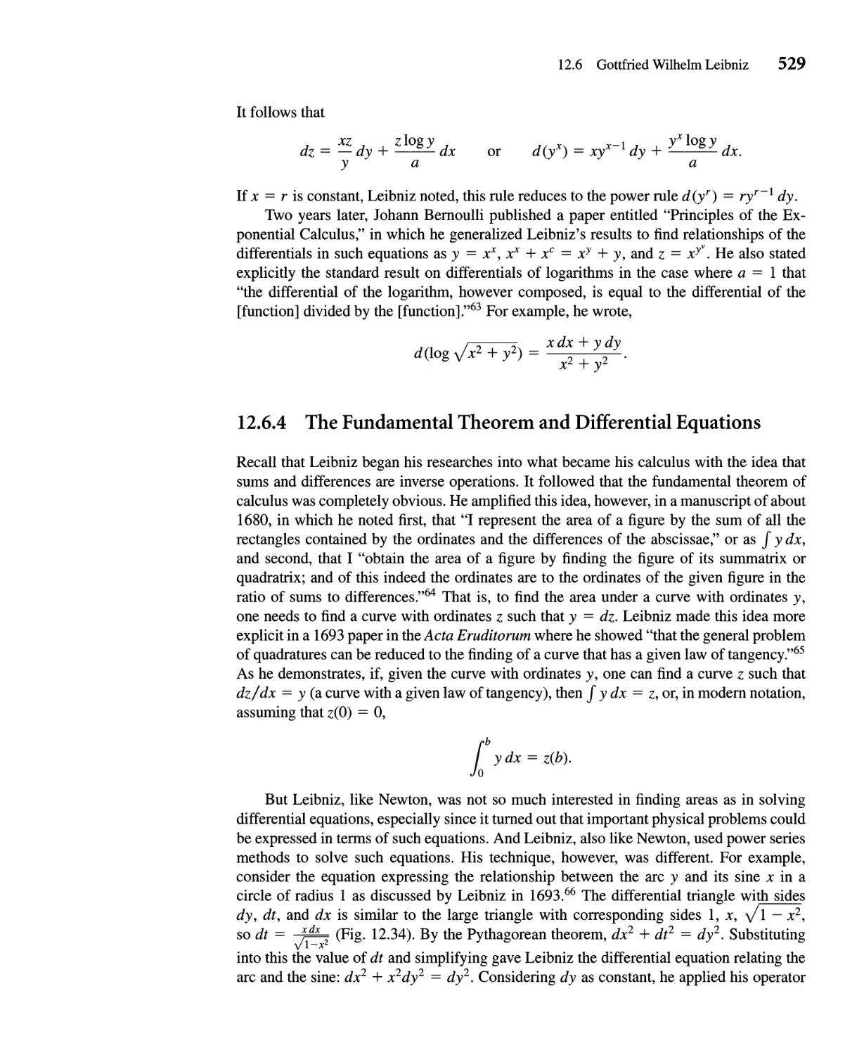
12.4 Rectification of Curves and the Fundamental Theorem 496
12.5 Isaac Newton 503
12.6 Gottfried Wilhelm Leibniz 522
12.7 First Calculus Texts 532
PART FOUR
Modern Mathematics: 1700-2000
CHAPTER 13 Analysis in the Eighteenth Century 544
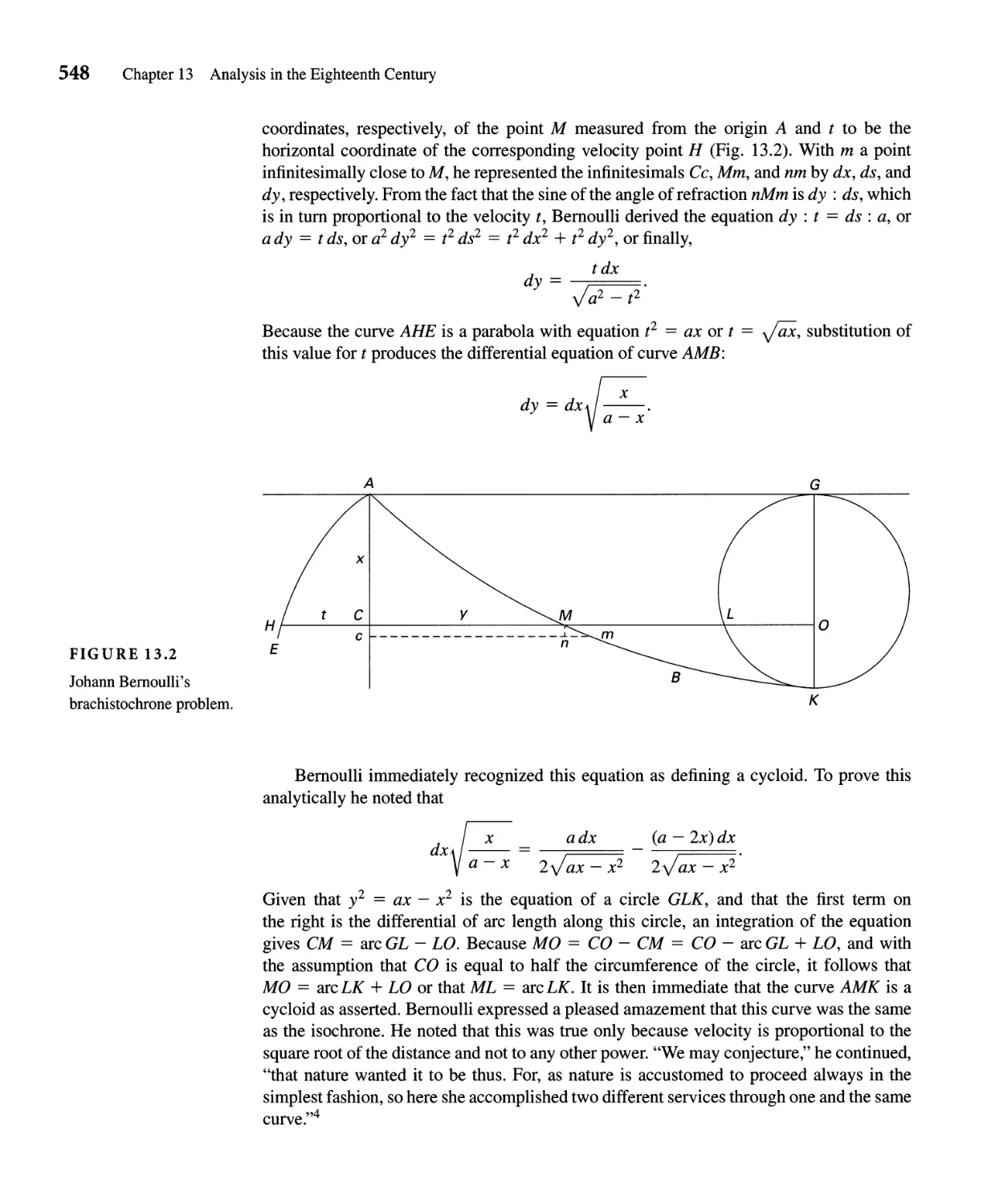
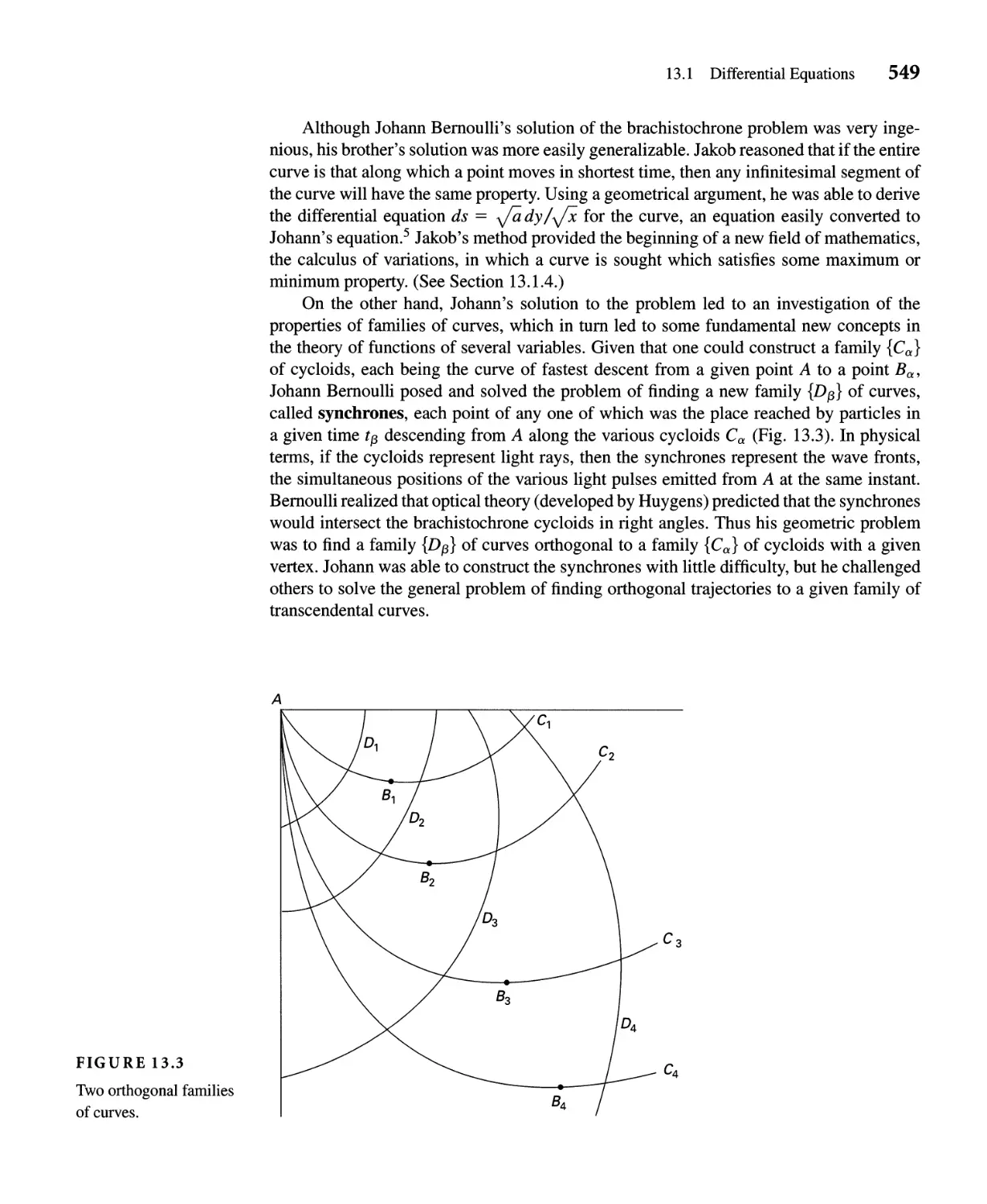
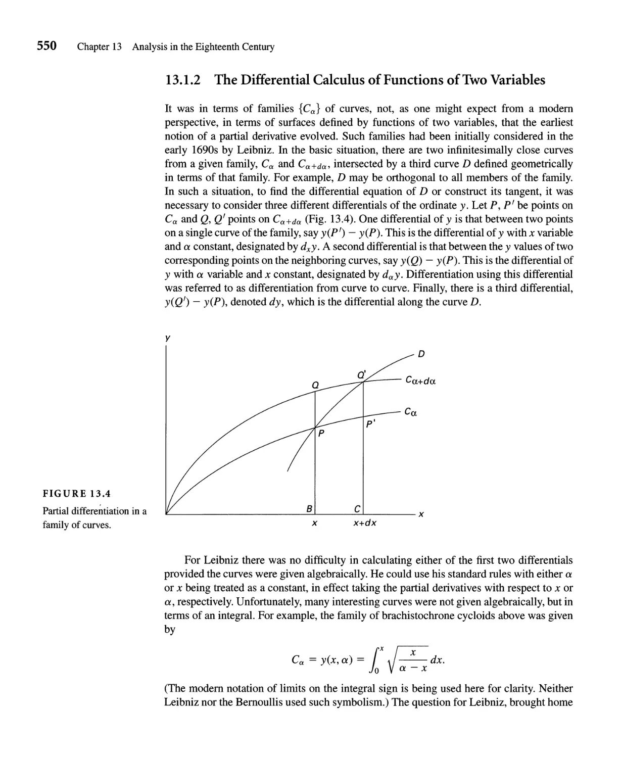
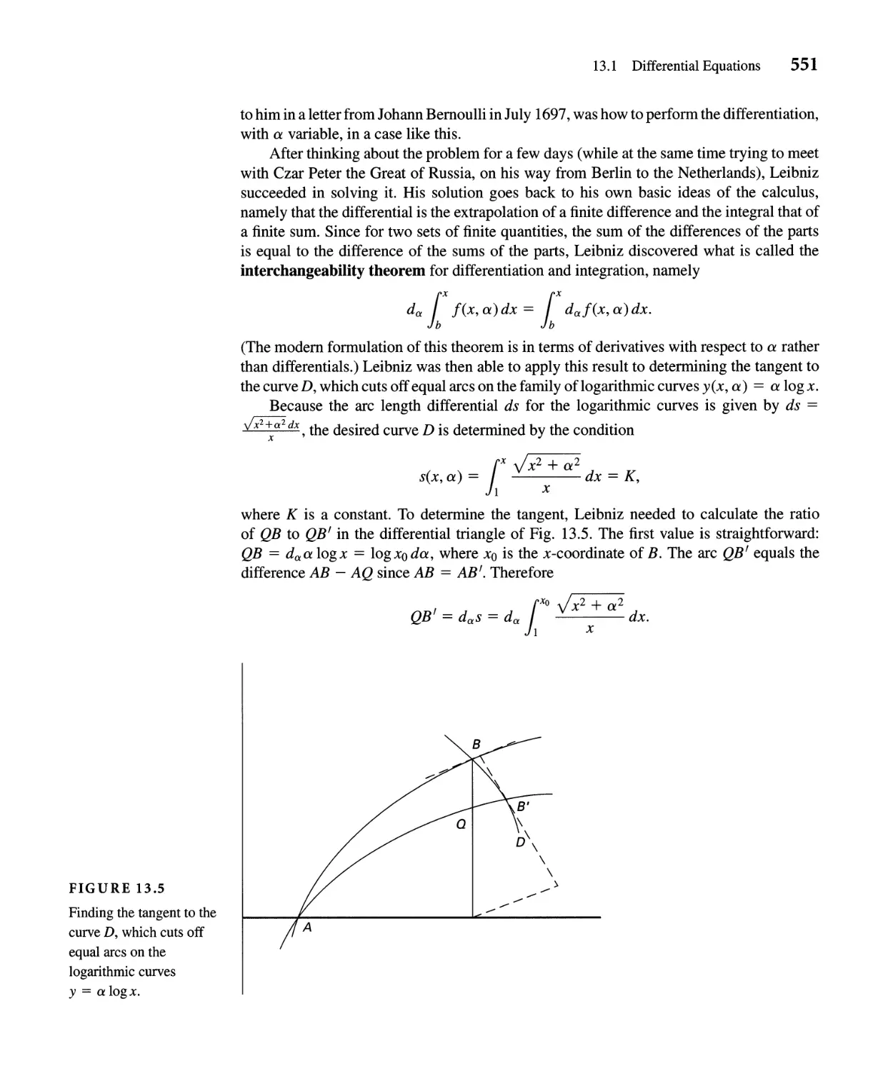
13.1 Differential Equations 545
13.2 Calculus Texts 560
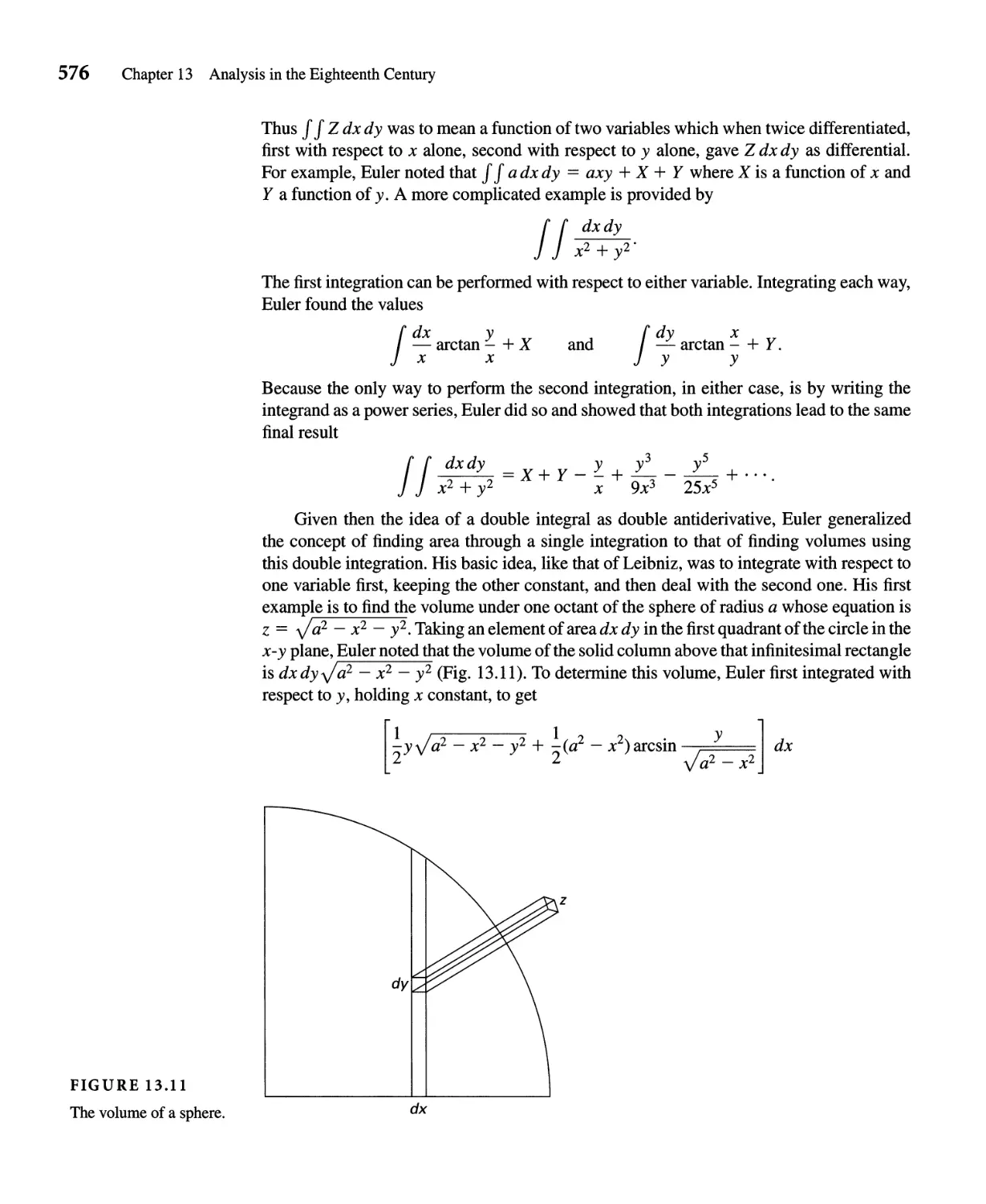
13.3 Multiple Integration 574
13.4 Partial Differential Equations: The Wave Equation 578
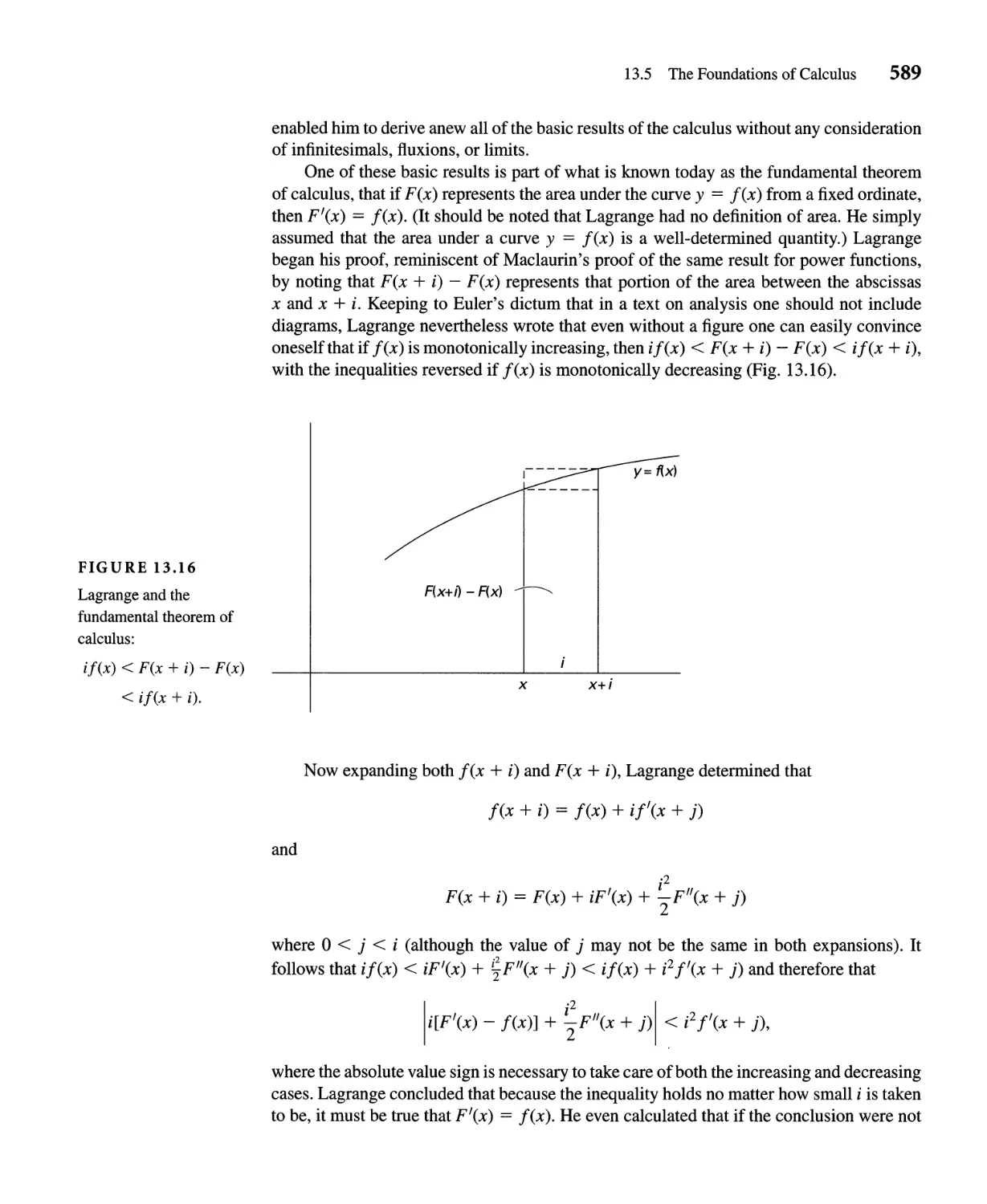
13.5 The Foundations of Calculus 582
...
VIII Contents
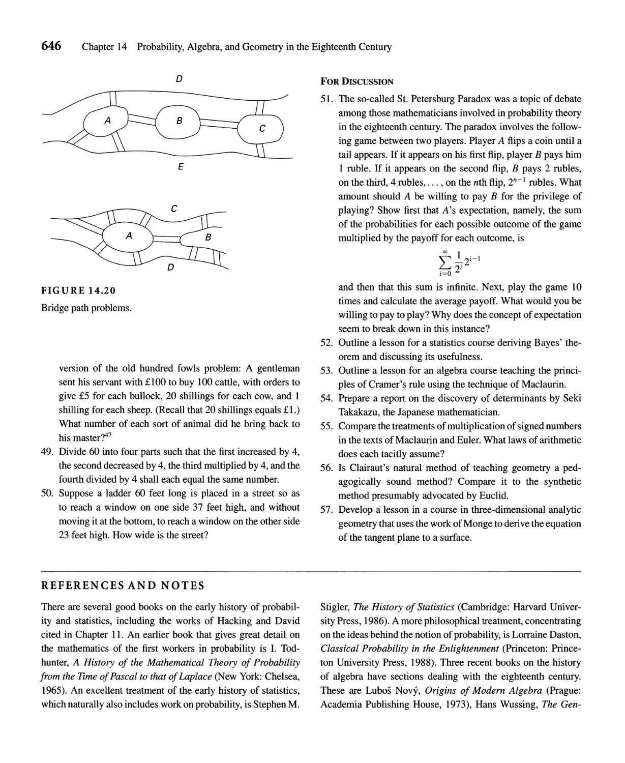
CHAPTER 14 Probability, Algebra, and Geometry in the Eighteenth Century 596
14.1 Probability 597
14.2 Algebra and Number Theory 610
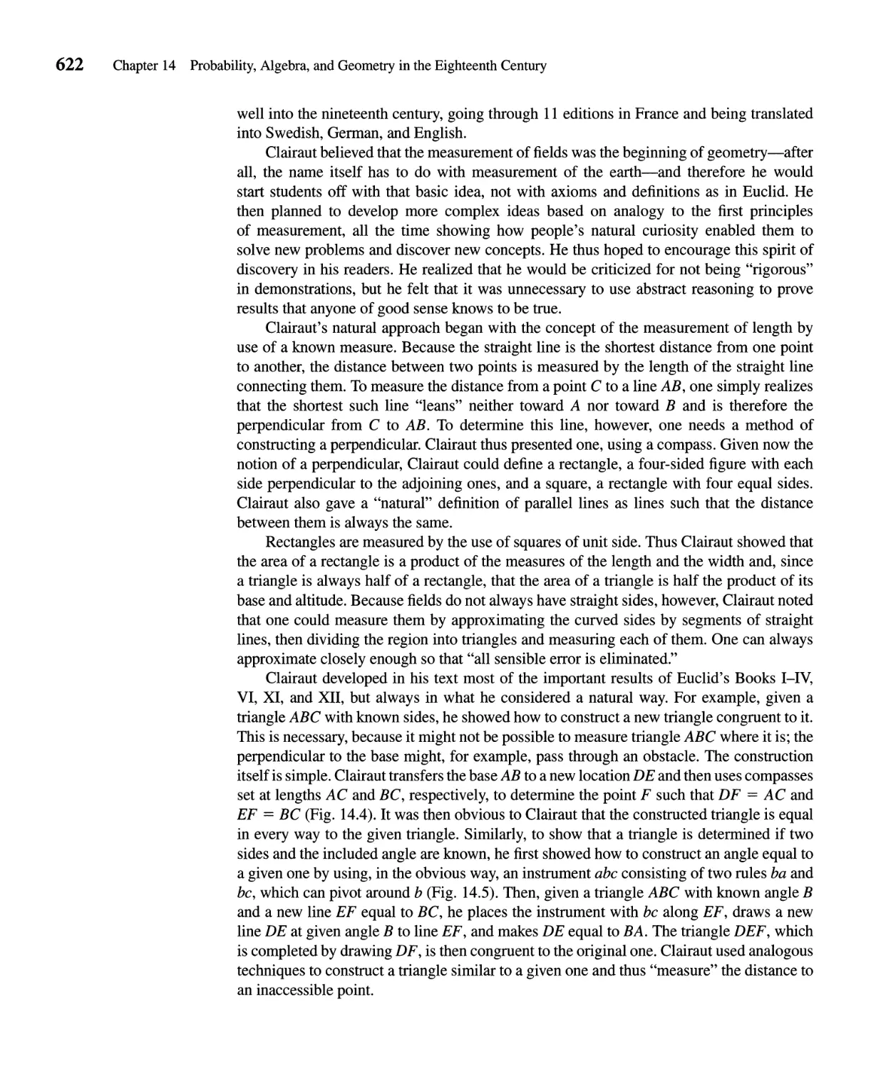
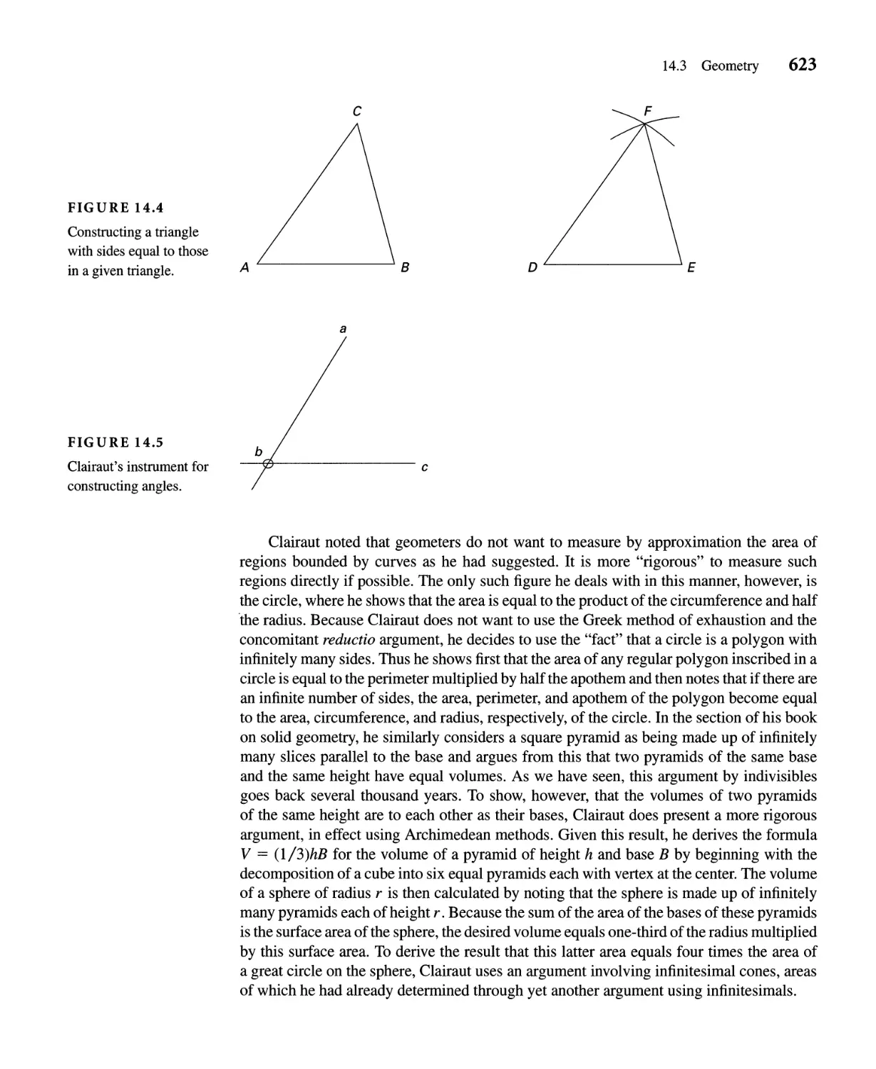
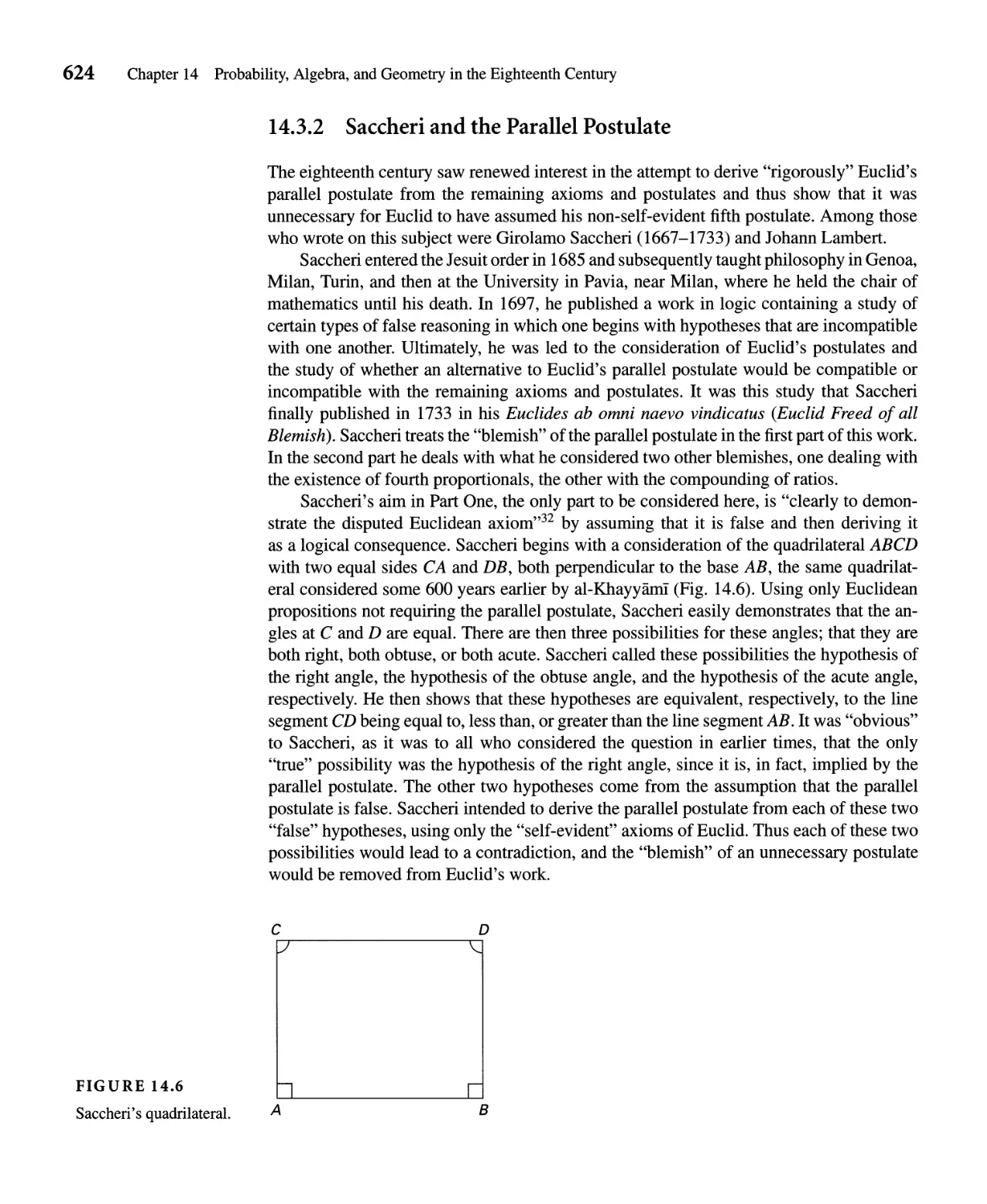
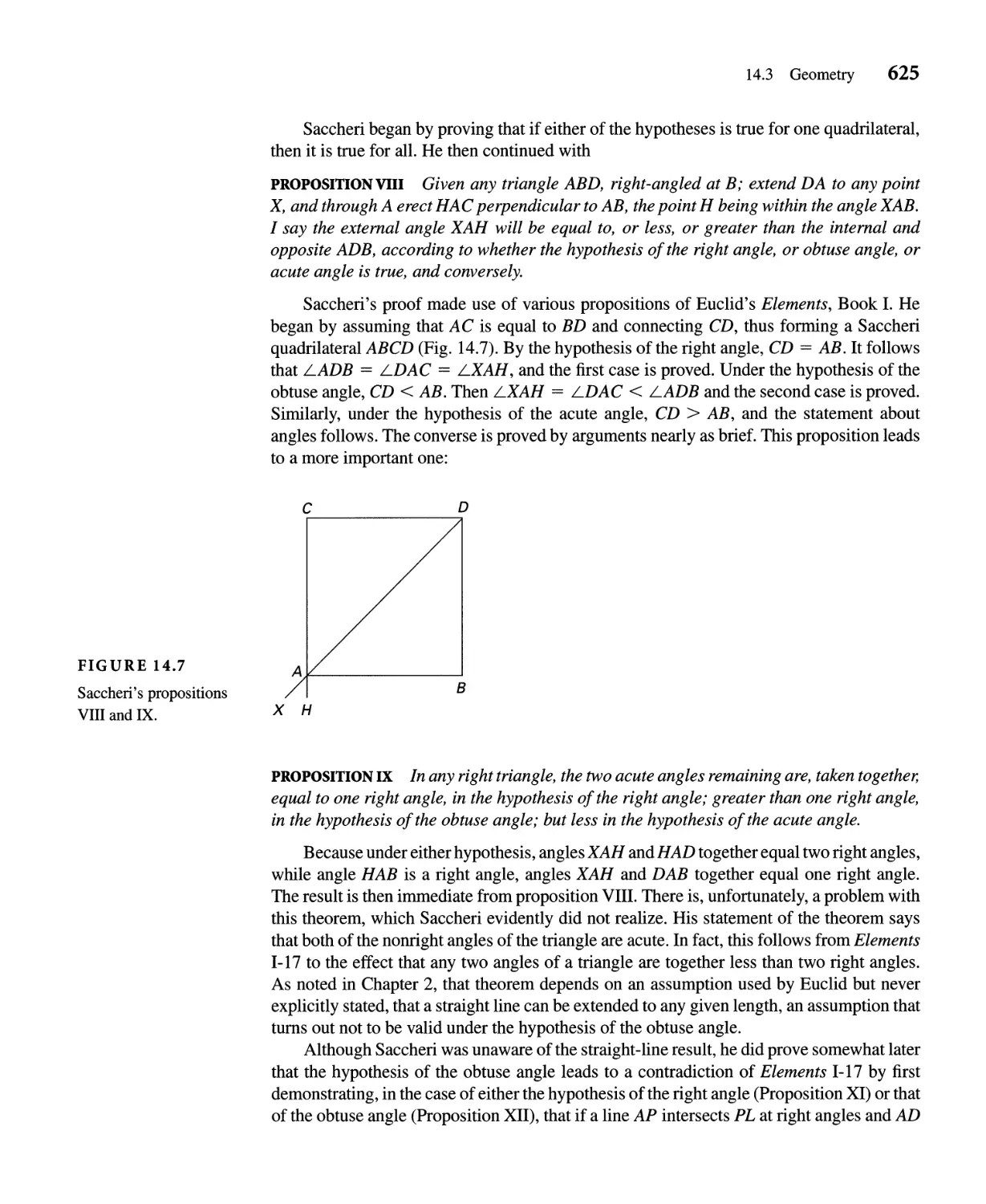
14.3 Geometry 621
14.4 The French Revolution and Mathematics Education 637
14.5 Mathematics in the Americas 640
CHAPTER 15 Algebra in the Nineteenth Century 650
15.1 Number Theory 652
15.2 Solving Algebraic Equations 662
15.3 Groups and Fields-The Beginning of Structure 670
15.4 Symbolic Algebra 677
15.5 Matrices and Systems of Linear Equations 687
CHAPTER 16 Analysis in the Nineteenth Century 704
16.1 Rigor in Analysis 706
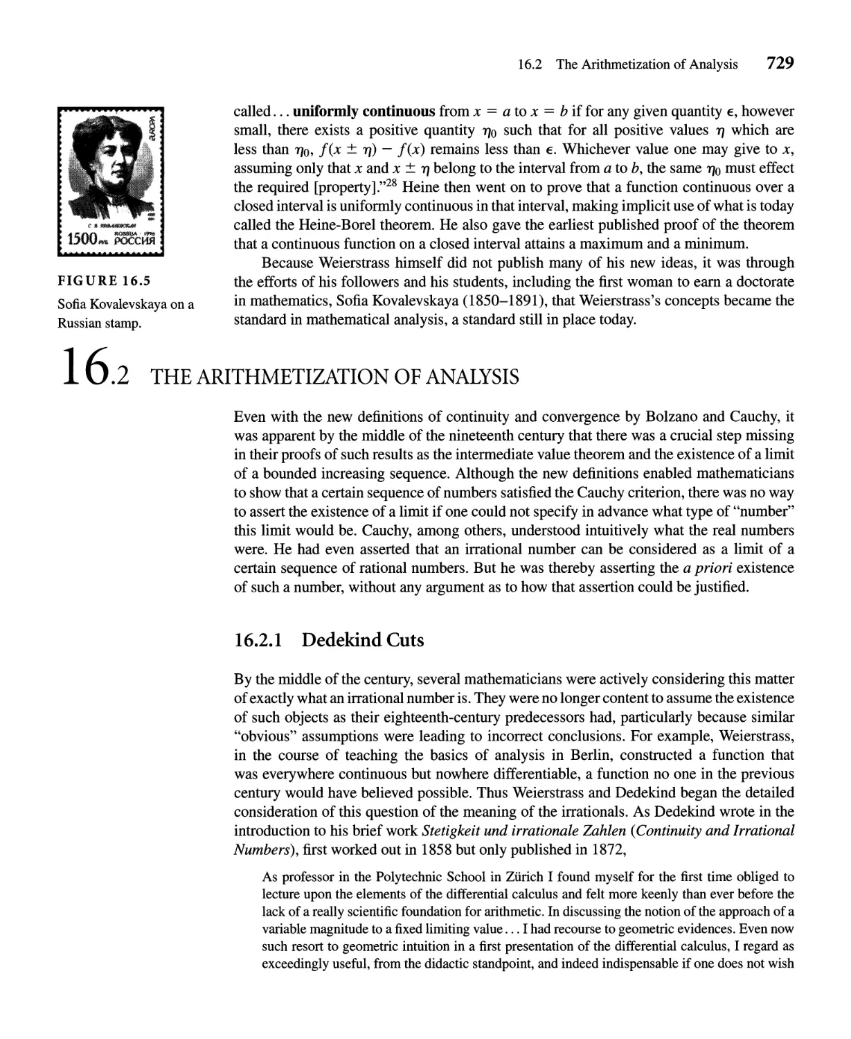
16.2 The Arithmetization of Analysis 729
16.3 Complex Analysis 737
16.4 Vector Analysis 746
16.5 Probability and Statistics 753
CHAPTER 17 Geometry in the Nineteenth Century 766
17.1 Differential Geometry 768
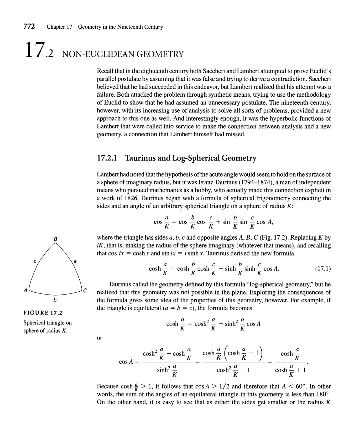
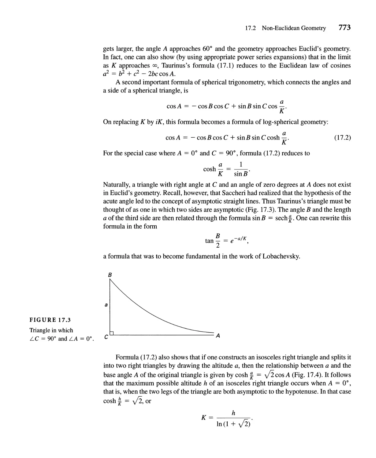
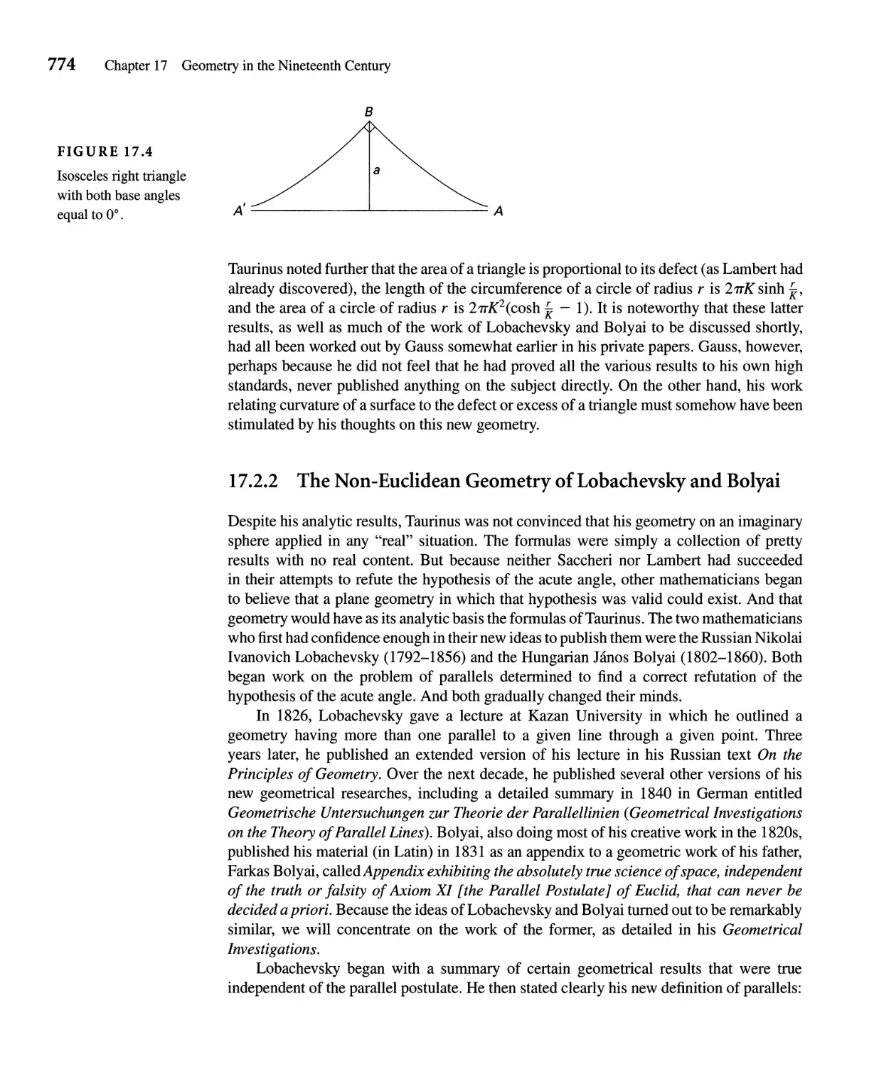
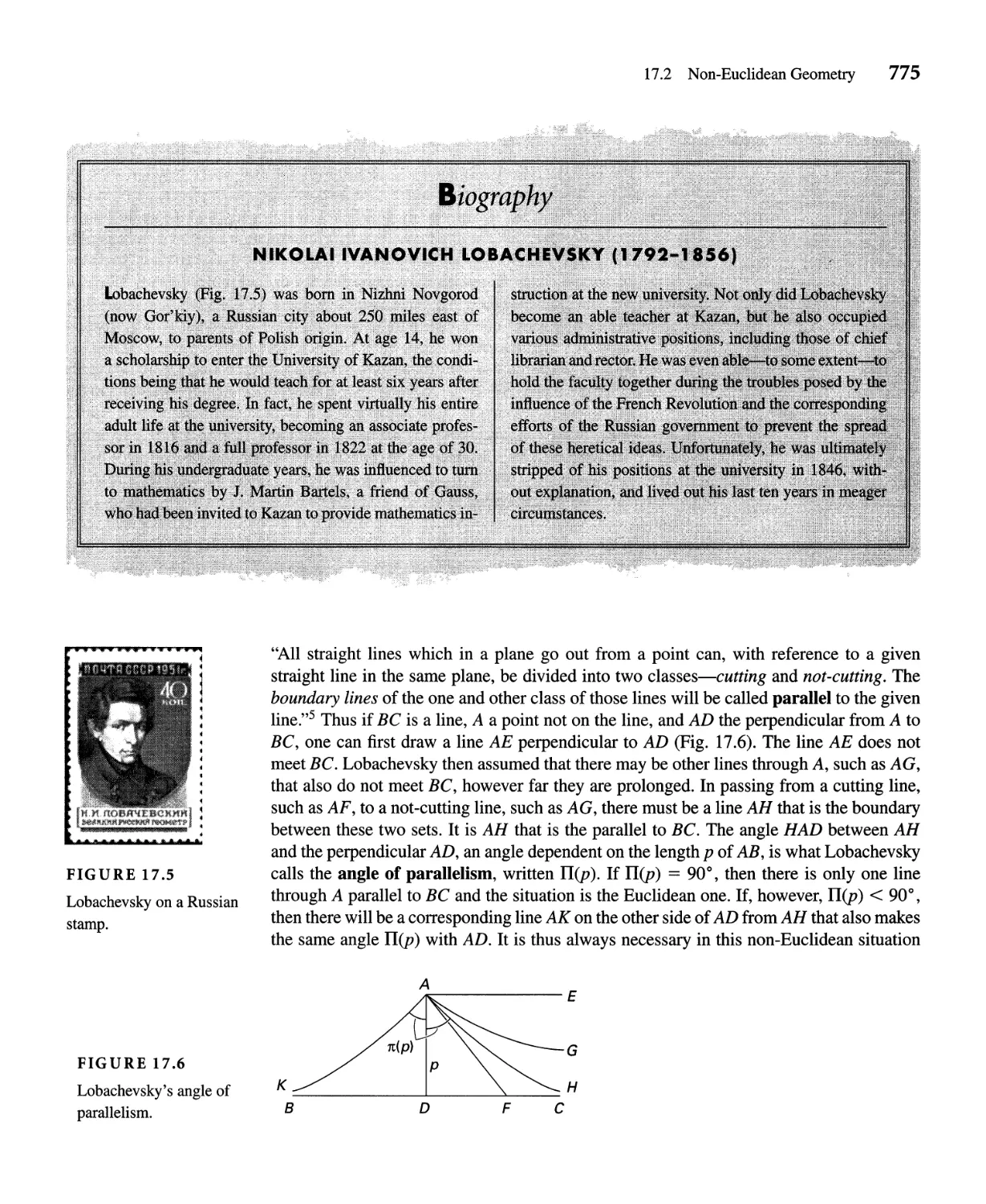
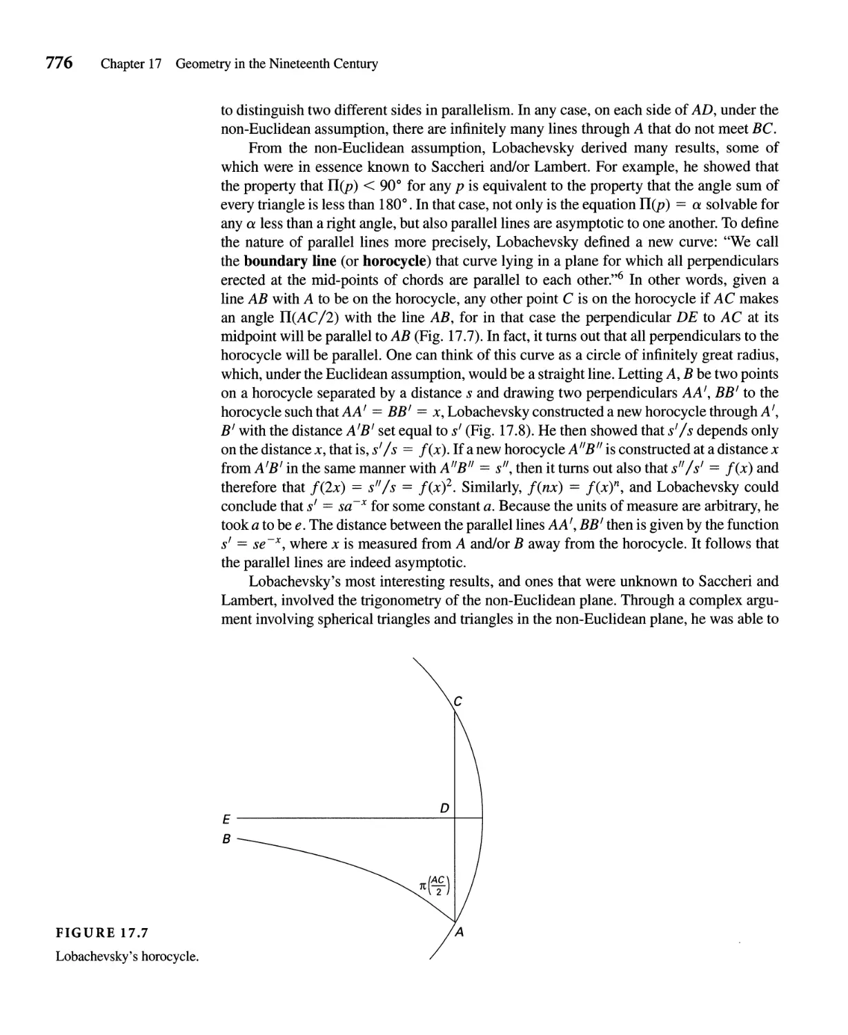
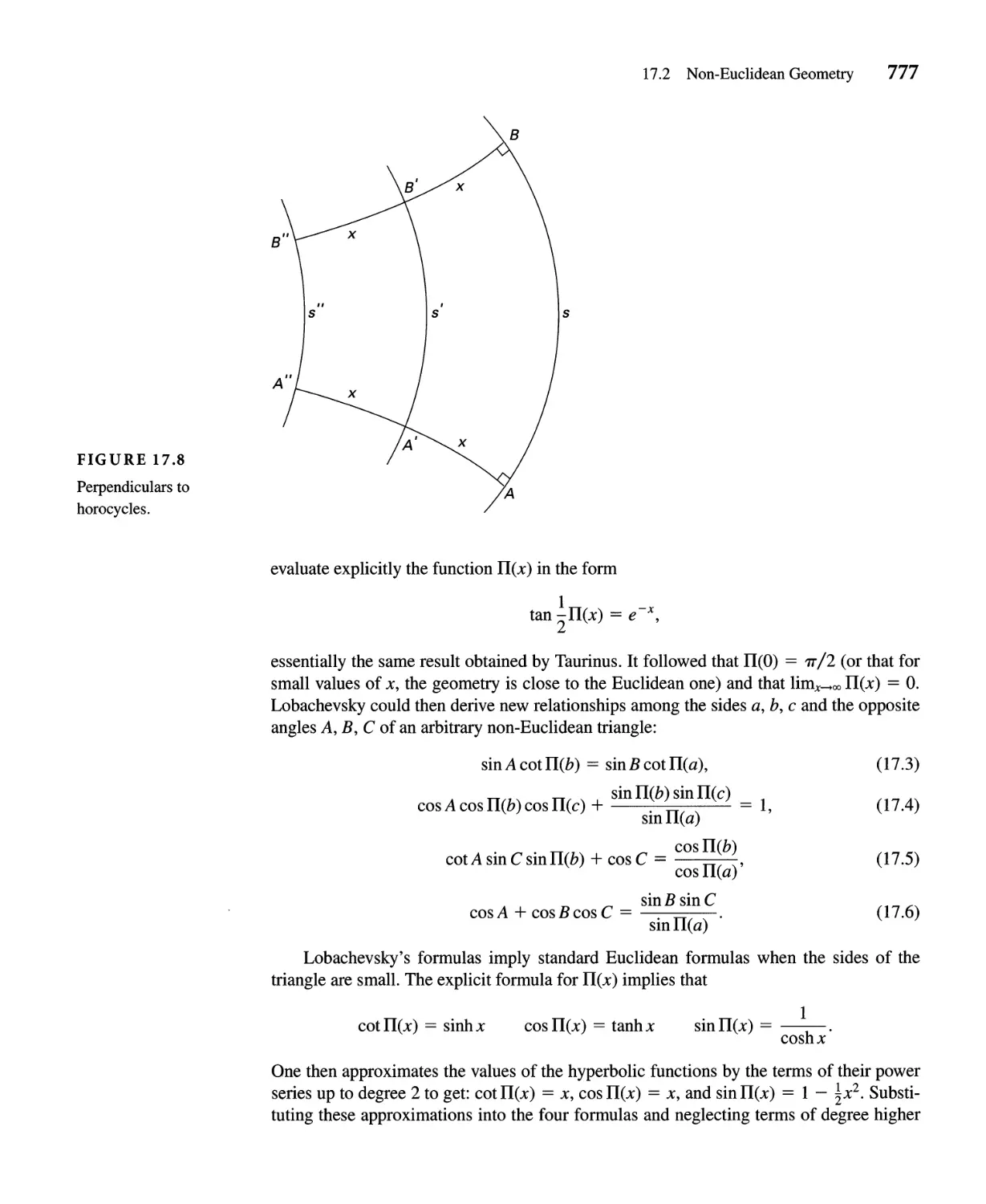
17.2 Non-Euclidean Geometry 772
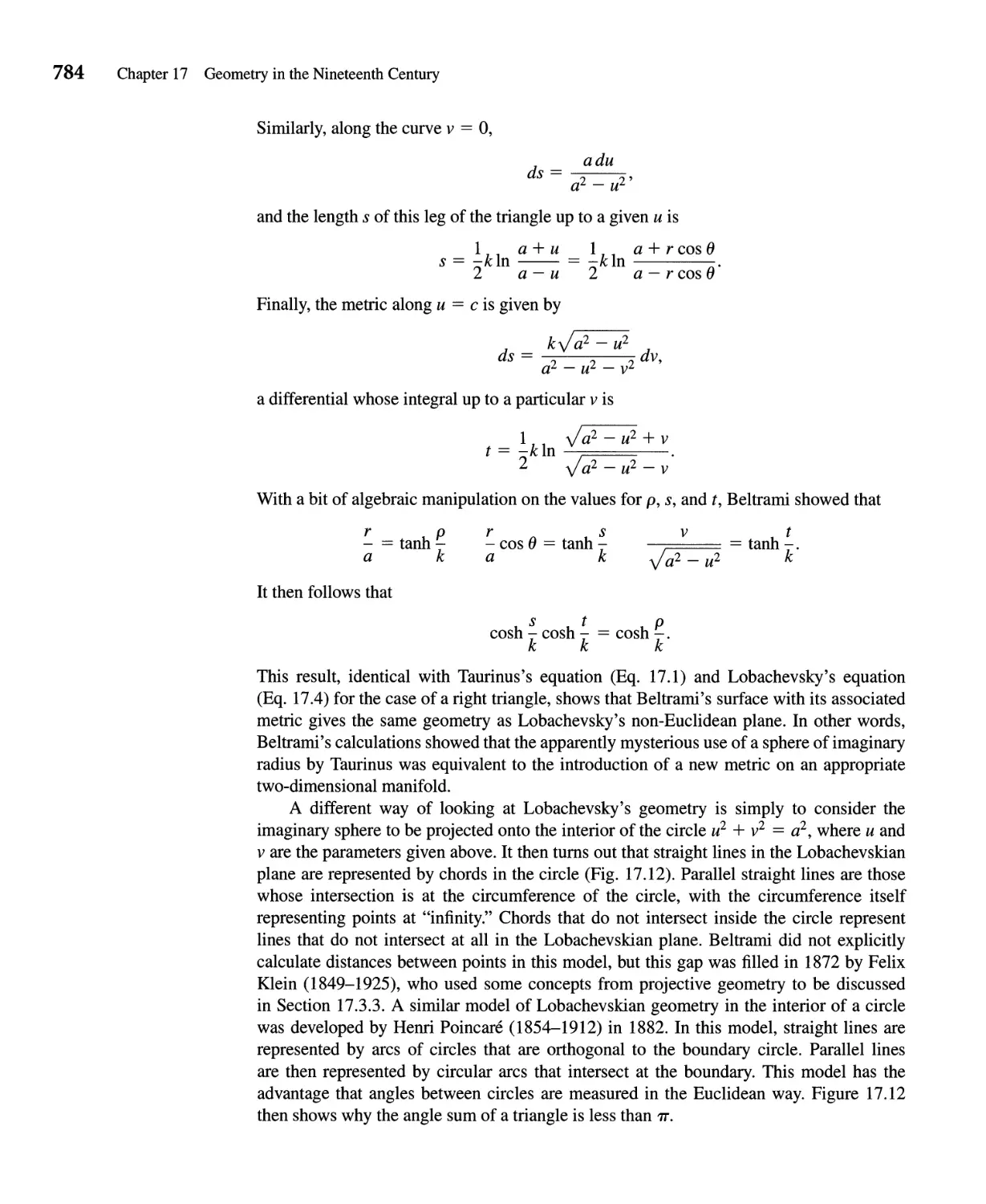
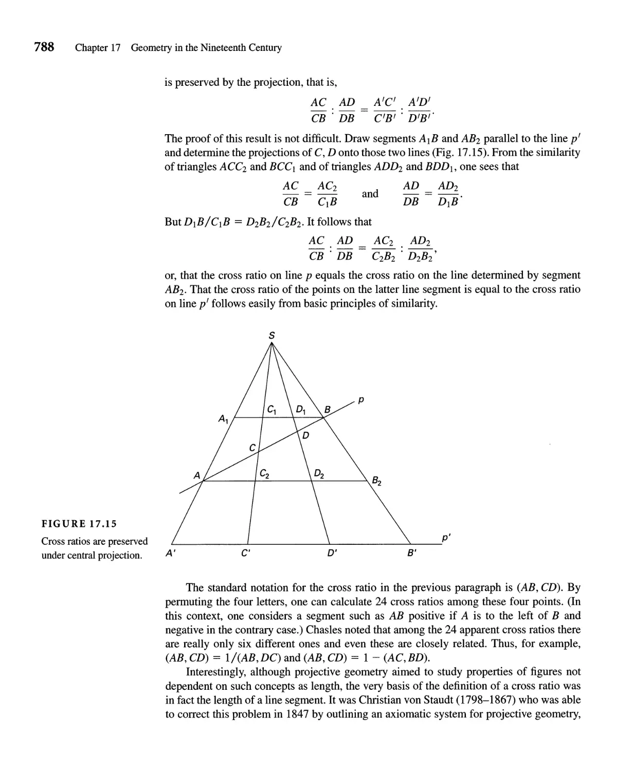
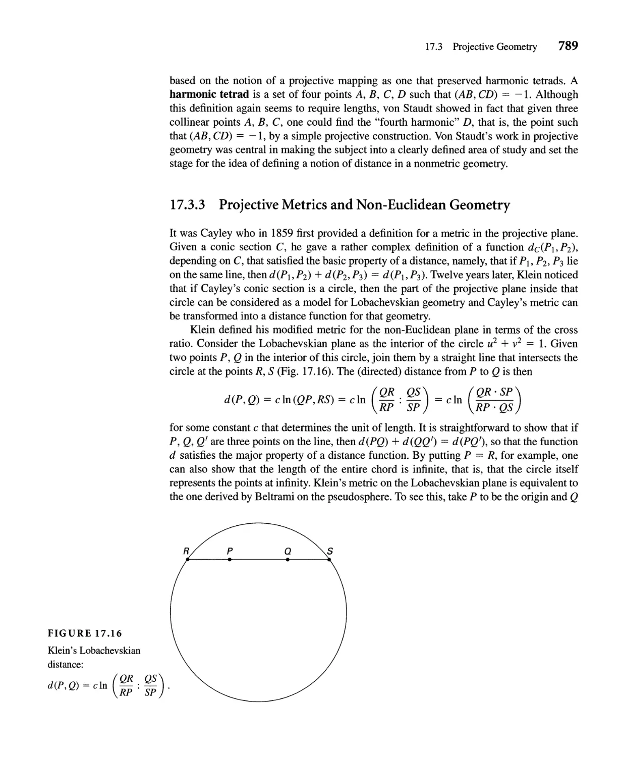
17.3 Projective Geometry 785
17.4 Geometry in N Dimensions 792
17.5 The Foundations of Geometry 797
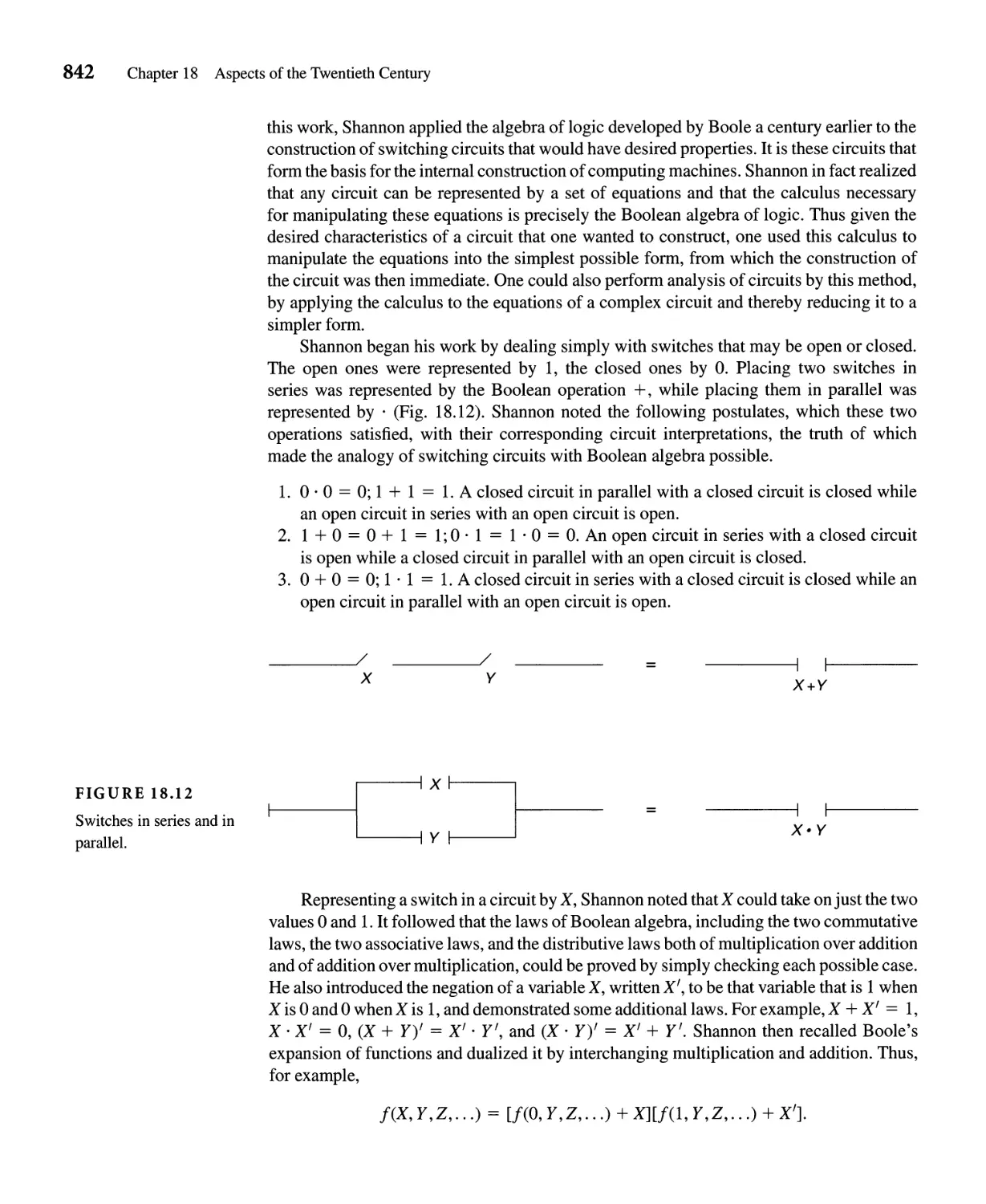
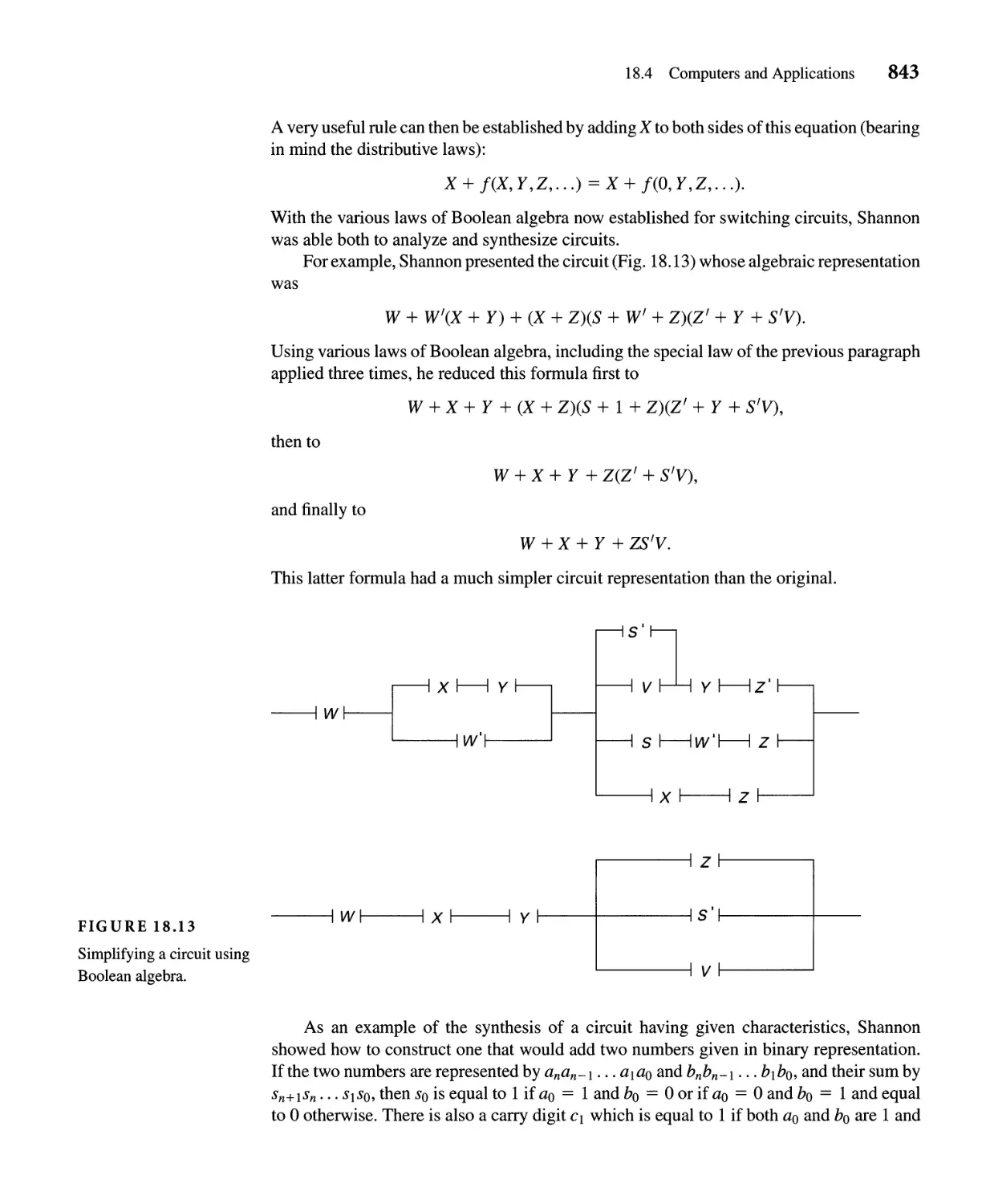
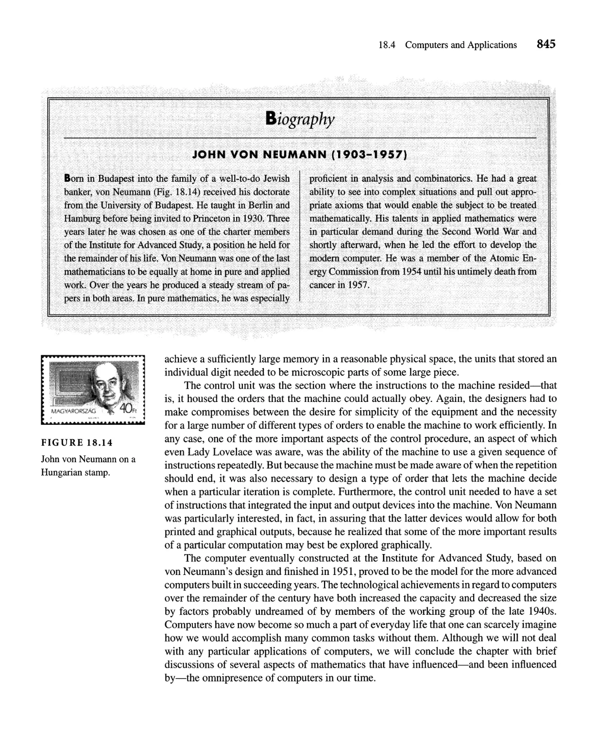
CHAPTER 18 Aspects of the Twentieth Century 805
18.1 Set Theory: Problems and Paradoxes 807
18.2 Topology 814
18.3 New Ideas in Algebra 822
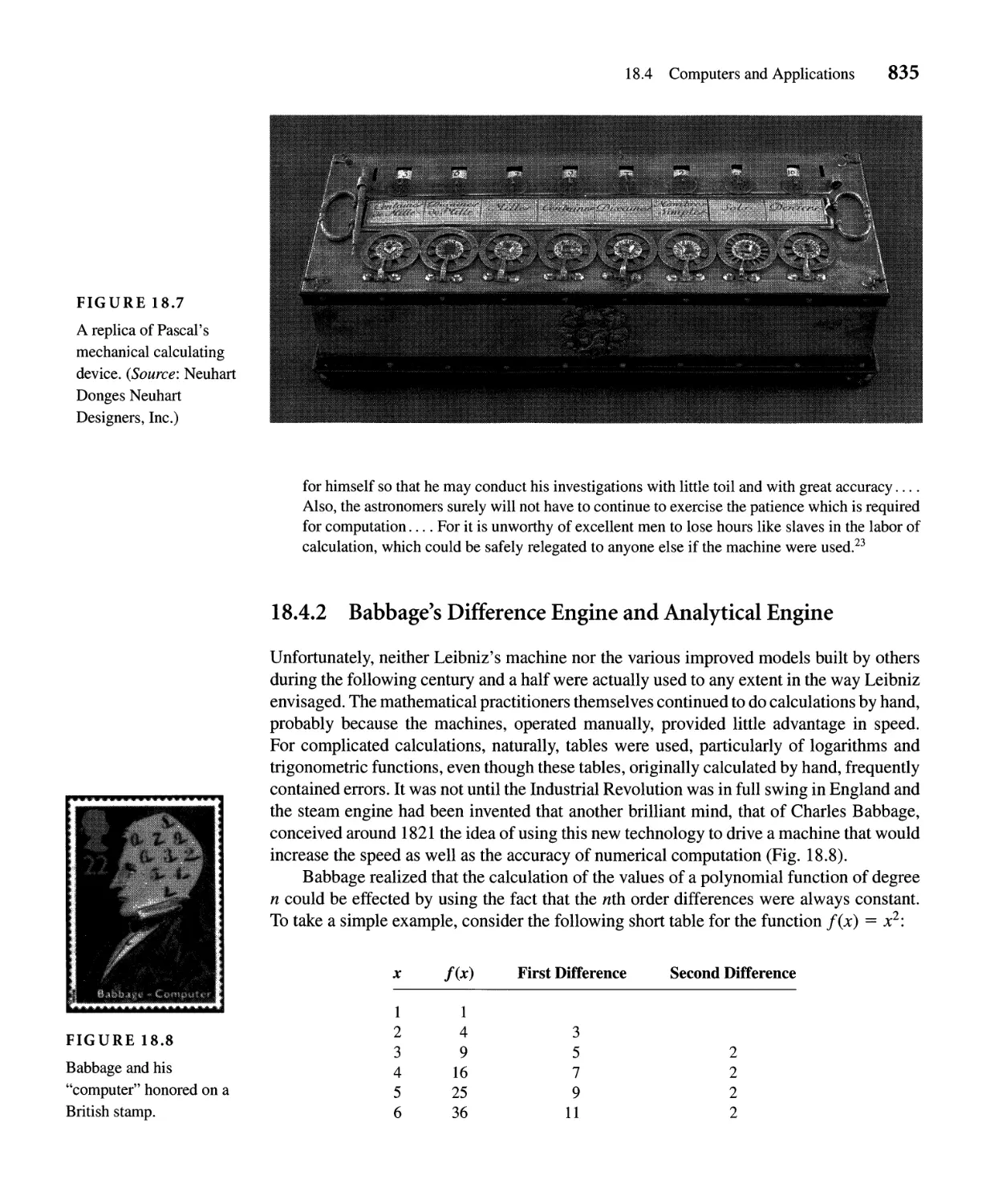
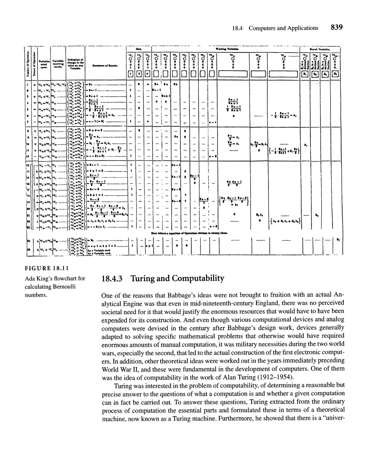
18.4 Computers and Applications 834
ANSWERS TO SELECTED PROBLEMS 857
GENERAL REFERENCES IN THE HISTORY OF MATHEMATICS 863
INDEX AND PRONUNCIATION GUIDE /-1
Preface
APPROACH AND GUIDING PHILOSOPHY
In A Call For Change: Recommendations for the Mathematical Preparation of Teachers of
Mathematics, the Mathematical Association of America's (MAA) Committee on the Math-
ematical Education of Teachers recommends that all prospective teachers of mathematics
in schools
develop an appreciation of the contributions made by various cultures to the growth and devel-
opment of mathematical ideas; investigate the contributions made by individuals, both female
and male, and from a variety of cultures, in the development of ancient, modem, and current
mathematical topics; [and] gain an understanding of the historical development of major school
mathematics concepts.
According to the MAA, knowledge of the history of mathematics shows students
that mathematics is an important human endeavor. Mathematics was not discovered in the
polished form of our textbooks, but often developed in intuitive and experimental fashion
out of a need to solve problems. The actual development of mathematical ideas can be
effectively used in exciting and motivating students today.
This new textbook in the history of mathematics grew out of the conviction that not
only prospective school teachers of mathematics but also prospective college teachers of
mathematics need a background in history to teach the subject more effectively to their
students. It is therefore designed for junior or senior mathematics majors who intend to
teach in college or high school and thus concentrates on the history of those topics typically
covered in an undergraduate curriculum or in elementary or high school. Because the history
of any given mathematical topic often provides excellent ideas for teaching the topic, there
is sufficient detail in each explanation of a new concept for the future (or present) teacher
of mathematics to develop a classroom lesson or series of lessons based on history. In fact,
many of the problems ask the reader to develop a particular lesson. My hope is that the
student and prospective teacher will gain from this book a knowledge of how we got here
from there, a knowledge that will provide a deeper understanding of many of the important
concepts of mathematics.
.
IX
x Preface
DISTINGUISHING FEATURES
Flexible Organization
Although the chief organization of the book is by chronological period, within each period
the material is organized topically. By consulting the detailed subsection headings, the
reader can choose to follow a particular theme throughout history. For example, to study
equation solving one could consider ancient Egyptian and Babylonian methods, the geo-
metrical solution methods of the Greeks, the numerical methods of the Chinese, the Islamic
solution methods for cubic equations by use of conic sections, the Italian discovery of an
algorithmic solution of cubic and quartic equations, the work of Lagrange in developing
criteria for methods of solution of higher degree polynomial equations, the work of Gauss
in solving cyclotomic equations, and the work of Galois in using permutations to formulate
what is today called Galois theory.
Focus on Textbooks
There is an emphasis throughout the book on the important textbooks of various periods. It
is one thing to do mathematical research and discover new theorems and techniques. It is
quite another to elucidate these in a way that others can learn them. In nearly every chapter,
therefore, there is a discussion of one or more important texts of the time. These will be
the works from which students learned the important ideas of the great mathematicians.
Today's students will see how certain topics were treated and will be able to compare these
treatments to those in current texts and see the kinds of problems students of years ago
were expected to solve.
Astronomy and Mathematics
Two chapters are devoted entirely to mathematical methods, that is, to the ways in which
mathematics was used to solve problems in other areas of endeavor. A substantial part of
both of these chapters, one for the Greek period and one for the Renaissance, deals with
astronomy. In fact, in ancient times astronomers and mathematicians were usually the same
people. It is crucial to the understanding of a substantial part of Greek mathematics to
understand the Greek model of the heavens and how mathematics was used in applying this
model to give predictions. Similarly, we will discuss the Copernicus-Kepler model of the
heavens and see how mathematicians of the Renaissance applied mathematics to its study.
Non- Western Mathematics
A special effort has been made to consider mathematics developed in parts of the world
other than Europe. Thus, there is substantial material on mathematics in China, India,
and the Islamic world. There is also an "interchapter" in which a comparison is made
of the mathematics in the major civilizations at about the turn of the fourteenth century.
That comparison is followed by a discussion of the mathematics of various other societies
.
Preface Xl
around the world. The reader will see how certain mathematical ideas have occurred in
many places, although not perhaps in the context of what we in the West call "mathematics."
Topical Exercises
Each chapter contains many exercises, collected by topic for easy access. Some of the
exercises are simple computational ones while others help to fill the gaps in the mathematical
arguments presented in the text. For Discussion exercises are open-ended questions for
discussion, which may involve some research to find answers. Many of these ask students
to think about how they would use historical material in the classroom. (Answers to most
of the computational exercises are provided in the answer section.) Even if readers do not
attempt many of the exercises, they should at least read them to gain a fuller understanding
of the material of the chapter.
Focus Essays
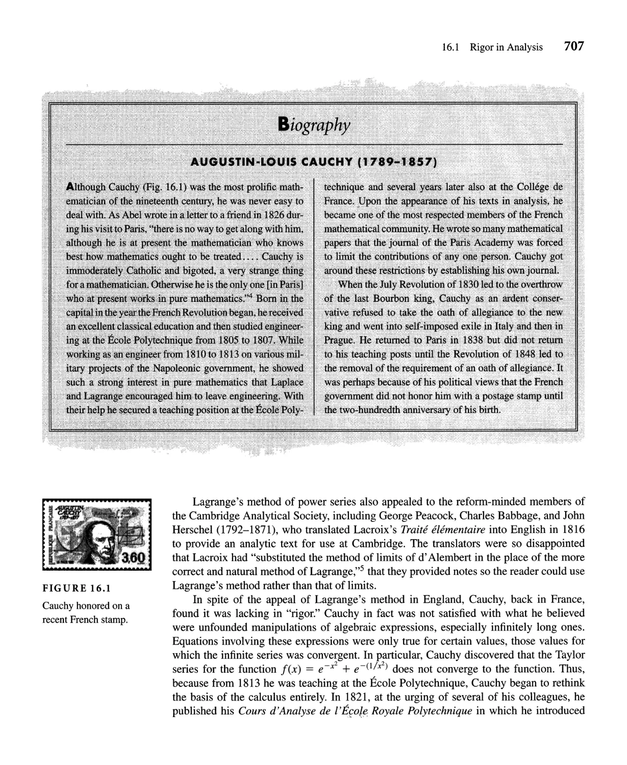
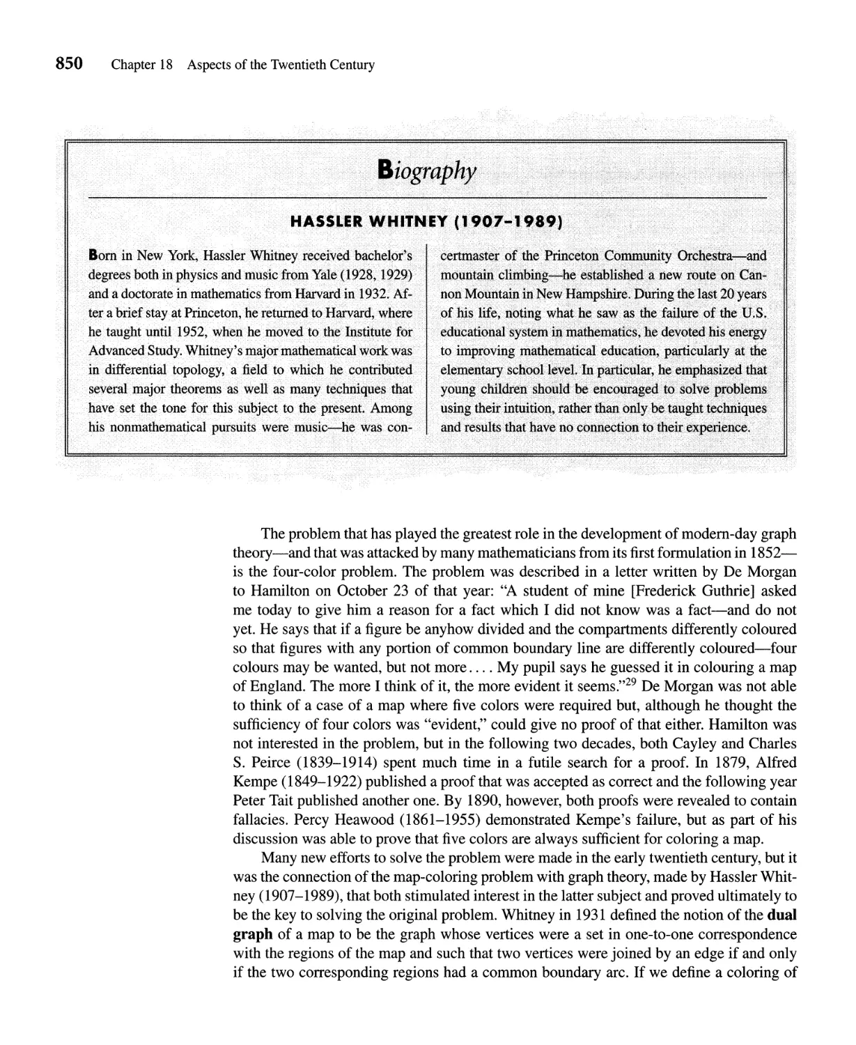
Biographies For easy reference, many biographies of the mathematicians whose work is
discussed are in separate boxes. In particular, although women have for various reasons not
participated in large numbers in mathematical research, biographies of several important
women mathematicians are included, women who succeeded, usually against heavy odds,
in contributing to the mathematical enterprise.
Special Topics There are also boxes on special topics scattered throughout the book.
These include such items as a treatment of the question of the Egyptian influence on
Greek mathematics, a discussion of the idea of a function in the work of Ptolemy, and a
comparison of various notions of continuity. There are also boxes containing important
definitions collected together for easy reference.
Additional Pedagogy Each chapter begins with a relevant quotation and a description
of an important mathematical "event." At the end of each chapter, a brief chronology of
the mathematicians discussed will help students organize their knowledge. Each chapter
also contains an annotated list of references to both primary and secondary sources from
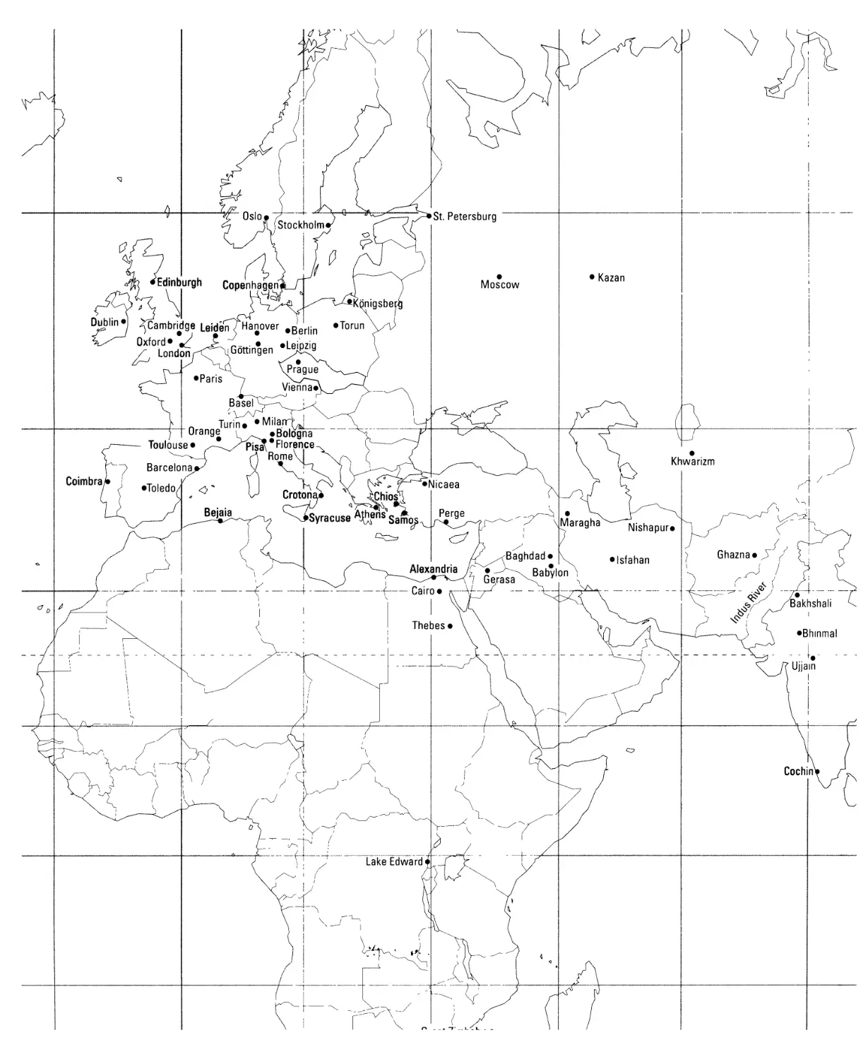
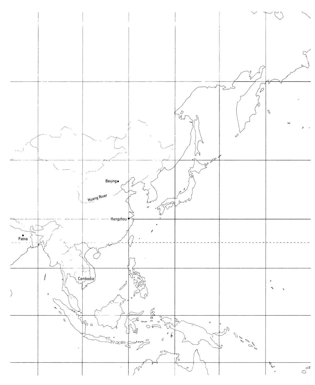
which the students can obtain more information. Finally, there is a time line of the history
of mathematics in the inside front cover and a map in the inside back cover indicating the
location of some of the important places mentioned in the text. Finally, given that students
may have difficulty pronouncing the names of some mathematicians, the index has a special
feature-a phonetic pronunciation guide.
PREREQUISITES
A working knowledge of one year of calculus is sufficient to understand the first twelve
chapters of the text. The mathematical prerequisites for the later chapters are somewhat more
demanding, but the titles of the various sections indicate clearly what kind of mathematical
..
XlI Preface
know ledge is required. For example, a full understanding of Chapters 14 and 15 will require
that the student has studied abstract algebra.
NEW FOR THIS EDITION
The generally friendly reception to the first edition of this book encouraged me to maintain
the basic organization and content. Nevertheless, I have attempted to make a number of
improvements, both in clarity and in content, based on the comments of many users of the
first edition as well as new discoveries in the history of mathematics which have appeared
in the recent literature. There are minor changes in virtually every section, but the major
changes include new material on combinatorics in the Islamic tradition, Newton's derivation
of his system of the world, linear algebra in the nineteenth and twentieth centuries, and
statistical ideas in the nineteenth century. I have attempted to correct all errors of fact
without introducing new ones, but would appreciate notes from anyone who discovers any
remaining errors. There are new problems in every chapter, some of them easier ones, and
the references to the literature have been updated wherever possible. There are also a few
new stamps as illustrations. One should note, however, that any portraits on these stamps-
or indeed elsewhere-purporting to represent mathematicians before the sixteenth century
are fictitious. There are no known representations of any of these people that have credible
evidence of being authentic.
COURSE FLEXIBILITY
There is far more material in this text than can be included in a typical one-semester course
in the history of mathematics. In fact, there is adequate material for a full year course, the
first half being devoted to the period through the invention of calculus in the late seventeenth
century and the second half covering the mathematics of the eighteenth, nineteenth, and
twentieth centuries. For those instructors who have only one semester, however, there are
several ways to use this book. First, one could cover most of the first twelve chapters and
simply conclude with calculus. Second, one could choose to follow one or two particular
themes through history. Some possible themes with the appropriate section numbers are
Equation Solving: 1.4, 1.8, 1.9, 2.4.3, 2.5, 5.2, 6.3, 6.4, 6.7, 6.8, 7.2, 8.3, 9.3, 9.4,
11.2, 14.2.4, 15.2
Ideas of Calculus: 2.3.2, 2.3.3, 2.4.9, 3.2, 3.3, 7.2.4, 7.4.4, 8.4, 10.5, 12, 13, 16.1,
16.2, 16.3, 16.4
Concepts of Geometry: 1.5, 1.8,2.1.2,2.2,2.4,3.3,3.4, 3.5, 4.3,5.3,7.4, 8.1, 10.1,
11.1,11.5,14.3,17,18.2
Trigonometry, Astronomy, and Surveying: 1.6, 4.1, 4.2, 6.2, 6.6, 7.5, 8.1, 10.2, 10.3,
12.5.6,13.1.3
Combinatorics, Probability, and Statistics: 6.8, 7.3, 8.2, 11.3, 14.1, 16.5
Linear Algebra: 1.4, 14.2.2, 14.2.4, 15.5, 17.4, 18.3.3, 18.4.7
Number Theory: 2.1.1, 2.4.7, 5.1, 11.4, 14.2.3, 15.1
Modem Algebra: 6.8,7.2, 8.3,9.1,9.2, 14.2, 15.2, 15.3, 15.4, 18.3, 18.4.4, 18.4.6,
18.4.8
Preface xiii
Third, one could cover in detail most of the first ten chapters and then pick selected
ideas from the later chapters, again following a particular theme. One could also assign
various sections for individual or small-group reading assignments and reports.
ACKNOWLEDGMENTS
Like any book, this one could not have been written without the help of many people. The
following people contributed to the first edition and their input continues to impact the text:
Marcia Ascher (Ithaca College), J. Lennart Berggren (Simon Fraser University), Robert
Kreiser (A.A.U.P.), Robert Rosenfeld (Nassau Community College), and John Milcetich
(University of the District of Columbia).
Many people made detailed suggestions for the second edition. Although I have not
followed every one of them (and may come to regret that), I sincerely appreciate the
thought they gave to improving the book. These people include Ivor Grattan-Guinness,
Kim Plofker, Eleanor Robson, Richard Askey, William Anglin, Claudia Zaslavsky, Rebekka
Struik, William Ramaley, Joseph Albree, Calvin Jongsma, David Fowler, John Stillwell,
Christian Thybo, Jim Tattersall, Judith Grabiner, Tony Gardiner, Ubi D' Ambrosio, Dirk
Struik, and David Rowe. My heartfelt thanks to all of them.
The many reviewers of sections of the manuscript have also provided great help with
their detailed critiques and have made this a much better book than it otherwise could have
been.
First Edition Reviewers: Duane Blumberg, University of Southwestern Louisiana;
Walter Czarnec, Framingham State University; Joseph Dauben, Herbert Lehman College-
CUNY; Harvey Davis, Michigan State University; Joy Easton, West Virginia Univer-
sity; Carl FitzGerald, University of California-San Diego; Basil Gordon, University of
California-Los Angeles; Mary Gray, American University; Branko Grunbaum, University
of Washington; William Hintzman, San Diego State University; Barnabas Hughes, Califor-
nia State University-Northridge; Israel Kleiner, York University; David E. Kullman, Miami
University; Robert L. Hall, University of Wisconsin, Milwaukee; Richard Marshall, Eastern
Michigan University; Jerold Mathews, Iowa State University; Willard Parker, Kansas State
University; Clinton M. Petty, University of Missouri-Columbia; Howard Prouse, Mankato
State University; Helmut Rohrl, University of California-San Diego; David Wilson, Uni-
versity of Florida; and Frederick Wright, University of North Carolina-Chapel Hill.
Second Edition Reviewers: Salvatore Anastasio, State University of New York, New
Platz; Bruce Crauder, Oklahoma State University; Walter Czarnec, Framingham State
College; William Eng and, Mississippi State University; David Jabon, Eastern Washington
University; Charles Jones, Ball State University; Michael Lacey, Indiana University; Harold
Martin, Northern Michigan University; James Murdock, Iowa State University; Ken Shaw,
Florida State University; Sverre Smalo, University of California, Santa Barbara; Domina
Eberle Spencer, University of Connecticut; Jimmy Woods, North Georgia College.
I have also benefited greatly from conversations with many historians of mathematics
at various forums. In particular, those who have regularly attended the annual History
of Mathematics seminars, organized by Uta Merzbach, former curator of mathematics
at the National Museum of American History, may well recognize some of the ideas
discussed there. The book has also profited from discussions over the years with, among
.
XlV Preface
others, Charles Jones (Ball State University), V. Frederick Rickey (Bowling Green State
University), Florence Fasanelli (MAA), Israel Kleiner (York University), Abe Shenitzer
(York University), Ubiratan D' Ambrosio (Univ. Estadual de Campinas), and Frank Swetz
(Pennsylvania State University). My students in History of Mathematics (and other) classes
at the University of the District of Columbia have also helped me clarify many of my
ideas. Naturally, I welcome any additional comments and correspondence from students
and colleagues elsewhere in an effort to continue to improve this book.
Special thanks are due to the librarians at the University of the District of Columbia
and especially to Clement Goddard, who never failed to secure any of the obscure books I
requested on interlibrary loan. Leslie Overstreet of the Smithsonian Institution Libraries'
Special Collections Department was extremely helpful in finding sources for pictures.
Thanks are due to my former editors at HarperCollins, Steve Quigley, Don Gecewicz,
and George Duda, who helped form the first edition.
I also want to thank Jennifer Albanese, my new editor at Addison Wesley Longman, for
her suggestions and her patience as she pushed this book to completion, as well as Rebecca
Malone and Barbara Pendergast, for their efforts in handling the production aspects, and
Susan Holbert for preparation of the index.
My family has been very supportive during the many years of writing the book. I thank
my parents for their patience and their faith in me. I thank my children Sharon, Ari, and
Naomi for help at various times and especially for allowing me to use our computer. And
last, I thank my wife Phyllis for long discussions at any hour of the day or night and for
being there when I needed her. I owe her much more than I can ever repay.
VICTOR 1. KATZ
c
h
a
p
t
c1r
Ancient
Mathematics
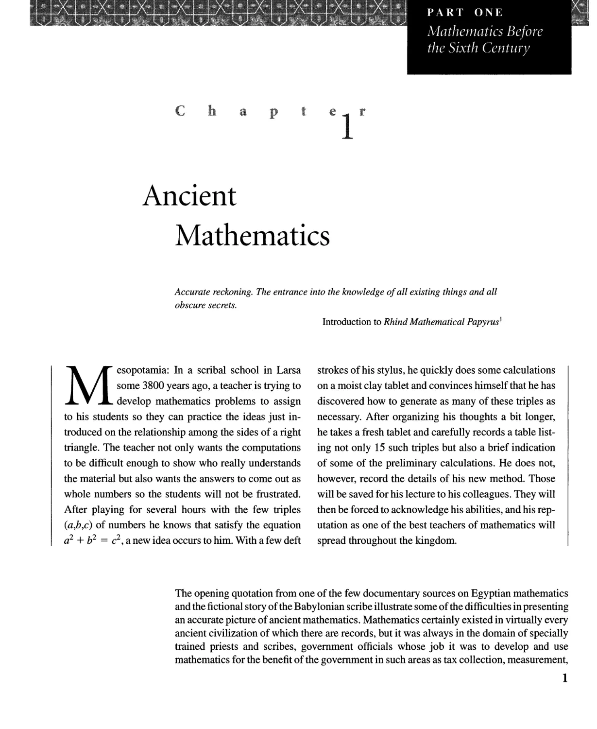
Accurate reckoning. The entrance into the knowledge of all existing things and all
obscure secrets.
M esopotamia: In a scribal school in Larsa
some 3800 years ago, a teacher is trying to
develop mathematics problems to assign
to his students so they can practice the ideas just in-
troduced on the relationship among the sides of a right
triangle. The teacher not only wants the computations
to be difficult enough to show who really understands
the material but also wants the answers to come out as
whole numbers so the students will not be frustrated.
After playing for several hours with the few triples
(a,b,c) of numbers he knows that satisfy the equation
a 2 + b 2 = c 2 , a new idea occurs to him. With a few deft
Introduction to Rhind Mathematical Papyrus 1
strokes of his stylus, he quickly does some calculations
on a moist clay tablet and convinces himself that he has
discovered how to generate as many of these triples as
necessary. After organizing his thoughts a bit longer,
he takes a fresh tablet and carefully records a table list-
ing not only 15 such triples but also a brief indication
of some of the preliminary calculations. He does not,
however, record the details of his new method. Those
will be saved for his lecture to his colleagues. They will
then be forced to acknowledge his abilities, and his rep-
utation as one of the best teachers of mathematics will
spread throughout the kingdom.
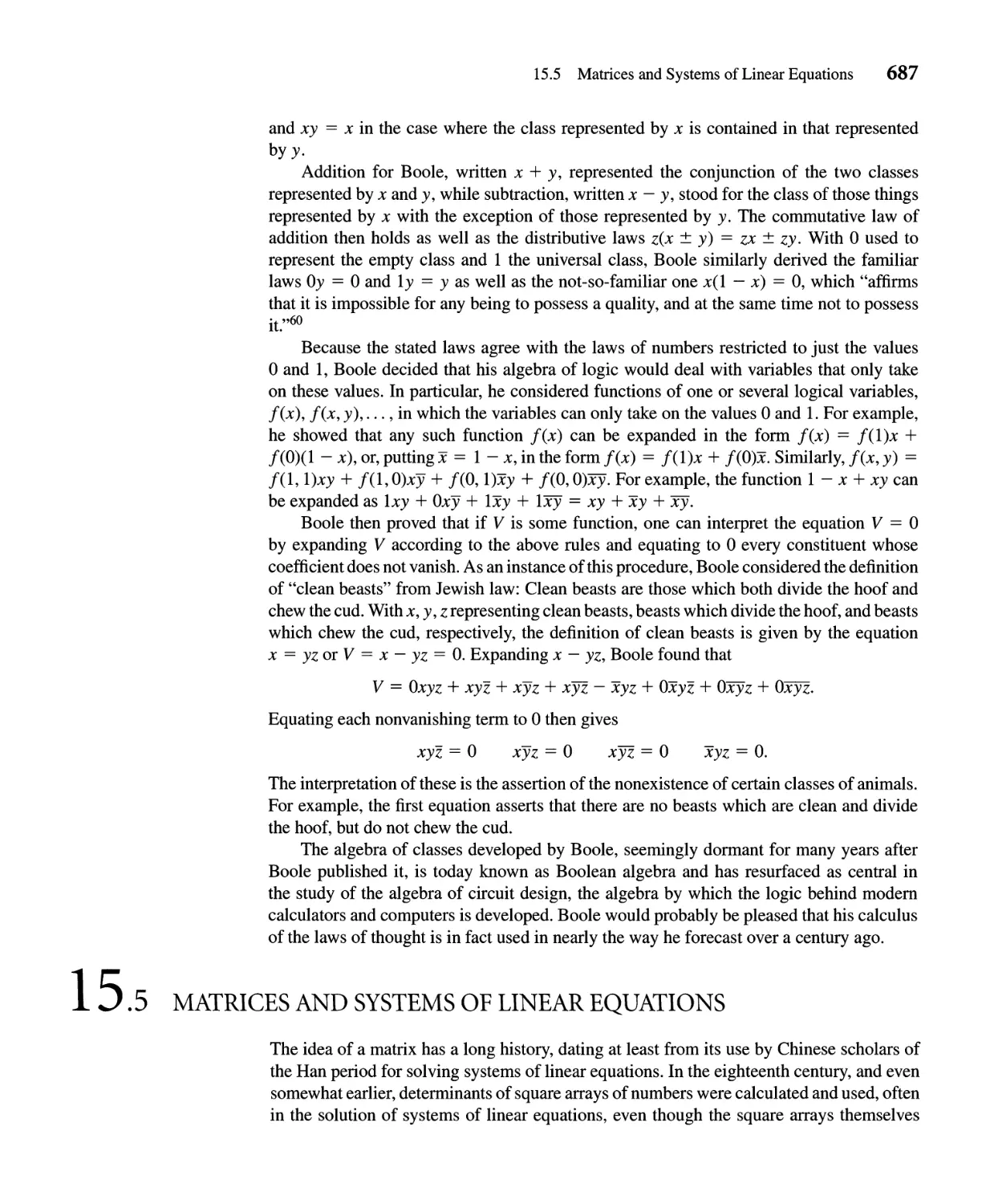
The opening quotation from one of the few documentary sources on Egyptian mathematics
and the fictional story of the Baby Ionian scribe illustrate some of the difficulties in presenting
an accurate picture of ancient mathematics. Mathematics certainly existed in virtually every
ancient civilization of which there are records, but it was always in the domain of specially
trained priests and scribes, government officials whose job it was to develop and use
mathematics for the benefit of the government in such areas as tax collection, measurement,
1
2 Chapter 1 Ancient Mathematics
1.1
building, trade, calendar making, and ritual practices. Yet, even though the origins of many
mathematical concepts stem from their usefulness in these contexts, mathematicians have
always exercised their curiosity by extending their ideas far beyond the limits of practical
necessity. Nevertheless, because mathematics was a tool of power, its methods were passed
on only to the privileged few, often through an oral tradition. Hence the written records are
generally sparse and seldom provide much detail.
In recent years, scholars have labored to reconstruct the mathematics of ancient civ-
ilizations from whatever clues can be found. Naturally, they do not agree on every point,
but enough consensus exists so that we can present a reasonable picture of the state of
mathematical knowledge in the ancient civilizations of Egypt, Mesopotamia, China, and
India. In order to see most clearly the similarities and differences in the mathematics of
these civilizations, we will not treat each civilization separately but will instead organize
our discussion around the following key topics: counting, arithmetic computations, linear
equations, elementary geometry, astronomical and calendrical computations, square roots,
the "Pythagorean" theorem, and quadratic equations. To place the story in context, we
begin with a brief description of the civilizations themselves and the sources from which
our knowledge of their mathematics is derived.
ANCIENT CIVILIZATIONS
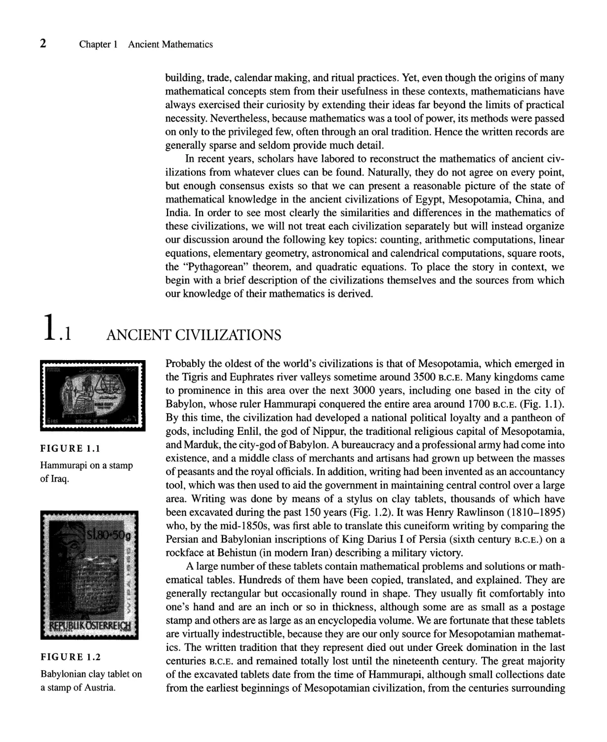
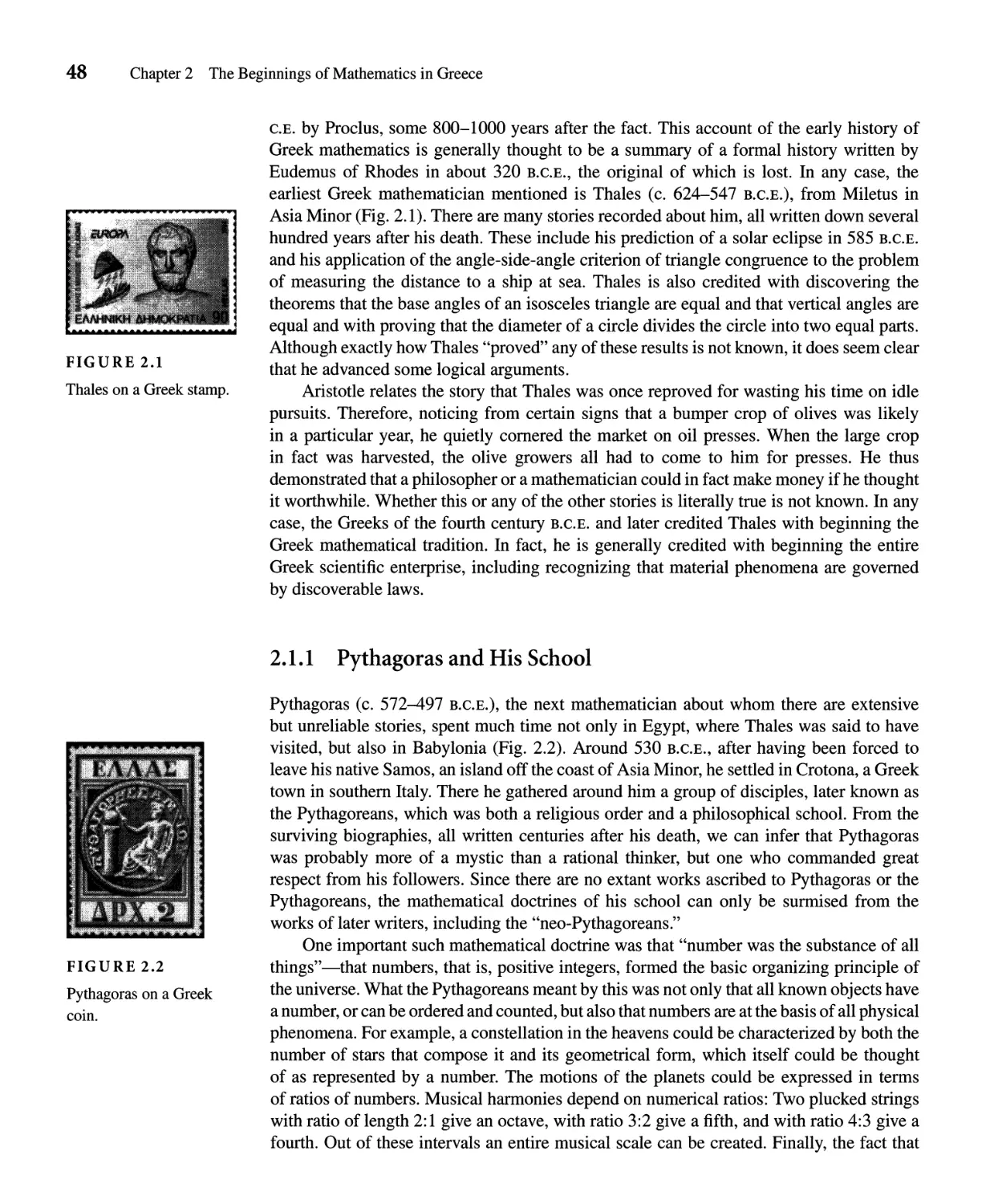
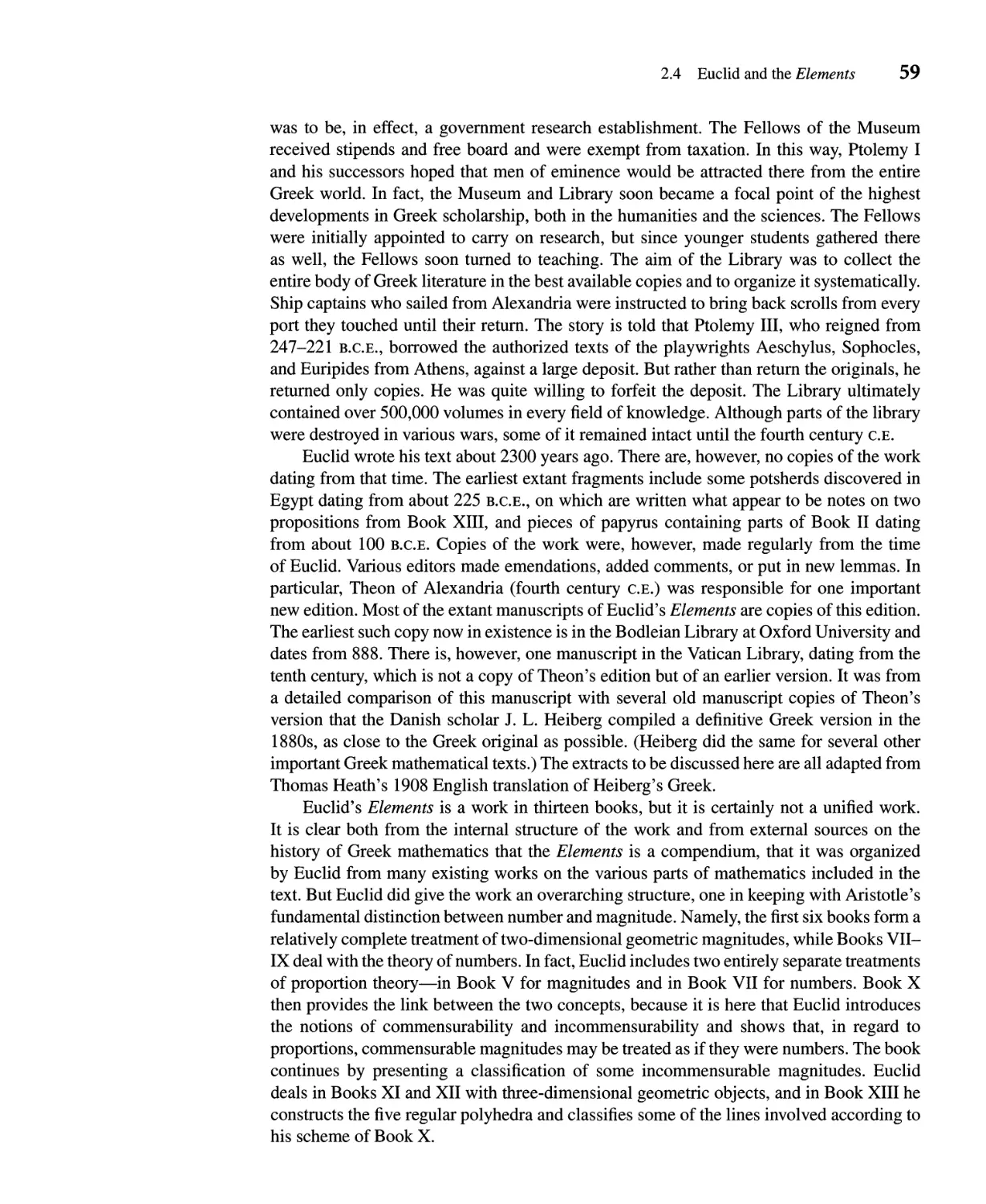
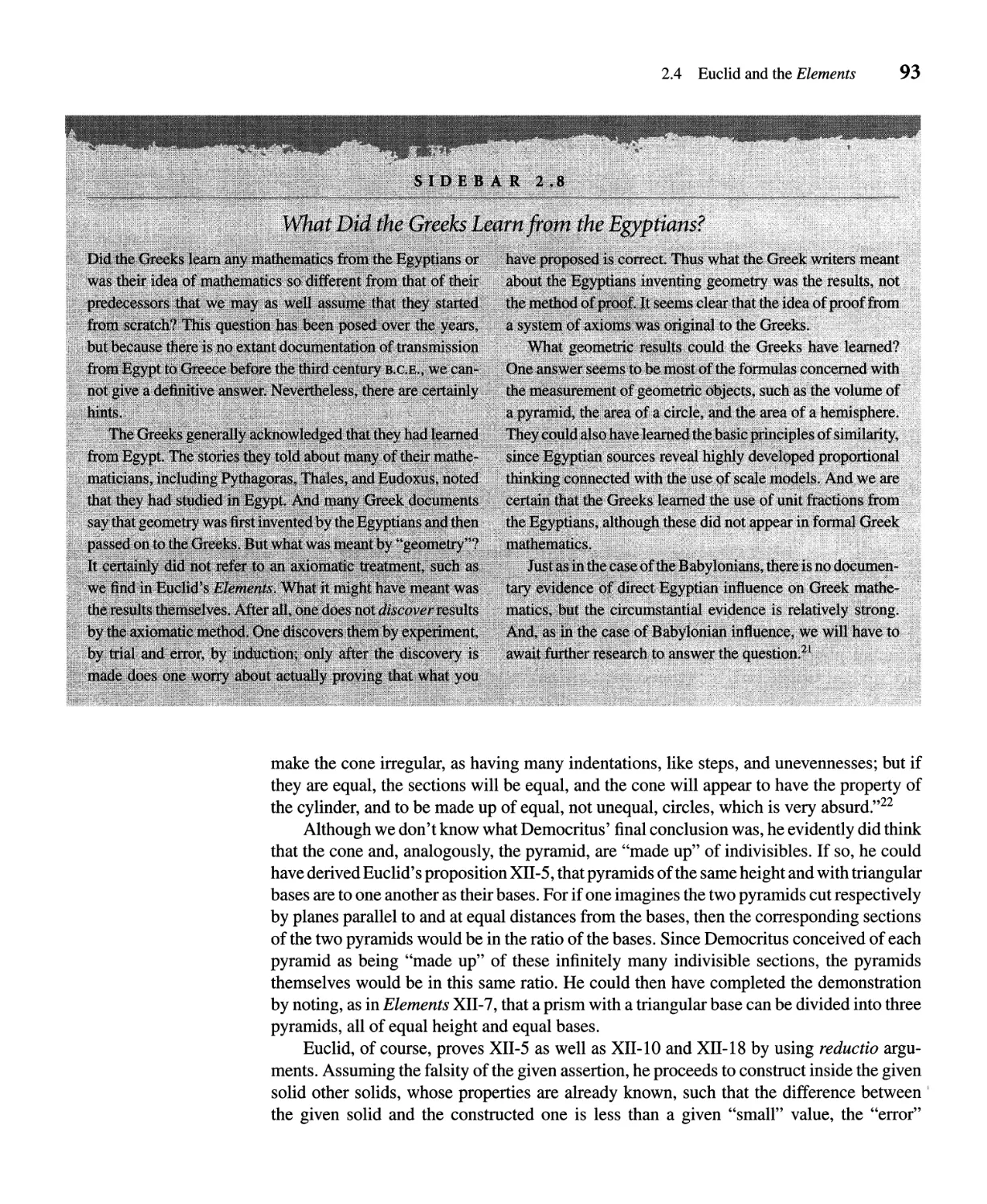
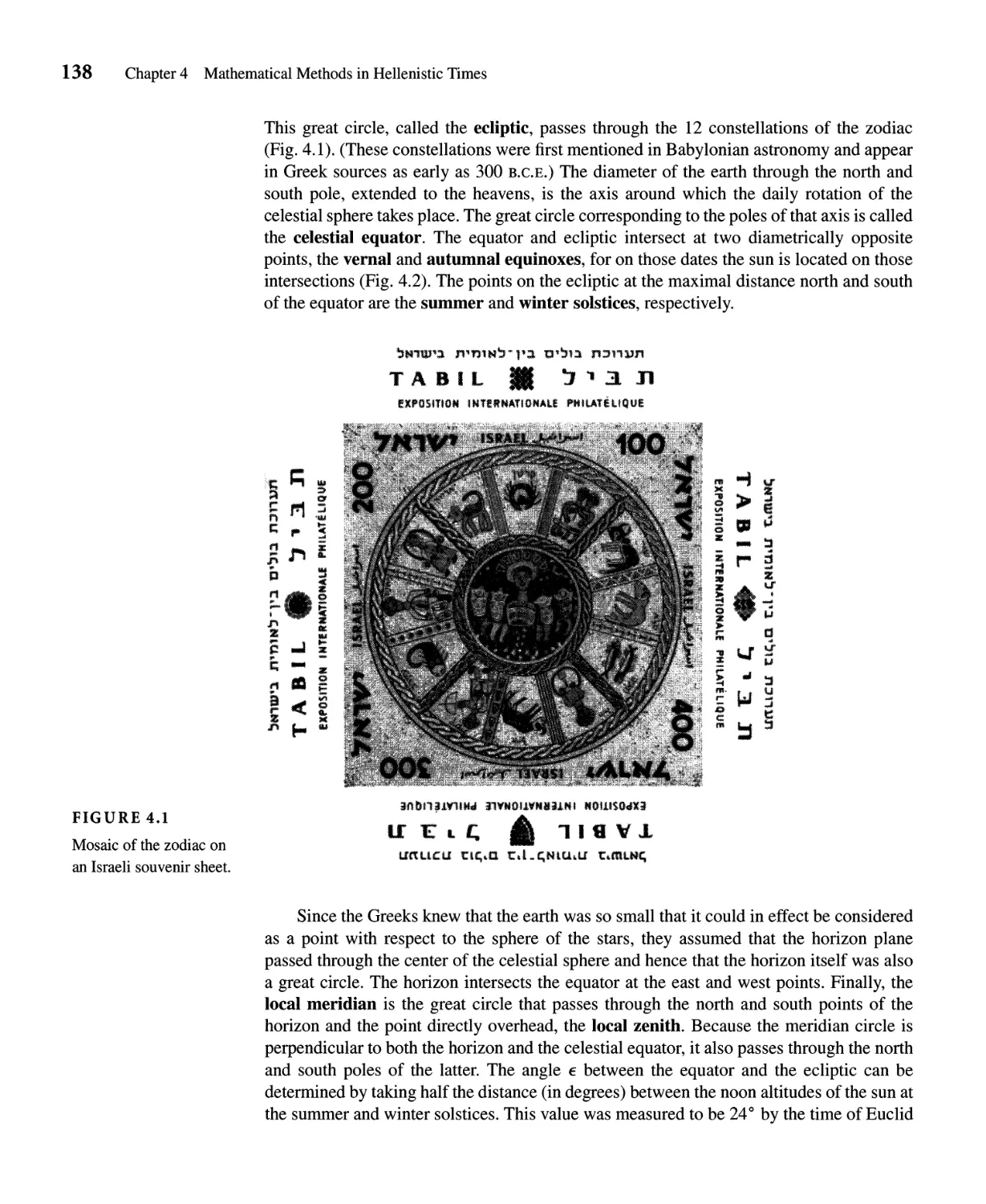
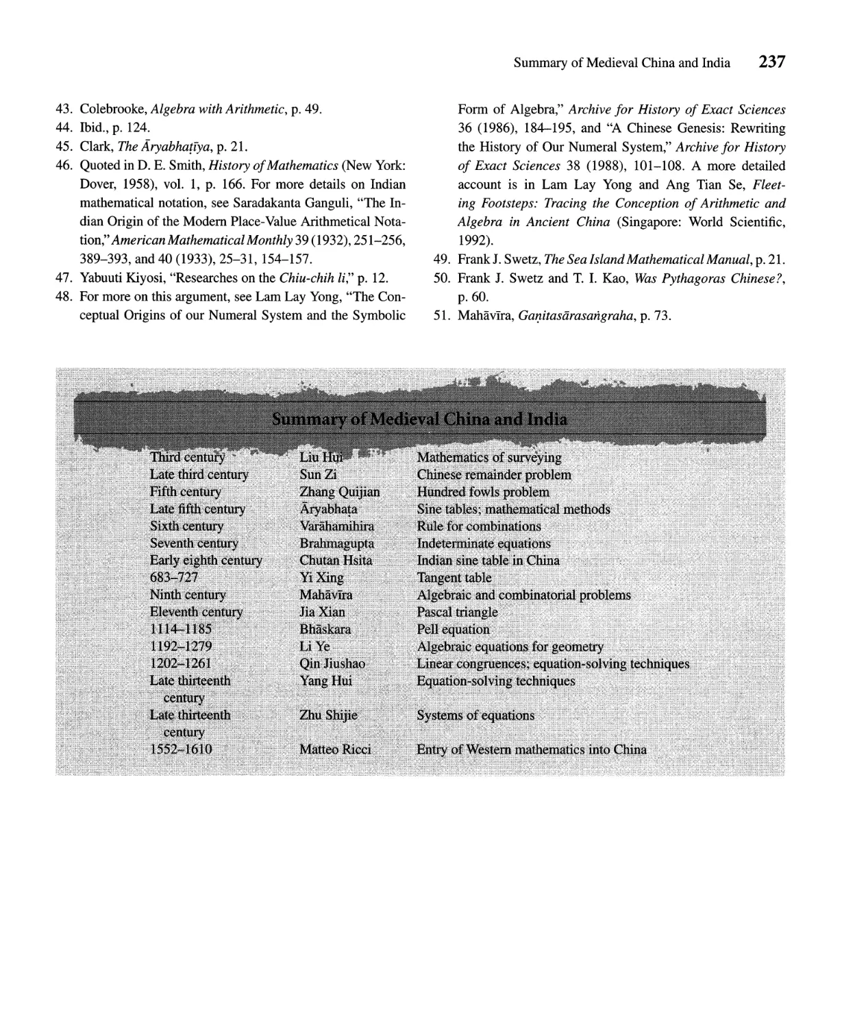
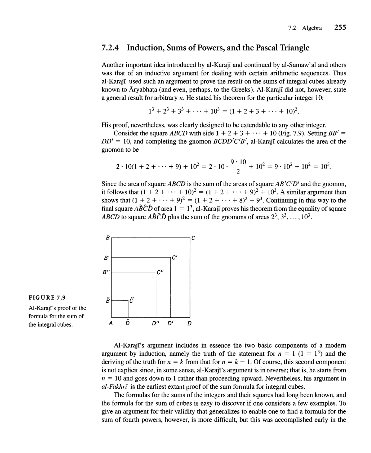
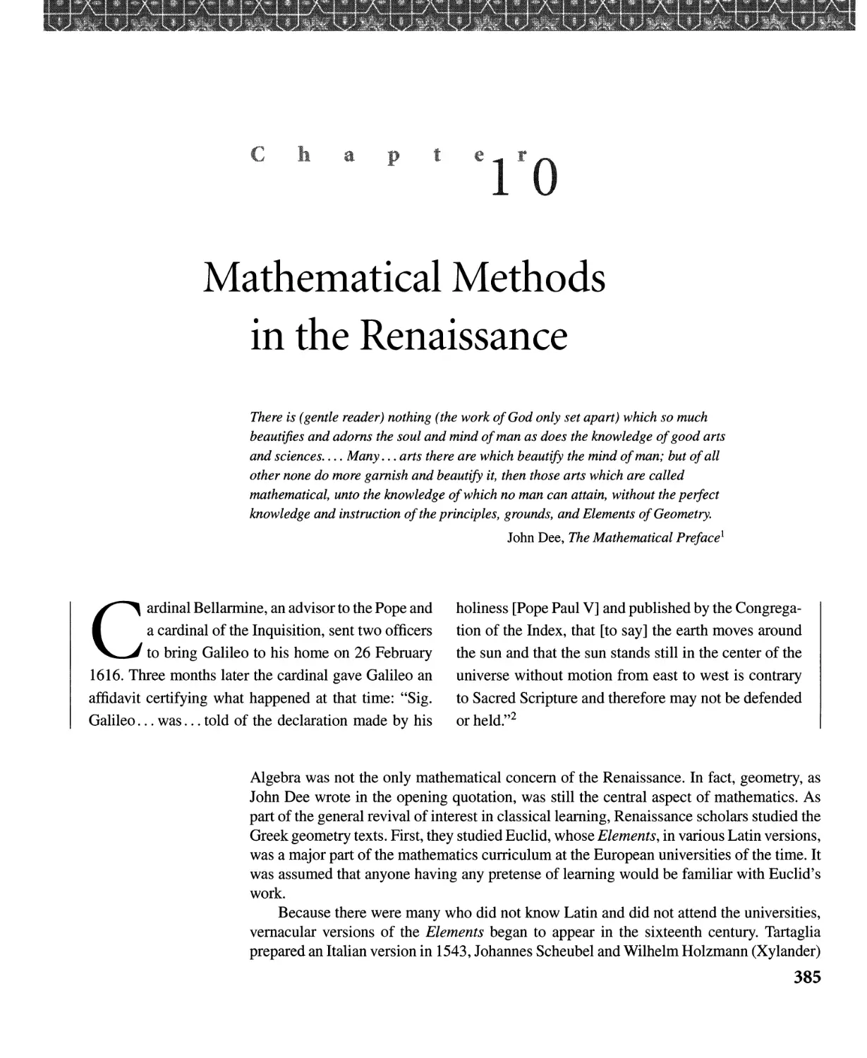
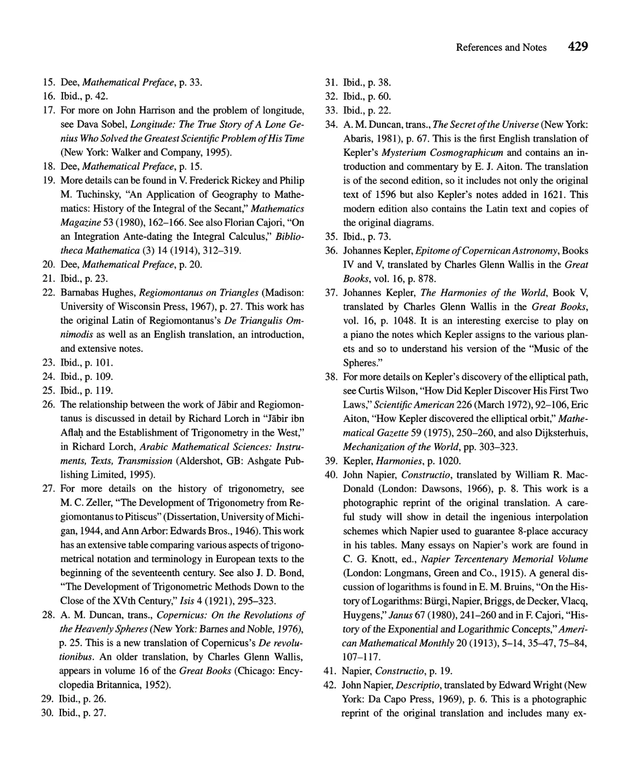
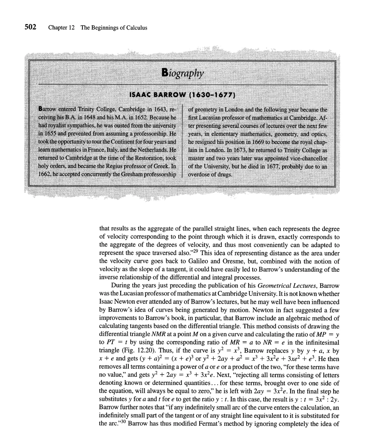
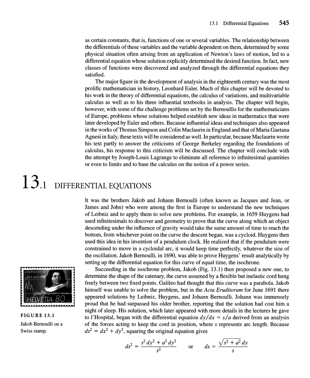
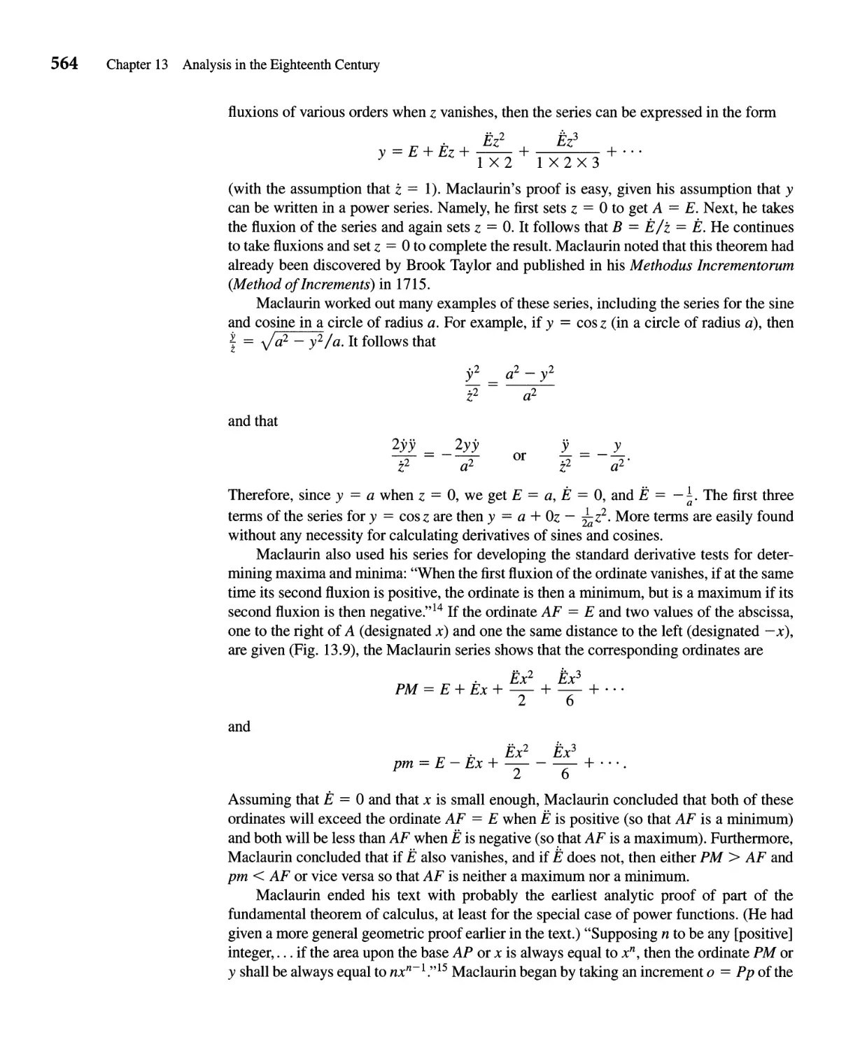
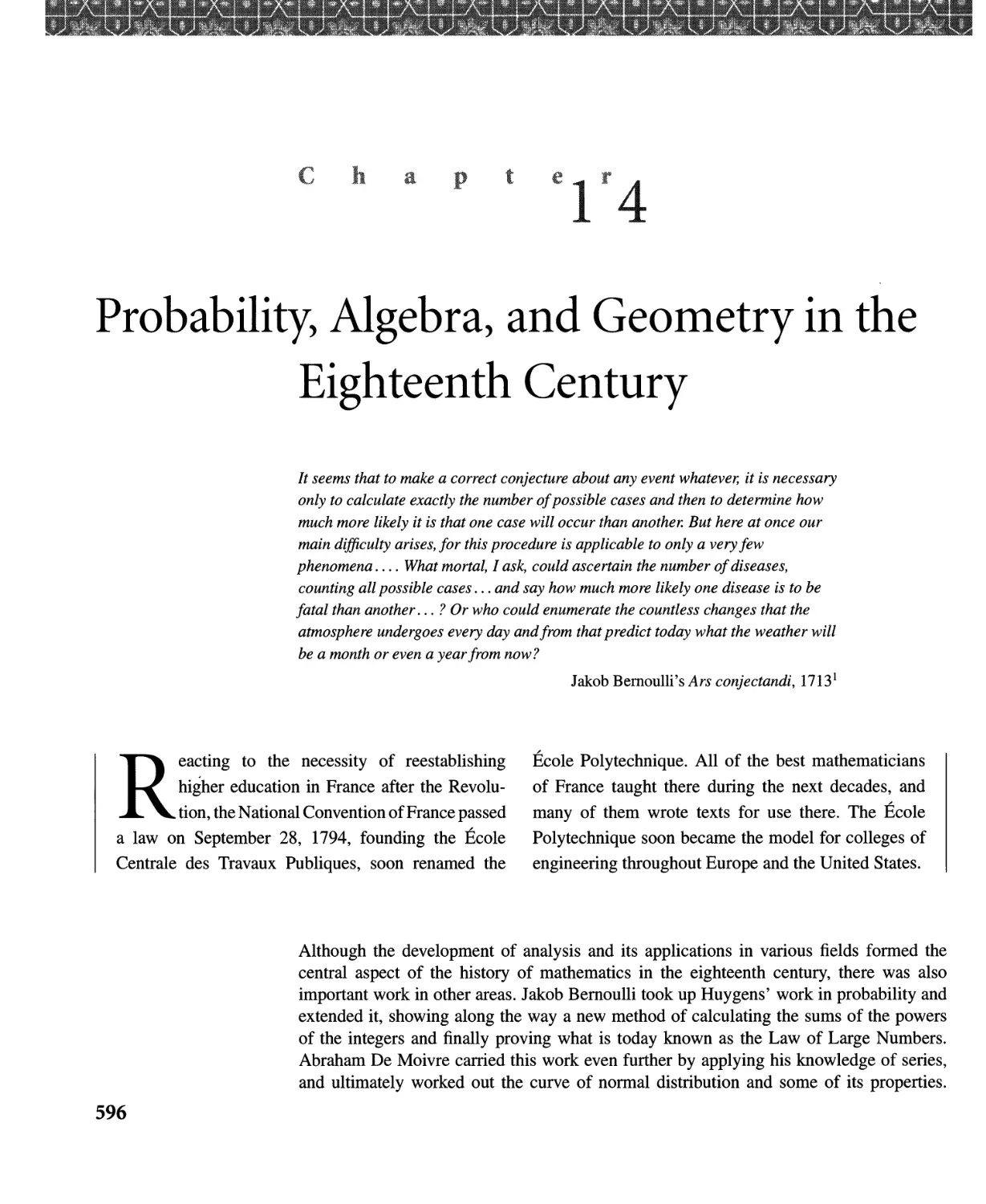
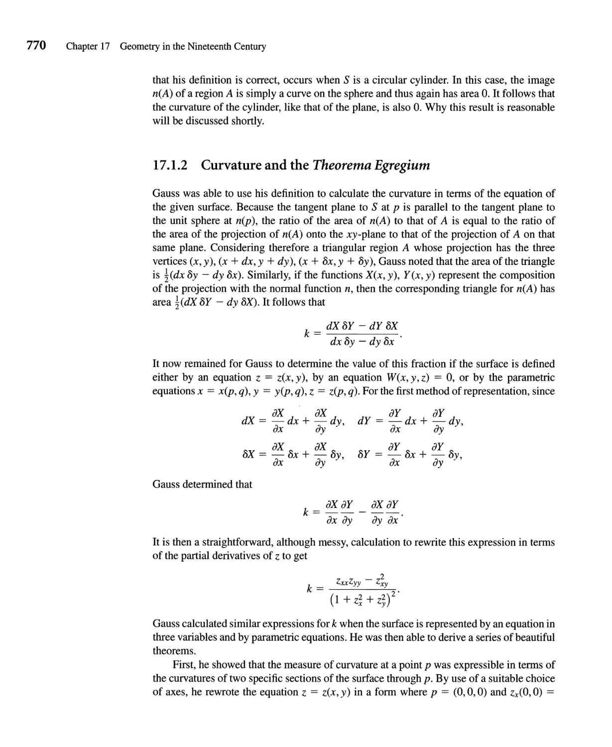
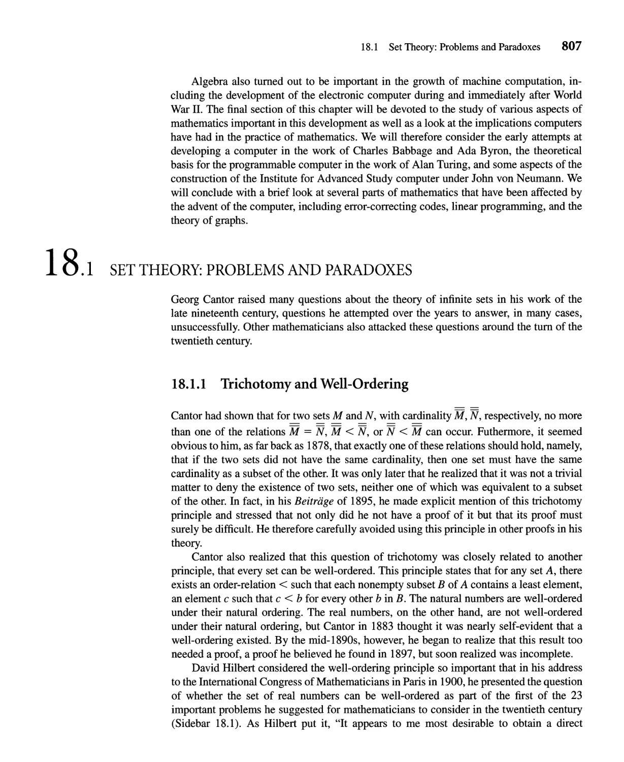
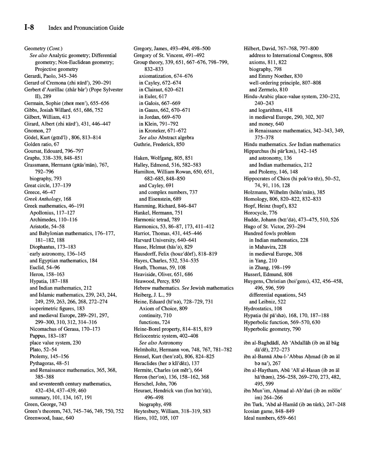
FIGURE 1.1
Hammurapi on a stamp
of Iraq.
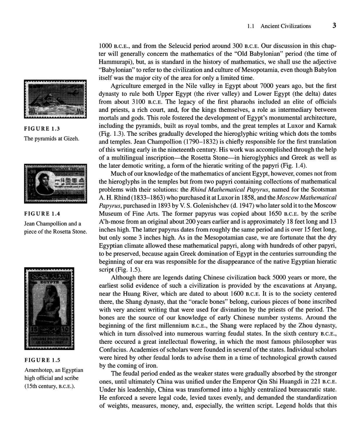
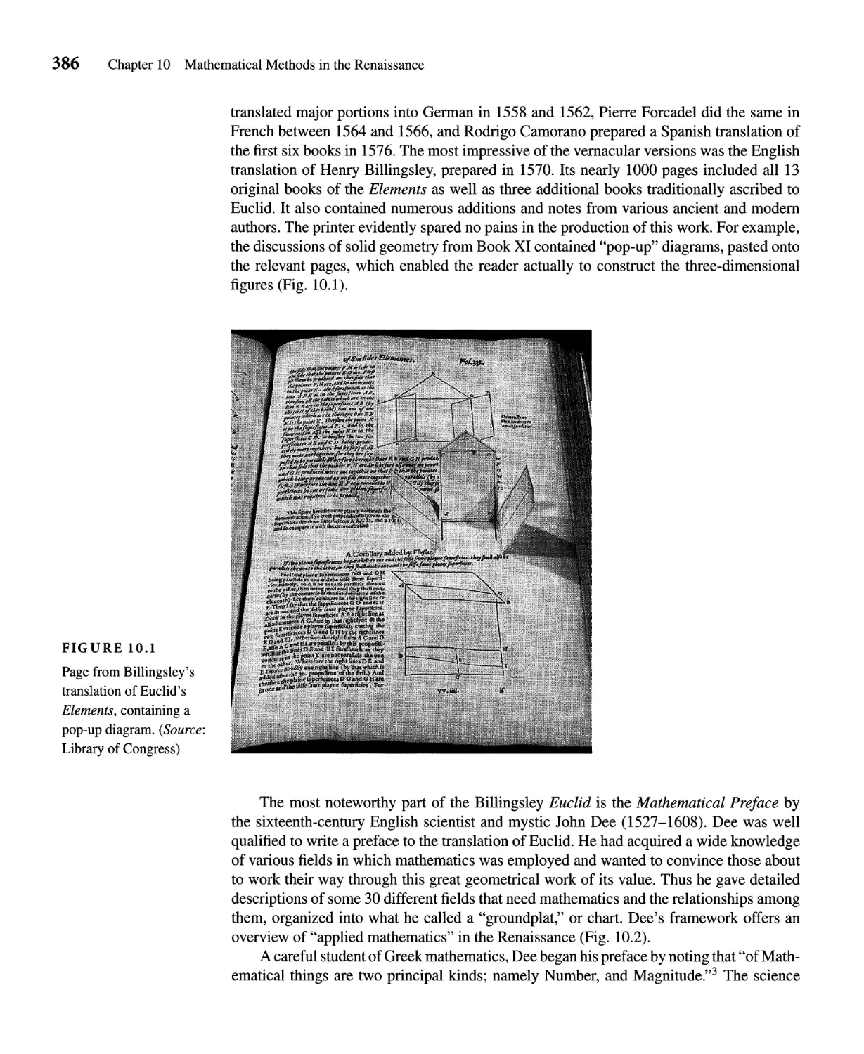
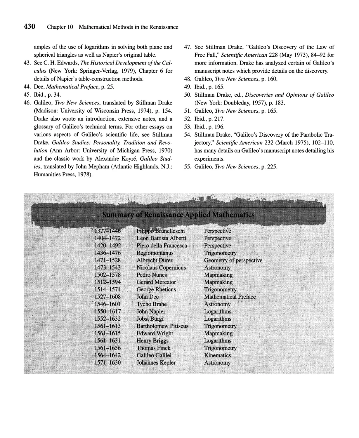
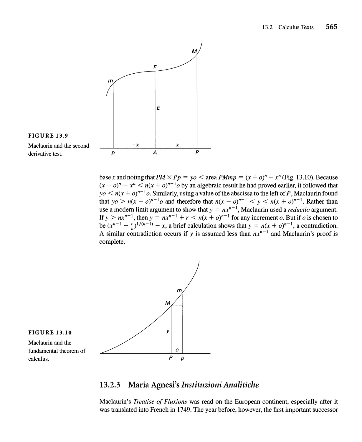
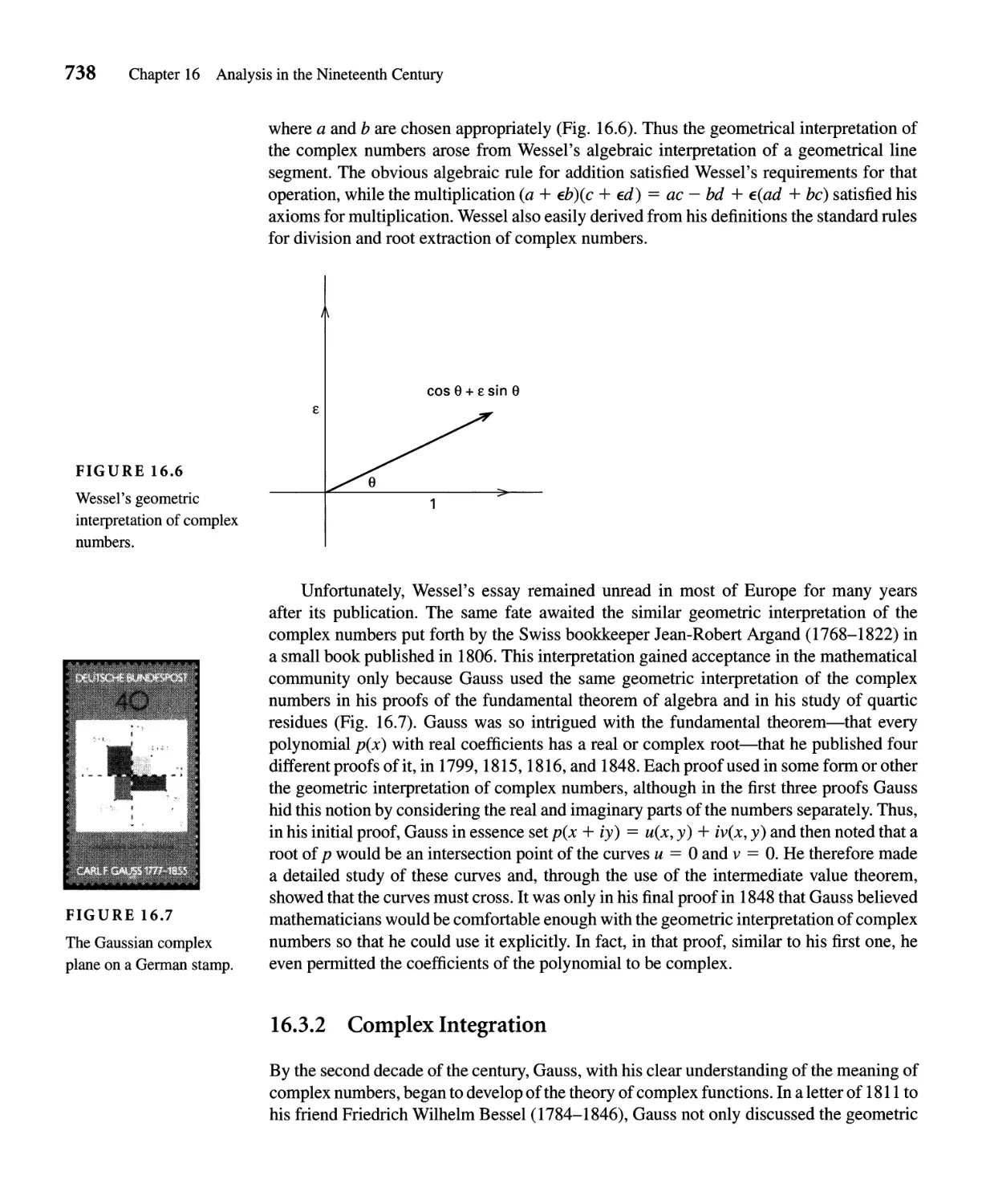
FIGURE 1.2
Babylonian clay tablet on
a stamp of Austria.
Probably the oldest of the world's civilizations is that of Mesopotamia, which emerged in
the Tigris and Euphrates river valleys sometime around 3500 B.C.E. Many kingdoms came
to prominence in this area over the next 3000 years, including one based in the city of
Babylon, whose ruler Hammurapi conquered the entire area around 1700 B.C.E. (Fig. 1.1).
By this time, the civilization had developed a national political loyalty and a pantheon of
gods, including Enlil, the god of Nippur, the traditional religious capital of Mesopotamia,
and Marduk, the city-god of Babylon. A bureaucracy and a professional army had come into
existence, and a middle class of merchants and artisans had grown up between the masses
of peasants and the royal officials. In addition, writing had been invented as an accountancy
tool, which was then used to aid the government in maintaining central control over a large
area. Writing was done by means of a stylus on clay tablets, thousands of which have
been excavated during the past 150 years (Fig. 1.2). It was Henry Rawlinson (1810-1895)
who, by the mid-1850s, was first able to translate this cuneiform writing by comparing the
Persian and Babylonian inscriptions of King Darius I of Persia (sixth century B.C.E.) on a
rockface at Behistun (in modem Iran) describing a military victory.
A large number of these tablets contain mathematical problems and solutions or math-
ematical tables. Hundreds of them have been copied, translated, and explained. They are
generally rectangular but occasionally round in shape. They usually fit comfortably into
one's hand and are an inch or so in thickness, although some are as small as a postage
stamp and others are as large as an encyclopedia volume. We are fortunate that these tablets
are virtually indestructible, because they are our only source for Mesopotamian mathemat-
ics. The written tradition that they represent died out under Greek domination in the last
centuries B.C.E. and remained totally lost until the nineteenth century. The great majority
of the excavated tablets date from the time of Hammurapi, although small collections date
from the earliest beginnings of Mesopotamian civilization, from the centuries surrounding
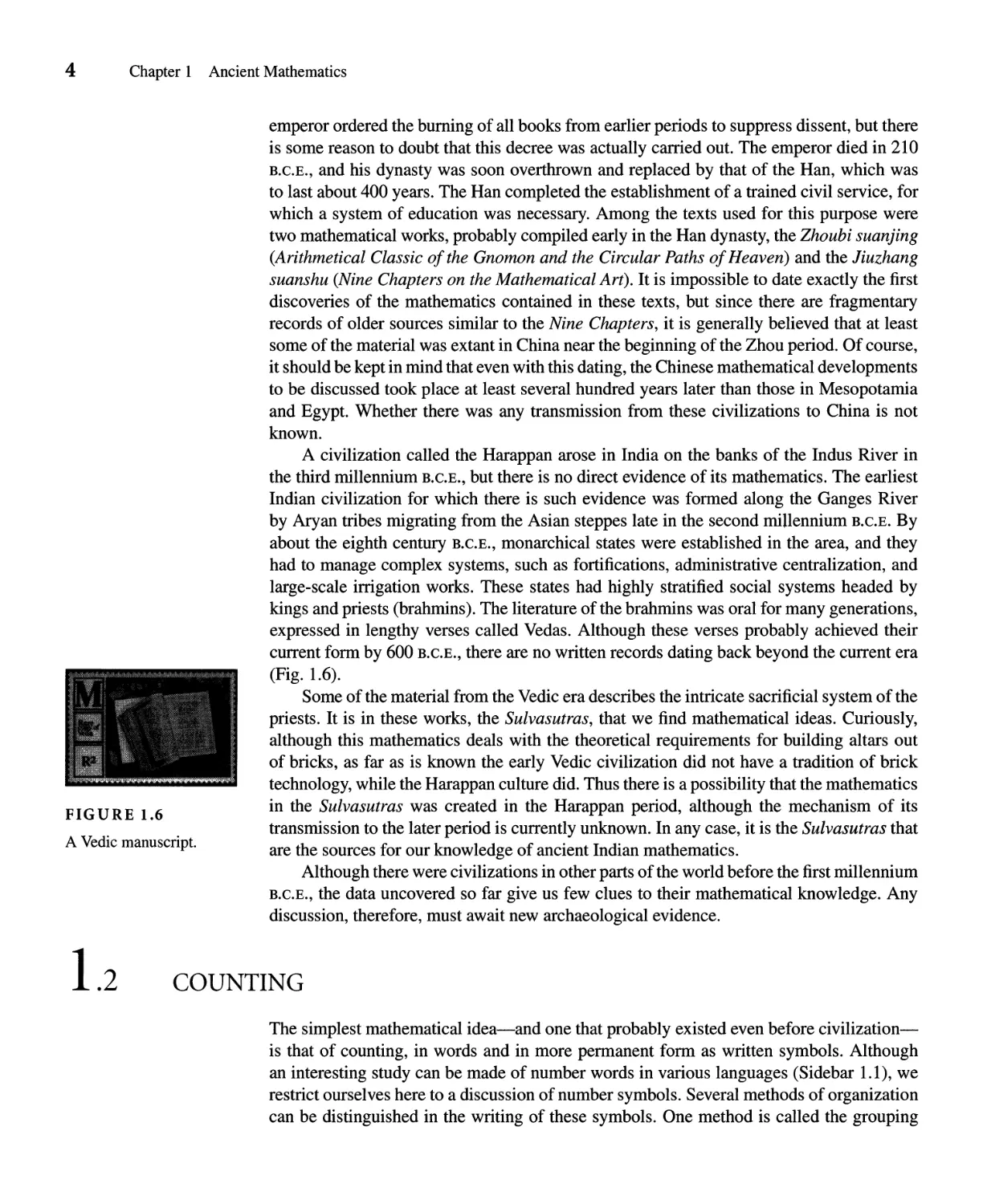
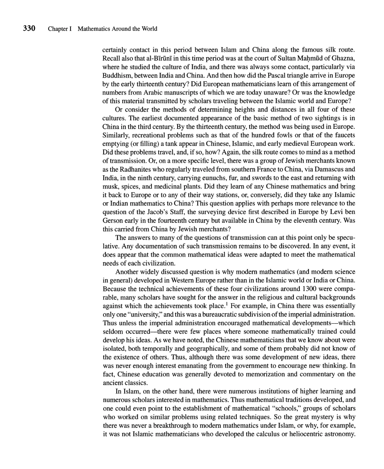
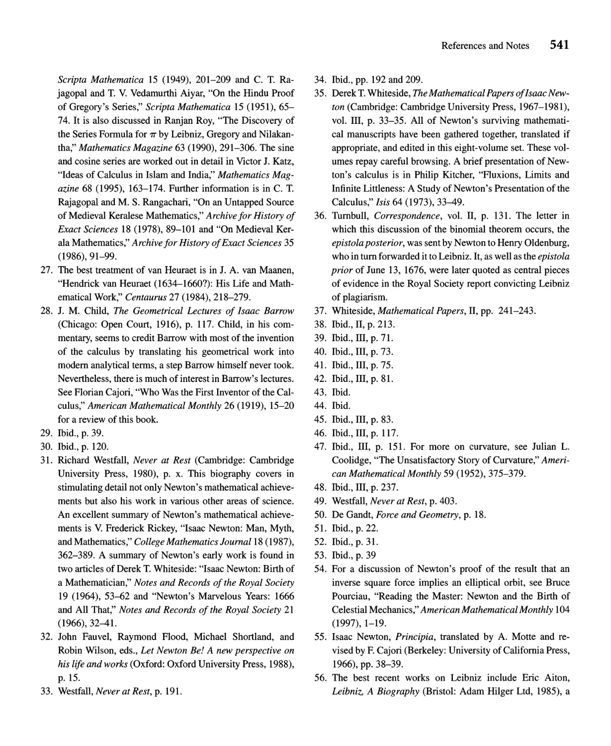
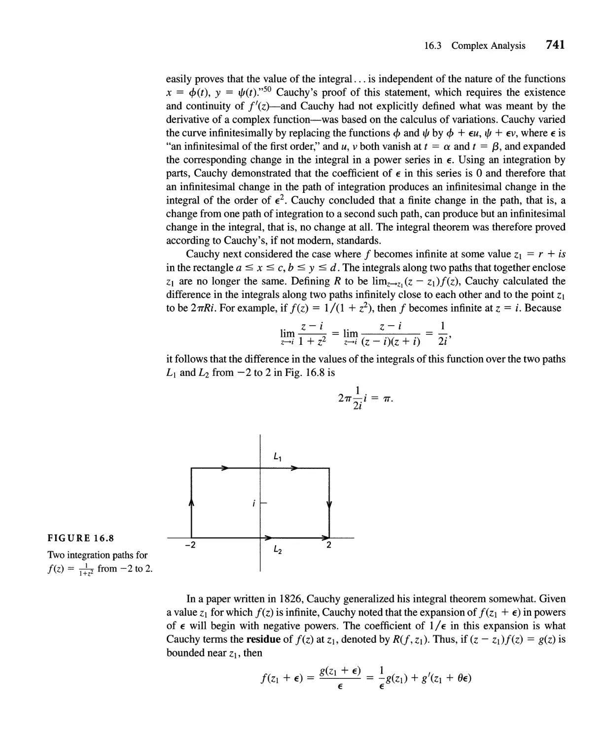
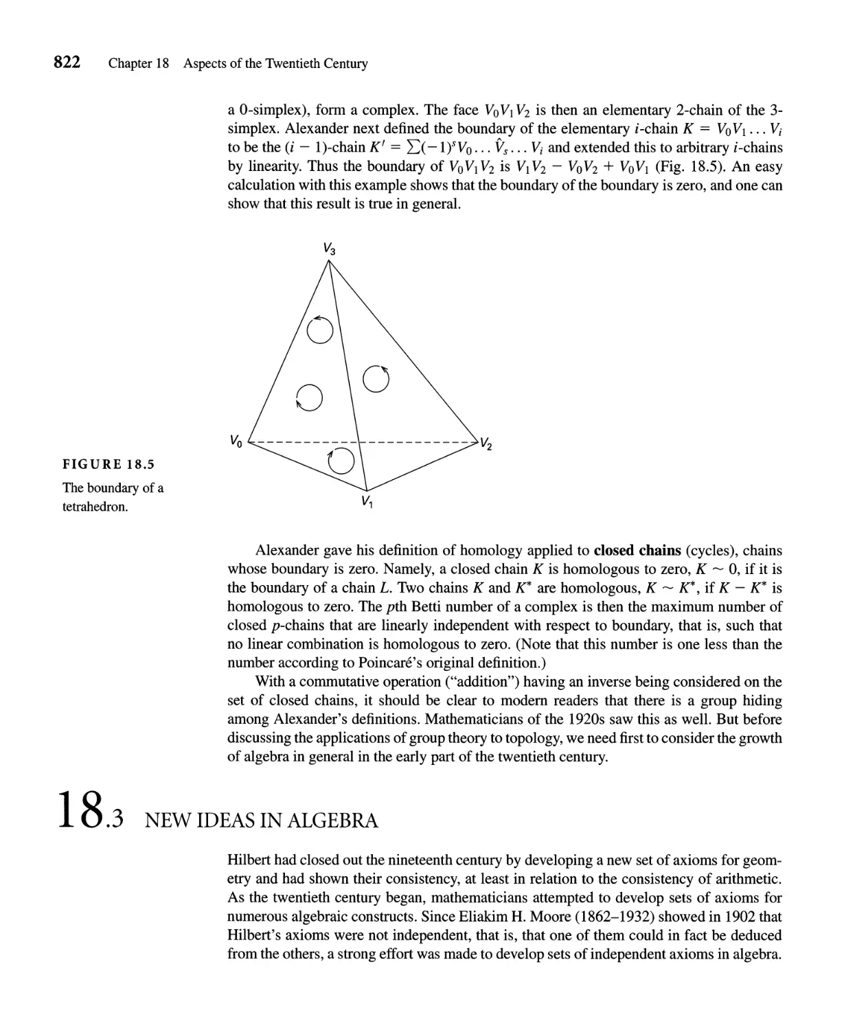
FIGURE 1.3
The pyramids at Gizeh.
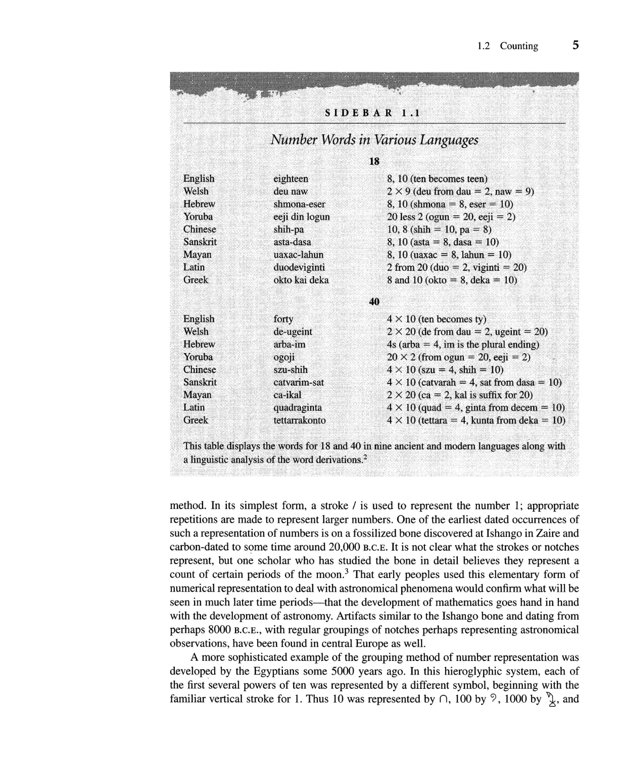
FIGURE 1.4
Jean Champollion and a
piece of the Rosetta Stone.
FIGURE 1.5
Amenhotep, an Egyptian
high official and scribe
(15th century, B.C.E.).
1.1 Ancient Civilizations 3
1000 B.C.E., and from the Seleucid period around 300 B.C.E. Our discussion in this chap-
ter will generally concern the mathematics of the "Old Babylonian" period (the time of
Hammurapi), but, as is standard in the history of mathematics, we shall use the adjective
"Babylonian" to refer to the civilization and culture of Mesopotamia, even though Babylon
itself was the major city of the area for only a limited time.
Agriculture emerged in the Nile valley in Egypt about 7000 years ago, but the first
dynasty to rule both Upper Egypt (the river valley) and Lower Egypt (the delta) dates
from about 3100 B.C.E. The legacy of the first pharaohs included an elite of officials
and priests, a rich court, and, for the kings themselves, a role as intermediary between
mortals and gods. This role fostered the development of Egypt's monumental architecture,
including the pyramids, built as royal tombs, and the great temples at Luxor and Karnak
(Fig. 1.3). The scribes gradually developed the hieroglyphic writing which dots the tombs
and temples. Jean Champollion (1790-1832) is chiefly responsible for the first translation
of this writing early in the nineteenth century. His work was accomplished through the help
of a multilingual inscription-the Rosetta Stone-in hieroglyphics and Greek as well as
the later demotic writing, a form of the hieratic writing of the papyri (Fig. 1.4).
Much of our knowledge of the mathematics of ancient Egypt, however, comes not from
the hieroglyphs in the temples but from two papyri containing collections of mathematical
problems with their solutions: the Rhind Mathematical Papyrus, named for the Scotsman
A. H. Rhind (1833-1863) who purchased it at Luxorin 1858, and the Moscow Mathematical
Papyrus, purchased in 1893 by V. S. Golenishchev (d. 1947) who later sold it to the Moscow
Museum of Fine Arts. The former papyrus was copied about 1650 B.C.E. by the scribe
A'h-mose from an original about 200 years earlier and is approximately 18 feet long and 13
inches high. The latter papyrus dates from roughly the same period and is over 15 feet long,
but only some 3 inches high. As in the Mesopotamian case, we are fortunate that the dry
Egyptian climate allowed these mathematical papyri, along with hundreds of other papyri,
to be preserved, because again Greek domination of Egypt in the centuries surrounding the
beginning of our era was responsible for the disappearance of the native Egyptian hieratic
script (Fig. 1.5).
Although there are legends dating Chinese civilization back 5000 years or more, the
earliest solid evidence of such a civilization is provided by the excavations at Anyang,
near the Huang River, which are dated to about 1600 B.C.E. It is to the society centered
there, the Shang dynasty, that the "oracle bones" belong, curious pieces of bone inscribed
with very ancient writing that were used for divination by the priests of the period. The
bones are the source of our knowledge of early Chinese number systems. Around the
beginning of the first millennium B.C.E., the Shang were replaced by the Zhou dynasty,
which in turn dissolved into numerous warring feudal states. In the sixth century B.C.E.,
there occured a great intellectual flowering, in which the most famous philosopher was
Confucius. Academies of scholars were founded in several of the states. Individual scholars
were hired by other feudal lords to advise them in a time of technological growth caused
by the coming of iron.
The feudal period ended as the weaker states were gradually absorbed by the stronger
ones, until ultimately China was unified under the Emperor Qin Shi Huangdi in 221 B.C.E.
Under his leadership, China was transformed into a highly centralized bureaucratic state.
He enforced a severe legal code, levied taxes evenly, and demanded the standardization
of weights, measures, money, and, especially, the written script. Legend holds that this
4 Chapter 1 Ancient Mathematics
FIGURE 1.6
A Vedic manuscript.
1.2
emperor ordered the burning of all books from earlier periods to suppress dissent, but there
is some reason to doubt that this decree was actually carried out. The emperor died in 210
B.C.E., and his dynasty was soon overthrown and replaced by that of the Han, which was
to last about 400 years. The Han completed the establishment of a trained civil service, for
which a system of education was necessary. Among the texts used for this purpose were
two mathematical works, probably compiled early in the Han dynasty, the Zhoubi suanjing
(Arithmetical Classic of the Gnomon and the Circular Paths of Heaven) and the Jiuzhang
suanshu (Nine Chapters on the Mathematical Art). It is impossible to date exactly the first
discoveries of the mathematics contained in these texts, but since there are fragmentary
records of older sources similar to the Nine Chapters, it is generally believed that at least
some of the material was extant in China near the beginning of the Zhou period. Of course,
it should be kept in mind that even with this dating, the Chinese mathematical developments
to be discussed took place at least several hundred years later than those in Mesopotamia
and Egypt. Whether there was any transmission from these civilizations to China is not
known.
A civilization called the Harappan arose in India on the banks of the Indus River in
the third millennium B.C.E., but there is no direct evidence of its mathematics. The earliest
Indian civilization for which there is such evidence was formed along the Ganges River
by Aryan tribes migrating from the Asian steppes late in the second millennium B.C.E. By
about the eighth century B.C.E., monarchical states were established in the area, and they
had to manage complex systems, such as fortifications, administrative centralization, and
large-scale irrigation works. These states had highly stratified social systems headed by
kings and priests (brahmins). The literature of the brahmins was oral for many generations,
expressed in lengthy verses called Vedas. Although these verses probably achieved their
current form by 600 B.C.E., there are no written records dating back beyond the current era
(Fig. 1.6).
Some of the material from the Vedic era describes the intricate sacrificial system of the
priests. It is in these works, the Sulvasutras, that we find mathematical ideas. Curiously,
although this mathematics deals with the theoretical requirements for building altars out
of bricks, as far as is known the early Vedic civilization did not have a tradition of brick
technology, while the Harappan culture did. Thus there is a possibility that the mathematics
in the Sulvasutras was created in the Harappan period, although the mechanism of its
transmission to the later period is currently unknown. In any case, it is the Sulvasutras that
are the sources for our knowledge of ancient Indian mathematics.
Although there were civilizations in other parts of the world before the first millennium
B.C.E., the data uncovered so far give us few clues to their mathematical knowledge. Any
discussion, therefore, must await new archaeological evidence.
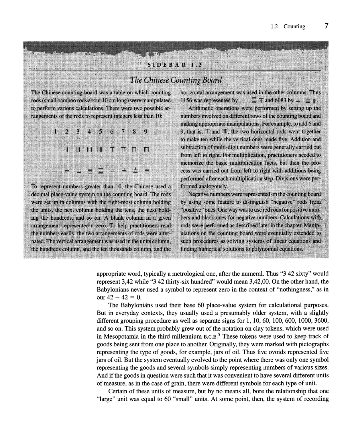
COUNTING
The simplest mathematical idea-and one that probably existed even before civilization-
is that of counting, in words and in more permanent form as written symbols. Although
an interesting study can be made of number words in various languages (Sidebar 1.1), we
restrict ourselves here to a discussion of number symbols. Several methods of organization
can be distinguished in the writing of these symbols. One method is called the grouping
1.2 Counting 5
. :' .
";',.., ;,;Ii;;;..' :" .jH;;'..:i:::.''if:'' V : :'' > ::y: : :;n j(.:i;I:'" ,:::;.::.: n .,' . ".::. .;,::' >'., '... . :
. .. . ." .n. '.;.; . ....,. ,.., SI.D'.;I. B. .1\ :,R.: I ..[.n . ..n ... ....... ., . ../ . . . ....... . '. ...:....
".' :..';.i. . .,,<.".' .): :i:;i:.:-::::.,:::""; . ....""c. .';'0 :?':/:'; "." '; :. :">:':" '.' .' :;:/.iF:::;
... 'i ..,.. i2:' .';"' };i }lj;m ; j;Sy, "l:11"?I";'; :cu< .,.. . . .<; i.ii ,..'
: . 'c . ..; : ,; : .. . . : . _ ii ; : . . : . E.\l . l : :; : ;.. . W . , . .: . ... . :; : ' . '" , . : . : : , . : . ,,2: . : , ' . : . . . ;" .. . ' "u ,..."i I.E ,.i : E 4' ;,,1 )' ,. . ..'.. .,..
. . 'i\;:, dt...,;. ' jf<li .IQgun.. ":""" .:'.' . :'i':":: '.Ies :i .( n..: . tl;: j :.:#.:;. O ...'j..;:.[.' it/:':'"
'Gnfiese"";' : . jfi ii :iU::'::,;:: .,: ,::"> .:':; ':.;.::: :(J;;8.. ..: !I: :la;.-¥#":S ;:," '."" . .... >.,...... . .......
I . . . : . j.. , . . . .. . . s . .tt . '11' . ;' , . . ;$ . m . :' , . . .. . ; . . . 't . ' . ' : .. . . : i . : . .''''''i" t!t;<" .... ,i
'. . . .. . . ;.; ...... ....... ....., ,. i( ;' :1'f[OJ .... :e; ·
i::i::M l"an ....... .... u<:li a IT1 un<;::::::..,8,' (J.€I : Sii'. , ' MQjI:,jl::lc) , .. ...
. .A . ',,", .U ' . ' . : . ;.j;:A . ' . : <i.:;';' l '; ;ri: l t. > . >. ...,:;" ..f r ....l ; o . . .::"q:"A u j .n== . ..;. tiy:.'c . i : . ; i . ' . . '; 'T\J4, i . ' ¥( . . . . '"i'"
. . .. . . . : . E. ,. . . .. :" :. . .. . .. . . . .. . . . : . a :. z . L . ' . '.' . , . E"' , .. " :'. , , , , ..:, ... u.""''''''!'!;>. .!<t . ...... . k .Jec .nJi<'"''''".... "S¥ Z(,("'...... .., """' ''''J i
. ._N, .......e/(. . . .. , ( ti ;$,' '. u .
<c.;> : ...;:,.. . . i . . . i'> . . . .'.. . . . ..... , . . . , . . ., ....... ;' '.n" .. . ...: /.' .i> .........:.:..",.. /.::::::: . <':.n.) ::y.:';)i.."ny:::ib;.
x.>. ,'.:'" ;';:.:.',:'::." ........ II';::"'" . .:",. ......... '. .......
':h:':::':::::;»'::::;:;;') . '.::: ' ....::!::!.::.>:i::::., .'. '.:. ..>:'. .... .'. ...... '..
. ::::vit....... .If;.t .v::'''' '.;' ,.. . . ..: . : . ; ; . .;-: . . . ...li . 1 .t ..' e ......... n :t... e . . h . ' . n . , : s . v . "'::: . "' . . 'ii: ;..' n
f ':: . . 'j ...... ............ ..... 't'0 12¥ ;. ':'1'!':! f"". J"'!. '... .... ...,
...... e.I f<> '. 'j: ::..: '. j.!Ig i t):::'... ......... .... .:;:....: ..>< . ;' fr() ' al1. ';. :, . gein '¥==C ....:
: J m.J:f'''e ., i i:'i., ...,.;i, S ( '. ' ;f I!''P 1I: r..
:,E;:( . 11fi . m . i . . . . . . . .. . . -'.,,\ . m .l . . .. . . . ! , . . : . .. . " . . : . . . ;.. . ; . , . : , . . ' . ;, . : .: .. . . . : . ... :. : . , . :.: . . . . :. . . . .. . : . . . ..; ..m :, :... . ., ..... . .e" ! ; ":: . jf'.f:S' )' 'ee
, . \kHu'-Io'-' i:':' :',:':'. i..;(d.: Jj'* r),1n:<.: :::'::,: :>< m(l} $Zl.t.. :' .:sm1i,, ,::If2) ::,?::: ..
t : t.. ; (E" a1tiiftl,, ... . .,", i4: f li'Z !iJ1;,;s ' ;fn}ti1If ' . ; . gf. . . . ' . ,' . > . .:' , ..: . :
::yi,\.: ; c ":;;-;::i"i ;< I } " . ">'c' B):>' 'io):m ,. rii;;..;,;.i';;..;j':;-;i ' 1 ."' 'r:i.gl1A'>.> '.J;: "
:";;;j+y !'... ..:::. .:n::.; ._plk; _,,:' "'!::::':..:i:}:: :l>R , Ga.t0.: ;:: ttl: i I f ;;l . ;.:., . ;;:;. ....
<if, Ieil: ;: '.C.i.::::":,::' t tt Ronto .... "::;.::::1'.><; ti tetta.ra'; 4.lijnm Ir(jjrn,:g itt,.i;:; f} .;.::, ,
'"!!. $ . l' . i ;i !ilt . ii fi !; !;Afi
.\. }.07,., "'1"1'?";'t+ ; C....__JJ...--.G7..,..7;IBS;......En,Ts::t( ..,...?T.77 r'.77-:-; .......... .......';;; .'i /:. ....... '..; .. ..........T........., i., .",.,. .......:.... ""'. ..)
.::
. .
.:.
method. In its simplest form, a stroke / is used to represent the number 1; appropriate
repetitions are made to represent larger numbers. One of the earliest dated occurrences of
such a representation of numbers is on a fossilized bone discovered at Ishango in Zaire and
carbon-dated to s<?me time around 20,000 B.C.E. It is not clear what the strokes or notches
represent, but one scholar who has studied the bone in detail believes they represent a
count of certain periods of the moon. 3 That early peoples used this elementary form of
numerical representation to deal with astronomical phenomena would confirm what will be
seen in much later time periods-that the development of mathematics goes hand in hand
with the development of astronomy. Artifacts similar to the Ishango bone and dating from
perhaps 8000 B.C.E., with regular groupings of notches perhaps representing astronomical
observations, have been found in central Europe as well.
A more sophisticated example of the grouping method of number representation was
develop d by the Egyptians some 5000 years ago. In this hieroglyphic system, each of
the first several powers of ten was represented by a different symbol, beginning with the
familiar vertical stroke for 1. Thus 10 was represented by n, 100 by G), 1000 by , and
6 Chapter 1 Ancient Mathematics
10,000 by . Arbitrary whole numbers were then represented by appropriate repetitions of
the symbols. For example, to represent 12,643 the Egyptians would write III R R .
(Note that the usual practice was to put the smaller digits on the left.)
The hieroglyphic number system was the one used for writing on temple walls or
carving on columns. But when the scribes wrote on papyrus, they needed a form of
handwriting. For this purpose they developed the hieratic system, an example of a ciphered
system. Here each number from 1 to 9 had a specific symbol, as did each multiple of 10
from 10 to 90 and each multiple of 100 from 100 to 900, and so on. A given number, for
example 37, was written by putting the symbol for 7 next to that for 30. Since the symbol
for 7 was Il.. and that for 30 was #i\, 37 was written Il..#i\. Again, since 3 was written as U',
40 as , and 200 as Y, the symbol for 243 was U' Y. Although a zero symbol is not
necessary in a ciphered system, the Egyptians did have such a symbol. It did not occur in
mathematical papyri, however, but in papyri dealing with architecture, where it is used to
denote the bottom leveling line in the construction of a pyramid, and accounting, where it
is used in balance sheets to indicate that the disbursements and income are equal. 4 Similar
ciphered systems were used in written Hebrew and Greek. In those two languages, the
specific symbols were simply the letters of the alphabet.
The Chinese from earliest recorded times used a multiplicative system of writing
numbers, again based on powers of 10. That is, they developed symbols for the numbers
1 through 9 as well as for each of the powers of 10. Then, for example, the number 659
would be written using the symbol for 6 (If) attached to that for 100 (@), then the 5 (X)
attached to the symbol for 10 (f), and finally the symbol ,5 for 9: 'Q' k ,5. The development
of this system was probably related to the early use of a counting board, in which rods were
arranged in vertical columns standing for the various powers of 10 (Sidebar 1.2). Therefore,
it was natural to think of 659 as 6 in the 100s column, 5 in the 10s column, and 9 in the 1 s
column and to represent each column in written form by a special symbol.
Each of these systems except the first is organized around the base 10. Namely, there
are always distinguished symbols for the integral powers of 10 around which symbols for
other numbers are organized. The Babylonians organized their number symbols around
two separate bases. First, they used a grouping system based on 10 to represent numbers up
to 59. Thus a vertical stylus stroke on a clay tablet 1 represented 1 and a tilted stroke
111
represented 10. By grouping they would, for example, represent 37 by 'Y'Y'Y. Then,
1
sometime in the third millennium B.C.E., the Babylonians developed the first positional or
place- value number system for numbers greater than 59. In such a system, the powers of the
base-in this case 60-are represented by "places" rather than symbols, and the digit in each
place represents the number of each power to be counted. Hence 3 X 60 2 + 42 X 60 + 9
(or 13,329) was represented by the Babylonians as 'Y'Y'Y j 'Y'Y ttt. (This
111
will be written from now on as 3,42,09 rather than with the Babylonian strokes.) The Old
Babylonians did not use a symbol for 0, but often left an internal space if a given number
was missing a particular power. There would not be a space at the end of a number, so it
is difficult to distinguish 3 X 60 + 42 (3,42) from 3 X 60 2 + 42 X 60 (3,42,00). Some-
times, however, they would give an indication of the absolute size of a number by writing an
1.2 Counting 7
appropriate word, typically a metrological one, after the numeral. Thus "3 42 sixty" would
represent 3,42 while "3 42 thirty-six hundred" would mean 3,42,00. On the other hand, the
Babylonians never used a symbol to represent zero in the context of "nothingness," as in
our 42 - 42 = O.
The Babylonians used their base 60 place-value system for calculational purposes.
But in everyday contexts, they usually used a presumably older system, with a slightly
different grouping procedure as well as separate signs for 1, 10, 60, 100, 600, 1000, 3600,
and so on. This system probably grew out of the notation on clay tokens, which were used
in Mesopotamia in the third millennium B.C.E. 5 These tokens were used to keep track of
goods being sent from one place to another. Originally, they were marked with pictographs
representing the type of goods, for example, jars of oil. Thus five ovoids represented five
jars of oil. But the system eventually evolved to the point where there was only one symbol
representing the goods and several symbols simply representing numbers of various sizes.
And if the goods in question were such that it was convenient to have several different units
of measure, as in the case of grain, there were different symbols for each type of unit.
Certain of these units of measure, but by no means all, bore the relationship that one
"large" unit was equal to 60 "small" units. At some point, then, the system of recording
8 Chapter 1 Ancient Mathematics
numbers developed to the point where the same digit 1 represented 60 as well. We do not
know why the Babylonians decided to have one large unit represent 60 small units and
then adapt this method for their numeration system. One conjecture is that 60 is evenly
divisible by many small integers. Therefore, fractional values of the "large" unit could easily
be expressed as integral values of the "small" unit. The Babylonian base 60 place-value
system is still in use in our units for angle and time measurement, units preserved over the
centuries in astronomical contexts and today an irreplaceable part of world culture.
There is no record of the written number system of ancient India, but there is literary
evidence that numerical symbols did exist. It is only from about the third century B.C.E. that
examples of written numbers are available. Originally, the system was mixed. There was
a ciphered system similar to the hieratic with separate symbols for the numbers 1 through
9 and 10 through 90. For larger numbers, the system was a multiplicative one similar to
the Chinese. For example, the symbol for 200 was a combination of the symbol for 2 and
that for 100, and the symbol for 70,000 combined the symbols for 70 and 1000. As will be
discussed in Chapter 6, it was in or near India that the modem base 10 place-value system
developed, but not until about the seventh century C.E.
1.3
ARITHMETIC COMPUTATIONS
Once their system of writing numbers came into existence, all of the civilizations under
discussion devised rules for the basic arithmetic operations-addition, subtraction, multi-
plication, and division-and as a consequence of the last operation, rules for writing and
operating with fractions. These rules may be considered as some of the earliest algorithms.
An algorithm is an ordered list of instructions designed to produce an answer to a
given type of problem. Ancient peoples produced algorithms of all sorts to handle many
different problems. In fact, ancient mathematics can be characterized as algorithmic in
nature, as opposed to the Greek mathematics, which emphasized theory. In most of the
available documents of ancient mathematics, the author describes a problem to be solved
and then proceeds to use an algorithm, either explicit or implicit, to obtain the solution.
There is little concern in the documents as to how the algorithm was discovered, why it
works, or what its limitations are. Instead, we simply are shown many examples of the use
of the algorithm, often in increasingly complex situations. Nevertheless, in our discussion
of these algorithms, we will describe the possible origins and justifications of each one and
will present the possible answers that the Babylonian, Chinese, or Egyptian scribes gave to
their students who asked the eternal question "why?"
In the Egyptian hieroglyphic grouping system, addition is simple enough: Combine the
units, then the tens, then the hundreds, and so on. Whenever a group of ten of one type of
symbol appears, replace it by one of the next. Hence, to add 783 and 275, put IIIRRRR
and IIlnnnn G) to g ether to g et IIllInnnnnnnn Since there are fifteen ns re p lace
II nnn III nnnnnnn G). ,
ten of them by one . This then gives ten of the latter. Replace these by one . The final
answer is 1111 n , or 1058. Subtraction is done similarly. In this case, of course, whenever
"borrowing" is needed, one of the symbols would be converted to ten of the next lower
symbol.
1.3 Arithmetic Computations 9
Such a simple algorithm for addition and subtraction is not possible in the hieratic
system. For these operations, the mathematical papyri do not provide much evidence; the
answers to addition and subtraction problems are merely written down. Most probably, the
scribes had addition tables. At some point these would have existed in written form, but
a competent scribe would, of course, have memorized them. The scribes presumably used
the addition tables in reverse for subtraction problems.
The Egyptian algorithm for multiplication was based on a continual doubling process.
To multiply two numbers a and b, the scribe would first write down the pair 1, b. He would
then double each number in the pair repeatedly, until the next doubling would cause the
first element of the pair to exceed a. Then, having determined the powers of 2 that add to
a, the scribe would add the corresponding multiples of b to get the answer. For example, to
multiply 12 by 13 the scribe would set down the following lines:
1 12
2 24
4 48
8 96
At this point, he would notice that the next doubling would produce 16 in the first column,
which is larger than 13. He would then check off those multipliers that added to 13, namely
1, 4, and 8, and add the corresponding numbers in the other column. The result would be
written as: Totals 13 156.
As before, there is no record of how the scribe did the doubling. The answers are simply
written down. Perhaps the scribe had memorized an extensive 2 times table. In fact, there
is some evidence that doubling was a standard method of computation in areas of Africa
to the south of Egypt, so it is likely that the Egyptian scribes learned from their southern
colleagues. 6 In addition, the scribes were somehow aware that every positive integer could
be uniquely expressed as the sum of powers of 2. That fact provides the justification
for the procedure. How was it discovered? Our best guess is that it was discovered by
experimentation and then passed down as tradition.
Because division is the inverse of multiplication, a problem such as 156 -;- 12 would
be stated as "multiply 12 so as to get 156." The scribe would then write down the same
lines listed before. This time, however, he would check off the lines having the numbers
in the right-hand column that sum to 156; in this case, 12, 48, and 96. Then the sum of
the corresponding numbers on the left, namely 1,4, and 8, would give the answer 13. Of
course, division does not always "come out even." When it did not, the Egyptians used
fractions.
The kind of fractions that the Egyptians used were unit fractions, or "parts" (fractions
with numerator 1), with the single exception of 2/3, perhaps because these fractions are
the most "natural." The fraction 1/ n (the nth part) is represented in hieroglyphics by the
symbol for the integer n with the symbol c:::> above. In the hieratic a dot is used instead.
.
Thus 1/7 is denoted in hieroglyphics by W: and in the hieratic by 1.. The single exception,
2/3, had a special symbol: <iT in hieroglyphics and r in hieratic. (The former symbol is
indicative of the reciprocal of 1 1/2.) In the remainder of this text, however, the notation n
will be used to represent l/n and 3 to represent 2/3.
10 Chapter 1 Ancient Mathematics
Because fractions show up as the result of divisions that do not come out evenly, we
need to be able to deal with fractions other than unit fractions. It was in this connection that
the most intricate of the Egyptian mathematical techniques developed, the representation
of any fraction in terms of unit fractions. The Egyptians did not put the question this way,
however. Where we would use a nonunit fraction, they would simply write a sum of unit
fractions. For example, problem 3 of the Rhind Mathematical Papyrus asks how to divide
6 loaves among 10 men. The answer is given that each man gets 2 10 loaves (that is,
1/2 + 1/10). The scribe checks this by multiplying this value by 10. We may regard the
scribe's answer as more cumbersome than our answer of 3/5, but in some sense the actual
division is easier to accomplish this way. If we divide five of the loaves in half and the
sixth one in tenths, and then give each man one-half plus one-tenth, it is then clear to all
concerned that everyone has the same portion of bread. Cumbersome or not, this Egyptian
unit-fraction method was used throughout the Mediterranean basin for over 2000 years.
In multiplying whole numbers, the important step is the doubling step. Likewise in
multiplying fractions, the scribe had to be able to express the double of any unit fraction.
For example, in the preceding problem, the check of the solution is written as follows:
1 2 10
'2 1 5
4 2 3 15
---
'8 4 3 10 30
10 6
How are these doubles formed? To double 2 10 is easy: Because each denominator is even, it
is merely halved. In the next line, however, 5 must be doubled. To perform calculations like
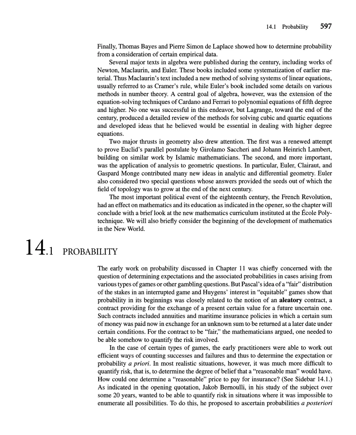
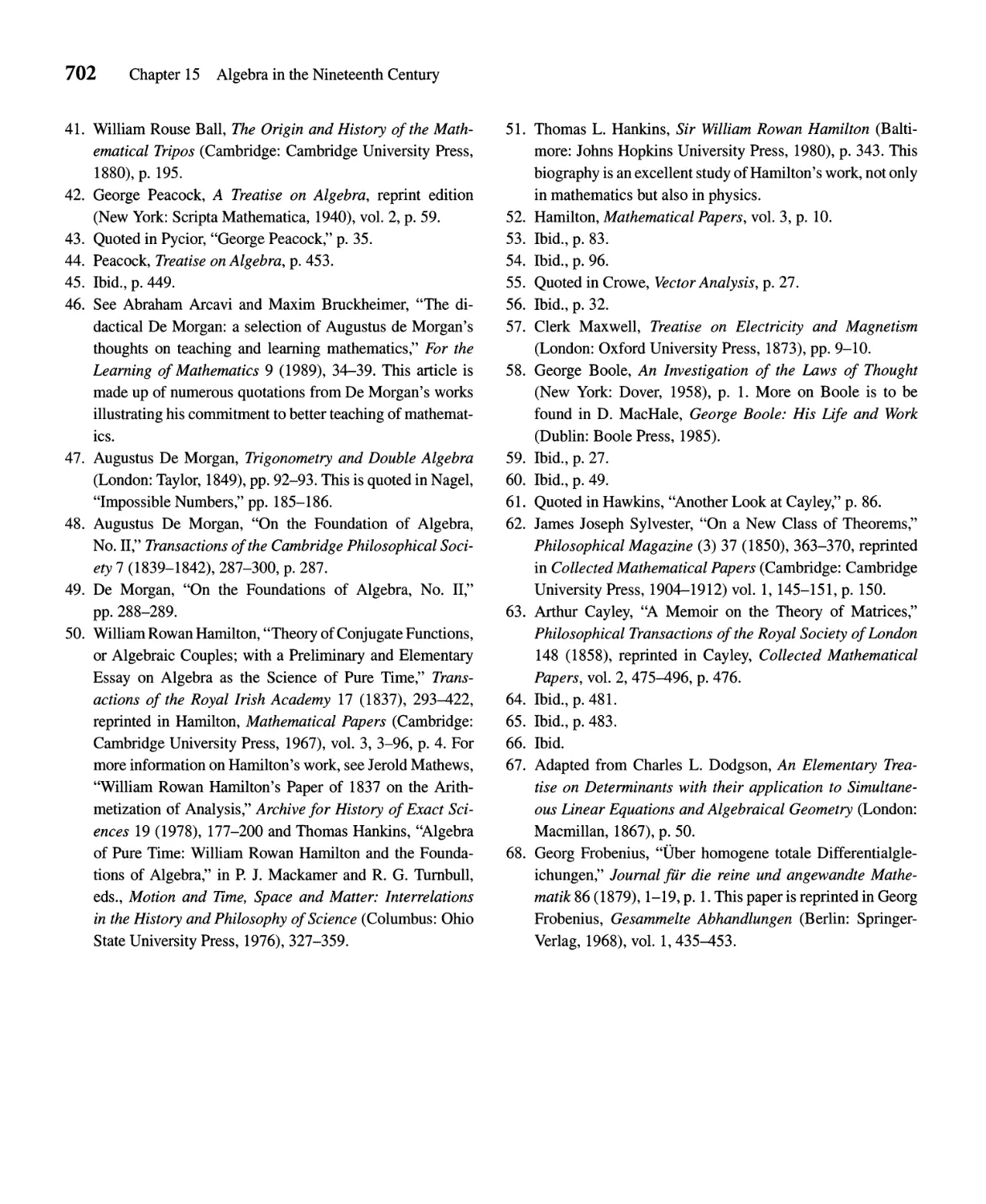
this, the scribe had to use a table to get the answer 3 15 (that is, 2 · 1/5 == 1/3 + 1/15).
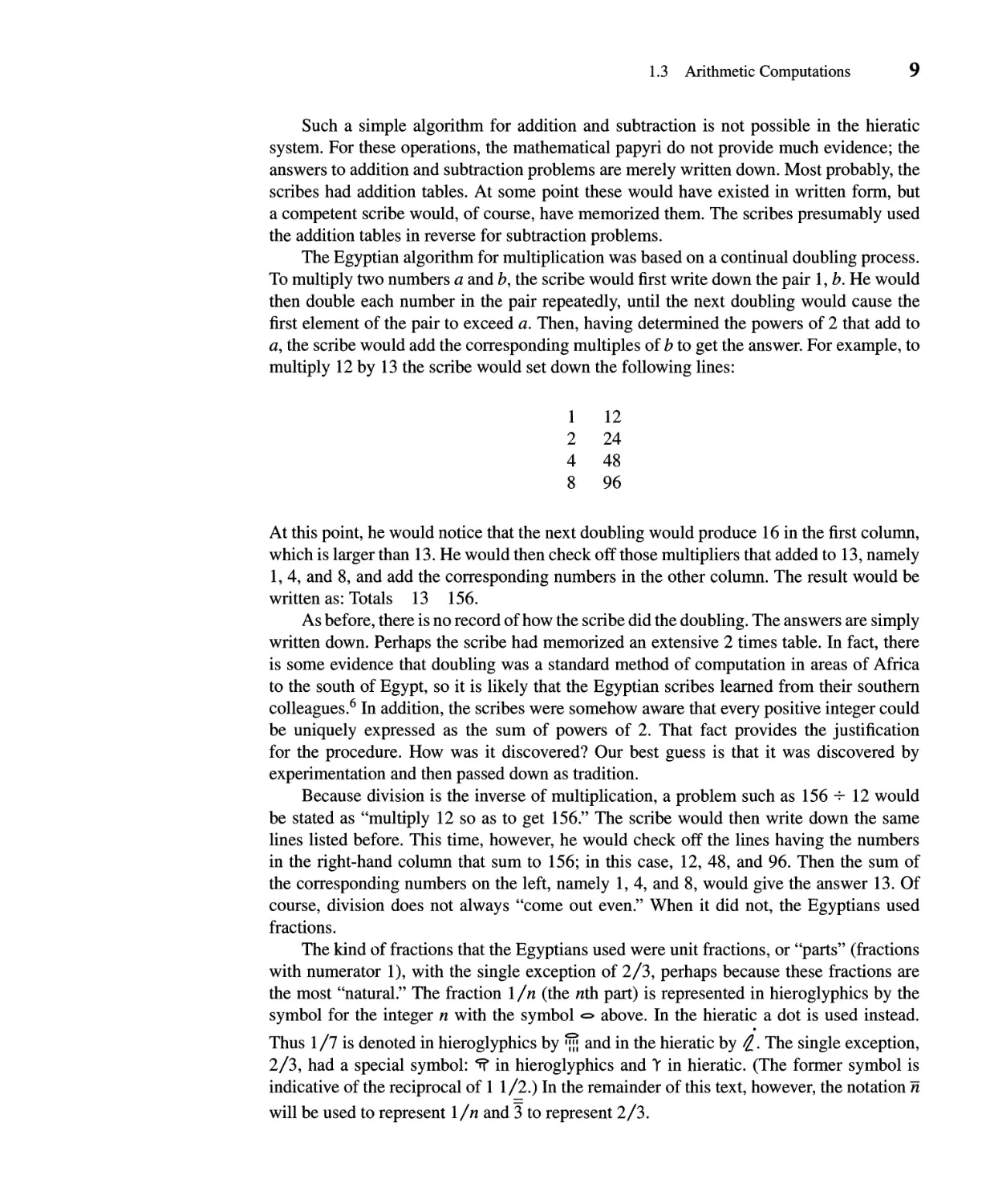
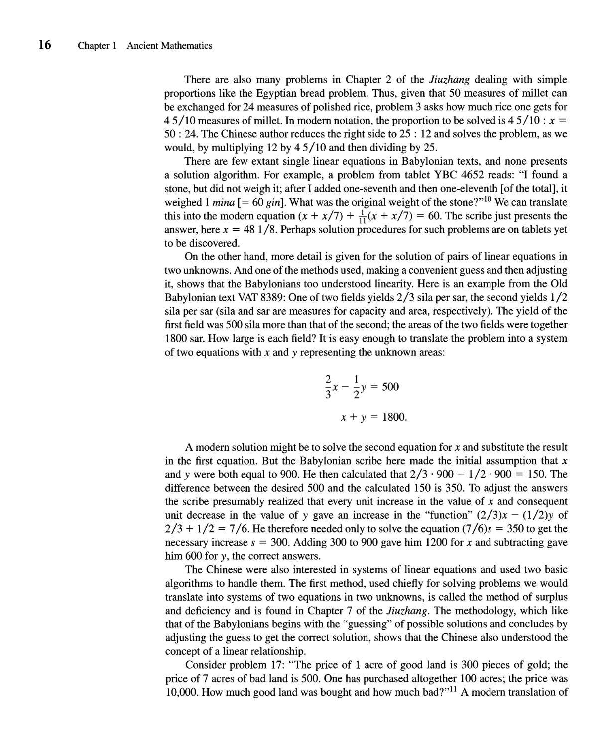
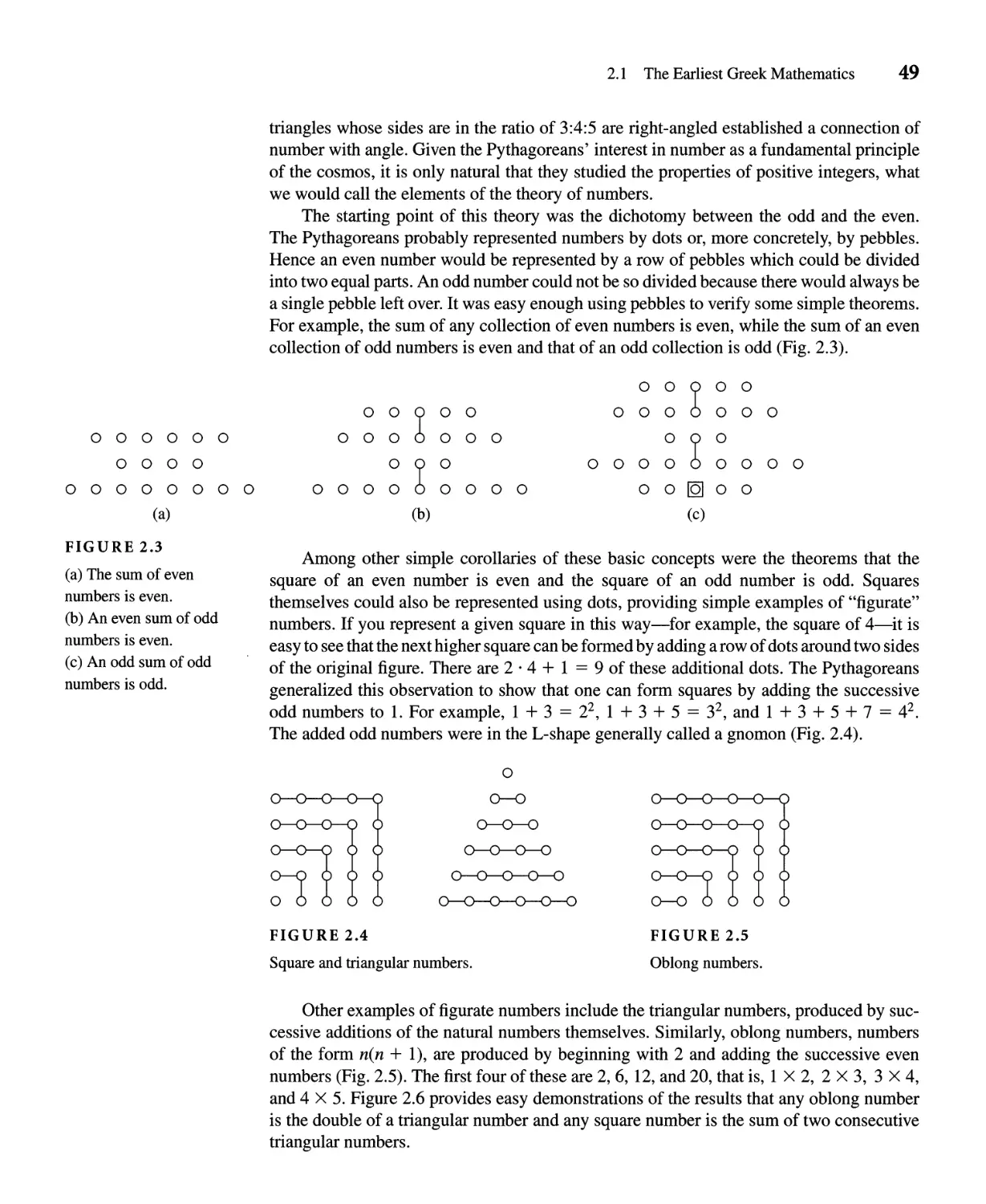
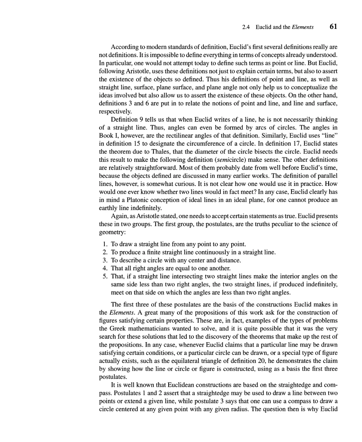
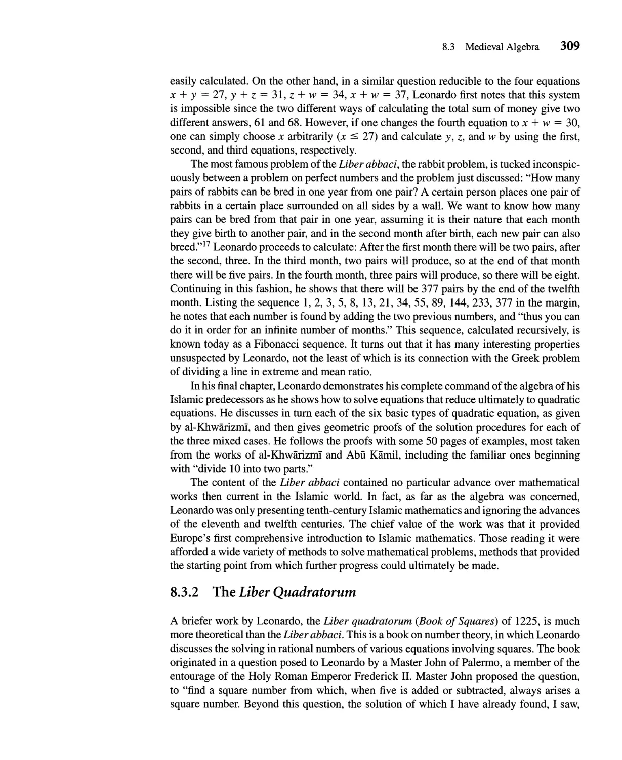
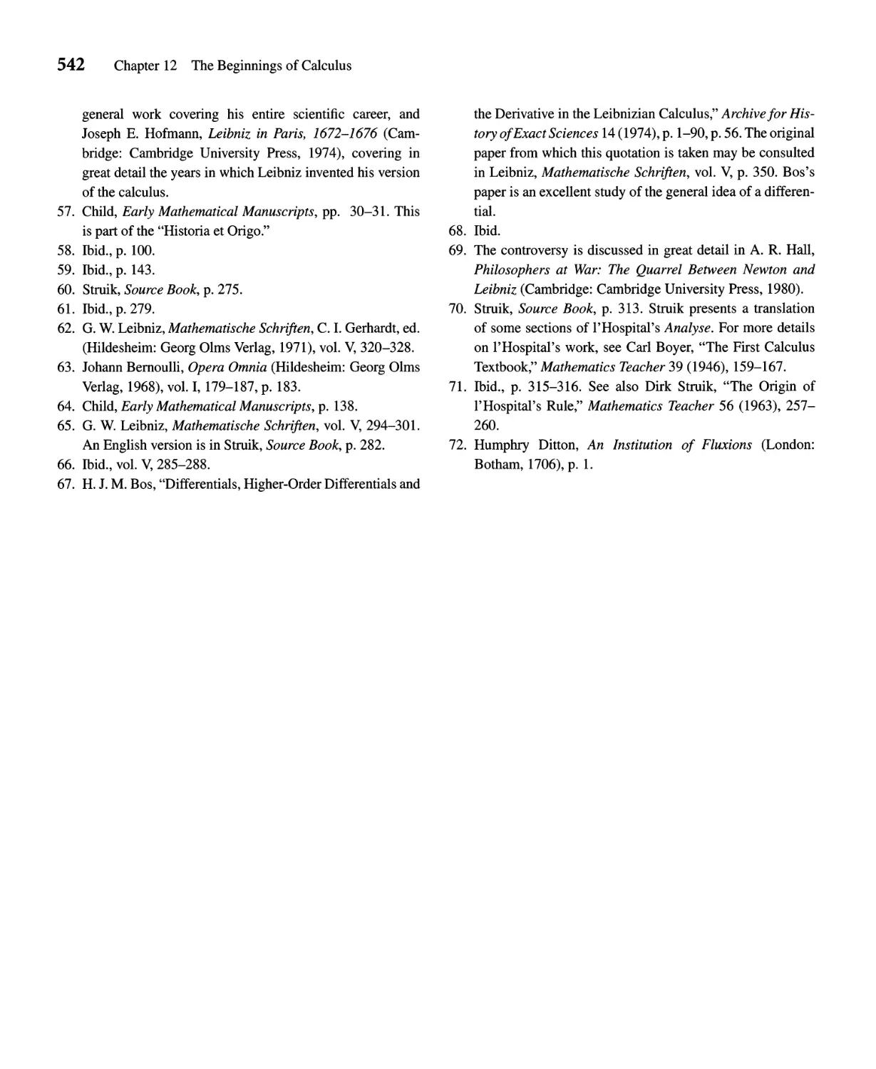
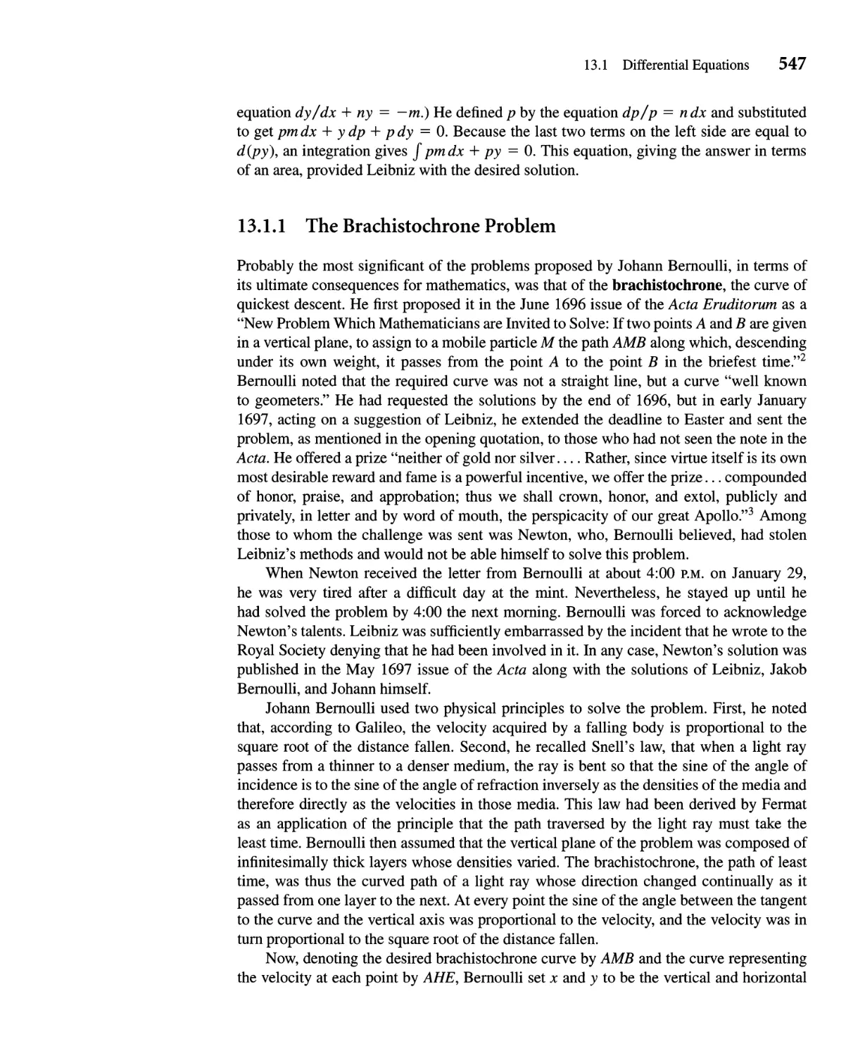
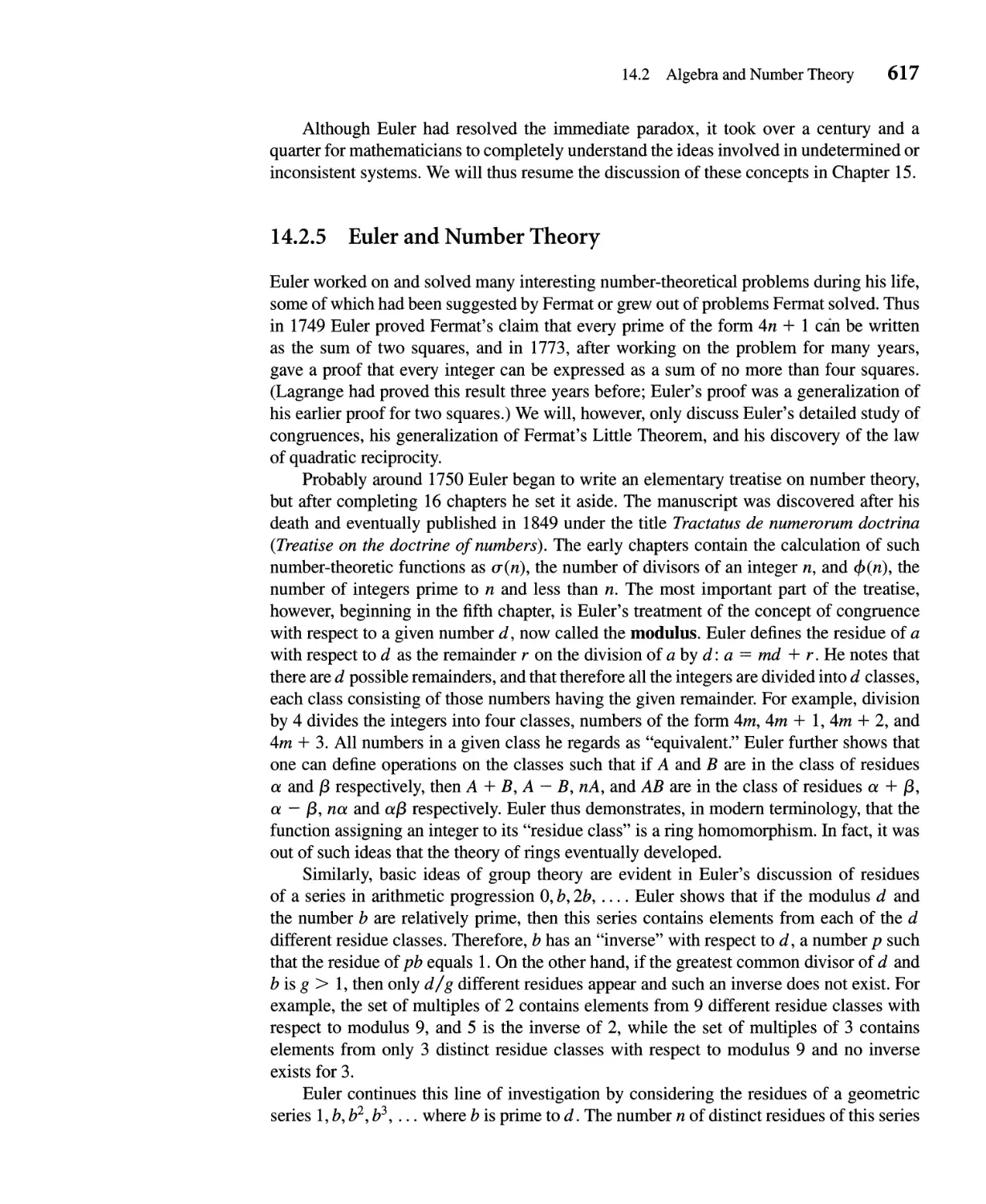
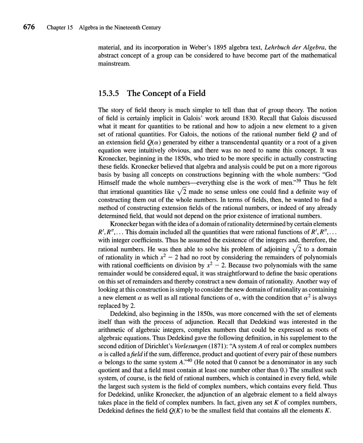
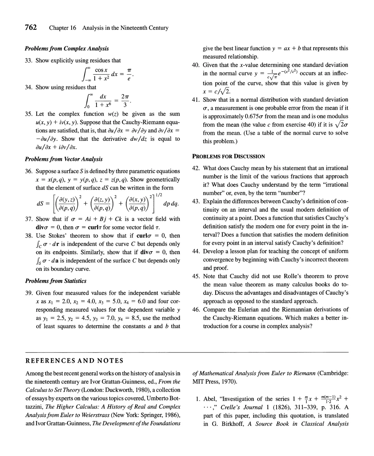
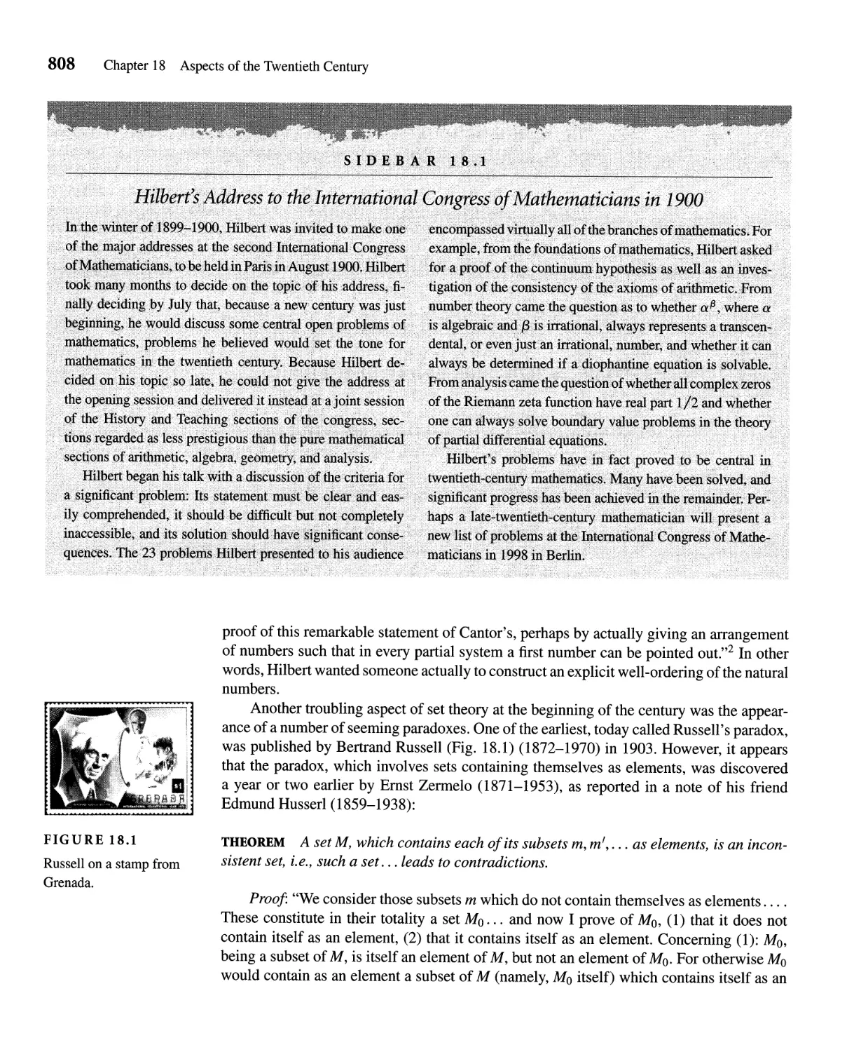
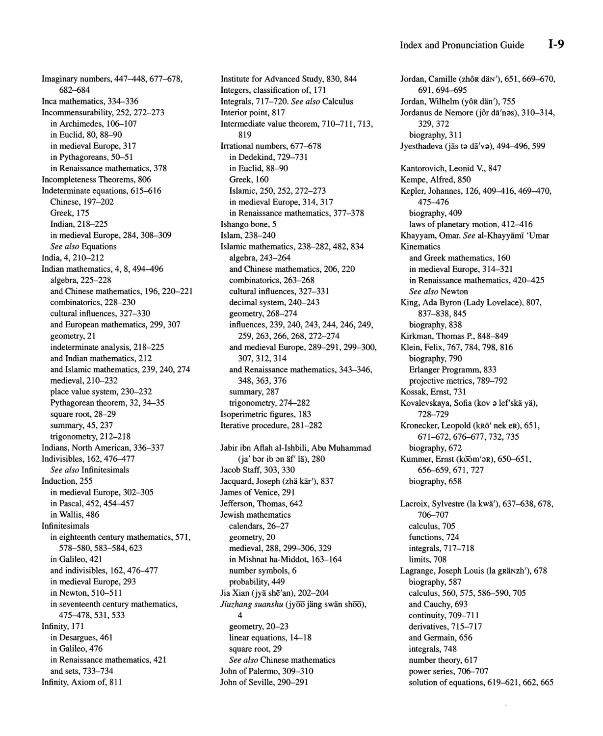
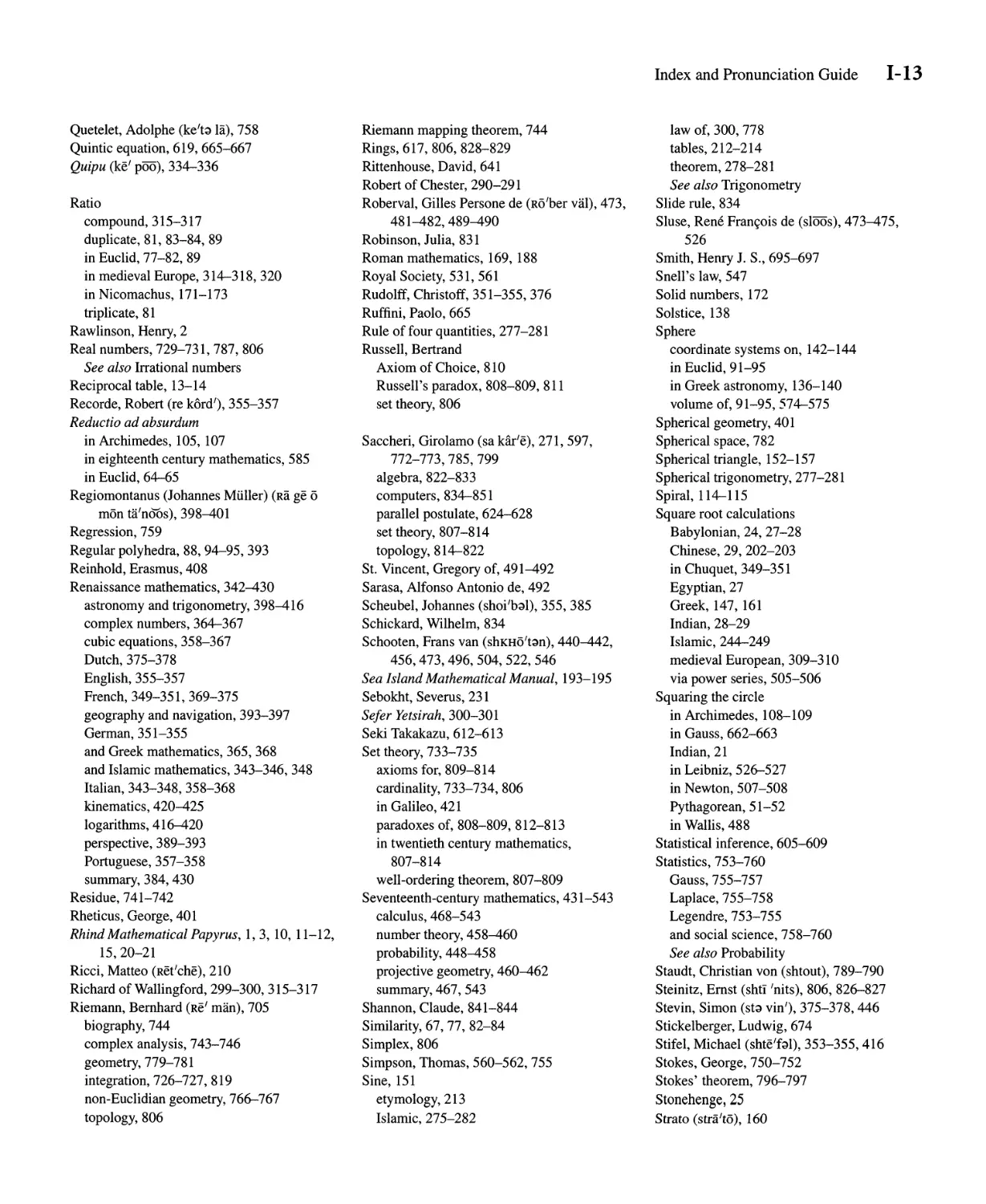
In fact, the first section of the Rhind Papyrus is a table of the division of 2 by every
odd integer from 3 to 101 (Fig. 1.7), and the Egyptian scribes realized that the result of
multiplying Ii by 2 is the same as that of dividing 2 by n. Although it is not known how
the division table was constructed, several scholarly accounts present hypotheses for the
scribes' methods. 7 In any case, the solution of problem 3 depends on using that table twice,
first as already indicated and second, in the next step, where the double of 15 is given as
10 30 (or 2 · 1/15 == 1/10 + 1/30). The final step in this problem involves the addition
- ---
of 1 5 to 4 3 10 30, and here the scribe just gave the answer. Again, the conjecture is that
for such addition problems an extensive table existed. The Egyptian Mathematical Leather
Roll, which dates from about 1600 B.C.E., contains a short version of such an addition table.
There are also extant several other tables for dealing with unit fractions and a multiplication
table for the special fraction 2/3. It thus appears that the arithmetic algorithms used by the
Egyptian scribes involved extensive knowledge of basic tables for addition, subtraction, and
doubling and then a definite procedure for reducing multiplication and division problems
into steps, each of which could be performed using the tables.
Often in dealing with division, the scribes replaced the doubling procedure by halving.
For example, in calculating 2 ...;- 7, the first steps are:
1 7
2 32
4 124
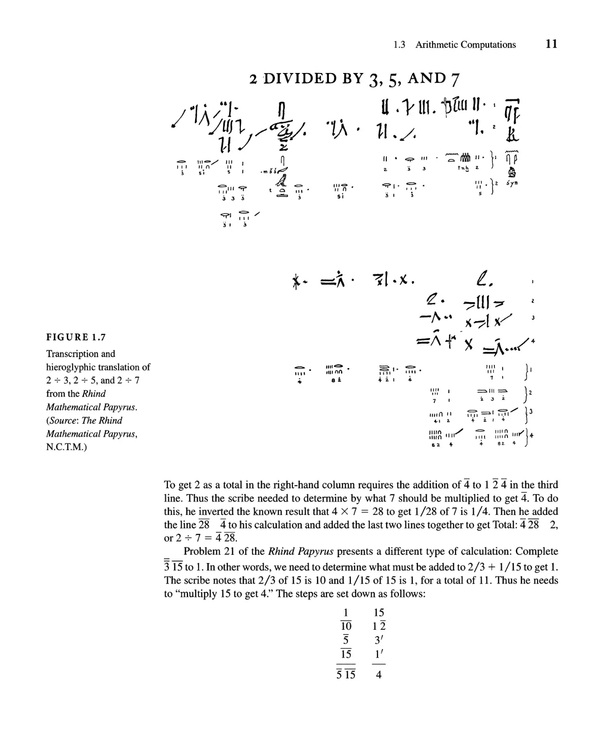
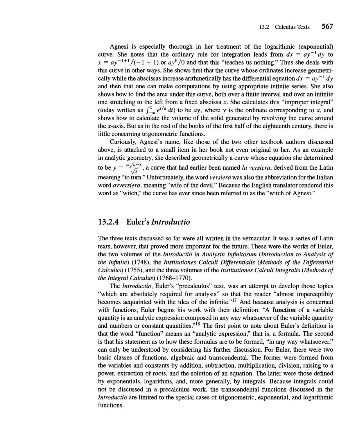
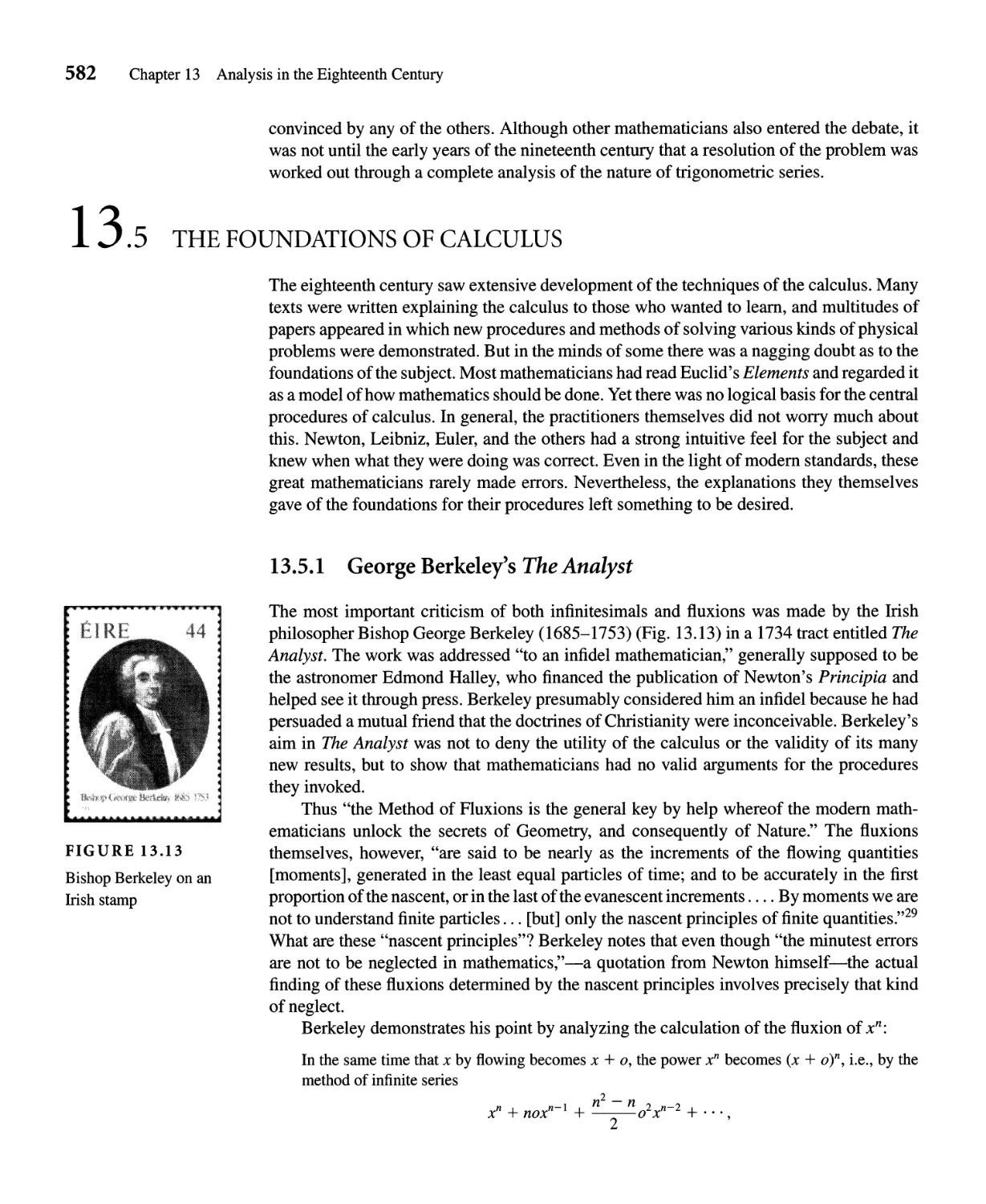
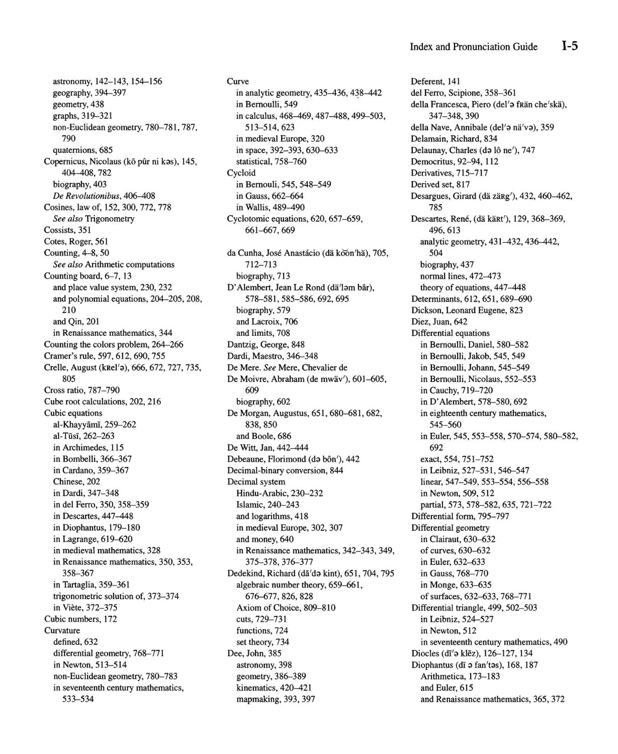
FIGURE 1.7
Transcription and
hieroglyphic translation of
2 -;- 3, 2 -;- 5, and 2 -;- 7
from the Rhind
Mathematical Papyrus.
(Source: The Rhind
Mathematical Papyrus,
N.C.T.M.)
1.3 Arithmetic Computations 11
2 -DIVIDED BY 3,5, AND 7
U · V 111. 13 liu If. I
I
'1,A' I ../. "1. 2
" · tt1. 0
/ lA;llJ /
l ./ z
<=> 111 c:::> /" III J
" , 'I n II
3 5 i 5 I
.m ;$
A.
c::::>
.., .
3
III 9
3 .3 :3
t a
c:::!:!:::a
I /
:5 I .3
.
c:::>
" , ,
+
....,
qf
lL
'"C> .
" n
5;
:; tflID II. l'
/I . <.;? /I, P
2- 3 .3 t'1\h 2.
<i? I . c::> "I 1 z :;yn
, , , 'I .
3 . 3 5
=::." .
t.6
· '/UJ ?'
-f'.... "71 ,,/
II"
=!\ 1 V ' /4
)\ A ". <
}I
III J 2
i .3 2.
l · " ·
z
3
III' c:::> .
.11' nn
81
c::::>
"" .
...
',',1,' I
., I
I-
.. II
4- i I
','.',' I
7
/1/10 "
+. 2.
<::::> I <::::>./" J 3
"./I:::=" ',.11 -
+ 2. , +
c:::::> III' n Y" J
III' III,n 1/1 +
+ sz, 4-
1111 n " 11./
IIlIn
s 2. +
To get 2 as a total in the right-hand column requires the addition of 4 to 1 2 4 in the third
line. Thus the scribe needed to determine by what 7 should be multiplied to get 4. To do
this, he inverted the known result that 4 X 7 = 28 to get 1/28 of 7 is 1/4. Then he added
- - --
the line 28 4 to his calculation and added the last two lines together to get Total: 4 28 2,
or 2 -;- 7 = 4 28.
Problem 21 of the Rhind Papyrus presents a different type of calculation: Complete
3 15 to 1. In other words, we need to determine what must be added to 2/3 + 1/15 to get 1.
The scribe notes that 2/3 of 15 is 10 and 1/15 of 15 is 1, for a total of 11. Thus he needs
to "multiply 15 to get 4." The steps are set down as follows:
1 15
10 1 2
5 3'
15 I'
5 15 4
12 Chapter 1 Ancient Mathematics
Here the scribe doubles from the second line to the third, but, since he realized that 1 is
1/3 of 3, he took thirds to get from the third line to the fourth. The answer to the original
problem is then 5 15.
As an example of other modifications that the scribes made to their basic procedure,
consider problem 69 of the Rhind Papyrus, which includes the division of 80 by 3 2 and its
subsequent check:
-
1 32 'I 2237 21
'2 -----
10 35 45 3 4 14 28 42
'20 '2 ---
70 1131442
'2 7 32 80
-
'3 23
'21 6
'7 2
-
2237 21 80
In the second line the scribe has taken advantage of the decimal nature of his "notation
to get the product of 3 2 by 10. In the fifth line he has used the 2/3 multiplication table
mentioned earlier. The scribe then realized that since the numbers in the second column
- - -
of the third through the fifth lines added to 79 3, he needed to add 2 and 6 in that column
- - - - -
to get 80. Thus, because 6 X 3 2 = 21 and 2 X 3 2 = 7, it follows that 21 X 3 2 = 6 and
7 X 3 2 = 2, as indicated in the sixth and seventh lines. The check shows several uses of
the table of division by 2 as well as great facility in addition.
That the Babylonians used tables in the process of performing arithmetic computa-
tions is proved by extensive direct evidence. Many of the preserved tablets are in fact
multiplication tables. No addition tables have ever been found, however. Because over 200
Babylonian table texts have been analyzed, we may assume that they did not exist and that
the scribes knew their addition procedures by heart and simply wrote down the answers
when needed. On the other hand, there do exist many examples of "scratch tablets" on
which a scribe has performed various calculations in the process of solving a problem. In
any case, since the Babylonian number system was a place-value system, the actual algo-
rithms for addition and subtraction, including carrying and borrowing, may well have been
similar to modem ones. For example, to add 23,37 (= 1417) to 41,32 (= 2492), one first
adds 37 and 32 to get 1,09 (= 69). One writes down 09 and carries 1 to the next column.
Then 23 + 41 + 1 = 1,05 (= 65), and the final result is 1,05,09 (= 3909).
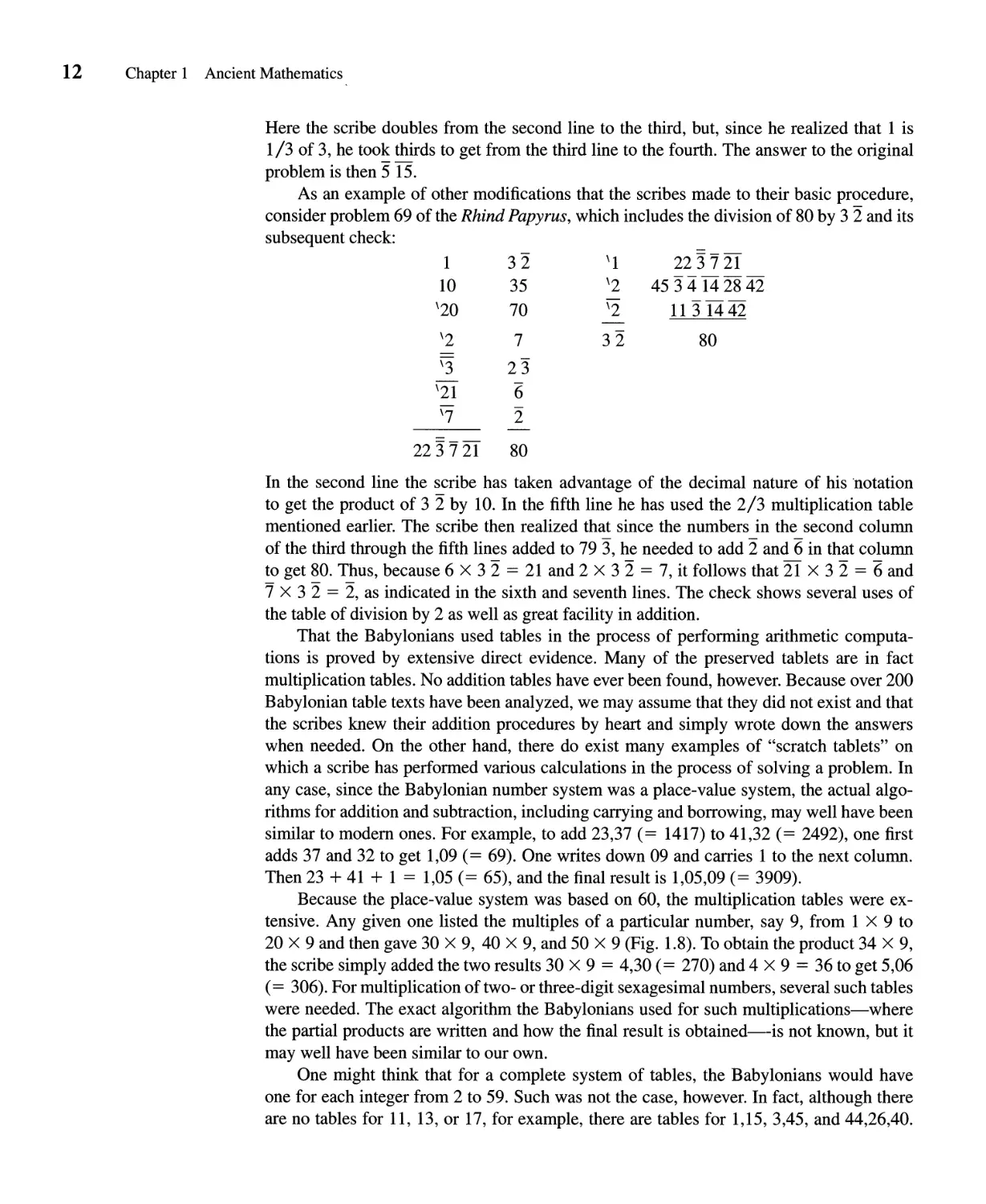
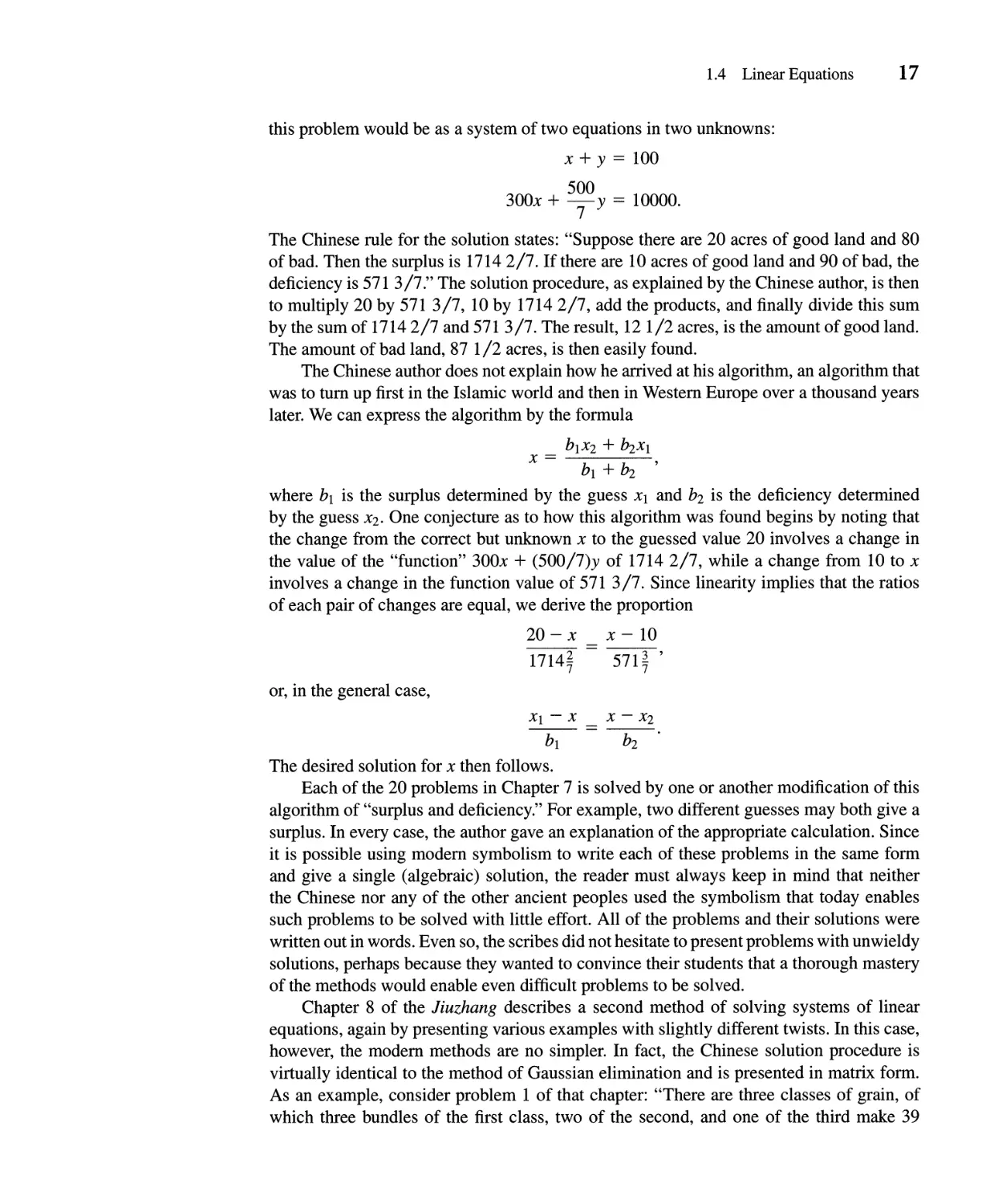
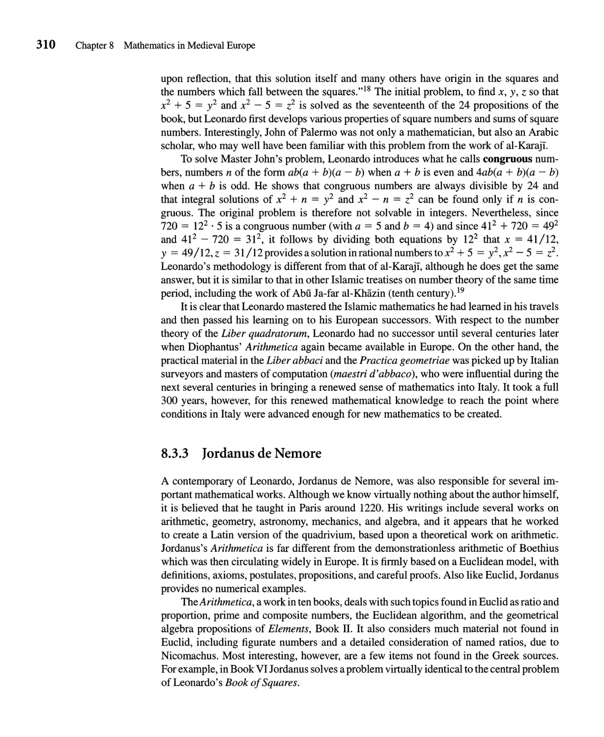
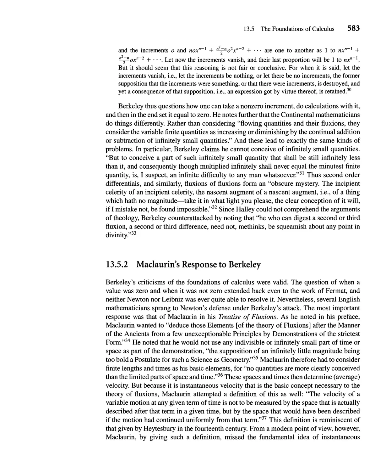
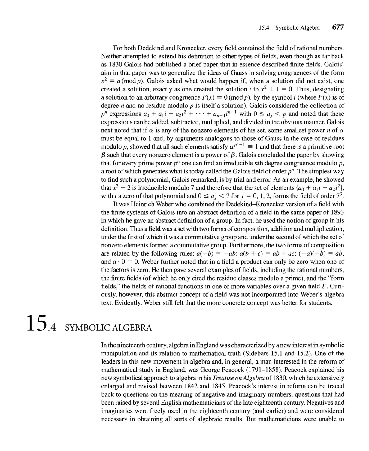
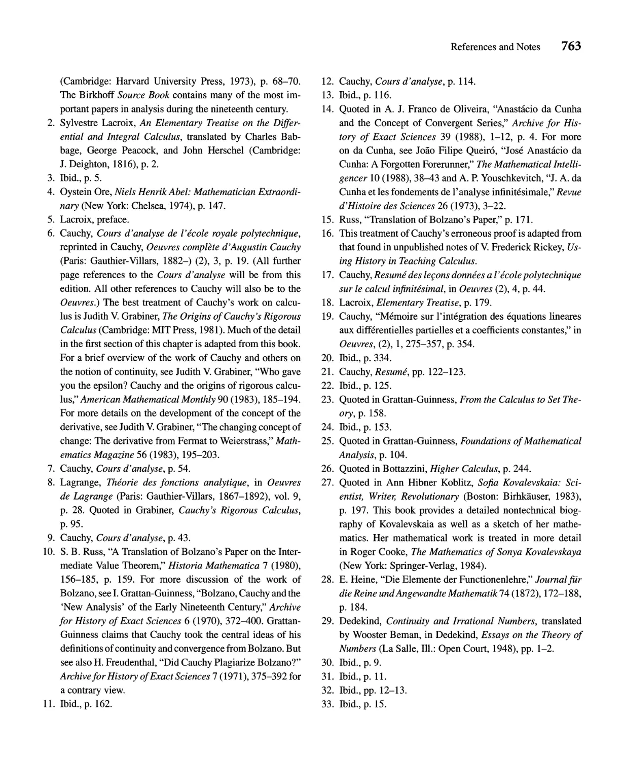
Because the place-value system was based on 60, the multiplication tables were ex-
tensive. Any given one listed the multiples of a particular number, say 9, from 1 X 9 to
20 X 9 and then gave 30 X 9, 40 X 9, and 50 X 9 (Fig. 1.8). To obtain the product 34 X 9,
the scribe simply added the two results 30 X 9 = 4,30 (= 270) and 4 X 9 = 36 to get 5,06
(= 306). For multiplication of two- or three-digit sexagesimal numbers, several such tables
were needed. The exact algorithm the Babylonians used for such multiplications-where
the partial products are written and how the final result is obtained--is not known, but it
may well have been similar to our own.
One might think that for a complete system of tables, the Babylonians would have
one for each integer from 2 to 59. Such was not the case, however. In fact, although there
are no tables for 11, 13, or 17, for example, there are tables for 1,15, 3,45, and 44,26,40.
FIGURE 1.8
A Babylonian
multiplication table for 9
(Department of
Archaeology, University
of Pennsylvania).
1.3 Arithmetic Computations 13
Cell
Cc{.I1
CJ[z
C,lIl
'.,. .
I '
. .......
-'
.
..0.:
\ \.
,
I
I
I
,.. .. :.. "
.... .
...." -0,
.i
t .'
, ".',
I
" "
" .
.' , ,
eo..
,
.,/..., . . ' , \ \ , ., J
. .-
t: '. .,,!
; -A,.. . : :'.:.';;., \ :
\ . , .. .,' :
1" ( .. .. \ .,. '. ;
..... ', - ,.
,.. .-4" /.
.... 'J. '-
\
-.,. ( 's.
, .. ..
, ...
. f
. '''-.f>
.
'"
,
,
,
.
1
."11 ...
,
...
1.
I :'
'. , ., ,
. , .,.
i' ..
!
r
06J1 r.se.
R.tve
Although we do not know precisely why the Babylonians made these choices, we do know
that, with the single exception of 7, all the multiplication tables found so far are for regular
sexagesimal numbers-that is, numbers whose reciprocal is a terminating sexagesimal
fraction. The Babylonians treated all fractions as sexagesimal fractions, analogous to our
use of decimal fractions. Namely, the first place after the "sexagesimal point," denoted by
";", represents 60ths, the next place 3600ths, and so on. Thus, the reciprocal of 48 is the
sexagesimal fraction 0;1,15, which represents 1/60 + 15/602, while the reciprocal of 1,21
(= 81) is 0;0,44,26,40, or 44/602 + 26/603 + 40/604. Because the Babylonians did not
indicate an initial 0 or the sexagesimal point, this last number would just be written as
44,26,40. As noted, there exist multiplication tables for this regular number. Such tables
provide no indication of the absolute size of the number, nor is one necessary. When the
Babylonians used the table they, of course, realized that the eventual placement of the
sexagesimal point depended on the absolute size of the numbers involved, so the placement
was finally determined by context.
Besides multiplication tables, the Babylonians also used extensive tables of reciprocals;
part of one is reproduced here. A table of reciprocals is a list of pairs of numbers whose
14 Chapter 1 Ancient Mathematics
product is 1 (where the 1 can represent any power of 60). Like the multiplication tables,
these tables only contained regular sexagesimal numbers.
2 30
3 20
10 6
16 3,45
25 2,24
40 1,30
48 1 , 15
1,04 56,15
1,21 44,26,40
The reciprocal tables were used in conjunction with the multiplication tables to do
division. Thus the multiplication table for 1,30 (= 90) served not only to give multiples
of that number, but also, since 40 is the reciprocal of 1,30, to do divisions by 40. In other
words, the Babylonians considered the problem 50 -;- 40 to be equivalent to 50 X 1/40, or,
in sexagesimal notation, to 50 X 0; 1 ,30. The multiplication table for 1,30, part of which
appears here, then gives 1,15 (or 1,15,00) as the product. The appropriate placement of the
sexagesimal point gives 1; 15( = 1 1/4) as the correct answer to the division problem.
1 1,30
2 3
3 4,30
10 15
11 16,30
12 18
30 45
40 1
50 1 , 15
In ancient China, arithmetic calculations were made on the counting board. In general,
whenever fractions were needed, they were expressed as common fractions. The Chinese
actually used our modem rules of calculation with fractions, including our device of
common denominators. There is some evidence, however, of the early use of decimal
fractions simply as additional columns on the counting board, particularly in dealing with
measures of length and weight. A fully developed decimal fraction system was not in place
until much later.
1.4
LINEAR EQUATIONS
Most of the mathematical sources from ancient times are concerned with the solution
of problems, to which various mathematical techniques are applied. Our study of these
problems begins with several methods for solving what are today known as linear equations.
Of course, one must always remember that none of the ancient peoples had any of the
symbolism for operations or unknowns that we use today. Nevertheless, the scribes were
able to solve problems using purely verbal techniques.
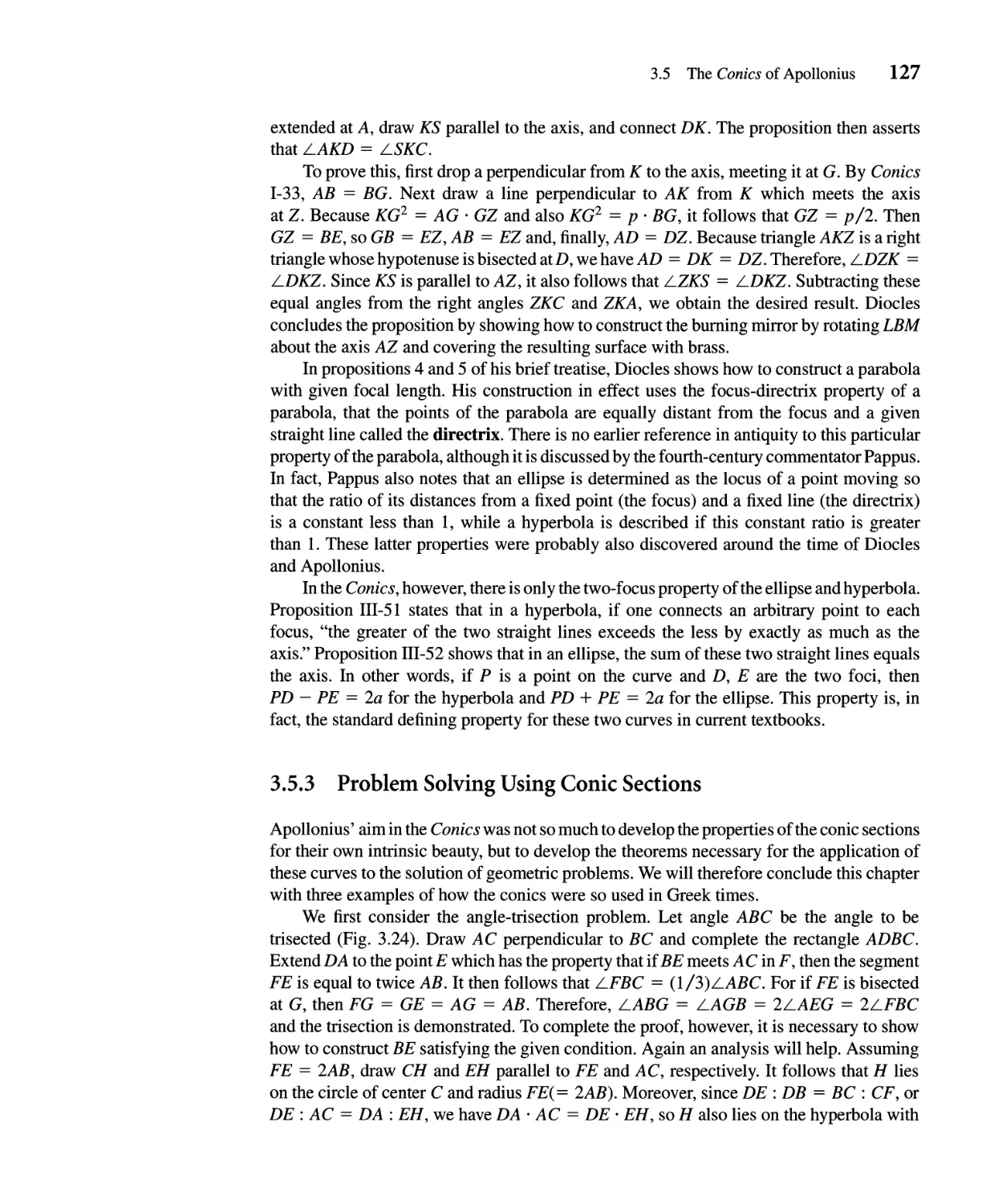
The Egyptian papyri present several different procedures for dealing with linear equa-
tions. For example, the Moscow Papyrus uses the current technique to find the number
such that if it is taken 1 1/2 times and then 4 is added, the sum is 10. In modem notation,
the equation is simply (1 1/2)x + 4 = 10. The scribe proceeds the same way we would
today: He first subtracts 4 from 10 to get 6, then multiplies 6 by 2 /3 (the reciprocal of
1 1/2) to get 4 as the solution. Similarly, problem 31 of the Rhind Papyrus asks to find
a quantity such that the sum of itself, its 2/3, its 1/2, and its 1/7 becomes 33-that is,
to find x such that x + (2/3)x + (1/2)x + (1/7)x = 33. The problem is not conceptu-
ally difficult, but it is arithmetically challenging. It and the three following problems were
probably put in to demonstrate methods of division, for the scribe solved the problem by
dividing 33 by 1 + 2/3 + 1/2 + 1/7. His answer-and this should be checked-is written
as 144 5697 194388 679776 (or, in modem notation, 14 28/97). These two problems are
1.4 Linear Equations 15
presented as purely abstract with no reference to real quantities such as areas or loaves of
bread. In fact, it would be difficult to find a real-life problem related to the second of these
examples. The scribe is simply showing that his technique works for any division problem,
no matter how difficult. Problem 35, on the other hand, does have a practical orientation.
It asks to find the size of a scoop that requires 3 1/3 trips to fill a 1 hekat measure. The
scribe solves the equation, which would today be written as (3 1/3)x = 1 by dividing 1 by
3 1/3. He writes the answer as 5" 10 and proceeds to prove that the result is correct.
A second technique for solving a linear equation is demonstrated in problem 26 of the
Rhind Papyrus, which seeks to find a quantity such that when it is added to 1/4 of itself the
result is 15. The problem is solved by the method of false position-that is, by assuming
a convenient but incorrect answer and then adjusting it appropriately. The scribe's solution
is as follows: "Assume [the answer is] 4. Then 1 4 of 4 is 5 . . . Multiply 5 so as to get 15.
The answer is 3. Multiply 3 by 4. The answer is 12."8 In modem notation, the problem is
to solve x + (1/4)x = 15. The first guess is 4, because 1/4 of 4 is an integer. But then the
scribe notes that 4 + 1/4 · 4 = 5. To find the correct answer, he must multiply 4 by the
quotient of 15 by 5, namely 3. The Rhind Papyrus has several similar problems, all solved
using false position. The step-by-step procedure that the scribe followed can therefore be
considered as an algorithm for the solution of a linear equation of this type. Even though
there is no discussion of how the algorithm was discovered or why it works, it is evident
that the Egyptian scribes understood the basic idea of a linear relationship between two
quantities-that a multiplicative change in the first quantity implies the same multiplicative
change in the second.
This understanding is further exemplified in the solution of proportion problems. For
example, problem 75 asks for the number of loaves of pesu 30 which can be made from
the same amount of flour as 155 loaves of pesu 20. (Pesu is the Egyptian measure for the
inverse "strength" of bread and can be expressed as pesu = [number of loaves]/[number of
hekats of grain], where a hekat is a dry measure approximately equal to 1/8 bushel.) The
problem is thus to solve the proportion x/30 = 155/20. The scribe accomplished this by
dividing 155 by 20 and multiplying the result by 30 to get 232 1/2. Similar problems occur
elsewhere in the Rhind Papyrus and in the Moscow Papyrus.
A final linear problem from the Rhind Papyrus, although one with an extra twist, uses
an entirely different technique. Problem 64 reads: "If it is said to thee, divide 10 hekats
of barley among 10 men so that the difference of each man and his neighbor in hekats of
barley is 1/8, what is each man's share?,,9 It is understood in this problem, as in similar
problems elsewhere in the papyrus, that the shares are to be in arithmetic progression. The
average share is 1 hekat. The largest share could be found by adding 1/8 to this average
share half the number of times as there are differences. However, since there are an odd
number (9) of differences, the scribe instead adds half of the common difference (1/16)
a total of 9 times to get 1 9/16 (1 2 16 ) as the largest share. He finishes the problem by
subtracting 1/8 from this value 9 times to get each share.
Similar problems concerning division of a certain commodity occur in Chapter 3 of
the Chinese Jiuzhang. For example, problem 1 asks for the division of five deer among five
officials in the proportion 5 : 4 : 3 : 2 : 1. To solve the problem, the author sums the five
terms of the proportion, getting 15, then multiplies in turn each number of the proportion by
the five deer and divides by 15. Thus the most important official receives 5 .5/15 = 1 2/3
deer, the second official 1 1/3 deer, and so on.
16 Chapter 1 Ancient Mathematics
There are also many problems in Chapter 2 of the Jiuzhang dealing with simple
proportions like the Egyptian bread problem. Thus, given that 50 measures of millet can
be exchanged for 24 measures of polished rice, problem 3 asks how much rice one gets for
45/10 measures of millet. In modem notation, the proportion to be solved is 4 5/10 : x ==
50 : 24. The Chinese author reduces the right side to 25 : 12 and solves the problem, as we
would, by multiplying 12 by 4 5/10 and then dividing by 25.
There are few extant single linear equations in Babylonian texts, and none presents
a solution algorithm. For example, a problem from tablet YBC 4652 reads: "I found a
stone, but did not weigh it; after I added one-seventh and then one-eleventh [of the total], it
weighed 1 mina [== 60 gin]. What was the original weight of the stone?,,10 We can translate
this into the modem equation (x + x/7) + 1\ (x + x/7) == 60. The scribe just presents the
answer, here x == 48 1/8. Perhaps solution procedures for such problems are on tablets yet
to be discovered.
On the other hand, more detail is given for the solution of pairs of linear equations in
two unknowns. And one of the methods used, making a convenient guess and then adjusting
it, shows that the Babylonians too understood linearity. Here is an example from the Old
Babylonian text VAT 8389: One of two fields yields 2/3 sila per sar, the second yields 1/2
sila per sar (sila and sar are measures for capacity and area, respectively). The yield of the
first field was 500 sila more than that of the second; the areas of the two fields were together
1800 sar. How large is each field? It is easy enough to translate the problem into a system
of two equations with x and y representing the unknown areas:
2 1
- x - - y == 500
3 2
x + Y == 1800.
A modem solution might be to solve the second equation for x and substitute the result
in the first equation. But the Babylonian scribe here made the initial assumption that x
and y were both equal to 900. He then calculated that 2/3 . 900 - 1/2 . 900 == 150. The
difference between the desired 500 and the calculated 150 is 350. To adjust the answers
the scribe presumably realized that every unit increase in the value of x and consequent
unit decrease in the value of y gave an increase in the "function" (2/3)x - (1/2)y of
2/3 + 1/2 == 7/6. He therefore needed only to solve the equation (7/6)s == 350 to get the
necessary increase s == 300. Adding 300 to 900 gave him 1200 for x and subtracting gave
him 600 for y, the correct answers.
The Chinese were also interested in systems of linear equations and used two basic
algorithms to handle them. The first method, used chiefly for solving problems we would
translate into systems of two equations in two unknowns, is called the method of surplus
and deficiency and is found in Chapter 7 of the Jiuzhang. The methodology, which like
that of the Babylonians begins with the "guessing" of possible solutions and concludes by
adjusting the guess to get the correct solution, shows that the Chinese also understood the
concept of a linear relationship.
Consider problem 17: "The price of 1 acre of good land is 300 pieces of gold; the
price of 7 acres of bad land is 500. One has purchased altogether 100 acres; the price was
10,000. How much good land was bought and how much bad?"ll A modem translation of
1.4 Linear Equations 17
this problem would be as a system of two equations in two unknowns:
x + y = 100
500
300x + T Y = 10000.
The Chinese rule for the solution states: "Suppose there are 20 acres of good land and 80
of bad. Then the surplus is 1714 2/7. If there are 10 acres of good land and 90 of bad, the
deficiency is 571 3/7." The solution procedure, as explained by the Chinese author, is then
to multiply 20 by 571 3/7, 10 by 1714 2/7, add the products, and finally divide this sum
by the sum of 1714 2/7 and 571 3/7. The result, 12 1/2 acres, is the amount of good land.
The amount of bad land, 87 1/2 acres, is then easily found.
The Chinese author does not explain how he arrived at his algorithm, an algorithm that
was to turn up first in the Islamic world and then in Western Europe over a thousand years
later. We can express the algorithm by the formula
b l X 2 + b 2 X I
x=
b l + b 2
where b l is the surplus determined by the guess Xl and b 2 is the deficiency determined
by the guess X2. One conjecture as to how this algorithm was found begins by noting that
the change from the correct but unknown X to the guessed value 20 involves a change in
the value of the "function" 300x + (500/7)y of 1714 2/7, while a change from 10 to x
involves a change in the function value of 571 3/7. Since linearity implies that the ratios
of each pair of changes are equal, we derive the proportion
20 -x
1714
x - 10
571 '
7
or, in the general case,
Xl - X X - X2
b l b 2
The desired solution for X then follows.
Each of the 20 problems in Chapter 7 is solved by one or another modification of this
algorithm of "surplus and deficiency." For example, two different guesses may both give a
surplus. In every case, the author gave an explanation of the appropriate calculation. Since
it is possible using modem symbolism to write each of these problems in the same form
and give a single (algebraic) solution, the reader must always keep in mind that neither
the Chinese nor any of the other ancient peoples used the symbolism that today enables
such problems to be solved with little effort. All of the problems and their solutions were
written out in words. Even so, the scribes did not hesitate to present problems with unwieldy
solutions, perhaps because they wanted to convince their students that a thorough mastery
of the methods would enable even difficult problems to be solved.
Chapter 8 of the Jiuzhang describes a second method of solving systems of linear
equations, again by presenting various examples with slightly different twists. In this case,
however, the modem methods are no simpler. In fact, the Chinese solution procedure is
virtually identical to the method of Gaussian elimination and is presented in matrix form.
As an example, consider problem 1 of that chapter: "There are three classes of grain, of
which three bundles of the first class, two of the second, and one of the third make 39
18 Chapter 1 Ancient Mathematics
measures. Two of the first, three of the second, and one of the third make 34 measures.
And one of the first, two of the second, and three of the third make 26 measures. How
many measures of grain are contained in one bundle of each class?" The problem can be
translated into modem terms as the system:
3x + 2y + z == 39
2x + 3y + z == 34
x + 2y + 3z == 26
The algorithm for the solution is then stated: "Arrange the 3, 2, and 1 bundles of the three
classes and the 39 measures of their grains at the right. Arrange other conditions at the
middle and at the left." This arrangement is presented in the diagram:
123
232
311
26 34 39
The text continues: "With the first class on the right column multiply currently the middle
column and directly leave out." This means to multiply the middle column by 3 (the first
class on the right) and then subtract off a multiple (in this case, 2) of the right-hand column
so that the first number in the middle column becomes o. The same operation is then
performed with respect to the left column. The results are presented as:
103
252
3 1 1
26 24 39
003
452
811
39 24 39
"Then with what remains of the second class in the middle column, directly leave out."
That is, perform the same operations using the middle column and the left column. The
result is:
003
052
36 1 1
99 24 39
Because this diagram is equivalent to the triangular system
3x + 2y + z == 39
5y + z == 24
36z == 99
the author explains how to solve that system by what is today called "back substitution"
beginning with z == 99/36 == 2 3/4.12
Unfortunately, as is normal in all the sources, there is no explanation of why this
algorithm works or how it was derived. We can only surmise that the Chinese discovered
that subtracting multiples of equations from other equations produces a new system with
the same solutions as the original one. What is clear is that the written method corresponds
1.5 Elementary Geometry 19
to the actual working out of the solution on a counting board with counting rods in the
various boxes. One might wonder what happened when such a matrix manipulation led to
a negative quantity in one of the boxes. A glance at problem 3 of the same chapter shows
that this was not a limitation. The method was carried through perfectly correctly for the
system
2x+ y = 1
3y + z = 1
x + 4z = 1
In fact, the author gave the rules for adding and subtracting with positive and negative
quantities: "For subtraction-with the same signs take away one from the other; with
different signs add one to the other; positive taken from nothing makes negative, negative
from nothing makes positive. For addition-with different signs subtract one from the other;
with the same signs add one to the other; positive and nothing makes positive; negative and
nothing makes negative." 13
As an example with a different difficulty, consider finally problem 13, a system of five
equations in six unknowns:
2x+ y =s
3y + z = s
4z + u = s
5u + v = s
x
+ 6v = s.
The matrix method leads ultimately to the equation v = 76s/721. If s = 721, then v = 76.
This is the single answer given. Unfortunately, it is not known if the Chinese considered
other possibilities for s or considered the implications of an infinite number of solutions. For
the most part, however, both the Babylonians and the Chinese dealt only with systems with
the same number of equations and unknowns. And there are no records of any discussion
of why that situation produces a unique solution or what happens in other situations.
1.5
ELEMENTARY GEOMETRY
The records show that all of the ancient peoples under discussion knew how to calculate
the areas of simple rectilinear figures. Examples of uses of the standard formulas A = bh
and A = (1 /2)bh for the areas of rectangles and triangles, respectively, abound in the texts,
although it is not always clear whether the lines whose measures are referred to here as b
and h are perpendicular. The Babylonians presented many formulas for computing areas
in what are today called coefficient lists-lists of constants that embody mathematical
relationships between certain aspects of various geometrical figures. Thus, the number
0;30 (= 1/2) given as the coefficient for a triangle means that the area is 1/2 the product
of the height and the base. Similarly, the number 0;52,30 (= 7/8) given as the coefficient
20 Chapter 1 Ancient Mathematics
if\
3
i
3
FIGURE 1.9
Octagon inscribed in a
square, from Rhind
Papyrus, problem 48.
for the height of a triangle means that the altitude of an equilateral triangle is 7 /8 of
the base. Here, of course, the result is only approximately correct. The correct multiple
would be J3 /2 = 0.866. Often, in fact, the ancient scribes were content with reasonable
approximations to lengths and areas.
A central example of the use of a reasonable approximation occurs in the measure of
the area and circumference of a circle. There is no easy way to measure the circumference
of a circle of given diameter or to calculate the area exactly. The modem formulas C = Trd
and A = Trr 2 both involve the same constant Tr. It may be obvious that the circumference
is proportional to the diameter and the area to the square of the radius, but it is much less
evident that the proportionality constants (today written as Tr) are the same. That ancient
peoples were aware of the proportionality of the circumference to the diameter is clear from
various texts. As far as the area is concerned, the Egyptians calculated it independently of
the circumference. The Babylonians and Chinese, however, were aware of the relationships
among the area, circumference, and diameter of a circle.
In many Babylonian tablets, the circumference of the circle is given as three times
the diameter. Similarly, problem 31 of Chapter 1 of the Jiuzhang states: "One has a round
field; the circumference is 30 steps, the diameter 10 steps." And in the Hebrew Bible,
1 Kings 7:23, dealing with the reign of Solomon in about 950 B.C.E., is written, "And he
made a molten sea of ten cubits from brim to brim, round in compass. . . and a line of thirty
cubits did compass it round about." Again, the circumference is taken as three times the
diameter. In some sense this is a curious result, because even crude measurements show
that the circumference is larger than three times the diameter. Perhaps this value was used
for so long because it was easy to calculate with and because, for practical purposes, it gave
accurate enough results. Or perhaps it had been handed down by tradition and was difficult
to change.
In most problems dealing with the circle, however, it is not the circumference that is
sought, but the area. And there is a wide variety of results. Problem 50 of the Rhind Papyrus
reads, "Example of a round field of diameter 9. What is the area? Take away 1/9 of the
diameter; the remainder is 8. Multiply 8 times 8; it makes 64. Therefore, the area is 64.,,14
In other words, the Egyptian scribe is using the formula A = (d - d/9)2 = [(8/9)d]2. A
comparison with the formula A = (Tr/4)d 2 shows that the Egyptian value for the constant
Tr in the case of area was 256/81 = 3.16049.... Where did the Egyptians get this value,
and why was the answer expressed as the square of (8/9)d rather than in modem terms as
a multiple (here 64/81) of the square of the diameter?
A hint is given by problem 48 of the same papyrus, in which is shown the figure of
an octagon inscribed in a square of side 9 (Fig. 1.9). There is no statement of the problem,
however, only a bare computation of 8 X 8 = 64 and 9 X 9 = 81. If the scribe had inscribed
a circle in the same square, he would have seen that its area was approximately that of the
octagon. Since the octagon has area 7/9 that of the square, the scribe might have simply
put A = (7/9)d 2 [= (63/81)d 2 ]. But apparently the scribe really wanted the answer as a
square. He was interested in the problem of squaring the circle, of finding a square whose
area was equal to a given circle. He therefore needed the side of a square whose area was
(7 /9) · 81 = 63. One way to find this is to start with the octagon in the square of side
9 and draw in the 81 small squares (Fig. 1.10). The top two shaded comers are equal
to the top row of small squares, and the bottom two are equal to the left-hand column.
FIGURE 1.10
Dissecting an octagon.
1.5 Elementary Geometry 21
Removing that row and column (removing one square twice) leaves a square of side 8/9
of the original, which closely approximates the area of the octagon and hence the circle.
This reconstruction perhaps clarifies why the scribe insists on writing "take away 1/9 of
the diameter" and then squares the remainder. It should be noted that problem 50 is not
an isolated problem. In two other problems, where the circle is part of a more complex
situation, the same procedure is used.
1<
>1
9
I
9
1
.......
.
........
"
I
8
1
In the Indian Sulvasutras the question of squaring the circle is also solved, in this case
in connection with the construction of a square altar of the same area as a circular one: "If
you wish to turn a circle into a square, divide the diameter into 8 parts, and again one of
these eight parts into 29 parts; of these 29 parts remove 28, and moreover the sixth part (of
the one part left) less the eighth part (of the sixth part).,,15 The Indian priest meant by this
that the side of the required square is equal to
7 1
-+
8 8 X 29
1
+
8 X 29 X 6
1
8 X 29 X 6 X 8
of the diameter of the circle. This is equivalent to taking 3.0883 for 7T.
The Babylonians and Chinese treated the area problem differently. In both civilizations,
the area of the circle is calculated by the formula A = Cd/4 = (C/2)(d/2), where C is
the circumference. Both also use the result A = C 2 /12, easily derivable from the former
by replacing d by C/3. In fact, the typical Babylonian coefficient for the circle is 1/12,
indicating that the area is determined by multiplying the square of the circumference by
this value. The Chinese sometimes used the formula A = 3d 2 /4, which could be derived
from A = Cd /4 by replacing C by 3d, but could also be found by averaging the areas of
the inscribed and circumscribed squares.
How did the Babylonians and Chinese discover the result A = (C/2)(d/2) and there-
fore connect the calculation of the area to that of the circumference? As usual, no answer
to this question is given in the texts. One possible explanation is that they considered
the slicing of a circle into sectors and their rearrangement into an approximate rectangle
(Fig. 1.11). Another possibility, for which there is textual evidence in medieval times, is via
the construction of a circle with concentric circles of "infinitesimally" thin threads. If one
22 Chapter 1 Ancient Mathematics
FIGURE 1.11
Dissecting a circle.
FIGURE 1.12
A circle made up of
infinitesimal threads.
p
s
FIGURE 1.13
Approximation to the area
of a segment of a circle.
'/2 C
<:
:>
slices this circle from the center to the circumference and unfolds it into a triangle, the base
of the triangle is the original circumference and the height is the radius. The area formula
follows immediately (Fig. 1.12).
--' --
---' ........
-
-
-
-
Some final results dealing with plane figures are the formulas dealing with the area
of a segment of a circle (often called a bow). In this case, the Jiuzhang gives the rule
A == (sp + p2)/2, where s is the length of the chord and p the length of the "arrow." This
formula is certainly not correct except in the special case of a semicircle (assuming 7T is
taken to be 3). It is, however, the correct formula for a trapezoid of height p with bases
p and s. The formula may therefore stem from approximating the desired area by that
trapezoid (Fig. 1.13). It is interesting that the same formula appears in a third-century B.C.E.
Egyptian papyrus and is referred to by a later writer as the method of "the ancients." The
Babylonians calculated areas of two different double bows-the "barge," made up of two
quarter-circle arcs, and the "bull' s eye," composed of two third-circle arcs (Fig. 1.14 )-but
in an entirely different fashion. The areas of these two figures are given as (2/9)a 2 and
(9 /32)a 2 , respectively, where in each case a is the length of the arc. These results are
accurate under the assumptions that the area of the circle is C 2 /12 and J3 == 7/4.
In the case of formulas from solid geometry, there is also widespread knowledge. The
rule giving the volume of a rectangular block as V == .ewh was well known as was the rule
FIGURE 1.14
Babylonian barge and
bull's eye.
1.5 Elementary Geometry 23
for a cylinder. In fact, there are several problems in the Rhind Papyrus where the scribe
uses the rule V = Bh for a cylinder where B, the area of the base, is calculated by the circle
rule already discussed.
In both Babylonian texts and the Jiuzhang there are problems concerned with the
volumes of walls and dams and the number of workers needed to build them. In many
cases the cross section of the wall is given as a trapezoid; the volume is then calculated by
multiplying the length of the wall by the area of the trapezoid.
Because one of the most prominent structures in Egypt was the pyramid, one might
hope to find a formula for its volume. Unfortunately, no such formula has been found.
The Moscow Papyrus, however, has a fascinating formula related to pyramids, namely the
formula for the volume of a truncated pyramid: "If it is said to thee, a truncated pyramid of
6 cubits in height, of 4 cubits of the base by 2 of the top; reckon thou with this 4, squaring.
Result 16. Double thou this 4. Result 8. Reckon thou with this 2, squaring. Result 4. Add
together this 16 with this 8 and with this 4. Result 28. Calculate thou 1/3 of 6. Result 2.
Calculate thou with 28 twice. Result 56. Lo! It is 56. Thou has found rightly."16 If this
algorithm is translated into a formula, with the length of the lower base denoted by a, that
of the upper base by b, and height by h, it gives the correct result V = (a2 + ab + b 2 ).
Although no papyrus gives the formula V = 1a 2 h for a completed pyramid of square base
a and height h, it is a simple matter to derive it from the given formula by simply putting
b = O. We therefore assume that the Egyptians were aware of this result. On the other
hand, it takes a higher level of algebraic skill to derive the volume formula for the truncated
pyramid from that for the complete pyramid. Still, although many ingenious suggestions
involving dissection have been given, no one knows for sure how the Egyptians found their
formula.
The Jiuzhang presents the same formula as the Moscow Papyrus, along with the
formula for complete pyramids. A third-century commentator gave a proof of the former
result, by a clever decomposition of the solid, but had to use the pyramid formula in his
argument. Of course, it is still not known how the Chinese mathematician who developed
the formula demonstrated the result.
The Babylonians also considered volumes of solids involving pyramids. The best
examples are from tablet BM 96954, on which there are several problems involving a grain
pile in the shape of a rectangular pyramid with an elongated apex, like a pitched roof
(Fig. 1.15a). The method of solution corresponds to the formula
V = hw ( + .£ )
32'
where is the length of the solid, w is the width, h is the height, and t is the length of the
apex. Although no derivation of this correct formula is given on the tablet, we can derive
it by breaking up the solid into a triangular prism with half a rectangular pyramid on each
24 Chapter 1 Ancient Mathematics
FIGURE 1.15
Babylonian grain pile and
dissection.
t
t
I
---------1-----
Ih
I
-l
(a)
11
- I
) --------I!f
I I
, i
il f
J t
,\
!I
i
11
J
,
l
(;
i].
¥i
f
\
,
-l-t
w
(b)
side. Then the volume would be the sum of the volumes of these solids (Fig. 1.15b). Thus
V == the volume of triangular prism + the volume of rectangular pyramid, or
V == hwt + hw(e - t) == hw.e + hwt == hw ( .e + )
2 3 3 6 3 2'
as desired. I ? No Babylonian tablets have yet been discovered showing the calculation of
the volume of a complete pyramid, but, as in the case of the Egyptians, it seems reasonable
to assume from the result discussed here that the Babylonians were aware of the correct
formula.
That assumption is even more convincing because there is a tablet giving a correct
formula for the volume of a truncated pyramid with square base a 2 , square top b 2 , and
height h in the form
v = [ ( a ; b r + ( a ; b r] h.
1.6
1.6 Astronomical Calculations 25
The complete pyramid formula, of course, follows from this by putting b = O. On the other
hand, there are tablets where this volume is calculated by the rule V = 1 (a 2 + b 2 )h, a simple
but incorrect generalization of the rule for the area of the trapezoid. It is well to remember,
however, that although this formula is incorrect, the calculated answers would not be very
different from the correct ones. It is difficult to see how anyone would realize that the
answers were wrong in any case, because there was no accurate method for measuring the
volume empirically. In any case, since the problems in which these formulas occurred were
practical ones, often related to the number of workers needed to build a particular structure,
the slight inaccuracy from the formula would have little effect on the final answer.
ASTRONOMICAL CALCULATIONS
FIGURE 1.16
British stamp of
Stonehenge indicating its
use as an astronomical
observatory.
Volume problems were important to both the Egyptians and the Babylonians because
these problems had real application in the building of pyramids, temples, and flood-control
installations. It was important for the architects and engineers to determine the amount
of material necessary for the construction, so they could calculate the number of workers
needed and the amount of bread necessary to feed them. In fact, Old Babylonian coefficient
lists contain standardized rates of work and pay for various classes of workers to be used
in solving such problems.
Many of these great civil engineering works were built for ritual purposes. Such
religious monuments were also built in many other places around the globe. To construct
these monuments required considerable technological and organizational skill. But even
before the general engineering problems were solved, the builders addressed the problem
of siting. Many of the monuments are aligned with significant astronomical events, so we
may therefore conclude that the architects were familiar with the basics of astronomy. This
knowledge was used not only in the construction of monuments, but also in the creation of
calendars. And as is true in later history as well, the problems of astronomy were crucial in
the development of certain mathematical tools.
What did ancient peoples know about the heavens? The most important heavenly
bodies were the sun and the moon. It was obvious that both rose in the east and set in the
west, but the actual movements of each were considerably more subtle. For example, the
sun rises at exactly the east point on the spring equinox, well north of east through the
summer, due east again at the autumn equinox, and south of east during the winter, at least
in the Northern Hemisphere. It was observed everywhere that this sun cycle repeated itself
at intervals. Wherever there are records of the calculation, the length of this interval, the
year, is specified to be about 365 days.
If you want to identify the important days in the yearly calendar, you need to be
able to observe the position of the sun. It was in part for this reason that the great stone
temple at Stonehenge in England was constructed beginning in the third millennium B.C.E.
(Fig. 1.16). Many similar but smaller structures were built elsewhere in England and other
parts of northern Europe. Although the reasons for the construction of these structures are
not entirely clear, most scholars believe that one purpose was to determine the farthest
north and farthest south sunrise and sunset positions.I 8 For example, the passage-grave
constructed at Newgrange in County Meath, Ireland, about 3200 B.C.E. is aligned so that
26 Chapter 1 Ancient Mathematics
(a)
(b)
FIGURE 1.17
(a) Alignment of stones at
Carnac, France.
(b) Passage grave at
Newgrange illuminated on
the winter solstice on Irish
stamp
on the three or four days surrounding the winter solstice-and just on those days-the rays
of the rising sun shine through a slit in the roof and illuminate the rear of the structure
(Fig. 1.17). In other constructions, an alignment between stones or between a stone and
a prominent natural landmark on the horizon mark precisely the directions of the solstice
sunrise or sunset.
In theory, a calendar can be constructed based on the sunrise positions of the sun. But
in most civilizations of which records exist, it was the motions of the moon that determined
the important intervals within the year-the months. The moon, like the sun, rises at
varying positions on the eastern horizon. Patient observations over many years evidently
enabled the builders of Stonehenge to mark the most northerly and southerly positions of
moonrise. They also may have noted the existence of an 18.6-year cycle of the moonrise
positions, which could have been used to help predict lunar eclipses. Eclipses, both lunar
and solar, were of great significance to ancient peoples. The ability to predict such striking
phenomena-and by appropriate ritual to cause the heavenly body to reappear after being
"consumed"-was an important function of the priestly classes. 19
The most prominent feature of the moon's appearance in the sky is not its position of
rising, however, but its phases. All early civilizations noted the times it took for the moon
to change from tiny crescent to full moon to invisibility and back to tiny crescent again,
and such observations may well have been the basis of the earliest numerical markings yet
found. The Egyptians and Babylonians both used the phases of the moon to establish the
months of their years, but in different ways. It was easy enough to determine that the time
from the appearance of the moon's crescent in the western sky just after sunset through all
the phases to the next appearance of the crescent was about 29 1/2 days. Unfortunately,
there is no integral multiple of 29 1/2 that equals 365, the number of days in the solar year,
so there was no simple way of constructing a calendar incorporating both the moon's phases
and the sun's control of the seasons. The Egyptians from a fairly early period simplified
matters entirely. They employed a 12-month calendar made up of 30-day months with
an additional 5 days tacked on at the end to give the 365-day year. By necessity, this
calendar ignored the moon's cycles. In addition, since the year is in fact 365 1/4 days long,
eventually even the yearly calendar fell out of step with the seasons. In other words, as the
Egyptian priests were well aware, the beginning of the year would in 1460 years (4 X 365)
make a complete cycle through the seasons. Thus for various religious purposes the priests
did keep track of the actual lunar months. They also discovered that the annual flooding of
the Nile, that most important agricultural event which brought rich silt to the fields, always
began just after the bright star Sirius first appeared in the eastern sky shortly before dawn
after a period of invisibility. They were thus able to make the accurate predictions which
helped to justify their power.
The calendrical situation in Babylon was different. The priests there wanted to accom-
modate the calendar to both the sun and the moon so that given agricultural events would
always occur in the same month. Hence the months generally alternated in length between
29 and 30 days, a new month always starting with the first appearance of the crescent moon
in the evening. Because 12 of these months equal 354 days, they decided to add an extra
month every few years. In earliest times, this was done by decree whenever it was believed
necessary, but in the middle of the eighth century B.C.E., the Babylonians codified the cal-
endar into a system of 7 leap years every 19 years, each leap year consisting of 13 months.
The lengths of the months were occasionally adjusted too so that in each 19-year cycle of
1.7
1.7 Square Roots 27
235 months there were 6940 days. In fact, the Babylonians were aware that the mean value
for the length of the moon's cycle was equal to about 29.53 days, which is in turn equal to
6940/235. The current Jewish calendar preserves the essence of the Babylonian calendar,
with some minor modifications to keep it in agreement with Jewish law.
The Chinese were also aware of this 19-year cycle as well as other longer periods. For
example, since 19 solar years actually contain 69393/4 days, they used 76-year periods of
27,759 days to get a whole number of days. The Chinese also considered lunar eclipse and
planetary periods to conclude that after 31,920 years "all things come to an end and return
to their original state.,,20
SQUARE ROOTS
FIGURE 1.18
Turning a rectangle into
a square.
Recall the Egyptian example of a square root calculation in the problem of squaring a
circle. The idea there was, in effect, to find a square of area 63/81. One way to look at this
is to rewrite that square as a rectangle 7 /9 X 9/9. To turn the rectangle into a square, cut
off a square of side 7 /9, divide the remaining rectangle (7 /9 X 2/9) into two parts and
then bring one of them around to a side of the square (Fig. 1.18). This results in a gnomon
figure, a square minus a comer. The Egyptian scribe was evidently content to assume that
the large square itself, of side 8/9, was a s ufficiently good approximation to this gnomon.
After all, he was not interested in J 63/81 as such, but in its use in approximating the area
of a circle. Since he did not know by how much even the area approximation was in error,
it did not matter if he ignored the little square of size 1/81.
9/9
7/ 9
'/9
7/ 9
I
I
I
I
I
I
7/ 9
'/9
Unfortunately, there are no other examples of the scribes actually calculating a square
root. Whenever square roots are needed, the problems are fixed so that they come out even.
That is not to say that all such square roots are integral. In one papyrus, the scribe writes
that the square root of 6 1/4 is 2 1/2. What is probably true is that the scribes used square
root tables, which are merely tables of squares read in reverse and are easy to construct. If
the table were large enough, the scribe could even interpolate to find square roots not given
explicitly, although no such examples are known.
The Babylonians also had extensive square and square root tables, as well as similar
ones for cubes and cube roots, examples of which still exist. Usually, when square roots are
needed in solving problems, the problems are arranged so that the square root is one that
is listed in a table and is a rational number. Cases do arise, however, where an irrational
square root is needed, in particular, y!2. When this particular value occurs, the result is
28 Chapter 1 Ancient Mathematics
30
1; 24,51,10
42;25,35
FIGURE 1.19
J2 on a Babylonian
tablet.
FIGURE 1.20
Geometric versio n of
IN = v a 2 + b =
a+ .b. .
generally written as 1 ;25 (= 1 5/12). There is, however, an interesting tablet, YBC 7289,
on which is drawn a square with side indicated as 30 and two numbers, 1 :24,51,10 and
42;25,35, written on the diagonal (Fig. 1.19). The product of 30 by 1;24,51,10 is precisely
42;25,35. It is then reasonable to assume that the last number represents the length of the
diagonal and the other number represents J2.
Whether J2 is given as 1 ;25 or as 1 ;24,51,10, there is no record as to how the value
was calculated. But since the scribes were surely aware that the square of either of these was
not exactly 2, or that these values were not exactly the length of the side of square of area 2,
they must have known that these values were approximations. How were they determined?
One possible method, a method for which there is some textual evidence, begins with the
algebraic identity (x + y)2 = x 2 + 2xy + y2, whose validity was probably discovered by
the Babylonians from its geometric equivalent. Now, given a square of area N for which one
wants the side IN, the first step would be to choose a regular value a close to, but less than,
the desired result. Setting b = N - a 2 , the next step is to find c so that 2ac + c 2 is as close as
possible to b (Fig. 1.20). If a 2 is "close enough" to N, then c 2 will b e small in relation to 2ac,
so c can be chosen to equal (1/2)b(1/a), that is, IN = vl a 2 + b :::::: a + (1/2)b(1/a). (In
keeping with Babylonian methods, the value for c has been written as a product rather than
a quotient, and, since one of the fa ctors is the reciprocal of a, we see why a must be regular.)
A similar argument shows that vi a 2 - b :::::: a - (1/2)b(1/a). In the particular case of J2,
one begins with a = 1;20 (= 4/3). Then a 2 = 1;46,40, b = 0;13,20, and l/a = 0;45,
so J2 = vi 1 ;46,40 + 0; 13,20 :::::: 1 ;20 + (0;30)(0; 13,20)(0;45) = 1 ;20 + 0;05 = 1 ;25 (or
17/12). Of course, one does not really need a procedure to get J2 :::::: 1 ;25. One simply
needs a good guess or a table in which 1 ;25 appears as one of the numbers to be squared.
After all, (1 ;25)2 differs from 2 by only 0;0,25 = 1/144.
a 2 ac
ac
c 2 ac
v
b
I The Indian Sulvasutras, interestingly enough, approximate J2 by
1 1 1 17
1+-+ - =-
3 3 X 4 3 X 4 X 34 12
1
12 X 34 .
This is easily derived from the formula for vi a 2 - b with a = 17 /12. For then
)2=
17
--
12
1
12 X 34
c r
1/144
34/12
1 17
--=--
144 12
100a 10b c
100a
10b
c
FIG URE 1.21
Chinese square root
algorithm.
1.7 Square Roots 29
Whether the Indians used this formula is not known. In any case, this value occurs in
connection with the construction of a square altar double the size of a given one.
It is not clear whether the Babylonians calculated their better approximation 1 ;24,51,10
to J2 by this method either, because 1 ;25 is not a regular sexagesimal number. It is possible
that they could have found an approximation to the reciprocal of 1 ;25, say 0;42,21,10, and
then calculated
J2 = y' 1;25 2 - 0;00,25 = 1;25 - 0;30 X 0;00,25 X 0;42,21,10
= 1;24,51,10,35,25.
Because the approximation formula leads to a slight overestimate of the true value, the
scribes would have truncated this answer to the desired 1 ;24,51,10. There is, however, no
direct evidence of this calculation nor even any evidence for the use of more than one step
of this approximation procedure.
In China, on the other hand, there is direct evidence of an explicit square root algorithm.
It too is based on the algebraic formula (x + y)2 = x 2 + 2xy + y2. The description of the
procedure is given in words in Chapter 4 of the Jiuzhang. But specialists in Chinese
mathematics have concluded that the original author probably had a diagram like Fig. 1.21
in mind. 2 1 To explain the Chinese algorithm, we use the example of problem 12, where
y' 55,225 is calculated. The idea is to find digits a, b, c so that the answer can be written as
100a + lOb + c. (Recall that the Chinese used a decimal system.) First, find the largest digit
a so that (1 00a)2 < 55,225. In this case, a = 2. The difference between the large square
(55,225) and the square on 100a (40,000) is the large gnomon in Fig. 1.21. If the outer thin
gnomon is neglected, it is clear that b must satisfy 55,225 - 40,000 > 2(100a)(10b) or
15,225 > 4000b. So certainly b < 4. To check that b = 3 is correct, that is, that with the
square on lOb included, the area of the large gnomon is still less than 15,225, it is necessary
to check that 2( 1 OOa)( lOb) + (10b)2 < 15, 225. Because this is in fact true, the same
procedure can be repeated to find c: 55,225 - 40,000 - 30(2 X 200 + 30) > 2 X 230c or
2325 > 460c. Evidently, c < 6. An easy check shows that c = 5 gives the correct square
root: y' 55,225 = 235.
The Chinese algorithm for calculating square roots is similar to one that was taught in
schools in recent years. This method gives a series of answers, in this case, 200, 230, 235,
each a better approximation to the true result than the one before. So it is an example of the
determination of a convergent sequence of numbers, each generated from the previous one
by an explicit algorithm. Although it appears clear to a modem reader that, if the answer
is not a whole number, the procedure could continue indefinitely using decimal fractions,
the Chinese author used common fractions as a remainder in the cases where there is no
integral square root.
Two further notes are in order here. First, a close examination of the algorithm shows
that the solution of a quadratic equation (or, at least, a quadratic inequality) is part of the
process. Second, the Jiuzhang also contains an analogous algorithm for finding cube roots,
perhaps derived from a consideration of actual cubes as this one was from squares. The
Chinese ultimately developed these ideas into a detailed procedure for solving polynomial
equations of any degree, a procedure to be discussed in Chapter 6.
30
Chapter 1 Ancient Mathematics
1.8
THE PYTHAGOREAN THEOREM
One of the Babylonian square root problems was connected to the relation between the
side of a square and its diagonal. That relation is a special case of the result known as
the Pythagorean theorem: In any right triangle, the sum of the squares on the legs equals
the square on the hypotenuse. This theorem, named after the sixth-century B.C.E. Greek
philosopher and mathematician, is arguably the most important elementary theorem in
mathematics, since its consequences and generalizations have wide-ranging application.
Nevertheless, it is one of the earliest theorems known to ancient civilizations; in fact, there
is evidence that it was known at least 1000 years before Pythagoras.
Some scholars have argued that the astronomically related stone temples in England
built in the third millennium B.C.E. were constructed using a knowledge of the Pythagorean
theorem and, in particular, Pythagorean triples, triples of integers (a, b, c) such that a 2 +
b 2 = c 2 . The evidence for this is rather tenuous, however. 22 There is much more substantial
evidence of interest in Pythagorean triples in the Babylonian tablet Plimpton 322 (Fig. 1.22),
which dates from approximately 1700 B.C.E. 23 The extant piece of the tablet consists of four
columns of numbers. (Other columns were possibly broken off on the left). The numbers
on the tablet follow, reproduced in modem decimal notation with the few corrections that
recent editors have made and with a conjectured fifth column on the left.
y ( )2 X d #
120 0.9834028 119 169 1
3456 0.9491586 3367 4825 2
4800 0.9188021 4601 6649 3
13,500 0.8862479 12,709 18,541 4
72 0.8150077 65 97 5
360 0.7851929 319 481 6
2700 0.7199837 2291 3541 7
960 0.6845877 799 1249 8
600 0.6426694 481 769 9
6480 0.5861226 4961 8161 10
60 0.5625 45 75 11
2400 0.4894168 1679 2929 12
240 0.4500174 161 289 13
2700 0.4302388 1771 3229 14
90 0.3871605 56 106 15
It was a major piece of mathematical detective work for modem scholars first to decide
that this was a mathematical work rather than a list of orders from a pottery business and
then to find a reasonable mathematical explanation. But find one they did. The columns
headed x and d (whose headings in the original can be translated as "square-side of the
width" and "square-side of the diagonal") contain in each row two of the three numbers of
a Pythagorean triple. It is easy enough to subtract the square of column x from the square
of column d. In each case, a perfect square results, whose square root is indicated in the
reconstructed column y. Finally, the other column represents the quotient ( ) 2 .
FIGURE 1.22
Plimpton 322. (Source:
George Arthur Plimpton
Collection. Rare Book and
Manuscript Library,
Columbia University)
1.8 The Pythagorean Theorem 31
How and why were these triples derived? One cannot find Pythagorean triples of this
size by trial and error. The ( ) 2 column, whose heading is unclear but says something like
"the auxiliary square of the rectangle which is tom out so that the width. . .," may give a hint
as to how the table was constructed. To find integer solutions to the equation x 2 + y2 = d 2 ,
one can divide by y and first find solutions to ( ) 2 + 1 = ( ) 2 , or, setting u = and
v = 4, to u 2 + 1 = v 2 . This latter equation is equivalent to (v + u)( v - u) = 1. That is, we
y
can think of v + u and v - u as the sides of a rectangle whose area is 1 (Fig. 1.23). Now
split off from this rectangle one with sides u and v - u and move it to the bottom left after
a rotation of 90°. The resulting figure is a gnomon with long sides both equal to v, a figure
which is the difference v 2 - u 2 = 1 of two squares. Note that the "missing" square, the
one "tom out," is the one whose area u 2 = ( )2 is the entry in the left-most column on the
tablet. To calculate the entries on the tablet, then, begin with a value for v + u. Next, find
v - u in a table of reciprocals and solve for u and v. Multiplication by a suitable number
y then gives an integral Pythagorean triple. For example, if v + u = 2; 15 (= 2 1/4), the
reciprocal v - u is 0;26,40 (= 4/9). Solving for v and u gives v = 1 ;20,50 = 1 25/72 and
u = 0;54,10 = 65/72. Multiplying each value by 1;12 = 72 gives the values 65 and 97 for
x and d, respectively, given in line 5. Conversely, the value of v + u for line 1 of the tablet
can be found by adding 169/120 (= 1;24,30) and 119/120 (= 0;59,30) to get 288/120
(= 2 ;24).
Why were the particular Pythagorean triples on this tablet chosen? Again, we cannot
know the answer definitively. But if we calculate the values of v + u for every line of the
tablet, we notice that they form a decreasing sequence of regular sexagesimal numbers of
32 Chapter 1 Ancient Mathematics
FIGURE 1.23
A rectangle of area 1
turned into the difference
of two squares.
FIGURE 1.24
Circumscribing a circle
about an isosceles
triangle.
v+ u
I I
I I
I I
I I
I I
I I
y- u I u I u
I I
y- u
I
I
I
I
y I
I
I u
-------
u
no more than four places from 2;24 to 1 ;48. Not all such numbers are included-there are
five missing-but it is possible that the scribe may have decided that the table was long
enough without them. He may also have begun with numbers larger than 2;24 or smaller
than 1 ;48 on tablets that have not yet been unearthed. In any case, he did work out a list of
integral Pythagorean triples, triples that could be used in constructing problems for students
for which the instructor would know that the solution would be possible in integers or finite
sexagesimal fractions.
Whether or not this method was the one the Babylonian scribe used to write Plimpton
322, the fact remains that the scribes were well aware of the Pythagorean relationship.
And although this particular table had no indication of a geometrical relationship except
for the headings of the columns, there are problems in Old Baby Ionian tablets that do
make explicit geometrical use of the Pythagorean theorem. For example, in a problem from
tablet BM 85196, a beam of length 30 stands against a wall. The upper end has slipped
down a distance 6. How far did the lower end move? Namely, d == 30 an d y == 24 are
given, and x is to be found. The scribe calculates x using the theorem: x == y' 30 2 - 24 2 ==
y324 == 18. Another slightly more complicated example comes from a tablet found at
Susa in modem Iran. The problem is to calculate the radius of a circle circumscribed
about an isosceles triangle with altitude 40 and base 60. By considering the right triangle
ABC (Fig. 1.24), whose hypotenuse is the desired radius, the scribe derived the equation
r 2 == 30 2 + (40 - r)2 from the Pythagorean theorem. He then calculated that 1,20r ==
30 2 + 40 2 == 41,40 and, using reciprocals, that r == (0;0,45)( 41,40) == 31; 15.
The Pythagorean theorem is mentioned in one of the Indian Sulvasutras and examples
of Pythagorean triples, including (5,12,13), (8,15,17), (7,24,25), and (12,35,37), are given.
There is even a construction shown of a square equal to the sum of two given squares, which
explicitly uses the theorem. Even more detail on the theorem is found in Chinese sources,
FIGURE 1.25
The length of a reed in a
pond, from the Jiuzhang,
Chapter 9, problem 6.
1.8 The Pythagorean Theorem 33
especially in Chapter 9 of the Jiuzhang, a chapter devoted to right-triangle problems, in
all of which the Pythagorean theorem is presupposed. Thus, in problem 6 we are given
a square pond with side 10 feet, with a reed growing in the center whose top is 1 foot
out of the water. If the reed is pulled to the shore, the top just reaches the shore. The
problem is to find the depth of the water and the length of the reed. In Fig. 1.25, y = 5
and x + a = d, where, in this case, a = 1. A modem solution might begin by setting
2 2
d 2 = x 2 + y2 and substituting for d. A brief algebraic calculation gives x = y a . With
the given numerical values, x = 12 and therefore d = 13. The Chinese rule states: "Multiply
half of the side of the pond by itself; decrease this by the product of the length of the reed
above the water with itself; divide the difference by twice the length of the reed above
the water. This gives the depth. Add this to the length of the reed above the water. This
gives the length of the reed.,,24 A translation of this rule into a formula gives the same
2 2
X = Y a already derived. It is not clear, however, whether the Chinese author found the
solution algebraically as above or by the equivalent geometric method illustrated, where
y2 = AC 2 = AB 2 - BC 2 = BD 2 - EG 2 = DE 2 + 2 X CE X BC = a 2 + 2ax. But what
is certain is that the author was fluent in the use of the Pythagorean theorem.
o
--
//- a
y
A
H
E
x
F
B G
As a further note, in problem 6, as in all problems of Chapter 9 of the Jiuzhang, the
answers are rational numbers. Because in every problem a right triangle is involved, it
follows that, as in the Baby Ionian texts, the problems were made up so that all these right
triangles would have rational sides. Not only do such familiar triples as (3,4,5) and (5,12,13)
occur, but also less obvious ones, such as (55,48,73) and (91,60,109). How did the author
calculate these triples so his problems come out even?
Problem 14 of the chapter gives a clue. There are two people, A and B, who start to
walk from the same place. The speed of A is 7 and that of B is 3. B goes east; A first goes
10 pu south and then toward the northeast until he meets B. How far did each of A and B
travel? Setting up a right triangle with legs x and y and hypotenuse z, we have y = 10 and
z + Y = x. The author then calculates
7 2 + 3 2
Z = 2 v,
7 2 - 3 2
Y = 2 v,
x = 7 . 3v,
where v is an arbitrary constant. Since y = 10, v must be 1/2, and therefore z = 14 1/2 pu
and x = 10 1/2 pu give the solution. The important point here is that the author has shown
how to calculate Pythagorean triples in general. For if z + Y = EX and Z2 - y2 = x 2 , then
34 Chapter 1 Ancient Mathematics
FIG URE 1.26
(a) Indian proof of a
special case of the
Pythagorean theorem.
(b) Chinese proof of the
Pythagorean theorem.
z - y = x 2 /(z + y) = x and
a 2 + b 2
z = 2ab x,
a 2 - b 2
y = 2ab x.
It follows that the formulas
x = ab
,
a 2 - b 2
y=
2
a 2 + b 2
z=
2
with a, b odd and a > b always determine a Pythagorean triple. For example, the triple
(55,48,73) can be obtained by taking a = 11 and b = 5, and the triple (91,60,109) comes
from a = 13, b = 7.
Pythagorean triples are useful for finding right triangles with integral sides. If in fact
this was the reason for their development, it follows that the geometric version of the
Pythagorean theorem was already known. The natural question then is how the theorem
was discovered and "proved." As in many other areas, there is no record of the discovery.
In all the texts mentioned, the theorem is taken as known. There are, however, hints of
"proofs."
The Indian Sulvasutras state, among their rules for altar construction, that "the cord
which is stretched across a square produces an area of double the size.,,25 This statement
suggests Fig. 1.26a, from which the proof of the quoted statement is obvious. Since this is
a special case of the Pythagorean theorem, it may be conjectured that the general case was
discovered by modifying this diagram. In fact, in the Chinese Zhoubi suanjing, which dates
back to at least several hundred years B.C.E., such a modification does appear (Fig. 1.26b).
The accompanying commentary is as follows:
Thus let us cut a rectangle [diagonally] and make the width 3 [units] and length 4 [units]. The
diagonal between the [opposite] corners will then be 5 [units]. Now after drawing a square on
this diagonal, circumscribe it by half-rectangles like that which has been left outside so as to
form a [square] plate. Thus the [four] outer half-rectangles of width 3, length 4, and diagonal 5,
together make two rectangles [of area 24]. Then [when this is subtracted from the square plate
of area 49], the remainder is of area 25. This [process] is called "piling up the rectangles.,,26
(a)
(b)
Although the commentary and picture are given for the specific case of a (3,4,5) triangle,
the proof (given in the last two lines) is quite general. Denote the width by a, the length
by b, and the diagonal by c. The argument is then as follows: (a + b)2 - 2ab = c 2 ; since
(a + b)2 = a 2 + b 2 + 2ab, the Pythagorean result a 2 + b 2 = c 2 is immediate. Looking at
it geometrically, the argument depends simply on dissecting the large square in two ways,
first as the square on a plus the square on b plus twice the rectangle ab, and second as the
square on c plus twice the rectangle ab. Again, the result follows immediately.
1.9 Quadratic Equations 35
Is the argument just given a proof? To meet modem standards, it would be necessary
to show either that the inscribed figure (the square on c) or the circumscribed figure (the
square on a + b) is in fact a square. To the ancients, however, and probably to most students
today, this was obvious. The Chinese had no notion of an axiomatic system from which
theorems could be derived. "Proof" means here simply a convincing argument. In fact, the
Greek word theorem is derived from theorein, to look at. If one looks at the diagram, one
sees the theorem at once. The earliest Baby Ionian records of the theorem have no argument
for it at all. Nevertheless, the argument given here would certainly have been accessible to
the scribes.
1.9
QUADRATIC EQUATIONS
Problems involving the product of two unknowns or the square of one lead to equations
known today as quadratic equations. For example, problems involving the theorem of
Pythagoras often lead to such equations. These equations were a major area of study for
the ancient Babylonians and also occur in the Chinese sources. In both civilizations, the
methodology of the solutions was based on geometric ideas, that is, geometric squares and
rectangles rather than arithmetic squares and products.
Chapter 9 of the Chinese Jiuzhang, the chapter on right triangles, contains several
problems translatable as quadratic equations. For example, problem 20 requires the solution
of x 2 + 34x = 71,000. Unfortunately, the Chinese author merely states the solution x = 250
without presenting any method. As will be seen in Chapter 6, however, the Chinese method
of solution assumed here by the author is closely related to the Chinese square root algorithm
discussed earlier, an algorithm that had a geometric origin. In other words, it is a recursive
procedure, which at each step gives a closer approximation to the correct answer.
Most of the quadratic problems of the Jiuzhang are ones we would translate into
systems of two equations. Thus problem 11 presents a door whose height is 6.8 feet more
than its width. The distance between the comers is given as 10, and the question is to
find the height and width. The problem, given the Pythagorean theorem, translates into the
system
x - y = 6.8
x 2 + y2 = 100.
The Chinese solution appears to be based on the Chinese "proof" of the Pythagorean
theorem presented earlier. If we rewrite this problem in the generic form x - y = d,
x 2 + y2 = c 2 , the figure used in that proof shows that (x + y)2 = 4xy + (x - y)2 and
also that c 2 = 2xy + (x - y)2, or t hat 4xy = 2c 2 - 2(x - y)2. It follows that (x + y)2 =
2c 2 - (x - y)2, or that x + y = y' 2c 2 - (x - y)2, or, finally, that
x+y
2
- ( r
It is the steps determined by this formula that enable the author first to determine that
x + y = 12.4 and then, by combining this with x - y = 6.8, to get the solution x = 9.6,
y = 2.8.
Although the Jiuzhang contains a few other problems that can be translated into
systems of linear and quadratic equations, it is the Babylonian sources that contain most of
36 Chapter 1 Ancient Mathematics
the examples of quadratic equations from ancient times. 27 In fact, many Old Babylonian
tablets contain extensive lists of quadratic problems. The standard form
x+y=b
xy = c
of some of these Babylonian problems suggests that originally the Babylonians wanted to
deal with the relation between the area and the perimeter of a rectangle. It appears that in
ancient times many believed that the area of a field, say, depended only on its perimeter.
There are various stories indicating that those who knew better used this knowledge to take
advantage of those holding that mistaken belief. It is thus conceivable that the Baby Ionian
scribes, in order to demonstrate that rectangles of the same perimeter could have very
different areas, constructed tables of areas c for a given perimeter 2b using different values
for the length x and the width y. A study of such tables relating the varying lengths
x = + z and widths y = - Z to t he areas c = ( + z) ( - z) = ( ) 2 - Z2 could well
have led to their noticing that z = J ( ) 2 - c and therefore that
x= + J( r c
y= - J( r c
is the solution to the given system. In any case, it is the algorithm described by these modem
formulas that the Babylonian scribes used to solve this type of problem.
Of course, the Babylonians do not give a formula. Each problem is presented with
numbers assigned to the length, width, and area, and specific numerical calculations are
indicated which we can interpret in terms of the above formula. For example, consider
the problem x + y = 6 1/2, xy = 7 1/2 from tablet YBC 4663. The scribe first halves
6 1/2 to get 3 1/4. Next he squares 3 1/4, getting 10 9/16. From this is subtracted
7 1/2, leaving 3 1/16, and then the square root is extracted to get 1 3/4. The length is
thus 3 1/4 + 1 3/4 = 5, while the width is given as 3 1/4 - 1 3/4 = 1 1/2. Whatever
the ultimate origin of this method, a close reading of the wording of the tablets seems to
indicate that the scribe had in mind a geometric procedure (Fig. 1.27), where for the sake
of generality the sides have been labeled in accordance with the generic system x + y = b,
xy = c. 28 The scribe begins by halving the sum b and then constructing the square on it.
Since = x - x;y = y + x;Y , the square on exceeds the original rectangle of area c by
the square on x;Y , that is,
( X+ y ) 2= + ( x-y ) 2
2 xy 2 .
Figure 1.27 then shows that if one adds the side of this square, namely J a) 2 - c, to
one finds the length x, while if one subtracts it from , one gets the width y. The algorithm
is therefore exactly that indicated in the previous paragraph.
Similar geometric interpretations can be given to the algorithms the Babylonians
developed for other classes of quadratic problems. For example, the solution of the system
x-y=b
x 2 + y2 = C
FIGURE 1.27
Geometric procedure for
solving the system
x + y = b, xy = c.
FIGURE 1.28
Geometric procedure for
sol ving the system
x - y = b, x 2 + y2 = c.
1.9 Quadratic Equations 37
x
y
b/ 2
..........
b/ 2
Y
>
/
<, .
.......
,d ........ < \ I
x-v
.. ....... .,> 2 I
_ _.J
was found by a procedure describable by the modem formula
x=
y=
_ ( ) 2 +
2 2 2
- ( r
b
2
Although this problem is of the same form as the Chinese one about the door, it appears
that the Babylonians developed the solution by using a different geometric idea. Figure
1.28 shows that
X 2 + i =2( X;y r +2 C;y )2.
It follows that c = 2 ( X;Y ) 2 + 2 ( ) 2 and therefore that X;y
x = x+y + x-y and Y = x+y - X-Y the result follows
2 2 2 2 ' .
J - ( )2. Because
x
y
A
x
v x-v
x+y 2
2
x+y
2
- ---------- --
x-v
2
x-v
2
The Babylonians solved single quadratic equations as well as systems. Several such
problems are given on tablet BM 13901, including the following: The sum of the area of
a square and 4/3 of the side is 11/12. Find the side. In modem terms, the equation to be
solved is x 2 + (4/3)x = 11/12. For the solution, the scribe tells us to take half of 4/3,
giving 2/3, square the 2/3, giving 4/9, then add this result to 11/12, giving 1 13/36.
This value is the square of 7/6. Subtracting 2/3 from 7/6 gives 1/2 as the desired side.
The Babylonian rule is easily translated into a modem formula for solving x 2 + bx = c,
38 Chapter 1 Ancient Mathematics
FIGURE 1.29
Geometric version of the
quadratic formula for
solving x 2 + bx = c.
namely,
x= J( r+c - ,
recognizable as a version of the quadratic formula. The question, however, is how the
Baby lonians interpreted their procedure. At first glance, it would appear that the statement
of the problem is not a geometric one, since we are asked to add a multiple of a side to
an area. But the geometric language of the solution seems to indicate that this multiple is
to be considered as a rectangle with length x and width 4/3, a rectangle that is added to
the square of side x (Fig. 1.29). Under this interpretation, the procedure amounts to cutting
half of the rectangle off from one side of the square and moving it to the bottom. Adding a
square of side b /2 "completes the square." It is then evident that the unknown length x is
equal to the difference between the side of the new square and b /2, exactly as the formula
implies.
x
b
b/ 2
x
x 2
I
.J
x
x 2
x
bx
b/ 2
One can similarly disco ver a geom etric argument which leads to a Babylonian proce-
dure for the solution x == J (b/2)2 + c + b/2 to an equation of the type x 2 - bx == c. One
should, however, keep in mind that the "quadratic formula" did not mean the same thing
to the Babylonian scribes as it means to us. First, the scribes gave different procedures
for solving the two types x 2 + bx == c and x 2 - bx == c because the two problems were
different; they had different geometric meanings. To a modem mathematician, on the other
hand, these problems are the same because the coefficient of x can be taken as positive or
negative. Second, the modem quadratic formula in these two cases gives a positive and a
negative solution to each equation. The negative solution, however, makes no geometrical
sense and was completely ignored by the Babylonians. Interestingly, the cases of quadratic
equations of the form x 2 + c == bx having two positive solutions were also ignored by the
Baby lonians. Such an equation does not appear in the tablets, even though problems that
we would put in that form do occur. The scribes evidently did not consider that a single
equation could have two different values for the same unknown. Therefore, they used all
sorts of ingenious devices to prevent this possibility. The simplest way of doing this was
to rewrite the problem into the form x + y == b, xy == c so that the two solutions would be
for two different unknowns. The only case where the equation x 2 + c == bx is treated is the
case where ( ) 2 == c, for in that CiS there is only one solution.
Exercises 39
There are many Baby Ionian tablets consisting of long sets of quadratic problems. The
problems of such sets are often quite involved algebraically. Some problem sets are written
in "abstract" form, but others appear as "real-world" problems in the context, for example,
of engineering situations. These latter quadratic problems are, in reality, just as artificial
as the ones found in most current algebra texts. That the authors knew they were artificial
is shown by the fact that, typically, all problems of a given set have the same answer. It
thus appears that the tablets were used to develop techniques of solution. In other words,
the purpose of solving the various problems was not to determine the answer, but to learn
various methods of reducing complicated problems to simpler ones. One can speculate,
therefore, that the mathematical tablets in general, and the ones on quadratic equations in
particular, were used to train the minds of future leaders of the country. In other words, it
was not really that important to solve quadratic equations-there were few real situations
that required them. What was important was for the students to develop skills in solving
problems in general, skills that could be used in dealing with the everyday problems a
nation's leaders need to solve. These skills included not only following well-established
procedures-algorithms-but also knowing how and when to modify the methods and how
to reduce more complicated problems to ones already solved. Today's students are often
told that mathematics is studied to "train the mind." It seems that teachers have been telling
their students the same thing for the past 4000 years.
EXERCISES
Counting
1. Determine the words for the numbers 18 and 40 in all the
languages you and your classmates know. Compare the con-
struction of these words. Are there any forms essentially
different from the ones in Sidebar 1. I?
2. Represent 125 in Egyptian hieroglyphics and Babylonian
cuneiform.
3. The Greeks used a ciphered system based on their alphabet
to represent numbers, at least from about 450 B.C.E. The
representation was as follows:
a 1 L 10 p 100
(3 2 K 20 a 200
)' 3 A 30 T 300
D 4 J.L 40 v 400
€ 5 v 50 <P 500
<; 6 60 X 600
7 0 70 f/I 700
'Y1 8 7r 80 w 800
8 9 9 90 7). 900
where the letters <; (digamma) for 6, 9 (koppa) for 90, and 7).
(sampi) for 900 are letters that by this time were no longer
in use. Hence 754 was written f/lvD and 293 was written
cr 9 Y. To represent thousands, a mark was made to the left
of the letters a through 8; for example, ,8 represented 9000.
Larger numbers still were written using the letter M to rep-
resent myriads (10,000) with the number of myriads written
above: M 8 = 40,000, M'lpoe = 71,750,000. Represent 125,
62, 4821, and 23,855 in Greek alphabetic notation.
4. The basic Chinese symbols for numbers from the Shang
period are
123456789
= == == z 11- + )( $
10 100 1000
I @
There were compound symbols for 20, 30, 40 (namely,
U lJJ lljJ), but in general notation followed the plan indi-
cated in the text. Hence 88 is )I( )( and 162 is @h=. Write
the Chinese form of 56, 554, 63, and 3282.
Arithmetic Computations
5. Use Egyptian technique to divide 84 by 5.
--- -
6. Multiply 7 24 8 by 12 3 using the Egyptian multiplication
technique. Note thatit is necessary to multiply each term of
the multiplicand by 3 separately.
7. A part of the Rhind Mathematical Papyrus table of divi-
-- ---
sion by 2 follows: 2 -;- 11 = 6 66, 2 -;- 13 = 8 52 104,
40 Chapter 1 Ancient Mathematics
2 -;- 29 = 2458 174232. The calculation of2 -;- 13 is given
as follows:
1
2
4
8
52
104
---
8 52 104
13
62
34
12"8 I
4
8
----
12488
2
Perform similar calculations for the divisions of 2 by 11 and
29 to check the results.
---
8. Given the value 2 -;- 13 = 852 104 above, the unit fraction
values of 3,4,5,. . . , 12 divided by 13 can be easily found.
----
For example, 3 -;- 13 = 8 13 52 104 (since 3 = 1 + 2) and
---
4 -;- 13 = 4 26 52 (since 4 = 2 X 2). Similarly, calculate
5 -;- 13, 6 -;- 13, and 8 -;- 13.
9. The second part of problem 79 of the Rhind Papyrus reads:
Houses
Cats
Mice
Spelt
Hekat
Total
7
49
343
2401
16,807
19,607
It has been surmised that this was a problem similar to the
Old English children's rhyme "As I was going to St. Ives."
Thus the complete problem may have read: "An estate has 7
houses, each house has 7 cats, each cat catches 7 mice, each
mouse eats 7 spelt, each spelt was capable of producing 7
hekats of grain. How many things were there in the estate?"
The first part of the problem shows that the product of 2801
by 7 is 19,607. Show that this is the correct answer for the
sum of the geometric series 7 + 49 + 343 + 2401 + 16,807.
10. Show that 1 -;- 7 gives the periodic sexagesimal fraction
0;8,34,17,8,34,17 . . . by dividing in base 60.
11. Find the reciprocals in base 60 of 18, 32, 54, and 64
(= 1,04). What is the condition on the integer n that insures
that it is a regular sexagesimal-that is, that its reciprocal is
a finite sexagesimal fraction?
12. In the Babylonian system, multiply 25 by 1,04 and 18 by
1,21. Divide 50 by 18 and 1,21 by 32 (using reciprocals).
Use our standard multiplication algorithm modified for base
60.
Linear Equations
13. Solve by the method of false position: A quantity and its
1/7 added together become 19. What is the quantity?
14. Problem 72 of the Rhind Mathematical Papyrus reads "100
loaves of pesu 10 are exchanged for loaves of pesu 45. How
many of these loaves are there?" The solution is given as,
"Find the excess of 45 over 10. It is 35. Divide this 35 by
10. You get 3 2. Multiply 3 2 by 100. Result 350. Add
100 to this 350. You get 450. Say then that the exchange is
100 loaves of pesu 10 for 450 loaves of pesu 45."29 Translate
this solution into modern terminology. Compare the method
here to the solution in the text of problem 75. How does this
solution demonstrate "linearity"?
15. Solve problem 3 of Chapter 3 of the Jiuzhang: Three people,
who have 560, 350, and 180 coins respectively, are required
to pay a total tax of 100 coins in proportion to their wealth.
How much does each pay?
16. Find the solution to problem 3 of Chapter 8 of the Jiuzhang
using the Chinese method: The yields of 2 bundles of the
best grain, 3 bundles of ordinary grain, and 4 bundles of the
worst grain are neither sufficient to make a whole measure.
If we add to the good grain 1 bundle of the ordinary, to the
ordinary 1 bundle of the worst, and to the worst 1 bundle of
the best, then each yield is exactly one measure. How many
measures does 1 bundle of each of the three types of grain
contain? Show that the solution according to the Chinese
method involves the use of negative numbers.
17. Solve problem 1 of Chapter 7 of the Jiuzhang using the
method of surplus and deficiency: Several people purchased
in common one item. If each person paid 8 coins, the surplus
is 3; if each paid 7, the deficiency is 4. How many people
were there and what is the price of the item?
18. Solve problem 26 of Chapter 6 of the Jiuzhang: There is a
reservoir with five channels bringing in water. If only the
first channel is open, the reservoir can be filled in 1/3 of
a day. The second channel by itself will fill the reservoir
in 1 day, the third channel in 2 1/2 days, the fourth one
in 3 days, and the fifth one in 5 days. If all the channels
are open together, how long will it take to fill the reservoir?
(This problem is the earliest known one of this type. Sim-
ilar problems appear in later Greek, Indian, and Western
mathematics texts.)
19. Solve problem 28 of Chapter 6 of the Jiuzhang: A man is
carrying rice on a journey. He passes through three customs
stations. At the first, he gives up 1/3 of his rice, at the second
1/5 of what was left, and at the third, 1/7 of what remains.
After passing through all three customs stations, he has left
5 pounds of rice. How much did he have when he started?
(Versions of this problem occur in later sources in various
civilizations. )
Elementary Geometry
20. Given a circle of radius 1 and a chord cutting off a central
angle of 90 0 , show that s, the length of the chord, is )2
2-J2
and that p, the length of the "arrow," is . Calculate the
area of the segment determined by this chord using both
the Chinese formula given in the text and modern methods.
Compare the answers. Do the same for a segment in an angle
of 60 0 and one in an angle of 45 0 .
21. Show that the area of the Baby Ionian "barge" (see Fig. 1.14)
is given by A = (2/9)a 2 , where a is the length of the
arc (one-quarter of the circumference). Also show that the
length of the long transversal of the barge is (17 / 18)a and
the length of the short transversal is (7 / 18)a. (Use the Baby-
lonian values of C 2 /12 for the area of a circle and 17/12
for )2.)
22. Show that the area of the Babylonian "bull's eye" (see
Fig. 1.14) is given by A = (9 /32)a 2 , where a is the length
of the arc (one-third of the circumference). Also show that
the length of the long transversal of the bull's eye is (7/8)a
while the length of the short transversal is (1 /2)a. (Use the
Babylonian values of C 2 /12 for the area of a circle and 7/4
for )3.)
23. Various conjectures have been made for the derivation of
the Egyptian formula A = ( d)2 for the area A of a circle
of diameter d. One of these uses circular counters, known
to have been used in ancient Egypt. Show by experiment
using pennies, for example, whose diameter can be taken as
1, that a circle of diameter 9 can essentially be filled by 64
circles of diameter 1. (Begin with one penny in the center;
surround it with a circle of 6 pennies, and so on.) Use the
obvious fact that 64 circles of diameter 1 also fill a square
of side 8 to show how the Egyptians may have derived their
formula. 3o
24. For the truncated pyramid from the Moscow Papyrus, com-
pare the correct volume given in the text with the volume
calculated by means of the incorrect Baby Ionian formula
V = (a 2 + b 2 )h. Find the percentage error. Do the same
for a truncated pyramid of lower base 10, upper base 8, and
height 2.
Exercises 41
25. In the Indian Sulvasutras, the priests gave the following pro-
cedure for finding a circle whose area was equal to a given
square. In square ABCD, let M be the intersection of the
diagonals (Fig. 1.30). Draw the circle with M as center and
MA as radius; let ME be the radius of the circle perpendic-
ular to the side AD and cutting AD in G. Let GN = GE.
Then MN is the radius of the desired circle. Show that if
AB = sand 2MN = d, then % = 2+(2 . Show that this
implies a value for 7T equal to 3.0883.
FIGURE 1.30
Indian procedure for "circling" the square.
Astronomical Calculations
26. Look up the 18.6-year cycle of moonrise positions in an
astronomy text. Discuss its astronomical basis and how it
can be used in predicting eclipses. Do you think it reason-
able that the priests at Stonehenge could have made such
predictions?
27. Look up details on the ancient Chinese calendar. How did
it reconcile the lunar and solar cycles?
28. Consult a reference on the details of the Jewish calendar.
Make a short report on how the length of each year is deter-
mined.
Square Roots
29. Convert the Babylonian approximation 1 ;24,51,10 to )2 to
decimals and determine the accuracy of the approximation.
30. Use the assumed Babylonian square root algorithm of the
text to show that )3 = 1; 45 by beginning with the value
2. Find a three-sexagesimal-place approximation to the re-
ciprocal of 1 ;45 and use it to calculate a three-sexagesimal-
place approximation to )3.
31. Show that 123 15 2432 is a good approximation to Jl64.
(This value appears in a late Greek-Egyptian papyrus.)
42 Chapter 1 Ancient Mathematics
32. Use the Chinese square root algorithm (which is the same
as the one taught currently) to derive a sequence of dec-
im al app roximations to J2 to five-place accuracy. Use
J a 2 + b = a + ! b ( ) to do the same. Which algorithm
works best; that is, which produces five-place accuracy with
the least amount of calculation?
Pythagorean Theorem
33. Show that taking v + u = 1; 48 (= 1 4/5) leads to line 15
of Plimpton 322 and that taking v + u = 2; 05 (= 2 1/12)
leads to line 9. Find the values for v + u that lead to lines 6
and 13 of that tablet.
34. The scribe of Plimpton 322 did not use the value v +
u = 2;18,14,24 with its associated reciprocal v - u =
0; 26,02, 30 in his work on the tablet. Find the smallest
Pythagorean triple associated with those values.
35. Solve problem 8 of Chapter 9 of the Jiuzhang: The height of
a wall is lOch' ih. A pole of unknown length leans against
the wall so that its top is even with the top of the wall. If the
bottom of the pole is moved 1 ch' ih farther from the wall,
the pole will fall to the ground. What is the length of the
pole?
36. Prove that the construction given in the Sulvasutras for con-
structing a square equal to the difference of two squares is
correct (Fig. 1.31): Let ABCD be the larger square with side
equal to a, and let PQRS be the smaller square with side
equal to b. Cut off AK = b from AB and draw KL perpen-
dicular to AK intersecting DC in L. With K as center and
radius KL, draw an arc meeting AD at M. Then the square
on AM is the required square.
L C
M
R
s
"
"
"
"
"
"
"
"
"
"
"
a
b
A
p
Q
K
B
b
FIGURE 1.31
Procedure in Sulvasutras for determining a square equal to the
difference of two squares.
Quadratic Equations
37. Solve the problem from the Old Babylonian tablet BM
13901: The sum of the areas of two squares is 1525. The
side of the second square is 2/3 of that of the first plus 5.
Find the sides of each square.
38. Solve the problem from the Berlin Papyrus: If the area of a
square of 100 square cubits is equal to the sum the areas
of two smaller squares, and if the side of one is 2 4 (= 3/4)
times the side of the other, then find the sides of the two
unknown squares.
39. Solve problem 20 of Chapter 9 of the Jiuzhang: A square
walled city of unknown dimensions has four gates, one at
the center of each side. A tree stands 20 pu from the north
gate. One must walk 14 pu southward from the south gate
and then turn west and walk 1775 pu before one can see the
tree. What are the dimensions of the city?
40. Give a geometric argument to justify the Babylonian
"quadratic formula" that solves the equation x 2 - bx = c.
41. Consider the system of equations taken from an Old Baby-
lonian text:
x = 30
xy - (x - y)2 = 500.
Show that the substitution of the first equation into the sec-
ond leads to a quadratic equation in y that has two positive
roots, a type the Babylonians did not address. Show that sub-
traction of the second equation from the square of the first
gives the equation (x - y)2 + 30(x - y) = 400, a quadratic
in x - y that has only one positive root.
42. Solve the following Babylonian problem:
5 xyxy
x + Y = 56 7 + 7 + 7 = 2
by first multiplying the second equation by 7 and then sub-
tracting off the first equation, thus reducing the system to a
standard form.
FOR DISCUSSION*
43. Discuss the pros and cons of using a grouping system, a
ciphered system, and a place-value system (all base 10)
in terms of brevity of expression, amount of memorization
required, and ease of arithmetic calculation.
*Discussion problems asking to "devise a lesso,n" are, intend d to help
future teachers (at the appropriate level) to use hIstory In t aching ,mat -
ematics. These problems are included in most of the exerCIse sets In th!s
book. It may be useful for a future teacher to present such a lesson In
class.
44. Compare a base 10 and a base 60 place-value system in
terms of the criteria of problem 43. Is there a base that is
better than either of these two? Explain.
45. Devise a lesson on place value using the Babylonian sys-
tem and, in particular, using the multiplication table of
Fig. 1.8.
46. Devise a lesson teaching the quadratic formula using geo-
metric arguments similar to the (assumed) Babylonian
ones.
47. Compare the standard division algorithm with the Babylo-
nian method of using reciprocals in terms of ease of use.
Determine which algorithm your calculator uses to perform
division.
References and Notes 43
48. Devise a lesson that explains the basic idea of linearity using
examples from Egyptian and Chinese sources.
49. Devise a lesson to convince students of the correctness of
the formula A = 7Tr 2 for the area of a circle, where 7T is
defined as . How would a value for 7T be determined?
How would you convince students that there is a constant of
proportionality between the circumference and the diameter
of every circle?
50. Why is it useful to have a calendar whose months are de-
termined by the cycles of the moon? Do we lose anything
today by not having such a calendar?
51. Devise a lesson teaching the Pythagorean theorem using
material from Chinese sources.
REFERENCES AND NOTES
Basic information on the ancient civilizations discussed can
be found, for example, in William McNeill, The Rise of the
West (Chicago: University of Chicago Press, 1970) and Peo-
ples and Places of the Past (Washington: National Geographic
Society, 1983). The standard accounts of Babylonian mathe-
matics are Otto Neugebauer, The Exact Sciences in Antiquity
(Princeton: Princeton University Press, 1951; New York: Dover,
1969) and B. L. Van der Waerden, Science Awakening I (New
York: Oxford University Press, 1961). More recent surveys are
by Jens H yrup: "Mathematics, algebra, and geometry," in The
Anchor Bible Dictionary, David N. Freedman, ed. (New York:
Doubleday, 1992), vol. IV, pp. 601-612 and by Joran Friberg,
"Mathematik," Reallexikon der Assyriologie 7 (1987-1990),
531-585 (in English). Translations and analyses of the Baby-
lonian tablets themselves are found principally in Otto Neuge-
bauer, Mathematische Keilschrift-Texte (New York: Springer,
1973, reprint of 1935 original), Otto Neugebauer and Abraham
Sachs, Mathematical Cuneiform Texts (New Haven: American
Oriental Society, 1945), and Evert Bruins and M. Rutten, Textes
mathematiques de Suse (Paris: Paul Geuthner, 1961). The best
source on Egyptian mathematics is Richard J. Gillings, Math-
ematics in the Time of the Pharaohs (Cambridge: MIT Press,
1972). See also Gillings, "The Mathematics of Ancient Egypt,"
Dictionary of Scientific Biography (New York: Scribners, 1978),
vol. 15,681-705. The Rhind Mathematical Papyrus is available
in an edition by Arnold B. Chace (Reston, Va: National Council
of Teachers of Mathematics, 1967). (This work is an abridgement
of the original publication by the Mathematical Association of
America in 1927 and 1929.) For a general discussion of Chinese
mathematics, see J. Needham, Science and Civilization in China
(Cambridge: Cambridge University Press, 1959), vol. 3 and Li
Yan and Du Shiran Chinese Mathematics-A Concise History,
translated by John N. Crossley and Anthony W. C. Lun (Oxford:
Clarendon Press, 1987). A brief survey of Chinese mathemat-
ics is Frank Swetz, "The Evolution of Mathematics in Ancient
China," Mathematics Magazine 52 (1979), 10-19. An English
translation of Chapter 9 of the Jiuzhang suanshu with commen-
tary has been published by Frank Swetz and T. I. Kao as Was
Pythagoras Chinese? (Reston, Va: N.C.T.M., 1977). There is
a detailed summary of the entire work in Lay Yong Lam, "Jiu
zhang suanshu: An overview," Archive for History of the Exact
Sciences 47 (1994), 1-51, as well as a complete German trans-
lation: Neun Bucher arithmetischer Technik, translated by Kurt
Vogel (Braunschweig: F. Vieweg und Sohn, 1968). There are no
comprehensive histories of ancient Indian mathematics, but two
approximations toward these are B. Datta and A. N. Singh, His-
tory of Hindu Mathematics (Bombay: Asia Publishing House,
1961) (reprint of 1935-38 original) and C. N. Srinivasiengar, The
History of Ancient Indian Mathematics (Calcutta: The World
Press Private Ltd., 1967). A more general work on ancient In-
dian science, which contains much interesting material on Indian
mathematics, is Debiprasad Chattopadhyaya, History of Science
and Technology in Ancient India-The Beginnings (Calcutta,
Firma KLM Pvt. Ltd., 1986). Finally, a book that discusses the
mathematics of these ancient societies comparatively and also
deals with the questions of transmission and a possible single
origin of mathematics is B. L. Van der Waerden, Geometry and
Algebra in Ancient Civilizations (New York: Springer, 1983).
44 Chapter 1 Ancient Mathematics
1. Chace, Rhind Mathematical Papyrus, p. 27.
2. For more information on number words, the standard refer-
ence is Karl Menninger, Number Words and Number Sym-
bols (Cambridge, MIT Press, 1977).
3. A discussion is found in Alexander Marshack, The Roots
of Civilization, 2nd edition (Mount Kisco, NY: Moyer Bell
Limited, 1991).
4. For the use of the zero in Egyptian architecture, see Dieter
Arnold, Building in Egypt (New York: Oxford University
Press, 1991), p. 17, and George Reisner, Mycerinus: The
Temples of the Third Pyramid at Giza (Cambridge: Harvard
University Press, 1931), pp. 76-77. For the use of the zero
in Egyptian accounting, see Alexander Scharff, "Ein Rech-
nungsbuch des Koniglichen Hofes aus der 13. Dynastie,"
Zeitschrift fUr Agyptische Sprache und Altertumskunde 57
(1922), 58-59.
5. See Denise Schmandt-Besserat, Before Writing: From
Counting to Cuneiform (Austin: University of Texas Press,
1992) for an extensive discussion, with many illustrations,
of the large collections of Babylonian tokens that have been
excavated during the past century.
6. See Theophile Obenga, L'Afrique dans L'Antiquite: Egypte
pharaonique-Afrique Noire (Paris: Presence Africaine,
1973), Chapter 9.
7. See Gillings, Mathematics in the Time of the Pharaohs, pp.
45-80. Also see Wilbur Knorr, "Techniques of Fractions in
Ancient Egypt and Greece," Historia Mathematica 9 (1982),
133-171.
8. Chace, Rhind Mathematical Papyrus, p. 69.
9. Gillings, Mathematics in the Time of the Pharaohs, p. 173.
10. Neugebauer and Sachs, Mathematical Cuneiform Texts, p.
101. The designations on the tablets refer to the collection in
which they are housed. For example, YBC refers to the Yale
Babylonian Collection, BM to the British Museum, VAT to
the Vorderasiatische Abteilung, Tontafeln of the Berlin Mu-
seum, and Plimpton to the Plimpton Collection of Columbia
University.
11. Vogel, Neun Bucher, p. 78.
12. Yoshio Mikami, Mathematics in China and Japan (New
York: Chelsea, 1974) (reprint of 1913 original), p. 18. This
work also provides a good, if dated, survey of Chinese math-
ematics and virtually the only survey of Japanese mathemat-
ics available in English.
13. Vogel, Neun Bucher, p. 82.
14. Gillings, Mathematics in the Time of the Pharaohs, p.
139. For further analysis, see Hermann Engels, "Quadra-
ture of the Circle in Ancient Egypt," Historia Mathematica
4 (1977), 137-140.
15. Abraham Seidenberg, "The Ritual Origin of Geometry,"
Archivefor History of Exact Sciences 1 (1962),488-527, p.
515. This article presents an interesting account of ancient
Indian geometry and its relationship to geometry elsewhere.
Also, see Seidenberg, "On the Area of a Semicircle," Archive
for History of Exact Sciences 9 (1973), 171-211 and "The
Origin of Mathematics," Archive for History of Exact Sci-
ences 18 (1978), 301-342.
16. Gillings, Mathematics in the Time of the Pharaohs, p. 188.
17. This analysis of the volume of a grain pile and the accompa-
nying figures are based on Eleanor Robson: Mesopotamian
Mathematics, 2100-1600 B.C.: Technical Constants in Bu-
reaucracy and Education (Oxford: Oxford University,
1998). Dr. Robson is one of the more active researchers
on Baby Ionian mathematics today. She will publish many
works in this field over the next several years, all of which
will be worth reading.
18. For Stonehenge astronomy, see Euan W. MacKie, Science
and Society in Prehistoric Britain (London: Paul Elek,
1977). Also see Gerald Hawkins, Stonehenge Decoded
(New York: Doubleday, 1965) and Fred Hoyle, On Stone-
henge (San Francisco: Freeman, 1977).
19. For an amusing fictional example of this, see Mark Twain,
A Connecticut Yankee in King Arthur's Court. The books by
Hawkins and Hoyle from the previous note have an exten-
sive discussion of the 18.6-year cycle and its use in eclipse
predictions.
20. Needham, Science and Civilization, p. 406.
21. See Wang Ling and J. Needham, "Horner's Method in Chi-
nese Mathematics: Its Origins in the Root Extraction Proce-
dures of the Han Dynasty," T'oung Pao 43 (1955),345-401.
22. For a discussion of the Pythagorean theorem in these stone
circles, see Van der Waerden, Geometry and Algebra. Also,
see the review by Frank J. Swetz in Historia Mathematica
13 (1986), 83-85 and W. R. Knorr, "The Geometer and the
Archaeoastronomer,"British Journal of the History of Sci-
ence 18 (1985), 202-211. The latter article argues strongly
against the view that the English stone-circle builders knew
the Pythagorean theorem.
23. The analysis of Plimpton 322 presented here is adapted
from a suggestion of Eleanor Robson (see note 17). Con-
sult Joran Friberg, "Methods and Traditions of Babylonian
Mathematics I: Plimpton 322, Pythagorean Triples, and the
Babylonian Triangle Parameter Equations," Historia Math-
Summary of Mathematical Achievements of Ancient Societies 45
ematica 8 (1981), 277-318, and "Mathematik," Reallexikon
der Assyriologie 7 (1987-1990), 531-585 for detailed dis-
cussions of other possible methods of construction of the
table on this tablet as well as discussions of the possible rea-
sons for the errors. See also R. C. Buck, "Sherlock Holmes
in Babylon," American Mathematical Monthly 87 (1980),
335-345.
24. Swetz, Was Pythagoras Chinese?, p. 30.
25. Jerold Mathews, "A Neolithic Oral Tradition for the van
der Waerden/Seidenberg Origin of Mathematics," Archive
for History of Exact Sciences 34 (1985), 193-220, p. 203.
This paper discusses the Chinese and Babylonian use of the
Pythagorean theorem as well as other geometric concepts.
26. Needham, Science and Civilization, p. 22.
27. A detailed discussion of the quadratic equation in Baby-
lonian tablets is found in Solomon Gandz, "The Origin
and Development of the Quadratic Equations in Babylo-
nian, Greek, and Early Arabic Algebra," Osiris 3 (1937),
405-557 and in Solomon Gandz, "Studies in Babylonian
Mathematics III: Isoperimetric Problems and the Origin of
the Quadratic Equation," Isis 32 (1947), 103-115. See also
Philip Jones, "Recent Discoveries in Babylonian Mathemat-
ics," Mathematics Teacher 50 (1957), 162-165,442-444,
570-571.
28. For a fresh look at the geometric bases of Babylonian meth-
ods, see Jens H0YruP, "Algebra and Naive Geometry: An
Investigation of Some Basic Aspects of Old Babylonian
Mathematical Thought," Altorientalische Forschungen 17
(1990). Some of the geometric ideas mentioned in this sec-
tion are adapted from this work.
29. Gillings, Mathematics in the Time of the Pharaohs, p. 134.
30. This suggestion comes from Paulus Gerdes, "Three Alter-
nate Methods of Obtaining the Ancient Egyptian Formula
for the Area of a Circle," Historia Mathematica 12 (1985),
261-267. Two other possibilities are also presented in that
article.
'," ',,",,".',",,", _,;.' _, '0 '_::'_'." '_'_'_."'_",.",'"
. ...i....» ...... .......... ............................................... .ii'») <.............. ...........
; «' :,.Do. >,, , . " ,..,< < ,'., '. ' · >
. ..... .....
. '. ff'
"... ,
.............. .... .............. ..<. ...H> ......
'. ...... ,'i
"'1%
............
c<)
..... ............
.... .....
.',<'
."0<
, "..'......'.... ..... ...... '«.' '."
v' ..;onl\ ....... ....... ">i '.:." ; '" . '* '. ...... ..... .... >;
, .. .'%.,: . '." ." ........ y 1 .Ioud;'B ClE.. ...... ...i,.......:) ..... . '.< ......... ..... .... ...... .... . .........
:;'l;t;' Si.<'. .../>.tfiJJii I!t ><>"">«
....Meas!.!'l'e1tl e J!.tgfc:ircle... . ...... . .' ........>:: 1:$9tlU' IldatC ,: :>: < '. ...... : >: <
, ..;'If .' t' 1Z ). ......' <n.< ,.,r.:.. "; ol.eof''''I . r . (j (JJb "l. ) . .i.i<'. . .......................;;.,. .
. .' .... . .... .. .... .........,'u... '. < '.' . ....... .... .......... ...,...<." .......... ...,.....'i .......... .......
. .« .... .., 0 ......-' } . ..... .'. .:.;. .. . . ...... .... ....... .........................>. .... ........<.. , . .
. . . .:> .Bal"loma .1.IQIB C.E. ........ .......... ',., >,' . ..... ........ .'.,.,
.' .., .,,"0:, ,'.. , .' ,J , ,; . :. . .:. . "": cor. "':" i . . ,'>" ...... .......................... .......... ....... .,.,
...: ' . @:):11 ? 7"va.lu s m,. '. ,:.:" ','." . st msioft rtiaear.em1.lati ns:.:. ........ . .... '" '
. / ure1ne tD'€)fcii(Zle. · . .. u ar ti I ti nsana$ t !11S ........... .........
..l11nn .. elld i: .... .... . .' .. quar .(a11dcu5e.foot DI i ...<
.' ....... ;:, J]Ju . J7() t :e c.ijJa <;>r:s tn g .ntne. em.:;<
{'> i ll s:<.. . .. ...... \l, Qf. a a t1 O
.. <f...... 'i' ... . .:. ........ . .... '.' ': .';:' ", . ....' ..... <
i . , ...... . mli a.>;e IDD,i;e E.' ." . if: .. ...........' .....(
-: ". .' " :: .'.... ....... .. ....',. 'H'. " . , . . . ...... ...........
u .g . t> em .. 'Ma w: 6 c Cle ..... ..... ....... ."
.'. .:. . g: l7(;): :9aJ.G 1a ns<.<g . i, .. ,............ ...... ............/ .i ..........
,',' . ,: '.; '.\ ....... ....... ..... ..... ........ 'i
.... .. '.' ." i .' ,. . hin . 2OQ..:tt.€.J;t... ........ .., . ....» · ... .'" .
.(0<nl tmln, aI"lin 'bas, .l : '. . J s(I)i"1.1 , l: e.Ilt.1 a.-r'm. t1ons .....i> ........ ....
.. a:sm men.tol clre e,H-: \. .' 'I{QIQII1 ;((1) . !. . ;.,:.,'" i'.. .,', .. ..... ...... ..........i<'. ..... ..... .............
< .$.gJ.1 'anl t.1be;root algorithm >. :.......... ' . ft.g 'ai::tl1eC} J;n'..':. . ........ ................... ..... .............:, ....., '.
..' .> . .....,....................... ....<, G s: It J ": ....i:...,. .,., \ ·
< bt i 'f6!) CJ)it<!s venatiavea1"e ose firbhal . o the U1 IIla cat't 'ij wt¥reiffio .1'heilll $(#Vhe* discoveri!)s erelIlade<
..'Ii?:' . .' ,..i..,: '.. . '. n ............. (i.'. " . ............... . "," '.. '. .. .. .' .' . ..... '..> .... "
.....;.............. ...... ..........."...... '....... .' ............. .... ..,'" ........ ..: .. .. '.. .............. ........ '..... ......,.:.:..'.. " ,....
..................... ....... . .'" ..... .,' .... ..' ..... .... He ..........
'... . . .'. ::, .........;.. ................;i.(.. .....;.......... ...................:H: ..i..... ..... ... .... ......:...'
... .. ", ",<::.t.. '. ., .. ..: i
,
>:.
.' .
..... ,
... .
..
. .
,..... ..
..
, ,.."
.'
. ..
..
>'
,
.... .
i
....,'
....
'. "
...
:ii:".'
,..
....
'.
: .'
..
c
h
p
a
t
C 2 r
The Beginnings of Mathematics
in Greece
Thales was the first to go to Egypt and bring back to Greece this study [geometry];
he himself discovered many propositions, and disclosed the underlying principles
of many others to his successors, in some case his method being more general, in
others more empirical.
Proclus' Summary (c. 450 C.E.) of Eudemus' History (c. 320 B.C.E.)l
A report from a visit to Egypt with Plato by Sim-
mias of Thebes in 379 B.C.E. (from a dramati-
zation by Plutarch of Chaeronea (first/second
century C.E.)): "On our return from Egypt a party of
Delians met us . . . and requested Plato, as a geometer,
to solve a problem set them by the god in a strange or-
acle. The oracle was to this effect: The present troubles
of the Delians and the rest of the Greeks would be at
an end when they had doubled the altar at Delos. As
they not only were unable to penetrate its meaning, but
failed absurdly in constructing the altar. . . , they called
on Plato for help in their difficulty. Plato . .. replied
that the god was ridiculing the Greeks for their neglect
of education, deriding, as it were, our ignorance and
bidding us engage in no perfunctory study of geom-
etry; for no ordinary or near-sighted intelligence, but
one well versed in the subject, was required to find two
mean proportionals, that being the only way in which
a body cubical in shape can be doubled with a similar
increment in all dimensions. This would be done for
them by Eudoxus of Cnidus. . . ; they were not, how-
ever to suppose that it was this the god desired, but
rather that he was ordering the entire Greek nation to
give up war and its miseries and cultivate the Muses,
and by calming their passions through the practice of
discussion and study of mathematics, so to live with one
another that their relationships should be not injurious,
but profitable.,,2
As the quotation and the (most likely) fictional account indicate, a new attitude toward
mathematics appeared in Greece some time before the fourth century B.C.E. No longer was
it sufficient merely to calculate numerical answers to problems: Now one had to prove that
46
2.1 The Earliest Greek Mathematics 47
the results were correct. To double a cube-that is, to find a new cube whose volume is
twice that of the original one-is equivalent to determining the cube root of 2, and that is
not a difficult problem numerically. The oracle, however, was concerned not with numerical
calculation, but with geometric construction. That, in turn, depended on geometric proof
by logical argument.
This change in the nature of mathematics, beginning around 600 B.C.E., was related to
the great differences between the emerging Greek civilization and the civilizations of Egypt
and Babylonia. The geography of Greece, primarily mountains and islands, effectively
prohibited the development of large-scale agriculture. As a possible consequence of this,
Greece did not develop a central government. The Greeks' basic political organization was
the polis, or city-state. The governments of the city-state were varied, but none controlled
populations of more than a few thousand. Whether the governments were democratic or
monarchical, they were not arbitrary. Each government was ruled by law, and thus its
citizens were motivated to learn the skills of argument and debate. It was perhaps this
atmosphere that promoted the necessity for proof in mathematics.
Because virtually every city-state had access to the sea, there was constant trade, both
within Greece itself and with other civilizations. As a result, the Greeks were exposed
to many different peoples and, in fact, themselves settled in areas all around the eastern
Mediterranean. At the same time, a rising standard of living helped attract to Greece able
people from other parts of the world. Hence the Greeks were exposed to differing answers
to fundamental questions about the world and they began to create their own answers. In
many areas of thought, they learned not to accept what had been handed down from ancient
times. Instead, they began to ask, and to try to answer, "why?" Greek thinkers gradually
came to the realization that the world around them was knowable, that they could discover
its characteristics by rational inquiry. Hence they were eager to discover and expound
theories in such fields as physics, biology, medicine, and politics. They were convinced
that mathematics was one of the primary sciences, the basis for all study of the physical
world. And even though Western civilization owes a great debt to the Greeks for their
achievements in literature, art, and architecture, it is to Greek mathematics that we owe the
idea of mathematical proof, an idea at the basis of modem mathematics and, by extension,
at the foundation of our modem technological civilization.
This chapter begins with a discussion of the contributions of the earliest Greek math-
ematicians in the sixth century B.C.E. and the beginnings of the Greek approach to problem
solving. We then discuss Plato and Aristotle's fourth-century study of the nature of mathe-
matics and the idea of logical reasoning. Finally, we present a detailed analysis of one of the
earliest mathematical treatises to survive the ages, the Elements of Euclid, written around
300 B.C.E. That analysis also addresses the work of various earlier Greek mathematicians
whose contributions are included in Euclid's text.
2.1
THE EARLIEST GREEK MATHEMATICS
Although there are no complete texts of Greek mathematics dating earlier than about 300
B.C.E., there do exist numerous fragments of mathematical manuscripts as well as many
references in later works to early Greek mathematics. The most complete reference to this
early work is in the commentary to Book I of Euclid's Elements written in the fifth century
48 Chapter 2 The Beginnings of Mathematics in Greece
FIGURE 2.1
Thales on a Greek stamp.
FIGURE 2.2
Pythagoras on a Greek
COIn.
C.E. by Proclus, some 800-1000 years after the fact. This account of the early history of
Greek mathematics is generally thought to be a summary of a formal history written by
Eudemus of Rhodes in about 320 B.C.E., the original of which is lost. In any case, the
earliest Greek mathematician mentioned is Thales (c. 624-547 B.C.E.), from Miletus in
Asia Minor (Fig. 2.1). There are many stories recorded about him, all written down several
hundred years after his death. These include his prediction of a solar eclipse in 585 B.C.E.
and his application of the angle-side-angle criterion of triangle congruence to the problem
of measuring the distance to a ship at sea. Thales is also credited with discovering the
theorems that the base angles of an isosceles triangle are equal and that vertical angles are
equal and with proving that the diameter of a circle divides the circle into two equal parts.
Although exactly how Thales "proved" any of these results is not known, it does seem clear
that he advanced some logical arguments.
Aristotle relates the story that Thales was once reproved for wasting his time on idle
pursuits. Therefore, noticing from certain signs that a bumper crop of olives was likely
in a particular year, he quietly cornered the market on oil presses. When the large crop
in fact was harvested, the olive growers all had to come to him for presses. He thus
demonstrated that a philosopher or a mathematician could in fact make money if he thought
it worthwhile. Whether this or any of the other stories is literally true is not known. In any
case, the Greeks of the fourth century B.C.E. and later credited Thales with beginning the
Greek mathematical tradition. In fact, he is generally credited with beginning the entire
Greek scientific enterprise, including recognizing that material phenomena are governed
by discoverable laws.
2.1.1 Pythagoras and His School
Pythagoras (c. 572-497 B.C.E.), the next mathematician about whom there are extensive
but unreliable stories, spent much time not only in Egypt, where Thales was said to have
visited, but also in Babylonia (Fig. 2.2). Around 530 B.C.E., after having been forced to
leave his native Samos, an island off the coast of Asia Minor, he settled in Crotona, a Greek
town in southern Italy. There he gathered around him a group of disciples, later known as
the Pythagoreans, which was both a religious order and a philosophical school. From the
surviving biographies, all written centuries after his death, we can infer that Pythagoras
was probably more of a mystic than a rational thinker, but one who commanded great
respect from his followers. Since there are no extant works ascribed to Pythagoras or the
Pythagoreans, the mathematical doctrines of his school can only be surmised from the
works of later writers, including the "neo-Pythagoreans."
One important such mathematical doctrine was that "number was the substance of all
things" -that numbers, that is, positive integers, formed the basic organizing principle of
the universe. What the Pythagoreans meant by this was not only that all known objects have
a number, or can be ordered and counted, but also that numbers are at the basis of all physical
phenomena. For example, a constellation in the heavens could be characterized by both the
number of stars that compose it and its geometrical form, which itself could be thought
of as represented by a number. The motions of the planets could be expressed in terms
of ratios of numbers. Musical harmonies depend on numerical ratios: Two plucked strings
with ratio of length 2: 1 give an octave, with ratio 3:2 give a fifth, and with ratio 4:3 give a
fourth. Out of these intervals an entire musical scale can be created. Finally, the fact that
0 0 0 0 0 0
0 0 0 0
0 0 0 0 0 0 0 0
(a)
FIGURE 2.3
(a) The sum of even
numbers is even.
(b) An even sum of odd
numbers is even.
(c) An odd sum of odd
numbers is odd.
2.1 The Earliest Greek Mathematics 49
triangles whose sides are in the ratio of 3:4:5 are right-angled established a connection of
number with angle. Given the Pythagoreans' interest in number as a fundamental principle
of the cosmos, it is only natural that they studied the properties of positive integers, what
we would call the elements of the theory of numbers.
The starting point of this theory was the dichotomy between the odd and the even.
The Pythagoreans probably represented numbers by dots or, more concretely, by pebbles.
Hence an even number would be represented by a row of pebbles which could be divided
into two equal parts. An odd number could not be so divided because there would always be
a single pebble left over. It was easy enough using pebbles to verify some simple theorems.
For example, the sum of any collection of even numbers is even, while the sum of an even
collection of odd numbers is even and that of an odd collection is odd (Fig. 2.3).
0 0 0 0
0 0 0 0 0 0 0 0 0 0
0 0 0 0 0 0 0 0
0 0 o 0 0 0 0 0 o 0
000 0 0 000 0 0 [Q] 0 0
(b) (c)
Among other simple corollaries of these basic concepts were the theorems that the
square of an even number is even and the square of an odd number is odd. Squares
themselves could also be represented using dots, providing simple examples of "figurate"
numbers. If you represent a given square in this way-for example, the square of 4-it is
easy to see that the next higher square can be formed by adding a row of dots around two sides
of the original figure. There are 2 · 4 + 1 = 9 of these additional dots. The Pythagoreans
generalized this observation to show that one can form squares by adding the successive
odd numbers to 1. For example, 1 + 3 = 2 2 , 1 + 3 + 5 = 3 2 , and 1 + 3 + 5 + 7 = 4 2 .
The added odd numbers were in the L-shape generally called a gnomon (Fig. 2.4).
o
0--0
0--0---0
0---0--0---0
0--0---0-0--0
0---0--0-0-0-o
51
FIGURE 2.4
FIGURE 2.5
Oblong numbers.
Square and triangular numbers.
Other examples of figurate numbers include the triangular numbers, produced by suc-
cessive additions of the natural numbers themselves. Similarly, oblong numbers, numbers
of the form n(n + 1), are produced by beginning with 2 and adding the successive even
numbers (Fig. 2.5). The first four of these are 2, 6, 12, and 20, that is, 1 X 2, 2 X 3, 3 X 4,
and 4 X 5. Figure 2.6 provides easy demonstrations of the results that any oblong number
is the double of a triangular number and any square number is the sum of two consecutive
triangular numbers.
50 Chapter 2 The Beginnings of Mathematics in Greece
0 0
0 0
FIGURE 2.6 0 0
Two theorems on 0 0
triangular numbers. 0 0 0 0 0 0
FIGURE 2.7
An odd square which is
the difference of two
squares.
o
o
o
o
o
Another number-theoretical problem of particular interest to the Pythagoreans was the
construction of Pythagorean triples. There is evidence that they saw that for n an odd number,
the triple (n, n 2 ;1 , n 2 ; 1 ) is a Pythagorean triple, while if m is even, (m, ( )2 - 1, ( )2 + 1)
is such a triple. An explanation of how the Pythagoreans may have demonstrated the first
of these results from their dot configurations begins with the remark that any odd number is
the difference of two consecutive squares. Hence if the odd number is itself a square, then
three square numbers have been found such that the sum of two equals the third (Fig. 2.7).
To find the sides of these squares, the Pythagorean triple itself, note that the side of the
gnomon is given since it is the square of an odd number. The side of the smaller square is
found by subtracting 1 from the gnomon and halving the remainder. The side of the larger
square is 1 more than that of the smaller. A similar proof can be given for the second result.
Although there is no explicit testimony to additional results involving Pythagorean triples,
it seems probable that the Pythagoreans considered the odd and even properties of these
triples. For example, it is not difficult to prove that in a Pythagorean triple, if one of the
terms is odd, then two of them must be odd and one even.
The geometric theorem out of which the study of Pythagorean triples grew, namely
that in any right triangle the square on the hypotenuse is equal to the sum of the squares
on the legs, has long been attributed to Pythagoras himself, but there is no direct evidence
supporting this. The theorem was known in other cultures long before Pythagoras lived.
Nevertheless, it was the knowledge of this theorem by the fifth century B.C.E. that probably
led to the first discovery of what is today called the irrational.
For the Pythagoreans, number always was connected with things counted. Because
counting requires that the individual units must remain the same, the units themselves can
never be divided or joined to other units. In particular, for the Pythagoreans, and throughout
formal Greek mathematics, a number meant a "multitude composed of units," that is, a
counting number. Furthermore, since the unit 1 was not a multitude composed of units, it
was not considered a number in the same sense as the other positive integers. Even Aristotle
noted that two was the smallest "number."
Because the Pythagoreans considered number as the basis of the universe, everything
could be counted, including lengths. In order to count a length, one of course needed a
measure. The Pythagoreans thus assumed that one could always be found. Once a measure
was found in a particular problem, it became the unit and thus could not be divided.
The Pythagorean failure to recognize the fundamental distinction between number and
magnitude, or between the indivisibility of the unit for number and the infinite divisibility
of measures of magnitudes such as length, was to lead to trouble.
Since all lengths could be counted, the Pythagoreans assumed that one could find
a measure by which both the side and diagonal of a square could be counted. In other
words, there should exist a length such that the side and diagonal were integral multiples
E
I
F
H
A
8
G
FIGURE 2.8
The incommensurability
of the side and diagonal of
a square (first possibility).
2.1 The Earliest Greek Mathematics 51
of it. Unfortunately, this turned out not to be true. The side and diagonal of a square are
incommensurable; there is no common measure. Whatever unit of measure is chosen such
that an exact number will fit the length of one of these lines, the other line will require
some number plus a portion of the unit, and one cannot divide the unit. This discovery, in
approximately 430 B.C.E., forced the Pythagoreans to give up their basic philosophy that all
things were made up of numbers and enabled Greek mathematicians to develop some new
theories.
So how did the discovery of this fundamental incommensurability take place? The only
hint is in the work of Aristotle, who notes that if the side and diagonal are assumed com-
mensurable, then one may deduce that odd numbers equal even numbers. One possibility
as to the form of the discovery is the following: Assume that the side BD and diagonal DB
in Fig. 2.8 are commensurable, that is, that each is represented by the number of times it is
measured by their common measure. It may be assumed that at least one of these numbers
is odd, for otherwise there would be a larger common measure. Then the squares DBB!
and AGFE on the side and diagonal, respectively, represent square numbers. The latter
square is clearly double the former, so it represents an even square number. Therefore its
side AG = DB also represents an even number and the square AGFE is a multiple of four.
Since DBB! is half of AGFE, it must be a multiple of two, that is, it represents an even
square. Hence its side BD must also be even. But this contradicts the original assumption
that one of DB, BD must be odd. Therefore, the two lines are incommensurable.
Such a proof presupposes that by this time the notion of proof was ingrained into the
Greek conception of mathematics. Although there is no evidence that the Greeks of the
fifth century B.C.E. possessed the entire mechanism of an axiomatic system and explicitly
recognized that certain statements need to be accepted without proof, they certainly had
decided that some form of logical argument was necessary for determining the truth of a
particular result. Furthermore, this entire notion of incommensurability represents a break
from the Babylonian and Egyptian concepts of calculation with numbers. There is naturally
no question that one can assign a numerical value to the length of the diagonal of a square
of side one unit, as the Babylonians did, but the notion that no "exact" value can be found
is first formally recognized in Greek mathematics.
2.1.2 Squaring the Circle and Doubling the Cube
The idea of proof and the change from numerical calculation are further exemplified in the
mid-fifth-century attempts to solve two geometric problems, problems that were to occupy
Greek mathematicians for centuries: the squaring of the circle (already attempted in Egypt),
and the duplication of the cube (as noted in the oracle). The multitude of attacks on these
particular problems and the slightly later one of trisecting an arbitrary angle serve to remind
us that a central goal of Greek mathematics was geometrical problem solving, and that,
to a large extent, the great body of theorems found in the major extant works of Greek
mathematics served as logical underpinnings for these solutions.
Hippocrates of Chios (mid-fifth century B.C.E.) (no connection to the famous physi-
cian) was among the first to attack the cube and circle problems. As to the first of these,
Hippocrates perhaps realized that the problem was analogous to the simpler problem of
doubling a square of side a. That problem could be solved by constructing a mean propor-
52 Chapter 2 The Beginnings of Mathematics in Greece
A 0
FIGURE 2.9
Hippocrates' lune on a
side of a square inscribed
in a circle.
2.2
tional b between a and 2a, a length b such that a : b = b : 2a, for then b 2 = 2a 2 . From the
fragmentary records of Hippocrates' work, it is evident that he was familiar with performing
such constructions. In any case, ancient accounts record that Hippocrates was the first to
come up with the idea of reducing the problem of doubling the cube of side a to the problem
of finding two mean proportionals b, c between a and 2a. For if a : b = b : c = c : 2a, then
a 3 : b 3 = (a : b)3 = (a : b)( b : c)( c : 2a) = a : 2a = 1 : 2
8
and b 3 = 2a 3 . Hippocrates was not, however, able to construct the two mean proportionals
using the geometric tools at his disposal. As will be discussed in Chapter 3, it was left to
some of his successors to find this construction.
Hippocrates similarly made progress in the squaring of the circle, essentially by show-
ing that certain lunes, figures bounded by arcs of two circles, could be "squared," that is,
that their areas could be shown equal to certain regions bounded by straight lines. To do
this, he first had to prove that the areas of circles are to one another as the squares on
their diameters. How he accomplished this in not known. In any case, he could square the
lune on a quadrant of a circle (Fig. 2.9): Suppose that AB is the diameter of a circle with
center D and AC, CB are two sides of an inscribed square, and let AEC be the semicircle
with diameter AC. Since AB 2 = 2AC 2 , semicircle ACB = 2(semicircle AEC). Since, in
addition, semicircle ACB = 2(quadrant ADC), it follows that semicircle AEC = quadrant
ADC. Subtracting off the common part, segment AFC, shows that the lune AECF is equal
to the triangle ADC.
Although Hippocrates gave constructions for squaring other lunes or combinations of
lunes, he was unable actually to square a circle. Nevertheless, it is apparent that his work on
the squaring and doubling problems was based on a large collection of geometric theorems,
theorems he organized into the first recorded book on the elements of geometry.
THE TIME OF PLATO
FIGURE 2.10
Plato and Aristotle: A
detail of Raphael's
painting The School of
Athens.
During the time of Plato (429-347 B.C.E.) (Fig. 2.10) scholars did significant work on the
problems of doubling the cube and squaring the circle and on incommensurability and
its impact on the theory of proportion. Advances were achieved partly because Plato's
Academy, founded in Athens around 385 B.C.E., drew together scholars from all over the
Greek world. These scholars conducted seminars in mathematics and philosophy with
small groups of advanced students and also conducted research in mathematics, among
other fields. There is an unverifiable story, dating from some 700 years after the school
was founded, that over the entrance to the Academy was inscribed the Greek phrase
ArEflMETRHTOI. MH EII. EII.ITfl, meaning, approximately, "Let no one ignorant
of geometry enter here." A student "ignorant of geometry" would also be ignorant of logic
and hence unable to understand philosophy.
The mathematical syllabus that Plato inaugurated for students at the Academy is
described in his most famous work, The Republic, where he discussed the education of
the philosopher-kings, the ideal rulers of a state. The mathematical part of this education
was to consist of five subjects, arithmetic (that is, the theory of numbers), plane geometry,
solid geometry, astronomy, and harmonics (music). The leaders of the state are "to practice
2.2 The Time of Plato 53
calculation, not like merchants or shopkeepers for purposes of buying and selling, but
with a view to war and to help in the conversion of the soul itself from the world of
becoming to truth and reality. . . . It will further our intentions if it is pursued for the sake
of knowledge and not for commercial ends. . . . It has a great power of leading the mind
upwards and forcing it to reason about pure numbers, refusing to discuss collections of
material things which can be seen and touched."3 In other words, arithmetic is to be studied
for the training of the mind (and incidentally for its military usefulness). The arithmetic of
which Plato writes includes not only the Pythagorean number theory already discussed but
also additional material, which is included in Books VII-IX of Euclid's Elements and will
be considered later.
Again, a limited amount of geometry is necessary for practical purposes, particularly in
war, when a general must be able to layout a camp, or extend army lines. But even though
mathematicians talk of operations in geometry such as squaring or adding, the object of
geometry, according to Plato, is not to do something but to gain know ledge, "know ledge,
moreover, of what eternally exists, not of anything that comes to be this or that at some time
and ceases to be.,,4 So, as in arithmetic, the study of geometry-and for Plato, this means
theoretical, not practical, geometry-is for "drawing the soul towards truth." It is well to
mention here that Plato distinguished carefully between, for example, the real geometric
circles drawn by people and the essential or ideal circle, held in the mind, which is the
true object of geometric study. In practice, one cannot draw a circle and its tangent with
only one point in common, although this is the nature of the mathematical circle and the
mathematical tangent.
The next subject of mathematical study should be solid geometry. Plato complains in
the Republic that this subject has not been sufficiently investigated. This is because "no state
thinks [it] worth encouraging" and because "students are not likely to make discoveries
without a director, who is hard to find."5 Nevertheless, Plato felt that new discoveries would
be made in this field, and, in fact, much was done between the dramatic date of the dialogue
(about 400 B.C.E.) and the time of Euclid, some of which is included in Books XI-XIII
of the Elements. In any case, a decent knowledge of solid geometry was necessary for the
next study, that of astronomy, or, as Plato puts it, "solid bodies in circular motion." Again,
in this field Plato distinguishes between the stars as material objects with motions showing
accidental irregularities and variations and the ideal abstract relations of their paths and
velocities expressed in numbers and perfect figures such as the circle. It is this mathematical
study of ideal bodies that is the true aim of astronomical study. Thus this study should take
place by means of problems and without attempting actually to follow every movement
in the heavens. Similarly, a distinction is made in the final subject, harmonics, between
material sounds and their abstraction. The Pythagoreans had discovered the harmonies that
occur when strings are plucked together with lengths in the ratios of certain small positive
integers. But in encouraging his philosopher-kings in the study of harmonics, Plato meant
them to go beyond the actual musical study, using real strings and real sounds, to the
abstract level of "inquiring which numbers are inherently consonant and which are not, and
for what reasons.,,6 In other words, they should study the mathematics of harmony, just as
they should study the mathematics of astronomy, and should not be overly concerned with
real stringed instruments or real stars. It turns out that a principal part of the mathematics
necessary in both studies is the theory of ratio and proportion, the subject matter of Euclid's
Elements, Book V.
54 Chapter 2 The Beginnings of Mathematics in Greece
2.3
Although it is not known whether the entire syllabus described in the Republic was
in fact taught at the Academy, it is certain that Plato brought in the best mathematicians
of his day to teach and do research, including Theaetetus (c. 417-369 B.e.E.) and Eudoxus
(c. 408-355 B.e.E.). The most prominent figure associated with the Academy, however, was
Aristotle.
ARISTOTLE
FIGURE 2.11
Bust of Aristotle.
FIGURE 2.12
Painting of Alexander on
horseback.
Aristotle (384-322 B.e.E.) (Fig. 2.11) studied at Plato's Academy in Athens from the time
he was 18 until Plato's death in 347. Shortly thereafter, he was invited to the court of Philip
II of Macedon to undertake the education of Philip's son Alexander, who soon after his own
accession to the throne in 335 began his successful conquest of the Mediterranean world
(Fig. 2.12). Meanwhile, Aristotle returned to Athens where he founded his own school,
the Lyceum, and spent the rest of his days writing, lecturing, and holding discussions
with his advanced students. Aristotle wrote on many subjects, including politics, ethics,
epistemology, physics, and biology. As far as mathematics is concerned, his strongest
influence was in the area of logic.
2.3.1 Logic
Although only fragmentary evidence of logical argument is found in mathematical works
before the time of Euclid (some appearing in the work of Hippocrates already mentioned)
it is apparent that from at least the sixth century, Greek thinkers were developing the
notions of logical reasoning. The active political life of the city-states encouraged the
development of argumentation and techniques of persuasion. And there are many examples
from philosophical works, including especially those of Parmenides (late sixth century) and
his disciple Zeno of Elea (fifth century), that demonstrate various detailed techniques of
argument. In particular, there are examples of such techniques as reductio ad absurdum, in
which one assumes that a proposition to be proved is false and then derives a contradiction,
and modus tollens, in which one shows first that if A is true, then B follows, shows next that
B is not true, and concludes finally that A is not true. It was Aristotle, however, who took
the ideas developed over the centuries and first codified the principles of logical argument.
Aristotle believed that logical arguments should be built out of syllogisms, where "a
syllogism is discourse in which, certain things being stated, something other than what is
stated follows of necessity from their being so."? In other words, a syllogism consists of
certain statements that are taken as true and certain other statements that are then necessarily
true. For example, the argument "if all monkeys are primates, and all primates are mammals,
then it follows that all monkeys are mammals" exemplifies one type of syllogism, while
the argument "if all Catholics are Christians and no Christians are Moslem, then it follows
that no Catholic is Moslem" exemplifies a second type.
After clarifying the principles of dealing with syllogisms, Aristotle notes that syllogistic
reasoning enables one to use "old knowledge" to impart new. If one accepts the premises of
a syllogism as true, then one must also accept the conclusion. One cannot, however, obtain
every piece of knowledge as the conclusion of a syllogism. One has to begin somewhere
with truths that are accepted without argument. Aristotle distinguishes between the basic
2.3 Aristotle 55
truths that are peculiar to each particular science and the ones that are common to all. The
former are often called postulates, and the latter are known as axioms. As an example
of a common truth he gives the axiom "take equals from equals and equals remain."
His examples of peculiar truths for geometry are "the definitions of line and straight."
By these he presumably means that one postulates the existence of straight lines. Only
for the most basic ideas does Aristotle permit the postulation of the object defined. In
general, however, whenever one defines an object, one must in fact prove its existence. "For
example, arithmetic assumes the meaning of odd and even, square and cube, geometry that
of incommensurable, . . . whereas the existence of these attributes is demonstrated by means
of the axioms and from previous conclusions as premises."g Aristotle also lists certain basic
principles of argument, principles earlier thinkers had used intuitively. One such principle
is that a given assertion cannot be both true and false. A second principle is that an assertion
must be either true or false; there is no other possibility.
For Aristotle, logical argument according to his methods is the only certain way
of attaining scientific knowledge. There may be other ways of gaining knowledge, but
demonstration via a series of syllogisms is the one way by which one can be sure of the
results. Because one cannot prove everything, however, one must always be careful that
the premises, or axioms, are true and well known. As Aristotle says, "syllogism there may
indeed be without these conditions, but such syllogism, not being productive of scientific
knowledge, will not be demonstration.,,9 In other words, one can choose any axioms one
wants and draw conclusions from them, but if one wants to attain knowledge, one must
start with "true" axioms. The question then becomes, how can one be sure that one's
axioms are true? Aristotle answers that these primary premises are learned by induction, by
drawing conclusions from our own sense perception of numerous examples. This question
of the "truth" of the basic axioms has been discussed by mathematicians and philosophers
ever since Aristotle's time. On the other hand, Aristotle's rules of attaining know ledge
by beginning with axioms and using demonstrations to gain new results have become the
model for mathematicians to the present day.
Although Aristotle emphasized the use of syllogisms as the building blocks of logical
arguments, Greek mathematicians apparently never used them. They used other forms, as
have most mathematicians down to the present. Why Aristotle insisted on syllogisms is
not clear. The basic forms of argument actually used in mathematical proof were analyzed
in some detail in the third century B.C.E. by the Stoics, of whom the most prominent was
Chrysippus (280-206 B.C.E.). This form of logic is based on propositions, statements that
can be either true or false, rather than on the Aristotelian syllogisms. Chrysippus' basic
rules of inference, with their traditional names, are the following, where p, q, and r stand
for propositions:
(1 ) Modus ponens
If p, then q.
p.
Therefore q.
(3) Hypothetical syllogism
If p, then q.
If q, then r.
Therefore, if p, then r.
(2) Modus tollens
If p, then q.
Not q.
Therefore, not p.
(4) Disjunctive syllogism
p or q.
Notp
Therefore q
56 Chapter 2 The Beginnings of Mathematics in Greece
For example, from the statements "if it is daytime, then it is light" and "it is daytime,"
one can conclude by modus ponens that "it is light." From "if it is daytime, then it is light"
and "it is not light," one concludes by modus tollens that "it is not daytime." Adding to
the first hypothesis the statement "if it is light, then I can see well," one concludes by the
hypothetical syllogism that "if it is daytime, then I can see well." Finally, from "either it
is daytime or it is nighttime" and "it is not daytime," the rule of the disjunctive syllogism
allows us to conclude that "it is nighttime."
2.3.2 Number vs. Magnitude
Another of Aristotle's contributions was the introduction into mathematics of the distinction
between number and magnitude. The Pythagoreans had insisted that all was number,
but Aristotle rejected that idea. Although he placed number and magnitude in a single
category, "quantity," he divided this category into two classes, the discrete (number) and
the continuous (magnitude). As examples of the latter, he cited lines, surfaces, volumes,
and time. The primary distinction between these two classes is that a magnitude is "that
which is divisible into divisibles that are infinitely divisible,"1o while the basis of number
is the indivisible unit. Thus magnitudes cannot be composed of indivisible elements, while
numbers inevitably are.
Aristotle further clarified this idea in his definition of "in succession" and "continuous."
Things are in succession if there is nothing of their own kind intermediate between them.
For example, the numbers 3 and 4 are in succession. Things are continuous when they
touch and when "the touching limits of each become one and the same."11 Line segments
are therefore continuous if they share an endpoint. Points cannot make up a line, because
they would have to be in contact and share a limit. Since points have no parts, this is
impossible. It is also impossible for points on a line to be in succession, that is, for there to
be a "next point." For between two points on a line is a line segment, and one can always
find a point on that segment.
Today, a line segment is considered to be composed of an infinite collection of points,
but to Aristotle this would make no sense. He did not conceive of a completed or actual
infinity. Although he used the term "infinity," he only considered it as potential. For example,
one can bisect a continuous magnitude as often as one wishes, and one can count these
bisections. But in neither case does one ever come to an end. Furthermore, mathematicians
really do not need infinite quantities such as infinite straight lines. They only need to
postulate the existence of, for example, arbitrarily long straight lines.
2.3.3 Zeno's Paradoxes
One of the reasons Aristotle has such an extended discussion of the notions of infinity,
indivisibles, continuity, and discreteness was that he wanted to refute the famous paradoxes
of Zeno. Zeno stated these paradoxes, perhaps in an attempt to show that the then current
notions of motion were not sufficiently clear, but also to show that any way of dividing
up space or time must lead to problems. The first paradox, the Dichotomy, "asserts the
non-existence of motion on the ground that that which is in locomotion must arrive at the
2.3 Aristotle 57
half-way stage before it arrives at the goal."12 (Of course, it must also then cover the half of
the half before it reaches the middle, and so on.) The basic contention here is that an object
cannot cover a finite distance by moving during an infinite sequence of time intervals. The
second paradox, the Achilles, asserts the same point: "In a race, the quickest runner can
never overtake the slowest, since the pursuer must first reach the point whence the pursued
started, so that the slower must always hold a lead."13 Aristotle, in refuting the paradoxes,
concedes that time, like distance, is infinitely divisible. But he is not bothered by an object
covering an infinity of intervals in a finite amount of time. For "while a thing in a finite
time cannot come in contact with things quantitatively infinite, it can come in contact with
things infinite in respect to divisibility, for in this sense time itself is also infinite."14 In fact,
given the motion in either of these paradoxes, one can calculate when one will reach the
goal or when the fastest runner will overtake the slowest.
Zeno's third and fourth paradoxes show what happens when one asserts that a contin-
uous magnitude is composed of indivisible elements. The Arrow states that "if everything
when it occupies an equal space is at rest, and if that which is in locomotion is always
occupying such a space at any moment, the flying arrow is therefore motionless." IS In other
words, if there are such things as indivisible instants, the arrow cannot move during that
instant. Since if, in addition, time is composed of nothing but instants, then the moving
arrow is always at rest. Aristotle refutes this paradox by noting that not only are there no
such things as indivisible instants, but motion itself can only be defined in a period of time.
A modem refutation, on the other hand, would deny the first premise because motion is
now defined by a limit argument.
The paradox of the Stadium supposes that there are three sets of identical objects, the
A's at rest, the B's moving to the right past the A's, and the C's moving to the left with equal
velocity. Suppose the B's have moved one place to the right and the C's one place to the
left, so that B 1 , which was originally under A4 is now under As, while C 1 , originally under
As is now under A4 (Fig. 2.13). Zeno supposes that the objects are indivisible elements of
space and that they move to their new positions in an indivisible unit of time. But since there
must have been a moment at which B 1 was directly over C 1 , there are two possibilities.
Either the two objects did not cross, and so there was no motion at all, or in the indivisible
instant, each object had occupied two separate positions, so that the instant was in fact
not indivisible. Aristotle believed that he had refuted this paradox because he had already
denied the original assumption, that time is composed of indivisible instants.
Controversy regarding these paradoxes has lasted throughout history. The ideas con-
tained in Zeno's statements and Aristotle's attempts at refutation have been extremely
fruitful in forcing mathematicians to the present day to think carefully about their assump-
tions in dealing with the concepts of the infinite or the infinitely small. And in Greek
@
@ @ @ @ @ @ .
FIGURE 2.13
Zeno's paradox of the @ @ @ @ @ @
Stadium. ...
58 Chapter 2 The Beginnings of Mathematics in Greece
2.4
times they were probably a significant factor in the development of the distinction between
continuous magnitude and discrete number so important to Aristotle and ultimately to
Euclid.
EUCLID AND THE ELEMENTS
FIGURE 2.14
Euclid (detail from
Raphael's painting The
School of Athens). Note
that there is no evidence
of Euclid's actual
appearance.
The most important mathematical text of Greek times, and probably of all time, the Elements
of Euclid, written about 2300 years ago, has appeared in more editions than any work other
than the Bible. It has been translated into countless languages and has been continuously
in print in one country or another nearly since the beginning of printing. Yet to the modem
reader the work is incredibly dull. There are no examples; there is no motivation; there are
no witty remarks; there is no calculation. There are simply definitions, axioms, theorems,
and proofs. Nevertheless, the book has been intensively studied. Biographies of many
famous mathematicians indicate that Euclid's work provided their initial introduction into
mathematics, that it in fact excited them and motivated them to become mathematicians.
It provided them with a model of how "pure mathematics" should be written, with well-
thought-out axioms, precise definitions, carefully stated theorems, and logically coherent
proofs. Although there were earlier versions of Elements before that of Euclid, his is the
only one to survive, perhaps because it was the first one written after both the foundations
of proportion theory and the theory of irrationals had been developed in Plato's school
and the careful distinctions always to be made between number and magnitude had been
propounded by Aristotle. It was therefore both "complete" and well organized. Since the
mathematical community as a whole was of limited size, once Euclid's work was recognized
for its general excellence, there was no reason to keep another inferior work in circulation.
The detailed analysis of Euclid's work that follows not only will give the reader insight
into the excellence of the Elements but also will explain the origins of the various parts of
Greek mathematics included. Virtually every aspect of the Elements to be discussed here
turned out to be of great importance for future developments.
Essentially nothing is known about the life of the author of the Elements. What is
written down about Euclid dates from some 750 years after he lived, in the Commentary of
Proclus (410-485 C.E.):
Not long after these men [Hermotimus of Colophon and Philippus of Mende, pupils of Plato]
came Euclid, who brought together the Elements, systematizing many of the theorems of Eu-
doxus, perfecting many of those of Theaetetus, and putting in irrefutable demonstrable form
propositions that had been rather loosely established by his predecessors. He lived in the time of
Ptolemy the First, for Archimedes, who lived after the time of the first Ptolemy, mentions Euclid.
It is also reported that Ptolemy once asked Euclid if there was not a shorter road to geometry
than through the Elements, and Euclid replied that there was no royal road to geometry. He was
therefore later than Plato's group but earlier than Eratosthenes and Archimedes. 16
In any case, it is generally assumed that Euclid taught and wrote at the Museum and
Library at Alexandria (Fig. 2.14). This complex was founded around 300 B.C.E. by Ptolemy
I Soter, the Macedonian general of Alexander the Great who became ruler of Egypt after the
death of Alexander in 323 B.C.E. "Museum" here means a "Temple of the Muses," that is,
a location where scholars meet and discuss philosophical and literary ideas. The Museum
2.4 Euclid and the Elements 59
was to be, in effect, a government research establishment. The Fellows of the Museum
received stipends and free board and were exempt from taxation. In this way, Ptolemy I
and his successors hoped that men of eminence would be attracted there from the entire
Greek world. In fact, the Museum and Library soon became a focal point of the highest
developments in Greek scholarship, both in the humanities and the sciences. The Fellows
were initially appointed to carry on research, but since younger students gathered there
as well, the Fellows soon turned to teaching. The aim of the Library was to collect the
entire body of Greek literature in the best available copies and to organize it systematically.
Ship captains who sailed from Alexandria were instructed to bring back scrolls from every
port they touched until their return. The story is told that Ptolemy III, who reigned from
247-221 B.C.E., borrowed the authorized texts of the playwrights Aeschylus, Sophocles,
and Euripides from Athens, against a large deposit. But rather than return the originals, he
returned only copies. He was quite willing to forfeit the deposit. The Library ultimately
contained over 500,000 volumes in every field of knowledge. Although parts of the library
were destroyed in various wars, some of it remained intact until the fourth century C.E.
Euclid wrote his text about 2300 years ago. There are, however, no copies of the work
dating from that time. The earliest extant fragments include some potsherds discovered in
Egypt dating from about 225 B.C.E., on which are written what appear to be notes on two
propositions from Book XIII, and pieces of papyrus containing parts of Book II dating
from about 100 B.C.E. Copies of the work were, however, made regularly from the time
of Euclid. Various editors made emendations, added comments, or put in new lemmas. In
particular, Theon of Alexandria (fourth century C.E.) was responsible for one important
new edition. Most of the extant manuscripts of Euclid's Elements are copies of this edition.
The earliest such copy now in existence is in the Bodleian Library at Oxford University and
dates from 888. There is, however, one manuscript in the Vatican Library, dating from the
tenth century, which is not a copy of Theon's edition but of an earlier version. It was from
a detailed comparison of this manuscript with several old manuscript copies of Theon's
version that the Danish scholar J. L. Heiberg compiled a definitive Greek version in the
1880s, as close to the Greek original as possible. (Heiberg did the same for several other
important Greek mathematical texts.) The extracts to be discussed here are all adapted from
Thomas Heath's 1908 English translation of Heiberg's Greek.
Euclid's Elements is a work in thirteen books, but it is certainly not a unified work.
It is clear both from the internal structure of the work and from external sources on the
history of Greek mathematics that the Elements is a compendium, that it was organized
by Euclid from many existing works on the various parts of mathematics included in the
text. But Euclid did give the work an overarching structure, one in keeping with Aristotle's
fundamental distinction between number and magnitude. Namely, the first six books form a
relatively complete treatment of two-dimensional geometric magnitudes, while Books VII-
IX deal with the theory of numbers. In fact, Euclid includes two entirely separate treatments
of proportion theory-in Book V for magnitudes and in Book VII for numbers. Book X
then provides the link between the two concepts, because it is here that Euclid introduces
the notions of commensurability and incommensurability and shows that, in regard to
proportions, commensurable magnitudes may be treated as if they were numbers. The book
continues by presenting a classification of some incommensurable magnitudes. Euclid
deals in Books XI and XII with three-dimensional geometric objects, and in Book XIII he
constructs the five regular polyhedra and classifies some of the lines involved according to
his scheme of Book X.
60 Chapter 2 The Beginnings of Mathematics in Greece
It is also useful to note that nearly all of the ancient mathematics discussed in Chap-
ter 1 is included in one form or another in Euclid's masterwork, with the exception of
actual methods of arithmetic computation. The methodology, however, is entirely different.
Mathematics in earlier cultures always involved numbers and measurement; numerical al-
gorithms for solving various problems are prominent. The mathematics of Euclid, however,
is completely nonarithmetical. There are no numbers used in the entire work aside from a
few small positive integers. There is also no measurement. Various geometrical objects are
compared, but not by use of numerical measures. There are no cubits or acres or degrees.
The only measurement standard-for angles-is the right angle. Nevertheless, the question
must be asked whether the material in Euclid that is related to ideas in earlier cultures was
developed originally in Greece or was adapted from those cultures. We will discuss certain
evidence in this chapter, but the answer to this question is still not clear.
2.4.1 Definitions and Postulates
As Aristotle suggested, a scientific work needs to begin with definitions and axioms. Euclid
therefore prefaced several of the thirteen books with definitions of the mathematical objects
discussed. The study of the Elements begins with the definitions for Book I (Sidebar 2.1).
n
,., .
"" ,,' > ,,'/' ,:VF,;":;:;,>,'J,:h:Li: 0, ;n:;i;i;i'nH;L:,';;i;;:;:::i;:ii' "
;.. 'ii" .... .. "', . . ""Imnin...wwliliilm,mlniiwi. ... '." ..........;i 1 !i J 'III'\\I'I!.. .. ",
..;i!! 'I '..j t i \1bP \1 nil... < · ....1 .i'l .... 'Ii '... 'e:f'muii8fI IhI"kllli:lJiliIlifIe t:sdPt lii iJis tiMlml ·
,: +:' ;_iii!iJsi,I laltij1es :1elltlj :::'>,:,<:::"""" " , "," ,::
J'n l fis jJinl '; ts' "',: . lilt ......, '.'
I; n,;' ' ;;,: i;$ Ir i. "
':/:':ii:; :'ii;;;i';:: li;.; II;i:"(i;":
,"
;;...... "1"1" . .. "pn' a:;cti':"ian"L£iI'£'ciirlll;iWin:nilliWII.:I:i'i7J8'ITII t.n:':titi',::::,
!r!nr\ (.;i: : ::;ili, ii.llli ! :
, '"'' , ,>, "," 11 > .J'ae nt;rangl s '.1..1.«J;;:£(1) ' neuian(f1tleEUti:e:aGI ()j 'itltl
: .:in J:I:II":':i::IJrijili!'!'II'Ii mmi "::; ;iJI: i ;W:\\im.;;jj1Bn;m 'Im Wni 1\ 'C 1f::li1mC mflm1.::: .....
2.4 Euclid and the Elements 61
According to modem standards of definition, Euclid's first several definitions really are
not definitions. It is impossible to define everything in terms of concepts already understood.
In particular, one would not attempt today to define such terms as point or line. But Euclid,
following Aristotle, uses these definitions not just to explain certain terms, but also to assert
the existence of the objects so defined. Thus his definitions of point and line, as well as
straight line, surface, plane surface, and plane angle not only help us to conceptualize the
ideas involved but also allow us to assert the existence of these objects. On the other hand,
definitions 3 and 6 are put in to relate the notions of point and line, and line and surface,
respecti vel y.
Definition 9 tells us that when Euclid writes of a line, he is not necessarily thinking
of a straight line. Thus, angles can even be formed by arcs of circles. The angles in
Book I, however, are the rectilinear angles of that definition. Similarly, Euclid uses "line"
in definition 15 to designate the circumference of a circle. In definition 17, Euclid states
the theorem due to Thales, that the diameter of the circle bisects the circle. Euclid needs
this result to make the following definition (semicircle) make sense. The other definitions
are relatively straightforward. Most of them probably date from well before Euclid's time,
because the objects defined are discussed in many earlier works. The definition of parallel
lines, however, is somewhat curious. It is not clear how one would use it in practice. How
would one ever know whether two lines would in fact meet? In any case, Euclid clearly has
in mind a Platonic conception of ideal lines in an ideal plane, for one cannot produce an
earthly line indefinitely.
Again, as Aristotle stated, one needs to accept certain statements as true. Euclid presents
these in two groups. The first group, the postulates, are the truths peculiar to the science of
geometry:
1. To draw a straight line from any point to any point.
2. To produce a finite straight line continuously in a straight line.
3. To describe a circle with any center and distance.
4. That all right angles are equal to one another.
5. That, if a straight line intersecting two straight lines make the interior angles on the
same side less than two right angles, the two straight lines, if produced indefinitely,
meet on that side on which the angles are less than two right angles.
The first three of these postulates are the basis of the constructions Euclid makes in
the Elements. A great many of the propositions of this work ask for the construction of
figures satisfying certain properties. These are, in fact, examples of the types of problems
the Greek mathematicians wanted to solve, and it is quite possible that it was the very
search for these solutions that led to the discovery of the theorems that make up the rest of
the propositions. In any case, whenever Euclid claims that a particular line may be drawn
satisfying certain conditions, or a particular circle can be drawn, or a special type of figure
actually exists, such as the equilateral triangle of definition 20, he demonstrates the claim
by showing how the line or circle or figure is constructed, using as a basis the first three
postulates.
It is well known that Euclidean constructions are based on the straightedge and com-
pass. Postulates 1 and 2 assert that a straightedge may be used to draw a line between two
points or extend a given line, while postulate 3 says that one can use a compass to draw a
circle centered at any given point with any given radius. The question then is why Euclid
62 Chapter 2 The Beginnings of Mathematics in Greece
FIGURE 2.15
Euclid's Elements,
Postulate 5, the parallel
postulate.
restricted constructions to these two devices, especially because other mathematicians, both
before and after Euclid, used different types of constructions to solve problems. No answer
for Euclid can be given definitively, however, other than to note that these constructions
are all he needed to develop what he considered the basic results, the "elements." Other
constructions belonged to "advanced" mathematics.
Postulates 4 and 5 are somewhat more difficult to understand than the first three. Of
course, there is no quarrel with the truth of postulate 4. The only question is why it is
necessary. The answer is that Euclid is here setting up the right angle as his standard for
measurement of angles. The postulate then asserts that this is a valid standard. Such a
standard is necessary to make sense of the next postulate.
Postulate 5, the so-called "parallel postulate," has always been the most intriguing of
Euclid's assumptions. It is certainly not as self-evident as the first four. The postulate asserts
that if the line..e crosses the lines m and n making the sum of angles 1 and 2 less than two
right angles, then the lines m and n will eventually meet in the direction of A (Fig. 2.15).
.f.
m
A
n
Whatever the origin of the first four postulates, the fact that Aristotle notes that in
his time the theory of parallels was not on a firm footing lends credence to the belief that
Euclid is responsible for the fifth postulate, a starting point for this theory. Nevertheless,
ever since Euclid's time various mathematicians have attempted to prove this postulate
as a theorem. All such attempts ultimately failed, so Euclid's decision to include this
statement as a postulate gives us a strong indication of his mathematical genius. On the
other hand, modem mathematicians have discovered that Euclid assumed other postulates
without stating them, some of which will be mentioned in the appropriate place. In the
overall scheme of things, these missing assumptions are of minor importance. In general,
the logical structure of the Elements remains as a model for mathematics.
After the postulates, Euclid included what he called "common notions," truths common
to all of the sciences:
1. Things which are equal to the same thing are also equal to one another.
2. If equals are added to equals, the wholes are equal.
3. If equals are subtracted from equals, the remainders are equal.
4. Things which coincide with one another are equal to one another.
5. The whole is greater than the part.
These axioms certainly appear to be self-evident. The first three are used often today in
elementary algebra. Euclid uses these and the other two in various geometrical arguments.
FIGURE 2.16
Elements, Proposition 1-1.
2.4 Euclid and the Elements 63
2.4.2 Basic Propositions
Many of the theorems of Book I will be familiar to the reader. Most of the results themselves,
if not the rigorous proofs, probably date back to the earliest period of Greek geometry. It
is possible that only the organization of the book and the inclusion of the Pythagorean
theorem are the work of Euclid.
The first three propositions of Book I are constructions. In particular, proposition 1
provides the construction of an equilateral triangle on a given straight line (Fig. 2.16). Let
AB be the given finite straight line. With center A and radius AB draw the circle BCD.
Again, with center B and radius BA draw the circle ACE. From the point C, in which the
circles intersect, draw the straight lines CA and CB to form the triangle ABC. To prove that
this constructed triangle is equilateral, Euclid notes that since A is the center of circle CDB,
AC is equal to AB. Again, since B is the center of the circle CAE, BC is equal to AB. Since
both AC and BC are equal to AB and since things that are equal to the same thing are also
equal to one another, Euclid concludes that AC, AB, and BC are all equal to one another
and therefore that triangle ABC is equilateral.
D
E
Because this is the first proposition, Euclid has only the definitions, postulates, and
axioms to appeal to in the proof. Therefore, he uses postulate 3 to allow him to construct
the two circles and postulate 1 to draw the two straight line segments. In the main body of
the proof, he appeals to the definition of a circle (definition 15) to conclude that A C equals
AB and BC equals BA. Finally, common notion 1 allows him to conclude that all three sides
of the constructed triangle are equal. If one attempts to analyze the logic of Euclid's proof,
one concludes that Euclid does not use Aristotelian syllogisms to get from one statement
to the next. Instead he uses the logic of propositions with a form of modus ponens.
Syllogisms or propositions aside, many commentators have noted that there is a logical
gap in this proof. How does Euclid know that the two circles BCD and ACE intersect? Some
postulate of continuity is necessary. This was supplied in the nineteenth century and will
be discussed in Chapter 17. Presumably, such a postulate was so obvious to Euclid that he
did not think to state it.
Propositions 2 and 3 are constructions that show how to draw line segments equal to
given ones. Proposition 4 is the first theorem in the book, that is, an assertion of a truth
about a particular geometric configuration. It is the first of the three triangle congruence
theorems, the one usually abbreviated as side-angle-side or SAS.
PROPOSITION 1-4 If two triangles have two sides equal to two sides respectively, and have
the angles contained by the equal sides also equal, then the two triangles are congruent.
64 Chapter 2 The Beginnings of Mathematics in Greece
A
D
E
FIGURE2.17
Elements, Proposition 1-5.
The word "congruent" is used here as a modem shorthand for Euclid's conclusion that
each part of one triangle is equal to the corresponding part of the other. Euclid proves this
theorem, as he also proves the second triangle congruence theorem, side-side-side or SSS
(proposition 8), by superposition. Namely, in the present case he imagines the first triangle
being moved from its original position and placed on the second triangle with one side
placed on the corresponding equal side and the angles also matching. Euclid here tacitly
assumes that such a motion is always possible without deformation. Rather than supply
such a postulate, nineteenth-century mathematicians tended to assume this theorem itself
as a postulate. For future reference, note that the third triangle congruence theorem, angle-
side-angle or ASA, in which the hypothesis is that two angles and one side of one triangle
are equal respectively to two angles and one side of a second, is proved as proposition 26.
PROPOSITION 1-5 In isosceles triangles the angles at the base are equal to one another,
and, if the equal straight lines are produced further, the angles under the base will be equal
to one another.
To prove this result, Euclid assumes that ABC is an isosceles triangle with AB = AC
(Fig. 2.17). He extends the equal sides to lines AD and AE and, taking an arbitrary point F
onBD, constructs AG equal to AF (proposition 3) and draws the lines FC and GB. The proof
proceeds to show that triangle AFC is congruent to triangle AGB by using proposition 4:
AF = AG, AB = AC, and the included angles are identical. It follows again by proposition
4 that triangles BFC and CGB are congruent and therefore that the corresponding angles,
FBC and GCB, are equal. Since it is also true that angle BCF equals angle CBG and angle
ACF equals angle ABG, Euclid concludes from common notion 3 that the base angles,
ACB and ABC, are equal.
Euclid's proof structure can be analyzed in terms of the hypothetical syllogism. If
p stands for the statement "ABC is an isosceles triangle" and q for "the base angles are
equal," then the theorem to be proved is "If p, then q." But if PI stands for "triangle AFC
is congruent to triangle AGB" and P2 stands for "triangle BFC is congruent to triangle
CGB" Euclid has shown that "if P then P " "if P then P " and "if P then q " Two
, , 1, 1, 2, 2, .
applications of the rule of hypothetical syllogism let him then conclude "if P, then q."
Chains of implications like this are typical in Euclidean proofs, but will not be detailed in
the other theorems to be studied.
However one analyzes the logic of this or other Euclidean arguments, it is well to
remember that the validity of the argument does not show us how Euclid, or one of his
predecessors, thought up the argument to begin with. Euclid himself does not say why he
proceeded in a certain way. Since the "why" of a result is never made clear, it is somewhat
difficult to use his work as a text. Presumably, however, Euclid and his successors at
Alexandria and other schools taught their students how to analyze problems and discover
proofs. The only detailed discussion in the ancient literature of the method of analysis, a
particularly important tool in discovering proofs in which one assumes that a given theorem
is true or that a desired construction has been made and then derives consequences until
one reaches a statement already known to be true, is given by Pappus in the third century
C.E. We will discuss this method in Chapter 5.
Euclid nevertheless does make explicit use of one form of analysis, in his use of the
proof method of reductio ad absurdum. In this method one assumes that the proposed
theorem P is false, or that not p is true, and then draws various conclusions until one
A
B C
FIGURE 2.18
Elements,
Proposition 1-6.
FIGURE 2.19
Elements, Proposition
1-16.
2.4 Euclid and the Elements 65
reaches a contradiction. This contradiction generally takes one of three forms. Either one
derives p (which contradicts not p), or one derives q and not q for some other proposition
q, or one derives not r for some true statement r. One then concludes p as desired.
Euclid's first example of a reductio proof is in
PROPOSITION 1-6 If in a triangle two angles are equal to one another, then the opposite
sides are also equal.
Given triangle ABC with angle B equal to angle C, Euclid assumes that AB is not equal
to AC (Fig. 2.18). There are two remaining possibilities: Either AB > AC or AB < AC.
Euclid begins by supposing the first alternative. He then finds D on AB so that DB = AC
and connects DC. Because LDBC = LACB, it follows from SAS that triangles BDC and
CAB are congruent. But then triangle BDC, the part, is equal to triangle CAB, the whole,
in contradiction to common notion 5. A similar argument then shows that "AB < AC" is
also false, and the equality of the two line segments follows. Not only is this a reductio
argument, but also it is typical of Euclid's proofs of the equality of two lines or two angles.
In such proofs he generally assumes, without explicit mention, the trichotomy principle,
that of two quantities a and b, one of the conditions a = b, a < b, or a > b must hold.
In other words, he assumes that the statement "not (a = b)" is equivalent to "(a < b) or
(a > b)," and is then able to conclude his desired result as shown.
Propositions 9 through 12 give more necessary constructions. Euclid shows how to
bisect a given rectilinear angle, to bisect a straight line segment, to draw a perpendicular
to a line from a point on it, and to draw a perpendicular to a line from a point not on it.
Proposition 13, on which much of the remainder of the book depends, is the familiar result
that if a given straight line meets another straight line, then the two angles on one side
either are both right angles or have their sum equal to two right angles. Proposition 14 is the
converse of proposition 13, while proposition 15 states that if two straight lines intersect
one another, the vertical angles are equal.
The next proposition is of interest because in its proof Euclid again makes an unstated
assumption:
PROPOSITION 1-16 In any triangle, if one of the sides is produced, the exterior angle is
greater than either of the interior and opposite angles.
Suppose side BC of triangle ABC is produced to D (Fig. 2.19). Bisect AC at E and
join BE. Euclid then claims that BE may be extended to F so that EF = BE. Unfortunately,
there is no postulate allowing him to extend a line to any arbitrary length. Of course, if that
A
F
B
D
C
66 Chapter 2 The Beginnings of Mathematics in Greece
FIGURE 2.20
Elements,
Proposition 1-29.
FIGURE 2.21
The Pythagorean theorem
on a Greek stamp.
assumption is granted, then the proof is straightforward. One connects FC and shows that
the triangles ABE and CFE are congruent. Thus LBAE = LECF. But LECF is part of
the exterior angle ACD; thus the latter angle is greater than LBAE.
An immediate corollary to proposition 16 is proposition 17, that two angles of any
triangle are always less than two right angles. As will be discussed in Chapter 14, this
proposition, with its faulty proof, was important in the developments leading to the discovery
of non-Euclidean geometry.
After dealing with triangles in several further propositions, Euclid begins at proposition
27 to deal with the important concept of parallel lines. It is in this group of propositions
that Euclid first uses his controversial postulate 5, and virtually every proposition in Book I
after proposition 28 depends on this postulate.
PROPOSITION 1-29 A straight line intersecting two parallel straight lines makes the al-
ternate angles equal to one another, the exterior angle equal to the interior and opposite
angle, and the interior angles on the same side equal to two right angles.
E
A
D
B
c
F
The second and third statements are easy consequences of the first. To prove that part,
Euclid uses a reductio argument beginning with the assumption that LAGH > LGHD
(Fig. 2.20). It follows that the sum of angles AGH and BGH is greater than the sum of
angles GHD and BGH. The first sum is equal to two right angles by proposition 13. So the
second sum must be less than two right angles. Postulate 5 then asserts that the lines AB
and CD must ultimately meet. But by hypothesis, they are parallel and hence cannot meet.
This contradiction and a similar contradiction to the assumption that LAGH < LGHD
prove the desired result.
Among other results depending on proposition 29 is the theorem that the three interior
angles of any triangle are together equal to two right angles, like proposition 17 a result
important to the development of non-Euclidean geometry.
Proposition 33 begins the study of parallelograms. Although Euclid does not deal with
measurement or formulas as such, he does prove results allowing one to compare the areas
of parallelograms and triangles. For example, he shows that parallelograms with equal
bases and in the same parallels (that is, with the same altitude) are equal (proposition 36)
and that a parallelogram on the same base and in the same parallels as a triangle is double
the triangle (proposition 41).
Book I concludes with probably the most famous theorems in the text, the Pythagorean
theorem and its converse (Fig. 2.21):
2.4 Euclid and the Elements 67
PROPOSITION 1-47 In right-angled triangles the square on the hypotenuse is equal to the
sum of the squares on the legs.
Euclid proves the result by constructing a perpendicular from the right angle A to the
base DE of the square on the hypotenuse and then showing that rectangle BL is equal to the
square on AB and rectangle CL is equal to the square on AC (Fig. 2.22). It is probable that
Euclid's proof was adapted from an earlier Greek proof using the concept of similarity. In
fact, the similarity of triangles ABN, CAN, and CBA implies that the square on AB equals
the rectangle with sides BC, BN (that is, the rectangle BL) and the square on AC equals the
rectangle with sides BC, NC (that is, the rectangle CL). Since the sum of the two rectangles
is the square on BC, the result follows. Euclid, however, wanted to place this result as early
as possible in his work. Because the material on similarity was not to come until Books V
and VI, he had to devise another method to show the equality of the squares on the legs with
the two rectangles making up the square on the hypotenuse. He therefore used the result that
parallelograms are double the triangles with the same base and between the same parallels.
In this case, rectangle BL is double triangle ABD, and square AF is double triangle FBC.
But the two triangles are congruent by SAS. Since an analogous result is true for the other
rectangle and square, the theorem is proved.
F
o
H
L
E
FIGURE 2.22
The Pythagorean theorem
in Euclid's Elements. K
2.4.3 Geometric Algebra
Book II of the Elements is quite different in tone from Book I. It deals with the relationships
between various rectangles and squares, most of which can be interpreted in modem terms
by the use of algebraic notions. In fact, it is the propositions in Book II, together with
propositions 43-45 of Book I and propositions 27-30 of Book VI, that form the content
of what is called "geometric algebra," the representation of algebraic concepts through
geometric figures. The subject of geometric algebra has stirred a major debate in recent
years among those interested in Greek mathematics, a debate centering around the questions
of whether the Greeks were interested in algebra at all and of whether this aspect of Greek
mathematics was directly or indirectly borrowed from the Babylonians. On the one hand,
68 Chapter 2 The Beginnings of Mathematics in Greece
w
a b
c
I
FIG URE 2.23
Elements, Proposition
II -1: 1 (a + b + c) =
la + Ib + lc.
a
b
FIGURE 2.24
Elements, Proposition
II - 4:
(a + b)2 = a 2 + b 2 + 2ab.
this collection of results does form a relatively coherent structure as a body of geometric
knowledge. On the other hand, it is quite easy to translate these various results into simple
algebraic rules as well as into the standard Babylonian procedures for solving quadratic
equations. 17
Euclid begins Book II with a definition:
Any rectangle is said to be contained by the two straight lines forming the right angle.
This definition shows Euclid's geometric usage. The statement does not mean that the
area of a rectangle is the product of the length by the width. Euclid never multiplies two
lengths together, because he has no way of defining such a process for arbitrary lengths. At
various places, he multiplies lengths by numbers (that is, positive integers), but otherwise
he writes only of rectangles contained by two lines. One question then is whether one
should interpret Euclid's "rectangle" as meaning simply a "product."
As an example of Euclid's use of this definition consider
PROPOSITION 11-1 If there are two straight lines, and one of them is cut into any number
of segments whatever, the rectangle contained by the two straight lines is equal to the sum
of the rectangles contained by the uncut straight line and each of the segments.
b
As an algebraic result, this proposition simply says that given a length I and a width w
cut into several segments, say w = a + b + c, the area of the rectangle determined by those
lines, namely lw, equals the sum of the areas of the rectangles determined by the length and
the segments of the width, namely la + lb + lc (Fig. 2.23). In other words, this theorem
states the familiar distributive law: lea + b + c) = la + lb + lc. Curiously, this result is
already used in the proof of the Pythagorean theorem in showing that the square on BC is
equal to the area of the rectangles BL and CL. If Euclid felt that this geometric result was
obvious in Book I, why did he feel compelled to prove it later, unless perhaps Book II was
meant to present the translation of various algebraic results?
PROPOSITION 11-4 If a straight line is cut at random, the square on the whole is equal to
the squares on the segments and twice the rectangle contained by the segments.
Algebraically this proposition is simply the rule for squaring a binomial, (a + b)2 =
a 2 + b 2 + 2ab, the basis for the square root algorithms discussed in Chapter 1 (Fig. 2.24).
Euclid's proof is rather complex, since he needs to prove that the various figures in the
diagram are in fact squares and rectangles. A modem proof would reduce the result to
proposition 1. Again, should one consider this result as algebra or as geometry?
The next two propositions can be interpreted as the geometric justifications of the
standard algebraic solutions of the quadratic equation.
PROPOSITION 11-5 If a straight line is cut into equal and unequal segments, the rectangle
contained by the unequal segments of the whole together with the square on the straight
line between the points of section is equal to the square on the half.
a
PROPOSITION 11-6 If a straight line is bisected and a straight line is added to it, the
rectangle contained by the whole with the added straight line and the added straight line
together with the square on the half is equal to the square on the straight line made up of
the half and the added straight line.
FIG URE 2.25
Elements, Propositions
11-5 and 11-6.
2.4 Euclid and the Elements 69
Figure 2.25 should help clarify these propositions. If AB is labeled in each diagram as
b, AC and BC as b/2, and DB as x, proposition 5 translates into (b - x)x + (b/2 - x)2 =
(b/2)2, while proposition 6 gives (b + x)x + (b/2)2 = (b/2 + x)2. The quadratic equation
bx - x 2 = c [or (b - x)x = c] can be solved using the first equality by writing (b/2 - x)2 =
(b/2)2 - c and then getting
x = - J ( r c.
Similarly, the equation bx + x 2 = c (or (b + x)x = c) can be solved from the second
equality by using an analogous formula. Alternatively, one can label AD as y and DB as x
in each diagram and translate the first result into the standard Babylonian system x + y = b,
xy = c and the second into the system y - x = b, yx = c. In any case, note that Fig. 2.25 is
essentially the same as Fig. 1.27, the figure representing the Babylonian scribes' probable
method for solving the first of these systems.
b
b/ 2
A
A C 0 B
b/ 2 X
b
C
A
B 0
L
H
M
I b/ 2 b/ 2 X
L H
M
K
K
E G
G F
F
E
Similarly, consider
PROPOSITION 11-9 If a straight line is cut into equal and unequal segments, the squares
on the unequal segments of the whole are double the sum of the square on the half and the
square on the straight line between the points of section.
One possible algebraic translation of this proposition is as
( ) 2
x+y x-y 2
x 2 +l=2 2 +2( 2 ) ,
the result used by the Babylonians to solve the system x - y = b, x 2 + y2 = c.
Euclid, of course, does not do any of these translations. He just uses the constructions
indicated in Fig. 2.25 to prove the equalities of the appropriate squares and rectangles
in propositions 5 and 6 while using a proof involving the Pythagorean theorem to demon-
strate proposition 9 (and the analogous proposition 10). He does not indicate anywhere that
these propositions are of use in solving what we call quadratic equations.
What did these theorems then mean for Euclid? Because proposition 9 is not used later
in the Elements, it is difficult to answer this question for that proposition. Perhaps it was
70 Chapter 2 The Beginnings of Mathematics in Greece
to be used to solve the Babylonian system. On the other hand, proposition 6 is used in the
proof of proposition 11.
PROPOSITION II-II To cut a given straight line so that the rectangle contained by the
whole and one of the segments is equal to the square on the remaining segment.
The goal of the proposition is to find a point H on the line so that AB X HB equals the
square on AH (Fig. 2.26). To translate this problem into algebra, let the line AB be a and
let AH be x. Then HB = a - x and the problem amounts to solving the equation
a(a - x) = x 2 or x 2 + ax = a 2 .
The Babylonian solution is
x = J ( f + a 2 - .
Euclid's proof seemingly amounts to precisely this formula. To get the square root of the
sum of two squares, the obvious method is to use the hypotenuse of a right triangle whose
sides are the given roots, in this case a and a/2. So Euclid draws the square on AB and then
bisects AC at E. It follows that EB is the desired hypotenuse. To subtract a/2 from this
length, he draws EF equal to EB and subtracts off AE to get AF; this is the needed value x.
Since he wants the length marked off on AB, he simply chooses H so that AH = AF. To
prove that this choice of H is correct, Euclid then appeals to proposition 6, which provides
the needed justification.
B
o
G
H
FIG URE 2.26
Elements,
Proposition 11-11.
F
A
E
c
Euclid has apparently solved a quadratic equation, albeit in geometric dress, in the
same manner as the Babylonians. Interestingly, he solves the same problem again in the
Elements as proposition VI-3D. There he wants to cut a given straight line in "extreme and
mean ratio," that is, given a line AB to find a point H such that AB : AH = AH : HB.
This translates algebraically into the proportion a : x = x : (a - x), which can be rewritten
as the equation given above. The ratio a : x from the proportion, namely J5 + 1 : 2, is
generally known as the golden ratio. Much has been written about its importance from
Greek times to the present. 18
Before considering an example of the use of proposition 11-5, a slight digression back
to Book I is necessary.
B
G
E F
o
c
FIGURE 2.27
Elements,
Proposition 11-14.
2.4 Euclid and the Elements 71
PROPOSITION 1-44 To a given straight line to apply, in a given rectilinear angle, a paral-
lelogram equal to a given triangle.
The aim of the construction is to find a parallelogram of given area with one angle
given and one side equal to a given line segment; that is, the parallelogram is to be "applied"
to the given line segment. This notion of the "application" of areas is, according to some
sources, due to the Pythagoreans. That this too can be interpreted algebraically is easily
seen if the given angle is a right angle. If the area of the triangle is taken to be c and the
given line segment to have length a, the goal of the problem is to find a line segment b
such that the rectangle with length a and width b has area c, that is, to solve the equation
ax = c. Given that Euclid does not deal with "division" of magnitudes, a solution for him
amounts to finding the fourth proportional in the proportion c : x = a : 1, where 1 is some
given unit length. But since he could not use the theory of proportions in Book I, he was
forced to use a more complicated method involving areas.
In proposition 1- 45, Euclid demonstrates how to construct a rectangle equal to any
given rectilinear figure, by simply dividing the figure into triangles and using the result of
1-44, among others. This proposition is then used in the first step of the solution of
PROPOSITION 11-14 To construct a square equal to a given rectilinear figure.
In algebraic terminology, Euclid's goal is to solve the equation x 2 = c. He begins by
using proposition 1-45 to find a rectangle with area c (Fig. 2.27). Placing the sides of the
rectangle BE, EF in a straight line and bisecting BF at G, he constructs the semicircle BHF
of radius GF, where H is the intersection of that semicircle with the perpendicular to BF
at E. Proposition 11-5 now shows that the rectangle contained by BE and EF together with
the square on EG is equal to the square on GF. But since GF = GH and the square on GH
equals the sum of the squares on GE and EH, it follows that the square on EH satisfies
the condition of the problem. Although one can think of 11-14 as the solving of a quadratic
equation, it seems to strain the terminology to consider the proof and the use of 11-5 as
algebraic.
Our final bit of evidence in this controversy comes from Book VI.
PROPOSITIONVI-28 To a given straight line to apply a parallelogram equal to a given
rectilinear figure and deficient by a parallelogram similar to a given one; thus the given
rectilinear figure must not be greater than the parallelogram described on the half of the
straight line and similar to the defect.
PROPOSITIONVI-29 To a given straight line to apply a parallelogram equal to a given
rectilinear figure and exceeding by a parallelogram figure similar to a given one.
The notion of applying a parallelogram to a given line already occurred in proposition
1-44. In these propositions from Book VI, Euclid deals with applications "deficient" and
"exceeding." In the first case, he proposes to construct a parallelogram of given area whose
base is less than the given line segment AB. The parallelogram on the deficiency, the line
segment SB, is to be similar to a given one (Fig. 2.28). In the second case, the constructed
parallelogram of given area has base greater than the given line segment AB, while the
parallelogram on the excess, the line segment BS, is to be similar to a given one. The
importance of these ideas of "deficient" and "exceeding" will be apparent in the discussion
of conic sections in Chapter 3. For the discussion of geometric algebra, it is simplest
72 Chapter 2 The Beginnings of Mathematics in Greece
Elements, Propositions
VI-28 and VI-29.
A
x
V W T
S B
X
'\
I V' w
T
FIG URE 2.28
E
A
E
B S
to assume that the given parallelogram in each case is a square. The propositions and
their proofs will be translated into algebra under that assumption. Thus the constructed
parallelogram must in each case be a rectangle.
Designate AB in both cases by b, and the area of the given rectilinear figure by c. The
problems reduce to finding a point S on AB (proposition 28) or on AB extended (proposition
29) so that x = BS satisfies x(b - x) = c in the first case and x(b + x) = c in the second.
That is, it is necessary to solve the quadratic equations bx - x 2 = c and bx + x 2 = c,
respectively. In each case, Euclid finds the midpoint E of AB and constructs the square on
BE, whose area is (b/2)2. In the first case, S is chosen so that ES is the side of a square
whose area is (b/2)2 - c. That is why the condition is stated in the proposition that in effect
c cannot be greater than (b /2)2. This choice for ES implies that
x = BS = BE - ES = - J ( r c.
In the second case, S is chosen so that ES is the side of a square whose area is (b/2)2 + c.
Then
x = BS = ES - BE = J ( ) 2 + c - .
In both cases, Euclid proves that his choice is correct by showing that the desired rect-
angle equals the gnomon XWV and that the gnomon is in turn equal to the given area c.
Algebraically, that amounts in the first case to showing that
X(b-X)=( r [( r-c]=c
and in the second that
x(b+x) = [( r +c] - ( r =c.
The argument that geometric algebra actually stems from a translation of Babylonian
results into geometry is very persuasive, particularly when one considers the similarity of
the geometric procedures to the algebraic ones, at least in the special cases discussed. One
can then argue that the Greek adaptation into their geometric viewpoint, given the necessity
of proof, was related to the discovery that not every line segment could be represented by a
"number." One can further argue that, once one has translated the material into geometry,
one might just as well state and prove the results for parallelograms as for rectangles,
2.4 Euclid and the Elements 73
since little extra effort is required. A further argument supporting the transmission and
translation is that the original Baby Ionian methodology itself may well have been couched
in a "naive" geometric form, a form well suited to a translation into the more sophisticated
Greek geometry. As we have noted, several of Euclid's propositions appear to be identical
to the assumed Babylonian geometric bases for their equation-solving algorithms.
Was there any opportunity for direct cultural contact between Babylonian mathematical
scribes and Greek mathematicians? Scholars long argued the impossibility of any such
contact, because there was no record of any Babylonian mathematics during the sixth to
the fourth centuries B.C.E., when the contact would have to have taken place, and the Greek
aristocracy, to which the mathematicians belonged, would have disdained the activities of
the scribes, who in Old Babylonian times were not members of the elite. Recent discoveries,
however, indicate that mathematical activity did indeed continue in the mid-first millennium
B.C.E. Furthermore, by this time, the Mesopotamian languages were often written in ink
on papyrus using a new alphabet. Cuneiform writing on clay tablets became reserved for
important documents that needed to be preserved, and those who could perform this service
had now become part of the elite, experts in traditional wisdom who were central to the
functioning of the state. Besides, from the sixth century on, Mesopotamia was a province
of the Persian empire, with which the Greeks did maintain contact.
Nevertheless, despite the attractiveness of the argument that Babylonian mathematics
could have been "translated" into Greek geometry, there is no direct evidence of any trans-
mission of Babylonian mathematics to Greece during or before the fourth century B.C.E.
In particular, there is no evidence that the Greeks of that time used any form of numer-
ical algebra at all. Even the Pythagorean number theory was represented in a somewhat
geometrical form. One might argue that even though the Greeks employed what we think
of as algebraic procedures, their mathematical thought was so geometrical that all such
procedures were automatically expressed in those terms. The Greeks prior to 300 B.C.E.
had no algebraic notation, so the only way they could manipulate expressions that stood
for magnitudes was by presenting them in geometric terms. In fact, Greek mathematicians
became very proficient in manipulating geometric entities. Finally, we note that there was
no way the Greeks could express, other than geometrically, irrational solutions of quadratic
equations.
A clear answer to the related questions of whether Babylonian algebra was transmitted
in some form to Greece by the fourth century B.C.E. and whether the theorems discussed in
this section should be considered as "algebra" cannot be given here. The interested reader
should consult some of the references listed and also carefully read the original sources.
2.4.4 Circles and the Pentagon Construction
In Books I and II, Euclid dealt with the properties of rectilinear figures, that is, figures
bounded by straight line segments. In Book III, he turns to the properties of the most
fundamental curved figure, the circle. The Greeks were greatly impressed with the symmetry
of the circle, the fact that no matter how you turned it, it always appeared the same. They
thought of it as the most perfect of the plane figures. Similarly, they considered the three-
dimensional analogue of the circle, the sphere, the most perfect of the solid figures. These
74 Chapter 2 The Beginnings of Mathematics in Greece
philosophical ideas provided the basis for the Greek ideas on astronomy, which will be
discussed in Chapter 4.
Many of the theorems in Books III and IV date from the earliest period of Greek
mathematics. Hippocrates' work on lunes, for example, shows that he was well aware
of the important properties of the circle. Although many of the propositions of Book III
are independent of one another and seem to appear only for their intrinsic interest, the
organizing principle of the book seems to be its use in the construction of regular polygons,
both inscribed in and circumscribed about circles, which are accomplished in Book IV.
In particular, most of the propositions from the last half of Book III are used in the
most difficult construction of Book IV, the construction of the regular pentagon. The
constructions of the triangle, square, and hexagon are relatively intuitive and are probably
the work of the Pythagoreans. The construction of the pentagon, however, involves more
advanced concepts, including the division of a line segment into extreme and mean ratio.
It is therefore probably a later development, perhaps the work of Theaetetus, in the early
fourth century B.C.E. This construction in turn is used in Euclid's construction of some of
the regular solids in Book XIII.
After presenting a few relevant definitions (Sidebar 2.2), Euclid begins Book III with
some elementary constructions and propositions. He then shows how to construct a tangent
to a circle.
PROPOSITION 111-16 The straight line drawn at right angles to the diameter of a circle
from its extremity will fall outside the circle, and into the space between the straight line
and the circumference another straight line cannot be interposed.
This proposition asserts that the line perpendicular to the diameter at its extremity is
what is today called a tangent. Euclid only remarks in a corollary that it "touches" the
circle, as in definition 2. But the statement that no straight line can be interposed between
the curve and the line ultimately became part of the definition of a tangent before the
introduction of calculus. Euclid's proof of this result, as to be expected, is by a reductio
argument.
Propositions 18 and 19 give partial converses to proposition 16. The former shows that
the line from the center of a circle that meets a tangent is perpendicular to the tangent; the
2.4 Euclid and the Elements 75
latter demonstrates that a perpendicular from the point of contact of a tangent goes through
the center of the circle. Propositions 20 and 21 also give familiar results, that the angle at
the center is double the angle at the circumference, if both angles cut off the same arc, and
that angles in the same segment are equal. The proofs of both are clear from Fig. 2.29 as is
the proof of proposition 22, that the opposite angles of quadrilaterals inscribed in a circle
are equal to two right angles.
FIG URE 2.29
Elements, Propositions
111-20, 111-21, and 111-22.
Proposition 31 asserts that the angle in a semicircle is a right angle. One could conclude
this immediately from proposition 20, if one is prepared to consider a straight angle as an
angle. For then the angle in a semicircle is half of the straight angle of the diameter, which
is in turn equal to two right angles. Euclid, however, does not consider a straight angle as
an angle, so he gives a different proof.
To prepare for the pentagon construction, we next consider propositions 36 and 37.
PROPOSITION 111-36 Iffrom a point outside a circle we draw a tangent and a secant to the
circle, then the rectangle contained by the whole secant and that segment which is outside
the circle equals the square on the tangent.
The statement may remind the reader of proposition 11-6. And, in fact, that proposition
is used in the proof. We will just consider the easier case here, where the secant line DCF A
goes through the center F (Fig. 2.30). Join FB to form the right triangle FBD. Proposition
11-6 now asserts that the rectangle contained by AD and CD, together with the square on
FC, equals the square on FD. But FC = FB and the sum of the squares on FB and BD
equals the square on FD. Therefore, the rectangle contained by AD and CD equals the
square on DB as claimed. The case where the secant line does not pass through the center
is slightly trickier.
B
FIG URE 2.30
Elements,
Proposition 111-36. 0
76 Chapter 2 The Beginnings of Mathematics in Greece
c
FIG URE 2.31
Construction of a regular
pentagon.
FIGURE 2.32
Elements,
Proposition IV-l o.
Proposition 111-37 is a converse oflll-36, asserting that if two straight lines are drawn to
a circle from a point outside, one a secant and one touching the circle, and if the relationship
between the rectangle and square of that proposition holds, then the second line is a tangent.
The treatment of the pentagon begins in Book IV after Euclid has already shown
the simpler techniques of inscribing triangles and squares in circles, inscribing circles in
triangles and squares, circumscribing triangles and squares about circles, and circumscrib-
ing circles about triangles and squares. Euclid then divides his construction of a regular
pentagon into two steps, the first being the construction of an isosceles triangle with each
of the base angles double the vertex (proposition IV-I0), and the second being the actual
inscribing of the pentagon in the circle (proposition IV-II). As usual, Euclid does not show
how he arrived at the construction, but a close reading of it can well give a clue to his
analysis of the problem. We will therefore assume the construction made and try to see
where that assumption leads.
So suppose ABCDE is a regular pentagon inscribed in a circle (Fig. 2.31) and draw the
diagonals AC and CEo Since angles CEA and CAE each subtend an arc double that subtended
by angle ACE, it follows that triangle ACE is an isosceles triangle with base angles double
those of the vertex. We have therefore reduced the pentagon construction to the construction
of that triangle. Assume then that ACE is such an isosceles triangle and let AF bisect angle A.
It follows that triangles AFE and CEA are similar, so EF : AF = EA : CEo But triangles
AFE and AFC are both isosceles, so EA = AF = FC. Therefore EF : FC = FC : CE, or,
in modem terminology, FC 2 = EF . CEo The construction is therefore reduced to finding
a point F on a given a line segment CE such that the square on CF is equal to the rectangle
contained by EF and CEo But this is precisely the construction of proposition II -11. Once F
is found, the isosceles triangle with base angles double the vertex angle can be constructed
by drawing a circle centered on C with radius CE and another circle centered on E with
radius CF. The intersection A of the two circles is the third vertex of the desired triangle.
Euclid performs this construction in proposition IV-I0 (Fig. 2.32), but, as in the case
of the Pythagorean theorem, he cannot use similarity arguments in his proof of its validity.
He therefore uses alternatives. The goal is to show that a = 28. If it is shown that {3 = 8,
then {3 + 'Y = 8 + 'Y = E. Also, since a = {3 + 'Y, then E = a. But then AE = AF, and
since by construction AE = FC, it follows that triangle AFC is isosceles and that 8 = 'Y.
Finally, a = {3 + 'Y = 8 + 8 = 28, as desired. To show that {3 = 8, circumscribe a circle
around triangle AFC. Since the rectangle contained by CE, FE equals the square on FC,
A
2.4 Euclid and the Elements 77
it follows that this rectangle also equals the square on AE. Proposition 111-37 then asserts
that under these conditions on the lines AE and CE, AE is tangent to the circle. Proposition
111-32, which asserts that if a line cutting a circle, here AF, is drawn from the point of
tangency of a tangent to a circle, here AE, then the angle formed by those two lines is equal
to the angle in the opposite segment of the circle formed by the cutting line. In this case,
the proposition shows that {3 = 8 as desired, and the proof of the construction is complete.
With the isosceles triangle constructed, the inscribing of the regular pentagon in a
circle is now straightforward. Euclid first inscribes the isosceles triangle A CE in the circle.
Next, he bisects the angles at A and E. The intersection of these bisectors with the circle
are points D and B, respectively. Then A, B, C, D, E are the vertices of a regular pentagon.
Euclid completes Book IV with the construction of a regular hexagon and a regular 15-
gon in a circle, but does not mention the construction of other regular polygons. Presumably
he was aware that the construction of a polygon of 2 n k sides (k = 3, 4, 5) was easy,
beginning with the constructions already made, and even that, in analogy with his 15-gon
construction, it was straightforward to construct a polygon of kl sides (k, I relatively prime)
if one can construct one of k sides as well as one of I sides. Whether he was aware of a
construction for the heptagon, however, is not known. In any case, that construction, the
first record of which is in the work of Archimedes, would for Euclid be part of advanced
mathematics, rather than part of the "elements," because it requires tools other than a
straightedge and compass.
2.4.5 Ratio and Proportion
Several important results in the first four books of the Elements could have been proved
by using elementary ideas of similarity. But Euclid organized the work so that as much
as possible could be done without introducing that notion, probably because the idea of
similarity requires first the notion of equal ratio of magnitudes, and that concept is a rather
subtle one. In fact, Book V, which is devoted to the basic concepts of ratio and proportion,
is prerequisite to the study of similarity in Book VI.
Book V greatly influenced the direction of mathematical research well into modern
times. Throughout the centuries, Euclid's theory of proportion determined the nature of
such diverse studies as the theory of equations, the properties of fractions, and the nature
of the real number system. An understanding of Euclid's material is thus important for an
understanding of much of this later history as well.
The first two definitions of Book V are easily understood (Sidebar 2.3). The important
idea to notice is that Euclid is dealing with magnitudes. Book V is to be a treatment of
proportion theory for magnitudes, that is, continuous quantities. Book VII is a treatment of
proportion theory for numbers, that is, discrete quantities. Even though in modern mathe-
matics the latter could easily be subsumed under the former, this is not possible for Euclid.
The two concepts are separate and distinct and must therefore be dealt with separately. In
any case, in these first two definitions, the meaning of one magnitude measuring another is
that an integral multiple of the first is equal to the second.
The third and fourth definitions, although a bit vague, help us to understand what
Euclid means by the term ratio. Two magnitudes can only have a ratio if they are of the
same kind, that is, both lines or both surfaces or both solids, and if there is a multiple of
78 Chapter 2 The Beginnings of Mathematics in Greece
.; ..... .:>
..... .... .. ..' . ...... ..: '. .... ...... .......... . ........ :". ....... t.: ..... . > . .... . '.,
,,' .,"iY"><:" .:..' ...... :' /' . ..' . ..................................L ..... .........i:. .,(Y, .....
"i ............: ....... > ....... .......... .....:< ..... ............. ..... ........... ...... ....
...> .
.. ";' ....:
, .' ,i,,; .).'
.. " 'y':<
"
"
:lii,,\tooR . $' ll 11 s8c. :fH. atelr :,,!Ii . ':.,.:'.: . " .'. 02 .IBe.t;maanituHes : Iiczn na e.;tne'same'rat10 'Ie' em1e(l:hro .;,:
13, t:m t . . .f::> :'";"O' .3;.,""..C"" .... ...., ,,;c;C .' ; "" . ..:;"", , '7""""'T. .r:.,.
........ '1>.,Jlif>ual:< :. . '." i" ., ':.: .'
. "':"':. ' .... ....:.. " .
"$. ,,: en7\i f neeCJlul ult1l-1 I,'.tffe 1111-1 ti 1 :; f,tijtl st: II% :, .'
. .:. ...::nj;WtI .a el$lIe:multi!re:() tl1f;is n ;;!1?ut tb 1I1 1t11 f;:":',,: ,
'; "S ,n'. ';", nn" Z' ,:<}E. J;fe_a ctQes:n<>t; x eee;tJ1t}}m_ llle ftne t0irtl1]rm r( . '.,. ..
:, 'N ,,'" ; ;, ; I\:t«t),, . ,;.;!,. t ;it ::;_ ;:_ , r: nl , '. ..:tne_fs ::is:'sail:;t()lHave.::_;il amr.; _tio tothese ()nlfflan:
;liL;ir1i;'iC,;'i: , i,>ii'; : j =I" .'i;_ ' ; t4,i ji. . ..,Ule' 1i1tS:to £() ;::,:;:,: o2J';Ji-':,J :", : : ,' ....
:111 Mi.!8$.tt\l. s Y: 1.S,. ;.;1 i_,...s:tmt , .' .; . . ..enu im ..ltu,a Staitel DI:rtl()n , lleAIFst s $a),
,. Jl ' nen; four. m IIiltu es .c()l1.tiQu. 't"!$I il I()mont\];JJ;1 ......" i
.............. .t1 stls;sait1l tc"l1a: <lt() ;[fQujjtll'tlTte. .till III ; a o o . m t..,
.'wllcllt,'flasttc, tHe s. <)n<.t':.' '/" .. .............. ii..;"/
. ."'1:..:1,.'. . ........ ...... . . . ,'. . >7,,' ;\l"" ......" y\
:.:>: . . . '_<: :?Y:C::' :,',.:_<.-: ":'.:::- ( ' o::\.::,:::;:::::r '_'___':--
;' ; ;;s" '.
o on , .
. ; ;>' ; :, :i :'>:( \',> .{<r ;
F' './, ' ;>., ,'\)1)/V
:.:;
: <.
...
each which is greater than the other. For example, since no multiple of the angle between
the circumference of a circle and the tangent line can exceed a given rectilinear angle, there
can be no ratio between these two angles.
The central concept of Book V is in the fifth definition, the notion of equal ratio. Today,
the equality a : b = c : d is generally considered equivalent to the equality of the fractions
a / band c / d . But the Greeks of Euclid's time and earlier did not use fractions at all in their
formal work. Recall that the unit could not be divided. In computational work, naturally,
fractions existed, but often the Greeks used the traditional Egyptian unit fractions, always
expressed as a "part." There are in fact numerous "division tables" extant, similar to the
table in the Rhind Papyrus, showing how to calculate with these "parts." For example, one
table notes that "of 12, the 17th part is , /2 ' /7 ' 3 ' 5\ ' 6 1 8 " for a calculation which would
today be handled using the fraction .19 In general, the replacement for common fractions
in formal Greek mathematics was the ratio of two quantities. To define equal ratio of two
pairs of numbers is easy enough, and Euclid did this in definition 20 of Book VII (Sidebar
2.5, on page 85). Recall, however, that late in the fifth century B.C.E. it was discovered that
there was no way to interpret both the side and the diagonal of a square as numbers. Hence
the Greeks sought a definition that would apply to all quantities, even incommensurable
ones. As far as can be determined, the process of finding such a definition began with the
Euclidean algorithm, the familiar process for finding the greatest common divisor of two
numbers.
This algorithm, known long before Euclid, is presented in propositions 1 and 2 of
Book VII. Given two numbers a, b with a > b, one subtracts b from a as many times as
possible; if there is a remainder c, which of course must be less than b, one then subtracts c
2.4 Euclid and the Elements 79
.. "IIIII"C / / '""" .' c""" ''iI/ iA ."""" . II
:'ci,,,,.",: .,.' "'::...:' '. ",.;"... 'eL.. . '. . =- '.'.. I"'.: ,.....l. .... .'h":., :.':: 'd.. '. .... t.. .. . . . .. . '. . /. .' ,;
: ;;;;::;;: : ::o ;'; {::!:: ,/) ih?t;1 ::;;: ;' '< :;::') ::"":: :';: ;;:" ::;;:/::: : '\t:,,::,:,:,'-:i :""", ';: n;',;[, ' ':,',Uii l :;Mi ;1;; ""; ':' ',;; i ii ;;i,,<,:<:' ,',,:' '::; ,,' :',,,: :', ";" ,,<.;:' ",:', ,:\' : ,';;,', "'0;1;;>\'
, ' ,,, '" '" w, w , " 0 "'" " " ,<" ", n ", , , , '" , '.d ';iT' " ," ' Iff/I" , , " " , ' , ,Pi
"
'" ::1'<'
,..,.. '" ""..,..".., , .. ,''''
"" "(Y
" ,../, "", ..,'"
'x; ..... " ' , 'c' '\<"'ii,;!'!':v: '../ .. ,
.....,(.. " ';";""";","'-"" ..'.>' '",::>< ';/' " .......' ".,'r',Hi;:::2" '
from b as many times as possible. Continuing in this manner, one eventually comes either
to a number m which "measures" the one before (proposition VII-2) or to the unit (1)
(proposition VII-I). In the first case, Euclid proves that m is the greatest common measure
( divisor) of a and b. In the second case, he shows that a and b are prime to one another.
For example, given the two numbers 18 and 80, first subtract 18 from 80. One can do this 4
times, with remainder 8. Next subtract 8 from 18; this can be done twice with remainder 2.
Finally, one can subtract 2 exactly four times from 8. It then follows that 2 is the greatest
common divisor of 18 and 80. In addition, this calculation shows that one can express the
ratio of 80 to 18 in the form (4,2,4), in the sense that the algorithm applied to any other pair
a, b such that a : b = 80 : 18 will also give (4,2,4).
It was probably Theaetetus who provided the next stage in the development of a
definition of proportionality for magnitudes by investigating the possibilities of applying
the Euclidean algorithm to such quantities. The results appear as propositions 2 and 3 of
Book X, in the procedure generally called anthyphairesis (reciprocal subtraction). Theaete-
tus showed how to determine whether the two magnitudes A and B have a common measure
(are commensurable) or do not (are incommensurable). The procedure is basically the same
as for numbers. Thus, supposing that A > B, one first subtracts B from A as many times
as possible, say no, getting a remainder b which is less than B. One next subtracts b from
B as many times as possible, say n 1, getting a remainder b 1 less than b. Euclid shows
in proposition X - 2 that if this process never ends, then the original two magnitudes are
incommensurable. If, on the other hand, one of the magnitudes of this sequence measures
the previous one, then that magnitude is the greatest common measure of the original two
(proposition X-3). A natural question here is how one can tell whether or not the process
ends. In general, that is difficult. But in certain cases, one observes a repeated pattern in the
remainders which shows that the process cannot end.
For example, to show by this method that the side s and the diagonal d of a square are
incommensurable, note first that s may be subtracted twice from d + s, leaving remainder
80 Chapter 2 The Beginnings of Mathematics in Greece
FIGURE 2.33
The incommensurability
of the side and diagonal of
a square (second
possibility).
SI = d - s (Fig. 2.33). Since S = SI + d I , the next step is to subtract the side SI of the small
square twice from SI + d I , leaving remainder S2 = d l - SI. That is, at every stage one is
subtracting a side of a square twice from the sum of the side and the diagonal. Because
this process never ends, d + sand S are incommensurable and therefore also d and s. It is
thought by some historians that the original discovery of the incommensurability of d and
s is due to this procedure rather than the one outlined earlier.
Given the anthyphairesis procedure, Theaetetus was able to give a definition of equal
ratio that applied to all magnitudes. Suppose there are two pairs of magnitudes, A, Band
C, D. Applying anthyphairesis to each pair gives two sequences of equalities:
A = noB + b
B=nIb+b I
b = n2bI + b 2
(b < B)
(b I < b)
(b 2 < b I )
C = moD + d
D=mId+d I
d = m2dI + d 2
(d < D)
(d l < d)
(d 2 < d I )
If the two sequences of numbers (no, nI, n2, . . .), (mo, mI, m2, . . .) are equal term by
term and both end at, say, nk = mk, then one can check that the ratios A : Band C : Dare
both equal to the same ratio of integers. Hence Theaetetus could give the general definition
that A : B = C : D if the (possibly never-ending) sequences (no, nI, n2, .. .), (mo, mI,
m2, . . .) are equal term by term. Of course, for specific magnitudes this definition may be
awkward to use, but there are interesting cases in which the sequence no, nI, n2, . .. is
relatively simple to determine. For example, we have shown that the ratio of the diagonal
to the side of a square can be expressed by (1, 2, 2, 2, . . .). In any case, although Aristotle
notes that Theaetetus' definition of equal ratio was the one in use in his time, Eudoxus
developed another definition which appears in Book V. 20
It is not known what inspired Eudoxus to his new definition of equal ratio, but a
reasonable guess can be made. Theaetetus' definition shows, for example, that if A : B =
C : D, then A > noB while C > noD (since mo = no). Since nIA = nInoB + nIb =
(nInO + 1)B - b I , also nIA < (nInO + 1)B and similarly nIC < (nInO + 1)D. A compar-
ison of further multiples of A and B and corresponding multiples of C and D shows that
for various pairs r, s of numbers, rA > sB whenever rC > sD and rA < sB whenever
rC < sD. Thus Eudoxus took for his definitions of same ratio and proportional the ones
now reproduced as definitions 5 and 6 of Book V (Sidebar 2.3) and used them to prove
rigorously the various theorems on proportion that make up Book V, thereby providing a
firm foundation to the geometric theory of similarity given in Book VI.
Translated into algebraic symbolism, definition 5 says that a : b = c : d if, given
any positive integers m, n, whenever ma > nb, also mc > nd, whenever ma = nb, also
mc = nd, and whenever ma < nb, also mc < nd. Another way of stating this in modern
terms is that for every fraction n/m, the quotients a/b and c/ d are alike greater than, equal
to, or less than that fraction.
Definition 9 is Euclid's version of what is today called the square of a ratio, or, equiv-
alently, the ratio of the squares. Euclid states that if a : b = b : c, then a : c is the duplicate
of the ratio a : b. A modern form would be a : c = (a : b)(b : c) = (a : b)(a : b) =
(a : b)2 = a 2 : b 2 , or, in fractions, a/c = (a/b)2 = a 2 /b 2 . Euclid, however, does not mul-
2.4 Euclid and the Elements 81
tiply ratios, much less fractions, just as he does not multiply magnitudes. He only multiplies
magnitudes by numbers. Similarly, he never divides magnitudes. One cannot interpret Eu-
clid's ratio a : b as a fraction corresponding to a particular point on a number line to which
can be applied the standard arithmetical operations. On the other hand, Euclid does use
the equivalence between the duplicate ratio of two quantities and the ratio of their squares
in the cases where it makes sense to speak of the "square" of a quantity, or between the
triplicate ratio of two quantities and the ratio of their cubes.
The first proposition of Book V asserts, in modem symbols, that if mal, ma2, . . . , man
are equal multiples of ai, a2,. . . , an, then mal + ma2 + . · . + man = m(al + a2 + · · · + an).
Similarly, proposition V-2 asserts in effect that ma + na = (m + n)a, while the next result
can be translated as m(na) = (mn)a. In other words, these first propositions of Book V give
versions of the modem distributive and associative laws.
Proposition V- 4 is the first in which the definition of same ratio is invoked. The result
states that if a : b = c : d, then ma : nb = mc : nd, where m, n are arbitrary numbers. To
show that equality, Euclid needs to show that if p(ma), p(mc) are equal multiples of ma, mc
and q(nb), q(nd) are equal multiples of nb, nd, then according as p(ma) >=< q(nb), so is
p(mc) > = < q(nd). But since a : b = c : d, the associative law and the definition of same
ratio for the original magnitudes allow Euclid to conclude the equality of the ratios for the
multiples.
Propositions 5 and 6 repeat the first two with addition being replaced by subtraction.
Proposition 7 shows that if a = b, then a : c = b : c and c : a = c : b, and proposition 8
asserts that if a > b, then a : c > b : c and c : b > c : a. The proof of the first part of the
latter shows Euclid's use of definitions 4 and 7. Since a > b, there is an integral multiple,
say m, of a - b which exceeds c (by definition 4). Let q be the first multiple of c that equals
or exceeds mb. Then qc >- mb > (q - l)c. Since m(a - b) = ma - mb > c, it follows
that ma > mb + c > qc. Because also mb < qc, definition 7 implies that a : c > b : c. A
similar argument gives the second conclusion.
82 Chapter 2 The Beginnings of Mathematics in Greece
Among other results of Book V are proposition 11, which asserts the transitive law,
if a : b = c : d and c : d = e : f, then a : b = e : f, and proposition 16, which states
that if a : b = c : d, then a : c = b : d. The remaining results give other properties of
magnitudes in proportion, in particular results dealing with adding or subtracting quantities
to the antecedents or consequents in various proportions.
2.4.6 Sinrrilarity
A
Book VI uses the results of the general theory of magnitudes in proportion to prove results
in the theory of similar rectilinear figures, defined in the first definition of that book (Sidebar
2.4). It is generally thought that the results of Book VI were known to the Pythagoreans,
since there are references to various aspects of similarity dating back to the fifth century
B.C.E. The foundation of the idea of similarity, however, the notion of equal ratio, was
originally based on the idea that all quantities could be thought of as numbers. Once this
notion was destroyed, the foundation for these results no longer existed. That is not to say
that mathematicians ceased to use them. Intuitively, they knew that the concept of equal
ratio made perfectly good sense, even if they could not provide a formal definition. In
Greek times, as also in modem times, mathematicians often ignored foundational questions
and proceeded to discover new results. The working mathematician knew that eventually
the foundation would be strengthened. Once this occurred, around 360 B.C.E., the actual
similarity results could be organized into a logically acceptable treatise. It is not known
who provided this final organization. What is probably true is that there was actually very
little to redo except for the proof of the first proposition of the book. That is the only one
that depends directly on Eudoxus' definition.
PROPOSITION VI-I Triangles and parallelograms which have the same height are to one
another as their bases.
H G BCD K
L Given triangles ABC, ACD with the same height, Euclid needs to show that as BC is
to CD, so is the triangle ABC to the triangle ACD. Proceeding as required by Eudoxus'
definition, he extends the base BD to both right and left so that he can take arbitrary multiples
of both BC and CD along that line (Fig. 2.34). Although Euclid writes about "any number"
of line segments, he has no notation to express this and therefore just takes two segments.
FIGURE 2.34
Elements,
Proposition VI-I.
2.4 Euclid and the Elements 83
Presumably, Euclid felt that this was what we may call a "generalizable example." He uses
a similar technique in other proofs as well. So working with the two line segments on
each side, Euclid notes that because triangles with equal heights and equal bases are equal,
whatever multiple the base HC is of the base BC, the triangle AHC is the same multiple of
triangle ABC. The same holds for triangle ALC with respect to triangle ACD. Since again
triangles AHC and ALC have the same heights, the former is greater than, equal to, or less
than the latter precisely when HC is greater than, equal to, or less than CL. Equal multiples
having been taken of base BC and triangle ABC, and other equal multiples of base CD and
triangle A CD, and the results compared as required by Eudoxus' definition, it follows that
BC : CD = ABC: ACD, as desired. The result for parallelograms is immediate, because
each parallelogram is double the corresponding triangle.
After showing in proposition 2 that a line parallel to one of the sides of a triangle
cuts the other two sides proportionally, and conversely, and in the following proposition
that the bisector of an angle of a triangle cuts the opposite side into segments in the same
ratio as that of the remaining sides, and conversely, Euclid next gives various conditions
under which two triangles are similar. Because the definition of similarity requires both that
corresponding angles are equal and that corresponding sides are proportional, Euclid shows
that one or the other of these two conditions is sufficient. He also states the conditions under
which the equality of only one pair of angles and the proportionality of two pairs of sides
guarantees similarity. Proposition 8 then shows that the perpendicular to the hypotenuse
from the right angle of a right triangle divides the triangle into two triangles each similar
to the original one.
Among the useful constructions of Book VI are the finding of proportionals. Given
line segments a, b, c, Euclid shows how to determine x satisfying a : b = b : x (proposition
11), a : b = c : x (proposition 12), and a : x = x : b (proposition 13). This last result is
equivalent to finding a square root-that is, to solving x 2 = ab-and is therefore nearly
identical to the result of proposition 11-14. In fact, the constructions in the proof are the
same; the only difference is that here Euclid uses similarity to prove the result, while earlier
he used geometric algebra.
Proposition 16 is in essence the familiar one that in a proportion the product of the
means is equal to the product of the extremes. But since Euclid never multiplies magnitudes,
he could not have stated this result in terms of Book V. In the geometry of Book VI, however,
he has the equivalent of multiplication, for line segments only.
PROPOSITIONVI-16 [ffour straight lines are proportional, the rectangle contained by the
extremes is equal to the rectangle contained by the means; and if the rectangle contained
by the extremes is equal to the rectangle contained by the means, the four straight lines will
be proportional.
Proposition 19 is of fundamental importance later. It also illustrates Euclid's notion of
duplicate ratio.
PROPOSITIONVI-19 Similar triangles are to one another in the duplicate ratio of the
corresponding sides.
A modern statement of this result would replace "in the duplicate ratio" by "as the
square of the ratio." But Euclid does not multiply either magnitudes or ratios. Ratios
are not quantities; they are not to be considered as numbers in any sense of the word.
84 Chapter 2 The Beginnings of Mathematics in Greece
Hence for this particular proposition, Euclid needs to construct a point G on BC so that
BC : EF = EF : BG (Fig. 2.35). The ratio BC : BG is then the duplicate of the ratio
BC : EF of the corresponding sides. To prove the result, he shows that the triangles ABG,
DEF are equal. Because triangle ABC is to triangle ABG as BC is to BG, the conclusion
follows immediately. Proposition 20 extends this result to similar polygons. In particular,
the duplicate ratio of two line segments is equal to the ratio of the squares on the segments.
A
FIG URE 2.35
D
Elements,
Proposition VI -19.
B
G
C E
F
Two parallelograms, of course, can be equiangular without being similar. Euclid is also
able to deal with the ratio of such figures, but only by using a concept not formally defined:
PROPOSITIONVI-23 Equiangular parallelograms have to one another the ratio com-
pounded of the ratios of the sides.
The proof shows what Euclid means by the term "compounded," at least in the context
of ratios of line segments. If the two ratios are a : band c : d, one first constructs a
segment e such that c : d = b : e. The ratio compounded of a : band c : d is then the
ratio a : e. In modern terms, the fraction a/ e is simply the product of the fractions a/b and
c / d = b / e. Interestingly enough, although Euclid never considers compounding again,
this notion became quite important in later Greek times as well as in the medieval period.
2.4.7 Number Theory
Book VII of the Elements is the first of three books dealing with the elementary theory of
numbers. Books VII, VIII, and IX form an entirely independent unit, and they make no
mention of the first six books. Only in later books is there some connection made between
the three arithmetic books and the earlier geometric ones. The new start that Euclid makes
in Book VII is evidence of his desire to maintain Aristotle's clear separation between
magnitude and number. The first six books deal with magnitudes, in particular lengths
and areas. The fifth book deals with the general theory of magnitudes in proportion. But
in Books VII-IX Euclid deals only with numbers. He does not consider them as types of
magnitudes, but as entirely separate entities. Therefore, although there are many results in
Book VII that appear to be merely special cases of results in Book V, for Euclid they are
quite different. One should not be misled by the line segments Euclid uses in these books
to represent numbers. He does not use the fact of the representation in his proofs. Perhaps
this representation was the only one that occurred to him.
It is reasonably certain that many of the propositions in the arithmetic books date back
to the Pythagoreans. But from the use of Book VII in Book X, it appears that the details of
2.4 Euclid and the Elements 85
;.;U :;- ..' .: ......... ..,) '. . . ,". . :,(,,'::-) (.:,; ...... ....::. .,<\. ..;,;,,!.'::{::.,.. .t. :: :1;,;:.jm'}:T. . . .;', .:,1Y:i;.:,,;.:;.....::;;::':;;.;(...< .... '. ..:.t: $<iE.:)V;: ....n ;.:)i;{;.,
.'E.... . ';:'" " ." · .i:.i;.... "';'ii''';:'';'' . '. d. ...... :( . . .;:: .. :i, ><: ....... .' in . .. " ... .... ..r!.. ......
...... ..... .,. ..... ... . . . .«'..., < .iif .'.,i<jii;;1;<!\:; .,;i<..f\,:....;j:: ;:::<:....q.L ::;,<;<.'
." ,..'<) ...... . ':..' .'.:, ... :.. . ," :". .:.::. ;:.:C:." "'..'):'.'. .:';. 'r:.: ',,,,'. ..'; :." ..;..nm.:\).. '.::;'£:. :i[,'j.TIjiEC. .:j:c.n;:"j.....;. ""':::':;:'::::::'. .': ,:,::,;,,:.:...L';>..,'i'["::«: ';.' ';.. . .:..';../\'. .:.;:>,:.<.... ::;..:,;,.::::;;.?
..:. '}'. :i::'>::;; , i::' 2 ., , i.i' .( ........"<".>:.;,. + . ;::_':: ,ie;.' .<.,.", . .>:;: ;,.. ,e:, 'c n, '. : ,';". '
"'" " ......;;;: iL ,t AX: Xi:;'::' U;" i) >: ;:'»";' 'Ie ..p: .}"'w ' ,>in, .. .. > , , ,.; . ,d. ,'., :;'E
.', ;." .., '.;, .;: > .'>;;,» . !:, >;:u. ,;:{ >, " ';< :;i.'l'0tij l .fiJi; Ij}C f1 ' "j1l'l i ?l£t l'>T'F:l'iid1i'I)t p;' ." ; ,.j;' ': ", 's '" "k ;ii;.; . >;
,:i)" ......... ......;/.:;.., fe? ' U{';;"JiI<'Zf!.t:lI'Ji lUll'''' tzvlX..fn;';(i1n,:H:;?' in i :, ?ii, .
:;,;..' C' ! ijut\! .? ii'. .> ..........:i >' n).;'7..,...C.::,.,TiiTD;;i.: '7..n);;7 ........ , i."" Vi' >, . . \. ,7 '\"7:, 'i; , :;
i. ,) HOc 'i\ h: ...........'... ";,, ,..i:::: ", ........." './ ,., ,'kV:A.; Ii r" . ',. . , , '" h.
".';/n. 'v"::..,, :"", ....... ',,"'..'.").'}..:: , ., . ;L .Yi;" .
J .: i. L.:s. '>;'::2;;" .h iS ,}.>; 1:2 ....... ' i";'" i:zi< <;1:'+:2"'''} ...,1" ., ...........,;;;:..:.. )}.< ' " ') ',..:" :\ tsi; 011 ;;2 L'':
,s' ;r<{ ")' "..'.1:[;;;1; :TI;s i "" i ! i :;>b' <in; :7:> y: ,,; ,T!0>....ii';';;;';":..';.",i...3. 't;..i,.::..;:iit.i.".{ ;;.;:i::t', .:dvf; , . ":""">:';;;;)" t
'.. dL' E e:Xl t.;ls;'lmlie£t: {)1 ; ;;iii.(;;i;;;E (:il:' .h;;;;::>,;:cn 'Hi;» m.easureu .1J htl1ec unltnll£)n.i:1lasI;a); OI<.lasureFC';>:;"'iii'
,,;;;.> ., ., ?. ::;::;.'''' <, , in.), .", y.:;,/,:? ,j';
'..,. (1, "Ai . 1,;;.. · u fol>';i£t>wU.L.f .......... .;.;;..):t :;.i. ;.!, i', ",;;1 Ii ,1. .A . A..."'ji.:.'Ui;,;...'I .f.i'i.lJiij;A . 1 4i ;..lI I " , 'l1Di.di':dJiUiJ.::lW:'k,*..;:i;;t.C:L.: ,} Ai ,
;: . Ie' 1I'nUml i: ? ;laFtie <I;jiltt;It' .'; ..;.ri.,.i;.;,Im:, i _ I '1Iess'r,E 1i , g a 1 ' 101\:;:i;..: . ',i ;imU il.l_,;[ i;a;llii ' ;iJls ;;; s;;;ma. _':. S!;:I ' :' Jiji I;;
.'.77 ".? ?, '/ :. ... ' ,. , , i;, ......
dLR ili';its.ri;:+: """':.x;,. .; W; /¥k \ . +"'" . .J;;:;}?;;{ ,? ",:;:;;:: , i k;i1' . fccj,i;:': > fh:1i t'K ¥,an4t .tUjit6';;c.& 'A.;'n ;rnw;;'.... :""'<!n D U '" ';
; , , ' , .' , ' 'y)'ip.;; y);»'»";: {H .,. y; ':":...?"" ;':.';)!\7<>.:d::d/. ..>, ' ,:.
!;;; i!¥. !rn R_ 'I!! _ i :!j S, .'.,: , '., ", ij.; ";"'" Jltl\!mfL' ", Y';'f./s.<iT!;i'; S;K!;Y<i<,..;.,;';'!;;"; ,«i" s'i' ,;;", " .<'.: t:: i ; "
: "iT"'''' : "t:!et: .I:J(y ,,,.IDc-c:,,,,' q " E !1.77';"'''' <t"<;;:i in ;', S'." YJ. ,i,' ' , ' 0\"S'" .,.,.;...If : r;'7:7/ . " n, ,., " ..
the compilation of that book are the work of the same mathematician who is responsible for
Book X, namely Theaetetus. Theaetetus took the loosely structured number theory of the
Pythagoreans and made it rigorous by introducing precise definitions and detailed proofs.
And it is these definitions and proofs that Euclid included in his version of the material.
Book VII, like most of Euclid's books, begins with definitions (Sidebar 2.5). The first
definition is, like the beginning definitions of Book I, mathematically useless in modem
terms. For Euclid, however, the definition appears as the mathematical abstraction of the
concept of "thing." What is more interesting is the second definition, that a number is a
multitude of units. Since "multitude" means plurality, and the unit is not a plurality, it
appears that for Euclid, as for the Pythagoreans earlier, 1 is not a number.
Definitions 3 and 5 are virtual word-for-word repetitions of definitions 1 and 2 in
Book V, while definition 4 would make no sense in the context of arbitrary magnitudes.
Definitions 11 and 12 are essentially modem definitions of prime and relatively prime, with
the note that for Euclid a number does not measure itself. Definition 15 is somewhat curious
in that this is the only arithmetic operation defined by Euclid. He assumes that addition and
subtraction are known. Note that there is no analogue of this definition in Book V.
Recall that the first two propositions of Book VII deal with the Euclidean algorithm.
Several of the next propositions are direct analogues of propositions in Book V. For example,
Euclid proves in propositions 5 and 6 what amounts to the distributive law, (b + d) =
b + d. He had proved this for magnitudes as proposition V-I, except that there the
result dealt with (integral) multiples rather than the parts-here represented as fractions-
of Book VII. Even the proofs of these results are virtually identical. That Euclid does
not simply quote results from Book V is evidence that for him number is not a type of
magnitude.
Propositions 11-22 include various standard results on numbers in proportion, several
of which Euclid proved for magnitudes in Book V. Most are used again in the following two
books. In particular, proposition 16 proves the commutativity of multiplication, a nontrivial
86 Chapter 2 The Beginnings of Mathematics in Greece
result given Euclid's definition of multiplication. Proposition 19 gives the usual test for
proportionality, that a : b = c : d if and only if ad = bc. Recall that Euclid had already
proved an analogue for line segments (proposition VI-16). The proof here, however, is
quite different. Given that a : b = c : d, it follows that ac : ad = c : d = a : b. Also
a : b = ac : bc. Therefore ac : ad = ac : bc. Hence ad = bc. The converse is proved
similarly. Proposition 20 shows that if a, b are the smallest numbers in the ratio a : b, then
a and b each divide c, d the same number of times, where c : d = a : b. It then follows that
relatively prime numbers are the least of those in the same ratio, and conversely.
Propositions 23-32 deal further with primes and numbers relatively prime to one
another. In particular, they present Euclid's theory of divisibility and give, together with
proposition IX -14, a version of the fundamental theorem of arithmetic, that every number
can be uniquely expressed as a product of prime numbers.
PROPOSITIONVII-31 Any composite number is measured by some prime number.
PROPOSITIONVII-32 Any number either is prime or is measured by some prime number.
The latter proposition is an easy consequence of the former. That one in turn is proved
by a technique Euclid uses often in the arithmetic books, the least number principle. He
begins with a composite number a, which is therefore measured (divided) by another
number b. If b were prime, the result would follow. If not, then b is in turn measured by
c, which will then measure a, and c is in turn either prime or composite. As Euclid then
says, "if the investigation is continued in this way, some prime number will be found which
will measure the number before it, which will also measure a. For, if it is not found, an
infinite series of numbers will measure the number a, each of which is less than the other;
which is impossible in numbers." One can again note the distinction between number and
magnitude. Any decreasing sequence of numbers has a least element, but the same is not
true for magnitudes.
Although Euclid does not do so, it is straightforward to demonstrate from VII-32 that
any number can be expressed as the product of prime numbers. To prove that this expression
is unique, we need
PROPOSITIONVII-30 If a prime number measures the product of two numbers, it will
measure one of them.
Suppose the prime number p divides ab and p does not divide a. Then ab = sp, or
p : a = b : s. But since p and a are relatively prime, they are the least numbers in that ratio.
It follows that b is a multiple of p, or that p divides b. Euclid uses this proposition to prove
the uniqueness of any prime decomposition in
PROPOSITION IX-14 If a number is the least of those that are measured by certain prime
numbers, then no other prime number will measure it.
Book VIII primarily deals with numbers in continued proportion, that is, with sequences
al, a2, . . . , an such that al : a2 = a2 : a3 = . . .. In modern terms, such a sequence is called
a geometric progression. It is generally thought today that much of the material in this
book should be credited to Archytas (fifth century B.C.E.), the scholar from whom Plato
received his mathematical training. In particular, proposition 8 is a generalization of a result
described by Archytas, who was interested in music as well as mathematics. The original
2.4 Euclid and the Elements 87
result is that there is no mean proportional between two numbers whose ratio in lowest
terms is equal to n + 1 : n. Recall that the ratio of two strings whose sound is an octave apart
is 2 : 1. This ratio is the compound of 4 : 3 and 3 : 2, so the octave is composed of a fifth
and a fourth. Archytas' result then states that the octave cannot be divided into two equal
musical intervals. Of course, in this case, the result is equivalent to the incommensurability
of /2 with 1. But the result also shows that one cannot divide a whole tone, whose ratio
of lengths is 9 : 8, into two equal intervals.
PROPOSITION VIII-8 If between two numbers there are numbers in continued proportion
with them, then, however many numbers are between them in continued proportion, so
many will also be in continued proportion between numbers which are in the same ratio as
the original numbers.
Euclid concerns himself in several other propositions of Book VIII with determining
the conditions for inserting mean proportional numbers between given numbers of various
types. Proposition 11 in particular is the analogue for numbers of a special case of VI-20.
Namely, Euclid shows that between two square numbers there is one mean proportional
and that the square has to the square the ratio duplicate of that which the side has to the
side. Similarly, in proposition 12 Euclid shows that between two cube numbers there are
two mean proportionals and the cube has to the cube the triplicate ratio of that which the
side has to the side. This is, of course, the analogue in numbers of Hippocrates' reduction
of the problem of doubling the cube to that of finding two mean proportionals.
The final book on number theory is Book IX. Proposition 20 of that book shows that
there are infinitely many prime numbers.
PROPOSITION IX-20 Prime numbers are more than any assigned multitude ofprime num-
bers.
In analogy to the proof of proposition VI-I, Euclid has no way of writing down an
arbitrary "assigned multitude" of primes. Therefore, he again uses the method of general-
izable example. He picks just three primes, A, B, C, and shows that one can always find
an additional one. To do this, consider the number N = ABC + 1. If N is prime, a prime
other than those given has been found. If N is composite, then it is divisible by a prime
p. Euclid shows that p is distinct from the given primes A, B, C, because none of these
divides N. It follows again that a new prime p has been found. Euclid presumably assumes
that his readers are convinced that a similar proof will work, no matter how many primes
are originally picked.
Propositions 21-34 form a nearly independent unit of very elementary results about
even and odd numbers. They probably represent a remnant of the earliest Pythagorean
mathematical work. This section includes such results as the sum of even numbers is even,
an even sum of odd numbers is even, and an odd sum of odd numbers is odd. These
elementary results are followed by two of the most significant results of the entire number
theory section of the Elements.
PROPOSITION IX-35 If as many numbers as we please are in continued proportion, and
there is subtracted from the second and the last numbers equal to the first, then, as the
excess of the second is to the first, so will the excess of the last be to all those before it.
88 Chapter 2 The Beginnings of Mathematics in Greece
In effect, this result determines the sum of a geometric progression. Represent the
sequence of numbers in "continued proportion" by a, ar, ar 2 , ar 3 , . . . , ar n and the sum
of "all those before [the last]" by Sn, (since there are n terms before ar n ). Euclid's result
states that
(ar n - a) : Sn = (ar - a) : a.
The modem form for this sum is:
a(r n - 1)
Sn = .
r - 1
The final proposition of Book IX, proposition 36, shows how to find perfect numbers,
those that are equal to the sum of all their factors. The result states that if the sum of
any number of terms of the sequence 1, 2, 2 2 , . . . , 2 n is prime, then the product of that
sum and 2 n is perfect. For example, 1 + 2 + 2 2 = 7 is prime; therefore, 7 X 4 = 28 is
perfect. And, in fact, 28 = 1 + 2 + 4 + 7 + 14. Other perfect numbers known to the
Greeks were 6, corresponding to 1 + 2; 496, corresponding to 1 + 2 + 4 + 8 + 16; and
8128, corresponding to 1 + 2 + 4 + 8 + 16 + 32 + 64. Although several other perfect
numbers have been found by using Euclid's criterion, it is still not known whether there are
any perfect numbers that do not meet it. In particular, it is not known whether there are any
odd perfect numbers. It is curious, perhaps, that Euclid devoted the culminating theorem
of the number theory books to the study of a class of numbers only four of which were
known. Nevertheless, the theory of perfect numbers has always proved a fascinating one
for mathematicians.
2.4.8 Irrational Magnitudes
Many historians consider Book X the most important of the Elements. It is the longest of
the 13 books and probably the best organized. The purpose of Book X is evidently the
classification of certain incommensurable magnitudes. One of the motivations for the book
was the desire to characterize the edge lengths of the regular polyhedra, whose construction
in Book XIII forms a fitting climax to the Elements. Euclid needed a nonnumerical way of
comparing the edges of the icosahedron and the dodecahedron to the diameter of the sphere
in which they were inscribed. In a manner familiar in modem mathematics, this simple
question was to lead to the elaborate classification scheme of Book X, far beyond its direct
answer. It is generally believed that much of this book is due to Theaetetus, since he is
credited with some of the polyhedral constructions of Book XIII and since it was in Plato's
dialogue bearing his name that the question of determining which numbers have square
roots incommensurable with the unit was brought up. It is the answer to that question, given
earl y in Book X, that then leads to the general classification.
The introductory definitions give Euclid's understanding of the basic terms "incom-
mensurable" and "irrational" (Sidebar 2.6). The first two definitions are relatively straight-
forward. The third one, however, needs some comment. First of all, it includes a theorem,
which is proved subsequently in Book X. But second, note that Euclid's use of the term
"rational" is different from the modem usage. For example, if the assigned straight line has
length 1, then not only are lines of length a/b called rational, but so also are lines of length
Rb (where a and b are positive integers).
2.4 Euclid and the Elements 89
".;'.;< ,o;;V ,
< : ,:::>, ;»,' , .
. ', " ':," .'.. , '
The first proposition of Book X is fundamental, not only in that book but also in
Book XII.
PROPOSITION X-I Two unequal magnitudes being given, iffrom the greater there is sub-
tracted a magnitude greater than its half, and from that which is left a magnitude greater
than its half, and if this process is repeated continually, there will be left some magnitude
less than the lesser of the given magnitudes.
The result depends on definition 4 of Book V, the criterion that two given magnitudes
have a ratio. That definition requires that some multiple n of the lesser magnitude exceeds
the greater. Then n subtractions of magnitudes greater than half of what is left at any stage
give the desired result.
Propositions 2 and 3 are the results on anthyphairesis discussed earlier. But since
Euclid has used the same procedure for magnitudes as he did for numbers in Book VII, he
can now connect these two distinct concepts. Namely, Euclid shows in propositions 5 and
6 that magnitudes are commensurable precisely when their ratio is that of a number to a
number. So even though number and magnitude are distinct notions, one can now apply
the machinery of numerical proportion theory to commensurable magnitudes. The more
complicated Eudoxian definition is then necessary only for incommensurable magnitudes.
Proposition 9 is the result due to Theaetetus that provides the generalization of the
Pythagorean discovery of the incommensurability of the diagonal of a square with its side,
or, in modem terms, the irrationality of -/2. Euclid shows in effect that the square root
of every nonsquare integer is incommensurable with the unit. In Euclid's terminology,
the theorem states that two sides of squares are commensurable in length if and only if
the squares have the ratio of a square number to a square number. The more interesting
part is the "only if" part. Suppose the two sides a, b are commensurable in length. Then
a : b = c : d, where c, d are numbers. Hence the duplicates of each ratio are equal. But
Euclid has already shown (VI-20) that the square on a is to the square on b in the duplicate
ratio of a to b as well as (VIII-II) that c 2 is to d 2 in the duplicate ratio of c to d. The result
then follows.
90 Chapter 2 The Beginnings of Mathematics in Greece
After some further preliminaries on criteria for incommensurability, Euclid proceeds
to the major task of Book X, the classification of certain irrational lengths, lengths that are
neither commensurable with a fixed unit length nor commensurable in square with it. The
entire classification is too long to discuss here, so only a few of the definitions, those that
are of use in Book XIII, will be mentioned to provide some of the flavor of Theaetetus'
accomplishments. It is well to note that although each of these irrational lengths can be
expressed today as a solution of a polynomial equation, Euclid did not use any algebraic
machinery. Everything is done geometrically. Nevertheless, for ease of understanding,
numerical examples of each definition are presented.
A medial straight line is one that is the side of a square equal to the rectangle contained
by two rational straight lines commensurable in square only. For example, because the
lengths 1, J5 are commensurable in square only, and because the rectangle contained by
these two lengths has an area equal to VS, the length equal to is medial. A binomial
straight line is the sum of two rational straight lines commensurable in square only. So
the length 1 + J5 is a binomial. Similarly, the difference of two rational straight lines
commensurable in square only is called an apotome. The length J5 - 1 provides a simple
example. A final, more complicated example is given by Euclid's definition of a minor
straight line. Such a line is the difference x - y between two straight lines such that x, y
are incommensurable in square, such that x 2 + y2 is rational, and such that xy is a medial
area, that is , equal to the square on a medial straight line. For example, if x = ) 5 + 2 J5
and y = ) 5 - 2J5, then x - y is a minor.
2.4.9 Solid Geometry
Book XI of the Elements is the first of three books dealing with solid geometry. This
book contains the three-dimensional analogues of many of the two-dimensional results of
Books I and VI. The introductory definitions include such notions as pyramids, prisms,
and cones (Sidebar 2.7). The only definition that is somewhat unusual is that of a sphere,
which is defined not by analogy to the definition of a circle, but in terms of the rotation
of a semicircle about its diameter. Presumably, Euclid used this definition because he did
not intend to discuss the properties of the sphere as he had discussed the properties of the
circle in Book III. The elementary properties of the sphere were in fact known in Euclid's
time and were addressed in other texts, including one by Euclid himself. In the Elements,
however, Euclid deals with spheres only in Book XII, where he considers the volume, and
in Book XIII, where he constructs the regular polyhedra and shows how they fit into the
sphere. His constructions in Book XIII, in fact, show how these polyhedra are inscribed in
a sphere by rotating a semicircle around them, as in his definition.
The propositions of Book XI include some constructions analogous to those of Book I.
For example, proposition 11 shows how to draw a straight line perpendicular to a given
plane from a point outside it, and proposition 12 shows how to draw such a line from a
point in the plane. There is also a series of theorems on parallelepipeds. In particular, in
analogy with proposition 1-36, Euclid shows that parallelepipeds on equal bases and with
the same height are equal, and then, in analogy with VI -1, that parallelepipeds of the same
2.4 Euclid and the Elements 91
;I.. ;;1!1,i' .LL;L. ,iWL'" L ... ...L LEI! .'.; LLLL. .. L;L.; ;!ii;;; ;i;1.. Ln!L ..' ;Ii. ;!ii!im'1,;r n [!mmmm m LTT ... . .mcnn'!:'. ;;;;,in.. ii'.. i.;.' ...;;.;..'.J .. ...,..i.'. i." L >.' ,'..n!;;;!!>;;, i. .>; . · i iL» i; .';'.>;,..... .'.'.'; i!! I ;FF .. .W.1
;ii' ';;0')1::0; . . ']J.; : ' . . L' , ' . < ' . "'mp: . '1.i;;.. . .B:.;::. .n .U4 . . Pi .. UA . . .. . :';'i; s ;';: . i;ii(-" . nU . ' 2S . :.L e ;"'V'i . ' . .i.i . ' . '<, . " . . ;.i.;.i;. . :. . .. . . ../ . .;i;;:;:E' . ' . :: . . . . ,i":i . '
J;"'''I :'' U:Lu:tf '"'UV: . U U:iJi ';;q.:.Q.Jt':,I.I"".Ii ""V:;';"P::..,::" . ,':;;:..... .' '. , ",;' ::' ...,
i;i,':V>.iF:
:':C, ;'i',:!' . r<
»;.'.\IBJili; ":;i':
,. ':" .1:IF
')'.' , ' "'"
"il',1:;;""I. .. . ce;. <if:
"\';"".'"1'''1.;1''''' '(1;:¥ ;k;:'+lf";lnc\<,s.Eli B 'r"' ;k :;' .., ., 11' 1 2 '''' .,.c:: ;;;!,>y'd"> ......... 1'<'
:i;:.:i :;;') :; :; ::i' i'i: ; '.: r;';<,:;; ).,::;;; 'f; . ;: , :: , . ;i'.;i:;;'1';,<i..:;:!';:': :,:::.';. <...':::
C;,Y:;ll:'" "l\iJ1i ;.2,;U(Jr'k:iic'D" <5;;fiE 'fiT' ......n8f' :TI lie]' ..........,..:!L)2;:r<£U:;;. D1.;,;nn;;. '.' ; ';('. ..
1 8 1 B . ; . .li l . .
:"h): ": ; i.i"!';;" ; i; ,. .; i,'.' : .iii.,':;;:>;';;";;;: '.;,':i}:,:);iii.,' iiii;;':i:;Ei;";;;;ig'.;i::;',Z:;" >;;';, :/.;:;;; .;:x ::<'. . .. .,;,.,A; f;":;:« : <;it;i;;: .' . c'. ; . " . .......... X ?' . .;;./
::::;;.;,>:: ;;;; :.,:::;, ::;::'. ;;;;;;"::;;::1;;',;';:: :L,.;;;:.:;;;;';'; ;;;;;,::;;;;:;.;;i;i;';:;".:.::;:;';"'i;:::'iiF.... ..;::;,;:;'. . .....,: .:,: ; ;.. .vi.;;;':::;';.;' . . .r':. . . . . ; :;":;;i . : : i . ' . J' , : . . . . .... .... . ; :':;,;/ ..
;,"i.H:;;.... .. '.""". ,;;;,....;,.,;",. ...,.'i....... "'....;;,.,,;/.,./...,..,JJ,./.............,.. ..,....."),;.'.,.,.,;,,..,;,.:,.... '.". ...... '.' . .... '.';';';..'.. . '.""" .... ......'. .,;; ..' ',J";, .,'
height are to one another as their bases. Also, in analogy with proposition VI-19, 20, he
shows in proposition 33 that similar parallelepipeds are to one another in the triplicate ratio
of their sides. Hence the volumes of two similar parallelepipeds are in the ratio of the cubes
of any pair of corresponding sides. As before, Euclid computes no volumes. Nevertheless,
one can easily derive from these theorems the basic results on volumes of parallelepipeds.
The "formulas" for volumes of other solids are included in Book XII.
The central feature of Book XII, which distinguishes it from the other books of the
Elements, is the use of a limiting process, generally known as the method of exhaustion.
This process, developed by Eudoxus, is used to deal with the area of a circle, as well as
the volumes of pyramids, cones, and spheres. "Formulas" giving some of these areas and
volumes were known much earlier, but for the Greeks a proof was necessary, and Eudoxus'
method provided a proof. What it did not provide was a way of discovering the formulas to
begin with.
The main results of Book XII are the following:
PROPOSITION XII-2 Circles are to one another as the squares on the diameters.
PROPOSITIONXII-7 (Corollary) Any pyramid is a third part of the prism which has the
same base with it and equal height.
PROPOSITIONXII-IO Any cone is a third part of the cylinder which has the same base
with it and equal height.
PROPOSITIONXII-18 Spheres are to one another in the triplicate ratio of their respective
diameters.
The first of these results is Euclid's version of the ancient result on the area of a circle,
a version already known to Hippocrates 150 years earlier. In modem terms, it states that
the area of a circle is proportional to the square on the diameter. It does not state what the
constant of proportionality is, but the proof does provide a method for approximating this.
Proposition XII -1, that similar polygons inscribed in circles are to one another as the squares
on the diameters, serves as a lemma to this proof. This result in turn is a generalization
92 Chapter 2 The Beginnings of Mathematics in Greece
FIGURE 2.36
Elements, Proposition
XII-2: The method of
exhaustion.
FIGURE 2.37
Democritus on a Greek
stamp.
of the result of VI-20 that similar polygons are to one another in the duplicate ratio of the
corresponding sides. It is not difficult to show first of all, that one can take any corresponding
lines in place of the "corresponding sides," even the diameter of the circle, and second, that
one can replace "duplicate ratio" by "squares."
The main idea of the proof of XII-2 is to "exhaust" the area of a particular circle by
inscribing in it polygons of increasingly many sides. In particular, Euclid shows that one
can inscribe in the given circle a polygon whose area differs from that of the circle by less
than any given value. His proof of the theorem begins by assuming that the result is not
true. That is, if the two circles C I , C 2 have areas AI, A 2 , respectively, and diameters d I ,
d 2 , he assumes that Al : A 2 =F df : di. Therefore, there is some area S, either greater or
less than A 2 , such that df : di = Al : S. (Note that Euclid has never proved the existence
of a fourth proportional to three arbitrary magnitudes, but only to three lengths. This is,
therefore, another unproved result in Euclid. Its truth needs to come from some kind of
continuity argument, but perhaps Euclid ignored it because he did not require the actual
construction of such a magnitude.) Suppose first that S < A 2 (Fig. 2.36). Then beginning
with an inscribed square and continually bisecting the subtended arcs, inscribe in C 2 a
polygon P 2 such that A 2 > P 2 > S. In other words, P 2 is to differ from A 2 by less than
the difference between A 2 and S. This construction is possible by proposition X-I, since at
each bisection one is increasing the area of the polygon by more than half of the difference
between the circle and the polygon. Next, inscribe a polygon PI in C I similar to P 2 . By
proposition XII-I, df : di = PI : P 2 . By assumption, this ratio is also equal to Al : S.
Therefore, PI : Al = P2 : S. But clearly, Al > Pl. It follows that S > P 2 , contradicting
the assumption that S < P 2 . Therefore S cannot be less than A 2 . Euclid proves that S also
is not greater than A 2 by reducing it to the case already explained. It then follows that the
ratio of the circles must be equal to the ratio of the squares on the diameters, as asserted.
It is virtually certain that the theorem giving the volume of the pyramid was known to
both the Egyptians and the Babylonians (Sidebar 2.8). Archimedes, however, writes that
although Eudoxus was the first to prove that theorem, the result was first discovered by
Democritus (fifth century B.C.E.) (Fig. 2.37). Unfortunately, we have no record of how the
Egyptians, the Babylonians, or Democritus may have made their discovery. For the latter,
there is a hint in a report given by Chrysippus in which Democritus discusses the problem
of slicing a cone into "indivisible" sections by planes parallel to the base. He wonders
whether these indivisible circles will be unequal or equal: "If they are unequal, they will
2.4 Euclid and the Elements 93
make the cone irregular, as having many indentations, like steps, and unevennesses; but if
they are equal, the sections will be equal, and the cone will appear to have the property of
the cylinder, and to be made up of equal, not unequal, circles, which is very absurd."22
Although we don't know what Oemocritus' final conclusion was, he evidently did think
that the cone and, analogously, the pyramid, are "made up" of indivisibles. If so, he could
have derived Euclid's proposition XII-5, that pyramids of the same height and with triangular
bases are to one another as their bases. For if one imagines the two pyramids cut respectively
by planes parallel to and at equal distances from the bases, then the corresponding sections
of the two pyramids would be in the ratio of the bases. Since Oemocritus conceived of each
pyramid as being "made up" of these infinitely many indivisible sections, the pyramids
themselves would be in this same ratio. He could then have completed the demonstration
by noting, as in Elements XII -7, that a prism with a triangular base can be divided into three
pyramids, all of equal height and equal bases.
Euclid, of course, proves XII-5 as well as XII-IO and XII-I8 by using reductio argu-
ments. Assuming the falsity of the given assertion, he proceeds to construct inside the given
solid other solids, whose properties are already known, such that the difference between I
the given solid and the constructed one is less than a given "small" value, the "error"
94 Chapter 2 The Beginnings of Mathematics in Greece
Cube
FIGURE 2.38
The five regular
polyhedra: cube,
tetrahedron, octahedron,
dodecahedron,
icosahedron.
defined by the false assumption. That is, he exhausts the solid. The known properties of
the constructed figure then lead him to a contradiction, as in the proof of XII-2. But the
quotation from Democritus shows us that from the earliest period of Greek mathematics,
there were attempts to discover certain results by use of infinitesimals, even though, as we
have seen, Aristotle banned such notions from formal Greek mathematics.
The final book of the Elements, Book XIII, is devoted to the construction of the
five regular polyhedra and their "comprehension" in a sphere (Fig. 2.38). This book is
the three-dimensional analogue to Book IV. The study of the five regular polyhedra-the
cube, tetrahedron, octahedron, dodecahedron, and icosahedron-and the proof that these
are the only regular polyhedra, are due to Theaetetus. The first three solids were known
in pre-Greek times, and there is archaeological evidence of bronze dodecahedra dating
back perhaps to the seventh century B.C.E. The icosahedron, however, was evidently first
studied by Theaetetus. It was also he who recognized that these five were the only regular
polyhedra, and that in fact the properties of the regular polyhedra were something to study.
Tetrahedron
Octahedron
Dodecahedron
Icosahedron
Euclid proceeds systematically in Book XIII to construct each of the polyhedra, to
demonstrate that each may be comprehended (inscribed) in a sphere, and to compare the
edge length of the polyhedron with the diameter of the sphere. For the tetrahedron, Euclid
shows that the square on the diameter is 1 1/2 times the square on the edge. In the cube, the
square on the diameter is triple the square on the edge, and in the octahedron, the square
on the diameter is double that on the edge. The other two cases are somewhat trickier.
Euclid proves that the edge of the dodecahedron is an apotome equal in length to the greater
segment of the edge of the inscribed cube when that edge is cut in extreme and mean
ratio. Thus, if the diameter of the sphere is 1, then the edge of the cube is c = J3 /3.
Therefore the edge length of the dodecahedron is the positive root of x 2 + cx - c 2 = 0
or (c/2)(y's - 1) = (1/6)(/15 - J3). Because both /15 and J3 are rational by
Euclid's definition, and because they are commensurable in square only, the edge length is
in fact an apotome.
For the icosahedron, Euclid proves that the side is a minor straight line. In this case,
the square on the diameter of the sphere is five times the square on the radius r of the circle
circumscribing the five upper triangles of the icosahedron. The bases of these five triangles
form a regular pentagon, each edge of which is an edge of the icosahedron. The side of a
pentagon inscribed in a circle of radius r is equal to
J 5 + 2v's - J 5 - 2v's = J lO - 2v's.
2.5 Euclid's Other Works 95
If the diameter of the sphere is 1, then r = J5 /5, a rational value, and the edge length of
the icosahedron is indeed a minor straight line. In particular, this edge length is
ft / 10 - 2..;5 = 1 / 50 - 10..;5.
In a fitting conclusion to Book XIII and the Elements, Euclid constructs the edges of
the five regular solids in one plane figure, thereby comparing them to each other and the
diameter of the given sphere. He then demonstrates that there are no regular polyhedra
other than these five.
2.5
EUCLID'S OTHER WORKS
Euclid wrote several mathematics books more advanced than the Elements. The most
important of the ones that have survived is the Data. 23 This was in effect a supplement to
Books I-VI of the Elements. Each proposition of the Data takes certain parts of a geometric
configuration as known and shows that therefore certain other parts are determined. Thus the
Data in essence transformed the synthetic purity of the Elements into a manual appropriate
to one of the goals of Greek mathematics, the solution of new problems.
Only two propositions from the Data will be considered here as examples of the general
method. These are closely related to proposition VI-29 of the Elements and deal again with
geometric algebra.
PROPOSITION 84 If two straight lines contain a given space in a given angle, and if the
one is greater than the other by a given line, then each of the straight lines is given (i.e.,
determined).
If, as in the discussion of proposition VI - 29, it is assumed that the given angle is a right
angle-and the diagram in the medieval manuscripts that survive shows such an angle-the
problem is related to one of the standard Babylonian problems: Find x, y if the product and
difference are given. That is, solve the system
xy = c
x - y = b.
Euclid begins by setting up the rectangle, one of whose sides is x, the other y, and
laying off y on the line of length x. But now he has a given area c applied to a given line b,
exceeding by a square figure. He can then apply proposition 59.
PROPOSITION 59 If there is applied to a given straight line a given space which exceeds it
by afigure given in species (i.e., one whose angles and the ratio of whose sides are given),
the sides of the excess space are given.
It is here that Euclid really solves the problem of proposition 84, using the same
diagram as in the discussion of VI-29. As there, he halves the length b, constructs the
square on b /2, notes that the sum of that square and the area c is equal to the square on
y + b /2 (or x - b /2), and thereby shows how either of those quantities can be determined
96 Chapter 2 The Beginnings of Mathematics in Greece
as the side of that square. Algebraically, this amounts to the standard Babylonian formula
y= J( r+c -
x= J( r +c + .
As before, Euclid deals only with geometric figures and never actually writes out a rule
like this. Nevertheless, one can easily translate the geometry into algebra. It also seems that
the problem is in fact to find two lengths satisfying certain conditions. In other words, even
its formulation is nearly identical to the Babylonian formulation. On the other hand, as in
VI-29, the statement of the result enables one to deal with parallelograms as well as with
the rectangles discussed by the Babylonians. Euclid treats other similar geometric-algebra
problems in the Data, including, in propositions 85 and 58, the geometric equivalent of the
system
xy = c
x + Y = b.
Whoever Euclid was, it appears from the texts attributed to him, including works in
such fields as optics, music, and the conic sections, that he saw himself as a compiler of the
Greek mathematical tradition to his time. Certainly this would be appropriate if he were
the first mathematician called to the Museum at Alexandria. It would therefore have been
his aim to demonstrate to his students not only the basic results known to that time but also
some of the methods by which new problems could be approached. The two mathematicians
in the third century B.C.E. who most advanced the field of mathematics, Archimedes and
Apollonius, probably received their earliest mathematical training from the students of
Euclid. And it was this that enabled them to solve many problems left unsolved by Euclid
and his predecessors.
EXERCISES
Problems from Thales
1. Thales is said to have invented a method of finding distances
of ships from shore by use of the angle-side-angle theorem.
One possible method is as follows: Suppose A is a point on
shore and S is a ship (Fig. 2.39). Measure the distance AC
along a line perpendicular to AS and bisect it at B. Draw CE
at right angles to AC and pick point E on it, which is in a
straight line with Band S. Show that 6.EBC :::: 6.SBA and
therefore that SA = EC.
2. A second possibility for Thales' method is the following:
Suppose Thales was atop a tower on the shore with an instru-
ment made of a straight stick and a crosspiece A C, which
could be rotated to any desired angle and then would remain
A .... S
....
....
....
....
....
....
A
C IJ C
/ "-
/ "-
/ "-
/ "-
/ "-
T L ____ E ----- S
............ B
....
....
....
E / C
FIGURE 2.39
Possible methods Thales could have used to determine the
distance to a ship at sea.
where it was put. One rotates AC until one sights the ship S,
then turns and sights an object T on shore without moving
the crosspiece. Show that 6.AET ......., 6.AES and therefore
that SE = ET.
Pythagorean Number Theory Problems
3. Show that the nth triangular number is represented alge-
braically as Tn = n(n; 1) and therefore that an oblong number
is double a triangular number.
4. Show algebraically that any square number is the sum of
two consecutive triangular numbers.
5. Show using dots that eight times any triangular number plus
1 makes a square. Conversely, show that any odd square di-
minished by 1 becomes eight times a triangular number.
Show these results algebraically as well.
6. Show that in a Pythagorean triple, if one of the terms is odd,
then two of them must be odd and one even.
7. Show that in a Pythagorean triple, if the largest term is
divisible by 4, then so are the other two terms.
8. State and prove the analogue of exercise 7, replacing "4" by
"3."
9. Construct five Pythagorean triples using the formula
( n2 - 1 n 2 + 1 ) h . dd C .
n, , were n IS 0 . onstruct five dIfferent ones
using the fonnula ( m, ( I)2 - 1, ( I)2 + 1), where m is even.
10. Show that V3 is incommensurable with 1 by an argument
similar to the proposed Pythagorean argument that /2 is
incommensurable with 1.
Problems from Euclid's Elements
11. Prove proposition 1-32, that the three interior angles of any
triangle are equal to two right angles. Show that the proof
depends on 1-29 and therefore on postulate 5.
12. Solve the (modified) problem of proposition 1-44, to apply
to a given straight line AB a rectangle equal to a given rect-
angle c. Use Fig. 2.40, where BEFG is the given rectangle,
D is the intersection of the extension of the diagonal HB
F
E
o
G
M
H
A
L
FIGURE 2.40
Elements, Proposition 1-44.
Exercises 97
and the extension of the line FE, and ABML is the rectangle
to be constructed.
13. Translate proposition 11-8 into an algebraic result and show
that it is valid: If a straight line is cut at random, four times
the rectangle contained by the whole and one of the seg-
ments together with the square on the remaining segment
is equal to the square on the whole and the former segment
taken together.
14. Show that proposition II -13 is equivalent to the law of
cosines for an acute-angled triangle: In acute-angled tri-
angles, the square on the side opposite the acute angle is
less than the sum of the squares on the other two sides by
twice the rectangle contained by one of the sides about the
acute angle, namely, that on which the perpendicular falls,
and the line segment between the angle and the perpen-
dicular. (Proposition 11-12 gives the law of cosines for an
obtuse-angled triangle.)
15. Provide the details of the proof of proposition III - 20: In
a circle, the angle at the center is double the angle at the
circumference, when the angles cut off the same arc.
16. Provide the details of the proof of proposition 111-21: In
a circle, the angles in the same segment are equal to one
another.
17. Prove proposition 111-31, that the angle in a semicircle is a
right angle.
18. Prove proposition 111-32: Suppose a line is tangent to a circle
and from the point of tangency a secant line is drawn. Then
the angles that the secant makes with the tangent will be
equal to the angles in the alternate segments of the circle. In
Fig. 2.41, EBF is the tangent, BD is the secant, AB is a diam-
A
E
B
F
FIGURE 2.41
Elements, Proposition 111-32.
98 Chapter 2 The Beginnings of Mathematics in Greece
eter, and C is an arbitrary point on arc DB. The proposition
then asserts that LFBD = LBAD and LEBD = LDCB.
Use the fact that LADB is a right angle.
19. Find a construction for inscribing a regular hexagon in a
circle.
20. Given that a pentagon and an equilateral triangle can be
inscribed in a circle, show how to inscribe a regular 15-gon
in a circle.
21. Prove that the last nonzero remainder in the Euclidean al-
gorithm applied to the numbers a, b is in fact the greatest
common divisor of a and b.
22. Use the Euclidean algorithm to find the greatest common
divisor of 963 and 657; of 2689 and 4001.
23. Suppose that a line of length 1 is divided in extreme and
mean ratio, that is, that the line is divided at x so that
l/x = x/(1 - x). Show by the method of the Euclidean
algorithm that 1 and x are incommensurable. In fact, show
that 1 : x can be expressed using Theaetetus' definition as
(1, 1, 1,. . .).
24. Use Theaetetus' definition of equal ratio to show that
46 : 6 = 23 : 3. Show that each can be represented by the
sequence (7, 1,2).
25. Compare Euclid's treatment of the distributive law in V-I
wi th the treatment in 11-1 in terms of the types of magnitudes
involved and the proofs given.
26. Prove proposition V-12 both by using Eudoxus' defini-
tion and by modern methods: If any number of magni-
tudes are proportional, as one of the antecedents is to
one of the consequents, so will all of the antecedents
be to all of the consequents. (In algebraic notation,
this says that if al : b i = a2 : b 2 = . . . = an : b n , then
(al + a2 + . . . + an) : (b i + b 2 + . . . + b n ) = al : b l .)
27. Use Eudoxus' definition to prove proposition V-16: If
a : b = c : d, then a : c = b : d.
28. Construct geometrically the solution of 8 : 4 = 6 : x.
29. Solve geometrically the equation 9/x = x/5 by beginning
with a semicircle of diameter 9 + 5 = 14.
30. Solve geometrically (using VI-28) the quadratic equation
x 2 + 10 = 7 x. There are two positive solutions to this equa-
tion. Modify the diagram so that both solutions are evident.
31. Solve geometrically (using VI-29) the quadratic equation
x 2 + lOx = 39.
32. Prove proposition VIII-8 and Archytas' special case that
there is no mean proportional between n + 1 and n.
33. Find the one mean proportional between two squares guar-
anteed by proposition VIII-II.
34. Find the two mean proportionals between two cubes guar-
anteed by proposition VIII -12.
35. Prove proposition VIII-14: If a 2 measures b 2 , then a mea-
sures b and conversely.
36. Use proposition VII-30 to prove the uniqueness (up to order)
of the prime decomposition of any positive integer. (This is
essentially proposition IX-14.)
37. Turn Euclid's proof of XII-2 into a recursive algorithm for
calculating the area of a circle. Use the algorithm several
times to approximate the area of a circle of radius 1.
38. Prove XIII-9: If the side of the hexagon and the side of the
decagon inscribed in the same circle are placed together in a
single straight line, then the meeting point divides the entire
line segment in extreme and mean ratio, with the greater
segment being the side of the hexagon. In Fig. 2.42, BC is
the side of a decagon and CD the side of a hexagon inscribed
in the same circle. Show that EBD is similar to EBC.
B
A
o
FIGURE 2.42
Elements, Proposition XIII-9.
39. Prove XIII -10: If an equilateral pentagon, hexagon, and
decagon are each inscribed in a given circle, then the square
on the side of the pentagon equals the sum of the squares
on the sides of the hexagon and the decagon. Do this by us-
ing the numerical values of the sides of the given polygons
inscribed in a circle of radius 1.
40. Solve geometrically, using the propositions from the Data,
the system x - y = 7; xy = 18.
FOR DISCUSSION
41. Eratosthenes of Cyrene (276-194 B.C.E.) is credited with
measuring the earth by an argument from parallel lines.
Namely, he found that at noon on the summer solstice the
sun was directly overhead at Syene, a place on the tropic of
Cancer, while at the same time at Alexandria, approximately
5000 stades due north, the sun was at 7 k 0 from the zenith.
Given that the rays from the sun to the earth are all paral-
lel, he concluded that LSOA = 7 k 0 (Fig. 2.43). Calculate,
therefore, Eratosthenes' value for the circumference of the
earth in stades. If the length of a stade is taken to be 516.7
feet (= 300 Royal Egyptian cubits), calculate Eratosthenes'
values for the circumference and diameter of the earth. How
accurate is the method described? How would Eratosthenes
know the distance from Alexandria to Cyene?
42. Outline the evidence that supports and that contradicts the
statement: The Greeks developed geometric algebra by
translating the algebraic techniques of the Babylonians into
geometric form.
43. Discuss the advantages and disadvantages of a geometric ap-
proach relative to a purely algebraic approach in the teaching
of the quadratic equation in school.
44. Prepare a lesson proving a number of simple algebraic
identities geometrically. (For example, prove (a + b)2 =
a 2 + 2ab + b 2 and (a + b)( a - b) = a 2 - b 2 .)
References and Notes 99
SUN
FIGURE 2.43
Eratosthenes' determination of the size of the earth.
45. Compare Euclid's treatment of triangle congruence with
that of a modern high school geometry text. Which method
is easier to teach?
46. Discuss whether Euclid's Elements fits Plato's dictums that
the study of geometry is for "drawing the soul toward truth"
and that it is to gain knowledge "of what eternally exists."
47. Discuss the military usefulness of such studies as arithmetic
and geometry, as suggested by Plato in The Republic. Why
would a general need to be expert in mathematics? And
why is military usefulness the only "practical" application
of mathematical studies mentioned by Plato?
48. Should one base the study of geometry in high school on
Euclid's Elements as was done for many years? Discuss
the pros and cons of Euclid as opposed to a "modern"
approach. 24
REFERENCES AND NOTES
A good source of basic information on Greek civilization is
H. D. F. Kitto, The Greeks (London: Penguin, 1951). Two excel-
lent general works on early Greek science are by G. E. R. Lloyd,
Early Greek Science: Thales to Aristotle (New York: Norton,
1970) and Magic, Reason and Experience (Cambridge: Cam-
bridge University Press, 1979). The latter work, in particular,
deals with the beginnings of logical reasoning in Greece and
the emergence of the idea of mathematical proof. The standard
reference on Greek mathematics is Thomas Heath, A History of
Greek Mathematics (New York: Dover, 1981, reprinted from the
1921 original). However, many of Heath's conclusions have been
challenged in the more recent works listed below as well as in the
notes to the next three chapters. Heath also prepared the standard
modern English version of Euclid's Elements (New York: Dover,
1956.) Many of the available fragments from earlier Greek math-
ematics are collected in Ivor Thomas, Selections Illustrating the
History of Greek Mathematics (Cambridge: Harvard University
Press, 1941). B. L. Van der Waerden's Science Awakening I
(Groningen: Noordhoff, 1954) also contains an extensive treat-
ment of Greek mathematics. A detailed, if somewhat controver-
sial, discussion of the background of Euclid's Elements is Wilbur
Knorr, The Evolution of the Euclidean Elements (Dordrecht:
Reidel, 1975). Knorr's more recent book, The Ancient Tradition
of Geometric Problems (Boston: Birkhauser, 1986), contains a
lengthy argument supporting the idea that geometric problem
solving was the motivating factor for much o f Gr eek mathemat-
ics. Another work involving a reconstruction of the background
for Greek mathematics, one that claims that the idea of anthy-
phairesis provides much of the impetus for Greek mathematics,
is D. H. Fowler, The Mathematics of Plato's Academy: A New
Reconstruction (Oxford: Clarendon Press, 1987). I have also
used material from the doctoral dissertation of Charles Jones,
100 Chapter 2 The Beginnings of Mathematics in Greece
On the Concept of One as a Number (University of Toronto,
1979) and I. Mueller, Philosophy and Deductive Structure in
Euclid's Elements (Cambridge: MIT Press, 1981) in organiz-
ing the treatment of Euclid's ideas in this chapter. Other useful
works on Greek mathematics include F. Las serre, The Birth of
Mathematics in the Age of Plato (Larchmont, N.Y.: American
Research Council, 1964), J. Klein, Greek Mathematical Thought
and the Origin of Algebra (Cambridge: MIT Press, 1968), and
Asger Aaboe, Episodes from the Early History of Mathematics
(Washington: MAA, 1964). Finally, there is a survey of the re-
cent literature on Greek mathematics by J. L. Berggren, "History
of Greek Mathematics: A Survey of Recent Research," Historia
Mathematica 11 (1984), 394-410.
1. From Proclus' Summary, translated in Thomas, Selections
Illustrating, I, p. 147.
2. Plutarch's Moralia, translated by Phillip H. De Lang and
Benedict Einarson, (Cambridge: Harvard University Press,
1959), VII, pp. 397-399.
3. Plato, Republic VII, 525. The translation used is that of
Frances Cornford (London: Oxford University Press, 1941),
but the references are to lines of the standard Greek text and
can be checked in any modern translation.
4. Ibid. VII, 527.
5. Ibid. VII, 528.
6. Ibid. VII, 531.
7. Aristotle, Prior Analytics I, 1, 24 b , 19. The translations of
Aristotle's works used are those in the Great Books edition
(Chicago: Encyclopedia Britannica, 1952), but as in the case
of Plato, the references are to line numbers in the standard
Greek version.
8. Aristotle, Posterior Analytics I, 10, 76 a 40-76 b 10.
9. Ibid. I, 2, 71 b 23.
10. Aristotle, Physics VI, 1, 231 b 15.
11. Ibid. V, 3, 227 a 12.
12. Ibid. VI, 9, 239 b 11. For more on Zeno's paradoxes, see F.
Cajori, "History of Zeno's Arguments on Motion," Ameri-
can Mathematical Monthly 22 (1915), 1-6,39--47,77-82,
109-115,145-149,179-186,215-220,253-258,292-297,
and also H. D. P. Lee, Zeno of Elea (Cambridge: Cambridge
University Press, 1936).
13. Ibid. VI, 9, 239 b 15.
14. Ibid. VI, 2, 233 a 26-29.
15. Ibid. VI, 9, 239 b 6.
16. Proclus, Commentary on the First Book of Euclid's Ele-
ments, translated by G. P. Morrow (Princeton: Princeton
University Press, 1970), p. 56. This edition also contains a
valuable introduction.
17. The debate over geometric algebra was renewed with a
vengeance in an article by Sabetai U nguru entitled "On
the need to rewrite the history of Greek mathematics,"
Archive for History of Exact Sciences 15 (1975), 67-114.
He was answered by several other historians over the next
two years. The most important responses were by B. L.
Van der Waerden, "Defence of a shocking point of view,"
Archive for History of Exact Sciences 15 (1976), 199-210,
and Hans Freudenthal, "What is algebra and what has it
been in history?" Archive for History of Exact Sciences
16 (1977), 189-200. A reply to these was offered by Un-
guru and David Rowe, "Does the Quadratic Equation Have
Greek Roots? A Study of Geometric Algebra, Application
of Areas, and Related Problems," Libertas Mathematica 1
(1981) and 2 (1982). These articles are recommended as
examples of the strong feelings historical controversy can
bring out.
18. For more details on division in extreme and mean ratio, see
Roger Herz-Fischler, A Mathematical History of Division in
Extreme and Mean Ratio (Waterloo, Ont.: Wilfrid Laurier
University Press, 1987).
19. D. H. Fowler, The Mathematics of Plato's Academy, p. 225.
This work contains a detailed study of anthyphairesis and
its possible implications in the development of Greek math-
ematics. See also D. H. Fowler, "Ratio in Early Greek Math-
ematics," Bulletin of the American Mathematical Society 1
(1979), 807-847.
20. The discussion of the origins of Eudoxus' theory of propor-
tion is adapted from the treatment in Knorr, The Evolution
of the Euclidean Elements.
21. There has been much recent historical controversy concern-
ing the relationship between Greek civilization and Egyp-
tian civilization and, in particular, the relationship between
Greek mathematics and Egyptian mathematics. The open-
ing shot in this battle was the publication of Martin Bernal's
Black Athena: The Afroasiatic Roots of Classical Civiliza-
tion (New Brunswick: Rutgers University Press, 1987). This
work asserted that classical Greek civilization has deep roots
in Afroasiatic cultures, but that these influences have been
systematically ignored or denied since the eighteenth cen-
tury, chiefly for racist reasons. Bernal did not write much
about science in this work, but summarized his views on
the contributions of Egyptian science to Greek science in
"Animadversions on the Origins of Western Science," Isis
83 (1992), 596-607. This article was answered by Robert
Palter in his "Black Athena, Afro- Centrism, and the History
of Science," History of Science 31 (1993),227-287. Bernal
responded in "Response to Robert Palter," History of Sci-
ence 32 (1994), 445-464; and Palter answered Bernal in the
same issue on pp. 464-468. The last word on this issue has
not yet been stated.
22. Thomas, Selections Illustrating, I, p. 229.
Summary of Greek Mathematics to c. 300 B.C.E. 101
23. There are two English versions of Euclid's Data. One is by
Shuntaro Ito, The Medieval Latin Translation of the Data
of Euclid (Boston: Birkhauser, 1980). The second is by
George L. McDowell and Merle A. Sokolik, The Data of
Euclid (Baltimore: Union Square Press, 1993).
24. See Paul Daus, "Why and How We Should Correct the
Mistakes in Euclid," Mathematics Teacher 53 (1960),
576-581.
( "%
j
h
p
a
t
e 3 l"
Archimedes
and Apollonius
The third book [of Conics] contains many remarkable theorems useful for the
syntheses of solid loci. . . ,. the most and prettiest of these theorems are new, and it
was their discovery which made me aware that Euclid did not work out the
synthesis of the locus with respect to three and four lines. . . ,. for it was not possible
for the said synthesis to be completed without the aid of the additional theorems
discovered by me.
T he following story is told by Vitruvius: "After
his victories [Hiero, the king of Syracuse in
the third century B.C.E.] determined to set up
in a certain temple a gold wreath vowed to the immortal
gods. He let out the execution as far as the craftsman's
wages were concerned, and weighed the gold out to the
contractor to an exact amount. At the appointed time the
man presented the work finely wrought for the king's
acceptance, and appeared to have furnished the weight
of the crown to scale. However, information was given
that gold had been withdrawn and that the same amount
of silver had been added in the making of the crown.
Hiero was indignant that he had been made light of,
(Preface to Book I of Apollonius' Conics)!
and failing to find a method by which he might detect
the theft, asked Archimedes to undertake the investi-
gation. While Archimedes was considering the matter,
he happened to go to the baths. When he went down
into the bathing pool he observed that the amount of
water which flowed outside the pool was equal to the
amount of his body that was immersed. Since this fact
indicated the method of explaining the case, he did not
linger, but moved with delight he leapt out of the pool,
and going home naked, cried aloud that he had found
exactly what he was seeking. For as he ran he shouted
in Greek: 'Eureka, eureka (I have found it).' ,,2
Greek mathematics in the third and early second centuries B.C.E. was dominated by two
major figures, Archimedes of Syracuse (c. 287-212 B.C.E.) and Apollonius of Perge (c. 250-
175 B.C.E.), each heir to a different aspect of fourth-century Greek mathematics. The former
102
3.1
3.1 Archimedes and Physics 103
took over the "limit" methods of Eudoxus and succeeded not only in applying them to de-
termine areas and volumes of new figures, but also in developing new techniques which
enabled the results to be discovered in the first place. Archimedes, unlike his predecessors,
was neither reluctant to share his methods of discovery nor afraid of performing numerical
calculations and exhibiting numerical results. Furthermore, Archimedes wrote several trea-
tises presenting mathematical models of certain aspects of what we would call theoretical
physics and applied his physical principles to the invention of various mechanical devices.
Apollonius, on the other hand, was instrumental in extending the domain of analysis
to new and more difficult geometric construction problems. As a foundation for these new
approaches, he created his magnum opus, the Conics, a work in eight books developing
synthetically the important properties of this class of curves, properties that were central in
developing new solutions to such problems as the duplication of the cube and the trisection
of the angle.
This chapter will survey the extant works of both of these mathematicians, as well as
the work of certain others who considered similar problems.
ARCHIMEDES AND PHYSICS
i
6
-
Z
Lit
FIGURE 3.1
Archimedes and the law
of the lever.
Archimedes was the first mathematician to derive quantitative results from the creation of
mathematical models of physical problems on earth. In particular, Archimedes is responsible
for the first proof of the law of the lever (Fig. 3.1) and its application to finding centers
of gravity as well as the first proof of the basic principle of hydrostatics and some of its
important applications.
3.1.1 The Law of the Lever
Everyone is familiar with the principle of the lever from having played on seesaws as a
child. Equal weights at equal distances from the fulcrum of the lever balance, and a lighter
child can balance a heavier one by being farther away. The ancients were well aware of
this principle as well. The law even appears in writing in a work on mechanics attributed to
Aristotle: "Since the greater radius is moved more quickly than the less by an equal weight,
and there are three elements in the lever, the fulcrum. . . and two weights, that which moves
and that which is moved, therefore the ratio of the weight moved to the moving weight is
the inverse ratio of their distances from the fulcrum."3
As far as is known, no one before Archimedes had created a mathematical model
of the lever, by which one could derive a mathematical proof of the law of the lever. In
general, a difficulty in attempting to apply mathematics to physical problems is that the
physical situation is often quite complicated. Therefore the situation needs to be idealized.
One ignores those aspects that appear less important and concentrates on only the essential
variables of the physical problem. This idealization is referred to today as the creation of a
mathematical model. The lever is a case in point. To deal with it as it actually occurs, one
would need to consider not only the weights applied to the two ends and their distances from
the fulcrum, but also the weight and composition of the lever itself. It may be heavier at
one end than the other. Its thickness may vary. It may bend slightly-or even break-when
104 Chapter 3 Archimedes and Apollonius
' ni::'
<,,'. ;,..",;;,.,.....< ....,.. ,:'!(', ,<.V,,' ,"'" "
, ,)'" " ", ,)
Ii .. Ii..' .' ... ."""""'. .:....... .,. :, . .
.. '.",.... ,"', ".' : ., :'''''B'i!I; .,r '.
", ,>/<' ':T ..' ".12iw c 'i,,>/,' "
":::":,, , l:iut: () ' 1<'.. l..j;ll e:..L_%I__" 'II . a ,l&.sr" :
$ ",;.:,"':' :ji }<; : ¥' \fljrt}, .il. l;"" "; k J : '::: filii:::" ',' ."t":","!J.i _ :,!' .
i K , '
.,;:' n B'''a:wWW iJJf}mng <('i1 . : 1fJ::im..&lii,1iIII::_ ':<'" ""':::::g' .' """' :lk
,:, ';>"J ;;7:77c, " k£' .""''''' ". ,L2' ' " ' ';' <', : ";I.j:,' : u;<'''"::/:,'-,, ,,' '''' ",' :,' '-:':,) , ':, '.' ", : 0:1!:;>i' ; : :, ;,,,,,"';:::, ",'''\: !> ::LL;;: ;,:';;: 8': "',,""" ,,':: : » <;;i i;= ' ( :
I t
':, Ii s]:Jjles , : 'n.(])WI e¥ ,; a$:s ent::ln;,li$llati ;'; raa $ ;: n@jjtf; ::', :,;"i lfj1[_IIII.illljl. !i_ill;:'i lf , " BI!I!I }(
:1 *:,r < :: " '< '< 0; '__'_
.'. ,ms, ss .iistciri _: '..'f$t.tb_I!'J.. ! . .>:, - . .! ::I8V.,.'''; ::::
::. iJ;;. !f ca_n;::m:.::i¥0 1!ml :"'. .ill : ..$ illl{,;;' 'c ::':: . :i :- .j,:::: ,-,,,:, '. .... -J. 'f'::::;:; :;;':2':;
.sions ms J1et1n'l:ration on ii . . a' i' '. . ., 'j . ':!I':'I/J//I,:, ":",,', . : " ('I' '. .;::':i,I::,:t i:':
;j:':; ' I"" , ' ,'< ,,' ;Ok>', < " ' ' , "", "if: ' < " ;' '0' ;"" " "'. " ', " ; ; ' ,;;
['r;''.ji,,;:f " , ',' , ',' , ' ,," " ' , ' ,' !. :" <,>'
........... .,;( ...; ,,' ' : "'in" ...... ,:.' '
FIGURE 3.2
Archimedes and the
Archimedean screw.
" , ,)<";",,,'.',
.i
,',' (;' "
certain weights are applied at certain points. In addition, the fulcrum is also a physical
object of a certain size. The lever may slip somewhat along the fulcrum, so it may not be
clear from what point the distance of the weights should be measured. To include all of
these factors in a mathematical analysis of the lever would make the mathematics extremely
difficult. Archimedes therefore simplified the physical situation. He assumed that the lever
itself was rigid, but weightless, and that the fulcrum and the weights were mathematical
points. He was then able to develop the mathematical principles of the lever.
Archimedes dealt with these principles at the beginning of his treatise On the Equilib-
rium of Planes, or The Centers of Gravity of Planes. Being well trained in Greek geometry,
he began by stating seven postulates he would assume, four of which are reproduced here.
3.1 Archimedes and Physics 105
1. Equal weights at equal distances are in equilibrium, and equal weights at unequal
distances are not in equilibrium but incline toward the weight which is at the greater
distance.
2. If, when weights at certain distances are in equilibrium, something is added to one of
the weights, they are not in equilibrium but incline toward the weight to which the
addition was made.
3. Similarly, if anything is taken away from one of the weights, they are not in equilibrium
but incline toward the weight from which nothing was taken.
6. If magnitudes at certain distances are in equilibrium, other magnitudes equal to them
will also be in equilibrium at the same distances.
These postulates come from basic experience with levers. The first postulate, in fact,
is an example of what is usually called the Principle of Insufficient Reason. That is, one
assumes that equal weights at equal distances balance because there is no reason to make
any other assumption. The lever cannot incline to the right, for example, since what is the
right side from one viewpoint is the left side from another. The second and third postulates
are equally obvious. The sixth appears at first to be virtually meaningless. In Archimedes'
terms, however, it appears that the second clause means "other equal magnitudes, the centers
of gravity of which lie at the same distances from the fulcrum, will also be in equilibrium."
In other words, the influence of a magnitude on the lever depends solely on its weight and
the position of its center of gravity.
Although Archimedes uses the term "center of gravity" in the title of the work, as well
as in many of its propositions, he never gives a definition. Presumably, he believed that
the concept was so well known to his readers that a definition was unnecessary. There are,
however, later Greek texts that do give a definition, perhaps even the one that was used in
Archimedes' time: "We say that the center of gravity of any body is a point within that body
which is such that, if the body be conceived to be suspended from that point, the weight
carried thereby remains at rest and preserves the original position.,,6 But it was also clear to
Archimedes-and this is what he expressed in postulate 6-that the downward tendency of
gravitation may be thought of as being concentrated in that one point. Note that in neither
the postulates nor the theorems is there any mention of the lever itself. It is just there. Its
weight does not enter into the calculations. Archimedes has in effect assumed that the lever
is weightless and rigid. Its only motion is inclination to one side or the other.
The first two in Archimedes' sequence of propositions leading to the law of the lever
are very easy:
PROPOSITION 1 Weights which balance at equal distances are equal.
PROPOSITION 2 Unequal weights at equal distances will not balance but will incline
toward the greater weight.
The proof of the first result is by reductio ad absurdum. For if the weights are not equal,
take away from the greater the difference between the two. By postulate 3, the remainders
will not balance. This contradicts postulate 1, since now we have equal weights at equal
distances. Our original assumption must then be false. To prove proposition 2, again take
away from the greater weight the difference between the two. By postulate 1, the remainders
106 Chapter 3 Archimedes and Apollonius
will balance. So if this difference is added back, the lever will incline toward the greater by
postulate 2.
PROPOSITION 3 Suppose A and B are unequal weights with A > B which balance at
point C (Fig. 3.3). Let AC = a, BC = b. Then a < b. Conversely, if the weights balance
and a < b, then A > B.
FIGURE 3.3
On the Equilibrium of
Planes, Proposition 3.
a
c
!J
b
o
o
The proof is again by contradiction. Suppose a 1:. b. Subtract from A the difference
A-B. By postulate 3, the lever will incline toward B. But if a = b, the equal remainders
will balance, and if a > b, the lever will incline toward A by postulate 1. These two
contradictions imply that a < b. The proof of the converse is equally simple.
In propositions 4 and 5, Archimedes shows that the center of gravity of a system of two
(and three) equally spaced equal weights is at the geometric center of the system. These
results are extended in the corollaries to any system of equally spaced weights provided
that those at equal distance from the center are equal. The law of the lever itself is stated in
propositions 6 and 7.
PROPOSITION 6, 7 Two magnitudes, whether commensurable [proposition 6] or incom-
mensurable [proposition 7], balance at distances inversely proportional to the magnitudes.
First assume that the magnitudes A, B are commensurable; that is, A : B = r : s where
r, s are numbers. Archimedes' claim is that if A is placed at E and B at D, and if C is taken
on DE with DC : CE = r : s, then C is the center of gravity of the two magnitudes A, B
(Fig. 3.4). To prove the result, assume that units have been chosen so that DC = rand
CE = s. Choose H on DE so that HE = r and extend the line past E to L so that EL also
equals r. Also extend the line in the opposite direction to K, making DK = HD = s. Then
C is the midpoint of LK. Now break A into 2r equal parts and B into 2s equal parts. Space
the first set equally along LH and the second along HK. Since A : B = r : s = 2r : 2s, it
follows that each part of A is equal to each part of B. From the corollary mentioned above,
the center of gravity of the parts of A will be at the midpoint E of HL, while the center
of gravity of the parts of B will be at the midpoint D of KH. By postulate 6, nothing is
changed if A itself is considered situated at E and B at D. On the other hand, the total
system consists of 2r + 2s equal parts equally spaced along the line KL. Hence the center
of gravity of the system is at the midpoint C of that line. Therefore, weight A placed at E
and weight B placed at D balance about the point C.
s
FIGURE 3.4 s r r
I I I I I I
K 0 r C H E L
On the Equilibrium of
Planes, Proposition 6. s
3.1 Archimedes and Physics 107
Archimedes concludes the proof in the incommensurable case by a reductio argument
using the fact that if two magnitudes are incommensurable, one can subtract from the first
an amount smaller than any given quantity such that the remainder is commensurable with
the second. Interestingly, Archimedes makes no use here of the Eudoxian proportion theory
for incommensurables of Elements, Book V nor even of Theaetetus' earlier version based
on the Euclidean algorithm. He instead essentially makes use of a continuity argument. But
even so, his proof is somewhat flawed.
Nevertheless, Archimedes uses the law of the lever in the remainder of the treatise to
find the centers of gravity of various geometrical figures. He proves that the center of gravity
of a parallelogram is at the intersection of its diagonals, of a triangle at the intersection
of two medians, and of a parabolic segment at a point on the diameter three-fifths of the
distance from the vertex to the base.
3.1.2 Applications to Engineering
Not only are there geometric consequences of the law of the lever, there are also physical
consequences. In particular, given any two weights A and B and any lever, there is always
a point C at which the weights balance. If A is much heavier than B, they will balance
when A is sufficiently close to C and B is sufficiently far away. But then any additional
weight added to B will incline the lever in that direction and will cause weight A to be
lifted. Archimedes therefore was able to boast that "any weight might be moved and. . . if
there were another earth, by going into it he could move this one.,,7 When King Hiero heard
of this boast, he asked Archimedes to demonstrate his principles in an actual experiment.
Archimedes complied, but instead of using a lever, he probably made use of some kind of
pulley or tackle system, which also provided a great mechanical advantage. Plutarch writes
that "he fixed accordingly upon a ship of burden out of the king's arsenal, which could not
be drawn out of the dock without great labor and many men; and loading her with many
passengers and a full freight, sitting himself the while far off, with no great endeavor, but
only holding the head of the pulley in his hand and drawing the cords by degrees, he drew
the ship in a straight line, as smoothly and evenly as if she had been in the sea."s Other
sources give a variant of Plutarch's story, to the effect that Archimedes was responsible for
the construction of a magnificent ship, named the Syracusa and singlehandedly launched
this 4200-ton luxury vessel.
Archimedes enjoyed the greatest fame in antiquity, however, for his design of various
engines of war. These engines enabled Syracuse to hold off the Roman siege for many
months. Archimedes devised various missile launchers as well as huge cranes by which he
was able to lift Roman ships out of the water and dash them against the rocks or simply
dump out the crew. In fact, he was so successful that any time the Romans saw a little rope
or piece of wood come out from the walls of the city, they fled in panic.
Plutarch relates that Archimedes was not particularly happy as an engineer: "He would
not deign to leave behind him any commentary or writing on such subjects; but, repudiating
as sordid and ignoble the whole trade of engineering, and every sort of art that lends itself to
mere use and profit, he placed his whole affection and ambition in those purer speculations
where there can be no reference to the vulgar needs of life.,,9 In fact, however, there is
evidence that Archimedes did write on certain mechanical subjects, including a book On
108 Chapter 3 Archimedes and Apollonius
Sphere Making in which he described his planetarium, a mechanical model of the motions
of the heavenly bodies, and another one on water clocks.
The incident of the gold wreath and the bath led Archimedes to the study of an entirely
new subject, hydrostatics, in which he discovered its basic law: that a solid heavier than
a fluid will, when weighed in the fluid, be lighter than its true weight by the weight of
the fluid displaced. It is, however, not entirely clear how Archimedes' noticing the water
being displaced in his bath led him to the concept of weight being lessened. Perhaps he
also noticed that his body felt lighter in the water.
As in his study of levers, Archimedes began the mathematical development of hydro-
statics, in his treatise On Floating Bodies, by giving a simplifying postulate. He was then
able to show, among other results, that the surface of any fluid at rest is the surface of a
sphere whose center is the same as that of the earth. He could then deal with solids floating
or sinking in fluids by assuming that the fluid was part of a sphere. Archimedes was able
to solve the wreath problem by using the basic law, proved as proposition 7. One way by
which he could have applied the law is suggested by Heath, based on a description in a
Latin poem of the fifth century C.E. IO Suppose the wreath is of weight W, composed of
unknown weights WI and W2 of gold and silver, respectively. To determine the ratio of gold
to silver in the wreath, first weigh it in water and let F be the loss of weight. This amount
can be determined by weighing the water displaced. Next take a weight W of pure gold
and let FI be its weight loss in water. It follows that the weight of water displaced by a
weight WI of gold is Fl. Similarly, if the weight of water displaced by a weight W of
pure silver is F 2 , the weight of water displaced by a weight W2 of silver is F 2 . Therefore,
FI + F 2 = F. Thus the ratio of gold to silver is given by
WI F - F 2
--
W2 FI - F
Vitruvius himself provides a somewhat different suggestion for solving the wreath problem,
more clearly based on the story of the bath, but not on the basic law of hydrostatics. He also
records that Archimedes found that the goldsmith had cheated the king. What happened to
the smith, however, is not mentioned.
3.2
ARCHIMEDES AND NUMERICAL CALCULATIONS
The brief treatise On the Measurement of the Circle contains numerical results, unlike
anything found in Euclid's work. Its first proposition gives Archimedes' answer to the
question of squaring the circle by showing that the area of a circle of given radius can be
found once the circumference is known.
PROPOSITION 1 The area A of any circle is equal to the area of a right triangle in which
one of the legs is equal to the radius and the other to the circumference.
Archimedes' result is equivalent to the Babylonian result that A = (C/2)(d/2), where
d is the length of the diameter and C is the length of the circumference. Archimedes,
however, gives a rigorous proof, using a Eudoxian exhaustion argument. Namely, if K is the
area of the given triangle, Archimedes first supposes that A > K. By inscribing in the circle
regular polygons of successively more sides, he eventually determines a polygon of area
3.2 Archimedes and Numerical Calculations 109
P such that A - P < A - K. Thus P > K. Now the perpendicular from the center of the
circle to the midpoint of a side of the polygon is less than the radius, while the perimeter of
the polygon is less than the circumference. It follows that P < K, a contradiction. Similarly,
the assumption that A < K leads to another contradiction and the result is proved.
The third proposition of this treatise complements the first by giving a numerical
approximation to the length of the circumference.
PROPOSITION 3 The ratio of the circumference of any circle to its diameter is less than
3 but greater than 3 j .
Archimedes' proof of this statement provides algorithms for determining the perime-
ter of certain regular polygons circumscribed about and inscribed in a circle. Namely,
Archimedes begins with regular hexagons, the ratios of whose perimeters to the diameter
of the circle are known from elementary geometry. He then in effect uses the following
lemmas to calculate, in turn, the ratios to the diameter of the perimeters of regular polygons
with 12, 24, 48, and 96 sides, respectively.
LEMMA 1 Suppose OA is the radius of a circle and CA is tangent to the circle at A. Let
DO bisect LCOA and intersect the tangent at D. Then DA/OA = CA/(CO + OA) and
D0 2 = OA 2 + DA 2 (Fig. 3.5).
c
o
A
B
FIGURE 3.5
Lemmas 1 and 2 to
Measurement of the
Circle.
A
LEMMA 2 Let AB be the diameter of a circle and ACB a right triangle inscribed in the
semicircle. Let AD bisect LCAB and meet the circle at D. Connect DB. Then AB 2 /BD 2 =
1 + (AB + AC)2/BC 2 and AD 2 = AB 2 - BD 2 .
Archimedes uses the first lemma repeatedly to develop a recursive algorithm for
determining the desired ratio using circumscribed polygons. He begins by assuming that
LCOA is one-third of a right angle (30°), so CA is half of one side of a circumscribed
regular hexagon. Therefore CA and CO are known. Since LDOA = 15°, it follows thatDA
is half of one side of a regular 12-gon. DA and DO are then calculated by use of the lemma.
Next, LDOA is bisected to get an angle of 7! 0. The piece of the tangent subtending that
angle is then half of one side of a regular 24-gon. Its length can be calculated as well. If
r is the radius of the circle, ti half of one side of a regular 3 X 2 i -gon (i > 1), and Ui the
length of the line from the center of the circle to a vertex of that polygon, the lemma can
be translated into the recursive formulas:
rti
ti+l =
Ui + r
Ui+1 = V r 2 + t1+1'
110 Chapter 3 Archimedes and Apollonius
The ratio of the perimeter of the ith circumscribed polygon to the diameter of the circle is
then6(2iti): 2r = 3(2iti): r.
Archimedes developed a similar algorithm for inscribed polygons by use of the second
lemma, and in both cases provided explicit numerical results at each stage. For example,
in his calculations involving hexagons in both the circumscribed and inscribed cases, he
needed to evaluate the ratio J3 : 1. What he wrote indicates that he knew that this ratio
is greater than 265 : 163 and less than 1351 : 780. Although it is not known exactly how
Archimedes found these results, it is certain that he, like many great mathematicians of later
times, was a superb calculator. After four steps of both algorithms, in fact, he concluded
that the ratio of the perimeter of the circumscribed 96-sided polygon to the diameter is less
than 14,688 : 4673! = 3 + 4 6 6 6 ;3 1 (}2 < 3 while the ratio of the inscribed 96-sided polygon
to the diameter is greater than 6336 : 2077 > 3 ' thus proving the theorem.
Archimedes' proof is the first recorded method for actually computing 1T. Once the
method was known, it became simply a question of patience to calculate 1T to as great
a degree of accuracy as desired. Archimedes does not tell us why he stopped at 96-sided
polygons. But his value of 3 has become a standard approximation for 1T to the present day.
It was Nicomedes (late third century B.C.E.), a successor of Archimedes, who used an
entirely new method to determine the length of the circumference of a circle and, therefore,
by proposition 1, to square the circle. He used the quadratrix, a curve probably introduced
a century earlier, defined via a combination of two motions: In the square ABCD, imagine
that the ray AB rotates uniformly around A from its beginning position to the ending
position on AD while at the same time the line BC moves parallel to itself from BC to
AD (Fig. 3.6). The quadratrix BZK is then the curve traced out by the moving intersection
point. It follows from this definition that a point Z on the quadratrix satisfies the proportion
ZL : BA = arcDG : arcBD, or ZL : arcDG = AB : arcBD. In modem notation, if the
polar equation of the curve is given by p = p( lJ), p satisfies the equation
p( lJ) sin lJ
alJ
a
--
11Ta '
2
where a is the length of a side of the square.
B
c
FIG URE 3.6
The quadratrix.
A
L K
o
3.3 Archimedes and Geometry 111
If we take the limit of the left side of the equation as (J approaches 0, we get the result
p(O) a
---
a 11Ta .
2
Naturally, the Greeks did not present such a limit argument, but the result, in the form
AK : AB = AB : arc BD, was proved, probably by Nicomedes, through a double reductio
argument. It then follows that arc BD, a quarter of the circumference of the circle, is a
third proportional to the known lines AK and AB and thus can be constructed by Euclidean
means. (It should be noted that even in ancient times this construction was criticized,
because the actual position of the terminal point K is not determined by the definition of
the curve. It can only be approximated.)
3.3
ARCHIMEDES AND GEOMETRY
What distinguishes Archimedes' work in geometry from that of Euclid is that Archimedes
often presents his method of discovery of the theorem and/or his analysis of the situation
before presenting a rigorous synthetic proof. The methods of discovery of several of his
results are collected in a treatise called The Method, which was unexpectedly discovered in
1899. The manuscript dates from the tenth century, but the writing had been partially washed
out in the thirteenth century and the parchment reused for a religious work. (Parchment
was a very valuable commodity in the Middle Ages.) Fortunately, the old writing is in large
part still readable. Heiberg inspected it in Constantinople in 1906 and soon after published
the Greek text.
3.3.1 Archimedes' Method of Discovery
The Method contains Archimedes' method of discovery by mechanics of many important
results on areas and volumes, most of which are rigorously proved elsewhere. The essential
feature of the method is the balancing of cross sections of a given figure against corre-
sponding cross sections of a known figure, using the law of the lever. Archimedes knew
that this method does not give a rigorous proof, because neither mechanical principles nor
"indivisible" cross sections could appear in a formal mathematical argument. Therefore, he
noted in his preface, the theorems "had to be demonstrated by geometry afterwards because
their investigation by the said method did not furnish an actual demonstration." He also
noted that "it is of course easier, when we have previously acquired, by the method, some
knowledge of the questions, to supply the proof than it is to find it without any previous
knowledge." I I
The first proposition of The Method, that a segment of a parabola is 4/3 of the triangle
inscribed in it, is presented here as a typical example of that work. By a segment ABC
of a parabola, Archimedes means the region bounded by the curve and a line AC, where
B is the point at which the line segment through the midpoint D of AC drawn parallel to
the axis of the parabola meets the curve (Fig. 3.7). The point B is called the vertex of the
parabolic segment. The vertex is also that point of the curve whose perpendicular distance
to AC is the greatest. Now given the parabolic segment ABC with vertex B, draw a tangent
112 Chapter 3 Archimedes and Apollonius
T
FIG URE 3.7
c
Balancing a parabolic
segment.
at C meeting BD produced at E and a line through A parallel to ED meeting the tangent
line at F. Produce CB to meet AF in K and extend it to H so that CK == KH. Archimedes
now considers CH as a lever with midpoint K. The idea of his demonstration is to show
that triangle CF A placed where it is in the figure balances the segment ABC placed at H.
He does this, line by line, by beginning with an arbitrary line segment M 0 of triangle
CF A parallel to ED and showing that it balances the line PO of segment ABC placed at H.
To show the balancing, two properties of the parabola are needed, first that EB == BD,
and second that MO : PO == CA : AO. (It is evident that Archimedes was quite familiar
with the elementary properties of parabolas.) From EB == BD it follows that FK == KA
and MN == NO, and from the proportion and the fact that CK bisects AF, it follows from
Elements VI-2 that MO : PO == CA : AO == CK : KN == HK : KN. If a line TG equal to
PO is placed with its center at H, this latter proportion becomes MO : TG == HK : KN.
Therefore, since N is the center of gravity of MO, by the law of the lever, MO and TG will
be in equilibrium about K.
Archimedes continues, "since the triangle CF A is made up of all the parallel lines like
MO, and the segment CBA is made up of all the straight lines like PO within the curve,
it follows that the triangle, placed where it is in the figure, is in equilibrium about K with
the segment CBA placed with its center of gravity at H.,,12 Because nothing is changed
by considering the triangle as located at its center of gravity, the point W on CK two-
thirds of the way from C to K, Archimedes derives the proportion 6.ACF : segment ABC
== HK : KW == 3 : 1. Therefore, segment ABC == (lj3)6.ACF. But 6.ACF == 46.ABC.
Hence segment ABC == (4 j3)6.ABC as asserted. Archimedes concludes this demonstration
with a warning: "Now the fact here stated is not actually demonstrated by the argument
used; but that argument has given a sort of indication that the conclusion is true. Seeing then
that the theorem is not demonstrated, but at the same time suspecting that the conclusion
is true, we shall have recourse to the geometrical demonstration which I myself discovered
and have already published." 13
Interestingly, Archimedes uses the same phraseology here that Democritus used two
centuries earlier, that indivisible sections of a plane area or a solid "make up" the entire
figure. But although Archimedes used indivisibles throughout The Method, he does not
give any explanation of their use. This leads us to believe that his contemporaries, and
Q
p
Q'
FIGURE 3.8
Area of a parabolic
segment by summation of
a geometric series.
3.3 Archimedes and Geometry 113
especially the mathematicians in Alexandria with whom he corresponded, understood the
use of indivisibles and, perhaps, used them in similar arguments even though they knew
that these arguments did not form a rigorous geometrical proof. 14
3.3.2 Sums of Series
The geometrical proof of the result on the segment of a parabola that Archimedes did
consider valid occurs in his treatise Quadrature of the Parabola and is based on Eudoxus'
method of exhaustion. The idea as before is to construct rectilinear figures inside the
parabolic segment whose total area differs from that of the segment by less than any given
value. The figures Archimedes used for this purpose are triangles. Thus in each of the
two parabolic segments PRQ, PR'Q' left by the original triangle PQQ' he constructed a
triangle PRQ, PR'Q'; in each of the four segments left by these triangles, he constructed
new triangles, and so on. (Fig. 3.8).
Archimedes next calculated that the total area of the triangles constructed at each stage
is 1/4 of the area of the triangles constructed in the previous stage. The more steps taken, the
more closely the sum of the areas approaches the area of the parabolic segment. Therefore,
to complete the proof, Archimedes in effect needed to find the sum of the geometric series
a + ia + (i)2 a + · · · + (i)n a + . · ., where a is the area of 6.PQQ'. Archimedes did
not use Euclid's formula for the sum of a geometric progression from Elements IX-35, but
instead gave that sum in the form
a +
a + (
) 2 a + . . . + (
) n a +
(
) n a =
a
4 4 4 34 3'
and completed the argument through a double reductio ad absurdum, just as he had done
in On the Measurement of the Circle. He assumed that K =
a is not equal to the area B
of the segment. If K is less than this area, then triangles can be inscribed as above so that
B - T < B - K, where T is the total area of the inscribed triangles. But then T > K. This is
impossible because the summation formula shows that T <
a = K. On the other hand, if
K > B, nisdetermined so that (i)n a < K - B. BecausealsoK - T =
(i)n a < (i)n a,
it follows that B < T, which is again impossible. Hence, K = B.
The important lemma to this proof shows how to find the sum of a geometric series.
Archimedes' demonstration of this result was given for a series of five numbers, because,
like Euclid, he had no notation to express a series with arbitrarily many numbers. But since
his method generalizes easily, we will here use modem notation with n denoting an arbitrary
positive integer. Archimedes began by noting that (i) n a +
(i) n a =
(i) n-l a. Then
he calculated:
1 ( 1 ) 2 ( l ) n 1 [ 1 ( 1 ) 2 ( l ) n ]
a + 4 a + 4 a + · · · + 4 a + 3 4 a + 4 a + · · · + 4 a
= a + (
a +
.
a) + [ (
) 2 a +
(
) 2 a] + . . . + [(
) n a +
(
) n a]
114 Chapter 3 Archimedes and Apollonius
FIG URE 3.9
Area of the Archimedean
spiral.
1 1 1 1 ( 1 ) n-l
= a + 3 a + 3 . 4 a + . · . + 3 4 a
1 1 [ 1 ( 1 ) n-l ]
= a + -a + - -a + · · . + - a
3 3 4 4 .
Subtracting equals and rearranging gives the desired result:
1 ( 1 ) 2 ( l ) n 1 ( l ) n 4
a + 4 a + 4 a + · · · + 4 a + 3 4 a = 3 a .
Another formula for a sum led to another area result in On Spirals, a result again
proved by Eudoxian methods. In proposition 10 of that book Archimedes demonstrated a
formula for determining the sum of the first n integral squares:
(n + l)n 2 + (1 + 2 + . · · + n) = 3 (1 2 + 2 2 + · · · + n 2 ) ,
as a corollary to which he showed that
3 (1 2 + 2 2 + · · · + (n - 1)2) < n 3 < 3 (1 2 + 2 2 + · · · + n 2 ) .
Archimedes needed the last inequality to determine the area bounded by one turn of
the "Archimedean spiral," the curve given in modem polar coordinates by the equation
r = a(). In proposition 24 of On Spirals he demonstrated that the area R bounded by one
complete circuit of that curve and the radius line AL to its endpoint equals one-third of the
area C of the circle with that line as radius. Archimedes first noted that one can inscribe
and circumscribe figures about the region R whose areas differ by less than any assigned
area E (Fig. 3.9). By continued bisection (according to Elements X-I), one can determine
an integer n such that the circular sector with radius AL and angle (360/ n) 0 has area less
than E. Then, inscribing a circular arc in and circumscribing a circular arc about the part
of the spiral included in each of the n sectors with this angle, one notes that the difference
between the complete circumscribed figure and the complete inscribed figure is equal to
the area of the sector chosen initially and thus is less than E.
The proof of the area result by a double reductio argument is now straightforward. For
suppose that R =1= 1 C. Then either R < 1 C or R > 1 C. In the first case, circumscribe a
figure F about R as described above so that F - R < 1C - R. Therefore F < 1C. From
the defining equation of the curve, it follows that the radii of the sectors making up F
A'
FIGURE 3.10
On the Sphere and
Cylinder II, Proposition 3.
3.3 Archimedes and Geometry 115
are in arithmetic progression, which can be considered as 1, 2,. . . , n. Because n . n 2 <
3(1 2 + 2 2 + . . · + n 2 ) and because the areas of the sectors (and the circle itself) are pro-
portional to the squares on their radii, it follows that C < 3F or C < F, a contradiction. A
similar argument using an inscribed figure shows that R > C also leads to a contradiction,
and the proposition is proved.
3.3.3 Analysis
Our final examples of Archimedes' work show again his concern that his readers learn not
only the solution to a geometric problem but also how the solution was found. In this case,
proposition 3 of On the Sphere and Cylinder II, he provides his procedure in the context of
a formal proof.
PROBLEM To cut a given sphere by a plane so that the surfaces of the segments may have
to one another a given ratio.
A
Archimedes' procedure, the method of analysis, is to assume the problem solved and
then deduce consequences until he reaches a result already known. Thus, he assumes that
the plane BB' cuts the sphere so that the surface of BAB' is to the surface of BA'B' as H
is to K (Fig. 3.10). He had already shown in On the Sphere and Cylinder I that the areas
of such segments equal the area of the circles on the radii AB, A' B. Hence he concludes
that AB 2 : A'B 2 = H : K and therefore that AM : A'M = H : K (since the areas of the
triangles are as the bases). But the dividing of a line segment in a given ratio is a known
procedure. Archimedes can therefore solve the original problem by beginning with that step
and proceeding in reverse. Namely, he takes M so that AM : MA' = H : K. The theorem
already quoted then shows that AM : MA' = AB 2 : A' B 2 = (circle with radius AB) : (circle
with radius A' B) = (surface of segment BAB') : (surface of segment BA'B'). The problem
is solved.
Archimedes presented the analysis of a more complex problem in proposition 4 of the
same book, where he proposed to cut a given sphere by a plane so that the volumes of the
segments are in a given ratio. In this case, his analysis reduced the problem to the following:
Given a straight line ABC with AB = 2BC and given a point E on BC, to cut AB in a point
M such that AB 2 : AM 2 = MC : EC (Fig. 3.11). If one sets AB = 2a, BC = a, EC = b,
and AM = x, the problem can be translated algebraically into (2a)2 : x 2 = 3a - x : b, or
3ax 2 - x 3 = 4a 2 b. Hence, Archimedes needed to solve a cubic equation. He proceeded to
do so by finding the desired point M as the intersection of a parabola and a hyperbola.
2a
a
A
b I
I I
B E C
FIGURE 3.11
On the Sphere and I
Cylinder II, Proposition 4. A
x
I
M
Archimedes' mathematical genius was far reaching. Only a few items from some of
the 14 extant treatises have been discussed here. Among other results, Archimedes proved
that the volume of a sphere is four times that of the cone with base equal to a great circle
116 Chapter 3 Archimedes and Apollonius
--11
I :
II
.I'f
FIGURE 3.12
Cylinder with base equal
to a great circle on a
sphere on stamp of
Archimedes from San
Marino.
3.4
of the sphere and height equal to its radius, that the volume of a segment of a paraboloid
of revolution is 3/2 that of the cone with the same base and axis, and that the surface of a
sphere is four times the greatest circle in it. There is also evidence that Archimedes wrote
more extensive works on balances and centers of gravity, on semiregular polyhedra, on
optics, and on astronomy. In fact, the Roman historian Livy refers to Archimedes as "an
unrivalled observer of the heavens and the stars." 15
Archimedes was buried near one of the gates of Syracuse. He had requested that his
tomb include a cylinder circumscribing a sphere together with an inscription of what he
evidently thought was one of his most important theorems, that a cylinder whose base is a
great circle in the sphere with height equal to the diameter is 3/2 of the sphere in volume
and also has surface area 3/2 of the surface area of the sphere (Fig. 3.12). The tomb was
found neglected by Cicero when he served as an official in Sicily about 75 B.C.E. and was
restored. Although there have been persistent rumors in recent decades that the tomb has
been rediscovered, there is no conclusive proof that this is true.
CONIC SECTIONS BEFORE APOLLONIUS
The exact origins of the theory of conic sections are somewhat hazy, but they may well be
connected to the problem of doubling the cube. Recall that Hippocrates in the fifth century
B.C.E. reduced the problem of constructing a cube double the volume of a given cube of
side a to the finding of two mean proportionals x, y between the lengths a and 2a, that is,
of determining x, y such that a : x = x : y = y : 2a. In modem terms, this is equivalent to
solving simultaneously any two of the three equations x 2 = ay, y2 = 2ax, and xy = 2a 2 ,
equations that represent parabolas in the first two instances and a hyperbola in the third.
It was Menaechmus (fourth century B.C.E.) who first constructed curves that satisfy
these algebraic properties and thus showed that the point of intersection of these curves
would give the desired two means and solve the problem of doubling the cube. It is not
known how he produced these curves, but a pointwise construction was certainly possible
using Euclidean methods. To construct the points of a curve satisfying y2 = 2ax, one could
just apply repeatedly the method of Elements VI-13 (Fig. 3.13). First, put segments of
length 2a and x together into a single line. Then, draw a semicircle having that line as
diameter, and erect a perpendicular at the join of the two segments. This perpendicular has
length y satisfying the equation. If this is done for various lengths x and the endpoints of
the perpendiculars are connected, the desired curve is drawn. 16 We note that although each
point of this curve has been constructed using Euclidean tools, the completed curve is not
a proper construction in Euclid's sense. In any case, it does appear that the conic sections
were introduced as tools for the solution of certain geometric problems. We have already
seen that Archimedes used them in solving a problem on spheres.
We can only speculate as to how the Greeks realized that curves useful in solving
the cube-doubling problem could be generated as sections of a cone. Someone, perhaps
Menaechmus himself, may have noticed that the circle diagram (Fig. 3.13) could be thought
of as a diagram of level curves of a certain cone, hence that the curve could be generated by
a section of such a cone. Another possibility is that these curves appeared as the path of the
FIGURE 3.13
Euclidean pointwise
construction of a parabola.
3.5
3.5 The Conics of Apollonius 117
moving shadow of the gnomon on a sundial as the sun traveled through its circular daily
path, which in turn was one base of a double cone whose vertex was the tip of the gnomon.
In this suggestion, the plane in which the shadow falls would be the cutting plane. It might
further have been noted that the apparent shape of a circle viewed from a point outside its
plane was an ellipse, and this shape comes from a plane cutting the cone of vision. In any
case, by the end of the fourth century there existed two extensive treatises on the properties
of the curves obtained as sections of cones, one by Aristaeus (fourth century B.C.E.) and
one by Euclid. Although neither is still available, a good deal about their contents can be
inferred from Archimedes' extensive references to basic theorems on conic sections.
Recall that Euclid (in Book XI of the Elements) defined a cone as a solid generated
by rotating a right triangle about one of its legs. He then classified the cones in terms of
their vertex angles as right-angled, acute-angled, or obtuse-angled. A section of such a
cone can be formed by cutting the cone by a plane at right angles to the generating line,
the hypotenuse of the given right triangle. The "section of a right-angled cone" is today
called a parabola, the "section of an acute-angled cone" an ellipse, and the "section of an
obtuse-angled cone" a hyperbola. The names in quotation marks are those generally used
by Archimedes and his predecessors.
THE CONICS OF APOLLONIUS
Apollonius, in his Conics, decided to define the conic sections slightly differently. He
decided that it was not necessary to restrict oneself to a cutting plane perpendicular to a
generator, nor even to a right circular cone, to determine the curves. In fact, he generalized
the notion of a cone as follows:
If from a point a straight line is joined to the circumference of a circle which is not in the same
plane as the point, and the line extended in both directions, and if, with the point remaining fixed,
the straight line is rotated about the circumference of the circle. . . , then the generated surface
composed of the two surfaces lying vertically opposite one another. . . [is] a conic surface. The
fixed point [is] the vertex and the straight line drawn from the vertex to the center of the circle
[is] the axis. . .. The circle [is] the base of the cone. 17
118 Chapter 3 Archimedes and Apollonius
.....' i:
'/i;"II I 'iJl")'} I ' " II ': ;,,::' ,i,' c, ' " ",::; ;; <,': ,: ,,' """', :": ':i':>,:,
:',' '", ';;:7, "/:<nii;ijj:i!I< :,',;, ' "'" ,,' , ' <: L,' < ">: ,," M;7: ' , ,,',',,',:, T " <' ;.@': , ";':"\,, :,,: , :' ',
On n . "" "...,,'h ;\ > ' ... q > (d , Z .. ,,, '}' ': '}' }":: ...}», (,.. ...»»... ,») v,< ',< '... < < "<... ..: ) ).... (""v'" <'» ,(';:::) < )
'" " ",i""'" "',,," , "," ,11' " ': i" ,:;:' · ':': :\, i ',: ''',: "; > ;i":' , "" ,,::::,,'.:,.,'!!:> ,,'. 't,:,: ,,\ ',,,:;, ,'8,",;"":::
""i,:;,""::' e,:"::,} iAPaUI_"I _, II g!J! , I, ,.I.!, I. ,,' " ' ;: i'" ,::' , ,'";,T":,,,, ,::: ::, ';'i,:':::;
"..iI o _:If :._ > ,'. 1 :::"":, ,, 'itIif '..>.fj::I
'," ,:"f:jQ.;lfl'j]s:mti..m:,' y':m ,' o,j;..; ul i;,im : t'iJoft:i, , Ii!eR:f ..tl:: ,,". "i,f'1fl:>, .: "
n. "
::.<:: "," " ,',. , + , .' ,'!2. _ " '.
" :':;l:l:! 'ii,:; ':,W:! il , !,jJi!i' :,i!i!i:: ' '" ,,:' , '::::':::!!!;:!:; :"il::;!!::::::;:::;;:::':!::::::::i:::,' :1,::,'::'
,"," ...................... ; "'."i;'; 'J[;i..':..;'.'/,» :: '" ";'i,.![i,i i"""""«' " " '" . '" """;;' ,
"';.' , : ,; i;;); ,>
'.. ,
. "
,
' ,c, ,....;" .. ,
fii.'f,f: "i,i,',;ii'f: :': :: .... '... ..
;
>"
.... ,
[ ' ,
, ,
('
" 'ii/i.
FIGURE 3.14
Title page of the first
Latin printed edition of
Apollonius' Conics, 1566.
(Source: Smithsonian
Institution Libraries,
Photo No. 86-4346)
".
('"
';C"""'--"
Ii
i'..
..i'
+ '
,,' 'r"",
;1. j;;".). ...... ........ . ..... .... .........;. ..... ....... ................ .......... ':""/;:"."">"'" .ii'
ii. ..'.;z:.. . .." .. '.',i>i" '. '.' .;: : :,){ v,,,,..;,, .,.
., ,.i'.": ::' "!";:';; '.' ,/J::;>'3'>, J,,:..i .., <' :> ,' , ;,.' ........ i;iL
iii> . c. ';1' 'iv' ,x;_, , "
. : ,';j;:1::: $" .
.; , , " .... :V'\If' .; , .
-i: ..... ','+i,i,0 E'g:.Ai:tl.:" '
. , ' ,.t,;""'7' ': " ,;>. : " v
, ....... ','" .................. / {,. . !.. ,.'
..... ,"'.,::: . .', ,,'v ',; ; ,
.':;, < S'" l\L' ylt,;liJ' ..
.......... i ..',..: ' \, w, , "
, .":.'.:> .... :\ ,It B; I. }.; ' s "
. :,.....:,.',....... ...'f!,:.........'.'..i' :.,.)f ili '
:: ...........> ',"'"'' v
.........:i::. 'Si'd,i.;1J::' ,M r :
".' ... '. g",V'HD '. ;'
..,i) ;, Ji 1 YL
.:,' "", '
>,,' ".:.. ',w, :' ,.. ; ,:'.."
\.. '''''''',;,7' . ............ .J'. ; ,'e ,::;'<
.; iH &«i/. : ........;' >,
"":. ....... ..::'........ ..... . ,
<... . ,v:,,' ':'
.........:;,<> . ,:>, ' ';' '(, .
. .................:': , . ........!"
.... , ..,..', ,!i'.,
..:,;(.: S:.. .'....', ' ; ...'
..'......,.:>',. ';,
.,;......;'1,.,:: 'i.;':;:t ; .' . ",...," 1 .'1"
......... .........,. C;y. ... _
:.ii'<{ : ..": ':'t .... :/' ; '
,;;<:: .'i< '\IIWdI'lI'«:
, . ';. ', ";H; ,".;c," ," '. .
; _:'_;i.>:::,U:>- >:: :':':':>,<';:.:.;':.;.) ; :;.:::::::,::: :'..;:.:.';'..; ;< '.: '.:';:".:::::::<:,: '; x n
..... < ,>: <"",i ,:1,LG1.... J..:.> ii.''': v:':iJ. szi;;Fi>,' "d ') ,:,1
........ '< o.:riilP(<>' .......' >, '
......... " : '. .l &_ .....'.i;;tl;ii il: 1;!' ,
. ...... ......., - ii;f :':" :'
/ ........ ....... ....i .......) . "'::cJ, ..... .J' w i ..... ii'..',
" . ........,." . ............................ '> ... fu.0 8f /.>// . ... ...n/ ..../"
', ............. 2' ........ .... ..... ......... .........................<, '<''0&%- '.,".,; .,< .........
> " ...."..-" ....,. .n, .../i<, ,'., .i!..<':;'.
',; : . :; ,; -:: ,-: .:....:-:':;' '<.: :..- . -;, ' " " . ;' :: ,: :'.;,..':-.;'.;:-:::'- ',;" :'':':';;;,: " ;;-, ;::?''::-::;' :..-'
:..
A
8
E
H
FIGURE 3.15
Derivation of the
symptoms of a parabola.
3.5 The Conics of Apollonius 119
For Apollonius, a conic surface is what is today called a double oblique cone. In general,
its axis is not perpendicular to the base circle, but in what follows, for simplicity, we will
take the axis perpendicular to the base.
To define the three curves, Apollonius first cuts the cone by a plane through the axis.
The intersection of this plane with the base circle is a diameter BC of that circle. The
resulting triangle ABC is called the axial triangle. The parabola, ellipse, and hyperbola are
then defined as sections of this cone by certain planes which cut the plane of the base circle
in the straight line ST perpendicular to BC or BC produced (Figs. 3.15, 3.16, and 3.17).
The straight line EG is the intersection of the cutting plane with the axial triangle. If EG
is parallel to one side of the axial triangle, the section is a parabola. If EG intersects both
sides of the axial triangle, the section is an ellipse. Finally, if EG intersects one side of
the axial triangle and the other side produced beyond A, the section is a hyperbola. In this
situation, there are two branches of the curve, unlike in the earlier obtuse-angled cone.
For each case, Apollonius derives the "symptom" of the curve, the characteristic
relation between the ordinate and abscissa of an arbitrary point on the curve that we can
easily translate into an algebraic equation. He begins by picking an arbitrary point L on the
section and passing a plane through L parallel to the base circle. The section of the cone
produced by the plane is a circle with diameter PRo Let M be the intersection of this plane
with the line EG. Then LM is perpendicular to PR, and therefore LM 2 == PM. MR.
If EG is parallel to A C, a side of the axial triangle, Apollonius derives the standard
symptom of a parabola, the relation between EM and LM, the abscissa and ordinate
respectively of the point L on the curve (proposition 1-11). To do this (Fig. 3.15), he
draws EHperpendicular to EK such that
EH
--
EA
BC 2
BA · AC
c
The right-hand side of this equation can be written as the product of BC/BA and BC/ AC.
But by similarity
BC PR PM MR and BC PR PM
- - -----
-------
BA PA EP EA AC AR EM
It follows that
EH MR · PM
--
EA EA · EM
But also
EH EH · EM
--
EA EA. EM
Therefore MR. PM == EH . EM and LM 2 == EH . EM. If we set LM == y, EM == x, and
EH == p, we have derived the standard equation of the parabola: y2 == px. The name
"parabola" comes from the Greek word paraboli (applied), because the square on the
ordinate y is equal to the rectangle applied to the abscissa x. The constant p, which only
depends on the cutting plane which determines the curve, is called the parameter of the
parabola.
120 Chapter 3 Archimedes and Apollonius
A
D,
"
"
"
"
"
"
"
"
"
" I
" I
" I
--------- --------
C IG
I
S
T
8
L
E
o
FIGURE 3.16
Derivation of the
symptoms of an ellipse.
H
In the other two cases, let D be the intersection of EG with the second side of the
axial triangle (ellipse) or with the second side produced (hyperbola) (Figs. 3.16 and 3.17).
Apollonius proves in these cases (propositions 1-12, 1-13) that the square on LM is equal to a
rectangle applied to a line EH with width equal to EM and exceeding (yperboli) or deficient
(ellipsis) by a rectangle similar to the one contained by DE and EH, thus indicating the
reason for the curves' names. He first chooses EH, drawn perpendicular to DE, so that
DE
--
EH
AK 2
BK. KC.
As before, the right side of this equation can be written as a product: (AK/BK) · (AK/KC),
where AK is parallel to DE. By similarity,
AK EG EM
-----
BK BG MP
and
AK DG DM
- -
-----
KC GC MR
Therefore
DE
--
EH
EM · DM
MP · MR .
FIG URE 3.17
Derivation of the
symptoms of a hyperbola.
3.5 The Conics of Apollonius 121
8
E
I
I '- I I
I '-,-,
r----- --
I HI,- I
- - - - - _1- _'-J
o X
M
But also
DE DM DM
------
EH MX EO
EM · DM
EM · EO .
It follows that MP . MR = EM - EO and therefore that LM 2 = EM . EO. In the case of the
hyperbola, EO = EH + H 0, while for the ellipse, EO = EH - H O. In either case, because
the rectangle contained by EM (= OX) and HO is similar to the one contained by DE and
EH, Apollonius has proved his result. In modem terms, because EM/HO = DE/EH, we
haveHO = EM-EH/DEandtherefore,settingLM = y,EM = x,EH = p,andDE = 2a,
Apollonius' symptoms become the modem equations
l = x (p + i: x )
and
l = x (p - i: x )
for the hyperbola and ellipse, respectively_ As before, the parameter p depends only on the
cutting plane determining the curve.
After giving the symptoms in this form, Apollonius, in proposition 1-21, proves that
for both ellipse and hyperbola the equation can be written in the form y2 = fa XIX2, where
Xl and X2 are distances of the point M from the two ends, E and D, of the axis of the curve.
We note, in the case of the ellipse, that if the point (x, y) is the endpoint of the minor axis
(of length 2b), then this equation shows that b 2 = f a a 2 or b 2 = P2 a . We thus have the basic
relationship between the parameter and the lengths of the two axes. For the hyperbola, as
we will see below, the same equation holds, with b being the perpendicular distance from
a vertex to an asymptote.
Furthermore, having derived the symptoms of the curves from their definitions as
sections of a cone, Apollonius shows conversely in the final propositions of Book I that
given a vertex (or a pair of vertices) at the end(s) of a given line (line segment), and a
122 Chapter 3 Archimedes and Apollonius
FIGURE 3.18
Constructing asymptotes
to a hyperbola.
parameter, a cone and a cutting plane can be found whose section is a parabola (ellipse
or hyperbola) with the given vertex (vertices), axis, and parameter. Henceforth, in Greek
geometry as well as in medieval and early modem geometry, an author could assert the
"construction" of a conic section with given vertices, axes, and parameter in the same
manner as the construction of a circle with given center and radius. New construction
postulates had thus been added to the basic ones of Euclid's Elements.
In deriving the properties of the conics, Apollonius generally uses the symptoms of the
curves, rather than the original definition, just as in modem practice these properties are
derived from the equation. Although Apollonius always uses geometric language, much of
his work can be characterized as geometric algebra. Namely, the symptom of a curve can be
thought of as an algebraic characterization of Apollonius' geometric derivation. Therefore,
in our brief survey of highlights of the Conics, algebra will be used to simplify some of the
statements and proofs.
In Book II, Apollonius deals with the asymptotes to a hyperbola. These are constructed
in proposition 11-1 (Fig. 3.18). Drawing a tangent to the vertex A of the hyperbola and
laying off on this tangent two segments AL, AL' (in opposite directions from the vertex)
such that AL 2 = AL,2 = P2 a (= b 2 ), Apollonius shows that the lines CL, CL' drawn to
L, L' from the center of the hyperbola do not meet either branch of the curve. (The word
asymptotos in Greek means "not capable of meeting.") Furthermore, in proposition 11-14
Apollonius shows that the distance between the curve and these asymptotes, if both are
extended indefinitely, becomes less than any given distance.
In proposition 11-4, Apollonius shows how to construct a hyperbola given a point
on the hyperbola and its asymptotes, thus providing a further construction postulate. In
II -8, he then establishes the fact that segments cut off by a secant of a hyperbola between
the hyperbola and the two asymptotes are equal. Then in 11-10 and 11-12 he shows that the
symptom of a hyperbola can be expressed in terms of its asymptotes instead of its parameter
and axis. Note that since AL = b, AC = a, and A is the origin of our coordinate system, the
equation of the asymptotes can be expressed in modem notation as y = + (x + a). Now
take Q, q on the hyperbola such that Qq is perpendicular to the diameter (Fig. 3.19). If R, r
3.5 The Conics of Apollonius 123
are the intersection points of Qq with the two asymptotes, and if we write Q = (x, y), then,
since b 2 = P2 a ,
QR · Qr = ( (x + a) - y) ( (x + a) + y) = (x + a)2 - l
b 2 x 2 2b 2 ax p 2
= - + + b 2 - px - -x
a 2 a 2 2a
( b 2 P ) ( 2b2 )
= - - - x 2 + - - P x + b 2 = b 2 .
a 2 2a a
Similarly, qr · qR = b 2 . If one draws from Q, q a pair of parallel lines to each of the
asymptotes, intersecting one at H, h, respectively, and the second at K, k, one sees that
RQ : Rq = HQ : hq and qr : Qr = qk : QK. It is then immediate that HQ : hq = qk : QK
or that HQ · QK = hq · qk. In other words, the product of the lengths of the two lines drawn
from any point of the hyperbola in given directions to the asymptotes is a constant. In
modem notation, this result shows that a hyperbola can be defined by the equation xy = k.
FIGURE 3.19
The symptom of a
hyperbola using
asymptotes.
3.5.1 Tangents and Normals
The problem of drawing tangents to the conic sections is discussed in Book I.
PROPOSITION 1-33 Let C be a point on the parabola CET with CD perpendicular to the
diameter EB. /fthe diameter is extended to A with AE = ED, then line AC will be tangent
to the parabola at C (Fig. 3.20).
Set DC = y, DE = x, and AE = t. The theorem says that if t = x, then line AC is
tangent to the curve at C. In other words, the tangent can be found by simply extending
the diameter past E a distance equal to x and connecting the point so determined with C.
124 Chapter 3 Archimedes and Apollonius
G
A
T
FIGURE 3.20
Conics, Proposition 1-33.
For Apollonius, as for Euclid, a tangent line is a line that touches but does not cut the
curve. So to prove the result, Apollonius uses a reductio argument and assumes that the
line through A and C does cut the curve again, say at K. Then the line segment from C
to K lies within the parabola. Pick F on that segment and drop a perpendicular from F
to the axis, meeting the axis at B and the curve at G. Then BG 2 : CD 2 > BF 2 : CD 2 =
AB 2 : AD 2 . Also, since G and C lie on the curve, the symptom shows that BG 2 = p · EB
and CD 2 = p . ED, so BG 2 : CD 2 = BE : DE. Therefore, BE : DE > AB 2 : AD 2 . So also
4BE . EA : 4DE . EA > AB 2 : AD 2 , and therefore
4BE . EA : AB 2 > 4DE . EA : AD 2 .
Now note that Elements 11-5 implies that for any lengths a, b, we have ab < ((a + b)/2)2
or 4ab < (a + b)2, with equality if and only if a = b. In this case, since AE = DE, we have
4DE . EA = AD 2 , while since AE < BE, we have 4BE . EA < AB 2 . Thus the left side of
the displayed inequality is less than 1, while the right side equals 1, a contradiction.
In the next proposition, Apollonius shows how to construct a tangent to an ellipse or
hyperbola. The proof is similar to the previous one.
PROPOSITION 1-34 Let C be a point on an ellipse or hyperbola, CB the perpendicular
from that point to the diameter. Let G and H be the intersections of the diameter with the
curve and choose A on the diameter or the diameter extended so that AH : AG = BH : BG.
Then AC will be tangent to the curve at C.
This result can be stated algebraically by letting AG = t and BG = x. In the case of the
ellipse, BH = 2a - x and AH = 2a + t, while in the case of the hyperbola, BH = 2a + x
and AH = 2a - t (Fig. 3.21). Therefore, for the ellipse (2a + t)/t = (2a - x)/x and for
the hyperbola (2a - t)/t = (2a + x)/x. Solving these for t gives t = ax/(a - x) for the
ellipse and t = ax/(a + x) for the hyperbola. The tangent line can now be constructed.
Apollonius completes his treatment of the tangents by proving the converses of these results
as propositions 1-35 and 1-36. Since the symptoms of the ellipse and hyperbola are virtually
identical, Apollonius often proves analogous properties about the two curves, even stating
them in the same proposition. Parabolas, on the other hand, are generally treated separately.
Apollonius considers normals to the conics in Book V. Only the parabola is considered
here.
PROPOSITIONV-8, V-13, V-27 In a parabola with vertex A and symptom y2 = px, let G
be a point on the axis such that AG > P /2. Let N be taken between A and G so that
FIGURE 3.21
Conics, Proposition 1-34.
FIGURE 3.22
Conics, Propositions V-8,
V-13, and V-27.
3.5 The Conics of Apollonius 125
c
c
A
H
NG = p/2. Then, if NP is drawn perpendicular to the axis meeting the curve in P, PG is
the minimum straight line from G to the curve. Conversely, if PG is the minimum straight
line from G to the curve, and PN is drawn perpendicular to the axis, NG = p /2. Finally,
PG is perpendicular to the tangent at P (Fig. 3.22). 18
T
For the proof, suppose P' is another point on the parabola with abscissa AN'. By the
defining property of the parabola, we have p'N,2 = p · AN' = 2NG · AN'. Also N'G 2 =
NN,2 + NG 2 + 2NG · NN' (with the sign depending on the position of N'). Adding these two
equations together and using the Pythagorean theorem gives P'G 2 = 2NG · AN + NN,2 +
NG 2 = PN 2 + NG 2 + NN,2 = PG 2 + NN,2. Thus PG is the minimum straight line from
G to the curve. The converse is proved by a reductio argument. Finally, to show that PG is
perpendicular to the tangent TP, note that AT = AN. Therefore NG : p = 1/2 = AN : NT,
so TN · NG = p · AN = PN 2 . Because the angle at N is a right angle, so is the angle TPG
as desired.
3.5.2 Foci
The next group of results, taken from Book III, deals with the focal properties of the ellipse
and hyperbola. In proposition 111-45, for example, Apollonius defines the foci of an ellipse i
to be the points F, G on the axis AB such that the rectangle on AF, FB equals one-fourth
126 Chapter 3 Archimedes and Apollonius
of the rectangle on the parameter N and the axis AB, and similarly for the rectangle AG,
GB. (Apollonius only calls these the "points arising from the application" of the rectangle
to the axis. The term "foci" was first used by Johannes Kepler in 1604.) In algebraic terms,
if the distances from F and G to the center 0 are equal to c, Apollonius' condition may be
translated as the equation
1
(a - c)(a + c) = - · 2ap
4
or
a 2 -c 2 = P; .
Given this definition, Apollonius then presents a series of propositions which culminate in
the well-known result that the lines from the two foci to any point on the ellipse make equal
angles with the tangent to the ellipse at that point.
Although Apollonius presents similar "results for the hyperbola, he does not deal with
the focal properties of the parabola, perhaps because he had discussed these in an earlier
work now lost. In any case, the analogous property for a parabola, that any line from the
focus to a point on the parabola makes an angle with the tangent at that point equal to the
one made by a line parallel to the axis, was probably first proved by Diocles (early second
century B.e.E.), a contemporary of Apollonius, in a treatise On Burning Mirrors, perhaps
written a few years before the Conics. It is in fact that property of the parabola that gives
this treatise its name. The problem is to find a mirror surface such that when it is placed
facing the sun, the rays reflected from it meet at a point and thus cause burning. Diocles
shows that this would be true for a paraboloid of revolution. There are stories told about
Archimedes and others that such a mirror was used to set enemy ships on fire. However,
there is no reliable evidence for the veracity of these stories.
To complete this topic of foci, then, we consider Diocles' proof of the focal property
of the parabola from proposition 1 of his treatise. 19 Given a parabola LBM with axis BW,
layoff BE along the axis equal to half the parameter and bisect BE at D (Fig. 3.23). It is
this point D, whose distance from the vertex is p /4, that is today called the focus. Pick
an arbitrary point K on the parabola, draw a tangent line AKC through K meeting the axis
c
A
s
w
FIGURE 3.23
Diocles' On Burning
Mirrors.
3.5 The Conics of Apollonius 127
extended at A, draw KS parallel to the axis, and connect DK. The proposition then asserts
that LAKD = LSKC.
To prove this, first drop a perpendicular from K to the axis, meeting it at G. By Conics
1-33, AB = BG. Next draw a line perpendicular to AK from K which meets the axis
at Z. Because KG 2 = AG · GZ and also KG 2 = p · BG, it follows that GZ = p/2. Then
GZ = BE, so GB = EZ, AB = EZ and, finally, AD = DZ. Because triangle AKZ is a right
triangle whose hypotenuse is bisected atD, we have AD = DK = DZ. Therefore, LDZK =
LDKZ. Since KS is parallel to AZ, it also follows that LZKS = LDKZ. Subtracting these
equal angles from the right angles ZKC and ZKA, we obtain the desired result. Diocles
concludes the proposition by showing how to construct the burning mirror by rotating LBM
about the axis AZ and covering the resulting surface with brass.
In propositions 4 and 5 of his brief treatise, Diocles shows how to construct a parabola
with given focal length. His construction in effect uses the focus-directrix property of a
parabola, that the points of the parabola are equally distant from the focus and a given
straight line called the directrix. There is no earlier reference in antiquity to this particular
property of the parabola, although it is discussed by the fourth-century commentator Pappus.
In fact, Pappus also notes that an ellipse is determined as the locus of a point moving so
that the ratio of its distances from a fixed point (the focus) and a fixed line (the directrix)
is a constant less than 1, while a hyperbola is described if this constant ratio is greater
than 1. These latter properties were probably also discovered around the time of Diocles
and Apollonius.
In the Conics, however, there is only the two-focus property of the ellipse and hyperbola.
Proposition III-51 states that in a hyperbola, if one connects an arbitrary point to each
focus, "the greater of the two straight lines exceeds the less by exactly as much as the
axis." Proposition III-52 shows that in an ellipse, the sum of these two straight lines equals
the axis. In other words, if P is a point on the curve and D, E are the two foci, then
PD - PE = 2a for the hyperbola and PD + PE = 2a for the ellipse. This property is, in
fact, the standard defining property for these two curves in current textbooks.
3.5.3 Problem Solving Using Conic Sections
Apollonius' aim in the Conics was not so much to develop the properties of the conic sections
for their own intrinsic beauty, but to develop the theorems necessary for the application of
these curves to the solution of geometric problems. We will therefore conclude this chapter
with three examples of how the conics were so used in Greek times.
We first consider the angle-trisection problem. Let angle ABC be the angle to be
trisected (Fig. 3.24). Draw AC perpendicular to BC and complete the rectangle ADBC.
Extend DA to the point E which has the property that if BE meets AC in F, then the segment
FE is equal to twice AB. It then follows that LFBC = (1/3)LABC. For if FE is bisected
at G, then FG = GE = AG = AB. Therefore, LABG = LAGB = 2LAEG = 2LFBC
and the trisection is demonstrated. To complete the proof, however, it is necessary to show
how to construct BE satisfying the given condition. Again an analysis will help. Assuming
FE = 2AB, draw CH and EH parallel to FE and AC, respectively. It follows that H lies
on the circle of center C and radius FE(= 2AB). Moreover, since DE : DB = BC : CF, or
DE : AC = DA : EH, we have DA . AC = DE. EH, so H also lies on the hyperbola with
128 Chapter 3 Archimedes and Apollonius
o
A
E
FIGURE 3.24
Angle trisection by way of
conic sections. 8
c
asymptotes DB, DE and passing through C. Therefore if one constructs the hyperbola and
the circle and drops a perpendicular from the intersection point H to DA extended, the foot
E of the perpendicular is the point needed to complete the solution.
Cube-duplication constructions virtually all begin with Hippocrates' reduction of the
problem to the construction of two mean proportionals between given lines AB and A C. One
of them from the time of Apollonius begins with the completion of the rectangle on these two
lines, the drawing of the diagonal AD, and the construction of the circle with diameter AD
passing through B (Fig. 3.25). Now, let F be the intersection of the circle with a hyperbola
through D with asymptotes AB and AC. Extend line DF to meet AB produced in E and AC
produced in G. By Conics 11-8, FE = DG, and therefore DE = FG. Furthermore, since F,
D, C, A, and B all lie on the same circle, Elements 111-36 implies that GA · GC = GF . GD
and EA . EB = ED · EF. Therefore GA · GC = EA . EB or GA : EA = EB : GC. By
similarity, GA : EA = DB : BE = AC : BE, and also GA : EA = GC : DC = GC : AB.
It follows that AC : BE = BE : GC = GC : AB, so that BE, GC are the two desired mean
proportionals.
FIGURE 3.25
\
\
\
\
\
\
\
\
\
,
,
" F
---
---
Doubling the cube using
conic sections.
Exercises 129
A final problem to be considered here, one that had reverberations down to the seven-
teenth century, is the three- and four-line locus problem. The problem in its most elementary
form can be stated as follows: Given three fixed straight lines, to find the locus of a point
moving so that the square of its distance to one line is in a constant ratio to the product of its
distance to the other two lines. (Here distance is to be measured at a fixed angle to each line.)
If one takes the special case where two of the lines are parallel and the third is perpendicular
to the first two, it is easy to see analytically that the given locus is a conic section. Recall
that one version of the equation of the ellipse and hyperbola was y2 = XIX2, where y is
the distance of a given point from the diameter of the conic, and Xl, X2 are the distances of
the abscissa of that point from the endpoints of the diameter. If tangents are drawn to the
conic at those two endpoints, these conics then provide a solution to the three-line locus
problem with respect to the diameter and the two tangents.
The problem for the Greek mathematicians was to generalize this solution, that is,
to show that the locus was a conic whatever the position of the three lines. Apollonius
wrote (see the opening quotation) that the three-line locus problem had been only partially
worked out by Euclid, but that his new results in Book III would enable the problem to
be completely solved. The text of Book III doesn't mention the problem as such, but in
fact one can derive the result that a conic has the property of the three-line locus relative
to two tangents to the curve from a given point and the secant joining the two points of
tangency from theorems in that book. Other theorems there enable one to show that a conic
also solves the four-line locus problem, to find the locus of a point such that the product
of its distances to one pair of lines is in a constant ratio to the product of its distances to
the other pair. In later Greek times, an attempt was made, without great success, to find the
locus with regard to greater numbers of lines. It was this problem that Descartes and Fermat
both demonstrated they could solve through their new method of analytic geometry in the
seventeenth century, a method whose germ came from a careful reading of Apollonius'
work. Descartes in fact was able to derive the equations of curves that satisfied analogous
conditions for various numbers of lines and to classify the solutions. As should be evident
from our description of many of the Greek problems in modem notation, the Greek tradition
of geometric problem solving, that was carried on in the Islamic world long after its demise
in the Hellenic world, ultimately led to new advances in mathematical technique, advances
which finally reduced much of this kind of Greek mathematics to mere textbook exercises.
EXERCISES
Archimedes' On the Equilibrium of Planes
1. Find where to place the fulcrum in a lever of length 10m so
that a weight of 14 kg at one end will balance a weight of
10 kg at the other.
2. If a weight of 8 kg is placed 10m from the fulcrum of a
lever and a weight of 12 kg is placed 8 m from the fulcrum
in the opposite direction, toward which weight will the lever
incline?
3. Prove the converse to proposition 6.
CONVERSE TO PROPOSITION 6 If two magnitudes bal-
ance, then their distances are inversely proportional to their
magnitudes.
Archimedes' On Floating Bodies
4. An alternative method by which Archimedes could have
solved the wreath problem is given by Vitruvius in On Archi-
tecture. Assume as in the text that the wreath is of weight W,
composed of weights WI and W2 of gold and silver, respec-
130 Chapter 3 Archimedes and Apollonius
tively. Assume that the crown displaces a certain quantity
of fluid, V. Furthermore, suppose that a weight W of gold
displaces a volume VI of fluid while a weight W of silver
displaces a volume V 2 of fluid. Show that V == VI + V 2
and therefore that WI == V V 2 - v v .
w2 - I
Archimedes' On the Measurement of the Circle
5. Prove the two lemmas (see page 109) Archimedes used to
derive his algorithms for calculating 7T.
6. Use a calculator (or program a computer) to calculate 7T
by iterating the algorithm of Archimedes given by lemma 1.
How many iterations are necessary to get five-decimal-place
accuracy?
7. Translate lemma 2 into a recursive algorithm for calculating
7T. Iterate this algorithm to calculate 7T to five-decimal-place
accuracy. How many iterations are necessary?
8. Show that if a is the nearest positive integer to the square
root of a 2 + b, then
b b
a + - > J a 2 + b > a + .
2a 2a + l
Beginning with 2 2 - 1 == 3, and therefore, as a first approx-
imation,2 - 1/4 > J3, show first that J3 > 5/3, second
that J3 < 26/15, third that J3 < 1351/780, and fourth
that J3 > 265/153. Note that these last two approxima-
tions are the values Archimedes uses in his Measurement of
a Circle.
Archimedes' The Method
9. Given the parabolic segment with MO parallel to the axis of
the segment and MC tangent to the parabola, show analyti-
cally that MO : OP == CA : AO (see Fig. 3.7).
10. The proof of proposition 2 of Archimedes' The Method is
outlined here:
PROPOSITION 2 Any sphere is (in respect of solid con-
tent) four times the cone with base equal to a great circle of
the sphere and height equal to its radius.
Let ABCD be a great circle of a sphere with perpendicular
diameters AC, BD. Describe a cone with vertex A and axis
A C and extend its surface to the circle with diameter EF.
On the latter circle erect a cylinder with height and axis AC.
Finally, extend AC to H such that HA == AC. Certain pieces
of the figures described are to be balanced using CH as the
lever (Fig. 3.26).
Let MN be an arbitrary line in the plane of the circle ABCD
and parallel to BD with its various intersections marked as
H
L
G
v
A
x
M
N
E
c
F
y
w
FIGURE 3.26
Archimedes' Method, Proposition 2.
in the diagram. Through MN, draw a plane at right angles to
AC. This plane will cut the cylinder in a circle with diameter
MN, the sphere in a circle with diameter OP, and the cone
in a circle with diameter QR.
(a) Show that MS . SQ == OS2 + SQ2.
(b) Show that HA : AS == MS : SQ. Then, multiplying both
parts of the last ratio by MS, show that HA : AS ==
MS 2 : (OS2 + SQ2) == MN 2 : (OP 2 + QR 2 ). Show that
this last ratio equals that of the circle with diameter MN
to the sum of the circle with diameter OP and that with
diameter QR.
(c) Conclude that the circle in the cylinder, placed where
it is, is in equilibrium about A with the circle in the
sphere together with the circle in the cone, if both the
latter circles are placed with their centers of gravity
atH.
(d) Archimedes concludes from the above that the cylin-
der, placed where it is, is in equilibrium about A with
the sphere and the cone together, when both are placed
with their center of gravity at H. Show therefore that
HA : AK == (cylinder) : (sphere + cone AEF).
( e ) From the fact that the cylinder is three times the cone
AEF and the cone AEF is eight times the cone ABD,
conclude that the sphere is equal to four times the cone
ABD.
11. Derive, by the general technique of The Method, proposition
4, that the volume of a segment of paraboloid of revolution
cut off by a plane at right angles to the axis is 3/2 the vol-
ume of a cone that has the same base and the same height.
Begin with triangle ABC inscribed in the segment BO APC
of a parabola (Fig. 3.27) with both inscribed in rectangle
EFCB. Rotate the entire figure around the axis AD to get a
cone inside of a paraboloid of revolution which is in turn
inside of a cylinder. Extend DA to H so that AD = AH;
draw MN parallel to BC; and imagine the plane through
MN producing sections of the cone, the paraboloid, and the
cylinder. Finally, imagine that HD is a lever with midpoint
A and use Archimedes' balancing techniques to show that
the circle in the cylinder of radius MS, placed where it is,
balances the circle in the paraboloid of radius OS, if the
latter is placed at H. Use the result that the volume of a cone
is 1/3 that of the inscribing cylinder to conclude the proof
of the theorem.
H
E
A
F
N
M
B
c
o
FIGURE 3.27
Archimedes' Method, Proposition 4.
Archimedes' Other Works
12. Use calculus to prove Archimedes' result that the area of a
parabolic segment is four-thirds of the area of the inscribed
triangle.
13. Show analytically that the vertex of a parabolic segment (see
the definition on p. 111) is that point on the curve whose
perpendicular distance to the base of the segment is greatest.
14. Use calculus to prove Archimedes' result that the volume
of a segment of a paraboloid of revolution is 3/2 that of the
cone with the same base and axis.
Exercises 131
15. Use calculus to prove Archimedes' result that the area
bounded by one complete turn of the spiral given in po-
lar coordinates by r = a() is one-third of the area of the
circle with radius 27Ta.
16. Generalize Archimedes' calculation of the sum of a geo-
metric series with ratio 1/4 to give the sum of a geometric
series with ratio 1/ n.
17. Consider proposition 1 of On the Sphere and Cylinder II:
Given a cylinder, to find a sphere equal to the cylinder. Pro-
vide the analysis of this problem. That is, assume that V
is the given cylinder and that a new cylinder P has been
constructed of volume (3/2) V. Assume further that another
cylinder Q has been constructed equal to P but with height
equal to its diameter. The sphere whose diameter equals the
height of Q would then solve the problem, because the vol-
ume of the sphere is 2/3 that of the cylinder. So given the
cylinder P of given diameter and height, determine how to
construct a cylinder Q of the same volume but whose height
and diameter are equal.
18. Determine the equations of the parabola and hyperbola
whose intersection provides the solution x to the cubic
equation 3ax 2 - x 3 = 4a 2 b needed by Archimedes to solve
proposition 4 of On the Sphere and Cylinder II. Sketch the
two curves on the same pair of axes.
19. Show that Archimedes' result on the sum of the first n
squares may be rewritten in the form
.2 _ n(n + 1)(2n + 1)
L,l - 6 .
;=1
20. There is a story about Archimedes that he used a "burning
mirror" in the shape of a paraboloid of revolution to set fire
to enemy ships in the harbor. What would be the equation
of the parabola that one would rotate to form the appropri-
ate paraboloid if it were to be designed to set fire to a ship
100 meters from the mirror? How large would the burning
mirror need to be? What is the likelihood that this story is
true?
From Apollonius' Conics
21. Show that in the curve y2 = px, the value p represents the
length of the latus rectum, the straight line through the focus
perpendicular to the axis.
22. Rewrite the equations y2 = X (p + i: x) and y2 =
X (p - fa x) for the hyperbola and ellipse, respectively, in
the current standard forms for those equations. What point
is the center of the curve? Show in the case of the ellipse,
where 2b is the length of the minor axis, that b 2 = pa/2.
132 Chapter 3 Archimedes and Apollonius
23. Use calculus to prove Conics 1-33.
24. Use calculus to prove Conics 1-34.
25. Apollonius states and proves many of the properties of con-
ics in a more general form than we have given. Namely,
instead of restricting himself to the principal diameters of
the conic, such as the major and minor axes of the ellipse, he
deals with any pair of conjugate diameters. For an ellipse,
given the tangent at any point, the parallel to this tangent
passing through the center of the ellipse is conjugate to the
straight line passing through the point of tangency and the
center (Fig. 3.28). (A similar definition can be given for a
hyperbola, but we restrict this problem to the case of the
ellipse. )
R
E
A
L
FIGURE 3.28
Conjugate diameters in an ellipse.
(a) Show that if DK is conjugate to PG, then PG is also
conjugate to DK.
(b) Assume the equation of the ellipse is given by b 2 x 2 +
a 2 y2 == a 2 b 2 in rectangular coordinates x, y. Denote
angle PCA by (J and angle DCA by a. Given that
diameter DK is parallel to the tangent to the ellipse
at P == (xo, Yo), show that tan (J == Yo/ Xo and that
tan a == -b2xo/ a 2 yo.
(c) Transform the equation of the ellipse to new oblique
coordinates x', y' based on the conjugate diameters PG
and DK. Show that the transformation is given by
x == x' cos (J + y' cos a
y == x' sin (J + y' sin a.
and that the new equation for the ellipse is Ax,2 +
Cy,2 == a 2 b 2 , where A == b 2 cos 2 (J + a 2 sin 2 (J and C ==
b 2 cos 2 a + a 2 sin 2 a.
(d) Let Q == (x', y') be a point on the ellipse, with coordi-
nates relative to the conjugate diameters PG and DK,
and let QV be drawn to diameter PG with QV parallel to
DK. Then set QV == y', PV == xf, GV == x , PC == a',
and DC == b' and show that the equation of the ellipse
can be written in the form
b,2
Y ,2 == -x' x'
a,2 1 2'
thus generalizing the version of Apollonius' proposition
1-21 given in the text.
(e) Show that the rectangles constructed on any pair of
conjugate diameters are equal (proposition VII-31).
Namely, if PF is drawn perpendicular to DK, show
that PF X CD == AC X BC == ab.
26. Use Conics 11-8 to show that the two line segments of a tan-
gent to a hyperbola between the point of tangency and the
asymptotes are equal. Then show, without calculus, that the
slope of the tangent line to the curve y == 1/ x at (xo, 1/ xo)
equals -1/X6.
27. Given an ellipse with diameter AA' == 2a, center C, and
symptom y2 == X (p - ia x), let G be any point on AA'
such that AG > (Fig. 3.29). Choose N on AG so that
NG : CN == p : 2a. Prove analytically that if NP is drawn
perpendicular to the axis and meets the curve at P, then PG
is the minimum straight line from G to the curve. Also show
that PG is perpendicular to the tangent at P.
p
A
A'
FIGURE 3.29
Finding the perpendicular to an ellipse.
28. Modify the result of the previous problem to determine the
normal line to a point on a hyperbola.
29. Show how to construct (using straightedge and compass) as
many points as desired on the ellipse y2 == X (p - ia x) and
on the hyperbola xy == k.
30. Give a proof using calculus that the line from the focus to a
point on a parabola makes an angle with the tangent at that
point equal to that made by a line parallel to the axis.
31. Show analytically that the solution to the three-line locus
problem is a conic section in the case where two of the lines
are parallel and the third is perpendicular to the other two.
Characterize the curve in reference to the distance between
the two parallel lines and the given ratio.
32. Show analytically that the solution to the general three-line
locus problem is always a conic section.
33. Use the quadratrix to trisect an arbitrary angle. That is,
given the quadratrix BZK and LBAZ, show how to con-
struct LBAX such that 3LBAX = LBAZ (see Fig. 3.6).
34. Fill in the details of the following solution to the angle-
trisection problem (given by Pappus but probably dating
from much earlier).20 Let the given angle AOG be placed at
the center of the circle, cutting off the arc AG on the circum-
ference (Fig. 3.30). To trisect this angle, it is sufficient to
trisect arc AG, that is, to find a point B on the circle such that
arc BG is one-half of arc AB. Using the method of analysis,
suppose that this has been done. Then LBGA = 2LBAG.
8
FIGURE 3.30
Angle trisection by way of conic sections, second method.
References and Notes 133
Draw GD to bisect LBGA and draw DE, BZ perpendicu-
lar to AG. Use Elements VI-3 and similarity to show that
BG : EZ = A G : AE = 2 : 1. Use the focus-directrix prop-
erty to conclude that B lies on a particular hyperbola, and
then complete the synthesis.
FOR DISCUSSION
35. Design a lesson for a precalculus course that will demon-
strate the formula for the sum of a geometric series as in
Archimedes' work.
36. Discuss whether one can adapt Archimedes' procedure for
determining the area of a parabolic segment and/or the area
bounded by one turn of the spiral to introduce a precalculus
class (or even a calculus class) to the calculation of areas
bounded by curves.
37. Design lessons for a precalculus course deriving the equa-
tions of the conic sections from their definitions as sections
of a cone, as in the work of Apollonius. How does this
method compare to the use of the standard modem textbook
definitions?
38. Design a series of lessons for a precalculus course that will
demonstrate the basic tangent and focal properties of the
conic sections.
39. How is Apollonius' treatment of the conic sections using
symptoms similar to a modern analytic geometry treatment
of the same subject? Can one consider Apollonius as an
inventor of analytic geometry?
40. Can one consider Archimedes as an inventor of the integral
calculus?
41. Why did the Greeks continue to search for solutions to the
problems of squaring the circle, trisecting an angle, and
doubling the cube, when solutions had already been found?
REFERENCES AND NOTES
Many of the books on Greek mathematics referred to in Chap-
ter 2 have sections on Archimedes and Apollonius. In partic-
ular, Thomas Heath's A History of Greek Mathematics, B. L.
Van der Waerden' s Science Awakening, and Wilbur Knorr's The
Ancient Tradition of Geometric Problems are good sources of
further reading on the material of this chapter. Selections from
the works of these two mathematicians as well as others dis-
cussed in this chapter can be found in Ivor T omas, Selec-
tions Illustrating the History of Greek Mathematics. A complete
translation of the extant works of Archimedes, slightly edited
for modem readers, is found in Thomas Heath, The Works of
Archimedes (New York: Dover, 1953). The most detailed dis-
cussion of Archimedes' works, however, is in E. J. Dijksterhuis,
Archimedes (Princeton: Princeton University Press, 1987). This
new edition of Dijksterhuis' work has a bibliographic essay by
Wilbur Knorr which gives the latest information on research on
the work of Archimedes, including several of Knorr's own con-
tributions. These include "Archimedes and the Measurement of
the Circle: A New Interpretation," Archive for History of Ex-
act Sciences 15 (1976), 115-140, "Archimedes and Spirals: The
Heuristic Background," Historia Mathematica 5 (1978), 43-
75, and "Archimedes and the Elements: Proposal for a revised
134 Chapter 3 Archimedes and Apollonius
chronological ordering of the Archimedean corpus," Archive for
History of Exact Sciences 19 (1978), 211-290. The only avail-
able English translation of part of Apollonius' Conics is by
R. Catesby Taliaferro (the first three books) and appears in the
Great Books (Chicago: Encyclopedia Britannica, 1952). Thomas
Heath's Apollonius of Perga (Cambridge: W. Heffer and Sons,
1961) contains all seven extant books of the Conics. But since
Heath modifies the order and often combines several theorems,
this cannot be considered a literal translation. Nevertheless, it is
still the only complete version of Apollonius' major work, with
commentary, available in English.
1. Prom the Preface to Book I of Apollonius' Conics, trans-
lated in Heath, Apollonius of Perga, pp. lxx-lxxi.
2. Vitruvius, On Architecture (Cambridge: Harvard University
Press, 1934), IX, 9-10.
3. A discussion of the pseudo-Aristotelian Mechanica can be
found in Thomas Heath, A History of Greek Mathematics,
I, pp. 344-346, and a translation of sections of this work is
found in Thomas, Selections Illustrating, I, p. 431.
4. Plutarch, The Lives of the Noble Grecians and Romans (Dry-
den translation), in the Great Books, 14, p. 254. This refer-
ence and the succeeding ones are taken from the section on
Marcellus.
5. Plutarch, Lives, p. 252.
6. Dijksterhuis,Archimedes, p. 299. The reference is to a trans-
lation of Pappus, Collectio VIII, 5, 11.
7. Plutarch, Lives, p. 252.
8. Ibid., p. 253.
9. Ibid., p. 253.
10. The discussion of the wreath problem is from Heath, The
Works of Archimedes, pp. 259-260. Heath's introduction
provides insight into the various mathematical techniques
of Archimedes.
11. Heath includes as an appendix to the previous work a trans-
lation of The Method of Archimedes. The present quotation
is found on p. 13. A valuable discussion of this work is also
found in Asger Aaboe, Episodes from the Early History of
Mathematics (Washington, MAA, 1964). A brief account
is in S. H. Gould, "The Method of Archimedes," American
Mathematical Monthly 62 (1955), 473-476.
12. Ibid., p. 17.
13. Ibid.
14. A discussion of the use of indivisibles in Greek mathemat-
ics is found in Wilbur Knorr, "The Method of Indivisibles
in Ancient Geometry," in Ronald Calinger, ed., Vita Math-
ematica (Washington: MAA, 1996), pp. 67-86.
15. Livy, History of Rome (Cambridge: Harvard University
Press, 1934), XXIV, sec. 34.
16. The picture and discussion are adapted from Wilbur Knorr,
The Ancient Tradition of Geometric Problems. Knorr has an
extensive discussion of the contributions of Apollonius to
Greek geometric problem solving.
17. The quotations from the first three books of Apollonius'
Conics are taken from the R. Catesby Taliaferro translation,
Great Books.
18. This theorem appears in Thomas Heath's Apollonius of
Perga, pp. 143, 152.
19. The discussion of Diocles' work is adapted from Gerald
Toomer, Diocles on Burning Mirrors (New York: Springer,
1976). This book provides a complete translation as well as
a discussion of the importance of Diocles' work.
20. Knorr, The Ancient Tradition, p. 128.
, ,":,,;;', , ;' >
" "." , ;.: " . .. ::.::'..,
-: v V '" : . '< ,\: ; !r.').
c
h
a
p
t
e 4 r
Mathematical Methods in
Hellenistic Times
Plato. . . set the mathematicians the following problem: What circular motions,
uniform and perfectly regular, are to be admitted as hypotheses so that it might be
possible to save the appearances presented by the planets?
Simplicius' Commentary on Aristotle's On the Heavens 1
H iring now: Calculators wanted to perform
extensive but routine calculations to create
tables necessary for major work on astron-
omy. Must be able to follow detailed instructions with
great accuracy. Compensation: Room and board plus
the gratitude of the thousands of people who will use
these tables for the next 1200 years. Contact: Claudius
Ptolemy at the Observatory. (A classified advertisement
in an Alexandrian newspaper, c. 150 C.E.)
Although such an advertisement did not actually appear, Claudius Ptolemy did write a
major work answering Plato's challenge, a work studied, commented upon, extensively
criticized, yet never replaced for fourteen hundred years, a work in which Ptolemy not
only used ideas from plane and spherical geometry but also devised ways to perform
the extensive numerical calculations necessary to make his book a useful one. Ptolemy's
text, and other ancient astronomical works from Babylonia and Egypt, were heavily used
in astrology. Nevertheless, the evidence from all of these civilizations indicates that the
primary reason for the study of astronomy was in order to solve problems connected with
the calendar-problems such as the determination of the seasons, the prediction of eclipses,
and the establishment of the beginning of the lunar month.
In the process of using mathematics to study astronomy, the Greeks created plane
and spherical trigonometry and also developed a mathematical model of the universe, a
model which they modified many times during the five centuries between the times of
135
136 Chapter 4 Mathematical Methods in Hellenistic Times
Plato and Ptolemy. Among the major contributors to the development of mathematical
astronomy whose ideas will be discussed in this chapter are Eudoxus in the fourth century
B.C.E., Apollonius late in the third century, Hipparchus in the second century, Menelaus
around 100 C.E., and, finally, Ptolemy. The chapter concludes with a survey of other work in
"practical mathematics" developed in the Greek world, mathematics applicable to problems
on earth rather than the heavens. In particular, the work of Heron in the first century C.E.
and Rabbi Nehemiah in the second century will be considered.
4.1
ASTRONOMY BEFORE PTOLEMY
Centuries of observation of the heavens had enabled the Babylonians to make relatively
accurate predictions of the recurrence of various celestial phenomena. These predictions
ranged from simple ones, such as the time of sunrise and sunset to more complicated ones,
such as the times of lunar eclipses. The techniques they applied to this study were never
more sophisticated than arithmetic and simple algebra. The Pythagoreans too explained
celestial phenomena via number. Neither the Babylonians nor the Pythagoreans, however,
developed a model to connect the various celestial phenomena. The initial creation of such
a model did not take place until fourth-century Greece, the time of Plato's Academy.
The basic model developed was one of two concentric spheres, the sphere of the earth
and the sphere of the stars. The immediate evidence of our senses indicates that the earth is
flat, but more sophisticated observations, including the facts that the hull of a ship sailing
away disappears before the top of the mast and that the shadow of the earth on the moon
during a lunar eclipse has a circular edge, convinced the Greeks of the earth's sphericity.
Their sense of esthetics-that a sphere was the most perfect solid shape-added to this
conviction. That the shape of the heavens should mirror the shape of the earth seemed only
natural.
The evidence of the senses, and some logical argument as well, further convinced the
Greeks that the earth was stationary in the middle of the celestial sphere. The second part of
this conclusion derived from the general symmetry of the major celestial phenomena, while
the first part derived from the lack of any sensation of motion of the earth. The Greeks also
noted that if the earth rotated on its axis once a day, its motion would of necessity be so
swift that "objects not actually standing on the earth would appear to have the same motion,
opposite to that of the earth; neither clouds nor other flying or thrown objects would ever
be seen moving toward the east, since the earth's motion toward the east would always
outrun and overtake them, so that all other objects would seem to move in the direction of
the west and the rear.,,2 With the earth considered immovable, the observed daily motion
in the sky must be due to the rotation of the celestial sphere, to which were firmly attached
the so-called fixed stars, grouped into patterns called constellations. These never change
their positions with respect to each other and form the fixed background for the "wandering
stars" or planets (Sidebar 4.1).
The seven wanderers-the sun, the moon, Mercury, Venus, Mars, Jupiter, and Saturn-
were more loosely attached to the celestial sphere. That they were attached was obvious;
in general, they participated in the daily east-to-west rotation of the celestial sphere. But
they also had their own motion, usually in the opposite direction (west to east) at much
4.1 Astronomy Before Ptolemy 137
' :;!f+>, ," .iY :;fW'4" "',,, <, "
, :ii'/' " "",,' "" ",:,ce
'>"": ,:' '" " ':'" ,"", "I"I(D Irb If'.' ;:I':: <:
:" .. ........ .... ... .. ". ,; <':":>;!!;;';',I .. .. .... ... . . ...
,,:,' '::v::,:'" "':': ", . ", '; "", " . " ' ;;.'<:"X;Li>:'':;';;:, :i':; fI ''' I :;': ::: i ' ' fI ;':; rIB :; I ': : m '';::' I :;; I :> I : : :'[ >' u ili;w.En l ;:;;'i ;]i l : ' f'l: ,L;':': ; I : fI ::' 1 ' ,:/';;;':/ " .,', ' . : '"
" ::S".' . .,.. . .'.">, " ',.' ',., ,." . , .., ' "'::ne
Ii,::"'\" "., "'j!'''''''' , " ",., ,:; , ','. ",,"" .,',:,; : ,"" '" ' "!1:,"'\1!
". tn;):.;,;:' ,'. '>"'" ", " , ' ,,: ';-' ",::'" T"." ',-':, <"'::;;::,;, ',:):. ,:; '-:-:.;c'sOJ ',i;'''' " ",. ',.' '" , , X" ":;,::::i:
,:,;:;.' , (;). [III as.cutil@trs .a;sst}tlil ar' I;(}. &nmu t('£ le;;:; :;, el1. I : vml.e'!Y'fewH,lie. fi@mmEe:rel1 irm . lle emil's::
Mi! . !' l ll .. ':: ! _'. "< IiI;=. ! lIq.K:t8Ittl !f.:
" ';im "tt)' Z\Uk R t1. 2 ] 1('" .. _'""q;;X 'L"m';£'lIja:I;' '1Is."'. .I' . ". .! 'L; 1i; !i; "''''. .,. .' , ',\Iii!:;: ' , mii: . . .,,,,' , .,
. .! ,;Jr; rl .' .',:r ;.;j: ;.:.i!;,i0 ;;:'i: :' .;, <: ;..,..j:; t1:;::,7ti;':i"i0;i:;i::;"ii:':,'; ".::,' < .,..... . "'. '. :,' . ",....... .. '.' '.:H',,'
". ,
;'\L'; ".,
.. '::U2 ;:;...'
.. .......:
:', : e.".. , .
slower speeds. It is these motions that the Greek astronomers (and indeed all earlier
astronomers) attempted to understand. The Greeks were limited in their efforts, however,
by an overriding philosophical stance: If the universe outside the earth was unchanging
and perfect, as Aristotle had said it was, then the only movements in the heavens were
the "natural" movements of these perfect bodies. Because the bodies were spherical, the
natural movements were circular. Thus astronomers and mathematicians attempted to solve
Plato's problem quoted at the opening of the chapter-that is, to develop a model that would
explain the phenomena in the heavens ("save the appearances")-through a combination of
geometrical constructs using circular and uniform motion. Although it was not the business
of the astronomer-mathematicians to decide whether or how such motions were physically
possible-for celestial physics as we know it was never a topic of study in ancient Greece-
they did in fact succeed in finding several different systems that met Plato's challenge.
Because the basic Greek model of the heavens consisted of spheres, the first element
in the study of celestial motion was the study of the properties of the sphere. Recall that
Euclid's Elements contained virtually no mention of these properties. Other texts written
in the fourth century, however, including works by Autolycus of Pitane (c. 300 B.e.E.)
and by Euclid himself, did cover the basics of Spherics, mostly in the context of results
immediately useful in astronomy. These books contained such definitions as that of a great
circle (a section of a sphere by a plane through its center) and its poles (the extremities
of the diameter of the sphere perpendicular to this plane). The texts also included three
important theorems: (1) Any two points on the sphere that are not diametrically opposite
determine a unique great circle. (2) Any great circle through the poles of a second great
circle is perpendicular to the original one, and, in this case, the second circle also contains
the poles of the first. (3) Any two great circles bisect one another.
There are several great circles on the celestial sphere that are important for astronomy.
For example, the sun's path in its west-to-east movement through the stars is a great circle.
138 Chapter 4 Mathematical Methods in Hellenistic Times
FIGURE 4.1
Mosaic of the zodiac on
an Israeli souvenir sheet.
This great circle, called the ecliptic, passes through the 12 constellations of the zodiac
(Fig. 4.1). (These constellations were first mentioned in Babylonian astronomy and appear
in Greek sources as early as 300 B.C.E.) The diameter of the earth through the north and
south pole, extended to the heavens, is the axis around which the daily rotation of the
celestial sphere takes place. The great circle corresponding to the poles of that axis is called
the celestial equator. The equator and ecliptic intersect at two diametrically opposite
points, the vernal and autumnal equinoxes, for on those dates the sun is located on those
intersections (Fig. 4.2). The points on the ecliptic at the maximal distance north and south
of the equator are the summer and winter solstices, respectively.
>ti !
E rrI :;
f' 'w
t; flit S
RJ-\f
p i
!.1al
:-.,;
J'\ z
Z
E ...;J ;
... -
c; ... .
<:)
i=
v;
C
0..
)it(
ill
t1 IG
.c
z
.1'\1-
N'W"3 "'n1M"" 1'3 Q'f n:) n::n1vn
TABIL . '3. Jl
eXPOSITH)M INTERHATIOHAlE ptULATek.AQuE
;;{'J bt1 1Y1INd alVNOUYNI..UrfI "OU.I$OcfX
U£L 6 '18Y
U£tL1CU t:u;..a r,l... NlthU t:4RU..Nc;
-tV'
z
.... .4
" I
CD tJ
m
)(
...
o
-
<:1
Z .. :3
- "'"
It .... :j
....' ""'"
i t
..... .......
- ..
j f.J
a
m 4
V
IJ
...
z
E · :::I
. f. . U
- .... :;:j
t:
m ::I
Since the Greeks knew that the earth was so small that it could in effect be considered
as a point with respect to the sphere of the stars, they assumed that the horizon plane
passed through the center of the celestial sphere and hence that the horizon itself was also
a great circle. The horizon intersects the equator at the east and west points. Finally, the
local meridian is the great circle that passes through the north and south points of the
horizon and the point directly overhead, the local zenith. Because the meridian circle is
perpendicular to both the horizon and the celestial equator, it also passes through the north
and south poles of the latter. The angle E between the equator and the ecliptic can be
determined by taking half the distance (in degrees) between the noon altitudes of the sun at
the summer and winter solstices. This value was measured to be 24 0 by the time of Euclid
FIGURE 4.2
Ecliptic and equator.
FIGURE 4.3
Horizon and equator.
FIG URE 4.4
Spheres of Eudoxus (with
earth at center) on lower
left side of Liberian stamp.
4.1 Astronomy Before Ptolemy 139
N
ecliptic
equator
and was taken to be 23 0 51'20" by Ptolemy. (In fact, this value is slowly decreasing and
is now about 23! 0 .) The angle between the horizon and the equator is 90 0 - cP, where cP
is the geographical latitude of the observer (Fig. 4.3). The measure of the arc between the
north celestial pole and the horizon is also given by cP.
N
celestial equator
4.1.1 Eudoxus and Spheres
Eudoxus, famous for his work on ratios and the method of exhaustion, was the scholar
largely responsible for turning astronomy into a mathematical science. He was probably
the inventor of the two-sphere model as well as of the modifications necessary to account
for the various motions of the sun, moon, and planets, nevertheless keeping to Plato's
dictum to use only circular motion. In his scheme each of the heavenly bodies was placed
on the inner sphere of a set of two or more interconnected spheres, all centered on the earth,
whose simultaneous rotation about different axes produced the observed motion (Fig. 4.4).
For example, the sun requires two spheres to account for its two basic motions. The outer
sphere represents the sphere of the stars; it rotates westward about its axis once in a day.
The inner sphere, which contains the sun, is attached to the outer sphere so that its axis is
inclined at angle E to the axis of the outer sphere. If this sphere now rotates slowly eastward
so that it makes a complete revolution in one year, the combination of the two motions will
140 Chapter 4 Mathematical Methods in Hellenistic Times
produce the apparent motion of the sun (Fig. 4.5). In the case of the moon, three spheres are
necessary. The outer sphere again rotates westward about its axis once a day. The innermost
sphere makes a complete eastward revolution in 27 days, the time it takes the moon to
make one complete journey through the ecliptic. But since the moon deviates up to 5° from
the ecliptic circle during its journey, Eudoxus postulated an intermediate sphere, inclined
at angle E to the outer sphere and 5° to the inner sphere, whose slow westward motion
produces, at least qualitatively, the moon's north and south deviation. For the even more
complicated motion of the planets, including not only their general eastward movement but
also their occasional retrograde (westward) motion, Eudoxus required four spheres. 5
FIGURE 4.5
Eudoxus' spheres for
the sun.
In all probability, Eudoxus regarded these spheres only as a computational device, not
as objects having physical existence. And although numerical parameters could be found
to permit the system to represent the various motions of the heavenly bodies, the system
could not account for all of the observed phenomena. For example, the four-sphere theory
of the planets did not predict the obvious changes in their brightness during their motion.
Nevertheless, Aristotle took a modified version of Eudoxus' system of spheres as a physical
reality, incorporating this system into his detailed cosmology. As such, it became part of
the general conception of the heavens which endured in Western civilization through the
sixteenth century.
4.1.2 Apollonius: Eccenters and Epicycles
About 150 years after Eudoxus, Apollonius attempted a new answer to Plato's challenge. It
had by then been known for 200 years that the seasons of the year were not equal in length;
for example, the time from the vernal equinox to the summer solstice is two days longer
than the time from the summer solstice to the autumnal equinox. Therefore, a simple model
of the sun revolving in a circle centered on the earth at constant speed, even if the sun
were attached to one of Eudoxus' spheres, could not account for this phenomenon. Because
nonuniform motion would not satisfy Plato's rules, Apollonius or one of his predecessors
proposed the following solution: Place the center of the sun's orbit at a point (called the
FIGURE 4.6
(a) Apollonius' eccenter
model for sun.
(b) Apollonius' epicycle
for sun.
4.1 Astronomy Before Ptolemy 141
eccenter) displaced away from the earth. Then if the sun moves uniformly around the new
circle (called the deferent circle), an observer on earth will see more than a quarter of
the circle against the spring quadrant (the upper right) than against the summer quadrant
(the upper left) (Fig. 4.6a). The distance ED, or better, the ratio of ED to DS, is known as the
eccentricity of the deferent. If line ED is extended to the deferent circle, the intersection
point closest to the earth is called the perigee of the deferent, and the one farthest from
the earth is called the apogee. Assuming that one can determine the correct parameters in
this model (the length and direction of ED) so that the seasonal lengths come out right, the
question in using the model is where the sun will be seen on a particular day. To answer this
question, one needs to find angle DES. This requires solving triangle DES, which in turn
requires trigonometry. In fact, it was the necessity for introducing numerical parameters
into these geometric models that led to the invention of trigonometry.
Apollonius also noticed that one can replace this eccentric model by another geometric
model, the epicyclic one. That is, instead of considering the sun as traveling on the eccentric
circle, it may be imagined as traveling on a small circle, the epicycle, whose center travels
on the original earth-centered circle (Fig. 4.6b). If the epicycle rotates once clockwise in
the same time as its center rotates around the earth-that is, if the two motions always keep
DECS a parallelogram-the actual path of the sun will be the same as it was using the
deferent circle above.
......-----
......
........
"-
"-
\
\
\
\
,
(a)
(b)
It then turns out that if one combines epicycles and eccentric circles, one can produce
the more complicated motions of the planets. In fact, Apollonius initiated the study of this
model. The planet P travels uniformly counterclockwise on an epicycle with center C. This
latter point travels in the same direction on a deferent circle with center D at a distance
DE from the earth (Fig. 4.7 a). If the speeds along these circles are set appropriately, the
planet as seen from the earth will in general travel eastward along the ecliptic, but during
certain periods will travel in the opposite direction (when the planet is on the inner part
of the epicycle) (Fig. 4.7b). To use this model it is again necessary to find the various
parameters involved, such as the lengths PC and ED and their relative directions. Once
these are established for a given planet, however, the position of the planet at any time can
be found by solving certain triangles.
142 Chapter 4 Mathematical Methods in Hellenistic Times
FIG URE 4.7
Apollonius' model for
planetary motion.
FIG URE 4.8
Hipparchus on a
Greek stamp.
.
E
-,
\
\ " ,
\ \ I
.........._
\
/\'
I \
\ I
J
\........../_/
I
/- ';
1/\
\ /
A/
.......... /
-
(a)
(b)
4.1.3 Hipparchus and the Beginning of Trigonometry
Apollonius himself did not possess the trigonometric machinery necessary to complete the
solution of these problems. It was Hipparchus of Bithynia (190-120 B.C.E.), who system-
atically carried out numerous observations of planetary positions, introduced a coordinate
system for the stellar sphere, and began the tabulation of trigonometric ratios necessary
to enable astronomers to solve right triangles easily and successfully address Apollonius'
questions (Fig. 4.8).
To deal quantitatively with the positions of the stars and planets, one needs both a
unit of measure for arcs and angles and a method of specifying where a particular body
is located on the celestial sphere-that is, a system of coordinates. Euclid's unit of angle
measure was simply a right angle. Other angles were referred to as parts or multiples of this
angle. The Babylonians, however, sometime before 300 B.C.E., initiated the division of the
circumference of the circle into 360 parts, called degrees, and within the next two centuries
this measure, along with the sexagesimal division of degrees into minutes and seconds, was
adopted in the Greek world. Hipparchus was one of the first to make use of this measure,
although he also used arcs of 1/24 of a circle and 1/48 of a circle, so-called "steps" and
"half-steps," in some of his work. Why the Babylonians divided the circle into 360 parts is
not known. Perhaps it was because 360 is easily divisible by many small integers or because
it is the closest "round" number to the number of days in the year. The latter reason gives
us the convenient approximation that the sun travels 1 0 along the ecliptic each day.
It was also the Babylonians who first introduced coordinates into the sky. The system
they used, later taken over by Ptolemy, is known as the ecliptic system. Positions of stars
are measured both along and perpendicular to the ecliptic. The coordinate along the ecliptic
(measured in degrees counterclockwise from the vernal point as seen from the north pole)
is called the longitude A; the perpendicular coordinate, measured in degrees north or south
of the ecliptic, is called the latitude f3 (Fig. 4.9a). This coordinate system is particularly
useful when dealing with the sun, moon, and planets. The sun, since it travels along the
FIG URE 4.9
(a) Ecliptic coordinate
system on the celestial
sphere.
(b) Equatorial coordinate
system on the celestial
sphere.
4.1 Astronomy Before Ptolemy 143
ecliptic, always has latitude 0° . Its longitude increases daily by approximately 1 ° from 0°
at the vernal equinox to 90° at the summer solstice, 180° at the autumnal equinox, and 270°
at the winter solstice. Often, however, in both the Babylonian sources and the later Greek
ones, longitudes were counted using the zodiacal signs; that is, the ecliptic was divided into
12 intervals of 30° each, named by the zodiacal constellations. Aries, for example, included
longitudes from 0° to 30°, and Taurus from 30° to 60°. Thus, if the sun had longitude
Taurus 5°, that meant it had ecliptic longitude 35°.
In place of this ecliptic coordinate system, Hipparchus used a system based on the
celestial equator. The coordinate along the equator, also measured counterclockwise from
the vernal point, is called the right ascension a. The perpendicular coordinate, measured
north and south from the equator, is called the declination 8 (Fig. 4.9b). Hipparchus drew
up a catalogue of fixed stars in which he described some of their positions in terms of this
coordinate system.
ecliptic
equator
(a)
(b)
To be able to relate the coordinates of a point in one coordinate system to its coordinates
in another-and this is necessary to solve astronomical problems-one needs spherical
trigonometry. But before this could be developed, it was necessary to understand plane
trigonometry. Hipparchus was evidently the first to attempt the detailed tabulation of lengths
which would enable plane triangles to be solved. Although there are no explicit documents
giving Hipparchus' table or his method, enough has been pieced together from various
sources to give us a reasonable picture of his work.
The basic element in Hipparchus' (and also, later, in Ptolemy's) trigonometry was the
chord subtending a given arc (or central angle) in a circle of fixed radius. Both men gave a
table listing a and chord( a) for various values of the arc a. Note that chord( a), henceforth
abbreviated crd( a), is simply a length (Fig. 4.10). If the radius of the circle is denoted by
R, then the chord is related to the sine by the equations
1 . a
- crd(a)/R == SIn-
2 2
or
crd(a) == 2R sin a .
2
Because the angle or arc was to be measured in degrees and minutes, Hipparchus
decided to use the same measure for the radius of the circle. Knowing that the circumference
144 Chapter 4 Mathematical Methods in Hellenistic Times
FIGURE 4.10
Chord( a) and
chord(180 - a).
crd(a)
a
equaled 27TR, and taking for 7T the sexagesimal approximation 3;8,30 (which is close to the
mean between the two Archimedean values of 3 and 3 ), he calculated the radius R as
60 ;.60 = ' ' = 57,18 = 3438' to the nearest integer. In a circle of this radius, the measure
of an angle (defined as length cut off on the circumference divided by the radius) equals its
radian measure.
To calculate a table of chords, Hipparchus began with a 60° angle. In this case, the
chord equals the radius, or crd(600) = 3438' = 57,18. For a 90° angle, the chord is
equal to R/2 = 4862' = 81,2. (Note that the mixed decimal and sexagesimal notation
used here is common in both Greek and modem angle measure.) To calculate chords
of other angles, Hippar chus used two g eometric results. First, it is clear from Fig. 4.10
that crd(180 - a) = V (2R)2 - crd 2 (a). Because crd(180 - a) = 2R cos I' this result is
equivalent to sin 2 a + cos 2 a = 1. Second, Hipparchus calculated crd( I ) from a version of
the half-angle formula. (It is conjectured that he used the method given later by Ptolemy.)
Suppose a = LBOC is bisected by OD (Fig. 4.11). To express crd( I) = DC in terms of
crd(a) = BC, choose E on AC so that AE = AB. Then L.ABD is congruent to L.AED and
BD = DE. Since BD = DC, also DC = DE. If DF is drawn perpendicular to EC, then
CF = !CE = !(AC - AE) = !(AC - AB) = !(2R - crd(180 - a». But also, triangles
ACD and DCF are similar, so AC : CD = CD : CF. Therefore,
crd 2 ( ) = CD 2 = AC. CF = R(2R - crd(180 - ex)).
FIGURE 4.11
Hipparchus- Ptolemy
half-angle formula.
o
4.2
4.2 Ptolemy and the Almagest 145
Putting this into modem notation gives
( 2R sin : r = R (2R - 2R cos ) ,
or, replacing a by 2a,
. 2 a 1 - cos a
SIn - -
2 2
the standard half-angle formula.
Hipparchus could now easily calculate the chord for every angle from 7! ° to 180°
in "half-steps" of 7! 0. For example, by applying the formula three times to crd(600), one
finds crd(7! 0). By complements, one then finds crd( 172! 0). This limited table enabled
Hipparchus to make some progress in solving triangles and applying the results toward
completing the models of the heavens. Because the actual works of Hipparchus are lost,
however, it is necessary to turn to the most influential astronomical work of antiquity, the
Almagest of Claudius Ptolemy.
PTOLEMY AND THE ALMAGEST
FIGURE 4.12
Ptolemy (with crown and
globe) (detail from
Raphael's painting The
School of Athens). The
crown represents
Raphael's mistaken
assumption that Ptolemy
was related to the rulers of
Egypt.
Nothing is known of the personal life of Claudius Ptolemy (c. 100-178 C.E.) other than
that he made numerous observations of the heavens from locations near Alexandria and
wrote several important books (Fig. 4.12). The Geography, for example, was a compilation
of places in the known world along with their latitudes and longitudes, which included a
discussion of the projections needed for map making. He also wrote works on astrology,
music, and optics and attempted a proof of Euclid's parallel postulate. He is most famous
today, however, for the Mathematiki Syntaxis (Mathematical Collection), a work in 13 books
which contained a complete mathematical description of the Greek model of the universe
with parameters for the various motions of the sun, moon, and planets. The book was
the culmination of Greek astronomy. Like Euclid's Elements, it replaced all earlier works
on its subject. It was the most influential astronomical work from the time it was written
until the sixteenth century, and it was copied and analyzed countless times. More than
any other book it gave impetus to the notion that astronomers could create a mathematical
model-that is, a quantitative description of natural phenomena-that would yield reliable
predictions. Virtually all subsequent astronomical works, both in the Islamic world and in
the West, up to and including the work of Copernicus, were based on Ptolemy's masterpiece.
Many centuries after it was written, it became known as the megisti syntaxis (the greatest
collection), to distinguish it from lesser astronomical works. Islamic scientists then began
to call the book al-magisti, and ever since it has been known as the Almagest (Fig. 4.13).
4.2.1 Chord Tables
Ptolemy began the Almagest with a basic introduction to the Greek concept of the cosmos
followed by strictly mathematical material detailing the plane and spherical trigonometry
necessary for the computation of the planetary positions. The first order of business for
146 Chapter 4 Mathematical Methods in Hellenistic Times
FIGURE 4.13
Woodcut from early
printing of a summary of
the Almagest (1496).
(Source: Smithsonian
Institution Libraries,
Photo No. 76-14409)
grms,. ·
Ii
_a"U'
",.; ..
.,;. ." '<........./....
:\Li .. ...., '.'\iL'.-
....., F... I7J".
...,
", ..........-
.....--- = ....."-"
....;:;......1 A
"f
...... .....y)l'}:
'..
--.c'
.' .....
. . ./,'. ...",.'"
I 1 "/// ......... ........X" ""
,y" lit)' /' ... 1./..... ......N'
d. ,." . : '.... ...... E. tWl \\" .... '.. " .
11/ ,'r...- !, \. \; ....,
,. ki ........ .... .... ...... ....... ...... ......... ..+ ........ ..:'.,..... ..'
j, _.d" .... .... \ A ['
E . .......... :\C ..............> .......d' l' J
,. .... ftt}i :\.;, ./
. .... __.:: "",,-0:" ,.: ........
I' > CO! 7A./X ....\"; ......:;; . · .....
"''s.Ji s..;' J f......
.... ...... ::: I
II \ \ 1 :-....."? ,j;;'O' ""'" <
\'" .\ ......... , H'.I.1]Io "
..... ... ,.,
'< ...... ..... ¥. ......... ". ...c,
..... "'\'\ IP. ..... .....,/ ...//<7 ..........
" . t ;:.o::;;:a..' ... ....'; '" '.' ..' ....... , ,"'. ...mT'J . .......
t u ........ ,..........-- .F . .'. ......Z...-.....
""lX\ ...... --.. .... /
-- .
RJr$df k. ;..'c ,>
, _t.l.
.e"
: :. .
b ....... ...
." j lIt " , 's ;';
..... i .....
I".
II
. :..........ui!'T'"""'; .\
. :
1< .......
" I
'f ..... i.
.1 III
,
j , UI U JU l;
Ptolemy was the construction of a table of chords more complete than that of Hipparchus.
To construct this table of chords of all arcs from ! 0 to 180 0 in intervals of ! 0 , as well as
find a scheme for interpolating between the computed values, he needed somewhat more
geometry than Hipparchus. Also, instead of taking R == 57,18, a rather difficult value to
compute with, he took R == 60, a unit in the sexagesimal system in which all of Ptolemy's
computations are made.
Ptolemy's first calculation established the chord of 36 0 , namely the length of a side of
a regular decagon inscribed in a circle. In Fig. 4.14, ADC is the diameter of the circle with
center D, BD is perpendicular to ADC, E bisects DC, and F is chosen so that EF == EB. By
Elements 11-6, we have CF . FD + ED 2 == EF 2 BE 2 . Therefore CF · FD == BE 2 - ED 2 ==
BD 2 == CD 2 , and the line CF has been divided at D in extreme and mean ratio. Recall from
Elements XIII -9 that if the side of a hexagon and decagon inscribed in the same circle are
placed together in a straight line, then the meeting point divides the entire line segment in
extreme and mean ratio. Because CD, the radius, equals the side of a hexagon inscribed in
the circle, Ptolemy has shown that DF is the side of a decagon; that is, DF == crd(36°). To
FIGURE 4.14
Ptolemy's calculation
of crd(36).
4.2 Ptolemy and the Almagest 147
B
A
c
calculate its length, he notes that
DF = EF - ED = EB - ED = y' BD2 + ED2 - ED = y' 3600 + 900 - 30 = 37;4,55.
Ptolemy next noted that since the square on the side of a regular pentagon (= crd(72 0»
equals the sum of the squares on the side of a regular decago n and the side of a regular
hexagon (Elements XIII-10), it followed that crd(72°) = R2 + crd 2 (36° ) = 70;32,3,
with, of course, crd@:) = 60. Furthermore, crd(900) = -j2ji2 = y' 7200 = 84;51,10
and crd(1200) = V3R2 = 103;55,23. Finally, because crd 2 (180 - a) = (2R)2 - crd 2 a,
Ptolemy could also calculate the chord of the supplement to any arc whose chord was
known. For example, crd(144°) = 114;7,37. He was therefore well started on a chord table
simply working from propositions of Euclidean geometry and the ability to calculate square
roots.
Ptolemy, like Archimedes four centuries earlier, never described how he calculated
these square roots, but merely presented the results. A commentary on Ptolemy's work by
Theon in the late fourth century presented a method Ptolemy could well have used: "If we
seek the square root of any number, we take first the side of the nearest square number,
double it, divide the product into the remainder reduced to minutes, and subtract the square
of the quotient; proceeding in this way, we reduce the remainder to seconds, divide it by
twice the quotient in degrees and minutes, and we shall have the required approximation to
the side of the square are a." 6
The method proposed by Theon to give two-sexagesimal-place approximations is
similar to the Chinese square root algorithm discussed in Chapter 1. For example, to
calculate y'7200 , note first that 84 2 = 7056 and 85 2 = 7225, so the answer must be of
the form 84;x,y. Since 7200 - 84 2 = 144, we divide 144 · 60 ("the remainder reduced
to minutes") by 2 · 84 and get 51 as the nearest integer. Therefore the answer is now
known to be of the form 84;51,y. Finally, 7200 - (84;51)2 = 0;28,39, which, converted to
seconds, is 1719. Dividing this by 2 .84;51 = 169;42 gives 10 to the nearest integer. The
desired square root approximation is thus 84;51,10, as noted. The relative complexity of
this operation, and the fact that Ptolemy simply stated the results of large numbers of such
calculations, leads us to believe that Ptolemy must have had the assistance of numerous
"calculators" who performed this tedious but necessary work. In particular, these calculators
148 Chapter 4 Mathematical Methods in Hellenistic Times
B
A
D
FIGURE 4.15
Ptolemy's theorem.
FIGURE 4.16
The difference formula
for chords.
were necessary to help Ptolemy complete his chord table, using the basic values above,
the half-angle formula from Hipparchus, and a new theorem from which certain sum and
difference formulas could be derived.
c
PTOLEMY)S THEOREM Given any quadrilateral inscribed in a circle, the product of the
diagonals equals the sum of the products of the opposite sides.
To prove that AC · BD = AB · CD + AD . BC in quadrilateral ABCD, choose E on AC
so that LABE = LDBC (Fig. 4.15). Then LABD = LEBC. Also LBDA = LBCA since
they both subtend the same arc. Therefore ABD is similar to EBC. Hence BD : AD =
BC : EC or AD · BC = BD · EC. Similarly, since LBAC = LBDC, ABE is similar to
DBC. Hence AB : AE = BD : CD or AB · CD = BD · AE. Adding equals to equals
gives AB . CD + AD. BC = BD. AE + BD. EC = BD(AE + EC) = BD. AC, and the
theorem is proved.
To derive a formula for the chord of a difference of two arcs a, {3, Ptolemy used
the theorem with AC = crd a and AB = crd {3 given. Applying the result to quadrilateral
ABCD gives AB · CD + AD · BC = AC . BD (Fig. 4.16). Because BC = crd(a - (3),
120 crd(a - (3) = crd a · crd(180 - (3) - crd (3 · crd(180 - a).
This is easily translated into the modem difference formula for the sine:
sin(a - (3) = sin a cos {3 - cos a sin {3.
A similar argument shows that
120 crd(180 - (a + (3» = crd(180 - a) crd(180 - (3) - crd (3 · crd a,
a formula equivalent to the sum formula for the cosine:
cos(a + (3) = cos a cos {3 - sin a sin (3.
D
U sing the difference formula and the half-angle formula, Ptolemy then calculated
crd(12°) = crd(72° - 60°), crd(6°) = crd(! · 12°), crd(3°), crd(1! 0), and crd( 0). His
last two results are crd(1! 0) = 1;34,15 and crd( 0) = 0;47,8. Using the addition formula
he could have built up the table in intervals of 1! ° or even 0. Because, however, he
4.2 Ptolemy and the Almagest 149
wanted his table to be in intervals of ! 0, and since, "if a chord such as the chord of I! 0
is given, the chord corresponding to an arc which is one-third of the previous one cannot
be found by geometrical methods (if this were possible we should immediately have the
chord of ! 0 )," Ptolemy could only find crd( 1 0) and crd(! 0) by a procedure which, although
"it cannot in general exactly determine the size [of chords], in the case of such very small
quantities can determine them with a negligibly small error.,,7 In other words, Ptolemy was
convinced, although he offered no proof, that Euclidean tools ("geometrical methods") are
not sufficient to determine crd(! 0), or, in general, to trisect an angle. An alternative method
is therefore necessary.
This alternative, an approximation procedure, is based on the lemma that if a < 13,
then crd 13 : crd a < 13 : a, or, in modem notation, that si x increases as x approaches O.
Applying this lemma first to a = 0 and 13 = 1 0 , Ptolemy found crd(1 0) < j crd( 0) =
1 (0;47,8) = 1 ;2,50,40. Applying it next to a = 1 0 and 13 = I! 0, he found crd( 1 0) >
crd( 1 ! 0) = (1 ;34, 15) = 1 ;2,50. Since all calculated values were rounded off to two
sexagesimal places, it appears that to that number of places, crd( 1 0) = 1 ;2,50 and therefore
crd(! 0) = 0;31,25. The addition formula now enabled Ptolemy to build up his table in
steps of ! 0 from crd(! 0) to crd( 180 0 ). To aid in interpolation for calculating chords of any
number of minutes, he appended a third column to his table containing one-thirtieth of the
increase from crd a to crd( a + ! 0). A small portion of the table, whose accuracy is roughly
equivalent to that of a modem five-decimal-place table, follows:
Arcs Chords Sixtieths Arcs Chords Sixtieths
1 0;31,25 0; 1 ,2,50 6 6; 16,49 0; 1,2,44
2
1 1 ;2,50 0; 1 ,2,50 47 47;51,0 0;0,57,34
1 1 1 ;34, 15 0; 1,2,50 49 49;45,48 0;0,57,7
2
2 2;5,40 0; 1 ,2,50 72 70;32,3 0;0,50,45
2 1 2;37,4 0; 1 ,2,48 80 77 ;8,5 0;0,48,3
2
3 3;8,28 0; 1 ,2,48 108 97;4,56 0;0,36,50
4 4;11,16 0;1,2,47 120 103;55,23 0;0,31,18
4 l 4;42,40 0; 1 ,2,47 133 110;2,50 0;0,24,56
2
4.2.2 Solving Plane Triangles
Given his chord table, Ptolemy could now solve plane triangles. Although he never stated
a systematic procedure for doing so, he does seem to apply fixed rules. One difference to
keep in mind when comparing Ptolemy's method to a modem one is that Ptolemy's table
contains lengths of chords when the radius is 60 rather than ratios. Therefore, he always
has to adjust his tabular values in a given problem to the actual length of the radius. We
consider here three examples of his procedures.
First, to calculate the length CF of the noon shadow of a pole CE of length 60 at Rhodes
(latitude 360) at the vernal equinox, Ptolemy began by noting that at that time the sun is
36 0 below the zenith (that is, LAEB = 360) (Fig. 4.17). Ptolemy considered CF as the
150 Chapter 4 Mathematical Methods in Hellenistic Times
FIGURE 4.17
Calculating the length
of a shadow.
FIGURE 4.18
Calculating the parameters
in the eccentric model of
the sun.
chord of the circle circumscribing triangle ECF. Because the angle at the center is double
the angle at the circumference, CF = crd(72°) = 70;32,3. Then CE = crd(180° - 72°) =
crd(108°) = 97;4,56. Since Ptolemy wanted the shadow when CE = 60, he reduced this
calculated value by the ratio 97 56 . Thus the desired shadow is 97 56 . (70;32,3) = 43;36.
This calculation for the finding of the leg a of a right triangle, given a and b, can be
rewritten as
a = b · crd(2a) = b. 2R sin a = b tan a
crd(180 - 2a) 2R cos a
in agreement with modem procedure. It is Ptolemy's lack of a tangent function and his
need to use actual chords in circles that forced him to calculate the chords of double both
the given angle and its complement as well as their quotient.
A
A second example shows how Ptolemy calculated the parameters for the eccentric
model of the sun. 8 The calculation amounts to solving the right triangle LDE where D
represents the center of the sun's orbit and E represents the earth (Fig. 4.18; compare
Fig. 4.6a). Divide the ecliptic into four quadrants by perpendicular lines through E and
similarly divide the eccentric circle. To find LD and LE, one must first calculate the arcs
- -
(J = ! VV I and T = ! WW I using the known inequalities of the seasons. Given that the spring
4.2 Ptolemy and the Almagest 151
path of the sun is 94.5 days while that of the summer is 92.5 days, and supposing that v is
the mean daily angular velocity of the sun, the diagram shows that 90 + (J + T = 94.5v for
the spring while 90 + (J - T = 92.5v for the summer. Because v equals the length of the
year (observed to be 365;14,48 days) divided by 360 0 , or 0 0 59'8" per day, it follows that
90 0 + (J + T = 93 0 9' while 90 0 + (J - T = 91 0 II'. A simple calculation then shows that
(J = 2 0 10' and T = 0 0 59'.
The sides of the triangle DLE can now be determined under the assumption that the
radius DX of the deferent is 60. Since DX bisects arc VV', it is evident that LE = OV =
! VV' = ! crd2(J = ! crd(4°20') = 2;16. Similarly, DL = ! crd2T = ! crd(l 058') = 1;2.
BythePythagoreantheorem,DE 2 = LE 2 +DL 2 = 6;12,20 and DE = 2;29,300r,approx-
imately, 2;30 = 2!. In modem terminology, Ptolemy has simply calculated LE = OV =
R sin (J and DL = CW = R sin T. The necessity of calculating half the chord of double the
angle so often led later astronomers to tabulate this quantity, the modem sine function.
To complete the solution of the triangle, Ptolemy calculated LLED by circumscribing
a circle around LDE. Since LD = 1;2 when DE = 2;29,30, it would be 49;46 if DE were
120. Using the table of chords in reverse, Ptolemy read off that the corresponding arc is
about 49 0 , hence LLED is half of that, or 24 0 30'. Then LLDE = 65 0 30' and the triangle
is solved. Again, in modem terminology, Ptolemy first calculated 120a/ c = 2R sin a or
sin a = a / c and then used the inverse sine relation to determine a.
A final example is provided by Ptolemy's solution of an oblique triangle. The problem
here is to find the direction LDES of the sun, from the eccentric model, given that DE =
2;30 if DS is arbitrarily picked to be 60 (Fig. 4.19). For a given day, the angle PDS is known
from the speed of the sun in its orbit and hence the angle EDS is known. Ptolemy made the
calculation where LPDS = 30 0 and LEDS = 150 0 . He first constructed the perpendicular
EK to SD extended. Considering as before the circle about triangle DKE, he concluded that
arc DK = 120 0 . From the table he noted that if the radius were 60 (or DE = 120), then
DK would be crd(120 0 ) = 103;55. Since, however, DE = 2;30, by proportionality DK
= 2;10. Then SK = SD + DK = 62;10. Since LKDE = 30 0 , also EK = !DE = 1;15.
Applying the Pythagorean theorem to SKE gives SE = 62; 11. Next, consider the circle
circumscribing SKE. Because KE = 1; 15 when SE = 62;11, it would be 2;25 if SE were
120. The chord table is now used in reverse to find that 2;25 corresponds to an arc of 2 0 18'.
It follows that LKSE = 1 0 9' and therefore that LDES is 180 0 - 150 0 - 1 0 9' = 28 0 51'.
FIGURE 4.19
Finding the position
of the sun.
152 Chapter 4 Mathematical Methods in Hellenistic Times
Ptolemy's procedure can be translated as follows. Given ABC with a, b, and l' > 90°
known, drop AD perpendicular to BC extended (Fig. 4.20). If AD = h and CD = p, then
P = crd(2')'-180).b and h = crd(360-2')').b It follows that
2R 2R .
c 2 = h 2 + (a + p)2
= 2 + ( crd 2 (360 - 2'Y) + crd 2 (2'Y - 180) ) b2 + 2abcrd(21' - 180)
a 4R2 4R2 2R
2 b 2 2 b crd(21' - 180)
=a + + a
2R
or
c 2 = a 2 + b 2 - 2ab cos 1',
precisely the law of cosines for the case where two sides and the included angle are known.
To find the angles, Ptolemy then noted that crd(2J3) = h.;R and found J3 from the table.
This translates as sin J3 = = b s n ')' . Hence Ptolemy has also used the equivalent of the
law of sines.
A
FIG URE 4.20
I
I
I
I
I
h:
I
I
I
I 'Y
CL________
ope
Ptolemy's law of cosines.
a
8
It should be noted that in giving the above example Ptolemy explicitly provides an
algorithm for calculating c and J3 given values of a, b, and 1'. In fact, such algorithms
are common in the Almagest. These algorithms of plane trigonometry can therefore be
translated into modem formulas without doing injustice to Ptolemy's own procedure.
4.2.3 Solving Spherical Triangles
Ptolemy dealt even more extensively with algorithms for solving spherical triangles. Al-
though spherical geometry had been studied as early as 300 B.C.E., the earliest work on
spherical trigonometry appears to be the Spherica of Menelaus (c. 100 C.E.). A major result
of that work, today known as Menelaus' theorem, gives the relationships among the arcs
of great circles in the configuration on a spherical surface illustrated in Fig. 4.21. Two arcs
AB, AC are cut by two other arcs BE, CD which intersect at F. With the arcs labeled as in
the figure, and with AB = m, AC = n, CD = s, and BE = r, Menelaus' theorem, written
using sines rather than chords, states that
sin(n2)
sin(nl)
sin(s2) sin(m2)
.
sin(sl) sin(m)
(4.1 )
FIGURE 4.21
Menelaus configuration.
FIGURE 4.22
Ptolemy's double
Menelaus configuration.
4.2 Ptolemy and the Almagest 153
A
B
c
and
sin(n) sin(s) sin(r2)
sin(nl) sin(sl) sin(r)
Menelaus proved these results (and the same proof also appears in the Almagest) by first
proving them for a similar plane configuration and then projecting the spherical diagram
onto a plane. 9 Ptolemy then used Menelaus' theorem to solve spherical right triangles,
triangles composed of arcs of great circles where two of the arcs meet in a right angle.
Given such a triangle with the right angle at C, and the sides opposite angles C, B, A
labeled c, b, and a, respectively (Fig. 4.22), Ptolemy constructed a Menelaus configuration
containing it. For example, if ABC is the right triangle, construct the great circles PM, QN
which have A, B, respectively, as poles, and extend each side of the triangle to meet both of
those great circles. There are then two Menelaus configurations, one with vertex at M, the
other with vertex at N. Since the length of an arc on a great circle subtended by an angle at
a pole of that circle is equal to the degree measure of the angle, and since P and Q are poles
of QM, PN, respectively, the two equations can be simplified considerably to get results
relating the angles and sides of the given triangle.
(4.2)
A
M
p
Q
B
First, if one uses the configuration with vertex M, Eq. (4.1) becomes
sin(90 - A) sin(90 - a) sin b tan a
. A . 90 or tan A = -:-- b . (4.3)
SIn sIn a sIn sIn
154 Chapter 4 Mathematical Methods in Hellenistic Times
FIG URE 4.23
Method for determining
the declination and right
ascension of the sun,
given its longitude.
Equation (4.2) becomes
sin 90 sin 90 SIn c
sin A sin a sin 90
. SIn a
SIn A = --:--.
SInc
(4.4)
or
Second, if one uses the configuration with vertex N, Eq. (4.1) becomes
sIn a
sin(90 - B)
sin 90
or
tan a
cos B = -
,
tanc
sInc
sin(90 - c)
( 4.5)
sin(90 - a)
and Eq. (4.2) becomes
sin 90
sin(90 - a)
sin 90
sin(90 - c)
sin(90 - b)
sin 90
cos c = cos a . cos b.
(4.6)
or
Ptolemy's first application of these results is to find the declination 8 and right ascension
a of the sun, given its longitude A (Fig. 4.23). Here, V A is the equator, VB is the ecliptic, and
V is the vernal point. The angle € between the equator and ecliptic, according to Ptolemy,
is 23 ° 51'20". Suppose the sun is at H, a point with longitude A. To determine H C = 8 and
VC = a, the right triangle VHC must be solved. From Eq. (4.4), sin € = sin 8/ sin 1\ or
sin 8 = sin € sin A. Ptolemy performed this calculation with both A = 30° and 1\ = 60° to
get in the first case, 8 = 11 ° 40' and in the second, 8 = 20° 30'9". Having thus demonstrated
the algorithm, he presumably set his calculators to work to produce a table for 8 given each
integral value of A from 1 ° to 90°. Similarly, from Eq. (4.5), cos € = tan a/ tan A or
tan a = cos € tan A. Again, Ptolemy calculated the value of a corresponding to A = 30°
to be 27° 50' while that corresponding to 1\ = 60° to be 57° 44'. He then listed the values
of a corresponding to other values of A. Note further that, by symmetry, a(A + 180) =
a(1\) + 180° and 8(1\ + 180) = -8(1\).
Equator
A
Ecliptic
Many of the other problems solved by Ptolemy are closely related to the determination
of the "rising time" of an arc of the ecliptic. Namely, at a given geographical latitude Ptolemy
wanted to determine the arc of the celestial equator that crosses the horizon at the same time
as a given arc of the ecliptic. Since it is sufficient to determine this for arcs one endpoint
of which is the vernal point, it is only necessary to determine the length VE of the equator
that crosses the horizon simultaneously with the given arc VH of the ecliptic (Fig. 4.24).
This arc length is called the "rising time" because time is measured by the uniform motion
of the equator around its axis. One complete revolution takes 24 hours, so 15 ° along
the equator corresponds to 1 hour, and 1 ° corresponds to 4 minutes. In any case, to solve
Ptolemy's problem it suffices to solve the triangle HCE for EC = O"(A, cf» and then subtract
that value from VC = a(A) already determined. For example, suppose that the latitude
4.2 Ptolemy and the Almagest 155
cf> = 36 0 and that A = 30 0 . By the calculation above, D = 11 040'. Equation (4.3) then gives
sinO" = tanD/tan(90 - cf» = tan Dtan cf> and, therefore, 0" = 8 0 38'. Since a = 27 0 50',
the rising time VE = 27 0 50' - 8 0 38' = 19 0 12'. Ptolemy (or his staff) calculated the rising
time p(A, cf» for values of A in 10 0 intervals from 10 0 to 360 0 at eleven different latitudes
cf> and presented the results in an extensive table.
Equator
Ecliptic
I
\
\
\
\
\
\
\
\
\
\
\
Horizon
FIG URE 4.24
Calculating the
rising time.
This table can now be used to calculate the length of day light L( A, cf> ) at any date at any
given latitude. If the sun is at longitude A, the point at longitude A + 180 is rising when the
sun is setting. Hence one simply needs to subtract the rising time of A from that of A + 180.
We can simplify matters somewhat by noting that, since O"(A + 180, cf» = - O"(A, cf», we
have
L(A, cf» = p(A + 180, cf» - p(A, cf» = a(A + 180) - O"(A + 180, cf» - a(A) + O"(A, cf»
= 180 0 + 20"(A, cf».
For example, when cf> = 36 0 and A = 30 0 , L(30,36) = 180 0 + 20"(30,36) = 180 0 +
17 0 16' = 197 0 16', which corresponds to approximately 13 hours, 9 minutes.
By use of Fig. 4.24, we can also calculate the position of the sun when it rises, that
is, the length of arc EH = f3. To determine this at latitude 36 0 when A = 30 0 , one uses
Eq. (4.4) to get
. f3 sin D sin 11 040'
SIn = - 0 25
sin(90 - cf» sin 54 0 - .
and f3 = 14 0 28'30". Therefore, on the day when A = 30 0 , the sun will rise at 5:25 A.M.
local time at a point 14 0 28'30" north of the east point on the horizon.
As a final application of spherical trigonometry, the distance of the sun from the
zenith at noon is calculated. The sun on any given day is always at a distance D from
the equator. Hence at noon, when it crosses the meridian, it is (assuming D > 0) between
the north pole N and the intersection T of the meridian with the equator at a distance D from
that intersection (Fig. 4.25). Because arc NT = 90 0 and arc NY = cf>, it follows that arc
SZ = 90 0 - (90 0 - cf» - 8 = cf> - 8. Note that if cf> - 8 > 0, or cf> > 8, the sun will be
in the south at noon and hence shadows will point north. Because the maximum value of D
is 23 0 51'20", this will always be the case for latitudes greater than that value. On the other
hand, when cf> = D, the sun is directly overhead at noon. The dates on which that occurs
156 Chapter 4 Mathematical Methods in Hellenistic Times
.; / . , . . .. . . .. .r. ,..:. '. .' . ....... ... .... : :::...:. .,':. . ..' " . . . :: ri' .
.: .. ... .. . . ..;;... . .. ...,r.:'}.. . ............:.. . ,. .... .'. C.. .
....... ............ . .... .. .. .' 'r>':r. '. .. :... .r.....: ." ....,.. . ........ ........... .' , ". .... '.': . . . . . .....r..
.. . . ...... .. .'....... ":::' ..'/ ,.:: ......T..;;'....: .:' ....... . '.' "r ..............: .. ......::..:..: ., ". '. · ". . ........ .'. '. ...:....' . '.. . ........T:i ..........
. .: .. . ": ;,:. . .' .' ': '. ........ :.... , . '11 .1'.'):18 .Jt. I 4: ....... '.' '.... .... ,', . 'F .' ': ......; ......< ...............
'."'. · .:. ...'.."/:'" .::,".:. ),:.:....:... ":.:. ....... ... ........:.... .: ........ ............. :}.. .......<..... ............:.. :.: ".:: .....'....... .' ..:. ..........::......
:i .. .... ,. . ',,':::: '.': ..... .' .......... .'.. ......' :./.:. <.:T .......
.......;1 ..; ..,,;; ... . .. .;.... ... t fe (;lnitfl Ila pf.... luttct't".ii . .. .. . .. ... ......., ..... ................................
< :, ..... .' .., ":" .: . ..... ......: ......<.,... ..........:.... ...'::.:....: ... .... ............. ........>
....;. ..' : ...: .':: ..' .:. .......... . . ............. '. . .'. '. .'. . .' . ::'. '. ........ ...... ..... '. ,>. . .....: . ..,: ..
..... ; .itnt1tioD..I sup Q;f OO&lde istbe' .tb(rVV il . P .9$. 300 tl$'Vatu ' J. S& ;t; n ..in
· '. '.u..1+ :W: ...... !:: . ",. '. .'; .. :2.:..'1 ...... .' ':'.' ;';1..,' .... 'r:' ": :...w'¥.i i:' . :i,2' .1:1 .'<\:j' '.. . .'.: h1' "1' >.,.;: Ir"';;;'::"''"'t.. t,. ..' ::, .......... .<i: . '. ............ " i>.. i. : .. .::..:
and also the dates when the sun is in the north at noon can easily be calculated for a given
latitude. In any case, given the angular distance of the sun from the zenith, Ptolemy was
able to calculate shadow lengths as previously described. He presented his results in a long
table. For 39 diff rent parallels of latitude he gave the length of the longest day as well as
the shadow lengths of a pole of length 60 at noon on the summer solstice, the equinoxes,
and the winter solstice.
The examples given here deal only with the sun and are taken from the first three books
of the Almagest. In the remainder of the work, Ptolemy discussed the moon and the planets.
For each heavenly body, he gave first a brief qualitative sketch of the phenomena to be
explained, then an account of the postulated geometrical model, which combined epicycles
FIGURE 4.25
Calculation of the distance
of the sun from the zenith.
4.3
4.3 Practical Mathematics 157
z
Meridian
and eccenters, and finally a detailed deduction of the parameters of the model from certain
observations he had personally made or of which he had records. He generally concluded
by showing that his model with the calculated parameters in fact predicted a new planetary
position, which was verified by observation. Ptolemy is thus the first mathematical scientist
of whom there is documented evidence of the use of mathematical models in actually
"doing" science. He began with a model and then used observations to improve it to
the point that it predicted observed phenomena to within the limits of his observational
accuracy.
Ptolemy was proud of his accomplishments in "saving the appearances," that is, in
showing that for all seven of the wandering heavenly bodies "their apparent anomalies can
be represented by uniform circular motions, since these are proper to the nature of divine
beings. . . Then it is right that we should think success in such a purpose a great thing
and truly the proper end of the mathematical part of theoretical philosophy. But, on many
grounds, we must think that it is difficult and that there is good reason why no one before us
has yet succeeded in it." 11 Ptolemy, however, overcame the difficulties and gave to posterity
a masterful mathematical work, one which did indeed predict the celestial phenomena. This
work was not superseded for 1400 years (Sidebar 4.2).
PRACTICAL MATHEMATICS
Hipparchus' and Ptolemy's trigonometry enabled the Greeks to "measure" triangles in the
heavens as well as those on the earth related to occurrences in the heavens. But surely the
Greeks needed to be able to solve ordinary triangles on earth in order to make indirect
measurements of distance and height. It would seem natural that, at least after the time of
Hipparchus, they would use trigonometrical methods, that is, methods involving the table
of chords. But the available historical evidence shows that they did not do so.
Naturally, before the time of Hipparchus one would only expect methods of indirect
measurement coming directly from the notion of similarity. And this is exactly what is found
in Euclid's Optics. This treatise is basically a work on the geometrical principles of vision,
based on the assumption that light rays travel in straight lines. But Euclid does include
several results on indirect measurement. Thus proposition 18 asks "to find the magnitude
of a given height, the sun being visible."12 In other words, with the sun at r, Euclid wanted
to determine the height of a tower AB whose shadow has length Bil (Fig. 4.26). Placing
an object of known height EZ in such a way that its shadow also has tip Il and therefore
length Ell, Euclid concluded from the similarity of triangles AB Il and ZEIl that the height
AB was determined.
158 Chapter 4 Mathematical Methods in Hellenistic Times
r
FIG URE 4.26
Calculating the heights
using the sun, from
Euclid's Optics.
B
E
d
4.3.1 The Work of Heron
Some 350 years after Euclid, there is a more detailed work on indirect measurement in the
Dioptra of Heron of Alexandria (first century C.E.). (The dioptra is a sighting instrument.)
Heron too used similar triangles, even though it appears from another of his books that
he was familiar with a table of chords. Thus Heron showed how to determine the distance
from the observer (at A) to an inaccessible point B by first choosing f so that f AB is
a straight line, then constructing the perpendicular f E to f AB, and finally sighting B
from E, thereby establishing a point d on BE such that Ad is also perpendicular to BAf
(Fig. 4.27). Since triangles ABd and f BE are similar, f E : Ad = f B : BA. The first ratio
is known, because each length can be measured. Therefore, the second ratio is known.
But fB: BA = (fA + AB): BA = fA: BA + 1, and since fA is known, BA can be
determined.
E
FIGURE 4.27
Calculating distance, from B
Heron's Dioptra.
A
r
Heron used analogous methods to determine such quantities as the distance between
two inaccessible points, the height of a tower (without using shadows), and the depth of
a valley. He also showed how to determine the direction to dig from each end in order to
construct a straight tunnel through a mountain.
Heron's many works include other significant ideas in applied mathematics. Thus his
Catoptrica contains an interesting proof that for light rays impinging on a mirror, the angle
of incidence equals the angle of reflection. Although the result was known earlier, Heron
based his proof on the hypothesis that "Nature does nothing in vain,"13 that is, that the path
4.3 Practical Mathematics 159
of the light ray from object C via the mirror to the eye D must be the shortest possible.
For suppose A is the point on the mirror GE that makes LCAE = LDAG (Fig. 4.28).
Extend DA to meet CE extended at F. It follows easily that 6.AEF is congruent to 6.AEC
and therefore that the light path DA + AC is equal to the straight line DAF. Now suppose
B is any other point on the mirror. Connect BF, BD, and BC. Since BF = BC, we have
DB + BC = DB + BF > DAF. Therefore any other proposed light-ray path is longer than
the one making the angle of incidence equal the angle of reflection.
E
F
c
FIGURE 4.28
The angle of incidence
equals the angle of
reflection.
D
G
In Heron's Mechanics, there appears what is today called the parallelogram of velocities
(although this idea too had appeared earlier in the work on mechanics attributed to Aristotle).
Suppose a point moves with uniform velocity along a straight line AB from A to B while
at the same time the line AB moves with uniform velocity parallel to itself, ending on the
line f d (Fig. 4.29). Suppose EZ is any intermediate position of line AB and that G is the
position of the moving point on it. Then AE : Af = EG : EZ (by definition of the motion),
so AE : EG = Af : EZ = Af : f d and G therefore lies on the diagonal Ad. In other
words, the diagonal is the actual path of the moving point. In modem terms, the "velocity
--+ ----+ ---+-
vector" Ad is the vector sum of the "velocity vectors" AB and Af .
A
FIGURE 4.29 E
Z
Parallelogram of
velocities, from Heron's
Mechanics. r d
B
Of course, the Greeks did not themselv s consider "velocity vectors." Velocity was not
considered as an independent quantity capable of being measured, and there was no such
concept as "miles per hour." Recall that according to Elements V, definition 3, ratios can
160 Chapter 4 Mathematical Methods in Hellenistic Times
only be taken between magnitudes of the same kind. One could not, therefore, consider
the ratio of a distance to a time. One could only compare distances or compare times.
Thus an early definition of velocity by Autolycus states, "a point is said to be moved with
equal movement when it traverses equal and similar quantities in equal time. When any
point on an arc of a circle or on a straight line traverses two lines with equal motion, the
proportion of the time in which it traverses one of the two lines to the time in which it
traverses the other is as the proportion of one of the two lines to the other." 14 In modem
terms, Autolycus states that the velocity of a point is uniform when it covers equal distances
in equal times, and, further, that if the point covers distance SI in time tl and distance S2
in time t2, then SI : S2 == tl : t2. It is from this definition that the initial proportions in the
previous paragraph as well as those in the discussion of the quadratrix in Chapter 3 stem.
Archimedes in fact discussed this matter in great detail at the beginning of his treatise On
Spirals, because the spiral itself is defined as the locus of a point moving with uniform
velocity along a line segment at the same time as the line segment revolves uniformly about
one of its end points.
The Greeks certainly observed that falling bodies did not move with uniform velocity.
Thus they were aware of the notion of acceleration. One of the few extant explicit comments
on accelerated motion, however, is from a sixth-century C.E. commentary on the lost treatise
On Motion by the physicist Strato (third century B.C.E.). Strato asserted first, that a falling
body "completes the last stage of its motion in the shortest time" and, further, that it traverses
"each successive space more swiftly." 15 In other words, accelerated motion implies that
successive equal distances are covered in shorter and shorter times and therefore with
increasing velocities. It is not clear from the brief fragment, however, whether Strato meant
to imply that the velocity of a falling body was proportional to distance fallen. A third-
century C.E. commentator on Aristotle did claim, however, that "bodies move downward
more swiftly in proportion to their distance from above.,,16
Although the Greeks were familiar with the basic notions of kinematics, there is no
evidence that they performed numerical calculations using them, as was done in the field
of astronomy. The Metrica of Heron, on the other hand, is an example of a handbook of
practical mensuration, a book which enabled its readers to learn how to measure areas
and volumes of various types of figures. Here, Heron showed how to arrive at numerical
answers, even where "irrational" quantities were involved. Heron sometimes gave proofs,
but always his aim was to calculate. In some sense, this work is reminiscent of Chinese
and Babylonian texts, but Heron often quoted the work of men such as Archimedes and
Eudoxus in justifying his rules.
Book I of the Metrica gives procedures for calculating areas of plane figures and
surface areas of solids. After the easy cases of the rectangle and the right and isosceles
triangles, Heron dealt with finding the area of a scalene triangle whose sides are given. He
presented two methods. The first method is based on Elements 11-12, 13: Given a triangle
ABC, drop the perpendicular AD to BC (or BC extended) and use the quoted theorems
to show that c 2 == a 2 + b 2 + 2a · CD (Fig. 4.30). It follows that CD is known, hence that
AD == h is known. The area is then !ah.
The second method is known today as Her on's formula. Namely, if s == !(a + b + c),
then the area equals y' s(s - a)(s - b)(s - c). As Heron stated it, "let the sides of the
triangle be 7, 8, and 9. Add together 7, 8, and 9; the result is 24. Take half of this, which
gives 12. Take away 7; the remainder is 5. Again, from 12 take away 8; the remainder is 4.
4.3 Practical Mathematics 161
A
FIGURE 4.30
c
B
Area of a triangle
from Heron.
D
a
And again 9; the remainder is 3. Multiply 12 by 5; the result is 60. Multiply this by 4; the
result is 240. Multiply this by 3; the result is 720. Take the square root of this and it will be
the area of the triangle." 17
Heron gave here a correct geometrical proof of this area result. The formula and
proof, probably due originally to Archimedes, are unusual in Greek times in that they
involve the product of four lengths, a completely "ungeometrical" concept. Heron made
no special note of this seeming aberration, so presumably it was already present in his
source. Although in the Elements only two or three lengths could be multiplied to give
a rectangle or a rectangular parallelepiped, the practical requirements of such aspects of
Greek mathematics as are discussed in this chapter led certain mathematicians to consider
lengths as "numbers" and, as such, to multiply them. This new concept of course violated
Aristotle's basic philosophical tenets as to how mathematics should be understood. It does
show again, however, that there was much going on in Greek mathematics behind its
"geometrical facade."
Heron continued in this passage to show how to calculate the necessary square roots:
Since 720 has not a rational square root, we shall make a close approximation to the root in this
manner. Since the square nearest to 720 is 729, having a root 27, divide 27 into 720; the result is
26 ; add 27; the result is 53 . Take half of this; the result is 26 . Therefore the square root of
720 will be very nearly 26 . For 26 multiplied by itself gives 720 3 1 6 ; so that the difference is
3 1 6 . If we wish to make the difference less than 3 1 6 ' instead of 729 we shall take the number now
found, 720 3 1 6 ' and by the same method we shall find an approximation differing by much less
than 3 1 6 . 18
This square root algorithm is another example of practical mathematics that is, interestingly
enough, quite different from Theon's description of Ptolemy's algorithm. Perhaps Heron's
method was the procedure when calculating in base 10, while Ptolemy's was the method
in astronomical sexagesimal calculation.
The Metrica also contains formulas for the area An of a regular polygon of n sides
of length a where n ranges from 3 to 12. For example, Heron showed that A3 a2,
As a2, and A7 i a 2 . In each case, he used approximations to the various square roots
which appeared in the geometrical derivations. It was in his derivation of the formula for
the regular 9-gon that Heron appealed to a "table of chords" in which he found that the
chord of a central angle of 40 0 is equal to one-third of the diameter of the circle. Therefore,
AC 2 = 9AB 2 , BC 2 = 8AB 2 (Fig. 4.31), and A9 = 9 ABO = ABC = BC · AB =
2 18a 2 2 . lla 2 = na 2
4YO 4 6 8.
162 Chapter 4 Mathematical Methods in Hellenistic Times
FIGURE 4.31
Calculating the area of a
regular 9-gon.
B
To find the area of a circle, Heron used Archimedes' value 22/7 for Tr, thus giving the
area of the circle as d 2 , where d is the diameter. He then quoted "the ancients" on the
formula for the area of a segment of a circle, A = !(b + h)h, where b is the base and h the
height of the segment. A more accurate value, he said, is given by adding the extra term
l ( )2. This new formula is certainly accurate for the semicircle, given that Tr = 22/7,
but is only approximate for other segments. Heron even noted that it is only "reasonably"
accurate when b < 3h.
In the preface to Book II of the Metrica, Heron notes that the volume of a rectangular
solid is the product of numbers representing the measure of its length, width, and depth,
because the solid can be divided into that many unit cubes. But then he states a more general
result: If in a solid figure, all of the sections parallel to the base are equal, while the centers
of the sections are on a straight line through the center of the base, either perpendicular
or oblique to the base, then the volume is equal to the product of the area of the base and
the perpendicular height of the figure. Heron does not justify the rule, nor can his initial
explanation apply, because the solid cannot in general be divided into an integral number
of unit cubes. Presumably, Heron understood that the justification could be given via an
argument with indivisibles. If one takes a rectangular solid whose base equals the base of
the given solid and whose height equals its height, then since each solid is "made up" of its
parallel "indivisible" sections and since the sections of one solid are equal to the sections of
the other, it follows that the volumes of the two solids are equal. Thus, because the volume
of the rectangular solid is the product of its base and height, the same is true for the given
solid. As we have noted in previous chapters, arguments by indivisibles seem to have been
present in Greek mathematics for centuries, although they were never given any formal
status and hence were never "published."
In the remainder of Book II, Heron gives formulas for calculating the volumes of many
other solid figures. For some of them he just quotes earlier results, and for others he gives
elementary arguments, though not formal proofs. Among other results here, he gives the
formulas for the volume of a torus (2Tr 2 ca 2 ), where a is the radius of a circular section and
c is the distance of the center of the section from the center of the torus, and for a regular
octahedron (1 y2a 3 ), where a is the edge length.
4.3 Practical Mathematics 163
4.3.2 The Mishnat ha-Middot
Heron's texts were circulated throughout the Greco-Roman world in the early centuries of
the common era. In addition, other similar works, even further removed from the Euclidean
model, were produced. One particularly interesting example is the Hebrew work, the
Mishnat ha-Middot, whose exact date and author are unknown. It is thought, however, that
it was written by Rabbi Nehemiah in the middle of the second century, probably for use by
Jewish farmers and artisans in Palestine. Like Heron's Metrica, it is a compilation of rules
for areas and volumes. Unlike the Metrica, however, it contains no proofs.
A few paragraphs will give the flavor of this text: 19
11-3 How is it with the circle? . . . Multiply the diameter into itself and throwaway from it one
seventh and the half of one seventh; the rest is the area. For instance: The diameter is 7 long,
its multiplication [into itself] is 49; a seventh and half a seventh is 10!; the area is thus 38!.
11-4 How is it with the bow? .. Add the arrow to the chord, [take] both together and multiply
them into the half of the arrow and put them aside; and again. . . take the half of the chord,
multiply it into itself and divide it upon 14 and the result let him add to the one standing
[aside]; the resulting [sum] is the area.
In other words, the directions for the area of a circle give the formula A = d 2 -
d2 - 1 d 2 = d 2 , and for the bow, that is, the segment of a circle, the result A =
(b + h) + 1 ( )2. Both of these formulas are identical with those of Heron.
11-10, 11 How do you compute [the volume of a frustum of a pyramid]? Take for example a
square pillar, its bottom is four cubits in four cubits, [and its height is ten cubits], decreasing
gradually as it rises, and its top is square, two cubits upon two cubits. . . . You can figure it
out in numbers: [The ratio of] the length of the pillar which is the half of the ascension to the
whole pillar is equal to the ratio of two to four. You find thus that the whole pillar till the top
is finished is twenty cubits, and till [the beginning of] the frustum is ten cubits.
Rabbi Nehemiah completed the computation by using the standard formula for a
pyramid to calculate that the volume of the entire pyramid of height 20 is 1 · 4 2 . 20 = 1 06
and that the volume of the (missing) top pyramid is 131. The frustum thus has volume
106 - 131 = 931. Heron apparently did not use this method, preferring the formula
v = h [ { (a + b) } 2 + {!(a - b)} 2 ] ,
where a, b are the edge lengths of the lower and upper bases, respectively, and h is the
height.
111-4 What is that [quadrilateral] with equal sides and unequal angles? For example: five to
each side, two narrow angles and two broad angles, and two threads [diagonals] cutting each
other in the midst, the one eight and other one six. If one wants to measure, let him multiply
one thread into the half of the other one, and the result is the area, 24 cubits.
The area of the rhombus with diagonals d 1 , d 2 is thus calculated as A = 1dld2. This
formula is also found in the work of Heron. Similarly, Nehemiah uses Heron's formula to
determine the area of a triangle.
164 Chapter 4 Mathematical Methods in Hellenistic Times
The final example demonstrates an attempt by Rabbi Nehemiah to overcome a potential
conflict between science and religion:
V-3 ... If you want to know the circumference all around [of a circle], multiply the diameter
into 3 and one-seventh . . .
V-4 Now it is written: "And he made a molten sea of ten cubits from brim to brim, round in
compass," and [nonetheless] its circumference is thirty cubits, for it is written: "And a line
of thirty cubits compassed it round about." What is the meaning of the verse "and a line of
thirty cubits," etc.? Nehemiah says, Since the people of the world say that the circumference
of a circle contains three times and a seventh of the diameter, take off from that one seventh
for the thickness of the sea on the two brims, then there remain "thirty cubits [that compass
it round about."
The Biblical quotation, as noted in Chapter 1, is from 1 Kings, 7:23. Nehemiah's
solution to the conflict between the Bible and the "people of the world" was to note that the
diameter of 10 cubits must have included the walls of the sea, while the circumference of
30 must be the inner circumference, excluding the walls. Unfortunately, it was not always
to prove so simple to resolve apparent conflicts between religious beliefs and mathematical
or scientific research.
EXERCISES
From Ptolemy's Almagest
1. Calculate crd(300), crd( 15 0), and crd(7! 0) using the
half-angle formula of Hipparchus, beginning with the
fact that crd(600) = R = 60. Also calculate crd(1200),
crd(1500), crd(165°), and crd(172! 0) using his formula for
crd(180° - a).
2. Use Theon's method to calculate V 4500 to two sexagesimal
places. The answer is 67;4,55.
3. Prove the sum formula,
120crd(180 - (a + 13)) = crd(180 - a)crd(180 - 13)
- crd a crd 13,
using Ptolemy's theorem on quadrilaterals inscribed in a
circle.
4. Use Ptolemy's difference formula to calculate crd(12°)
and then apply the half-angle formula to calculate crd(6°),
crd(3 0), crd( 1 ! 0), and crd( 0). Compare your results to
Ptolemy's.
5. Write a computer program to do the calculations (in sexa-
gesimal notation) of exercise 4.
6. Compare the derivation of the half-angle formula of Hip-
parchus to the method used by Archimedes in lemma 2 in
Measurement of a Circle.
7. Prove that crd 13 : crd a < 13 : a or, equivalently, that
s n < li for 0 < a < 13 .
sma a
8. Derive the law of cosines for the case where 'Y is acute by
a method analogous to that of Ptolemy in his algorithm for
finding the direction of the sun.
9. Calculate, using Ptolemy's methods, the length of a noon
shadow of a pole of length 60 at the vernal equinox at a
place of latitude 40° and one of latitude 23! ° .
10. Explain why the angle E between the equator and the eclip-
tic can be determined by taking half the angular distance
between the noon altitudes of the sun at the summer and
winter solstices. (See Fig. 4.32.)
11. Calculate the shadow lengths at the summer and winter sol-
stices of a pole of length 60 for latitudes 23! ° and 36 ° . (In
Fig. 4.33, G represents the position of the sun at noon on the
summer solstice, B at noon on the equinox, and L at noon
on the winter solstice. According to exercise 10, arc GB =
arc B L = 23! ° .)
12. Calculate the declination and right ascension of the sun
when it is at longitude 90° (summer solstice), 120°, and
45°. By symmetry, find the declination at longitudes 270°,
240°, and 315°.
13. Write a computer program to calculate rising times peA, <p)
for any values of the longitude A and the geographic lati-
tude <p.
14. Calculate the rising times peA, <p) for <p = 45° and A = 60°
and 90°.
15. Calculate the length of daylight on a day when A = 60° at
Local Zenith
\
\
Sun's rays on. \
summer solstice \
........ \
................ \
........
................ \
................ \
........
,,\ I / /
:::: 0 /
...... .........
/ / / \ \' ................
........
Sun at noon Qn
summer solstice ......"""
......
........ ......
..........
......
......
........
........
......
......
......
Sun's rays on
winter sOlstice
......
......
,,\ 1// ......"""
:::: O """
...... .........
// / \ \'
Sun at noon on
winter solstice
FIGURE 4.32
Calculating the inclination of the ecliptic.
FIGURE 4.33
Shadow lengths.
latitude 36 0 . Calculate the local time of sunrise and sun-
set. Calculate the length of daylight at latitude 45 0 on a
day when A = 60 0 . Calculate the local time of sunrise and
sunset in that case.
16. Suppose that the maximum length of day at a particular
location is known to be 15 hours. Calculate the latitude of
that location and the position of the sun at sunrise on the
summer and winter solstices.
17. The formula sin (J" = tan D tan <p only makes sense if the
right-hand side is less than or equal to 1. Since the maxi-
mum value of D is 23! 0 , show that the right-hand side will
be greater than 1 whenever 4> > 66! o. Interpret the formula
in this case in terms of the length of daylight.
Exercises 165
18. Calculate the angular distance of the sun from the zenith at
latitude 45 0 when A = 45 0 and 90 0 .
19. At approximately what dates is the sun directly overhead at
noon at a place whose geographical latitude is 20 0 ?
20. Calculate the sun's maximal northerly sunrise point for lat-
itudes 45 0 , 36 0 , and 20 0 . At approximately what date does
the "midnight sun" begin at latitude 75°?
From Heron's Works
21. Show how to calculate the distance between two inacces-
sible points A, B by the use of similar triangles. (Assume,
for example, that the two points are on the bank of a river
opposite your position.)
22. Calculate the area of a triangle with sides of lengths 4, 7,
and 10 using both of Heron's methods.
23. In Heron's formula A3 = ;6 a 2 for the area of an equilateral
triangle with side a, what approximation has he used for
/3? Derive this value by his square root algorithm.
24. Derive a formula for the area As of a regular pentagon with
side a (using plane geometry). Discuss the differences be-
tween Heron's formula As = a2 and your formula.
25. Heron derived his formula for the area A7 of a regular hep-
tagon of side a, A7 = i a 2 , by assuming that a = r, where
r is the radius of the circumscribed circle. Use this approx-
imation to derive Heron's result. What square root approxi-
mation is necessary here?
26. Derive 17/6 as an approximation to /8 to complete the
proof of Heron's formula for A9.
27. Using trigonometry, derive a general formula for the area
An of a regular n-gon of side a.
28. Derive Heron's formula for the volume /2a 3 of a regular
octahedron of edge length a.
FOR DISCUSSION
29. Outline a trigonometry course following Ptolemy's order of
presentation. Namely, derive the major formulas as tools for
producing a sine table. Discuss the advantages and disad-
vantages of this approach compared to the standard textbook
approach today.
30. Ptolemy must have been aware of a method of trisecting
angles by the use of conic sections. Such a method would
have enabled him to construct the chord of ! 0 given that he
knew the chord of 1 ! o. Why would Ptolemy not have con-
sidered this to be a construction by "geometrical methods"?
Can one use such a construction to calculate the chord of
! 0 numerically?
166 Chapter 4 Mathematical Methods in Hellenistic Times
31. Discuss the potential for including some spherical trigonom-
etry in courses on trigonometry, following the general lines
of Ptolemy's approach.
32. Outline a lesson using the basic formulas of spherical
trigonometry to calculate some simple astronomical phe-
nomena.
33. What observations would have convinced the Greeks that
the radius of the celestial sphere was so large that the earth
could in effect be considered a point with respect to that
sphere?
34. List evidence that convinces you that the earth (a) rotates on
its axis once a day and (b) revolves around the sun once a
year. Would this evidence have convinced the Greeks? How
would you refute the reasons Ptolemy gives for the earth's
immovability?
35. Look up in an astronomy work the "equation of time," and
discuss why the times of sunrise and sunset calculated via
the methods in the text are likely to be incorrect by several
minutes.
36. Read the 1990 article in Mathematics Magazine to learn why
the extrema of sunrise and sunset times do not occur on the
solstices, even though those days are in fact the longest and
shortest of the year. 20 Prepare a brief report to explain this
surprising phenomenon.
REFERENCES AND NOTES
Thomas Heath's A History of Greek Mathematics and B. L.
Van der Waerden's Science Awakening, referred to in Chapter 2,
have sections on the material of this chapter. Selections from
the works of Ptolemy and others can be found in I vor Thomas,
Selections Illustrating the History of Greek Mathematics. The
standard reference on the subject of the applications of mathe-
matics to astronomy from Babylonian times to the sixth century
C.E., however, is Otto Neugebauer, A History of Ancient Math-
ematical Astronomy (New York: Springer, 1975). This work
provides a detailed study of the mathematical techniques used
by Ptolemy and other astronomers as they worked out their
versions of the system of the heavens. The best available En-
glish translation of Ptolemy's Almagest is by Gerald T. Toomer:
Ptolemy's Almagest (New York: Springer, 1984). An earlier
translation by R. Catesby Taliaferro is available in the Britannica
Great Books.
1. Simplicius' commentary on Aristotle's On the Heavens,
quoted in Pierre Duhem, To Save the Phenomena (Chicago:
University of Chicago Press, 1969), p. 5. Duhem's work
provides a detailed look at how the Greeks attempted to
"save the appearances."
2. Ptolemy, op. cit., I, 7.
3. Thomas Heath, The Works of Archimedes (New York: Dover,
1953), p. 222.
4. Plutarch's On the Face of the Moon, in Thomas, Selections
Illustrating, II, p. 5.
5. The discussion is adapted from Thomas Kuhn, The Coper-
nican Revolution (Cambridge: Harvard University Press,
1957), p. 58. This work provides excellent background
reading for the nature of astronomy in Greek times. A
more recent work, especially designed for undergraduates,
is Michael J. Crowe, Theories of the World from Antiquity
to the Copernican Revolution (New York: Dover Publica-
tions, 1990). A very detailed mathematical description of
the motion of the planetary spheres, with several diagrams,
is found in Neugebauer, History of Ancient, pp. 677-685.
6. Theon's Commentary on Ptolemy's Syntaxis, quoted in
Thomas, Selections Illustrating, I, p. 61.
7. Ptolemy, Almagest, I, 10.
8. The following discussion is adapted from that of J. L.
Berggren in "Mathematical Methods in Ancient Science:
Astronomy," in I. Grattan-Guinness, ed., History in Mathe-
matics Education, (Paris: Belin, 1987).
9. For a proof of Menelaus' theorem, see Ptolemy, Almagest,
I, 13 or Neugebauer, History of Ancient, pp. 27-28.
10. Olaf Pedersen, A Survey of the Almagest (Odense: Univer-
sity Press, 1974), p. 93. This work is an excellent companion
to a translation of Ptolemy's work. It provides background
and commentary on all of Ptolemy's mathematical and asto-
nomical material.
11. Ptolemy, Almagest, IX, 2.
12. Euclid, L' Optique et La Catoptrique, translated into French
by Paul Ver Eecke (Paris: Desclee de Brouwer, 1938), p. 13.
13. Thomas, Selections Illustrating, II, p. 497.
14. Quoted in Marshall Clagett, The Science of Mechanics in
the Middle Ages (Madison: University of Wisconsin Press,
1961), p. 165. Although this work is chiefly concerned with
medieval mechanics, there are summaries of Greek work at
the beginning of most chapters.
15. Simplicius' Commentary on Aristotle's Physics, in Morris
Cohen and I. E. Drabkin, A Source Book in Greek Science
(Cambridge: Harvard University Press, 1948), p. 211. This
book is an excellent source of original materials in Greek
mathematics, astronomy, physics, and the other sciences.
16. Quoted in Marshall Clagett, Greek Science in Antiquity
(New York: Collier, 1963), p. 92. Clagett provides here a
succinct treatment of various aspects of Greek science from
its beginnings through its effect on Latin science up through
the early Middle Ages.
17. Thomas, Selections Illustrating, II, p. 471.
18. Ibid., II, p. 471.
19. From the Mishnat ha-Middot in Solomon Gandz, Studies
in Hebrew Astronomy and Mathematics. Copyright @1970
Summary of Astronomy and Practical Mathematics 167
KTA V Publishing House, Inc. Reprinted by permission.
Gandz provides an introduction giving his reasons for plac-
ing this work in the second century. A more recent study
by Gad B. Sarfatti, "The Mathematical Terminology of the
Mishnat ha-Middot," Leshonenu 23, 156-171, particularly
of the language used, casts some doubts on Gandz's con-
clusion and suggests that the work was not written until the
ninth century. However, the close resenlblance between it
and Heron's M etrica does lead one to believe that the author
was familiar with that work and might have adapted it to the
conditions of second-century Palestine.
20. Stan Wagon, "Why December 21 is the Longest Day of the
Year," Mathematics Magazine 63 (1990), 307-311.
c
h
I)
a
t
esr
The Final Chapters of Greek
Mathematics
This tomb holds Diophantus. . . [and] tells scientifically the measure of his life. God
granted him to be a boy for the sixth part of his life, and adding a twelfth part to
this, he clothed his cheeks with down. He lit him the light of wedlock after a seventh
part, and five years after his marriage He granted him a son. Alas! late-born
wretched child; after attaining the measure of half his father's life, chill Fate took
him. After consoling his grief by this science of numbers for four years, he ended
his life.
(Epigram 126 of Book XIV of the Greek Anthology (c. 500 C.E.»!
E gypt, March, 415 C.E.: "A rumor was spread
among the Christians that [Hypatia], the daugh-
ter of Theon, was the only obstacle to the rec-
onciliation of the prefect [Orestes] and the archbishop
[Cyril]. On a fatal day in the holy season of Lent, Hypa-
tia was tom from her chariot, stripped naked, dragged
to the church, and inhumanly butchered by the hands
of Peter the reader and a troop of savage and merciless
fanatics. . . The murder of Hypatia has imprinted an in-
delible stain on the character and religion of Cyril of
Alexandria.,,2
Although the Egyptian-Greek empire of the Ptolemies, under whose rule the Museum
and Library flourished, collapsed under the onslaught of Roman might in 31 B.C.E., the
intellectual-scientific tradition of Alexandria continued to exist for many centuries. In
Chapter 4, we discussed the work of three prominent mathematicians who flourished under
Roman rule in Egypt, Heron, Menelaus, and Ptolemy, as well as that of a rabbi from
Roman-ruled Judaea. There were other mathematicians in the first centuries of the common
era whose works also had influence stretching into the Renaissance. This chapter will deal
with four of them (Sidebar 5.1).
168
Chapter 5 The Final Chapters of Greek Mathematics 169
..' ". .)) ..... .... .'. ." " ..... . .... ........> ..... ...... .... ')... .... ......... ..... ........ .H< ........... . ... ....... . '. ..... ........ ... ..' ..... ..... .' '... . " .' .
.... ,/' ,is'' I m I, II 11, II. I" I '" " ",' ,"', ", '
, , ........ ; ....... " j ',':' ' I\BHit ,'"7/" '.''''7" ,:I2:: ,....... ,," , '"'' "'" ', ,,':>' ":,, ::,:,' , "", " " , :"",:", ,::, ' , " .., '::
..
".
....... ....
, ,,", :',,, ',""",
.. '......... ,,' .Jtn .fjtt 8 'i:l{ IR.m. J '. ' , , """ ' ",
;, , "7,:'2;:,;/:>,', ' ",:.... ' " ": ' , " " " "
, " ,,' :, :'" .........;.' ' " " >;",....).., , , ",,'" , " "" " '" '''''''' ,"', "', iii: "
, tnas,..IQQg: n J:e gnizea, tna.t m re, was nQ II m:;tlfmilJ; ' 't1$,e ()nl , , F1. .)1 tij iUjfi . J[qUGl s: ;C) J,1JJ;JJ _a,,: ;;:F:<,;;
" , , , , ,,'" ",' '" ':" " , " ,.(; "'" ' " ,'"'' '"'' " ,,"" '" , , ,,' " "',"" ," , ' ',':"" ',;,,', ' ',:
,.'.(.'/ ' , , , ,,' , , , ',:' ' ' " , " ,,' , " " " ::' ,'::: "H " " ':' ,', ,,':iT "
, .. _' '.. .. I .... f
"........ ' , ' , , '" ,,'" , , , ' " , , " , , , ", , .." ,
'" ,(5()until1?fi} B"!"'/"::>"'" '", ,'" ,«;. semetimes'f:alls':i()utSiCle':t11e (Jirel i: (j)ni;'tnen<_kS',-wleil:::; '
.. '7' ", ,,- c....,:.'n:.:. ......' ,.../., , , " , ,..,,,... .» '77' , ;..I, , , ',' , .,.. W:J Hi " 1';"9, '" ,
,''.. "'!" " , ' , , , , '" "., ' , ,,,
, ' '+ ,., u«i...", ''t! . :tiT+- + c; :t...kt! :;.. , .r' ", ;C.......l...;.':;.c...;.A . i..., 'ti,:;, :': : W.::"l':"':t,; : +1+0 ,;..rit" Li '",,,, '4- ..... .',-" :.:1;1 ' , '2 :'A'.;.,-';,,;; 1.;.: i .....Ag st.t.,*;;:;.;, :,
, , :j.::J ..,.t;i,zbi;;+:""ii1'1"+' '*' ', q;)l ,«f, "te,ji.+: 1.;;[Ei,:.1;.t. «t:kU!i.j'" '6"E"}'8i:'; F1L\ ,,/ ./.::""".; ........ ,:;. !) ;)i)'i;; ,:', '
:t...l '",,;C "'" , , :!; lSis..:.;t 1.;.: , , 't""....l;iV:;'l:;.:) i::;:.,.l4.:t:' " >A.7m"";;4'k.,;";;",;.2... ;.;I'A.;Io;' Ui !:..W,,,,":T\'L1' :,,'..4;";" ''', :');I!..!2..1"i,i!,'+e.:;.Ai;r:t ":'i;:
" 1.;.:":;.4;"''.1,,4 CF"1't « .iti.iL:l£",t;.;.) .,,'... :c k::+,,,,,:::. ,;.i.:W.,;,;F.-a:.k 1.lik../t,,2": ttii;fFi ;;j 'i c.; >l:.l.t. ' " '" J..;.'. t;,Yi'IT!:::.w....Ai'j7I', "'1d:ii1.;.:: kJ.l'."" £ i)')!" j",,' ;C
G...:...;:r.' ;d'l; :!f.:'k:.;jk;ic: ;.:<' , lCa'12jj4b:.2.i. :;.;QA;:i1'Ui:Ii<lS"" ' , l't ';..':<trtt,.» ;Dl?I«' ' "W1' i.";:rt\:tT:Jb':i;;Ari;;;'m .d:,,;;:> " ur2 Df'" :LL;;;' ":'""",,
'!-- . .._ - : :;;;:'::,..'. ','N' ' :: .?_ ::::::
;.;.+; " " k';;';W1..kj '';';''''1':;!;a'' ",' k k.l1i " 'i.:: ;.;2,LA'.n;.;; ; nf ii.si0i;b" '2: 4iK:...:i:2i:¥: ;ipI .0' ' " ,:,"
J.:'l1 + ;J:I).a Je: t1Q l 1 6 S;iQ\}uf\1+1:J\Q, ,11, :d; u,JtJrtc, , 1. :"" 0:>:i:n ,,: $e;i\1'+;: iJi l.7 n ;:;;;;:;::;;; i ,;i,', ' , ,Ii, :;:;C,:. , ''',,' ::::,:iHi;:;: , ,: :,j ,;;;:
,.. ' '" .' ,;, ::;"" , "', ' , ' , , ",' ":".' ''':' , '" ,',: ' ':'''' }? ',,' '"'' ':" " ''':'',' "',"":'",''',''' , , " ',,;, ,
, 'L.ilX ;: .c ;iJit.:t.;.r ;;;,;, t..1:"'/, ," '::14i;4:Li.;iLI;iiPL...:e ; '2':i:;ia/in..i. ':;i,; ';,::;.e ',' ;>Ei1.;i , ,W:'><llil ' , " · ' 'k;' :;;i <i4;k :i'';;; , i,ii ' " '<?,' :;ii:i..::i:,,', " ':," ' ,ckA.i&.:!8t;:', : :;", :e
1;r l ,Q.t:: ':I dng 1 :': 1 U::: i:(}R: e ,,:a. P U :' i; :t "i::; l 1: j;!;(j)J; 'llli;tl P: ;; ;: : ,i; J r ::,',1;:i;
.! t p1!id }Qf Uij; .% :0il ml!i. Ji 'I .' ... . ;. ! ..) ii . a ii ii'..
'i4;tyt;,;j:;6..wtyl :c.< ' ,;; ".;'':;:2:',:''':<'<:, ........ ,,', ''':,' :,' ' .ni:c. 1 i ::*,'itiUQ+ "a nffA;t;.m:Amtiiiif.i-S0 D:'\Tl';',jikY ;, ';;';.#.i;;:(:lr j;,' n'\A i 'ri I ' ,'.' ::;
S b I L t i , ' i I , ,;::: : ,; ,: ' i' ' _j : i ; ,::,
.'"" I.l 'nT' h:T '4-k 1:1iidird'-'"' U ": ,a'4"'ii ;;",; :'; . ':Dl: : ' n ';<;, .ri S '" i:f,tK ;: :c'¥1ki ;:, : ':i;;r14 ; ir a'4-'cH' S ' li ' : : Cie.,::, ':: e:;' i<. ;i 'k,:+:: : , :gt;; :'i;d:'&6*i'A<J.ft ;#!:!;>t
" xtanti's e In:'" 'manuaIs"slc> s:" tnat.;tle :1Ie>rt1ari :sumt ;" 0 !;<: :i:I1iI il8jlfj : 'tll''' lljs :stmli I:mitllm.a. lfti w '':i ;n,,',;:'\:I:. ,
... n...'.... Tg.""SFW"'..:)m.<:...,.... ....).m.. .... . . . ...r ....L ..'.,....... ... . ... .. ...........m)".m..:mmm..m...... ..... .... · '.m\11:.g;"..m..))iii
, ".
<
170 Chapter 5 The Final Chapters of Greek Mathematics
FIGURE 5.1
Determining true north.
N
c
B
FIGURE 5.2
Finding the distance
across a nver.
H
We will first discuss the works of Nicomachus of Gerasa, a Greek town in Judaea. He
wrote in the late first century an Introduction to Arithmetic, based on his understanding
of Pythagorean number philosophy. Besides Books VII-IX of Euclid's Elements, this is
the only extant number theory work from Greek antiquity. However, there was another
important work entitled Arithmetica, written by Diophantus of Alexandria in the mid-
third century, which was destined to be of far more importance than Nicomachus' book.
Despite its title, this was a work in algebra, consisting mostly of an organized collection
of problems translatable into what are today called indeterminate equations, all to be
solved in rational numbers. Like Heron's Metrica, the style of the Arithmetica is that of
a Chinese or Babylonian problem text rather than a classic Greek geometrical work. The
third mathematician to be considered is also from Alexandria, the geometer Pappus of the
early fourth century. He is best known not for his original work, but for his commentaries
on various aspects of Greek mathematics and in particular for his discussion of the Greek
method of geometric analysis. The chapter will be concluded with a brief discussion of the
work of Hypatia, the first woman mathematician of whom any details are known. It was
her death at the hands of an enraged mob which marked the effective end of the Greek
mathematical tradition in Alexandria.
5.1 Nicomachus and Elementary Number Theory 171
5.1
NICOMACHUS AND ELEMENTARY NUMBER THEORY
Almost nothing is known about the life of Nicomachus, but since his work is suffused with
Pythagorean ideas, it is likely that he studied in Alexandria, the center of mathematical
activity and of Neo-Pythagorean philosophy. Two of his works survive, the Introduction
to Arithmetic and the Introduction to Harmonics. From other sources, it appears that he
also wrote introductions to geometry and astronomy, thereby completing a series on Plato's
basic curriculum, the so-called quadrivium. .
Nicomachus' Introduction to Arithmetic was probably one of several works written
over the years to explain Pythagorean number philosophy, but it is the only one still extant.
Since no text exists from the time of Pythagoras, it is the source of some of the ideas about
Pythagorean number theory already discussed in Chapter 2. Because the work was written
some 600 years after Pythagoras, however, it must be considered in the context of its time
and compared with the only other treatise on number theory available, Books VII-IX of
Euclid's Elements.
Nicomachus began this brief work, written in two books, with a philosophical intro-
duction. Like Euclid, he follows the Aristotelian separation of the continuous "magnitude"
from the discontinuous "multitude." Like Aristotle, he notes that the latter is infinite by
increasing indefinitely, while the former is infinite by division. Continuing the distinction
in terms of the four elements of the quadrivium, he distinguishes arithmetic and music,
which deal with the discrete, the former absolutely, the latter relatively, from geometry and
astronomy, which deal with the continuous, the former at rest and the latter in motion. Of
these four subjects, the one that must be learned first is arithmetic, "not solely because. . . it
existed before all the others in the mind of the creating God like some universal and ex-
emplary plan, relying upon which as a design and archetypal example the creator of the
universe sets in order his material creations and makes them attain to their proper ends, but
also because it is naturally prior in birth inasmuch as it abolishes other sciences with itself,
but is not abolished together with them.,,6 In other words, arithmetic is necessary for each
of the other three subjects.
Most of Book I of Nicomachus' Introduction is devoted to classification of integers
and their relations. For example, the author divides the even integers into three classes, the
even-times-even (those that are powers of two), the even-times-odd (those that are doubles
of odd numbers), and the odd-times-even (all the others). The odd numbers are divided into
the primes and the composites. Nicomachus takes what appears to us an inordinate amount
of space discussing these classes and showing how the various members are formed. But
it must be remembered that he was writing an introduction for beginners, not a text for
mathematicians.
Nicomachus discusses the Euclidean algorithm of repeated subtraction to find the
greatest common measure of two numbers and to determine if two numbers are relatively
prime. He also deals with the perfect numbers, giving the Euclidean construction (Elements
IX-36) and, unlike Euclid, actually calculating the first four, 6, 28,496, and 8128. However,
also unlike Euclid, Nicomachus presents no proofs. He just gives examples.
The final six chapters of the first book are devoted to an elaborate tenfold classification
scheme for naming ratios of unequal numbers, a scheme that probably had its origin in early
music theory. The scheme was in common use in medieval and Renaissance arithmetics, and
172 Chapter 5 The Final Chapters of Greek Mathematics
is sometimes found in early printed editions of Euclid's Elements. Among the classes in this
scheme of naming the ratio A : B, which reduces to lowest terms as a : b, are multiple, when
a == nb, superparticular, when a == b + 1, and superpartient, when a == b + k( 1 < k < b).
It is Book II of Nicomachus, however, that is of most interest to us, because this is
where he discusses plane and solid numbers, again in great detail but without proofs. This
material is not mentioned at all by Euclid. Nicomachus not only deals with triangular and
square numbers (see Chapter 2), but also considers pentagonal, hexagonal, and heptagonal
numbers and shows how to extend this series indefinitely. For example, the pentagonal
numbers are the numbers 1, 5, 12, 22, 35, 51,. . . (although Nicomachus notes here that 1
is only the side of a "potential" pentagon). Each of these numbers can be exhibited, using
the dot notation of Chapter 2, as a pentagon with equal sides (Fig. 5.3). Beginning with 5,
each is formed from the previous one in the sequence by adding the next number in the
related sequence 4, 7, 10,. . . . So 5 == 1 + 4, 12 == 5 + 7, 22 == 12 + 10, and so on. This is
in perfect analogy to the series of triangular numbers 1, 3, 6, 10,. . . , each of which comes
from the previous one by adding numbers of the sequence 2, 3, 4,. . . , and the series of
squares, 1, 4, 9, 16,... , each of which results from the previous one by adding numbers
of the sequence 3, 5, 7,. . . . Nicomachus continues this analogy and displays the first 10
numbers of each of the polygonal classes mentioned.
FIGURE 5.3
5 + 7 = 12
......-,
I . "
I \
\ \
\ \
. \ . \
\ \
\ \
\ \
. . \. \
\ \
\ ,
. . .'.\
\ I
I I
. . . I . I
I I
I I
. . .'. I
/ I
......---------/ I
/
I. . . . I
\ I
'-------------_/
.
1
/
I .
,
"-
,
. \
I
,.---
I
( .
,
,
,
\
\
\
\
.\
\
I
. I
/
-----......
-......
/ ,
I . "
, \
" \\
. " . \
\ \
\ ,
. .'. \
\ I
I I
I
. . I . I
,._____...... I
I I
(. . . I
, I
,--------_/
1+4=5
Pentagonal numbers.
12 + 10 = 22
Nicomachus further explores the solid numbers. A pyramidal number, on a given
polygonal base of side n, is formed by adding together the first n polygonal numbers of
that shape. For example, the pyramidal numbers with triangular base are 1, 1 + 3 == 4,
1 + 3 + 6 == 10, 1 + 3 + 6 + 10 == 20,. . . , and those with square base are 1, 1 + 4 == 5,
1 + 4 + 9 == 14, 1 + 4 + 9 + 16 == 30,. .. . One can similarly construct pyramidal numbers
on any polygonal base.
Another form of solid number is the cubic number. Nicomachus notes, again without
proof, that the cubes are formed from odd numbers, not even. Thus, the first (potential)
cube, 1, equals the first odd number, the second cube, 8, equals the sum of the next two odd
numbers, the third cube, 27, equals the sum of the next three odd numbers, and so on. Thus
the cubes are closely related to the squares, which are also formed by adding odd numbers.
And, Nicomachus concludes, these two facts show that the odd numbers, not the even, are
the cause of "sameness."
5.2 Diophantus and Greek Algebra 173
The final topic of the treatise is proportion. Nicomachus, referring to pre-Euclidean
terminology, uses the word proportion in a different sense from Euclid's definition 2 of
Elements, Book VII. For Euclid, three numbers are in proportion if the first is the same
multiple (or part or parts) of the second that the second is of the third. Nicomachus notes
that "the ancients" considered not only this type (the type he calls geometric), but also two
others, the arithmetic and the harmonic. For Nicomachus, an arithmetic proportion of three
terms is a series in which each consecutive pair of terms differs by the same quantity. For
example, 3, 7, 11 are in arithmetic proportion. Among the properties of such a proportion
is that the product of the extremes is smaller than the square of the mean by the square of
the difference. In a geometric proportion, "the only one in the strict sense of the word to be
called a proportion,"? the greatest term is to the next greatest as that one is to the next. For
example, 3, 9, 27 are in geometric proportion. Among the properties of such a proportion
is that the product of the extremes equals the square of the mean. Nicomachus quotes two
results of Euclid in this regard, namely that only one mean term lies between two squares
while two lie between two cubes.
The third type of proportion among three terms, the harmonic, is that in which the
greatest term is to the smallest as the difference between the greatest and mean terms is to
the difference between the mean and the smallest terms. For example, 3, 4, 6 are in harmonic
proportion because 6 : 3 = (6 - 4) : (4 - 3). Among the properties of this proportion is
that when the extremes are added together and multiplied by the mean, the result is twice
the product of the extremes. Nicomachus gives as a possible reason for the term "harmonic"
that 6, 4, 3 come from the most elementary harmonies. The ratio 6 : 4 = 3 : 2 gives the
musical fifth; the ratio 4 : 3 gives the fourth, and the ratio 6 : 3 = (4 : 3)(3 : 2) == 2 : 1
gives the octave. Today, it is more common to use the names "arithmetic," "geometric," and
"harmonic" for means rather than for proportions. Thus 7 is the arithmetic mean of 3 and
11, 9 the geometric mean of 3 and 27, and 4 the harmonic mean of 3 and 6.
The Introduction to Arithmetic was obviously just that, a basic introduction to elemen-
tary ideas about the positive integers. Although it has some points in common with Euclid's
Elements, it is written at a much lower level. There are no proofs at all, just a large number
of examples. The book was therefore suitable for use by beginners in schools. It was in
fact used extensively during ancient times, was translated into Arabic in the ninth century,
and was used in a Latin paraphrase by Boethius (c. 480-524) throughout the early Middle
Ages in Europe. For these reasons, copies still exist. That it was so popular and that no
more advanced work on the subject, including Euclid's Elements, was studied during much
of this period in Europe, shows the level to which mathematical study had fallen since its
Greek heyday. These elementary number properties were for many centuries the summit of
the arithmetic curriculum.
5.2
DIOPHANTUS AND GREEK ALGEBRA
Little is known about Diophantus' life, other than what is found in the epigram at the
beginning of the chapter, except that he lived in Alexandria. It is through his major work,
the Arithmetica, that his influence has reached modem times. Diophantus tells us in his
introduction that the Arithmetica is divided into thirteen books. Only six have survived in
Greek. Four others were recently discovered in an Arabic version. From internal references,
174
Chapter 5 The Final Chapters of Greek Mathematics
,< ) '}i, ",'f ,:
"':;; ',0' ).
" ;2 1 : i ,, t, , "i, :;;;;,@ i :t, i ;;f)i;;'] f, »;t:'i>::;;;i: :;:,; :i;'::;m ': , :I:,;;;:,:
;;a;Maaa: ._ ; ::
;'x" \; 1W! ti: ' ,',':,' :'>:/} ;H,T".",<, u:: :', "IIij)Wif1aGI8ililS]@'S1 'Jt.tlmJl>erS: 'wliGnli¥e' iijl ft :tl '811':"::
-- - .-i''_ -"1111411.11.;11 m mI. ;_ . me
:, ;: t ;>1W FF!11 ;j];"!._!lr.i;:I'= j
- 0 I M S: . T
. ,,,,3;' , ',' 'tiWt"'f;;" '" ,,0 1 u , , . . ""., o. :. &231!.'. ".,,, , .. '.il. ' @i'IJ"l;;;;('f 1]" .¥/ffl'Y;'" . , . .
_. . : I
;n
;?
it appears that these form books 4 through 7 of the complete work, while the final three
Greek books come later. 9 We will refer to the Greek books as I-VI and the Arabic ones
as A, B, C, and D. The style of the Arabic books is somewhat different from that of the
Greek in that each step in the solution of a problem is explained more fully. It is quite
possible, therefore, that the Arabic work is a translation not of Diophantus' original, but of
a commentary on the Arithmetica, written by Hypatia around 400.
Before dealing with the problems of the Arithmetica, it is worthwhile to discuss
Diophantus' major advance in the solution of equations, his introduction of symbolism.
The Egyptians and Babylonians wrote out equations and solutions in words. Diophantus,
though, introduced symbolic abbreviations for the various terms involved in equations
(Sidebar 5.2). And in a clear break with traditional Greek usage, he worked with powers
higher than the third.
Note that all of Diophantus' symbols are abbreviations, including the final two: is
o
a contraction of the first two letters of apLeJLO (arithmos or number) while M stands for
JLova (monas or unit). Thus the manuscripts contain expressions such as d Y 'Y Lf3Me,
which stands for 3 squares, 12 numbers, and 9 units, or, as we will write it, 3x 2 + 12x + 9.
(Recall that the Greeks used an alphabetic cipher for representing numbers in which, for
example, 'Y = 3, Lf3 = 12, and e = 9.) Diophantus further used these symbols with the
mark X to designate reciprocals. For example, d Yx represented 1/ x 2 . In addition, the symbol
.S\, perhaps coming from an abbreviation for A€U/JL (lepsis or wanting or negation), is used
5.2 Diophantus and Greek Algebra 175
for "minus" as in K Y a l'A Y l'Ma for x 3 - 3x 2 + 3x - 1. (Negative terms are always
collected, so a single A suffices for all terms following it.) In the discussion of Diophantus'
problems, however, we will use modem notation.
Diophantus was also aware of the rules for multiplying with the minus: "A minus
multiplied by a minus makes a plus, a minus multiplied by a plus makes a minus.,,10 Of
course, Diophantus is not here dealing with negative numbers, which did not exist for him.
He is simply stating the rules necessary for multiplying algebraic expressions involving
subtractions. Diophantus assumes that the rules for adding and subtracting with positive
and negative terms are known. Near the conclusion of his introduction he states,
It is well that one who is beginning this study should have acquired practice in the addition,
subtraction, and multiplication of the various species [types of terms]. He should know how
to add positive and negative terms with different coefficients to other terms, themselves either
positive or likewise partly positive and partly negative, and how to subtract from a combination
of positive and negative terms other terms either positive or likewise partly positive and partly
negative.
The basic rules for solving equations are then succinctly stated:
If a problem leads to an equation in which certain terms are equal to terms of the same species
but with different coefficients, it will be necessary to subtract like from like on both sides, until
one term is found equal to one term. If by chance there are on either side or on both sides any
negative terms, it will be necessary to add the negative terms on both sides, until the terms on
both sides are positive, and then again to subtract like from like until one term only is left on
each side. This should be the object aimed at in framing the hypotheses of propositions, that is
to say, to reduce the equations, if possible, until one term is left equal to one term; but I will
show you later how, in the case also where two terms are left equal to one term, such a problem
is solved. I I
In other words, Diophantus' general method of solving equations is designed to lead to an
equation of the form ax n = bx m , where, in the first three books at least, m and n are no
greater than 2. On the other hand, he does know how to solve quadratic equations of, for
example, the form ax 2 + c = bx.
5.2.1 Linear and Quadratic Equations
Most of Diophantus' problems are indeterminate, that is, can be written as a set of k
equations in more than k unknowns. Often there are infinitely many solutions. For these
problems, Diophantus generally gives only one solution explicitly, but one can easily extend
the method to give other solutions. For determinate problems, once certain quantities are
made explicit, there is only one solution. Examples of both of these types will be described
in what follows. 12
PROBLEM 1-1 To divide a given number into two having a given difference.
Diophantus presents the solution for the case where the given number is 100 and
the given difference is 40. If x is the smaller of the two numbers of the solution, then
2x + 40 = 100, so x = 30, and the required numbers are 30 and 70. This problem is
determinate, once the "given" numbers are specified, but Diophantus' method works for
176 Chapter 5 The Final Chapters of Greek Mathematics
any pair. If a is the given number and b < a the given difference, then the equation would
be 2x + b == a, and the required numbers would be !(a - b) and !(a + b).
PROBLEM 1-5 To divide a given number into two numbers such that given fractions (not
the same) of each number when added together produce a given number.
In modem notation, we are given a, b, r, s (r < s) and asked to find u, v such
that u + v == a, u + v == b. (Diophantus here, and usually, takes his fractions to be
unit fractions.) Diophantus notes that for this problem to be solvable, it is necessary that
!a < b < !a. He then P resents the solution in the case where a == 100, b == 30, r == 3,
s r
and s == 5: Let the second part (of 100) be 5x. Therefore, the first part is 3(30 - x). Hence
90 + 2x == 100 and x == 5. The required parts are then 75 and 25.
Like problem 1-1, once the "given" numbers are specified, this problem is determinate,
and the method works for any choice of the "givens" meeting the required condition. In the
present case, Diophantus takes for his unknown 1/5 of the second part. This allows him to
avoid fractions in the rest of his calculation because 1/3 of the first part must then equal
30 - x and the first part must be 3(30 - x). The remainder of the solution is clear. To check
the generality, let sx represent the second part of a and r(b - x) the first. The equation
becomes sx + r(b - x) == a or br + (s - r)x == a. Then x == __ is a perfectly general
solution. Since x must be positive, a - br > 0 or b < a, the first half of Diophantus'
necessary condition. The second half, that a < b, or a < sb, comes from the necessity that
sx < a or s( __ ) < a. In this particular problem, as in most of the problems in Book I,
the given values are picked to ensure that the answers are integers. But in the other books,
the only general condition on solutions is that they be positive rational numbers. Evidently
Diophantus began with integers merely to make these introductory problems easier. In what
follows, then, the word "number" should always be interpreted as "rational number."
PROBLEM 1-28 To find two numbers such that their sum and the sum of their squares are
given numbers.
It is a necessary condition that double the sum of the squares exceeds the square of the
sum by a square number. In the problem presented, the given sum is 20 and the sum of the
squares is 208.
This problem is of the general form x + y == a, x 2 + y2 == b, a type solved by the
Babylonians. Three other Babylonian types appear in 1-27,1-29, and 1-30, namely x + y ==
a, xy == b; x + Y == a, x 2 - y2 == b; and x - y == a, xy == b, respectively. Diophantus'
solution to the present problem, as to the others, is strictly algebraic, unlike the quasi-
geometric Babylonian solution. Namely, he takes the two unknowns as 10 + z and 10 - z.
The equation with the squares becomes 200 + 2Z2 == 208, so z == 2 and the required two
numbers are 12 and 8. Diophantus' method, applicable to any system of the given form,
can be translated into the modem formula
a vi 2b - a 2
x==-+
2 2
a
y==--
2
vi 2b - a 2
2
His condition is then necessary to ensure that the solution is rational. Interestingly, the
answers to problems 27, 29, and 30 are also 12 and 8, reminding us of the common
Babylonian practice of having the same answers to a series of related problems.
FIGURE 5.4
Part of page 61 from the
1670 edition of the
Arithmetica of
Diophantus. This page
contains problem 11-8 and
the note of Fermat in
which he states the
impossibility of dividing a
cube into a sum of two
cubes or, in general, any
nth power (n > 2) into a
sum of two nth powers.
(Source: Smithsonian
Institution Libraries,
Photo No. 92-337)
5.2 Diophantus and Greek Algebra 177
Did Diophantus learn his methods from Euclid's Data or did he have access to the
Baby Ionian material? These questions cannot be answered. It is, however, apparent that
there is no geometric methodology in Diophantus' procedures. Perhaps by this time the
Babylonian algebraic methods, stripped of their geometric origins, were known in the Greek
world.
PROBLEM 11-8 To divide a given square number into two squares.
Let it be required to divide 16 into two squares. And let the first square == x 2 ; then the other will
be 16 - x 2 ; it shall be required therefore to make 16 - x 2 == a square. I take a square of the form
(ax - 4)2, a being any integer and 4 the root of 16; for example, let the side be 2x - 4, and the
square itself 4x 2 + 16 - 16x. Then 4x 2 + 16 - 16x == 16 - x 2 . Add to both sides the negative
terms and take like from like. Then 5x 2 == 16x, and x == 16/5. One number will therefore be
256/25, the other 144/25, and their sum is 400/25 or 216, and each is a square. 13 (Fig. 5.4)
178 Chapter 5 The Final Chapters of Greek Mathematics
This is an example of an indeterminate problem. It translates into one equation in
two unknowns, x 2 + y2 = 16. This problem also demonstrates one of Diophantus' most
common methods. In many problems from Book II onward, Diophantus requires a solution,
expressed in the form of a quadratic polynomial, which must be a square. To ensure a rational
solution, he chooses his square in the form (ax + b)2 with a and b selected so that either
the quadratic term or the constant term is eliminated from the equation. In this case, where
the quadratic polynomial is 16 - x 2 , he uses b = 4 and the negative sign, so the constant
term will be eliminated and the resulting solution will be positive. The rest of the solution
is then obvious. The method can be used to generate as many solutions as desired to
x 2 + y2 = 16, or, in general, to x 2 + y2 = b 2 . Take any value for a and set y = ax - b.
Then b 2 - x 2 = a 2 x 2 - 2abx + b 2 or 2abx = ( a 2 + l ) x 2 so x = 2ab
, a 2 + 1 .
As another example where Diophantus needs a square consider
PROBLEM 11-19 To find three squares such that the difference between the greatest and the
middle has a given ratio to the difference between the middle and the least.
Diophantus assumes that the given ratio is 3 : 1. If the least square is x 2 , then he takes
(x + 1)2 = x 2 + 2x + 1 as the middle square. Because the difference between these two
squares is 2x + 1, the largest square must be x 2 + 2x + 1 + 3(2x + 1) = x 2 + 8x + 4.
To make that quantity a square, Diophantus sets it equal to (x + 3)2, in this case choosing
the coefficient of x so that the x 2 terms cancel. Then 8x + 4 = 6x + 9, so x = 24 and
the desired squares are 6 , 12 , 30 . One notices, however, that given his initial choice of
(x + 1)2 as the middle square, 3 is the only integer b Diophantus could use in (x + b)2 that
would give him a solution. Of course, with other values of the initial ratio, there would be
more possibilities as there would with a different choice for the second square. In any case,
in this problem as in all of Diophantus' problems, only one solution is required.
Problem II -11 introduces another general method, that of the double equation.
PROBLEM 11-11 To add the same (required) number to two given numbers so as to make
each of them a square.
Diophantus takes the given numbers as 2 and 3. If his required number is x, he needs
both x + 2 and x + 3 to be squares. He therefore must solve x + 3 = u 2 , x + 2 = v 2 for x,
u, v. Again, this is an indeterminate problem. Diophantus describes his method as follows:
"Take the difference between the two expressions and resolve it into factors. Then take
either (a) the square of half the difference between these factors and equate it to the lesser
expression or (b) the square of half the sum and equate it to the greater." 14
Since the difference between the expressions is u 2 - v 2 and this factors as (u + v)(u - v),
the difference of the two factors is 2v and the sum is 2u. What Diophantus does not mention
explicitly is that the initial factoring must be carefully chosen so that the solution for x is
a positive rational number. In the present case, the difference between the two expressions
is 1. Diophantus factors that as 4 X 1/4. Thus u + v = 4 and u - v = 1/4, so 2v = 15/4,
x + 2 = v 2 = 225/64, and x = 97/64. Note, for example, that the factorization 2 X 1/2
would not give a positive solution, nor would the factorization 3 X 1/3. The factorization
1 = a · 1/ a needs to be chosen so that [4 (a - )] 2 > 2.
5.2 Diophantus and Greek Algebra 179
5.2.2 Higher Degree Equations
Book A begins with a new introduction. Since the problems now begin to involve cubes
and even higher powers, Diophantus describes the rules for multiplying such powers:
When I then multiply x 3 by x, the result is the same as when x 2 is multiplied by itself, and it
is called x 4 . If x 4 is divided by x 3 , the result is x, namely the root of x 2 ; if it is divided by x 2 ,
the result is x 2 ; if it is divided by x, namely the root of x 2 , the result is x . . . . When x 5 is then
multiplied by x, the result is the same as when x 3 is multiplied by itself and when x 2 is multiplied
by x 4 , and it is called x 6 . If x 6 is divided by x, namely the root of x 2 , the result is x 5 ; if it is
divided by x 2 , the result is x 4 ; if it is divided by x 3 , the result is x 3 ; if it is divided by x 4 , the
result is x 2 ; if it is divided by x 5 , the result is x, namely the root of X 2 . 15
It is perhaps a bit misleading to translate Diophantus' rules using the symbolism of
x n , since that symbolism makes the rules almost self-evident. Diophantus' own symbols,
recall, are d Y, K Y , d Y d, dK Y , and K Y K for x 2 through x 6 . So his readers would read
statements like dK Y multiplied by equals K Y multiplied by itself, equals d Y multiplied
by d Y d, and all equal K Y K.
Diophantus, continuing his introduction, explains that as before, his equations will
end up with a term in one power equaling a term in another, that is, ax n = bx m (n < m).
Now, however, m may be any number up to 6. To solve, one must use the rules to divide
both sides by the lesser power and end up with one "species" equal to a number, that is,
a = bx m - n . The latter equation is easily solved. Speaking to the reader, he writes, "when
you are acquainted with what I have presented, you will be able to find the answer to many
problems which I have not presented, since I shall have shown to you the procedure for
solving a great many problems and shall have explained to you an example of each of their
types." 16
As an example of Diophantus' use of higher powers of x, consider
PROBLEM A-25 To find two numbers, one a square and the other a cube, such that the sum
of their squares is a square.
The goal is to find x, y, and z such that (x 2 )2 + (y3)2 = Z2. Thus this is an indeterminate
problem with one equation in three unknowns. Diophantus sets x equal to 2y (the 2 is
arbitrary) and performs the exponentiation to conclude that 16y4 + y6 must be a square
which he takes to be the square of ky2. So 16y4 + y6 = k 2 y4, y6 = (k 2 - 16)y4, and
y2 = k 2 - 16. It follows that k 2 - 16 must be a square. Diophantus chooses the easiest
value, namely k 2 = 25, so y = 3. It then follows that the desired numbers are y3 = 27
and (2y)2 = 36. This solution is easily generalized. Take x = ay for any positive a. Then
k and y must be found so that k 2 - a 4 = y2 or so that k 2 - y2 = a 4 . Diophantus had,
however, already demonstrated in problem 11-10 that one can always find two squares
whose difference is given.
Problem B-7 shows that Diophantus knew the expansion of (x + y)3. As he puts it,
"whenever we wish to form a cube from some side made up of the sum of, say, two
different terms-so that a multitude of terms does not make us commit a mistake-we have
to take the cubes of the two different terms, and add to them three times the results of the
multiplication of the square of each term by the other." 17
180 Chapter 5 The Final Chapters of Greek Mathematics
PROBLEM B-7 To find two numbers such that their sum and the sum of their cubes are
equal to two given numbers.
The problem asks to solve x + y = a, x 3 + y3 = b. This system of two equations
in two unknowns is determinate. It is a generalization of the "Babylonian" problem 1-28,
x + y = a, x 2 + y2 = b. Diophantus' method of solution generalizes his method there.
Letting a = 20 and b = 2240, he begins as before by letting the two numbers be 10 + z
and 10 - z. The second equation then becomes (10 + Z)3 + (10 - Z)3 = 2240 or, using
the expansion already discussed, 2000 + 60z 2 = 2240 or 60z 2 = 240, Z2 = 4, and z = 2.
Diophantus gives, of course, a condition for a rational solution, namely, that 4b a3 is a
square (equivalent to the more natural condition that b-2 /2)3 is a square). It is interesting
that the answers here are the same as in 1-28, namely 12 and 8.
When reading through the Arithmetica, one never quite knows what to expect next.
There are a great variety of problems. Often there are several similar problems grouped
together, one involving a subtraction where the previous one involved an addition, for
example. But then one wonders why other similar ones were not included. For example,
the first four problems of Book A ask for (1) two cubes whose sum is a square, (2) two
cubes whose difference is a square, (3) two squares whose sum is a cube, and (4) two
squares whose difference is a cube. What is missing from this list is, first, to find two
squares whose sum is a square-but that had been solved in problem 11-8-and second, to
find two cubes whose sum is a cube. This latter problem is impossible to solve, and there
are records stating this impossibility dating back to the tenth century. Probably Diophantus
was also aware of the impossibility. At the very least, he must have tried the problem and
failed to solve it. But he did not mention anything about it in his work. A similar problem
with fourth powers occurs as problem V-29: To find three fourth powers whose sum is a
square. Although Diophantus solves that problem, he does not mention the impossibility
of finding two fourth powers whose sum is a square. Again, one assumes that he tried the
latter problem and failed to solve it.
In his discussion of problem D-ll, he finally does discuss an impossibility. After
solving that problem, to divide a given square into two parts such that the addition of one
part to the square gives a square and the subtraction of the other part from the square also
gives a square, he continues, "since it is not possible to find a square number such that,
dividing it into two parts and increasing it by each of the parts, we obtain in both cases a
square, we shall now present something which is possible." 18
PROBLEM D-12 To divide a given square into two parts such that when we subtract each
from the given square, the remainder is (in both cases) a square.
Why is the quoted case impossible? To solve x 2 = a + b, x 2 + a = c 2 , x 2 + b = d 2
would imply that
3x 2 = c 2 + d 2
or
3=( r+( r.
It is, in fact, impossible to decompose 3 into two rational squares. One can show this easily
by congruence arguments modulo 4. Diophantus himself does not give a proof, nor later,
when he states in problem VI -14 that 15 is not the sum of two squares, does he tell why.
The solution of problem D-12, however, is very easy.
5.2 Diophantus and Greek Algebra 181
5.2.3 The Method of False Position
In Book IV, Diophantus begins use of a new technique, a technique reminiscent of the
Egyptian "false position."
PROBLEM IV-8 To add the same number to a cube and its side and make the first sum the
cube of the second.
To solve x 3 + y = (x + y)3, an indeterminate problem, Diophantus begins by assuming
x = 2y. Thus
8 y 3 + Y = (3y)3 = 27 y 3
or
y = 19 y 3
or
19 y 2 = 1.
But, writes Diophantus, "19 is not a square." So he needs to find a square to replace 19.
Retracing his steps, he notes that 19 is 3 3 - 2 3 and 3 comes from the assumed value x = 2y
by increasing the coefficient by 1. Hence he needs to find two consecutive numbers z, z + 1
such that their cubes differ by a square. Thus (z + 1)3 - Z3 = 3Z2 + 3z + 1 must be a
square. By his usual square-finding technique, he sets this equal to (1 - 2Z)2. SO Z = 7, and
z + 1 = 8. Returning to the beginning of the problem, he starts again by setting x = 7y.
Then 343 y 3 + Y = (8y)3 = 512 y 3 or 1 = 169 y 2. It follows that y, the added number, is
1/13. The desired cube has side 7 / 13. One might note that in his finding a square, his
choice of m = 2 in 1 - mz is the only choice that gives a positive integral solution for z.
In problem IV-31, Diophantus finds again that his original assumption does not work.
But here the problem is that a mixed quadratic equation, the first one to appear in the
Arithmetica, fails to have a rational solution.
PROBLEM IV-31 To divide unity into two parts so that, if given numbers are added to them
respectively, the product of the two sums is a square.
Diophantus sets the given numbers at 3,5 and the parts of unity as x, 1 - x. Therefore
(x + 3)(6 - x) = 18 + 3x - x 2 must be a square. Since neither of his usual techniques for
determining a square will work here (neither 18 nor -1 are squares), he tries (2x)2 = 4x 2
as the desired square. But the resulting quadratic equation, 18 + 3x = 5x 2 , "does not
give a rational result." He needs to replace 4x 2 by a square of the form (mx)2 which
does give a rational solution. Thus, since 5 = 2 2 + 1, he notes that the quadratic equation
will be solvable if (m 2 + 1) . 18 + (3/2)2 is a square. This implies that 72m 2 + 81 is a
square, say (8m + 9)2. (Here, his usual technique succeeds.) Then m = 18 and, returning
to the beginning, he sets 18 + 3x - x 2 = 324x 2 . He then simply presents the solution:
x = 78/325 = 6/25, and the desired numbers are 6/25,19/25.
Although Diophantus does not give details in problem IV-31 on the solution of the
quadratic, he does gives them in problem IV-39. His words in that problem are easily
translated into the formula
+ Ja c+ ( )2
x=
a
for solving the equation c + bx = ax 2 . This formula is the same as the Babylonian formula,
assuming that one first multiplies the equation through by a and solves for ax. That technique
is in fact used in Babylonian problems. Diophantus was sufficiently familiar with this
182 Chapter 5 The Final Chapters of Greek Mathematics
FIGURE 5.5
Diophantus' Arithmetica,
Problem V-I O.
formula and its variants that he used it in various later problems not only to solve quadratic
equations but also to solve quadratic inequalities.
PROBLEM V-IO To divide unity into two parts such that, ifwe add different given numbers
to each, the results will be squares.
In this problem the manuscripts have, for one of only two times in the entire work,
a diagram (Fig. 5.5). Diophantus assumes that the two given numbers are 2 and 6. He
represents them, as well as 1, by setting DA = 2, AB = 1, and BE = 6. The point G is
chosen so that DG(= AG + DA) and GE(= BG + BE) are both squares. Since DE = 9,
the problem is reduced to dividing 9 into two squares such that one of them lies between 2
and 3. If that square is x 2 , the other is 9 - x 2 . Unlike the situation in previous problems,
Diophantus cannot simply put 9 - x 2 equal to (3 - mx)2 with an arbitrary m, for he needs
x 2 to satisfy the inequality condition. So he sets it equal to (3 - mx)2 without specifying m.
Then
6m
x = m 2 + 1 .
Rather than substitute the expression for x into 2 < x 2 < 3 and attempt to solve a
fourth degree inequality, he picks two squares close to 2 and 3, respectively, namely
289/144 = (17/12)2 and 361/144 = (19/12)2 and substitutes the expression into the
inequality 17/12 < x < 19/12. Therefore
176m 19
- < < -.
12 m 2 + 1 12
The left inequality becomes 72m > 17m 2 + 17. Although the corresponding quadratic
equation has no rati onal solution, n evertheless Diophantus uses the quadratic formula and
shows that since V (72/2)2 - 17 2 = VI 007 is between 31 and 32, the number m must
be chosen so that m < 67/17. The right inequality similarly shows that m > 66/19.
Diophantus therefore picks the simplest m between these two limits, namely 3 . So
9 - x 2 = (3 - 3 x r and x = ; .
Then x 2 = 7056/2809 and the desired segments of 1 are 1438/2809 and 1371/2809.
G
I I I I
o 2 A 1 B
6
I
E
Diophantus' work, the only example of a genuinely algebraic work surviving from
ancient Greece, was highly influential. Not only was it commented on in late antiquity, but
it was also studied by Islamic authors, including al-KarajI. Many of its problems were taken
over by Rafael Bombelli and published in his Algebra of 1572, while the initial printed
Greek edition of Bachet, published in 1621, was carefully studied by Pierre Fermat and led
him to numerous general results in number theory of which Diophantus himself only hinted.
Perhaps more important, however, is the fact that this work, as a work of algebra, was in
5.3 Pappus and Analysis 183
effect a treatise on the analysis of problems. Namely, the solution of each problem began
with the assumption that the answer x, for example, had been found. The consequences of
this fact were then followed to the point where a numerical value of x could be determined
by solving a simple equation. The synthesis, which in this case is the proof that the answer
satisfies the desired conditions, was never given by Diophantus because it only amounted
to an arithmetic computation. Thus Diophantus' work is at the opposite end of the spectrum
from the purely synthetic work of Euclid.
5.3
PAPPUS AND ANALYSIS
FIGURE 5.6
Although analysis and synthesis had been used by all of the major Greek mathematicians,
there was no systematic study of the methodology published, as far as is known, until the
work of Pappus, who lived in Alexandria early in the fourth century (Sidebar 5.3). Pappus
was one of the last mathematicians in the Greek tradition. He was familiar with the major
and minor works of the men already discussed, and even extended some of their work
in certain ways. He is best known for his Collection, a group of eight separate works on
various topics in mathematics, probably put together shortly after his death by an editor
attempting to preserve his papers. The books of the collection vary greatly in quality, but
most of the material consists of surveys of certain mathematical topics collected from the
works of Pappus' predecessors.
The preface to Book 3 provides an interesting sidelight to the work. Pappus addresses
the preface to Pandrosian, a woman teacher of geometry. He complains that "some persons
professing to have learned mathematics from you lately gave me a wrong enunciation
of problems.,,19 By that Pappus meant that these people attempted to solve problems
by methods that could not work, for example, to solve the problem of the two mean
proportionals using only circles and straight lines. There is no indication of how Pappus
knew that such a construction was impossible. From his remark, however, we learn that
women were involved in mathematics in Alexandria. 2o
Book 5, the most polished book of the Collection, deals with isoperimetric figures,
figures of different shape but with the same perimeter. Pappus' introduction provides a
counterpoint to the pure mathematics of the text as he writes of the intelligence of bees:
[The bees], believing themselves, no doubt, to be entrusted with the task of bringing from the
gods to the more cultured part of mankind a share of ambrosia in this form,. . . do not think it
proper to pour it carelessly into earth or wood or any other unseemly and irregular material, but,
collecting the fairest parts of the sweetest flowers growing on the earth, from them they prepare
for the reception of the honey the vessels called honeycombs, [with cells] all equal, similar and
adjacent, and hexagonal in form.
That they have contrived this in accordance with a certain geometrical forethought we may
thus infer. They would necessarily think that the figures must all be adjacent one to another and
have their sides common, in order that nothing else might fall into the interstices and so defile
their work. Now there are only three rectilineal figures which would satisfy the condition, I
mean regular figures which are equilateral and equiangular, inasmuch as irregular figures would
be displeasing to the bees.. . . [These being] the triangle, the square and the hexagon, the bees in
their wisdom chose for their work that which has the most angles, perceiving that it would hold
more honey than either of the two others (Fig. 5.6).
Honeycomb in hexagons
on Luxembourg stamp.
184 Chapter 5 The Final Chapters of Greek Mathematics
Bees, then, know just this fact which is useful to them, that the hexagon is greater than
the square and the triangle and will hold more honey for the same expenditure of material in
constructing each. But we, claiming a greater share in wisdom than the bees, will investigate a
somewhat wider problem, namely that, of all equilateral and equiangular plane figures having an
equal perimeter, that which has the greater number of angles is always greater, and the greatest
of them all is the circle having its perimeter equal to them. 21
5.3.1 The Domain of Analysis
The most influential book of Pappus' Collection, however, is Book 7, On the Domain of
Analysis, which contains the most explicit discussion from Greek times of the method of
analysis, the methodology Greek mathematicians used to solve problems. The central ideas
are spelled out in Pappus' introduction to Book 7:
That which is called the Domain of Analysis. . . is, taken as a whole, a special resource. . . for
those who want to acquire a power in geometry that is capable of solving problems set to them;
and it is useful for this alone. It was written by three men, Euclid the writer of the Elements,
Apollonius of Perga, and Aristaeus the elder, and proceeds by analysis and synthesis.
Now analysis is the path from what one is seeking, as if it were established, by way of its
consequences, to something that is established by synthesis. . . . There are two kinds of analysis;
FIGURE 5.7
Anal ysis of Elements
XIII-I.
5.3 Pappus and Analysis 185
one of them seeks after truth and is called "theorematic," while the other tries to find what was
demanded, and is called "problematic." In the case of the theorematic kind, we assume what
is sought as a fact and true, then advance through its consequences, as if they are true facts
according to the hypothesis, to something established; if this thing that has been established is a
truth, then that which was sought will also be true, and its proof the reverse of the analysis; but
if we should meet with something established to be false, then the thing that was sought too will
be false. In the case of the problematic kind, we assume the proposition as something we know,
then proceed through its consequences, as if true, to something established; if the established
thing is possible and obtainable, which is what mathematicians call "given," the required thing
will also be possible, and again the proof will be the reverse of the analysis; but should we meet
with something established to be impossible, then the problem too will be impossible. 22
According to Pappus, then, to solve a problem or prove a theorem by analysis, begin
by assuming what is required, then consider the consequences flowing from it until a result
is reached which is known to be true or "given." That is, begin by assuming that which is
required, p, for example, and then prove that p implies ql, ql implies q2,. . . , qn implies q,
where q is something known to be true. To give the formal synthetic proof of the theorem,
or solve the problem, reverse the process beginning with q implies qn. This method of
reversal has always been controversial; after all, not all theorems have valid converses. In
fact, however, most important theorems from Euclid and Apollonius do have at least partial
converses. Thus the method does often provide the desired proof or solution, or at least
demonstrates, when there are only partial converses, the conditions under which a problem
can be solved.
There are few examples in the extant literature of theorematic analysis, because Euclid,
for example, never shares his method of discovery of his proofs. But some of the manuscripts
of Elements, Book XIII contain, evidently as an interpolation made in the early years of the
common era, an analysis of each of the first five propositions. Consider
PROPOSITION XIII-I If a straight line is cut in extreme and mean ratio, the square on the
sum of the greater segment and half of the whole is five times the square on the half.
Let AB be divided in extreme and mean ratio at C, A C being the greater segment, and let
AD = !AB (Fig. 5.7). To perform the analysis, assume the truth of the conclusion, namely
CD 2 = 5AD 2 , and determine its consequences. Since also CD 2 = AC 2 + AD 2 + 2AC · AD,
therefore AC 2 + 2AC · AD = 4AD 2 . But AB · AC = 2AC . AD and, since AB : AC =
AC : BC, also AC 2 = AB · BC. Therefore AB . BC + AB · AC = 4AD 2 or AB 2 = 4AD 2 ,
or, finally, AB = 2AD, a result known to be true. The synthesis can then proceed by reversing
each step: Since AB = 2AD, we have AB 2 = 4AD 2 . Since also AB 2 = AB · AC + AB · BC,
it follows that 4AD 2 = 2AD · AC + AC 2 . Adding to each side the square on AD gives the
result CD 2 = 5AD 2 .
I
o
I
A
I
C
I
B
More important for Greek mathematics than theorematic analysis is the problematic
analysis. We have already discussed several examples of this type of analysis, including
the problems of angle trisection and cube duplication and Archimedes' problems on the
division of a sphere by a plane. And although Euclid does not present the analysis as such,
186 Chapter 5 The Final Chapters of Greek Mathematics
one can carry out the procedure in solving Euclid VI-28, the geometric algebra problem
leading to the solution of the quadratic equation x 2 + c = bx. The analysis there shows
that an additional condition is required for the solution, namely that c < (b /2)2.
Pappus' Book 7, then, is a companion to the Domain of Analysis, which itself consists
of several geometric treatises, all written many centuries before Pappus. These works,
Apollonius' Conics as well as six other books (all but one lost), Euclid's Data and two other
lost works, and single works (both lost) by Aristaeus and Eratosthenes, even though the last-
named author is not mentioned in Pappus' introduction, provided the Greek mathematician
with the tools necessary to solve problems by analysis. For example, to deal with problems
that result in conic sections, one needs to be familiar with Apollonius' work. To deal with
problems solvable by "Euclidean" methods, the material in the Data is essential.
Pappus' work does not include the Domain of Analysis itself. It is designed only to be
read along with these treatises. Therefore, it includes a general introduction to most of the
individual books along with a large collection of lemmas which are intended to help the
reader work through the actual texts. Pappus evidently decided that the texts themselves
were too difficult for most readers of his day to understand. The teaching tradition had been
weakened through the centuries, and there were few, like Pappus, who could appreciate
these several-hundred-year-old works. Pappus' goal was to increase the numbers who could
understand the mathematics in these classical works by helping his readers through the steps
where the authors wrote "clearly. . . !" He also included various supplementary results as
well as additional cases and alternative proofs.
Among these additional remarks is the generalization of the three- and four-line locus
problems discussed by Apollonius. Pappus notes that in that problem itself the locus is a
conic section. But, he says, if there are more than four lines, the loci are as yet unknown,
that is, "their origins and properties are not yet known." He is disappointed that no one has
given the construction of these curves that satisfy the five- and six-line locus. The problem
in these cases is, given five (six) straight lines, to find the locus of a point such that the
rectangular parallelepiped contained by the lines drawn at given angles to three of these
lines has a given ratio to the rectangular parallelepiped contained by the remaining two
lines and some given line (remaining three lines). Pappus notes that one can even generalize
the problem further to more than six lines, but in that case, "one can no longer say 'the ratio
is given between some figure contained by four of them to some figure contained by the
remainder' since no figure can be contained in more than three dimensions." Nevertheless,
according to Pappus, one can express this ratio of products by compounding the ratios
which individual lines have to one another, so that one can in fact consider the problem
for any number of lines. But, Pappus complains, "[geometers] have by no means solved
[the multi-line locus problem] to the extent that the curve can be recognized.. . . The men
who study these matters are not of the same quality as the ancients and the best writers.
Seeing that all geometers are occupied with the first principles of mathematics. . . and
being ashamed to pursue such topics myself, I have proved propositions of much greater
importance and utility.,,23
Pappus concludes Book 7 by stating one of the "important" results he had proved,
that "the ratio of solids of complete revolution is compounded of that of the revolved
figures and that of the straight lines similarly drawn to the axes from the center of gravity
in them.,,24 The modem version of this theorem is that the volume of a solid formed by
revolving a region n around an axis not intersecting n is the product of the area of nand
5.3 Pappus and Analysis 187
the circumference of the circle traversed by the center of gravity of fl. Unfortunately, there
is no record of Pappus' proof. There is some indication that it is in one of the books of the
Collection now lost.
Much of the explicit analysis in Greek mathematics has to do with material we generally
think of as algebraic. The examples from Elements Xlll-1 and VI-28 are clearly such. The
examples using the conic sections are ones that today would be solved using analytic
geometry, a familiar application of algebra. It is somewhat surprising, then, that Pappus
does not mention the strictly algebraic Arithmetica of Diophantus as a prime example of
analysis, because, in effect, every problem in Diophantus' work is solved according to
Pappus' model. Possibly Pappus did not include this work because it was not on the level
of the classic geometric works. In any case, it was the algebraic analysis of Diophantus and
the "quasi- algebraic" analysis of many of the other mentioned works, rather than the pure
geometric analysis, that provided the major impetus for sixteenth- and seventeenth-century
European mathematicians to expand on the notion of algebra and develop it into a major
tool to solve even purely geometric problems. 25
5.3.2 Hypatia and the End of Greek Mathematics
Pappus' aim of reviving Greek mathematics was unsuccessful, probably in part because an
increasingly confused political and religious situation affected the stability of the Alexan-
drian Museum and Library. In his time, Christianity, once a persecuted sect, was emerging
as the official religion of the Roman Empire. In 313 the Emperor Galerius issued an edict
of toleration in the eastern empire, and two years later Constantine did the same in the
West. Constantine, in fact, was converted to Christianity before his death in 337. Within 60
years, Christianity became the state religion of the Empire and the ancient worship of the
Roman gods was banned. Of course, the banning of paganism did not cause everyone to
adopt Christianity. In fact, in the late fourth and early fifth centuries, Hypatia (c. 355-415),
the daughter of Theon of Alexandria, was a respected and eminent teacher in that city, not
only of mathematics but also of some of the philosophic doctrines dating back to Plato's
Academy. And although she maintained her non-Christian religious beliefs, she enjoyed
intellectual independence and even had eminent Christians among her students, including
Synesius of Cyrene (in Libya), who later became a bishop.
Although there is some evidence that women before Hypatia were involved in Greek
mathematics, we know very little about their mathematical accomplishments. About Hy-
patia, however, there is substantial evidence. She was given a very thorough education in
mathematics and philosophy by her father. And although the only surviving documents
with a clear reference to her are Synesius' letters to her requesting scientific advice, recent
detailed textual studies of Greek, Arabic, and medieval Latin manuscripts lead to the con-
clusion that she was responsible for many mathematical works. These include several parts
of her father's commentary on Ptolemy's Almagest, the edition of Archimedes' Measure-
ment of the Circle from which most later Arabic and Latin translations stem, a work on areas
and volumes reworking Archimedean material, and a text on isoperimetric figures related
to Pappus' Book 5. 26 She is also responsible for commentaries on Apollonius' Conics and,
as noted earlier, on Diophantus' Arithmetica.
188 Chapter 5 The Final Chapters of Greek Mathematics
::! n .
xL' . .'... i
,
c
," '. «
','
.,.""
" .: y
','\
/
c,\
'W, ."
. ,.:.
'i :.: ." \':.. ,..cc.....
" 'f',. .........<>, ccc/c .,........' .c...r'
SI D BB' 11.5. .1
c. ..c....
. .'
. .'
'.'
"
" ; ./
;"
,/, :".,'
....
"
..
':.'n n
:S:, .: . " .:. .c. . ..... ,:' . ...,,:.:: v;.'.' .....c..,.c...c . ../" "'.' "'c'" '('; .
.::.: ...... , . " . "" ...'.....
\: "c"'. ' " . .':'g:> ;'1]:1" "", c"tf/lf2lli'i.1z .. th;/.i ..,; ti/, i; <" :<:;;1<::;'1 1 ' 'C '.' ,
,j' '. ., ...."... '.' t. : ., .... ""CC D: '.' .'. .... ....2 "'c' ;.:. 0:';::J :;::'rfd!:CL '.:r& , . ':8;'\;: ............ 'k' "'JJi.' ..... .. .... ) E;;".. " om ;f,.", ." ..
...., '! f ;mthe' _., d.". '.cen es: : J!'J: nl g'.the .... ner . ..A\, !, r n on'i .tWstt. n.th , ..'. .
. . .'.$e¥eplU_ ';m:;tht " W$ n\..tRm i, .Q tj;1R. . m ttha 'tR g 0jf t mimc iroUI(I .
';: '. '..'..' . n.: ." '...' . ". ';' '. ', /..\>\. .". .:: . ....... '. .,ii' . .": 7/.,.".... ;,.,... ..T":'''''' . : T ';::-:....:::..'....' .....'.. ... ." .. ""'.' . .. :. ..... :;,,".':--:
'. . . ..... nsi \t ii x.tit1itnevatd" ..... .ii10t; Dt f{jj...I ; ; ll$ijme;! W . ttJle!. ....
.'. t . .!s m .sf!ark()fm Uec.!c git }}iCIl.... ....tb .. ! ,; ;th 0 0nera.. '6y . tn " 'ti ..
. f _I I II ikc _IB : .G , I di i _..
'. '." ," .... :. '. '. . .. ..... . .' .'. '.'. . .' .,::, : . . . ::..' :.. .... :'. . .: ,:: ..... :.' .' .'
.' '. .v _!m ti af! 1miq e$,nQt<for .i;i _ , .... .' .me t ;math tnati ;&tfi S'i;n. ()me; ei';Sl iscn01m'$>
.... . . SjjlM gin ll tiiil cl1 le e!., le ,.; tlie.... ...... er tI<t<i h:<m tbem .:t()the. #() d1ee ... .
;it!;m_' rs;"ttre n JIn l.em .cunoS',,: . . ftff. e.W' ;!! E1. l1..... ;i_ 'lXad1ti()f1 .
7":. .' ....." . ,.:":i.;: . . .... '.:. '.' ;' >' :: "" ';, '. ii'..", . <'s........: ..' : ..,....<',;:,'; . : .'. .... ..' ..... .'. . .:;;':;:::'.:". . '. '.0:..' .>",,<'J7':;::yK-!;Y
'. . matic ;. M I ., ! I 1ae c ntint..'.' <'n ; '6 ' M': a thti .. S tnl1
.. .... ' ; e,' ' 1l,tt gemifft$n t; t; ;e; ;' . . 'iii 'M$p.,:mtn in' 's ;1 .C(),Iii) n i :
. .............. ...n .," . . .... :1':- ,"7: ;. .' '7777' .' ,.....' ;,..,... ..,":', ". ....:". .:' '. , '. ...... ..... .'" ".: . ;,:;c- '{7. .' ;,'. > ::. ,.... ; ;",07' ;;..,."',....". '.;'. ,'.: .. . .
; , .. ,
.....;... i .. 2 ti i1oimws r; e1. :l():. ..E;. i & ; $;SWfia e' j;t ...
. em lU. el1 Is".but,. t v rc .. ... .' .c0ijl(l.: ht a iillleen !,o 1 :.ftftb . .)i je .
.[! ;fj tI: < :re ng tJ was2i1 $ '. ...:. . . j_ em tl ."
.,<:
Unfortunately, although Hypatia had many influential friends in Alexandria, including
the Roman prefect Orestes, they were primarily from the upper classes. The populace at
large in general supported the patriarch Cyril in his struggle with Orestes for control of the
city. So when Cyril spread rumors that the famous woman philosopher in reality practiced
sorcery as part of her philosophical, mathematical, and astronomical work, a group emerged
that wanted to eliminate this "satanic" figure. Hypatia's life was thus cut short as already
described. Her death effectively ended the Greek mathematical tradition of Alexandria
(Sidebar 5.4).
Exercises 189
EXERCISES
From Nicomachus' Introduction to Arithmetic
1. Devise a formula for the nth pentagonal number and for the
nth hexagonal number.
2. Derive an algebraic formula for the pyramidal numbers with
triangular base and one for the pyramidal numbers with
square base.
3. Show that in a harmonic proportion the sum of the extremes
multiplied by the mean is twice the product of the extremes.
4. Nicomachus defined a subcontrary proportion, which oc-
curs when in three terms the greatest is to the smallest as
the difference of the smaller terms is to the difference of the
greater. Show that 3, 5, 6 are in the subcontrary proportion.
Find two other sets of three terms that are in subcontrary
proportion.
5. Nicomachus claims that if three terms are in subcontrary
proportion, then the product of the greater and mean terms
is twice the product of the mean and smaller; for, he notes,
6 times 5 is twice 5 times 3. Show that Nicomachus is
incorrect.
6. Nicomachus defined a "fifth proportion" to exist whenever
among three terms the middle term is to the lesser as their
difference is to the difference between the greater and the
mean. Show that 2, 4, 5 are in fifth proportion. Find two
more triples in this proportion.
From Diophantus' Arithmetica
7. Determine Diophantus' age at his death from the epigram
at the opening of the chapter.
8. Solve Diophantus' problem 1-27 by the method of 1-28: To
find two numbers such that their sum and product are given.
Diophantus gives the sum as 20 and the product as 96.
9. Solve Diophantus' problem 11-10: To find two square num-
bers having a given difference. Diophantus puts the given
difference as 60. Also, give a general rule for solving this
problem given any difference.
10. Generalize Diophantus' solution to problem 11-19 by choos-
ing an arbitrary ratio n : 1 and the value (x + m)2 for the
second square.
11. Solve Diophantus' problem 11-13 by the method of the dou-
ble equation: From the same (required) number to subtract
two given numbers so as to make both remainders square.
(Take 6, 7 for the given numbers. Then solve x - 6 == u 2 ,
X - 7 == v 2 .)
12. Solve Diophantus' problem B-8: To find two numbers such
that their difference and the difference of their cubes are
equal to two given numbers. (Write the equations as x - y ==
a, x 3 - y3 == b. Diophantus takes a == 10, b == 2120.) De-
rive necessary conditions on a and b which ensure a rational
solution.
13. Solve Diophantus' problem B-9: To divide a given number
into two parts such that the sum of their cubes is a given
multiple of the square of their difference. (The equations
become x + y == a, x 3 + y3 == b(x - y)2. Diophantus takes
a == 20 and b == 140 and notes that the necessary condition
for a solution is that a 3 (b - a) is a square.)
14. Solve Diophantus' problem D-12: To divide a given square
into two parts such that when we subtract each from the
given square, the remainder (in both cases) is a square. Note
that the solution follows immediately from problem 11-8.
15. Solve Diophantus' problem IV-9: To add the same number
to a cube and its side and make the second sum the cube of
the first. (The equation is x + Y == (x 3 + y)3. Diophantus
begins by assuming that x == 2z and y == 27 Z3 - 2z.)
16. Solve Diophantus' problem V-I 0 for the two given numbers
3, 9.
17. Book VI of the Arithmetica deals with Pythagorean triples.
For example, solve problem VI-16: To find a right triangle
with integral sides such that the length of the bisector of
an acute angle is also an integer. Hint: Use Elements VI-3,
that the bisector of an angle of a triangle cuts the opposite
side into segments in the same ratio as that of the remaining
sides.
Problems Related to Pappus' Collection
18. Carry out the analysis of Elements VI-28: To a given straight
line to apply a parallelogram equal to a given rectilinear fig-
ure and deficient by a parallelogram similar to a given one.
Just consider the case where the parallelograms are all rect-
angles. Begin with the assumption that such a rectangle has
been constructed and derive the condition that "the given
rectilinear figure must not be greater than the rectangle de-
scribed on the half of the straight line and similar to the
defect."
19. Provide the analysis for Elements XIII-4: If a straight line
is cut in extreme and mean ratio, the sum of the squares on
190 Chapter 5 The Pinal Chapters of Greek Mathematics
the whole and on the lesser segment is triple the square on
the greater segment.
20. Write an equation for the locus described by the problem
of five lines. Assume for simplicity that all the lines are
either parallel or perpendicular to one of them and that all
the given angles are right.
21. Show that a regular hexagon of given perimeter has a greater
area than a square of the same perimeter.
22. Find the volume of a torus by applying Pappus' theorem.
Assume that the torus is formed by revolving the disk of
radius r around an axis whose distance from the center of
the disk is R > r.
From the Greek Anthology (c. 500 C.E.)
23. Solve Epigram 116: Mother, why do you pursue me with
blows on account of the walnuts? Pretty girls divided them
all among themselves. Por Melission took two-sevenths of
them from me, and Titane took the twelfth. Playful Asty-
oche and Philinna have the sixth and third. Thetis seized
and carried off twenty, and Thisbe twelve, and look there
at Glauce smiling sweetly with eleven in her hand. This
one nut is all that is left to me. How many nuts were there
origin all y?27
24. Solve Epigram 130: Of the four spouts, one filled the whole
tank in a day, the second in two days, the third in three days,
and the fourth in four days. What time will all four take to fill
it? (Note the similarity of this problem to the problem from
Chapter 6 of the Jiuzhang in the Exercises to Chapter 1.)
25. Solve Epigram 145: A: Give me ten coins and I have three
times as many as you. B: And if I get the same from you, I
have five times as much as you? How many coins does each
have?
FOR DISCUSSION
26. Why would surveyors in Roman times have been ignorant
of trigonometry and not have made use of it in their work?
27. Read Nicomachus' discussion of his naming scheme for ra-
tios and devise a verbal "formula" for finding the name of
any given ratio of integers.
28. "Quadratic equations were totally useless in solving prob-
lems necessary to the running of the Roman Empire." Give
arguments for and against this statement.
29. What factors influence mathematical development in a par-
ticular civilization? Give examples from the civilizations
already studied.
30. Why were there so few women involved in mathematics in
Greek times?
REFERENCES AND NOTES
Thomas Heath's A History of Greek Mathematics and B. L.
Van der Waerden's Science Awakening, referred to in Chapter 2,
have sections on the material discussed in this chapter. A trans-
lation of Nicomachus' major work in found in M. L. D'Ooge,
F. E. Robbins, and L. C. Karpinski, Nicomachus of Gerasa:
Introduction to Arithmetic (N ew York: Macmillan, 1926). This
translation can also be found in the Great Books, vol. 11. The six
books of Diophantus still extant in Greek are found in Thomas
L. Heath, Diophantus of Alexandria: A Study in the History of
Greek Algebra (New York: Dover, 1964). Heath does not, how-
ever, translate Diophantus literally. He generally just outlines
Diophantus' arguments. More literal translations of certain of the
problems are found in Thomas, Selections Illustrating the His-
tory of Greek Mathematics. A translation of and commentary on
the four newly discovered books of Diophantus' Arithmetica is 1.
Sesiano, Books IV to VII of Diophantos' Arithmetica in the Ara-
bic Translation of QUS{ii ibn Liiqii (New York: Springer, 1982).
A brief survey of Diophantus' work is in 1. D. Swift, "Diophan-
tus of Alexandria," American Mathematical Monthly 63 (1956),
163-170. The entire extant text of Pappus' Collection is trans-
lated into Prench in Paul Ver Eecke, Pappus d'Alexandrie, La
Collection Mathematique (Paris: Desclee, De Brouwer et Cie.,
1933). A recent English translation of Book 7, with commentary,
is provided by Alexander Jones, Pappus of Alexandria: Book 7
of the Collection (New York: Springer, 1986). There is a recent
biography of Hypatia: Maria Dzielska, Hypatia of Alexandria,
trans. by P. Lyra (Cambridge: Harvard University Press, 1995).
Although the book has little discussion of her mathematics, that
gap is filled by Michael A. B. Deakin in "Hypatia and her Mathe-
matics," American Mathematical Monthly 101 (1994),234-243.
1. W. R. Paton, trans., The Greek Anthology (Cambridge: Har-
vard University Press, 1979), Volume V, pp. 93-94 (Book
XIV, Epigram 126).
2. Edward Gibbon, The Decline and Fall of the Roman Em-
pire (Chicago: Encylopedia Britannica, 1952) (Great Books
edition), Chapter 47, p. 139.
3. Cicero, Tusculan Disputations (Cambridge: Harvard Uni-
versity Press, 1927), I, 2.
4. Vitruvius, On Architecture (Cambridge: Harvard University
Press, 1934), I.
5. For a good treatment of Roman surveying, see o. A. W.
Dilke, The Roman Land Surveyors: An Introduction to the
Agrimensores (Newton Abbot: David-Charles, 1971).
6. Nicomachus, Introduction to Arithmetic, I, IV, 2.
7. Nicomachus, Introduction, II, XXIV, 1.
8. Thomas, Selections Illustrating, II, pp. 519-523.
9. Details of this argument are presented in J. Sesiano, Books
IV to VII of Diophantos " pp. 71-75.
10. Thomas, Selections Illustrating, p. 525.
11. Thomas L. Heath, Diophantus of Alexandria, pp. 130-131.
12. The problems from Books I-VI are adapted from Heath,
Diophantus; those from Books A-D are taken from Sesiano,
Books IV to VII of Diophantos '.
13. Thomas, Selections Illustrating, II, p. 553.
14. Heath, Diophantus, p. 146.
15. Sesiano, Books IV to VII of Diophantos', p. 88.
16. Ibid., p. 87.
17. Ibid., p. 130.
Summary of Greek Algebra and Analysis 191
18. Ibid., p. 165.
19. Thomas, Selections Illustrating, II, p. 567.
20. The arguments for concluding that Pandrosian is a woman
are given in Jones, Pappus of Alexandria.
21. Thomas, Selections Illustrating, II, pp. 589-593.
22. This translation is adapted from one in Michael Mahoney,
"Another Look at Greek Geometrical Analysis," Archive
for History of Exact Sciences 5 (1968), 318-348 and from
Jones, Pappus of Alexandria. Mahoney's conclusions about
Greek analysis are disputed in some respects in J. Hintikka
and U. Remes, The Method of Analysis: Its Geometrical
Origin and Its General Significance (Boston: Reidel, 1974).
23. Jones, Pappus of Alexandria, pp. 120-122 and Thomas,
Selections Illustrating, II, p. 601.
24. Jones, Pappus of Alexandria, p. 122.
25. An extensive discussion of the algebraic analysis of Dio-
phantus and its effects on the development of algebra is
found in J. Klein, Greek Mathematical Thought and the
Origin of Algebra (Cambridge: MIT Press, 1968).
26. Details on the attribution of various mathematical works to
Hypatia are found in Wilbur Knorr, Textual Studies in An-
cient and Medieval Geometry (Boston: Birkhauser, 1989) as
well as in Michael Deakin, "Hypatia and Her Mathematics."
27. This problem and the next two are taken from Paton, The
Greek Anthology.
c
11
p
a
't
e 6 r
Medieval China
and India
Now the science of mathematics is considered very important. This book [precious
Mirror of the Four Elements, by Zhu Shijie]. . . therefore will be of great benefit to
the people of the world. The knowledge for investigation, the development of
intellectual power, the way of controlling the kingdom and of ruling even the whole
world, can be obtained by those who are able to make good use of the book. Ought
not those who have great desire to be learned take this with them and study it with
great care?
(Introduction to Precious Mirror of the Four Elements, 1303)1
M athematical myth: According to a story
which appears in the work of a Persian
commentator, astrologers predicted that
the daughter LIHivatI of the Indian mathematician
Bhaskara (1114-1185) would not wed. But her father,
being an expert astronomer and astrologer himself, di-
vined the one lucky moment for her marriage. The time
was kept by a water clock, but shortly before the exact
6.1
hour, while LTIavatI was looking into the clock, a pearl
from her headdress accidentally dropped into the clock
unnoticed and stopped the flow of water. By the time it
was discovered, the designated moment had passed. To
console his daughter, Bhaskara named the chapter on
arithmetic of his major work, the SiddhiintasiromafJi,
after her.
INTRODUCTION TO MEDIEVAL CHINESE MATHEMATICS
The Han dynasty in China disintegrated early in the third century C.E., and China broke up
into several warring kingdoms. The period of disunity lasted until 581 , when the Sui dynasty
was established, followed 37 years later by the Tang dynasty, which was to last nearly 300
192
6.2 The Mathematics of Surveying and Astronomy 193
years. Although another brief period of disunity followed, much of China was again united
under the Song dynasty (960-1279), a dynasty itself overthrown by the Mongols under
Ghengis Khan. Throughout this thousand-year period, however, it is possible to speak of
"Chinese" mathematics. Despite the numerous wars and dynastic conflicts, a true Chinese
culture was developing throughout most of east Asia, with a common language and common
values.
The Han dynasty had already instituted a civil service based on examination results
rather than family ties. This system of imperial examinations lasted-with various short
periods of disruption-into the twentieth century. Although the examination was chiefly
based on Chinese literary classics, the demands of the empire for administrative services,
including surveying, taxation, and calendar making, required that many civil servants be
competent in certain areas of mathematics. The Chinese imperial government therefore
encouraged the study of applicable mathematics, as indicated in the opening quotation. In
fact, at various times there was an imperial Institute of Mathematics where officials were
trained in "practical mathematics." At other times, mathematics was part of the Institute of
Astronomy or the Institute of Records. In general, however, the mathematical texts studied
by candidates for such institutes were collections of problems with methods of solution.
New methods were rarely introduced. The examination system often required the recitation
of relevant passages from the mathematics texts, as well as the solving of problems in
the same manner as described in these texts. Thus there was no particular incentive for
mathematical creativity.
Nevertheless, creative mathematicians did appear in China, mathematicians who ap-
plied their talents not only to improving old methods of solution to practical problems, but
also to extending these methods far beyond the requirements of practical necessity. The
first half of this chapter is devoted to the work of some of these Chinese mathematicians.
In particular, we will begin by considering the work of Liu Hui in the third century on
surveying problems and then discuss the importation of trigonometric methods from India
in the eighth century to help with calendrical problems. Next, we will consider the extensive
work of Chinese authors toward solving what are today called linear congruences. These
problems first appear in the work of Sun Zi in the fourth century and Zhang Qiujian in
the fifth century, but are not completely addressed until the extensive work of Qin Jiushao
in the thirteenth century. The final section will discuss some of the additional work of the
thirteenth-century Chinese mathematicians in the area of equation solving. Besides Qin
Jiushao, those who contributed to this work include Li Ye, Yang Hui, and Zhi Shijie.
6.2
THE MATHEMATICS OF SURVEYING AND ASTRONOMY
Liu Hui (third century) came from the northern kingdom of Wei, during the period shortly
after the breakup of the Han Empire, but virtually nothing is known of his life. His major
mathematical work was a commentary on the Jiuzhang suanshu. Because the last several
problems of that book were elementary surveying problems, Liu decided to add an ad-
dendum on more complicated problems of that type. This addendum ultimately became a
separate mathematical work, the Haidao suanjing (Sea Island Mathematical Manual).
This brief work, in the continuing tradition of problem texts, was simply a collection
of nine problems with solutions, derivations, illustrations, and commentary. Unfortunately,
194 Chapter 6 Medieval China and India
all that remains today are the problems themselves with the computational directions for
finding the solutions. No reasons are given to explain why these particular computations
are to be performed, so in the discussion to follow we will present some possible methods
by which Liu Hui worked out his rules.
The first of the nine problems, for which the text is named, shows how to find the
distance and height of a sea island. The others demonstrate how to determine such values
as the height of a tree, the depth of a valley, and the width of a river. The sea island problem
reads, "for the purpose of looking at a sea island, erect two poles of the same height, 5 feet,
the distance between the front and rear pole being 1000 feet. Assume that the rear pole is
aligned with the front pole. Move away 123 feet from the front pole and observe the peak
of the island from ground level. Move backward 127 feet from the rear pole and observe
the peak of the island from ground level again; the tip of the back pole also coincides with
the peak. What is the height of the island and how far is it from the front pole?" 2
Liu Hui's answer is that the height of the island is 1255 feet while its distance from
the pole is 30,750 feet. He also presents the rule for the solution (Fig. 6.1):
Multiply the distance between poles by the height of the pole, giving the shi. Take the difference
in distances from the points of observations as the fa to divide the shi. Add what is thus obtained
to the height of the pole; the result is the height of the island. [Thus the height h is given by the
formula h = a + C d ' where a is the height of the pole, b the distance between the poles, and c
and d the respective distances from the poles to the observation points.] To find the distance of
the island from the front pole, multiply the distance of the backward movement from the front
pole by the distance between the poles, giving the shi. Take the difference in distance at the
points of observation as the fa to divide the shi. The result is the distance of the island from the
pole. [The distance s is given by s = C d .]3
A
A
o G
L
p
B
B
Q
h
c
K
N T
R
c
F K
N
R
V J '----v------"
b c
FIGURE 6.1
Problem 1 of the Sea
Island Mathematical
Manual.
Liu Hui called his method the method of "double differences," because two differences
are used in the solution procedure. A modem derivation of the method would use similar
triangles: Construct MT parallel to EK. Then L.AEM is similar to L.MTR and L.ABM is
similar to L.MNR. Therefore ME : TR = AM : MR == AB : MN, so
ME . MN FN . EF
AB == =
TR TR
6.2 The Mathematics of Surveying and Astronomy 195
and the height h( == AB + BC) of the island is
h FN . EF ab
== + EF == + a,
TR c - d
as noted above. A similar argument gives Liu Hui's result for the distance s of the island.
However, there are other ways of deriving Liu Hui's formula. In the mid-thirteenth
century, Yang Hui commented on this particular problem and gave a justification using
only congruent triangles and area relationships, a justification more in keeping with what
is known about early Chinese mathematical techniques. Since triangles APR and ACR are
congruent, as are triangles ALM and ABM, trapezoid LPRM has the same area as trapezoid
BMRC. Subtracting off the congruent triangles M QR and MNR shows that rectangles LPQM
and BMNC are also equal in area. By a similar argument, rectangle DGHE equals rect-
angle BECF. It follows that rectangle EMNF(== rectangle BMNC - rectangle BECF) ==
rectangle LPQM - rectangle DGHE. Writing each of the areas of the rectangles as prod-
ucts gives
FN . EF == PQ · QM - GH . HE == PQ . RN - PQ . FK == PQ(RN - FK)
== AB(RN - FK).
Therefore, AB == :: and the height h == AC is given by
FN . EF
h == AC == AB + BC == + EF
RN - FK
as desired. The distance s == CF can then be determined by beginning with the equality of
the areas of rectangles DGHE and BCFE, that is, with CF · BC == DE. EH, and replacing
DE == AB by the value already found.
In problem 4, Liu Hui calculates the depth of a valley from two observations made
along the valley wall. Figure 6.2 illustrates the situation, where x is the desired depth and
the measurements are in feet. A modem solution would again use similar triangles, namely,
6 y + 30
--
8.5 z
and
6 y
---
9.1 z
It follows that 6z == 8.5(y + 30) == 9.1y. So 0.6y == 8.5(30) and y == 8.5 l == 425. Liu
Hui gives precisely this calculation and then notes that the valley depth is 6 feet less than
this value, or 419 feet. But again, it is more likely that Liu Hui used an area manipulation
similar to that of problem 1 to justify his solution method.
Calculations using similar triangles may often be thought of as "trigonometry" calcu-
lations. One can thus consider the instructions in problem 4 as instructions for finding y by
multiplying 8.5 by the tangent ( l ) of angle {3 in Fig. 6.2. Other problems in the Haidao
suanjing similarly involve multiplying lengths by tangents of angles. However, because
neither Liu Hui nor his later commentators mention angles as such, it would be difficult to
characterize the method of this text as trigonometric.
In the eighth century, Chinese astronomers did use genuine trigonometric methods
involving tables of tangents calculated for various angles. The Chinese emperors, like rulers
elsewhere, had always been interested in problems of the calendar, that is, in predicting
various celestial events such as eclipses. Unfortunately, Chinese astronomers were not very
196 Chapter 6 Medieval China and India
6
8.5
1\
30 1 \
1 \
1 \
1 \
I \
I \
6 1 ex\
\ {
\9.'1
\ 1
\ I
\ I
y \ 1
\ 1
x \ 1
\ 1
FIGURE 6.2 \ 1
\ I
Problem 4 of the Sea \ 1
Island Mathematical
Manual. z
FIGURE 6.3
successful in predicting eclipses because they did not fully understand the motions of the sun
and moon. Indian astronomers, because of Greek influence in the creation of a geometrical
model, were more successful. Thus in the eighth century, when Buddhism was strong in
both India and China and there were many reciprocal visits of Buddhist monks, the Chinese
emperors of the Tang dynasty brought in Indian scholars as well to provide a new expertise.
These scholars, led by Chutan Hsita (early eighth century), prepared an astronomical work
in Chinese in 718, the Chiu-chih Ii (Nine Planets [sun, moon, five ordinary planets, and two
invisible ones J), based on Indian sources. In particular, this work contained a description
of the construction of a sine table in steps of 3 0 45' using a circle radius of 3438'. (More
details will be given in Section 6.6.1.)
In 724, the State Astronomical Bureau of the Tang dynasty began an extensive program
of field research to determine the length of the shadows cast by a standard gnomon (of
length 8 feet) at latitudes ranging from 29 0 to 52 0 along the same meridian (114 0 E), at the
summer and winter solstices and at the equinoxes. These observations were then analyzed
by the chief astronomer, Yi Xing (683-727), himself a Buddhist monk (Fig. 6.3). Yi Xing's
goal was to use these and other observations, as well as various interpolation techniques, to
calculate the length of such shadows, the duration of day light and night, and the occurrence
of eclipses, whatever the position of the observer. (Yi Xing was not aware of the sphericity
of the earth and therefore could not make use of the classic Greek model.) Among the tables
Yi Xing produced for these purposes in his Ta yen Ii was a shadow table based on the sun's
zenith distance a rather than on the latitude and date. Yi Xing's table gave the length of a
shadow of a gnomon of 8 feet for each integral value of the zenith angle a from 1 to 79.
In modem terms, this is a table of the function s( a) == 8 tan a and is the earliest recorded
version of a tangent table. 4
Yi Xing on a Chinese
stamp.
6.3 Indeterminate Analysis 197
It is not known how Yi Xing calculated the table, but a detailed comparison of his
work with the standard Indian astronomical works and with the sine table in the Chiu-chih
Ii leads one to the tentative conclusion that he interpolated in the sine table and used the
resulting values to calculate shadow lengths by the formula s( a) == 8 Sin( a) . In any case,
although the Ta yen Ii and even the Chiu-chih Ii were preserved in Chinese compendia, Yi
Xing's tangent table ideas were not continued in his own country. Trigonometric methods
do not appear again in China until after general contact with the West was opened in the
seventeenth century. On the other hand, the next appearance of a shadow (tangent) table
is in Islamic sources in the ninth century. Whether transmittal of this idea occurred across
central Asia during that century is not known.
6.3
INDETERMINATE ANALYSIS
Calendrical problems led the Chinese mathematicians to another mathematical question,
that of solving systems of indeterminate linear equations. For example, the Chinese assumed
that at a certain point in time, the Shang yuan, there occurred simultaneously the beginning
of the 60-day cycle used in Chinese dating, the winter solstice, and the new moon. If in
a certain other year, the winter solstice occurred r days into a 60-day cycle and s days
after the new moon, then that year was N years after Shang yuan, where N satisfied the
simultaneous congruences
aN = r (mod 60)
aN = s (mod b),
where a is the number of days in the year and b is the number of days from new moon to
new moon. In the extant records of ancient calendars, however, there is no indication as to
how the Chinese astronomers solved such problems.
6.3.1 The Chinese Remainder Problem
Simpler versions of congruence problems occur in mathematical works. The earliest such
example is in the Sunzi suanjing (Master Sun's Mathematical Manual), a work probably
written late in the third century which later became part of the required course of study
for civil servants. This manual consisted chiefly of methods of arithmetical operation, but
it also contained the following example of what is today called the Chinese remainder
problem.
"We have things of which we do not know the number; if we count them by threes, the
remainder is 2; if we count them by fives, the remainder is 3; if we count them by sevens,
the remainder is 2. How many things are there?" In modem notation, the problem is to find
N which simultaneously satisfies
N == 3x + 2
N == 5y + 3
N == 7z + 2
for integral values x, y, z, or, what amounts to the same thing, which satisfies the congruences
N = 2 (mod 3)
N = 3 (mod 5)
N = 2 (mod 7).
198 Chapter 6 Medieval China and India
Sun Zi gives the answer, 23, as well as his method of solution: "If you count by threes and
have the remainder 2, put 140. If you count by fives and have the remainder 3, put 63. If
you count by sevens and have the remainder 2, put 30. Add these numbers and you get
233. From this subtract 210 and you get 23." Sun Zi explains further: "For each unity as
remainder when counting by threes, put 70. For each unity as remainder when counting by
fives, put 21. For each unity as remainder when counting by sevens, put 15. If the sum is
106 or more, subtract 105 from this and you get the result.,,5
In modem notation, Sun Zi has apparently noted that
70 = 1 (mod 3) = 0 (mod 5) = 0 (mod 7),
21 = 1 (mod 5) = 0 (mod 3) = 0 (mod 7),
and
15 = 1 (mod 7) = 0 (mod 3) = 0 (mod 5).
Hence 2 X 70 + 3 X 21 + 2 X 15 == 233 satisfies the desired congruences. Since any
multiple of 105 is divisible by 3, 5, and 7, one subtracts off 105 twice to get the smallest
positive value. Because this problem is the only one of its type presented by Sun Zi, it is
not known whether he had developed a general method of finding integers congruent to 1
modulo ILi but congruent to 0 module ILj, j =1= i, for given integers ILl, IL2, IL3,. . . , ILk, the
most difficult part of the complete solution. The numbers in this particular problem are easy
enough to find by inspection, but note for future reference that 70 == 3. .7 · 2, 21 == 3. .7 . 1,
and 15 == 3. .7 . 1.
Perhaps two centuries after Sun Zi there appeared the Zhang Quijian suanjing (Zhang
Quijian's Mathematical Manual) (c. 475), another of the mathematical works adopted
during the Tang dynasty as part of the examination system. In this book, which also
contains interesting material on progressions and the solving of numerical equations, is
the first appearance of the problem of the "hundred fowls," famous because it also occurs
in various guises in mathematics texts in India, the Islamic world, and Europe. Zhang's
original problem is as follows: "A rooster is worth 5 coins, a hen 3 coins, and 3 chicks 1
coin. With 100 coins we buy 100 of the fowls. How many roosters, hens, and chicks are
there?,,6 In modem notation, with x the number of roosters, y the number of hens, and z
the number of chicks, the problem translates into two equations in three unknowns:
1
5x + 3y + 3 z == 100
x + y + z == 100.
Zhang gives three answers: 4 roosters, 18 hens, 78 chicks; 8 roosters, 11 hens, 81 chicks;
and 12 roosters, 4 hens, 84 chicks; but he only hints at a method: "Increase the roosters
every time by 4, decrease the hens every time by 7, and increase the chicks every time
by 3." Namely, he has noted that changing the values this way preserves both the cost
and the number of fowls. It is possible to solve this problem by a modification of the
"Gaussian elimination" method known from the Jiuzhang suanshu and get as a general
solution x == -100 + 4t, y == 200 - 7t, Z == 3t from which Zhang's description follows.
In fact, Zhang's answers are the only ones in which all three values are positive. It is not
known, however, if Zhang used this method or some other one.
6.3 Indeterminate Analysis 199
Several Chinese authors over the next centuries commented on this hundred fowls
problem, but none succeeded in giving a reasonable explanation of the method or a way of
generalizing it to other problems. No explanation of Sun Zi's remainder problem appeared
either, although there is a record of a calendrical computation by Yi Xing in the early eighth
century which used indeterminate analysis to relate several astronomical cycles by solving
the simultaneous congruences
N = 0 (mod 1,110,343 X 60)
N = 44,820 (mod 60 X 3040)
N = 49,107 (mod 89,773).
The answer is given as N = 96,961,740 X 1,110,343.
6.3.2 Qin Jiushao and the Ta- Yen Rule
It was not until 1247, during the Song dynasty, that Qin Jiushao (c. 1202-1261) published
a general method for solving systems of linear congruences in his Shushu jiuzhang (Math-
ematical Treatise in Nine Sections). This work was greatly influenced by the old Jiuzhang
suanshu, as were most Chinese mathematical works through the fifteenth century. Like the
earlier work, Qin's Mathematical Treatise was a collection of problems with solutions and
methods. Many of these problems were similar to those of the old text and were solved
by similar methods, but they did tend to be somewhat more difficult. The significant new
development, however, was the ta- yen rule for solving simultaneous linear congruences,
congruences which in modem notation are written N = ri (modmi) for i = 1,2,..., n.
Ten of the problems of the Mathematical Treatise are remainder problems of this type.
In particular, we consider problem I, 4. The problem, a "practical" one, like all problems
in the text, deals with tax collections in seven different cities, labeled A through G. Each
city is owed the same unknown amount N in taxes. Taxes are supposed to be paid in "full
strings" of 100 coins, but since money is relatively scarce, each city actually collects a
smaller amount per string, with 12 coins per 100 in A and decreasing by 1 coin per hundred
per city down to 6 coins per hundred in G. The problem states that after counting off the
full strings, city A has a remainder of 10 coins, D and G have a remainder of 4 coins, E has
a remainder of 6 coins, while the other cities have no remainder. In modem notation, the
problem is then to find N such that
N = 10 (mod 12) = 0 (mod 11) = 0 (mod 10) = 4 (mod 9)
= 6 (mod 8) = 0 (mod 7) = 4 (mod 6),
where the congruences relate to cities A through G, respectively.
The first step is to reduce the moduli to ones relatively prime. (Note that in the example
from Sun Zi, the moduli were already relatively prime.) Qin gives a detailed procedure
for doing this, which amounts to finding the least common multiple of the moduli, ml,
m2, . . . , m n , then finding integers ILl, IL2,..., ILn, relatively prime in pairs, whose least
common multiple is the same and such that ILi divides mi for each i. The solution to N = ri
(mod ILi) for all i is then the same as that to N = ri (mod mi) as long as ri - rj is divisible
200 Chapter 6 Medieval China and India
",;J( ,hiJiii' , , 0" ,',,;.. ,<. " '"
.",;-,>, '.':? '," . .,." ,.';;::';;;'..':',', ;">""",
'", "'j',;i;ij;;;;f < '.. , ' " "0' 'V;)X/ ' . . .'" ',",' ','<', tTL.o po ,; ' . ;." ...., 'w .. . ";'..',..,',,;;C , 0;,;"','0 ;d'j , , ;..j, "" . . ; ,,' ..' ' " t !;! tl" v '<,'vO ;;",oO'i,,'; "+:;< [ 11111'111 . " .' ', ,' o'v<;cT '; '." ; '
; . ,' ";';;;}ii';ii{' '.; :' . -: :::':;' " " :': \ > ;'::" ':' ": ' , ,; ..;{:,,' : :,0' ' ;:,: ':.' I :\ j: : I : I :':. ": I ' ":' ' t.(:: I " ::; .I. O I ' i ) i ;: ;::;:;:::I(;::::;; :: F:r :t:v:} ( ;';: ' ';:;:i::: : ;;':::;:;';' ,,;; ;:;::::;;:;::;j :: ;:::: ::;:;::;i;;;ui;"
; 0 " ", ,. "" ., ' , " '.', " 'Mi. p, /. '. ,.."!M1" ; ,:' ).E. )TI!i s1iil;111i!tr;'w", h, ',';,','0, .... 0 '.,' n "" 'w. ,,'
....: :ff';;Y;' J]!!; J" . .' '. . .... '. . , · · .', i;llm'j: ';; 1"ITl.' ;:,:<,,:;. II j: ' ';I :i:j:,:::' . I'; ,":;'H"1.1:1. ili" ": (' ';.\:I": i IT ::';';';";{';"';'; ;j: . t ,:,,;;;.,,;; !.,,;.::
. .,,'''',, . , JI, ..., .. Di !I. iiJil 'o" ;> b{ ,, $,.k f I,J& 1; '; II»!L ,%oB ' ., '. ' ',,' " ., ," ':' ".o< !J;i1",,, ..Y', , ,.9 n,.., ,., ig)J>, ,", ' " "v', ' .' " ; ,', ' "H ' ' "
;. ? ; .. :;, .,, : . . a . I "';;:"
': .;,;'",; £Ji1 ;.u:,, ;a;"'1'!t 9:t;i Lf ;.uU " ,,*Q;., i1i'H . a ;J f 14;:'j,gjl /i n : \lj ).' ;,-;' J.!' i;r ..lf Ai , L; .i 1; i?11 J?f7 r: ;L ) j., ,, fYI;:!;H r\US?\ <: , ;.,,:
( ( ..../> } < ,, ') \ ( v ):v <,) (d p :T < ':; " jt\g{H ! n :'X:H')$ ),02\,.PM8,"Oj {:: \:"...() t. / ( ) : : rs:(:'" "1' :..." ( :>... (') '),- oY'r ' ,<t€ jH"'/(>\"; : )"\" / £ ,Ho/,,,," 'rH..' / .. ' {.. ( q Ir ..v):: " : >' ';: m' t 8>" H'
' i !
1111 . Z J , I i :, : ':i :; m J.t: ; i i %
, .'j}1\ ;YY;Q;? ,; LU.t t . J. .q,ut,lI n.U\i.?ltM m;£tI;ffi; Y"i? .t J:vJf ;g itt¥ ;;;;mt;i;Q:;;i;l;j::,;Ii »'.JhY,""Uiii '; ¥t"","!.r; !i1,';\ h; ",. ,. m ,) FE ",',,;; Ji m ,)tU tM . .t ". ,',',
, ",' 7" '.S, / ,') ',' ," ' ,.....',' :; m111;;(J,jt, " iJ.' ,:,;. ; .1' ,; ;> ( , ,. ,w ,.e:! 0:, '"q?f77 '7>0'. .,' "' < ""'7 Jn ><""T?""77 '. ' " /,' 0'
,;' ',', 0 ',' ...;:tt,-r: /'..,,;,: , ;.., ' ;, ',.' : ' .:' r7:>7Yr8 'ii '?7;;">o ; ( , . ;W'" '" '..", ',,; ' .,' ".' . ,,: , ",' ,', ',/, 't: Fn; : > , \ ,,';;,;J;il ,;:-.>.;; "',..,RG lr ;i)'< /,0'... ')". v':", ';{i m t !IIIB ti'X ',;.'<A ;,' ; , " ,
,: ' >. Lm{i; .tttTi; AnnA I ;1. . .s J t ;' II I ' I Ji'B OO; llil I;;"j,' ,;,;, :lBiusil:lllil iiitl tjjmliru':.I_ d lls ];m;iliiU..i;;mllt: :: <' ' . :;;;, ,o:i
, ,',: ,:;nt$h L i7"".;(;$;r ? )' 'T' C l!:i1 Y; ..Af >; :/, ::;' jJ , , """,... , ' . ;', :; ' i];!IIII' : ,«, .,.,' ,:,,', ::). :;' :;<, .: .'!J.t. , ,' , ':;:,,;, <3 r'r;n';, <,:..' , N!-; ',:;;, , , '; "..,>':s t ,; ,:..; :';:. o,' ;'{,:;;: <
,', , :', :'o'liltril;;. _;;_I illl '_ * ; ":" ; iG.ti;i ft i ;ltm "" :: " i!ml-.I I'I ;i' imat .;i; I ' i1i! 1i!;. ili ii li!iI{Etlill(f , <'
o < ) 7:'r::0:' )tf): ) E< ( v .. .. ( 1t .tf .. .. ;1 :: :H ,,(> 6 / (llJ\ " v ( ': ) 3)ft:"7; :«:r ).. .. "( .::": .. "> (.. t .. > ,..' \," {} .. 1(1 )..( ()) /' (,0< (')) ( .. 0 p:JJL..) 0"0 .-.;<' ".. () ,r.... 0 ,<
.:,> : ' 0 ',r";, :LJ:;,:; :h;UL) ' n. "/ > ,;":,J' :0;; ,;,;>' ::,4J/.' :-' T"'>WI$jl1B;)tS;; d2bwv.:l :riti,':::; : <:/ mrj ;,' ;:. .:itl?AA1!¥tJ :bi 11i£ i£t;;i': T ,«: 'i:' g W#1Je: ' ;, ' / ;i ii .x ;*iAitfi::tt iJ e:1)d:;'; I ' :;iC4;4ii;.; '+ : .
;'::: _ i d ; :: , ' ; fi i I I_ :_I, I_I!:;: ;
( /< \ ( )' ,... < oC? x) () 'oJ1)\'fr. <' H ',J) J O(J ).. ;J) J O( "U.. "c .. ..)V {) ..>0 o.. .. ..) (Hh> .. ..' .. H,' "H.../, { o "{{ »\O,,; {, >.JW r'IT1g.......) "'U <{ "011: :! '> {"h ? )'v :? ' "" ?:>:) '...< . r:,,:::\<:>' "" d.. ..
l ltl
" ; ';: :', ',' ,;,: :, ,>:<: ', )::,:,, . ;.:. : ,:;' ,; :.: :." <. ':'<, . :::,\::;: ? ::,;,\, ::, ,.' , t (': ',.' ':. :;.: T : L;>::,)1! ;. :':.:: :",:: ",,,;/.::,;:!\:. ;.; ;;;:;, i::' : ::';:',::" ,;>"', \: \, >;,:;;:' : ;:;:;',:'\::; '.;'., < ,; ;.: : :,:':} ,; :" / .i/ : .
by the greatest common divisor of mi, m j for all i, j. (This condition is not noted by Qin
although all of his examples actually satisfy it.) In the present case, 11 and 7, being prime,
are left as is, and so are 9 = 3 2 and 8 = 2 3 . But since 12 = 2 2 X 3, 10 = 2 X 5, and
6 = 2 X 3, and since 2 and 3 already appear to higher powers, the modulus 10 is reduced to
5 and the moduli 12 and 6 both to 1. The new relatively prime moduli, called the dingshu,
are then J.LI = 1, J.L2 = 11, J.L3 = 5, J.L4 = 9, J.L5 = 8, J.L6 = 7, and J.L7 = 1. The yenmu 0,
equal to the product of the dingshu or to the least common multiple of the original moduli
is, in this case, 0 = 11 X 5 X 9 X 8 X 7 = 27,720.
For the second step, Qin divides the yenmu by each of the dingshu in turn to get what
he calls the yenshu, which we will designate by Mi. Here M I = 0 -;- 1 = 27,720, M 2 =
o -;- 11 = 2520, M3 = 5544, M4 = 3080, M5 = 3465, M6 = 3960, and M7 = 27,720.
Each M i satisfies M i = 0 (mod J.L j) for j =1= i.
In the third step, Qin subtracts from each of the yenshu as many copies of the cor-
responding dingshu as possible, that is, he finds the remainders of M i modulo J.Li. These
remainders, labeled Pi, are PI = 27,720 - 27,720 X 1 = 0, P2 = 2520 - 229 X 11 = 1,
P 3 = 4, P 4 = 2, P 5 = 1, P 6 = 5, and P 7 = o. Of course, Pi = M i (mod J.Li) for each i, so
Pi and J.Li are relatively prime, whenever Pi =1= o.
FIGURE 6.4
Counting board diagrams
for solving 65x = 1
(mod 83) by method
of Qin Jiushao.
6.3 Indeterminate Analysis 201
It is finally time to solve congruences, in particular, the congruences PiXi = 1 (mod J..Li).
Once this is done, one answer to the modified problem with relatively prime moduli is easily
seen to be
n
N == L riMixi,
i=1
in analogy with the solution to Sun Zi' s problem. Because each J..Li divides (J, any multiple
of (J can be subtracted from N to get other solutions. 9
To solve PiXi = 1 (mod J..Li) with Pi and J..Li relatively prime, Qin uses what he calls
the "technique of finding one." In effect, this procedure uses the Euclidean algorithm. Qin
describes it using diagrams of the counting board. Because the congruences in this particular
example can be solved by inspection, however, we demonstrate the technique by using the
example 65x = 1 (mod 83) from another problem in Qin's treatise. Qin begins by placing
65 in the upper right of a counting board with four squares, 83 in the lower right, 1 at the
upper left, and nothing in the lower left. As he writes, "first divide right bottom by right
top, multiply the quotient obtained by the top left and [add it to] the bottom left, [at the
same time replacing the bottom right by the remainder of the division]. And then use the
right column top and bottom; using the smaller to divide the greater, dividing alternately,
immediately multiply by the quotient obtained [and add it] successively... into the left
column top or bottom until finally the top right is just 1, then stop. Then take the top left
r sult [as the solution]."10 The diagrams in Fig. 6.4 represent the following computations:
83 == 1 · 65 + 18
65 == 3 - 18 + 11
18==1.11+7
11==1-7+4
7==1.4+3
4==1.3+1
1.1+0==1
3-1+1==4
1.4+1==5
1.5+4==9
1 · 9 + 5 == 14
1 · 14 + 9 == 23
D 65
o 83
0 65
1 18
[) 11
1 18
D 11
5 7
0 4
5 7
0 4
14 3
f231l
U
The last numbers in the second column can be thought of as representing the absolute
values of the successive coefficients of 65 obtained by substitution_ Namely, begin with
18 == 83 - 1 . 65 and substitute this into 11 == 65 - 3 · 18 to get 11 == 65 - 3 · (83 -
1 · 65) == 4 · 65 - 3 · 83, where the 4 is the result of the second calculation in the second
column. Similarly, 7 == 18 - 1 - 11 = (83 - 1 .65) - 1 · (4 · 65 - 3 . 83) = 4 - 83 - 5 - 65.
202 Chapter 6 Medieval China and India
The final result is that 1 = 23 · 65 - 18 · 83, so that 23 is a solution to the congruence.
(Qin always adjusts matters so that the final coefficient is positive.)
In the main example, the solutions Xi to the congruences with Pi =1= 0 are X2 = 1,
X3 = 4, X4 = 5, X5 = 1, and X6 = 3. These solutions are called the chenglu. Taking
Xl = X7 = 0, Qin completes the solution by multiplying each Xi by the corresponding M i
and ri to get the tsungshu riMixi. In this case, these values are nonzero only for i = 4
and i = 5: r4M4x4 = 4 X 3080 X 5 = 61,600 and r5M5x5 = 6 X 3465 X 1 = 20,790.
Their sum, 82,390, is then reduced by twice the yenmu, or 55,440, to get the final result:
N = 26,950 in taxes.
The outline given of Qin' s procedure is abstracted from the detailed verbal description
given in the text itself. 1 1 In his actual solutions of the ten remainder problems in the
Mathematical Treatise, Qin often modifies the steps in one way or another, not only to
simplify matters but also sometimes to demonstrate that he could deal with very large
numbers. Not surprisingly, two of the problems are calendrical problems in which the
question is to find the common cycle of several different cyclical events. Although the
numbers in these problems are quite large and involve fractions or decimals, Qin was able
to modify his method appropriately to find the solutions.
6.4
SOLVING EQUATIONS
In addition to the first description of the procedure for solving systems of linear congruences,
the Shushu jiuzhang also contains many problems in solving polynomial equations. The
methods for solving these equations which appear here and in several other Chinese works
can be considered as a generalization of the methods for solving pure quadratic equations
(x 2 = a) detailed in the Jiuzhang suanshu and discussed in Chapter 1. Recall that there is
an example in that text of a mixed quadratic equation, but that no method of solution is
indicated.
Similar problems appear in other Chinese works through the centuries. For example, in
Zhang Quijian's Mathematical Manual there appears the following: Given a segment of a
circle with chord 68 and area 514 ; , find the height. The solution is given as 12 , but the
description of the method is missing from the manuscript. Presumably the author used the
formula A = h(h + c) and converted it into a quadratic equation for h. In this case, after
clearing fractions, the equation becomes 45h 2 + 3087h = 46,324. Cubic equations occur
in a work by Wang Xiaotong (early seventh century), but again no method of solution is
given other than a cryptic reference to solve according to the rule of cube root extraction.
Evidently then, a method existed for solving such equations during the first millennium of
the common era.
In the mid-eleventh century Jia Xian, in a work now lost, both generalized the square
and cube root procedures of the Jiuzhang suanshu to higher roots by using the array of
numbers known today as the Pascal triangle and also extended and improved the method
into one usable for solving polynomial equations of any degree. Jia Xian's methods are
discussed in a work of Yang Hui written about 1261.
Jia's basic idea stems from the original square and cube root algorithms which made use
of the binomial expansions (r + s)2 = r 2 + 2rs + s2 and (r + s)3 = r 3 + 3r 2 s + 3rs 2 + s3,
FIG URE 6.5
Yang Hui' s diagram of the
Pascal triangle. (Source:
From "The Chinese
Connection between the
Pascal Triangle and the
Solution of Numerical
Equations of Any Degree"
by Lam Lay- Yong,
Historia Mathematica
Vol. 7, No.4, November
1980. Copyright @ 1980
by Academic Press, Inc.
Reprinted by permission
of Academic Press, Inc.
and Dr. Lam Lay-Yong.)
6.4 Solving Equations 203
respectively. For example, consider the solution of the equation x 3 = 12,812,904, which
a reasonable guess shows is a three-digit number starting with 2. In other words, the
closest integer solution can be written as x = 200 + lOb + c. Ignoring temporarily the
c, we need to find the largest b so that (200 + 10b)3 = 200 3 + 3 · 200 2 · lOb + 3 · 200 ·
(10b)2 + (10b)3 < 12,812,904, or so that 3 · 200 2 · lOb + 3 · 200 · 100b 2 + 1000b 3 =
b(1,200,000 + 60,000b + 1000b 2 ) < 4,812,904. By trying in turn b = 1, 2, 3,... , one
discovers that b = 3 is the largest value satisfying the inequality. Since 3( 1 ,200,000 +
60,000 · 3 + 1000 · 3 2 ) = 4,167,000, one next subtracts 4,167,000 from 4,812,904 and
derives a similar inequality for c: c(3 · 230 2 + 3 · 230c + c 2 ) < 645,904. In this case, it
turns out that c = 4 satisfies this as an equality, so the solution to the original equation is
x = 234.
Jia realized that this solution process could be generalized to nth order roots for n > 3
by determining the binomial expansion (r + s)n. In fact, as Yang Hui reports, not only did
he write out the Pascal triangle of binomial coefficients through the sixth row (Fig. 6.5), but
he also developed the usual method of generating the triangle: "Add the numbers in the two
places above in order to find the number in the place below."12 Yang Hui further explained
how Jia used the binomial coefficients to find higher order roots by a method analogous to
that just described.
J,
f "
t 88
1808
.OOGG
..OO0@G
18000@8
t8 @ CD@(1)@G
If" )' t fi fi-
t J. r ,
f..;t .J} /J
rt
\
Evidently, Jia went even further. He saw that his method could be used to solve arbitrary
polynomial equations, especially since these appeared as part of the root extraction process,
but that it would be simpler on the counting board to generate the various multiples by
binomial coefficients step by step rather than from the triangle itself.
204 Chapter 6 Medieval China and India
800
-40642560000
o
763200
o
-1
FIGURE 6.6
Initial counting board
configuration for solution
of - X 4 + 763,200x 2 -
40,642,560,000 = O.
6.4.1 Qin Jiushao and the Solution of Polynomial Equations
The first detailed account of Jia's method for solving equations, probably somewhat im-
proved, appears in Qin Jiushao' s Shushu jiuzhang. This method will be presented in the
context of a particular equation, - x 4 + 763,200x 2 - 40,642,560,000 == 0, where the equa-
tion comes from a geometrical problem of finding the area of a pointed field (see Exercise 6).
The initial steps in solving such an equation are the same as those in the solving of the
pure equation: First, determine the number of decimal digits in the answer; and second,
guess the appropriate first digit. In this case, it is found, by experience or by trial and error,
that the answer will be a three-digit number beginning with 8. Qin's approach, like that
of the old cube root algorithm, is, in effect, to set x == 800 + y, substitute this value into
the equation, and then derive a new equation in y whose solution will be only a two-digit
number. One can then guess the first digit of y and repeat the process. Given the decimal
nature of the Chinese number system, the Chinese could repeat this algorithm as often as
desired to approximate the answer to any predetermined level of accuracy. Qin in fact does
give answers to some problems to one or two decimal places, but in other cases where the
solution is not a whole number, he states the remainder as a fraction.
The Chinese did not, of course, use the techniques of modem algebra to "substitute"
x == 800 + Y into the original equation as William Homer did in his essentially similar
method of 1819. The problem was set up on a counting board with each row standing
for a particular power of the unknown (Fig. 6.6). For reasons of space, we will write the
coefficients horizontally. Thus for the problem at hand, the opening configuration is
-1
763200
- 40642560000.
o
o
Given that the initial approximation to the root was 800, Qin described what is now called
the repeated (synthetic) division of the original polynomial by x - 800 (== y). The first step
gIves:
800 1
763200
- 640000
123200
o
98560000
98560000
-40642560000
78848000000
1 382 05440000
-1
o
-800
-800
-1
Qin's description of the counting board process tells exactly what numbers to multiply and
add (or subtract) to give the arrangement on the third line. For example, the -1 is multiplied
by 800 and the result added to the O. That result ( - 800) is then multiplied by 800 and the
product subtracted from the 763,200. In algebraic symbolism, this first step shows that the
original polynomial has been replaced by
(x - 800)( - x 3 - 800x 2 + 123200x + 98560000) + 38205440000
== y( - x 3 - 800x 2 + 123200x - 98560000) + 38205440000.
Qin repeated the procedure three more times, dividing each quotient polynomial by
the same y == x - 800. The final result is
o == - x 4 + 763200x 2 - 40642560000
== y {y [y(-y - 3200) - 3076800] - 826880000} + 38205440000
6.4 Solving Equations 205
or
_y4 - 3200y3 - 3076800y2 - 826880000y + 38205440000 == O.
Of course, Qin only has numbers on the counting board. His diagrams (one for each step)
are here combined into a single large diagram:
800 1 -1 0 763200 0 -40642560000
-800 - 640000 98560000 78848000000
-1 -800 123200 98560000 1 38205440000
-800 - 1280000 - 925440000
800 1 -1 -1600 -1156800 1 - 826880000
-800 1920000
800 1 -1 - 2400 1 - 3076800
-800
800 1 -1 1 - 3200
l=l
-1
-3200
-40
-3240
- 3076800
-129600
- 3206400
- 82688000
-128256000
-955136000
38205440000
- 38205440000
lQ
-1
The third line from the bottom contains the coefficients of Qin' s equation for y along
with his guess of 4 as the first digit of the two-digit answer. (This came simply from dividing
38205440000 by 826880000.) In the example, as is normally the case in our texts today, the
answer "comes out even." The equation for y is exactly divisible by y - 40. The solution
to the original equation is then x == 840.
To see the relationship of Qin's description to Jia's method by the Pascal triangle
and how the binomial coefficients are generated step by step, consider how the equation
x 3 == 12,812,904 would be solved using Qin's procedure. The layout of the figures in this
case IS
200 1 1 0 0 -12812904
200 40000 8000000
200 1 1 200 40000 1 - 4812904
200 80000
200 1 1 400 1 120000
200
200 1 1 600
l!
206 Chapter 6 Medieval China and India
1
l!
iJ
1
600
30
630
30
660
30
1 6 90
120000
18900
138900
19800
1158700
138700
2776
161476
-4812904
4167000
1- 645904
-645904
645904
lQ
One can easily see the binomial coefficients in this table. For example, the ninth line
implies that the equation for the second decimal digit b is (10b)3 + 3 · 200 · (10b)2 + 3 .
200 2 · lOb + (200 3 - 12812904) = 0, exactly as specified by Jia.
Qin himself gave no theoretical justification of his procedure, nor did he mention
the Pascal triangle. But since he solved 26 different equations in the Shushu jiuzhang by
the method and since several of his contemporaries solved similar equations by the same
method, it is evident that he and the Chinese mathematical community in general were in
possession of a correct algorithm for solving these problems. This algorithm, since it was
rediscovered in Europe more than five centuries after Qin's time, deserves a few additional
comments.
First, the texts only briefly state how the guessed values for the digits of the root are
found. In some cases, it is clear that the solver simply made a trial division of the constant
term by the coefficient of the first power of the unknown, as is generally done in the square
root algorithm itself. Sometimes several trials are indicated and the author picks one that
works. But in general, one can only surmise that the Chinese mathematicians possessed
extensive tables of powers which could be used to make the various guesses. Second, there
is no mention in the texts of multiple roots. Qin's fourth-degree equation above, in fact,
has another positive root, 240, as well as two negative ones. The root 240 could easily have
been found by the same method provided one had guessed 2 for the initial digit. But in this
case, the geometric problem from which the equation was derived had only one solution,
840, and Qin did not deal with equations in the abstract. Third, operations with negative
numbers were performed as easily as those with positives. Recall that the Chinese used
different colored counting rods to represent the two types of numbers and had long before
discovered the correct arithmetic algorithms for computations. On the other hand, negative
roots do not appear, again because the problems from which the equations arise have positive
solutions. Fourth, because they could deal with negative numbers, the Chinese generally
represented equations in a form equivalent to f(x) = O. This represents a basic difference
in approach compared to the ancient Babylonian method or to the medieval Islamic one.
Finally, it appears that the Chinese method of solving quadratic equations is completely
different from that of the Babylonians. The latter essentially developed a formula which
could only be applied to such equations. The Chinese developed a numerical algorithm that
they ultimately generalized to equations of any degree.
1
1
1
690
4
694
1
6.4 Solving Equations 207
..,;; {;;... .......
..... .; .'; . (>,y, ..'
,'.......:>;..:;'...,'.:.., /, . ":'" ,:" ':...,>
" ,.,..'" 'v:, ;T,::}(.;" .: .,r> .. ,:;/: : .. ',: :" .:i" ,
: I:; ..i ;i ll /)'i! i'lil i l < :,m:,i:".i;i,i. i\' iT I!i\.; "ii.'i .. . i.. i.. .,!... ....., ... i.i'.':;;' <; ;i \ . i Ii .. .,;. .' '.. ... . . i i'
:".:, ;.i;:;".;. ""';,:'i.'E;;» ,. E :'\;-;':'U..:;;;.;:k::....i;U'...".. ,':; ,:lia,>:.::.;,: +c".>:; I '1. (;T itJ. I ;'l :e' . .,,:;;.O' ".: ..........'. (11;;;1'
iY ::i:m/:';':::::... :,:""':':::'::::;:':;; [:;,;;::;:.:H:;::ii"'::;ii::'; :;;:::':i;" ;.::;;:...i:,:: '" ic; '.,.' : : I: , Ii;t;;;;, :,;> " :. ;) ..;. ...:n::;;,:, ',';; ,,,,:,,,,,::;,, ";<n::;::
, , :.? '\., ':,:. :.:y e;::::.::)(':"':"/ .:;. .:/,)::. ::....)::n ,< ':.:::.' :/. . ::::...: '::;:::.. "'.: :;;,,, ' ,>;::; ,
. , :'C;: .'<'H(, " . ,') ii:: i:,;;:>'. . /t}:.:::: ::c":i. \':< »:,,:,;,,)::::;,:\: :;:,:k:;.:>::. n , ? 'iT " it Ai<:: ""C! .::::P:' ,'i:,,::;
;" ::(".,/. .. .'r . ...,.:. , FC' :::''':;>.:.: . :.;'}.::<,::/:/:::::hk;n;:/y:"....' ':, ,,/.:.:,"'kid':.::';;1:">;::::;?
.; .:' . ;:' :'; ,':p:>; '; :::::2 ,,::::.,;:>; :;:;(: ; ;..:;!"",'??i' I I_ E ', I I I' 1 ft ..12:,,:,-.;. ft I] : ....... ri :.. :. ':y. '.: .;./ ::e: :n; ,':5,;
, ,Ci " ' '.'; ::::::; ';;:'::::; i;':: En: :.;;;,y" ,J):;':i....\,, E :".--, f#A;'7.I' 'f'.' :.,' /; . , <}i':':;;; ,.
<.:iF'" ,>'i';: <:<",,:,.;; ,:'; ,;';.,).;:: '//)":7'?':):;:?» ,<:p':i:t: '}"'V.V ",.t.: '(:>.e}., .... ';;:X,;;:;;:;; 'U. it> ,
::i::";: '.' V:r:.; '(",..:'.:.,::>::: <:<;i/;i,:,, > '>:::;, ,,:,::;';;;:::;;::':':<:":': , ' > ',H: ;;;:<;:;,./;:'\ :,:!:: '} t?S: . , 'em;)
. ,;..:" " ".,' ';;!<? >f::' ,>:y p:p,.'<':;":'>;-;":. ' , ,>, . " .,',;,,, ::>. ,,' " ,." ""...'" . '
....i e"lIi 'rt. f :Jj$i .fu'Sery .lI.' . l".'i.;
, 'u
:: ;\;/
;F::;':.8t);;liliiu;j";a¥i:i'al ' ': ::Q!;'al'.j;)me1iL;at:tr er';;_<1leiQtw::,lle:;i' H ,., ....
..ji,..1 m. i .... ...... '. ..,j. I.. I... . .'0 " I' ....!' '01!lli,."..m.', 01.. ..... Ii '.W .... ....",.0 f" ..m"i[ ... '.' ....
'.. "' H ,::::;::: ; :;;
.'.?': .
.,.""" " '((::",;;;;'" , ,."
,:;":,.:.',<. 'S.' ,..,..,..'......." .<;.:.,
:L:)\ . '. . .... , "
<
"
.
.'
.......
......
......
.....
...
.'. ....
,',
,
.
.>
6.4.2 The Work of Li Ye, Yang Hui, and Zhu Shijie
Qin Jiushao had three contemporaries who also made significant contributions to the math-
ematics of solving equations, Li Ye (1192-1279), Yang Hui (second half of the thirteenth
century), and Zhu Shijie (late thirteenth century). But because of the war between the
Mongols and the two Chinese dynasties of the Jin and the Southern Song, which lasted
most of the century, it is doubtful that any of these mathematicians had much influence on
the others.
Li Ye wrote two major mathematical works, the Ceyuan haijing (Sea Mirror of Circle
Measurements) in 1248 and the Yigu yanduan (Old Mathematics in Expanded Sections)
in 1259, as well as numerous works in other fields. The Ceyuan haijing addressed the
properties of circles inscribed in right triangles, but was chiefly concerned with setting
up and solving algebraic equations for dealing with these properties. The Yigu yanduan
similarly dealt with geometric problems on squares, circles, rectangles, and trapezoids, but
again its main objective was to teach methods for setting up the appropriate equations,
invariably quadratic, for solving the problem.
We give one example of Li Ye's methods from his Yigu yanduan:
Problem 8: There is a circular pond inside a square field and the area outside the pond is 3300
square feet. The sum of the perimeters of the square and the circle is 300 feet. Find the two
perimeters. 13
Li's discussion is virtually identical to what one would find in a modem text. He sets x
to be the diameter of the circle and 3x (11' = 3) to be the circumference. Then 300 - 3x is
the perimeter of the square. Squaring that value, he gets 90,000 - 1800x + 9x 2 as the area
of 16 square fields. Also, because 3 2 is the area of one circular pond, 12x2 is the area of
16 circular ponds. The difference of the two expressions, namely 90,000 - 1800x - 3x 2
is equal to 16 portions of the area outside the pond, or 16 X 3300 = 52,800. The desired
208 Chapter 6 Medieval China and India
FIGURE 6.7
Problem 8 from Li Ye's
Yigu yanduan.
equation is then 37,200 - 1800x - 3x 2 = O. In contrast to the work of Qin, Li Ye now
merely asserts that 20 is the root, or the diameter, and therefore that 60 is the circumference
of the circle and 240 is the perimeter of the square.
It is interesting that Li Ye nearly always follows his algebraic derivation with a geo-
metric derivation (Fig. 6.7). Here the side of the large square is 300, the sum of the given
perimeters. The shaded areas represent 16 X 3300. Since 300x is the area of each long
strip, x 2 the area of each small square, and 12x2 the total area of the 16 circular ponds,
he derives the equation 300 2 - 16 X 3300 = 6 X 300x - 9x 2 + 12x2 = 1800x + 3x 2 or
37,200 = 1800x + 3x 2 as before. (Note that the diagram indicates the three small squares
at the bottom right.)
300
x
x
x
I I I I
__.!.__.!.__2
The text thus provides more evidence for the development of Chinese mathematics.
Not only did the solution method originally have a geometric basis, but also the very setting
up of the problems did as well. Because the numerical results were recorded and calculated
on the counting board, the Chinese scholars ultimately recognized patterns on that board
and developed them into numerical algorithms. At the same time, they probably began
to abstract the geometrical concept of, for instance, square, into simply a position on the
counting board and then into the algebraic idea of the square of an unknown numerical
quantity. Once the notion of squares of an unknown became abstract, there was no barrier
to considering equations of higher degree. Qin Jiushao's equations were based on real, and
even geometric problems, but he had no hesitation about using powers of the unknown that
had no geometric meaning whatsoever.
About Yang Hui, whose reports on the work of Jia Xian have been discussed earlier,
little is known other than that he lived under the Song dynasty in the south of China. Two
major works of his are still extant, the Xiangjie jiushang suanfa (A Detailed Analysis of
the Arithmetical Rules in the Nine Sections) of 1261 and the collection known as Yang Hui
suanfa (Yang Hui's Methods of Computation) of 1275. The latter work, like the work of Li
Ye, contained material on quadratic equations. In contrast to Li' s work, however, Yang Hui
gave a detailed account of his methods. In general, Yang used the same method as Qin, but
he also gave alternative methods more reminiscent of the Chinese method of square root
extraction described earlier, namely, the explicit use of double the first approximation in
deriving the second equation. In addition, Yang presented geometric diagrams consisting
of squares and rectangles illustrating the various numerical methods used.
a
b
FIGURE 6.8
Problem 1 of the Sijuan
yujian of Zhu Shijie.
6.4 Solving Equations 209
Little is also known about the life of the last of the important thirteenth-century Chinese
mathematicians, Zhu Shijie. He was probably born near present-day Beijing, but spent most
of his life as a wandering teacher, that is, as a professional mathematics educator. He wrote
two major works, the Suanxue Qimeng (Introduction to Mathematical Studies) in 1299 and
the Sijuan yujian (Precious Mirror of the Four Elements) in 1303.
One of Zhu's major contributions was his adaptation of Qin's method of solving
polynomial equations into a procedure for solving systems of equations. We illustrate his
method by considering the first problem of the Precious Mirror: "Given that the length
of the diameter of a circle inscribed in a right triangle multiplied by the product of the
lengths of the two legs equals 24, and the length of the vertical leg added to the length of
the hypotenuse equals 9, what is the length of the horizontalleg?"14 Note here that in the
actual Chinese wording of the problem, single Chinese characters stand for such words as
"the length of the diameter of a circle inscribed in a right triangle" or "the product of the
lengths of the two legs." Hence the actual wording is virtually equivalent to our symbolic
equations, and a modem translation remains in the spirit of the Chinese work. Thus, let a
stand for the vertical leg, b the horizontal leg, c the hypotenuse, and d the diameter of the
circle (Fig. 6.8). The problem can be translated into the two equations
dab = 24
a+c=9
Zhu in addition assumes as known the two equations
a 2 + b 2 = c 2
d = b - (c - a),
where the second gives the relationship between the diameter of the inscribed circle and
the lengths of the sides of the triangle. (Note that the center of the circle lies on the angle
bisectors of the three angles of the triangle.)
As is unfortunately common to many of these Chinese texts, the method of solution
is only briefly indicated, and the fifth degree equation satisfied by b is simply written
down. Evidently, it was expected that teachers would fill in the missing details. But there
are indications that the solution procedure was the following: First, from b 2 = c 2 - a 2 =
(c - a)(c + a) and c + a = 9, conclude that b 2 = 9(c - a). Next, multiply the equation
(c + a) - (c - a) = 2a by 9 to get 9(c + a) - 9(c - a) = 18a. Thus 81 - b 2 = 18a and
18ab = 81b - b 3 . (6.1)
Third, multiply d = b - (c - a) by 9 to get 9d = 9b - 9(c - a) or
9d = 9b - b 2 . (6.2)
Multiplying together Eqs. (6.1) and (6.2) gives
162dab = 729b 2 - 81b 3 - 9b 4 + b 5 .
(This is the first equation actually written out by Zhu.) Because dab = 24, Zhu needs to
solve the fifth degree equation in b:
b 5 - 9b 4 - 81b 3 + 729b - 3888 = O.
Zhu does not show his method of solution, merely writing that b = 3.
210 Chapter 6 Medieval China and India
FIGURE 6.9
Matteo Ricci on a stamp
from Taiwan.
6.5
As can be surmised from its title, Zhu's other text is on a much more elementary level,
probably being intended for beginners or for reference in the Office of Mathematics. In
general, problems and methods are repeated, or only slightly modified, from the classic
Jiuzhang suanshu. The first several chapters deal with procedures of arithmetic. These are
followed by such topics as proportions, interest, taxation, areas, and volumes. In fact, the
various formulas used show no improvement over the sometimes erroneous results given
in the Han dynasty work. Other chapters deal with such procedures for solving systems
of linear equations as the surplus and deficiency method and the Gaussian elimination
method. Similarly, the Yang Hui suanfa contains many examples of systems of equations.
It also contains the early indeterminate problems of Sun Zi as well as the "hundred fowls"
problem, with no indication that Yang Hui understood the methods of solution better than
his predecessors of centuries earlier. ( Clearly, Yang Hui did not know of the work of Qin
Jiushao.) Yang also includes some problems involving the summation of series, as does
Zhu in his second book.
What gencral conclusions can we draw about Chinese mathematics in the medieval
period? The Chinese mathematicians were proficient in solving many kinds of algebraic
problems. Many of their methods probably stemmed from geometric considerations but
in the end were apparently translated into purely algebraic procedures. From the texts
we have, it also appears that the Chinese scholars were primarily interested in solving
problems of importance to the Chinese bureaucracy. Although some development of better
techniques evidently occurred over the centuries, to a large extent "progress" was stifled by
the general Chinese reverence for the past. Hence even incorrect methods from such works
as the Jiuzhang suanshu were repeated through the centuries. Although the thirteenth-
century mathematicians exploited the counting board to the fullest, its very use imposed
limits. Equations remained numerical, so the Chinese were unable to develop a theory of
equations comparable to the one developed several centuries later in the West. In fact, a
combination of political circumstances led to a decline in Chinese mathematical activity
during the Mongol (Yuan) and the later Ming dynasties, so even some of the great thirteenth-
century works were no longer studied. Finally, in the late sixteenth century, with the arrival
of the Jesuit priest Matteo Ricci (1552-1610), Western mathematics entered China and the
indigenous tradition began to disappear (Fig. 6.9).
INTRODUCTION TO THE MATHEMATICS
OF MEDIEVAL INDIA
A number of rival Aryan states developed in north India during the middle of the first
millennium B.C.E. In the sixth century, one, Magadha, gradually gained prominence. The
caste system, having originated during or perhaps before the Aryan invasions, became
solidified. The brahmins, or priests, were the bearers of the religious traditions that grew
into Hinduism. These traditions, which originated before India had a written language, were
handed down orally from brahmin to brahmin, even after writing had developed. To assist
in memorization of the important ideas, many of the works were put into poetic stanzas.
Not only were the strictly religious works treated this way, but also other aspects of culture,
including, for example, the basics of astronomy and mathematics. Astronomical knowledge
in India as elsewhere was from ancient times part of what kept the ruling class in power.
FIGURE 6.10
A pillar of Ashoka is on
the right of this Indian
stamp.
6.5 Introduction to the Mathematics of Medieval India 211
In any case, the lack of written work from ancient India clouds our knowledge today of
the developments in Indian mathematics. Even when the mathematics was committed to
writing, the condensed nature of the verses often makes it difficult to understand.
In 327 B.C.E., Alexander the Great crossed the Hindu Kush mountains into northeast-
ern India and, during the following two years, conquered the small Indian kingdoms of
the area. Greek influence began to spread into India. Alexander brought scientists and
historians in his entourage, arriving not just as a conqueror interested in plunder but on a
mission to "civilize" the East. Naturally, the Indians believed they were already "civilized."
Each people considered the other "barbarians." Alexander's grand designs ended with his
premature death in 323. His Indian provinces were soon reconquered by Chandragupta
Maurya, who had earlier become king of Magadha. Chandragupta established friendly
relations with Seleucus, Alexander's successor in Western Asia, and through this rela-
tionship there was evidently some interchange of ideas. Shortly after Chandragupta's
death, Ashoka succeeded to the throne. He proceeded to conquer most of India, but then
converted to Buddhism and sent missionaries both east and west to convert the neighboring
kingdoms. Ashoka left records of his reign in edicts carved on pillars throughout his
kingdom. These pillars contain some of the earliest written evidence of Indian numerals
(Fig. 6.10).
During the first century C.E., northern India was conquered by Kushan invaders. The
Kushan empire soon became the center of a flourishing trade between the Roman world
and the East. Early in the fourth century, northern India was again united under a native
dynasty, that of the Guptas. Under their rule, which lasted only about a century and a half,
India reached a high point of culture with the flowering of art and medicine and the opening
of universities. It was also during this period that Indian colonists spread Hindu culture to
various areas of southeast Asia, including Burma, Malaya, and Indochina.
A northern Indian kingdom was revived in 606 by Harsha, a remarkably tolerant and
just ruler, but after his death in 647 his empire collapsed and northern India broke up into
many small states. Southern India at the time also consisted of numerous small kingdoms.
Nevertheless, a degree of cultural unity was maintained in the Indian subcontinent, primarily
based on the use of Sanskrit as a common learned language. Thus, even after the seventh
century one can speak of Indian mathematics. Beginning in the eighth century there were
periodic incursions of Moslem Arabs into the north and major battles between Moslems
and Hindus. Finally, toward the end of the twelfth century, northern India was conquered by
a Moslem army under Mohammed Ghori, and in 1206 the Moslem Sultanate of Delhi was
established, an empire which was to last over 300 years. The Sultanate even succeeded in
conquering parts of the Hindu kingdoms in the south of India, kingdoms that had generally
been independent even of the earlier native kingdoms of the north.
Throughout the centuries, in spite of invasions and new kingdoms, it appears that the
study of astronomy was always encouraged. No matter who ruled the country, astronomers
were needed to help with calendrical questions and, of course, to give astrological advice.
Thus the earliest of the Indian mathematical works of this period-indeed, of any period-
were parts of astronomical works. Nevertheless, here, as elsewhere, creative mathematicians
went beyond the strict requirements of practical problem solving to develop new areas of
mathematics which they found of interest. We will consider in the remainder of this chapter
first the development of trigonometry and associated techniques exemplified in Indian texts
of the fifth through the seventh centuries; next the work of Brahmagupta in the seventh
212 Chapter 6 Medieval China and India
century and Bhaskara II in the twelfth century on the solution of two classes of indeterminate
equations, including the so-called Pell equation; and finally the general work in algebra
and combinatorics of various Indian mathematicians of the entire medieval period.
6.6
INDIAN TRIGONOMETRY
During the first centuries of the common era, in the period of the Kushan empire and that of
the Guptas, there is strong evidence of the transmission of Greek astronomical knowledge
to India, probably along the Roman trade routes. Curiously, Ptolemy's astronomy and math-
ematics were not transmitted but the work of some of his predecessors instead, in particular,
the work of Hipparchus. Just as the needs of Greek astronomy led to the development of
trigonometry, the needs of Indian astronomy led to Indian improvements in this field.
6.6.1 Construction of Sine Tables
The earliest known Indian work containing trigonometry is the Paitiimahasiddhiinta, written
in the early fifth century. This is the earliest of several similar works dealing with astronomy
and its associated mathematics written over the next several centuries. To provide a basis
for the spherical trigonometrical calculations necessary to solve astronomical problems, the
Paitiimahasiddhiinta contains a table of "half-chords," the literal translation of the Sanskrit
term jyii-ardha (Sidebar 6.1). Recall that Ptolemy, in order to solve triangles using a table
of chords, often had to deal with half the chord of double the angle. It was probably an
unknown Indian mathematician who decided that it would be much simpler to tabulate the
half-chords of double the angle rather than the chords themselves. Thus in this work, as
in all later Indian astronomical works, it is this half-chord "function" that is used. Now
Ptolemy tabulated his chords in a circle of radius 60, while Hipparchus, several centuries
earlier, had used a radius of 3438. Because this latter radius is used as the basis of the table
in the Paitiimahasiddhiinta, we surmise that it was Hipparchus' trigonometry rather than
Ptolemy's that first reached India. For our purposes, we will use the modem word "sine,"
rather than "half-chord," always bearing in mind that until the eighteenth century the word
sine designated the length of a line in a circle of a particular radius.
We will consider an early description of the construction of a sine table, not in the
imperfectly preserved Paitiimahasiddhiinta, but in a slightly later work, the Aryabha[fya of
Aryabha!a (b. 476), the earliest Indian mathematics and astronomy work by an identifiable
author. Little is known about the author, other than that he wrote the book in 499 at
Kusumapura, near the Gupta capital of Pa!alipura (modem Patna) on the Ganges in Bihar
in northern India. The Aryabha[fya is a brief book of four sections and 123 stanzas, the
second section of 33 stanzas dealing with mathematics. By no means a detailed working
manual, it was only a brief descriptive work perhaps intended to be memorized and surely
only intended as a resume of either a more detailed treatise or simply of lectures given by
the author. The description of the construction method for a sine table is given in stanza 12
of section II, and a table of differences for the sines is given in I, 10. 15
STANZA II, 12 By what number the second sine [difference] is less than the first sine, and
by the quotient obtained by dividing the sum of the preceding sine [differences] by the first
sine, by the sum of these two quantities the following sine [differences] are less than the
first sine.
6.6 Indian Trigonometry 213
':: "
:i'::,', ,,< ;,'.,,<x ')i:,,:;,,;': :\:£"' H/,('
......' . '<»:;4/)', ":j':,' \''':':(''::':'5'<'
n::;,;.;", ,"> ........'. ,7\,' "; ,........" '. 'n:') <:;;<:,:,:,,"i. .:;.,.:::,C......:i>:::X'i':(' .;:\')"::/'
,"::;:::::>:'" .>,..::
, ' n n...:: ..
x:, '
:>: ,.'i ....t
".
,.::::c ::;:;: .::;
.F'.....,':i!.: ...
. c, ,
, .
.":, 'n:" ..'"
The "first sine" Sl in Indian trigonometry always means the sine of an arc of 3 0 =
3 0 45', and this sine, in a circle of radius 3438, is the same as the arc measure in minutes,
namely Sl = 225. The rule in this stanza then allows us to calculate the sines of each arc in
turn in steps of 3 0 45'. Thus to calculate S2, the sine of 7 0 30', we subtract 225 from 225 to
get 0 (at this stage, the first and second sines are the same), then divide 225 by 225 to get 1,
then subtract 0 + 1 = 1 from 225 to get 224. That number is the second sine difference, so
S2 = 225 + 224 = 449. To get S3, subtract 224 from 225 to get 1, then divide 449 by 225,
giving 2, then subtract 1 + 2 = 3 from 225 to get 222 as the next sine difference. Thus S3,
the sine of 11 0 15', is given by S3 = 449 + 222 = 671. In general, the nth sine S n (the sine
of n X 3 0 45') can be calculated as
_ ( _ Sl + S2 + . . · Sn-l )
Sn - Sn-l + Sl ,
Sl
where the term in parentheses is the nth sine difference. These are listed in
STANZA I, 10 The twenty-four sine [differences] reckoned in minutes of arc are 225, 224,
222,219,215,210,205,199,191,183,174,164,154,143, 131, 119, 106,93,79,65,51,
37, 22, 7.
The values here actually show several slight discrepancies from the values calculated
according to the method given above. Perhaps the fractional values of the division process
were from time to time distributed among the sines. In any case, it seems unlikely that the
Indians originally calculated the sines by this method. More likely, they calculated them
as Hipparchus did: The sine of 90 0 is equal to the radius 3438'; the sine of 30 0 is half the
radius, 1719'; the sine of 45° is 3 = 2431'; and the sines of the other arcs are calculated
by use of the Pythagorean theorem and the half-angle formula.
Once the table of sines from 3 0 45' to 90 0 in steps of 3 0 45' had been constructed,
a table of differences and second differences could also have been constructed. If the
Indians noticed then that the second differences were proportional to the sines, it would
not have been difficult to construct the rule given in stanza II, 12. Similar sine tables of
roughly the same accuracy were produced in India by many authors over the next several
hundred years. Varahamihira (sixth century) tabulated the cosine as well as the sine for his
214 Chapter 6 Medieval China and India
radius of 120 and described the standard relationships between these functions. And the
Siirya-Siddhiinta, probably written in the seventh century, may have been the source of the
Chinese calculation of the tangent function discussed earlier and even hints at the secant.
For although it does not tabulate these functions, verses 21-22 of Chapter 3, in discussing
the shadow cast by a gnomon, read, "Of [the sun's meridian zenith distance] find the base
sine and the perpendicular sine [cosine]. If then the base sine and radius be multiplied
respectively by the measure of the gnomon in digits, and divided by the perpendicular sine,
the results are the shadow and hypotenuse at mid-day.,,16
6.6.2 Indian Approximation Techniques
Interestingly, no Indian astronomical text until the time of Bhaskara (twelfth century)
contained a sine table for arcs closer together than 3 o. Instead, Indian mathematicians
developed methods of approximation. The simplest method, of course, was linear inter-
polation between the tabulated values. But as early as the seventh century, Brahmagupta
(b. 598) had developed a somewhat more accurate interpolation scheme using the second
order differences. In modem notation, if D i represents the ith sine difference (given in
Aryabha!a's stanza I, 10), Xi the ith arc, and h = 3 0 , the interval between these arcs, then
Brahmagupta's result is that
sin(xj + 0) = sin(xj) + :h (Dj + Di+l) - ::2 (D j - Di+d.
For example, to calculate sin(20 0 ), note that 20 = 18 + 1 , where 18 = X5. The formula
then gives
sin(20) = sin (18 + 1 )
( 3 ) 11 (11)2
= sin 18- 4 + (43) (215 + 210) - 4 2 (215 - 210)
2 3 4 2 (3 )
1 1
= 1105 + 6(425) - 18(5) = 1176
to the nearest integer, where the sine is for a circle of radius 3438.
Brahmagupta unfortunately gave no justification for this interpolation formula, al-
though later Indian mathematicians did give a rationale. On the other hand, we can un-
derstand why this formula works in terms of standard approximation techniques using
differences, techniques which were worked out in Europe in the seventeenth century. But
curiously Brahmagupta also used an algebraic formula to approximate sines, a formula
which seems to have been first given by his older contemporary Bhaskara I (early seventh
century) in Sanskrit verse in the Mahiibhiiskariya:
I briefly state the rule [for finding the sine] without making use of the sine differences 225 and
so on. Subtract the degrees of the [arc] from the degrees of half a circle. Then multiply the
remainder by the degrees of the [arc] and put down the result in two places. At one place subtract
the result from 40,500. By one-fourth of the remainder [thus obtained] divide the result at the
other place as multiplied by the radius. . . . Thus is obtained the [sine to that radius].17
6.6 Indian Trigonometry 215
In modem notation, Bhaskara's formula is
R . L} RO(180 - 0)
SIn v =
(40,500 - 0(180 - 0))
4RO(180 - 0)
40,500 - 0(180 - 0).
If we use the formula to calculate the sine of 0 = 20 0 , we get
. 4 . 20 · 160
3438 SIn 20 = 3438 · 40 500 _ 20 . 160 = 1180
,
to the nearest integer, a value in error by approximately 0.3%.
There are two questions to ask here: First, how was this algebraic formula derived?
And second, why did the Indians use an algebraic formula for the sine when they had
an accurate table, derived geometrically, as well as standard interpolation methods? As
usual, the ancient sources provide little help with these questions, so we will consider the
simplest modem suggestion. This idea is that the inventor noted the close resemblance
of the sine function R sin 0 to the parabolic function P(O) = RO(180 - 0)/8100 in the
sense that both functions are 0 at 0 = 0 and 0 = 180 and are equal to R at 0 = 90.
He then noted that the same is true for the function P sin O. Because P(30) = (5/9)R and
P(30) sin(30) = (5 /18)R, he proceeded to adjust P to give the correct value R/2 for 0 = 30
by the use of simple proportions:
P - R sin 0
P sin 0 - R sin 0
R - lR
9 2
5 1.
T8 R - 'i R
This reduces to the equation
. 4P
R SIn 0 = p ,
5--
R
which in turn gives us Bhaskara's formula. I8
The apparent method of producing an approximation formula by beginning with a
good guess and then tinkering with it to make it agree with the correct result on a few
selected values appears in other parts of Indian mathematics. But since no author says that
he is just "tinkering," it is difficult to know not only how the results were obtained but
also why. It may simply be that, as usual, mathematicians exercised their creative faculties
to produce clever and beautiful results. And because the sine function was necessary in
so many calculations for astronomical purposes, it was a benefit to astronomers to have a
very accurate rational approximation to the sine which saved them the labor of constantly
doing interpolations in the published sine tables. As we will note later in other contexts,
there is little evidence that Indian mathematicians restricted themselves to methods based
on a particular formal proof structure. Thus, even though it is certain that they often knew
how to "prove" mathematical results, the extant texts often demonstrate that once there was
sufficient plausibility to a result, it was just passed down through the generations.
6.6.3 Aryabha!a and the Aryabhatiya
The mathematical stanzas of the Aryabha{fya contain much more than trigonometrical
results. In fact, they provide rules of procedure for solving a wide variety of mathemat-
216 Chapter 6 Medieval China and India
ical problems, including problems in surveying, numerical calculation, and algebra. But
Arhabha!a does not give any justifications for his methods in his text.
Stanza II, 5 provides a rule for calculating cube roots:
STANZA II, 5 One should divide the second aghana by three times the square of the cube
root of the preceding ghana. The square (of the quotient) multiplied by three times the purva
(that part of the cube root already found) is to be subtracted from the first aghana and the
cube (of the quotient of the above division) is to be subtracted from the ghana.
The technical terms in the stanza refer to the places in the given number. Counting from
right to left, the first, fourth, and so on places are named ghana (cubic); the second, fifth,
and so on are called the first aghana (noncubic); and the third, sixth, and so on are called
the second aghana. But as the example of calculating the cube root of 12,977,875 shows,
certain steps are not spelled out explicitly, probably due to the limitations of Sanskrit verse.
1 2 9 7 7 8 7 5)2 First digit 2 =
8 2 3
1 2 4 9 )3 12 = 3 X 2 2
3 6 3 approximates 49 +- 12 because 4 is too large
1 3 7 36 = 3 X 2 2 X 3
5 4 54 = 3 X 2 X 3 2
8 3
2
1 5 8 7 18 1
7 9
1
1
7
7 3 3
0 8 )5 1587 = 3 X 23 2
3 5 5 approximates 8108 +- 1587
7 3 7 7935 = 3 X 23 2 X 5
7 2 5 1725 = 3 X 23 X 52
1 2 5
1 2 5 53
The basis for this algorithm is the expansion of (a + b)3. In this case, for example,
23 3 = (20 + 3)3 = 20 3 + 3 X 20 2 X 3 + 3 X 20 X 3 2 + 3 3 .
STANZA II, 16 The distance between the ends of the two shadows multiplied by the length
of the first shadow and divided by the difference in length of the two shadows gives the
ko{f. The kOfimultiplied by the length of the gnomon and divided by the length of the (first)
shadow gives the length of the bhujii.
This stanza gives a method for finding the height of a pole (bhujii) with a light at the
top by measuring various shadows. In Fig. 6.11, DE and D'E' are two gnomons of length g.
The lengths DF = Sl and D'C = S2 of the shadows cast by the bhujii AB as well as the
distance FC between the shadow ends are known. The lengths of the bhujii AB = x and
the ko{f AF = y are to be found. The formulas of the stanza may be translated as
(S2 + t)Sl
y=
and
yg
x =-.
Sl
S2 - Sl
Note that this problem is very similar both in form and solution method to problem 1 in the
Chinese Sea Island Mathematical Manual.
FIGURE 6.11
Measuring distance and
height in the Aryabhatfya.
6.6 Indian Trigonometry 217
B
x
c
A
0 51 F
0' 52
v
y
STANZA II, 19 The desired number of terms minus one, halved, . . . multiplied by the com-
mon difference between the terms, plus the first term, is the middle term. This multiplied by
the number of terms desired is the sum of the desired number of terms. Or the sum of the
first and last terms is multiplied by half the number of terms.
Aryabhara is here providing us with a formula for the sum Sn of an arithmetic progres-
sion with initial term a and common difference d. The formula translates to
Sn = n [ ( n ; 1 ) d + a] = [a + (a + (n - l)d)].
(6.3)
STANZA 11,20 Multiply the sum of the progression by eight times the common difference,
add the square of the difference between twice the first term and the common difference, take
the square root of this, subtract twice the first term, divide by the common difference, add
one, divide by two. The result will be the number of terms.
In the same circumstances as above, Sn is given and n is to be found. The formula
gIven IS
1 [ V 8Snd + (2a - d)2 - 2a ]
n=2 d +1.
(6.4)
IfEq. (6.3) for Sn is rewritten as a quadratic equation in n, namely dn 2 + (2a - d)n - 2S n =
0, then the value for n in Eq. (6.4) follows from the quadratic formula. Although Aryabhara
does not explicitly present a quadratic formula, Brahmagupta, a century and a quarter later,
wrote out the formula in the form needed. It appears then that the formula was known to
Aryabhara as well.
STANZA 11,22 The sixth part of the product of three quantities consisting of the number of
terms, the number of terms plus one, and twice the number of terms plus one is the sum of
the squares. The square of the sum of the (original) series is the sum of the cubes.
These two statements give us formulas for the sums S , S of the first n integral squares
and cubes, namely, S = n(n + 1)(2n + 1) and S = (1 + 2 + · · · + n)2. The first of these
formulas was in essence known to Archimedes. The second formula is almost obvious, at
least as a hypothesis, if one tries a few numerical examples. How Aryabhara discovered
them, of course, is a matter of conjecture.
218 Chapter 6 Medieval China and India
The final two stanzas of the mathematics portion of the Aryabha{fya deal with a method
of solving indeterminate equations of the first degree in integers. The conciseness of the
expression has led to various conflicting interpretations of exactly what method Aryabhara
had in mind. Rather than deal with these here, we will consider the clearer explanations of
the same problem in the work of Brahmagupta.
6.7
INDIAN INDETERMINATE ANALYSIS
Brahmagupta was born in 598 in northwestern India. He probably lived most of his life in
Bhillamala (modem Bhinmal in Rajasthan), which was the capital of the kingdom of the
Guyaras, but was, during most of his lifetime, part of the empire of Harsha. Brahmagupta
himself, whose major work, the Brahmasphu{asiddhanta (Correct Astronomical System of
Brahma) was written when he was 30, is often referred to as Bhillamalacarya, the teacher
from Bhillamala.
Like most other mathematical works of medieval India, the mathematical work of Brah-
magupta was imbedded as chapters in an astronomical work. The mathematical techniques
described are applied to various astronomical problems. Like Aryabhara, Brahmagupta
wrote in verse. However, his descriptions of procedures are generally fuller than those of
his predecessor, and he gives some examples. Nevertheless, either because of faulty copying
over the years or because the oral tradition never required that every step be written down,
there are many problems in which Brahmagupta's description of the method simply does
not match the steps of his examples. The modem explanations to be presented do, however,
convey his main ideas. Brahmagupta himself has nothing a modem reader would consider
a proof. He just presents algorithms for solving the problems.
6.7.1 Linear Congruences
Brahmagupta was interested in solving the problem of finding an integer which when
divided by each of two positive integers leaves a given remainder. In modem notation, his
goal is to find N satisfying N = a (mod r) and N = b (mod s), or to find x and y such that
N = a + rx = b + sy, or so that a + rx = b + sy, or finally, setting c = a - b, so that
rx + c = sy.
We follow Brahmagupta's rule, the method of ku!{aka, by using an example from his
text: N = 10 (mod 137) and N = 0 (mod 60). The problem can be written as the single
equation 137x + 10 = 60y.
The divisor which yields the greatest remainder is divided by that which yields the least; the
residue is reciprocally divided; and the quotients are severally set down one under the other.
Therefore, divide 137 by 60 and continue by dividing the residues. In other words,
apply the Euclidean algorithm until the final nonzero remainder is reached:
137=2-60+17
60=3.17+9
6.7 Indian Indeterminate Analysis 219
17=1.9+8
9=1.8+1
Then list the quotients one under the other:
2
3
1
1
Brahmagupta lists 0 for the first quotient, evidently taking the first division as 60 =
o · 137 + 60, despite his statement of which divisor is divided into which.
The [final] residue is multiplied by an assumed number such that the product having added to it
(or subtracted from it) the difference of the remainders is exactly divisible. That multiplier is to
be set down [underneath] and the quotient last.
The final residue is 1. Multiply that by some number v so that 1 . v + 10 is exactly
divisible by the last divisor, in this case 8. Brahmagupta explains that one uses the + when
there are an even number of quotients and the - when there are an odd number. Here,
because 0 is one of the quotients, the last equation becomes 1 v - 10 = 8w. Choose v = 18
and w = 1. The new column of numbers is then
o
2
3
1
1
18
1
The penultimate term is multiplied by the term next above it, and the product is added to the
ultimate term. [The process is continued to the top of the column.] The number at the top is [the
agrante ].
Multiply 18 by 1 and add 1 to get 19. Then replace the term "above," namely 1, by 19,
and remove the last term. Continue in this way as in the table until there are only two terms.
0 0 0 0 0 130
2 2 2 2 297 297
3 3 3 130 130
1 1 37 37
1 19 19
18 18
1
The top term, the agrante, is 130. So x = 130, y = 297 is a solution to the original
equation. Brahmagupta, however, wants a smaller solution, so he first determines N:
[The agrante] is divided by the divisor yielding the least remainder; and the residue, multiplied
by the divisor yielding the greatest remainder and added to the greater remainder, is a remainder
of the product of the divisors. 19
220 Chapter 6 Medieval China and India
Therefore, we divide 130 by 60 and obtain a remainder of 10. Multiplying 10 by 137
and adding the product to 10 then gives 1380 as the value for N modulo the product of 137
and 60, or, N = 1380 (mod 8220). Brahmagupta then solves for y by dividing 1380 by 60
(since N = 60y) and calculates a new value for x. Hence y = 23, x = 10 is a solution to
the equation 137x + 10 = 60y.
Although we do not know how Brahmagupta justified his procedure to his own students,
we will present a modem explanation. Begin with the equation 137x + 10 = 60y and make
step-by-step substitutions in accordance with the successive quotients appearing in the
Euclidean algorithm. Note that after each substitution the sign of 10 changes.
137x + 10 = 60y
137x + 10 = (0 · 137 + 60)y
137(x - Oy) + 10 = 60y
137z + 10 = 60y
60y - 10 = 137z
60y - 10 = (2 - 60 + 17)z
60(y - 2z) - 10 = 17z
60t - 10 = 17 z
17 z + 10 = 60t
17z + 10 = (3 · 17 + 9)t
17(z - 3t) + 10 = 9t
17u+l0=9t
9t - 10 = 17u
9t - 10 = (1 · 9 + 8)u
9(t - lu) - 10 = 8u
9v - 10 = 8u
8u + 10 = 9v
8u + 10 = (1 . 8 + l)v
8(u-lv)+ 10 = Iv
8w + 10 = 1 v
1 v - 10 = 8w
60 = 0 · 137 + 60
z = x - Oy
137=2.60+17
t=y-2z
60=3.17+9
u = z - 3t
17=1-9+8
v = t - lu
9=1.8+1
w = u - Iv
This last equation, already mentioned in Brahmagupta's own explanation, is solved
by inspection: v = 18, w = 1. The remaining variables are then found by substitution, the
process of which is exactly that described by Brahmagupta.
u = Iv + w = 1.18 + 1 = 19
t = lu + v = 1 · 19 + 18 = 37
z = 3t + u = 3 · 37 + 19 = 130
y = 2z + t = 2 · 130 + 37 = 297
x = Oy + z = 0 . 297 + 130 = 130
In modem terminology, both Brahmagupta and Qin Jiushao were interested in solving
systems of linear congruences, but a close inspection shows that the two methods were quite
different, especially since the Indian author usually dealt with a system of two congruences,
while the Chinese author dealt with a larger system. Even when Brahmagupta did deal with
6.7 Indian Indeterminate Analysis 221
a problem similar to a "Chinese remainder problem," such as, "What number, divided by
6, has a remainder of 5; and divided by 5, a remainder of 4; and by 4, a remainder of 3; and
by 3, a remainder of2?" he solved these congruences two at a time. Namely, he first solved
N = 5 (mod 6) and N = 4 (mod 5) to get N = 29 (mod 30), then solved N = 29 (mod 30)
and N = 3 (mod 4) and so on. It appears, then, that the only similarity between the Indian
and Chinese methods is that both make use of the Euclidean algorithm. A more interesting
question, then, unanswerable with current evidence, is whether either culture learned the
algorithm from the Greeks, whether all three learned it from an earlier culture, or whether
the two Asian cultures simply discovered the algorithm independently.2o
There is good evidence, however, that Brabmagupta and A.ryabhara were interested
in congruence problems for the same basic reason as the Chinese, namely, for use in
astronomy. The Indian astronomical system of the fifth and sixth century had been heavily
influenced by Greek astronomy, especially in the notion that the various planets traveled
on epicycles which in turn circled the earth. Therefore, Indian astronomers, like their
Greek counterparts, needed trigonometry to calculate positions. But a significant idea of
Hindu astronomy, similar to one from ancient China but not particularly important in
Greece, was that of a large astronomical period at the beginning and end of which all the
planets (including the sun and moon) had longitude zero. It was thought that all worldly
events would recur with this same period. For Aryabhara, the fundamental period was the
Mahayuga of 4,320,000 years, the last quarter of which, the Kaliyuga, began in 3102 B.C.E.
For Brahmagupta, the fundamental period was the Kalpa of 1000 Mahayugas.
In any case, to do calculations with heavenly bodies one had to know their average
motion. Since it was difficult to determine these motions empirically, it became necessary
to calculate them from current observations and the fact that all the planets were at appro x -
imately the same place at the beginning of the period. These calculations were made by
solving linear congruences.
6.7.2 The Pell Equation
An entirely different type of indeterminate equation of interest to Indian mathematicians
was the quadratic equation of the form Dx2 + b = y2, whose first occurrence is in the
work of Brahmagupta. Today the special case Dx2 + 1 = y2 is usually referred to as Pell's
equation (mistakenly named after the seventeenth-century Englishman John Pell). There
is some evidence that certain special cases of this equation were solved in Greece, but
the earliest extant documentation of an effort to solve this equation in some generality is
from India. Brahmagupta, as in the case of the kuuaka, introduces rules for dealing with
equations of this type, in conjunction with examples. Consider the following:
[A person who can] make the square of [a number] . . . multiplied by ninety-two. . . with one
added to the product an exact square within a year [is] a mathematician.
This equation, 92x 2 + 1 = y2, will be solved here in considerably less than a year.
Brahmagupta's solution rule begins as follows:
A root [is set down] two-fold, and [another, deduced] from the assumed square multiplied by
the multiplier, and increased or diminished by a quantity assumed.
222 Chapter 6 Medieval China and India
So set down any value, say 1, and note that if 92 is multiplied by 1 2 and the product
added to 8 (the quantity assumed), then the sum is a square, namely 100. Thus, three numbers
Xo, b o , Yo have been found satisfying the equation DX5 + b o = Y5. For convenience, we
will write that (xo, Yo) is a solution for additive boo In this case, (1, 10) is a solution for
additive 8. Brahmagupta next writes this solution in two rows as
Xo Yo b o
Xo Yo b o
or
1 10 8
1 10 8
The product of the first [pair] taken into the multiplier, with the product of the last [pair] added,
is a last root.
Namely, a new value for the "last root" y is found by setting YI = DX5 + Y5. In this
example, YI = 92(1)2 + 10 2 = 192.
The sum of the products of oblique multiplication is a first root. The additive is the product of
the like additive or subtractive quantities. 21
A new value for the "first root" x is determined as Xl = xoYo + xoYo or Xl = 2xoYo,
while a new additive is b l = b5. In other words, (Xl, YI) = (20, 192) is a solution for additive
b l = 64, or 92(20)2 + 64 = 192 2 . This result is straightforward to verify, but Brahmagupta
in fact considers the more general result, that if (uo, vo) is a solution for additive Co and
(UI, VI) is a solution for additive CI, then (UOVI + ulvO,DuOUI + VOVI) is a solution for
additive COCI. To check this result, consider the identity
D(UOVI + UI vO)2 + COCI = (DUOUI + VOVI)2,
given that DU6 + Co = v6 and Dui + CI = vi. We will call this new solution the composition
of the solutions (uo, vo) and (UI, VI). Brahmagupta concludes his basic rule: "The roots [so
found] divided by the [original] additive or subtractive quantity, are [roots] for additive
unity." In the present example, divide 20 and 192 by 8 to get that ( , 24) is a solution for
additive 1. Since, however, one of these roots is not an integer, this is not a satisfactory
answer for the author. So he composes this solution with itself to get the integral solution
for additive 1, (120, 1151).lnotherwords,92. 120 2 + 1 = 1151 2 .
This example, as well as illustrating Brahmagupta's method, shows its limitations. The
solution for additive 1 in the general case is the pair (I;:;, ). There is no guarantee that
these will be integers or even that one can generate integers by combining this solution
with itself. Brahmagupta simply gives several more rules and examples, without noting the
conditions under which integral solutions exist. First, he notes that composition allows him
to get other solutions for any additive provided he knows one solution for this additive as
well as a solution for additive 1. In general, the given equation will have infinitely many
solutions.
Second, if he has found a solution (u, v) for additive 4, he shows how to find a solution
for additive 1. Namely, if V is odd or U is even, then
( ( V2-1 ) ( V2-3 ))
(UI,VI) = U 2 ,V 2
6.7 Indian Indeterminate Analysis 223
is the desired solution. In the case where v is even and u is odd,
_ ( 2uv Du 2 + v 2 _ 2v 2 - 4 )
(UI, VI) - 4' 4 - 4
is an integral solution. As an example of the first case, Brahmagupta solves 3x 2 + 1 = y2
by beginning with the solution u = 2, V = 4 for 3u 2 + 4 = v 2 .
Brahmagupta gives a similar rule for subtractive 4, as well as rules for solving the Pell
equation in other special circumstances. Although his methods are always correct, the text
has no proofs, nor do we learn how Brahmagupta discovered the method. Why the Indian
mathematicians were interested in this problem is also a mystery. Some of Brahmagupta's
examples use astronomical variables for x and y, but there is no indication that the problems
actually came from real-life situations.
In any case, the Pell equation became a tradition in Indian mathematics. It was studied
through the next several centuries and was solved completely by the otherwise unknown
Acarya Jayadeva (c. 1000). The solution given by Bhaskara II (1114-1185), the most
famous of all medieval Indian mathematicians, is more easily followed, however.
Bhaskara's goal in his algebra text, the Lflavatf, was to show how any equation of the
form Dx2 + 1 = y2 can be solved in integers. He began by recapitulating Brahmagupta's
procedure. In particular, he emphasized that once one has found one solution pair, indefi-
nitely many others can be found by composition. More importantly, however, he discussed
the so-called cyclic method (chakravala). The basic idea is that by continued appropriate
choices of solution pairs for various additives by use of the ku{{aka method, one eventually
reaches one that has the desired additive 1. We present Bhaskara's rule for the general case
Dx2 + 1 = y2 and follow its use in one of his examples, 67 x 2 + 1 = y2.
Making the first and last roots and additive a dividend, additive and divisor, let the multiplier be
thence found.
Begin as before by choosing a solution pair (u, v) for any additive b. In this example take
(1,8) as a solution for additive -3. Next, solve the indeterminate equation um + v = bn
for m, here 1m + 8 = -3n. The result is m = 1 + 3t, n = -3 - t for any integer t.
The square of that multiplier being subtracted from the given coefficient, or the coefficient being
subtracted from the square (so the remainder is small), the remainder, divided by the original
additive, is a new additive; which is reversed if the subtraction be [of the square] from the
coefficient. The quotient corresponding to the multiplier will be the first root; whence the last
root may be deduced.
In other words, choose t so that the square of m is as close to D as possible and take
b l = + Db m2 (which may be nega tive) for t he new additive. The new first root is UI = umb+v
while the new last root is VI = V D ut + hi. In the given example, Bhaskara wants m 2 close
to 67, so he chooses t = 2 and m = 7. Then (D - m 2 )/b = (67 - 49)/( -3) = -6. But,
because the subtraction is of the square from the coefficient, the new additive is 6. The new
first root is UI = 1. ;8 = -5, but since these roots are always squared, UI can be taken as
positive. Then VI = J 67 · 25 + 6 = Jl68l = 41, and (5,41) is a solution for additive 6.
With these, the operation is repeated, setting aside the former roots and additive. This method
mathematicians call that of the chakravala. Thus are integral roots found with four, two, or one
224 Chapter 6 Medieval China and India
.:.:t:t/ti:t ......,.. ,:.. ....... · ..... ... :///:/:J JJt::,/JJJ;: /: !JJJJJ:J,J ..,/. ... ....... ......... y'ii!"m;., ..........i.;/.;.t.., .' ; ." ......; ...... ". .
1a :,J _? ; ;.J .....X'i ........'... ......,. . .'i.... .... iY" ." . ...... ..' ,
'!';;;I ;"s'? .. .,<mi. . ..n n.' -0.'." ..". '. . . .. . e -. '7t.a '. mt.
;,Ij.';" ".y' ...........H..'::.i< . "ii ..' .'. ..;j ltt.ril ,.." '. ..'.' . ,.... ..' ... ". ".
), :.' ." . .."...:.... .. .......:: '. ,.:. ........
,.. ..,:.::; .. ..;.:+. .,... .., :> ."., .,'.,'.'
" .. .::" '<... ....,.. .. :i::,:;'''" .. .n:», ...... J' .."...."'..;:'" ..C" .::':'::.;); , ../.. ......... " "': .<
;J ..........J .,.. ......' .,' ..i!! .;.}J!Ji..J!....;'.il1ls.i.iII:.11.'11I41i!".I.i\.. ,'. '. "',; .. '. '. ., . '. . "i'
.. ,. > i J' .'. 7C. W ,... ..W'?'. .,cc"fTI ... ....... J . "["" '. ..... ..... , "J. ,. .. . ........ ......... . .... .,X; ......
"
j;" "G1.""!i:i/.;:!<i'J.J: =,,", ';J,' '''''JJ ,:r lt'.!"..' '. J..... ..... ..,' c:' .. . 'C' J'" . .' ..... . ", ..... "".!! . '. .' ". '; ;'. ,,,;' . ,. . . . .' .... ....
!'!;"'!,f!i' '_f,', ....... .. f::,;: :" " .... ,.,..," .y,., .i." /, .... ' ;'
additive [or subtractive]; and composition serves to deduce roots for additive unity from those
which answer to additives [or subtractives] four and twO. 22
Bhaskara here notes that if the above operation is repeated, eventually a solution for
additive or subtractive 4, 2, or 1 will be reached. As already noted, from a solution with
additive or subtractive 4, a solution for additive 1 can be found. This is also easy to do
with additive or subtractive 2 and with subtractive 1. Before continuing with the example,
however, we need to discuss two questions, neither of which is addressed by Bhaskara.
First, why does the method always give integral values at each stage? Second, why does
the repetition of the method eventually give a solution pair for additives + 4, + 2, or + I?
To answer the first question, note that Bhaskara's method can be derived by composing
the first solution (u, v) for additive b with the obvious solution (1, m) for additive m 2 - D.
It follows that (u ' , v') = (mu + v, Du + mv) is a solution for additive b(m 2 - D). Dividing
the resulting equation by b 2 gives the solution (UI, VI) = ( mub+v , Du;mv ) for additive m 2 ;D .
It is then clear why m must be found so that mu + v is a multiple of b. It is not difficult to
prove, although as usual the text does not have a proof, that if m +v is integral, so are m 2 ;D
and Du;mv = +)D UT + b,.23
The reason that m 2 - D is chosen "small" is so that the second question can be
answered. Unfortunately, the proof that the process eventually reaches additive 1 is quite
difficult; the first published version dates only to 1929. 24 It may well be that neither
Bhaskara nor Jayadeva proved the result. They may simply have done enough examples to
convince themselves of its truth. In fact, one can show that the chakraviila method leads to
the smallest possible solution of the equation and therefore to every solution. 25
In any case, we continue with Bhaskara's example. Beginning with 67 · 1 2 - 3 = 8 2 ,
we have derived 67 · 52 + 6 = 41 2 . Thenextstepistosolve5m + 41 = 6n, with 1m 2 - 671
small. The appropriate choice is m = 5. Then (U2, V2) = (11,90) is a solution for additive
6.8 Algebra and Combinatorics 225
-7, or 67 · 11 2 - 7 = 90 2 . Again, solve 11m + 90 = -7n. The value m = 9 works
and (U3, V3) = (27,221) is a solution for additive -2, or 67 · 27 2 - 2 = 221 2 . At this
point, since additive -2 has been reached, it is only necessary to compose (27,221) with
itself. This gives (U4, V4) = (11, 934, 97, 684) as a solution for additive 4. Dividing by 2,
Bhaskara finally gets the desired solution x = 5967, y = 48, 842 to the original equation
67 x 2 + 1 = y2.
6.8
ALGEBRA AND COMBINATORICS
Although the method for solving Pell's equation can be considered the high point of
medieval Indian mathematics, the works of Brahmagupta and Bhaskara and those who came
between contain much else of interest in the history of mathematics, including methods
of calculation with positive and negative numbers, solutions for quadratic equations and
systems of linear equations, and basic results in combinatorics.
6.8.1 Techniques of Algebra
The Indian mathematicians of the medieval period were basically algebraists. Their works
are filled with rules for calculating with positive and negative numbers, with fractions, and
with algebraic expressions. They teach how to solve linear and quadratic equations in one
and several variables. They give rules for summing arithmetic and geometric series, as well
as squares, cubes, and triangular numbers. They give procedures for dealing with surds.
They indicate how to count combinations and permutations. And perhaps most important,
all the rules and methods are correct. What is missing in most cases is any indication of
how the methods and rules were derived or why they are true.
The preserved texts also give some geometric rules, rules for finding areas and volumes.
Here to modem eyes the Indians are less successful. Formulas are indicated that are not
strictly true but are only approximations, and no mention is made that they are only
approximate. These formulas appear to have the same standing as the strictly correct rules
appearing on nearby pages. Again, of course, there are no written proofs of any type, no
arguments to convince one of the correctness of the results.
It seems probable that, in general, the Indian mathematicians were not interested in
Greek-style proofs. They somehow discovered their rules and derived all sorts of conse-
quences, but there was evidently little incentive to write down the details of the derivations.
In fact, it has been suggested that one reason not to write down derivations, particularly of
unusual or striking results, is as a guard against plagiarism; that is, a mathematician who
tried to pass off a particular rule as his own could well be detected if he could not in fact
produce a derivation. 26
Despite the lack of written derivations, the Indian mathematicians must have been able
to justify their work. The texts clearly needed interpretation and clarification. Some of their
students surely asked why the rules and methods worked. Just as surely, the teachers must
have answered them. Unfortunately, their answers, the proofs and reasons, have not been
recorded.
226 Chapter 6 Medieval China and India
We will, nevertheless, consider some of the Indian rules, beginning with the basic
rules of arithmetic. Brahmagupta, for example, presents rules for operations on positive
and negative numbers:
The sum of two positive quantities is positive; of two negative is negative; of a positive and a
negative is their difference; or, if they are equal, zero. . . . In subtraction, the less is to be taken
from the greater, positive from positive; negative from negative. When the greater, however, is
subtracted from the less, the difference is reversed. . . . When positive is to be subtracted from
negative, and negative from positive, they must be thrown together. The product of a negative
quantity and a positive is negative; of two negative, is positive; of two positive, is positive. . . .
Positive divided by positive or negative by negative is positive. . . . Positive divided by negative
is negative. Negative divided by positive is negative. 27
Even in multiplication and division, zero was generally treated like any other number.
Brahmagupta noted that the product of zero with any quantity was zero, but also stated
that zero divided by zero was zero and that "a positive or negative, divided by zero, is
a fraction with that for denominator.,,28 Bhaskara explained further that "this fraction, of
which the denominator is zero, is termed an infinite quantity. In this quantity consisting
of that which has zero for its divisor, there is no alteration, though many be inserted or
extracted; as no change takes place in the infinite and immutable God, at the period of the
destruction or creation of worlds, though numerous orders of beings are absorbed or put
forth."29 Nevertheless, multiplication and division by zero could be used when desired, for
although "the product of zero [with a definite quantity] is zero, . . . , it must be retained as
a multiple of zero if any further operation impends. . . . Should zero afterwards become a
divisor, the definite quantity must be understood to be unchanged."3o Thus Bhaskara could
set the problem, "What number is it, which multiplied by zero, and added to half itself,
and multiplied by three, and divided by zero, amounts to the given number 63?,,31 He was
simply thinking of the equation
3 (Ox + ! Ox) _
o - 63,
which, by factoring out the zeros in the numerator and "cancelling," becomes 3x + x = 63,
an equation whose solution is 14.
Bhaskara also was quite aware of the distributive law:
Multiplicand 135. Multiplicator 12. Product (multiplying the digits of the multiplicand succes-
sively by the multiplicator)-1620. Or, subdividing the multiplicator into parts, as 8 and 4; and
severally multiplying the multiplicand by them; adding the products together, the result is the
same-1620. . . . Or, taking the digits as parts, 1 and 2; the multiplicand being multiplied by
them severally, and the products added together, according to the places of figures, the result is
the same-1620. 32
Brahmagupta presented the quadratic formula virtually in the same form as we know it:
Take absolute number on the side opposite to that on which the square and simple unknown are.
To the absolute number multiplied by four times the [coefficient] of the square, add the square
of the [coefficient of the] unknown; the square root of the same, less the [coefficient of the]
unknown, being divided by twice the [coefficient of the] square is the [value of the] unknown.
As an example, he presented the solution to the equation x 2 - lOx = -9:
6.8 Algebra and Combinatorics 227
Now to the absolute number [-9] multiplied by four times the [coefficient of the] square [-36],
and added to the square [100] of the [coefficient of the] unknown, (making 64), the square root
being extracted [8], and lessened by the [coefficient of the] unknown [-10], the remainder 18
divided by twice the [coefficient of the] square [2] yields the value of the unknown 9. 33
Note here that the given equation actually has a second positive solution, corresponding
to taking the negative of the square root less the coefficient of the unknown. Although
Brahmagupta makes no mention of this second solution, his words can easily be translated
into the formula
v4ac + b 2 - b
2a
for finding one solution of the equation ax 2 + bx = c.
Bhaskara, on the other hand, does deal with multiple roots. His basic technique for
solving quadratic equations is that of completing the square. Namely, he adds an appropriate
number to both sides ofax 2 + bx = c so that the left side becomes a perfect square:
(rx - s)2 = d. He then solves the equation rx - s = /d for x. But, he notes, "if the
root of the absolute side of the equation is less than the number, having the negative sign,
comprised in the root of the side involving the unknown, then putting it negative or positive,
a two-fold value is to be found of the unknown quantity.,,34 In other words, if /d < s, then
there are two values for x, namely
x=
(s + /d)
and
(s - /d)
r
r
Bhaskara does, however, hedge his bets. As he says, "this [holds] in some cases." We
consider two examples to see what he means.
The eighth part of a troop of monkeys, squared, was skipping in a grove and delighted with their
sport. Twelve remaining monkeys were seen on the hill, amused with chattering to each other.
How many were they in all?
Bhaskara writes the equation as (k x) 2 + 12 = x, then multiplies by 64 and subtracts
to get x 2 - 64x = -768. Adding 32 2 to each side, he gets x 2 - 64x + 1024 = 256. Taking
square roots: x - 32 = 16. He then notes that "the number of the root on the absolute side
is here less than the known number, with the negative sign, in the root on the side of the
unknown." Therefore, 16 can be made positive or negative. So, he concludes, "a two-fold
value of the unknown is thence obtained, 48 and 16."
The fifth part of the troop less three, squared, had gone to a cave; and one monkey was in sight
having climbed on a branch. Say how many they were?
The equation becomes x 2 - 55x = -250, and Bhaskara finds the two roots 50 and 5.
"But the second [root] is in this case not to be taken; for it is incongruous. People do not
approve a negative absolute number.,,35 Here, the negative number is not from the equation
itself but from the problem. One cannot subtract three monkeys from one-fifth of five. In
the case of quadratic equations which for us have a positive and a negative root, Bhaskara
simply finds the positive root. He never gives examples of quadratic equations having two
negative roots or no real roots at all, nor does he give examples of quadratic equations having
irrational roots. In every example, the square root in the formula is a rational number.
228 Chapter 6 Medieval China and India
The Indian mathematicians also easily handled equations in several variables. Thus
Mahavlra (ninth century), a mathematician from Mysore in southern India, presented a
version of the hundred fowls problem in his major treatise, the Ga1Jitasiirasangraha: "Doves
are sold at the rate of 5 for 3 coins, cranes at the rate of 7 for 5, swans at the rate of 9 for 7,
and peacocks at the rate of 3 for 9. A certain man was told to bring at these rates 100 birds
for 100 coins for the amusement of the king's son and was sent to do so. What amount does
he give for each ?,,36
Mahavlra gave a rather complex rule for the solution. Bhaskara, on the other hand,
presented the same problem with a procedure showing explicitly why the problem has
multiple solutions. He put his unknowns, which we label d, c, s, and p, equal to the number
of "sets" of doves, cranes, swans, and peacocks, respectively. From the prices and the
numbers of birds he derived the two equations
3d+5c+7s+9p= 100
5d + 7c + 9s + 3p = 100
and proceeded to solve them. He solved each equation for d, then equated the two ex-
pressions and found the equation c = 50 - 2s - 9p. Taking an arbitrary value 4 for p, he
reduced the equation to the standard indeterminate form c + 2s = 14 for which the solution
is s = t, c = 14 - 2t with t arbitrary. It follows that d = t - 2. Then setting t = 3, he
calculated that d = 1, c = 8, s = 3, and p = 4, hence that the number of doves is 5, of
cranes 56, of swans 27, and of peacocks 12, their prices being, respectively, 3, 40, 21, and
36. He noted further that other choices of t gave different values for the solution. Thus, "by
means of suppositions, a multitude of answers may be obtained."3?
6.8.2 Combinatorics
The earliest recorded statements of combinatorical rules appear in India, although again
without any proofs or justifications. For example, the medical treatise of Susruta, perhaps
written in the sixth century B.C.E., states that 63 combinations can be made out of six
different tastes-bitter, sour, salty, astringent, sweet, and hot-by taking them one at a
time, two at a time, three at a time,. . . 38 In other words, there are six single tastes, 15
combinations of two, 20 combinations of three, and so on. Other works from the same
general time period include similar calculations dealing with such topics as philosophical
categories and senses. In all these examples, however, the numbers are small enough that
simple enumeration is sufficient to produce the answers. We do not know whether relevant
formulas had been developed.
On the other hand, a sixth-century work by Varahamihira deals with a larger value.
It plainly states that "if a quantity of 16 substances is varied in four different ways, the
result will be 1820."39 In other words, since Varahamihira was trying to create perfumes
using four ingredients out of a total of 16, he had calculated that there were precisely 1820
(= Cl 6 ) different ways of choosing the ingredients. It is unlikely that the author actually
enumerated these 1820 combinations, and so we assume that he knew a method to calculate
that number. There is no formula for the combinatorial numbers in the Indian literature
of the time, but there seems to be a cryptic reference in Varahamihira's work to a rule
6.8 Algebra and Combinatorics 229
c...... . ..... ...... .... ..' . .. ". .......'.. .... "'CC ',:; . ............ .,. .wi .
<' .>..;,:' ..... .'. .......... .:>%. . . . '.< ........... 'i'" ...... ,. ....... ............. ............... ................................::i ......./
". <.);.i'.:.,:«:' .i... .......; : ""..;;.<>:::; .............,. ,..< ...' . ....,....... .,.......,'..< > ".>... .... ...... ..... ...... ..i: ...................> . .........
"i.'. .,>:.','....:. ,;..:::: .::' .' . '.''''':':..2.$.:..2.< :..i..'./';'<c':'.'" : . ...'...... .','.' ........... ....... '.. . ....... ............... .
...................,..,,<;....i .. ............. ......... .................. .' ..' < ...... . ............"....'........'... . .SI.If)IBA ..I)... 2 . ............/............. ........ .... > .............. ,.i>.....> ,...............'...... ........':
. ..: .. ..... ...... "<""... ...., '''.'''.' .... c. .. .. .... ..... ....,":... ..... ''',,' ..... .... ..,. '. ',,,'''. c'"' '. ..' .' ... . I.....;J. . .. .... ....... . . . ". .... . ,......i>.
:X'..:«.>." "U:" ....ii."...' . <i...... ......... .... .. ..' .... . ." ., . ........ ........<......".... .......".. ..... ...... .7"8)"":7 ..>i. 'c.' .:....... """.'...'.,.....,..,......... . ............. '. . ............ .,...,..............)/i..../......./. .............. ........< .' >:
I ;I ; S I IIII I llp. .. ..&j ·
:::..:...:::::T .,i!2. r"':lli .i:.. ':'&:I.' } .' "' ".. .., . .,; . . .' '..: tf1"',},'" : :",.' i:" .._; I> ''' :de. ...... ., · tectllre.' in ". '.1"Os.o€JJ'riliiu'.ootlcsana ... .0et.... il1 to. icana i;.i
for deriving these numbers one by one, like the standard method for producing the Pascal
triangle. 41
In the ninth century, however, Mahavlra gave an explicit algorithm for calculating the
number of combinations:
The rule regarding the possible varieties of combinations among given things: Beginning with
one and increasing by one, let the numbers going up to the given number of things be written
down in regular order and in the inverse order (respectively) in an upper and a lower horizontal
row. If the product of one, two, three, or more of the numbers in the upper row taken from right
to left be divided by the corresponding product of one, two, three, or more of the numbers in the
lower row, also taken from right to left, the quantity required in each such case of combination
is obtained as the result. 42
Mahavlra did not, however, give any proof of this algorithm, which can be translated
into the modem formula
n(n - 1 )(n - 2) · · · (n - r + 1)
C n -
r , .
r.
He simply applies the rule to two problems, one about combinations of the tastes-as his
predecessor did-and another about combinations of jewels on a necklace, where these
may be diamonds, sapphires, emeralds, corals, and pearls.
Bhaskara, after essentially repeating Mahavlra's rule, noted further that "this is a
general rule. It serves in poetry, for those versed therein, to find the variations of meter;
in the arts to compute the changes upon apertures; . .. in medicine, the combinations of
different savors.,,43 As an example of such a calculation, Bhaskara asks, "In a pleasant,
spacious and elegant edifice, with eight doors, constructed by a skillful architect, as a palace
for the lord of the land, tell me the combinations of apertures taken one, two, three, etc."
He then computed the results to get 8 ways in which the doors can be opened by ones, 28
ways in which the doors can be opened by twos, and so on. He concluded by noting that
230 Chapter 6 Medieval China and India
the total number of ways in which the doors may be opened is 255. (He did not include "all
doors being closed" as one of the possibilities.)
Bhaskara also calculated that the number of permutations in a set of order n as n!. Thus
he asks and answers the question
How many are the variations of form of the god Sambhu by the exchange of his ten attributes
held reciprocally in his several hands: namely the rope, the elephant's hook, the serpent, the
tabor, the skull, the trident, the bedstead, the dagger, the arrow, and the bow?44
Although the medieval Indian mathematicians chiefly dealt with algebraic problems,
the needs of astronomy always required them to be familiar with the ideas of trigonometry.
It was out of the continuing study of these notions that Indian mathematicians from the
fourteenth through the sixteenth century in Kerala, in the south of India, developed ideas
on ways of representing the sine (and related functions) by infinite series, ideas that were
not seen in Europe until the seventeenth century. In fact, the Kerala school, for virtually
the only time in India, did produce precise derivations and proofs of their results. But since
these results are closely related to ideas in calculus, we will postpone a discussion of them
until Chapter 12.
6.9
THE HINDU-ARABIC DECIMAL PLACE-VALUE SYSTEM
This chapter concludes with a brief discussion of the origins of our own number system,
the decimal place-value system, usually referred to as the Hindu-Arabic system because
of its supposed origins in India and its transmission to the West by means of the Arabs.
However, the actual origins of the important components of this system, the digits 1
through 9 themselves, the notion of place value, and the use of 0, are to some extent lost
to the historical record. We present here a summary of the most recent scholarship on the
beginnings and development of these three ideas.
Symbols for the first nine numbers of our number system have their origins in the
Brahmi system of writing in India, which dates back to at least the time of King Ashoka
(mid-third century B.C.E.). The numbers appear in various decrees of the king inscribed on
pillars throughout India. There is a fairly continuous record of the development of these
forms. These digits were picked up by the Moslems, probably in the eighth century during
the time of the Islamic incursions into northern India and their conquest of much of the
Mediterranean world. The digits then appear a century later in Spain, and still later in Italy
and the rest of Europe (Fig. 6.12).
More important than the form of the number symbols themselves, however, is the
notion of place value, and here the evidence is somewhat weaker. The Babylonians had a
place-value system, but it was based on 60. Although this system was adopted by the Greeks
for astronomical purposes, it did not have much influence on the writing of numbers in other
situations. The Chinese from earliest times had a multiplicative system with base 10. This
probably was derived from the Chinese counting board, which itself contained columns
each representing a different power of 10. In India, although there were number symbols
to represent the numbers 1 through 9, there were also symbols to represent 10 through 90.
Larger numbers were represented, as in the Chinese written forms, by combining a symbol
for 100 or 1000 with a symbol for one of the first nine numbers. Hence in the early centuries
FIGURE 6.12
Development of our
modern numerals.
(Source: From Number
Words and Number
Symbols, A Cultural
History of Numbers by
Karl Menninger.
Translated by Paul
Broneer from the revised
German edition. English
translation copyright
@ 1969 by The
Massachusetts Institute of
Technology. Reprinted by
permission. )
6.9 The Hindu-Arabic Decimal Place-Value System 231
f - - - J1I(o 7 t., ? I
-
Brahmi numerals
1 1 ? .1 lJ 'I 1<- ? t G) c» I
Indian (Gvalior)
11 g 1 9 rC:DI
San skrit-Devanagari (I ndian)
I' r rrrDIYv/\ 9 .1
East Arabic (still used in Turkey)
I f 2.. 1 6 '1 r J
West Arabic (gubar)
l,tJJtt; lo 89.1 I Jt'+516' 789 oJ
15th century 16th century (Durer)
of our era, the Indians, like the Chinese, used a multiplicative system. Aryabhata, in fact,
lists names for the various powers of ten in his text: "dasa [ten], sata [hundred], sahasra
[thousand], ayuta [ten thousand], niyuta [hundred thousand] . . . .,,45
Around the year 600, the Indians evidently dropped the symbols for numbers higher
than 9 and began to use their symbols for 1 through 9 in our familiar place-value arrange-
ment. The earliest dated reference to this use, however, does not come from India itself.
In a fragment of a work of Severns Sebokht, a Syrian priest, dated 662, is the remark
that the Hindus have a valuable method of calculation "done by means of nine signs.,,46
Severns only speaks of nine signs, and there is no mention of a sign for zero. However, in
the Bakhshali manuscript, a mathematical manuscript in fairly poor condition discovered
in 1881 in the village of Bakhshali in northwestern India, the numbers are written using
the place-value system and a dot to represent zero. The best evidence we have indicates
that this manuscript also dates from the seventh century. Perhaps Severns did not consider
the dot as a "sign." In other Indian works from the same period, numbers are generally
written in a quasi-place-value system to accommodate the poetic nature of the documents.
For example, in the work of Mahavira, certain words stand for numbers: moon for 1, eye
for 2, fire for 3, and sky for O. Then the word fire-sky-moon-eye would stand for 2103 and
moon-eye-sky-fire for 3021. Note that the place value begins on the left with the units.
Curiously, the earliest dated inscriptions using the decimal place-value system includ-
ing the zero are found in Cambodia. The earliest one appears in 683, where the 605th year
232 Chapter 6 Medieval China and India
of the Saka era is represented by three digits with a dot in the middle and the 608th year by
three digits with our modem zero in the middle. The dot as symbol for 0 as part of a decimal
place-value system also appears in the Chiu-chih Ii, the Chinese astronomical work of 718
compiled by Indian scholars in the employ of the Chinese emperor. Although the actual
symbols for the other Indian digits are not known, the author does give details of how the
place-value system works: "Using the [Indian] numerals, multiplication and division are
carried out. Each numeral is written in one stroke. When a number is counted to ten, it is
advanced into the higher place. In each vacant place a dot is always put. Thus the numeral
is always denoted in each place. Accordingly there can be no error in determining the place.
With the numerals, calculation is easy. . .47
The question remains then as to why the Indians early in the seventh century dropped
their own multiplicative system and introduced the place-value system, including a symbol
for zero. We cannot answer definitively. It has been suggested, however, that the true origins
of the system in India may be found in the Chinese counting board. Counting boards were
portable. Certainly, Chinese traders who visited India brought them along. In fact, since
southeast Asia is the border between Hindu culture and Chinese influence, it may well have
been the area in which the interchange took place. Perhaps what happened was that the
Indians were impressed with the idea of using only nine symbols, but they took for their
symbols the ones they had already been using. They then improved the Chinese system of
counting rods by using exactly the same symbols for each place value rather than alternating
two types of symbols in the various places. And because they needed to be able to write
numbers in some form, rather than just have them on the counting board, they were forced
to use a symbol, the dot and later the circle, to represent the blank column of the counting
board. 48 If this theory is correct, it is somewhat ironic that Indian scientists then returned
the favor and brought this new system back to China early in the eighth century.
In any case, we can be certain that a fully developed decimal place-value system for
integers existed in India by the eighth century, even though the earliest definitively dated
decimal place-value inscription there dates to 870. Well before then, this system had been
transmitted not only to China but also west to Baghdad, the center of the developing Islamic
culture. It is well to note, however, that although decimal fractions were used in China,
again as places on the counting board, in India itself there is no early evidence of their
use. It was the Moslems who completed the Indian written decimal place-value system by
introducing these decimal fractions.
EXERCISES
Surveying Problems from China
1. Solve problem 3 of the Sea Island Mathematical Manual:
To measure the size of a square walled city ABCD, we
erect two poles 10 feet apart at F and E (Fig. 6.13). By
moving northward 5 feet from E to G and sighting on D,
the line of observation intersects the line EF at a point H
such that HE = 3 93/120 feet. Moving to point K such that
KE = 13 1/3 feet, the line of sight to D passes through F.
Find DC and EC. 49 (Liu Hui gets DC = 943 3/4 feet while
EC = 1245 feet.)
A
D
B
c
E
G
K
FIGURE 6.13
Problem 3 of the Sea Island Mathematical Manual.
2. Solve problem 24 of Chapter 9 of the Jiuzhang suanshu.
(This is an example of the type of elementary surveying
problem that stimulated Liu Hui to write his Sea Island
Mathematical Manual): A deep well 5 feet in diameter is
of unknown depth (to the water level). If a 5-foot post is
erected at the edge of the well, the line of sight from the top
of the post to the edge of the water surface below will pass
through a point 0.4 feet from the lip of the well below the
post. What is the depth of the well ?50
Problems in Indeterminate Analysis from China
3. Solve problem I, 1 from the Shushu jiuzhang: N =
1 (mod 1), N = 1 (mod 2), N = 3 (mod 3), N = 1 (mod4).
4. Solve problem I, 5 from the Shushu jiuzhang: N = 32
(mod 83), N = 70 (mod 110), N = 30 (mod 135).
5. From Zhang Qiujian's Mathematical Manual: Each pint of
high-quality wine costs 7 coins, each pint of ordinary wine
costs 3 coins, and 3 pints of wine dregs cost 1 coin. If 10
coins are used to buy 10 pints in all, find the amount of each
type and the total money spent on each.
Problems in Numerical Equation Solving
6. The numerical equation from Qin Jiushao's text analyzed
in Section 6.4.1 came from the geometrical problem of
finding the area of a pointed field. If the sides and one
diagonal are labeled as in Fig. 6.14, show t hat the area
of the lower triangle is given by B = (c/2) y' b 2 - (C/2)2
FIGURE 6.14
A pointed field from the Shushujiuzhang.
Exercises 233
and that of the upper triangle by A = (c/2) y' a 2 - (c/2)2.
Then the area x of the entire field is given by x = A + B.
Show that x satisfies the fourth degree polynomial equation
-x 4 + 2(A 2 + B2)x 2 - (A 2 - B2)2 = O. If a = 39, b = 20,
and c = 30, show that this equation becomes the one solved
by Qin in the text.
7. Solve the following two equations numerically using Qin
Jiushao's procedure. Both are taken from his text.
(a) 16x 2 + 192x - 1863.2 = 0
(b) - x 4 + 15,245x 2 - 6,262,506.25 = 0
The following four problems are from the Yang Hui suanfa. They
are to be solved numerically using Qin's method.
8. The area of a rectangle is 864. The width is less than the
length by 12. Find the length.
9. The area of a rectangle is 864. The difference between the
length and width is 12. Find the sum of the length and
width. In Yang Hui's diagram (Fig. 6.15), the given rectan-
gle is put in four times and the central square has side equal
to the difference of the length and width.
FIGURE 6.15
From the Yang Hui suanfa.
10. The area of a rectangle is 864. The sum of the length and
width is 60. By how much does the length exceed the width?
(U se the same diagram as in problem 9.)
11. The area of a rectangle is 864. The sum of the length, twice
the width, three times the sum of the length and width, and
four times the difference of the length and width is 312.
Find the width.
12. Use Qin's method to solve the pure quadratic equation
x 2 = 55,225. Compare this method to the procedure given
in Chapter 1 to solve this same equation.
13. Solve the pure fourth degree equation y4 = 279,841 using
Qin's procedure. Show how the fourth order coefficients of
the Pascal triangle 4 6 4 1 appear in the solution procedure.
234 Chapter 6 Medieval China and India
14. This problem is from Zhu Shijie: The sum of the square root
of the circumference of a circle and the area of the circle is
114. Find the circumference and the diameter. (Zhu derives
a fourth degree equation in order to solve this problem.)
Problems from Indian Trigonometry
15. Calculate the fourth, fifth, and sixth sine differences by the
method of Aryabha!a and compare your values to the val-
ues given in stanza 1,10. Then use these values to calculate
the sines of 15 0 , 18 0 45', and 22 0 30' (for a radius of 3438).
Calculate these same sines using the half-angle formula and
compare your results.
16. Use a graphing calculator and/or calculus techniques to
show that the algebraic formula of Bhaskara I approximates
the sine between 0 and 180 degrees with an error of no more
than 1 %. Find the values that are most in error.
17. Calculate the cube root of 13,312,053 using Aryabha!a's
method.
Problems in Indeterminate Analysis from India
18. This problem is from Brahmagupta's work on congruences.
Given that the sun makes 30 revolutions through the eclip-
tic in 10,960 days, how many days have elapsed (since the
sun was at a given starting point) if the sun has made an
integral number of revolutions plus 8080/10,960 of a rev-
olution, that is, "when the remainder of solar revolutions
is 8080." If y is the number of days sought and x is the
number of revolutions, then, because 30 revolutions take
10,960 days, x revolutions take (1096/3)x days. There-
fore, y == (x + 808/1096)(1096/3), or 1096x + 808 == 3y.
Thus, solve N = 808 (mod 1096) and N = 0 (mod 3).
19. Solve the congruence N = 23 (mod 137), N = 0 (mod 60)
using Brahmagupta's procedure.
20. Solve 1096x + 1 == 3y using Brahmagupta's method. Given
a solution to this equation (with "additive" 1), it is easy to
find solutions to equations with other additives by simply
multiplying. For example, solve 1096x + 10 == 3y.
21. Prove Brahmagupta's rule of ku!{aka. Begin by noting that
the Euclidean algorithm allows one to express the greatest
common divisor of two positive integers as a linear com-
bination of these integers. Note further that a condition for
the solution procedure to exist is that this greatest common
divisor must divide the "additive." Brahmagupta does not
mention this, but Bhaskara and others do.
22. Solve the problem N = 5 (mod 6) = 4 (mod 5) =
3 (mod 4) = 2 (mod 3) by the Indian procedure and by the
Chinese procedure. Compare the methods.
23. Solve the congruence N = 10 (mod 137) = 0 (mod 60) by
the Chinese procedure and compare your solution step by
step with the solution by the ku!{aka method. How do the
two methods compare?
24. Solve the indeterminate equation 17n - 1 == 75m by both
the Indian and Chinese methods explicitly using the Eu-
clidean algorithm. Compare the solutions.
25. Prove thatD(uOvI + UI vO)2 + COCI == (DUOUI + vovd 2 given
that DU6 + Co == v6 and Dui + CI == vi.
26. Solve 83x 2 + 1 == y2 by Brahmagupta's method. Begin by
noting that (1, 9) is a solution for subtractive 2.
27. Show that if (u, v) is a solution to DX2 - 4 == y2,
then (UI, vd == ( uv(v2 + 1)(v 2 + 3), (v 2 + 2)[ (v2 + 1)
(v 2 + 3) - 1]) is a solution to Dx2 + 1 == y2 and that both
UI and VI are integers regardless of the parity of U or v.
28. Solve 13x 2 + 1 == y2 by noting that (1,3) is a solution for
subtractive 4 and applying the method of exercise 27.
29. Show that if (u, v) is a solution to Dx2 + 2 == y2, then
(UI, VI) == (uv, v 2 - 1) is a solution to Dx2 + 1 == y2. De-
duce a similar rule if (u, v) is a solution to Dx2 - 2 == y2.
30. Solve 61x 2 + 1 == y2 by Bhaskara's chakravala process.
The solution is x == 226,153,980, y == 1,766,319,049.
Algebra Problems from India
31. Solve the following problem from Mahavlra: "One night,
in a month of the spring season, a certain young lady. . .
was lovingly happy along with her husband on . . . the floor
of a big mansion, white like the moon, and situated in a
pleasure garden with trees bent down with the load of the
bunches of flowers and fruits, and resonant with the sweet
sounds of parrots, cuckoos, and bees which were all intox-
icated with the honey obtained from the flowers therein.
Then on a love quarrel arising between the husband and
the wife, that lady's necklace made up of pearls became
sundered and fell on the floor. One-third of that necklace of
pearls reached the maid-servant there; one-sixth fell on the
bed; then one-half of what remained (and one-half of what
remained thereafter and again one-half of what remained
thereafter and so on, counting six times in all) fell all of
them everywhere; and there were found to remain (unscat-
tered) 1161 pearls. . .. Give out the (numerical) measure of
the pearls (in that necklace)."51
32. Solve the following problem from Mahavlra: There are four
pipes leading into a well. Among these, each fills the well
(in order) in 1/2, 1/3, 1/4, and 1/5 of a day. In how much
of a day will all of them together fill the well and each of
them to what extent?
33. Solve the following problem from the BakhshalI manu-
script: One person goes 5 yojanas a day. When he has pro-
ceeded for seven days, the second person, whose speed is 9
yojanas a day, departs. In how many days will the second
person overtake the first?
34. A problem from Mahavlra: If 3 peacocks cost 2 coins, 4
pigeons cost 3 coins, 5 swans cost 4 coins, and 6 sarasa
birds cost 5 coins, and if you buy 72 birds for 56 coins, how
many of each type of bird do you have?
35. Another problem from Mahavlra: Two travelers found a
purse containing money. The first said to the second, "By
securing half of the money in this purse, I shall become
twice as rich as you." The second said to the first, "B y se-
curing two-thirds of the money in the purse, I shall, with the
money I have on hand, have three times as much money as
what you have on hand." How much did each have and how
much was in the purse?
References and Notes 235
FOR DISCUSSION
36. Devise a lesson for a number theory course developing the
Chinese remainder theorem in the manner of Qin Jiushao.
37. Devise a lesson for a precalculus course showing how syn-
thetic division can be used to find numerical solutions to
polynomial equations.
38. Compare the methods of Liu Hui and Aryabha!a for deter-
mining the distance and height of a distant object.
39. Devise a lesson for a number theory course on solving in-
determinate equations of the form rx + c = sy, using the
methods of Brahmagupta.
40. Why would the Indians have thought it better to use an
algebraic approximation to the sine function rather than
calculate values using geometric methods and methods of
interpolation?
41. Compare the Chinese and Indian attitudes toward the study
of mathematics.
42. Look up the story of Matteo Ricci, the Jesuit who visited
China in the late sixteenth century, and write a report on his
influence on the study of mathematics in China.
REFERENCES AND NOTES
As noted in the References to Chapter 1, the best surveys of
Chinese mathematics are J. Needham, Science and Civilization
in China (Cambridge: Cambridge University Press, 1959), vol.
3, and Li Yan and Du Shiran, Chinese Mathematics-A Con-
cise History (translated by John N. Crossley and Anthony W. C.
Lun) (Oxford: Clarendon Press, 1987). A somewhat older work
is Yoshio Mikami, The Development of Mathematics in China
and Japan (New York: Chelsea, 1974). A detailed work on as-
pects of Chinese mathematics in the thirteenth century and its
relationship to mathematics at other times and in other countries
is Ulrich Libbrecht, Chinese Mathematics in the Thirteenth Cen-
tury: The Shu-shu chiu-chang of Ch 'in Chiu-shao (Cambridge:
MIT Press, 1973). A guide to the literature on Chinese mathe-
matics is Frank Swetz and Ang Tian Se, "A Brief Chronological
and Bibliographic Guide to the History of Chinese Mathemat-
ics," Historia Mathematica 11 (1984), 39-56. General histories
of Indian mathematics, neither of them comprehensive, include
B. Datta and A. N. Singh, History of Hindu Mathematics (Bom-
bay: Asia Publishing House, 1961) and C. N. Srinivasiengar, The
History of Ancient Indian Mathematics (Calcutta: The World
Press Private Ltd., 1967). The text of Aryabha!a is available in
an English translation by Walter E. Clark: The Aryabha{fya of
Aryabha{a (Chicago: University of Chicago Press, 1930). The
major mathematical texts of Bhaskara and Brahmagupta were
translated by H. T. Colebrooke in Algebra with Arithmetic and
Mensuration from the Sanskrit of Brahmegupta and Bhascara
(London: John Murray, 1817).
1. E. L. Konantz, "The precious mirror of the four elements,"
China Journal of Arts and Science 2 (1924), 304-310. This
quotation is from the introduction to Zhu Shijie's work by
Chien Chiu Shimoju.
2. Frank J. Swetz, The Sea Island Mathematical Manual: Sur-
veying and Mathematics in Ancient China (University Park,
Pa.: Pennsylvania State University Press, 1992), p. 20. This
small book has a translation and analysis of the entire Sea
Island Mathematical Manual as well as a discussion of sur-
veying in ancient China.
3. Ibid.
4. For more information on trigonometrical work in China, see
Yabuuti Kiyosi, "Researches on the Chiu-chih /i-Indian
Astronomy under the T' ang Dynasty," Acta Asiatica 36
236 Chapter 6 Medieval China and India
(1979), 7-48, and Christopher Cullen, "An Eighth Cen-
tury Chinese Table of Tangents," Chinese Science 5 (1982),
1-33. The first article contains an English translation and
commentary on the Chiu-chih Ii, while details of how and
why Yi Xing developed his table of tangents are found in
the second article.
5. Libbrecht, Chinese Mathematics, p. 269.
6. Ibid., p. 277.
7. Libbrecht, Chinese Mathematics, p. 62.
8. Ibid., p. 31. Here Libbrecht quotes Chou Mi, a contemporary
of Qin.
9. The earliest proof that Qin' s method works is by V. A.
Lebesgue, Exercices d'analyse numerique (Paris, 1859),
p. 56. Kurt Mahler in "On the Chinese Remainder The-
orem," Mathematische Nachrichten 18 (1958), 120-122,
gives a modern proof.
10. Li Yan and Du Shiran, Chinese Mathematics, p. 163.
11. See Libbrecht, Chinese Mathematics, Chapter 17 for more
details and further examples.
12. Lam Lay Yong, "On the Existing Fragments of Yang Hui's
Hsiang Chieh Suan Fa," Archive for History of Exact Sci-
ences 5 (1969), 82-86. For more details on the use of the
Pascal triangle in solving equations, see Lam Lay Yong,
"The Chinese Connection between the Pascal Triangle and
the Solution of Numerical Equations of Any Degree," His-
toria Mathematica 7 (1980), 407-424.
13. Lam Lay Yong and Ang Tian Se, "Li Ye and his Yi Gu Yan
Duan," Archive for History of Exact Sciences 29 (1984),
237-266.
14. Problem quoted from Jock Hoe, Les systemes d'equations
polynomes dans Ie Siyuan Yujian (1303) (Paris: College
de France, Institut des Hautes Etudes Chinoises, 1977),
pp. 94ff.
15. The translations of the stanzas of Aryabha!a are adapted
from W. E. Clark, The Aryabhatiya, copyright 1930 by the
University of Chicago. All rights reserved. Reprinted by
penrusslon.
16. E. Burgess, "Translation of the Siirya-Siddhanta, a Textbook
of Hindu Astronomy," Journal of the American Oriental So-
ciety 6 (1860), 141-498, p. 252.
17. Quoted in R. C. Gupta, "Bhaskara I's Approximation to
Sine," Indian Journal of History of Science 2 (1967), 121-
136, p. 122.
18. This suggestion is discussed in R. C. Gupta, "On Derivation
of Bhaskara I's Formula for the Sine," Ga1Jita Bharat18
(1986), 39-41. A more detailed discussion of approxima-
tion methods in general is found in the doctoral dissertation
of Kim Plofker: Mathematical Approximation by Transfor-
mation of Sine Functions in Medieval Sanskrit Astronomical
Texts (Brown University, 1995).
19. Colebrooke, Algebra with Arithmetic, pp. 325ff.
20. See the discussion of this in B. L. Van der Waerden, Geom-
etry and Algebra in Ancient Civilization, Chapter 5A.
21. Colebrooke, Algebra with Arithmetic, pp. 364ff.
22. Ibid., pp. 175ff.
23. See the proof in C. N. Srinavasiengar, History of Ancient,
p. 113.
24. Krishnaswami A. A. Ayyangar, Journal of the Indian Math-
ematics Society 18 (1929), 232-245.
25. A detailed discussion of the entire process of solving the
Pell equation is found in C. O. Selenius, "Rationale of the
Chakravala Process of Jayadeva and Bhaskara II," Historia
Mathematica 2 (1975), 167-184.
26. See Plofker, Mathematical Approximation, for more de-
tails of this argument in favor of leaving out derivations
for "copyright protection."
27. Colebrooke, Algebra with Arithmetic, pp. 339-340.
28. Ibid., p. 340.
29. Ibid., p. 135.
30.lbid.,p.19.
31. Ibid., p. 40.
32. Ibid., p. 7.
33. Ibid., pp. 346-347.
34. Ibid., pp. 207-208.
35. Ibid., pp. 215-216.
36. Mahavlra, Ga1Jitasarasangraha, M. Rangacarya, ed. and
trans. (Madras: Government Press, 1912), p. 134.
37. Cole brooke, Algebra with Arithmetic, p. 235.
38. Gurugovinda Chakravarti, "Growth and Development of
Permutations and Combinations in India," Bulletin of Cal-
cutta Mathematical Society 24 (1932), 79-88. More infor-
mation can be found in N. L. Biggs, "The Roots of Combi-
natorics," Historia Mathematica 6 (1979), 109-136.
39. The quotation is from the Brhat Sarhhita, Chapter 77, rule
20, as translated in J. K. H. Kern, "The Brhatsamhita of
Varahamihira," Journal of Royal Asiatic Society (1875),81-
134.
40. Mahavlra, Ga1Jitasarasangraha, sec. 1.
41. See R. C. Gupta, "Varahamihira's Calculation ofnC r and the
Discovery of Pascal's Triangle," Ga1Jita-BharatlI4 (1992),
45-49.
42. Mahavlra, Ga1Jitasarasangraha, p. 150.
43. Colebrooke, Algebra with Arithmetic, p. 49.
44. Ibid., p. 124.
45. Clark, The Aryabha{fya, p. 21.
46. Quoted in D. E. Smith, History of Mathematics (New York:
Dover, 1958), vol. 1, p. 166. For more details on Indian
mathematical notation, see Saradakanta Ganguli, "The In-
dian Origin of the Modern Place-Value Arithmetical Nota-
tion," American Mathematical Monthly 39 (1932),251-256,
389-393, and 40 (1933), 25-31, 154-157.
47. Yabuuti Kiyosi, "Researches on the Chiu-chih ii," p. 12.
48. For more on this argument, see Lam Lay Yong, "The Con-
ceptual Origins of our Numeral System and the Symbolic
Summary of Medieval China and India 237
Form of Algebra," Archive for History of Exact Sciences
36 (1986), 184-195, and "A Chinese Genesis: Rewriting
the History of Our Numeral System," Archive for History
of Exact Sciences 38 (1988), 101-108. A more detailed
account is in Lam Lay Yong and Ang Tian Se, Fleet-
ing Footsteps: Tracing the Conception of Arithmetic and
Algebra in Ancient China (Singapore: World Scientific,
1992).
49. FrankJ. Swetz, The Sea Island Mathematical Manual, p. 21.
50. Frank J. Swetz and T. I. Kao, Was Pythagoras Chinese?,
p. 60.
51. Mahavlra, GaIJitasarasangraha, p. 73.
c
h
a
p
t
e 7 r
The Mathematics
of Islam
You know well. . .for which reason I began searching for a number of
demonstrations proving a statement due to the ancient Greeks... and which
passion I felt for the subject. . . so that you reproached me my preoccupation with
these chapters of geometry, not knowing the true essence of these subjects, which
consists precisely in going in each matter beyond what is necessary. . .. Whatever
way he [the geometer] may go, through exercise will he be lifted from the physical
to the divine teachings, which are little accessible because of the difficulty to
understand their meaning. . . and because of the circumstance that not everybody is
able to have a conception of them, especially not the one who turns away from the
art of demonstration.
Preface to the Book on Finding the Chords in the Circle by al-BlriinI, c. 1030 1
A story is told that as a student, Omar Khayyam
made a compact with two fellow students,
Ni am al Mulk and l:Iassan ibn Sabbah, to
the effect that the one who first achieved a high po-
sition and great fortune would help the other two. It
was Ni am who in fact became the grand vizier of the
Seljuk Sultan Jalal ai-Din Malik-shah and proceeded
to fulfill his promise. l:Iassan received the position of
court chamberlain, but after he attempted to supplant
his friend in the sultan's favor, he was banished from the
court. Omar, on the other hand, declined a high posi-
tion, accepting instead a modest salary which permitted
him to have the leisure to study and write.
In the first half of the seventh century a new civilization came out of Arabia. Under the
inspiration of the prophet MUQammad, the new monotheistic religion of Islam was devel-
oped, and it quickly attracted the allegiance of the inhabitants of the Arabian peninsula. In
less than a century after MUQammad's capture of Mecca in 630, the Islamic armies con-
quered an immense territory as they propagated the new religion first among the previously
238
Chapter 7 The Mathematics of Islam 239
polytheistic tribes of the Middle East and then among the adherents of other faiths. First
Syria and then Egypt were wrested from the Byzantine empire. Persia was conquered by
642, and soon the victorious armies had reached as far as India and parts of central Asia. In
the west, North Africa was quickly overrun, and in 711 the Islamic forces entered Spain.
Their forward progress was eventually halted at Tours by the army of Charles Martel in
732. Already, however, the problems of conquest were being replaced by the new problems
of governing the immense new empire. Mul)ammad's successors, the caliphs, originally
set up their capital in Damascus, but after about a hundred years of wars, including great
victories but also some substantial defeats, the Caliphate split up into several parts. In the
eastern segment, under the Abbasid caliphs, the growth of luxury and the cessation of wars
of conquest created favorable conditions for the development of a new culture.
In 766 the caliph al-Man iir founded his new capital in Baghdad, which soon became
a flourishing commercial and intellectual center. The initial impulses of Islamic orthodoxy
were soon replaced by a more tolerant atmosphere, and the intellectual accomplishments
of all residents of the caliphate were welcomed. The caliph Hartin ai-RashId, who ruled
from 786 to 809, established a library in Baghdad. Manuscripts were collected from various
academies in the Near East which had been established by scholars fleeing from the per-
secutions of the ancient academies in Athens and Alexandria. These manuscripts included
many of the classic Greek mathematical and scientific texts. A program of translation into
Arabic was soon begun. Hartin's successor, the caliph al-Ma'miin (813-833), established a
research institute, the Bayt al-lfikma (House of Wisdom), which was to last over 200 years.
To this institute were invited scholars from all parts of the caliphate to translate Greek and
Indian works as well as to conduct original research. By the end of the ninth century, many
of the principal works of Euclid, Archimedes, Apollonius, Diophantus, Ptolemy, and other
Greek mathematicians had been translated into Arabic and were available for study to the
scholars gathered in Baghdad. Islamic scholars also absorbed the ancient mathematical
traditions of the Babylonian scribes, still available in the Tigris-Euphrates valley, and in
addition learned the trigonometry of the Hindus.
The Islamic scholars did more than just bring these sources together. They amalgamated
them into a new whole and, in particular, as the opening quotation indicates, infused their
mathematics with what they believed was divine inspiration. Creative mathematicians of
the past had always carried investigations well beyond the dictates of immediate necessity,
but in Islam many felt that this was a requirement of God. Islamic culture, at least in
the early period, regarded "secular knowledge" not as in conflict with "holy knowledge,"
but as a way to it. Learning was therefore encouraged, and those who had demonstrated
sparks of creativity were often supported by the rulers (usually both secular and religious
authorities) so that they could pursue their ideas as far as possible. The mathematicians
responded by always invoking the name of God at the beginning and end of their works and
even occasionally referring to Divine assistance throughout the texts. Furthermore, since
the rulers were naturally interested in the needs of daily life, the Islamic mathematicians,
unlike their Greek predecessors, nearly all contributed not only to theory but also to practical
applications. 2 (Of course, there were some Islamic rulers who did not support mathematical
or scientific research, believing that everything necessary to know was already in the Koran.)
Given the influence of Islam on science in general, and mathematics in particular, the
mathematics of this period will be referred to here as "Islamic" rather than "Arabic," even
though not all of the mathematicians were themselves Moslems. Nevertheless, it was the
240 Chapter 7 The Mathematics of Islam
FIGURE 7.1
The Arab contribution to
science on a Tunisian
stamp.
7.1
Arabic language which was generally in use in the Islamic domains and hence the works
to be discussed were all written in that language. A complete history of the mathematics
of medieval Islam cannot yet be written, since so many of these Arabic manuscripts
lie unstudied and even unread in libraries throughout the world. The situation has been
improving recently as more and more texts are being edited and translated, but political
difficulties continue to block access to many important collections. Still, the general outline
of mathematics in Islam is known. In particular, Islamic mathematicians fully developed
the decimal place-value number system to include decimal fractions, systematized the
study of algebra and began to consider the relationship between algebra and geometry,
brought the rules of combinatorics from India and reworked them into an abstract system,
studied and made advances on the major Greek geometrical treatises of Euclid, Archimedes,
and Apollonius, and made significant improvements in plane and spherical trigonometry
(Fig. 7.1).
DECIMAL ARITHMETIC
The decimal place-value system had spread from India to at least Syria by the mid-seventh
century. It was certainly available in Islamic lands by the time of the founding of the House
of Wisdom. In fact, in 773 an Indian scholar visited the court of al-Man iir in Baghdad,
bringing with him a copy of a an Indian astronomical text, quite possibly Brahmagupta's
Briihmasphu{asiddhiinta. The caliph ordered this work translated into Arabic. Besides
containing the Indian astronomical system, this work included at least some indication of
the Hindu number system. The Moslems, however, already had a number system which
was satisfactory to those who needed to use mathematics. In fact, there were two systems
in use. The merchants in the marketplace generally used a form of finger reckoning which
had been handed down for generations. In this system, calculations were generally carried
out mentally. Numbers were expressed in words, and fractions were expressed in the
Babylonian scale of sixty. When numbers had to be written, a ciphered system was used
in which the letters of the Arabic alphabet denoted numbers. Many Arabic arithmetic texts
in which one or the other of these systems was discussed were written between the eighth
and the thirteenth centuries.
Gradually knowledge of the Hindu system began to seep into Islamic mathematics.
The earliest available arithmetic text that deals with Hindu numbers is the Kitiib ai-jam 'wal
tafrfq bi lJisiib ai-Hind (Book on Addition and Subtraction after the Method of the Indians)
by Mul)ammad ibn-Miisa al-KhwarizmI (c. 780-850), an early member of the House of
Wisdom (Sidebar 7.1). Unfortunately, there is no extant Arabic manuscript of this work,
only several different Latin versions made in Europe in the twelfth century. In his text
al-KhwarizmI introduced nine characters to designate the first nine numbers and, as the
Latin versions tell us, a circle to designate zero. He demonstrated how to write any number
using these characters in our familiar place-value notation. He then described the algorithms
of addition, subtraction, multiplication, division, halving, doubling, and determining square
roots, and gave examples of their use. The algorithms, however, were usually set up to be
performed on the dust board, a writing surface on which sand was spread. Thus calculations
were generally designed to have figures erased at each step as one proceeded to the final
answer. Although al-KhwarizmI was not consistent in this regard, he most often expressed
7.1 Decimal Arithmetic 241
" ,
i;;
" "", /,? '" "'':> '" ni, ' " , 'n!;; ;i; E'2 it: ',;?/ 'cia :; ; \,;.u" ct." t; , "
/ ; <, \/',' Pi 1;; " nY' ;, "'<,;, ' ,,'/, ';i, > :i;' 'i" ' , " ", '« ' ,;;;(;4+i:iJt1d,jtl i'N!1r :i> ' , ,/ H: " t;i " ,'i.lii '"
, ,'\' P<E) , ;:;; u! g; pi iii;i ;;u:' iii ",', ": "/>15 ," 'et 'in'iD H;e' ".: ;i'id < ',?:S.': R"ili4flZl'u W;N i l4il;IIiC(D ' '< " , , , ", v, ',';.,;, :: ': '
: ,,' iit!it I; niP in? ;e, ?' '" i';' , iD, ii' ,'Zi C;<",/ 7'07" S7'7 Fs IiSnT ;'!i"!ii ' "'ii",, j, e
:-:::: + ... ( > ., « ( :;:::-::: : :::;: ... .; v (.... < ' ...
V J ') v'; ;. .; .; , : :r: ) .;-: : . ..;;::,:_:":( > ) ( ({ .;.; ) ) , , ) >.; .. ) ) ) ;.) .. ..
fractions in the Egyptian mode as sums of unit fractions. It is important to note that one of
the most important features of our place-value system, decimal fractions, was still missing.
Nevertheless, al-KhwanzrnI's work was important not only in the Islamic world but also
because it introduced many Europeans to the basics of the decimal place-value system
(Sidebar 7.2).
Numerous arithmetic works were written in Arabic over the next centuries explaining
the Indian methods, both on their own and in connection with the older systems already
mentioned. The earliest extant Arabic arithmetic, the Kitiib al-fu iil fi-l- isiib al-hindf (The
Book of Chapters on Hindu Arithmetic) of Abu I-I:Iasan al-UqlldlsI, was written in 952 in
Damascus. The author made clear one of the major reasons for what he knew would be the
ultimate success of the Indian numbers:
Most scribes will have to use it [the Indian method] because it is easy, quick, and needs little
precaution, little time to get the answer, and little keeping of the heart busy with the working
that he has to see between his hands, to the extent that if he talks, that will not spoil his work;
and if he leaves it and busies himself with something else, when he turns back to it, he will find
it the same and thus proceed, saving the trouble of memorizing it and keeping the heart busy
';;; :;;; '; ," :/': , ',' '," : )iii" :;/;) '> '" : ' , ;i;;';' ,<: ;'i:i";,,,;; /;:"i{ .lirtJill'/lfIJJj/ii ilI'JJ'{I'Ii'.1f!fl€l.3.j.1tIJJild", ',', , ;en ;: : ";
, Hz iii' ,i.; ir, ":>', ,;;iii: <i ;iC di;; {in;;!!'> ie,' , , , , ,'./i "\; ;f1Iml'<'t2 Ims1 Y j';218} .... in ",,\,,:i!«:i<>,:<,>;' ,;: :,I;\", in.'<" ./ ,,'< ii; "
" , , ,'0', , '>' ;;: ,c ,ii;;, , ue', , "",,; / :' " ",' ";>, 'i(',X"""" < ;,{; ,'( ," ,iA,!>""'(""'" ' ',' 'it/,T ;;; /i ,
'"
i,,, ';;;iliiQ;NJr:,mF "" , 00 00' " , n;0""T?,..,.tt '" ,,"'C;'7' "(n';Ji*;,,;I , J ', , ;" I",,,,, ," ,',.'r;"",,,,, "in;; < , 0 " , , i: "';"':;;> . '
'J;" ';HUi!;i;;;;;' ,;.;;;;,;i;iW;;;;;';;';::c;:.,'; ';" ' :i;;;;i;':;;t;L:: ,i; T, ,,' , ''''',,'' < ' , ); :;;;i;ii;: ,;ij;;i::;;k'; ,'; ,:i;;;;::;;r,J::. .;i::;; >1'l;i;i;!:;';;';: ';; ihi;: ", :' , " "fe,> i i',.,;",.
242 Chapter 7 The Mathematics of Islam
with it. This is not the case in the other (arithmetic) which requires finger bending and other
necessaries. Most calculators will have to use it [the Indian method] with numbers that cannot
be managed by the hand because they are big. 3
AI-UqlidisI's text, like that of al-Khwanzmi, dealt with the various algorithms of
arithmetic. But there were two major innovations. First, the author showed how to perform
arithmetic calculations on paper. As he noted, some think it "ugly to see the [dust board]
in the hands of the scribe. . . sitting in the market places [so]... we have substituted for
it something that will not require [the dust board]." For example, al-Uqlidisi gave the
following procedure for multiplying 3249 by 2735. He wrote the first number above the
second, multiplied each digit of the first by the entire second number, then added the
resulting terms together. For example, the first line of the calculation is 6 21 9 15 (= 2 · 3,
7 . 3, 3 . 3, 5 . 3).
3249
2735
6
21
4
9
14
8
15
6
28
18
10
12
63
20
27
45
The result, 8,886,015, is found by careful adding of the columns, keeping track of the
various places. Thus the second digit from the right in the answer comes from adding the
o and 7 of 20 and 27 to the 4 in 45. The third digit from the right comes from adding the
"carry" (1) from the previous addition to the 2 in 20, the 2 in 27, the 0 in 10, the 2 in 12,
and the 3 in 63. In any case, all the numbers are written down and preserved so anyone can
check them.
Second, al-Uqlidisi treated decimal fractions, the earliest recorded instance of these
fractions outside of China. This treatment is in al-UqlidisI's section on halving: "In what is
drawn on the principle of numbers, the half of one in any place is 5 before it. Accordingly,
if we halve an odd number we set the half as 5 before it, the units place being marked by a
sign' above it, to denote the place. The units place becomes tens to what is before it. Next,
we halve the five as is the custom in halving whole numbers. The units place becomes
hundreds in the second time of halving. So it goes always.,,4 The central idea of decimal
fractions is clear here. In dealing with numbers less than one, one operates on them in
exactly the same manner as on whole numbers. It is only after performing the operation
that one worries about the decimal place. AI-Uqlidisi provided as an example the halving
of 19 five times. In order, he gets 9'5, 4'75, 2'375, 1'1875, and 0'59375. He read the latter
number as 59,375 of a hundred thousand. Similarly, in a section on increasing numbers he
noted that to find one-tenth of a number, one simply repeats it "one place down." So to
increase 135 by one-tenth of itself five times, he wrote
1
3
1
5
3
5
The sum is 148'5. One tenth of this is 14'85; the new sum is 163'35. Continuing this process
another three times gives the final answer of 217'41885.
FIGURE 7.2
AI-Kashlon an Iranian
stamp.
7.2
ALGEBRA
7.2 Algebra 243
Although al-UqlIdIsI used decimal fractions, it is not clear that he completely grasped
their meaning. The only divisions he deals with are by two and ten; he does not try to
calculate the decimal form of 14/3, for example. By contrast, al-Samaw'al ibn Yal)ya ibn
Yahiida al-MaghribI (c. 1125-1174), in his Treatise on Arithmetic of 1172, showed that he
fully understood decimal fractions in the context of approximation. He began by describing
the basic idea: "Given that proportional places, starting with the place of the units, follow
one another indefinitely according to the tenth proportion, we therefore suppose that on the
other side [of the units] the place of the parts [of ten follow one another] according to the
same proportion, and the place of units lies half-way between the place of the integers whose
units are transferred in the same way indefinitely, and the place of indefinitely divisible
parts.,,5
As an example, al-Samaw'al divides 210 by 13, and notes that the division does not
come out even, but can be carried as far as desired. He wrote the result to five places as 16
plus 1 part of 10 plus 5 parts of 100 plus 3 parts of 1,000 plus 8 parts of 10,000 plus 4 parts of
100,000. Similarly, he calculated the square root of 10 verbally to be 3 plus 1 part of 10 plus
6 parts of 100 plus 2 parts of 1,000 plus 2 parts of 10,000 plus 7 parts of 100,000 plus 7 parts
of 1,000,000 (3.162277). Unlike his predecessor, he still used words to describe the various
places. Nevertheless, he understood the value of using decimal fractions for approximating
rational numbers or irrational numbers. In fact, when al-Samaw' al calculated higher roots
by a method similar to that used in China, he explicitly noted the purpose of the successive
steps of the algorithm: "And thus we operate to determine the side of a cube, of a square-
square, a square-cube and other [powers]. This method enables us. . . to obtain an infinite
number of answers, each one being more precise and closer to the truth than the preceding
one.,,6 AI-Samaw'al evidently realized that, in theory at least, one can calculate an infinite
decimal expansion of a number, and that the finite decimals of this expansion "converge"
to the exact value, a value not expressible in any finite form.
But even with this important work, the development of the place-value system was
not complete. It is in the work of Ghiyath ai-DIn JamshId al-KashI (d. 1429) in the early
fifteenth century that we first see both a total command of the idea of decimal fractions and a
convenient notation for them (Fig. 7.2). AI-KashI used a vertical line to separate the integer
part of a number from the decimal fraction part. We can then say that the Hindu-Arabic
place-value system was complete. The system, including decimal fractions, also appeared
around this time in a Byzantine textbook, with the method described as "Turkish," that is,
Islamic. This textbook was brought to Venice in 1562, but even before then the notation
appeared occasionally in European works. However, it was not until the beginning of the
seventeenth century that the complete system was in use in Europe.
The most important contributions of the Islamic mathematicians lie in the area of algebra.
They took the material already developed by the Babylonians, combined it with the classical
Greek heritage of geometry, and produced a new algebra, which they proceeded to extend.
By the end of the ninth century, the chief Greek mathematical classics were well known
in the Islamic world. Islamic scholars studied them and wrote commentaries on them. The
most important idea they learned from their study of these Greek works was the notion of
244 Chapter 7 The Mathematics of Islam
proof. They absorbed the idea that one could not consider a mathematical problem solved
unless one could demonstrate that the solution was valid. How does one demonstrate this,
particularly for an algebra problem? The answer seemed clear. The only real proofs were
geometric. After all, it was geometry that was found in Greek texts, not algebra. Hence
Islamic scholars generally set themselves the tasks of justifying algebraic rules, either the
ancient Babylonian ones or new ones that they themselves discovered, and justifying them
through geometry.
7.2.1 The Algebra of al-Khwarizmi and ibn Turk
One of the earliest Islamic algebra texts, written about 825 by al- KhwarizmI, was en-
titled Al-kitab al-muhJa ar fi J:zisab al-jabr wa-l-muqabala (The Condensed Book on the
Calculation of al-Jabr and al-Muqabala) and ultimately had even more influence than his
arithmetical work. The term al-jabr can be translated as "restoring" and refers to the opera-
tion of "transposing" a subtracted quantity on one side of an equation to the other side where
it becomes an added quantity. The word al-muqabala can be translated as "comparing" and
refers to the reduction of a positive term by subtracting equal amounts from both sides
of the equation. Thus, the conversion of 3x + 2 = 4 - 2x to 5x + 2 = 4 is an example
of al-jabr, and the conversion of the latter to 5x = 2 is an example of al-muqabala. Our
own word "algebra" is a corrupted form of the Arabic al-jabr. It came into use when this
and other similar treatises were translated into Latin. No translation was made of the word
al-jabr, which thus came to be taken for the name of this science.
AI-KhwarizmI explained in his introduction why he came to write his text:
That fondness for science, by which God has distinguished the Imam al-Ma'mun, the Com-
mander of the Faithful, . . . that affability and condescension which he shows to the learned, that
promptitude with which he protects and supports them in the elucidation of obscurities and in
the removal of difficulties, has encouraged me to compose a short work on calculating by al-jabr
and al-muqiibala, confining it to what is easiest and most useful in arithmetic, such as men
constantly require in cases of inheritance, legacies, partition, law-suits, and trade, and in all their
dealings with one another, or where the measuring of lands, the digging of canals, geometrical
computation, and other objects of various sorts and kinds are concerned. 7
AI- KhwanzmI was interested in writing a practical manual, not a theoretical one.
Nevertheless, he had already been sufficiently influenced by the introduction of Greek
mathematics into the House of Wisdom that even in such a manual he felt constrained
to give geometric proofs of his algebraic procedures. The geometric proofs, however,
are not Greek proofs. They appear to be, in fact, very similar to the Babylonian geometric
arguments out of which the algebraic algorithms grew. Again, like his oriental predecessors,
al-KhwarizmI gave numerous examples and problems, but the Greek influence showed
through in his systematic classification of the problems he intended to solve, as well as in
the very detailed explanations of his methods.
AI-KhwarizmI began by noting that "what people generally want in calculating. . . is
a number,"8 the solution of an equation. Thus the text was to be a manual for solving
equations. The quantities he dealt with were generally of three kinds, the square (of the
unknown), the root of the square (the unknown itself), and the absolute numbers (the
FIGURE 7.3
AI-KhwanzmI on a stamp
from the former Soviet
Union.
7.2 Algebra 245
, , ' ';:',;::' < ,>' <; ,'
constants in the equation). He then noted that there are six types of equations that can be
written using these three kinds of quantities:
1. Squares equal to roots (ax 2 = bx)
2. Squares equal to numbers (ax 2 = c)
3. Roots equal to numbers (bx = c)
4. Squares and roots equal to numbers (ax 2 + bx = c)
5. Squares and numbers equal to roots (ax 2 + c = bx)
6. Roots and numbers equal to squares (bx + c = ax 2 )
The reason for the six-fold classification is that Islamic mathematicians, unlike the
Hindus, did not deal with negative numbers. In their system, coefficients, as well as the
roots of the equations, had to be positive. The types listed are the only types that have positive
solutions. Our standard form ax 2 + bx + c = 0 would make no sense for AI-KhwarizmI,
because if the coefficients were all positive, the roots could not be.
AI- KhwarizmI' s solutions to the first three types of equations are straightforward.
We only need note that 0 is not considered as a solution to the first type. His rules for
the compound types of equations are more interesting. We present his solution to type 4.
Because al-KhwanzmI used no symbols, we will follow him in writing everything out in
words, including the numbers of his example: "What must be the square which, when
increased by ten of its own roots, amounts to thirty-nine? The solution is this: You halve
the number of roots, which in the present instance yields five. This you multiply by itself;
the product is twenty-five. Add this to thirty-nine; the sum is sixty-four. Now take the root
of this which is eight, and subtract from it half the number of the roots, which is five; the
remainder is three. This is the root of the square which you sought for.,,9
246 Chapter 7 The Mathematics of Islam
AI-KhwanzmI's verbal description of his procedure is essentially the same as that of
the Babylonian scribes. Namely, in modem notation, the solution of x 2 + bx = c is
x= J( r+c - .
AI-KhwanzmI's geometric justification of this procedure also demonstrates his Babylonian
heritage. Beginning with a square representing x 2 , he adds two rectangles, each of width
five ("half the number of roots") (Fig. 7.4). The sum of the area of the square and the two
rectangles is then x 2 + lOx = 39. One now completes the square with a single square of
area 25 to make the total area 64. The solution x = 3 is then easily found. This geometric
description corresponds to the Babylonian description of the solution of x 2 + 1 x = i .
(See Chapter 1, p. 38 and Fig. 1.29)
5
---
I
I
I
X
FIGURE 7.4
AI-KhwanzmI's x
geometric justification for
the solution of
x 2 + lOx = 39.
5
Although al-KhwarizmI's geometric description of his method appears to have been
taken over from Babylonian sources, he or his (unknown) predecessors in this field suc-
ceeded in changing the focus of quadratic equation solving away from actually finding sides
of squares and into finding numbers satisfying certain conditions. For example, he explains
the term "root" not as a side of a square but as "anything composed of units which can be
multiplied by itself, or any number greater than unity multiplied by itself, or that which is
found to be diminished below unity when multiplied by itself."Io Also, his procedure for
solving quadratic equations of type 4, when the coefficient of the square term is other than
one, is the arithmetical method of first multiplying or dividing appropriately to make the
initial coefficient one, and then proceeding as before. AI-KhwanzmI even admits somewhat
later in his text, when he is discussing the addition of the "polynomials" 100 + x 2 - 20x
and 50 + lOx - 2x2, that "this does not admit of any figure, because there are three different
species, i.e., squares and roots and numbers, and nothing corresponding to them by which
they might be represented. . . [Nevertheless], the elucidation by words is easy." I I
Finally, al-KhwarizmI's presentation of the method and geometric description for
type 5, squares and numbers equal to roots, shows that, unlike the Babylonians, he could
deal with an equation with two positive roots, at least numerically. In this case, x 2 + c = bx,
his verbal description of the solution procedure easily translates into our formula
x= + .
(7.1 )
FIGURE 7.5
Al- Khwfu1zmI' s
geometric justification
for the solution of
x 2 + c = bx.
7.2 Algebra 247
In fact, he states that one can employ either addition or subtraction to get a root and also
notes the condition on the solution: "If the product [of half the number of roots with itself]
is less than the number connected with the square, then the instance is impossible; but if the
pr09uct is equal to the number itself, then the root of the square is equal to half of the number
of roots alone, without either addition or subtraction.,,12 The geometric demonstration in
this case, which reminds us of the Babylonian description for the system x + y = b, xy = c
into which they would have converted this equation (see Chapter 1, p. 36 and Fig. 1.27),
only deals with the subtraction in Eq. (7.1). In Fig. 7.5, square ABCD represents x 2 , and
rectangle ABNH represents c. Therefore HC represents b. Bisect HC at G, extend TG to
K so that GK = GA, and complete the rectangle GKMH. Finally, choose Lon KM so that
KL = GK and complete the square KLRG. It is then clear that rectangle MLRH equals
rectangle GATB. Since the area of square KMNT is ( ) 2 and that square less square KLRG
equals rectangle ABNH or c, it follows that square KLRG equals ( )2 - c. Since the side
of that square is equal to AG, it follows that x = AC = CG - AG is given by Eq. (7.1)
using the minus sign. Although al-KhwanzmI briefly noted that CR could also represent a
solution, he did not demonstrate this by a diagram, nor did he deal in his diagram with the
special conditions mentioned in his verbal description.
M
L K
H
A x
R G
x
c
N
T 8
D
AI-KhwanzmI's text contains the word "condensed" in the title, which suggests that
there existed other books that gave a more detailed discussion of algebraic procedures and
their attendant geometric justifications. There is, however, only a fragment of such a work
now extant, the section Logical Necessities in Mixed Equations from a longer work Kitiib
al-jabr wa'l muqiibala by 'Abd ai-HamId ibn Wasi ibn Turk ai-JIlT, a contemporary of
al-KhwanzmI about whom very little is known. The sources even differ as to whether ibn
Turk was from Iran, Afghanistan, or Syria.
In any case, the extant chapter of ibn Turk's book deals with quadratic equations of al-
KhwanzmI's types 1, 4, 5, and 6 and includes a much more detailed geometric description
of the method of solution than is found in al- KhwanzmI' s work. In particular, in the case of
type 5, ibn Turk gave geometric versions for all possible cases. His first example is the same
as al-KhwanzmI's, namely x 2 + 21 = lOx, but he began the geometrical demonstration
by noting that G, the midpoint of CH, may be either on the line segment AH, as in al-
KhwanzmI's diagram, or on the line segment CA of Fig. 7.6. In this case, squares and
rectangles are completed, similar in form to those in Fig. 7.5, but the solution x = A C
is now given as CG + GA, thus using the plus sign in Eq. (7.1). In addition, ibn Turk
248 Chapter 7 The Mathematics of Islam
FIG URE 7.6
fun Turk's geometric
justification for one case
of x 2 + c = bx.
FIG URE 7.7
fun Turk's geometric
justification of the
impossibility of solving
x 2 + 30 = lOx.
discussed what he called the "intermediate case," where the root of the square is exactly
equal to half the number of roots. His example for this situation is x 2 + 25 = lOx; the
geometric diagram then simply consists of a rectangle divided into two equal squares.
b
A
H
A G
c
L I--- K
E
T
x
N
x
D
8
Ibn Turk further noted that "there is the logical necessity of impossibility in this type
of equation when the numerical quantity... is greater than [the square of] half the number
of roots,"!3 as, for example, in the case x 2 + 30 = lOx. Again, he resorted to a geometric
argument. Assuming that G is located on the segment AH, we know as before that the
square KMNT is greater than the rectangle HABN (Fig. 7.7). But the conditions of the
problem show that the latter rectangle equals 30 while the former only equals 25. A similar
argument works in the case where G is located on CA.
M
K
H
A x
G
x
c
N
T 8
D
Although the section on quadratic equations is the only part of ibn Turk's algebra still
extant, al-KhwarizmI's text contains much else of interest, including an introduction to
manipulation with algebraic expressions, explained by reference to similar manipulations
with numbers. For example, he notes that if a + b is multiplied by c + d, then four
multiplications are necessary. Although none of his numbers are negative, he does know
the rules for dealing with multiplication and signs. As he states, "If the units [b and d in our
notation]. . . are positive, then the last multiplication is positive; if they are both negative,
7.2 Algebra 249
then the fourth multiplication is likewise positive. But if one of them is positive and one
negative, then the fourth multiplication is negative.,,14
AI-Khwarizmi's text continues with a large collection of problems, many of which
involve these manipulations, and most of which result in a quadratic equation. For example,
one problem states, "I have divided ten into two parts, and having multiplied each part by
itself, I have put them together, and have added to them the difference of the two parts
previously to their multiplication, and the amount of all this is fifty-four.,,15 It is not difficult
to translate this problem into the equation (10 - x)2 + x 2 + (10 - x) - x = 54. The author
reduces this to the equation x 2 + 28 = 11x and then uses his rule for this equation of
type 5 to get x = 4. He ignores here the second root, x = 7, for then the sum of the
two squares would be 58 and the conditions of the problem could not be met. In another
example, al- Khwarizmi deals with a nonrational root: "I have divided ten into two parts; I
have multiplied the one by ten and the other by itself, and the products were the same.,,16
The equation here is lOx = (10 - x)2 and the solution is x = 15 - /125. Here he again
ignores the root with the positive sign, because 15 + /125 could not be a "part" of 10.
Although al-Khwarizmi promised in his preface that he would write about what is
"useful," very few of his problems leading to quadratic equations deal with any "practical"
ideas. Many of them are similar to the previous examples and begin with "I have divided ten
into two parts." There are a few problems concerned with dividing money among a certain
number of men, but even these problems are in no sense practical. In fact, one of these
reduces to the equation x 2 + x = 3/4, where x is the number of men, the solution of which
is x = 1/2! An entire section of the text is devoted to elementary problems of mensuration,
which will be discussed later, and a brief section is devoted to the "rule of three," but neither
of these provides any practical uses of quadratic equations either. Finally, the second half of
the text is devoted entirely to problems of inheritance. Dozens of complicated situations are
presented, for the solution of which one needs to be familiar with Islamic legacy laws. The
actual mathematics needed, however, is never more complicated than the solution of linear
equations. One can only conclude that although al-Khwanzmi was interested in teaching
his readers how to solve mathematical problems, and especially how to deal with quadratic
equations, he could not think of any real-life situations that required these equations. Things
apparently had not changed in this regard since the time of the Babylonians.
7.2.2 The Algebra of Thabit ibn Qurra and Abu Kamil
Within 50 years of the works by al-Khwanzmi and ibn Turk, the Islamic mathematicians
had decided that the necessary geometric foundations to the algebraic solution of quadratic
equations should be based on the work of Euclid rather than on the ancient traditions.
Perhaps the earliest of these justifications was given by Thabit ibn Qurra (c. 830-890).
Thabit was born in Harran (now in southern Turkey), was discovered there by one of the
scholars from the House of Wisdom, and was brought to Baghdad in about 870 where he
himself became a great scholar. Among his many writings on mathematical topics is a short
work entitled Qawl fi ta f masii'it al-jabr bi l-bariihfn al-handasfya (On the Verification
of Problems of Algebra by Geometrical Proofs). To solve the equation x 2 + bx = c, for
example, Thabit used Fig. 7.8, where AB represents x, square ABCD represents x 2 , and
BE represents b. It follows that the rectangle DE = AB X EA represents c. If W is the
250 Chapter 7 The Mathematics of Islam
FIG URE 7.8
Thabit ibn Qurra's
geometric justification
for the solution of
x 2 + bx == c.
A
8
w
E
v
b
D
c
midpoint of BE, Euclid's Elements 11-6 implies that EA X AB + BW 2 = A W 2 . But since
EA X AB and BW 2 are known (equaling, respectively, c and (b/2)2), it follows that A W 2
and therefore A Ware known. Then x = AB = A W - BW is determined. Thabit noted
explicitly that the geometric procedure of Elements 11-6 is completely analogous to the
procedure of "the algebraists," that is, the algorithm stated by al-Khwarizmi, and therefore
provides the necessary justification. Thabit also showed how to use this same proposition
to solve x 2 = bx + c and how to use Elements 11-5 to solve x 2 + c = bx.
Similar justifications of these solutions using Elements II were given by the Egyptian
mathematician Abu Kamil ibn Aslam (c. 850-930) in his own algebra text, Kitiib fi al-jabr
wa'l-muqiibala: "I shall explain their rule using geometric figures clarified by wise men of
geometry and which are explained in the Book of Euclid."I? Abu Kamil, however, unlike
Thabit, proved Euclid's results anew in the course of his discussion and also presented
numerical examples, in fact the same initial numerical examples as al-Khwanzmi. Like his
predecessor, Abu Kamil followed his discussion of the various forms of quadratic equations
by a treatment of various algebraic rules and then a large selection of problems. But he
made some advances over the earlier mathematician by considering many more complicated
identities and more complex problems, including in particular manipulations with surds.
Abu Kamil was not at all worried about dealing with "irrationals." He used them freely
in his problems, many of which, like those of al-Khwanzmi, start with "divide 10 into 2
parts." For example, consider problem 37: "If one says that 10 is divided into two parts, and
one part is multiplied by itself and the other by the root of 8, and subtract the quantity of
the product of one part times the root of 8 from. . . the product of the other part multiplied
by itself, it gives 40."18 The equation in this case is (10 - x)(10 - x) - xJ8 = 40. After
rewriting it in the form x 2 + 60 = 20x + J&J (= (20 + yS)x), Abu Kamil carried out
the algo rithm for the case squares and numbers equal roots to con clude that x = 10 +
J2 - ..j 42 + y800 and that 10 - x, the "other part," is equal to ..j 4 2 + y800 - J2.
Abu Kamil even applied substitutions to simplify problems and could deal with equa-
tions of degree higher than 2 as long as they were quadratic in form. Problem 45 illustrates
both ideas: "One says that 10 is divided into two parts, each of which is divided by the
other, and when each of the quotients is multiplied by itself and the smaller is subtracted
from the larger, then there remains 2." 19 The equation is
( x ) 2 _ ( 10 - x ) 2 = 2.
10 - x x
Abu Kamil made a new "thing" y equal to IO;x and derived the new equation }2 = y2 + 2.
Multiplying both sides by y2 gave him the quadratic equation in y2: (y2)2 + 2 y2 = 1 for
7.2 Algebra 251
which the solution is y2 = ..fi - 1. Hence y = .j ..fi - 1. Then
10 - x = .j ..fi - 1,
x
and Abu Kamil proceeded to solv e for x by first squaring bo th sides of this equation. The
final result is x = 10 + J50 - .j 50 + J 20,000 - J 5000.
When considering Abu Kamil' s algebra, remember that it, like all Islamic algebra texts
of his era, was written without symbols. Thus the algebraic manipulation which modem
symbolism makes almost obvious is carried out completely verbally. More importantly,
however, Abu Kamil is willing to use the algebraic algorithms which had been systematized
by the time of al-KhwanzmI with any type of positi ve "num ber." He makes no distinction
between operating with 2 or with or even with .j ..fi - 1. Since these algorithms came
from geometry, on one level that is not surprising. After all, the Greek failure to find a
"numerical" representation of the diagonal of a square was one of the reasons for their use
of the geometric algebra of line segments and areas. But in dealing with these quantities,
Abu Kamil interpreted all of them in the same way. It did not matter whether a magnitude
was technically a square or a fourth power or a root or a root of a root. For Abu Kamil, the
solution of a quadratic equation was not a line segment, as it would be in the interpretation
of the appropriate propositions of the Elements. It was a "number," even though Abu Kamil
could not perhaps give a proper definition of that term. He therefore had no compunction
about combining the various quantities that appeared in the solutions, using general rules.
Abu Kamil' s willingness to handle all of these quantities by the same techniques helped
pave the way toward a new understanding of the concept of number fully as important as
al-Samaw'al's use of decimal approximations.
7.2.3 Al-Karajl, al-Samaw'al, and the Algebra of Polynomials
The process of relating arithmetic to algebra, begun by al-KhwarizmI and Abu Kamil,
continued in the Islamic world with the work of Abu Bakr al-KarajI (d. 1019) and al-
Samaw'al over the next two centuries. These latter mathematicians were instrumental
in showing that the techniques of arithmetic could be fruitfully applied in algebra and,
reciprocally, that ideas originally developed in algebra could also be important in dealing
with numbers.
Little is known of the life of al-KarajI other than that he worked in Baghdad around
the year 1000 and wrote many mathematics works as well as works on engineering topics.
In the first decade of the eleventh century he composed a major work on algebra entitled
al-Fakhrf (The Marvelous). The aim of al-Fakhrf, and of algebra in general according to
al- KarajI, was "the determination of unknowns starting from knowns.,,20 In pursuit of this
aim he made use of all the techniques of arithmetic, converted into techniques of dealing
with unknowns. He began by making a systematic study of the algebra of exponents.
Although earlier writers, including Diophantus, had considered powers of the unknown
greater than the third, al-KarajI was the first fully to understand that these powers can be
extended indefinitely. In fact, he developed a method of naming the various powers x n and
252 Chapter 7 The Mathematics of Islam
their reciprocals ;n . Each power was defined recursively as x times the previous power. It
followed that there was an infinite sequence of proportions
1 : x = x : x 2 = x 2 : x 3 = · · ·
and a similar one for reciprocals
1 1
1
1
1
1
-----.-=-.-=...
x . x 2 x2. x 3 x3. x 4
Once the powers were understood, al-KarajI could establish general procedures for
adding, subtracting, and multiplying monomials and polynomials. In division, however, he
only used monomials as divisors, partly because he was unable to incorporate rules for
negative numbers into his theory and partly because of his verbal means of expression.
Similarly, although he developed an algorithm for calculating square roots of polynomials,
it was only applicable in limited circumstances.
AI-KarajI was more successful in continuing the work of Abu Kamil in applying
arithmetic operations to irrational quantities. In particular, he explicitly interpreted the
various classes of incommensurables in Elements X as classes of "numbers," on which
the various operations of arithmetic were defined. Like Abu Kamil, he gave no definition
of "number," but just dealt with the various surd quantities using numerical rather than
geometrical techniques. As part of this process, he developed various formulas involving
surds, such as
J A + J A2 - B2 J A - J A2 - B2
J A+B= +
2 2
and
+ Vi = ?/ 3 ij A2B + 3 ij AB2 + A + B.
Further work in dealing with algebraic manipulation was accomplished by al-Samaw' al
who, in particular, introduced negative coefficients. He expressed his rules for dealing with
these coefficients quite clearly in his algebra text Al-Biihir fi' l- isiib (The Shining Book of
Calculation ):
If we subtract an additive number from an empty power [Ox n - ax n ], the same subtractive number
remains; if we subtract the subtractive number from an empty power [Ox n - (-axn)], the same
additive number remains. If we subtract an additive number from a subtractive number, the
remainder is their subtractive sum; if we subtract a subtractive number from a greater subtractive
number, the result is their subtractive difference; if the number from which one subtracts is
smaller than the number subtracted, the result is their additive difference. 21
Given these rules, al-Samaw' al could easily add and subtract polynomials by combining
like terms. To multiply, of course, he needed the law of exponents. AI- KarajI had in essence
used this law, as had Abu Kamil and others. However, since the product of, for example,
a square and a cube was expressed in words as a square-cube, the numerical property
of adding exponents could not be seen. AI-Samaw'al decided that this law could best
be expressed by using a table consisting of columns, each column representing a different
power of either a number or an unknown. In fact, he also saw that he could deal with powers
7.2 Algebra 253
'.mi)", :,,,.L
:..\/' .......... :i"
. .......: ,.:./.)::,,;-,(> >;:;:::.:\(. :...
'n....
X.
"L'A ;<'> <>,>
:;;;;;h,+";:;.;J> ;"i;;; ,i ; i '8;m; 1;;;; ;'/iii': ';;.' \ ;,':rTv;; r;m1.0i8;sfu;e;nh;i,Hn'18Ef; ;;;<T/,' > '." 0 ;::; , ' .,', ./: ;;T": ',, ;;';'>;,./d>" .',,/; ;/,'; /:' , "ii"" '" 'r>', . 'H. ,;,' , ".
w, '<>;>:,i;;:;;," '" :; ;ij : e, ;; s ; ;' . ,""'0 ':] j 1; i II :;r ;SV" """';:: i11 ! :!ij rl ;i lt ;'j t : '.. . t ;: ;n;;::? ;iJFWf':F;iti i;Yt,,:,. < ', : :';" ? '/\Y, ": r:,\ " " '>:; ,';,:; :':'> :, .'.' :',. , .,'.:, ,:.;;",::/"111;....
.n "«" "'"f,W v.v" ! N ] r ".v,w i ! :j ]I ! fl ;. lr <F<2SW" " , , , '! r! ! v ,. H "; ,i".,' '". :[11'];,:
: ; :';;I; I ,;,,;:i;,;:1m f:; {: I ,",it:: !i ;] ',' ;>:; Jji;i'} :;0!\ ;: 1;1 ';. 1: ;: i;'; ' ':11: ',t, : .i:"; i'I\: '. ':. u, I' 'I' . .1,:: .'.' ,. ." :'!!:::; ..' .., ! ;';!
0 1 :' !iP\ : : ::,,:!:,;, ;"'u-":1.;. .; :: :i1 !
"""""""II"m .,.&t, ,n,' "> . .' , A:tlt;D;'; 'iHUJ;f: 'iIIIi]] 86' m ' "ii:l1 .' 1-' II.' , . . tilt' . iI"'"
. "",';"i ""'; ",,,,m:'_"":;::'iitk"- S ' i =ri;;!:fri' ;t;LJ:):,'i "nr'l;:1'.. " ,.
o, :g: Ji(':V F j;!\iii .,. y JHi"P....Q.i:({"i ; ,i t 'tJiI1r?/'.J.)UQ; \J:I'.I'Y;,",J,r :J;v.a:: rtv' t11 ,VY; .I.'IU . .
Il :; ;;
: I i
,> «, '0"> > < "<,,
. ', . ".':
; , " . "
",,";'<'; '," . ' .
.......
.,....., "
of l/x as easily as with powers of x. In his work the columns are headed by the Arabic
letters standing for the numerals, reading both ways from the central column labeled O. We
will simply use the Arabic numerals themselves. Each column then has the name of the
particular power or reciprocal power. For example, the column headed by a 2 on the left is
named "square," that headed by a 5 on the left is named "square-cube," that headed by a 3
on the right is named "part of cube," and so on. To simplify matters we will just use powers
of x. In his initial explanation of the rules, al-Samaw' al also put a particular number under
the 1 on the left, such as 2, and then the various powers of 2 in the corresponding columns:
7
x 7
128
6
x 6
64
5
x 5
32
4
x 4
16
3
x 3
8
2
x 2
4
x
2
1
o
1
1
1
-1
X
1
2
2 3 4 5 6 7
-2 -3 -4 -5 -6 -7
X X X X X X
1 1 1 1 1 1
4 8 16 32 64 128
AI-Samaw'al now used the chart to explain what we call the law of exponents, xnx m =
xm+n: "The distance of the order of the product of the two factors from the order of one
of the two factors is equal to the distance of the order of the other factor from the unit.
If the factors are in different directions then we count (the distance) from the order of the
first factor towards the unit; but, if they are in the same direction, we count away from the
unit. ,,22 So, for example, to multiply x 3 by x 4 , count four orders to the left of column 3 and
get the result as x 7 . To multiply x 3 by x- 2 , count two orders to the right from column 3 and
get the answer xl. Using these rules, al-Samaw'al could easily multiply polynomials in x
and l/x as well as divide such polynomials by monomials.
AI-Samaw'al was also able to divide polynomials by polynomials using a similar
chart. In this new chart, which reminds us of the Chinese counting board as used in solving
polynomial equations, each column again stands for a given power of x or of . But now
254 Chapter 7 The Mathematics of Islam
the numbers in each column represent the coefficients of the various polynomials involved
in the division process. For example, to divide 20x 2 + 30x by 6x 2 + 12, he first sets the 20
and the 30 in the columns headed by x 2 and x, respectively, and the 6 and 12 below these
in the columns headed by x 2 and 1. Since there is an "empty order" for the divisor in the x
column, he places a 0 there. He next divides 20x 2 by 6x 2 , getting 3 1/3. That number goes
in the units column on the answer line. The product of 3 1/3 by 6x 2 + 12 is 20x 2 + 40.
The next step is subtraction. The remainder in the x 2 column is naturally O. In the x column
the remainder is 30, while in the units column the remainder is -40. AI-Samaw'al now
writes a new chart in which the 6, 0, 12 are shifted one place to the right, and the directions
are given to divide that into 30x - 40. The initial quotient of 30x by 6x 2 is 5. 1/ x, so a 5
is placed in the answer line in the column headed by , and the process is continued. We
display here al-Samaw'al's first two charts for this division problem:
x 2
x
1
3 1
3
1
x
1
x 2
1
x 3
20 30
6 0 12
x 2 X 1
3 1
3
30 -40
6 0
1
1
x 2
1
x 3
x
5
12
In this particular example, the division is not exact. AI-Samaw' al continues the process
through eight steps to get
3 + 5 ( ) - 6 ( ) - 10 ( ) + 13 ( )
3 x 3 x 2 x 3 3 x 4
+ 20 ( ) - 26 ( ) - 40 ( ) .
x 5 3 x 6 x 7
To show his fluency with the multiplication procedure, he now checks the answer by
multiplying it by the divisor. Because the product differs from the dividend by terms only
in ;6 and ;7 ' he calls the result given "the answer approximately." Nevertheless, he also
notes that there is a pattern to the coefficients of the quotient. In fact, if an represents the
coefficient of ;n , the pattern is given by a n +2 = -2a n . He then proudly writes out the next
21 terms of the quotient, ending with 54, 613 1 ( x 8 ) .
Given that al-Samaw' al thought of extending division of polynomials into polynomials
in , and thought of partial results as approximations, it is not surprising that he would
divide whole numbers by simply replacing x by 10. As already noted, al-Samaw'al was the
first explicitly to recognize that one could approximate fractions more and more closely by
calculating more and more decimal places. The work of al-KarajI and al-Samaw'al was thus
extremely important in developing the idea that algebraic manipulations and manipulations
with numbers are parallel. Virtually any technique that applies to one can be adapted to
apply to the other.
FIGURE 7.9
AI-KarajI's proof of the
formula for the sum of
the integral cubes.
7.2 Algebra 255
7.2.4 Induction, Sums of Powers, and the Pascal Triangle
Another important idea introduced by al-KarajI and continued by al-Samaw'al and others
was that of an inductive argument for dealing with certain arithmetic sequences. Thus
al-KarajI used such an argument to prove the result on the sums of integral cubes already
known to Aryabhata (and even, perhaps, to the Greeks). AI-KarajI did not, however, state
a general result for arbitrary n. He stated his theorem for the particular integer 10:
1 3 + 2 3 + 3 3 + · · · + 10 3 = (1 + 2 + 3 + · · · + 10)2.
His proof, nevertheless, was clearly designed to be extendable to any other integer.
Consider the square ABCD with side 1 + 2 + 3 + · · · + 10 (Fig. 7.9). Setting BB' =
DD' = 10, and completing the gnomon BCDD'C'B', al-KarajI calculates the area of the
gnomon to be
9 · 10
2 · 10(1 + 2 + · · · + 9) + 10 2 = 2 · 10. 2 + 10 2 = 9 · 10 2 + 10 2 = 10 3 ,
Since the area of square ABCD is the sum of the areas of square AB'C'D' and the gnomon,
it follows that (1 + 2 + . . . + 10)2 = (1 + 2 + · · · + 9)2 + 10 3 . A similar argument then
shows that (1 + 2 + . . . + 9)2 = (1 + 2 + . · · + 8)2 + 9 3 . Continuing in this way to the
final square AiJeb of area 1 = 1 3 , al- KarajI proves his theorem from the equality of square
ABCD to square ABeb plus the sum of the gnomons of areas 2 3 , 3 3 , . . . , 10 3 .
B
C'
C"
'"
C
C
B'
B"
'"
B
A
'"
o
D
D" D'
AI-KarajI's argument includes in essence the two basic components of a modem
argument by induction, namely the truth of the statement for n = 1 (1 = 13) and the
deriving of the truth for n = k from that for n = k - 1. Of course, this second component
is not explicit since, in some sense, al-KarajI's argument is in reverse; that is, he starts from
n = 10 and goes down to 1 rather than proceeding upward. Nevertheless, his argument in
al-Fakhrf is the earliest extant proof of the sum formula for integral cubes.
The formulas for the sums of the integers and their squares had long been known, and
the formula for the sum of cubes is easy to discover if one considers a few examples. To
give an argument for their validity that generalizes to enable one to find a formula for the
sum of fourth powers, however, is more difficult, but this was accomplished early in the
256 Chapter 7 The Mathematics of Islam
.. ........ > .».
,;,...;'} ,;; ......"i,................. ..' ..'
".;.".... <,....,V,.. ...... ;;, ...,....'.'..,;..............
,/
.,;.;....
,.,...,....
.... .....
... .........
.......,,<.. "',.."
'.;:,;., C",':
[ -
.. .....,.... .) ....., ,...........; . i,<.' ""i,;' ........,....<},,'
..",' 'V;.,:..:.:B
Xi
..'
"".
;..I iijllJl' ..
":, '>" "< ,',.', .",',', , ' '" ";; '.;\'" ":Li' "., ,. ';
, ", >/, /; ,x;.,. '" y,;;: ":::t.:<..,,, :;, , , .:;';", , ",ii,
, ... . .,
':':-.:;. ;" ,;' y>;iX I : B .. 'it.J.,:;: ;'.:..;..j. U. ...:'I : . ; :.", 3 'j,,\'y '" .'...., ';:.;
i : > ;'-.:;, ,',. ;" .. ,..;W:...,;,.:"J, ; ;Jd',I\I,"Q:tt'li . ;til,:' :;.:,V I>. ' ,"';,' ,: ' ",,,.' '" " , ,',
:;;.; . ljj .. i1 4';Wt)'S j; mt.!i f t. .,.'..,. .........6t-im ; i .!fotm . . I ,;mt.;i;Ml0 .i .. ..
. I ..
ti!'/li'.i' ii :a!II Q1JlfQI; 'tm 1; .ii1il ; ver Ca (r .'. '. .e, , tli_ce ; * lmlm ifiliJ' ij)ncliY:e '"
*. ,;;i n;.' i . . :iE & .;:1;;' . : ; -ii .! !1t; SllC9,e UI . ·
i,; ..;!. ! &W s.tr .m..ffI liji ; I ! ! .. ..... tm;tl1e: Ie11i .ant1 vit ."O tIi ks: ... ....
i'i!;., :41I1a;;;ii .$t ;ii(J: t> 1J E ..it\. .( t.. ' . ..mi;tlmlinnw ..t1 \ sn'lif1f¥i nfa1* Ity.mam;. ;ijiSF ....
0 j i .; I i . I . I_ ·
....i! . ... .,.... f.. ......
........... ........" ,':'r,',. ....... ....... ....
....... ..V....... ...... .,
....'
':...:...:.......:..
. . <:1i;"1:
::...;
, ... :. .'
:":':i;;::;i\' i"
:;:;;.
" :.:::: :,'
FIGURE 7.10
Ibn al-Haytham's work on
optics is honored on a
stamp from Pakistan.
..>:
,.'.: ,
.:",
'.......
:' '::". ;
"" "'. '
, .:
..
.
.':
. "
eleventh century in a work by the Egyptian mathematician Abii 'All al-l:Iasan ibn al-l:Iasan
ibn al-Haytham (965-1039). That he did not generalize his result to find the sums of higher
powers is probably because he needed only the formulas for the second and fourth powers
in his computation of the volume of a paraboloid, to be discussed in Section 7.4.4. 23
The central idea in ibn al-Haytham's proof of the sum formulas was the derivation of
the equation
(n + 1) ik = ik+1 + (t ik ) .
Ibn al-Haytham did not state this result in general form but only for particular integers,
namely n = 4 and k = 1, 2, 3. His proof, however, which, like al-KarajI's, uses inductive
reasoning, is immediately generalizable to any values of nand k. We consider his proof for
k = 3 and n = 4:
(7.2)
(4 + 1)(1 3 + 2 3 + 3 3 + 43) = 4(1 3 + 2 3 + 3 3 + 43) + 1 3 + 2 3 + 3 3 + 4 3
= 4. 4 3 + 4(1 3 + 2 3 + 33) + 1 3 + 2 3 + 3 3 + 4 3
= 4 4 + (3 + 1)(1 3 + 2 3 + 33) + 1 3 + 2 3 + 3 3 + 4 3
But, because Eq. (7.2) is assumed true for n = 3, we have
(3 + 1)(1 3 + 2 3 + 33) = 1 4 + 2 4 + 3 4 + (1 3 + 2 3 + 33) + (1 3 + 23) + 1 3 .
7.2 Algebra 257
Thus Eq. (7.2) is proved for n == 4. It is straightforward to rewrite this argument into a
modem proof by induction on n.
Ibn al-Haytham uses Eq. (7.2) to derive formulas for the sums of integral powers,
formulas which are stated in all generality. Thus, for k == 2 and k == 3 we have
n ( n 1 ) ( 1 ) n3 n 2 n
L i 2 == - + - n n + - == - + - + -
i=l 3 3 2 3 2 6
n ( n 1 ) n4 n 3 n 2
L i 3 == - + - n(n + 1)n == - + - + -
i=l 4 4 4 2 4
We will not consider the proofs of these results here, but only the proof of the analogous
result for fourth powers. This result, although stated (at the end) in all generality, is only
proved for the case n == 4. But we can consider this to represent the method of "generalizable
example," a method we have seen Euclid use earlier. In any case, ibn al-Haytham proved the
formula for fourth powers by substituting the formulas for cubes and squares into Eq. (7.2):
(1 3 + 2 3 + 3 3 + 4 3 )5 == 1 4 + 2 4 + 3 4 + 4 4 + (1 3 + 2 3 + 3 3 + 43)
+(1 3 + 2 3 + 33) + (1 3 + 23) + 1 3
( 44 43 4 2 ) ( 34 33 3 2 )
== 1 4 + 2 4 + 3 4 + 4 4 + - + - + - + - + - + -
424 424
( 24 2 3 2 2 ) ( 14 1 3 1 2 )
+ -+-+- + -+-+-
424 424
1
= 1 4 + 2 4 + 3 4 + 4 4 + 4 (14 + 2 4 + 3 4 + 44)
1 1
+ _ ( 13 + 2 3 + 3 3 + 43) + - (1 2 + 2 2 + 3 2 + 4 2 )
2 4
5 1
== _ (14 + 2 4 + 3 4 + 44 ) + _ (13 + 2 3 + 3 3 + 43)
4 2
1
+4 (e + 2 2 + 3 2 + 4 2 )
4 ( 1 ) 1
1 4 + 2 4 + 3 4 + 4 4 = :5 (13 + 2 3 + 3 3 + 43) 4 + 2" -:5 (12 + 2 2 + 3 2 + 4 2 )
= (4 + ) ( + ) 4(4 + 1)4 - ( + ) 4 (4 + )
and finally
1 4 + 2 4 + 3 4 + 4 4 = ( + ) 4 ( 4 + ) [( 4 + 1)4 - ] .
258 Chapter 7 The Mathematics of Islam
From this result for the case n == 4, ibn al- Haytham simply stated his general result in
words we can translate into the modem formula:
n -4 _ ( n 1 ) ( 1 ) [ 1 ]
l - 5 +:5 n n+ 2 (n+l)n- 3 .
Another inductive argument, this time in relation to the binomial theorem and the
Pascal triangle, is found in al-Samaw'al's Al-Bahir where he refers to al-KarajI's treatment
of these subjects. Because the particular work of al-KarajI's in which this discussion occurs
is no longer extant, we consider al-Samaw'al's version. The binomial theorem is the result
n
(a + b)n == L Ckan-kb k
k=O
where n is a positive integer and the values C k are the binomial coefficients, the entries in
the Pascal triangle. Naturally, al-Samaw' ai, having no symbolism, writes this formula in
words in each individual instance. For example, in the case n == 4 he writes, "For a number
divided into two parts, its square-square [fourth power] is equal to the square-square of
each part, four times the product of each by the cube of the other, and six times the product
of the squares of each part.,,24 AI-Samaw' al then provides a table of binomial coefficients
to show how to generalize this rule for greater values of n:
X x 2 x 3 x 4 x 5 x 6 x 7 x 8 x 9 x IO xlI x I2
1 1 1 1 1 1 1 1 1 1 1 1
1 2 3 4 5 6 7 8 9 10 11 12
1 3 6 10 15 21 28 36 45 55 66
1 4 10 20 35 56 84 120 165 220
1 5 15 35 70 126 210 330 495
1 6 21 56 126 252 462 792
1 1 28 84 210 462 924
1 8 36 120 330 792
1 9 45 165 495
1 10 55 220
1 11 66
1 12
1
The procedure he provides for constructing this table is the familiar one, that any entry
comes from adding the entry to the left of it to the entry just above that one. He then notes
that one can use the table to read off the expansion of any power up to the twelfth of "a
number divided into two parts."
With this table in mind, let us see how al-Samaw'al demonstrates the quoted result for
n == 4. Assume the number c is equal to a + b. Since c 4 == cc 3 and c 3 is already known
to be given by c 3 == (a + b)3 == a 3 + b 3 + 3ab 2 + 3a 2 b, it follows that (a + b)4 ==
(a + b)(a + b)3 == (a + b)(a 3 + b 3 + 3ab 2 + 3a 2 b). By using repeatedly the result
(r + s)t == rs + rt, which al-Samaw'al quotes from Euclid's Elements II, he finds
that this last quantity equals (a + b)a 3 + (a + b)b 3 + (a + b)3ab 2 + (a + b)3a 2 b ==
7.2 Algebra 259
a 4 + a 3 b + ab 3 + b 4 + 3a 2 b 2 + 3ab 3 + 3a 3 b + 3a 2 b 2 = a 4 + b 4 + 4ab 3 + 4a 3 b + 6a 2 b 2 .
The coefficients here are the appropriate ones from the table, and the expansion shows that
the new coefficients are formed from the old ones exactly as stated in the table construction.
AI-Samaw' al next quotes the result for n = 5 and asserts his general result: "He who has
understood what we have just said, can prove that for any number divided into two parts, its
quadrato-cube [fifth power] is equal to the sum of the quadrato-cubes of each of its parts,
five times the product of each of its parts by the square-square of the other, and ten times
the product of the square of each of them by the cube of the other. And so on in ascending
order.,,25 Like the proofs of al-KarajI and ibn al-Haytham, al-Samaw'al's argument contains
the two basic elements of an inductive proof. He begins with a value for which the result
is known, here n = 2, and then uses the result for a given integer to derive the result for
the next. Although al-Samaw' al did not have any way of stating, and therefore proving, the
general binomial theorem, to modem readers there is only a short step from al-Samaw'al's
argument to a full inductive proof of the binomial theorem, provided that in the statement of
that theorem the coefficients themselves are defined inductively, essentially as al-Samaw' al
did define them, as C::Z = C::z-=- \ + C::z- 1 . In any case, the Pascal triangle, both in Islam
and, as we have noted, in China, was used to develop an algorithm to calculate roots of
numbers. In the Islamic case, this algorithm is documented from the time of al-Samaw'al,
while there are strong indications that it was known at least a century earlier.
7.2.5 Omar Khayyam and the Solution of Cubic Equations
There was another strand of development in algebra in the Islamic world alongside of its
arithmetization and the development of inductive ideas, namely the application of geometry.
By the end of the ninth century Islamic mathematicians, having read the major Greek texts,
had noticed that certain geometric problems led to cubic equations, equations that could be
solved through finding the intersection of two conic sections. Such problems included the
doubling of the cube and Archimedes' splitting of a sphere into two parts whose volumes
are in a given ratio. Several Islamic mathematicians during the tenth and eleventh centuries
also solved certain cubic equations by taking over this Greek idea of intersecting conics.
But it was the mathematician and poet 'Umar ibn IbrahIm al-KhayyamI (1048-1131)
(usually known in the West as Omar Khayyam), who first systematically classified and then
proceeded to solve all types of cubic equations by this general method.
AI-KhayyamI's major mathematics text, the Risala fi-l-barahln 'ala masa'i! al-jabr
wa'l-muqabala (Treatise on Demonstrations of Problems of al-Jabr and al-Muqabala),
is primarily devoted to the solution of cubic equations. As the author makes clear in the
preface, the reader of the work must be thoroughly familiar with Euclid's Elements and
Data as well as the first two books of Apollonius' Conics, since cubic equations can
only be solved geometrically using the properties of conic sections. Nevertheless, the text
addresses algebraic, not geometric, problems, and al-KhayyamI would have liked to have
provided algebraic algorithms for solving cubic equations, analogous to al-KhwarizmI's
three algorithms for solving quadratic equations. As he wrote, "When, however, the object
of the problem is an absolute number, neither we, nor any of those who are concerned with
algebra, have been able to solve this equation-perhaps others who follow us will be able
to fill the gap.,,26 It was not until the sixteenth century that 'Umar's hope was realized.
260 Chapter 7 The Mathematics of Islam
}
, ... ..
',' .'" .
....Lei '....
'.< -<
;. Hi}'
;.' ;
,<>
.'. C'.;:',
'}"
.......
"'.' ",",
'..;
........, .....
.<. .....,... ",".
'.
....,..}<}
<
........... .
......<......
...............,'..,..
.;.;...,..,... ii},
. '/.: ::.'
,.......,
. .
,.,.'> '.. ......;...,.
;', . > .......
';.
. ...)
.. .. 't. .... ?< .li l1f:ra n ......
,s . '., j; ,. ..,'.. . ...\';. . ,; .D! 'l;"rs < .,
. ....... ........ , ...... . .;ci . ..........'...' .". 'S; 'C\. .. " ' \,
...... ;;, ..;.,;'.' ' . .ii' ........ .,.iiJ ,)..,' .;. ..,\< ,.., "'..
. ........... <.S,',' <."......... .. .. "'AJ IM1111"l "0I.'11 ... ............ ...... .'.
'. . r.j; .ii',t?)' ,. , ..'" ,. ;;,i..; .', >' S.'f' ";"""";><, ,.....,. '.'. .';, '; , . <..> 'i .. . ,f\
.1 W!t ' NfSb W','fi )in'1fJ4Ssnn )1... '. 'I\m vi6U'i1 t (),! .t1()tSa e itMa ."
1 ,..'...:.:.:.....21., ..'.'...;....?<'L:.i< """' s ; ee "" a l)ifl; l " <:,.# t .1-\01i;o.t.:aA1!non 11"\ t jOi"'; n +"iA n i' s SA1;: tr)...:t,;iS." i4ii4.L.....
.... leijuK rUlers mfact, fie SHeaf man! ea;rsat..tn.eo1:Jse1W'a7 '.,., vU 9 f+e.'M'U)1il U;" H 1U ""1.\J_.Id "" e{41v UU,Lll;,;
II. "71ft -;:7",..7.'":'77...., ...... nH;r,c.;l.;;;.fr.k;";:I1'"" ;' t""F.....;AI );;;:J;i;.:,;..''ba'''''+it ,'"":' f
;t(jfui i1'iIsf3ib.an at the lieao OT a.prol11')wor q.rore..f()f1n< ..... one dQ]j)r:e erSJ ,!>nes .a,J11\.J.i\-;Q $.ll.l.SK t(!) fJf"'.t
C:7''fJ Ofr',.,. ,t'" 0, .c.l.1 1 kL LkW.l.; . '';;;;:'A/l' «;:a=.......i.:'L.... ::.;......,c. ""'.......>1:1 .;.;.="'-"'1..
tl1bi '"'aJ..;";;;;<iaIAit ;;.....c d" ;{,,>ti '''':I( ;''''1 ; 1" l j"iA 1P-ri ..... '. "i la senOOu art lle$ '['arV()J.ulng ,I, D 1:1. Manu,..tFeaCue ,
e c en .J .."Va c>:usl mes, asm er el' 3.ucutr'll; } :r .1 e ..' u........ r A ",,,, .c.;:.!.';.... U,;t;.;;",;.;;,;;,.:'dk1 A1"",,"i .c; ;. < p t....::.J6.: 1:XTt.,.....\..l l"'i'i...';.;:1
;CEnfL...".......A ......t':JJLl;;. ..., 1ti......1..;L....... 22ijUt:i} i, !S:..;j).1....id.fl.tl Y'(ITI.( SmlS ':lI1illit"anU;;11utl\.e lun.O,l( 111m 'VVlten. \JOU
:, .... 1en ." .lfltOUtSlavor,..pUt.. ne<was auleJ"ntllI1a' 1:!. (')i;gan).. 1" +',.-....;;k;J.;.W;J Fj'. +t.;;;..1.o;,":"< W;;+ ' :J. k.c;,':' :Z1.l.i4);t....:...l;;..cur lp
« ........ ........ ......... ......., ......." ............../ 1.av'Oreu me.'W' t1: tl1emtlma..te:\l1"1en'+ !.I.,I..I J.rnSJ:iX;..
lgJ:l,r u.pport......to......wt1te. ...1J1. .... ...... matnematIcal.. ('fastrQ...'?'..: ce]lencV";(1)uo:l<>ti0'1s..an();Wjii"lue]]5 rCJ.:.tne su'".reme
i..i ;...L2..4.;">... ......... ......2.'2.,.;.:..;.....414;),4] .'cc";'W;';';:. 1.. Jt 1J:'. .b . kJ... ;7r'':'' "' T +,\'-.., 1:17
ttlfa t heisbest I{qPl'niJltlle W'estfor1l.ecQllecttorrof. < ............ ......... Sna1re Cjf.meetiBo\suQlI aman'wnoco omeiin':
i'......? ..........................;...i ....... ................ ...... ............. : £,= LX;J C '..' .. <...". ", J.J4,
.. ""......;""'- <::,J;"'" t.;....l)L.4;: :'-, T .. I 4-i.. ..J....:£;e..e t...'L", .......... . ........'i...L1 .'C'. ...... <> .1L.li'
, PO JJ1 l\.uo\VtlaS tl1c.l.\,u alY' t"..[,[ l pre1aceoIJ.l1s:igreatr .( hlmse[f.n :founG.tP'()W' r InS'b 11C .Wltnfirmness.. f< . '....
> ............................ ..' L,...I ilJ. ; .... . ; ..... .t' 1"!' . ....... ....... . ·
. nj;nto.w()_ . . [J!k;...ntit...tl1 Il... ed.i..tne......ruIer wlt()i.I"() eCl....nim . . .. ...:ryJJ . >l'()welt . "w . as>J . sti! . ,e"' . g . ttienc . e.I . .1:Jy] . n . 'i i.ll em1 . ' . vi n .HiS-, y
: . . 1\..{i'ii.. >:S '>' ...... ......< . .....«i. . ...... ..c,'. ....... T <J.L.i;;lt.;; ilk:.Cj.T Jkt...c.:.'..:.;>.: ."",' .;,""';;..: ... ''k40.h'';';''''..'L
S ...... wdtheti @!'Y Slit_rt:<;,: . '. '.. '. ...... ..... "';" ..... .... . 1,lVQ.rII.i!t" '...11J;t.J.;;1I3JU;gtlt .e menell1'el',tIJi' $.'SJW& .' ....
): .' ,'1tA. l .'A.¥+i'\.l"A."'6a n . +.,.; a "'''' e \.'tt\v.,ji'Wri,jcftt;+ S :f;;i''in'i:;' l :f.u;:...;.i..J& xl' ..... ,.......... '" ....: . . ..' '::.. .. '. . ,:",'.' .
. .ourcOJ,1tefu.p<.JranesJare l'se\.la()...sei JJtist.swno.mirtgle .'. . c' "?77 . 77 '.7 'c"7. . .. .' .'. .... . . ......... ....
..... . '. ":'i..-,'. ............. . ...... ............................... . . .......... . ..... ............ i: '.. <i ...'. '.;>i' . ," . . , .......11'.......
..ii<> .....i... ....... ....... .> '. ................./ .:', ........11
.........'. ........... .....c... .............. ........ ...... '....':\ ...... ... . .... ........:. ..... . .: 'i".'.".,> ',:..." ..... ' . ;/". .., "' , . .........,....,...
< ....... .......... ..: ...... /' · .... .i...............>..> i .; . .....'..> .,..... ',> ...... .............. .... ............. .............. ..' ....... ......... ;, ........... .........>,/
.< .. "'.' ',: .'.>< .:' \:i,,,: "".e', :,. .........', ., ,e', ...>"...'i"..,. .. ii?' 'i"" , '" ',','
. ......... :.... .......... i..... ...... ............. ..........i. .....y ...... ...........,<> ..... ." . ..... ............ ..... .... ..... .. ..
......... ....:.................... ....
:..
.",.
..\ ........ '.
..:.....
..... .
.............
.
...
............. ., . .. 'C:
;,. ... ......;..
.:: .......i
. ....
':".,
.
......:...
.
.. '.
.,
,.
:..
....
.i'
....,
.'. :
....
i'
..:.....
J'"
i:
':
..
"",
AI-KhayyamI began his work, in the style of al-KhwarizmI, by giving a complete
classification of equations of degree up to three. Since for al- KhayyamI, as for his pre-
decessors, all numbers were positive, he had to list separately the various forms that
might possess positive roots. Among these were fourteen not reducible to quadratic or
linear equations. These were in three groups, one binomial equation, x 3 = d, six trinomial
equations, x 3 + cx = d, x 3 + d = cx, x 3 = cx + d, x 3 + bx 2 = d, x 3 + d = bx 2 , and
x 3 = bx 2 + d; and seven tetranomial equations, x 3 + bx 2 + cx = d, x 3 + bx 2 + d = cx,
x 3 + cx + d = bx 2 , x 3 = bx 2 + cx + d, x 3 + bx 2 = cx + d, x 3 + cx = bx 2 + d, and
x 3 + d = bx 2 + cx. Each of these equations is analyzed in detail by the author. He de-
scribes the conic sections necessary for their solution, proves that his solution is correct,
and finally discusses the conditions under which there may be no solutions or more than
one solution. We will discuss here al-KhayyamI's solution of x 3 + cx = d or, as he puts it,
the case where "a cube and sides are equal to a number."
Unlike al-KarajI and al-Samaw'al, al-KhayyamI was very careful to keep to the Greek
idea of homogeneity. Namely, he conceives of the cubic equation as an equation between
solids. Since x represents a side of a cube, c must represent an area (expressible as a
FIGURE7.11
AI-KhayyamI's
construction for the
solution of x 3 + ex = d.
7.2 Algebra 261
square), so that cx is a solid, while d itself represents a solid. To construct the solution,
al-KhayyarnI sets AB equal in length to a side of the square c, or AB == /C (Fig. 7.11).
He then constructs BC perpendicular to AB so that BC . AB 2 == d, or BC == d/ c. Next,
he extends AB in the direction of Z and constructs a parabola with vertex B, axis BZ, and
parameter AB. In modem notation, this parabola has the equation x 2 == /Cy. Similarly, he
constructs a semicircle on the line BC. Its equation is
(x- c r +i = ( c r
or
x ( - x) = i.
The circle and the parabola intersect at a point D. It is the x-coordinate of this point, here
represented by the line segment BE, which provides the solution to the equation.
d
c
A
. )
c
E
F
AI- KhayyamI proved that his solution is correct by using the basic properties of the
parabola and the circle. If BE == DZ == Xo and BZ == ED == Yo, then first, x5 == /CYo
or JC == xo , because D is on the parabola, and second, Xo ( 4- - xo ) == Y o 2 or Xo == ,
Xo Yo c Yo - - Xo
because D is on the semicircle. It follows that C
C x 2
_ 0_
- ---
x6 Y5
Y5
(% - xo) 2
Yo Xo
d
- - Xo Yo
c
Xo
d
- - Xo
c
and then that x6 == d - cXo, so Xo is the desired solution. AI-KhayyarnI notes here, without
any indication of a proof, that this class of equations always has a single solution. In other
words, the parabola and circle always intersect in one point other than the origin. The
origin, though, does not provide a solution to the problem. AI- KhayyamI' s remark reflects
the modem statement that the equation x 3 + cx == d always has exactly one positive
solution.
AI-KhayyamI treats each of his fourteen cases in the same manner. In those in which
a positive solution does not always exist he gives a geometric condition for the existence.
Namely, there are zero, one, or two solutions depending on whether the conic sections
involved do not intersect or intersect at one or two points. His one failure in this analysis is
in the case of the equation x 3 + cx == bx 2 + d, where he does not discover the possibility of
three solutions. In general, however, he does not relate the existence of one or two solutions
to conditions on the coefficients. Even when he does so, in the case x 3 + d == bx 2 , it is
in only a limited way. In that equation he notes that if -ifd == b, there can be no solution.
For if x were a solution, then x 3 + b 3 == bx 2 , so bx 2 > b 3 and x > b. Since x 3 < bx 2 ,
262 Chapter 7 The Mathematics of Islam
FIGURE 7.12
Modem graphic
interpretation of Sharaf
aI-DIn al- TiisI's analysis
of the cubic equation
x 3 + d = bx 2 .
it is also true that x < b, a contradiction. Similarly, there can be no solution if -?/d > b.
The condition -?/d < b, however, does not guarantee a solution. AI-KhayyamI notes again
that there may be zero, one, or two (positive) solutions, depending on how many times the
conics for this problem (a parabola and a hyperbola) intersect.
7.2.6 Sharaf aI-DIn aI-Tiisi and Cubic Equations
AI-KhayyamI's methods were improved on by Sharaf ai-DIn al-riisI (d. 1213), a math-
ematician born in Tus, Persia. Like his predecessor, he began by classifying the cubic
equations into several groups. His groups differed from those of al- KhayyamI, because he
was interested in determining conditions on the coefficients which determine the number
of solutions. Therefore his first group consisted of those equations that could be reduced
to quadratic ones, plus the equation x 3 == d. The second group consisted of the eight cubic
equations that always have at least one (positive) solution. The third group consisted of
those types that mayor may not have (positive) solutions, depending on the particular
values of the coefficients. These include x 3 + d == bx 2 , x 3 + d == cx, x 3 + bx 2 + d == cx,
x 3 + cx + d == bx 2 , andx 3 + d == bx 2 + cx.
For the second group of equations, his method of solution is the same as al- KhayyamI' s.
He determines the solution by intersecting two appropriately chosen conic sections. But
he goes beyond al-KhayyamI by always describing carefully why the two conics in fact
intersect. It is in the third group, however, that he makes his most original contribution.
Consider Sharaf ai-Din's analysis of x 3 + d == bx 2 . He begins by putting the equation
in the form x 2 (b - x) == d. He then notes that the question of whether the equation has
a solution depends on whether the "function" f(x) == x 2 (b - x) reaches the value d or
not. In other words, he needs to consider the question of the maximum value of x 2 (b - x)
(Fig. 7.12). He then claims that the value Xo == 2; in fact provides the maximum value for
f(x), that is, for any x between 0 and b, x 2 (b - x) <: ( 2; ) 2 ( ) == 4,j; . It is curious that he
does not say why he has chosen this particular value for Xo. Perhaps he guessed it by analogy
to the fact already known to the Greeks (Elements VI-28) that x == provides the maximum
value for the expression x(b - x), or by a close study of problem 4 of Archimedes' On
4b 3
----------------d > -
27
4b 3
27
I
I 4b 3
___-1______ d < -
I I 27
I I
I I
I I
I I
2b x2
3
7.3 Combinatorics 263
the Sphere and Cylinder II, a problem that involves a cubic equation of this type. It has
also been suggested that he found this maximum by considering the conditions on x under
which f(x) - fey) > 0 for both y < x and y > x, that is, in essence calculating a zero of
the "derivative" of f(x). 28 However he derived it, he does give a perfectly correct geometric
proof that this value is in fact the maximum. He was able to complete a similar analysis for
each of the five equations of his third group.
Given that 2; provides the maximum, Sharaf ai-DIn then notes that if the maximum
value 4,{; is less than the given d, there can be no solutions to the equation. If 4,{; equals d,
there is only one solution, x == 2; . Finally, if 4;1; is greater than d, there are two solutions,
Xl and X2, where 0 < Xl < 2; and 2; < X2 < b. Knowing that solutions now exist, Sharaf
ai-DIn proceeds to solve the equation by reducing it to a form already known, in this
case the equation x3 + bx2 = k where k = 4,{; - d. He demonstrates that if a solution
X to that equation is found geometrically by the intersection of two conic sections, then
the larger solution X2 to the given equation is X2 = X + 2; . To find the remaining root
Xl, the author provides a new method. He finds the positive solution Y to the quadratic
equation x2 + (b - X2)X = x2(b - X2) and then demonstrates, again geometrically, that
Xl = Y + b - X2 is the other positive root of the original equation. Hence the root of the
new polynomial is related to that of the old by this change of variable formula. It is clear,
therefore, that Sharaf ai-DIn had a solid understanding of the nature of cubic equations
and the relationship of their roots and coefficients. Unlike his predecessors, he was able
to see that the various types of cubic equations were related. Solutions of one type could
be conveniently used in solving a second type. Note also that although he in effect used
the discriminant of a cubic equation, here 4,{; - d, to determine whether positive solutions
existed, he was not able to use it algebraically to determine the numerical solutions.
On the other hand, Sharaf ai-DIn was interested in finding numerical solutions to these
cubic equations. The example he gave in the case discussed was x3 + 14,837,904 = 465x 2 .
By the above method, he first calculated that 4,{; = 14,895,500 and k = ; - d = 57,596.
It followed that there were two solutions Xl, x2, with 0 < Xl < 310 and 310 < X2 < 465. To
find X2 he needed to solve x3 + 465x2 = 57,596. He found that 11 is a solution and therefore
that X2 = 2; + 11 = 310 + 11 == 321. To find Xl he needed to solve the quadratic equation
x2 + 144x = 46,224. The (positive) solution is an irrational number approximately equal to
154.73, a solution he found by a numerical method related to the Chinese method discussed
in Chapter 6. The solution Xl to the original equation is then 298.73.
The Islamic algebraists evidently made great strides in developing the algebra they
had received from the Babylonians. They incorporated into their work the notion of proof
derived from the Greeks and thereby put their methods on a firm footing. Some of this work
was transmitted to Europe, giving Europeans their first look at algebra, while some of it was
unfortunately not transmitted, forcing Europeans to rediscover certain ideas themselves.
We will discuss later the paths the transmitted ideas took.
7.3
COMBINATORICS
As we have seen, the basic formulas for combinations and permutations were known in India
by the ninth century and probably even earlier. Islamic mathematicians too were interested
n such studies. For example, ai-Khalil ibn Ahmad (717-791), a lexicographer interested
264 Chapter 7 The Mathematics of Islam
in classifying the words in the Arabic language, calculated the number of words one could
get by taking 2, 3, 4, or 5 letters out of the Arabic alphabet of 28 letters. And al-Samaw' ai,
in discussing methods for solving large systems of equations, actually wrote down in a
systematic fashion all 210 combinations of ten unknowns taken six at a time in his Al-
Biihir. He did not, however, indicate how to calculate the number for other cases. It is only
in the thirteenth century that we see evidence of the derivation of the basic combinatorial
formulas. We will consider the contributions of several Islamic mathematicians to this
work.
7.3.1 Counting the Colors
Early in the thirteenth century Al}mad al-Ab'dari ibn Mun'im discussed the calculation of
the number of combinations of r things from a set of n by looking at this number in terms
of combinations of r - 1 things. Little is known about ibn Mun'im, but he probably lived
at the Almohade court in Marrakech (now in Morocco) during the reign of Mohammed ibn
Ya'kub ai-Nasir (1199-1213). Although the Almohade dynasty originally ruled over a large
empire including much of North Africa and Spain, ai-Nasir was defeated by a coalition of
Christian kings at the battle of Las Navas de Tolosa in Spain in 1212 and lost many of his
Spanish domains.
Ibn Mun'im was basically examining the old question of the number of possible words
that could be formed out of the letters of the Arabic alphabet. But before dealing with that
question, he considered a different problem: How many different bundles of colors can be
made out of ten different colors of silk? He calculated carefully. First, he notes that with
only one color, there are ten possibilities, that is CIa == 10. To calculate the possibilities for
two colors, ibn Mun'im lists the pairs in order (where Ci represents the ith color):
(C2, CI); (C3, CI), (C3, C2);... (CIO, CI), (CIO, C2),..., (CIO, C9)
and then notes that
cd ° == c I + ci + · . . + ci == 1 + 2 + · . · + 9 == 45.
C can be calculated similarly for values of k less than 10. To calculate Cio, ibn Mun' im
proceeds analogously.
To determine the number of combinations of three colors, one first combines the third color
with the first and the second, then combines the fourth color with each pair of colors among
the three colors which precede it-the first, the second, and the third-then combines the fifth
color with each pair of colors among the four preceding colors,. . . to the combination of the
tenth color with each pair of colors among the nine preceding colors. But each pair of colors is
a combination from the second line. 29
In other words, for each Ck with k == 3,4,. . . , 10, ibn Mun'im considers the pairs from
the previous calculation which have all indices less than k, for example,
(C3, (C2, CI)); (C4, (C2, CI)), (C4, (C3, CI)), (C4, (C3, C2)); (cs, (C2, CI)),...
Thus Cio is the sum 1 + 3 + 6 + · · · + 36 == Ci + Ci + ci + . · · + Ci, each of which
numbers has already been calculated "in the second line." The word "line" here refers to the
table in which ibn Mun' im presents these results. The first line of the table lists the numbers
7.3 Combinatorics 265
1,2,... ,10 (== ct, Cf,... , cto), the second line the numbers 1, 3, 6,... ,36 (== ci, Ci,
ci,. . . , Ci), and so on. Ibn Mun'im constantly refers to this table, the Pascal triangle, to
show how the various calculations can be easily made (Fig. 7.13). He develops this table
line by line as he calculates C k for n -< 10 and k -< n. What he has shown then, at least for
those values of nand k, is that
C k == C:= I + C:- 1 + C: I + . . . + C k = t.
FIGURE 7.13
J j ' J JL:.J' t..,.:h I j j, -
j1
, /
0 1 " 11 ;) "c I:f 1
u 1,.11 ;; u l,Jf c:JA JlI '-;-'..J IrJl J, 9 10
ul,JI Wul,Ji w JlI'-;-'..JlrJl J, 8 36 45
u 1,.11 u l,Ji .;JI ,-;-,)rJl J, / 7 28 84 120
u ' f i..:- u I i ...:..... Lf' I ..) IrJl J, , 6 I 21 56 126 210
. // I
- - - //
U 1,.11 0',.11 ; .... /1 5 1 5 I 35 I 70 126 252
<: :. ,,/ I
U I,JI 4--w.) I u 1,.11 J t cJA /1 4 10 20 35 56 84 210
u l,Ji ;;.;)1.; u l,Ji ;.;)1.; 3 I 6 10 1 5 21 28 ;6 120
,J ,J 2 3 4 5 6 7 8 9 45
iU,Ju,J 1 1 1 1 1 1 1 1 1 10
"- t
.:) .J .J 'J oJ .:) .J .J .:> .')
- J J - J J J J J J
«"\ r
-:) .') 1 LI
4 -
U lJl "1
)
.')
Ibn Mun'im's
combinatorial table.
(Source: A. Djebbar,
Publications Mathe-
matiques D'Orsay,
1985)
Returning now to the question of words, ibn Mun'im also dealt with the question of
permutations:
The problem is: We want to determine a canonical procedure to determine the number of
permutations of the letters of a word of which the number of letters is known and which does
not repeat any letter. If the word has two letters, it is clear that there will be two permutations,
since the first letter may be made the second and the second the first. If we augment this by one
letter and consider a three letter word, it is clear that, in each of the permutations of two letters
of a two letter word, the third letter may be before the two letters, between the two letters, or in
266 Chapter 7 The Mathematics of Islam
the final position. The letters of a three letter word therefore have six permutations. If the word
is now augmented by another letter to make a four letter word, the fourth letter will be in each of
the six permutations [in one of four positions]. The four letter word will thus have twenty-four
permutations. 3o
Ibn Mun'im concludes that no matter how long the word, the number of permutations
of the letters is found by multiplying one by two by three by four, by five, and so on, up to
the number of letters of the word. Ibn Mun'im pursues several other problems, including
permutations with repetitions, before dealing with matters of pronunciation and vowel signs.
His aim is to determine the number of possible Arabic words and, after some discussion of
exactly what this means, he uses some of the above ideas to calculate explicitly the number
of words of nine letters, each word having two nonrepeated letters, two letters repeated
twice, and one letter repeated three times. The number turns out to have 16 decimal digits.
7.3.2 Combinatorics and Number Theory
In the late thirteenth century, the question of the combinatorial formulas was taken up
by Kamal ai-DIn al-FarisI (d. 1320), who lived in Persia, this time in connection with
factorization of integers and the concept of amicable numbers. Recall that in Book IX of
the Elements, Euclid had shown how to find perfect numbers, numbers that equaled the sum
of their proper divisors. Later Greek mathematicians had generalized this idea and defined
the notion of amicable numbers, a pair of numbers each of which equaled the sum of the
proper divisors of the other. Unfortunately, the Greeks had discovered only one such pair,
220 and 284, and had not been able to find a general theorem that produced such pairs.
It was Thabit ibn Qurra who first discovered and proved such a theorem, stated here in
modem notation:
IBN QURRNS THEOREM For n > 1, let Pn == 3 . 2 n - 1, qn == 9 . 2 2n - I - 1. If Pn-I, Pn,
and qn are prime, then a == 2 n pn-IPn and b == 2 n qn are amicable.
As the simplest example, we can take n == 2; then PI == 5, P2 == 11, and q2 == 71 are all
prime, and the resultant pair of numbers is 220, 284. Although other Islamic mathematicians
studied ibn Qurra's result, it was not until the late thirteenth century that a second pair of
amicable numbers, 17,296 and 18,416, was found by al-FarisI, in connection with his own
study of the theorem.
AI-FarisI's work on ibn Qurra's theorem was through combinatorial analysis, in this
case the combinations of the prime divisors of a number. It is these combinations that
determine all of the proper divisors of a number. For example, if n == PIP2P3, where each
Pi is prime, then the divisors of n are 1, PI, P2, P3, PIP2, PIP3, P2P3, and PIP2P3. Thus
there are C6 + ci + ci + cj divisors in all. Thus a knowledge of the relationships among
the combinatorial numbers was necessary for a complete study of the divisors of integers.
AI-FarisI was able to work out these relationships in some detail, using an argument
similar to that of ibn Mun'im. In fact, he also developed the "Pascal" triangle and was
able to relate columns not only to numbers of combinations but also to figurate numbers-
triangular, pyramidal, and higher order solids-while at the same time giving an algebraic
proof of ibn Qurra's theorem.
7.3 Combinatorics 267
7.3.3 Ibn al-Banna and the Combinatorial Formulas
AI-FarisI, like his predecessors, developed the results for combinations by taking sums. It
was a direct successor of ibn Mun' im in Morocco, Abu-l-' Abbas Al).mad al- Marrakushi ibn
al-Banna (1256-1321), also of Marrakech, who was able to derive the standard multiplicative
formula for finding combinations, the formula which was stated much earlier in India. In
addition, he dealt with combinatorics in the abstract, not being concerned with what kinds
of objects were being combined.
Ibn al-Banna began by using a counting argument to show that C = n(n - 1)/2: An
element a1 is associated with each of n - 1 elements, a2 is associated with each of n - 2
elements, and so on, so C is the sum of n - 1, n - 2, n - 3, . . . , 2, 1. He then showed that
to find the value C k ' "we always multiply the combination that precedes the combination
sought by the number that precedes the given number, and whose distance to it is equal
to the number of combinations sought. From the product, we take the part that names
the number of combinations."31 We can translate ibn al-Banna's words into the modem
formula
c n _ n - (k - 1) C n
k - k k-1'
To prove this result, ibn al- Banna begins with C 3 . To each set of two elements from
the n elements, one associates one of the n - 2 remaining elements. One obtains then
(n - 2)C different sets. But because Ci = 3, each of these sets is repeated three times. For
example, {a, b, c} occurs as {{a, b}, c}, {{a, c}, b}, and as {{b, c}, a}. Therefore, C 3 = n;2 C
as claimed. For the next step, we know that cj = 4. It follows that if we associate to each
set of three elements one of the n - 3 remaining elements, the total (n - 3)C 3 is four times
larger than C , or C = n 3 C 3 . A similar argument holds for other values of k. Putting
these results together, it follows that
n(n - 1 )(n - 2) . . · (n - (k - 1))
C n -
k -
1.2.3...k '
the standard formula for the number of ways to pick k elements out of a set of n. Using this
result and the result of ibn Mun'im that the number of permutations of a set of n objects
was n!, ibn al-Banna showed by multiplication that the number pr of permutations of k
objects from a set of n is
pr = n(n - l)(n - 2) · · . (n - (k - 1)).
Ibn al-Banna's proof of the formula for C k as well as ibn Mun'im's proof of the
permutation rule are, like earlier proofs of al-KarajI and al-Samaw'al, in inductive style.
That is, the author begins with a known result for a small value and uses it to build up step
by step to higher values. But neither ibn al-Banna nor any of his predecessors explicitly
states an induction principle to be used as a basis for proofs. Such a statement was first
made by Levi ben Gerson, a younger contemporary of ibn al- Banna, and will be considered
in Chapter 8.
268
Chapter 7 The Mathematics of Islam
7.4
GEOMETRY
Islamic mathematicians dealt at an early stage with practical geometry, but later worked
on various theoretical aspects of the subject, including the parallel postulate of Euclid, the
concept of an irrational magnitude, and the exhaustion principle for determining volumes
of solids.
7.4.1 Practical Geometry
The earliest extant Arabic geometry, like the earliest algebra, is the work of al- KhwarizmI,
and it occurs as a separate section of his algebra text. In his geometry, even more so than in his
geometric demonstrations in algebra, al- KhwarizmI was not at all influenced by theoretical
Greek mathematics. His text is an elementary compilation of rules for mensuration such as
might be needed by surveyors. It includes no axioms or proofs (except for a proof of the
Pythagorean theorem for isosceles right triangles), and it appears very similar to the older
Hebrew geometry, the Mishnat ha-Middot, discussed in Chapter 4.
We begin with al- KhwarizmI's rules for the circle:
In any circle, the product of its diameter, multiplied by three and one-seventh, will be equal to the
circumference. This is the rule generally followed in practical life, though it is not quite exact. The
geometricians have two other methods. One of them is, that you multiply the diameter by itself,
then by ten, and hereafter take the root of the product; the root will be the circumference. The
other method is used by the astronomers among them. It is this, that you multiply the diameter
by sixty-two thousand eight hundred thirty-two and then divide the product by twenty thousand.
The quotient is the circumference. Both methods come very nearly to the same effect. . . . The
area of any circle will be found by multiplying half of the circumference by half of the diameter,
since, in every polygon of equal sides and angles,. . . the area is found by multiplying half of
the perimeter by half of the diameter of the middle circle that may be drawn through it. If you
multiply the diameter of any circle by itself, and subtract from the product one-seventh and half
of one-seventh of the same, then the remainder is equal to the area of the circle. 32
The first of the approximations for 'IT given here is the Archimedean one, 3 , familiar
to Heron as well as included in the Mishnat ha-Middot. In fact, al-KhwarizmI gives the
same example as the Mishnat ha-Middot when he calculates the area of a circle of diameter
7 by squaring 7 to give 49, then subtracting off one-seventh and half of one-seventh, or
104, to get 384. The approximation of 'IT by JiO, attributed to geometricians, was used
in India. Interestingly, however, it is less exact than the "not quite exact" value of 3 . The
earliest known occurrence of the third approximation, 3.1416, was also in India, in the work
of A.ryabhata. The attribution of this value to astronomers is probably connected with its
use in the Indian astronomical works that were translated into Arabic. One might assume
that al-KhwarizmI's reference to geometricians for these latter approximations meant that
he knew of some demonstration for them. He did not give any such in his own geometry
work, however.
The formula for the area of a rhombus is given simply: "You may then compute the
area [of the rhombus]. . . from both [diagonals]. . . . You multiply the one by the half of the
x 14 - x
14
FIGURE 7.14
AI- KhwanzmI' s
calculation of the area of a
triangle.
7.4 Geometry 269
other.,,33 The example given here is the same as that of the Hebrew work, namely a rhombus
with sides equal to five and diagonals equal to six and eight. The area is then 24.
The discussion of the volume of the frustum of a pyramid is also quite similar to
that in the Mishnat ha-Middot and the example is again the same. Rather than give a
formula directly, as in the Moscow Papyrus, al- KhwarizmI calculates the height to the top
of the completed pyramid by using similar triangles, then subtracts the volume of the upper
pyramid from that of the lower.
AI-KhwarizmI's work differs from the Hebrew work, however, in his computation of
the area of a triangle with sides 13, 14, and 15. Rather than use Heron's formula, he drops
a perpendicular to the side of length 14 from the opposite vertex, takes as his unknown
the distance x of the base of that perpendicular from one end of that side, and uses the
Pythagorean theorem twice to calculate the height h of the triangle (Fig. 7.14). Thus,
13 2 - x 2 = 15 2 - (14 - x)2, X = 5, h = 12, and the area of the triangle is 84.
7.4.2 The Parallel Postulate
AI-KhwanzmI's geometry can certainly be classified as "practical." Islamic authors were,
however, greatly influenced by their reading of the Greek theoretical works and soon
became interested in pure geometrical questions stemming from their knowledge of Euclid
and other authors. One of the ideas that recurs in Islamic geometry is that of parallel lines
and the provability of Euclid's fifth postulate. Even in Greek times, mathematicians were
disturbed with this postulate. Many attempts were made to prove it from the others. So
too in the Islamic world. Ibn al- Haytham, for example, in his Maqiila fi sharl:z mu iidariit
kitiib U q lfdis (Commentary on the Premises of Euclid's Elements), attempted to reformulate
Euclid's theory of parallels. He began by redefining the concept of parallel lines. Euclid
had defined parallel lines as two lines that never meet, but ibn ai-Hay them's "more evident"
definition included the assumption of the constructibility of such lines. Namely, he wrote
that if a straight line moves so that one end always lies on a second straight line and so that
it always remains perpendicular to that line, then the other end of the moving line will trace
out a straight line parallel to the second line. In effect, this definition characterized parallel
lines as lines always equidistant from one another and also introduced the concept of motion
into geometry. Later commentators, including al- Kh ayy amI, were not satisfied with this.
They doubted the "self-evidence" of a line moving and always remaining perpendicular to
a given line, and therefore they could not accept a proof based on this idea. As they knew,
Euclid had used motion only in generating new objects from old, as a sphere is generated
by rotating a semicircle. Nevertheless, ibn al-Haytham used this idea in his "proof" of the
fifth postulate.
The crucial step in ibn al-Haytham's proof is the following.
LEMMA If two straight lines are drawn at right angles to the two endpoints of a fixed
straight line, then every perpendicular line dropped from the one line to the other is equal
to the fixed line.
In Fig. 7.15, GA and DB are drawn at right angles to AB, and a perpendicular is dropped
from G to the line DB. It must be proved that GD is equal to AB. Ibn al-Haytham's proof is
by contradiction. He first assumes that GD > AB. He extends GA past A so that AE = AG.
270 Chapter 7 The Mathematics of Islam
FIGURE 7.15
Tho al-Haytham's proof of
his lemma dealing with
the parallel postulate. T
c
A
FIGURE 7.16
Al- KhayyamI' s
quadrilateral: AC = BD,
AC 1. AB, and BD 1. AB.
Are the angles at C and D
acute, obtuse, or right?
Similarly, BD is extended past B. From the point E a perpendicular is dropped to the line
DB extended, meeting it at T. Then the lines GB and BE are drawn. Triangles EAB and
GAB are congruent by side-angle-side. Therefore LGBA = LEBA, so LGBD = LEBT,
and GB = BE. It follows that the triangles EBT and GBD are congruent and therefore that
GD = ET. Now, using his concept of motion, ibn al-Haytham imagines line ET moving
along line TD and remaining always perpendicular to it. When T coincides with B, point E
will be outside line AB, since ET > AB. We call ET at this particular time HB. Of course,
when ET reaches GD, the two lines will coincide. It now follows from the definition of
parallelism that line GHE is a straight line parallel to DBT. By construction, GAE is also
a straight line, so there would be two different straight lines with the same endpoints and
therefore two straight lines would enclose a space. This, of course, is impossible. A similar
contradiction results from the assumption that GD < AB. Hence the proof is complete.
E
G
H
8
o
o
Because GD = AB, it follows easily that LAGD, like the three other angles of quadri-
lateral ABDG, is a right angle. It is then not difficult to demonstrate Euclid's postulate.
Of course, what ibn al-Haytham did not realize was that his original definition of parallel
lines already implicitly contained that postulate. In any case, his result makes clear the
reciprocal relationship between the parallel postulate and the fact that the angle sum of any
quadrilateral is four right angles.
AI- KhayyamI was also interested in this question of parallelism. In his Shar mii
ashkala min mu iidariit kitiib Uqlfdis (Commentary on the Problematic Postulates of the
Book of Euclid), he began with the principle that two convergent straight lines intersect, and
it is impossible for them to diverge in the direction of convergence. By convergent lines,
he meant lines that approached one another. Given this postulate, al-KhayyamI proceeded
to prove a series of eight propositions culminating in Euclid's fifth postulate. He began by
constructing a quadrilateral with two perpendiculars of equal length, A C and BD, at the two
ends of a given line segment AB and then connecting the points C and D (Fig. 7.16). He
proceeded to prove that the two angles at C and D were both right angles by showing that
the two other possibilities, that they were both acute or both obtuse, led to contradictions.
If they were acute, CD would be longer than AB, while if they were obtuse, CD would be
shorter than AB. In each case he showed that the lines A C and BD would diverge or converge
on both sides of AB, and this would contradict his original postulate. AI- KhayyamI was
now able to demonstrate Euclid's fifth postulate. In some sense, his treatment was better
than ibn al-Haytham's because he explicitly formulated a new postulate to replace Euclid's
rather than have the latter hidden in a new definition.
About a century after al-KhayyamI, another mathematician, Na Ir ai-DIn al-riisI
(1201-1274), subjected the works of his predecessor to detailed criticism and then at-
8
FIGURE7.17
NasIr aI-DIn al- TiisI.
. .
FIGURE 7.18
NasIr al- DIn al- TiisI' s
. .
hypothesis on parallels
and perpendiculars.
7.4 Geometry 271
......< '..:..' ';
- /# ."
....'. .(.. ","/'.' ." ... ,.........,. . .......... ...... ,.,. . ....." ...... ....."......
.. . .:.....;...,. ............., ".',':' ,,' ............... ....<..'...,,. "c" ,,>,... \."..'
',. ';,. '. .... ,.., /,. ..;i,... .,........ ',. '.<' ..
......<,Ji,.i.!1 <' .,."..'" . . i. ,,'i" </i, !! I ..;.'.........;.:. .....:.!... .,...................:.: '.:...:.:...:.;;.;.!..... ......... .............;.i....:.. ...:... .;............... ......... ........,.:... j.).j.:.;. ...:..........:..... ..:i...... :.;...:.;.:.: :.....:... :.i.....:.: ,... .' ........... : :;.:.;.'.:...:' .....
..
-.
':."':'" .:7....; ,: t;1.,>.% !; ,i t W M€fJ1' ""' $.i : ...:.; : al. <J1 :: Ji})$ ? ;A;.;; t<;> k.b-:,7 :. I. '...;.;
,ii...i.i t ! 9 , Q i9il'ifW;e9 yi J* jj i i ,..!.t. ,/
..... ....... .' N'L,£8.;....;:.. l' ]Ir'n.:::.p" 'ijdL,(f('CI".' . . #i'ftn . ,.:.. ........ .'I:...:...:..':t;i :.an'-:.:..-lf:;'1' t. r\,:d iLj ,. :&:" t '. .:.:b."iJl.:....ryLift;a; .... .tn;: ..:':.';
:.., .,€>:gS XY; t . tfV! ! ,. :: O; ;}\\;:.alJ:([) t,:: :!ml :.< ! t,l.. ; :':;n ,aV1t1\Zf.: ::wasl1 ;.:tJ: a; .: a 1f;';y;.:.
,) .' :: :nIn :sent'me st,cj iirs;lif i;f:t JJ. aiI!. I:aJiar' .;;rC)u':of: asttol1orne s .lfi111iI1 :'tl1. tii e fie::. "
....:',<:p'/..'c..".,.::::...../i ':':.:: '.' ',cc.",)
<.,..c.,.;'c:"';: ............ ,.c.,...,..,,:>.: ..... .. · ..... '.c'"'' .......' ';"i> 'i'}
. . "'.'.'" :"".'
.
tempted his own proof of the fifth postulate in his book of about 1250 entitled Al-risala
al-shafiya 'an al-shakk fi-l-khu{ii{ al-mutawaziya (Discussion Which Removes Doubt about
Parallel Lines). He considered the same quadrilateral as al-KhayyamI and also tried to de-
rive a contradiction from the hypotheses of the acute and obtuse angles. But in a manuscript
probably written by his son adr ai-DIn in 1298, based on Na Ir ai-DIn's later thoughts
on the subject, there is a new argument based on another hypothesis, also equivalent to
Euclid's, that if a line GH is perpendicular to CD at H and oblique to AB at G, then the
perpendiculars drawn from AB to CD are greater than GH on the side on which GH makes
an obtuse angle with AB and less on the other side (Fig. 7.18). The importance of this latter
work is that it was published in Rome in 1594 and was studied by European geometers.
In particular, it became the starting point for the work of Saccheri and ultimately for the
discovery of non-Euclidean geometry. 334
A
B
c
H
o
272 Chapter 7 The Mathematics of Islam
7.4.3 Incommensurables
Another geometric subject that interested Islamic mathematicians was incommensurables.
Many Arabic commentaries were written on the topic of Euclid's Elements Book X. Recall
that Islamic algebraists began early on to use irrational quantities in their work with
equations, ignoring the Euclidean distinction between number and magnitude. There were,
however, several commentators who made some attempt to put this use into a theoretical
framework consistent with the Euclidean work.
In the Risiila fi' l-maqiidir al-mushtaraka wa' l-mutabiiyana (Treatise on Commensu-
rable and Incommensurable Magnitudes), written sometime around 1000, Abu 'Abdallah
al-l:Iasan ibn ai-BaghdadI attempted to reconcile the operational rules already being used
for irrational quantities with the main principles of the Elements and thus to prove that the
contemporary methods of computation were valid. He was quite aware that these numerical
methods of computation were simpler than the geometric modes of Euclid: "It is easier. . . to
assume a number and to base oneself on it than to make a similar assumption concern-
ing a magnitude.,,35 Because he knew of Aristotle and Euclid's fundamental distinction
between number and magnitude, he began by relating the two concepts by establishing a
correspondence between numbers and line segments in what appears to be a modem way.
Namely, given a unit magnitude a, each "whole number" n corresponds to an appropriate
multiple na of the unit magnitude. Parts of this magnitude, such as (m/n)a, then correspond
to parts of a number (m/n). Ibn ai-BaghdadI considered any magnitude expressible this
way as a rational magnitude. He showed that these magnitudes relate to one another as
numbers to numbers, as in Elements X-5. Magnitudes that are not "parts" are considered
irrational magnitudes. In effect, ibn ai-BaghdadI attempted to imbed the rational numbers
into a number line. But he also wanted to connect irrational magnitudes to "numbers."
Ibn ai-BaghdadI made the connection through the idea of a root. The root of a number
n was the middle term x in the continuous proportion n : x == x : 1. Such a root mayor may
not exist. He then defined the root of a magnitude na similarly as the mean proportional
between the unit magnitude a and the magnitude na. This quantity is always constructible
by straightedge and compass, so it necessarily exists. It may, of course, be either rational
or irrational. Since "rational numbers" correspond to "rational magnitudes," and since the
latter always have roots, which mayor may not be rational, he could consider roots of the
former to continue this correspondence. In particular, he noted that for magnitudes, roots and
squares were of the same geometric type. In other words, the root of a magnitude expressed
as a line segment was another line segment, just as the square of a line segment could
be expressed as a line segment. Ibn ai-BaghdadI, like some of his Islamic predecessors,
hence moved away from the Greek insistence on homogeneity and toward the notion that
all "quantities" can be expressed in the same way, essentially as "numbers."
Ibn ai-BaghdadI concluded his book by dealing extensively with the various types of
irrational magnitudes treated by Euclid in Book X. As a result of that discussion, he was
able to prove a result on the "density" of irrational magnitudes, namely, that between any
two rational magnitudes there exist infinitely many irrational magnitudes. For example, he
considered the magnitudes represented by the consecutive numbers 2 and 3. The squares
of these magnitudes are represented by 4 and 9. Between those magnitudes are magnitudes
represented by the numbers 5, 6, 7, and 8. Their roots, 0, J6, Vi, and J8, which
ibn ai-BaghdadI calls magnitudes of the first order of irrationality, lie between 2 and 3.
7.4 Geometry 273
Similarly, the squares of 4 and 9, namely 16 and 81, also represent magnitudes, as do the
squares 25, 36, 49, and 64. Corresponding to the integers 17, 18,...,24 are magnitudes
of the first order of irrationality Jl7, Jl8,. . . , J24 as well as magnitudes of the second
order of irrationality V Jl7 , V Jl8 , · · · , V J24 . The latter magnitudes lie between the
original magnitudes 2 and 3. Ibn ai-BaghdadI noted that one can continue in this way to
find as many magnitudes as one wants, of various higher orders of irrationality, between
the two original ones. Ibn al-BaghdadI's work thus demonstrated that Islamic authors both
understood the arguments of their Greek predecessors in keeping separate the realms of
magnitude and number but also wanted to break the bonds imposed by this dichotomy so
that they could justify their increasing use of "irrationals" in computation.
7.4.4 Volumes and the Method of Exhaustion
One final area of geometry we will discuss also demonstrates that Islamic authors un-
derstood the works of the Greeks and wanted to go beyond them, namely, their work in
calculating volumes of solids via the method of exhaustion pioneered by Eudoxus and
used so extensively by Archimedes. It turned out that although Islamic mathematicians
read Archimedes' work On the Sphere and the Cylinder, they did not have access to On
Conoids and Spheroids in which Archimedes showed how to calculate the volume of the
solid formed by revolving a parabola about its axis. Thus Thabit ibn Qurra found his own
proof, which was quite long and complicated, and some 75 years later Abii Sahl al-KiihI
(tenth century), from the region south of the Caspian sea, simplified Thabit's method and
solved some similar problems on volumes and analogous problems on the centers of grav-
ity. AI-KiihI in turn was criticized shortly afterward by ibn al-Haytham for not solving the
paraboloid problem in all generality, that is, for not considering the volume of the solid
formed by revolving a segment of a parabola about a line perpendicular to its axis. It is this
latter problem that ibn al-Haytham proceeded to solve himself.
In modem terminology, ibn al-Haytham proved that the volume of the solid formed by
rotating the parabola x = ky2 around the line x = kb 2 (which is perpendicular to the axis
of the parabola) is 8/15 of the volume of the cylinder of radius kb 2 and height b. His formal
argument was a typical exhaustion argument. Namely, he assumed that the desired volume
was greater than 8/15 of that of the cylinder and derived a contradiction, then assumed that
it was less and derived another contradiction. But the essence of ibn al-Haytham's argument
involved "slicing" the cylinder into n disks, each of thickness h = bin, the intersection
of each with the paraboloid providing an approximation to the volume of a slice of the
paraboloid (Fig. 7.19). The ith disk in the paraboloid has radius kb 2 - k( ih)2 and therefore
has volume Trh(kh 2 n 2 - ki 2 h 2 )2 = Trk 2 h 5 (n 2 - i 2 )2. The total volume of the paraboloid is
therefore approximated by
n-l n-l
Trk 2 h 5 L(n 2 - i 2 )2 = Trk 2 h 5 L(n 4 - 2n 2 i 2 + i 4 ).
i=l i=l
But ibn al-Haytham already knew formulas for the sums of integral squares and integral
fourth powers. Using these, he could calculate that
274 Chapter 7 The Mathematics of Islam
FIGURE 7.19
Revol ving a segment of a
parabola around a line
perpendicular to its axis.
7.5
n-l 8 1 1 8 1 1
(n4 - 2n 2 i 2 + i 4 ) == -(n - l)n 4 + -n 4 - -n == -n. n 4 - -n 4 - -n
f=1 15 30 30 15 2 30
and therefore that
8 n-l 8
-(n - l)n 4 < E(n 2 - i 2 )2 < -n · n 4 .
15 i=l 15
But the volume of a typical slice of the circumscribing cylinder is Trh(kb 2 )2 == Trk 2 h 5 n 4 , and
therefore the total volume of the cylinder is Trk 2 h 5 n · n 4 , while the volume of the cylinder
less its "top slice" is Trk 2 h 5 (n - 1 )n 4 . Therefore the inequality shows that the volume of
the paraboloid is bounded between 8/15 of the cylinder less its top slice and 8/15 of the
entire cylinder. Since the top slice can be made as small as desired by taking n sufficient! y
large, it follows that the paraboloid is exactly 8/15 of the cylinder as asserted.
b -----------
x = ky2 I
I
kb 2 - k(ih)2 I
I
--------T--------
--------+--------
I
I
I
I
I
I
I
I
---J
_-.J
I
I
I
I
x = kb 2
TRIGONOMETRY
An Indian Siddhanta was brought to Baghdad late in the eighth century and translated into
Arabic. Thus Islamic scholars were made aware of the trigonometrical knowledge of the
Hindus, which had earlier been adapted from the Greek version of Hipparchus. They were
also soon aware of Ptolemy's trigonometry as detailed in his Almagest when that work was
translated into Arabic as well. As in other areas of mathematics, the Islamic mathematicians
absorbed what they found from other cultures and gradually infused the subject with new
ideas.
As in both Greece and India, trigonometry in Islam was intimately tied to astronomy, so
in general mathematical texts on trigonometry were written as chapters of more extensive
astronomical works. The mathematicians were particularly interested in using trigonometry
to solve spherical triangles because Islamic law required that Moslems face the direction
of Mecca when they prayed. To determine the appropriate direction at one's own location
required an extensive knowledge of the solution of such triangles on the sphere of the earth.
The solution of both plane and spherical triangles was also important in the determination
of the correct time for prayers. These times were generally defined in relation to the onset of
dawn and the end of twilight as well as the length of daylight and the altitude of the sun on
a given day, notions which again required spherical trigonometry to determine accurately.
7.5 Trigonometry 275
.... ..' ..'. " " '.,";:;:' bL. ...... . .. .., ...... ":/ +.' ," ,"i< ),:: . "
......., ...,.......,... ..:</ ".. .....,.... " .. ..... ." .' ....." ",' A:::..)",,' ". : ::,t: DC ; "" , ",.' . ./ .h: .....
., .iF' ,,'.' n"> """/, .........:. ,,,,Li' .... . . . ...... :V::;::; ',,'< 'J
n I"..... nn, :;: ..... ......'. ".' ".' "n ,:» "to.. ....... :/ ... nn . ,n · 1:1 ::', ,,"
" ::', n.,;."" L. j,'y', en' .., ...!.'....'..., . 'Y/',;;,' ," ? ./ "
'U ..... ' n j'< '; :; . \ , :::.:b ;;:: .n ";;;:) , ' , 2.£.' ;in ';ii.. <L.. ),' .. ,
I ;,'i'IC.. ..'., .,.. . ., i'R ':: "". .. ,.,... ." Ji . . I D,iJ Ii":; ,U:i'i:' I 'J:"1Izi ,' ..' :,' " ' "A;':, h ::. .r, ';",',' , .' :, .;i, . ,.' '...;';::,' ,; ;".' "n;,;: ;'.
. ; "fj( :":: .' "n:,';;,;.j ",,' /j:in?i;" ",w :,": ' '( ',':," ',' ,>:',' '.':: ;: II:",'+;,rl"i: i ";;;;::':;;":h i .\>,:,'..:.;': ";;':;<>::;,,: ",i'>, :,:,:::;: ;n:,:::.;<"::'.,,: ;\;";:i '+,:;::':
1'<: ;;nn. z;..::; :. .i'ib:d" .. :;in, "FU" '" :n' , , ' \i;Ji::iin ,; n, " , ,.. ',;:;'" . ..', ,;: , . .' " v" ' ' " ".';" ,,\ ",;' , ;; " 1111'
. '. .. ..n;' n :i;;,. ,,; ", ."t' "..,.. ,;' :i::',:', : ",:'" '\h '.' ',: ':':"" ;'i'" "i'Y"::',; " ' , " '.'. :(::'"", : ;' ';:;' ,: '.':' 0 ,,:... v::;,...; ',. " ::,' ,;
',. ';,:'(, g, ' ',.;, >: ';1!;;;! .Ai?:: :- . ..C',< ,:iL.;iiY;E:;"; gu:+':,::;;;:;;; ;F;;:;;';: <;;:, .;; . , ,: o'..,," i:" '., ,', . ," F:i, "":.,,' :;;1',
:" , ',:n ":' ' ' ,'".:. :0;" ,;,:1: ,,<>. , ,,:'Q} m b' , ;;: :: , ;. ;; ; ,,>%}t :' I ,:':'li,:' >;: ,;.' ' .. ,,' ': , . :,::,; ;:' ,: ,;'j'::; '::' :;: :';.' :' '.. ,> '/ ::,; ,
. , ' u" do' i::' (, 'ilJli"";_<llI.u..,'j tlllaih;.I,,g; ;7d#;:::' :::' 'i'i/';'" )in ,;' '../' DC'. ' >" ";; ';" '.
," " ,'::": ' bi .;q.;i; ";; "'. ':'!;::: )'it', '" ,;..;,;..;.....,.;':;::;:;;;'".;>, ";>;w,..'v+x.':" ,;,;", , / :, ;,' "'.' ;i' 'y, T'.'; " .. ':;" ;;' v .'" , ":,
.... ....; ;;'j,:;':?:n,;,:I;;'i' . ,;: ," hi' ,> ;;!;F+ i:':i; "':;"«;ii;;;;;:;')'»L, .:Uin" ,:;;:> ,f ,,',';';: +, ':;;,; ;h '" . ",,') ',,' "';, ,,:; "",,' ,', "";,,,'" ,:
,;u::.:, , , . , , ' , " "" ;«' '" '''','", .' ., '''' , ,,' .;" '.P ; . , '. ,''';" ". " .", , '; '.,..,,'." '
.. ;.g,'f:s;"SG70"B"'" ,,{' ;'::J. '.,,' <ii'. .;./m<J;;" '; ;, 'r: ;"':'7; i2K:"""';" , , 7'7..,?" j(i'; J"; v ,?;, ':',' , . '.' 't::!ti:":'T;;fj'!;:.ff 7:'7;m'if%.t:tlW Y; Jj!'msj;R;2;'
FIGURE 7.20
AI-BlriinI on a Syrian
stamp.
7.5.1 The Trigonometric Functions
Recall that Ptolemy used only one trigonometric "function," the chord, in his trigonometric
work, while the Hindus modified that into the more convenient sine. Early in Islamic
trigonometry, both the chord and the sine were used concurrently, but eventually the sine
won out. (The Islamic sine of an arc, like that of the Hindus, was the length of a particular
line in a circle of given radius R.) It is not entirely clear who introduced the other functions,
but we do know that Abu 'Abdallah Mul)ammad ibn Jabir al-BattanI (c. 855-929) used
the "sine of the complement to 90 0 " (our cosine) in his astronomical work designed to be
an improvement on the Almagest. Because he did not use negative numbers, he defined
the cosine only for arcs up to 90 0 . For arcs between 90 0 and 180 0 , he used the versine,
defined as versin a = R + R sin(a - 90 0 ). Since al-BattanI did not make use of the tangent,
however, his formulas were no less clumsy than those of Ptolemy.
The tangent, cotangent, secant, and cosecant functions made their appearance in Islamic
works in the ninth century, perhaps earliest in the work of A]:1mad ibn 'Abdallah al-MarwazI
Habas al-I:Iasib (c. 770-870), although the tangent function had already been used in China
in the eighth century. We consider here, however, the discussion of these functions by
Abu I-Rayl)an Mul)ammad ibn Al)mad al-BlriinI (973-1055) in his Exhaustive Treatise on
Shadows. "An example of the direct shadow [cotangent] is: Let A be the body of the sun and
BG the gnomon perpendicular to EG, which is parallel to the horizon plane, and ABE the
sun's ray passing through the head of the gnomon BG (Fig. 7.21(a)). . . . EG is that which
is called the direct shadow such that its base is G and its end E. And EB, the line joining
the two ends of the shadow and the gnomon, is the hypotenuse of the shadow [cosecant]."36
276 Chapter 7 The Mathematics of Islam
0) 0) 1-- --
FIGURE 7.21 "- "- I --
"- "- I
"-,,- 8 "- G
"- I
AI-BlIiinI's definition of 8
tangent, cotangent, secant, -------
\ \
and cosecant. In (a), GE is \ \
\ \
the cotangent of angle E \ \
\ \
and EB is the cosecant. In \ \
\ \
(b), GE is the tangent of \ G E \ E
\ \
\ -------------------- --
angle B and BE is the -- --
--...,J
secant. (a) (b)
The tangent and secant are defined similarly by using a gnomon parallel to the horizon
plane. In Fig. 7.21(b), GE is called the "reversed shadow" (tangent) and BE is called the
"hypotenuse of the reversed shadow" (secant).
AI-BlriinI demonstrated the various relationships among the trigonometric functions.
For example, he showed that the "ratio of the gnomon to the hypotenuse of the shadow is as
the ratio of the sine of the altitude to the total sine.,,37 By the "total sine," al-BlriinI meant
the sine of a 90 0 arc, namely the radius R of the circle on which the arcs are being taken.
The formula can then be translated as
g
g csc a
R sin a
R
(where g is the length of the gnomon) or as
1
csc a = -:--.
sIn a
AI-BlriinI noted further that "if we are given the shadow at a certain time, and we want
to find the altitude of the sun for that time, we multiply the shadow by its equal and the
gnomon by its equal and we take [the square root] of the sum, and it will be the cosecant.
Then we divide by it the product of the gnomon by the total sine, and there comes out the
sine of the altitude. We find its corresponding arc in the sine table and there comes out
the altitude of the sun at the time of that shadow."38 In modem notation, al-BlriinI has used
the relationship
vi g2 cot 2 a + g2 = g csc a
(or cot 2 a + 1 = csc 2 a)
and then the previous formula in the form gR/ g csc a = R sin a to determine the sine
function based on the particular value of the radius R used. He then consulted his sine table
in reverse to determine a. AI-BlriinI similarly gave rules equivalent to tan 2 a + 1 = sec 2 a
and tan a = sin a and P resented a table for the tan g ent and cotan g ent in which he used the
cosa
relationship cot a = tan(90° - a).
It is perhaps surprising that with the wealth of trigonometrical knowledge collected
in his text al-BlriinI only used it for dealing with astronomical problems. For determining
terrestrial heights and distances he described nontrigonometrical methods. For example,
FIG URE 7.22 (a)
AI-QablsI's method for
determining height and
distance by way of two
angle determinations.
FIGURE 7.22(b)
Astrolabe on an Iranian
stamp.
7.5 Trigonometry 277
to determine the height of a minaret, where the base is accessible, he suggested that, "if
surveyed at a time when the altitude of the sun equals an eighth of a revolution [45°], there
will be between the end of the shadow and the foot of the vertical a distance equal to [its
height]."39 If the base is not accessible, however, al-BlriinI described a procedure similar to
the Chinese and Indian procedures discussed in Chapter 6. Unlike his Indian and Chinese
predecessors, however, he gave a description in his text of his reasoning, using the idea of
similar triangles.
Three-quarters of a century before the appearance of On Shadows, however, Abii l- aqr
al-QabI I (tenth century) had described a trigonometric method, using only the sine, for
determining the height and distance of an inaccessible object. One sights the summit A
from two locations C, D and determines, using an astrolabe (an angle-measuring instrument
usually used for astronomical purposes), the angles a} = LACB and a2 = LADB (Fig.
7.22a and b). If CD = d, then the height y = AB and the distance x = BC are given by:
d sin a2 Y sin(90 - a})
y = . 90 sin(90 - a}) sin a2 ' x = SIn a}
sIn( - a2) - .
sIn a}
A
y
B
C d
o
x
7.5.2 Spherical Trigonometry
Although there were a few instances of the use of trigonometry on earth, the major use
of the trigonometric functions was to solve spherical triangles arising from astronomical
problems. Islamic mathematicians were able to derive simpler methods than those of
Ptolemy for dealing with these problems. It appears that the basic results were discovered
independently by two contemporaries of al-BlriinI, Abii Na r Man iir ibn 'Iraq (d. 1030), one
of al-BlriinI's teachers, and MUQammad Abii'l-Waffi' al-BiizjanI (940-997), an important
astronomer of Baghdad. We will follow the work of the latter as presented in his astronomical
handbook Zfj al-Majis{f.
The first result is what has become known as "the rule of four quantities":
THEOREM If ABC and ADE are two spherical triangles with right angles at B, D, respec-
tively, and a common acute angle at A, then sin BC : sin CA = sin DE : sin EA (Fig. 7.23).
An immediate corollary of this theorem is one of the special cases of Menelaus'
theorem discussed in Chapter 4: If ABC is a right spherical triangle with right angle at B,
then sinA = . To prove this, extend the hypotenuse AC and the base AB to points E
and D, respectively, such that both AD and AE are quadrants of a great circle. Then the
278 Chapter 7 The Mathematics of Islam
FIGURE 7.23
The "rule of four
quantities."
FIGURE 7.24
Abii'l-Wafii's proof of the
sine theorem.
o
great circle arc from E to D is perpendicular to both AD and AE, and we can apply the
theorem. Because sin DE == sin A, our result is proved. This corollary was in essence used
by Ptolemy in many of his calculations. Abii'l-Waffi also gave proofs of other special cases
of the Menelaus theorem, including the results == co c and : == ta A . In addition, he
gave a proof of the sine theorem for arbitrary spherical triangles.
THEOREM In an y S p herical trian g le ABC s!na == s!nb == s,inc (Fi g . 7.24).
, smA slOB smC
T
o
Given the spherical triangle ABC, let CD be an arc of a great circle perpendicular to
AB. Extend AB and AC to AE and AZ, both quadrants, and extend BA and BC to BH and
BT, also both quadrants. Then A is a pole for the great circle EZ and B a pole for the
great circle TH. Because the angles at E and H are right angles, it follows that the triangles
ADC and AEZ are spherical right triangles with a common angle at A, while the triangles
BDC and BHT are spherical right triangles with a common angle at B. By the rule of four
quantities, we have
sin DC
sinb
sin TH
sin TB .
sin ZE
sin ZA
sin DC
and
sIn a
But because A and B are poles of ZE and TH, respectively, arc ZE equals LA and arc TH
FIGURE 7.25
The problem of the qibla.
7.5 Trigonometry 279
equals LB. Thus the equations can be rewritten in the form
sin DC sin A sin DC
- - and
sin b R SIn a
sinB
R
Thus sin A sin b = sin B sin a, and the sine theorem is proved.
Given the sine theorem, al- BlriinI was able to show how to determine the qibla, the
direction of Mecca relative to one's own location. One of al-BlriinI's solutions to this
problem is outlined here. 4o Assume that M is the position of Mecca and that P is one's
current location (Fig. 7.25). Let arc AB represent the equator and T the north pole, and draw
meridians from T through P and M, respectively. The qibla is then LTPM on the earth's
sphere. Assuming the latitudes a, {3 and the longitudes 'Y, 8 of P and M, respectively, are
known, then arcs TP and TM are known (90 0 - a, 90 0 - (3, respectively), and also LPTM
(= 8 - 'Y) is known. Unfortunately, the sine theorem by itself is not sufficient to solve the
triangle PTM because no single angle and side opposite are known. AI- BlriinI, however,
used the theorem repeatedly on a series of triangles.
B
v
w
We follow al-BlriinI's method, taking as example P to be Jerusalem (latitude 31 0 47' N,
longitude 35 0 13' E). Mecca itself has latitude 21 0 25' N, longitude 39 0 49' E. Let the circle
KSQN represent the horizon circle of the point P (or its local zenith) as viewed from above
and M represent the zenith of Mecca (Fig. 7.26). If S is the south point of the horizon (P is
northwest of M), N is the north point, and the arcs PMK and NPS are drawn, the arc NK
represents the qibla. Let circle CFD represent the horizon circle of Mecca and circle MHJ
represent the horizon circle of F and draw circle MTL through the north celestial pole T.
The data of this problem give TN = a = 31 0 47', TL = {3 = 21 0 25', MT = 90 0 - {3 =
68 0 35', and LMTH = 8 - 'Y = 4 0 36'. Since MT, LMTH, and LTHM = 90 0 are known,
the sine theorem for triangle MTH shows that
. - sinMT sin LMTH - 0 0 466
sInMH - . - . 7 .
SIn L THM
Therefore MH = 4 0 17' and HJ = 90 0 - MH = 85 0 43'. Because LTFL = HJ and TL
and LTLF = 90 0 are known, the sine theorem applied to triangle TFL determines
. sin TL sin LTLF 0 3661
SIn TF = . =. 7,
SIn LTFL
280 Chapter 7 The Mathematics of Islam
FIGURE 7.26
AI-BlriinI's solution of the
qibla.
so TF = 21 °29', and therefore FN = a - TF = 10° 18' and PF = 90° - FN = 79°42'.
Next, apply the rule of four quantities to triangles FPI and FRJ. Again, because PF,
FH = 90°, and HJ are known, sin PI is determined as
. = sinPF sinHJ = 0 98114
SIn PI . .,
SIn FH
soPI = 78°51'andIQ = 90° -PI = 11°9'.ButCisthepoleofcircleKMPIQ.Therefore
LFCN (= IQ) is known. Finally, apply the sine theorem to triangle CFN. Again, three
quantities are known, namely LFCN, LCFN (= LTFL), and FN, so the fourth quantity,
NC, is determined. Thus
sinNC = sin CFN sin FN = 0.92204,
SIn LFCN
NC = 67° 14' and the qibla NK = NC + CK = 67° 14' + 90 0 = 157 0 14'.
5
N
The sine theorem and the theorem of the four quantities, along with their various
corollaries and the tables of the various functions, enabled Islamic mathematicians to solve
the spherical triangles important for astronomical and associated religious purposes. These
results appeared in various astronomical works in all parts of the Islamic world. By the
twelfth century, these basic theorems of spherical trigonometry were even available in
Spain, in the work of Abii Mul)ammad Jiibir ibn Aflal) al-IshbflI (early twelfth century).
Virtually nothing is known of Jiibir's life except that he was from Seville, but his major
book, a critique of Ptolemy's Almagest, was translated into Latin late in the twelfth century
and provided Europeans with one of the earliest versions of the Islamic advances on the
trigonometry of Ptolemy.
In the Islamic world itself, it was not until the thirteenth century that a systematic and
comprehensive work on spherical and plane trigonometry, independent of astronomy, was
7.5 Trigonometry 281
written, the Kitab al shakl al-qita' (Treatise on the Transversal Figure, usually known as the
Treatise on the Complete Quadrilateral), by Na ir ai-DIn al- rusI. In this work, the author
proved the theorem of sines for plane triangles, then used it systematically to solve plane
triangles. He did not, however, mention the possibility of two solutions in the "ambiguous"
case, where two sides and the angle opposite one of them are known. And there was also no
mention of the law of cosines; in the cases where we normally use that theorem, he divided
the triangle into two right triangles and used standard right triangle methods to complete
his solution.
Na ir ai-DIn's work also contained the rules for solving spherical triangles. Not only
did he include all four of the special cases of Menelaus' theorem for spherical right
triangles mentioned in Chapter 4, but he included two additional ones: cos c = cot A cot B
and cos A = cos a sin B. Using these six results systematically, he showed how to solve any
type of spherical triangle. In particular, he showed how to solve the case where the three
sides are known and provided the first discussion of the solution of the case in which the
three angles are known.
7.5.3 Trigonometric Tables
To deal with the problems of astronomy and geography, not only were formulas for solving
triangles necessary, but also highly accurate tables were needed. These were gradually
developed. AI-BIriinI, for example, calculated a table of sines at intervals of 15' accurate
to four sexagesimal places. As in the calculations of Ptolemy, the accuracy of such a table
depended primarily on the accuracy of the calculation of sin 1 0 . Various methods were used
to do this calculation, the most impressive being the method of al- KashI in the early fifteenth
century. He started with a version of the triple angle formula sin 3 (J = 3 sin (J - 4 sin 3 8.
Putting (J = 1 0 gives a cubic equation for x = sin 1 0 , namely, 3x - 4x 3 = sin 3 0 . Because
al- KashI calculated his sine table based on a circle of radius 60, he needed to calculate
Y = 60 sin 1 0 = 60x. His equation was therefore 3 Y - : = 60 sin 3 0 , or
900(60 sin 30) + y3
Y = 45 · 60
Recall that sin 3 0 can be calculated to whatever accuracy is needed by use of the
difference and half-angle formulas. AI- KashI in fact used as his value for 60 sin 3 0 the
sexagesimal 3:8,24,33,59,34,28,15. His equation, written in sexagesimal notation, was
therefore
47,6;8,29,53,37,3,45 + y3
Y = 45 0
,
He proceeded to solve this equation by an iterative procedure, given that he knew that
the solution was a value close to 1. Writing the equation symbolically as y = q+ y3 , and
p
assuming that the solution is given as y = a + b + c + ..., where the various letters
represent successive sexagesimal places, one begins with the first approximation YI
q/p a (= 1). To find the next approximation Y2 = a + b, solve for b by setting
282 Chapter 7 The Mathematics of Islam
FIGURE 7.27
Uliigh Beg on a stamp
from Turkey.
q + y3
Y _ 1
2-
P
or
q + a 3
a+b= .
p
Then
q - ap + a 3
b (= 2).
p
Similarly, if Y3 = a + b + c, set
q + y3
Y _ 2
3 -
P
q + (a + b)3
a+b+c=
p
or
and find
q - (a + b)p + (a + b)3
(= 49).
P
AI-KashI did not justify this iterative approximation procedure, but he evidently knew it
converged more rapidly than the solution procedures for cubic equations used by his prede-
cessors. In this case, he calculated y = 1 ;2,49,43,11,14,44,16,26,17, a result equivalent to
a decimal value for sin 1 0 of 0.017452406437283571, quite a feat for the days before elec-
tronic calculators. AI-KashI's patron, Uliigh Beg (Fig. 7.27), himself an astronomer who
ruled a domain in central Asia from his capital of Samarkand, used this work to calculate
sine and tangent tables for every minute of arc to five sexagesimal places, a total of 5400
entries in each table!
By the time of al-KashI, however, Islamic science was in a state of decline, and there
were few other scientists of consequence in the years to come. Even before the fifteenth
century, though, mathematical activity had resumed in Europe. A central factor in this
revival was the work of twelfth-century translators who made available to Europeans a
portion of the Islamic mathematical corpus. Other parts of this work may have found their
way to Europe by routes not yet fully understood, but unfortunately some of the advanced
work of the mathematicians discussed in this chapter did not reach Europe in time to be of
use to Europeans in their own mathematical explorations. We will indicate what is known
about the transmission of mathematical ideas from Islam to Europe in Chapter 8 as well as
in later chapters.
c
EXERCISES
Problems from Decimal Arithmetic
itself. Add this square to the number. Extract the square
root. Add this to the half of the number of roots. That is the
solution. Translate this rule into a formula. Give a geomet-
ric argument for its validity using Fig. 7.28, where x = AB,
b = HC, c is represented by rectangle ABRH, and G is the
midpoint of HC.
4. Solve the following problems due to AI-KhwanzmI by ap-
plying the appropriate formula:
(a) ( x + 1)( x + 1) = 20
(b) x 2 + (10 - x)2 = 58
(c) x/3 . x/4 = x + 24
1. Multiply 8023 by 4638 using the method of al-UqlIdlsl.
2. Use al-UqlIdlsI's method to increase 135 by one-tenth of it-
self 5 times, and check that the resulting value is 217.41885,
as given in the text.
Problems from Algebra
3. AI-KhwanzmI gives the following rule for his sixth case,
bx + c = x 2 : Halve the number of roots. Multiply this by
Exercises 283
B M A 11. Use al-Samaw'al's procedure to divide 20x 6 + 2x 5 +
58x 4 + 75x 3 + 125x 2 + 96x + 94 + 1401. + 50 +
N K x x
90-\- + 20-4 by 2x 3 + 5x + 5 + 101.. (His answer is
R H x x x
10x 3 + x 2 + 4x + 10 + 8 + 2-\-.)
x x
12. Give a complete inductive proof of the result
x
G b t i3 = (tiY
L T
o
c
FIGURE 7.28
Al- KhwarlzmI's justification for the solution rule for
bx + c = x 2 .
5. Sol ve x 2 + 5x = 28 by multiplying first by 2 and then
using AI-KhwarlzmI's procedure. Similarly, solve 2X2 +
lOx = 48 by first dividing by 2.
6. Solve the problem of AI-KhwarlzmI: I have divided ten into
two parts, and have divided the first by the second, and the
second by the first and the sum of the quotients is 2 1/6.
Find the parts.
7. Solve the following problems of Abu Kamil:
(a) Suppose 10 is divided into two parts and the product of
one part by itself equals the product of the other part by
the square root of 10. Find the parts.
(b) Suppose 10 is divided into two parts, each one of which
is divided by the other, and the sum of the quotients
equals the square root of 5. Find the parts. (Abu Kamil
solves this in two ways, once directly for x, and a second
time by first setting y = IO;x .)
8. Solve the following problems of Abu Kamil:
(a) [x - (2VX + 10)2]2 = 8x (First substitute x = y2.)
(b) (x + .j!;) 2 = 4x (Abu Kamil does this three differ-
ent ways; he first solves directly for x, next substitutes
x = y2, and finally substitutes x = 2 y 2.)
(c) (x + 7)y3; = lOx (Abu Kamil gives two solutions.)
9. Solve the following problem in three variables due to Abu
Kamil: x < y < z, x 2 + y2 = Z2, xz = y2, xy = 10. (Begin
by setting y = 10/ x, z = 100/ x 3 and substituting in the
first equation.)
10. Complete al-Samaw'al's procedure of dividing 20x 2 + 30x
by 6x 2 + 12 to get the result stated in the text. Prove that
the coefficients of the quotient satisfy the rule a n +2 = - 2a n
where an is the coefficient of 1/ x n .
and compare with al-KarajI's proof.
13. Use ibn al-Haytham's procedure to derive the formula for
the sum of the fifth powers of the integers:
1 5 + 2 5 + . . . + n 5 = ! n 6 + ! n 5 + n 4 - n 2
6 2 12 12
14. Show, using the formulas for sums of fourth powers and
squares, that
n-l 8 1 1
L (n 4 - 2n 2 i 2 + i 4 ) = -(n - l)n 4 + _n 4 - -n
i=l 15 30 30
_ 8 4 1 4 1
- 15 n . n - 2 n - 30 n.
15. Show that one can solve x 3 + d = ex by intersecting the
hyperbola y2 - x 2 + % x = 0 with the parabola x 2 = ICy.
Sketch the two conics. Find sets of values for c and d for
which these conics do not intersect, intersect once, and in-
tersect twice.
16. Show that one can solve x 3 + d = bx 2 by intersecting the
hyperbola xy = d and the parabola y2 + dx - db = O. As-
suming that W < b, determine the conditions on b and
d which give zero, one, or two intersections of these two
conics. Compare your answer with Sharaf aI-DIn al- TusI's
analysis of the same problem.
17. Show that x 3 + ex = bx 2 + d is the only one of al-
Khayyanu's cubics that could have three positive solutions.
Under what conditions do these three positive solutions ex-
ist?
18. Show using calculus that Xo = 2b /3 does maximize the
function x 2 (b - x). Then use calculus to analyze the graph
of y = x 3 - bx 2 + d and confirm Sharaf al-DIn's conclu-
sion on the number of positive solutions to x 3 + d = bx 2 .
19. Show, as did Sharaf aI-DIn al- TusI, that if X2 is the larger
positive root to the cubic equation x 3 + d = bx 2 , and if Y
is the positive solution to the equation x 2 + (b - X2)X =
x2(b - X2), then Xl = Y + b - X2 is the smaller positive
root of the original cubic.
20. Analyze the possibilities of positive solutions to x 3 + d =
ex by first showing that the maximum of the function
284 Chapter 7 The Mathematics of Islam
x( c - x 2 ) occurs at Xo = N3. Use calculus to consider
the graph of y = x 3 - ex + d and determine the condi-
tions on the coefficients giving it zero, one, or two positive
solutions.
Problems from Combinatorics and Number Theory
21. Show that 17,296 and 18,416 are amicable by using ibn
Qurra's theorem.
22. Show that 1184 and 1210 are amicable numbers which are
not a consequence of the theorem of Thabit ibn Qurra.
23. Find a pair of amicable numbers different from those in the
text. (Hint: Try the case n = 7 of ibn Qurra's theorem.)
24. Give a modern proof by induction on k of ibn al-Banna's
result that C n = n-(k-l) C n
k k k-l.
Problems from Geometry
25. Demonstrate Euclid's postulate 5 (the parallel postulate)
by assuming the truth of ibn al-Haytham's lemma: If two
straight lines are drawn at right angles to the two endpoints
of a fixed straight line, then every perpendicular line dropped
from the one line to the other is equal to the fixed line.
26. Demonstrate the following equalities, typical examples of
material on irrationals occurring in works of Islamic com-
menta tors on Ele ments X:
(a) J vis + J6 = \!if :t \fi.
(b) 02 + \13 = J ..jfi + V24 = \/ 51 + V 25 92 .
27. Abii Sahl al- KiihI knew from his own work on centers of
gravity and the work of his predecessors that the center of
gravity divides the axis of certain plane and solid figures in
the ratios shown here.
Triangle:
Segment of a parabola:
Tetrahedron: i
Paraboloid of revolution:
Hemisphere:
Noting the pattern, he guessed that the corresponding value
for a semicircle was 3/7. Show that al-KiihI's first five
results are correct, but that his guess for the semicircle im-
plies that 7T = 3 1/9. (AI-KiihI realized that this value con-
tradicted Archimedes' bounds of 3 10/71 and 3 1/7, but
concluded that there was an error in the transmission of
Archimedes' work.)
Problems from Trigonometry
28. Derive al-QabIsI's trigonometric formula for determining
the height y of an inaccessible object.
29. Use al-BIriinI's procedure to determine the qibla for Rome
(latitude 41 0 53' N, longitude 12 0 30' E).
30. Write a computer program using al-BIriinI's algorithm that
will compute the qibla for any location whose latitude and
longitude are specified. Use the program to compute the
qibla for your location.
31. AI-BIriinI devised a method for determining the radius r of
the earth by sighting the horizon from the top of a mountain
of known height h. That is, al- BIriinI assumed that one could
measure a, the angle of depression from the horizontal at
which one sights the apparent horizon (Fig. 7.29). Show that
r is determined by the formula
h cos a
r = .
1 - cos a
AI-BIriinI performed this measurement in a particular case,
determining that a = 0 0 34' as measured from the summit
of a mountain of height 652;3,18 cubits. Calculate the ra-
dius of the earth in cubits. Assuming that a cubit equals
18", convert your answer to miles and compare to a modern
value. Comment on the efficacy of al-BIriinI's procedure.
FIGURE 7.29
AI-BIriinI's method for calculating the earth's radius.
32. Na ir aI-DIn al- riisI demonstrated a method to solve a spher-
ical triangle if all three sides are known. Let ABC be the
triangle with given arcs AB, AC, and BC (Fig. 7.30). Ex-
tend AB and AC to quadrants AD and AE, respectively.
Then draw the great circle through DE and extend it to
meet BC extended at F. Because the angles at D and E
are right, the rule of four quantities implies that sin CF :
sin BF = sin CE : sin BD. Because CE = 90 - CA and
BD = 90 - BA are known, the ratio of the sine of CF
E
FIGURE 7.30
Solving a spherical triangle with all sides known.
to the sine of BF is known. In addition BF - CF = BC is
known. Show that under these conditions, arcs BF and CF
can be found. Then show that arcs DF and EF can be found
by using results on right spherical triangles. It follows that
DE = DF - EF can be found and therefore that angle A
(= arc DE) can be found. The remaining angles can then
be found by the law of sines. Apply this method to solve a
spherical triangle of sides 60 0 , 75 0 , and 31 0 .
33. Calculate the first four sexagesimal places of the approxi-
mation to y = 60 sin 1 0 following the method indicated in
the text. Your calculation should show why the iteration
method works.
References and Notes 285
FOR DISCUSSION
34. Why did it take many centuries after its introduction for
the decimal place-value system to become the system of
numeration universally used in the Islamic world?
35. Outline a lesson teaching the quadratic formula using geo-
metric arguments in the style of al-KhwarlzmI.
36. Compare and contrast the geometric proofs of the quadratic
formulas of al-KhwarlzmI and Thabit ibn Qurra. Which
method would be easier to explain?
37. Design a lesson for a calculus class using the methods of
Sharaf aI-DIn al- TiisI that will demonstrate the number of
solutions to various cubic equations.
38. Design a lesson deriving the multiplicative formula for C k
based on the work of ibn al-Banna.
39. Design a lesson for a trigonometry class showing the appli-
cation of the rules for solving spherical triangles to various
interesting problems.
40. Should spherical trigonometry be taught in schools today?
Give arguments for and against, but first determine in which
countries this subject is in fact taught.
41. Given ibn al-Haytham's "integration" to determine the vol-
ume of a paraboloid of revolution and his general rule for
determining the sums of kth powers of integers, why did
Islamic mathematicians not discover that the area under the
curve y = x n was n 1 for an arbitrary positive integer n?
What needed to happen in Islamic civilization for Islamic
mathematicians to discover calculus?
REFERENCES AND NOTES
The best general work on Islamic mathematics is Adolf P.
Youschkevitch, Les Mathematiques Arabes (VIIIe-xv e siecles)
(Paris: 1. Vrin, 1976). This is one part of a more general work
on medieval mathematics (in Russian) and was translated into
French by M. Cazenave and K. J aouiche. Another excellent
work in English which treats various important ideas of Islamic
mathematics is 1. Lennart Berggren, Episodes in the Mathe-
matics of Medieval Islam (New York: Springer Verlag, 1986).
This work, although not a history of Islamic mathematics as
such, treats certain important mathematical ideas considered by
Islamic mathematicians at a level accessible to university math-
ematics students. A collection of papers by Roshdi Rashed has
been recently edited and translated into English as The Develop-
ment of Arabic Mathematics: Between Arithmetic and Algebra
(Dordrecht: Kluwer, 1994). This collection presents much of
Rashed's recent research and provides a new look at the arith-
metical and algebraic aspects of Islamic mathematics. A general
survey of Islamic work in the sciences, which includes material
on mathematics, is Edward S. Kennedy, "The Arabic Heritage
in the Exact Sciences," AI-Abhath 23 (1970), 327-344. This ar-
ticle, and many other useful articles on Islamic science, can also
be found in D. A. King and M. H. Kennedy, eds., Studies in the
Islamic Exact Sciences (Beirut: American University of Beirut
Press, 1983).
1. Jens H yrup, "The Formation of 'Islamic Mathematics':
Sources and Conditions," Science in Context 1 (1987), 281-
329, p. 306-307.
2. Ibid. This article contains a detailed development of these
ideas. The author contends that there was an Islamic
"miracle," comparable to the Greek one, involving the
286 Chapter 7 The Mathematics of Islam
integration of mathematical theory and practice, which was
also crucial for the creation of modern science.
3. A. S. Saidan, The Arithmetic of Al-Uqlfdisf (Boston: Reidel,
1978), p. 35. This work provides a complete translation of
al-UqlIdisT's work, along with a commentary.
4. Ibid., p. 110.
5. AI-Samaw'al is quoted in Roshdi Rashed, Arabic Mathe-
matics, p. 116.
6. Ibid., p. 123.
7. Frederic Rosen, The Algebra of Muhammed ben Musa (Lon-
don: Oriental Translation Fund, 1831), p. 3. This translation
from the Arabic of al-KhwarizmT's Algebra is long out of
print and difficult to find. A more recent English translation,
from a twelfth-century Latin translation, is Louis Karpin-
ski, Robert of Chester's Latin Translation of the Algebra of
al-Khowarizmi (Ann Arbor: University of Michigan Press,
1930).
8. Ibid., p. 5.
9. Ibid., p. 8.
10. Karpinski, Robert of Chester's, p. 69.
11. Rosen, Algebra of, pp. 33-34.
12. Ibid., p. 12.
13. A. Sayili, Logical Necessities in Mixed Equations by 'Abd
al-Hamfd ibn Turk and the Algebra of his Time (Ankara:
Turk Tarih Kurumu Basimevi, 1962), p. 166.
14. Rosen, Algebra of, p. 22.
15. Ibid., p. 43.
16. Ibid., p. 51.
17. Martin Levey, The Algebra of Abu Kamil, Kitab fi'l-
muqabala, in a Commentary by Mordecai Finzi (Madison:
University of Wisconsin Press, 1966), p. 32. This is an edi-
tion and English translation of the fifteenth-century Hebrew
translation of Abu Kamil' s work, and provides a detailed
discussion of the relation of his algebra to previous Greek
and Islamic work.
18. Ibid., p. 144.
19. Ibid., p. 156.
20. Franz Woepcke, Extrait du Fakhrf, traite d' algebre par
Aboit Bekr Mohammed ben Alha an al-Karkhf (Paris:
L'imprimerie Imperiale, 1853), p. 45. (This translation
is available in a 1982 reprint by Georg Olms Verlag,
Hildesheim.) Note that al- KarajI' s name is here given as
al- KarkhI. It is not known which transliteration is correct,
since available Arabic manuscripts give both versions.
21. Adel Anbouba, Al Samaw' al, in the Dictionary of Scientific
Biography (New York: Scribners, 1970-1980), vol. XII,
91-95; p. 92.
22. Berggren, Mathematics of Medieval, p. 114.
23. For more details on ibn al-Haytham's argument, see Roshdi
Rashed, "Ibn al-Haytham et la mesure du paraboloide,"
Journal for the History of Arabic Science 5 (1981), 262-
291.
24. Rashed, Arabic Mathematics, p. 65.
25. Ibid. See also J. Lennart Berggren, "Proof, Pedagogy, and
the Practice of Mathematics in Medieval Islam," Inter-
change 21 (1990), 36-48 and M. Yadegari, "The Bino-
mial Theorem: A Widespread Concept in Medieval Islamic
Mathematics," Historia Mathematica 7 (1980), 401-406.
Berggren does not believe that al-Samaw'al has stated the
binomial theorem in all generality, because there is no way
that he could have done so, and that therefore he cannot be
said to have proved it.
26. Daoud S. Kasir, The Algebra ofOmar Khayyam (New York:
Columbia Teachers College, 1931), p. 49. This English
translation of al-KhayyamI's work on algebra includes a
detailed discussion of his contributions to the subject. For
more on Omar Khayyam, see D. J. Struik, "Omar Khayyam,
Mathematician," Mathematics Teacher 51 (1958), 280-
285 and B. Lumpkin, "A Mathematics Club Project
from Omar Khayyam," Mathematics Teacher 71 (1978),
740-744.
27. Ibid., p. 44.
28. For more details on Sharaf aI-DIn aI-rusT's work, see J.
Lennart Berggren, "Innovation and Tradition in Sharaf al-
DIn al- rusT's al Mu 'adalat," Journal of the American Orien-
tal Society 110 (1990), 304-309, Jan P. Hogendijk, "Sharaf
aI-DIn al-rusI on the Number of Positive Roots of Cubic
Equations," Historia Mathematica 16 (1989), 69-85, and
Roshdi Rashed Arabic Mathematics, Chapter 3. Sharaf al-
DIn's text has been translated into French by Roshdi Rashed
as Sharaf al-Dfn al- Tusf, oeuvres mathematiques: Algebre
et geometrie au Xlle siecle (Paris: Societe d'Edition Les
Belles Lettres, 1986). Rashed gives not only an edited Ara-
bic text and a translation, but also an extensive commentary
on the mathematics involved, relating it in particular to var-
ious modern concepts.
29. Ahmed Djebbar, L'Analyse Combinatoire au Maghreb:
L'Exemple d'lbn Mun'im (Xlle_Xllle) s. (Orsay: Universite
de Paris Sud, Publications Mathematiques D'Orsay, 1985),
pp. 51-52. This booklet discusses ibn Mun'im's work in
great detail.
30. Ibid., pp. 55-56.
31. Rashed, Arabic Mathematics, p. 300.
32. Rosen, Algebra of, pp. 71-72. Another English translation of
the Geometry of al-KhwarizmI appears in Solomon Gandz,
"The Mishnat Ha Middot and the Geometry of Muhammed
ibn Musa al-Khowarizmi," reprinted in Solomon Gandz,
Studies in Hebrew Astronomy and Mathematics (New York:
Ktav, 1970). Gandz argues strongly for the dependence of
al-KhwarizmI on the Hebrew geometry.
33. Ibid., p. 76.
34. For more information on non-Euclidean geometry in the
Islamic world, see Chapter 2 of B. A. Rosenfeld, A H is-
tory of Non-Euclidean Geometry: Evolution of the Concept
of a Geometric Space, translated by Abe Shenitzer (New
York: Springer Verlag, 1988) and Chapter 3 of Jeremy Gray,
Ideas of Space: Euclidean, Non-Euclidean, and Relativis-
tic, second edition (Oxford: Clarendon Press, 1989). See
also D. E. Smith, "Euclid, Omar Khayyam, and Saccheri,"
Scripta Mathematica 3 (1935), 5-10.
35. Ibn aI-BaghdadI is quoted in Galina Matvievskaya, "The
Summary of Medieval Islam 287
Theory of Quadratic Irrationals in Medieval Oriental Math-
ematics," in D. A. King and G. Saliba, eds., From Deferent to
Equant: A Volume of Studies in the History of Science in the
Ancient and Medieval Near East in Honor of E. S. Kennedy
(New York: New York Academy of Sciences, 1987) 253-
277, p. 267.
36. E. S. Kennedy, The Exhaustive Treatise on Shadows by Aba
al-Rayhiin al-Bfranf (Aleppo: University of Aleppo, 1976),
p. 64. This work provides a translation and detailed com-
mentary on the work of al-BIriinI. See also E. S. Kennedy,
"An Overview of the History of Trigonometry," in Histor-
ical Topics for the Mathematics Classroom (Reston, Va.:
National Council of Teachers of Mathematics, 1989), 333-
359.
37. Ibid., p. 89.
38. Ibid., p. 90.
39. Ibid., p. 255.
40. See Berggren, Episodes in the Mathematics of Medieval
Islam, Section 6.8, for more details.
.... ,....... .,.' . "".. '....
. ", .. ;.'::. .'." .'. .. " ", . " .. ..,
,; " .. ,.,. .." ....n.'.......
. .....,. ... ':".. " no ,,'
.. .."..'" ,.,.,....... '.' . ...' "'.' ......
..... .,.,...,....
" '.. <, ....
.<; ...;. ; . :.: ';. > ;; ;-::,
.., .. L.;'.. .,'(
, , ., > .,-"
,-, ''' ,.''.. . , .. ' ,' ,,; " .
. ';;:,',; . ;:; ;; :. ,3
".. ,,: ;', '> ' '.'';: T'''' :
-';';," ."" .""
" > .." ;; ' ; .. '; ; .. ..' .. ,
." ",' ,<. ;" , , .. ) ....
<,,,} .. .:: \g:'? :.,:: ) .:.
. ,.. .. ,. x.. "' ' ........ '. ....,.... > ," '>
:<. ::{.; . .;: ) :; :{; :.: ": :' ; .;>.
.. ,"" ; :: ::: c .. ;. . : ;. /: »:: :'
. ,........ ,,'., ..' ... '"
. , .' '.: ,. .... ., . ';'.:" ":>' " ..;.,}..,.... ::.::::::.::::: v ,
, .: "<. ::::.,..: : ; ' .' :: . , r :rl:; :
. .: ';' (; : J5 "',' c ' ,,,.. '"> '
(:
h,
p
a
t
e 8 r
Mathematics in
Medieval Europe
Who wishes correctly to learn the ways to measure surfaces and to divide them,
must necessarily thoroughly understand the general theorems of geometry and
arithmetic, on which the teaching of measurement. . . rests. If he has completely
mastered these ideas, he. . . can never deviate from the truth.
Introduction to the Liber embadorum, Plato of Tivoli's Latin translation of the
Hebrew Treatise on Mensuration and Calculation by Abraham Bar I:Iiyya, 1116 1
T he Holy Roman Emperor Frederick II (1194-
1250) was interested in mathematics, as we
learn from a report of Leonardo of Pisa in 1225:
"After being brought to Pisa by Master Dominick to the
feet of your celestial majesty, most glorious prince, I
met Master John of Palermo; he proposed to me a ques-
tion that had occurred to him, pertaining not less to
geometry than to arithmetic. .. . When I heard recently
from a report from Pisa and another from the Imperial
Court that your sublime majesty deigned to read the
book I composed on numbers [the Liber abbaci] and
that it pleased you to listen to several subtleties touching
on geometry and numbers, I recalled the question pro-
posed to me at your court by your philosopher. I took
upon myself the subject matter and began to compose
in your honor this work, which I wish to call The Book
of Squares. I have come to request indulgence if in any
place it contains something more or less than right or
necessary, for to remember everything and be mistaken
in nothing is divine rather than human; and no one is
exempt from fault nor is everywhere circumspect.,,2
The Roman Empire in the West collapsed in 476 under the onslaught of various "barbarian"
tribes. Feudal societies were soon organized in parts of the old empire, and the long process
of the development of the European nation-states began. For the next five centuries, however,
the general level of culture in Europe remained very low. Serfs worked the land, and few of
the barons could read or write, let alone understand mathematics. In truth, there was little
288
FIGURE 8.1
Gerbert of Aurillac, Pope
Sylvester II.
Chapter 8 Mathematics in Medieval Europe 289
practical need for the subject, because the feudal estates were relatively self-sufficient and
trade was almost nonexistent, especially after the Moslem conquest of the Mediterranean
sea routes.
Despite the lack of mathematical endeavor, the early Middle Ages had inherited from
antiquity the notion that the quadrivium-arithmetic, geometry, music, and astronomy-
was required study for an educated man. Thus St. Augustine (354-430) had written in his
City of God that "we must not despise the science of numbers, which, in many passages
of Holy Scripture, is found to be of eminent service to the careful interpreter. Neither has
it been without reason numbered among God's praises: 'Thou hast ordered all things in
number, and measure, and weight.' ,,3 At the time, however, the only texts available for the
study of the "science of numbers" were Latin versions of Nicomachus' Arithmetic, parts
of Euclid's Elements, and elementary introductions to music and astronomy by the Roman
scholar Boethius (480-524) and the seventh-century bishop Isidore of Seville (560-636).
Thus the outline of the mathematical quadrivium was in place, but it was only a shell.
Virtually the only schools in existence were connected with the monasteries, many
of which were founded by monks from Ireland, the first country not originally part of the
Roman Empire to adopt Christianity. While much of continental Europe was in turbulence,
monks in the Irish monasteries copied Greek and Latin manuscripts and thus preserved much
ancient learning. Students from all over Europe came to study there. Then, in the sixth to
eighth centuries, the Church sent missionaries from Ireland to the Continent to establish
the centers of learning from which, several centuries later, new intellectual developments
emerged.
Even in the earliest part of the Middle Ages, there was one significant mathematical
problem to be considered: the determination of the calendar. In particular, the Church
debated whether Easter should be determined using the Roman solar calendar or the
Jewish lunar calendar. The two methodologies could be reconciled, but only by those
with mathematical knowledge. Thus Charlemagne, even before his coronation in 800 as
Holy Roman Emperor, formally recommended that the mathematics necessary for Easter
computations be part of the curriculum in Church schools.
Charlemagne brought in Alcuin of York (735-804) to serve as his educational adviser
and to assist him in establishing more schools. Alcuin, who had studied with an Irish
teacher and was assisted in Charlemagne's court by several Irish clerics, generally sent
to England and Ireland when he needed books. We do not have much direct information
about his knowledge of mathematics, but a collection of 53 arithmetical problems from his
time, entitled Propositiones ad acuendos juvenes (Propositions for Sharpening Youths), is
generally attributed to him. The problems in the collection often require some ingenuity for
solving, but they do not depend on any particular mathematical theory or rules of procedure.
In the tenth century, a revival of interest in mathematics began with the work of Gerbert
d' Aurillac (945-1003), who became Pope Sylvester II in 999 (Fig. 8.1). In his youth, Gerbert
studied in Spain, where he probably learned some of the mathematics of the Moslems. Later,
under the patronage of Otto II, the Holy Roman Emperor, Gerbert reorganized the cathedral
school at Rheims and successfully reintroduced the study of mathematics. Besides teaching
basic arithmetic and geometry, Gerbert dealt with the mensuration rules of the Roman
surveyors and the basics of astronomy. He also taught the use of a counting board, divided
into columns representing the (positive) powers of ten, in each of which he would place a
single counter marked with the western Arabic form of one of the numbers 1,2, 3,. . . ,9.
290 Chapter 8 Mathematics in Medieval Europe
Zero was represented by an empty column. Gerbert's work represents the first appearance
in the Christian West of the Hindu-Arabic numerals, although the absence of the zero and
the lack of suitable algorithms for calculating with these counters showed that Gerbert did
not understand the full significance of the Hindu-Arabic system.
Despite the limited sources available to Europeans at the turn of the millennium,
scholars did know that much had been achieved by Greek mathematicians but it was virtually
inaccessible to them at the time. This heritage, as well as a portion of the mathematics
developed in the Islamic world, was only brought into Western Europe through the work
of translators. European scholars discovered the major Greek scientific works (primarily in
Arabic translation) beginning in the twelfth century and started the process of translating
these into Latin. Much of this work was accomplished at Toledo in Spain, which had
recently been retaken by the Christians from the former Moslem rulers. Here could be
found repositories of Islamic scientific manuscripts as well as people straddling the two
cultures. In particular, there was a flourishing Jewish community, many of whose members
were fluent in Arabic. The translations were often made in two stages, first by a Spanish
Jew from Arabic into Spanish, and then by a Christian scholar from Spanish into Latin. The
list of the translations of major mathematical works (with their dates) is fairly extensive
(Sidebar 8.1).
Among the earliest of the translating teams were John of Seville and Domingo Gundis-
alvo, who were active in the first half of the twelfth century. John was born a Jew, his original
name probably being Solomon ben David, but converted to Christianity, and Gundisalvo
was a philosopher and Christian theologian. The most important of their mathematical trans-
lations was of an elaboration of al- KhwarizmI's work on arithmetic. They also translated a
large number of astronomical works, including commentaries on the work of Ptolemy, and
numerous medical and philosophical works.
A contemporary of John of Seville was Adelard of Bath (1075-1164), who was born
in Bath and spent much of his youth traveling in France, southern Italy, Sicily, and the Near
East. In the latter two places in particular many Arabic treatises were available. Adelard
was responsible for the first translation, from the Arabic, of Euclid's Elements. He also
translated the astronomical tables of al- KhwanzmI in 1126. This translation contains the
first sine tables available in Latin as well as the first tangent tables, the latter having been
added to al-KhwarizmI's work by an eleventh-century editor. Another Englishman, Robert
of Chester, who lived in Spain for several years, translated the Algebra of al- KhwarizmI in
1145, thus introducing to Europe the algebraic algorithms for solving quadratic equations.
In the same year, Plato of Tivoli translated from the Hebrew the Liber embadorum (Book
of Areas) by the Spanish-Jewish scholar Abraham bar I:Iiyya, a work that also contained
the Islamic rules for solving quadratic equations.
The most prolific of all the translators was Gerard of Cremona (1114-1187), an Italian
who worked primarily in Toledo and is credited with the translation of more than 80 works.
Undoubtedly, not all of these are due to him alone. Many were done by others under his
direction, but the names of most of his assistants have been lost to history. Among Gerard's
works was a new translation of Euclid's Elements from the Arabic of Thabit ibn Qurra and
the first translation of Ptolemy's Almagest from the Arabic in 1175.
By the end of the twelfth century, then, many of the major works of Greek mathematics
and a few Islamic works were available to Latin-reading scholars in Europe. During the
following centuries, these works were assimilated and the Europeans themselves began to
Chapter 8 Mathematics in Medieval Europe 291
; ',0, ,,'/ ' ;: > <;;::,;;:: ;'L,' "";-';: " ':>" , ' : <:::::;;: ::;,,<, ,,' :;:,' ,;:E:>;, '; :':,::<: ': ',', " , " ,,' ": :, ,' ,'" ..... '/ s' " , ,
,,, iA, " , , , ,I':'I;:R I; ::[1::"11' l Jk: Hj;r;1.
,,,,,:',, ' h: ':<" n", " ; ;i;'<:::'i/,iGE;;:;;;;H':n ;;;i;:;Uij:.<i" ;:,,;:,;,::',:;::
", ,,><, ""0 ,," ,,'" "n "";-;'.,;.:\.,'V/.' " "",, '",,"' n "
>'
,,' ,,: ' ': :'.'::<';:':WriJlhl,Z :fl , llr,:.:R f2 :l:fsfJ lrttilJfl) '
.... . ....i.".:.}!t'!: . . ...$]!..... .. :..Ji . ;...:c:..!.,,:}}". ..' .'. . . . .. .... < . . .. .
, . ;; , " tf: l_rJ [: ,i ,o ,i;::", ::;: ',' 0 ,\y,:i::;", ',:: ,
, ':u;;<:;i;itli::,:. > ;d;i' ",; ti ;Lijl:m;:ii;{;; : ' i,::j4;i fI':lii' ::':" .:;;::;::iI;""', :t£'" "0i1:.. iRi: , ' } ,.<
, 'i:i::'!:':':I;;l;! ;;:'i:;ifjl: : ::" ;: :,z :;:." '; i ;;;; : :; 8:'CJ ,:,i: ;: ,: ': ::;'i; ',;,::,: .:; ; '::,'
, :;li.lelaJjl;[,li.lfllS; ;:I'I.. (t)¥ 1' IJ; H;/ '/;.: ' ';.; ;,' '" " n" , " ,,"" ." "
':' ,: );( ; id1j;; ; i 1;:;',' JC;;; ' i; ' t::;L: '2 :;;;;i;;ffZ;. bi;L :L ! i; : i'/:';"";'" .... ,.: ';::: :,,;
, ':;;;( ; f:(f)1Jtflm 'fif/J: b; ittt ,; 'S: <) ',i1i ... t m1:',; , , ,
r!F_ , 1\1_la::'ri!r';!»:»";> . . . .. . ..' ...... .... . .. .
,.,";'!..:.r ri j .; , 'W?! j .
, ;;:iii;I II!tllil 111!.;1.E)m1l1l1f)j;.llill aEI<:[(I]:;, 1IB1144:l 18:1,":rn, ,:':;:" ,,,i '/
,;":' ''';' ;:; ;:;71''7 ;i.:' ",' :':"" ";/, ",:;:;"" ':"': "" :".;ft , ; " ' '>, ..' HYC/;, "
,;:';;:";3:;::tJl "8" i ;JAt1Ilf)lii m Ylle', ; :l1iiali:G(jgl:irismetiti/ft.:e:;;;an,t l i ra.tlon I, 11 . " ,:' -'8 :ritim6tt ........
);UUJo ;\ ;,;:' / ;';:', ' \0;:/ ";:;';',o/ ,:,J[\, ),'Ilh,,;';" , ;'" ',"" ",",", "; ." . ' ';' .,,:,,,, > .,.., ';,,':',', :"; , , ' " r:', "
"';;:;;I'I t ;! 1:1i! ;! R ;: '1' ':II j;;;,;:)i;;« <\ ;in:'::.;;:';: , " ' " :: '
,. ; ...... i :f ::. ! ,. i,i,Hj;::.H>..>:>..}i.} ......., ..... .... .' . . ....:. · .i.... ..'
, i 1#. ., .;; ! J !, ;; ;i .. SJ._0 J$lat _aJ lr tlilaB 1,11eW'
:u;iu;(H'; # : ,Il :i .:: , " , : " "':,' ,
":i:';ilict l;!; EI:zL;i4i;l,'" :, ,;: :; : ;i'r:rA;; d:uLh :J;L;:ki.nrui ' " " ,,"
:' i;:L;,,:;;:;ffl ii : :; : ;!I1 ; I a::: "',," '" "
" !i.!' I = :;:::;;:I.!i::::::;::H:::II'i:!:;::' . ... .:;:i.
o" "I::);<,, ,,' , 7,, F{ yi 1 ,, ; YE f? """, < ,y' , , ;, ',', ",'",', ,'i"("":;:<,,,,,,. ' , ' , "',,, ,', , , '
;:':; ij .'.i ,; _ i:: ,o! tm ;;t $;, t}:ij1 '; i n:i. lJonaQJ1
':";: ! 'I! ; !: l!;: I ! : i:' ;,',;>, " ,,":Y '" .
; ;<;Iit ;:I:;!i ' , i :';: ;,; "',, "," "
} ;:;::' ;;:. :':&$;la lt ;i ta;ill".lfQ d: us 'c; ..
:.!..}:.....,ia,i :Iiii ::; ::...::. :.:.::.... :'.
"': ; ::Q;.; itffli;21: ii.I:', ',".::<,., ''''','' "
,' U. \ ll:im{J"!:I nn, ',;<:::;>' ,:"':,'" ,,' ,',
:,: I , ;, j rt ' Z : ',.i _ ;:; ,,';;;: " " ,," ...... · "
';'liti; i a;::€)II_ iiaS$III' )'''' "" " ',: ;, ' : :,;:,,"::; ,": " ' ,,'
: >7;:.tr;<:t ;T> ',e':;:' "iT " :;)0 ="i;0;j ;,,,,}, " " ,; , , " ; ,,;,,:;
u:1i e :. f';>: " , ;
';.i .'J:;# ij ; e1t J :::, ;;;\,::\," :,' " ':; ,
',.II lr ;j_ ili...I." . :;y';':: ::::::;,,';:: ,,' , ,
;' ,'; !: /; r::': ::: : ::::(, sr 1 ;; :,:: < :'::1i:; :r' ;;;,;:':::;;, ';';;i:0<::;;t,;; T;'" ';;:i' ::::,:::' ,
",,}tfilnft';bn+nFii'i(t'f;' A'iitAm;% ;' ,iT;JZi 1.'k:'h i:A6li1iW't.\..,
F : ; :r : -? : : : r ':: wn ' Q f :¥ -i: ",'
1t1i tlti.i:;'1r;;,,;;:;e '1thl;.d8jltt;ii:..0;lg; it: ':' ;d't:Jiz:ti;;i;;j; i :a ': ;"',;," "
, , '''''nxif; .t 'fi(lv i ;IM ,: > ;¥ti :'1; P;¥'1::;;;;i:';' " '
, ,:;;:';;:'; i.ii;jj;fitiz&!;I ti lil I I. ;; ;;i ;',d');; ;;;,;::;L'; '::,: ,,';:' ',:"",,,< "fi;il; "
;:.;!::::.:;;'!! . !.t .M ! I n1 .:"': '..
,j;;>;; , " , wl'X!2lJr "' '"'''' , "lfl:W;.2i£21:2' Jii'?DI: _1i:a. ' ' ,
i::.'..j"I1..! i". .11' .:I ::W':,=f' 1 ' i1\; "'1 ': :!," :1i1..! . ..... !
"";';;"D':ii. f; 'f!}; gl; j< ", :. :I jll ', i;;;;t;1;;;1; " '
':: ;; _ 1J J t; _;; jJJ _ , !.; p.fiiil.la $:: I :::11:: I: !' '; : , " :;
h,: '\;;;i1 ,";; 1; i;;ztt!iiU6;E j0id;iilkJ;,;01:;;cici1JX8I:18H;l::;;;; ' <N:WlG't.\.,..M.. : A '," ::<: " .'
:;;i:: tj; ;;;;":: ; ;; : !i f 1i ;) !i, l e s::,' , ," '"
>
i
>, ,
"
.' . '.
,
..
i,
" .'
......»
'/.> "
<' " ;,'
,
'0'
:
,
,
,
'.
........
.........;,
,,'i
:
.,.
;,
,"
:, "
.....
...........
....,..., .....
>
,i".,
i
,/
........
......
:
'"b,.
i.i1 i i1.;:i:.,.i.;.;.'i..
;i/.....J;j.!i" ,;
>t "
'.
" ,
,
"
", ..,
..., ;
:t ............:
. ;
'..:
:'
,
,.
292 Chapter 8 Mathematics in Medieval Europe
create new mathematics. It is well to note, however, that some Spanish-Jewish scholars
had earlier read the Arabic works in the original and had produced works on their own, in
Hebrew. During the twelfth century, in fact, the cultural exchange among the three major
civilizations of Europe and the Mediterranean basin-the Jewish, Christian, and Islamic-
was very intense. The Islamic supremacy of previous centuries was on the wane, and the
other two civilizations were gaining strength. By the end of the next century, the genius of
western Christendom had manifested itself, while various restrictions on the circumstances
of the Jews began to lessen the Jewish contribution.
This chapter will discuss both the Jewish and the Christian contributions of the twelfth
through the fourteenth centuries. We will first consider geometry and trigonometry, then
developments in combinatorics, then the algebra that grew out of the introduction of Islamic
algebra into Europe, and, finally, some of the mathematics of kinematics that stemmed from
the study of Aristotle's works in the medieval universities.
8.1
GEOMETRY AND TRIGONOMETRY
Euclid's Elements was translated into Latin early in the twelfth century. Before then, of
course, Arabic versions were available in Spain. So when Abraham bar l:Iiyya (d. 1136) of
Barcelona wrote his Hibbur ha-Meshihah ve-ha-Tishboret (Treatise on Mensuration and
Calculation) in 1116 to help French and Spanish Jews with the measurement of their fields,
he began the work with a summary of some important definitions, axioms, and theorems
from Euclid. Not much is known of the life of Abraham bar l:Iiyya, but from his Latin
title of Savasorda, a corruption of the Arabic words meaning "captain of the bodyguard,"
it is likely that he held a court position, probably one in which he gave mathematical and
astronomical advice to the Christian monarch.
8.1.1 Abraham bar l:Iiyya's Treatise on Mensuration
Like most of those who dealt with geometry over the next few centuries, Abraham was
not so much interested in the theoretical aspects of Euclid's Elements as in the practical
application of geometric methods to measurement. Nevertheless, he adopted the Islamic
tradition of proof, absorbed from the Greeks, and gave geometric justifications of methods
for solving the algebraic problems he included as part of his geometrical discussions. In
particular, he included in his work the major results of Elements lIon geometric algebra
and used them to demonstrate methods of solving quadratic equations. Abraham's work
was the first in Europe to give the Islamic procedures for solving such equations.
For example, Abraham posed the question, "If from the area of a square one subtracts
the sum of the (four) sides and there remains 21, what is the area of the square and what
is the length of each of the equal sides?,,4 We can translate Abraham's question into the
quadratic equation x 2 - 4x = 21, an equation he solves in the familiar way by halving 4 to
get 2, squaring this result to get 4, adding this square to 21 to get 25, taking the square root
to get 5, and then adding that to the half of 4 to get the answer 7 for the side and the answer
49 for the area. Abraham's statement of the problem is not geometrical, in that he writes of
subtracting a length (the sum of the sides) from an area. But in his geometric justification he
FIGURE 8.2
Area of segment B f3C =
Area of sector AB f3C -
Area of triangle ABC;
Area of sector = r .
8.1 Geometry and Trigonometry 293
c
restates the problem to mean the cutting off of a rectangle of sides 4 and x from the original
square of unknown side x to leave a rectangle of area 21. He then bisects the side of length
4 and applies Elements 11-6 to justify the algebraic procedure. Thus Abraham evidently
had learned his algebra not from al-KhwarizmI (whose Algebra was translated into Latin
in the same year as Abraham's work), but from an author such as Abu Kamil, who used
Euclidean justifications. Abraham similarly presented the method and Euclidean proof for
examples of the two other Islamic classes of mixed quadratic equations, x 2 + 4x = 77 and
4x - x 2 = 3. In the latter case, he gave both positive solutions. Abraham also solved such
quadratic problems as the systems x 2 + y2 = 100, x - y = 2 and xy = 48, x + y = 14.
Abraham's original contribution, however, is found in his section on measurements in
circles. He began by giving the standard rules for finding the circumference and area of a
circle, first using 3 1/7 for 7T but then noting that if one wants a more exact value, as in
dealing with the stars, one should use 3 8 Jt 2 (= 3 /;0 ). Curiously, in the Hebrew version of
the text, but not in the Latin, there is a justification of the area formula A = by use of
infinitesimals (see p. 22 and Fig. 1.12). To measure areas of segments of circles, Abraham
noted that one must first find the area of the corresponding sector by multiplying the radius
by half the length of the arc (Fig. 8.2). One then subtracts the area of the triangle formed
by the chord of the segment and the two radii at its ends. But how does one calculate the
length of the arc, assuming one knows the length of the chord? By the use of a table relating
chords and arcs. And so for the first time in Europe there appears what one can call a
trigonometric table (Fig. 8.3). Unlike the table of sines of al-KhwanzmI, which appeared
in Latin translation shortly after Abraham's book and which used degrees to measure arcs
and a circle radius of 60, Abraham's table was a table of arcs to given chords using what
seemed to Abraham more convenient measures. Namely, he used a radius of 14 parts, so
the semi circumference would be integral (44), and then gave the arc (in parts, minutes, and
seconds) corresponding to each integral value of the chord from 1 to 28. So to determine
the length of the arc of a segment of a circle, given the chord s and the distance h from the
center of the chord to the circumference, Abraham first determined the diameter d of the
circle by the formula
S2
d=-+h
4h
(Fig. 8.4). Then he multiplied the given chord by 28/ d (to convert to a circle of diameter
28), consulted his table to determine the corresponding arc a, and multiplied a by d/28 to
find the actual arc length. Abraham's procedure here provides one of the earliest uses of a
trigonometric table to measure quantities on earth, rather than in the heavens. But note that
trigonometry is used to measure pieces of circles rather than triangles.
8.1.2 Practical Geometries
Abraham's Hebrew text was one of the earliest of many practical geometrical works to
appear in medieval Europe. Another early one, in Latin, appeared in the 1120s, probably
written by Hugh of St. Victor (1096-1141), a theologian and master of the abbey of St.
Victor in Paris. This text, designed for surveyors, was written at a much simpler level than
Abraham's. Apparently, knowledge of trigonometry had not yet reached Paris, nor was
294 Chapter 8 Mathematics in Medieval Europe
FIGURE 8.3
Arcchord table of
Abraham bar I:Iiyya.
Partes I Arcus I
Cordatum I Partes II Min. II Sec. I
1 1 0 2
2 2 0 8
3 3 0 26
4 4 0 55
5 5 1 44
6 6 2 54
7 7 4 42
8 8 7 11
9 9 9 56
10 10 13 42
11 11 18 54
12 12 24 38
13 13 31 9
14 14 40 0
15 15 50 10
16 17 2 16
17 18 16 36
18 19 33 27
19 20 53 26
20 22 17 10
21 23 45 6
22 25 19 24
23 27 0 0
24 28 49 56
25 31 26 37
26 33 20 52
27 36 27 32
28 44 0 0
FIG URE 8.4
Length of arc
f3 = .!L arcchord ( 28 S )
28 d '
2
where d = 2r = h + h.
there any mention of Euclid. Hugh did, however, make use of the astrolabe, the sighting
device developed by Islamic astronomers from earlier Greek models and brought into
Western Europe through Spain. Thus, Hugh's methods of measurement involved the use
of the alidade, an altitude-sighting device attached to the astrolabe, which enabled one to
measure the ratio of height to distance of an object sighted (Fig. 8.5). If this ratio r is
known, and the distance d of the object is also known, then the height h is given by h = rd.
Like his predecessors in India, China, and the Islamic world, Hugh knew that it is not
always possible to measure the distance d of a distant object. In that case, one needs two
measurements (Fig. 8.6). At point Sl, one finds the ratio rl of height h to distance d 1 , while
at point S2, one finds the ratio r2 of h to d 2 . It then follows that d 2 = (rl/r2)d 1 . But since
d 2 - d 1 = f can be measured, Hugh can calculate d 1 as
d 1 = !:!. 1
'2
and then evaluate h by h = rl d 1 . 5
FIGURE 8.5
Astrolabe with alidade
OA. One holds the line
o B horizontal and sights
the distant object along
OA. Then r gives the ratio
of the height to distance of
that object.
FIGURE 8.6
Measuring height of a
distant object using two
sightings according to
Hugh of St. Victor.
8.1 Geometry and Trigonometry 295
A
S2
h
f
d,
\.
v
.J
d 2
By late in the twelfth century, however, trigonometry and knowledge of Euclid had
reached Paris, as exemplified in the anonymous practical geometry generally known by
the first three words of the manuscript, Artis cuiuslibet consummatio (The perfection of
any art). This work, originally written in Latin but translated into French in the thirteenth
century, opens with a rather poetic introduction:
The perfection of any art, seen as a whole, depends on two aspects: theory and practice. Anyone
deprived of either of these aspects is labeled semiskilled. Truly the modern Latins... [by]
neglecting the practice fail to reap where they sowed the richest fruits as if picking a spring
flower without waiting for its fruit. What is sweeter when once the qualities of numbers have
been known through arithmetic than to recognize their infinite dispositions by subtle calculation,
the root, origin, and source necessarily available for every science? What is more pleasant when
once the proportion of sounds has been known through music than to discern their harmonies by
hearing? What is more magnificent when once the sides and angles of surfaces and solids have
been proved through geometry than to know and investigate exactly their quantities? What is
more glorious or excellent when once the motion of the stars has been known through astronomy
than to discover the eclipses and secrets of the art? We prepare for you therefore a pleasant treatise
and delightful memoir on the practice of geometry so that we may offer to those who are thirsty
what we have drunk from the most sweet source of our master. 6
To be truly educated, the author seems to be saying, one not only must study the
theoretical aspects of the quadrivium, but also must understand how these subjects are used
296 Chapter 8 Mathematics in Medieval Europe
12
s
FIGURE 8.7
The calculation of the
altitude of the sun given
the shadow and conversely
from the Artis cuius libet
consummatio:
a = 90 - arcsin ( 60s ) ;
y's2+ 144
S = 12si (90-a) .
sma
in the real world. Artis cuiuslibet consummatio intends to show, then, the practical aspects
of one of the quadrivial subjects, namely, geometry.
The book is divided into four parts: area measurement, height measurement, volume
measurement, and calculation with fractions. The last section is designed to help the reader
with the computations necessary in the earlier parts. The first part, on areas, begins with
the basic procedures for finding the areas of triangles, rectangles, and parallelograms, most
of which are justified by an appeal to Euclidean propositions. The author follows this with
a section on the areas of various equilateral polygons. All of the formulas he presents are
incorrect. Instead of being formulas for areas of pentagons, hexagons, heptagons, and so
on, of side n, the formulas are always those for the nth pentagonal, hexagonal, heptagonal,
number. For example, the procedure given for finding the area of a pentagon of side n
amounts to using the formula
3n 2 - n
A=
2 .
The author may well have been influenced by the material on figurate numbers derived
from the work of Nicomachus.
The section of the book on heights shows the author's knowledge of trigonometry. For
example, the procedure for measuring the altitude of the sun using the shadow of a vertical
gnomon of length 12 is given: "Let the shadow be multiplied by itself. Let 144 be added to
the product. Let the root of the whole sum be taken. And then let the shadow be multiplied
by 60. Let the product be divided by the root found. The result will be the sine; let its arc be
found. Let the arc be subtracted from 90; the remainder will be. . . the altitude of the sun."7
Namely, if the shadow is designated by s, the altitude a is given by
a = 90 - arcsin ( J 60s )
s2 + 144
where, as in most of the Islamic trigonometrical works, the sines are computed using a
radius of 60 (Fig. 8.7). Similarly, the author calculates the shadow from the altitude by
uSIng
12 sin(90 - a)
s=
sIn a
These two problems demonstrate that the author knew the use of a table of sines but
probably did not know of the tables of cosines, tangents, or cotangents, even though these
had already been developed in the Islamic world. Only the earliest of the Hindu and Islamic
improvements on Greek work were then available.
For surveying, the author returns to the ancient methods. To measure the height of
a tower, not only does he not use trigonometric methods, he also reverts to probably the
oldest (and simplest) method available: "Wait until the altitude of the sun is 45 degrees. . . ;
then the shadow lying in the plane of any body will be equal to its body."g If the tower is
inaccessible, the author uses the ancient methods requiring two sightings similar to those
in the Chinese and Indian sources. As in almost all of the Indian, Islamic, and medieval
European sources, even when trigonometric methods are known, they are applied solely to
heavenly triangles, not to earthly ones.
8.1 Geometry and Trigonometry 297
These two twelfth-century Latin geometries give us an idea of the state of geometrical
know ledge in northern Europe at that time. Greek geometrical traditions were just beginning
to be reestablished, but practical geometrical methods, also dating to ancient times and not
all strictly correct, were used for actually computing geometrical quantities of use in
daily life. In southern Europe, however, the Islamic influence was stronger and Euclidean
traditions of proof are more in evidence, as in the work of Abraham bar I:Iiyya. Another
example is provided by the geometrical work of one of the first Italian mathematicians,
Leonardo of Pisa (c. 1170-1240).
8.1.3 Leonardo of Pis a's Practica Geometriae
Leonardo's Practica geometriae (1220) is more closely related to the work of Abraham
bar I:Iiyya than to the Artis cuiuslibet consummatio or the work of Hugh of St. Victor. In
fact, some of the sections appear to be taken almost directly from the Liber embadorum.
Leonardo's work is, however, somewhat more extensive. As in the earlier book, Leonardo
begins with a listing of various definitions, axioms, and theorems of Euclid, including
especially the propositions of Book II. So in his section on measuring rectangles, in which
he includes the standard methods for solving quadratic equations, he is able to quote Euclid
in justification of his procedures. He does provide more examples than Abraham, including
equations in which the coefficient of the square term is greater than 1. For example, to
solve the equation three squares and four roots equal 279 (3x 2 + 4x = 279), he divides by
3 and reduces the equation to x 2 + 1 x = 93 before applying the standard method. Also,
many of his problems involve the diagonal of a rectangle and thus deal with the sums of
the squares of the sides.
Leonardo, again like Abraham, wrote a section on circles in which he quoted the
standard 22/7 for 1T. But Leonardo, in addition, showed how to calculate this value by the
procedure of Archimedes. He found that the ratio of the perimeter of a 96-sided polygon
circumscribed about a circle to the diameter of the circle is 1440 to 458 1/5, and the ratio of
the perimeter of an inscribed 96-sided polygon to the diameter is 1440 to 458 4/9. Noting
that 458 1/3 is approximately halfway between 458 1/5 and 458 4/9, he asserted that
the ratio of circumference to diameter is close to 1440 : 458 1/3 = 864 : 275. Because
864 : 274 10/11 = 3 1/7 : 1, Leonardo had rederived the Archimedean value.
Leonardo also calculated areas of segments and sectors of circles. To do this, he needed
a table of arcs and chords. Strangely enough, although he defined the sine of an arc in the
standard way, he did not give a table of sines, but one of chords, and in fact reproduced the
Ptolemaic procedure for determining the chord of half an arc from that of the whole arc.
His chord table, though, was not Ptolemaic. In fact, it may well be original to Leonardo
because it is based on a radius of 21. Like the value 14 of Abraham, this was chosen so the
semicircumference of the circle is integral, but unlike Abraham's table, this table is a direct
chord table (Fig. 8.8). For each integral arc from 1 to 66 rods (and also from 67 to 131), the
table gives the corresponding chord, in the same measure, with fractions of the rods not in
sixtieths, but in the Pisan measures of feet (6 to the rod), unciae (18 to the foot), and points
(20 to the uncia). Leonardo then demonstrated how to use the chord table to calculate arcs
to chords in circles of radius other than 21.
Like Abraham bar I:Iiyya, Leonardo used the table of chords only to calculate areas of
circular sectors and segments. When, later in the same chapter, he calculated the lengths
298 Chapter 8 Mathematics in Medieval Europe
FIGURE 8.8
Chord table of Leonardo
of Pisa.
... =
, ..\ ft..US I 'Cnrdc I Ar r Cuu :Ai I' 1..\r( ls ..\rc J f!Cnr(! - i ...\r ! C \ '--,fAI II
,tArcu8 i I.
rVl'rticl" perl ice' perl ice' pt'des', ,-ncie puncta. I prrt!t'l' yertlCI'(l>crllce;1 prdl'S ,"ncic puncta i
! I.
o 5 I ti I!
i t t31 t7 34 9 30 2 6 i7
I
2 130 t S ., f3 35 97 31 0 8 5
3 f!9 I S 17 .t+ ::US 96 31 , 8 7
, tl8 3 15 17 I 3 '9$ 31 ,. S i5
I
!S 127 . .t 12 fO 38 9 33 G I -9
6 tl6 :) 5 f6 ,+ 39 93 34 3 f3 0
I
7 t!5 6 :) j4 5 .to 92 35 t f5
8 t2 '1 5 it 9 .ft 9t 35 A tt to
j J
, 1
.
9 1!3 8 5 8 16 42 90 36 J 0 0
i
to 122 ' 9 5 i 1 8 3 89 36 :5 3 I)
I
1
)
II tit 10 5 .. 2 4 8 .37 "2 4 is
,is tJO II .. t'i is ,.(5 87 27 5 - 2
I '13 149 it 13 , 6 86 38 f t7 15
,
,
, il8 13 4 47 85 38 i t3
I 'f4 7 16 t2
, J '" ! -
I I
,
.15 1tq i.f " t 0 -18 '84 38 t j .I G
16 '116 15 3 it fS :49 83 91 :) --if i5
-
17 tiS 6 3 3 it SO 82 39 I :) ,$7 :1
18 il4 f7 ! 12 8 6t 81 .40 2 '2 t
tl .tt3 18 I " 0 tIS -52 80 40 4 ! to I
'20 lit 19 f 8 12 .53 '19 ..to 0 t} it I
I
"!t ttf 20 0 I 13 f8 54 '18 f f.t 5 I
I
I 22 110 !t 0 j 0 0 55 tz1 .41 3 . :s I
I ,
i ! I
I f t
I I
! .23 f09 !f 5 2 f6 56 76 . ..t. 4 :16 i
i i08 12 .t I
I 24 .. 5 57 v.s t G .,f 12 ,
t !
- I
I as t07 13 3 8 s 74 1 41 t 8 t. I
I I !
i '!G tOG 2" ! I 3 2 I 59 73 .41 II 2 9 0 I
- 1 ' I 72 1
: I i I
Ii 27 {OS 25 t , 0 () ao 3 7 t.t
:
28 to"' 25 5 tG 2 ,at 71 \ 41 ! 4 9 2
! 261. 10...- t !
, 70 !
I i
I 29 103 J 8 0 ti2 041 4 15 to 'I
j
I
\ 30 i02 27 :'
I 3 0 3 I 63 69 .\1 5 6 9 ;
! ! I
. !
3f tOI 28 f 9 7 64 68 .4t :; 12 i7
i
I 32 iOO 28 5 t6 4 tiS fi7 .tJ 5 6 14 I
I
! ,
t I 66 I .42 /, I
! I
:1 33 1'9 r 29 I -I 3 9 66 0 0 0 .11
. I i
8.1 Geometry and Trigonometry 299
of the sides and diagonals of a regular pentagon inscribed in a circle, he did not use what
seems to us the obvious method of consulting his table of chords. He returned to Euclid
and quoted appropriate theorems from Book XIII relating the sides of a hexagon, pentagon,
and decagon to enable him actually to perform the calculations. And toward the end of the
book, when he wanted to calculate heights, again he did not use trigonometry. He used the
old methods of similar triangles, starting with a pole of known height to help sight the top
of the unknown object, then measuring the appropriate distances along the ground.
8.1.4 Trigonometry
That trigonometry in the medieval period was not used to measure earthly triangles is
further demonstrated by two fourteenth-century trigonometry works, one by the Englishman
Richard of Wallingford (1291-1336) and the other by the French Jew Levi ben Gerson
(1288-1344).
Richard of Wallingford was a monk who spent the final nine years of his life as the
abbot at St. Albans monastery. The Quadripartium, a four-part work on the fundamentals
of trigonometry, was written while he was still a student at Oxford, probably around 1320.
Perhaps ten years later, Richard revised and shortened this work in another treatise entitled
De sectore. The goal of both works, like that of most texts on trigonometry, was to teach
the methods required for the solution of problems in spherical trigonometry, which in
turn was required for astronomy. It appears that the chief source of the Quadripartium
was the Almagest of Ptolemy, modified to incorporate the Hindu sines in addition to the
more ancient chords. But by the time Richard revised the work, he had become familiar
300 Chapter 8 Mathematics in Medieval Europe
with Jabir's trigonometry. In fact, in his section on spherical trigonometry, he presented
virtually the whole of Jabir's treatment right after Ptolemy's version based on the theorem
of Menelaus.
Richard's treatment of the theorem of Menelaus, both in its plane and spherical versions,
is extremely detailed. Because this theorem is concerned with ratios among the various
sides in the Menelaus configuration, Richard needed first to consider the basics of the
theory of proportions. His study of proportions is closely related to the work of several
contemporaries in the universities and will be considered in Section 8.4.1. Here we only
note that in his treatment of Menelaus' theorem, Richard considered all the possible cases
of Menelaus' configuration and proved the result anew each time. While modem readers
might consider his work tedious, he evidently felt that such detail was necessary for the
less mathematically experienced readers for whom he was writing. One also sees here, as
well as in the beginning sections of the book on the basic results of plane trigonometry,
Richard's commitment to strictly Euclidean rigor of argument as he exhausts all the cases.
Recall that even though mathematical knowledge was at a low ebb during the early Middle
Ages, the basic notion of a mathematical proof survived and was reinvigorated, as, for
example, by Richard, once the need for more mathematics had established itself.
The trigonometrical work of Levi ben Gerson was roughly contemporaneous with the
Quadripartium. It formed part of an astronomical treatise which in turn formed part of a
major philosophical work, Sefer mil amot Adonai (Wars of the Lord). Levi's trigonometry
is based chiefly on Ptolemy, though again, like Richard, Levi generally uses sines rather
than chords. Levi's main departure from Ptolemy, and also from Richard, is that he gives
detailed procedures for solving plane triangles. He first gives the standard methods for
solving right triangles and then proceeds to general triangles. In the case where three sides
are known, Levi solves the triangle by dropping a perpendicular from one vertex to the
opposite side (or opposite side extended), and then applying the version of the law of
cosines of Elements 11-12 and 11-13. The same method also works where two sides and the
included angle are known. For the case where two sides and the angle opposite one of them
are known, Levi uses (with proof) the law of sines. He does not, however, mention the
possible ambiguity of this case. Of course, in any particular problem, one of the unknown
angles is required to be acute or obtuse, so a single solution of the triangle can be found.
Finally, Levi notes that the case where two angles and a side are known can also be solved
using the law of sines.
Certainly, Levi's methods are not new. Although his procedures are somewhat different
from those of Jabir, the methods were available in other Islamic trigonometries. Neverthe-
less, Levi's brief treatise provides one of the earliest treatments of the basic methods for
solving plane triangles available in Europe. But as in the Islamic works and the practical
geometry texts, the methods Levi presents are used only for solving astronomical triangles,
never for solving earthly ones.
8.2
COMBINATORICS
We have already discussed the interest in combinatorics in Indian and Islamic sources.
In medieval Europe, there was also interest in such questions, primarily in the Jewish
community. The earliest Jewish source on this topic seems to be the mystical work Sefer
8.2 Combinatorics 301
Yetsirah (Book of Creation), written sometime before the eighth century and perhaps as
early as the second century. In it the unknown author calculates the various ways in which
the 22 letters of the Hebrew alphabet can be arranged. He was interested in this calculation
because the Jewish mystics believed that God had created the world and everything in it
by naming these things (in Hebrew, of course): "God drew them, combined them, weighed
them, interchanged them, and through them produced the whole creation and everything
that is destined to be created. . . . Two stones [letters] build two houses [words], three build
six houses, four build twenty-four houses, five build one hundred and twenty houses, six
build seven hundred and twenty houses, seven build five thousand and forty houses.,,9
Evidently, the author understood that the number of possible arrangements of n letters
was n!. An Italian rabbi, Shabbetai Donnolo (913-970), derived this factorial rule very
explicitly in a commentary on the Sefer Yetsirah:
The first letter of a two-letter word can be interchanged twice, and for each initial letter of a
three-letter word the other letters can be interchanged to form two two-letter words-for each
of three times. And all the arrangements there are of three-letter words correspond to each one
of the four letters that can be placed first in a four-letter word: a three-letter word can be formed
in six ways, and so for every initial letter of a four-letter word there are six ways-altogether
making twenty-four words, and so on. lO
8.2.1 The Work of Abraham ibn Ezra
Although the author of the Sefer Yetsirah briefly mentioned how to calculate the number
of combinations of letters taken two at a time, a more detailed study of combinations
was carried out by Rabbi Abraham ben Meir ibn Ezra (1090-1167), a Spanish-Jewish
philosopher, astrologer, and Biblical commentator. It was in an astrological text that ibn
Ezra discussed the number of possible conjunctions of the seven "planets" (including the
sun and the moon). It was believed that these conjunctions would have a powerful influence
on human life. Ibn Ezra thus calculated cZ for each integer k from 2 to 7 and noted that
the total was 120. He began with the simplest case, that the number of binary conjunctions
was 21. This number was equal to the sum of the integers from one to six and could be
calculated by ibn Ezra's rule for the sum of the integers from one up to a particular number:
Multiply that number by its half and by half of unity. In modem terms, we can write
this as:
n-l n - 1 1 n(n - 1)
C 2 == L i == (n - 1) · + (n - 1) · - == .
i=l 2 2 2
To calculate ternary combinations, ibn Ezra explains, "We begin by putting Saturn with
Jupiter and with them one of the others. The number of the others is five; multiply 5 by
its half and by half of unity. The result is 15. And these are the conjunctions of Jupiter." 11
Namely, there are five ternary combinations involving Jupiter and Saturn, four involving
Jupiter and Mars, but not Saturn, and so on. Hence, there are C == 15 ( == 5 · i + 5 · )
ternary conjunctions involving Jupiter. Similarly, to find the ternary conjunctions involving
Saturn but not Jupiter, ibn Ezra needs to calculate the number of choices of two planets
302 Chapter 8 Mathematics in Medieval Europe
from the remaining five: C = 10. He then finds the ternary conjunctions involving Mars,
but neither Jupiter nor Saturn, and finally concludes with the result
cI = C + C + ci + C + ci = 15 + 10 + 6 + 3 + 1 = 35.
Ibn Ezra next calculates the quaternary conjunctions by analogous methods. The
conjunctions involving Jupiter require choosing three planets from the remaining six.
Those with Saturn but not Jupiter require choosing three from five. So finally, Cl =
C + C + cj + C = 20 + 10 + 4 + 1 = 35. Ibn Ezra then just states the results for the
conjunctions involving five, six, and seven planets. Essentially, he has given an argument
for the case n = 7, easily generalizable to the general combinatorial rule:
n-l
C k = L CL-I.
i=k-l
Note that ibn Mun'im gave a similar argument for the same result several decades later.
Besides his work on astrology, ibn Ezra also wrote a work on arithmetic (1146) in
which he introduced the Hebrew-speaking community to the decimal place-value system.
He used the first nine letters of the Hebrew alphabet to represent the first nine numbers and
then instructed his readers on the meaning of place value, the use of the zero (which he
wrote as a circle), and the various algorithms for calculation in the Hindu-Arabic system.
8.2.2 Levi ben Gerson and Induction
Early in the fourteenth century, Levi ben Gerson gave careful, rigorous proofs of various
combinatorial formulas in a major work, the Maasei lfoshev (The Art of the Calculator)
(1321). Levi's text is divided into two parts, a first theoretical part in which every theorem
receives a detailed proof, and a second "applied" part in which explicit instructions are given
for performing various types of calculation. (Levi used ibn Ezra's "Hebrew" place-value
system in this part.) Levi's theoretical first section begins with a quite modem justification
for considering theory at all:
Because the true perfection of a practical occupation consists not only in knowing the actual
performance of the occupation but also in its explanation, why the work is done in a particular
way, and because the art of calculating is a practical occupation, it is clear that it is pertinent
to concern oneself with its theory. There is also a second reason to inquire about the theory in
this field. Namely, it is clear that this field contains many types of operations, and each type
itself concerns so many different types of material that one could believe that they cannot all
belong to the same subject. Therefore, it is only with the greatest difficulty that one can achieve
understanding of the art of calculating, if one does not know the theory. With the knowledge of
the theory, however, complete mastery is easy. One who knows it will understand how to apply
it in the various cases which depend on the same foundation. If one is ignorant of the theory,
one must learn each kind of calculation separately, even if two are really one and the same. 12
Of course, as in any mathematical work, the reader must know the prerequisites, in
this case Books VII, VIII, and IX of Euclid's Elements, "since it is not our intention in this
book to repeat [Euclid's] words." But Levi does insist on giving careful, Euclidean-style
proofs of all his results. The most important aspects of Levi's work are the combinatorial
theorems. It is here that he uses, somewhat more explicitly than his Islamic predecessors,
the essentials of the method of mathematical induction, what he calls the process of "rising
"',
>".'.' ,,'.
'.'. '.n:: '
.:>'<:
,:,:.:
..";
8.2 Combinatorics 303
.,> ," "e) 'Y.
'.> ',..
'e{ :;.,
, ",(,
.....' '
.......
" ....
'F
"'.."'"
..,.....;" ,.,....
ii" ':.,':"" ........,
,> ."'. >
,'. .....
":,'
"""""">::.:.,:>
',". .:>
)'" ,
, '" " ,
, ,
.. '.'" ". .' ....." ,.'
.1I rtl' tll >
. :":>;,>
:i "
;' .....
. i)
, )
.:: . ,
", ",' . (c'.
", ',.'. :'
'" ':..r,,'.:.': " n " ". ':. "0.' :
":H,r , '" .. " . '.., , , .. .. . .. . ,
':',:'" ,:,n, )', " ,',' ,.,,' ,,: "EE'I;;IE:tln 'Jt._ 8.;l' I_:I ;ll_IJ ,.'.> ...... '
I lf - , :
.. .' .... t s9 lli$ (1Jl# i.tt1' 9 nJ1er..) i <iCfj)mnl n ..... '. ... Qn as1itOfi.Q y;. tii .: .j!\)JliQf J 09 -.; iji '..:.. .
" '; :' <> ; 110 ' ; 121i :! >t > 0 ., ', s': s ' iG t 8 \ I GS ::,''':'
.' ',. c()n lI im. ;{, biij t J:ffX re# "1J6tweett a\i nl!1) e ,nrn:I ! ti t!UI.Wi i.
: ,......qu ' som :of. li Jj'n Q. <ht'sett) "i(stl:QnQrmB!, ." si1Ct rtlt en tillisw u it.fQr ml\'i .'" ..
'taIII'.lRs,lari(jus'iw tls'.,SI1 mat'jle witsacguit:i.nt I.\ii.11. ' . '..1fi nafIRQs S;'fjl]{I ..8J 1.'> ' , '"'' "'d' .
..' ......,. , . .,/, . '.v' ' . ',,' .'. . "'::"'[S ' . .. .,.. , r . : .. . . . .. . , ...... ., . . : . ',............... , . . " . ' . . ' , ' " , ' .... ., . ., . . . , ..:' . ... .' . ' , ' . ... , . , <,.;;,
.!U '{,;i.,." :' :'/, ..' . ...... ..
......(,
FIGURE 8.9
Jacob Staff, invented by
Levi ben Gerson.
:':. '::
: ........:.
. .'
..
\
'c' ..... '
'.,
,,'
.......
..'
, ''': '"
.......
.....
.......
'.: "'" ::',:
'(
step by step without end." In general, when Levi uses such a proof, he first proves the
inductive step, the step that allows one to move from k to k + 1, then notes that the process
begins at some small value of k, then finally states the complete result. Nowhere does he
state the modem principle of induction, but it does appear that he knows how to use it. In
fact, he uses it initially in two of the earliest theorems in the book, theorems that deal with
associativity and commutativity of multiplication.
PROPOSITION 9 If one multiplies a number which is the product of two numbers by a third
number, the result is the same as when one multiplies the product of any two of these three
numbers by the third.
PROPOSITION 10 If one multiplies a number which is the product of three numbers by a
fourth number, the result is the same as when one multiplies the product of any three of
these four numbers by the fourth.
In modem notation, the first result states that a(bc) == b(ac) == c(ab) while the second
extends that result to four factors. The proof of proposition 9 simply involves counting
the number of times the various factors of the product appear in that product. In the proof
of proposition 10, Levi notes that a(bcd) contains bcd a times. Since by proposition 9,
bcd can be thought of as b(cd), it follows that the product a(bcd) contains acd b times,
or, a(bcd) == b(acd), as desired. Levi then generalizes these two results to any number of
factors: "By the process of rising step by step without end, this is proved; that is, if one
multiplies a number which is the product of four numbers by a fifth number, the result is
the same as when one multiplies the product of any four of these by the other number.
Therefore, the result of multiplying any product of numbers by another number contains
any of these numbers as many times as the product of the others."!3 We see here the essence
of the principle of mathematical induction. Levi uses the principle again in proving that
304 Chapter 8 Mathematics in Medieval Europe
(abc)d == (ab)(cd) and concludes that one can use the same proof to demonstrate the result
without end: Any number contains the product of two of its factors as many times as the
product of the remaining factors.
Levi is certainly not consistent about applying his induction principle. The middle
of the text contains many theorems dealing with sums of various sequences of integers,
theorems that could be proved by induction. But for many of these, Levi uses other methods.
For example, in proving that the sum of the first n integers equals !n(n + 1) (where n is
even), he uses the idea that the sums of the first and last integers, the second and next to
last, and so on, are each equal to n + 1. The same result when n is odd is proved by noting
that those same sums are equal to twice the middle integer. In his proof of the formula for
the sum of the first n integral cubes, however, he does use induction, in a way reminiscent
of al-KarajI 's proof of the same result. The basic inductive step is
PROPOSITION 41 The square of the sum of the natural numbers from 1 up to a given
number is equal to the cube of the given number added to the square of the sum of the
natural numbers from 1 up to one less than the given number. (In modern notation, the
theorem says that (1 + 2 + · · · + n)2 == n 3 + (1 + 2 + . . . + (n - 1))2.)
We present Levi's proof in modem notation. First, n 3 == n. n 2 . Also, n 2 == (1 + 2 +
· · · + n) + (1 + 2 + . . . + (n - 1)). (This result is Levi's proposition 30.) Then
n 3 == n[(1 + 2 + · · · + n) + (1 + 2 + · · · + (n - 1))]
== n 2 + n[2(1 + 2 + . · . + (n - 1))].
But
(1 + 2 + · · · + n)2 == n 2 + 2n( 1 + 2 + . . . + (n - 1)) + (1 + 2 + · . . (n - 1))2.
It follows that n 3 + (1 + 2 + · . . + (n - 1))2 == (1 + 2 + . . . + n)2.
Levi next notes that although 1 has no number preceding it, "its third power is the
square of the sum of the natural numbers up to it." In other words, he gives the first step of
a proof by induction for the result stated as
PROPOSITION 42 The square of the sum of the natural numbers from 1 up to a given
number is equal to the sum of the cubes of the numbers from 1 up to the given number.
Levi's proof is not quite what we would expect of a proof by induction. Instead of
arguing from n to n + 1, he argues, as did al- Karaji, from n to n - 1. He notes that, first
of all, (1 + 2 + . . . + n)2 == n 3 + (1 + 2 + . . . + (n - 1))2. The final summand is, also
by the previous proposition, equal to (n - 1)3 + (1 + 2 + · · · + (n - 2))2. Continuing in
this way, Levi eventually reaches 1 2 == 1 3 , and the result is proved. We note further that,
although the proposition is stated in terms of an arbitrary natural number, in his proof Levi
only writes a sum of five numbers in his first step rather than the n used in our adaptation.
The five are represented by the five initial letters of the Hebrew alphabet. Like many of
his predecessors, Levi has no way of writing the sum of arbitrarily many integers and so
uses the method of generalizable example. Nevertheless, the idea of a proof by induction
is evident in Levi's demonstration.
Inductive proofs are also evident in the final section of the theoretical part of the Maasei
lfoshev, that on permutations and combinations. Levi's first result in this section shows that
the number of permutations of a given number n of elements is what we call n!:
8.2 Combinatorics 305
PROPOSITION 63 If the number of permutations of a given number of different elements
is equal to a given number, then the number of permutations of a set of different elements
containing one more number equals the product of the former number of permutations and
the given next number.
Symbolically, the proposition states that Pn+I == (n + l)P n (where Pk stands for the
number of permutations of a set of k elements). This result provides the inductive step
in the proof of the proposition P n == n!, although Levi does not mention that result until
the end. His proof of proposition 63 is very detailed. Given a permutation, say abcde, of
the original n elements and a new element f, he notes that fabcde is a permutation of
the new set. Because there are P n such permutations of the original set, there are also P n
permutations of the new set beginning with f. Also, if one of the original elements, for
example e, is replaced by the new element f, there are P n permutations of the set a, b, c, d, f
and therefore also P n permutations of the new set with e in the first place. Because any of
the n elements of the original set, as well as the new element, can be put in the first place, it
follows that the number of permutations of the new set is (n + l)Pn. Levi finishes the proof
of proposition 63 by showing that all of these (n + l)P n permutations are different. He then
concludes, "Thus it is proved that the number of permutations of a given set of elements
is equal to that number formed by multiplying together the natural numbers from 1 up to
the number of given elements. For the number of permutations of 2 elements is 2, and that
is equal to 1 · 2, the number of permutations of 3 elements is equal to the product 3 · 2,
which is equal to 1 · 2 · 3, and so one shows this result further without end.,,14 Namely, Levi
mentions the beginning step and then notes that with the inductive step already proved, the
complete result is also proved.
After proving, using a counting argument, that P == n(n - 1) (where P k repre-
sents the number of permutations of k elements in a set of n), Levi proves that P k ==
n(n - l)(n - 2) · . . (n - k + 1) by induction on k. As before, he states the inductive step
as a theorem:
PROPOSITION 65 If a certain number of elements is given and the number of permutations
of order a number different from and less than the given number of elements is a third
number, then the number of permutations of order one more in this given set of elements is
equal to the number which is the product of the third number and the difference between
the first and the second numbers.
Modem symbolism replaces Levi's convoluted wording with a brief phrase: PJ+I
(n - j)PJ. Levi's proof is quite similar to that of proposition 63. At the end, he states
the complete result: "It has thus been proved that the permutations of a given order in a
given number of elements are equal to that number formed by multiplying together the
number of integers in their natural sequence equal to the given order and ending with the
number of elements in the set."IS To clarify this statement, Levi first gives the initial step
of the induction by quoting his previous result in the case n == 7; that is, the number of
permutations of order 2 in a set of 7 is equal to 6 · 7. Then, the number of permutations
of order 3 is equal to 5 · 6 · 7 (since 5 == 7 - 2). Similarly, the number of permutations of
order 4 is equal to 4 · 5 · 6 . 7, "and so one proves this for any number."
306 Chapter 8 Mathematics in Medieval Europe
,', " ,,';
'%
i
, "
" ' ' ;: ,{ , , ' , , ')'; .;'
" .,,, " <", '; ,,« ,.<, .'S:;l.IJ,::ltlfi!li :1.i :,<,8., , : ,,'. ." :,' """, ,;:'," . ,.::' : ., :,,' "'. ., .,
, W n , . v '" , v v, "v . . v ., v! . . ., ': " .., . v% v, :'.. v' ;.';" U ,'., . '::,:" =; :" v'. '<' . : . ,;: " ,,'
"" 1!111 1 1411111.t'"" dil. 12 _wii ._;e iflG" :II_I ::" "::::::¥ ." ,/:":... 'ii ::\.:. '.' :!i 1
" .. hi iNJim$«i: $Jtev .I meiWiiest i:.jq . .:" '!!: s m: 1,i f'L I:i 'n€i' . fli :::.:::
.!: ;.: .J! :.tIDmJinat(j_ ft'j : n._: :wdl"..: .D ": 1.: :. \ ;"lli ill:
.&; '.t}X_I. t1:Pf, q. ijjt".:IIIIP :_ ' jJi1Jl\?i
: :::::J' sifi\P:le nswefto. me llist: uest1o:o,:is:lldlre:m ..\.m:!: h: jlllfi"Jjl.',:t .I 1%fntii l. ..... .,:
........:: ! ii "i:: I.manus rimt ;; ; E i:g::. llI. . ti ,i :.:..:....
: . mi.4(i fo1tsome:copies .:we; :me eY _ OI! ist l_ .!II'JI .'.IPI. . . I
. <>, , 'i_.I ':an !, €t i _ 1 > iljr;IIII " ,
. .. W;h;m !n1ort!:intB t!j 1:i : e1J!:ji l. :; i ",: as:j j .:' " ; ' j:;
; '.:e :=::fW o,u i1 .eO . 'if1. ::yj::lliYZZ :r_..._-';I:;il
... ,C.;:,: : ',c;:. . ..... .......j\ ......< . .... . / .! !i!' : '.' . ...... tiz"""', 7" · .:.... .. '. .......... '.. '"T"". "" .... '.' ". .1.:::::::[1
.............<c. ........ .:. ..... ...., ....... .... c .,. ...... ". .... mH"::':"'...'.< ..... '... ,"""'" ............ ,.,..... ".,' .'.; , "
.
v< "
In the final three propositions of the theoretical part of Maasei lfoshev, Levi completes
his development of formulas for permutations and combinations. Proposition 66 shows
that P k = Cr pf, while proposition 67 simply rewrites this as Cr = P k / pf. Since he has
already given formulas for both the numerator and denominator of this quotient, Levi thus
has demonstrated the standard formula for Cr:
n(n - 1) . · · (n - k + 1)
C n -
k - .
1.2...k
And finally, proposition 68 demonstrates that Cr = C -k.
Thus, by 1321 the basic results on combinatorics were available in Europe. It is curious,
however, that virtually no one seemed to consider the mathematics of combinatorics for
the next two centuries and, when combinatorics finally reappeared, there was no mention
of Levi's contributions (Sidebar 8.2).
8.3 Medieval Algebra 307
8.3
MEDIEVAL ALGEBRA
Although the theory of combinatorics appears to have developed in Europe through the
Jewish tradition, the writers on algebra in medieval Europe were direct heirs to Islamic
work.
8.3.1 Leonardo of Pis a's Liber Abbaci
One of the earliest European writers on algebra was Leonardo of Pisa, most famous for
his masterpiece, the Liber abbaci or Book of Calculation. (The word abbaci (from abacus)
does not refer to a computing device, but simply to calculation in general.) The first edition
of this work appeared in 1202, while a slightly revised one was published in 1228. The
many surviving manuscripts testify to the wide readership the book enjoyed. The sources
for the Liber abbaci were largely in the Islamic world, which Leonardo visited during many
journeys, but he enlarged and arranged the material he collected through his own genius.
The book contained not only the rules for computing with the new Hindu-Arabic numerals,
but also numerous problems of various sorts in such practical topics as calculation of
profits, currency conversions, and measurement, supplemented by the now standard topics
of current algebra texts such as mixture problems, motion problems, container problems,
the Chinese remainder problem, and, at the end, various forms of problems solvable by
use of quadratic equations. Interspersed among the problems is a limited amount of theory,
such as methods for summing series and geometric justifications of the quadratic formulas.
Leonardo used a great variety of methods in his solution of problems. Often, in fact,
he used special procedures designed to fit a particular problem rather than more general
methods. One basic method used often is the old Egyptian method of "false position" in
which a convenient, but wrong, answer is given first and then adjusted appropriately to get
the correct result. Leonardo also used the methods of al-KhwanzmI for solving quadratic
equations. For many of the problems, it is possible to cite Leonardo's sources. He often
took problems verbatim from such Islamic mathematicians as al-KhwanzmI, Abii Kamil,
and al-Karaji, many of which he found in Arabic manuscripts discovered in his travels.
Some of the problems seem ultimately to have come from China or India, but Leonardo
probably learned them in Arabic translations. The majority of the problems, however, are
of his own devising and show his creative abilities. A few of Leonardo's problems and
solutions should give the flavor of this most influential mathematical work.
Leonardo began his text by introducing the Hindu-Arabic numerals: "The nine figures
of the Indians are 9, 8, 7, 6, 5, 4, 3, 2, 1. With these nine figures, and with the sign
0, which the Arabs call "zephirum" (cipher), can be written every number, as we will
demonstrate below."16 He then shows precisely that, giving the names to the various places
in the place-value system (for integers only). Leonardo then deals with various algorithms
for adding, subtracting, multiplying, and dividing whole numbers and common fractions.
His notation for mixed numbers differs from ours in that he writes the fractional part first,
but his algorithms are generally close to the ones we use today. For example, to divide
83 by 5 2/3 (or, as he writes, 2/3 5), Leonardo multiplies 5 by 3 and adds 2, giving 17.
308 Chapter 8 Mathematics in Medieval Europe
He then multiplies 83 by 3, giving 249, and finally divides 249 by 17, giving 14 11/17.
To add 1/5 + 3/4 to 1/10 + 2/9, Leonardo multiplies the first two denominators, 4 and
5, to get 20, then multiplies this by the denominator 9 to get 180. A multiplication by
10 is unnecessary since 10 is already a factor of 180. Then 1/5 + 3/4 times 180 is 171,
while 1/10 + 2/9 times 180 is 58. The sum of these two, 229, is then divided by 180 to
get the final result, 1 49/180. Leonardo writes the answer as ! 120 1, by which he means
1 + 2.9 1 .10 + 9. 0 + 1 2 0 . This latter notation perhaps derives from the Pisan monetary system.
Because 1 pound is divided into 20 solidi and each solidus is divided into 12 denarii, it
is convenient for him, for example, to write 17 pounds, 11 solidi, 5 denarii as t2 ib 17.
Notations aside, Leonardo was able to use his procedures effectively to show his readers
how to perform the intricate calculations needed to convert among the many currencies in
use in the Mediterranean basin during his time.
Leonardo presents several versions of the classic problem of buying birds. In the first
he asks how to buy 30 birds for 30 coins, if partridges cost 3 coins each, pigeons 2 coins
each, and sparrows 2 for 1 coin. He begins by noting that he can buy 5 birds for 5 coins
by taking 4 sparrows and 1 partridge. Similarly, 2 sparrows and 1 pigeon will give him 3
birds for 3 coins. By multiplying the first transaction by 3 and the second by 5, he procures
12 sparrows and 3 partridges for 15 coins and 10 sparrows and 5 pigeons also for 15
coins. Adding these two transactions gives the desired answer: 22 sparrows, 5 pigeons, 3
partridges.
Another classic problem is that of the lion in the pit: The pit is 50 feet deep. The lion
climbs up 1/7 of a foot each day and then falls back 1/9 of a foot each night. How long
will it take him to climb out of the pit? Leonardo here uses a version of "false position." He
assumes the answer to be 63 days, since 63 is divisible by both 7 and 9. Thus in 63 days the
lion will climb up 9 feet and fall down 7, for a net gain of 2 feet. By proportionality, then,
to climb 50 feet, the lion will take 1575 days. (By the way, Leonardo's answer is incorrect.
At the end of 1571 days the lion will be only 8/63 of a foot from the top. On the next day
he will reach the top.)
Problems in later chapters of the book tend to be more explicitly algebraic. For example,
suppose that two men each have some money. The first says to the second, "If you give me
one denarius, we will each have the same amount." The second says to the first, "If you
give me one denarius, I will have ten times as much as you." How much does each have?
In modem notation, if x and y represent the amounts held by the first and second men
respectively, this problem can be translated into the system of equations x + 1 = y - 1,
y + 1 = 10(x - 1). Leonardo, however, looks at the problem somewhat differently by
introducing the new unknown z = x + y (the total sum of money). Then x + 1 = !z and
y + 1 = z. Adding these two equations together gives z + 2 = i z, from which z = 4 ,
X = 1 , and y = 3 .
Leonardo also deals comfortably with determinate and indeterminate problems in more
than two unknowns. For example, suppose there are four men such that the first, second,
and third together have 27 denarii; the second, third, and fourth together have 31; the third,
fourth, and first have 34; while the fourth, first, and second have 37. To determine how
much each man has requires solving a system of four equations in four unknowns. Leonardo
accomplished this expeditiously by adding the four equations together to determine that
four times the total sum of money equals 129 denarii. The individual amounts are then
8.3 Medieval Algebra 309
easily calculated. On the other hand, in a similar question reducible to the four equations
x + y = 27, y + z = 31, z + w = 34, x + w = 37, Leonardo first notes that this system
is impossible since the two different ways of calculating the total sum of money give two
different answers, 61 and 68. However, if one changes the fourth equation to x + w = 30,
one can simply choose x arbitrarily (x < 27) and calculate y, z, and w by using the first,
second, and third equations, respectively.
The most famous problem of the Liber abbaci, the rabbit problem, is tucked inconspic-
uously between a problem on perfect numbers and the problem just discussed: "How many
pairs of rabbits can be bred in one year from one pair? A certain person places one pair of
rabbits in a certain place surrounded on all sides by a wall. We want to know how many
pairs can be bred from that pair in one year, assuming it is their nature that each month
they give birth to another pair, and in the second month after birth, each new pair can also
breed." 17 Leonardo proceeds to calculate: After the first month there will be two pairs, after
the second, three. In the third month, two pairs will produce, so at the end of that month
there will be five pairs. In the fourth month, three pairs will produce, so there will be eight.
Continuing in this fashion, he shows that there will be 377 pairs by the end of the twelfth
month. Listing the sequence 1,2, 3, 5, 8, 13,21,34,55, 89, 144,233, 377 in the margin,
he notes that each number is found by adding the two previous numbers, and "thus you can
do it in order for an infinite number of months." This sequence, calculated recursively, is
known today as a Fibonacci sequence. It turns out that it has many interesting properties
unsuspected by Leonardo, not the least of which is its connection with the Greek problem
of dividing a line in extreme and mean ratio.
In his final chapter, Leonardo demonstrates his complete command of the algebra of his
Islamic predecessors as he shows how to solve equations that reduce ultimately to quadratic
equations. He discusses in turn each of the six basic types of quadratic equation, as given
by al-KhwanzmI, and then gives geometric proofs of the solution procedures for each of
the three mixed cases. He follows the proofs with some 50 pages of examples, most taken
from the works of al-KhwanzmI and Abii Kamil, including the familiar ones beginning
with "divide 10 into two parts."
The content of the Liber abbaci contained no particular advance over mathematical
works then current in the Islamic world. In fact, as far as the algebra was concerned,
Leonardo was only presenting tenth-century Islamic mathematics and ignoring the advances
of the eleventh and twelfth centuries. The chief value of the work was that it provided
Europe's first comprehensive introduction to Islamic mathematics. Those reading it were
afforded a wide variety of methods to solve mathematical problems, methods that provided
the starting point from which further progress could ultimately be made.
8.3.2 The Liber Quadratorum
A briefer work by Leonardo, the Liber quadratorum (Book of Squares) of 1225, is much
more theoretical than the Liber abbaci. This is a book on number theory, in which Leonardo
discusses the solving in rational numbers of various equations involving squares. The book
originated in a question posed to Leonardo by a Master John of Palermo, a member of the
entourage of the Holy Roman Emperor Frederick II. Master John proposed the question,
to "find a square number from which, when five is added or subtracted, always arises a
square number. Beyond this question, the solution of which I have already found, I saw,
310 Chapter 8 Mathematics in Medieval Europe
upon reflection, that this solution itself and many others have origin in the squares and
the numbers which fall between the squares.,,18 The initial problem, to find x, y, z so that
x 2 + 5 = y2 and x 2 - 5 = Z2 is solved as the seventeenth of the 24 propositions of the
book, but Leonardo first develops various properties of square numbers and sums of square
numbers. Interestingly, John of Palermo was not only a mathematician, but also an Arabic
scholar, who may well have been familiar with this problem from the work of al-KarajI.
To solve Master John's problem, Leonardo introduces what he calls congruous num-
bers, numbers n of the form ab(a + b)(a - b) when a + b is even and 4ab(a + b)(a - b)
when a + b is odd. He shows that congruous numbers are always divisible by 24 and
that integral solutions of x 2 + n = y2 and x 2 - n = Z2 can be found only if n is con-
gruous. The original problem is therefore not solvable in integers. Nevertheless, since
720 = 12 2 · 5 is a congruous number (with a = 5 and b = 4) and since 41 2 + 720 = 49 2
and 41 2 - 720 = 31 2 , it follows by dividing both equations by 12 2 that x = 41/12,
y = 49/12, Z = 31/12 provides a solution in rational numbers to x 2 + 5 = y2, x 2 - 5 = Z2.
Leonardo's methodology is different from that of al-KarajI, although he does get the same
answer, but it is similar to that in other Islamic treatises on number theory of the same time
period, including the work of Abii Ja-far al-Khazin (tenth century). 19
It is clear that Leonardo mastered the Islamic mathematics he had learned in his travels
and then passed his learning on to his European successors. With respect to the number
theory of the Liber quadratorum, Leonardo had no successor until several centuries later
when Diophantus' Arithmetica again became available in Europe. On the other hand, the
practical material in the Liber abbaci and the Practica geometriae was picked up by Italian
surveyors and masters of computation (maestri d'abbaco), who were influential during the
next several centuries in bringing a renewed sense of mathematics into Italy. It took a full
300 years, however, for this renewed mathematical knowledge to reach the point where
conditions in Italy were advanced enough for new mathematics to be created.
8.3.3 Jordanus de Nemore
A contemporary of Leonardo, Jordanus de Nemore, was also responsible for several im-
portant mathematical works. Although we know virtually nothing about the author himself,
it is believed that he taught in Paris around 1220. His writings include several works on
arithmetic, geometry, astronomy, mechanics, and algebra, and it appears that he worked
to create a Latin version of the quadrivium, based upon a theoretical work on arithmetic.
Jordanus's Arithmetica is far different from the demonstrationless arithmetic of Boethius
which was then circulating widely in Europe. It is firmly based on a Euclidean model, with
definitions, axioms, postulates, propositions, and careful proofs. Also like Euclid, Jordanus
provides no numerical examples.
The Arithmetica, a work in ten books, deals with such topics found in Euclid as ratio and
proportion, prime and composite numbers, the Euclidean algorithm, and the geometrical
algebra propositions of Elements, Book II. It also considers much material not found in
Euclid, including figurate numbers and a detailed consideration of named ratios, due to
Nicomachus. Most interesting, however, are a few items not found in the Greek sources.
For example, in Book VI Jordanus solves a problem virtually identical to the central problem
of Leonardo's Book of Squares.
8.3 Medieval Algebra 311
PROPOSITION VI-12 To find three square numbers whose continued differences are equal.
In modern symbols, Jordanus wants to determine y2, x 2 , and Z2 so that y2 - x 2 =
x 2 - Z2. His solution amounts to setting
a 2 b 2
y=-+ab--
2 2
x=
a 2 + b 2
2
b 2 a 2
Z = 2 + ab - 2'
where a, b have the same parity. In contrast to Leonardo, Jordanus is just interested in
integral solutions, but does not give any example. Nevertheless, it is straightforward to see
that the difference of the squares in Jordanus's theorem is a congruous number according
to Leonardo's definition.
And in Book IX, Jordanus displays the "Pascal" triangle for the first time in a European
work. The construction of the triangle is the standard one:
Put 1 at the top and below two 1 's. Then the row of two l's is doubled so that the first 1 is in
the first place and another 1 in the last place as in the second row; and 1, 2, 1 will be in the third
row. The numbers are added two at a time, the first 1 to the 2 in the second place, and so on
through the row until a final 1 is put at the end. Thus the fourth row has 1, 3, 3, 1. In this way
subsequent numbers are made from pairs of preceding numbers. 21
Most of the medieval manuscripts of the Arithmetica display a version of the triangle
at this point, some even up to the tenth line. Jordanus then uses the triangle explicitly in
proposition IX -70 to construct series of terms in given ratios. For example, if a = b =
c = d = 1, then the numbers e = Ia = 1, f = Ia + Ib = 2, g = Ia + 2b + Ic = 4, and
h = Ia + 3b + 3c + Id = 8 form a continued proportion with constant ratio 2. Similarly,
k = Ie = I,.e = Ie + If = 3,m = Ie + 2f + Ig = 9,andn = Ie + 3f + 3g + Ih = 27
form a continued proportion with ratio 3.
312 Chapter 8 Mathematics in Medieval Europe
Jordanus's Arithmetica was widely read, at least judging from the number of extant
manuscripts. Similarly, his major work on algebra, De numeris datis (On Given Numbers),
also had a large circulation in medieval Europe. De numeris datis is an analytic work
on algebra, based on but differing in spirit from the Islamic algebras that had made their
way into Europe by the early thirteenth century. It appears to be modeled on Euclid's
Data, available to Jordanus in a Latin translation of Gerard of Cremona, in that it presents
problems in which certain quantities are given and then shows that other quantities are
therefore also determined. The problems in De numeris datis, however, are algebraic rather
than geometric. Jordanus's proofs are also algebraic, or, perhaps, arithmetical. In fact, one
of his aims was apparently to base the new algebra on arithmetic, the most fundamental of
the subjects of the quadrivium, rather than on geometry, and especially on his own work on
the subject. He also organized his book in a logical fashion and, in a major departure from
his Euclidean model, and even from his own Arithmetica, provided numerical examples for
most of his theoretical results.
Although many of the actual problems and the numerical examples were available in
the Islamic algebras, Jordanus adapted them to his own purposes. In particular, he made
the major change of using letters to stand for arbitrary numbers. Jordanus's algebra was
no longer entirely rhetorical. That is not to say that his symbolism is modem-looking.
He picks his letters in alphabetical order with no distinction between letters representing
known quantities and those representing unknowns and uses no symbols for operations.
Sometimes a single number is represented by two letters. At other times the pair of letters
ab represents the sum of the two numbers a and b. The basic arithmetic operations are
always written in words. And Jordanus does not use the new Hindu-Arabic numerals. All
of his numbers are written as Roman numerals. Nevertheless, the idea of symbolism, so
crucial to any major advance in algebraic technique, is found, at least in embryonic form,
in J ordanus' s work.
To understand Jordanus's contribution, we consider a few of the text's more than 100
propositions, organized into four books. Like Euclid, Jordanus writes each proposition in
a standard form. The general enunciation is followed by a restatement in terms of letters.
By use of general rules, the letters representing numbers are manipulated into a canonical
form from which the general solution can easily be found. Finally, a numerical example
is calculated following the general outlines of the abstract solution. The canonical forms
themselves are among the earliest of the propositions.
PROPOSITION I-I If a given number is divided into two parts whose difference is given,
then each of the parts is determined.
Jordanus's proof is straightforward: "Namely, the lesser part and the difference make
the greater. Thus the lesser part with itself and the difference make the whole. Subtract
therefore the difference from the whole and there will remain double the lesser given
number. When divided [by two], the lesser part will be determined; and therefore also the
greater part. For example, let lObe divided in two parts of which the difference is 2. When
this is subtracted from 10 there remains 8, whose half is 4, which is thus the lesser part.
The other is 6."22
In modem symbolism, Jordanus's problem amounts to the solution of the two equations
x + y = a, x - y = b. Jordanus notes first that y + b = x, so that 2y + b = a and therefore
2y = a-b. Thus y = !(a - b) and x = a - y.
8.3 Medieval Algebra 313
J ordanus uses this initial proposition in many of the remaining problems of Book I.
For example, consider
PROPOSITION 1-3 If a given number is divided into two parts, and the product of one by
the other is given, then of necessity each of the two parts is determined.
This proposition presents one of the standard Babylonian problems: x + y = m,
xy = n. Jordanus's method of solution, however, is different from the classic Babylo-
nian solution, and, in addition, he uses symbolism as indicated: Suppose the given number
abc is aivided into the parts ab and c. Suppose ab multiplied by c is d and abc multiplied
by itself is e. Let f be the quadruple of d, and g be the difference of e and f. Then g is the
square of the difference between ab and c. Its square root b is then the difference between
ab and c. Since now both the sum and difference of ab and c are given, both ab and c are
determined according to the first proposition. J ordanus' s numerical example has 10 as the
sum of the two parts and 21 as the product. He notes that 84 is quadruple 21, that 100 is
10 squared, and that 16 is their difference. Then the square root of 16, namely 4, is the
difference of the two parts of 10. By the proof of the first proposition, 4 is subtracted from
10 to get 6. Then 3 is the desired smaller part while 7 is the larger.
Jordanus's solution, translated into modem symbolism, amounts to using the identity
(x - y)2 = (x + y)2 - 4xy = m 2 - 4n to determine x - y a nd reduce the problem to
proposition 1-1. The solution is then y = !(m - v m 2 - 4n), x = m - y. Jordanus's
method appears to be new with him, and he continues to use his own methods throughout
the work. Even his solution of problems in Book I equivalent to pure quadratic equations
use methods different from the standard ones used by the Islamic algebraists. Nevertheless,
the numerical examples themselves have a familiar look. In fact, every proposition in Book
I deals with a number divided into two parts, and in every example but one the number
to be divided is 10. The solution methods may differ somewhat from those in the Islamic
texts, but it is clear that al-KhwarizmI's problems live on!
Many of the propositions in the remaining three books of Jordanus's treatise deal with
numbers in given proportion. They demonstrate his fluency in dealing with the rules of
proportion found in Books V and VII of Euclid's Elements, most of which are also found
in his own Arithmetica. Consider
PROPOSITION 11-18 If a given number is divided into however many parts, whose contin-
ued proportions are given, then each of the parts is determined.
Because Jordanus, like his contemporaries, had no way to express arbitrarily many
"parts," he deals in his proof with a number divided into three parts: a = x + y + z. Then
x : y = band y : z = c are both known ratios. J ordanus notes that the ratio x : z is also
known. It follows that the ratio of x to y + z is known and therefore also that of a to x. Since
a is known, x and then y and z can be determined. His example enables us to follow his
verbal description. The number 60 is divided into three parts, of which the first is double
the second and the second is triple the third. That is, x + y + z = 60, x = 2 y, y = 3z. Then
x = 6z and therefore y + z = x. So 60 = 1 x, and x = 36, y = 18, z = 6. One notes
that Jordanus easily inverts ratios if necessary and also knows how to combine them.
Among the propositions in Book IV are three giving the three standard forms of the
quadratic equation, all presented with algebraic rather than geometric justifications. For
314 Chapter 8 Mathematics in Medieval Europe
these problems, however, Jordanus does use the standard Islamic algorithms, but with his
own symbolism. Consider
PROPOSITION IV-9 If the square of a number added to a given number is equal to the
number produced by multiplying the root and another given number, then two values are
possible.
Thus Jordanus asserts that there are two solutions to the equation x 2 + c = bx. He
then gives the procedure for solving the equation: Take half of b, square it to get f, and let
g be the difference of x and !b, that is, g = + (x - !b). Then x 2 + f = x 2 + c + g2 and
f = c + g2. Jordanus concludes by noting that x may be obtained by either subtracting g
from b/2 or by adding g to b/2. His example makes his symbolic procedure clearer. To
solve x 2 + 8 = 6x, he squares half of 6, giving 9, and then subtracts 8 from it, leaving 1.
The square root of 1 is 1, and this is the difference between x and 3. Hence x can be either
2 or 4.
Among the other quadratic problems Jordanus solves in Book IV are the systems
xy = a, x 2 + y2 = band xy = a, x 2 - y2 = b. In each case, as in all the previous cases,
the given example results in a positive integral answer. While J ordanus often uses fractions
as part of his solution, he has carefully arranged matters so that final answers are always
whole numbers. If, in fact, he had read Abii Kamil's Algebra, which was available in
Latin, Jordanus would have seen nonintegral, and even nonrational, solutions to this type
of problem. He nevertheless rejected such solutions when he made up his examples. Given
his very formal style, however, Jordanus may still have been under the influence of Euclid
and have felt that irrational "numbers" simply did not belong in a work based on arithmetic.
Hence, although De numeris datis represents an advance from the Islamic works in the use
of analysis, in the constant striving toward generality, and in some symbolization, it returns
to the strict Greek separation of number from magnitude, an idea from which Jordanus's
Islamic predecessors had already departed. Thus it appears that although Jordanus certainly
made use of the new Islamic material available in Europe, his goal was to provide his
readers with a mathematics based as much as possible on Greek principles.
8.4
THE MATHEMATICS OF KINEMATICS
The algebraic work of Jordanus de Nemore was not developed further in the thirteenth
century, even though a group of followers had appeared in Paris by the middle of that
century. Perhaps Europe was not yet ready to resume the study of pure mathematics. By the
early fourteenth century, however, certain other aspects of mathematics began to develop
in the universities of Oxford and Paris as scholars attempted to clarify certain remarks in
Aristotle's physical treatises (Sidebar 8.3).
8.4.1 The Study of Ratios
One of the new mathematical ideas came from the effort to derive a relationship among
the force F applied to an object, its resistance R, and its velocity V. A basic postulate
of medieval physics was that F must be greater than R for motion to be produced. (The
8.4 The Mathematics of Kinematics 315
medieval philosophers did not attempt to measure these quantities in any particular units.)
The simplest relationship among these quantities implied by Aristotle's own words may be
expressed by the statement that F / R is proportional to V. This mathematical relationship,
however, quickly leads to a contradiction of the postulate. For if F is left fixed, the continual
doubling of R is equivalent to the continual halving of V. Halving a positive velocity keeps
it positive, but the doubling of R eventually makes R greater than F, thus contradicting the
notion that F must be greater than R for motion to take place.
Thomas Bradwardine (1295-1349) of Merton College, Oxford, in his 1328 Tractatus
de proportionibus velocitatum in motibus (Treatise on the proportions of velocities in
movements), proposed a solution to this dilemma, that is, a "correct" interpretation of
Aristotle's remarks. The rule noted above implies that for two forces F I , F 2 , two resistances
R I, R 2 , and two velocities VI, V 2 , the equation
F 2 _ V 2 F I
----
R 2 VI R I
is satisfied. Bradwardine suggested that this should be replaced by the relationship expressed
in modem notation as
F 2 = ( FI ) V2/V[ .
R 2 R I
In other words, the multiplicative relation should be replaced by an exponential one.
This solution does indeed remove the absurdity noted above. Given initially that F > R (or
F /R > 1), halving the velocity in this situation is equivalent to taking roots of the ratio F /R.
Consequently, F /R will remain greater than 1, and R will never be greater than F. Neither
Bradwardine nor anyone else in this period, however, attempted to give any experimental
justification for this relationship. The scholars at Merton wanted a mathematical explanation
of the world, not a physical one. As it turned out, Bradwardine's idea was discarded as a
physical principle by the middle of the next century, but the mathematics behind it led to
important new ideas. Dealing with them required a systematic study of ratios, in particular
the idea of compounding (or multiplying) ratios.
Until the fourteenth century, compounding was performed in the classical Greek style.
Thus to deal with the ratio compounded of a : band c : d, one needed to find a magnitude
e such that c : d = b : e. Then the desired compound ratio would be a : e. Gradually,
however, the more explicit notion of multiplication of ratios was introduced. For example,
Bradwardine's contemporary at Oxford, Richard of Wallingford, defined ratios as well as
their compounding and dividing in part II of his Quadripartitum:
1. A ratio is a mutual relation between two quantities of the same kind.
2. When one of two quantities of the same kind divides the other, what results from the
division is called the denomination of the ratio of the dividend to the divisor.
3. A ratio [is said to be] compounded of ratios when the product of the denominations
gives rise to some denomination.
4. A ratio [is said to be] divided by a ratio when the quotient of the denominations gives
rise to some denomination. 23
316 Chapter 8 Mathematics in Medieval Europe
" ".....
\;;,; ;: i:; ,,;' ' ",,'" , " ,:;"'" ' '" , <,..,;':,' :: "'''. H. .'" "'"" if ,< 1 '<i:::
ii:" " ";.,>c "" >\'< .........'" ,
, ,, ;n' ",/' , '; ", ':" ,,'::' ,;:' " , "",,, " ,:." ,"." i ...... i .i.i.i...i.,.j' ' ,}: V jJt fi niAC:;D> D «:'&' " ..... ....... '........i
" "" '"'' " '" "" '.''0 :1 '1:)' :DBl1 n :'0..'13
"" " .... ., , ' . .'.,
>';:"i,<'>;:lE: :G\2'::: :::; :::>::>:<',:;':, ": :i;> ':,,\ ;.Gi{\:::1.> :2]:1':;j.;i>22Ji.jt8 :\ii{<::'<", 'b :. ':':' ,iL.i,di,\. ";;r'<', i2 i<:i2: :i:.:L;':;::::,::::: · .;.;;., . ;..;iL' ' ': .""" ...... ,'", ',,:;, :
,&
,.f;';
'w ,<, ."'.' ... ..'
" ,.:,..... ,,:' ..: . .......,.., v, > .....,' .:::':"i:;
There are several important notions here. First, Richard emphasizes that ratios can be
taken only between quantities of the same kind. This Euclidean idea meant that velocity
could not be treated as a ratio of distance to time. Second, the word denomination in these
definitions refers to the "name" of the ratio in "lowest terms" as given in the terminology due
to Nicomachus now standard in Europe. For example, the ratio 3 : 1 is called a triple ratio
while that of 3 : 2 is called the sesquialter. Finally, definitions 3 and 4 show that for Richard,
unlike Euclid, multiplication (of numbers) was involved in compounding, and the inverse
notion of division could also be applied. Thus, although he compounded the ratios 4 : 16,
16 : 2, and 2 : 12 to get 4 : 12, he noted that since the first ratio is a subquadruple (1 : 4),
the second an octuple (8 : 1), and the third a subsextuple (1 : 6), they can be compounded
by first dividing 8 by 4 to get 2, and then dividing 6 by 2 to get 1 : 3 (a subtriple) as the
FIGURE 8.10
The quadrivium-
arithmetic, geometry,
astronomy, music-on
two stamps from the
Netherlands Antilles.
8.4 The Mathematics of Kinematics 317
final result. Thus one can actually use the standard algorithm for multiplying fractions to
"compound" ratios.
Nicole Oresme (1320-1382), a French cleric and mathematician associated with the
University of Paris, undertook a very detailed study of ratios in his Algorismus proportionum
(Algorithm of Ratios) and his De proportionibus proportionum (On the Ratios of Ratios).
In addition to performing compounding in the traditional manner, Oresme noted explicitly
that one can also compound ratios by multiplying the antecedents and then multiplying the
consequents. Thus 4 : 3 compounded with 5 : 1 is 20 : 3. The connecting link between the
two methods is presumably that a : b can be expressed as ac : bc, c : d as bc : bd, and
hence the compound of a : b with c : d as the compound of ac : bc with bc : bd or as
ac : bd. In any case, given a way of multiplying two ratios, Oresme also noted that one
could reverse the procedure and divide two ratios. Thus the quotient of a : b by c : d was
the ratio ad : bc.
Now that the product of any two ratios had been defined, Oresme discussed the product
of a given ratio with itself. Thus a : b compounded with itself n times gives what would
now be written as (a : b)n. More importantly, given any ratio, Oresme devised a language
for discussing what are now called "roots" of that ratio. Thus since 2 : 1 is a double ratio,
Oresme called that ratio which when compounded twice with itself equals 2 : 1 half of
a double ratio. (In modem terminology, this is the ratio (2 : 1)1/2). Similarly, he called
(3 : 1)3/4 three fourth parts of a triple ratio. Oresme next developed an arithmetic for these
ratios. For example, to multiply (2 : 1)1/3 by 3 : 2, Oresme cubed the second ratio to
get 27 : 8, multiplied this by 2 : 1 to get 27 : 4, and then took the cube root of the ratio
considered as a fraction to get (6 )1/3. Similarly to divide (2 : 1)1/2 by 4 : 3, he divided
2 : 1 by the square of 4 : 3, namely 16 : 9, to get 9 : 8 and then took the square root of that,
(9 : 8) 1 /2. In some sense, then, Oresme' s works show for the first time operational rules for
dealing with exponential expressions with fractional exponents.
Oresme even attempted to deal with what we would call irrational exponents. He felt
intuitively that "every ratio is just like a continuous quantity with respect to division,"
that is, that one could take any possible "part" of such a ratio. So, "there will be some
ratio which will be part of a double ratio and yet will not be half of a double nor a third
part or fourth part or two-thirds part, etc., but it will be incommensurable to a double
and, consequently [incommensurable] to any [ratio] commensurable to this double ratio.,,24
Because Oresme had no notation for irrational exponents, he could only convey his sense
of them negatively. Namely, he felt that ratios of the form (2 : 1)' should exist even when
r was not a rational number. "And further, by the same reasoning there could be some ratio
incommensurable to a double and also to a triple ratio and [consequently incommensurable]
to any ratios commensurable to these. . . . And there might be some irrational ratio which
is incommensurable to any rational ratio. Now the reason for this seems to be that if some
ratio is incommensurable to two [rational ratios] and some ratio is incommensurable to
three rational ratios and so on, then there might be some ratio incommensurable to any
rational ratio whatever... . However, I do not know how to demonstrate this.,,25 What
Oresme was apparently expressing, in terms of modem ideas, was that since the number
line is continuous and since, for example, the fractional powers of 2 do not exhaust all (real)
numbers, there must be (nonfractional) powers of 2 equal to the real numbers not already
included. In fact, somewhat later in the text he states a theorem to the effect that irrational
ratios are much more prevalent than rational ones:
318 Chapter 8 Mathematics in Medieval Europe
PROPOSITION 111-10 It is probable that two proposed unknown ratios are incommensu-
rable because if many unknown ratios are proposed it is most probable that any [one}
would be incommensurable to any [other}.
Although Oresme had no formal way of proving this result, he noted that if one
considers all the integral ratios from 2 : 1 up to 101 : 1, there are 4950 ways of comparing
these two by two in terms of exponents (always comparing a greater ratio to a smaller), but
only 25 ways with rational exponents. For example, 4 : 1 = (2 : 1)2 and 8 : 1 = (4 : 1)3/2.
On the other hand, there is no rational exponent r such that 3 : 1 = (2 : 1)'. Oresme then
used a probability argument to conclude that astrology must be fallacious. His argument
is that with great probability the ratio of any two unknown ratios-for example, those that
represent various celestial motions-will be irrational. Since, therefore, there can be no
exact repetitions of planetary conjunctions or oppositions, and since astrology rests on such
endless repetitions, the whole basis of that "science" is false.
8.4.2 Velocity
The efforts to turn Aristotle's ideas on motion into quantitative results also led to new
mathematics. In particular, these ideas were developed in the early fourteenth century
by Bradwardine and another scholar at Merton College, William Heytesbury. Recall that
Greek mathematicians, including Autolycus and Strato, had dealt with the notion of uni-
form velocity and, to some extent, accelerated motion, but never considered velocity or
acceleration as independent quantities that could be measured. Velocities were only dealt
with by comparing distances and times, and therefore, in essence, only average velocities
(over certain time periods) could be compared.
In the fourteenth century, however, there appeared the beginning of the notion of
velocity, and in particular instantaneous velocity, as measurable entities. Thus Bradwardine
in his Tractatus de continuo (Treatise on the continuum ) (c. 1330) defined the "grade" of
motion as "that part of the matter of motion susceptible to 'more' and 'less.'" 26 Bradwardine
then showed how to compare velocities: "In the case of two local motions which are
continued in the same or equal times, the velocities and distances traversed by these
[movements] are proportional, i.e., as one velocity is to the other, so the space traversed by
the one is to the space traversed by the other. . . . In the case of two local motions traversing
the same or equal spaces, the velocities are inversely proportional to the time, i.e., as the
first velocity is to the second, so the time of the second velocity is to the time of the first.,,27
In other words, if two objects travel at (uniform) velocities VI, v2 respectively in times tl,
t2 and cover distances Sl, S2, then (1) if tl = t2, then VI : V2 = Sl : S2, and (2) if Sl = S2,
then VI : V2 = t2 : tl. Bradwardine thus considered uniform velocity itself as a type of
magnitude, capable of being compared with other velocities.
Heytesbury, only a few years later in his Regule solvendi sophismata (Rules for solving
sophisms) (1335), gave a careful definition of instantaneous velocity for a body whose
motion is not uniform: "In nonuniform motion. . . the velocity at any given instant will be
measured by the path which would be described by the. . . point if, in a period of time, it
were moved uniformly at the same degree of velocity with which it is moved in that given
instant, whatever [instant] be assigned."28 Having given this explicit definition, Heytesbury
8.4 The Mathematics of Kinematics 319
noted by example that if two points have the same instantaneous velocity at a particular
instant, they do not necessarily travel equal distances in equal times, because their velocities
may well differ at other instants.
Heytesbury also dealt with acceleration in this same section: "Any motion whatever
is uniformly accelerated if, in each of any equal parts of the time whatsoever, it acquires
an equal increment of velocity. . . . But a motion is nonuniformly accelerated. . . when it
acquires. . . a greater increment of velocity in one part of the time than in another equal
part. . . . And since any degree of velocity whatsoever differs by a finite amount from zero
velocity. . . , therefore any mobile body may be uniformly accelerated from rest to any
assigned degree of velocity.,,29 This statement provides not only a very clear definition of
uniform acceleration, but also, in nascent form at least, the notion of velocity changing with
time. In other words, velocity is being described by Heytesbury as a "function" of time.
How does one determine the distance traveled by a body being uniformly accelerated?
The answer, generally known today as the mean speed rule, was first stated by Heytesbury
in this same work: "When any mobile body is uniformly accelerated from rest to some
given degree [of velocity], it will in that time traverse one-half the distance that it would
traverse if, in that same time it were moved uniformly at the [final] degree [of velocity] . . . .
For that motion, as a whole, will correspond to. . . precisely one-half that degree which is
its terminal velocity.,,3o In modem notation, if a body is accelerated from rest in a time t
with a uniform acceleration a, then its final velocity is v f = at. What Heytesbury is saying
is that the distance traveled by this body is s = !vft. Substituting the first formula in the
second gives the standard modem formulation s = !at 2 .
Heytesbury gave a proof of the mean speed theorem by an argument from symmetry,
taking as his model a body d accelerating uniformly from rest to a velocity of 8 in one
hour. (The number 8 does not represent any particular speed, but is just used as the basis
for his example.) He then considers three other bodies, a moving uniformly at a speed of
4 throughout the hour, b accelerating uniformly from 4 to 8 in the first half hour, and c
decelerating uniformly from 4 to 0 in that same half hour. First, he notes that body d goes
as far in the first half hour as does c and as far in the second half hour as does b. Therefore,
d travels as far in the whole hour as the total of band c in the half hour. Second, he argues
that since b increases precisely as much as c decreases, together they will traverse as much
distance in the half hour as if they were both held at the speed of 4. This latter distance is
the same that a travels in the whole hour. It follows that d goes exactly as far as does a in
the hour, and the mean speed theorem is demonstrated, at least to Heytesbury's satisfaction.
He then proves the easy corollary, that the body d traverses in the second half hour exactly
three times the distance it covered in the first half hour.
Other scholars at Merton College in the same time period began to explore the idea
of representing velocity, as well as other varying quantities, by line segments. The basic
idea seems to come, in effect, from Aristotle, because such notions as time, distance, and
length (of line segments) were conceived of as magnitudes in the Greek philosopher's
distinction between the two types of quantities. All were infinitely divisible, and hence
it was not unreasonable to attempt to represent the somewhat abstract idea of velocity,
now itself being quantified, by the concrete geometric idea of a line segment. Velocities of
different "degrees" would thus be represented by line segments of different lengths. Oresme
carried this idea to its logical conclusion by introducing a two-dimensional representation
of velocity changing with respect to time. In fact, in his Tractatus de configurationibus
320 Chapter 8 Mathematics in Medieval Europe
FIGURE 8.11
Uniform velocity.
e,
d 2 d,
FIGURE 8.12
U niforml y difform
velocity, where
d 1 : d 2 = el : e2.
( Line o
summit
FIGURE 8.13
Difformly difform
velocity, or nonuniform
acceleration.
c
A
D
B
FIGURE 8.14
Proof of mean speed
theorem due to Oresme.
qualitatum et motuum (Treatise on the configuration of qualities and motions) of about
1350, Oresme even generalized this idea to other cases where a given quantity varied in
intensity over either distance or time.
Oresme began by explaining why one can use lines to represent such quantities as
velocity:
Every measurable thing except numbers is imagined in the manner of continuous quantity.
Therefore, for the mensuration of such a thing, it is necessary that points, lines, and surfaces, or
their properties, be imagined. For in them, as [Aristotle] has it, measure or ratio is initially found,
while in other things it is recognized by similarity as they are being referred by the intellect to
them [the geometrical entities]. Although indivisible points, or lines, are nonexistent, still it is
necessary to feign them mathematically for the measures of things and for the understanding of
their ratios. Therefore, every intensity which can be acquired successively ought to be imagined
by a straight line perpendicularly erected on some point. 31
G
From these straight lines Oresme constructed what he called a configuration, a
geometrical figure consisting of all the perpendicular lines drawn over the base line. In
the case of velocities, the base line represented time, while the perpendiculars represented
the velocities at each instant. The entire figure represented the whole distribution of veloc-
ities, which Oresme interpreted as representing the total distance traveled by the moving
object. Oresme did not use what we call coordinates. There was no particular fixed length
by which a given degree of velocity was represented. The important idea was only that
"equal intensities are designated by equal lines, a double intensity by a double line, and
always in the same way if one proceeds proportionally."32
For Oresme, then, a uniform quality, for example, a body moving with uniform velocity,
is represented by a rectangle, for at each point the velocity is the same (Fig. 8.11). The
area of the rectangle represents the total distance traveled. The distance traveled by a body
beginning at rest and then moving with constant acceleration, representing what Oresme
calls a "uniformly difform" quality, one whose intensity changes uniformly, is the area
of a right triangle (Fig. 8.12). As Oresme notes, "A quality uniformly difform is one in
which if any three points [of the subject line] are taken, the ratio of the distance between
the first and the second to the distance between the second and the third is as the ratio
of the excess in intensity of the first point over that of the second point to the excess of
that of the second point over that of the third point, calling the first of those three points
the one of greatest intensity.,,33 This equality of ratios naturally defines a straight line, the
hypotenuse of the right triangle. Finally, a "difformly difform" quality, such as non-uniform
acceleration, is represented by a figure whose "line of summit" is a curve which is not a
straight line (Fig. 8.13). Namely, Oresme in essence has developed the idea of representing
the functional relationship between velocity and time by a curve. In fact, he notes, "the
aforesaid differences of intensities cannot be known any better, more clearly, or more easily
than by such mental images and relations to figures.,,34 In other words, this geometrical
representation of varying quantities provides the best way to study them.
Given this representation of the motion of bodies, it was easy for Oresme to give a geo-
metrical proof of the mean speed theorem. For if triangle ABC represents the configuration
of a body moving with a uniformly accelerated motion from rest, and if D is the midpoint
of the base AB, then the perpendicular DE represents the velocity at the midpoint of the
journey and is half the final velocity (Fig. 8.14). The total distance traveled, represented by
Exercises 321
-
G
- -
J
'/8
f
'/4 '/8
'/2 '/4 '/8
triangle ABC, is then equal to the area of the rectangle ABGF, precisely as stated by the
Mertonians.
Oresme's geometric technique reappeared some 250 years later in the work of Galileo.
The difference between the two lay mainly in that Galileo assumed that uniform acceleration
from rest was the physical rule obeyed by bodies in free fall, while Oresme was studying
the subject only abstractly. This abstraction is evident in Oresme' s consideration of cases
involving velocities increasing without bound. For example, he considers the case where
the velocity of an object during the first half of the time interval AB, taken equal to 1 unit, is
equal to 1, that in the next quarter is 2, that in the next eighth is 3, that in the next sixteenth
is 4, and so on, and proceeds to calculate the total distance traveled. In effect, he is summing
the infinite series
A
B
111 1
-.1 + - .2+ - .3+ ... + - .n+ ...
2 4 8 2 n .
His result is that the sum, representing the total distance, is 2, or, as he puts it, "precisely
four times what is traversed in the first half of the [time] ."35 His proof, given geometrically,
is very elegant. He draws a square of base CD equal to AB (= 1) and divides it "to infinity
into parts continually proportional according to the ratio 2 to 1" (Fig. 8.15). Namely, E
represents half of the square, F one quarter, G one eighth, and so on. The rectangle E is
placed over the right half of the square on AB, F atop the new configuration over its right
quarter, G atop the right eighth, and so on. It is then evident that the total area of the new
configuration, which represents the total distance traveled, is not only equal to the sum of
the infinite series but also equal to the sum of the areas of the two original squares.
Oresme's idea of representing velocities, as well as other qualities, geometrically was
continued in various works by others over the next century. However, no one was able to
extend the representation of distances to situations more complex than Oresme's uniformly
difform qualities. Eventually, even this idea was lost. Much the same fate befell the ideas
of the other major European mathematicians of the medieval period. Their works were not
studied and their new ideas had to be rediscovered centuries later. This lack of "progress"
is evident in the stagnant mathematical curricula at the first universities as well as at the
many new ones founded in succeeding centuries. With the works of Aristotle continuing
to be the basis of the curriculum, the only mathematics studied was that which found its
use in helping the student to understand the works of the great philosopher. Although an
Oresme might carry these ideas further, such men were rare. In addition, the ravages of the
Black Death and the Hundred Years War caused a marked decline in learning in France
and England. It was therefore in Italy and Germany that a few of the ideas of the medieval
French and English mathematicians found other mathematicians to study them. It was there
that new ideas were generated in the Renaissance.
E
F G
c
o
FIGURE 8.15
Oresme's summation of
1.1+1.2+1.3+
248
... + 2 1 n .n+ ....
EXERCISES
Problems from Alcuin's Propositiones ad acuendos juvenes
1. A cask is filled to 100 metreta capacity through three pipes.
One-third of its capacity plus 6 modii flows in through one
pipe; one-third of its capacity flows in through another pipe;
but only one-sixth of its capacity flows in through the third
pipe. How many sextarii flow in through each pipe? (Here
a metreta is 72 sextarii and a modi us is 200 sextarii.)36
2. A man must ferry a wolf, a goat, and a head of cabbage
across a river. The available boat, however, can only carry
the man and one other thing. The goat cannot be left alone
322 Chapter 8 Mathematics in Medieval Europe
with the cabbage, nor the wolf with the goat. How should
the man ferry his three items across the river?
3. A hare is 150 paces ahead of a hound which is pursuing
him. If the hound covers 10 paces each time the hare covers
6, in how many paces will the hound overtake the hare?
Problems from Abraham bar Ifiyya
4. Given a chord of length 6 }n a circle of diameter 10 1/2,
find the length of the arc cut off by the chord.
5. Find the area of the circle segment determined by the chord
in exercise 4.
6. Find the length of the chord which cuts off an arc of length
5 1/2 in a circle of diameter 33.
7. If a chord of length 8 has distance 2 from the circumference,
find the diameter of the circle.
8. In a rectangle whose diagonal is 10 and whose length ex-
ceeds the width by 2 find the length, the width, and the
area.
9. How long is the side of a rhombus, if one diagonal is 16 and
the other 12?
Problems in Practical Geometry
10. Show that
3n 2 - n
A=
2
provides a formula for the nth pentagonal number. Calculate
the area of regular pentagons with sides of length n = 1, 2,
3 and compare to the answer value of the (n + l)st pentag-
onal number. How close an approximation does the given
formula provide?
11. Suppose you sight a tower from two stations as in Fig. 8.6.
At station S 1, you calculate that the ratio of height to dis-
tance d l is 2 : 5. At station S2, you calculate the ratio of
height to distance d 2 to be 2 : 7. If the distance between the
two stations is 50 feet, how high is the tower?
12. Use Leonardo's table of chords to solve the following: Sup-
pose a given chord in a circle of diameter 10 is 8 rods, 3
feet, 16 unciae. Find the length of the arc cut off by the
chord.
13. From Leonardo's Practica geometriae: Given the quadrilat-
eral inscribed in a circle with ab = ag = 10 and bg = 12,
find the diameter ad of the circle (Fig. 8.16).
a
d
FIGURE 8.16
Determining the diameter of a circle in the work of Leonardo
of Pisa.
Problems from Trigonometry
14. Develop a formula, as did Richard of Wallingford, to calcu-
late the chord of the sum of three arcs. Translate this into a
formula for the sine of the sum of three arcs.
15. Prove this theorem from Levi ben Gerson's Trigonometry:
If all sides of any triangle whatever are known, its angles
are also known. Start by dropping a perpendicular from one
vertex to the opposite side (or opposite side extended) and
show how one can calculate the angles.
Problems from Arithmetic
16. Prove the general combinatorial rule by induction:
n-l
C = L C1-1
i=k-l
17. Prove proposition 30 from the Maasei lfoshev:
(1 + 2 + . . . + n) + (1 + 2 + . . . + (n - 1» = n 2 .
18. Prove proposition 32 of the Maasei lfoshev:
1 + (1 + 2) + (1 + 2 + 3) + . . . + (1 + 2 + . . . + n)
= { 12 + 3 2 + . . . + n 2
2 2 + 4 2 + . . . + n 2
19. Prove proposition 33 of the Maasei lfoshev:
(1 + 2 + 3 + . . . + n) + (2 + 3 + . . . + n)
n odd;
n even.
+(3 + . . . + n) + . . . + n = 1 2 + 2 2 + . . . + n 2
20. Prove proposition 34 of the Maasei lfoshev:
[(1 + 2 + . . . + n) + (2 + 3 + . . . + n) + . . . + n]
+ [1 + (1 + 2) + . . . + (1 + 2 + . . . + (n - 1»]
= n( 1 + 2 + . . . + n)
21. Use the three previous results to prove:
2 2 2 [ 1 ]
1 +2 +...+n = n-3"(n-l) [1+2+...+n]
22. Prove that the difference of the squares of two consecu-
tive triangular numbers is a cube. (Factor the difference of
squares as a sum times a difference and use the result of
exercise 17.) (This result is from Jordanus's Arithmetica.
Jordanus uses this result, as did al-KarajI and Levi ben Ger-
son, to prove that the sum of the integral cubes from 1 to n
is the square of the nth triangular number.)
23. Recall that Jordanus used the Pascal triangle in proposition
IX-70 of the Arithmetica to determine series of numbers in
continued proportion. Namely, beginning with the series 1,
1, 1, 1 .. ., he derived first the series 1, 2, 4, 8 . . ., and by us-
ing those terms, he derived the series 1, 3, 9, 27 . . .. Now use
this latter series in the same way to derive the series 1, 4, 16,
64, . . .. Formulate and prove by induction a generalization
of this result.
24. If one uses the numbers 8, 4, 2, 1 in the Pascal triangle in
the same way as indicated in our discussion of Jordanus's
proposition IX -70 (that is, in the reverse order of the way
we used them originally), one gets the series 8, 12, 18, 27,
a geometric series whose common ratio is 3/2. Explore a
generalization of this result.
Problems from Leonardo of Pisa
25. If a lion eats one sheep in 4 hours, a leopard eats one sheep
in 5 hours, and a bear eats one sheep in 6 hours, how long
would it take the three animals together to devour one sheep?
(Begin by supposing that the answer is 60, the least common
multiple of 4, 5, 6.)
26. The Fibonacci sequence (the sequence of rabbit pairs)
is determined by the recursive rule Fo = F 1 = 1 and
Fn = F n - 1 + F n - 2 . Show that
Fn+l . F n - 1 = F - (-I)n
and that
lim = 1 + J5 .
n- oo Fn-l 2
27. Find a number which when divided by 2 has remainder
1; by 3 has remainder 2; by 4, 3; by 5, 4; by 6, 5; and
is evenly divisible by 7. (Leonardo begins by finding the
smallest number evenly divisible by 2, 3, 4, 5, 6, namely,
60. Leonardo probably found this problem in the work of
ibn al-Haytham.)
Exercises 323
28. There are two numbers that differ by 5. If we multiply the
greater by J8 and the lesser by jW the results are equal.
Find the numbers.
29. Prove that Leonardo's "congruous" numbers are always di-
visible by 24.
30. From the Book of Squares: Find a square number for which
the sum of it and its root is a square number and for which
the difference of it and its root is similarly a square number.
(In modern notation, find x, y, z such that x 2 + x = Z2 and
x 2 - x = y2. Leonardo begins his solution by using the con-
gruous number 24 in solving a 2 + 24 = b 2 , a 2 - 24 = c 2 ;
he then divides everything by 24.)
Problems from lordanus's De numeris datis
31. If the sum of the product of the two parts of a given
number and of their difference is known, then each of
them is determined. Namely, solve the system x + y = a,
xy + x - Y = b. Use Jordanus's example where a = 9 and
b = 21.
32. If the sum of the two quotients formed by dividing the two
parts of a given number by two different known numbers is
given, then each of the parts is determined. Namely, solve the
system x + y = a, x/b + y / c = d. Jordanus sets a = 10,
b = 3, c = 2, and d = 4.
33. If the sum of two numbers is given together with the product
of their squares, then each of them is determined. Jordanus's
example is x + Y = 9, x 2 y2 = 324.
Problems from Oxford and Paris
34. Use Oresme's technique to divide a sesquialterate ratio
(3 : 2) by a third part of a double ratio (2 : 1)1/3.
35. Show that there are in fact 4950 ways of comparing (by
ratio) the 100 integral ratios from 2 : 1 up to 101 : 1 and
that precisely 25 will have rational exponents.
36. Show that under the assumptions of the mean speed theorem,
if one divides the time interval into four equal subintervals,
the distances covered in each interval will be in the ratio
1 : 3 : 5 : 7. Generalize this statement to a division of the
time interval into n equal subintervals and prove your result.
37. From Oresme's Tractatus de configurationibus qualitatum
et motuum: Show geometrically that the sum of the series
1
48 . 1 + 48 . 4: . 2
+ 48 . ( ) 2 . 4 + . . . + 48 ( ) n . 2n + . . .
is equal to 96.
324 Chapter 8 Mathematics in Medieval Europe
38. Solve the following problem of Oresme: Divide the line AB
of length 1 (representing time) proportionally to infinity in
a ratio of 2 : 1; that is, divide it so the first part is one-half,
the second one-quarter, the third one-eighth, and so on. Let
there be a given finite velocity (say, 1) in the first interval, a
uniformly accelerated velocity (from 1 to 2) in the second,
a constant velocity (2) in the third, a uniformly accelerated
velocity (from 2 to 4) in the fourth, and so on (Fig. 8.17).
Show that the total distance traveled is 7/4.
39. Prove the result of Oresme: 1 + 1/2 + 1/3 + 1/4 + . . .
becomes infinite. (This series is usually called the harmonic
series. )
FOR DISCUSSION
40. Determine what mathematics was necessary to solve the
Easter problem. What was the result of the debate in the
Church? How is the date of Easter determined today? (Note
that the procedure in the Roman Catholic Church is different
from that in the Eastern Orthodox Church.)
41. Compare Levi ben Gerson's use of "induction" to that of al-
KarajI. Should the methods of either be considered "proof
by induction"? Discuss.
4
1
A
B
FIGURE8.17
A problem of Oresme.
42. Write a lesson demonstrating proof by induction using some
of Levi ben Gerson's examples.
43. Write a lesson developing some of the basic combinatorial
rules using the methods of Abraham ibn Ezra and Levi ben
Gerson.
44. Write a short class lesson demonstrating geometrically the
sums of various infinite series. Start with those of Oresme
and generalize.
REFERENCES AND NOTES
Among the best general sources on the mathematics of medieval
Europe are Marshall Clagett, Mathematics and Its Applications
to Science and Natural Philosophy in the Middle Ages (Cam-
bridge: Cambridge University Press, 1987) and David C. Lind-
berg, ed., Science in the Middle Ages (Chicago: University of
Chicago Press, 1978). In particular, Chapter 5 on Mathemat-
ics by Michael S. Mahoney and Chapter 7 on The Science of
Motion by John E. Murdoch and Edith D. Sylla in the latter
work provide good surveys. An excellent collection of original
source materials translated into English is Edward Grant, ed.,
A Source Book in Medieval Science (Cambridge: Harvard Uni-
versity Press, 1974). Another source book dealing mainly with
aspects of mechanics is Marshall Clagett, The Science of Me-
chanics in the Middle Ages (Madison: University of Wisconsin
Press, 1961). Basic biographical information on mathematicians
of the Middle Ages can be found in George Sarton, Introduc-
tion to the History of Science (Huntington, New York: Robert E.
Krieger, 1975), especially Volumes II and III. Finally, a system-
atic survey of mathematics in the Middle Ages not only in Europe
but also in Islam, China, and India is Adolf P. Juschkewitsch,
Geschichte der Mathematik im Mittelalter (Leipzig: Teubner,
1964), a German translation of the Russian original of 1961.
1. Maximilian Curtze, "Der Liber Embadorum des Abraham
bar Chijja Savasorda in der Ubersetzung des Plato von
Tivoli," Abhandlungen zur Geschichte der mathematischen
Wissenschaften 12 (1902), 1-183, p. 11. This article pro-
vides a German translation of the Latin version as well as
an edition of the Latin. There is no complete modem trans-
lation directly from the Hebrew.
2. Leonardo Pisano Fibonacci, The Book of Squares, edited and
translated by L. E. Sigler (Boston: Academic Press, 1987),
p. 3. Sigler annotates and explains Leonardo's work and
translates much of the mathematics into modem notation.
3. St. Augustine, City of God, XI, 30, quoting Wisdom of
Solomon, 11 :20.
4. Curtze, "Liber Embadorum," p. 35.
5. For a translation and discussion of Hugh of St. Victor's
work, see Frederick A. Homann, S. J., Practical Geome-
try, Attributed to Hugh of St. Victor (Milwaukee: Marquette
University Press, 1991).
6. Stephen Victor, Practical Geometry in the High Middle
Ages. Artis Cuiuslibet Consummatio and the Pratike de
Geometrie (Philadelphia: American Philosophical Society,
1979), pp. 109-111. This work contains much general infor-
mation on the tradition of practical geometry in the Middle
Ages as well as the translation of the two texts of the title.
Another practical geometry is discussed in H. L. B usard,
"The Practica Geometriae of Dominicus de Cal vasio,"
Archive for History of Exact Sciences 2 (1965), 520-575.
Other similar works are discussed in Gillian Evans, "The
'Sub-Euclidean' Geometry of the Earlier Middle Ages, up
to the Mid-Twelfth Century," Archive for History of Exact
Sciences 16 (1976), 105-118.
7. Ibid., p. 221.
8. Ibid., p. 295.
9. Isidor Kalisch, ed. and trans., The Sepher Yezirah (The Book
of Formation) (Gillette, N.J.: Heptangle Books, 1987), p. 23.
10. Quoted in Nachum L. Rabinovitch, Probability and Sta-
tistical Inference in Ancient and Medieval Jewish Litera-
ture (Toronto: University of Toronto Press, 1973), p. 144.
This book provides an interesting look at the beginnings
of various central ideas in probability and statistics in the
discussions of the rabbis of ancient and medieval times
on various points of Jewish law. An older work on Jewish
mathematics is M. Steinschneider, Mathematik bei den Ju-
den (Hildesheim: Georg Olms, 1964), a reprint of original
articles of 1893-1901.
11. J. Ginsburg, "Rabbi ben Ezra on Permutations and Com-
binations," The Mathematics Teacher 15 (1922), 347-356,
p. 351.
12. Gerson Lange, Sefer Maasei Choscheb. Die Praxis der
Rechners. Ein hebriiisch-arithmetisches Werk des Levi ben
Gerschom aus dem Jahre 1321 (Frankfurt: Louis Golde,
1909), p. 1. This book has a Hebrew edition and a German
translation of Levi ben Gerson's work on combinatorics.
The propositions that follow are all translated from the Ger-
man. For more details on Levi's ideas on induction, see
N achum L. Rabinovitch, "Rabbi Levi ben Gershon and the
Origins of Mathematical Induction," Archive for History of
Exact Sciences 6 (1970), 237-248.
13. Ibid., p. 8.
14. Ibid., p. 49.
15. Ibid., p. 51.
16. B. Boncompagni, ed., Scritti di Leonardo Pisano (Rome: Ti-
References and Notes 325
pografia delle scienze matematiche e fisiche, 1857-1862),
vol. 1, p. 2. This work is the standard edition of all of
Leonardo's writings. The first volume contains the Liber
abbaci. The various problems of Leonardo's that we dis-
cuss are taken from this edition.
17. Ibid., p. 283.
18. Leonardo Pisano, The Book of Squares, p. 3.
19. For details on al-Khazin, see Roshdi Rashed, The Develop-
ment of Arabic Mathematics, Chapter IV. For more infor-
mation on the relationship of Leonardo's work to that of his
Islamic predecessors, see Roshdi Rashed, "Fibonacci et les
mathematiques arabes," in Le scienze alla corte di Federico
II (Paris: Brepols, 1994), pp. 145-160.
20. The letter is quoted in Jens H yrup, "Jordanus de Nemore,
13th Century Mathematical Innovator: an Essay on Intellec-
tual Context, Achievement, and Failure," Archive for His-
tory of Exact Sciences 38 (1988), 307-363. This article pro-
vides a broad overview of the work of Jordanus. The article
by Wilbur Knorr, "On a Medieval Circle Quadrature: De
circulo quadrando," Historia Mathematica 18 (1991), 107-
128 makes a new attempt to place J ordanus in the context
of early thirteenth-century Paris.
21. Barnabas Hughes, "The Arithmetical Triangle of Jordanus
de Nemore," Historia Mathematica 16 (1989), 213-223.
A critical edition of the entire Arithmetica, with English
paraphrase, is H. L. L. Busard, Jordanus de Nemore, De El-
ementis Arithmetice Artis (Stuttgart: Franz Steiner Verlag,
1991) .
22. Barnabas Hughes, Jordanus de Nemore: De numeris datis
(Berkeley: University of California Press, 1981), p. 57. This
work provides a critical Latin edition and an English trans-
lation of Jordanus's work on algebra. Hughes also discusses
the sources of the work and gives a modem symbolic trans-
lation of each proposition. The propositions quoted on the
next few pages have been translated direct! y from the Latin
to give a better flavor of Jordanus's words than Hughes's
more modem translation.
23. These definitions are taken from John North, Richard of
Wallingford. An Edition of His Writings with Introductions,
English Translations and Commentary (Oxford: Clarendon
Press, 1976), p. 59. The three volumes of this set pro-
vide critical editions and English translations of much of
Richard's mathematical and astronomical work, as well as
commentaries.
24. Edward Grant, Nicole Oresme: De proportionibus propor-
tionum and Ad pauca respicientes (Madison: University of
326 Chapter 8 Mathematics in Medieval Europe
Wisconsin Press, 1966), p. 161. This edition of Oresme's
On the Ratios of Ratios provides not only the Latin version
and a complete English translation, but also an extensive
analysis of the background of Oresme's ideas.
25. Ibid., pp. 161-163.
26. Clagett, The Science of Mechanics, p. 230. A detailed intro-
duction to the work of Bradwardine and his contemporaries
is found in A. G. Molland, "The Geometrical Background to
the 'Merton School': An Exploration into the Application of
Mathematics to Natural Philosophy in the Fourteenth Cen-
tury," British Journal for the History of Science 4 (1968),
108-125.
27. Ibid., pp. 230-231.
28. Grant, A Source Book in Medieval Science, p. 238. This
quotation from William of Heytesbury is also found in
Clagett, The Science of Mechanics, p. 236. A detailed study
of the work of Heytesbury is Curtis Wilson, William Heytes-
bury: Medieval Logic and the Rise of Mathematical Physics
(Madison: University of Wisconsin Press, 1956).
29. Grant, Source Book, p. 238 and Clagett, The Science of
Mechanics, p. 237.
30. Grant, Source Book, p. 239 and Clagett, The Science of
Mechanics, p. 271.
31. Marshall Clagett, Nicole Oresme and the Medieval Geom-
etry of Qualities and Motions. A Treatise on the Uniformity
and Difformity of Intensities Known as Tractatus de con-
figurationibus qualitatum (Madison: University of Wiscon-
sin Press, 1968), pp. 165-167. Besides the Latin text and a
complete English translation, this edition contains a detailed
commentary as well as translations of some related works.
32. Ibid., p. 167. A study of the use of lines to express functions
is in Edith Sylla, "Medieval Concepts of the Latitude of
Forms: The Oxford Calculators," Archives d'Histoire Doc-
trinal et Litterarie du Moyen Age 40 (1973), 223-283.
33. Ibid., p. 193.
34. Ibid., p. 193.
35. Ibid., p. 415.
36. David Singmaster, "Some early sources in recreational
mathematics," in Cynthia Hay, ed., Mathematics from
Manuscript to Print: 1300-1600 (Oxford: Clarendon Press,
1988), p. 199.
'."'.....'..','.",,.,.,, ">,,,< ,u:' "",,, '."" .'.".'.',. " .....,." ..". "....... "'. ."..,...... ....... '." .'<'> ',,".' . "",/. ,.",.. ,., ,., .,.... .,'. .'.'.'" '.,
"':,:,:; .,. ,":,.i" .,>/.> > .. ',"n ""'U'"
: ;' ".. :.. . ,...,....." ....,.. ......, \,»,:,.' ""'." ' "
4' .,. .? B ., .... . .... · ...... .. till;.ieBl .. i. i<'t'. !Ii
..i 6 ." "', .' .... 1 id l fS(jvile. .......... .. .... .lkatiiitf} i.i.P Wr,; ? m. '&.;.";gi!Iir,;'!,F liffiim:qi1jl
; ':%T35..Q80?f' '. , .,..',.. '"C n A:1euin. t'''IGrlu. '
" ,:)14$.;.100fj '...... ......., .: '.'.., ,.......<1e:tD \(t Aunl1ac, ........
, ce,c ....,.. .T'":,... . ,,} ,"C, "', : , "","cc. ,. , '.'.
'. fi I '4J. ). U ...... A:ieliTa.'O y ata .
",'" , :.,....: :..;.. ,.., , ' " .
, " .J:Ef},1! t tweIEtli. GentJ.lty.I10n1:€Jf 11 /:'>;
", . . ,marlN"lWelf-thoetlt { ,, jr.anam: ar' ir
, 'i;,:(,";11!\lt ,:}' l t-w lf't 'c n. , ,.....I ttt . .jJ]i¥Qll;:<>.: '
!, 'i:1, 11;1 :i::i\.h::' .';' mi:liZijf:
b'HAr: ",.,Mil.2twelfil1: e t Ii'::n',::R:a rf() }jester,;,. : ,."
>", ,!,. "111 r18'7 ....... < ". ...... .. d-erar(1'Q <bremona:
, v11vpvl#4.Clr '.\ Le()nara of sa/. '
. JP#e nmeenE" .........JQ1"tlanls!e;NeI1).oJ"6..
.' < , .'." . .. ......,...." . '..
..1 1 .....:<> ... , :lWlln pJ'; (I):r I"
. . 0 0'; .
,': : "1. 8 [I ;tl-:. 'F :' n {lSevi;!t> n..:Gerson"/ .::,::;
'n ' .', :::';;'I: .[1iliI'3Io' . "' cnara.()f:WmIi.gra
.. :,-,',."., ........ .. . :,Li.;;;Ji;k;.;;;:i. aim:;:,;;;;;,",mg;: m'# f , m,.
,)j)/;i.. ·
",)..""" ....
1(11'1....
<;'.""",(.'..,
. " ,,
. . . ,
I
n
t
e
:r
c
11
a
p
t
e
r
Mathematics Around
the World
Having studied in some detail the mathematics of China, India, the Islamic world, and
Europe up to about the year 1300, it is useful to compare the mathematics known in
these places at that time. And because there were many common ideas in these widely
separated cultures, we will also discuss the question of the possible transmission of some
of these concepts from one culture to another and raise the issue of why it was that modem
mathematics developed in Europe rather than elsewhere. We can also ask the question as to
what mathematical ideas were known in other parts of the world at this time. This question
is difficult to answer in detail, given our current knowledge, but we will present an overview
of what is known about mathematics in the Americas, Africa, and the Pacific.
1.1
MATHEMATICS AT THE TURN OF THE
FOURTEENTH CENTURY
We begin with geometry. Practical geometry-that is, the measure of fields, the deter-
mination of unknown distances and heights, the calculation of volumes, and so on-was
performed by using basically the same techniques in the four societies studied. All of them
knew how to calculate areas and volumes, at least approximately, and all knew and used the
Pythagorean theorem when dealing with right triangles. Even the techniques of determining
the height of a distant tower were nearly the same.
As far as theoretical geometry was concerned, it was in the world of Islam that the
heritage of classical Greek geometry was preserved and studied and in which certain
advances were made. It was there that questions were raised and answered about the exact
volumes of certain solids and about the locations of centers of gravity, using both heuristic
methods for arriving at answers and the technique of exhaustion for giving proofs. It was
there that questions were raised and answers attempted about Euclid's parallel postulate.
It was there that questions were raised and new ideas developed about the classical Greek
separation of number and magnitude. And it was there that the Greek idea of proof from
stated axioms was most fully understood and developed.
327
328 Chapter I Mathematics Around the World
Although in Europe at least a version of Euclid's Elements had always been available,
at the beginning of the fourteenth century a renewal of interest in Euclid and other Greek
geometers, stimulated by the appearance of a mass of translations of this material in the
twelfth and thirteenth centuries, was only beginning to take place. But although the idea
of proof survived, there was still no new work in theoretical geometry. Neither India nor
China had been exposed to classical Greek geometry, as far as is known, but that is not to
say that they had no notion of proof. In the works of the Chinese mathematicians and their
numerous commentators, there are always derivations of results. These derivations are not,
however, based on explicitly stated axioms. They are, on the other hand, examples of logical
arguments. In India, derivations are even rarer, but it is still clear that mathematicians at
some point thought about the reasons why certain procedures gave correct results.
Related to geometry is the subject of trigonometry, developed in the Hellenic world
as a part of the study of astronomy. By the year 1300, trigonometry was in active use in
India, Islam, and Europe, generally for the same purpose of studying the heavens. The
subject was modified and extended as it traveled from one country to another, but those
interested in the heavens in those three civilizations were all fluent in at least some version
of the subject. It appears that only China was lacking trigonometry, even though Indian
scholars had introduced the elements of the subject in their visits in the eighth century. It is
probable that trigonometry was simply not useful to the Chinese in their own astronomical
and calendrical calculations.
In certain aspects of algebra, on the other hand, the Chinese were first to develop
techniques that were later used elsewhere. For example, they had from early times developed
efficient methods of solving systems of linear equations. And by the fourteenth century,
they had developed their early root finding techniques, which involved the use of the Pascal
triangle, into a detailed procedure for solving polynomial equations of any degree. They also
worked out the basis of what is today called the Chinese remainder theorem, a procedure
for solving simultaneous linear congruences.
Linear congruences were also solved in India, by a method different from that of the
Chinese but still using the Euclidean algorithm. Indian scholars were even prouder, however,
of the techniques they developed for solving the quadratic indeterminate equations known
today as the Pell equations. Although there is fragmentary evidence that certain simple
cases of these equations were studied in Greece, the general case that was developed in
India was studied nowhere else until eighteenth-century Europe. The Indian mathematicians
were also familiar with the standard techniques of solving quadratic equations, but since
there is no documentation of how they thought about the method, we do not know whether
they developed the technique independently or absorbed it from the ancient Babylonians.
A third possibility is that they learned it somehow from the work of Diophantus, who in
turn was probably aware of the methods at least indirectly from the Babylonians.
For Islam, of course, there is copious documentation of an interest in algebra. Not only
did Islamic mathematicians study the quadratic equation in great detail, giving geometric
justifications for the various algebraic procedures involved in the solution, but also they
studied cubic equations. For these equations, Islamic mathematicians developed a solution
method involving conic sections and gained some understanding of the relationship of the
roots to the coefficients of these equations. In addition, they knew a method of solving
polynomial equations numerically, similar to the Chinese method, ultimately based on the
Pascal triangle.
1.1 Mathematics at the Turn of the Fourteenth Century 329
The Pascal triangle also appeared in Islamic mathematics in connection with the
binomial theorem and the study of combinatorics. The latter field first appears in India, but
the proofs were apparently first worked out in detail in North Africa. Islamic mathematicians
who dealt with these two aspects of the Pascal triangle also developed proof techniques
closely resembling our modem proof by induction. Such techniques were further worked
out in Europe by Levi ben Gerson. Furthermore, Islamic algebraists developed in great
detail the methods for manipulating algebraic expressions, especially those involving surds,
and thereby began the process of negating the classical Greek separation of number and
magnitude.
By the turn of the fourteenth century, algebraic techniques were only beginning their
appearance in Europe. Those techniques that were available were clearly based on the
Islamic work, although Jordanus de Nemore considered the material from a somewhat
different point of view. He also introduced a form of symbolism in his algebraic work,
something missing entirely in Islamic algebra but also present, in different form, in India
and China. On the other hand, European algebra of this time period, like its Islamic
counterpart, did not consider negative numbers at all. India and China, however, were very
fluent in the use of negative quantities in calculation, even if they were still hesitant about
using them as answers to mathematical problems.
The one mathematical subject present in Europe in this time period which was appar-
ently not considered in the other areas was the complex of ideas surrounding motion. It was
apparently only in Europe that mathematicians considered the mathematical question of
the meaning of instantaneous velocity and therefore were able to develop the mean speed
rule. Thus the seed was planted which ultimately grew into one branch of the subject of
calculus nearly three centuries later.
It appears that the level of mathematics in these four areas of the world was comparable
at the turn of the fourteenth century. Although there were specific techniques available in
each culture that were not available in others, there were many mathematical ideas and
methods common to two or more. The question then arises as to whether ideas developed
independently in the four areas were transmitted among them.
For certain ideas, the lines of transmission are clear. Thus trigonometry moved from
Greece to India to Islam and back to Europe, with each culture modifying the material to
meet its own requirements. Also, the decimal place-value system, with its beginnings in
China or India (or perhaps on the border between them) moved to Baghdad in the eighth
century and then to Europe (via both Italy and Spain) in the eleventh and twelfth centuries.
But for other common ideas, the situation is less clear. For example, in trigonometry
the tangent function is useful in relating the length of a shadow to the altitude of the sun.
The first tabulation of the tangent function was in China in the early eighth century, where
Yi Xing developed this idea probably with the aid of Indian computations of the sine. The
next appearance of a tabulated tangent function was in Islam. Was this notion carried there
by Chinese technicians captured in the Battle of the Talas River in 751 which established
Islamic hegemony in western Central Asia? In any case, although tangent tables were
brought to Europe early in the twelfth century with the translation of an edited version of
al-KhwarizmI's astronomical tables, the tangent function is not found in the early European
trigonometry works.
What about the Pascal triangle? It appears in Islam in the early eleventh century and
then in China perhaps in the middle of that century. Was there transmission? There was
330 Chapter I Mathematics Around the World
certainly contact in this period between Islam and China along the famous silk route.
Recall also that al-BlriinI in this time period was at the court of Sultan Mal:1miid of Ghazna,
where he studied the culture of India, and there was always some contact, particularly via
Buddhism, between India and China. And then how did the Pascal triangle arrive in Europe
by the early thirteenth century? Did European mathematicians learn of this arrangement of
numbers from Arabic manuscripts of which we are today unaware? Or was the knowledge
of this material transmitted by scholars traveling between the Islamic world and Europe?
Or consider the methods of determining heights and distances in all four of these
cultures. The earliest documented appearance of the basic method of two sightings is in
China in the third century. By the thirteenth century, the method was being used in Europe.
Similarly, recreational problems such as that of the hundred fowls or that of the faucets
emptying (or filling) a tank appear in Chinese, Islamic, and early medieval European work.
Did these problems travel, and, if so, how? Again, the silk route comes to mind as a method
of transmission. Or, on a more specific level, there was a group of Jewish merchants known
as the Radhanites who regularly traveled from southern France to China, via Damascus and
India, in the ninth century, carrying eunuchs, fur, and swords to the east and returning with
musk, spices, and medicinal plants. Did they learn of any Chinese mathematics and bring
it back to Europe or to any of their way stations, or, conversely, did they take any Islamic
or Indian mathematics to China? This question applies with perhaps more relevance to the
question of the Jacob's Staff, the surveying device first described in Europe by Levi ben
Gerson early in the fourteenth century but available in China by the eleventh century. Was
this carried from China by Jewish merchants?
The answers to many of the questions of transmission can at this point only be specu-
lative. Any documentation of such transmission remains to be discovered. In any event, it
does appear that the common mathematical ideas were adapted to meet the mathematical
needs of each civilization.
Another widely discussed question is why modem mathematics (and modem science
in general) developed in Western Europe rather than in the Islamic world or India or China.
Because the technical achievements of these four civilizations around 1300 were compa-
rable, many scholars have sought for the answer in the religious and cultural backgrounds
against which the achievements took place. 1 For example, in China there was essentially
only one "university," and this was a bureaucratic subdivision of the imperial administration.
Thus unless the imperial administration encouraged mathematical developments-which
seldom occurred-there were few places where someone mathematically trained could
develop his ideas. As we have noted, the Chinese mathematicians that we know about were
isolated, both temporally and geographically, and some of them probably did not know of
the existence of others. Thus, although there was some development of new ideas, there
was never enough interest emanating from the government to encourage new thinking. In
fact, Chinese education was generally devoted to memorization and commentary on the
ancient classics.
In Islam, on the other hand, there were numerous institutions of higher learning and
numerous scholars interested in mathematics. Thus mathematical traditions developed, and
one could even point to the establishment of mathematical "schools," groups of scholars
who worked on similar problems using related techniques. So the great mystery is why
there was never a breakthrough to modem mathematics under Islam, or why, for example,
it was not Islamic mathematicians who developed the calculus or heliocentric astronomy.
1.1 Mathematics at the Turn of the Fourteenth Century 331
In fact, as we have noted earlier, Islamic mathematics suffered a period of decline after the
thirteenth century, and significant ideas of earlier time periods were lost.
Although we cannot be sure, it would appear that one of the central factors is that,
even when mathematics was being highly developed in Islam, those areas of mathematics
more advanced than basic arithmetic were classified as "foreign sciences," in contrast to
the "religious sciences," including religious law and speculative theology. To many Islamic
religious leaders, the foreign sciences were potentially subversive to the faith and certainly
superfluous to the needs of life, either here or hereafter. And although the earliest Islamic
leaders encouraged the study of the foreign sciences, over the centuries the support for such
study lessened as more orthodox religious leaders came to the fore. Even al-BlriinI in the
eleventh century realized this:
The number of sciences is great, and it may be still greater if the public mind is directed towards
them at such times as they are in the ascendancy and in general favor with all, when people
not only honor science itself, but also its representatives. To do this is, in the first instance, the
duty of those who rule over them, of kings and princes. For they alone could free the minds
of scholars from the daily anxieties for the necessities of life, and stimulate their energies to
earn more fame and favor, the yearning for which is the pith and marrow of human nature. The
present times, however, are not of this kind. They are the very opposite, and therefore it is quite
impossible that a new science or any new kind of research should arise in our days. What we
have of sciences is nothing but the scanty remains of bygone better times. 2
Although there were certainly mathematical achievements in Islam after the time of
al-BlriinI, the rate of such achievements began to drop. And although there continued to
be institutions of higher learning throughout the Islamic world, the madrasas, these tended
to concentrate on the teaching of Islamic law. A scholar in charge of one of these schools
could, of course, teach the foreign sciences, but if he did, he could be the subject of a legal
ruling from traditionalists, a ruling which would in fact be based on the law establishing
the school specifying that nothing inimical to the tenets of Islam could be taught.
Interestingly, Catholic leaders in Europe also issued decrees forbidding the teaching
of certain subjects. In fact, at several times, it was officially forbidden to teach aspects of
Aristotle's works that were apparently in conflict with church doctrine. However, it appears
that scholars at the universities in Paris and elsewhere to a large extent ignored the church
decrees. The universities in Europe, unlike the madrasas of Islam, were corporate bodies,
having legally defined autonomy. And if the faculty decided to discuss scientific topics,
and develop new mathematical ideas surrounding them, it was usually not easy for church
leaders to ban such work. Thus the path was opened in Europe for the development of
modem mathematics and, of course, modem science.
That is not to say that the Islamic achievements had no effect. To the contrary, we have
already noted various aspects of Islamic mathematical work that were transmitted to Europe
during the twelfth and thirteenth centuries. In certain areas of mathematics, Europe's first
ideas were direct consequences of original Islamic work or of Islamic modifications to
Greek or Hindu work. In subsequent chapters, we will detail some of the influences of
Islam on European mathematics. Nevertheless, the locus of the history of mathematics
after the fourteenth century was primarily in Europe, so, for better or worse, the remaining
chapters of this book will concentrate on the mathematical achievements that took place
there.
332
Chapter I Mathematics Around the World
1.2
MATHEMATICS IN AMERICA, AFRICA, AND THE PACIFIC
FIG URE 1.1
Detail from a Mayan
ceramic vessel (c. 750
C.E.) depicting two
mathematicians. The one
on the left is a man, while
the one in the upper right
corner is a woman. The
mathematicians are
identified by scrolls with
number symbols emerging
from their annpits. 3
There were mathematical ideas in the world in civilizations different from the four major
medieval societies already considered. Unfortunately, most of the other civilizations were
nonliterate, and so written documentation is not available. Thus, any description of the
mathematics of these societies necessarily comes from artifacts or from the descriptions
of ethnologists. Much research on mathematics in various societies has been carried out
in recent years, but there are still many unanswered questions. We can only present here a
brief sketch of what is known about the mathematical ideas of various societies. References
to the current literature are provided, however, so that the interested reader can pursue these
matters further.
We will begin in the Americas with the Mayans, the society in the New World about
whose mathematics the most is known, primarily because the Mayans did have a writ-
ten language. Mayan civilization flourished in southern Mexico, Guatemala, Belize, and
Honduras and reached its high point between the third and ninth centuries. Thereafter, the
Mayans came under the influence of other peoples of Mexico and many of their cultural
centers fell into ruin. Nevertheless, a strong Mayan culture still existed when the Spaniards
arrived in the early sixteenth century. Although the Spaniards conquered the Mayans, they
never succeeded in completely destroying the Mayan culture. Today there still remain ap-
proximately two and a half million speakers of Mayan languages who have managed to
conserve some aspects of their ancient way of life.
Like many ancient civilizations, the Mayans had a priestly class which studied math-
ematics and astronomy and kept the calendar (Fig. 1.1). The records of the priests were
written down and preserved on a bark-paper or else carved into stone monuments. Unfor-
A
B C
D
E
F
G
H
K
ii
o
p
Q R
s
j
FIG U RE 1.2
Dreden codex on a stamp
of the German Democratic
Republic.
1.2 Mathematics in America, Africa, and the Pacific 333
tunately, the Spanish conquerors destroyed most of the documents they found, so there are
very few extant today. And because modem-day Mayans cannot read the ancient hiero-
glyphics, it has been a long and tedious process to decipher the few documents that remain,
in particular, the Dresden codex (named for the library that owns it), which dates from the
twelfth century and deals with aspects of the Mayan calendar (Fig. 1.2). Nevertheless, schol-
ars today understand the basics of the classic Mayan calendrical and numeration systems.
The documents only provide, however, the results of calculations. There is no record of the
methods by which the calculations were made. Some of what follows in the description of
Mayan mathematics is therefore speculative.
The Mayan numeration system was a mixed system, like the Babylonian. It was a
place-value system with base 20 on one level, but for the representation of numbers less
than twenty, it was a grouping system with base 5. The Mayans used only two symbols to
represent numbers, a dot ( · ) to represent 1 and a line ( ) to represent 5. These were
grouped in the appropriate way to represent numbers up to 19. Thus represented 8,
and .. represented 17. For numbers larger than 19, a place-value system was used. The
first place represented the units, the second place the 20s, the third place the 400s, and so
on. Unlike the Babylonians, however, the Mayans did have a symbol for 0, namely E3,
used to designate an "empty" place. Mayan numbers were generally written vertically, with
the highest place value at the top, but for convenience we will write them horizontally,
using the same conventions we used to represent the Babylonian numbers. Thus 3,5 will
represent 3 X 20 + 5, or 65.
For calendrical purposes, the Mayans modified their numeration system slightly, using
the third place from the bottom to represent 360s, rather than 400s, with every other place
still representing 20 times the place before. It is this system we will use in what follows,
because it was in calendrical calculations that the Mayans used numbers most extensively.
In this calendrical numeration system, then, 2,3,5 will represent 2 X 360 + 3 X 20 + 5,
or 785, while 2,0, 12, 15 will represent 2 X 7200 + 12 X 20 + 15 or 14,655.
For the Babylonians, there is extensive evidence of the methods of calculation used.
The natural question to ask with regard to the Mayans then is how they calculated in their
place-value system. Unfortunately, all that exists in the Mayan documents are the results
of various computations, nearly all of them correct, without any record of the methods
themselves. It is surmised that for addition and subtraction the Mayans used some sort of
counting-board device to collect the dots and lines in each place and move any excess over
20 into the next place. To do multiplication, presumably all one needs to know are three
basic facts: 1 X 1 = 1, 1 X 5 = 5, and 5 X 5 = 1,5. To perform any other multiplication,
one needs only the distributive law and a way to keep track of the places, but, naturally,
multiplication tables up to 19 X 19 would make computation easier. There is no record,
however, of the use of such tables.
The most important use of computation for the Mayan priests appears to have been for
calendrical computations. To understand these, one must first understand the basic Mayan
calendar system. The Mayans used two different calendars at the same time. First, there
was the 260-day almanac which was the product of two cycles, one of length 13 and the
other of length 20. Namely, any day in the almanac is specified by a pair (t,v), where t is
a day number from 1 to 13 and v is one of 20 day names. For example, because the list
of 20 day names begins with lmix and lk, the day Ilmix wil1 be written as (1,1) while
the day 5 Ik will be written as (5,2). The second calendar was the 365-day year. This
334 Chapter I Mathematics Around the World
FIG URE 1.3
Mayan observatory, EI
Caracol, at Chichen Itza in
the Yucatan peninsula of
Mexico.
FIG URE 1.4
Inca runner carrying
quzpu.
calendar year was divided into 18 months of 20 days and an extra period of 5 days. For our
purposes, however, it is sufficient to designate a day in the 365-day year by its number y.
Thus, because Muan is the fifteenth month of the calendar, the second day of Muan will be
designated by y = 282. The three cycles of 13 day numbers, 20 day names, and 365 days
of the year were traversed independently and thus the complete cycle of triples (t, v, y) was
repeated after 13 · 20 · 73 = 18,980 days, or 52 calendar years, or 73 almanacs. This entire
cycle is generally called the "calendar-round."
The two basic calendrical problems the Mayans needed to solve were first, given a date
(as a triple) and a specified number of days later, to determine the new date, and second,
given two Mayan dates (as triples), to determine the least number of days between them.
If the specified number of days is denoted, in base 20 calendrical notation, by m,n,p,q,r,
where 0 < m,n,p,r < 19, 0 < q < 17, the first question can be written in modem notation
as given an initial date (ta,va,Ya), determine the date (t,v,y) which is m,n,p,q,r days later.
The answer is given by
t = ta - m - 2n - 4p + 7q + r (mod 13)
v = Va + r (mod 20)
Y = Ya + 190m - lOOn - 5p + 20q + r (mod 365) .
(The coefficients in the first equation come from the fact that 20 = 7 (mod 13), 18 X 20 =
-4 (mod 13), 20 X 18 X 20 = -2 (mod 13), and 20 X 20 X 18 X 20 = -1 (mod 13).) For
example, if the given date is (4,15,120), the new date 0,2,5,11,18 days later is (10,13,133).
The second calendrical problem requires one first to determine the smallest intervals be-
tween the dates in each of the three component cycles, second to combine the first two to
determine the smallest interval in the almanac, and third to combine this value with the
third to determine the number of days in the calendar-round.
There is no evidence of the exact method used by the Mayan priests to solve either
of these problems. But it seems virtually certain that they must have gone through a
computation similar to that indicated by the algebraic formulas above, without, of course,
the algebraic notation itself. In any case, the priests were able to use their base 20 notation
to solve the problems they needed to keep track of their calendar and thus to provide the
Mayan government with the correct days on which to celebrate festivals, make appropriate
sacrifices, plant the maize, or accomplish whatever other tasks were necessary to run the
Mayan kingdom (Fig. 1.3).4
About 2000 miles south of the Mayan heartland, there was another major civilization of
about four million people, the Inca, which flourished in what is now Peru and surrounding
areas from about 1400 to 1560. The Incas did not have a written language, but did possess
a logical-numbering system of recording in the knots and cords of what are called quip us.
The quipus were the means by which the Inca leadership monitored its domains. They
necessarily received and sent many messages daily, including details of items that were
needed in storehouses, taxes that were owed, numbers of workers needed for certain public
works projects, and so on. The messages were encoded on the quipus and sent to their
destination by a series of runners (Fig. 1.4). Of necessity, the messages were concise and
compact, so quipu makers were trained in Cuzco, the capital, to design and create the quipus
on which the messages were carried.
FIGURE 1.5
Quipu from the Museo
Nacional de Antropologia
y Arqueologia in Lima,
Peru. 5
1.2 Mathematics in America, Africa, and the Pacific 335
A quipu is collection of colored knotted cords, where the colors, the placement of the
cords, the knots on the individual cords, the placement of the knots, and the spaces between
the knots all contribute to the meaning of the recorded data. Every quipu has a main cord,
thicker than the others, to which are attached other cords, called pendant cords, to each
of which may be attached further cords, called subsidiary cords. Sometimes there is a top
cord, a cord placed near the center of several pendant cords and tied so that when the quipu
lies flat it falls in a direction opposite to the pendant cords. Data are recorded on the cords
(other than the main cord) by a system of knots. The knots are clustered together in groups
separated by spaces and represent numbers using a base 10 place-value system with the
highest value place closest to the main cord. Thus the cord with three knots near the top
and nine knots near the bottom represents the number 39. As additional help for reading
the numbers, the knots representing units are generally larger knots than those representing
higher powers of ten. The largest number so far discovered on a quipu is 97,357. Zeros are
generally represented by a particularly wide space (Fig. 1.5).
336 Chapter I Mathematics Around the World
The pendant cords on quipus are themselves generally clustered in groups, sometimes
with each group consisting of the same set of distinct colors. It is assumed that each color
refers to a particular class of data being recorded on the quipu. In addition, one often has
a top cord associated to a group of cords on which is recorded the sum of the numbers on
the individual cords of the group. Sometimes certain of the pendant cords record sums of
the numbers on other such cords. Sometimes it appears that the knots on a particular cord
do not represent data at all but are simply labels. In any case, the quip us are not calculating
tools, but only records. The calculations on which these records are based must have been
done elsewhere, probably with some sort of counting board.
What is not generally known is exactly what kinds of data a given quipu records, but
one particular quipu is known to be a record of census data for a region of seven provinces.
In this case, the people in each province were classified in one of two groups, each of which
was further divided into two subgroups. Thus the individual pieces of data recorded on
certain of the cords were the number of households in each province belonging to each of
the subgroups. Other cords then represented the sums of various pieces of this data, with
one cord finally giving the grand total of the number of households in the entire region.
In modem terminology, a quipu can be thought of as a particular type of graph known
as a tree. (See Chapter 18.) Certainly the quipu makers had to ask themselves the types
of questions often associated with the study of trees, including how many different trees
can be constructed with a given number of edges. And since the Inca official associated
numbers to each edge of the tree as well as colors, the questions that had to be answered in
designing these objects so that they could be useful were not trivial ones. 6
In the Inca civilization, as in the Mayan, there was a professional class of "mathemati-
cians,,, people who had to deal with the mathematics of the culture on a regular basis to help
the civilization maintain itself. But in the other cultures to be discussed next, such a class
did not exist. In fact, these peoples had no category in their lives called "mathematics."
Nevertheless, there are certain aspects of their culture that we today recognize as being
mathematical. The people involved did not distinguish and classify these aspects as we do.
The mathematical ideas were simply part of what they needed to conduct their lives, to
farm, to build, to worship. This mathematics of a group of people, used on a regular basis,
is what today is often called "ethnomathematics," the study of which allows us to see the
importance of mathematical ideas to various such groups. 7
Perhaps the most sophisticated civilization in what is now the United States in pre-
Columbian times was that of the Anasazi, who lived in the Four Comers area of the
southwest from about 600 B.C.E. to around 1300 C.E. The high point of their civilization
was reached in the years after 1000 during which they constructed elaborate pueblos
and ceremonial structures at various sites, the most prominent being at Mesa Verde (in
southwestern Colorado) and at Chaco Canyon (in northwestern New Mexico). It appears
that viewing areas were set up in many of their structures for the same purposes as sight
lines at the temple at Stonehenge, namely to determine the occurrences of certain important
astronomical events, including the summer and winter solstice and even the 18.6-year cycle
of moonrise positions.
Although the Anasazi have left no documented records of their mathematics, we
can speculate about what mathematics was necessary for their lives by considering the
archaeological remnants of their civilization. For example, one important notion in the
Anasazi religion, deriving from the myths of their origins, is that of the four cardinal
1.2 Mathematics in America, Africa, and the Pacific 337
directions. It was evidently important to the Anasazi to align their major buildings in
these directions and even to build their roads that way. One of the major roads out of
Chaco Canyon was aligned due north and built that way for many miles, irrespective
of topographical obstacles. And the great ceremonial structure in Chaco Canyon, Casa
Rinconada, is a 63-foot diameter circle, the roof of which was originally supported by four
pillars forming the comers of a square aligned exactly along the cardinal directions. The
question, then, is how the Anasazi determined the direction of true north. One possibility,
because they were certainly aware of the daily and yearly motions of the sun, is that
they used the same techniques as the Roman surveyors of a millennium earlier, to draw
a circle centered on a pole, then record the curve of the endpoints of the pole's shadow
throughout the day and determine the two points where the curve intersects the circle. The
line connecting those two points is an east-west line to which a perpendicular bisector can
be drawn to determine a north-south line. (See Fig. 5.1.)8
Other North American Indians built carefully aligned structures and even entire urban
areas, thus displaying a knowledge of astronomy and geometry. For example, the Cahokian
mounds in East St. Louis, Illinois, built by the civilization known as the Mississippian
during the period from 900 to 1200, display not only alignments to important celestial
events but also evidence of detailed city planning. Similarly, the Bighorn Medicine Wheel,
near the summit of Medicine Mountain in the Bighorn Mountains of northern Wyoming,
and the Moose Mountain Medicine Wheel in southeastern Saskatchewan were probably
constructed by Plains Indians to determine the summer solstice. The Moose Mountain
Medicine Wheel probably dates from over 2000 years ago, while the Bighorn Medicine
Wheel is of much more recent origin.
Like the North American Indians, most African cultures of the past did not leave written
records, so it is not possible to say with any degree of certainty when and how mathematical
ideas were created in these cultures. What makes matters even worse for the historian is that
few artifacts are available from which mathematical ideas can be inferred, partly because
comparatively little archaeology has been done in Africa south of the Sahara. One major
ancient structure which is only now being studied in detail is Great Zimbabwe, a massive
stone complex 17 miles south of Nyanda, Zimbabwe, which was probably built in the
twelfth century. It is evident that the empire that built this complex required mathematics
to deal with the administrative and engineering requirements of the construction as well
as the trade, taxes, and calendars required to keep the empire functioning. Similarly, the
bureaucracies of the west African states of the medieval period, including Ghana, Mali,
and Songhai, also required mathematics like their colleagues elsewhere in the world.
Because the influence of Islam penetrated to much of west Africa, and because an Islamic
university was in existence in Timbuktu from the fourteenth century until at least 1600,
scholars of that region were probably exposed to some of the mathematics of Islam.
However, we have no direct information on mathematics or mathematicians of this time
and place.
Until more archaeological finds are discovered, we can find out about the mathematics
of the peoples of Africa by considering the reports of the ethnographers who studied
these peoples in the nineteenth and twentieth centuries and extract from their studies
what we consider mathematical ideas. In addition, in certain African cultures we can
study indigenous practices that have been relatively unaffected by colonialism to discover
mathematical ideas. Such studies have been made in recent years in Mozambique and
338 Chapter I Mathematics Around the World
FIGURE 1.6
Examples of Tshokwe
graphs.
surrounding areas of southern Africa. 9 Unfortunately, neither of these methods permits us
to determine the sources and the dates of the ideas.
One mathematical idea that appears in the Bushoong culture in Zaire and also in
the Tshokwe culture of northeastern Angola is the graph theoretical idea of tracing out
certain figures in a continuous curve without lifting one's finger from the sand. In Western
mathematics, this idea was first dealt with by Leonhard Euler in 1736. (See Chapter 14.)
The Bushoong children, who first showed their diagrams to a European ethnologist in 1905,
were evidently not only aware of the conditions that insured that the graph could be drawn
continuously but also knew the procedure that permitted it to be drawn most expeditiously.
For the Tshokwe, figure drawing is not a children's game, but part of a storytelling tradition
among the elders. As part of their storytelling, dots are used to represent humans and the
rather complex curves are drawn including certain dots within the figure and excluding
certain others. In fact, the procedure for drawing is to set out a rectangular grid of dots on
which the curve is superimposed (Fig. 1.6). Without a special study of the diagrams, it is
not easy to determine which dots are inside and which are outside, but the detailed drawing
rules the Tshokwe follow enable them to construct the curves quickly in one continuous
motion. 10
Another mathematical idea that occurs in many African cultures is the idea of a
geometric pattern, as used in cloth weaving or decorative metal work. There are numerous
examples from all over Africa of patterned strips, using the seven possible strip patterns,
as well as most of the 17 other plane patterns. 11 In fact, the Bakuba people from Zaire use
all seven strip patterns in their cloth, as well as at least 12 of the plane patterns. The artists
of Benin (Nigeria) decorate their bronze castings with all of the strip patterns and some of
the other plane patterns as well (Fig. 1.7).
Mathematical games and puzzles occur in Africa too. For example, the board game
known variously as wari, omweso, and mankala is played throughout Africa and is quite
useful in teaching children counting and strategy. Similarly, the familiar puzzle story of a
person attempting to transport three objects, A, B, C, across a river, but only being able to
take one at a time and not being able to leave either A or C alone with B, occurs in several
African cultures. Among the Bamileke (Cameroon), the objects are a tiger, a sheep, and a
big spray of reeds. A different problem, where the person can take two objects at a time, is
FIGURE 1.7
Examples of strip patterns
from Benin.
1.2 Mathematics in America, Africa, and the Pacific 339
found, among other places, in Algeria (where the objects are a jackal, a goat, and a bundle
of hay), in Liberia (a cheetah, a fowl, and some rice), and in Zanzibar (a leopard, a goat,
and some tree leaves). Recall that this puzzle also occurred in eighth-century Europe in
Alcuin's Propositiones.
Moving to the South Pacific, we find the idea of tracing figures continuously in the sand
also in Malekula, in the Republic of Vanuatu, an island chain some 1200 miles northeast
of Australia. The drawing of figures here is imbedded in Malekula religious life. In fact,
passage to the Land of the Dead requires being able to draw these figures accurately.
The Malekulans devised standard algorithms for tracing their complicated figures using
symmetry operations on a few basic drawings. Thus, one can analyze the Malekulan figures
using some of the language of modem-day group theory.
Group theory is also convenient in analyzing the kin relationships in Malekula. In fact,
the elders explained these relationships to an anthropologist using diagrams which can
easily be transformed into a group table. The basic idea is that the society is divided up into
six sections, and men of one section can only marry women of a different section, while
their children belong to still another section. If a given male belongs to the section we label
as e (identity), his mother will belong to section m and his father to section f. Then the
mother of his father will be in section m f and the father of his mother in section fm. It turns
out that the kin rules are such that all the possible "products" of m and f form the dihedral
group of order 6, that is, the group of six elements generated by the elements m, f with the
relations m 3 = e, f2 = e, and (mf)(mf) = e. Marriage can only take place between A and
B, if B belongs to the section of the mother of the father of A, or, equivalently, if A belongs
to the section of the mother of the father of B. A similar kin relationship group structure of
order 8 occurs among the Warlpiri of northern Australia. 12
In another part of the South Pacific, the Marshall Islands, stick charts are an element of
the navigation tradition. Some of these stick constructions contain idealized shapes which
were used to train navigators in the principles of wave motion and especially the interaction
of the waves with the land masses. Other models are essentially maps of the entire Marshall
Island archipelago or some subset of it. In both cases, it is clear that the navigators have
constructed mathematical models, that is, representations of the most important elements
in the complex interaction of wind and water necessary to sail from one island to another.
340 Chapter I Mathematics Around the World
FIGURE 1.8
Stick charts from the
Marshall Islands.
And these models have been passed down through the generations, so that new generations
of navigators always have the necessary knowledge (Fig. 1.8).13
Mathematics in the South Pacific is also found in recreational pursuits. For example,
the Maori of New Zealand play mu torere, a game between two people using four markers
each on a game board in the shape of an eight-pointed star. A complete analysis of the game
involves many of the common formulas of combinatorics. Played between two players
of equal ability, the game involves many careful choices and consideration of multiple
opportunities in order to avoid pitfalls and to trap one's opponent.
This brief trip through the world of ethnomathematics shows us that two of the central
ideas of mathematics, logical thought and pattern analysis, occur in societies around the
world. And although most societies did not have the formal "mathematics" of the literate
civilizations of China, India, Islam, or Europe, mathematics was, and is, a force in the lives
of people in all parts of the globe.
EXERCISES
1. Show why the formulas for determining the Mayan date a
specified number of days later than a given date are valid.
2. Given the Mayan date (8,10,193), determine the Mayan date
that is 0,2,3,5,10 days later.
3. Find an algorithm for deciding the minimum number of
days between two Mayan dates (to, vo, Yo) and (tl, VI, YI). It
might be easier first to ignore the 365-day cycle altogether
and simply determine the minimum number of days between
the two almanac dates of (to, vo) and (tl, YI). For help with
this problem, consult the works of Closs and Lounsbury
mentioned in note 4.
4. Show that the minimum number of days between the two
Mayan dates of (8,20,13) and (6,18,191) is 1,8,15,18
(= 10,398). Because these two dates are the birth and death
dates of Pacal, a Mayan king, and because it is known from
other sources that Pacal' s age at death was more than 60 and
less than 100 years, determine the number of days of Pac aI's
life and his age at death. (Recall that the number of days
calculated by the algorithm in exercise 3 is only determined
up to a multiple of one calendar-round, 18,980 days, or 52
calendar years.)
5. Work out the group table of the kin structure in Malekulan
society. For a woman in each of the six sections, determine
the section of her husband, her mother, her father, and her
children.
6. Write a report on the seven possible strip patterns and the
17 possible plane patterns of symmetry. Find examples of
each in wallpaper patterns or in fabric patterns. Consult
D. K. Washburn and D. W. Crowe, Symmetries of Culture
(Seattle: University of Washington Press, 1988).
7. Learn the game mankala and design a lesson for young chil-
dren using the game to teach various arithmetic concepts.
See Laurence Russ, Mancala Games (Algonac, Mich.: Ref-
erence Publications, 1984), H. J. R. Murray, A History of
Board Games Other than Chess (Oxford: Clarendon Press,
1952), or M. B. Nsimbi, Omweso, a Game People Play
in Uganda (Los Angeles: African Studies Center, UCLA,
1968) for details.
8. Read the paper by Anna Sofaer, RolfM. Sinclair, and Joey B.
Donahue, "Solar and Lunar Orientations of the Major Ar-
chitecture of the Chaco Culture of New Mexico," in Pro-
ceedings of the Colloquio lnternazionale Archeologia e As-
tronomia (Venice, 1990) and some of the references cited in
the paper. Do these articles convince you that the Anasazi
used mathematical tools in the orientation and basic design
of their buildings? What other types of evidence would be
worth considering?
9. Chapter 6 of Marcia Ascher and Robert Ascher, Code of
the Quipu, cited in note 6, deals with quipus in terms of
the mathematical structure known as a tree. Read the chap-
ter and do some of the exercises. What kinds of analyses
of trees did Inca quipu makers have to perform in order to
create quipus appropriate for various purposes?
References and Notes 341
REFERENCES AND NOTES
1. Books that discuss the question of why modern science arose
in the West rather than in Islam or China include Toby E.
Huff, The Rise of Early Modern Science: Islam, China, and
the West (Cambridge: Cambridge University Press, 1993)
and H. Floris Cohen, The Scientific Revolution: A Histori-
ographical Inquiry (Chicago: University of Chicago Press,
1994). More information on the study of science in Islam
can be found in J. L. Berggren, "Islamic Acquisition of
the Foreign Sciences: A Cultural Perspective," in F. Jamil
Ragep and Sally P. Ragep, eds., Tradition, Transmission,
Transformation (Lei den: E. J. Brill, 1996), pp. 263-284.
2. Quoted in H. Floris Cohen, The Scientific Revolution, p. 367.
3. This picture is taken from Persis B. Clarkson, "Classic Maya
Pictorial Ceramics: A Survey of Content and Theme," in
Raymond Sidrys, ed., Papers on the Economy and Archi-
tecture of the Ancient Maya (Los Angeles: Institute of
Archaeology, UCLA., 1978), 86-141. Clarkson identified
this person as a female scribe. Michael Closs identified her
as a mathematician because of the number scroll coming
from her armpit.
4. See Michael Closs, "The Mathematical Notation of the An-
cient Maya," in Native American Mathematics, Michael P.
Closs, ed. (Austin: University of Texas Press, 1986), 291-
369, and Floyd G. Lounsbury, "Maya Numeration, Compu-
tation, and Calendrical Astronomy," in Dictionary of Scien-
tific Biography (New York: Scribners, 1978), Vol. 15, 759-
818 for more details on Mayan mathematical techniques.
5. Source: Marcia Ascher. Used by permission.
6. See Marcia Ascher and Robert Ascher, Code of the Quipu:
A Study in Media, Mathematics, and Culture (Ann Arbor:
University of Michigan Press, 1980) for more details on qui-
pus. This work has recently been reprinted under the title
Mathematics of the Incas: Code of the Quipu (New York:
Dover Publications, 1997). It provides a mathematical anal-
ysis of various techniques of quipu making and also provides
exercises to help students learn the relevant mathematical
ideas.
7. Claudia Zaslavsky, Africa Counts: Number and Pattern
in African Culture (Boston: Prindle, Weber and Schmidt,
1973) is the most complete work to date on the mathematics
of African peoples. A more recent work, extending to other
areas of the world as well, is Marcia Ascher, Ethnomathe-
matics: A Multicultural View of Mathematical Ideas (Pacific
Grove, Ca.: Brooks/Cole, 1991). Both of these books pro-
vide not only great detail on the mathematical ideas but also
numerous references for further reading. A discussion of
the general idea of ethnomathematics is found in Marcia
Ascher and Robert Ascher, "Ethnomathematics," History of
Science 24 (1986), 125-144 and Bill Barton, "Making sense
of ethnomathematics: ethnomathematics is making sense,"
Educational Studies in Mathematics 31 (1996), 201-233.
See also Ubiratan D' Ambrosio, Etnomatematica: Arte ou
tecnica de explicar e conhecer (Sao Paulo: Editora Atica
S.A., 1990) for a more philosophical study of the notion
of ethnomathematics. For the Learning of Mathematics 14
(2) (1994) was a special issue devoted to ethnomathemat-
ics in mathematics education, edited by Marcia Ascher and
Ubiratan D' Ambrosio. The Newsletter of the International
Study Group on Ethnomathematics provides current infor-
mation in this field.
8. For more details on the Anasazi, consult William Ferguson
and Arthur Rohn, Anasazi Ruins of the Southwest in Color
(Albuquerque: The University of New Mexico Press, 1986).
For details on the astronomy of the Anasazi and other North
American Indians, see Ray A. Williamson, Living the Sky:
The Cosmos of the American Indian (Norman: University
of Oklahoma Press, 1987) and E. C. Krupp, ed., In Search
of Ancient Astronomies (New York: McGraw-Hill, 1978).
9. See Paulus Gerdes, "Geometrical-educational Explorations
Inspired by African Cultural Activities" (Washington:
MAA, 1998) for details on many mathematical ideas present
in Mozambican culture and other cultures of southern
Africa.
10. More details on the graphing procedures of the Tshokwe are
found in the book of note 9 as well as in Paulus Gerdes, "On
Mathematical Elements in the Tchokwe 'Sona' Tradition,"
For the Learning of Mathematics 10 (1990), 31-34, from
which Fig. 1.6 is taken. Also, consult Ascher, Ethnomathe-
matics, Chapter 2.
11. See Zaslavsky, Africa Counts, Chapter 14. This chapter, en-
titled "Geometric Symmetries in African Art," was written
by D. W. Crowe. The patterns in Fig. 1.7 are taken from that
book and used by permission of Professor Crowe.
12. See Ascher, Ethnomathematics, Chapter 3.
13. For a detailed survey of the stick charts from the Marshall
Islands, see Marcia Ascher, "Models and Maps from the
Marshall Islands: A Case in Ethnomathematics," Historia
Mathematica 22 (1995), 347-370.
.,/
h
a
p
Algebra in the
Renaissance
t
e 9 r
But of number, cosa [unknown], and cubo [cube of the unknown], however they are
compounded. . . , nobody until now has formed general rules, because they are not
proportional among them. . . . And therefore, until now, for their equations, one
cannot give general rules except that, sometimes, by trial, . . . in some particular
cases. And therefore when in your equations you find terms with different intervals
without proportion, you shall say that the art, until now, has not given the solution
to this case, . .. even if the case may be possible."
From the Summa de Arithmetica, Geometrica, Proportioni et Proportionalita
of Luca Pacioli, 1494 1
I n Chapter 11 ofhisArs Magna, Girolamo Cardano
gave his account of the discovery of the rule for
the algebraic solution of a cubic equation: "Scipio
Ferro of Bologna well-nigh thirty years ago [c. 1515]
discovered this rule and handed it on to Antonio Maria
Fior of Venice, whose contest with Niccolo Tartaglia
of Brescia gave Niccolo occasion to discover it. He
[Tartaglia] gave it to me in response to my entreaties,
though withholding the demonstration. Armed with this
assistance, I sought out its demonstration in [various]
forms. This was very difficult.,,2
Many changes began to take place in the European economy in the fourteenth century that
eventually had an effect on mathematics. The general cultural movement of the next two
centuries known as the Renaissance also had its impact, particularly in Italy, so it is to that
country that we now return.
The Italian merchants of the Middle Ages were what we might call venture capitalists.
They traveled to distant places in the East, bought goods that were wanted back home,
then returned to Italy in hopes of selling these goods at a profit. These merchants needed
very little mathematics other than the ability to determine their costs and revenues for
342
9.1 The Italian Abacists 343
each voyage. By the early fourteenth century, however, a commercial revolution spurred
originally by the demands of the Crusades had begun to change this system greatly. New
technologies in shipbuilding and greater safety on the shipping lanes enabled the sedentary
merchants of the Renaissance to replace the traveling merchants of the Middle Ages. These
"new men" could remain at home in Italy and hire others to travel to the various ports,
make the deals, act as agents, and arrange for shipping. Their business led to the creation
of international trading companies centered in the major Italian cities, and these companies
needed far more sophisticated mathematics than did their predecessors. They had to deal
with letters of credit, bills of exchange, promissory notes, and interest calculations. Double-
entry bookkeeping began as a way of keeping track of the various transactions. Business
was no longer composed of single ventures but of a continuous flow of goods consisting of
many shipments from many different ports en route simultaneously. The medieval economy,
based in large part on barter, was gradually being replaced by the money economy of today.
The Italian merchants needed a new facility in mathematics to be able to deal with the
new economic circumstances, but the mathematics they needed was not the mathematics of
the quadrivium, the mathematics studied in the universities. They needed new tools for cal-
culating and problem solving. To meet this need there appeared in early fourteenth-century
Italy a new class of "professional" mathematicians, the maestri d' abbaco or abacists, who
wrote the texts from which they taught the necessary mathematics to the sons of the
merchants in new schools created for this purpose.
The first section of this chapter will discuss the mathematics of the abacists in Italy,
and, in particular, their algebra. Because the commercial revolution soon spread to other
parts of Europe as well, the next section will deal with late fifteenth- and early sixteenth-
century algebra in France, England, Germany, and Portugal. But because the major new
discoveries in algebra in this time period took place in Italy, partly in response to Luca
Pacioli's statement in the opening quotation that, as of 1494, cubic equations were in general
unsolvable algebraically, we will go back to Italy to tell the marvelous story of the ultimate
discovery of such a solution in the work of Scipione del Ferro, Niccolo Tartaglia, Girolamo
Cardano, and Rafael Bombelli.
All of the algebraists mentioned based their work on the Islamic algebras first translated
into Latin in the twelfth century. But by the middle of the sixteenth century, virtually
all of the surviving works of Greek mathematics, newly translated into Latin from the
Greek manuscripts which had been stored in Constantinople, were available to European
mathematicians. The last section of this chapter is thus devoted to the works of Fran ois
Viete, who used his understanding of Greek mathematics to revamp entirely the study of
algebra, and of Simon Stevin, who once and for all eliminated the Aristotelian distinction
between number and magnitude, in effect giving us our current concept of "number."
9.1
THE ITALIAN ABACISTS
The Italian abacists of the fourteenth century were instrumental in teaching the merchants
the "new" Hindu-Arabic decimal place-value system and the algorithms for using it. As
usual, when a new system replaces a traditional one, there was great resistance to the change.
For many years, account books were still kept in Roman numerals. The current system of
writing out the amounts on checks in words dates from this time. It was believed that
344 Chapter 9 Algebra in the Renaissance
the Hindu-Arabic numerals were too easily altered to depend on them alone in recording
large commercial transactions. The advantages of the new system, however, eventually
overcame the initial hesitation. The old counting board system required not only a board
but a bag of counters to be carried around, while the new system required only pen and
paper and could be used anywhere. In addition, the nature of operating on the counting
board required that preliminary steps in the calculation be eliminated as one worked toward
the final answer. With the new system, all the steps were available for checking when the
calculation was finished. (Of course, these advantages would have meant nothing had there
not been recently introduced a steady supply of cheap paper.) The abacists instructed entire
generations of middle-class Italian children in the new methods of calculation, and these
methods soon spread throughout the Continent.
In addition to the algorithms of the Hindu-Arabic number system, the abacists taught
their students methods of problem solving using the tools of both arithmetic and the Islamic
algebra. The texts written by the abacists, of which several hundred different ones still exist,
are generally large compilations of problems along with their solutions. 3 These include not
only genuine business problems of the type the students would have to solve when they
joined their fathers' companies, but also plenty of recreational problems typical of the
kind found in modem elementary algebra texts. There were also sometimes geometrical
problems as well as problems dealing with elementary number theory, the calendar, and
astrology. The solutions in the texts were written in great detail with every step fully
described. In general, there was no reason given for the various steps, nor any indication
of the limitations of a particular method. The texts did not tell the reader what to do if
one came upon an impossible situation. Whether the teachers discussed such situations in
class is unknown. In any case, it seems clear that these abacus texts were designed not only
for classroom use, but also to serve as reference manuals for the merchants themselves.
The solution of a particular type of problem could easily be found and readily be followed
without the merchant having to understand the theory behind the solution.
The following are examples of the types of problems found in these texts, most of
which can be solved by using the ancient methods of the rule of three or false position:
The gold florin is worth 5 lire, 12 soldi, 6 denarii in Lucca. How much (in terms of gold florins)
are 13 soldi, 9 denarii worth? (One needs to know that 20 soldi make up 1 lira and 12 denarii
make 1 soldo.)
The lira earns 3 denarii a month in interest. How much will 60 lire earn in 8 months? (This
is a problem in simple interest. Problems in compound interest also appeared where the period
of compounding was generally one year.)
A field is 150 feet long. A dog stands at one corner and a hare at the other. The dog leaps 9
feet in each leap while the hare leaps 7. In how many feet and leaps will the dog catch the hare?
Although these texts were strictly practical, they did have significant influence on the
development of mathematics because they instilled in the Italian merchant class a facility
with numbers without which no future advances could be made. Furthermore, some of these
texts also brought to this middle class the study of Islamic algebra as a basic part of the
curriculum. During the fourteenth and fifteenth centuries the abacists extended the Islamic
methods in several directions. In particular, they introduced abbreviations and symbolism,
developed new methods for dealing with complex algebraic problems, and expanded the
rules of algebra into the domain of equations of degree higher than the second. More
9.1 The Italian Abacists 345
important than the introduction of a few new techniques, however, was the general teaching
of how algebra could be used to solve practical problems. With a growing competence in
algebra brought about by the study of these abacus texts, it was only natural that European
scholars would attempt to apply these techniques to solve more theoretical problems arising
from the rediscovery of many of the classic Greek mathematical texts. This combination
of algebra and Greek geometry was to lead in the seventeenth century to the new analytic
techniques that serve as the basis of modem mathematics.
9.1.1 Algebraic Symbolism and Techniques
Islamic algebra was entirely rhetorical. There were no symbols for the unknown or its
powers nor for the operations performed on these quantities. Everything was written out
in words. The same was generally true in the works of the early abacists and in the earlier
Italian work of Leonardo of Pisa. Early in the fifteenth century, however, some of the
abacists began to substitute abbreviations for unknowns. For example, in place of the
standard words cosa (thing), censo (square), cubo (cube), and radice (root), some authors
used the abbreviations c, ce, cu, and R. Combinations of these abbreviations were used
for higher powers. Thus, ce di ce or ce ce stood for censo di censo or fourth power; ce cu
or cu ce, designating censo di cubo and cubo di censo, respectively, stood for fifth power
(x 2 x 3 ); and cu cu, designating cubo di cubo, stood for sixth power (x 3 x 3 ). By the end of the
fifteenth century, however, the naming scheme for higher powers had changed, and authors
used ce cu or censo di cubo to designate the sixth power ((x 3 )2) and cu cu or cubo di cubo
to represent the ninth power ((x 3 )3). The fifth power was then designated as p.r. or primo
relato and the seventh power as s. r. or secondo relato.
Near the end of the fifteenth century, Luca Pacioli introduced the abbreviations p and
m to represent plus and minus (piit and meno). (These particular abbreviations probably
came from a more general practice of using the bar over a letter to indicate that some letters
were missing.) As with other innovations, however, there was no great movement on the
part of all the writers to use the same names or the same abbreviations. This change was
a slow one. New symbols gradually came into use in the fifteenth and sixteenth centuries,
but modem algebraic symbolism was not fully formed until the mid-seventeenth century.
Even without much symbolism, the Italian abacists, like their Islamic predecessors,
were competent in handling operations on algebraic expressions. For example, Paolo Ger-
ardi, in his Libro di ragioni of 1328, gave the rule for adding the fractions lOO/x and
lOO/(x + 5):
You place 100 opposite one cosa [x], and then you place 100 opposite one cosa and 5. Multiply
crosswise as you see indicated, and you say. . . 100 times the one cosa that is across from it
makes 100 cose. And then you say 100 times one cosa and 5 makes 100 cose and 500 in number.
Now you must add one with the other which makes 200 cose and 500 in number. Then multiply
one cosa times 1 cosa and 5 in number, making 1 censo [x 2 ] and 5 cose. Now you must divide
200 cose and 500 in number by one censo and 5 cose [(200x + 500)/(x 2 + 5x)].4
100 X 1 cosa
100 1 cosa piu 5
346 Chapter 9 Algebra in the Renaissance
Similarly, the rules of signs were also written out in words and even justified, here in
a late-fourteenth-century manuscript by an unknown author:
Multiplying minus times minus makes plus. If you would prove it, do it thus: You must know
that multiplying 3 and 3/4 by itself will be the same as multiplying 4 minus 1/4 [by itself].
Multiplying 3 and 3/4 by 3 and 3/4 gives 14 and 1/16. To multiply 4 minus 1/4 by 4 minus
1/4. . ., say 4 by 4 is 16; now multiply across and say 4 times minus one quarter makes minus 4
quarters, which is 1, and 4 times minus 1/4 makes minus 1, so you have minus 2. Subtract this
from 16 and it leaves 14. Now take minus 1/4 times minus 1/4. That gives 1/16, so one has
the same as the other [multiplication].5
In general, the abacus manuscripts have lists of products and quotients of monomials
written out, using the abbreviations for the powers of the unknown given above. But one
fifteenth-century manuscript makes explicit the rules of exponents after having named the
first nine powers of the unknown:
If you wish to multiply these names [of the powers],. . . multiply the quantities [the coefficients
of the powers] one into the other; then add together the degrees of the names and see the degree
which is named. . . . If you wish to divide one of those names by another, it is necessary that
what you wish to divide has a degree greater than that by which you wish to divide it. Make so:
divide the quantities one by another. Afterwards, subtract the quantity of the degrees of those
names one from another, . . . and [if] so many degrees remain, that quantity will be of so many
degrees. 6
Antonio de' Mazzinghi (1353-1383), one of the few abacists about whom any bio-
graphical details are known, taught in the Bottega d'abbaco at the monastery of S. Trinita
in Florence. His algebraic problems survive in several fifteenth-century manuscripts. An-
tonio was expert in devising clever algebraic techniques for solving complex problems.
In particular, he explicitly used two different names for the two unknown quantities in
many of these problems. For example, consider the following: "Find two numbers such
that multiplying one by the other makes 8 and the sum of their squares is 27.,,7 The abacist
began the solution by supposing that the first number is un co sa meno la radice d'alchuna
quantita (a thing minus the root of some quantity) while the second number equals una cosa
piu la radice d'alchuna quantita (a thing plus the root of some quantity). The two words
cosa and quantita then serve in his rhetorical explication of the problem as the equivalent
of our symbols x and y, that is, the first number is equal to x - JY, the second to x + JY.
9.1.2 Higher Degree Equations
The third major innovation of the Italian abacists was the extension of Islamic quadratic-
equation solving techniques to higher degree equations. In general, all of the abacists began
their treatments of algebra by presenting al- KhwarizmI' s six types of linear and quadratic
equations and showing how each can be solved. But Maestro Dardi of Pisa, in a work
written in 1344, extended this list to 198 types of equations of degree up to four, some of
which involved radicals. 8 Most of the equations can be solved by a simple reduction to one
of the standard forms, although in each case Dardi gave the solution anew, presenting both
a numerical example and a recipe for solving the particular type of equation. For example,
9.1 The Italian Abacists 347
he noted that the equation ax 4 = bx 3 + cx 2 has the solution given by
( ) 2 + :: +
2a a 2a'
x=
that is, it has the same solution as the standard equation ax 2 = bx + c. (Note that 0 is never
considered as a solution.) Similarly, the equation n = ax 3 + .J1;;3 can be solved for x 3 by
reducing it to a quadratic equation in #.
More interesting than these quadratic equations are four examples of irreducible cubic
and quartic equations. Dardi's cubic equation is x 3 + 60x 2 + 1200x = 4000. His rule tells
us to divide 1200 by 60 (giving 20), cu be the result (which gives 8000), add 4000 (giving
12,000), take the cube root ( 12,000), and fi nally subtract the quotient of 1200 by 60.
Dardi's answer, which is correct, is that x = 12,000 - 20. If we write this equation using
modem notation and then give Dardi's solution rule, we obtain the solution to the equation
x 3 + bx 2 + cx = d in the form
x= ( r +d - .
It is easy enough to see that this solution is wrong in general, and Dardi even admits as much.
How then did Dardi figure out the correct solution to his particular case? We can answer
this question by considering the problem that illustrates the rule, a problem in compound
interest: A man lent 100 lire to another and after 3 years received back a total of 150 lire in
principal and interest, where the interest was compounded annually. What was the interest
rate? Dardi set the rate for 1 lira for 1 month at x denarii. Then the annual interest on 1 lira
is 12x denarii or (1/20)x lire. So the amount owed after 1 year is 100(1 + x/20) and after
3 years is 100(1 + x/20)3. Dardi's equation therefore is
100 (1 + ;0 ) 3 = 150 or 100 + 15x + x2 + g10 x3 = 150
or finally
x 3 + 60x 2 + 1200x = 4000.
Because the left side of this equation comes from a cube, it can be completed to a cube
once again by adding an appropriate constant. In general, because (x + r)3 = x 3 + 3rx 2 +
3r 2 x + r 3 , to complete x 3 + bx 2 + cx to a cube, we must find r satisfying two separate
conditions,3r = band 3r 2 = c, conditions which can only be satisfied when b 2 = 3c. In
Dardi's example, with b = 60 and c = 1200, the condition is satisfied and r = c/b = 20.
Dardi gives a similar rule for solving special quartic equations, while Piero della
Francesca (c. 1420-1492), more famous as a painter than as an abacist, extends these
rules to fifth and sixth degree equations in his own Trattato d'abaco. Neither man states
explicitly that the rules only apply to the cases reducible to the form h( 1 + x)n = k, where
n = 4, 5, 6. There is another (anonymous) manuscript of this period which suggests that
the equation x 3 + px 2 = q can be solved by setting x = y - where y is a solution of
y3 = 3 ( ) 2 Y + [q - 2 ( ) 3]. This is correct as far as it goes, but the author has only
managed to replace one cubic equation by another. In the numerical example presented,
348 Chapter 9 Algebra in the Renaissance
''e'
X
£
G
(}
2
)0<
c -
g fRA L1JCA PASi;0l!.JT t-UA 700 ;:
FIGURE 9.1
Pacioli on an Italian
stamp.
9.2
he solves the new equation by trial, but this could also have been done with the original.
Nevertheless, although the abacists did not manage to give a complete general solution to
the cubic equation, they, like their Islamic predecessors, wrestled with the problem and
arrived at partial results, as noted in the opening quotation from the work of Luca Pacioli
(1445-1517).
Pacioli, one of the last of the abacists, was ordained as a Franciscan friar in the 1470s
and taught mathematics at various places in Italy during the remainder of his career. He
became so famous as a teacher that there is a painting of him by Jacopo di Barbari now
hanging in the Naples Museum which shows him teaching geometry to a young man
tentatively identified as Guidobaldo, the son of his patron, the Duke of Urbino (Fig. 9.1).
As part of his teaching, Pacioli composed three different abacus texts for his students. He
regretted what he believed to be the low ebb to which teaching had fallen. Because he
felt that one of the problems was the scarcity of available subject material, he gathered
mathematical materials for some 20 years and in 1494 completed the most comprehensive
mathematics text of the time, and one of the earliest mathematics texts to be printed. This
was the Summa de arithmetica, geometrica, proportioni et proportional ita, a 600-page
work written in the Tuscan dialect rather than in Latin. It contained not only practical
arithmetic but also much of the algebra already discussed, the first published treatment of
double-entry bookkeeping, and a section on practical geometry. There was little that was
original in this work. In fact, a large number of the algebra problems are taken directly
from Piero's treatise, while the practical geometry is very similar to that of Leonardo of
Pi sa. Nevertheless, its comprehensiveness and the fact that it was the first such work to
be printed caused it to be widely circulated and influential, a text extensively studied by
sixteenth-century Italian mathematicians. It became the common base from which these
men were able to extend the range of algebra. Before considering these advances, however,
we first turn to contemporaneous developments elsewhere in Europe. It is not only from
Italy that our algebra comes.
ALGEBRA IN FRANCE, GERMANY, ENGLAND,
AND PORTUGAL
Algebra was developing in Italy in the fourteenth and fifteenth centuries owing in large
measure to a need generated by the developing mercantile economy. The economy was
changing in the rest of Europe as well, although somewhat later than in Italy. Mathematics
texts also appeared elsewhere to meet the new needs of the society. We will consider here
the work of Nicolas Chuquet in France, Christoff Rudolff, Michael Stifel, and Johannes
Scheubel in Germany, Robert Recorde in England, and Pedro Nunes in Portugal. There is
much similarity among their works in algebra and there are also similarities between these
works and the Italian algebra of the fifteenth century, so it is clear that these mathematicians
all had some knowledge of the contemporaneous work being done elsewhere in Europe,
even though explicit reference to the work of others is generally limited or lacking entirely.
But each of them also seems to have some original material. It appears that by the fifteenth
century the knowledge of Islamic algebra had spread widely in Europe. Each person
attempting to write new works used this material and works in algebra from elsewhere in
Europe, adapted them to fit the circumstances of his own country, and introduced some of
his own new ideas. By the late sixteenth century, with the spread of printing, new ideas
9.2 Algebra in France, Germany, England, and Portugal 349
could circulate more rapidly throughout the continent, and those generally felt to be most
important were absorbed into a new European algebra.
9.2.1 France: Nicolas Chuquet
Nicolas Chuquet (d. 1487) was a French physician who wrote his mathematical treatise in
Lyon near the end of his life. Lyon in the late fifteenth century was a thriving commercial
community with a growing need, as in the Italian cities, for practical mathematics. It
was probably to meet this need that Chuquet composed his Triparty in 1484, a work on
arithmetic and algebra in three parts, followed by three related works containing problems in
various fields in which the rules established in the Triparty are used. 9 These supplementary
problems show many similarities to the problems in Italian abacus works, but the Triparty
itself is on a somewhat different level in that it is a text in mathematics itself. Most of the
mathematics in it was certainly known to the Islamic algebraists and also to Leonardo of
Pisa. Nevertheless, since it is the first detailed algebra in fifteenth-century France, we will
consider some of its important ideas.
The first part of the Triparty is concerned with arithmetic. Like the Italian works, it
begins with a treatment of the Hindu-Arabic place-value system and details the various
algorithms for the basic operations of arithmetic, both with whole numbers and with
fractions. One of Chuquet's procedures with fractions is a rule "to find as many numbers
intermediate between two neighboring numbers as one desires.,,10 His idea is that to find a
fraction between two fractions, one simply adds the numerators and adds the denominators.
Thus between 1/2 and 1/3 is 2/5, and between 1/2 and 2/5 is 3/7. Chuquet gives no
proof that the rule is correct, but he does apply it to deal with finding roots of polynomials.
For example, to find the root of x 2 + x = 39 13/81, Chuquet begins by noting that 5 is too
small to be a root while 6 is too large. He then proceeds to find the correct intermediate
value by first checking, in turn, 5 1/2, 5 2/3, 5 3/4, and 5 4/5 and determining that the
root must be between the two last values. Applying his rule to the fractional parts, he next
checks 5 7/9, which turns out to be the correct answer.
In part two of the Triparty, Chuquet applies the rule to the calculation of square roots
of numbers that are not perfect squares. Noting that 2 is too small and 3 too large to be the
square root of 6, he begins the next stage of his approximation procedure by determining
that 2 1/3 is too small and 2 1/2 too large. His next several approximations are, in turn,
22/5,23/7,24/9,25/11, and 2 9/20. At each stage he calculates the square of the
number chosen and, depending on whether it is larger or smaller than 6, determines between
which two values to use his rule of intermediates. He notes that "by this manner one may
proceed, . . . until one approaches very close to 6, a little more or a little less, and until
it is sufficient. And one should know that the more one should continue in this way, the
nearer to 6 one would approach. But one would never attain it precisely. And from all this
follows the practice, in which the good and sufficient root of 6 is found to be 2 89/198,
which root multiplied by itself produces 6 plus 1/39,204."11 Chuquet is evidently aware
of the irrationality of V6 and has developed a new recursive algorithm to calculate it to
whatever accuracy may be desired. He has therefore taken another step on the road to
denying the usefulness of the Greek dichotomy between the discrete and the continuous,
the final elimination of which was to occur about a century later.
350 Chapter 9 Algebra in the Renaissance
Chuquet also displays in the second part of his work the standard methods for calcu-
lating the square and cube roots of larger integers, one integral place at a time, but as is
usual in the discussion of these methods, he does not take the method below the unit. He
shows no knowledge of the idea of a decimal fraction. If the standard method does not give
an exact root, one has the choice of calculating using common fractions by his method of
intermediates or (and this is the method he prefers) of simply not bothering to calculate at all
and leaving the answer in the form R 2 6 or R 3 12, his notation for our V6 and . Chuquet
also uses the Italian p and m for plus and minus, but introduces an underline to indicate
grouping. Thus what we would write as J 14 + Jl8O, Chuquet writes as R 2 14pR 2 180 . He
proceeds to use this notation with complete understanding through the rest of this second
part as he displays a solid knowledge of computations with radical expressions, both simple
and compound, including the necessary rules for dealing with positives and negatives in
addition, subtraction, multiplication, and division.
The third part of the Triparty is more strictly algebraic. Chuquet here shows how to
manipulate with polynomials and how to solve various types of equations. As part of his
discussion of polynomials, he introduces an exponential notation for the powers of the
unknown which makes calculation somewhat easier than the Italian abbreviations. Thus he
writes 12 2 for what we would write as 12x2 and, introducing actual negative numbers for the
first time in a European work, writes m 12 2m for what we would write as -12x- 2 . He even
notes that the exponent 0 is to be used when one is dealing with numbers themselves. These
expressions (diversities) involving exponents (denominations) are to be added, subtracted,
multiplied, and divided using our standard rules, and there is no problem even when one of
the exponents is negative. Thus "whoever would multiply 8 3 by 7 1m it is first necessary to
multiply 8 by 7 coming to 56, then he must add the denominations, that is to say 3 p with 1 m
coming to 2. Thus this multiplication comes to 56 2 , and so should others be understood." 12
Not only does he give this rule, similar to that of one of his Italian contemporaries, but
he also justifies it. He writes down in two parallel columns the powers of 2 (beginning
with 1 = 2° and ending with 1,048,576 = 220) and the corresponding denomination and
then notes that multiplication in the first column corresponds to addition in the second.
For example, 128 (which corresponds to 7) multiplied by 512 (which corresponds to 9)
gives 65,536 (which corresponds to 16). Because the addition rule of exponents works for
numbers, he simply extends it to his diversities. But although he has shown he understands
the meaning of negative exponents, his table for numbers does not include them, and, in
fact, unlike al-Samaw'al, he makes little use of them in what follows.
Chuquet also has a few innovations in his equation-solving techniques. First, he gen-
eralizes al-KhwanzmI's rules to equations of any degree that are of quadratic type, thus
going somewhat further than the Italian abacists. For example, he gives the solution of the
equation cx m = bxm+n + xm+2n to be
x = n J ( r + c - ( ).
Second, he notes that a particular system of two equations in three unknowns has multiple
solutions. To solve the system x + y = 3z, x + z = 5y, he first picks 12 for x and then
finds y = 3 3/7 and z = 5 1/7. Then he picks 8 for y and calculates x = 28 and z = 12.
9.2 Algebra in France, Germany, England, and Portugal 351
"Thus," he concludes, "it appears that the number proposed alone determines the varying
answer."13 Finally, although he is not consistent about this, Chuquet is willing under some
circumstances to consider negative solutions to equations, again for the first time in Europe.
For example, he solves the problem t2 (20- x) = 10togetx = -7 ?1 .Hethenchecks
the result carefully and concludes that the answer is correct. In other problems, however, he
himself rejects negative solutions as "impossible," and he never considers 0 to be a solution.
The three supplements to the Triparty contain hundreds of problems in which the
techniques of that work are applied. Many of the problems are commercial, of the same
type found in the Italian abacus works, while others are geometrical, both practical and
theoretical. This work may have been intended as a text, although probably not in a
university, but, unfortunately, the Triparty was never printed and exists today only in
manuscript form. Some parts of it were incorporated into a work of Estienne de la Roche
(probably one of Chuquet's students) in 1520, but neither this work nor Chuquet's itself
had much influence.
9.2.2 Germany: Christoff Rudolff, Michael Stifel,
and Johannes Scheubel
Algebra in Germany first appears late in the fifteenth century, probably due to the same
reasons that had led to its development in Italy somewhat earlier. It is likely, in fact, that
many of the actual techniques were also imported from Italy. The very name given to algebra
in Germany, the Art of the Coss, reveals its Italian origin. Coss was simply the German
form of the Italian cosa, or thing, the name usually given to the unknown in an algebraic
equation. Two of the most important Cossists in the first half of the sixteenth century were
Christoff Rudolff (first half of the sixteenth century) and Michael Stifel (1487-1567).
Christoff Rudolff wrote his Coss, the first comprehensive German algebra, in Vienna
in the early 1520s. 14 It was published in Strasbourg in 1525. As usual, the book begins with
the basics of the place-value system for integers, giving the algorithms for calculation as
well as a short multiplication table. In a section dealing with progressions, Rudolff included
a list of non-negative powers of 2 alongside their respective exponents, just as Chuquet
had done. He also noted that multiplication in the powers corresponded to addition in the
exponents. This idea is then extended to powers of the unknown, again as Chuquet had
done. Although Rudolff did not have the exponential notation of his French predecessor, he
did have a system of abbreviations of the names of these powers, where his naming scheme
was similar to the Italian multiplicative one (Sidebar 9.1).
To help the reader understand these terms, Rudolff gave as examples the powers of
various numbers. He then showed how to add, subtract, multiply, and divide expressions
formed from these symbols. Because it is not obvious how to multiply these symbols,
unlike the situation in Chuquet's system, Rudolff presented a multiplication table for use
with them, which showed, for instance, that 2€ times g was ct. To simplify matters, he
then included numerical values for his symbols. Thus radix was labeled as 1, zensus as 2,
cubus as 3, and so on, and he noted that in multiplying expressions one could simply add
the corresponding numbers to find the correct symbol. In this section Rudolff also dealt
with binomials, terms connected by an operation sign, and included, for the first time in
an algebra text, the current symbols of + and - to represent addition and subtraction. The
352 Chapter 9 Algebra in the Renaissance
signs had been used earlier in an arithmetic work of 1518 of Heinrich Schreiber (Henricus
Grammateus), Rudolff's teacher at the University of Vienna. Even earlier these signs had
appeared in a work of Johann Widman of 1489. There, however, they represented excess
and deficiency rather than operations.
Rudolff also introduced in this work the modem symbol vi for square root. He modified
this symbol somewhat to indicate cube roots and fourth roots, but did not use modem
indices. He did, however, give a detailed treatment of operations on surds, showing how to
use c onjugates in division as well as how to find the square roots of surd expressions such
as J 27 + VWO. He also introduced a symbol for "equals," namely a period, as in 12€.2
(x = 2). Often, however, he relied on the German gleich.
The second half of Rudolff's Coss is devoted to the solving of algebraic equations.
Rather than using the standard al-KhwanzmI six-fold classification of such equations,
Rudolff uses his own eight-fold classification. The rule for the solution of each type of
equation is given in words and then illustrated with examples. Although Rudolff deals with
equations of higher degree than two in his classes, like Chuquet he includes only those that
can be solved by reduction to a quadratic equation or by simple roots. Thus, for example,
one of his classes is that now written as ax n + bx n - l = cx n - 2 . The solution given is the
standard
( b ) 2 C b
2a + - 2a .
x=
His sample equations illustrating this class include 3x 2 + 4x = 20 and 4x 7 + 8x 6 = 32x 5 ,
both of which have the solution x = 2. Like the other authors, however, Rudolff does not
deal with either negative roots or zero as a root.
After presenting the rules, Rudolff, as is typical, gives several hundred examples of
problems that can be solved using the rules. Many are commercial problems dealing with
buying and selling, exchange, wills, and money, or recreational problems, including a
version of the old 100-birds-for-l00-coins problem. Most of the problems, especially the
more practical ones, are given as examples of Rudolff's first class of equations, ax n = bx n - l ,
9.2 Algebra in France, Germany, England, and Portugal 353
for which the solution is x = b / a. The problems needing a version of the quadratic formula
are generally artificial ones, including the ubiquitous "divide 10 into two parts such that. . . ."
At the end of the text, Rudolff presents three irreducible cubic equations with their answers
but without giving a method of solution. He simply notes that others who come later will
continue the algebraic art and teach how to deal with these. Curiously, on the final page
there is a drawing of a cube of side 3 + J2 divided into eight rectangular prisms. Whether
Rudolff intended this diagram to be a hint for the solution of the cubic equation is not
known.
A new edition of Rudolff's text was brought out in 1553 by Michael Stifel who nine
years earlier had prepared a text of his own, the Arithmetica Integra. 15 In this work, Stifel
used the same symbols as Rudolff for the powers of the unknowns, but he was more
consistent in using the correspondence between these letters and the integral "exponents."
He went further than Rudolff in writing out a table of powers of 2 along with their exponents
which included the negative values -1, -2, -3 as corresponding to 1/2, 1/4, and 1/8
respectively, but he was probably not aware of Chuquet's similar work with negative
exponents.
Although Stifel, like most of his contemporaries, did not accept negative roots to
equations, he was the first to compress the three standard forms of the quadratic equation
into the single form x 2 = bx + c where band c were either both positive or were of opposite
parity. The solution, expressed in words, was then equivalent to
x = + / ( r + c ,
354 Chapter 9 Algebra in the Renaissance
where the negative sign was only possible in the case where b was positive and c negative.
In that case, as long as (b /2)2 + c > 0, there were two positive solutions. Combining the
three cases of the quadratic into one does not seem a major advance, but in the context
of the sixteenth century it was significant. It was another step toward the extension of the
number concept, although two centuries were to pass before all algebra texts adopted this
procedure.
Stifel's work also included one of the earliest European publications of a version of the
"Pascal triangle" of binomial coefficients (Table 9.1). (An earlier publication was on the
TABLE 9.1 The Pascal Triangle
Stifel's Version
1
2
3 3
4 6
5 10 10
6 15 20
7 21 35 35
8 28 56 70
9 36 84 126 126
10 45 120 210 252
11 55 165 330 462 462
12 66 220 495 792 924
13 78 286 715 1,287 1,716 1,716
14 91 364 1 ,001 2,002 3,003 3,432
15 105 455 1,365 3,003 5,005 6,435 6,435
16 120 560 1,820 4,368 8,008 11,440 12,870
17 136 680 2,380 6,188 12,376 19,448 24,310
Scheu bel 's Version
2
3 3
4 6 4
5 10 10 5
6 15 20 15 6
7 21 35 35 21 7
8 28 56 70 56 28 8
9 36 84 126 126 84 36 9
10 45 120 210 252 210 120 45 10
11 55 165 330 462 462 330 165 55 11
12 66 220 495 792 924 792 495 220 66 12
13 78 286 715 1,287 1,716 1,716 1,287 715 286 78 13
14 91 364 1 ,001 2,002 3,003 3,432 3,003 2,002 1,001 364 91 14
15 105 455 1,365 3,003 5,005 6,435 6,435 5,005 3,003 1,365 455 105 15
16 120 560 1,820 4,368 8,008 11,440 12,870 11,440 8,008 4,368 1,820 560 120 16
9.2 Algebra in France, Germany, England, and Portugal 355
title page of Peter Apianus' Arithmetic of 1527, but Apianus made no use of the triangle
in his book.) Stifel noted that he had discovered these coefficients and the procedure for
using them in finding roots only with great difficulty as he had been unable to find any
written accounts of them. Thus, although these coefficients had been used for that purpose
in China and in Islamic works several centuries earlier, knowledge of the procedure only
reached Stifel indirectly.
Other texts by German authors over the next several decades also made use of the
Pascal triangle to find roots. For example, Johannes Scheubel (1494-1570) displayed the
triangle in his De numeris et diversis rationibus of 1545 with the standard instructions for
calculating its entries. Scheubel's book, written in Latin, was evidently aimed at a different
audience than the books of Rudolff and Stifel. In particular, he makes little effort to include
"practical" applications of the material, but he does devote many pages to working through
the method of extracting higher roots using the entries in the Pascal triangle. Although
Scheubel's De numeris was not an algebra text, in 1552 Scheubel published an algebra
text, again in Latin. This work, Algebrae compendiosa facilisque descriptio was printed,
however, in France and was the first algebra work printed there with the exception of de la
Roche's version of Chuquet' s Triparty.
9.2.3 England: Robert Recorde
The Arithmetica Integra and Stifel's 1553 revision of Rudolff's Coss were very important
in Germany, influencing textbook writers well into the next century and helping to develop
in Germany, as had already been done in Italy, mathematical awareness among the middle
classes. They also had influence in England, where they were the major source of the first
English algebra, The Whetstone of Witte, published in 1557 by the first English author of
mathematical works in the Renaissance, Robert Recorde (1510-1558) (see Fig. 9.2).
....... ..X};?
.... '" '.":>';;;;HHi!; "A,,;., '/ " "
o ,:c, ' ::' 0,,,1 "" "<;, " , "' , " ,III I!II , ': ,, ' ;,,, , :';;i"
';\ :;; J<, 0 :,:." !1+:j;! :;il; '" Y1 H 'i Y ;;i!;: <is ;;, \hE', d ;if (,.i;) , " ,::'; '::: '0" " 'ji";: " .. . .
Jii , " '" , " ?E ;} hiP , ;; ", ,,' ',,', ;t In hi '" v2; ...... ' I ; ,","',".,.VL' ',/'.., , '\ "
n; :,' ',;:::: ;,., " ')it :Lii ':j:;; Cf ;;;;;,' :;;;,...::;' ':,' :,,:;;.';;0 ::: :;;;" ,<": " ; ;,;;;'" ; ;': I ';' :' I ' ' I ; :'rt I O ,': :;;i :1 " ,'i " ,,0
: : : < \ 0)/'/( )C}: ( ( )'( ) ( ) () ( ) ( () o ) .J/ { , {t'f ", _ I ( ""
:, . fii" ,0 ': ",d,' ,< ';';0",':::/0<", /,i,y" ':":0 "i!;; ",E ','" ,,:;' ',:, :::, 'i"",,, .::< : i:, ;;;;;';;> >;',;;:;; .,,';> /', < 00';';"'; ',' " ; .,; ;<:;:;':".,
:;I::;;!I ,!i;iliil : i ; ;; 111 1 ' ;: ;;; L;)iL!;: i'l: "il H L ",;, ;';I: Mi,; ;!; .!I< .:;,i,',1..,;,.;;t";!;:,i;n n'm!l !l .... , .>1< ,ik:k';!' ii, ;Vi .'.... . / , . . . 'u,
iH%lli \i;; ', ' in;";;; :;;:;" ;Ii ';;;'1;; ,',' ", '+1!1 ; ';; ",;ii;' ':' ;11( ';11,11,1,1'-',11;; 1t 1 11l l lJjl ° ,f; I' IHI'.:.J I' II:I; .;. ",', ......... ........
;;Ultii " !it n% Y , ,,;;L ,,' , , , , H ,n, 0, ," , t , ul: h, 1«;-;']7 ,''I
j.nHl,E 0: " '; ,':" "'iT " i.ij 'in .w;' <un " ,/' ,in:, ':;", ':,);:;;:';iY;;;;;.,:;J;;;;;''iiYZ\ ':, ,0, ,,', n(i :';.., ',': ' ;,' ,;' ,',,: , " "
YiiiU( , i;i" "'i: "i ;H:i '));> ''/);';';;,: ' ° ;,:V" y;': 3;:< , ' , ,.; , ::, :: ',.i;iii;,;;:;!ii i;'::,', '::;;.:} ;", , . '::; , '..', ; , " :< :' ",' :;:: :),;:.), ;i;;;kD:; > ' " " ; '», , " '
'" '" ,;" ";' ,"" '" , " " '0 0 , 0 ,. " ' , , , , 'it" ",' ," '" , ;<" "',' , , '
L > ;!l . .I I. '
, , , '," ", ',0' " , , " '0'. ,,;, ,," ,>, ", " " " " , .) ,
;'111m ,;i;o;:: .. ltl ;;; al;! fd;*",*ii I " P6i;' k. $slfim;;li.n;:.eki€)mIliAHI'. 0" :; ; "; nia;.I1 fiiil,_ tvveenrma1steral.liu ilhmmlifeft'eHI.;;siteni; " '
'i" .',o' ,'; ,',' ;'" ,,,' ,;. , ;AiJ "iEl{!\li WV ; " K) t".%= W ';=p,' ;9 '=n ' :i;, ;H;j; f;'"F/ ,,,' gQ , " "77, k; ]j1'1TIJ:1i d-,'i '.I.,: j V Jr' ;';
,j;;;i :;il !giln. j;;&lje_i'sB. I BI 11iaHj 1 jltKesi l:Ntl!II 1R4;; " ':";';lti':it;;rliaDi J;tI.it.liltJu:e'; ag';em:e1fj.t ;:pl II1ileBl';";; ../'
,;/ ;/, ',"h',; ,he' 0 ',' ! " , ' ,;N ',," "', ';' '," "JL ",.q?: ') U? m, k ,I;f;ii';;' " "'CO' " ii ''7; M iWO;;;' w, ,, iniliiiJ' '"" 'Ii
I I iL L;i,;;;'.;. i;Lin HiUii U;I;;LV!l.i 'ii.,;II'i" . .H Y Y !li. U,
.. ';.?' " '}
,,' " , , " . ""/' " ;. <\'/ .... " ,.. <>'.':: .;, .'U'."'} ',-".. '..
<: ""c;P'? ..' .... 'ii"'" "';J,,/.>: ' ';";C':' ". ,.
...
0>';
....... ..........".. .
. > ,.>L' >, ,,')',?,"'"
356 Chapter 9 Algebra in the Renaissance
FIGURE 9.2
Title page of Robert
Recorde's The Whetstone
of Witte (1557). (Source:
Smithsonian Institution
Libraries, Photo No.
92-338)
The Whetstone of Witte had little that was original in technique, because it was based
on the German sources and even used the German symbols for powers of the unknown, but
there are a few points of interest in the text, which taught algebra to an entire generation
of English scientists. First, Recorde created the modem symbol for equality: "To avoid the
tedious repetition of these words-is equal to-I will set as I do often in work use, a pair
of parallels, or gemow [twin] lines of one length, thus , because no 2 things can be
more equal.,,16 Second, he modified and extended the German symbolization of powers
of the unknown to powers as high as the 80th, setting the integer of the power next to
each symbol and noting that multiplication of these symbols corresponds to addition of the
corresponding integers. In fact, he showed how to build the symbol for any power out of
the square g, the cube r{, and various sursolids (prime powers higher than the third) * Sg
(where * stands for a letter designating the order of the prime). The fifth power is written Sg,
the seventh power as bSg (second sursolid), and the eleventh power as C Sg (third sursolid). I
Then, for instance, the ninth power is written r{r{ (cube of the cube), the twentieth power
9.2 Algebra in France, Germany, England, and Portugal 357
as g Jg (square of the square of the fifth power), and the twenty-first power as ctbSg (cube
of the seventh power). Finally, to help students remember the various rules of operation,
he gave them in poetic form. His verse giving the procedure for multiplying and dividing
expressions of the form ax n , where the power n is called the "quantity" of the expression,
includes the standard rule of signs for those operations as well as the rule of exponents:
Who that will multiplie,
Or yet divide trulie:
Shall like still to have more,
And mislike lesse in store.
Their quantities doe kepe soche rate,
That .M. doeth adde; and .D. abate.
9.2.4 Portugal: Pedro Nunes
Mathematics was also necessary in Portugal, where already in the fifteenth century naviga-
tors were extending Europeans' knowledge of the rest of the world. It was here that Pedro
Nunes (1502-1578) wrote his Libro de Algebra in 1532. 17 Nunes was influenced by his
reading of the work of Pacioli. His notation clearly derives from the Italian writers, and
it appears that he had no knowledge of his German contemporaries. Thus he uses Italian
abbreviations for the various powers of the unknown-co for cosa, ce for censo, cu for
cubo-as well as p and m for plus and minus. In his text, he deals with the procedures
for combining algebraic expressions, for solving equations, and for dealing with radicals
and proportions. He includes dozens of problems, but unlike those in most of the other
algebra texts mentioned, his are all abstract. Neither commercial nor recreational problems
are included. He does, however, include a section on applications of algebraic techniques
to geometry.
To give the flavor of Nunes' text, we consider how he solved one of the standard
problems, to find two numbers whose product and the sum of whose squares is known. The
product is given as 10 and the sum of the squares as 30. Nunes solves the problem three
different ways to demonstrate various algebraic techniques. We will use modem notation,
with, for example, x rather than Nunes' co. First, letting x be the smaller of the two numbers,
he takes 10/ x as the larger, squares each, and gets the equation
x 2 + 1 0 = 30.
x
Multiplying by x 2 , he reduces this to a quadratic equation in x 2 whose solution by one
of al-Khwariz mI's fo rmulas is x 2 = 15 + Jl25. Thus the two desired numbers are
V 15 - Jl25 and V 15 + Jl25. For his second method, he notes that the two num-
bers cannot be equal, then represents the squares of the two numbers respectively as
15 - x and 15 + x. Th e numb er s thems elves being the square roots of these quantities, he
derives the equation V 15 - x V 15 + x = 10, which easily reduces to x = Jl25. There-
fore, the solution is the same as before. Nunes' third solution makes use of the identity
358 Chapter 9 Algebra in the Renaissance
',.,:i', ; ....,,'..'i,i'
. .' .:: ,",,',' l l':: ....,...'",,',.,..':. , ....,.." ,'..,', 'n. ",':., ,...' '..,.,;, '.,'
,",.' ,....... ".....,.".,'.,.,'.'... ,'.'....".,....., . .', ..,., "..'" ,,".'., "i,i" ,...."..' ,i.., ...,,'.... ..,'.,.........,. i.',...,. ."'..' ,i .',...' ""'i,:'>, .. .... " '.,.... .,,".' "',"';" ,.'",' ,','.,',....'.'.. v,'.
,'iii ..,',,".'. 'i" "", ..."."",".'..,"'"" '.,.".,., ,"".>, , , """""" ' ""'" .ii': v ,'.. . " ,'",,", ',ii' '...,.
'i 1,'<.... ,'.; .' '. '; .'........,....' '.'; .... ......,....'.,..,..'. ","'" ';,,""""',. ......... ,.' ""'c,':"'.>':;' >i «,,'>i ,C ,,:'\;,""', ,. ,','..,' '.";;",,; .,.,'. ..',.,'. "',,,','. "'>'),i · ":,?/'.c"c..,, . ,,'.,',:,,;;.".'
""",..". I',".' "<" " ,i '.'."".., ,,", ,.".."....<.. , " ",I, '. . ' , ......,..jl',..............'....,...C'."""" ", ..'.. 11 ...'." ,. ...,.,,.,. "' , >< , .' , ......... . ;"y;:.' , '.' , ':< , ' , "' ; ' , " , " , . , "" , . ' .'",' , , ':""' , '; , " . . ,, ' , ,..... , . " i< , . " ). , ..." , ' , ' : .,,. , .' , .. . . . V , " ; '::' , ' , '
Ii,' ;,,'i. ",ii """. ....., ,...... .' ,.....,.... ./ ,. ".-1'/"1 1 "" it!i"1 I "" .. ';" " .,'. ",:' ',' .......V.; '.,c:", ......") "...'..."",.>:.;.",,;,..,>
, " ".,...,.",....., ,,; .;>.:.......,.".'.IIV',':.IiJ;', ,, "'. """')' 'i,...'>' .,,'....,.. '.., . ">" . ",.),".' ;i, """"',<., ,i,;,;",;"
....,.... , .,,', .' . "...,...'."..,,:i,RE,I)I. .,;p(: ,Q.ISI_,_,II; 50 ..,. ,.1, .7'.,, :].:<.,(,<, ,.".... ..' "L',.,,',..,',..,. C;'."'::"::,:;
....... Ii .. 'man ca blltteceived a degreeii! 1i!1ydi eint1SbQ 4I. 925J.j. p. @,C1;;1tt1trt.at. Jt Hi& he.Nune,S0;"!I.t btJ!l. t'. ..
. I .".'". '.','. ",." .... ....,'...',. ....,.7.,., .",' .,' ,", .', '.' .;,,' " . .Li' 1 "/;";".1 "",' "":',;.,;, ,,,,, ';". '..,": "';'
, i:' .' d ' 1.... ,'. :}... + '.' , " . '. " , ' ').,.. , ..' th . .-I7;;,..,..cn .... ".' "" 1 "" h '. ..,' .;,..;,;. . . . 1 A u'...,,<....i',.,...,.,....;..#, :2:g;!....: ,....;p. .. c<f_J....i..:...:.22 1"'1i;.c1U'....ii ..,
" i,...'.:.:......:... and . .. pr . O . +. e ' ssor ' 0 , f " m '.' a "' th ' e '. m ' atl .' c ' S . a ...'+. . t ..... e fT n j l .: v ...' . r '.: sl .' t ..".h. J:# o '. ... m .'L.. r . a il:; , ,:.i'c p ' a '.h1 s t... " h ' e "f-.M an '. 'ji:1 g Hl a ':" t ' . e ::1 1 .' t :"' l .' n :l, 0 :,Ctr\ a: '."' n ' .. t .....1 g tt,,:.> g ... o .;.-e:. m . 'k:.Q:it'\Ta6 ):lY a : t 'u:"' e " .+i.' ·
i>.................:........:.. ..... .'. 'i . .........;:...>. . . (::..: ....YT' .i '-!,:...f..d.... ;:i', '. \ 1 ":..i... ..... ,....,.. .'i.".' . ..:........ . .:......../ ..2:"...,',....."..". '.')<2"'i
.......:. I' .Jewisn origin, li \\'as.tl y r _ r...pers cuteit,....1:>y . .t eiln'lu sitio1), >:»:'t()P.i.s'scieI1 1ic 'W() l<', !\Vasa1S;C>:3:P() :Qr pm ' () e " " . ,(
............ r ...... : .... .. '.. ....:.,: ..' .......... ......... ..../ .................. ............................:.... ...:........... ....... . ...... ....... ....:......... .'.' '.i..::; \:'.,':.., . '. '., ...... .' : ".;'" ........ .',. ..>", .'''';' ","";' ..: .,,'. .,;'. .,>:,...', .'i iii " "....,'. ..;(
........:.... I',. ....... ......"..,. , . ........... .......... ','i',""",,', '.."'i'/.," . ...i,'>';". ....... ,:,".",),'.' .:.....: ............. .::' . ..... .....:...,;:.,...,..:' ":,;;,"'.:'."
, li',/. .....:.... ............. ... '., .............:.. ........ ..... ....... .... ........ . ...... "(". ......:....,.,:....:.... .i..........' ......;, . . .' ":':';:'. .:' .' ..:....,,.::;..:. ..;' . ..<,'i "';...ii':.:: C .;:;:.' :..., '"
/....... "i .'i." . """/i;' '.,. ...... ....'i ".,;-c/",' ,:, .,., ,;:' ........:.... ,. "'.. .:........, c'; "). ...... '.:.....:..:. .
.......,. . .....:..: '. .' .... ..'.:." ............. '....:.):: ..........,. ." '::: ........,. .' .>Y',/: . , /.....c.: .........,',.... .C,' ,C.i
'.. ", '. .., '.,':,' ..'i' . i; '. ........ ,',. ,/.. . .;,", .". ........., "'C::'.' ".'."" <:". ........ .'.. ",.
.......... ,..'...:........,.;,.,..;. ...;, ...,. ';. .. "
',. .... .... .' :..' ":..' .' ....: . "i
FIGURE 9.3
Pedro Nunes on a
Portugese stamp. Notice
the algebra problem in
the background.
9.3
(a + b)2 == a 2 + 2ab + b 2 . The square of the sum of the two numbers is 50, so their sum
is yI5O. The two numbers, therefore, are (1/2)yI5O - x and (1/2)yI5O + x. Multiplying
these together gives the equation
12 - x 2 10,
w hence x == V2 1/ 2. The two numbers in this case are then V 12 1/2 - V 2 1/2 and
V 12 1/2 + V 2 1 /2. Nunes' problem now is to show that this pair of numbers is the same
as the pair found by the first two methods. He does this by comparing their respective
squares, even though he realizes that the equality of squares does not necessarily imply the
equality of the roots. Although he is not sure how to avoid this difficulty, he is convinced
that the solutions are in fact the same, because both pairs do satisfy the original equation.
THE SOLUTION OF THE CUBIC EQUATION
Fra Luca Pacioli noted in 1494 that there was not yet an algebraic solution to the general
cubic equation, but throughout the fifteenth and early sixteenth centuries many mathemati-
cians were working on this problem. Finally, sometime between 1500 and 1515, Scipione
del Ferro (1465-1526), a professor at the University of Bologna, discovered an algebraic
method of solving the cubic equation x 3 + cx == d. Recall from our study of the Islamic
solutions to cubic equations that, since most mathematicians still did not deal with negative
numbers even as coefficients of equations, there were 13 different types of mixed irreducible
cubic equations depending on the relative positions of the (positive) quadratic, linear, and
constant terms. So del Ferro had only begun the process of "solving" the cubic equation
with his solution of one of these cases.
9.3 The Solution of the Cubic Equation 359
In modem academia, professors announce and publish new results as quickly as pos-
sible to ensure priority, so it may be surprising to learn that del Ferro did not publish, nor
even publicly announce, his major breakthrough. But academic life in sixteenth-century
Italy was far different from that of today. There was no tenure. University appointments
were mostly temporary and subject to periodic renewal by the university senate. One of
the ways a professor convinced the senate that he was worthy of continuing in his position
was by winning public challenges. Two contenders for a given position would present each
other with a list of problems, and, in a public forum some time later, each would present
his solutions to the other's problems. Often, considerable amounts of money, aside from
the university positions themselves, were dependent on the outcome of such a challenge.
As a result, if a professor discovered a new method for solving certain problems, it was to
his advantage to keep it secret. He could then pose these problems to his opponents secure
in the knowledge that he would prevail.
Before he died del Ferro disclosed his solution to his pupil, Antonio Maria Fiore (first
half of the sixteenth century), and to his successor at Bologna, Annibale della Nave (1500-
1558). Although neither of these men publicized the solution, word began to circulate
among Italian mathematicians that this old problem had been, or soon would be, solved.
Another mathematician, Niccolo Tartaglia of Brescia (1499-1557), in fact, boasted that
he too had discovered the solution to a form of the cubic, x 3 + bx 2 = d. In 1535, Fiore
challenged Tartaglia to a public contest, hoping to win on the strength of his knowledge of
the earlier case. Each of his 30 submitted problems dealt with that class of cubic equations.
For example, one of the problems read, "A man sells a sapphire for 500 ducats, making
a profit of the cube root of his capital. How much is this profit?" [x 3 + x = 500] .18 But
Tartaglia, the better mathematician, worked long and hard on that case, and, as he later
wrote, on the night of February 12, 1535, he discovered the solution. Since Fiore was
unable to solve many of Tartaglia's questions covering other areas of mathematics besides
the cubic, Tartaglia was declared the winner, in this case of 30 banquets prepared by the loser
for the winner and his friends. (Tartaglia, probably wisely, declined the prize, accepting
just the honor of the victory.)
Word of the contest and the new solutions of the cubic soon reached Milan, where
Gerolamo Cardano (1501-1576) was giving public lectures in mathematics, supported by
a grant from the will of the scholar Tommasso Piatti for the instruction of poor youths.
Cardano wrote to Tartaglia, asking that Tartaglia show him the solution so it could be
included, with full credit, in the arithmetic text Cardano was then writing. Tartaglia initially
refused, but after many entreaties and a promise from Cardano to introduce him and his
new inventions in artillery to the Milanese court, he finally came to Milan in early 1539.
Tartaglia, after extracting an oath from Cardano that he would never publish Tartaglia's
discoveries-Tartaglia planned to publish them himself at some later date-divulged the
secrets of three different forms of the cubic equation to Cardano in the form of a poem.
Here is the verse explaining x 3 + cx = d:
When the cube and its things near
Add to a new number, discrete,
Determine two new numbers different
By that one; this feat
Will be kept as a rule
Their product always equal, the same,
360 Chapter 9 Algebra in the Renaissance
, ,........ ......) ,......< .........
.......... ., ....'... > .......,' i'
'......
i,>
, ,.....
.'
" ....... .':' .....'
." ..' ..........> ,
.....'
" ,'..
,
,;..,. ,
..........:111.
";'"''
,..,........,..
) .,'.,
.-i;'li\ "
..,......
, ' .
" .'
...... '
.........
,".
, .'
.
....
;',';
,.....
:.' ,
':,
':,'.'
"Y i t],'
. . ..,y . .
........... .'. <'lli!
"
..
.'"
......>' ........ ........... ....
..........
, .. '
.
, ....,
?' .'...... ..
, .".. , ". '
. li I .t:jIf"iI .
, :' "2'ur'!" ' <:':",iI!:., f1J" /, .
"U,}:":0)<S; " ".: '.'" ',"
: . .::.: "(>'\/)'
"""....;0>'.'+ ; ..;.;..i',.;",
..
.>',"
... '
'.'
......
.......', .
. ';
, ',.... .......
.....> , ' .......
......
:'.>
.:, '
ii' "',:'''>.'.
',,'" .:'.
:..,," ,', :<.':,
. , " .. , . . "
'. /, ....... '. '.' " ..... . ',. '.' '. ": : ., ";::, .'. ,: ",;:::::.:' '>', ': '. . .\):: .,,<::;;(','.::;',:,.c:: . ",',:,,:;;.: "'.. "';' :\ ")ri":' "', :.,,:'w::,; '.,'t.
. '....... '. ....' ...... ,..'..........,... '.< ....., ".'. ,'.> . ,.,g E . ..R : i; Dt..I..Q . . ' . : AN.{llll,I. l,'. I:l: '.' .... '. '. . ..... "..'''.' ........, .' ;
.':...<, . ........ .'. ... ....... ......... ............ . . :.......,. ... ",...., ,."""" ., ..,....' ,kilt:
. ''''. ': ",...: " .." ' .' ,< :' XC":. ";;>":'..,»:' .', ,;-;4Fk:
iIrtianewaii.tmneaaiia 1) S!C , \1t'Was.ti m = ..' . ...!m
., ' ssiontotlle ilan@0:11 ge'(;)ffRnMSt Jat1s;) use! f'ni$: .., . ;;<:
..,', ' i11 giti11ia.teU61riltlRf} s vert11 tfarf> :tn refQre;ne!, raetice{f '.
,.'. . "', .' .,>", . 'i'" .... .,' ,'." ' ..", .. ,: :: :;.;:-' ' .: "
...... ..... ':,medicin :..in ..a...small,.town['n mt..'Padl1a ...t mfl):inl...t .....i.1an:,i.J1:..'..:.... ...:.:.....!I....,.:.
<"I.. ___ . - _ S .. . . . .. .. . .... .. ... . .... . . .. .... .. . .. . . ... . . .. . . .. . .. .
.... ...:........"... ..... ..........)........ .,' ... ..... ....... ,'<.' ...27J>U',',7.;.."t',i.', '" ..{'i::::::
. l'.", ;..A':...... . +]......l.......>i.,; "h ! .¥ <1:'''' ."', +1...,.;.;0.;;;.;.;1)" '. ,.;.]... . ' , · 1;;. L;;.5i"'lZ'Al122.i';A:X1'T u::':""'L/Z' 'n .' ' mied:2fl':;;"i::": Lf;'L )i;i;;i';': jh'" ,
. '..' .... '. .' . .... .... . ........ .. '.'" ,. ......... '.' . .... . ...... . /' ,.,. .. ....H.. Y .... .......'}........ <,......'<.,.<,......,"...\'0'"
...., miligeits mt ;IE;araItOOS66rtoocan1&me. Q$f nt .!(frtfY at '., <i. < 'i <
.s/' - ..TT''C.. '.' ........T"'T....;::"'""T7'.'TT.:J'+- .... ".i. . ""'. :. 7'.. .' ... . .. .' ....... .,<c",' --".:: ' J':'');< ".' ..... . ,n.,.':. .... 'i:",,' "n::;"
.' ks .() ti$ ,,! d;. liis.n ;a n ; <l. .... . f; SY.1 J 0: s n : :; . :.;;.,
.. . .. <atCf1blSn6p _ .ll_.. . .i.if.....[jjrdan f .< ti;t: ¥. < ..I.: ;< I ;
< ... . .nal . (seve¥e..iU . lerg . . . <i;.tO .au fiitUlers . .m':m.e}}e .fiti<si f<ii . ijif . :.. .lii a,i1t i. ORrta ,u ...... .... . . ,;,>' ;
; ....... E;$'dan\'trect!rmiientfud l;bat..belidmg:J;)eCll. .<. ....... ..... . .. .. .. . · .... "p',Ft> ..... .' .;'1i'.<c:..,y , ..',.
.... :; ., .......... 7' .'. .';>.';)' ./< ...: "...:;;. '... ....... <n . ' ....:;::, ,'ni( ,
: , ".'.' ..' .. .... ," .......................................... ,«. ..... .". ", '.' .', .. . ' . . .. ",>;;:':, . '. '. :n" :;!;,
}:," . ',n ...... <pP ,.:u;', ....... ...... . ;<' "n ..... ..............,. ,'.;'-.; i/'.'<
".,. .... ...... ...... "".", ...... '.. . <...
..... ........,..:
..
To the cube of a third
Of the number of things named.
Then, generally speaking,
The remaining amount
Of the cube roots subtracted
Will be your desired count. 19
9.3.1 Gerolamo Cardano and the Ars Magna
Cardano kept his promise not to publish Tartaglia's result in his arithmetic book, which
soon appeared. In fact, he sent Tartaglia a copy off the press to show his good faith. Cardano
then began to work on the problem himself, probably assisted by his servant and student,
Lodovico Ferrari (1522-1565). Over the next several years he worked out the solutions and
their justifications to all of the various cases of the cubic. Ferrari himself managed to solve
the fourth degree equation as well. Meanwhile, Tartaglia still had not published anything on
the cubic. Cardano did not want to break his solemn oath, but he was eager that the solutions
should be made available. Acting on rumors of the original discovery by del Ferro, he and
FIGURE 9.4
Title page of Gerolamo
Cardano's Ars Magna.
(Source: Smithsonian
Institution Libraries,
Photo No. 76-15322)
9.3 The Solution of the Cubic Equation 361
Ferrarijoumeyed to Bologna and called on della Nave. He graciously gave them permission
to inspect del Ferro's papers, and they were able to verify that del Ferro had discovered
the solution first. Cardano no longer felt an obligation to Tartaglia. After all, he would not
be publishing Tartaglia's solution, but one discovered some 20 years earlier by a man now
deceased. So in 1545 Cardano published his most important mathematical work, the Ars
Magna, sive de Regulis Algebraicis (The Great Art, or On the Rules of Algebra), chiefly
devoted to the solution of cubic and quartic equations (Fig. 9.4). Tartaglia, of course, was
furious when Cardano's work appeared. He felt he had been cheated of the rewards of his
labor, even though Cardano did mention that Tartaglia was one of the orfginal discoverers
of the method. Tartaglia's protests availed him nothing. In an attempt to recoup his prestige,
he had another public contest, this time with Ferrari, but was defeated. To this day, the
formula providing the solution to the cubic equation is known as Cardano' s formula.
362 Chapter 9 Algebra in the Renaissance
It is now time to consider the details of the cubic formula, as presented in poetry
by Tartaglia (seen earlier) and in prose by Cardano in the Ars Magna, for the equation
x 3 + cx = d, or, as Cardano puts it, "cube and first power equal to number": "Cube one-
third the coefficient of the thing; add to it the square of one-half the constant of the equation;
and take the square root of the whole. You will duplicate this and to one of the two you add
one-half the number you have already squared and from the other you subtract one-half the
same. . . . Then subtracting the cube root of the [second] from the cube root of the [first],
the remainder [or] that which is left is the value of the thing.,,2o Tartaglia's poem tells us
(lines 3-4) to find two numbers u, v, such that u - v = d and (lines 6-8) uv = (c/3)3.
Then (lines 10-12), x = -?fU - . Cardano explains this further. If one solves the system
of two equations in u, v by solving the second for v (v = (j) 3 ) and substituting in the
first, one gets u - (j) 3 = d or
u 2 - ( r = du,
a quadratic equation in u. This is easily solved to get
u= ( r+( r+ .
The solution for v differs only by a sign. One then has precisely the formula enunciated by
Cardano:
( d ) 2 ( c ) 3 d _ 3
- + - +-
232
( r + ( r
d
2
x=
Cardano proves this result by a geometric argument involving cubes applied to a
specific example. The essence of his proof can be seen more easily through the following
algebraic argument: If x = -?fU - where u - v = d and uv = (c/3)3, then
x 3 + ex = ( - V'v)3 + e ( - V'v)
= u - 3M + 3 - v + 3 ( - V'v)
= u - v - 3 ( - V'v) + 3 ( - V'v)
= d.
To clarify his rule, Cardano presents the example x 3 + 6x = 20. The formula tells us, since
c/3 = 2 and d/2 = 10, that
x = 1 JW8 + 10 - 1 JW8 - 10.
(In this formula, the square and cube root symbols as well as the operation symbols are
modem. Cardano himself used R for square root, cub R for cube root, p for plus, and m for
minus.) There is an obvious question about the answer given here. It is clear to us that the
solution to the equation x 3 + 6x = 20 is x = 2. The answer given by the formula is in fact
9.3 The Solution of the Cubic Equation 363
equal to 2, but that is certainly not evident. Cardano himself noted this a few pages later,
but did not show how to transform the answer given by the formula into the value 2.
Similarly, in the chapter "On the cube equal to the thing and number," that is, x 3 =
cx + d, Cardano presents and proves a rule differing little from his rule for cube and thing
equal to number. In this case, the formula becomes
x=
3 d
-+
2
( r ( r + 3
( r ( r
After presenting as examples the equations x 3 = 6x + 40 and x 3 = 6x + 6, he notes the
difficulty here if (c/3)3 > (d/2)2. In that case, one could not take the square root. To
circumvent the difficulty, Cardano describes other methods for special cases. As we will
see later, it was Rafael Bombelli who showed how to deal with the square roots of negative
numbers in the Cardano formula.
Cardano's discussion of the solutions of the various cases of the cubic are in Chapters
11-23 oftheArs Magna. But the text opens with some general results, including a discussion
of the number of roots a given equation could have, whether the roots are positive (true)
or negative (fictitious), and how the roots of one equation determine the roots of a related
equation. For example, Cardano tells us that equations of the form x 3 + cx = d always
have one positive solution and no negative ones. Conversely, the number and sign of the
roots of the equation x 3 + d = cx depend on the coefficients. If
2c =d
3 Y"3 '
then this equation has one positive root r = and one negative one -s = -2 .
If
2c >d
3 Y"3 '
then there are two positive roots rand s and one negative root -t, where t = r + s. In
addition, t is the positive root of the equation x 3 = cx + d. Parenthetically, Cardano notes
that in the first case, one could consider the positive root r as two separate roots, for the
negative root equals - 2r. Finally, if
2c <d
3 Y"3 '
then there are no positive roots. There is one negative root -s, where s is the positive
root of x 3 = cx + d. Sharaf ai-DIn al-riisI had given a similar discussion of the roots
of this equation (and certain others) some 300 years earlier and had arrived at the same
criteria for the existence of positive roots, but whether Cardano used the same method
of considering maximums is unknown. Cardano does provide more information than his
Islamic predecessor, however, since he considers negative roots. Thus he is also able to
understand, if not prove, that when there are three real roots to a cubic equation, their sum
is equal to the coefficient of the x 2 term.
364 Chapter 9 Algebra in the Renaissance
Cardano's pupil Lodovico Ferrari succeeded in finding the solution to the fourth degree
equation. Cardano presented this solution briefly near the end of the Ars Magna, where he
listed the 20 different types of quartic equations, outlined a basic procedure, and calculated
a few examples. This basic procedure begins with a linear substitution which eliminates
the term in x 3 , leaving an equation of the form x 4 + cx 2 + e = dx, for instance. To solve
this equation, second degree and constant terms are added to both sides to turn each side
into a perfect square. One then takes square roots and calculates the answer. We illustrate
the procedure with one of Cardano's examples: x 4 + 3 = 12x. If we add 2bx 2 + b 2 - 3 to
both sides (where b is to be determined), the left side becomes x 4 + 2bx 2 + b 2 , a perfect
square, while the right side becomes 2bx 2 + 12x + b 2 - 3. For this latter to be a perfect
square, we must have 2b(b 2 - 3) = (12/2)2 or 2b 3 = 6b + 36. Therefore, we need to solve
a cubic equation in b. (This equation is now called the resolvent cubic of the given quartic.)
Cardano, of course, has a rule for solving this equation, but in this case it is clear that b = 3
is a solution. Thus the added polynomial is 6x 2 + 6, and the original equation is transformed
into x 4 + 6x 2 + 9 = 6x 2 + 12x + 6. Taking square roots gives x 2 + 3 = J6(x + 1), the
solutions to which are easily found to be
x=fI +v J6 1 .
Are these the only roots of the quartic? One can attempt to find others by taking negative
square roots in the equation x 4 + 6x 2 + 9 = 6x 2 + 12x + 6, but that leads to complex
values for x which Cardano ignores. In other examples, he does use both sets of roots. One
could also look for other roots by using a second solution of the resolvent cubic. Cardano
evidently considered this possibility but only teases us about what happens: "I need not say
whether having found another value for b . . . we would come to two other solutions [for x].
If this operation delights you, you may go ahead and inquire into this for yourself.,,21
Much else of interest is found in Cardano' s masterpiece, including a solid under-
standing of the use of negative numbers as solutions to problems and the first appearance
of complex numbers, not in connection with cubic equations, but in connection with a
quadratic problem. This problem is simply to divide 10 into two parts (here we go again!)
such that the product is 40. By standard techniques of solving quadratic equations, Cardano
showed that the two parts must be 5 + J=l5 and 5 - J=l5 . Although he checked that
these answers in fact satisfy the conditions of the problem, he was not entirely happy with
the solution, for, as he wrote, "So progresses arithmetic subtlety the end of which, as is
said, is as refined as it is useless.,,22 Cardano thus left off the discussion and wrote no more
about complex numbers.
9.3.2 Rafael Bombelli and Complex Numbers
Cardano's Ars Magna was extremely influential, marking the first substantive advance over
the Islamic algebra so long studied in Europe. The author himself was quite proud of his
work. At the end of the text there appears in large type, "WRITTEN IN FIVE YEARS,
MAY IT LAST AS MANY THOUSANDS." Nevertheless, the book itself was difficult to
read. Its arguments were often prolix and not easily followed, and its organization left much
9.3 The Solution of the Cubic Equation 365
, /' ..' ,:;n: ,> ""';' i.,> ,,' "',", ..... . ,," ?,? n '.. n ,. '
. . . " " ' . . .., '.' ., . ....... ..'. .........'.,.::... ...... ..x...m. C :..... ....
D . , . ';;H;;H'> ' ' ';ii' ,,/.' '<i;/ ,i,,'}: '>0, ;); 'ie, :ii:;" ;Ii' 'In 'n' <i ;;) ,;V' :T C',;;: ;;,>:?,',0d\ln":':1n;:n,:;,::< . .;y.:, ' " "n i",' " "..,,' ........, , <' . '.' ';'
: L' "" 'ii" 'is .".:/ ; '/ ,,0: "" , "'.c. ' ,},..::t '", ' :;;'-i"'} ,n ' ,,< iJ ,ie'i: '/ciC"',, .C"'.,' -: 'ii: ',' ' . ;,' ,i,' < n, '" , n ' , , '. ' '/ :"
"@ij;: ';C LSY;,S'n; ,', Vi: " ; ,: ,,;;;','< Lt"")i' ;i"', . ''ei: , I/Fi ii, ./ ??,,>:, '? :;U;;;?; ;,: iA 'c;. < .......... .......? ..... ............ n' i.:
, i,i,' ':: ,?u iE) ,.; ',"" ie";, :F;; :+" L:,' ';' ' ',J' ",i. "Vi >: ''''','. ,?, ........ ,i.., ........'.,
" ii; Y' ,W ,::;OV ;, : """ ,I; F, y\ ;;( (" 'Ii ,:Un', < :'; R .;;;;-.; I!A': . 'lt ' . < ':ft"','i B '"" """ E 1: IV I I'I .'e -...,J.'. I ;. ft,\/: ...... ,> ........ .':
n '>H 0'; i:" , ,,', ........ '''<,<7" C; Hi ' 0' 11; '! i, l!!I.'-'ID" 1ii Cii '.':1 ',""7/:\ , lii;I ;il:i:. ¥" U07};. (,. I, ...... ".< .......).........:; .....
, " \ . <;n:/; ip ,o' v;,,: 'iP':;; >;;1; , >;i;i2;;;" . ','. '.;;"; ,.i',';:;' d'7';:,,'/<.:;/.'..::! ,,:;!i:<'.,i;;< ,,>'> >
': ')', " " ',«,cY;:,;;"; :: f),: ,; ,,' ".!; !,..iii:)., ,:..,,;>;;," )'\,,:,!;%:, <.,<,:<:,,).» ,;: " ,. ........
';i; ;iT' ':i il l
iij iV;, (J J4i<;w i;e II i;f;1i$': u JJjjI[J11'f17 at;).a gl,e ;: 1.;U;t l;: ;; ";;I I.,.c :n.:$t:t,f.mnt; n<a I I ImJ CtI()r,tl1e wat1'1:tng. Oi .......
',: ' <,iN" "',,',<', ' ' Tp::q(k };0Y.? t :T ;:-/; 'f v:'! ;':CFc7i :;Jj"c' ,T'J,'CT';; %;-; 1i;P :':'So?;a;' i , in ; J,; :""'7:T,""" ""', . ",. ..... .J l.B:t d.""""
:;; ;;{J "t<; :!Jm';; H'?i; Vi; ,,:c, "<.' ;"':8"1 ;+ ; C"':7;"; ;;""."7 '::"?'fk:. rd ' ;; ::)Td:;:i y,'; ; , ' <'''7'7'"'7:i ;i; : L-,,: ", ,, ::y.>., ;9 bO ,';\.J (t ::.)::J,
;), i1F ,Lia:,!), , , m ",! , Y;"'"m; I.l< >,:1 , ::A ; ;': V} ;:" :;; ' P; ,>' ......,. < pi t .',. ,t,1t l.'. F,
J' , i;'; ;lql;lfe ,must :1 It ml, ;.t; nl.T.;i1: jt; !Blm1e.liJ1 1atteI1;;s rjMel '<i',:;;;;' > ......... ........ ............. ......
!r :[ ! . . . . ik . :t;1 ]JIi lli! . : . ; i .
....... . ................ "..HH',., ...),;1 . >;;;:',;;;;,.:::;i; .. '{:':n;,,:;,;" ;
.....
to be desired. To improve the teaching of the subject, and to clear up some of the difficulties
still remaining, Rafael Bombelli (1526-1572) some 15 years later decided to write a more
systematic text in Italian to enable students to master the material on their own. Although
only the first three of the five parts were published in his lifetime, and although in the
questions concerning multiple roots of cubic equations Bombelli did not achieve as much
as Cardano, nevertheless Bombelli' s Algebra marks the high point of the Italian algebra of
the Renaissance.
Bombelli's Algebra was more in the tradition of Luca Pacioli' s Summa and the German
Coss works than was Cardano's book. Bombelli began the book with elementary material
and gradually worked up to the solving of cubic and quartic equations. Like Cardano,
he gave a separate treatment to each class of cubics, but he expanded on Cardano' s brief
treatment of quartics by giving a separate section to each of those classes as well. After
dealing with the theoretical material, he presented the student with a multitude of problems
using the techniques developed. He had originally intended to include practical problems
similar to those of the earlier abacus works, but after studying a copy of Diophantus' s
Arithmetica at the Vatican Library, he decided to replace these with abstract numerical
problems taken from Diophantus and other sources.
Algebraic notation was gradually replacing the strictly verbal accounts of the Moslems
and the earliest Italian algebraists, and Bombelli contributed to that change. He used R.q.
to denote the square root, R.c. to denote the cube root, and similar expressions to denote
higher roots. He used l J as parentheses to enclose long expressions, as in R.c.l2 p R.q.21J,
but kept the standard Italian abbreviations of p for plus and m for minus. His major
notational innovation was the use of a semicircle around a number n to denote the nth
power of the unknown. Thus x 3 + 6x 2 - 3x would be written as I l p6 6 m3-l. Writing
powers numerically rather than in the German form of symbols allowed him easily to
express the exponential laws for multiplying and dividing monomials.
366 Chapter 9 Algebra in the Renaissance
Late in the first part of the Algebra Bombelli introduced "another sort of cube root
much different from the former, which comes from the chapter on the cube equal to the
thing and number; . . . this sort of root has it own algorithms for various operations and a
new name.,,23 This root is the one that occurs in the cubic equations of the form x 3 = cx + d
when (d/2)2 - (c/3)3 is negative. Bombelli proposed a new name for these numbers, which
are neither positive (Piu) nor negative (meno), that is, the modem imaginary numbers. The
numbers written today as bi, -bi, respectively, Bombelli calledpiu di meno (plus of minus)
and meno di meno (minus of minus). For example, he wrote 2 + 3i as 2 p di m 3 and
2 - 3i as 2 mdi m 3. Bombelli presented the various laws of multiplication for these new
(complex) numbers, such as piu di meno times piu di meno gives meno and piu di meno
times meno di meno gives piu ((bi)(ci) = -bc, bi( -ci) = bc).
To illustrate his rules, Bombelli next gave numerous examples of the four arithm etic
o perations o n these new numbers. He noted that to find the product of 1 2 + A and
1 2 + A one first multiplies A by itself to get -3, then 2 by itself to get 4, then
adds these two to get 1 for the "real" p art. Next on e multiplies 2 by A and doubles the
result to get vi 48 . The answer is 1 1 + vi 48. To divide 1000 by 2 + Iii, Bombelli
multiplied both numbers by 2 - IIi. He then divided the new denominator, 125, into 1000,
giving 8, which in turn he multiplied by 2 - 11 i to get 16 - 88i as the result. The standard
rules for adding and subtracting are also presented in detail with examples. Bombelli,
although he noted that "the whole matter seems to rest on sophistry rather than on truth,,,24
nevertheless presented here for the first time the rules of operation for complex numbers.
It seems clear from his discussion that he developed these rules strictly by analogy to the
known rules for dealing with real numbers. Arguing by analogy is a common method of
making mathematical progress, even if one is not able to give rigorous proofs. Bombelli,
of course, because he did not know what these numbers "really" were, could give no such
proofs.
Proofs notwithstanding, with the rules for dealing with complex numbers now available,
Bombelli could discuss how to use Cardano's formula for the case x 3 = cx + d whether
(d/2)2 - (c/3)3 is positive or negative. He first con sidere d the exam ple x 3 = 6x + 40.
The formula easily enough gives x = 1 2 0 + .J392 + 1 20 - .J392, even though it is
obvious that the answer is x = 4. Bombelli showed how one can see that the sum of the
two cube roots is in fact 4. He assumed that 20 + .J392 equa ls the cube of a quantity of the
fo rm a + Vb for some numbers a and b, or ?j 2 0 + .J392 = a + Vb. This implies that
1 2 0 - .J392 = a - Vb. Multiplying these two equations together gives = a 2 - b or
a 2 - b = 2.
Furthermore, cubing the first equation and equating the parts without square roots gives
a 3 + 3ab = 20.
Bombelli did not attempt to solve this system of two equations in two unknowns by a general
argument. Rather, he noted that the first equation implies that a 2 > 2 and the second shows
that a 3 < 20. The only integer satisfying both inequalities is a = 2. Fortunately, b = 2 then
9.4 The Work of Viete and Stevin 367
provides the other value in each equation, so Bombelli had shown that 1 20 + J392 =
2 + J2. It follows that the solution to the cubic equation may be written as x = (2 + J2) +
(2 - J2) = 4 as desired.
For the equation x 3 = 15x + 4, the Card ano formula gives
x = 1 2 + V -121 + 1 2 - V -121,
although again it is clear that the answer is x = 4. Bombelli used his newfound knowl-
e dge of comp lex numbers to apply the same me thod as above. He first assumed that
1 2 + V -121 = a + A . Then 1 2 - V -121 = a - A , and a short calculation
leads to the two equations
a 2 + b = 5
and
a 3 - 3ab = 2.
Thus Bombelli needed to find a number a whose square was less than 5 and whose cube
was greater than 2. He very carefully showed that neither a = 1 nor a = 3 would work,
and therefore that a = 2 was the only possibility. Then b = 1 provides the other solution
and the desired cube root is 2 + A . It followed that the solution to the cubic equation
is x = (2 + A ) + (2 - A ) or x = 4.
Bombelli presented several more examples of the same type, where in each case he
was able somehow to calculate the appropriate values of a and b. He did note, however,
that this was not in general possible. If one attempts to solve the system in a and b by a
general method, such as substitution, one is quickly led back to another cubic equation.
Bombelli also showed that complex numbers could be used to solve quadratic equations
which previously had been thought to have no solution. For example, he used the standard
quadratic formula to show that x 2 + 20 = 8x has the solutions x = 4 + 2i and x = 4 - 2i.
Although he could not answer all questions about the use of complex numbers, his ability
to use them to solve certain problems provided mathematicians with the first hint that
there was some sense to dealing with them. Since mathematicians were still not entirely
happy with using negative numbers-Cardano called them fictitious and Bombelli did not
consider them as roots at all-it is not surprising that it took many years before they were
entirely comfortable with using complex numbers.
Bombelli was the last of the Italian algebraists of the Renaissance. His Algebra,
however, was widely read in other parts of Europe. Two men, one in France and one in the
Netherlands, just before the turn of the seventeenth century, used both Bombelli's work and
some newly rediscovered Greek mathematical works to take algebra into new directions.
9.4
THE WORK OF VIETE AND STEVIN
The European algebraists of the sixteenth century had achieved about as much as was
possible in their continuation of the Islamic algebra of the Middle Ages. They were now
expert in algebraic manipulations, even though their symbolism still left something to be
368 Chapter 9 Algebra in the Renaissance
desired, and they knew how to solve any polynomial equation of degree up to four. The
solutions, however, were given in the form of rules of procedure. Most of these authors
used some symbolization for the unknown and its powers, but there were no symbols for
the coefficients. Thus the best that could be done to illustrate the procedure was to use
numerical examples. In none of these algebra texts is there a formula written down, like the
quadratic formula found in every current elementary algebra textbook. To be able to write
down such formulas required a new approach to symbols.
There was another major trend in mathematics during the sixteenth century in Italy
besides this continuation of Islamic algebra. As part of the general revival of knowledge of
classical antiquity, there developed a great interest in retrieving all of the Greek mathemati-
cal works. The basic works of Euclid, Archimedes, and Ptolemy had been translated several
centuries earlier. Since the translators were not expert mathematicians, however, their ver-
sions were not always completely understandable. In the sixteenth century, a concerted effort
was made to retranslate these works as well as to translate other Greek mathematical works
from the original Greek, these new translations to be prepared by mathematicians. The
most important figure in this mathematical renaissance was the Italian geometer Federigo
Commandino (1509-1575), who singlehandedly prepared Latin translations of virtually all
of the known works of Archimedes, Apollonius, Pappus, Aristarchus, Autolycus, Heron,
and others. Commandino's mathematical talents allowed him to conquer many of the ob-
scurities that centuries of copyists had introduced into the Greek manuscripts. Thus he
included with each translation extensive mathematical commentaries, clarifying difficulties
and providing references from one treatise to other related ones.
With the entire corpus of Greek mathematical works that had survived the destruction
of the major libraries in late antiquity now available to Europeans, they now began to address
in earnest the question of how the Greeks discovered their theorems. In particular, with the
availability of Pappus' Mathematical Collection and especially Book VII, On the Domain
of Analysis, European mathematicians began to search for the "methods of analysis" used
by the ancient Greeks. Most Greek mathematics texts were models of synthetic reasoning,
beginning with axioms and proceeding step by step to increasingly complex results. The
texts generally gave little clue to how the results were found or how one might find similar
results. Pappus' work was the only one available to provide some hints of the Greek method
of geometrical analysis. Not only did Pappus discuss the basic procedure of analysis, but he
also gave in Book VII a guide to the major Greek texts which provided the tools enabling
mathematicians to use analysis in the discovery of new results or in the solving of new
problems. Unfortunately, aside from Euclid's Data and Apollonius' Conics, the treatises
referred to by Pappus were no longer available. With a mixture of curiosity and frustration,
the Europeans then studied the available Greek texts to try to ferret out the Greek methods
and to reconstruct the lost texts of the Domain of Analysis using the hints and descriptions
of Pappus.
Rene Descartes in 1629 best expressed these feelings in Rule IV of his Rules for the
Direction of the Mind:
But when I afterwards bethought myself how it could be that the earliest pioneers of Philosophy
in bygone ages refused to admit to the study of wisdom anyone who was not versed in
Mathematics, evidently believing that this was the easiest and most indispensable mental exercise
and preparation for laying hold of other more important sciences, I was confirmed in my suspicion
that they had knowledge of a species of Mathematics very different from that which passes
9.4 The Work of Viete and Stevin 369
current in our time. I do not indeed imagine that they had a perfect knowledge of it. . . but I
am convinced that certain primary germs of truth implanted by nature in human minds. . . had
a very great vitality in that rude and unsophisticated age of the ancient world... . Indeed I
seem to recognize certain traces of this true Mathematics in Pappus and Diophantus. . . . But
my opinion is that these writers then with a sort of low cunning, deplorable indeed, suppressed
this knowledge. Possibly they acted just as many inventors are known to have done in the case
of their discoveries; i.e., they feared that their method being so easy and simple would become
cheapened on being divulged, and they preferred to exhibit in its place certain barren truths,
deductively demonstrated with show enough of ingenuity, as the results of their art, in order to
win from us our admiration for these achievements, rather than to disclose to us that method itself
which would have wholly annulled the admiration accorded. Finally, there have been certain
men of talent who in the present age have tried to revive this same art. For it seems to be precisely
that science known by the barbarous name of Algebra, if only we could extricate it from that vast
array of numbers and inexplicable figures by which it is overwhelmed, so that it might display
the clearness and simplicity which we imagine ought to exist in a genuine Mathematics. 25
9 .4.1 Fran ois Viete and The Analytic Art
One of the first "men of talent" who attempted to identify the Greek analysis with the new
algebra, and who tried to display this new algebra with "clearness and simplicity" was
Fran ois Viete (1540-1603). In the closing years of the sixteenth century, he composed the
several treatises collectively known as The Analytic Art, in which he effectively reformulated
the study of algebra by replacing the search for solutions to equations by the detailed study
of the structure of these equations, thus developing the earliest consciously articulated
theory of equations.
Viete began his program in his In Artem Analyticem Isagoge (Introduction to the
Analytic Art) of 1591 with an announcement of what he wanted to accomplish:
There is a certain way of searching for the truth in mathematics that Plato is said first to have
discovered. Theon called it analysis. . . Although the ancients propounded only two kinds of
analysis, zetetics and poristics, to which the definition of Theon best applies, I have added a
third, which may be called rhetics or exegetics. It is properly zetetics by which one sets up an
equation or proportion between a term that is to be found and the given terms, poristics by which
the truth of a stated theorem is tested by means of an equation or proportion, and exegetics by
which the value of the unknown term in a given equation or proportion is determined. Therefore
the whole analytic art, assuming this three-fold function for itself, may be called the science of
correct discovery in mathematics. 26
Recall from the discussion in Chapter 5 that Pappus called the two kinds of analysis of
the Greeks problematic analysis and theorematic analysis. Viete renamed these methods,
but entirely altered their meaning, meanwhile adding a new type. For Viete, problematic
analysis became zetetic analysis, the procedure by which one transforms a problem into
an equation linking the unknown and the various knowns; theorematic analysis became
poristic analysis, the procedure exploring the truth of a theorem by appropriate symbolic
manipulation; and, finally, exegetics is the art of transforming the equation found by zetetics
to find a value for the unknown. It is not entirely surprising that Viete tried to identify Greek
analysis with algebra. The procedure for solving an equation assumes that one can treat the
unknown x as if it were known by using the basic rules of operation. At the end of the series
370 Chapter 9 Algebra in the Renaissance
',;", .;::':, ,"
. ....,.,T<; "/ ,,;,,':,;< ',/.:,/, . . .,.;,; " ,.
.,., ' ' ., ' ' ,,'. . ", ','".,i"";' ...",'" ';;";>':";, ".<'
0
0..
.; , . .<. '.>C' i<:: ....;.;,', , .
.;'.;
! ; .,;", :i'). .,
('11::;+;- . >': ..' ::"
, }f:aH{?fL ' , , " :({
....; (:;4'".. .,,, vi' " "
:' .. ,. ., ',; "" ..; .. n ",';;: ,..' ',i. .. ,..",' ., " ." ..' "":\;: >1:;Y;i;:;:;,::':, '''".':: .. " ,n"
, " . ,
"
j;??'>::;, ..'? ..'.:' . .... ,. .. ...'...';. . ,...., .,.......,:..'".,.... _1;:.1
"".i;" . ...., '. ..' ; ;;. '.::-.' " :".c"""
.. ,..(:
; :
(.:
,
of operations, one then has the unknown expressed (x =) in terms of the knowns. This is in
some sense the same procedure that Pappus described of assuming what is sought as known
and then proceeding through its consequences to something already given. But Viete's use
of the terms is not the same as that of Pappus. The actual burden of "finding" the unknown
is borne by the new third kind of analysis, exegetics, rather than by the two earlier kinds.
In any case, we can understand clearly Viete's goal, as stated in the last sentence of the
quotation of the previous paragraph as well as in the final paragraph of the Introduction:
"Finally, the analytic art endowed with its three forms of zetetics, poristics, and exegetics,
claims for itself the greatest problem of all, which is to leave no problem unsolved."27
In the Introduction, Viete presents one of his most important contributions, a new form
of symbolization. "Numerical logistic is that which employs numbers; symbolic logistic
that which uses symbols, as, say, the letters of the alphabet."28 Viete will thus manipulate
letters as well as numbers. "Given terms are distinguished from unknown by constant,
general and easily recognized symbols, as (say) by designating unknown magnitudes by
the letter A and the other vowels E, I, 0, U, and Y and given terms by the letters B, G, D and
the other consonants.,,29 While Viete uses a convention differing from the current one in
distinguishing knowns from unknowns, he is now able to manipulate completely with these
letters. Furthermore, these letters do not need to stand for numbers only. They may stand for
any quantity to which one can apply the basic operations of arithmetic. Viete has, however,
not entirely broken away from his predecessors. He continues to use words or abbreviations
for powers rather than exponents as suggested by Bombelli and Chuquet. Rather than using
A 2 , B 3 , or C 4 , Viete writes A quadratum, B cubus, or C quadrato-quadratum, the first
and third of which he sometimes abbreviates to A quad or C quad-quad. He therefore
must give verbal rules for multiplying and dividing powers, like, for example, latus (side)
times quadratum equals cubus, and quadratum times itself equals quadrato-quadratum.
9.4 The Work of Viete and Stevin 371
In numerical examples, Viete often uses a different scheme of symbolization, namely N
stands for numerus (number), Q for quadratus (square), and C for cubus (cube).
In symbolizing operation, Viete adopted the German forms + and - for addition and
subtraction. For multiplication, he generally used the word in, while for division, he used
the fraction bar. Hence
A inB
C quadratum
means, in modem notation, AB / C 2 . Square roots are written using the symbol L for latus:
L64 means the square root of 64, and LC64 stands for the cube root of 64. Sometimes,
however, he used R for radix to symbolize square root. Viete, like most of his predecessors,
insisted on the law of homogeneity, that all terms in a given equation must be of the same
degree. So to make sense of the equation we would write as x 3 + cx = d, Viete insisted
that c be a plane (so that cx is a solid) and that d be a solid. He would write the equation
as A cubus + C piano in A aequetus D solido. Note that he does not use a symbol for
"equals" but a word.
While Viete had come only part way toward modem symbolism, the crucial step of
allowing letters to stand for numerical constants enabled him to break away from the
style of examples and verbal algorithms of his predecessors. He could now treat general
examples rather than specific ones and give formulas rather than rules. In addition, the
elimination of the possibility of actually carrying out numerical computations involving the
symbolic constants made it possible to focus on the procedures of the solution rather than
the solution itself. One could see that the solution procedures could be applied to quantities
other than numbers, such as, for example, line segments or angles. Further, solving equations
symbolically made the structure of the solution more evident. Instead of replacing 5 + 3
by 8, for example, one kept the expression B + D in the displayed formula so that at the
end of the argument one could consider its relationship to the original constants. Viete was
thus able in some circumstances to discover how the roots of an equation were related to
the expressions from which the equation was constructed.
We consider here a few of Viete's problems and methods of solutions in the various
treatises that make up The Analytic Art, beginning with material from the Prior Notes on
Symbolic Logistic, probably written at the same time as the Introduction but not published
until 1631. In these Notes, Viete shows how to operate on symbolic quantities. He derives
many of the standard algebraic identities, most of which were previously known in verbal
form at least but are here written for the first time purely in symbols. For example, Viete
notes that A - B times A + B equals A 2 - B 2 and that (A + B)2 - (A - B)2 = 4AB. Viete
also writes out the expansion of (A + B)n for each integer n from 2 to 6, but does not write out
the general binomial theorem. The reason that he did not see this generalization is probably
related to his using words rather than numbers to designate the various powers. Similarly,
Viete writes out the products of A - B with A 2 + AB + B 2 , A 3 + A 2 B + AB 2 + B 2 ,. . . to
get A 3 - B 3 , A 4 - B 4 , . . . , A 6 - B 6 but does not attempt to give any general rule.
In another section of the Prior Notes, Viete applies his algebra to trigonometry. Using
the identity (BG + DF)2 + (DG - BF)2 = (B 2 + D 2 )(F 2 + G 2 ), he shows that given two
right triangles, one with base D, perpendicular B, and hypotenuse Z, the other with base
G, perpendicular F, and hypotenuse X, a new right triangle can be constructed with base
DG - BF, perpendicular BG + DF, and hypotenuse ZX. The angle at the base of this new
372 Chapter 9 Algebra in the Renaissance
triangle is then the sum of the angles at the base of the two original triangles (assuming
that that sum is less than 90°). It follows that if one starts with two identical triangles
with base D, perpendicular B, and hypotenuse Z, the new triangle, with base D 2 - B 2 ,
perpendicular 2BD, and hypotenuse Z2, has base angle double that of the original. The
results here are equivalent to the familiar double-angle formulas of trigonometry. Viete
then performs the same construction using the "double-angle" triangle and the original one
to get the "triangle of the triple angle." This triangle has base D 3 - 3B 2 D, perpendicular
3BD 2 - B 3 , and hypotenuse Z3 . These formulas for the base, perpendicular, and hypotenuse
are equivalent to the modem triple-angle formulas for cosine and sine. Viete continues his
construction to generate formulas for the quadruple and quintuple angles as well.
In the Five Books of Zetetics (1591), Viete uses his symbolic methods of calculation to
deal with a large number of algebraic problems drawn from a variety of sources, both ancient
and contemporary. In each problem, as promised, he shows how to derive the equation
relating the unknown and the known quantities. He begins with the same problem with which
both Diophantus and Jordanus de Nemore began their texts: Given the difference between
two numbers and their sum, to find the numbers. Viete's procedure is straightforward:
Letting B be the difference, D the sum, and A the smaller of the two numbers, he notes
that A + B is the greater. Then the sum of the numbers is 2A + B, which equals D. Hence
2A = D - BandA = (1/2)D - (1/2)B. The other number is thenE = (1/2)D + (1/2)B.
Having written down the solution in symbols, Viete then restates it in words: "Half the sum
of the numbers minus half the difference equals the lesser number, plus that difference, the
greater.,,30 He concludes with an example: If B is 40 and D is 100, then A is 30 and E is 70.
This format is typical of Viete' s work. Although he has introduced symbolic methods, he
often restates his answers in words as if to convince skeptical readers that the new symbolic
method can always be translated back into the more familiar verbal mode of expression.
It is enlightening to compare the same problem in Diophantus, Jordanus, and Viete to
see the differences. Diophantus, although stating the problem generally, in fact solves it
only for a particular numerical example, the same one that Viete uses. Jordanus solves it
generally but in words: "Subtract the difference from the whole and there will remain double
the lesser given number." Viete solves it totally symbolically. This problem exemplifies the
change in algebra over 1350 years. Similar comparisons can be made using many other
common problems.
In the second book of zetetics, Viete deals with products of unknowns as well as various
powers. He shows that if one knows the product of two values and the sum of their squares,
or if one knows the product of two values and their sum, or if one knows the sum of two
values and the difference between their squares, one can find the unknown values. Several
of the results of this book are important in Viete' s later treatment of cubic equations. For
example, problem 20 asks to find two values given their sum and the sum of their cubes. In
this case, Viete sets G equal to the sum of the unknown values, D equal to the sum of the
cubes, and A equal to the product of the unknowns. From the formula for the expansion of
the cube of a binomial, Viete then derives the result G 3 - D = 3GA, or, in modem notation,
(r + s)3 - (r 3 + s3) = 3(r + s)rs.
(9.1 )
Thus the product A is known and one can find the two unknown values.
9.4 The Work of Viete and Stevin 373
9.4.2 Viete's Theory of Equations
The central work in Viete's theory of equations is found in the Two Treatises on the
Recognition and Emendation of Equations. Here Viete shows how to transform various
kinds of equations into a few canonical forms, each of which he then shows how to solve.
For example, rather than give a separate procedure for each of the 13 cases of the cubic, as
did Cardano and Bombelli, Viete shows in each case how to transform the cubic into a form
containing no term of second degree. He then shows how to solve each of these latter forms.
Before dealing with these formulas, however, Viete demonstrates how cubic equations can
be constructed, generally in terms of the classical theory of proportions rather than in terms
of the roots.
We consider, in particular, the equation x 3 - mx = n. In Chapter 4 of the first of
the two treatises on equations, Viete shows that this equation, which he here writes as
x 3 - b 2 x = b 2 d, partly in keeping with his homogeneity rules, comes from the existence of
four continued proportionals, the first of which is b and the second x, with d the difference
between the second and the fourth. That is, if b : x = x : y = y : x + d, then
( r
x Y
yx+d
x
x + d'
It follows that x 3 = b 2 (x + d) and the given equation is evident. As an example, Viete
notes that if x 3 - 64x = 960, there are four continued proportionals beginning with 8 such
that the difference between the fourth and second is 960/64 = 15. He concludes that the
proportionals are 8, 12, 18, and 27, and the solution is x = 12.
In Chapter 6, Viete derives this same equation another way. Here he writes it as
x 3 - 3bx = d and refers back to identity 9.1. Thus x is the sum of two values rand s,
whose product rs equals b and such that r 3 + s3 = d. As an example, he gives x 3 - 6x = 9,
where 6/3 = 2 is the product of two numbers the sum of whose cubes is 9. These numbers
are 1 and 2, and it follows that the unknown x is 3, their sum. Viete further notes here that
because (r 3 - s3)2 = (r 3 + s3)2 - 4(rs)3, this method will only work when d 2 > 4b 3 .
If the inequality is not satisfied, there are two other methods of deriving the equation.
First, Viete uses a more complicated identity, (r + s)3 - (r 2 + s2 + rs)(r + s) = rs(r + s),
to show that x = r + s if 3b = r 2 + s2 + rs and d = rs(r + s). Thus, in the example
x 3 - 21x = 20, he needs to find r, s so that r 2 + s2 + rs = 21 and rs(r + s) = 20. These
values are 1 and 4, so the desired root is 5.
Viete displays a second alternate method for analyzing this cubic under the condition
d 2 < 4b 3 using the trigonometrical identities he had developed earlier, since "the constitu-
tion of equations of this sort is more elegantly and clearly brought out by an angular section
analysis."3! He begins by rewriting the equation as
x 3 - 3b 2 x = b 2 d.
(9.2)
The inequality then becomes b > d/2. Viete had already shown that the base of a "triple-
angle" triangle could be expressed as D 3 - 3B 2 D and the hypotenuse as Z3 where the
original triangle had base D, perpendicular B, and hypotenuse Z. In modem terminology,
the formula for the base can be rewritten as cos 3a = cos 3 a - 3 sin 2 a cos a or as cos 3a =
374 Chapter 9 Algebra in the Renaissance
4 cos 3 a - 3 cos 2 a or finally as
3 1
cos 3 a - 4cos a = 4cos3a.
(9.3)
By setting x = r cos a and substituting in Eq. (9.2), that equation becomes r 3 cos 3 a -
3b 2 r cos a = b 2 d or
3b 2 b 2 d
cos 3 a - - cos a = -.
r 2 r 3
(9.4)
Comparing Eqs. (9.4) and (9.3) shows first that
3b 2 3
---
r 2 4
or
r = 2b
and second that
1 b 2 d b 2 d
- cos 3a = - = -
4 r 3 8b 3
or
d
cos 3a = 2b .
The inequality for the coefficients of Eq. (9.2) insures that this final equation makes sense.
Thus if a satisfies cos 3a = d/2b and r = 2b, then x = r cos a is a solution to Eq. (9.2).
For example, if x 3 - 300x = 432, the hypotenuse b equals 10, and twice the base of the
first triangle, d, equals 432/100. It follows that cos 3a = 432/2000. By consulting tables,
one determines that cos a = 0.9 and thus x = 2b cos a = 18.
Given Viete's analysis of the equation, the question still remains of how to solve a
cubic equation algebraically. After all, one can only use the identities in relatively simple
cases. In the second of the two treatises on equations, Viete shows how to reduce every
cubic equation to one of the three types x 3 + bx = d, x 3 - bx = d, or bx - x 3 = d by a
linear substitution of the form x = y + c where 3c is the coefficient of the x 2 term of the
original equation. Thus x 3 - 3cx 2 = d is transformed by use of the substitution x = y + c
to y3 - 3c 2 y = d + 2c 3 and x 3 + 3cx 2 - bx = d is transformed by use of the substitution
x = y - c into y3 - (3c 2 + b)y = d - 2c 3 - bc. Given these transformations, Viete finally
demonstrates the method of solution. For the equation written now as x 3 - 3bx = 2d,
Viete first notes that b 3 must be less than d 2 . (The trigonometric method must suffice if this
condition is not satisfied.) Since x must be the sum of two numbers whose product is b,
he sets up the equation y(x - y) = b, or xy - y2 = b, a quadratic equation in y with two
distinct solutions. Solving the equation for x gives
b + y2
x=
Y
Substituting this expression into x 3 - 3bx = 2d and multiplying all terms by y3 produces
the quadratic equation in y3 ,
2d y 3 - (y3)2 = b3.
The solutions to this are y3 = d + V d 2 - b 3 , so the reason for the inequality condition is
evident. Because the desired root x is the sum of the two values for y, the final result is the
9.4 The Work of Viete and Stevin 375
formula slightly modified fro m the descriptio n of C ardano,
x = .(j d + V d 2 - b 3 + .(j d - V d 2 - b 3 .
Although Viete did not consider negative or complex roots to equations, he did deal to
some extent with the relationship of the roots to the coefficients. For example, Viete was
aware that the quadratic equation bx - x2 = c could have two positive roots. To discover
the relationship between these two roots, Xl and X2, he equates the two expressions bXI - xi
and bX2 - x . Then xi - x = bXI - bX2, and, dividing through by Xl - X2, he finds that
Xl + X2 = b, that is, "b is the sum of the two roots being sought." Substituting Xl + X2 for
b in the equation bXI - xi = c, he gets the other relationship XIX2 = c, or "c is the product
of the two roots being sought.,,32
Viete tries the same device for the cubic equation bx - x3 = d, which he also knows
may have two positive roots, Xl, X2. In this case, the results are not so simple. Viete finds
that the coefficient b is equal to xi + x + Xl X2, while the constant d is xi X2 + X XI. What
about cubic equations having three positive roots? Such an equation, of course, must have a
term of the second degree. Viete's normal method of solving it would replace the equation
by an equation without a second degree term through the use of a linear substitution, and
the new equation would have at most two positive roots. So Viete would not normally
be able to find a third root. In fact, in an example he gave of such a reduction, using the
equation x3 - 18x 2 + 88x = 80, he only calculated the integer root of the reduced equation
20y - y3 = 16 and thus gave only one root for the original equation. Nevertheless, at the
very end of the second treatise on equations, Viete stated four propositions without proof,
one for each degree of equation from two through five, expressing the coefficients of the
equation as elementary symmetric functions of the roots. Thus, for the third degree equation,
"If x3 - x2(b + d + g) + x(bd + bg + dg) = bdg, X is explicable by any of the three b, d
or g" and for the fourth, "If x(bdg + bdh + bgh + dgh) - x 2 (bd + bg + bh + dg + dh +
gh) + x 3 (b + d + g + h) - x 4 = bdgh, X is explicable by any of the four b, d, g, or h.,,33
Viete considered these theorems "elegant and beautiful" and a "crown" of this work, an apt
point to conclude the study of this brilliant French algebraist.
9.4.3 Simon Stevin and Decimal Fractions
Contemporary with Viete, but living most of his life in the Netherlands, was another
mathematician who made a substantial contribution to a major change in mathematical
thinking around the turn of the seventeenth century, Simon Stevin (1548-1620). This
contribution was the creation of a well-thought -out notation for decimal fractions, for the
use of which he proved himself a strong advocate. He also played a fundamental role
in changing the basic concepts of "number" and in erasing the Aristotelian distinction
between number and magnitude. These contributions are set forth in his most important
mathematical works, De Thiende (The Art of Tenths), known in its French version as La
Disme, and I 'Arithmetique, a work containing both arithmetic and algebra, both published
in 1585. 34
Decimal fractions were not used in Europe in the late Middle Ages or in the Renais-
sance. The various arithmetic texts written throughout Europe from the thirteenth through
376 Chapter 9 Algebra in the Renaissance
FIGURE 9.5
Simon Stevin on a Belgian
stamp.
the sixteenth centuries, although they invariably discussed the Hindu-Arabic place-value
system, used it only for integers. If fractions were needed, they were written as common
fractions or, in many trigonometric works, as sexagesimal fractions. Both Rudolff and Viete
hinted at decimal fractions in works written during the sixteenth century, but without mak-
ing a major impact. For example, Viete noted that if one needs to calculate the square root of
2 to a high degree of accuracy, one should add as many zeros as necessary, and calculate the
square root of, for example, 20,000,000,000,000,000,000,000,000,000,000,000. That root
he shows to be 141,421,356,237,309,505, and thus the square root of 2 is approximately
1 41,421,356,237,309,505 . And Rudolff did write decimal fractions by using a vertical line to
100,000,000,000,000,000
separate the whole number part from the fraction part. Thus he uses 41314375 to represent
413.4375. But neither Rudolffnor Viete nor any of the others who had used some notation
for fractions with denominator a power of ten demonstrated a clear understanding of the
concept of such a fraction. In Islam, however, recall that al-Samaw' al had understood the
concept, while al-Kashi had also developed a convenient notation for decimal fractions.
Stevin, who was probably not influenced by the Islamic development, put idea and
notation together in his De Thiende. In the preface Stevin states the purpose of his work:
"It teaches (to speak in a word) the easy performance of all reckonings, computations,
and accounts, without broken numbers [common fractions], which can happen in man's
business, in such sort as that the four principles of arithmetic, namely addition, subtraction,
multiplication, and division, by whole numbers may satisfy these effects."35 Thus Stevin
promised to show that all operations using his new system can be performed exactly as if
one were using whole numbers. That, of course, is the basic advantage of decimal fractions.
Stevin begins De Thiende by defining thiende as arithmetic based on geometric progression
9.4 The Work ofViete and Stevin 377
by tens, using the Hindu-Arabic numerals, and by calling a whole number a commencement
with the notation @. Thus 364 is to be thought of as 364 commencements and is written
as 364@. His major definition, in which he describes his terminology and notation for
decimal fractions, is the third: "And each tenth part of the unity of the commencement we
call the prime, whose sign is CD, and each tenth part of the unity of the prime we call the
second, whose sign is @ and so of the other; each tenth part of the unity of the precedent
sign, always in order one further.,,36 To explain this, he gives examples: 3 CD 7 @ 5 G) 90
means 3 primes, 7 seconds, 5 thirds, and 9 fourths, or 3/10,7/100,5/1000,9/10,000, or,
altogether 3759/10,000. Similarly, 8 (grio is written as 8 @ 9 CD 3 @ 7G). Stevin makes the
point that no fractions are used in his notation and that except in the case of @, there are
only single digits to the left of the signs (circled digits). The numbers written according to
these rules Stevin names decimal numbers.
Stevin proceeds in the second part of this brief pamphlet to show how the basic opera-
tions are performed on decimal numbers. The important idea, naturally, is that operations
are performed exactly as on whole numbers, with the proviso that one must take into ac-
count the appropriate signs. Thus in addition and subtraction the numbers must be lined
up with all CDs, for example, under one another. For multiplication, Stevin notes that once
the multiplication in integers is performed, the sign of the right-most digit is determined
by adding the signs of the right-most digits of the multiplicands. For division, one simi-
larly subtracts the right-most sign of the divisor from the right-most sign of the dividend.
He also gives rules for determining the sign when finding square and cube roots. Thus,
although his notation is somewhat different from our own, Stevin has clearly set out the
basic rules and rationale for using decimal fractions in calculation. The concluding section
of De Thiende consists of pleas to use his new decimal system for calculations in various
trades. He suggests using a known basic unit in each case as the commencement and then
applying his system for fractions of that unit. His suggestion, however, was not generally
carried out until 200 years later, when the French revolutionary government introduced the
metric system.
How the idea of decimal fractions in De Thiende is connected with a change in the
basic concept of number is demonstrated in Stevin's other mathematical work of 1585,
I 'Arithmetique. Certainly, many authors over the centuries had been treating irrational
quantities as "numbers," that is, had been dealing with them using the same rules and
concepts as with the whole numbers. Gradually, the Euclidean distinction between number
and magnitude, between discrete quantity and continuous quantity, had broken down. It
was Stevin who first stated this breakdown explicitly. Thus, he began 'l'Arithmetique with
two definitions:
1. Arithmetic is the science of numbers.
2. Number is that which explains the quantity of each thing.
Thus, at the very beginning of the work, Stevin makes the point that number represents
quantity, any type of quantity at all. Number is no longer to be only a collection of units,
as defined by Euclid. Stevin even writes in capitals at the top of the page, THAT UNITY
IS A NUMBER. The Greeks had rejected this notion. To them, unity was not a number,
but only the generator of number, as the point was the generator of a line. Through the
centuries, this idea had been argued. As late as 1547, one of the questions Ferrari sent to
378 Chapter 9 Algebra in the Renaissance
Tartaglia as part of the challenge competition mentioned earlier was whether unity was a
number. Tartaglia complained that the question did not have to do with mathematics but
with metaphysics. He then hedged his answer by asserting that unity was a number "in
potential" but not one "in actuality." Stevin, by contrast, is very sure of himself. His basic
philosophical argument is that since the part is of the same matter as the whole, and since
unity is a part of a multitude of units (that is, a "number"), then unity must itself be a
number. The mathematical argument is simply that one can operate on unity just as on
other "numbers." In particular, one can divide unity into as many parts as desired. The
Euclidean special role of unity as the basis of "collections of units" and therefore as the
basis of the distinction between the discrete and the continuous, no longer makes sense
to Stevin. He boldly asserts this particular idea as well, that "number is not discontinuous
quantity.,,3? Any quantity, including the unit, can be divided "continuously." In some sense,
this is the basis of the idea of a decimal fraction. One can continue the signs as far as one
likes to determine any division of unity, however fine.
Stevin further explains what number should mean by giving several special definitions.
For example, "number explaining the value of the geometric quantity is called a geometric
number and receives the name conforming to the species of the quantity that it explains." A
"square number" represents a square and a "cube number" represents a cube. Stevin points
out, however, that any (positive) number is a square number, and thus the root of any square
number is also a number: "The part is of the same matter that is the whole. The root of 8
is part of its square 8. Therefore y] is of the same matter that is 8. But the matter of 8 is
number. Therefore the matter of VB is number. And, by consequence, VB is a number.,,38
The decimal number system of De Thiende then enables Stevin to represent VB to any
accuracy desired, just as it enables one to represent 8 itself.
Stevin does distinguish between pairs of numbers that are commensurable (have a
common measure) and incommensurable (do not have a common measure). But all of these
quantities are numbers in his sense. Thus, there is no real point in Euclid's multitude of
distinctions of classes of irrational lines in Book X. All of these lines are represented as
numbers and can be dealt with by the standard arithmetical operations. Stevin notes that
we can even consider more kinds of lines than Euclid did by simply taking more roots
and combinations of roots. And all of these lines (or numbers) can be calculated using his
decimal arithmetic.
From the current vantage point, where the discrete Euclidean "numbers" have long
been incorporated into the continuous number line, it is somewhat difficult to understand
the fundamental contribution of Stevin. But Euclid had always been the center of the
study of mathematics. His ideas always had to be confronted. If one wanted to change
his notions, one needed to make strong and continued arguments. Many mathematicians
who read Euclid did ignore his distinctions, both in the Islamic world and in Europe. In
particular, the algebraists studied in this chapter tended to manipulate with all quantities in
the same way. Others more philosophically inclined, however, were somewhat bothered by
this generally cavalier attitude toward Euclid's work. These mathematicians needed to be
convinced that there was no longer any mathematical necessity for the distinction. Naturally,
Stevin alone did not do this. Not until the nineteenth century was the work of imbedding
"discrete arithmetic" into "continuous magnitude" completed. Nevertheless, Stevin stood
at a watershed of mathematical thinking. Ultimately he was so successful that it is difficult
to understand what happened before.
Exercises 379
EXERCISES
Problems from Italian Abacus Texts
1. The gold florin is worth 5 lire 12 soldi, 6 denarii in Lucca.
How much (in florins) are 13 soldi, 9 denarii worth? (Note
that 20 soldi make 1 lira and 12 denarii make 1 soldo.)
2. If 8 braccia of cloth are worth 11 florins what are 97 braccia
worth?
3. I have 25 pounds of silver alloy which contain 8 ounces
of pure silver per pound and 16 pounds which have 9 1/2
ounces of sil ver per pound. How much copper must be added
to the total so that I can make coins containing 7 1/2 ounces
of silver per pound?
4. This problem is from the Treviso Arithmetic, the first printed
arithmetic text, dated 1478: The Holy Father sent a courier
from Rome to Venice, commanding him that he should reach
Venice in 7 days. And the most illustrious Signoria of Venice
also sent another courier to Rome, who should reach Rome
in 9 days. And from Rome to Venice is 250 miles. It hap-
pened that by order of these lords the couriers started their
journeys at the same time. It is required to find in how many
days they will meet, and how many miles each will have
traveled. 39
5. This problem and the next two are from the work of Piero
della Francesca. Three men enter into a partnership. The
first puts in 58 ducats, the second 87; we do not know how
much the third puts in. Their profit is 368, of which the
first gets 86. What shares of profit do the second and third
receive and how much did the third invest?
6. Of three workmen, the second and third can complete a job
in 10 days. The first and third can do it in 12 days, while the
first and second can do it in 15 days. In how many days can
each of them do the job alone?
7. A fountain has two basins, one above and one below, each
of which has three outlets. The first outlet of the top basin
fills the lower basin in two hours, the second in three hours,
and the third in four hours. When all three upper outlets are
shut, the first outlet of the lower basin empties it in three
hours, the second in four hours, and the third in five hours.
If all the outlets are opened, how long will it take for the
lower basin to fill?
8. Solve this problem from the work of Antonio de' Mazzinghi.
Find two numbers such that multiplying one by the other
makes 8 and the sum of their squares is 27. (Put the first
number equal to x + /y and the second equal to x - /y;
then the two equations are x 2 - y = 8 and 2X2 + 2y = 27.)
9. Divide 10 into two parts such that if one squares the first,
subtracts it from 97, and takes its square root, then squares
the second, subtracts it from 100, and takes its square root,
the sum of the two roots is 17. (This problem is also from
the work of Antonio de' Mazzinghi. Antonio set the parts
u, v equal to 5 + x and 5 - x respectively and derived an
equation in x.)
10. Maestro Dardi gives a rule to solve the fourt h degree eq ua-
tion x 4 + bx 3 + cx 2 + dx = e as x = (d/b)2 + e -
/dlb. His problem illustrating the rule is the follow-
ing: A man lent 100 lire to another and after 4 years
received back 160 lire for principal and (annually com-
pounded) interest. What is the interest rate? As in the
text's example, set x as the monthly interest rate in denarii
per lira. Show that this problem leads to the equation
x 4 + 80x 3 + 2400x 2 + 32,000x = 96,000 and that the so-
lution found by "completing the fourth power" is given by
the stated formula.
11. Piero della Francesa gives the problem to divide 10 into two
parts such that if their product is divided by their difference,
the result is /18. To solve this he uses a rule for solving the
fourth degree equation ax + bx 2 + cx 4 = d + ex 3 , namely,
x = (b/4c)2 + (d/c) + (e/4c) - J a/2e . Show that this
formula works in this case, but not in general. How did Piero
derive the formula?
12. The equation 6x 3 = 43x 2 + 79x + 30 is solved in the
Summa of Luca Pacioli as follows: "Add the number to
the cose to form a number, and then you get one cubo equal
to 7 1/6 censi plus 18 1/6, after you have reduced to one
cubo [divided all the terms by 6]. Then divide the censi
in half and multiply this half by itself, and add it onto the
number. It will be 31 1/144 and the cosa is equal to the
root of this plus 3 7/12, which is half of censi.,,40 Show that
Pacioli ' s answer is incorrect. What was he thinking of in
presenting his rule?
Problems from Chuquet
13. Carry Chuquet's approximation procedure for J6 fur-
ther. That is, since 2 4/9 < J6, 2 5/11 > J6, and
2 9/20 > J6, the next approximation is 2 13/29. Con-
tinue the procedure until you reach Chuquet's final value of
289/198.
14. Use Chuquet's approximation procedure to calculate his
values for -/5, namely 2 161/682.
380 Chapter 9 Algebra in the Renaissance
15. Find two numbers in the proportion 5 : 7 such that the square
of the smaller multiplied by the larger gives 40.
16. Find a number which, when multiplied by 20 and then hav-
ing 7 added to the product, has the sum in the proportion
3 : 10 with the number formed by multiplying the original
number by 30 and subtracting 9. (Chuquet notes that the
problem is impossible. Why?)
17. In a vessel full of wine there are three taps such that if one
opens the largest it will empty the vessel in 3 hours, if one
opens the middle one it will empty it in 4 hours, and if one
uses the smallest tap it will empty it in 6 hours. How long
would it take to empty the vessel if all three taps are open?
18. A man makes a will and dies leaving his wife pregnant. His
will disposes of 100 eeus such that if his wife has a daughter,
the mother should take twice as much as the daughter, but if
she has a son, he should have twice as much as the mother.
[Sexist problem!] The mother gives birth to twins, a son and
a daughter. How should the estate be split, respecting the
father's intentions?
Problems from Rudolff's Coss
19. Express .J 27 + J200 as a + ..;h.
20. I am owed 3240florins. The debtor pays me 1 florin the first
day, 2 the second day, 3 the third day, and so on. How many
days does it take to payoff the debt?
21. Divide 10 into two parts such that their product is 13 +
/128.
Problems from Stifel's Arithmetica Integra
22. In the sequence of odd numbers, the first odd number
equals 1 5 . After skipping 1 number, the sum of the next
4 numbers (5 + 7 + 9 + 11) equals 2 5 . After skipping
the next 3 numbers, the sum of the following 9 numbers
(19 + 21 + 23 + 25 + 27 + 29 + 31 + 33 + 35) equals
3 5 . At each successive stage, one skips the next triangular
number of odd integers. Formulate this power rule of fifth
powers in modem notation and prove it by induction.
23. The basis of Stifel's procedure for finding higher order
roots (as well as that of Scheubel and others of his time)
was the appropriate binomial expansion, or, more specif-
ically, the entries in the appropriate row of the "Pascal"
triangle. For example, to find the fourth root of 1,336,336,
one first notes that the answer must be a two-digit num-
ber beginning with 3. One then subtracts 30 4 = 810,000
from the original number to get remainder 526,336. Re-
calling that the entries in the fourth row of the triangle
are 1, 4, 6, 4, 1, and guessing that the next digit is 4,
one checks this by successively subtracting from that re-
mainder 4 X 30 3 X 4 = 432,000, 6 X 30 2 X 4 2 = 86,400,
4 X 30 X 4 3 = 7680, and 4 4 = 256. In this case, the result
is 0, so the desired root is 34. Write a brief report explaining
this procedure in detail and use it to calculate the fourth root
of 10,556,001.
Problems from Recorde's Whetstone of Witte
24. There is a certain army composed of Dukes, Earls, and sol-
diers. Each Duke has under him twice as many Earls as
there are Dukes. Each Earl has under him four times as
many soldiers as there are Dukes. The two hundredth part
of the number of soldiers is 9 times as many as the number
of Dukes. How many of each are there?
25. A gentleman, willing to prove the cunning of a bragging
Arithmetician, said thus: I have in both hands 8 crowns. But
if I count the sum of each hand by itself severally and add
to it the squares and the cubes of the both, it will make in
number 194. Now tell me, what is in each hand?41
Problems from Cardano's Ars Magna
26. Show that if r, s are two positive roots of x 3 + d = ex, then
t = r + s is a root of x 3 = ex + d.
27. Sh ow that if t is a root of x 3 = ex + d, th en r = t/2 +
v e - 3(t/2)2 and s = t/2 - v e - 3(t/2)2 are both roots
of x 3 + d = ex. Apply this rule to solve x 3 + 3 = 8x.
28. Prove that the equation x 3 + ex = d always has one positive
solution and no negative ones.
29. Use Cardano's formula to solve x 3 + 3x = 10.
30. Use Cardano's formula to solve x 3 = 6x + 6.
31. Consider the equation x 3 = ex + d. Show that if (e/3)3 >
(d/2)2 (and thus that Cardano's formula involves imaginary
quantities), then there are three real solutions.
32. Solve x 3 + 21x = 9x 2 + 5 completely by first using the
substitution x = y + 3 to eliminate the term in x 2 and then
solving the resulting equation in y.
33. Use Ferrari's method to sol ve the quartic equation x 4 + 4x +
8 = 1 Ox 2 . Begin by rewriting this as x 4 = 10x 2 - 4x - 8
and adding -2bx 2 + b 2 to both sides. Determine the cubic
equation which b must satisfy so that each side of the result-
ing equation is a perfect square. For each solution of that
cubic, find all solutions for x. How many different solutions
to the original equation are there?
34. The dowry of Francis' wife is 100 aurei more than Francis'
own property and the square of the dowry is 400 more than
the square of his property. Find the dowry and the property.
(Note the negative answer for Francis' property; Cardano
interpreted this as a debt.)
Challenge Problems from the Contest Between Ferrari
and Tartaglia
35. Find two numbers x, y with x > y such that x + y =
y3 + 3yx 2 and x 3 + 3 xy 2 = x + y + 64. (Tartaglia's so-
lution is
x= 34+ )15215 + 34- )15215 +2
216 216
whiley = x - 4.)
36. Divide 8 into two parts x, y such that xy(x - y) is a maxi-
mum. (Note that this was posed in the days before calculus.)
Problems from Bombelli
37. It is obvious that 3 is a root of x 3 + 3x = 36. Show that the
Cardano formula gives
x = 1 Jill + 18 - 1 Jill- 18.
Using Bombelli's methods, show that this number is in fact
equal to 3.
38. Express 1 52 + J -2209 in the form a + b J=1 .
Problems from Viete
39. Given a right triangle with base D, perpendicular B, and
hypotenuse Z, and a second right triangle with base G, per-
pendicular F, and hypotenuse X, show that the right triangle
constructed in the text with base DG - BF, perpendicular
BG + DF, and hypotenuse ZX has its base angle equal to
the sum of the base angles of the original triangles.
40. Given the product of two numbers and their ratio, find the
roots. Let A, E, be the two roots, AE = B, A : E = S : R.
Show that R : S = B : A 2 and S : R = B : E 2 . Viete' s ex-
ample has B = 20, R = 1, S = 5. Show in this case that
A = 10 and E = 2. (Jordanus has the same problem but
with different numbers.)
41. Given the difference between two numbers and the differ-
ence between their cubes, find the numbers. Let E be the
Exercises 381
sum of the numbers, B the difference between them, and D
the difference between the cubes. Show that E 2 = 4D3 B3 .
Once E 2 is known, so is E and then the numbers themselves.
Find the solution when B = 6 and D = 504. (Diophantus
has the same problem twice, once in Book IV with these
numerical values and once in Book B.)
42. Show that if x 3 + bx = b 2 c, then there are four continued
proportionals, the first of which is b, the sum of the second
and fourth being c, and the unknown x being the second.
Use this result to solve x 3 + 64x = 2496.
Problems from Stevin
43. Write 13.395 and 22.8642 in Stevin's notation. Use his rules
to multiply the two numbers together and to divide the sec-
ond by the first.
44. Given the two numbers 237 @ 5 CD 7 @ 8el) and 59 @ 7 CD
3 @ 9el), subtract the second from the first.
FOR DISCUSSION
45. Why is Cardano's formula no longer generally taught in a
college algebra course? Should it be? What insights can it
bring to the study of the theory of equations?
46. Outline a lesson introducing the study of complex numbers
via the problems with Cardano' s formula giving a real root
as the sum of two complex values. Discuss the merits of
such an approach.
47. Compare the various notations for unknowns used by the
mathematicians discussed in the text. Write a brief essay on
the importance of a good notation for increasing a student's
understanding in algebra.
48. The first printed mathematics book is the so-called Treviso
Arithmetic of 1478, by an unknown author. Write a brief
essay on its contents and its importance. Consult Frank J.
Swetz, Capitalism and Arithmetic (note 39).
49. Why was the know ledge of mathematics necessary for the
merchants of the Renaissance? Did they really need to know
the solutions of cubic equations? What, then, was the pur-
pose of the detailed study of these equations in the works of
the late sixteenth century?
50. Compare the symbolism of Jordanus and Viete. In what way
is Viete's work an advance on that of Jordanus?
51. Explain why mathematicians of the sixteenth century
equated the new algebra with the Greek analysis as de-
scribed by Pappus.
382 Chapter 9 Algebra in the Renaissance
REFERENCES AND NOTES
General works on the material of this chapter include Paul
Lawrence Rose, The Italian Renaissance of Mathematics: Stud-
ies on Humanists and Mathematicians from Petrarch to Galileo
(Geneva: Droz, 1975), Warren van Egmond, "The Commer-
cial Revolution and the Beginnings of Western Mathematics in
Renaissance Florence, 1300-1500," Dissertation (University of
Indiana, 1976), and R. Franci and L. Toti Rigatelli, "Towards
a History of Algebra from Leonardo of Pisa to Luca Pacioli,"
Janus 72 (1985), 17-82. Chapter 2 of B. L. Van der Waerden, A
History of Algebra from al-Khwarizmi to Emmy Noether (New
York: Springer, 1985) also provides a good introduction to the
material.
1. Quoted in R. Franci and L. Toti Rigatelli, "Towards a His-
tory of Algebra," pp. 64-65.
2. Girolamo Cardano, The Great Art, or The Rules of Algebra,
translated and edited by T. Richard Witmer (Cambridge:
MIT Press, 1968), p. 96.
3. Warren van Egmond, "Commercial Revolution." This dis-
sertation examines the works of the maestri d' abbaco, in-
cluding both the arithmetic and the algebra contained in
them. It also discusses the great importance of these works
for reintroducing the basic ideas of mathematics into the
general culture.
4. R. Franci and L. Toti Rigatelli, "Towards a History of Alge-
bra," p. 31. This article provides a detailed look at the works
of various maestri d'abbaco and analyzes their relationship
to the works of Leonardo of Pisa and Luca Pacioli.
5. R. Franci and L. Toti Rigatelli, "Fourteenth-century Italian
algebra," in Cynthia Hay, ed., MathematicsfromManuscript
to Print: 1300-1600 (Oxford: Clarendon Press, 1988), 11-
29, p. 16. This article summarizes the contents of several
important fourteenth-century abacus manuscripts.
6. R. Franci and L. Toti Rigatelli, "Towards a History of Alge-
bra," p. 49.
7. Warren van Egmond, "Commercial Revolution," p. 266.
For more details on Mazzinghi, see R. Franci and L. Toti
Rigatelli, "Towards a History of Algebra," and B. L. van der
Waerden, History of Algebra.
8. Warren Van Egmond, "The Algebra of Master Dardi of
Pisa," Historia Mathematica 10 (1983), 399-421.
9. A translation of much of Chuquet's manuscript has
been published in Graham Flegg, Cynthia Hay, and Bar-
bara Moss, Nicolas Chuquet, Renaissance Mathematician
(Boston: Reidel, 1985). In addition to Chuquet's text, this
volume contains a discussion of the author's life and his
place in the history of mathematics.
10. Ibid., p. 90.
11. Ibid., p. 105.
12. Ibid., p. 151.
13. Ibid.,p.177.
14. There is no modern edition of Rudolff's Coss of 1525.
There is an extensive study of all German algebra works
of the Renaissance by P. Treutlein, "Die Deutsche Coss,"
Abhandlungen zur Geschichte der mathematischen Wis-
senschaften 2 (1879), 1-124. A more recent work, a col-
lection of articles by experts on individual German alge-
braists and Rechenmeisters, is Rainer Gebhardt and Hel-
muth Albrecht, eds., Rechenmeister und Cossisten der
fruhen Neuzeit (Annaberg-Buchholz: Schriften des Adam-
Ries-Bundes, 1996).
15. The work of Michael Stifel is discussed in Joseph Hofmann,
Michael Stifel1487?-1567: Leben, Wirken und Bedeutung
fUr die Mathematik seiner Zeit (Wiesbaden: Franz Steiner
Verlag, 1968).
16. A photographic reprint of Robert Recorde, The Whetstone
of Witte (New York: Da Capo Press, 1969) is available. The
pages are unnumbered.
17. Information on Nunes' Algebra can be found in H. Bosmans,
"Sur Ie 'Libro de algebra' de Pedro Nunez," Bibliotheca
Mathematica (3) 8 (1907), 154-169 and H. Bosmans,
"L' Algebre de Pedro Nunez," Annaes scientificos da
academia politechnica do Porto 3 (1908), 222-271. A more
general treatment of his life and work is by Rodolpho
Guimaraes, Sur la vie et l'oeuvre de Pedro Nufies (Coimbra:
Imprimerie de l'Universite, 1915). The text of the Libro de
Algebra was photographically reprinted by the Academia
das Ciencias de Lisboa in 1946.
18. John Fauvel and Jeremy Gray, ed., The History of Mathe-
matics: A Reader (London: Macmillan, 1987), p. 254. Many
of the problems involved in the challenges between Fiore
and Tartaglia and between Ferrari and Tartaglia, as well as
Tartaglia's description of his discussion with Cardano are
translated in Chapter 8A of that book.
19. Translated from the Italian by my daughter, Sharon Katz,
with the assistance of other students at Princeton University.
20. Cardano, The Great Art, p. 98-99. This work will repay a
careful reading as there are many gems included in it not
discussed in this text. An English-language biography of
Cardano is Oystein Ore, Cardano: The Gambling Scholar
(Princeton: Princeton University Press, 1953). Cardano's
autobiography is available as Cardano, The Book of My
Life, translated by J. Stoner (New York: Dover, 1962). See
also Richard Feldman, "The Cardano- Tartaglia Dispute,"
Mathematics Teacher 54 (1961), 160-163 and James Bid-
well and Bernard Lange, "Girolamo Cardano: A Defense of
His Character," Mathematics Teacher 64 (1971), 25-31.
21. Ibid., p. 250.
22. Ibid., p. 220.
23. Rafael Bombelli, Algebra (Milan: Feltrinelli, 1966), p. 133.
This is a modern Italian reprint of the original 1572 edi-
tion. There is no English translation available. For more on
Bombelli, see three articles of S. A. Jayawardene: "The In-
fluence of Practical Arithmetics on the Algebra of Rafael
Bombelli," Isis 64 (1973), 510-523; "Unpublished Doc-
uments Relating to Rafael Bombelli in the Archives of
Bologna," Isis 54 (1963),391-395; and "Rafael Bombelli,
Engineer-Architect: Some Unpublished Documents of the
Apostolic Camera," Isis 56 (1965), 298-306.
24. Ibid.
25. Rene Descartes, Rules for the Direction of the Mind, trans-
lated by Elizabeth S. Haldane and G. R. T. Ross, Great
Books edition (Chicago: Encyclopedia Britannica, 1952),
pp.6-7.
26. Fran90is Viete, The Analytic Art, translated and edited by
T. Richard Witmer (Kent, Ohio: Kent State University Press,
1983), pp. 11-12. All further quotations are taken from
this edition, but sometimes have been amended better to
give the sense of the original Latin. There is an alterna-
tive translation of the Two Treatises on the Recognition
and Emendation of Equations, somewhat more faithful to
the original-and therefore somewhat harder for a modern
reader to understand-by Robert Schmidt, published in The
Early Theory of Equations: On Their Nature and Constitu-
tion (Annapolis: Golden Hind Press, 1986). There is much
in Viete's work that we have not considered in the text.
References and Notes 383
Many of his methods could well be adapted to modern use.
Unfortunately, there is no English study of these methods.
27. Ibid., p. 32.
28. Ibid., p. 17.
29. Ibid., p. 24.
30. Ibid., p. 84.
31. Ibid., p. 174.
32. Ibid., p. 210.
33. Ibid., p. 310.
34. The second half of Charles Jones's dissertation "On the Con-
cept of One as a Number" (University of Toronto, 1978) is
primarily devoted to a study of Stevin's ideas on decimals
and what Jones calls "the breakdown of the Greek number
concept." I have summarized some of his arguments in the
tex t.
35. Henrietta O. Midonick, ed., The Treasury of Mathematics
(New York: Philosophical Library, 1965), p. 737. The En-
glish translation of De Thiende was made by Robert Norton
in 1608 and is reprinted in the volume cited as well as in
The Principal Works of Simon Stevin, volume II, edited by
Dirk J. Struik (Amsterdam: Swets and Zeitlinger, 1958).
More on Stevin can be found in Dirk J. Stroik, The Land of
Stevin and Huygens: A Sketch of Science and Technology in
the Dutch Republic During the Golden Century (Dordrecht:
Reidel, 1981).
36. Ibid., p. 740.
37. Charles Jones, "Concept of One," p. 239.
38. Ibid., p. 248.
39. Frank J. Swetz, Capitalism and Arithmetic: The New Math
of the 15th Century (LaSalle, 11.: Open Court, 1987), p. 158.
This work provides a complete translation of the Treviso
Arithmetic as well as a detailed commentary on the math-
ematics and the social setting in which the book was pro-
duced.
40. R. Franci and L. Toti Rigatelli, "Towards a History of Alge-
bra," p. 65.
41. Robert Recorde, The Whetstone of Witte.
384
Chapter 9 Algebra in the Renaissance
"<,',.,'
"""
.,/.......'.... '..:'" ..<..../.'.'.>\.......",'.........
'.' .,<>....".,...,.,.".....".."'.'....."....,:.
'::' . ..........,y
,"\\ '..... '. .........,................ ...............'..,.'
.',.. ." . ..i...........................................,......,
> ..................
.i '.
......\,.,
ii .. ...,.
... ""
...,.i...'..,..'i,...".....
.'::/'
.".. "': .." .'..,
, .:. ." ' " .....'../,../ >:. ;...... ,'... ,.. ....... \!" .......... . ................
, "" .. . '1:1 · . ..;.;. :'> ' . '" 'A. :f' ..',' '''i:'A.b LY > ';. - :"<X . ......................, . .'.,.' ',::.'-
.'. ", . . ' ., . . ; .. .. , . :. : .. ' . i. . . . , .. : . . . . .. . .. . ." . . . . ::! .,. " " ' . " __ .. . ,. ' . . . . ,. . , . . . . "' . ' . . .. '.: .. ' . . ". : . . . ' " ' ... ' . : ... . ,,. : .
; .. ? , ..; . . ,,, .. . _ . ,. _ . ' . . : . , ..... . s , . :, ' : . . .'r . . . ..!. ". . . . , . . .. , . , ;; . . _ ...!::s " . . . . .. , . , . ., ........ .. : , ' , . . .' ''' . . . ,., . . . .. . , . .,., ' ,. 1 : .. . " .: . , . ' : " ' , ' " . ,
;;.i"; "'," ..' ' . . . ' . ., . . .. . .., . . . .. : ... ' . ... ., . . : . .".' . . . ' ,. ;,:1 ,. ' . : . 1 . 4 .. . .. i " .. tlili.i' .. ' . : ., ' .. : .. ' . 1 , . . i , ' . ' . '1 ... . . 1 . , . 7< . '.,.. . . . . .. . '. . , ' . " .. " ,.. « . ,: . , . ""i . ........,," ;:Tili . ' . '-"" . u . .. c . ' . a..' .... '. . e . acioI1 . i, . . .. ,' .. - . . ' ' ......ilt . a1 . .."' . J .. ia: ... .....'... . n:.a.ntb . ...........,.........". . m .. . . . .. etician . <iaI . oe1:Jra\ .....,..... .,...............
"':i,X, ,,',+, }'9,.., : ., ,i.> ....... ,>,. .... .','. ...,. ,', ''''....-.--- ...... ........... ...............7 ,"'," "" . ...................70.,... .......:: .'.>
,.'. , . . . . . . . . ' . . . ' .. .. , ' . ., . ' , . . : . . , . . . .; . , ".i.... , . , . . . . . , . . . , .' . : , . .. . ; ' . ' , ".""' . ' . ' . ' . ., ' , ' . . . . . . ; e . ; . " , '::: . ' . . ..... . .. . . , .. . . . : . .. . . , ' . . , ' .H ,i"L ' f?:;: B ',,;\' ...............:/u. . .... .i '? J?- I1'J,... -l.. Jl1,"<:>iHH<.i... ...... .. ,....;tJ. H g:'!al;l(.)1.1 . . . . . Hi;i;) . ." . .... ...... ... .
);: .'m',,;', .... . .' :,.,..,;<';,,' £..;I,. Li.2.j1+Lt..;\.i"'1.. · .. .<> . .,.....,i.2...:.lL1.&.G 1 . .. .A1.a1t)i 'i.;r!... 2-6:17 .......<) ........, . .' . ...... ..... .... . · ....... ..... ..... . ...... ..... ...... ...... ..' ..' .... ". .........
,.ii. . .. .') .. .. 'S: i!. ; . ......... .. f;$tit''Tl'r.. ....... ...... .. .. s ............... .. .... .....i'
.( ; ..i..?::.i...:.... ...........)....j.j.:ij.,....!.!. ! ! ...:..:).; ........ .! !#f B2 1 .........; om . ;. ; .j... ..... ....;.;.
.:;'<... 'if:;':';;,,::,:; '.',.::.1;',':1' 12j iC'o- 'c, . . ..' ...ALZ.....;,-4J '1;' A '11 D '\.T1;';<. ................... c ..' t..ly .:JC/;' t '.:_E:i,.. .....\'.<.i ..................
. ;,;.; < ." ..... .: < .H'.. ";1Y' T7' '..) O,, "',' . ........... ' .,. :nrt:l li?til.teVel1-alNaye . '.. ..... .uu c eq1.JFt1011S..,.) ......... <: ........
"n" ""., n." :.' . .. ."iHi' '.n ." .:,.... .:;..,;;.;,;..(, .i.",i ........... . '.' ........ ../." . "/'4<') ..... 'i. ... "; .... .... . . .'. .... .... .... .:. ." '.Vi' H' .n.......... .« .... ................. ....... ,..........."
' H . .... H.... i:' ,:....:/,';.''. ' m,I-.2. (J'H\'>,..:\{.< ... r(;)]am()(13)"d.a.n()H ...... <."i H :'. ........H(1ijt)i e.l'It1a.tipns..H).<\/ .... ............... ....... ........ ...................'
..; . . : . . . , i . ,:,.. , .. . .. , . . ; . . , ; . ; . . . .. . t . . , . , . . <\ . .. , . , . . . . . . ' . . . ... . . , . . . . . . . . ;! ,. . . ' . . . . . : , . . . . .. . . , . . . . .. . " . . .. . .. , . . .. . . . . , . . ' . . . . .. . . . .
iii'., .i:"' , ct:..' " ::'...'.:.;.' . '< . .. . . . <' .. .. . :,';",J , ' . i , 4 . ' . " . ' -- . 7, . .. . . . . . .. , . . ' . s\ . .. . i . . . o } . . . '.'.. . .' . "" . .' ' . ': ....... '.,i< , ;. . ' ...: ....;.., .. , 0 . ' q . :QM . ... . .ic . ' . ():F . .rr . .. . .. . . . .- , .an . .L2 . " . , .,' . .. . '. . " . :.'..., , ,Q . 11 . ' art . ... . ' . i , ... . ' , :. CJ.u . a . t . . . l , . . OnS H', ............ ,i ...... .........\ ..... ... ........
<c, ..., '. "'/",: ....... '. '" .".. . "', ......... ..... ......... ':, .'<.s . ..... .t .i" .....,.__.7' .,.J , c,,,..-/. "..i ..... ........... .<.../ . ...............:: ....
,,:<:.'..:,;;." .. ." < J;2 , , ': . : , l.iffi . .;2," . ' . .......,.. . >< . . ';':: i.' , .......... R.afa....'1 . e . l. ombe ,. . 111/ . ' '''<.13 . '.omfilex . Ii . n . ' . U ., m . . .. . . bers« ........................'.......... ........ .,.......................... .....,<.
:.......... ,.' "'<2:"';"'<' .. "£." '. .<..... . ........' ..........<. 7r', .... . . "i ........ .....: >' ................. .<
. . . . : . : . ' . . . '. . . . . . > . .:, . .. . ... . .. . . . . . . . , . ' " . . . . . ., . '. . . . ... .. .. . ...:',., . ....".".:;., 'A".;.)L{V1....,..::.'.... :....... ..E....... ..' ..... "":l. " t "':'" '.<":. ....... ..mt..;.. ,..:{:j...£.'" ..... . .........:. .L,' ..... ..... ...... ......i M .. .........: ......................
.. .', . .......... ' ,':..,. ......1 ..;f JH1iti;"jf\,. ............ ..... ". ...........' . 0.' . . ...... ." ....'.(;1+ · ',;':: 'C:," ......r\< . '..iGl,-k. ... ... " t '. .1-'. .',' ..., ....... '.:" ..... ...... ...............
.." . , . ,. ... . ... . L , .' : '. . ,.: . . . . . /.... " , . . . . : . . .. .. . ' , :".."" '. : , .... , . ,. .. . . . . . . ,. .,.,...,... , . . . . . . ........ . . . . ,. . . ' .. . . : , :: . ' . .. .. ' . .. . \.. , ' . .. . . , ;" " .:: > . . . . .. . .. . . .. . .' . .: . . . :' . .' .. .:, . 7< . :;,. . ':; . "' , .1 . . ' . 'TJo:c? ., . .Ft .. p . ., . . . 7T .. . ,. . . ,. . ' .. , . , . , . .t;:Q4i ,. , . \J , l' . ' " . ' , ' . '..' . .. , ,:/i . '. . .. . y. . . .. . . ' . ", " . ' . . ' . . .......... . . . > . :: . :' . " . ' '. " lm . .. . . . . . . D .. ' . ' . h , tevl . n . . . . . ' '.' . ...... .-4!. . Q . . ).""' . m . ,....",(:l.J. .. .. , l; . ,.... . ra<?... ()n. . . . ..... ...... . '.. ......: . ..... ............... '.. ..... .. '" .. .... ....... ......
;;:.;;.;, .:>:.v:::.. ,.' .... ::+: . .. ..... ............... ......:' ., '<... ,. ..,"'''.'< ........ '.' .... ..' .....n. .... ....<.i '
c
h
a
p
t
e 1 rO
Mathematical Methods
in the Renaissance
There is (gentle reader) nothing (the work of God only set apart) which so much
beautifies and adorns the soul and mind of man as does the knowledge of good arts
and sciences. . . . Many. . . arts there are which beautify the mind of man; but of all
other none do more garnish and beautify it, then those arts which are called
mathematical, unto the knowledge of which no man can attain, without the peifect
knowledge and instruction of the principles, grounds, and Elements of Geometry.
John Dee, The Mathematical Preface 1
C ardinal Bellarmine, an advisor to the Pope and
a cardinal of the Inquisition, sent two officers
to bring Galileo to his home on 26 February
1616. Three months later the cardinal gave Galileo an
affidavit certifying what happened at that time: "Sig.
Galileo . . . was. . . told of the declaration made by his
holiness [Pope Paul V] and published by the Congrega-
tion of the Index, that [to say] the earth moves around
the sun and that the sun stands still in the center of the
universe without motion from east to west is contrary
to Sacred Scripture and therefore may not be defended
or held."2
Algebra was not the only mathematical concern of the Renaissance. In fact, geometry, as
John Dee wrote in the opening quotation, was still the central aspect of mathematics. As
part of the general revival of interest in classical learning, Renaissance scholars studied the
Greek geometry texts. First, they studied Euclid, whose Elements, in various Latin versions,
was a major part of the mathematics curriculum at the European universities of the time. It
was assumed that anyone having any pretense of learning would be familiar with Euclid's
work.
Because there were many who did not know Latin and did not attend the universities,
vernacular versions of the Elements began to appear in the sixteenth century. Tartaglia
prepared an Italian version in 1543, Johannes Scheubel and Wilhelm Holzmann (Xylander)
385
386 Chapter 10 Mathematical Methods in the Renaissance
FIGURE 10.1
Page from Billingsley's
translation of Euclid's
Elements, containing a
pop-up diagram. (Source:
Library of Congress)
translated major portions into German in 1558 and 1562, Pierre Forcadel did the same in
French between 1564 and 1566, and Rodrigo Camorano prepared a Spanish translation of
the first six books in 1576. The most impressive of the vernacular versions was the English
translation of Henry Billingsley, prepared in 1570. Its nearly 1000 pages included all 13
original books of the Elements as well as three additional books traditionally ascribed to
Euclid. It also contained numerous additions and notes from various ancient and modem
authors. The printer evidently spared no pains in the production of this work. For example,
the discussions of solid geometry from Book XI contained "pop-up" diagrams, pasted onto
the relevant pages, which enabled the reader actually to construct the three-dimensional
figures (Fig. 10.1).
The most noteworthy part of the Billingsley Euclid is the Mathematical Preface by
the sixteenth-century English scientist and mystic John Dee (1527-1608). Dee was well
qualified to write a preface to the translation of Euclid. He had acquired a wide knowledge
of various fields in which mathematics was employed and wanted to convince those about
to work their way through this great geometrical work of its value. Thus he gave detailed
descriptions of some 30 different fields that need mathematics and the relationships among
them, organized into what he called a "groundplat," or chart. Dee's framework offers an
overview of "applied mathematics" in the Renaissance (Fig. 10.2).
A careful student of Greek mathematics, Dee began his preface by noting that "of Math-
ematical things are two principal kinds; namely Number, and Magnitude.,,3 The science
FIGURE 10.2
Dee's "groundplat" from
the preface to the
Billingsley translation of
Euclid's Elements.
(Source: Smithsonian
Institution Libraries,
Photo No. 93-345)
Chapter 10 Mathematical Methods in the Renaissance 387
388 Chapter 10 Mathematical Methods in the Renaissance
,,;;;;;C;;i)j!', . '. '" _ 11'"
. ' ,.:.,/ ';'e,.,d/;;,""""" "'. "::"I;/\:,,.i ..e, ,'. '.'p " , H,' """...:,.,./";,;:;",,,
ii! .:,-: ;,:; :;\(1;'", "::n:F> o ,"0' , , @" ' .'
"'. , " " ,,' xC':' , " " , . , ,. " , , , ' ,,,,., , , "'"'' '" H ,. 'v " "'" '"'' I H " "w7" .
.1. .......... '?,.., .......... ... ......>.,.<...' h.. 'ff . "':'.:' .,L.:'..t ...i.!i, ,.1.. .......0..:<..ff..., ."..':."1.'.'..' .,,',..'; ,u". '. .... ' .1. .'.
.... . .. . ... ..u.:w...,.. '1 .m'''lil ....w.... .'. .... . ., .... . .
1 11111,.m." .... ....., ..... .... .';'. ...... ......' .. ....... .... ..... ....,.;..1. 'h.".". .'. ,. ',.'... .........,........ .;.. m..', . .... ...,.,' ...'.,.; ;... ..1..,.' .'IL,..I; ..,....::..1.... .........;. '.' ....11....; .:i........ ......... i........ ....;1. .'1...,.. .i;';".,' .:... .." ...... . ' , 'f ..... .'. ..1' ,..... .'1. . · . .. .'.'
..... .. .' ". .' '..11: 'h?' ..... u.' .. 'ldil..EEu'lilm'III .'w . ........,...'. . .' u .... .... .... .'
. .' . .' .'. ..'.' ';;;..,' '.... .hl.'); .::.. .1; 1'..i..,;,:'.'.';f';;h ,;;bT ". ,.f,f. '..,i; ;; .; ...f. 'if...:ifl,....;;;.;',:,..".... .: ". ':.', ,; . .: .;.,'..;.<. ..,. ..... '. '.'
,,' , , .' <F",< ,,)!'<'/ <,': "i e " " '.." "\i;;;n 1;;.F in);. :3;/" ' .
of number is called arithmetic, that of magnitude, geometry. These are the two principal
divisions of the mathematical arts. Dee notes that arithmetic originally meant the study
of whole numbers, but arithmeticians have "extended their name farther than to numbers
whose least part is a unit.,,4 Various other kinds of numbers have been introduced, including
common fractions, sexagesimal (or astronomical) fractions, and radical numbers (roots).
Arithmetic has also been extended into the "Arithmetical Art of Equation," that is, algebra.
It is, however, the application of geometry, the "science of magnitude," to which most of
his preface is devoted.
Dee gives a brief history of geometry to justify its name (meaning "land measuring"),
which, he says, is too "base and scant for a science of such dignity and ampleness." The
name "has been suffered to remain, that it might carry with it a perpetual memory of the
first and notablest benefit, by that science, to common people showed, which was, when
bounds. . . of land and ground were lost and confounded or, that ground bequeathed, were
to be assigned. . . or . . . that commons were distributed into severalties. For, where, upon
these and such like occasions, some by ignorance, some by negligence, some by fraud, and
some by violence, did wrongfully limit, measure, encroach, or challenge. . . those lands and
grounds, great loss, disquietness, murder and war did (full oft) ensue. Till, by God's mercy
and man's industry, the perfect science of lines, planes, and solids. . . gave unto every man,
his own."s It is good to know that this science at its origins prevented war and helped to
dispense justice.
Dee divides the applications of geometry into two classes, "vulgar" geometry, which
includes the various sciences of measurement such as stereometry, the measure of solids,
and geography, the study of the methods for creating maps, and the "methodical arts,"
"which, declining from the purity, simplicity, and immateriality of our principal science of
magnitudes, do yet nevertheless use the great aid, direction, and method of the said princi-
10.1 Perspective 389
pal science.,,6 Among these methodical arts are perspective, astronomy, music, astrology,
statics, architecture, navigation, anthropography (the study of the geometry of the human
body), trochilike (the study of circular motions), menadry (the study of simple machines),
and zography (the study of painting). This chapter will survey some of these fields, dis-
cussing both Dee's analysis and the actual work of some of the practitioners in the sixteenth
and early seventeenth centuries.
10.1
PERSPECTIVE
FIGURE 10.3
According to Dee, "Perspective is an Art Mathematical which demonstrates the manner
and properties of all radiations direct, broken and reflected." This art explains why "walls
parallel. . . approach afar off" and why "roof and floor parallels, the one to bend downward,
the other to rise upward, [approach each other] at a little distance from you.,,7 Closely related
to perspective is the art of zography, "which teaches and demonstrates how the intersection
of all visual pyramids, made by any plane assigned. . . may be by lines. . . represented."g
It is these two arts with which a painter must be well acquainted in order that "in winter
he can show you the lively view of summer's joy and riches and in summer exhibit the
countenance of winter's doleful state and nakedness. Cities, towns, forts, woods, armies,
yea whole kingdoms. . . can he, with ease bring with him, home (to any man's judgment)
as patterns lively of the things rehearsed."9
Although there was some use of perspective in ancient times, it was only during the
Renaissance that painters began in earnest to attempt to give visual depth to their works. The
earliest painters accomplished this through trial and error, but by the fifteenth century, artists
were attempting to derive a mathematical basis for displaying three-dimensional objects on
a two-dimensional surface. Clearly, objects that are farther away from the observer must
be drawn smaller to give the picture realism. The question then becomes how small a given
object should be. The answer to this question, painters ultimately realized, had to come from
geometry. Filippo Brunelleschi (1377-1446) was the first Italian artist to make a serious
study of the geometry of perspective, but Leon Battista Alberti (1404-1472) (Fig. 10.3)
wrote the first text on the subject, the Della Pittura of 1435. Alberti noted in this treatise
that the first requirement of a painter is to know geometry. Thus he presented a geometrical
result showing how to represent a set of squares in the "ground plane" on the plane of the
canvas, the "picture plane."
The picture plane may be thought of as pierced by rays of light from the various
objects in the picture to the artist's eye, whose position is called the "station point." Hence
the picture plane is a section of the projection from the eye to the scene to be pictured
(Fig. 10.4). The perpendicular from the station point to the picture plane intersects the latter
in a point V called the "center of vision" or the "central vanishing point." The horizontal
line A V through the central vanishing point is called the "vanishing line" or "horizon
line." The words "vanishing point" and "vanishing line" are used because all horizontal
lines in the picture perpendicular to the picture plane must be drawn to intersect at the
"vanishing point." All other sets of parallel horizontal lines will intersect at some point on
the "vanishing line."
To represent a square tiled pavement (a checkerboard) in the ground plane with sides
parallel to and perpendicular to the picture plane, Alberti began by marking off a set of
Leon Battista Alberti on
an Italian stamp.
390 Chapter 10 Mathematical Methods in the Renaissance
A
d
v
A' eye
FIGURE 10.4 h h
picture
Alberti's rule for plane
perspective drawing
of a tiled floor. B E Z B' d b
FIGURE 10.5
Self-portrait of
Albrecht Durer.
equally spaced points B, C, D, E, . . . on the line of intersection BZ of the picture plane and
the ground plane, the "ground line." He connected these to the central vanishing point, thus
giving one set of sides. To determine the set of sides parallel to the ground line, Alberti
invented the following method. Mark the point A on the vanishing line at distance d from
the vanishing point V, where d is the distance of the eye from the picture plane. Then draw
lines connecting A to each of the points B, C, D, E, . . . . The lines parallel to BZ through the
intersections of BV with AC, AD, AE, . . . will then represent the lines of pavement parallel
to the ground line.
To demonstrate that this construction is correct, we will use algebra. Alberti himself
did not give any demonstration. Suppose that the eye is situated at a height h above the
ground line. If a line in the ground plane is parallel to the ground line and at a distance b
behind it, then its position in the picture plane should be at a distance c above the ground
line, where c is determined by the proportion c : b = h : (d + b) derived from the similar
triangles in Fig. 10.4. Thus c = hb/(d + b). Now if AB and the ground line BZ are taken
as coordinate axes, the equation of the line connecting B and V is
h
y = d x,
while the equation of the line connecting A = (0, h) and C = (b,O) is
h
y = -bx + h.
The y-coordinate of the intersection of the two lines is then hb/(d + b) as desired. One can
easily demonstrate the correctness for as many parallel lines as desired. 10
This checkerboard construction is at the heart of the system of "focused perspective"
used by artists from the fifteenth century to the present day. Alberti himself did not discuss
any more advanced perspective constructions, but Piero della Francesca (1420-1492),
in his work De prospectiva pingendi (On Perspective for Painting), written sometime
between 1470 and 1490, gave a detailed discussion of how to draw various two- and three-
dimensional geometrical objects in focused perspective. Della Francesca, besides being
an artist, was a competent mathematician, problems from whose abacus tract appeared in
Chapter 9. His text on perspective includes a drawing showing the calculations the artist
made in preparing a painting in focused perspective. 1 1
Another artist-mathematician of this period was the German Albrecht Durer (1471-
1528), who spent several years in Italy studying works on perspective before finally writing
two major treatises of his own (Fig. 10.5). The first treatise, the Underweysung der Messung
mit Zirckel und Richtscheyt in Linien, Ebnen, und gantzen Corporen (Treatise on Mensura-
FIGURE 10.6
St. Jerome in His Study.
Here, DUrer illustrates his
application of the theory
of perspective. (Source:
The Nelson-Atkins
Museum of Art, Kansas
City, Missouri, 58-70/21,
gift of Robert B. Fizzell)
10.1 Perspective 391
tion with the Compass and Ruler in Lines, Planes, and Whole Bodies), published in 1525,
was the first geometric text written in German. 12 Diirer had to create a new German vocabu-
lary for scientific terms, including abstract mathematical concepts. When possible, he used
the expressions handed down from generation to generation by artisans. For example, "der
neue Mondschein" (crescent) denoted the intersection of two circles, "Gabellinie" (fork
line) meant hyperbola, and "Eierlinie" (egg line) meant ellipse.
Diirer believed that he needed to instruct German artists in many of the preliminary
geometrical ideas involved in drawing before they could approach perspective, dealt with
at the end of the Underweysung der Messung. In his opinion, German painters were equal
to any in practical skill and imagination, but they were well behind the Italians in rational
knowledge. "And since geometry is the right foundation of all painting, I have decided to
teach its rudiments and principles to all youngsters eager for art."13 Therefore, the work is
eminently practical. Diirer shows how to apply geometric principles to the representation
of objects on canvas (Fig. 10.6).
The first of the four books of the Underweysung der Messung deals with the represen-
tation of space curves. Diirer's idea is to project the curve onto both the yz plane and the xy
plane in order to determine its nature. Unfortunately, this is not always a straightforward
392 Chapter 10 Mathematical Methods in the Renaissance
FIGURE 10.7
DUrer's construction of an
ellipse by projection.
task. Consider his construction of an ellipse from its definition as a section of a right circular
cone (Fig. 10.7). Durer first projects the cone with its cutting plane onto the yz plane. The
line segment fg representing the diameter of the ellipse is divided into 12 equal parts, and
both vertical and horizontal lines are drawn through the division points. At each of the
11 points i, the horizontal line represents part of the diameter of the circular section C i
made by a horizontal cutting plane. The two points of intersection of this circle with the
ellipse are symmetrically located on the ellipse with respect to its diameter and therefore
determine the width Wi of the ellipse there. The projection of the cone onto the xy plane
then consists of this series of concentric circles C i . The continuation of each vertical line
becomes a chord in the corresponding circle whose length is Wi. Durer thus has a rough
projection of the ellipse. The outline of the ellipse, however, is not symmetric about its
minor axis, since this projection is not taken from a direction perpendicular to the plane
of the ellipse itself. But when Durer attempts to draw the ellipse from its projection, he
simply transfers the line segment representing the axis of the ellipse to a new vertical line
fg, divides it at the same points i, draws horizontal line segments through each of width
Wi, and then sketches the curve through the ends of these line segments. Durer's drawing
is therefore in error, because the curve is wider at the bottom than at the top. A possible
reason Durer did not realize that the ellipse should be symmetric about its minor axis is
j+
tr;r
Pm;; f'rr
f ,.
c5
4"m !Jff
g
(.
10.2 Geography and Navigation 393
that the centerline of the cone, around the projection of which all the circles are drawn,
does not pass through the center of the ellipse. Although one can prove that Wi = W12-i
(i = 1, 2, 3,4, 5) by an analytic argument, Durer probably believed that the ellipse was in
fact egg-shaped-he does call it an Eierlinie-because the cone itself widens toward the
bottom. 14
After describing the construction and representation by projections of other space
curves, Durer continued in the second book of the Underweysung to describe methods
for constructing various regular polygons, both exact ones using the classical tools of
straightedge and compass and approximate ones, taken from the tradition of artisans. Thus
the work, which was published in Latin several years after its German edition, served both to
introduce the artisans to the Greek classics and to familiarize professional mathematicians
with the practical geometry of the workshop. The third book of the text was purely practical,
showing how geometry could be applied in such varied fields as architecture and typography.
Here Durer suggested new types of columns and roofs as well as the methods of accurately
constructing both Roman and Gothic letters. In the final book Durer returned to more
classical problems and dealt with the geometry of three-dimensional bodies. In particular,
he presented a construction of the five regular solids by paper folding, a method still found
in texts today, as well as similar procedures for certain semiregular solids. He also presented
other problems of construction, including that of doubling the cube, before concluding the
work with the basic rules for the perspective drawing of these solid figures.
Durer's most original geometrical work was in his Vier Bucher von menschlicher
Proportion (Four Books on Human Proportion), published in 1528. In this work is contained
the study of "Anthropography," the "description of the number, measure, weight, figure,
situation, and color of every diverse thing contained in the perfect body of man, with certain
knowledge of the symmetry, figure, weight, characterization, and due local motion, of any
parcel of the said body, assigned." 15 Durer included numerous measurements of human
bodies of various sizes with projections of the body parts, especially heads, in all three
coordinate planes. The last of the four books treats bodies in motion. Durer's treatise, like
some earlier work of Leonardo da Vinci (1452-1519), demonstrated that there was much
geometry behind the accurate representation of human figures on canvas. Earlier treatments
could now be replaced by a carefully worked out mathematical theory destined to have
wide influence in the following centuries.
10.2
GEOGRAPHY AND NAVIGATION
Two related aspects of mathematics discussed by Dee and extremely important to the
world of the sixteenth century were geography and navigation. "The art of Navigation
demonstrates how, by the shortest good way, by the aptest direction, and in the shortest
time, a sufficient ship, between any two places (in passage navigable) assigned, may be
conducted; and in all storms and natural disturbances chancing, how to use the best possible
means, whereby to recover the place first assigned." 16 In the fifteenth and sixteenth centuries,
Europeans were exploring the rest of the world, and methods of navigation were of central
importance. The country that could employ new techniques well had great advantages in
the quest for new colonies and their attendant natural resources.
394 Chapter 10 Mathematical Methods in the Renaissance
FIGURE 10.8
Harrison's final timepiece
on a British stamp.
The major question of navigation on the seas was the determination of the ship's
latitude and longitude at any given time. The first of these was not too difficult. One's
latitude, in the northern hemisphere, was equal to the altitude of the north celestial pole,
and this was marked, approximately, by Polaris, the pole star. A good approximation of the
latitude could be found simply by taking the altitude of that star (although because in the
fifteenth century Polaris was about 31 0 from the pole, appropriate adjustments needed to be
made). An alternative method of finding latitude, especially when sailing close to or south
of the equator, was by observation of the sun. As noted in Chapter 4, the zenith distance
of the sun at local noon is equal to the latitude minus the sun's declination. Navigators of
the fifteenth century had accurate tables of the declination for any day of the year, so they
needed only to take a reading of the sun's altitude at noon. This altitude was, of course,
the highest altitude of the day and could be determined by finding the shortest shadow of a
standard pole.
The determination of longitude was much more difficult. Knowing the difference
between the longitudes of two places is equivalent to knowing the difference between their
local times, because 15 0 of longitude is equivalent to one hour. Theoretically, if one had a
clock set to the time at a place of known longitude and could determine when, on that clock,
local noon occurred at one's current location, the difference in time would enable one to
make a determination of longitude. Alternatively, one could compare the known time of an
astronomical event, such as an eclipse of the moon, at the place of known longitude with
its local time at one's current location. Unfortunately, these methods could not work given
the current state of knowledge of the moon's motion or of the accuracy of time-keeping
devices. The clocks in use were simply not precise enough, especially if operated on the
moving decks and in the changing temperatures of a ship at sea. When Columbus attempted
to determine longitude on his second voyage to America in 1494 using an eclipse of the
moon, his error was about 18 0 . As late as 1707, four British warships ran aground at the
Scilly Isles near the southwestern tip of England with the loss of 2000 men because the
admiral and his navigators had misjudged the ships' longitude. The British government then
offered a reward of £20,000 (approximately $12,000,000 in today's currency) for a method
of accurately determining longitude at sea. The money (most of it, at least) was ultimately
paid to the English watchmaker John Harrison (1693-1776) after his series of increasingly
accurate timepieces survived numerous trials both on land and at sea and won praise from
Captain James Cook on his voyages to the South Pacific (Fig. 10.8). Around the same
time, lunar tables accurate enough for use in determining longitude began to be produced
following a century of detailed observations at the Royal Greenwich Observatory. 17
Given the difficulties of determining one's location at sea, it is not surprising that
seamen often used methods of "guesstimation" rather than mathematical astronomy. While
scholars were aware that a great circle route was the shortest distance between two points,
sailors generally preferred to sail to the latitude of their destination as quickly as possible
and then head due east or west until they reached land. Whatever the method of navigating,
however, the seamen needed accurate maps. Dee called the making of these maps geography:
"Geography teaches ways by which in sundry forms (as spherical, plane, or other) the
situation of cities, towns, villages, forts, castles, mountains, woods, havens, rivers, creeks,
and such other things, upon the outface of the earthly globe... may be described and
designed in commensurations analogical to nature and verity, and most aptly to our view,
may be represented.,,18
FIGURE 10.9
Relation of length of a
degree of longitude at
latitude cf> to that of a
degree of longitude at
equator.
10.2 Geography and Navigation 395
Maps had been drawn since antiquity. Ptolemy in his Geography had analyzed some
of the problems of mapping the round earth onto flat paper, had exhibited the longitude
and latitude of the known localities of the inhabited world, and had included some 26
regional maps as well as a world map. To construct his maps, he needed to use some form
of projection, that is, some way of constructing a function from a portion of the earth's
spherical surface to a flat piece of paper. Presumably, Ptolemy wanted the resultant maps
to represent the shape of the land masses depicted as closely as possible. In any case,
a projection is determined by the grid of longitude and latitude lines, generally known
as meridians and parallels, respectively. For his regional maps, Ptolemy simply used a
rectangular grid for these lines. But because the spacing of the meridians depends on the
latitude, he chose a scale in the two directions so that it corresponded approximately to
the ratio of the length of one degree of longitude on the middle parallel of the map to
one degree of latitude. This ratio is equal to MN : AB (because the length of a degree
of longitude at the equator is equal to that of a degree of latitude), which in turn equals
NP : BC, NP : NC, and finally cos cp, where cp is the middle latitude (Fig. 10.9). For
example, because Ptolemy's map of Europe reaches from latitude 42 0 to latitude 54 0 , the
given ratio should be approximately cos 48 0 = 0.6691, or 2 : 3.
T
A
p
/
Equator
B
For his world map, which included only what he calculated to be 180 0 of longitude,
stretching from the Strait of Gibraltar to China, Ptolemy chose two different methods.
In the first, the parallels were represented by concentric circles centered on the north
pole and the meridians were straight lines from the pole, which was not included on the
map. Ptolemy realized that this projection could not preserve the proper ratio between
degrees of longitude and degrees of latitude, except within a smaIl region of a particular
parallel, which he took as the parallel of Rhodes, 36 0 . Thus, as in all projections of a major
portion of the earth's surface, some distortion was inevitable. Ptolemy later developed a
more natural appearing map by modifying the meridians into circular arcs as well. This
map gives a correct representation of distance on three selected parallels through which the
circular arcs are drawn, but still has distortion far from the center of the map (Fig. 10.10).
396 Chapter 10 Mathematical Methods in the Renaissance
FIGURE 10.10
Ptolemy's world map for
the 1552 Basel edition of
his Geography. (Source:
Smithsonian Institution
Libraries, Photo No.
90-15779)
Because it is impossible to make an absolutely correct map on a flat piece of paper, the
mapmaker always needs to make some choice of the particular qualities of the projection
desired. The mapmaker can choose to preserve areas or shapes or directions or distances.
The larger the portion of the earth's surface to be represented, the more difficult it is for
the map to include several of these qualities, even approximately. In general, the maps
used by seamen during the early Renaissance were constructed according to a different
criterion, ease of drawing. These "plane charts" used a rectangular grid for parallels and
meridians, with the same scale on each. Because the distances between the meridians were
the same at all latitudes, and because the true distance depends on the cosine of the latitude,
shapes on these maps had the appearance of being elongated in the horizontal direction.
Thus shape was not preserved and, more important for the sailor, lines of constant compass
bearing, called rhumbs, were not represented by straight lines. When such maps were of
relatively small areas, the rhumb lines were straight enough and were often drawn in for
each of 8 or 16 compass directions. But as long sea voyages became increasingly common,
improvements were required.
One of the first to attempt to apply mathematics to the improvement of mapmaking
methods was Pedro Nunes, in his Tratado da sphera of 1537. He discovered that on a
sphere a rhumb line or loxodrome, as it is now called, becomes a spiral terminating at
the pole. Using globes for navigation, however, was inconvenient because they could not
be made large enough. Nunes therefore attempted to develop a map in which loxodromes
were straight lines. For accuracy, however, it was necessary that the meridians converge
near the poles. Although Nunes was able to design a device that enabled sailors to measure
10.2 Geography and Navigation 397
FIGURE 10.11
the number of miles in a degree along each parallel, he was not able to solve the problem
he had set.
By 1569, Nunes' problem was solved from a slightly different point of view by
Gerard Mercator (1512-1594) (Fig. 10.11), who used a new projection known ever since as
Mercator's projection. Both parallels and meridians were represented by straight lines on
this map. To compensate for the "incorrect" spacing of the meridians, therefore, Mercator
increased the spacing of the parallels toward the poles. He claimed that on his new map
rhumb lines were now straight and a navigator could simply lay a straightedge on his map
between his origin and his destination to determine the constant compass bearing to follow.
Mercator did not explain the mathematical principle he followed for increasing the distance
between the parallels, and some believe that he did it by guesswork alone. Not until the
work of Edward Wright (1561-1615), On Certain Errors in Navigation (1599), did an
explanation of Mercator's methods appear in print.
Recall that the ratio of the length of a degree of longitude at latitude cP to one at the
equator is equal to cos cP. If meridians are straight lines, then the distances between them
at a latitude cP are stretched by a factor of sec cP. For loxodromes to be straight on such a
map, the vertical distances must also be stretched by the same factor. Because sec cP varies
at each point along a meridian, the stretching factor needs to be considered for each small
change of latitude. If we denote by D( cP ) the distance on the map between the equator and
the parallel of latitude cP, the change dD in D( cP) caused by a small change dcP in cP is
determined by dD = sec cP dcP. Because the same factor applies horizontally as well, any
"small" region on the globe will be represented on the map by a "small" region of the same
shape. The angle at which a line crosses a meridian on the globe will be transformed into
that same angle on the map and loxodromes will be straight. It follows from this argument
that, in modem terminology, the map distance between the equator and the parallel at
latitude cP is given by
Mercator on a Belgian
stamp.
D(cfJ) = 10/ see cfJ dcfJ,
(10.1 )
where the radius of the globe is taken as 1. Wright, of course, did not use integrals. He took
for his dcP an angle of I' and computed a table of what he called "meridional parts" by
adding the products sec cP dcP for latitudes up to 75° . D( cP) can be calculated by calculus
techniques as
In(sec cP + tan cP)
or
In (tan ( + ; )) .19
John Dee met Mercator on one of his trips to the Continent. He returned with several of
Mercator's globes and probably conferred with Wright concerning the mathematical details
of Mercator's projection. Thus he was involved in the process of making maps "analogical
to nature." Mercator's map, although well suited for navigation, was unfortunately not "ana-
logical to nature" for regions far from the equator. The spacing out of the parallels greatly
increased the relative size of such regions. The popularity of the map led generations of
students to believe, for example, that Greenland is larger than South America. Nevertheless,
its simplicity of use made it the prime sea chart during the age of European exploration.
398 Chapter 10 Mathematical Methods in the Renaissance
10.3
ASTRONOMY AND TRIGONOMETRY
According to Dee, "Astronomy is an art mathematical which demonstrates the distance,
magnitudes, and all natural motions, appearances, and passions proper to the planets and
fixed stars, for any time past, present and to come, in respect of a certain horizon, or without
respect of any horizon. By this art we are certified of the distance of the starry sky and
of each planet from the center of the earth, and of the greatness of any fixed star seen, or
planet, in respect of the earth's greatness.,,20 Thus, the purpose of astronomy is to predict the
motions of the heavenly bodies as well as to determine their sizes and distances. A related
art is cosmography, "the whole and perfect description of the heavenly, and also elemental
part of the world,. . . and mutual collation necessary.,,21 As Dee notes further, cosmography
explains the relationship of heavenly to earthly events, allowing us to determine "the rising
and setting of the sun, the lengths of days and nights. . . with very many other pleasant and
necessary uses."
10.3.1 Regiomontanus
Since astronomy and cosmography in the Renaissance, like astronomy in earlier periods,
were heavily dependent on trigonometry, we begin with a discussion of the first "pure"
trigonometry text written in Europe, the De Triangulis Omnimodis (On Triangles of Every
Kind) of Johannes Muller (1436-1476), generally known as Regiomontanus because he
was born near Konigsberg in Lower Franconia. (De Triangulis was written about 1463 but
not published until 70 years later.)
Regiomontanus had made a new translation of Ptolemy's Almagest directly from the
Greek and, after completing it, realized that there was a need for a compact systematic
treatment of the rules governing the relationships of the sides and angles in both plane
and spherical triangles that would improve on Ptolemy's seemingly ad hoc approach. He
considered such a treatment a necessary prerequisite to the study of the Almagest: "You,
who wish to study great and wonderful things, who wonder about the movement of the
stars, must read these theorems about triangles. Knowing these ideas will open the door to
all of astronomy and to certain geometric problems.,,22
Regiomontanus presented his material in On Triangles in careful geometric fashion,
beginning with definitions and axioms. He proved each theorem by using the axioms, results
from Euclid's Elements, or earlier results in the text. Most theorems are accompanied by
diagrams and many are followed by examples illustrating the material. Regiomontanus
based his trigonometry on the sine of an arc, defined as the half chord of double the arc, but
he did note that one can also consider the sine as depending on the corresponding central
angle. Like his European predecessors, he made no use of the tangent function, even though
he must have been aware of tables of tangents which had appeared in Europe, mostly taken
from Islamic astronomical works. These tables appeared as tables of shadow lengths of a
gnomon of particular size and were available not only in texts but also on many astrolabes to
make astronomical calculations convenient. Perhaps Regiomontanus did not include these
in his book because they were not necessary to his theoretical treatment. He did include
10.3 Astronomy and Trigonometry 399
a table of tangents, which he called a tabula fecunda (fruitful table), in a compilation of
astronomical tables he prepared in 1467. In any case, Regiomontanus was able to solve all
of the standard problems of trigonometry using just the sine, an extensive table for which,
based on a radius (or total sine) of 60,000, he appended to the text.
The first half of Regiomontanus' s text deals with plane triangles, the second half with
spherical ones. Among his results are various methods for solving triangles. Conceptually,
there is nothing particularly new in his methods, but unlike earlier European authors on
trigonometry, Regiomontanus often provides clear and explicit examples of his procedures.
For example, theorem 1-27 shows how to determine the angles of a right triangle if two
sides are known, while theorem 1-29 shows how to determine the unknown sides of a right
triangle, if one of the two acute angles and one side are given. In both cases, Regiomontanus
uses his sine table. His example for the second of these theorems assumes that one acute
angle is 36 0 and that the hypotenuse equals 20. Thus the other angle is 54 0 , and the two
sides would be 35,267 and 48,541, respectively, if the hypotenuse were 60,000. Using
the rule of three, Regiomontanus calculates that because the hypotenuse is 20, these sides
are equal to 11 and 16 6 ' respectively. Theorem 1-49 shows the reader how to solve an
arbitrary triangle when two sides and the included angle are known. Supposing AB and BC
are known together with the included angle ABC, Regiomontanus uses the same procedure
as Levi ben Gerson (Fig. 10.12). A perpendicular AD is dropped to BC or BC extended. In
the right triangle ABD, one of the acute angles and a side are known. By theorem 1-29, the
remaining sides and angle can be calculated. Two sides of the right triangle ADC are now
known and theorem 1-27 provides the missing side and angles.
A
FIGURE 10.12
De Triangulis: 1-49.
B
D
c
For the so-called ambiguous case, where two sides and an angle opposite one of them
are known, Regiomontanus improves on Levi ben Gerson by providing several possibilities.
He first deals with the case where the given angle A CB opposite the known side AB is obtuse,
AC also being known, by dropping a perpendicular AD to AC extended (Fig. 10.13). The
triangle is then solved as in the previous problem. In his treatment of the case where the
given angle is acute, however, he notes that "there is not enough [information given] to find
the [ other] side and the remaining angles.,,23 For with an acute angle ABC given opposite
side A C, there are two possible triangles that can be constructed, one of which has an acute
angle opposite AB, the other an obtuse angle. He shows how to find the unknown side and
angles in each case, but fails to note the possibility that there might not exist any solution,
probably because he always considered that the particular triangle, the unknown parts of
which were sought, did exist.
400 Chapter 10 Mathematical Methods in the Renaissance
A
A
FIGURE 10.13
1
1
1
1
1
1
__J
C D
De Triangulis: The
ambiguous case.
B
B
C
C
In theorem 11-1 Regiomontanus proves the law of sines: "In every rectilinear triangle
the ratio of [one] side to [ another] side is as that of the right sine of the angle opposite one of
[the sides] to the right sine of the angle opposite the other side.,,24 Because Regiomontanus' s
sines are lines in a circle of given radius, his proof of the theorem for the triangle ABG
requires circles drawn with centers Band G having equal radii BD and GA, respectively
(Fig. 10.14). Drawing perpendiculars to BG from A and D, intersecting that line at K and
B, respectively, Regiomontanus then notes that DB is the sine of LABG while AK is the
sine of LAGB, using circles of the same radius. Since BD = GA, LABG is opposite side
GA, and LAGB is opposite side AB, the similarity of triangles ABK and DBB provides
the desired result. Regiomontanus now uses this result to solve anew the case of a triangle
with two sides and the angle opposite one of them known.
FIGURE 10.14
D
/1
// 1
/ 1
/ 1
1
1
I
I
1
Proving the law of sines.
B
H
L
G
In the remainder of Book II of On Triangles, Regiomontanus shows how to determine
various parts of triangles if certain information is given, such as the ratio of the sides or the
length of the perpendicular from a vertex to the opposite side. In two of these theorems,
rather than using geometric arguments, he uses arguments from algebra, what he calls
"the art of thing and square," because he claims that no "geometric" proof of his result is
available. Thus, to find the sides AB, AG of a triangle given that the base BG = 20, the
perpendicular AD = 5, and the ratio AB : AG = 3 : 5, Regiomontanus sets segment DE
equal to BD and, for algebraic simplicity, sets the unknown segment EG as 2x (Fig. 10.15).
Then BE = 20 - 2x, BD = 10 - x, and DG = 10 + x. Since AB 2 = BD 2 + AD 2 and
AG 2 = DG 2 + AD 2 , and since the ratio AB 2 : AG 2 = 9 : 25, Regiomontanus concludes
FIGURE 10.15
Regiomontanus's use of
algebra.
10.3 Astronomy and Trigonometry 401
A
B
G
10-x
D
10-x E 2x
that
(10 - x)2 + 25
( 1 0 + x)2 + 25
9
--
25.
This equation reduces easily to 16x 2 + 2000 = 680x. Regiomontanus stops his solution
here, noting only that "what remains [to be done], the rules of the art [of algebra] show.,,25
Book III of On Triangles provides a basic introduction to spherical geometry, includ-
ing especially many results on great circles. This discussion is preliminary to the standard
material on spherical trigonometry contained in the final two books of the text, where
Regiomontanus includes the law of sines for both right and arbitrary spherical triangles
as well as various methods for solving such triangles. Cardano commented that much of
this material seems to have been taken from the work of Jabir ibn Afla!). In fact, a detailed
comparison between Regiomontanus's theorems and the corresponding results of his Span-
ish predecessor show in many cases the same proof and even the same diagram letters. 26
Nevertheless, Regiomontanus included more material in these last two books than Jabir
and, despite his use of Islamic (and other) sources without attribution, his work did provide
the first comprehensive and systematic treatment of both plane and spherical trigonometry
available in Europe. Interestingly, however, like all previous works on trigonometry, this
one contained no examples of the application of the plane trigonometrical results to solving
triangles on earth.
After Regiomontanus's On Triangles, roughly a score of other works on trigonometry
appeared in the last two-thirds of the sixteenth century, many quite similar to his work. 27
Some authors improved his tables and included tables of all of the other trigonometric
functions. Generally, these were, like the sine, defined as lengths of certain lines depending
on a given arc in a circle of a fixed radius, usually of size Ion or 6 X Ion. The value
of n tended to be larger toward the end of the century as more and more accuracy was
required for astronomical calculations. The large radius enabled all values to be given in
integers, since decimal fractions were still not in use. George Joachim Rheticus (1514-
1574), however, defined the trigonometric functions in his work directly in terms of angles
of a right triangle, holding one of the sides fixed at a large numerical value. Rheticus thus
called the sine the "perpendiculum" and the cosine the "basis" of the triangle with fixed
hypotenuse. Other authors gave other names to the trigonometric functions. The first author
to use the modem terms "tangent" and "secant" was Thomas Finck (1561-1656) in his
Geometria rotundi libra XIV of 1583. He called the three cofunctions "sine complement,"
"tangent complement," and "secant complement." Many of these trigonometry texts gave
various numerical examples to illustrate methods of solving plane and spherical triangles,
but not until the work of Bartholomew Pitiscus (1561-1613) in 1595 did there appear any
problem in such a text explicitly involving the solving of a real plane triangle on earth.
402 Chapter 10 Mathematical Methods in the Renaissance
FIGURE 10.16
Measuring the height of a
tower.
Pitiscus, in fact, invented the term "trigonometry." He titled his book Trigonometriae sive,
de dimensione triangulis, Liber (Book of Trigonometry, or the Measurement of Triangles).
Pitiscus intended in the text to show how to measure triangles and, in appendix 2
on Altimetry, he gave trigonometric methods for determining the height BC of a distant
tower. In Fig. 10.16 a quadrant is used to measure LAKM = LABC = 60°20'. The
distance A C from the observer to the tower is measured as 200 feet. Pitiscus sets up the
proportion sin 60°20' : AC = sin 29° 40' : BC and then calculates that BC = 113 : i , or,
approximately, 114 feet. This calculation uses Pitiscus' s sine table, calculated to a radius
of 100,000. He gives a second procedure using his tangent table, in which the required
proportion is AC : 100,000 = BC : tan 29° 40'. The major difference between Pitiscus's
methods and current ones is that he always has to adjust for the fact that his trigonometric
values are lengths of certain lines in a particular circle. The trigonometric ratios in use
today had yet to arrive.
B
A
M
c
10.3.2 Nicolaus Copernicus and the Heliocentric System
The trigonometry of the fifteenth century exemplified by Regiomontanus's work, even
without trigonometric ratios, provided the mathematics necessary to attack the astronomical
problems of the day. Some of these problems, discussed in Regiomontanus' s edition of the
Almagest, were ones involving fundamental questions about Ptolemy's system, still the
accepted view of the structure of the universe. Islamic and Jewish astronomers through
the centuries had noted certain discrepancies between Ptolemy's predictions and their own
observations and had made various adjustments to some of Ptolemy's details. But the
Christian view of the universe at the beginning of the Renaissance was still based on the
views of Aristotle and Ptolemy, which maintained that the universe was composed of a
system of nested spheres centered on the earth and that it was the rotation of these spheres,
to which were attached the planets, that caused the appearances in the heavens. The various
additional parts of the model, such as epicycles and eccenters, were all somehow embedded
in the various spheres. This basic view of the universe can perhaps most easily be seen
in Dante's Divine Comedy (1328), which describes the poet's journey through each of the
celestial spheres holding the planets and stars up to the final immovable sphere containing
the throne of God.
10.3 Astronomy and Trigonometry 403
" .'.".
;"...".........,.'.?'....,...
,;..",
,.' :.,.
....i....'.),?., . ...:..:i..,.<;......
.....y. ..... ,<if),;.
. 'i':: '
.........;:,:f>;'",,? .... "".< ..\::,.
"
.? :
n
:<:/->::: (" ">< >"
,.,.:. .c:
........."...:. .
,<} '"
t,i;" .;l? : . ,... H:':';':t,, £';. ' '., ,,',I, \ :' · , ' ; ,. :<.. , ',':r' , ' ',.1" , "'. ; 1,:JIf":";,:1
<;.;:; Z; :il; i:!I:i; ;'I;! ' '.::{.r!: ;;\ .:i';:, I., J Ili ' .<'1;.:.:;:::.; ,:=:, v"::' ,.;<lr.;': <'''H:;L;ililrl;:!;;ii:1 :<:>!., ' ': ,< < , ,,:' ,:,,' ,I:':; ':ill f
rl llll <,«:!
'Jr" .; n ."", ",' ' 1 ft);lf' , '""; '" I".d ,',., 2j1 " '.n? iliFWI@l8m> Ill' ..ID.j' w .'"",,,,,
".,
' ' <: ;j
..,....0:,.
.. ....:. ""., .:i'.....,....".'
" ,"...., ,
I; iff
":"':."'?.,.,:"
?'i:m.' ;';Y ,. ,.';
FIGURE 10.17
Copernicus and his system
on a Hungarian stamp.
By the fifteenth century, astronomers were having very serious difficulties accepting
Ptolemy's system in detail. One type of error was pointed out by Regiomontanus, who noted
that Ptolemy's theory of the moon required the observed size to vary considerably more
than it really does. More importantly, because even small errors tended to accumulate over
the centuries, astronomers found many occasions when Ptolemy's predictions of planetary
positions or lunar eclipses were greatly in error. And as European explorers set out on
voyages around the globe, they needed improved navigational techniques, which could
come only through correct astronomical tables. In addition, through these explorations,
Europeans found so many parts of the world previously unknown to them that they realized
404 Chapter 10 Mathematical Methods in the Renaissance
that Ptolemy's Geography was also in error. The way was thus prepared for concluding that
the fundamentals of his astronomy could be wrong.
The Catholic Church was also aware by the early Renaissance that the Julian calendar,
used since the time of the Roman Empire, had serious inadequacies. In particular, since
the true solar year was II! minutes less than the 365! days on which that calendar was
based, the cumulative errors threatened to change the relationship of the calendar months
to the seasons. For instance, according to Church law, Easter was to be celebrated on the
first Sunday after the first full moon following the vernal equinox. The equinox was always
reckoned as March 21, but by the sixteenth century it actually took place about March 11.
Without correction, Easter would eventually arrive in the summer rather than in the spring.
When calendar reform became an official Church project, however, astronomers advised
that existing astronomical observations were inadequate and did not yet permit an accurate,
mathematically based calendar change.
Among the astronomers who refused an invitation to participate in the reform of the
calendar was Nicolaus Copernicus (1473-1543), who, having studied Ptolemy's system in
great detail and having become aware of all its inaccuracies, came to the conclusion that it
was no longer possible to patch up the earth-centered approach. "[The astronomers] have
not been able to discover or deduce from [their hypotheses] the chief thing, that is the form
of the universe, and the clear symmetry of its parts. They are just like someone including
in a picture hands, feet, head, and other limbs from different places, well painted indeed,
but not modelled from the same body, and not in the least matching each other, so that a
monster would be produced from them rather than a man.,,28 To redo the "painting" and
eliminate the monster, Copernicus decided to read the opinions of the ancients to determine
whether anyone had proposed a system of the universe different from the earth-centered
one. On learning that some Greek philosophers had proposed a sun-centered (heliocentric)
system in which the earth moves, Copernicus explored the consequences of reforming the
system under that assumption: "Thus assuming the motions which I attribute to the Earth,
. . . I eventually found by long and intensive study that if the motions of the wandering stars
are referred to the circular motion of the Earth and calculated according to the revolution
of each star, not only do the phenomena agree with the result, but also it links together the
arrangement of all the stars and spheres, and their sizes, and the very heaven, so that nothing
can be moved in any part of it without upsetting the other parts and the whole universe.,,29
Copernicus's fundamental treatise in which he expounded his system of the universe
was De Revolutionibus Orbium Coelestium (On the Revolutions of the Heavenly Spheres),
a book that represented the work of a lifetime but was only published in 1543, the year
of his death. This book sets forth the first mathematical description of the motions of the
heavens based on the assumption that the earth moves, for, as Copernicus notes in his
preface, "Mathematics is written for mathematicians.,,3o This work, following closely the
model of Ptolemy's Almagest, is a very technical work in which the author uses detailed
mathematical calculation, based on the assumption that the sun is at the center of the universe
and buttressed by the results of observations taken by Copernicus and his predecessors, to
describe the orbits of the moon and the planets and to show how these orbits are reflected in
the positions observed in the skies. Copernicus sketched his theory very briefly in the first
book of De Revolutionibus and presented the simplified diagram of the sun in the center of
seven concentric spheres, one each for the six planets, including the earth, and one for the
fixed sphere of the stars (Fig. 10.18).
FIGURE 10.18
Copernicus's system of
the universe.
A
FIGURE 10.19
Ptolemy's equant: The
planet A moves on the
epicycle centered at E; E
travels around the circle
centered at C in such a
way that the radius vector
VE moves uniformly
around V, the equant
point.
10.3 Astronomy and Trigonometry 405
It should be emphasized that Copernicus, like his predecessors, conceived of the system
of the universe as a series of nested spheres containing the planets, rather than as empty
space through which the planets travel in circles. Copernicus had no physics to keep the
planets in their orbits. Spheres for Copernicus, however, as for Aristotle, had a natural
motion which needed no other physical basis: "The movement of a sphere is a revolution
in a circle, expressing its shape by the very action, in the simplest of figures, where neither
beginning nor end is to be found, nor can the one be distinguished from the other, as it moves
always in the same place."3! In fact, one of Copernicus's aims in his reform of Ptolemy's
work was to return to one of the classic principles of astronomy, that all heavenly motion
must be composed of uniform motion of circles about their centers. Copernicus believed
Ptolemy had violated that principle by accounting for certain aspects of a planet's motion
through the use of the equant, a point within the planet's orbit around which the radius
vector to the center of the planet's epicycle revolved uniformly (Fig. 10.19). The uniform
motion in that case was not about the center of the circle on which the epicycle traveled.
Islamic astronomers at Maragha, led by Nasir ai-DIn al-rusI, had also been bothered by
this problem. Copernicus adapted their solution in his own work, although it is not known
how he learned of the Islamic work. The Islamic astronomers, of course, had not taken
Copernicus's major step of challenging the centrality and immovability of the earth.
Copernicus himself does not-and could not-present any real evidence for either
the earth's daily rotation on its axis or its yearly revolution about the sun. For the first
motion, he simply argues that it is more reasonable to assume that the relatively small earth
rotates rather than the immense sphere of the stars. For the second motion, his argument
is in essence that the qualitative behavior of the planets can more easily be understood by
attributing part of their motion to the earth's own yearly revolution. Thus, retrogression of a
406 Chapter 10 Mathematical Methods in the Renaissance
FIGURE 10.20
Retrograde motion for a
planet outside the orbit of
the earth. The observed
positions of the planet
against the sphere of the
stars are marked, in order,
1,2,3,4,5,6,7.
Retrogresson takes place
between 3 and 5.
planet can be explained in terms of the combined orbital motions of the earth and the planet
rather than by an epicycle (Fig. 10.20). The observed variation in the planets' distances
from the earth also is more easily understood in terms of the two orbits. Copernicus answers
the objection to the earth's motion around the sun-that it would cause the fixed stars to
appear different at different times of the year (the so-called annual parallax)-by assuming
that the radius of the earth's orbit is so much smaller than the radius of the sphere of the
stars that no such parallax could be observed. Thus one of the effects of Copernicus's theory
was vastly to increase astronomers' estimates of the size of the universe.
P 3
P 2
P,
Sphere
of sta rs
Orbit of Earth
After his basic introduction to the new system, Copernicus follows his mentor Ptolemy
by presenting an outline of the plane and spherical trigonometry necessary to solve the
mathematical problems presented by the movements of the celestial bodies. Despite the
advances in trigonometric technique available in Europe following the work of Regiomon-
tanus, Copernicus's treatment stays very close to that of the second-century astronomer,
even including the use of chords. He does, however, make two concessions to the 1400 years
of work accomplished since the time of Ptolemy. First, he uses 100,000 for his circle radius
(now that Arabic numerals were in general use) rather than the 60 used by the ancients.
Second, his table does not give the chords of the various arcs but instead half the chords
of twice the arcs "because the halves come more frequently into use in demonstration and
calculation than the whole chords do.,,32 Copernicus does not use the now common term
"sine." Nor, in his brief outline of methods of solving plane triangles, does he mention the
law of sines. His basic method of solution involves drawing appropriate perpendiculars and
then dealing with right triangles.
Copernicus follows his treatment of plane triangles with a collection of results on
spherical triangles. Again, he uses only chords (or half chords). Not only does he fail to
give the law of sines for spherical triangles, he does not give any of the simplifications of
Menelaus's results that come from using the other trigonometric relations. Nevertheless,
his discussion of how to solve spherical triangles is comprehensive and is sufficient for the
astronomical work to follow.
FIGURE 10.21
Earth revolves around C E ,
which rotates on an
epicycle centered at 0,
where 0 revolves around
the sun.
10.3 Astronomy and Trigonometry 407
In the remaining books of his treatise, Copernicus uses his new sun-centered model,
along with both ancient and modem observations, to calculate the basic parameters of the
orbits of the moon and the planets. It is in reading these later books that one sees that
moving the center of the universe away from the earth has not simplified Ptolemy's picture
very much. Copernicus found that simply placing the planets on sun-centered spheres did
not satisfy the requirements of observation. Thus he, like Ptolemy, had to introduce more
complicated devices such as epicycles. For example, Copernicus's calculations showed that
the center of the earth's (circular) orbit was not the sun, but a point C E in space that revolved
on an epicycle whose center 0 revolved about the sun (Fig. 10.21). Similarly, the centers
of the various planetary orbits were neither located at the sun nor even at the center of the
earth's orbit. In the end, the full system as described in De Revolutionibus was of the same
order of complexity as that of Ptolemy.
The mathematical details of Copernicus's work made it unreadable to all but the
best astronomers of his day, its primary audience. Over the next several decades, these
mathematicians found that calculations of astronomical phenomena were simplified by
applying Copernicus's theory and techniques. It was unnecessary to believe in the movement
of the earth to use these techniques. Therefore, many people, both astronomers and the
educated public, took Copernicus's work merely as a mathematical hypothesis and not as
a physical theory. In fact, the preface to the printed text of De Revolutionibus, written by
Andreas Osiander, the Lutheran theologian who saw the book through the press, claimed
that Copernicus's views on the earth's motion should not be taken as true, but only as a
hypothesis for calculation, "since the true laws cannot be reached by the use of reason.,,33
During the latter half of the sixteenth century, however, various churchmen, particularly
Protestant clerics deeply involved in fierce conflict with the Roman Catholic Church, began
to express severe opposition to Copernicus's ideas because they explicitly contradicted
various Biblical passages asserting the earth's stability. These Protestant leaders believed
that the Roman Church had departed greatly from the views expressed in the Bible. They
vehemently rejected any doctrines seen as deviating from the literal words of Scripture.
408 Chapter 10 Mathematical Methods in the Renaissance
POSTE VATICANE
».* x .:;:, ,
FIGURE 10.22
The four-hundredth
anniversary of the
Gregorian calendar on a
Vatican stamp.
,
.
.
,
\I
,
,
.
\I
.
,
.
,
,
II '
FIGURE 10.23
Tycho Brahe's
observatory, with one of
his quadrants and the nova
of 1572, on a stamp from
Ascension Island.
During this same period, the Catholic Church itself had little to say about Copernicus's work.
De Revolutionibus, in fact, was taught at various Catholic universities, and the astronomical
tables derived from it provided the basis for the reform of the calendar promulgated for
the Catholic world by Pope Gregory XIII in 1582 (Fig. 10.22). Ironically, it was not until
the seventeenth century, after most astronomers were convinced of the earth's movement
by new evidence and a better heliocentric theory than that of Copernicus, that the Catholic
Church brought its full power to bear against the heresy then seen to be represented by the
theory that the earth moves.
10.3.3 Tycho Brahe
One astronomer who used Copernicus's work as the basis for astronomical calculations was
Erasmus Reinhold (1511-1553). In 1551 he issued the first complete set of astronomical
tables prepared in Europe for over three centuries, generally called the Prutenic tables
after his patron, the Duke of Prussia. These tables were markedly superior to the older
ones, partly because they were based on more and better data. Nevertheless, they were not
intrinsically more accurate than tables based on Ptolemy's work. There were still errors of
a day or more in the prediction of lunar eclipses.
One way to improve the results no matter how one calculated the tables was to have
better observations. Tycho Brahe (1546-1601) was one astronomer who devoted much of
his life to making these observations. This of course required excellent instruments, which
in return required funds. It was fortunate that in 1576 Tycho was able to convince King
Frederick II of Denmark to allow him the use of the island of Hveen near Copenhagen and to
provide him with funds for building a magnificent observatory and for hiring the assistants
necessary to provide year-round observations using the newly constructed instruments
(Fig. 10.23). Tycho was the first astronomer to realize the necessity for making continuous
observations of the various planets. Although he eventually left Denmark and moved to
Prague to work for the Austrian emperor Rudolph II, he was able to accumulate enormous
amounts of data over a 25-year period, generally to an accuracy of a couple minutes of arc,
an accuracy far in excess of the best work of any of the ancients.
Two ofTycho's most important series of observations convinced him that the Ptolemaic
system with its Aristotelian philosophy could not be correct. First, beginning in late 1572
he tracked for 16 months a new object that had appeared in the heavens, a nova. Because
this object did not move with respect to the sphere of the stars- Tycho demonstrated this
by very precise observation-he concluded that it belonged to the region of the fixed stars.
Hence it became clear that, despite Aristotle, change was possible in the heavens, and
therefore one distinction between the earth and the heavens was removed. The possibility
of change in the heavens was further confirmed by Tycho's observation of a comet in 1577.
Again, by a comparison of the parallax of the comet with that of the moon and the planets,
he concluded that the comet lay beyond the moon and that it revolved around the sun at a
distance greater than that of Venus. Since its distance from the sun apparently varied greatly
during the course of his observations, Tycho further concluded that the heavens could not
be filled by solid spheres carrying the planets. There must in fact be space between the
planets in which another heavenly object could travel.
10.3 Astronomy and Trigonometry 409
10.3.4 Johannes Kepler and Elliptical Orbits
Tycho was primarily an excellent observer, rather than a theoretician. He did devise a
model of the universe "intermediate" between that of Ptolemy and Copernicus in which all
of the planets except the earth traveled around the sun, while the whole system revolved
around the central immovable earth, but he was not able to elaborate it mathematically.
Johannes Kepler (1571-1630), who worked with Tycho for the final two years of his life in
Prague, was the astronomer able to use the mass of Tycho's observations to construct a new
heliocentric theory which could accurately predict heavenly events without the elaborate
machinery of epicycles.
FIGURE 10.24
Kepler and his system of
the universe on a
Hungarian stamp.
..
..
.
.
., "
., <
,.
.
.
it
.
.
..
..
.
.
.
..
.
it
410 Chapter 10 Mathematical Methods in the Renaissance
It was perhaps his theological training, combined with a philosophical bent, that
provided Kepler with the goal from which he never wavered: discovering the mathematical
rules God used for creating the universe. As he stated in his earliest work, the Mysterium
Cosmographicum (The Secret of the Universe) of 1596, "Quantity was created in the
beginning along with matter.,,34 In a note to the second edition of 1621, Kepler clarified
what he meant: "Rather the ideas of quantities are and were coeternal with God, and God
himself. . . . On this matter the pagan philosophers and the Doctors of the Church agree.,,35
Throughout his life, Kepler attempted through both philosophical analysis and prodigious
calculation to demonstrate the numerical relationships with which God had created the
universe. His goal appeared to be nothing less than to reconfirm on a higher level the
Pythagorean doctrine that the universe is made up of number. Taking as his starting point
Copernicus's placing of the sun at the center of the universe, he was able to discover
the three laws of planetary motion today known as Kepler's laws and also many other
relationships that today we tend to dismiss as mystical.
Kepler discusses one of these relationships in great detail in the Mysterium Cosmo-
graphicum: Why are there precisely six planets? Because "God is always a geometer," the
Supreme Mathematician wanted to separate the planets with the regular solids. Euclid had
proved that there could be only five such solids, so Kepler took this as the reason that God
chose to provide just six planets. He then worked out the idea that between each pair of
spheres containing the orbits of adjacent planets there was inscribed one of the regular
solids (Fig. 10.25). Thus, inside the sphere of Saturn was to be inscribed a cube which in
turn circumscribed the orbit of Jupiter. Similarly, between the orbits of Jupiter and Mars
was a tetrahedron, between Mars and Earth a dodecahedron, between Earth and Venus an
icosahedron, and between Venus and Mercury an octahedron. These solids lay in the inter-
spherical spaces, and their sizes provided a measure of the relationship between the sizes
of the various planetary orbits. For example, Kepler noted that the diameter of Jupiter's
orbit is triple that of Mars, while the ratio of the diameter of the sphere circumscribed
about the tetrahedron is triple that of the sphere inscribed in the tetrahedron. Not all of the
values came out exactly correct. There was still some discrepancy. But even this fact did
not bother Kepler too much. He gave various reasons why the values could not be expected
to be exact, including the fact that even the data from the Prutenic tables were not entirely
accurate. He was so convinced of the correctness of his basic idea that such discrepancies
were of little moment to him. Kepler's views on this matter were not a mere function of his
youth. In fact, he returned time and again to this basic proposition, each time attempting to
adduce new reasons for its correctness.
Kepler also interested himself in the ratios of the sizes of the planets themselves. In his
Epitome Astronomiae Copernicanae (Epitome of Copernican Astronomy) (1618) he noted,
"Nothing is more in concord with nature than that the order of magnitudes [of the sizes]
should be the same as the order of the spheres.,,36 In other words, Mercury should be the
smallest planet and Saturn the largest. But what ratios should exist among these sizes? He
gives several possibilities. Since Saturn is approximately 10 times as far from the sun as
the earth, he claims that either Saturn's diameter will be 10 times that of the earth, or its
surface area will be 10 times that of the earth, or its mass will be 10 times that of the
earth. To choose among these possibilities, he refers to certain new telescopic observations
and picks the third version. It follows that the ratios of the diameters will be as the cube
roots of the distance while the ratios of the surface areas will be as the square of the cube
FIGURE 10.25
Kepler's regular solids
representing the orbits of
the planets, on a plate
from the Mysterium
Cosmographicum of 1621.
(Source: Courtesy of the
Department of Special
Collections, Stanford
University Libraries)
10.3 Astronomy and Trigonometry 411
roots, provided that the density of Saturn was the same as that of the earth. Kepler had little
evidence to check whether his theoretical statements were true-there was no way he could
measure the mass of a planet-so the assertion remained simply a theory. But as in the case
of the sizes of the orbits, Kepler was convinced that a simple numerical relationship had to
hold.
Kepler, who was well schooled in music, would have been very familiar with the
Pythagorean ratios of string lengths which give consonant harmonies: A ratio of 1 : 2 is
that of an octave, 2 : 3 a fifth, 3 : 4 a fourth, and so on. In Harmonices Mundi (Harmonies
of the World) (1619), he attempted to assign these harmonic ratios to various numbers
connected with the different planets. First, he tried the periods of revolution, but these did
not give any harmonic ratios. Next, he tried the volumes of the planets, the greatest and
smallest solar distances, the extreme velocities, and the variations in time needed by a
planet to cover a unit length of its orbit. Nothing appeared to work. Finally, after a lengthy
argument, Kepler hit on the "right" numbers, the apparent daily angular movements of the
planets as seen from the sun. Thus the daily movement of Saturn at aphelion (the point
on its orbit farthest from the sun) is 1'46", while its daily movement at perihelion (the
point closest to the sun) is 2'15". The ratio between these two values is approximately
4 : 5, a major third. The corresponding ratio for Mars is 26'14" : 38'1" or approximately
2 : 3, a fifth. Not only did Kepler find consonances between the extreme movements of the
individual planets, he also found them between movements of different planets. The ratio of
Saturn at perihelion to Jupiter at aphelion turned out to be 1 : 2, an octave. Further, when he
412 Chapter 10 Mathematical Methods in the Renaissance
Q
FIGURE 10.26
Kepler's assumption for
the earth's orbit.
/
transposed a particular set of these relations into a common key, Kepler found a major scale
beginning with the aphelion of Saturn and a minor one beginning with Saturn's perihelion.
Kepler included in his book the various notes "played" by the planets, both singly and
together, concluding with several multipart harmonies: "Accordingly the movements of the
heavens are nothing except a certain everlasting polyphony. . . . Hence it is no longer a
surprise that man, the ape of his Creator, should finally have discovered the art of singing
polyphonically. . . in order that he might play the everlastingness of all created time in some
short part of an hour by means of an artistic concord of many voices and that he might to
some extent taste the satisfaction of God the Workman with His own works, in that very
sweet sense of delight elicited from this music which imitates God.,,37
One may well wonder if Kepler should indeed be viewed as a scientist, given his
propensity toward what we might today call mysticism. The answer, however, is a resound-
ing yes. Kepler was responsible for some of the most important astronomical discoveries of
his time. There is a direct line from his three laws of planetary motion to the fundamental
work of Newton on the laws of motion.
Kepler announced in his Mysterium Cosmographicum that among his goals was to
discover the "motion of the circles" of the planets, that is, to determine their orbits. He
gave numerous arguments in that work for the basic correctness of the Copernican system,
but by the end of the century he realized that Copernicus's mathematical details did not
provide the complete solution to the problem. For example, Copernicus still treated the
earth as special rather than as just another planet. To correct Copernicus's work, Kepler
knew that he needed better observational data, data that could come only from Tycho Brahe.
By 1601, with these finally in hand, Kepler could proceed to determine the exact details of
the planetary orbits. He began with the case of Mars, because that planet's orbit had always
been the most difficult to comprehend. If he could understand the orbit of Mars, Kepler
believed, he could understand them all.
In his Astronomia Nova (New Astronomy) of 1609, Kepler takes us through his eight
years of detailed calculations, false starts, stupid mistakes, and continued perseverance to
calculate the orbit of Mars. He first decided that he needed accurate parameters for the
earth's own orbit, because his overriding Copernican theory was that the motion of Mars
was viewed from a moving earth. Kepler took the earth's orbit as a circle with radius r
centered on a point C, with the sun at a point S making CS = e = 0.018r (Fig. 10.26).
(The orbit of the earth is very close to circular, so the assumption that it was a circle did
not lead Kepler astray.) Furthermore, there was another point A on the diameter CS, with
AC = CS, such that LEAQ varied uniformly with time, where Q is the earth's aphelion. In
other words, he reintroduced the equant, which Copernicus had rejected. Because the earth
moved with a constant angular velocity on its orbit with respect to A, its linear velocity
necessarily changed as its distance from the sun changed. Kepler showed that the earth's
velocity near aphelion and perihelion varied inversely with its distance from the sun, and
then I generalized this result to the rest of the orbit. (Unfortunately, that rule turned out
to be incorrect. As Kepler understood later, it is the component of the planet's velocity
perpendicular to the radius vector that varies inversely with the distance from the sun.)
Unlike Ptolemy or Copernicus, however, Kepler was interested not only in the pure
mathematics of the celestial motions, that is, in "saving the appearances," but in the physics
as well. He was trying to describe the actual orbit of the earth through space and so wanted
to know what caused the earth to move, what kept it in its orbit, and why the velocity
FIGURE 10.27
Kepler's second law: A
planet sweeps out equal
areas in equal times. The
time of the planet's
motion from Q to P is
equal to that from R to T
when area SPQ is equal to
area SRT.
10.3 Astronomy and Trigonometry 413
changed with the distance to the sun. Having read the work of William Gilbert, On Magnets
(1601), Kepler settled on the fact that some force emanating from the sun acts on the planet
and sweeps it around in its orbit. He could understand this force acting on the earth as it
moved around in a circle much better than he could see it acting on a planet moving on
an epicycle. It also made sense that, like magnetic force, the sun's force weakened with
distance, so that the planet's velocity was smaller at a greater distance. This change from a
mathematical to a physical point of view was one of the reasons Kepler felt comfortable in
reintroducing the equant as well as rejecting epicycles.
Returning to the motion of Mars, Kepler began by using his earlier assumption of the
circularity of its orbit, because it at least provided approximately correct results. His aim
was to calculate the relation between the length of arc QP traveled by the planet after
aphelion Q and the time it takes to traverse that arc. He knew that the planet moved more
slow ly the farther it was from the sun. Since the calculation of the exact relationship between
velocity and arc, however, was beyond his capabilities, Kepler resorted to approximation.
His assumption, now taken for Mars as well as for the earth, that the planet's velocity varied
inversely with the length of the radius vector, implied that the time required to pass over an
(infinitesimal) arc was proportional to that vector. The time could therefore be represented
by the radius vector, with appropriate choice of units. Kepler then argued that the total time
required to pass over a finite arc QP could be thought of as the sum of the radius vectors
making up that part of the circle, or as the area swept out by the radius vector (Fig. 10.27).
Kepler realized that such an infinitesimal argument was not rigorous, but he stated it anyway
as a law based on the incorrect circular orbit and the incorrect velocity law: The radius
vector sweeps out equal areas in equal times. This law is generally referred to as Kepler's
second law, because it is today regarded as a supplement to the first law. Interestingly
enough, Kepler made no attempt to prove it differently, even when he discovered that the
correct planetary orbit was an ellipse.
That the shape of the orbit is an ellipse is the content of Kepler's first law. Kepler
informs us fully how he discovered this law as well. Having worked out the orbit of the
earth, he made various calculations of the distances of Mars to the supposed center of its
orbit and found that they were larger near aphelion and perihelion and smaller during the
remainder of the orbit. Thus the circularity of the orbit was impossible. Kepler concluded
that the orbit had to be an oval of some sort. It was somewhat strange to reject the comforting
circularity of the Greeks and replace it with a rather vaguely shaped oval, because such a
414 Chapter 10 Mathematical Methods in the Renaissance
FIGURE 10.28
Kepler's derivation of the
elliptical orbit.
curve would seemingly destroy all possibility of the "harmony of the spheres" for which
Kepler had been searching. Nevertheless, Kepler began the long process of calculating the
exact shape of the oval.
After two years of calculation, the result appeared to Kepler virtually by accident. To
aid in certain computations, he had been approximating the oval by an ellipse. He noted
that the distance AR between the circumference of the circle and the end of the minor axis
of the ellipse was equal to 0.00429 (the radius of the circle being set at 1), which turned
out to be (1 /2)e 2 where e = CS was the distance between the center of the circle and the
sun (Fig. 10.28). It followed that the ratio
e 2 e 2
CA : CR = 1 : 1 - 2: 1 + 2: = 1.00429.
What struck Kepler about this number was that he had seen it before. It was equal to the
secant of 5 ° 18', the value of the angle cf> between the directions A C and AS, where A
is the point on the circle 90° away from the aphelion point Q. The secant in this case is
the ratio of the length of the radius vector to its projection onto a diameter. Realizing that
CA : CR SA : SB SA : CA, Kepler then had the brilliant inspiration that when the
angle between CQ and a direction CP had any value {3 (and not just 90°), the ratio of the
distance SP to that actual sun-Mars distance was also the ratio of SP to its perpendicular
projection PT on a diameter. In other words, he realized that the actual sun-Mars distance
was PT, where PT = PC + CT = 1 + e cos {3. The remaining question for Kepler was
how to layoff this distance. Kepler first decided to lay it off with one end at the sun and
the other on the radius vector PC, that is, to make SV = PT. Unfortunately, the curve so
traced turned out to be not quite in accord with observation and, in fact, was not exactly an
ellipse, which, for various reasons, Kepler was now convinced was the true orbit.
Q
A
Kepler finally discovered the correct result, that the distance given by p = 1 + e cos {3
should be laid off from the sun so that the endpoint is on a line perpendicular to the line
FIGURE 10.29
Kepler's proof that the
curve of the orbit is an
ellipse.
FIGURE 10.30
Kepler's working out of
elliptical orbits on a
German stamp.
10.3 Astronomy and Trigonometry 415
Q
CQ, where {3 is the angle that CQ makes with the line from C to the intersection W of that
perpendicular with the auxiliary circle (Fig. 10.29). (One should note that the difference
between Kepler's first idea and this one is extremely small, producing discrepancies of at
most about 5' of arc.) Kepler was able to demonstrate that the curve he now produced was
an ellipse using an argument summarized here in modem notation. Assume that an ellipse
is centered at C with a = 1 and b = 1 - e; , where e = CS. This ellipse can be thought
of as being formed from the circle of radius 1 by reducing all the ordinates perpendicular
to QC in the proportion b. If v represents the angle at S subtended by the arc RQ, then
p cos v = e + cos {3 and p sin v = b sin {3. Squaring the two equations and adding gives
p2 = e 2 + 2e cos f3 + cos 2 f3 + (1 - ) 2 sin 2 f3
4
= e 2 + 2e cos {3 + 1 - e 2 sin 2 {3 + =- sin 2 {3.
4
Neglecting the term in e 4 then produces the result
p2 = 1 + 2e cos {3 + e 2 cos 2 {3 = (1 + e cos (3)2.
Thus the equation of the ellipse can be written as p = 1 + e cos {3, exactly the same equation
as already derived for the curve of the orbit itself. In addition, the distance c of the center
of the ellipse from the focus is given by
c 2 = 1 - b 2 = 1 _ (1 _ ) 2 = e 2 ,
if again the term in e 4 is ignored. It follows that the sun is at one focus of the ellipse and
that e is the eccentricity (Fig. 10.30). We have now derived Kepler's first law of planetary
motion: A planet travels in an ellipse around the sun with the sun at one focus. Kepler
416 Chapter 10 Mathematical Methods in the Renaissance
himself, having derived the law for the case of Mars, merely checked it briefly for the other
planets before asserting its general validity.38
Kepler's third law appears for the first time in the Harmonice Mundi, stated as an
empirical fact. In some sense it was a culmination of the work begun earlier in the Mysterium
Cosmographicum because it provided another answer to the general questions Kepler had
asked regarding the size and motions of the orbits: "It is absolutely certain and exact that
the ratio which exists between the periodic times of any two planets is precisely the ratio
of the th power of the mean distances [of the planet to the sun] .,,39 Kepler discovered the
law by studying more of Tycho Brahe's measurements, but never gave any derivation of it
from other principles.
Kepler's three laws of planetary motion had great consequences in the development of
astronomical as well as physical theory. Their discovery provides an excellent example of
the procedures used by scientists. They need some theory to begin with, but then must always
compare the results of the theory with the results of observation. If they have confidence
in their observations, and these do not agree with the predictions of their theory, they must
modify the theory. Kepler did this often until he finally reached theoretical results agreeing
with his observations. He spent years performing the necessary calculations. Toward the
end of his life, however, the invention of logarithms greatly simplified his calculations as
well as those of other astronomers.
10.4
LOGARITHMS
The idea of the logarithm probably had its source in the use of certain trigonometric formulas
that transformed multiplication into addition or subtraction. Recall that if one needed to
solve a triangle using the law of sines, a multiplication and a division were required. Because
sines were generally calculated to seven or eight digits (using a circle of radius 10,000,000
or 100,000,000), these calculations were long and errors were often made. Astronomers
realized that it would be simpler and would reduce the number of errors if the multiplications
and divisions could be replaced by additions and subtractions. To accomplish this task,
sixteenth-century astronomers often used formulas such as 2 sin a sin (3 = cos(a - (3) -
cos(a + (3). Thus to multiply 4,378,218 by the sine of 27° 15'22", for example, one would
determine a such that sin a = 2,189,109, set (3 = 27° 15'22", and use a table to determine
cos(a - (3) and cos(a + (3). The difference of these two latter values was then the desired
product, found without any actual multiplying.
A second, more obvious, source of the idea of a logarithm was probably found in
the work of such algebraists as Stifel and Chuquet, who both displayed tables relating the
powers of 2 to the exponents and showed that multiplication in one table corresponded to
addition in the other. But because these tables had increasingly large gaps, they could not be
used for the necessary calculations. Around the turn of the seventeenth century, however,
two men working independently, the Scot John Napier (1550-1617) and the Swiss Jobst
Burgi (1552-1632) came up with the idea of producing an extensive table that would
allow one to multiply any desired numbers together (not just powers of 2) by performing
additions. Napier published his work first.
FIG URE 10.31
Napier's moving points.
10.4 Logarithms 417
10.4.1 The Idea of the Logarithm
Napier's logarithmic tables first appeared in 1614 in a book entitled Mirifici Logarithmorum
Canonis Descriptio (Description of the Wonderful Canon of Logarithms). This work con-
tained only a brief introduction showing how the tables were to be used. His second work on
logarithms, Mirifici Logarithmorum Canonis Constructio (Construction of the Wonderful
Canon of Logarithms), which appeared in 1619, two years after his death, described the
theory behind the construction of the tables. This latter work sets forth his imaginative idea
of using geometry to construct a table for the improvement of arithmetic.
Realizing that astronomers' calculations involved primarily trigonometric functions,
especially sines, Napier aimed to construct a table by which multiplications of these sines
could be replaced by addition. For the definition of logarithms Napier conceived of two
number lines. On one line an increasing arithmetic sequence, 0, b, 2b, 3b, . . . is represented,
and on the other a sequence whose distances from the right endpoint form a decreasing
geometric sequence, ar, a 2 r , a 3 r , . . . , where r is the length of the second line (Fig. 10.31).
(Napier chose r to be 10,000,000, because that was the radius for his table of sines, and a
to be a number smaller than but very close to 1 (Sidebar 10.1).) The points on this line can
be marked 0, r - ar, r - a 2 r, r - a 3 r, . . . . For Napier, these points generally represent
sines of certain angles.
p
o
2b
5b
3b
4b
b
Q
1 I I
o r-ar r-a 2 r r-a 3 r r-a 4 r
r
Napier now considers points P and Q moving to the right on each line as follows:
P moves on the upper line "arithmetically" (that is, with constant velocity). Thus P
covers each equal interval [0, b], [b, 2b], [2b, 3b], . .. in the same time. Q moves on the
lower line "geometrically." Its velocity changes so that it too covers each (decreasing)
interval [0, r - ar], [r - ar, r - a 2 r], [r - a 2 r, r - a 3 r], ... in the same time. The dis-
tances traveled in each interval form a decreasing geometric sequence r(l - a), ar(l - a),
a 2 r(1 - a), . . . each member of the sequence being the same multiple of the distance of
the left endpoint of the interval to the right end of the line. Because distances covered in
equal times have the same ratios as the velocities, it follows that the point's velocity over
each interval is proportional to the distance of the beginning of that interval from the right
end of the line. It appears that Napier initially thought of the velocity of the lower point
as changing abruptly when it passed each marked point, remaining constant in each of the
given intervals. In his definition of logarithm, however, Napier smoothed out these changes
by considering the second point's velocity as changing continuously (without, naturally,
using that terminology). Thus a point moves geometrically if its velocity is always propor-
tional to its distance from the right end of the line. For Napier, "the logarithm of a given
418 Chapter 10 Mathematical Methods in the Renaissance
. '" ..,.",.,....
" ,,',",," ..
"
".., , ....,.. .....,.
,.... .. .. .." ..,..,.. '......., ,
. .' .... . ", " .., .. .. . .. > ....
. ... """..,.., , ... '-'" , ",
. "".., < .. .. ".. "........ '....... .. ,
> ,. < "",,,,.-.' ..,'..."....
..> ,..>< ." ..,..,........ .......,......,,
" ......,,,..,,,...u.....,'..'
,,,.. ....."..........."
"..,..... ,......""............'
.'.' ........., -,,,..
.. " , < ' .. , ...." ,. , ...,. ".' .. ,. .' ,. {,' , . , ) ....
". /. .." " .. .. . '. .. <,.. ;.. .. ,;.., ..,... ... " ...'
.., ,.,'. ...... .....,. "",'.. ,'.......'.. .
. ',' .",' ","..-,-...............
, , " ,.., .
""" .. ". .. .
" ..-..-..... ..., "'''''} "..
. -.. ......."....................
.. .""" ..........
sine is that number which has increased arithmetically with the same velocity throughout
as that with which radius began to decrease geometrically, and in the same time as radius
has decreased to the given [ number] .,,41 In other words, if the upper point P begins moving
from 0 with constant velocity equal to that with which the lower point Q also begins moving
(geometrically) from 0, and if P has reached y when Q has reached a point whose distance
from the right endpoint (radius) is x, then y is said to be the logarithm of x.
In modem calculus notation, Napier's idea is reflected in the differential equations
dx
- =-x
dt '
x(O) = r;
dy
- =r
dt '
y(O) = O.
The solution to the first equation is In x = - t + In r, or t = In . Combining this with the
solution y = rt of the second equation shows that Napier's logarithm y (here written as y =
Nlog x) may be expressed in terms of the modem natural logarithm as y = Nlog x = r In .
Napier's logarithm is thus closely related to the natural logarithm. It does not, however,
share the common properties of the natural logarithm since, for example, its value decreases
when the value of x increases.
10.4.2 The Use of Logarithms
Although Napier's definition is somewhat different from the modem one, he nevertheless is
able to derive important properties of logarithms analogous to those of our modem logarithm
as well as show how to construct a table of logarithms of sines. He begins by noting that the
definition implies immediately that Nlog r = 0, for the upper point will not have moved at
all. Napier in fact realized that he could have assigned 0 to be the logarithm of any fixed
number, but, he says, "it was best to fit it to the whole sine, that the addition or subtraction
of the logarithm which is most frequent in all calculations, might never after be any trouble
to US.,,42 Similarly, if al {3 = 1'18, then Nlog a - Nlog {3 = Nlog l' - Nlog 8. This result
10.4 Logarithms 419
also follows from the definition because the geometrical motion of the lower point implies
that its time to travel from a to {3 equals its time to travel from l' to 8. From this result
follow rules enabling one to use logarithms in calculation. For example, if x : y = y : z, then
2Nlog y = Nlog x + Nlog z, and if x : y = z : w, then Nlog x + Nlog w = Nlog y + Nlog z.
On the other hand, Napier does not show us how to calculate the logarithm of a product,
probably because he is not interested in pure multiplications as such. He constructed his
logarithms with trigonometry in mind, and many calculations involved in the solving of
triangles require the finding of a fourth proportional, for which his rules indeed apply.
As an example of this type of calculation, consider the right triangle whose hypotenuse
c and leg a are known. The problem is to find the angle a opposite the given leg. Napier
makes use of the basic trigonometric relation
SIn a a
,
r c
where r = 10 7 is the radius of the circle in which the sines are defined. Napier then uses his
table and the rule for proportions given above to calculate Nlog sin a = Nlog a - Nlog c +
Nlog r. Because Nlog r = 0, he has now found the logarithm of the sine of a in terms of
the logarithms of the sides. Reading his table in reverse gives the desired angle. Although
Napier's table is a table of logarithms of sines, he uses it to calculate the logarithms of the
numerical lengths needed in this problem by looking in the table for a sine that is close
enough to the desired number, making appropriate adjustments for the number of digits in
one or the other, and then taking the logarithm of that sine value.
Napier gives many other examples of the use of the table. To solve a plane triangle
given two sides a, b and the angle a opposite side a, Napier applies his logarithm laws to
the law of sines
sIn a _ sin {3
---
a b'
noting that there are two possible values for {3, one less than a right angle and one greater.
To solve a triangle given two sides a, b and the included angle 1', Napier does not use
the standard method of dropping a perpendicular, because that method is not suited to
logarithmic calculation. Instead, he makes use of the law of tangents:
a + b _ tan !(a + (3)
a - b tan! (a - (3) .
If l' is given, then a + {3 is known. Applying logarithms to this proportion allows him
to find tan !(a - (3), therefore !(a - (3), and therefore both a and {3. How did Napier
calculate the logarithm of a tangent from his table of logarithms of sines? To answer this
question, we present one line of Napier's actual table, given in seven columns for each
minute of arc from 0 0 to 45 0 .
34 0 40'
5688011
5642242
3687872
1954370
8224751
55 0 20'
The first column gives the value of an arc (or angle), while the second gives the sine
of that arc. The final column gives the arc that is complementary to that in the first column,
while the sixth column gives its sine. It follows that the sixth column gives the sine of
the complement of the arc of the first column, that is, the cosine of that arc. The third
420 Chapter 10 Mathematical Methods in the Renaissance
and fifth columns give Napier's logarithms of the sines in the second and sixth columns,
respectively, or, as Napier also notes, the logarithms of the sine complements of the sixth
and second columns, respectively. Finally, the middle column represents the difference of
the entries in the third and fifth columns, or Napier's logarithm of the tangent of the arc of
the first column. Because the logarithm of 10,000,000 is 0, logarithms of numbers greater
than 10,000,000 must be negative and are defined by simply reversing the directions of
the moving points in the original definition. These numbers, of course, cannot represent
sines, but can represent tangents or secants. In this case, the negative of the logarithm in the
middle column is the logarithm of the tangent of 55°20', while the negative of the logarithm
in the third column is the logarithm of the secant of that same angle.
Although we cannot detail Napier's actual construction of his table of logarithms from
his kinematical definition, we note that the construction took him 20 years. 43 And even
though this work was done in the era of hand calculations, there were remarkably few errors.
Late in his life, however, Napier decided that it would be more convenient to have logarithms
whose value was 0 at 1 rather than at 10,000,000. In that case, the familiar properties of
logarithms, log xy = log x + log y and log:! = log x - log y, would hold. Furthermore, if
y
the logarithm of 10 were set at 1, the logarithm of a X lon, where 1 <: a < 10, would simply
be n added to the logarithm of a. Napier died before he could construct a new table based
on these principles, but Henry Briggs (1561-1631), who discussed this matter thoroughly
with Napier in 1615, began the calculation of such a table. Rather than simply converting
Napier's logarithms to these new "common" logarithms by simple arithmetic procedures,
however, Briggs worked out the table from scratch. Starting with log 10 = 1, he calculated
successively 00, V 00 , J V 00 , . .. , until after 54 such root extractions he reached
a number very close to 1. All of these calculations were carried out to 30 decimal places.
Since log jiO = 0.5000, log V jiO = 0.2500, . . . ,log(1Ol/2 54 ) = 1/254, he was able
to build up a table of logarithms of closely spaced numbers using the laws of logarithms.
Briggs' table, completed by Adrian Vlacq in 1628, became the basis for nearly all logarithm
tables into the twentieth century. Astronomers very quickly discovered the great advantages
of using logarithms for calculations. Logarithms became so important that the eighteenth-
century French mathematician Pierre-Simon de Laplace was able to assert that the invention
of logarithms, "by shortening the labors, doubled the life of the astronomer."
10.5
KINEMATICS
The final mathematical arts of John Dee that we will consider are those that deal with
motion. Thus, "Statics is an art mathematical which demonstrates the causes of heavi-
ness and lightness of all things and of motions and properties to heaviness and lightness
belonging,"44 while "Trochilike . . . demonstrates the properties of all circular motions, sim-
ple and compound.,,45 The man generally considered to be the founder of modem physics,
Galileo Galilei (1564-1642), was responsible in large measure for reformulating the laws
of motion considered first by the Greeks and later by certain medieval scholars. But like his
predecessors, he proposed to use geometry, not algebra, to explicate his ideas. Although he
did work in what today is generally called statics, his most important new ideas, dealing
10.5 Kinematics 421
with the "natural" accelerated motion of free fall and the "violent" motion of a projectile,
were published in 1638 in his Discourses and Mathematical Demonstrations Concerning
Two New Sciences. Galileo thus applied mathematics to the study of motion on earth much
as Copernicus and Kepler had applied it to the study of motion in the heavens.
10.5.1 Accelerated Motion
The Two New Sciences is written in the form of a dialogue among three people whose
discussion of motion is carried out around the framework of a formal treatise on motion
written in the Euclidean format including a definition, a postulate, and many theorems
and proofs. The definition reads, "Motion is equably or uniformly accelerated which,
abandoning rest, adds on to itself equal momenta of swiftness in equal times.,,46 Galileo,
although beginning with the same definition as his medieval predecessors, made two major
advances. First, he discovered by 1604 that uniformly accelerated motion is precisely that
of a freely falling body, and second, he worked out numerous mathematical consequences
of this fact, some of which he could confirm by experiment. 47
At one time Galileo believed that the velocity of a falling body increased in the ratio
of the distances fallen rather than in the ratio of the times elapsed. In the Two New Sciences
he gives an argument showing that this first possibility is erroneous. First, he notes that
if two different velocities of a given body are proportional to the distances covered while
the body has each velocity in turn, then the times for the body to cover those distances are
equal. This statement is virtually obvious for velocities constant over the given period of
time. Galileo then assumes it true for continuously changing velocities as well. Thus, "if
the speeds with which the falling body passed the space of four braccia were the doubles
of the speeds with which it passed the first two braccia, as one space is double the other
space, then the times of those passages are equal.,,48 Galileo here compares two (infinite)
sets of velocities, those at each instant in which the falling body passes a point in the first
two braccia (an Italian measure of distance) with those at each instant it passes a point
in the first four braccia twice as far from the point of origin. His statement that the total
times are equal amounts to applying the statement for finite times to infinitesimal times and
adding up the entire set of these infinitesimal times. Galileo concludes that it is ridiculous
that a given fallen body starting from rest could cover both two braccia and four braccia
in the same time, and thus that it is false that speed increases as the distance traveled.
Galileo's argument by comparing two infinitesimal sets provides one of the first such
arguments in mathematical history, but one that he uses in other contexts as well. In
particular, he uses this method in his proof of a result that is essentially the medieval
mean-speed rule.
THEOREM The time in which a certain space is traversed by a moveable in uniformly
accelerated movement from rest is equal to the time in which the same space would be
traversed by the same moveable carried in uniform motion whose degree of speed is
one-half the maximum and final degree of speed of the previous, uniformly accelerated,
motion. 49
With AB representing the time of travel, EB representing the maximum speed attained
by the moveable, and F the midpoint of BE, Galileo constructs right triangle ABE and
422 Chapter 10 Mathematical Methods in the Renaissance
,,;2,,; ' "" ..... ....
. " .".; '.,,,. . ",',.",: ":'"
.' ,,>,,/':"'..':.! .X',..' ..,"'....:::.:.:,.".. "';i""... ""","'';''''; ," , , ;' n:, " , ' , , , ' >', "
,',',,,, 'i!'i\1f ""_ ,",,, " , ' ,', '" ,,, , ",,""",' ":,,,',,' ,,',", "',,, ,', ,i', ,,''':
",: " "",' , , "" ,"i",' ".., ': ",' 'I: :;':" ," "',,' .': ,:i"". ,,' .,
'::;i_ :" "".:' " '. '.MII:",,:,,; ,"" ", " " ",::;:{;':/>::,;'>::S; ;; ,:':,;:,'" "
! I)]" "'fi:j ; 1:1;,;' ' , " :8J1'lljBI'B< lIiIlEI[E;11;? I;1 'lil:_I;I ;B.I'I' ;, ',', ",i."- v : ",\ ',',:>, x ,"': ;[: ';i;s ;; 111 1i ;.'i;; ) ;,;: ': \ ; ;:, :",
" ':: ::::: "",i'" " ," 'i ' , " , ' > ,"', ',' ",'" " ". " ", ",' Tlli1' >'"i"., ,"Y i'ii,' :',' ' ',,".,.: 'J::iff':f:.t,:"i>::.'
, :" ,... tt:U. s ea i1t oo1ni ii i If' pi l »Ii jj1 -d ' ,,::,i",':"i ' I , ,:' :"; "' :;itl ; ; i illt;..:: :; :>:,; "
, x 1iiJ< ' , ,'}ffrllEi / v7 M ,: Jk ',,, A > ' " ,_d , : ",' ,< ' :F : >W ; [t[ .liill[I li,, o Jt,> > ,
:,, ' ,, : S '
.: ": k .; " ll i , : ;; ;i 111.' ; rlti ,,; . ;:i'i > ': " i ', .. '., '{,;.. '.,
.. , ' "', , , ' > <, < .. ' ,' , A >, , " ' v > :, , ,', > ; ,< < < > ;< ,< , ' ; ,; '<> < A« ' " <A , ' < < .., v, > < '<,
': " < ':, "" lti mIIC$ ';ldi nlm:lllemm .( H1 ffil'ltil : I;!n;I.m ] r',IIF:tiMiI "J:wii _ A> ':: . > ; V::::; ;, ' rm r i" ' i1' 'i , ;i; ;:'x(1m : :.&: ;>:k ' <:,:
....., . rim. f' i .". ,'. + .. .'; · .: r' u ? ,' '. .....":T.; ". ,":I" .Njt}:l i:':.'i ]li,': ' :';i..i'f . '.1'.;;,
, ,i::" ;: i lll'
' ' ,, ;, ',;" ',; , ,; , i ", " " , 1 111'/' ';, ',;i, ",':,:; ..iii I1I ; '1 iiJ.: I,'; ;;i ,;!fT (" >, '/i;' ;':, ); , ,' ; " '", >' ,)', "J<x ; , ' /,,/":" ;,; '" ':' ;, > ': ':',,' <;,,;,,::, , , ;,
, ,', ',', :' ,\ti e'itte! :ltel :r; , 'me "janl'a(, aiJ T ;;lltl;, .'I't€Jleji" 'B ' iimlf.;; j ', tia,til€ittJj ," ;j/tiul:'" ; ;''' . rl ,ri5tl ii; :><"<sc ":'; : ;,:
x,, , ,Jm ".',' ' ,," "" ,' , ,>::" ' : , ' ,I , "i ;"" ";,,' ,,' ',,' ,', " ,,, '" ':;, " ,'; <,';" ',; '" ''"'Z'iL <'!'1?f"i;.." >,, T'" ,';; ',,/,"i' ' ;' '; ';"" '" ; /h;' >
' ' i ';; ', {anijt _ ;j m£) ;' t1li. ie l;ls; lr l1J i I ;Jts ; <.j,;;l1lrlli;'iit,' ', ,', :in1);!i', ,;;:,IJ, ", , ' ::,. il(' h'" 'jl "'>"" ,JB;,, !','" ,::?,: '::'
" . ",n, "", , ,n' ,', M 1W ''''L , ,L ,,,, ", ,,,,',, , n'n " . .... ", '. n """"L,'q!»f L!iID'iLBiI " "n"" " Bijt ,,',,,,», .' ",' ""»'
: ,, gilf'... .tI IIi.:::,";11i ''''>i.It\ . . ".r I_'.;;;
, :.: .,'./11",.1: '.0m.,Miai;, 'to t,;.ii ",, _. , '.' ", ;'.,ji ::'»""" "
';' t, ,,_ jdgs; ! »II_ tII.i"'i : : ." ........,.. ,, ; ,'i;f.... } , ,
!I',.!.._.._ _c. .. . .. ....if..: »""It .'.£,,'.. 'T'" I,
;Jttt: i }: ,; 'iIi.j:n iGl0 ! ti te , ' ,; viJ.iii..: it:iI i, 1£Si:if;;;: fi.[ ';: .,;'! e , : ; " i , "[fii1 , '" ' ii( lfii:' >x,, ,: ':"" ,hj r 'I'
.};'ifJi') ">""'"'"'" , >, ,x ' " , '"",', '''', ';: T m, ,$>;1 . ,;.", 'X" ,"', " , , ,"" ,, "", ,,, "
';i[in;!;'; ::i;i!'.i _; nlt;"tI : _I, ] I<I" f> I(ill n . ti:,', " t, ::, i7*::"\ "ii, tl t"itl"' t.t[ '; ;,? ':;, :j *':,isirti.llt lilf ' ::'lii ,
v .... , v v < ...> ... < .;> v > < > v« «,'> > <':«A <') A ' : A < ' < .. » ,) ,
' " ' Lf i . , " , , , :' ,.. - +, J jL ' :" '
.... , ' , , ' , ,,;:;;Sii':!\/; ....... ............" '. :W'i.,"""
'{ '/'f '. ..... .......... ." ".>( ...... .;,«, ; "{';;/C ' 'f;<'W"".'
..,:<>:t., " ",;
...3'.,'""...,./>:
rectangle ABFG, which are of equal areas (Fig. 10.33). There are then one-to-one cor-
respondences between the instants of time represented by points of the line AB and the
parallels in the triangle representing the increasing degrees of speed on the one hand, and
those instants and the parallels in the rectangle representing the equal speeds at half the
final speed on the other. Galileo concludes that "there are just as many momenta of speed
consumed in the accelerated motion according to the increasing parallels of triangle AEB
FIGURE 10.32
Galileo on an Italian
stamp.
G
A
E F
8
FIGURE 10.33
Gali1eo's proof of the
mean-speed theorem.
FIG URE 10.34
Galileo and the
brachistochrone problem.
10.5 Kinematics 423
as in the equable motion according to the parallels of the [rectangle] GB,"51 because the
deficit above the halfway point is made up by the surplus below it. Since these "momenta"
of speed for each instant of time are proportional to the distances traveled in those instants, it
follows that the total distance in each case is the same. As before, Galileo uses an argument
with infinitesimals. One may wonder why he believed in such arguments, given that they
violated classic geometric concepts. But use them he did.
As a corollary to the theorem, Galileo proves that in the case of a moveable falling from
rest, the distances traveled in any times are as the squares of those times. Namely, if the
body falls a distance d l in time tl, and d 2 in time t2, then d l : d 2 = tf : ti. Galileo's result in
modem notation is written as d = kt 2 , but Galileo always used Euclidean proportionality
concepts instead of modem "function" concepts. To prove this corollary, Galileo first
notes that for two bodies both traveling at constant, but unequal, velocities, the distances
traveled are in the ratio compounded of the ratios of the speeds and the times, or d I : d 2 =
(VI : V2)(tl : t2). This result is derived from the facts that for equal times distances are
proportional to velocities and for equal velocities distances are proportional to times. By
the theorem, the distances traveled by the falling body in the two times are the same as if
in each case the body had a constant velocity equal to half its final velocity. These halves
of the final velocities are also proportional to the times. It follows that in the compound
ratio, the ratio of the velocities can be replaced by the ratio of the times, and the corollary
is proved.
Galileo stated and proved some 38 propositions on naturally accelerated motion. He
was interested in comparing velocities, times, and distances for motion along inclined
planes as well as for free fall. Thus he presented a postulate to the effect that the velocity
acquired by an object sliding down an inclined plane (without friction) depends only on
the height of the plane and not on the angle of inclination. Using this postulate, he deduced
results such as that the times of descent for a given object along two different inclined planes
of the same height are to one another as the lengths of the planes, and, conversely, the times
of descent over planes of equal lengths are to one another inversely as the square roots
of their heights. Galileo also made progress toward solving the brachistochrone problem,
that is, of discovering the path by which an object moves in shortest time from one point
to another point at a lower level. He showed that in a given vertical circle, the time taken
for a body to descend along a chord from any point to the bottom of the circle, say DC,
is greater than its time to descend along the two chords DB, BC, the first beginning at the
same point as the original chord, the second ending at the same bottom point (Fig. 10.34).
(Here DC must subtend an arc no greater than 90 0 .) By extending this result to more and
more chords, he concluded, erroneously, that the path of swiftest descent is a circular arc.
It was not until the end of the century that several mathematicians deduced that this curve
was in fact a cycloid.
D
c
424 Chapter 10 Mathematical Methods in the Renaissance
10.5.2 The Motion of Projectiles
In the final part of the Two New Sciences, Galileo discusses the motion of projectiles.
These motions are compounded from two movements, the horizontal one being of constant
velocity and the vertical one being naturally accelerated. As he wrote,
I mentally conceive of some moveable projected on a horizontal plane all impediments being
put aside. Now it is evident. . . that equable motion on this plane would be perpetual if the plane
were of infinite extent; but if we assume it to be ended, and [situated] on high, the moveable.. . ,
driven to the end of this plane and going on further, adds on to its previous equable and indelible
motion that downward tendency which it has from its own heaviness. Thus there emerges a
certain motion, compounded from equable horizontal and from naturally accelerated downward
[motion], which I call projection. 52
Galileo here states part of the fundamental law of inertia, that a body moving on a
frictionless horizontal plane at constant velocity will not change its motion, because, as
he had noted earlier, "there is no cause of acceleration or retardation."53 Isaac Newton
extended this principle into one of his laws of motion by replacing Galileo's "causes" by
his own notion of force. Galileo, however, was not as interested in the law itself as in the
path of the projectile. Thus he proved
THEOREM When a projectile is carried in motion compounded from equable horizontal
and from naturally accelerated downward [motions], it describes a semiparabolic line in
its movement.
Galileo discovered this theorem in 1608 in connection with an experiment rolling balls
off tables, an experiment that convinced him that the horizontal motion was unaffected
by the downward motion due to gravity. 54 His proof in the Two New Sciences uses this
assumption. Galileo draws a careful graph of the path of the object, noting that in equal
times the horizontal distances traveled are equal while in those same times the vertical
distances increase in proportion to the squares of the times. Therefore the curve has the
property that for any two points on it, say F, H, the ratio of the squares of the horizontal
distances, FG 2 : HL 2 , is the same as that of the vertical distances (to the plane), BG : BL
(Fig. 10.35). Galileo then concludes from his familiarity with the work of Apollonius that
the curve was a parabola as claimed.
Galileo continued this discussion of projectile motion by proving that for objects fired
at an angle to the horizontal, as from a cannon, the path would also be parabolic. In fact,
he calculated several tables giving the height and distance traveled by such a projectile as
functions of the initial angle of elevation, showing, for example, that the maximum range
is achieved by an initial angle of 45 0 . Tartaglia had already established this latter rule in his
Nova Scientia of 1537, without, however, knowing that the path was a parabola. He even
anticipated Galileo in determining that projectiles shot at complementary angles would
have equal ranges.
But Tartaglia, unlike Galileo, had not started with any basic principles of physics. Nor
did he have the solid understanding of the idea of a mathematical model that Galileo had. As
Galileo wrote, "No firm science can be given of such events of heaviness, speed, and shape
which are variable in infinitely many ways. Hence to deal with such matters scientifically,
it is necessary to abstract from them. We must find and demonstrate conclusions abstracted
E
D
c
FIGURE 10.35
Galileo and the parabolic
motion of a projectile.
Exercises 425
8
o
G
L
from the impediments, in order to make use of them in practice under those limitations that
experience will teach us. . . . Indeed, in projectiles that we find practicable, . . . the deviations
from exact parabolic paths will be quite insensible."55 Galileo thus stated his firm belief in
the application of mathematics to physics. One must always form a mathematical model
by considering only the most important ideas in a given situation. Only after deriving
mathematically the consequences of one's model and comparing these to experiment can
one decide whether adjustments to the model are necessary. Galileo, like Kepler, followed
these basic precepts of mathematical modeling of physical phenomena. Kepler, because
he was dealing with astronomical phenomena, could only compare his theoretical results
to observation. Galileo, on the other hand, conducted experiments to verify (or refute)
the results of his reasoning. The detailed explication of this process of mathematical
modeling, even more than his actual physical theorems, formed Galileo's most fundamental
contribution to the mutual development of mathematics and physics. His ideas came into
full flower as the scientific revolution of the seventeenth century reached its climax in the
work of Isaac Newton.
EXERCISES
Problems in Perspective
1. Make a perspective drawing of a checkerboard. First estab-
lish a reasonable distance for the vanishing line and vanish-
ing point and then construct the horizontal lines using the
rules given in the text.
2. Read Chapter 3 of The Mathematics of Great Amateurs by
Julian Lowell Coolidge on Piero della Francesca and write
a brief outline of Piero's method of drawing a cube in space.
3. Prepare a small collection of Renaissance paintings, includ-
ing some from Piero, Alberti, and DUrer. Mark the vanishing
point and vanishing line and indicate some lines in the paint-
ing that meet at the vanishing point.
Problems from Geography and Navigation
4. Prepare a brief research paper on the problem of map projec-
tion. Give a mathematical description of a few of the most
common projections used today and describe their proper-
ties. Include in your description examples of stereographic,
conical, and cylindrical projections.
5. This problem provides details on constructing a Mercator
chart to represent the region between the equator and 30 0 N
426 Chapter 10 Mathematical Methods in the Renaissance
latitude and between 75° and 85 ° W longitude. Draw a line
10 cm long to represent the equator between those meridi-
ans. Divide it into intervals of 1 cm and draw the meridians
perpendicular to the line of the equator. Then 1 ° of longi-
tude is taken as 1 cm. To find the distance on the map to
the 10° parallel, note first that since 1 cm corresponds to
1 ° on a great circle, the radius of the corresponding sphere
must be 180/1T. One must therefore multiply this value by
D(100), computed by formula 10.1. Similarly, to calculate
the distance to the parallel at 20 ° from that at 10°, find
D(200) - D(100) and multiply by the radius. Also calculate
the distance of the 30° parallel from the equator. To make
the chart somewhat more precise, determine the distances
of the parallels at 5°, 15°, and 25° .
6. Modify the calculation of problem 5 for placing parallels in
order to map a region between 80° and 100° W longitude
and between 40° and 60° N latitude, assuming that 1 cm on
the parallel of 40° N corresponds to 1 ° of longitude.
Problems from Trigonometry
7. Solve the problem from On Triangles discussed in the
text of finding two sides AB, AG of triangle ABG given
that BG = 20, the perpendicular AD = 5, and the ratio
AB : AG = 3 : 5 (see Fig. 10.15).
8. In triangle ABC, suppose the ratio LA : LB = 10 : 7 and
the ratio LB : L C = 7 : 3. Find the three angles and the
ratio of the sides. (This problem and the next are also from
On Triangles.)
9. In triangle ABC with AD perpendicular to BC, suppose
AB - AC = 3, BD - DC = 12, and AD = 30. Find the
three sides.
10. The following problem is from Pitiscus' s Trigonometry:
Find the area of the field ABCDE given the following
measurements: AB = 7, BC = 9, AC = 13, CD = 10,
8
C
/ 1 '
/ ,
/ 1 ,
// 1 ,
/ I'
/ ,
'/ 1 ,
, / 1 ,
'/ 1 ,
// F 1 ,
/ 1 ' /
/ / 1 H <,
D
A
G
FIGURE 10.36
A problem in area from Pitiscus's Trigonometry.
CE = 11, DE = 4, and AE = 17. Begin by drawing
BF .1. AC, CG .1. AE, and DB .1. CE (Fig. 10.36).
11. This problem is from Copernicus' De Revolutionibus. Given
the three sides of an isosceles triangle, to find the angles.
Circumscribe a circle around the triangle and draw another
circle with center A and radius AD = AB (Fig. 10.37).
Then show that each of the equal sides is to the base as the
radius is to the chord subtending the vertex angle. All three
angles are then determined. Perform the calculations with
AB = AC = 10andBC = 6.
FIGURE 10.37
To find the angles of an isosceles triangle.
12. Prove that
sinO' sin/3 = [cos(O' - /3) - cos(O' + /3)].
13. Use the formula of exercise 12 to multiply 4,378,218 by
the sine of 27 ° 15'22". Check your answer by using your
calculator in the standard way.
Problems from Astronomy
14. Given that the period of the earth is 1 year, and given that
Mars' mean distance from the sun is 1.524 times that of the
earth's mean distance, use Kepler's third law to determine
the period of Mars.
15. According to Kepler's second law, at what point in the
planet's orbit will the planet be moving the fastest?
Problems on Logarithms
The next five exercises outline a method of deriving the modern
natural logarithm by slightly modifying Napier's definition.
16. Conceive of two number lines, the top one of which is
marked with an arithmetic sequence . .. - 4a, - 3a, - 2a,
- a, 0, a, 2a, 3a, 4a, . . . and the bottom one with a geometric
sequence. . . 1/ r 3 , 1/ r 2 , 1/ r, 1, r, r 2 , r 3 ,. . . where r > 1
(Fig. 10.38). Consider points P, Q moving on the two lines
respectively so that P covers each marked interval [0, a],
[a,2a], [2a, 3a],... in the same time, while Q also covers
each marked interval [1, r], [r, r 2 ], [r 2 , r 3 ],. . . in the same
time. Consider the velocity of Q constant in each of the
marked intervals. Show that this definition of the motion
of Q implies that the velocity of Q at any marked point is
proportional to the point's distance from the left endpoint, O.
I I I
-3a -2a -a 0
I I I
a 2a 3a 4a
I I I
1/r 3 1/,2 1/,
,2
,3
1
,
FIGURE 10.38
Deriving the modern notion of a logarithm.
17. Show that given any two marked intervals on the bottom
line [a, {3], [')',8] of whatever length, with {3/a = 8/')', the
time for Q to cover [a, {3] equals the time for Q to cover
[')',8].
18. Smooth out the velocity jumps in the lower line somewhat
by introducing in that line the point s = vr between 1 and
r as well as points representing all integral powers of s. Sim-
ilarly, introduce on the upper line the point b = a between
o and a and all its integral multiples. Show that if Q is still
required to cover each new marked interval [1, s], [s, s2],. . .
in equal times while P continues at constant velocity, then
the results of exercises 16 and 17 still hold.
19. To eliminate all velocity jumps, assume that the velocity of
Q increases smoothly so that at any point of the lower line
that velocity is proportional to the distance from O. Assume
further that P travels at constant velocity, say v, and that Q
starts at 1 with velocity v at the same time that P starts at
O. Suppose now that Q is at the number x at the same time
as P is at the number y. Define the logarithm of x, written
log x, to be y. Show that log 1 = 0 and that if {3/a = ')'/8,
then Q covers [a, {3] in the same time as it covers [')',8].
Conclude therefore that log (3 - log a = log 8 - log 1'.
Exercises 427
20. From the final relationship of exercise 19, conclude by
appropriate specialization that log( 8/ ')') = log 8 - log ')',
that 10g({3')') = log {3 + log ')', and that for integral n,
10g({3n) = n log {3. Also show that for m a positive inte-
ger, log( vrt3) = log {3 / m and that for any rational value r,
10g({3r) = r log {3.
21. Show using calculus that the logarithm function defined in
problem 19 is the modern natural logarithm function.
22. Using the definition of the function Nlog presented in the
text, determine Nlog (xy) and Nlog (x / y ) in terms of Nlog x
and Nlog y.
23. Find out how the use of logarithms was mechanized in the
seventeenth century by the invention of the slide rule. Give
examples of the various types of slide rules used. When did
the slide rule itself become obsolete and why?
Problems from Galileo's Two New Sciences
24. Prove: If the same moveable is carried from rest on an in-
clined plane and also along a vertical of the same height, the
times of movements will be to one another as the lengths of
the plane and of the vertical. A corollary is that the times of
descent along differently inclined planes of the same height
are to one another as the lengths.
25. Prove: The times of motion of a moveable starting from
rest over equal planes unequally inclined are to each other
inversely as the square root of the ratio of the heights of the
planes.
26. Show that a projectile fired at an angle a from the horizontal
follows a parabolic path.
27. Show that if a projectile fired at an angle a from the hori-
zontal at a given initial speed reaches a distance of 20,000
if a = 45 0 , then with the same initial speed it will reach a
distance of 17,318 if a = 60 0 or a = 30 0 .
28. Show that if a projectile fired at a given initial speed at an
angle a to the horizontal reaches a maximum height of 5000
if a = 45 0 , then with the same initial speed it will reach a
height of 2499 when a = 30 0 and a height of 7502 when
a = 60 0 .
29. Given that the distances traveled in any times by a body
falling from rest are as the squares of the times, show that
the distances traveled in successive equal intervals are as
the consecutive odd numbers 1,3,5,. . . .
FOR DISCUSSION
30. Compare Galileo's and Kepler's attitudes toward the interac-
tion of experiment (or observation) and theory in developing
a new body of knowledge.
428 Chapter 10 Mathematical Methods in the Renaissance
31. Read Kepler's biography in Arthur Koestler's The Sleep-
walkers, referred to in the References section of this chapter.
Koestler also discusses the lives of Copernicus and Galileo.
How believable is Koestler's "sleepwalking" hypothesis to
explain the discovery of the new ideas in astronomy? Com-
ment.
32. Look up the eccentricities of the orbits of Mars and the other
visible planets. Compare these with the eccentricity of the
earth to see why Kepler was able to assume the circularity
of the earth's orbit. Considering these eccentricities, why
did Kepler study Mars in detail rather than Mercury?
33. Does the treatment of natural logarithms outlined in exer-
cises 15 to 19 form a reasonable method of introducing the
subject in a precalculus class? Compare this method with
the methods found in standard texts. Comment.
34. Look up a treatment of geometrical perspective in a modern
text on techniques of painting. How does it compare to the
discussion of Alberti?
35. Look up the recent review of Galileo's case by the Roman
Catholic Church. Has the Church revised its opinion that
Galileo disobeyed orders?
REFERENCES AND NOTES
There are several books that discuss aspects of the applied
mathematics of the Renaissance in greater detail. Julian Lowell
Coolidge, The Mathematics of Great Amateurs, Second Edition
(Oxford: Clarendon Press, 1990) contains three chapters dealing
with the mathematics of the artists of the Renaissance as well as a
chapter on John Napier. Thomas S. Kuhn, The Copernican Rev-
olution (Cambridge: Harvard University Press, 1957) and E. J.
Dijksterhuis, The Mechanization of the World Picture (Prince-
ton: Princeton University Press, 1986) each contain sections on
the developments in astronomy. The latter work, in particular, has
mathematical details. Arthur Koestler, The Sleepwalkers (New
York: Penguin, 1959) provides a lively treatment of the history
of astronomy from Greek times to the time of Galileo, including
biographies of Copernicus, Brahe, Kepler, and Galileo. Many of
his interpretations are controversial. Finally, Ernan McMullin,
ed., Galileo, Man of Science (Princeton Junction: The Scholar's
Bookshelf, 1988) is a collection of essays on various aspects of
Galileo's scientific achievements.
1. John Dee, Mathematical Preface (New York: Science His-
tory Publications, 1975), Introduction. This is a photo-
graphic reproduction of the original with an introduction
by Allen G. Debus, who discusses Dee's life and influence.
The pages are unnumbered just as in the original. A discus-
sion of Dee's philosophy and of the mathematical preface
is also found in F. A. Yates, Theatre of the World (Chicago:
Chicago University Press, 1969).
2. Stillman Drake, Galileo at Work (Chicago: University of
Chicago Press, 1978), pp. 347-348. There is an enormous
literature on Galileo and his conflict with the Church. One
of the more interesting volumes on this subject is Pietro Re-
dondi, Galileo Heretic, Raymond Rosenthal, trans. (Prince-
ton: Princeton University Press, 1987), but a glance at the
appropriate shelf in any university library will provide many
more.
3. John Dee, Mathematical Preface, p. 3.
4. Ibid., p. 5.
5. Ibid., p. 13.
6. Ibid., p. 19.
7. Ibid.
8. Ibid., p. 38.
9. Ibid.
10. For more on Alberti's work on perspective, see J. and
P. Green, "Alberti's Perspective: A Mathematical Com-
ment," Art Bulletin 64 (1987), 641-645.
11. For more information on Leon Battista Alberti and Piero
della Francesca, see Julian Lowell Coolidge, Mathematics
of Great, Chapter 3. In addition, J. V. Field, The Invention
of Infinity: Mathematics and Art in the Renaissance (Ox-
ford: Oxford University Press, 1997) describes in detail the
relationship between art and mathematics during this time
period.
12. An English version of this work is available as W. Strauss,
trans., The Painter's Manual (New York: Abaris, 1977).
13. Erwin Panofsky, "DUrer as a Mathematician," in James R.
Newman, ed., The World of Mathematics (New York: Si-
mon and Schuster, 1956), vol. 1,603-621, pp. 611-612.
This section is taken from Erwin Panofsky, Albrecht Durer
(Princeton: Princeton University Press, 1945), a work that
discusses DUrer's life and art in great detail.
14. For more information, see Roger Herz-Fischler, "DUrer's
Paradox or Why an Ellipse is not Egg-Shaped," Mathemat-
ics Magazine 63 (1990), 75-85.
15. Dee, Mathematical Preface, p. 33.
16. Ibid., p. 42.
17. For more on John Harrison and the problem of longitude,
see Dava Sobel, Longitude: The True Story of A Lone Ge-
nius Who Solved the Greatest Scientific Problem of His Time
(New York: Walker and Company, 1995).
18. Dee, Mathematical Preface, p. 15.
19. More details can be found in V. Frederick Rickey and Philip
M. Tuchinsky, "An Application of Geography to Mathe-
matics: History of the Integral of the Secant," Mathematics
Magazine 53 (1980),162-166. See also Florian Cajori, "On
an Integration Ante-dating the Integral Calculus," Biblio-
theca Mathematica (3) 14 (1914), 312-319.
20. Dee, Mathematical Preface, p. 20.
21. Ibid., p. 23.
22. Barnabas Hughes, Regiomontanus on Triangles (Madison:
University of Wisconsin Press, 1967), p. 27. This work has
the original Latin of Regiomontanus' s De Triangulis Om-
nimodis as well as an English translation, an introduction,
and extensive notes.
23. Ibid., p. 101.
24. Ibid., p. 109.
25. Ibid., p. 119.
26. The relationship between the work of Jabir and Regiomon-
tanus is discussed in detail by Richard Lorch in "Jabir ibn
Afl and the Establishment of Trigonometry in the West,"
in Richard Lorch, Arabic Mathematical Sciences: Instru-
ments, Texts, Transmission (Aldershot, GB: Ashgate Pub-
lishing Limited, 1995).
27. For more details on the history of trigonometry, see
M. C. Zeller, "The Development of Trigonometry from Re-
giomontanus to Pitiscus" (Dissertation, University of Michi-
gan, 1944, and Ann Arbor: Edwards Bros., 1946). This work
has an extensive table comparing various aspects of trigono-
metrical notation and terminology in European texts to the
beginning of the seventeenth century. See also J. D. Bond,
"The Development of Trigonometric Methods Down to the
Close of the XVth Century," Isis 4 (1921), 295-323.
28. A. M. Duncan, trans., Copernicus: On the Revolutions of
the Heavenly Spheres (New York: Barnes and Noble, 1976),
p. 25. This is a new translation of Copernicus's De revolu-
tionibus. An older translation, by Charles Glenn Wallis,
appears in volume 16 of the Great Books (Chicago: Ency-
clopedia Britannica, 1952).
29. Ibid., p. 26.
30. Ibid., p. 27.
References and Notes 429
31. Ibid., p. 38.
32. Ibid., p. 60.
33. Ibid., p. 22.
34. A. M. Duncan, trans., The Secret of the Universe (New York:
Abaris, 1981), p. 67. This is the first English translation of
Kepler's Mysterium Cosmographicum and contains an in-
troduction and commentary by E. J. Aiton. The translation
is of the second edition, so it includes not only the original
text of 1596 but also Kepler's notes added in 1621. This
modern edition also contains the Latin text and copies of
the original diagrams.
35. Ibid., p. 73.
36. Johannes Kepler, Epitome of Copernican Astronomy, Books
IV and V, translated by Charles Glenn Wallis in the Great
Books, vol. 16, p. 878.
37. Johannes Kepler, The Harmonies of the World, Book V,
translated by Charles Glenn Wallis in the Great Books,
vol. 16, p. 1048. It is an interesting exercise to play on
a piano the notes which Kepler assigns to the various plan-
ets and so to understand his version of the "Music of the
Spheres."
38. For more details on Kepler's discovery of the elliptical path,
see Curtis Wilson, "How Did Kepler Discover His First Two
Laws," Scientific American 226 (March 1972), 92-106, Eric
Aiton, "How Kepler discovered the elliptical orbit," Mathe-
matical Gazette 59 (1975), 250-260, and also Dijksterhuis,
Mechanization of the World, pp. 303-323.
39. Kepler, Harmonies, p. 1020.
40. John Napier, Constructio, translated by William R. Mac-
Donald (London: Dawsons, 1966), p. 8. This work is a
photographic reprint of the original translation. A care-
ful study will show in detail the ingenious interpolation
schemes which Napier used to guarantee 8-place accuracy
in his tables. Many essays on Napier's work are found in
C. G. Knott, ed., Napier Tercentenary Memorial Volume
(London: Longmans, Green and Co., 1915). A general dis-
cussion of logarithms is found in E. M. Bruins, "On the His-
tory of Logarithms: Burgi, Napier, Briggs, de Decker, Vlacq,
Huygens," Janus 67 (1980), 241-260 and in F. Cajori, "His-
tory of the Exponential and Logarithmic Concepts," Ameri-
can Mathematical Monthly 20 (1913), 5-14,35-47, 75-84,
107 -117.
41. Napier, Constructio, p. 19.
42. John Napier, Descriptio, translated by Edward Wright (New
York: Da Capo Press, 1969), p. 6. This is a photographic
reprint of the original translation and includes many ex-
430 Chapter 10 Mathematical Methods in the Renaissance
amples of the use of logarithms in solving both plane and
spherical triangles as well as Napier's original table.
43. See C. H. Edwards, The Historical Development of the Cal-
culus (New York: Springer-Verlag, 1979), Chapter 6 for
details of Napier's table-construction methods.
44. Dee, Mathematical Preface, p. 25.
45. Ibid., p. 34.
46. Galileo, Two New Sciences, translated by Stillman Drake
(Madison: University of Wisconsin Press, 1974), p. 154.
Drake also wrote an introduction, extensive notes, and a
glossary of Galileo' s technical terms. For other essays on
various aspects of Galileo' s scientific life, see Stillman
Drake, Galileo Studies: Personality, Tradition and Revo-
lution (Ann Arbor: University of Michigan Press, 1970)
and the classic work by Alexandre Koyre, Galileo Stud-
ies, translated by John Mepham (Atlantic Highlands, N.J.:
Humanities Press, 1978).
47. See Stillman Drake, "Galileo' s Discovery of the Law of
Free Fall," Scientific American 228 (May 1973), 84-92 for
more information. Drake has analyzed certain of Galileo's
manuscript notes which provide details on the discovery.
48. Galileo, Two New Sciences, p. 160.
49. Ibid., p. 165.
50. Stillman Drake, ed., Discoveries and Opinions of Galileo
(New York: Doubleday, 1957), p. 183.
51. Galileo, Two New Sciences, p. 165.
52. Ibid., p. 217.
53. Ibid., p. 196.
54. Stillman Drake, "Galileo's Discovery of the Parabolic Tra-
jectory," Scientific American 232 (March 1975), 102-110,
has many details on Galileo' s manuscript notes detailing his
experiments.
55. Galileo, Two New Sciences, p. 225.
c
h
a
p
t
e1r 1
Geometry, Algebra, and Probability
in the Seventeenth Century
Whenever two unknown magnitudes appear in a final equation, we have a locus, the
extremity of one of the unknown magnitudes describing a straight line or a curve.
Pierre de Fermat's Introduction to Plane and Solid Loci, 1637 1
s o that he could improve his chances at gambling,
Antoine Gombaud, the chevalier de Mere, asked
Blaise Pascal two questions on betting around
1652. The first was on the number of tosses of two dice
necessary to have at least an even chance of getting a
double six and the second on the equitable division of
stakes in a game interrupted before its conclusion. It
was out of Pascal's answers that the theory of proba-
bility grew. The two men had been introduced by the
Duke of Roannez, who had a salon in Paris early in the
1650s which provided a meeting place for mathemati-
cians among others.
In the early seventeenth century the pace of mathematical development began to accelerate.
By now printing was well established, and communication, through both letters and the
printed word, was becoming much more rapid. The ideas of one mathematician were passed
on to others more readily, and then were criticized, commented upon, and finally extended.
In this chapter we survey some of the newly developing areas of mathematics.
Viete's ideas on the use of algebra in analysis were reformulated in the 1630s into the
new subject of analytic geometry, a subject formed by the merger of algebra and geometry.
The two central figures in the development of analytic geometry, which was to prove vital
in the subsequent invention of the calculus, are Pierre de Fermat and Rene Descartes. Both
of these men played central roles in other areas of mathematics as well. Descartes, along
with Thomas Harriot and Albert Girard, reworked some of Viete's algebraic ideas into a
theory of equations. Fermat was involved, in his correspondence with Blaise Pascal, in
the early development of probability theory, the first textbook on which was written by
431
432 Chapter 11 Geometry, Algebra, and Probability in the Seventeenth Century
Christian Huygens in 1656. Fermat also was responsible for the first new work in number
theory since Leonardo of Pisa, while Pascal, along with Girard Desargues, made some of
the earliest contributions to the subject of projective geometry.
11.1
ANALYTIC GEOMETRY
Analytic geometry was born in 1637 of two fathers, Rene Descartes (1596-1650) and
Pierre de Fermat (1601-1665). Naturally, there had been a gestation period, but early in
that year Fermat sent to his correspondents in Paris a manuscript entitled Ad locos pianos
et solidos isagoge (Introduction to Plane and Solid Loci). At about the same time Descartes
was readying for the printer the galley proofs of his Discours de la methode pour bien
conduire sa raison et chercher la verite dans les sciences (Discourse on the Method for
Rightly Directing One's Reason and Searching for Truth in the Sciences) with its three
accompanying essays, among which was La geometrie (The Geometry). Both Fermat's
Introduction and Descartes' Geometry present the same basic techniques of relating algebra
and geometry, the techniques whose further development culminated in the modem subject
of analytic geometry. Both men came to the development of these techniques as part of
the effort of rediscovering the "lost" Greek techniques of analysis. Both were intimately
familiar with the Greek classics, in particular with the Domain of Analysis of Pappus,
and both tested their new ideas against the four-line-locus problem of Apollonius and its
generalizations. But Fermat and Descartes developed distinctly different approaches to their
common subject, differences rooted in their differing points of view toward mathematics.
11.1.1 Fermat and the Introduction to Plane and Solid Loci
Fermat began his study of mathematics with the normal university curriculum at Toulouse,
which probably covered little more than an introduction to Euclid's Elements. But after
completing his baccalaureate degree and before beginning his legal education, he spent
several years in Bordeaux studying mathematics with former students of Viete, who during
the late 1620s were engaged in the editing and publishing of their teacher's work. Fermat
became familiar both with Viete's new ideas for symbolization in algebra and with his
program of discovering and elucidating the secret analysis of the Greek mathematicians. In
Bordeaux, Fermat began his own project of using Pappus's annotations and lemmas in the
Domain of Analysis to restore the Plane Loci of Apollonius. Fermat tried to reconstruct the
original work along with Apollonius's reasoning in the discovery of the various theorems.
His study of Viete naturally led Fermat to attempt to replace Apollonius' s geometric analysis
with an algebraic version. It is this algebraic version of Apollonius's locus theorems that
provided the beginnings of Fermat's analytic geometry.
For example, Fermat considered the following result: If, from any number of given
points, straight lines are drawn to a point, and if the sum of the squares of the lines is equal
to a given area, the point lies on a circumference [circle] given in position. The theorem
deals with an indeterminate number of points, but Fermat's treatment of the simplest case,
that of two points, contains the germs of the two major ideas of analytic geometry, the
11.1 Analytic Geometry 433
<,.c > .. '..".. .,.,
, ,<,,;t,,' , ',,' ,,,,':, '; " """',...:,;/,,. .,,.,;..,,,, ")i)i"';'";,,
,<, ;",<,,; : :;,,: '.k> . ' ,;;:; ;,;,,', ,:";,;:",::',,,; ,,:: ",\ , , ,<"" "Vi?;!;,,:, > '.: . ;:, :":, ',:;,,,' ,;.;' ' :, ' I ' ,':: ,:;', ;:';;;', X, : ;' ,::; :;';':; ,;,,;,;: ; :,,; : :"'" ' ;,;;;;!;;;!' , . ' ; :', f ,,::: ; ::' ;:,;,;:;','> :;,; \:, '.,
> U H H > > >HH»> 'H» H> H H H > > > > >, > >, = > > >, > H " "u'H > > > H>'>'»II >H H n" H Ii!it» > ,> Hr» ,> >H> >, > HH> » >H » "u
;i ,;I! ::: lis l i:i ,i' i!I 'lssiij;:i, :i,l i:i il,'i;ji!i ",i' 'i;i,;;;,:.,,:;,;II,i!i'!;i;;:iJ,:i ,iii;i::: lu;,"s" ,;1:; i,:,:i.! :,: I';" >','; · ,i':<i'; :,i:.ii!'ii;': j,,!:j'jji;ji:iji'.:i,j:l,;.,.;:j,; 'i >:,i;ii,"!.",:;,iiliiili!, :1: ::"ijti'i'tjt,,":':j;'1:' !I'; ;il ii
I' in!' ,n" i'h! ,!f!r'!i",!!' m!rill!:lllil!!!: . ..... ! ,. ., , ., ,.l"JIILII mil!I!!".,.!,!',,,,,,!,.';:I!!!! i"",.' ", " · " "" "H' " Ilrr!rl !ui,,,,,
': 1:'li'llii:il:'111'ili 'il I ,;iii,I, 1 iiil'liiilll!illl!I!IL,. ,;,. :,,;ii;:,;:il;';;;i" ;;ili;,II; li;:; 'I:;i'm;:';;;;, ',i;i ;Ii:;; ;;i;i,!;ii:i;i i';'i;il' ::;i'i!liilii!;iLI!lil!!iii, ,', i..,!' ;, ./;;;t!i!!!;I;mll: i ', :;:::;';;:'; " i,:i;:11 ii'I:( ""ii;:!!!
I J;1 !ijii
, , ,, ' N ;',; ' ', """Fit ' ; ' );: ; '!F3 b81:r</ ='F"i'T;'/"P?"?En",;,,,,d1i >; ,o ,';;; ,'Jk; '';' , ' , , ,', '", <:;e'v 'J!I!;:;I;;; ,,'';' f;T; ;i; i; i : %'\' ;, ; , ,w.)J,,; N: ,< .t'k NH w,,<eoo", H' ' ',' , , >, ;,.}i!A,,)/ ,',,,, ,
<) < tt )" '; < ::{ : : : B ( (' ) ) O'{>" , v (' ' v <, 7:m:7 '\ <' )" , , ... ,>, .. .. '0: ,.. '{ ,.. : :::»IT ;:::o.; :;7 . :}3: :'Q ( .;{) .; ).. .. .. .. , .. .. :: , , ,),)') .; .; <}.;, ) ) ) >.:. O' '; ( )';': " ,...", .. .. ,> , » ) 0),,) { '(},'" >- '" ,_ ,>" "
:;;; g><,V,!,; ':, , ) ::.\ ,JS11m: , ,'J; ",;', ';'}: >, "',:," ,' 'u ",;, Jit '11, ', : , !:N( 0" I ;,;" , 'O ;',' L,J ;;j,'"",: J lj ;tJ;:'ll' RL '; e,; ,:"", , ,;' ,Ih JjJ), >' "", 00' ,; >,,;, ';,r;",,8.<):\:: :::;;
:; :;, ),(>,( :;/J;),(> / Q(>, ::o,){){(> oi () :;J : :;:/':;: )::) ( { ')\. «' ,{, , , ....,:;,'; , ', , ,':;{,.. { ,,' ( ,: v (, ,,( ) (> (0, ( ':) , : /'.;. ',) ' ) ') ( (> .... '( ( ',V"" , ...... 5 ': , , "" .."'./....\.. ;( ;>{) ), ) ( /(;') > c (' , , (' (} >,:> ",":: 8( ( ', </' ,' r) ) ,' » .;.,
;;i; :;: ;;;;'J'ltirIl11i :j: ;@;:tml:i% ln.i: ;q;"W77'lIiit ;HfI:i" l< ',' "s 'f&' , '" ":',;,tfi ' ; <: ':1 <;. "< !*,1,': ,,";:'lmllli; t>D EQi!eESle8' :in1;ianofneE :m:ena: iLiI\Jjl}:m" ';'; " iise.s', : :;IS;' " , ; '"
, , , ,,," ..<"" iJ,rell'$; n; '" ,;;;;i JL IJr-l qlP" ,' ; ln;g I""I, Ul1:@1 LIf Q!\l;" , "" " "'" "'" "" , v ' " '" '''' , " , " " "o,r"'; ;,,"<, , , , I;i: t", ,0, , iliifi'>, , ',,",
)' , \ ,) (: '" \: {: ," ; ;,': ; ?' ? /," _;( ,) N <><> :?fv) H }H t <5JfW 6 <;>:{(' { ) ( ,:: { ::) >:: ,.........;. ( )'::...., ::,::: :: < : } : ; ; ): (: ) ¥ ( ; ¥,> v ! ) : {:{ : ) H ){ } hV 7 < } ,,' ({(:({ ;:} : { : A / ( < :; : A{ ? < : r r-r:: ;<
, ;; ";:' >">'+ !! BtITIji!Fj;ry>3T,r7Ti'T ;;f'>;' ';v; ,,;, ,i'; y<; ,J !t, " " .; ' , :;, ) )' ' /;,i "in;, q;;; < ,T,: ' :" ',' "W; iiii ;< ' , ,;' ; L " ,f" ; « >< ';'; v ' ; ," , ", ' / , ,;: ;,< ;, 1'fITk " ,/<,;;,;",
, ) ',' : ,' ', ,;"""",,,1;, ')'0,'" ;' " ""'";;',8,$;;B"" ;" PN, ,,'V,' 'i" >'""?" !:i;t+"",..d m,*Mi7:'W%17;4i;;i; I!;1i,',, , """",o; nh,,,,<, ," Hi, , , ,"," , ,,' ," "',", ",1m"" "h ,, , ""' " " "",,'
(i r ); :<{ <d :v/:R : : '> }f 1q:T:P < " ?Tm: : :: '> :; t :?;: ): C O '> (:/ v 0 \ ( O ) v /( \ v8 \ ) f\f H '> : <<- // <- )/::f < ,> "v: j ) d ;} )L>v\ { : < : v H v / : ' }), \ ¥( { } '>v'>/ /b «( ;: vv< ;n {
0i; I __ i,. . _ ,;,;:,;,:;; % _gi. I_ :: R ;
. . . .
'", ; ':') 1'<, ',> ", ' ' "',, !i$'t );;", )?P"", " ,,' ,,' ; " '" "'" :, ,:," ;' ,0 ' ,: ,; ,";,,,, :::", '",,, ;;;;,> <> ' ';bi"c. "Fi7gZ;.;U>,:,:: ;" <, '\;, , '" ,'" ,',,;' ," '";,c;;;;,, ,; '" '''' ,,;' , "" '" ,v;F;mm; : 11 ":" ;t:
» : }< \ n ) V )tT5:}tv :) : {{> : ::v : : Jrf: :. ' ' :.> : <:' ::; ,/r:'"f :v } :{ } ; v: : ):})' ) A { : ::: ,< < t@rmrtgl! } )v{{{, { 1 7t :z ; : : ) ({ :, :} jfx :) ): : : >i : : {Hr ( )
;,;, ; ; ;! ..... - ;. - , ':: ._ . ._ . _I ;;'
';p, , :+,>";;;>p r;i:;;>;<',>,,;,, :;,,'; :;1,:,<;;'?'> , , w ", );;, , ;; < ::f t;!i Ei1<, J;;' :; 1: ', ;,' /i," ' ,:;/ '/<::' ;',;> ' ; o""'d ,, '<> ,>,;;rt ,,! ';" x ,/j;:L,:: IN,> L ',', ;<WP:""i ;n > ; ,',m ;;; ,, xd';, '<' >, i;V,
::' -
' ,,' "'<, ',."'''''; . .;,» ' ;" ' """".>H') ...'
, ..... '}'" ,,,,'\Y" ';;;;;v;i;i';:,,,,;;' ,
correspondence between geometric loci and indeterminate algebraic equations in two or
more variables, and the geometric framework for this correspondence, a system of axes
along which lengths are measured.
Fermat takes the two given points A, B and bisects the line AB at E. With IE as radius (I
yet to be determined) and E as center, he describes a circle (Fig. 11.1). 3 He then shows that
any point P on this circle satisfies the conditions of the theorem, namely that Ap 2 + Bp 2
equals the given areaM, provided that I is chosen so that 2(AE 2 + IE2) = M. The important
ideas in this proof are that the locus, the circle, is determined by the sum of the squares
of two variable quantities, AP and BP, and that the point I is determined in terms of its
"coordinate" measured from the "origin" E.
The idea of using an origin from which to determine the (horizontal) coordinate of
a point also is apparent in Fermat's treatment of the case of Apollonius's theorem with
several noncollinear points. In that situation, he takes a baseline such that all the points
lie on one side and drops perpendiculars from the given points to the line. Not only does
he use the horizontal coordinates GH, GL, GK in his analysis of the problem, but also
he uses the vertical coordinates GA, HB, LD, KC measured along perpendiculars to the
baseline (Fig. 11.2). In fact, he shows that the horizontal coordinate GM of the center 0
434 Chapter 11 Geometry, Algebra, and Probability in the Seventeenth Century
FIGURE 11.1
Fermat's analysis of a
special case of a theorem
of Apollonius.
FIGURE 11.2
A second special case of
Apollonius's theorem.
Ap 2 + Bp 2 = pZ2 + AZ 2 + pV2 + BV 2
= (PE + EZ)2 + AP - EZ 2
+ (PE - EV)2 + BE 2 - EV 2
= PE 2 + 2PE . EZ + EZ 2 + AP
- EZ 2 + PE 2 - 2PE . EV + EV 2
+BE 2 -EV2
= 2PE 2 + 2AE 2
= 2(AE 2 + IE2)
A
c
G
H
M
L
K
of the desired circle is given by GM = i(GH + GL + GK) while the vertical coordinate
MO = i(GA + HB + LD + KC). The radius OP is determined by the equation
M = A0 2 + B0 2 + C0 2 + D0 2 + 40p2,
where M is the given area.
In his treatment of the general case of Apollonius' s theorem, however, Fermat did not
express the circle by means of an equation, probably because he was trying to write the
text as Apollonius would have done. But two years after he finished his reconstruction, he
set down his new ideas on analytic geometry in his Introduction to Plane and Solid Loci
with the sentence quoted in the opening of the chapter sounding the central theme. Fermat
asserted that if in solving algebraically a geometric problem one ends up with an equation
in two unknowns, the resulting solution is a locus, either a straight line or a curve, the points
of which are determined by the motion of one endpoint of a variable line segment, the other
endpoint of which moves along a fixed straight line.
Fermat's chief assertion in this brief introduction is that if the moving line segment
makes a fixed angle with the fixed line, and if neither of the unknown quantities occurs to
a power greater than the square, then the resulting locus will be a straight line, a circle, or
one of the other conic sections. He proceeds to prove his result by a treatment of each of
the various cases that occur. We illustrate his method first in the case of the straight line:
Fermat's analysis of the
equation D times A equals
B times E. N
FIGURE 11.3
P I
r-------------
I
I
I
I
I
I E
I
I
: A
N Z
FIGURE 11.4
Fermat's analysis of the
equation Aq equals D
times E.
11.1 Analytic Geometry 435
"Let NZM be a straight line given in position, with point N fixed. Let NZ be equal to the
unknown quantity A, and ZI, the line drawn to form the angle NZI, the other unknown
quantity E. If D times A equals B times E, the point I will describe a straight line given
in position.,,4 Fermat thus begins with a single axis NZM and a linear equation (Fig. 11.3).
(Fermat uses Viete's convention of vowels for unknowns and consonants for knowns.) He
wants to show that this equation, which we write as dx = by, represents a straight line.
Because D · A = B · E, also B : D = A : E. Because B : D is a known ratio, the ratio A : E
is determined, and so also the triangle NZI. Thus the line NI is, as Fermat says, given in
position. Fermat dismisses as "easy" the necessary completion of the argument, to show
that any point T on NI determines a triangle TWN with NW : TW = B : D.
z
w
M
Although the basic notions of modem analytic geometry are apparent in Fermat's
description, Fermat's ideas differ somewhat from current ones. First, Fermat uses only one
axis. The curve is thought of not as made up of points plotted with respect to two axes, but as
generated by the motion of the endpoint I of the variable line segment ZI as Z moves along
the given axis. Fermat often takes the angle between ZI and ZN as a right angle, although
there is no particular necessity for doing this. A second difference is that to Fermat, as to
Viete and most others of the time, the only proper solutions to algebraic equations were
positive. Thus Fermat's "coordinates" ZN and ZI, solutions to his equation D · A = B · E,
represent positive numbers. Hence, Fermat only draws the ray emanating from the origin
into the first quadrant.
Fermat's restriction to the first quadrant is apparent also in his treatment of the parabola:
"If Aq equals D times E, point I lies on a parabola."5 Fermat intended to show that the
equation x 2 = dy (in modem notation) determines a parabola. He began with the basic
two line segments NZ and ZI, in this case at right angles. Drawing NP parallel to ZI,
he then asserted that the parabola with vertex N, axis NP, and latus rectum D is the
parabola determined by the given equation (Fig. 11.4). Fermat was, of course, assuming
that his readers were very familiar with Apollonius' s Conics. In the case of the parabola,
Apollonius's construction showed that the rectangle contained by D and NP was equal to
the square on PI (or NZ), a statement translated into algebra by the equation dy = x 2 .
Although Fermat knew what a parabola looked like, his diagram only included part of half
of it. He did not deal with negative lengths along the axis.
Fermat proceeded to determine the curves represented by five other quadratic equations
in two variables. In modem notation, xy = band b 2 + x 2 = ay2 represent hyperbolas,
b 2 - x 2 = y2 represents a circle, b 2 - x 2 = ay2 represents an ellipse, and x 2 + xy = ay2
436 Chapter 11 Geometry, Algebra, and Probability in the Seventeenth Century
represents a straight line. In each case, his argument assumed the construction of a particular
conic section according to Apollonius's procedures and showed that this conic had the
desired equation. Finally, Fermat sketched a method of reducing any quadratic equation to
one of his seven canonical forms, by showing how to change variables. For example, he
asserted that any equation containing ax 2 and ay2 along with bx and/or cy can be reduced
to the canonical equation of a circle, provided that the angle between the axis and the line
tracing out the curve is a right angle. Thus, the equation
p2 _ 2hx - x 2 = y2 + 2ky
is transformed by first adding k 2 to both sides so the right side becomes a square. Setting
r 2 = h 2 + k2 + p2
or
r 2 - h 2 = k2 + p2,
Fermat could now rewrite the original equation as
r 2 - (x + h)2 = (y + k)2,
the canonical equation of a circle if x + h is replaced by x' and y + k by y'. Fermat also
dealt with equations containing an xy term by an appropriate change of variable.
Fermat was able to determine the locus corresponding to any quadratic equation in
two variables and show that it had to be a straight line, a circle, or a conic section. To
conclude his Introduction, Fermat noted that one could apply his methods to the following
generalization of the four-line-locus problem: "If, given any number of lines in position,
lines be drawn from one and the same point to each of them at given angles, and if [the
sum of] the squares of all of the drawn lines is equal to a given area, the point will lie on a
[conic section] given in position.,,6 Fermat, however, left the actual solution to the reader.
11.1.2 Descartes and the Geometry
Fermat's brief treatise created a stir when it reached Paris. A circle of mathematicians,
centered on Marin Mersenne (1588-1648), had been gathering regularly to discuss new
ideas in mathematics and physics. Mersenne acted as the recording and corresponding
secretary of the group, and as such, received material from various sources, copied it, and
distributed it widely. Mersenne thus served as France's "walking scientific journal." Fermat
had begun a regular correspondence with Mersenne in 1636, but because many of his
manuscripts were brief and lacking in detail, Mersenne often forwarded to Fermat requests
to amplify his work. Nevertheless, the reception to the Introduction was positive and
established Fermat as a first-class mathematician. The manuscript had, however, reached
Paris and then Descartes just prior to the publication of Descartes' own version of analytic
geometry. One can only imagine Descartes' chagrin at seeing material similar to his own
appearing before his own work reached its intended audience.
Descartes' analytic geometry was, nevertheless, somewhat different from that of Fer-
mat. To understand it, one must realize that the Geometry was written to demonstrate
the application to geometry of Descartes' methods of correct reasoning discussed in the
Discourse, reasoning based on self-evident principles. Like Fermat, Descartes had studied
the works of Viete and saw in them the key to the understanding of the analysis of the
........ ........ ....... ,..........:"!:;;!.... .' .:. . ?'4";....:. .':....... _ 1 ' ","" ,,' ;' ;,';'<::',' ,: '
, .... ... ........'''...11,.,.,....., ,'...".......>...,.,;
.... ... II i I ' . ''C>iJi1I I '. . ...i". .... " ......, .'<,.u . ""'i' ".:';;: ...
, ' ,'!.l!"h:', ": " ,',' ',,', ,',," ,; ," ',', ;,' U;> ;,;,,;, ,> ',;, '",':; 'v/,';'-:,,',,' "',:>;;17> 11 1';
),' < ) ::_,::: > ) ( ( ) ) ,,,,',0 o¥«(:(:: ( h; ))) : (o: v):v, ( (' >: ;\':;\ ;:\ > : : : : ::; :) ) <, ;;r: : ,) -:' ; :\ :: )::;j
" '" ) v.... ).:::;.: » ) ) ) v.; ( <') > ( ) )} ()(' ( ( " ,> , <» , , ....)< ...' > < < > > v <
, ',< ' , ,,' " ," , ',' ;' <,' ;;;, :': ; :'.,,,,, '; :::": ;<:,;:;0':; " >;" ';, '<;; :"", " ",;;::::: ,,'
.' .....REHi.ESI.III1EIIIIII ) .I.r....:'...: ,L;j!!!!!i!!lill!!\\llc;:,<.c;;/"':... .
'c. ... c.... ." . . . ... . '. , .... ...... ....... .'. '. ... u '. .'. ,;; .''''c . . ...!.'; H.! 'U.;,i ....;.;........ i,.;'" ::r.:"...... .!; .!',;;;.;...;!,;!;! ';"'!;;\" i', ;:"1'< ;!,;.; ....! ';,'i. .
}, Descartes mi ':, .11) aS 60141:.3.£ 'ma lIi;';"e nQw 1.111'8) e-;:" "> m 111 ;0 l ltia.tll atl II::;[ asmId.H'''' ;.Ql]('I<simr :ll,,;I€lU'iil:lij;:L:;; ; ;;
, , , ;..,g:. , ," ":1/:l, ,"", "", '" " I,,,, \i " r:'f'';, i1'", ,;?1 ," " , ""'7':"'";" '" ' " " " ' ('''''';''''''' ,I 0 ,,' ,' i" I, ," .)1 0 r";"70t'i7!TITI7?" v"
.... .. ::: -:.::'''1 ",:::<.. .... .. > .. .....,.. ....".. .., ,.. ..,.... , "," .. '}' .; }, ",), (' » ".. ,.....(, '.;,. ')".., )....,', "> , ' ,'.. ..,..,.. "..,.... '-,'
) .; > ) .; ) )")' ....... .. ..),.. v ,.......',....)....; <.....; .. {',' ){),>" .; ....,..,..( '('; (0.'') "o:.> >< {) $"( ") {{' {.... ....< ..:-;..{ ..)(..x..{..... .. v }{ "......{ " :-;," .....;...:-;...; .... x.. ,.:-
, ¥ I(;) U;;m ;:IIt)lt II' enenlM !as InQmtoo ' lim 1(tilal. H \"; , ':': rig;tlat;;a:;smal[;la()l_nll,1_lil!:II:':" , " ; '01;*!; A!;;I ii;f:EfJti) ':::
, J:(; " , ;h'i", I ",,,, ",I" "", " " ,'" '''''' " " '''''''>, "' , " H ;', i ,81m.,,,,,
oC",,,,"",,,.,,,,1 " , " "7>,', " " ,," " " ", >" , " ' '", " " ;"),,,,"'r.r : I'::F::;q;m:;"1I'[. 1 "" "" '" 'x',,, , " , ,lr tTI""":Ni",',', "7n,, "'",,,, v " ""''"0 "
, , , ",,, , ", ",'" " " :,)t ,,;'" :'" ", " ';" , '" ' ; ,:': '\, ," ,",,';; ",';' ',' "''';' , 1 ;x'" , (iF' ;" ":", '" 1 !!I,II ;!tr"I! ;r'YL""; ;,;> :!,,,)i\L,,:o,:; '71i;');; ,lili! '
OE,iUQul1ts, tnat: Ie le ile :iti,, ___ iI ids 'S_ml6S : .sii:, ,: ":;' ;.. ; 1t_til__ iBSUJJi I ;i: J.il . _'I _:! !. !II. .! . j: _I [ ;
, ,," ','" ;'; : "",' ' < ;'",", ''':; ;,<;' ,"';' 81 1 i ,,;,',", ";,:';, ;, ,,';,> ; ":+:i,Hili;iB;m;'imun 3B Wugn;,'(,;;,3 ili l bhi "" <i;'i,jE;;3;?>\f,F /,,;'
, r 0:tt Cli:ln.ms':igis aur&e:,:on 'llelli/iJl; '7 lmus!l;;tn !eB i1Iti;' <> ':, ssa, ',g>(j1a ',()ci°l stm I.ll ' k; ;!.'_I;; " , ""< " " " ,,;;. <11I1811 Y: fff:
I ' , "," >' '/:',''i , ,' >:,"', ' '" ';'" "" ", ',<" ,"',': ;':,': ",,;, )li !I! m !I ( ,?; :,,;; h;',;' ,';'»:"j:,\:: _L,,>,,<,,:,,>;,; <,,:: '+ ' >;\Xi;b;;'1TI;wjLF!;f:}/,>;.
m': 8um' t ii a;1te}I' :ti )se ;)GtT>.tnSijal.l' _es: 'a!t .' uent", ., sllilli[ml!;imiEi:,," .i;ft:lmD\:; f:lli.I. ";»,:::;::;' ::Y;:::;: ::<> ;::h: :Y' h ; ;:;: !!r irr::t\
> , <.c:,,?:!,{IJ , , , , , ' ",' ,',", , , ',"', ,, '0" ," '",' "\ ;;': ",' ," ' \' ', ';, ;',' ,,; ",,' ',';; "'; ,' t\F?'<;" ,',';,; , ,>' ,; ':;" )">'; >,/; j v;v>:,v,', ?/;\' ," "
. ';,: '>'\ ;' ;: :j:!':
::' ':;;; 011S" neri ; ;rw0 1f?1ni;di ; i i;;I:.!i! .!! I i l&i1f" :.." - ;f:;
11::;:( ::B1'(:: }'( ) .. t'f: n... ,' )JJ6 )/ .; (" /) ;) ) )/ « / -::o; ( o //< / , / /(/<,,' ;»/ (' ':: '); ).,) ,),A .;.; .;,.'<'; )' ,(/.. / ) <,' ';);:;: : : :h( "" <:.. <"(o..'; {::- , '-::«¥:q::T : ? : ,;') >, ' ::<:: :: ./o:o" <:: :::o.;,. '" (' , .. .::...
. i? ' , :"'; v< ;''; :! ;; t
) .. )v(» ,.. .... , " ,...... ",.. ,.., v , ..,.." ...,X{',u,/</< »)'?' : {(>'( (',', )'),<,({ ....,v ".;..,....,, ,.."....).. .. {
,Jj" " t:5'?V' , ' , ", ", : "j ;,' ," ,,> ; , l'\'FFrn,,(;k;ll II " , >?, ,i !if"; ¥P ,,,,>, , A ',; ; "',, JimM w <ni'1' ,:'" v ",;
, Jr > ", ,," " , ,,:JifEn'h77'FP)t', ,,; ,,' ":"; ,,' ;,,' ,', ", > ,</: ,:,!1{;TcJ! >, ", " ' v; ," ,;' ' ' ;,' ,,<' ' > /,;,,;;. ; ",",;> ,', ,' ,,' >" " , , "', :' ,:H L;,: ,
, " liJ, :;', , ; ::, y ; !li)"" V"" ' ,:', I,\:U,,,', '''' "l i, ,,> ' , ; ;};'I, 0i'" , ,"I :t:N::Mqr:' I;!!'J! J; jill, I 'i< , , " ",, ; 0,, '
.' . aO&OI smreit :m. ' I:,ffi l f '... J ; .n J:I! !I' ; . . i;::
resc) ¥el IDaecent:as 'on[if;il IS;;;s<)ii rne 1rllli;lilli;jj " > ; tlllii i\,' ' 11i!lnt 1ii1'liltH 'In':!I. I <; ',:::::::,;:::':\ \/,;: ';t:;:' H: i\<C:: ;"'\;"' ' :;:<:<i > > ;;;;L}::':1:
]i;;'II:\;' " ., " 1!' , " , J; > " " , , " , >;, (757', ',;' "','" ," "," '53' v , ;,; ,:;;, , ;" ";c;;,,,,;,, ,,',,',;', ,';,;" ,,',<" ;,' ",,' ",;; ,;,' ';' , ,";;;" ,;,';,;
, '+U!lt 4.'L' 'T.lC\111J<1:)ha1:n:'d. ri ' J.ti'iiliWi :i&ri iUan'" :f ' "Jefiil;;tkrt:ti;; i:, ,", '",, :, , :;, -: :' . : :,; :t>';, " <: <", " ',v: ': : '> ' ;; :>:(, <\,;;,;: ;;;/ >; ;;:::;;:,,:: : ,', ,: ;, ':::":;::' :; : >;:; ',; ,v i :1:1:
, - lt"t :t11V'JI ::y y;u: ltt:: :L! fu:g.:Q .I )Uuu U:t; I.; :ttl ¥)/ :t:. '?: ' v )Yl ((> ) ' " ,( ' " ,::,,)') "')',' , , ' ""»':. :?'" ...,.. ,), ', ),(), ,\V <,,{, { )(
, "", 'i. ',', ' ',' , ,;' :,:'(t'/" . ";::;:; :; :' :;:;': ':<';'" ',:- 'v::ie;.j;, ,': ,' ,>" ':' ;,,>:;:::;;::, ,: _ ,;':;;;' ;:, ' :;:::: ";::E::;ijti;;:; : ; ' " ;I ;;ji;; : ::;;:, ;;; ::; ji;;;; ::;;i :i >:i
, .. 0,' '" ' ,,':',' 0; >,; ;' " , : ',.', ' 'Xi:',';'<"'., ,'\' '; ;',,, < >;;) h:':ix ' {',
, , ,> ' ' ......, v, ' " , ,,', ,', " ',; , " "';' ' .<... (+;)'., , , "/.H)/:'\ :"" , ,'.....;,,:>,. ' ':' ," ; ,
.) . ....... ,,:'P,;:,. '))"'\ ,. (;:.;; "
....... "":"'. "
, ....:..:
FIGURE 11.5
Descartes and his
Discours de la Methode
on a French stamp.
11.1 Analytic Geometry 437
....
"
Greeks. But rather than dealing with the relationship of algebra to geometry through the
study of loci, Descartes was more concerned with demonstrating this relationship through
the geometric construction of solutions to algebraic equations. In some sense, then, he
was merely following in the ancient tradition, a tradition that had been continued by such
Islamic mathematicians as al-KhayyamI and Sharaf ai-DIn ai-rust. But Descartes did take
the same crucial step as Fermat, a step that his Islamic predecessors had failed to take, of
using coordinates to study this relationship between geometry and algebra.
The Geometry begins, "Any problem in geometry can easily be reduced to such terms
that a knowledge of the lengths of certain straight lines is sufficient for its construction."8
In the first of the three books of this work, Descartes solves geometric problems requiring
only the use of lines and circles, the standard Euclidean curves. But Descartes makes these
Euclidean techniques appear modem in his clear use of algebraic techniques. For example,
to construct the solution of the quadratic equation Z2 = az + b 2 , he constructs a right
438 Chapter 11 Geometry, Algebra, and Probability in the Seventeenth Century
o ...........----,
/ "'- R
/ \
/ \
I \
I I
\ I
\ /
\ /
" Q
"'-
,
-
-
L M
FIGURE 11.6
Descartes' construction of
the solution to a quadratic
equation.
triangle NLM with LM = band LN = 1a (Fig. 11.6). Prolonging the hypotenuse to 0,
where NO = NL and constructing the circle centered on N with radius NO, he concludes
that OM is the required value z, because the value of z is given by the standard formula
1
z = "2 a + V 4 a2 + b 2 .
Under the same conditions, MP is the solution to Z2 = -az + b 2 , while if MQR is drawn
parallel to LN, then MQ and MR are the two solutions to Z2 = az - b 2 .
Descartes notes, however, that "often it is not necessary thus to draw the lines on
paper, but it is sufficient to designate each by a single letter."9 As long as it is known what
operations are possible geometrically, it is feasible just to perform the algebraic operations
and state the result as a formula. In these algebraic operations Descartes takes another major
step. The terms a 2 and a 3 -for which he is the first to use modem exponential notation
consistently-are all represented by Descartes as line segments, rather than as geometric
squares and cubes. Thus he can also consider higher powers without worrying about
their lack of geometric meaning. Descartes makes only a brief bow to the homogeneity
requirements carefully kept by Viete by noting that any algebraic expression could be
considered to include as many powers of unity as necessary for this purpose, but in fact he
freely adds algebraic expressions whatever the power of the terms. Furthermore, Descartes
replaces Viete's vowel-consonant distinction of unknowns and knowns with the current
usage of letters near the end of the alphabet for unknowns and those near the beginning for
knowns.
Descartes concludes his first book with a detailed discussion of Apollonius's problem
of the four lines. It is here that he introduces a coordinate axis to which all the lines as well
as the locus of the solution are referred. The problem requires the finding of points from
which lines drawn to four given lines at given angles satisfy the condition that the product
of two of the line lengths bears a given ratio to the product of the other two. Descartes
notes that "since there are always an infinite number of different points satisfying these
requirements, it is also required to discover and trace the curve containing all such points." 10
Using Fig. 11.7, Descartes notes that matters are simplified if all lines are referred to
two principal ones. Thus he sets x as the length of segment AB along the given line EG and
y as the length of segment BC along the line BC to be drawn, where C is one of the points
satisfying the requirements of the problem. The lengths of the required line segments, CB,
CH, CF, and CD (drawn to the given lines EG, TH, FS, and DR, respectively), can each be
expressed as a linear function of x and y. For example, because all angles of the triangle ARB
are known, the ratio BR : AB = b is also known. It follows that BR = bx and CR = y + bx.
Because the three angles of triangle DRC are also known, so is the ratio CD : CR = c,
and therefore CD = cy + bcx. Similarly, setting the fixed distances AE = k and AG =
and the known ratios BS : BE = d, CF : CS = e, BT : BG = f, and CH : TC = g, one
shows in turn that BE = k + x, BS = dk + dx, CS = y + dk + dx, CF = ey + dek + dex,
BG = - x, BT = f - fx, CT = y + f - fx, and finally CH = gy + fg - fgx.
Because the problem involves comparing the products of certain pairs of the line lengths,
it follows that the equation expressing the desired locus is a quadratic equation in x and y.
Furthermore, as many points of the locus as desired can be constructed, because if any value
of y is given, the value of x is expressed in the form of a determinate quadratic equation
whose solution has already been provided. The required curve can then be drawn. In book
11.1 Analytic Geometry 439
FIGURE 11.7
The problem of the
four-line locus.
----
/' H
/'
/'
/'
/'
/'
/'
/'
/'
/'
/'
two of the Geometry, Descartes returns to this problem and shows that the curve given
by the quadratic equation in two variables is either a circle or one of the conic sections,
depending on the values of the various constants involved.
Descartes' main concern in the Geometry was the actual construction of points that
were the solution of geometric problems. Implicit in this work was the necessity of deciding
what types of curves were legitimate in such a construction. Naturally, circles and straight
lines, which he used to construct the points on the locus of the four-line problem, were
among the legitimate curves and were the simplest of these. These were the curves used
by Euclid. Other Greek authors, however, had not hesitated to use conic sections as well as
certain other curves. II
Descartes decided to base his definition of curves acceptable in geometry on Euclid's
Postulates 1 and 3 on drawing straight lines and circles and on the following new one: "Two
or more lines can be moved, one upon the other, determining by their intersection other
curves.,,12 He therefore accepted only curves traced by some continuous motion generated
by certain machines. It is not entirely clear today how Descartes would decide which curves
fall under his terminology, but he gave several examples of instruments designed to trace
such curves. For example, in Fig. 11.8, GL is a ruler pivoting at G. It is linked at L with a
device CNKL which allows L to be moved along AB, always keeping the line KN parallel to
itself. The intersection C of the two moving lines GL and KN determines a curve. Descartes
found the equation of this curve from simple geometrical considerations. Setting CB = y,
BA = x, and the constants GA = a, KL = b, and NL = c, Descartes calculated that
BK = (b/c)y, BL = (b/c)y - band AL = x + (b/c)y - b. Since CB : BL = GA : AL,
Descartes derived the equation
ab _ b 2
- Y - ab - xy + - Y - by,
c c
or, finally,
C
y2 = cy - J;xy + ay - ac.
Descartes stated, without proof, that this curve is a hyperbola.
440 Chapter 11 Geometry, Algebra, and Probability in the Seventeenth Century
FIGURE 11.8
......
.. ..
.. .
.. .
. ..
... C ·
..
..
,.
..
,.
e
..
..e
..
..
.e
.e
.
..
.e
.
.
.
.
.
.
.
.
.
.
I'l
.
.
.
.
.
.
.
.
.
.
.
Descartes' curve-drawing
instrument.
A
Presumably, Descartes expected his readers to understand enough of Apollonius's
work to understand why the curve constructed by this device is a hyperbola. Frans van
Schooten (1615-1660) in his commentary of 1649, however, felt it necessary to give a
demonstration. Extend AG to D, with DG = MA (Fig. 11.9). Since M is the point on the
curve obtained when GL corresponds with GA, it follows that MA = NL. Now draw DF
parallel to NK, intersecting AK at F. (One could also consider DF to be the extension
of KN when GL is parallel to KN.) We can now construct a hyperbola through M having
F
H
K
b
L
B
FIGURE 11.9 x
x
Van Schooten' s proof of
Descartes' construction of
a hyperbola. 0 G M A
11.1 Analytic Geometry 441
the lines DF and AF as asymptotes and will show that this hyperbola is the same as
the curve already constructed. Extend BC to cut DF in I, and draw DH parallel to AF,
meeting BC at H. Then triangles KLN and DIH are similar, so KL : NL = DH : HI.
But DH = AB = x, so HI = cx/b, IB = AD - HI = AG + DG - HI = a + c - cx/b,
and therefore IC = IB - BC = a + c - cx/b - y. By Apollonius's Conics 11-10 (see
Chapter 3), IC · BC = DM . MA. Therefore,
(a + c - c; - y) y = ac
or
C
y2 = cy - -xy + ay - ac
b
and the constructed hyperbola has the same equation as the original curve.
It appears that Descartes' basic reason for defining what he called "geometric" curves
was that "all points of those curves... must bear a definite relation to all points of a
straight line, and that this relation must be expressed by means of a single equation."13 In
other words, any such curve must be expressible as an algebraic equation. It is apparent
that Descartes also believed the converse of this statement, that any algebraic equation in
two variables determines a curve whose construction could be realized by an appropriate
machine. He could not prove such a statement, but he devoted much of the third book of
the Geometry to showing how to construct points on algebraic curves of degree higher than
two. Descartes was convinced that curves for which one could construct arbitrary points
were amenable to a tracing by continuous motion by one of his machines.
There are probably several reasons why Descartes defined "geometric" curves by con-
tinuous motion rather than directly as curves having an algebraic equation. First, Descartes
was interested in reforming the study of geometry. Defining acceptable curves by a com-
pletely algebraic criterion would have reduced his work to algebra. Second, because he
wanted to be able to construct the solution points of geometric problems, he needed to
be able to determine intersections of algebraic curves. It was evident to him that defining
curves by continuous motion would explicitly determine intersection points. It was not
at all evident that curves defined by algebraic equations had intersection points. In line
with his basic philosophy, Descartes could not adopt the algebraic definition as an axiom.
Finally, Descartes evidently was not convinced that an algebraic equation was the best
way to define a curve. Nowhere in the Geometry does he begin with an equation. Unlike
Fermat, Descartes always describes a curve geometrically and then, if appropriate, derives
its equation. An equation for Descartes is thus only a tool in the study of curves and not the
defining criterion.
It must also be asked, on the other hand, why Descartes rejected curves not definable
geometrically. He was certainly aware of curves without algebraic equations. An ancient
example was the quadratrix, defined by a combination of a rotary and a linear motion
(see Fig. 3.6). What bothered Descartes about such a curve, as it had also bothered the
ancients, was that the two motions had no exact, measurable relation, because one could
not precisely determine the ratio of the circumference of the circle to its radius. As Descartes
wrote, "the ratios between straight and curved lines are not known, and I believe cannot
be discovered by human minds, and therefore no conclusion based upon such ratios can
be accepted as rigorous and exact.,,14 Unfortunately for Descartes, the first determination
of the exact lengths of various curves in the 1650s as well as the study of areas under
his nongeometric (or transcendental) curves soon undermined Descartes' basic distinction
between acceptable and nonacceptable curves in geometry.
442 Chapter 11 Geometry, Algebra, and Probability in the Seventeenth Century
It is clear that both Fermat and Descartes understood the basic connection between a
geometric curve aGd an algebraic equation in two unknowns. Both used as their basic tool
a single axis along which one of the unknowns was measured rather than the two axes used
today, and neither insisted that the lines measuring the second unknown intersect the single
axis at right angles. Both used as their chief examples the familiar conic sections, although
both were also able to construct curves whose equations were of degree higher than two.
Finally, although both dealt with the analytic geometry of curves rather than functions, each
understood in his own way the idea of a function, that change in one variable determined
change in the other.
The two men, however, approached the subject of analytic geometry from different
viewpoints. Fermat gave a very clear statement that an equation in two variables determines
a curve. He always started with the equation and then described the curve. Descartes, on
the other hand, was more interested in geometry. For him, the curves were primary. Given a
geometric description of a curve, he was able to come up with the equation. Thus Descartes
was forced to deal with algebraic equations considerably more complex than those of
Fermat. It was the very complication of Descartes' equations that led him to discover
methods of dealing with polynomial equations of high degree, methods to be discussed in
Section 11.2.2.
Descartes and Fermat emphasized the two different aspects of the relationship between
equations and curves. Unfortunately, Fermat never published his work. Although it was
presented clearly and circulated throughout Europe in manuscript, it never had the influ-
ence of a published work. Descartes' work, conversely, proved very difficult to read. It was
published in French, rather than the customary Latin, and had so many gaps in arguments
and complicated equations that few mathematicians could fully understand it. Descartes
was actually proud of the gaps. He wrote at the end of the work, "I hope that posterity
will judge me kindly, not only as to the things which I have explained, but also as to those
which I have intentionally omitted so as to leave to others the pleasure of discovery." 15 But
a few years after the publication of the Geometry, Descartes changed his mind somewhat.
He encouraged other mathematicians to translate the work into Latin and to publish com-
mentaries to explain what he had intended. It was only after the publication of the Latin
version by van Schooten, a professor at the engineering school in Leiden, first in 1649 with
commentary by van Schooten himself and by Florimond Debeaune (1601-1652) and then
with even more extensive commentaries and additions in 1659-1661, that Descartes' work
achieved the recognition he desired.
11.1.3 TheWorkofJandeWitt
One of the additions to van Schooten's 1659-1661 edition of Descartes' Geometry was a
treatise on conic sections by Jan de Witt (1623-1672). In his student days, de Witt had
studied with van Schooten, who had known Descartes and had studied Fermat's works
during a sojourn in Paris. Through van Schooten, de Witt became acquainted with the
works of both of the inventors of analytic geometry. In 1646, at the age of 23, he composed
the Elementa curvarum linearum (Elements of Curves) in which he treated the subject
of conic sections from both a synthetic and an analytic point of view. The first of the
two books of the Elements was devoted to developing the properties of the various conic
11.1 Analytic Geometry 443
FIGURE 11.10
J an de Witt on a Dutch
stamp.
sections using the traditional methods of synthetic geometry. In the second book, the first
systematic treatise on conic sections using the new method, de Witt extended Fermat's
ideas into a complete algebraic treatment of the conics beginning with equations in two
variables. Although the methodology was similar to that of Fermat, de Witt's notation was
the modem one of Descartes.
For example, theorem I notes that the equation y = bx/a has for its locus a straight
line. De Witt's proof is similar to that of Fermat, except that he explicitly shows by use
of similarity that any point with coordinates x, y on his constructed line satisfies the
relationship a : b = x : y. Like Fermat, de Witt deals only with positive values in both his
constants and his coordinates, so the desired line only appears as a ray emanating from the
origin A. But he goes further by next showing that several other equations also determine
straight lines: y = b: + c, y = b: - c, y = c - , y = c, and x = c. Only that part of the
line lying in the first quadrant is drawn, however, in each case.
Again, de Witt proceeds like Fermat to show that y2 = ax represents a parabola.
He also shows the graphs of parabolas determined by such equations as y2 = ax + b 2 ,
y2 = ax - b 2 , y2 = b 2 - ax and the equations formed from these by interchanging x
and y. As before, only that part of the graph for which both x and y are positive is shown.
But de Witt also considers in detail the more complicated equation
2bxy b 2 x 2
y2 + _ + 2cy = bx - - - c 2 .
a a 2
Setting z = y + bx/ a + c reduces the equation to
2 2bc
z = -x + bx,
a
or, with d = 2 c + b, to Z2 = dx, an equation which de Witt knows represents a parabola.
He then shows how to use this transformation to draw the locus. If the coordinates of
444 Chapter 11 Geometry, Algebra, and Probability in the Seventeenth Century
FIGURE 11.11
De Witt's construction of
the parabola
2bxy
y2 + _ + 2ey
a
b 2 x 2
= bx - - e 2 .
a
D are (x, y) using AE as the x-axis and AF as the y-axis, he sets BE = AG = c and
extends DB to C such that GB : BC = a : b or BC = bx/a (Fig. 11.11). It follows that
DC = y + c + bx/a = z. Also, setting GB : GC = a : e gives GC = ex/a. In modem
terminology, de Witt has used the transformation x = (a/e)x'; y = z - (b/e)x' - c to
convert from the oblique axes AE and AF to the perpendicular axes GC and GF; thus
the point D with coordinates (x, y) has new coordinates (x', z) related to the original ones
by means of this transformation. In the new coordinates, the equation of the curve is
now Z2 = (da/e)x', a parabola with vertex G, axis GC, and latus rectum of length dale.
De Witt thus draws this parabola, or, more particularly, the part ID above the original axis
AE, because only that part can serve as the desired locus. De Witt completes the proof by
noting that given an arbitrary point D on this locus, the basic property of a parabola implies
that the square on DC equals the rectangle on GC(= ex/a) and the latus rectum dale.
Thus Z2 = dx, and substituting z = y + c + bx/a gives back the original equation.
F
I
I
I
I
I
I
I
I
I
AI
I
C I
I
I
G
De Witt similarly gives detailed treatments of both the ellipse and the hyperbola,
presenting standard forms such as
2
ey = f2 - x 2 (ellipse)
g
and
2
ey = x2 - f2
g
and
xy = f2 (hyperbolas)
first and then showing how other equations can be reduced to one of these by appropriate
substitutions. Although de Witt does not state the conditions on the original equation that
determine whether the locus is a parabola, ellipse, or hyperbola, it is easy enough to discover
these by analyzing his examples. De Witt concludes his work by noting that any quadratic
equation in two variables can be transformed into one of the standard forms and therefore
represents a straight line, circle, or conic section. Although both Fermat and Descartes had
sketched this same result, it was de Witt who provided all the details to solve the locus
problem for quadratic equations.
11.2 The Theory of Equations 445
11.2
THE THEORY OF EQUATIONS
Algebraic methods for solving cubic and quartic equations were discovered in Italy in the
sixteenth century and improved on somewhat by Viete near the turn of the seventeenth
century. But Cardano was hampered by the lack of a convenient notation and Viete always
restricted himself to positive solutions. Thus even though the former gave various examples
of relationships among the roots of a single cubic equation and between roots of related
equations and the latter was able to express algebraically the relationship between the
coefficients and the solutions of equations of degree up to five, provided all values were
positive, the general theory was still incomplete.
11.2.1 Thomas Harriot and his Mathematical Manuscripts
Thomas Harriot (1560-1621) made a careful study of Viete's work and, because he under-
stood the necessity of dealing with negative and even imaginary roots of equations, was able
to make some progress toward this general theory. Harriot entered the service of Sir Walter
Raleigh after finishing his undergraduate studies at Oxford and went on an expedition to
Virginia in 1585 as an expert on cartography. Besides learning how to smoke there, a habit
which ultimately led to his death from cancer, he also compiled a brief report on the colony
and its native inhabitants.
Much of Harriot's mathematical work remains today only in manuscript form, although
it appears that many of these manuscripts circulated in England during and after his lifetime.
But because he never took the time to put his work into publishable form, many of his
ideas remain in unfinished form in his notes, and the published version, the Artis analyticae
praxis (Practice of the Analytic Art), which appeared posthumously in 1631, only considers
positive roots of equations.
Harriot took over from Viete the idea of using vowels for unknowns and consonants for
knowns, although he used small letters instead ofViete's capital letters, but he improved the
latter's notation for powers by using repeated copies of a single letter. Thus he wrote aaaa
for a 4 , rather than using an abbreviation for "square-square." He realized too that equations
could be generated from their roots b, c, d, . .. by multiplying together expressions of the
form b - a, c - a, d - a . . . . Thus he was led to the basic relationship between the roots
and the coefficients of the equation, even in the case of negative and imaginary roots,
although he never seems to have stated this explicitly as a theorem.
For example, Harriot notes that if one multiplies together b + a, c - a, and df - aa,
one gets the equation he writes as
bcdf - bdf a - df aa + baaa + cdf a - bcaa - caaa + aaaa = 0000
and then notes that the roots are a = c, a = -b, and a = .Jdl. In this example, he did not
seem to realize that there should be two square roots of df, but in the following example,
he was even able to come up with two complex roots to an equation. Taking the equation
12 = 8a - 13aa + 8aaa - aaaa, he saw first that two of the roots are 2 and 6. Noting
that the sum of these real roots is already equal to 8, the coefficient of a 3 , he stated that
there could not be any further real roots, because they would make the sum greater than 8.
(Looking at his previous example, one wonders how he reached that conclusion.) But he
446 Chapter 11 Geometry, Algebra, and Probability in the Seventeenth Century
proceeded to solve the equation by substitution. Putting a = 2 - e, he found the new
equation -20e + llee - eeee = 0, whose real roots are 0 and -4. The sum of the other
roots must then be 4, while their product is 5. Harriot then writes that these additional
roots are e = 2 + R and e = 2 - R and therefore the complex roots of the original
equation area = 2 - (2 + R ) = - R and a = 2 - (2 - R ) = + R .16
11.2.2 Albert Girard and the Fundamental Theorem of Algebra
Albert Girard (1595-1632) was much clearer than Harriot on the relationship between the
roots and coefficients of a polynomial in his 1629 work, Invention nouvelle en I' algebre (A
New Discovery in Algebra), and also gave the first explicit statement of the fundamental
theorem of algebra. Girard was probably born in St. Mihiel in the French province of
Lorraine, but spent much of his life in the Netherlands, where he studied at Leiden and
served as a military engineer in the army of Frederick Henry of Nassau. Although he wrote
a work on trigonometry and edited the works of Stevin, his most important contributions
are to algebra. In A New Discovery in Algebra, Girard clearly introduced the notion of a
fractional exponent, "the numerator is the power and the denominator the root" 17 as well
as the current notation for higher roots, e.g., for cube root as an alternative to exponent
1/3. Furthermore, he was among the first to note the geometric meaning of a negative
solution to an equation: "The minus solution is explicated in geometry by retrograding; the
minus goes backward where the plus advances.,,18 He even gave an example of a geometric
problem whose algebraic translation has two positive and two negative solutions and noted
on the relevant diagram that the negative solutions were to be interpreted as being laid off
in the direction opposite that of the positive ones.
Not only did Girard understand the meaning of negative solutions to equations, but
also he systematized the work of Viete and Harriot and explicitly considered factions,
today called the elementary symmetric functions of n variables: "When several numbers
are proposed, the entire sum may be called the first faction; the sum of all the products
taken two by two may be called the secondfaction; the sum of all the products taken three
by three may be called the third faction; and always thus to the end, but the product of all
the numbers is the lastfaction. Now, there are as many factions as proposed numbers." 19 He
pointed out that for the numbers 2, 4, 5, the firstfaction is 11, their sum; the second is 38,
the sum of all products of pairs; and the third is 40, the product of all three numbers. He also
noted that the Pascal triangle of binomial coefficients, which Girard called the "triangle of
extraction," tells how many terms each of the factions contains. In the case of four numbers
the first faction contains 4 terms, the second, 6, the third, 4, and the fourth and last, 1.
Girard's basic result in the theory of equations is the following theorem, for which he
gives no proof:
THEOREM Every algebraic equation. . . admits of as many solutions as the denomination
of the highest quantity indicates. And the first faction of the solutions is equal to the
[coefficient of the second highest] quantity, the second faction of them is equal to the
[coefficient of the third highest] quantity, the third to the [fourth], and so on, so that the last
faction is equal to the [constant term]-all this according to the signs that can be noted in
the alternating order. 20
11.2 The Theory of Equations 447
What Girard meant by the last statement about signs is that one first needs to arrange
the equation so that the degrees alternate on each side of the equation. Thus x 4 == 4x 3 +
7x 2 - 34x - 24 should be rewritten as x 4 - 7x 2 - 24 == 4x 3 - 34x. The roots of this
equation being 1, 2, - 3, and 4, the first faction is equal to 4, the coefficient of x 3 ; the
second to -7, the coefficient of x 2 ; the third to - 34, the coefficient of x; and the fourth
to - 24, the constant term. Similarly, the equation x 3 == 167 x - 26 can be rewritten as
x 3 - 167 x == Ox 2 - 26. Because -13 is one solution, his result implies that the product of
the two remaining roots is 2, while their sum is 13. To fi nd these simply require s solving a
quadratic equation. The answers are 6 1/2 + V 40 1/4 and 6 1/2 - V 401/4.
In the first part of the theorem, Girard is asserting the truth of the fundamental theorem
of algebra, that every polynomial equation has a number of solutions equal to its degree
(denomination of the highest quantity). As his examples show, he acknowledged that a given
solution could occur with multiplicity greater than one. He also fully realized that in his
count of solutions he would have to include imaginary ones (which he called impossible).
So in his example x 4 + 3 == 4x, he noted that the four factions are 0,0,4,3. Because 1 is a
solution of multiplicity 2, the two remaining solutions have the property that their product
is 3 and their sum is -2. It follows that these are -1 + H . In answer to the anticipated
question of the value of these impossible solutions, Girard answered that "they are good
for three things: for the certainty of the general rule, for being sure that there are no other
solutions, and for its utility.,,21
What the "utility" of impossible solutions is, Girard did not explain. Nor did he show
how he derived the theorem. Given that he considered solutions with multiplicity greater
than one, however, it appears he, like Harriot, must have understood that equations of degree
n come from multiplying together n expressions of the form x - ri, where some of the ri
may be identical. It was Descartes, however, who made this procedure precise.
11.2.3 Descartes and Equation Solving
Girard used his factions in certain cases to reduce the degree of an equation once one
solution a was known. The standard method of dividing the original polynomial by x - a
was first explicated by Descartes in the third book of his Geometry. Descartes begins
his own study of equations by quoting-almost-Girard's result that "every equation can
have as many distinct roots as the number of dimensions of the unknown quantity in the
equation.,,22 Descartes uses "can have" rather than Girard's "admits of" because he only
considers distinct roots and because, at least initially, he does not want to consider imaginary
roots. Later on, however, he does note that roots are sometimes imaginary and that "while
we can always conceive of as many roots for each equation as I have already assigned [that
is, as many as the dimension], yet there is not always a definite quantity corresponding to
each root so conceived of.,,23
Descartes shows explicitly how equations are built up from their solutions. Thus if
x == 2 or x - 2 == 0 and if also x == 3 or x - 3 == 0, Descartes notes that the product of
the two equations is x 2 - 5x + 6 == 0, an equation of dimension 2 with the two roots 2
and 3. Again, if this latter equation is multiplied by x - 4 == 0, there results an equation of
dimension 3, x 3 - 9x 2 + 26x - 24 == 0, with the three roots 2, 3, and 4. Multiplying further
448 Chapter 11 Geometry, Algebra, and Probability in the Seventeenth Century
by x + 5 == 0, an equation with a "false" root 5, produces a fourth degree equation with four
roots, three "true" and one "false." Descartes concludes that "it is evident from the above
that the sum of an equation having several roots [that is, the polynomial itself] is always
divisible by a binomial consisting of the unknown quantity diminished by the value of one
of the true roots, or plus the value of one of the false roots. In this way, the degree of an
equation can be lowered. Conversely, if the sum of the terms of an equation is not divisible
by a binomial consisting of the unknown quantity plus or minus some other quantity, then
this latter quantity is not a root of the equation.,,24 This is the earliest statement of the
modem factor theorem. In his usual fashion, Descartes does not give a complete proof. He
just says that the result is "evident."
Similarly, Descartes also states without proof the result today known as Descartes'
Rule of Signs: "An equation can have as many true [positive] roots as it contains changes
of sign, from + to - or from - to +; and as many false [negative] roots as the number of
times two + signs or two - signs are found in succession.,,25 As illustration, the equation
x 4 - 4x 3 - 19x 2 + 106x - 120 == 0 has three changes of sign and one pair of consecutive
- signs. Thus it can have up to three positive roots and one negative one. In fact, the roots
are 2, 3, 4, and -5.
Descartes is, however, primarily interested in the construction of solutions to equations,
so toward the end of the third book he demonstrates explicitly some construction methods
for equations of higher degree. In particular, for equations of degree 3 or 4, he uses the
intersection of a parabola and a circle, both of which meet his criteria for constructible
curves. Descartes' methods are similar to those of al- KhayyamI, but, unlike his Islamic
predecessor, Descartes realized that certain intersection points represented negative (false)
roots of the equation and also that "if the circle neither cuts nor touches the parabola at any
point, it is an indication that the equation has neither a true nor a false root, but that all the
roots are imaginary."26
Descartes showed further how to solve equations of degree higher than the fourth by
intersecting a circle with a curve constructed by one of his machines. Although he only
briefly sketched his methods and applied them to a few examples, Descartes believed that
it was "only necessary to follow the same general method to construct all problems, more
and more complex, ad infinitum; for in the case of a mathematical progression, whenever
the first two or three terms are given, it is easy to find the rest.,,27 Over the remainder of the
century, various mathematicians attempted to generalize Descartes' methods to find other
geometrical means for constructing the solutions to various types of equations. Geometric
methods, however, proved inadequate to gaining a complete understanding of the nature of
such solutions. It turned out that algebraic methods as well as the new ideas of calculus
were better suited for solving even the kinds of geometrical problems to which Descartes
applied his construction techniques.
11.3
ELEMENTARY PROBABILITY
The modem theory of probability is usually considered to begin with the correspondence
of Pascal and Fermat in 1654, partially in response to the gambling questions de Mere
presented to Pascal, which are noted in the opening of the chapter. Because gambling is
one of the oldest leisure activities, it is likely that from earliest times people had considered
11.3 Elementary Probability 449
the basic ideas of probability, at least on an empirical basis, and, in particular, had at least
a vague conception of how to calculate the odds of the occurrence of any given event in
a gambling game. Dice from several ancient cultures have been found. Although it is not
always certain what the purpose of these objects was, there are strong indications that they
were used for predicting the future and for gaming. Unfortunately, no written evidence
survives from any of these civilizations about how the various games were played and
whether any calculations of odds were made.
A little more is known about such calculations in Jewish sources dating back to the
early years of the common era, although these were concerned with the application of
various Jewish laws rather than with games. The Talmud, the Jewish work recording the
discussions of the rabbis in their interpretations of Jewish law, contains applications of the
laws of addition and multiplication for determining the probability of events compounded
of events of known probability. Such probabilities are then used to justify various decisions.
While there is evidence of an intuitive understanding of some probability laws and their
applications in decision theory, there is no hint of any systematic working out of the
details. 28
11.3.1 The Earliest Beginnings of Probability Theory
In Europe in the late Middle Ages some elementary probabilistic ideas connected with dice
playing are spelled out. For example, there are several documents that calculate the number
of different ways two or three dice can fall, 21 ways in the case of two dice and 56 ways in
the case of three dice. These numbers are correct, assuming one only counts the different
sets of dots that can occur, without examining the order in which they happen. Thus, in the
case of two dice, there is one way to roll a 2, one way to roll a 3, two ways to roll a 4 (2, 2
and 1,3), two ways to roll a 5 (1,4 and 2,3), and so on. In modem terms, these ways are
not "equiprobable" (equally likely) and could not serve as the basis for calculating odds in
play. But counting the ways the dice could fall most likely came from the earlier use of dice
in divination, where it was the actual dice faces showing that determined the future and
where odds were not involved. The earliest known comment that the 56 ways three dice
fall are not equiprobable occurs in an anonymous Latin poem, De Vetula, written sometime
between 1200 and 1400: "If all three [ dice] are alike there is only one way for each number;
if two are alike and one different there are three ways; and if all are different there are six
ways.,,29 An analysis of the situation according to the stated rule then shows that the total
number of ways for three dice to fall is 216 (Fig. 11.12).
By the sixteenth century, the idea of equiprobable events was beginning to be un-
derstood and thus it became possible for actual probability calculations to be made. The
earliest systematic attempt to make these calculations is in the Liber de Ludo Aleae (Book
on Games of Chance), written about 1526 by Cardano, although not published during his
lifetime. Besides counting accurately the number of ways two or three dice can fall, Cardano
demonstrated an understanding of the basic notions of probability. Thus, having counted
that there are 11 different throws of two dice in which a 1 occurs, 9 additional ones in which
a 2 occurs, and 7 more in which a 3 occurs, he calculated that for the problem of throwing
aI, 2, or 3 there are 27 favorable occurrences and 9 unfavorable ones, and therefore the
odds are 3 to 1. It follows that a fair wager would be 3 coins for the one betting on getting
450 Chapter 11 Geometry, Algebra, and Probability in the Seventeenth Century
FIGURE 11.12
Page from De Vetula
showing all 56 ways three
dice can fall. (Source: The
Houghton Library,
Harvard University)
aI, 2, or 3 versus 1 coin for the player betting against, because in four throws they would
expect to come out even.
Cardano also was aware of the multiplication rule of probabilities for independent
events, but in his book he recorded his initial confusion as to what exactly should be
multiplied. Thus he calculated that the chances of at least one 1 appearing in a toss of three
dice is 91 out of 216, so the odds against are 125 to 91. To determine the odds against
throwing at least one 1 in two successive rolls, he squared the odds and calculated the result
as 15,625 to 8281, or approximately 2 to 1. After consideration of the matter, however, he
noted that this reasoning must be false, because if the chances of a given event are even
(odds of 1 to 1), the reasoning would imply that the chances would still be even of the given
event occurring twice or three times in succession. This, he noted, is "most absurd. For if
a player with two dice can with equal chances throw an even and an odd number, it does
not follow that he can with equal fortune throw an even number in each of three successive
casts.,,30 Cardano then proceeded to correct his error. After careful calculation in some easy
cases he realized that it is the probabilities that must be multiplied and not the odds. Thus
by counting in a case where the odds for success are 3 to 1, or the probability of success is
3/4, he showed that for two successive plays, there are 9 chances of repeated success and
7 otherwise. Therefore, the probability of succeeding twice is 9/16, while the odds are 9
to 7 in favor. He then generalized and noted that for n repeated trials in a situation with f
possible outcomes and s successes, the correct odds in favor are sn to fn - sn.
11.3 Elementary Probability 451
Cardano also discussed the problem de Mere had posed to Pascal of determining how
many throws must be allowed to provide even odds for attaining two sixes on a pair of
dice, a problem which evidently was popular for years. Cardano argued that since there is
one chance in 36 of throwing two sixes, on average such a result will occur once every 36
rolls. Therefore, the odds are even that one will occur in half that number of rolls, or 18.
He similarly argued that in dealing with one die, there are even odds that a 2 would appear
in three rolls. Cardano's reasoning implies that in six rolls of one die a 2 is certain or in 36
rolls of two dice a double 6 is certain, but he did not realize his error.
The problem posed by de Mere to Pascal on the division of the stakes had also been
considered earlier in Italy, in particular, in the Summa of Luca Pacioli. Pacioli's version of
the problem has two players playing a fair game, which was to continue until one player
had won six rounds. The game actually stops when the first player has won five rounds
and the second player has won three. Pacioli' s answer to the division of the stakes was that
they should be split in the ratio of 5 to 3. Tartaglia, in his Generale Trattato, written some
60 years later, noted that this answer must be wrong, for the reasoning implied that if the
first player had won one round and the second none when the game was suspended, the
first player would collect all of the stakes, an obviously unjust result. Tartaglia argued that
since the difference between the two scores was two games, one-third the number needed
to win, the first player should take one-third of the second's share of the stake, and therefore
the total stake should be divided in the ratio of 2 to 1. Tartaglia was evidently not entirely
confident of his answer either, for he concluded that "the resolution of such a question is
judicial rather than mathematical, so that in whatever way the division is made there will
be cause for litigation.,,31
11.3.2 Blaise Pascal, Probability, and the Pascal Triangle
The ideas of Cardano and Tartaglia on probability were not taken up by others of their time
and were forgotten. It was only in the decade surrounding 1660 that probability entered
European thought and then it happened in two senses, first as a way of understanding stable
frequencies in chance processes, and then as a method of determining reasonable degrees
of belief. The work of Blaise Pascal (1623-1662) exemplifies both of these senses. In his
mathematical answer to de Mere's division problem, Pascal deals with a game of chance,
yet in his decision-theoretic argument for belief in God there is no concept whatever of
chance.
Pascal described his solution to the division problem in several letters to Fermat in 1654
and then in more detail a few years later at the end of his Traite du triangle arithmetique
(Treatise on the Arithmetical Triangle). He began with two basic principles to apply to the
division. First, if the position of a given player is such that a certain sum belongs to him
whether he wins or loses, he should receive that sum even if the game is halted. Second, if
the position of the two players is such that if one wins, a certain sum belongs to him and if
he loses, it belongs to the other, and if both players have equally good chances of winning,
then they should divide the sum equally if they are unable to play.
Pascal next noted that what determines the split of the stakes is the number of games
remaining and the total number that the rules say either player must win to obtain the entire
stake. Therefore, if they are playing for a set of two games with a score of 1 to 0, or for a
452 Chapter 11 Geometry, Algebra, and Probability in the Seventeenth Century
FIGURE 11.13
Pascal on a French stamp.
set of three games with the score 2 to 1, or for a set of 11 games with the score 10 to 9,
the results of the division of the stakes at the time of interruption should all be the same. In
all these cases, the first player needs to win one more game, while the second player needs
two.
As an example of Pascal's principles, suppose that the total stake in the contest is $80.
First, if each player needs one game to win and the contest is stopped, simply divide the
$80 in half, so each gets $40. Second, suppose that the first player needs one game to win
and the second player needs two. If the first player wins the next game, he will win the
$80. If he loses, then both players will need one game, so by the first case, the first player
will win $40. If they stop the contest now, the first player is therefore entitled to the $40
he would win in any case plus half of the remaining $40, that is, $60, the mean of the two
possible amounts he could win. Similarly, if the first player needs one game to win while
the second player needs three games, there are two possibilities for the next game. If the
first player triumphs, he wins the $80, while if he loses, the situation is the same as in the
second case, in which he is entitled to $60. It follows that if that next game is not played,
the first player should receive $60 plus half of the remaining $20, that is, $70, the mean of
his two possible winnings.
The general solution to the division problem, it turns out, requires some of the properties
of Pascal's triangle. Before considering Pascal's solution, therefore, we must first look at his
construction and use of what he called the arithmetical triangle, the triangle of numbers
that had been used in various parts of the world for more than 500 years. Pascal's Treatise
on the Arithmetical Triangle, famous also for its explicit statement of the principle of
mathematical induction, begins with his construction of the triangle starting with a 1 in the
upper-left-hand comer and then using the rule that each number is found by adding together
the number above it and the number to its left (Fig. 11.14). In the discussion of Pascal's
results, however, it will be clearer to use the modem table and modern notation to identify
FIGURE 11.14
Pascal's version of the
arithmetical triangle.
11.3 Elementary Probability 453
Par.llel Rows
!
QC
..
-!
e
....
"
e
!
the various entries in the triangle. The standard binomial symbol ( ) will be used to name
the kth entry in the nth row (where the initial column and initial row are each numbered 0).
The basic construction principle then is that
G) (n k 1) + G = ).
Row\Column 0 1
0 1
1 1 1
2 1 2
3 1 3
4 1 4
5 1 5
6 1 6
7 1 7
8 1 8
2
3
4
7
8
5
6
1
3 1
6 4 1
10 10 5 1
15 20 15 6 1
21 35 35 21 7 1
28 56 70 56 28 8 1
Pascal begins his study by considering how various entries are related to sums of
others. His proofs are usually by the method of "generalizable example," because, like his
forebears, he had no good way of symbolizing general terms. For example, Pascal's "third
consequence" (of the definition of the triangle) states that any entry is the sum of all the
elements in the preceding column up to the preceding row:
( ) n-l ( . )
n = L J .
k j=k-l k - 1
454 Chapter 11 Geometry, Algebra, and Probability in the Seventeenth Century
In this case, Pascal takes as his example the particular entry ( ), which, by the method
of construction, is equal to ( ) + ( ). Because ( ) = (i) + ( ) and ( ) = ( ), the result
follows.
Pascal's proof of the eighth consequence, that the sum of the elements in the nth row
is equal to 2 n , is by mathematical induction, where the inductive step, going from k to
k + 1, is accomplished in the seventh consequence: The sum of the elements of any row
is double that of the preceding row. The proof of that proposition is again by the method
of generalizable example. He takes a particular row, the third, notes that the first and last
entries are equal to the first and last entries in the second row and that every other entry
in the third row is equal to the sum of two entries in the second row. Thus the sum of the
entries in the third row includes each element of the second row twice. Pascal completes
the demonstration of the eighth consequence by simply noting that the Oth row has a single
1 in it, thus its sum equals 2°, while each succeeding row is double the previous one.
Curiously, it is only in the proof of the twelfth consequence that Pascal states the
principle of mathematical induction explicitly, not in all generality but just in the context
of the specific result to be proved:
(:): (k:l) =k+l:n-k
Pascal notes that "although this proposition has an infinity of cases, I shall demonstrate
it very briefly by supposing two lemmas," namely, the two basic parts of an induction
argument. "The first, which is self evident, [is] that this proportion is found in the [first row],
for it is perfectly obvious that [( ) : ( ) = ] 1 : 1. The second [is] that if this proportion
is found in any [row], it will necessarily be found in the following [row]. Whence it is
apparent that it is necessarily in all the [rows]. For it is in the second [row] by the first
lemma; therefore by the second lemma it is in the third [row], therefore in the fourth, and to
infinity."32 Although this is a clear statement of the induction principle for the specific case
at hand, and of the reason for its use in demonstrating a general result, Pascal again does not
prove the second lemma generally but only shows that the truth of the lemma in the third
row implies its truth in the fourth row. Thus, to demonstrate that (1) : ( ) = 2 : 3, he first
notes that ( ) : ( ) = 1 : 3 and therefore that (1) : ( ) = (( ) + ( )) : ( ) = 4 : 3. Next,
since ( ) : ( ) = 2 : 2, it follows that ( ) : ( ) = (( ) + ( )) : ( ) = 4 : 2. The desired
result comes from dividing the first of these two proportions by the second. Pascal is aware
that this proof is not general, for he completes it by noting that "the proof is the same for
all other [rows], since it requires only that the proportion be found in the preceding [row],
and that each [entry] be equal to the [entry above it and the entry to the left of that one],
which is everywhere the case.,,33 In any case, this twelfth consequence does enable Pascal
to demonstrate easily, by compounding ratios, that
( ) ( ) = (n - k + 1)(n - k + 2) · · · n : k(k - 1) · · . 1
: :
or, since ( ) = 1, that
(:)
n(n - 1) · · · (n - k + 1)
k!
11.3 Elementary Probability 455
Having set out the basic properties of the arithmetical triangle, Pascal shows how to
apply it in several areas. He demonstrates, using an argument by induction, that ( ) equals
the number of combinations of k elements in a set of n elements. He shows that the row
entries in the triangle are the binomial coefficients, that is, that the numbers in row n are
the coefficients of the powers of a in the expansion (a + l)n. But one of the more important
applications of the triangle, Pascal believed, was to the problem of the division of stakes.
He solved this in the following
THEOREM Suppose that the first player lacks r games of winning the set while the second
player lacks s games where both rand s are at least 1. If the set of games is interrupted at
this point, the stakes should be divided so that the first player gets that proportion of the
total as 2:t-=b ( ) is to 2 n , where n = r + s - 1 (the maximum number of games left).
The theorem asserts that the probability of the first player winning is the ratio of the
sum of the first s terms of the binomial expansion of (1 + l)n to the total 2 n . One can
consider the first term of the expansion as giving the number of chances for the first player
to win n points, the second the number of chances to win n - 1 points, and so on, while
the sth term gives the number of chances to win n - (s - 1) = r points. Since one may as
well assume that in fact exactly n more games must be played, these coefficients give all of
the ways the first player can win.
Pascal proves the theorem by induction, beginning with the case where n = 1, or
r = s = 1, the case where the stakes should be evenly split. The assertion of the theorem is
that they should be divided so that the first player gets the proportion (b) to 2, or 1/2, and
therefore the result is true for n = 1. The next step is to assume that the result is true when
the maximum number of games left is m and prove it for the case where the maximum
number of games left is m + 1, where the first player lacks r games and the second player
lacks s games. As before, Pascal's proof of this inductive step is by a generalizable example,
taking m = 3. But we will provide the complete proof, using modem notation. Consider
the two possibilities if the players were to play one more game. If the first player wins,
he would then lack r - 1 games while the second player would still lack s games. Since
r - 1 + s - 1 = m, the induction hypothesis shows that the first player should get that
proportion of the stakes that 2:t-=b (7) is to 2 m . On the other hand, if the first player loses
the next game, the induction hypothesis shows that he should be awarded that proportion
of the stakes that 2:t-= (7) is to 2 m . Thus, by Pascal's basic principles, the award to the
first player if that next game is not played should be the mean of those two values, namely
that proportion of the stakes which
I: ( m ) + ( m )
k=O k k=O k
is to 2 · 2 m . The sum of binomial coefficients can be rewritten as
( m ) s-l ( m ) s-l ( m )
o + k + k-l .
By the rule for construction of the arithmetic triangle, and because ( ) = (m; 1), this sum
456 Chapter 11 Geometry, Algebra, and Probability in the Seventeenth Century
is in turn equal to
s-l ( m + 1 )
L k .
k=O
Because 2 · 2 m = 2m+ 1 , the award to the first player is precisely as asserted by the theorem
for the case n = m + 1, and the proof is complete.
Pascal had thus completely answered de Mere's problem of division. In his correspon-
dence with Fermat, the two men discussed the same problem when there were more than
two players and found themselves in agreement on the solution. Pascal also mentioned
briefly the other problem, that of determining the number of throws of two dice for which
there are even odds that a pair of sixes will occur. He noted that in the analogous problem
for one die, the odds for throwing a six in four throws are 671 to 625, but did not show
his method of calculating the result. De Mere evidently believed that since four throws
were sufficient to guarantee at least even odds in the case of one die (where there are six
possible outcomes), the same ratio 4 : 6 would hold no matter how many dice were thrown.
Because there were 36 possibilities in tossing two dice, he thought that the correct value
should be 24. He probably posed the question to Pascal because this value did not seem to
be empirically correct. Pascal noted that the odds are against success in 24 throws, but did
not detail in his letters or in any other work the theory behind this statement.
Pascal's decision-theoretic argument in favor of belief in God demonstrates the second
side of probabilistic reasoning, a method of coming to a "reasonable" decision. Either God
is or God is not, according to Pascal. One has no choice but to "wager" on which of these
statements is true, where the wager is in terms of one's actions. In other words, a person may
act either with complete indifference to God or in a way compatible with the (Christian)
notion of God. Which way should one act? If God is not, it does not matter much. If God is,
however, wagering that there is no God will bring damnation while wagering that God exists
will bring salvation. Because the latter outcome is infinitely more desirable than the former,
the outcome of the decision problem is clear, even if one believes that the probability of
God's existence is small: The "reasonable" person will act as if God exists.
11.3.3 Christian Huygens and the Earliest Probability Text
FIGURE 11.15
Pascal's argument in favor of belief in God is certainly valid, given his premises. (Whether
one accepts the premises is a different matter.) In fact, his notion of somehow calculating the
"value" of a particular action became the basis for the first systematic treatise on probability,
written in 1656 by Christian Huygens (1629-1695) (Fig. 11.15), a student of van Schooten.
Huygens became interested in the question of probability during a visit to Paris in 1655 and
wrote a brief book on the subject, the De Ratiociniis in Aleae Ludo (On the Calculations in
Games of Chance), which appeared in print in 1657.
Huygens' work contained only 14 propositions and concluded with five exercises for
the reader. The propositions included some dealing with both of de Mere's problems, but
Huygens also gave detailed discussions of the reasoning behind the solutions, in particular
how to calculate in a game of chance: "Although in a pure game of chance the results
are uncertain, the chance that one player has to win or to lose depends on a determined
Christian Huygens on a
Dutch stamp.
11.3 Elementary Probability 457
value.,,34 Huygens' "value" is similar to Pascal's notion in his wager, but in the case of
games of chance, Huygens could calculate it explicitly. In modem terms, the "value" of a
chance is the expectation, the average amount that one would win if one played the game
many times. It is this amount that a player would presumably pay to have the privilege
of playing an equitable game. For example, Huygens' first proposition is: "To have equal
chances of winning [amounts] a or b is worth (a + b)/2 to me.,,35 This proposition is
the same as one of the principles Pascal stated in solving the division problem. Huygens,
however, gave a proof. He postulated two players each putting in a stake of (a + b)/2 with
each player having the same chance of winning. If the first wins, he receives a and his
opponent receives b. If the second wins, the payoffs are reversed. Huygens considered this
an equitable game. In modem terminology, since the probability of winning each of a or b
is 1/2, the expectation for each player is (1/2)a + (1/2)b, Huygens' "yalue" of the chance.
Huygens generalized this result in his third proposition: "To have p chances to win a
and q chances to win b, the chances being equivalent, is worth (pa + qb)/(P + q) to me.,,36
In other words, if p + q = r, if the probability of winning a is p / r , and if the probability of
winning b is q/r, then the expectation is given by (p/r)a + (q/r)b. Huygens proved this
result by embedding the problem in a symmetric game played by p + q players arranged
in a circle, each of whom puts in the same stake x and each of whom has the same chance
of winning. 37 If a given player wins, he takes the entire stake, pays b to each of the q - 1
players to his left and a to each of the p players to his right, retaining the remainder. To
make this remainder equal to b, it must be true that
pa + qb
x=
p+q
But now it is clear that each player has q chances of winning band p chances of winning
a, so the game is equitable, and each player should be willing to risk the stated stake.
Huygens took as an axiom that each player in an equitable game would be willing
to risk the calculated fair stake and would not be willing to risk more. In fact, however,
as the history of gambling shows, that assumption is, at the very least, debatable. It is not
at all clear that the fair stake defined by Huygens is the most a given person is willing
to pay for the chance to participate in a game. The success of state-run lotteries, not to
mention the gambling palaces in Las Vegas and Atlantic City, testifies to precisely the
opposite. Nevertheless, Huygens based the remainder of his treatise on the results of his
third proposition, and even today the concept of expectation is considered a useful one.
Huygens' discussion of de Mere's problem of division was similar to Pascal's, but he
gave a more extensive analysis of the problem of the dice in proposition 11. He showed
how to determine the number of times two dice should be thrown, so that one would be
willing to wager (1 /2)a in order to win a if two sixes appear in that many plays. Huygens
proceeded in stages. Supposing that one wins a when two sixes turn up, he argued that on
the first throw one has 1 chance of winning a and 35 chances of winning 0, so the value of
a chance on one throw is (1 /36)a. If the player fails on the first throw, he takes a second,
whose value is naturally the same (1 /36)a. Hence for the first throw the player has 1 chance
of winning a and 35 chances of taking the second throw, which is worth (1/36)a. The value
of his ch,ance of throwing a double six on the two throws is, by the third proposition,
(p + q)x - (q - l)b - pa = b
or
la + 35(1/36)a
1 + 35
or
71
1296 a.
458 Chapter 11 Geometry, Algebra, and Probability in the Seventeenth Century
Huygens next moved to the case of four throws. If the player gets a double six on one of
the first two plays, he wins a; if not, he has a second pair of chances, the value of which is
(71/1296)a. Since there are 71 chances of winning a on the first pair of plays and therefore
1225 chances of not winning (out of 1296), there are 1225 chances of reaching the second
pair of plays, whose value is also (71/ 1296)a. Again by the third proposition, the value of
the player's chance on a double six in four throws is
71a + 1225(71/1296)a 178,991
or a.
1296 1,679,616
Because this value is still considerably less than the desired (1 /2)a, Huygens had to continue
the process. Although he did not present any further calculations, he noted that one next
considers 8 throws, then 16, and then 24 and 25. The results show that in 24 throws the
player is at a very slight disadvantage on the bet of (1 /2)a while for 25 he has a very slight
advantage. 38
At the conclusion of his little treatise, Huygens presented as exercises some problems
of drawing different colored balls from urns, problems of the type that today appear in every
elementary probability text. These problems were discussed by many mathematicians over
the next decades, especially since Huygens' text was the only introduction available to the
theory of probability until the early eighteenth century. Even then, its influence continued,
because James Bernoulli incorporated it into his own more extensive work on probability,
theArs ConJectandi of 1713.
1 1.4
NUMBER THEORY
Fermat, involved in the beginnings of analytic geometry and probability, also made contri-
butions to number theory, contributions that were virtually ignored during his lifetime and
indeed until the middle of the next century. One of the reasons for this was probably his
deep secrecy about his methods. Thus, although many of his results are known, because he
announced them proudly in letters to his various correspondents and presented them with
challenges to solve similar problems, there are virtually no records of any of his proofs and
only vague sketches of some of his methods.
Fermat's earliest interest in number theory grew out of the classical concept of a perfect
number, one equal to the sum of all of its proper divisors. Book IX of Euclid's Elements
contains a proof that if 2 n - 1 is prime, then 2 n - 1 (2 n - 1) is perfect. The Greeks had,
however, only been able to discover four perfect numbers, 6, 28, 496, and 8128, because it
was difficult to determine the values of n for which 2 n - 1 is prime. Fermat discovered three
propositions that could help in this regard, propositions he communicated to Mersenne in
a letter of June 1640. The first of these results was that if n is not itself prime, then 2 n - 1
cannot be prime. The proof of this result just exhibited the factors: If n = rs, then
2 n - 1 = 2's - 1 = (2' - 1)(2,(s-l) + 2,(s-2) + · . . + 2' + 1).
The basic question therefore reduced to asking for which primes p is 2 P - 1 prime. Such
primes are today called Mersenne primes in honor of Fermat's favorite correspondent.
Fermat's second proposition was that if p is an odd prime, then 2p divides 2 P - 2,
or p divides 2 p - 1 - 1. His third was that, with the same hypothesis, the only possible'
11.4 Number Theory 459
divisors of 2 P - 1 are of the form 2pk + 1. Fermat indicated no proofs of these results in
his letter, giving instead only a few numerical examples. He confirmed that 2 37 - 1 was
composite by testing its divisibility by numbers of the form 74k + 1 until he found the
factor 223 = 74 · 3 + 1. But in a letter written a few months later to Bernard Frenicle
de Bessy (1612-1675), he stated a more general theorem of which these two propositions
are easy corollaries. This theorem, today known as Fermat's Little Theorem, is, in modem
terminology, that if p is any prime and a any positive integer, then p divides a P - a. (The
theorem is often written in the form a P = a (mod p), or, adding the condition that a and
p are relatively prime, in the form a P - 1 = 1 (mod p). It follows that if n is the smallest
positive integer such that p divides an - 1, then n divides p - 1 and, in addition, that
all powers k such that p divides a k - 1 are multiples of n.) Fermat gave no indication in
any of his writings how he discovered or proved this result. In any case, the second of
the propositions in the letter to Mersenne is simply the case a = 2 of the theorem (where
p > 2). The third proposition requires only a bit more work. Suppose q is a prime divisor
of 2 P - 1. The theorem then implies that p divides q - 1 or that q - 1 = hp for some
integer h. Since q - 1 is even, 2 must divide hp and therefore must divide h. It follows that
h = 2k and q = 2kp + 1 as asserted.
Fermat's Little Theorem turned out to be an extremely important result in number
theory with many applications. But his work on another aspect of primality showed that
even Fermat could be mistaken. In his correspondence he repeatedly asserted that the so-
called Fermat numbers, those of the form 2 2n + 1, were all prime. As late as 1659, he wrote
that he had found a proof. It is not difficult to show that the numbers of this form for n = 0,
1, 2, 3, and 4 are prime. But Leonhard Euler discovered in 1732 that 641 was a factor of
2 25 + 1, and, in fact, no prime Fermat numbers have been found beyond 2 24 + 1. How did
Fermat make such an error? It is quite likely that his attempted proof was of the type he
outlined in another area of his number theoretic work, the method of infinite descent, and
that he simply believed that the methods used for integers up to 4 would work for larger
ones.
The method of infinite descent is involved in the only number theoretic proof that
Fermat actually wrote out in detail, the problem of finding an integral right triangle whose
area is a given number. Fermat commented that the area of such a triangle cannot be a square,
that is, it is impossible to find integers x, y, z, w such that x 2 + y2 = Z2 and (1 /2)xy = w 2 .
The method of infinite descent, by which Fermat proved this result, demonstrates the
nonexistence of positive integers having certain properties by showing that the assumption
that one integer has such a property implies that a smaller one has the same property. By
continuing the argument, one gets an infinite decreasing sequence of positive integers, an
impossibility.
In this particular case, Fermat showed first that if a particular Pythagorean triple, one
generated by the relatively prime pair p, q of opposite parity, satisfied the stated condition,
then there would exist two fourth powers whose difference is a square. For, since x = 2pq
and y = p2 - q2, the area (1 /2)xy = pq(p2 - q2) would be a square. Because the factors of
this product are relatively prime, each of them must also be a square. So p = d 2 , q = f2, and
p2 - q2 = d 4 - f4 = c 2 as stated. Next, Fermat noted that since c 2 = (d 2 + f2)(d 2 - f2)
and since d and f are relatively prime, d 2 + f2 and d 2 - f2 must both also be squares,
say, d 2 + f2 = g2 and d 2 - f2 = h 2 . Subtracting the second of the two equations from the
first gives 2f2 = g2 - h 2 = (g + h)(g - h). Because g2 and h 2 are both odd and relatively
460 Chapter 11 Geometry, Algebra, and Probability in the Seventeenth Century
prime, g + h and g - h are both even and can have no common factor other than 2. It
follows that g + h can be written as 2m 2 and g - h as n 2 (or vice versa), where n is even and
m odd. So g = m 2 + n 2 /2, h = m 2 - n 2 /2, and d 2 = (1/2)(g2 + h 2 ) = (m 2 )2 + (n 2 /2)2.
But then m 2 and n 2 /2 are sides of a new right triangle whose area m 2 n 2 /4 is also a square.
Since the hypotenuse d of this new triangle is smaller than the hypotenuse of the original
triangle, the method of infinite descent implies that the original assumption must be false.
One can pull out of this argument an argument by infinite descent showing that one
cannot find three positive integers a, b, c such that a 4 - b 4 = c 2 . It follows that one also
cannot express a fourth power as a sum of two other fourth powers. It is the generalization
of this result, to the effect that "one cannot split a cube into two cubes, nor a fourth power
into two fourth powers, nor in general any power beyond the square in infinitum into two
powers of the same name,,,39 which Fermat wrote as a marginal note to Diophantus's
problem II, 8 in his copy of the 1621 Latin edition of the Arithmetica, that constitutes the
content of what has become known as Fermat's Last Theorem (see Fig. 5.4.) In modem
terms, this conjecture asserts that there do not exist nonzero integers a, b, c, and n > 2,
such that an + b n = c n . This result, of which Fermat claimed he had "a truly marvelous
demonstration. . . which this margin is too narrow to contain," has provided mathematicians
since the seventeenth century with a major challenge. In 1995, Andrew Wiles (b. 1953) of
Princeton University gave the first proof of Fermat's Last Theorem, a proof based on the
work of many other mathematicians in the late twentieth century and using techniques from
algebraic geometry unavailable to Fermat. Thus most historians believe that Fermat erred
in his own claim of a proof, probably because he erroneously assumed that the method
of infinite descent, which works in the cases n = 3 and n = 4, would generalize to larger
values of n.
Although Fermat's claim in the case of the Fermat numbers was wrong and his assertion
of the truth of Fermat's Last Theorem was premature, most of his claims of results in
number theory announced in his correspondence or scribbled in the margins of his copy of
Diophantus have proved true. But although he tried on many occasions to stimulate other
European mathematicians to work on his various number theoretic problems, his pleas fell
on deaf ears. It took until the next century before a successor could be found to continue
the work in number theory begun by the French lawyer.
11.5
PROJECTIVE GEOMETRY
The fate of being ignored also befell Girard Desargues (1591-1661), a French engineer
and architect whose most original contributions to mathematics were in the field of pro-
jective geometry. As part of his professional interests, he wanted to continue the study
of perspective begun by the Renaissance artists. Having mastered the geometrical work
of the Greeks, especially that of Apollonius, he proposed to unify the various methods,
not by algebraicizing them as did Fermat, but by subsuming them under new synthetic
techniques of projection. In particular, he attempted in his Brouillon projet d'une atteinte
aux evenemens des rencontres d'un cone avec un plan (Rough Draft of an Attempt to Deal
with the Outcomes of the Meetings of a Cone with a Plane) of 1639 to unify the study of
conics by use of projective techniques. It was well known, for example, that a circle viewed
obliquely appears as an ellipse. Because viewing obliquely is equivalent to projecting the
11.5 Projective Geometry 461
circle from a certain point not in its plane onto another plane, Desargues wanted to study
those properties of conics that are invariant under projections.
As part of his study, Desargues had to consider points at infinity, the points, like the
vanishing point in a drawing in perspective, where parallel lines meet. "Every straight line
is, if necessary, taken to be produced to infinity in both directions." When several straight
lines are either parallel or intersect at the same point, Desargues says that they belong to
the same ordinance. "Thus any two lines in the same plane belong to the same ordinance,
whose butt [intersection point] is at a finite or infinite distance.,,4o The collection of all the
points at infinity makes the line at infinity. It follows that every plane must be considered
to extend to infinity in all directions. In addition, because the cylinder could be considered
a cone with vertex at infinity, Desargues treated cones and cylinders simultaneously. Thus,
two plane sections of a cone are related by a projective transformation, projection from
the vertex, and two plane sections of a cylinder are related by projection from the point at
infinity. Since the circle is a plane section of a cone (or cylinder), Desargues was able to
regard all conics as projectively equivalent to a circle. The ellipses are those projections
that do not meet the line of infinity in their plane, the parabolas are those that just touch
it, and the hyperbolas are those projections of circles that cut the line at infinity. Thus any
property of the circle invariant under projections could easily be proved to be a property of
all conics.
Desargues' most famous result, however, occurs not in the Rough Draft, but in the
appendix to a practical work by a friend, Abraham Bosse (1602-1676), Maniere universelle
de M. Desargues pour practiquer la perspective (Universal Method of M. Desargues for
Using Perspective): "When the lines HDa, HEb, cED, ga, .ejb, H.eK, DgK, EfK, in
different planes or in the same plane, having any order or direction whatsoever, meet in
like points, the points c, f, g lie in one line cfg."41 In modem terminology, Desargues is
considering two triangles, KED and ab.e, which are related by a projection from the "like"
point H (Fig. 11.16). In other words, the lines joining pairs of corresponding vertices meet
at H. The conclusion is then that the intersection points g, f, c of pairs of corresponding
sides, here DK, ae; EK, b.e; and DE, ab, all lie on the same line. Desargues proved the
result by applying Menelaus's theorem.
H
b
FIGURE 11.16
c
K
Desargues' theorem.
462 Chapter 11 Geometry, Algebra, and Probability in the Seventeenth Century
Desargues' work was not well received, partly because he invented and used so many
new technical terms that few could follow it, and partly because mathematicians were just
beginning to appreciate Descartes' analytic unification of geometry and were not ready
to consider a new synthetic version. Apparently the only contemporary mathematician to
appreciate his work was Pascal, who published in 1640 a brief Essay on Conics in which he
credited Desargues for introducing him to projective methods. This work contains a version
of the theorem ever since known by Pascal's name:
THEOREM If a hexagon is inscribed in a conic, then the opposite sides intersect in three
collinear points (Fig. 11.17).
/
/
/
/
/
--
FIGURE 11.17
Pascal's hexagon theorem.
......
......
......
......
......
......
......
......
......
......
-- ............
......
-- ......
-- ............
......
......
......
-- ......
--......
Because this theorem is meant to be a statement in projective geometry, among the
possible cases are those where some of the pairs of opposite sides are parallel and have
their intersection point at infinity. This is naturally the case when the hexagon is a regular
one inscribed in a circle. Pascal gave no proof of his theorem in his brief essay. He merely
claimed its truth first for circles and then for arbitrary conics. Presumably, he meant to prove
the general result by following Desargues' outline. Pascal promised to reveal more of his
results along with his methods in a more complete work on conics, a work he wrote in the
mid-1650s. Unfortunately, this larger work was never published, and all manuscript copies
have subsequently disappeared. In fact, projective methods in geometry were effectively
ignored until early in the nineteenth century.
EXERCISES
Problems from Fermat's Introduction
1. Assuming that xy = c represents a hyperbola with asymp-
totes the x- and y-axes, show that xy + c = rx + sy also
represents a hyperbola. Find its asymptotes.
2. Determine the locus of the equation b 2 - 2X2 = 2xy + y2.
(Hint: Add x 2 to both sides.)
3. Show that b 2 + x 2 = ay represents a parabola. Draw that
portion lying in the first quadrant.
4. Determine the equation of the circle that solves the problem
from Apollonius's Plane Loci for the case of two points.
(Set the coordinates of A and B in Fig. 11.1 to be (- a, 0)
and (a, 0), respectively.)
5. Determine the equation of the circle that solves the problem
from Apollonius's Plane Loci for the case of four non-
collinear points (Xi, Yi) (i = 1, 2, 3, 4).
Problems from Descartes' Geometry
6. Using the various constants mentioned in the text, determine
the equation of the locus that solves the four-line problem
in the special case where the product of the first two lines
equals the product of the second two lines. What type of
curve is this?
7. Show that MQ and MR in Fig. 11.6 represent the two solu-
tions to the equation Z2 = ax - b 2 .
8. How can one use Fig. 11.6 to represent the negative solution
to Z2 = az + b?
9. To solve the fourth degree equation x 4 - px 2 - qx - r = 0,
Descartes considers the cubic equation in y2: y6 - 2 py 4 +
(p2 + 4r )y2 - q2 = O. If y is a solution, show that the orig-
inal polynomial factors into two quadratics: rl (x) = x 2 -
Y x + l. y 2 - l. p -.!L r2(x) = x 2 + Y x + l. y 2 - l. p + .!L
2 2 2y , 2 2 2y ,
each of which can be solved. Apply this method to solve
the equation x 4 - 17 x 2 - 20x - 6 = O. Note that the corre-
sponding equation in y, y6 - 34 y 4 + 313 y 2 - 400 = 0 has
the solution y2 = 16.
10. Solve the equation x 3 - V3X2 + x - 270 = 0 by first
substituting y = V3x and then z = 3y to get an equation
in z with integral coefficients.
11. Investigate the nature of the roots of 2x 4 - 9x 2 - 5x + 1 by
using Descartes' rule of signs.
12. Construct Descartes' graphical solution to the cubic equa-
tion x 3 = -4x + 16. Construct al-Khayyanu's graphical
solution to the same equation. Which method is simpler?
13. Read the section from the third book of Descartes' Geome-
try that gives details on the graphical method of constructing
solutions to fourth degree polynomial equations. Outline the
method and use it to solve x 4 = x 2 + 5x + 2.
Problems from de Witt
14. In de Witt's substitution z = y + x + c, which simplifies
the equation
2bxy b 2 x 2
y2 + _ + 2cy = bx - - - c 2 ,
a a 2
he has rotated one of the axes through an angle a. Find the
sine and cosine of a.
15. Show that de Witt's equation
2 2bxy fx 2
y + - + 2cy = - + ex + d
a a
represents a hyperbola. (Use the substitution z = y + x +
c and show that this substitution, when combined with a sub-
stitution of the form x' = f3x, converts the original oblique
x- y coordinate system into a new x' -z coordinate system
based on perpendicular axes.) Sketch the curve.
Problems from Girard
16. Solve x 3 = 300x + 432 using Girard's technique, given that
x = 18 is one solution.
17. Solve x 3 = 6x 2 - 9x + 4 using Girard's technique. First,
determine one solution by inspection.
Exercises 463
18. Show that in the equation x 4 + BX2 + D = Ax 3 + Cx, A is
the sum of the roots, A 2 - 2B is the sum of the squares of
the roots, A 3 - 3AB + 3C is the sum of the cubes of the
roots, and A 4 - 4A 2 B + 4AC + 2B 2 - 4D is the sum of the
fourth powers of the roots.
19. This problem illustrates Girard's geometric interpretation of
negative solutions to polynomial equations. Let two straight
lines DG, BC intersect at right angles at 0 (Fig. 11.18). De-
termine A on the line bisecting the right angle at 0 so that
ABOF is a square of side 4. Draw ANC as in the diagram
so that NC = Ji53. Find the length FN. (Girard notes that
if x = FN, then x 4 = 8x 3 + 121x2 + 128x - 256 and so
there are four possible solutions, each of which can be cal-
culated. The two positive solutions are represented by FN
and FD, while the two negative ones are represented by FG
and FH, the latter two taken in the opposite direction from
the former two.)
D
L
c
H
FIGURE 11.18
A problem from Girard.
Problems from Pascal
20. Prove by induction on n that
G) j l (k j 1)
for all k less than n.
464 Chapter 11 Geometry, Algebra, and Probability in the Seventeenth Century
21. Prove that
G): (k:l) =(k+l):(n-k).
22. Prove that
G) : (n k 1) = n: (n - k).
23. Prove that
t ( n ) = t ( n - 1 ) + ( n - 1 )
k=O k k=O k k=O k
for any j less than n.
24. Pascal stated that the odds in favor of throwing a six in four
throws of a single die are 671 to 625. Show why this is true.
25. Show that the odds against at least one 1 appearing in a
throw of three dice is 125 : 91. (This answer was stated by
Cardano.)
26. Determine the appropriate division of the stakes in a game
between two players if the first player is lacking 3 games to
win and the second is lacking 4 games.
27. Suppose three players playa fair series of games under the
condition that the first player to win 3 games wins the stakes.
If they stop play when the first player needs one game while
the second and third players each need two games, find the
fair division of the stakes. (This problem was discussed in
the correspondence of Pascal with Fermat.)
28. For a roll of three dice, show that both a 9 and a 10 can be
achieved in six different ways. Nevertheless, show that the
probability of rolling a 10 is higher than that of rolling a 9.
(A discussion of this idea is found in a fragment of a work
of Galileo.)
29. Construct a tangent to a point P on a conic section by us-
ing Pascal's hexagon theorem. Consider the tangent line as
passing through two neighboring points at P. Then pick four
other points on the conic and apply the theorem.
Problems from Huygens
30. If two players playa game with two dice with the condition
that the first player wins if the sum thrown is 7, the second
wins if the sum is 6, and the stakes are split if there is any
other sum, find the expectation (value of the chance) of each
player.
31. If I play with another player throwing two dice alternately
under the condition that I win when I have thrown a 7 and
he wins when he throws a 6, and if he throws first, what is
the ratio of my chance to his?
32. There are 12 balls in an urn, 4 of which are white and 8
black. Three blindfolded players, A, B, C, draw a ball in
turn, first A, then B, then C. The winner is the one who
first draws a white ball. Assuming that each (black) ball is
replaced after being drawn, find the ratio of the chances of
the three players.
33. There are 40 cards, 10 from each suit. A wagers B that he
will draw four cards and get one of each suit. What are the
fair amounts of the wagers of each?
Problems from Fermat's Number Theory
34. Prove that if p is prime, then 2 P = 2 (mod p) by writ-
ing 2 P = (1 + l)P, expanding by the binomial theorem,
and noting that all of the binomial coefficients ( ) for
1 < k < p - 1 are divisible by p. Prove a P = a (mod p)
by induction on a, using this result and the fact that
(a + I)P = a P + 1 (modp).
35. For a proof of Fermat's Little Theorem in the case where a
and p are relatively prime, consider the remainders of the
numbers 1, a, a 2 , . . . , on division by p. These remainders
must ultimately repeat (why?), and so a n + r = a r (mod p)
orar(a n - 1) = 0 (modp) or an = 1 (modp). (Justify each
of these alternatives.) Take n as the smallest positive inte-
ger satisfying the last congruence. By applying the division
algorithm, show that n divides p - 1.
FOR DISCUSSION
36. The best known quotation from Descartes is, "I think, there-
fore I am," from the Discourse on Method. The context is
Descartes' resolve only to accept those ideas that are self-
evidently true. There is a well known joke based on this
quote: Descartes goes into a restaurant. The waiter asks
him, "Would you like tonight's special?" He replies, "I think
not," and disappears. Comment on the logical validity of this
joke. 42
37. Compare the analytic geometries of Descartes, Fermat, and
de Witt. Adapt the formulation of one of these authors to
give a presentation of the subject to a precalculus class.
38. What advances in technique and/or understanding enabled
Girard to state that every algebraic equation has as many so-
lutions as its degree? Why were Cardano and Viete unable
to do so?
39. Outline a lesson in the theory of equations using Descartes'
algebraic techniques to teach such results as the factor the-
orem and the methods of solving polynomial equations of
degree higher than two.
40. Outline a lesson in elementary probability theory using the
ideas of Cardano. Include material on justification of the
various rules involved and on the possible mistakes one can
make.
41. Outline a lesson on the principle of mathematical induction
using material from Pascal's Treatise on the Arithmetical
Triangle.
42. Compare Pascal's use of mathematical induction to the use
of it by ibn al-Haytham, al-Samaw'al, and Levi ben Gerson.
(For more information on the European origin of induction,
References and Notes 465
see W. H. Bussey, "The Origin of Mathematical Induction,"
American Mathematical Monthly 24 (1917), 199-207.)
43. Find out who first used the term "mathematical induction"
to describe the technique of Pascal and others. Why was
this term chosen? (See Florian Cajori, "The Origin of the
Name 'Mathematical Induction,'" American Mathematical
Monthly 25 (1918), 197-201.)
REFERENCES AND NOTES
The only general history of analytic geometry is Carl Boyer,
History of Analytic Geometry (New York: Scripta Mathematica,
1956). This work covers the subject from its beginnings in an-
cient times up through the nineteenth century. There is a recent
reprint of this work available from The Scholar's Bookshelf. A
brief survey of the work of Fermat and Descartes is in Carl Boyer,
"Analytic Geometry: The Discovery of Fermat and Descartes,"
Mathematics Teacher 37 (1944), 99-105 and "The Invention
of Analytic Geometry," Scientific American 180 (January 1949),
40-45. The best general histories of probability that deal to some
extent with the seventeenth century and earlier are F. N. David,
Games, Gods, and Gambling (New York: Hafner, 1962) and Ian
Hacking, The Emergence of Probability (Cambridge: Cambridge
University Press, 1975). The latter book is more philosophical,
while the former discusses the relevant texts in more detail. A
general history of number theory from a historical point of view
is Andre Weil, Number Theory: An approach through history
from Hammurapi to Legendre (Boston: Birkhauser, 1983). The
work of Desargues and Pascal on projective geometry is dis-
cussed in 1. V. Field and 1. 1. Gray, The Geometrical Work of
Girard Desargues (New York: Springer, 1987).
1. David Eugene Smith, A Source Book in Mathematics (New
York: Dover, 1959), vol. 2, p. 389.
2. The best study of the life and mathematical work of Fer-
mat is Michael S. Mahoney, The Mathematical Career of
Pierre de Fermat 1601-1665 (Princeton: Princeton Univer-
sity Press, 1973). This book contains a detailed analysis of
Fermat's work, not only in analytic geometry but also in the
various aspects of the calculus to be treated in Chapter 12.
3. Ibid., pp. 102-103.
4. Smith, Source Book, p. 390.
5. Ibid., p. 392.
6. Mahoney, Mathematical Career, p. 91.
7. Rene Descartes, Discourse on Method, Optics, Geometry,
and Meteorology translated by Paul 1. Olscamp (Indianapo-
lis: Bobbs-Merrill, 1965), p. 9. This version contains not
only the Geometry, but also the other two essays. The Op-
tics in particular contains more of Descartes' mathematics
as he demonstrates how to construct certain curves, lenses
in the shape of which will have prescribed optical proper-
ties. For a general study of Descartes' work in mathematics
and physics, see J. F. Scott, The Scientific Work of Rene
Descartes (London: Taylor and Francis, 1952).
8. David Eugene Smith and Marcia L. Latham, trans., The Ge-
ometry of Rene Descartes (New York: Dover, 1954), p. 2.
This is the standard modern version of the Geometry. It
contains the original French and the English translation on
facing pages as well as Descartes' original notation and
diagrams.
9. Smith and Latham, Geometry, p. 5.
10. Ibid., p. 22.
11. See the very interesting paper of H. J. M. Bos, "On the Rep-
resentation of Curves in Descartes' Geometrie," Archive
for History of Exact Sciences 24 (1981), 295-338. Bos
discusses Descartes' general program for geometry, which
is outlined in the Geometry. See also A. MoHand, "Shift-
ing the Foundations: Descartes' Transformation of Ancient
Geometry," Historia Mathematica 3 (1976), 21-49. See
E. G. Forbes, "Descartes and the Birth of Analytic Geome-
try," Historia Mathematica 4 (1977), 141-161 for an argu-
ment that analytic geometry should be credited to Marino
Ghetaldi (1566-1627), a pupil of Viete.
12. Smith and Latham, Geometry, p. 43. For more information
on Descartes' curve-drawing devices, see David Dennis,
"Rene Descartes' Curve-Drawing Devices: Experiments in
the Relations Between Mechanical Motion and Symbolic
Language," Mathematics Magazine 70 (1997), 163-175.
466 Chapter 11 Geometry, Algebra, and Probability in the Seventeenth Century
13. Ibid., p. 48.
14. Ibid., p. 91.
15. Ibid., p. 240.
16. For more on Harriot, see J. A. Lohne, "Dokumente zur Reva-
lidierung von Thomas Harriot als Algebraiker," Archive for
History of the Exact Sciences 3 (1966), 185-205 and "Es-
says on Thomas Harriot," Archive for History of Exact Sci-
ences 20 (1979), 189-312.
17. The Early Theory of Equations: On Their Nature and Con-
stitution (Annapolis: Golden Hind Press, 1986), p. 107. This
book contains Ellen Black's translation of Girard's A New
Discovery in Algebra as well as treatises by Viete and De-
beaune.
18. Ibid., p. 145.
19. Ibid., p. 138.
20. Ibid., p. 139.
21. Ibid., p. 141.
22. Smith and Latham, Geometry, p. 159.
23. Ibid., p. 175.
24. Ibid., p. 159.
25. Ibid., p. 160.
26. Ibid., p. 200.
27. Ibid., p. 240.
28. The early contributions of the Jews to probability are dis-
cussed in Nachum L. Rabinovitch, Probability and Statis-
tical Inference in Ancient and Medieval Jewish Literature
(Toronto: University of Toronto Press, 1973).
29. Quoted in David, Games, Gods, p. 33.
30. Oystein Ore, Cardano, the Gambling Scholar (Princeton:
Princeton University Press, 1953), p. 203. Gerolamo Car-
dano's The Book on Games of Chance appears in transla-
tion by Sydney Henry Gould at the end of this biographical
work. Ore discusses Cardano' s work in detail and argues
more strongly than either David or Hacking for crediting
Cardano with originating many of the central ideas of prob-
ability.
31. Quoted in Oystein Ore, "Pascal and the Invention of Proba-
bility Theory," American Mathematical Monthly 67 (1960),
409-419, p. 414.
32. Blaise Pascal, Treatise on the Arithmetical Triangle, Richard
Scofield, trans., Great Books of the Western World (Chicago:
Encyclopedia Britannica, 1952), vol. 33, p. 452. This edi-
tion also contains the letters between Pascal and Fermat on
probability. For more on Pascal, see Harold Bacon, "The
Young Pascal," Mathematics Teacher 30 (1937), 180-185,
Morris Bishop, Pascal, The Life of Genius (New York: Rey-
nal and Hitchcock, 1936), and Jean Mesnard, Pascal, His
Life and Works (New York: Philosophical Library, 1952).
33. Ibid.
34. Christian Huygens, On the Calculations in Games of
Chance in Oeuvres completes (The Hague: 1888-1950),
vol. 14, p. 61.
35. Ibid., p. 62.
36. Ibid., p. 64.
37. Huygens' version of his game is incomplete. This improve-
ment is found in Olav Reiersol, "Notes on some Proposi-
tions of Huygens in the Calculus of Probability," Nordisk
Matematisk Tidskrift 16 (1968), 88-91.
38. For a modern discussion of de Mere's dice problem, see
Jane B. Pomeranz, "The Dice Problem-Then and Now,"
College Mathematics Journal 15 (1984), 229-237.
39. Quoted in Mahoney, Mathematical Career, p. 344. For
more on Fermat's method of infinite descent, see Howard
Eves, "Fermat's Method of Infinite Descent," Mathematics
Teacher 53 (1960), 195-196. See also Michael Mahoney,
"Fermat's Mathematics: Proofs and Conjectures," Science
178 (1972), 30-36.
40. Field and Gray, Geometrical Work, pp. 69-70. For more
on Desargues, see N. A. Court, "Des argues and his Strange
Theorem," Scripta Mathematica 20 (1954), 5-13, 155-164.
41. Smith, Source Book, p. 307-308.
42. Told to me by my son Ari.
Summary of Seventeenth-Century Geometry, Algebra, and Probability 467
c
h
p
a
t
e 1 r 2
The Beginnings of Calculus
The prime occasionfrom which arose my discovery of the method of the
Characteristic Triangle, and other things of the same sort, happened at a time when
/ had studied geometry for not more than six months. . . . At that time / was quite
ignorant of Cartesian algebra and also of the method of indivisibles; indeed / did
not know the correct definition of the center of gravity. For, when by chance / spoke
of it to Huygens, / let him know that / thought that a straight line drawn through the
center of gravity always cut a figure into two equal parts... Huygens laughed when
he heard this, and told me that nothing was farther from the truth. So /, excited by
this stimulus, began to apply myself to the study of the more intricate geometry."
From a 1680 letter from Gottfried Leibniz to
Ehrenfried Walter von Tschirnhaus (1651-1708)1
F earful of giving away too many secrets, Newton
concealed the basic goal of his version of the
calculus by an anagram in his second (and last)
letter for Leibniz (the Epistola posterior), which he sent
by way of Henry Oldenburg on October 24, 1676. The
anagram read 6accdre13eft7i319n404qrr4s8t12ux, and
it is doubtful that Leibniz was able to read it as "Data
requatione quotcunque fluentes quantitates involvente,
fluxiones invenire; et vice versa" (given an equation
involving any number of fluent quantities, to find the
fluxions, and vice versa).2 Although Leibniz responded
enthusiastically to Newton's letter, as he had also re-
sponded to the Epistola prior, giving details of his own
work on the calculus and encouraging further dialogue,
Newton never replied.
Building on the work of many mathematicians over the centuries who considered the
problems of determining the areas of regions bounded by curves and of finding the maximum
or minimum values of certain functions, two geniuses of the last half of the seventeenth
century, Isaac Newton and Gottfried Leibniz, created the machinery of the calculus, the
foundation of modem mathematical analysis and the source of application to an increasing
number of other disciplines. The maximum-minimum problem and the area problem, along
with the related problems of finding tangents and determining volumes, had been attacked
468
FIGURE 12.1
Quantities connected with
a curve: x is the abscissa,
y the ordinate, s the arc-
length, t the subtangent, T
the tangent, n the normal,
and v the subnormal.
12.1
12.1 Tangents and Extrema 469
and solved for various special cases over the years. But in virtually every case solved,
either in pre-Greek times, or by the Greeks themselves, or by their Islamic successors, the
solution had required an ingenious construction. No one had developed an algorithm that
would enable these problems to be solved easily in new situations.
New situations did not often occur in either the Greek or the Islamic setting, since these
mathematicians had few ways of describing new curves or solids for which to calculate
tangents, areas, or volumes. But with the advent of analytic geometry in the first half of
the seventeenth century, it suddenly became possible to construct all sorts of new curves
and solids. After all, any algebraic equation determined a curve, and a new solid could
be formed, for example, by rotating a curve around any line in its plane. With an infinity
of new examples to deal with, mathematicians of the seventeenth century sought for and
discovered new ways of finding maximums, constructing tangents, and calculating areas
and volumes. These mathematicians were not, however, concerned with functions. They
were concerned with curves, defined by some relation between two variables. And in the
process of finding tangents they often considered other geometric aspects of the curves.
Figure 12.1 illustrates some of the quantities connected with a point on a given curve: the
abscissa x, the ordinate y, the arc length s, the subtangent t, the tangent 'T, the normal n,
and the subnormal v.
I t
In this chapter we will explore first the various methods used to construct tangents and
find extrema, next the methods developed to determine areas and volumes, third the idea
of a power series, which was to prove extremely useful in extending the range of curves
to which area techniques could be applied, and fourth the ways of accomplishing what
Descartes said could not be done, determining the lengths of curves. We will then consider
the work of the mathematicians who were first able to combine these various ideas into an
organized whole, chiefly Newton and Leibniz, and conclude with a study of the contents of
the earliest textbooks in the new field of calculus.
TANGENTS AND EXTREMA
In 1615, Kepler wrote his Nova Stereometria Doliorum Vinariorum (New Solid Geometry
of Wine Bottles), in which he showed that Austrian wine merchants had a rather accurate
way of aetermining how much wine remained in a given barrel. As part of this study of
470 Chapter 12 The Beginnings of Calculus
various solid shapes, he proved that the largest parallelepiped that can be inscribed in a
given sphere is a cube. In fact, he actually tabulated the volumes of parallelepipeds inscribed
in a sphere of radius 10 for all integral altitudes from 1 to 20. It was therefore clear to him
that near the maximum value of approximately 1540, the volume changed little with small
changes in the altitude: "Near the maximum, the decrements on both sides are initially
imperceptible.,,3
12.1.1 Fermat's Method of Adequality
Fermat, in the late 1620s, was able to turn Kepler's idea into an algorithm, but he was
stimulated to consider the question by a study of Viete' s work relating the coefficients to
the roots of a polynomial: "While I was pondering Viete's method... and was exploring
more accurately its use in discovering the structure of. . . equations, there came to mind
a new method to be derived from it for finding maxima and minima, by means of which
some doubts pertaining to diorismos [conditions], which have caused trouble to ancient and
modem geometry, are most easily dispatched."4
Viete had shown that the sum of the two roots Xl, x2 of bx - x2 == c was b by equating
bXI - xf and bX2 - x and dividing through by Xl - X2. The equation bx - x2 == c comes
from the geometric problem of dividing a line of length b into two parts whose product is c.
Fermat knew from Euclid that the maximum possible value of c was b 2 /4 and also that
for any number less than the maximum, there were two possible values for X whose sum
was b. But what happened as c approached its maximum value? The geometrical situation
made it clear to Fermat that even for this maximum value, the equation had two solutions,
each of the same value: Xl == b/2 and X2 == b - Xl == b - b/2 == b/2. This insight gave
Fermat his method for maximizing a polynomial p(x): Set P(XI) == P(X2). Then divide
through by Xl - X2 to find the relationship between the coefficients and any two roots of
the polynomial. Finally, set the two roots equal to one another and solve.
From bXI - xf == bX2 - x , Fermat derived the fact that b == Xl + X2, an equation
holding for any two roots. Setting Xl == X2 (== X) gives b == 2x. Thus the maximum occurs
when X == b /2. Similarly, to maximize bx2 - x3, Fermat set bXf - xi == bx - x and
derived b(xf - x ) == xi - x and bXI + bX2 == xf + XIX2 + x . He then set Xl == X2(== X)
and determined that 2bx == 3x2, from which he concluded that X == 2b /3 provides the
maximum value. Fermat's procedure here brings up two obvious questions. Why did he
discard the solution X == 0, and how did he know that the solution he chose gave a maximum
and not a minimum? For Fermat the answers were simple. The problem was a geometrical
one dealing with volumes. Hence the answer X == 0 had no meaning, and the positive
answer obviously provided the maximum. But more generally, Fermat failed to consider
what happens when there are two or more solutions to the final equation his method
provides. In any given case, he simply appealed to the geometry of the situation. Fermat's
method raises one other question. How can one divide through by Xl - X2 and then set
that value equal to O? For Fermat, the geometric situation showed that the roots were even
distinguishable when their difference was O. Thus, he never felt he was dividing by O. He
simply assumed that the relationships worked out using Viete's methods were perfectly
general (for example, Xl + X2 == b) and thus held for any particular values of the variables,
even those at the maximum.
FIGURE 12.2
Fermat's method for
determining subtangents.
12.1 Tangents and Extrema 471
Fermat did realize, however, that if the polynomial p(x) were somewhat complicated,
the division by Xl - X2 might be rather difficult. Thus he modified his method to avoid this.
Instead of considering the two roots as Xl and X2, he wrote them as X and X + e. Then, after
equating p(x) with p(x + e)-Fermat actually used the term adequate, which he had read
in Diophantus-he had only to divide by e or one of its powers. In the resulting expression
he then removed any term that contained e to get an equation enabling the maximum to
be found. Thus, using his original example of p(x) = bx - x 2 , Fermat adequated bx - x 2
with b(x + e) - (x + e)2 = bx - x 2 + be - 2ex - e 2 . (We will write this as bx - x 2 :::::::
bx - x 2 + be - 2ex - e 2 .) Cancelling common terms gave him be ::::::: 2ex + e 2 , and, on
dividing bye, b ::::::: 2x + e. Removing the term that contains e gave Fermat his known
result: X == b /2. In his description of this procedure, which was probably written before
1630 but only reached Paris in late 1636, Fermat wrote that "we can hardly expect a more
general method."s
In this same document, Fermat showed how the method of adequaUty can be adapted
to determine a tangent to a curve, in particular to a parabola. Because Fermat discovered
this method before he invented analytic geometry, he used a geometric description of the
parabola. In 1638, however, once the possibility opened up of defining curves by algebraic
equations rather than through geometric properties, Fermat could explain his method more
easily. (Descartes, in fact, had strongly criticized his geometric explanation.) To draw a
tangent line at B to a curve represented in modem notation by y = f(x), pick an arbitrary
point A on the tangent line and drop perpendiculars AI and BC to the axis (Fig. 12.2).
Fermat's idea is then to adequate FI/BC with EI/CE, where F is the intersection of AI
with the curve. If CI = e, CD == x, and CE = the subtangent t, this adequaUty can be
written
f(x + e) ::::::: t + e
f(x) t
or tf(x + e) ::::::: (t + e )f(x). By applying his rules of cancelling common terms, dividing
through bye, and then removing any remaining terms containing e, Fermat could calculate
the relation between t and X that determines the tangent line. For exam ple, if the curve is the
parabola f(x) = jX, then Fermat's method gives the adequaUty t v x + e ::::::: (t + e)jX.
Squaring both sides and simplifying gives t 2 e ::::::: 2etx + e 2 x. If we divide through by e
and then remove the term still containing e, we get the result t = 2x. This is, of course,
Apollonius's result (proposition 1-33) that the subtangent to the parabola at a point is double
the abscissa.
E
D
C I
v
t
472 Chapter 12 The Beginnings of Calculus
In response to a challenge from Descartes, Fermat modified his method to deal with
curves expressed in the form f(x, y) == 0 and, in fact, justified his method to Descartes
by showing him how the method could be used to find the tangent to the curve Descartes
proposed to him, x 3 + y3 == pxy. 6
12.1.2 Descartes and the Method of Normals
One of the reasons Descartes was critical of Fermat was that Fermat had discovered the
same new mathematics as Descartes, independently of the great philosopher. And Descartes
was immensely proud of his own discovery of a method of drawing a normal to a curve
at any point, from which, naturally, one could easily determine the tangent as well. As
Descartes wrote in his Geometry, "I dare say that this is not only the most useful and most
general problem in geometry that I know, but even that I have ever desired to know."?
Descartes derived his idea for drawing a normal from the realization that a radius of a
circle is always normal to the circumference. Thus the radius of a circle tangent to a given
curve at the given point will be normal to that curve as well. To construct a circle tangent to
a curve required an idea similar to that of Fermat, namely, that the two intersection points
of a circle with the curve near the given point will become one if the circle is in fact tangent.
To carry out this procedure at a point C of a curve given by y == f(x), assume that P is
the center of the required circle, take an arbitrary point A on the axis through P, and set
CP == nand PA == v (Fig. 12.3). If C == (x, y), then PM == v - x and the equation of the
circle is n 2 == y2 + (v - x)2. Descartes then used this equation to determine v, which in
turn determines the point P. As he noted, "if the point P fulfills the required conditions, the
circle about P as center and passing through the point C will touch but not cut the curve CE;
but if this point P be ever so little nearer to or farther from A than it should be, this circle
must cut the curve not only at C but also in another point. Now if this circle cuts [the curve
also at E], the equation. . . must have two unequal roots. . . . The nearer together the points C
and E are taken, however, the less difference there is between the roots; and when the points
coincide, the roots are exactly equal.,,8 In other words, for P to be the center of a tangent
circle, the equation [f(x)]2 + v 2 - 2vx + x 2 - n 2 == 0, which determines the intersection
of the circle with the curve y == f(x), must have a double root. As Descartes knew from
his study of roots of equations, this meant that the polynomial has a factor of (x - xO)2
where xo is the double root. Setting then [f(x)]2 + v 2 - 2vx + x 2 - n 2 == (x - xO)2 q (x)
and equating the coefficients of like powers of x, Descartes could solve for v in terms of xo.
FIGURE 12.3
Descartes' method for
finding normals.
A
M
p
v
12.1 Tangents and Extrema 473
As usual in the Geometry, Descartes provided quite difficult examples of his procedure.
We therefore present a simple example to clarify his method, namely, that of determining
a normal to the parabola y == x 2 at the point (xo, x5). In this case, the polynomial that has a
double root is (x 2 )2 + v 2 - 2vx + x 2 - n 2 . Because this is a fourth degree polynomial, it
must be equated to (x - xO)2 q (x), where q(x) has degree two. Thus
x 4 + x 2 - 2vx + v 2 - n 2 == (x - xO)2(x 2 + ax + b)
or
x 4 + x 2 - 2vx + v 2 - n 2
= x 4 + (a - 2xo)x3 + (b - 2xoa + x5)x 2 + (ax5 - 2bxo)x + bX5.
Equating coefficients gives
a- 2x o=0
b - 2xoa + x5 = 1
aX5 - 2bxo == - 2v
bX5 = v 2 - n 2 .
Solving the first three equations for v by setting a = 2xo and b = 2axo - x5 + 1 gives
v == 2x6 + Xo as the (horizontal) coordinate of the desired point P. (Since v determines n,
the fourth equation is not necessary.) Because Descartes was interested just in constructing
the normal, he stopped the procedure here with the point P determined. But we note further
that the slope of the normal line is
- Yo - x5 - 1
----
v -xo 2x6 2xo'
and therefore the slope of the tangent line is 2xo, a familiar result.
12.1.3 The Algorithms of Hudde and Sluse
By the late 1630s, Gilles Persone de Roberval (1602-1675) had discovered a kinematic
method of determining tangents by considering a curve to be generated by a moving point.
But his method depended on the geometric description of the curve and thus could not meet
the need for a simple algebraic algorithm to determine tangents. The procedures of Fermat,
and especially of Descartes, lead to such complicated algebra that these methods too could
not provide the desired ease of calculation. But a study of these methods led two other
mathematicians, Johann Hudde (1628-1704) and Rene Fran<;ois de Sluse (1622-1685) to
discover simpler algorithms in the 1650s.
Hudde was one of van Schooten's students, who, like de Witt, became active in political
life in the Netherlands. His contributions to mathematics were made in the late 1650s, when
two of his papers appeared in van Schooten's 1659 edition of Descartes' Geometry. In De
maxim is et minimis (On maximums and minimums) Hudde described his algorithm for
simplifying the calculations necessary to determine a double root to a polynomial equation,
necessary for Descartes' method of finding normals. Hudde's rule, for which he only
474 Chapter 12 The Beginnings of Calculus
sketched a proof, states that if a polynomial f(x) == ao + alX + a2x2 + · · · + anx n has a
double root x == a, and if p, p + b, p + 2b, . . . p + nb is an arithmetic progression, then
the polynomial pao + (p + b)alx + (p + 2b)a2x2 + · · · + (p + nb)anx n also has the root
x == a. In modem terminology, the new polynomial can be expressed as pf(x) + bxf'(x).
Hudde's result follows immediately, because if f(x) has a double root, then f'(x) has the
same root. Although his rule permitted the arbitrary choice of an arithmetic progression,
Hudde most often used the progression with p == 0, b == 1. In this case the new polynomial
is xf'(x), a result that helped to bring out the computational importance of what we now
call the derivative.
As a first example of the rule, consider the problem of determining the normal to
the parabola y == x 2 , where it is necessary to find the relationship between the coefficient
v and the double root Xo of the polynomial x 4 + x 2 - 2vx + v 2 - n 2 . Using Hudde's
rule with p = 0 and b = 1 gives the new polynomial equation 4x 4 + 2x2 - 2vx = 0 or
4x 3 + 2x2 - 2v == O. Because Xo is a solution of this equation, it follows as before that
v == 2x6 + Xo and therefore that the slope of the tangent line is (v - xo)/x6 == 2xo. An easy
generalization of this example makes it possible to show that the slope of the tangent line to
y == x n at (xo, xo) is nx o - l , a result extremely difficult to find using Descartes' procedure.
Hudde also applied his rule to the determination of extreme values, using Fermat's idea
that if a polynomial f(x) has an extreme value M, then the polynomial g(x) == f(x) - M has
a double root. Thus to maximize x 2 (b - x), use the rule with p = 0, b = 1 on the polynomial
- x 3 + bx 2 - M. The new polynomial equation is - 3x 3 + 2bx 2 == 0, the nonzero root of
which, x == 2b/3, gives the desired maximum. Hudde in addition used his rule to find the
tangents to curves determined by equations of the form f(x, y) == 0, but Sluse gave an even
simpler algorithm for this case.
Sluse was born and spent most of his life in Liege in what is now Belgium and, like
Hudde, had little time for mathematics. He nevertheless carried on an extensive correspon-
dence with mathematicians all over Europe. His algorithm for determining the subtangent
t (and of course the tangent) to a curve given by a polynomial equation f(x, y) == 0 was
probably discovered in the 1650s but only appeared in print in a letter to Henry Old-
enburg (1615-1677) in England in 1673. The algorithm begins with the elimination of
constant terms. One then leaves all terms with x on the left and transfers all terms with
y to the right with appropriate change of sign. Thus any term containing both x and y
will now appear on each side of the equation. Next, one multiplies each term on the right
by its exponent of y and each term on the left by its exponent of x. Finally, one replaces
one x in each term on the left by t and solves the resultant equation for t. For example,
given the equation x 5 + bx 4 - 2q2y3 + x 2 y3 - b 2 = 0, one eliminates the constant term
and transfers all the terms in y to get x 5 + bx 4 + x 2 y3 = 2q2y3 - x 2 y3. Multiplying
by the appropriate exponents and replacing one x in each term on the left by t gives
5x 4 t + 4bx 3 t + 2txy3 == 6q2 y 3 - 3x 2 y3. The subtangent t is therefore given by
6q2 y 3 - 3x 2 y3
t ==
5x 4 + 4bx 3 + 2xy3
and the slope of the tangent by
y _ 5x 4 + 4bx 3 + 2 xy 3
t 6q2y2 - 3x 2 y2
12.2 Areas and Volumes 475
In modem terms, it is easy enough to see that Sluse has calculated
t = _ yfy(x,y)
fx(x, y)
or
dy = _ fx(x, y)
dx fy(x, y).
Sluse, however, gave no written justification of his method or hinted how he discovered it.
The best guess is that he generalized it from a study of many examples. In any case, the
importance of the rules of Hudde and Sluse was that they provided general algorithms by
which one could routinely construct tangents to curves given by polynomial equations. It
was no longer necessary to develop a special technique for each particular curve. Anyone
could now determine the tangent.
12.2
AREAS AND VOLUMES
Both Greek and Islamic mathematicians had been able to determine areas and volumes of
certain regions bounded by curved lines or surfaces. The texts available, however, generally
gave only the result with a proof based on the method of exhaustion. Such results gave
seventeenth-century mathematicians few clues as to how to determine the areas bounded
by the many new curves now available for study or the volumes of solid regions generated
by revolving these curves around lines in the plane. The only clear idea passed down from
Greek times was that somehow the given region needed to be broken up into very small
regions, whose individual areas or volumes were known.
12.2.1 Infinitesimals and Indivisibles
Recall that Kepler used the procedure of adding up small regions in his discovery of the
laws of planetary motion. And in his Nova stereometria, he calculated the area of a circle
of radius AB by first noting that "the circumference. . . has as many parts as points, namely,
an infinite number; each of these can be regarded as the base of an isosceles triangle with
equal sides AB so that there are an infinite number of triangles in the area of the circle,
all having their vertices at the center A.,,9 Kepler then stretched the circumference of the
circle out into a straight line, upon each point of which, "arranged one next to the other,"
he placed triangles equal to the ones in the circle, all having the altitude AB (Fig. 12.4). It
follows that the area of the triangle ABC "consisting of all those triangles, will be equal
FIGURE 12.4
Kepler's method of
detennining the area
of a circle.
A
--
---
--
--
---
---
B
circumference
476 Chapter 12 The Beginnings of Calculus
FIGURE 12.5
Galileo's soup bowl cut
out of a cylinder.
to all the sectors of the circle and therefore equal to the area of the circle which consists
of all of them." Therefore, the area of the circle is one-half of the radius multiplied by the
\ circumference, or, as Kepler put it, the area of the circle is to the square on the diameter
as 11 to 14. Similarly, Kepler calculated the volume of a ring (torus) by slicing it into "an
infinite number of very thin disks," 10 each of which is thinner toward the center and thicker
toward the outside. Kepler never claimed, however, that his method was rigorous, noting
only that "we could obtain absolute and in all respects perfect demonstrations from these
books of Archimedes themselves, were we not repelled by the thorny reading thereof." I I
Kepler's use of "very thin" disks and very small triangles illustrates what came to be
called the method of infinitesimals. Galileo, in contrast, used the method of indivisibles,
in which a given geometric object is considered to be made up of objects of dimension one
lower. Thus, like Archimedes, he considered plane figures as made up of lines and solid
figures as made up of surfaces. Nor did he believe he needed an Archimedean argument to
justify their use. As he wrote,
I say it is most true and necessary that the line be composed of points, and the continuum of
indivisibles. . . . Recognize clearly that the continuum is divisible into parts always divisible
only because it is constituted of indivisibles. For if the division and subdivision must be able to
go on forever, it must necessarily be that the multitude of the parts is such that one can never
go beyond it, and therefore the parts are infinite [in number], otherwise the subdivision would
come to an end, and if they are infinite, they must be without magnitude, because an infinity of
parts endowed with magnitude compose an infinite magnitude.,,12
Infinity, however, has strange characteristics, one of which, a possible equality between
a point and a line, Galileo illustrated in his calculation of the volume of a "soup bow I." We
begin with a half-sphere AFB resting in a cylinder and also consider a cone whose vertex
is at the point C on the diameter AB with base equal to AB (Fig. 12.5). If we now remove
the sphere from the solid cylinder, what remains is the solid region called the soup bowl.
To calculate the volume of the soup bowl, Galileo considers a horizontal slice along GK
(of the vertical slice of all the solids in the figure). We have IC 2 == Ip 2 + PC 2 . But IC ==
AC == GP; therefore Gp 2 == Ip2 + PC 2 . But PC == PH and hence Gp 2 == Ip2 + PH 2 ,
or, Gp 2 - Ip 2 == PH 2 . Because the cone and the soup bowl are generated by revolving
the various segments around the central axis CF and because circles are as the squares on
their diameters, it follows that the slice of the soup bowl is equal in area to the slice of
the cone. By the principle used earlier by Heron, that two solids with equal cross sections
A
c
B
G
K
F
12.2 Areas and Volumes 477
at corresponding heights have the same volume, Galileo concluded that the volume of the
soup bowl equals the volume of the cone. But what concerned Galileo was not so much the
volumes, but the fact that the equality at each level proved above must also be true at the
top of the figure, in which case the cone is equal to a point and the soup bowl is equal to a
complete circle. Thus, a point is equal to a line. As Galileo says, "Now why should these
not be called equal, if they are the last remnants and vestiges left by equal magnitudes?,,13
It was Bonaventura Cavalieri (1598-1647), a disciple of Galileo, who first developed
a complete theory of indivisibles, elaborated in his Geometria indivisibilibus continuorum
nova quadam ratione promota (Geometry, advanced in a new way by the indivisibles of the
continua) of 1635 and his Exercitationes geometricae sex (Six geometrical exercises) of
1647. The central concept of Cavalieri's work was that of omnes lineae, or "all the lines" of a
plane figure F, to be written as OF( ). By this Cavalieri meant the collection of intersections
of the plane figure with a perpendicular plane moving parallel to itself from one side of the
given figure to the other. These intersections are lines, and it is the collection of such lines,
thought of as a single magnitude, that Cavalieri dealt with throughout his work. Cavalieri's
lines in some sense made up the given figure, but he was careful to distinguish OF( ) from
F itself. He was also able to generalize the idea by considering higher dimensional objects
such as "all the squares" or "all the cubes" of a given figure. One can think of "all the
squares" of a triangle, for example, as representing a pyramid, each of whose cross sections
is a square of side the length of a particular line in the triangle.
The basis for Cavalieri's computations was a result to this day known as Cavalieri's
principle, a principle we have already seen in the work of Heron and Galileo: "If two plane
figures have equal altitudes and if sections made by lines parallel to the bases and at equal
distances from them are always in the same ratio, then the plane figures are also in this
ratio." 14 Cavalieri proved this result by an argument using superposition. It followed that
if there were a fixed ratio between corresponding lines of the two figures F and G, then
OF(-f) : OG(-f) = F : G. For example, suppose the rectangle F of length a and width b is
divided by its diagonal into two triangles T, S (Fig. 12.6). Since each line segment BM
478 Chapter 12 The Beginnings of Calculus
FIGURE 12.6
Cavalieri's method of "all
the lines" in a triangle and
rectangle.
T
H
E
B
b
------------------- A
5
a
in triangle T corresponds to one and only one equal line segment HE in triangle S, then
OT( ) = Os( ). On the other hand, since every line segment BA of the rectangle is made
up of one segment from triangle S and one from triangle T, OF( ) = OT( ) + Os( ). It
follows that OF( ) = 20T( ), or, all the lines of the rectangle are double all the lines of
the triangle. In modem notation, this result is equivalent to
i b a
ab = 2 - t dt
o b
or, more simply, to
b 2 = 2i b t dt.
Cavalieri was similarly able to demonstrate that "all the squares" of the rectangle F
are triple of "all the squares" of each triangle, or, in modem notation, that
a 2 b = 3 i b t 2 dt or b 3 = 3 l b t 2 dt.
By 1647, he had demonstrated analogous results for certain higher powers and was able to
infer that the area under the "higher parabola" y = xk inscribed in a rectangle is k 1 times
the area of the rectangle, or, that
{b xk dx = 1 bk+ 1 .
Jo k + 1
This result was also discovered by Fermat, Pascal, Roberval, and Torricelli in the same time
period.
12.2.2 Torricelli and the Infinitely Long Solid
Evangelista Torricelli (1608-1647), another disciple of Galileo, also worked with indivisi-
bles, but he cautioned that their uncritical use could lead to paradoxes. For example, suppose
one uses mutually perpendicular indivisibles to calculate the areas of the two triangles in
the rectangle ABCD (Fig. 12.7). In this case, since the lines FE are always to the lines
EG as AB is to BC, it would seem to follow that the triangle ABD is to the triangle DBC
in that same ratio, an absurd result. Torricelli's solution to this paradox was essentially to
revert to intinitesimals, namely, to consider that the "indivisible" line segments in fact had a
12.2 Areas and Volumes 479
A
B
F E
FIGURE 12.7
Torricelli's paradox using
indivisibles. D G C
FIGURE 12.8
thickness. In this particular case, the vertical line segments were thicker than the horizontal
ones in the ratio AB to BC, so that when one took all of them together, the triangles ABD
and DBC did in fact have the same area. Although much of Torricelli's work was not
published in his lifetime, it did circulate in Italy in the work of his own students. Thus,
it was known that he had solved the problem of determining areas under and tangents to
the curves y = xm/n. Interestingly, he, unlike many of his contemporaries, generally gave
complete classical proofs of his results by reductio ad absurdum arguments.
Torricelli's most surprising discovery, however, was announced in 1643. He showed
that the volume of the infinitely long solid formed by rotating the hyperbola xy = k 2 around
the y-axis from y = a to y = 00 was finite and in fact that the sum of its volume and that
of the cylinder of radius k 2 / a and altitude a was equal to the volume of the cylinder of
altitude k 2 / a and radius equal to the semi-diameter AS = /2k of the hyperbola (Fig. 12.9).
Torricelli used a method similar to the cylindrical shell method taught today, but expressed
in terms of indivisibles, analogous to the lines of his friend Cavalieri. First, he showed that
the lateral surface area of any cylinder inscribed in his infinite hyperbolic solid, such as
Torricelli on an Italian
stamp.
480 Chapter 12 The Beginnings of Calculus
o
I
I
I
I
I
: S(k,k)
_ _ -:_ _ _ _ _ _:-, / _ _ _ ( 2 , a)
I )/
I / I
I // I
P I ---A -'--.... IN
\
\
\
\
\
\
\
I
I
I
I
I
I
I
I
,
,
,
,
I
I
I
I
I
Torricelli's infinite
hyperbolic solid.
H
FIGURE 12.9
POMN, was equal to the area of the circle of radius AS. (In modem terms, this is simply that
21TX(k 2 / x) = 1T( /2k)2.) Next, he noted that the infinite solid (including its base cylinder)
can be considered to be composed of all these cylindrical surfaces, to each of which there
corresponds one of the circles making up the cylinder ACHI. It follows that the infinite
solid is equal to the cylinder ACHI.
Torricelli wrote that "it may seem incredible that although this solid has an infinite
length, nevertheless none of the cylindrical surfaces we considered has an infinite length,
but all of them are finite." 15 Because he believed that this result was "incredible," however,
he decided to present a second proof, this one by exhaustion, to lend more strength to this
result.
12.2 Areas and Volumes 481
12.2.3 Fermat and the Area Under Parabolas and Hyperbolas
In a letter to Roberval of September 22, 1636, Fermat claimed that he had been able to
square "infinitely many figures composed of curved lines," in particular, that he could
calculate the area of a region under any higher parabola y = px k . He noted further that "I
have had to follow a path other than that of Archimedes in the quadrature of the parabola
and that I would never have solved it by the latter means.,,16 Fermat was here recalling that
Archimedes used triangles in his quadrature. Fermat himself would use simpler figures.
Roberval, writing back in October, claimed that he too had found the same result, using a
formula for the sums of powers of the natural numbers: "The sum of the square numbers is
always greater than the third part of the cube which has for its root the root of the greatest
square, and the same sum of the squares with the greatest square removed is less than the
third part of the same cube; the sum of the cubes is greater than the fourth part of the [fourth
power] and with the greatest cube removed, less than the fourth part, etc.,,17 In other words,
finding the area of the region bounded by the parabola y = px k , the x-axis, and a given
vertical line depends on the formula
N-l N k + 1 N
L i k < < L i k .
i=l k + 1 i=l
It is easy enough to see why this formula is fundamental, by considering the graph of
y = px k over the interval [0, xo]. Divide the base interval into N equal subintervals, each of
length xo/N, and erect over each subinterval a rectangle whose height is the y-coordinate
of the right endpoint (Fig. 12.10). The sum of the areas of these N circumscribed rectangles
is then
x Xo ( 2x O)k Xo (NxO)k Xo _ px +l (l k 2 k N k )
P -- + P - + ... + P - - + + ... + .
Nk N Nk N Nk N Nk+ 1
Similarly, one can calculate the sum of the areas of the inscribed rectangles, those whose
height is the y-coordinate of the left endpoint of the corresponding subinterval. If A is the
area under the curve between 0 and Xo, then
px k + 1 pxk+l
o (1 k + 2 k + . . . + (N - l)k) < A < 0 (1 k + 2 k + . . . + N k ).
Nk+l Nk+l
The difference between the outer expressions of this inequality is simply the area of the
rightmost circumscribed rectangle. Because Xo and Yo = px are fixed, this difference may
be made less than any assigned value simply by taking N sufficiently large. It follows from
the inequality cited by Roberval that both the area A and the value
px +l _ xoYo
k+l k+1
are "squeezed" between two values whose difference approaches O. Thus Fermat (and
Roberval) found that
A = xoYo
k + 1.
482 Chapter 12 The Beginnings of Calculus
FIGURE 12.10
The area under y = px k
according to Fermat and
Roberval.
Xo I
- I
N I
2xo
N
ixo
N
Xo
The obvious question then is how either of these two men discovered the formula for
the sums of powers, a formula that was in essence known to ibn al-Haytham 600 years
earlier. Fermat claimed that he had a "precise demonstration" and doubted that Roberval
had one. In fact, as is typical in Fermat's work, all we have is his own general statement
in terms of numbers, pyramidal numbers, and the other numbers that occur as columns in
Pascal's triangle: "The last side multiplied by the next greater makes twice the triangle. The
last side multiplied by the triangle of the next greater side makes three times the pyramid.
The last side multiplied by the pyramid of the next greater side makes four times the
triangulotriangle. And so on by the same progression in infinitum."18 Fermat's statement,
which we write as
N ( N + k ) = (k + l) ( N + k )
k k + 1 '
is equivalent to Pascal's twelfth consequence. V sing the properties of Pascal's triangle, it
is then not difficult to derive for each k in turn (beginning with k = 1) an explicit formula
for the sum of the kth powers. This formula will be of the form
N N k + I N k
L i k = + - + peN)
i=l k + 1 2
where peN) is a polynomial in N of degree less than k. A careful study of the form of peN)
enables one then to derive Roberval's inequality.
It is not known whether Fermat actually proved the general result indicated or merely
tried a few values of k and assumed it would be true for any value. And it is also not known
how Fermat derived formulas for the sums of powers of integers. Probably, Fermat was
not aware of the work of Johann Faulhaber (1580-1635), a Rechenmeister from Vim, who
by 1631 had developed explicit formulas for the sums of kth powers of integers through
k = 17. 19 And Pascal himself, writing in 1654, may not have been aware of Fermat's results
either, when he showed an explicit derivation for sums of powers from properties of his
FIGURE 12.11
Fermat's procedure for
determining the area
under y = px- k .
12.2 Areas and Volumes 483
triangle and noted that "those who are even a little familiar with the doctrine of indivisibles
will not fail to see that one may use this result for the determination of curvilinear areas.
This result permits one immediately to square all types of parabolas and an infinity of other
curves.,,20
In any case, Fermat was not completely satisfied with his method of finding areas
because it only worked for higher parabolas. He could not see how to adapt it for curves of
the form ym = px k or for "higher hyperbolas" of the form ym xk = p. In modem terms, this
method for finding areas under y = px k worked only if k were a positive integer. Fermat
wanted a method that would work if k were any rational number, positive or negative.
Although he only announced such a method in his Treatise on Quadrature of about 1658,
it seems clear that he discovered this new procedure in the 1640s.
To apply his earlier method to the question of determining the area under y = px- k
to the right of x = xo required dividing either the x-axis or the line segment x = xo
from 0 to Yo = px O k into finitely many intervals and summing the areas of the inscribed
and circumscribed rectangles. Using the latter procedure, however, would give Fermat an
infinite rectangle as the difference between his circumscribed and inscribed rectangles, one
for which it was not at all clear that the area could be made as small as desired. On the
other hand, there was no way of dividing the (infinite) x-axis into finitely many intervals
ultimately to be made as small as one wishes. Fermat's solution to his dilemma was to
divide the x-axis into infinitely many intervals, whose lengths were not equal but formed a
geometric progression, and then to use the known formula for summing such a progression
to add up the areas of the infinitely many rectangles.
Fermat began by partitioning the infinite interval to the right of Xo at the points ao = Xo,
m ( m ) 2 ( m ) i h d ( ) ...
al = Ii Xo, a2 = Ii Xo,..., ai = Ii Xo,... were m an n m > n are pOSItIve Integers
(Fig. 12.11). The intervals [ai-I, ad will ultimately be made as small as desired by taking
m/n sufficiently close to 1. Fermat next circumscribed rectangles above the curve over
Xo Xo ( )2xO ( )3xo ( )4xO
484 Chapter 12 The Beginnings of Calculus
each small interval. The first circumscribed rectangle has area
RI = ( : Xo - XO) Yo = ( : - 1) Xo = ( : - 1) X?I O
The second rectangle has area
R2 = [( : y Xo - ( : ) XO]
p
( xO)k
n
( : ) ( : - 1) Xo ( : Y = ( : Y- I Rio
Similarly, the third rectangle has area
( n ) 2 C k-l)
R3 = - R I .
m
It follows that the sum of all the circumscribed rectangles is
( ) k-I ( ) 2Ck-l)
R = RI + : RI + : RI + · · ·
[ n k-I ( n ) 2 C k-l) ]
= RI 1 + ( m ) + m + · · ·
or, using the formula for the sum of a geometric series,
1 1 ( m ) p
R = 1 _ ( )k-I RI = 1 _ ( )k-I -;; - 1 x -I
1 p
+ ( ) 2 + . . . + ( ) k -I x -I .
Fermat could have made a similar calculation for the inscribed rectangles, but decided
it wasn't necessary. He let the area of the first rectangle "go to nothing," or, in modem
terminology, found the limiting value of his sum, by letting n/m approach 1. The value of
R then approaches k 1 xf-l , and therefore, the desired area A is given by
o
1
A = k _ 1 xoYo.
Fermat quickly noticed that this division of the axis into infinite intervals could also be
applied to find the known area under the parabolas y = px k from x = 0 to x = xo. He
simply divided this finite interval [0, xo] into an infinite set of subintervals by beginning
from the right: ao = Xo, al = xo, a2 = ( )2xO' ... ,ai = (;)ixo, ... where here n < m,
and proceeded as above to show that this area is equal to k 1 XoYo. In the other cases Fermat
wanted to solve, namely, the areas under the curves xkym = p and ym = px k , the method
had to be modified slightly to avoid having the geometric series involve fractional powers
(Sidebar 12.1). But Fermat did succeed in showing that the area under the "hyperbola"
12.2 Areas and Volumes 485
.....'>:' ...... . : <':, '. ,,:: ,:' ':':': ".,' , '" ',' '.:'?::: ,::>: :;, :::;:.':' ,;,:"i:':).,.'.:: :::" .'. ,i" :'.:':;t:::i.,':> '..: .: >""; .:,': "', ',,' ': ' ,.': '<, :', ,.;:, ': ' . "', ; (;
, ". ,'. ' . ....,:. ;, S I m iI B 1\;..,BLI, ..]; ,,,;, .... .... ,,' . . . .'" .'.:
. '.. . '.' '. . ,'. . .,' '. '. ". .' '.:.. ..... ','.., ;',;,7;" 7:,<,:'.',.'."',,::::",',,,««'...."'/' ..: < .', .'. ,', . .,:':., ,.....< ....... <
. . . . . ..... ........ ....... '. .., .' i .'. ... .. .... . .' '. .......... .....,.. ',i!:iVi · .......}"i '.:':.II";"::: ;i.}>'\ ' }i. ......:... .. .. . iVX"
. '.. . .... .... ........... ,,'ii '.' i 'iiii 'ii> '. i ...i ". .... '. .lJ,. I rntJ'tJ1:f1, e. i 'f!t ..m;>;>'i .. . .. ............. '. ". .. .................... '.. .....<.. .... .... ..... .
, n;..,., "": '.,' . ,.;/, ,.:: ".., .... ','.' . '. .... .'.', ;...... ":: ....'..' ,..... ..,";;;;' .. 'i";' ....>:.;.i"';.:.:.,,;;;',.;.....:<..'.;';';,.,...; " .' "'. .';;.:. . .' , .. CO,", .' ,'. ". ." n.' ';"':': ". '.' ':;
... .i<... .t.() .Ui rQt@.. .!1$. '\ii!rpt;()f e..<. . ,,,::i .. ;. c ... . UieD1. . .!t(ii 1;t1.tn, ! t (}nUi ' 'i QUie" p:li¥i!f ·
..iJl)t.. eh..R imem..fn .na ,a»lr .i(f. $()...... i i i ' Sj Us;. (ti .n .generlJlI .; i ... ....
'" .......... i i i...m.n :: :( gent.t(). SU i j fSilIce.......... ....... .. i : j" nt..ri ;i : 'V 'tf WM! i
· i' Ii , l .. ijjii le SofmeQ}ilCU1Q ' . :! '.$ . at j tIh l. aIet(. 7rRl It .
,. ....; ..' .:,......( ,'. ':....""':.":'f., .!.-e,"'. "';, ".', ..i.....' i..' .'...;.....' ".":""""":'<"::::,'.. .................H)';p::'"'C::"".':.........\....... .......,...... ..c'-"L: . .,.
........... tmt. n t; tg:. _ !'mu: ]h'at.... .... ' era;;c m': .. .nn<ta fe.,:.....
.;.J1f ..qi<J:1f()1jt .\ dJli{ .Wl 1!f...tJ. et}11'. ...... ..... m. l(1ttle.. \t, iIi a£ :, i.
. ",",". 1' '"" "''''''",,''''....m': '7':'t.> ., '..' .... .' ..',,;, " fK . ;/. .............. ..,., ""';:H..'7 'Hr:"'H'H"""'" ....:> .' ...'; ) '..' H...... .........'. ... ...... "',': .<r 7i ""'Y
.' .......fiYti) i .. nmf)l}sm1;m ai .i;w1f . .!!I. j *"..;!:: J. : . sei;wa1\ lt(j... \VI i. ti aS'.:...
...tiVe. .tn,e fel ;. fi; termin .rmw. : .1i f ¥..,'r$ver $ a _'m ';amaft nJ . t.....
I . . . . . i
.'. . "'matme.. clertvati'V 'bj ;. ; Xk-. wasUie'tU:nQtion.'>II ..;i;!'. i.aia ...............i;oWil\rik.... tiS..._ori&ti.Fe1matwas a111 . tQgi'lVe.' "WQ
'. ..'''''' '''> ""'J" ". ........,""(.,.xJ. '.:x . ..., "'." . S<.... . ..... ,.' . . l:::IJL"n., .. ". ....... ' "'.';\;'
.... ..:i Plt( QbailJimmeaia 1y.:t . gm M , . .7,... e\ ti .gUe: tion$; It W s.ot1l . h(}.wete dl ..
.e . .e Qfq.i eiat}.\MaSnm .ljiest1 :.. iRetmat ,.. .. .... .....i... ..' . ;i: ...
.'w.: Ia;Ilii11 to!.if ti,(if)Jl& p.:m1a; "'..: :.:.. ....... ii.,;, ......i
..,.....;i;,;;:., >. .. .......,,', ," '. '.' .. , ....../. i.
:.
xkym == p to the right of x == Xo is k m xoYo while that under the "parabola" ym == px k from
o to Xo is k m xoYO.
12.2.4 Wallis and Fractional Exponents
Another mathematician who derived the same "integration" formulas as Fermat was John
Wallis (1616-1703). Wallis, the first mathematician actually to explain fractional exponents
and use them consistently, had read about Cavalieri's work but was never able to find a
copy of his books. Thus, although he used indivisibles, he took an approach somewhat
different from Cavalieri's in his Arithmetica infinitorum (Arithmetic of In finites) of 1655. To
determine the ratio of the area under y == x 2 between x == 0 and x == Xo to the circumscribed
rectangle whose area was xoYo, he noted that the ratio of the corresponding line segments
over a given abscissa x was x 2 : x5. But since there were infinitely many such abscissas,
Wallis needed to calculate the ratio of the sum of the infinitely many antecedents to the
sum of the infinitely many consequents. Taking his abscissas in arithmetic progression
0, 1, 2, . . . , Wallis wanted to determine what in modem terminology would be
0 2 + 1 2 + 2 2 + . . . + n 2
lim 2 2 2 2 .
n oon +n +n +...+n
486 Chapter 12 The Beginnings of Calculus
= .........1..
',," ,i;;,i/ ",' ':,":;, i' " ,,' ,,"
'i;"":;,,, ". <"ii;i;:,
",0'0 ' 'un, ': '" " . ' . :;"'oi,,;i;:;;' ' ". ,. :'<';;;; "":>( ' , !.o" " , "<:;;"';i ' ,
"" , ",'i.,', :.:: ,",;>,,, ,,'" H >; 'L ," "0'" "".' " . . .. ...' ; .;".c'.
'. ... .' ,. .... .'.'., .,.. ..... ......> . .'. .... L "". .... j ' ....: . ..... ....... .."" 'k' '; j,jj ." .. .... .. .. .... "'. '. . .... .. ... ".;
'0,' '0 ,,";',,;, , , , "",' ,." ;;yJ'.'II'1i iiWIIEUII 'II" 'I '6-I',IiIl'II""";;'f,i. '" ,,' ','" '" ""', """, '" ' "",
, X:')?i>,.
.;, ".."".
'" ,.;,')
,,: :: <,
,',
.,
'.' "
, ;,_'I:>J;:'Bmwfli1 ('j .__;W in! IQ.j. . sitm itr..;:iI'llIi'''- \\! iIt;f\\!_I11! . .. {
. ...; 'wmf{l}!;_Il $.'fi ' ea:j,.:miIliSf.tUs;g <m._; '. m1 teiiis ai!ifl:lmi! .e.. _' ,
," ;;;,. ,i,astrenf;tml,,:ai1 lm .ani $ : m lf ile 1J11 l1t u, iti#'.:\\;j:i ,.aj,mifZla1ft s.' ;,' " ' ,,' , 1 ;\;:: '>,ii'i;;;;'n'-:; , ' ; ;' ,',' ,:,': ,
}it ' ' " ' , ",,', " ' "J;! ;';,P7, ilj , ' " " ' :;;iH:r;';( , " , ,
. ...., '. A " '..' ' I ' '. ..... ;" . ' .... ,.. " .";".",.,," '. .....':..... ....j,,,!.
,/,'j';X'/" '.,; '. .i 'C'<:.'
7"""'" ,,'k ';:";,';:iY",;';' . ",";;,,'; '..;c; "" . "'.' . . ",;,,:'
....,.... ", ;,.. " ....., "X\', i;%u
To calculate this ratio he tried various cases:
o + 1 1 1 1
=-=-+-
1+1 2 3 6
0+1+4 5 1 1
=-=-+-
4 + 4 + 4 12 3 12
o + 1 + 4 + 9 14 1 1
=-=-+-
9 + 9 + 9 + 9 36 3 18
and, in general,
0 2 + 1 2 + 2 2 + · · · + n 2 1 1
= -+-
n 2 + n 2 + n 2 + · · · + n 2 3 6n .
Wallis concluded that if the number of terms was infinite, that is, if the lines "filled up"
the desired areas, the ratio would be exactly 1/3. After calculating the analogous ratio for
cubes to be 1/4, Wallis took the leap by what he called "induction" to the conclusion that
for any positive integer k,
Ok + 1 k + 2 k + · · · + n k
n k + n k + n k + · · . + n k
if there were an infinite number of terms.
Wallis's next step was to generalize this result to other powers by using analogy. Thus
he noted that given any arithmetic sequence of powers, say 2, 4, 6,. . . , the consequents
of the corresponding ratio of areas was also an arithmetic sequence, namely, 3, 5, 7,. . . .
1
k+l
12.2 Areas and Volumes 487
It followed that if the consequent of the ratio was 1, the sequence of powers must have
index 0, that is, that m O must be 1 for every m. Furthermore, he noted that the sequence
of second powers, with consequent 3, was composed of the square roots of the sequence
of fourth powers, with consequent 5, and that 3 is the arithmetic mean between the 1
and 5, the consequents of the series of powers 0 and 4. Wallis then made another bold
generalization. Taking the series of terms yO, 0, J2, . . . , whose terms are the square
roots of the series 0, 1, 2, . . . , he decided that the consequent of the corresponding ratio
should be the arithmetic mean between 1 and 2, the consequents of the series of powers 0
and 1. In other words, the ratio
yO+0+J2+...jn
jn+ jn+ jn+ ... + jn
must ultimately be equal to 1 {/2 = . In addition, the power of this series should be the
arithmetic mean between 0 and 1, namely, 1/2, or, as Wallis put it, the index of IX is
1/2. Wallis similarly concluded that the index of must be 1/3 and that of W must be
2/3, while the consequents of their corresponding ratios must be the two arithmetic means
between 1 and 2, namely, 1 and 1 . Then, defining a fractional power for an arbitrary
positive fraction p / q as the index of the qth root of the pth power, Wallis brought all
these generalizations together into a theorem: "If we take an infinite series of quantities,
beginning with a point or 0, continuously increasing in the ratio of any power, an integer
or a rational fraction, then the ratio of the whole to the series of as many numbers equal to
the highest number is 1 divided by the index of this power plus 1.,,21
Although Wallis applied this result to solve the area problem for a curve of the form
Y = x p / q that is he found
, ,
( O ! xp/q dx = 1
io p. + 1 '
q
he did not prove that his answer was correct except in the case where the index was 1/q.
He was, however, a firm believer in the power of analogy. Thus, he generalized his ideas
of indexes to both negative and irrational numbers and showed that these indexes obeyed
our familiar laws of exponents. His methods fell short when he attempted to generalize
his theorem and the solution of the area problem to curves of the form y = x- k . His
basic rule told him that the corresponding ratio in the case of exponent -1 should be
1/( -1 + 1) = 1/0 while in the case of exponent -2 the ratio should be 1/-1. It was
reasonable to assume that the area under the hyperbola y = 1/ x was in some sense 1/0 or
infinity, but what did it mean that the area under the curve y = 1/ x 2 was 1/ -1 ? Since for
indices 3, 2, 1, 0, the corresponding ratios were 1/4, 1/3, 1/2, and 1/1, and these values
formed an increasing sequence, he assumed that the ratio 1/- 1 for index - 2 should be
greater than the ratio 1/0 for index -1. But what it meant for 1/ -1 to be greater than
infinity, Wallis could never quite figure out.
Passing over this problem, but also realizing that his method could be applied to
finding areas under curves given by sums of terms of the form ax p / q , Wallis next attempted
to generalize his methods to the more complicated problem of determining arithmetically
488 Chapter 12 The Beginnings of Calculus
the area of a circle of radius 1, namely, of finding the area under the curve y = V I - x 2 =
(1 - x 2 )1/2. To use his technique of arguing by analogy, he actually attacked a more
general problem, to find the ratio of the area of the unit square to the area enclosed in the
first quadrant by the curve y = (1 - x 1 / p )n. The case p = 1/2, n = 1/2 is the case of the
circle, where the ratio is 4/ 1T. It was easy enough for Wallis to calculate by his known
methods the ratios in the cases where p and n were integral. For example, if p = 2 and
n = 3, the area under y = (1 - x 1 / 2 )3 from 0 to 1 is that under y = 1 - 3x 1 / 2 + 3x - x 3 / 2 ,
that is, 1 - 2 + 3/2 - 2/5 = 1/10. Since the area of the unit square is 1, the ratio here is
1 : 1/10 = 10. Wallis thus constructed the following table of these ratios where, for p = 0,
he simply used the area under y = 1 n:
p\n 0 1
011
112
213
314
234
111
345
6 10 15
10 20 35
5 6
1 1
6 7
21 28
56 84
7
1
8
36
120
Wallis clearly recognized Pascal's arithmetical triangle in his table. What he wanted
was to be able to interpolate rows corresponding to p = 1/2,p = 3/2, ... and columns
corresponding to n = 1/2, n = 3/2. . . from which he could find the desired value, which
he wrote as 0, when both parameters equaled 1/2. Prom his knowledge of Pascal's triangle,
Wallis realized that in his table the relationship ap,n = p:n a p ,n-l holds, where ap,n = (P:n)
designates the entry in row p, column n. Using this same rule for the row p = 1/2,
he noted first that al/2,0 = 1, because all other entries in column 0 were equal to 1.
It followed that al/2,1 = ( 1/;+ 1 ) . 1 = 3/2, al/2,2 = ( 1/ +2 ) · = · = Ii , al/2,3 =
· . = oi ,.... Similarly, since al/2,1/2 = 0, he had al/2,3/2 = ( 1/;ji/ 2 )0 = 10,
al/2,5/2 = · 1 0 ,... and the row p = 1/2 was
1 0
3
2
4
-0
3
15
8
8
-0
5
Wallis was able to fill in the remainder of the table analogously, but since he was interested
in calculating 0, he considered the ratios in this row. Because it was evident that the
ratios of alternate terms continually decreased, that is, al/2,k+2 : al/2,k > al/2,k+4 : al/2,k+2
for all k, he made the assumption that this was true for ratios of adjoining terms as
well. It followed that 0 : 1 > 3/2 : 0, so 0 > /31i; that 3/2 : 0 > (4/3)0 : 3/2, so
o < 3/2J3/4 = [(3 X 3)/(2 X 4)]J4/3; and, similarly, that 0 > [(3 X 3)/(2 X 4)J574,
o < (3 X 3 X 5 X 5)/(2 X 4 X 4 X 6)V6f5,. . .. Wallis was thus able to assert that 0 (or
4/ 1T) could be calculated as an infinite product:
4 3X3X5X5X7X7X...
0=-= .
1T 2X4X4X6X6X8X...
FIGURE 12.12
Roberval's determination
of the area bounded
by a cycloid.
12.2 Areas and Volumes 489
12.2.5 Roberval and the Cycloid
Although an infinite product was not perhaps the kind of area result Wallis had hoped
for, other mathematicians of the period also had to be satisfied with answers not strictly
arithmetical in their consideration of curves other than the power curves. Roberval, for
example, around 1637 determined the area under a cycloid, the curve traced by a point
attached to the rim of a wheel rolling along a line. Roberval defined this curve as follows:
"Let the diameter AB of the circle AGB move along the tangent AC, always remaining
parallel to its original position, until it takes the position CD, and let AC be equal to the
semicircle AGB [Fig. 12.12]. At the same time, let the point A move on the semicircle AGB
in such a way that the speed of AB along AC may be equal to the speed of A along the
semicircle AGB. Then, when AB has reached the position CD, the point A will have reached
the position D. The point A is carried along by two motions-its own on the semicircle
AGB and that of the diameter along AC.,,22
8
o
K
H
z
AMNOPQRS TC
Roberval began his calculation by dividing the axis AC and the semicircle AGB into
infinitely many equal parts. Along the semicircle these parts are AE = EF = FG = · · ·
while along the axis they are AM = MN = NO = · · .. Furthermore, since the motion
that generates the cycloid is composed of equal motions along the semicircle and the axis,
Roberval set AE = AM, EF = MN, . . . . Because the point A will be at E when the base of
the diameter is at M, the point M 2 , whose horizontal distance from M is the same as that
of E from the point EI on the axis, is a point on the cycloid. Similarly, the point N 2 whose
horizontal distance from N is the same as the distance of F from the point FI on the axis, is
also a point on the curve, as are the points 02, P2, . . . indicated in Fig. 12.12. Roberval then
constructed a new curve, the companion of the cycloid, through the points M 1 , N 1 , 0 1 , . . .
where M 1 has the same x-coordinate as M and the same y-coordinate as E, and so on. In
modem notation, this curve is given by x(t) = at, yet) = a(1 - cos t), or, in nonparametric
form, as y = a (1 - cos ), where a is the radius of the circle. The cycloid itself is given
by x(t) = aCt - sin t), yet) = a( 1 - cos t).
To determine the area under half of one arch of the cycloid, Roberval first determined
that the area between the cycloid and its companion is equal to that of half the generating
circle. This follows from Cavalieri's principle, because M 1 M2 = EE 1 ,N 1 N 2 = FF 1 , ...
and the corresponding pairs of lines are each at the same altitude. To finish his calculation,
Roberval noted that to each line VZ in region ACDM 1 , there corresponds an equal line WY
490 Chapter 12 The Beginnings of Calculus
in AM1DB. Therefore, again by Cavalieri's principle, the companion curve to the cycloid
bisects the rectangle ABCD. Because the area of the rectangle is equal to the product of half
the circumference of the circle with the diameter (or 21Ta 2 ), the area under the companion
curve is equal to that of the generating circle (1Ta 2 ). It follows that the area under half of
one arch of the cycloid is equal to 3/2 that of the generating circle or that the area under
an entire arch is three times that of the circle.
Roberval's companion to the cycloid was in effect a cosine curve, although Roberval
did not identify it as such. But in the same work he did draw, probably for the first time, a
curve identified as a curve of sines, although it only consisted of the sines of one quadrant
of the circle. In addition, Roberval was able to determine that the area under this curve was
equal to the square of the radius defining the particular sines. Pascal, some 20 years later,
in a small treatise entitled Traite des sinus du quart de cercle (Treatise on the sines of a
quadrant of a circle), was able to find the area under any portion of that curve. Consider the
quadrant ABC of the circle and let D be any point from which the sine DI is drawn to the
radius AC (Fig. 12.13). Pascal then draws a "small" tangent EDE' and perpendiculars ER,
E'R' to the radius. His claim is that "the sum of the sines of any arc of a quadrant is equal to
the portion of the base between the extreme sines, multiplied by the radius.,,23 By the "sum
of the sines," Pascal means the sum of the infinitesimal rectangles formed by multiplying
each sine by the infinitesimal arc represented by the tangent EE'. Hence, Pascal's theorem
in modem terms is that
1{3 r sin 0 d(rO) = r(r cos a - r cos 13).
For his proof, Pascal notes that triangles EKE' and DIA are similar, hence DI : DA =
E'K : EE' = RR' : EE' and therefore DI . EE' = DA . RR'. In other words, the rectangle
formed from the sine and the infinitesimal arc (or tangent) is equal to the rectangle formed
by the radius and the part of the axis between the ends of the arc, or, r sin Od (rO) =
r(r cos(O + dO) - r cos(O)) = r(d(r cos 0)). Adding these rectangles up between the two
given angles produces the result cited. Although this result proved important, and although
Pascal generalized it immediately to give formulas for the integrals of powers of the
sine, the most significant aspect of Pascal's work was the appearance of the "differential
triangle" EKE'. Leibniz's study of this particular work of Pascal was instrumental in his
own realization of the connection between the area problem and the tangent problem.
B
FIGURE 12.13
Pascal's area under the
SIne curve
A
R I R' C
FIGURE 12.14
The Frontispiece of
Gregory of St. Vincent's
Opus geometricum.
Gregory claimed that he
had squared the circle.
(Source: Special
Collections Division,
USMA Library, West
Point, New York)
12.2 Areas and Volumes 491
12.2.6 The Area Under the Rectangular Hyperbola
Our final example of a mid-seventeenth-century solution to the area problem is the work
of the Belgian mathematician Gregory of St. Vincent (1584-1667) on the area under the
hyperbola xy = 1 (Fig. 12.14). In his Opus geometricum of 1647, Gregory showed that if
(Xi, Yi) for i = 1, 2, 3, 4 are four points on this hyperbola such that X2 : Xl = X4 : X3, then
the area under the hyperbola over [Xl, X2] equals that over [X3, X4] (Fig. 12.15). To prove
this, divide the interval [Xl, X2] into subintervals at the points ai, i = 0, . . . , n. Because X2 :
Xl = X4 : X3, it follows that X3 : Xl = X4 : X2 = v or X3 = VXI, X4 = VX2. One can therefore
conveniently subdivide the interval [X3, X4] at the points b i = vai, i = 0,. . . , n. Ifrectangles
are then inscribed in and circumscribed about the hyperbolic areas Aj over [aj, aj+l] and
492 Chapter 12 The Beginnings of Calculus
FIGURE 12.15
Gregory of St. Vincent
and the area under the
hyperbola xy = 1.
X1
8j 8j+1 x2
X3
b j b j + 1 x4
Bj over [b j , b j + 1 ], it is straightforward to calculate the corresponding inequalities:
1 1
(a.+l - a.)- < A. < (a'+l - a.)-
J J a J J J a
j+l j
1 1
and ( b'+ l - b. ) - < B. < ( b'+ l - b. ) -
J J b J J J b .
j+l j
Substituting the values b j = va j into the second set of inequalities gives
1 1
(a'+l - a.)- < B. < (a'+l - a.)-.
J J a J J J a
j+l j
Thus both hyperbolic regions are squeezed between rectangles of the same areas. Because
both intervals can be divided into subintervals as small as desired, it follows that the two
hyperbolic areas are equal.
When the Belgian Jesuit Alfonso Antonio de Sarasa (1618-1667) read Gregory's work
in 1649, he immediately noticed that this calculation implied that the area A(x) under the
hyperbola from 1 to x had the logarithmic property A(aJ3) = A(a) + A(J3). (Because the
ratio J3 : 1 equals the ratio aJ3 : a, the area from 1 to J3 equals the area from a to aJ3.
Because the area from 1 to aJ3 is the sum of the areas from 1 to a and from a to aJ3, the
logarithmic property is immediate.) Thus if one could calculate the areas under portions of
the hyperbola xy = 1, one could calculate logarithms. The search for means of calculating
these areas led to the power series methods of Newton and others in the 1660s, methods
that were instrumental in Newton's version of the calculus.
12.3
POWER SERIES
In 1668, Nicolaus Mercator (1620-1687) published his Logarithmotechnic (Logarithmic
Teachings), in which appeared the power series expansion for the logarithm. Mercator,
having read the hint of de Sarasa that the logarithm was related to the area under a
hyperbola and having learned from Wallis how to calculate certain ratios of infinite sums
12.3 Power Series 493
of powers, decided to calculate loge 1 + x ) (the area A under the hyperbola y = 1 1(1 + x)
from 0 to x) by using such infinite sums. He divided the interval [0, x] into n subintervals
of length xl n and approximated A by the sum
+ ( 1 ) + ( 1 : ) + · · · + : ( 1 + n l)X ) .
Since each term 1 + (kx/n) is the sum of the geometric series Ej=o( -1)j ( k: )j, it follows that
x x . ( x ) j x . ( 2X ) j x 00 . ( (n - l)X ) j
A - + - (-l)J - + - (-1)J - + ... + - E(-l)J
n n j=O n n j=O n n j=O n
X x 2 n-l x 3 n-l .xj+1 n-l .
= n- - - i + - i 2 + · · · + ( -l ) J - i J + · · ·
2 3 j+l
n n i=l n i=l n i=l
n-l . n-l .2 n-l .j
_ L.Ji=l 1 2 + L.Ji=l 1 3 + + ( l)J . L.Ji=l 1 J '+l +
-x- x x... - . x....
n · n n · n 2 n · n J
By Wallis's results, the coefficient of xk+ 1 in this expression is equal to kll if n is infinite.
Therefore,
x 2 x 3 x 4
10 g( 1 + X ) = x - - + - - - + · · ·
234 '
a power series in x which enabled actual values of the logarithm to be calculated easily.
Power series for other transcendental functions were discovered by James Gregory
(1638-1675) in Scotland around 1670 and communicated to John Collins (1625-1683),
the secretary of the Royal Society, without any indication of how they were discovered.
For example, in a letter of December 19, 1670, Gregory wrote that the arc whose sine is B
(where the radius of the circle is R) is expressible as
B B3 3B 5 5B 7 35B 9 24
+ 6R2 + 40R4 + 112R6 + 1152R8 + ....
In modem terminology, Gregory's series is the series for arcsin , which, if R = 1, can
be written
x 3 3x 5 5x7 35x 9
arcsin x = x + - + - + - + - + · · ·
6 40 112 1152 .
Similarly, in a letter of February 15, 1671, Gregory included, among others, the series for
the arc y given the tangent x and vice versa, written in modem notation as:
x 3 x 5 x 7 x 9
arctan x = x - - + - - - + - - · · ·
3 579
y3 2 y 5 17y 7 3233 y 9 25
tany = y + 3 + 15 + 315 + 181,440 + · · · .
A study of Gregory's notes, found on the margins and other blank spaces of letters he
received, has led modem scholars to believe that Gregory used a version of the rule for
494 Chapter 12 The Beginnings of Calculus
FIGURE 12.16
Jyesthadeva's derivation
of the arctangent series.
Taylor's series first published over 40 years later, the rule that in modem notation expresses
a function as a series in terms of its derivatives:
f(x) = f(O) + f'(O)x + f;( ) x 2 + f;;O) x 3 + · · · .
However Gregory derived these series, it turns out that the arctangent series, as well as
series for the sine and cosine, which Newton found in the mid-1660s, had been discovered
in southern India perhaps 200 years earlier. These series appear in Sanskrit verse in the
Tantrasa1igraha-vyiikhyii (c. 1530), a commentary on a work by Kerala Gargya Nilakat}.!ha
(1445-1545) written some 30 years earlier. Surprisingly, a detailed derivation of these series
exists, in the Yuktibhii a, a work in Malayalam, the language of Kerala, the southwestern
region of India. The Yuktibhii a, written by Jyesthadeva (1530-1610), credits the arctangent
series to the earlier mathematician Madhava (1340-1425), who lived near Cochin.
The Sanskrit verse giving the arctangent series may be translated as follows:
The product of the given sine and the radius, divided by the cosine, is the first result. From the
first [and the second, third, etc.] results, obtain [successively] a sequence of results by taking
repeatedly the square of the sine as the multiplier and the square of the cosine as the divisor.
Divide the above results in order by the odd numbers one, three, and so on [to get the full
sequence of terms]. From the sum of the odd terms subtract the sum of the even terms. The result
becomes the arc. In this connection. . . the sine of the arc or that of its complement, whichever
is smaller, should be taken here [as the given sine]; otherwise the terms obtained by the [above]
repeated process will not tend to the vanishing magnitude. 26
It is not difficult to translate these words into the modem symbolism of the same
arctangent series Gregory found, noting that the author has realized that convergence only
occurs when x == tan y <: 1.
Jyesthadeva's derivation of the arctangent series begins with the following lemma
where, for simplicity, the radius of the circle is set equal to 1:
LEMMA Let BC be a small arc of a circle with center o. [fOB, OC meet the tangent at any
point A of the circle in the points BI' C 1 , respectively, then arc BC is given approximately
by: arcBC B 1 C 1 /(1 + ABf) (Fig. 12.16).
o
c,
B,
A
12.3 Power Series 495
If perpendiculars BD, B 1 D 1 are drawn to OC, it follows by similarity that g} =
OB = --L and B}D} = OA = -L and therefore that BD = B} C} . When arc BC is very
OBI OBI B} C} OCt OCt OBI .OC}
small OB I ::::::: OC and therefore arc BC ::::::: BD = B} C} = B} C}
, 1 OB2 1 + AB2 .
} }
Dividing the tangent t = AC 1 to arc AC into n equal parts, applying the lemma to each
in turn, and then letting n get indefinitely large gives
n-l tin
arctan t = lim L 2
n oo r =0 1 + ( )
n -1 t [ ( rt ) 2 ( rt ) 4 k ( rt ) 2k ]
= !!. n 1 - -;;: + -;;: - · · · + (-1) -;;: + · · ·
= lim [ + ( 1 _ + _ . .. ) + ( 1 _ 22t 2 + 2 4 t 4 _ . . . )
n oo n n n 2 n 4 n n 2 n 4
+ ( 1 _ 3 2 t 2 + 3 4 t 4 _ . . . ) + . . . + ( 1 _ (n - lit 2 + (n - 1)4t 4 _ .. . )J
n n 2 n 4 n n 2 n 4
= lim [ t - ( 12 + 2 2 + · · · + (n - 1)2 ) + ( 14 + 2 4 + . . · + (n - 1)4 ) - · . . J .
n oo n 3 n 5
To complete the derivation, Jyesthadeva needed to show that the sums of integral
powers could be replaced by simpler expressions, in particular, that Wallis's theorem holds:
1 n-l 1
lim - jP = .
n oo n P + 1 P + 1
}=1
Although he stated this result generally, he could not derive it for all p. Thus, although
we will give his results in modem general notation, J yesthadeva just checked these for
small values of p and assumed they were true for any value. But he did use an inductive
argument, starting with the obvious fact that Wallis's theorem holds for p = 1. He began
with a version of ibn al-Haytham's formula 7.2:
n n n-l k
n LjP-l = LjP + LLjP-l.
j=1 j=1 k=1 j=1
Next, he showed that if Wallis's result is true for exponent p - 1, then, as n gets large,
n-l kIn
" .p-l -... .p
J -"'- J.
k=1 j=1 P j=1
It follows that, as n gets large,
n-l ( 1 ) n-l + 1 n-l
n L jP-l = 1 + - L jP = P L jP
j=1 P j=1 P j=1
496 Chapter 12 The Beginnings of Calculus
and therefore that
. 1 n-l. . 1 p n P 1
hm - JP = hm - n- = .
n oo n P + 1 f=1 n oo n P + 1 p + 1 p p + 1
Wallis's theorem is thus true by induction, and we can use it to replace sums of powers in
the expression for arctan t. The final result is therefore
t 3 t 5 t 7
arctan t = t - "3 + "5 - ""7 + · · · .
Why were Hindu authors interested in this series? Their main goal seems to have been
the calculation of lengths of circular arcs, values of which were necessary for astronomical
purposes. This series permitted that calculation. For example, direct substitution of t = 1
gives TT/4 = 1 - 1/3 + 1/5 - 1/7 + . . .. Because this series converges very slowly, how-
ever, it was necessary to make various modifications. Thus, the Tantrasarigraha- vyiikhyii
contains other series whose convergence is considerably more rapid, including
TT 3 1 1 1
-=-+ - + -...
4 4 3 3 - 3 53 - 5 7 3 - 7 .
Interestingly enough, it was the same question of determining arc length of a curve that
brought European authors to the realization that the tangent problem and the area problem
were related.
12.4
RECTIFICATION OF CURVES AND THE
FUNDAMENTAL THEOREM
Descartes stated in his Geometry that the human mind could discover no rigorous and exact
method of determining the ratio between curved and straight lines, that is, of determining
exactly the length of a curve. Only two decades after Descartes wrote those words, however,
several human minds proved him wrong. Probably the first rectification of a curve was that
of the semicubical parabola y2 = x 3 by the Englishman William Neile (1637-1670) in
1657 acting on a suggestion of Wallis. This was followed within the next two years by the
rectification of the cycloid by Christopher Wren (1632-1723), the architect of St. Paul's
Cathedral and much else in London, and the reduction of the rectification of the parabola
to finding the area under a hyperbola by Huygens. The most general procedure, however,
was that by Hendrick van Heuraet (1634-1660(?)), which appeared in van Schooten's 1659
Latin edition of Descartes' Geometry.
12.4.1 The Work of van Heuraet
Van Heuraet began his paper De transmutatione curvarum linearum in rectas (On the
transformation of curves into straight lines) by showing that the problem of constructing
a line segment equal in length to a given arc is equivalent to finding the area under a
certain curve. Let P be an arbitrary point on the arc MN of the curve a (Fig. 12.17).
FIGURE 12.17
Van Heuraet's rectification
of a curve.
12.4 Rectification of Curves and the Fundamental Theorem 497
N'
1 0
p
A
RS
The length PS of the normal line from P to the axis can be determined by Descartes'
method. Taking an arbitrary line segment (J", van Heuraet defines a new curve a' by the
ratio P' R : (J" = PS : PR, where P' is the point on a' associated to P. (The (J" is included so
that both ratios are ratios of lines.) Drawing the differential triangle ACB with AC tangent
to a atP, he notes thatPS : PR = AC : AB. In modem notation, if AC = ds andAB = dx,
then van Heuraet's ratios yield P'R : (J" = ds : dx or (J" ds = P'R dx. Because the sum of
the infinitesimal tangents, or equivalently, the infinitesimal pieces of the arc, over the curve
MN gives the length of MN, van Heuraet concludes that (J" · (length of MN) = area under
the curve a' between M' and N'. Thus, if it is possible to derive the equation of a' from that
of a and to calculate the area under it, the length of MN can a lso be calculated. Again using
modem terminology, withz = P'R = 0- : = o- V 1 + ( )2, van Heuraet's procedure can
be written as
0- · (length of MN) = l b Z dx = l b 0- 1 + ( ) 2 dx,
where a and b represent the x-coordinates of M and N, essentially the modem arc-length
formula.
Van Heuraet illustrated his procedure with one of the few curves for which the area
under the associated curve can actually be calculated, the semicubical parabola y2 = x 3
which had been considered by Neile somewhat earlier. Using Descartes' normal method, he
calculated that the equation which must have a double root is x 3 + x 2 - 2vx + v 2 - n 2 = o.
Using Hudde's rule for finding the double root, he multiplied the terms of thi s equation
by 3, 2, 1, 0 to get 3x 3 + 2x2 - 2vx = O. Therefore v - x = 3 2 , and PS = V x4 + x 3 .
Setting (J" = 1/3, van Heuraet defined the new curve a' by taking
z = P'R = 0-' PS = y'(9/4)x4 + x 3 = J x +
PR 3 4 9
or, equivalently, Z2 = (1/4)x + 1/9. Van Heuraet easily identified this curve as a parabola,
the area under which he knew how to calculate. The length of the semicubical parabola
498 Chapter 12 The Beginnings of Calculus
from x = 0 to x = b then equals this area divided by 0', that is,
V(b+ r - ;7 '
After remarking that one can similarly explicitly determine the lengths of the curves
y4 = x 5 , y6 = x 7 , y8 = x 9 ... , van Heuraet concluded the paper with the more difficult
rectification of an arc of the parabola y = x 2 , a length that depends on the determination
of the area under the hyperbola z = J 4x 2 + 1. That problem, in 1659, had not yet been
satisfactorily solved. Nevertheless, van Heuraet's methods soon became widely known. In
particular, the use of the differential triangle and the association of a new curve to the given
curve helped to lead others to the ideas relating the tangent problem to the area problem.
12.4.2 Gregory and the Fundamental Theorem
Among the mathematicians who related the tangent problem to the area problem were Isaac
Barrow (1630-1677) and James Gregory, both of whom decided to organize the material
relating to tangents, areas, and rectification gathered in their travels through France, Italy,
and the Netherlands, and to present it systematically. Not surprisingly, then, the Lectiones
Geometricae (Geometrical Lectures) (1670) of Barrow and the Geometriae pars universaUs
(Universal Part of Geometry) (1668) of Gregory contained much of the same material
presented in similar ways. In effect, both of these works were treatises on material today
identified as calculus, but with presentations in the geometrical style each author had
learned in his university study. Neither was able to translate the material into a method of
computation useful for solving problems.
12.4 Rectification of Curves and the Fundamental Theorem 499
As an example, consider how Gregory presented the fundamental theorem of calculus,
the result linking the ideas of area and tangent. This result was the natural outcome of Gre-
gory's study of the general problem of arc length as he found it in the work of van Heuraet.
Consider a monotonically inc reasing curve y = y(x) with two other curves associ ated to it,
the normal curve n(x) = Y V 1 + (dy/dx)2 and u(x) = cn/y = c V 1 + (dy/dx)2, where c
is a given constant. Now constructing the differential triangle dx, dy, ds at a given point, he
argues from its similarity with the triangle formed by the ordinate y, the subnormal v, and
the normal n that y : n = dx : ds = c : u and thus that both u dx = cds and n dx = y ds
(Fig. 12.18). Summing the first equation over the curve shows Gregory, as it did van Heuraet,
that the arc length J ds can be expressed in terms of the area under the curve u(x). The
sum of the second equation enables Gregory to show that the area under n = n(x) is equal,
up to a constant multiple, to the area of the surface formed by rotating the original curve
FIGURE 12.18
Gregory's differential
triangle.
500 Chapter 12 The Beginnings of Calculus
around the x-axis. Gregory proves both of these results by a careful Archimedean argument
using inscribed and circumscribed rectangles and a double reductio ad absurdum.
Having now shown that arc length can be found by an area, Gregory makes a funda-
mental advance by asking the converse question. Can one find a curve u(x) whose arc length
s has a constant ratio to the area under a given curve y(x)? In modem notation, Gregory is
asking to determine u such that
c l x 1 + ( : r dx = l x y dx.
But this means that c 2 (1 + (du/dx)2) = y2 or that du/dx = (l/c) J y2 - c 2 . In other
words, Gregory must de termine a curve u, the slope of whose tangent is equal to a given
function. Letting z = J y2 - c 2 , Gregory simply defines u(x) to be the area under the curve
z/ c from the origin to x. His task is then to show that the slope of the tangent to this curve
is given by z/ c. What he in fact demonstrates, again by a reductio argument, is that the line
connecting a point K on the u curve to the point on the axis at a distance cu/z from the
x-coordinate of K is tangent to the curve at K.
Gregory's crucial advance, then, was to abstract the idea of area under a specific curve
between two given x-values into the idea of area as a function of a variable. In other words,
he constructed a new curve whose ordinate at any value x was equal to the area under the
original curve from a fixed point up to x. Once this idea was conceived, it turned out that it
was not difficult to construct the tangent to this new curve and show that its slope at x was
always equal to the original ordinate there.
12.4.3 Barrow and the Fundamental Theorem
Gregory had the idea of constructing a new curve only in dealing with arc length. Isaac
Barrow, on the other hand, stated a more general version of part of the fundamental theorem
as proposition 11 of lecture X of his Geometrical Lectures:
THEOREM Let ZGE be any curve of which the axis is AD and let ordinates applied to
this axis, AZ, PG, DE, continually increase from the initial ordinate AZ. Also let AIF be a
curve such that if any straight line EDF is drawn perpendicular to AD, cutting the curves
in the points E, F, and AD in D, the rectangle contained by DF and a given length R is
equal to the intercepted space ADEZ. Also let DE : DF = R : DT and join FT. Then TF
will be tangent to AIF (Fig. 12.19).28
Like Gregory, Barrow began with a curve ZGE, which we write as y = f(x), and
constructed a new curve AIF = (g(x)) such that Rg(x) is always equal to the area bounded
by f(x) between a fixed point and the variable point x. In modem notation,
Rg(x) = l x f(x) dx.
Barrow then proved that the length t(x) of the subtangent to g(x) is given by Rg(x)/ f(x),
or that
g'(x) = g(x) = f(x)
t(x) R
or
d (X
dx Ja f(x) dx = f(x).
FIGURE 12.19
Barrow's version of the
fundamental theorem.
12.4 Rectification of Curves and the Fundamental Theorem 501
y = g(x}
A
}
T
p
o
y = ((x)
Barrow proved this result by showing that the line TF always lies outside of the curve. If I
is any point on the curve g(x) on the side of F toward A, and if IG is drawn parallel to AZ
and KL parallel to AD, the nature of the curve shows that LF : LK = DF : DT = DE : R
or R · LF = LK · DE. Because R · IP equals the area of APZG, it follows that R · LF
equals the area of PDEG. Therefore LK · DE = area PDEG < PD · DE. Hence LK < PD
or LK < LI and the tangent line is below the curve at I. A similar argument applies for a
point I on the side of F away from A.
In proposition 19 of lecture XI, Barrow proved the second part of the fundamental
theorena, nanaely, that
l b Rf'(x) dx = R(f(b) - f(a)),
by showing a correspondence between infinitesimal rectangles in the region under the curve
Rf'(x) and those in the (large) rectangle R(f(b) - f(a)).
How did Barrow discover the inverse relationship of the tangent and the area problems?
Barrow does not tell us explicitly, but a careful reading of the early parts of the Geometrical
Lectures shows that he often thought of curves as being generated by the motion of a
moving point. Thus he demonstrates that the slope of the tangent line at a point P to a
curve so generated is equal to the velocity of the moving point at P. Furthermore, he also
represents the varying velocities of a point by the varying ordinates of a curve whose axis
represents time. "Hence, if through all points of a line representing time are drawn straight
lines so disposed that no one coincides with another (i.e., parallel lines ), the plane surface
502 Chapter 12 The Beginnings of Calculus
that results as the aggregate of the parallel straight lines, when each represents the degree
of velocity corresponding to the point through which it is drawn, exactly corresponds to
the aggregate of the degrees of velocity, and thus most conveniently can be adapted to
represent the space traversed also.,,29 This idea of representing distance as the area under
the velocity curve goes back to Galileo and Oresme, but, combined with the notion of
velocity as the slope of a tangent, it could have easily led to Barrow's understanding of the
inverse relationship of the differential and integral processes.
During the years just preceding the publication of his Geometrical Lectures, Barrow
was the Lucasian professor of mathematics at Cambridge University. It is not known whether
Isaac Newton ever attended any of Barrow's lectures, but he may well have been influenced
by Barrow's idea of curves being generated by motion. Newton in fact suggested a few
improvements to Barrow's book, in particular, that Barrow include an algebraic method of
calculating tangents based on the differential triangle. This method consists of drawing the
differential triangle NMR at a point M on a given curve and calculating the ratio of MP = y
to PT = t by using the corresponding ratio of MR = a to NR = e in the infinitesimal
triangle (Fig. 12.20). Thus, if the curve is y2 = x 3 , Barrow replaces y by y + a, x by
x + e and gets (y + a)2 = (x + e)3 or y2 + 2ay + a 2 = x 3 + 3x 2 e + 3xe 2 + e 3 . He then
removes all terms containing a power of a or e or a product of the two, "for these terms have
no value," and gets y2 + 2ay = x 3 + 3x 2 e. Next, "rejecting all terms consisting of letters
denoting known or determined quantities. . . for these terms, brought over to one side of
the equation, will always be equal to zero," he is left with 2ay = 3x 2 e. In the final step he
substitutes y for a and t for e to get the ratio y : t. In this case, the result is y : t = 3x 2 : 2 y .
Barrow further notes that "if any indefinitely small arc of the curve enters the calculation, an
indefinitely small part of the tangent or of any straight line equivalent to it is substituted for
the arc.,,30 Barrow has thus modified Fermat's method by ignoring completely the idea of
12.5 Isaac Newton 503
FIGURE 12.20
Barrow's differential
triangle.
A
T
Q
p
adequality. He makes no attempt to justify the method but only notes that he has frequently
used it in his own calculations (Sidebar 12.2).
The work of Barrow and Gregory can be thought of as a culmination of all of the
seventeenth-century methods of area and tangent calculations, but neither of these men in
1670 could mold these methods into a true computational and problem-solving tool. In the
five years before that date, however, Isaac Newton, communicating with practically no one
from his rooms at Cambridge, was already using his intense powers of concentration to
consolidate and extend the work of all his predecessors into the subject we today call the
calculus.
12.5
ISAAC NEWTON
Isaac Newton, according to biographer Richard Westfall, was "one of the tiny handful of
supreme geniuses who have shaped the categories of the human intellect, a man not finally
reducible to the criteria by which we comprehend our fellow beings."31 Because calculus
504 Chapter 12 The Beginnings of Calculus
: 68
... : I 7
: MIW'5-
:
: -
. -
. --.----
IIIIoI D : '--»
.
:
::
.
FIGURE 12.21
Newton on a stamp from
the Soviet Union.
12.5 Isaac Newton 505
was only one of the many areas in which he made major contributions to our understanding
of the world around us, and because his collected mathematical papers, newly edited by
Derek Whiteside, fill up eight thick volumes, we can only present here a brief glimpse of the
reasons why he is considered such "supreme genius." But what will be apparent in the next
several pages is that over the course of a brief few years in the 1660s, Newton succeeded
in consolidating and generalizing all the material on tangents and areas developed by his
seventeenth-century predecessors into the magnificent problem-solving tool exhibited in
the 1000-page calculus textbooks of our own day.
Having mastered the entire achievement of seventeenth-century mathematics by self-
study, Newton spent the two years from late 1664 to late 1666 working out his basic ideas on
calculus, partly in his room at Cambridge and partly back at his home in Woolsthorpe. More
work followed in the next several years, although there were breaks in his mathematical
study during that time which he devoted to other topics including optics, mechanics, and
alchemy. On at least three occasions, Newton wrote up his researches into a form suitable
for publication. Unfortunately, for various reasons, Newton never published any of these
three papers on calculus. Nevertheless, the so-called October 1666 tract on fluxions, the
De analysi per aequationes numero terminorum infinitas (On Analysis by Equations with
Infinitely Many Terms) of 1669, and the Tractatus de methodis serierum et fluxionum (A
Treatise on the Methods of Series and Fluxions) of 1671 all circulated to some extent in
manuscript in the English mathematical community and demonstrated the great power of
Newton's new methods. Because the latter treatise summarizes and deepens the results of
the two earlier ones, we will use it as the framework for the study of Newton's calculus,
referring to the others as necessary.
12.5.1 Power Series
It is with the topic of power series that the 1671 treatise begins. The central idea for
Newton is the analogy between the infinite decimals of arithmetic and the infinite degree
"polynomials," which we call power series:
Since the operations of computing in numbers and with variables are closely similar.. . I am
amazed that it has occurred to no one (if you except N. Mercator with his quadrature of the
hyperbola) to fit the doctrine recently established for decimal numbers in similar fashion to
variables, especially since the way is then open to more striking consequences. For since this
doctrine in species has the same relationship to Algebra that the doctrine in decimal numbers
has to common Arithmetic, its operations of Addition, Subtraction, Multiplication, Division and
Root-extraction may easily be learnt from the latter's provided the reader be skilled in each,
both Arithmetic and Algebra, and appreciate the correspondence between decimal numbers and
algebraic terms continued to infinity. . . . And just as the advantage of decimals consists in this,
that when all fractions and roots have been reduced to them they take on in a certain measure
the nature of integers, so it is the advantage of infinite variable-sequences that classes of more
complicated terms (such as fractions whose denominators are complex quantities, the roots of
complex quantities and the roots of affected equations) may be reduced to the class of simple
ones: that is, to infinite series of fractions having simple numerators and denominators and
without the all but insuperable encumbrances which beset the others. 35
506 Chapter 12 The Beginnings of Calculus
Newton proceeds to show by example the advantage of infinite variable-sequences, or
power series, which he considers simply as generalized polynomials with which he can
operate just as with ordinary polynomials. Thus, for example, the fraction 1/( 1 + x) can
be written as the series
1 - x + x 2 - x 3 + x 4 - x 5 + · · ·
by simply using long division to divide 1 + x into 1. Similarly, one can use the standard
arithmetic algorithm for determining squ are roo ts to calculate the roots of polynomials as
power series. Applying this method to V I + x 2 , Newton easily calculates the result as
x 2 x 4 x 6 5x 8 7x 10
1+---+---+--...
2 8 16 128 256
The reduction of "affected equations," that is, the solving of an equation f(x, y) = 0
for y in terms of a power series in x, is somewhat more difficult, Newton believed, because
the method of solving equations fey) = 0 numerically was not completely familiar. Thus
Newton explains his method of solving such equations in terms of the example y3 - 2y -
5 = O. He notes first that the integer 2 can be taken as an initial approximation to a root.
He then sets y = 2 + P and substitutes in the original equation to get the new equation
p3 + 6p2 + lOp - 1 = O. Because p is small, Newton can neglect p3 and 6p2 and solve
lOp - 1 = 0 to get p = 0.1. It follows that y = 2.1 is the second approximation to the
root. The next step is to set p = 0.1 + q and substitute that into the equation for p. In the
resulting equation, q3 + 6.3 q 2 + 11.23q + 0.061 = 0, the two highest degree terms are
again neglected. The linear equation is then solved to get q = -0.0054, yielding a new
approximation for y as 2.0946. One can continue this method as far as desired. Newton
himself stops after one more step with the value y = 2.09455148. He then adapts the
numerical equation solving method to algebra and calculates several examples. Thus, the
solution of y3 + a 2 y + axy - 2a 3 - x 3 = 0 is given as
x x 2 131x 3 509x 4
Y = a - 4 + 64a + 512a 2 + 16384a3 + . · ·
while that of y5 /5 - y4 /4 + y3/3 - y2/2 + Y - z = 0 is
1 2 13 14 15
Y = z + 2 z + 6 z + 24 z + 120 z +....
12.5.2 The Binomial Theorem
Newton's discovery of power series came out of his reading of Wallis's Arithmetica infinito-
rum, especially the section on determining the area of a circle. In fact, he got out of Wallis's
work more than Wallis had put in. In considering areas, Wallis had always looked for a
specific numerical value, or the ratio of two such values, because he wanted to determine
the area under a curve between two fixed values, say, 0 and 1. Newton realized that one
could see further patterns if one calculated areas from 0 to an arbitrary value x, namely, if
one considered area under a curve as a function of the varying endpoint of the interval. Thus
in looking at the same problem as Wallis of calculating the area of a circle, he considered
12.5 Isaac Newton 507
a sequence of curves similar to those of Wallis, namely, the curves y = (1 - x 2 )n. But
Newton then tabulated the values under these curves as functions of the variable x. For
example, using modem notation,
l X (1 - x 2 )o dx = x
L x 1
(1 - x 2 )1 dx = x - -x 3
o 3
L x 2 1
(1 - x 2 )2dx = x - -x 3 + -x 5
0 35
L x 3 3 1
(1 - x 2 )3 dx = x - -x 3 + -x 5 - _x 7
o 357
L x 4 6 4 1
(1 - x 2 )4 dx = x - -x 3 + -x 5 - -x 7 + -x 9
o 3 579
Newton then tabulated not numerical areas, but the coefficients of the various powers of x:
n=O n=l n=2 n=3 n=4 times
1 1 1 1 1 x
0 1 2 3 4 x3
3
0 0 1 3 6 x5
5
0 0 0 1 4 x 7
7
0 0 0 0 1 x 9
9
Like Wallis, Newton realized that Pascal's triangle was here and so he attempted to
interpolate. In fact, to solve the problem of the area of the circle, he needed the values in the
column corresponding to n = 1/2. To find these values, he rediscovered Pascal's formula
( ) = n(n-l)(n- ".(n-k+l) for positive integer values of n and decided to use the same
formula even when n was not a positive integer. Thus the entries in the column n = 1/2
would be
(t) = 1, 0) = , (1) = !(! 2- 1)
( ! ) = ! (! - 1) (! - 2) =
3 6 16'....
1
8'
Newton could now fill in the table for columns corresponding to n = k/2 for any positive
integral k. He realized further that in the original table each entry was the sum of the number
to its left and the one above that. If, in his table with extra columns interpolated, he revised
that rule slightly to read that each entry should be the sum of the number two columns to
its left and the one above that, the new entries found by the binomial coefficient formula
satisfied that rule as well. Not only did this give Newton confidence that his interpolation
was correct, but it also convinced him to add columns to the left corresponding to negative
values of n. The sum rule made it clear to him that in the column n = -1 the first number
508 Chapter 12 The Beginnings of Calculus
had to be 1, while the next number had to be -1, since 1 + (- 1) = 0, and 0 was the
second entry in the column n = O. Similarly, the third number in the n = -1 column was
1, the fourth, - 1, and so on. Of course, the binomial coefficient formula gave these same
alternating values of 1 and -1 as well. Newton's interpolated table for calculating the area
under y = (1 - x2)n from 0 to x was then the following:
n =-1
1
-1
1
-1
1
n =_1
2
1
1
2
3
8
5
16
35
128
n=O
1
o
o
o
o
n = 1
2
1
1
2
1
8
3
48
15
384
n=1
1
1
o
o
o
n = J
2
1
3
2
3
8
1
16
3
128
n=2
1
2
1
o
o
n =
2
1
5
2
15
8
5
16
5
128
times
x
x 3
3
x 5
5
x 7
7
x 9
9
Newton soon realized that, first, there was no necessity of dealing only with fractions
with denominator 2. The multiplicative rule for ( ) would apply for any fractional value of
n, positive or negative. Second, as he noted in his letter to Leibniz of October 24, 1676, he
realized that the terms (1 - x2)n for n integral "could be interpolated in the same way as the
areas generated by them; and that nothing else was required for this purpose but to omit the
denominators 1, 3, 5, 7, etc., which are in the terms expressing the areas,,36 (and, of course,
reduce the corresponding powers by 1). Finally, there was no reason to limit himself to
binomials of the form 1 - x 2 . With appropriate modification, the coefficients of the power
series for (a + bx)n for any value of n could be calculated using the formula for the binomial
coefficients. Thus, Newton had discovered, although hardly proved, the general binomial
theorem. He was, however, completely convinced of its correctness because it provided
him in several cases with the same answer that he had derived in other ways. For example,
Newton noted that the series derived from 1/(1 + x) by division was the same as that
derived from the binomial theorem using exponent - 1 :
(1 + x)-l = 1 + (-l)x + (-1)(-2) x 2 + (-1)(-2)(-3) x 3 + ...
2! 3!
1 23
= -x+x -x +....
Using his knowledge that the area under y = 1/(1 + x) was the logarithm of 1 + x,
Newton found the power series for 10g(1 + x) by integrating the above series term by term
and then proceeded to calculate the logarithms of 1 + 0.1, 1 + 0.2, 1 + 0.01, and 1 + 0.02
to over 50 decimal places. Using appropriate identities, such as 2 = (1.2 X 1.2)/(0.8 X 0.9)
and 3 = (1.2 X 2)/0.8, as well as the basic properties of logarithms, Newton was able to
calculate the logarithms of many small positive integers.
The knowledge of the binomial theorem let Newton deal with many other interesting
series. For example, he worked out the series for y = arcsin x using a geometrical argument:
Suppose the circle AEC has radius 1 and BE = x is the sine of the arc y = AE, or y =
arcsin x (Fig. 12.22). The area of the circular sector A PE is kno wn to be 1Y = 1 arcs in x. On
the other hand, it is also equal to the area under y = J 1 - x 2 from 0 to x less 1 x J 1 - x 2 .
FIGURE 12.22
Newton's power series for
y = arCSlnx.
12.5 Isaac Newton 509
A
x
B
-V1-x 2
p
F
c
By his earlier calculation , Newt on knew that
V I - x 2 = 1 - ! x 2 - ! x 4 - x 6 - . . .
2 8 16 .
It follows by integrating te rm by term and multipl ying the above series by x that
l x 1 3 5
y = arcsin x = 2 V I - x 2 dx - x V 1 - x 2 = x + - x 3 + - x 5 + - x 7 + · · ·
o 6 40 112 .
Newton could then solve this "equation" for x = sin y by his method for affected equations.
Thus in De analysi there occurs for the first time in European mathematics the series
_. _ 13 15 1 7
X - slny - y - 6 Y + 120 Y - 5040 Y +...
as well as the series for x = cosy, which Newton derived by calculating V I - (siny)2.
In dealing with power series today, one always considers the question of convergence. It
would seem that Newton did not worry much about this problem. Near the end of De analysi
he wrote, "Whatever common analysis performs by equations made up of a finite number
of terms, . . . , this method [of series] may always perform by infinite equations. To be sure,
deductions in the latter are no less certain than in the other, nor its equations less exact,
even though we, mere men possessed only of finite intelligence, can neither designate all
their terms nor so grasp them as to ascertain exactly the quantities we desire from them.,,37
Nevertheless, Newton clearly realized the limitations of his methods, at least intuitively.
Although he never gave a formal treatment of the question of convergence, he did note,
for example, in the course of the calculations that gave him the area under the hyperbola
y = 1/(1 + x), that the first few terms of this logarithm series "will be of some use and
sufficiently exact provided x be considerably less than [1]."38
12.5.3 Algorithms for Calculating Fluxions
Series were of fundamental importance to Newton's calculus. He used them in dealing
with every algebraic or transcendental relation not expressible as a finite polynomial in one
510 Chapter 12 The Beginnings of Calculus
variable. But there was naturally much more in his Treatise on Methods, beginning with
the problems that he only indicated in his second letter to Leibniz using an anagram, the
problems he considered the two basic aspects of calculus: "1. Given the length of the space
continuously [that is, at every time], to find the speed of motion at any time proposed.
2. Given the speed of motion continuously, to find the length of the space described at any
time proposed.,,39 For Newton the basic ideas of calculus had to do with motion. Every
variable in an equation was to be considered, at least implicitly, as a distance dependent on
time. Of course, this idea was not new with Newton, but he did make the idea of motion
fundamental: "I consider quantities as though they were generated by continuous increase
in the manner of a space over which a moving object describes its course.,,40 The constant
increase of time itself Newton considered virtually an axiom, for he gave no definition of
time. What he did define was the concept of fluxion: The fluxion x of a quantity x dependent
on time (called the fluent) was the speed with which x increased through its generating
motion. In his early works Newton did not attempt any further definition of speed. The
concept of continuously varying motion was, Newton believed, completely intuitive.
Newton solved problem 1 by a perfectly straightforward algorithm that determined the
relationship of the fluxions x and y of two fluents x and y related by an equation of the form
f(x, y) = 0: "Arrange the equation by which the given relation is expressed according to
the dimensions of some fluent quantity, say x, and multiply its terms by any arithmetical
progression and then by . Carry out this operation separately for each one of the fluent
quantities and then put the sum of all the products equal to nothing, and you have the desired
equation.,,41 As an example, Newton presented the equation x 3 - ax 2 + axy - y3 = O. First
considering this as a polynomial of degree 3 in x, Newton multiplied using the progression
3, 2, 1, 0 to get 3x 2 x - 2axx + ayx. Next, considering the equation as a polynomial of
degree 3 in y and using the same progression, he calculated axy - 3y2y. Putting the sum
equal to nothing gave the desired relationship 3x 2 x - 2axx + ayx + axy - 3y2y = O. In
terms of a ratio, this result is x : y = (3y2 - ax) : (3x 2 - 2ax + ay).
There are several important ideas to note in Newton's rule for calculating fluxions.
First, Newton is not calculating derivatives, for he does not in general start with a function.
What he does calculate is the differential equation satisfied by the curve determined by
the given equation. In other words, given f(x, y) = 0 with x and y both functions of t,
Newton's procedure produces what is today written as
af dx + af dy = O.
ax dt ay dt
Second, Newton uses Hudde's notion of multiplying by an arbitrary arithmetic progression.
In practice, however, Newton generally uses the progression starting with the highest power
of the fluent. Third, if x and y are considered as functions of t, the modem product rule for
derivatives is built into Newton's algorithm. Any term containing both x and y is multiplied
twice and the two terms added.
Newton presents a justification for his rule, in effect, through infinitesimals. He first
defines the moment of a fluent quantity to be the amount by which it increases in an
"infinitely small" period of time. Thus, the increase of x in an infinitesimal time 0 is the
product of the speed of x by 0, or xo. It follows that after this time interval, x will become
x + xo and similarly y will become y + yo. "Consequently, an equation which expresses a
relationship of fluent quantities without variance at all times will express that relationship
12.5 IsaacNewton 511
equally between x + xo and y + yo as between x and y; and so x + xo and y + yo may be
substituted in place of the latter quantities, x and y, in the said equation.,,42
Newton continues by showing how the method applies to the example x 3 - ax 2 +
axy - y3 = 0 given earlier. Substituting x + xo for x and y + yo for y, the new equation
becomes
(x 3 + 3x 2 xo + 3xx 2 0 2 + x 3 0 3 ) - (ax 2 + 2axxo + ax 2 0 2 )
+ (axy + ayxo + axyo + axy02) - (y3 + 3y2yo + 3yy 2 02 + y 3 03) = o.
"Now by hypothesis x 3 - ax 2 + axy - y3 = 0, and when these terms are erased and the
rest divided by 0 there will remain
3x 2 x + 3xx 2 0 + x 3 0 2 - 2axx - ax 2 0 + ayx + axy + axyo - 3y2y - 3yy 2 0 - y 3 02 = o.
But further, since 0 is supposed to be infinitely small so that it [will] be able to express
the moments of quantities, terms which have it as a factor will be equivalent to nothing in
respect of the others. I therefore cast them out and there remains 3x 2 x - 2axx + ayx +
. 3 2. - 0 b ,,43
axy - y y - , as . . . a ove.
Although this calculation is only an example and not a proof, Newton notes that it is
immediately generalizable: "It is accordingly to be observed that terms not multiplied by 0
will always vanish, as also those multiplied by 0 of more than one dimension; and that the
remaining terms after division by 0 will always take on the form they should have according
to the rule. This is what I wanted to show.,,44 In other words, Newton assumes that the reader
realizes that the coefficient of x n - 1 xo in the expansion of (x + xo)n is n itself. But note also
that Newton's only justification of his step of "casting out" any terms in which 0 appears
is that they are "equivalent to nothing in respect of the others." There is no limit argument
here. There is only the intuitive notion of the properties of these infinitesimal increments
of time.
The product rule for derivatives is essentially built into Newton's algorithm. Newton's
approach to the modem chain rule is through sub stitution . For example, to determine the
relationship of the fluxions in the equation y - v a 2 - x 2 he puts z for the square root and
deals with the two equations y - z = 0 and Z2 - a 2 + x 2 = O. The first gives y - z = 0
while the second gives 2zi + 2xx = 0, or z = - xx / z. Thus the relationship between the
fluxions of x and y is
xx
y + = O.
V a 2 - x 2
A similar approach works in dealing with quotients.
To solve the problem of finding the relationship of fluents given the relationship of
their fluxions, Newton simply reverses the above procedure if possible: "Since this problem
is the converse of the preceding, it ought to be resolved the contrary way: namely by
arranging the terms multiplied by x according to the dimensions of x and dividing by x/x
and then by the number of dimensions, . . . by carrying out the same operation in the terms
multiplied by. . . y, and, with redundant terms rejected, setting the total of the resulting
terms equal to nothing.,,45 As his example, he takes the same problem used before. Starting
with 3x 2 x - 2axx + ayx - 3y2y + axy = 0, he divides the terms having x by x/x (or,
512 Chapter 12 The Beginnings of Calculus
what amounts to the same thing, removes the x and raises the power of x by 1), then
divides each term again by the new power of x to get x 3 - ax 2 + axy. Doing the analogous
operation on the terms containing y, he gets _y3 + axy. Noting that axy occurs twice, he
removes one and gets the final equation x 3 - ax 2 + axy - y3 = o.
Newton naturally realizes that this procedure does not always work. He suggests, in fact,
that one always check the result. But if the problem cannot be solved by this simple "anti-
derivative" approach, Newton generally uses the method of power series. Since the fluent
equation determined by the fluxional equation y = xnx or y Ix = x n is y = xn+ 1 I(n + 1),
he suggests that when y Ix depends only on x, one should express the ratio by a power
series and apply that rule to each term. For example, the equation y2 = xy + x 2 x 2 can
be rewritten as y 2 1 x 2 = y Ix + x 2 . This quadratic equation in y Ix can be solved to give
ylx = 1/2 + v 1/4 + x 2 . By applying the binomial theorem, one gets the two series
= 1 + x 2 - x 4 + 2x 6 - 5x 8 + · · ·
x
and
y = - x 2 + x 4 - 2x 6 + 5x 8 + · · · .
x
The solutions to the original problem are then easily found to be
1 3 1 5 2 7
Y = x + -x - -x + -x +...
357
and
1 3 1 5 2 7
Y = --x + -x - -x +...
357 .
The solution method is more complicated if y 1 x is given by an equation in both x and y, but
even then Newton's basic idea is to express the given equation in terms of a power series.
12.5.4 Applications of Fluxions
With the calculation of fluxions accomplished, Newton uses them to solve various problems.
Maxima and minima are found by setting the relevant fluxion equal to zero. For "when a
quantity is greatest or least, at that moment its flow neither increases nor decreases; for if it
increases, that proves that it was less and will at once be greater than it now is, and conversely
so if it decreases.,,46 Again he uses the equation x 3 - ax 2 + axy - y3 = 0 as his example
for determining the greatest value of x. Setting x = 0 in the equation involving the fluxions,
he gets -3y2y + axy = 0 or 3y2 = ax. This equation must then be solved simultaneously
with the original one to find the desired value for x. Similarly, to find the maximum
value of y, one sets y = 0 and uses the resulting equation 3x 2 - 2ax + ay = O. Newton's
discussion of this method is brief, however, and he gives no criteria for determining whether
the values found are maxima or minima. Presumably, that determination can be made from
the context in any given problem.
Newton's central idea for drawing tangents is to use Barrow's differential triangle.
Thus, if x changes to x + xo while y changes to y + yo, then the ratio yo : xo = y : x
of the sides of this triangle is the slope of the tangent line, thought of as the direction
of instantaneous motion of the particle describing the curve. This ratio is in turn equal
to that of the ordinate y to the subtangent t. Since to draw the tangent means to find
the subtangent, Newton simply notes that t = y(xly). As a slight simplification in this
calculation and others, Newton sometimes sets x = 1. This is equivalent to considering x
as flowing uniformly, or as itself representing time.
FIGURE 12.23
Newton's method for
finding curvature.
12.5 Isaac Newton 513
A final example of Newton's use of fluxions is his calculation of the curvature of a
curve, a problem that "has the mark of exceptional elegance and of being preeminently
useful in the science of curves.,,47 Newton defines curvature in terms of a circle, that is, he
notes that a circle has the same curvature everywhere and that the curvatures of two circles
are inversely proportional to their radii. In modem terminology, the curvature of a circle of
radius r is defined to be K = 1 I r. For an arbitrary curve, Newton defines the curvature at
a point to be the curvature of the circle tangent to the curve at the point that has the further
property that no other tangent circle can be drawn between the curve and the circle. The
definition means that this osculating circle at a point D also passes through any point d
infinitely close to D. To find the curvature at D, one simply needs to find the radius of this
circle, that is, the distance DC to the intersection point of the normals to the curve at D
and d, respectively (Fig. 12.23). Drawing the tangent line dDT to the curve through D and
d, completing the rectangle DGCH, taking g on GC so that Cg = 1, and setting AB = x,
BD = y, andg8 = z, Newton concludes from the similarity of triangle DBT to triangle Cg8
that Cg : g8 = TB : BD or that 1 : z = x : y. Since d is infinitely close to D, it follows that
8 f = zo , DE = xo, and dE = yo. Furthermore, since one can consider DdF a right triangle,
DE: dE = dE: EF and therefore DF = DE + EF = DE + (dE 2 IDE) = xo + (y 2 0Ix).
Thus, Cg : CG = 8f : DF = zo : (xo + y 2 01x) and CG = (x 2 + y2)lxz. Assuming that
x = 1, Newtonconcludesthaty = z, CG = (1 + z2)lz,DG = (CG. BD)IBT = z. CG =
(z + Z3) I z, and finally that
( 1 + 2 ) 3/2
DC = V CG2 + DG2 = .
z
9
H
c
514 Chapter 12 The Beginnings of Calculus
D
A
B
FIGURE 12.24
Newton and the
fundamental theorem.
Newton's result is naturally equivalent to the modem version, that the curvature of y = f(x)
equals
y"
(1 + yI2)3/2 '
since his z is our y I and his z our y".
12.5.5 Procedures for Finding Areas
Problem 2 of the Treatise on Methods asks to find the distance, given the velocity. Newton
realized very early in his researches that this problem is equivalent to finding the area under
a curve from its equation. From his reading of Wallis, he also knew how to find that area
for curves whose equations were finite sums of terms of the form ax n (n =1= -1) and had
extended this basic idea to infinite sums, or power series. Newton also, however, discovered
and used the fundamental theorem of calculus to solve area problems. For him, this theorem
was virtually self-evident. Because he thought of the curve AFD as being generated by the
motions of x and y, it followed that the area AFDB was generated by the motion of the
moving ordinate BD (Fig. 12.24). It was therefore obvious that the fluxion of the area was
in fact the ordinate multiplied by the fluxion of BD. That is, if z represents the area under
the curve, then z = yx, or z/x = y. This equation translates immediately into part of the
modem fundamental theorem, that if A(x) represents the area under y = f(x) from 0 to x,
then dA/ dx = f(x). Newton notes that the area z can be found explicitly from the equation
z/x = y by using the techniques already discussed of finding fluents. But as he writes a
few pages later, "hitherto we have exposed the quadrature of curves defined by less simple
equations by the technique of reducing them to equations consisting of infinitely many
simple terms. However, curves of this kind may sometimes be squared by means of finite
equations also.,,48
To square curves by finite equations (that is, to find the area under them), one needs
a table of integrals. Newton provides quite an extensive one. The first entry in his table is
the simple one-the area under y = ax n - 1 is xn-but the others are considerably more
complex. In this brief excerpt from Newton's table, the function z on the right represents
the area under the function y on the left:
ax n - 1
y=
(b + cxn)2
y = ax n - 1 v! b + cx n
(a/nb)x n
z=
b + cx n
2a /
z = -(b + Cx n )3 2
3nc
2a ( 2b 1 )
z = - --- + -x n (b + cx n )3/2
nc 15 c 5
z = 2a ( - + !xn ) v! b + cx n
nc 3c 3
y = ax 2n - 1 v! b + cx n
ax2n -1
y=
v! b + CX n
Comparing Newton's table to a modem table of integrals, one notes that there are no
transcendental functions listed, no sines or cosines or even logarithms. Although Newton
12.5 Isaac Newton 515
knew the power series of these functions, he never treated them on an equal basis with
algebraic functions. He did not operate with the sine, cosine, or logarithm algebraically, by
combining them with polynomials and other algebraic expressions. Newton did, however,
extend his table to functions whose integrals today would be expressed in terms of tran-
scendental functions by expressing the integrals in terms of areas bounded by certain conic
sections, areas that could be calculated by the use of power series techniques. For example,
given y = xn-1/(a + bx n ), he wrote that the area z can be expressed as Iln times the area
under the hyperbola v = 1 I (a + bu), where u = x n .
E
F
FIGURE 12.25 B
Newton's calculation of
the area bounded by an
arch of a cycloid. A T G H
J
Slif It ,(.# f.: lit £ JrlTtli f!Mt.tttr)
FIGURE 12.26
The three hundredth
anniversary of Newton's
Principia honored by a
British stamp.
There were some curves, however, for which his table could not give an answer, namely
curves defined geometrically, as, for example, the cycloid. In such a case, Newton simply
proceeded geometrically. Given the cycloid ADF traced by the point A as the circle ALE
rolls along EF (Fig. 12.25), Newton notes that the tangent DT to the cycloid at an arbitrary
point D is always parallel to AL, where L is the intersection with the circle of the line
through D parallel to EF. This is because the motion generating the cycloid is composed
of the equal motions of the diameter AE moving along EF and the motion of A around the
circle. Because y : x is the slope of the tangent line, and this is equal to DG : GT or to
DG : BL, it follows that (DG)x = (BL)y. But (DG)x is the fluxion of the area ADG and
(BL)y is the fluxion of the area ALB. It follows that the area AHF below the half-arch of
the cycloid equals the area of the semicircle ALEB. Because the area of rectangle AEFH
is twice that of the generating circle, it follows that the area above one complete arch of
the cycloid is equal to three times that of the circle, the same result discovered by Roberval
over three decades earlier.
There is much else in Newton's Treatise on Methods, including techniques equivalent
to the modem rules of substitution (as in the previous integral example) and integration
by parts as well as the method of determining arc length. This never-published text thus
includes virtually all of the important ideas found in the first several chapters of any modem
calculus text, as well as some that are thought too advanced for such. One missing idea,
however, is that of a limit. That is not to say that Newton never considered that idea. He
did, but only published it in connection with his masterpiece, the Philosophiae NaturaUs
Principia Mathematica (Mathematical Principles of Natural Philosophy) of 1687, the work
in which he formulated his laws of motion and used them along with his theory of gravity
and the mathematics of the heavens to derive the "system of the world" (Fig. 12.26).
516 Chapter 12 The Beginnings of Calculus
12.5.6 The De Motu and the Mathematics of the Heavens
The story of the mathematics of the heavens begins in the summer of 1684 when the young
English astronomer Edmond Halley (1656-1741) traveled to Cambridge to pose a critical
question to Newton: "What would be the curve that would be described by the planets
supposing the force of attraction towards the sun to be reciprocal to the square of their
distance from it?,,49 Newton's immediate answer was that he had already "calculated" the
answer to this problem and that the curve would be an ellipse. When Halley pressed Newton
for details, the Cambridge professor promised to send them to him shortly. Several months
went by, but in November 1684 Halley received a ten-page treatise from Newton, not only
purporting to answer the original question but also sketching a reformulation of astronomy
in terms of forces. Halley was so impressed with this work, De motu corporum in gyram
(On the motion of bodies in an orbit), that he hurried back to Cambridge to attempt to
persuade Newton to publish. Evidently, Halley did not have to work very hard on Newton;
Newton was already on the way to revising and expanding the treatise into the Principia.
Even today, the Principia is a daunting book, partly because it is written in the lan-
guage of geometry, not our modem language of analysis. Thus rather than analyzing its
mathematics, we will consider De motu, a much more elementary introduction to force,
acceleration, and the motion of the heavenly bodies. The basic ideas are here, both physical
and mathematical, but they are unencumbered with the myriad details Newton added to his
masterwork. This little treatise contains four theorems and seven problems, with the work
starting, as usual, with several definitions and "hypotheses." The definitions deal with two
types of force, a concept which at the time was not clear even to Newton. Centripetal
force is that by which a body is "attracted" to some point viewed as a center, while the
force innate in a body is that by which the body endeavors to persevere in its motion
along a straight line. Notice that here even inertia requires a force. On the other hand, one
of Newton's hypotheses is that "every body by its innate force alone proceeds uniformly
to infinity in a straight line, unless it be impeded by something extrinsic."so Using another
hypothesis, that "a body in a given time is carried by a combination of forces to the same
place to which it is borne by the separate forces acting successively in equal times," Newton
could now deal with orbiting bodies. His basic idea is that it is the centripetal force which
combines with the body's innate force along the tangent to produce the actual curve of
motion. And finally, to provide a way of measuring the effects of forces, Newton proposes
that "the space that a body, urged by any centripetal force, describes at the very beginning of
its motion is in the [squared] ratio of the time." This hypothesis takes Galileo's theorem that
the distance traveled by falling bodies near the earth's surface is as the square of the time
and generalizes it to variable forces. But the generalization only holds "infinitesimally," or,
as Newton puts it, only at the "very beginning" of the motion.
We consider Newton's first theorem, that "all orbiting bodies describe, by radii drawn
to the center, areas proportional to the times." This result is, of course, Kepler's second law.
The proof demonstrates Newton's understanding of the physical principles involved and
also of the mathematics of infinitesimals. Newton begins by dividing the time into equal
finite parts. Suppose that in the first part, the body by its "innate force" moves along the
straight line segment AB (Fig. 12.27). If nothing were to impede it, it would move in the
next time interval along an equal segment Bc in the same direction. Thus, if lines are drawn
from A, B, and c to the center S, the triangles ASB and BSc will have equal areas. But
FIGURE 12.27
Newton's determination of
the area law.
FIG URE 12.28
Determination of a
geometrical method to
measure the force.
12.5 IsaacNewton 517
F
s
c
since the body is being drawn to the center, Newton assumes that when it reaches B the
centripetal force acts and causes the body to change its path so it moves in the direction BH.
Now draw a line from c parallel to BS, meeting BH at C. According to Newton's hypothesis
on the combination of forces, at the end of the second time interval, then, the body will
be found at C. If we now connect the center S to C, then triangle BSC is equal in area
to triangle BSc and therefore to triangle ASB. Because this argument can be repeated for
other equal time intervals, it follows that in equal times, equal areas are described, at least
under the assumption that the centripetal force acts discretely. Newton knows, of course,
that the force acts continuously. Thus, he concludes his proof with the following: "Let
these triangles be infinite in number and infinitely small, so that each triangle corresponds
to a single moment of time, and with the centripetal force then acting unremittingly, the
proposition will be established."51 The "passage to the limit," as we would put it today, is
accomplished by Newton with a wave of the hand.
To deal with the relationship of the centripetal force to the orbit, Newton needed a
geometrical method to measure the force. This he accomplished in theorem 3, in which a
body is orbiting about a center S in any curve (Fig. 12.28). If PX is tangent to the curve
at P, if QT is perpendicular to PS at any other point Q on the orbit, and if QR is drawn to
PX parallel to PS, then the centripetal force will be inversely as the solid (SP 2 X QT2)/QR,
"provided that one always takes the ultimate quantity of that solid when the points P
and Q coincide."52 Newton's proof assumes that QR, the deviation from the tangent, is
x
A
518 Chapter 12 The Beginnings of Calculus
FIGURE 12.29
An elliptical orbit entails
an inverse square force
law.
proportional to the force. (This assumption will later become Newton's second law of
motion, that change of motion is proportional to force.) From his hypothesis on Galileo' s
result, he also knows that QR is proportional to the square of the time, or, by the first
theorem, to the square of the area swept out. Thus QR is proportional both to the centripetal
force and to (SP X QT)2, from which the result follows. But again note that the result only
holds "infinitesimally," or, in modem terms, "in the limit." Newton's intuition on such ideas
allowed him to get his results without using any machinery from a theory of limits.
With a geometrical representation of the force at hand, Newton could now calculate it
for various specific orbits. He accomplished this for a circular orbit, where the centripetal
force is toward a point on the circumference, for an elliptical orbit, where the force is
toward the center, and finally-the case of most interest-for an elliptical orbit where
the force is directed toward a focus S (Fig. 12.29). In the latter case, using the same
notation as in theorem 3, let DK, PG be conjugate diameters of the ellipse, where DK
is parallel to PR, and let QV be drawn parallel to RP meeting PG at V. Furthermore,
Newton draws SP, which cuts DK at E and QV at Y, thus completing the parallelogram
QYPR. As usual, we will use a and b to represent the lengths of the semimajor and
semiminor axes of the ellipse, respectively, and p to represent the parameter. Newton
next proves a lemma, that PE = a. For if H is the second focus of the ellipse, and if
HI is drawn parallel to EC, then ES = EI and LPIH = LYPR = LZPH = LPHI. Thus
PE = (PS + PI)/2 = (PS + PH)/2 = 2a/2 = a. He then sets out five proportions, which
he will ultimately multiply together to get his final results:
p X QR : p X PV = QR : PV = PY : PV = PE : PC = a : PC
p X PV : GV X PV = p : GV
GV X PV : QV 2 = PC 2 : CD 2
QV 2 : Qy 2 = M : N
Qy 2 : QT 2 = PE 2 : PF 2 = a 2 : PF 2 = CD 2 : b 2
(12.1 )
( 12.2)
(12.3)
(12.4)
(12.5)
z
12.5 Isaac Newton 519
Proportion 12.1 follows from the similarity of triangles PVY and PCE and from the. lemma,
while proportion 12.2 is simply the cancellation law. Newton knew proportion 12.3 from his
study of conic sections; this is Apollonius's proposition 1-21 referred to a pair of conjugate
axes. (See Chapter 3, exercise 25d.) Proportion 12.4 is simply a definition of M and N, while
the final proportion depends on the similarity of triangles QTY and PFE and Apollonius's
VII-31, that the rectangles constructed on any pair of conjugate diameters are equal. (See
Chapter 3, exercise 25e.) If one now multiplies these proportions together, recalling that
b 2 = pal2, the result is that p X QR : QT 2 = (2PC : GV) X (M : N). But as the points
P and Q "coalesce," the two ratios on the right become ratios of equality. It follows that
p X QR = QT 2 and, on multiplying both sides by SP 2 I QR, that
SP 2 X QT 2
P X S p 2 =
QR .
Thus the centripetal force is inversely proportional to p X Sp 2 and, since p is a constant, is
inversely proportional to the square of the distance SP of a point from the focus.
Although this result is the one dealing with the actual orbits of the planets around the
sun, Newton had not answered Halley's question. He had answered the converse, namely,
that if the orbit is an ellipse, then the force is inversely proportional to the square of the
distance. But curiously, in a scholium to this proposition, Newton asserted Kepler's first
law: "Therefore, the major planets orbit in ellipses having a focus at the center of the Sun.,,53
Was he confused about the difference between theorems and their converses? The answer
to this question has consumed enormous amounts of paper over the past three centuries.
Johann Bernoulli, to begin with, thought Newton was confused, and produced the earliest
analytic proof that an inverse square force produced an elliptical orbit. But interestingly,
Newton provided the tools that enabled Bernoulli to give this proof, both in De motu and in
the Principia itself. In De motu, Newton shows how to determine the particular ellipse that
a body describes, given that it is acted on by a force inversely proportional to the square
of the distance and that the orbit is in fact a conic section. And in the Principia, he gives
several propositions showing how to calculate orbits in general, given any centripetal force.
From a modem point of view, the proof that an inverse square force produces an
elliptical orbit requires the solving of a differential equation, and Newton's results in the
Principia just sketch how to do that, granting, as he says, "the quadrature of curvilinear
figures," that is, integration of certain functions. But by the time of the second, and more
particularly, the third editions of the Principia (1713 and 1726), Newton realized that
something more had to be said. Thus he gave a very brief argument to the effect that a conic
section can be constructed through a given point with a given focus, given tangent, and
given curvature, that motion along this conic satisfies an inverse square force law, and that
because the force and velocity together determine the curvature, this conic is the unique
solution to the initial-value problem implied by the inverse square force law. 54
Newton did, however, prove Kepler's third law in the De motu, again using infinitesi-
mals. Thus in this little work, Newton had outlined the important results of the Principia.
He had proved Kepler's three laws (almost) from an assumption about centripetal force
and had also showed that the elliptical orbit entails a particular type of force, the force
which, in Book III of the Principia, became the basis for Newton's law of universal gravi-
tation. Where he was not entirely successful, though, was in establishing his mathematical
procedures with the rigor that we demand today.
520 Chapter 12 The Beginnings of Calculus
12.5.7 The Principia and the Concept of a Limit
Newton used limit-type arguments in De motu as he had also used them in his development
of fluxions. It is only in the Principia, however, that he attempted to make this concept
precise, starting in section I of Book One:
LEMMA 1 Quantities, and the ratios of quantities, which in any finite time converge con-
tinually to equality, and before the end of that time approach nearer to each other than by
any given difference, become ultimately equal.
The proof was obvious. If the quantities are ultimately unequal, they differ by a positive
value D and therefore do not approach nearer to equality than D, a contradiction. He further
used the idea of a limit in his concept of "ultimate ratio of evanescent quantities." For
example, in lemma 7 he showed that the ultimate ratio of an arc and its chord as the
two endpoints approach one another (or as the length of each "evanesces") is the ratio of
equality. Newton knew intuitively what an ultimate ratio ought to be. In effect, he had used
this concept in his work with fluxions 20 years before the writing of the Principia in his
notion of instantaneous speed, for that was a ratio of distance to time as both quantities
evanesced. But Newton also knew that those steeped in Greek geometry would object to
this concept. In the scholium to section I he attempted to answer his critics:
Perhaps it may be objected, that there is no ultimate proportion of evanescent quantities; because
the proportion, before the quantities have vanished, is not the ultimate, and when they are
vanished, is none. But by the same argument it may be alleged that a body arriving at a certain
place, and there stopping, has no ultimate velocity; because the velocity, before the body comes
to the place, is not its ultimate velocity; when it has arrived, there is none. But the answer is
easy; for by the ultimate velocity is meant that with which the body is moved, neither before
it arrived at its last place and the motion ceases, nor after, but at the very instant it arrives. . . .
And in like manner, by the ultimate ratio of evanescent quantities is to be understood the ratio
of the quantities not before they vanish, nor afterwards, but with which they vanish. . . . There
is a limit which the velocity at the end of the motion may attain, but not exceed. This is the
ultimate velocity. And there is the like limit in all quantities and proportions that begin and cease
to be. ... Those ultimate ratios with which quantities vanish are not truly the ratios of ultimate
quantities [that is, there are no indivisibles] but limits towards which the ratios of quantities
decreasing without limit do always converge, and to which they approach nearer than by any
given difference, but never go beyond, nor in effect attain to, till the quantities are diminished in
infinitum. 55
A translation of Newton's words into an algebraic statement would give a definition
of limit close to, but not identical with, the modem one. Newton never made such a
translation. Nevertheless, it seems clear that Newton intuitively knew what he was doing in
using "limits" to calculate fluxions. He knew that he could deal with the ratios of quantities
involving his vanishing 0 and at the end let that 0 be zero. His answers were correct, and
in De motu and the Principia he was able to apply these ideas to the basic principles of
physics.
It has frequently been asserted that Newton developed the calculus in order to work out
his system of the world in the Principia. The evidence from his mass of manuscripts shows
that this is not the case, that in fact the calculus was developed well before the physics.
Nevertheless, as should be clear from the discussion in the previous section, Newton did
12.5 Isaac Newton 521
use the ideas and the methodology of the calculus, although not the algebraic machinery,
to derive many physical results. In his physical arguments based on geometry, he usually
proceeds in three steps. First, he establishes a result for finite regions. Then, he assumes
that the result will remain true in infinitesimal regions of the same type. And finally, he uses
the infinitesimal result to conclude something about the original figure. In theorem 1 of De
motu, for example, having proved the area rule for finite triangles, he simply assumes that
the result will also hold for infinitesimal triangles. He then seems to assert that because the
area law is true infinitesimally and because the infinitely many infinitely small triangles
make up the region encompassed by the orbit, the area law must hold true for the entire
region. Similarly, in theorem 3, he shows that a force can be measured by a particular solid,
then that this result holds infinitesimally, and finally, in the following applications, that the
infinitesimal result can be converted into a result dealing with finite distances. And in his
fluxion arguments, whether algebraic or geometric, he uses the same three steps. He first
finds a result using finite quantities, then asserts that it is true even if certain of the quantities
are infinitesimally small, and finally applies the new result to a finite situation.
So although Newton did not invent the calculus to do celestial mechanics, it is important
to realize that he used the ideas of fluxions as the mathematical underpinning of his major
physical works. And even though he did not publish any of his treatises on fluxions until late
in his life, the ideas he generated in his rooms at Cambridge and at home in Woolsthorpe
in the mid-1660s proved critical when he began to work out his system of the world in the
mid-1680s. It is also important to note that, contrary to what Newton himself tried to have
us believe in his reminiscences toward the end of his life, the basic ideas of De motu and
the Principia were not developed in the 1660s. He had certainly begun to think about the
problem of gravity then, but it was only in the 1680s that he was able to tie together the
mathematical and physical ideas into his magnum opus of 1687.
The Principia, arguably the most important text of the Scientific Revolution, was
the work that defined the study of physics for the next 200 years. It secured Newton's
reputation and ultimately led to his becoming Master of the Mint in 1696 and President
of the Royal Society in 1703. Newton's calculus, on the other hand, had relatively little
influence because only parts of it appeared in print and even those were not seen until many
522 Chapter 12 The Beginnings of Calculus
years after they were written. In fact, it was work accomplished some eight to ten years
after Newton's own discoveries that constituted the basis of the first publication of the ideas
of the calculus, work done by the coinventor of the calculus, Gottfried Wilhelm Leibniz
(1646-1716) (Sidebar 12.3).
12.6
GOTTFRIED WILHELM LEIBNIZ
As indicated in the opening of the chapter, Christian Huygens brought Leibniz to the
frontiers of mathematical research during his stay in Paris from 1672 to 1676 by encouraging
him to read such material as van Schooten's edition of Descartes' Geometry and the
works of Pascal which included the differential triangle. Leibniz was then able to begin
the investigations that led to his own invention of the differential and integral calculus
toward the end of that period. It was only about ten years later, however, that he began
to publish his results in short notes in the Acta Eruditorum, the German scientific journal
he helped to found. The presentation here of Leibniz's calculus will be taken from those
notes, a work entitled Historia et origo calculi differentialis (History and Origin of the
Differential Calculus) which Leibniz wrote in 1714 as a response to the assertion by
English mathematicians that he had stolen his methods from Newton, and the manuscripts
of his early work in Paris in which he kept virtually a running log of his thoughts on the
new calculus. 56
12.6.1 Sums and Differences
Leibniz's idea out of which his calculus grew was the inverse relationship of sums and
differences in the case of sequences of numbers. He noted that if A, B, C, D, E was an
increasing sequence of numbers, and L, M, N, P was the sequence of differences, then
E - A = L + M + N + P, that is, "the sums of the differences between successive terms,
no matter how great their number, will be equal to the difference between the terms at the
beginning and the end of the series.,,57 It followed that difference sequences were easily
summed. Thus Leibniz considered not only the arithmetical triangle of Pascal, in which
each column consists of the sums of elements of the preceding column, or conversely, each
column consists of the differences of the succeeding column, but also a new triangle of
fractions with similar properties, which he called his "harmonic triangle":
1
1
1 1
2 2
1 1 1
3 6 3
1 1 1 1
4 12 12 4
1 1 1 1 1
5 20 30 20 5
1 1 1 1 1 1
6 30 60 60 30 6
1 1 1 1 1 1 1
7 42 105 140 105 42 7
12.6 Gottfried Wilhelm Leibniz 523
FIGURE 12.30
Leibniz on a German
stamp.
Each column in this harmonic triangle is formed by taking quotients of the first col-
umn with the corresponding columns of the arithmetical triangle. For example, the ele-
ments 1/3,1/12,1/30,... of the third column arise from dividing 1/1,1/2,1/3,... by
3,6, 10,. . . , the elements in the third column of Pascal's triangle. Because each column
consists of differences of the elements in the column to its left, it follows that the sum
of the elements in each column up to a certain value can be found by Leibniz's principle
as the difference of the first and last values in the column immediately preceding. Thus,
1/2 + 1/6 + 1/12 = 1/1 - 1/4. Leibniz noted in addition that this rule could be extended
to infinite sums because the more terms taken, the smaller the last value of the preceding
sequence became. He was therefore able to derive such results as
1 1 1 1 1
- + - + - + . . . + + . . . = -.
3 12 30 n(n + 1)(n + 2)/2 2
524 Chapter 12 The Beginnings of Calculus
By multiplying this sequence by 3, Leibniz was able to rewrite it as the sum of reciprocals
of the pyramidal numbers:
1 1 1 3
-+-+-+...==-
1 4 10 2.
Leibniz's actual results here were not new. Their importance lay in what the possibility
of summing difference sequences implied when the idea was transferred to geometry. Thus
Leibniz considered a curve defined over an interval divided into subintervals and erected
ordinates Yi over each point Xi in the division. If one forms the sequence {8Yi} of differences
of these ordinates, its sum, L: i 8Yi, is equal to the difference Yn - Yo of the final and initial
ordinates. Similarly, if one forms the sequence {L: Yi}, where L: Yi == Yo + Yl + · · · +
Yi, the difference sequence {8 L: Yi} is equal to the original sequence of the ordinates.
Leibniz extrapolated these two rules to handle the situation where there were infinitely
many ordinates. He considered the curve as a polygon with infinitely many sides, at each
intersection point of which an ordinate Y is drawn to the axis. If the infinitesimal difference
in ordinates is designated by dy, and if the sum of infinitely many ordinates is designated by
J Y, the first rule translates into J dy == Y while the second gives d J Y == y. Geometrically,
the first means simply that the sum of the differentials (infinitesimal differences) in a
segment equals the segment. (Leibniz assumed here that the initial ordinate equals 0.) The
second rule does not have an obvious geometric interpretation, because the sum of infinitely
many finite terms may well be infinite. So Leibniz replaced the finite ordinate Y with an
infinitesimal area Y dx, where dx was the infinitesimal part of the x-axis determined by
the intersection points of the sides of the infinite-sided polygon. Thus, J Y dx could be
interpreted as the area under the curve and the rule d J Y dx == Y dx simply meant that the
differences between the terms of the sequence of areas J y dx are the terms y dx themselves.
As part of his quest for the appropriate notation to represent ideas, Leibniz introduced
the two notations d and J to represent his generalization of the idea of difference and sum.
The latter is simply an elongated form of the letter S, the first letter of the Latin summa,
while the former is the first letter of the Latin differentia. For Leibniz, both dy and J y
were variables. In other words, d and J were operators which assigned an infinitely small
variable and an infinitely large variable respectively to the finite variable y. But dy is always
thought of as an actual difference, that between two neighboring values of the variable y,
while J y is conceived of as an actual sum of all values of the variable y from a certain
fixed value to the given one. Since dy is a variable, it too can be operated on by d to give a
second order differential, written as d dy, or even one of higher order. It is perhaps difficult
for a modern reader to conceive of these infinitesimal differences and infinite sums, but
Leibniz and his followers became extremely adept at using these concepts in developing
methods for solving many types of problems.
12.6.2 The Differential Triangle and the Transmutation Theorem
One of the earliest applications Leibniz made of the concept of a differential was to the
idea of the differential triangle, a version of which he had seen in his reading of Pascal and,
perhaps, of Barrow. The differential triangle, the infinitesimal right triangle the hypotenuse
ds of which connects two neighboring vertices of the infinite-sided polygon representing
12.6 Gottfried Wilhelm Leibniz 525
a given curve, is similar to the triangle composed of the ordinate y, the tangent T, and the
subtangent t, so ds : dy : dx = T : y : t (Fig. 12.31). Because ratios are involved in the idea
of a tangent, Leibniz generally made one of these three differentials a constant. In other
words, in choosing how to represent a curve as a polygon with infinitely many sides, he
could either make the polygon have equal sides (ds constant or d ds = 0), the projection
of the sides on the x-axis equal (dx constant or d dx = 0), or the projection of the sides
on the y-axis equal (dy constant or d dy = 0). In some sense, the variable chosen to have
a constant differential can be thought of as the independent variable. In any case, it was
through manipulations of the differentials in the differential triangle, using his basic rules
for manipulating with differentials, that Leibniz found the central techniques for his version
of the calculus.
FIGURE 12.31
dy
Liebniz's differential
triangle.
t
v
Pascal had used the differential triangle in a circle of radius r to show that, in Leibniz' s
language, y ds = r dx. Leibniz realized that this rule could be generalized to any curve if
one replaced the radius by the normal line n, because the triangle made up of the ordinate,
normal, and subnormal v was similar to the differential triangle. Therefore, y : dx = n : ds
or y ds = n dx. Because 21T)l ds can be interpreted as the surface area of the surface formed
by rotating ds around the x-axis, this formula replaced a surface area calculation with an
area calculation. Similarly, Leibniz noted that dx : dy = y : v or y dy = v dx. Because
he realized that J y dy represented a triangle whose area was (1/2)b 2 where b was the
final value of the ordinate y, he had the result that J v dx = (1 /2)b 2 . Therefore, to find
the area under a curve with ordinate z, it was sufficient to find a curve y whose subnormal
v was equal to z. But since v = y(dy / dx), this was equivalent to solving the equation
y(dy/dx) = z. In other words, an area problem was reduced to what Leibniz called an
inverse problem of tangents.
Although these particular rules did not lead Leibniz to any previously unknown result,
a generalization of this method gave him his "transmutation theorem" and led him to his
arithmetical quadrature of the circle, a series expression for 7T / 4. In the curve OPQD,
where P and Q are infinitesimally close, he constructed the triangle OPQ. Extending
PQ = ds into the tangent to the curve, drawing OW perpendicular to the tangent, and
setting hand z as in Fig. 12.32, he showed, using the similarity of triangle TWO to the
differential triangle, that dx : h = ds : z or that z dx = h ds. The left side of the second
equation is the area under the rectangle UVRS while the right side is twice the area of the
526 Chapter 12 The Beginnings of Calculus
FIGURE 12.32
Leibniz's transmutation
theorem.
1
X
FIGURE 12.33
The transmutation
function for the circle:
x
Z2 == -
2-x
or
2Z2
x==
1 + Z2.
w
o
0
I
I
I
I
I
I
I
I
V I
I
I
I
I
I
I
I
I
I
I
I
I
R S G
triangle OPQ. It follows that the sum of all the triangles, namely the area bounded by the
curve OPQD and the line OD, equals half the area under the curve whose ordinate is z,
or (1/2) J z dx == J y dx - (1/2)OG . GD. Denoting OG by Xo and GD by Yo, Leibniz's
transmutation theorem can now be stated as
J y dx = (X OYO + J Z dx ) ·
Because z == y - PU == y - x(dy / dx), and because Leibniz could calculate tangents by
using the rules of Hudde or Sluse, the transmutation theorem enabled him to find the area
under the original curve, provided that J z dx was simpler to compute than J y dx. Leibniz
applied this result to calculate the area of a quarter of the circle of radius 1 given by
y2 == 2x - x 2 . In this case
z == y - x ( 1 - x ) = x = 0
y y V
or
Z2 == x
2-x
or, finally,
2Z2
x==
1 + Z2 .
By Leibniz's transmutation theorem, J y dx (or 7T/4) is equal to (1/2)(1 + J z dx). Since
it is clear from Fig. 12.33 that J z dx == 1 - J x dz, Leibniz concluded that J y dx is equal
2
to 1 - J 1 Z2 dz. By an argument analogous to Mercator's, he showed that
Z2
== Z2 ( 1 - Z2 + z 4 - z6 + · · . )
1 + Z2
12.6 Gottfried Wilhelm Leibniz 527
and hence that
j YdX = 1 - Z3 + Z5 - Z7 +...
3 5 7 .
Leibniz's formula for arithmetical quadrature, that 7T/4 = 1 - 1/3 + 1/5 - 1/7 + . . .,
followed immediately.
12.6.3 The Calculus of Differentials
Leibniz discovered his transmutation theorem and the arithmetical quadrature of the circle
in 1674. During the next two years he discovered all of the basic ideas of his calculus of
differentials. He only first published some of these results in "A New Method for Maxima
and Minima as well as Tangents, which is neither impeded by fractional nor irrational
Quantities, and a remarkable Type of Calculus for them," a brief article appearing in 1684
in the Acta Eruditorum. In this paper Leibniz was reluctant to define his differentials dx as
infinitesimals because he believed there would be great criticism of these quantities which
had not been rigorously defined. Thus he introduced dx as an arbitrary finite line segment.
If y was the ordinate of a curve for which x was the abscissa, and if T was the tangent to
the curve at a point with t the subtangent, then dy was defined to be that line such that
dy : dx = y : t. He then stated some basic rules of operation. If a is a constant, then da = 0;
d(v + y) = dv + dy; d(vw) = vdw + wdv; andd(v/y) = ( + vdy + ydv)/y2. (The signs
in the quotient rule depend, according to Leibniz, on whether the slope of the tangent line
is positive or negative.)
Leibniz had discovered the product and quotient rules in 1675. In fact, in a manuscript
of November 11 of that year he writes, "Let us now examine whether dx dy is the same thing
as d(xy), and whether dx/dy is the same thing as d(x/y)."S8 To check his conjecture for
the product rule he does an example, where y = Z2 + bz and x = cz + d . First he calculates
dy as the difference of the y values at z + dz and at z. So dy = (z + dZ)2 + b(z + dz) -
Z2 - bz = (2z + b) dz + (dZ)2. Since (dZ)2 is infinitely less than dz, he discards that term
and concludes that dy = (2z + b)dz. Similarly, dx = cdz and dxdy = (2z + b)c(dz)2.
He then writes, "but you get the same thing if you work out d(xy) in a straightforward
manner." Unfortunately, Leibniz does not here "work it out." Later in the manuscript,
however, he realized his error in another example by showing that d (x 2 ) is not the same
as (dx)2. Ten days later, he writes the correct version of the product rule, later giving a
simple proof by a difference argument: "d (xy) is the same thing as the difference between
two successive xy's; let one of these be xy, and the other (x + dx)(y + dy); then we have
d(xy) = (x + dx)(y + dy) - xy = xdy + ydx + dxdy. The omission of the quantity
dx dy, which is infinitely small in comparison with the rest,. . . will leave x dy + y dx."S9
The quotient rule is proved similarly.
In the 1684 paper, Leibniz continues by giving, also without proof, the power rule
d(x n ) = nxn-1dx and the rule for roots d = (a/b) !:! xa-bdx , noting that the first law
includes the second if a root is written as a fractional power. The chain rule is almost o bvious
using Leibniz's notation. For example, to calculate the differential of z = vi g2 + y2, where
g is a constant, Leibniz sets r = g2 + y2 and notes that dr = 2y dy and dz = d Vi =
528 Chapter 12 The Beginnings of Calculus
dr /2 Jr. Substituting the first equation into the second, he concludes that
dz = 2ydy
2z
ydy
z
To demonstrate the usefulness of his new calculus, Leibniz discusses how to determine
maxima and minima. Thus he notes that dv will be positive when v is increasing and
negative when v is decreasing, since the ratio of dv to the always positive dx gives the slope
of the tangent line. It follows that dv = 0 when v is neither increasing nor decreasing. At
that place the ordinate will be a maximum (if the curve is concave down) or a minimum (if
it is concave up). The tangent there will be horizontal. The question of concavity, Leibniz
notes further, depends on the second differences d dv: "When with increasing ordinates v its
increments or differences dv also increase (that is, when dv is positive, d dv, the difference
of the differences, is also positive, and when dv is negative, d dv is also negative), then the
curve is [concave up], in the other case [concave down]. Where the increment is maximum
or minimum, or where the increments from decreasing turn into increasing, or the opposite,
there is a point of inflection,"6o that is, when d dv = O.
In the final problem of this 1684 paper, Leibniz gives an example of one of "the most
difficult and most beautiful problems of applied mathematics, which without our differential
calculus or something similar no one could attack with any such ease.,,61 This is the problem
that had been posed by Debeaune to Descartes in 1639 to find a curve whose subtangent
is a given constant a. If y is the ordinate of the proposed curve, the differential equation
of the curve is y(dx/dy) = a or ady = ydx. Leibniz sets dx as constant, equivalent to
having the abscissas form an arithmetical progression. The equation then can be written
as y = k dy where k is constant. It follows that the ordinates y are proportional to their
increments dy, or that the y' s form a geometric progression. Since the relationship of a
geometric progression in y to an arithmetic progression in x is as numbers are to their
logarithms, Leibniz concludes that the desired curve will be a "logarithmic" curve. (We call
it an exponential curve, but, after all, our exponential and logarithmic curves are the same
curves referred to different axes.) It follows from Leibniz's discussion that, since x = log y,
d (log y) = a( dy / y) where the constant a determines the particular logarithm used.
Leibniz did not consider the logarithm further in 1684, but after discussion with Johann
Bernoulli (1667-1748) some years later, returned in 1695 to the question of the differential
not only of the logarithm but also of the exponential function. In a paper of that year, he
responded to criticism by Bernard Nieuwentijdt (1654-1718) that his methods would not
suffice to calculate the differential of the exponential expression z = yX (where x and y
are both variables). 62 A direct calculation of the differential gives dz = (y + dy)x+dx - yX.
Applying the binomial theorem and discarding powers of dy higher than the first as well
as multiples dx dy produces the equation dz = yx+dx + xyx+dx-l dy - yX, a differential
equation which is not homogeneous and cannot apparently be simplified further, even in the
special case where y = b is constant and therefore dy = O. To circumvent this difficulty,
Leibniz, following a suggestion of Bernoulli of 1694, attacked the problem differently by
taking logarithms of both sides of the equation z = yX to get log z = x log y. The differential
of this equation is then
dz dy
a- = xa- + logydx.
z y
12.6 Gottfried Wilhelm Leibniz 529
It follows that
d xz d z log y d
z=- y+ x
y a
or
_ yX log y
d(yX) = xyx 1 dy + dx.
a
If x = r is constant, Leibniz noted, this rule reduces to the power rule d (yr) = ryr -1 dy.
Two years later, Johann Bernoulli published a paper entitled "Principles of the Ex-
ponential Calculus," in which he generalized Leibniz' s results to find relationships of the
differentials in such equations as y = xx, XX + XC = x y + y, and z = x yv . He also stated
explicitly the standard result on differentials of logarithms in the case where a = 1 that
"the differential of the logarithm, however composed, is equal to the differential of the
[function] divided by the [function]."63 For example, he wrote,
del V 2 2 ) _ X dx + Y dy
og X + Y - 2 2 .
X + Y
12.6.4 The Fundamental Theorem and Differential Equations
Recall that Leibniz began his researches into what became his calculus with the idea that
sums and differences are inverse operations. It followed that the fundamental theorem of
calculus was completely obvious. He amplified this idea, however, in a manuscript of about
1680, in which he noted first, that "I represent the area of a figure by the sum of all the
rectangles contained by the ordinates and the differences of the abscissae," or as J y dx,
and second, that I "obtain the area of a figure by finding the figure of its summatrix or
quadratrix; and of this indeed the ordinates are to the ordinates of the given figure in the
ratio of sums to differences.,,64 That is, to find the area under a curve with ordinates y,
one needs to find a curve with ordinates z such that y = dz. Leibniz made this idea more
explicit in a 1693 paper in the Acta Eruditorum where he showed "that the general problem
of quadratures can be reduced to the finding of a curve that has a given law of tangency.,,65
As he demonstrates, if, given the curve with ordinates y, one can find a curve z such that
dz/ dx = y (a curve with a given law of tangency), then J y dx = z, or, in modem notation,
assuming that z(O) = 0,
l b ydx = z(b).
But Leibniz, like Newton, was not so much interested in finding areas as in solving
differential equations, especially since it turned out that important physical problems could
be expressed in terms of such equations. And Leibniz, also like Newton, used power series
methods to solve such equations. His technique, however, was different. For example,
consider the equation expressing the relationship between the arc y and its sine X in a
circle of radius 1 as discussed by Leibniz in 1693. 66 The differential triangle wi th side s
dy, dt, and dx is similar to the large triangle with corresponding sides 1, x, V i - x 2 ,
so dt = R (Fig. 12.34). By the Pythagorean theorem, dx 2 + dt 2 = dy2. Substituting
I-x
into this the value of dt and simplifying gave Leibniz the differential equation relating the
arc and the sine: dx 2 + x 2 dy2 = dy2. Considering dy as constant, he applied his operator
530 Chapter 12 The Beginnings of Calculus
FIGURE 12.34
Liebniz's derivation of the
differential equation for
the sine.
...J 1 - x 2
d to this equation and concluded that d (dx 2 + x 2 dy2) = 0 or, using the product rule,
that 2dx( d dx) + 2x dx dy2 = O. Leibniz simplified this into the second order differential
equation
d 2 x
dy2 = -x,
the familiar differential equation of the sine. (Note that Leibniz' s method of manipulating
with second order differentials explains our seemingly strange placement of the 2s in the
modern notation for second derivative.)
Given the differential equation, Leibniz next assumed that x could be written as a
power series in y: x = by + cy3 + ey5 + fy 7 + gy9 + · · ., with the coefficients to be
determined. It was obvious to him that there could be no even degree terms and that,
since sin 0 = 0, the constant term was also O. Differentiating this series twice gives =
2 . 3cy + 4 . 5 ey 3 + 6 · 7 fy5 + 8 · 9gy 7 + . . ., a power series to be equated to the power
series expressing - x. The identity of the coefficients then gives a series of simple equations:
d 2 x+xdy2=0
or
2 · 3c = - b
4 · 5e = -c
6 · 7 f = -e
8 · 9g = - f
...=.
Setting b = 1 as the second initial condition, Leibniz solved these easily to get c = - i! ,
- 1 f - 1 - 1 d h d . h . . . h h d d . d
e - 5! ' - - 7! ' g - 9! ' . .. an t us enves t e sIne senes, a senes e a Iscovere
by 1676:
. 1 3 1 5 1 7 1 9
X = sIn Y = Y - - y + Y Y + Y +
3! 5! - 7! 9! · · .
Leibniz had by the early 1690s discovered most of the ideas present in current calculus
texts, but had never written out a complete, coherent treatment of the material. Nevertheless,
12.6 Gottfried Wilhelm Leibniz 531
like Newton, he too was somewhat bothered by his use of infinitesimals. In some of his later
writings, therefore, he attempted to justify their use. Although he never made clear whether
he believed infinitesimals actually exist, he justified his procedures with two different
approaches. First, he attempted to relate infinitesimals to Archimedean exhaustion: "For
instead of the infinite or the infinitely small, one takes quantities as large, or as small, as
necessary in order that the error be smaller than the given error, so that one differs from
Archimedes' style only in the expression, which are more direct in our method and conform
more to the art of invention.,,67 Thus, he seemed to think, like Kepler, that any argument
using infinitesimals can be replaced by a perfectly rigorous argument in the style of the
Greeks. But if one always had to give those arguments, one would never be able to gain new
insights. Leibniz's second approach was by use of a law of continuity: "If any continuous
transition is proposed terminating in a certain limit, then it is possible to form a general
reasoning, which covers also the finallimit.,,68 In other words, if one determined that a
particular ratio is true in general, when, for example, the quantities dx, dy are finite, the
same ratio will be true in the limiting case, when these quantities are themselves equal to O.
In any case, the question as to whether infinitesimals exist became for Leibniz an irrelevant
one. The basic calculations gave correct answers and, in the end, all infinitesimals were
replaced by finite quantities whose ratios are the same as the infinitesimals. Nevertheless, the
technique of manipulating with these infinitesimals became a very useful one, particularly
for Leibniz's immediate followers, Johann Bernoulli and Jakob Bernoulli (1655-1705).
They seemed to accept infinitesimals as actual mathematical entities and through their use
achieved many important results both in calculus itself and in its applications to physical
problems.
A few words about the priority controversy between Leibniz and Newton are in or-
der here. 69 It should be clear that although the two men discovered essentially the same
rules and procedures that today are collectively called the calculus, their approaches to
the subject were entirely different. Newton's approach was through the ideas of veloc-
ity and distance while Leibniz's was through differences and sums. Nevertheless, since
Newton's work was not published until the early eighteenth century, although it was
well known in England much earlier, the success of Leibniz and the Bernoulli broth-
ers in applying their version caused certain English mathematicians to accuse Leib-
niz of plagiarism, particularly since he had read some of Newton's material during his
brief visits to London in the 1670s and had received two letters from Newton through
Henry Oldenburg, the secretary of the Royal Society, in which Newton himself dis-
cussed some of his results. Conversely, precisely because Newton had not published,
the Bernoullis accused Newton of plagiarism from Leibniz. In 1711, the Royal Soci-
ety, of which Newton was then the president, appointed a commission to look into the
charges. Naturally, the commission found Leibniz guilty as charged. The unfortunate
result of the controversy was that the English and Continental mathematicians virtu-
ally ceased the interchange of ideas. As far as the calculus was concerned, the English
mathematicians adopted Newton's methods and notation, while on the Continent, math-
ematicians used those of Leibniz. It turned out that Leibniz' s notation and his calcu-
lus of differentials were easier to work with, and thus progress in analysis took place
more rapidly on the Continent. To its ultimate detriment, the English mathematical com-
munity deprived itself of this significant progress for nearly the entire eighteenth cen-
tury.
532 Chapter 12 The Beginnings of Calculus
12.7
FIRST CALCULUS TEXTS
The differences between the English and the Continental approaches appear vividly in the
first calculus texts, those of the Marquis de l'Hospital (1661-1704) in France in 1696 and
those of Charles Hayes (1678-1760) and Humphry Ditton (1675-1715) in England in 1704
and 1706, respectively. We will conclude this chapter with a brief study of certain aspects
of these initial texts to give the reader an idea of what an early student of the calculus would
need to master.
12.7.1 L'Hospital's Analyse des Infiniment Petits
Guillaume Fran ois l'Hospital was born into a family of the nobility and served in his youth
as an army officer. About 1690 he became interested in the new analysis which was just
then beginning to appear in journal articles by Leibniz as well as the Bernoulli brothers.
Unfortunately, these articles were often brief to the point of obscurity, at least where the
methods were concerned. Because Johann Bernoulli was spending time in Paris in 1691,
l'Hospital asked him to provide, for a good fee, lectures on the new subject. Bernoulli agreed
and some of the lectures were given. After about a year, Bernoulli left Paris to become a
professor at the University of Groningen in the Netherlands. Because l'Hospital wanted
the instruction to continue, they came to an agreement that for a large monthly salary,
Bernoulli would not only continue sending l'Hospital material on the calculus including
any new discoveries he might make, but also would deny access to anyone else. In effect,
Bernoulli was working for l'Hospital. By 1696, l'Hospital decided that he understood
differential calculus well enough to publish a text on it, and since he felt he had paid well
for Bernoulli's work, he felt no compunction about using much of the latter's organization
and discoveries in the new mathematics. Although Bernoulli was somewhat unhappy that
his work was being published by another with only a bare acknowledgment, he kept silent
on the matter. Since l'Hospital died before he could publish a work on integral calculus,
Bernoulli eventually published his own lectures on that material.
L'Hospital begins in this first, extremely successful calculus text, entitled Analyse
des infiniment petits pour l'intelligence des !ignes courbes (Analysis of infinitely small
quantities for the understanding of curves), by defining variable quantities as those that
continually increase or decrease and then gives his fundamental definition of a differential:
"The infinitely small part by which a variable quantity increases or decreases continually
is called the differential of that quantity." He then presents two postulates that will govern
his use of these differentials:
1. Grant that two quantities, whose difference is an infinitely small quantity, may be taken
(or used) indifferently for each other; or (which is the same thing) that a quantity which
is increased or decreased only by an infinitely small quantity may be considered as
remaining the same.
2. Grant that a curve may be considered as the assemblage of an infinite number of
infinitely small straight lines; or (which is the same thing) as a polygon of an infinite
12.7 First Calculus Texts 533
number of sides, each infinitely small, which determine the curvature of the curve by
the angles they make with each other. 70
For l'Hospital then, t ere is no question about the existence of infinitesimals. They
exist, they can be represented by elements of the differential triangle, and calculations can
be made using the various rules he presents. The rules are generally stated and proved the
same way that Leibniz did originally, but although Leibniz and the Bernoullis had begun
to consider transcendental curves in their own work, l'Hospital deals virtually exclusively
with algebraic curves. He only mentions briefly the logarithmic curve, defined as one
whose subtangent y(dxl dy) is constant, and deals not at all with anything resembling a
trigonometric curve.
L'Hospital's treatment of maxima and minima is slightly more general than that of
Leibniz. He notes that the differential dy will be positive if the ordinates are increasing
and negative if they are decreasing, but shows further that dy can change from positive to
negative, and the ordinates from increasing to decreasing, in two possible ways, if dy passes
through 0 or through infinity. As part of this discussion, he presents diagrams illustrating
four possibilities, two where the tangent line is horizontal and two where there are cusps
and the tangent line is vertical, as well as examples illustrating these possibilities. Thus, to
find the maximum of y - a = a 1 / 3 (a - x)2/3, he calculates
dy = _ 2va dx .
3 a - x
Since dy = 0 is impossible, he sets dy equal to infinity. This implies that 3 a - x = 0
or that x = a. L'Hospital gives no particular method for distinguishing between maxima
and minima, but the nature of the extremum is generally clear from the conditions of the
problem. For example, consider the now standard problem of finding among all rectangular
parallelepipeds with a given volume a 3 and with one side equal to a given line b the one
with the least surface area. Since the sides of the parallelepiped are b, x, and a 3 lbx, the
problem reduces to finding the minimum of y = bx + a 3 Ix + a 3 lb. L'Hospital concludes
that this minimum occurs when x = va 3 lb .
L'Hospital naturally discusses second order differences and concludes like Leibniz
that points of inflection occur when d 2 y = 0, assuming dx is taken as constant. He also
develops the formula
r =
(dx 2 + dy2)3/2
dx d 2 y
for determining the radius of curvature of a given curve by a method similar to Newton's.
But L'Hospital'sAnalyse is probably most famous as the source ofl'Hospital's rule-which
should probably be renamed Bernoulli's rule-for calculating limits of quotients in the case
where the limits of both numerator and denominator are zero:
PROPOSITION Let AMD be a curve (AP = x, PM = y, AB = a) such that the value of
the ordinate y is expressed by a fraction, of which the numerator and denominator each
become 0 when x = a, that is to say, when the point P corresponds to the given point B. It
is required to find what will then be the value of the ordinate BD (Fig. 12.35).71
534 Chapter 12 The Beginnings of Calculus
FIGURE 12.35
L' Hospital's diagram
illustrating l'Hospital's
rule. Notice that the A
function g is drawn below
the x-axis, but the quotient
function, represented by
curve AMD, is above the
x-axis. Think of all values
of the functions involved
as representing positive
quantities. C
d
Supposing that y = p / q, l'Hospital simply notes that for an abscissa b infinitely close
to B, the value of the ordinate y will be given by
p+dp
Y + dy = d .
q+ q
But since this ordinate is infinitely close to y, and since at B both p and q are 0, l'Hospital
simply equates y with dp / dq. In other words, "if the differential of the numerator be found,
and that be divided by the differential of the denominator, after having made x = a... ,
we shall have the value of the ordinate. . . sought." (Note that no limits are involved in the
statement or proof of this theorem.) L' Hospital does not believe here in trivial examples.
His first, communicated to him some years earli er by Bernoulli, is the function
V2a 3 x - x 4 - aM
a-
y=
where the value is to be found when x = a. A straightforward calculation of differentials
gives him the answer y = (16/9)a.
12.7.2 The Works of Ditton and Hayes
Turning to the English writers, we find in Ditton's An Institution of Fluxions and Hayes'
A Treatise of Fluxions a somewhat different type of text. The two authors were not well
known. They had both studied the new calculus, however, and were teaching it to their own
students, for whom they felt that an English-language text would be useful. Although they
had both read the Continental authors, they naturally preferred the fluxional approach of
Newton to the differential approach of Leibniz. Thus Ditton wrote that quantities are not
12.7 First Calculus Texts 535
to be imagined as "the aggregates or sums total of an infinite number of little constituent
elements but as the result of a regular flux, proceeding incessantly, from the first moment
of its beginning to that of perfect rest. A line is described not by the apposition of little
lines or parts, but by the continual motion of a point. . . . The fundamental principle upon
which the method of fluxions is built is more accurate, clear, and convincing than those
of differential calculus."72 Ditton then attempted to convince the reader that the discarding
of certain terms because they are "nothing" in the differential calculus was not as valid as
the removal of terms in the fluxional calculus because they were multiplied by a quantity
which "does at last really vanish." Whether these philosophical arguments convinced the
students or not, both Hayes and Ditton gave a clear treatment, similar to that of Newton, of
the basics of both branches of the calculus.
It is in the detailed calculus of the logarithm and exponential functions, taken pre-
sumably from Bernoulli's paper, as well as in the treatment of the integral calculus, that
these books differ in content from l'Hospital's work. Thus, both proved Bernoulli's the-
orem that the fluxion of the logarithm of any quantity is equal to the fluxion of the
quantity divided by the quantity. (In fluxional notation, this result is .e(x) = x/x, where
,f(x) represents the logarithm.) Ditton gave a proof using power series: Since ,f(l + x) =
x - ! x 2 + t x 3 - i x 4 + · · ., it follows that .e (l + x) = x - xx + x 2 X - x 3 X + · .. =
x( 1 - x + x 2 - x 3 + · · .) = x / (l + x), a result equivalent to the desired theorem.
With the logarithm taken care of, both authors turned to the exponential function
y = aX, treating it in a way directly translated from Leibniz's procedure. To calculate the
fluxion of y, the authors note that,f (y) = :d (a) and, taking fluxions of both sides, calculate
that y / y = x,f (a) + x.e (a). Because a is constant, the fluxion of its logarithm is O. It follows
that y = yX-e(a) = aX,f(a)x.
Hayes also considers the curve determined by the exponential function. Recall that
the logarithmic curve is the curve whose ordinates are in geometric progression when its
abscissas are in arithmetic proportion or as the curve whose subtangent is constant. Because
the subtangent of any curve y is given by y(x/y), and because the subtangent of the curve
y = aX is given by
x
y yX-e(a)
1
--
,f(a)'
the curve defined by y = aX must be the logarithmic curve. Furthermore, Hayes calculates
the area under it by first noting that, in general, the fluxion of area is yx. Because in
this case the subtangent y(x/y) to the curve is a constant c, it follows that yx = cy and,
therefore, the fluxion of the area is cy and the area itself must be cy. Hayes' conclusion is the
area under the logarithmic curve between any two abscissas is proportional to the difference
between the corresponding ordinates, a result not explicit in the work of either Leibniz or
Bernoulli.
Ditton treated other aspects of the integral calculus in detail, including rectification of
curves, areas of curved surfaces, volumes of solids, and centers of gravity. But his text,
like those of Hayes and l'Hospital, included no treatment of the calculus of the sine or
cosine. There was an occasional mention of these trigonometric relations as part of certain
problems, but nowhere at the turn of the eighteenth century was there any treatment of the
calculus of these functions. This was not to come until the work of Leonhard Euler in the
l730s.
536 Chapter 12 The Beginnings of Calculus
EXERCISES
Problems on Tangents and Extrema
1. Show that the largest parallelepiped that can be inscribed in
a sphere is a cube. Determine the dimensions of the cube
and its volume if the sphere has radius 10.
2. Show that the largest circular cylinder that can be inscribed
in a sphere is one in which the ratio of diameter to altitude
is y2 : 1. (Kepler)
3. Show that Fermat's two methods of determining a maxi-
mum or minimum of a polynomial p(x) are both equivalent
to solving p'(x) = O.
4. Use one of Fermat's methods to find the maximum of
bx - x 3 . How would Fermat decide which of the two solu-
tions to choose as his maximum?
5. Justify Fermat's first method of determining maxima and
minima by showing that if M is a maximum of p(x), then
the polynomial p(x) - M always has a factor (x - a)2 where
a is the value of x giving the maximum.
6. Use Fermat's tangent method to determine the relation be-
tween the abscissa x of a point B and the subtangent t which
gives the tangent line to y = x 3 .
7. Modify Fermat's tangent method to be able to apply it to
curves given by equations of the form f(x, y) = c. Be-
gin by noting that if (x + e, y) is a point on the tangent
line near (x, y), then y = t e y. Then adequate f(x, y) to
f(x + e, t e y). Apply this method to determine the subtan-
gent to the curve x 3 + y3 = pxy.
8. Show that in modern notation, Fermat's method of find-
ing the subtangent t to y = f(x) determines t as t =
f(x)/ f'(x}. Show similarly that the modified method of
exercise 7 is equivalent in modern terms to determining t as
t = -y(af/ ay)/(af/ ax).
9. Use Fermat's method to determine the subtangent to the el-
lipse x 2 / a 2 + y2/b 2 = 1. Compare your answer with that
of Apollonius in Chapter 3.
10. Use Descartes' circle method to determine the subnormal
to y = x 3 / 2 .
11. Use Descartes' circle method to determine the slope of the
tangent line to y2 = x.
12. Use Hudde's rule applied to Descartes' method to show that
the slope of the tangent line to y = x n at (xo, xo) is nx o - 1 .
13. Maximize 3ax 3 - bx 3 - 2;:a x + a 2 b using Hudde's rule.
(This example is taken from Hudde's De maximis et min-
imis. )
14. Apply Sluse's rule to Fermat's equation x 3 + y3 - pxy = O.
15. Apply Sluse's rule to find the tangent to the circle x 2 + y2 =
bx.
16. Derive Sluse's rule for the special case f(x, y) = g(x) - y
from Fermat's rule for determining the subtangent to y =
g(x). Derive Sluse's general rule from the modification of
Fermat's rule discussed in exercise 7.
Problems on Areas and Volumes
17. Given that the volume of a cone is (1/3)hA where h is the
height and A is the area of the base, use Kepler's method to
divide up a sphere of radius r into infinitely many infinites-
imal cones of height r and then add up their volumes to get
a formula for the volume of the sphere.
18. Show that Fermat's rule
N(N;k) =(k+1)( :n
is equivalent to
N+k-l ( j ) _ N(N + 1) . . . (N + k)
N j l k - 1 - (k + 1) (k + I)!
and also to
N j (j + 1) . . . (j + k - 1)
k!
N(N + 1). . . (N + k)
(k + I)!
19. Set k = 3 in the last formula of exercise 18 and derive
the formula for the sums of cubes from this result and the
known formulas for the sum of the integers and the sums of
the squares.
20. Discover the fifth degree polynomial formula for 'L-7=1 j4
by using the formulas of exercise 18.
21. Prove by induction on k that
N N k + 1 Nk
L:jk = - + - + Pk-l(N)
j=l k + 1 2
where Pk-l (N) is a polynomial of degree less than k.
22. Fermat included the following result in a letter to Roberval
of August 23, 1636: If the parabola with vertex A and axis
AD is rotated around the line BD, the volume of this solid
has the ratio 8 : 5 to the volume of the cone of the same
base and vertex (Fig. 12.36). Prove that Fermat is correct
and show that this result is equivalent to the result on the
volume of this same solid discovered by ibn al-Haytham
and discussed in Chapter 7.
4/ 5
C 2/3
'/2 I
I
R,
I
I
I
'/4 '/2 3/ 4 1
B
A
D
FIGURE 12.36
Fermat's problem of revolving a parabola around a line
perpendicular to its axis.
23. Determine the area under the curve y = px k from x = 0
to x = Xo by dividing the interval [0, xo] into an infinite
set of subintervals, beginning from the right with the points
ao = Xo, al = (n/m)xo, a2 = (n/m)2xo, . .. , where n < m,
and proceeding as in Fermat's derivation of the area under
the hyperbola.
24. Show using indivisibles that Wallis's results on the ratio of
sums imply that
l xo q
x p / q dx = x p + q / q .
o p+q 0
25. Using Wallis's method, interpolate the row and column cor-
responding to p = 3/2 and n = 3/2 into his ratio table.
26. Calculate an infinite series for log 2 by approximating the
area under the hyperbola y = xlI between x = 0 and
x = 1 by using the method of William, Viscount Brouncker
(1620-1684) in 1667 of dividing that area into rectangles
(Fig. 12.37). Show that R I = 1 2 ' R 2 = 3 4 ' R3 = 5 6 '
R4 = 7 8 . Then find the next four terms of this series.
Finally conclude with the general rule for continuation
of this series and deduce that log 2 = I 2 + 3 4 + 5 6 +
--L+...
7X8 .
Problems from Gregory, van Heuraet, and Barrow
27. Derive the power series for the tangent function (through
the ninth power term) using Taylor's formula and compare
with Gregory's result. Is Gregory in error?
28. Gregory derived various formulas for calculating the sub-
tangents of curves composed of other curves by addition,
subtraction, and the use of proportionals and used these in
his calculations of power series. In particular, suppose that
Exercises 537
FIGURE 12.37
Determining the area under the hyperbola y = xlI by a
method of Brouncker.
four functions are related by the proportion u : v = w : z.
Show that the subtangent t z is given by the formula
tutvt w
t z = .
tut v + tut w + tvt w
Derive the product and quotient rules for derivatives from
this formula, given that if a function u is a constant, then its
subtangent t u is infinite.
29. Find the length of arc of the curve y4 = x 5 from x = 0 to
x = b.
30. Show that to find the length of an arc of the parabola
y = x 2 one needs to determine the area under the hyper-
bola y2 - 4x 2 = 1.
31. Use Barrow's a, e method to determine the slope of the
tangent line to the curve x 3 + y3 = a 3 .
32. Barrow was perhaps the first to calculate the slope of the
tangent to the curve y = tan x using his a, e method.
Suppose DEB is a quadrant of a circle of radius 1 and
BX the tangent line at B (Fig. 12.38). The tangent curve
AM 0 is defined to be the curve such that if AP is equal
to arc BE, then PM is equal to BG, the tangent of arc
BE. Use the differential triangle to calculate the slope of
the tangent to curve AMO as follows: Let CK = f and
538 Chapter 12 The Beginnings of Calculus
KE = g. Since CE : EK = arcEF : LK = PQ : LK, it fol-
lows that 1 : g = e : LK or L K = g e and CL = f + ge.
Then LF = V i - f2 - 2fge = V g 2 - 2fge. Because
CL : LF = CB : BH, one can transfer the ratio in the cir-
cle to that on the tangent curve. Demonstrate finally that
PT = t = BF.CB2 = BG.CK 2 and show that this result can be
CG2 CE2
translated into the familiar formula d (tan x) / dx = sec 2 x.
Given this result, can one say that Barrow has differentiated
a trigonometric function? Why or why not?
x
D
H
G
c
K L
B
o
A
T
Q
p
FIGURE 12.38
Barrow's calculation of the tangent line to the tangent function.
Problemsfrom Newton
33. Calculate a power series for V I + x by applying the square
root algorithm to 1 + x.
34. Calculate a power series for 1/(1 - x 2 ) by using long divi-
SIon.
35. Use Newton's method to solve the equation x 2 - 2 = 0 to
a result accurate to eight decimal places. How many steps
does this take? Compare the efficacy of this method with
that of the Chinese square root algorithm.
36. Solve y3 + Y - 2 + xy - x 3 = 0 for y as a power series
in x. Begin by finding the value of y when x = 0, that is, by
solving y3 + Y - 2 = O. Since y = 1 is a solution, assume
that y = 1 + P is a solution to the original equation. Substi-
tute this value for y and get 1 + 3p + 3p2 + p3 + 1 + P -
2 + x + px - x 3 = O. Removing all terms of degree higher
than 1 in x and p, solve 4p + x = 0 to get p = -(1/4)x.
Thus 1 - (1/4)x are the first two terms of the desired power
series for y. To go further, substitute p = -(1/4)x + q in
the equation for p and continue as before. Show that the
next term in the series is (1/64)x 2 .
37. Use Newton's method of exercise 36 to solve the equation
(1/5)y5 - (1/4)y4 + (1/3)y3 - (1/2)y2 + Y - z = 0 for
y. Begin with the first approximation y = z. Next, substitute
y = z + p into the series, delete nonlinear terms in p and
solve to get y = z + (1 /2)Z2 as the second approximation.
Continue in this way to get two more terms, (1/ 6)Z3 and
(1/24)z4, of this series.
38. Square Newton's power series for (1 - X 2 )1/2 and show that
the resultant power series is equal to 1 - x 2 . (You need to
convince yourself that every coefficient beyond that for x 2
is equal to 0.)
39. Calculate, using the power series for log( 1 + x), the values
of the logarithm of 1 + 0.1, 1 + 0.2, 1 + 0.01, 1 + 0.02 to
eight decimal places. Using the identities presented in the
text and others of your own devising, calculate a logarithm
table of the integers from 1 to 10 accurate to eight decimal
places.
40. Calculate the relationship of the fluxions in the equation
x 3 - ax 2 + axy - y3 = 0 using multiplication by the pro-
gression 4, 3, 2, 1. What do you notice? What would happen
if you used a different progression?
41. Find the relationship of the fluxio ns using Newton's rules
for the eq uation y2 - a 2 - x V a 2 - x 2 = O. Put z =
x V a 2 - x 2 .
42. Solve the fluxional equation y /x = 2/x + 3 - x 2 by first
replacing x by x + 1 and then using power series techniques.
43. Suppose in a simplified solar system that all planets revolved
uniformly on circles with the sun at the center. If the cen-
tripetal force is inversely as the square of the radius, show
that the squares of the periodic times of the planets are as
the cubes of the radii. (This is a special case of Kepler's
third law.)
Problems from Leibniz
44. Construct Leibniz's harmonic triangle by beginning with
the harmonic series 1/1,1/2,1/3,1/4, ... and taking dif-
ferences. Develop a formula for the elements in this triangle.
45. Given the curve yq = x P (q > P > 0), show using the trans-
mutation theorem that
l xo d qxoyo
y x = .
o p+q
Note that from Y q = x P , it follows that qdy = pdx and
y x '
therefore that z = Y - x dy = q-P y .
dx q
46. Prove the quotient rule d ( ) = y dXj/ dy by an argument
using differentials.
47. Derive the power series for the logarithm by beginning with
the differential equation dy = xlI dx, assuming that y is a
power series in x with undetermined coefficients, and solv-
ing simple equations to determine each coefficient in turn.
48. Derive the power series that determines the number x + 1
given its logarithm y, as Leibniz puts it, that is, the power
series for the exponential function, by the method of unde-
termined coefficients. Begin with the differential equation
x+l=dx/dy.
Problems from Early Calculus Textbooks
49. Apply l'Hospital's rule to his exa mple
V2a3x - x 4 - aM
a-
to find the value when x = a.
y=
References and Notes 539
50. Use the method of Hayes and Ditton to calculate the fluxion
of y = xx.
FOR DISCUSSION
51. Compare and contrast the "calculuses" of Newton and Leib-
niz in terms of their notation, their ease of use, and their
foundations.
52. Compare the efficacy of the tangent method of Fermat and
the circle method of Descartes to determine the slope of the
tangent line to the curve y = x n . Note the kinds of calcula-
tions needed in each instance.
53. Outline a lesson introducing the concept of integration us-
ing the method of Fermat applied to curves whose equations
are of the form y = x n for n a positive integer.
54. Outline a series of lessons on power series using the ideas
of Newton. Is it useful to introduce such series early in a
calculus course? Why or why not?
55. Could one structure a calculus course along the lines of
Newton's Treatise on Methods? How would this differ from
the normal organization of a calculus course? How would
this organization compare to that of one of the new reform
calculus courses?
56. Outline a lesson introducing the determination of arc length
using the method of van Heuraet. How does this differ from
the method normally presented in calculus texts?
57. Is the notion of a differential as an infinitesimal a useful idea
to present in a modern calculus class, either a standard one
or a reform one? Would it make the derivation of the basic
rules of calculus easier? Why or why not?
58. Outline a lesson on the general binomial theorem following
the argument from analogy of Newton.
59. Why are Newton and Leibniz considered the inventors of
the calculus rather than some of the earlier mathematicians
considered in this chapter?
REFERENCES AND NOTES
There are three current works on the history of calculus which
together provide a fairly complete treatment of the material. The
earliest is Carl Boyer, The History of the Calculus and its Con-
ceptual Development (New York: Dover, 1959). This work deals
primarily with the central concepts underlying the calculus. Al-
though it generally considers ideas only as they prefigure modern
ones rather than considering them as part of their own time, the
book is still an excellent treatment which covers most of the
ideas studied not only in this chapter but also, insofar as they are
relevant to calculus, those of several earlier and later chapters.
Margaret E. Baron, The Origins of the Infinitesimal Calculus
(Oxford: Pergamon Press, 1969) traces more of the methods ac-
tually used in the calculus up to the time of Newton and Leibniz.
This work is very strong on the first part of the seventeenth cen-
540 Chapter 12 The Beginnings of Calculus
tury in particular and provides many examples that are useful in
understanding how various mathematicians actually solved the
problems they encountered. The third book, C. H. Edwards, The
Historical Development of the Calculus (New York: Springer,
1979), also is devoted to showing exactly how mathematicians
calculated, but unlike the previous work, it covers in detail the
contributions of Newton and Leibniz as well the work of their
eighteenth- and nineteenth-century successors. A brief overview
of the history of calculus is found in Arthur Rosenthal, "The His-
tory of Calculus," American Mathematical Monthly 58 (1951),
75-86. A more general discussion of seventeenth-century math-
ematics is found in D. T. Whiteside, "Patterns of Mathematical
Thought in the Later Seventeenth Century," Archive for History
of Exact Sciences 1 (1960-62), 179-388. Further information
on the ideas of calculus as they were developed through the
early twentieth century is in I vor Grattan-Guinness, ed. From
the Calculus to Set Theory, 1630-1910: An Introductory His-
tory (London: Duckworth, 1980).
1. J. M. Child, The Early Mathematical Manuscripts of Leibniz
(Chicago: Open Court, 1920), p. 215. This work contains
the edited translations of many of Leibniz's mathematical
manuscripts up to about 1680. The commentaries must be
read with care, because Child seems to be most interested
in showing that much of Leibniz's work is derived from that
of Isaac Barrow.
2. H. W. Turnbull, ed., The Correspondence of Isaac Newton
(Cambridge: Cambridge University Press, 1960), vol. II,
p. 115 and p. 153. This seven-volume set contains virtually
all the extant letters to and from Newton, as well as other
related material. In interpreting the anagram, one must keep
in mind that in Latin, the letters "u" and "v" are interchange-
able. '
3. Johann Kepler, Gesammelte Werke, ed. by M. Caspar (Mu-
nich: Beck, 1960), vol. IX, p. 85.
4. Quoted in Michael Mahoney, The Mathematical Career of
Pierre de Fermat, 1601-1665 (Princeton: Princeton Univer-
sity Press, 1973), p. 148.
5. D. J. Struik, ed.,A Source Book in Mathematics, 1200-1800
(Cambridge: Harvard University Press, 1969), p. 223.
6. For a discussion of the dispute between Fermat and
Descartes regarding Fermat's method, and the role
Mersenne played in exacerbating it, see Mahoney, Math-
ematical Career, Chapter IV.
7. David Eugene Smith and Marcia L. Latham, trans., The Ge-
ometry of Rene Descartes (New York: Dover, 1954), p. 95.
8. Ibid., pp. 100-104.
9. Stroik, Source Book, p. 194.
10. Ibid., p. 196.
11. Quoted in Edwards, Historical Development, p. 103.
12. Quoted in Fran ois De Gandt, Force and Geometry in
Newton's Principia (Princeton: Princeton University Press,
1995), pp. 172-173. This book traces back some of the basic
physical and mathematical ideas that served as a basis for
Newton's masterwork of 1687.
13. Ibid., p. 176.
14. Kirsti Andersen, "Cavalieri's Method of Indivisibles,"
Archive for History of Exact Sciences 31 (1985), 291-367,
p. 316. The discussion of Cavalieri is largely based on this
paper.
15. Paolo Mancosu and Ezio Vailati, "Torricelli's Infinitely
Long Solid and Its Philosophical Reception in the Seven-
teenth Century," Isis 82 (1991), 50-70, p. 54.
16. Mahoney, Mathematical Career, p. 220.
17.lbid.,p.221.
18. Ibid., p. 230.
19. For a discussion of attempts to develop formulas for the
sums of integral powers, see I vo Schneider, "Potenzsum-
menformeln im 17. Janrhundert," Historia Mathematica 10
(1983), 286-296.
20. Blaise Pascal, Oeuvres, ed. by L. Brunschvicg and
P. Boutroux (Paris: Hachette, 1909), vol. III, p. 365.
21. Struik, Source Book, p. 247. For more on the work of John
Wallis, see J. F. Scott, The Mathematical Work of John Wal-
lis (New York: Chelsea, 1981).
22. Evelyn Walker, A Study of the Traite des Indivisibles of
Gilles Persone de Roberval (New York: Columbia Univer-
sity, 1932), p. 174.
23. Stroik, Source Book, p. 239.
24. H. W. Turnbull, ed., James Gregory Tercentenary Memorial
Volume (London: G. Bell and Sons, 1939), p. 148.
25. Ibid., p. 170.
26. R. C. Gupta, "The Madhava-Gregory Series," The Mathe-
matics Educator (India) 7 (1973),67-70, p. 68. The earliest
twentieth-century reports on the Indian power series were
in K. Mukunda Marur and C. T. Rajagopal, "On the Hindu
Quadrature of the Circle," Journal of the Bombay Branch
of the Royal Asiatic Society 20 (1944), 65-82 and C. T. Ra-
jagopal and A. Venkataraman, "The Sine and Cosine Power
Series in Hindu Mathematics," Journal of the Royal Asiatic
Society of Bengal, Science 15 (1949), 1-13. A commentary
on the proof of the arctangent series is included in C. T.
Rajagopal, "A Neglected Chapter of Hindu Mathematics,"
Scripta Mathematica 15 (1949), 201-209 and C. T. Ra-
jagopal and T. V. Vedamurthi Aiyar, "On the Hindu Proof
of Gregory's Series," Scripta Mathematica 15 (1951), 65-
74. It is also discussed in Ranjan Roy, "The Discovery of
the Series Formula for 7T by Leibniz, Gregory and Nilakan-
tha," Mathematics Magazine 63 (1990), 291-306. The sine
and cosine series are worked out in detail in Victor J. Katz,
"Ideas of Calculus in Islam and India," Mathematics Mag-
azine 68 (1995), 163-174. Further information is in C. T.
Rajagopal and M. S. Rangachari, "On an Untapped Source
of Medieval Keralese Mathematics," Archive for History of
Exact Sciences 18 (1978), 89-101 and "On Medieval Ker-
ala Mathematics," Archive for History of Exact Sciences 35
(1986),91-99.
27. The best treatment of van Heuraet is in J. A. van Maanen,
"Hendrick van Heuraet (1634-1660?): His Life and Math-
ematical Work," Centaurus 27 (1984), 218-279.
28. J. M. Child, The Geometrical Lectures of Isaac Barrow
(Chicago: Open Court, 1916), p. 117. Child, in his com-
mentary, seems to credit Barrow with most of the invention
of the calculus by translating his geometrical work into
modern analytical terms, a step Barrow himself never took.
Nevertheless, there is much of interest in Barrow's lectures.
See Florian Cajori, "Who Was the First Inventor of the Cal-
culus," American Mathematical Monthly 26 (1919), 15-20
for a review of this book.
29. Ibid., p. 39.
30. Ibid., p. 120.
31. Richard Westfall, Never at Rest (Cambridge: Cambridge
University Press, 1980), p. x. This biography covers in
stimulating detail not only Newton's mathematical achieve-
ments but also his work in various other areas of science.
An excellent summary of Newton's mathematical achieve-
ments is V. Frederick Rickey, "Isaac Newton: Man, Myth,
and Mathematics," College Mathematics Journal 18 (1987),
362-389. A summary of Newton's early work is found in
two articles of Derek T. Whiteside: "Isaac Newton: Birth of
a Mathematician," Notes and Records of the Royal Society
19 (1964), 53-62 and "Newton's Marvelous Years: 1666
and All That," Notes and Records of the Royal Society 21
(1966), 32-41.
32. John Fauvel, Raymond Flood, Michael Shortland, and
Robin Wilson, eds., Let Newton Be! A new perspective on
his life and works (Oxford: Oxford University Press, 1988),
p. 15.
33. Westfall, Never at Rest, p. 191.
References and Notes 541
34. Ibid., pp. 192 and 209.
35. Derek T. Whiteside, The Mathematical Papers of Isaac New-
ton (Cambridge: Cambridge University Press, 1967-1981),
vol. III, p. 33-35. All of Newton's surviving mathemati-
cal manuscripts have been gathered together, translated if
appropriate, and edited in this eight-volume set. These vol-
umes repay careful browsing. A brief presentation of New-
ton's calculus is in Philip Kitcher, "Fluxions, Limits and
Infinite Littleness: A Study of Newton's Presentation of the
Calculus," Isis 64 (1973), 33-49.
36. Turnbull, Correspondence, vol. II, p. 131. The letter in
which this discussion of the binomial theorem occurs, the
epistola posterior, was sent by Newton to Henry Oldenburg,
who in turn forwarded it to Leibniz. It, as well as the epistola
prior of June 13, 1676, were later quoted as central pieces
of evidence in the Royal Society report convicting Leibniz
of plagiarism.
37. Whiteside, Mathematical Papers, II, pp. 241-243.
38. Ibid., II, p. 213.
39. Ibid., III, p. 71.
40. Ibid., III, p. 73.
41. Ibid., III, p. 75.
42. Ibid., III, p. 81.
43. Ibid.
44. Ibid.
45. Ibid., III, p. 83.
46. Ibid., III, p. 117.
47. Ibid., III, p. 151. For more on curvature, see Julian L.
Coolidge, "The Unsatisfactory Story of Curvature," Ameri-
can Mathematical Monthly 59 (1952), 375-379.
48. Ibid., III, p. 237.
49. Westfall, Never at Rest, p. 403.
50. De Gandt, Force and Geometry, p. 18.
51. Ibid., p. 22.
52. Ibid., p. 31.
53. Ibid., p. 39
54. For a discussion of Newton's proof of the result that an
inverse square force implies an elliptical orbit, see Bruce
Pourciau, "Reading the Master: Newton and the Birth of
Celestial Mechanics," American Mathematical Monthly 104
(1997), 1-19.
55. Isaac Newton, Principia, translated by A. Motte and re-
vised by F. Cajori (Berkeley: University of California Press,
1966), pp. 38-39.
56. The best recent works on Leibniz include Eric Aiton,
Leibniz, A Biography (Bristol: Adam Hilger Ltd, 1985), a
542 Chapter 12 The Beginnings of Calculus
general work covering his entire scientific career, and
Joseph E. Hofmann, Leibniz in Paris, 1672-1676 (Cam-
bridge: Cambridge University Press, 1974), covering in
great detail the years in which Leibniz invented his version
of the calculus.
57. Child, Early Mathematical Manuscripts, pp. 30-31. This
is part of the "Historia et Origo."
58. Ibid., p. 100.
59. Ibid., p. 143.
60. Stroik, Source Book, p. 275.
61. Ibid., p. 279.
62. G. W. Leibniz, Mathematische Schriften, C. I. Gerhardt, ed.
(Hildesheim: Georg Olms Verlag, 1971), vol. V, 320-328.
63. Johann Bernoulli, Opera Omnia (Hildesheim: Georg Olms
Verlag, 1968), vol. I, 179-187, p. 183.
64. Child, Early Mathematical Manuscripts, p. 138.
65. G. W. Leibniz, Mathematische Schriften, vol. V, 294-301.
An English version is in Struik, Source Book, p. 282.
66. Ibid., vol. V, 285-288.
67. H. J. M. Bos, "Differentials, Higher-Order Differentials and
the Derivative in the Leibnizian Calculus," Archive for His-
tory of Exact Sciences 14 (1974), p. 1-90, p. 56. The original
paper from which this quotation is taken may be consulted
in Leibniz, Mathematische Schriften, vol. V, p. 350. Bos's
paper is an excellent study of the general idea of a differen-
tial.
68. Ibid.
69. The controversy is discussed in great detail in A. R. Hall,
Philosophers at War: The Quarrel Between Newton and
Leibniz (Cambridge: Cambridge University Press, 1980).
70. Struik, Source Book, p. 313. Struik presents a translation
of some sections of l'Hospital's Analyse. For more details
on l'Hospital's work, see Carl Boyer, "The First Calculus
Textbook," Mathematics Teacher 39 (1946), 159-167.
71. Ibid., p. 315-316. See also Dirk Struik, "The Origin of
l'Hospital's Rule," Mathematics Teacher 56 (1963), 257-
260.
72. Humphry Ditton, An Institution of Fluxions (London:
Botham, 1706), p. 1.
Summary of Calculus 543
-:> ( ) :;: ):;
i:} 0 ( " ') { ::. «(
, " '
) .;. { (
.... *: { H )
"
(h> '<)
hh %: > -:- < ,'O{ , > .;. {<'H< ,', ; x X (
"
,
" ':" 1i 0.;.;.,:" , ',:;' ',< " ,p ,', , , " >-, , , ",::< \ : I " "/ :,' ;ilihi;i ;:' < " , " ,,:'; j;; " ::; , "', , ' 'v, , , ,:,"f , , v :':: ' ,
$" " " ',', , '/0":>' , ' ", 'It '''' ' ,,' ',>L:khhhIu:.:h b 'I;r ;S: S, ,,:< ',', ' ,,' ' ' " ,', ,'", , , :,'L ' , '
:::: :':' ,\ , ,/;,I IIII ",:" " ',' ':'& t J __lld; . 1JI ,"; ,':"L,,:: : L>:D :eE ;><:",:,:'(,:,:':,:' :,,: '::;:; <i":',::, co,: :';,: ' " :' ,:",<, ' :: ::>< :;:; ",',', :;;/ : ,:,>, ' :", ': "': ;
1 111111111[111
' o, ,:,'"" ) I f:JliliIR iI::: ,,' ""':' ' . 1 >"",, ,:iI ilii1 llil<' """0 :',;:, ::'" ":',:,,',,, ,,':,i ; : ; ;i;;.IB.I ..I _S i ;;\" ;1;1;,;;:::;"':;': ,' :'", ,"" ,; ',',; i,: ;!;;,' ' ",:,:-: ' : ',:;v, ',:,': :' ::,
>'::'>;°'0" ,,"", ",", ,'ii" '23,"", ",r';;<T; F:'!"; : <" '" ; i i: ':', : t, ',: ,', '; ';:"', ' v ,v " :i : + ; ;1£ ;td, [/ ,: :;r:: l:U ,: :: ;:: :;<;';' "::;:::;" >:; :',), :::;;::": ',,; ,,'; " '/ '; "v,,:
" " " . JI :.,...,ul1. n1j..!n!i..;; , ,,\...lJ. "'''''>':::,:.:;,..:::.t., ' ". .. .'. .
1 1111111111111'.' ". '.......' .'.,' I II . ;r . '. f . I IIIII."ff .".:.:.:.;:: . ;:I :;;:.!:[11:: i .,r,jf.'t:i.::.:..I! j:: ::;. ":j;.t.. '. ,.. ::,,:..:L ' , . .. ..,. . '.
, " I_ :II,I, "'0 ,%""o",jl; Il II.I!!WlIiII!t1ilm, """";B<""<",;",'"/, ,,,, ; II[JL (g 'NN'.'''W' i kWin? ';,'+;' ,,',><' ;Ht«{ ""''' ;'. ,' ""v v; '<'@;, ,'" , '
;i;;%;\HHt' , '1 1j ';;tlil;ms( ,,'< :;< '>;Rlljlt. II_li t<' >:": ,': "':,, ,', ' ,', ',\< r"/iilii ijp t'<)"':'1' ,'" ',: W;<: ;:>:\J<:l', :'i ;::;;:'t :;::;;1 't;:h!;:tk' <:" x "' " "i!i'f: f:1 f'[ V "'" ""',,, ,
;;:;;it?:;!i" :': ", ,; '; :'>'L : \?i::; >:: : \': ,;;, '> ;.;.;:::"Y<\' ":' :",: ',' /:,,:: :: ':'> : :,:',;:: : 'v " : , , " V; ;: : r ."' ' i"':': ?'\ ',>': : ;':;::; \""""; ,,';:::,,: '5":;:'::,: " : , :,::' ', ,\>::fi' '\: :\ i :;f: \ l r::: i: :: ::! :ii;ii; ;;il :"';f: ;:' ""< :"'V:: :::' !'
>,An, ,' i'>i.gn@i;n; Ii , ,1 ii; I IJili';" 0" " 'l J'f;¥ el1!1 ili! l ", "' ), ' ; ,; ,;IfU " ,{ ,,'; ';k , ,;, ,,, " ':) ,' // Ia Il" "', '; ;"WL'; , , ,L; ,', ; ,,\
! 11! fll! < (@%IWIUN { .... .... .;. "( V )( ( ).. { 0 { }.;. -:. ".. { { ... { { ......» .;. {> , , <: { ... S....... {{ > <> { <
;, "; }, ":' , ; ', ._I' I:_I:i CO:> "" 1 J;BIIBII. ; .'me l. ' :>;:"; L:;:; ,', ,ie' : _. ' ,,' _.i ;: :,;::;:::i;!;:;/:2 :" ",'" ' ':, ':;:< ;:; ; ;:: ' >r;, ;>;::';;;::;;;i :' ,", ,
" "', "", "','" ' ",'" '"", ' , ",',"" ,:7tN"IT?'f-" " """, ;,,, "':; v', ,,; ', 'V; N , , <,,,0-' ',' '»" ' ,, " ,, ',;', ';;"v , '",;, ,'o!,' t !\\", >", ;"',',?" dt< i,." vi' ", ,;, ; ' " , ,'" 'F<"' ?" j'q'";;,, ','
, , 11;i1IrI;ll(' '< ,;, "'<' >_ . ' , ' ' " 111811IDt¥ ''>' ;; ' > >/ .ii)1Iii jI.ifli'I:.I II1_II_s; ',0,< ' ; >,</\, ; , <; ,< (;<j + ,y ,;, ",'<! ,,
" ' ':'> >: 1<; < ' .11 ij: : ;: I ; ;i:.::,:,:;.::: ;j it!ffi1fHfi!!:r ..:.:y ..;. < . ';,. :.;.; , ." .: . ::::;1; '1< ";;' ;;,i, 'I: i' "{';;'l:;}.m:::::i; :; \t:'::i: ,':.'" .. ','
'0" ,:<:') t ; ; ;: ', ;::;<:i:/: :;';;,::a l:'l ;% Yj ',', ;* jI1i;'; i;!;;;L >' ,', 1: ',', ,',' v :' v, " ' 1P ;' ':,:: ',0;L:\;::: :;' ;:':>"", ': ':' '(,',;, ,;:, ,,,' ,"',';:; ,>; "i: <? ,;;;::;'?'\:::': ,:, x/:::;,: ':ill ' ""
,'>, , "; :, 'J; , " ; , " ,,,\:',,,,L ::' ;;,>:, ;t\I ; ",' ,c, ,\, " ,,,,' '\' , , ,,: "b ', " ;' \ S/', ' ",; ,",' > ",' /"; ,,? : ',,;" ;;i:':;;<' !>/j '");:;;;;; ::;,?tt:'> :::::',, :,L;L': ;;:/t;;;",:<'\, ',
;: ': " " , WtlB_II,_II?:v, ,'; ,,'WiUlli.li!.II IDE":':: >; ":,'<' :',:>,::' v:' ::!i<":';>:.lw j'!$iil81i I:rn m1i_mm$:T';" ,,'.,>':';;;;;;;;;; :i;;1;;;:!;):L;::,"";)": :,"t" ";;;+ i < :i; ::; } ,;;U<;i;i l ;
) "(>,, < » ) ::::: ::: ::;<> ...{.} ) .:. ( > ) :: ) v > > '> > ,' < ) )0< )'''<v ( < ,0 ) " ... < < ... "'''0 < ( ")...,.... ( ) :a<) ) )::: :::; : ;* :::: 8"Tm v «) v >( » ) >... > >" ,, > > > »> " > ( >,, " '(
, ", ii&i;i';1;lZ 'I;mi1i V'" ;;}i;i: < 1 "v' '.1 1It.* m1fS i ll" '" I : 111il ;; , i;:o': " ( ':':T.IIII. . ': " I€iE vSD..a<i4 ijj"::: , , " ,: ' :; 6,;<'t':,' :': : J,:;,; <; :- '<, "/;;;,;;, ;1; :,;\ c,;h;,'" ,;,
',' " :,';,: F;#i > p :4i " ) ' / . "/' / , ti,,' , ;1;8;0'f;', ,, ,: ,,',' , ,H , :', ,;" :','vv ,<"rp \ v '",' ' L,' : ", :', ;"', ,' " '<; ',,'i'::':,:; ;' H 'v : ;;i<'; 7: /: ',):;';;,' , ,,'::::, ':> ':,
, , " " lilli.21m' " '" ;<;", ,ill B "'I1I:]!!f ,", , " " '" ", '" "" _1' , , " , , , " , , " " ", ","'" " " " , " ""
;!!!!!.li!!!i<; . !}ii ;.;:;, 1:: :<1. 1 1' '.. ';<.'i.t;; . : ":': ..:'.;;';, i;};,.. ",;' ,,":<::;':'::',;.;\;,/,:1', y
j; !;! !iil,;!;:;:, ': ' " ;' , ":,' i;a' " ',,;., t;:i: ::;:L :,; v ,' ',;', , :: ,; ' ,<> ?::':'/> > " ,'" ":"Ho" < ' " ::/:t::,,::';: ',::", ," > «' >; "" "<" Uk;j:; :: ::,;:: ::' C;: : ;;;:«:;:,'" ' :'::", ' / , , , ': :,:" : ""':\?/:':;:;' ' h';' ",
:':,:::: :<::;:'n; n;;::<;;. ;: O-;" !L;l;I:!l;U:";'i! :; :!:;:i:;;:)t!:!:, ;: H' , ',' v " 'v",,' ", ':', " " ;, <';'::::; :<::=H;:::<:,,:kcf'::: ,> ; ': d; 'U;;}' ,>,' > :';;;;;;:"i"; ;,w<' ,':,,' ,,' ,<" ><;; ::;: :;;j:>; ';>' ,'" H 0 / , '", ;; ,';; ' ', '
" , ,' ",'ol milillf ;\>i+,Mk ik "; ";;;g' , : ,',< i,,+""'>'i)i\,t; i W>2ri',o:IJIIB .$, i;. ,lm.lli>,," , '«, ' " 'X",\i:"",,' , ,' ',,,", h',
, ;r ":';1{ltJ Jld;iHl8 i:: : >;,;:,: t;: ,'v' :: k: :d ; ;i: :(;«ii,i <::, L : ll;:h>;:J ::':; ;;;: ? '::? ':> lij ",: , ' . ><;", :J ; 6><;;; ',' o :' ,';', ': ' , ",::{ ::; :i;; +:' ':': ' ,/" ',0: , 'L',
> v :;lliI88a :w;mliliJ:U L ( v::.... >y ( "l'J _1El_ ..." v... v (>H>dtQ9:.J >,,>.::(> (>" < > IAnltfJ > " ::-...... , > > Qv"v(> "( " ( «... h (> « ... "v
)'t: :¥f ;rk", ", " ,, '\ ("W""),, l' W " , '" "'" w v ", w"" , ><, "')'i'W"' ',' , , v v " '" ' " H' , , " " " " '
" ", , <1' ml d;'iI). : I ';;<: , ; : ':;' ,;; ,;;'/ : > ",,;;:,,:<: <;:: ': ,'o' : " : "',. !Iii '; r:: :: :' :: :,:; _ ,":: V;:< ' :';';' <: y; > ' <' " , '/<''',',' ,,; >;', :':\v" ,: f::: ;':(i;:'?\:\: ,' ' """,,,,'
"" "" i.lJaa;OitrtHE\J ri. , ", v "L v S, 1S?Q1ra , , , ' ',',' "" , , " ",<>, '; , " S>,'" ," >', ,', ' , ',,'" "" ',' ',v,',','" ,1 'Ht"";"o'o, '
( ? (<> (}) ( ),,» > ,0> (> O< "'h>O' >< " ::"..> .;. g\;: ; & }< > (" W (...> }dTI:f H( <> > >" ',,(':: "V ) L > Qd OP > ><" > <" ('( > ") :; < ( « ,,>t><,, ( >Loo" :: v v «((\: b ( 0) o( ;
; :" " " , "'!III. I:III'>'>;', ,'/ t%' ' I ;;;;JI' , , 'fi;;: ; " v " ><, ,', ,; 'c +ibmW ".'I4.aI: 1 'iAjjtl.llllW. ' ' W ;', :U' lh e; " , , ,
";"" :;", " , '" ;'t'iZ !' :ft' i i ':: ; '}: ;£: ( 'f) ': { "' I. ::! :::;::;; J :;k ;: F:j.1'11 11 ; i :t!1 : j :i:: , ; r:/f;;jj' ',,< ;, "
; , :,,;', ""'" ': ;j-If, !li ',:;f ;;;' : "" '''Wi v, ,,' ",' ;..;\, : !. !. :, '"'' ", J;jI '-: :";;L ;;: ;:; k;jllll ' 1;.! ; "' " ",' ' <' , ,: , Lk,:; : ,>' ;:;':f,,!',,' ,
, '0 '''f1 ' >1,,';'*17 ,',v k,'v'"g,; ,,<,,, " " v ", <vJi'jiini 1KiiW!l,f<, , , if" ,w F'" , .'; m Sr;£.' .nPA;( ' 'ifi" ' ]jl:j;' ; v',; ,' ,'" ",', ",'
";' ,," ," \ j -: , yt; ; ; ,;< ,h<;:;;!; : ;;!;:i!>', i :;, , i :::: ', " ,,,' ! L: ) ;r:jm ;; :;J:i; "1; t" ,(,Jr,a , , i Ii"f!,' ,' ;Th ':)!ffT:::';;,<::;; ::" :'::;\ (:; j i:;;:<;:'
, '1HtZtr ;1.lli,jV"ia;o "" cok " ' T1F "" <"".)ii1tEo" ' ",, p , '"," 'vo' '" , , " ,, N" "lt!::gl'" 'vv ,", j;:&?h;/ ,,', X,' ',""'<''', ,',
,' ::, ',: ',,; , ,':,t[ UJ:l 1i1f :':'::: :;{ ,;:: ': t' ;,', "" ,,: ;jt;d {;;«:'P ' <:,>, :?/:; i:; ! ;?;, ':; ' ';'?' :W>, ,', " ,'" , 1l. ;;, < " o:; :f /1 ',>:' ': :y':. '
" '0: ::,/';:' ",/ 1 I IIjlll : m< t ?v :;: '::::::v " ,S" h" ; ;; ?';::::! !! ::':<i ; :<'j', ry::'!; :; :: >;:: ; i;:;: t:;' ; 1; , 1'{f:;,' , " > > 0' '" ;:':"' "', 0
, ,: ,";', ,,";' , '; ,,'X;it 'i1i Zf" ','''v,: 'w.; ia?r1 8:;i'iiH2 i1 11! ' iJ} , ' , " : :' , "V, v ' "" l lml] ' > '" ",mwt F I ""lliijE,;iii:iJ ;t : ':::,: ,," ", , ' > ;,',
> < (I>U (IFJ) , <>, (, ,,,j i.11 1 ( @ f ( (><» >(» v« m: ,,:e 9:: 'ffl1 ( : }; : >< ' '(>">, <,,">"
/ :" ; ,<' ,: : ,:' " '; , , v'":,<:: ';:,,c< v;:{:\;,;::::; ::::1;: : :: :,v ;'» "0" " ',' 0 ',"" , ":', '" x:';:,: ",T :::r :"8 ::'" ':') ;;i;11 IIIIII ll.lti;:1;;' ;f:'!(;:: 'r ' ,
;", ,;;, -: ,;", "0' ,;;, , ,;' ' ;, , ;,; : T>)';: ; /{ : '", i" ': "" \> ' ",<", ;"; ;;" ' ,'1;;;;1" "' ; <; ; ;),::' , }h}LLim£>v' v
c
h
p
a
t
e 1 r 3
Analysis in the
Eighteenth Century
Jean Bernoulli, public professor of mathematics, pays his best respects to the most
acute mathematicians of the entire world. Since it is known with certainty that there
is scarcely anything which more greatly excites noble and ingenious spirits to
labors which lead to the increase of knowledge than to propose difficult and at the
same time useful problems through the solution of which . . . they may attain to fame
and build for themselves eternal monuments among posterity, so I should expect to
deserve the thanks of the mathematical world if. . . I should bring before the leading
analysts of this age some problem upon which. . . they could test their methods,
exert their powers, and, in case they brought anything to light, could communicate
with us in order that everyone might publicly receive his deserved praise from us.
Proclamation made public at Groningen, the Netherlands, January, 1697 1
O n March 30, 1739, Leonhard Euler presented
a .paper to the Academy of Sciences at St.
Petersburg in which appears, for the first
time, a discussion of the calculus of the trigonomet-
ric functions. Until that time there had been no sense
of the sine and cosine functions being expressed, like
the algebraic functions, as formulas involving letters
and numbers whose relationship to other such formu-
las could be studied using the techniques of the calcu-
lus. It was only then that Euler realized that the sine
and cosine functions appeared naturally as solutions to
differential equations coming from the theory of vibra-
tions. They could then be combined with functions of
other types. Euler made his discovery known through
letters to other mathematicians and finally published
the material in detail in his Introductio in 1748.
The driving force in the continued development of the calculus in the eighteenth century
was the desire to solve physical problems, the mathematical formulation of which was
generally in terms of differential equations. Both Newton and Leibniz had solved differential
equations in their study of curves, but the mathematicians who followed them gradually
shifted their emphasis from the study of curves and the geometric variables associated with
them to the study of analytical expressions involving one or more variable quantities as well
544
13.1
13.1 Differential Equations 545
as certain constants, that is, functions of one or several variables. The relationship between
the differentials of these variables and the variable dependent on them, determined by some
physical situation often arising from an application of Newton's laws of motion, led to a
differential equation whose solution explicitly determined the desired function. In fact, new
classes of functions were discovered and analyzed through the differential equations they
satisfied.
The major figure in the development of analysis in the eighteenth century was the most
prolific mathematician in history, Leonhard Euler. Much of this chapter will be devoted to
his work in the theory of differential equations, the calculus of variations, and multivariable
calculus as well as to his three influential textbooks in analysis. The chapter will begin,
however, with some of the challenge problems set by the Bernoullis for the mathematicians
of Europe, problems whose solutions helped establish new ideas in mathematics that were
later developed by Euler and others. Because influential ideas and techniques also appeared
in the works of Thomas Simpson and Colin Maclaurin in England and that of Maria Gaetana
Agnesi in Italy, these texts will be considered as well. In particular, because Maclaurin wrote
his text partly to answer the criticisms of George Berkeley regarding the foundations of
calculus, his response to this criticism will be discussed. The chapter will conclude with
the attempt by Joseph-Louis Lagrange to eliminate all reference to infinitesimal quantities
or even to limits and to base the calculus on the notion of a power series.
DIFFERENTIAL EQUATIONS
FIGURE 13.1
Jakob Bernoulli on a
Swiss stamp.
It was the brothers Jakob and Johann Bernoulli (often known as Jacques and Jean, or
James and John) who were among the first in Europe to understand the new techniques
of Leibniz and to apply them to solve new problems. For example, in 1659 Huygens had
used infinitesimals to discover and geometry to prove that the curve along which an object
descending under the influence of gravity would take the same amount of time to reach the
bottom, from whichever point on the curve the descent began, was a cycloid. Huygens then
used this idea in his invention of a pendulum clock. He realized that if the pendulum were
constrained to move in a cycloidal arc, it would keep time perfectly, whatever the size of
the oscillation. Jakob Bernoulli, in 1690, was able to prove Huygens' result analytically by
setting up the differential equation for this curve of equal time, the isochrone.
Succeeding in the isochrone problem, Jakob (Fig. 13.1) then proposed a new one, to
determine the shape of the catenary, the curve assumed by a flexible but inelastic cord hung
freely between two fixed points. Galileo had thought that this curve was a parabola. Jakob
himself was unable to solve the problem, but in the Acta Eruditorum for June 1691 there
appeared solutions by Leibniz, Huygens, and Johann Bernoulli. Johann was immensely
proud that he had surpassed his older brother, reporting that the solution had cost him a
night of sleep. His solution, which later appeared with more details in the lectures he gave
to I' Hospital, began with the differential equation dy / dx = s / a derived from an analysis
of the forces acting to keep the cord in position, where s represents arc length. Because
ds 2 = dx 2 + dy2, squaring the original equation gives
S2 dy2 + a 2 dy2
ds 2 =
s2
y' S2 + a 2 dy
ds =
or
s
546 Chapter 13 Analysis in the Eighteenth Century
...... .. .... ....... ..... ...... .. ....... .................. .... ...il t.111
';';, /::;' ,:i':; " ' : ,'::':'i:{::/ .ilir;;"::;t '>'): ......;.. ':."::',.::,;: ',\
, ,. E ...
> .......
" ,0
' .., , ".... /.,W:.f;';:;p' J i't;b;;;;L";'ihn" l m;:;;' ,t:,i:..' .. ,,"';'/";<",}\:,.2S " . '.. . .
. ". ,..':.. . ',, ' .' .....; ;T.'.;... X...fl... .. w .......... . : :. . ....:?..,., . ...:.,. .., ,... ...... ... II
;2 ')1:", .2';;:Hi,?g,f!jml')'''[...>: . .' ..... . . .' .." ...,.....,.. ........., ,.,.',' <'..">"'"
J
:':'.
......;
.'
,
<'
. ......... ;.
r'm:;.
...
,{.
>.),
or, finally,
sds
dy =
V s2 + a 2
An integration then shows that y = V S2 + a 2 or that s = V y2 - a 2 . Bernoulli concluded
that
d ady ady
x=-=
s V y2 - a 2
He was not able to express this integral in closed form, but was able to construct the desired
curve by making use of certain coni c sectio ns. In modem terminology, this equation can be
solved in the form x = aln(y + V y2 - a 2 ) or in the form y = a cosh . For Bernoulli in
1691, however, as for his contemporaries, an answer in terms of areas under, or lengths of,
known curves was sufficient.
Over the next several years, both brothers posed other problems involving differential
equations and, along with Leibniz, made much progress in developing methods of solution.
In particular, in 1691 Leibniz found the technique of separating variables, that is, of
rewriting a differential equation in the form f(x) dx = g(y) dy and then integrating both
sides to give the solution. He also developed the technique for solving the homogeneous
equation dy = f(y/x)dx by substituting y = vx and then separating variables. By 1694,
Leibniz had in addition solved the general first order linear differential equation m dx +
ny dx + dy = 0 where m and n are both functions of x. (In modem notation, this is the
13.1 Differential Equations 547
equation dy/dx + ny = -m.) He defined p by the equation dp/p = ndx and substituted
to get pm dx + y dp + P dy = O. Because the last two terms on the left side are equal to
d(py), an integration gives J pmdx + py = O. This equation, giving the answer in terms
of an area, provided Leibniz with the desired solution.
13.1.1 The Brachistochrone Problem
Probably the most significant of the problems proposed by Johann Bernoulli, in terms of
its ultimate consequences for mathematics, was that of the brachistochrone, the curve of
quickest descent. He first proposed it in the June 1696 issue of the Acta Eruditorum as a
"New Problem Which Mathematicians are Invited to Solve: If two points A and B are given
in a vertical plane, to assign to a mobile particle M the path AMB along which, descending
under its own weight, it passes from the point A to the point B in the briefest time.,,2
Bernoulli noted that the required curve was not a straight line, but a curve "well known
to geometers." He had requested the solutions by the end of 1696, but in early January
1697, acting on a suggestion of Leibniz, he extended the deadline to Easter and sent the
problem, as mentioned in the opening quotation, to those who had not seen the note in the
Acta. He offered a prize "neither of gold nor silver. . . . Rather, since virtue itself is its own
most desirable reward and fame is a powerful incentive, we offer the prize. . . compounded
of honor, praise, and approbation; thus we shall crown, honor, and extol, publicly and
privately, in letter and by word of mouth, the perspicacity of our great Apollo.,,3 Among
those to whom the challenge was sent was Newton, who, Bernoulli believed, had stolen
Leibniz's methods and would not be able himself to solve this problem.
When Newton received the letter from Bernoulli at about 4:00 P.M. on January 29,
he was very tired after a difficult day at the mint. Nevertheless, he stayed up until he
had solved the problem by 4:00 the next morning. Bernoulli was forced to acknowledge
Newton's talents. Leibniz was sufficiently embarrassed by the incident that he wrote to the
Royal Society denying that he had been involved in it. In any case, Newton's solution was
published in the May 1697 issue of the Acta along with the solutions of Leibniz, Jakob
Bernoulli, and Johann himself.
Johann Bernoulli used two physical principles to solve the problem. First, he noted
that, according to Galileo, the velocity acquired by a falling body is proportional to the
square root of the distance fallen. Second, he recalled Snell's law, that when a light ray
passes from a thinner to a denser medium, the ray is bent so that the sine of the angle of
incidence is to the sine of the angle of refraction inversely as the densities of the media and
therefore directly as the velocities in those media. This law had been derived by Fermat
as an application of the principle that the path traversed by the light ray must take the
least time. Bernoulli then assumed that the vertical plane of the problem was composed of
infinitesimally thick layers whose densities varied. The brachistochrone, the path of least
time, was thus the curved path of a light ray whose direction changed continually as it
passed from one layer to the next. At every point the sine of the angle between the tangent
to the curve and the vertical axis was proportional to the velocity, and the velocity was in
turn proportional to the square root of the distance fallen.
Now, denoting the desired brachistochrone curve by AMB and the curve representing
the velocity at each point by ARE, Bernoulli set x and y to be the vertical and horizontal
548 Chapter 13 Analysis in the Eighteenth Century
FIGURE 13.2
Johann Bernoulli's
brachistochrone problem.
coordinates, respectively, of the point M measured from the origin A and t to be the
horizontal coordinate of the corresponding velocity point H (Fig. 13.2). With m a point
infinitesimally close to M, he represented the infinitesimals Cc, Mm, and nm by dx, ds, and
dy, respectively. From the fact that the sine of the angle of refraction nMm is dy : ds, which
is in turn proportional to the velocity t, Bernoulli derived the equation dy : t = ds : a, or
a dy = t ds, or a 2 dy2 = t 2 ds 2 = t 2 dx 2 + t 2 dy2, or finally,
dy = t dx .
V a 2 - t 2
Because the curve AHE is a parabola with equation t 2 = ax or t = vax, substitution of
this value for t produces the differential equation of curve AMB:
dy = dx .
y
A
G
x
t C
y
c ----------------- -
n
K
Bernoulli immediately recognized this equation as defining a cycloid. To prove this
anal yticall y he noted that
dx = adx _ (a - 2x)dx .
y 2 V ax - x 2 2 V ax - x 2
Given that y2 = ax - x 2 is the equation of a circle GLK, and that the first term on
the right is the differential of arc length along this circle, an integration of the equation
gives CM = arc GL - LO. Because MO = CO - CM = CO - arc GL + LO, and with
the assumption that CO is equal to half the circumference of the circle, it follows that
MO = arcLK + LO or that ML = arcLK. It is then immediate that the curve AMK is a
cycloid as asserted. Bernoulli expressed a pleased amazement that this curve was the same
as the isochrone. He noted that this was true only because velocity is proportional to the
square root of the distance and not to any other power. "We may conjecture," he continued,
"that nature wanted it to be thus. For, as nature is accustomed to proceed always in the
simplest fashion, so here she accomplished two different services through one and the same
curve.,,4
FIGURE 13.3
Two orthogonal families
of curves.
13.1 Differential Equations 549
Although Johann Bernoulli's solution of the brachistochrone problem was very inge-
nious, his brother's solution was more easily generalizable. Jakob reasoned that if the entire
curve is that along which a point moves in shortest time, then any infinitesimal segment of
the curve will have the same property. Using a geometrical argument, he was able to derive
the differential equation ds = va dy / IX for the curve, an equation easily converted to
Johann's equation. 5 Jakob's method provided the beginning of a new field of mathematics,
the calculus of variations, in which a curve is sought which satisfies some maximum or
minimum property. (See Section 13.1.4.)
On the other hand, Johann's solution to the problem led to an investigation of the
properties of families of curves, which in turn led to some fundamental new concepts in
the theory of functions of several variables. Given that one could construct a family {C a }
of cycloids, each being the curve of fastest descent from a given point A to a point Ba,
Johann Bernoulli posed and solved the problem of finding a new family {Df3} of curves,
called synchrones, each point of anyone of which was the place reached by particles in
a given time tf3 descending from A along the various cycloids C a (Fig. 13.3). In physical
terms, if the cycloids represent light rays, then the synchrones represent the wave fronts,
the simultaneous positions of the various light pulses emitted from A at the same instant.
Bernoulli realized that optical theory (developed by Huygens) predicted that the synchrones
would intersect the brachistochrone cycloids in right angles. Thus his geometric problem
was to find a family {Df3} of curves orthogonal to a family {C a } of cycloids with a given
vertex. Johann was able to construct the synchrones with little difficulty, but he challenged
others to solve the general problem of finding orthogonal trajectories to a given family of
transcendental curves.
A
C 3
C 4
550 Chapter 13 Analysis in the Eighteenth Century
FIGURE 13.4
Partial differentiation in a
family of curves.
13.1.2 The Differential Calculus of Functions of Two Variables
It was in terms of families {Co:} of curves, not, as one might expect from a modem
perspective, in terms of surfaces defined by functions of two variables, that the earliest
notion of a partial derivative evolved. Such families had been initially considered in the
early 1690s by Leibniz. In the basic situation, there are two infinitesimally close curves
from a given family, Co: and Co:+do:, intersected by a third curve D defined geometrically
in terms of that family. For example, D may be orthogonal to all members of the family.
In such a situation, to find the differential equation of D or construct its tangent, it was
necessary to consider three different differentials of the ordinate y. Let P, pI be points on
Co: and Q, Q' points on Co:+do: (Fig. 13.4). One differential of y is that between two points
on a single curve of the family, say yep ') - yep). This is the differential of y with x variable
and a constant, designated by dxY. A second differential is that between the y values of two
corresponding points on the neighboring curves, say y(Q) - yep). This is the differential of
y with a variable and x constant, designated by do: y. Differentiation using this differential
was referred to as differentiation from curve to curve. Finally, there is a third differential,
y(Q/) - yep), denoted dy, which is the differential along the curve D.
y
D
Ca+da
8
x
C
x+dx
x
For Leibniz there was no difficulty in calculating either of the first two differentials
provided the curves were given algebraically. He could use his standard rules with either a
or x being treated as a constant, in effect taking the partial derivatives with respect to x or
a, respectively. Unfortunately, many interesting curves were not given algebraically, but in
terms of an integral. For example, the family of brachistochrone cycloids above was given
by
C a = y(x, a) = r rx- dx.
Jo V
(The modem notation of limits on the integral sign is being used here for clarity. Neither
Leibniz nor the Bemoullis used such symbolism.) The question for Leibniz, brought home
FIGURE 13.5
Finding the tangent to the
curve D, which cuts off
equal arcs on the
logarithmic curves
y = a logx.
13.1 Differential Equations 551
to him in a letter from Johann Bernoulli in July 1697, was how to perform the differentiation,
with a variable, in a case like this.
After thinking about the problem for a few days (while at the same time trying to meet
with Czar Peter the Great of Russia, on his way from Berlin to the Netherlands), Leibniz
succeeded in solving it. His solution goes back to his own basic ideas of the calculus,
namely that the differential is the extrapolation of a finite difference and the integral that of
a finite sum. Since for two sets of finite quantities, the sum of the differences of the parts
is equal to the difference of the sums of the parts, Leibniz discovered what is called the
interchangeability theorem for differentiation and integration, namely
d a l x f(x, a)dx = l x daf(x, a)dx.
(The modem formulation of this theorem is in terms of derivatives with respect to a rather
than differentials.) Leibniz was then able to apply this result to determining the tangent to
the curve D, which cuts off equal arcs on the family of logarithmic curves y(x, a) = a log x.
Because the arc length differential ds for the logarithmic curves is given by ds =
dx , the desired curve D is determined by the c ondition
j x V x 2 + a 2
sex, a) = dx = K,
1 x
where K is a constant. To determine the tangent, Leibniz needed to calculate the ratio
of QB to QB ' in the differential triangle of Fig. 13.5. The first value is straightforward:
QB = d a a log x = log Xo da, where Xo is the x-coordinate of B. The arc QB I equals the
difference AB - AQ since AB = AB ' . Therefore
j X O v x2 + a 2
QB ' = das = d a dx.
1 X
........
........
........
........
........
552 Chapter 13 Analysis in the Eighteen Century
By the interchangeability theorem, this integral is equal to
j X O J x 2 + a 2 _ j X O a
d a dx - dadx.
1 x 1 x J x 2 +a 2
Because the limits of integration involve only x, however,
j X O dx
QB' = a da .
1 x J x 2 +a 2
QB', now expressed by the area under a particular curve, could be considered as known;
hence so was the desired ratio.
Leibniz sent his solution to Bernoulli, who was certain that Leibniz's result would
enable him to make significant progress in solving the problem of orthogonal trajectories
for curves defined by integrals involving the parameter. Unfortunately, although he found the
differential equation of the desired family of curves, the technical difficulties in integrating
it were overwhelming and Bernoulli was never able to develop a truly general method
using Leibniz's result. Nevertheless, the interchangeability theorem became one of the
foundations of the differential calculus of functions of two variables.
Two other important aspects of the calculus of functions of two variables, the notion of
a total differential and the equality of the mixed second order differentials, were discovered
by Nicolaus Bernoulli (1687-1759), a nephew of both Johann and Jakob, who lived in
the shadow of his more famous uncles and chose to publish very little in mathematics.
In an article in the Acta Eruditorum of June 1719, Nicolaus discussed the orthogonal
trajectory problem, but he did not provide the demonstrations until years later and then
only in manuscript form. In that manuscript, Nicolaus asserted that the differential dy
associated with a family of curves with parameter a is given by dy = p dx + q da, an
expression he called the complete differential equation of the family, today known as
the total differential. In modem terminology, p and q are the partial derivatives of y with
respect to x and a, respectively. Although Bernoulli did not say how he derived this result,
one possible method was by means of a geometric argument. The differential dy along the
curve D crossing the given family can be expressed by
dy = y(Q') - yep) = [y(Q') - y(Q)] + [y(Q) - yep)]
= dx(y + daY) + daY = dxY + dxday + daY.
Since the middle term, a second order differential, is infinitely small compared to the other
terms, the result is that dy = dxY + daY, or dy = p dx + q da (see Fig. 13.4). As we will
see later, it was Euler who eventually made the differential coefficients p and q themselves
the fundamental concept of his calculus, replacing the differentials of Leibniz and the
Bernoullis.
The equality of mixed second order differentials follows from another geometrical
argument based on Fig. 13.4, one in which the line segment P'Q' is found in two different
ways. On the one hand, P'Q' = PQ + dxPQ = daY + dxday. On the other, P'Q' = daCP',
which is in turn equal to da(BP + dxBP) = daBP + dadxBP = daY + dadxY. Compar-
ing the two expressions yields the result dxday = dadxY. Interestingly enough, Nicolaus
Bernoulli did not consider this argument as a proof, but simply as an illustration of a result
"which I thought to be obvious to anybody from the mere notion of differentials."6 He
13.1 Differential Equations 553
.
.
.
41
.
..
4
..
"
.
;, -
used this result in his own work on orthogonal trajectories, but because his main arguments
did not appear in his published work, they had little influence. The theorem on equality of
mixed partial differentials was thus proved anew about ten years later by Leonhard Euler
(1707-1783), who noted that this result and the interchangeability theorem, which both he
and Nicolaus Bernoulli derived from the equality theorem, provided the basis of a theory of
partial derivatives. Euler used it to give his own solutions to the same problems discussed
by his predecessors of finding new curves defined geometrically in terms of given families
of curves.
FIGURE 13.6
Euler on a Swiss stamp.
554 Chapter 13 Analysis in the Eighteenth Century
Another important idea in the solution of differential equations, developed around 1740
by Euler, was found independently by Alexis-Claude Clairaut (1713-1765) in 1739, namely
the condition for solvability of the homogeneous linear differential equation P dx + Q dy =
0, where P and Q are functions of x and y. If P dx + Q dy is the total differential of a
function f(x, y), then the equality of the mixed second order differentials shows that
ap / ay = aQ/ ax. More importantly, however, Clairaut demonstrated that this condition
was sufficient for P dx + Q dy to be a total differential. He asserted, in fact, that under
that condition, the function f(x,y) was given by J Pdx + r(y), where r was a function
of y to be determined. The differential of J P dx + r(y) was, by Leibniz's result, equal to
P dx + dy J 1; dx + dr. But since
ap _ aQ and J JQ dx = Q + s(y),
ay ax ax
the differential can be rewritten as P dx + Q dy + dr + s dy. Therefore, if r is chosen so that
dr = - s dy, the differential becomes P dx + Q dy as desired. Clairaut had thus reduced
the original two-variable problem to an ordinary differential equation in one variable, an
equation he assumed to be solvable. He also easily extended this "exactness" result to
homogeneous linear equations in more than two variables.
13.1.3 Differential Equations and the Trigonometric Functions
Although the ideas involving functions of several variables proved important in the solution
of differential equations, other techniques were also developed by Euler in the 1730s,
techniques that led to his invention of the modem notion of the sine and cosine functions.
Recall that in 1693 Leibniz had derived the differential equation for the sine by a geometrical
argument and then had solved the equation using undetermined coefficients to get the power
series representation of the sine. In the early years of the eighteenth century, physical
problems that led to such equations were typically solved geometrically. For example, the
equation
cds
dt =
v c 2 - s2
would be solved for t as t = c arcsin by consideration of the geometrical situation, rather
than as s = c sin . One of the problems that led to an equation of this type was that of
determining the motion of an object subject to a force proportional to its distance from a
given point, considered by Johann Bernoulli in 1728. The sine, however, was still considered
as a line in a circle of given radius rather than as a function in modem terms and was not a
part of these solutions.
In contrast to the "missing" sine function, the exponential function was well known
to Euler by 1730. In fact, in a manuscript on differential calculus, which he wrote for use
as a text shortly after arriving in St. Petersburg, Euler noted that there were two classes of
functions, algebraic and transcendental. The latter class consisted solely of the exponential
and logarithmic functions, the properties of which he proceeded to discuss. Thus he knew
that the differential equation satisfied by y = e ax was dy = ae ax dx, or, to put this the
other way around, that the solution to dy = ay dx was y = e ax . In various papers in the
13.1 Differential Equations 555
early 1730s, Euler made use of this property of the exponential to solve other differential
equations. For example, he noted that the equation
z dv dv
dz - 2z dv + - = -
v v
could be solved by multiplying through by the "integrating factor" e- 2v v to give e- 2v v dz -
2e- 2v zv dv + e- 2v z dv = e- 2v dv. Because the left side is the differential of e- 2v vz, the
solution of the equation is
e- 2v vz = C - e-2V
2
or
2vz + 1 = Ce 2v .
Higher order equations could also be solved by exponential functions, but by the
mid-1730s Euler realized that these functions were not sufficient. For example, in 1735
Daniel Bernoulli wrote to Euler to discuss a problem on the vibrations of an elastic band.
The problem led to the fourth order equation k 4 (d 4 y/dx 4 ) = y. Both Bernoulli and Euler
realized that e x / k was a solution, but Bernoulli wrote that this solution is "not general
enough for the present business."7 Euler was able to solve the equation using power series
methods, but did not recognize a sine or cosine in the resulting answer., It was not until 1739
that Euler realized that the sine function would enable closed-form solutions of such higher
order equations to be given. On March 30 of that year Euler presented a paper to the St.
Petersburg Academy of Sciences in which he solved the differential equation of motion of
a sinusoidally driven harmonic oscillator, that is, of an object acted on by two forces, one
proportional to the distance and one varying sinusoidally with the time. The very statement
of the problem is perhaps the earliest use of the sine as a function of time, and the resulting
differential equation
S dt 2 a dt 2 t
2ad 2 s+ - + -sin- = 0
b g a
(where s represents position and t time) is the earliest use of that function in such an equation.
There are two aspects of Euler's solution that are of interest. First, as a special case, he
deleted the sine term and solved the equation 2a d 2 s + s 2 = 0, or, after multiplying
through by bds, the equation 2abdsd 2 s = -sdsdt 2 . An integration with respect to s then
gave 2abds 2 = (C 2 - s2)dt 2 , or
dt = ::t ds
J C2-s2'
the differential equation for the arcsine (with the positive sign) or the arccosine (with the
negative sign). Euler, since he was interested in the motion rather than the time, solved the
arccosine equation for s instead of t: s = C cos(t/ ), the first such explicit analytic
solution on record. Second, to solve the general case, Euler postulated a solution of the
form s = u cos(t/ ), where u is a new variable. He then substituted that solution into
the equation and solved for u. This manipulation shows that Euler was already familiar with
the basic differentiation rules for the sine and cosine. These had, in effect, been known to
Leibniz and, as will be noted below, had already appeared in several printed sources.
556 Chapter 13 Analysis in the Eighteenth Century
There is more to the story of the sine and cosine. On May 5, 1739, Euler wrote to Johann
Bernoulli noting that he had solved in finite terms the third order equation a 3 d 3 y = y dx 3 :
"Although it appears difficult to integrate, needing a triple integration and requiring the
quadrature of the circle and hyperbola, it may be reduced to a finite equation; the equation
of the integral is
/ - / . (f + x) J3
y = be x a + ce x 2a sIn
2a
. . . where b, c, f are arbitrary constants arising from the triple integration."g Euler did
not reveal how he discovered this solution, but a good guess would be that he used the
known exponential solution y = e X / a to reduce the order of the equation. In this technique,
which Euler had used earlier, one multiplies the original equation a 3 d 3 y - y dx 3 = 0 by
e- x / a and assumes that this is the differential of e-x/a(A d 2 y + B dy dx + Cy dx 2 ). It is
then straightforward to show that a new solution of the original equation also satisfies
the second order equation a 2 d 2 y + a dy dx + Y dx 2 = O. To solve this latter equation
requires a different Eulerian technique. Namely, one guesses a solution to be of the form
y = ue OCX and substitutes this for y in the equation. Again, a bit of manipulation shows that
the term dudx can be eliminated by setting a = -(1/2)a. The equation then reduces to
a 2 d 2 u + (3/4)u dx 2 = 0, an equation of the same form as the one Euler solved in March.
In this case, the solution is u = C sine (x + f) J3 /2a), from which the general solution
to the original third order equation follows. Note that this reconstruction uses both the
quadrature of the hyperbola (the exponential function, related naturally to the logarithm
function defined as area under a hyperbola) and the quadrature of the circle (the sine
function, related to the arcsine function whose definition involves the area of the circle), as
well as three integrations.
Since the sine and exponential functions had been used in the solution of the same
differential equation, it was clear that Euler now considered the sine, and by extension, the
other trigonometric functions, as functions in the same sense as the exponential function.
But even more interesting, it was the very introduction of these functions into calculus that
led Euler to the solution method for the class of linear differential equations with constant
coefficients, that is, equations of the form
dy d 2 y d 3 y dny
y + al - + a2 - + a3 - + · · · + an - = O.
dx dx 2 dx 3 dx n
Euler noted in a letter to Johann Bernoulli on September 15, 1739, that "after treating this
problem in many ways, I happened on my solution entirely unexpectedly; before that I
had no suspicion that the solution of algebraic equations had so much importance in this
matter.,,9 Euler's "unexpected" solution was to replace the given differential equation by
the algebraic equation
1 + alP + a2p2 + a3p3 + . · · + anpn = 0,
and factor this "characteristic polynomial" into its irreducible real linear and quadratic
factors. For each linear factor 1 - ap, one takes as solution y = Ae x / a, while for each
13.1 Differential Equations 557
irreducible quadratic factor 1 + ap + {3p2 one takes as solution
( x y 4{3 - a 2 x y 4{3 - a 2 )
e -ax/2{3 C sin + D cos .
2{3 2{3
The general solution is then a sum of the solutions corresponding to each factor. As an
example, Euler solved the equation proposed by Daniel Bernoulli some four years earlier:
_ k 4d4y _ 0
y --
dx 4 .
The corresponding algebraic equation 1 - k 4 p4 factors as (1 - kp)(1 + kp)(1 + k2p2).
Thus the solution is
y = Ae-x/k + Bex/ k + C sin + DCOS .
Euler did not say how he arrived at his algebraic solution method. But since several
months earlier he had discovered that trigonometric functions were involved in the solution
to the equation y - a 3 : = 0, one can surmise that he merely generalized that method.
For given one solution of the equation, of the form y = ex/a, the reduction procedure
indicated there provides in essence a factorization of the characteristic polynomial as
1 - a 3 p3 = (1 - ap)(1 + ap + a 2 p2). The general factorization method indicated in Euler's
September letter would then have followed easily. In particular, it would have been clear
that the sine and cosine terms come from the irreducible quadratic factors.
Johann Bernoulli was somewhat bothered by Euler's solution. He noted that the ir-
reducible quadratic factors of the characteristic polynomial could be factored over the
complex numbers, and thus that Euler's method led to complex roots of this polynomial
being related to real solutions involving sines and cosines. Euler finally convinced Bernoulli
that 2 cos x and e ix + e -ix were identical, because they satisfied the same differential equa-
tion, and therefore that using imaginary exponentials amounted to the same thing as using
sines and cosines. It also followed that complex exponential functions were related to sines
and cosines by the relationships
e ix = cosx + isinx
and
e - ix = cos X - i sin x.
The formulas for e ix and e -ix helped to clear up a controversy over the status of logarithms of
negative numbers. If such were to be defined, it would appear, for example, that 210g( -1) =
loge -1)2 = log 1, or, more generally, that loge - x)2 = loge + x)2, hence that 210g( - x) =
210g( + x), and loge - x) = loge + x). In fact, Johann Bernoulli argued precisely this, that
the logarithmic curve must be symmetric around the vertical axis, a position seemingly
confirmed by the equality
d (log( - x))
dx
1 d (log( + x))
- --
x dx
But Euler's formula shows that ix = log(cosx + i sin x) and thus that a given (complex)
number has infinitely many logarithms. For example, log 1 = log(cos 2n7T) = 2n7Ti where
n can be any integer. Because, similarly, loge -1) = log(cos(2n + 1)7T) = (2n + 1)7Ti, it
is in fact true that 210g( -1) = log 1 in the sense that doubles of logarithms from one set
558 Chapter 13 Analysis in the Eighteenth Century
are equal to logarithms from the other set. Thus, as Euler wrote, his methods made "all
the difficulties and contradictions disappear"lo of dealing with logarithms of negative and
complex numbers.
13.1.4 The Calculus of Variations
Euler contributed heavily to another area of analysis related to differential equations, the
calculus of variations. This subject grew out of consideration of problems in which the
goal was to find a curve that maximizes or minimizes a particular integral. For example,
the problem of the brachistochrone was to find a curve that minimized the time of descent
under gravity, that is, a curve that rrunimized
- J - J ds - J V I + y,2dx
I - dt - --
v /2iY'
where dt is the element of time, ds is the element of arc length, g is the acceleration due to
gravity, Y == y(x) represents the curve, and v == /2iY represents the velocity of the body
falling under the influence of gravity.
After studying this problem and many similar ones, Euler was able to combine them all
into a general theory, that of determining a curve y that minimizes or maximizes an integral
of the form I(y) == J: F(x, y, y') dx. This theory appeared in a few early papers and then in
his classic work of 1744, Methodus inveniendi lineas curvas maximi minimive proprietate
gaudentes (Method of Finding Curved Lines that Show some Property of Maximum or
Minimum). Euler's central idea was to use a polygonal approximation to the integral to
develop a necessary condition for an extremal value. We give a brief outline of his method
in modem notation.
Partition [a,b] into n equal subintervals [Xi-l,xd, where Xi == Xi-l + Ilx,i == 1, ... ,n,
and consider the polygonal curve connecting the points (Xi, Yi), where Yi == Y(Xi) (Fig. 13.7).
Then I(y) can be approximated by
n-l ( )
Yi+l - Yi
I(y) = I(YI, Y2,. · · , Yn-I) = F Xi, Yi, X X.
For the curve Y to be an extremum, the derivative of I with respect to each Yi must be 0; that
is, any change in the "comers" of the curve must result in the integral losing its extremal
property. Thus for each i from 1 to n - 1 we have the equation
o == JI
Il x Jy i
== JF ( . . Yi+l - Yi ) JF ( . . Yi+l - Yi ) ( =! )
ay X" y" x + ay' X" y" x x
JF ( Yi - Yi-l ) ( 1 )
+ ay' Xi-I, Yi-I, X X
13.1 Differential Equations 559
y(X) y(Xi)
\:7 I :;0.-
I
:7 I I
I I
I I
I I
FIGURE 13.7 I I
I I I
Euler's polygonal I 1+- 4 x-1
approximation to
a=x o x. Xi+1 xn=b
y = y(x). I
aF ( Yi+I - Yi ) ( I ) [ aF ( Yi ) aF ( Yi-I )]
= ay Xi, Yi, X - X ay' Xi, Yi, X - ay' Xi-I, Yi-I, X
_ aF ( Yi ) _ Ll ( )
- ay Xi, Yi, X X
When there are infinitely many subintervals and comers, these equations can be replaced
by the single differential equation
aF _ ( a F ) = 0
ay dx ay 1 '
the fundamental necessary condition of the variational problem today known as the Euler
equation. Euler himself used differential notation to write his equation: If F is a function
of X, y, and p = dy / dx, so that dF = M dx + N dy + P dp, then the integral will have
an extreme value when N dy - p dP = O. But because dy = p dx, this can be rewritten as
N dx - dP = 0 or as N - dP / dx = O.
To illustrate the use of Euler's equation, we give two examples. First, it is well known
that the shortest distance between two points is a straight line. To find this through the
calculus of variations, we must minimize d s for an y curve between the two p oints, th at is,
we must find y which minimizes I = J V I + y'2dx. Since F(X,y,y') = V I + y'2, and
therefore aF / ay = 0, it follows that the Euler equation reduces to
d ( aF ) - 0
dx ay'
or
aF
-=c
ay'
or
y'
= c.
V I + y'2
But this last equation reduces to y 1 = a, for some constant a, and 'therefore the desired
curve is of the form y = ax + b, that is, a straight line.
Our second example, again one giv en by Euler, is the brachistochrone problem. In this
case, since the function F = V I + Y 12 / V2iY is only a function of y and y I, it is easiest to
560 Chapter 13 Analysis in the Eighteenth Century
modify Euler's equation to handle that situation. Note first that in that case
dF ,aF 1/ aF
- == y - + Y -.
dx ay ay'
By Euler's equation,
aF _ !£ ( aF )
ay dx ay 1 '
It follows that
so
dF 1 d ( aF ) 1/ aF d ( 1 aF )
dx = y dx ay' + y ay' = dx y ay' .
!£ ( F - y, aF ) == 0
dx ay'
In the case of interest, the last equation becomes
or
aF
F - y' - == c.
ay'
V I + y'2 y'2
- == c or
J2iY J2iY V l + y'2
1
== c or
J2iY V l + y'2
1
== c 2
2gy(1 + y'2) .
If we set a == 1 /2gc 2 , this last equation can be rewritten as 1 + Y 12 == a / y or as y 12 ==
(a - y)/y. Thus,
F
dy = VydX
or
dx = dy ,
V -;;=y
the same equation, with x and y interchanged, which Johann Bernoulli found for the
cycloid. 11
Euler eventually realized that his derivation of the Euler equation was not completely
adequate and that it did not give a sufficient condition for an extremum. But after he
received a letter in 1755 from Joseph-Louis Lagrange (1736-1813) giving a better method
for deriving his equation, he praised Lagrange, presented Lagrange's method to the Berlin
Academy, and left it to the younger man to develop the field further.
13.2
CALCULUS TEXTS
Although there were a few calculus texts written around the turn of the eighteenth century,
including those discussed in Chapter 12, the middle third of the century saw many more,
both in England and on the European continent. These included both texts in the vernacular,
for the education of the layman, and an important series of texts in Latin, designed for those
with a university education.
13.2.1 Thomas Simpson)s Treatise ofPluxions
In England a growing demand for mathematical knowledge by the middle class was met
in part by a group of private teachers who wrote texts to supplement their instruction. A
typical example was Thomas Simpson (1710-1761), whose earliest text, A New Treatise of
Fluxions, was published in 1737 by subscription of his private students.
13.2 Calculus Texts 561
Simpson's Treatise is basically Newtonian in approach, making much use of infinite
series to solve, in particular, problems in integration. It is replete with problems, many of
which have become familiar to today's students. Thus, in an early section on maxima and
minima, Simpson showed how to find the greatest parallelogram inscribed in a triangle, the
smallest isosceles triangle that circumscribes a given circle, and the cone of least surface
area with a given volume. Also included in this section is perhaps the earliest solution
to the problem of determining the maximum of a function of several variables, namely,
w = (b 3 - x 3 )(x 2 Z - Z3)(xy - y2). Although Simpson did not use the language of partial
derivatives, he did calculate the relationships of the fluxions of w to that of each of x, y,
and z separately, holding the other two variables constant, before setting tV equal to 0 in
each case and solving the resulting equations simultaneously. In a later section of the book,
buried in a problem on navigation, is probably the first publication in a text of the rule
for differentiating the sine. In Simpson's words, "the fluxion of any circular arch is to the
fluxion of its sine, as radius to the cosine." 13 The proof, given over 20 years earlier in a
paper by Roger Cotes (1682-1716), the editor of the second edition of Newton's Principia,
uses similar triangles. If z denotes the arc of a circle of radius An centered on A, x = Ab
the sine of z, and bn its cosine, then the differential triangle nrm, whose hypotenuse nr
represents z (the fluxion of the arc) and whose side mr represents x (the fluxion of the sine),
is similar to triangle Anb (Fig. 13.8). It follows that z : x = An : bn, the result quoted. In
modem notation, taking An = 1, this can be written as d(sinz)/dz = cosz.
Simpson is most famous today for the rule for numerical integration by parabolic
approximation that bears his name. This rule appears not in his calculus text but in his
562 Chapter 13 Analysis in the Eighteenth Century
FIGURE 13.8
The fluxion of the sine.
r
A
b
Mathematical Dissertations on a Variety of Physical and Analytical Subjects of 1743. It is,
however, not original to Simpson, having appeared in the works of other authors even in
the seventeenth century.
13.2.2 Colin Maclaurin)s Treatise ofPluxions
The name of the Scottish mathematician Colin Maclaurin (1698-1746) is also known to
today's students from a concept in the calculus text not original to him, the Maclaurin
series. The series is found in Maclaurin's A Treatise of Fluxions, which appeared in 1742
partly in response to the criticism of the foundations of the theory of fluxions voiced by
George Berkeley (1685-1753) eight years earlier. (A discussion of this criticism appears
in Section 13.5.1.) Book I of this work treated the foundations of the Newtonian calculus
from a geometric point of view. But in Book II, Maclaurin had a different agenda, to
demonstrate the rules of fluxions and their applications in an algebraic and algorithmic
manner. Maclaurin thus provided details of the entire range of problems to which the
calculus was being applied. He discussed maxima and minima and points of inflection,
he found tangent lines and asymptotes, he determined curvature, and he gave a complete
account of the brachistochrone problem. Maclaurin calculated areas under curves given
by y in terms of x by showing that the fluxion of this area was yx and then using one of
several methods to determine the fluent of this expression. Similarly, he calculated volumes
and surface areas of solids of revolution by first determining their fluxions. He used an
elementary form of multiple integration to study the gravitational attraction of ellipsoids.
Finally, in dealing with logarithms, Maclaurin began with Napier's original definition in
13.2 Calculus Texts 563
,};<\:\;k, ,'...././i.. . "', .........i. . .,.... .,!"/ /:.>'
icy' .' in;,;>;,} ... "ie';. .'.<': .' ,. ,. ,.,.., '. '.' '" , . ....
',>: :.'. co.":", .;, ,', ,',:i'/y. '. /,".ii' ' '.:' . . ,: :.;.:'<., .'.:: ...; .cO;....,. ',.c',.'. .' ".': .y:, : ,. i. " ;' \..... .: :" .' :: ,'/}.;};:;:' : .';'" . :...,.' .;, ': . '. .;.;,...:.; ., .;: " '.' ' .." " ;.,...;. ,.'.
,," > ,..
""
'.' ,.. ''''(.. :;
n "',"",'.L\: 'f' n Gbil1'" 1i ;1 1 " ";f:W li,a:;.;; '.1.1 1 ');1' ",'" w;t'ti. ,., " ;iH;> '.' . . "" <"" ," . .. < ,..... .
:mlll,; ;vy; ll t,m : ;l<J]11 :i;b"III'W;1 'InS, S D; : :S \: E i: ". . if;!) ;Y ;;;;" ';.:-;'." V' ,:,;'. '.". .,', :>.::': ' ';:://:':\; ::;: , < ', '; ,, , i;,
((ilffffo .... .."ITHHoo .,, .Oj : _ : i;:*;f;"iii(i:;;;i;.o;ii:ii.:o.HH .. . iiimoi}ii.:o.. _ I:J\': ''',..\.:,<:::: : ":.:::: ;.': ,:;i;ii;. }f:,,:;:, :::;: (;ii; .
Y,' : ,:j;j1' ;! ,;' ,X?; ': " . );:;1':;;;,;1::;) ;;:;!;j!1:' ,"i)? , .' ,', . "',; " :' ...:' .ii;....'.: ,
, """" ,.."..'.... , .>" >/>
" .....; ..,,} ''':';j',,; "')iii: .
terms of motion. It was then easy for him to determine the standard fluxional properties of
the logarithm and to use these properties to calculate the fluxions of exponential functions.
Maclaurin's work contained somewhat more about trigonometric functions than Simp-
son's or any earlier work. For example, in addition to Simpson's theorem on sines, he
showed geometrically that the fluxion of an arc is to the fluxion of its tangent in the
duplicate ratio of the radius to the cosine and that the fluxion of an arc is to the flux-
ion of its secant as the square on the radius is to the rectangle determined by the secant
and the tangent. Although these results can be translated into modem calculus theorems
( d d tan x = +; d d sec x = sec x tan x), for Maclaurin the y onl y g ave ratios of fluxions in
x cos x x
relation to those of the line segments that represented the trigonometric functions. These
results were not applied analytically as were those on the calculus of logarithmic and expo-
nential functions. Maclaurin's results involving inverse trigonometric functions, however,
were so applied. They appeared in the context of finding fluents (or integrals) of given
fluxions. Thus Maclaurin noted that the fluent f a 2 t y 2 was the arc whose tangent was y
in a circle of radius a, while the fluent of was the arc whose sine was y. More
interestingly, however, Maclaurin also realized that a minor change in the function changed
the fluent from a circular arc to a logarithm. For example, a change in the sign of y2 in the
first problem changes the fluent to 2 1 a log ( ). It thus seemed that circular arcs could be
represented by imaginary logarithms. This same idea had appeared earlier in Cotes' work,
but neither Cotes nor Maclaurin was able to derive the complete analogy worked out by
Euler.
The series named for Maclaurin occurs in Book II: Suppose that y is expressible as a
series in z, say y = A + Bz + Cz 2 + Dz3 + · · .. If E, E, E, . . . are the values of y and its
564 Chapter 13 Analysis in the Eighteenth Century
fluxions of various orders when z vanishes, then the series can be expressed in the form
.. 2 :. 3
. Ez Ez
y = E + Ez + 1 X 2 + 1 X 2 X 3
+ . . .
(with the assumption that z = 1). Maclaurin's proof is easy, given his assumption that y
can be written in a power series. Namely, he first sets z = 0 to get A = E. Next, he takes
the fluxion of the series and again sets z = O. It follows that B = Elz = E. He continues
to take fluxions and set z = 0 to complete the result. Maclaurin noted that this theorem had
already been discovered by Brook Taylor and published in his Methodus Incrementorum
(Method of Increments) in 1715.
Maclaurin worked out many examples of these series, including the series for the sine
and cos ine in a circle of radius a. For example, if y = cos z (in a circle of radius a), then
! = V a 2 - y2 I a. It follows that
.2 a2 _ y2
Y
--
.2 a 2
Z
and that
2yy 2yy Y y
-- - or
.2 a 2 .2 2 .
Z Z a
Therefore, since y = a when z = 0, we get E = a, E = 0, and E = - . The first three
terms of the series for y = cos z are then y = a + Oz - 2 Z2. More terms are easily found
without any necessity for calculating derivatives of sines and cosines.
Maclaurin also used his series for developing the standard derivative tests for deter-
mining maxima and minima: "When the first fluxion of the ordinate vanishes, if at the same
time its second fluxion is positive, the ordinate is then a minimum, but is a maximum if its
second fluxion is then negative.,,14 If the ordinate AF = E and two values of the abscissa,
one to the right of A (designated x) and one the same distance to the left (designated - x),
are given (Fig. 13.9), the Maclaurin series shows that the corresponding ordinates are
.. 2 :. 3
. Ex Ex
PM = E + Ex + - + - + . . .
2 6
and
.. 2 :. 3
. Ex Ex
pm = E - Ex + 2 - (; + · · · .
Assuming that E = 0 and that x is small enough, Maclaurin concluded that both of these
ordinates will exceed the ordinate AF = E when E is positive (so that AF is a minimum)
and both will be less than AF when E is negative (so hat AF is a maximum). Furthermore,
Maclaurin concluded that if E also vanishes, and if E does not, then either PM > AF and
pm < AF or vice versa so that AF is neither a maximum nor a minimum.
Maclaurin ended his text with probably the earliest analytic proof of part of the
fundamental theorem of calculus, at least for the special case of power functions. (He had
given a more general geometric proof earlier in the text.) "Supposing n to be any [positive]
integer, . . . if the area upon the base AP or x is always equal to x n , then the ordinate PM or
y shall be always equal to nx n - I .,,15 Maclaurin began by taking an increment 0 = Pp of the
FIGURE 13.9
Maclaurin and the second
derivative test.
FIGURE 13.10
Maclaurin and the
fundamental theorem of
calculus.
13.2 Calculus Texts 565
F
E
-x
x
p
A
p
base x and noting that PM X Pp = yo < area PMmp = (x + o)n - x n (Fig. 13.10). Because
(x + o)n - x n < n(x + 0 )n-l 0 by an algebraic result he had proved earlier, it followed that
yo < n(x + 0 )n-l o. Similarly, using a value of the abscissa to the left of P, Maclaurin found
that yo > n(x - o)n-I o and therefore that n(x - o)n-l < y < n(x + o)n-l. Rather than
use a modem limit argument to show that y = nx n - l , Maclaurin used a reductio argument.
If y > nx n - l , then y = nx n - l + r < n(x + 0 )n-l for any increment o. But if 0 is chosen to
be (x n - l + )l/(n-l) - x, a brief calculation shows that y = n(x + 0 )n-l , a contradiction.
A similar contradiction occurs if y is assumed less than nx n - l and Maclaurin's proof is
complete.
P P
13.2.3 Maria Agnesi)s Instituzioni Analitiche
Maclaurin's Treatise of Fluxions was read on the European continent, especially after it
was translated into French in 1749. The year before, however, the first important successor
566 Chapter 13 Analysis in the Eighteenth Century
to l'Hospital's text appeared in Europe, the Instituzioni analitiche ad uso delta gioventu
italiana (Foundations of Analysis for the use of Italian youth), by Maria Gaetana Agnesi
(1718-1799). Agnesi's text, not surprisingly, showed the influence of Leibniz and his
followers rather than Newton. Thus it was written in the language of differentials and
infinitesimals rather than that of fluxions. (Interestingly enough, the English translator
replaced all of the dx's by x's, although he often kept the word "differential" rather than
replacing it by "fluxion.") The text explained concepts clearly and provided numerous
examples. Thus, in her section on maxima and minima, Agnesi presented such problems as
that of cutting a line at a point so that the product of the length of one segment and the square
of the other is maximal and that of finding the line segment of minimum length that passes
through one vertex of a rectangle and intersects the extensions of both of the opposite sides.
She even showed how to find the point of maximal curvature on the logarithmic curve, that
defined by a(dy/y) = dx.
For Agnesi, as for Johann Bernoulli, the integral calculus is the inverse of the differ-
ential calculus, that is, the method of determining, from a given differential expression, the
quantity of which that expression is the differential. The symbol J y dx means an antideriva-
tive. But the symbolism of the integrand, that y dx represents the area of an infinitesimal
rectangl , leads her, virtually as an afterthought, to note that areas under curves can be
calculated by this same inverse process.
13.2 Calculus Texts 567
Agnesi is especially thorough in her treatment of the logarithmic (exponential)
curve. She notes that the ordinary rule for integration leads from dx = ay -1 dy to
x = ay -1 + 1 /(-1 + 1) or ayo /0 and that this "teaches us nothing." Thus she deals with
this curve in other ways. She shows first that the curve whose ordinates increase geometri-
cally while the abscissas increase arithmetically has the differential equation dx = ay -1 dy
and then that one can make computations by using appropriate infinite series. She also
shows how to find the area under this curve, both over a finite interval and over an infinite
one stretching to the left from a fixed abscissa x. She calculates this "improper integral"
(today written as J oo e t / a dt) to be ay, where y is the ordinate corresponding to x, and
shows how to calculate the volume of the solid generated by revolving the curve around
the x-axis. But as in the rest of the books of the first half of the eighteenth century, there is
little concerning trigonometric functions.
Curiously, Agnesi's name, like those of the two other textbook authors discussed
above, is attached to a small item in her book not even original to her. As an example
in analytic geometry, she described geometrically a curve whose equation she determined
to be y = a , a curve that had earlier been named la versiera, derived from the Latin
meaning "to turn." Unfortunately, the word versiera was also the abbreviation for the Italian
word avversiera, meaning "wife of the deviL" Because the English translator rendered this
word as "witch," the curve has ever since been referred to as the "witch of Agnesi."
13.2.4 Euler's lntroductio
The three texts discussed so far were all written in the vernacular. It was a series of Latin
texts, however, that proved more important for the future. These were the works of Euler,
the two volumes of the Introductio in Analysin Infinitorum (Introduction to Analysis of
the Infinite) (1748), the Institutiones Calculi Differentialis (Methods of the Differential
Calculus) (1755), and the three volumes of the Institutiones Calculi Integralis (Methods of
the Integral Calculus) (1768-1770).
The Introductio, Euler's "precalculus" text, was an attempt to develop those topics
"which are absolutely required for analysis" so that the reader "almost imperceptibly
becomes acquainted with the idea of the infinite."17 And because analysis is concerned
with functions, Euler begins his work with their definition: "A function of a variable
quantity is an analytic expression composed in any way whatsoever of the variable quantity
and numbers or constant quantities.,,18 The first point to note about Euler's definition is
that the word "function" means an "analytic expression," that is, a formula. The second
is that his statement as to how these formulas are to be formed, "in any way whatsoever,"
can only be understood by considering his further discussion. For Euler, there were two
basic classes of functions, algebraic and transcendental. The former were formed from
the variables and constants by addition, subtraction, multiplication, division, raising to a
power, extraction of roots, and the solution of an equation. The latter were those defined
by exponentials, logarithms, and, more generally, by integrals. Because integrals could
not be discussed in a precalculus work, the transcendental functions discussed in the
Introductio are limited to the special cases of trigonometric, exponential, and logarithmic
functions.
568 Chapter 13 Analysis in the Eighteenth Century
An important tool in Euler's discussion of functions is that of a power series. Euler
was convinced that any function could be expressed, except perhaps at isolated points, by a
power series, but gave no proof. Rather, he attempted to convince the reader of this truth by
showing how to expand any algebraic function as well as various transcendental functions
into such a series. His methods for algebraic functions were not new, being a combination
of Newton's methods using division (in the case of rational functions) and the binomial
theorem (for functions expressible in terms of any powers). And there is no discussion of
convergence.
The sections of the Introductio that were to have the most influence, however, dealt
with the exponential, logarithmic, and trigonometric functions, for it is there that Euler
introduced the notations and concepts that were to make obsolete all the discussions of
such functions in earlier texts. All modem treatments of these functions are in some sense
derived from those of Euler. Thus Euler defined exponential functions as powers in which
exponents are variable and then-and this is a first-logarithms in terms of these. Namely,
if a Z = y, Euler defined z to be the logarithm of y with base a. The basic properties of the
logarithm function are then derived from those of the exponential.
Euler developed power series for the exponential and logarithmic functions to arbi-
trary base a by use of the binomial theorem. His technique made important use of both
"infinitely small" and "infinitely large" numbers, concepts whose use today is frowned
upon. Nevertheless, Euler rarely erred. For example, he noted that since aO = 1, it follows
that a W = 1 + t/1 where both wand t/1 are infinitely small. Therefore, t/1 must be some
multiple of w, depending on a, and
a W = 1 + kw
or
w = 10ga(1 + kw).
Euler noted next that for any j, a jw = (1 + kw)j, and, expanding the right side by the
binomial theorem, that
a jw = 1 + L kw + j(j - l) k 2 w 2 + j(j - 1)(j - 2) k 3 w 3 + ....
1 1.2 1.2.3
If j is taken to equal z/ w, where z is finite, then j is infinitely large and w = z/ j. The
series now becomes
Z _ 1 1 k 1 (j - 1) k 2 2 1 (j - 1 )(j - 2) k 3 3
a- +-z+ z+ z+....
1 1 · 2j 1 . 2j · 3 j
Because j is infinitely large, (j - n)/ j = 1 for any positive integer n. The expansion then
reduces to the series
kz k 2 z 2 k 3 z 3
a Z =I+-+-+ +...
1 1.2 1.2.3
where k depends on the base a. Euler also noted that the equation w = 10ga(1 + kw)
implies that if (1 + kw)j = 1 + x, then 10ga(1 + x) = jw. Since then kw = (1 + x)l/j - 1,
it follows that
. .
loga(1 + x) = i(1 + x)l/ j - i.
13.2 Calculus Texts 569
Another clever use of the binomial theorem finally allows him to derive the series
1 ( X X2 X 3 )
log (1 + x) = - - - - + - - · · ·
a k 1 2 3 .
The choice of k = 1, or equivalently, a = e, gives the standard power series for e Z and In z.
Euler's treatment of "transcendental quantities which arise from the circle" is the
first textbook discussion of the trigonometric functions that deals with these quantities
as functions having numerical values, rather than as lines in a circle of a certain radius.
Euler does not, in fact, give any new definition of the sine and cosine. He merely notes
that he will always consider the sine and cosine of an arc z to be defined in terms of
a circle of radius 1. All basic properties of the sine and cosine, including the addition
and periodicity properties, are assumed known, although Euler does derive some relatively
complicated identities. More importantly, he derives the power series for the sine and cosine
through use of the binomial theorem and complex numbers. From the easily derived identity
(cos z + i sin z)n = cos nz + i sin nz, Euler concludes that
(cosz + i sinz)n + (cosz - i sinz)n
2
cos nz =
and, by expanding the right side, that
cosnz = (cosz)n - n(n -/) (cos z)n-2(sind
1 .
n(n - 1)(n - 2)(n - 3) ( ) n-4 ( . ) 4
+ cos z sin z +....
1.2.3.4
Again letting z be infinitely small, n infinitely large, and nz = v finite, it follows from
sin z = z and cos z = 1 that
v 2
cos V = 1 - - +
1.2 1.2.3.4
v 4
The remainder of volume one of the Introductio includes much else about infinite
processes, including infinite products as well as infinite series. For example, Euler shows
how to determine the infinite sums
00 1
L n 2k
n=l
by use of the properties of the sine. He also considers the equality
1 1
II 1 - 1- = L m n '
p pn m
where the product is taken over all primes and the sum over all positive integers. This
product and sum, both generalized to the case where n is any complex number s, are today
called the Riemann zeta function of the variable s, the study of which has led to much new
mathematics. It is also in terms of products and factors that the hyperbolic functions appear,
570 Chapter 13 Analysis in the Eighteenth Century
although they are not named. Thus Euler shows that
2
x
=-+
1
x 3
x 5
eX - e- x
+
1.2.3
1.2.3.4.5
+ . . .
may be factored as
2
= x ( 1 + x 2 ) ( 1 + ) ( 1 + ) . · ·
n 2 4n 2 9n 2
eX - e - X
and similarly
eX+e- x =1+ + x 4 +...= ( 1+4x 2 ) ( 1+4x2 ) ( 1+4X2 ) ....
2 1 · 2 1 · 2 · 3 · 4 n 2 9 n 2 25 n 2
It was Johann Heinrich Lambert (1728-1777) who introduced the names hyperbolic sine
(sinhx) and hyperbolic cosine (coshx) for these functions in 1768 and worked out the
analogies between these functions and the ordinary sine and cosine.
13.2.5 Euler's Differential Calculus
Although volume one of the Introductio was largely concerned with series-volume two,
on analytic geometry will be dealt with in Chapter 14-Euler considered this material as
the algebra necessary for the calculus. He discussed the calculus itself in his Institutiones
Calculi Differentialis of 1755. That work begins with his definition of the differential
calculus: "[It] is the method of determining the ratios of the evanescent increments which
functions receive to those of the evanescent increments of the variable quantities, of which
they are functions.,,19 Euler had already given a definition of "function" in the Introductio,
but here he generalized it somewhat: "When, however, quantities depend on others in such
a way that [the former] undergo changes themselves when [the latter] change, then [the
former] are called functions of [the latter]; this is a very comprehensive idea which includes
in itself all the ways in which one quantity can be determined by others.,,20 Thus Euler
no longer required a function to be an "analytic expression." The reason for this change is
perhaps connected to the controversy over the vibrating string problem to be discussed in
Section 13.4. And although Euler was well aware of the many applications of the differential
calculus to geometry, he insisted that this work was a work of pure analysis. As such, there
were to be no diagrams whatsoever.
Because calculus has to do with ratios of "evanescent increments," Euler starts with
a discussion of increments in general, that is, with finite differences. Given a sequence of
values of the variable, say x, x + w, x + 2w, . . . and the corresponding values of the function
y, y', y", . . . , Euler considers various sequences of finite differences. The first differences
are dy = y' - y, dy' = y" - y', dy" = ylll - y", . . . ; the second differences are ddy =
d y' - d y, dd y' = d y" - d y', . . . ; third and higher differences are defined analogously.
For example, if y = x 2 , then y' = (x + w)2 and dy = 2wx + w 2 , ddy = 2w 2 , while the
third and higher differences are all O. Using various techniques, including expansion in
series, Euler is able to calculate the differences for all of the standard elementary functions.
Furthermore, using the sum L to denote the inverse of the d operation, he derives various
formulas for that operation as well. Thus, because dx = w, it follows that L w = x and
13.2 Calculus Texts 571
that 2: 1 = x/ w. Similarly, because dx 2 = 2wx + w 2 , it follows that 2:(2wx + w 2 ) = x 2
and that
LX = ;: - L = ;: - .
Euler then easily develops rules for 2: from the corresponding rules for d. Rather than
discuss the rules for finite differences, however, it will be more useful to discuss Euler's
rules for differentials.
"The analysis of infinitesimals. . . is nothing but a particular case of the method of
differences.. . which arises when the differences, which were previously assumed to be
finite, are taken as infinitely small.,,21 Euler's rules for calculating with these infinitely small
quantities, the differentials, produce the standard formulas of the differential calculus. For
exam p le if Y = x n then Y ' = ( X + dx ) n = x n + nx n - 1 dx + n(n-l) x n - 2 dx 2 + . .. Thus
, , 1.2.
dy = y' - y = nx n - 1 dx + n(; l) nn-2 dx 2 + · · .. "But in this expression the second term
with the rest of the sequence will vanish in comparison with the first.,,22 Thus d(x n ) =
nx n - 1 dx. It should be noted here that Euler intended his argument to apply not just to
positive integral powers of x, but to arbitrary powers. The binomial theorem, after all,
applies to all powers. Thus the expansion of (x + dx)n does not necessarily represent a
finite sum; it may well represent an infinite series. Euler therefore notes immediately that
d ( ;m ) = - ; and, more generally, that d(x JL / V ) = (/L/v)x(JL-v)/v dx.
Euler does not give an explicit statement of the modem chain rule, but does deal with
special cases as the need arises. Thus if p is a function of x whose differential is dp, then
d (pn) = npn-l dp. Euler's derivation of the product rule is virtually identical to that of
Leibniz, but his derivation of the quotient rule is more original. He expands l/(q + dq)
into the power series
1 = ( 1 _ dq + dq2 _.. . )
q + dq q q q2 '
neglects the higher order terms, and then writes
p+dp = (p+dp) ( _ d q ) = p _ pdq + dp _ dpdq .
q + dq q q2 q q2 q q2
It follows, since the second order differential dp dq vanishes with respect to the first order
ones, that
d ( p ) = p + dp _ p = dp _ pdq = qdp - pdq .
q q + dq q q q2 q2
The differential of the logarithm requires the power series derived in the lntroductio.
If y = In x, then
( dX ) dx dx 2 dx 3
dy = In(x + dx) - In(x) = In 1 + = - 2x2 + 3x 3 - · · · .
Dispensing with the higher order differentials immediately gives Euler the formula
d(1nx) = dx/x. The approach to the arcsine function is through complex numbe rs. Sub-
stituting y = arcsin x into the formula e iy = cos y + i sin y gives e iy = V I - x 2 + ix. It
572 Chapter 13 Analysis in the Eighteenth Century
follows that y = t In ( V I - x 2 + iX) and therefore that
dy = d(arcsinx) = 1 ( + Z )
l V 1 - x 2 + ix V 1- x 2 .
dx
dx =
V I - x 2 .
Finally, Euler's derivation of the differential of the sine function begins with the calculation
d (sin x) = sin(x + dx) - sin x = sin x cos dx + cos x sin dx - sin x. Euler then recalls his
series expansions of the sine and cosine and, again rejecting higher order terms, notes that
cosdx = 1 and sindx = dx. It follows that d(sinx) = cosxdx as desired.
Euler's chapter on the differentiation of functions of two or more variables does not
record any of the struggles discussed earlier in the development of this idea. He merely
notes that in dealing with such a function, the variables can change independently. The
central concepts in this chapter, as in the case of functions of one variable, are that of
the differential and the differential coefficient (our derivative or partial derivative). Euler
shows, chiefly through the use of examples, that if V is a function of the two variables x
and y, then dV, the change in V resulting from the changes x to x + dx and y to y + dy,
is given by dV = p dx + q dy where p, q are the differential coefficients resulting from
leaving y and x constant, respectively. There is naturally no difficulty in calculating p or q,
since, in modem terms, p = av / ax and q = av / ay. One merely applies the rules already
derived, treating one or the other variable as a constant. Euler shows further, by an algebraic
argument involving differentials, that the "mixed partial derivatives" are equal.
Euler's text has many other features, including an introduction to differential equations,
in which he shows how to generate such equations from a given equation in two variables,
a discussion of the Taylor series, a chapter on various methods of converting functions to
power series, an extensive discussion on finding the sums of various series, including those
for the sums of the various powers of the integers, and a variety of ways of finding the
roots of equations numerically. The remainder of the discussion here, however, will center
on Euler's two chapters on finding maxima and minima. Recall that there are no diagrams
in the text and therefore no pictures of curves possessing maxima or minima. Everything
is done analytically. But Euler does begin the discussion by distinguishing between an
absolute maximum, a value greater than any other of the function, and a local maximum,
a value of y taken at x = f which is greater than any other value of y for x "near" f on
either side. There is, however, no discussion of exactly what "near" means.
Euler derives the basic criteria for a function to have a maximum or minimum value
at x = ex, in terms of the first and second derivatives, by the use of the Maclaurin series,
in a way virtually identical to that of Maclaurin himself. But Euler provides many more
examples than his Scottish predecessor and often seeks to generalize. Thus, after considering
maxima and minima for several specific polynomials, he discusses in some detail the case
of an arbitrary polynomial y = x n + Ax n - l + Bx n - 2 + · · · + D. After dealing with several
cases of rational functions, he considers the more general rational function
(ex + f3x)m
('Y + DX)n .
After discussion of the lack of a power series for x2/3 around 0, and, therefore, the necessity
of formulating some different criteria for a maximum or minimum, he deals with the
more general case x 2pz /(2q-I). Most of Euler's examples are of algebraic functions, but he
13.2 Calculus Texts 573
concludes with a few examples using transcendental functions, including the functions xlix
and x sin x, both of which require detailed numerical work to arrive at an exact solution for
an extreme value.
For functions V of two variables, Euler begins by considering the special case of
functions of the form X + Y where X is a function solely of x and Y of y. In that case, a pair
of values (xo, Yo) such that Xo is a maximum for X and Yo a maximum for Y clearly gives
a maximum for X + Y. For the more general case, Euler realizes, by holding each variable
constant in turn, that an extreme value of V can only occur when the differential dV =
P dx + Q dy = 0, therefore only when both P = av / ax = 0 and Q = av / ay = O. The
question of determining whether a point (xo, Yo) where both first partial derivatives vanish
produces a maximum, a minimum, or neither is more difficult and, in fact, Euler fails to give
complete results. He claims, in fact, that if : and 2 are both positive at (xo, Yo), then the
function V has a minimum there, and if they are both negative, there is a maximum. Euler
gives several examples illustrating the method, including V = x 3 + y2 - 3xy + (3/2)x.
His criteria imply that V has a minimum both when x = 1, y = 3/2 and when x = 1/2,
y = 3/4. Unfortunately, the latter point is not a minimum, but a saddle point.
13.2.6 Euler's Integral Calculus
The final part of Euler's trilogy in analysis, the lnstitutiones Calculi Integ ra lis, begins
with a definition of integral calculus. It is the method of finding, from a given relation of
differentials of certain quantities, the quantities themselves. Namely, for Euler, as it was
for Agnesi and Johann Bernoulli, integration is the inverse of differentiation rather than the
determination of an area. Thus the first part of the work deals with techniques for integrating
(finding anti derivatives of) functions of various types while the remainder of the text deals
with the solutions of differential equations. Euler begins with such results as
j axndx = a xn+l + C
n + 1
for n =1= - 1 and
j adX
= alnx + C = lncx a ,
and then gives a detailed discussion of partial fraction techniques that enable one to integrate
rational functions. He deals with various methods of substitution to integrate functions
involving square roots, although not with the modem trigonometric substitutions. One
chapter deals with integration by the use of infinite series, Newton's favorite technique,
while another treats integration by parts, particularly in the case of functions involving
logarithms and exponentials, and a third considers reduction formulas for integration of
powers of trigonometric functions. Euler even uses the substitution cos cP = , sin cP =
1 :2 to convert rational functions involving sines and cosines to ordinary rational functions.
The bulk of the text deals with methods of solving differential equations. Euler
solves the general first order linear equation dy + Py dx = Q dx (or, in modem terms,
574 Chapter 13 Analysis in the Eighteenth Century
Y I + Py = Q) by separation of variables to get the general solution
y = e- JPdx J eJPdxQdx,
a result he had proved in 1734. He shows how to integrate P dx + Q dy in the "exact" case
where ap / ay = aQ/ ax, using Clairaut's idea of 1739. He discusses how to find integrating
factors in the case where P dx + Q dy is not exact, methods he and Clairaut had also
found earlier. He deals with various cases of second and higher order differential equations,
including the linear case with constant coefficients. Finally, Euler concludes the book with
a discussion of partial differential equations, a prime example of which will be discussed
in Section 13.4. But even though the original motivation for consideration of differential
equations came largely from physical problems, Euler never mentions them in the text.
The Integral Calculus, like the Differential Calculus and the Introductio, is a text in
pure analysis, so much so that Euler does not even deal with applications to geometry.
This fact perhaps explains the significant differences between Euler's works and a modem
calculus text. Thus in the Differential Calculus there are no tangent lines or normal lines,
no tangent planes, no study of curvature-all topics with which Euler was fully conversant
in 1740 but which only appear in some of his geometrical works. Even more surprisingly,
there is no calculation of areas in the Integral Calculus, nor any material on lengths of
curves, or volumes, or surface areas of solids. It follows that the fundamental theorem of
calculus, central to modem works, does not appear. There is not even a calculation of a
definite integral. Euler was certainly familiar with using anti derivatives to calculate area
and in fact used such ideas in various papers. On the other hand, since there does not appear
in his work any clear notion of the area under a curve as a function, he did not consider the
derivative of such an area function.
Despite the gaps a modem reader might find in Euler's calculus texts, they proved
influential to the end of the century in presenting an organization and a clear explanation
of the material Euler and his predecessors had developed. All the mathematicians of the
second half of the eighteenth century made constant use of Euler's works. By the early
years of the next century, however, the needs of students began to change. It was the new
students entering the sciences after the upheavals of the French Revolution who inspired the
writing of many new texts, texts that replaced those of Euler and were the direct ancestors
of the texts of today.
13.3
MULTIPLE INTEGRATION
Although Euler did not discuss multiple integration in his Integral Calculus, he was involved
in developing the important ideas of the subject, a subject which had its beginnings in
Leibniz's solution to a challenge problem of Vincenzo Viviani (1622-1703) of April 4,
1692. Viviani, hiding behind the anagram D. Pio Lisci Pusillo Geometra (which stood
for Postremo Galileo Discipulo (the last student of Galileo», proposed the problem of
determining four equal "windows" on a hemispherical surface such that the remainder of
the surface was equal in area to a region constructible by straightedge and compass. Leibniz
solved the problem on May 27, 1692, the same day he received it. In doing so, he had to
13.3 Multiple Integration 575
calculate areas of various regions on a hemisphere, for which he integrated expressions
involving products of two differentials by integrating first with respect to one variable, with
the second held constant, and then with respect to the second.
This problem and similar ones were solved somewhat later by the Bemoullis and
I'Hospital, among others, but it was not until 1731 that a systematic attempt to calculate
volumes of certain regions as well as the areas of their bounding surfaces was published
by Clairaut in his Recherches sur les courbes a double courbure (Research on Curves
of Double Curvature). Although Clairaut demonstrated that surfaces could in general be
represented by a single equation in three variables, he most often considered cylindrical
surfaces generated by a curve in one of the coordinate planes. Thus to calculate the volume
of a region between two cylinders given by y = f(x), Z = g(y), he showed that the element
of volume was given by dx J z dy, then used his equations to rewrite z and dy in terms of x
so that he could integrate z dy. With the volume element now given entirely in terms of x,
he was able to integrate again to c alculate th e desired volume. Similarly, he expressed an
element of surface area by dx J J dx 2 + dy2 and performed analogous calculations.
In a work on the calculus of variations in 1760, Joseph-Louis Lagrange (1736-1813)
also had to deal with vo lumes and su rface areas. Lagrange simply wrote J J z dx dy for the
volume and J J dx dy J 1 + p2 + Q2 for the surface area, where the equation of the surface
is given by z = f(x, y) and where dz = P dx + Q dy. These notations occur without much
discussion in both his letters of the 1750s to Euler and in his early papers, although he
does note that the double integral signs indicate that two integrations must be performed
successively.
13.3.1 The Concept of a Double Integral
It was only in a paper of 1769 that Euler gave the first detailed explanation of the concept of
a double integral. Euler began by generalizing his notion of an integral as an antiderivative.
576 Chapter 13 Analysis in the Eighteenth Century
Thus J J Z dx dy was to mean a function of two variables which when twice differentiated,
first with respect to x alone, second with respect to y alone, gave Z dx dy as differential.
For example, Euler noted that J J a dx dy = axy + X + Y where X is a function of x and
Y a function of y. A more complicated example is provided by
11 dx dy
x2 + y2.
The first integration can be performed with respect to either variable. Integrating each way,
Euler found the values
1 dx arctan y + X
x x
and
1 dy arctan + Y.
y y
Because the only way to perform the second integration, in either case, is by writing the
integrand as a power series, Euler did so and showed that both integrations lead to the same
final result
11 dx dy = X + Y _ Y + y3 - L + . . . .
x 2 + y2 x 9x 3 25x 5
Given then the idea of a double integral as double antiderivative, Euler generalized
the concept of finding area through a single integration to that of finding volumes using
this double integration. His basic idea, like that of Leibniz, was to integrate with respect to
one variable first, keeping the other constant, and then deal with the second one. His first
examp le is to find th e volume under one octant of the sphere of radius a whose equation is
z = J a 2 - x 2 - y2. Taking an element of area dx dy in the first quadrant of the circle in the
x- y plane, Euler noted th at the volume of the solid column above that infinitesimal rectangle
is dxdy J a 2 - x 2 - y2 (Fig. 13.11). To determine this volume, Euler first integrated with
respect to y, holding x constant, to get
[ Y Ja2 - x 2 - y2 + (a2 - x 2 )arcsin Y ] dx
2 2 J a 2 - x 2
FIGURE 13.11
The volume of a sphere.
dx
13.3 Multiple Integration 577
as the volume under that piece of the s phere over the rectangle whose width is dx and whose
length is y. Replacing y by V a 2 - x 2 , Euler calculated the volume of the same piece up to
that value of y to be (a 2 - x 2 ) dx. Integrating with respect to x then gives (a 2 x - x3)
as the volume from the y-axis to x, and replacing x by a gives the total volume of the octant
as a 3 and that of the whole sphere as 4; a 3 .
After showing further how to calculate volumes of solid regions bounded above by the
sphere and below by various areas of the plane, Euler noted that a double integral may also
be used to calculate surface area. He gave, without much discussion, the element of surface
area of the sphere as
a dx dy
V a 2 - x 2 - y2 '
presumably knowing the general formula given earlier by Lagrange. Furthermore, he also
noted that J J dx dy over a region A was precisely the area of A.
13.3.2 Change of Variables in Multiple Integration
The most interesting part of Euler's paper on double integrals was his discussion of what
happens to a double integral if the variables are changed. In other words, if x and y are given
as functions of two new variables t and v, Euler wanted to determine how to transform the
integral of Z dx dy into a new integral with area element dt dv.
Euler realized that if the given transformation of variables is a translation followed by
a rotation, that is, if
x = a + mt + VV 1 - m 2
y = b + t V I - m 2 - mv
where m is the cosine of the angle () of the rotation, then the area elements dx dy and dt dv
should be equal. But when he performed the obvio us form al calculation
dx = mdt + dvV 1 - m 2
dy = dt V I - m 2 - m dv
and multiplied the two equ ations to gether, he arrived at
dxdy = m V 1 - m 2 dt 2 + (1 - 2m2) dt dv - m V 1 - m 2 dv 2 ,
a result that he noted was obviously wrong. Clearly, a similar calculation would also be
wrong if t, v were related to x, y by a more complicated transformation. What Euler wanted
to do, then, was to develop a method that in the above situation gave dx dy = dt dv and in
the more general case dx dy = W dt dv, where W is some function of t and v.
Euler's idea was to deal with one variable at a time, just as was done in double
integration. Thus, he first introduced the new variable v such that y was a function of
x and v. Then dy = P dx + Q dv. Assuming x fixed, Euler obtained dy = Q dv and
J J dx dy = J J Q dx dv = J dv J Q dx. Similarly, now letting x be a function of t and
578 Chapter 13 Analysis in the Eighteenth Century
v so that dx = R dt + S dv and holding v constant, he calculated that J dv J Q dx =
J dv J QR dt = J J QR dt dv. Thus his initial solution to his problem was that dx dy =
QR dt dv. This answer was not completely satisfactory, however, because Q may depend
on x and because the method is not symmetric. Euler therefore continued by considering y
as a function of t and v and calculating dy anew:
dy = Pdx + Qdv = P(Rdt + Sdv) + Qdv = PRdt + (PS + Q)dv.
Because it was also true that dy = T dt + V dv, it followed that PR = T and PS + Q = V
or that QR = VR - ST. Euler's final answer was that dx dy = (VR - ST) dt dv. He noted
further that one must, in fact, use the absolute value of VR - ST, because area is a positive
quantity. In modem notation, Euler's result, expressed for double integrals of functions, is
that
JJ JJ ax ay ax ay
f(x,y)dxdy = f(x(t, v),y(t, v)) -- - -- dtdv,
at iJv iJv at
where the domains over which the integrals are taken are related by the given functional
relationship between (x, y) and (t, v).
As is typical of eighteenth-century mathematical proofs, Euler's argument was formal.
And Lagrange used a similar formal argument to derive a change of variable formula in an
integration in three dimensions. Neither man used any notion of a limit or an infinitesimal
approximation or even worried whether there were points at which the relevant derivatives
might not exist. But although Euler in particular was immensely successful in developing
new mathematics through the use of such arguments, the lack of an axiomatic foundation
on the model of Greek geometry bothered some of his contemporaries. Thus a debate
developed as to the proper basis of the chief concepts of the calculus, a debate we will
consider in Section 13.5.
13.4
PARTIAL DIFFERENTIAL EQUATIONS: THE WAVE EQUATION
The beginnings of the theory of partial differential equations took place in the middle of
the eighteenth century with the work not only of Euler, ultimately recorded in his Integral
Calculus, but also of Jean Le Rond d' Alembert (1717-1783) and Daniel Bernoulli. We will
discuss here only one particular type of partial differential equation, the wave equation,
because the debate over the subject of vibrating strings, from which the equation was
derived, led not only to certain methods of solution but also to a new understanding of the
notion of a function.
13.4.1 The Work of d'Alembert
The discussion on the subject of vibrating strings began with a paper of d' Alembert written
in 1747, in which he proposed a solution to the problem of the shape of a taut string placed
in vibration. Because the position of a point on the string varies both with its abscissa and
with time, this shape is determined by a function y = y(t, x) of two variables. D' Alembert
considered the string to be composed of an infinite number of infinitesimal masses and then
13.4 Partial Differential Equations: The Wave Equation 579
FIGURE 13.12
D' Alembert on a French
stamp.
used Newton's laws to derive the partial differential equation for y now called the wave
equation and given in modem notation as
a 2 y a 2 y
- = c 2 -
at 2 ax 2 .
D' Alembert then solved the equation for the special case c 2 = 1 in the form y = '\}I(t + x) +
r(t - x), where '\}I and r are arbitrary twice-differentiable functions. As d' Alembert pointed
out, "this equation includes an infinity of curves.,,23 The elaboration of that statement led
to much controversy.
D' Alembert himself first discussed the case where y = 0 when t = 0 for every x,
that is, where the string is in the equilibrium position for t = O. He further required that
y = 0 for x = 0 and x = 1 for all t, that is, that the string be held fixed at the two
ends of the interval [0, I]. The first requirement shows that '\}I (x ) + r( - x) = 0, while the
second gives the results '\}I(t) + r(t) = 0 and '\}I(t + I) + r(t - I) = O. It follows that
r(t - x) = -'\}I(t - x) or that y = '\}I(t + x) - '\}I(t - x); that \}I( - x) = - rex) = \}I(x)
or that \}I is an even function; and that \}I(t + I) = \}I(t - 1) or that \}I is periodic of
period 21. Furthermore, because the initial velocity is given by ay / at at t = 0, that is, by
v = '\}I/(X) - '\}I/(-X), and because the derivative of an even function is odd, d'Alembert
concluded that "the expression for the initial velocity. . . must be such that when reduced to
a series it includes only odd powers of x. Otherwise. . . the problem would be impossible."24
In a paper written shortly afterward, d' Alembert generalized the solution to the case where
the initial position of the string was given by y(O, x) = f(x) and the initial velocity by
v(O, x) = g(x). In this case, he obtained the result that the solution is only possible if f(x)
and g(x) are odd functions of period 21 and, in order that one could operate with these,
that each function is given by a single analytic expression that is twice differentiable. For
d' Alembert, then, a function was exactly what Euler defined in his lntroductio. Thus even
580 Chapter 13 Analysis in the Eighteenth Century
though f(x) and g(x) are given just on [0, I], the function y = '¥(u) determining them must
itself be given as an "equation" defined for all values of u. No other type of function could
occur as a solution to a physical problem. As d' Alembert concluded in another paper three
years later, "in any other case, the problem cannot be solved, at least by my method, and
I am not certain whether it will not surpass the power of known analysis. . .. Under this
supposition we find the solution of the problem only for the cases in which all the different
figures of the vibrating string can be comprehended by one and the same equation. It seems
to me that in all other cases it will be impossible to give y a general form.,,25
13.4.2 Euler and Continuous Functions
Two years after d' Alembert's initial paper, Euler published his own solution to the same
problem, getting the same formal result as d' Alembert although with a somewhat different
derivation. But Euler differed from d' Alembert in what kinds of initial position functions
f could be permitted. First, he announced that f could be any curve defined on the interval
[0, I], even one that was not determined by an analytic expression. It could be a curve drawn
by hand. Thus it was not necessary for the function to be differentiable at every point.
Second, it was only the definition on the initial interval that was important. One could make
the curve odd and periodic by simply defining it on [-I, 0] by f ( - x) = - f (x) and then
extending it to the entire real line by using f(x + 21) = f(x). After all, Euler reasoned,
contrary to d' Alembert, as far as the physical situation was concerned, the initial shape
of the string could be arbitrary. Even if there were isolated points where the function was
not differentiable, one could still consider the curve a solution to the differential equation,
because behavior at isolated points was not, Euler believed, relevant to the general behavior
of a function over an interval.
Euler had already defined, in the second volume of his lntroductio, the notions of
continuous and discontinuous curves: "A continuous curve is one such that its nature
can be expressed by a single function of x. If the curve is of such a nature that for its
various parts. . . different functions of x are required for its expression, that is, after one
part . .. is defined by one function of x, then another function is required to express the
[next] part. . . , then we call such a curve discontinuous. . . . This is because such a curve
cannot be expressed by one constant law, but is formed from several continuous parts.,,26
Thus, in this debate, d' Alembert insisted that only "continuous" curves could be used for
the initial conditions, while Euler responded that the various parts of the curve need not
be connected by any such law of continuity. Ultimately, Euler changed his definition of
"function" to reflect his new view of the situation and somewhat later wrote to d' Alembert
that the consideration of such functions "opens to us an entirely new field of analysis."27
D' Alembert, however, continued to maintain that such "discontinuous" curves lay outside
the purview of analysis.
13.4.3 Daniel Bernoulli and Physical Strings
Both d' Alembert and Euler, although they carried on their analyses in terms of general
"functions," always had in mind the examples of the sine and cosine. The former was odd
and periodic while the latter was even and periodic. In fact, in 1750 d' Alembert derived the
13.4 Partial Differential Equations: The Wave Equation 581
solution y = (A cosNt)(B sinNx) to the wave equation by the technique of separation of
variables, that is, by assuming y = f(t)g(x) and then differentiating. Nevertheless, it was
the third participant in the debate, Daniel Bernoulli, who explicitly referred to combinations
of sines and cosines in his attempt to bring the debate back to the reality of physical strings.
Bernoulli, whose positions at the University of Basel encompassed medicine, metaphysics,
and natural philosophy, and whose chief work was in hydrodynamics and elasticity, wrote
in a paper of 1753, "The calculations of Messrs. d' Alembert and Euler, which certainly
contain all that analysis can have at its deepest and most sublime,. . . show at the same
time that an abstract analysis which is accepted without any synthetic examination of the
question under discussion is liable to surprise rather than enlighten us. It seems to me that
we have only to pay attention to the nature of the simple vibrations of the strings to foresee
without any calculation all that these two great geometers have found by the most thorny
and abstract calculations that the analytical mind can perform.,,28
Bernoulli's more physical solution of the problem was to explore the idea that a
vibrating string potentially represents an infinity of tones, each superimposed upon the
others, and each being separately represented as a sine curve. It followed, although Bernoulli
did not write out the result in this generality, that the movement of a vibrating string can be
represented by the function
. TTX 7Tt 27TX 27Tt . 37TX 37Tt
Y = a SIn T cos T + (3 sin I cos I + 'Y SIn I cos I + · · ·
where the sum is infinite. The initial position function, over which Euler and d' Alembert
quarreled, is then represented by the infinite sum
. TTX . 27TX 37TX
y(O, x) = a SIn T + (3 sIn I + 'Y sin I + . . · .
Interestingly enough, Euler had written these series in 1750, probably intending only a
finite sum, as an example of a possible solution to the equation. Bernoulli believed that the
latter series could represent any arbitrary initial position function f(x) with the appropriate
choice of constants a, (3, 'Y, . . . but could give no mathematical argument for the correctness
of his view, only writing somewhat later that his representation provides an infinite number
of constants which can be used for adjusting the curve to pass through an infinite number
of specified points. His view was challenged by Euler, who not only could not see any way
of determining these coefficients but also realized that for a function to be represented by
such a trigonometric series it had to be periodic. By this argument, though, Euler showed
himself to be caught between his original view of what a function was and the more modem
view, which he was instrumental in helping evolve. Euler, after all, was willing to allow
the arbitrary curve f(x) defined over the interval [0, I] to be extended by periodicity to the
entire real line. But this was an example of what may be called geometric periodicity. It
took no account of the algebraic expression by which f may be expressed. On the other
hand, Euler's argulnent against Bernoulli was based on the algebraic periodicity of the
trigonometric functions themselves on the whole real line. Euler had only an inkling of the
modem notion of the domain of a function with the concomitant possibility that functions
can be represented by different expressions on various parts of their domain.
The debate over the kinds of functions acceptable as solutions to the wave equation was
continued through the next decades by these three mathematicians without anyone being
582 Chapter 13 Analysis in the Eighteenth Century
13.5
convinced by any of the others. Although other mathematicians also entered the debate, it
was not until the early years of the nineteenth century that a resolution of the problem was
worked out through a complete analysis of the nature of trigonometric series.
THE FOUNDATIONS OF CALCULUS
FIGURE 13.13
Bishop Berkeley on an
Irish stamp
The eighteenth century saw extensive development of the techniques of the calculus. Many
texts were written explaining the calculus to those who wanted to learn, and multitudes of
papers appeared in which new procedures and methods of solving various kinds of physical
problems were demonstrated. But in the minds of some there was a nagging doubt as to the
foundations of the subject. Most mathematicians had read Euclid's Elements and regarded it
as a model of how mathematics should be done. Yet there was no logical basis for the central
procedures of calculus. In general, the practitioners themselves did not worry much about
this. Newton, Leibniz, Euler, and the others had a strong intuitive feel for the subject and
knew when what they were doing was correct. Even in the light of modem standards, these
great mathematicians rarely made errors. Nevertheless, the explanations they themselves
gave of the foundations for their procedures left something to be desired.
13.5.1 George Berkeley's The Analyst
The most important criticism of both infinitesimals and fluxions was made by the Irish
philosopher Bishop George Berkeley (1685-1753) (Fig. 13.13) in a 1734 tract entitled The
Analyst. The work was addressed "to an infidel mathematician," generally supposed to be
the astronomer Edmond Halley, who financed the publication of Newton's Principia and
helped see it through press. Berkeley presumably considered him an infidel because he had
persuaded a mutual friend that the doctrines of Christianity were inconceivable. Berkeley's
aim in The Analyst was not to deny the utility of the calculus or the validity of its many
new results, but to show that mathematicians had no valid arguments for the procedures
they invoked.
Thus "the Method of Fluxions is the general key by help whereof the modem math-
ematicians unlock the secrets of Geometry, and consequently of Nature." The fluxions
themselves, however, "are said to be nearly as the increments of the flowing quantities
[moments], generated in the least equal particles of time; and to be accurately in the first
proportion of the nascent, or in the last of the evanescent increments. . . . By moments we are
not to understand finite particles. . . [but] only the nascent principles of finite quantities.,,29
What are these "nascent principles"? Berkeley notes that even though "the minutest errors
are not to be neglected in mathematics,"-a quotation from Newton himself-the actual
finding of these fluxions determined by the nascent principles involves precisely that kind
of neglect.
Berkeley demonstrates his point by analyzing the calculation of the fluxion of x n :
In the same time that x by flowing becomes x + 0, the power x n becomes (x + o)n, i.e., by the
method of infinite series
n 2 - n
x n + nox n - 1 + 02X n - 2 + . . . ,
2
13.5 The Foundations of Calculus 583
and the increments 0 and nox n - 1 + n2-n 02xn-2 + . .. are one to another as 1 to nx n - 1 +
2
n 2 :;n ox n - 2 + . . .. Let now the increments vanish, and their last proportion will be 1 to nx n - 1 .
But it should seem that this reasoning is not fair or conclusive. For when it is said, let the
increments vanish, i.e., let the increments be nothing, or let there be no increments, the former
supposition that the increments were something, or that there were increments, is destroyed, and
yet a consequence of that supposition, i.e., an expression got by virtue thereof, is retained. 3o
Berkeley thus questions how one can take a nonzero increment, do calculations with it,
and then in the end set it equal to zero. He notes further that the Continental mathematicians
do things differently. Rather than considering "flowing quantities and their fluxions, they
consider the variable finite quantities as increasing or diminishing by the continual addition
or subtraction of infinitely small quantities." And these lead to exactly the same kinds of
problems. In particular, Berkeley claims he cannot conceive of infinitely small quantities.
"But to conceive a part of such infinitely small quantity that shall be still infinitely less
than it, and consequently though multiplied infinitely shall never equal the minutest finite
quantity, is, I suspect, an infinite difficulty to any man whatsoever.,,3} Thus second order
differentials, and similarly, fluxions of fluxions form an "obscure mystery. The incipient
celerity of an incipient celerity, the nascent augment of a nascent augment, i.e., of a thing
which hath no magnitude-take it in what light you please, the clear conception of it will,
if I mistake not, be found impossible."32 Since Halley could not comprehend the arguments
of theology, Berkeley counterattacked by noting that "he who can digest a second or third
fluxion, a second or third difference, need not, methinks, be squeamish about any point in
divinity."33
13.5.2 Maclaurin's Response to Berkeley
Berkeley's criticisms of the foundations of calculus were valid. The question of when a
value was zero and when it was not zero extended back even to the work of Fermat, and
neither Newton nor Leibniz was ever quite able to resolve it. Nevertheless, several English
mathematicians sprang to Newton's defense under Berkeley's attack. The most important
response was that of Maclaurin in his Treatise of Fluxions. As he noted in his preface,
Maclaurin wanted to "deduce those Elements [of the theory of Fluxions] after the Manner
of the Ancients from a few unexceptionable Principles by Demonstrations of the strictest
Form.,,34 He noted that he would not use any indivisible or infinitely small part of time or
space as part of the demonstration, "the supposition of an infinitely little magnitude being
too bold a Postulate for such a Science as Geometry.,,35 Maclaurin therefore had to consider
finite lengths and times as his basic elements, for "no quantities are more clearly conceived
than the limited parts of space and time.,,36 These spaces and times then determine (average)
velocity. But because it is instantaneous velocity that is the basic concept necessary to the
theory of fluxions, Maclaurin attempted a definition of this as well: "The velocity of a
variable motion at any given term of time is not to be measured by the space that is actually
described after that term in a given time, but by the space that would have been described
if the motion had continued uniformly from that term.,,3? This definition is reminiscent of
that given by Heytesbury in the fourteenth century. From a modem point of view, however,
Maclaurin, by giving such a definition, missed the fundamental idea of instantaneous
584 Chapter 13 Analysis in the Eighteenth Century
FIGURE 13.14
Maclaurin's differential
triangle.
velocity as a limit of average velocities as the time interval approaches zero. In any case,
given the definition of variable velocity, Maclaurin presented axioms for the use of this
definition and then proceeded to prove numerous theorems in the "manner of the ancients,"
using each time a double reductio ad absurdum.
In particular, because one of Maclaurin's aims was to show that "infinitesimals" in
the arguments of Newton can always be replaced by finite quantities, he demonstrated that
even the differential triangle can be derived rigorously:
PROPOSITION Let ET be the tangent of the curve FE at E and, EI being parallel to the
base AD, let IT be parallel to the ordinate DE. Then the fluxions of the base, ordinate, and
curve shall be measured by the lines EI, IT, and ET, respectively (Fig. 13.14).38
F
A
o
Maclaurin proved this result by first noting that if the curve is concave up, then the
increase of the ordinate in the time of a given increase of the base is greater than that
which would have been generated had the motion of the ordinate been uniform. To show
that this latter increase, proportional to the fluxion of the ordinate DE, is precisely equal
to IT, he made the initial assumption that it was greater than IT and showed by use of his
axioms on velocity that a contradiction results. A similar contradiction followed from the
contrary assumption. The entire proof was then repeated in the case where the curve was
concave down. From a modem point of view, the problem with Maclaurin's proof lies in
his definition of a tangent, a concept generally accepted by his contemporaries as "self-
evident." True to his belief in the methods of the ancients, however, Maclaurin presented
the ancient definition, that a tangent to a curve is a straight line that touches the curve in
such a way that no other straight line can be inserted between the curve and the line.
But despite his definition taking instantaneous velocity as the basic concept and his
geometrical definition of a tangent, Maclaurin was well aware of Newton's use of the
notion of "ultimate proportion of evanescent quantities" or "limits." Thus, he wrote about
the ratio that is the limit of the various proportions that finite simultaneous increments of two
variable quantities bear to one another as the two increments decrease until they vanish. He
13.5 The Foundations of Calculus 585
noted that to discover this limit one must first determine the ratio of increments in general
and then reduce to the simplest terms so that a part of the result might be independent
of the value of the increments themselves. The desired limit then readily appears if one
supposes the increments to "decrease until they vanish."39 For example, to find the ratio of
the fluxion of x 2 to the fluxion of ax, Maclaurin calculated the ratio of the increments (as x
increases to x + 0) to be 2xo + 0 2 : ao or 2x + 0 : a. "This ratio of 2x + 0 to a continually
decreases while 0 decreases and is always greater than the ratio of 2x to a while 0 is any
real increment, but it is manifest that it continually approaches to the ratio of 2x to a as its
limit.,,4o
Maclaurin vehemently denied Berkeley's contention that the method of first supposing
a finite increment and then letting that increment vanish is contradictory. In fact, he noted,
this method allows one to determine the ratio of the increments when the increments are
finite and determine how the ratio varies with the increment. One can then easily determine
what limit the ratio approaches as the increments are diminished. As a final response to
Berkeley, he even defined the tangent as a limit: "The tangent. . . is the. . . line that limits
the position of all the secants that can pass through the point of contact, though strictly
speaking it be no secant, [just as] a ratio may limit the variable ratios of the increments,
though it cannot be said to be the ratio of any real increments."41
The problem with Maclaurin's treatment of the calculus, as noted by many of his
contemporaries, was not that he failed rigorously to derive the rules, but that he really did
this in the "manner of the ancients." In particular, he used the method of exhaustion and its
accompanying reductio ad absurdum argument. The use of such a method imposed a heavy
toll on the reader. For example, the first 590 pages of this 754-page work do not contain
any notation of fluxions. Every new idea is derived geometrically with great verbosity.
And in the eighteenth century, few were willing to read through these detailed arguments.
Maclaurin himself realized that the advantages of the new calculus were that it enabled old
problems to be solved in an expeditious fashion and new discoveries to be made with ease.
"B ut when the principles and strict method of the ancients, which had hitherto preserved the
evidence of this science entire, were so far abandoned, it was difficult for the Geometricians
to determine where they should stop.,,42 Nevertheless, although Maclaurin's great efforts
answered Berkeley's objections, they were not appreciated by most eighteenth-century
mathematicians, people who saw themselves as breaking new ground rather than extending
the methods of the ancients.
13.5.3 Euler and d' Alembert
Even on the European continent, however, some justification of the procedures was neces-
sary. In his Differential Calculus, Euler developed the idea that the ratios involved in the
calculation of derivatives were in fact simply versions of the ratio 0 : O. For Euler, infinitely
small quantities were quantities actually equal to 0, because the latter is the only quantity
smaller than any given quantity. "Hence there are not so many mysteries hidden in this
concept as there are usually believed to be.,,43 But although two zeros are equal in such
a way that their difference is always zero, Euler insists that the ratio of two zeros, which
depends on the origin of the quantities that are becoming zero, must be calculated in each
specific case. As an example, he notes that 0 : 0 = 2 : 1 is a correct statement because the
586 Chapter 13 Analysis in the Eighteenth Century
first quantity on each side of the equal sign is double the second quantity. In fact, then, the
ratio 0 : 0 may be equal to any finite ratio at all. Therefore, "the calculus of the infinitely
small is. . . nothing but the investigation of the geometric ratio of different infinitely small
quantities.,,44
Euler continues his discussion in this vein, noting further, for example, that "infinitely
small quantities vanish in comparison with finite ones, and thus can be rejected insofar as
those finite quantities are concerned," hence "the objection that the analysis of the infinitely
small neglects mathematical rigor disappears. . . since nothing else is rejected but what is
nothing at all.,,45 Similarly, the infinitely small quantity dx 2 will vanish with respect to dx
and can thus be neglected because (dx + dx 2 )/dx = 1 + dx = 1.
Interestingly enough, d' Alembert, in the article "Differentiel," which he wrote for the
Encyclopedie in 1754, combined the ideas of both Euler and Maclaurin. He agreed with
Euler that there was no absurdity in considering the ratio 0 : 0 because it may in fact be
equal to any quantity at all. But the central idea of the differential calculus is that dy / dx
is the limit of a certain ratio as the quantities involved approach O. The "most precise and
neatest possible definition of the differential calculus" is that it "consists in algebraically
determining the limit of a ratio, for which we already have the expression in terms of lines,
and in equating those two expressions.,,46 As an example of what he meant, d' Alembert
calculated the slope of the tangent line to the parabola y2 = ax by first determining the
slope of a secant through the two points (x, y) and (x + u, y + z). This slope, the ratio z : u,
is easily seen to be equal to a : 2y + z. "This ratio is always smaller than a : 2y; but the
smaller z is, the greater the ratio will be and, since one may choose z as small as one pleases,
the ratio a : 2y + Z can be brought as close to the ratio a : 2y as we like. Consequently,
a : 2y is the limit of the ratio a : 2y + Z.,,47 It follows that dy / dx = a/2y. D' Alembert's
wording is virtually identical to that of Maclaurin. He went somewhat further, however, by
giving an explicit definition of the term "limit" in his Encyclopedie article on that notion:
"One magnitude is said to be the limit of another magnitude when the second may approach
the first within any given magnitude, however small, though the second magnitude may
never exceed the magnitude it approaches.,,48 His idea, although apparently geometric
rather than arithmetic, was not followed up by his eighteenth-century successors. Through
the remainder of the century, most of the works on calculus attempted to explain the basis
of the subject in terms of infinitesimals, fluxions, or the ratios of zeros.
13.5.4 Lagrange and Power Series
It was Lagrange near the end of the eighteenth century who attempted to give a precise
definition of the derivative by eliminating all reference to infinitesimals, fluxions, zeros, and
even limits, all of which he believed lacked proper definitions. He sketched his new ideas
about derivatives in a paper of 1772 and then developed them in full in his text of 1797,
the full title of which expressed what he intended to do: The Theory of Analytic Functions,
containing the principles of the differential calculus, released from every consideration of
the infinitely small or the evanescent, of limits or of fluxions, and reduced to the algebraic
analysis of finite quantities. How could Lagrange accomplish the reduction of calculus
purely to algebraic analysis? He did so by formalizing an idea that most of his predecessors
used without question, the idea that any function can be represented as a power series. For
13.5 The Foundations of Calculus 587
_ ' > ,i"'" ;';i;;!;i(,tijl'!!li;1ii;i;;;;iiiE;H;il;;;Q,;;;h:. niii ;;i;ii (j;ii,';iiim;HnHikH;:/';i;ii;;\;: " , '
,it!]I:;; ;;;U1': <i ' ;;:, ,';;:; ,;; i' ';;:;'Y': " ;;; ;n' :+;;:,';
. ':; 1 . : -.. . " ._.; ;. .; " ::'; " :
, >, j !I; I!;il;l i:!'i ij!llr;" ", , > ..,,"," i' " i ' 11 [llljjll.!I , I e 1'}.;.v l }.;"Iiii ; 1 I " - ' I , ll v " ! ;i ' ,,< ,
:: }: :ll::: .. < > < '" '" ;.: , {> , < .. > > v., __.., ... ( '" !iI..,..,U__x _ '__: _ .. 31 > ( : ::::' <' ..
:i:i'.;;II:: ' " '< 'v ",.', , , '., . ,'" > <,' ,',' '; ", >';" ',; ",',', 0',." , ,, ., ',v, l ,,', . -". ',';,:;0' , ','8'., , ' , , ,'; , . >,,,,,,,' " " , " . , , ,"
,mil:' .' .::.>;i:i6 '>:i i , 'I:.' .,.. '. : :'; ,>.'->; d ,::::;::!i:::I!I:: :".:, :"j,;, " ',,' : I: ",Di '.,,':;' ':;Wfiii:I:!:::i Iljllt .,,.!.':: ' " , ,. ,,' ., !,:i;, ,.:: "" :' ::', : 'Ilirr:
. '"!' II '" v, , 'vml v ; : _ ")"V; I i; "", : >I ' : m fr ;.I1,; "II N _;MJI , S t' ' vv
':> :}: :! { <..,. ,. ':> .. ) ... ) "" {,. )" .. ,.,... ..) ( < >, .; ...; .; t .... ).. .. t <, ,., ..
::'; .... . ., ':i.; '.",,1: ,,', .::n "' ', jlgil_ -: IL 'lItr ' 3h ' 11imi ...!I_ :,.
, , rl I( 'x ':. , v 1_lt !!!ili!i;!'J!II [I G _i1tm 'S S v E2m [lf i I'I. IW 1fi :< "
! ;!I i " , 11 ': " ",. , o ,', , s. IJ::' _ : ;: :v,. ,<:: ' l1Y ,t:ii.",' ,,', ' ' iW,Ji or4i itii I;lia ; E S .£11 :: '
:i{4Ijf.i[ I: :j,., ,.ij :'; '.:Jili;:i;'i l :I _; ;i;; ; lu:;;:,;j
' ',:"i:" : i, I , >:I,€lSJiI: m, '1Il Si :/.' "<,,,m;1. ;1r j;.\;l1; ,as,;U'\Ji d;DlidJJM,ll0J10f: UI,4U,a;l<hWTl;10l"J:nS,;,::,,>
.c. . :!iil:; 'j::;J>i,
,;';Ai: ,
{i';'"".. ,;,
'i' .Y",'
ii" ,F"';"
; ;
! ,"';"'""""\
" ',<:'>>
" ,
. ,...>." 'i'< ......,i""./.
".. ,"
_,},:.,i,>
""
':'f;';
FIGURE 13.15
Lagrange, if y = f(x) is any function, then f(x + i), where i is an indeterminate, can "by
the theory of series" be expanded into a series in i:
f (x + i) = f (x) + pi + qi 2 + ri 3 + . . .
where p, q, r ... are new functions of x independent of i. Lagrange then showed that
the ratio dy / dx can be identified with the coefficient p(x) of the first power of i in this
expansion. He therefore had a new definition of this basic concept of the calculus. Since the
function p is "derived" from the original function f, Lagrange named it afonction derivee
(from which comes the English word derivative) and used the notation f'(x). Similarly, the
derivative of f' is written f", that of f" is written fill, etc. Lagrange easily showed that
q = (1/2)f", r = (1/6)flll,. . . .
To answer the obvious question of why Lagrange believed that every function could
be expanded into a power series, one must first consider Lagrange's definition of a func-
tion, which appears at the very beginning of his text: "One names a function of one or
several quantities any mathematical expression in which the quantities enter in any manner
whatever, connected or not with other quantities which one regards as having given and
constant values, whereas the quantities of the function may take any possible values.,,49 In
other words, Lagrange has returned in essence to Euler's first definition of function, leaving
Lagrange on a French
stamp.
588 Chapter 13 Analysis in the Eighteenth Century
somewhat vague the notion of "mathematical expression" and "in any manner whatever."
Lagrange's experience with functions told him that algebraic expressions can always be
expanded in power series: "This supposition is in fact verified by the expansion of different
known functions; but no one that I know has sought to demonstrate it a priori."50. Lagrange
realized that for a particular value of x such a series may fail to exist, but for him, particular
exceptional values are not important. He emphasized that x as well as i are to be considered
as indeterminate, so that f(x) and f(x + i) are only formal expressions and cannot therefore
be "infinite" in value.
Lagrange's argument for the expansion of a function f begins with the assertion that
f(x + i) = f(x) + iP, where P(x, i) is defined by
P( . ) = f(x + i) - f(x)
x, l . .
l
Lagrange assumes further that one can separate out from P that part p which does not
vanish at i = O. Namely, p(x) is defined as P(x, 0) and then
Q(x, i) = P(x, i) .- p(x)
l
or P = P + iQ. It follows that f(x + i) = f(x) + ip + i 2 Q. Repeating the argument for
Q, he writes Q = q + iR and substitutes again. As an example of the procedure, Lagrange
takes f(x) to be l/x. Since f(x + i) = l/(x + i), he calculates
P = ( x i - ) = - x(x 1+ i) P = - :2
Q = ! ( _ 1 + ) 1 q =
i x(x + i) x 2 x 2 (x + i) x 3
Thus the series becomes
IIi i 2 i 3
=---+---+...
x + i x x 2 x 3 x 4 .
At each stage of the expansion, the terms iP, i 2 Q, . . . can be considered as the error
terms resulting from representing f(x + i) by terms up to that point. Furthermore, Lagrange
claims, the value of i can always be taken so small that any given term of this series is greater
than the sum of the remaining terms, that is, that the remainders are always sufficiently
small so that in fact the function is represented by the series. In fact, this result is what
Lagrange uses often later on. He also uses a somewhat different form of his expansion
result containing what is now called the Lagrange form of the remainder in the Taylor
series. Namely, he shows that for any given positive integer n, one can write
i 2 fl/(x) in f(n) (x) in+ 1 f(n+ 1) (X + j)
f(x + i) = f(x) + if/ex) + + . . . + +
2 n! (n + I)!
for some value j between 0 and i. Although this new form is, perhaps, no more convincing
to the modem reader than his earlier one, Lagrange himself was satisfied that his principle
of a power series representation for every function was correct. After all, he claimed, it
FIGURE 13.16
Lagrange and the
fundamental theorem of
calculus:
if(x) < F(x + i) - F(x)
< if(x + i).
13.5 The Foundations of Calculus 589
enabled him to derive anew all of the basic results of the calculus without any consideration
of infinitesimals, fluxions, or limits.
One of these basic results is part of what is known today as the fundamental theorem
of calculus, that if F(x) represents the area under the curve y = f(x) from a fixed ordinate,
then F'(x) = f(x). (It should be noted that Lagrange had no definition of area. He simply
assumed that the area under a curve y = f(x) is a well-determined quantity.) Lagrange
began his proof, reminiscent of Maclaurin's proof of the same result for power functions,
by noting that F(x + i) - F(x) represents that portion of the area between the abscissas
x and x + i. Keeping to Euler's dictum that in a text on analysis one should not include
diagrams, Lagrange nevertheless wrote that even without a figure one can easily convince
oneself that if f(x) is monotonically increasing, then if(x) < F(x + i) - F(x) < if(x + i),
with the inequalities reversed if f(x) is monotonically decreasing (Fig. 13.16).
F(x+/) - F(x)
i
x
X+I
Now expanding both f(x + i) and F(x + i), Lagrange determined that
f(x + i) = f(x) + if'(X + j)
and
'2
l
F(x + i) = F(x) + iF'(x) + -F"(x + j)
2
where 0 < j < i (although the value of j may not be the same in both expansions). It
follows that if (x) < iF'(x) + i; F"(x + j) < if(x) + i 2 f'ex + j) and therefore that
.2
l
i[F'(x) - f(x)] + - F"(x + j) < i 2 f'ex + j),
2
where the absolute value sign is necessary to take care of both the increasing and decreasing
cases. Lagrange concluded that because the inequality holds no matter how small i is taken
to be, it must be true that F'(x) = f(x). He even calculated that if the conclusion were not
590 Chapter 13 Analysis in the Eighteenth Century
true, the inequality would fail for
. F'(x) - I(x)
l < 1 .
f'ex + j) - 2: F "(x + j)
To finish his proof Lagrange removed the condition that I(x) be monotonic on the original
interval [x, x + i]. For if it is not, there is a maximum or minimum of I on that interval
and i can be chosen small enough so that the extreme value falls outside of the new interval
[x,x+i].
It is curious, of course, that despite Lagrange's claim that this work will only use
"algebraic analysis of finite quantities," he has in fact in this very important proof, as well
as in his remainder arguments, used the notion of a limit. In other sections of the work,
where he finds tangent lines, curvature, and maxima and minima, among other geometric
quantities, Lagrange uses limits in the same way, along with his central concept of the
expansion of the functions involved in a power series. And, in fact, these very arguments
were used in the nineteenth-century treatments of calculus, which used limits explicitly.
Most of the early objections to Lagrange's new foundation for the calculus were aimed
at his new notations and the length of some of his calculations rather than at his assertion
that any function can be expanded in a power series. Mathematicians in general continued
to use the earlier differential methods, especially since Lagrange's book assured them that
because there was a correct basis to the entire subject, any method that worked would be
legitimate. Even Lagrange in some of his other work continued to employ the notation
of differentials rather than that of derivatives. It was not until the second decade of the
nineteenth century that various mathematicians pointed out that there existed differentiable
functions that do not have a power series representation and thus that Lagrange's basic
concept was not tenable. The story of the new attempts to supply a foundation to the ideas
of calculus will therefore be continued in Chapter 16.
EXERCISES
Problems in Differential Equations
Note: The problems in this section generally require a basic
knowledge of the subject of differential equations.
1. Derive the equation of the catenary in closed form from
Johann Bernoulli's differential equation
dy = a dx .
yI x 2 - a 2
2. Derive Johann Bernoulli's differential equation for the
brachistochrone dy = dx yl a:x from Jakob Bernoulli's
. d dy
equatIon s = V; .
3. Determine a procedure for finding the differential equa-
tion of a family of orthogonal trajectories to a given family
f(x, y, a) = 0, assuming that the given function f is al-
gebraic. (Use the fact that orthogonal lines have negative
reciprocal slopes.) Use your procedure to find the family
orthogonal to the family of hyperbolas x 2 - y2 = a 2 .
4. Determine and solve the differential equation for the fam-
ily of synchrones, the family orthogonal to the family of
brachistochrones.
5. Suppose A = al + a2 + . . . + an and B = b I + b 2 + . . . +
b n . Show that (bi - ai) = B - A, or that the sum of the
differences of the parts is equal to the difference of the sums
of the parts.
6. Translate Leibniz's solution of m dx + ny dx + dy = 0
into modern terms by noting that dp / p = n dx is equiv-
alent to lnp = fndx or to p = ef ndx . Solve -3xdx +
(l/x)y dx + dy = 0 by using Leibniz's procedure.
7. Show that in the homogeneous equation dy = f(y / x) dx
the variables can be separated by using the substitution
y = vx. Apply this technique to solve the equation x 2 dy =
(y2 + 2xy) dx.
8. Show that y = e x / a is a solution to the differential equa-
tion ad 3 y - y dx 3 = O. Next, assume that the product
e-(x/a)(ad 3 y - y dx 3 ) is the differential of e-(x/a)(A d 2 y +
B dy dx + Cy dx 2 ) and show that a new solution of the orig-
inal equation must also satisfy a 2 d 2 y + a dy dx + Y dx 2 =
O. (Hint: Calculate the differential and equate the two ex-
pressions. It may be easier if you rewrite the equations in
modern notation using derivatives.)
9. Given that y = eX is a solution of ylll - 6y" + lly' - 6y =
0, show by a method analogous to that of exercise 8 that any
other solution must satisfy y" - 5y' + 6y = O.
10. Solve the differential equation of exercise 9 by using Euler's
procedure of factoring the characteristic polynomial.
11. Show that if y = ue CU is assumed to be a solution of
a 2 d 2 y + ady dx + y dx 2 = 0, then if a = -(1/2)a, con-
clude that u is a solution to a 2 d 2 u + (3/4)udx 2 = O.
12. Solve a 2 d 2 u + (3/4)u dx 2 = o. First multiply by du and
integrate once to get 4a 2 du 2 = (K 2 - 3u 2 ) dx 2 or
2a
dx = duo
V K2 - 3u 2
Integrate a second time to get
2a . J3u
x = -arCSln- -f.
J3 K
Rewrite this equation for u in terms of x as
. ( x + f)J3 )
u = K SIn 2a .
13. Since any complex number z can be written as z = re i8 =
r(cos 8 + i sin 8) with r > 0, one can define log z = log re i8
to be log r + i8, where log r is the real logarithm of the pos-
itive number r. Show therefore that a complex number has
infinitely many logarithms. Under what circumstances is
any logarithm of a complex number real?
14. Solve the differential equation (2 xy 3 + 6x 2 y2 + 8x) dx +
(3x2y2 + 4x 3 y + 3) dy = 0 using Clairaut's method from
Section 13.1.2.
15. Find the curve joining two points in the upper half-plane
that, when revolved around the x-axis, generates a sur-
face of minimal surface area. If y = f(x) is the equa-
tion of the curve, the n the d esired surface area is I =
27T J Y ds = 27T J Y V I + y,2 dx. So use the Euler equa-
tion in the modified form F - y'(aF / ay') = c, where
Exercises 591
F = Y V I + y,2. (Hi nt: Begin by multiplying the equation
through by V i + y,2.)
Problems from Calculus Textbooks
16. Find the isosceles triangle of smallest area that circum-
scribes a circle of radius 1. (Simpson)
17. Find the cone of least surface area with given volume V.
(Simpson)
18. Show that w = (b 3 - X 3 )(x 2 Z - Z3)(xy - y2) has a max-
. 1 3 1 3 d _ b 3 /5
lmum when x = "2 b V 5, y = "4 b V 5, an z - 2)3 .
(Simpson)
19. Calculate the first four nonzero terms of the power series
for y = cos z using Maclaurin's technique without explic-
itly using the derivatives of the cosine or sine. Assume that
the radius of the circle is 1.
20. Find the point of maximal curvature on the curve defined
by the differential equation a(dy/y) = dx. (Agnesi)
21. Given a rectangle, find the line through one vertex of min-
imum length that passes through the extensions of the two
opposite sides. (Agnesi)
22. Sketch a particular example of the "witch of Agnesi," the
curve given by y2 = 4(2;x) . Show that it is symmetric about
the x-axis and asymptotic to the y-axis. Show that the area
between the curve and its asymptote is 47T.
23. Assume that after the flood the human population was 6
and that 200 years later the population was 1,000,000. Find
the annual rate of growth of the population. (Euler) Hint: If
the annual rate of growth is 1/ x, then the equation for the
problem is
( 1 +x ) 200
6 x = 1,000,000.
24. Show that k in the series given in the text for a Z and
10ga(1 + x) is given by k = In a. (Euler)
25. Derive the power series for In(1 + x) from the equation
10g(1 + x) = j(1 + x)l/j - j by using the binomial theo-
rem and assuming that j is infinitely large. (Eu ler)
26. If y = arct an x, show that sin y = x/VI + x 2 and
co s y = I /V l + x 2 . Th en, if p = x /V I + x 2 , show that
V i - p2 = I/Vl + x 2 . Sincey = arcsinp,itfollowsthat
dy = dp /V l - p2 and dp = dx/(1 + x 2 )3/2. Conclude
that
27.
dx
dy = 1 + x 2 . (Euler)
Determine all the relative extrema for V = x 3 + y2 - 3xy +
(3/2)x, and for each one determine whether it is a maximum
or minimum. Compare your answer with that of Euler.
592 Chapter 13 Analysis in the Eighteenth Century
28.
Calculate dy for y = aX by noting that dy = a x + dx - aX =
aX (a dx - 1) and then expanding a dx - 1 into the power series
In a dx + (lna dx2 + . . .. (Euler)
Calculate dy for y = tan x by using the addition formula
tan x + tandx
tan(x + dx) = d . (Euler)
1 - tan x tan x
Given that the roots of Z' - an are a ( cos 1T + i sin 1T ) ,
k = 0, 1, . . . , n - 1 and that the complex roots always occur
in conjugate pairs, show that Z2 - 2az cos 2:1r + a 2 is a real
quadratic factor of zn - an for 1 < k < . (This exercise
and the following four exercises provide Euler's derivation
of a value for the sum of the reciprocals of the integral
squares. )
Recall that a jw = (1 + kw)j for w infinitely small and j
infinitely large. Set jw = x (a finite quantity), a = e, and
k = 1. Then eX = (1 + ] Y and similarly e- X = (1 - ] r
Show from exercise 30 that the quadratic factors of eX - e - X
are all of the form
4x 2 4k2 2 4k2 2x2
.2 .2 .4
) } }
for k = 1, 2, . . .. (Hint: Because j is infinitely large, use
only the first two terms in the power series expansion for
cos 2k.7T .)
}
Show from exercise 31 that, since the third term in the tri-
nomial factor is infinitely small with respect to the other
two terms, eX -; - X is divisible by 1 + k f : 2 for k = 1, 2, . . . .
Conclude that
eX - e- X = x ( 1 + x 2 ) ( 1 + ) ( 1 + ) . . . .
2 4 9
Replace x by ix in exercise 32 to conclude that
29.
30.
31.
32.
33.
e ix - e- ix
sIn x =
2i
34.
= x ( 1 - x 2 ) ( 1 - ) ( 1 - ) . . . .
2 4 2 9 2
Note that this product representation shows that sin x has
zeros at 0, + , + 2 , + 3 , . . . .
Since
sin x = x - + - . . . = x (1 _ x: + - . · .) ,
conclude from the product representation in exercise 33 that
00 1 1 00 1 2
L k2 2 = 6 or that L k 2 = 6.
k=l k=l
This result, sought by both Jakob and Johann Bernoulli, was
first demonstrated by Euler in 1735.
Double Integrals
35. Suppose that x and y are given in terms of t and u by the
functions
t
x=
V I + u 2 '
tu
y=
V I + u 2 .
Show that the change of variable formula is given by
d d - t dt du
x y- 1 2.
+u
36. Use Clairaut's technique to calculate the volume of the solid
bounded by the cylinders ax = y2, by = Z2, the coordinate
planes, and the plane x = Xo. First determine the volume
element dx J z dy by converting the integrand to a function
of x and integrating. Then integrate the volume element
with appropriate limits. Compare this method to the stan-
dard modern method.
The Wave Equation
37. Suppose that the solution to the wave equation ? = :
is given by y = 'I'(t + x) - 'I'(t - x). Show that the initial
conditions y(O, x) = f(x), (O, x) = g(x) and the condition
y(t,O) = y(t, l) = 0 for all t lead to the requirements that
f(x) and g(x) are odd functions of period 21. (D' Alembert)
38. Suppose that y = F(t)G(x) = 'I'(t + x) - 'I'(t - x) is a
solution to the wave equation ? = : . Show by dif-
ferentiating twice that ' = C;;' = C, where C is some
constant, and therefore that F = ce tVC + de -tVC and
G = c'e xVC + d'e- xVC . Apply the condition y(t,O) =
y(t, l) = 0 to show that C must be negative and hence
derive the solution F(t) = A cosNt, G(x) = B sinNx for
appropriate choice of A, B, and N. (D' Alembert)
Foundations of the Calculus
39. Translate d' Alembert's definition of a limit into algebraic
language and compare with the modern definition of a limit.
40. Use Lagrange's technique to calculate the quantities p, q,
r for the function f (x) = Vi and thus determine the first
three terms of its power series representation.
41. Show why Lagrange's power series representation fails for
the case f(x) = e- 1 / x2 .
42. Given that f(x + i) = f(x) + pi + qi 2 + ri 3 + . . ., show
that p = f'(x), q = f"(x)/2!, r = f/l/(x)/3!,....
FOR DISCUSSION
43. Did eighteenth-century mathematicians prove or use the
fundamental theorem of calculus in the sense it is used to-
day? What concepts must be defined before one can even
consider this theorem? How are these concepts dealt with by
eighteenth-century mathematicians? Did these mathemati-
cians consider the fundamental theorem as "fundamental"?
44. Develop a lesson to enhance students' understanding of
the fundamental theorem of calculus by using the work of
Maclaurin and Lagrange.
45. Develop a lesson for teaching the change of variable theo-
rem in multiple integration using the technique of Euler.
References and Notes 593
46. Compare Euler's trilogy of precalculus and calculus texts to
a modern series. What items are common? What does Euler
have that is missing in today's texts and conversely? Could
one use Euler's texts today?
47. Trace the development of the concept of the limit from
Newton through Maclaurin to d' Alembert. How do their
formulations agree? How do they compare with the modern
formulation of this concept?
48. Develop several lessons teaching the basic methods for solv-
ing various classes of differential equations using the for-
mulations of Leibniz, Clairaut, and Euler.
REFERENCES AND NOTES
Although there is no single work treating in detail all of the topics
of this chapter, several books treat certain aspects of this mate-
rial. These include S. B. Engelsman, Families of Curves and the
Origins of Partial Differentiation (Amsterdam: Elsevier, 1984),
Umberto Bottazzini, The Higher Calculus: A History of Real
and Complex Analysis from Euler to Weierstrass (New York:
Springer- Verlag, 1986), and Ivor Grattan-Guinness, The Devel-
opment of the Foundations of Mathematical Analysis from Euler
to Riemann (Cambridge: MIT Press, 1970). Two good survey
articles dealing with this material are H. J. M. Bos, "Calculus
in the Eighteenth Century-The Role of Applications," Bulletin
of the Institute of Mathematics and Its Applications 13 (1977),
221-227 and Craig Fraser, "The Calculus as Algebraic Analy-
sis: Some Observations on Mathematical Analysis in the 18th
Century," Archive for History of Exact Sciences 39 (1989), 317-
336.
1. David Eugene Smith, A Source Book in Mathematics (New
York: Dover, 1959), vol. 2, p. 646.
2. Ibid., p. 645. The original problem as well as Johann
Bernoulli's solution are presented here.
3. Ibid., p. 647.
4. Ibid., p. 654.
5. Jakob Bernoulli's solution to the brachistochrone problem
appears in D. J. Struik, A Source Book in Mathematics,
1200-1800 (Cambridge: Harvard University Press, 1969),
pp. 396-399.
6. Engelsman, Families of Curves, p. 106. This work is the
best presentation of the history of partial differentiation and
the source of much of the material of this section.
7. C. Truesdell, "The Rational Mechanics of Flexible or Elas-
tic Bodies: 1638-1788," in Leonhard Euler, Opera Omnia
(Leipzig, Berlin, and Zurich: Societas Scientarum Natural-
ium Helveticae, 1911-), (2) 11, part 2, p. 166. This article
contains many details on aspects of Euler's work. It is an
introduction to a section of Euler's collected works, now
totalling over 70 volumes, which has been appearing in four
series for over 80 years and is still not complete. All ref-
erences to papers of Euler will include a reference to their
location in this set. A more detailed treatment of the inven-
tion of the calculus of the sine and cosine functions is found
in Victor J. Katz, "The Calculus of the Trigonometric Func-
tions," Historia Mathematica 14 (1987), 311-324. Various
articles on the work of Euler are found in a special journal
issue on the bicentenary of his death: Mathematics Maga-
zine 56 (5) (1983). Also, see E. A. Fellmann, ed., Leonhard
Euler 1707-1783: Beitriige zu Leben und Werk (Boston:
Birkhauser, 1983).
8. G. Enestrom, "Der Briefwechsel zwischen Leonhard Eu-
ler und Johann I Bernoulli," Bibliotheca Mathematica (3) 6
(1905),16-87, p. 31.
9. Ibid., p. 46.
10. John Fauvel and Jeremy Gray, The History of Mathematics:
A Reader (London: Macmillan, 1987), p. 452. This quota-
tion is from a translation of part of the original paper of
Euler, "De la Controverse entre Mrs Leibniz et Bernoulli
sur les Logarithmes des Nombres Negatifs et Imaginaires,"
Mem. Acad. Sci. Berlin (1749) = Opera Omnia (1) vol. 17,
195-232.
11. This treatment of Euler's version of the calculus of vari-
594 Chapter 13 Analysis in the Eighteenth Century
ations is due to Steven Schot, of American University, in
some unpublished lectures. A detailed history of the calcu-
lus of variations can be found in Herman H. Goldstine, A
History of the Calculus of Variations from the 17th through
the 19th Century (New York: Springer Verlag, 1980).
12. Frances Marguerite Clarke, Thomas Simpson and his Times
(New York: Columbia University, 1929), p. 16. This work is
the only biography of Thomas Simpson and provides many
details of his life and work.
13. Thomas Simpson, A New Treatise of Fluxions (London:
Gardner, 1737), p. 179.
14. Colin Maclaurin, A Treatise of Fluxions (Edinburgh: Rud-
dimans, 1742), p. 694.
15. Ibid., p. 753. For more details on Maclaurin's calculus and
its influence, see Judith Grabiner, "Was Newton's Calcu-
lus a Dead End? The Continental Influence of Maclaurin's
Treatise of Fluxions," American Mathematical Monthly 104
(1997),393-410.
16. Edna Kramer, "Maria Agnesi," Dictionary of Scientific Bi-
ography, vol. 1, p. 76. A more recent work on Agnesi is
C. Truesdell, "Maria Gaetana Agnesi," Archive for History
of Exact Sciences 40 (1989), 113-147.
17. Euler, Introduction to Analysis of the Infinite, Book I, trans-
lated by John D. Blanton (New York: Springer-Verlag,
1988), p. v. This work is the first volume of a recent English
translation of Euler's Introductio. (For the second volume,
see note 26.) It repays a careful reading as there is much in
there that could not be summarized in the text. See also Carl
Boyer, "The Foremost Textbook of Modern Times (Euler's
Introductio in analysin infinitorum)," American Mathemat-
ical Monthly 58 (1951), 223-226.
18. Ibid., p. 3. For more on the notion of functions, see A. P.
Y oushkevitch, "The Concept of Function up to the Middle
of the Nineteenth Century," Archive for History of Exact
Sciences 16 (1982), 37-85.
19. Euler, Institutiones Calculi Differentialis in Opera Omnia
(1) vol. 10, p. 5.
20. Ibid., p. 4.
21. Ibid., p. 84.
22. Ibid., p. 99.
23. D. 1. Struik, Source Book, p. 355. Stroik provides transla-
tions of the important parts of the papers involved in the
controversy over vibrating strings. A discussion of the en-
tire matter can be found in Jerome R. Ravetz, "Vibrating
Strings and Arbitrary Functions," a chapter in The Logic of
Personal Knowledge: Essays Presented to Michael Polanyi
on his Seventieth Birthday, 11 March 1961 (London: Rout-
ledge and Paul, 1961), 71-88, as well as in Chapter 1 of
Bottazzini, Higher Calculus and in C. Truesdell, "Ratio-
nal Mechanics." A comprehensive study of the work of
d' Alembert is Thomas Hankins, Jean d'Alembert: Science
and the Enlightenment (Oxford: Clarendon Press, 1970).
24. Quoted in Truesdell, "Rational Mechanics," p. 239.
25. Quoted in Struik, Source Book, p. 361.
26. Euler, Introduction to Analysis of the Infinite, Book II,
translated by John D. Blanton (New York: Springer-Verlag,
1990), p. 6.
27. Quoted in Bottazzini, Higher Calculus, p. 27.
28. Quoted in Stroik, Source Book, p. 361.
29. George Berkeley, The Analyst, in James Newman, The
World of Mathematics (New York: Simon and Schuster,
1956), vol. 1, 288-293, pp. 288-289. Selections of Berke-
ley's work are reprinted here and also in Struik, Source
Book, pp. 333-338.
30. Ibid., pp. 291-292.
31. Struik, Source Book, p. 335.
32. Newman, World of Mathematics, p. 289.
33. Ibid., p. 290.
34. Maclaurin, Treatise of Fluxions, p. 1. A brief biography of
Colin Maclaurin appears in H. W. Turnbull, Bicentenary of
the Death of Colin Maclaurin (Aberdeen, University Press,
1951). See also C. Tweedie, "A Study of the Life and Writ-
ings of Colin Maclaurin," Mathematical Gazette 8 (1915),
132-151 and 9 (1916), 303-305 and H. W. Turnbull, "Colin
Maclaurin," American Mathematical Monthly 54 (1947),
318-322.
35. Ibid., p. 4.
36. Ibid., p. 53.
37. Ibid., p. 55.
38. Ibid., p. 181.
39. Ibid., p. 420.
40. Ibid., p. 421.
41. Ibid., p. 423.
42. Ibid., p. 38.
43. Stroik, Source Book, p. 384. Struik has a translation of a
few pages of Euler's discussion of the metaphysics of the
calculus from his Institutiones calculi differentialis.
44. Ibid.
45. Ibid., p. 385.
46. Ibid., p. 345. This selection is from the article "Differentiel"
by d' Alembert in the Encyclopedie.
47. Ibid., pp. 343-344.
Summary of Eighteenth-Century Analysis 595
48. From the article "Limite," in the Encyclopedie.
49. Lagrange, Theory of Analytic Functions, in Oeuvres
de Lagrange (Paris: Gauthier-Villars, 1881), vol. 9,
p. 15. A brief selection is translated in Stroik, Source Book,
pp. 388-391.
50. Ibid., p. 22.
, , ( ", ' 'n' '
': ' ' ,' ,',
, ;' ' ,""
c
h
a
p
t
e l r 4
Probability, Algebra, and Geometry in the
Eighteenth Century
It seems that to make a correct conjecture about any event whatever, it is necessary
only to calculate exactly the number of possible cases and then to determine how
much more likely it is that one case will occur than another. But here at once our
main difficulty arises, for this procedure is applicable to only a very few
phenomena. . .. What mortal, I ask, could ascertain the number of diseases,
counting all possible cases. . . and say how much more likely one disease is to be
fatal than another. . . ? Or who could enumerate the countless changes that the
atmosphere undergoes every day andfrom that predict today what the weather will
be a month or even a year from now?
R eacting to the necessity of reestablishing
higher education in France after the Revolu-
tion, the National Convention of France passed
a law on September 28, 1794, founding the Ecole
Centrale des Travaux Publiques, soon renamed the
Jakob Bernoulli's Ars conjectandi, 1713 1
Ecole Poly technique. All of the best mathematicians
of France taught there during the next decades, and
many of them wrote texts for use there. The Ecole
Poly technique soon became the model for colleges of
engineering throughout Europe and the United States.
Although the development of analysis and its applications in various fields formed the
central aspect of the history of mathematics in the eighteenth century, there was also
important work in other areas. Jakob Bernoulli took up Huygens' work in probability and
extended it, showing along the way a new method of calculating the sums of the powers
of the integers and finally proving what is today known as the Law of Large Numbers.
Abraham De Moivre carried this work even further by applying his knowledge of series,
and ultimately worked out the curve of normal distribution and some of its properties.
596
14.1 Probability 597
Finally, Thomas Bayes and Pierre Simon de Laplace showed how to determine probability
from a consideration of certain empirical data.
Several major texts in algebra were published during the century, including works of
Newton, Maclaurin, and Euler. These books included some systematization of earlier ma-
terial. Thus Maclaurin's text included a new method of solving systems of linear equations,
usually referred to as Cramer's rule, while Euler's book included some details on various
methods in number theory. A central goal of algebra, however, was the extension of the
equation-solving techniques of Cardano and Ferrari to polynomial equations of fifth degree
and higher. No one was successful in this endeavor, but Lagrange, toward the end of the
century, produced a detailed review of the methods for solving cubic and quartic equations
and developed ideas that he believed would be essential in dealing with higher degree
equations.
Two major thrusts in geometry also drew attention. The first was a renewed attempt
to prove Euclid's parallel postulate by Girolamo Saccheri and Johann Heinrich Lambert,
building on similar work by Islamic mathematicians. The second, and more important,
was the application of analysis to geometric questions. In particular, Euler, Clairaut, and
Gaspard Monge contributed many new ideas in analytic and differential geometry. Euler
also considered two special questions whose answers provided the seeds out of which the
field of topology was to grow at the end of the next century.
The most important political event of the eighteenth century, the French Revolution,
had an effect on mathematics and its education as indicated in the opener, so the chapter will
conclude with a brief look at the new mathematics curriculum instituted at the Ecole Poly-
technique. We will also briefly consider the beginning of the development of mathematics
in the New World.
14.1
PROBABILITY
The early work on probability discussed in Chapter 11 was chiefly concerned with the
question of determining expectations and the associated probabilities in cases arising from
various types of games or other gambling questions. But Pascal's idea of a "fair" distribution
of the stakes in an interrupted game and Huygens' interest in "equitable" games show that
probability in its beginnings was closely related to the notion of an aleatory contract, a
contract providing for the exchange of a present certain value for a future uncertain one.
Such contracts included annuities and maritime insurance policies in which a certain sum
of money was paid now in exchange for an unknown sum to be returned at a later date under
certain conditions. For the contract to be "fair," the mathematicians argued, one needed to
be able somehow to quantify the risk involved.
In the case of certain types of games, the early practitioners were able to work out
efficient ways of counting successes and failures and thus to determine the expectation or
probability a priori. In most realistic situations, however, it was much more difficult to
quantify risk, that is, to determine the degree of belief that a "reasonable man" would have.
How could one determine a "reasonable" price to pay for insurance? (See Sidebar 14.1.)
As indicated in the opening quotation, Jakob Bernoulli, in his study of the subject over
some 20 years, wanted to be able to quantify risk in situations where it was impossible to
enumerate all possibilities. To do this, he proposed to ascertain probabilities a posteriori
598 Chapter 14 Probability, Algebra, and Geometry in the Eighteenth Century
i I':ID!:I i ! i ;: r !m\\lii" II)J );i ! [J !l:",_1'(i I , iiij':;j ',:,::'i' iiil"{ mi!!!; j'!!i: i II , "' :l \.l : I.'.: . 3, ." .... ::. ....... ... . ......
0' tt? ",.", n, . : ; -:'; ., ,,"":7;"';' "'. : 'O ,:;.;""'.;'." ,,' .'d' ,,' ,," 1 11:\
' "h' " .' " ... ,:, :' ,.<.; '.: . /' ,'. ,.:} :. ., :.,; '.: ' , , . . " :D\mHHm
hii.!" E 311 3 "'" .'. i iilii
. ' . !'i0J0 .
,!i; ---
..
"
. ,
", ', :;,;. ; ? ,.'
.ijl ;;;imt' ';i l :.lil11"B , i' ';:"jJl(f)urWJ;; ttl',emis i;101 j el11tUl:e .fanll}!arl 111441:;tlese;:;ie ame." .;'
, ' ' : ,: : \:
i" . 'C: . :. .: , I . I . : : r ; :'. . :i£ . . . . : . i : :
: . ow,, <'''',,,,, 111i.ilf.\£_.\_.' ittlItirlfr ="" '.' i'1:!j ' f '"" 12 'rZSll.ll;;I"" '. 'c,c '".
'!!:.i:_:!f :::!!I i : d:l:i!:i i:.!'.."niiil rtj ;i111i!1
""'." ""';'iliil! tll.;14ilit';<'int""'M ' 1"'W'''''l'd;IW '11 ml't[mu <"" ,,,.,,.. " .ZI_HII! ; .";,.....o; W!.IfI'..I[Ii);E;;i .'....
'" "" ,'> , , . ...,' " .. . . 'fil;.1r' 11 J 4aGI''''' .,.. ,
:: : " ;! " { I:., . J!-r;:?: , i!!fif;t _:.;;"" 1!i 'i:i .,i;::i'
. . -'.',--,','.-,-.V'" .. .. , ),"" ... """""';.::./:./:,," ,,' ,..
",' ..
$'
)
f\
t j :' jt j ij1ii;ifi j
; !!;
'I :::
by looking at the results observed in many similar instances. "For example, if we have
observed that out of 300 persons of the same age and with the same constitution as a certain
Titius, 200 died within ten years while the rest survived, we can with reasonable certainty
conclude that there are twice as many chances that Titius also will have to pay his debt to
nature within the ensuing decade as there are chances that he will live beyond that time.,,2
14.1.1 Jakob Bernoulli and the Ars Conjectandi
It seemed reasonably obvious to Bernoulli that the more observations one made of a given
situation, the better one would be able to predict future occurrences. But he wanted to give a
"scientific proof" of this principle, which would show not only that increases in the number
14 .1 Probability 599
of observations would enable the actual probability of the event to be estimated to within
any desired degree of accuracy, but also how to calculate exactly how many observations
were necessary to ensure that the result was within a predetermined interval around the true
answer. By the time of his death in 1705, Bernoulli had provided this scientific proof in
his Law of Large Numbers. This was included in his important text on probability, the Ars
conjectandi (Art of Conjecturing), a work not published until 1713.
The Law of Large Numbers appears in the fourth and last part of the Ars conjectandi.
The first three parts are more in the spirit of earlier work on probability. In fact, part one
is essentially a reprint of Huygens' 1657 work, with added commentary. Part two develops
anew various laws of combinations, most of which were known in previous centuries, while
part three applies these laws to solve more problems about games. There are two original
aspects of Bernoulli's work which bear mention, however. First, he generalized Pascal's
ideas on the division of stakes in an interrupted game from Pascal's case where the chances
of each player winning a given point were equal to the case where the chances of the two
players are not equal, or, more generally, to the case of an experiment in which the chances
of success or failure are not equal. Bernoulli showed that if the chance of success is a while
that of failure is b (out of a + b trials), then the probability of r successes in n trials is the
ratio of (n r)ar b n - r to (a + b)n. Similarly, the probability of at least r successes in n trials
is the ratio ofL'J:o (;)an-jb j to (a + b)n.
A second contribution, which also made use of Pascal's arithmetic triangle, was
Bernoulli's calculation of the sums of integral powers. Bernoulli surpassed ibn al-Haytham
and Jyesthadeva in this regard, not only by writing out formulas for the sums of the integral
powers up to order 10, but also by noting a pattern which gave him a general result for any
power c:
.c _ 1 c+l + 1 c + c B c-l + c(c - 1)(c - 2) B c-3
J - c + 1 n 2 n 2 2 n 2 . 3 . 4 4 n
}=1
c(c - 1)(c - 2)(c - 3)(c - 4) c-5
+ B 6 n + · · ·
2.3.4.5.6 '
where the series ends at the last positive power of n and where B2 = i, B4 = - 3 1 0 ' B6 =
12 ' . . . . These latter quantities, today called the Bernoulli numbers, may be calculated
by noting that on the first sum in which a given one occurs, it is that number which
"completes to unity" the sum of the previous coefficients of the powers of n. Thus, because
'" J .4 = 1 n 5 + 1 n 4 + 1 n 3 + B 4 n B 4 = 1 - 1 - 1 - 1 = -..!.. 3
L..J 5 2 3 ' 5 2 3 30 .
Part IV of the Ars conjectandi is entitled On the Use and Applications of the Doctrine in
Politics, Ethics, and Economics. Although Bernoulli does not in fact discuss any practical
applications, he does discuss various kinds of evidence seen in real life and how these
pieces of evidence might be combined into a single probability statement. Realizing that in
most real situations, absolute certainty (or probability equal to 1) is impossible to achieve,
Bernoulli introduced the idea of moral certainty. He decided that for an outcome to be
morally certain, it should have a probability no less than 0.999. Conversely, an outcome
with probability no greater than 0.001 he considered to be morally impossible. It was to
determine the moral certainty of the true probability of an event that Bernoulli formulated
his theorem, the Law of Large Numbers.
600 Chapter 14 Probability, Algebra, and Geometry in the Eighteenth Century
To understand the discussion of the theorem, one should keep in mind one of Bernoulli's
examples. Suppose there is an urn containing 3000 white and 2000 black pebbles, although
that number is unknown to the observer. The observer wants to determine the proportion
of white to black by taking out, in turn, a certain number of pebbles and recording the
outcome, at each step always replacing each pebble before taking out the next. Thus, in
what follows, an observation is the removal of one pebble and a success is that the pebble is
white. Assume then, in general, that N observations are made, that X of these are successes,
and that p = r/(r + s) is the (unknown) probability of a success. (Here r is the total
of successful cases and s is the total of unsuccessful ones. In the example, p = 3/5.)
Bernoulli's theorem, in modem terminology, states that given any small fraction E (which
Bernoulli always took in the form l/(r + s)) and any large positive number c, a number
N = N(c) may be found so that the probability that X/N differs from p by no more than E
is greater than c times the probability that X/N differs from p by more than E. In symbols,
this result can be written as
p ( - p < e) > cP ( - p > e) .
In other words, the probability that X/N is "close" to p is very much greater than the
probability that it is not "close." In modem texts, the theorem is usually stated as follows:
Given any E > 0 and any positive number c, there exists an N such that
p ( X _ p > e ) < 1 .
N c+1
Because the calculation of probabilities involved the summation of certain terms of the
binomial expansion (r + s)N, Bernoulli undertook a detailed analysis of the terms of that
expansion. This gave him not only a proof of the theorem, but also a way of determining
N ( c). In particular, he showed that, if t = r + s, then N ( c) could be taken to be any integer
greater than the larger of
st(m - 1)
mt+
r + 1
and
rt(n - 1)
nt +
s + 1
where m, n are integers such that
log c(s - 1)
m >
log(r + 1) - log r
and
log c(r - 1)
n > .
log(s + 1) - log s
In his example, Bernoulli calculated that for r = 30 and s = 20, the second expression
was larger and therefore N = 25,550 for c = 1000. In other words, Bernoulli's result
enabled him to know that 25,550 observations would be sufficient for moral certainty that
the relative frequency found would be within 1/50 of the true proportion 3/5. Bernoulli's
text ended with this calculation and similar ones for other values of c, perhaps because he
was unhappy with this result. For the early 1700s, 25,550 was an enormous number, larger
than the entire population of Basel, for example. What the result seemed to say was that
nothing reliable could be learned in a reasonable number of experiments. Bernoulli may
have felt that he had failed in his quest to quantify the measure of uncertainty, especially
since his intuition told him that 25,550 was much larger than necessary.4 He therefore did not
include the promised applications of his method to politics and economics. 5 Nevertheless,
14.1 Probability 601
Bernoulli pointed the way toward a more successful attack on the problem by his slightly
younger contemporary, Abraham De Moivre (1667-1754).
14.1.2 De Moivre and The Doctrine of Chances
De Moivre's major mathematical work was The Doctrine of Chances, first published in
1718, with new editions in 1738 and 1756. This probability text is much more detailed than
the work of Huygens, partly because of the general advances in mathematics since 1657.
De Moivre gives not only general rules but also detailed applications of these rules, often
to the playing of various games common in his time. As an example, consider the dice
problem of de Mere, solved as part of a more comprehensive problem.
PROBLEM III To find in how many trials an event will probably happen, or how many
trials will be necessary to make it indifferent to lay on its happening or failing, supposing
that a is the number of chances for its happening in anyone trial and b the number of
chances for its failing. 6
De Moivre begins his solution by noting that if there are x trials, then (a xb)X is the
probability for the event failing x consecutive times. Since there are to be even odds as to
whether the event happens at least once in x trials, this probability must equal 1/2, that is,
x must satisfy the equation
b X
(a + b)X
1
2
or
(a + b)X = 2b x .
De Moivre easily solves this equation by taking logarithms:
log 2
x= .
log(a + b) - log b
Furthermore, he notes that if a : b = 1 : q, so that the odds against a success are q to 1,
then the original equation can be rewritten in the form
(1+ r=2
or
x log (1 + ) = log 2.
By expanding 10g(1 + 1) in a power series, De Moivre concludes that if "q is infinite, or
q
pretty large in respect to unity,,,7 then the first term 1 / q of the series is sufficient and the
solution can be written as x = q log 2 or x 0.7 q. Thus to solve de Mere's problem of
finding how many throws of two dice are necessary to give even odds of throwing two
sixes, De Moivre simply notes that q = 35, so x = 24.5. The required number of throws is
therefore between 24 and 25, the same answer as Huygens found by a much more detailed
calculation.
De Moivre often uses infinite series to perform his probability calculations. But more
important than these calculations themselves is his detailed discussion of approximating
the sum of the terms of the binomial (a + b)n, printed as an appendix to The Doctrine
of Chances in its second and third editions, although first written in 1733, and in which
appears for the first time the so-called normal approximation to the binomial distribution.
De Moivre' s aim in his discussion, like that of Bernoulli, was to estimate probability by
602 Chapter 14 Probability, Algebra, and Geometry in the Eighteenth Century
",>: ",.i'i); .' <>;,;", j'il','\;;»;;;!;;j;r' ,'<' 'ms'!;;;!';:,,' :
.i> ..... .... .... >.'.; '.. ... .,.< H .... ....iH.. . E :1\ II IIE 1:11
;:,,, " ,",,':, ' f ij:!',,' . . .' . · iF! . .' . . .>. ; I ""i ;j l ':'" ," ......;.:.... .,... :.,......:.::.'; ...:,,:.: ...........}:.,;:\....:.:;\;;:.:.....:: '.';.g, :..... ....:'
;i " < , '< \IJ II!! II , " <,. ''',' ", " '" "" ,< .. <>" " '" ".. " H' '" "'. '
t...::;' ...:" .. ' . . . ,.. .. ... . ,..... . ::, '.. .....,:. . . .,: .: .....' . .'.. ,. ;;,'< I '" .:' . '. .., ", A,'<' .>. ..".'.' .,,',.::' ",,: ' .. . ....,.::Ii' ..,. '," , ,> >"..: . . ..: ,.,.::, . .::".,,' ..,' ." . i ',,,
iW E Wj . .. . I : I
= ..... ...='h" J." '.' ....... ..' '-...1'%'.__11. '.
_ :: "::;:'i:m:':':: :" ":':';;:j::;, H:';":';;;'i;;;:m:{: ;\
means of experiment: "Supposing for instance that an event might as easily happen as not
happen, whether after three thousand experiments it may not be possible it should have
happened two thousand times and failed a thousand; and that therefore the odds against
so great a variation from equality should be assigned, whereby the mind would be the
better disposed in the conclusions derived from the experiments.,,8 For De Moivre, as for
Bernoulli, the method of calculating the relevant probabilities lay in the calculation of
certain binomial coefficients. He initially restricted himself to equally likely occurrences
and sought to find the probability of n /2 successes in n trials, that is, the ratio the middle
term of (1 + l)n has to the sum of all the terms, 2 n , for n large and even. He determined
that this ratio ( n /2) : 2 n approached 2T as n got large, where
n nn n - 1
1 1 1 1 B 2 B4 B6 B8
log T = 12 - 360 + 1260 - 1680 + · · · = 1=2 + 3 · 4 + 5 . 6 + 7 · 8 + · · · ,
the B i being the Bernoulli numbers.
De Moivre' s derivation of this result shows his great familiarity with infinite series and
with logarithms. He began by noting that the middle term M = (n/2) = n!/( ) !2, where
n = 2m, can be written as
(m + l)(m + 2) . . . (m + (m - l))(m + m)
M= .
(m - l)(m - 2) · · · (m - (m - l))m
It follows that log M can be written as a sum of logarithms of quotients of the factors. Each
of these logarithms can then be expanded in a power series in 1/ m. Thus,
m + 1 m + 2 m + (m - 1)
log M = log + log + · · · + log + log 2,
m - 1 m - 2 m - (m - 1)
14.1 Probability 603
and, for example,
1 m + 1
og
m-1
1
1 +-
m
= log
1 - .!
m
= 2 ( .! + + + · · . )
m 3m 3 5m 5
and
2
m + 2 1 + m ( 2 8 32 )
log m _ 2 = log 2 = 2 m + 3m 3 + 5m5 + · .. .
1- -
m
De Moivre then cleverly noted that the sum of these power series can be determined by
adding vertically instead of horizontally. Thus, except for the term log 2, this sum can be
expressed as the sum of the following columns, where s = m - 1:
2
co!. 1 = - (1 + 2 + · . . + s)
m
2
col. 2 = 3m 3 (1 3 + 2 3 + · · · + s3)
2
col.3= 5m 5 (15+25+...+s5)
... = ...
The columns, because they involve sums of integral powers, can be calculated using
Bernoulli's formulas to write each sum as a polynomial in s. De Moivre added the highest
degree terms of each polynomial together, getting a power series which he could express
in finite terms as (2m - 1) log (2m - 1) - 2m log m. Similarly, the sum of the second
highest degree terms of each polynomial forms the power series expressing the function
(1/2) log(2m - 1). The sums of third, fourth,. . . , highest degree terms are more difficult to
determine, but De Moivre showed that in the limit as m approaches infinity, these become
l2 ' - 3 O ' . . . . Remembering the extra term log 2, De Moivre concluded that the logarithm
of M is
(2m - ) log(2m - 1) - 2mlogm + log 2 + 11 2 - 3 O + ...
and, subtracting off log 2 n = log 2 2m = 2m log 2, that the logarithm of the ratio M : 2 n is
111
n log(n - 1) - 2 10g (n - 1) - n log n + log 2 + 12 - 360 + · · . .
Thus M : 2 n = 2T(n-l)n as stated.
nn v;;=I
Because De Moivre wanted to be able to calculate with this ratio, he showed by use of
the series for log T that 2T is approximately 2.168 = 2 21/125. He also determined, by a
method similar to that described above, that for m large,
logm! = f)ogk = ( m + ) logm - m + 10gB or m! Bmm+l/2e- m ,
k=l
604 Chapter 14 Probability, Algebra, and Geometry in the Eighteenth Century
where 10gB = 1 -logT, a formula today named for James Stirling (1692-1770). Stir-
ling was responsible for calculating that B = y!2;, probably by an argument simi-
lar to De Moivre's but starting from Wallis's product for 7T. It followed then that
log T = 1 - ! log 27T, or that T = e/ y!2;. Since De Moivre knew that if n is large,
then (n:})n = (1 - )n approximates e- 1 , he concluded that the ratio of the middle term M
of (1 + l)n to the sum 2 n is equal to 2/ V27Tn .
To deal with terms other than the middle terms, De Moivre generalized his method
somewhat and concluded that if Q is a term of the binomial expansion (1 + l)n at a distance
t from the middle term M, then
log = (m + t - ) log(m + t - 1) + (m - t + ) log(m - t + 1)
m + t
-2mlogm + log
m
where m = n/2. He concluded, again approximating the logarithms by power series, that
for n large,
log ( ) = _ 2 2
In modem notation, this means that
P ( X = n + t ) P ( X = n ) e-(2t2/n) = 2 e-(2t 2 /n).
2 2 v27Tn
De Moivre thought of the various values of Q = P(X = + t) as forming a curve: "If the
terms of the binomial are thought of as set upright, equally spaced at right angles to and
above a straight line, the extremities of the terms follow a curve. The curve so described
has two inflection points, one on each side of the maximal term.,,9 He calculated that the
inflection points of this curve, today known as the normal curve, occurred at a distance
! vn from the maximum term.
With his approximation to the individual terms of the binomial expansion, De Moivre
was able to calculate the sums of large numbers of such terms and thus improve considerably
on Bernoulli's quantification of uncertainty. To find
or
Q Me -(2t 2 /n).
t p ( X = n + t ) ,
t=O 2
he approximated this sum by
2 {k e -(21 2 In) dt
v27Tn Jo
and evaluated the integral by writing the integrand as a power series and integrating term
by term. For k = ! vn, the series converged rapidly enough for him to conclude that the
sum was equal to 0.341344 and therefore that "if it was possible to take an infinite number
of experiments, the probability that an event which has an equal number of chances to
happen or fail shall neither appear more frequently than !n + ! vn nor more rarely than
14 .1 Probability 605
1 n - 1 vn times will be expressed by the double sum of the number exhibited. . . , that
is, by 0.682688."10 In modem terminology, De Moivre had shown that for n large, the
probability that the number of occurrences of a symmetric binomial experiment would
fall within 1 vn of the middle value 1n was 0.682688. De Moivre then calculated the
corresponding values for various other multiples of vn. Thus, "to apply this to particular
examples, it will be necessary to estimate the frequency of an event's happening or failing
by the square root of the number which denotes how many experiments have been, or are
designed to be taken; and this square root, . . . will be as it were the modulus by which we
are to regulate our estimation." 11 For De Moivre, vn was the unit by which distances from
the center were to be measured. Thus the accuracy of a probability estimate increases as
the square root of the number of experiments.
The discussion above only applies to cases where the chances of an event happening
or failing are equal. But De Moivre did sketch a generalization of his method to the general
case by showing how to approximate terms in (a + b)n, where a =1= b. Using these general
methods, one can calculate that far fewer experiments are necessary to achieve the accuracy
demanded in Bernoulli's example. In fact, in the case where Bernoulli required 25,550 trials,
De Moivre's method only requires 6498. De Moivre himself, however, only gave examples
in the equiprobable case. Thus he showed, for example, that 3600 experiments will suffice
to give the probability 0.682688 that an event will occur at least 1770 times and no more
than 1830 times or the probability 0.99874 that an event will occur at least 1710 times and
no more than 1890 times. Unfortunately, although De Moivre's results were in fact more
precise than those of Bernoulli, he was not able to apply them. Apparently, he did not even
recognize the importance of the curve he had developed other than having the vn serve
as a measure for estimating the accuracy of an experiment. Nevertheless, his work was to
have profound influence on later developments in the century.
14.1.3 Bayes and Statistical Inference
One reason that neither De Moivre's nor Bernoulli's work was immediately applied was
that they did not directly answer the question necessary for applications, the question of
statistical inference: Given empirical evidence that a particular event happened a certain
number of times in a given number of trials, what is the probability of this event happening
in general? They could only tell how likely it was that observed frequencies approximated
a given probability. The first person to attempt a direct answer to the question of how to
determine probability from observed frequencies was Thomas Bayes (1702-1761) in his
An Essay towards solving a Problem in the Doctrine of Chances, written toward the end of
his life and not published until three years after his death.
Bayes began his essay with a statement of the basic problem: "Given the number of
times in which an unknown event [i.e., an event of unknown probability] has happened
and failed. Required the chance that the probability of its happening in a single trial lies
somewhere between any two degrees of probability that can be named.,,12 In modem
notation, if X represents the number of times the event has happened in n trials, x the
probability of its happening in a single trial, and rand s the two given probabilities, Bayes'
aim is to calculate Per < x < s I X), that is, the probability that x is between rand s,
given X. Bayes proceeded to develop axiomatically, from a definition of probability, the
606 Chapter 14 Probability, Algebra, and Geometry in the Eighteenth Century
two basic results that he would need. Proposition 3 states that "the probability that two
subsequent events will both happen is a ratio compounded of the probability of the 1 st, and
the probability of the 2nd on supposition the 1st happens." Proposition 5, today generally
known as Bayes' theorem, is: "If there be two subsequent events, the probability of the
2nd b/N and the probability of both together P /N, and it being first discovered that the
2nd event has happened, from hence I guess that the 1 st event has also happened, the
probability I am in the right is P /b.,,13 In modem notation, letting E be the first event
and F the second, proposition 3 can be written as P(E n F) = P(E)P(F I E), that is, the
probability of both happening is the product of the probability of E with the probability
of F given E, while Bayes' theorem itself can be written as P(E I F) = P(E n F)/P(F),
that is, the probability of E given that F has happened is the quotient of the probability of
both happening divided by the probability of F alone. Bayes' basic problem, then, is the
calculation of P(E I F), where E is the event "r < x < s" and F is the event "X successes in
n trials." To apply proposition 5 to this calculation, he therefore needed a way of calculating
the two probabilities P(E n F) and P(F).
Bayes naturally knew Bernoulli's result that if the probability of a success were a and
that of a failure were b, then the probability of p successes and q failures in n = p + q trials
was (;)aPb q . But whereas Bernoulli could only give a rough approximation to the sum of
these terms and De Moivre chiefly considered the equiprobable case where a = b, Bayes
used De Moivre's approach through area to attack the problem directly. Thus he began by
modeling the probabilities by a certain area:
I suppose the square table. . . ABCD (Fig. 14.1) to be so made and levelled, that if either of the
balls 0 or W be thrown upon it, there shall be the same probability that it rests upon anyone
equal part of the plane as another. . . . I suppose that the ball W shall be first thrown, and through
the point where it rests a line ot shall be drawn parallel to AD, and meeting CD and AB in t and 0;
and that afterwards the ball 0 shall be thrown p + q or n times, and that its resting between AD
and ot after a single throw be called the happening of the event M in a single trial. 14
(For simplicity in what follows, the length of AB will be 1.) In terms of the basic
problem, the position of W determines the probability x. Bayes notes that the probability
of the point 0 falling between any two points r and s is simply the length rs. Similarly, the
probability of the event M given that W has been thrown is the length of Ao.
To calculate P(E n F), Bayes uses proposition 3. Any given probability range for the
point 0 is represented by an interval on the axis AB, say [x, x + dx], measured from A.
Because a particular x represents the probability of the ball landing to the right of ot,
1 - x represents the probability of it landing to the left. The probability that the ball will
land to the right p times in p + q = n throws is therefore given by y = (;)x P (1 - x)q =
(;)x P (1 - x)n- p . Bayes draws the curve given by this function below the axis AB and uses
proposition 3 to conclude that the probability of W lying above the coordinate interval
[x, x + dx] and the ball landing p times to the right of W is represented by the area under
[x, x + dx] and above the curve. It follows that P(E n F) = P((r < x < s) n (X = p)) is
represented by the total area under the interval [r, s] and above the curve, or, in modem
notation, by
IS (;)x P (1 - xt- P dx.
14.1 Probability 607
c
t
o
B
FIGURE 14.1
Bayes' theorem.
Because P(F) = P(X = p) can be thought of as P((O < x < 1) n (X = p)), it follows
from the above argument that P(X = p) is represented by the entire area under the axis AB
and above the curve, or by
1 1 (;)x P (1 - xt- P dx.
Proposition 5 then implies that
is (n)x P (1 - xt- P dx
peE I F) = P ((r < x < s) I (X = p)) = '1 P .
1 (;)XP(l - xt- P dx
Bayes thus concludes "that in the case of such an event as I there call M, from the number
of times it happens and fails in a certain number of trials, without knowing anything more
concerning it, one may give a guess whereabouts its probability is, and, by the usual methods
computing the magnitudes of the areas there mentioned, see the chance that the guess is
right." 15
Although Bayes' problem was, in fact, formally solved, there were two obstacles to
be overcome before one could consider the solution as a practical one. First, does Bayes'
physical analogy of rolling balls on a table truly mirror the actual problems to which the
theory would be applied? Could nature's choice of an unknown probability x really be the
same as the rolling of a ball across a level table? Bayes answered this question by, in effect,
restricting the application of the rule to just those circumstances in which for any given
608 Chapter 14 Probability, Algebra, and Geometry in the Eighteenth Century
number n of trials, all possible outcomes X = 0, X = 1, X = 2,. . . are equally likely, that
is, for events concerning which "I have no reason to think that, in a certain number of
trials, it should rather happen anyone possible number of times than another.,,16 But this
particular statement of Bayes has generated wide debate to the present time as to the nature
of the circumstances to which he referred. Is ignorance about the probabilities in a given
situation equivalent to all possible outcomes being equally likely?
Second, can one actually calculate the integrals in Bayes' formula? Bayes attempted to
do so by expanding the integrands in power series. The integral in the denominator turned
out to be nll . The integral in the numerator, while not difficult to approximate when either
p or n - p is small, turned out to be very difficult otherwise. Richard Price (1723-1791),
the friend of Bayes who submitted his paper to the Royal Society, worked out a few special
cases when p is close to n. For example, if p = n, then the relevant quotient is
i s
xndx
r 1 = sn + 1 - r n + 1 .
1 xndx
So suppose nothing is known about an event M except that it has happened once. The
chance that the unknown probability x of M is greater than 1/2, that is, between 1/2 and
1, is then 1 2 - (1/2)2 = 3/4. Similarly, if M has happened twice, the probability that x is
greater than 1/2 is 7 /8; in other words, the odds are 7 to 1 that there is more than an even
chance of it happening. In this same situation, the odds are still better than even that the
probability of x is greater than 2/3.
14.1.4 The Calculations of Laplace
Bayes' formula does provide a start in answering the basic question of statistical inference.
Further progress was made a few years later by Pierre Simon de Laplace (1749-1827).
In 1774, Laplace, using principles similar to those of Bayes, derived essentially the same
result involving integrals for determining probability, given empirical evidence. Returning
to the question of drawing tickets from an urn, he supposed that p white and q black tickets
had been drawn from an urn containing an unknown ratio x of white tickets. Given then
any guessed value for x, Laplace showed how to calculate the probability that x differed
from P + by as small a value E as one wished. He was in fact able to demonstrate that
P q
P ( x- P
p+q
<: E I X = P ) == 2(p + q?/2 r e _[(p+q)3 /2pq]Z2 dz
J2;.;pq Jo
2 i E/a
:::: e -(u 2 /2) du
J2; 0
where (J"2 = pq / (p + q)3 . To show that this probability approached 1 as p + q became large,
14.1 Probability 609
FIGURE 14.2
whatever the value of E, Laplace had to integrate Jo oo e -(u 2 /2) duo Using a result of Euler's,
he was in fact able to show that this integral equaled V 7T /2 and therefore established his
result. (Note that, in effect, De Moivre had already proved this.)
To go further in calculating, naturally, Laplace had to evaluate the integral J[ e -(u 2 /2) du
for arbitrary T. This he did in 1785 by deriving two different series for this integral, one
that converged rapidly for small T and one for large T. He then applied his results to a
genuine problem in statistical inference. During the 26-year period from 1745 to 1770,
251,527 boys and 241,945 girls had been born in Paris. Setting x as the probability of a
male birth, he made a straightforward calculation using his analysis and demonstrated that
the probability that x -< 1/2 was 1.15 X 10- 42 . He therefore concluded that it was "morally
certain" that x > 1/2. He then extended his analysis using similar data from London to
show that it was also morally certain that the probability of a male birth in London was
greater than that in Paris.
With a real problem in statistical inference now solved, Laplace turned his attention
back to astronomy. Some of his further contributions to probability, in part derived from
his analysis of errors of observation in astronomy, will be discussed in Chapter 16.
Laplace on a French
stamp.
610 Chapter 14 Probability, Algebra, and Geometry in the Eighteenth Century
14.2
ALGEBRA AND NUMBER THEORY
There were few major new developments in algebra in the eighteenth century, in contrast
to the work in other fields. The major effort, accomplished by mathematicians whose
chief influence was felt elsewhere, was a systematization of earlier material. Thus three
major algebra texts will be considered here, one by Newton (compiled from his lectures
at Cambridge between 1673 and 1683 but only published in 1707), one by Maclaurin
(published in 1748 although probably written in the 1730s), and one by Euler (published
in 1767), each of which served to introduce students to the field and set the basis for future
work. Newton's text went through numerous editions, in Latin, English, and French, into
the early nineteenth century; Maclaurin's text too was republished several times, the last as
late as 1796; and Euler's work appeared in print at least 30 times in six languages during
the 50 years after its initial publication. These texts show what was considered important
in algebra in the eighteenth century.
14.2.1 Newton's Arithmetica Universalis
Newton lectured on algebra for ten years at Cambridge until finally, in 1683, he decided
he should comply with the rules of the Lucasian professorship. Thus sometime during the
winter of 1683-1684, he wrote up the lectures, carefully noting the date that each one was
supposedly delivered, and deposited them as required in the University library. Some 20
years later, Newton's successor William Whiston (1667-1752) prepared the lectures for
publication and, although Newton was not entirely happy with the results, they appeared in
published form in 1707.
Newton begins his Universal Arithmetic at a very elementary level, but by the end he
has given a rather comprehensive course with many interesting details on the solution of
algebraic equations. Consider first Newton's treatment of addition and multiplication:
Addition: In the case of numbers which are not unduly complicated addition is self-evident.
Thus it is clear at first glance that 7 and 9, that is, 7 + 9, make 16 and that 11 + 15 make 26.
But in more complicated cases the operation is achieved by writing the numbers in a descending
sequence and gathering the sums of the columns separately. I?
Multiplication: Simple algebraic terms are multiplied by "drawing" numbers into numbers
and variables into variables, and then setting the product positive if both factors be positive or
both negative, and negative otherwise. I8
Newton makes no attempt here, or elsewhere, to justify the multiplication rule. He just
states it. Nor does he justify any of his other arithmetic algorithms. Evidently, justification
was not necessary for his listeners or, presumably, his readers. All that was necessary was
techniques for manipulation. And Newton has these in abundance, both with numbers and
with algebraic expressions. He also covers the basics of solving equations and spends a good
deal of time showing how to translate problems into algebra, including much material from
geometry. He presents the quadratic formula and also Cardano's cubic formula-although
for the latter, he says it is "extremely rare of use."
14.2 Algebra and Number Theory 611
Many of Newton's "word problems" are very familiar, since versions still appear in
algebra texts today:
If two couriers A and B, 59 miles apart, set out one morning to meet each other, and of these A
completes 7 miles in 2 hours and B 8 miles in 3 hours, while B starts his journey 1 hour later
than A: how far a distance has A still to travel before he meets B?19
If a scribe can copy out 15 sheets in 8 days, how many scribes of the same output are needed
to copy 405 sheets in 9 days?2o
By the end of his text, however, Newton has also solved much more difficult problems,
including problems in physics and astronomy, and has developed Descartes' rule of signs,
the relationships between the coefficients of a polynomial and its roots, and formulas to
determine the sum of various integral powers of the roots of a polynomial equation. Yet
because Newton was no longer heavily involved in mathematics in 1707, he never put the
work into a truly polished form. It was his successors, Maclaurin and Euler, who absorbed
his insights and reworked his material into texts that were to have even more influence.
14.2.2 Maclaurin's Treatise of Algebra
Maclaurin, like Newton, thought of algebra as "a general method of computation by certain
signs and symbols which have been contrived for this purpose and found convenient. It is
called an Universal Arithmetic and proceeds by operations and rules similar to those in
common arithmetic, founded upon the same principles."21 In other words, for Maclaurin
algebra is not "abstract" but simply generalized arithmetic. Thus, because it is necessary to
understand arithmetic before one can understand algebra, Maclaurin begins his A Treatise
of Algebra in Three Parts not only with algorithms for calculation but also with attempts
to explain the reasoning behind the algorithms. For example, in dealing with negative
numbers, he notes that any quantity can enter algebraic computation as either an increment
or a decrement. As examples of these two forms, he includes such concepts as excess
and deficit, value of money due to a man and due by him, a line drawn to the right and
one to the left, and elevation above horizon and depression below. He notes that one can
subtract a greater quantity from a lesser of the same kind, the remainder in that case
always being opposite in kind, but one can only do this if it makes sense. For example, one
cannot subtract a greater quantity of matter from a lesser. Nevertheless, Maclaurin always
considers a negative quantity to be no less real than a positive one. He thus demonstrates
how to calculate with positive and negative quantities. In particular, to show the reason
for the rule of signs in multiplying such quantities, he notes that since +a - a = 0, also
n( +a - a) = O. But the first term of this product, +na, is positive. The second term
must therefore be negative. Therefore -a multiplied by +n is negative. Similarly, since
- n( +a - a) = 0 and the first term of this product is negative, the second term, (- n)( -a),
must be positive and equal to + na.
Maclaurin continues in the first part of his work to deal with such topics as manipulation
with fractions, powers of binomials, roots of polynomials, and sums of progressions. He
shows the reader how to calculate terms in the expansion (a + b)n, both for n integral
and fractional, the latter calculation naturally resulting in an infinite series. He shows how
to solve linear and quadratic equations, including a fair number of "word problems" as
612 Chapter 14 Probability, Algebra, and Geometry in the Eighteenth Century
examples. In the case of linear equations in more than one unknown, he shows in the cases
of two and three equations in the same number of unknowns that the solution can be found
by solving for one unknown in terms of the others and substituting. He notes that if there
are more unknowns than equations, there may be an infinite number of solutions, while in
the opposite case, there may be no solutions at all, but he does not give any examples of
either situation.
He does, however, present what he calls a "general theorem" for eliminating unknowns
in a system of equations, the method known today as Cramer's rule, named after the Swiss
mathematician Gabriel Cramer (1704-1752) who used it in a book on curves in 1750. If
ax + by = c
dx + ey = f,
then solving the first equation for x and substituting gives
af - dc
y=
ae - db '
and a similar answer for x. The system of three equations
ax + by + cz = m
dx + ey + fz = n
gx + hy + kz = p
is dealt with by first solving each equation for x, thus reducing the problem to one in two
unknowns, and then using the earlier rule to find
aep - ahn + dhm - dbp + gbn - gem
z= .
aek - ahf + dhc - dbk + gbf - gec
In addition to giving the answer, Maclaurin notes the general rule that the numerator consists
of the various products of the coefficients of x and y as well as the constant terms, each
product consisting of one coefficient from each equation, while the denominator consists
of products of the coefficients of all three unknowns. He also explains how to determine
the sign of each term. Furthermore, he solves for y and x and shows that the general rule
determining each of these values is analogous to the one for z. In particular, each of the
three expressions has the same denominator. Maclaurin even extends the rule to systems of
four equations in four unknowns, but mentions nothing about any further generalization.
The numerators and denominators involved in Maclaurin's solutions are, of course,
what are known today as determinants. But the use of such combinations of coefficients
as tools for solving systems of linear equations had appeared somewhat earlier. Leibniz
had suggested a similar idea in a letter to l'Hospital in 1693 and had even devised a way
of indexing the coefficients of the system by the use of numbers. And halfway around
the world, the Japanese mathematician Seki Takakazu (1642-1708) described the use of
determinants in a manuscript of ten years earlier, carefully showing by use of diagrams
how to decide whether a given term is to be positive or negative.
14.2 Algebra and Number Theory 613
"";\/' ,'uiiiiE;;i;(,>,("(Av,,;>c,, <,' ,,' , .........,;;;;;;C;", '
.
.'
" "
. .....i..I ; i: .!=J .i.;i .i,:i; li\i:.:,:i;.; i: ;..!! "'..i. ff "..!., '.:i! 1if;li'im !:'. k ",'::",f illi .. : .'.! "I :s'-= 'iIf .c :ti_:b'I'.' ....
, ,y': :. ,IS ,', · ' , e ;;1" ere.i.l.S.:e:V1U enGe:m:J IS; man.uHm.at1J1.1S " " , !8Lr iI ;::;? ::>;:: '. tl:me' (;), ;€) ;;, "B.rm.tmpl;:'" : . m D:S:>Ag: '" '\ , ; e : ,;;:;» "
't;! " "
" " " ' , ""';>;i<;;n : , ' .':.'3;;::'7 ( j} V: '/"'/\.7"'" (. . \',
.,,, '. .....J:;.> ;' , ,..... ...... ..: ",'>iC;ij;T' , , " ' ;;1i; ". :
FIGURE 14.3
Seki Takakazu on a
Japanese stamp.
The second part of Maclaurin's work is a treatise on the solving of polynomial equations
that presents all that had been discovered up to his time in well-organized form. Thus
Maclaurin includes not only Cardano's rule for solving cubics and Ferrari's rule for quartics,
but also Descartes' rule of signs and Newton's methods for approximating numerically the
solution to an equation. He notes that the procedure by which equations are generated-
multiplying together equations such as x - a = 0 or other equations of degree smaller
than the given one-shows that no equation can have more roots than the degree of the
highest power. Furthermore, "roots become impossible [complex] in pairs" and therefore
"an equation of an odd dimension has always one real root.,,22 He then discusses the general
procedure for finding integral roots of monic polynomials: Check all divisors of the constant
term as possible roots and, if one such root a is found, divide the polynomial by x - a to
reduce the degree.
Maclaurin concludes his text with a discussion of the application of algebraic tech-
niques to geometric problems and, conversely, the use of geometrical procedures to solve
equations. The major difference between the uses of algebra and geometry, he notes, is
that in the former, one can express even impossible roots explicitly, but in the latter such
quantities do not appear at all. Maclaurin includes in this part detailed rules for constructing
solutions to quadratic equations using circles and solutions to cubic and quartic equations
using conic sections. Although there was little new mathematically in the text, Maclaurin's
work provided the students of the eighteenth century with a solid introduction to the algebra
of the day.
614 Chapter 14 Probability, Algebra, and Geometry in the Eighteenth Century
14.2.3 Euler's Introduction to Algebra
An even better introduction to algebra, perhaps, was provided by Euler's Vollstiindige
Anleitung zur Algebra (Complete Introduction to Algebra). Euler, like Maclaurin, begins
his text by providing a definition of the subject: "The foundation of all the mathematical
sciences must be laid in a complete treatise on the science of numbers, and in an accurate
examination of the different possible methods of calculation. This fundamental part of
mathematics is called Analysis, or Algebra. In Algebra, then, we consider only numbers,
which represent quantities, without regarding the different kinds of quantity.,,23 Later on in
the text, he makes the definition somewhat more specific: Algebra is "the science which
teaches how to determine unknown quantities by means of those that are known.,,24 He
notes that even ordinary addition of two known quantities can be thought of as fitting under
this definition and so the second, perhaps more common, definition really includes the first.
Euler starts with a discussion of the algebra of positive and negative quantities. His
discussion of multiplication is somewhat less formal than that of Maclaurin: "Let us begin
by multiplying -a by +3. Now, since -a may be considered as a debt, it is evident that
if we take that debt three times, it must thus become three times greater, and consequently
the required product is - 3a.,,25 Euler then notes the obvious generalization that - a times
b will be -ba or -ab and continues on to the case of the product of two negatives. Here
he simply says that -a times -b cannot be the same as -a times b, or -ab, and therefore
must be equal to +ab.
After discussing various other operations, Euler introduces the concept of an imaginary
number:
Since all numbers which it is possible to conceive are either greater or less than 0, or are 0
itself, it is evident that we cannot rank the square root of a negative number amongst possible
numbers, and we must therefore say that it is an impossible quantity. In this manner we are led
to the idea of numbers, which from their nature are impossible; and therefore they are usually
called imaginary quantities, because they exist merely in the imagination. All such expressions
as yCl , A . .. are consequently impossible, or imaginary numbers, since they represent
roots of negative quantities;. . . But notwithstanding this these numbers present themselves to
the mind; they exist in our imagination, and we still have a sufficient idea of them; since we
know that by R is meant a number which, multiplied by itself, produces -4; for this reason
also, nothing prevents us from making use of these imaginary numbers, and employing them in
calculation. 26
Curiously, Euler does not realize that there may be problems in these calculations. For
although he has noted that R X R = -4, somewhat later h e writes th at the general
rule for multiplying square roots implies that A X R = V ( -1)( -4) = J4 = 2.
Euler continues the text by discussing logarithms, infinite series, and the binomial
theorem. He defines logarithms as he did in the Introductio: If a h = c, then b is the
logarithm of c with base a. Logarithms are then applied in a chapter on calculation of
compound interest. Infinite series are introduced in terms of division, with the first example
being 1 a = 1 + a + a 2 + a 3 + · · .. Although Euler does not discuss convergence as
such, he asserts that "there are sufficient grounds to maintain that the value of this infinite
series is the same as that of the fraction."27 He then deals with some examples so that this
statement will be "easily understood." Thus, if a = 1, the fraction is equal to 1/0, "a number
14.2 Algebra and Number Theory 615
infinitely great," while the series becomes 1 + 1 + 1 + · · ., also infinite, thus confirming
the assertion. But, Euler concludes, "the whole becomes more intelligible" if values for a
less than 1 are taken. In that case, "the more terms we take, the less the difference [between
the fraction and the series] becomes; and consequently, if we continue the series to infinity,
there will be no difference at all between its sum and the value of the fraction."28
The final part of Euler's text is devoted to a subject not found at all in the works of
Newton and Maclaurin, the solution of indeterminate equations. Many of the problems
solved in this part are, in fact, the problems of Diophantus's Arithmetica. But Euler, like
Fermat a century earlier, always gives general solutions to the problems rather than the
single solution typical of the Greek algebraist. As an example, consider the following
problem, virtually the same as Diophantus' s problem 11-11:
QUESTION 2 To find such a number x, that if we add to it any two numbers, for example,
4 and 7, we obtain in both cases a square. 29
Diophantus solved this problem by the method of the double equation. Euler uses a
different technique. Setting x + 4 = p2, he concludes that x + 7 = p2 + 3 is a square
whose root is p + q. Setting q = r/s, it follows that p2 + 3 = p2 + 2pq + q2 or that
p = (3 - q2)/2q or finally that
9 - 22 q 2 + q4
x=p2-4=
4q2
9s 4 - 22r 2 s 2 + r 4
4r 2 s2
Euler then notes that any choice of integers for rand s gives a solution for x.
Much of this section on indeterminate equations, however, is devoted to some general
methods rather than specific problems. Euler deals especially with techniques for finding
solutions, in either rational numbers or integers, to equations of the form p(x) = y2 where
p(x) is a polynomial of degree 2, 3, or 4. As a special case, he considers the solution in
integers of the equation Dx2 + 1 = y2 discussed in Chapter 6, the equation whose solution
Euler incorrectly attributed to the English mathematician John Pell (1610-1685) and which
Fermat claimed to have had. Rather than presenting a general method of solution, Euler
demonstrates a procedure to be applied in each case separately. He then concludes his
discussion by presenting a table in which solutions to the equation are listed for values of
D from 2 to 100. Although Euler did not prove that solutions exist for every D, such a
proof was given by Lagrange in 1766 and included as an appendix in later editions of the
Algebra.
14.2.4 Euler and Systems of Linear Equations
In his Introduction to Algebra, Euler does not go into great detail on the subject of solving
systems of linear equations. He does not present Cramer's rule or any other general pro-
cedure. He simply suggests that one solve a system by solving for one unknown in terms
of the others, substituting, and thus reducing the system to one with fewer equations and
fewer unknowns.
On the other hand, by 1750 Euler was already exploring some more general ideas in
the solving of systems of equations. In a paper of that year, his concern was to resolve
616 Chapter 14 Probability, Algebra, and Geometry in the Eighteenth Century
Cramer's paradox. This paradox was based on two propositions which everyone believed
in the early eighteenth century: (1) An algebraic curve of order n is uniquely determined by
n(n + 3)/2 of its points. (2) Two algebraic curves of order nand m intersect in nm points.
The first result comes from elementary combinatorics. Basically, a curve of order n, one
described by an nth degree polynomial in two variables, has one coefficient of degree 0,
two of degree 1, three of degree 2, four of degree 3, and so on. But since we can divide by
anyone coefficient, the total number of "independent" coefficients is
. _ _ (n + 1)(n + 2) _ _ n(n + 3)
l 1- 2 1- 2 '
1= 1
and thus that many points are necessary to determine the curve. In fact, it was this problem
of determining the coefficients of a curve by a know ledge of certain points on it that had
led Cramer to his own discovery of Cramer's rule and also to formulating the paradox. For
the second result, although it was known that the points of intersection of algebraic curves
may be multiple or imaginary, examples were known where all mn points were real and
distinct. The paradox then came from consideration of the case n :> 3, where it appears
from the second proposition that there are n 2 points common to two algebraic curves of
order n, while the first proposition implies that n(n + 3)/2 (which is less than n 2 ) points
should determine a unique curve.
Euler discussed the paradox and concluded that the first result, based on the fact that
n linear equations in n unknowns should determine a unique n-fold solution, was not true
without restriction. The conviction at the time that n equations determined n unknowns was
so strong that no one earlier had really taken the pains to discuss the cases where this did
not happen. As we noted, Maclaurin briefly discussed the situation where the number of
equations was not equal to the number of unknowns, but had not mentioned the possibilities
in the present instance.
In his paper, Euler discussed various examples without, however, being able to state a
definite theorem. For example, he noted that 3x - 2y = 5,4y = 6x - 10 do not determine
two unknowns, because if we solve for x and substitute, the equation for y becomes an
identity, which does not allow us to determine a value. He also gave a system of four
equations in four unknowns in which, after solving for two of the variables in terms of the
others and substituting into the remaining two equations, again identities appeared, so that
the remaining two values are undetermined. Thus the four equations do not determine four
unknowns. So, he concluded, when it is said that to determine n unknowns it is sufficient to
have n equations, it is necessary to add the restriction that these equations are so different
that none of them is already "comprised" in the others. Although Euler did not explicitly
define "comprise," it seems that, at least intuitively, he understood the concept of the "rank"
of a system.
To resolve Cramer's paradox, Euler finally noted that "When two curves of fourth
order meet in 16 points, as 14 points, when they lead to different equations, are sufficient
to determine one curve of this order, these 16 points will always be such that three or more
equations are already comprised in the others. In this way, these 16 points do not determine
more than if they were 13 or 12 or even fewer points and in order to determine the curve
entirely, one must add to these 16 points one or two others.,,3o
14.2 Algebra and Number Theory 617
Although Euler had resolved the immediate paradox, it took over a century and a
quarter for mathematicians to completely understand the ideas involved in undetermined or
inconsistent systems. We will thus resume the discussion of these concepts in Chapter 15.
14.2.5 Euler and Number Theory
Euler worked on and solved many interesting number-theoretical problems during his life,
some of which had been suggested by Fermat or grew out of problems Fermat solved. Thus
in 1749 Euler proved Fermat's claim that every prime of the form 4n + 1 can be written
as the sum of two squares, and in 1773, after working on the problem for many years,
gave a proof that every integer can be expressed as a sum of no more than four squares.
(Lagrange had proved this result three years before; Euler's proof was a generalization of
his earlier proof for two squares.) We will, however, only discuss Euler's detailed study of
congruences, his generalization of Fermat's Little Theorem, and his discovery of the law
of quadratic reciprocity.
Probably around 1750 Euler began to write an elementary treatise on number theory,
but after completing 16 chapters he set it aside. The manuscript was discovered after his
death and eventually published in 1849 under the title Tractatus de numerorum doctrina
(Treatise on the doctrine of numbers). The early chapters contain the calculation of such
number-theoretic functions as (T(n), the number of divisors of an integer n, and cf>(n), the
number of integers prime to n and less than n. The most important part of the treatise,
however, beginning in the fifth chapter, is Euler's treatment of the concept of congruence
with respect to a given number d, now called the modulus. Euler defines the residue of a
with respect to d as the remainder r on the division of a by d: a = md + r. He notes that
there are d possible remainders, and that therefore all the integers are divided into d classes,
each class consisting of those numbers having the given remainder. For example, division
by 4 divides the integers into four classes, numbers of the form 4m, 4m + 1, 4m + 2, and
4m + 3. All numbers in a given class he regards as "equivalent." Euler further shows that
one can define operations on the classes such that if A and B are in the class of residues
a and {3 respectively, then A + B, A - B, nA, and AB are in the class of residues a + {3,
a - {3, na and a{3 respectively. Euler thus demonstrates, in modem terminology, that the
function assigning an integer to its "residue class" is a ring homomorphism. In fact, it was
out of such ideas that the theory of rings eventually developed.
Similarly, basic ideas of group theory are evident in Euler's discussion of residues
of a series in arithmetic progression 0, b, 2b, . . . . Euler shows that if the modulus d and
the number b are relatively prime, then this series contains elements from each of the d
different residue classes. Therefore, b has an "inverse" with respect to d, a number p such
that the residue of pb equals 1. On the other hand, if the greatest common divisor of d and
b is g > 1, then only d / g different residues appear and such an inverse does not exist. For
example, the set of multiples of 2 contains elements from 9 different residue classes with
respect to modulus 9, and 5 is the inverse of 2, while the set of multiples of 3 contains
elements from only 3 distinct residue classes with respect to modulus 9 and no inverse
exists for 3.
Euler continues this line of investigation by considering the residues of a geometric
series 1, b, b 2 , b 3 , . . . where b is prime to d. The number n of distinct residues of this series
618 Chapter 14 Probability, Algebra, and Geometry in the Eighteenth Century
can be no more than J.L = cf>(d). Euler notes that this number n is the smallest number
greater than 1 such that b n has residue 1, because once this power is reached, all subsequent
powers simply repeat the same remainders. To show that n is a factor of J.L, he uses an
argument later to be standard in group theory by, in effect, considering the cosets of the
subgroup of powers of b in the multiplicative group of residues of d relatively prime to
d and showing that the order of the subgroup divides the order of the group. Euler first
demonstrates that if rand s are residues, say, of b P and b U , then rs is also a residue, of
b P + u . Similarly, r / s is a residue. Thus if r is a residue and x < d is a nonresidue (a number
prime to d not a residue of the series of powers), xr must also be a nonresidue. Therefore,
if 1, a, {3, . . . form the entire set of n residues, then x, xa, x{3, . . . form a set of n distinct
nonresidues. Because any nonresidue not included in this latter list also leads to a set of n
nonresidues, all distinct from the first list, Euler concludes that J.L = mn for some integer m.
It follows that bP- = b mn has remainder 1 on division by d, or that bP- - 1 is divisible by d.
A special case of this theorem, when d is a prime p, is Fermat's Little Theorem.
The question of residues of powers was of interest to Euler over a long period of his
life, and he often did computations using them. Thus the end of the seventh chapter of the
manuscript provides a list of tables of powers of numbers and their residues for all moduli
d from 2 to 13. Euler also did extensive computing of prime divisors of expressions of the
form x 2 + ny2 and attempted to determine which primes can be written in that form. He
published a paper in 1751 which simply contained tables of such results for 16 positive and
18 negative values of n. These calculations led Euler by 1783 to a statement of a theorem
equivalent to the quadratic reciprocity theorem.
Euler called p =/:= 0 a quadratic residue with respect to a prime q if there exist a and
n such that p = a 2 + nq, that is, if x 2 = p (modq) has a solution. Note that the condition
of being a quadratic residue with respect to q depends only on the residue class of p with
respect to q. For example, 1, 4, 9, 5 = 4 2 , and 3 = 52 are quadratic residues with respect
to 11, while 2, 6, 7, 8, and 10 are nonresidues. In his paper of 1783 Euler first proved that
if q = 2m + 1 is an odd prime, then there are exactly m quadratic residues and therefore
m nonresidues. Furthermore, he showed that the product and the quotient of two quadratic
residues are again quadratic residues. He then determined that -1 is a residue with respect
to q if q is of the form 4n + 1, while it is a nonresidue if q is of the form 4n + 3. At the end
of the paper, however, after considering more examples, he wrote down four conjectures
relating, for two different odd primes q and s, conditions under which each mayor may not
be a quadratic residue with respect to the other, conditions that may be written as follows:
1. If q = 1 (mod 4) and q is a quadratic residue with respect to s, then sand -s are both
quadratic residues with respect to q.
2. If q = 3 (mod 4) and -q is a quadratic residue with respect to s, then s is a quadratic
residue and - s is not with respect to q.
3. If q = 1 (mod4) and q is not a quadratic residue with respect to s, then sand -s are
both nonresidues with respect to q.
4. If q = 3 (mod4) and -q is not a quadratic residue 'with respect to s, then -s is a
quadratic residue and s is a nonresidue with respect to q.
Euler was not able to prove these results in 1783. They were restated in a somewhat
different form by Adrien-Marie Legendre (1752-1833) in a paper of 1785 and in his
textbook Essai sur la theorie des nombres of 1798, both times, however, with an incomplete
14.2 Algebra and Number Theory 619
proof. The first complete proof was given by Carl Friedrich Gauss in 1801 in his great work
Disquisitiones Arithmeticae, to be considered in Chapter 15.
14.2.6 Lagrange and the Solution of Polynomial Equations
Another aspect of algebra considered in the eighteenth century was the solution of poly-
nomial equations. Many mathematicians, in fact, attempted to generalize the methods of
Cardano and Ferrari to solve algebraically polynomial equations of degree five and higher,
but without success. Lagrange, in his Reflexions sur la theorie algebrique des equations
(Reflections on the algebraic theory of equations) of 1770, began a new phase in this work
by undertaking a detailed review of these earlier solutions to determine why the methods for
cubics and quartics worked. He was not able to find analogous methods for higher degree
equations, but was able to sketch a new set of principles for dealing with these equations
which he hoped might ultimately succeed.
Lagrange began with a systematic study of the methods of solution of the cubic
equation x 3 + nx + p = 0, starting essentially with the procedure of Cardano. Setting x =
y - (n/3y) transforms this equation into the sixth degree equation y6 + py3 - (n 3 /27) = 0
which, with r = y3, reduces in turn to the quadratic equation r 2 + pr - (n 3 /27) = O. This
latter equation has two roots, rl, and r2 = - (!! 3 )2.1. But whereas Cardano took the sum of
,}
the real cube roots of rl and r2 as his solution, Lagrange knew that each equation y3 = rl
and y3 = r2 had three roots. Thus there were six possible values for y, namely, ,
w . w2 , . w , and w 2 , where w = ( -1 + R ) /2 is a complex root
of x 3 - 1 = 0, or of x 2 + x + 1 = O. Lagrange could then show that the three distinct roots
of the original equation were given by
Xl = +
X2 = w + w 2
X3 = w 2 + w .
Lagrange next noted that rather than consider x as a function of y, one could reverse
the procedure, because the equation for y, which he called the reduite or reduced equation,
was the one whose solutions enabled the original equation to be solved. The idea then was
to express those solutions in terms of the original ones. Thus Lagrange noted that any of the
six values for y could be expressed in the form y = 1(x' + wx" + W 2 XIll) where (x', x", XIII)
was some permutation of (Xl, x2, X3). It was this introduction of the permutations of the
roots of an equation that provided the cornerstone not only for Lagrange's method but for
the methods others were to use in the next century.
In the case of the cubic, there are several important ideas to note. First, the six
permutations of the Xi lead to the six possible values for y and thus show that y sat-
isfies an equation of degree six. Second, the permutations of the expression for y can
be divided into two sets, one consisting of the identity permutation and the two per-
mutations that interchange all three of the Xi, and the second consisting of the three
permutations that just interchange two of the Xi. (In modem terminology, the group of
permutations of a set of three elements has been divided into two cosets.) For exam-
620 Chapter 14 Probability, Algebra, and Geometry in the Eighteenth Century
pie, if YI == 1(XI + WX2 + w2X3), then the two nonidentity permutations in the first set
change YI to Y2 == 1(X2 + WX3 + w2XI) and Y3 == 1(X3 + WXI + w2X2) respectively. But
then WY2 == W 2 Y3 == YI and Yi == Yi == yj. Similarly, if the results of the permutations of
the second set are Y4, Ys, and Y6, it follows that Yl == Y == Y . Thus, because there are
only two possible values for y3 == 2 (x' + WX" + w 2 X 111)3 , the equation for y3 is of degree
two. Finally, the sixth degree equation satisfied by Y has coefficients that are rational in
the coefficients of the original equation. Lagrange considered several other methods of
solution of the cubic equation, but found in each case the same underlying idea. Each led to
a rational expression in the three roots that took on only two values under the six possible
permutations, thus showing that the expression satisfied a quadratic equation.
Lagrange next considered the solutions of the quartic equation. Ferrari's method of
solving x4 + nx2 + px + q == 0 was to add 2yx 2 + y2 to each side, rearrange, and then
determine a value for Y such that the right side of the new equation
x4 + 2yx 2 + y2 == (2y - n)x 2 - px + y2 - q
was a perfect square. After taking square roots of each side, he could then solve the resulting
quadratic equations. The condition that the right side be a perfect square is that
(2y - n)(i - q) = ( r
or
n 4nq - p2
l - 2 i - qy + 8 = O.
Therefore, the reduite is a cubic, which can, of course, be solved. Given the three solutions
for y, Lagrange then showed, as in the previous case, that each is a permutation of a rational
function of the four roots Xl, X2, X3, X4 of the original equation. In fact, it turned out that YI ==
!(XIX2 + X3X4) and that the 24 possible permutations of the Xi lead to only three different
values for that expression, namely YI, Y2 == !(XIX3 + X2 X 4), and Y3 == !(XIX4 + X2 X 3).
The expression must therefore satisfy a third degree equation, again one with coefficients
rational in the coefficients of the original equation.
Having studied the methods for solving cubics and quartics, Lagrange was ready to
generalize. First, as was clear from the discussion of cubic equations, the study of the roots
of equations of the form x n - 1 == 0 was important. For the case of odd n, Lagrange could
show that all the roots could be expressed as powers of one of them. In particular, if n is
prime and a =/:= 1 is one of the roots, then am for any m < n can serve as a generator of all
of the roots. Second, however, Lagrange realized that to attack the problem of equations
of degree n, he needed a way of determining a reduite of degree k < n. Such an equation
must be satisfied by certain functions of the roots of the original equation, functions that
take on only k values when the roots are permuted by all n! possible permutations. Because
relatively simple functions of the roots did not work, Lagrange attempted to find some
general rules for determining such functions and the degree of the equation they would
satisfy.
Lagrange noted that if the values of the roots of the reduite are fl, f2, . . . , fk, where
each fi is a function of the n roots of the original equation, then the reduite is given
by (t - fl )(t - f2) . · · (t - fk) == O. Although he could not prove that the degree of this
equation in general is less than n!, he was able to show that its degree k, the number of
different values taken by f under the permutations of the variables, always divided n!. One
can read into this statement Lagrange's theorem to the effect that the order of any subgroup
14.3 Geometry 621
of a group divides the order of the group, but Lagrange never treated permutations as a
"group" of operations. Lagrange went on, however, to show how functions of the roots
may be related. He proved that if all permutations of the roots that leave one such function
u unchanged also leave another such function v unchanged, then v can be expressed as
a rational function of u and the coefficients of the original equation. Furthermore, if u
is unchanged by permutations that do change v, and if v takes on r different values for
each one taken on by u, then v is the root of an equation of degree r whose coefficients
are rational in u and the coefficients of the original equation. For example, in the cubic
equation x3 + nx + p == 0, the expression v == 2 (XI + WX2 + w2X3)3 takes on two values
under the six permutations of the roots while u == Xl + X2 + X3 is unchanged under those
permutations. Then v 2 + pv - (n 3 /27) == 0 is the equation satisfied by v. (Note here that
u == 0.)
Lagrange presumably hoped to solve the general polynomial equation of degree n
by use of this theorem. Namely, he would start with a symmetric function of the roots,
say u == Xl + X2 + · · · + X n , which was unchanged under all n! permutations, then find a
function v that takes on r different values under these permutations. Thus v would be a root
of an equation of degree r with coefficients rational in the original coefficients (because the
given symmetric function u was one of those coefficients). If that equation could be solved,
then he could find a new function w that takes on, say, s values under the permutations that
leave v unchanged. Thus w would satisfy an equation of degree s. He would continue in this
way until the function Xl is reached. Unfortunately, Lagrange was unable to find a general
method of determining these intermediate functions such that they were of a form that
could be solved by known methods. He was thus forced to abandon his quest. Nevertheless,
his work did form the foundation on which all nineteenth-century work on the algebraic
solution of equations was based. The story will therefore be continued in Chapter 15.
14.3
GEOMETRY
Geometry in the eighteenth century was connected both to algebra, through the relationships
codified under the term analytic geometry, and to calculus, through the application of
infinitesimal techniques to the study of curves and surfaces. But there was also considerable
interest in the continuing problem of Euclid's parallel postulate. Before considering these
aspects of geometry, however, we will look at one of the textbooks written to introduce
students to this field.
14.3.1 Clair aut and the Elements of Geometry
One of the important geometry texts of the eighteenth century, Clairaut's Elements de
geometrie (Elements of Geometry) of 1741, exemplified the author's belief that beginners
in the subject should learn the material in what he called a "natural" way. Thus Clairaut
wrote, "I intended to go back to what might have given rise to geometry; and I attempted
to develop its principles by a method natural enough so that one might assume it to be the
same as that of geometry's first inventors, attempting only to avoid any false steps that they
might have had to take."31 His text had considerable influence on the teaching of geometry
622 Chapter 14 Probability, Algebra, and Geometry in the Eighteenth Century
well into the nineteenth century, going through 11 editions in France and being translated
into Swedish, German, and English.
Clairaut believed that the measurement of fields was the beginning of geometry-after
all, the name itself has to do with measurement of the earth-and therefore he would
start students off with that basic idea, not with axioms and definitions as in Euclid. He
then planned to develop more complex ideas based on analogy to the first principles
of measurement, all the time showing how people's natural curiosity enabled them to
solve new problems and discover new concepts. He thus hoped to encourage this spirit of
discovery in his readers. He realized that he would be criticized for not being "rigorous"
in demonstrations, but he felt that it was unnecessary to use abstract reasoning to prove
results that anyone of good sense knows to be true.
Clairaut's natural approach began with the concept of the measurement of length by
use of a known measure. Because the straight line is the shortest distance from one point
to another, the distance between two points is measured by the length of the straight line
connecting them. To measure the distance from a point C to a line AB, one simply realizes
that the shortest such line "leans" neither toward A nor toward B and is therefore the
perpendicular from C to AB. To determine this line, however, one needs a method of
constructing a perpendicular. Clairaut thus presented one, using a compass. Given now the
notion of a perpendicular, Clairaut could define a rectangle, a four-sided figure with each
side perpendicular to the adjoining ones, and a square, a rectangle with four equal sides.
Clairaut also gave a "natural" definition of parallel lines as lines such that the distance
between them is always the same.
Rectangles are measured by the use of squares of unit side. Thus Clairaut showed that
the area of a rectangle is a product of the measures of the length and the width and, since
a triangle is always half of a rectangle, that the area of a triangle is half the product of its
base and altitude. Because fields do not always have straight sides, however, Clairaut noted
that one could measure them by approximating the curved sides by segments of straight
lines, then dividing the region into triangles and measuring each of them. One can always
approximate closely enough so that "all sensible error is eliminated."
Clairaut developed in his text most of the important results of Euclid's Books I-IV,
VI, XI, and XII, but always in what he considered a natural way. For example, given a
triangle ABC with known sides, he showed how to construct a new triangle congruent to it.
This is necessary, because it might not be possible to measure triangle ABC where it is; the
perpendicular to the base might, for example, pass through an obstacle. The construction
itself is simple. Clairaut transfers the base AB to a new location DE and then uses compasses
set at lengths AC and BC, respectively, to determine the point F such that DF = AC and
EF = BC (Fig. 14.4). It was then obvious to Clairaut that the constructed triangle is equal
in every way to the given triangle. Similarly, to show that a triangle is determined if two
sides and the included angle are known, he first showed how to construct an angle equal to
a given one by using, in the obvious way, an instrument abc consisting of two rules ba and
bc, which can pivot around b (Fig. 14.5). Then, given a triangle ABC with known angle B
and a new line EF equal to BC, he places the instrument with bc along EF, draws a new
line DE at given angle B to line EF, and makes DE equal to BA. The triangle DEF, which
is completed by drawing D F, is then congruent to the original one. Clairaut used analogous
techniques to construct a triangle similar to a given one and thus "measure" the distance to
an inaccessible point.
FIGURE 14.4
Constructing a triangle
with sides equal to those
in a given triangle.
FIGURE 14.5
Clairaut's instrument for
constructing angles.
14.3 Geometry 623
c
E
A
D
B
a
c
Clairaut noted that geometers do not want to measure by approximation the area of
regions bounded by curves as he had suggested. It is more "rigorous" to measure such
regions directly if possible. The only such figure he deals with in this manner, however, is
the circle, where he shows that the area is equal to the product of the circumference and half
'the radius. Because Clairaut does not want to use the Greek method of exhaustion and the
concomitant reductio argument, he decides to use the "fact" that a circle is a polygon with
infinitely many sides. Thus he shows first that the area of any regular polygon inscribed in a
circle is equal to the perimeter multiplied by half the apothem and then notes that if there are
an infinite number of sides, the area, perimeter, and apothem of the polygon become equal
to the area, circumference, and radius, respectively, of the circle. In the section of his book
on solid geometry, he similarly considers a square pyramid as being made up of infinitely
many slices parallel to the base and argues from this that two pyramids of the same base
and the same height have equal volumes. As we have seen, this argument by indivisibles
goes back several thousand years. To show, however, that the volumes of two pyramids
of the same height are to each other as their bases, Clairaut does present a more rigorous
argument, in effect using Archimedean methods. Given this result, he derives the formula
V = (1/3)hB for the volume of a pyramid of height h and base B by beginning with the
decomposition of a cube into six equal pyramids each with vertex at the center. The volume
of a sphere of radius r is then calculated by noting that the sphere is made up of infinitely
many pyramids each of height r. Because the sum of the area of the bases of these pyramids
is the surface area of the sphere, the desired volume equals one-third of the radius multiplied
by this surface area. To derive the result that this latter area equals four times the area of
a great circle on the sphere, Clairaut uses an argument involving infinitesimal cones, areas
of which he had already determined through yet another argument using infinitesimals.
624 Chapter 14 Probability, Algebra, and Geometry in the Eighteenth Century
14.3.2 Saccheri and the Parallel Postulate
The eighteenth century saw renewed interest in the attempt to derive "rigorously" Euclid's
parallel postulate from the remaining axioms and postulates and thus show that it was
unnecessary for Euclid to have assumed his non-self-evident fifth postulate. Among those
who wrote on this subject were Girolamo Saccheri (1667-1733) and Johann Lambert.
Saccheri entered the Jesuit order in 1685 and subsequently taught philosophy in Genoa,
Milan, Turin, and then at the University in Pavia, near Milan, where he held the chair of
mathematics until his death. In 1697, he published a work in logic containing a study of
certain types of false reasoning in which one begins with hypotheses that are incompatible
with one another. Ultimately, he was led to the consideration of Euclid's postulates and
the study of whether an alternative to Euclid's parallel postulate would be compatible or
incompatible with the remaining axioms and postulates. It was this study that Saccheri
finally published in 1733 in his Euclides ab omni naevo vindicatus (Euclid Freed of all
Blemish). Saccheri treats the "blemish" of the parallel postulate in the first part of this work.
In the second part he deals with what he considered two other blemishes, one dealing with
the existence of fourth proportionals, the other with the compounding of ratios.
Saccheri's aim in Part One, the only part to be considered here, is "clearly to demon-
strate the disputed Euclidean axiom"32 by assuming that it is false and then deriving it
as a logical consequence. Saccheri begins with a consideration of the quadrilateral ABCD
with two equal sides CA and DB, both perpendicular to the base AB, the same quadrilat-
eral considered some 600 years earlier by al-KhayyamI (Fig. 14.6). Using only Euclidean
propositions not requiring the parallel postulate, Saccheri easily demonstrates that the an-
gles at C and D are equal. There are then three possibilities for these angles; that they are
both right, both obtuse, or both acute. Saccheri called these possibilities the hypothesis of
the right angle, the hypothesis of the obtuse angle, and the hypothesis of the acute angle,
respectively. He then shows that these hypotheses are equivalent, respectively, to the line
segment CD being equal to, less than, or greater than the line segment AB. It was "obvious"
to Saccheri, as it was to all who considered the question in earlier times, that the only
"true" possibility was the hypothesis of the right angle, since it is, in fact, implied by the
parallel postulate. The other two hypotheses come from the assumption that the parallel
postulate is false. Saccheri intended to derive the parallel postulate from each of these two
"false" hypotheses, using only the "self-evident" axioms of Euclid. Thus each of these two
possibilities would lead to a contradiction, and the "blemish" of an unnecessary postulate
would be removed from Euclid's work.
c
D
FIGURE 14.6
Saccheri's quadrilateral.
A
B
14.3 Geometry 625
Saccheri began by proving that if either of the hypotheses is true for one quadrilateral,
then it is true for all. He then continued with
PROPOSITION VIII Given any triangle ABD, right-angled at B; extend DA to any point
X, and through A erect HAC perpendicular to AB, the point H being within the angle XAB.
I say the external angle XAH will be equal to, or less, or greater than the internal and
opposite ADB, according to whether the hypothesis of the right angle, or obtuse angle, or
acute angle is true, and conversely.
Saccheri's proof made use of various propositions of Euclid's Elements, Book I. He
began by assuming that AC is equal to BD and connecting CD, thus forming a Saccheri
quadrilateral ABCD (Fig. 14.7). By the hypothesis of the right angle, CD = AB. It follows
that LADB = LDAC = LXAH, and the first case is proved. Under the hypothesis of the
obtuse angle, CD < AB. Then LXAH = LDAC < LADB and the second case is proved.
Similarly, under the hypothesis of the acute angle, CD > AB, and the statement about
angles follows. The converse is proved by arguments nearly as brief. This proposition leads
to a more important one:
c
D
FIGURE 14.7
Saccheri's propositions
VIII and IX. X H
PROPOSITION IX In any right triangle, the two acute angles remaining are, taken together,
equal to one right angle, in the hypothesis of the right angle; greater than one right angle,
in the hypothesis of the obtuse angle; but less in the hypothesis of the acute angle.
Because under either hypothesis, angles XAH and HAD together equal two right angles,
while angle HAB is a right angle, angles XAH and DAB together equal one right angle.
The result is then immediate from proposition VIII. There is, unfortunately, a problem with
this theorem, which Saccheri evidently did not realize. His statement of the theorem says
that both of the nonright angles of the triangle are acute. In fact, this follows from Elements
I -17 to the effect that any two angles of a triangle are together less than two right angles.
As noted in Chapter 2, that theorem depends on an assumption used by Euclid but never
explicitly stated, that a straight line can be extended to any given length, an assumption that
turns out not to be valid under the hypothesis of the obtuse angle.
Although Saccheri was unaware of the straight-line result, he did prove somewhat later
that the hypothesis of the obtuse angle leads to a contradiction of Elements 1-17 by first
demonstrating, in the case of either the hypothesis of the right angle (Proposition XI) or that
of the obtuse angle (Proposition XII), that if a line AP intersects PL at right angles and AD
626 Chapter 14 Probability, Algebra, and Geometry in the Eighteenth Century
FIGURE 14.8
Saccheri's propositions XI
and XII that AD and PL
will ultimately intersect.
FIGURE 14.9
Saccheri ' s proposition
XIII: AD and PL
eventually intersect.
at an acute angle, then AD will ultimately intersect PL (Fig. 14.8). He proves this by taking
pointsM},M 2 ,M 3 , ... along AD withAM} = M}M 2 = M2M3 = ... andshowingthatifN i
is the foot of the perpendicular from M i to AP for each i, then AN} < N}N2 < N 2 N 3 < · · · .
It follows that some N i will lie beyond the point P and therefore that AD intersects PL at
some point between M i -} and Mi. Saccheri could now prove Euclid's parallel postulate
under these hypotheses:
A
N,
N 2 ---
N 3
N 4 - - -
D
p
L
PROPOSITION XIII If the straight line XA (of given length however great) meets two
straight lines AD, XL, making with them on the same side internal angles XAD, AXL less
than two right angles (Fig. 14.9), I say that these two, even if neither angle is right, will
meet in some point on the side of those angles, and indeed at a finite distance, if either
hypothesis holds, of the right angle or of the obtuse angle.
A
x
L
D
p
Again, the proof depends on Elements 1-17. Because one of the angles, say AXL, is
acute, one can drop a perpendicular AP on XL, which, by that proposition, falls on the side
of the acute angle AXL. Because in either hypothesis the two acute angles PAX and PXA
are not together less than a right angle, if these are subtracted from the sum of the given
angles XAD and AXL, the remaining angle DAP will be less than a right angle. Propositions
XI and XII then allow Saccheri to conclude that the two lines will intersect.
But now, because the acute angles of triangle APX are, under the hypothesis of the
obtuse angle, greater than one right angle, Saccheri could choose an acute angle PAD which,
together with those two angles, make up two right angles. By proposition XII, the line AD
eventually intersects XP extended at, say, L. It then follows that two angles of triangle XAL
themselves sum to two right angles, contradicting 1-17. Also, of course, because the parallel
postulate has been proved, Saccheri can use it to prove, as Euclid did in Elements Book I,
FIGURE 14.10
Saccheri's proposition
XVII: BD and AH do not
ultimately intersect.
14.3 Geometry 627
that the three angles of any triangle are together equal to two right angles, contradicting,
through Proposition IX, the hypothesis of the obtuse angle itself. As he therefore put it,
PROPOSITION XIV The hypothesis of the obtuse angle is absolutely false, because it
destroys itself.
Saccheri next showed that the hypotheses of the right, obtuse, and acute angles are
equivalent respectively to the results that the sum of the angles of any triangle is equal to,
greater than, or less than two right angles and that the sum of the angles of a quadrilateral
is equal to, greater than, or less than four right angles. He then proceeded to investigate in
more detail the consequences of the hypothesis of the acute angle. Here, however, he was
not able to derive the parallel postulate as a consequence. He did, however, derive other
intriguing results. For example,
PROPOSITION XVII If the straight line AH is at right angles to any straight line AB
however small, I say that under the hypothesis of the acute angle it cannot be true that
every straight line BD intersecting AB in an acute angle will ultimately meet AH produced
(Fig. 14.10).
x
H
M
A
B
Suppose BM is also perpendicular to AB. Drop a perpendicular from M to AH inter-
secting that line at H. Because the sum of the angles of a quadrilateral is less than four right
angles, it follows that angle BMH is acute. Similarly, if BX is drawn from B perpendicular
to HM, intersecting that line at D, then angle XBA is also acute. But now BD extended
cannot intersect AH extended, because, the angles at Hand D both being right, this would
contradict Elements 1-17.
Because proposition XVII implies that there are two straight lines in the plane which
do not meet, Saccheri could show in proposition XXIII that for such lines, either they
have a common perpendicular or else "they mutually approach ever more toward each
other.,,33 Furthermore, in the latter case, the distance between the lines becomes smaller
than any assigned length; that is, the lines are asymptotic. Saccheri was then able to prove
in proposition XXXII that given a line BX perpendicular to a line segment AB, there is a
certain acute angle BAX such that the line AX "only at an infinite distance meets BX,,,34
while lines making smaller acute angles with BA intersect BX and those making larger ones
all have a common perpendicular with BX (Fig. 14.11). Saccheri then concluded
628 Chapter 14 Probability, Algebra, and Geometry in the Eighteenth Century
FIGURE 14.11
Saccheri's "angle of
parallelism": AX and BX
only meet at an "infinite"
point X.
x
A
B
PROPOSITION XXXIII The hypothesis of the acute angle is absolutely false, because it is
repugnant to the nature of the straight line.
Saccheri hardly gave a "proof" of this result. It appears, in fact, that he only ended his
quest with this proposition because he had faith that the parallel postulate must be true. He
merely wrote that, given the hypothesis of the acute angle, there must exist two straight
lines that eventually run together "into one and the same straight line, truly receiving, at
one and the same infinitely distant point a common perpendicular in the same plane with
them.,,35 But then, apparently having second thoughts on the matter, he spent the next 30
pages attempting a further justification of his result, showing along the way that two straight
lines cannot enclose a space, that two straight lines cannot have a segment in common,
and that there is a unique perpendicular to a given line at a given point, all of which ideas
relate to finite straight lines and none of which have much to do with his two straight lines
that both join together and have a common perpendicular at infinity. NevertheJess, Saccheri
believed that he had accomplished his aim.
14.3.3 Lambert and the Parallel Postulate
Johann Lambert, having studied at least a summary of Saccheri' s work, attempted to improve
upon it. But his work on the parallel postulate, the Theorie der Parallellinien (Theory of
Parallel Lines), finished by 1766, was never published, perhaps because Lambert was not
finally happy with the conclusions. In the book, he considered a quadrilateral with three
right angles and made three hypotheses as to the nature of the fourth angle, essentially
the same three hypotheses as had Saccheri, that it could be right, obtuse, or acute. Again
using the principle that a straight line can be of arbitrarily great length, Lambert rejected
the second hypothesis. But he had great difficulty in rejecting the third hypothesis. As he
noted, "this hypothesis would not destroy itself at all easily.,,36
Like Saccheri, Lambert began to deduce various consequences from that hypothesis.
The most surprising was that in his fundamental quadrilateral the difference between 360 0
and the sum of the angles depended on the area of the quadrilateral; in fact, the larger the
quadrilateral, the smaller the angle sum. For consider the quadrilateral ABCD with right
angles at A, B, and C and an acute angle at D of measure f3 (Fig. 14.12). At point E
between A and B, construct a perpendicular EF to AB. It follows that LCFE is also acute.
14.3 Geometry 629
< {< {,",
. ,. ..." ". ,
} ".'}" "
"".... . .',
,,-, '" "'. .
. " . { } .
",., < -},.. ,
", '. ,
If its measure is a, then the measure of LEFD is 180 0 - a. But the sum of the angles
of quadrilateral EBFD is less than 360 0 ; thus 90 + 90 + 180 - a + f3 < 360 or f3 < a.
Therefore the angle sum of quadrilateral ABCD is less than that of quadrilateral AECF, as
stated.
C F 0
a 180-a
FIGURE 14.12
Lambert's proof that the
angle of a quadrilateral
decreases with the size of
the quadrilateral. A E B
Lambert concluded from this result that "if the third hypothesis holds we would have
an absolute measure of length for each line, for the content of each surface, and each bodily
space.,,37 In other words, if we assume that quadrilateral AEFC has AE = A C, then LEFC
is a determined acute angle, an angle that can fit no other such quadrilateral. Thus, the
measure a of LEFC may be taken as the absolute measure of the quadrilateral. Lambert
was not able to deduce this absolute measure, that is, he could not determine what the angle
would be if AE = A C = 1 foot, but he did realize that this hypothesis destroyed entirely
the notion of similar figures. He was also able to show that the difference between 180 0 and
the sum of the angles of a triangle, the defect of the triangle, was proportional to the area
of the triangle. Lambert realized that a similar result is true under the second hypothesis,
630 Chapter 14 Probability, Algebra, and Geometry in the Eighteenth Century
with the defect being replaced by the excess of the angle sum over 180 0 . But he also knew
that spherical triangles had this same property that their angle sum was greater than 180 0
and that the excess was proportional to the area. He then argued by analogy: "I should
almost therefore put forward the proposal that the third hypothesis holds on the surface of
an imaginary sphere.,,38
Lambert abandoned his study of Euclid's parallel postulate once he felt that he could
not successfully refute the hypothesis of the acute angle, even though it seems he was
convinced that Euclid's geometry was true of space. Nevertheless, he believed that because
the geometry of the obtuse angle hypothesis was reflected in geometry on the sphere, the
sphere of imaginary radius would perform the same function for the acute angle hypothesis.
Although by 1770 he had introduced the hyperbolic functions as complex analogues of the
circular ones, in the sense that cosh ix = cos x and sinh ix = i sin x, he was not able to apply
these functions to develop a geometry on the imaginary sphere based on the hypothesis
of the acute angle, nor could he give a construction in three-dimensional space of this
imaginary sphere. It was only in the early nineteenth century, when analysis of this type
could be brought to bear on the alternatives to the parallel postulate, that what is today
called Non-Euclidean geometry was developed. That story will be related in Chapter 17.
14.3.4 Clairaut and Space Curves
The central thrust of eighteenth-century geometry was its connection to analysis. Thus
the second volume of Euler's lntroductio provided a clear organization of the topic of
plane curves. Euler began with a classification of quadratic and cubic curves and then
gave a treatment of quartics which included 146 different forms. He next dealt with the
various properties of curves in general, without the use of calculus, including asymptotes,
curvature, and singular points. He even included a chapter on transcendental curves, in
which he considered curves given by equations such as 2y = xi + x- i (or y = cos(lnx))
and y = XX and also sketched the earliest graph of y = arcsin x. For certain curves, such as
the Archimedean spiral, he made use of polar coordinates, described in a modem fashion.
Thus, if s represents the polar angle and z the length of the radius, then the equation of that
spiral is z = as. Similarly, the equation z = ae s / n represents the logarithmic spiral, whose
graph he also displayed.
The earliest published work on curves in space was the 1731 Recherches sur les courbes
a double courbure (Researches on Curves of Double Curvature) by Clairaut. For Clairaut,
a curve in space could only be defined as an intersection of certain surfaces. Thus he began
his study by dealing with various simple cases of surfaces. He showed from the geometric
definition that a sphere has equation x 2 + y2 + Z2 = a 2 , that a paraboloid is y2 + Z2 = ax,
and that, in general, the equation of a surface of revolution fo rmed b y revolving a curve
f(x, u) = k around the x-axis is found by replacing u by V y2 + Z2. He developed the
general notion of a cone as a surface formed by connecting an arbitrary curve in the plane
to a point outside the plane and showed that every equation in three variables in which each
term is of the same degree must be a conic surface. And he proved the general result that
an equation in three variables always defines a surface whose properties are determined by
the equation.
FIGURE 14.13
Clairaut and tangents to
space curves.
14.3 Geometry 631
Clairaut applied the techniques of differential calculus to find tangents and perpen-
diculars to curves in space and, therefore, considered such curves as being composed of
"an infinity of small sides.,,39 To determine the tangent line to a curve at a point N is to
determine the point t where the extension of the line segment Nn, which connects N to an
infinitely close point n on the curve, intersects the xy-plane, or, if M is the projection of
N onto that plane, to determine the length Mt (Fig. 14.13). Of course, this goal of finding
the subtangent Mt is the direct analogue of the standard seventeenth-century method of
determining tangents to plane curves. The result is the direct analogue of the result in two
dimensions as well, although the procedure in three-space is complicated somewhat by the
necessity of keeping all relevant lines in the same plane. Clairaut takes Mm as the projection
in the xy-plane of the infinitesimal side Nn of the curve and extends it to meet the intersec-
tion point t. Then the triangle NtM defines the plane in which the tangent line lies. Clairaut
only makes use of one axis, the x-axis. So if AP is taken to represent the x-coordinate of N,
the z- and y-coordinates are represented by the length MN of the perpendicular from N to
the xy-plane and the length MP of the perpendicular from there to the axis, respectively. If
Ap, nm, pm, are the corresponding coordinates of n, and further, if Nh is drawn parallel to
Mm and MH parallel to Ap, then Pp represents dx, nh represents dz, mH represents dy, and
y dx 2 + dy2 represents Mm. Because triangles nNh and NMt are similar, Clairaut derives
the proportion nh : Nh == MN : Mt. Because Nh == Mm, it follows that
or
z y dx 2 + dy2
Mt ==
dz
dz z
--
y dx 2 + dy2 Mt
The tangent Nt itself is then given by
. / z . / dx 2 + dy2 + dz 2
Nt = V MN2 + Mt 2 = V dz .
Furthermore, the perpendicular NO from the curve to the xz-plane which is also perpendic-
ular to the plane of triangle NtM is given by
z . / dx 2 + dy2 + dz 2
NO == V .
y dx 2 + dy2
h
./
./
./
./
./
./
./
./
./
./
./
./
./
./
./
./
./
./
./
./
./
./ ---
./ ---
t?---
o
---
---
A
632 Chapter 14 Probability, Algebra, and Geometry in the Eighteenth Century
Clairaut gives several examples of this computation, including the curve determined
by the intersection of the two parabolic cylinders ax == y2 and by == Z2. In this case
a dx == 2y dy and b dy == 2z dz. It follows that
dy = adx dz = bdy abdx and V dx2 + dy2 = dXV4x + a .
2yiaX 2VfJY 4 b2a3x3 4x
Since z == ab2x , the subtangentMt == (z V dx2 + dy2 )/dz i s given by Mt == V 4x + a.
Similarly, the tangent Nt is found to be Nt == V by + 4x + a. An analogous calculation
can be made for the perpendicular NO.
14.3.5 Euler and Space Curves and Surfaces
It was not until 1775 that Euler took up the subject of space curves, this time expressing
them parametrically through the arc length s.40 Thus, a curve was given by three equations
x == x(s), y == y(s), z == z(s). Taking differentials of each led Euler to the expressions
dx == p ds, dy == q ds, dz == r ds from which he derived the result p2 + q2 + r 2 == 1. The
functions p, q, r, the derivatives of the coordinate functions with respect to arc length,
are the components of the unit tangent vector to the curve. These components are also
called the direction cosines of the tangent line (or of the curve itself) at the specified
point. To define the curvature of the curve, Euler used the unit sphere centered at a point
(x(s), y(s), z(s)). If the "unit vectors" (p, q, r) at the neighboring parameter values sand
s + ds, both considered to be emanating from that center, differ by an arc on the sphere
equal to ds', then the curvature K at that point was defined as 1 I, a value measuring how
the curve at any point differs from a great circle on the sphere. Because the vector ds' is
given by
( dx dx dy dy dz dz )
ds (s + ds) - ds (s), ds (s + ds) - ds (s), ds (s + ds) - ds (s)
( d 2 x d2y d 2 z )
== ds 2 ds, ds 2 ds, ds 2 ds ,
it follows that
K==
ds'
ds
( d 2 X ) 2 + ( d 2y ) 2 + ( d 2 Z ) 2
ds 2 ds 2 ds 2
Euler next defined the radius of curvature p to be the reciprocal of the curvature. Thus
ds 2
p==
yI (d2x)2 + (d 2 y)2 + (d 2 z)2'
It turned out, although it was not proved until the nineteenth century, that curvature is
one of the two essential properties of a space curve. The other quantity is the torsion, which
measures the rate at which the curve deviates from being a plane curve. If the curvature
and torsion are given as functions of arc length along a curve, then the curve is completely
determined up to its actual position in space.
14.3 Geometry 633
Besides dealing with space curves, Euler also elaborated on Clairaut's treatment of
surfaces, both in the second volume of his lntroductio and in an important paper some
years later. In the lntroductio, he systematized the subject of quadric surfaces. Like Clairaut,
Euler used a single coordinate plane, with only one axis defined on it, and represented the
third coordinate by the perpendicular distance from a point to that plane. But he did remark
that it was possible to use three coordinate planes and often described a surface by means
of its trace in various such planes. He gave the equation for a plane in three-space as
ax + f3y + '}'Z == a but described the meaning of the coefficients onl y in terms of the
cosine of the angle f) between that plane and the xy-plane: cos f) == '}' / J a 2 + f32 + '}'2. In
his discussion of the quadric surfaces themselves, Euler began by noting that the general
second degree equation in three variables can be reduced by a change of coordinates to one
of the forms Ax2 + B y 2 + Cz 2 == a 2 , Ax2 + B y 2 == Cz, or Ax2 == By. The relationships
among the coefficients then determined the type of surface: ellipsoid, elliptic or hyperbolic
paraboloid, elliptic or hyperbolic hyperboloid (now called the hyperboloids of one and two
sheets, respectively), cone, and parabolic cylinder.
Because the lntroductio is a precalculus work, Euler made no attempt to deal there
with such ideas as tangent planes and normal lines to surfaces in three-space. It was his
paper of 1760, Recherches sur Za courbure des surfaces (Research on the Curvature of
Surfaces), that one might call the beginning of the differential geometry of surfaces. 41 In
that work Euler noted that although the method of finding the curvature of a plane curve at
a given point was well known, even to define the curvature of a surface in space at a point
was difficult. Each section of a surface by a plane through the given point gives a different
curve, and the curvatures of each of these sections may well be different, even if one restricts
oneself to plane sections that are perpendicular to the surface. In the paper, Euler calculated
these various curvatures and established some relationships among them. First, however, he
needed to characterize planes perpendicular to the surface, that is, planes that pass through
the normal line to the surface at the given point P. He showed that the plane with equation
z == ay - f3x + '}' is perpendicular to the surface defined by z == f(x, y) if f3 - a == 1.
Defining the principal plane to be the plane through P perpendicular both to the surface and
to the xy-plane, Euler then demonstrated that if a given plane perpendicular to the surface
makes an angle cP with the principal plane, the curvature of the section formed by that plane
is given by K<f> == L + M cos 2cP + N sin 2cP where L, M, N depend solely on the partial
derivatives of z at P. Taking the derivative of this expression with respect to cP, Euler found
that the maximum and minimum curvatures occur when - 2M sin 2cP + 2N cos 2cP = 0
or when tan2cP == N/M. But since tan(2cP + 180°) == tan2cP, Euler concluded that if a
maximum curvature occurs for a given value of cP, the minimum occurs at cP + 90°. He
was finally able to show that if KI is the maximum curvature and K2 the minimum, and if the
minimum curvature occurs at the principal plane, then the curvature of any section made by
a plane at angle cP to the principal plane is given by K == 4(KI + K2) - 4(KI - K2) cos 2cP.
14.3.6 The Work of Monge
Gaspard Monge (1746-1818) systematized the basic results of both analytic and differential
geometry and added much new material in several papers beginning in 1771 and finally in
two textbooks written for his students at the Ecole Poly technique at the end of the century.
634 Chapter 14 Probability, Algebra, and Geometry in the Eighteenth Century
..........
":< '"..,
. . ".'.....,.....
,
,.",;';'Y;..,..
.......,.:::',;C..'"..,'.. ,..i
{""/'"
'''' ./,
...C, ....c.. .......,,/ ........... ............ .......,,, ,.....,>>', .'Ix
i .. .« ' <,<{.< ./<> :.. ........
,c. ......>'. .... . > . " .". . ::: . :. 1 )".,;, . . . = .. .... . .:;" .' ... ' . .. . ' , .. . . . ,4 . , . \1 . . ., .. . ,. II :' .. :'; . '; .. .:., . .. " ' ,::,:.... 'y:> "" <,' '" ,'t '
.': :.>.';.... ; :., ; ",. . .. d'.Z"I I F7 I . . 1 ' . ,: , ;:!:' :\ii;;:1iJ.,:\,,;:;:;1 .t.::...,.. "0 ..' '." '" .,.,.... , .
. ., :' ; . {I?I '.. '.. .' . v 'ii" ,.:U, . ,. ,..,. '" .. . . . : . . . : , . .. .: . . . : .. w . . . : . . . v .. :" : - . .. , ; .. ,....,.., . , . . . : .. . . . : . . .. . . . : .. . " . .. : :,. - '. . . ; . . . . . : . . . . . . , . . ',:c.: . . .,. . . . .. . . . . . . : , . . . , .. ,. . . . ,.. . . . .. . . . .. . . : , . . .. .. . .. : :. . .. . . : , . . . . . . . ." . .. .. . .. ::i , . . . . . . . . ' . . , . . . ., . .. < . . . . ; . . . .. . .. : . . . . . ' C, . .. ;;: . ' ,. . . n. ., . .. : : . . : . . .. : , . . . .. : . . . . . . . . .. ' . . .. : . . .:. . . .. . . .. . , . . . . . . . . . . .. . . . .. . ' . . , . . . . .. . .. . .. . . . .' ...
"
......;' .......
c',
, , .. . .. . ".{c >"i,'.c. ,A) /(' " ,'- .. '. " n,,'/;.}.{..,,:;::::": <.".' ' ,,",'
.' n_l ll!f Iancf{) ;!;! ciU$ oU icatjomilisfea !lii1! . t 1: e' oi1ti1 _ _. . J,
I .
new g(almcaImetnoa .a memoane.suls Ut1Jltl! t11¥lea. . .ii}: ';!}I .. . x.>",:;! v '. '...w _ .'.i:,' ,y"', . V'v
, .: .'.i..,%,.' . <.' .): ' '.' v : v . <.', Hi
..... ',......., .............. . , ..... . ..I ..'iu....I.':..
'i, ", '.... ..... .....c... c.c.....cc.. n;' >. " ,X::> .....::'.> .c.....
V,......
.'
.'c.., .......C . .{'
.; ';C
.":" I I
:: :'::: ...
'"'' it ,,; '..", ' ..;:
V" ,::;::'.' :;/¥ A
./
FIGURE 14.14
For example, in a paper published in 1784, Monge presented for the first time the point-slope
form of the equation of a line: "If one wishes to express the fact that this line [with slope-
intercept equation y == ax + b] passes through the point M of which the coordinates are x'
and y', which determines the quantity b, the equation becomes y - yl == a(x - x'), in which
a is the tangent of the angle which the straight line makes with the line of x'S.,,42 Monge's
text Geometrie descriptive of 1799, on the other hand, did not deal with algebra at all, but
relied on the basic ideas of pure geometry. Monge outlined many techniques for representing
three-dimensional objects in two dimensions. He systematically used projections and other
transformations in space to draw in two dimensions various aspects of space figures. He
described in detail such concepts as the tangent plane to a surface, the intersection of two
surfaces, the notion of a developable surface (a surface that can be flattened out to a plane
without distortion), and the curvature of a surface.
In his second text, the Application de I' analyse a la geometrie of 1807, which grew out
of lecture notes dating from 1795, Monge showed how to apply analysis to geometry. The
first part of this work, which used only algebra, contained the earliest detailed presentation
of the analytic geometry of lines in two- and three-dimensional space as well as planes in
three-dimensional space. Thus Monge indicated that points in space are to be determined by
considering perpendiculars to each of three coordinate planes. A line in space is determined
by its projection onto two of these three planes, the equations of the projections onto the
xy-plane, for example, being given in the slope-intercept form or in the point-slope form.
Monge showed how to find the intersection of two lines, as well as how to find a line parallel
to a given line through a given point and a line through two given points. He also noted
that the lines in the plane with equations y == ax + a and y == a ' x + a I are perpendicular
if aa ' == -1.
Monge on a French stamp.
14.3 Geometry 635
Monge wrote the equation of a plane both in the form z = ax + by + c, where a and
b are the slopes of the lines of intersection of this plane with the xz-plane and the yz-plane,
respectively, and in the symmetric form Ax + By + Cz + D = 0, where the coefficients A,
B, and C determine the direction cosines of the angles between the plane and the coordinate
planes. He then proceeded to discuss all of the familiar problems dealing with points, lines,
and planes, such as finding the normal line to a plane passing through a given point, finding
the shortest distance between two lines, and finding the angle between two lines or between
a line and a plane.
The second part of Monge's text was devoted to the study of surfaces. Here he used
the entire machinery of calculus to develop analytically all of the topics he had considered
in his Geometrie descriptive. Thus he considered in detail how to determine from various
types of descriptions the partial differential equation that represents a given surface as well
as how, in certain cases, to integrate that equation. To develop the equations of the tangent
plane and normal line to a surface, Monge began by noting that the differential equation
that represents the surface z = f(x, y) near a point (x', y', z') is
az az
dz = - dx + - dy,
ax ay
where the partial derivatives are evaluated at x' and y'. On the other hand, the equation of
any plane through (x', y', z') can be written as A(x - x') + B(y - y') + C(z - z') = O. For
this plane to be a tangent plane, any point on it infinitely near the given point must also be
on the surface, that is, must satisfy the differential equation of the surface. So, taking x - x'
as dx, y - y' as dy, z - z' as dz, Monge noted that the equation A dx + B dy + C dz = 0
must be identical to dz = dx + dy. It follows that AI C = - azl ax, B I C = - azl ay,
and that the equation of the tangent plane is
az az
z - z' = (x - x')- + (y - y')-.
ax ay
The equations of the normal line to the surface, that is, the normal line to the tangent plane,
are then calculated to be
az
x - x' + (z - z') ax = 0;
az
y - y' + (z - z')- = O.
ay
Monge's general idea of connecting partial differential equations with the geometry
of space has had great influence through the years. Perhaps even more importantly, his
teaching at the Ecole Poly technique influenced an entire generation of French engineers,
mathematicians, and scientists, a matter to which we will return in Section 14.4.
14.3.7 Euler and the Beginnings of Topology
It was in the mid-1730s that Euler became aware of a little problem coming out of the town
of Konigsberg, in East Prussia (now in Russia). In the middle of the river Pregel, which ran
through the town, there were two islands. The islands and the two banks of the river were
connected by seven bridges. The question asked by the townspeople was whether it was
possible to plan a stroll that passes over each bridge exactly once. Euler, as usual, instead
636 Chapter 14 Probability, Algebra, and Geometry in the Eighteenth Century
of considering this problem in isolation, attacked and solved the general problem of the
existence of such a path, whatever the number of regions and bridges. In a paper published
in 1736, he noted first that if one labeled the regions by letters A, B, C, D, . . . , one could
then label a path by a series of letters representing the successive regions passed through
(Fig. 14.15). Thus ABDA would represent a path leading from region A to region B and then
to D and back to A, regardless of the particular bridges crossed. It followed immediately
that a complete path satisfying the desired conditions must contain one more letter than the
number of bridges. In the Konigsberg case, that number must be eight.
c
FIGURE 14.15
The seven bridges of
Konigsberg.
Next, Euler realized that if the number k of bridges leading into a given region is odd,
then the letter representing that region must occur (k + 1)/2 times. Thus, if there is one
bridge leading to region A, then A will occur once; if there are three bridges, A will occur
twice; and so on. It does not matter in this case whether the path starts in the region A or in
some other region. On the other hand, if k is even, then the letter representing that region
will occur k/2 times if the path starts outside of the region and k/2 + 1 times if the path
begins in the region. For example, if there are four bridges leading into region A, then A
will occur twice if the route begins outside of A and three times if it begins in A. From
the two different determinations of the number of letters that occur in his representation of
a particular path, Euler could determine whether a path passing over each bridge exactly
once is possible:
If the total of all the occurrences [calculated above for each region] is equal to the number of
bridges plus one, the required journey will be possible, and will have to start from an area with
an odd number of bridges leading to it. If, however, the total number of letters is one less than
the number of bridges plus one, then the journey is possible starting from an area with an even
number of bridges leading to it, since the number of letters will therefore be increased by one. 43
In the Konigsberg case, there is an odd number of bridges leading into each of the
regions A, B, C, D, namely, 5, 3, 3, and 3, respectively. The sum of the corresponding
numbers, 3, 2, 2, and 2, is 9, which is more than "the number of bridges plus one." It
follows that the desired path is impossible. In general, Euler noted that such a path will
always be impossible if there are more than two regions approached by an odd number of
bridges. If there are exactly two such regions, then the path is possible as long as it starts
in one of those regions. Finally, if all the regions are approached by an even number of
bridges, then a path crossing each bridge exactly once is always possible. Because once
one knows whether a path is possible, the actual construction of it is straightforward, Euler
had completely solved the problem he set.
FIGURE 14.16
Euler and the polyhedron
formula on a stamp from
the D.D.R.
14.4
14.4 The French Revolution and Mathematics Education 637
This particular problem, as well as another solved by Euler, that given any simple
polyhedron with V vertices, E edges, and F faces, then V - E + F = 2, were merely
isolated facts in the eighteenth century (Fig. 14.16). Euler did note, nevertheless, that they
are apparently part of a branch of geometry in which the relations depend on position
alone and not at all on magnitudes. It was not until the late nineteenth and early twentieth
centuries, however, that these facts and certain others were systematically studied and
finally turned into the subject of topology.
THE FRENCH REVOLUTION AND MATHEMATICS EDUCATION
The major mathematicians of the eighteenth century were associated, not with universities,
but with academies founded under the patronage of various monarchs to gain prestige for
their countries as well as to provide a ready source of scientific assistance in both military
and civilian projects necessary for the advancement of the nation. The universities in general
did not provide an advanced education in mathematics, since even in the eighteenth century
they were primarily dominated by philosophers. In France in particular there had been
no first-rate mathematicians associated with the University of Paris since the fourteenth
century. The only schools that provided a mathematical and scientific education were the
military schools, one of whose major functions was to produce military engineers. Thus
early in his career Monge taught at the military school at M6zieres, where he developed
his earliest ideas on descriptive geometry in connection with drafting plans for military
fortifications. Similarly, Laplace and Legendre taught for a time at the Ecole Militaire in
Paris.
Because the military schools and the universities were centers of Royalist support
during the French Revolution, most were closed by 1794 when the revolution reached its
most radical phase. Nevertheless, with the attacks on France by the armies of her neighbors
as well as the fleeing of some of her best-educated citizens, it was necessary to have schools
in which students of non noble background, who showed a "constant love of liberty and
equality and a hatred of tyrants,,,44 could be trained to serve in both military and civilian
capacities as engineers and scientists. It was for this purpose that the National Convention
on September 28, 1794, founded the Ecole Centrale des Travaux Publiques, soon renamed
the Ecole Poly technique. The school was to be more than just an engineering school,
however. It was also to develop well-educated citizens and, in particular, to stimulate the
talent necessary to advance science in general.
Monge, who before the revolution had helped to reform the teaching of science in
the naval schools, was appointed to the commission responsible for organizing the Ecole
Poly technique. He was therefore instrumental in developing the "revolutionary course," the
three-month concentrated survey of the sciences that the first students began in December
and that was to serve as a preview of the two- or three-year course of study they would
ultimately pursue. The students were to study four basic areas-descriptive geometry,
chemistry, analysis and mechanics, and physics-as well as have a course in engineering
drawing. The latter course met for three hours every evening, while the first three each
had an hour lecture scheduled every morning followed by an hour of directed study. The
638 Chapter 14 Probability, Algebra, and Geometry in the Eighteenth Century
physics course, however, only met for four hours in each ten-day decade. (The revolutionary
calendar divided the month into three ten-day periods, decades, rather than into seven-day
weeks.)
The first month of the descriptive geometry course taught by Monge himself was to
cover essentially the material described in Section 14.3.6. Thus the students were to study
general methods of projection, the determination of tangents and normals to curves and
surfaces, the construction of intersections of surfaces, and the notion of a developable
surface. They would also consider applications of these ideas to various questions in
such fields as building construction and mapmaking. The second month of the course
covered architecture and public works, and the third month dealt with fortifications. The
course in analysis, also to be taught by Monge, was to start the first month with the
solution of polynomial equations up through the fourth degree and then to continue with
algebraic and geometric methods for solving systems of equations and a study of the curves
and surfaces these equations represent. The second month was to deal with the theory
of series, exponential and logarithmic functions, elementary probability, and differential
calculus with applications to geometry. The final month was then to deal with the integral
calculus, including the finding of lengths, areas, and volumes, and the solution of differential
equations.
The syllabus was ambitious. Unfortunately, it could not and did not work. Monge
was ill when the school opened for classes on December 21, 1794. His course in descrip-
tive geometry was therefore postponed, while C. J. Ferry taught his analysis course, and
C. Griffet-Labaume repeated the course for those students who wanted it during the free
hour. Unfortunately, it was clear before the first decade was finished that most of the stu-
dents could not comprehend the course at all. Lagrange, who was on the governing board
of the school, soon decided to let Griffet - Labaume teach an elementary course in algebra
instead of his repetitions. But even though this new course did not go further in the first
month than the representation of plane curves by equations in two variables, fewer than
a third of the students remained to the end. Things improved somewhat in the second
month, with the continuation of the elementary algebra course, the addition of a course in
trigonometry, and Monge's return to teach his course in descriptive geometry, but it was
still evident that there was a great gap between the plans and the reality. There were several
reasons for the poor beginning of the school, among which was the severe Paris winter,
aggravated by a food shortage. But the primary reason was the poor preparation of the
students. Students had been examined in their hometowns before being admitted, chiefly
for "political correctness," but a political test for entrance could not make up for the lack
of any consistent academic standards.
Despite the poor beginning, Monge and others were soon able to make vast improve-
ments at the Ecole Poly technique, which became the model for colleges of engineering
throughout Europe and the United States. National standards for education were estab-
lished, partly through the creation in 1795 of a new national school for teachers, the Ecole
Normale Superieure. But even before these standards were established, the Ecole Poly-
technique itself sent examiners to the provinces to insure that admitted students were well
prepared. The course offerings were made somewhat more realistic. The "revolutionary
course" was not taught again, only the regular courses, spread over the three-year program.
Finally, France's best mathematicians all taught at the school, including Lagrange, Laplace,
and Sylvestre Lacroix (1765-1843), and several wrote elementary textbooks for use there.
t
.
FIGURE 14.17
A French stamp
commemorating the
introduction of the
metric system.
FIGURE 14.18
Plate from French work of
the Commission
temporaire des poids et
mesures (1793) giving
conversions from old
standards of weight to the
new metric standard. Note
that the basic unit of
weight was called a grave
or a nouveau poid, rather
than a kilogram. (Source:
Smithsonian Institution
Libraries, Photo No.
89-8736)
14.4 The French Revolution and Mathematics Education 639
Lacroix, in particular, wrote texts on arithmetic, trigonometry, analytic geometry, synthetic
geometry, and differential and integral calculus. Most of these works went through numer-
ous editions and were translated into several languages. In fact, Lacroix's calculus text,
translated into English in 1816, was influential in bringing Continental methods to both
England and the United States.
Besides changing the nature of technical education in France, the revolutionary gov-
ernment was also responsible for the standardization of weights and measures in France
and the introduction of the metric system (Fig. 14.17). The Constituent Assembly passed
an initial law requiring the standardization in May 1790, and the Academy of Sciences then
formed a committee, including Laplace, Lagrange, and Monge, to consider the subject.
The first recommendation was that the unit of length should be that of a pendulum which
beats in seconds, but by March 1791 the committee decided that the standard length should
be the ten-millionth part of a quadrant of a great circle on the earth, since that would be
more "natural" than using time. The Assembly then enacted a law providing for a new
geodesic survey of the meridian of Paris so this length could be accurately determined.
With the unit of length defined-it was named the "meter" a year later on a suggestion
of Laplace-the committee decided that all subdivisions and multiples would be decimal.
Furthermore, measures for area and volume were to be defined in terms of the measure for
length. Thus, a basic unit for area, the square on a side of 100 meters, was to be called
an "are." Similarly, a basic unit of mass, the gram, was defined to be the mass of a cubic
centimeter of water at a given temperature (Fig. 14.18).
640 Chapter 14 Probability, Algebra, and Geometry in the Eighteenth Century
The members of the committee went even further, devising decimal systems for money,
related to weight through the value of gold and silver, and for angles, by dividing the
quadrant of a circle into 100 equal parts, now called grads. Finally, they designed the
revolutionary calendar to extend the metric system to the realm of history. Laplace went
along with this division of the month into three ten-day decades, with five extra holidays at
the end of the year, even though he realized that this decimalization of the calendar would
cause more problems than it would solve, given the incommensurability between the day
and the year. Interestingly enough, although over the next century virtually the entire world
came to accept the decimalization of weights and measures, the decimalization of angles
and the calendar did not last more than a dozen years.
Napoleon, having taken control of France in 1799, restored the Gregorian calendar to
France in 1806. Meanwhile, he had been able to gain the support of France's important
scientists. Monge, in particular, having traveled to Egypt with Bonaparte in 1798, became a
strong supporter of the emperor. In return, he was named a senator for life and later a grand
officer of the Legion of Honor and count of P6luse. Legendre, Lagrange, and Laplace also
received honors, the first being named a Chevalier de l'Empire, and the others counts. With
the fall of Napoleon in 1815, Monge lost all of his positions, spending the remaining three
years of his life in intellectual exile. Lagrange had died in 1813, but Laplace and Legendre
were able to make peace with the restored monarchy and continue their work unabated.
14.5
MATHEMATICS IN THE AMERICAS
The political upheavals of late-eighteenth-century France were to some extent inspired by
the American Revolution of 1776. Mathematics in America, however, was nowhere near the
level of that in France. By the time of the Revolution, there were nine colleges in what was to
become the United States. Because most were founded with the primary purpose of training
clergymen, many of the professors of mathematics were themselves members of the clergy
and were mainly interested in theology rather than mathematics. Thus the level of instruction
in the subject was even lower than the corresponding instruction in European universities
of the time. There were generally courses available in arithmetic, algebra through the
solution of simple equations, basic geometry, and trigonometry through the solution of
plane triangles by use of logarithms, with application to surveying and astronomy. By
the middle of the eighteenth century, courses in fluxions began to be offered, at least at
Harvard and Yale. Private instruction in mathematics was also available. Thus by 1727
Isaac Greenwood (1702-1745), Hollis Professor of Mathematics at Harvard from 1728 to
1738, was available for teaching both the method of fluxions and the Liebnizian differential
calculus, as well as navigation, surveying, mechanics, optics, and astronomy. In 1729 he
authored the first published arithmetic work written by an American. In general, however,
Americans used textbooks imported from England.
Two scientific societies were founded in America during the century, modeled on
similar societies in Europe. These were the American Philosophical Society, founded in
1743, and the American Academy of Arts and Sciences, organized in 1780. But even the
journal of the latter society was pessimistic about American achievement in mathematics at
the time. An editorial in the first volume of its Memoirs noted that the mathematical papers
14.5 Mathematics in the Americas 641
''''''';''1,;'/v>+, ,T> 'if", ' '........... ........... , ........ .....
iI1! __L. ,;;;;;.;;;;;,..,........,..1 .,;.;;. ;;..ii;.I..;._." . ... .....'''' . .. ../......."' 1 ......... ......... ..; .
r, ;; II;[;'.>;.il; ; lij!j ',,' ""'" ,'"" 00'" " '0'" '00 , , '" '"" 0 '0 00" "" %'", '," '00 ''''','''' ," ' " , '" , , , ,00 ,. '" 0 >""" " /[.i !.ii; i!';l;;;I
',; "'8"';' '. . ,1"" co" 0 ,,,, 'Ii ,> ' 'Irlif' 'fW' ";;".,, oo'.Wm"iil'''''' ".."" .L "'0 ".2I;"Ii£;i,W ";'>11r Ziii f£i'1 0 ,'"'' "" "" I.&;t' 81 Iii>' l s 'WI" "11"" ,'i;;'II:;;;
; I J "' i
;:::,.s ij; ;"'1r' ;!. 'i;;';'J:':":>;'i';:ii;i; _:;r.ii. ld J;ij "{_' ii: 1'£'"tIV ....; .';.,": fi'ii:! i"';., ' !11 '
,.
'.,,; .... . '."._ . ':::: 1:_!it :i : i l.tu.I:UIII ; Itil iiSf..'iSOO1.l[1
I llm'ii: i 1 !I !! ii ! ;.;;,: /i ,.: 11,:,'.'; il":I i i:m !1lUili': I£.jja :. i! SS':;;:H
1';i . ;', ,'J. .,. _ . .' ' i1 ':: i i '-
.'. . 1iIfI' Ii RmiimBlIAI lflii ." '_!I iifq 'Z liili:'lil/Ui!ti. III!
i?'!1iii'llli1;11:f 111fllfIIJ:1111f'lll:i:1!!lii!{{!11j!1i'ill!'II' fl1.11'1fI111;iil:!!ii':i!1iiiii
FIGURE 14.19
appearing would be of interest to very few readers and that, in any case, they contained
little in the way of research, being chiefly practical.
Although there were no research mathematicians in America during the eighteenth cen-
tury, there were astronomers and surveyors of note who at least appreciated the importance
of the subject. John Winthrop (1714-1779), who served for more than 40 years as Hollis
Professor of Mathematics at Harvard, taught mathematics in the Newtonian tradition, in-
cluding such topics as "the elements of Geometry, together with the doctrine of Proportion,
the principles of Algebra, Conic Sections, Plane and Spherical Trigonometry, with general
principles of Mensuration of Planes and Solids, the use of globes, [and] the calculations of
the motions and phenomena of the heavenly bodies according to the different hypotheses of
Ptolemy, Tycho Brahe, and Copemicus.,,45 David Rittenhouse (1732-1796), an astronomer,
clockmaker, and surveyor, who performed many detailed astronomical observations and as-
sisted in the establishment of the Mason-Dixon line, published a few mathematical papers,
including one dealing with the integration of powers of the sine. And Benjamin Banneker
(1731-1806), the first African-American to achieve distinction in science, taught himself
sufficient mathematics and astronomy to publish a series of almanacs in the 1790s.
There were also two major public figures who provided some encouragement to the
study of mathematics in the late eighteenth century. Benjamin Franklin (1706-1790),
although not himself a mathematician, encouraged its study through essays and through
Bejamin Banneker
honored on a u.s. stamp.
642 Chapter 14 Probability, Algebra, and Geometry in the Eighteenth Century
his influence in founding the University of Pennsylvania. Because he was also well known
in Europe and a member of the Royal Society, he was able to provide the beginnings of
an interaction between the scientific communities of Europe and the nascent one in the
United States. Finally, Thomas Jefferson (1743-1826), who had studied some mathematics
at William and Mary but was largely self-educated in the field, developed during his time
as ambassador to France a renewed interest in mathematics and its applications, publishing
numerous articles in such fields as surveying, astronomy, spherical trigonometry, and the
new metric system. In a letter of 1799 written from his home in Monticello, he expressed
his views on the value of mathematics:
Trigonometry. . . is most valuable to every man. There is scarcely a day in which he will not resort
to it for some of the purposes of common life. The science of calculation also is indispensable
as far as the extraction of the square and cube roots. Algebra as far as the quadratic equation
and the use of logarithms are often of value in ordinary cases. But all beyond these is but a
luxury, a delicious luxury indeed, but not to be indulged in by one who is to have a profession
to follow for his subsistence. In this light I view the conic sections, curves of the higher orders,
perhaps even spherical trigonometry, algebraical operations beyond the second dimension, and
fluxions. 46
At the end of the eighteenth century, and indeed well into the nineteenth, the United
States had no need of the "luxuries" of mathematics.
In other parts of the Americas, the only concern for mathematics was also a practical
one. For example, Father J. P. DeBonnecamps taught applied mathematics, including hy-
drography, surveying, and astronomy, at Quebec. And south of the Rio Grande, the decision
of the Pope to divide that part of the Americas between Spain and Portugal led to the need
for competent surveyors in South America. The very first mathematics work in the Ameri-
cas was written in Mexico in 1560 by Father Juan Diez, the Sumario Compendioso de las
Cuentas (Brief Summary of Reckoning), a book that contained extensive tables relating to
gold and silver exchange, among other monetary affairs, as well as arithmetic problems re-
lating to the tables and some elementary algebra. In general, the earliest mathematics texts
elsewhere in Latin America also contained very practical material, especially including
material useful for military purposes. But although there were a few universities founded
in Latin America during the colonial period, little mathematics was taught. It was not until
independence in the nineteenth century that there was a chance for mathematics to develop
there. Ultimately, both north and south of the Rio Grande, enough students mastered the
basics of mathematics that the mathematics of Europe could be further developed in the
New World.
EXERCISES
Problems from Bernoulli's Ars conjectandi
1. Calculate the Bernoulli numbers B 8 , B IO , and B 12 . The se-
quence of Bernoulli numbers is usually completed by setting
Bo = 1, B 1 = -(1/2), and Bk = 0 for k odd and greater
than 1.
2. Write out explicitly, using Bernoulli's techniques, the for-
mulas for the sums of the first n fourth, fifth, and tenth
powers. Then show that the sum of the tenth powers of the
first 1000 positive integers is
91,409,924,241,424,243,242,241,924,242,500.
Bernoulli claimed that he calculated this value in "less than
half of a quarter of an hour" (without a calculator).
3. Show that if one defines the Bernoulli numbers B i by setting
x L oo Bi .
= -x'
eX - 1 i=O i! '
then the values of B i for i = 2, 4, 6, 8, 10, 12 are the same
as those calculated in the text and in exercise 1.
4. Complete Bernoulli's calculation of his example for the Law
of Large Numbers by showing that if r = 30 and s = 20
(so t = 50) and if c = 1000, then
rt(n - 1) stem - 1)
nt + > mt +
s + 1 r + 1
where m, n are integers such that
log c(s - 1)
m >
log(r + 1) - log r
and
log c(r - 1)
n > .
loges + 1) - log s
Conclude that in this case the necessary number of trials is
N = 25,550.
5. Use Bernoulli's formula to show that if greater certainty is
wanted in the problem of exercise 4, say c = 10,000, then
the number of trials necessary is N = 31,258.
6. Suppose that a is the probability of success in an experiment
and b = 1 - a is the probability of failure. If the experiment
is repeated three times, show that the probabilities of the
number of successes S being 3, 2, 1, 0 respectively are given
by peS = 3) = la3, pes = 2) = 3a 2 b, pes = 1) = 3ab 2 ,
and P (S = 0) = 1 b 3 .
7. Generalize exercise 6 to the case of n trials. Show that the
probability of r successes is peS = r) = (n r) a r b n - r .
8. Using the results of exercise 7, with a = 1/3, b = 2/3, and
n = 10, calculate P(4 < S < 6).
Problems from De Moivre
9. Suppose that the probability of success in an experiment is
1/10. How many trials of the experiment are necessary to
insure even odds on it happening at least once? Calculate this
both by De Moivre's exact method and his approximation.
10. How many throws of three dice are necessary to insure even
odds that three ones will occur at least once?
11. In a lottery in which the ratio of the number of losing tick-
ets to the number of winning tickets in 39 : 1, how many
tickets should one buy to give oneself even odds of winning
a prize?
Exercises 643
12. Generalize De Moivre' s procedure in Problem III (of his
text) to solve Problem IV: To find how many trials are nec-
essary to make it equally probable that an event will happen
twice, supposing that a is the number of chances for its
happening in anyone trial and b the number of chances for
its failing. (Hint: Note that b X + xab x - l is the number of
chances in which the event may succeed no more than once,
while (a + b)X is the total number of chances.) Approximate
the solution for the case where a : b = 1 : q, with q large,
and show that x = 1.678q.
13. Show that the sums labeled co!. 1, co!. 2, and co!. 3 in
De Moivre's derivation of the ratio (nI2) : 2 n may be writ-
ten explicitly as
S2 + s
co!. 1 =
m
! S4 + s3 + ! S2
co!. 2 = 2 2
3m 3
! s6 + s5 + S4 - ! S2
co!. 3 = 3 6 6
5m 5
Determine the corresponding value for co!. 4.
14. Add the highest degree terms of the columns from exercise
13 to get
( s 1 s3 1 S5 1 s 7 )
S m + 2. 3 m 3 + 3 . 5 m 5 + 4. 7 m 7 + . . .
which, setting x = s / m, is equal to
( 2x 2x 3 2x 5 2x 7 )
s -+-+-+-+... .
1.2 3.4 5.6 7.8
Show that the series in the parenthesis can be expressed in
finite terms as
log ( 1 +x ) + !10g(l-x2)
I-x x
and therefore that the original series is
mxlog ( 1 + x ) + mlog(1 _ x 2 ).
1 - x
Since s = m - 1 (or mx = m - 1), show therefore that the
sum of the highest degree terms of the columns of exercise
13 is equal to
(m - 1) log
m - 1
1 +
m
m - 1
1 -
m
+mlog [ (1 + m 1 ) (1 _ m 1 ) ] ,
which in turn is equal to (2m - 1) 10g(2m - 1) - 2m log m.
644 Chapter 14 Probability, Algebra, and Geometry in the Eighteenth Century
15. Show that the sum of the second highest degree terms of
each column from exercise 13 is
s s3 S5 S7
-+-+-+-+...
m 3m 3 5m 5 7m 7
which, since s = m - 1, is equal to
1 ( 1 + !... )
2: log I -
16. Derive De Moivre's result
log G ) = - 2 2
IOg( ) = 2 2 .
(Hint: Divide the arguments of the first two logarithm terms
in the expression in the text by m. Then simplify and replace
the remaining logarithm terms by the first two terms of their
respective power series.)
or
1
2 log(2m - 1).
or equivalently
Problems from Bayes
17. Calculate Per < x < s I X = n - 1) explicitly, using
Bayes' theorem. In particular, suppose that you have drawn
10 white and 1 black ball from an urn containing an un-
known proportion of white to black balls. If you now guess
that this unknown proportion is greater than 7/10, what is
the probability that your guess is correct?
18. Show that if an event of unknown probability happens n
times in succession, the odds are 2n+l - 1 to 1 for more
than an even chance of its happening again.
19. Imagine an urn with two balls, each of which may be either
white or black. One of these balls is drawn and is put back
before a new one is drawn. Suppose that in the first two
draws white balls have been drawn. What is the probability
of drawing a white ball on the third draw?
Problems on Annuities and Lotteries
20. De Moivre found from a consideration of mortality tables
that one could assume that, at least for ages k beyond 10,
the probabilities of living 1,2,3, . . . years could be approx-
imated b y n-l , n-2 , n-3 , . . ., where n = 86 - k re p resents
n n n
what De Moivre called the complement of life. Show that
the present value of a life annuity of 1 pound per year for
someone of age k, assuming an interest rate r, is given by
n-l n-2 n-3
+ + +....
n(1 + r) n(1 + r)2 n(1 + r)3
21. If P = I: =l (1 +lr)m is the present value of an annuity of 1
pound per year for n years, where r is the interest rate, show
that the present value of a life annuity for a person of age k,
given the assumptions and notation of exercise 20, is given
by
A=
1 - (1 + r )P
n
r
Show that the present value of an annuity of 1 pound per
year for 36 years with interest at 5% is 16.5468. Then cal-
culate the present value of a life annuity of 1 pound per year
for a 50-year-old person.
In the French royal lottery of the late eighteenth century,
five numbered balls were drawn at random from a set of 90
balls. Originally, a player could buy a ticket either on any
one number or on a pair or on a triple. Later on, one was
permitted to bet on a set of four or five as well as on a set
given in the order drawn. Show that the odds against win-
ning with a bet on a single number, a pair, and a triple are
17 : 1, 399.5 : 1, and 11,747 : 1, respectively. The payoffs
on these bets were 15, 270, and 5500.
Problems from Newton's Universal Arithmetic
22.
23. Of three workmen, A can finish a given job once in three
weeks, B can finish it three times in eight weeks, and C can
finish it five times in twelve weeks. How long will it take
for the three workmen to complete the job together?
24. If 12 cattle eat up 3 1/3 acres of meadow in 4 weeks and 21
cattle eat up 10 acres of exactly similar meadow in 9 weeks,
how many cattle shall eat up 36 acres in 18 weeks? (Hint:
The grass continues to grow.)
25. Given the perimeter a and the area b 2 of a right triangle, find
its hypotenuse.
Problems from Maclaurin's A Treatise of Algebra
26. Suppose that the distance between London and Edinburgh
is 360 miles and that a courier for London sets out from the
Scottish city running at 10 mph at the same time that one
sets out from the English capital for Edinburgh at 8 mph.
Where will the couriers meet?
27. Derive Cramer's rule for three equations in three unknowns
from the rule for two equations in two unknowns: Given the
system
ax + by + cz m
dx + ey + fz n
gx + hy + kz = P
sol ve each equation for x in terms of y and z, then form
two equations in those variables and solve for z. Finally,
determine y and x by substitution.
28. A company dining together find that the bill amounts to
$175. Two were not allowed to pay. The rest found that
their shares amounted to $10 per person more than if all had
paid. How many were in the company?
Problems from Euler's Complete Introduction to Algebra
29. How can one reconcile the algebraic rule va Vb = v;;b
with the computation RR = -2 * ) (-1)(-4)?
Why do you think Euler erred in his discussion of this mat-
ter?
30. Twenty persons, men and women, dine at a tavern. The share
of the bill for one man is $8, for one woman $7, and the
entire bill amounts to $145. Required, the number of men
and women separately.
31. A horse dealer bought a horse for a certain number of crowns
and sold it again for 119 crowns, by which means his profit
was as much per cent as the horse cost him. What was the
purchase price?
32. Three brothers bought a vineyard for $100. The youngest
says that he could pay for it alone if the second gave him
half the money he had; the second says that if the eldest
would give him only a third of his money, he could pay
for the vineyard singly; lastly, the eldest asks only a fourth
part of the money of the youngest, to pay for the vineyard
himself. How much money did each have?
33. Calculate the distinct residues 1, a, {3, . .. of 1,5,5 2 , . . .
modulo 13. Then pick a nonresidue x of the sequence of
powers and determine the coset x, xa, x{3, . . . . Continue to
pick nonresidues and determine the co sets until you have
divided the group of all 12 nonzero residues modulo 13 into
nonoverlapping subsets, the cosets of the group of powers
of 5.
34. Determine the quadratic residues modulo 13.
35. Prove that -1 is a quadratic residue with respect to a prime
q if and only if q = 1 (mod 4).
Problems from Lagrange
36. Show that if n is prime, then the roots of x n - 1 = 0 can all
be expressed as powers of any such root a * 1.
37. Let Xl, X2 be the two roots of the quadratic equation
X2 + bx + c = O. Since t = Xl + X2 is invariant under the
two permutations of the two roots, while v = Xl - X2 takes
on two distinct values, v must satisfy an equation of degree
2 in t. Find the equation. Similarly, Xl is invariant under the
same permutations as Xl - X2. Thus Xl can be expressed
Exercises 645
rationally in terms of Xl - X2. Find such a rational expres-
sion. Use the rational expression and equation you found to
"solve" the original quadratic equation.
38. Determine the three roots Xl, X2, X3 of x3 - 6x - 9 = O.
Use Lagrange's procedure to find the sixth degree equa-
tion satisfied by y, where X = Y + 2/ y. Determine all six
solutions of this equation and express each explicitly as
(x' + WX" + w 2 XIII), where (x', x", XIII) is a permutation of
(Xl, X2, X3) and w is a complex root of x3 - 1 = O.
Problems from Clairaut, Euler, and Monge
39. Clairaut developed the method of finding the length of a
space curve by the use of the integr al calculus, namely by
integrating ds = ) dX2 + dy2 + dz 2 . Use this result to find
the length of the curve given by the intersection of the cy lin-
ders ax = y2 and (9/ 16)az 2 = y3, between the origin and
the point (xo, Yo, zo).
40. Use Clairaut's methods to calculate the subtangent and the
tangent to the curve defined as the intersection of the cylin-
ders X2 - a 2 = y2, y2 - a 2 = Z2.
41. Calculate the length of the perpendicular from a point P
on the curve defined by ax = y2, by = Z2 to the xz-plane,
where the perpendicular is also perpendicular to the plane
defined by the tangent and subtangent to that curve.
42. Prove that the angle (J between the plane ax + {3y + 'YZ = a
and the xy-plane is given by cos (J = l' / ) a 2 + {32 + 1'2.
Determine the cosine of the angles this plane makes with
the other two coordinate planes.
43. Show that the plane z = ay - (3x + l' is perpendicular to
. az az
the surface z = f(x, y) If {3 - - a - = 1. (Show that the
ax ay
plane contains a normal line to the surface.)
44. Find the normal line to the plane Ax + By + Cz + D = 0
which passes through the point (xo, Yo, zo).
45. Convert Monge's form of the equations of the normal line
to the surface z = f(x, y) into the modern vector equation
of the line.
46. Show that an "Euler path" over a series of bridges connect-
ing certain regions (a path which crosses each bridge exactly
once) is always possible if there are either two or no regions
that are approached by an odd number of bridges.
47. Construct Euler paths in the situations of Fig. 14.20.
Problems from Banneker's Notebook
48. Benjamin Banneker was fond of solving mathematical puz-
zles and recorded many in his notebook, including his own
646 Chapter 14 Probability, Algebra, and Geometry in the Eighteenth Century
D
E
FIGURE 14.20
Bridge path problems.
version of the old hundred fowls problem: A gentleman
sent his servant with £100 to buy 100 cattle, with orders to
give £5 for each bullock, 20 shillings for each cow, and 1
shilling for each sheep. (Recall that 20 shillings equals £1.)
What number of each sort of animal did he bring back to
his master?47
49. Divide 60 into four parts such that the first increased by 4,
the second decreased by 4, the third multiplied by 4, and the
fourth divided by 4 shall each equal the same number.
50. Suppose a ladder 60 feet long is placed in a street so as
to reach a window on one side 37 feet high, and without
moving it at the bottom, to reach a window on the other side
23 feet high. How wide is the street?
FOR DISCUSSION
51. The so-called St. Petersburg Paradox was a topic of debate
among those mathematicians involved in probability theory
in the eighteenth century. The paradox involves the follow-
ing game between two players. Player A flips a coin until a
tail appears. If it appears on his first flip, player B pays him
1 ruble. If it appears on the second flip, B pays 2 rubles,
on the third, 4 rubles, . . . , on the nth flip, 2 n - 1 rubles. What
amount should A be willing to pay B for the privilege of
playing? Show first that A's expectation, namely, the sum
of the probabilities for each possible outcome of the game
multiplied by the payoff for each outcome, is
t i-'
i=O 2 l
and then that this sum is infinite. Next, play the game 10
times and calculate the average payoff. What would you be
willing to pay to play? Why does the concept of expectation
seem to break down in this instance?
52. Outline a lesson for a statistics course deriving Bayes' the-
orem and discussing its usefulness.
53. Outline a lesson for an algebra course teaching the princi-
ples of Cramer's rule using the technique of Maclaurin.
54. Prepare a report on the discovery of determinants by Seki
Takakazu, the Japanese mathematician.
55. Compare the treatments of multiplication of signed numbers
in the texts of Maclaurin and Euler. What laws of arithmetic
does each tacitly assume?
56. Is Clairaut's natural method of teaching geometry a ped-
agogically sound method? Compare it to the synthetic
method presumably advocated by Euclid.
57. Develop a lesson in a course in three-dimensional analytic
geometry that uses the work of Monge to derive the equation
of the tangent plane to a surface.
REFERENCES AND NOTES
There are several good books on the early history of probabil-
ity and statistics, including the works of Hacking and David
cited in Chapter 11. An earlier book that gives great detail on
the mathematics of the first workers in probability is I. Tod-
hunter, A History of the Mathematical Theory of Probability
from the Time of Pascal to that of Laplace (New York: Chelsea,
1965). An excellent treatment of the early history of statistics,
which naturally also includes work on probability, is Stephen M.
Stigler, The History of Statistics (Cambridge: Harvard Univer-
sity Press, 1986). A more philosophical treatment, concentrating
on the ideas behind the notion of probability, is Lorraine Daston,
Classical Probability in the Enlightenment (Princeton: Prince-
ton University Press, 1988). Three recent books on the history
of algebra have sections dealing with the eighteenth century.
These are Lubos Novy, Origins of Modern Algebra (Prague:
Academia Publishing House, 1973), Hans Wussing, The Gen-
esis of the Abstract Group Concept (Cambridge, MIT Press,
1984), and B. L. van der Waerden, A History of Algebra (New
York: Springer-Verlag, 1985). The standard work on the history
of non-Euclidean geometry is Roberto Bonola, Non-Euclidean
Geometry, A Critical and Historical Study of its Development,
translated by H. S. Carslaw (New York: Dover, 1955). More
recent works, both of which contain material on Saccheri and
Lambert, include Jeremy Gray, Ideas of Space: Euclidean, Non-
Euclidean and Relativistic (Oxford: Clarendon Press, 1989) and
Boris A. Rosenfeld, A History of Non-Euclidean Geometry: Evo-
lution of the Concept of a Geometric Space, translated by Abe
Shenitzer (New York: Springer-Verlag, 1988). A briefer look
at the subject is Jeremy Gray, "Non-Euclidean Geometry-A
Re-interpretation," Historia Mathematica 6 (1979), 236-258.
Finally, a general survey of the history of differential geometry
is found in Dirk J. Struik, "Outline of a History of Differential
Geometry," Isis 19 (1933), 92-120, and the history of analytic
geometry, including material on the eighteenth century, is de-
tailed in Carl Boyer, History of Analytic Geometry (New York:
Scripta Mathematica, 1956).
1. From Jakob Bernoulli, Ars conjectandi, Part IV, in James
Newman, ed., The World of Mathematics (New York: Simon
and Schuster, 1956), vol. 3, 1452-1455, p. 1452.
2. Ibid., p. 1453.
3. These formulas and related material can be found in the sec-
tion of Part II of Bernoulli's Ars conjectandi in D. J. Struik,
A Source Book in Mathematics, 1200-1800 (Cambridge:
Harvard University Press, 1969), 316-320. A brief look
at the entire Ars conjectandi is in Ian Hacking, "Jacques
Bernoulli's Art of Conjecturing," British Journal for the
History of Science 22 (1971), 209-229.
4. See Stigler, History of Statistics, pp. 66-70, for more details.
See also O. B. Sheynin, "On the Early History of the Law of
Large Numbers," Biometrika 55 (1968),459--467, reprinted
in E. S. Pearson and M. G. Kendall, Studies in the His-
tory of Statistics and Probability (London: Griffin, 1970),
231-240 and Karl Pearson, "James Bernoulli's Theorem,"
Biometrika 17 (1925), 201-210.
5. See Daston, Classical Probability, Chapter 3 for more de-
tails on insurance, annuities, and lotteries during the eigh-
teenth century.
6. Abraham De Moivre, The Doctrine of Chances, 3rd ed.
(New York: Chelsea, 1967), p. 36. This reprint edition of
the entire work is well worth perusing for its many prob-
lems and examples. More information on De Moivre can
References and Notes 647
be found in H. M. Walker, "Abraham De Moivre," Scripta
Mathematica 2 (1934),316-333 and in Ivo Schneider, "Der
Mathematiker Abraham De Moivre (1667-1754)," Archive
for History of Exact Sciences 5 (1968),177-317.
7. Ibid., p. 37.
8. Ibid., p. 242.
9. Quoted in Stigler, History of Statistics, p. 76.
10. De Moivre, Doctrine of Chances, p. 246.
11. Ibid., p. 248.
12. Thomas Bayes, "An Essay towards solving a Problem in the
Doctrine of Chances," reprinted with a biographical note by
G. A. Barnard in E. S. Pearson and M. G. Kendall, History
of Statistics and Probability, 131-154, p. 136.
13. Ibid., p. 139.
14. Ibid., p. 140.
15. Ibid., p. 143.
16. Ibid. This quotation has led to numerous discussions in the
literature as to the types of situations to which Bayes' theo-
rem applies. Two recent analyses of this matter are in Stigler,
History of Statistics, pp. 122-131 and Donald A. Gillies,
"Was Bayes a Bayesian?" Historia Mathematica 14 (1987),
325-346.
17. Isaac Newton, The Mathematical Papers, vol. V, p. 65.
18. Ibid., p. 73.
19. Ibid., p. 137.
20. Ibid., p. 141.
21. Colin Maclaurin, A Treatise of Algebra in Three Parts, 2nd
ed. (London: Millar and Nourse, 1756), p. 1.
22. Ibid., p. 132.
23. Leonhard Euler, Elements of Algebra, translated from the
Vollstiindige Anleitung zur Algebra by John Hewlett (New
York: Springer-Verlag, 1984), p. 2. This Springer edition, a
reprint of the original 1840 English translation, contains an
introduction by C. Truesdell. Its many problems and inge-
nious methods of solution are worth a careful reading.
24. Ibid., p. 186.
25. Ibid., p. 7.
26. Ibid., p. 43.
27. Ibid., p. 91.
28. Ibid., pp. 91-2.
29. Ibid., p. 413.
30. Quoted in Jean-Luc Dorier, "A General Outline of the Gen-
esis of Vector Space Theory," Historia Mathematica 22
(1995), 227-261, p. 230. The original paper is Leonhard
Euler, "Sur une contradiction apparente dans la doctrine
des lignes courbes," Memoires de I 'Academie des Sciences
648 Chapter 14 Probability, Algebra, and Geometry in the Eighteenth Century
de Berlin 4 (1750), 219-223 = Opera Omnia (3) vol. 26,
33-45.
31. Alexis-Claude Clairaut, Elements de geometrie (Paris,
1741), preface.
32. Girolamo Saccheri, Euclides Vindicatus, translated by G. B.
Halstead (New York: Chelsea, 1986), p. 9. This Chelseaedi-
tion is a reprint of the first English translation of 1920 with
added notes by Paul Stackel and Friedrich Engel. For a brief
treatment of Saccheri's ideas, see Louis Kattsoff, "The Sac-
cheri Quadrilateral," Mathematics Teacher 55 (1962), 630-
636.
33. Ibid., p. 117.
34. Ibid., p. 169.
35. Ibid., p. 173.
36. John Fauvel and Jeremy Gray, eds., The History of Math-
ematics: A Reader (London: Macmillan, 1987), 517-520,
p. 517. This source book contains an English selection from
Lambert's Theorie der Parallellinien. For more on Lam-
bert, see 1. 1. Gray and L. Trilling, "Johann Heinrich Lam-
bert, Mathematician and Scientist," Historia Mathematica
5 (1978), 13-41.
37. Ibid.
38. Ibid., p. 520.
39. Alexis-Claude Clairaut, Recherches sur les courbes d dou-
ble courbure (Paris: Quillau, 1731), p. 39.
40. Leonhard Euler, "Methodus facilis omnia symptomata lin-
earum curvarum non in eodem pIano sitarum investigandi,"
Acta A cad. Sci. Petrop. 1 (1782), 19-57 = Opera (1) 28,
348-381.
41. Leonhard Euler, "Recherches sur la courbure des surfaces,"
Mem. de l'Academie des Sciences de Berlin 16 (1760), 119-
143 = Opera (1) 28, 1-22.
42. Quoted in Boyer, Analytic Geometry, pp. 205-206.
43. Norman L. Biggs, E. Keith Lloyd, Robin 1. Wilson, Graph
Theory: 1736-1936 (Oxford: Clarendon Press, 1986), p. 6.
This volume contains a complete translation of Euler's arti-
cle on the problem of the seven bridges of Konigsberg.
44. Janis Langins, La Republique avait besoin de savants (Paris:
Belin, 1987), p. 123. This book provides a detailed study of
the first year of the Ecole Poly technique and includes copies
of many of the relevant documents.
45. Quoted in Dirk J. Struik, "Mathematics in Colonial Amer-
ica," in Dalton Tarwater, ed., The Bicentennial Tribute to
American Mathematics: 1776-1976 (Washington: Mathe-
matical Association of America, 1976), 1-7, p. 3.
46. Quoted in David Eugene Smith and Jekuthiel Ginsburg, A
History of Mathematics in America before 1900 (Chicago:
Mathematical Association of America, 1934), p. 62.
47. See Silvio A. Bedini, The Life of Benjamin Banneker (New
York: Scribner's, 1972) for details on Banneker's life and
work as well as copies of various relevant documents,
including the problems included here.
Summary of Eighteenth-Century Probability, Algebra, and Geometry 649
(':
h.
p
a
t
elr S
Algebra in the
Nineteenth Century
It is greatly to be lamented that this virtue of the real integers that they can be
decomposed into prime factors which are always the same for a given integer does
not belong to the complex integers [of arbitrary cyclotomic number fields], for were
this the case, the entire theory, which is still laboring under many difficulties, could
be easily resolved and brought to a conclusion. For this reason, the complex
integers we are considering are seen to be impeifect, and there arises the question
whether other types of complex numbers can be found. . . which would preserve the
analogy with the real integers with respect to this fundamental property.
Ernst Kummer, in "De numeris complexis, qui radicibus
unitates et numeris integris realibus constant," 1847 1
L ate one fall afternoon, William Rowan Hamilton
discovered quaternions, as he later reported in a
letter to his son: "On the 16th day of [October,
1843]-which happened to be a Monday, and a Coun-
cil day of the Royal Irish Academy-I was walking in
to attend and preside, and your mother was walking
with me, along the Royal Canal;. . . and although she
talked with me now and then, yet an under-current of
thought was going on in my mind, which gave at last
a result, whereof it is not too much to say that I felt
at once the importance. An electric circuit seemed to
close; and a spark flashed forth. . . Nor could I resist
the impulse-unphilosophical as it may have been-to
cut with a knife on a stone of Brougham Bridge. . . the
fundamental formula with the symbols i, j, k, namely,
i 2 = j2 = k 2 = ijk = -1,
which contains the Solution of the Problem.,,2
Algebra in 1800 meant the solving of equations. By 1900, the term encompassed the study
of various mathematical structures, that is, sets of elements with well-defined operations,
satisfying certain specified axioms. It is this change in the notion of algebra that will be
explored in this chapter.
650
Chapter 15 Algebra in the Nineteenth Century 651
The nineteenth century opened with the appearance of the Disquisitiones Arithmeticae
of Carl Friedrich Gauss, in which the "Prince of Mathematicians" discussed the basics
of number theory, not only proving the law of quadratic reciprocity, but also introducing
various new concepts which provided early examples of groups and matrices. Gauss's study
of higher reciprocity laws soon led to his study of the so-called Gaussian integers, complex
numbers of the form a + bi where a and b are ordinary integers. Attempts to generalize
the properties of these integers to integers in other number fields led Ernst Kummer to the
realization that some of the most important of these properties, such as unique factorization,
fail to hold. To recover this property, along with a reasonable new meaning of the term
"prime," Kummer created what he called "ideal complex numbers" by 1846, the study of
which led Richard Dedekind in the 1870s to define "ideals" in rings of algebraic integers,
these ideals having the property of unique factorization into primes.
Gauss's study of the solutions of cyclotomic equations in the Disquisitiones as well
as the detailed study of permutations by Augustin-Louis Cauchy in 1815 helped with a
new attack on the problem of solving algebraic equations of degree higher than four. It
was Niels Henrik Abel who finally proved the impossibility of the solution of a general
equation of degree five or higher in terms of radicals (in 1827). Soon thereafter, Evariste
Galois sketched the relationship between algebraic equations and groups of permutations
of the roots, a relationship whose complete development transformed the question of the
sol vability of equations to one of the study of subgroups and factor groups of the group of
the equation. Galois' work was not published until 1846 nor completely understood until
somewhat later. In 1854 Arthur Cayley gave the earliest definition of an abstract group, but
his work, too, was somewhat in advance of its time and was not fully developed until the
late 1870s by Cayley himself and then a few years later by Walther von Dyck and Heinrich
Weber. Meanwhile, the study of the "numbers" determined by the solutions of algebraic
equations led to the definition of a field of numbers both by Leopold Kronecker and Richard
Dedekind and soon after to an abstract definition of a field by Weber.
English mathematicians of the first third of the nineteenth century, including George
Peacock and Augustus De Morgan, attempted to axiomatize the basic ideas of algebra and
to determine exactly how much one can generalize the properties of the integers to other
types of quantities. Such study led eventually to William Rowan Hamilton's discovery of
quaternions in 1843, partly in an attempt to determine a physically meaningful algebra in
three-dimensional space. Quaternions, however, were four-dimensional objects, and so the
physicists could only use the three-dimensional part of the quaternions in any algebraic
manipulations. After a debate lasting nearly to the end of the century, the algebra of vectors
developed by Oliver Heaviside and Josiah Willard Gibbs won out over the algebra of
quaternions to become the language of physicists. Meanwhile, the algebraic freedom to
determine laws of operation, exploited by Hamilton for use in physics, was applied by
George Boole to the study of logic. Boole's work turned out to be important in computer
design a century later.
Another aspect of what is today called modem algebra, the theory of matrices, also
developed in the mid-nineteenth century. Determinants had been used as early as the
seventeenth century, but it was only in 1850 that James Joseph Sylvester coined the term
matrix to refer to a rectangular array of numbers. Soon thereafter, Cayley developed the
algebra of matrices. Cauchy began the study of eigenvalues early in the century in his work
on quadratic forms, and then Camille Jordan, Georg Frobenius, and others developed his
652 Chapter 15 Algebra in the Nineteenth Century
ideas. Frobenius in particular organized the theory of matrices into essentially the form it
has today.
15.1
NUMBER THEORY
Legendre had published his work on number theory in 1798, but at the same time a
young man in Brunswick, a city in northern Germany, was putting the finishing touches
on a number-theoretic work that would ultimately have far more influence than that of
Legendre. Carl Friedrich Gauss (1777-1855) noted in the preface to his Disquisitiones
Arithmeticae (Investigations in Arithmetic), published in 1801, that he had written most of
it before studying the works of some of his contemporaries. But although some of what he
thought he had discovered was already known to Euler or Lagrange or Legendre, Gauss's
work contains many new discoveries in the theory of numbers.
15.1.1 Gauss and Congruences
Gauss began in Chapter 1 by presenting the modem definition and notation for congruence:
The integers band c are congruent relative to the modulus a if a divides the difference of
band c. Gauss wrote this as b = c (mod a), noting that he adopted the symbol = "because
of the analogy between equality and congruence,,,3 and called band c each a residue of
the other. He then discussed the elementary properties of congruence. For example, Gauss
showed that the linear congruence ax + b = c (mod m) is always solvable by use of the
Euclidean algorithm, if the greatest common divisor of a and m is 1. He also showed how
to solve the Chinese remainder problem and calculate the Euler function cp(n) giving the
number of integers less than n that are relatively prime to n. In Chapter 3, Gauss, like Euler
before him, considered residues of powers. Noting that if p is prime and a any number less
than p, then the smallest exponent m such that am = 1 (mod p) is a divisor of p - 1, Gauss
went on to show that in fact "there always exist numbers with the property that no power
less than the (p - 1 )st is congruent to unity.,,4 A number a satisfying this property is called
a primitive root modulo p. If a is a primitive root, then the powers a, a 2 , a 3 , . . . , a P - 1 all
have different residues modulo p and thus exhaust all of the numbers 1, 2, . . . , p - 1. In
particular, a(P-l)/2 = -1 (mod p), a property crucial to Gauss's proof of
WILSON'STHEOREM (p - I)! = -1 (modp).
Let a be a primitive root modulo p. Then
(p - I)! = a 1 a 2 . . . a P - 1 = a 1 +2+...+p-l = a P (P-l)/2.
Because pep; 1) = p; 1 (mod p - 1), it follows that (p - I)! = a(p-l )/2 = - 1 (mod p).
(This theorem had first been stated by John Wilson (1 741-1793) and first been proved by
Lagrange in 1773.)
The central topic of Chapter 4 of the Disquisitiones is the law of quadratic reciprocity.
Recall that Euler had stated, but not proved, this law stating the conditions under which
two odd primes are quadratic residues of each other. Gauss considered this theorem so
15.1 Number Theory 653
important that he gave six different proofs, the first of which he found in the spring of 1796
after much effort. In the Disquisitiones, Gauss gave numerous examples and special cases
derived from calculations before presenting his second proof. He showed first, following
Euler, that - 1 is a quadratic residue of primes of the form 4n + 1 and a nonresidue of
primes of the form 4n + 3. He next dealt with 2 and -2 and concluded that for primes
of the form 8n + 1, both 2 and -2 are quadratic residues; for primes of the form 8n + 3,
-2 is a quadratic residue and 2 is not; for primes of the form 8n + 5, both 2 and -2 are
nonresidues; and for primes of the form 8n + 7, 2 is a quadratic residue and - 2 is not. The
demonstrations of these properties are not difficult. For example, to prove the first result,
Gauss chose a primitive root a for the prime 8n + 1 and noted that a 4n = -1 (mod 8n + 1).
This congruence can be rewritten in either of the two forms
(a 2n + 1)2 = 2a 2n (mod 8n + 1)
or
(a 2n - 1)2 = -2a 2n (mod 8n + 1).
Therefore, both 2a 2n and - 2a 2n are squares modulo 8n + 1. But because a 2n is a square, it
follows that so are 2 and - 2.
Gauss went on to characterize the primes for which 3 and - 3 are quadratic residues
as well as those for 5 and - 5 and 7 and -7. He could then state the general result:
QUADRATIC RECIPROCITY THEOREM If p is a prime number of the form 4n + 1, + P will
be a [quadratic] residue or nonresidue of any prime number which taken positively is a
residue or nonresidue of p. If p is of the form 4n + 3, - p will have the same property.
The proof is too long to be discussed here, but note that Gauss was unaware of
Legendre's suggestive notation for quadratic residues, a notation that enables the result to
be stated succinctly. Legendre defined the symbol ( ) to be equal to 1 if p is a quadratic
residue modulo q and -1 if not, where q is an odd prime. The theorem can then be stated
in the following elegant form:
( p ) ( q ) _ p-l q-l
- - - (-1) 2 2.
q P
Similar formulas can be written expressing quadratic residue properties of -1 and + 2
modulo a prime p. Given the product rule for residues, that ( ) ( !2) = ( ), where a, b
are prime to p, as well as rules for determining the residue situation when two numbers
have common factors, Gauss could then determine for any two positive numbers P and Q
whether Q is a residue or nonresidue of P. For example, to decide whether 453 is or is
not a quadratic residue modulo 1236 (= 4 · 3 · 103), he noted first that 453 is a quadratic
residue both of 4 and of 3. By the Chinese remainder theorem, it follows that the question
is reduced to determining ( ig ). Using Legendre's notation, we have
( ) = C 3 ) = ( 13 ) (_1) 412"0 -1 = C:1 3 ) = (- )
= ( - 4\ ) ( : ) ( 11 ) ·
Because each of the three factors on the right is equal to 1, it follows that 453 is a
quadratic residue modulo 103 and also modulo 1236. Gauss showed, in fact, that 453 =
297 2 (mod 1236).
654 Chapter 15 Algebra in the Nineteenth Century
n'" < /,
,.<,>'" . , . ',/\>
':\.' ,i ",,','i>',». ',.". . .....\,;'!\
" ..... ........'..
(, t..::;D;:". ".;.., ' '. :. . i:>' ...... ... .......;;;:::;;:::;. . "
,... , ;,;;;,! :,';'. -r I I.PJ;I1:L' . . '. . "III:'.!(iffl;f!!f i !:'I:!!;( i..... '.
J:!::m ; . .;{;filll::,,;;;. .: " }..;. .. !: J":, ;;;: - . :..... >.. . .'. .. .,.. . .
....... ',','
< '" ',,0> Is:mf.;i t :::jij:, '1lI1' ,,.,:;tlll : I\; .)F ,,':: m ,m, ,'S'o.i tt $ ; l1n f_nanlj(j 'e<>l1unue s::' esearc11HIa.eli':;::::'
.':: 'i'::' ,.:: ,,', ==: l llle: ,: :=::=== ::=='n==;
,,?.It'<:"7=''C= '-''''"Ci ' ,,' ,. c
: I, sm ' ': , Ifan e 18m():.lmll 1111 >wa. () U]f) <'I1) tl Irenen(.'u '
" ,v " ,' II 11i11 : " arm « ltortlli.ate1!t r,'gtZi f;lce, lie iiencn enerro.na.a.XtJeenT'
, .",), ", , ' " ", , ' '" " " , ,i
1i: :::::;;;:': :,; :':::::: ...... :,.:: I. : SQ .. \iene:jjj.rtlit!\i .:jj) to.i .,p.ut fffli(ij'aU' s WelfB!fhi:tS .'
""-""""'!: . ': 1 ';: 0! ! I . I sj' ,.,, II !I i ! B.j III ITI";"
'S' , ! v . '> " v l , '" .'; ' .. . ..... .. .. ,I_A\3 .., '. J ' . ..' '£I _mHs_t ,mnmIma .
; ; ' : "jL. , '. ' " " M ,," , 'u. , , , ' ,"C' ,', " , " ,,' ,,", : , " 'i'", "
;;i:;t : : . ")I "" tiMIiliBlll1I :' !l!;!'[ \at;' . " :" " 'tJi 8tEemm.l1ler,(jjfllfismlreu' <i(jmgmsearcn "II':
"
"" ,
"
«"18,$1$111 ' + , ,el i]IIIL: / ';'llli';;.a;ill.J IP / ;:i:',>:i> .Jiltus.:' i;; as>';IIv:ln':::*_0nl: Lld;: 'Iii :, :,:: lt]if::ma0liii:2:::, "
0 r .0 (
;;j';', ,..': :::i:, :,: '" , , ,J;} ; _',,,, ",,"X", :L;.:".Jel ::;ttQ@L. J;ia ,',' l't(j) J:ie (1,i;mJ wL mj:,, efl;'ti';lis,r:l1.c s E m r!aD:fjflls::;:,:. :,
._............,.
':':": ,;'.;
"c.,
, ."
".,</ ,."",'<:.
,<
.......,.
,.'," ....:......i
,i"
. ...
Over the next several decades, Gauss attempted to generalize the law of quadratic
reciprocity to laws of cubic and quartic reciprocity, that is, to laws determining when
numbers are congruent to cubes or fourth powers modulo other numbers. As early as 1805
he realized that "the natural source of a general theory [of quartic residues] is to be found
in the expansion of the domain of arithmetic."6 Thus he was led to consider the Gaussian
integers, the complex numbers a + bi where a and b are ordinary integers. His investigations
FIGURE 15.1
Gauss on a German stamp.
15.1 Number Theory 655
of these numbers are contained in a paper published in 1832 in which he establishes certain
analogies between the Gaussian integers and ordinary integers. After noting that there are
four units (invertible elements) among the Gaussian integers, 1, -1, i, and - i, he defines
the norm of an integer a + bi to be the product a 2 + b 2 of the integer with its complex
conjugate a - bi. He then calls an integer prime if it cannot be expressed as the product
of two other integers, neither of them units. His next task is to determine which Gaussian
integers are prime. Because an odd real prime p can be expressed as p == a 2 + b 2 if and
only if it is of the form 4n + 1, it follows that such primes, considered as Gaussian integers,
are composite, p == (a + bi)(a - bi). Conversely, primes of the form 4n + 3 are still prime
as Gaussian integers. Because 2 = (1 + i)( 1 - i), 2 is also composite. To determine which
other Gaussian integers a + bi are prime, Gauss uses the norm and shows that a + bi is
prime if and only if its norm is a real prime, which can only be 2 or of the form 4n + 1. In
other words, 2 and primes of the form 4n + 1 split as the product of two Gaussian primes
in the domain of Gaussian integers, while primes of the form 4n + 3 remain prime there.
With primes defined in the domain of Gaussian integers, Gauss proved the analogue
of the fundamental theorem of arithmetic, using theorems analogous to those in Euclid's
Elements, Book VII. First, he easily showed that any integer can be factored as the product
of primes. To complete the analogy with ordinary integers, he then proved that this factor-
ization is unique, at least up to unit factors, by first demonstrating, using his description of
primes, that if any Gaussian prime p divides the product qrs. . . of Gaussian primes, then
p must itself be equal to one of those primes, or one of them multiplied by a unit. Having
established the unique factorization property of the Gaussian integers, Gauss considered
congruence modulo Gaussian integers and then quartic reciprocity, stated in terms not of
ordinary integers but of Gaussian integers. He was furthermore aware that a law of cubic
reciprocity would involve complex numbers of the form a + bw, where w 3 = 1 and a, b
are ordinary integers. Thus primes and factorization of numbers of that type would need to
be investigated, a task Gauss never completed.
15.1.2 Fermat's Last Theorem and Unique Factorization
This entire question of factorization in various domains turned out to be related not only to
reciprocity but also to the continued attempts to prove Fermat's Last Theorem, the result
that x n + yn = zn has no nontrivial integral solutions if n > 2. It was Euler who in 1753
first announced a proof of the case n = 3 of the theorem using Fermat's method of infinite
descent, publishing it in his Algebra of 1770.
The next mathematician to make any progress on the theorem was Sophie Germain
(1776-1831). In the early 1820s, she showed that x n + yn = zn has no solution where xyz
is not divisible by n for n any odd prime less than 100. Unfortunately, her technique did
not help to determine the truth of Fermat's Last Theorem in the case where one of x, y,
z is divisible by n. In 1825, however, Legendre succeeded in proving the complete result
for n == 5. Seven years later, Peter Lejeune-Dirichlet (1805-1859) proved the theorem for
n = 14, and seven years after that Gabriel Lame (1795-1870) proved the result for n = 7.
These latter proofs were all very long, involved difficult manipulations, and did not appear
capable of generalization. If the theorem were to be proved, it seemed that an entirely new
approach would be necessary.
656 Chapter 15 Algebra in the Nineteenth Century
", ,co.' ,,' ....:,?:,:"'.'.A>;. .'-\\:.. " "";"> "';"»" ; ..n;,>; ...J
, " " , , :: ::
..:-.. , (' '..
; ; "",.. :';:::::
"
<.
,.. 0 "
,..
,"
" ",.., ... v'v,,,
, "> '.;;' :>.: :,' c' ,<.:"".,0"", ',,;;":"",f;-\ . ,,,..', ,:,': .' (n"';" ,'ih:,: ,II. ,1I.Exlll,..III-::'I'..Zillig'l 'B.I';I'l' . , . iU . '.:" '.' " " ,
., __ . . .lt ; II1. i&s... ",
:jr1i,'ii ":'i":": ' ;:! ;\:;i': j J " , .1::i,i:ii:i: ; ;i!iI i::'. ;;:::,:: ,'it c1' f;""..:,
i: =; i'
If8ftg ;:11 " ,,,''so, 'un '. < . ' V ir' ......",," . "S .. L n, .. , n" ".D.;;nkliili!' '+i£lriliH;:'i1:' mZ'ti s , .
..,...../.../:..
Such a new approach to proving Fermat's Last Theorem was announced with great
fanfare by Lame at the Paris Academy meeting of March 1, 1847. 8 Lame claimed he had
solved this long-outstanding problem and gave a brief sketch of the proof. The basic idea
began with the factorization of the expression x n + yn over the complex numbers as
x n + yn = (x + y)(x + ay)(x + a 2 y). · · (x + an-1y)
where a is a primitive root of x n - 1 = O. Lame next planned to show that if x and yare
such that the factors in this expression are all relatively prime and if also x n + yn = zn,
then each of the factors must itself be an nth power. He would then use Fermat's technique
of infinite descent to find a solution in smaller numbers. On the other hand, if the factors
were not relatively prime, he hoped to show that they had a common factor. Dividing
by this factor would then reduce the problem to the first case. When Lame finished his
presentation, Joseph Liouville (1809-1882) took the floor and cast some serious doubt on
Lame's proposal. Basically, he noted that Lame's idea to conclude that each factor was an
nth power because the factors were relatively prime and their product was an nth power
depended on the theorem that any integer can be uniquely factored into a product of primes.
It was by no means obvious, he concluded, that such a result was true for complex integers
of the form x + a j y .
Over the next several weeks, Lame tried without success to overcome Liouville's
objection. But on May 24, Liouville read into the proceedings a letter from Ernst Kummer
15.1 Number Theory 657
(1810-1893) which effectively ended the discussion. Namely, Kummer noted not only that
unique factorization fails in some of the domains in question, but that three years earlier
he had published an article, admittedly in a somewhat obscure publication, in which he
had demonstrated this failure. Kummer's article of 1844 was related to the question of
higher reciprocity laws, but contained a general study of complex numbers involving roots
of unity.
15.1.3 Kummer and Ideal Numbers
The complex numbers studied by Kummer, important in connection with Fermat's Last
Theorem and with general reciprocity laws, are called the cyclotomic integers. They are
the complex numbers of the form
f( ) 2 n-1
a =aO+a1a+a2a +...+an-1a
where a =1= 1 is a root of x n - 1 = 0 and each ai is an ordinary integer. In particular,
we will assume here that n is prime. The numbers formed by replacing a by the other
solutions a i =1= 1 of the equation x n - 1 = 0, written f( ( 2 ), f( ( 3 ), . . . , f( an-I), are called
the conjugates of the given number f(a). The product of all the conjugates is called the
norm of f( a), written N f( a), and is an ordinary integer. The norm satisfies the relation-
ship N[f(a)g(a)] = N f(a)N g(a). This multiplication property of the norm became one
of Kummer's primary tools to deal with factorization of cyclotomic integers, because a
factorization of such an integer h( a) implies a factorization of the ordinary integer N h( a).
To deal with Kummer's argument, we need two definitions. A complex integer in a
particular domain is irreducible if it cannot be factored into two other integers in that
domain, neither of which is a unit. It is prime if whenever it divides a product it divides one
of the factors. (Note that this definition is different from that of Gauss.) It is not difficult
to show that a prime is irreducible. Kummer found, however, that in the domain r of
cyclotomic integers generated by a, a 23rd root of unity, there were irreducible integers
that are not prime. He was then able to demonstrate the failure of unique factorization in r .
First, Kummer showed that the norm of any integer in r is of the form (x 2 + 23y2)/4.
It followed that the primes 47 and 139 are not the norms of any integer because neither
4 · 47 = 188 nor 4 . 139 = 556 can be written as a square plus 23 times a square. On
the other hand, 47 · 139 is the norm of f3 = 1 - a + a -2. It follows that f3 divides
47 · 139. If f3 were prime, it would have to divide either 47 or 139. But this is impossible
because N(f3) divides neither N(47) = 47 22 nor N(139) = 139 22 . If f3 could be factored,
the norm of one of these factors would have to be 47, contradicting the result that 47 is
not a norm. It follows that f3 is irreducible but not prime. An explicit decomposition of
47 · 139 into two different sets of irreducible factors is then feasible. First, 47 · 139 = N(f3),
giving a factorization into 22 irreducible factors each of norm 47 · 139. Second, if h(a) =
a 10 + a- 10 + a 8 + a- 8 + a 7 + a- 7 and g(a) = a 10 + a- 10 + a 8 + a- 8 + a 4 + a- 4 ,
then N h(a) = 47 2 and N g(a) = 139 2 , so h(a), g(a) and all of their conjugates are
irreducible. Further, setting f(a) = h(a)g(a), one can show that
47 . 139 = f(a)f(a 4 )f(a -7)f(a -s)f(a 3 )f(a -11 )f(a 2 )f(a 8 )f(a 9 )f(a -lO)f(a 6 )
658 Chapter 15 Algebra in the Nineteenth Century
" ,;"!Ai.:::
" ,; ,":,,:' ;i.',:.' . ;:';", ';',it'''.> ,.' ,', . "", " ........ ; ;,i::}.;':;..,., '.. .. .'"., (":;': . ,,/
" "," ...., ., . ".. , ',', ..." '"'' "" . '" ""'\ .j;' '''I Irlll."'III'.' ,I;: "'1'11 !1;II 1111l' '" " , " ,','..;n;;;. . ...." ",; // ',41"
r!i',"1. ! jin; 1. i.l.jll 1 m;.:,..:i. il... . ! . 1' lj ; .. 11 .ij:il.in..
" I"" ",' fta.I ;(illelfCif ''''"''->'''''"''']1' ""11' k;J1I"FW-;kl;<i21:1 Bi';A!;4t"''".;\'I;;1!! ,., "" .....c, ",," " 't}}imi; 'm;il " ."'........".;tjn .;' "' t.' W.; i1l' r8.;;iiliI ' i
': :,i:.::,; 10 : ;...';.\,;< .:::;:: ,;:;,,';; ;,;i>;>:''; :;:;: ;, 'TI'FITi!r:;:; :.::;";:;>..;:;: ,'T' ;::. ,:;:::";::, ::';i;2 ;:;>":i:;;\:j::; .';;'>;,;; ,;'/' :;:;;".:::::+v ;' : :; ,,:;':\r :iT:;:..:i;:;i;'::;;;:;:;. ).;;:",; ;;:,:::",;'. ': :: ;':::::::;:,.';'1::' .:,i::::;;';>' ; ::;:::: :::;;<;':' ':'" z';:
" ,. "i ;I'B,x",";1;l"';(!;){;'.;;n:]:SI ;1i t ....". . . t:;il'£",";:iIAN;i'.;'[ii;_W.Vm;;.1 2 'in . In' tW::olJ''[j;' ' i" , "'''' £;2'' .', ' " '"'' !in'" /.;. ';i' , 'x' NY 'iU;: '''''''',;, . , ,
.111i; iri j.t i t!i .J;ii r ;,....I"'.mi.i , i", iili'm.illm;,1'li.',1'.'.' ::'......,i::.........,...............ili',.::........., ..
:;;;qj,)jh;:;;;i;;! ::::;: J!f;Trf;S;20 <;' :;':;;:f;S G(m' ;j;;','}: .::;:,:,;;[':1 I ; '8'0m' <\lr';mijL'Li . i<?:7i>T'i :<'0" ';'," ',ii.' ,i';>:.::, i ,':;: '; !,;;;': "'::;;':::"' ;,:""i; ;!;;':< >:":" ',.,;' ,;,', ";: ,'" ::;:, ',';c;':':' ,'. "', ,''': .::;. ;». ,i ; "
...,,;:n':i'# I ':' .;;:: .', ,,:,?::.:, ;.,,:;;:,:;.i:;: ""'8 ' "', ;'c":.:; ;'''; ;v " ,:"o " ',> ,', "::;\ '" . ", " ' 1IiJD ' .... '.,.' Jimc , ]"m .... . .'
i; " , ("'; ", } ':):;;;,; .it, ,,'n
" . ,', ,;,'.),,' ""'<i"'':'"''''''''C''''' "',;.,' '};';".;"., ....,
,:.""V.,...,i' ,.'\ "
, . ",,",' ".. ",C. : ".,;'«:;;;,;:, ".c., .,. ::
; ., ':- ):-
'..
.'. J.
'"
.
,), ,'i',.
:': .,
.. "
where the factors are those conjugates generated by the transformation of a to a 4 . This
new factorization of 47 · 139 into 22 irreducibles, half with norm 47 2 and half with norm
139 2 , is clearly different from the original one. Interestingly enough, Liouville, before he
had heard from Kummer in May 1847, had written in his notebook a much simpler example
of nonunique factorization, in the domain generated by a root of x 2 = - 17 rather than
x n = 1:
169 = 13,13 = (4 + 3 v=t7 ) (4 - 3 v=t7 )
Having discovered nonunique factorization, Kummer spent the next several years
fashioning an answer to the question posed in the opening quotation of this chapter. He
devised a new type of complex numbers, "ideal complex numbers," which would uniquely
factor into "ideal" prime factors. As an example, consider the domain of the 23rd roots of
unity, in which neither 47 nor 139 have prime factors. In terms of "ideal" prime factors,
however, because N(l - a + a- 2 ) = 47 · 139, it should be true that each of the 22
irreducible factors on the left would be divisible by two ideal prime factors on the right,
one a factor of 47 and the other a factor of 139. To describe such a prime factor, Kummer
defined what it meant to be divisible by it. Thus, let P be the prime factor of 47 which
divides {3 = 1 - a + a- 2 and t/! the product of the 21 conjugates of {3. Then t/! will be
divisible by all of the ideal prime factors of 47 except P, so that 'Yt/! will be divisible by 47
if and only if 'Y is divisible by P. Hence an integer 'Y in the domain of the 23rd roots of unity
is divisible by the ideal prime factor P if 'Yt/! is divisible by 47. Similarly, 'Y is divisible m
times by P if 'Yt/!m is divisible by 47 m . Kummer generalized this idea to arbitrary domains of
cyclotomic integers and, because an arbitrary ideal number was defined to be the (formal)
product of prime ideal numbers, he succeeded, virtually by definition, in restoring unique
15.1 Number Theory 659
factorization into primes to the ideal numbers. By further detailed study of these ideal
numbers, Kummer was also able to establish certain conditions on a prime integer n under
which Fermat's Last Theorem was true for that n and to prove the theorem for all primes
less than 100 with the exception of 37, 59, and 67. 9
In his original paper on ideal complex numbers, Kummer wrote that he intended to
generalize his work to domains other than the cyclotomic integers, domains generated by a
root of x2 - D = 0, where D is an integer. Kummer never published any such generalization,
partly because he could not find the "correct" generalization of the concept of integer to
those domains. The obvious generalization appears to be that an integer of that domain
would be a complex number of the form a + bJD, where a and b are ordinary integers. It
turns out, however, that this definition leads to problems. For example, consider the domain
of numbers of the form a + b H , and let f3 = 1 + H . Then f33 = - 8. Since 2 does
not divide f3 in this domain, there must be an ideal prime factor P of 2 that divides 2 with
a greater multiplicity than it divides f3. For simplicity, we write this as J.Lp(2) > J.Lp(f3).
On the other hand, 2 k divides 8f3k for all k. It follows that kJ.Lp(2) < J.Lp(8) + kJ.Lp(f3) or
k(J.Lp(2) - J.Lp(f3)) < J.Lp(8) for all k. This implies that J.Lp(2) < J.Lp(f3), a contradiction.
15.1.4 Dedekind and Ideals
It was Richard Dedekind (1831-1916) who by 1871 solved this problem of defining the
integers. Furthermore, since he was unhappy that "Kummer never defined the ideal numbers
themselves but only divisibility by them,,,IO Dedekind created a new concept to restore
unique factorization to his newly defined domains. Dedekind began by defining an algebraic
number as a complex number 0 that satisfies any algebraic equation over the rational
numbers, that is, an equation of the form
On + alO n - 1 + a2 0n - 2 +.. .an-IO + an = 0
where the ai are rational numbers. He then defined an algebraic integer to be an algebraic
number that satisfied such an equation with all coefficients being ordinary integers. For
example, 0 = ! + ! H is an algebraic integer because it satisfies the equation 0 2 - 0 +
1 = 0, even though it is not of the "obvious" form a + b H with a, b integers. Dedekind
then showed that the sum, difference, and product of algebraic integers are also algebraic
integers. He defined divisibility in the standard way: An algebraic integer €X is divisible by
an algebraic integer f3 if €X = f3'Y for some algebraic integer 'Y. To develop general laws of
divisibility, however, Dedekind needed to restrict himself to only a part of the domain of all
algebraic integers. Thus, given any algebraic integer 0 that satisfies an irreducible equation
of degree n, he defined the system of algebraic integers f 0 corresponding to 0 to be the set
of those algebraic integers of the form Xo + Xl 0 + X202 + · · · + Xn-l on-I, where the Xi
are rational numbers. In any domain f 0, Dedekind could now define, like Kummer, what it
meant for an integer to be prime or irreducible.
Dedekind noted that the Gaussian integers f i are a system of algebraic integers and
that Gauss had proved that unique factorization into primes is true in this system. But,
following the work of Dirichlet, he gave a proof different from that of Gauss. Namely, he
first showed that the Euclidean division algorithm is true in this domain in the sense that
given any two nonzero Gaussian integers z and m, there always exist two other Gaussian
660 Chapter 15 Algebra in the Nineteenth Century
FIGURE 15.2
Dedekind and i eal
factorization on a stamp
from the D.D .R.
integers q and r such that z = qm + r with N(r) < N(m). (It turns out that such a division
algorithm does not generally exist in domains of algebraic integers; a domain in which it
is true is called a Euclidean domain.) Dedekind then showed, exactly as in the case of
ordinary integers, that the repeated use of the division algorithm determines for any two
Gaussian integers z and m a greatest common divisor d, which can be written in the form
d = az + bm. In particular, if an irreducible Gaussian integer p divides a product rs of two
Gaussian integers, then it must divide one of the factors. For if p does not divide r, then
1 = ap + br or s = aps + brs and p divides s. Unique factorization follows immediately,
and Dedekind, like Gauss, could determine all the primes of r i .
Dedekind noted further that if () is a root of any of the equations x 2 + x + 1 = 0,
x 2 + x + 2 = 0, x 2 + 2 = 0, x 2 - 2 = 0, or x 2 - 3 = 0, then a similar division algorithm
is valid in r (J and unique factorization holds. On the other hand, the algorithm does not
apply to the domain determined by a root of x 2 + 5 = 0, where the norm of any integer
w = x + Y H is N(w) = x 2 + 5 y 2. Dedekind considered the integers a = 2, b = 3,
b l = -2+ H ,b 2 = -2- H ,d l = 1 + H ,andd 2 = 1- H andproved,by
use of the norm, that each of these integers is irreducible. Furthermore, easy multiplications
showed that ab = d I d 2 , b 2 = b l b 2 , and ab l = df. It followed that unique factorization does
not hold. Dedekind went further, however. "Imagine for an instant that the. . . preceding
numbers are rational integers." II Using the general laws of divisibility and assuming that
a and b are relatively prime, and also b l and b 2 , Dedekind deduced that there would exist
integers a, 'Y, and 8 such that a = a 2 , b = 'Y8, b l = 'Y 2 , b 2 = 8 2 , d l = a'Y, andd 2 = a8.
Then, for example, ab = a 2 'Y8 = d l d 2 . These integers, however, do not exist in the given
15.1 NumberTheory 661
domain. After all, the original integers are all irreducible. To create substitutes for these
new integers and thereby restore unique factorization was Dedekind' s goal in the creation
of his new concept, the ideal, a concept he believed easier to understand than Kummer's
ideal numbers.
Dedekind decided that "there was no more need for any new creation, like that of the
ideal number of Kummer, and it sufficed completely to consider system of numbers already
existing.,,12 Because Kummer had only defined divisibility by an ideal number, Dedekind
took for his "system of numbers already existing" the set I of all those integers in r 8 that
are divisible by the given ideal number, a set he named an ideal. Because for any numbers
a and f3 divisible by an ideal number, the sum a + f3 is also divisible, and because wa is
divisible for any w in r 8, these conditions are necessary for a set to be an ideal. But because
any set satisfying those conditions was the set divisible by some ideal number, Dedekind
could take those conditions as his definition of an ideal I in a domain r 8 of algebraic
integers. Furthermore, he defined a principal ideal (a) to be the set of all multiples of a
given integer a. If a and f3 are both elements of r 8, then the ideal consisting of all integers
of the form ra + sf3, with r, s in r 8, is denoted by (a, (3).
Dedekind's next task was to define divisibility of ideals. He noted that if a is divisible
by f3, or a = J.Lf3, the principal ideal generated by a is contained in that generated by
f3. Conversely, if every multiple of a is also a multiple of f3, then a is divisible by f3.
Dedekind therefore extended this definition to arbitrary ideals: An ideal I is divisible by
an ideal J if every number in I is contained in J. An ideal P, different from r 8, is said to
be prime, if it has no divisor other than itself and r 8, that is, if it is contained in no other
ideal except r 8 itself. For example, the principal ideal (2) in r R' although it is generated
by an irreducible element, is not prime; it is contained in the prime ideal (2, 1 + ;=5 ).
Dedekind noted further that there was a natural definition of a product of two ideals,
namely, that IJ consists of all sums of products of the form af3 where a is in I and f3 is
in J. It is then obvious that I J is divisible by both I and J. To complete the relationship
between the two notions of product and divisibility, however, he had to prove two further
theorems.
THEOREM If the ideal C is divisible by an ideal I, then there exists a unique ideal J such
that the product I J is identical with C.
THEOREM Every ideal different from r 8 is either a prime ideal or may be represented
uniquely in the form of a product ofprime ideals.
It is these two theorems that provided Dedekind his new way of restoring unique
factorization to any domain of algebraic integers. Thus, in the domain of algebraic integers
of the form x + y ;=5 , the (nonexistent) prime factors a, ')', 8 were replaced by prime
ideals A = (2,1 + ;=5 ), G = (3,1 + ;=5 ), D = (3,1 - ;=5 ) so that the principal
ideals (a) = (2), (b) = (3), (d 1 ) = (1 + ;=5 ), (d 2 ) = (1 - ;=5 ) factored as (a) = A 2 ,
(b) = GD, (d 1 ) = AG, and (d 2 ) = AD. The nonunique integer factorization ab = d 1 d 2
could then be replaced by the unique factorization into prime ideals: (a)(b) = A 2 GD =
(d 1 )(d 2 ).
662 Chapter 15 Algebra in the Nineteenth Century
15.2
SOLVING ALGEBRAIC EQUATIONS
Because the solving of equations was the central concern of algebra before the nineteenth
century, it is not surprising that major features of the new forms algebra took in that century
grew out of new approaches to this problem. In fact, some of the central ideas of group
theory grew out of these new approaches.
15.2.1 Cyclotomic Equations
Lagrange had studied in detail the solvability of equations of degree less than five and
had indicated possible means of attack for equations of higher degree. In the final chapter
of his Disquisitiones Arithmeticae, Gauss discussed the solution of cyclotomic equations,
equations of the form x n - 1 = 0, and the application of these solutions to the construction
of regular polygons. Naturally, Gauss knew the solutions of this equation in the form
cos 27rk + i sin 27rk for k = 0, 1, 2, . . . , n - 1, but his aim in this cha p ter was to determine
n n
these solutions algebraically. Because the solution of the equation for composite integers
follows immediately from that for primes, Gauss restricted his attention to the case where
n is prime, and because x n - 1 factors as (x - 1 )(x n - I + x n - 2 + · . · + x + 1), it was the
equation
x n - I + x n - 2 + · . · + x + 1 = 0
that provided the focus for his work.
Gauss's plan for the solution of this (n - l)st degree equation was to solve a series of
auxiliary equations, each of degree a prime factor of n - 1, with the coefficients of each in
turn being determined by the roots of the previous equation. Thus for n = 17, where n - 1 =
2 . 2 · 2 · 2, he wanted to determine four quadratic equations, while for n = 73 he needed
three quadratics and two cubics. Gauss knew that the roots of x n - I + x n - 2 + · · · + x + 1
could be expressed as powers r i (i = 1,2, . . . , n - 1) of any fixed root r. Furthermore,
he realized that if g is any primitive root modulo n, the powers 1, g, g2, . . . , gn-2 include
all the nonzero residues modulo n. It follows that the n - 1 roots of the equation can be
d g g2 gn-2 A Ag Ag 2 Agn-2 .j: \ I h
expresse as r, r , r ,..., r or even as r , r , r , . . . , r lor any 1\ ess t an n.
His method of determining the auxiliary equations involved constructing periods, certain
sums of the roots r j , which in turn were the roots of the auxiliary equations. An analysis
of the particular example n = 19 will give the flavor of Gauss's work.
For n = 19, the factors of n - 1 are 3, 3, and 2. Gauss begins by determining three
periods of six terms each, each period to be the root of an equation of degree 3. The periods
are found by choosing a primitive root modulo 19, here 2, setting h = 2 3 , and computing
5
(Xi = L r ihk
k=O
for i = 1, 2, 4.
In modem terminology, the permutations of the 18 roots of x I8 + x I7 + · · . + x + 1 = 0
form a cyclic group G determined by the mapping r -+ r 2 , where r is any fixed root. The
periods here are the sums that are invariant under the subgroup H of G generated by the
15.2 Solving Algebraic Equations 663
mapping r -+ r h . These sums contain six elements because h 6 = 2 18 = 1 (mod 19), that is,
H is a subgroup of G of order 6. Furthermore, for i = 1, 2, 4 those mappings of the form
r -+ r ihk for k = 0, 1, . . . , 5 are precisely the three co sets of H in the group G. For example,
because H = {r -+ r, r 8 , r 64 , r 512 , r 4096 , r 32 ,768}, it follows that
al = r + r 8 + r 7 + r 18 + r 11 + r 12
where the powers are reduced modulo 19. Similarly,
a2 = r 2 + r 16 + r 14 + r 17 + r 3 + r 5
and
a4 = r 4 + r 13 + r 9 + r 15 + r 6 + r 1 0 .
Gauss then shows that aI, a2, a4 are roots of the cubic equation x 3 + x 2 - 6x - 7 = O.
The next step is to divide each of the three periods into three further periods of two
terms each, where again the new periods will satisfy an equation of degree 3. These periods,
1
f3i = L r imk
k=O
for i = 1,2,4, 8, 16, 13, 7, 14, 9
where m = 2 9 , are invariant under the subgroup M generated by the mapping r -+ r m .
Because m 2 = 1 (mod 19), M has order 2 and has nine co sets corresponding to the values
of i given. For example,
a 1 = f31 + f38 + f37 = (r + r 18) + (r 8 + r 11) + (r 7 + r 12) .
Given these new periods of length 2, Gauss shows that f31, f38, and f37 are all roots of
the cubic equation x 3 - alx2 + (a2 + (4)x - 2 - a2 = O. It turns out that each of the
other f3i can be expressed as a polynomial in f31. Finally, Gauss breaks up each of the
periods with two terms into the individual terms of which it is formed and shows that, for
example, rand r 18 are the two roots of x 2 - f31x + 1 = O. The sixteen remaining roots of
the original equation are then simply powers of r or can be found by solving eight other
similar equations of degree 2.
Because the equations of degree 3 involved in the above example are solvable by the
use of radicals, as is the equation of degree 2, Gauss has demonstrated that the roots of
x 19 - 1 = 0 are all expressible in terms of radicals. His more general result, applicable to
any equation x n - 1 = 0, only shows that a series of equations can be discovered, each of
prime degree less than n - 1, whose solutions would determine the solution of the original
equation. But, Gauss continues,
Everyone knows that the most eminent geometers have been unsuccessful in the search for
a general solution of equations higher than the fourth degree, or (to define the search more
accurately) for the reduction of mixed equations to pure equations. [Pure equations are those
of the form x m - A == 0, which can be solved by taking an mth root once the solutions of
x m - 1 == 0 are known.] And there is little doubt that this problem is not merely beyond the
powers of contemporary analysis but proposes the impossible.. . . Nevertheless, it is certain
that there are innumerable mixed equations of every degree which admit a reduction to pure
equations, and we trust that geometers will find it gratifying if we show that our equations are
always of this kind. 13
Gauss then sketches a proof, although one with a minor gap, that the auxiliary equations
involved in his solution of x n - 1 = 0 for n prime can always be reduced to pure equations.
He therefore demonstrates, by induction, that these equations are always solvable in radicals.
664 Chapter 15 Algebra in the Nineteenth Century
Naturally, if n - 1 is a power of 2, all of the auxiliary equations are quadratic and no
special proof is necessary. In this case, however, Gauss notes further that the solutions can
be constructed geometrically by Euclidean techniques. Because the roots of x n - 1 = 0
can be considered as the vertices of a regular n-gon (in the complex plane), Gauss has
proved that such a polygon can be constructed whenever n - 1 is a power of 2. The
only such primes known to Gauss, and even to us today, are 3, 5, 17, 257, and 65,537.
In fact, the story is told that Gauss's discovery of the construction of the regular 17-
gon was instrumental in his decision to pursue a career in mathematics. Gauss concludes
with a warning: "Whenever n - 1 involves prime factors other than 2, we are always led to
equations of higher degree. . . . We can show with all rigor that these higher-degree equations
cannot be avoided in any way nor can they be reduced to lower degree equations. . . . We
issue this warning lest anyone attempt to achieve geometric constructions for sections [of
the circle] other than the ones suggested by our theory (e.g., sections into 7, 11, 13, 19, etc.,
parts) and so spend his time uselessly." 14
Interestingly, although Gauss made this assertion, he did not in fact prove that regular
n-gons, where n = 7, 11, 13, 19, and so on cannot be constructed. This gap was filled in
1837 by Pierre Wantzel (1814-1848). Wantzel also gave the final resolution of two classical
Greek construction problems by showing that any construction problem that does not lead
to an irreducible polynomial equation with degree a power of two and with constructible
coefficients cannot be accomplished using straightedge and compass. For example, because
the problem of doubling a cube of side a requires the solution of the irreducible cubic
x 3 - 2a 3 = 0, it is impossible to construct this solution with Euclidean tools. Similarly,
the problem of trisecting an angle a requires the solution of the irreducible cubic equation
expressing x = sin(a/3) in terms of the known value a = sin a: 4x 3 - 3x + a = O. Again,
Wantzel's result shows that this construction is impossible with Euclidean tools.
Recall, however, that Greek mathematicians solved both of these problems using conic
sections, a result generalized by both Omar Khayyam and Descartes, who gave explicit
constructions for solving cubics. Analogously, the American mathematician James Pierpont
(1866-1932) proved in 1895 that a regular polygon of n sides (n prime) can be constructed
using conic sections if and only if n - 1 contains no prime factors other than 2 or 3. For
example, a regular 7-gon can be constructed using conics while a regular 11-gon cannot.
The other important construction problem unsolved by the Greeks, that of squaring
the circle, was also shown to be impossible. Algebraically, this problem is equivalent to
solving x 2 - 7T = 0, a quadratic equation. Unfortunately, one coefficient of this quadratic
is 7T, and the Greeks found no way of constructing, using Euclidean tools, a line segment
with that length. By the nineteenth century, it had long been suspected that 7T could not be
expressed as the root of any algebraic equation with rational coefficients, that is, that it was
a transcendental number rather than an algebraic number. It was Liouville who in 1844
was the first actually to display a transcendental number:
1 1 1 1
- + - + - + · . . + - + . . . = 0 11000100000000000000000100. . .
10 10 2 ! 10 3 ! Ion! .
He then attempted without success to show that both e and 7T were also transcendental.
A protege of Liouville, Charles Hermite (1822-1901), finally demonstrated that e was
transcendental in 1873 and, on the basis of Hermite's ideas, Ferdinand Lindemann (1852-
15.2 Solving Algebraic Equations 665
1939) showed that 7T was transcendental nine years later. It followed immediately that it
was impossible to square the circle with Euclidean tools.
15.2.2 The Theory of Permutations
It is clear that Gauss was convinced that the general equation of degree higher than four could
not be solved by radicals. Recall that Lagrange had already attempted to find a solution by
considering permutations of the roots. To consider the question of higher degree equations
in detail, therefore, it was necessary to understand the theory of permutations. Substantial
work on this concept was accomplished early in the nineteenth century by Augustin-Louis
Cauchy (1789-1857).
Up to Cauchy's time, the term "permutation" generally referred to an arrangement of
a certain number of objects, say letters. It was Cauchy who first considered the importance
of the action of changing from one arrangement to another. He used the word substitution
to refer to such an action, what one would today call a permutation, that is, a one-to-one
function from the given (finite) set of letters to itself. In a series of papers on the subject
nearly 30 years after his initial efforts of 1815, Cauchy used the words "substitutions" and
"permutations" interchangeably to refer to such functions. To avoid confusion, it is the
latter word that we will generally use, in its modem sense, here.
Besides focusing on the functional aspect of a permutation, Cauchy used a single letter,
say S, to denote a given permutation and defined the product of two such permutations S,
T, written ST, to be the permutation determined by first applying S to a given arrangement
and then applying T to the resulting one. He named the permutation that leaves a given
arrangement fixed the identity permutation, noted that the powers S, S2, S3, . . . of a given
permutation must ultimately result in the identity, and then defined the degree of a per-
mutation S to be the smallest power n such that sn is equal to the identity. Cauchy even
defined what he called a circular (cyclic) permutation on the letters at, a2, . . . , an to be one
that takes at to a2, a2 to a3,... , an-t to an, and an to at. In 1844, Cauchy introduced the
notation (at a2 · · · an) for such a permutation. At that time he also defined the inverse of a
permutation S in the obvious way, using the notation s-t , and introduced the notation 1 for
the identity. Further, given any set of substitutions on n letters, he defined what he called
the system of conjugate substitutions determined by these, today called the subgroup
generated by the given set, as the collection of all substitutions formed from the original
ones by taking all possible products. Finally, he showed that the order of this system (the
number of elements in the collection) always divides the order n! of the complete system
of substitutions on n letters.
15.2.3 The Unsolvability of the Quintic
The first proposed proof that the general fifth degree equation could not be solved using
radicals appeared in a privately printed treatise by the Italian Paolo Ruffini (1765-1822)
in 1798, a treatise whose purported proof no contemporary could understand. In the mid-
1820s, however, Niels Henrik Abel (1802-1829) finally gave a complete proof of the
impossibility of such a solution.
666 Chapter 15 Algebra in the Nineteenth Century
...............
.: n ...........
c.,).'; II ." .',
.> . .!,;'<'" n .........<h<. ii(.;"
.//' .. .C....,.. ", . . .
n ,
;t:S::: :S != 'III: I'::= . "", . :': "H':"'/ .
s / .== :: =.::==- : ; = ..__..,:),;"
.' £to: eaJ?cJJtt.iJ1 tlle iaJIT a 4 .[I e:lJlD1: J:iI.tHe .;0 ; )I,iI e':::> :;i :;'IiI, ; ,t(1)_ . ')11"' ,< " , . . , , '. ;'; ! ; . .::': :<::.:
. H : : T__ B
" fi: ':: ':. ....
" . :: : III _.H" ,.
<:.i./ ..
.'
......
; ..... ... 'Co
" :.' /'
.,.
.
i/
'IF;'
.n
... , ::-:::' ::.... .:'
; > :. v' ......................".. ,. .", >... >
"
..
" ,,,,."',." {,,'....,{>:,...:>:..><. --
...........:
.'
......'.»
.....
FIGURE 15.3
Abel's unsolvability proof involved applying results on permutations to the set of the
roots of the equation. 16 It is well to note, however, that after proving his unsolvability
result, Abel continued his research to attempt to solve the following problems: "(1) To find
all equations of any given degree that are algebraically solvable. (2) To decide whether
a given equation is algebraically solvable or not.,,17 Although he was not able in what
remained of his life to solve either of these questions in its entirety, he did make progress
with a particular type of equation. In a paper published in Crelle's Journal in 1829, Abel
generalized Gauss's solution method for the equations x n - 1 = O. For that equation, every
root is expressible as a power of one of them. Abel was able to show that "if the roots
of an equation of any degree are related so that all of them are rationally expressible in
terms of one, which we designate as x, and if, furthermore, for any two of the roots Ox and
01X [where 0 and 0 1 are rational functions], we have 001X = 0 1 Ox, then the equation is
algebraically solvable."18 He demonstrated this result by showing that in this situation, as in
the cyclotomic case, one could always reduce the solution to that of auxiliary equations of
prime degree. It is because of this result that commutative groups today are often referred
to as Abelian.
Abel honored on a
Norwegian stamp.
15.2 Solving Algebraic Equations 667
15.2.4 The Work of Galois
Although Abel could not complete his research program, this was largely accomplished
by another genius who died young, Evariste Galois (1811-1832). Galois' thoughts on the
subject of solvability of algebraic equations by radicals are outlined in the manuscript he
submitted to the French Academy in 1831. In that manuscript, he begins by clarifying the
idea of rationality. Since an equation has coefficients in a certain domain, for example, the
set of ordinary rational numbers, to say that an equation is solvable by radicals means that
one can express any root using the four basic arithmetic operations and the operation of
root extraction, all applied to elements of this original domain. It turns out, however, that
it is usually convenient to solve an equation in steps, as Gauss did in the cyclotomic case.
Therefore, once one has solved x n = lX, for instance, one has available as coefficients in
the next step these solutions, expressible as \fa, r \fa, r 2 \fa, . . . , where r is an nth root
of unity. Galois notes that such quantities are adjoined to the original domain and that any
quantity expressible by the four basic operations in terms of these new quantities and the
original ones can then also be considered as rational. (In modem terminology, one begins
with a particular field, then constructs an extension field by adjoining certain quantities not
in the original field.) Of course, "the properties and the difficulties of an equation can be
altogether different, depending on what quantities are adjoined."19 Galois also discusses in
his introduction the notion of a permutation, using the same somewhat ambiguous language
as Cauchy, and uses the word "group," although not in a strictly technical sense, sometimes
to refer to a set of permutations which is closed under composition and other times just to
refer to a set of arrangements of letters determined by applying certain permutations.
Galois' main result is expressed as
PROPOSITION I Let an equation be given of which a, b, c,. .. are the m roots. [Galois
tacitly assumes that this equation is irreducible and that all the roots are distinct.] There
will always be a group of permutations of the letters a, b, c,. .. which has the following
property: (1) that every function of the roots, invariant under the substitutions of the group,
is rationally known; (2) conversely, that every function of the roots which is rationally
known is invariant under the substitutions. 20
Galois called this group of permutations the group of the equation. In modem usage,
one normally extends each permutation of the roots to an automorphism of the entire field
created by adjoining the roots of the equation to the original field of coefficients. Galois'
result is then that there exists a group of automorphisms of this new field that leaves invariant
precisely the elements of the original field (the elements "rationally known"). Besides giving
a brief proof of his result, Galois presented Gauss's example of the cyclotomic polynomial
ll for n prime. In that case, supposing that r is one root and g a primitive root modulo
n, the roots can be expressed in the form a = r, b = r g , c = r g2 ,. . . and the group of the
equation is the cyclic group of n - 1 permutations generated by the cycle (abc. . . k). On
the other hand, the group of the general equation of degree n, that is, of the equation with
literal coefficients, is the group of all n! permutations of n letters.
With the main theorem stated, Galois explores its application to the solvability question.
His second proposition shows what happens when one adjoins to the original field one or
all of the roots of some auxiliary equation (or of the original equation). Because any
automorphism leaving the new field invariant certainly leaves the original field invariant,
668 Chapter 15 Algebra in the Nineteenth Century
;
...........
tit;' '. ..' . .... ..'11
.'. .;!1... ;.;. .!....,i.ifJ. I >IR".'l
.. ",' "':. ,n:: ..R: ':fL.......
. ......
.;
..;
....
,\
.. .....
'''.'
.....i' ".,' ........ ....',.,,
. (/.7>,0
.\ .. ,.....
,.
,.,'. .
'i,:":;>.,
............
..........
. . ;.(,
.
.S"
:,
..
,__ .... .i ' ..; .!' ,. ..
'" , " ,
.. :;;\;. ;.;;' ' .
i 'J'lr':,,' " , , ....., ,:',,'::IVA,IJII1J' ._'I{:UDlI'::,II:I'I,f'," :_:::I_:-l'
.. .. .. ". .. .... , ..;' . : .:' .; :: .'.:: ' --:+ .:: ::.,. :. ::i..: ::'::':.>:. ....:;:;:.>; ,.>:1:;<, ".:' . ." .' '., ,:." .:'
.". .'.W t)ri I jn iS Dj et" tt' .. . u iii Itltmth$il Q; 1 ul6i!nQt. .
i.l .I,D , IQ fBt; gm i;> ; t . . m&1\ . . :!i .'. .. u.. ... ...,...
. : i 2
... '.' ... .' " . ;itt tii. * ij ;; ; j'U : .., .asi , f.iti,,",. .'ri l a li; ;; Qt ! dm
.. > j,> . > >y
=" :_ ; ; :: . .. : '.':: ' . . _ .._II .n'
.. _ ' i i ;, l_ \ t...!' .: ;"s. i ii .i ._ fI¥m ..,."';
::i::].
'" v
.,
;
,. ............. .......
'..':' '. ',: . ..... :':H:" , i:::\
,
.
'.
......'..:..1
..\.;.,..;.
'..........'......
...........
;;.;;;.;,.;;....
"; .'
.......
the group H of the equation over the new field is a subgroup of the group G over the
original field. In fact, G can be decomposed either as G = H + HS + HS' + · . . or as
G = H + TH + T'H + . . . where S, S', T, T',... are appropriately chosen permutations.
Galois explains this entire procedure in his letter to Chevalier and notes that ordinarily these
FIGURE 15.4
Galois on a French stamp.
15.2 Solving Algebraic Equations 669
two decompositions do not coincide. When they do, however, and this always happens when
all the roots of an auxiliary equation are adjoined, he calls the decomposition proper. "If
the group of an equation has a proper decomposition so that it is divided into m groups of
n permutations, one may solve the given equation by means of two equations, one having
a group of m permutations, the other one of n permutations.,,24 In modem terminology, a
proper decomposition occurs when the subgroup H is normal, that is, when the right co sets
{HS} coincide with the left cosets {TH}. In these circumstances, the question of solvability
reduces to the solvability of two equations each having groups of order less than the original
one.
Gauss had already shown that the roots of the polynomial x P - 1 with p prime can be
expressed in terms of radicals. It follows that if the pth roots of unity are assumed to be in
the original field, then the adjunction of one root of x P - a amounts to the adjunction of
all of the roots. If G is the group of an equation, this adjunction therefore leads to a normal
subgroup H of the group G such that the index of H in G (the quotient of the order of G
by that of H) is p. Galois also proves the converse, that if the group G of an equation has a
normal subgroup of index p, then one can find an element a of the original field (assuming
that the pth roots of unity are in that field) such that adjoining -era reduces the group of the
equation to H. Galois concludes, both in his manuscript and in his letter, that an equation
is solvable by radicals as long as one can continue the process of finding normal subgroups
until all of the resulting indices are prime. Galois gave the details of this procedure in the
case of the general equation of degree four, showing that the group of the equation of order
24 has a normal subgroup of order 12, which in turn contains one of order 4, which contains
one of order 2, which contains the identity. It follows that the solution can be obtained by
first adjoining a square root, then a cube root, and then two more square roots. Galois notes
that the standard solution to the quartic equation uses precisely those steps.
15.2.5 Jordan and the Theory of Groups of Substitutions
With Galois' death, his manuscripts lay unread until they were finally published in 1846
by Liouville in his Journal des mathematiques. Within the next few years, several math-
ematicians included Galois' material in university lectures or published commentaries on
the work. It was not until 1866, however, that Galois theory was included in a text, the
third edition of the Cours d'algebre of Paul Serret (1827-1898). Four years later, Camille
Jordan (1838-1922) published his monumental Traite des substitutions et des equations
algebriques (Treatise on Substitutions and Algebraic Equations), which contained a some-
what revised version of Galois theory.
It is in Jordan's text, and in some of his papers of the preceding decade which are
essentially incorporated in it, that many modem notions of group theory first appear,
although always in the context of groups of permutations (substitutions). Thus Jordan
defines a group to be a system of permutations of a finite set with the condition that the
product (composition) of any two such permutations belongs to the system. He is then able
to show that every group contains a unit element 1 and, for every permutation a another
permutation a-I such that aa- 1 = 1. Jordan defines the transform of a permutation a
by a permutation b to be the permutation b -1 ab and the transform of the group A =
{al,a2, ... ,an} by b to be the group B = {b-1a}b,b-1a2b, ... ,b- 1 a n b} consisting of all
670 Chapter 15 Algebra in the Nineteenth Century
the transforms. If B coincides with A, then A is said to be permutable with b. Although
Jordan does not explicitly define a normal subgroup of a group, he does define a simple
group to be one that contains no subgroup (other than the identity) that is permutable with
all elements of the group. For a nonsimple group G, there must then exist a composition
series, a sequence of groups G = Ho, HI, H 2 ,. . . , {I} such that each group is contained
in the previous one and is permutable with all its elements (that is, is normal), and that
no other such group can be interposed in this sequence. Jordan further proves that if the
order of G is n and the orders of the subgroups are successively I' A: ' A;V '...' then the
integers A, J.L, v, . . . , are unique up to order, that is, that any other such sequence has the
same composition factors. 25
Jordan then restates some of Galois' results in group-theoretic language. He defines
a solvable group to be one that belongs to an equation solvable by radicals. Thus a
solvable group is one that contains a composition series with all composition factors prime.
Because a commutative group always has prime composition factors, Jordan could show
that an Abelian equation, one "of which the group contains only substitutions which are
interchangeable among themselves,"26 is always solvable by radicals. On the other hand,
because the alternating group on n letters, which has order n!/2, is simple for n > 4, it
follows immediately that the general equation of degree n is not solvable by radicals. With
Jordan's work clarifying that of Galois, it was now evident that the theory of permutation
groups was intimately connected with the solvability of equations.
15.3
GROUPS AND FIELDS-THE BEGINNING OF STRUCTURE
Certain concepts of group theory were implicit in the early-nineteenth-century develop-
ments in number theory and the solvability of equations by radicals, in both of which areas
Gauss played a significant role. Gauss's work in the theory of quadratic forms was also
important in bringing to the fore ideas that were ultimately to be part of the abstract theory
of groups.
15.3.1 Gauss and Quadratic Forms
Gauss discussed the theory of quadratic forms, that is, functions of two variables x, y of the
form ax 2 + 2bxy + cy2, with a, b, c integers, in Chapter 5 of his Disquisitiones. Gauss's
primary aim in his discussion of forms was to determine whether a given integer can be
represented by a particular form. As a tool in the solution of this problem, he defined
equivalence of two forms. A form f = ax 2 + 2bxy + cy2 is equivalent to a form f' =
a'x,2 + 2b'x'y' + cy,2 if there exists a linear substitution x = ax' + l3y', y = yx' + 8y'
with a8 - l3y = 1, which transforms f into f'. An easy calculation shows that any two
equivalent forms have the same discriminant b 2 - ac. On the other hand, two forms with
the same discriminant are not necessarily equivalent. Gauss was able to show that for any
given value D of the discriminant there were finitely many classes of equivalent forms. In
particular, there was a distinguished class, the principal class, consisting of those forms
equivalent to the form x 2 - D y 2.
15.3 Groups and Fields-The Beginning of Structure 671
To investigate these classes, Gauss presented a rule of composition for forms. In other
words, given forms I, I', of the same discriminant, Gauss defined a new form F composed
of I, I' (written F = I + I'), which had certain desirable properties. First, Gauss showed
that if I and g are equivalent and if I' and g' are equivalent, then I + I' is equivalent
to g + g'. Therefore, the composition operation is an operation on classes. Gauss next
showed that the operation of composition is both commutative and associative. Finally,
Gauss showed that "if any class K is composed with the principal class, the result will
be the class K itself," that for any class K there is a class L (opposite to K) such that the
composite of the two is the principal class, and that "given any two classes K, L of the same
[discriminant],. . . we can always find a class M with the same [discriminant] such that L
is composed of M and K." Given that composition enjoys the basic properties of addition,
Gauss noted that "it is convenient to denote composition of classes by the addition sign, +,
and identity of classes by the equality sign.,,27
With the addition sign as the sign of operation, Gauss designated the composite of a
class C with itself by 2C, the composite of C with 2C as 3C, and so on. Gauss then proved
that for any class C, there is a smallest multiple mC, which is equal to the principal class
and that, if the total number of classes is n, then m is a factor of n. Naturally, this result
reminded him of earlier material in the Disquisitiones. "The demonstration of the preceding
theorem is quite analogous to the demonstrations [on powers of residue classes] and, in
fact, the theory of the [composition] of classes has a great affinity in every way with the
subject treated [ earlier] .,,28 He could therefore assert, without proof, various other results
that came from this analogy, in terms of what is now the theory of Abelian groups.
15.3.2 Kronecker and the Structure of Abelian Groups
Gauss, although he recognized the analogy between his two treatments, did not attempt
to develop an abstract theory of groups. This development took many years. In the mid-
1840s, Kummer, in working out his theory of ideal complex numbers, noted that it was
analogous in many respects to Gauss's theory of forms. In particular, Kummer defined an
equivalence of ideal complex numbers which partitioned them into classes whose properties
were analogous to those of Gauss's classes of forms. But it was Kummer's student, Leopold
Kronecker (1823-1891), who finally saw that an abstract theory could be developed out of
these analogies.
In a paper of 1870 in which he developed certain properties of the number of classes of
Kummer's ideal complex numbers, Kronecker recalled Gauss's work on quadratic forms:
The very simple principles on which Gauss's method rests are applied not only in the given
context but also frequently elsewhere, in particular in the elementary parts of number theory.
This circumstance shows, and it is easy to convince oneself, that these principles belong to a
more general, abstract realm of ideas. It is therefore appropriate to free their development from
all unimportant restrictions, so that one can spare oneself from the necessity of repeating the
same argument in different cases. This advantage already appears in the development itself, and
the presentation gains in simplicity, if it is given in the most general admissible manner, since
the most important features stand out with clarity.29
Kronecker thus begins to develop the simple principles: "Let (J, (JII, (JII',. .. be finitely
many elements such that to each pair there is associated a third by means of a definite
672 Chapter 15 Algebra in the Nineteenth Century
"
, , ,
procedure." Kronecker goes on to require that this association, which he first writes as
f( (J', (J") = (Jill and later as (J' · (J" = (Jill, be commutative and associative and that, if
(J" =1= (Jill, then (J' (J" =1= (J' (Jill. From the finiteness assumption, Kronecker then deduces the
existence of a unit element 1 and, for any element (J, the existence of a smallest power no
such that (Jno = 1.
Finally, Kronecker develops the fundamental theorem of finite Abelian groups, that
there exists a finite set of elements (Jl, (J2, . . . , (Jm such that every element (J of the group can
be expressed uniquely as a product of the form (J I (J 2 · · · (J m where for each i, 0 < hi < no,.
Furthermore, the (Ji can be arranged so that each no is divisible by its successor and the
product of these numbers is precisely the number of elements in the system. With the
abstract theorem proved, Kronecker interprets the elements in various ways, noting that
analogous results in each case had been proved previously by others.
15.3.3 Cayley and the Definition of a Group
Interestingly enough, Kronecker did not give a name to the system he defined, nor did he
interpret it in terms of the permutation groups arising from Galois theory. Kronecker was
also probably unaware that, 16 years earlier, Arthur Cayley (1821-1895) had developed a
similar abstract theory based on the notion of groups of substitutions.
Cayley, in his "On the Theory of Groups," noted that the idea of a group of permutations
was due to Galois and immediately proceeded to generalize it to any set of operations, or
functions, on a set of quantities. He used the symbol 1 to represent the function that leaves
all quantities unchanged and noted that for functions, there is a well-defined notion of
composition which is associative, although not, in general, commutative. But then Cayley
abstracted the basic ideas out of the concrete notion of operations and defined a group to
be a "set of symbols, 1, a, {3, . . . , all of them different, and such that the product of any two
of them (no matter in what order), or the product of anyone of them into itself, belongs to
15.3 Groups and Fields-The Beginning of Structure 673
the set. . . It follows that if the entire group is multiplied by anyone of the symbols, either
[on the right or the left], the effect is simply to reproduce the group.,,30 From a modem
perspective, we see that Cayley has left out a significant portion of the definition, and thus,
it is not clear why the last statement "follows." It seems, though, that Cayley basically
was thinking of groups of permutations on finite sets and therefore assumed that the set of
symbols was finite, that the product was associative, and that every symbol had an inverse,
another symbol whose product with the first was 1.
To study different abstract groups, Cayley introduced the group table
1
a
f3
f3
f3a
f32
1
1
a
a 2
af3
a
a
f3
f3
in which, as he claimed in his definition, each row and each column contains all the symbols
of the group. Furthermore, if there are n elements in the group, Cayley noted that each
element e satisfies the symbolic equation en = 1.
Cayley showed by a familiar argument that if n is prime, then the group is necessarily
of the form 1, a, a 2 ,..., an-I. If n is not prime, there are other possibilities. In particular,
he displayed the group tables of the two possible groups of four elements and the two
possible groups of six elements. In a further paper of 1859, he described all five groups of
order eight by giving a list of their elements and defining relations as well as the smallest
674 Chapter 15 Algebra in the Nineteenth Century
power (index) of each element that equals 1. For example, one of these groups contains
the elements 1, a, 13, l3a, y, ya, yl3, yl3a with the relations a 2 = 1, 132 = 1, y2 = 1,
a{3 = l3a, ay = ya, and l3y = yl3. Each element in this group, except the identity, has
index 2.
Although Cayley wrote an article for the English Cyclopedia in 1860 in which he
explained the term "group," among others, no Continental mathematician over the next
few years paid attention to this (nearly) abstract definition. No one noticed either that
Kronecker's definition of 1870 defined, albeit with the extra condition of commutativity,
the identical structure. In 1878, however, Cayley published four new papers on the same
subject in which he repeated his definition and results of 1854. In particular, he wrote that "a
group is defined by means of the laws of combinations of its symbols."31 Further, "although
the theory [of groups] as above stated is a general one, including as a particular case the
theory of substitutions, yet the general problem of finding all the groups of a given order
n is really identical with the apparently less general problem of finding all the groups of
the same order n which can be formed with the substitutions upon n letters.,,32 Cayley took
this result, today known as Cayley's theorem, as nearly obvious, noting merely that any
element of a group may be thought of as acting upon all the elements of the group by the
group operation, such operation inducing a permutation of the group elements. However,
Cayley noted, this "does not in any wise show that the best or the easiest mode of treating
the general problem is thus to regard it as a problem of substitutions; and it seems clear
that the better course is to consider the general problem in itself, and to deduce from it the
theory of groups of substitutions."33 Thus Cayley, like Kronecker, realized that problems
in group theory could often best be attacked by considering groups in the abstract, rather
than in their concrete realizations. In fact, it is often only by dealing with the abstractions
that one can make further progress.
15.3.4 The Axiomatization of the Group Concept
Events proceeded rapidly after 1878 in the recognition that the definitions of Kronecker and
Cayley could be combined into a single abstract group concept. Thus in 1879 there appeared
a paper by Georg Frobenius (1849-1917) and Ludwig Stickelberger (1850-1936) in which
the authors began with "classes of numbers incongruent relative to a given modulus and
relatively prime to it," but attempted to deal with these "without making any use of the
special properties of these elements." They then made a definition: "A collection of these
elements forms a (finite) group if the product of any two is itself contained among them.,,34
Three years later, Eugen Netto (1846-1919) wrote a text in which, although primarily
interested in permutation groups, he stated, almost verbatim, Kronecker's definition of
1870.
There were two other publications in 1882, however, that could be said to mark the
complete axiomatization of the group concept. First, Walter Dyck (1856-1934) published
his "Gruppentheoretische Studien" in which he formulated the basic problem: "To define
a group of discrete operations, which are applied to a certain object, while one ignores
any special form of representation of the individual operations, regarding these only as
given by the properties essential for forming the group.,,35 Dyck, although he alluded to
the associative and inverse properties, did not give these as defining properties of a group.
15.3 Groups and Fields-The Beginning of Structure 675
Instead, he showed how to construct a group by use of generators and relations. Namely, he
began with a finite number of operations, A I, A 2 , . . . , Am, then built the "most general" group
G on these elements by considering all possible products of powers of these elements and
their inverses. This group, today called the free group on {Ai}, automatically satisfies the
modem group axioms. Dyck next specialized to other groups by assuming various relations
of the form F(A I, A 2 , . . . , Am) = 1. In fact, he showed that if the group G is formed from
operations A I, A 2 ,. . . , Am that satisfy the given relations, then "all these infinitely many
operations of the group G, which are equal to the identity in G , form a [sub ] group Hand
this. . . commutes with all operations S, S', . .. of the group G.,,36 Dyck then proved that
the mapping Ai -+ A i defined what he called an isomorphism from G onto G . In modem
terminology, Dyck had shown that the subgroup H is normal in G and that G is isomorphic
to the factor group GIH.
A second paper of the same year, this one by Heinrich Weber (1842-1913) on quadratic
forms, was the first to give a complete axiomatic description of a finite group without any
reference to the nature of the elements composing it:
A system G of h elements of any sort 8 1 , 8 2 , . . . , 8h is called a group of order h if it satisfies the
following conditions:
I. Through some rule, which is called composition or multiplication, one derives from any
two elements of the system a new element of the same system. In signs, 8r 8s = 8 t .
II. Always (8r8s)8t = 8r(8s8t) = 8r8s8t.
III. From 88r = 88s and from 8r 8 = 8s 8, there follows 8r = 8 s . 37
From the given axioms and the finiteness of the group, Weber derived the existence of
a unique unit element and, for each element, the existence of a unique inverse. He further
defined a group to be an Abelian group if the multiplication is commutative and then
proved the fundamental theorem of Abelian groups by essentially the same method used
by Kronecker.
Although the use of the abstract group concept became more common over the next
several years, it was not until 1893 that Weber published a definition that included infinite
groups. He repeated his three conditions of 1882 and noted that if the group is finite these
suffice to insure that if any two of the three group elements A, B, C are known there is a
unique solution to the equation AB = c. On the other hand, this conclusion is no longer
valid for infinite groups. In that case, one must assume the existence of unique solutions to
AB = C as a fourth axiom. This fourth axiom, even without finiteness, implies a unique
identity and unique inverses for every element of the group.
After defining the modem notion of isomorphism of groups, Weber illuminated the
basis for his abstract approach: "One can combine all groups isomorphic to one another into
a class of groups, which itself is again a group, whose elements are the generic characters
which one obtains if one combines the corresponding elements of the individual isomorphic
groups into a general concept. The individual isomorphic groups are then to be considered
as different representatives of the generic concept, and it is irrelevant which representative
one uses to study the properties of the group.,,38 Weber produced many examples of groups,
including the additive group of vectors in the plane, the group of permutations of a finite
set, the additive group of residue classes modulo m, the multiplicative group of residue
classes modulo m relatively prime to m, and the group of classes of binary quadratic forms
of a given discriminant under Gauss's law of composition. With the publication of this
676 Chapter 15 Algebra in the Nineteenth Century
material, and its incorporation in Weber's 1895 algebra text, Lehrbuch der Algebra, the
abstract concept of a group can be considered to have become part of the mathematical
mainstream.
15.3.5 The Concept of a Field
The story of field theory is much simpler to tell than that of group theory. The notion
of field is certainly implicit in Galois' work around 1830. Recall that Galois discussed
what it meant for quantities to be rational and how to adjoin a new element to a given
set of rational quantities. For Galois, the notions of the rational number field Q and of
an extension field Q( a) generated by either a transcendental quantity or a root of a given
equation were intuitively obvious, and there was no need to name this concept. It was
Kronecker, beginning in the 1850s, who tried to be more specific in actually constructing
these fields. Kronecker believed that algebra and analysis could be put on a more rigorous
basis by basing all concepts on constructions beginning with the whole numbers: "God
Himself made the whole numbers-everything else is the work of men.,,39 Thus he felt
that irrational quantities like V2 made no sense unless one could find a definite way of
constructing them out of the whole numbers. In terms of fields, then, he wanted to find a
method of constructing extension fields of the rational numbers, or indeed of any already
determined field, that would not depend on the prior existence of irrational numbers.
Kronecker began with the idea of a domain of rationality determined by certain elements
R', R",. . . This domain included all the quantities that were rational functions of R', R",. . .
with integer coefficients. Thus he assumed the existence of the integers and, therefore, the
rational numbers. He was then able to solve his problem of adjoining V2 to a domain
of rationality in which x 2 - 2 had no root by considering the remainders of polynomials
with rational coefficients on division by x 2 - 2. Because two polynomials with the same
remainder would be considered equal, it was straightforward to define the basic operations
on this set of remainders and thereby construct a new domain of rationality. Another way of
looking at this construction is simply to consider the new domain of rationality as containing
a new element a as well as all rational functions of a, with the condition that a 2 is always
replaced by 2.
Dedekind, also beginning in the 1850s, was more concerned with the set of elements
itself than with the process of adjunction. Recall that Dedekind was interested in the
arithmetic of algebraic integers, complex numbers that could be expressed as roots of
algebraic equations. Thus Dedekind gave the following definition, in his supplement to the
second edition of Dirichlet's Vorlesungen (1871): "A system A of real or complex numbers
a is called afield if the sum, difference, product and quotient of every pair of these numbers
a belongs to the same system A.,,4o (He noted that 0 cannot be a denominator in any such
quotient and that a field must contain at least one number other than 0.) The smallest such
system, of course, is the field of rational numbers, which is contained in every field, while
the largest such system is the field of complex numbers, which contains every field. Thus
for Dedekind, unlike Kronecker, the adjunction of an algebraic element to a field always
takes place in the field of complex numbers. In fact, given any set K of complex numbers,
Dedekind defines the field Q(K) to be the smallest field that contains all the elements K.
15.4 Symbolic Algebra 677
For both Dedekind and Kronecker, every field contained the field of rational numbers.
Neither attempted to extend his definition to other types of fields, even though as far back
as 1830 Galois had published a brief paper that in essence described finite fields. Galois'
aim in that paper was to generalize the ideas of Gauss in solving congruences of the form
x 2 = a (mod p). Galois asked what would happen if, when a solution did not exist, one
created a solution, exactly as one created the solution i to x 2 + 1 = O. Thus, designating
a solution to an arbitrary congruence F(x) = 0 (mod p), by the symbol i (where F(x) is of
degree n and no residue modulo p is itself a solution), Galois considered the collection of
pn expressions ao + al i + a2i2 + . . . + an-l i n - l with 0 < a j < p and noted that these
expressions can be added, subtracted, multiplied, and divided in the obvious manner. Galois
next noted that if a is any of the nonzero elements of his set, some smallest power n of a
must be equal to 1 and, by arguments analogous to those of Gauss in the case of residues
modulo p, showed that all such elements satisfy a pn - l = 1 and that there is a primitive root
f3 such that every nonzero element is a power of f3. Galois concluded the paper by showing
that for every prime power pn one can find an irreducible nth degree congruence modulo p,
a root of which generates what is today called the Galois field of order pn. The simplest way
to find such a polynomial, Galois remarked, is by trial and error. As an example, he showed
that x 3 - 2 is irreducible modulo 7 and therefore that the set of elements {ao + al i + a2i2},
with i a zero of that polynomial and 0 < a j < 7 for j = 0, 1, 2, forms the field of order 7 3 .
It was Heinrich Weber who combined the Dedekind-Kronecker version of a field with
the finite systems of Galois into an abstract definition of a field in the same paper of 1893
in which he gave an abstract definition of a group. In fact, he used the notion of group in his
definition. Thus a field was a set with two forms of composition, addition and multiplication,
under the first of which it was a commutative group and under the second of which the set of
nonzero elements formed a commutative group. Furthermore, the two forms of composition
are related by the following rules: a( -b) = -ab; a(b + c) = ab + ac; (-a)( -b) = ab;
and a . 0 = O. Weber further noted that in a field a product can only be zero when one of
the factors is zero. He then gave several examples of fields, including the rational numbers,
the finite fields (of which he only cited the residue classes modulo a prime), and the "form
fields," the fields of rational functions in one or more variables over a given field F. Curi-
0usly, however, this abstract concept of a field was not incorporated into Weber's algebra
text. Evidently, Weber still felt that the more concrete concept was better for students.
15.4
SYMBOLIC ALGEBRA
In the nineteenth century, algebra in England was characterized by a new interest in symbolic
manipulation and its relation to mathematical truth (Sidebars 15.1 and 15.2). One of the
leaders in this new movement in algebra and, in general, a man interested in the reform of
mathematical study in England, was George Peacock (1791-1858). Peacock explained his
new symbolical approach to algebra in his Treatise on Algebra of 1830, which he extensively
enlarged and revised between 1842 and 1845. Peacock's interest in reform can be traced
back to questions on the meaning of negative and imaginary numbers, questions that had
been raised by several English mathematicians of the late eighteenth century. Negatives and
imaginaries were freely used in the eighteenth century (and earlier) and were considered
necessary in obtaining all sorts of algebraic results. But mathematicians were unable to
678 Chapter 15 Algebra in the Nineteenth Century
" " ,':,. " ,<"'..(" " " '
"
" ,)
, ..,
, ,.,,;:;>,(. .......) ,
'ltJl I ig t ntl,, p, , atne atios fiijcl ije€ome een- ,
jmJ.;. 'i.11Ji '..:Slst iji., ;. I ....'. ijme.s,.!.'..s : 1i1 :....s .....lf.a "I1 ::':
.QS ) _ a't . a1TJ1Il tiQ at:; amllll .,t ;¥lela /EI use:i., : ;: ' := ' Q; ' ' , : ' . ..!I , .; . ce!,,, , ' , .:" , i i :[ ;, , , ' 1: , : , m , .IIII""'i1 , : , ;: , :"" ,: . ,.'.; , :. . . ;,;<,.;: J : , " , / , ,}; k" . L . . , ' " :: , : , <" g , . , , , , , ; , " " , ;:':: , ; < , , :
,,;'stud ;jj\ mrt C8 was _ed;t6I;uev li'>1 me.m11tU anu' ''' iblt1:mer an..;JI''...,;; ;;;;
-<': ;:.:;':;<.::;:: o::::;::}, ( ::: 'c,,, ,,' . "" ,/> ;, .' n:' ;,',: :' '" <. nn' ; ": " ; '" ' ' ,' ( E :k :: Y: ' ;,,;\:h> ? 5'>/" ' i d: '(
.., 1iG&;0D aidt:alit..t.\1S;;; ; m iUg ;, _ : a 'i 'Xi"
.
.C" "
.:.... ....................'..'c,,).;..>....'
".0> ',:,. ,,""':.' c........,'.....'....
explain their meanings in any way other than by various physical analogies. It was this lack
of an adequate foundation for these concepts that led Francis Maseres (1731-1824) and
William Frend (1757-1841) to write algebra texts specifically renouncing their use. It was
clear, however, that this was too radical a step to be generally accepted, given the practical
value of negatives and imaginaries in the study of solutions of equations.
15.4.1 Peacock's Treatise on Algebra
Peacock took it upon himself to rescue negatives and imaginaries by distinguishing two
types of algebra, what he called "arithmetical algebra" and "symbolical algebra." Arith-
metical algebra was universal arithmetic, that is, a means of developing the basic principles
of the arithmetic of the nonnegative real numbers by use of letters rather than the numbers
themselves. Thus in arithmetical algebra one can write that a - (b - c) = a + c - b but
only under the conditions that c < band b - c < a, so that the subtractions can in fact be
performed. In symbolical algebra, on the other hand, the symbols (letters) need not have any
15.4 Symbolic Algebra 679
particular interpretation. Manipulations with the symbols are to be derived from analogous
manipulations in arithmetic, but in symbolical algebra it is not necessary to limit their range
of applicability. For example, the equation above is universally valid in symbolical algebra.
Peacock's answer to the question what is a negative number is that it is simply a symbol
of the form -a. One operates with these symbols in the way derived from arithmetic. Since
(a - b)(c - d) = ac - ad - bc + bd in arithmetic, provided that a > band c > d, the
same rule applies in symbolical algebra without that restriction. It follows then, setting
a = c = 0, that (-b)( -d) = bd and, setting a = d = 0, that (-b)c = -bc. Similarly,
A is simply a symbol that obeys the same rules that the square root symbols obey in
arithmetic. Therefore A A = -1. These examples are examples of what Peacock
called the principle of the permanence of equivalent forms: "Whatever algebraical forms
are equivalent, when the symbols are general in form but specific in value, will be equivalent
likewise when the symbols are general in value as well as in form.,,42 In other words, any
law of arithmetic, expressible as an equation, determines a law of symbolical algebra by
the removal of any limitations on the interpretation of the symbols involved. As an example
not involving negatives or imaginaries, Peacock noted that since
x 2
(1 + x)m = 1 + mx + m(m - 1)- + · · ·
1 · 2
is true in arithmetic if m is rational and 0 < x < 1, the same equation holds in symbolical
algebra, no matter what the values of x and m.
In the first version of his Algebra in 1830, Peacock defined symbolical algebra as
"the science which treats of the combinations of arbitrary signs and symbols by means of
680 Chapter 15 Algebra in the Nineteenth Century
,.
, ..........,..
:.
"
..... ,'! .....
':...:,(.:........:.... .T"/it;? '
...,....<>,... ,. '::'"
.'" '.c;.)' ..", ,
.....
.... iii" .>y';'<
. ..' ......
,'" '..,
,.....,... ............
" . " . ....... . ;>:'.': .,'" <.),'
" i. . " 'i'> "
..< .. ."U. . ,.\' i... // '.. . : X,;,
ie' . :/.: .; "
.... ,>.. .... . II..I (i1" iltt..... <.. ..... ......
........ "........ ..... ' '.' .' . > ". (f:f:r1f'i ,"..' .'..... ......, .......;.> ......
': ,'.. .......?>.;. ..> .: ......,.., .'0:,: , "'.',,> ,. ..' .......... < ."'" ........) .... ,..... .......... .......... "',',
y: ...
...... .. ..:. :"'.. :'.. ' ,. .. .".....,..;.. ......; ..,, ! ;, ,"V' E .' ." ......... ..' .... . .. . .... ..... . .... . . .... . ..' .... ..... .... .....
(: ' . ." ... .. ' . ' . ' ,"" . .: : . ' i. '. " . : .. . . :' . ' . :;; . " .: . ' . "'. '.:> . .' .... " . ,....... . ... . , . G_ED . :,.'., . ' . . J . G . . . . ' ;';;I.l ! . . . . : .. .. . ' I' . :(: . : . . . K . ::8: . '1 . ;, , :; : ... . .,':']T . . . . . . . 7.: > . I.J '/ '.' . .. . . ':." .. . .. . .: . '>": . . ,"i';. '....
': :' ,",. ." " '.' .' . ,,>' ,.' '.,' '. '\/'. : " . '.... ............... .... :..', '.. . . . .... ". . . . .;.> ..........,.. , ..'
.'Jt .:W f ; &t ; 'IX wnm TIitf _;d l;emtOr t't1ie $e. ,r; 1.$11 t()18); t1Tat l ' '. ':
,.) ."< ...:.' :"..'.' .::.... ............. .........: .::.::.... i..: ....... .' ..' '. '.' . ..... . ',':. .:'.. :" ...... .;...... .........'.. '. '.:"':". "". .'.... '.......:>. '. ...::.' ".
. ." " 'f W;" mm wt pf , " ..I .Il 'ei1te ..... · .'fi1!t\l1tQin e. t1 f1tM'matl1eifi $mto.tI1at'exani.
:.:"i'.' J«£ I j ..t1! ¥an fcfo\n'.. ;;a_'g dn- S_ i _i'Jatet,';l1e'p G N t ...fJj. . ssi(')ri1. I. ...'" .
". \L """:'::" ". ,.":. .,' :. <.':' :.... ....,,;.:.. ,..'.... ",. .. .... .: ..; .... ';. . .';' . ' .... .... . .../ "". . .' ". .'. ... ... >.T .>/ ...... . ." ......
, , :. . . . . . 'rm . .. . ..: : : : L! .. i . ' :..: . ' . ' . ' > ; . e:;:.;:' . O .. : , . I . .egj . . e . . . : : . . .,., : ., . . .e . Gtijr : :. :' . 'e . . . r . .: . . a: . . .. ;,ft.t . : . 't . Q... . 11 .. . g,a . : . . . ; n . . 1 . : . ';m . . . ;1 . ...8 . . 7l . ?} . i . ,..pJfuLj . <> ... les . . .. S . . . 0 . r.'. '.pr{n ecauls1tes;t()r' ;m eivlng "' . :(1teg e, . : ......... '. ......... .. : .. .. . ... ?ii . ..': ',' . . . . .
i' ' .',.': : ..., ..... ..' .:. . ....... ..' '. . :. '.' 'H'" .f<-(f\ ............, "<;,'. """.. ..... i> '.'/ ....... .
. ',()fa.stE()n(;)m anai ()m Im.,.lt! s;:l11 O$lt1 nastijQi1:" .'. ' . .t>' ..i . ...... .... .' ,'. .. ....f .
.. ,,'.. , ',' ' '. ,; " ',. '.' i.::; '/", ".! 'ii,,;.',:,.' .:':; """ ." 'Yi: "'"... . ':,:. ". .....
.. "::::"( " ...} ...... .....
..........:.
-c"(" ,
",".. .....
.i'.', ....
....' '''":',, '/
................L,.. .....
...... ...,:.'
H:. ...
.,.
i'
'i".":,
:t...
...,.....
.'
." .
" ,'. .
'"
:.
;\ ')"< . '.. . . ,."
;..' ...........:. ';;. .." ....
..', ...... : < .",..; , ..... :: .....'..
". . . '.... ...... . .,', ,.,.... '" '.,
,,' ....' :"}}':. ..
..>'i
."
: ".
./ .' ..........;
ii'i
. ....ie..
"
,
.
. ;
......
.,
, '.
.. ,
.......
..., ,
....',' ..
."
defined though arbitrary laws.,,43 He thus began a shift in the focus of algebra away from
the meaning of the symbols to the laws of operation on these symbols. Peacock, however,
did not avail himself of the "arbitrary laws" of combination he advocated, either in 1830
or in 1845. All the laws in his symbolical algebra were in fact derived by the principle of
permanence from the corresponding laws of arithmetic for the same operations. In fact,
in 1845 he wrote that "I believe that no views of the nature of Symbolical Algebra can
be correct or philosophical w,hich made the selection of its rules of combination arbitrary
and independent of arithmetic."44 But despite his failure to use his asserted freedom to
create laws for symbolical algebra, Peacock's statement that the results of this algebra
"may be said to exist by convention only,,45 marks the beginning of a new meaning for
the entire subject of algebra, a meaning that was soon to be exploited by other English
mathematicians.
15.4.2 De Morgan and the Laws of Algebra
Augustus De Morgan (1806-1871) was influenced by his reading of Peacock's treatises,
but recognized more clearly than his predecessor that the laws of algebra could be created
without using those of arithmetic as a suggestive device. Rather than beginning with the
laws of arithmetic, De Morgan believed that one could create an algebraic system by
beginning with arbitrary symbols and creating (somehow) a set of laws under which these
symbols are operated on. Only afterward would one provide interpretations of these laws.
He gave a simple example of such a creation in 1849:
Given symbols M, N, +, and one sole relation of combination, namely that M + N is the same
as N + M. Here is a symbolic calculus: how can it be made a significant one? In the following
ways, among others. (1) M and N may be magnitudes, and + the sign of addition of the second
to the first. (2) M and N may be numbers, and + the sign of multiplying the first by the second.
(3) M and N may be lines, and + the direction to make a rectangle with the antecedent for a
15.4 Symbolic Algebra 681
(;n ;:'
\. '.".'. ,n
." .';,;",
';;', .;; ;";';';;';;;,,;;;';
>;,,"';""
;,'
;""',
.'."
"',',""';'
;;",.;;." ......);.
. ;';,ie . ',,;; ;;,;,
i.'. ,., "',;;';.
,..0' .:.' ">C:":"),.,.,
.;;,;""'" .
;..'.;';.;....;;;;;;
.' :
....;;; ......... ...;..'
'.'.' .:',,/;''::'
':;:,.;.,' ,
.' .;..;.......... ..,....... .:
,;.;. ,
"
"" .
, ;.,....;t..."",
" m;;;:;
L';';/'" """ '" "" n " ;,).,;',;;;;::;, "i;:;;.> :In: ':;';(' :' , ' .::;;:;;';:!;;,'
;.'::'. '<.;;.'t' .... ... = ","if.; ....r . .' I . :i ! I : m:J , :; ,.:5' . : .;,;;,:"
....e:. .,;> .. . '."" ;c,. = .:: : : ::::i , :: 1'::i: i;: ; f.. ;"'1', " !f E fY . .:.;;:, '. '." .... c .
!:<;':':: . ',,':;: . ';:>:::;' i;: ,.... .... 'P;; ..; ;;. n :;i>;;.':;;n, .:i'<»' :,'\:;ii: :; :;;;i;;;H.i',i. ';:: ,it:.)')::. ,;;::,;",':P'.h: ;:;;i:';:,:::' ;,),:v!;;,:
" '..
..;.;.. , ' ' " , :z,;,;;:;. .: ,; : I'; l'i::::;;: i:;;V;,U(i' .;;;.;.;.; :; ',;
,.; ;.;.; '," , ';: ;i;'; ,;i,. " in i,;';:;: ;; {; ),
n, H; , ' ',/ ,;; ";. ,i.i: \';;(' ..,>.;,;' i"c:;:; : :; >:: :";::':0 , "
. , ' ;: ::,,'::J:': :'r i¥II JI !'!! ; , :: ; U :. j ' 1 <1mtr ';;;::'" .... .,'"..
... . Jt I j. ' i,!''' oi..1ti:. .: v .iJi?; ! , as: i1ttW;; i:l l i
,';, ,:aaeEiS me:; f;eea'G 1 :s:;mf(t) :ian;l{})n ;l:nt0j;;If e :;rl'tl:g ..!;; : ';10SJt1olJ:pe;ilellt0r;:.Qs ;(j)I::tl : e$'t', 0I' i mslic l l),Re:M(j»)Jgan';;JL'
, " ,,:' , , , ,C" ";.'.;;';;.
<..:,;: '. 0 1! "2:. :" 0\1 z-:t . S0 ._ tUjom; .. ;'1'
E>; )atit nr'" i;'I;!JMt.I;:1itl:..ml.l.at1 $;;III;:$(f;:' (t'e 'arel;:,III/ IlI<:;!;"'::ii ft':tIi.;te-aenin" <>I;:mimem.aties :. >:)>, ' >, ' . ;:;..
en;::
" :.
>
.
,
,., ,
"'::':'.
" ,n . ..
base, and the consequent for an altitude. (4) M and N may be men and + the assertion that the
antecedent is the brother of the consequent. (5) M and N may be nations, and + the sign of the
consequent having fought a battle with the antecedent. 47
Although De Morgan asserted the freedom to create algebraic axioms for his sym-
bols and even realized that the symbols could represent things other than "quantities" or
"magnitudes," he, like Peacock, did not attempt to create any new system that obeyed
laws different from those obeyed by the numbers of arithmetic. In fact, in 1841 he set
out what he believed were the rules that were "essential to algebraical process.,,48 These
rules include the substitution principle (that two expressions connected by an = sign can
be substituted for one another), the inverse principle for both addition and multiplication
(that + and - as well as X and -=- are "opposite in effect"), the commutative principle for
addition and multiplication, the distributive laws (of multiplication over both addition and
subtraction), and the exponential laws aba c = a b + c and (ab)C = a bc . Having presented the
laws, which he believed to be "neither insufficient nor redundant," he commented that the
"most remarkable point. . . is that the laws of operation prescribe much less of connexion
between the successive symbols a + b, ab and a b than a person who has deduced these laws
from arithmetical explanation would at first think sufficient."49 In other words, there is no
necessity of deriving the meaning of multiplication from that of addition nor the meaning
of exponentiation from that of multiplication. Nevertheless, although one can certainly
derive all sorts of algebraic results by using just these principles, such an algebra would
have no more meaning than the putting together of a jigsaw puzzle by using the backs of
the pieces. True mathematics, De Morgan believed, must have real content. Laying out the
axiomatic structure of a system was far less important than the task of interpretation. It was
only the interpretation, which De Morgan recognized was outside of the logical framework
established by axioms, that gave a mathematical system its meaning and significance.
682 Chapter 15 Algebra in the Nineteenth Century
15.4.3 Hamilton: Complex Numbers and Quaternions
It was the Irish mathematician and physicist William Rowan Hamilton (1805-1865) who
was able finally to create a new algebraic system having a genuine interpretation but not
conforming to all of the axioms set out by De Morgan. Like Peacock and De Morgan,
Hamilton wanted to be able to justify the use of negatives and imaginaries in algebra,
concepts he agreed had poor foundations. As he wrote in his fundamental paper of 1837,
"Theory of Conjugate Functions, or Algebraic Couples; with a Preliminary and Elementary
Essay on Algebra as the Science of Pure Time,"
It requires no peculiar scepticism to doubt, or even to disbelieve, the doctrine of Negatives
and Imaginaries, when set forth (as it has commonly been) with principles like these: that a
greater magnitude may be subtractedfrom a less, and that the remainder is less than nothing;
that two negative numbers or numbers denoting magnitudes each less than nothing, may be
multiplied. . . and that the product will be a positive number. . . and that although the square of
a number. .. is therefore always positive, whether the number be positive or negative, yet that
numbers, called imaginary, can be found or conceived or determined, and operated on by all the
rules of positive and negative numbers, as if they were subject to those rules, although they have
negative squares and must therefore be supposed to be themselves neither positive nor negative,
nor yet null numbers, so that the magnitudes which they are supposed to denote can neither be
greater than nothing, nor less than nothing, nor even equal to nothing. 5o
To place algebra, like geometry, on a firm foundation required creating for it certain
intuitive principles, and these Hamilton felt could come from the intuition of pure time.
What Hamilton meant by "pure time" derives from his reading of Immanuel Kant's Critique
of Pure Reason; it is "the form of inner sense by which we order all perceptions or sensi-
ble intuitions as existing simultaneously or successively.,,51 In more modem terminology,
Hamilton assumed that there was a set M of "moments" that were ordered by a relation <
such that for all A, B in M, either A = B or A < B or A > B. Hamilton then defined an
equivalence relation on the set of pairs of moments by setting (A, B) equivalent to (C, D) if
the following conditions are satisfied: "If the moment B be identical with A, then D must be
identical with C; if B be later than A, then D must be later than C, and exactly so much later;
and if B be earlier than A, then D must be earlier than C, and exactly so much earlier.,,52 To
avoid confusion later, it should be noted that Hamilton did not use the modem pair notation
in discussing this equivalence. He represented the equivalence class defined by this relation
first by the suggestive notation B - A and later by a single symbol a, a symbol one can
think of as denoting the time step from A to B.
It is the time steps that provide the basis of Hamilton's construction of negatives.
Namely, if a represents the pair B - A, then E>a (Hamilton's notation for -a) represents
the pair A - B. (Hamilton created this particular notation from the letter 0, the initial
letter of the Latin oppositio (opposite).) Taking a given step a as a unit, and using a
natural definition of the sum of two steps, Hamilton then proceeded to construct the set of
rational numbers. Positive integers are determined by multiples (successive sums) of a with
itself while negatives come from multiples of E>a. Rational numbers are defined through
the comparison of two integral multiples of the step a. Hamilton then demonstrated the
standard rules for the arithmetic operations on these (positive and negative) multiples. For
example, the product of two negative multiples of a must be positive since such a product
involves reversing the direction of the step a twice. Having to his own satisfaction answered
15.4 Symbolic Algebra 683
'. '.
," "\ ................
.,'"
..;/.,\.
.....
....
........... .....r ..............
. '/
..;<:'/. ' :";,,;
....... ........
........ ....... .... ..........
':.
. ......,/, ......:> '. ,........') ........ ,
, .......: ,,».', .."..
;... """')'
:T
:> n
.. 'C,...
....;.:
, .... .... , ,, .' .' . .. ..'; '. '.:+8i l.[18: . I 'c. ,c ."1' .. ....., .
I .::::;,;,.:::.::,...' ::., .. ... " :), ,,' .. .".. :.'.:;.i;;,;',L, ";:i;,':::;;n:>.. >;;;;:J ;rlJIJ;fJ)li,;I.: 'f;:.,>!. .,
'" ",: .... " ";.;.:.::?(::...... " ". ., ...", . .., " ;c', ; ",., .. ,,"" '. .'.c/. ...
;,,;;;.i;; .:;:::;; ..;.: .:' . :<>v""; : .)+.: .:: " .".. ",', , '. .. .':' ......'.<: .': ,. '.:;;::'" . ., 'U:;: : ::i.":;:;': "0"...""; ," .,
. ::, ;::';:.:: , "". "'. "..;.:: .:. .... .... ,eo;:.'; .." " .. .Y .}
.} J ,
i: " .. ..... . ,. ' B; .,:,.i;Ii;;;;:iL I;' ,:':.
; :;';)1.); . . . .' . :' .j'''::"..., . . . ....:..
it;:
';.,....;.'/'}}', . . ';." ..:....;..;,. ,....,\. ')'::.
:.u/.
.;:;n \
.','.
;; : .:::::
::; ' :"'>' I ;>i :\;;::;; . :;;':;i:; <;:.: :
,,, .." , , , ,
, " ,..,
'.. , "
. '.' . .." ....;c..;.. ..........
:. .;, 'j ";' '.' .
"
:'.. '" ::.;:; .::'. ,..;
... :......
.' ,,'
:.'
, .. .'"
.. /...
.'
:.,.
...... ".,: :
'.'
,,}' .
'.;'
.. ....
FIGURE 15.5
the objections to negative numbers indicated above, without resorting to quantities "less
than nothing," Hamilton attempted next to construct the real numbers from the rationals.
Not only was this attempt a failure from a modem perspective, but it also had little effect
on the arithmetization of analysis carried out in Germany later in the century. On the other
hand, his construction of the complex numbers from the reals in the final part of this same
essay is the one often used in textbooks today.
In this final part, Hamilton considered couples, or pairs, of moments, time steps,
and numbers. Thus two pairs (A1,B 1 ), (A 2 ,B 2 ) of moments determine a pair (a, b) =
(B 1 - AI, B 2 - A 2) of time steps, while the ratio a of the two pairs of steps (aa, ab), (a, b)
led Hamilton to conceive that any two pairs of steps would have a ratio expressible as a
pair of numbers (a, (3). (The original ratio a would then be replaced by the pair (a, 0).) It
was clear that addition and subtraction of these pairs should be defined by
Hamilton on an Irish
stamp.
(a, (3) + (y, 8) = (a + y, (3 + 8).
Assuming the distributive law for multiplication, Hamilton then argued that a general rule
for multiplication can be given by
(a,{3)(y,S) = (ay - (3S,{3y + as).
684 Chapter 15 Algebra in the Nineteenth Century
FIGURE 15.6
The rules for quatemions
inscribed on an Irish
stamp in commemoration
of their discovery.
It followed that division should be defined as
(a, (3) = ( ay + f38 f3y - (8 )
( y, 8) y2 + 8 2 ' y2 + 8 2 .
As Hamilton wrote, "these definitions are really not arbitrarily chosen, and that though
others might have been assumed, no others would be equally proper,,,53 because from
them follow the known laws of operation on complex numbers. For example, (0, 1)(0, 1) =
(-1,0) and therefore, with the identification of (a, 0) with the number a, R can be
identified with the pair (0, 1). The complex number a + f3 R can then simply be defined
to be the number pair (a, (3). The rules above then determine the standard rules of operation
of complex numbers. Hamilton thus succeeded in constructing the complex numbers from
the reals, bypassing any appeal to "imaginary" numbers, thereby answering the question of
what complex numbers really are.
Hamilton concluded his essay with the statement that he hoped to develop a "The-
ory of Triplets and Sets of Moments, Steps and Numbers, which includes this Theory of
Couples.,,54 He had already learned that the operations on complex numbers have a geomet-
rical interpretation in the two-dimensional plane. But because much of physics took place
in three-dimensional space, a system of operations (that is, an algebra) of triplets would
prove immensely useful. As he wrote to De Morgan in 1841, "if my view of Algebra be
just, it must be possible, in some way or other, to introduce not only triplets but polyp lets, so
as in some sense to satisfy the symbolical equation a = (aI, a2, . . . , an); a being here one
symbol, as indicative of one (complex) thought; and aI, a2, . . . , an denoting n real numbers
positive or negative.,,55 The struggle for Hamilton, of course, was not in the addition of his
triplets-that was easy-but in the multiplication. Knowing the basic laws for his couples,
he wanted his triplets simil ly to satisfy the associative and commutative properties of
multiplication as well as the distributive law. He wanted division to be always possible
(except by 0) and to always have a unique result. He wanted the moduli to multiply, that is,
if (aI, a2, a3)(b I , b 2 , b 3 ) = (CI, C2, C3), then (ay + a + a )(by + b + b ) = cy + c + c .
Finally, he wanted the various operations to have a reasonable interpretation in three-
dimensional space. Hamilton had begun his search for a multiplicative law for triplets as
early as 1830. After 13 years of considering the problem, he finally solved it, but not in the
way he had hoped, in an experience described in the opening of this chapter.
Hamilton's solution was not to consider triplets at all, but quadruplets, (a, b, c, d), which
he wrote, in analogy with the standard notation for complex numbers, as a + bi + cj + dk.
The basic multiplication laws i 2 = j2 = k 2 = ijk = -1 and the derived rules ij = k,
ji = -k, jk = i, kj = -i, ki = j, and ik = - j, when extended by the distributive law
to all quadruplets, or quaternions, gave this system all of the properties Hamilton sought,
with the sole exception of the commutative law of multiplication (Fig. 15.6). In modem
terminology, the set of quaternions forms a noncommutative division algebra over the real
numbers. Hamilton's system was the first significant system of "quantities" that did not
obey all of the standard laws that Peacock and De Morgan had set down. As such, its
creation broke a barrier to the consideration of systems violating these laws, and, soon, the
freedom of creation advocated by Peacock became a reality.
Hamilton himself was so taken with his discovery that he spent the remainder of his life
writing several tomes on the theory of quaternions. In these works, he justified the necessity
for objects with four components in dealing with three-dimensional space by considering
<. {-:**-:- S:<
FIGURE 15.7
Maxwell on a stamp from
San Marino.
15.4 Symbolic Algebra 685
"quotients" of vectors. A quotient of a vector v by a vector w would represent the "quantity"
that would turn w into v. In two dimensions, this quantity was composed of two numerical
values, the ratio of the lengths of the two vectors and the angle needed to rotate w into v.
Thus one could reasonably think of the quotient of two vectors in two dimensions as being
again a vector in two dimensions. In the three-dimensional case, however, the rotation itself
depends on three numerical values, two to determine the direction of the axis of rotation, a
third to give the angle of rotation, while a fourth value is necessary to represent the ratio of
the lengths. Therefore, a quotient of two vectors in three dimensions determines a quantity
with four components, a quatemion.
Although few physicists used quaternions in their work, Hamilton's idea marked the
beginning of today's common use of vector terminology in physical theories. In fact,
Hamilton himself noted the convenience of writing a quaternion Q == a + bi + c j + dk
in two parts, the real part a and imaginary part bi + cj + dk. He named the former the
scalar part, because all values it can attain are on "one scale of progression of number
from negative to positive infinity," while he named the lqtter the vector part, because it
can be geometrically constructed in three-dimensional space as a "straight line or radius
vector.,,56 (The word "radius vector" had been part of mathematical vocabulary since the
early eighteenth century. It was Hamilton, however, who first used the word "vector" in
today's more general sense.) Thus Hamilton wrote Q = S.Q + V.Q, where S.Q is the scalar
part and V. Q the vector part. In particular, if we consider the product
(ai + bj + ck)(xi + yj + zk) =
- (ax + by + cz) + (bz - cy)i + (cx - az)j + (ay - bx)k
of two quaternions a, f3 with zero scalar parts, then S.af3, is the negative of the modem dot
product of the vectors a and f3, while the V.af3 is the modem cross product.
15.4.4 Quaternions and Vectors
Hamilton's successors in the advocacy of quaternion concepts for use in physics were the
Scottish physicists Peter Guthrie Tait (1831-1901) and James Clerk Maxwell (1831-1879)
(Fig. 15.7), friends and fellow students at both the University of Edinburgh and Cambridge
University. Tait in fact wrote an Elementary Treatise on Quaternions in 1867 in which he
advocated quaternion methods in physics. Tait's treatise contained equivalents of virtually
all the modern laws of operation of the dot and cross product of vectors, although written
in quaternion notation. In particular, he showed that S.af3 = -TaTf3 cos 0, where Ta is
the length of a and 0 is the angle between a and f3, and that V.af3 = TaTf3 sin 0 . 'Y} where
'Y} is a unit vector perpendicular to both a and f3.
Maxwell, in his Treatise on Electricity and Magnetism, also advocated Hamilton's
ideas. His main purpose, however, as stated in his opening chapter, was "to avoid explicitly
introducing the Cartesian coordinates, and to fix the mind at once on a point of space instead
of its three coordinates, and on the magnitude and direction of a force instead of its three
components.,,57 Thus quaternions and the associated vectors were to be used to represent
physical quantities in a more conceptual way than the usual coordinate form. In the treatise
686 Chapter 15 Algebra in the Nineteenth Century
itself Maxwell generally expressed his physical results both ways, in coordinate form and
in quatemion form.
It was, however, Josiah Willard Gibbs (1839-1903) at Yale University and Oliver
Heaviside (1850-1925) in England who independently realized, after their reading of Tait
and Maxwell, that the full algebra of quatemions was not necessary for discussing physical
concepts. It was only the two types of products of vectors, the dot product and the cross
product, that were needed. Gibbs published his version of vector analysis privately in 1881
and 1884 and lectured on the subject for many years at Yale, while Heaviside first published
his method in papers on electricity in 1882 and 1883. It is to the former, however, that our
modem notations of A · B and A X B, for the dot product and the cross product, respectively,
are due. With the formal publication of Gibbs' Vector Analysis in a 1901 work derived from
his lectures, it was clear to the physics community that vectors, rather than quatemions,
provided the necessary language for describing physical concepts. Although quatemions
were to remain important mathematically, their use in physics soon died a quiet death.
15.4.5 Boole and Logic
The algebraic freedom advocated by Peacock and De Morgan was exploited in a different
way by the self-taught English logician George Boole (1815-1864). In 1847, Boole pub-
lished a small book, The Mathematical Analysis of Logic, and, seven years later, expanded
it into An Investigation of the Laws of Thought, a book that helped bring the study of logic
out of metaphysics, where it had remained since the time of Aristotle, and into mathemat-
ics. Boole's aim in his Laws of Thought was to "investigate the fundamental laws of those
operations of the mind by which reasoning is performed; to give expression to them in the
symbolical language of a Calculus, and upon this foundation to establish the science of
Logic and construct its method."58
Because algebra is studied by means of signs, Boole put into his opening proposition
the basic signs by which logic would be analyzed:
PROPOSITION 1 All the operations of Language, as an instrument of reasoning, may be
conducted by a system of signs composed of the following elements, viz.:
1 st. Literal symbols, as x, y, etc., representing things as subjects of our conceptions.
2nd. Signs of operation, as +, -, X, standing for those operations of the mind by
which the conceptions of things are combined or resolved so as to form new conceptions
involving the same elements.
3 rd. The sign of identity, =.
And these symbols of Logic are in their use subject to definite laws, partly agreeing
with and partly differing from the laws of the corresponding symbols in the science of
Algebra. 59
Boole next defined the laws of his symbols of language. A letter was to represent a
class, or set, of objects. Thus x could stand for the class of "men" and y for the set of "good
things." The combination xy would then stand for the class of things to which both x and y
are applicable, that is, the class of "good men." It was obvious to Boole that the commutative
law holds for his multiplication: xy = yx. Among other laws for multiplication that Boole
derived are that x 2 = x, since the class to which x and x are applicable is simply that of x,
15.5 Matrices and Systems of Linear Equations 687
and xy == x in the case where the class represented by x is contained in that represented
by y.
Addition for Boole, written x + y, represented the conjunction of the two classes
represented by x and y, while subtraction, written x - y, stood for the class of those things
represented by x with the exception of those represented by y. The commutative law of
addition then holds as well as the distributive laws z(x + y) == zx + zy. With 0 used to
represent the empty class and 1 the universal class, Boole similarly derived the familiar
laws Oy == 0 and ly == y as well as the not-so-familiar one x(1 - x) == 0, which "affirms
that it is impossible for any being to possess a quality, and at the same time not to possess
it.,,6o
Because the stated laws agree with the laws of numbers restricted to just the values
o and 1, Boole decided that his algebra of logic would deal with variables that only take
on these values. In particular, he considered functions of one or several logical variables,
I(x), I(x, y), . . . , in which the variables can only take on the values 0 and 1. For example,
he showed that any such function I(x) can be expanded in the form I(x) == 1(I)x +
1(0)(1 - x), or, putting x == 1 - x, in the form I(x) == 1(I)x + I(O) x . Similarly, I(x, y) ==
1(1, l)xy + 1(1, O)x y + 1(0, l) xy + 1(0, O) xy . For example, the function 1 - x + xy can
be expanded as lxy + Ox y + l xy + l xy == xy + x y + xy .
Boole then proved that if V is some function, one can interpret the equation V == 0
by expanding V according to the above rules and equating to 0 every constituent whose
coefficient does not vanish. As an instance of this procedure, Boole considered the definition
of "clean beasts" from Jewish law: Clean beasts are those which both divide the hoof and
chew the cud. With x, y, z representing clean beasts, beasts which divide the hoof, and beasts
which chew the cud, respectively, the definition of clean beasts is given by the equation
x == yz or V == x - yz == O. Expanding x - yz, Boole found that
V == Oxyz + xyz + x yz + x yz - xy z + O xy z + O xyz + O xyz .
Equating each nonvanishing term to 0 then gives
xyz == 0
x yz == 0
x yz == 0
xy z == O.
The interpretation of these is the assertion of the nonexistence of certain classes of animals.
For example, the first equation asserts that there are no beasts which are clean and divide
the hoof, but do not chew the cud.
The algebra of classes developed by Boole, seemingly dormant for many years after
Boole published it, is today known as Boolean algebra and has resurfaced as central in
the study of the algebra of circuit design, the algebra by which the logic behind modem
calculators and computers is developed. Boole would probably be pleased that his calculus
of the laws of thought is in fact used in nearly the way he forecast over a century ago.
15.5
MATRICES AND SYSTEMS OF LINEAR EQUATIONS
The idea of a matrix has a long history, dating at least from its use by Chinese scholars of
the Han period for solving systems of linear equations. In the eighteenth century, and even
somewhat earlier, determinants of square arrays of numbers were calculated and used, often
in the solution of systems of linear equations, even though the square arrays themselves
688 Chapter 15 Algebra in the Nineteenth Century
were not singled out for attention. Other work in the nineteenth century led to more formal
computations with such arrays and by mid-century to a definition of a matrix and the
development of the algebra of matrices. But alongside this formal work, there was a deeper
side to the development of the theory of matrices, namely the work growing out of Gauss's
study of quadratic forms, which ultimately led to the concepts of similarity, eigenvalues,
diagonalization, and, finally, the classification of matrices through canonical forms.
15.5.1 Basic Ideas of Matrices
Recall that Gauss, in his theory of binary quadratic forms, considered the idea of a linear
substitution that transforms one form into another. Namely, if P = ax2 + 2bxy + cy2, then
the substitution
x = ax' + {3y'
y = "IX' + 8y'
converts P into a new form P' whose coefficients depend on the coefficients of P and
those of the substitution. Gauss noted that if P' is transformed into P" by a second linear
substitution
x' = EX" + y"
y' = 1JX" + (}y"
then the composition of the two substitutions gives a new substitution transforming F
into p":
x = (aE + {31J)x" + (a + {3(})y"
Y = ()IE + 81J)X" + ()l1J + 8(})y"
The coefficient "matrix" of the new substitution is the product of the coefficient matrices
of the two original substitutions. Gauss performed an analogous computation in his study
of ternary quadratic forms Ax2 + 2Bxy + Cy2 + 2Dxz + 2Eyz + pZ2, which in effect gave
the rule for multiplying two 3 X 3 matrices. But although he wrote the coefficients of the
substitution in a rectangular array and even used a single letter S to refer to a particular
substitution, Gauss did not explicitly refer to this idea of composition as a "multiplication."
In 1815 Cauchy published a fundamental memoir on the theory of determinants in
which he not only introduced the name "determinant" to replace several older terms, but
also used the abbreviation (al,n) to stand for what he called the "symmetric system"
al,l a2,2 al,n
a2, 1 a2,2 a2,n
an, 1 a n ,2 an,n
to which the determinant is associated. Although many of the basic results on calculating
determinants had been known earlier, Cauchy gave the first complete treatment of these
in this memoir, including such ideas as the array of minors associated to a given array
15.5 Matrices and Systems of Linear Equations 689
(the adjoint) and the procedure for calculating a determinant by expanding on any row or
column. In addition, he followed Gauss in explicitly recognizing the idea of composing
two systems (al,n) and (al,n) to get a new system (ml,n), where the latter is defined by the
familiar law of multiplication
n
mi,j = L ai,kak,j.
k=l
He then showed that the determinant of the new system was the product of those of the two
original ones.
Ferdinand Gotthold Eisenstein (1823-1852), a student of Gauss who visited Hamil-
ton in Ireland in 1843, introduced the explicit notation S X T to denote the substitution
composed of Sand T in his discussion of ternary quadratic forms in a paper of 1844,
perhaps because of Cauchy's product theorem for determinants. About this notation Eisen-
stein wrote, "Incidentally, an algorithm for calculation can be based on this; it consists in
applying the usual rules for the operations of multiplication, division and exponentiation
to symbolical equations between linear systems; correct symbolical equations are always
obtained, the sole consideration being that the order of the factors, i.e., the order of the
composing systems, may not be altered."61 It is interesting, but probably futile, to speculate
whether Eisenstein's discussions with Hamilton in 1843 stimulated either to realize the
possibility of an algebraic system with a noncommutative multiplication.
15.5.2 Matrix Operations
Eisenstein never developed fully his idea of an algebra of substitutions because of his
untimely death at the age of 29. That development was carried out in England by Arthur
Cayley and James Joseph Sylvester (1814-1897) in the 1850s.
In 1850 Sylvester coined the term matrix to denote "an oblong arrangement of terms
consisting, suppose, of m lines and n columns," because out of that arrangement "we may
form various systems of determinants."62 (The English word "matrix" meant "the place
from which something else originates.") Sylvester himself made no use of the term at the
time. It was his friend Cayley who put the terminology to use in papers of 1855 and 1858.
In the former, Cayley noted that the use of matrices is very convenient for the theory of
linear equations. Thus he wrote
a, {3, y,
a' {3', y',
(g,'Y}, ,...) = a", {3", y",
(x,y,z,...)
to represent the square system of equations
g = ax + {3y + yz + · · ·
'Y} = a' x + {3'y + y'z + · · ·
= a" x + {3" Y + y" z + · · ·
... = ... + ... + ... + ...
690 Chapter 15 Algebra in the Nineteenth Century
He then determined the solution of this system using what he called the inverse of the
matrix:
a, {3, ')',
a', {3', ')",
(x, y, Z,.. .) = a", {3", ')''',
-1
(g, 11, ,.. .).
This representation came from the basic analogy of the matrix equation to a simple linear
equation in one variable. Cayley, however, knowing Cramer's rule, then described the
entries of the inverse matrix in terms of fractions involving the appropriate determinants.
In 1858, Cayley introduced single letter notation for matrices and showed not only how to
multiply them but also how to add and subtract:
It will be seen that matrices (attending only to those of the same order) comport themselves as
single quantities; they may be added, multiplied or compounded together, &c.: the law of the
addition of matrices is precisely similar to that for the addition of ordinary algebraical quantities;
as regards their multiplication (or composition), there is the peculiarity that matrices are not in
general convertible [commutative]; it is nevertheless possible to form the powers (positive or
negative, integral or fractional) of a matrix, and thence to arrive at the notion of a rational and
integral function, or generally of any algebraical function, of a matrix. 63
Cayley then exploited his idea, making constant use of the analogy between ordinary
algebraic manipulations and those with matrices, but carefully noting where this analogy
fails. Thus, using the formula for the inverse of a 3 X 3 matrix, he wrote that "the notion of
the inverse. . . matrix fails altogether when the determinant vanishes; the matrix is in this
case said to be indeterminate. . . . It may be added that the matrix zero is indeterminate;
15.5 Matrices and Systems of Linear Equations 691
and that the product of two matrices may be zero, without either of the factors being zero,
if only the matrices are one or both of them indeterminate."64
It was Cayley's use of the notational convention of single letters for matrices that
perhaps suggested to him the result known as the Cayley-Hamilton theorem. For the case
of a 2 X 2 matrix
M=
( a b )
cd'
Cayley stated this result explicitly as
( a - M b )
det c d - M = O.
Cayley first communicated this "very remarkable" theorem in a letter to Sylvester in
November 1857. In 1858, he proved it by simply showing that the determinant M 2 -
(a + d)M 1 + (ad - bc)W equalled 0 (where W is the identity matrix). Stating the general
version in essentially the modem form that M satisfies the equation in A, det(M - AI) = 0,
the characteristic equation, Cayley noted that he had "verified" the theorem in the 3 X 3
case, but wrote further that "I have not thought it necessary to undertake the labour of a
formal proof of the theorem in the general case of a matrix of any degree.,,65 It was Georg
Frobenius (1849-1917) who took advantage of Cayley's notational innovation to give a
complete proof some 20 years later.
Cayley's motivation in stating the Cayley-Hamilton theorem was to show that "any
matrix whatever satisfies an algebraical equation of its own order" and therefore that "every
rational and integral function. . . of a matrix can be expressed as a rational and integral
function of an order at most equal to that of the matrix, less unity.,,66 Cayley went on to
show that one can adapt this result even for irrational functions. In particular, he showed
how to calculate L = -1M, where M is the 2 X 2 matrix shown above. The result is given
in the form
a+ Y b
-
X X
L=
c d+Y
X X
where X = .J a + d + 2 J a d - be and Y = J ad - be. Cayley failed, however, to give
conditions under which this result holds. A similar argument, again dependent on manip-
ulation of symbols without any consideration of special cases in which the manipulation
fails, enabled Cayley to come to a false characterization of all the matrices L that commute
with M. In fact, it was that very question that led Camille Jordan 10 years later to de-
velop a fundamental classification of matrices by means of what today is called the Jordan
Canonical Form.
15.5.3 Eigenvalues and Eigenvectors
Jordan's classification depends not on formal manipulation of matrices but on spectral
theory, the results surrounding the concept of an eigenvalue. In modem terminology, an
692 Chapter 15 Algebra in the Nineteenth Century
eigenvalue of a matrix is a solution A of either the matrix equation AX = AX, where A
is an n X n matrix and X is an n X 1 matrix or of XA = AX, where A is n X n and X is
1 X n. An eigenvector corresponding to the eigenvalue A is a vector X that satisfies the
same equation. These concepts, in their origins and later development, were independent of
matrix theory per se; they grew out of a study of various ideas that ultimately were included
in that theory. Thus the context within which the earliest eigenvalue problems arose during
the eighteenth century was that of the solution of systems of linear differential equations
with constant coefficients. D' Alembert, in works dating from 1743 to 1758, and motivated
by the consideration of the motion of a string loaded with a finite number of masses (here
restricted for simplicity to three), considered the system
d2y. 3
d 2l + E aikYk = 0 i = 1, 2, 3.
t k=I
To solve this system he multiplied the ith equation by a constant Vi for each i and added
the equations together to obtain
3 d2Yi 3
EVi + E ViaikYk = o.
i=I dt i k=I
,
If the Vi are then chosen so that L = I Viaik + A Vk = 0 for k = 1, 2, 3, that is, if (VI, V2, V3) is
an eigenvector corresponding to the eigenvalue - A for the matrix A = (aik), the substitution
u = VI YI + V2Y2 + V3Y3 reduces the original system to the single differential equation
d 2 u
-+Au=O
dt 2 '
an equation that, after Euler's work on differential equations, was easily solved and led to
solutions for the three Yi. A study of the three equations in which it appears shows that
A is determined by a cubic equation that has three roots. D' Alembert realized that for the
solutions to make physical sense they had to be bounded as t --+ 00. This, in turn, would
only be true provided that the three values of A were distinct, real, and positive.
It was Cauchy who first solved the problem of determining in a special case the nature
of the eigenvalues from the nature of the matrix (aik) itself. In all probability, he was not
influenced by d' Alembert's work on differential equations, but by the study of quadric
surfaces, a study necessary as part of the analytic geometry that Cauchy was teaching from
1815 at the Ecole Poly technique. A quadric surface (centered at the origin) is given by
an equation I(x, Y, z) = K, where I is a ternary quadratic form. To classify such surfaces
Cauchy, like Euler earlier, needed to find a transformation of coordinates under which I
is converted to a sum or difference of squares. In geometric terms, this problem amounts
to finding a new set of orthogonal axes in three-dimensional space by which to express
the surface. But Cauchy then generalized the problem to quadratic forms in n variables,
the coefficients of which can be written as a symmetric matrix. For example, the binary
quadratic form ax 2 + 2bxy + cy2 determines the symmetric 2 X 2 matrix
( ;).
15.5 Matrices and Systems of Linear Equations 693
Cauchy's goal then was to find a linear substitution on the variables such that the matrix
resulting from this substitution was diagonal, a goal he achieved in a paper of 1829. Because
the details in the general case are somewhat involved and because the essence of Cauchy's
proof is apparent in the two-variable case, that is the case we will deal with here.
To find a linear substitution that converts the binary quadratic form I(x, y) = ax2 +
2bxy + cy2 into a sum of squares it is necessary to find the maximum and minimum of
I(x, y) subject to the condition that x2 + y2 = 1. The point at which such an extreme value
of I occurs is then a point on the unit circle that also lies on the end of one axis of one
member of the family of ellipses (or hyperbolas) described by the equations I(x, y) = k. If
one takes the line from the origin to that point as one of the axes and the perpendicular to
that line as the other, the equation in relation to those axes will only contain the squares of
the variables. By the principle of Lagrange multipliers, the extreme value occurs when the
ratios Ix /2x and I y /2y are equal. Setting each of these equal to A gives the two equations
ax + by = A and bx + cy = A,
x Y
which can be rewritten as the system
(a - A)x + by = 0
and
bx + (c - A)y = 0
Cauchy knew that this system has nontrivial solutions only if its determinant equals 0, that
is, if (a - A)( c - A) - b 2 = O. In matrix terminology, this equation is the characteristic
equation det(A - AI) = 0, the equation dealt with by Cayley some 30 years later.
To see how the roots of the characteristic equation allow one to diagonalize the matrix,
let Aland A2 be those roots and (Xl, Yl), (X2, Y2) the corresponding solutions for X and y.
Thus
(a - Al)Xl + bYl = 0
and
(a - A 2 )X2 + bY2 = O.
If one multiplies the first of these equations by X2, the second by Xl, and subtracts, the result
is the equation
(A 2 - A l )XlX2 + b(YlX2 - XlY2) = O.
Similarly, starting with the two equations involving c - Ai, one arrives at the equation
b(Y2 X l - YlX2) + (A 2 - A l )YlY2 = O.
Adding these two equations gives (A 2 - A l )(XlX2 + YlY2) = O. Therefore, if Al =1= A 2 -
and this is surely true in the case being considered, unless the original form is already
diagonal-then XlX2 + YlY2 = O. Because (Xl, Yl), (X2, Y2) are only determined up to a
constant multiple, one can arrange to have xf + Yf = 1 and x + Y = 1. In modem
terminology, the linear substitution
X=XlU+X2 V
Y = YlU + Y2 V
is orthogonal. One easily computes that the new quadratic form arising from this substitution
is AlU 2 + A 2 v 2 as desired. That Al and A 2 are real follows from assuming, on the contrary,
that they are complex conjugates of one another. In that case, Xl would be the conjugate
694 Chapter 15 Algebra in the Nineteenth Century
of X2 and YI that of Y2, and XIX2 + Y2Y2 could not be O. Cauchy had therefore shown that
all eigenvalues of a symmetric matrix are real and, at least in the case where they are all
distinct, that the matrix can be diagonalized by use of an orthogonal substitution.
15.5.4 Canonical Forms
The basic arguments of Cauchy's paper provided the beginnings to an extensive theory
dealing with the eigenvalues of various types of matrices and with canonical forms. In
general, however, throughout the middle of the nineteenth century, these results were all
written in terms of forms, not in terms of matrices. Quadratic forms lead to symmetric
matrices. The more general case of bilinear forms, functions of 2n variables of the form
n
L aijXiYj,
i,j= I
lead to general square matrices.
The most influential part of the theory of forms was worked out by Camille Jordan in
his Traite des substitutions. Jordan came to the problem of classification, not through the
study of bilinear forms, but through the study of the linear substitutions themselves. He had
made a detailed study of Galois' work on solutions of algebraic equations and especially of
his work on solving equations of prime power degree. These solutions involved the study
of linear substitutions on these roots, substitutions whose coefficients could be considered
to be elements of a finite field of order p. Such a substitution on the roots Xl, X2, . . . X n could
be expressed in terms of a matrix A. In other words, if X represents the n X 1 matrix of the
roots Xi, then the substitution can be written as X' = AX (mod p). Jordan's aim was to find
what he called a "transformation of indices" so that the substitution could be expressed in
as simple terms as possible. In matrix notation, that means that he wanted to find an n X n
invertible matrix P so that P A = DP where D is the "simplest possible" matrix. Thus if
Y = PX, then PAP- l Y = PAX = DPX = DY and the substitution on Y is "simple." Using
the characteristic polynomial for A, Jordan noted that if all of the roots of det(A - AI) = 0
are distinct, then D could be taken to be diagonal, with the diagonal elements being the
eigenvalues. On the other hand, if there are multiple roots, Jordan showed that a substitution
can be found so that the resulting D is in block form
DI 0 0 0
o D 2 0 0
o 0 0 Dm
where each block D i is a matrix of the form
Ai 0 0
Ai Ai 0
o 0
o 0
o 0 0
Ai Ai
15.5 Matrices and Systems of Linear Equations 695
and Ai =1= 0 (mod p) is a root of the characteristic polynomial. The canonical form known
today as the Jordan canonical form, where the values Ai off of the main diagonal of the
matrix are all replaced by Is, was introduced by Jordan in 1871 when he realized that his
method could be applied to the solution of systems of linear differential equations, whose
coefficients, instead of being taken from a field of p elements, were either real or complex
numbers. Thus Jordan returned, over a hundred years after the work of d' Alembert, to the
origins of the entire complex of ideas associated with the eigenvalues of a matrix.
Jordan, however, did not use Cayley's single letter notation to represent linear substi-
tutions. It was Frobenius who in 1878 combined the ideas of his various predecessors into
the first complete monograph on the theory of matrices. In particular, Frobenius dealt with
various types of relations among matrices. For example, he defined two matrices A and B
to be similar if there were an invertible form P such that B = P -1 AP and congruent if a
P existed with B = pt AP, where pt is the transpose of P. He showed that when two sym-
metric matrices were similar, the transforming matrix P could be taken to be orthogonal,
that is, one whose inverse equaled its transpose. Frobenius then made a detailed study of
orthogonal matrices and showed, among other things, that their eigenvalues were complex
numbers of absolute value 1. Frobenius concluded his paper by showing the relationship
between his symbolical matrix theory and the theory of quaternions. Namely, he deter-
mined four 2 X 2 matrices whose algebra was precisely that of the quantities 1, i, j, and k
of quaternion algebra.
15.5.5 Solutions of Systems of Equations
Frobenius was also responsible for clarifying the question of the nature of the set of
solutions to a system of linear equations, a special case of which Euler had considered
many years earlier. Recall that Euler had been bothered because a particular system did not
determine a specific value for each of the unknowns. He did realize, of course, that it was
the vanishing of the determinant of the matrix of coefficients of the system of n equations in
n unknowns that prevented that system from having a unique solution. By the middle years
of the nineteenth century, mathematicians were asking different questions; they wanted
not only to determine when a system of m linear equations in n unknowns had solutions,
but also the size of the set of solutions. From experience with determinants, they learned
that if one extracted from such a system a subsystem of k equations with a nonvanishing
k X k determinant in its matrix of coefficients, that subsystem could be solved, although it
would not have a unique solution. There were then other conditions on the determinants of
the original system that would determine the nature of the solution set to that system, or
indeed whether it could be solved at all. In the case where there were more equations than
unknowns, it was understood that, in general, there would not be solutions; the system was
overdetermined. So the major concern was with systems in which n > m, a system we will
write in Cayley's notation in the form AX = B, with A an m X n matrix.
One of the first to concern himself with the theory behind these notions was Henry J. S.
Smith (1826-1883), the Savilian Professor of Geometry at Oxford University. In a paper
of 1861 he developed two basic concepts, what he called the index of indeterminates of a
homogeneous system of equations AX = 0 and the idea of a complete set of independent
solutions of such a system, both concepts only discussed in the case where n > m and A
696 Chapter 15 Algebra in the Nineteenth Century
had a nonvanishing determinant of order m. The former concept is the excess of the number
of unknowns above the number of "really independent equations," that is, n - m. Smith
then showed that there was a set of n - m solutions (XiI, Xi2, . . . , Xin), i == 1, 2, . . . , n - m
such that any solution is a linear combination of these and such that the determinants of
order m of the matrix (xij) were not all zero. In fact, he found numerous ways of actually
determining this complete set of independent solutions. In addition, Smith noted that to
solve a nonhomogeneous system AX == B, where B =1= 0, one just needed to find one
particular solution X* and then any solution would be expressible in the form X* + X,
where X is a solution of the corresponding homogeneous system.
Although Smith used the phrase "really independent equations," he did not consider the
case where that number was smaller than the actual number of equations, or, equivalently,
the case where the maximal order of a nonzero determinant of the matrix A was less than m.
That case was thoroughly covered by Charles L. Dodgson (1832-1898), more commonly
known today as Lewis Carroll, in his An Elementary Treatise on Determinants of 1867.
There he discussed conditions on both the m X n matrix A of the linear system AX == B
and the m X (n + 1) augmented matrix (A I B) of the system that implied that it was
consistent or inconsistent. Furthermore, he stated and proved a very general theorem that
specified the nature of the set of solutions of an arbitrary system:
DODGSON)STHEOREM If there are m equations, containing n variables (n > m), and
if there are among them r equations which have a nonvanishing order r determinant of
their unaugmented matrix; and if when these r equations are taken along with each of
the remaining equations successively, each set of r + 1 equations has every order r + 1
determinant of its augmented matrix equal to zero, then the equations are consistent. If any
nonvanishing order r determinant of the system of r equations is selected, then the n - r
variables whose coefficients are not contained in it may have arbitrary values assigned to
them. For each such set of arbitrary values, there is only one set of values for the other
variables, and the remaining equations are dependent on these r equations. 67
Dodgson's proof of this result was very constructive, and he proceeded to give several
examples. Thus, consider the system of four equations in five unknowns:
u+ v-2x+y- z==6
2u + 2v - 4x - y + z == 9
u+ v-2x ==5
u - v + x + Y - 2z == 0
Dodgson noted that there is a nonvanishing order 2 determinant for the first two equations,
that there is no nonvanishing order 3 determinant for the first three equations, but that there
is a nonvanishing order 3 determinant for the system consisting of equations 1, 2, and 4.
Thus, he concludes, those equations are consistent, and, since they contain five variables,
there are 5 - 3 == 2 variables to which one can assign arbitrary values. In addition, equation
3 is dependent on equations 1 and 2.
The notion of rank is implicit in Dodgson's theorem, but it was Frobenius who was able
to abstract this concept from the work of his predecessors in 1879: "If in a determinant all
minors of order r + 1 vanish, but not all of those of order r are zero, then I call r the rank
of the determinant."68 A few years earlier, he had also clarified Smith's notion of "really
15.5 Matrices and Systems of Linear Equations 697
independent equations" and defined the notion of linear independence, both for equations
and for n-tuples representing solutions to a system: Thus, in a homogeneous system,
the solutions (xu, X12, . . . , Xl n ), (X21, X22, . . . , X2n), . . . , (Xkl, Xk2, . . . , Xkn) are independent
when CI Xlj + C2X2j + · · · + CkXkj cannot be zero for j = 1, 2, . . . , n without all of the Ci
being zero. To define independence for equations, Frobenius set up a duality relationship.
To a given system of linear homogeneous equations he associated a new system for which
the coefficients of the equations constituted a basis for the solutions of the original system.
Thus n-tuples and equations were similar objects seen from two different points of view.
He then demonstrated that if the rank of a system of m equations in n variables was r,
one can find a set of n - r independent solutions. Reversing the roles of coefficients and
coordinates of the solution set, he then found the associated system, which had rank n - r,
and showed that this new system itself has an associated system with the same solutions as
the original system.
For example, we have already seen that the homogeneous system
u+ v-2x+y- z=O
2u + 2v - 4x - y + Z = 0
u+ v-2x =0
u- v+ x+y-2z=0
has rank 3. Thus it has a set of two independent solutions, and a basis for the set of solutions
can be taken to be (1,3,2,0,0) and (1, -1,0,2,2). The associated system is then
u + 3v + 2x = 0
u - v + 2y + 2z = 0
This system has rank 2, with a basis for the set of solutions given by (1, 1, -2,0,0),
(3, -1,0, -2,0), (3, -1,0,0, -2). It is then straightforward to show that the system asso-
ciated to these solutions, namely
u+v-2x
=0
3u - v
3u - v
- 2y = 0,
-2z=0
has the same solutions as the original system.
Although Frobenius had completed the study of solutions to systems of equations, as
well as the properties of various special classes of matrices, it was not until the beginning
of the twentieth century that textbooks appeared in which all of that material was organized
in the terminology of matrices. And it was not until the fourth decade of the century that
the fundamental relationship of matrices to linear transformations of vector spaces was
explicitly recognized. For that to happen, it was necessary for the abstract idea of a vector
space to be made explicit. Because that development grew out of certain geometric ideas,
we postpone its discussion until Chapter 17.
698 Chapter 15 Algebra in the Nineteenth Century
EXERCISES
Problems from Gauss's Number Theory
1. Prove that if p is prime and 0 < a < p, then the smallest
exponent m such that am = 1 (mod p) is a divisor of p - 1.
2. For the prime p = 7, calculate for each integer a with 1 <
a < 7 the smallest exponent m such that am = 1 (mod 7).
Show that the theorem in Exercise 1 holds for all a.
3. Determine the primitive roots of p = 13, that is, determine
numbers a such that p - 1 is the smallest exponent such
that a P - 1 = 1 (mod p).
4. Prove that for primes of the form 8n + 3, - 2 is a quadratic
residue and 2 is not.
5. Complete Gauss's determination that 453 is a quadratic
residue modulo 1236 by showing that
(a) If x 2 = 453 (mod 4), x 2 = 453 (mod 3), and x 2 -
453 (mod 103) are all solvable, then so is x 2 -
453 (mod 4 . 3 . 103).
(b) 453 is a quadratic residue modulo both 4 and 3.
( c ) ( 1 ) = ( :d3 ).
(d) ( 11 ) = 1.
6. Show that the Gaussian integer a + bi is prime if and only
if the norm a 2 + b 2 is an ordinary prime.
7. Show that if any Gaussian prime p divides the product
abc . . . of Gaussian primes, then p must equal one of those
primes, or one of them multiplied by a unit. (Hint: Take
norms of both sides.)
8. Factor 3 + 5i as a product of Gaussian primes.
Problems from Algebraic Number Theory
9. Show that a prime complex integer is irreducible.
10. Show that in the domain of integers of the form
a + b F17 , Liouville's factorization 169 = 13 . 13 =
(4 + 3 F17 )(4 - 3 F17 ) in fact demonstrates that
unique factorization into primes fails in that domain. (Hint:
Use norms to show that each of the four factors is irre-
ducible.)
11. Show that the Gaussian integers form a Euclidean do-
main. That is, show that, given two Gaussian integers z,
m, there exist two others, q, r such that z = qm + rand
N(r) < N(m).
12. Show that the domain of complex integers of the form
a + bJ2 is Euclidean. First, determine explicitly the ana-
logue of the Euclidean algorithm in this domain.
13. Show that in the domain of complex integers of the form
a + b H , the integers 2, 3, -2 + H , -2 - H ,
1 + H , 1 - H are all irreducible.
14. Show that in the domain of complex integers of the form
a + b H , the principal ideal (2) is equal to A 2 , where A
is the ideal (2, 1 + H ).
Problems in Cyclotomic Equations
15. Determine the cosets of the cyclic subgroup of order 6 of
the cyclic group of order 18.
16. Use Gauss's method to solve the cyclotomic equation
x 6 + x 5 + x 4 + x 3 + x 2 + x + 1 = O.
17. In the example dealing with Gauss's solution to x 19 - 1 = 0,
show that aI, a2, and a4 are roots of the cubic equation
x 3 + x 2 - 6x - 7 = O. (Hint: Use the relationship between
the coefficients of this equation and the symmetric functions
of the roots.)
18. In the example dealing with Gauss's solution tox 19 - 1 = 0,
show that {31, {38, and {37 are roots of the cubic equation
x 3 - alx2 + (a2 + a4)x - 2 - a2 = 0 where the a's and
{3 , s are as in the text.
19. In the example dealing with Gauss's solution to x 19 - 1 = 0,
show that rand r 18 are both roots of x 2 - {31 x + 1 = 0,
where rand {31 are as in the text.
Problems from Group Theory and Field Theory
Note: Some of the problems in this section require knowledge
of group theory and Galois theory.
20. Show that two equivalent quadratic forms have the same
discriminant.
21. Use Cardano' s formula to calculate the group G of the equa-
tion x 3 + 6x = 6 over the rational numbers. Show that this
group has a normal subgroup H such that both H and the
index of H in G are primes.
22. Describe the five distinct groups of order 8.
23. Create a field of order 53 by finding a third degree irreducible
congruence modulo 5.
24. Compare Weber's definition of a group with the standard
modern definition. Show that they are equivalent.
25. Compare Weber's definition of a field with the standard
modern definition. Can some of Weber's axioms be proved
from other ones?
Problems in Symbolic Algebra
26. Show that Hamilton's laws of operation on number couples
(a, (3) mirror the analogous laws of operation on complex
numbers a + {3i.
27. Try to create a multiplication for number triples, written, say,
in the form a + {3i + yj, that satisfies Hamilton's criteria
for a reasonable multiplication. Namely, the multiplication
must satisfy the commutative and associative laws, must be
distributive over addition, must allow unique division, and
must satisfy the modulus multiplication rule.
28. Leta = 3 + 4i + 7 j + kand{3 = 2 - 3i + j - kbequater-
nions. Calculate a{3 and a/ (3.
29. Define the modulus lal of a quaternion a + bi + cj + dk
by lal = a 2 + b 2 + c 2 + d 2 . Show that la{31 = lall{3l.
30. Determine the general form of the expansion of a func-
tion f(x, y, z) of three logical variables into a polynomial in
terms of the form x' y' z', where x', for example, represents
either x or x. Use this expansion to expand the function
V = x - yz.
31. Interpret the remaining three of Boole's equations xyz = 0,
xyz = 0, xyz = 0 in the case in the text, where x stands for
clean beasts, y for beasts which divide the hoof, and z for
beasts which chew the cud.
Problems from Matrix Algebra
32. Show that if the substitution x = ax' + {3y', Y = yx' + Sy'
with as - (3y = 1 transforms the quadratic form F =
ax 2 + 2bxy + cy2 into the form F' = a'x'2 + 2b'x'y' +
c' y '2, then there is an "inverse" substitution of the same
form that transforms F' into F.
33. Prove that if the product of two matrices is the zero matrix,
then at least one of the factors has determinant O.
34. Show explicitly the truth of the Cayley-Hamilton theo-
rem that a matrix A satisfies its characteristic equation
det(A - AI) = 0 in the case where A is a 2 X 2 matrix.
35. Show that the matrix
L=
a+Y
X
b
X
d+Y
X
c
X
where X = Va +d+2 v ad-bcandY = v ad-bc,is
the square root of the matrix
M=( ).
Exercises 699
36. Determine the conditions on the 2 X 2 matrix M of exer-
cise 35 so that a square root exists. How many square roots
are there?
37. Determine explicitly the square root L of an arbitrary 3 X 3
matrix M. Use the facts that L 2 = M and that M satisfies its
characteristic equation.
38. Determine explicitly the matrices that commute with the
2 X 2 matrix
M=( ).
Show that these depend on the number of roots of the char-
acteristic polynomial of M.
39. Using d' Alembert's method, determine explicitly the solu-
tion to the system of differential equations
d2y. 3
----i- + L aikYk = 0 for i = 1,2,3.
dt k=l
Show why the three eigenvalues of the matrix (aik) must be
distinct, real, and positive for the solution to make physical
sense.
40. Use Cauchy's technique to find an orthogonal substitution
that converts the quadratic form 2x2 + 6xy + 5 y2 into a sum
or difference of squares.
Problems in the Solution of Linear Systems
41. Solve explicitly the system of linear equations
2u + v + 2x + y + 3z = 0
5u+3v-4x+3y- 6z=0.
u + v - 8x + Y - 12z = 0
First determine the order of the maximal nonvanishing de-
terminant in the matrix of coefficients.
42. Determine the rank of the matrix of coefficients of the sys-
tem of equations in exercise 41. Find a basis for the set of
solutions of this system.
43. Using the result of exercise 42, determine a system of linear
equations that is associated to the system of exercise 41.
Find a basis for the set of solutions for this system and then
show that the system associated to the new system has the
same solution set as the system of exercise 41.
FOR DISCUSSION
44. Find a copy of Weber's Lehrbuch der Algebra (1895) and
compare it to a standard modern algebra text.
700 Chapter 15 Algebra in the Nineteenth Century
45. Design a lesson introducing the concept of a group through:
(a) the notion of a permutation of a finite set;
(b) the notion of composition of quadratic forms;
(c) the notion of the residue classes modulo a prime p.
46. Compare the advantages and disadvantages of introducing
a class to algebraic number fields by Kronecker's method
of construction and by Dedekind' s method of considering
subfields of the complex numbers.
47. Compare De Morgan's version of the laws of algebra with
Weber's axioms for a field.
48. Design a lesson explaining negative numbers using either
Peacock's principle of permanence of equivalent forms or
Hamilton's formulation through pairs of positive numbers.
Which formulation would work better in a classroom?
Why?
49. How do students in high school "understand" negative num-
bers? Do they understand why a negative times a negative
is positive? Is such an understanding necessary?
50. Design a lesson explaining complex numbers using Hamil-
ton's ordered pairs.
51. Outline a lesson on manipulation of matrices following Cay-
ley's 1858 treatment of the subject.
REFERENCES AND NOTES
General references on the history of algebra include the three
works mentioned in the notes to Chapter 14, the books of Novy,
Wussing, and van der Waerden. Other useful works include
Michael J. Crowe, A History of Vector Analysis: The Evolu-
tion of the Idea of a Vectorial System (Notre Dame: University
of Notre Dame Press, 1967) for vector algebra and two books
by Harold Edwards, Fermat's Last Theorem. A Genetic Intro-
duction to Number Theory (New York: Springer-Verlag, 1977)
and Galois Theory (New York: Springer-Verlag, 1984). An ex-
cellent survey of the history of group theory is Israel Kleiner,
"The Evolution of Group Theory: A Brief Survey," Mathematics
Magazine 59 (1986), 198-215. There have been several excel-
lent studies of British algebra, including Joan Richards, "The
Art and Science of British Algebra: A Study in the Perception
of Mathematical Truth," Historia Mathematica 7 (1980), 343-
365; Helena Pycior, "George Peacock and the British Origins
of Symbolical Algebra," Historia Mathematica 8 (1981), 23-
45, and Ernest Nagel, '''Impossible Numbers': A Chapter in the
History of Modern Logic," History of Ideas 3 (1935),429-474.
These articles contain a much fuller picture of British algebra
than could be presented in the text. The history of the theory
of matrices is presented in three articles by Thomas Hawkins:
"Cauchy and the Spectral Theory of Matrices," Historia Mathe-
matica 2 (1975), 1-29; "Another Look at Cayley and the Theory
of Matrices," Archives Internationales d'Histoire des Sciences
26 (1977), 82-112; and "Weierstrass and the Theory of Matri-
ces," Archive for History of Exact Sciences 17 (1977),119-163.
A reading of these articles gives a very detailed picture of the de-
velopment of matrix theory and related areas of mathematics. A
briefer and more elementary survey of the history of matrix the-
ory is R. W. Feldmann, "History of Elementary Matrix Theory,"
Mathematics Teacher 55 (1962), 482-484, 589-590, 657-659
and 56 (1963), 37-38,101-102, 163-164.
1. Ernst Kummer, "De numeris complexis, qui radicibus
unitatis et numeris integris realibus constant," Journal
de mathematiques pures et appliquees 12 (1847), 185-
212, reprinted in Kummer's Collected Papers (New York:
Springer-Verlag, 1975), vol. 1, 165-192, p. 182.
2. Michael 1. Crowe, Vector Analysis, p. 29.
3. Carl Friedrich Gauss, Disquisitiones Arithmeticae, trans-
lated by Arthur A. Clarke (New York: Springer-Verlag,
1986), p. 1. A perusal of the entire book is well worth
the trouble.
4. Ibid., p. 35.
5. A recent biography of Gauss, which includes a bibliogra-
phy of his works and a survey of the secondary literature,
is W. K. Blihler, Gauss: A Biographical Study (New York:
Springer-Verlag, 1981).
6. Translated from Gauss, Untersuchungen iiber hohere arith-
metik (New York: Chelsea, 1965), p. 540. This work consists
of the German translations by H. Maser of various papers of
Gauss on "higher arithmetic" and was originally published
in 1889.
7. Quoted in Edwards, Fermat's Last Theorem, p. 61. Two
recent articles on Sophie Germain are J. H. Sampson, "So-
phie Germain and the Theory of Numbers," Archive for
History of Exact Sciences 41 (1991), 157-161 and Amy
Dahan Dalmedico, "Sophie Germain," Scientific American
(December 1991), 117-122.
8. The story of the Paris Academy meeting of March 1, 1847,
is told in more detail in Edwards, Fermat's Last Theorem,
pp. 76-80.
9. For a more detailed discussion of divisors and of Kum-
mer's work on Fermat's Last Theorem, consult Chapter 4 of
Edwards, Fermat's Last Theorem. See also H. M. Edwards,
"The Genesis of Ideal Theory," Archive for History of Exact
Sciences 23 (1980), 321-378.
10. Richard Dedekind, "Sur la Theorie des Nombres en tiers
algebriques," Bulletin des Sciences mathematiques et astro-
nomiques 11 (1877) 1-121, part of which is reprinted in his
Mathematische Werke, vol. 3, 262-296, p. 268.
11. Ibid., p. 280.
12. Ibid., p. 268. For more on the creation of ideals, see
H. M. Edwards, "Dedekind's Invention of Ideals," in Esther
Phillips, ed., Studies in the History of Mathematics (Wash-
ington: MAA, 1987), 8-20.
13. Gauss, Disquisitiones, p. 445.
14. Ibid., p. 459.
15. For a biography of Abel, see Oystein Ore, Niels Henrik
Abel: Mathematician Extraordinary (New York: Chelsea,
1974) .
16. See Van der Waerden, History of Algebra, pp. 85-88 for
details of the proof.
17. Quoted in Wussing, Abstract Group Concept, p. 98.
18. Ibid., p. 100.
19. Galois, "Memoir on the Conditions for Solvability of
Equations by Radicals," translated by Harold Edwards, in
Edwards, Galois Theory, p. 102.
20. A detailed discussion of Galois' propositions and their
proofs is in Edwards, Galois Theory. A further clarification
is in H. M. Edwards, "A Note on Galois Theory," Archive
for History of Exact Sciences 41 (1991), 163-169.
21. The best recent article on the life of Galois is T. Rothman,
"Genius and Biographers: the Fictionalization of Evariste
Galois," American Mathematical Monthly 89 (1982), 84-
106. The fictionalized biography is Leopold Infeld, Whom
the Gods Love: The Story of Evariste Galois (New York:
Whittlesey House, 1948). A new book, which presents a new
theory of the duel, is Laura Toti Rigatolli, Evariste Galois,
1811-1832, trans. by John Denton (Basel: Birkhauser,
1996).
22. Quoted in Rothman, "Fictionalization of Evariste Galois,"
p. 97.
23. R. Bourgne and 1. P. Azra, eds., Ecrits et Memoires
Mathematiques d' Evariste Galois (Paris: Gauthier-Villars,
References and Notes 701
1962), p. 185.
24. Ibid., p. 175.
25. Camille Jordan, Traite des substitutions et des equations
algebriques (Paris: Gauthier-Villars, 1870), sec. 54.
26. Ibid., sec. 402. For more information on the history of Galois
theory, see B. Melvin Kiernan, "The Development of Galois
Theory from Lagrange to Artin," Archive for History of Ex-
act Sciences 8 (1971),40-154.
27. Gauss, Disquisitiones, pp. 264-265.
28. Ibid., p. 366.
29. Quoted in Wussing, Abstract Group Concept, p. 64.
30. Arthur Cayley, "On the Theory of Groups, as depending
on the Symbolic Equation on = 1," Philosophical Maga-
zine (4) 7, 40-47, p. 41. This paper is also found in Cay-
ley, The Collected Mathematical Papers (Cambridge: Cam-
bridge University Press, 1889-1897), vol. 2, 123-130.
31. Arthur Cayley, "On the Theory of Groups," Proceedings
of the London Mathematical Society 9 (1878), 126-133,
p. 127. This paper is reprinted in Cayley, Collected Mathe-
matical Papers, vol. 10, 324-330.
32. Arthur Cayley, "The Theory of Groups," American Jour-
nal of Mathematics 1 (1878), 50-52, p. 52. This paper is
reprinted in Cayley, Collected Mathematical Papers, vol. 10,
401-403.
33. Ibid.
34. Quoted in Wussing, Abstract Group Concept, p. 235.
35. Walter Dyck, "Gruppentheoretische Studien," Mathematis-
che Annalen 20 (1882), 1-44, p. 1. This paper is discussed
further in Wussing, Abstract Group Concept, p. 240 and
van der Waerden, History of Algebra, p. 152.
36. Ibid., p. 12.
37. Heinrich Weber, "Beweis des Satzes, dass jede eigentlich
primitive quadratische Form unendlich viele Primzahlen
fahig ist," Mathematische Annalen 20 (1882), 301-329,
p. 302. Weber's work is also discussed in the books of
Wussing and van der Waerden.
38. Heinrich Weber, "Die allgemeinen Grundlagen des
Galois'schen Gleichungstheorie," Mathematische Annalen
43 (1893), 521-549, p. 524.
39. Quoted in Kurt-R. Biermann, "Kronecker," Dictionary of
Scientific Biography (New York: Scribners, 1970-1980),
vol. 7, 505-509.
40. Richard Dedekind, Supplement XI to Dirichlet, Vorlesun-
gen iiber Zahlentheorie (Braunschweig: Vieweg und Sohn,
1893) p. 452. The quoted edition is the fourth one, but the
material also occurs in the second and third editions.
702 Chapter 15 Algebra in the Nineteenth Century
41. William Rouse Ball, The Origin and History of the Math-
ematical Tripos (Cambridge: Cambridge University Press,
1880), p. 195.
42. George Peacock, A Treatise on Algebra, reprint edition
(New York: Scripta Mathematica, 1940), vol. 2, p. 59.
43. Quoted in Pycior, "George Peacock," p. 35.
44. Peacock, Treatise on Algebra, p. 453.
45. Ibid., p. 449.
46. See Abraham Arcavi and Maxim Bruckheimer, "The di-
dactical De Morgan: a selection of Augustus de Morgan's
thoughts on teaching and learning mathematics," For the
Learning of Mathematics 9 (1989), 34-39. This article is
made up of numerous quotations from De Morgan's works
illustrating his commitment to better teaching of mathemat-
ICS.
47. Augustus De Morgan, Trigonometry and Double Algebra
(London: Taylor, 1849), pp. 92-93. This is quoted in Nagel,
"Impossible Numbers," pp. 185-186.
48. Augustus De Morgan, "On the Foundation of Algebra,
No. II," Transactions of the Cambridge Philosophical Soci-
ety 7 (1839-1842), 287-300, p. 287.
49. De Morgan, "On the Foundations of Algebra, No. II,"
pp. 288-289.
50. William Rowan Hamilton, "Theory of Conjugate Functions,
or Algebraic Couples; with a Preliminary and Elementary
Essay on Algebra as the Science of Pure Time," Trans-
actions of the Royal Irish Academy 17 (1837), 293-422,
reprinted in Hamilton, Mathematical Papers (Cambridge:
Cambridge University Press, 1967), vol. 3, 3-96, p. 4. For
more information on Hamilton's work, see Jerold Mathews,
"William Rowan Hamilton's Paper of 1837 on the Arith-
metization of Analysis," Archive for History of Exact Sci-
ences 19 (1978), 177-200 and Thomas Hankins, "Algebra
of Pure Time: William Rowan Hamilton and the Founda-
tions of Algebra," in P. J. Mackamer and R. G. Turnbull,
eds., Motion and Time, Space and Matter: Interrelations
in the History and Philosophy of Science (Columbus: Ohio
State University Press, 1976), 327-359.
51. Thomas L. Hankins, Sir William Rowan Hamilton (Balti-
more: Johns Hopkins University Press, 1980), p. 343. This
biography is an excellent study of Hamilton's work, not only
in mathematics but also in physics.
52. Hamilton, Mathematical Papers, vol. 3, p. 10.
53. Ibid., p. 83.
54. Ibid., p. 96.
55. Quoted in Crowe, Vector Analysis, p. 27.
56. Ibid., p. 32.
57. Clerk Maxwell, Treatise on Electricity and Magnetism
(London: Oxford University Press, 1873), pp. 9-10.
58. George Boole, An Investigation of the Laws of Thought
(New York: Dover, 1958), p. 1. More on Boole is to be
found in D. MacHale, George Boole: His Life and Work
(Dublin: Boole Press, 1985).
59. Ibid., p. 27.
60. Ibid., p. 49.
61. Quoted in Hawkins, "Another Look at Cayley," p. 86.
62. James Joseph Sylvester, "On a New Class of Theorems,"
Philosophical Magazine (3) 37 (1850), 363-370, reprinted
in Collected Mathematical Papers (Cambridge: Cambridge
University Press, 1904-1912) vol. 1,145-151, p. 150.
63. Arthur Cayley, "A Memoir on the Theory of Matrices,"
Philosophical Transactions of the Royal Society of London
148 (1858), reprinted in Cayley, Collected Mathematical
Papers, vol. 2, 475-496, p. 476.
64. Ibid., p. 481.
65. Ibid., p. 483.
66. Ibid.
67. Adapted from Charles L. Dodgson, An Elementary Trea-
tise on Determinants with their application to Simultane-
ous Linear Equations and Algebraical Geometry (London:
Macmillan, 1867), p. 50.
68. Georg Frobenius, "Uber homogene totale Differentialgle-
ichungen," Journal fUr die reine und angewandte Mathe-
matik 86 (1879), 1-19, p. 1. This paper is reprinted in Georg
Frobenius, Gesammelte Abhandlungen (Berlin: Springer-
Verlag, 1968), vol. 1, 435-453.
Summary of Nineteenth-Century Algebra 703
",j \'":\,,j:';: '
',,""""""":"'.
,
, ,
, ' "
,," \.<'i/{;; " i -, ::'" ,," ,,, ",, :r ' " ; ;1'I R iij II' '1 11 I;; ' _s;h'i? ' :'., :
ijjjl II!I': 1()IIi.e! dlL ' :, , 1 1.:;:-"'" ':'II;lI.ll.;;,.,:;c;,;,;::;;;:;(;L::):-:.. ,,;':, ><:,: :'<":;'ii:;:,,\, :; "" '
i lli I lfllllfll I e " .us'>':: , ,,:,"";', , ,,<: : . ::: ,,; ":': : "atli OOG' ,0)6,; j ,s'::
, " , , , " ' ," ' \ " ",," ,I ' , ," ," ' "I:: ,?I" " ' "''''','
1r1Qqi44 ih I;' ,'.... : :..Iu(t'h.n- ' ,iSQ11 : 1\1 ': ", ::::"R ii' 6ti{jIB> II' ; aii S ,::t}iOiji1iai u ", '
: ',' '110/71: ....... OJ, :'.. ,, Y , " " Y;:"" J' , '''''' ,, i H :"';7:7!'7',,<'" '," , .;I; J; " ',;mm ,",""',,,,,,",,,,,,,1""P:
" 11 'I; I'I l a rfg\';;' , em le e I ;;'i,,;,: '..: ,.:';« , ";':/"" If Jjl ..li :WI. q ii; i 'i;:i1;: ; " " "'" :;;;:\'Ji:,::';'
.. . l iSi! ,..Ii.,.::. " ." ... e' "' lItI._, '
tlJ 11; I IS _.. ilfi,"'_ 8:';': ::;:;.:,:'::i':,;>'" ..
<"::' LWIi1S.,' '. .,. .i !. 1111,:.,.'" ,: ' t l!!.tI;,' ;, iinu:.II;k" >Fe\Ei:!;: ;; ',L'" ",,::';,: ",i>:,'"
';'::"11:'<1'';: .._ ',''': . " "":1,E!'.,:,.: ,'<:,:,' _' ': ,,,,: .... :, ',' " ,.,' '
.. "illlllili2 III'" , "Ir 'w " <,', '" ,,, '" ,'" "" , JI'" , ' ,
" , " '" ;,i :; ,,',:/ " , ';': L' ::':,i , ';: .': ;;", " ;, :), ,,;i;:;); ' ,';<! <'i:<i,;...,;;': ;;j ! ;; ;j:;i,;:;, : ': i,::;;j(/>d;,' , : :::"",:.' ';: ;i , , "",', ;, ;i,( :, , " ',,;'il-"
" ' I:II I; ; :;", ;,' dDmst' i_B::);i:,' ':;;;,',:::0;:<T:i:JF>,' ',';'::;:;, :'), li(l.1tlaijlil ;;il[ii$ti s.!;V" ""!r! ;1 "
';':,; .' III.IIII, !II1.s ii,. 1!1 ;( ':' \; , : '< {v' ", ,:' , ' : '.0 s' ;l:i;»i1iiltil.ill f1
, w iC; " 1';If; ", w, ,JKd: ' n , ;
;i'i,;:', , , ""I ' I l ;<:n:': ",' ,,,',' " """ ":,,,:::' ,, ':; ', ; :, BC) 'i,'::'c;i;<'" , < , : ' ',' : \!\,',;: ;\d'\;;n
'. ..: .. !U $$! i; , .'i..'<: .';. ... tI) ;.... .... .i!:iii.... '. .... '. , " ' : ;! , :' , , . , ' :" , . , " : : : " " , " , ' , : , : , ': " , : " , <' , : , : ,, :'i , ' , : , '?
" " 'iU liwi:I'811, ,".C' " 1I llfllnl'>' ''''''miiJl / '>,;;' ': l1oldsi ';c.'mamii.' ; :,":/ >' " 1'1;1 1 ;;11: '" '.:> "
" ',,' X ':+ n? ' ; ",' '" :::t; :',>,>,:.' ':i;,;' ',:, ;;,' ",' ", ':;i': ;; ',',' Y;:',', .' ' :;';,,<:,,;,. ,":'" " ," '" , , " ' , "
, ", ' ;Sl ' ' "iil ,,'" """" """ Msmaf"lf ' 1" ":IBI ; ,," "'" ", :, :: /: ; AO' :1;
.*.y' .. ." ;i;'f; r:I ?:: ...,i''' , ,,!.. :::I ;i!\\"JiI'.( ::,J . ".,",".,N,.,;\ :<:;',,:;':
. I I_III'''.: 1v . mJim8 ,..: ,ii,':<.,'\ ',>.; :' . :: ;::.": f . .... " .:. ':.c fl ,:::'.:,(!!'
, 1 'A;1i ' j;j>rst ;a' 1& >:';j4: , ':,> 'i , :::', 'ft, ' 1ttA"" , ',,' , ",,3+ii@ '.',>, ':> ,'$,
,," , " ";'I m£j :"" .ar;u 1J1t4.pn " ,:: :: ,,' ' -:;t , ,1l It1 ' , ::' :', .. 'I' <, :,: : ", '<::, , '
" , ' ; 0 ' i1il);Q)mt1ill.;1;ntit : ; ; v ; 1ir 1ati>rt\ ;'[ wil>: ;,;;;;:.;;<;,};y, .:,:,' ' ,::;" ; :" J £i;*h\:j&J i(,i;;;ll1'iii iO+A r 'il ' :.'];,;i; ;1ii1;!;,, ;;,," '; ,; ::
'.',," , ' ',1,0i3JQt71;Q\70: ',,',> , ! ! ;I; 'Llu,*C1 vJ.;J,;: : ":","', '", ,,' , ''', ' ' N'IMflavu',F"Ji"l !II \,tt$.,Uil;, I1)," , "< ;,i?'1lcr\:jr ,: ",,':;,0 ,
1 1:11' ' 1 "«II«f1.1"'" ," ', " ill .'f I'; '> , ' "'Ii',:' ',,' ' i"' '::::':: ,":: :::>{ :"":" :'0 ""' I lirig 0i: in .;;S I) '1111_ mi l ll.' ' '" :\' ,"':'\," ':""'::<"\"h';:;' i::'1; X;;,:,;
, ' '" " 'i"" ", ':ci bG : , ' ,.' , ' : ,' '-: :<'" \ :', ::' :,' , ; <i;; ! " :'>< " .'.' ;:: " , g,,- <: ,;, : i; : ::,; " : ':,, ,[!TI0 'GS0L: ,,::' , " :' , : :: t'>:':\\:;h; \;; : ,:: :1 li 'i;;[; '1ij 2 ,: \ i '
, , , III 1181;11' " :" " "",;,,:,, ,'," lI:.tmrs " ',:.. "" , \ " '" lj1i :';;:' ,', ," ",,,, ', ,;,' " \ ,x ,'" "'j ,; !J: ii.;iji,li ' ,,,,,,, ,,
'. ' :' " " '!If;) ;;\' 1 ";{;i',"" ', ;&..i' 1' i" "\'::':,:,\i:;i: ;i, : ;i,;';, ;:'i: ':, ; ; ::':''': :::n::>;< :>::;'" i i / ;::,:; ' ui' " C:::,{ ::;ii:"':::':::;;;;>:;';::::);,::, ,: '<"'" ;, ' ';!\; ,;; , ::',::'::, ':i:'?',:,?:': :: ':::"::: : ;: 'i ;)::;L:; , :
w i 11.1\1 , f_ fif;I""1 "";:;:::r;I : , ,':<, 'i'''''''' " ma ' ',""" ::,:,":":;;';<::':
: :::;;r [:" "r;'" ' , iXI I I' :II : ;' " " ' ., ," <" '{' "': :';:):2: " r rilll ':' " ,,7i7C, "" :: ;', ' , i 'lltIJII' :i[';;i!;i! I;I:i 1 ); i 1 ! I;! iji; r ;' < '::: , : ' , ,',} ' < ' ' :i:", \,;: }v,:' 3
" >< m l llilli: " 'li II"" , 'l l1li:IOC.I;'m .' ': ", ' '::" ',: '" ' > " llart , ;b ", ": ': \ ''''';':'' '''' ' ," ,:,' " :' :::; ,;, ':'';;:'-
'. ....:;' I'_H>O ':'... 1 1111>1' '.:;; ',;;,; :' ' : t ;; , , ' > ' ' ! i 'i; 1i1!, J ;':' .:' l iIJ ...' :: "'>' ' . . . :;::,:: ,'," < "'; .::,;;:,';,::i:
',; m,;\ ,1 fG.' !. l',';' ;; '" , ,<' ''''\, ..,', , > ::,,:", w " i'''i " "",';' ,,', , i./c" , S", "", ; "dFm , , ' ,' , "" 'j:;];,:? " '"" 'T'.,{ , " , , ' : " X'i,', ,,. '''' ; 'v",,' ,,,,,;,,,,, >/t,<
;;iJ;;;;:, 'j;D,;,:j;i';'! :[; , ,"',': " <, ":i ;,:::':; i::;;;; :;,;:\;: :':' ':',;,';;,:::,.':: , :::':' ;,',,':;'/': ',' ' , i, <)< ::",.,,",; ,; ;, Fi1 Y;':=' , <)' ' ; 'x ,: :" ,'<"':" ', ' ,'";''' ,:.,::,;'..,:, ' <; " " J : ,"
F,:,J.,'; '"
i 'ct,;""
,iV';?'
c
h
1*
a
t
e 1 r 6
Analysis in the
Nineteenth Century
In the above mentioned work of M. Cauchy [Cours d'analyse de l'Ecole
Poly technique ] . . . one finds the following theorem: "If the different terms of the
series Uo + U1 + U2 + U3 + . . . are functions of one and the same variable quantity
x, and indeed are continuous functions with respect to that variable in the
neighborhood of a particular value for which the series converges, then the sum s
of the series, in the neighborhood of this particular value, is also a continuous
function of x." But it appears to me that this theorem admits exceptions. For
example, the series sin x - sin 2x + sin 3x - . . . is discontinuous for each value
(2m + 1)7T of x, where m is an integer. It is well known that there are many series
with similar properties.
Niels Henrik Abel, in "Untersuchungen fiber die Reihe
1 + !!! x + !!! m - 1 x 2 + !!! m - 1 m - 2 X 3 + . .. " 1826 1
1 12 123 '
I n the autumn of 1858, Richard Dedekind, profes-
sor in the Polytechnic School in Zurich, had to
lecture for the first time on the elements of the
differential calculus. In preparing for these lectures,
he decided that although the traditional geometric ap-
proach to some of the basic concepts of the subject
had pedagogic value in an introductory course, there
was still no truly "scientific" foundation for that part of
the calculus having to do with limits of functions. He
decided therefore to concentrate his energies on provid-
ing the basis for an arithmetic definition of the concept
of the real numbers. On November 24,1858, Dedekind
reached his goal and shortly thereafter communicated
the results to a friend and to some of his best students.
But because he did not feel completely at ease with his
presentation, he did not publish his idea of "Dedekind
cuts" until 1872.
Toward the end of the eighteenth century, with the French Revolution's restructuring of
mathematics education throughout the European Continent and with the increasing ne-
cessity for mathematicians to teach rather than just do research, there was an increasing
704
Chapter 16 Analysis in the Nineteenth Century 705
concern with how mathematical ideas should be presented to students and a concomitant
increase in concern for "rigor." Recall that Lagrange attempted to base all of calculus on the
notion of a power series. And although Lacroix wrote his calculus texts using Lagrange's
method, among others, it was soon discovered that not all functions could be expressed by
such series.
It was Augustin-Louis Cauchy, the most prolific mathematician of the nineteenth
century, who first established the calculus on the basis of the limit concept so familiar today.
Although the notion of limits had been discussed much earlier, even by Newton, Cauchy was
the first to translate the somewhat vague notion of a function approaching a particular value
into arithmetic terms by means of which one could actually prove the existence of limits.
Cauchy used his notion of limit in defining continuity (in the modem sense) and convergence
of sequences, both of numbers and of functions. Cauchy's notion of convergence, first
published in 1821, was also developed in essence by the Czech mathematician Bernhard
Bolzano in 1817 and by the Portuguese mathematician Jose Anastacio da Cunha as early as
1782. Unfortunately, the works of these latter two appeared in the far comers of Europe and
were not appreciated, nor even read, in the mathematical centers of France and Germany.
Thus it was out of Cauchy's work that today's notions developed.
One of Cauchy's important results, that the sum of an infinite series of continuous func-
tions is continuous, assuming this sum exists, turned out not to be true. Counterexamples
were discovered as early as 1826 in connection with the series of sine and cosine functions
now known as Fourier series. These series, although considered briefly by Daniel Bernoulli
in the middle of the eighteenth century, were first studied in detail by Joseph Fourier in his
work on heat conduction in the early nineteenth century. Fourier's works stimulated Peter
Lejeune-Dirichlet to study in more detail the notion of a function and Bernhard Riemann
to develop the concept known today as the Riemann integral.
Some unresolved questions in the work of Cauchy and Bolzano as well as the study of
points of discontinuity growing out of Cauchy's wrong theorem led several mathematicians
in the second half of the century to consider the structure of the real number system. In
particular, Richard Dedekind and Georg Cantor each developed methods of constructing
the real numbers from the rational numbers and, in this connection, began the detailed study
of infinite sets.
In his calculus texts, Cauchy defined the integral as a limit of a sum rather than as an
antiderivative, as had been common in the eighteenth century. His extension of this notion
of the integral to the domain of complex numbers led him by the 1840s to develop many
of the important concepts studied today in a first course in complex variables, including
the idea of a residue. These ideas were further developed and extended by Riemann in the
following decade.
Because integration in the complex domain can be thought of as integration over a
real two-dimensional plane, Cauchy was also able to state the theorem today known as
Green's theorem relating integration around a closed curve to double integration over the
region it bounds. Similar theorems relating integrals over a region to integrals over the
boundary of the region were discovered by Mikhail Ostrogradsky and William Thomson.
These theorems, today known as the divergence theorem and Stokes' theorem, were soon
applied in physics to such areas as electricity and magnetism.
A final aspect of analysis to be dealt with in this chapter is the nineteenth-century
progress in probability and statistics. We will consider the work of Legendre and Gauss in
706 Chapter 16 Analysis in the Nineteenth Century
the development of the method of least squares and Gauss's derivation of the normal curve
of errors. After a brief look at Laplace's synthesis of the previous ideas of probability, we
will consider the work of Quetelet and the English school of statistics in developing some
of the basic tools of the subject.
16.1
RIGOR IN ANALYSIS
Silvestre-Fran90is Lacroix replaced Lagrange at the Ecole Poly technique in 1799. Two
years earlier the first of the three volumes of his Traite du calcul differentiel et du calcul
integral had appeared. Lacroix intended this work to be a survey of the methods of cal-
culus developed since the time of Newton and Leibniz. Thus Lacroix presented not only
Lagrange's view of the derivative of a function f(x) as the coefficient of the first-order term
in the Taylor series for f, but also dealt with the definition of dy / dx as a limit in the style
of d' Alembert and as a ratio of infinitesimals in the manner of Euler. Lacroix was proud of
the book's comprehensiveness and hoped that the true metaphysics of the subject would be
found in what the various methods had in common.
For his teaching in Paris, however, Lacroix wrote a shortened one-volume version of
the text entitled Traite elementaire du calcul differentiel et du calcul integral, a text whose
continued popularity is attested to by its appearance in nine editions between 1802 and 1881.
In this work, Lacroix decided to base the differential calculus initially on the notion of a
limit, defined in the process of his determination of the limit of a differential quotient. Thus
he showed that if u = ax 2 and UI = a(x + h)2, then 2ax is "the limit of the ratio (UI - u)/h,
or, is the value towards which this ratio tends in proportion as the quantity h diminishes,
and to which it may approach as near as we choose to make it.,,2 After calculating several
other limits of ratios, Lacroix explained that in fact "the differential calculus is the finding
of the limit of the ratios of the simultaneous increments of a function and of the variables
on which it depends."3 Thus Lacroix, following his predecessors Euler and Lagrange,
made no attempt at the beginning of the book to motivate the differential calculus in terms
of slopes of tangent lines. The differential calculus was part of "analysis" and required
no geometrical motivation or diagrams. Tangent lines were simply an application of the
calculus and as such were discussed in section 7 of the text, "On the Application of the
Differential Calculus to the Theory of Curves."
Despite Lacroix's decision in the Traite elementaire to begin differential calculus with
limits, he rapidly moved to establish the Taylor series of a function. Like Lagrange, he
believed that all functions could be expressed as series except perhaps at isolated points.
He then proceeded to use the Taylor series representation to develop the differentiation
formulas for various transcendental functions and the methods for determining maxima
and minima, even for functions of several variables. As part of this latter discussion, he
corrected Euler's error in giving the conditions for a function of two variables to have an
extreme value. In fact, he showed that a sufficient condition for u(x, y) to have an extreme
value at a point where both first partial derivatives vanish is that
a 2 u a 2 u
-->
ax 2 ay2
[ a2u ] 2
axay
at that point.
16.1 Rigor in Analysis 707
,;;/. i;tV 11;;;;:,}.,;]:"..,::: .........,:::::.
11111< ..IJlJliIL ;It,;m;i;;\m;;;;;;;;;;m;\\;;m\::il _ .', . . ... I ..... <,hf< ..... ',,: ..f<., . :" i': .' . .... .'. ; . .ililtimm.m;t.;mm;mk " . '.' .... .: ..' :.. ;1::' . . .. JlliIJI;: .:\;:;:iiV
.... .......... ...... ... .. ...,.. " "F. li..
. !h!;.":.'.:'.!;j:,",I.'.!'!I:.'I,'.!;JlllljjllllllllllIjl: . . ..'1" ,.1;. ,"I'lIlIIr.).' , ".!' . ." ..... ..
II i..';:.. I.."..," . '1; I ; " ',!IIIII!II!III!!II I !I.:! : :,>..,..,. ..' <"v; .;'.' ..,.. n, !m ..'< . . 1!i";' Ii ':'" ' "
0' ' "0"', , ., , l ilf!!:!II" ", ", 0 "0", , 0 " 0 " " ,. . " " , '", "'" I ' III, ,,'
i:: i :;:; ; :.:::::;,;: :; ; ';:',F '" :;'<:<i/': ',: Y :':i ,>, :'.,:";':;:::;:;',;:;:i' )\::::;:;:':::(::;':' ,',;::,::;:. ;:;,:,:;::,','< ,':,,' .;,:, "-: "" ,', ' ,>:,ii,:,. ,: ;;0,: \',': "":': ' ..
;i, ,',:' ',","" ;";' " " ' , " ';" ,,', " ., ",5", IIU'II;II'lml"'M'II.I;IIII' II RI! 1'1' 'B .ii"I"I<1 I
il'I!,!"""",III!I!.;''',;I'':;','';,',.,.::!!;I:',! '\il;!"'; !"':'!':"V;." "<,,',,'},'!<:.\ ..I':.:'"II;!;, ....i... " " ',.1 ..': . '.' .' .... .!'. !';IIllili
;:;;! !i', !;i ji. .g; ; i ' ;: i ;!i.j. $If;1:j I . ' >; ;": !; ;H ';: :;;; E.ji ;: ' " \ :\)Iid ic:':r!; fi"< ; / n;c . ;" . ';:., ;'KiS'if01ttS ';irI;;. d:vsis8' p, "':" ;; '::
'" ;, ¥: t l;; ;; , ;.; ;.: , t\ ", ",; , t,.; ;i : F i' ;"? iJ;; .' ,'" ',', , "i a ,,' ,;t.?1t1;¥ S\ 1tf 1 ;: i ,£1 "t, " , , JiT'7 " Yi" . .
'.lu{ ii'!!.II gi. 'li 1 m!!I. i.!!.iJ m. j um"1. t . mamem 1t I, .. '. .
';",' ,;""; < ; "< ,,,,Inq ';'<;. ' " ,,,,;,;;/ ; ,I ;': ';,;;',,; ' ,; ;'; ; ;" r7:: ":" :';' ' ;'7 ':'" .' "'.,' ',,, ' " , ;"',,,, '" ""I?dm., ." '" """ ," ,. ,., '"'' ' ' ",,,, fit , "", ' ,
t , 1 Uf ' i "- ..
':. : ::;;: i ii I i J;I.: ! ':( ! ! gg j(; ; :j:::i' !!" i ' I i I I I : '. . " : :'
<:: ,'! ';:', ;,,;+ '::n;<! ;!l!':!l!<; /!i! ;> ; i! >;: ;;: ;: ' :',' ';:, " ji( ;t .Sn\-,,\!:< }t 1;!C7 q:<W_ :. ,'. ' ',,; ' ', ' ," , , ,," "" ,, . . ,J:\? "c"" ."" ;",} ,' ","', "', " ,
f S * ' J . lr
:; ! ; ;\ i i i I ; ' :: ; Mi _ . I I ill: ' l_. H j ;::1111 '
":;; I IIII!
' : ' Ri' '; ) :: ;, ,; t ;: ,;; U l " .JI 1: !>;\; '; !" ,,,n U ;;>;l;i; k: i:;t ! : ;H ':,' ; ;<,., I ] ;ii ;; i;; ,' ;' jt , ,: ;S: D "'k\' " ;,; u, iI, . ,, <?I:L: ', ; :.
,/:; , ...ft;;i i ;i;: : f:;;:k:'i ;I1flm; il '_ilm:" I;II i:j s!!iW ':j( >;ihfi'I !tt k I' ': . '>C>IES: u" i J;;me gl-l<>li i<>n QI;;II.II jlitt f";': ; ,"
,/ < , Y>;';;l;P' <::t"1;.1te! !: ' _;!j0iT'i0'(J:!,;HJfl : ;t! ,;,,!.> , /,,,';;'; i :,;" " ":! '£ "ci!)i! :i: ,w>,; "i'i ';,' ;, '!11l FP, c. 1_1;1;_8'1'''''' ,L ,11 , ' '" ", ',;:;11;' ',
, ;" , ;' 9ri' , ',: ",cyq;; " v,,, " ,;,' ;; , ,' ,,;;8;?'T;'] ' ;" ;.ne;L',', n;,\!.;:! S;';'P"; '," ,';.'", ;,, ' ;." , , ",'" ."": , , , ,', , .
I II
i' ''In " _ ""Iwm""".""""", " , ,,' ",,,,,;;!;i;:.;,,;:i;,,,," ;i.:.i;;'; ,,,,,,, ,., .
"/) l;; ," ";' !',,1:!1) .j\,*;, H, , '... ....... :i . .' ....""" .h, " . . .'; .. ......... .;;; , .. '.
;;i'U,kY " , ,,; . . ....x /;;q' ,'<ci;,>;;; \;>; I;Ti;I;"
FIGURE 16.1
Cauchy honored on a
recent French stamp.
,
Lagrange's method of power series also appealed to the reform-minded members of
the Cambridge Analytical Society, including George Peacock, Charles Babbage, and John
Herschel (1792-1871), who translated Lacroix's Traite elementaire into English in 1816
to provide an analytic text for use at Cambridge. The translators were so disappointed
that Lacroix had "substituted the method of limits of d' Alembert in the place of the more
correct and natural method of Lagrange,"5 that they provided notes so the reader could use
Lagrange's method rather than that of limits.
In spite of the appeal of Lagrange's method in England, Cauchy, back in France,
found it was lacking in "rigor." Cauchy in fact was not satisfied with what he believed
were unfounded manipulations of algebraic expressions, especially infinitely long ones.
Equations involving these expressions were only true for certain values, those values for
which the infinite series was convergent. In particular, Cauchy discovered that the Taylor
series for the function f(x) = e- x2 + e-(1/x 2 ) does not converge to the function. Thus,
because from 1813 he was teaching at the Ecole Poly technique, Cauchy began to rethink
the basis of the calculus entirely. In 1821, at the urging of several of his colleagues, he
published his Cours d'Analyse de l'Ero/ Royale Poly technique in which he introduced
708 Chapter 16 Analysis in the Nineteenth Century
, ,
liIIIJiiWIf_."""''1\8:milliiS",JJ'$s j/ nd" manj'i,. '1 , .III ..IIItii, '111'"61'
,,'..
"
,\m
;.1:::;;:;:1;1
.;:; ;:::; ;
' ' i; :
:: ::-
"" "'ElfW.i.di:k L1 S''' ", ". ", 'iriUr"'il JiUW 111.'"'' "". . """I " 'I g "i ;llf;.i£il;iiniiiKiiL. '>";""" ,. . . '" "". T'i2Dlrllf'" "' '''' ' n;]}migd;i.t::m !it iillifinLWllii.gll""""" . '. " ':', ':;".,
1;.IiI;II;: l' 20:;:il'li ; II L;'i! f
....."......."...............
}" ," n 'I' . Iii' ''''',n" .., "' J1I r '1.;' . . ,. "" "ti'" '(]' "''11' ""'II' .. jti, ...... .. '" "" I iI . 'I' , " " ". ., , "",., ,,,,,, ,'" , ,""'0..,,,, .'...."..'..,
\';;I: :" )" ; '.'II'.I; ' 'I ..I; ' :I:I ; ;I{! !; ;I' .:III' 'I,I}' " :":,:1' ,:I",: I;:,...... .,:!:ill",;'.p i 1 ,l l":I.'I:'i:: I': ; ]' ",l"11'.:.,.:'.i:i;i;;., ;"]!,'i;!! ]i' 'IIIII!il:
new methods into the foundations of the calculus. We will study Cauchy's ideas on limits,
continuity, convergence, derivatives, and integrals in the context of an analysis of this text
as well as its sequel of 1823, Risume des Le ons donnees a l'Ecole Royale Poly technique
sur Ie Calcul Infinitesimal, for it is these texts, used in Paris, that were to provide the model
for calculus texts for the remainder of the century.
16.1.1 Limits
Cauchy's definition of limit occurs near the beginning of his Cours d'Analyse: "If the
successive values attributed to the same variable approach indefinitely a fixed value, such
that finally they differ from it by as little as one wishes, this latter is called the limit of
all the others.,,6 As an example, Cauchy noted that an irrational number is the limit of
the various fractions that approach it (Sidebar 16.1). He also defined an infinitely small
quantity to be a variable whose limit is zero. Note that Cauchy is not defining the modern
concept limx_a f(x) = b, for that concept involves two different variables. He seems to
suppress the role of the independent variable entirely. Furthermore, it may appear that
Cauchy's definition of a limit is little different from that of d' Alembert. To see, however,
what Cauchy meant by his verbal definition and to discover the difference between it and the
definitions of his predecessors, it is necessary to consider his use of the definition to prove
certain specific results on limits. In fact, Cauchy not only deals with both the dependent
and independent variables, but also translates his statement arithmetically by use of the
language of inequalities. As an example, consider Cauchy's proof of the following
16.1 Rigor in Analysis 709
THEOREM If, for increasing values of x, the difference f(x + 1) - f(x) converges to a
certain limit k, the fraction f(x) I x converges at the same time to the same limit. 7
Cauchy egins by translating the hypothesis of the theorem into an arithmetic statement:
Given any value E, as small as one wants, one can find a number h such that if x > h, then
k - E < f(x + 1) - f(x) < k + E. He now proceeds to use this translation in his proof.
Because each of the differences f(h + i) - f(h + i-I) for i = 1,2,..., n satisfies the
inequality, so does their arithmetic mean
f(h + n) - f(h)
n
It follows that
f(h + n) - f(h) = k + a
n
where - E < a < E or, setting x = h + n, that
f(x) - f(h) = k + a.
x-h
But then f(x) = f(h) + (x - h)(k + a) or
f(x) = f(h) + ( 1 - ) (k + a).
x x x
Because h is fixed, Cauchy concludes that as x gets large, f(x)lx approaches k + a, where
-E < a < E. Because E is arbitrary, the conclusion of the theorem holds. Cauchy also
proves the theorem for the cases k = + 00 and then uses the result to conclude, for example,
that as x gets large log xix converges to 0 and aX Ix (a > 1) has limit 00.
16.1.2 Continuity
Given the definition of a limit, Cauchy could now define the crucial concept of continuity.
Recall that for Euler a continuous function was one expressed by a single expression while
a discontinuous one was expressed in different parts of its domain by different expressions.
Cauchy realized that such a definition was contradictory. For example, the function f(x)
which is equal to x for positive values and -x for negative values would appear to be
discontinuous according to Euler's definition. On the other hand, one can write this same
function using the single analytic expression
2 roo x 2 dt
f(x) = 7T Jo [2 + x 2 '
so f(x) is continuous. The geometric notion of a continuous curve, one without any breaks,
was generally understood, but Cauchy sought to find an analytic definition expressing this
idea for functions. Lagrange had attempted such a definition earlier in the specific case of
a function "continuous at 0" and having value 0 there: "We can always find an abscissa h
710 Chapter 16 Analysis in the Nineteenth Century
..., ';' M., . . ....., ; ,.,' \..:7Ji. ' ./ .. . ....'D i, ::(ij ft'i_,"!ill!.i';lll::/' .." . ....\ '. .... ... . ..... ..,.....,/."1',,.,,;.. .
/ =: . o.J.',. /..;/ , lf /. ll, .
.;.. i .DJj ,i { }! . I gj 'g tf,..'... . . ! (1 E , . ' Cti T j I1 =. ! c y&.::
F,: : ;;:2U;SE;' :A:<4I.,'::i . :'>" . ' ",p:,:1:'"'J.;:':""1i<. . ,..c.""'L' .. . . ';:1.'."';"'l":';1li{ :', 1 L5 :.?>" . .' "',!'.", ......... ", '. Ya1 . .:,u:e' . .lX\/ ;; .1, f' r. :g . , ,1 . : . :,;I\I . . ft,!. nl£. . , . < . ' . r:,: : . . ,., . J l;,i.r)t!;
.< ,I . .f(.)¥l . , . "q.lt). QaD , " . ' tiJ,e,.t .N . . a$,.Sm., ,I$"' RleaS . . '. ,:Un .... .SliJ > . '.'..... . / j . .. n','''' : . k> . > . ''::,i.i.'l . :' . ', Jd.; . ,.}.;" . n ' . ' . ',' " n)...:., . 4.<'L: . . \:,;:,!C..:y;'\;'..;P':Z . ,,,>e, . ,.
".' ;:. " ;. .,,:/, <,.}:. .': ... " ':", : ' "'n ..: " ..i :,.. " :,.\, ':,' '0 .. ., ':, tuere'exlstS:!! RQSltJ.¥enUmlJe:r': () W1tH'b:le,mttQ ,'t:tla't l()rn .:;y::
fff $ . .. l:tle.. ;:'a, nti u0u$ fibti()nfO s.. .., .."t . '.(}f. ( .. :ij T:Tmif'; . .t!';:. . ti() 't:I.J ..' ......f .
corresponding to an ordinate less than any given quantity; and then all smaller values of h
correspond also to ordinates less than the given quantity.,,8
Having read Lagrange's work, Cauchy generalized Lagrange's idea and gave his own
new definition: "The function f(x) will be, between two assigned values of the variable x,
a continuous function of this variable if for each value of x between these limits, the
numerical [absolute] value of the difference f(x + a) - f(x) decreases indefinitely with
a (Sidebar 16.2). In other words, the function f(x) will remain continuous with respect to
x between the given values if, between these values, an infinitely small increment of the
variable always produces an infinitely small increment of the function itself."9 Note that
Cauchy presents both an arithmetic definition and one using the more familiar language
of infinitely small quantities. But because Cauchy had already defined such quantities in
terms of limits, the two definitions mean the same thing. Cauchy demonstrated how to
use his definition by showing, for example, that sin x is continuous (on any interval). For
sin(x + a) - sin x = 2 sin ! a cos (x + ! a), and the right side clearly decreases indefinitely
with a.
It is interesting that Bernhard Bolzano (1781-1848), a Czech mathematician also
familiar with the work of Lagrange, had some four years earlier given a definition of
continuity virtually identical to Cauchy's. As part of his plan to prove rigorously the
intermediate value theorem, "that between any two values of the unknown quantity
which give results of opposite sign [when substituted in a continuous function f(x)] there
must always lie at least one real root of the equation [f(x) = 0],"10 Bolzano needed to give
16.1 Rigor in Analysis 711
FIGURE 16.2
a clear definition of the type of functions for which the theorem would hold. Noting that
others had given definitions of continuity in terms of nonmathematical concepts such as
time and motion, Bolzano gave what he called a "correct definition": "A function f(x) varies
according to the law of continuity for all values of x inside or outside certain limits. . . if
[when] x is some such value, the difference I(x + w) - I(x) can be made smaller than
any given quantity provided w can be taken as small as we please."ll Although the two
definitions are very similar, there is no convincing evidence that Cauchy had read Bolzano' s
work when he produced his own definition. Both men, being interested in giving a definition
from which certain "obvious" results could be proved, came up with essentially the same
idea.
From a modem point of view, of course, neither man defined continuity at a point. They
both defined continuity over an interval. It would appear, however, that one can read each
definition as defining continuity at each point in the interval. Namely, given a particular
value x and an € > 0, one can find a 8 > 0 such that If(x + a) - I(x) I < € whenever
a < 8. As we will see in the next section, though, Cauchy was not entirely clear on what
quantities 8 depended. This lack of clarity would lead him to an incorrect result.
Bolzano on a
Czechoslovakian stamp.
16.1.3 Convergence
Cauchy's concept of the convergence of series also had predecessors. But it was his defini-
tion, accompanied by explicit criteria that could be used actually to test for convergence, that
has lasted to the present. Cauchy's definition appears in Chapter 6 of his Cours d'Analyse:
"Let Sn = Uo + Ul + U2 + · · · + Un-l be the sum of the first n terms [of a series], n desig-
nating an arbitrary integer. If, for increasing values of n, the sum Sn approaches indefinitely
712 Chapter 16 Analysis in the Nineteenth Century
a certain limit s, the series will be called convergent, and the limit in question will be
called the sum of the series. On the contrary, if, as n increases indefinitely, the sum Sn does
not approach any fixed limit, the series will be divergent and will not have a sum.,,12 To
clarify the definition, Cauchy stated what has become known as the "Cauchy criterion"
for convergence. He realized that for a series to be convergent, it was necessary that the
individual terms Un must decrease to zero. This condition, however, was not sufficient.
Convergence could only be assured if the various sums Un + u n + 1, Un + U n + 1 + U n +2,
Un + U n +l + U n +2 + U n +3,. . . "taken, from the first, in whatever number one wishes, finish
by constantly having an absolute value less than any assignable limit." 13 Cauchy offered no
proof of this sufficiency condition, because without some arithmetical definition of the real
numbers no such proof is possible. He did, however, offer examples. Thus he showed that
the geometric series 1 + x + X2 + X3 + . . . , with Ixi < 1, converges, because the sums
x n + xn+l, x n + xn+l + xn+2,..., respectively equal to x n \-=- , x n \-=- ,..., are always
between x n and I X and the latter values both converge to zero with increasing n.
Cauchy had been preceded in his statement of the Cauchy criterion not only by Bolzano,
but also by the Portuguese scholar Jose Anastacio da Cunha (1744-1787), who included
this material in his Principios Mathematicos, a comprehensive text that stretched from
basic arithmetic to the calculus of variations and was published in sections beginning
in 1782. Da Cunha's version of convergence and the Cauchy criterion is as follows: "A
convergent series, so Mathematicians say, is one whose terms are similarly determined,
each one by the number of the preceding terms, in such a way that the series can always
be continued, and finally it need not matter whether it does or does not because one may
neglect without considerable error the sum of any number of terms one might wish to add
to those already written or indicated."14 Da Cunha even used the criterion to demonstrate,
like Cauchy, the convergence of the geometric series. Unfortunately, although da Cunha's
work was translated into French in 1811, it was apparently little noticed and had little
influence.
Bolzano's work, published as well in a remote comer of Europe, also had little con-
temporary influence. But in this work Bolzano showed that the Cauchy criterion implied
the least upper bound principle, eventually seen to be one of the defining properties of
the real number system. Bolzano's convergence definition and his statement of the Cauchy
criterion (applied to a series of functions rather than constants) are contained in a
THEOREM If a series of quantities F 1 (x), F 2 (x), F 3 (x),. . . , Fn(x),. .. [where each Fi(x)
can be thought of as representing the sum of the first i terms of a series], has the property
that the difference between its nth term Fn(x) and every later term Fn+r(x), however far
from the former, remains smaller than any given quantity if n has been taken large enough,
then there is always a certain constant quantity, and indeed only one, which the terms of this
series approach, and to which they can come as close as desired if the series is continued
far enough. 15
Bolzano's proof of uniqueness of the limit is straightforward, but his proof of the
existence for each x of a number X(x) to which the series converges is faulty because
Bolzano, like Cauchy, had no way of defining an arbitrary real number X. Nevertheless,
he did show how to determine the X to within any degree of accuracy d. If n is taken
sufficiently large so that Fn+r(x) differs from Fn(x) by less than d for every r, then Fn(x)
is the desired approximation to X.
16.1 Rigor in Analysis 713
Bolzano could now also prove the least upper bound property of the real numbers:
THEOREM If a property M does not belong to all values of a variable x, but does belong
to all values which are less than a certain u, then there is always a quantity U which is the
greatest of those of which it can be asserted that all smaller x have property M.
Bolzano's proof of the existence of this least upper bound U of all numbers having
the property M involves the creation of a series to which the convergence criterion can
be applied. Because M is not valid for all x, there must exist a quantity V = u + D
such that it is false that M is valid for all x smaller than V. Now Bolzano considers the
quantities V m = u + D 12 m for each positive integer m. If for all m it is false that M is
valid for all x less than V m , then u itself must be the desired least upper bound. On the
other hand, suppose that M is valid for all x less than u + D 12 m but not for all x less
than u + D 12 m - I . The difference between those two quantities is D 12 m , so Bolzano next
applies this bisection technique to the interval [u + D 12 m - I , U + D 12 m ] and determines
the smallest integer n so that M is valid for all x less than u + D 12 m + D 12m+n but not
for all x less than u + D/2 m + D/2 m + n - 1 . Continuing this procedure, Bolzano constructs
a sequence u, u + D 12 m , U + D 12 m + D 12m+n,. .. which satisfies his Cauchy criterion
and therefore must converge to a value U, a value that he can easily prove satisfies the
conditions of the theorem. (Bolzano's proof was modified slightly by Weierstrass in the
1860s to demonstrate what is now called the Bolzano- Weierstrass theorem, that given any
bounded infinite set S of real numbers, there exists a real number r in every neighborhood
of which there are other points of S.)
The least upper bound principle easily implies the intermediate value theorem. For
suppose f(a) < 0 and f((3) > O. Without loss of generality, we can also assume that
f(x) < 0 for all x < a. Then the property M that f(x) < 0 is not satisfied by all x but
714 Chapter 16 Analysis in the Nineteenth Century
is satisfied by all x smaller than a certain U = a + w, where w < {3 - a (because f is
assumed continuous). It follows that there is a value U that is the largest such that f(x) < 0
for all x < U. It is straightforward to show that feU) can neither be positive nor negative.
Thus feU) = 0 and the theorem is proved.
Cauchy's own proof of the same result does not make use of the Cauchy criterion.
Instead, it relies implicitly on another axiom of the real number system, that any bounded
monotone sequence has a limit, and explicitly on a result he had proved earlier that if f(x) is
continuous and the sequence {ai} converges to a, then the sequence {f(ai)} converges to f(a).
Cauchy's procedure derives from a standard approximation procedure used by Lagrange
and earlier mathematicians to approximate the solution to a polynomial equation f(x) = O.
Thus, if f(a) < 0 and f({3) > 0, then setting h = (3 - a and m an arbitrary positive integer,
Cauchy considers the signs of f( a + : ) for i = 1, 2, . . . , m. Because there is some pair of
consecutive values, say al and (3I, for which f( aI) < 0 and f({3I) > 0, with a < al <
{3I < {3, Cauchy next divides the interval [aI, {3I] of length him into subintervals of length
hi m 2 and repeats the argument. Continuing, he obtains an increasing sequence a, aI, a2, . . .
and a decreasing sequence {3, {3I, (32, . . . , each of which must converge to the same limit a.
It follows that both sequences f( a), f( aI), f( a2), . . . and f({3), f({3I), f({32), . . . converge
to the common limit f(a). Because the values of the first sequence are all negative and
those of the second positive, it must be that f(a) = 0 and the theorem is proved. It is
noteworthy, however, that this proof was presented in the appendix of Cauchy's text. In the
main body of the text, he gave only a geometric argument, noting that the curves y = f(x)
and y = 0 must cross each other. One can only speculate as to which method Cauchy
actually presented in his classes.
Given the Cauchy criterion for the convergence of a series, Cauchy developed in his text
various tests by which one could demonstrate convergence in particular cases, beginning
with tests for series of positive terms, say Uo + UI + U2 + · · · . The comparison test, that
if a given series is term-by-term bounded by a convergent series, then the given series is
itself convergent, was used by Cauchy without any particular comment. His most common
comparison was to a geometric series with ratio less than 1, a series whose convergence
Cauchy proved initially by use of the Cauchy criterion. In fact, he used the comparison test
to demonstrate the validity of many of his other tests. For example, Cauchy proved the root
test, that if the limit of the values is a number k less than 1, then the series converges.
Choosing a number U such that k < U < 1, Cauchy noted that for n sufficiently large,
< U or Un < un. It then follows by comparison with the convergent geometric series
1 + U + U 2 + U 3 + . . . that the given series also converges. Similarly, if the limit of the
roots is a number greater than 1, then the series diverges.
Cauchy used a similar proof to demonstrate the ratio test: If, for increasing values of
n, the ratio u n + I IU n converges to a fixed limit k, the series Un will be convergent if one has
k < 1 and divergent if one has k > 1.
For series involving positive and negative terms, Cauchy deals with the idea of absolute
convergence (although not with that terminology), adapts the root and ratio test to that case,
proves the alternating series test, and shows how to calculate the sum and product of two
convergent series. He also adapts his various tests to sequences of functions. In particular,
he shows how to find the interval of convergence of a power series. Although some of the
individual results on series had been known previously, Cauchy was the first to organize ,
them into a coherent theory that allowed him and others to generalize to the case of series
of complex numbers and functions.
16.1 Rigor in Analysis 715
There is one significant result in the Cours d 'Analyse, however, that, as Abel noted in
1826, is incorrect as stated:
THEOREM 6-1-1 When the different terms of the series [L =o un] are functions of the same
variable x, continuous with respect to that variable in the neighborhood of a particular
value for which the series is convergent, the sum s of the series is also, in the neighborhood
of this particular value, a continuous function of x.
Cauchy's "proof" of this result is quite simple. We will present his argument in words
as Cauchy did and then translate the words into modem symbols. Writing Sn as the sum of
the first n terms of the series and s as the sum of the entire series, Cauchy denotes by r n
the remainder s - Sn. (Here s, Sn, and r n are all functions of x.) To prove continuity of she
needs to show that an infinitely small increment in x leads to an infinitely small increment
in s(x), that is, given E > 0,
38 such that Va, lal < 8 => Is(x + a) - s(x)1 < E.
(16.1 )
Although in certain earlier proofs, Cauchy actually calculated appropriate values for 8, in
this case he just attempted an argument using arbitrary infinitely small quantities. Thus,
he wrote that an infinitely small increment a of x leads to an infinitely small increment of
sn(x) because the latter is continuous for every n, or
38 such that Va,lal < 8 => ISn(x + a) - sn(x)1 < E.
( 16.2)
Next, because the series converges for any x, r n will itself be infinitely small for n large
enough and will remain so for an infinitely small increment of x, or
3N such that Vn, n > N => Irn(x)1 < E and Irn(x + a)1 < E.
(16.3)
Because the increment of s is the sum of those of Sn and r n , Cauchy concludes that this
increment is also infinitely small and therefore that s is itself continuous. We would write
Is(x + a) - s(x)1 = ISn(x + a) + rn(x + a) - sn(x) - rn(x) I
< ISn(x + a) - sn(x)1 + Irn(x + a)1 + Irn(x)1
(16.4)
< E + E + E = 3E.
What Cauchy failed to notice was that the 8 in Eq. (16.2) depends on E, x, and n, while
the N in Eq. (16.3) depends on E, x, and a. Unless we know that there is some value N
that will work in Eq. (16.3) for all a with lal < 8, we cannot assert the truth of Eq. (16.4)
(or Eq. 16.1). Cauchy's arguments with infinitely small increments obscured the needed
relationships among the various quantities involved. For the proof to be valid, a notion of
uniform convergence was necessary, that is, one needs the additional hypothesis that the
number N can be chosen independently of x, at least in some fixed interval. We will return
to this question in Section 16.1.8. 16
16.1.4 Derivatives
Cauchy's Cours d'Analyse provided a treatment of the basic ideas of functions and series.
In his 1823 text Resume des Lerons donnees a L' Ecole Royale Poly technique sur Ie Calcul
716 Chapter 16 Analysis in the Nineteenth Century
Infinitesimal, Cauchy applied his new ideas on limits to the study of the derivative and the
integral, the two basic concepts of the infinitesimal calculus.
After beginning this text with the same definition of continuity as in the earlier one,
Cauchy proceeded in Lesson 3 to define the derivative of a function, what he called the
fonction derivee, as the limit of [f(x + i) - f(x)]/i as i approaches the limit of 0, as
long as this limit exists. Just as he did in his definition of continuity, Cauchy defined
the concept of a derivative over an interval, in fact an interval in which the function f
is continuous. He noted that this limit will have a definite value for each value of x,
and therefore is a new function of that variable, a function for which he used Lagrange's
notation f' (x). The definition itself, although it can be thought of as expressing the quotient
of infinitesimal differences as in Euler's work, is more directly taken from that section of
Lagrange's Analytic Functions in which Lagrange, as part of his power series expansion
of f, showed that f(x + i) = f(x) + if'(x) + iV where V is some function that goes to
zero with i. Cauchy was able to translate this theorem about derivatives into a definition
of the derivative. He then calculated the derivatives of several elementary functions. For
example, if f(x) = sin x, then the quotient of the definition reduces to
sin (1 /2)i
(1/2)i cos (x + (1/2)i),
whose limit f'ex) is seen to be cos x.
There is, of course, nothing new about Cauchy's calculations of derivatives. Nor is there
anything particularly new about the theorems Cauchy was able to prove about derivatives.
Lagrange had derived the same results from his own definition of the derivative. But because
Lagrange's definition of a derivative rested on the false assumption that any function could
be expanded into a power series, the significance of Cauchy's works lies in his explicit use
of the modem definition of a derivative, translated into the language of inequalities through
his definition of limit, to prove theorems. The most important of these results, in terms of
its later use, was in Lesson 7:
THEOREM If the function f(x) is continuous between the values x = Xo and x = X, and
ifwe let A be the smallest, B the largest value of the derivative f'ex) in that interval, then
the ratio of the finite differences
f(X) - f(xo)
X-Xo
must be between A and B. I ?
Cauchy's proof of this theorem is the first to use the 8 and E so familiar to today' s
students. Cauchy began by choosing E > 0 and then choosing 8 so that for all values of i
with Iii < 8 and for any value of x in the interval [xo, X], the inequality
f'ex) - € < f(x + i - f(x) < f'ex) + €
1
holds. That such values exist follows from Cauchy's definition of the derivative as a limit.
Note, however, that Cauchy used the fact, implicit in his definition of derivative on an
interval rather than at a point, that, given E, the same 8 works for every x in the interval.
In any case, Cauchy next interposed n - 1 new values Xl < X2 < . · . < Xn-l between
16.1 Rigor in Analysis 717
Xo and X n == X with the property that Xi - Xi-l < D for each i and applied the above
inequality to the subintervals determined by each successive pair of values. It follows that
for i == 1, 2, . . . , n,
A - E < f(Xi) - f(Xi-l) < B + E.
Xi - Xi-l
Cauchy then used an algebraic result to conclude that the sum of the numerators divided
by the sum of the denominators also must satisfy the same inequality, that is, that
A - E < f(X) - f(xo) < B + E.
X -Xo
Because this result is true for every E, the conclusion of the theorem follows.
As an immediate consequence of this theorem, Cauchy derived the mean value theorem
for derivatives. Assuming that f'(x) is continuous in the given interval, an assumption that
of course justifies the assumption that it has a smallest value A and a largest value B, Cauchy
used the intermediate value theorem to conclude that f'(x) takes on every value between
A and B, with X between Xo and X. In particular, f'(x) takes on the value in this theorem.
Thus, there is a value (J between 0 and 1 so that
f(X) - f(xo) = f'(xo + 8(X - xo».
X-xo
U sing this mean value theorem, Cauchy then proved that a function with positive derivative
on an interval is increasing there, one with negative derivative is decreasing, and one with
zero derivative is constant.
16.1.5 Integrals
Cauchy's treatment of the derivative, although using his new definition of limits, was closely
related to the treatments in the works of Euler and Lagrange. Cauchy's treatment of the
integral, on the other hand, broke entirely new ground. Recall that in the eighteenth century
integration was defined simply as the inverse of differentiation. Even Lacroix wrote that
"the integral calculus is the inverse of the differential calculus, its object being to ascend
from the differential coefficients to the function from which they are derived."18 Although
Leibniz had developed his notation to remind one of the integral as an infinite sum of
infinitesimal areas, the problems inherent in the use of infinities convinced eighteenth-
century mathematicians to take the notion of the indefinite integral, or antiderivative, as
their basic notion for the theory of integration. It was recognized, naturally, that one
could evaluate areas not only by use of anti derivatives but also by various approximation
techniques. But it was Cauchy who first took these techniques as fundamental and proceeded
to construct a theory of definite integrals upon them.
There are probably several reasons why Cauchy felt compelled to define the integral as
the limit of a sum rather than in terms of antiderivatives. First, there were many situations
where it was clear that an area under a curve made sense even though it could not be
calculated by evaluating an antiderivative at the endpoints of an interval; such was the
case in particular for certain piecewise continuous functions that showed up in the work
718 Chapter 16 Analysis in the Nineteenth Century
of Fourier on series of trigonometric functions. A second reason may well have developed
out of Cauchy's work, to be discussed in Section 16.3.2, in developing a theory of integrals
of complex functions. Finally, Cauchy may have realized in the course of organizing
his material for lectures at the Ecole Poly technique that there is no guarantee that an
anti derivative exists for every function. Cauchy's own explanation of his reason for choosing
to define an integral in terms of a sum, however, was that it works. As he wrote in an 1823
article, "it seems to me that this manner of conceiving a definite integral [as the sum of
the infinitely small values of the differential expression placed under the integral sign]
ought to be adopted in preference. . . because it is equally suitable to all cases, even to
those in which we cannot pass generally from the function placed under the J sign to the
primitive function."19 Furthermore, he noted, "when we adopt this manner of conceiving
definite integrals, we easily demonstrate that such an integral has a unique and finite value,
whenever, the two limits of the variable being finite, the function under the J sign itself
remains finite and continuous in the entire interval included between these values.,,2o
In the second part of his Resume, Cauchy presented the details of a rigorous definition
of the integral using sums. Cauchy probably took his definition from the work on approx-
imations of definite integrals by Euler and Lacroix. But rather than consider this method
a way of approximating an area, presumably understood intuitively to exist, Cauchy made
the approximation into a definition. Thus, supposing that f(x) is continuous on [xo, X], he
took n - 1 new intermediate values Xl < X2 < · · · < Xn-l between Xo and X n = X and
formed the sum
S = (Xl - xo)f(xo) + (X2 - xI)f(XI) + · . . + (X - xn-l)f(xn-l).
Cauchy noted that S depends both on n and on the particular values Xi selected. But, he
wrote, "it is important to observe that if the numerical values of the elements [Xi+l - xd
become very small and the number n very large, the method of division will have only an
insensible influence on the value of S.,,21
To prove this result, Cauchy noted that if one chose a new subdivision of the interval by
subdividing each of the original subintervals, the corresponding sum S' could be rewritten
in the form
S' = (Xl - xo)f (xo + OO(XI - xo)) + (X2 - XI)f (Xl + 0 1 (X2 - Xl)) + · · ·
+ (X - xn-l)f (Xn-l + On-l (X - Xn-l)),
where each Oi is between 0 and 1. By the definition of continuity, this expression can be
rewritten as
S' = (Xl - xo)[f(xo) + eo] + (X2 - Xl )[f(XI) + el] + · · · + (X - Xn-l )[f(Xn-l) + en-I]
= S + (Xl - XO)el + (X2 - XI)e2 + . . · + (X - Xn-l)en-l
= S + (X - xo)e'
where e' is a value between the smallest and largest of the ei. Cauchy then argued that if
the subintervals are sufficiently small, the ei and consequently e' will be very close to zero,
so that the taking of a subpartition does not change the value of the sum appreciably. Given
any two sufficiently fine subdivisions, one can take a third that subdivides each. The value
of the sum for this third is then arbitrarily close to the values for each of the original two.
16.1 Rigor in Analysis 719
It follows that "if we let the numerical values of [the lengths of the subdivisions] decrease
indefinitely by increasing their number, the value of S ultimately becomes sensibly constant
or, in other words, it will end by attaining a certain limit that will depend uniquely on the
form of the function f(x) and the extreme values xo, X attributed to the variable x. This
limit is what we call the definite integral [written I x f(x) dx] .,,22 This definition thus uses a
Xo
generalization of Cauchy's criterion for convergence to sequences not necessarily indexed
by the natural numbers.
With the integral now defined in terms of a limit of sums, it was not difficult for Cauchy
to prove the mean value theorem for integrals, that
l x f(x) dx = (X - xo)f [xo + O(X - xo)]
Xo
where 0 < (J < 1, and also the additivity theorem for integrals over intervals. He then
easily demonstrated the
FUNDAMENTAL THEOREM OF CALCULUS If f(x) is continuous in [xo,X], if x E [xo,X],
and if
F(x) = l x f(x)dx,
Xo
then F'(x) = f(x).
To prove the theorem, Cauchy used the mean value theorem and additivity to get
l x + a
F(x + a) - F(x) = M x f(x)dx = af(x + Oa).
If one divides both sides by a and passes to the limit, the conclusion follows from the
continuity of f(x). This version of the fundamental theorem can be considered the first
one meeting modem standards of rigor, because it was the first in which F(x) was clearly
defined through an existence proof for the definite integral.
Although one of Cauchy's original hypotheses for the existence of a definite integral
of f(x) was that f(x) be continuous on the interval of integration, Cauchy also realized that
his definition made sense even if that condition were relaxed somewhat. Hence he showed
that if f(x) had finitely many discontinuities in the given interval, the integral could still be
defined by breaking the interval into subintervals at the points of discontinuity and defining
the integral by a further limit argument. Similarly, if f(x) is continuous on (a, b], Cauchy
made the definition
l b f(x)dx = 1im l b f(x)dx.
a e--+O a+e
Cauchy made analogous definitions for integrals of functions over infinite intervals.
Cauchy used a different generalization of his definition of an integral in his presentation
of a new method of integrating the differential equation A dx + B dy in the case where
aA/ ay = aB / ax. Cauchy showed that the desired integral f(x, y) could be defined by
taking definite integrals in the plane from a fixed point (xo, Yo):
f(x,y) = l x A(x,y)dx + [Y B(xo,y)dy.
Xo Yo
720 Chapter 16 Analysis in the Nineteenth Century
Because this definition implies that a f / ax = A(x, y) and
l xM l x
- = -(x,y)dx + B(xo,y) = -(x,y)dx + B(xo,Y)
ay Xo ay Xo ax
= B(x, y) - B(xo, y) + B(xo, y) = B(x, y),
this function indeed solves the problem.
The Cours d'Analyse and the Resume were the bases of Cauchy's first-year course at
the Ecole Poly technique. In the second year, he gave a detailed introduction to the theory of
differential equations. Much of that course was concerned with the standard techniques for
solving such equations already developed in the eighteenth century, including, of course,
the theorem just mentioned. But with his new concern for rigor in analysis, Cauchy wanted
to determine the conditions under which one could prove the existence of a solution to
y' = f(x, y) satisfying a prescribed initial condition. The approximation technique he used
in his proof of beginning with the given initial point (xo, Yo) and constructing small straight
line segments to approximate the desired curve had in essence been used in the eighteenth
century. It was Cauchy who was able to demonstrate, however, by use of a version of the
Cauchy criterion, that if both f(x, y) and af(x, y)/ ay are finite, continuous, and bounded in
a region of the plane containing (xo, Yo), then the approximation method produces polygons
that converge to a solution curve to the differential equation in some neighborhood of
(xo, Yo) contained in the original region.
There is a curious story connected with Cauchy's treatment of differential equations.
Cauchy never published an account of this second-year course, and it is only recently that
proof sheets for the first 13 lectures of the course have come to light. It is not clear why the
notes stop at this point, but there is evidence that Cauchy was reproached by the directors of
the school. He was told that, because the Ecole Poly technique was basically an engineering
school, he should use class time to teach applications of differential equations rather than to
deal with questions of rigor. Cauchy was forced to conform and announced that he would
no longer give completely rigorous demonstrations. He evidently then felt that he could not
publish his lectures on the material, because they did not reflect his own conception of how
the subject should be handled.
16.1.6 Fourier Series and the Notion of a Function
Abel's counterexample to Cauchy's false result on convergence was a Fourier series, a
series of trigonometric functions of the type Euler and Daniel Bernoulli argued about in the
middle of the eighteenth century. It was Joseph Fourier (1768-1830) who made a detailed
study of these series in connection with his investigation of heat diffusion early in the
nineteenth century. He first presented his work to the French Academy in 1807 and later
reworked and expanded it into his Theorie analytique de la chaleur (Analytic theory of
heat) in 1822. Fourier began by considering the special case of the temperature distribution
v(t, x, y) at time t in a rectangular lamina infinite in the positive x direction, of width 2 in
the y direction, with the edge x = 0 being maintained at a constant temperature 1 and the
edges y = + 1 being kept at temperature O. By making certain assumptions about the flow
16.1 Rigor in Analysis 721
of heat, Fourier was able to show that v satisfies the partial differential equation
av a 2 v a 2 v
-=-+-
at ax 2 ay2 .
Fourier then solved this equation under the condition that the temperature of the lamina
had reached equilibrium, that is, that av / at = O. Assuming that v = cf>(x)o/(y) (the method
of separation of variables), he differentiated twice with respect to each variable to get
cf>"(x)o/(y) + cf>(x)o/"(y) = 0 or
cf>(x) = _ o/(y) = A
cf> "(x) 0/ "(y )
for some constant A. The obvious solutions to these equations are 4> (x ) = ae mx , f/J(y) =
{3 cos ny, where m 2 = n 2 = 1/ A. Physical reasoning dictates that m be negative (for
otherwise the temperature would tend toward infinity for x large), so Fourier concluded that
the general solution of the original partial differential equation is a sum of functions of the
types v = ae -nx cos ny. By using the boundary conditions v = 0 when y = + 1, Fourier
showed that n must be an odd multiple of 7T /2 and therefore that the general solution is
given by the infinite series
v = at e -( 1Tx/2) cos ( 7 ) + a2 e -(31TX/2) cos ( 3; ) + a3 e -(51TX/2) cos ( 5; ) + . . . .
722 Chapter 16 Analysis in the Nineteenth Century
FIGURE 16.3
Fourier's square wave:
y = cos u - 1 cos 3u +
cos 5 u - cos 7 u + . . . .
To determine the coefficients ai, Fourier used the additional boundary condition that
v = 1 when x = O. Setting u = TTY /2, that implied that the ai satisfied the equation
1 = al cos u + a2 cos 3u + a3 cos 5u + · · · ,
a single equation for infinitely many unknowns which Fourier turned into infinitely many
equations by differentiating it infinitely often and each time setting u = O. By noting the
patterns determined by solving the first several of these equations, Fourier was able to
determine that al = 4/1T, a2 = -4/31T, a3 = 4/51T,... and therefore solve the partial
differential equation. But in the usual spirit of mathematicians, once the original problem
was solved he began to consider the mathematical ramifications of his new type of solution.
First, he noted that his values for the coefficients implied that
1 1 1T
cos U - - cos 3u + - cos 5u - . . . = -
354
with u E (- I' I). But the same series clearly represents 0 for u = and represents - ;
for u E (I' 3; ). Fourier realized that this result would not be immediately believable to his
readers, however: "As these results appear to depart from the ordinary consequences of the
calculus, it is necessary to examine them with care and to interpret them in their true sense.
One considers the equation y = cos u - 1 cos 3u + cos 5u - cos 7u + · · · as that of a
line of which u is the abscissa and y the ordinate. One sees. . . that this line must be composed
of separate parts aa, bb, cc, dd,. . . of which each is parallel to the axis and equal to [1T].
These parallels are placed alternatively above and below the axis at a distance of [ 1T /4] and
are joined by the perpendiculars ab, cb, cd, ed, . . . which are themselves part of the line.,,23
In other words, Fourier considered the infinite cosine series to represent the "square wave"
of Fig. 16.3. To a modem reader, it is not clear why Fourier drew in the line segments
perpendicular to the abscissa, for the value of the series at u = k1T /2 for k odd is always O.
Fourier, however, realizing that the partial sums of this series could always be represented
by a curve without breaks, thought that the infinite sum too should be represented by such a
curve. The questions of whether this curve represented a "function" in the modem sense or
whether the series represented a "continuous" function in Cauchy's sense were not relevant
to Fourier's work. He was interested in a physical problem and probably conceived of this
solution in geometrical terms, where he could draw a "continuous" curve without worrying
about whether it represented a "function."
Fourier next investigated the representation of various functions by series of trigono-
metric functions, the most general being the series of the form Co + Cl COS x + C2 COS 2x +
. . . + d 1 sin x + d 2 sin 2x + . . . . Usually, however, Fourier limited himself to either a sine
a c c e
a e
11 31t 51t 71t
2 2 2 2
b b d d
16.1 Rigor in Analysis 723
series or a cosine series. Furthermore, because he wanted to convince his readers of the
validity of his methods, he determined the coefficients of his original series and others by
new methods. For example, he showed that if one writes the function (1/2)1Tf(x) as a sine
serIes
!1Tf(x) = at sin x + a2 sin2x + a3 sin3x + ...,
one can multiply both sides by sin nx dx for each integer n in turn and integrate over the
interval [0, 1T]. Because
1" sin mx sin nx dx = { /2'
if m =1= n;
if m = n,
it follows that
ak = 1" f(x)sinkxdx,
as long as the integrals representing the coefficients make sense, that is, as long as the area
under f(x) sin kx is well defined.
What kinds of functions, then, could be represented by these trigonometric series? To
begin to answer this question, Fourier defined what he meant by the term "function": "In
general, the function f(x) represents a succession of values or ordinates each of which
is arbitrary. An infinity of values being given to the abscissa x, there is an equal number
of ordinates f(x). All have actual numerical values, either positive or negative or null.
We do not suppose these ordinates to be subject to a common law; they succeed each
other in any manner whatever, and each of them is given as if it were a single quantity.,,24
Despite this modem-sounding definition, Fourier never considered what would today be
called "arbitrary functions." His examples show that he only intended to consider piecewise
continuous functions. And, of course, Fourier only asserted that the series represented the
given arbitrary function on the interior of a particular finite interval, such as [0, 1T]. The value
of the series at the endpoints could easily be calculated separately, while the periodicity
properties of the sine function enabled one to extend the original function geometrically to
the entire real line (Sidebar 16.3).
Fourier attempted in certain cases to prove that his expansion actually represented the
function by using trigonometric identities to rewrite the partial sum of the first n terms in
closed form and then considering the limit as n increased. In general, however, he believed
that his explicit calculation of the coefficients in his proposed expansion of an arbitrary
function in terms of integrals that represented real areas was a convincing enough argument
that the expansion was valid. Thus, for example, he calculated the expansion given later by
Abel:
1 . 1. 2 1. 1. 4
- x = SIn x - - sIn x + - sIn 3x - - sIn x + . · .
2 2 3 4 .
This series represented (1 /2)x on [0, 1T /2) and the function of Fig. 16.4 over the entire real
line. Abel realized that not only did this function violate Cauchy's result on the sum of a
series of continuous functions, but also that Fourier's attempts at a proof that the Fourier
series converged to the original function were not sufficient.
724 Chapter 16 Analysis in the Nineteenth Century
1t
2
1t
-2
FIGURE 16.4
Fourier's graph of
y = sin x - sin 2x +
sin 3x - * sin 4x + . . . .
16.1 Rigor in Analysis 725
,H.
: "
.. .........'..... '." ....,........
""
" ,
..
. .
> >' '..,'......»,<>
". ........
"'" '..... ..>..,,:....,....,(
'..... '.'..,...
;,' ?"',
i
",,>' ':
,:',;
;'C. .'
'i>'. </ >'
,>,.i"
';
/,
'li(? ! 1 .... . II ..' .... ..........i, .....
" .......:. ....,. ...... ..... ",,'. ..,.... . """ . :>".' ..... .... .." i:"... ....,.,:. ", .: ". : . ". .. ,x ..'. , .: ..... .': , ., " . ..... .' ...,.,
':.,.',..'..;.,..... .... .'''''': .:'::Gu:s'_\fr"IIE"E'RI..JEURE/ I)IRlaHl.lt;;I' 815 IBtI91....' , ,..,.....,.....
." ...... ..... .... .......... .... .. ...... ....... ..... . .'17':""iI''''''''';"'':'. ..... ....).... . \1'd.'.@;;,..::'" ';,j"> '.I; ; .' .' ...... ',' .. . '" .....
'.: ".' '.., .'.'. ' '." "t o .-:.!?",:!::". ,>.. ", ',',' ... .;':'. '.' .";' .: :', ' ......' ' .' '. '. . ":,,,.>J ". . ,"'., :'i"':"/:>':.";: ' ..'.(. '.:! .)"?i;: '.:'.' ,
' ._' :W :: ' ', _*. f . - . ':': .,
· ....... !t# i ... ., .!; . hiiJ1i; . n'ta .. tlj #:........;'E; i " :l!fid' .n ;: it a ..ij1:.i'..II.jI
;i, [[ ,,,mati $.: jt)imelle J. _.' (g)'.tJm1ttn ';:iJj}I'atZi: ,an .._i:>: .;1 51 '" '" '", ','; ?: ." ';.i.:' , . ,
C:'..;';:'::. '.:,:. ;.- .".' ."'--::T7"":'7}>;;:",: " .,.,.I.i;:;:.::;;....;:c;-,;?, ." . ',. '.:11'
'. :;.. ;m.; I: . f; ' h '. ; ' 'f'; . ;::. . : . />\ . :.. . ' . .. , : .. ...... <"" , .....'..,......."..'.. , i::II<
.f': '..'f'y,. '.7 ....i.. ';::f:i'i ."<iII.!;.!jj; . ..' .... ;2 '2'; ..... . .... ...........,.".,;<",,,=::'..,...,...
..........." .. . ". .' '. ......' .....c.),:? )" .. .
. :
" ,....
........
.........
>>.,
..... '.
".
....:
:.< .'
" .}:,
.',.,
Cauchy himself attempted a new proof of Fourier's assertion in 1826, but in that proof
he assumed that if (Uk - Vk) -+ 0 and k -+ 00, and if L: Uk is convergent, then the same is
true of L: Vk. That this assumption was erroneous was noted by Dirichlet in a paper of 1829
which contained the counterexample
Uk =
( - 1 )k
Jk
( - 1 )k 1
Vk = Jk + k'
where it is obvious that the first series converges while the second diverges. Dirichlet then
successfully attacked the problem of the convergence of Fourier series with a proof in the
style of Cauchy's own analysis.
Rather than try to show that the Fourier series for an "arbitrary" function converged,
Dirichlet lowered his sights drastically and found sufficient conditions on the function
that would assure this convergence. In particular, he showed that if a function f(x) de-
fined on [ -1T, 1T] was continuous and bounded on that interval, except perhaps for a finite
number of finite discontinuities, and in addition had only a finite number of turning val-
ues in that interval, then the Fourier series converged at each x in (-1T, 1T) to the value
lime-o ! [f(x - e) + f(x + e)]. (This value is equal to f(x) if f is continuous at x.) The
result held at the endpoints as well if, like Fourier, one interpreted f(x) as being geometri-
cally periodic outside the given interval. Dirichlet chose his conditions in order to be able to
integrate products of the given function with trigonometric functions over certain intervals.
And Cauchy's new formulation of the definite integral only guaranteed the existence of the
integral for functions with finitely many discontinuities. Dirichlet realized the difficulties
of extending this result to functions with infinitely many discontinuities in a given interval.
In fact, he provided an example of a function that did not satisfy his original conditions, a
726 Chapter 16 Analysis in the Nineteenth Century
function that is continuous nowhere: "f(x) equals a determined constant c when the variable
x takes a rational value, and equals another constant d, when this variable is irrational. The
function thus defined has finite and determined values for every value of x, and meanwhile
one cannot substitute it into the series, seeing that the different integrals which enter into
that series lose all significance in this case.,,25
16.1.7 The Riemann Integral
In 1853, Georg Bernhard Riemann (1826-1866) attempted to generalize Dirichlet's result by
first determining precisely which functions were integrable according to Cauchy's definition
of the integral J: f(x) dx. He began, in fact, by changing the definition somewhat. Like
Cauchy, he divided the interval [a, b] into n subintervals [Xi-I, Xi] for i == 1, 2,. . . , n. Setting
Di == Xi - Xi -1, he now considered the sum
n
S == L Dif(Xi-l + EiDi)
i=1
where each Ei is between 0 and 1. This sum is more general than Cauchy's because Riemann
allowed the argument of the function f to take any value in the relevant subinterval. He
then defined the integral to be the limit to which S tends, provided it exists, no matter how
the Di and Ei are taken. Riemann now asked a question that Cauchy had not: In what cases is
a function integrable and in what cases not? Cauchy himself had only shown that a certain
class of functions was integrable, but had not tried to find all such functions. Riemann, on
the other hand, formulated a necessary and sufficient condition for a finite function f(x)
to be integrable: "If, with the infinite decrease of all the quantities D, the total size s of
the intervals in which the variations of the function f(x) are greater than a given quantity
(J" always becomes infinitely small in the end, then the sum S converges when all the D
become infinitely small,,26 and conversely. (The variation of a function in an interval is
the difference between the maximum and minimum values of the function on that interval.)
As an example of a function defined on [0, 1] that does not satisfy Cauchy's criterion for
integrability but is Riemann-integrable, Riemann gave
f(x) = t c!>(n:) ,
n
n=1
where cf>(x) is defined to be X minus the nearest integer, or, if there are two equally close
integers, is defined to be equal to O. It turns out that f is continuous everywhere except at the
infinitely many points x == p /2n with p and n relatively prime. But, because the variation
of f near such a point is equal to 1T 2 /8n 2 , the points near which the variation is greater than
any (J" > 0 are finite in number and the function satisfies Riemann's integrability criterion.
With a new class of functions now proved to be integrable, Riemann was able to extend
Dirichlet's result on convergence of Fourier series. But rather than determine sufficient
conditions on a function that insure the convergence of its series, Riemann attacked the
problem in reverse by beginning with a function that is representable by a trigonometric
series and attempting to determine what consequences this representation has for the
behavior of the function. Riemann was able in this way to find many types of functions that
16.1 Rigor in Analysis 727
were representable by trigonometric series, but never answered the entire question to his
own satisfaction. Probably this was the reason Riemann never published the manuscript in
which this material appears.
16.1.8 Uniform Convergence
The work of Dirichlet and Riemann made it absolutely clear that a Fourier series can
represent a discontinuous function and that therefore Cauchy's theorem on the sum of
a series of continuous functions had to be modified. This was accomplished by several
mathematicians, but it was Karl Weierstrass who realized how to insure that the sum
function was continuous over an entire interval as Cauchy had originally concluded. In the
course of his lectures at the University of Berlin beginning in the 1850s, Weierstrass made
a careful distinction between convergence of a series of numbers and that of a series of
functions, a distinction Cauchy had glossed over. He was then able to identify a crucial
property of convergence of functions, the property of uniform convergence over an interval:
An infinite series L: Un (x), is uniformly convergent in [a, b] when, given any € > 0, there
exists an N (dependent on €) such that Irn(x)1 < € for every n > N and for every x in the
interval [a, b].
728 Chapter 16 Analysis in the Nineteenth Century
,
, '
.»cr. ,n" .."......ii.,,,
, .' , . ,,' '. '.: ...., .",,',,::.
;, .........
...., ,'''';',
..'; ." ,. " .'"
, . :: :' '''',..:'.
{..:.:.' .
.,.'.... .........:,..........
............ .::. .,.<ii:,.'; .
. .<: ,,<i. '
....'.. ".
>:"', ;
. ." .
,.' ":i, ,:
,
','\:i
>,' 'c.
. .
'.
.
.
: '
i: . .U."
: '. ..... ." ,
....,... '
"
. ::.::..
: :C'
· a'......? . ..;;..1.... . ·
... ......J f JI................ ....
, ',n' " ,,;";'. ' ,'" I, , ''''. "'.:,
"'. Wni1e,':somelt:ttle&irls awol{ei'{o 'aeli.cate:lt>w r8()tJ..:tl.eir '::t;ilB"eIloUO;l1l ' fitooUc i.I'.laruttlteuo,.'g:: : ¥cftil.:rew, :vears i < ::,
. ,'" " " " " , . ,', ' ,., _. ":".''C;., , .", 77' .' , .',' .":'"',:"":...:7"'"";:: ::t,::'7-':' Jj':,.,T . . 7". : '!'r0'0'ittL ;'. .. .."., '.", . ....t; ;',',J.7'!.70'0'7 " .
n::; . _ti_ ld. ma . : _ .... ._ .._,'.:,
'. .wi I.llecture,n()tes:t¥(;)m alIiOstm(jifa.lsi1\l':s .:U $ "": .' ,bm lv.s ' , i":. ;fa¥Gif ftl_m l "'" ' jmil:s.iilt Gn f)ms. .:','. .,:';
....... ,fi1; fi;.;;.;= j;;. ;d .;- . ".: 1 .' }f _i. . .iii; :.;u,.
. . !t. '; t1 wW: ;'; k' I _; _tmB m. .ttt . ; >; I;
t:wOmen;J()atten(1iDm J+annW;!famit!:wom.l_ !,![:iil as Im\ie.«ii_. ...;/Jt11B r;'8
nrmit !I!' !g . ,me;.Qi lEum limi;V!\n'sitli;il- il:'i:lrif_¥jiIi-1( -" .__i InMi,Qf' !
.... - S 10jp 01 I S i lh 0 : 0 0 B i I 101 01 .
....<. 'C"", F. '. .. . '. '. ....J.-:":c"-... . r:"'-:--'. c. "'f.]i"V,V. . . . . .,< : ..,.--:-- " . . .;" .. :.' :':::. '.. . '. ';., "'i ;; J'.. ," ,'.:. '7;7",,:",'0$/ . . . '. "
.., I: j,mR0 n s 2.mi _: ='.::". _' ' _' .d6__11111 '.'
..... ..' . ,if¥.Q]&ff_ "C n8.,recei;ve(ttref. il....i.... .....__. :. i 'i1e1\. i l\i n(b.¥_ ......
. ' . m !Oq * i I.' ;
. . . ,),.;;'... " '" " .........<>/:.::D..,. ....... ..........A::'''' . ;" . '.' , .' ", . ;;;,....,; ',',' '.. , " ,. '.' ,'>'''''\::i '''.i,:; " ,,,' ;,', ;",'."",;,;;" ",', , .'.' ': ',' . .;;,.
;/ : , i !O: , SS [ , _n c;:::"::' 'i; '!::; l i ;II I I@ 'l I' : Sdi.:.:
..' R.etijrmno- to :R.ussla, tne 0¥ale¥s1%tis'D ame CtJl;1 ftU 7,' I ' f0:F slftntjt1> ers 1.tlt ;!li KtS:' 1 woHi .: BiD. '1();B .' '. . ....... .. .
.i ';" 0 ..: '.,. '-:--., ..... J. ., .......:3:'8:.. ", , , . , ;
< ..i.:' · , / ' ...... > ' . '
':'; ........ ...... ...... ........ ...... ' '., - _..::>
'.{:\ .. ............::. .... ............. .'(:m' ". ..............
....... .... '...' ,;..... ... :'" ,.'. ; '...
.... ........
.................
......
......
.
-"..'
:.
". ....
..' ..
'.'/;.
.
Given Weierstrass's definition, it was simple enough to correct Cauchy's proof for
the case where the convergence of the series was uniform. But this definition also had a
deeper influence. Not only did Weierstrass make absolutely clear how certain quantities in
his definition depended on other quantities, but he also completed the transformation away
from the use of terms such as "infinitely small." Henceforth, all definitions involving such
ideas were given completely arithmetically. For example, Eduard Heine (1821-1881), a
professor at Halle who spent much time in Berlin discussing mathematics with Weierstrass,
not only gave a definition of continuity at a point in a paper of 1872, but also reworked
Cauchy's definition of continuity over an interval into the following: "A function f(x) is
16.2 The Arithmetization of Analysis 729
1.500M rocCHR
called. . . uniformly continuous from x = a to x = b if for any given quantity E, however
small, there exists a positive quantity 110 such that for all positive values 11 which are
less than 110, f(x + 11) - f(x) remains less than E. Whichever value one may give to x,
assuming only that x and x + 11 belong to the interval from a to b, the same 110 must effect
the required [property] .,,28 Heine then went on to prove that a function continuous over a
closed interval is uniformly continuous in that interval, making implicit use of what is today
called the Heine-Borel theorem. He also gave the earliest published proof of the theorem
that a continuous function on a closed interval attains a maximum and a minimum.
Because Weierstrass himself did not publish many of his new ideas, it was through
the efforts of his followers and his students, including the first woman to earn a doctorate
in mathematics, Sofia Kovalevskaya (1850-1891), that Weierstrass's concepts became the
standard in mathematical analysis, a standard still in place today.
FIGURE 16.5
Sofia Kovalevskaya on a
Russian stamp.
16.2
THE ARITHMETIZATION OF ANALYSIS
Even with the new definitions of continuity and convergence by Bolzano and Cauchy, it
was apparent by the middle of the nineteenth century that there was a crucial step missing
in their proofs of such results as the intermediate value theorem and the existence of a limit
of a bounded increasing sequence. Although the new definitions enabled mathematicians
to show that a certain sequence of numbers satisfied the Cauchy criterion, there was no way
to assert the existence of a limit if one could not specify in advance what type of "number"
this limit would be. Cauchy, among others, understood intuitively what the real numbers
were. He had even asserted that an irrational number can be considered as a limit of a
certain sequence of rational numbers. But he was thereby asserting the a priori existence
of such a number, without any argument as to how that assertion could be justified.
16.2.1 Dedekind Cuts
By the middle of the century, several mathematicians were actively considering this matter
of exactly what an irrational number is. They were no longer content to assume the existence
of such objects as their eighteenth-century predecessors had, particularly because similar
"obvious" assumptions were leading to incorrect conclusions. For example, Weierstrass,
in the course of teaching the basics of analysis in Berlin, constructed a function that
was everywhere continuous but nowhere differentiable, a function no one in the previous
century would have believed possible. Thus Weierstrass and Dedekind began the detailed
consideration of this question of the meaning of the irrationals. As Dedekind wrote in the
introduction to his brief work Stetigkeit und irrationale Zahlen (Continuity and Irrational
Numbers), first worked out in 1858 but only published in 1872,
As professor in the Polytechnic School in Ziirich I found myself for the first time obliged to
lecture upon the elements of the differential calculus and felt more keenly than ever before the
lack of a really scientific foundation for arithmetic. In discussing the notion of the approach of a
variable magnitude to a fixed limiting value. . . I had recourse to geometric evidences. Even now
such resort to geometric intuition in a first presentation of the differential calculus, I regard as
exceedingly useful, from the didactic standpoint, and indeed indispensable if one does not wish
730 Chapter 16 Analysis in the Nineteenth Century
to lose too much time. But that this form of introduction into the differential calculus can make
no claim to being scientific, no one will deny.. . . The statement is so frequently made that the
differential calculus deals with continuous magnitude, and yet an explanation of this continuity
is nowhere given; even the most rigorous expositions of the differential calculus. . . depend upon
theorems which are never established in a purely arithmetic manner. . .. It then only remained
to discover the true origin [of these theorems] in the elements of arithmetic and thus at the same
time to secure a real definition of the essence of continuity. 29
Dedekind's program of research led to what is now called the arithmetization of
analysis, the deduction of the theorems of analysis first from the basic postulates defining
the integers and then from the principles of the theory of sets.
To secure his definition of the "essence of continuity" in a "purely arithmetic manner,"
Dedekind began by considering the order properties of the set R of rational numbers. The
ones he considered most important were first, that if a > band b > c, then a > c; second,
that if a =1= c, then there are infinitely many rational numbers lying between a and c; and
third, that any rational number a divides the entire set R into two classes Al and A 2 , with
A I consisting of those numbers less than a and A 2 consisting of those numbers greater than
a, the number a itself being assigned to either one of the two classes. These two classes
have the obvious property that every number in Al is less than every number in A 2 . In
making the correspondence between rational numbers and points on the line, Dedekind
noted that it was clear even to the Greeks that "the straight line L is infinitely richer in
point-individuals than the domain R of rational numbers in number-individuals." But one
cannot use the geometrical line to define numbers arithmetically. Dedekind's aim, therefore,
was "the creation of new numbers such that the domain of numbers shall gain the same
completeness, or . . . the same continuity, as the straight line.,,3o
To create these new numbers Dedekind decided to transfer to the domain of number
the property that he considered the essence of continuity of the straight line, namely, that "if
all points of the straight line fall into two classes such that every point of the first class lies
to the left of every point of the second class, then there exists one and only one point which
produces this division."31 Thus Dedekind generalized his third property of the rationals
into a new definition: "If any separation of the system R into two classes A I, A 2 is given
which possesses only this characteristic property that every number al in Al is less than
every number a2 in A 2 , then... we shall call such a separation a cut and designate it by
(A I, A 2 ).,,32 Every rational number a determines a cut for which a is either the largest of the
numbers in Al or the smallest of those in A 2 , but there are certainly cuts not produced by
rational numbers, for example the cut determined by defining A 2 to be the set of all positive
rational numbers whose square is greater than 2 and A I to be the set of all other rational
numbers. "In this property that not all cuts are produced by rational numbers consists the
incompleteness or discontinuity of the domain R of all rational numbers. Whenever, then,
we have to do with a cut (AI, A 2 ) produced by no rational number, we create a new, an
irrational number a, which we regard as completely defined by this cut (A I, A 2 ); we shall
say that the number a corresponds to this cut, or that it produces this cut.,,33 Dedekind
thus considered a to be a new creation of the mind which corresponded to the cut. Other
mathematicians, however, felt that it was better to define the real number a to be the cut.
In any case, the collection of all such cuts determines the system 'R of real numbers.
Dedekind was able to show that this system possessed a natural ordering < that satisfies the
same properties of order satisfied by the rational numbers. He then proved that the system
16.2 The Arithmetization of Analysis 731
'R also possessed the attribute of continuity, that if it is broken up into two classes l,
2 such that every number al in l is less than every number a2 in 2, then there exists
one and only one real number a that is either the greatest number in l or the smallest
number in 2. In fact, a is the real number corresponding to the cut (A},A 2 ) where Al
consists of all rational numbers in l and A 2 consists of all rational numbers in 2. It is
straightforward to show that a possesses the requisite properties.
Dedekind completed his essay by defining the standard arithmetic operations in his new
system 'R. He was thus able to "arrive at real proofs of theorems (as, e.g., J2J3 = J6),
which to the best of my knowledge have never been established before."34 One of these
theorems was that every bounded increasing sequence {J3i} of real numbers has a limit.
Letting 2 be the set of all numbers l' such that J3i < l' for all i, and l all remaining
numbers, Dedekind easily showed that the cut ( l, 2) determines the number a that is
the least number in 2 and that is the required limit.
16.2.2 Cantor and Fundamental Sequences
Dedekind's work on cuts appeared in print in 1872. Interestingly enough, the question of
defining the real numbers arithmetically was then so much in the air that at least four other
works accomplishing the same goal were published around that same time, all based on the
general idea of defining an irrational number in terms of a sequence satisfying Cauchy's
convergence criterion. Charles Meray (1835-1911) was the first to publish (in 1869),
followed, in 1872, by Ernst Kossak (1839-1902), who gave an account of Weierstrass's
method, Georg Cantor (1845-1918), and Eduard Heine, who used Cantor's method to
derive the basic theorems of the arithmetic of the real numbers. We will just discuss
Cantor's method here, because it had far-reaching implications for the theory of sets.
Cantor approached the problem of creating the real numbers from a point of view
different from that of Dedekind. He was interested in the old problem of the convergence
of Fourier series and took up the question of whether a trigonometric series that represents
a given function is necessarily unique. In 1870 he managed to prove uniqueness under
the assumption that the trigonometric series converged for all values of x. But then he
succeeded in weakening the conditions. First, in 1871, he showed that the theorem was
still true if either the convergence or the representation failed to hold at a finite number of
points in the given interval. Second, in the following year, he was able to prove uniqueness
even if the number of these exceptional points was infinite, provided that the points were
distributed in a specified way. To describe accurately this distribution of points, Cantor
realized that he needed a new way of describing the real numbers.
Beginning like Dedekind with the set of rational numbers, Cantor introduced the notion
of a fundamental sequence, a sequence aI, a2, . . . , an, . . . with the property that "for any
positive rational value E there exists an integer nl such that la m + n - ani < E for n > nl,
for any positive integer m.,,35 Such a sequence, now called a Cauchy sequence, satisfies the
criterion Cauchy set out in 1821. For Cauchy, it was obvious that such a sequence converged
to a real number b. Cantor, on the other hand, realized that to say this was to commit a
logical error, for that statement presupposed the existence of such a real number. Therefore,
Cantor used the fundamental sequence to define a real number b. In other words, Cantor
associated a real number to every fundamental sequence of rational numbers. The rational
732 Chapter 16 Analysis in the Nineteenth Century
number r was itself associated to a sequence, the sequence r, r , . . . , r , . . . , but there were
also sequences that were not associated to rationals. For example, the sequence 1, 1.4, 1.41,
1.414, . . . , generated by a familiar algorithm for calculating J2, was such a fundamental
sequence.
Realizing that two fundamental sequences could well converge to the same real number,
Cantor went on to define an equivalence relation on the set of such sequences. Thus, the
number b associated to the sequence {ai} was said to be equal to the number b ' associated to
the sequence {aI} if for any E > 0, there exists an n 1 such that Ian - a I < E for n > n 1. The
set B of real numbers was then the set of equivalence classes of fundamental sequences. It
was not difficult to define an order relationship on these sequences as well as to establish
the basic arithmetic operations. But Cantor wanted to show that the set he had defined was
in some sense the same as the number line. It was clear to Cantor that every point on the
line corresponded to a fundamental sequence, but he realized that the converse required
an axiom, namely, that to every real number (equivalence class of fundamental sequences)
there corresponds a definite point on the line.
Having now defined real numbers, Cantor returned to his original question in the theory
of trigonometric series. By using his identification of the real numbers with the points on
the line, he defined the limit point of a point set P to be "a point of the line so placed that in
every neighborhood of it we can find infinitely many points of P . . . . By the neighborhood
of a point should here be understood every interval which has the point in its interior.
Thereafter it is easy to prove that a [bounded] point set consisting of an infinite number of
points always has at least one limit point.,,36 Cantor denoted the set of these limit points
by pI, calling this set the first derived set of P. Similarly, if P I is infinite, Cantor defined
the second derived set pI! to be the set of the limit points of p'. (If pI is finite, the set of
its limit points is empty.) Continuing in this way, Cantor defined derived sets of any finite
16.2 The Arithmetization of Analysis 733
order. He then distinguished two types of bounded point sets. Those of the first species
were ones for which the derived set p(n) was empty for some value of n, while those of the
second species were those that did not satisfy this condition. For example, in the interval
[0, 1] the point set {I, 1/2, 1/3,. . .} has derived set {O} and is therefore of the first species,
while the set of rational numbers in that interval has the entire interval as the derived set
and is therefore of the second species. Cantor was able to show that point sets of the first
species existed for which p(n) was finite for any given n and was then able to demonstrate
that the trigonometric series corresponding to a function was unique provided that either
the convergence or the representation failed only at a point set of the first species.
16.2.3 Infinite Sets
The concept of a derived set led Cantor into an entirely new realm. Because he realized
that for any set P, it was true that p' :J p" :J P 1/1 :J . . . , he defined a new set Q to be the
intersection of all the p(n). Q is not in general a derived set, in the sense of Cantor's original
definition. Nevertheless, because it is "derived" from P, Cantor wrote Q = p(oo). He then
began the process again, defining p(oo+ 1) as (p(oo»)', p(oo+2) = (p(oo»)",. . . , and even
p(oo.2) = n p(oo+n).
n
Thus Cantor was led to consider what are now called the transfinite ordinal numbers, those
"beyond" the finite ones.
Another question also occurred to Cantor in dealing with these point sets. He knew that
the rational numbers were dense, but they were not continuous. It would seem, therefore,
that in some sense there should be "more" real numbers than rational numbers. In November
1873 he posed this question in a letter to Dedekind: "Take the collection of all positive
whole numbers n and denote it by (n); then think of the collection of all real numbers x and
denote it by (x); the question is simply whether (n) and (x) may be corresponded so that
each individual of one collection corresponds to one and only one of the other? . . As much
as I am inclined to the opinion that (n) and (x) permit no such unique correspondence, I
cannot find the reason.,,37
Dedekind could not answer Cantor's question, but only a month later Cantor was able
to show that such a correspondence was impossible. His proof was by contradiction. If the
real numbers in the interval (a, b) could be put into one-to-one correspondence with the
natural numbers, then one could list these real numbers sequentially: rl, r2, r3,. . . , r n ,. . . .
Cantor then proceeded to find a real number in the interval that was not included in the
list. He picked the first two numbers a', b' from the sequence such that a' < b'. Similarly,
he picked the first two numbers a", b" in (a', b') such that a" < b". Continuing in this
way he determined a nested sequence of intervals (a, b), (a', b'), (a", b"),. . . . There were
then two possibilities. First, the number of such intervals could be finite. In that case, there
was certainly a real number in the smallest interval (a(n), b(n») that was not in the original
list. Second, if the number of such intervals were infinite, they determined two bounded
monotonic sequences {a(i)}, {b(i)}, which had the limits a, b, respectively. If a =1= b, then the
- -
interval (a, b) surely contained a real number not in the original list. Finally, if a = b = 11,
then 11 cannot be in the list either. For if it were equal to rk for some k, it would not be in
734 Chapter 16 Analysis in the Nineteenth Century
the intervals past a certain index, while from its definition as a limit it must be in all of the
intervals.
In the paper of 1874 that contained the above proof, Cantor also included a proof that the
set of all algebraic numbers can be put into one-to-one correspondence with the set of natural
numbers. It followed that there were an infinite number of transcendental numbers. More
importantly, however, Cantor had established a technique of counting infinite collections
and had determined a clear difference in the size (or cardinality) of the continuum of real
numbers on the one hand and the set of rational or algebraic numbers on the other. Shortly
afterward, in another letter to Dedekind, he asked whether it might be possible to find a one-
to-one correspondence between a square and an interval. The obvious answer here was "no"
and, in fact, some of Cantor's colleagues felt that the question was ridiculous. But within
three years Cantor discovered that the answer was "yes." He constructed the correspondence
by mapping the pair (x, y) represented by the infinite decimal expansions x = al a2a3 . . . ,
y = b l b 2 b 3 . . . to the point z represented by the expansion z = al b l a2b2a3b3 . . . There was a
slight problem with this correspondence, related to the fact that 0.19999 . . . and 0.20000. . .
represented the same number, but Cantor soon corrected his proof and established that a one-
to-one correspondence existed. Although the result surprised the mathematical community,
Dedekind pointed out that Cantor's mapping was discontinuous and therefore had little
to do with the geometric meaning of dimension. In fact, several mathematicians soon
offered proof that no such continuous one-to-one mapping was possible and that, therefore,
dimension was invariant under continuous, one-to-one correspondences.
16.2.4 The Theory of Sets
Cantor soon realized that his concept of a one-to-one correspondence could be placed at the
foundation of a new theory of sets. In 1879, he used it to begin the study of the cardinality
of an infinite set, a concept he ultimately related to the idea of transfinite ordinals. Two sets
A and B were defined to be of the same power if there was a one-to-one correspondence
between the elements of A and the elements of B. Cantor initially singled out two special
cases, those sets of the same power as the set N of natural numbers-these were called
denumerable sets-and those of the power of the set of real numbers. In his further attempt
to understand the properties of the continuum, Cantor was led to establish over the next two
decades a detailed theory of infinite sets. Much of this theory was outlined in two papers
published in 1895 and 1897 and collectively titled Beitriige zur Begrundung der transfiniten
Mengenlehre (Contributions to the Founding of Transfinite Set Theory).
The Beitriige began with a definition of a set as "any collection into a whole M of
definite and separate objects m of our intuition or our thought.,,38 "Every set M has a definite
'power,' which we will also call its 'cardinal number,' " he continued. "We will call by
the name 'power' or 'cardinal number' of M the general concept which, by means of our
active faculty of thought, arises from the set M when we make abstraction of the nature of
its various elements m and of the order in which they are given.,,39 By this "abstraction"
Cantor meant that the cardinality of an infinite set was the generalization of the concept
of "number of elements" for a finite set. Thus the set of natural numbers and the set of
real numbers have different cardinal numbers. That of the set of natural numbers, the set
of smallest transfinite cardinality, Cantor called "aleph-zero," written o, while that of the
16.2 The Arithmetization of Analysis 735
real numbers is denoted C. Two sets are equivalent, or have the same cardinality, if there
is a one-to-one correspondence between them. Cantor also defined the notion of < for
transfinite cardinals: The cardinality M of a set M is less than that of a set N if there is no
part of M that is equivalent to N while there is a part of N that is equivalent to M. It is
- - - -
- - - -
then clear that for two sets M and N no more than one of the relations M = N, M < N,
- -
or N < M can occur. But Cantor could not show that at least one of these relations had to
occur.
Because Xo < C, Cantor posed the question whether any other cardinalities were
possible for subsets of the real numbers. In 1878, he thought he had answered this question
in the negative: "Through a process of induction, which we do not describe further at this
point, one is led to the theorem that the number of classes of linear point-sets yielded
by this [ equivalence] is finite and, indeed, that it is equal to two.,,40 This conjecture that
every subset of the real numbers has cardinality either Xo or C is called the Continuum
Hypothesis. Although Cantor many times believed he had a proof of the result, and at least
once believed that he had a proof of its negation, neither he nor anyone else was able to
prove or disprove the hypothesis. In fact, the Continuum Hypothesis was eventually shown
to be unprovable by use of any reasonable collection of axioms for the theory of sets.
Although Cantor was unable to answer all of the questions he raised in connection with
the theory of infinite sets, his conception of these sets soon achieved both wide acceptance
and strong criticism. In particular, Leopold Kronecker believed that any mathematical
construct must be capable of being completed in a finite number of operations. Because
some of Cantor's constructions did not meet Kronecker's criterion, Kronecker, as an editor
of Crelle's Journal, held up the publication of one of Cantor's articles for so long that
Cantor refused to publish again in the Journal, even though it was the most influential
of the mathematics journals of the time. Nevertheless, although Kronecker and others
continued to oppose Cantor's transfinite methods, there were also a growing number of
mathematicians who supported his new approach to set theory. The conflict between the
two groups, however, continues to this day.
16.2.5 Dedekind and Axioms for the Natural Numbers
Cantor had developed some of the more advanced ideas of set theory and had shown, along
with Dedekind, how to construct the real numbers starting from the rational numbers. But
it was Dedekind who completed the process of arithmetizing analysis by characterizing the
natural numbers, and therefore the rational numbers, in terms of sets. In the work in which
he accomplished this task, Was sind und was sol/en die Zahlen? (What are the (natural)
numbers and what do they mean?), developed over a 15-year period but only published in
1888, he also provided an introduction to the basic notions of set theory.
To characterize the natural numbers, Dedekind began with the notion that the natural
numbers form a set of things, or "objects of our thought." Therefore, Dedekind defined
the term systeme, here translated as set: "It very frequently happens that different things,
a, b, c, . . . for some reason can be considered from a common point of view, can be associated
in the mind, and we say that they form a set S . . . . Such a set S as an object of our thought
is likewise a thing; it is completely determined when with respect to every thing it is
736 Chapter 16 Analysis in the Nineteenth Century
determined whether it is an element of S or not.,,41 Given this necessarily somewhat vague
definition, Dedekind proceeded to describe various simple relations involving sets. For
example, a set A is a part of a set S when every element of A is also an element of S. Also,
the set compounded out of any sets A, B, C,. . . , denoted .7vl(A, B, C,. . .), consists of those
elements that are in at least one of the sets A, B, C, . . . , while the set of elements common
to A, B, C,. . . , is denoted (i(A, B, C,. . .). In modem terminology, Dedekind's "part" has
become our "subset", .7vl(A, B, C,. . .) has become the "union" of the sets A, B, C,. . . , and
(i(A, B, C,...) is their "intersection."
A fundamental property of the natural numbers is the notion that to each number there
is a unique successor. In other words, there is a function t/J from the set N of natural numbers
to itself given by t/J( n) = n + 1. In general, Dedekind defined a function cp on S to be a "law
according to which to every determinate element s of S there belongs a determinate thing
which is called the transform of s and denoted by cp(s)."42 Because different elements
of N have different successors, Dedekind was led to the notion of an iihnlich (similar or
injective) transformation, one for which "to different elements a, b of the set S there always
correspond different transforms a' = cp(a), b' = cp(b)."43 In this case there is an inverse
transformation cp of the system S' = cp(S), defined by assigning to every element s' of S'
the unique element s that was transformed into it by cp. Two sets Rand S are then said to
be similar to one another if there exists an injective transformation cp defined on R such
that S = cp(R).
The natural numbers also have the property that the image of N under the successor
transformation is a proper subset of N itself, with the only element not belonging to that
image being the element 1. It is, in fact, in the property that the image is a proper subset that
the infinitude of the set N resided: "A set S is said to be infinite when it is similar to a proper
part of itself; in the contrary case S is said to be a finite set.,,44 But do there exist infinite
sets at all? Dedekind was hesitant to prove results about such sets without an argument that
they exist, so he gave one: "The totality S of all things which can be objects of my thought
is infinite. For if s signifies an element of S, then is the thought s', that s can be object of
my thought, itself an element of S .,,45 Given the transformation from S to itself defined by
s -+ s', for which it is clear that the image is not all of S and that the transformation is
injective, Dedekind concluded that the set S does satisfy the requirements of his definition.
Dedekind realized that the properties that N was a set possessing an injective successor
function whose image was a proper subset of N did not characterize N uniquely. There
may well be extraneous elements in any set S that satisfied these properties, elements that
are not natural numbers. For example, the set of positive rational numbers satisfies all of
the properties. So Dedekind added one more property, that an element belongs to N if and
only if it is an element of every subset K of S having the property that 1 belongs to K and
that the successor of every element of K is also in K. In other words, N is characterized by
being the intersection of all sets satisfying the original properties. N thus contains a base
element 1, the successor cp(l) of 1, the successor cp(cp(I)) of that element, and so forth, but
no other elements.
From his characterization of the natural numbers, Dedekind was able to derive the
principle of mathematical induction as well as to give a definition and derive the properties
of the order relationship on N and the operations of addition and multiplication. Two
other mathematicians, Giuseppe Peano (1858-1932) and Gottlob Frege (1848-1925), also
considered the same question of the construction of the natural numbers and the derivation
16.3 Complex Analysis 737
of their important properties in the 1880s. Frege's work appeared in print in 1884 and
Peano's in 1889. It was this work, together with the work of Weierstrass and his school, that
enabled calculus to be placed on a firm foundation beginning with the basic notions of set
theory. Thus it was shown that calculus has an existence independent of the physical world
of motion and curves, the world used by Newton to create the subject in the first place.
16.3
COMPLEX ANALYSIS
Recall that William Rowan Hamilton had by 1837 developed the theory of complex numbers
as ordered pairs of real numbers, thus giving one answer to the question of what this
mysterious square root of -1 really was. But mathematicians had been using complex
numbers since the sixteenth century and even after Hamilton's work did not generally
conceive of them in this abstract form. It was the geometrical representation of these
numbers, first published by the Norwegian surveyor Caspar Wessel (1745-1818) in an
essay in 1797, that ultimately became the basis for a new way of thinking about complex
quantities, a way that soon convinced mathematicians that they could use these numbers
without undue worry.
16.3.1 Geometrical Representation of Complex Numbers
Wessel's aim in his On the Analytical Representation of Direction was not initially related
to complex numbers as such. He felt that certain geometrical concepts could be more
clearly understood if there was a way to represent both the length and the direction of a
line segment in the plane by a single algebraic expression. Wessel made clear that these
expressions had to be capable of being manipulated algebraically. In particular, he wanted
a way of algebraically expressing an arbitrary change of direction more general than the
simple use of a negative sign to indicate the opposite direction.
Wessel began by dealing with addition: "Two straight lines are added if we unite them
in such a way that the second line begins where the first one ends and then pass a straight
line from the first to the last point of the united lines. This line is the sum of the united
lines.,,46 Thus, whatever the algebraic expression of a line segment was to be, the addition
of two had to satisfy this obvious property drawn from Wessel's conception of motion. In
other words, he conceived of line segments as representing vectors. It was multiplication,
however, that provided Wessel with the basic answer to his question of the representation
of direction. To derive this multiplication, he established a number of properties which he
felt were essential. First, the product of two lines in the plane had to remain in the plane.
Second, the length of the product line had to be the product of the lengths of the two factor
lines. Finally, if all directions were measured from the positive unit line, which he called
1, the angle of direction of the product was to be the sum of the angles of direction of the
two factors. Designating by e the line of unit length perpendicular to the line 1, he easily
showed that his desired properties implied that e 2 = (-e)2 = -lor that e = .;=t . A line
of unit length making an angle 0 with the positive unit line could now be designated by
cos 0 + e sin 0 and, in general, a line of length A and angle 0 by A( cos 0 + e sin 0) = a + eb
738 Chapter 16 Analysis in the Nineteenth Century
FIGURE 16.6
Wessel's geometric
interpretation of complex
numbers.
FIGURE 16.7
The Gaussian complex
plane on a German stamp.
where a and b are chosen appropriately (Fig. 16.6). Thus the geometrical interpretation of
the complex numbers arose from Wessel's algebraic interpretation of a geometrical line
segment. The obvious algebraic rule for addition satisfied Wessel's requirements for that
operation, while the multiplication (a + eb)(c + Ed) = ac - bd + e(ad + bc) satisfied his
axioms for multiplication. Wessel also easily derived from his definitions the standard rules
for division and root extraction of complex numbers.
cos e + E sin e
E
1
Unfortunately, Wessel's essay remained unread in most of Europe for many years
after its publication. The same fate awaited the similar geometric interpretation of the
complex numbers put forth by the Swiss bookkeeper Jean-Robert Argand (1768-1822) in
a small book published in 1806. This interpretation gained acceptance in the mathematical
community only because Gauss used the same geometric interpretation of the complex
numbers in his proofs of the fundamental theorem of algebra and in his study of quartic
residues (Fig. 16.7). Gauss was so intrigued with the fundamental theorem-that every
polynomial p(x) with real coefficients has a real or complex root-that he published four
different proofs of it, in 1799, 1815, 1816, and 1848. Each proof used in some form or other
the geometric interpretation of complex numbers, although in the first three proofs Gauss
hid this notion by considering the real and imaginary parts of the numbers separately. Thus,
in his initial proof, Gauss in essence set p(x + iy) = u(x, y) + iv(x, y) and then noted that a
root of p would be an intersection point of the curves u = 0 and v = O. He therefore made
a detailed study of these curves and, through the use of the intermediate value theorem,
showed that the curves must cross. It was only in his final proof in 1848 that Gauss believed
mathematicians would be comfortable enough with the geometric interpretation of complex
numbers so that he could use it explicitly. In fact, in that proof, similar to his first one, he
even permitted the coefficients of the polynomial to be complex.
16.3.2 Complex Integration
By the second decade of the century, Gauss, with his clear understanding of the meaning of
complex numbers, began to develop of the theory of complex functions. In a letter of 1811 to
his friend Friedrich Wilhelm Bessel (1784-1846), Gauss not only discussed the geometric
16.3 Complex Analysis 739
interpretation of the complex numbers but also discussed the meaning of J; cf>(x) dx where
the variable x is complex:
We must assume that x passes through infinitely small increments (each of the form a + f3i)
from the value for which the integral is 0 to x = a + bi, and then sum all the cP(x) dx. In this
way the meaning is completely established. But the passage can occur in infinitely many ways;
just as one can think of the entire domain of all real magnitudes as an infinite straight line,
so one can make the entire domain of all magnitudes, real and imaginary, meaningful as an
infinite plane, wherein each point determined by abscissa = a and ordinate = b represents the
magnitude a + bi as it were. The continuous passage from one value of x to another a + bi
accordingly occurs along a line and is consequently possible in infinitely many ways.47
Gauss went on to assert the "very beautiful theorem" that as long as cf>(x) is never
infinite within the region enclosed by two different curves connecting the starting and
ending points of this integral, then the value of the integral is the same along both curves.
Although he did not express himself in those terms, Gauss was considering cf>(x) as an
analytic function. In any case, he never published a proof of this result. Such a proof was
published in 1825 by Cauchy, however, so the theorem is generally called Cauchy's integral
theorem.
Cauchy first considered the question of integration in the complex domain in a memoir
written in 1814 but not published until 1827. In this work he was mainly interested in the
evaluation of definite integrals where one or both of the limits of integration is infinite. To
perform such an evaluation, he attempted to make rigorous various procedures developed
by Euler and Laplace involving moving the paths of integration into the complex plane. In
particular, he used an idea of Euler's to derive the Cauchy-Riemann equations. Euler, in a
paper written about 1777, asserted that the most important theorem about complex functions
was that every function Z(x + iy) that can be written as the sum M(x, y) + iN (x, y) has the
property that Z(x - iy) = M - iN. In this case it follows that if
V = ! Z dz = ! (M + iN)(dx + i dy) = ! M dx - N dy + i ! N dx + M dy = P + iQ,
then, replacing x + iy by x - iy,
P-iQ= !(M-iN)(dX-id Y » = ! MdX-NdY-i! Ndx+Mdy.
Therefore P = J M dx - N dy and Q = J N dx + M dy, where, as usual for Euler, the
integral signs stand for antidifferentiation. Because P is the integral of the differential
M dx - N dy it follows that
aM aN
--
ay ax
Similarly, the expression for Q shows that
aM aN
---
ax ay
These two equations, the Cauchy-Riemann equations, ultimately became the characteristic
property of complex functions.
740 Chapter 16 Analysis in the Nineteenth Century
In his 1821 Cours d' analyse, Cauchy dealt with complex quantities, as had Euler,
by considering separately the real and imaginary parts. Thus he considered the "symbolic
expressions" a + ib and multiplied them together using normal algebraic rules "as if R
was a real quantity whose square was equal to - 1."48 He defined a function of a complex
variable in terms of two real functions of two real variables and showed what is meant by
the various standard transcendental functions in the complex domain. He then generalized
m ost of h is results on convergence of series to complex numbers by using the modulus
J a 2 + b 2 of the quantity z = a + ib as the analogue of the absolute value of a real number.
He also defined continuity for a complex function in terms of the continuity of its two
constituent functions.
Not until 1825, however, having discovered his new definition of a definite integral,
was Cauchy able to deal with complex functions in their own right. In his Memoire sur les
integrales definies prises entre des limites imaginaires (Memoir on definite integrals taken
between imaginary limits), he explicitly defined the definite complex integral
l c+id f(z) dz
a+ib
to be the "limit or one of the limits to which the sum of products of the form
[(Xl - a) + i(YI - b)]f(a + ib), [(X2 - Xl) + i(Y2 - YI)]f(XI + iYI),. . . , [(c - Xn-l) +
i(d - Yn-l)]f(xn-l + iYn-l) converge when each of the two sequences a, Xl, X2,. . . , Xn-l, C
and b, YI, Y2,. . . , Yn-l, d consist of terms that increase or decrease from the first to the
last and approach one another indefinitely as their number increases without limit.,,49
In other words, Cauchy directly generalized his definition of a real definite integral by
simply taking partitions of the two intervals [a, b] and [c, d]. Cauchy realized, however,
as had Gauss, that there were infinitely many different paths of integration beginning at
a + ib and ending at c + id. It was therefore not clear that this definition made sense. To
demonstrate his integral theorem, which in effect stated that the definition did make sense,
he began by considering a path determined by the parametric equations X = cf>(t), Y = tf1(t),
where cf> and tf1 are monotonic differentiable functions of t in the interval [a, J3], with
cf>(a) = a, cf>(J3) = c, tf1(a) = b, and tf1(J3) = d. The two sequences {Xj} and {Yj} are then
determined by taking a single sequence a, tl, t2,..., tn-I, f3 and calculating the values of
this sequence under cf> and tf1, respectively. Assuming that the lengths of the various subin-
tervals determined by the tj are small, Cauchy noted that Xj - Xj-l ::::::; (tj - tj-l)cf>'(tj)
and Yj - Yj-l ::::::; (tj - tj-I)tf1'(t). It follows that the definite integral is the limit of sums
of terms of the form (tj - tj-l)[cf>'(tj) + itf1'(tj)]f[cf>(tj) + itf1(tj)] and therefore can be
rewritten in the form
l C + id 1 {3
f(z)dz = [cf>'(t) + itf1'(t)]f[cf>(t) + itf1(t)]dt,
a+ib a
or, setting x' = cf>'(t), y' = tf1'(t), as
l f3 (x' + iy')f(x + iy) dt.
"Now suppose that the function f(x + iy) remains bounded and continuous as long as
X stays between the limits a and c, and Y between the limits band d . In this special case one
FIGURE 16.8
Two integration paths for
f(z) = l1 z 2 from -2 to 2.
16.3 Complex Analysis 741
easily proves that the value of the integral. . . is independent of the nature of the functions
x = cf>(t), Y = t/1(t).,,50 Cauchy's proof of this statement, which requires the existence
and continuity of f'(z)-and Cauchy had not explicitly defined what was meant by the
derivative of a complex function-was based on the calculus of variations. Cauchy varied
the curve infinitesimally by replacing the functions cf> and t/1 by cf> + eu, t/1 + ev, where e is
"an infinitesimal of the first order," and u, v both vanish at t = a and t = {3, and expanded
the corresponding change in the integral in a power series in e. Using an integration by
parts, Cauchy demonstrated that the coefficient of e in this series is 0 and therefore that
an infinitesimal change in the path of integration produces an infinitesimal change in the
integral of the order of e 2 . Cauchy concluded that a finite change in the path, that is, a
change from one path of integration to a second such path, can produce but an infinitesimal
change in the integral, that is, no change at all. The integral theorem was therefore proved
according to Cauchy's, if not modem, standards.
Cauchy next considered the case where f becomes infinite at some value Zl = r + is
in the rectangle a < x < c, b < Y < d. The integrals along two paths that together enclose
Zl are no longer the same. Defining R to be limz zl (z - zl)f(z), Cauchy calculated the
difference in the integrals along two paths infinitely close to each other and to the point Zl
to be 21TRi. For example, if fez) = 1/(1 + Z2), then f becomes infinite at Z = i. Because
Z - l 1
I . Z - l I .
1m =lm
z i 1 + Z2 z i (z - i)( z + i) 2i '
it follows that the difference in the values of the integrals of this function over the two paths
LI and L2 from - 2 to 2 in Fig. 16.8 is
1
21T-i = 1T
2i .
L,
--
-
--
-
I
i -
"
-2
.....
-
--
-2
L 2
In a paper written in 1826, Cauchy generalized his integral theorem somewhat. Given
a value Zl for which fez) is infinite, Cauchy noted that the expansion of f(zl + e) in powers
of e will begin with negative powers. The coefficient of 1/ e in this expansion is what
Cauchy terms the residue of fez) at Zl, denoted by R(f, Zl). Thus, if (z - Zl )f(z) = g(z) is
bounded near z I, then
g(ZI + e) 1 ,
f(zl + e) = = -g(ZI) + g (Zl + Be)
e e
742 Chapter 16 Analysis in the Nineteenth Century
for (J a number between 0 and 1. It follows that the residue of fez) at ZI is g(ZI), the same
value denoted earlier by R.
Cauchy noted that his theory of residues had applications to such problems as the
splitting of rational fractions, the determination of the values of certain definite integrals,
and the solution of certain types of equations. For example, he demonstrated that
J oo cosx d -1
X = 1Te
-00 1 + x 2
by extending the interval of integration to a closed path in the complex plane containing
the value i for which the integrand becomes infinite. The central idea in this calculation is
that the integral over the path consisting of a half circle and an interval on the real line can
be calculated by means of residues, but as the radius of the half circle (and the length of
the interval) get larger, the part of the integral taken over the half circle approaches O.
16.3.3 Complex Functions and Line Integrals
There are many other standard results in complex function theory for which Cauchy was at
least partially responsible, most being applications of his integral theorem or his calculus of
residues. But the discussion of his work will be concluded with a brief analysis of a paper
of 1846 which, although it did not mention complex functions at all, led to a new way of
proving the integral theorem and also provided the beginning of some fundamental ideas in
both vector analysis and topology. This short paper, Sur les integrales qui s' etendent a tous
les points d'une courbe fermee. (On the integrals which extend to all the points of a closed
curve) contained the bare statement of several theorems, without proofs. Cauchy promised
to provide the proofs later, but apparently did not do so. The theorems deal with a function
k of several variables x, y, z, . .. that is to be integrated along the boundary curve r of a
surface S lying in a space of an unspecified number of dimensions. The most important
results are collected in the following
THEOREM Suppose
dx dy dz
k=X-+Y-+Z-+...
ds ds ds
where X dx + Y dy + Z dz + · · · is an exact differential. (To say that this differential is
exact is to say that ax/ ay = ay / ax, ax/ az = az/ ax, ay / az = az/ ay, . . . .) Suppose that
the function k is finite and continuous everywhere on S except at finitely many points
p, pI, pl!,. . . in its interior. If a, {3, ')I,. . . are closed curves in S surrounding these points
respectively, then
t k ds = 1 k ds + k ds + i k ds + · · · .
In particular, if there are no such singular points, then
t k ds = O.
16.3 Complex Analysis 743
In the two-dimensional case, where S is a region of the plane and k is an arbitrary
differential, then
f k ds = + j f ( ax - ay ) dx dy.
ir is ay ax
If k is an exact differential, then ax/ ay = ay / ax, so the right side, and therefore the left,
vanish.
The Cauchy integral theorem follows from the last statement. A complex function
fez) = f(x + iy) can be expressed as f(x, y) = u(x, y) + iv(x, y) and, therefore, since
dz = dx + i dy,
j f(z)dz = j(UdX - vdy) + i j(VdX + udy).
The Cauchy-Riemann equations then imply that both integrands are exact differentials and
therefore that the integral theorem holds.
More interesting than the integral theorem, however, is the appearance in Cauchy's
paper both of the concept of a line integral in n-dimensional space (and of the matter-of-fact
occurrence of a space of dimension higher than three) and of the statement (in the next to
the last sentence) of the theorem today generally known as Green's theorem. In fact, results
somewhat akin to that theorem appear in an 1828 paper of George Green (1793-1841)
dealing with electricity and magnetism, but Cauchy's version is the first printed statement
of the result so named in today's textbooks. Finally, the expression of the line integral around
the boundary of the surface as a sum of line integrals around isolated singular points, whose
values are called periods, marked the beginning of the study of the relationships of integrals
to surfaces over which they are not defined everywhere. Since Cauchy never published the
proof of his 1846 theorem, one can only speculate as to how far he carried all of these new
concepts. It was Riemann, however, who restated Cauchy's results a few years later, with
full proofs, and extended the result on periods far beyond Cauchy's conception.
16.3.4 Riemann and Complex Functions
Riemann's dissertation, Grundlagen fUr eine allgemeine Theorie der Functionen einer
veriinder/ichen complexen Grosse (Foundations for a general theory of functions of one
complex variable), began with a discussion of an important distinction between real and
complex functions. Although the definition of function, "to every one of [the] values [of
a variable quantity z] there corresponds a single value of the indeterminate quantity w,,,51
can be applied both to the real and the complex case, Riemann realized that in the latter
case, where z = x + iy and w = u + iv, the limit of the ratio dw / dz defining the derivative
could well depend on how dz approaches O. Because for functions defined algebraically
one could calculate the derivative formally and not have this problem, Riemann decided to
make this existence of the derivative the basis for the concept of a complex function: "The
complex variable w is called a function of another complex variable z when its variation is
such that the value of the derivative dw / dz is independent of the value of dZ.,,52 Cauchy, of
744
Chapter 16 Analysis in the Nineteenth Century
.,\, .......,,:...) ...... ...,....
'L:;'. n'.'.....'..;'.... ....'... ....'...."..., 'Y.«;, .::::::',:':..?.c':':"Y':..:.'>':..'d':: '.'i; I ,..fz... I / I "".":".".7c;'..' , ::.<>.;....,.. ....' '<'. '.:" ,..... ",
<,:: ".' ..,....... ...... ...... ......, "'. ...... . . ." .,; ." ,',""" "',> ,< "';:,,;,',"" ,. ,.::1 . 't;,. ,,'lit. ' If't ,.(..,,' <.< '<"<, '
.. '.}.,.,;.;',;::::;",;,':i':i'",p;.:;iUi;::':.;::E.., '. .;.' :::.ft' E ' '"' R ''' 'ft.;." . .J'" E ''' ; R ".' ".,.;s.:If' R ".' R ' \ I " E ' . ....... .'* ;:':t.:i l ':/..i: 8 :j!'l::I.' I ..i':i...: B ' ': i;,;:.}:>'.::::<:::.).':<::;><..: ......,.: ............
..,'.,::/;::n:,. ': ,.)L.'C;:" .;i';"";', ..... . .........'. ... ..,<:: < . . . ..... ' it.,.'... .;.,..,I '0' ,... :. .. ...... .... ..::m, I .'''' :\''.'' ....1& 0','... ..'y. J .,:'.....<>:./>.. "', ". . .. .,' ..... ·
. . ... .' .:Y> . H>" ...... .. <'" ...s . >.: . . ...... :.. ...:., . .)'. .... .' ..... .. . . ." ':i> . .;>.::!...,;.....'C..,..»<,......\..........;; .;......Ci. . '.' '><" . .:: '., . . ' " ...,..,:8:: . .,. ..\ ,<;"<;7::: .>, . .,. ..<'s" ..... ............ . . ,.p:..... ........' .......' .....
.. '.. '....<..".Yi...........<. ..s:.......::,...,........".... ....<..i........>.........:'.. . . .''';:''> . ............. ....i "'<'" ........ .' ..' "\'i\. .<\ .
.... . ....:.:: . .. ,.... ":",;' ..".'... )'" ... . . . ' . ..;;' ,:" . .."..........,.. . ,"','e . :. . ...".. . . ", . ., . . n., . . "'.''':> . ' ."'i',; . .::....,./...i... . ,: . ............ . .. .j,,' . ' . '.' ...2.../:< . ..... . " . . . "'??} . ......Y.................. . ". '.. '.' .' . :., . ..,7;.<:... . . . "G;y: . ... . "" . ,.., . .,.. .' . ' . .... ,,;;,"" ........... ....n:; --..,.T- . ..<-- s:{ . .,. ... ;{:-" . " " . H
.' .....i.,<:. n . e . "2 . .. 'sm . ' . .:lrF;Q. . 'r.lf1 . . (jlQ2CJ. . :.Aia . l1ii .. . . ..:;:. :lil(jlQ .::.. ' . . .. ().:tle. t1(l.. . .Qti:m; . ..:at11.2' ! !jji- . .:' ,<. . ..<.: . ..tur s;1 . . . f()t-l1 . r . t.s.....tlaf>iZi ati()n.;;t():.:..............' . . uali ...tQ . .:]eachat'm()ttin . ...el}.;..... ·
. .:",,":.;. '<';7 .;' 'i :, .. .';',"', .Y'.Z3TI0. . ;n"'?ITT.:: ...;'......ITF. ;!T?n, ,:2..::. TIT..:.H . . . ...., i::..'t i ..<j:::"":"" 7--;. TIR: '2Sy,....!S.+.,.7.: i .' :T.TT; .: :"r:r,i'n',p :: . -:--... . .M'/'",, ?7'.,:.;, . '. ..... . .... .' '. '.' .t2;;
..;:;T"j . :."if ,"".."".ti<'1;'Jn"IQI{5wl . .. n n.n ''':nr . 11 :'0 . . .....:.t:'m..: ::/ . 'l2Ti,c;; ".r . ;....'i . t.t"..., . ..'f ;....< ..Ift;.1.85. ..;h;.'wi;.;. . ...:e;f';f . OmOO'4Y:'r'131 "' ;";"();"ii¥A'l)t""ti'.. ". or.' :':";0 . d. ....
:'.',TFt . .ma;...,., . . . . (:) '; P.>:.I . ,.Q' . " . .' ." . . . t: . . .e . .e . .., 0.. ' . <a . ... :>.'......,. . ,, . ./:., t).).¥ . J 7 $ ,'. ....... .<.) . ....7 ................ . ',/i":'".' ,..... ..:. ." S ....<J:+ " . . . 1.7--...'...,\J.... . .... a.s.a.u....(J s..., . .p...Q.,.ess- . ,..a.t1,7T'X .,
.... , ;: ....;'; ..' ......, ....... .'. ..... .... ...........,.... .......'.,::,.::...-.:.;.;.;.'.:..:........... .' .'...,..:,..:..:..:.... ......,. "' \ ; :" ..."....,."."..:..,',..,',,:'...."'............ .
::..:'!;(1ottin 4 enl.He.naa: .stmea':l1fe:iJjj';tne:iyi1Jla'se"Qf'Bre.selenz' ..............'t\Vo;..;::eafSlaterl ..on..tne;;aeaffi. of f>iTicnleti:' wl1o"na(lill.tne'. .. .,:
,... . . .:.. ."':.:. .".:... .... .. ...,.',..... . . ;:,..J.'}':'-? T":"",". ;C'-T<,r:;\>I-: 0X:.;ZG" ......::... . :'::. '6(' .;'.: ;" ' . '. .-;;7 . . . . .": ..:. ..... 33. I Lf>... . ....,::: ..:..:jr;} ..... ..,.....>/..:...............> ..:7U;:...................::'?,-.(.!.' .'.,;.... ;..s. ..J:- ".5:". ......... .;.':.'.,..'!......': i.':
; '.<:: . ::' . 'at>0U' . t'Q(J . 'ItU . . es...southeast T:Bamti . 1.1 . r g :,'flB . :;ij w::he . . . ' . woUJ.a '. :,:.;rt . "meaium . . . 'e 0m . e . ....to;:G($tltn . .......iJ:en........as.:.'ml...:- p WtQ£e8801".'. . . "'s'mal . II+::":; ..'
. . ...:.p....'S. .";' .. ;.. ..' '.' . .' ." . .' . .. :." :.' ". .' : ."",:'.-.".0"'-,,""0''<";7'.. '.. .......''''...: '. ;,..... '.' .... . . .... ..:>-....---'8> . . i>..........7-...........>7 ....,... . "SFT:...,g. '.: .'. ...':2.D >r-D'-f .::--c .'..)..i/.. ....:. ..RSTY7 7 . i .,::."'.....::.'T:...... .......... c.
'..;....ioume v ,to.:OerIirrl'eC'ause,'matJilemafics..e1ucatlon::was.not< . >ematicafweri!was.lJri;11Iant '..;})uttuoercu)()SlS.cur..l11s'worK.'; ... ::,
.......,..F'mh Fd i& fit '\6. F ;- ;t F . n t'bis s ,, ilH.Fst '[ t.tdffijdacW:e:.\ .'... 7"))[ . . . ...
... .w::!. e s,l tr .. ! . , . Jitd '.'. ;....'IT'3-1.1.s. .... c.t.:..f e . .. .....t . .'.: l . ...i.:.t I;t...... . .. . ",.. ...........:F. ... .... .', ."...., ."..' ..'.. . .. . '.... ...., ....... '('.. '." .........., ......... .
:;".::<' :"'''' ... ":',;.;'.' .........;;,;...'.. .?: ; ..( ,.. ...,..,..<,'. .........x;::.;.,; ".,. ... ..::,'., ;i'.' ; " ;... ......'. : .......: > ......... ......... <:. : ...':: ."< ..'
.:.......,. .":;: ,.,,!,. . ,i"', .i. .:. '. "':':;. ........, .'." ..... ,.>"'?' """',"., ;;.'>:.'.. """,'t.>, >:..;.. ........:..:..>.i'.;,.,.< "." .' ,:v.'. """"'<"';'" .,.,.> ., .:.'; ... :'.
"" .....t.....»: 'i:';...'.<:? <i".,.';' ...... ........... .......... ',.....' ......... ........ ... ............. ...... .......y
,"'..,'" .... ....... ..' .............. .......... ...... ...........".n .':.... ..........>.:,..,.. ............. .......
,'.
, ."
course, had essentially used this notion in his entire discussion of complex functions but
had only made it explicit tO,ward the end of his career.
As a first application of this definition, Riemann showed that such a complex function
considered as a mapping from the z-plane to the w-plane preserves angles. For suppose p'
and p" are infinitely close to the origin P in the z-plane, with their images q', q" infinitely
close to the image Q of P. Writing the infinitesimal distance from p' to P both as dx' + i dy'
and as e' e i <!>', and that from q' to Q as both du' + i dv' and 11' eN!', with similar notations for
the other infinitesimal distances, Riemann noted that his condition on the function implies
that
du' + idv'
dx' + i dy'
du" + i dv"
dx" + i dy"
or that
du' + i dv'
du" + i dv"
,
11 i( t/J' - t/J")
lie
11
dx' + i dy'
dx" + i dy"
,
e i( <!>' - <!>")
lie
e
It follows that TJ' / TJff = €' / €ff and that 0/' - 0/" = <p I - <p ", or, in other words, that the
infinitesimal triangles p' Pp" and q' Qq" are similar. Such an angle-preserving mapping is
called a conformal mapping. In some sense, both Euler and Gauss knew that analytic
complex functions had this property, but it was Riemann who gave this argument and who,
in addition, was able to demonstrate the Riemann mapping theorem, that any two simply
connected regions in the complex plane can be mapped conform ally on each other by means
of a suitably chosen complex function.
16.3 Complex Analysis 745
Riemann next derived the Cauchy-Riemann equations by determining what the exis-
tence of the derivative means in terms of the two functions u and v:
au dx + au dy + i ( av dx + av d Y )
dw _ du + i dv _ ax ay ax ay
--
dz dx + i dy dx + i dy
( au + i av ) dx + ( av _ i au ) i dy
_ ax ax ay ay
dx + i dy
If this value is independent of how dz approaches 0, then setting dx and dy in turn equal to
zero and equating the real and imaginary parts of the two resulting expressions shows that
au av
---
ax ay
and
av au
ax ay
Conversely, if those Cauchy-Riemann equations are satisfied, then the desired derivative is
easily calculated to be au/ax + i av / ax, a value independent of dz. Riemann made these
equations the center of his theory of complex functions, along with the second set of partial
differential equations easily derived from them:
a 2 u a 2 u
-+-=0
ax 2 ay2
and
a 2 v a 2 v
-+-=0
ax 2 ay2 .
As an example, Riemann gave a detailed proof of the Cauchy integral theorem following
the outline provided by Cauchy in 1846. The important idea was Green's theorem, which
Riemann stated in the following form:
THEOREM Let X and Y be two functions of x and y continuous in a finite region T with
infinitesimal area element designated by dT. Then
f ( ax + ay ) dT = - r (X cos g + Y cos T/) ds
iT ax ay is
where the latter integral is taken over the boundary curve SofT, g, 'Y1 designating the angles
the inward pointing normal line to the curve makes with the x- and y-axis respectively.
Riemann proved this by using the fundamental theorem of calculus to integrate ax/ax
along lines parallel to the x-axis, getting values of X where the lines cross the boundary of
the region. Because dy = cos g ds at each of those points, he could integrate with respect
to y to get
J [J dX] dy = - J Xdy = - J Xcosgds.
The other half of the theorem is proved similarly. Riemann then noted that
dx dy _
- = + cos 'Y1 and - = + cos g
ds ds
where the sign depends on whether one gets from the tangent line to the inward normal
line by traveling counterclockwise or clockwise. It follows that Green's theorem can be
746 Chapter 16 Analysis in the Nineteenth Century
rewritten as
f ( ax + ay ) dT = f ( x dY _ y dX ) ds,
} T ax ay } s ds ds
from which the Cauchy integral theorem follows easily.
Much of Riemann's dissertation involved the introduction of an entirely new concept
in the study of complex functions, the idea of a Riemann surface. In the case of functions
of a real variable, it is possible to picture the function by a curve in two-dimensional space.
Such a representation is no longer possible for complex functions, because the graph would
need to be in a space of four real dimensions. An alternative way of picturing complex
functions, then, is to trace the independent variable z along a curve in one plane and consider
the curve generated by the dependent variable w in another plane. Riemann realized from
the fact that a complex function always had a power series representation that "a function
of x + iy defined in a region of the (x, y) plane can be continued analytically in only one
way." It follows that once one knows the values in a certain region, one can continue the
function and even return to the same z value by, say, a continuous curve. There are then two
possibilities. "Depending on the nature of the function to be continued, either this function
will always assume the same value for the same value of [z], no matter how it is continued,
or it will not.,,53 In the first case, Riemann called the function single-valued, while in the
second it is multiple-valued. As a simple example of the latter, one can take w = Zl/2. To
study such functions effectively, it was not possible simply to use two planes as indicated
above, for one would not know which value the function had for a given point on the first
plane. Thus Riemann came up with a new idea, to use a multiple plane, a covering of the
z-plane by as many sheets as the function has values. These sheets are attached along a line,
say the negative real axis, in such a way that whenever one moves in a curve across that
line one changes from one sheet to another. In this way the multiple-valued function has
only one value defined at each point of this Riemann surface. Since it may happen that after
several circuits (two in the example above) one returns to a former value, the top sheet of this
covering must be attached to the bottom one. It follows that it is not in general possible to
construct a physical model of a Riemann surface in three-dimensional space. Nevertheless,
the study of Riemann surfaces, initiated by Riemann to deal with multiple-valued complex
functions, soon led Riemann and others into the realm of what is today called topology.
The connection of topology with integration along curves and surfaces, barely touched by
Cauchy in 1846, was explored in great detail in the second half of the nineteenth century
and the early years of the twentieth.
16.4
VECTOR ANALYSIS
Green's theorem was stated by Riemann in 1851 in terms of the equality of a double integral
with an integral along a curve taken with respect to the curve element ds. The use in physics
of integrals over curves to represent work done along the curves seems to have inspired a
change in notation which occurred in the 1850s in which the curve integral was replaced by
a line integral, an integral of the form J p dx + q dy. Although this notation had been used
in complex integration, the physicists converted it into an expression involving vectors.
16.4 Vector Analysis 747
Other physical concepts involving vectors led to other important integral theorems during
the nineteenth century.
16.4.1 Line Integrals and Multiple Connectivity
Clerk Maxwell noted in 1855 that if a, f3, and')' are the components of the "intensity
of electric action" € parallel to the X-, y-, and z-axes, respectively, and if .e, m, n are the
corresponding direction cosines of the tangent to the curve (the cosines of the angles that
the tangent makes with the three coordinate axes), then € (considered as operating along
the curve) can be written in the form.ea + mf3 + n')'. Because.e ds = dx, mds = dy, and
n ds = dz, Maxwell wrote J € ds = J a dx + f3 dy + ')' dz. The following year this notation
appeared in a physics text by Charles Delaunay (1816-1872). Delaunay was somewhat more
explicit than Maxwell, noting that if F is a force and Fl its tangential component along
a curve, then the work done by the force acting along the curve could be represented by
J F I ds. Again, if the rectangular components of F are X, Y, Z, this latter integral can be
rewritten as J X dx + Y dy + Z dz.
The line integral notation quickly became standard in physics and was adopted by
Riemann in a paper of 1857 in which he studied the (Riemann) surfaces R on which
were described the curves over which these line integrals were taken. Riemann began by
observing that the integral of an exact differential X dx + Y dy is zero when taken over the
perimeter of a region in this surface:
Hence the integral J (X dx + Y dy) has the same value when taken between two fixed points
along two different paths, provided the two paths together form the entire boundary of a region
of R. Thus, if every closed curve in the interior of R bounds a region of R, then the integral
always has the same value when taken from a fixed initial point to one and the same endpoint,
and is a continuous function of the position of the endpoint which is independent of the path
of integration. This gives rise to a distinction among surfaces: simply connected ones, in which
every closed curve bounds a region of the surface-as, for example, a disk-and multiply
connected ones, for which this does not happen-as, for example, an annulus bounded by two
concentric circles. 54
Riemann proceeded to refine the notion of multiple connectedness: "A surface F is
said to be (n + I)-ply connected when n closed curves AI,.. . , An can be drawn on it which
neither individually nor in combination bound a region of F, while if augmented by any
other closed curve An + 1, the set bounds some region of F .,,55 Riemann noted further that an
(n + I)-ply connected surface can be changed into an n-ply connected one by means of a
cut, a curve going from one boundary point through the interior, to another boundary point.
For example, an annulus, which is doubly connected, can be reduced to a simply connected
region by any cut q which does not disconnect it. A double annulus needs two cuts to be
reduced to a simply connected region.
Using the idea of cuts, Riemann was able to describe exactly what happened when
one integrated an exact differential on an (n + I)-ply connected surface R. If one removes
n cuts from this surface, there remains a simply connected surface R'. Integration of
the exact differential X dx + Y dy from a fixed starting point over any curve in R' then
determines, as before, a single-valued continuous function Z of position on this surface.
748 Chapter 16 Analysis in the Nineteenth Century
However, whenever the path of integration crosses a cut, the value jumps by a fixed number
dependent on the cut. There are n such numbers, one for each cut. This notion of multiple
connectedness turned out to be important in physics, particularly in fluid dynamics and
electromagnetism, and so it was extended to regions of three-dimensional space by such
physicists as Hermann von Helmholtz (1821-1894), William Thomson (1824-1907), and
Maxwell.
16.4.2 Surface Integrals and the Divergence Theorem
Physicists were interested not only in line integrals but also in surface integrals, integrals
of functions, and vector fields over two-dimensional regions. Recall that as early as 1760
Lagrange had given an explicit expression for the element of surface dS in the process
of calculating surface areas. It was not until 1811, however, in the second edition of his
M ecanique analytique, that Lagrange introduced the general notion of a surface integral.
He noted that if the tangent plane at dS makes an angle y with the xy-plane, then simple
trigonometry allows one to rewrite dx dy as cos ydS. It followed that if A is a function
of three variables, then J A dx dy = J A cos y dS, the second integral being taken over a
region in the surface, the first over the projection of that region in the plane. Similarly, if f3
is the angle the tangent plane makes with the xz-plane and a that with the yz-plane, then
dx dz = cos f3 dS and dy dz = cos a dS. Lagrange noted that a, f3, and y could also be
considered as the angles that a normal to the surface element makes with the x-, y-, and
z-axes, respectively.
Lagrange used surface integrals in dealing with fluid dynamics. Gauss in 1813 used
the same concept in considering the gravitational attraction of an elliptical spheroid. But
Gauss went further than Lagrange in showing how to calculate an integral with respect to
dS in the case where the surface S is given parametrically by three functions x = x(p, q),
y = yep, q), and z = z(p, q). Using a geometrical argument, he demonstrated that
[ 2 2 2 ] 1/2
dS = ( a(y,z) ) + ( a(z,x) ) + ( a(x,y) ) dpdq
a(p, q) a(p, q) a(p, q)
and hence that any integral with respect to dS can be reduced to an integral of the form
J f dp dq, where f is either explicitly or implicitly a function of the two variables p, q.
Gauss used his study of integrals over surfaces to prove certain special cases of what is
today known as the divergence theorem. The general case of this theorem was, however, first
stated and proved in 1826 by Mikhail Ostrogradsky (1801-1861), a Russian mathematician
who was studying in Paris in the 1820s. 56 In his paper entitled "Proof of a theorem in Integral
Calculus," which came out of his study of the theory of heat, Ostrogradsky considered a
surface with surface element € bounding a solid region with volume element w. With p,
q, and r being three differentiable functions of x, y, z and with the angles a, f3, and y as
defined above, Ostrogradsky stated the divergence theorem in the form
J ( ap aq ar ) J
- + - + - w = (pcosa + qcosf3 + rcosy)€,
ax ay az
16.4 Vector Analysis 749
.:.,............) ,:
...
<.....:>.....,
}..,.< , ..
....",' ..,
'.
......>
.'.
)'{'.'
...,....... '.',. ....."... .)[\
......,. ..
:i:,j' ·
i'."
")' >.' ...., ....
.' . ...... :',.
. , ...... d..<
....
",".
.'" ',." :.:
: .... ',.
.. ...... ...... ..'....
'.
... ..
, .......
...... ,'i I I . I . ;t : ... . : : . .. . ..... .: .:.... .. ,. . . . '. . ' . '
IPi!.r,;,!;;. n. :: nnW' ,,,' <.;.g>, 'n.. ::':;':: , " :: '::... "",::cO
. . .. · .' ..> . .'. . . .... ....... .......'...> .;llii,i.',' i'", ,'!!!!'" . ....... ""i'ci . .... .' '.'
.'.,'"
, ',.
.i;
r.
::'..
.......,
"
. .
""..
,
,........:
...........
:"
.'
',:
'..
'.
. ....:..
" ,..
.::>
i..,'.
,,"
. .:
.:
:
,', "
" ,;,:,,".,:
r '::
:.;:;.
, ' Ui , ' , "'':'''i4J.i
j 0ttG 8\c:j:il i
'" :. :..
,.,'
::::;> :<x! , ,.. ""'" ,
"/i::. d .".,..':...
.'.':.,..,.r>;.... ,",',','."..,'
......,
'.:........,..,.;....
,.,....,; ',',."
:"'<.' .,.'..,.....', .
....... '.,..:,i..,.'.. '. ...... ....
,::;;;
.,..,.....,u',
....'..,.,..,.,:;'.
)<:'d,
}'
'.......:".
'. .
where the left-hand integral is taken over the solid V and the right-hand one over the
boundary surface S. Today the theorem is generally written, by use of Lagrange's idea, in
the form
11 { ( ap + aq + ar ) dx dy dz = 1 r P dy dz + q dz dx + r dx dy.
Jv ax ay az Js
This result, like Green's theorem, is a generalization of the fundamental theorem of cal-
culus, so Ostrogradsky's proof uses that theorem. To integrate (ap/ ax)w over a "narrow
cy linder" going through the solid in the x-direction with cross-sectional area w , he used the
fundamental theorem to express the integral as J (PI - po) w , where Po and PI are the values
of p on the pieces of surface where the cylinder intersects the solid (Fig. 16.10). Because
w = El cos al on one section of the surface and w = - EO cos ao on the other, where al
and ao are the angles made by the normal at the surface elements EI, EO, respectively,
Ostrogradsky had demonstrated that
1 w = 1 PIE 1 CO sa 1 + 1 PoEocosao = l(pcosa)E
where the left integral is over the cylinder and the right ones are over the two pieces of
surface. Adding up the integrals over all such cylinders gives one-third of the desired result,
the other two-thirds being done similarly. Interestingly enough, o s tro grad sky generalized
his result to n dimensions in 1836, thus giving one of the earliest statements of a result in
dimension greater than three.
FIGURE 16.9
Ostrogradsky on a
Russian stamp.
750 Chapter 16 Analysis in the Nineteenth Century
FIGURE 16.10
o s trograd sky , s proof of
the divergence theorem.
'
I £,
I I I
I : I
I : I
I I I
I : I
I
I
I
I
I
I I
Goo
16.4.3 Stokes' Theorem
The divergence theorem relates an integral over a solid to one over the bounding surface,
while Green's theorem relates an integral over a region in the plane to one over the
boundary curve. A similar result comparing an integral over a surface in three dimensions
to one around the boundary curve, a result now known as Stokes' theorem, first appeared
in print in 1854. George Stokes (1819-1903) had for several years been setting the Smith's
Prize Exam at Cambridge University and, in the February 1854 examination, asked the
following
PROBLEMS If X, Y, Z be functions of the rectangular coordinates x, y, z; dS an element
of any limited surface; .e, m, n the cosines of the inclinations of the normal at dS to the
axes; ds an element of the boundary line, shew that
11 [ .e ( az - ay ) + m ( ax _ az ) + n ( aY _ ax )] dS
ay az az ax ax ay
= 1 ( x dX + y dy + z dZ ) ds
ds ds ds
. . . the single integral being taken all around the perimeter of the surface. 57
It is not known whether any of the students proved the theorem, although Maxwell
did sit for the exam. However, the theorem had already appeared in a letter of William
Thomson to Stokes on July 2, 1850, and the integrand on the left side had appeared in two
16.4 Vector Analysis 751
earlier works of Stokes where it represented the angular velocity of a certain fluid. The first
published proof of the result appeared in a monograph of Hermann Hankel (1839-1873)
in 1861, at least for the case where the surface is given explicitly as a function z = z(x, y).
Hankel substituted the value of z and dz = (az/ax)dx + (az/ay)dy into the right-hand
integral, thus reducing it to an integral in two variables, then used Green's theorem to
convert it to a double integral easily seen to be equal to the surface integral on the left.
Stokes himself proved a related result. It was clear that
a ( az ay ) a ( ax az ) a ( aY ax ) - 0
ax ay - az + ay az - ax + az ax - ay - ·
In 1849, Stokes proved what amounted to the converse, namely, that if A, B, and C are
functions satisfying
aA + aB + ac = 0,
ax ay az
then there exist functions X, Y, and Z such that
A = az _ ay
ay az
ax az
B=---
az ax
C = ay _ ax .
ax ay
This result, like Clairaut's result in two dimensions that an exact differential is the differ-
ential of a function, is only valid in certain simple domains. Neither Stokes nor Thomson,
who gave a different proof in 1851, dealt with that limitation. Their proofs required that
certain differential equations be solvable, and they simply assumed that the solutions could
752 Chapter 16 Analysis in the Nineteenth Century
be found without worrying about the specific conditions that would assure this. In any case,
their result, combined with Stokes' theorem itself, shows that under the conditions stated
on A, B, and C, the surface integral J J(.eA + mB + nC) dS (or, in more modem notation,
J J A dy dz + B dz dx + C dx dy) does not depend on the surface but only on the boundary
curve.
Both Stokes' theorem and the divergence theorem appear in the opening chapter of
Maxwell's Treatise on Electricity and Magnetism and are used often in the remainder
of the work. Because Maxwell was an advocate of quaternion notation in physics, he
wrote out these theorems in quaternion form, using the fact that if the vector operator
V = (a / ax)i + (a / ay) j + (a / az)k is applied to the vector (J" = Xi + Yj + Zk, the resulting
quaternion can be written
V (J" = - ( ax + ay + az ) + ( az _ ay ) i + ( ax _ az ) j + ( ay _ ax ) k.
ax ay az ay az az ax ax ay
Maxwell named the scalar and vector parts of V (J" the convergence of (J" and the curl of (J" ,
respectively, because of his interpretation of their physical meaning. Maxwell's convergence
is the negative of what is today called the divergence of (J".
The pure vector form of these theorems finally appeared in the work of Gibbs near the
end of the century. Setting dV = dx dy dz to be the element of volume, d a = dy dz i +
dz dx j + dx dy k the element of surface area, and d r = i dx + j dy + k dz, Gibbs wrote
the divergence theorem in the form
J J J V · CTdV = J J CT' da
and Stokes' theorem as
J J (V X CT) · da = J CT · dr.
Note that the left-hand integrands in the two theorems can also be written as div (J" dV and
curl (J" · d a, respectively.
Even in vector form it is not obvious that Green's theorem, Stokes' theorem, and the
divergence theorem can be united into a single result. But Vito Volterra (1860-1940) in
1889 was able to unite them in the course of a study of hypersurfaces in n-dimensional
space. (The study of n-dimensional space was new in 1836, but 50 years later, it was
already commonplace.) Not only did Volterra state a result using a plethora of indices, of
which the three theorems mentioned were all low-dimensional special cases, but he also,
along with Henri Poincare (1854-1912), generalized to higher dimensions the result of
Stokes and Thomson on what Poincare called the integrability conditions. These integra-
bility conditions were the conditions on line integrals, surface integrals, and their higher
dimensional analogues that insured that the integrals did not depend on the curve, surface,
or hypersurface over which they were being integrated, but only on the boundary of that
geometric object. It was this generalization, now known as Poincare's lemma, that helped
to provide the tools for Poincare's study of the relationship of such multiple integrals to the
topology of the domains of integration, a study that Reimann had already begun. Poincare,
in a series of papers near the turn of the twentieth century, developed this study into the
beginnings of the subjects now called algebraic and differential topology, some aspects of
which we will consider in Chapter 18.
16.5 Probability and Statistics 753
16.5
PROBABILITY AND STATISTICS
The nineteenth century saw the beginning of the application of statistical methods in various
fields, particularly agriculture and the social sciences. It was in fact these applications
that led to the development of various standard statistical techniques, mostly in the early
twentieth century. In this section, we will begin with one of the earliest statistical methods,
that of least squares, then, after a brief look at Laplace's survey of the entire field of
probability and statistics, consider the new interpretation of the normal curve in the middle
of the nineteenth century, and conclude with a consideration of some of the developments
in statistical procedures in the final decades of the nineteenth century.
16.5.1 Legendre and the Method of Least Squares
Perhaps the most important statistical method of the nineteenth century was that of least
squares. This method provided one of the primary tools for what was called the "combination
of observations," a way of collecting numerous observational measurements of a particular
event into a single "best" result. For example, suppose one knows that a particular physical
relationship is expressed by a linear function Y = a + bx. One performs several observa-
tions of the phenomenon in question and finds the data points (Xl, YI), (X2, Y2),. . . , (Xk, Yk).
Replacing X and Y in the equation by these k pairs in turn gives k equations for the two
unknown coefficients a, b. The system of k linear equations in two unknowns is thus over-
determined and, in general, has no exact solution. The idea, then, is somehow to determine
the "best" approximation to a solution. In geometrical terms, the problem is to find the
straight line that is "closest," in some sense, to passing through the k observed points.
This problem of the combination of observations was discussed by various mathemati-
cians in the eighteenth century, primarily in regard to astronomical observations. Among
those who attempted solutions to the problem were Roger Cotes about 1715, Leonhard
Euler in 1749, Tobias Mayer (1723-1762) in 1750, and Roger Boscovich (1711-1787)
in 1760. Cotes sketched his idea briefly in a paper published posthumously; it amounted
to weighting the various observations and computing a weighted mean. Euler, in working
on a problem involving the mutual gravitational influence of Jupiter and Saturn on each
other's orbits, ended up with a system of 75 equations in eight unknowns. He attempted
to find the best solution by solving various small sets of his equations and combining the
answers. Mayer, on the other hand, in looking at the detailed motion of the moon, had to
solve a system of 27 equations in three unknowns. He developed a systematic method of
attack by dividing his equations into three groups of nine, adding the equations in each
of the groups separately, and then solving the resulting system of three equations in three
unknowns. What was not entirely clear was exactly what criteria should be used to divide
up the equations. It was Boscovich who made a significant advance in this problem as he
dealt with a question involving the true shape of the earth. He stated the actual criteria
that a method of determining the solutions to such systems of equations ought to satisfy,
including the important one of minimizing the sum of the absolute values of the errors
determined by substituting any particular set of values into the equations. A few years later,
754 Chapter 16 Analysis in the Nineteenth Century
Laplace turned Boscovich's method into a detailed algebraic method in his own work on
the same problem.
Although it is not known what influenced Adrien Marie Legendre to develop an even
better method in 1805, it is Legendre's method of least squares that has come down to the
present as the best method for solving an over-determined system of linear equations. This
method appears as an appendix to a work on the determination of cometary orbits.
Legendre began his discussion by giving a reason for introducing the method: "In
the majority of investigations in which the problem is to get from measures given by
observation the most exact results which they can furnish, there almost always arises a
system of equations of the form E = a + bx + cy + fz + · · · in which a, b, c, f,. .. are
the known coefficients which vary from one equation to another, and x, y, z, . .. are the
unknowns which must be determined in accordance with the condition that the value of E
shall for each equation reduce to a quantity which is either zero or very small.,,58 In more
modem terminology, one. has a system of m equations Vj({Xi}) = ajO + ajlXI + aj2X2 +
· · · + ajnxn = 0 (j = 1,2,..., m) in n unknowns (m > n) for which one wants to find the
"best" approximate solutions Xl, X2,. . . , xn. For each equation, the value Vj({Xi}) = Ej is
the error associated with that solution. Legendre's aim, like those of his predecessors, was
to make all the E i small: "Of all the principles which can be proposed for that purpose, I
think there is none more general, more exact, and more easy of application, than that of
which we have made use in the preceding researches, and which consists of rendering the
sum of the squares of the errors a minimum. By this means there is established among
the errors a sort of equilibrium which, preventing the extremes from exerting an undue
influence, is very well fitted to reveal that state of the system which most nearly approaches
the truth."59
To determine the minimum of the squares of the errors, Legendre applied the tools of
calculus. Namely, for the sum of the squares Ei + Ei + · . . + E to have a minimum when
Xl varies, its partial derivative with respect to Xl must be zero:
m m m m
EajlajO + Xl E a 71 + X2 Eajlaj2 + · · · + X n Eajlajn = O.
j=l j=l j=l j=l
Because there are analogous equations for i = 2, 3, . . . , n, Legendre noted that he now had n
equations in the n unknowns Xi and therefore that the system could be solved by "established
methods." Although he offered no derivation of the method from first principles, he did
observe that his method was a generalization of the method of finding the ordinary mean
of a set of observations of a single quantity. For in that case (the special case where n = 1
and a jl = -1 for each j), if we set b j = a jO, then the sum of the squares of the errors is
(b l - x)2 + (b 2 - x)2 + · . · + (b m - x)2. The equation for making that sum a minimum is
(b l - x) + (b 2 - x) + · · · + (b m - x) = 0, so that the solution
b l + b 2 + . . . + b m
X=
m
is just the ordinary mean of the m observations.
16.5 Probability and Statistics 755
16.5.2 Gauss and the Derivation of the Method of Least Squares
Within ten years of Legendre's publication, the method of least squares was a standard
method in solving astronomical and geodetical problems throughout the European Con-
tinent. In particular, it appeared in 1809 in Gauss's Theoria motus corporum celestium
(Theory of Motion of the Heavenly Bodies). Gauss, however, did not quote Legendre. In
fact, Gauss claimed that he had been using the principle himself since 1795. Gauss's state-
ment led to a pained reaction from Legendre, who noted that priority in scientific discoveries
could only be established by publication. Their quarrel lasted for a number of years. As late
as 1827, Legendre was still berating Gauss for appropriating the discoveries of others. 6o
The priority dispute notwithstanding, Gauss went further with the method than Legen-
dre. First, he realized that it was not enough to say that one can use "established methods" to
solve the system of n equations in n unknowns which the method of least squares produces.
In real applications, there are often many equations and the coefficients are not integers but
real numbers calcu1ated to several decimal places. Cramer's method in these cases would
require enormous amounts of calculation. Gauss therefore devised a systematic method
of elimination for systems of equations, a method of multiplying the equations by appro-
priately chosen values and then adding these new equations together. The procedure, now
known as the method of Gaussian elimination and virtually identical with the Han Chinese
method of 1800 years earlier, results in a triangular system of equations, that is, a system
in which the first equation involves but one unknown, the second two, and so on. Thus
the first equation can be easily solved for its only unknown, the solution substituted in the
second to get the value for the second unknown, and so on until the system is completely
solved. Gauss's procedure was improved somewhat later in the century by the German
geodesist Wilhelm Jordan (1842-1899), who used the method of least squares to deal with
surveying problems. Jordan devised a method of substitution, once the triangular system
had been found, to further reduce the system to a diagonal one in which each equation only
involved one unknown. This Gauss-Jordan method is the one typically taught in modem
linear algebra courses as the standard method for solving systems of linear equations. 61
Second, Gauss developed a much better justification for the method of least squares
than the somewhat vague "general principle" of Legendre. Namely, he derived the method
from his prior discovery of a suitable function <f>(x) describing the probability of an error
of magnitude x in the determination of an observable quantity. Earlier attempts to discover
a reasonable error function had been made by Thomas Simpson in 1755 and by Laplace
in the 1770s. The former, in a paper read to the Royal Society, attempted to show that the
error in observations would be diminished by taking the mean of several observations. He
did this by assuming, for example, that the probability of errors in seconds of sizes -5,
-4, -3, -2, -1,0, 1,2,3,4,5 in a particular astronomical measurement was respectively
proportional to 1, 2, 3, 4, 5, 6, 5, 4, 3, 2, 1. Thus the probability that a single error does not
exceed 1 second is 16/36 = 0.444 and that it does not exceed 2 seconds is 24/36 = 0.667.
On the other hand, he calculated that the probability that the mean of six errors does not
exceed 1 second is 0.725 and that it does not exceed 2 seconds is 0.967, thus showing the
advantage of taking means.
Simpson attempted to generalize this result on taking means to more general error
functions. He was criticized, however, by Thomas Bayes, who noted that "the more obser-
vations you make with an imperfect instrument, the more certain it seems to be that the
756 Chapter 16 Analysis in the Nineteenth Century
error in your conclusion will be proportional to the imperfection of the instrument made use
of.,,62 Laplace in the 1770s then tried to derive a reasonable error function amenable to more
careful analysis by making explicit assumptions on the conditions such a function should
meet. These conditions were, first, that <I>(x) should be symmetric about zero, assuming
explicitly in answer to Bayes' criticism that the instruments were such that it is equally
probable that an observation is too big as that it is too small; second, that the curve must be
asymptotic to the real axis in both directions, because the probability of an infinite error is
zero; and third, that the total area under <I>(x) should be 1, since the area under that curve
between any two values represents the probability that the observation has error between
those values. Unfortunately, there were many curves that satisfied Laplace's requirements.
Through the use of various other arguments, Laplace settled on the curve y = (mI2)e -mlxl
for some positive value m. Laplace soon found out, however, that calculations based on this
error function led to great difficulties. Although he then tried other functions, it was Gauss
who in 1809 succeeded in deriving a new answer to Laplace's question.
Gauss began with the same basic criteria as Laplace. He joined these, however,
to the original problem of Legendre of determining the values of m linear functions
VI, V 2 ,.. . , V m of n unknowns Xl, X2,.. . , Xn. Supposing that the observed values of these
were M I , M 2 ,. . . , M m , with corresponding errors l, 2,. . . , m, Gauss noted that because
the various observations were all independent, the probability of all these errors occur-
ring was n = <I>( I)<I>( 2). · · <I>( m). To find the most probable set of values meant
maximizing n, but to do this required a better knowledge of <1>. Thus Gauss made the
further assumption that "if any quantity has been determined by several direct observa-
tions, made under the same circumstances and with equal care, the arithmetical mean
of the observed values affords the most probable value.,,63 Taking each Vi as the sim-
plest linear function of one variable, namely Vi = Xl, he determined <I> by supposing that
Xl = (l/m)(M I + M 2 + · . . M m ), the mean of the observations, gives the maximum value
of n. That maximum occurs when ani aXi = 0 for all i. Because n is a product, Gauss
replaced these equations with a:; (log n) = 0, or
a a
-(<I>( l)) -(<I>( 2))
aXi + aXi
CP( I) <I>( 2)
;. (<f>(ilm»
+ · · · + (.6.m) = o.
( 16.5)
For each j, a:i (<f>(.6. j » = :X j : . Because : = 0 for i > 1 and : = -1 for all j, the n
equations (16.5) all reduce to the single equation
<I>'( l) + <I>'( 2) + . . . + <I>'( m) = 0
<I>( l) <I>( 2) <I>( m)'
( 16.6)
where we have written <I> I ( j) in place of :X. . To simplify further, Gauss supposed that each
J
of the observations M 2 , M 3 ,. . . , M m were equal to M I - mN for some value N. It followed
that Xl = M I - (m - l)N, that l = MI - Xl = (m - l)N, and that i = -N for i > 1.
Substituting these values in Eq. (16.6) gave Gauss the relation
<f>'[(m - I)N] = (1 _ m) <f>'( -N) .
<I>[(m-1)N] <I>(-N)
16.5 Probability and Statistics 757
Because this is true for every positive integer m, Gauss concluded that
cf>'(Ll) = k
Ll cf>(Ll)
for some constant k and therefore that loge cf>(Ll)) = 1kLl2 + C or that cf>(Ll) = Ae(1/2)k 2.
The Laplacian conditions on cf> enabled Gauss to conclude that k is negative, say k = - 2h 2 ,
and then finally that
A.,. ( A _ h -h2 2
0/ L.l) - fi e ·
That this was the "correct" error function followed for Gauss because he was able
easily to derive from it the method of least squares. After all, given this function cf>, the
product 0 in the general case was given by
o = h m 7T -(1/2)m e -h2( l+ i+."+ ).
To maximize 0, therefore, it is necessary to minimize the Lll, that is, to minimize the
sum of the squares of the errors, the very procedure that Legendre had developed.
That the distribution of errors is "normal," that is, is determined by Gauss's function,
gained even more credence because it was soon supported by much empirical evidence. In
particular, Friedrich Bessel made three sets of measurements of star positions for several
hundred stars and compared the theoretical number of errors between given limits, according
to the normal law, with the actual values. The comparison showed very close agreement.
Meanwhile, Laplace gave a new theoretical derivation of the normal law in a paper
of 1810. Laplace's result was based on what is today called the central limit theorem, his
generalization of De Moivre' s calculations of the previous century involving the terms of
the binomial theorem. In fact, Laplace showed, under the assumption that the error arising
from each observation is equally likely to be -n, -n + 1, -n + 2,. . . , -1,0,1,.. . , n - 2,
n - 1, n, that for large s the probability that the sum of the errors arising from s independent
observations is between
-2T J n(n ; l)s
and
2T J n(n ; l)s
is (2/7T) J: e- x2 dx. Laplace derived a similar result in more general cases of error proba-
bilities as well. In any case, the work of Laplace soon established the function y = Ae- kx2
as that representing error distributions and, in general, probability distributions, in a wide
variety of situations.
Laplace included the above material in his major work, the Theorie analytique des
probabilites (Analytic Theory of Probability), published in 1812. In that book Laplace
collected all the material so far developed in probability theory, beginning with the definition
of probability of an event as "the ratio of the number of cases favorable to it, to the number
of possible cases, when there is nothing to make us believe that one case should occur rather
than any other.,,64 He thus included the statement and proof of the central limit theorem
and its application to the question of the inclinations of the orbits of comets, a problem
which he had considered for many years. Furthermore, he dealt with the applications of the
758 Chapter 16 Analysis in the Nineteenth Century
FIGURE 16.11
Quetelet on a Belgian
stamp.
theory of probability to such topics as insurance, demographics, decision theory, and the
credibility of witnesses. In fact, it was Laplace's view that through the theory of probability
mathematics could be brought to bear on the social sciences, just as calculus was the major
tool in mathematizing the physical sciences.
16.5.3 Statistics and the Social Sciences
The normal curve y = Ae- kx2 was first developed by De Moivre from computations of
probabilities in a binomial experiment and then turned out to be important in minimizing
errors of measurement. In its formulation by Gauss and then Laplace, it in fact represented
a distribution of errors. But by the middle of the nineteenth century, this curve had been
seized on by Adolphe Quetelet (1796-1874) (Fig. 16.11), a Belgian mathematician, as-
tronomer, meteorologist, sociologist, and statistician, as the key to developing his concept
of the "average man." By compiling vast numbers of statistics covering not only physi-
cal characteristics such as height and weight, but also "moral characteristics" such as the
propensities for individuals to commit crimes or to become drunk, he proposed to be able
to develop the idea of the representative individual in a given society at a given time. The
purpose of the concept of the average man-and there were of course different average
men (and, perhaps, women) for various ages and classes in each country-was to serve as
a device for smoothing the manifold variations among people and somehow revealing the
regular laws of society, a "social physics."
Quetelet noticed that many of the characteristics he gathered could be plotted in terms
of a normal curve. That is, there was a mean value and "errors" from the mean that were
distributed in the same way as errors of measurement. In 1846, he wrote a letter to the Grand
Duke of Saxe Coburg expressing his belief in the use of the normal curve in this fashion.
Suppose, he said, that one wanted to make a thousand copies of a particular statue. These
copies would naturally be subject to a wide variety of errors, but, in fact, the errors would
combine in a very simple fashion. In fact, he wrote, "the experiment has been already made.
Yes, surely, more than a thousand copies have been measured of a statue. . . which in all
cases differs little from it. These copies were even living ones.,,65 Quetelet's "statues" were
Scottish soldiers; he had compiled the chest circumferences of 5732 of them and noted that
they were distributed normally around a mean of about 40 inches. His conclusion was that
because the measurements were distributed as they would be if nature were aiming for an
ideal type, this must be the case. Thus, his distribution showed that there was an "average"
Scottish soldier, and the deviations from the average were simply due to a combination of
accidental causes.
In his use of the normal curve in this situation and others, Quetelet' s unit of deviation
from the mean was that of "probable error," rather than the now common "standard de-
viation." A data point is one probable error from the mean if it has a percentile rank of
25 or 75. That is, in a normal distribution, a particular value is as likely to be within one
probable error of the mean as not. This measure of deviation had been introduced early in
the century in connection with the theory of errors.
Certainly many disagreed with Quetelet's program of looking for normal distribu-
tions everywhere; nevertheless the idea of a normal distribution became central in many
arguments involving statistics. Francis Galton (1822-1911), an English statistician, used
16.5 Probability and Statistics 759
Quetelet's ideas in trying to mathematize Charles Darwin's theory of evolution by looking
at the inheritance of variation. One experiment that he conducted in 1875 was on the size of
a particular type of sweet pea. He took an equal number of pea seeds of each of seven sizes
and studied their offspring. It turned out that the sizes in each set of progeny were normally
distributed, but that the variability in each group-that is, the spread of the data-was
essentially the same. Further, he found that the mean of each group was not the same as
that of the parental seed sizes. In fact, the means were linearly related to those of the parent
seeds, but with the slope of this line being one-third. In other words, the second generation
"regressed" to the overall mean. Thus Galton originated the statistical study of regression
(or reversion, as he first called it). Interestingly, to calculate the slope of this regression
line, Galton simply plotted the points and estimated the slope of the straight line that "best"
connected these points.
Galton carried out several other studies involving inheritance, including an extensive
one on the heights of children as related to the heights of their parents, and found similar
results. He then realized that in many circumstances, the two variables he was considering
were "co-related," that is, the slopes of the regression lines of each upon the other were
the same, when both sets of data were scaled by units of probable error. This common
slope, again roughly approximated, became the correlation coefficient and could be used
to measure the strength of the relationship of the two variables. Galton realized, of course,
that a strong correlation does not necessarily imply a causal relationship.
Other English statisticians tried to clarify and extend the work of Galton and come
to grips with the basic philosophy behind looking at normal curves representing various
types of distributions. Francis Edgeworth (1845-1926) commented on the difference be-
tween observations, as used in astronomy, and statistics as collected in the social sciences:
"Observations and statistics agree in being quantities grouped about a Mean; they differ, in
that the Mean of observations is real, of statistics is fictitious. The mean of observations is a
cause, as it were the source from which diverging errors emanate. The mean of statistics is
a description, a representative quantity put for a whole group, the best representative of the
group, that quantity which. . . minimizes the error unavoidably attending such practice.,,66
Thus Edgeworth realized that the use of statistics in the social sciences would not have the
"objective" character that the use of the theory of errors had in measurements in astronomy.
Nevertheless, he worked to develop this new tool as best he could.
For example, Edgeworth was very conservative in using the normal curve to detect
significant differences. In fact, using as his unit of deviation in the normal curve y =
1;:; e-(x 2 /c 2 ) the modulus c rather than the standard deviation cjyfi, he generally only
Cy 7T
concluded that the difference between two means was significant if it exceeded two moduli.
This is equivalent to using a two-sided test of significance at a level of 0.005, a much
stronger requirement than the levels of 0.05 or 0.01 often used today.
In the last decade of the nineteenth century, two other English statisticians, Karl Pearson
(1857-1936) and his student George Udny Yule (1871-1951), did further work in showing
how to use statistics to come to definite conclusions about the relationships between several
quantities. Pearson not only introduced the "standard deviation" in 1893 but also developed
the chi-square statistic as one way of measuring the relationship between two quantities.
And Yule showed how to calculate the regression equation by using, in essence, Gauss's
least-squares technique to find the line of best fit. But all of the procedures of these
760 Chapter 16 Analysis in the Nineteenth Century
statisticians were only designed to show relationships in quantities already tabulated. A
significant use of statistics today is in the design and analysis of experimental procedures
that will enable, for example, farmers to determine the effectiveness of different types of
fertilizer on the yield of crops and doctors to determine the efficacy of differing treatments
for a particular disease. Such procedures were first developed in the 1930s through the work
of Ronald Fisher (1890-1962), who also worked out easily used tests of significance. The
debates on the use of statistical procedures, however, continue to the present day.67
EXERCISES
Problems from Cauchy
1. Prove the theorem of Cauchy:
If lim f(x + 1) - f(x) = 00, then lim f(x)/x = 00.
x-+oo x-+oo
2. Use the theorem of exercise 1 to show that
lim aX = 00 and lim log x = o.
x-+oo X x-+oo X
3. Show that
roo x 2 dt = Ixl.
1T } 0 t 2 + x 2
4. Use the modern definition of continuity and Cauchy's
trigonometric identity
sin(x + a) - sin x = 2 sin !a cos (x + !a)
to show that sin x is continuous at any value of x.
5. Prove the following theorem of Cauchy: If f(x) is pos-
itive for sufficiently large values of x and if the ratio
f(x + 1)/ f(x) converges to k as x increases indefinitely,
then [f(x)]l/x also converges to k as x increases indefinitely.
6. Use the theorem of exercise 5 to show that
lim xlix = 1.
x-+ oo
7. Use the Cauchy criterion to show that the series
111
1+-+-+-+...
I! 2! 3!
converges.
8. Show that if the sequence {a;} converges to a and if f is
continuous, then the sequence {f(ai)} converges to f(a).
9. Show that the series {Uk (x)}, where Ul (x) = x and Uk(X) =
Xk - X k - l for k > 1, satisfies the hypotheses of Cauchy's
theorem 6-1-1 in a neighborhood of x = 1 but not the con-
clusion. Analyze Cauchy's proof for this case to see where
it fails.
10. Use the trigonometric formula of exercise 4 to prove that
the derivative of the sine function is the cosine.
11. By putting a i = 1 + {3, use Cauchy's definition of derivative
to show that the derivative of y = aX is y' = aX /loga(e).
12. Prove the algebraic result used by Cauchy in his main the-
orem about derivatives:
a.
If A < b; < B for i = 1, 2, . . . , n,
h 2:7-1 ai
t en A < 2:7=1 b i < B.
13. Show that if f(x) is continuous on [a, b] and if a = Xo <
Xl < . . . < X n = b is a partition of [a, b] into subintervals,
then the sum
f(xo)(xl - xo) + f(xl)(x2 - Xl) + . . .
+ f(xn-l )(x n - Xn-l)
is equal to (b - a)f(xo + O(b - a)) for some 0 between 0
and 1.
14. Let f(x) = x 2 + 3x on [1,3]. Partition [1,3] into eight
subintervals and determine the 0 that satisfies the property
of exercise 13.
Problems from Bolzano
15. Complete Bolzano's proof of the least upper bound crite-
rion by showing that the value U to which the constructed
sequence converges is the least upper bound of all numbers
having the property M.
16. Let A be the set of numbers in (3/5,2/3) that have decimal
expansions containing only finitely many zeros and sixes
after the decimal point and no other integer. Find the least
upper bound of A.
17. Suppose M is the property that x 3 < 3. Since this property
does not belong to all x but does belong to all x less than 1,
this property satisfies the conditions ofBolzano's least upper
bound theorem. Beginning with the quantity V = 1 + 1, for
which M is not valid for all x smaller than it, use Bolzano's
proof method to construct an approximation to -0 accurate
to three decimal places.
Problems from Fourier
18. Show that 4>(x) = exemx, t/1(y) = {3 cos ny, with m 2 = n 2 =
1/ A, are solutions to
4> (x) = _ t/1(y) = A.
cp " (x) .p" (y )
Conclude that v = ae -nx cos ny is a solution to
a 2 v a 2 v
- + - = O.
ax 2 ay2
19. Show that
1 7r . . d { 0, if m =1= n;
O SIn mx SIn nx x = 1T/2,
if m = n.
20. Calculate the coefficients b i in the Fourier cosine series of
a function 4>(x). That is, determine b i if
1
21T4>(x) = b o + b 1 cos x + b 2 cos 2x + b 3 cos 3x + . . . .
21. Use Fourier's method of integration to calculate the Fourier
series for 4>(x) = (1/2)x quoted in the text. Check the cor-
rectness of this result for x = 1T /2 by using other known
senes sums.
Problems on Continuity
22. Consider the Riemann function
f(x) = f-- cf>(nx)
L n2
n=1
defined on [0, 1], where 4>(x) is equal to x minus the nearest
integer, or, if there are two equally near integers, equal to
O. Show that f is continuous except at the infinitely many
points x = p /2n with p and n relatively prime.
23. Prove Cauchy's theorem on the continuity of the sum of a
series of continuous functions under the additional assump-
tion that the series converges uniformly.
24. Let
1
U -
k - k(k + 1)
and
2h
vk(h) = Uk + ((k - l)h + 1)(kh + 1) '
where h is a positive real variable. Show that limh_o vk(h) =
Uk, that L Uk converges, and that L vk(h) converges for suf-
ficiently small h. Show also that
lim L vk(h) =1= L Uk.
h-O
Exercises 761
Problems from the Arithmetization of Analysis
25. Let 'R be the set of all real numbers as defined by Dedekind
via his cuts. Show that this set possesses the basic attribute
of continuity. Namely, show that if 'R is split into two classes
.52\.1, .52\.2 such that every real number in .52\.1 is less than every
real number in .52\.2, then there exists exactly one real number
ex which is either the greatest number in .52\.1 or the smallest
number in .52\.2.
26. Define a natural ordering < on Dedekind's set of real num-
bers 'R defined by the notion of cuts. That is, given two cuts
ex = (.J\.1,.52\.2), and {3 = ( 1, 2), define ex < {3. Show that
this ordering < satisfies the same basic properties on 'R as
it satisfies on the set of rational numbers.
27. Define an addition on Dedekind's cuts. Show that ex + {3 =
{3 + ex for any two cuts ex and {3.
28. Prove the theorem that every bounded increasing sequence
of real numbers has a limit number, using Dedekind's cuts
and also using Cantor's fundamental sequences. Which
proof is easier?
29. Show that if {ai} and {b i } are fundamental sequences with
{bi} not defining the limit 0, then {ai /bJ is also a fundamen-
tal sequence.
30. Define the product AB of two fundamental sequences
A = {ai} and B = {b i } as the sequence consisting of the
products {aibJ. Show that this definition makes sense and
that if AB = C, then B = C/ A, where division is defined
as in exercise 29.
31. Determine explicitly a point set P whose first and second
derived sets, pI, and P", are different from P and from each
other.
32. In 1890 Cantor gave a second proof that the real numbers
of the interval (0, 1) could not be placed in one-to-one cor-
respondence with the natural numbers. Suppose that these
numbers were in one-to-one correspondence with the natu-
ral numbers. Then there is a listing rl, r2, r3,. . . of the real
numbers in the interval. Write each such number in its infi-
nite decimal form:
rl = O.all a 12 a 13 . . .
r2 = 0.a21 a22 a 23 . . .
r3 = 0.a31 a32 a 33 . . .
Now define a number b by choosing b = 0.b l b 2 b 3 ... where
b l =1= a II, b 2 =1= a22, b 3 =1= a33,. . . . Show that b cannot be in
the original list and thus that such a listing cannot exist.
762 Chapter 16 Analysis in the Nineteenth Century
Problems from Complex Analysis
33. Show explicitly using residues that
1 00 cosx d _ 1T
2 X - -.
-00 1 + x e
34. Show using residues that
roo d 21T
Jo 1 +\6 - :3
35. Let the complex function w(z) be given as the sum
u(x, y) + iv(x, y). Suppose that the Cauchy-Riemann equa-
tions are satisfied, that is, that au / ax = av / ay and av / ax =
-au/ay. Show that the derivative dw/dz is equal to
auf ax + iav / ax.
Problems from Vector Analysis
36. Suppose a surface S is defined by three parametric equations
x = x(p, q), y = yep, q), z = z(p, q). Show geometrically
that the element of surface dS can be written in the form
dS = [( a(y,z» ) 2 + ( a(z,y» ) 2 + ( a(x,y» ) 2 ] 1/2 dpdq.
a(p,q) a(p,q) a(p,q)
37. Show that if a = Ai + B j + Ck is a vector field with
divO" = 0, then a = curlT for some vector field T.
38. Use Stokes' theorem to show that if curia = 0, then
Ie a . dr is independent of the curve C but depends only
on its endpoints. Similarly, show that if diva = 0, then
Is a . d a is independent of the surface C but depends only
on its boundary curve.
Problems from Statistics
39. Given four measured values for the independent variable
x as Xl = 2.0, X2 = 4.0, X3 = 5.0, X4 = 6.0 and four cor-
responding measured values for the dependent variable y
as YI = 2.5, Y2 = 4.5, Y3 = 7.0, Y4 = 8.5, use the method
of least squares to determine the constants a and b that
give the best linear function y = ax + b that represents this
measured relationship.
40. Given that the x-value determining one standard deviation
in the normal curve y = l e-(x2 /c 2 ) occurs at an inflec-
Cy 7T'
tion point of the curve, show that this value is given by
x = c//2.
41. Show that in a normal distribution with standard deviation
a, a measurement is one probable error from the mean if it
is approximately 0.675a from the mean and is one modulus
from the mean (the value c from exercise 40) if it is /2a
from the mean. (Use a table of the normal curve to solve
this problem.)
PROBLEMS FOR DISCUSSION
42. What does Cauchy mean by his statement that an irrational
number is the limit of the various fractions that approach
it? What does Cauchy understand by the term "irrational
number" or, even, by the term "number"?
43. Explain the differences between Cauchy's definition of con-
tinuity on an interval and the usual modern definition of
continuity at a point. Does a function that satisfies Cauchy's
definition satisfy the modern one for every point in the in-
terval? Does a function that satisfies the modern definition
for every point in an interval satisfy Cauchy's definition?
44. Develop a lesson plan-for teaching the concept of uniform
convergence by beginning with Cauchy's incorrect theorem
and proof.
45. Note that Cauchy did not use Rolle's theorem to prove
the mean value theorem as many calculus books do to-
day. Discuss the advantages and disadvantages of Cauchy's
approach as opposed to the standard approach.
46. Compare the Eulerian and the Riemannian derivations of
the Cauchy-Riemann equations. Which makes a better in-
troduction for a course in complex analysis?
REFERENCES AND NOTES
Among the best recent general works on the history of analysis in
the nineteenth century are I vor Grattan-Guinness, ed., From the
Calculus to Set Theory (London: Duckworth, 1980), a collection
of essays by experts on the various topics covered, U mberto Bot-
tazzini, The Higher Calculus: A History of Real and Complex
Analysis from Euler to Weierstrass (New York: Springer, 1986),
and I vor Grattan-Guinness, The Development of the Foundations
of Mathematical Analysis from Euler to Riemann (Cambridge:
MIT Press, 1970).
1. Abel, "Investigation of the series 1 + T x + m( ; 1) x 2 +
. . .," Crelle's Journal 1 (1826), 311-339, p. 316. A
part of this paper, including this quotation, is translated
in G. Birkhoff, A Source Book in Classical Analysis
(Cambridge: Harvard University Press, 1973), p. 68-70.
The B irkhoff Source Book contains many of the most im-
portant papers in analysis during the nineteenth century.
2. Sylvestre Lacroix, An Elementary Treatise on the Differ-
ential and Integral Calculus, translated by Charles Bab-
bage, George Peacock, and John Herschel (Cambridge:
J. Deighton, 1816), p. 2.
3. Ibid., p. 5.
4. Oystein Ore, Niels Henrik Abel: Mathematician Extraordi-
nary (New York: Chelsea, 1974), p. 147.
5. Lacroix, preface.
6. Cauchy, Cours d' analyse de l' ecole royale poly technique ,
reprinted in Cauchy, Oeuvres complete d'Augustin Cauchy
(Paris: Gauthier-Villars, 1882-) (2), 3, p. 19. (All further
page references to the Cours d' analyse will be from this
edition. All other references to Cauchy will also be to the
Oeuvres.) The best treatment of Cauchy's work on calcu-
lus is Judith V. Grabiner, The Origins of Cauchy's Rigorous
Calculus (Cambridge: MIT Press, 1981). Much of the detail
in the first section of this chapter is adapted from this book.
For a brief overview of the work of Cauchy and others on
the notion of continuity, see Judith V. Grabiner, "Who gave
you the epsilon? Cauchy and the origins of rigorous calcu-
lus," American Mathematical Monthly 90 (1983),185-194.
For more details on the development of the concept of the
derivative, see Judith V. Grabiner, "The changing concept of
change: The derivative from Fermat to Weierstrass," Math-
ematics Magazine 56 (1983),195-203.
7. Cauchy, Cours d'analyse, p. 54.
8. Lagrange, Theorie des fonctions analytique, in Oeuvres
de Lagrange (Paris: Gauthier-Villars, 1867 -1892), vol. 9,
p. 28. Quoted in Grabiner, Cauchy's Rigorous Calculus,
p. 95.
9. Cauchy, Cours d' analyse, p. 43.
10. S. B. Russ, "A Translation of Bolzano's Paper on the Inter-
mediate Value Theorem," Historia Mathematica 7 (1980),
156-185, p. 159. For more discussion of the work of
Bolzano, see I. Grattan-Guinness, "Bolzano, Cauchy and the
'New Analysis' of the Early Nineteenth Century," Archive
for History of Exact Sciences 6 (1970), 372-400. Grattan-
Guinness claims that Cauchy took the central ideas of his
definitions of continuity and convergence from Bolzano. But
see also H. Freudenthal, "Did Cauchy Plagiarize Bolzano?"
Archivefor History of Exact Sciences 7 (1971), 375-392 for
a contrary view.
11. Ibid., p. 162.
References and Notes 763
12. Cauchy, Cours d'analyse, p. 114.
13. Ibid., p. 116.
14. Quoted in A. J. Franco de Oliveira, "Anastacio da Cunha
and the Concept of Convergent Series," Archive for His-
tory of Exact Sciences 39 (1988), 1-12, p. 4. For more
on da Cunha, see Joao Filipe Queir6, "Jose Anastacio da
Cunha: A Forgotten Forerunner," The Mathematical Intelli-
gencer 10 (1988), 38-43 and A. P. Youschkevitch, "J. A. da
Cunha et les fondements de I' analyse infinitesimale," Revue
d'Histoire des Sciences 26 (1973), 3-22.
15. Russ, "Translation of Bolzano's Paper," p. 171.
16. This treatment of Cauchy's erroneous proof is adapted from
that found in unpublished notes of V. Frederick Rickey, U s-
ing History in Teaching Calculus.
17. Cauchy, Resume des lerons donnees a l' ecole poly technique
sur le calcul infinitesimal, in Oeuvres (2), 4, p. 44.
18. Lacroix, Elementary Treatise, p. 179.
19. Cauchy, "Memoire sur l' integration des equations lineares
aux differentielles partielles et a coefficients constantes," in
Oeuvres, (2), 1, 275-357, p. 354.
20. Ibid., p. 334.
21. Cauchy, Resume, pp. 122-123.
22. Ibid., p. 125.
23. Quoted in Grattan-Guinness, From the Calculus to Set The-
ory, p. 158.
24. Ibid., p. 153.
25. Quoted in Grattan-Guinness, Foundations of Mathematical
Analysis, p. 104.
26. Quoted in Bottazzini, Higher Calculus, p. 244.
27. Quoted in Ann Hibner Koblitz, Sofia Kovalevskaia: Sci-
entist, Writer, Revolutionary (Boston: Birhkauser, 1983),
p. 197. This book provides a detailed nontechnical biog-
raphy of Kovalevskaia as well as a sketch of her mathe-
matics. Her mathematical work is treated in more detail
in Roger Cooke, The Mathematics of Sonya Kovalevskaya
(New York: Springer-Verlag, 1984).
28. E. Heine, "Die Elemente der Functionenlehre," Journal fUr
die Reine undAngewandte Mathematik 74 (1872),172-188,
p. 184.
29. Dedekind, Continuity and Irrational Numbers, translated
by Wooster Beman, in Dedekind, Essays on the Theory of
Numbers (La Salle, Ill.: Open Court, 1948), pp. 1-2.
30. Ibid., p. 9.
31. Ibid., p. 11.
32. Ibid., pp. 12-13.
33. Ibid., p. 15.
764 Chapter 16 Analysis in the Nineteenth Century
34. Ibid., p. 22.
35. Quoted in Bottazzini, Higher Calculus, p. 277.
36. Ibid., p. 278.
37. Quoted in Joseph Dauben, Georg Cantor: His Mathematics
and Philosophy of the Infinite (Princeton: Princeton Uni-
versity Press, 1979), p. 49. Dauben' s biography provides a
detailed study of Cantor's work and how it relates to the
mathematics and philosophy of his day.
38. Cantor, Contributions to the Founding of the Theory
of Transfinite Numbers, translated by Philip Jourdain
(Chicago: Open Court, 1915), p. 85.
39. Ibid., p. 86.
40. Quoted in Gregory H. Moore, "Towards a History of Can-
tor's Continuum Problem," in David Rowe and John Mc-
Cleary, eds., The History of Modern Mathematics (San
Diego: Academic Press, 1989), vol. 1, 79-121, p. 82. The
two-volume work of Rowe and McCleary presents the pro-
ceedings of a conference on nineteenth-century mathemat-
ics held in 1988. The papers are well worth reading.
41. Dedekind, The Nature and Meaning of Numbers, translated
by Wooster Beman, in Dedekind, Theory of Numbers, p. 45.
42. Ibid., p. 50.
43. Ibid., p. 53.
44. Ibid., p. 63.
45. Ibid., p. 64.
46. Wessel, "On the Analytical Representation of Direction,"
translated in David Smith, A Source Book in Mathematics
(New York: Dover, 1959), 55-66, p. 58.
47. Quoted in Bottazzini, Higher Calculus, p. 156, from the
letter published in Gauss, Werke (Gottingen, 1866), vol. 8,
pp.90-92.
48. Cauchy, Cours d'analyse, p. 154.
49. Cauchy, Memoire sur les integrales definies prises entre des
limites imaginaires (Paris, 1825), pp. 42-43, translated in
Birkhoff, Source Book, p. 33.
50. Ibid., p. 44; p. 34.
51. Riemann, Grundlagen jar eine allgemeine Theorie der
Functionen einer veriinderlichen complexen Grosse, parts
of which are translated in Birkhoff, Source Book, 48-50,
p. 48.
52. Ibid., p. 49.
53. Riemann, "Theorie der Abel'sche Funktionen," Crelle's
Journal 54 (1857), parts of which are translated in Birkhoff,
Source Book, 50-55, p. 51.
54. Ibid., pp. 52-53.
55. Ibid.
56. More information on the divergence theorem, as well as
Green's theorem and Stokes' theorem, can be found in Vic-
tor J. Katz, "The History of Stokes' Theorem," Mathematics
Magazine 52 (1979), 146-156.
57. Stokes, Mathematical and Physical Papers (Cambridge:
Cambridge University Press, 1905), vol. 5, p. 320.
58. Legendre, "Sur la Methode des moindres quarres," in Legen-
dre, Nouvelles Methodes pour La determination des orbites
des cometes (Paris, 1805), translated in Smith, Source Book,
576-579, p. 576.
59. Ibid., p. 577.
60. For more details, see R. L. Plackett, "The discovery of the
method of least squares," Biometrika 59 (1972), 239-251.
This paper is reprinted in M. G. Kendall and R. L. Plack-
ett, eds., Studies in the History of Statistics and Probability,
vol. 2 (New York: Macmillan, 1977), 279-291. This vol-
ume, and its companion, E. S. Pearson and M. G. Kendall,
eds., Studies in the History of Statistics and Probability, vol.
1 (Darien, Conn.: Hafner, 1970), provide a valuable collec-
tion of essays on the history of probability and statistics,
most of which originally appeared in Biometrika.
61. For more details, see Steven C. Althoen and Renate
McLaughlin, "Gauss-Jordan Reduction: A Brief History,"
The American Mathematical Monthly 94 (1987), 130-142
and Victor J. Katz, "Who is the Jordan of Gauss-Jordan?"
Mathematics Magazine 61 (1988), 99-100.
62. Quoted in Stephen M. Stigler, The History of Statistics
(Cambridge: Harvard University Press, 1986), p. 94. This
work provides a detailed study of the development of the
field of statistics from its beginnings through 1900 and is
the source of the discussions in the text in Section 16.5.3.
63. Gauss, Theoria motus corporum celestium (Hamburg:
Pertheset Besser, 1809), translated by C. H. Davis as The-
ory of Motion of the Heavenly Bodies Moving about the Sun
in Conic Sections (Boston: Little, Brown, 1857), p. 258.
For more information on Gauss and the method of least
squares, see O. B. Sheynin, "C. F. Gauss and the Theory of
Errors," Archive for History of Exact Sciences 20 (1979),
21-72 and William C. Waterhouse, "Gauss's First Argu-
ment for Least Squares," Archive for History of Exact Sci-
ences 41 (1991), 41-52. For a discussion of the work of
Robert Adrain (1775-1843), an early American mathemati-
cian who also contributed to the method of least squares,
see Jacques Dutka, "Robert Adrain and the Method of Least
Squares," Archive for History of Exact Sciences 41 (1991),
1 71-184.
64. Laplace, Theorie analytique des probabilites (Paris:
Courcier, 1812), p. 181.
65. Adolphe Quetelet, Letters Addressed to H.R.H. the Grand
Duke of Saxe Coburg and Gotha, on the Theory of Prob-
abilities, as Applied to the Moral and Political Sciences,
translated by O. G. Downes (London: Charles and Edwin
Layton, 1849), p. 136.
66. Francis Y sidro Edgeworth, "Observations and statistics: An
essay on the theory of errors of observation and the first prin-
ciples of statistics," Transactions of the Cambridge Philo-
sophical Society 14 (1885), 138-169, p. 139. This work is
Summary of Nineteenth-Century Analysis 765
discussed in Stigler, History of Statistics, Chapter 9.
67. For more information on statistics in the nineteenth century,
consult Stigler, History of Statistics and Theodore M. Porter,
The Rise of Statistical Thinking (Princeton: Princeton Uni-
versity Press, 1986). For information on twentieth-century
developments, see Gerd Gigerenzer, et aI., The Empire of
Chance: How probability changed science and everyday
life (Cambridge: Cambridge University Press, 1989) and
Lorenz Kriiger, Lorraine Daston, and Michael Heidelberger,
eds., The Probabilistic Revolution (Cambridge: MIT Press,
1987).
' , '
c
h
p
a
t
e 1 r 7
Geometry in the
Nineteenth Century
I am ever more convinced that the necessity of our geometry cannot be proved-at
least not by human reason for human reason. It is possible that in another lifetime
we will arrive at other conclusions on the nature of space that we now have no
access to. In the meantime we must not put geometry on a par with arithmetic that
exists purely a priori but rather with mechanics."
Gauss, in a letter to Heinrich Olbers (1758-1840), 1817 1
F or becoming a mathematics lecturer at the Uni-
versity of Gottingen, it was necessary to present
an inaugural lecture to the members of the philo-
sophical faculty, a lecture designed to show that the can-
didate could apply his mathematical research to more
general intellectual issues. Bernhard Riemann submit-
ted three possible topics for this Habilitationsschrift,
the first two being closely related to some already com-
pleted research on complex functions and trigonomet-
ric series. Gauss, however, acting on behalf of the fac-
ulty, picked Riemann's third topic, "On the Hypotheses
which Lie at the Foundation of Geometry." On June 10,
1854, Riemann made his presentation. The lecture had
few mathematical details but was packed with so many
ideas about what geometry should be about that mathe-
maticians have been studying it for well over a century.
The centrality of analysis in the late eighteenth century, spurred in large extent by the work
of Euler and continued in the early nineteenth century by Cauchy, among others, tended to
lessen the importance of pure geometry during that period. But the applications of analysis
to geometry led to various important new geometrical ideas.
Although Gauss early in his career had considered various aspects of what is today
called differential geometry, it was only during his work on a detailed geodetic survey of
the kingdom of Hanover, required of him as the Director of the Gottingen Astronomical
Observatory, that he finally clarified his ideas on the subject of the theory of surfaces.
766
Chapter 17 Geometry in the Nineteenth Century 767
He published these ideas in 1827 in a brief but densely packed paper in which he carried
forward the introductory work of Euler on the theory of surfaces, applying the techniques
of calculus to show that some of the basic notions of surface theory, including the notion of
curvature, were intrinsic to the surface and did not depend on how the surface was situated
in three-dimensional space.
In his work on surfaces, Gauss established a relationship between curvature and the
sum of the angles of a triangle on the surface. This relationship turned out to be closely
connected to the old question of the parallel postulate, whose truth implied that the sum
of the angles of a plane triangle was equal to two right angles. Toward the end of his life,
Gauss noted that he had long been convinced that the parallel postulate could not be proved
and that the acceptance of alternatives could well lead to new and interesting geometries,
the "truth" of which for the physical world could only be established by experiment.
Nevertheless, Gauss never published any of his ideas on the subject. It was therefore left
for Nikolai Lobachevsky and Janos Bolyai in the 1820s to publish, independently of each
other, the first full treatments of a non-Euclidean geometry.
It took nearly 40 years, however, for the ideas of non-Euclidean geometry to make an
impression in the mathematical community. It was only with the work of Riemann in 1854
and Hermann von Helmholtz in 1868 on the general notion of a geometrical manifold of
arbitrary dimension that the meaning of these new ideas for the study of geometry took hold.
Shortly thereafter, various models of non-Euclidean geometries in Euclidean space were
introduced, thus convincing the mathematical public that the non-Euclidean geometries
were as valid as the Euclidean one from a logical standpoint and that the question of the
"truth" of Euclidean geometry for the world in which we live no longer had an obvious
answer.
There were also advances in the subject of projective geometry over the early work
of Pascal and Desargues, accomplished by such mathematicians as Jean-Victor Poncelet,
Michel Chasles, and Julius Plucker. In 1871, Felix Klein showed a connection between
projective and non-Euclidean geometry through the idea of a metric. The following year
he gave a new definition of a geometry in terms of transformations, a definition that
demonstrated the relationship of projective to Euclidean geometry and also the connection
of geometry with the emerging theory of groups.
Geometry as studied to the middle of the nineteenth century dealt with objects of
dimension no greater than three. But with the increasing use of analytical and algebraic
methods, it became clear that for many geometric ideas there was no particular reason to
limit the number of dimensions to just the number that could be physically realized. Thus,
various mathematicians generalized their formulas and theorems to n dimensions, where
n could be any positive integer. It was Hermann Grassmann, however, who, beginning in
1844, first attempted a detailed study of n-dimensional vector spaces from a geometric point
of view. Unfortunately, Grassmann's work, like that of Bolyai and Lobachevsky, was not
appreciated until the end of the century. At that time Giuseppe Peano gave a set of axioms
for a finite-dimensional vector space to provide a basis for the study of higher dimensional
geometry and Elie Cartan applied Grassmann's work to the study of differential forms.
With the creation of the various new geometries, many mathematicians toward the end
of the century felt that it was time to redo the foundations of the entire subject, just as was
being done in analysis. Flaws had been discovered in Euclid's reasoning, and these flaws
led to certain problems in developing the non-Euclidean geometries. Thus David Hilbert
768 Chapter 17 Geometry in the Nineteenth Century
brought out a new set of axioms for Euclidean geometry which helped to remove the various
flaws and clarify exactly what had to be assumed in order to develop both the old and the
new geometries.
17.1
DIFFERENTIAL GEOMETRY
Having led the survey of Hanover from 1820 to 1825, and having introduced various new
methods establishing geodesy as a recognized science, Gauss was finally able by 1827
to put on paper the results of his thoughts of over a quarter century on the subject of
curved surfaces. Gauss noted in the abstract of his paper, "Disquisitiones Generales circa
Superficies Curvas" (General Investigations of Curved Surfaces), that
although geometers have given much attention to general investigations of curved surfaces and
their results cover a significant portion of the domain of higher geometry, this subject is still
so far from being exhausted, that it can well be said that, up to this time, but a small portion
of an exceedingly fruitful field has been cultivated. Through the solution of the problem, to
find all representations of a given surface upon another in which the smallest elements remain
unchanged, the author sought some years ago to give a new phase to this study. The purpose of
the present discussion is further to open up other new points of view and to develop some of the
new truths which thus become accessible. 2
Gauss had already solved his problem of establishing the conditions for mapping one
surface conformally onto another (so that "the smallest elements remain unchanged") by
1822 in a challenge question that he had suggested the Copenhagen Scientific Society pose.
The answer was that the function had to be representable as a complex analytic one in the
parameters representing the two surfaces. (Gauss did not, however, use complex function
theory at the time.) But in the course of developing this answer, Gauss realized that a central
idea involved in the study of surfaces was that of curvature, and, in particular, he realized
how curvature could be calculated in terms of an analytic description of the surface in
question.
17.1.1 The Definition of Curvature
Gauss began his "Disquisitiones Generales" with the notion of the curvature of a curved
surface. He decided that he would deal only with surfaces, or parts of surfaces, with
"continuous curvature," that is, surfaces (or parts) that possess tangent planes at all points.
Thus, the vertex of a cone would not be considered, since there is no tangent plane, and no
curvature, at that point. Because the sphere was Gauss's "model" surface, a surface with
constant curvature analogous to the constant curvature of the circle in the plane, Gauss
decided to define the curvature at a point on a surface by comparing a region around that
point to a corresponding region around a point on the unit sphere. Curvature is a local
property on a surface S. However it is to be defined, it is clear that the curvature may vary
from point to point. On the unit sphere, however, the curvature at every point is set at 1. To
make his comparison, therefore, Gauss created a mapping n (today called the Gauss normal
map) from S to the unit sphere defined so that the vector from the center to q = n(p) is
17.1 Differential Geometry 769
parallel to the normal vector to S at p (that is, to the normal vector to the tangent plane to
S at p) (Fig. 17.1). This mapping takes a bounded region A of the surface S to a bounded
region n(A) of the sphere. Gauss then defined the total curvature of A to be the area of
n(A), while he defined the more important concept of the measure of curvature at a point
as the "quotient when the [total] curvature of the surface element about a point is divided
by the area of the element itself; and hence it denotes the ratio of the infinitely small areas
which correspond to one another on the curved surface and on the sphere.,,3 In more modem
terminology, Gauss defined the curvature at a point p to be
k(P) = lim area of n(A)
A-.p area of A
where the limit is taken as the region A around p shrinks to the point p itself. It follows that
the total curvature of a region A is equal to J k du where du is the element of area on the
surface and the integral is taken over the region A.
FIGURE 17.1
Gauss's normal map.
A modem reader might note at least two problems with Gauss's definition of the
measure of curvature. First, how is the area on an arbitrary curved surface to be defined
and, second, assuming this is done, how do we know that the limit, if it exists, is independent
of the way the shrinking of the region is done? Gauss did not address these problems. In
fact, he did not really define the curvature as a limit but merely as the ratio of infinitesimals.
He then used his geometric intuition to assure himself that the definition made sense. For
example, if the surface S is a sphere of radius r, then the area of n(A) is equal to 1/ r 2 times
the area of A (for any region A) and therefore the curvature at every point is equal to l/r 2 .
Similarly, if S is a plane, then n(A) is equal to a point for any region A. Its area is therefore
0, as is the curvature. A somewhat more surprising result, but one that convinced Gauss
770 Chapter 17 Geometry in the Nineteenth Century
that his definition is correct, occurs when S is a circular cylinder. In this case, the image
n(A) of a region A is simply a curve on the sphere and thus again has area O. It follows that
the curvature of the cylinder, like that of the plane, is also O. Why this result is reasonable
will be discussed shortly.
17.1.2 Curvature and the Theorema Egregium
Gauss was able to use his definition to calculate the curvature in terms of the equation of
the given surface. Because the tangent plane to S at p is parallel to the tangent plane to
the unit sphere at n(p), the ratio of the area of n(A) to that of A is equal to the ratio of
the area of the projection of n(A) onto the xy-plane to that of the projection of A on that
same plane. Considering therefore a triangular region A whose projection has the three
vertices (x, y), (x + dx, y + dy), (x + 8x, y + 8y), Gauss noted that the area of the triangle
is !(dx 8y - dy 8x). Similarly, if the functions X(x, y), Y(x, y) represent the composition
of the projection with the normal function n, then the corresponding triangle for n(A) has
area !(dX 8Y - dy 8X). It follows that
k = dX 8Y - dY 8X .
dx 8y - dy 8x
It now remained for Gauss to determine the value of this fraction if the surface is defined
either by an equation Z = z(x, y), by an equation W(x, y, z) = 0, or by the parametric
equations x = x(p, q), y = y(p, q), z = z(p, q). For the first method of representation, since
ax ax
dX = - dx + - dy,
ax ay
ax ax
8X = - 8x + - 8y,
ax ay
ay aY
dY = -dx + -dy,
ax ay
ay ay
8Y = - 8x + - 8y,
ax ay
Gauss determined that
k - ax ay _ ax ay
- -- --
ax ay ay ax'
It is then a straightforward, although messy, calculation to rewrite this expression in terms
of the partial derivatives of z to get
k=
ZxxZyy - Z;y
2 .
(1 + z + z )
Gauss calculated similar expressions for k when the surface is represented by an equation in
three variables and by parametric equations. He was then able to derive a series of beautiful
theorems.
First, he showed that the measure of curvature at a point p was expressible in terms of
the curvatures of two specific sections of the surface through p. By use of a suitable choice
of axes, he rewrote the equation z = z(x, y) in a form where p = (0,0,0) and zx(O,O) =
17.1 Differential Geometry 771
Zy(O,O) = Zxy(O,O) = O. It then followed that the maximum and minimum curvatures of all
curves formed by normal sections through p are zxx(O, 0) and Zyy(O, 0). Thus the measure
of curvature k(P) at p is ZxxZyy, the product of the two extreme curvatures of the normal
sections.
Second, Gauss proved his theorema egregium to the effect that the measure of cur-
vature was an isometric invariant of the surface, that is, it did not change if the surface
was transformed by a distance-preserving transformation. To accomplish this, he took the
parametric form of representation of the surface, x = x(u, v), y = y(u, v), Z = z(u, v), set
E = x + y + z , F = XuXv + YuYv + ZuZv, and G = x; + y; + z , and derived a formula
for the curvature expressed solely in terms of E, F, G and their partial derivatives of first
and second order with respect to u and v. It is not difficult to show that the distance ele-
ment ds itself can also be expressed in terms of these quantities: ds 2 = dx 2 + dy2 + dz 2 =
E du 2 + 2F du dv + G dv 2 . Thus the curvature is determined by the distance element. Gauss
then could state his "remarkable" theorem that, if one surface is "developed" onto another,
that is, if there is a one-to-one function from one surface to another that preserves the ele-
ment of length, then the measures of curvature at corresponding points of the two surfaces
are always equal. For example, because the plane can be developed onto a cylinder, the
curvature of the cylinder equals that of the plane, namely O. Gauss emphasized that his
result was only the beginning of a new and important method of studying a surface,
not as the boundary of a solid, but as a flexible, though not extensible, solid, one dimension
of which is supposed to vanish. [In this way] the properties of the surface depend in part upon
the form to which we can suppose it reduced, and in part are absolute and remain invariable,
whatever may be the form into which the surface is bent. To these latter properties, the study of
which opens to geometry a new and fertile field, belong the measure of curvature and the integral
curvature. . . . From this point of view, a plane surface and a surface developable on a plane, e.g.,
cylindrical surfaces, conical surfaces, etc., are to be regarded as essentially identica1. 4
Finally, Gauss demonstrated the important relationship between the total curvature of a
triangle formed by geodesic arcs on the surface (arcs of shortest length) and the sum of the
angles in that triangle. In fact, he calculated that the total curvature J k du over a geodesic
triangle was equal to A + B + C - 1T, where A, B, C are the measures of the three angles
of that triangle. For example, on a surface of constant positive curvature every geodesic
triangle has angle sum greater than 1T, while on a surface of constant negative curvature
every such triangle has angle sum less than 1T. Gauss's result was a generalization of the
well-known result that on a unit sphere, where the total curvature of a region equals its
area, the angle sum of a triangle composed of great circle arcs (geodesics) was greater than
1T by a value equal to the area of the triangle.
Gauss's treatise on the differential geometry of surfaces was not only significant in
and of itself but also had great consequences for future work. In particular, it turned out
that the relationship of the angle sum of a triangle to the intrinsic geometry on the surface
helped lead to the solution of the question of the validity of Euclid's parallel postulate.
Furthermore, Gauss's characterization of a surface in terms of its length element, which
is in turn expressible in terms of the quantities E, F, G, proved to be the beginning of
the general theory of n-dimensional manifolds, many important aspects of which were
developed in the work of Riemann some 30 years later.
772 Chapter 17 Geometry in the Nineteenth Century
17.2
NON-EUCLIDEAN GEOMETRY
B
A
b
FIGURE 17.2
Spherical triangle on
sphere of radius K.
Recall that in the eighteenth century both Saccheri and Lambert attempted to prove Euclid's
parallel postulate by assuming that it was false and trying to derive a contradiction. Saccheri
believed that he had succeeded in this endeavor, but Lambert realized that his attempt was a
failure. Both attacked the problem through synthetic means, trying to use the methodology
of Euclid to show that he had assumed an unnecessary postulate. The nineteenth century,
however, with its increasing use of analysis to solve all sorts of problems, provided a new
approach to this one as well. And interestingly enough, it was the hyperbolic functions of
Lambert that were called into service to make the connection between analysis and a new
geometry, a connection that Lambert himself had missed.
17.2.1 Taurinus and Log-Spherical Geometry
Lambert had noted that the hypothesis of the acute angle would seem to hold on the surface of
a sphere of imaginary radius, but it was Franz Taurinus (1794-1874), a man of independent
means who pursued mathematics as a hobby, who actually made this connection explicit in
a work of 1826. Taurinus began with a formula of spherical trigonometry connecting the
sides and an angle of an arbitrary spherical triangle on a sphere of radius K:
a b c . b. c
cos - = cos - cos - + SIn - sIn - cos A
KKK K K '
where the triangle has sides a, b, c and opposite angles A, B, C (Fig. 17.2). Replacing K by
iK, that is, making the radius of the sphere imaginary (whatever that means), and recalling
that cos ix = cosh x and sin ix = i sinh x, Taurinus derived the new formula
h a h b h c . h b . h c
cos - = cos - cos - - SIn - sIn - cosA.
KKK K K
(17.1)
c
Taurinus called the geometry defined by this formula "log-spherical geometry," but he
realized that this geometry was not possible in the plane. Exploring the consequences of
the formula gives some idea of the properties of this geometry, however. For example, if
the triangle is equilateral (a = b = c), the formula becomes
cosh!!.- = cosh 2 !!.- - sinh 2 !!.- cos A
KKK
or
2 a a
cosh - - cosh -
K K
cos A =
sinh 2 !!.-
K
cosh i (COSh i-I )
cosh 2 - 1
K
a
cosh -
K
a
cosh - + 1
K
Because cosh R > 1, it follows that cos A > 1/2 and therefore that A < 60 0 . In other
words, the sum of the angles of an equilateral triangle in this geometry is less than 180 0 .
On the other hand, it is easy to see that as either the sides get smaller or the radius K
17.2 Non-Euclidean Geometry 773
gets larger, the angle A approaches 60° and the geometry approaches Euclid's geometry.
In fact, one can also show (by using appropriate power series expansions) that in the limit
as K approaches 00, Taurinus' s formula (17.1) reduces to the Euclidean law of cosines
a 2 == b 2 + c 2 - 2bccosA.
A second important formula of spherical trigonometry, which connects the angles and
a side of a spherical triangle, is
.. a
cos A == - cos B cos C + SIn B sIn C cos -.
K
On replacing K by iK, this formula becomes a formula of log-spherical geometry:
cos A == - cos B cos C + sin B sin C cosh !!.-.
K
For the special case where A == 0° and C == 90°, formula (17.2) reduces to
a 1
cosh - == ----:--.
K SIn B
Naturally, a triangle with right angle at C and an angle of zero degrees at A does not exist
in Euclid's geometry. Recall, however, that Saccheri had realized that the hypothesis of the
acute angle led to the concept of asymptotic straight lines. Thus Taurinus's triangle must be
thought of as one in which two sides are asymptotic (Fig. 17.3). The angle B and the length
a of the third side are then related through the formula sin B == sech R. One can rewrite this
formula in the form
(17.2)
B
tan - == e- a / K
2 '
a formula that was to become fundamental in the work of Lobachevsky.
B
a
A
FIGURE 17.3
Triangle in which
LC = 90 0 and LA = 0 0 . C
Formula (17.2) also shows that if one constructs an isosceles right triangle and splits it
into two right triangles by drawing the altitude a, then the relationship between a and the
base angle A of the original triangle is given by cosh R == 12 cos A (Fig. 17.4). It follows
that the maximum possible altitude h of an isosceles right triangle occurs when A == 0°,
that is, when the two legs of the triangle are both asymptotic to the hypotenuse. In that case
cosh == 12, or
K== h
In (1 + 12).
774 Chapter 17 Geometry in the Nineteenth Century
FIGURE 17.4
Isosceles right triangle
with both base angles
equal to 0 0 .
B
A'
A
Taurinus noted further that the area of a triangle is proportional to its defect (as Lambert had
already discovered), the length of the circumference of a circle of radius r is 2 'TTK sinh -k,
and the area of a circle of radius r is 2'TTK 2 (cosh -k - 1). It is noteworthy that these latter
results, as well as much of the work of Lobachevsky and Bolyai to be discussed shortly,
had all been worked out by Gauss somewhat earlier in his private papers. Gauss, however,
perhaps because he did not feel that he had proved all the various results to his own high
standards, never published anything on the subject directly. On the other hand, his work
relating curvature of a surface to the defect or excess of a triangle must somehow have been
stimulated by his thoughts on this new geometry.
17.2.2 The Non-Euclidean Geometry of Lobachevsky and Bolyai
Despite his analytic results, Taurinus was not convinced that his geometry on an imaginary
sphere applied in any "real" situation. The formulas were simply a collection of pretty
results with no real content. But because neither Saccheri nor Lambert had succeeded
in their attempts to refute the hypothesis of the acute angle, other mathematicians began
to believe that a plane geometry in which that hypothesis was valid could exist. And that
geometry would have as its analytic basis the formulas ofTaurinus. The two mathematicians
who first had confidence enough in their new ideas to publish them were the Russian Nikolai
Ivanovich Lobachevsky (1792-1856) and the Hungarian Janos Bolyai (1802-1860). Both
began work on the problem of parallels determined to find a correct refutation of the
hypothesis of the acute angle. And both gradually changed their minds.
In 1826, Lobachevsky gave a lecture at Kazan University in which he outlined a
geometry having more than one parallel to a given line through a given point. Three
years later, he published an extended version of his lecture in his Russian text On the
Principles of Geometry. Over the next decade, he published several other versions of his
new geometrical researches, including a detailed summary in 1840 in German entitled
Geometrische Untersuchungen zur Theorie der Parallellinien (Geometrical Investigations
on the Theory of Parallel Lines). Bolyai, also doing most of his creative work in the 1820s,
published his material (in Latin) in 1831 as an appendix to a geometric work of his father,
Farkas Bolyai, called Appendix exhibiting the absolutely true science of space, independent
of the truth or falsity of Axiom XI [the Parallel Postulate] of Euclid, that can never be
decided a priori. Because the ideas of Lobachevsky and Bolyai turned out to be remarkably
similar, we will concentrate on the work of the former, as detailed in his Geometrical
Investigations.
Lobachevsky began with a summary of certain geometrical results that were true
independent of the parallel postulate. He then stated clearly his new definition of parallels:
17.2 Non-Euclidean Geometry 775
FIGURE 17.5
"All straight lines which in a plane go out from a point can, with reference to a given
straight line in the same plane, be divided into two classes-cutting and not-cutting. The
boundary lines of the one and other class of those lines will be called parallel to the given
line."s Thus if BC is a line, A a point not on the line, and AD the perpendicular from A to
BC, one can first draw a line AE perpendicular to AD (Fig. 17.6). The line AE does not
meet BC. Lobachevsky then assumed that there may be other lines through A, such as AG,
that also do not meet BC, however far they are prolonged. In passing from a cutting line,
such as AF, to a not-cutting line, such as AG, there must be a line AH that is the boundary
between these two sets. It is AH that is the parallel to BC. The angle HAD between AH
and the perpendicular AD, an angle dependent on the length p of AB, is what Lobachevsky
calls the angle of parallelism, written TI(p). If TI(p) = 90 0 , then there is only one line
through A parallel to BC and the situation is the Euclidean one. If, however, TI(p) < 90 0 ,
then there will be a corresponding line AK on the other side of AD from AH that also makes
the same angle TI(p) with AD. It is thus always necessary in this non-Euclidean situation
Lobachevsky on a Russian
stamp.
A
FIGURE 17.6
Lobachevsky's angle of
parallelism.
E
G
K
B
D
F
H
C
776 Chapter 17 Geometry in the Nineteenth Century
to distinguish two different sides in parallelism. In any case, on each side of AD, under the
non-Euclidean assumption, there are infinitely many lines through A that do not meet BC.
From the non-Euclidean assumption, Lobachevsky derived many results, some of
which were in essence known to Saccheri and/or Lambert. For example, he showed that
the property that TI(p) < 90 0 for any p is equivalent to the property that the angle sum of
every triangle is less than 180 0 . In that case, not only is the equation TI(p) = a solvable for
any a less than a right angle, but also parallel lines are asymptotic to one another. To define
the nature of parallel lines more precisely, Lobachevsky defined a new curve: "We call
the boundary line (or horocycle) that curve lying in a plane for which all perpendiculars
erected at the mid-points of chords are parallel to each other.,,6 In other words, given a
line AB with A to be on the horocycle, any other point C is on the horocycle if AC makes
an angle TI(AC/2) with the line AB, for in that case the perpendicular DE to AC at its
midpoint will be parallel to AB (Fig. 17.7). In fact, it turns out that all perpendiculars to the
horocycle will be parallel. One can think of this curve as a circle of infinitely great radius,
which, under the Euclidean assumption, would be a straight line. Letting A, B be two points
on a horocycle separated by a distance s and drawing two perpendiculars AA', BB' to the
horocycle such that AA' = BB' = x, Lobachevsky constructed a new horocycle through A',
B' with the distance A' B' set equal to s' (Fig. 17.8). He then showed that s'l s depends only
on the distance x, that is, s'l s == f(x). If a new horocycle A"B" is constructed at a distance x
from A'B' in the same manner with A"B" = s", then it turns out also that s" Is' = f(x) and
therefore that f(2x) = s" Is = f(x)2. Similarly, f(nx) = f(x)n, and Lobachevsky could
conclude that s' = sa - x for some constant a. Because the units of measure are arbitrary, he
took a to be e. The distance between the parallel lines AA', BB' then is given by the function
s' = se- x , where x is measured from A and/or B away from the horocycle. It follows that
the parallel lines are indeed asymptotic.
Lobachevsky's most interesting results, and ones that were unknown to Saccheri and
Lambert, involved the trigonometry of the non-Euclidean plane. Through a complex argu-
ment involving spherical triangles and triangles in the non-Euclidean plane, he was able to
D
E
B
FIGURE 17.7
Lobachevsky's horocycle.
17.2 Non-Euclidean Geometry 777
"
5
.
5
5
FIGURE 17.8
Perpendiculars to
horocycles.
evaluate explicitly the function TI(x) in the form
1
tan 2 TI (x) = e- x ,
essentially the same result obtained by Taurinus. It followed that TI(O) = 7T /2 (or that for
small values of x, the geometry is close to the Euclidean one) and that limx_oo TI(x) = O.
Lobachevsky could then derive new relationships among the sides a, b, c and the opposite
angles A, B, C of an arbitrary non-Euclidean triangle:
sinAcotTI(b) = sinBcotTI(a),
sin TI(b) sin TI(c)
cos A cos II(b) cos II(e) + . II( ) = 1,
SIn a
. . TI b cosTI(b)
cot A SIn C sIn () + cos C = TI( ) '
cos a
sin B sin C
cos A + cos B cos C = . II( .
SIn a)
Lobachevsky's formulas imply standard Euclidean formulas when the sides of the
triangle are small. The explicit formula for TI(x) implies that
(17.3)
(17.4 )
(17.5)
(17.6)
cotTI(x) = sinh x
cosTI(x) = tanh x
. TI 1
SIn (x) = h .
cos x
One then approximates the values of the hyperbolic functions by the terms of their power
series up to degree 2 to get: cotTI(x) = x, cosTI(x) = x, and sinTI(x) = 1 - !x 2 . Substi-
tuting these approximations into the four formulas and neglecting terms of degree higher
778 Chapter 17 Geometry in the Nineteenth Century
than 2 gives the results
b sin A = a sin B,
a 2 = b 2 + c 2 - 2bccos A,
asin(A + C) = bsinA,
cosA + cos(B + C) = o.
The first two results are the familiar laws of sines and cosines, respectively, while the last
two, when combined with the first two, are equivalent to the result that A + B + C = 7T.
It also follows that if one replaces the sides a, b, c of the triangle by ia, ib, ic, respec-
tively, Lobachevsky's results transform into standard results of spherical trigonometry.
Thus Lobachevsky's geometry is essentially the same as Taurinus's log-spherical geometry
on the sphere of imaginary radius.
Lobachevsky probably never read Taurinus's work. So what he saw in his trigono-
metric formulas was simply "a sufficient foundation for considering the assumption of
[non-Euclidean] geometry as possible. Hence," he concluded, "there is no means, other
than astronomical observations, to use for judging of the exactitude which pertains to the
calculations of the ordinary geometry.,,7 Gauss, too, realized that the creation of a new
and apparently valid geometry in which Euclid's parallel postulate did not hold showed
that there was no "necessity" to Euclid's geometry and that one could not automatically
conclude that Euclid's geometry held in the world in which we live. It was necessary to
experiment to decide whether the geometry of the physical universe was Euclidean or not.
Lobachevsky in fact attempted such an experiment, using data on star positions, but the
results were inconclusive.
Bolyai also commented that it is not decided whether Euclidean geometry or a non-
Euclidean geometry represents "reality." In fact, he claimed, "it remains to demonstrate
the impossibility (apart from any supposition) of deciding a priori whether [Euclidean
geometry] or some [non-Euclidean] geometry (and which one) exist. This, however, is
reserved for a more suitable occasion."g Although the "more suitable occasion" never
occurred, Bolyai did derive most of the same mathematical results as Lobachevsky. He
was, however, more explicit in dealing with absolute geometry, the collection of theorems
that were true independent of the parallel postulate. For example, he proved that "in any
rectilinear triangle, the [circumferences of the] circles with radii equal to its sides are as
the sines of the opposite angles.,,9 In Euclidean geometry, where the circumference of a
circle of radius r is 27Tr, this result is simply that a : b : c = sin A : sin B : sin C, the law of
sines. In non-Euclidean geometry, where the corresponding circumference is 27TK sinh f<,
for some constant K (each such constant determining for Bolyai a different geometry), the
theorem translates into
. h a . h b . h c . A . . C
SIn -: sIn -: sIn - = sIn : sIn B : sIn ,
KKK
a result equivalent to Lobachevsky's equation (17.3). Bolyai was able also to prove the
interesting result that in non-Euclidean geometry it is possible to construct a square of area
equal to that of a circle of radius 1 by using essentially Euclidean tools.
The work of Bolyai and Lobachevsky, although responding to an age-old question
about the parallel postulate, drew very little response from the mathematical community
17.2 Non-Euclidean Geometry 779
FIGURE 17.9
Bolyai on Hungarian
stamp.
before the 1860s. There are several reasons for this, including the fact that some (though
not all) of their articles were published in somewhat obscure sources and not in the major
languages of the day, as well as the general difficulties surrounding the acceptance of an
entirely new idea into mathematics. But it would appear that the most important reason
that the discoveries of the Hungarian and the Russian did not immediately become part of
the mainstream of mathematics was that few could understand what a non-Euclidean plane
really was. Although the arguments of the founders were correct and logically coherent, and
although they displayed what appeared to be reasonable mathematical formulas involving
known functions, the "reality" of this new geometry simply was not accepted. Until non-
Euclidean geometry could be seen as part of a more general system of geometry and be
connected through this system to Euclidean geometry, it would not be anything more than
a curious sidelight.
17.2.3 Riemann's Hypotheses on Geometry
The first mathematician to create a new general system of geometry was Riemann. He pre-
sented his ideas to the professors of the philosophical faculty in his inaugural lecture entitled
"Uber die Hypothesen welche der Geometrie zu Grunde liegen" (On the Hypotheses which
lie at the Foundation of Geometry). In the lecture, Riemann gave few mathematical details,
but devoted much time to explaining what geometry ought to be about. Thus he began with
"the task of constructing the concept of a multiply-extended quantity from general notions
of quantity. It will be shown that a multiply-extended quantity is susceptible of various
780 Chapter 17 Geometry in the Nineteenth Century
metric relations, so that space constitutes only a special case of a triply-extended quantity.
From this, however, it is a necessary consequence that the theorems of geometry cannot be
deduced from general notions of quantity, but that those properties which distinguish space
from other conceivable triply-extended quantities can only be deduced from experience."IO
In other words, for Riemann the most general geometrical notion was what is today called
a manifold. On a manifold one can establish various metric relations, ways of determining
distance. The usual "space" dealt with by (three-dimensional) Euclidean geometry, which
had generally been assumed to be the physical space in which we live, is then a special
case of a three-dimensional manifold, having attached to it the Euclidean metric, expressed
infinitesimally as ds 2 = dx2 + dy2 + dz 2 . Agreeing with Gauss, he also argued that the
precise nature of physical space could not be determined a priori but only by "experience."
In part one of his lecture, Riemann dealt with the idea of a manifold of n-dimensions.
He constructed such a manifold inductively, beginning with the idea of a one-dimensional
manifold, or curve, "whose essential characteristic is, that from any point in it a con-
tinuous movement is possible in only two directions, forwards and backwards." I I A two-
dimensional manifold is created by having one one-dimensional manifold pass continuously
into a second one; the two-dimensional manifold then consists of all the points formed by
this passage. Similarly, a three-dimensional manifold is formed by the continuous passage
of one two-dimensional manifold into a second and so on for ever-higher dimensions. The
central idea for Riemann appears to be that the introduction of each higher dimension
results in the addition of one further direction in which one can go at a point or, in more
modem terminology, the addition of a new dimension to the tangent space to the manifold at
a point. Riemann noted further that one can reverse the procedure in some sense and define
an (n - I)-dimensional manifold as the zeroes of a function defined on an n-dimensional
one. One can take these functions to be what are today called coordinate functions. It then
follows that each point on the manifold is determined by n numerical quantities, that is, n
coordinates.
Part two of Riemann's lecture is devoted to the idea of a metric relation on the manifold,
a way of determining the length of a curve on the manifold independent of its position.
This is the only section of the talk that involved any mathematical formulas, but even here
Riemann just presented them without any derivations. Riemann's basic assumption, based
on Gauss's earlier work, was that the expression for the length ds of an infinitesimal element
of a curve is the square root of a homogeneous positive definite quadratic function of the
dXi, that is,
n n
ds 2 = LLgijdxidxj,
i= I j= I
where gij = gji and all of the gij are continuous functions on the manifold. Ordinary
(Euclidean) space has the simplest case of this metric, namely ds 2 = L dXf. Riemann
showed that it is not in general possible to transform a given metric into another. Therefore,
the manifolds having this simplest metric form a special class, a class Riemann named
"flat."
To deal with curved (or nonflat) manifolds, Riemann constructed a special set of
coordinates, today called Riemannian normal coordinates. Through the use of these co-
ordinates, Riemann defined a notion of curvature that generalizes the idea of Gauss and
showed that it too is intrinsic to the manifold and depends only on the coefficients g ij. All
.W........... ..T
t , I\:," '''''' U}% j * p,uH,qi :
i i
.
.
.
,
i
.
,
4
.
, on;t<;.(Hf E'NiH t(wt M*Uv 4
:: ... 1
FIGURE 17.10
Helmholtz on a German
stamp
17.2 Non-Euclidean Geometry 78 I
the properties of the geometry of the manifold can then be described in terms of the metric
and the coordinate grid. For example, one could use asymptotic parallel lines and their
associated horocycles as the coordinate grid on a two-dimensional surface and, using an
appropriate metric, develop all the properties of Lobachevsky' s non-Euclidean geometry
without making any assumption about the existence of parallels to a given line. Riemann
noted that manifolds with constant curvature have the important property that "figures can
be moved in them without stretching." In fact, "since the metric properties of the manifold
are completely determined by the curvature, they are therefore exactly the same in all the
directions around anyone point as in the directions around any other. . . . Consequently, in
the manifolds with constant curvature figures may be given any arbitrary position.,,12
The final section of Riemann's lecture deals with the relationship of his ideas to our
usual concept of three-dimensional (Euclidean) space. Riemann presented three sets of con-
ditions, each of which he claimed is sufficient to determine whether a three-dimensional
manifold is flat. One of these sets of conditions is that bodies be free to move and turn and
that all triangles have the same angle sum. Riemann noted that it is difficult to determine
whether these conditions hold because of the necessity of extending our observations to
the immeasurably large and the immeasurably small. He did state, however, that one can
assume that physical space forms a three-dimensional unbounded manifold. The unbound-
edness, however, does not imply that space is infinite, because if the curvature is constant
but positive, space would necessarily be finite. As to the immeasurably small, Riemann
concluded that the metric relations do not necessarily follow from those in the large and
that, in fact, the curvature may vary from point to point as long as the total curvature of every
measurable portion of space is close to zero. The accurate determination of the curvature
and the associated metric, however, is a matter for physics and not mathematics.
17.2.4 The Systems of Geometry of Helmholtz and Clifford
Riemann made no effort to publish his lecture, perhaps because he had not initially desired
to give this talk on geometry and was therefore working on several other projects at the
time. Thus, although Gauss was quite impressed with it, its new ideas had very little
effect elsewhere until it was published in 1868 after Riemann's untimely death. Once this
occurred, however, Riemann's work met with widespread acclaim. In particular, Hermann
von Helmholtz (1821-1894) (Fig. 17.10) in Germany and William Clifford (1845-1879) in
England were both influenced by Riemann's work and published their own interpretations
and extensions which helped bring it to the attention of the wider community.
Helmholtz, in a paper appearing shortly after the publication of Riemann's lecture and
with a title remarkably similar, "Uber die Thatsachen die der Geometrie zu Grunde liegen"
(On the facts that lie at the Foundations of Geometry), attempted to list a set of hypotheses
that would provide the basis for any reasonable study of geometry. First, like Riemann,
he assumed that a space of n dimensions is a manifold. His definition was somewhat
more explicit than Riemann's, however, in that he assumed the existence of n independent
coordinates near a point, at least one of which varies continuously as the point moves.
It seems clear from his examples that he did not require that the same set of coordinates
always applied in the entire manifold. Helmholtz's second axiom was that rigid bodies exist.
This assumption permits one to equate two different spatial objects by superposition. Third,
782 Chapter 17 Geometry in the Nineteenth Century
Helmholtz asserted that rigid bodies can move freely. In other words, any point in such a
body can be moved to any other point in space; other points in the body will be carried by
this motion to other points whose coordinates are related to the first by a particular set of
equations. With the further assumption that n = 3, these hypotheses led Helmholtz to his
own concept of the physical space in which we live, namely, that of a three-dimensional
manifold of constant curvature. It follows that there are three possibilities for physical
space: its curvature could be positive, negative, or zero. The third option leads to Euclidean
geometry. Contrariwise, "if the measure of curvature is positive we have spherical space,
in which straightest lines return upon themselves and there are no parallels. Such a space
would, like the surface of a sphere, be unlimited but not infinitely great. A constant negative
measure of curvature on the other hand gives pseudospherical space, in which straightest
lines run out to infinity, and a pencil of straightest lines may be drawn, in any flattest
surface, through any point, which does not intersect another given straightest line in that
surface.,,13 Thus Helmholtz succeeded in placing Lobachevsky's non-Euclidean geometry
in the context of Riemann's work. Furthermore, spherical geometry also turned out to be
a non-Euclidean geometry, one in which no parallel lines exist. Thus the two possible
negations of Euclid's parallel postulate could both lead to possible geometries of our
physical space.
In a series of lectures in England in the early 1870s, William Clifford also attempted to
determine the postulates of physical space. He noted, more specifically than Helmholtz, that
one way to distinguish between Euclidean and non-Euclidean spaces was by a postulate
of similarity, "that any figure may be magnified or diminished in any degree without
altering its shape." 14 This postulate turns out to be equivalent to the assumption of zero
curvature and is therefore not true for Lobachevsky's geometry. Clifford was particularly
impressed, however, by the revolution wrought by Lobachevsky's ideas, comparing the
effect of these in respect to Euclid to that of Copernicus's ideas with respect to Ptolemy. In
both cases, humanity's view of the universe was fundamentally altered. In particular, with
non-Euclidean geometry of either positive or negative curvature a possibility for physical
space, it turned out that humanity's knowledge of that space, particularly in its far reaches,
was limited to the distances its powers of observation could reach.
Clifford also noted in a brief paper of 1876 that in fact, although finite portions of
space do have curvature zero to within the limits of our experimental accuracy, we do not
really know whether all the axioms of space apply for very small portions of space. In fact,
Clifford provided some new speculations which contradicted Helmholtz's concept that our
space had constant curvature. Explaining these ideas, which in more recent times have
come to the forefront of research in cosmology, Clifford wrote,
I hold in fact
1. That small portions of space are in fact of a nature analogous to little hills on a surface
which is on the average flat; namely, that the ordinary laws of geometry are not valid in
them.
2. That this property of being curved or distorted is continually being passed on from one
portion of space to another after the manner of a wave.
3. That this variation of the curvature of space is what really happens in that phenomenon
which we call the motion of matter, whether ponderable or etherial.
4. That in the physical world nothing else takes place but this variation, subject (possibly) to
the law of continuity." 15
FIGURE 17.11
Beltrami ' s calculations on
the pseudosphere:
1 a + r
p = -k In -
2 a-r
s = ! k In a + r cos 8
2 a - r cos 8
1 V a 2 - u 2 + v
t = - k In .
2 v a 2 - u 2 - V
17.2 Non-Euclidean Geometry 783
Clifford's speculations about the physical world thus made Riemann's ideas on the
theory of manifolds into an important research tool in physics. In fact, they turned out to
be central in the revolutionary developments in physics related to the theory of relativity
that occurred early in the twentieth century.
17.2.5 Models of Non-Euclidean Geometry
Because Lobachevsky's geometry appeared to be valid on a surface of constant negative
curvature, Eugenio Beltrami (1835-1900), an Italian mathematician who held chairs in
mathematics in Bologna, Pisa, Pavia, and finally Rome, attempted to construct such a
surface, the so-called pseudosphere. It turned out that one could construct only a portion
of the surface in Euclidean three-dimensional space. Nevertheless, Beltrami succeeded in
determining the appropriate metric on this surface and showing the connection between
this metric and Lobachevsky's trigonometric laws for non-Euclidean space. He began by
parametrizing the sphere of radius k (and curvature l/k2) situated in Euclidean three-
dimensional space by
uk
x==
vi a 2 + u 2 + v 2 '
ak
z==
vi a 2 + u 2 + v 2
vk
y==
vi a 2 + u 2 + v 2 '
for some value a. It is then straightforward to calculate the metric form ds 2 on the sphere
by substitution into the Euclidean form ds 2 == dx 2 + dy2 + dz 2 :
( a 2 + v 2 ) du2 - 2uv du dv + ( a 2 + u 2 ) dv2
ds 2 == k 2 2 .
(a 2 + u 2 + v 2 )
To transform this result into one on a pseudosphere of curvature -1 /k2, Beltrami simply
replaced u by iu and v by iv. The resulting metric
( a 2 - v 2 ) du2 + 2uv du dv + ( a 2 - u 2 ) dv2
ds 2 == k 2
(a 2 - u2 - v 2 )2
turned out to have the required properties. 16
On the pseudosphere, the curves u == c and v == c are geodesics orthogonal to v == 0
and u == 0, respectively, for any constant c < a. Thus Beltrami could consider a right
triangle with one vertex at the origin, one leg along the curve v == 0, one leg along a curve
u == c, and the hypotenuse along a geodesic through the origin, which makes an angle (J
with v == 0 (Fig. 17.11). He calculated the lengths of these three sides by integration of the
appropriate metric forms. For the hypotenuse, set u == r cos (J and v == r sin (J. It follows
that
ds == kadr
a 2 - r 2 .
This element of arc is easily integrated from 0 to r to get the length p of the hypotenuse:
1 a + r
p == 2 k In
a-r
784 Chapter 17 Geometry in the Nineteenth Century
Similarly, along the curve v == 0,
adu
ds == 2 2 '
a - u
and the length s of this leg of the triangle up to a given u is
s == k In a + u == k In a + r cos (J .
2 a - u 2 a - r cos (J
Finally, the metric along u == c is given by
k v a 2 - u 2
ds == 2 2 2 dv,
a -u -v
a differential whose integral up to a particular v is
1 V a 2 - u 2 + v
t == - k In .
2 V a 2 - u 2 - v
With a bit of algebraic manipulation on the values for p, s, and t, Beltrami showed that
r p
- == tanh -
a k
r s
- cos (J == tanh -
a k
v t
== tanh - k .
V a 2 - u 2
It then follows that
s t P
cosh - cos h - == co sh -
k k k.
This result, identical with Taurinus's equation (Eq. 17.1) and Lobachevsky's equation
(Eq. 17.4) for the case of a right triangle, shows that Beltrami's surface with its associated
metric gives the same geometry as Lobachevsky's non-Euclidean plane. In other words,
Beltrami's calculations showed that the apparently mysterious use of a sphere of imaginary
radius by Taurinus was equivalent to the introduction of a new metric on an appropriate
two-dimensional manifold.
A different way of looking at Lobachevsky's geometry is simply to consider the
imaginary sphere to be projected onto the interior of the circle u 2 + v 2 == a 2 , where u and
v are the parameters given above. It then turns out that straight lines in the Lobachevskian
plane are represented by chords in the circle (Fig. 17.12). Parallel straight lines are those
whose intersection is at the circumference of the circle, with the circumference itself
representing points at "infinity." Chords that do not intersect inside the circle represent
lines that do not intersect at all in the Lobachevskian plane. Beltrami did not explicitly
calculate distances between points in this model, but this gap was filled in 1872 by Felix
Klein (1849-1925), who used some concepts from projective geometry to be discussed
in Section 17.3.3. A similar model of Lobachevskian geometry in the interior of a circle
was developed by Henri Poincare (1854-1912) in 1882. In this model, straight lines are
represented by arcs of circles that are orthogonal to the boundary circle. Parallel lines
are then represented by circular arcs that intersect at the boundary. This model has the
advantage that angles between circles are measured in the Euclidean way. Figure 17.12
then shows why the angle sum of a triangle is less than 7T.
FIGURE 17.12
(a) Parallel straight lines
in Klein's model of the
Lobachevskian plane.
(b) Parallel straight lines
in Poincare's model of the
Lobachevskian plane.
17.3
17.3 Projective Geometry 785
(a)
(b)
It was the use of models of Lobachevskian geometry as subsets of the ordinary Eu-
clidean plane that helped to convince mathematicians by the end of the century that non-
Euclidean geometry was as valid as Euclid's. Any contradiction in the former geometry
would, by translation to the model, lead to a contradiction in the latter. Saccheri' s attempts
to "vindicate" Euclid had failed. With the work of Lobachevsky, Bolyai, Beltrami, Klein,
and Poincare, it was now clear that Euclid was truly vindicated. He had been completely
correct in his decision 2200 years earlier to take the parallel postulate as a postulate. Be-
cause the Lobachevskian alternative to Euclid's parallel postulate led to a geometry as valid
as Euclid's, it was impossible to prove that postulate as a theorem.
PROJECTIVE GEOMETRY
The work of Monge on descriptive geometry late in the eighteenth century, particularly
his work on representing three-dimensional objects in two dimensions by various types of
projection, led in the early nineteenth century to a renewed interest in the formal study of
projective geometry, that is, the study of projective invariants of geometric figures. Certain
aspects of projective geometry had been studied by artists in the Renaissance as part of their
effort to master the theory of perspective, and Desargues and Pascal in the mid-seventeenth
century had worked out the beginnings of the theory of the subject. But it was only in the
nineteenth century that mathematicians expanded the scope of this study.
17.3.1 Poncelet and Duality
It was a student of Monge, Jean-Victor Poncelet (1788-1867) who composed the first
text in synthetic projective geometry in 1822, Traite des proprietes projectives des figures
(Projective properties of figures). Poncelet started with the theory ofpolars in conic sections.
Given a conic section C, one can associate to any point p its polar 7T, the straight line joining
the points of contact of the tangents drawn from p to C. Similarly, to any line 7T' crossing
the conic, one can associate a point p', its pole, the intersection point of the tangent lines to
the conic at the points where 7T' meets C. Poncelet saw that these concepts were reciprocal,
that is, that if p'lies on 7T, then 7T', the polar of p', goes through p, the pole of 7T (Fig. 17.13).
Out of this duality of pole and polar, Poncelet developed a more general notion of
duality between points and lines. He saw that, in general, a true proposition about "points"
786 Chapter 17 Geometry in the Nineteenth Century
FIGURE 17.13
Reciprocal relationship of
poles and polars.
FIGURE 17.14
Central projection of F
onto F'.
1t
P
P'
and "lines" remains true if we interchange the two words. For example, the statement,
"Two distinct points detern1ine exactly one line on which they both lie" becomes "Two
distinct lines determine exactly one point through which they both pass." (Note that the
latter statement is not true in ordinary Euclidean geometry, but becomes true when points
at infinity are added to the plane to provide intersections of parallel lines. This idea will
be discussed below.) As a more complicated example, recall Pascal's theorem: "If the six
vertices of a hexagon lie on a conic, then the points of intersection of the three pairs of
opposite sides lie on a line." The dual theorem is: "If the six sides of a hexagon are tangent
to a conic, then the lines joining the three pairs of opposite vertices intersect in a point."
Although Poncelet did not establish the principle of duality as a theorem, he did use it as a
valuable tool of discovery.
The results of Poncelet's discoveries, and the primary objective of his text, however,
were the properties of central projection. Given a figure F in a plane 7T and a point P outside
the plane, a central projection of F onto another plane 7T' is the figure consisting of the points
of intersection with 7T' of all lines from P through the points of F (Fig. 17.14). For example,
17.3 Projective Geometry 787
the projection of a square in 7T is a quadrilateral in 7T', not necessarily a square, while the
projection of a circle is a conic section. Poncelet's aim was to determine which properties
of figures are invariant under such a projection. Clearly, the length of a line segment is not
a projective invariant, but the property that a straight line can intersect a circle in at most
two points is such an invariant. Poncelet noted that because a projection may transform
parallel lines into intersecting lines, and because projections preserve intersections, it was
necessary to introduce the points at infinity to be used as the intersection points of ordinary
parallel lines. It is then useful to assume that all the points at infinity in a given plane
together make up a line at infinity. Thus Poncelet's ideas led to the consideration of a
new object, the projective plane, consisting of the ordinary points on the plane as well
as the points at infinity. In the geometry of this projective plane, however, there is no
distinction between an ordinary (Euclidean) point and a point at infinity, because there
is always a central projection that takes any ordinary point into a point at infinity and
conversely.
To deal with points at infinity it proved necessary to develop a coordinate system
for the projective plane. This was accomplished by Julius Plucker (1801-1868) with his
introduction in 1831 of homogeneous coordinates. A point P in the plane with rectangular
coordinates (X, Y) has the homogeneous coordinates (x, y, t), if x == Xt and y == Yt. With
this definition, a point does not have a unique set of coordinates; any two sets differ by a
constant multiple. Nevertheless, the use of these coordinates means that any polynomial
equation f(X, Y) == 0 (in rectangular coordinates) is rewritten in the form g(x, y, t) == 0
where all terms of g have the same degree (thus the name "homogeneous"). In addition, the
points at infinity of the projective plane have homogeneous coordinates (x, y, 0). Plucker
noted that any straight line in the projective plane has the equation ax + by + ct == 0 in
these coordinates. Namely, given constants (a, b, c), the set of points {(x, y, t)} satisfying the
equation all lie in a particular line. But surprisingly, if one takes (x, y, t) as the constants,
this equation also characterizes the set of lines {(a, b, c)} that all pass through the given
point (x, y, t). Thus Poncelet's interchange of "point" and "line" in the principle of duality
is justified algebraically by the interchange of "constant" and "variable" in the equation
ax + by + ct == O.
17.3.2 The Cross Ratio
Poncelet did not discover the most important projective invariant, the cross ratio of four
points on a line. This concept was, however, thoroughly investigated by his younger coun-
tryman Michel Chasles (1793-1880) under the name of the anharmonic ratio. Recall that if
a segmentAB on a line p is projected onto a segment A'B' on a line p' by a central projection
from a point S, then the length A'B' in general differs from the length AB. Similarly, if
C is a point on segment AB and C' the corresponding point on A'B', the ratio AC : CB
differs from the ratio A'C' : C'B'. But if C and D are two points on the segment AB whose
corresponding points on segment A'B' are C', D', respectively, then the cross ratio
AC AD
- -
CB . DB
788 Chapter 17 Geometry in the Nineteenth Century
is preserved by the projection, that is,
AC AD A'C' A'D'
. - .
- --- -
CB . DB C'B' . D'B'.
The proof of this result is not difficult. Draw segments A} Band AB2 parallel to the line p'
and determine the projections of C, D onto those two lines (Fig. 17.15). From the similarity
of triangles ACC 2 and BCC} and of triangles ADD 2 and BDD}, one sees that
AC AC 2 AD AD2
--- and ---
CB C}B DB D}B
But D}B/C}B = D2B2/C2B2. It follows that
AC . AD _ AC2 . AD2
CB . DB C 2 B 2 . D 2 B 2 '
or, that the cross ratio on line p equals the cross ratio on the line determined by segment
AB 2 . That the cross ratio of the points on the latter line segment is equal to the cross ratio
on line p' follows easily from basic principles of similarity.
s
FIGURE 17.15
p'
Cross ratios are preserved
under central projection. A '
c'
0'
B'
The standard notation for the cross ratio in the previous paragraph is (AB, CD). By
permuting the four letters, one can calculate 24 cross ratios among these four points. (In
this context, one considers a segment such as AB positive if A is to the left of Band
negative in the contrary case.) Chasles noted that among the 24 apparent cross ratios there
are really only six different ones and even these are closely related. Thus, for example,
(AB,CD) = 1/(AB,DC) and (AB, CD) = 1- (AC,BD).
Interestingly, although projective geometry aimed to study properties of figures not
dependent on such concepts as length, the very basis of the definition of a cross ratio was
in fact the length of a line segment. It was Christian von Staudt (1798-1867) who was able
to correct this problem in 1847 by outlining an axiomatic system for projective geometry,
17.3 Projective Geometry 789
based on the notion of a projective mapping as one that preserved harmonic tetrads. A
harmonic tetrad is a set of four points A, B, C, D such that (AB, CD) == -1. Although
this definition again seems to require lengths, von Staudt showed in fact that given three
collinear points A, B, C, one could find the "fourth harmonic" D, that is, the point such
that (AB, CD) == -1, by a simple projective construction. Yon Staudt's work in projective
geometry was central in making the subject into a clearly defined area of study and set the
stage for the idea of defining a notion of distance in a nonmetric geometry.
17.3.3 Projective Metrics and Non-Euclidean Geometry
It was Cayley who in 1859 first provided a definition for a metric in the projective plane.
Given a conic section C, he gave a rather complex definition of a function dC(PI, P2),
depending on C, that satisfied the basic property of a distance, namely, that if PI, P 2 , P 3 lie
on the same line, then d (PI, P 2 ) + d (P 2 , P 3 ) == d (PI, P 3 ). Twelve years later, Klein noticed
that if Cayley's conic section is a circle, then the part of the projective plane inside that
circle can be considered as a model for Lobachevskian geometry and Cayley's metric can
be transformed into a distance function for that geometry.
Klein defined his modified metric for the non-Euclidean plane in terms of the cross
ratio. Consider the Lobachevskian plane as the interior of the circle u 2 + v 2 == 1. Given
two points P, Q in the interior of this circle, join them by a straight line that intersects the
circle at the points R, S (Fig. 17.16). The (directed) distance from P to Q is then
d (P, Q) == c In (QP, RS) == c In ( QR : QS ) == c In ( QR · SP )
RP SP RP · QS
for some constant c that determines the unit of length. It is straightforward to show that if
P, Q, Q' are three points on the line, then d(PQ) + d(QQ') == d(PQ'), so that the function
d satisfies the major property of a distance function. By putting P == R, for example, one
can also show that the length of the entire chord is infinite, that is, that the circle itself
represents the points at infinity. Klein's metric on the Lobachevskian plane is equivalent to
the one derived by Beltrami on the pseudosphere. To see this, take P to be the origin and Q
FIGURE 17.16
Klein's Lobachevskian
distance:
( QR QS )
d(P Q) = cln -: - .
, RP SP
790 Chapter 17 Geometry in the Nineteenth Century
to be a point at Euclidean distance r < 1 to the right of P. Then
d(P,Q) = cln ( -(1 + r). (-1) ) = cln ( 1 + r )
1 · (1 - r) 1 - r
which, for appropriate choice of c, is the same distance value Beltrami had calculated.
Klein also used the cross ratio to give a definition of the angle between two lines in
the plane. This definition is, however, easier to understand in a slightly different form.
Suppose that the two lines are given in projective coordinates by the triples (al, b l , Cl),
(a2, b 2 , C2), that is, by the equations alX + bly + clt = 0 and a2x + b 2 y + C2t = O. These
lines intersect in the point Xo = blc2 - c l b 2 , Yo = cla2 - alC2, to = a l b 2 - b1a2. Their
angle of intersection a is then given by
J t 2 -x2 - y2
. 000
a = arcsIn .
J ( a 2 + b 2 - c 2 )( a 2 + b 2 - c 2 )
1 1 1 2 2 2
Notice that this formula implies that the angle of intersection is 0 if the point of intersec-
tion of the lines is on the boundary circle x2 + y2 = t 2 , that is, (x/t)2 + (y/t)2 = 1 or
u 2 + v 2 = 1.
Klein was further able to show that, with somewhat different choices of boundary
curve, an analogous definition of distance would lead either to Euclidean geometry or
to the non-Euclidean geometry of the sphere. (Klein named the geometry of the sphere
elliptic geometry; Euclidean geometry, parabolic geometry; and Lobachevsky's geom-
etry, hyperbolic geometry.) In fact, Klein modified the non-Euclidean geometry of the
17.3 Projective Geometry 791
sphere, because as it stood, two points did not always determine a unique straight line.
The modification lay in identifying diametrically opposite points on the sphere. The new
"half-sphere" could no longer exist in ordinary three-dimensional space (because opposite
points along the equator were identified), but a distance function could be defined on it
by multiplying the logarithm of a particular cross ratio by an imaginary constant. It then
turned out that the total length of a geodesic is 'TTR (where R is the radius of the sphere).
Klein's unification of Euclidean geometry with the two non-Euclidean versions by use of
the same type of distance function was an additional factor in convincing mathematicians
that non-Euclidean geometry was as consistent as the Euclidean version.
17.3.4 Klein's Erlanger Programm
In 1872, Klein made another important contribution to the study of geometry in his Erlanger
Programm. This paper detailed the notion that the various geometrical studies of the
nineteenth century could all be unified and classified by viewing geometry in general
as the study of those properties of figures that remained invariant under the action of a
particular group of transformations on the underlying space (or manifold). In fact, Klein's
demonstration of the relationship of geometry to groups of transformations helped to
provide impetus for the development of the abstract notion of a group by the end of the
century.
Klein's starting point may have been his realization that any projective transformation
of the projective plane into itself that preserved the boundary circle of his model of the
Lobachevskian plane left the cross ratio unaltered and hence preserved both distance
and angle. It is these transformations that are the rigid motions on his model of the
Lobachevskian plane. Having studied some of the early works in the theory of groups,
Klein realized further that because the composition of any two transformations in this set
belonged to the set and the inverse of any transformation in the set again belonged to
it, the set of all the projective transformations preserving the boundary curve formed a
group of transformations. Moreover, because the basic properties of figures in this plane
are invariant under this group, one could consider the geometry of this non-Euclidean plane
to be precisely the study of those invariant properties. Thus in his paper of 1872, Klein
defined in general what a "geometry" was to mean: "Given a manifold and a group of
transformations of the same; to investigate the configurations belonging to the manifold
with regard to such properties as are not altered by the transformations of the group.,,17
Klein provided several examples of geometries and their associated groups. Ordinary
Euclidean geometry in two dimensions corresponded to what Klein called the principal
group, the group composed of all rigid motions of the plane along with similarity transfor-
mations and reflections. It is the invariants under these transformations that form the object
of study in classical Euclidean geometry. Projective geometry consists of the study of those
figures that are left unchanged by projections, or, what is the same thing, by collineations,
those transformations that take lines into lines. These transformations can be expressed
analytically in the form
I all x + a12Y + a13
x ==
,
a31 x + a32Y + a33
I a21 x + a22Y + a23
Y == ,
a31 x + a32Y + a33
792 Chapter 17 Geometry in the Nineteenth Century
where det(aij) =1= O. Because the principal group can be expressed analytically as the set of
transformations of the form
X' == ax - by + c,
y' == bex + aey + d
with a 2 + b 2 =1= 0 and e == + 1, it is clear that it is a subgroup of the projective group. It then
follows that there are fewer invariants of the latter than of the former and so any theorem
of projective geometry remains a theorem in Euclidean geometry, but not conversely.
Klein's Erlanger Programm paper, which contained very little detailed analysis, was
intended as the basis of a research program for the study of geometry. It was, however, little
noticed until it was translated into Italian, French, and English in the early 1890s. After
that, Klein's idea that the invariants of a group of transformations were the important object
of study in any field of geometry became a central facet in geometrical research well into
the twentieth century.
17.4
GEOMETRY IN N DIMENSIONS
We have already seen examples of how the Greek limitations of geometry to three dimen-
sions had been breached by various mathematicians in the early nineteenth century. For
example, Ostrogradsky in the 1830s had generalized his divergence theorem to n dimen-
sions almost casually (by simply adding three dots to the end of various formulas), while
Cauchy even earlier had dealt with geometric objects of arbitrary dimensions in explaining
his version of the diagonalization of a symmetric matrix. The actual term "geometry of n
dimensions" seems to have first appeared in the title of a paper of Cayley in 1843. The
article itself, however, was purely algebraic and touched on geometry only in passing.
17.4.1 Grassmann and the Ausdehnungslehre
The first mathematician to present a detailed theory of spaces of dimension greater than
three was Hermann Grassmann (1809-1877), a German mathematician and philologist
whose brilliant work was unfortunately not recognized during his lifetime. Grassmann's
aim in his Die linea Ie Ausdehnungslehre (The science of linear extension) of 1844 and in
its reworking in 1862 was to develop a systematic method of expressing geometrical ideas
symbolically, beginning with the notion of geometrical multiplication.
Four years before he wrote his first detailed work discussing n-dimensional spaces,
Grassmann was already able to deal with the multiplication of vectors in two- and three-
dimensional spaces in a paper devoted to a new explanation of the theory of the tides.
He defined the geometrical product of two vectors to be "the surface content of the
parallelogram determined by these vectors" and the geometrical product of three vectors
to be the "solid (a parallelepiped) formed from them.,,18 Defining in an appropriate way the
sign of such products, he was able to show that the geometrical product of two vectors is
distributive and anticommutative and that the geometrical product of three vectors all lying
in the same plane is zero. Because the area of the parallelogram that is the geometrical
product of two vectors is equal to the product of the lengths of the two vectors and the
17.4 Geometry in N Dimensions 793
sine of the angle between them, this product is identical in numerical value to the length
of the modem cross product. The difference, of course, is in the geometrical nature of the
object produced by multiplying. Rather than the product being a new vector, it is a two-
dimensional object. But because there is a one-to-one correspondence between Grassmann's
parallelograms (considering two as equal if they have the same area and lie in the same or
parallel planes) and modem vectors in three-dimensional space, determined by associating
to each parallelogram the normal vector whose length equals the parallelogram's area, the
two multiplications are essentially identical. The advantage of Grassmann's, however, is that
it, unlike the cross product, is generalizable to higher dimensions. It is that generalization
that is the basis of Grassmann's major works of 1844 and 1862.
Grassmann began the discussion in his text, particularly in the clearer 1862 version,
with the notion of a vector as a straight line segment with fixed length and direction. Two
vectors are to be added in the standard way by joining the beginning point of the second
vector to the endpoint of the first. Subtraction is simply the addition of the negative, that is,
the vector of the same length and opposite direction. Vectors are the simplest examples of
what Grassmann calls an extensive quantity. In general, such a quantity is defined abstractly
as "any expression derived by means of numbers from a system of units.,,19 Grassmann
means here that one begins with a set €1, E2,. . . , En of linearly independent quantities and
then takes as an extensive quantity any linear combination of these "units." Addition of
extensive quantities is by the obvious method: I: ai€i + I: 13i€i == I:(ai + 13i)€i. Similarly,
one can multiply an extensive quantity by a scalar. Grassmann notes that the basic laws of
794 Chapter 17 Geometry in the Nineteenth Century
algebra hold for his extensive quantities and defines the space of the quantities {Ei} to be
the set of all linear combinations of them.
Grassmann next defines multiplication of extensive quantities by use of the distributive
law: (L aiEi) (L f3jEj) == L aif3j[Ei E j] where each quantity [EiEj] is called a quantity
of the second order. Because this new sum must be an extensive quantity, it too must
be expressible as a linear combination of units. Thus Grassmann needs to define second-
order units. He demonstrates that, assuming that the multiplication rules defined on units
extend to the same rules on any extensive quantities, there are only four basic possibilities
for defining second-order units. First, all of the quantities [Ei E j] could be independent.
Second, one could have [EiEj] == [EjEd. (This multiplication satisfies all of the ordinary
algebraic multiplication rules.) Third, one could have [EiEj] == -[EjEd. (This implies that
[Ei Ei] == 0 for all i.) Finally, one could have all products [Ei E j] == O. It is the third form of
multiplication, called combinatory multiplication, with which Grassmann primarily deals
in the remainder of his work. According to his condition, then, for any first-order extensive
quantities A and B, the multiplication rule [AB] == - [BA] holds.
With the combinatory product of two first-order units defined, it is straightforward for
Grassmann to define products of three or more first-order units using the same basic rules.
For example, if there are three first-order units EI, E2, E3, then there are three second-order
units [EI E2], [E2 E 3], [E3EI] and one third-order unit [EI E2E3]. (Any other product of three
first-order units would have two factors in common and would therefore be equal to 0.) If
there are four first-order units, then there are six second-order units, four third-order units,
and one fourth-order unit. Grassmann notes further that the product of n linear combinations
of n first-order units, (L aliEi) ( L a2i E i) · · · (L aniEi), is equal to det( aij)[ EI E2 · · · En],
where the bracketed expression is the single unit of nth order.
Grassmann's combinatory product of his Ausdehnungslehre determines, in modem
terminology, the exterior algebra of a vector space. Its ideas came from Grassmann's desire
to express symbolically various geometrical concepts. So, in particular, he thought of his
second-order quantities as parallelograms and his third-order quantities as parallelepipeds.
But even though there was no specifically geometric interpretation of higher order quantities,
Grassmann saw that the symbolic manipulations did not require the limitation to any
particular number of dimensions. Not only did he construct the exterior algebra, however,
but he also developed many of the important ideas relating to vector spaces, that is, to the
space of all linear combinations of n units. As early as 1840, he had developed the notion
of the inner product of two vectors as the "algebraic product of one vector multiplied by the
perpendicular projection of the second onto it,,20 and showed that in coordinate form, the
inner product was given by (L aiEi) ( L f3 jEj) == L aif3i. And in the Ausdehnungslehre,
he developed the notion of linear independence and basis, showed that any vector can be
uniquely expressed as a linear combination of the elements in a basis, and proved that in an
n-dimensional space, any vector in a basis can be replaced by another vector independent
of the remaining n - 1 vectors. He demonstrated that an orthogonal system of quantities is
linearly independent (where two vectors are orthogonal if their inner product is zero) and
proved the well-known result that for two subspaces U, W of a space V,
dim(U + W) == dim U + dim W - dim(U n W).
Grassmann's work was not appreciated during his lifetime. But his ideas in linear
algebra and the exterior algebra were rediscovered late in the nineteenth century and
17.4 Geometry in N Dimensions 795
applied to many new areas of mathematics, including the theory of differential forms and
the theory of vector spaces.
17.4.2 Vector Spaces
The basic notions of linear algebra, including those of linear independence and linear
combinations, were used in many parts of mathematics during the nineteenth century, but
it was not until the end of the century that an abstract definition of a vector space was
formulated. The first mathematician to give such a definition was Giuseppe Peano in his
Calcolo geometrico of 1888. Peano' s aim in the book, as the title indicates, was the same
as Grassmann's, namely to develop a geometric calculus. Thus much of the book consists
of various calculations dealing with points, lines, planes, and solid figures. But in chapter
IX Peano gave a definition of what he called a linear system. Such a system consists
of quantities provided with operations of addition and scalar multiplication. The addition
must satisfy the commutative and associative laws (although these laws were not named
by Peano), while the scalar multiplication satisfies two distributive laws, an associative
law, and the law that 1 v == v for every quantity v. In addition, Peano included as part of
his axiom system the existence of a zero quantity satisfying v + 0 == v for any v as well
as v + (-l)v == O. Peano also defined the dimension of a linear system as the maximum
number of linearly independent quantities in the system. In connection with this idea, Peano
noted that the set of polynomial functions in one variable forms a linear system, but that
there is no such maximum number of linearly independent quantities and therefore the
dimension of this system must be infinite.
Peano's work, like that of Grassmann, had no immediate effect on the mathematical
world. His definition was forgotten, although mathematicians continued to use the basic
concepts involved. For example, Dedekind in 1893, as part of his work on algebraic number
fields, defined a space fl as the set of all linear combinations of an independent set of n
algebraic numbers with coefficients in a field. He noted that the numbers of\ this space
satisfy the basic properties we attribute to a vector space, without referring to any such
definition elsewhere. And he proved, using induction, the important result that any n + 1
numbers in fl are dependent. Although he did not state explicitly that no smaller set of
generators would determine the space, his definition essentially assured this and thus he
had shown that the dimension of a (finite-dimensional) vector space is well defined. 21
Aspects of vector space theory continued to appear in the mathematical literature, but
it was not until the twentieth century that a fully axiomatic treatment of the subject entered
the mathematical mainstream.
17.4.3 Differential Forms
Grassmann's exterior multiplication found one of its most important applications in the
development of the theory of differential forms by Elie Cartan (1869-1951). Naturally,
differential forms, the "things under the integral sign," had been extensively used throughout
the nineteenth century, particularly in line integrals, surface integrals, and volume integrals.
But there was no attempt to define the forms themselves, only the integrals. Cartan, having
796 Chapter 17 Geometry in the Nineteenth Century
read Grassmann's work, decided in the late 1890s that one could define differential forms in
an n-dimensional space by taking for the system of units the differentials dXI , dX2, dX3, . . . .
The multiplication of these units would be Grassmann's combinatory multiplication, while
the coefficients of the units would be differentiable functions in the space. Thus a one-form
in two dimensions was an expression of the form A(x, y) dx + B(x, y) dy, a two-form in
three dimensions would have the form A(x, y, z) dx dy + B(x, y, z) dy dz + C(x, y, z) dz dx,
and multiplication would follow the rule dXi dXj == -dxj dXi and therefore dXi dXi == o.
Caftan realized, of course, that this combinatory multiplication would solve Euler's
problem of finding a formal way of determining the change of variable formula. For if
u == u(x, y) and v == v(x, y) are functions defining the change from variables x, y to u, v,
then du == dx + ; dy, dv == : dx + dy and the product du dv is given by
( au au )( av av )
dudv== -dx+-dy -dx+-dy
ax ay ax ay
av av av av
==-- +-- +-- +--
( auav_auav )dd _a(u,v) dd
-- -- x y - x y
ax ay ayax a(x, y)
as desired.
Besides developing the algebra of differential forms, Caftan also developed their
calculus. Namely, in 1899 he defined the derived expression (now called the exterior
derivative) of a one-form w == L Ai dXi to be the two-form dw == L dA i dXi. For example,
the derived expression of the form A dx + B dy is the form
( aA aA ) ( aB aB ) ( aB aA )
dw == -dx + -dy dx + -dx + -dy dy == - - - dxdy.
Note that this derived expression appears in the statement of Green's theorem, while the
exterior derivative of the one-form A dx + B dy + C dz appears in the statement of Stokes'
theorem. In 1901, Cartan generalized his definition of the exterior derivative to forms of any
degree. Namely, if w == L aij...kdxi dXj · · · dXk, then the exterior derivative dw is defined
to be L daij...k dXi dx j · · · dXk. It is straightforward to show then that the exterior derivative
of the two-form A dy dz + B dz dx + C dx dy is the three-form
( aA aB ac )
- + - + - dx dy dz,
ax ay az
the expression that shows up in the divergence theorem.
Although Caftan realized that these three theorems of vector calculus could be easily
stated using differential forms, it was Edouard Goursat (1858-1936) in 1917 who first
noted that Volterra's generalization of these theorems, today called the generalized Stokes'
theorem, could be written in the simple form
Is w = t dw,
17.5 The Foundations of Geometry 797
where w is a p-form in n-space, and S is the p-dimensional boundary of the (p + 1)-
dimensional region T. Goursat also used differential forms to state and prove the Poincare
lemma and its converse, namely that if w is a p-form, then dw = 0 if and only if there is
a (p - I)-form YJ with w = dYJ. Goursat did not notice, however, that the "only if" part of
the result depends on the domain of wand is not true in general. Cartan himself in 1922
gave a counterexample, which provided one of the impulses in the next decade for the
development of the differential cohomology of differentiable manifolds. 22
17.5
THE FOUNDATIONS OF GEOMETRY
The late nineteenth century saw the appearance of axiom systems for various types of
mathematical structures. The notions of group and field were axiomatized as was the notion
of a vector space. Similarly, axioms were developed for the set of positive integers and
a great deal of effort went into the precise definition of the idea of a real number. Of
course, the oldest axiom system in existence was that of Euclid for the study of geometry.
In fact, that system provided the model for the creation of the various axiom systems in
this period. There were, however, several flaws in Euclid's system. In particular, various
mathematicians through the ages noticed that Euclid had made assumptions in some of
his proofs which were not explicitly mentioned in his list of axioms and postulates. With
the new developments in non-Euclidean geometry causing mathematicians to reexamine
the nature of the various axioms, it is not surprising that several made a concerted effort
to rectify the situation with regard to Euclid's work and thus put Euclid's geometry on as
strong a foundation as possible.
17.5.1 Hilbert's Axioms
Of the attempts to set up a complete set of axioms from which Euclidean geometry could
be derived, the most successful was by probably the premier mathematician of the late
nineteenth and early twentieth centuries, David Hilbert (1862-1943). In 1899, Hilbert
published his Grundlagen der Geometrie (Foundations of Geometry), essentially a record
of his lectures on Euclidean geometry presented at the University of Gottingen in the
winter semester of 1898-1899. His aim in this work was "to choose for geometry a simple
and complete set of independent axioms and to deduce from these the most important
geometrical theorems in such a manner as to bring out as clearly as possible the significance
of the different groups of axioms and the scope of the conclusions to be derived from the
individual axioms.,,23
Hilbert's idea was to begin with three undefined terms, point, straight line, and plane,
and to define their mutual relations by means of the axioms. As Hilbert noted, it is only the
axioms that define the relationships. One should not have to use any geometrical intuition
in proving results. In fact, one could easily replace the three notions by other ones-
Hilbert suggested chair, table, and beer-mug-as long as these satisfy the axioms. One
sees, therefore, that Hilbert's idea of an axiom system was somewhat different from those
798 Chapter 17 Geometry in the Nineteenth Century
of Euclid and Aristotle. The Greek thinkers had attempted merely to state certain "obvious"
facts about concepts they already understood intuitively. Hilbert, on the other hand, like
those who stated the group axioms, was determined to abstract the desired properties away
from any concrete interpretation. Thus, any object could be a "point" or a "line" as long
as the "points" and "lines" satisfied the axioms of the geometry, just as any set of objects
could be a group as long as there was a law of "multiplication" of these objects that satisfied
the axioms of a group.
Hilbert divided his axioms into five sets: the axioms of connection, of order, of paral-
lels, of congruence, and of continuity and completeness. The first group of seven axioms
established the connections among his three fundamental concepts of point, line, and plane.
Thus not only do two points determine a line (axiom I, 1), but they determine precisely one
line (axiom I, 2). Similarly, three points not on the same line determine one (I, 3) and only
one (I, 4) plane. The fifth axiom asserts that if two points of a straight line lie in a given
plane, then so does the entire line. The sixth axiom says that any two planes that have a
common point have at least a second common point. Finally, the seventh axiom of the first
group asserts the existence of at least two points on every straight line, three noncollinear
points on each plane, and four noncoplanar points in space. After listing these axioms,
Hilbert noted as consequence that two straight lines in a plane either have one point or no
points in common and that two planes either have no point or a straight line in common.
17.5 The Foundations of Geometry 799
Hilbert's second group of axioms enabled him to define the idea of a line segment AB
as the set of points lying between the two points A and B. Euclid himself had assumed
the properties of "betweenness" implicitly, probably because of the "obviousness" of the
diagrams in which they occurred. Hilbert made Euclid's assumptions explicit by axioma-
tizing this idea of "between." For example, axiom II, 3 asserts that of any three points on a
straight line, there is always one and only one that lies between the other two, while axiom
II, 5 asserts that any line passing through a point of one side of a triangle and not passing
through any of the vertices must pass through a point of one of the other two sides. With
these axioms, Hilbert was able to deduce the important theorem that any simple polygon
divides the plane into two disjoint regions, an interior and an exterior, and that the line
joining any point in the interior with any point in the exterior must have a point in common
with the polygon.
The third group of axioms consists solely of Hilbert's version of the parallel axiom: "In
a plane a there can be drawn through any point A, lying outside of a straight line a, one and
only one straight line which does not intersect the line a.,,24 The fourth group asserts the
basic ideas of congruence. Recall that Euclid proved his first triangle congruence theorem
by "placing" one triangle on the second. Many questioned the validity of this method
of superposition, and it is for this reason that Hilbert listed six axioms concerning the
undefined term congruence. For example, axiom IV, 1 asserts that given a segment AB and
a point A', there is always a point B' such that segment AB is congruent to segment A'B',
while IV, 2 states in essence that congruence is an equivalence relation. Similarly, after
defining an angle as a system consisting of two distinct half-rays emanating from a single
point, Hilbert asserts that given one angle and a given ray, one can determine a second
angle congruent to the first. The final axiom of this group almost asserts Elements I, 4: If
two triangles have two sides and the included angle congruent, then the remaining angles
will also be congruent. Hilbert does not assert the congruence of the third sides, but proves
it by an argument by contradiction. With the aid of these axioms, he can then also prove the
other two triangle congruence theorems, Euclid's postulate that all right angles are equal
to one another, the alternate-interior angle theorem, and the theorem that the sum of the
angles of a triangle is equal to two right angles.
Hilbert's final set of axioms contains two that concern the basic idea of continuity.
First, there is the axiom of Archimedes: Suppose A, B, C, D are four distinct points. Then
on the ray AB there is a finite set of distinct points, AI, A 2 , . . . , An such that each segment
AiAi+l is congruent to the segment CD and such that B is between A and An. In other words,
given any line segment and any measure, there is an integer n such that n units of measure
yield a line segment greater than the given line segment. Among the consequences of this
axiom, when used in conjunction with the earlier axioms, is that there is no limit to the
length of a line. Thus this tacit assumption of Euclid, important in Saccheri's and Lambert's
rejection of the hypothesis of the obtuse angle, is now made explicit. Hilbert's final axiom
states in essence that the points on the line are in one-to-one correspondence with the real
numbers. In other words, there are no "holes" in the line. This axiom answers the objection
made to Euclid's construction of an equilateral triangle in Elements I, 1 that there is no
guarantee that the two constructed circles actually intersect. According to Hilbert's axiom,
no points can be added to the two circles and therefore they cannot simply "pass through"
one another.
800 Chapter 17 Geometry in the Nineteenth Century
17.5.2 Consistency, Independence, and Completeness
Having stated the axioms, Hilbert proceeded to show that they were consistent, that is,
that one could not deduce any contradiction from them, at least under the assumption that
arithmetic had no contradictions. His idea, similar to that of Klein and others in showing
that non-Euclidean geometry had no contradictions, was to construct a geometry, using only
arithmetic operations, that satisfied the axioms. For example, beginning with a certain set
o of algebraic numbers, Hilbert defined a point p to be an ordered pair (a, b) of numbers in
o and a line L to be a ratio (u : v : w) of three numbers in 0, where u, v are not both O. Then
p lies on L if ua + vb + w = O. With every geometric concept interpreted arithmetically
in this fashion and with all the axioms satisfied in the interpretation, Hilbert had created
an arithmetic model of his axioms for geometry. If the axioms led to a contradiction in
geometry, there would be an analogous contradiction in arithmetic. Therefore, assuming
the axioms of arithmetic are consistent, so are the axioms of geometry.
Another important characteristic of an axiom system is independence, that is, that
no axiom can be deduced from the remaining ones. Although Hilbert did not demonstrate
independence completely, he did show that the various groups of axioms were independent
by constructing several interesting models in which one group was satisfied but not another.
For example, he constructed a system in which all the axioms were satisfied except the
axiom of Archimedes. Hilbert did not deal with a further characteristic of an axiom system,
that of completeness, that any statement that can be formulated within the system can be
shown to be either true or false. It is virtually certain, however, that Hilbert believed that his
system was complete. In fact, several mathematicians soon showed that all of the theorems
of Euclidean geometry could be proved using Hilbert's axioms.
The importance of Hilbert's work lay not so much in his answering the various ob-
jections to parts of Euclid's deductive scheme, but in reinforcing the notion that any
mathematical field must begin with undefined terms and axioms specifying the relation-
ships among the terms. As we have discussed, there were many axiom schemes developed
in the late nineteenth century to clarify various areas of mathematics. Hilbert's work can
be considered the culmination of this process, because he was able to take the oldest such
scheme and show that, with a bit of tinkering, it had stood the test of time. Thus the mathe-
matical ideas of Euclid and Aristotle were reconfirmed at the end of the nineteenth century
as still the model for pure mathematics. A century later, these ideas continue to prevail.
EXERCISES
Problems from Gauss's Differential Geometry
1. Show that the area of an (infinitesimal) triangle with ver-
tices (x, y), (x + dx, y + dy), (x + 8x, y + 8y) is equal to
1(dx 8y - dy 8x).
2. Show that if a surface is given in the form z = z(x, y), then
the measure of curvature k can be expressed as
2
k = zxxZyy - Zxy
2 .
(1 + z + z )
Hint: Show first that if X, Y, Z are coordinates on the unit
sphere corresponding to the point (x, y, z(x, y» on the given
surface, then
-Zx
X=
. / 1 + Z2 + Z2 '
V x y
-Z y
Y=
. / 1 + Z2 + Z2 '
V x y
1
Z=
. / 1 + Z2 + Z2 .
V x y
3. Calculate the curvature function k of the paraboloid z =
x2 + y2.
4. If x = x(u, v), y = y(u, v), z = z(u, v) are the paramet-
ric equations of a surface and if E = x + y + z , F =
xuxv + yuyv + ZuZv, and G = x; + y; + z , show that
dx 2 + dy2 + dz 2 = E du 2 + 2F du dv + G dv 2 .
5. Calculate E, F, G on the unit sphere parametrized by
x = cos u cos v, y = cos u sin v, z = sin u, and show that
ds 2 = du 2 + cos 2 U dv 2 .
Problems from Non-Euclidean Geometry
6. Derive the formula cos a = cos b cos c + sin b sin c cos A
for an arbitrary spherical triangle with sides a, b, c and
opposite angles A, B, C on a sphere of radius 1 by divid-
ing the triangle into two right triangles and applying the
formulas of Chapter 4.
7. Show that the formula in exercise 6 changes to
a be .b.c A
cos - = cos - cos - + SIn - sIn - cos
KKK K K
if the sphere has radius K.
8. By using power series, show that Taurinus's "log-spherical"
formula
h a h b h e . h b. h c
cos K = cos - cos - - SIn - sIn - cos A
KKK K
reduces to the law of cosines as K 00.
9. Show that Taurinus's formula for an asymptotic right tri-
angle on a sphere of imaginary radius i, namely sin B =
1/ cosh x, is equivalent to Lobachevsky's formula for the
angle of parallelism, tan = e - x .
10. Show that the circumference of a circle of radius r on the
sphere of imaginary radius iK is 2'TT'K sinh i. Show that this
value approaches 2'TT'r as K 00. (Hint: First determine
the circumference of a circle on an ordinary sphere of
radius K.)
11. Given that tan 1 ll(x) = e- X where ll(x) is Lobachevsky's
angle of parallelism, derive the formulas
. II 1 II
SIn (x) = and cos (x) = tanh x
cosh x
and show that their power series expansions up to degree 2
are sinll(x) = 1 -1X2 and cosll(x) = x, respectively.
12. Substitute the results of exercise 11 into Lobachevsky's for-
mulas
sin A tan ll(a) = sin B tan ll(b)
A ll (b) ll( ) sin ll(b) sin ll(c)
cos cos cos c + . II = 1
SIn (a)
Exercises 801
to derive the laws of sines and cosines when the sides a, b,
c of the non-Euclidean triangle are "small."
13. Show that if ABC is an arbitrary triangle with sides
a, b, c, then the formulas a sin (A + C) = b sin A and
cos A + cos (B + C) = 0, along with the law of sines, imply
that A + B + C = 'TT'.
14. Show that Lobachevsky's basic triangle formulas
(Eqs. 17.3-17.6) transform into standard formulas of spher-
ical trigonometry if one replaces the sides a, b, c of the
triangle by ia, ib, ie, respectively. (For simplicity, assume
that angle C is a right angle.)
15. Describe geometrically Beltrami's parametrization of the
sphere of radius k given by
uk
x=
V a 2 + u 2 + v 2
ak
z=
V a 2 + u 2 + v 2
16. Show that replacing u, v by iu, iv, respectively, transforms
the sphere of exercise 15 with curvature l/k2 to a pseudo-
sphere with curvature -1/k 2 .
17. Show that Beltrami's formulas for the lengths p, s, t of the
sides of a right triangle on his pseudosphere transform into
vk
y=
V a 2 + u 2 + v 2
r p
- = tanh -
a k
r s
- cos (J = tanh -
a k
v t
= tanh -
V a 2 - u 2 k
and then show that
s t P
cosh k cosh k = cosh k.
Problems from Projective Geometry
18. Demonstrate how a central projection can transform parallel
lines into intersecting lines.
19. Demonstrate the following relationships for the cross ratio:
1
(AB, CD) = 1 - (AC,BD) (AB, CD) = (AB,DC) .
20. Denote the cross ratios (AB, CD), (AC, BD), (AD, BC) by
A, J.L, v, respectively. Show that
1 1 1
A + - = J.L + - = v + - = - AJ.LV = 1.
J.L v A
21. Show that if the point p' lies on the polar 'TT' of a point p with
respect to a conic C, then 'TT", the polar of p', goes through
p. (Hint: Assume first that C is a circle.)
802 Chapter 17 Geometry in the Nineteenth Century
22. Determine homogeneous coordinates of the points (3, 4) and
( -1, 7).
23. Write the homogeneous coordinates of the point at infinity
on the line 2x - y = o.
24. Determine rectangular coordinates of the points (3, 1, 1) and
(4, -2,2) given in homogeneous coordinates.
25. Determine the equation (in rectangular coordinates) of a
line that passes through the point at infinity (2, 1, 0) and the
point (6,2,2).
26. Show that every circle in the plane passes through the two
points at infinity (1, i, 0) and (1, -i, 0).
27. Given three collinear points A, B, P, show that the point Q
determined by the construction in Fig. 17.17 makes A, B,
P, Q into a harmonic tetrad, that is, makes the cross ratio
(AB, PQ) equal to - 1.
Q
A
p
B
FIGURE 17.17
To determine Q so that (AB, PQ) = - 1. Draw any two lines
through A. Draw a line through P intersecting those lines at
G and H. Connect G and H to B. The line through the
intersection points F and E (of BG with AF and of BE with
AG, respectively) intersects lines APB at the desired point Q.
28. Using Klein's definition of distance d in the interior of the
circle represeilting the Lobachevskian plane, show that if P,
Q, Q' are three points on a line, then d(P, Q) + d(Q, Q') =
d(P, Q).
Problems from Grassmann
29. Letting i, j, k be first-order units in three-dimensional
space, determine the combinatory product of 2i + 3 j - 4k,
3i - j + k, i + 2j - k.
30. Show that in Grassmann's combinatory multiplication,
(L:a1iEi) (L:a2iEi)... (L:aniEi)
= det( aij)[ EI E2 . . . En],
where each linear combination is of a given set of n first-
order units and where [EI E2 . . . En] is the single unit of nth
order.
Problems in Differential Forms
31. If w is the differential one-form in three dimensions given
by w = A dx + B dy + C dz, show that
( ac aB ) ( aA ac )
dw = - - - dydz + - - - dzdx
ay Jz Jz ax
( aB aA )
+ - - - dxdy.
ax ay
32. Show that the exterior derivative of w
B dz dx + C dx dy is the three-form
( aA aB ac )
- + - + - dx dy dz.
ax ay az
33. Show that d (dw) = 0 for w a differential one-form or two-
form in three-dimensional space.
34. Let w be the two-form in R 3 - {o} given by
A dy dz +
xdydz + ydzdx + zdxdy
(x 2 + y2 + Z2)3/2
Show that dw = 0, but that there is no one-form T/ such
that dT/ = w. (Hint: If there were such a one-form, then by
Stokes' theorem, with T being the unit sphere, we would
have IT w = IT dT/ = Is T/ = 0, because the boundary ofT
is empty. Then calculate IT w direct! y.)
w=
PROBLEMS FOR DISCUSSION
35. Study several new high school geometry texts. Do they
follow Euclid's axioms or Hilbert's axioms or some com-
bination? Comment on the usefulness of using Hilbert's
reformulation in teaching a high school geometry class.
36. Is the analytic form of non-Euclidean geometry as presented
by Taurinus, Lobachevsky, and Beltrami a better way of pre-
senting the subject than the synthetic form? How can one
make sense of a sphere of imaginary radius?
37. Why were both of the mathematicians who first published
accounts of non-Euclidean geometry from countries not in
the mainstream of nineteenth-century mathematics? Is this
by chance or are there substantive reasons?
38. Read a complete version of Riemann's lecture "On the Hy-
potheses which lie at the Foundation of Geometry." De-
scribe Riemann's major new ideas and comment on how
they have been followed up in the twentieth century. In
particular, comment on the oft-repeated statement that Rie-
mann's work was a precursor of Einstein's general theory
of relativity.
References and Notes 803
REFERENCES AND NOTES
Some of the important works on various aspects of the his-
tory of geometry in the nineteenth century include Jeremy Gray,
Ideas of Space: Euclidean, Non-Euclidean and Relativistic (Ox-
ford: Clarendon Press, 1989), B. A. Rosenfeld, A History of
Non-Euclidean Geometry (New York: Springer Verlag, 1988),
Roberto Bonola, Non-Euclidean Geometry. A Critical and His-
torical Study of Its Development (New York: Dover, 1955), Ju-
lian Lowell Coolidge, A History of Geometrical Methods (New
York: Dover, 1963), Michael 1. Crowe, A History of Vector Anal-
ysis (New York: Dover, 1985), and, for aspects of the history re-
lated to group theory, Hans Wussing, The Genesis of the Abstract
Group Concept (Cambridge: MIT Press, 1984).
1. Gauss, letter to Olbers, quoted in Rosenfeld, History of
Non-Euclidean Geometry, p. 215.
2. Gauss, Abstract of the Disquisitiones Generales Circa
Superficies Curvas, presented to the Royal Society of
Gottingen, included in General Investigations of Curved
Suifaces, translated with notes by Adam Hiltebeitel and
James Morehead (Hewlett, NY: Raven Press, 1965), p. 45.
3. Gauss, General Investigations of Curved Suifaces, p. 10.
This paper, a somewhat earlier version, and the historical
background are all included in the Raven Press edition and
are well worth reading. For those with experience in differ-
ential geometry, it is worth attempting to translate Gauss's
ideas into modern language. A discussion of this matter is
found in Michael Spivak, A Comprehensive Introduction
to Differential Geometry (Waltham, MA: Brandeis Univer-
sity, 1970), vol. II. Gauss's work is also discussed in D. J.
Stroik, "Outline of a History of Differential Geometry," Isis
19 (1933), 92-120 and 20 (1933), 161-191.
4. Ibid., p. 21.
5. Lobachevsky, Geometrical Investigations on the Theory
of Parallel Lines, translated by G. B. Halsted, in Bonola,
Non-Euclidean Geometry, p. 13. The book by Bonola con-
tains not only a translation of this fundamental paper of
Lobachevsky, but also a translation of Bolyai's Appendix.
The two treatments of non-Euclidean geometry can there-
fore be easily compared. For more on Lobachevsky, see
A. Vucinich, "Nikolai I vanovich Lobachevski, The Man
Behind the First Non-Euclidean Geometry," Isis 53 (1962),
465-481 and V. Kagan, N. Lobachevski and his Contribution
to Science (Moscow: Foreign Language Publishing House,
1957).
6. Ibid., p. 30.
7. Ibid., pp. 44-45.
8. Bolyai, Appendix exhibiting the absolutely true science
of space, translated by G. B. Halsted, in Bonola, Non-
Euclidean Geometry, p. 48.
9. Ibid., p. 20.
10. Riemann, "On the Hypotheses which lie at the Foundation
of Geometry," translated by Spivak in his A Comprehensive
Introduction to Differential Geometry, vol. II, pp. 4A-4-
4A-20. In addition to translating Riemann's lecture, Spivak
also discusses the work in detail.
11. Ibid., p. 4A-7.
12. Ibid., p. 4A-15.
13. Helmholtz, "On the Origin and Significance of Geometrical
Axioms," in James Newman, ed., The World of Mathemat-
ics (New York: Simon and Schuster, 1956), vol. 1,646-668,
p.657.
14. Clifford, "The Postulates of the Science of Space," in New-
man, World of Mathematics, vol. 1,552-567, p. 564.
15. Clifford, "On the Space Theory of Matter," in Newman,
World of Mathematics, vol. 1,568-569.
16. Beltrami's papers in which he deals with the metric for the
pseudosphere and its relation to non-Euclidean geometry
have been translated into English and appear in John Still-
well, Sources of Hyperbolic Geometry (Providence: Amer-
ican Mathematical Society, 1996). This book also includes
fundamental papers by Felix Klein and Henri Poincare.
17. Klein, "Vergleichende Betrachtungen tiber neuere geo-
metrische Forschungen," (Erlangen: Deichert, 1872) and
Mathematische Annalen 43 (1893), 63-100, translated by
M. W. Haskell as "A Comparative Review of Recent Re-
searches in Geometry," Bulletin of the New York Mathemat-
ical Society, 2 (1893), 215-249, p. 218. There have been
several recent articles on Klein's seminal work, including
Thomas Hawkins, "The Erlanger Programm of Felix Klein:
Reflections on its Place in the History of Mathematics," His-
toria Mathematica 11 (1984),442-470 and David Rowe, "A
Forgotten Chapter in the History of Felix Klein's Erlanger
Pro gramm," Historia Mathematica 10 (1983), 448-454.
18. Grassmann, "Theorie der Ebbe und Flut," quoted in Crowe,
History of Vector Analysis, p. 61. Crowe's work provides
a detailed study of various aspects of the history of vec-
tor analysis, in particular the conflict between the adherents
of quaternions and those of vectors in the last half of the
nineteenth century.
804 Chapter 17 Geometry in the Nineteenth Century
19. Grassmann, Ausdehnungslehre (1862 version), quoted in
David Eugene Smith, A Source Book in Mathematics (New
York: Dover, 1959), p. 685. The Ausdehnungslehre is dis-
cussed in detail in 1. V. Collins, "An Elementary Exposi-
tion of Grassmann's Ausdehnungslehre, or Theory of Exten-
sion," American Mathematical Monthly 6 (1899), 193-198,
261-266, 297-301, and 7 (1900), 31-35, 163-166, 181-
187, 207-214, 253-258. A recent work on Grassmann's
creation of linear algebra is Desmond Feamley-Sander,
"Hermann Grassmann and the Creation of Linear Algebra,"
American Mathematical Monthly 86 (1979),809-817. The
1844 version of the Ausdehnungslehre has been translated
into English and appears, with other works of Grassmann,
as Hermann Grassmann, A New Branch of Mathematics,
Lloyd C. Kannenberg, trans. (Chicago: Open Court, 1995).
20. Grassmann, "Theorie der Ebbe und Flut," quoted in Crowe,
History of Vector Analysis, p. 63.
21. For more details on the origins of the theory of vector spaces
and abstract linear algebra, see Jean-Luc Dorier, "A General
Outline of the Genesis of Vector Space Theory," Historia
Mathematica 22 (1995), 227-261 and Gregory H. Moore,
"The Axiomatization of Linear Algebra: 1875-1940," His-
toria Mathematica 22 (1995), 262-303.
22. For more details on the development of differential forms,
see Victor J. Katz, "Differential Forms-Cartan to De
Rham," Archive for History of Exact Sciences 33 (1985),
321-336.
23. Hilbert, The Foundations of Geometry (La Salle, 11.: Open
Court, 1902), p. 1. See also Michael Toepell, "Origins of
David Hilbert's Grundlagen der Geometrie," Archive for
History of Exact Sciences 35 (1986), 329-344.
24. Ibid.. p. 12.
(-'
2 w J
llii}
ii.#.
p
A.
[
1 rS
Aspects of the
Twentieth Century
[Emmy NoetherJ had great stimulating power, and many of her suggestions took
final shape only in the works of her pupils or co-workers. . . . Hasse acknowledges
that he owed the suggestion for his beautiful papers on the connection between
hypercomplex quantities and the theory of class fields to casual remarks by Emmy
Noether. She could just utter a far-seeing remark like this, "Norm rest symbol is
nothing else than cyclic algebra," in her prophetic lapidary manner, out of her
mighty imagination that hit the mark most of the time and gained in strength in the
course of years; and such a remark could then become a signpost to point the way
for difficult future work. . . . She originated above all a new and epoch-making style
of thinking in algebra.
From an address in memory of Emmy Noether by Hermann Weyl, 1935 1
E ver wondering whether they would finish their
project, Kenneth Appel and Wolfgang Haken
finally completed a proof of the four-color the-
orem on July 24, 1976, with the help of a computer, by
showing that the last of the 1936 unavoidable config-
urations was reducible. This theorem, that four colors
suffice to color any map, was first proposed in 1852.
On July 26, the two men submitted a report of their
work to the American Mathematical Society, a report
that appeared in the September issue of the Bulletin of
the AMS. Interestingly enough, in mid-June, Haken had
submitted an abstract to the AMS of a paper he planned
to present at the summer meeting in August. The paper
was entitled, "Why is the Four Color Problem Diffi-
cult?"
A quick glance at any research library in mathematics shows that the mathematical output
of the twentieth century far exceeds that of all previous centuries put together. There are
shelves upon shelves of journals, most of which were started in this century. And the
twentieth-century segments of even the strongest of the journals of the nineteenth century,
such as Crelle's or Liouville's, dominate their designated spaces. For better or for worse,
however, most of the mathematics taught to undergraduates dates from the nineteenth
805
806 Chapter 18 Aspects of the Twentieth Century
century or earlier, so in a text designed for the undergraduate level, one can barely scratch
the surface of the mathematics of the twentieth century. Therefore in this chapter we will
concentrate on only four selected areas of twentieth-century mathematics, those that are
covered to some extent in a typical undergraduate curriculum. For those who want to
explore the mathematics of the twentieth century more extensively, the library shelves are
open and there are many resources available as a guide.
We begin with a consideration of the problems in the foundations of mathematics at the
beginning of the century. Cantor's work in the theory of infinite sets, which caused immedi-
ate controversy on its inception late in the nineteenth century, continued to cause problems
early in the twentieth century. Cantor himself, as well as numerous other mathematicians,
attempted to prove seemingly "obvious" results for infinite sets with only limited success.
For example, Cantor's attempt to prove the trichotomy law for infinite cardinals, the law
that for any two cardinal numbers A, B, exactly one of the properties A = B, A < B, or
A > B held, ran into unexpected trouble, as did his attempt to prove that the real numbers
could be well-ordered. The key to solving these problems turned out to be a new axiom
for set theory, the axiom of choice, an axiom that was in fact used implicitly for many
years until it was explicitly stated by Ernst Zermelo in 1904. Zermelo's statement of this
new axiom, however, caused new controversy, in answer to which Zermelo produced an
axiomatization of set theory. This axiomatization also helped to resolve various paradoxes
in set theory which Bertrand Russell had discovered around the turn of the century. Zer-
melo's hope, and that of others, was that once a sound axiomatization of set theory was
found, the theory of arithmetic could be based on it and mathematics in general could be
given a secure foundation. Things turned out differently from what most mathematicians
expected, however, when in 1931 Kurt G6del established his Incompleteness Theorems,
declaring that any theory in which the arithmetic of natural numbers could be expressed
had true results that could not be proved from the axioms of that theory. G6del's result thus
closed, in some sense, the axiomatic phase of mathematics, the attempt to give complete
and consistent sets of axioms on which to base the various parts of the subject.
A second aspect of twentieth-century mathematics to be discussed is the growth of
topology, both point-set topology and combinatorial topology, subjects barely begun in the
previous century but destined to become one of the "growth" areas in mathematics in this
century. The roots of point-set topology lie in the work of Cantor on the theory of sets of
real numbers, extended by numerous mathematicians into the consideration of other kinds
of sets. The roots of combinatorial topology are in Riemann's attempts to integrate complex
functions in regions with "holes." The beginnings of a theory of such regions, however,
were in the work of Henri Poincare in the 1890s, particularly his definition of homology.
Early in the twentieth century his definition was modified by the use of simplexes, but it
was not until the 1920s that the connections of combinatorial topology with algebra were
recognized at G6ttingen by the group of mathematicians led by Emmy Noether.
The subsequent algebraization of topology is part of the third aspect of twentieth-
century mathematics to be considered, the growth of algebraic techniques in all areas of
mathematics. This growth included new ideas in the theory of fields with the work of Kurt
Hensel and Ernst Steinitz, the axiomatization of the idea of a vector space, particularly in
the work of Stefan Banach, and the intensive study of a new structure, that of a ring, centered
again in the work of Noether. The growth of abstraction in algebra continued and perhaps
culminated in the theory of categories and functors, introduced by Samuel Eilenberg and
Saunders Mac Lane in 1945.
18.1 Set Theory: Problems and Paradoxes 807
Algebra also turned out to be important in the growth of machine computation, in-
cluding the development of the electronic computer during and immediately after World
War II. The final section of this chapter will be devoted to the study of various aspects of
mathematics important in this development as well as a look at the implications computers
have had in the practice of mathematics. We will therefore consider the early attempts at
developing a computer in the work of Charles Babbage and Ada Byron, the theoretical
basis for the programmable computer in the work of Alan Turing, and some aspects of the
construction of the Institute for Advanced Study computer under John von Neumann. We
will conclude with a brief look at several parts of mathematics that have been affected by
the advent of the computer, including error-correcting codes, linear programming, and the
theory of graphs.
18.1
SET THEORY: PROBLEMS AND PARADOXES
Georg Cantor raised many questions about the theory of infinite sets in his work of the
late nineteenth century, questions he attempted over the years to answer, in many cases,
unsuccessfully. Other mathematicians also attacked these questions around the turn of the
twentieth century.
18.1.1 Trichotomy and Well-Ordering
Cantor had shown that for two sets M and N, with cardinality M , N , respectively, no more
- -- - - -
than one of the relations M = N , M < N , or N < M can occur. Futhermore, it seemed
obvious to him, as far back as 1878, that exactly one of these relations should hold, namely,
that if the two sets did not have the same cardinality, then one set must have the same
cardinality as a subset of the other. It was only later that he realized that it was not a trivial
matter to deny the existence of two sets, neither one of which was equivalent to a subset
of the other. In fact, in his Beitriige of 1895, he made explicit mention of this trichotomy
principle and stressed that not only did he not have a proof of it but that its proof must
surely be difficult. He therefore carefully avoided using this principle in other proofs in his
theory.
Cantor also realized that this question of trichotomy was closely related to another
principle, that every set can be well-ordered. This principle states that for any set A, there
exists an order-relation < such that each nonempty subset B of A contains a least element,
an element c such that c < b for every other b in B. The natural numbers are well-ordered
under their natural ordering. The real numbers, on the other hand, are not well-ordered
under their natural ordering, but Cantor in 1883 thought it was nearly self-evident that a
well-ordering existed. By the mid-1890s, however, he began to realize that this result too
needed a proof, a proof he believed he found in 1897, but soon realized was incomplete.
David Hilbert considered the well-ordering principle so important that in his address
to the International Congress of Mathematicians in Paris in 1900, he presented the question
of whether the set of real numbers can be well-ordered as part of the first of the 23
important problems he suggested for mathematicians to consider in the twentieth century
(Sidebar 18.1). As Hilbert put it, "It appears to me most desirable to obtain a direct
808 Chapter 18 Aspects of the Twentieth Century
· . ....ht... ..win : f t8 ld (m ftw$ tofu e011 '... ..' ii I1 '\i a1i 16£.e. C11e tXIWitije atiC1J1.POt .
.. . '" .,.;C' " :.' .. :' . . ....0:. . .. .c:. ".: ' ..>.>: . . . . . :.<:.> . ..: . . . ..... ,...: . .;, . ,,",'c' . .' ":. .... . : . ..':: 0 . . . .......:{..
· ....Q .(tll .. i;.a $$. aat.tlle.aec(jnlii.Ittre naJGofl ss... . '. le;ffr; .t1!ieJ t.jQ sof then1l1ti<.1si . itmd"
. ij _ t(j_ :oiJ..tj p.jti'5 ' .1i : ..... .'ttgati()'t1'()tm 'C n:Si8 . e t ti€;. .....
U. ' .
. ..... t! : .WOUlO!djscU8Sj$Om;e..centf . t1.m-.tnS..() .. ..... ..... r f!j l€an<1j. jiS'.irr jm N: p t&a n .. .....
... · ... e1ttanC$; P1"ohletXI$.tie!Jileneil' .( dUJ.di:iset.. tlle,(tone.. Qr.( .... dental. ore justianirifau(jnjjl}<.numn i.an wlietlie !it. ilil'..,. '.
· ....... tI1e att 't1l .tweMetli.. nt (: $ .: ft..ft ... . '.alwais ned(iE. : i ! ij is".s l aI) '.'.
... . . : . . ," ::": . cinL .: : . e . a . . F . r . . . i:JL . n . "' . :: ni"' . S : to : n , : . i 'J . . ' . :c)l . '. . ei . 'n . . ' : <c . ..'. . () . tr . l . fl " . no .. ' t . . . .. . . .. . . . : . :... :. M . Sl . :'e . . : . .k . tne . :t\(ilressia . :t i . ;S:t ti1 . m . . V . '"SiS'C . ' ' . ' . am . . . ;:L;etll 't. . ' . l1 . . ., "" . e . "' . :s . ' ti i1c . ' .. . . t) . ":" ... : . £ . L'- . . '":n . . ' . 'eme . 'r . M . "];JiJi . ,C . 0 . ' . m . LnI" . e' . . Xil . e . . . . ro .. ' . S . .:. .
. . ),. '. : YJf. . . -.' .......01" ,,'L ..' '... ....... .... . /J. . .')\;?. : . . "-1. . ...... '.' ::",..I;,!", 'g'-::tj': :It:fc;; ; . ....
.. .... .:.. ..' '. ." ...'.,. .... .... ... ::...... . .....,.... .' .... . '..... .:
... .... :CQf.! ,ftti!f. · and. .1' acfiing;:!se S:Qr ecfCI}.n !:$ttog .. 0nec mw Y1>&(j]ll I! ¥a1u dteJ£lsiwtbe;th
.. . on8tOgard'ea :'lessP1"eS l.l8m the W- '!fllQt1i.an at.. ....... .. . amM).rentiat.equutions:ii;:: . .... .......'..( ... .." '. . ............ ..... ',";'.
: .' <:seCtl011s"- . 0:r: . 'fin'mm t1 .
......autiett an.lliSt _a:djS SSimJH tb <:i;i a f ....... .......tWe ti th n ;n1atht; tics y e: n!0t .m<I>.
. i . y S
c. .....il:¥.. . !..!sJmim!. mn..nm:. rt ifp ty. . "fiaf!Sli<fate¥t ,, .< t .'iWUI::!Rre :.81'.
:ci/'C', ':"":""' "' I.n .. .' . .,: .... .,.Y..:n.. ." '.':.' , . 7t<:..".., .: .' '; "7?"' f... . '''' ''.......' .....< . .... :::n .... :..n .... ,':'. ,. "". : ." ." .<' .' .'n' ''':.'' .:"
. .'. ,'.' '.. .'. ...... ...," ..... "H' . . .... .." ..... '. .. . ..............',............ . .... . ". "..' .... . ..... ... .... . ..... . . '. . ....' .' .... .' .... ..' ......,. .... . ..... ..... ............
:.: <4 I . . .. . . p pD77; . ;; 1 '.; s I I_.:. . .:' . Is . ::atl<II . . . enc , ymatieigl . , n Bernn:..> "':. .. '::' .......... .....:.;
,,'.' . . ....:::..,::..,'.:::... ..> ......... .,::. : . '.'.".' :. .... . .,.. ':<F..:,:'::<.:,.»<..::'.':, ..' . . ....i.. " <> \ :. > .
. .. . ,. .,.......,., :..:,.>.,::... .,. ..' . ".C". .......,;.... . ............,'. ...:.'.,....'...'............. ....... . . .... ..... .'.>.. ," "
FIGURE 18.1
Russell on a stamp from
Grenada.
proof of this remarkable statement of Cantor's, perhaps by actually giving an arrangement
of numbers such that in every partial system a first number can be pointed out.,,2 In other
words, Hilbert wanted someone actually to construct an explicit well-ordering of the natural
numbers.
Another troubling aspect of set theory at the beginning of the century was the appear-
ance of a number of seeming paradoxes. One of the earliest, today called Russell's paradox,
was published by Bertrand Russell (Fig. 18.1) (1872-1970) in 1903. However, it appears
that the paradox, which involves sets containing themselves as elements, was discovered
a year or two earlier by Ernst Zermelo (1871-1953), as reported in a note of his friend
Edmund Husserl (1859-1938):
THEOREM A set M, which contains each of its subsets m, m',. . . as elements, is an incon-
sistent set, i.e., such a set. . . leads to contradictions.
Proof "We consider those subsets m which do not contain themselves as elements. . . .
These constitute in their totality a set Mo. .. and now I prove of Mo, (1) that it does not
contain itself as an element, (2) that it contains itself as an element. Concerning (1): Mo,
being a subset of M, is itself an element of M, but not an element of Mo. For otherwise Mo
would contain as an element a subset of M (namely, Mo itself) which contains itself as an
18.1 Set Theory: Problems and Paradoxes 809
element, and that would contradict the notion of Mo. Concerning (2): Hence Mo itself is
a subset of M which does not contain itself as an element. Thus it must be an element of
it A ,,3
1Y10.
Russell himself published several other versions of this paradox, the simplest being the
barber paradox: A barber in a certain town has stated that he will cut the hair of all those
persons and only those persons in the town who do not cut their own hair. Does the barber
cut his own hair?
By early in the twentieth century it was therefore clear that Cantor's approach to set
theory, although fruitful in the development of many new concepts, had flaws that needed
correcting. Not only did some seemingly obvious results resist any proof, but also some of
his intuitive ideas apparently led to contradictions. Interestingly, although many other fields
of mathematics were being axiomatized during this time period, Cantor himself did not
attempt to base his set theory on any collection of axioms. His definitions and arguments
grew out of his intuition. Recall, in particular, that he had defined a set as any collection
of objects of thought. It was this extremely broad definition of set that was at the heart of
the above paradoxes. And it was the lack of appropriate axioms that prevented a solution
to the problems of trichotomy and well-ordering.
18.1.2 The Axiom of Choice
The twin objections to Cantor's set theory were cleared away by Ernst Zermelo in the period
from 1904 to 1908. In 1904, Zermelo published a proof of the well-ordering theorem,
basing it on a principle that had appeared implicitly in various arguments for many years,
the principle known today as the Axiom of Choice, which Zermelo first made explicit:
"Imagine that with every subset M' [of an arbitrary nonempty set M] there is associated an
arbitrary element m', that occurs in M' itself; let m' be called the distinguished element of
M,.,,4 Thus Zermelo asserted as an axiom that there always existed a "choice" function, a
function')' : S M (where S is the set of all subsets of M) such that ')'(M') E M' for every
M' in S. In other words, one can always somehow "choose" an element from each subset
of a given set.
Zermelo realized that the axiom he had introduced was an important principle. Not
only did it allow him to prove the well-ordering theorem, but it also gave him a proof of
the trichotomy principle. In addition, he noted, "this logical principle cannot. . . be reduced
to a still simpler one, but it is applied without hesitation everywhere in mathematical
deduction. For example, the validity of the proposition that the number of parts into which
a set decomposes is less than or equal to the number of all of its elements cannot be
proved except by associating with each of the parts in question one of its elements.,,5
(Here, "number" means "cardinality.") As Zermelo knew, this result had been employed by
Cantor in the 1880s. In fact, the axiom of choice had been used, although not stated, even
earlier. Strictly speaking, for choices in which a rule for the choice is specified, the axiom
is not necessary. But as early as 1871, both Cantor and Heine, in their work publicizing the
unpublished research of Weierstrass, used the axiom of choice implicitly in the case where
no choice rule can be specified to prove the result that a real function sequentially continuous
(see Section 18.2.2) at a point p is also continuous at p. (A sequence of numbers had to be
chosen, each in a specified interval.) Dedekind too had implicitly used the axiom in picking
810 Chapter 18 Aspects of the Twentieth Century
representatives of certain equivalence classes with respect to an ideal. Notwithstanding the
fact that the axiom had been used for the past 30 years, its publication by Zermelo soon
raised a storm of controversy.
The essence of the controversy was whether the use of infinitely many arbitrary choices
was a legitimate procedure in mathematics. This question soon became part of the broader
question as to what methods were permissible in mathematics at all, and if all methods
must be constructive. And then of course the questions arose of what constituted a con-
struction and what it meant to say that a mathematical object existed. Mathematicians
had rarely debated such points before, but the use of the seemingly innocuous principle
of making choices now led to the proof of a result, the well-ordering theorem, of which
many mathematicians were skeptical. There was therefore a wide diversity of opinion in
the mathematical community as to the validity of Zermelo's results. Some accepted them
fully and went on to use the axiom of choice explicitly in their own research, while others
denied the validity of both the axiom and Zermelo's proof. One group of mathematicians,
of which Russell was a prominent member, steered a middle ground by making a careful
attempt to determine what results already accepted in set theory had proofs dependent on
the axiom of choice, so as to know explicitly what a rejection of that axiom would mean.
Unfortunately, even Russell was at the time unable to prove that a particular result required
the axiom of choice for its proof.
18.1.3 The Axiomatization of Set Theory
\
'\
One of the problems with this debate within the mathematical community was that there was
no accepted collection of axioms for set theory by which one could decide what methods
were acceptable. There were many principles in print, especially after Zermelo' s proof,
18.1 Set Theory: Problems and Paradoxes 811
which some mathematicians accepted while others denied. Hence Zermelo decided that to
solidify his proof and to clarify the terms of the argument surrounding it, an axiomatization
of the theory of sets would be appropriate in which his proof would be imbedded. This
axiomatization would not only include the axiom of choice, but also an axiom designed
to eliminate some of the paradoxes created by Cantor's overly broad definition of a set.
Zermelo's method ofaxiomatization, influenced by Hilbert's axioms for geometry, began
with a collection of unspecified objects and a relation among them that was defined by the
axioms. In other words, Zermelo started with a domain 'B of objects and a relation E of
membership between some pairs of these objects. An object is called a set if it contains
another object (except as specified by axiom 2). To say that A C B meant that if a E A,
then also a E B. Zermelo's seven axioms were as follows (with the names he gave them):
1. (Axiom of Extensionality) If, for the sets Sand T, S C T and T C S, then S = T.
2. (Axiom of Elementary Sets) There is a set with no elements, called the empty set, and
for any objects a and b in 'B, there exist sets {a} and {a, b}.
3. (Axiom of Separation) If a propositional function P(x) is definite (see below) for a set
S, then there is a set T containing precisely those elements x of S for which P(x) is
true.
4. (Power Set Axiom) If S is a set, then the power set P(S) of S is a set. (The power set
of S is the set of all subsets of S.)
5. (Axiom of Union) If S is a set, then the union of S is a set. (The union of S is the set
of all elements of the elements of S.)
6. (Axiom of Choice) If S is a disjoint set of nonempty sets, then there is a subset T of
the union of S which has exactly one element in common with each member of S.
7. (Axiom of Infinity) There is a set Z containing the empty set and such that for any
object a, if a E Z, then {a} E Z.6
Zermelo never discussed exactly why he chose the particular axioms he did, but one
can surmise the reasons for most of them. The first axiom merely asserts that a set is
determined by its members, while the second was probably motivated by Zermelo's desire
to have the empty set as a legitimate set and also to distinguish between an element and the
set consisting solely of that element. Similarly, the power set axiom and the axiom of union
were designed to make clear the existence of certain types of sets constructed from others,
types that were used in many arguments. The axiom of separation is Zermelo's method
of correcting Cantor's definition of a set as defined by any property, thereby eliminating
Russell's paradoxes. Namely, by this axiom, there must be first a given set S to which the
function describing the property applies, and second a definite propositional function, a
function defined in such a way that the membership relation on 'B and the laws of logic
always determine whether P(x) holds for any particular x in S. Finally, Zermelo designed
the axiom of infinity to clarify Oedekind's argument as to the existence of infinite sets.
That argument had been met with disapproval by many mathematicians, partly because it
seemed to be a psychological rather than a mathematical argument. Zermelo thus proposed
his own axiom, which asserts that an infinite set can be constructed.
The reaction to Zermelo's axiomatization was mixed. First, Zermelo was criticized for
not proving his axioms to be consistent. After all, Hilbert had done so for his geometrical
axioms by relying on the consistency of the real numbers. Zermelo admitted that he could
not prove consistency, but felt that it could be done eventually. He was convinced, however,
812 Chapter 18 Aspects of the Twentieth Century
FIGURE 18.2
Stefan Banach on a Polish
stamp.
that his system was complete in the sense that from it all of Cantorian set theory could be
derived. Second, Zermelo was criticized for the specific axioms he included and those he left
out. There was certainly no consensus about the correct basis of an axiomatic system, and
because Zermelo could not show that his system had no flaws, it was difficult to convince
the community at large that this set of axioms would accomplish the desired goal.
To gain any consensus, two changes had to take place in Zermelo's system. First, the
axioms themselves needed to be somewhat modified. On the suggestion of several mathe-
maticians, Zermelo himself in 1930 introduced a new system, now called Zermelo-Fraenkel
set theory (after Abraham Fraenkel (1891-1965)). The major change from Zermelo's orig-
inal system was the introduction of a new axiom, the axiom of replacement, intended to
insure that the set {N, P(N), P(P(N)),. . .} exists in the Zermelo theory, where N is the set
of natural numbers. Fraenkel's original formulation of this axiom was: "If M is a set and if
M' is obtained by replacing each member of M with some object of the domain [ ], then
M' is also a set.,,7 As a second change, the nature of a "definite" propositional function had
to be clarified, because this was essential to the axiom of separation. It turned out that this
clarification had more to do with logic than with set theory, and ultimately it became the
accepted view that axiomatic set theory needed to be imbedded in the field of logic. For
various reasons we will not discuss here, there are even today certain schools of mathe-
maticians who do not accept one or more of Zermelo's axioms. But it is fair to say that the
successes achieved within mathematics on the basis of these axioms have convinced the
great majority of working mathematicians that they form a workable basis for the theory of
sets. 8
The axiom of choice itself, although probably the most controversial of Zermelo' s
axioms, turned out to have numerous applications, not only in analysis but also in algebra.
For example, it was used to prove that every vector space has a basis and that in a commu-
tative ring every proper ideal can be extended to a maximal ideal. It was used repeatedly
in the new discipline of topology, where, among many other results, it provided the basis
for the proof that the product of any family of compact spaces was compact. It also proved
essential in the study of mathematical logic.
One of the most important mathematical tools derived from the axiom of choice was a
maximal principle, usually known as Zorn's lemma, which was ultimately proved equivalent
to the axiom. Although there were many precursors to the maximal principle, we state it in
the form given by Max Zorn (1906-1993) in 1935: If 5\ is a family of sets which contains
the union of every chain contained in it, then there is a set A* in 5\ which is not a proper
subset of any other A E 5\. (By a chain is meant a set of sets such that for every two
sets B 1, B 2 in , either B 1 C B2 or B 2 C B 1.) Zorn's aim in stating this axiom was, in
fact, to replace the well-ordering theorem in various proofs in algebra. He claimed that the
latter, although equivalent to his own axiom, did not belong in algebraic proofs because
it was somehow a transcendental principle. In any case, Zorn's lemma soon became an
essential part of the mathematician's toolbox and was used 6xtensively both in algebra
and topology. In fact, it was published in 1939 in the first volume of Nicolas Bourbaki's
monumental Elements de mathematique: Les structures fondamentales de l'analyse and
used consistently throughout the work.
Even though the axiom of choice proved useful, some of its consequences were unset-
tling and totally unexpected. Among the most surprising of these results was the Banach-
Tarski paradox first noted by Stefan Banach (Fig. 18.2) (1892-1945) and Alfred Tarski
18.1 Set Theory: Problems and Paradoxes
813
,,, '. .' .., ..'" ..... :......'< .. .'. ..... .",.
. .... '. ....i....y ',.' ..... .... ......,. ..'.......,.......... .'. ,.... .....,....... ...:.... .... .......... ..... ',. . ..... ...... >.'. .... .......... ..... ....... " ',:,' '.. " ,"! : :",...' .,>:. .y"" "'.y:.
." ".:..' , .........'. ..'. .........'...... ....,................ . </". .. ............... ". ... ..........' '.:..:»..'.....:.... ...... ..'...' ...............,........,............ .............'.... .:.......:. ..'..:.. .....: 'c.',',. ,..' ',' .............. , ........ .'..' .'. ..,. . ..'.............. .............. ,'." "...J' . . ... ...... ......... ......> , ....... ........'....
<. ....".....'..........:>,.>'; ,';:............' ' :. :,:: ...........y..., '..: . ...................'......" .;,,,.,' ",', ......'. '.i......... """':.', . ........ " ...,. "'. ........ .'...............,:'.':,;..",.:
'. . " ",:'::.' . ' . ., ' , "' . :' ,.,....,.: . .....................>'.>.,:. ,."'.': .:,.i::.."..,;..::," ,.:.,.',.""..,'.........;. ' ............. .,: ... ..... '.>,......... ....>
. .. . .. "':....'> .>. ....,.' '., " ............ ............>.. ..... ....., .... '" , ", "y .'. '., ,',.o.
",'; .....,...o.,»....' .....".;' .............' "..,<..........,",.".".' . ',....,'" '< n '..'.'........... ..',' ..... ..,."" ......, . ,........;:.... , .....<, ,'" ",
.',., , ' ....., ......... ' ,".,'.'" ",:":.",,<.I:, 'l< O ..... I :.L.< . : . ' " 'tZ ""':' 1J " .', " :r .' , ,r, ''''''';;'. , .' .....,. ........:,,' ..,........
, " ..... .... , ' ,....:...> '. ,,,,"r " , ': '.".' ,r ' '.:. "..,,' ..... ..... · .'. ... .'. .....
.......... ......', ."'>"; , :::";"F. . ,'o. '...." ..' ,............... ......'.,., ... " . 5,,'-,:": ,', ". ' "",..'. ... ......,. : : ' ,,' ',' ......
..,::, ,..', , . "',, ,;,,';' " : ,,' '",' '.. ..........' , ,,', .X'.".:::...:.,:;:."'>::!:." .".i. '.... ,y .", ...:. ,.:::r':'. ","'" "...... ......." > '.'.. ,
.: : '. .,:,' ",:, ' ','.;,.",::>, '......:, :,.. '/, " ".'::{,.,::>.. :",' ,::0,;" ,,' " , '..... ,.' . ........ ...,.... .."'r ,: , ,., ,'" ':.
,'." ';. ,.' ........':.." > ,::,: '... '........':.,....,::.. ':«<'" .E;2.2s< ' ' ',', ' "','" '. ,....:.. .......... ........ '," "
'" ' '.", ...,' '. ",.....' "",,,..' ,.......,..., ",.' ,', ': 1i'1 1 ''''';;' H ''' ft:i.A' S ",I I ' 'rw. "I:' RI .A: 17; 1 ',' .,......, ".' ............................... ':::,'" ,.y..,
,.'.... : ......"'. ': ,,';.. ,:, ",,,:;' " ,;,..'. ." ,: .' ,;., "":.""" ,»,.,>.1,. ,"",.. W: """ . 7,.,.U..".,..-""": ""i"" ,.... ,'.'.... ':"':""" ........ ", ....:..' ......,.......:.......,...... ..............'.......,
.. .... '.('....:: ...;" ",,.,,....,, ,,:,",F,",',:"""""': .... '."'{' ".':.. '" " ,., . .:i, . ., ........ ".',," , "............ .... ........ ,>.
,. , ;::','" .""'.", ';>"":.:." " . '. ,.,.....::':...::....,,'., '.,' ",',' .....:.. .........':...:....,...:. ,.,;'. ....:' ..' ...'.............,......' "',' ,',: .',,'; ,.....,,>::.'.,...... ,....,....."........"
.> ...< . 1J.. Ci J iJ1 ffii t Qs '..... . . B ;i3,j @ ..i .. i ; s gi..
· . .(I I I ia t$ i 6 igft. ;.,irt. ,pt.. f>.;}it ,'tii liJri'i ; Itt .theB . .:p.'". . ;G
.i. .' en *n .. ..... .... . ; . ...it, PJtne.fb .., m$.' lPr1i£........ W.
..i.' 1. . . liii '..elJ.ia';f Q ..o1 .;. ... ......., !t .s.. i * *I[i;I!\Il T w i"BiQj1rB. > ';.
. .. . .;
i Ii}
..iI ii f , . . . l ;.. ex i! 'wli i' f:j; w; .,.
.f1 I ' tjrS';:i1. UhaL,' l?;::f12.. e 1.;i .i.t, u ' 2s ;{i 1 . n :'\f:& ' o : ,"..; u .6: Te s:iA s }:;'m Qoverv::()i:ti ,p:eneralm 01!V";:B'ouroa.Ki' s.'i1"ll e:was" .. \
. ...... . .'. ,c"";,,.Y.": "r:".. . :.!. .. . . :;z:t ;:'i.tJ.l ("'n . '.', .' \.J,.Xd ,V J..., :2:. -:;S t:-:J<. >. : ;-?J...........:{.:t...:: 1 .. ' n' .... ... ".7....i\' .:' .",: 'I,> ;.., ....., }....,.;." '
'. ',' . . '..;i....., "'." '" .:" '. " .n'/,.,nn, ""'. '" ,n .,.::""...nn:" '''.: n:n, ..n ".:. ,. .:.:,n,. "'" '. ." n" . "'.' "';. '. .:' '.' .' ".
', f';<' /if.>;,;; Hi. 7'.";H H T ., . .. ". ,<.. ..jT'.... .. iT · .... .. '.. .. ";;' ... ."
,,' '.
" :
...... :
"
: ./ .;:,. ,:'>
7. .::..
,n;:
........ ........ :,:J,
:'3!: : .:' ::.n )
..
....
'dOC
i..
.....
:o.: ......
,;'"
'n .....
':':':
.. ,;i
.......;
:\ .} .
;'<".':.'
... n
.
'n
.'.
(1901-1983) in 1924. They proved, using the axiom, that any two spheres of different radii
are equivalent under finite decomposition. One can take a sphere A of radius one inch
and a sphere B the size of the earth and partition each into the same number of pieces
AI, A 2 ,... Am and B 1 , B 2 ,... Bm, respectively, such that Ai is congruent to B i for each i.
With results such as this provable using the axiom of choice, there was great interest in
clarifying its exact status with regard to the other axioms of set theory. It was certainly not
clear that the axiom could not lead to a contradiction.
Zennelo realized that a proof of the consistency of his axioms would be extremely
difficult. Although he and others worked on this problem through the 1920s, it was not
until 1931 that Kurt Godel (1906-1978), an Austrian mathematician who spent most of his
life at the Institute for Advanced Study in Princeton, showed in essence that there could
814 Chapter 18 Aspects of the Twentieth Century
be no such proof. In fact, he showed that in any system that contains the axioms for the
natural numbers-Oedekind's axioms, for example, could be proved in Zermelo-Fraenkel
set theory-it was impossible to prove the consistency of the axioms within that system.
Godel also showed that this system was incomplete, that is, that there are propositions
expressible in the system for which neither they nor their negations are provable. Given
these results, the only hope for dealing with the axiom of choice was to prove that it
was relatively consistent, that is, that its addition to the set of axioms did not lead to any
contradictions that would not already have been implied without it. Godel was able to give
such a proof by fall 1935. Within the next three years he also succeeded in showing that
the continuum hypothesis was relatively consistent within Zermelo- Fraenkel set theory.
A final result in the determination of the relationship of the axiom of choice to Zermelo-
Fraenkel set theory was completed by Paul Cohen (b. 1934) in 1963. Cohen, using entirely
new methods, was able to show that both the axiom of choice and the continuum hypothesis
are independent of Zermelo-Fraenkel set theory (without the axiom of choice). In other
words, it is not possible to prove or to disprove either of those axioms within set theory, and,
furthermore, one is free to assume the negation of either one without fear of introducing any
new contradictions to the theory. With these and other more recent results, it seems to be the
case in set theory, as had already been shown in geometry, that there is not one version but
many different possible versions, depending on one's choice of axioms. Whether this will
be good or bad for the progress of mathematics is a matter for the next century to decide.
18.2
TOPOLOGY
Topology, that part of geometry concerned with the properties of figures invariant under
transformations that are continuous and have continuous inverses, grew from various roots
in the nineteenth century to become a full-fledged division of mathematics by early in
the twentieth century. The two branches of the subject to be considered here are point-set
topology, concerned with the properties of sets of points of some abstract "space," and
combinatorial topology, concerned with how geometrical objects are built up out of certain
well-defined "building blocks."
Point-set topology grew out of Cantor's studies of sets of real numbers. As such, its
central aim is to provide an appropriate context for generalizing such properties of the real
numbers as the Bolzano- Weierstrass property and the Heine-Borel property. Both of these
are closely related to the important modem notion of compactness, a notion central in the
generalization of the theorem on the existence of a maximum of a continuous function
on a closed interval. The Bolzano- Weierstrass property is the property that every bounded
infinite set of real numbers contains at least one point of accumulation, a point in every
open interval of which there is another point of the set. In other words, this property asserts
the "completeness" of the real numbers. We considered Bolzano's proof of this result in
Section 16.1.3.
The Heine-Borel property, formulated by Emile Borel (1871-1956) in 1894, states that
if an infinite set 5\ of intervals covers a finite closed interval B of real numbers, in the sense
that every number of B lies in the interior of at least one element of 5\, then there is a finite
subset of 5\ that has the same property. (Although Heine had used this result implicitly in
the 1870s, it was Borel who first stated and proved this theorem with respect to a countable
18.2 Topology 815
set 5\. Henri Lebesgue (1875-1941) generalized it to arbitrary infinite collections 5\ in
1904.) Borel's proof is by contradiction. Let 5\ = {AI, A2,..., Am,.. .}. If the conclusion
is not true, then for every n there is a point b n E B such that b n is not in Ai for every i < n.
If one bisects the interval B, the same statement is true for at least one of the halves. If
one continues this bisection process, one obtains a decreasing nested sequence of closed
intervals B i , each of which has the same property as B itself. But nB i contains a point p.
By hypothesis, p is in the interior of Ak for some k, so Ak must contain one of the intervals
B i , a contradiction.
The key to Borel's proof is what is often called the nested interval property, that the
intersection of a nested family of closed intervals contains a point. It was this result that was
later to be abstracted into the earliest definition of compactness. It was also this result that
was among the earliest presented in the first systematic exposition of set theory as a whole,
the 1906 Theory of Sets of Points by William Young (1863-1942) and Grace Chisholm
Young (1868-1944).
18.2.1 The Youngs and The Theory of Sets of Points
The text of the Youngs deals with sets of points on the real line or in the real plane and
gives explicit definitions of many fundamental concepts that were later to be generalized.
For example, a point x that belongs to an interval "unclosed" at both ends is said to be an
internal point of the corresponding closed interval. A point L is said to be a limit point
of a given set of real numbers if inside every interval containing L as an internal point
there is a point of the set other than L. A set that contains all its limit points is said to be
closed, while one that does not is said to be unclosed or open. (Note that this is not the
definition of "open" in use today.) The Youngs then reformulated the Bolzano-Weierstrass
and Heine-Borel theorems in terms of these definitions and presented proofs.
The Youngs next generalized the notion of "interval" in the line to that of "region"
in the plane by considering the latter to be generated by a set of triangles contained in it
and then generalized the notion of limit point by replacing "interval" by "region." They
noted further that, in analogy with the properties of an interval, a region divides the plane
into three disjoint sets, internal points (those internal to at least one generating triangle),
boundary points (those other than internal points that are limit points of internal points),
and external points (those that are neither internal points nor boundary points). They then
easily stated and proved the generalizations of the Bolzano-Weierstrass and Heine-Borel
theorems to the plane.
Another fundamental notion in modem topology, the idea of connectedness, stems from
some considerations of Cantor. Cantor, as part of his work in dealing with the "continuum,"
the entire set of real numbers, tried to characterize this set. As part of this attempt, he
found it necessary to define what it meant for the set to be in one piece. Because he saw
this idea in terms of the minimal distance between points of the set being 0, he defined
"connected" in terms of distance: A set T is connected if given any two points p and q in
it and any positive number E, there is a finite number of points tl, t2, . . . , t n in T such that
the distances ptl, tl t2, . . . , tnq are all less than E. The Youngs, among others, realized that it
would be better to give a definition not using distance, but purely in set-theoretic terms, so
they translated this notion as follows: "A set of points such that, describing a region in any
816 Chapter 18 Aspects of the Twentieth Century
...........'.i;, ..............................>.<"<,,.'>.) ............ <. ...........................................),,< ..:........... .... .....y" ........................ ............, '" ..... .... ..... ............i . .... ....... .......',.i. .........
'. ..... . . ....,. ..... ...............)...i.. ....... .....' ............... .............,..............:.......... .................................. ..... ..... .., . ". ................, ..... .......... .... ..................., .....y< ..................................... .......... ......................i ..........
... .................i ...........' ....... . ................,.........y .'.. .......i'.' .... ....., ........ .' ..............y., ..... .>
...... "i.'i>' ..... ......,',.<. . .. .... h ..... ......... .'
..'>....... ....... ..... ....:... .......... '0' ............< ....................................... ". ...........,........i............':.<c... i 1AtZ'1 /1.f':) ''\1 ...... .i
, .......y.,., ............. ..............y\'.i..ii '..,....1 Ifvt!')Jutp fZ) ...............i y ..... ........ ....... ...... ......... ....
<i>' . ' . ............'.... . .. ..... . '.,' ................ ," "< 6 ' . ' '., I A ' . . ''' . ''''' E .. . .. . ..u. H '< . . ':" I.S ' . . . .. . H ... . . O . . . .. . .1. ,.0 . , . v a. ' .U ' .N. . 6 " . ( ' . ' 18 " . .1.. 8 ' . _ . . ft 4 ' 4 "' . .ii .i' ,y . ..i
...:.........\.. . . ,::.(:t.'i .... ..' '" "'....... . .' . """ 'D.I' . ." . U , ..'7. .. I'.' .y<,
»i><i»< .... .. ... i> .<t. ........ .i.... ..... ...1 .. .... ... ......i< ... ....... . . .... ..,.i >< ....
..i. r1). l1isAol . t fe, n 1,()ndon,sh . !fnritful both in mathematics and in c liF (sixJ. Althou . .i
..> ut 4 thomeand thenetlteredGl {)tt ?l ege, <tt1lTI {) to e ? than 200 tnaticit1 at>ers andbooks i ..
....... ii e;>tP f!J: t..EngliSh.in&tituti? berewomen...co .......1.. bich iensued..were. in.Win 't9u g'sname,. Graceljad... i ... <
....... uriiVersity education.I-t ving tt > . !lpetio I <amaj?r rQle in tfteir producti()11.< Wil i {Ilrtot dinan"<
i<>$Core Qntht}gllIIlbridge 'frippsexaxn l S 2{Sh a (}ided<., (}l of1914, he had discussedth fi1ajoi i ea of the. work . ...>
.....i<to go <JQttingen to con ttlfe erstudi tlSifth .i ' itl1his"'df 'andGrace h ela i tedt afgI1fi1dl1fandi>
;:;:::.: . " ,2.:' . W . ' . as . . . . ... ' .. fl . O . ' . . .' . :P . , , 0 . ' . s... . . s . it> . 1 . .1 . i . . . t . , . 0 . f' i' .. .8;. . et . ¥ . an . '_ :_ . " . ' . tL . . . a . r" . S . . . t . U . d . Y . . i . .... . . . . . . . g . 1 . la2 . ' . no .. ; . . . F . ' . ' . e . . li . '?', . .. .... . . . ........... t;p . U . :.. (....' . dle p . ape . r . ; . intO . ... . pu . ..... . l . .i . S . hable . . " . . to . tItI . ... . . . . ... . Th . ... . ir . '.."""'. . " . . . . ug . h . te .. r W . r . . . ... . otei.»
................,.1' '.. .. ... .. .. . .._-'....: .'(rL_2....... . ...... . ',,' . . .' '.' .' ' "'. >. · ". ..., ........... IZ_' ':?" .' ,-2_. -;.j,'i? .......
...< ri lfthrough a perSQ .iJ1'1 J)'I il t1m ate(l; y . patftet1c aui:lit(f1ce'f'( t? Gr<lC i .i.
i........ith they would succeed. . ('J.'ftere were otfteFjXl p:1 9f:< provIde thIS 1idI(mce, but sftt)< t ol1adtfte Imtlat1\1e and<c i
...... . c .c ftrst. (} torecelve. .<Je ili r teJ ........ fi.. e o tbre. .(}.f Worl4War .I .(Jrac i, Engl&nd.Sh ..<
.......i fn1 t1<;s ? the ]' j"If; F?B . .Ut.l 6,. be< I ed 1944,justbefore to receIve anAonor J <
. . 1ll1arnYoun ranEng1i$h fi1athe (l anWho I.degt'ee from the Fellows f <JIlTon College. TWooftfteit'.i
i..... an jiertutoratGl1TO ... .. ....>i <.:> I sons liS w l as One ofthelt. anddaughters also became .......i
}...[he¥oungsspeJ1t the n.ext 4--4. years 111 a partnership Ima,themattClans.. ..ii'i i.. .................i ............ '.' ........
.'i .....:;.}. . ..' .'-:'..,'; iS ...... '. ...... '. . ...... ............ .............. , ., ....... i'...... "'.ii .....i. i...........
'.;" ......... "."iy" ........ ......... 'C,'i,>.i "i. , '. ................. .....ii ...... i" ..... .i.....i..ii '" ".i' . ...... ....., ......, ......... .' .....
""", . ..... . .... ,......i .i'" . ....... ........ i................i..... ........... ...... . ..............' '., ....... .. ................ . '. . ....... i...ii ........ ........
manner round each point and each limiting point of the set as internal point, these regions
always generate a single region, is said to be a connected set provided it contains more
than one point.,,9 Using this definition, the authors then proved that a set is connected if
and only if it cannot be divided into two closed components without common points.
18.2.2 Frechet and Function Spaces
In the same year as the Youngs' text appeared, Maurice Frechet (1878-1973) began the
process of generalizing results on points in the plane to more general contexts. In his
dissertation dealing with the theory of functionals, functions operating on certain sets of
functions, he had to be able to decide when two functions were "close" to each other
and therefore decided "to establish systematically certain fundamental principles of the
Functional Calculus, and then to apply them to certain concrete examples." By doing
so, "one often gains thereby from seeing more clearly that which was essential in the
demonstration, . . . from the simplification, and in the freeing [of the proofs] from that
18.2 Topology 817
which only depends on the particular nature of the elements considered."lo In other words,
Frechet decided to reconsider the basic notions of the topology of the real line in terms of
arbitrary sets and then apply these notions to his particular sets of interest. He realized that
he could prove numerous results of topology in a general context once and for all and then
apply them in concrete instances rather than prove the same result over and over again.
He especially wanted to answer questions about convergence of functionals to limits and
determine the circumstances under which the limit functional has the same properties as
the functionals of which it is the limit.
Frechet thus began, not by defining "limit," but by characterizing the notion by means
of axioms. That is, a set E belongs to L, the class for which limits are defined, if given any
infinite subset {ai} of E it is possible to determine whether or not a unique element a exists
having appropriate properties. This element is to be the limit of {ai}. The limit element a
is subject to the conditions that if each ai = a, then the limit is a, and if a is the limit of
{ai}, then it is also the limit of any subsequence of {ai}. With this abstract notion of a limit,
Frechet stated various definitions, some of which had already been considered by Cantor:
The derived set E' of E is the set of its limit elements. The set E is closed if E' C E and
perfect if E' = E. The point a is an interior point of E if a is not the limit of any sequence
not in E.
As part of his study of functionals, Frechet wanted to generalize the Heine-Weierstrass
result on the existence of a maximum and minimum of a continuous function on a closed
interval so that it could apply to function spaces. To accomplish this generalization, he took
the central idea of the proof of the Heine-Borel theorem as a definition in a brief note of
1904: "We call a compact set every set E such that there always exists at least one element
common to every infinite sequence of subsets E 1 , E 2 ,. . . , En,. . . of E, if these (possessing
at least one element each) are closed and each is contained in the preceding one."11 Frechet
then proved that a necessary and sufficient condition for a set E to be compact was that
every infinite subset F had at least one limit element in E, an element that is the limit
of some sequence of distinct points of F. Noting that compact sets by his definition had
properties analogous to those of closed and bounded sets in space, Frechet was able to
generalize the Weierstrass result, using for his definition of continuity the property that
today is generally known as sequential continuity: A function f is continuous at a in
the closed set E if lim n - Hx ) f(a n ) = f(a) for all sequences {an} in E that converge to a.
Interestingly, in his dissertation of 1906, Frechet took for his definition of "compact" the
necessary and sufficient condition above rather than the intersection property, adding the
statement that any finite set will also be considered compact.
Having shown that the concept of a distance was not necessary to develop various
familiar notions, Frechet proceeded to reintroduce that notion in a more general setting.
Namely, he considered a subclass T of the class L consisting of members E in which
can be defined a metric, a real valued function (a, b) satisfying (1) (a, b) = (b, a) > 0;
(2) (a, b) = 0 if and only if a = b; and (3) (a, b) < (a, c) + (c, b) for any three elements a,
b, c of E. Using the metric, Frechet defined a Cauchy sequence to be any sequence {an}
such that for every E > 0 there is an m so that for all p > 0, we have (am, a m + p ) < E. Limit
elements and the concepts associated with them are then defined in terms of the metric and
Cauchy sequences. In particular, Frechet considered the subclass of normal sets consisting
of sets that are perfect, separable (contain a countable dense subset), and in which every
Cauchy sequence has a limit (complete, in modem terminology). It is for sets of this type
818 Chapter 18 Aspects of the Twentieth Century
that he could prove a generalization of the Heine-Borel theorem: A normal set E is compact
if and only if for every collection (j of sets {I} such that every element of E is in the interior
of at least one member of that collection, there exists a finite subset of (j- with the same
property. Frechet gave a number of examples of spaces with metrics for which his general
theorems held, including examples of sets of functions. One such example was the set of
real functions continuous on a given closed interval. Here the metric was the maximum
norm
(f, g) = max If(x) - g(x)l,
xEI
under which Frechet proved that the set was normal. A second example was the set of all
sequences of real numbers x = {Xl, x2, . . . , } with the metric
( ) = Ixp - Ypl
x, Y p! 1 + Ixp - Ypl"
Frechet noted that this metric is better than a more standard one (x, y) = max p Ixp - YP I
in the sense that the former always gives a finite distance while the latter does not. Again,
Frechet showed that this set is normal and, furthermore, that the same is true for the set of
real functions defined on it with an appropriate metric.
18.2.3 Hausdorff and Topological Spaces
It was Felix Hausdorff (1868-1942) who was able to give a full axiomatization of the
notion of a topological space derived from standard properties of sets of real numbers. He
described this axiomatization in his 1914 text, Grundzuge der Mengenlehre (Foundations
of Set Theory). Although his axioms and definitions have been modified since 1914 and
numerous subsidiary definitions and concepts have been introduced, the basics of point-set
topology as currently taught are all to be found in this fundamental work.
Hausdorff noted that there are three basic concepts by means of which one can base
a general theory of topological spaces, the notions of distance, neighborhoods, and limits.
Frechet had in effect used both the first and the third. Hausdorff noted that if one begins
with the concept of distance, one can derive the other two, while if one begins with that of
neighborhood, one can define the notion of limits. In general, however, one cannot reverse
these procedures. Although the method one chooses, according to Hausdorff, is a matter
of taste, he decided to begin with the concept of neighborhood to define the notion of a
topological space. Such a space, today known as a Hausdorff space, is a set E to each
element x of which is associated a collection of subsets {U x } of E, called neighborhoods,
that satisfy the following axioms:
1. Each point x belongs to at least one neighborhood U x and every neighborhood U x
contains x.
2. If U x , V x are two neighborhoods of the same point x, then their intersection also
contains a neighborhood of that point.
3. If Y E U x , then there is a neighborhood U y such that U y C U x .
4. For two different points x, Y there are two neighborhoods U x , U y whose intersection
is empty.12
18.2 Topology 819
After showing that a metric space, with the neighborhoods defined by U x ==
{y I (y, x) < p} for every real number p, satisfies the axioms given, Hausdorff devel-
oped the same basic theory as had Frechet. The major change is that the central concept
now is the domain or, in more modem terms, the open set. For Hausdorff, a domain A is a
subset of E containing only interior points, where the latter are defined as points x that have
a neighborhood U x contained in A. That the entire set E and each of the neighborhoods
U x are domains follows from axioms 1 and 3. Hausdorff also showed that the union of
arbitrarily many domains and the intersection of finitely many are domains. A closed set,
on the other hand, is one that contains all of its accumulation points. Hausdorff then showed
that the closed sets are precisely the complements of the domains.
Using Frechet's limit definition for compact sets, Hausdorff proved the intersection
property of nested, closed, compact sets and then a generalization of the Heine-Borel
theorem, modifying the original proof only slightly. He also gave a new definition of limit
point and convergence general enough to apply in any topological space: The point x is a
limit of the infinite set A, if every neighborhood U x of x contains all but a finite number of
points of A. Further, because any set A either has a single limit x or none at all, one writes
in the first case that x == lim A or that A converges to x. 13 Among the other new definitions
was one for connectedness: "A set A differing from the empty set is connected if it cannot
be divided into two disjoint, non-null, sets both closed relative to A [that is, such that each
set is the intersection with A of a closed set in the ambient space E].,,14 Hausdorff noted that
because closed sets are the complements of domains, he could equally well have specified
in the definition that the components needed to be domains.
Because the idea of a neighborhood was the point of departure for Hausdorff's de-
velopment, it is not surprising that he defined continuity using that concept. Namely, he
took the standard € - 8 definition of continuity for functions of a real variable, noted that
this definition used neighborhoods on the real line, and then translated it into a general
definition for topological spaces: "The function y == f(x) is called continuous at the"point
a, if for each neighborhood Vb of the point b == f(a) there exists a neighborhood U a of the
point a, whose image lies in Vb; i.e., f(U a ) C V b .,,15 Hausdorff then generated an equivalent
definition: The function I : A -+ B is continuous at a if and only if, for each subset Q of B
which has b == I(a) as an interior point, the inverse image 1-1(Q) also contains the point
a as an interior point. Using this definition, it is easy to prove that a continuous function
preserves connectedness and compactness. Hausdorff naturally noted that the first of these
facts implies the intermediate value theorem while the second implies the existence of a
maximum and minimum value for a continuous function on a closed interval. In other
words, Hausdorff showed that a topological space is the natural setting for these classical
results about functions of a real variable.
18.2.4 Combinatorial Topology
Combinatorial topology grew out of the study of the idea of multiple connectivity of a
surface in space, an idea developed by Riemann in his work on the integration of differen-
tials. This idea was further refined by mid-nineteenth-century physicists, because it turned
out to be important in fields such as fluid dynamics and electromagnetism. It was Enrico
Betti (1823-1892), however, who in 1871 generalized the idea of multiple connectedness
820 Chapter 18 Aspects of the Twentieth Century
to n-dimensional spaces by using hypersurfaces without boundaries as the analogues of
Riemann's closed curves. Betti furthermore applied this idea to study the integration of
differential forms over spaces of dimension n. The differences in connectivity of two sur-
faces were a way of telling that the surfaces were essentially "different," that there could
be no continuous invertible function from one to the other. To deal with this method of
distinguishing surfaces, however, Poincare developed the idea of homology.
In his fundamental paper Analysis Situs of 1895, and four years later in a supple-
mentary work, Poincare made the following definition: A homology relation exists among
p-dimensional subvarieties VI, V2,. . . , V r of an n-dimensional variety V, written
VI + V2 + · · · + V r ,....., 0,
if for some integer k, the set consisting of k copies of each of the Vi constitutes the complete
boundary of a (p + I)-dimensional subvariety W. (A "variety" for Poincare (now generally
called a manifold) was the generalization to higher dimensions of a curve in one dimension
or a surface in two dimensions and was generally thought of as being defined, at least
locally, either as the set of zeros of an appropriate system of functions or parametrically as
the image of a certain set of such functions.) Poincare introduced "negatives" of varieties
by considering orientation. That is, - V is the same variety as V but with the opposite
orientation. As an example of a homology relation, let VI and V2 be the outer and inner
boundaries, respectively, of the ring in Fig. 18.3 with the indicated orientations. Then VI
and V2 together form the complete boundary of the ring, and, since - V2 has the opposite
orientation as V2, the relation VI - V2 ,....., 0 holds. Poincare further observed that the varieties
in homology relations can be added, subtracted, and multiplied by integers and therefore
was able to call a set of varieties linearly independent if there were no homology relation
among them with integer coefficients.
To clarify the notion of multiple-connectedness, Poincare went on to define the
p-dimensional Betti number Bp of a variety V to be one more than the maximum number
of linearly independent, closed, p-dimensional subvarieties, where a closed variety is one
FIGURE 18.3
V 1
Homology relations.
18.2 Topology 821
FIGURE 18.4
without a boundary. Thus according to Poincare the I-dimensional Betti number of the ring
in Fig. 18.3 is 2, while that of the double ring is 3. On the other hand, the I-dimensional Betti
number of the disc is 1. Poincare applied his notion of homology to the study of integration
over varieties of various dimensions and also attempted to prove a duality theorem, that for
compact, connected, orientable manifolds of dimension n, the relationship Bp = Bn-p held
for 1 < p < n - 1. Poincare's proof, however, and even his definition, have flaws in the
eyes of modem readers. It took about 20 years to construct a homology theory containing
Poincare's basic ideas that was rigorous by today's standards.
The modem theory of homology was developed by several mathematicians in the early
twentieth century. One major simplification of Poincare's ideas was the consideration of
p-dimensional submanifolds not as solutions to systems of equations but as being formed
from certain simple p-dimensional manifolds, each of which was the continuous image of a
p-dimensional "triangle." The appropriate definitions were completely worked out by James
w. Alexander (1888-1971) by 1926, when he defined a p-simplex to be the p-dimensional
analogue of a triangle and a complex to be a finite set of simplexes such that no two had
an interior point in common and such that every face of a simplex of the set was also a
simplex of the set. An elementary i-chain of a complex was defined to be an expression of
the form + V o VI . .. Vi where the V's are vertices of an i-simplex. The expression changes
sign upon any transposition of the V's, thus giving each chain an orientation. An elementary
i-chain was then an i-dimensional "face" of a p-simplex, while an arbitrary i-chain was
a linear combination of elementary i-chains with integer coefficients. As an example, the
tetrahedron with vertices V o , VI, V 2 , V 3 is a 3-simplex while it together with its four
faces (each a 2-simplex), its four edges (each a I-simplex), and its four vertices (each
Poincare on a French
stamp.
822 Chapter 18 Aspects of the Twentieth Century
a O-simplex), form a complex. The face V o VI V 2 is then an elementary 2-chain of the 3-
simplex. Alexander next defined the boundary of the elementary i-chain K = Vo VI . . . Vi
to be the (i - I)-chain K' = L( -1)SV o . . . V S . . . Vi and extended this to arbitrary i-chains
by linearity. Thus the boundary of V o VI V 2 is VI V 2 - V o V 2 + Vo VI (Fig. 18.5). An easy
calculation with this example shows that the boundary of the boundary is zero, and one can
show that this result is true in general.
V 3
V o
V 2
FIGURE 18.5
The boundary of a
tetrahedron.
v,
Alexander gave his definition of homology applied to closed chains (cycles), chains
whose boundary is zero. Namely, a closed chain K is homologous to zero, K ,....., 0, if it is
the boundary of a chain L. Two chains K and K* are homologous, K ,....., K*, if K - K* is
homologous to zero. The pth Betti number of a complex is then the maximum number of
closed p-chains that are linearly independent with respect to boundary, that is, such that
no linear combination is homologous to zero. (Note that this number is one less than the
number according to Poincare's original definition.)
With a commutative operation ("addition") having an inverse being considered on the
set of closed chains, it should be clear to modem readers that there is a group hiding
among Alexander's definitions. Mathematicians of the 1920s saw this as well. But before
discussing the applications of group theory to topology, we need first to consider the growth
of algebra in general in the early part of the twentieth century.
18.3
NEW IDEAS IN ALGEBRA
Hilbert had closed out the nineteenth century by developing a new set of axioms for geom-
etry and had shown their consistency, at least in relation to the consistency of arithmetic.
As the twentieth century began, mathematicians attempted to develop sets of axioms for
numerous algebraic constructs. Since Eliakim H. Moore (1862-1932) showed in 1902 that
Hilbert's axioms were not independent, that is, that one of them could in fact be deduced
from the others, a strong effort was made to develop sets of independent axioms in algebra.
18.3 New Ideas in Algebra 823
:
i .::..... . ...iii>..t'.>.. . ........i' ..... H> ........ ....... . ..... .......i. . .... .......... ...... ........ :.:.'
i........ "'. .... . ..........y .... "Hi . .................. >t n . ........ ...........}.» .... ....... .........:.......... ....: c...c.............. ...... . ..... 'c'.'c'..y> '.i' "cci
..... ...... ...c.... >.......... ......... ............. ... ....c.. i ....... ...........,. .......,...... .....,..idY.... ...c.... .... .ye. '.. ". ........ . c......... .... ...d. .....'c. ..::.' "c.c. H.
.... ......., ".. n:... .,.i.' ...... ..... >....,..}i .,'c'.' : . ..,...... .i n ......i ....... .:
. 'Cd .." . 'd d : .' .. n 'i.>;".ii' . ....'
C":,. ii ".:nl l ' . :,./> d., . ; ili'.'. , . . .. '.i'Y . .
: : , t(fll'tt!ltIIJ//,rr "
...... ....'. s;;;;;.i;1;;;i i'I ; c' . .', .' ..
,', ,'::':'" """'.'H"":':":''': . ','"
.'. .... . *..q .'E...I'I II.;B.,','U! ;. !f . . ........ J
. G : ' 'f Iw e ti ; . .... ii t ;ume.ist f>i Wft6 fs. a'WQri;il'1R
1/'.. . tl i: i; illU\t 1ft C& . ' lli I; F... i;.". ti'aG tbe yOl{l i¥#: '9 .TW..
. .' . " . i Gfiijffi ;. re ; i t>,;b1;i fTit . .:. J;' ei tne1'i j ti8 il _i;lfil. tQiOC 1 ; '.
:'!l.ruong:rI l'n st:li1B():rtanE()f' tl1 latter as l1is:P1 J;l .el1 :.n....:? ", ....... ':y '. n. . if:' " ':'
..; ". .... ...... i', 'i,. .... . .i; '. i", ", ...... i'" ii'i;.i. ..".." .... ...' .. ";' . ....... .' ..... , '. ...........i
........c'..< '. . .'. ...'......' '.'" '.' ........ :......'. ',' .... "":'. ...... ..', ,) ...... c..... ...., > "H" ....... '. ....c. ." ," .",., .....
. ...
.:
....... ',>
C'C'H,
:"C
...'
For example, in 1903 Leonard Eugene Dickson (1874-1954) developed a new set of axioms
for a field, a set that he believed was an improvement on the work of Weber some ten years
earlier. Dickson defined a field to be a set with two rules of combination, designated by +
and x, that satisfy the following nine axioms:
1. If a and b belong to the set, then so does a + b.
2. a + b = b + a.
3. (a + b) + c = a + (b + c).
4. For any two elements a and b of the set, there exists an element x in the set such that
(a + x) + b = b.
5. If a and b belong to the set, then so does a X b.
6. a X b = b X a.
7. (a X b) X c = a X (b X c).
8. For any two elements a and b of the set, such that c X a =1= a for at least one element c
of the set, there exists an element x in the set such that (a Xx) X b = b.
9. a X (b + c) = (a X b) + (a X c).
Naturally, among the axioms are the familiar closure, commutative, and associative
laws of addition and multiplication, as well as the distributive law. Dickson's innovation
was to replace the identity and inverse laws for both addition and multiplication by the new
axioms 4 and 8. He then proceeded to prove independence by creating, for each axiom, a
system with two rules of combination that did not satisfy that axiom but did satisfy each
of the other eight axioms. For example, a system satisfying every axiom except for the
second one consists of all positive rational numbers with ordinary multiplication, but with
the new addition rule, a + b = b. Similarly, the set of all rational numbers with ordinary
multiplication but with addition given by a + b = - a - b satisfies all axioms but the third.
In this case, axiom 4 is satisfied by taking x = 2b - a.
824 Chapter 18 Aspects of the Twentieth Century
18.3.1 The p-adic Numbers
As a result of many papers similar to Dickson's, dealing with such constructs as groups,
the algebra of logic, and linear associative algebras (to be discussed in Section 18.3.4), the
axiomatic approach to algebra gained favor. Once it was clear that a particular construct
was important, mathematicians attempted to discover an independent set of axioms and
then derive as much as possible about the system without any appeal to a particular concrete
manifestation of the axiom set. Nevertheless, concrete examples were always needed in
order to develop new conjectures to prove. Thus early in the twentieth century Kurt Hensel
(1861-1941) discovered a new type of field, the field of p-adic numbers, a field different
from the nineteenth-century examples known to Weber.
Hensel started by noting that given any prime p, a positive integer A can be written
uniquely in the form
A == ao + alP + a2p2 + . · · + arpr
where each ai satisfies 0 < ai < P - 1. In this new representation, two numbers are to
be thought of as "close" relative to p if they are congruent modulo high powers of p. To
develop his theory conveniently, Hensel used the analogy between this representation and
the ordinary decimal representation of a fraction to write A in the form A == ao.a I a2 · . · a r ,
where the coefficient of pk is in the kth place after the period. Then the two numbers 3 + 2 . 5
and 3 + 2 · 5 + 4 · 5 10 , represented respectively by the numbers 3.2 and 3.2000000004,
which are close if thought of as decimal fractions, were also to be thought of as "close"
relative to the prime 5 because they were congruent modulo each power of 5 up through
the 10th. More specifically, Hensel called the numbers Ak == aO.ala2 · · · ak for k < r the
approximate values of A relative to p, since each Ak was congruent to A modulo a higher
power of p than Ak -I .
To turn the positive integers in this new representation into a field, one needed to be able
to perform the usual operations on them. Guided by the analogy with finite (and infinite)
decimal fractions, Hensel showed how one must do this. Addition and multiplication are
performed in nearly the standard way, by use of the "decimal" analogy, except that one
works from left to right and carries forward an appropriate multiple of p when any sum or
product is greater than or equal to p. For example, again using p == 5, one has the sum
2.3042134
+3.2413123
0.10113031
As would be expected, it is the operations of subtraction and division that force Hensel
to add new elements to this set of positive integers, elements that are represented in a
surprising way. Consider the subtraction
3.131312
-4.424322
Beginning at the left and borrowing as necessary from the right, one gets 4.10243 for the
first six digits of the answer. In other words, 3.131312 - 4.424322 = 4.10243 (mod 5 j ) for
18.3 New Ideas in Algebra 825
j < 5. Can one, however, get an exact answer rather than just an approximation? After all,
if one translates these representations back into the ordinary decimal representation, the
answer is a negative integer. To introduce these "negatives," Hensel simply permitted the
number of places to the right of the period to increase without limit. In this example, one can
see that by placing indefinitely many Os to the right in both the minuend and the subtrahend,
the answer becomes 4.102434444 . . . in the sense that if one cuts off this number at the
nth place, the result will be congruent to the actual difference modulo 5 n . Hensel showed
further that the use of indefinitely many digits after the period was also necessary to be
able to perform divisions AIB in the special case where B =1= 0 (mod p) and that in both
subtraction and this case of division, the infinite p-adic expansion was periodic.
Having rewritten the elements of a subfield of the field of rational numbers (those
quotients AI B such that B =1= 0 (mod p)) in a periodic p-adic expansion, Hensel extended
the analogy with ordinary decimals by introducing a new set, the set of all power series of
the form
A = ao + alP + a2p2 + . . . + anpn + · · · = ao.a 1 a2 . . . an . . . ,
where each coefficient ai satisfies 0 < ai < p. As before, the finite series Ak =
aO.ala2... ak, k = 1,2,..., are each approximations to A, because Ak is congruent to
A modulo pk+l. But now, because there are infinitely many such approximations, each
better than the previous one, Hensel turns to analysis and writes
A = lim Ak.
k-oo
The set of power series so defined is not, however, a field. Although one can perform addi-
tion, subtraction, and multiplication by using the earlier rules on the various approximands
and taking limits, the attempt to divide arbitrary power series forces one to generalize these
series to those that include a finite number of terms with negative exponents. (As a very
simple case, 6 -;- 5 is written as 1 . 5 -1 + 1.) Thus, Hensel incorporated such terms and
then showed easily that the set of all series of the form
A = ampm + a m + 1p m+l + · · · (m any integer)
is indeed a field, the field today called the field Qp of p-adic numbers.
Having defined a new set of fields, one for each prime p, Hensel was able to apply
various concepts from the general theory of fields to these particular ones. Thus the integers
of the field are those whose smallest power of p is nonnegative while the units are those
whose smallest power of p is the zero power. (The units are precisely those integers whose
multiplicative inverse is again an integer.) Hensel dealt with polynomials whose coefficients
are in this field and applied the usual constructions to them, including the adjunction of
roots of such polynomials to form extension fields to which Galois theory can be applied.
But because the field of p-adic numbers has a natural topology, with neighborhoods of a
point defined in terms of congruence to a given power of p, one can apply analytic concepts
as well as the algebraic ones. For example, the notion of a Cauchy sequence of p-adic
numbers can be defined as well as the notion of a limit, and it can be shown that every such
Cauchy sequence has a limit.
826 Chapter 18 Aspects of the Twentieth Century
18.3.2 The Classification of Fields
It was this creation of new fields by Hensel that influenced Ernst Steinitz (1871-1928) to
undertake a new detailed study of the entire subject of fields. His study appeared in 1910
under the title Algebraische Theorie der Korper (Algebraic Theory of Fields). Steinitz's
goal was "to produce a survey of all possible types of fields and to establish the relationships
among them.,,16 The first distinction among fields involves the concept of the prime field
and the characteristic. The prime field of any field K is its smallest subfield, that is, the
intersection of all of its subfields. If e is the multiplicative unit of this prime field, then
there are two possibilities for the set I of all integral multiples me of e. First, they could all
be distinct. In this case, I is isomorphic to the set of positive integers and the prime field is
isomorphic to the field of rational numbers. K is then said to be of characteristic O. The
second possibility for I is that there is a smallest natural number p, of necessity prime, such
that pE = O. In this case I is isomorphic to the set of residue classes modulo p. Thus I is
itself a field, the finite field of p elements, and K is said to be of characteristic p.
Steinitz continued his work by discussing various types offield extensions. In particular,
an extension L of a field K is algebraic if each element of L is a root of a polynomial
equation with coefficients in K while it is a transcendental extension otherwise. An
algebraic extension L of K is said to be finite and of dimension n if there are n elements of
L linearly independent over K while any set of more than n elements is linearly dependent.
The extension is infinite if there is no maximal number of linearly independent elements.
The finite algebraic extensions are further divided into those to which Galois theory applies
and those to which it does not apply. (Galois theory, in the fullest sense, applies only to
those fields in which irreducible polynomials have distinct roots.) Fields to which Galois
theory applies, including all fields of characteristic 0, are called separable; the others
are called inseparable. Infinite algebraic extensions include, for example, the algebraic
closure of a prime field K, an extension field in which every polynomial over K factors
into linear factors. Steinitz showed how to construct such an algebraic closure for the prime
fields of characteristic p, but noted that for the field of rational numbers, this construction
involved the use of the axiom of choice. Not surprisingly, then, his general proof of the
existence of an algebraic closure for an arbitrary field also involved that axiom. Finally,
Steinitz discussed transcendental extensions. Defining a purely transcendental extension
of a field K to be one formed by the adjunction of finitely or infinitely many unknowns,
Steinitz was able, using the well-ordering theorem, to demonstrate that every extension of
a field K can be formed by taking a purely transcendental extension and then an algebraic
extension.
18.3.3 The Axiomatization of Vector Spaces
Steinitz certainly made use of linear algebra notions in his definition of a finite algebraic
extension of a field. And he went on to prove certain results about finite dimensional
vector spaces in the context of field extensions. In particular, he proved explicitly what
Dedekind some years earlier had assumed implicitly, that a generating set for a finite
dimensional vector space cannot have fewer elements than the dimension of the space. His
statement and proof of this result were, of course, in the context of the coordinate system
18.3 New Ideas in Algebra 827
determined by the generators. For suppose the dimension of Lover K is n. Thus there
are n linearly independent generators {ai} of Lover K. If, in addition, there were a set of
n - 1 generators 13 j, i = 1, 2,..., n -. 1, then each ai could be written in the form ai =
Cn 131 + Ci2f32 + · . . + Cin-l f3n-l. But then the equation d 1 al + d 2 a 2 + . . . + dna n = 0
would have a nontrivial solution {d i }. For this equation is equivalent to the system
clld 1 + C21 d 2 +... + Cnldn = 0
C12 d l + C22 d 2 +... + Cn2dn = 0
C 1 n - 1 d 1 + C2n - 1 d 2 + · . · + C nn -1 d n = 0,
and any homogeneous system with more unknowns than equations has a nonzero solution.
Thus the ai would be dependent, contradicting the original assumption.
Although Steinitz worked out many of the basic results of the theory of finite dimen-
sional vector spaces, they were in the context of algebraic extensions of fields. He did not
attempt to give a system of axioms for a vector space in general. And as we noted earlier,
the system of Peano of more than 20 years earlier had been ignored. It was Hermann Weyl
(1885-1955) in his book Raum-Zeit-Materie (Space-Time-Matter) of 1918 who made a
new attempt to give an axiomatic treatment of the subject as a basis to his development
of the theory of relativity from basic principles. Although there is no indication that he
was familiar with the work of Peano, his axiom system was virtually the same. The only
difference was that, unlike his Italian predecessor, Weyl insisted that vector spaces be finite
dimensional. Thus his final axiom stated that "there are n linearly independent vectors, but
every n + 1 vectors are linearly dependent.,,17 Unfortunately, Weyl's work was even less
influential than that of Peano. The notion of a vector space thus needed a third discovery,
this time in the context of analysis.
Several mathematicians in the 1920s became interested in a notion that generalized
both the algebraic and the topological properties of the systems they were working with.
They were aware of Frechet's notion of a metric space and were certainly familiar with the
idea of a vector space. To put these two notions together, Stefan Banach, in his dissertation
of 1920, introduced the notion of what is now called a Banach space, a vector space
possessing a norm (a distance function) under which all Cauchy sequences converged. As
he wrote in the published version of 1922, "the aim of the present work is to establish
certain theorems valid in different functional domains. . . . Nevertheless, in order not to
have to prove them for each particular domain, which would be painful, I have chosen
to take a different route; that is, I will consider in a general sense the sets of elements
of which I will postulate certain properties. I will deduce from them certain theorems
and then I will prove for each specific functional domain that the chosen postulates are
true.,,18 Thus, Banach began with a set of 13 axioms characterizing the notion of a vector
space over the real numbers. And since Banach was interested in spaces of functions, his
vector spaces were not limited to a finite dimension. Although Banach's axiom system
contained more axioms than necessary, his paper had great influence. And by the time of
the publication ten years later of his Theorie des operateurs linea ires , in which the axioms
were repeated, the abstract notion of a vector space had become part of the mathematical
vocabulary.
828 Chapter 18 Aspects of the Twentieth Century
18.3.4 The Theory of Rings
The vector spaces of Steinitz and of Dedekind earlier were also fields and thus possessed
a reasonable multiplication operation in addition to the additive one. A mathematical
structure R with two operations, addition and multiplication, is today called a ring if R is
a commutative group with respect to addition, if multiplication is associative, and if the
distributive laws hold. The first detailed study of such objects, under the name of "linear
associative algebras," was carried out by the American mathematician Benjamin Peirce
(1809-1880) around 1870. By a linear associative algebra, today just called an algebra,
Peirce meant a ring that is at the same time a finite dimensional vector space over a field F.
(Peirce limited the field of coefficients to the field of real numbers.) Peirce's chief aim in
his work was to describe all possible algebras of dimensions 1 through 5, and some of
dimension 6, by considering the possible multiplication tables for the basis elements. In
the course of this work, however, which turned out to be incomplete, he introduced two
important definitions: A nonzero element a of a ring is nilpotent if some power an is zero,
while it is idempotent if a 2 = a. Peirce was then able to demonstrate the following
THEOREM In every algebra there is at least one idempotent or at least one nilpotent
element.
The proof is not difficult. Because the algebra is finite dimensional, any nonzero
element A of the algebra must satisfy an equation of the form
n
LaiAi = 0
i=l
for some m. This equation can be rewritten in the form BA + alA = 0 or (B + al)A = 0,
where B is a linear combination of powers of A. It follows that (B + al)A k = 0 for every
k > 0 and therefore that (B + al)B = 0 or B 2 + alB = O. It is immediate from the last
equation that if al =1= 0, then
(- : r
B
al
and - B / a I is an idempotent. If a I = 0, B 2 = 0 and B is a nilpotent element.
Several other mathematicians in the last quarter of the nineteenth century studied
special algebras, in particular simple ones, those having no nontrivial two-sided ideals. (A
two-sided ideal in an algebra, or in any ring R, is a subset I such that if a and f3 belong to I
so does a + f3, ra and ar for any r in R. This notion generalizes the definition of Dedekind
for ideals in a ring of algebraic integers. Naturally, a two-sided ideal can be thought of as a
subalgebra. )
Elie Caftan was able to show that every simple algebra over the complex numbers (with
a multiplicative identity) was a matrix algebra, that is, was isomorphic to the algebra of
n X n matrices with complex coefficients for some n. His work was generalized by Joseph
Henry Maclagan Wedderburn (1882-1948) in a paper of 1907 entitled On Hypercomplex
Numbers, which contained a detailed study of the structure of algebras over any field.
Among many other results, Wedderburn proved that any simple algebra is a matrix algebra,
18.3 New Ideas in Algebra 829
..... .... ......i '.. .... .... .) .... ." '.. y ." "', .....
" . ......... .... ...........> ....... ...........'i, .......... ....... ' ......... ............ ..' .....................,».:, ................ .... ...... ..... .;. ....... ..... ...........'Y; .........d.. .......... ........... 'd ....i. 'yd,>?
..... -';,,>//,.:..,,:,....'> i:. ........ . .,>..,. ". ......, .'/i.. ......... '. .' ,i.... ....'..'d :i.,dd /": ........... ,'.. ..
ii . . . .. . .' . .......................... . :. . . . .. . .. . Y . . . .. . . .. .......... . ...ii . . . .i. . i . . .. . .. . .. 'd' ,'i:.d.';"""d";.:; ." ", ? ....... ...,.X . ......... . .:'i . ..... · "' . :' . "' . ' . .. c. . .. . . . .. . .. . .. . . . ...... . .. . ... . .. . .. . .d . i . ' " . ..'i . .... . < . ... . ::: . i>'( ........ · ................. ...... . . .......' · "...
>;Z'iic\Vi;> ...'. )I i) ;.;,).'.:.;;:i;i;f; ;.. ;;/.;'; ;;,.i;,.... .;;; 'Bri tif#-ili 'c;'/>/';....'; ... .' c.... ............ .i". .....' ....
(" .... . .,:". (:\.' < ......" ........ ...... . .....::0'" '7 . ........cZ>.... T ;;.::J:G;.T.> ........ ....... .........' ..... ...... .............< '" ........,
'...., ....... ... ..,;" ....... ........ ':"'.', ...... .......,. Y..'> .".1'"'''':.. "!", . .\ ,..C. . ..... . . ''',''i' . ...... ............Y ...........,.. .... ,.. ........... ........,. ...,............ , .'
.;: '., ...... ....... "'> :X'. ........, ><,>.... . "',,., .:"'. . ..... · ,,' ....c .. ...........,.,...... ............ .... ......'. ...... .. . ',. ....'.
...... .,)., ........,.,;'}'... ............;,..< ..... ..........:,., .....< ......... .......:.}.}} .............} .............. ......... .................C} ......... .........
< \}i.. >:ill Y ....... ........ ....... ........) ........... '}'C d '. · ....} ..) . .... ..... ......Y ..... .... ......
......... ......i.)HF.' .................};> ',);j l S I BO}' H 2,: "''' M ,&. E D .. D ""'..... E 4ni B 2 ..1 1. .. ., '* 8 ..' 8 ..... . ri i 4 '" II ,:. ...... .................d ............ ". ........ ......
: .......... ....,..:.y.......i.} i ..............i...:.. ....... ....... ............. ..O}.............> .........,. ...," ......... ..... ..........i}} ..........
i '.i.&;,LtjjJ :t..Di,,2'>I..;.] .i" ,} ' c t'c ;iW;..;:v.2....:i1.'.A....,.;,k 0c" ..? zt.........CJW C'1')d.} /..61'.:L .ii. ..<;:1 ;cl.: ,.21.... Gin;.- <>"We.: 1,.;i........,:2 .:.; ri<
.. < .1r¥:g P r ertiU ,..U()Jm.ln ..JQ(),I."J;ar,.OeOLla.nU,.fJ, wn:au()t:ttC. \!.iQ:l::}.S P;S (Ztl()n 10fWlllCn rmn.(fet(:;)nue<;.(;1.It1el\:1l()wl1 J.';il..1.r- ...... :.
+'} ):...... .........../..... ..... ...... ....... ... ............ ............. .i...../...".... ................,. ...........d. .. ""'" ...... ....} ... ... ...........» ..../..
} ...... .. l., kG;c EAt 11£1£t..,,1..... .)ACt.. .;4. \/£'} ...t.;, .......fi.S. n7:1A ''Ii: T 'U,i j d1lA :t.... ;.,,: ...... A i f.)'D . . t.. ....... 1........ ........
>:21\' ' LC.2.i '.c' -.21 Yj.... >.:,>./ '''"",)1 ,ZiL ._2:;.2:1.:....... '""...... ......>...:... ................ i:L2.... L.:.....:.L...........,. 2.<" ... ....
... .."-'!....:ti'i..e..J7'!k!...c'.2.J,....fi.:....,...L<!ci, ,..:A t..T.£2.;.,2)11"'i!il....:..... ....A.c... 't.. ....J.A.. .iA....k....'A.......... 1'-. :cIA....:..1...j.,... ., .c...r..Uj l t A...., 8 T t ....-'- l '---.f'.
\{; .i j.i.i.. / ...........}?"'),"'".J.} l,,}l]:. ....2Lill.d. . ....""l') ._L?t"\>__ l....L.......................> l dj2jl+' ............. ........1..._ c .....l...A ............n;;C ....» ...
......... ....ii.it,Ll:.. ................. '..; ...........::.:Y?i..i2.:.1<.:' /2:"",) '.2.""" '.l_C...: ....... .;...2...;EJ...r............:.t......:,....................... .Y...... ..... .......... .......i.......... ......................... .............. ....
< >«, ........ .......... ........ ........ . ....< " ..H i ): ......., » .........'... ....... ..... ...... ..... ..... .................. ...... ....... .......
... :.'. .... .C' ........,>... '. .....,< ..... . ..........,......".y.. ..... .... ... . ......> ..... >'.. ".
...... n "'... ..........'. .,,' .............. :.. ........... ....... .... ......... .'.' ................. '. ..... .....: . .. · . ..i...:.........> ......
not necessarily over a field, but over a division algebra. (A division algebra is an algebra
with multiplicative identity such that every nonzero element has a multiplicative inverse.)
To further classify algebras, it was necessary to classify division algebras. Frobenius
had already proved that over the field of real numbers there were only three division
algebras, the real numbers, the complex numbers, and the quatemions. Wedderbum himself
proved in 1909 that the only finite division algebras were the finite fields themselves, and
these were well known. Division algebras over the field of p-adic numbers were classified
by Helmut Hasse (1898-1979) in 1931 and over any algebraic number field by Hasse,
Richard Brauer (1901-1977), and Emmy Noether (1882-1935) in 1932. Because these
classifications involve many advanced concepts from algebraic number theory, including
class field theory, they will not be discussed here.
18.3.5 Noetherian Rings
Much work on the theory of rings was accomplished by Noether and others at Gottingen
in the 1920s. In particular, Noether was able to develop a decomposition theory for ideals
analogous to Dedekind' s prime factorization but applicable to rings more general than
the rings of integers in algebraic number fields of her predecessor. These more general
rings are now called Noetherian rings, commutative rings with identity that satisfy the
ascending chain condition, that every chain 1 1 ,/ 2 ,. . . , I k ,. . . of ideals in the ring such that
I k C Ik+I breaks off after a finite number of terms. For these rings, Noether was able to
derive decomposition results that were somewhat weaker than unique prime factorization
of ideals.
Noether was also able to characterize those rings R for which the entire Dedekind
theory of prime factorization of ideals holds by a set ofaxioms:
830 Chapter 18 Aspects of the Twentieth Century
".;.,.,,,.;
"....:: :'>'.."),. "","",,.
. ,/ ,,". ;"'i "
.....;,; . ., ".
:"':;""':)< . ,:";'" ;:.
......
'. ....
.' .
,;::....
,'ii'
",.' <C'.
': .
.'
./" ,,'..
.,
.
;,;.'.
..,":'..;
."
.
,. ".(
." ."):/.... . .
,.
. , , . '
i":IF' ,
'1I f .i" '. ..' .. ....; ......
'.; ,..:,:;:,.;)':'"7"..0%;'... " c:+/ 'U' <: 0)
. ":::". . ..,..)?
" ,,'" ,'" ,c, ?'. ',. .;c '0.. " ..0 .. ..... ..... .'
'. '" .;. . 1 ':..0 - ..... I ....1a E ' ,"<i..' B " B ' ft :. n 3 ,' ,;. \ . " .."..:. ....... ,.........,i.<
'c' .', ",' ,'" '. :' .......,.... "ID'Y"':: 1.-il)I7I' '\! ;>J ".)148 1 ' ' :I .. .", .... . . .V', '/" ....'.i< .yi
- i i. c . ' I
.fi.'I..'mj: J_"lt,"'&nI. .'IeSSQ.", .r;.E;;..aa.<1U . !t!ti asnG _Em ; rn' an "T
...tl.... ". ....: l,! im!'>titlor:Wo ld. :rfimat.&J,J. ;;w:as: letoxrece17ve'an...
.' ...O. tt. sit1lijj(: .me._'Ver&i ( .!r '1 _enr!!:.. "
, .: .' . . .:m ges c. sl}a ,.\. u1illgN tJ]e.neJfirteJ'J: . i .atG-(;)ttmg rt ];;ter '" ii,
.... ,; c . . '.' '. ....". '" . .. .." , . , . c.' . " ,.. ..., .' '.. , .
".. .:'.' ml en()e' as . e t Jl1e:tn $ ;i();)C)tl1 ,!t" ;.mJ(;J];;tImo i',:;n)
.' ' . I ' . . .
. . Qt;; _ 'ifl1'-'7.m'11.ernfSt&Omes1&i,Btmi 'Aiiil t()0\i arilei1i'1rii tUf.eaf,m :T:tit'e_.I on6r s .... '.
.{{W :. "" . .' ',;: .". ';'." ,:, '..:': ' .: " '. .?,; "i.?, ''. ..... ... ;'.... ". .",, .," :\ r .", .l{ 2""''''':.' in.. .'7 -,('f""'e:-e.I"Sc . ,
. .' '. .)w. !!!nl : "WI1I.m :'!ijq c ntQ. m.t P_... ....of Miatli.em tician$in jific.Jj....)....' '))'./.. .' :
I . . )
' It:L",'.._ rs rtt. 's ient d4 r)\e 'ifater, .... ...... ma $an .'* g ;.* i' lj..t9 :on tll ......
· 'eott f;..W ;. r:II() .'.a:l5t ...f.i;'im$ition,;j ...
.. .' "'iWaSi() nGt't(jrl1er til nM wt{8!CJl1eg n at"lnlila11elfi.t1.ia,. /
. .. . '.. . ..' .;.".. . . ;.; ..... '.. . .. . '. ..... ',."":....,.',
............ ... g.inlan;j f).a:IQ (}tt.tn r\\' iZlO$t}en()agq: '.. .
-'.... ... Jfi ,e tQnf()Ir'nerl(Jl i i a eWr I! : ,i.ij'faQtlMine at'tn . ....
.!:IF S' ..., ';I.nstitite; ()r1.1. CJ': tua 'Sl1e'dieq, u(:fQe1)I ip:.1N:F>J:U......, ...
...... - ". ..',.l $; '_seenunglilf$UoeeSS surg fW Q"ato a .
.... .sU S.ii'fi.'.w. l l.ate'oi' ner&i:W.':r'«I o . ..I;J.tm ,' . ..... .) '. ... . ...... ...... ..... '.' /...) .' .' .') ...... '.' .r
. :. c .""c i ... '.Y',n. ',H'TRF,:T:7;. .,'" ::: ,TG;F7 ,DTt/ ,f5::.:? <'Lit". .:.. .,' :.' ,... . '.. . ,. .7: '.' .' ':-;::7 7 »I.,. .C,.., . .....< .:......
. ',:<:.' '.., . ' '..' . .. ,.... .., . . . , . ...,..' .'. .iCC' ....... ..i ...... .' . ......{i
i pll .. '-=,'i'''''',''''''", " ... ..:i.. .... . ...... ....... ......
'<,'. "", co'." .... .C;' '.}' <'<i...../,. ......... .' ......u/
: "C" . ' ". ':..' ....' .: " "'};;:'. .... ........ ..... .'.. '. ........... ....... .... ..... ....
.'
, "".
'i';,
1. R satisfies the ascending chain condition.
2. The residue class ring R/ A satisfies the descending chain condition for every nonzero
ideal A. (The descending chain condition is the same as the ascending chain condition
with the C replaced by :J.)
3. R has a multiplicative identity element.
4. R is an integral domain, that is, it has no zero divisors.
5. R is integrally closed in its quotient field. In other words, every element of the field
that satisfies a polynomial equation over the ring is itself in the ring.
She then showed that if R satisfies these five axioms, then its integral closure in a
finite separable extension of its quotient field also satisfies them. In particular, because any
u .'
" .'
.'
18.3 New Ideas in Algebra 831
,"-
" ,i?'.
.}\ '
:?:i:); 5t::i,
"',,'
»'," .n
" wi
n.. . t:i;.S iI:ri 1_ ,.A:<,JI:,:'{'s<i.2 "'/,' n
; ::< ,:..:::.
, n
'" .. :.
'. ".
',,,, ,"
';<:;/'n'....,..;o,.>::«>.. .. »,.>;.;,i.nt ! e < :... . .....<. . s' . . ..... ...;.'. . . <....
.::' ". lie: a_ln_Me'1J a .nr, ilt;n V:e;:il i e.Et'.th.lt.. ' le\i 'I .ttl f, ,.:li .tje: a.mgi1a i ims"t() 8: meiemat. aim,. ¥en .:witl ufa>' '.
+... ;; ;i ';tIi ; i't. . ; i.;{ '..... '.J Jj.tIte .a$Fil. . 1;m;titc.,ip em aP1T" i.,..
i:':'1II11t1ii " $ P'" . ! Il i n aQ el j ; () rt«#.,..."
' i " 0
Fii.;......'...
'..
"
"
..:
""
"" ..
......
.>:
principal ideal domain (integral domain in which every ideal is principal) satisfies these
axioms, her result shows not only that all domains of integers in finite algebraic number
fields possess unique factorization of ideals into primes, but also that the integrally closed
subrings in finite algebraic extensions of the fields of algebraic functions in one variable
have this property.
As indicated in the opening of this chapter, N oether had great influence on her cowork-
ers, especially in emphasizing the structural rather than the computational aspects of algebra.
In fact, the second volume of probably the most important algebra text of the first half of the
twentieth century, Modern Algebra, by B. L. van der Waerden (1903-1996), is largely due
to her. A comparison of this text to texts only a few years earlier shows the great changes
she initiated (Sidebar 18.2).
832 Chapter 18 Aspects of the Twentieth Century
18.3.6 Algebraic Topology
One of Noether's suggestions, which was to create a whole new field of study, was inspired
by lectures in topology by Pavel Sergeiivich Aleksandrov (1896-1982) in Gottingen in
1926 and 1927. As Aleksandrov put it in his address in her memory, "When in the course
of our lectures she first became acquainted with a systematic construction of combinatorial
topology, she immediately observed that it would be worthwhile to study directly the groups
of algebraic complexes and cycles of a given polyhedron and the subgroup of the cycle
group consisting of cycles homologous to zero; instead of the usual definition of Betti
numbers and torsion coefficients, she suggested immediately defining the Betti group as
the [ quotient] group of the group of all cycles by the subgroup of cycles homologous
to zero.,,20 With Noether's remarks and the subsequent publications of Leopold Vietoris
(b. 1891) and Heinz Hopf (1894-1971), the subject of algebraic topology began in earnest.
Vietoris in 1927 defined the homology group H(A) of a complex A to be the quotient
group of cycles modulo boundaries, as Noether recommended. At about the same time,
Hopf defined several other Abelian groups, namely the groups LP, ZP, RP, and R P generated
by the p-simplexes, the p-cycles, the p-boundaries (those chains that were the boundary
of some chain), and the p-boundary-divisors (those chains for which a multiple was a
boundary), respectively. Then for Hopf, the factor group Bp == ZP/ R? was a free group (a
group none of whose elements had a multiple equal to 0) whose rank (the number of basis
elements) turned out to be the pth Betti number of the complex.
Matters progressed so quickly in this new field that just a year later Walther Mayer
(1887-1948) published an axiom system for defining homology groups. Namely, Mayer
was no longer concerned with the topological complexes themselves, but solely with the
algebraic operations that were defined on them. Thus a complex ring I was a collection of
elements (complexes) K(P), to each of which was attached a dimension p. The p-dimensional
elements formed a finitely generated free Abelian group KP. For each p, a homomorphism
Rp : KP -+ KP-l is defined such that R p - 1 (Rp(KP)) == O. (R p is called the pth boundary
operator. Often, one just uses R, without subscripts, and then writes the last equation in
the form R 2 == 0.) Given these axioms, Mayer defined the group of p-cycles CP to be
those elements K of KP for which R(K) == 0 and the group of p-boundaries to be R(KP+ 1 ).
Modifying Hopf's definition slightly, he defined the pth homology group of I to be the
factor group Hp(I) == CP /R(KP+ 1).
The attachment of a group to certain topological concepts soon led to a similar group-
theoretic study of other types of objects. For example, the set of differential forms defined
on a manifold A with an appropriate addition can be considered as a complex of Abelian
groups similar to the one defined by Mayer. By introducing an operator d (the exterior
derivative), which takes k-dimensional forms to (k + 1 )-dimensional forms, an operator
that has the same property as the boundary operator, namely d 2 == 0, it is possible to define
in an analogous way both cycles and boundaries and then to define the cohomology groups
of a manifold, generally written Hk(A).
In the cases of both the homology groups and the cohomology groups of a mani-
fold, the assignment of the groups to the space carries over to the assignment of functions
between spaces and the corresponding groups. That is, if f : A -+ B is a continuous func-
tion between two manifolds A and B, considered as simplicial complexes, and if Hk(A),
18.3 New Ideas in Algebra 833
Hk(B) are the kth homology groups of A and B, respectively, then there is a well-defined
group homomorphism Hk(f) : Hk(A) -+ Hk(B). In fact, Hk(f) is defined on a k-chain
by Hk(f)(V o VI . . . V k ) = f(Vo)f(V I ). . . f(Vk). One can prove that this assignment makes
sense in terms of the homology groups, that is, that cycles are taken into cycles and
boundaries into boundaries, and therefore that it defines a homomorphism of the appro-
priate quotient groups. A similar assignment can be made in the case of the cohomology
groups when there is a differentiable function f : A -+ B, although in that case the group
homomorphism Hk(f) is a mapping from Hk(B) to Hk(A).
It was the consideration of relationships between functions defined on members of
one collection of objects and new functions defined on related members of a different
collection that led Samuel Eilenberg (b. 1913) and Saunders Mac Lane (b. 1909) to the
creation of an even more abstract algebraic structure, that of a category, in a paper of 1945.
Generalizing in some sense the ideas of Klein's Erlanger Programm, they realized that it
was always appropriate whenever a new collection of mathematical objects was defined,
that a definition be given of mappings between these objects. Thus a category C was
defined to be a dual collection {A, a} consisting of "an aggregate of abstract elements A
(for example, groups), called the objects of the category, and abstract elements a (for
example, homomorphisms), called mappings of the category.,,21 These mappings were
subject to certain axioms, including the existence of an appropriate product mapping
that satisfies the associativity property and of an identity mapping corresponding to each
object A. Examples of categories besides that of groups and homomorphisms include
topological spaces and continuous maps, sets and functions, and vector spaces and linear
transformations.
Following their own dictum, Eilenberg and Mac Lane further introduced the concept
of a functor, a function between categories. Namely, if C = {A, a} and 1) = {B, 13} are two
categories, a (covariant) functor T from C to 1) is a pair of functions, both designated by the
same letter T, an object function and a mapping function. The object function assigns to each
A in C an object T(A) in 1), while the mapping function assigns to each mapping a : A -+ A'
in C a mapping T(a) : T(A) -+ T(A') in 1). This pair must further take identity mappings
into identity mappings and must satisfy the condition T(aa') = T(a)T(a') whenever the
product aa' exists in c. (For a contravariant functor, the mapping function is reversed,
that is, T(a) : T(A') -+ T(A) and T(aa') = T(a')T(a).) For example, homology is
a covariant functor from the category of manifolds and continuous transformations to
the category of Abelian groups and homomorphisms. And the assignment to each finite
dimensional vector space V of the vector space T(V) of all real-valued linear functions on V
induces a contravariant functor from the category of vector spaces and linear transformations
to itself.
Perhaps surprisingly, even the study of categories and functors, what might be con-
sidered an abstraction of an abstraction, has proved to be important in various recent
developments in algebra and also in differential and algebraic geometry. Other seemingly
abstract developments in modem algebra, including the recently completed classification
of the finite simple groups, also appear to have importance in other areas. Thus, although
mathematicians often are criticized for working on abstractions for abstractions' sake, it
appears today, as it has over centuries past, that mathematical ideas developed for their own
sake very often prove critical in solving real-world problems. 22
834 Chapter 18 Aspects of the Twentieth Century
18.4
COMPUTERS AND APPLICATIONS
FIGURE 18.6
Schickard's computing
machine.
When a nontechnically educated person thinks of mathematics in the late twentieth century,
the most obvious aspect of the subject that comes to mind is computers. Mathematicians
themselves are only gradually accepting the entrance of machine computation into their
subject. For many mathematicians, pencil and paper are still the most important tools. Yet
the rapid advances in computing power since the 1950s have brought the computer into the
mainstream of mathematics, and a growing number of mathematicians now make use of it
not only in generating examples but also in constructing proofs. Interestingly, many aspects
of theoretical mathematics that had lain dormant for years have received renewed attention
because of their applications to the general field of computer science. Although there is not
space here to give a detailed history of the development of the computer, we will conclude
this chapter with a sketch of the most important aspects of that history and of a few areas
of mathematics that are closely related to it.
18.4.1 The Prehistory of Computers
The dream of mechanical calculation must have occurred as far back as Greek times when
Ptolemy was probably forced to use a large number of human "computers" to generate the
various tables that appear in his Almagest. Some Islamic scientists in the Middle Ages in
fact did use certain instruments to help in their own calculations, particularly those related
to astronomy. The calculation of astronomical tables was important in Europe as well by
the early seventeenth century, and logarithms were invented in part to help in this regard. In
short order, two Englishmen, Richard Oelamain (first half of the seventeenth century) and
William Oughtred (1574-1660), independently created a physical version of a logarithm
table in the form of a slide rule, a circular (later rectilinear) arrangement of movable
numerical scales, which enabled multiplications and divisions, as well as computations
involving trigonometric functions, to be performed easily.
About the same time, Wilhelm Schickard (1592-1635), a professor of astronomy and
mathematics at the University of Tiibingen, designed and built a machine that performed
addition and subtraction automatically, as well as multiplication and division semiautomat-
ically (Fig. 18.6). Schickard described the machine in letters to Kepler in 1623 and 1624,
but the machine he intended to build for Kepler's own use was destroyed in a fire before it
was completed. The remaining copies of the machine, as well as the designer, perished in
the Thirty Years War, so Schickard's device had no influence on later work. Some 20 years
later, Pascal constructed a mechanical adding and subtracting machine (Fig. 18.7), while in
1671 Leibniz constructed a machine that also did multiplication and division. Leibniz was
quite sure that his machine would be of great practical use:
We may say that it will be desirable to all who are engaged in computations which, it is well
known, are the managers of financial affairs, the administrators of others' estates, merchants,
surveyors, geographers, navigators, astronomers, and [those connected with] any of the crafts
that use mathematics. But limiting ourselves to scientific uses, the old geometric and astronomic
tables could be corrected and new ones constructed by the help of which we could measure all
kinds of curves and figures. . . . Furthermore,. . . it will be easy for anyone to construct tables
x f(x)
1 1
FIGURE 18.8 2 4
3 9
Babbage and his 4 16
"computer" honored on a 5 25
British stamp. 6 36
FIG URE 18.7
A replica of Pascal's
mechanical calculating
device. (Source: Neuhart
Donges Neuhart
Designers, Inc.)
18.4 Computers and Applications 835
for himself so that he may conduct his investigations with little toil and with great accuracy. . . .
Also, the astronomers surely will not have to continue to exercise the patience which is required
for computation. . . . For it is unworthy of excellent men to lose hours like slaves in the labor of
calculation, which could be safely relegated to anyone else if the machine were used. 23
18.4.2 Babbage's Difference Engine and Analytical Engine
Unfortunately, neither Leibniz's machine nor the various improved models built by others
during the following century and a half were actually used to any extent in the way Leibniz
envisaged. The mathematical practitioners themselves continued to do calculations by hand,
probably because the machines, operated manually, provided little advantage in speed.
For complicated calculations, naturally, tables were used, particularly of logarithms and
trigonometric functions, even though these tables, originally calculated by hand, frequently
contained errors. It was not until the Industrial Revolution was in full swing in England and
the steam engine had been invented that another brilliant mind, that of Charles Babbage,
conceived around 1821 the idea of using this new technology to drive a machine that would
increase the speed as well as the accuracy of numerical computation (Fig. 18.8).
Babbage realized that the calculation of the values of a polynomial function of degree
n could be effected by using the fact that the nth order differences were always constant.
To take a simple example, consider the following short table for the function f{x) == x 2 :
First Difference
Second Difference
3
5
7
9
11
2
2
2
2
836 Chapter 18 Aspects of the Twentieth Century
FIGURE 18.9
A modem model of
Babbage's Difference
Engine. (Source: Neuhart
Donges Neuhart
Designers, Inc.)
Note that in this case the second differences, that is, the differences of the first dif-
ferences of the values, are all 2. Thus to calculate the values of f(x), it is only necessary
to perform additions, working backward from the second-difference column to the first-
difference column to the desired tabular values. (Naturally, one must begin with certain
given values, say 2 2 = 4 and the first first difference, 3.) This idea was the principle behind
Babbage's original machine, his Difference Engine (Fig. 18.9). The plans for the machine
called for seven axes, representing the tabular values and the first six differences, each axis
containing wheels that could be set to represent numbers of up to 20 decimal digits. The
axes would be interconnected so that the constant set up in one of the difference axes would
add to the number set up in the next-lower difference axis and so on, until the tabular axis
was reached. By repeating the process continually, the desired tabular values for polyno-
mial functions of degree up to six could be calculated for as many values of the variable
as desired. Babbage realized too that any continuous function could be approximated in
an appropriate interval by a polynomial and therefore that the machine could be used to
calculate tables for virtually any function of interest to scientists of the day. His aim, in fact,
was to attach the machine to a device for making printing plates so that the tables could be
printed without any new source of error being introduced. Unfortunately, although Babbage
succeeded in convincing the British government to provide him with a grant to help in the
building of the Difference Engine, a complete model was never constructed, because of
various difficulties in developing machine parts of sufficient accuracy, because ultimately
the government lost interest in the project, and because Babbage himself became interested
in a new project, the development of a general-purpose calculating machine, his Analytical
Engine.
18.4 Computers and Applications 837
Babbage began his new project in 1833 and had elaborated the basic design by 1838.
His new machine contained many of the features of today's computers. Constructed again
of numerous toothed wheels on axes as hardware, it was to consist of two basic parts, the
store and the mill. The store was the section in which numerical variables were kept until
they were to be processed and where the results of the operations were held, and the mill
was the section in which the various operations were performed. To control the operations,
Babbage took an idea of Joseph Jacquard (Fig. 18.10) (1752-1834), who had automated
the weaving industry in France through the introduction of punched cards that described
the desired pattern for the loom. Babbage thus devised his own system of punched cards,
which were to contain both the numerical values and the instructions for the machine.
Although Babbage never wrote out a complete description of his Analytical Engine and,
in fact, never had the financial resources actually to construct it, he did leave for posterity
some 300 sheets of engineering drawings, each about 2 by 3 feet, and many thousands of
pages of detailed notes on his ideas. Modem scholars have concluded by examining these
papers that the technology of the time was probably sufficient to construct the engine, but
because there was insufficient interest on the part of the British government to finance such
a massive project, the engine remained only a theoretical construct. 24
In 1840, Babbage gave a series of seminars on the workings of the Analytical Engine to
a group of Italian scientists assembled in Turin, one of whom summarized the seminars in a
published article. The 17 -page article was translated into English in 1843 and supplemented
by an additional 40 pages of notes by Ada Byron King, Countess of Lovelace (1815-1852).
In her notes, Lovelace not only expanded on various parts of the article about the detailed
functioning of the engine, but also gave explicit descriptions of how it would solve specific
problems. Thus she described, for the first time in print, what would today be called a
computer program, in her case a program for computing the Bernoulli numbers. She began
from a description of the Bernoulli numbers as the coefficients B j in the expansion
x x x 2 x 4 x 6
eX - 1 = 1 - 2 + B22: + B4 4! + B6 6! + · · · .
(See Chapter 14, exercise 3.) By a bit of algebraic manipulation using the power series
expansion for eX, Lovelace rewrote this equation in the form
FIGURE 18.10
Joseph Jacquard on a
French stamp.
o = -! 2n - 1 + B ( 2n ) + B ( 2n(2n - 1 )(2n - 2) )
2 2n + 1 2 2! 4 4!
( 2n(2n - 1). . · (2n - 4) )
+B 6 + ... +B 2
6! n,
a form from which the various B j can be calculated recursively. Thus to calculate B 2n ,
one needs three numerical values 1, 2, n, as well as the values B j for i < 2n, values that
presumably have already been calculated. Instruction cards then are needed to multiply n
by 2, subtract 1 from that result, add 1 to that result, divide the two last results, multiply
the result by -1/2, divide 2n by 2, multiply the result by B 2 , and so on. The results of
certain of these calculations, such as 2n - 1, are used several times during the calculations
and therefore need to be moved to various registers where the calculations will take place.
At certain stages in the calculation, the machine is instructed to subtract an integer from
2n and then decide on the next step, depending on whether the result is positive or o. If it
838 Chapter 18 Aspects of the Twentieth Century
is 0, the equation for B 2n is complete and the machine easily solves it; if it is positive, the
machine repeats many of the preceding steps. It is not difficult to see that some of the basic
concepts of modem-day programming, including loops and decision steps, are included in
Lovelace's description. Furthermore, she had printed with her notes a detailed diagram of
the above program, perhaps the first "flowchart" ever constructed (Fig. 18.11).
Besides discussing the basic functioning of the analytical engine, Lovelace described
what kinds of jobs it could do and noted explicitly that it could perform symbolic algebraic
operations as well as arithmetic ones. But, she noted,
the Analytical Engine has no pretensions whatever to originate anything. It can do whatever we
know how to order it to perform. It can follow analysis; but it has no power of anticipating any
analytical relations or truths. Its province is to assist us in making available what we are already
acquainted with. . . . But it is likely to exert an indirect and reciprocal influence on science itself
in another manner. For, in so distributing and combining the truths and the formulas of analysis,
that they may become most easily and rapidly amenable to the mechanical combinations of
the engine, the relations and the nature of many subjects in that science are necessarily thrown
into new lights, and more profoundly investigated. . . . It is however pretty evident, on general
principles, that in devising for mathematical truths a new form in which to record and throw
themselves out for actual use, views are likely to be induced, which should again react on the
more theoretical phase of the subject.,,25
A better description of the computer's limitations and its implications for the develop-
ment of mathematics could hardly be written today.
· X IV I X'V, 'V.. 'V.. IV, t : : : : : I -III ................................. ... I · In I I. I.
I" IV. _IV. . .
I 'v. _IV, . ......... 'VI _IV, -1.- .............................. I ... ... n -,
_. J'V. _IV.
3 + IV. +'V I .Y. ......... 1 1V , _ 'V. - I. + 1 ........................... .
{ IV _'V } 111-'
" + 'V,+IV. 'V.. ......... IV: _IV: - 111+' ........................... ...
{ 'V -IV, } I 1.-1
5 + IV..+".I 'V.. ......... . v:' _IV: - f . (;:i:l ..................... ...
I { .v.._'v.. } · 111-1
II .V.._.V..IV........... 'V.._IV.. _-f.(;':t:l-A. ............ ...
\: : :::::: :: :::::::.: ; ; i :::: :..::: : ::: : : .:. . .
I {'V, _'V,} III
19 + IV, +IV, IV.. ......... { :: ::::: } - T - :: ....:........................ ...
10 X Iv l1 x,V..IV., ......... 'Vaa_IV.. - 8. . " - ,A, .................. ...
! { IV.,-"YlIl . '.-1 I.
III + IV..+IVIJI\'II ......... "'II_IVIIT - -I. t-'-.f' + BI . T ... ... ...
I { 'V .._.v l , } I I .
I -=- IV.._IV I tV.. ......... IV I -'V, - n - (- ) ..................... ...
:'3 [ - IV. _1'.1 1\', ......... 1 : : : } - till -. ............................ ...
I + . . \ . IVI _IV, } t + . · .
I j IV, +", f ......... {; : :} - till _ .-. ........................ ...
I:: [ ::::::.:: : :::::: ! j. ! : . ::: :=::::::::::::::::::: ::: I I ::: ...'... . . . ...
I .. IV, _tV, I + . .. .
-Iii + IV, +sv, .v, ......... IV, _IV I - - .. ........................ ... I ... I ... ... ... 4
IV, _I". I. -I !
IIU +IV,+'V, 'V, ......... IV, _IV, - --.- .............................. ... ... I." ... I.-I ·
I ., { IV,_,V. } I.. t..-I In-I I
lto I X IV, X.V u VII ......... .V..-'V u - T. ,- . -.- - AI ... ... ...'... ...
I ' .. { IV._IV. } I. 1.-1 ,.-,
" 1 XIV.X."...V........... 'VI._IV aa -8 1 ' T .-,-.-j--DaA.... ... ... ...!...
In l i' V I:+IV., IV.. ......... {: ::::: l - .\. + III '\1 + 0, A, ............... ... ... ... I ...
r- Is, { 'V"_'V.. I' .
IJ3 - ,..._1'.1 lVI' ......... IV, _'V, - .. - (- J ...................... ...... ... I ...
Iti
I I
.i .i
f e
A- Variab," V.labla
'; '; ac&e4 melyln.
.i !: upon. rftulee.
I
:eo
Indicaalon ot
chin.. In ....
wallie Gel In,
V.riaW
._ --. -- -.--1- '---'------'- .- -
Data. I Work'" Veri.......
. I I
o 0 000 0 0 0 0 0
0000 1 000000
0000000000
1 ,.0000000
o 0 EJ 0 jD 0 ODD 0 I
I
.., ... ... .+ . I
: = : : = = = =1=
S".....n' ot ....1..
... ... ... ... ...
. ... ... ...
... .o. ... ... I
... ... o.. I. I
... .o. ... ... o..
... ... ... .., o..
... ... ... ... ...
... ... ... Ia-'
... I ... ... ... I
... ... ... 1.-' a
... ...
... ...
... ...
... ...
." I. - a
I
... I ...
I
... i ...
::: 1.=.
1.- .
,..-
o
I.-I
... : ...
... I 0 !
I
... "1 i...
,
... ' ...
... I ... I. - a
18.4 Computers and Applications 839
R....II Variabl...
IV"
o
o
o
o
'V.. ............ 'v" 'v. 'v. IV.....
o O. O. 0.0
: ;11 1.! ;1.! 0
o .1.1 .r!i ..r1J g.
,
IV..
o
o
o
o
I CJ f
1.- .
h+1
. I. - ,
T. fii+l
. I. - .
- T . iia+l - A.
o
-
In
T- AI
I. I.
T- A , B'.T-B,A ......... B,
......... 0 { . 1.-' I.}
- i . ._+' +B'.T
---
I
I. I. - 1
I. --.-
{ I!. '.!.::.!. -I }
I a ,
- A.
0 "A, ......... ...... B.
......... 0 { A, + B. A. + B,'A,}
Here r...... . ,.,..Idoa 01 OpaIdou dlltteeII .. ,.na,......
+I \ IV "+'VI IV" ......... I{ ;::: ;} - a, . . ..... ..... I ......:............. .. 1 . ... ... ...
IV' IV} - · + - · + .., ............ ... · + I ...
+,'V, + 1\' IV. ........., .V:: 'V: It, n Varllbl..cant.
! _... __ .; , , _ey, ,1t! V ' ! hlu !..'!:. . ___' __ ________
FIGURE 18.11
Ada King's flowchart for
calculating Bernoulli
numbers.
o
.;. L J ...
I .........
...... ...... ...... 8,
18.4.3 Turing and Computability
One of the reasons that Babbage's ideas were not brought to fruition with an actual An-
alytical Engine was that even in mid-nineteenth-century England, there was no perceived
societal need for it that would justify the enormous resources that would have to have been
expended for its construction. And even though various computational devices and analog
computers were devised in the century after Babbage's design work, devices generally
adapted to solving specific mathematical problems that otherwise would have required
enormous amounts of manual computation, it was military necessities during the two world
wars, especially the second, that led to the actual construction of the first electronic comput-
ers. In addition, other theoretical ideas were worked out in the years immediately preceding
World War II, and these were fundamental in the development of computers. One of them
was the idea of computability in the work of Alan Turing (1912-1954).
Turing was interested in the problem of computability, of determining a reasonable but
precise answer to the questions of what a computation is and whether a given computation
can in fact be carried out. To answer these questions, Turing extracted from the ordinary
process of computation the essential parts and formulated these in terms of a theoretical
machine, now known as a Turing machine. Furthermore, he showed that there is a "univer-
840 Chapter 18 Aspects of the Twentieth Century
.......\ .....
.. .. ........... .. ... .. '. ....:y. ............ ....' ........ «< ....... ........ ... ....... ........ '.'::.' ............ . .. i" ......
......... ..... ...... ....... '., ....... · ...... .......... .......... ..>.....<../ ... .... .....yi... '.' ......
.'.;' "..ii.' . '.<',' . 'i.','. ......... ........... ...... .' ../ ". ,,'.' .....::..< ... ......,.. ......... .'. . ........,.
:..... .'. . ........i:.; ..i " .......... ": "'." '.' '.' ...<................. .......i. ............ ..........:. ,. . . ...... <"';i i'
......c. ..... .... ... .... ." ...... ....C. ......i " .......... .....i...' . .c.....: /<:) ..... ......c. >: .............< . ..... i<) ....' ...... 'C",
.........c.......... ..... ...... i" ...... .......,..... '. ....... .. ......c..c.. .......,... .......c ......... ..... ....... ........ ...c....c.. .....
....... ......... .... ....C...' ....., ......... ....»../... . . :<! ..........<>.: ./ ......... .... .... ...... ...... ........ ....:,.:....... c>..... ...... .............. ................. ..... ...... ........ .d ......C......... .......
.... ..... ......... ../. ..... ... ..... .................. 'i.i .... . .... .. ....;/..... ....i .i.t. II1lJ.i!.1j ..... ...... ..... .. ...... .u.... ...... · ... .......... .... ... .. .....i ..... . ... .. .......; ,i.
.... ....« ...... ....y .......... ......... ..d.....i.ddd .........d). .:..........:...'.' dd<d . '<ddd" .' "'di ............d.............. ..... dddd. . """d., .......... ...... '..' ...... ........ ". .d) ..<
. ..>. ............. ......, , . . .' ..' I.
:..... d.i'.> ...<...... ..' . .................y.......... ./. "c..".. ........ . '.'-ic..>.;i d ..«/... ..... .'. ........<y:Y'< !
......... . ...; :' . ., ..' '.'.., ......... ........ ........ .........;y ' .. ., . ,"<' ........ .' ........ . . ..... .' ......c............ :d . "" . ........<. '" d.........' d'
.... . '..... .:' . AlsiE. . cr-ri. ft" ...,., ....£2 1;.. ....; ',cti .. (,. '1;..2 '-bd '.:2k ' .. . . . . . . .... 'j ",tT:' h j. .L .' .c'j. .....;.j .f1 h .. . m.. L .".:.:"':: } ' ..:. d ............. th . '.':.., .....J;cll" l t.....,
'"+7? ....nn' . .................. . :0 . . . .g . ....... . . .. l; . d(t . .t. ,. . ... . . an . " . nlc . .i r . l . n< . ..tJ . . ...... ...... .. r1 . . .. t . l .. Su. .. . . a m . . . . . . . 1tl. . l . -. urm . lg . ' . 7 . e . . n . e )C . . t e . w . .year..".? . . s . ... . ' t a . f. . nn . g, . ...""' . c.. ........ . . . 7 . .su. . c . c s . s. . ...:.\. .........
.'......d ..... :..... ............' ." . T:..........1 L;t d....;;.1 . (1 . IA t..2 1...!1""';" . .'" '<1..4 . V..:........; ..:.....1;1 :.: ........"...:£.u>.....' .'1":. ...t.."-...r1 .2...........A...f'1j......... .".....1'A ..>-.... ;ce... ...... . .... 'J.;.; . . ki
.tf 1 . .,4l , fu J:!!=:l:i;f ..\V? Hjpe $¥ . .,. nQ t. \ . , 0 'Gnl ma... \ ; ". 'lQtttllat. ...
....i{i:.!:m fQ :e;:y . ..t1lret . n .s ()1J i am:.........! ..........: rI ,:SI;uri g. c) tin t s, ln. t(> tiC.......:.. ,\....
.... .. .. ... dge .. lto st1l ah7SAnd \r d ;; . put ngmachiiies, d) edti!.lt: ?nal hyslc Eal)-> ....
... .....d greefQ ..lat \\f:1 !! : tiMd\j81 t\Vlt1i... ..o to'w .()11.tl1e . gnof. , om 'lfeCOnt1l1ued......!.. ........
....' u . ..s . , . si . :a..... . n . L':e . rr > . . . :eti mf: . .is . . . . O .. Ftlc . 'Y'<t 7 . 11 .. ' . er . j l . jDfowever . ",' . ,ln . - . .. ; . . ' . ' . t . _ . : " . ..8 . . '3 :__ . W . . orlc; . at . ... . ti .. t .. eT . W, ' . rI1 . . V . 'e . r"" . S . Jty . . ..... . OF . - . M . . . ,-fltl. . .. . st . . r . ..i . ..:. . a . .... . ftL2 . . . . . P19 . . . ... . 6, . '... . 'J,1\ll,' . - . . '::
"'<1... pP', A';''- -';t.,;.'!.L ........ ),L ........ ..... ....... .'. '.L1i..,.ik.k'''VU':11... '.. 'k'.. . '::.. . """",,d...! 2S.;......:........1;......:.....;.......';...: . ' <1' 'W ....;I' .";;O;........ h ...1i:...... i.
... ..... .aec . is . . . ion . p':'- . :rob . ,,; .. le . n1, and1" s() . 1 . 'V'edlt. . . . it . <; . inLJ . thc . .......pa . .. . j;>....J . e . t . .J . tr' . W . n . . ien ..........wl"le:n . 'I . .n.e . "" . , . was.'arre . steain.19:5 . 2 . .p.. . . . :6 . 0r' . 'gro . $sjtl . decencyY...Ke.. . ..... . ...
i .........................,."- .........:.... .... .................. ...:<... '. .... ............... ............... ...... '. ...... ." ....... ....... .... ,... .... .. .... "Ii. .. ....... ... ...< ..... ......... ........ · ......
'.. ..............1l1esame.ti1Xie, .1\.lol1z()f8hurchinPritl ()11pU . ' l)lishe . . d.an: ."sex . ua.l . acts we:reagainst. tnela""tn.Englana,,:'1:he..penalty.. .
. ......... l e............... ....................... '.' ".i" ..........,..,\ ................. .... .. ....... = ....... . "< .... .......
.U".......21 ," . ...U L Ul' 'c;<ITL.......:....ftr...,....W.....)f' .'. Al.l.... \.ct... .' '. . <"' b :' .'",. 1')' .}.;, .....:.::1 ,.:." .......; d ...... ,..i.'
/ . $ i .. t0! e! .. qa I..
... ;nq I 9 'fi CJ)hurch. > i ....... _ +ttea t .tg"q IT'c',tm Idif e,..{J . ...i>
'. ., ..... "'Wqrld\Varll, to serve at thefj()v t'11It1entqo . deand.<EYpher..i..< . .............. ......"a.fitt>f<te;,pt"l(ssjon,'lUrfllgcotinnitted"sulcJ.de"inJune '1954' ..' ...j .....
.". ...:....... ..... ..................... ...... ..... >..,/, , ..... . .....>... '. ....... .....,.. .........
\ , .. "i, ... ...... ....................> ........... . .. ......... .... ..... . .'. ............. ..' . ............... ,/ "'. ......< ....... ........ ................... ........ ,'i
"//. . n ..... .' '.' . ...... . <........ . .... '.. .... ........ . ....... ....... . . ........... .' .... ...... ...... . . ........ ...... .... ...... .. ........... ......
...........,. ......................... ................................... ................ . ........... ..... ... .......... ....... .............. ...... .<i...... ........ ............. ... .... ....... .... ........... .. ......... '.' ....... ......
...... ") ........... ...... ...... ........ .\ ..' · ........... . , ":/ .............i</.. "i'.<. { .......<\... ....... . .... ....... ..... · ........ ..............
..... ............... ..... ..... .......... · .... .................i ...... ..............,. ........... .... . .... ..... .' . .« :'. ..... .: . .................... '.' ...... ......... .>< ...... ......... 'ii ....... '.. ............ ..... .... .............. ..... '{>' ..... ....,..:
. ...... . ...... ......« . ........ . .... ..... .. .............. ....... . '." ........ .............. ....... ..../. ,........... ....
. ..................
.<........................
:n..>
..
sal" Turing machine, which can calculate any number or function that can be calculated by
any special machine, provided it is given the appropriate instructions.
Turing's machine, presented in a major paper of 1936, was formed from three basic
concepts, a finite set of states, or configurations, {qt, q2,. . . , qk}; a finite set of symbols
{ao, at, a2,. . . , an} which are to be read and/or written by the machine (where ao is taken
as a blank symbol); and a process of changing both the states and the symbols to be read.
To accomplish its job, the machine is supplied with instructions by means of an (infinite)
tape running through it, divided into squares, with a finite number of these squares bearing
a nonblank symbol. At any given time, there is just one square, say the rth, in the machine,
bearing a symbol Sr. To simplify matters further, the possible instructions given by a
symbol are limited to replacing the symbol on the square by a new one, moving the tape
one square to either the right or the left, and changing the state of the machine. Thus at
any given moment, the pair (qi, Sr) will determine the behavior of the machine according
to the particular functional relationship that defines it. If the function is not defined on a
particular pair (qi, Sr), the machine simply halts. It is the symbols printed by the machine,
or at least a determined subset of them, that represent the number to be computed. Turing's
contention, backed up by many arguments in his paper, is that the operations just described
are all that are actually necessary to compute a number.
18.4 Computers and Applications 841
As an example, Turing constructed a machine to compute the sequence 010101 . · ..
This machine is to have four states, ql, q2, q3, q4, and is capable of printing two symbols, 0
and 1. The tape for this machine is entirely blank initially and the machine begins in state
ql. The instructions that the machine uses are as follows:
1. If it is in state ql and reads a blank square, it prints 0, moves one square to the right,
and changes to state q2.
2. If it is in state q2 and reads a blank square, it moves one square to the right and changes
to state q3.
3. If it is in state q3 and reads a blank square, it prints a 1, moves one square to the right,
and changes to state q4.
4. If it is in state q4 and reads a blank square, it moves one square to the right and changes
to state ql.
It is easy enough to see that this machine does accomplish what is desired, although
Turing for technical reasons arranged the printing so that there are figures only on alternate
squares. (This particular machine could be simplified if the printing were done on adjacent
squares.) And although this example does not demonstrate it, the reason for the motion of
the tape in either direction is to give the machine a memory. Thus the machine can reread a
particular square and act in different ways depending on its particular state at the time. In
this way the machine can "remember" numbers written earlier and use them in subsequent
computations.
It is the possibility of memory that leads to perhaps the most surprising part of Turing's
paper, his proof of the existence of a single machine that can compute any computable
number. Turing's idea for this was to take the set of instructions for any given machine,
like those written above, and turn that set systematically into a series of symbols, called
the standard description of the machine. The "universal" machine is then supplied with a
tape containing this standard description followed by the symbols on the input originally
supplied to that machine. Turing was in fact able to give a rather explicit description of
the behavior of this universal machine in terms of a functional relationship as described
earlier. The main idea is that the machine acts in cycles, each cycle representing first, a
look at the standard description of the particular machine, second, a look at one square
of that machine's input, and finally, a corresponding action. Although Turing did not at
the time attempt the physical construction of a machine with the capabilities he proved
could exist, it was his idea that led directly to the concept of an all-purpose computer that
could be programmed to do any desired computation. Naturally, there are physical limits
to the size of a machine and the length of a program, limits that did not exist in Turing's
theoretical model with its infinite tape. Modem technology, however, seems to extend these
physical limits so often that with each passing year computers are becoming better and
better approximations to Turing's universal machine.
18.4.4 Shannon and the Algebra of Switching Circuits
A more direct application of mathematical ideas to the construction of a computer was
developed by Claude Shannon (b. 1916) in 1938 as part of his master's thesis at M.LT. In
842 Chapter 18 Aspects of the Twentieth Century
FIGURE 18.12
Switches in series and in
parallel.
this work, Shannon applied the algebra of logic developed by Boole a century earlier to the
construction of switching circuits that would have desired properties. It is these circuits that
form the basis for the internal construction of computing machines. Shannon in fact realized
that any circuit can be represented by a set of equations and that the calculus necessary
for manipulating these equations is precisely the Boolean algebra of logic. Thus given the
desired characteristics of a circuit that one wanted to construct, one used this calculus to
manipulate the equations into the simplest possible form, from which the construction of
the circuit was then immediate. One could also perform analysis of circuits by this method,
by applying the calculus to the equations of a complex circuit and thereby reducing it to a
simpler form.
Shannon began his work by dealing simply with switches that may be open or closed.
The open ones were represented by 1, the closed ones by o. Placing two switches in
series was represented by the Boolean operation +, while placing them in parallel was
represented by · (Fig. 18.12). Shannon noted the following postulates, which these two
operations satisfied, with their corresponding circuit interpretations, the truth of which
made the analogy of switching circuits with Boolean algebra possible.
1. O. 0 = 0; 1 + 1 = 1. A closed circuit in parallel with a closed circuit is closed while
an open circuit in series with an open circuit is open.
2. 1 + 0 = 0 + 1 = 1; 0 . 1 = 1 · 0 = O. An open circuit in series with a closed circuit
is open while a closed circuit in parallel with an open circuit is closed.
3. 0 + 0 = 0; 1 . 1 = 1. A closed circuit in series with a closed circuit is closed while an
open circuit in parallel with an open circuit is open.
/
X
/
Y
I I
X+Y
=
: : :
I I
X-Y
=
Representing a switch in a circuit by X, Shannon noted that X could take on just the two
values 0 and 1. It followed that the laws of Boolean algebra, including the two commutative
laws, the two associative laws, and the distributive laws both of multiplication over addition
and of addition over multiplication, could be proved by simply checking each possible case.
He also introduced the negation of a variable X, written X', to be that variable that is 1 when
X is 0 and 0 when X is 1, and demonstrated some additional laws. For example, X + X' = 1,
X . X' = 0, (X + f)' = X' . f/, and (X . f)' = X' + f'. Shannon then recalled Boole's
expansion of functions and dualized it by interchanging multiplication and addition. Thus,
for example,
f(X, f,Z,...) = [f(O, f,Z,...) + X][f(l, f,Z,...) + X'].
FIGURE 18.13
Simplifying a circuit using
Boolean algebra.
18.4 Computers and Applications 843
A very useful rule can then be established by adding X to both sides of this equation (bearing
in mind the distributive laws):
X + f(X, Y,Z,...) = X + f(O, Y,Z,.. .).
With the various laws of Boolean algebra now established for switching circuits, Shannon
was able both to analyze and synthesize circuits.
For example, Shannon presented the circuit (Fig. 18.13) whose algebraic representation
was
w + W'(X + Y) + (X + Z)(S + W' + Z)(Z' + Y + S'V).
Using various laws of Boolean algebra, including the special law of the previous paragraph
applied three times, he reduced this formula first to
W + X + Y + (X + Z)(S + 1 + Z)(Z' + Y + S'V),
then to
W + X + Y + Z(Z' + S'V),
and fin all y to
W + X + Y + ZS'V.
This latter formula had a much simpler circuit representation than the original.
x r----1 y
5 1 1
V Y r----1 z I
I w
Wi
5 r----1 w I r----1 z
x I I z
z
I w l
51
I x l
I y
V
As an example of the synthesis of a circuit having given characteristics, Shannon
showed how to construct one that would add two numbers given in binary representation.
If the two numbers are represented by anan-l . . . al ao and bnb n - l . . . b l b o , and their sum by
Sn+lSn.. . SlSO, then So is equal to 1 if ao = 1 and b o = 0 or if ao = 0 and b o = 1 and equal
to 0 otherwise. There is also a carry digit Cl which is equal to 1 if both ao and b o are 1 and
844 Chapter 18 Aspects of the Twentieth Century
o otherwise. Thus So is represented by the equation So = aobb + abb o and Cl is represented
by Cl = aob o . Each s j for j >- 1 requires the addition not only of a j and b j but also the
carry digit Cj. Thus the formula for Sj is Sj = (ajbj + ajbj)cj + (ajbj + ajbj)'cj while
that for the next carry digit Cj+l is Cj+l = ajb j + cj(ajbj + ajb j ). The circuit construction
of an adder determined by these equations is the basis for the design of addition methods
in modem-day calculators and computers.
18.4.5 Yon Neumann's Computer
The works of Turing and Shannon were only two facets of the many theoretical and applied
problems that had to be solved before the modem computer could be constructed, and
numerous people worked on these problems, particularly during the 1940s. But the man
most responsible for the shape of the ultimate result was probably John von Neumann
(1903-1957), who immediately after the Second World War gathered a brilliant group of
scientists and engineers at the Institute for Advanced Study in Princeton. Their task was
to take the experience developed during the war years in the development of two early
computers, the ENIAC and the EDVAC, and combine it with recently developed theoretical
knowledge to develop what one of its backers called "the most complex research instrument
now in existence. . . . Scholars have already expressed great interest in the possibilities of
such an instrument and its construction would make possible solutions of which man at the
present time can only dream.,,26
The group under von Neumann decided to organize the computer into four main
sections, an arithmetic unit, a memory, a control, and an input-output device, the first
two being analogous to Babbage's mill and store, respectively. The arithmetic unit, now
generally called the central processing unit, is the place where the machine performs the
elementary operations, those operations that it is decided should not be reduced any further.
These elementary operations are essentially wired into the machine, like, for example, the
addition previously described, while any other operation is built out of the elementary ones
by a set of instructions. Recall that the number system of Babbage's Analytical Engine was
decimal. But with the advent of electronic, rather than mechanical, devices for representing
numbers, it became simpler to represent numbers in binary, so that any particular device
holding a digit would only need to have two states, on and off, to represent the two
possibilities of 1 and o. Yon Neumann was in fact instrumental in designing efficient sets of
decimal-binary and binary-decimal conversion instructions so that the operator could enter
numbers in the normal decimal mode and receive answers in that mode as well, without
compromising the speed and ease of construction of the machine.
The memory unit of the machine needed to be able to take care of two different tasks,
storing the numbers that were to be used in the calculations and storing the instructions
by which the calculations were to be made. But because instructions themselves can be
stored in appropriate numerical code, the machine only needs to be able to distinguish
between the actual numbers and coded instructions. Moreover, in order to compromise
between the "infinite" memory desired by the user of the machine and the finite memory
constructible by the engineer, the group decided to organize the memory in hierarchies,
such that some limited amount of memory was immediately accessible while a much larger
amount could be accessed at a somewhat slower rate. They also decided that in order to
18.4 Computers and Applications 845
.. .... i .. . ..... ..... ...r .... i .(».>. ....... .. . <. ...iri ...(..i.....< ...../. .. ......i < ..i . ,{/, . :: !:.\ . i . i . . . i . ;j;Y . ::;}f . ' . ;,j'.;:': . : . >' . ;;,; . ' . ;' . .. . '! . . .. " : . : . '
, ............i"."': ........ ..............":,, ",,'.;, , .' , ..... .... ......... ':p; . <,i",",",":','.;:, . p' ... .. . ..;.. .. ... ... ,< ...5
.. ')i' ......'i' 'i",.>: '::':".,;",.:" .........."." ,'.',. ,"', .,';, ........ "',':" ..', " i>"',., , ::;:, ;.:..,. . i< . i . \( .::i;j;
. . cP,,', ........',i'..':):, : ," ,;:.i.',"\';':'?':.:" . ......... ........' .........' ....... ,i:,;
...... . ," . '.. ," .. " i: ..... ;.>""..... .'".,,; '." ......... , .,....... .. .... . . I :. . 'i.' . .......... . . . ...,.............".......... . .. . . . " 11 : . .......,,'.................., . :.................. ....., .........,.. ''';;;" ,;,:
.......,. .........,: ':,.i;;; .",:",,:'.'" ,';, ".. ...... it . ........ . .: . ..,",. ;, .......,: ' ...' ".
..Li.}.}.L ..... . ... .Li L < ... < i<T! II.F_r.<iL.. ........... .iL./ .... iiiiL iiT lIst
""... .......:, , ,'i.;::::; ..........; ........: ;":.:: :,':::::;:'.. ;}.:.:,,:.... '''''i" ..:., ..;>..,....;::i:,;;,. ........ :. ....;:....... :...........,,' '.. ..')
........:.:;. /i,:' .......,...".'i.: ....... .;........,;;...,;,;"..'; ;;.,;,.;..../>:3.... ........ .,. ....i' , .........'........ .................:.... ......;i; )
........... ......,...;.; .........:'...,..........,.::..;:......... ...........:........'......: . ...;j/D,: ' ...... ....... .,.':;::,; ...... ....... ...... ........,,;,.': ...........(".:......." ..... / .........;:::; '.,;
.. ........... ..... .:, l :::£.>.....;........ ':'........... ....:;'(i,..'..........."'.....>;:::,...,,y. i h:: ,';:.,, i...'..;.,'/.;:/,..,..i':.......'..., ........... .... · · .... ...... ;.i...;
......:.. ......... ..I1()1"tl. l1..'JIJ'1;]. R t t(;):tl1e farml¥::g ...CJ....,YXell-to a0:J'ewls1J.. i.....:..Ji):r(;)fi,Qt nt... n...aJ, Y" , ;....and comOlnatoncs. FIe..naa a gr /.... : :::: 'c
, ....".;. .......,.,:,:"..",'>,.,.,>:,:;......,;;/ :'<, ;;;" ii"c;e,u..;,.;"';:';( ..................'. i;""'::::,':".;'.; ",.; ..'.
....... 1.;.;.....1.;.1", L' "","'Tci{i':';;""..J..vD' {" I S U I A\ )ii, ..:.:.....)I.t..:.1'j\;.,:I .... <ii'" '.:-:: k"l' 'i:r'z..;.Sz2\.}""",e;.'i:£Y:...5zJSfZ£d.32.L........... d ,.......2_'--11.:2:. t /2,
U(;tl1l\. onJ.: eu. .....i\.I? gt::...I;..<?.f ?f2. e<.3fRJ¥Rlt:;LllS:VQctora ,... i.........,.;alJl lty.: Q...: ....lnt,oq.(;)m.l? :iislt1.la",1011,S an l1U :: tI. ..; RP (;)';;" ;i.
..,:;..,..2,.,;<,."./;,//....:;..»'..'.'..\/<..>\..,.>... ;';'i'.ee" ., (,;:/ ........:,.c, .:., ";
/ ':i $£":'iL,,7¥t.: :T.TZ A.':ji'",!'; , J?'D: ..Ak, ...." H': t;.:'; n.p.:"; l.''''EA::, . ;,,",",h' .....:::;...t..:""'i .. .:..2.. 14;'.:'-'.k1 'it..: .U..... t..f....:... (, t....;./.....'-'......;,:,;4:;.
...... ........ nom.Ute ..\9.nl:vi1r :0J;....;DlluuReSt .....FI g . t1: 11: '"!4.;, ...:,'Rn9t i,: :X 9m. tllat 'U i: y .L!! .. J;1uJ / Q/lJe..;trea u'. ,!, .
::.V ',.,./,.,..,';;..;.',......, ..... ." .c.'",:",,;,"/:':":"):'/"": "'<>:' i¥:< ,.,,:'"",',;:.;.::./ ,.'....../.,
'UT'k....'t.,t::...:.z;..Jk. '.P.:.di..Et..:jZ.i.;i'lC;...;,;, }, ...::1/ :"'i).2.:L<:: ..........,........1'Qal\m1.;... .:. ,).......... 1.,;1.2:." . ri1 1 'tSI.r +1...:" +.,,(;4......... . 1.Uhrl ;....+1.. 2:.U.......... t 1 .....1.:\'"-''' i: V.
....... . l fI; 'Tg u J,9Jt , 1nl tt¥u to £ ceton m\J. 9 i} ... !J.pe.:,.W 1,l. w.atl(j,w r,:fCJ.lS.,' 1;\ <R \i ...all . m.a,,!,I. I11.fL $ re
.,':::.:..::7;;::'...,.;...;..;'>':\,....::/./ " ...,........:.:,;..........:" ie.:;:........::....:'..:;:.. ,.;;':.............',,'.:.,: ........ ""..':' ..::.............,', .....';......... ."'.....:... .....,.: ...............
, "', . 1.:::...;,'i::l + K....'.....\ ........1.. ,.;.. ....:,-:2..j:"i1.l\...:.......t.l....¥f!..... ...;,.......;;;;;.... ;;;t...::::,:,:::,: <" ri..A, , 1.{£::; d l.;..i;...fA.22 .....:.:.'f.kC\ A U,f; lA :\'1L.... .j .....A" .....
......., .....: a.t" ! e; .;+'l' 'W(;l ,. 10 e[l:l:as one ()l::l!J,e.. .J..J. tll;::m I11t;Je:tisz, i;......' 11'Q.J.:4 'JJlar,t;- t1:).j,}nv.u1J.11:1'lI . ue oeconU. .....'yOfUJ;yy(J1"'aRu:::
...,....'" ", ;.,p"''',...,:: .' ........ "ii.","'>""'. "., ,.....:;;,..,,"/'..0./..\:' ", .....:',..;.;.'.
/:";#,:1'1..:' :-t...2'2iP";;fri......:A'A2?'''''ACI .,;1' ',cit--'.- y .]; i.Gi.. I A.4; :;{.. i/--t.l t ....., h+: ;';":.;4-" 1..: .-.... u .l l ")f.+t..:, ...4.;,.;1:' 1 1:.. 4-k :'
; Ol:UIe.J.I1strtttte,£()l" l"1.u:vaneeu ()m.u. ,.a...J»<? lt p,.....ue:. + lor> i.s""l,g,.t , f?fMl \;J..,,:W!1 J111, ,.J;t' :Ule.. J.lol"t,I()p.e¥tt.()P . Je;i"
,c ,.,...:..".,... .: '.. ::',', .,."'.<...,......'.....,..."" '" .......... .c.... .--' .;,........ ;," ....
...... ....:;';'';'£'22.:'':'; LS.AZi'.pt.n":"r41: ":::"(1:1\'.12:0:2 .":...2. 6 ;,; .....4i4.I..."i.... ,....;';)..s2.\, 'UT ....... ,..;;..1n .o:..L""':..';:"'i b i'....../....... f ' G, A ,......2 1} 1:1/':; ...
, ::> Jl tetXla :g er01J.Jl$..dJ. ..V(;)J;lsl"' UJnann: a. :()1.Y,,l.e ast.;: i::..mouerl'lL. QmJ»uter..... .FIe s a mem ero ..tne..l''1:tormc...Ein }: ..
: ,....,....,.;.....: .' '...':::..,:/.'...'.,..../.. ",',' ",.,,:"" > ,. ..... '
: ........:1 J t..: J<:i i flJ'.s.... '"....'1...;'1.) "'Al I i:";' ....} t k< 2 . >:':'_3...< Ji'''A !;i.,Ll::-"';I>.: i,;:. ..:.;.,.ci :n.222" ......:,./..:.:......&:....;.&...1 r\;(Zjf ".:1 t..: .:f. ..:..L.2.1-- ;r..... t k.c...;.....: i...:a>c
.. ...2£,:"' ..':hC.;Si.:' 1o.. ki:41 ;'2':u' tS, ';A;.222.0i:.",,' ::..';, 21.:1\':".: .G2"" ,,,:.y:'b .pi..:. ' , ,'><..: iIT;1li: ; 7 ;>.:;D.1:. '.L'i i:'......... ........ .............i;.:' ......;/ .......i: .............;
........ OI'1\.;.\;.,.ver,.l.Ii! ..'Yeaf$!l .}i)rOq.l.\ u.a.$te y.$tre IJ.. .I( la..o;; ........ :canc .( 1l1.+Y9:.,. ........ .. <>iP", ". 'P<' ..? ..... .......... ..... ....p' .......... ....... ........
....,:.<//..,:;,1":.,'.,..:",;/:. ,..<,....,.". .., ...................>!.; ;.....,,,., .>,.,...'" '....s .....
.. .: .J..;...J..j:i.:':.£2.a:. >CY-4#"''..o 1i '"';1i....LDS.LE..;.-t.:':Ii._2.:/S"" ..'E...i '>:.."'? ,'i. ......... ..' .......................:.,. ..............:".: .......p
· .' .:,.:' ...... . ......'. .0 ......... 'e.' 'f;' .\;....'..'i,.,."..'.,... '.'. .......... .'
· ...... ....... '. ..........,i,:: ......is. .<....,... ........".,. '.' ............. ..::'\." .....« s<. .'.: . ....,. ........ ..... ........'..i..................................... .....,... ...... ... ..,..i..........,.
":i.','" .. .;;'''>.. "'i'" '..:":""""'" '. . ....... . ,'.,
...............'C,:.. ." "
FIGURE 18.14
John YOn Neumann on a
Hungarian stamp.
achieve a sufficiently large memory in a reasonable physical space, the units that stored an
individual digit needed to be microscopic parts of some large piece.
The control unit was the section where the instructions to the machine resided-that
is, it housed the orders that the machine could actually obey. Again, the designers had to
make compromises between the desire for simplicity of the equipment and the necessity
for a large number of different types of orders to enable the machine to work efficiently. In
any case, one of the more important aspects of the control procedure, an aspect of which
even Lady Lovelace was aware, was the ability of the machine to use a given sequence of
instructions repeatedly. But because the machine must be made aware of when the repetition
should end, it was also necessary to design a type of order that lets the machine decide
when a particular iteration is complete. Furthermore, the control unit needed to have a set
of instructions that integrated the input and output devices into the machine. Yon Neumann
was particularly interested, in fact, in assuring that the latter devices would allow for both
printed and graphical outputs, because he realized that some of the more important results
of a particular computation may best be explored graphically.
The computer eventually constructed at the Institute for Advanced Study, based on
von Neumann's design and finished in 1951, proved to be the model for the more advanced
computers built in succeeding years. The technological achievements in regard to computers
over the remainder of the century have both increased the capacity and decreased the size
by factors probably undreamed of by members of the working group of the late 1940s.
Computers have now become so much a part of everyday life that one can scarcely imagine
how we would accomplish many common tasks without them. Although we will not deal
with any particular applications of computers, we will conclude the chapter with brief
discussions of several aspects of mathematics that have influenced-and been influenced
by-the omnipresence of computers in our time.
846 Chapter 18 Aspects of the Twentieth Century
18.4.6 Error Detecting and Correcting Codes
When large amounts of information are sent from one place to another electronically, we
usually want to be certain that the information is received with as few errors as possible.
As Richard Hamming (b. 1915), the author of the first major paper on error-correcting
and detecting codes (1950), noted, this capability is especially important when there is a
long period of unattended operation with a minimum of standby equipment in a system
where one failure could destroy the entire operation and where there may be noise in the
transmission, as, for example, in the case of "jamming."
Hamming's interest in coding had been stimulated in 1947 when he was using an
early Bell System relay computer on weekends only. During the weekends the machine
was unattended and, in that mode, would dump any work in which it discovered an error
and proceed to the next problem. Hamming realized that it would be worthwhile for the
machine to be able not only to detect an error but also to correct it, so that his jobs would
in fact be completed. He then proceeded to develop his error-correcting codes in 1948,
although because of patent considerations he was not able to publish them until 1950.
In his paper, Hamming assumed that a code word consisted of exactly n binary digits,
where m digits carry the information and the remaining k = n - m check digits are used
for error correction and detection. His aim was to determine a single-error correcting code
with as few check digits as possible. Each check digit would be a "parity" check of certain
code digits, that is, it would be chosen to be 0 or 1 if the total number of 1 s in the code
digits to be checked was even or odd, respectively. The idea was that on the reception of a
given code word, the sequence of Os and Is of the check digits would be read as a binary
number and would be required to give the position of any single error. Therefore, the k
check digits must be able to describe m + k + 1 = n + 1 possibilities, because an error
could be in anyone of the n digits or there might be no errors at all. It follows that the total
number of possible strings of k digits, namely 2 k , must be at least as great as n + 1. To put
it another way, the relationship between m and n was given by the inequality
2 m < 2 n .
n + 1
For example, a code word with 7 positions would need to use 3 of these as check digits and
4 for actual information carrying. Namely, in using words 7 positions long, of which there
are 2 7 = 128 possibilities, only 2 4 = 16 of these would be possible to use for actual code
symbols.
Hamming developed a geometric model of his method by considering an n-digit code
word to be a vertex of the unit cube in the n-dimensional vector space over the field of
two elements. He further introduced a metric in the space such that the distance D(x, y)
between two such vertices is the number of coordinates in which they differ. For example,
if n = 3, the distance D(x, y) between x = 001 and y = 111 is 2. Hamming noted that if
all the code points are at least distance 2 from each other, a single error will be detectable,
because such an error would change a code point into a point at distance 1 from some other
one. If all code points are at least distance 3 from each other, then a single error would still
leave the new point closest to exactly one true code point, and thus the error would also be
correctable. Thus it turns out that the problem of determining error-correcting codes is the
same as that of finding subsets of points in the space that are at least a certain minimum
18.4 Computers and Applications 847
distance apart. In particular, if this minimum distance is 3, each point can be surrounded by
a "sphere" of radius 1 such that no two spheres have a common point. (A sphere of radius r
centered on x is the set of points at distance less than or equal to r from x.) Hamming could
now use the geometric model to answer the question how many actual code words there
could be. Because each sphere of radius 1 has n points on its "surface;' as well as a center
point, it contains exactly n + 1 points. Because the entire space consists of 2 n points, there
are at most 2 n / (n + 1) spheres, so the number of code points 2 m can be no greater than this
number, just as had been noted earlier.
In his paper, Hamming gave a particular code of length 7 digits satisfying the require-
ments for the check digits, a code of a type today known as a Hamming code. It turned out,
and Hamming vaguely realized it, that the set of actual code words of 4 digits in this code
was a group or, more specifically, a 4-dimensional vector subspace of the 7 -dimensional
space of all 7 -digit binary strings. Ultimately, the Hamming codes could in fact be described
as the kernels of certain linear transformations over appropriate vector spaces. The study
of codes, begun by Hamming, was to lead to various other areas of mathematics, but the
story of this is readily available in a recent book. 27
18.4.7 Linear Programming
Linear programming deals with the problem of maximizing or minimizing a linear function
alxl + a2X2 + . . · anx n subject to constraints that are linear inequalities in the variables
Xi. Strangely enough, although methods for solving systems of linear equations have been
studied for over 2000 years, prior to the Second World War there had been virtually no
attention paid to the study of systems of linear inequalities and even less to that of solutions
that maximized a linear function. Only Fourier, in 1826, considered such a problem and
even he did not go into the matter very deeply.
The modem work on linear programming stems from two major sources, military and
economic. Among the mathematicians who dealt with economic questions was the Russian
Leonid V. Kantorovich (1912-1986), who in 1939 wrote a book entitled Mathematical
Methods in the Organization and Planning of Production. Kantorovich believed that one
way to increase productivity in a factory or an entire industrial organization was to improve
the distribution of the work among individual machines, the orders to various suppliers,
the different kinds of raw materials, the different types of fuels, and so on. Kantorovich
was the first to recognize that these problems could all be put into the same mathematical
language and that the resulting mathematical problems could be solved numerically. For
various reasons, however, Kantorovich's work was not followed up by Soviet economists
or mathematicians, so the general mathematical solutions to problems such as the ones he
explored were first discovered in the United States.
It was U.S. Air Force staff requirements during the Second World War that led to the
consideration of linear programming problems in the United States. The specific problems
they addressed concerned such matters as deployment of particular units to particular
theaters of war, scheduling of training for technical personnel, and supply and maintenance
of equipment. It soon became clear that the efficient coordination of the various aspects of
these problems required new mathematical techniques, which were only developed around
1947. The Air Force set up at that time a working group called Project SCOOP (Scientific
848 Chapter 18 Aspects of the Twentieth Century
Computation of Optimum Programs), among the principal members of which was George
Dantzig (b. 1914). It was he who worked out the basic ideas of the simplex method for
solving linear programming problems.
The first step is to determine the feasible set of solutions, namely the convex polyhedron
in the appropriate dimensional space which contains all solutions to the set of linear
inequalities. The next step, to move along the edges of this polyhedron from one vertex
to another to maximize the linear function, was first rejected by Dantzig as inefficient, but
was ultimately seen in fact to provide the most efficient way of determining the desired
solution, a solution that is always achieved at one of the vertices. Yon Neumann, on
learning of Dantzig's solution method, immediately realized the relationship between linear
programming problems and the theory of games, whose fundamental theory he had worked
out by 1944, and made several proposals for numerical solutions of both linear programming
and game-theoretic problems.
Although simple linear programming problems could be solved by hand, the problems
of most interest for applications all involved large numbers of variables and equations and
thus required some sort of machine computation. Thus the first test of the simplex method
on a major problem was accomplished in fall 1947 on an early computer. Over the next
several years, various computational techniques were worked out that enabled the newly
developed computers to be employed in solving linear programming problems with several
hundred variables and equations. In fact, the applications of linear programming have grown
rapidly over the past decades in parallel with the increasing speed and computational power
of the modem computer. 28
18.4.8 Graph Theory
A graph in modem terminology consists of a nonempty set V, whose elements are called
vertices, and a set E whose elements are edges, where each edge consists of a pair of vertices.
In geometrical terminology, the edges of the graph are arcs that join pairs of vertices. Graph
theory in the West has its origins in Euler's 1736 solution of the problem of the seven
bridges of Konigsberg, discussed in Section 14.3.7. Although Euler himself solved the
problem algebraically, it is easy enough to draw a graph with the vertices representing
the regions of the city and the edges representing the bridges. Another interesting problem
which later became part of graph theory was found by William Rowan Hamilton in 1856. In
fact, Hamilton turned the problem into a game, which was marketed in 1859. This /cosian
game consisted of a graph with 20 vertices on which pieces were to be placed in accordance
with various conditions, the overriding consideration being that a piece was always placed
at the second vertex of an edge on which the previous piece had been placed (Fig. 18.15).
The first set of extra conditions Hamilton proposed was, given pieces placed on five initial
points, to cover the board with the remaining pieces in succession such that the last piece
placed is adjacent to the first. In more modem terminology, Hamilton's problem was to
discover a cyclic path that passed through each vertex exactly once, in contrast to Euler's
problem of discovering a path traversing each edge exactly once. Hamilton gave several
examples of ways in which this could be accomplished but gave no general method for
determining in cases other than his special graph whether or not such a path could be
constructed. At about the same time, Thomas P. Kirkman (d. 1892), an English pastor,
FIGURE 18.15
The Icosian game of
William Rowan Hamilton.
FIGURE 18.16
Different trees with r
branches, for r = 1, 2, 3.
18.4 Computers and Applications 849
R
w
5
v
T
wrote a brief article discussing the same sort of problem in somewhat more generality.
In fact, Kirkman described a general class of graphs for which no such cyclic path is
possible.
The earliest purely mathematical consideration of a special class of graphs appeared
in an article of Arthur Cayley in 1857. Cayley, inspired by a consideration of possible
combinations of differential operators, defined and analyzed the general notion of a tree, a
connected graph that has no cyclic paths and therefore in which the number of edges is one
fewer than the number of vertices. In particular, Cayley dealt with the notion of a rooted
tree, a tree in which one particular vertex is designated as the root. He exhibited the possible
rooted trees with two, three, and four vertices (which Cayley called knots), or, equivalently,
with one, two, or three edges (branches, to continue the botanical analogy). By a clever
combinatorial argument, Cayley then developed a recursive formula for determining the
number Ar of different trees with r branches (where "different" is appropriately defined)
(Fig. 18.16). Thus he showed, for example, that Al = 1, A 2 = 2, A3 = 4, A4 = 9, and
As = 20. In 1874, Cayley applied his results to the study of chemical isomers and a few
years later succeeded in developing a formula for counting the number of unrooted trees
with a given number of vertices.
I
/\
Il\
A, = 1
A 3 = 4
A 2 = 2
850 Chapter 18 Aspects of the Twentieth Century
"..,..' .............. ....... '....'... .........
.'" .... .........., ......... . .......... ...> ....'. .....,...i ........>.. ..:<>:.i, .... ..i ......'..', .........., ':«.i:.<i .....,....... ...... ...... .'....... ........< ..',.'.
. ...... .//;<.i.. . . .f...../....... .;L/... m ..//... .// //. \ ......./.......,.j;". 'i;/..<. ./ .....;... i
,....> ,.,......... ...... ,'..' ...... ........... ..........u ........ ...."......,.. ..'(. .'., ,. ,'1E\ I .' ',./ i1J"""". "\..'(......'.,...<....... ......',..:.'... .c..... ..........'...i,..............n><> <.'...,........ .'?>... .',' ...,'.'" ....':<..,/>.. .',".. tv
.'.,,". ..'... ......, · .... .'. . .'. · ..' ....'. . .'. .< .........> ... ..... '..> '. '...... ...... , '."' , " . ' "!"': , "' , ' . / , .="'....\..l ,r....,., .. . . .1 1 , '.' , ';If... . ' " ' .u . '"Z , .' . " " . ,, ' , . ,. .. . .'. .<i , ' , .' , ....... , .. , .. " >.:', ":' , " ,iu .', ,,' ". , . : . , . ' , ' , .. . . . .. ,. . . . , .. , (U,."..'...'....'. , . i , '. ' . . . .' . .. ., .. . .: . , ..".........,.'>:......'. , . , '."':."?". ":.. ,..'.......
........,.< ..... ........, '. ,',".' ."'''''''/7,< », ' .' "", "':""" .6:>,/ "," , '" ' ." ',/..' . ,...." "..
..... ..,....>. ..........<. ...< .<> ...........................'...............,.,......,. ': ... ,..... "', : '.: ........ .. . . :..n,:: C. .....:' « ..
;/ ....... H It. .".'1'I\I. I. .. ...... I... I.P I......... "i./.; ..... ...............;.:......
· ...Bom in New York, .Hassler Whitney r ivedb ohelor's..... aSter . .. 8 ....B tI}1ity..C)j' , <..
) degrees both in hysics and usic ftQrn Yalet.1928, 1929c <.. ;. . ji1 i8sfflb IJ ,;; . ! .! ...
..Jer a bnef stay at Pnnceton,heretqmfd.to.HIttv d,wherr....;uf:. J m ; . . ' i of' . ' l'..
." he taught. until 1952, when he moved to the l!l-st te f()r'i? tioniil S:Yst€m' ' th€m ti . , eY(;! ros\j\tJ.tW ....
· Advanced Study. WhitIley's major mathematical wor w s . ...... t9jmPr(}villg a em tiCal ,, QJl . c1ilarlY ...
.... · in differential topology, afield to \vhich he nnibUteti.el n 11 F ,<b 8 !I:li ifi'. ....
'several xnajor theorems as w.eUas many hW9y that .!!}i l € !., , i'.fn
: . k _Wk </
: i:.
...... ... ...... ....... .'. .... .. .... ..... ....... ....... . '.' .. '. .... .... ..... .... .... ". ....... ......... .>. ........... ............. ". ........... ...... ,............. ........... .'i. ". ....i.u» ........ .... ......;/u.???,u.... .'u .....?ii ? . .....
..... .......... ..... . .... ........ ..... ..... ......... ................... ..... ...... ." ... .... ......... ...... .... '. . <....... . ><> ........ ........ ...... . .../. ........ '.i ........t.;)...?..?' . .....),.? .;;;"'ii '..;'
...... ...........;...... ............... .>? ...... ....i' .;.......... ...........? ......... ?ii: ..........<.. ". ......
.....<.
.;......
i'
>
......./
..' .........
............... .........
The problem that has played the greatest role in the development of modem-day graph
theory-and that was attacked by many mathematicians from its first formulation in 1852-
is the four-color problem. The problem was described in a letter written by De Morgan
to Hamilton on October 23 of that year: "A student of mine [Frederick Guthrie] asked
me today to give him a reason for a fact which I did not know was a fact-and do not
yet. He says that if a figure be anyhow divided and the compartments differently co loured
so that figures with any portion of common boundary line are differently coloured-four
colours may be wanted, but not more. . . . My pupil says he guessed it in colouring a map
of England. The more I think of it, the more evident it seems.,,29 De Morgan was not able
to think of a case of a map where five colors were required but, although he thought the
sufficiency of four colors was "evident," could give no proof of that either. Hamilton was
not interested in the problem, but in the following two decades, both Cayley and Charles
s. Peirce (1839-1914) spent much time in a futile search for a proof. In 1879, Alfred
Kempe (1849-1922) published a proof that was accepted as correct and the following year
Peter Tait published another one. By 1890, however, both proofs were revealed to contain
fallacies. Percy Heawood (1861-1955) demonstrated Kempe's failure, but as part of his
discussion was able to prove that five colors are always sufficient for coloring a map.
Many new efforts to solve the problem were made in the early twentieth century, but it
was the connection of the map-coloring problem with graph theory, made by Hassler Whit-
ney (1907-1989), that both stimulated interest in the latter subject and proved ultimately to
be the key to solving the original problem. Whitney in 1931 defined the notion of the dual
graph of a map to be the graph whose vertices were a set in one-to-one correspondence
with the regions of the map and such that two vertices were joined by an edge if and only
if the two corresponding regions had a common boundary arc. If we define a coloring of
Exercises 851
a graph to be an assignment of colors to the vertices so that no two vertices that lie on a
common edge have the same color, then the four-color theorem for maps is equivalent to
a four-color theorem for graphs. It was thus possible to apply many of the results of the
emerging study of graphs to this old problem.
A proof of the four-color theorem for graphs was presented by Kenneth Appel (b. 1932)
and Wolfgang Haken (b. 1928) in 1976, as mentioned in the chapter opening. Their method
of proof involved the reduction of the theorem to a large number of special cases of
subgraphs that could occur in a particular graph and then a consideration of the coloring
possibilities for each of these subgraphs. For the work to be accomplished in a feasible
amount of time, Appel and Haken were forced to use a computer in a nontrivial way.
Namely, the number of individual checks that needed to be performed was so large that
no human, or collection of humans, could possibly have completed the proof by hand. In
fact, Appel and Haken used some six months of computer time to accomplish their task.
Although the proof has subsequently been simplified somewhat, there does not seem to be
any possibility on the horizon of giving a non-computer-based proof.
A proof by an essential use of the computer is an entirely new phenomenon in mathe-
matics. Computers, since their introduction, have been used to help mathematicians make
conjectures, but the proof of the four-color theorem is the first in which the computer was
actually used for the detailed work of constructing a formal proof. As was to be expected,
this proof has generated much controversy since its appearance. Many mathematicians still
do not accept the proof as valid, because the general standard of acceptance of a proof has
always been that it has been checked by many members of the mathematical community.
And although the computer program itself can be checked, there is no way for mathemati-
cians to check the various details of the work actually performed by the computer. How
this debate over the use of the computer will be resolved is not at all clear. It is possible
that other important results will also be resolved with the assistance of computers, or even
that the four-color theorem will one day be proved in the traditional way, but in any case, a
new debate over what constitutes a mathematical proof has begun.
More fuel has been added to this debate by the recent classification of the finite simple
groups. Because this classification is scattered over thousands of pages written by hundreds
of mathematicians, it does not appear that anyone person could actually absorb and verify
the entire argument. In this particular case, however, most mathematicians accept the result
as valid because the individual pieces of the proof have been subjected to traditional checks.
But the question still remains as to how one convinces others that a mathematical result is
"true." This question, which has been asked from as far back as records exist, thus appears
to be one that will continue to be asked far into the future.
EXERCISES
Problems from Set Theory
1. The following is the Richard paradox (named after its orig-
inator, Jules Richard (1862-1956)): Arrange all two-letter
combinations in alphabetic order, then all three-letter com-
binations and so on, and then eliminate all combinations
which do not define a real number. (For example, "six" de-
fines a real number, while "sx" does not.) Then the set of
real numbers definable in a finite number of letters forms a
denumerable, well-ordered setE = {Ph P2,. . .}. Now define
the real number s = .a 1 a2 . . . between 0 and 1 by requiring
an to be one more than the nth decimal of Pn if this decimal is
not 8 or 9 and equal to 1 otherwise. Although s is defined by
a finite number of letters, it is not in E, a contradiction. How
852 Chapter 18 Aspects of the Twentieth Century
can one resolve this paradox? How is this paradox related
to the barber paradox or to Zermelo's original paradox?
2. Show that the trichotomy law follows from Zermelo's well-
ordering theorem.
3. Show that Zermelo's axiom of separation resolves Russell's
barber paradox as well as the Richard paradox (exercise 1)
in the sense that certain "sets" are now excluded from dis-
CUSSIon.
Problems in Point-Set Topology
Note: The problems in this section assume some familiarity with
the basic concepts of topology.
4. Formulate and prove the Heine-Borel theorem in the plane.
5. Prove that a connected set A, in the sense of the Youngs,
cannot be expressed as A = B U C, where B and C are
closed and B n C = <1>.
6. Show that the set of rational numbers in [0, 1] is not con-
nected.
7. Assume that a set E is compact according to Frechet's defi-
nition in terms of nested sets. Show that every infinite subset
El of E has at least one limit element in E.
8. Show by use of examples that the nested set property on
the real line depends on the subsets being both closed and
bounded.
9. Show that a real function sequentially continuous on a
closed and compact setE (in Frechet's definition) is bounded
there and attains its upper bound at least once.
10. Show that if E is closed and compact according to Frechet's
definition, and if {En} is a nested sequence of closed subsets
E, then the intersection nnEn is not empty.
11. Prove that the space of real functions continuous on [a, b]
under the maximum norm metric is "normal" in the sense
of Frechet.
12. Show that the space of all infinite sequences of real numbers
{x = {Xl, X2,.. .}} with the metric
( ) _ 1 Ixp - YP I
X Y - -
, p=l p! 1 + Ixp - Ypl
is normal.
13. Show that in the metric space defined in exercise 12, there
is a number a such that (x, y) < a for all x, Y in the space.
14. Show that if E is a topological space and A a closed sub-
set, that is, one containing all its accumulation points, then
E - A is a domain (open set) in the notion of Hausdorff.
Conversely, if the subset B of E is an open set, show that
E - B is closed, using Hausdorff's definition.
15. Show that under Hausdorff's definition of a limit point, a
given infinite set A can have no more than one.
16. Show that Hausdorff's two definitions of continuity at a
point are equivalent.
17. Use Hausdorff's neighborhood definition of continuity to
show that a continuous function preserves connectedness
and compactness.
Problems in Combinatorial Topology
18. How many linearly independent closed one-dimensional
subvarieties are there on the sphere? On the torus?
19. Determine the boundary of the tetrahedron Va VI V 2 V 3 indi-
cated in Fig. 18.5. Show that the boundary of the boundary
is O.
20. Given the face Va VI V 3 of the tetrahedron of the previous
exercise, calculate its boundary and show that the boundary
of the boundary is O.
Problems in Algebra
21. Using Dickson's axioms for a field, derive the following
theorems:
(a) For any two elements a, b of the set, there exists in the
set one element Y such that a + Y = b.
(b) If a + z = a for a particular element a, then b + z = b
for every element b.
(c) If a + b = a + b', then b = b'.
22. Show that the set {O, 1, -I} with ordinary addition and mul-
tiplication satisfies each of Dickson's axioms except the
first.
23. Show that the set S = {r J2 I r rational} with ordinary ad-
dition and multiplication satisfies each of Dickson's axioms
except axiom 5. Find the x in this situation that satisfies
(a X x) X b = b.
24. Show that the product 4.324 X 3.403 is equal to 2.2312242
in Hensel's multiplication relative to p = 5.
25. Show that the quotient 3.12 +- 4.21 is equal in Hensel's
arithmetic relative to p = 5 to the periodic "decimal"
2.42204220. . . by actually performing the long division.
26. Show that 3.12 +- 0.2 = 4 . 5- 1 + 0 + 1 . 5 in Hensel's field
of 5-adic numbers.
27. Show for Hensel's p-adic numbers that the multiplicative
inverse of a unit (a number whose smallest power of p is the
zero power) is again a unit.
28. Let x be a p-adic number. Define the r-neighborhood of
x, Ur(x), where r is an integer, to be Ur(x) = {y I Y =
x (mod pr)}. Show that this choice of neighborhoods of x
makes the field Qp into a topological space in the sense of
Hausdorff.
29. Any number x in Qp may be written uniquely as x = pCY. e
where e is a unit. The integer a is called the order of x
relative to p, written vp(x). For any x, y in Qp define (x, y)
to be (l/p)Vp(x-y). Show that (x, y) defines a metric on Qp
in the sense of Frechet.
30. Using the metric of exercise 29, define the notion of Cauchy
sequence in Qp as usual. Show that every Cauchy sequence
in Qp converges to a limit.
31. Show that each of the following multiplication tables of
two basis elements i, j determines an associative algebra of
degree 2 over the real numbers. Are there any other ones?
;tti .
l }
l l }
j j 0
rtti . j
i j 0
j 0 0
tH .
l }
i i j
j 0 0
32. Give several examples of categories different from those
mentioned in the text. Give several examples of functors
using the categories you listed as well as the categories in
the text.
Problems from Computers
33. Show that for a polynomial of degree n, the nth order dif-
ferences are always constant.
34. Construct a difference table that would enable Babbage's
Difference Engine to calculate the pyramidal numbers, the
numbers that are the sums of the triangular numbers and can
be considered as representing, say, the number of cannon
balls contained in triangular pyramids of given height.
35. Show that the defining equation for the Bernoulli numbers
in exercise 3 of Chapter 14 can be transformed into the equa-
tion used by Ada Lovelace to write a program for calculating
these numbers. (Hint: Use the power series for eX.)
36. Consider a Turing machine with two states ql, q2 capable
of printing two symbols 0 and 1. Suppose it is defined by
the following instructions:
(a) If the machine is in state ql and reads a 1, it prints 1,
moves one square to the right, and remains in state ql.
(b) If the machine is in state ql and reads a blank, it prints
1, moves one square to the right, and changes to state q2.
Exercises 853
(Note that there is no instruction for the machine when it is
in state q2.) Suppose the machine begins in state ql with a
tape whose first square is blank, whose next two squares to
the right have 1 s, and all of the rest of whose squares to the
right are blank, and suppose further that the leftmost 1 is the
initial square to be read. Show that the final configuration of
the tape will be the same as the initial one except that it will
have three 1 s instead of two. In general, interpreting a tape
with n ones as representing the number n + 1, show that this
Turing machine will calculate the function f(n) = n + 1 for
n any nonnegative integer.
37. Determine a Turing machine that computes the function
f(n) = 2n.
38. Prove the following expansion theorem of Boole: f(x, y) =
[f(O, y) + x][f(l, y) + x'] where f is a Boolean function
of the two Boolean variables x, y.
39. Use the distributive law of addition over multiplication,
a + (be) = (a + b)(a + c) and the theorem of exercise
38 to establish the following law for Boolean functions:
x + f(x,y) = x + f(O,y).
40. Prove the Boolean expansion theorem f(x, y) = xf(l, y) +
x'f(O,y) and the theorem xf(x,y) = xf(l,y). Note that
these are the duals of the results in exercises 38 and 39.
41. Construct a circuit representing the addition of binary num-
bers as outlined in the text.
PROBLEMS FOR DISCUSSION
42. Look up the Banach- Tarski paradox in a text on set theory
and discuss its meaning and implications. Do you believe
the result? How does this relate to your belief in the truth of
the axiom of choice?
43. Outline a series of lessons developing Hensel's p-adic num-
bers for a class in modern algebra. Show how one can de-
velop both the algebra and the analysis on such a field.
44. Could one use Hausdorff's text of 1914 in a topology course
today? Get a copy and compare it with a current text.
45. Find a copy of an early edition of Van der Waerden's Modern
Algebra text. Compare it with your current algebra text.
46. Read one or more of the references on the Appel- Haken
proof of the four-color theorem. Discuss the implications
of this proof. Do you believe that the argument proves the
theorem?
854 Chapter 18 Aspects of the Twentieth Century
REFERENCES AND NOTES
Although there is no easily accessible general history of
twentieth-century mathematics, each of the topics covered in this
chapter is dealt with by one or more excellent works. Gregory H.
Moore, Zermelo's Axiom of Choice: Its Origins, Development,
and Influence (New York: Springer, 1982) deals with the mate-
rial of the first part of this chapter. The original texts of many of
the articles referred to can be found in Jean van Heijenoort, ed.,
From Frege to Godel: A Source Book in Mathematical Logic,
1879-1931 (Cambridge: Harvard University Press, 1967). A
general history of point set topology is Jerome Manheim, The
Genesis of Point Set Topology (New York: Macmillan, 1964).
The history of algebraic topology is discussed in great detail in
Jean Dieudonne, A History of Algebraic and Differential Topol-
ogy, 1900-1960 (Boston: Birkhauser, 1989). Histories of two
important concepts of point set topology are Raymond Wilder,
"Evolution of the Topological Concept of 'Connected'," Amer-
ican Mathematical Monthly 85 (1978), 720-726 and J.-P. Pier,
"Historique de la notion de compacite," Historia Mathematica
7 (1980), 425-443. A good part of twentieth-century algebra,
including particularly the theory of algebras, is covered in part
three of B. L. Van der Waerden, A History of Algebra from
al-Khwarizmi to Emmy Noether (New York: Springer, 1985).
Among the books that provide histories of computing in one facet
or another are B. V. Bowden, ed. Faster Than Thought (London:
Pitman, 1953), which includes a copy of Lady Lovelace's trans-
lation and notes as well as material on British computers of the
immediate postwar period, Herman Goldstine, The Computer
from Pascal to von Neumann (Princeton: Princeton University
Press, 1972), which deals primarily with work in which the au-
thor was involved in the 1940s and 1950s, and N. Metropolis,
et. al., eds., A History of Computing in the Twentieth Century
(New York: Academic Press, 1980), which contains the proceed-
ings of a 1976 conference in which presentations were made by
many of the pioneers of computing.
1. Auguste Dick, Emmy Noether, 1882-1935 (Boston:
Birkhauser, 1981), p. 130.
2. Felix E. Browder, ed., Mathematical Developments arising
from Hilbe rt' s Problems (Providence: American Mathemat-
ical Society, 1976), p. 9. This work contains Hilbert's ad-
dress as well as essays discussing the progress on each of
Hilbert's problems from 1900 to the time of writing.
3. Quoted in B. Rang and W. Thomas, "Zermelo's Discovery
of the 'Russell Paradox'," Historia Mathematica 8 (1981),
15-22, pp. 16-17.
4. Zermelo, "Beweis, dass jede Menge wohlgeordnet werden
kann," Mathematische Annalen, 59 (1904), 514-516, trans-
lated in van Heijenoort, From Frege to Godel, 139-141,
pp. 139-140.
5.lbid.,p.141.
6. Zermelo, "Untersuchungen tiber die Grundlagen der Men-
genlehre I," Mathematische Annalen 65 (1908), 261-281,
translated in van Heijenoort From Frege to Godel, 199-215,
pp.201-204.
7. Quoted in Moore, Zermelo's Axiom of Choice, p. 263.
8. Moore, Zermelo's Axiom of Choice has a good discussion
of this point.
9. Young and Young, The Theory of Sets of Points (New York:
Chelsea, 1972), p. 204. This is a recent reprint of the original
work.
10. Quoted in Michael Bernkopf, "The Development of Func-
tion Spaces with Particular Reference to Their Origins in
Integral Equation Theory," Archive for History of Exact Sci-
ences 3 (1966/67), 1-96, p. 37.
11. Frechet, "Generalisation d' un theoreme de Weierstrass,"
Comptes Rendus 139 (1904),848-850.
12. Hausdorff, Grundziige der Mengenlehre (New York:
Chelsea, 1949), p. 213. This Chelsea reprint gives the full
text of the original work.
13. Ibid., p. 232.
14. Ibid., p. 244.
15. Ibid., p. 359.
16. Steinitz, "Algebraische Theorie der Korper," Journal fiir die
Reine und Angewandte Mathematik 137 (1910), 167-310,
p. 167.
17. Hermann Weyl, Space-Time-Matter, Henry Brose, trans.
(New York: Dover Publications, 1952), p. 19.
18. Stefan Banach, "Sur les operations dans les ensembles ab-
straites et leur application aux equations integrales," Fun-
damenta Mathematicae 3 (1922), 133-181, p. 134. This is
quoted in Gregory H. Moore, "The Axiomatization of Lin-
ear Algebra: 1875-1940," Historia Mathematica 22 (1995),
262-303, which contains many more details on how the
abstract notion of a vector space developed.
19. Quoted in Constance Reid, Hilbert (New York: Springer-
Verlag, 1970), p. 143. More information on Noether's math-
ematics and the developments it inspired is found in James
W. Brewer and Martha K. Smith, eds., Emmy Noether: A
Tribute to Her Life and Work (New York: Marcel Dekker,
1981 ).
20. Dick, Emmy Noether, pp. 173-174. Aleksandrov's entire
talk, as well a memorial talk by Van der Waerden, are found
in this volume.
21. EilenbergandMacLane, "General Theory of Natural Equiv-
alences," Transactions of the American Mathematical Soci-
ety 58 (1945), 231-294, p. 237.
22. See Morris Kline, Mathematics: The Loss of Certainty (New
York: Oxford University Press, 1980), for a polemic on the
overabstractness of much of modern mathematics. On the
other hand, see Eugene P. Wigner, "The Unreasonable Ef-
fectiveness of Mathematics in the Natural Sciences," Com-
munications in Pure and Applied Mathematics 13 (1960),
1-14 for the view that even abstract mathematical develop-
ments have applicability.
23. Leibniz, in David Eugene Smith, A Source Book in Mathe-
matics (New York: Dover, 1959), pp. 180-181.
24. See Allan G. Bromley, "Charles Babbage's Analytical En-
gine, 1838," Annals of the History of Computing 4 (1982),
196-217, for more details.
25. Ada Lovelace, "Note G" to her translation ofL. F. Menabrea,
"Sketch of the Analytical Engine Invented by Charles Bab-
bage," in Philip and Emily Morrison, eds., Charles Bab-
bage: On the Principles and Development of the Calculator
and Other Seminal Writings by Charles Babbage and Oth-
ers (New York: Dover, 1961), 225-297, p. 284.
References and Notes 855
26. Quoted in Goldstine, The Computer, pp. 243-244.
27. A history of the subject of error-correcting codes and the
mathematical developments that followed from their study
is found in Thomas Thompson, From Error Correcting
Codes Through Sphere Packings to Simple Groups (Wash-
ington: Mathematical Association of America, 1983).
28. See George B. Dantzig, Linear Programming and Exten-
sions (Princeton: Princeton University Press, 1963) for more
information on linear programming and its historical devel-
opment. That work also contains numerous references to
original papers in the field.
29. This letter is quoted in Norman Biggs, E. Keith Lloyd,
and Robin 1. Wilson, Graph Theory, 1736-1936 (Oxford:
Clarendon, 1976), pp. 90-91. This book contains many of
the original papers on aspects of graph theory, including
work on the four-color problem. The more recent history
of that problem is found in Thomas L. Saaty and Paul C.
Kainen, The Four-Color Problem: Assaults and Conquest
(New York: Dover, 1986). For a discussion of the philo-
sophical implications of the computer-assisted proof of the
four-color theorem, see two articles by Thomas Tymoczko:
"Computers, Proofs and Mathematicians: A Philosophical
Investigation of the Four-Color Proof," Mathematics Maga-
zine 53 (1980),131-138 and "The Four-Color Problem and
its Philosophical Significance," Journal of Philosophy 76
(1979), 57-83.
856 Chapter 18 Aspects of the Twentieth Century
" .. "
".., '.."
" :-:,
n
.. ,.;
v ,
, ,
, "
.. '.. .. .. .., , .. ..
n
, ,
Answers to Selected Problems
CHAPTER ONE
2. 'Nnnc;; 11
111
11
3. 125 = pKE,62 = 13, 4821 = ,l>wKa,23,855 = M{3I'YWVE
4. Z ()-, Z , It = , @J )'( =
5. 16 2 4 20 (There are other possible ways of representing
this answer in Egyptian fractions.)
6. 9924
7. 2 -;- 11: 1 11 2 -;- 23: 1 23
- -
3 73 3 15 3
3 33 3 73
-
6 136' 6 323
66 6' 12 1246'
276 12 '
666 2
--
12 276 2
---- --- ----
8. 5 -;- 13 = 4 13 26 52; 6 -;- 13 = 4 26 52 = 4 8 13 104
11. 18 3,20; 32 1,52,30; 54 1,6,40; 1,04 56,15
12. 25 X 1,04 = 26,40; 18 X 1,21 = 24,18; 50 -;- 18 = 50 X
0; 03,20 = 2;46,40; 1,21 -;- 32 = 1,21 X 0;01,52,30 =
2;31,52,30
13. 16 2 8 = 16
15. 5l 16 ' 32 1 9 ' 16 150
16 9 7 4
· 25 ' 25 ' 25
17.
18.
19.
There were 7 people and the price was 53
.!l of a da y
74
10.9375 pounds
90 0 I . 1 1r - 1. 60 0 I . 11-6)3 - 076 1r
20. ang e. 4' 4" 2' ang e. 8 -. , 6
f = 0.091; 45 0 angle: .032, .039
24. The correct formula in the first case gives V = 56,
while the Babylonian version gives V = 60 for an er-
ror of 7%. In the second case, the correct formula gives
V = 488/3 = 162 2/3, while the Babylonian formula
gives V = 164, for an error of 0.8%.
29. 1;24,51,10 = 1.414212963; J2 = 1.414213562
30. 1 -;- 1 ;45 0;34,17,09; J3 1; 43, 55, 42
31. 12 3 15 24 32 = 12 129/160; (12 129/160)2 -
164.0000391
33. Line 6: v + u = 2 = 2;13,20; Line 13: v + u = l =
1 ;52,30
34. (67319, 72000, 98569)
35. 50.5
37. 30, 25
38. 8, 6
39. Side of square is 250 pu
42. x = 3 , y = 2
CHAPTER TWO
4. n 2 = (n 1)n + n(n;1)
5. 8. n(n;1) + 1 = 4n 2 + 4n + 1 = (2n + 1)2
9. Examples: (a) (3,4,5), (5,12,13), (7,24,25), (9,40,41),
(11,60,61); (b) (8,15,17), (12,35,37), (16,63,65),
(20,99,101), (24,143,145)
13. 4ax + (a - X)2 = (a + X)2
22. 9; 1
24. For 46:6, the calculation is: 46 = 7 . 6 + 4; 6 = 1 . 4 + 2;
4 = 2 . 2. For 23:3, the calculation is: 23 = 7 . 3 + 2;
3 = 1 .2+ 1; 2 = 2 . 1.
33. ab is the mean proportional between a 2 and b 2 .
857
858 Answers to Selected Problems
34. a 2 band ab 2 are the two mean proportionals between a 3
and b 3 .
41. Circumference = 250,000 stades = 129,175,000 ft =
24,465 miles; Diameter = 79577.5 stades = 41,117,680
ft = 7787 miles
CHAPTER THREE
1. 4 m from the heavier weight
2. Toward the heavier weight
6. Ten iterations on my calculator produce a value for 7T
of 3.141593746. The actual value of 7T to 9 places is
3.141592654. Your calculator may produce slightly dif-
ferent results.
18. x 2 = 4ay, y(3a - x) = ab
21. Focus of y2 = px is at ( , 0 ). Length of latus rectum is
therefore 2 Jp . = 2 . = p.
22. The equation of the ellipse may be written as (x: )2 +
2
P /2 = 1. Thus b 2 = pa /2.
CHAPTER FOUR
1. crd 30 0 = 31.3 30. crd 15 0 = 15.3947. crd 7 1 0 =
", ", 2
7;50,54; crd 120 0 = 103;55,23; crd 150 0 = 115;54,40;
crd 165 0 = 118;58,25; crd l72 0 = 119;42,28
4. crd 12 0 = 12;32,36
9. At latitude 40 0 , shadow length is 50;21. At latitude 23 0 ,
shadow length is 26;5.
11. Summer solstice: At latitude 36 0 , shadow length is 13; 19.
At latitude 23 0, shadow length is O. Winter solstice: At
latitude 36 0 , shadow length is 101;52. At latitude 23 0,
shadow length is 64;21.
12. 450: a = 16 0 37'; a = 42 0 27';
3150: 8 = -16 0 37'; a = -42 0 27';
900: a = 23°5l';a = 900;
2700: a = -23 0 51'; a = -900;
120 0 : 8 = 20 0 30'; a = 122 0 16';
240 0 : a = -20 0 30'; a = -122 0 16'
14. A = 60 0 , p = 35 0 47'; A = 90 0 , p = 63 0 45'
15. At latitude 36 0 , length of day is 211 0 32' = 14 hrs, 6 min-
utes; therefore sunrise is at 4:57 A.M. and sunset is at 7:03
P.M. At latitude 45 0 , length of day is 223 0 54' = 14 hrs, 56
minutes; therefore sunrise is at 4:32 A.M. and sunset is at
7:28 P.M.
16. Latitude is 40 0 53'; position of sunrise at the summer sol-
stice is 32 0 20' north of east and position of sunset is 32 0 20'
7.
8.
9.
11.
12.
13.
15.
16.
22.
23.
24.
25.
north of west. Position of sunrise at the winter solstice is
32 0 20' south of east and position of sunset is 32 0 20' south
of west.
18. A = 45 0 : sun is 28 0 23' from zenith; A = 90 0 : sun is 21 0 9'
from zenith.
19.
20.
Approximately May 20 and July 21
At latitude 45 0 , maximal northerly sunrise point is 34 0 53'
north of east. At latitude 36 0 , it is 29 0 59' north of east. At
latitude 20 0 , it is 25 0 29' north of east. Midnight sun begins
approximately April 30 at latitude 75 0 .
10.9
'3 26
V .) 15
J23
22.
23.
25.
CHAPTER FIVE
1. nth pentagonal number is 3n -n ; nth hexagonal number is
2n 2 - n.
2. nth pyramidal number with triangular base is n(n+ 1J(n+2) ;
nth pyramidal number with square base is n(n+1 2n+1) .
84
12,8
72 , l32
121
16
13,3
12,8
x = Y = 267
7 ' 343
2481 5440
7921 ' 7921
27T 2 r 2 R
336
g of a da y
25
A : 15 , B : l8
CHAPTER SIX
2. 57.5
3. 9
4. 24600
5. One solution is 1 pint of high quality wine and 9 pints of
wine dregs.
7. (a) 6.35; (b) 20
8. 36
9. 60
10. 12
11.
13.
14.
15.
17.
18.
19.
20.
22.
24.
26.
28.
31.
32.
33.
34.
24
23
d = 12, C = 36
sin 15 0 = 890; sin 18 0 45' = 1105: sin 22 0 30' = 1315
237
x = 2, y = 1000, N = 3000
x = 41, y = 94, N = 5640
x = 2,y = 73l;x = 20,y = 7310
59
m = 12, n = 53
x = 9, y = 82
x = 180, y = 649
148,608
1 f d .2 3 4 5
14 0 a ay, 14 ' 14 ' 14 ' 14
8 J
4
One solution is 9 peacocks, 26 pigeons, 7 swans, 30 sarasa
birds.
35. One solution is that the first traveler had 11 coins, the
second 13 coins, and that the purse had 30 coins.
CHAPTER SEVEN
4. (a) 12; (b) 3; (c) 24
5. (a) 4; (b) 3
6. 6, 4
7. (a ) x = V2 + JIOOO - Ff, y = 10 + Ff -
V 2 + Jl000 ; (b) x = 15 - /125, y = /125 - 5.
8. (a) x = (1+J2+ V 13+J8)\(b)X=4 -J8;
(c) x = 3, 161
9. x = \! J 12500 - 50, y = lO/x, z = 100/x 3
15. Examples: c = 2, d = 2 give no intersection; c = 3,
d = 2 give one intersection; c = 4, d = 2 give two in-
tersections.
21. 17,296 = 2 4 p3P4, 18,416 = 2 4 q4
29. 124 0 32'
31. 13,331,731 cubits, or approximately 3787 miles
32. If AB = 60 0 , AC = 75 0 , and BC = 31 0 , then LA =
29 0 32', LB = 112 0 25', and LC = 55 0 59'.
Answers to Selected Problems 859
CHAPTER EIGHT
1. 3600, 2400, 1200
3. 375 paces
4.
5.
6.
7. 10
8.
9.
10.
11. 50
12. 10
13.
25.
27.
28.
6:23,21 = 6.389
13.3
4.64
.e = 8 w = 6 A = 48
, ,
10
The area of a regular pentagon with side 1 is 1.72.
12 1
2
1 23 hours
37
119
25 + 100,20 + 100
30. U r
31. x = 5, y = 4 or x = 6, y = 3
32. x = 6, y = 4
33. x = 3, y = 6
CHAPTER I
2. (11,20,88)
3. Let Ilt = tl - to (mod 13), Il v = VI - Vo (mod 20), and
Il y = Yl - Yo (mod 365). Then the minimum number of
days is 365[401lt - 391lv -Ily] + Ily (mod 18980).
4. 1,8,15,18 + 2,12,13,0 = 4,1,10,18 = 29,378 days. Pacal
lived into his 81 st year.
5. A woman in section e has a mother in section m, a father in
section f, a husband in section mf and children in section
m 2 .
CHAPTER NINE
1. b of a florin
2. 133
3. 32.6 lb
860 Answers to Selected Problems
4. They will meet in 3 days; the courier from Rome will
have traveled l40i miles, while the one from Venice will
have traveled 1 09 miles.
5. Third partner invested 103 9 8 3 ; profit of second partner was
129; profit of third partner was 153.
6. First: 10 days; second: 24 days; third: 17 t days
7. 3 hours
8 J43 + Jil J43 _ Jil
· 2 2 ' 2 2
9 5 359 4 30
· 389 ' 389
10. Approximately 2.5 denarii per lira per month
15. 1225 1225
7 ' 5
17. 1 hr
3
18. Daughter: 14 ; Mother: 28 ; Son: 57
19. 5 + /2
20. 80 days
21. 5 - 2 V 3 - 2/2, 5 + 2 V3 - 2/2
24. 15 dukes, 450 earls, 27,000 soldiers
25. 3, 5
27. 3:tf ,-3
29. x = V26 + 5 - V26 - 5
30. x = + .
32. 5, 2 + 0
33. b = 3; Two solutions are x = 1 + 0.
34. Francis: -48; Dowry: 52
36. 4 + 0
38. 4+ A
41. 8, 2
42. x = 12
43. 13 @ 3 CD 9 @ 5 0; 22 @ 8 CD 6 @ 4 0 2 0
44. 177 @ 8 CD 3 @ 9 0
CHAPTER TEN
5. Distance from equator to 10 0 : 10.05 cm; distance from 10 0
to 20 0 : 10.37 cm; distance from 20 0 to 30 0 : 11.05 cm
7. AB = 8.46; AG = 14.10
8. LA = 900; LB = 630; LC = 270;
a : b : c = 1.12 : 1 : 0.51
9. BC = 15.78; AB = 33.06; AC = 30.06
10. 121.41
11. Vertex angle is 35 0 ; base angles are 72.5 0
14. 1.88 years = 687 days
CHAPTER ELEVEN
2. An ellipse
4. x 2 + y2 = I - a 2 (m is given area)
6. (e - cg)y2 + (de + fgc - bcg)xy + bcfgx 2 +
(dek - fg.ec)y - bcfg.ex = 0
9. 2 + J7,2 - J7, -2 + /2, -2 - /2
20 0 40
10. 9' 3' 9
14. sin a = Q,cosa =
a a
16.
17.
19.
24.
x = -9 + V57
X = 1, 4
1, 16, -41 + 1 JU, -41 - 1 JU.
The probability of no six in four throws is ( )4 = 1 6 .
Thus the odds in favor are (1296 - 625) : 625 = 671 :
625.
42:22
26.
27.
30.
31.
32.
33.
17 2- 2-
27' 27' 27
1 st . 37 . 2nd . 35
. 72' . 72
31 :30
9:6:4
A : 1000 vs. B : 8139
CHAPTER TWELVE
1. s = 20(3 , V = 80 j3 1539.6
4 2b fi
· 3 V "3
t = pxy-3 y 3
7. 3x 2 -py
9 t = _ a 2 y2
· b 2 x
10. v = x5 + Xo
29. 4 { [ yfa ( a; - })] + 1 2 5 } where a = I + i Vb
33. vi 1 + x = 1 + - 2 + - i ; + . . .
41.
= a 2 - 2x2
X 2 rl a2 - x2
2 3 4 2 5
Y = 4x - 2x + x 3 - x 2 - +- - . . .
42.
CHAPTER THIRTEEN
3. xy = k
6. y = x 2 +
_ kx 2
7. y - a-kx
10. y = Ae X + Be 2x + Ce 3x
14. x 2 y3 + 2x 3 y2 + 4x 2 + 3y = k
15. The catenary: y = c cosh
16. Base = 20, Altitude = 3, Side = 20
17. r = 1 3 f;v , h = V2r
20. When y = a'f
21. If the length of the rectangle is a and the width b, and if
the vertex through which the lines pass has coordinates
(0,0), then the desired line passes through ( - , b)
and (a, - ).
23. Approximatel y 116
27. (1, ) i.s maximum, while (!, ) is neither a maximum
nor a lTIlnlmum.
36 1- a 3/4 b l/2 x 7/4
· 21 0
40. p = 2 ' q = - 8X ' r = 32x;0
CHAPTER FOURTEEN
1 B _1 B - 5 B - 691
· 8 - - 30 ' 10 - 66 ' 12 - - 2730
2. '"' } .1O = l..n 11 + 1. n lO + ?.n 9 - n 7 + n 5 - 1. n 3 + .1. n
L..J 11 2 6 2 66
8 24864 = 0 42
· 59049 .
9. x = 6.6, while the approximation is 6.3. With 7 trials, the
odds are better than even, while with 6 they are less than
even.
10.
11.
17.
19.
21.
23.
24.
25.
26.
150
12
0.91
9/10
10.35
of a week
54 cattle
a 2 -4b 2
2a
200 miles from Edinburgh
Answers to Selected Problems 861
28. 7
30. 5 men, 15 women
31. 70 crowns
32. Youngest: 64; Second: 72; Eldest: 84
33. (1, 5, 8, 12), (2, 10, 3, 11), (4, 7, 6, 9)
34. Quadratic residues module 13 are 1,3,4,9, 10, 12.
38. 3, 2w + w 2 , 2w 2 + w
39. Xo + Yo
40.
2- 2 2
Subtangent =
2X2 -a 2
x 2 - a 2
41.
48.
49.
50.
abxvby+4x+a
ZY V 4x + a
19 bullocks, 1 cow, 80 sheep
28 68 12 192
5'5'5' 5
102.65 feet
CHAPTER FIFTEEN
2.
3.
8.
15.
2 3 = 1 3 6 = 1 4 3 = 1 56 = 1 6 2 = 1
, , , ,
2, 6, 7, 11
3 + 5i = (1 - 4i)( -1 + i)
If the group is {I, a, a 2 , . . . , a 17}, then the cyclic
subgroup of order 6 is {1,a3,a6,a9,aI2,aI5} and
the other cosets are {a,a4,a7,alO,a13,aI6} and
{a 2 , a 5 , a 8 , all, a 14, a 17 }.
16.
Let p = 1 (1 + 3 A ) and a = 1 (1 - 3 A ) .
Let al = l(-l + P + a), a2 = lC-l + w 2 p + wa),
a3 = l C - 1 + wp + w 2 a), where w is a complex cube ro ot
of 1. Then the six solutions are x = ! ( ai + v al - 4)
for i = 1, 2, 3.
S3
Three of them are abelian.
x 2 + x + 1 is irreducible modulo 5. Therefore{ao + ala +
a2a2} is a field of order 53, where a satisfies a 3 = -a - 1
and 0 < a j < 5, for j = 0, 1, 2.
a Q = 12 - 9i + l8 } . + 24k = 23 i + } . - 1k
fJ , {3 15 3 3
xyz = 0: There are no beasts that are clean and chew the
cud, but do not divide the hoof.
x = u + -Lv Y = - -Lu + v
o 0' 0 0
/
Order of maximal nonvanishing determinant is 2. One
way of expressing solution is: u = -lOx - l5z, v =
l8x - y + 27 z, with x, y, z arbitrary.
21.
22.
23.
28.
31.
40.
41.
862 Answers to Selected Problems
42. Rank = 2; one basis for the set of solutions is
(-10, 18, 1,0,0), (0, -1,0, 1,0), (-15,27,0,0, 1).
43. Associated system is -IOu + 18v + x = 0, - v + Y = 0,
-15u + 27v + z = 0; a basis for the set of solutions is
(1,0, 10,0, 15), (0, 1, -18, 1,27).
CHAPTER SIXTEEN
14. (J = 0.46
16. 2/3
31. Example: P = { - m(n 1 +1) }' where m, n are positive in-
tegers, pI = {l, !, , ,.. .}, p" = {O}
38. First part: Let C I, C 2 be two paths connecting the points
PI, P2 in 3-space. Let C be the closed path from PI
to P2 which goes along C 1 from PI to P2 and then
goes back to PI along C 2 . Then, Jc} a . dr - JC2 a .
dr = Jc a . dr = J JA(V X a) . da = O. It follows that
fa. dr = fa. dr.
J c} J C 2
39. a = 1.53, b = -0.87
CHAPTER SEVENTEEN
1 1 dx dy = (dx ay - dyax)
· 2 ax ay 2
3 k - 4
· - (1 +4x 2 +4y2)2
10. Circumference of a circle of radius r on a sphere of radius
K is 27TK sin
22. (3,4,1),(-1,7,1)
23. (1, 2, 0)
24. (3, 1), (2, -1)
25. -x+2y+l=0
29. -18[ijk]
CHAPTER EIGHTEEN
18. 1; 2
19. Boundary: VI V 2 V 3 - V o V 2 V 3 + Vo VI V 3 - Vo VI V 2 ;
Boundary of the boundary: V 2 V 3 - VI V 3 + VI V 2 -
+ - + - + - +
V O V 2 - VOV I = 0
20. Boundary is VI V 3 - Vo V 3 + Va VI; Boundary of the bound-
ary is V 3 - VI - V 3 + V o + VI - Vo = 0
22. 1 + 1 = 2, which is not in the set.
23. If a = rV2, then x = 2 1 r V2
General References in the
History of Mathematics
Each chapter of this text provides a section of annotated references to works useful in providing
further information on the material of that chapter. In general, however, if one wants to learn the
history of a specific topic in mathematics, it pays to begin one's search in one of the following works:
1. Ivor Grattan-Guinness, ed., Companion Encyclopedia of the History and Philosophy of the
Mathematical Sciences (London: Routledge, 1994). This two-volume encyclopedia includes brief
(sometimes too brief) articles on some 180 topics in the history and philosophy of mathematics,
each written by an expert in the field. The encyclopedia is particularly strong on what are
generally thought of as applied mathematical topics, such as mechanics, physics, engineering,
and the social sciences while is relatively weak on some of the more standard topics in the history
of mathematics. Nevertheless, it is an excellent source in which to begin research on a topic in
the history of mathematics.
2. Morris Kline, Mathematical Thought from Ancient to Modern Times (New York: Oxford Uni-
versity Press, 1972). This book is the most comprehensive of the recent works in the history of
mathematics and pays particular attention to the nineteenth and twentieth centuries. It provides
chapter bibliographies for further help. It is, however, lacking completely in information about
Chinese mathematics and is very sketchy in information about the mathematics of India and the
Islamic world.
3. Ivor Grattan-Guinness, The Fontana History of the Mathematical Sciences (London: Fontana
Press, 1997). This new one-volume history, though slightly less comprehensive than Kline's
work, is more up to date. The author has made good use of the encyclopedia he edited and is able
to pull together the work of the experts into a coherent whole. The book, like the encyclopedia,
is particularly strong in applied topics in the nineteenth century
4. Charles C. Gillispie, ed., Dictionary of Scientific Biography (New York: Scribners, 1970-1990).
This l8-volume encyclopedia (including two recent supplementary volumes) is in essence a
comprehensive history of science organized biographically. There are articles about virtually
every mathematician mentioned in this text and, naturally, articles about many who are not
mentioned. There are also special essays on topics in Egyptian, Babylonian, Indian, Japanese,
and Mayan mathematics and astronomy. The DSB provides an extensive index which allows one
to begin with a mathematical topic and find references to all the mathematicians who considered it.
863
864 General References in the History of Mathematics
5. Kenneth O. May, Bibliography and Research Manual of the History of Mathematics (Toronto:
University of Toronto Press, 1973). This work is an extensive bibliography of both expository
and research articles on the history of mathematics written from the middle of the nineteenth
century until about 1970 (including over 30,000 entries). It is organized not only biographically,
but also by mathematical topic and historical classification. Although it is very comprehensive,
the references do not include titles (to save space), so that one does not always know the exact
subject of the articles referred to.
6. Joseph W. Dauben, The History of Mathematics from Antiquity to the Present: A Selective
Bibliography (New York: Garland, 1985). This bibliography, although with some 2000 references
much more limited than May's work, is easier to use because it is carefully annotated. In addition,
only the "best" work on a given subject is included (in the judgment of the editor and his staff).
In any case, this is probably the best place to start on a quest for historical articles on a particular
topic.
Other standard works on the history of mathematics that are useful to consult include David
E. Smith, History of Mathematics (New York: Dover, 1958), Eric T. Bell, The Development of
Mathematics (New York: McGraw-Hill, 1945), Eric T. Bell, Men of Mathematics (New York: Simon
and Schuster, 1961), Edna E. Kramer, The Nature and Growth of Modern Mathematics (New York:
Hawthorn, 1970), Dirk J. Stroik, A Concise History of Mathematics (New York: Dover, 1967),
Carl Boyer and Uta Merzbach, A History of Mathematics (New York: Wiley, 1989), Howard Eves,
An Introduction to the History of Mathematics (Philadelphia: Saunders, 1990), and David Burton,
The History of Mathematics: An Introduction (Dubuque, la.: William C. Brown, 1991). If one
reads German, one should also consult F. Klein et al., eds., Encyklopiidie der mathematischen
Wissenschaften (Leipzig: Teubner, 1898-1935), a massive work containing long articles by specialists
in various aspects of the mathematical sciences.
For original sources, there are several collections of selections from important mathematical
works, all translated into English. These include Ronald Calinger, ed., Classics of Mathematics
(Englewood Cliffs, NJ: Prentice Hall, 1995), D. J. Struik, ed., A Source Book in Mathematics, 1200-
1800 (Cambridge: Harvard University Press, 1969), Garrett Birkhoff, ed., A Source Book in Classical
Analysis (Cambridge: Harvard University Press, 1973), David Eugene Smith, ed., A Source Book
in Mathematics (New York: Dover, 1959), and John Fauvel and Jeremy Gray, eds., The History of
Mathematics: A Reader (London: Macmillan, 1987).
Naturally, more research continues to be done in the history of mathematics, and there are many
journals that publish articles on the subject. The most important such journals, which can be found in
most major university libraries, are Historia Mathematica and Archive for History of Exact Sciences.
The former publishes in each issue a list of abstracts of recent articles in the history of mathematics.
To keep up fully with current literature, however, it is best to consult Mathematical Reviews, published
monthly by the American Mathematical Society, or the Isis Current Bibliography of the History of
Science and its Cultural Influences, published as its fifth issue every year by Isis, the journal of the
History of Science Society. This latter volume contains an extensive listing, by subject, of articles
published during the previous twelve months on the history of science, including, of course, the
history of mathematics. These sources are today available online at many research libraries.
Index and Pronunciation Guide*
PRONUNCIATION KEY
a act, bat J just, fudge (E as in German schon or in French feu
a cape, way k keep, token R rolled r as in French rouge or in German rot
a dare, Mary KH as in Scottish loch or in German ich sh shoe, fish
a alms, calm N as in French bon or un th thin, path
ch child, beach 0 ox, wasp u up, love
e set, merry 6 over, no fi urge, bum
e equal, bee 00 book, poor y yes, onion
like a in alone or e in system 00 ooze, fool z zeal, lazy
g give, beg 0 ought, raw zh treasure, mirage
if, big 01 oil, joy
I ice, bite ou out, cow
Abacists,343-348
Abel, Niels Henrik (a'b l), 638, 651,
665-667, 704, 715
biography, 666
and Fourier series, 720, 723
and Jordan, 670
and Kronecker, 671-672
and Weber, 675
Abraham bar Hiyya (KHe'y ), 288, 290-291,
292-293
Abraham ibn Ezra, 301-302
Absolute geometry, 778
Abstract algebra
Boolean algebra, 686-687, 842-844
categories and functors, 806, 833
division algebra, 682
equations, 662-670
equivalence classes, 671-672, 732
fields, 651, 667, 676-677, 797, 806,
822-826
groups, 339,617,620-621,651,662,
667-676, 791-792, 797-799,
832-833
ideals and ideal numbers, 659-661,
671-672
integral domain, 831
matrices, 687-695
nurnbertheory,652-661
rings, 617, 806, 828-829
set theory, 812
symbolic, 677-687
vector spaces, 763, 794-795,833
See also Algebra
Abu Kamil ibn Aslam (a'b oo ka'm l),
250-251,293
Abu'l-Wata, Muhammad (a'b oo I wa'f ),
277-281
Abu Nasr Mansur (a'b oo na s r man' soor),
277-281
Acarya Jayadeva, 223
Acceleration, 318-319,421-423
Acrostic, 1,46, 102, 135, 168, 192,238,288,
342,385,431,468,544,596,650,704,
766,805
Addition. See Arithmetic computations
Adelard of Bath, 290-291
African mathematics, 337-339
See also Egyptian mathematics
Agnesi, Maria Gaetana (ag na'ze), 565-567
al-BattanI, Abu 'Abdallah (al ba ta'ne), 275
al-BIrOnI, Abu I-Rayhan (al bIR oo 'ne), 238,
275-277,281,330
aI-Din, Sadr, 271
al-FarisI, Kamal aI-DIn, (al fa r se'), 266
al-KarajI, Abu Bakr (al ka ra'je), 186,
251-252,255,258
al-KashI, Ghiyath aI-DIn (al ka'she), 243,
281-282
aI-Khalil ibn Ahmad, (ib n aKH' m d),
263-264
*To help the student pronounce the names of the various mathematicians discussed in the book, the phonetic pronunciation of many of them is
included in parentheses after the name. Naturally, sinc many foreign languages have sounds that are not found in English, this pronunciation guide
is only approximate. To get the exact pronunciation, the best idea is to consult a native speaker of the appropriate language.
1-1
1-2 Index and Pronunciation Guide
al-KhayyamI, 'Umar Oil KHa ya'me), 238,
269-271,437,624
biography, 260
cubic equations, 259-262
al- KhwaDzmI, Muhammad (al KHwar iz'me),
240-241,244-249
biography, 245
and European mathematics, 293, 350
al-KuhI, Abu Sahl (al koo 'e), 273
al-Samaw'al, ibn Yahya (al sa'ma wal),
252-255,258-259,376
biography, 253
combinatorics, 264
number system, 243
al- TusI, NasIr aI-DIn (al too 'se), 270-271, 405
al- TusI, Sharaf aI-DIn (al too 'se), 262-263,
363,437
al-UqIIdIsI, Abu I-Hasan (al 06k l de'ze),
241-243
Alberti, Leon Battista, 389-390
Alcuin of York (al'kwin), 289
Aleksandrov, Pavel Sergeiivich (al ig
zan'dRov),832
Alexander, James W., 821-822
Alexandria Museum and Library, 58-59, 96,
168, 187, 188
Algebra
Babylonian, 16, 35-39
Boolean, 686-687
Chinese, 15-19, 35, 197-210
Diophantine, 173-183
Egyptian, 14-15
etymology, 244
in Euler, 614-619
French, 349-351
geornetric,67-73,95-96,122-125
Indian, 225-228
Islamic, 243-263, 343-346, 348
Italian, 343-348, 358-367
in Lagrange, 619-621
linear, 14-19, 755
in Maclaurin, 611-613
medieval European, 282-290, 293,
307-314,328-329
in Newton, 610-611
polynomials, 251-254, 346-348
quadratic equations, 35-39
symbolic, 677-687
and trigonometry, 371-372
twentieth century, 822-833
vectors, 794-795
in Viete, 370-375
See also Abstract algebra; Equations
Algebraic symbolism, 370-371,445-446
in Descartes, 438
in Diophantus, 174-175
in Fermat, 432, 435
in medieval Europe, 312
in Renaissance mathematics, 345-346,
350-352,356,365
Algorithm
defined, 8
etymology, 241
American Mathematical Society, 805
American mathematics
computers, 839-851
eighteenth century, 640-642
twentieth century, 823, 828, 830
Amicable numbers, 266
Analysis
complex analysis, 737-746
eighteenth century, 544-590
nineteenth century, 704-760
probability and statistics, 753-760
summary, 595, 765
vector analysis, 746-752
Analytic geometry, 431-434, 633-635
See also Geometry
Anasazi mathematics, 336-337
Angle of parallelism, 775
Anthyphairesis, 79, 89
Apogee, 141
Apollonius (ap 16'ne s), 102-103, 134, 678
and astronomy, 140-141
biography, 118
Conics, 117-129, 184
and Renaissance mathematics, 368
and seventeenth century mathematics,
432-433,435,438,460
Appel, Kenneth, 805, 851
Approximation methods, 214-215
Arabia. See Islamic mathematics
Arabic names, 241
Arclength, 293,469,496-498
Archimedes (ar k me'dez), 55, 102-117,
134,368
biography, 102, 107, 111, 116
engineering, 107-108
geometry, 111-116
Hilbert's axioms, 799
and Islamic mathematics, 259, 262-263,
273
law of the lever, 103-107
and Leibniz, 531
The Method, 111-113
method of discovery, 111-113
On the Equilibrium of Planes, 105-106
On Floating Bodies, 108
On the Measurement of the Circle,
108-111,187
On the Sphere and Cylinder, 115
On Spirals, 114-115
principle of insufficient reason, 105
Quadrature of the Parabola, 113-114
and Renaissance mathematics, 368
sums of series, 113-115
velocity, 160-161
Archytas (ar kI't s), 86-87
Area
of circle, 19-22, 162, 268, 488
of polygon, 161, 296
of rectangle, 622
of region bounded by curves, 468-469,
487-488,499-503,513-514,623,
717-718
of segment of a circle, 22, 162, 273, 293,
297
of segment of a parabola, 113-115
of segment of a spiral, 114-115
of surface, 574-575
of surface of a sphere, 115-116
of triangle, 19-20, 160-161,269
See also Geometry
Argand, Jean-Robert (ar'gand), 738
Aristaeus (a ri stI' s), 117, 134, 184, 186
Aristarchus (ar star'k s), 137, 368
Aristotle (ar' stot I), 54-58, 159
and astronomy, 140
Hilbert's axioms, 800
logic, 54-56
in medieval Europe, 314-316, 319
Arithmetic computations, 349
Babylonian, 12-14
Chinese, 14
with decimals, 376-377
Egyptian, 8-12
Greek, 175
Indian, 226
Islamic, 240, 242
Mayan, 333
in medieval Europe, 307-308
Arithmetization of analysis, 683, 729-737
Artis cuiuslibet consummatio, 295-296
Aryabhata (ar ya ba't ), 212-213, 215-218,
231
Associative law, 81, 823
Astrolabe, 294
Astrology, 301-302
Astronomy
ancient, 25-27
Babylonian, 136, 138, 142
in Brahe, 408
Chinese, 195-197
in Copernicus, 404-408
early Greek, 135-145
Indian, 212, 218, 221
Islamic, 274, 277
in Kepler, 409-416
and logarithms, 416-420
Mayan, 332
in Newton, 516-522
Ptolemaic, 145-157
Renaissance, 398-416
summary, 167
See also Trigonometry
Asymptote, 122-123
Augustine, 289
Autolycus (0 tol'i k s), 137, 160, 368
Axioms, 55
algebraic, 822-823
Boolean, 686-687
of Choice, 809-810
completeness, 806
for group theory, 674-676
Hilbert's, 767-768, 797-800
for natural numbers, 735-737
for non-Euclidean geometry, 781
in Peacock, 678-680
for set theory, 810-814
for topology, 817-818
for vector spaces, 826-827
See also Proof
Babbage, Charles, 678, 707, 807
difference and analytical engines, 835-838,
844
Babylonia, 2
Babylonian mathematics, 1-3
arithmetic computations, 12-14
ascronorny, 136, 138, 142, 156
calendars, 26-27
and Chinese mathematics, 206
geometry, 19-25
and Greek mathematics, 67-68, 70, 72-73,
96, 176-177, 181-182, 188
and Islamic mathematics, 239, 240, 243,
244,263
number symbols, 6-8
place value system, 230
quadratic equations, 35-39
square roots, 27-28
summary, 45
Bakhshall manuscript, 231
Banach, Stefan (ba'naKH), 806
Banach space, 827
Banach- Tarski paradox, 812-813
Banneker, Benjamin (ban'i k r), 641
Barrow, Isaac, 498, 500-503
biography, 502
Bartels, Martin, 654, 775
Bayes, Thomas, 605-608, 755-756
Bayt al-Hikma (House of Wisdom) (ba et al
KHik'ma), 239
Beltrami, Eugenio, 783-784, 789
Berkeley, George (bark'le), 582-583
response to, 583-585
Bernoulli, Daniel (b r noo 'le), 555, 578,
580-582,705,837
Bernoulli, Jakob (Jacques, James), 458, 545,
549,575
Ars conjectandi, 597-601
biography, 546
Bernoulli, Johann (Jean, John), 519, 528,
531-535,556-557,575
biography, 546
differential equations, 545-549
orthogonal crajectories, 551-552
Bernoulli, Nicolaus, 552-553
Bessel, Friedrich Wilhelm, 738, 757
Betti, Enrico, 819-820
Betti number, 820-821, 833
Bhaskara I (bas'ka r ), 214-215
Bhaskara II, 218-226
biography, 192,224
and combinatorics, 229-230
Billingsley, Henry, 386
Binary number, 844
Binomial theorem, 506-509
Boethius (bo e'the s), 173, 289
Bolyai, Janos (bo'lyoi), 785
biography, 779
non-Euclidean geometry, 767, 774,
778-779
Bolzano, Bernhard (bolt sa'no), 705,
710-711,814-815
biography, 711
Bolzano- Weierscrass property, 814-815
Bombelli, Rafael, 182, 364-367
biography, 365
Boole, George, 651, 686-687, 842
Borel, Emile (bo reI'), 814-815
Bosse, Abraham, 461
Boundary line, 776
Bourbaki, Nicolas (boor ba ke'), 812-813
Brachistochrone problem, 547-549, 562
Bradwardine, Thomas, 315-316, 318
Brahe, Tycho (bra'e), 408-409
Brahmagupta (bra m goop't ), 214-215,
218-223,226-227
biography, 218
Brauer,BUchard,829
Briggs, Henry, 420
Brunelleschi, Filippo (b roo nelles'ke), 389
Buddhism, 196
BUrgi, Jobst (bur'ge), 416
Index and Pronunciation Guide 1-3
Byron King, Ada (Lady Lovelace), 807,
837-838,845
biography, 838
Calculus, 468-543
areas and volumes, 475-492
differential, 469-475, 502, 509-514,
522-524,527-531,570-573,585-590,
632-633, 715-717
of exponential and logarithmic functions,
416,492-496,528-529,535,554-558,
567,571
foundations of, 582-590
of functions of several variables, 550-554,
561-562,572,575-578
fundamental theorem of, 498-503. See also
Fundamental theorem of calculus
integral, 475-492, 496-498, 514-515,
522-524,529-531,573-574,717-720,
726-727
inventor of, 485, 503, 521
and Leibniz, 522-531
and Newton, 503-522
and nineteenth century analysis, 706-708
summary, 543
texts, 532, 534, 560-574, 706
of trigonometric functions, 493-495, 533,
554-558,572-573
of variations, 558-560
of vectors, 746-752
Calendar
Babylonian, 26-27
Chinese, 197
Christian, 289
Egyptian, 26-27
French revolutionary, 637-638, 640
Jewish, 26-27
Julian, 404
Mayan, 333-334
Cambodia, 231-232
Cambridge University, 502, 678, 679, 840
professors, 502, 566, 707, 750-751
students, 388, 504, 673, 681, 685, 690, 816
Camorano, Rodrigo, 386
Canonical forms, 694-695
Cantor, Georg (kan'tor), 705
biography, 732
connectedness, 815
fundamental sequences, 731-735
infinite sets, 806
real numbers, 814
set theory, 807-812
Cardano, Gerolamo (kar da'no), 342,
359-367,445,613
Ars Magna, 360-367
I -4 Index and Pronunciation Guide
Cardano (Cont.)
biography, 360
and probability, 449-451
Cartan (kar taN'), Elie, 767, 795-797, 828
Cartan, Henri, 813
Cartography, 393-397
Cauchy, Augustin-Louis (k6 she'), 651, 705,
707-720
biography, 707
complex analysis, 739-742
continuity, 657-658, 709-711, 715, 725
convergence, 711-715, 720, 729
Cours d'Analyse, 707-708, 720
derivatives, 715-717
determinants, 688-689
differential equations, 719-720
eigenvalues, 692-694
integrals, 717-720, 726
irrational numbers, 729
limits, 708-709
n dimensions, 792
permutations, 665
Resume des Lerons sur le Calcul
Infinitesimal, 708, 715-716
Cauchy criterion, 712, 719, 729
Cauchy-Riemann equations, 739, 743, 745
Cauchy sequence, 711-712,817-818,825
Cavalieri, Bonaventura (ka va lye'Re),
477-478
Cayley, Arthur, 651, 672-674, 689-691, 789
biography, 673
graphs, 849-850
and Jordan, 695
n dimensions, 792
Celestial equator, 138, 143, 154-155
Center of gravity, 105-107
Champollion, Jean (ShaN po IYON'), 3
Chasles, Michel (shaI), 767, 788-789
Chevalier, August (sh va lya'), 668
China, 3-4, 192-193
Chinese mathematics, 3-4, 15-19
algebra, 35
arithmetic calculations, 14
astronomy, 195-197
and Babylonian mathematics, 206
counting board, 6-7, 13. See also Counting
board
cultural influences, 327-330
and European mathematics, 307
and Gaussian elimination, 755
geometry, 20-23
indeterminate analysis, 197-202
and Indian mathematics, 196, 220-221
and Islamic mathematics, 206, 220
linear equations, 687
medieval, 192-210
place value system, 230
polynomial equations, 202-210
Pythagorean theorem, 32-35
summary, 45, 237
surveying, 193-195
Chinese remainder problem
in Indian mathematics, 221
in medieval mathematics, 328
and number theory, 652, 653
in Qin Jiushao, 199-202
in Sun Zi, 197-199
Chords
in Hipparchus, 143-145
in Indian astronomy, 212
in Islamic mathematics, 275
in medieval Europe, 297-299
in Ptolemy, 146-149
See also Trigonometry
Christianity
and medieval mathematics, 331
and Renaissance mathematics, 402-404,
407-408
Chrysippus (krl sip' s), 55
Chuquet, Nicolas (sh oo ka'), 349-351,416
Church, Alonzo, 840
Chutan Hsita (j oo ' tan dse' t ), 196
Circle, area of
in al-KhwanzmI, 268
in Archimedes, 108-109
in Babylonia, 19-22
in China, 20-22
in Egypt, 20-21
in Euclid, 91-92
in Heron, 162
in India, 21
in Mishnat ha-Middot, 163
Clairaut, Alexis-Claude (kl R6'), 554, 575,
597,621-623,630-632
and Stokes, 751
Clifford, William, 781-783
Closed set, 817
Cohen, Paul, 814
Cohomology group, 832
Collins, John, 493
Combinatorial topology, 806
Combinatorics
Indian, 228-230
Islamic, 263-267
in medieval Europe, 300-306
Combinatory multiplication, 794
Commandino, Federigo, 368
Compactness, 815, 817-818
Complex analysis, 737-746
in Cauchy, 718
derivatives, 743
functions, 742-746
integration, 738-742
residues, 741-742
in Riemann, 743-746
Complex numbers, 364-367,446-447,
659-660
in eighteenth century mathematics,
557-558
in Euler, 614
in Gauss, 654-655
in Hamilton, 682-684
in Peacock, 678-679
Compounding, 315-317
Computers, 807, 834-851
Babbage's engines, 835-838, 844
early developments, 834-835
switching circuits for, 841-844
Turing machine, 839-841
and von Neumann, 844-845
Cone, 91-94
See also Conic sections
Congruences
higher order, 652, 653
linear, 197-199,218-221,328,617-618,
651
quadratic, 618-619, 652-653
Conic sections, 116-129
analytic geometry of, 433-434, 438-444
asymptotes, 122-123
conjugate diameters, 132
construction of, 392-393
directrix, 127
foci, 125-127
Islamic, 259
normals, 124
in projective geometry, 460-462, 785-787,
790-791
symptoms, 119-122
tangents, 123-125
Connectedness, 748, 815, 819
Continuity
in Cauchy, 709-711
defined, 710
Continuous function, 817
Continuum hypothesis, 734-735, 814
Convergence, 819
in Cauchy, 711-715, 719
Cauchy criterion for, 729
in Euler, 614-615
in Newton, 509
tests, 713-714
uniform, 715, 727-729
Coordinate systems
analytic geomety, 435
astronomy, 142-143, 154-156
geography, 394-397
geometry, 438
graphs, 319-321
non-Euclidean geometry, 780-781, 787,
790
quaternions, 685
Copernicus, Nicolaus (k6 pur ni k s), 145,
404-408, 782
biography, 403
De Revolutionibus, 406-408
Cosines, law of, 152, 300, 772, 778
See also Trigonometry
Cossists, 351
Cotes, Roger, 561
Counting, 4-8, 50
See also Arithmetic computations
Counting board, 6-7, 13
and place value system, 230, 232
and polynomial equations, 204-205, 208,
210
and Qin, 201
in Renaissance mathematics, 344
Counting the colors problem, 264-266
Cramer's rule, 597, 612, 690, 755
Crelle, August (kRel' ), 666, 672, 727, 735,
805
Cross ratio, 787-790
Cube root calculations, 202, 216
Cubic equations
al-KhayyamI,259-262
al- Tiisi, 262-263
in Archimedes, 115
in Bombelli, 366-367
in Cardano, 359-367
Chinese, 202
in Dardi, 347-348
in del Ferro, 350, 358-359
in Descartes, 447-448
in Diophantus, 179-180
in Lagrange, 619-620
in medieval mathematics, 328
in Renaissance mathematics, 350, 353,
358-367
in Tartaglia, 359-361
trigonometric solution of, 373-374
in Viete, 372-375
Cubic numbers, 172
Curvature
defined, 632
differential geometry, 768-771
in Newton, 513-514
non-Euclidean geometry, 780-783
in seventeenth century mathematics,
533-534
Curve
in analytic geometry, 435-436, 4 8-442
in Bernoulli, 549
in calculus, 468-469, 487-488, 499-503,
513-514,623
in medieval Europe, 320
in space, 392-393, 630-633
statistical, 758-760
Cycloid
in Bernouli, 545, 548-549
in Gauss, 662-664
in Wallis, 489-490
Cyclotomic equations, 620, 657-659,
661-667,669
da Cunha, Jose Anastacio (da koon'ha), 705,
712-713
biography, 713
D' Alembert, Jean Le Rond (da'l m bar),
578-581,585-586,692,695
biography, 579
and Lacroix, 706
and limits, 708
Dantzig, George, 848
Dardi, Maestro, 346-348
De Mere. See Mere, Chevalier de
De Moivre, Abraham (de mwav'), 601-605,
609
biography, 602
De Morgan, Augustus, 651, 680-681, 682,
838,850
and Boole, 686
De Witt, Jan, 442-444
Debeaune, Florimond (d bon'), 442
Decimal-binary conversion, 844
Decimal system
Hindu-Arabic, 230-232
Islamic, 240-243
and logarithms, 418
in medieval Europe, 302, 307
and money, 640
in Renaissance mathematics, 342-343, 349,
375-378,376-377
Dedekind, Richard (da'd kint), 651, 704, 795
algebraic number theory, 659-661,
676-677,826,828
Axiom of Choice, 809-810
cuts, 729-731
functions, 724
set theory, 734
Dee, John, 385
astronomy, 398
geometry, 386-389
kinematics, 420-421
mapmaking, 393, 397
Index and Pronunciation Guide 1-5
Deferent, 141
del Ferro, Scipione, 358-361
della Francesca, Piero (del' fRan che'ska),
347-348,390
della Nave, Annibale (del' na'v ), 359
Delamain, Richard, 834
Delaunay, Charles (d 10 ne'), 747
Democritus, 92-94, 112
Derivatives, 715-717
Derived set, 817
Desargues, Girard (da zaRg'), 432, 460-462,
785
Descartes, Rene, (da kaRt'), 129, 368-369,
496,613
analytic geometry, 431-432, 436-442,
504
biography, 437
normal lines, 472-473
theory of equations, 447-448
Determinants, 612, 651, 689-690
Dickson, Leonard Eugene, 823
Diez, Juan, 642
Differential equations
in Bernoulli, Daniel, 580-582
in Bernoulli, Jakob, 545, 549
in Bernoulli, Johann, 545-549
in Bernoulli, Nicolaus, 552-553
in Cauchy, 719-720
in D' Alembert, 578-580, 692
in eighteenth century mathematics,
545-560
in Euler, 545, 553-558, 570-574, 580-582,
692
exact, 554, 751-752
in Leibniz, 527-531, 546-547
linear, 547-549, 553-554, 556-558
in Newton, 509, 512
partial, 573, 578-582, 635, 721-722
Differential form, 795-797
Differential geometry
in Clairaut, 630-632
of curves, 630-632
in Euler, 632-633
in Gauss, 768-770
in Monge, 633-635
ofsurlaces,632-633,768-771
Differential triangle, 499, 502-503
in Leibniz, 524-527
in Newton, 512
in seventeenth century mathematics, 490
Diocles (di' klez), 126-127, 134
Diophantus (di fan't s), 168, 187
Arithmetica, 173-183
and Euler, 615
and Renaissance mathematics, 365, 372
I -6 Index and Pronunciation Guide
Dirichlet, Peter Lejeune (de Re kla'), 655, 659,
705, 725-726
and continuity, 710
Distributive law, 81, 226, 823
Ditton, Humphry, 532, 534-535
Divergence theorem, 748-749
Division. See Arithmetic computations
Dodgson, Charles L., 696
Domingo Gundisalvo, 290-291
Donnolo, Shabettai, 301
Double difference, method of, 194
Doubling the cube, 51-52, 128, 662-663
Duality, 785-787
Durer, Albrecht (dyoor' r), 390-393
Dyck, Walther von (dik), 651, 674-675
Eccenter, 141, 402
Eccentricity, 141
Ecliptic, 137-139
Ecole Poly technique, 637-639, 668, 683, 692,
706-707
and Cauchy, 719, 720
and Germain, 656
and Monge, 633, 635
Edgeworth, Francis, 759
Education
eighteenth century, 637, 678
medieval, 316, 330-331
nineteenth century, 678, 679, 720
Renaissance, 359
seventeenth century, 704-705
See also Textbooks
Egypt, 3
Egyptian Mathematical Leather Roll, 10
Egyptian mathematics, 1, 188
algebra, 13-14
arithmetic computations, 8-12
calendars, 26-27
counting, 5-6
geometry, 20-21
and Greek mathematics, 93, 100n22, 184,
188
square root, 27
summary, 45
Eigenvalues, 691-694
Eighteenth century mathematics,
544-642
algebra, 610-621
analysis, 544-590
differential equations, 545-560
education, 637-640
geometry, 621-637
number theory, 617-619
probability, 597-609
Eilenberg, Samuel, 806, 833
Eisenstein, Ferdinand Gotthold (i'z n shtin),
689
Elements of Euclid, 58-95
Book I, 63-67, 71
Book II, 67-73, 124,249-250
Book III, 73-76
Book IV, 76-77
Book V, 77-82
Book VI, 71-72, 82-84, 116
Book VII, 84-86
Book VIII, 86-87
Book IX, 86-88, 458
Book X, 88-90
Book XI, 90-91, 117
Book XII, 91-94
Book XIII, 94-95
Definitions and Postulates, 60-62
structure of, 59-60
See also Euclid
Elliptic geometry, 790
Epicycle, 140, 402, 413
Equations
abstract algebra, 662-670
construction of solutions of, 437-438,
447-448
cubic. See Cubic equations
cyclotomic, 620, 657-659, 661-667, 669
differential. See Differential equations
indeterminate, 175, 197-202,218-225,
284,308-309,615-616
linear. See Linear equations
polynomial. See Polynomial equations
quadratic. See Quadratic equations
systems. See Linear equations
theory of, 373-375,445-448, 667-670
Equinox, 138
Eratosthenes (er tos'th nez), 55, 104, 186
Error-correcting codes, 846-847
Ethnomathematics,332-340
Euclid (y oo 'klid), 58-59, 184
analysis, 185-186
and Apollonius, 118, 122, 124, 129
application of areas, 71
and Archimedes, 107, 108, 111, 114
basic propositions, 63-67
circles and pentagons, 73-77
conic sections, 116, 117
constructions, 61-62
Data, 186
and Diophantus, 177
and education, 678
and eighteenth century mathematics, 582,
621-637
geometric algebra, 67-73, 95-96
and Heron, 159-161
Hilbert's axioms, 799-800
irrational magnitudes, 90
and Islamic mathematics, 241, 249-250,
262,269
and medieval Europe, 297, 299, 302, 327,
328
and Nicomachus, 171-173
and Nicomedes, 111
and nineteenth century mathematics,
659
nurnbertheory,84-88
Optics, 157
parallel postulate, 62. See also Parallel
postulate
probability, 601
and Ptolemy, 146
ratio and proportion, 77-84
and Renaissance mathematics, 368,
377-378,385-386
and seventeenth century mathematics,
437-439,504
similarity, 67, 77, 82-84
solid geometry, 90-95
See also Elements of Euclid
Euclidean algorithm, 78
and Chinese mathematics, 201
and Indian mathematics, 218
in Nicomachus, 171
Euclidean constructions, 66-69
Euclidean domain, 660
Eudemus (y oo ' d m s), 48
Eudoxus (y oo dok's s), 46, 50, 91
and astronomy, 136, 139-140
biography, 81
Euler, Leonhard (oi'l r), 544
biography, 553
calculus of variations, 558
continuity, 709-710
curves, 630, 632-633
derivatives, 715-718
differential equations, 553-558, 570-574,
580-582,692
differential geometry, 630, 632-633
double integrals, 575-578
Fourier series, 720
functions, 724
Institutiones Calculi Differentialis,
570-573,585
Institutiones Calculi Integralis, 573-574
Introductio in Analysin Infinitorum,
567-570
Introduction to Algebra, 614-615
linear equations, 615-617, 695
matrices, 692
multiple integration, 577-578
and nineteenth century analysis, 706, 739,
744
number theory, 617-619, 652-653,655
primes, 459
theory of surfaces, 767
topology, 635-637, 848
Expectation, 457-458
Exponents, rules of
in Diophantus, 179
Islamic, 252-253
in medieval Europe, 317
in Renaissance mathematics, 346, 350, 370,
416
Extensive quantity, 793
Exterior derivative, 796
Factor theorem, 448
Factorial rule, 301
False position
in Egypt, 15
in Greece, 181-182
in medieval Europe, 307, 344
in Renaissance mathematics, 344
Faulhaber, Johann, 482
Fermat, Pierre de (feR ma'), 129, 182
analytic geometry, 431-436, 442
areas, 481-485
biography, 433
and Diophantus, 182
Last Theorem, 459-460, 655-657, 659
Little Theorem, 459,617-618
maxima and minima, 470-472
number theory, 458-460, 617-618, 655
probability, 448, 451
tangents, 471
Ferrari, Lodovico, 360-361, 364, 613
Fibonacci. See Leonardo of Pisa
Fibonacci sequence, 309
Fields, 651
defined, 676-677
in nineteenth century mathematics, 667,
676-677
in twentieth century mathematics, 823-826
Figurate numbers, 49
Finck, Thomas, 401
Finzi, Mordecai, 306
Fisher, Ronald, 760
Fluxions and ftuents
in Agnesi, 566
in Berkeley, 582-583
in Dixon and Hayes, 534-535
in Maclaurin, 562-565
in Newton, 509-514
in Simpson, 560-562
Foci, 125-127
Forcadel, Pierre, 386
Four-color theorem, 805, 850
Fourier, Charles, 847
Fourier, Joseph (tOO' Rya), 705, 720-726
biography, 720
Fractions
Babylonian, 13
Chinese, 14
in Chuquet, 349-351
decimal, 242-243, 375-378
Egyptian, 9-12
in exponents, 317, 446, 485-488
in Gerardi, 345
Greek, 78
in medieval Europe, 302, 307
in Renaissance mathematics, 375-378
in Richard of Wallingford, 315-317
Fraenkel, Abraham, 812
Franklin, Benjamin, 641-642
Frechet, Maurice (fRa she'), 816-819
Frege, Gottlob (fRa'g ), 736-737
French revolution, 637-640, 707, 721, 775
Frend, William, 678, 838
Frobenius, Georg (fRO ba' ne s), 651-652,
674,691,695-697
Functions
continuous, 581, 709-711, 715, 723-726,
817,819
defined, 567, 587, 723, 724
in Euler, 567-570
and graphs, 319-321
in Greece, 143-145, 157
integrable, 726-727
representable as trigonometric series,
722-726
spaces of, 816-818
symmetric, 375, 446
uniformly continuous, 727-729
and wave equation, 578-582
See also Trigonometry
Functor, 833
Fundamental theorem of algebra, 447, 738
Fundamental theorem of arithmetic, 86
Fundamental theorem of calculus, 498-503,
719
in Lagrange, 589-590
in Leibniz, 529-531
in Maclaurin, 564-565
in Newton, 514
in Ostrogradsky, 749
in Riemann, 745
Galilei, Galileo (ga Ie le'o ga Ie Ie' e), 321,
385,420-425,502
biography, 422
Index and Pronunciation Guide 1-7
Two New Sciences, 421-425
Galois, Evariste (gal wa'), 651, 667-669,
676-677,694
Galton, Francis, 758-759
Gauss, Carl Friedrich (gous), 651
and Abel, 666
biography, 654
complex analysis, 738-739, 744
cyclotomic equations, 662-664
and Dedekind, 659-660
Disquisitiones Arithmeticae, 652-653,
662-664,670-671
fields, 678
geometry, 766-771, 774, 778-780, 781
integrals, 748-749
least squares, 755-757
number theory, 652-655
primes, 657
quadratic forms, 670-671, 677, 688
Theorema Egregium, 770-771
Gauss-Jordan elimination, 755
Gaussian elimination, 17-19, 755
Gaussian integers, 654-655
Geography, 393-397
Geometric algebra, 1 OOn 17
Geometrical product, 792
Geometric progression, 86-87, 416
Geometry
absolute, 778
in African weaving, 338
analytic, 431-444
in Archimedes, 111-116
Babylonian, 19-25
Chinese, 20-23, 193-197,207
in Clairaut, 621-623, 630-632
and complex analysis, 737-746
of conic sections, 117-129
in Dee, 385-389
Egyptian, 20-21
eighteenth century, 621-637
Euclidean, 58-96, 776
in Euler, 632-633, 635-637
foundations of, 797-800
groups in, 791-792
Indian, 21, 225
Islamic, 259, 268-274
Lambert, 628-639
medieval European, 292-299, 327-328
in Monge, 633-635
in n dimensions, 780, 792-797
nineteenth century, 766-800
of perspective, 389-393
in Plato, 52-54
Riemannian, 779-781
in Saccheri, 624-628
I -8 Index and Pronunciation Guide
Geometry (Cont.)
See also Analytic geometry; Differential
geometry; Non-Euclidean geometry;
Projective geometry
Gerardi, Paolo, 345-346
Gerard of Cremona (zhi Rard'), 290-291
Gerbert d' Aurillac (zhar bar') (Pope Sylvester
II), 289
Germain, Sophie (zheR men'), 655-656
Gibbs, Josiah Willard, 651, 686, 752
Gilbert, William, 413
Girard, Albert (zhi Rard'), 431, 446-447
Gnomon, 27
Godel, Kurt (gCEd'l) , 806, 813-814
Golden ratio, 67
Goursat, Edouard, 796-797
Graphs, 338-339,848-851
Grassmann, Hermann (gRas'man), 767,
792-796
biography, 793
Great circle, 137-139
Greece, 46-47
Greek Anthology, 168
Greek mathematics, 46-191
Apollonius, 117-127
Archimedes, 110-116
Aristotle, 54-58
and Babylonian mathematics, 176-177,
181-182, 188
Diophantus, 173-183
. early astronomy, 136-145
and Egyptian mathematics, 184
Euclid, 54-96
Heron, 158-163
Hypatia, 187-188
and Indian mathematics, 212
and Islamic mathematics, 239, 243, 244,
249,259,263,266,268,272-274
isoperimetric figures, 183
and medieval Europe, 289-291, 297,
299-300,310,312,314-316
Nicomachus of Gerasa, 170-173
Pappus, 183-187
place value system, 230
Plato, 52-54
Ptolemy, 145-156
Pythagoras, 48-51
and Renaissance mathematics, 365, 368,
385-388
and seventeenth century mathematics,
432-434,437-439,460
summary, 101, 134, 167, 191
Green, George, 743
Green's theorem, 743, 745-746, 749, 750, 752
Greenwood, Isaac, 640
Gregory, James, 493-494, 498-500
Gregory of St. Vincent, 491-492
Group theory, 339, 651, 667-676, 798-799,
832-833
axiomatization,674-676
in Cayley, 672-674
in Clairaut, 620-621
in Euler, 617
in Galois, 667-669
in Gauss, 662, 670-671
in Jordan, 669-670
in Klein, 791-792
in Kroneker, 671-672
See also Abstract algebra
Guthrie, Frederick, 850
Haken, Wolfgang, 805, 851
Halley, Edmond, 516, 582-583
Hamilton, William Rowan, 650, 651,
682-685,848-850
and Cayley, 691
and complex numbers, 737
and Eisenstein, 689
Hamming, Richard, 846-847
Hankel, Hermann, 751
Harmonic tetrad, 789
Harmonics, 53, 86-87, 173,411-412
Harriot, Thomas, 431, 445-446
Harvard University, 640-641
Hasse, Helmut (has' ), 829
Hausdorff, Felix (houz'dorf), 818-819
Hayes, Charles, 532, 534-535
Heath, Thomas, 59, 108
Heaviside, Oliver, 651, 686
Heawood, Percy, 850
Hebrew mathematics. See Jewish mathematics
Heiberg, 1. L., 59
Heine, Eduard (hI'n ), 728-729, 731
Axiom of Choice, 809
continuity, 710
functions, 724
Heine-Borel property, 814-815, 819
Heliocentric system, 402-408
See also Astronomy
Helmholtz, Hermann von, 748, 767, 781-782
Hensel, Kurt (hen'z l), 806, 824-825
Heraclides (her kll'dez), 137
Hermite, Charles (eR met'), 664
Heron (her'on), 136, 158-162, 368
Herschel, John, 706
Heuraet, Hendrick van (fon hCE'rat),
496-498
biography, 498
Heytesbury, William, 318-319, 583
Hiero, 102, 105, 107
Hilbert, David, 767-768, 797-800
address to International Congress, 808
axioms, 811, 822
biography, 798
and Emmy Noether, 830
well-ordering principle, 807-808
and Zermelo, 810
Hindu-Arabic place-value system, 230-232,
240-243
and logarithms, 418
in medieval Europe, 290, 302, 307
and money, 640
in Renaissance mathematics, 342-343,349,
375-378
Hindu mathematics. See Indian mathematics
Hipparchus (hi par'k s), 142-145
and astronomy, 136
and Indian mathematics, 212
and Ptolemy, 146, 148
Hippocrates of Chios (hi pok'r tez), 50-52,
74,91,116,128
Holzmann, Wilhelm (h6lts'man), 385
Homology, 806, 820-822, 832-833
Hopf, Heinz (hupf), 832
Horocycle,776
Hudde, Johann (hCE'd ), 473-475,510,526
Hugo of St. Victor, 293-294
Hundred fowls problem
in Indian mathematics, 228
in Mahavira, 228
in medieval Europe, 308
in Yang, 210
in Zhang, 198-199
Husserl, Edmund, 808
Huygens, Christian (hoi'gens), 432, 456-458,
496,596,599
differential equations, 545
and Leibniz, 522
Hydrostatics, 108
Hypatia (hI pa'sh ), 168, 170, 187-188
Hyperbolic function, 569-570, 630
Hyperbolic geometry, 790
ibn aI-BaghdadI, Ab 'Abdallah (ib n al bag
da'de),272-273
ibn al-Banna Abu-l-' Abbas Ahmad (ib n al
b na'), 267
ibn al-Haytham, Abii 'All aI-Hasan (ib n al
ha'th m), 256-258, 269-270, 273, 482,
495,599
ibn Mun'im, Al).mad al-Ab'dari (ib n m oo n'
im) 264-266
ibn Turk, 'Abd aI-HamId (ib n turk), 247-248
Icosian game, 848-849
Ideal numbers, 659-661
Imaginary numbers, 447-448, 677-678,
682-684
Inca mathematics, 334-336
Incommensurability, 252, 272-273
in Archimedes, 106-107
in Euclid, 80, 88-90
in medieval Europe, 317
in Pythagoreans, 50-51
in Renaissance mathematics, 378
Incompleteness Theorems, 806
Indeterminate equations, 615-616
Chinese, 197-202
Greek, 175
Indian, 218-225
in medieval Europe, 284, 308-309
See also Equations
India, 4, 210-212
Indian mathematics, 4, 8, 494-496
algebra, 225-228
and Chinese mathematics, 196, 220-221
combinatorics,228-230
cultural influences, 327-330
and European mathematics, 299, 307
geometry, 21
indeterminate analysis, 218-225
and Indian mathematics, 212
and Islamic mathematics, 239,240, 274
medieval, 210-232
place value system, 230-232
Pythagorean theorem, 32, 34-35
square root, 28-29
summary, 45, 237
trigonometry, 212-218
Indians, North American, 336-337
Indivisibles, 162,476-477
See also Infinitesimals
Induction, 255
in medieval Europe, 302-305
in Pascal, 452, 454-457
in Wallis, 486
Infinitesimals
in eighteenth century mathematics, 571,
578-580,583-584,623
in Galileo, 421
and indivisibles, 162,476-477
in medieval Europe, 293
in Newton, 510-511
in seventeenth century mathematics,
475-478,531,533
Infinity, 171
in Desargues, 461
in Galileo, 476
in Renaissance mathematics, 421
and sets, 733-734
Infinity, Axiom of, 811
Institute for Advanced Study, 830, 844
Integers, classification of, 171
Integrals, 717-720. See also Calculus
Interior point, 817
Intermediate value theorem, 710-711, 713,
819
Irrational numbers, 677-678
in Dedekind, 729-731
in Euclid, 88-90
Greek, 160
Islamic, 250, 252, 272-273
in medieval Europe, 314, 317
in Renaissance mathematics, 377-378
Ishango bone, 5
Islam, 238-240
Islamic mathematics, 238-282,482, 834
algebra, 243-264
and Chinese mathematics, 206, 220
combinatorics,263-268
cultural influences, 327-331
decimal system, 240-243
geometry, 268-274
influences, 239, 240, 243, 244, 246, 249,
259,263,266,268,272-274
and medieval Europe, 289-291, 299-300,
307,312,314
and Renaissance mathematics, 343-346,
348,363,376
summary, 287
trigonometry, 274-282
Isoperimetric figures, 183
Iterative procedure, 281-282
Jabir ibn Aflah al-Ishbili, Abu Muhammad
(ja' b r ib n af' la), 280
Jacob Staff, 303, 330
Jacquard, Joseph (zha kar'), 837
James of Venice, 291
Jefferson, Thomas, 642
Jewish mathematics
calendars, 26-27
geometry, 20
medieval, 288, 299-306, 329
in Mishnat ha-Middot, 163-164
number symbols, 6
probability, 449
Jia Xian (jya she'an), 202-204
Jiuzhang suanshu (jy oo jang swan s hoo ),
4
geometry, 20-23
linear equations, 14-18
square root, 29
See also Chinese mathematics
John of Palermo, 309-310
John of Seville, 290-291
Index and Pronunciation Guide 1-9
Jordan, Camille (zhoR daN'), 651, 669-670,
691,694-695
Jordan, Wilhelm (YOR dan'), 755
Jordanus de Nemore (jor da'n s), 310-314,
329,372
biography, 311
Jyesthadeva (jas t da'v ), 494-496, 599
Kantorovich, Leonid V., 847
Kempe, Alfred, 850
Kepler, Johannes, 126,409-416,469-470,
475-476
biography, 409
laws of planetary motion, 412-416
Khayyam, Omar. See al- Khayyami 'Umar
Kinematics
and Greek mathematics, 160
in medieval Europe, 314-321
in Renaissance mathematics, 420-425
See also Newton
King, Ada Byron (Lady Lovelace), 807,
837-838,845
biography, 838
Kirkman, Thomas P., 848-849
Klein, Felix, 767, 784, 798, 816
biography, 790
Erlanger Programm, 833
projective metrics, 789-792
Kossak, Ernst, 731
Kovalevskaya, Sofia (kov lef'ska ya),
728-729
Kronecker, Leopold (kR6' nek eR), 651,
671-672,676-677,732,735
biography, 672
Kummer, Ernst (koom' R), 650-651,
656-659,671,727
biography, 658
Lacroix, Sylvestre (la kwa'), 637-638, 678,
706-707
calculus, 705
functions, 724
integrals, 717-718
limits, 708
Lagrange, Joseph Louis (la gRaNzh'), 678
biography, 587
calculus, 560, 575, 586-590, 705
and Cauchy, 693
continuity, 709-711
derivatives, 715-717
and Germain, 656
integrals, 748
number theory, 617
power series, 706-707
solution of equations, 619-621, 662, 665
1-10
Index and Pronunciation Guide
Lambert, Johann (Him'beRt), 570, 597,
628-630,772,799
biography, 629
Lame, Gabriel (la ma'), 655
Laplace, Pierre-Simon de (la plas'), 420, 678
biography, 609
and education, 637-639
probability, 608-609
statistics, 755-758
Latitude
asttonorny, 142, 154-156
geography, 394-397
See also Coordinate systems
Law of cosines, 152, 300, 772, 778
Law of Large Numbers, 599-600
Law of sines, 300, 778. See also Sine
Law of the lever, 103-107
Least upper bound property, 713-715
Lebesgue, Henri (l beg'), 815
Legendre, Adrien-Marie (l zhaN'dr ),
618-619,653,753-755
and education, 637
Leibniz, Gottfried Wilhelm (lIp' nits ), 468,
490,522-531,583,834-835
biography, 523
differentials, 522-524, 546-547
integrals, 718
interchangeability theorem, 550-552
limits, 708
and Maclaurin, 612
and Newton, 510, 591
transmutation theorem, 524-527
Leonardo da Vinci, 393
Leonardo of Pisa, 288, 297-299, 307-309
biography, 299
Lever, law of, 103-107
Levi ben Gerson (la've ben ger'sh n),
299-300,302-306,329
biography, 303
L'Hospital, Guillaume (lo pe tal'), 532-534,
575,612
Li Ye (le yoo), 207-208
Limits
in Bolzano, 712-713
in Cantor, 732
in Cauchy, 708-709, 719-720
defined, 708
in eighteenth century mathematics, 586
in Maclaurin, 584-585
in Newton, 511, 515, 520
and nineteenth century analysis, 706-709
and p-adic numbers, 825
in twentieth century mathematics, 815-819
Lindemann, Ferdinand, 664-665
Linear congruence, 197-199,218-221,328
Linear equations
in ancient mathematics, 14-19
Chinese, 197-202
Greek, 175-176
in medieval Europe, 309, 314
in Renaissance mathematics, 350
solutions to, 695-697
systems of, 309, 314, 328, 350, 372,
612-613,615-617,687-697
Line integrals, 742-743, 747-748
Liouville, Joseph (ly oo vel'), 656-657, 664,
669,805
Liu Hui (lY oo hwa), 193-195
Lobachevsky, Nikolai (lu bu chyef'skye), 789
biography, 775
non-Euclidean geometry, 767, 774-779,
782-785
Loci. See Analytic geometry; Three- and
four-line locus problem
Logarithms, 418-420, 493, 614
in Euler, 567, 568
invention of, 416-418, 834
in Leibniz, 528-529
in Newton, 508-509
in Renaissance mathematics, 416-420
in seventeenth century mathematics, 535
Logic
Aristotelian, 50-51, 54-56
Boolean, 686-687
in Euclid, 63-65
See also Proof
Longitude
astronomy, 142, 154-156
geography, 394-397
See also Coordinate systems
Lovelace, Lady (Ada Byron King), 807,
837-838,845
biography, 838
Lunes,52
Mac Lane, Saunders, 806, 833
Maclaurin, Colin
biography, 563, 708
Treatise of Algebra, 611-613
Treatise of Fluxions, 562-565, 583-585
Madhava (ma' d va), 494
Mae stri di' abbaco (abacists), 343-348
Mahavlra (m ha ver' ), 228
Manifolds, 780-783, 791-792
Map-making, 393-397
Mapping, 833
Maseres, Francis, 678
Mathematical games, 338-339
Mathematical model, 127-129
in Archimedes, 103
Matrices, 687-695
in ancient mathematics, 17-19
and canonical forms, 694-695
defined, 651, 689
and eigenvalues, 691-694
Maxima and minima, 468-469, 473-475,819
in eighteenth century mathematics, 561,
566,572
in Lacroix, 706
in Leibniz, 528
in I'Hospital, 533
in Newton, 512
Maxwell, James Clerk, 685-686, 747-748,
750, 752
Mayan mathematics, 332-334
Mayer, Walther (mI' R), 832-833
Mazzinghi, Antonio de' , 346
Mean speed rule, 319, 320-321,421
Mean value theorem, 717, 719
Medieval mathematics, European, 288-321
algebra, 307-314
combinatorics,300-306
cultural influences, 327-331
geornetty,292-299
and Greek mathematics, 289-291, 297,
299-300,310,312,314-316
and Indian and Chinese mathematics, 299,
307
and Islamic mathematics, 289-291,
299-300,307,312,314
kinematics, 314-321
probability, 449
summary, 326
trigonometry, 293, 296, 298-300
Menabrea, L. F., 838
Menaechmus (m nek' m s), 116, 134
Menelaus (men la' s), 136, 152-153
Meray, Charles, 731
Mercator, Gerard (meR ka'toR), 397
Mercator, Nicolaus, 493, 505
Mere, Chevalier de (meR), 431, 448, 452-458,
599,601-602
Mersenne, Marin (meR sen'), 306,436,458
Mesopotamia. See Babylonian mathematics
Method of analysis, 115-116, 127-128,
183-185,187,369-370,432
See also Proof
Method of exhaustion, 91
in Archimedes, 113, 114
in Islamic mathematics, 273-274
Method of least squares, 753-758
in Gauss, 755-757
in Legendre, 753-755
Metric, 780-781, 784
functional spaces, 817-818
projective, 789-791
Metric system, 639
A1ishnatha-A1iddot,163-164,268
A1odusponens,55-56
A10dus toliens, 55-56
Monge, Gaspard (moNzh), 597, 633-635,
721
and education, 637-639
and projective geometry, 785
Moon. See Astronomy
Moore, Eliakim H., 822
A1oscow A1athematical Papyrus, 3, 14-15,
23-25
MUller, Johannes, 398-401
Multiple integration, 574-578
Multiplication. See Arithmetic computations
Music, 48-49, 53, 86-87, 171, 173,411-412
n-dimensional geometry, 792-797
Napier, John (na'pe r), 416-420
Natural numbers, 734, 807, 814
axioms, 735-736
Navigation, 393-394
Negative numbers, 677-678
Chinese, 19
in Euler, 614
in Hamilton, 682-684
Indian, 226
Islamic, 245, 252
in Maclaurin, 612
in medieval mathematics, 329
in Peacock, 678-680
in Renaissance mathematics, 353-354,
364
Nehemiah, Rabbi (n KHem' y ), 136,
163-164
Neile, William, 496
Neiuwentijdt, Bernard, 528
Netto, Eugen, 674
Newton, Isaac, 503-522
and Berkeley, 582-585
biography, 468, 504
and Cambridge University, 678-679
and De A1otu, 516-519
differential equations, 547
fluxions and fluents, 509-514
and Leibniz, 510, 591
limits, 708
and Maclaurin, 613
and nineteenth century analysis, 705
Philosophiae Naturalis Principia
A1athematica, 515-516, 520-522
power series, 505-506
and probability, 610-611
Nicomachus (ni k6 ma' k s), 170-173
Nicomedes (nl k6 me'dez), 110-111, 134
Nilakantha, Kerala Gargya (ne l kun't ),
494
Nine Chapters of the A1athematical Art. See
Jiuzhang suanshu
Nineteenth-century mathematics, 650-804
algebraic equations, 662-670
analysis, 704-760
complex analysis, 737-746
differential geometry, 768-771
groups and fields, 670-677
Hilbert's axioms, 797-800
matrices, 687-697
n-dimensional geometry, 792-797
non-Euclidean geometry, 772-785
number theory, 652-661
probability and statistics, 753-760
projective geometry, 785-792
summary, 703, 765,804
symbolic algebra, 677-687
vector analysis, 746-752
Noether, Emmy (nCE' t r), 805-806, 829-832
biography, 830
Noetherian ring, 829-832
Non-Euclidean geometry, 767, 772-785
in Bolyai, 778-779
in Helmholtz and Clifford, 781-783
in Islamic mathematics, 271
in Klein, 789-792
in Lambert, 628-630
in Lobachevsky, 774-779, 782-785
metricsin,789-791
models, 783-785
in Riemann, 779-781
in Saccheri, 624-628
in Taurinus, 772-774
Nonnalcurve,604-605,758-760
Normal set, 817
Normals, 124,472-473
North American Indians, 336-337
Notation. See Algebraic symbolism
Number symbols
ancient, 5-8
European, 308
Mayan, 333
origin of, 230-231
Number theory
algebraic, 659-661, 677-678
in Euclid, 84-88
in Euler, 617-619
in Fermat, 458-460
in Gauss, 652-655
Islamic, 266
in Leonardo of Pisa, 310
in Nicomachus, 171-173
Index and Pronunciation Guide 1-11
Pythagorean, 48-51, 73
Number vs. magnitude, 56, 85-86
in Islamic mathematics, 272-273
in medieval Europe, 314, 327, 329
in Nicomachus, 171
in Renaissance mathematics, 349, 377-378,
386-388
N umber words, 5
Nunes, Pedro ( noo nzh), 357-358, 396-397
Olbers, Heinrich, 766
Oldenburg, Henry, 468, 531
Oracle, 46
Oresme, Nicole (6 rem'), 317-318, 502
Ostrogradsky, Mikhail (os tr6 grat'ske), 705,
748-749, 792
Oughtred, William ( oo 'tred), 504, 834
Oxford University, 316, 318,695
p-adic numbers, 824-825, 829
Pacific Island mathematics, 339-340
Pacioli, Luca (pa che 6'le), 342, 345-346,
348,357,451
Paitamahasiddhanta, 212
Pandrosian, 183
Pappus (pa'p s), 170, 183-187
and analytic geometry, 432
and Renaissance mathematics, 368
Parabola, 119, 122
Parabolic geometry, 790
Parallel postulate, 62, 720
in eighteenth century geometry, 624-630
in Islamic mathematics, 269-271
in non-Euclidian geometry, 772, 775-776,
785
Parameter, 119
Parmenides (par men' i dez), 54
Pascal, Blaise (pas kal'), 431-432, 490
adding machine, 834
biography, 452
and Desargues, 462
and Fermat, 482-484
and Leibniz, 522
probability, 448, 451-456
projective geometry, 785
Pascal's triangle, 329-330, 452-456
Chinese, 202-203, 205-206
in Fermat, 482
Islamic, 258-259, 266
in Leibniz, 522-524
in medieval Europe, 311
in Newton, 507-508
and probability, 599
in Renaissance mathematics, 354-355
in Wallis, 488
1-12
Index and Pronunciation Guide
Peacock, George, 651, 677-680
biography, 680
and Boole, 686
and Lagrange, 706
Peano, Giuseppe (pe a' no), 736-737, 795
vector spaces, 767, 827
Pearson, Karl, 759
Peirce, Benjamin (pfirs), 828
Peirce, Charles, 850
Pell equation, 221-225, 615
Pentagon construction, 76-77
Perfect numbers, 88, 458
Perfect set, 817
Perigee, 141
Permutations, 651, 665, 669-670
in Lagrange, 619-621
in medieval Europe, 305-306
See also Combinatorics
Perspective, 389-393
See also Projective geometry
Pi (7T)
ancient, 18
in Archimedes, 110-111
Islamic, 268
in Leibniz, 526-527
and probability, 604
in Wallis, 488
Pitiscus, Bartholomew (pi tis'k s), 401-402
Place-value system
in ancient mathematics, 6-8
Hindu-Arabic, 230-232
Islamic, 240-243
and logarithms, 418
Mayan, 333
in medieval Europe, 290, 302, 307
and money, 640
in Renaissance mathematics, 342-343, 349,
375-378
Plane numbers, 172
Plane triangle, 149-152, 399-401
Planets. See Astronomy
Plato (pHi'to), 52-54, 135
Plato of Tivoli, 288, 290-291
Plimpton 322, 30-32
PlUcker, Julius (plyoo'k r), 767, 787
Plutarch, (pl oo 'tark), 104, 107
Poincare, Henri (pwaN ka Ra'), 784, 785
biography, 821
homology, 820-821
and Stokes, 752
topology, 806
Point of accumulation, 814
Point set, 732-733
Point-set topology, 806
Pole, 785-786
Polygonal numbers, 172
Polyhedra, 88,94-95,393
Polynomial equations, 328
Chinese, 202-210
in eighteenth century mathematics, 613,
619-621
Islamic, 244-249, 251-254
in nineteenth century mathematics, 651,
662-663,665-667,694
in Renaissance mathematics, 346-348,
350-351,363-364
in seventeenth century mathematics,
446-447,505-506
Poncelet, Jean-Victor (pons Ie'), 767,
785-787
Power series, 505-506
in eighteenth century mathematics,
563-564,568-570
in Lagrange, 586-590
in Leibniz, 530
in nineteenth century analysis, 706-707
in seventeenth century mathematics,
492-496
in twentieth century mathematics, 825
Price,BUchard,608
Prime field, 826
Prime numbers, 171,657-659
in Euclid, 85-88
in Fermat, 458-460
Principal ideal domain, 832
Probability, 448-458
in Bayes, 605-608
in Bernoulli, Jakob, 458, 597-609
and de Mere problems, 431, 448, 452-458,
599,601-602
in De Moivre, 601-605
in Huygens, 456-458
in medieval Europe, 318, 449
in Pascal, 451-456
and statistics, 605-609, 753-760
Proclus (pro'kl s), 48
Projective geometry, 767, 785-792
in Chasles, 788-789
cross ratio, 788-790
in Desargues, 460-462
in DUrer, 390-393
in Galileo, 424-425
in Klein, 791-792
in mapmaking, 394-397
metric for, 789-791
in Monge, 633-635
in Pascal, 462
and perspective, 389-393
in PlUcker, 787
in Poncelet, 785-787
Proof
in Archimedes, 115-116
in Diophantus, 183
in Euclid, 58, 185
and Hilbert's axioms, 797-800
Indian, 215, 218,225
Islamic, 244-245
Jewish, 163
in medieval mathematics, 292, 300,
328
in Renaissance mathematics, 366
See also Axioms
Proportion, 173
rules of, 313
Pseudo sphere, 782-784, 789
Ptolemy, Claudius (tol' me), 135, 145-157,
212, 782
Almagest, 145-157,834
Geography, 145,395
and Renaissance mathematics, 398,
402-404,406-408
Ptolemy I, 58-59
Ptolemy III, 59
Pyramid, volume of, 20-21, 23-25, 92-93,
163,269
Pythagoras (pi thag' r s), 48-51
Pythagorean theorem, 50
in ancient mathematics, 30-35
Chinese proof of, 32-35
Euclidean proof of, 66-67
Indian proof of, 32, 34-35
Pythagorean triples, 30-32, 50
Pythagoreans, 48-51, 136, 410
Qin Jiushao (chin jy oo shou), 199-202,
204-206,220
biography, 200
Quadratic equations
in analytic geometry, 436, 437-444
Babylonian, 35-39
Chinese, 35, 207-208
in Diophantus, 176-179, 181-182
in Euclid, 70
Indian, 221-227
Islamic, 246-249
in medieval mathematics, 293, 309, 314
in Renaissance mathematics, 328, 357-358,
366-367
See also Equations
Quadratic formula, 226-227,441
Quadratic reciprocity theorem, 618-619, 651,
653
Quadratrix, 110-111, 441
Quadrivium, 289
Quaternions, 650, 682-686, 752
Quetelet, Adolphe (ke't Hi), 758
Quintic equation, 619, 665-667
Quipu (ke' p oo ), 334-336
Ratio
cornpound,315-317
duplicate, 81, 83-84, 89
in Euclid, 77-82, 89
in medieval Europe, 314-318, 320
in Nicomachus, 171-173
triplicate, 81
Rawlinson, Henry, 2
Real numbers, 729-731, 787, 806
See also Irrational numbers
Reciprocal table, 13-14
Recorde, Robert (re kord'), 355-357
Reductio ad absurdum
in Archimedes, 105, 107
in eighteenth century mathematics, 585
in Euclid, 64-65
Regiomontanus (Johannes Milller) (Ra ge 0
mon ta'noos), 398-401
Regression, 759
Regular polyhedra, 88, 94-95, 393
Reinhold, Erasmus, 408
Renaissance mathematics, 342-430
astronomy and trigonometry, 398-416
complex numbers, 364-367
cubic equations, 358-367
Dutch, 375-378
English, 355-357
French, 349-351,369-375
geography and navigation, 393-397
German, 351-355
and Greek mathematics, 365, 368
and Islamic mathematics, 343-346, 348
Italian, 343-348, 358-368
kinematics, 420-425
logarithms, 416-420
perspective, 389-393
Portuguese, 357-358
summary, 384, 430
Residue, 741-742
Rheticus, George, 401
Rhind Mathematical Papyrus, 1,3, 10, 11-12,
15,20-21
Ricci, Matteo (Ret'che), 210
Richard of Wallingford, 299-300, 315-317
Riemann, Bernhard (Re' man), 705
biography, 744
complex analysis, 743-746
geometry, 779-781
integration, 726-727, 819
non-Euclidian geometry, 766-767
topology, 806
Riemann mapping theorem, 744
Rings, 617, 806,828-829
Rittenhouse, David, 641
Robert of Chester, 290-291
Roberval, Gilles Persone de (Ro'ber val), 473,
481-482,489-490
Robinson, Julia, 831
Roman mathematics, 169, 188
Royal Society, 531, 561
Rudolff, Christoff, 351-355, 376
Ruffini, Paolo, 665
Rule of four quantities, 277-281
Russell, Bertrand
Axiom of Choice, 810
Russell's paradox, 808-809, 811
set theory, 806
Saccheri, Girolamo (sa kar'e), 271, 597,
772-773, 785, 799
algebra, 822-833
computers, 834-851
parallel postulate, 624-628
set theory, 807-814
topology, 814-822
St. Vincent, Gregory of, 491-492
Sarasa, Alfonso Antonio de, 492
Scheubel, Johannes (shoi'b l), 355, 385
Schickard, Wilhelm, 834
Schooten, Frans van (shKHo't n), 440-442,
456,473,496,504,522,546
Sea Island Mathematical Manual, 193-195
Sebokht, Severus, 231
Sefer Yetsirah, 300-301
SekiTakakazu,612-613
Set theory, 733-735
axioms for, 809-814
cardinality, 733-734, 806
in Galileo, 421
paradoxes of, 808-809, 812-813
in twentieth century mathematics,
807-814
well-ordering theorem, 807-809
Seventeenth-century mathematics, 431-543
calculus, 468-543
number theory, 458-460
probability, 448-458
projective geometry, 460-462
summary, 467, 543
Shannon, Claude, 841-844
Similarity, 67, 77, 82-84
Simplex, 806
Simpson, Thomas, 560-562, 755
Sine, 151
etymology, 213
Islamic, 275-282
Index and Pronunciation Guide
1-13
law of, 300, 778
tables, 212-214
theorem, 278-281
See also Trigonometry
Slide rule, 834
Sluse, Rene Fran<;ois de (sl oo s), 473-475,
526
Smith, Henry 1. S., 695-697
Snell's law, 547
Solid numbers, 172
Solstice, 138
Sphere
coordinate systems on, 142-144
in Euclid, 91-95
in Greek astronomy, 136-140
volume of, 91-95, 574-575
Spherical geometry, 401
Spherical space, 782
Spherical triangle, 152-157
Spherical trigonometry, 277-281
Spiral, 114-115
Square root calculations
Babylonian, 24, 27-28
Chinese, 29, 202-203
in Chuquet, 349-351
Egyptian, 27
Greek, 147, 161
Indian, 28-29
Islamic, 244-249
medieval European, 309-310
via power series, 505-506
Squaring the circle
in Archimedes, 108-109
in Gauss, 662-663
Indian, 21
in Leibniz, 526-527
in Newton, 507-508
Pythagorean, 51-52
in Wallis, 488
Statistical inference, 605-609
Statistics, 753-760
Gauss, 755-757
Laplace, 755-758
Legendre, 753-755
and social science, 758-760
See also Probability
Staudt, Christian von (shtout), 789-790
Steinitz, Ernst (shtl'nits), 806, 826-827
Stevin, Simon (st vin'), 375-378, 446
Stickelberger, Ludwig, 674
Stifel, Michael (shte'f l), 353-355,416
Stokes, George, 750-752
Stokes' theorem, 796-797
Stonehenge, 25
Strato (stra'to), 160
1-14
Index and Pronunciation Guide
Subtraction. See Arithmetic computations
Sulvasutras, 4, 21, 28-29
See also Indian mathematics
Sums
of arithmetic series, 203-204
and differences, 522-524
of geometric series, 113-115, 711-712
of infinite series, 321, 601-604, 711-712,
715, 723-726
of integral powers, 255-256, 304-305,
481-482,599
of trigonometric series, 582
Sun. See Astronomy
Sun Zi (soon dse), 197-198,210
Surds
Islamic, 252
in Renaissance mathematics, 352
Surlace, 632-633, 635, 692-693
theory of, 766-767
Surlace integrals, 748-749
Surveying
Chinese, 193-195
medieval European, 293, 296-297
Roman, 169
Siirya-Siddhiinta, 214
Susruta, 228
Syllogisms, 54-55
Sylvester, James Joseph, 651, 689-691
Symbolic algebra, 677-687
Symbolism. See Algebraic symbolism
Tait, Peter, 685, 850
Tangent, 500-502,631
in Apollonius, 123-125
Chinese, 195-196
in Euclid, 74
Islamic, 275-277
in Maclaurin, 584-585
in medieval mathematics, 329
in Newton, 512
in seventeenth century mathematics,
469-475
Tarski, Alfred, 812-813
Tartaglia, Niccolo (HiR ta'gle ), 359-361,
451
Taurinus, Franz (to re'n s), 772-774,
777-778, 784
Taylor, Brook, 564
Taylor series, 494, 588, 706
Textbooks
algebra, 676, 678
calculus, 532, 534, 560-574, 706
eighteenth century, 597
geometry, 621-630, 633-635,637-639
See also Education
Thabit ibn Qurra (Ui'bit ib n kOR'a),
249-250,273
Thaetetus (the te't s), 85, 88
biography, 79
Thales (tha'lez), 46, 48
Theon of Alexandria, 59, 147, 187
Thomson, William, 705, 748, 750-752
Three- and four-line locus problem, 129,
186
and analytic geometry, 432, 439, 444
Topological space, 818
Topology, 814-822
algebraic, 822, 832-833
axioms for, 817-818
Bolzano- Weierstrass theorem, 713,
814-815
combinatorial, 806, 819-822
differential, 743, 747-748, 753, 795-797
in Euler, 635-637
Heine-Borel theorem, 729, 814-815,
819
point set, 732-733, 806, 815-816
well-ordering theorem, 807-809
Torricelli, Evangelista (tOR Re chel'le),
478-480
Transcendental numbers, 665, 826
Translations, 290-291, 386
Transmutation theorem, 524-527
Tree, 336, 850
Triangles, solution of, 149-156, 300,
398-402,419-420
Trichotomy, 807-809
Trigonometry
Chinese, 195-197
etymology of terms, 401-402
formulas, 371-372, 772-774, 777-779
functions, 143-145, 157, 195-197,
212-215,274-282,299-300,401,
489-490,494-496,508-509,530,554,
556-558,569,581-582
Greek, 142-145
Indian, 212-218
Islamic, 274-282
and logarithms, 417-420
medieval European, 293, 296, 298-300,
328,329
non-Euclidean, 772-774, 777-779, 784
plane, 143, 147, 149-152,399-401
in Renaissance mathematics, 371-374
series, 582, 722-726, 731, 733
spherical, 143, 152-157,277-281,
299-300,401
tables, 145-149,195-197,212-215,
281-282,293,296-299,
333,401
Tripos exam, 679, 816. See also Cambridge
University
Trisecting the angle, 51, 127-128, 664
Turing, Alan, 807
biography, 840
Turing machine, 839-841
Twentieth-century mathematics, 805-851
algebra, 822-833
computers, 834-851
set theory, 808-814
topology, 814-822
Uliigh Beg, 282
Unique factorization, 655-657
Universities. See Cambridge University;
Education; Textbooks
University of Berlin, 658, 672, 725, 727, 728,
732,810
University of Bologna, 316, 358-359, 566
University of Gottingen, 654, 725, 728, 790,
797,816,830
University of Leiden, 376
University of Paris, 316, 317, 635, 821
van der Waerden, B. L. (van d r var'd n), 831
van Heuraet, Hendrick (fon h<E'rat), 496-498
biography, 498
van Schooten, Frans. See Schooten, Frans van
Varahamihira, 228
Vector, 651, 685-686, 794-795
in Heron, 159-160
Vector analysis, 746-752
divergence theorem, 748-749
Green's theorem, 743, 745-746, 749, 750,
752
line integrals, 742-743, 747-748
Stokes' theorem, 750-752
surlace integrals, 748-749
Vector space, 794-795,833
axiomatization of, 826-827
Velocity, 501-502
in Heron, 159-160
in Maclaurin, 583-584
in medieval Europe, 314-315, 318-321,
329
in Renaissance mathematics, 421-423
Vertex, 111, 117
Vibrating string problem, 578-582
Viete, Fran<;ois (ve et'), 369-375, 446, 504
and analytic geometry, 431-432, 436, 438
biography, 370
Vietoris, Leopold, 832
Vitruvius (vi t roo 've s), 102, 108, 169
Viviani, Vincenzo, 574-575
Vlacq, Adrian (vlak), 420
Volterra, Vito, 752
Volume
of paraboloid, 273-274
of pyramid, 20-21, 23-25, 92-93, 163,269
of solids, 162-163,468-469, 574-575
of sphere, 91-95, 574-575
von Neumann, John (von noi'man), 807,
844-845
biography, 845
von Staudt, Christian (shtout), 788-789
Wallis, John, 485-488, 495-496, 504, 521
biography, 486
Wang Xiaotong, 202
Wantzel, Pierre (van'tsel), 664
Wave equation, 578-582
Weber, Heinrich (va'b R), 651, 675-677, 824
Wedderburn, Joseph H. M., 828-829
Weierstrass, Karl (VI' R shtRas), 658, 672,
727-729,732,737,809
biography, 727
Bolzano- Weierstress property, 814-815
WeB, Andre, (va), 813
Well-ordering theorem, 807-809
Wessel, Caspar (ves' l), 737-738
Weyl, Hermann (vII), 805, 827
Whiston, William, 610
Whitney, Hassler, 850
Wilhelm of Moerbeke, 291
Wilson's theorem, 652
Winthrop, John, 641
Witt, Jan de, 442-444
Women in mathematics, 311, 831
Agnesi, 565-567
Germain, 655-656
Hypatia, 168, 170, 187-188
Kovalevskaya, 728-729
Lovelace, 807, 837-838
Noether, 805-806, 829-832
Pandrosian, 183
Young, 815-816
Wren, Christopher, 496
Yale University, 640, 686
Yang Hui (yang hwa), 195, 202-203, 207,
208
Index and Pronunciation Guide 1-15
Yi Xing (ye sheng), 196-197
Young, Grace Chisholm, 815-816
Young, William, 815-816
Yule, George Udny, 759
Zenith, 155-156
Zeno of Elea, 54
Zeno's paradoxes, 56-58
Zermelo, Ernst (tser me'16) , 806,
808-814
biography, 810
Zero
in calculus, 583
etymology, 241
in Indian mathematics, 226
in medieval Europe, 302
and place value system, 231, 240
Zhang Qiujian (jang chy oo jyan), 198-199,
202
Zhoubi suanjing, 4
Zhu Shijie (j oo she je), 192,207,209-210
Zodiac. See Astronomy
Zorn, Max, 812
'\J
St. Petersburg
! i
+----------- r---- ---
I !
!
I
-
Moscow
- Kazan
r::J [) t1
I
I
!
!--- -}
I _/
'/
(-1
I
\,1
/J ::it
f--J (i
) j '
r (
-Isfahan ( Ghazna - 5 (
\ { /
'\ rJ I '
I' ( ( ,
- -- - -- -- ---- - -1 1 : '- - t:J-B h-a;; -(
? ' <:;:-"($ ( :
" '
I
I -Bhlnmal
I
I
I
I
I
I
I
b
-
Khwarizm
I I
! I
: I
: I
r/-
Yl
"\ )
I ' /
1'1
I'
I
\
I \
;1 q , __ /
;-0 t
\ -----J
:V I
-- t-i-- ---------
" I / Lake Edward
" /
/"'-' I I
I I
I !
Y
I
---f- '\
i '" / L,
I ,,---' I
)i------ t - . 21 =
! r - _______, y
\ t-- -_/ _-/'\ -_/ "
---v \ !
r r"\ _ _ . __ '- _ L _ _
o
"
I
i
()
\
____J -L _ /_____ -
\ - /
I
- ---+ ---- ----
I ---
I
. - - -........ -.. j - .. - --....-........ -.. - -- -...... -.. ........ ..- - -- - -.. -- ---..... H a n 9 z h 0 U
c
_ __ a na _fy / )
y l'
/
_/ I
IU-
I
I
f
- ,
..........
)
'V IV
I
I
,./
J
1----- -
---t---
I
I
I
/'- -
I
I
I
I
I
-'L I
/ I
I
c:J
r \
//jJ
I
I
L/'-"
/- -> I
/
-.... .. ..--.... -.. --.. ! / ---- -...... ........ .. ...... -- - .. .. r::::-L
) \
/
,, -
"-..
' -
-- -
\
( (\ \\je{ -
" \-\uC\
C7
(
/ o
D°i{)
r-/r ' - \
_ ... _un.... _n.... _
j
'"'
,
'
\
':::,.
)
A
v:z
o
\
\