Circulant matrices—those in which a
basic row of numbers is repeated again
and again, but with a shift in
position—constitute a nontrivial but simple
set of objects that can be used to
practice, and ultimately to deepen, a
knowledge of matrix theory. Circulant
matrices have many connections to
problems in physics, image processing,
probability and statistics, numerical
analysis, number theory, and geometry.
Their built-in periodicity means that
circulars tie in with Fourier analysis and
group theory. Circulant theory is also
relatively easy—practically every
matrix-theoretic question for circulants can
be resolved in "closed form."
This book is intended to serve as a
general reference on circulants as well
as to provide alternate or supplemental
material for intermediate courses in
matrix theory. It begins at the level of
elementary linear algebra and increases
in complexity at a gradual pace. First, a
problem in elementary geometry is
given to motivate the subsequent study.
The complete theory is contained in
Chapter 3, with further geometric
applications presented in Chapter 4. Chapter
5 develops some of the generalizations
of circulants. The final chapter places
and studies circulants within the
context of centralizers—taking readers to
the fringes of current research in matrix
theory.
The work includes some general
cussions of matrices (e.g., block
trices, Kronecker products, the
theorem, generalized inverses). Τ
topics have been included becau:
their applications to circulants anc
cause they are not always availat
general books on linear algebra
matrix theory. There are more thar
problems of varying difficulty.
Readers will need to be familiar wit
geometry of the complex plane anc
the elementary portions of matrix tr
up through unitary matrices and th*
gonalization of Hermitian matrices
few places, the Jordan form is use<
795

ODEN and REDDY—An Introduction to the Mathematical Theory of Finite Elements
PAGE—Topological Uniform Structures
PASSMAN—The Algebraic Structure of Group Rings
PRENTER—Splines and Variational Methods
RIBENBOIM—Algebraic Numbers
RICHTMYER and MORTON—Difference Methods for Initial-Value Problems, 2nd Edition
RTVLIN—The Chebyshev Polynomials
RUDD4—Fourier Analysis on Groups
SAMELSON—An Introduction to Linear Algebra
SIEGEL—Topics in Complex Function Theory
Volume 1—Elliptic Functions and Uniformization Theory
Volume 2—Automorphic Functions and Abelian Integrals
Volume 3—Abelian Functions and Modular Functions of Several Variables
STAKGOLD—Green's Functions and Boundary Value Problems
STOKER—Differential Geometry
STOKER—Nonlinear Vibrations in Mechanical and Electrical Systems
STOKER—Water Waves
WHTTHAM—Linear and Nonlinear Waves
WOLJK—A Course of Applied Functional Analysis

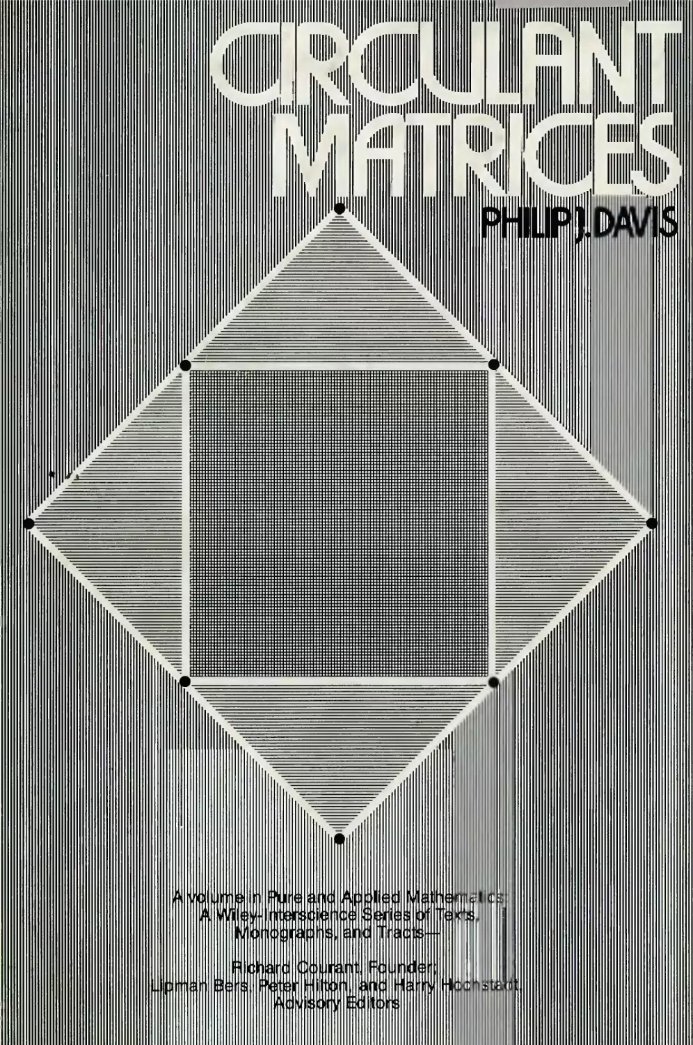
CIRCULANT MATRICES
PHILIP J. DAVIS
Division of Applied Mathematics
Brown University
A WILEY-INTERSCIENCE PUBLICATION
JOHN WILEY & SONS, New York · Chichester · Brisbane · Toronto

Copyright © 1979 by John Wiley & Sons, Inc.
All rights reserved. Published simultaneously in Canada.
Reproduction or translation of any part of this work
beyond that permitted by Sections 107 or 108 of the
1976 United States Copyright Act without the permission
of the copyright owner is unlawful. Requests for
permission or further information should be addressed to
the Permissions Department, John Wiley & Sons, Inc.
Library of Congress Cataloging in Publication Data
Davis, Philip J 1923-
Circulant matrices.
(Pure and applied mathematics)
"A Wiley-Interscience publication."
Bibliography: p.
Includes index.
1. Matrices. I. Title.
QA188.D37 512.943 79-10551
ISBN 0-471-05771-1
Printed in the United States of America
10 9 8765432 1

What is circular is eternal;
what is eternal is circular.

χ

PREFACE
"Mathematics," wrote Alfred North Whitehead, "is
the most powerful technique for the understanding of
pattern and for the analysis of the relations of
patterns. " In its pursuit of pattern, however,
mathematics itself exhibits pattern; the mathematics on the
printed page often has visual appeal. Spatial
arrangements embodied in formulae can be a source of
mathematical inspiration and aesthetic delight.
The theory of matrices exhibits much that is
visually attractive. Thus, diagonal matrices,
symmetric matrices, (0, 1) matrices, and the like are
attractive independently of their applications. In
the same category are the circulants. A circulant
matrix is one in which a basic row of numbers is
repeated again and again, but with a shift in
position. Circulant matrices have many connections to
problems in physics, to image processing, to
probability and statistics, to numerical analysis, to number
theory, to geometry. The built-in periodicity means
that circulants tie in with Fourier analysis and group
theory.
A different reason may be advanced for the study
of circulants. The theory of circulants is a
relatively easy one. Practically every matrix-theoretic
question for circulants may be resolved in "closed form."
Thus the circulants constitute a nontrivial but simple
set of objects that the reader may use to practice,
and ultimately deepen, a knowledge of matrix theory.
Writers on matrix theory appear to have given
circulants short shrift, so that the basic facts are
VII

viii
Preface
rediscovered over and over again. This book is
intended to serve as a general reference on circulants as
well as to provide alternate or supplemental material
for intermediate courses in matrix theory. The reader
will need to be familiar with the geometry of the
complex plane and with the elementary portions of matrix
theory up through unitary matrices and the diagonaliza-
tion of Hermitian matrices. In a few places the Jordan
form is used.
This work contains some general discussion of
matrices (block matrices, Kronecker products, the UDV
theorem, generalized inverses). These topics have been
included because of their application to circulants and
because they are not always available in general books
on linear algebra and matrix theory. More than 200
problems of varying difficulty have been included.
It would have been possible to develop the theory
of circulants and their generalizations from the point
of view of finite abelian groups and group matrices.
However, my interest in the subject has a strong
numerical and geometric base, which pointed me in the
direction taken. The interested reader will find references
to these algebraic matters.
Closely related to circulants are the Toeplitz
matrices. This theory and its applications constitute
a world of its own, and a few references will have to
suffice. The bibliography also contains references to
applications of circulants in physics and to the
solution of differential equations.
I acknowledge the help and advice received from
Professor Emilie V. Haynsworth. At every turn she has
provided me with information, elegant proofs, and
encouragement.
I have profited from numerous discussions with
Professors J. H. Ahlberg and Igor Najfeld and should
like to thank them for their interest in this essay.
Philip R. Thrift suggested some important changes.
Thanks are also due to Gary Rosen for the Calcomp
plots of the iterated n-gons and to Eleanor Addison for
the figures. Katrina Avery, Frances Beagan, Ezoura
Fonseca, and Frances Gajdowski have helped me
enormously in the preparation of the manuscript, and I wish to
thank them for this work, as well as for other help
rendered in the past.

Preface
IX
The Canadian Journal of Mathematics has allowed
me to reprint portions of an article of mine and I
would like to acknowledge this courtesy.
Finally, I would like to thank Beatrice Shube
for inviting me to join her distinguished roster of
scientific authors and the staff of John Wiley and
Sons for their efficient and skillful handling of the
manuscript.
Philip J. Davis
Providence, Rhode Island
April, 1979

χ

CONTENTS
Notation xin
Chapter 1 An Introductory Geometrical
Application 1
1.1 Nested triangles, 1
1.2 The transformation σ, 4
1.3 The transformation a, iterated with
different values of s, 10
1.4 Nested polygons, 12
Chapter 2 Introductory Matrix Material 16
2.1 Block operations, 16
2.2 Direct sums, 21
2.3 Kronecker product, 22
2.4 Permutation matrices, 24
2.5 The Fourier matrix, 31
2.6 Hadamard matrices, 37
2.7 Trace, 40
2.8 Generalized inverse, 40
2.9 Normal matrices, quadratic forms,
and field of values, 59
Chapter 3 Circulant Matrices 66
3.1 Introductory properties, 66
3.2 Diagonalization of circulants, 72
3.3 Multiplication and inversion of circulants, 85
3.4 Additional properties of circulants, 91
3.5 Circulant transforms, 99
3.6 Convergence questions, 101
xi

Xll
Contents
Chapter 4 Some Geometric Applications of 108
Circulants
4.1 Circulant quadratic forms arising in
geometry, 108
4.2 The isoperimetric inequality for isosceles
polygons, 112
4.3 Quadratic forms under side conditions, 114
4.4 Nested n-gons, 119
4.5 Smoothing and variation reduction, 131
4.6 Applications to elementary plane geometry:
n-gons and Kr-grams, 139
4.7 The special case: circ(s, t, 0, 0, ..., 0), 146
4.8 Elementary geometry and the Moore-Penrose
inverse, 148
Chapter 5 Generalizations of Circulants:
g-Circulants and Block Circulants 155
5.1 g-circulants, 155
5.2 0-circulants, 163
5.3 PD-matrices, 166
5.4 An equivalence relation on {1, 2, ..., n}, 171
5.5 Jordanization of g-circulants, 173
5.6 Block circulants, 176
5.7 Matrices with circulant blocks, 181
5.8 Block circulants with circulant blocks, 184
5.9 Further generalizations, 191
Chapter 6 Centralizers and Circulants 192
6.1 The leitmotiv, 192
6.2 Systems of linear matrix equations. The
centralizer, 192
6.3 τ algebras, 203
6.4 Some classes Ζ(Ρ , Ρ ), 206
6.5 Circulants and their generalizations, 208
6.6 The centralizer of J; magic squares, 214
6.7 Kronecker products of Ι, π, and J, 223
6.8 Best approximation by elements of
centralizers, 224
Appendix 227
Bibliography 235
Index of Authors 245
Index of Subjects 247

С the complex number field
С ^ the set of m χ η matrices whose elements are
m><n _
in С
Τ
A transpose of A
A conjugate of A
A* conjugate transpose of A
A ® В direct (Kronecker) product of A and В
A ° В Hadamard (element by element) product of
A and В
A* Moore-Penrose generalized inverse of A
r(A) rank of A
If A is square,
det(A) determinant of A
tr(A) trace of A
λ(A) eigenvalues of A; individually or as a set
A inverse of A
ρ (A) spectral radius of A ...
Xlll

xiv Notation
Τ
diagtd^ d2, . .., d^) = diagCd-^ d2, . .., d^)
d± 0 ...
0 d^ . . .
0 ...
Ζ (A) centralizer of A (Section 6.2).
If A and В are square,
A 0
Α θ В = diag(A, В) = (Q β) = direct sum of A and В
dg A = dg(a±.) = diagCa.^, a^, ..., anR)
offdg A = A - dg A
Special Square Matrices
Subscripts are often (but not exclusively) used to
designate the order of square matrices.
0 = zero = circ(0, 0, . .., 0)
1 = identity = circ(l, 0, .../ 0)
π = fundamental permutation matrix = circ(0, 1, 0,
. . . , 0)
Q = r-circ(l, 0, . .., 0); (λ = QkU) = Jordan block
J = circ(l, 1, . .., 1); all entries of J are 1
Ω = diag(l, w, w , . .., w ), w = exp(2Tri/n), π=3.14,
η = π diag ("l-^ Tn-i^
Λ, = diag(0, 0, . .., 0, 1, 0, ..., 0), 1 is in the
kth position
F = Fourier matrix
Bk = F*AkF

Notation
xv
Γ = (-l)-circ(l, 0f ..., 0)
К = counteridentity = (-l)-circ(O, 0,
, 0, 1)
V = V(zQ, ζχ, . .
S = selector matrix
ζ -, ) = Vandermonde matrix
n-l
-tj= χ / \ n n-l n-2
If φ(χ) = χ - a Ίχ - a 0x
γ η-1 η-2
a the companion matrix of Φ is
С, =
. 0
. 0
. 0
. 1
. а
• - а..х
п-1
-λ'
'λ'
t
= λ λ if λ ? 0
Other notation
ξ 0 if λ = 0
= set of polynomials with scalar coefficients

χ

CIRCULANT MATRICES

χ

1
AN INTRODUCTORY
GEOMETRICAL APPLICATION
1.1 NESTED TRIANGLES
We begin with a figure from elementary plane geometry.
It will serve us as a point of departure and an
inspiration.
Figure 1.1.1
Draw a triangle Т.. in the plane. Mark the
midpoints of the sides of this triangle and form the
"midpoint triangle" T^. There are many things that can be
said about this simple configuration. We observe
particularly the following:
(1) T2 is similar to T,.
(2) Perimeter of T2 = 1/2 perimeter of Т.. .
(3) Area of T2 = 1/4 area of Т.. .

2
An Introductory Geometrical Application
(4) Given a T^, there is a unique triangle Т..
whose midpoint triangle it is.
(5) The area of T2 is minimum among all triangles
Τ^ that are inscribed in T, and whose
vertices divide the sides of T, in a fixed
ratio, cyclically.
(6) If the midpoint triangle of T2 is T^, and
successively for Τ,, Τ , ..., this nested
set of triangles converges to the center of
gravity of Т.. with geometric rapidity.
[By the center of gravity (e.g.) of a
triangle whose vertices have rectangular
coordinates (x., y.)/ i = 1/ 2, 3, is meant the
point 1/3(x1 + x2 + x3, y1 + y2 + У3)·]
PROBLEMS
Figure 1.2.2
1. Prove that the triangles Τ are all similar.
2. Prove that the medians of Τ , η = 2, 3, ..., lie
along the medians of Τ,. η
3. Prove that the e.g. of Τ , η= 2, 3, ...,
coincides with the e.g. of T,.

Nested Triangles
3
10.
11.
12.
Prove that area Τ , Ί = 1/4 area Τ .
n+l η
Prove that the perimeter of Τ , = 1/2 perimeter
of Τ . n
η
Conclude, on this basis, that Τ converges to
e.g. T1 (Figure 1.1.2). n
Describe the situation when T, is a right
triangle; when T, is equilateral.
Given a triangle Τ,, construct a triangle T~ such
that T, is its midpoint triangle.
The midpoint triangle of Т.. divides Т.. into four
subtriangles.
Suppose that T^ designates one of
these, selected arbitrarily. Now let Τ desig-
nate the sequence of triangles that result from
an iteration of this process. Prove that Τ
converges to a point. Prove that every point
inside Т.. and on its sides is the limit of an
appropriate sequence Τ .
Systematize, in some way, the selection process
in Problem 9.
If two triangles have the same area and the same
perimeter are they necessarily congruent?
Let Ρ be an arbitrary point lying in the triangle
e
T1 = ΔΑ В С,
Figure 1.1.3

4
An Introductory Geometrical Application
Figure 1.1.3. Determine the rate at which σ (Т.. )
converges to P.
1.2 THE TRANSFORMATION σ
As a first generalization, consider the following
transformation σ of the triangle T, . Select a
nonnegative number s: 0 < s < 1, and set
(1.2.1) s + t = 1.
Let A2, B2, C2 be the points on the sides of the
triangle Т.. such that
A A0 ΒΊΒ0 C-C0
(1.2.2) 12_12_12_s_ s
Α2Βχ B2CX С2АХ t 1 - S '
In this equation A..A2 designates the length of the
line segment from A-. to A^, and so on. Thus the
points A2, B2, C2 divide the sides of T, into the
ratio s/t, working consistently in a counterclockwise
fashion. (See Figure 1.2.1.)

The Transformation σ
5
Write
(1.2.3) T2 = ЛА2В2С2 = σ(Τχ)
and in general
(1.2.31) Τ = σ(Τ )
n+1 η
= ση(Τ ) , η = 1, 2, 3, ... .
Figure 1.2.2 illustrates the sequence Τ for s =
1/4, t = 3/4. n
'Figure 1.2.2
The transformation σ depends, of course, on the
parameter s, and we shall write σ when it is
necessary to distinguish the parameter.
To analyze this situation, one might work with
vectors, but it is particularly convenient in the case
of plane figures to place the triangle T, in the
complex plane. We write z=x+iy, ζ = χ - iy, i= /-T,
and designate the coordinates of Τ systematically by
ζ.. , z^ , z^ . Write, for simplicity, ζ.... = ζ.. , ζ _ =
Ζρ, ζ^1 = ζ~. The transformation σ operating
successively on Τ,, Τ2, ..., is therefore given by

6
An Introductory Geometrical Application
Zl,n+1 = SZl,n + tz2,n
(1.2.4) σ: ^,η+Ι = sz2,n + tz3,n "=1,2
z~ ,, = sz. + tz.,
3,n+l 3,n l,n
Lemma. Centers of gravity are invariant under σ; that
is,
(1.2.5) c.g.(a(T)) = e.g.(T).
Proof. e.g. (0(1^)) = 3"(z12 + z22 + z32)
= 3-((sz1 + tz2) + (sz2 + tz3)
+ (sz3 + tz1))
= i( (s + t)z1 + (s + t)z2
+ (s + t)z3)
= jizj^ + z2 + z3) = c.g.CTj^).
It follows that e.g.(T ) = e.g.(Т.. ), η = 1, 2,
...; hence that the point e.g.(T,) is contained in all
the Τ .
η
It will simplify computations if one assumes, as
one may, that e.g.(T ) is located at the origin ζ = 0.
This means that in what follows we assume that
(1.2.6) ζ + z2 + z3 = 0.
Place three unit point masses at the vertices of
T... Their polar moment of inertia, V, about an axis
perpendicular to T^ and passing through e.g. (Т..) is
V = OA2 + OB2 + OC^ or
(1.2.7) ν(Τχ) = |Zl|2 + |z2|2 + |z3|2.
We next compute ν(σ(Τ..)). We have
ι ι 2 . . 2 . .2
V(a(T )) = |szx + tz2| + |sz2 + tz3| + |sz3 + tz1|

The Transformation σ
= (sz, + tz2)(sz1 + tz2) + (sz2 + tz3)
(sL + tz ) + (sz + tz ) (sz3 + tz1)
? 9 ι ι ? ι ι ? . ι 2
= (sz + tz) (|ζχ|ζ + |z2|z + |ζ3Γ)
+ st(z;.z + ζ z2 + ζ ζ + z2z3
+ ζ3ζχ + ζ3ζχ).
Now, from (1.2.6), (z.. + z2 + z.) (z1 + ζ + z3)
so that ζχζ2 + ζχζ2 + z3z3 + z2z3 + z^ + z^
-(|z..| + |z?| + |z~| ). Therefore
(1.2.8) ν(σ(Τχ)) = (s2 - st + t2) (|ζχ|2 + |z2|2
+ \*3\2)
= (s2 - st + t2)V(T1)
= (1 - 3s + 332)ν(Τχ)
= (s3 + (1 - s)3)V(T1).
Set
(1.2.9) g(s) = 1 - 3s + 3s2
so that
(1.2.10) ν(σ(Τχ)) = g(s)4(T1) .
We have g(s) = 1 if and only if s = 0, 1,
(1.2.11) j £ g(s) < 1 for 0 < s < 1.
From (1.2.10),
ν(οη(Τλ)) = gn(s)V(T1)/ η = lf 2, ... .
Hence, for fixed s: 0 < s < 1,
(1.2.12) limV(an(T1)) = 0.
n->oo
Thus

8
An Introductory Geometrical Application
(1.
so
(1.
2.13)
that
2.14)
lim
n->oo
lim
n->oo
Jl,n+1'
5. = 0
i,n
J2,n+l!
J3,n+1'
= 0f
for i = 1, 2, 3.
We have therefore proved the following theorem.
Theorem 1.2.1. Let 0 < s < 1 be fixed and let Τ be
η
the sequence of nested triangles given by Τ =
ση(Τ-,), η = 1, 2, ... . Then Τ converges to e.g.(Τ,).
The function V(T) is a simple example of a
Lyapunov function for a system of difference equations.
The e.g. is known as the limit set of the process.
It is also of interest to see how the area of T,
Assum-
changes under σ. Designate the area by μ (Т.. )
ing, as we have, that ζ = χη + iy-, ,
z2 = X2 + iy
2'
= x„
+ iy. are the vertices of T-, in
counterclockwise order, we have
(1.2.15)
so that
2μ (ΤΊ
2μ(σ(Τχ))
sx + tx2,
sx + tx~,
SX. + tX-j,
= s
Syl + ty2'
sy2 + ty3f
Sy3 + tyl'
+ t
+ st
X-
X'
x.
X-.
1
1
1

The Transformation σ
9
= (s2 + t2)(2y(T1)) + st(-2y(T1)
Hence
(1.2.16) μ(σ(Τ1)) = (s3 + t3)y(T1)
= g(s)y(T1) .
Theorem 1.2.2. min0< <1У(а(т1)) occurs uniquely when
s = 1/2 and equals (Τ/4)μ(Τχ).
2
Proof. The minimum value of g(s) = 1 - 3s + 3s
occurs uniquely when s = 1/2 and equals 1/4.
PROBLEMS
1. Interpret the transformation σ geometrically when
s is real but does not satisfy 0 < s < 1. What
does σ do when s = 1?
2. Interpret the transformation σ geometrically when
s and t are complex.
3. In this case, find a formula for ν(σ(Τ..)).
4. Let V(T,) designate the polar moment of inertia of
T-. about its center of gravity, regarding T-. as a
lamina of unit density. Prove that
V(a(T1)) = g2(s)V(T1) .
5. Let σ(Τ1) have vertices A2, B2, C2- Then the lines
A1B2' B1C2' C1A2 are concurrent if and only if s =
t = 1/2. (Use Ceva's theorem.)
6. Let Τ be an equilateral triangle. Then for any s,
σ (Τ) is equilateral. Interpret this as an
eigenvalue property of
(s t 0 \
0 s t j .
t 0 s '
Thus the equilateral triangles are "eigenfigures"

10
An Introductory Geometrical Application
of σ. Generalize. Hint; Let the vertices of Τ
in counterclockwise order be z,, z~, z~. Then Τ
is equilateral if and only if z-, + wz2 + w ζ = 0,
where w = exp(2Tri/3).
1.3 THE TRANSFORMATION σ, ITERATED WITH DIFFERENT
VALUES OF s
As observed, the transformation σ depends on the
selection of the parameter s. Let us indicate this by
writing σ . Begin with the triangle T-. and form
(1.3.1) T0 = σο (τΊ).
2. S-. 1
Now iterate this, using different values of the
parameter s. We obtain
(1.3.2) T- = og (T0),
3 2
so that, in general,
(1.3.3) Tn = as as ··· σ (Τ ).
n-1 n-2 1
We then have from (1.2.10)
(1.3.4) v(Tn) = ^(sn-l)g(sn-2} '" g(s1)v(T1)·
Whether or not V(T ) converges to 0 depends on the
behavior of the infinite product n^_-,g(s, ) =
'W1 - 3sk + 3£Φ·
Let pk = 3sk - 3sk = 3sk(l - sk). Then
nk=1g(sk) = nk=1(l " Pk). Assuming that 0 < sk < 1,
we have 0 < p, < 3/4. As is well known, if Σ,_-,ρ, < °°,
then limn^oonk=1(l-pk) exists and is not zero. On the
other hand, if Ik=1Pk = », then limn_>oonk=1 (l~Pk) = 0.
(See, e.g., Knopp, 1928, pp. 219-221.) Thus we must
investigate the convergence of Σ" ,s,(l-s,). To thi
end, for 0 < sk < 0, introduce K x k k
, s. if 0 < s, < -=-,
(1.3.5) s* = min(sk, 1 - s ) = { k k " 2
<1 - sk if - < sk < 1.
s

Different Values of s
11
Σοο 2 . r°°
k=l(sk " Sk} < °° lf and °nly lf ^k=lSk < °°'
Proof.
0 < s, - s = s (1 - s,) < and £ min(sk, l-sk) = s*
1 - sk
ΣΟΟ Γ-.00 2
, _,s* < oo implies Κ=ι (s^ " s^) < °°- 0n the
other hand,
if 0 < Sk < \. |s* = |sk < sk - S2;
if I i sk K !' Isk = I(1 " sk} ± sk " V
ΣΟΟ r^OO 2
k=lSk = °° imPlies ^k=l(sk " Sk) = °°'
This leads to
Theorem 1.3.1
(a) If l£=1s* = ~ then
lim V(T ) = lim μ(Τ ) = 0.
П->оо П п->°о П
(b) If l£=lsk < - then
lim V(T ) = V > 0 and
η °°
П-усо
lim μ(Τ ) = μ > 0.
П °о
П->оо
In Case (a), as before, lim Τ = e.g. (Т..). In
n->oo n ^ 1
case (b), one conjectures that {T } approach a non-
trivial limiting triangle Τ (see Figure 1.3.1). We
shall return to this point in Section 3.6 for a more
complete analysis.
PROBLEMS
2
1. Let s = l/(k + 1) , к = 1, 2, ... . Compute,

12 An Introductory Geometrical Application
Figure 1.3.1
approximately, lim ^μ (Т.)/у (Т.. ) .
2. Do the same with s, = exp (-\ik) , μ > 0, к =
1 ο κ
-1- Ι л-, I ... ·
1.4 NESTED POLYGONS
We pass now from triangles to polygons. Let z,, z?,
..., ζ be ordered vertices of a polygon Ρ (assumed to
be located in the complex plane). We make no
restrictions on the complex numbers ζ , so that Ρ may be
convex or nonconvex, simply covered or not; furthermore,
the points z, are not necessarily distinct so that the
polygon may have · "multiple vertices." All geometric
constructions described below are to be interpreted
appropriately with this in mind. We shall also call
such a figure a ρ-gon. We shall assume, however, that
the center of gravity of P, l/p(z, + ··· + z. ) , is at
the origin. This means that p
(1.4.1) ζχ + z2 + ··· + ζ = 0.

Nested Polygons
13
Each side of Ρ is now divided in length into the
ratio s/t, 0<_s<_l, t=l-s, proceeding cyclically
counterclockwise. The points of division form the
vertices of a new polygon σ(Ρ). (See Figure 1.4.1.) We
wish to discuss what happens when this transformation
is iterated.
Figure 1.4.1
Let Ρ = σ (ΡΊ), let the vertices of Ρ have the
η 1 η
., ζ , and for simplicity
ρ,η
coordinates ζ, , ζ0 ,
1 ,η λ, η
The transformation
σ may obviously be written in matrix form as
write ζ.. .. = ζ.. ,
"' ZP,1 ZP'
(1.4.2)
Jl,n+1
J2,n+1
Jp,n+1
s
0
0
t
t
s
0
0
0
t
s
•
•
0
t
•
•
•
0
•
0
0
0
s
z,
l,n
Z2,n
•
ζ

14
An Introductory Geometrical Application
If one writes
ζ
l,n
(i.4.3) | : l = zn,
Zp,n
and abbreviates the ρ χ ρ matrix in the right hand of
(1.4.2) by G, then
(1.4.2') Ζ _ = GZ ; Z, = a given initial vector.
This is a linear autonomous system of difference
equations, that is, G is independent of n. The solution
of this iteration is
(1.4.4) Ζ = Gn_1Z,.
η 1
Thus the limiting behavior of Ρ (i.e., Ζ ) as η -* °°
n η
depends substantially on the behavior of G as η -> <».
The matrix G is a circulant matrix; that is, in
each successive row the elements move to the right
one position (with wraparound at the edges). It is
also true that the matrix G is a nonnegative, doubly
stochastic, irreducible, and normal matrix. In this
essay we emphasize the circulant aspect of G. We
postpone further discussion of the p-gon problem until we
have somewhat developed the theory of circulants.
PROBLEMS
1. Let G = (g. .) be a ρ χ ρ matrix. Let the p-gon Z..
be transformed into the p-gon Z~ linearly by means
of Z? = GZ.. . What are necessary and sufficient
conditions on G that it preserve centers of
gravity? Express as an eigenvalue-vector
condition.
2. Let G (as in Problem 1) satisfy G = I for some
positive integer k. Describe the geometric
situation upon iteration.
3. Suppose that Ζ is given and that

Nested Polygons
15
Z3n+1 = G3Z3n'
Z3n+2 = GlZ3n+l' for η = 0f 1
Z3n+3 = G2Z3n+2'
Find a formula for Ζ .
η
4. Generalize this section to space p-gons (in three
dimensions).
5. Develop analytical apparatus for generalizing
this section to nested polyhedra. In particular,
let T1 be a tetrahedron. Let T2 be the
tetrahedron whose vertices are the c.g.'s of the faces of
Т., . Iterate this.
REFERENCES
Convergence of nested polygons: Berlekamp et al.;
Rosenman; Huston; Schoenberg [1].
p-gons in a general setting: Bachmann and Schmidt;
Davis [1], [2].
Liapunov functions, limit sets: LaSalle [2].

2
MATERIAL
2.1 BLOCK OPERATIONS
It is very often convenient in both theoretical and
computer work to partition a matrix into submatrices.
This can be done in numerous ways as suggested by
this example:
2 I 3
I
« ! 7
1
10 ι 11
I
14 ! 15
2
6
10
3 I
I
7 I
I
11 I 12
13 14 | 15 | 16
Each submatrix or block can be labeled by subscripts,
and we can display the original matrix with
submatrices or blocks for its elements. The general form
of a partitioned matrix therefore is
11
12
1£
(2.1.1) A =
kl
*k2
"k£
Dotted lines, bars, commas are all used in an obvious
way to indicate partitions. The size of the blocks
must be such that they all fit together properly.
16

Block Operations
17
This means that the number of rows in each A..
ID
must be the same for each i and the number of columns
must be the same for each j. The size of A.. is
therefore m. χ η. for certain integers m. and п.. We
iD * ι υ
indicate this by writing
No. of columns
m-,
iru
тл
No. of rows
"11
12
\U
(2.1.1') A =
τα
к 2
"k£
A square matrix A of order η is often partitioned
symmetrically. Suppose that η = ri]_ + n2 + · · · + η
with п. > 1. Partition A as
ι —
11
(2.1.2)
A =
12
lr
rl
r2
rr
*1J X1l " "J
square matrices of order n..
The diagonal blocks A.. are
Example.
X
X
X
X
X
X
χ 1
X
X
X
X
X
X
X
X
X
X
X
|
X
X
X
X
X
X
X
X
X
X
X
X
X
X
X
X
X
η = 6
η, = 2
n2 = 1
Пл = 3
is a symmetric partition of a 6 χ 6 matrix.
Square matrices are often built up, or compounded,
of square blocks all of the same size.

18
Introductory Matrix Material
Example.
X
X
X
X
X
X
X
X
X
X
X
X
X
X
X
X
X
X
X
X
X
X
X
Ι χ
X
X
X
X
X
X
X
X
X
X
X
X
If a square matrix A of order nk is composed of η χ η
square submatrices all of order k, it is termed an
(n, k) matrix. Thus the matrix depicted above is a
(2, 3) matrix.
Subject to certain conformability conditions on
the blocks, the operations of scalar product,
transpose , conjugation, addition, and multiplication are
carried out in the same way when expressed in block
notation as when they are expressed in element nota-
tion. This means
(2.1.3)
11
W
cA
11
. cA
11
kl
Ία
CA.
kl
cA.
k£
(2.1.4)
11
Akl
All
lu
k£
*U'
11
ЧА
A*
All
"kl
A.
k£
A*
Akl
(2.1.5)
Ak]
k£
A*
Al£
A*
Ak£
Here Τ designates the transpose and * the conjugate
transpose.

Block Operations
19
(2.1.6)
All ' ' ' AU\ / Bll ' ' ' Bl£
Akl ' " Ak£ Bkl ' " Bk£
All + Bll """ Al£ + Bl£
Akl + Bkl ' " Ak£ + Bk£
'All '" Al£\ /Bll '" Bln4 /Cll '" Cln
(2.1.7)
Akl ''' Ak£ B£l ''' B£n Ckl ' " Ckn
where С
.. = f .Α. Β ..
!~j ^Г=1 1Г rj
In (2.1.6) the size of each A.. must be the size
in
of the corresponding B... J
In (2.1.7), designate the size of A.. by α. χ β.
and the size of B.. by γ. χ δ.. Then, if 3 = Ύ for
±j 2 ' ι j r 'r
1 <_ r <_ £, the product A. В . can be formed and
produces an α. χ 6. matrix, independently of r. The sum
can then be found as indicated and the С.. are α. χ 6.
ID ID
matrices and together constitute a partition. Note
that the rule for forming the blocks C.. of the matrix
product is the same as when A.. and B.. are single
numbers. 1-J ^
Example. If A and В are η χ η matrices and if
»C :)■
then

20
Introductory Matrix Material
2 / A2 + B2, AB - BA
BA - AB, A2 + B2
PROBLEMS
2
1. In the example just given what is С if A and В
commute?
3
2. In the example, compute С . What if A and В
commute?
3. Let
Bl ° \ Cl °
B2 1 ( C2
r 0 s
be two block diagonal matrices. When can the
product MN be formed? What is the product?
4. "Hadamard matrices" of order 2n are given
recursively by means of the definition
ι ι TV Vl
н2 - [λ _λ], н к+1 -
н к "н к
2К 2
Τ
Write out H4 and H3 explicitly. Compute Η2Η2/
Τ
H4H4'
5. Let А, В, С, D all be η χ η and let a, b, c, d be
scalars. What is
/» .\ /.I Ы\
\ С D / \cl dl/
6. Let I be the identity of order p. Prove that
P /1 B\
det p 1 = det С
\o c/

Block Operations
21
A B
If A and С are square, prove that det(n ) =
(det A)(det C).
If A and С are square, prove that the eigenvalues
A B
of (Q ) are those of A together with those of C.
2.2 DIRECT SUMS
For i = 1, 2, . .., k, let A^ be a square matrix of
order n··. The block diagonal square matrix
rA, 0 ... 0'
(2.2.1) A = | Z | = diag(A1# A2, ..., Afc)
0 0 . . .
of order nj + П2 + ··· + nk is called the direct sum
of the Ak and is designated by
(2.2.2) A = Α.. θ Α0 Θ · · · Φ Α, = Θ Α..
1 Ζ Κ ±=1 ι
The following identities are easily established.
(1) (Α Θ Β) Θ С = Α Θ (Β Θ С) .
(2) (А + В) Θ (С + D) = (Α Θ В) + (С Θ D) .
(3) (Α Θ В) (С Θ D) = АС Θ BD.
(4) (Α Θ В)Т = АТ Θ ΒΤ.
(5) (Α Θ В) * = Α* Θ В*.
(6) (Α Θ В) = Α Θ Β , assuming that the
indicated inverses exist.
(7) det(Α Θ Β) = (det A)(det B).
(8) tr(A Θ Β) = tr A + tr B.
(9) If ρΑ(λ) designates the characteristic
polynomial of A, then ΡΑφΒ(λ) = (ΡΑ(λ) ) (ρΒ(λ) ) .
(10) Hence λ(Α Θ Β) = {λΑ, λΒ}. (λΑ designates
the set of eigenvalues of A.)

22
Introductory Matrix Material
PROBLEMS
Let A = Α, Θ Α0 Θ · · · Θ Α, . Prove that det A =
к ρ ρ ρ
Π.=1 det A. and that for integer ρ, Α^ = A^ Θ Α^ Θ
•·: Φ He' X
Give a linear algebra interpretation of the direct
sum along the following lines. Let V be a finite-
dimensional vector space and let L and Μ be sub-
spaces. Write V = L Θ Μ if and only if every
vector χ Ε V can be written uniquely in the form
χ = у + ζ with у Ε L, ζ Ε Μ. Show that V = L Θ Μ
if and only if
(a) dim V = dim L + dim M, L Π Μ = {0}.
(b) if {x ,...,x } and {y_,...,y } are bases for
L and M, then {x, , . . . ,x„ ,y.. , . . . ,y } is a
basis for V.
The fundamental theorem of rank-canonical form for
square matrices tells us that if A is a η χ η
matrix of rank r, then there exist nonsingular
matrices P, Q such that PAQ =1 Θ 0 _ . Verify
this formulation. r n
2.3 KRONECKER PRODUCT
Let A and В be m χ η and ρ χ q respectively. Then the
Kronecker product (or tensor, or direct product of A
and B) is that mp χ nq matrix defined by
(2.3.1) A ® В =
allB' a12B' ·'■' alnB
a , Β, a ~B. ....a B
ml m2 mn
Important properties of the Kronecker product are
as follows (indicated operations are assumed to be
defined):
(1) (αΑ) ® Β = Α Θ (aB) = a (A ® B) ; a scalar.
(2) (A + В) ® С = (Α Θ С) + (Β Θ С) .
(3) Α Θ (Β + С) = (Α Θ В) + (А ® С).
(4) Α Θ (В ® С) = (Α Θ Β) ® С.

Kronecker Product
23
(5) (Α Θ В) (С Θ D) = (AC) Θ BD.
(6) Α Θ Β = Α Θ Β.
(7) (Α Θ Β)Τ = АТ ® ВТ; (А ® В)* = Α* Θ В*.
(8) г (Α Θ В) = г (А)г (В) .
We now assume that A and В are square and of
orders m and n. Then
tr (Α Θ Β) = (tr (A) ) (tr (B) ) .
If A and В are nonsingular, so is Α Θ Β and
(Α Θ Β)"1 = A_1 Θ Β-1.
det(A Θ Β) = (det A)n(det В)Ш.
There exists a permutation matrix Ρ (see
Section 2.4) depending only on m, n, such
that Β Θ Α = Ρ*(Α Θ Β)Ρ.
(13) Let 0(x, y) designate the polynomial
0(x, y) = I a. xDy .
j,k=0 Dk
Let 0 (A; B) designate the mn χ mn matrix
ι. J
(9)
(10)
(11)
(12)
?
a. Ί Α3 Θ Bk.
j,k=0
Thtin the eigenvalues of 0 (A; B) are
0(λ / μ ), г = 1, 2, ..., m, s = 1, 2, ..
η where λ and μ are the eigenvalues of
and В respectively. In particular, the
eigenvalues of A 0 В are λ μ , г = 1, 2,
• · · ILL / О ™~ _L ψ £* ξ т · · ξ χΧ ·
PROBLEMS
1. Show that I ® I = I .
m η mn
2. Describe the matrices Ι Θ Af Α Θ I.
3. If A is m χ m and В is η χ η, then A ® В =
(Α Θ I ) (Ι Θ Β) = (Ι Θ Β) (Α Θ Ι ) .
η m m η

24
Introductory Matrix Material
4. If A and В are upper (or lower) triangular, then
so is A 0 B.
5. If A ® В 7^ 0 is diagonal, so are A and B.
6. Let A and В have orders m, η respectively. Show
that the matrix (I ® B) + (A ® I ) has the
m η
eigenvalues λ + μ , i = 1, 2, ..., m, j =
1, 2, . .., n, where λ and μ are the eigenvalues
of A and B. This matrix is often called the
Kronecker sum of A and B.
7. Let A and В be of orders m and n. If A and В
both are (1) normal, (2) Hermitian, (3) positive
definite, (4) positive semidefinite, and (5)
unitary, then A ® В has the corresponding
property. See Section 2.9.
Г21
8. Kronecker powers: Let A = A ® A and, in
general, A[k+1] = Α Θ A[k]. Prove that A[k+£] =
A[k] * Α[£].
9. Prove that (AB)[k] = A[k]B[k].
Τ
10. Let Ax = λχ and By = μγ, χ = (χη, ..., χ ) .
ιρ ιρ Τ Τ η
Define Ζ by Ζ = [χ-,γ , x~y , . . . , χ у ] . Prove
that (Α Θ Β)Ζ = λμΖ.
2.4 PERMUTATION MATRICES
By a permutation σ of the set N = {1, 2, ..., n} is
meant a one-to-one mapping of N onto itself.
Including the identity permutation there are n! distinct
permutations of N. One can indicate a typical
permutation by
σ(1) = ±λ
(2.4.1) σ(2) = ±2
σ(η) = in
which is often written as

Permutation Matrices
25
/1 2 ... η \
(2.4.1') σ: I I.
\L1 i2 '" in I
The inverse permutation is designated by σ . Thus
G_1(ik) = k.
Let Ε. designate the unit (row) vector of η
components which has a 1 in the jth position and O's
elsewhere:
(2.4.2) E. = (0, ..., 0, 1, 0, ..., 0).
By a permutation matrix of order η is meant a
matrix of the form
E.
(2.4.3) Ρ = Ρ =
One has
E.
*2
E.
1n
a. /·\ — -*-/ ^- — -*-/^/···/^·ι
(2.4.4) P= (a..) where 1'σ^1^
J a. . = 0/ otherwise.
If]
The ith row of Ρ has a 1 in the a(i)th column and O's
elsewhere. The jth column of Ρ has a 1 in the
σ (j)th row and 0's elsewhere. Thus each row and
each column of Ρ has precisely one 1 in it.
Example
/0001
Ρ = [ 1 ° ° °
^σ I 0 0 1 0
\0 1 0 0
It is easily seen that

26
Introductory Matrix Material
Χσ(1)
(2.4.5) «■-.-. X°(2)
χσ(η)
Hence if A = (a..) is an η χ r matrix,
(2.4.6) ΡσΑ= (aa(i)fj>,
that is, Ρ A is A with its rows permuted by σ.
Moreover,
(2.4.7) (χχ, x2, ..., χη)ρσ
IX _ -ι / X _-ι / · · · / 2C _-i / /
σ χ(1) σ ±(2) α ± (n)
so that if A = (a..) is r χ η,
(2.4.8) АР = (a _χ ).
ί,σ (j)
That is, АР is A with its columns permuted by σ
Note also that
(2.4.9) ΡσΡχ = Ρσχ,
where the product of the permutations ο, τ is applied
from left to right. Furthermore,
(2.4.10) (Ρσ)* = Ρ _±;
о
hence
(2.4.11) (Ρσ)*Ρσ = Ρ _χΡσ = ΡΣ = Ι.
σ
Therefore
(2.4.12) (Ρσ)* = Ρ _λ = (Ρσ)_1.
σ
The permutation matrices are thus unitary, forming a
subgroup of the unitary group.

Permutation Matrices
27
From (2.4.6), (2.4.8) and (2.4.12) it follows
that if A is η χ η
(2.4.13) Ρ АР* = (а ,.Ν ,.J,
σ σ σ(ι),σ (υ)
so that the similarity transformation Ρ АР* causes a
л о о
consistent renumbering of the rows and columns of A by
the permutation σ.
Among the permutation matrices, the matrix
0 1 0 0 ... 0
0 0 1 0 ... 0
(2.4.14)
I
0
plays a fundamental role in the theory of circulants.
This corresponds to the forward shift permutation
σ(1) = 2, o(2) = 3, ..., σ(η-1) = η, σ (η) = 1, that
is, to the cycle σ = (1, 2, 3, ..., η) generating the
cyclic group of order η (π is for "push")· One has
2
π =
/ °
I °
.
0
0
.
1
0
.
0 . .
1 . .
.
. . 0
. . 0
.
(2.4.15)
0 ... 0
2 2 2
corresponding to σ for which σ (1) =3, σ (2) =4,
2 к к
..., σ (η) = 2. Similarly for π and σ . The matrix
π corresponds to σ = I, so that
(2.4.16) πη = I.
Note also that
(2.4.17) πΤ = π* = π"1 = π11"1.
A particular instance of (2.4.13) is
(2.4.18) ттАтгТ = (a±+1^j + 1)
where A = (a..) and the subscripts are taken mod n.

28
Introductory Matrix Material
1
0
0
0
0
0
0
0
0
0
0
1
0
0
1
0
0
1
0
0
Here is a second instance. Let L = (λ-, , λ9,
Τ .
λ ) . Then, for any permutation matrix Ρ ,
(2.4.19) Pa(diag L)P* = diag(PaL).
A second permutation matrix of importance is
(2.4.20) Γ =
0 1 ... 0 0 0
which corresponds to the permutation σ(1) = 1, σ(2) =
η, ο(3) = η - 1, ..., a(j) = η - j + 2, ..., σ(η) = 2.
Exhibited as a product of cycles, σ = (1)(2, η)
2
(3, η - 1), . .., (η, 2). It follows that σ = I, hence
that
(2.4.21) Γ2 = I.
Also,
(2.4.22) Γ* = ΓΤ = Γ = Γ"1.
Again, as an instance of (2.4.13),
(2.4.23) Г(diag L)Г = diag(TL).
Finally, we cite the counteridentity K, which has
l's on the main counterdiagonal and 0's elsewhere:
0 ... 0
0 ... 1
(2.4.24) К = К =
η
One has K=K*, K2=I, K=K1.
Let Ρ = Ρ designate an η χ η permutation matrix.

Permutation Matrices
29
Now σ may be factored into a product of disjoint
cycles. This factorization is unique up to the
arrangement of factors. Suppose that the cycles in
the product have lengths p.. , p2, ..., ρ , (p1 + ρ +
•·· + ρ = η). Let π designate the π matrix
Pk
(2.4.14) of order p, . By a rearrangement of rows and
columns, the cycles in Ρ can be brought into the
form of involving only contiguous indices, that is,
indices that are successive integers. By (2.4.13),
then, there exists a permutation matrix R of order η
such that
(2.4.25) RPR* = RPR-1 = π Θ π Θ --- Θ π
Ρ1 Ρ2 Pm
Since the characteristic polynomial of π is
Pk pk Pk
(-1) (λ - 1), it follows that the characteristic
m pk Pk
polynomial of RPR*, hence of P, is π£=1(-1) (λ - 1) .
The eigenvalues of the permutation matrix Ρ are
therefore the roots of unity comprised in the totality of
roots of the m equations:
Pk
λ =1, k=l, 2, ...,m.
Example. Let σ be the permutation of 1, 2, 3, 4, 5, 6
for which σ(1) = 5, σ(2) = 1, σ(3) = 6, σ(4) = 4,
σ(5) = 2, σ(6) = 3. Then σ can be factored into cycles
as σ = (152) (4) (36). Therefore, m = 3 and p. = 3,
P2 = 1, p~ = 2. The matrix Ρ is
0 0 0 0 10
10 0 0 0 0
Ρσ =
0 0 0 0 0 1
0 0 0 10 0
0 10 0 0 0
0 0 10 0 0

30
Introductory Matrix Material
The matrix R corresponding to τ(1)
τ(2) = 3, τ(4) = 4, τ (3) = 5, τ (б)
Ι, τ(5) = 2,
6, is such that
\
0
1 о
1
0
0
•
1
0
0
0
0
0
0 1
1
0
0
0
0
0 I
0
0
1
0
0
0
0
0
0
0
1
0
0
0
0
1
0
RPaR* =
The eigenvalues of Ρ are therefore the roots of
3 2 °
(XJ - 1) (λ - 1) (λζ - 1).
A permutation σ is called primitive if its
factorization consists of one cycle of full length n.
The eigenvalues of a primitive permutation matrix are
the nth roots of unity, hence they are distinct.
PROBLEMS
1.
2.
3.
4.
If Μ is m χ n, describe the relationship between
M, KM, and MK .
m η г /?i
Prove that det Kn = (-1)[n/zl, where [x]
designates the largest integer <_ x.
Determine the characteristic polynomial of π.
For integer p, set Μ = тгР + тг~р. Prove that
M^ = Μ ,Mn=M = 21, MM =M, +M
Ρ η-ρ ο η ρ q p+q p-q
Μ . Ί = M..M - Μ ...
p+1 1 ρ p-1
Let С (x) = 2 cos ηθ, where χ = 2 cos Θ,
designate the Tschebyscheff polynomials of the first
kind. One knows that С ,.(χ) = xC (χ) - С Ί (χ),
η+1 η η-1
CQ(χ) = 2, C, (χ) = χ. Referring to Problem 4,
prove that Μ = С (М,).
Let N={0,1, 2, ..., 2η-1} and let σ
designate the permutation of N that results from
reversing the binary bits of the elements of N.

Permutation Matrices
31
Example.
0 ■* 000
1 ■* 001
2 ■* 010
3 + Oil
4 ■* 100
5 -» 101
6 ■* 110
7 ■* 111
->■
->■
->■
->■
->■
->■
->■
-Э-
Wher
000
100
010
110
001
101
Oil
111
ι η =
+ о,
- 4,
+ 2,
+ 6,
- 1,
+ 5,
- 3,
■* 7.
Discuss the factorization of σ for η = 3. What
about the general case?
7. Describe the matrices Ι Θ π ; π ® Ι .
m η η m
8. If m > 1, prove that Ι Θ π and π Θ I are
' * m η η m
derogatory, that is, their minimal polynomial
is not their characteristic polynomial.
9. Prove that Κ Θ Κ = К ^ .
~m ~n «m+n
2
10. Let π be of order n. Prove that I + π + π +
ΤΊ— 1
··· + π = J, where J is the matrix of all l's.
11. If σ is a primitive permutation, prove that σ
is primitive.
12. If σ and τ are primitive permutations, is it true
that στ is primitive?
13. Ρ is a primitive permutation matrix if and only
if it is of the form Ρ = R*uR where R is a
permutation matrix.
14. Ρ is a primitive permutation matrix of order η
if and only if η is the least positive integer
for which Pn = I.
2.5 THE FOURIER MATRIX
Let η be a fixed integer >_ 1 and set
/orr-ix /2ττί4 2 π , . . 2π . /—=-
(2.5.1) w = exp ( ) = cos — + ι sin — , ι = /-1.
In a good deal of what follows, w might be taken as
any primitive nth root of unity, but we prefer to
standardize the selection as in (2.5.1). Note that

32
Introductory Matrix Material
(2.5.2) (a) wn = 1,
(b) ww = 1,
-1
(c) w = w
/..χ -к -к n-k
(d) w = w = w ,
(e) 1 + w + w + ··· + w =0.
By the Fourier matrix of order n, we shall mean
the matrix F (= F ) where
η
(2.5.3) F* = l-(w(i-1)(^1))
/H
1
/Ё
1
/l
f ι
I;
1
w
2
w
•
1
2
w
4
w
•
1
n-1
w
2(n-1)
w
. n-1 2 (n-1) -(n-1) (n-1),
1 W W . . . W
Note the star on the left-hand member. The sequence
w , k= 0, 1, ..., is periodic; hence there are only η
distinct elements in F. F can therefore be written
alternatively as
(2.5.4) F* = η 1/2
It is easily established that F and F* are
symmetric:
(2.5.5) F = FT, F* = (F*)T = F, F = F * .
It is of fundamental importance that
1
1
1
.
•
•
1
1
w
2
w
.
•
•
n-
w
-1
1
2
w
4
w
.
.
•
n-2
w
...
...
1
n-1
w
n-2
w
t
w

The Fourier Matrix
33
Theorem 2.5.1. F is unitary:
(2.5.6) FF* = F*F =1 or F~ = F* or
—τ —τ -l —τ
FF = F F =1 or F = F .
Proof. This is a result of the geometric series
identity
n-1 , · -, ч η n(j-k) , n if j = k,
^ wr(D-k)= 1 - w ^J = f J
r=0 1 - wj"k v 0 if j ί к.
A second application of the geometrical identity
yields
Theorem 2.5.2
F*2 = F*F* =Γ= Ι Λ Λ -, Λ Ι = F'
1 0
0 0
0 0 ... 1
0 1
3 4-1
F*J = f* (F*) =
0
1
0
0
= i:
4 2 ^
Corollary. F* = Γ = I. F* = F* (F*) = IF = F.
We may write the Fourier matrix picturesquely in
the form
(2.5.7) F = ?T .
(It may be shown that all the qth roots of I are of
the form Μ DM where D = diag(y.., μ?, ..., μ ), μ. = 1,
and where Μ is any nonsingular matrix.)
Corollary. The eigenvalues of F are ±1, ±i, with
appropriate multiplicities.
Carlitz has obtained the characteristic
polynomials f(X) of F* (= F*). They are as follows.
n ξ 0(mod 4), f(X) = (λ - 1)2(λ - i) (λ + 1)
(χ4 - i)(n/4)-\

34
Introductory Matrix Material
η = l(mod 4), f(λ) = (λ - 1) (λ4 - 1) (1/4) (n 1),
η -= 2(mod 4), f(X) = (λ2 - 1)(λ4 - ι,(1/4)(η-2)
η ξ 3(mod 4), f(X) = (λ - i)(λ2 - 1)
(λ4 - Ι)'1/4"-3).
The discrete Fourier transform. Working with
complex η-tuples, write
Τ
Ζ = (z_, z_, . . . , ζ ) and
12 η
л /ч ^ ~ Τ
1 ζ η
The linear transformation
(2.5.8) Ζ = FZ
where F is the Fourier matrix is known as the discrete
Fourier transform (DFT). Its inverse is given simply
by
(2.5.9) Ζ = F_1Z = F*Z.
The transform (2.5.8) often goes by the name of
harmonic analysis or periodogram analysis, while the
inverse transform (2.5.9) is called harmonic synthesis.
The reasons behind these terms are as follows: suppose
ΤΊ— Ί
that p(z) =an + a,z+ ··· +az is a polynomial of
degree <_ η - 1. It will be determined uniquely by
specifying its values p(z ) at η distinct points ζ, ,
η к.
к = 1, 2, ..., η in the complex plane. Select these
points z, as the η roots of unity 1, w, w , ..., wn
Then clearly
(2.5.10) n1/2F*
p(w )
so that

The Fourier Matrix
35
(2.5.11)
.= n"1^
n-1
p(w )
The passage from functional values to coefficients
through (2.5.11) or (2.5.8) is an analysis of the
function, while in the passage from coefficient values
to functional values through (2.5.10) or (2.5.9) the
functional values are built up or "synthesized."
These formulas for interpolation at the roots of
unity can be given another form.
By a Vandermonde matrix V(z , ζη, ..
meant a matrix of the form
, \
z„-l>
is
(2.5.12)
V =
n-1
Jl
2
n-1
\
n-1
2
zn-l
n-1
:n-l
From (2.5.4) one has, clearly,
(2.5.13)
V(l, w, w ,
V(l, w, w2,
n-1, 1/2^*
w ) = η ' F*,
-n-1, 1/2:=* 1/2^
w ) = η ' F = η ' F.
One now has from (2.5.11)
n-1,
(2.5.14) p(z) = (1, ζ, ..., ζ .) (aQ, a1# ..., ^η_χ)
/τ η-14 -1/2
= (1, ζ, ..., ζ )η
F(p(l), p(w) , . .., p(wn_1))T
-1/2/Ί η-1ΝΤΤ/Ί - -2
= η (1, ζ, ..., ζ )V(1, w, w ,
-η-14 , /Ί ν , ν , η-1Ν Ν Τ
..., w )(p(l), p(w), ..., p(w )) .

36
Introductory Matrix Material
Note. In the literature of signal processing, a
sequence^to-sequence transform is known as a discrete
or digital filter. Very often the transform [such as
(2.5.8)] is linear and is called a linear filter.
Fourier Matrices as Kronecker Products. The Fourier
matrices of orders 2n may be expressed as Kronecker
products. This factorization is a manifestation,
essentially, of "the idea known as the Fast Fourier
Transform (FFT) and is of vital importance in real
time calculations.
Let F' designate the Fourier matrices of order
2П
2 whose rows have been permuted according to the bit
reversing permutation (see Problem 6, p. 30).
1 1
-1 1
i -1
-i -1
One has
(2.5.15) F^ = (I2 Θ F^)D4(F^ ® I2),
where D, = diag(l, 1, 1, i). This may be easily
checked out.
As is known, A ® Β = Ρ(Β ® Α)Ρ* for some
permutation matrix Ρ that depends merely on the dimensions
of A and B. We may therefore write, for some
permutation matrix S4 (one has, in fact, S. = S,) :
(2.5.16) F^ = (I2 Θ F2)D4S4(I2 Θ F2)S4'
Similarly,
(2.5.17) F|6 = (Ι β FJ)D (f; ® I )

The Fourier Matrix
37
where
(2.5.18) D16 = diag(I, D2, D, D3)
with
(2.5.19) D = diag(l, w, w , w ) , w = exp ^ .
Again, for an appropriate permutation matrix S-.^.
-1 _ Τ
S16 " S16'
(2.5.20) Fi6 = (I4 Θ F4)D16S16(I4 Θ FJJS^.
For 256 use
(2.5.21) D256 = diag(I, D8, D4, ..., D15)
where the sequence 0, 8, 4, ..., 15 is the bit
reversed order of 0, 1, .... f 15 and where
/о г оо\ т^ j· /τ 15ν 2πί/256
(2.5.22) D = diag(l, w, ..., w ), w = e '
PROBLEMS
1. Evaluate det F .
η
2. Find the polynomial ρ _, (ζ) of degree <_ η - 1 that
takes on the values 1/z at the nth roots of unity,
w, j = 1, 2, ..., n. What is the limiting
Write F = R + is where R and S are real and i =
behavior of ρ (ζ) as η -* °°? (de Mere)
/-T. Show that R and S are symmetric and that
R2 + S2 = I, RS = SR.
Exhibit R and S explicitly.
2.6 HADAMARD MATRICES
By a Hadamard matrix of order η, Η (= Η ), is meant a
matrix whose elements are either +1 or -1 and for
which

38
Introductory Matrix Material
(2.6.1) HHT = HTH = nl.
-1/2
Thus, η ' Η is an orthogonal matrix.
Examples
Ηχ = (1),
/2 F2 = H2 =
/ ι
l·1
H4,l= l-l
\ ι
<i
1
-1
1
-1
-i>.
1
1
1
1
1
1
-1
-1
H4,2
It is known that if η > 3, then the order of an
Hadamard matrix must be a multiple of 4. With one
possible exception, all multiples of 4 <_ 200 yield at
least one Hadamard matrix.
Theorem 2.6.1. If A and В are Hadamard matrices of
orders m and η respectively, then A ® В is an Hadamard
matrix of order mn.
Proof
(Α Θ Β)(Α Θ B)T = (A ® В)(AT ® BT) = (AAT) ® (BBT)
= (ml ) ® (nl ) = mn(I ® I ) = mnl
m η m η mn
In some areas, particularly digital signal
processing, the term Hadamard matrix is limited to the
matrices of order 2 given specifically by the
recursion

Hadamard Matrices
39
(2.6.2) Ηχ = (1), H2 = (1 -1}'
Η , = Η ® Η .
2η+1 2η 2η
These matrices have the additional property of being
symmetric,
(2.6.3) Η ^ = Η1" ,
2n 2n
so that
(2.6.4) H2 = 2nl.
2П
The Walsh-Hadamard Transform. By this is meant the
transform
(2.6.5) Ζ = HZ
where Η is an Hadamard matrix.
PROBLEMS
1. Hadamard parlor game: Write down in a row any
four numbers. Then write the sum of the first
two, the sum of the last two; the difference of
the first two, the difference of the last two to
form a second row. Iterate this procedure four
times. The final row will be four times the
original row. Explain, making reference to H..
Generalize.
2. Define a generalized permutation matrix Ρ as
follows. Ρ is square and every row and every
column of Ρ has exactly one nonzero element in it.
That element is either a +1 or a -1. Show that
if Η is an Hadamard matrix, and if Ρ and Q are
generalized permutation matrices, then PHQ is an
Hadamard matrix.
3. With the notation of (2.6.2) prove that
H2n+1 = <H2n 0 V'V8 H2b

40
Introductory Matrix Material
Using Problem 3, show that the Hadamard transform
of a vector by Η can be carried out in
2
< η 2 additions or subtractions.
If Η is an Hadamard matrix of order n, prove that
Idet Hi = nn/2.
2.7 TRACE
The trace of a square matrix A = (a..) of order η is
defined as the sum of its diagonal elements:
η
(2.7.1) tr A = I a...
j = l ^
The principal general properties of the trace are
(1) tr(aA + bB) = a tr(A) + b tr(B).
(2) tr (AB) = tr (BA) .
(3) tr A = tr(S AS), S nonsingular.
(4) If λ. are the eigenvalues of A, then
tr A = Уп ., λ. .
(5) More generally, if ρ designates a polynomial
Ρ(λ) = I a XD,
j = 0 3
then tr(p(A)) = £JJ=1 p(Xk).
tr(AA*) = tr(A*A) = ln ._Ja..|2 = square
1/D —ι ID
of Frobenius norm of A.
(6)
(7) tr (Α Θ Β) = tr A + tr B.
(8) tr(A ® B) = (tr A)(tr B).
2.8 GENERALIZED INVERSE
For large classes of matrices, such as the square
"singular" matrices and the rectangular matrices, no

Generalized Inverse
41
inverse exists. That is, there are many matrices A
for which there exists no matrix В such that AB = BA
= I.
In discussing the solution of systems of linear
equations, we know that if A is η χ η and nonsingular
then the solution of the equation
AX = B,
where X and В are η χ m matrices, can be written very
neatly in matrix form as
X = A_1B.
Although the "solution" give above is symbolic,
and in general is not the most economical way of
solving systems of linear equations, it has important
applications. However, we have so far only been able
to use this idea for square nonsingular matrices. In
this section we show that for every matrix A, whether
square or rectangular, singular or nonsingular, there
exists a unique "generalized inverse" often called
the "Moore-Penrose" inverse of A, and employing it,
the formal solution X = A B can be given a useful
interpretation. This generalized inverse has several
of the important properties of the inverse of a
square nonsingular matrix, and the resulting theory
is able in a remarkable way to unify a variety of
diverse topics. This theory originated in the 1920s,
but was rediscovered in the 1950s and has been
developed extensively since then.
2.8.1 Right and Left Inverses
Definition. If A is an m χ η matrix, a right inverse
of A is an η χ m matrix В such that AB = I . Similar-
m
ly a left inverse is a matrix С such that CA = I .
J η
Example. If
V1 2 з/'
a right inverse of A is the matrix

42
Introductory Matrix Material
B- (-1 l).
\ о о /
since AB = I9.
However, note that A does not have a left
inverse, since for any matrix C, by the theorem on
the rank of a product, r (CA) <_ r (A) = 2, so that CA φ
I~. Similarly, although A is, by definition, a left
inverse of B, there exists no right inverse of B.
The following theorem gives necessary and
sufficient conditions for the existence of a right or left
inverse.
Theorem 2.8.1.1. An m χ η matrix A has a right (left)
inverse if and only if A has rank m(n).
Proof. We work first with right inverses.
Assume that AB = I . Then m = r(I ) < r(A) < m.
m m — —
Hence r(A) = m.
Conversely, suppose that r(A) = m. Then A has m
linearly independent columns, and we can find a
permutation matrix Ρ so that the matrix A = AP has its
first m columns linearly independent. Now, if we can
find a matrix В such that AB = APB = I, then В = PB
is clearly a right inverse for A.
Therefore, we may assume, without loss of
generality, that A has its first m columns linearly
independent. Hence A can be written in the block form
A = (A1# A2)
where Α.. is an m χ m nonsingular matrix and A? is some
m χ (n - m) matrix. This can be factored to yield
A = A1(Im, Q) (Q = Α^Α2).
Now let
-C:)
where B, is m χ η and B0 is (n - m) χ m. Then AB = I

Generalized Inverse
if and only if
A1B1 + A1QB2 = If
or if and only if
Bl + QB2 = AIX'
or if and only if
Bl = AIX " QB2-
Therefore, we have
■■ ^)-(ΐ)-α)-
for an arbitrary (n - m) χ m matrix B2- Thus there is
a right inverse, and jLf η > m, it is not unique.
We now prove the theorem for a left inverse.
Suppose, again, that A is m χ η and r(A) = n. Then
A is η χ m and r(AT) = n. By the first part, AT has
a right inverse: А В = I. Hence В A = I and A has a
left inverse.
Corollary. If A is η χ η of rank n, then A has both
a right and a left inverse and they are the same.
Proof. The existence of a right and a left
inverse for A follows immediately from the theorem.
To prove that they are the same we assume
AB = I, CA = I.
Then C(AB) = CI = C. But also,
C(AB) = (CA)B = IB = B,
so that В = С. This is the matrix that is defined to
be the inverse of A, denoted by A

44
Introductory Matrix Material
PROBLEMS
Ι1 Λ
1. Find a left inverse for 12 0 J . Find all the
left inverses. \3 \J
2. Does
1
2
3
4
have a left inverse?
3. Let A be m χ η and have a left inverse B. Suppose
that the system of linear equations AX = С has a
solution. Prove that the solution is unique and
is given by X = ВС.
4. Let В be a left inverse for A. Prove that ABA = A
and BAB = B.
Τ
5. Let A be m χ η and have rank n. Prove that A A is
Τ —1 Τ
nonsingular and that (A A) A is a left inverse
for A.
6. Let A be m χ η and have rank n. Let W be m χ m
τ
positive definite symmetric. Prove that A WA is
Τ —1 Τ
nonsingular and that (A WA) A W is a left inverse
for A.
2.8.2 Generalized Inverses
Definition. Let A be an m χ η matrix. Then an η χ m
matrix X that satisfies any or all of the following
properties is called a generalized inverse:
(1) AXA = A,
(2) XAX = X,
(3) (AX)* = AX,
(4) (XA) * = XA.
Here the star * represents the conjugate transpose. A
matrix satisfying all four of the properties above is
called a Moore-Penrose inverse of A (for short: an
M-P inverse). We show now that every matrix A has a
unique M-P inverse. It is denoted by A'. It should
be remarked that the M-P inverse is often designated

Generalized Inverse
45
by other symbols, such as A . The notation A' is used
here because (a) it is highly suggestive and (b) it
comes close to one used in the APL computer language.
We first prove the following lemma on "rank
factorization" of a matrix.
Lemma. If A is an m χ η matrix of rank r, then A = ВС,
where Bismxr, Cisrxn and r(B) = r(C) = r.
Proof. Since the rank of A is r, A has r linearly
independent columns. We may assume, without loss of
generality, that these are the first r columns of A,
for, if not, there exists a permutation matrix Ρ such
that the first r columns of the matrix AP are the r
linearly independent columns of A. But if AP can be
factored as
АР = ВС,
r(B) = r(C) = r.
then
A = ВС
л -1
where С = CP and r(C) = r(C) = r, since Ρ is non-
singular.
Thus if we let В be the m χ r matrix consisting
of the first r columns of A, the remaining η - r
columns are linear combinations of the columns of B,
of the form BQ ^ for some r χ 1 vector Q -3
if we let Q be the r χ (η - r) matrix,
Then
Q = (Q
(1)
Q(n"r)),
we have
r n-r
A = (B, BQ)
(letters over blocks
indicate number of columns)
If we let
we have
С = (Ir, Q),
A = B(I , Q) = ВС
and r(B) = r(C) = r.

46
Introductory Matrix Material
We next show the existence of an M-P inverse in
the case where A has full row or full column rank.
Theorem 2.8.2.1
(a) If A is square and nonsingular, set A' = A
(b) If A is η χ 1 (or 1 χ n) and A ^ 0, set
A = (A*A) A* (ОГ A = (AA*) A*}'
(c) If A is m χ η and r(A) = m, set A' =
A*(AA*)~ . If A is m χ η and r(A) = n, set
A^ = (A*A)_1A*.
Then A' is an M-P inverse for A. Moreover, in the
case of full row rank, it is a right inverse; in the
case of full column rank, it is a left inverse.
Note that (a) and (b) are really special cases
of (c).
Proof. Direct calculation. Observe that if A is
m χ η and r(A) = m, then AA* is m χ m. It is well
known that r(AA*) = m, so that (AA*) can be formed.
Similarly for A*A.
We can now show the existence of an M-P inverse
for any m χ η matrix A.
If A = 0, set A' = 0* = 0 . This is readily
' n,m 2
verified to satisfy requirements (1), (2), (3) and (4)
for a generalized inverse.
If A ^ 0, factor A as in the lemma into the
product
A = ВС
where В is m χ г, С is r χ η and г(В) = r(C) = r. Now
В has full column rank while С has full row rank, so
that B' and C' may be found as in the previous theorem.
Now set
AT = C~B~.
Theorem 2.8.2.2. Let A' be defined as above. Then it
is an M-P inverse for A.

Generalized Inverse
47
Proof. It is easier to verify properties (3)
and (4) first. They will then be used in proving
properties (1) and (2).
(3) AA' = B(CCT)BV = BIBT = BB^, and since
BB^ = (BBT)*, we have AAT = (AAT)*.
(4) Similarly, A
(1) (AAT)A = (BB
(2) (A^A)AT = (C
A = C'C = (C'C) * = (A'A) *.
)BC = ВС = A.
C)CTBT = CTBV = AT.
Now we prove that for any matrix A the M-P inverse is
unique.
Theorem 2.8.2.3. Given an m χ η matrix A, there is
only one matrix A' that satisfies all four properties
for the Moore-Penrose inverse.
Proof. Suppose that there exist matrices В and
С satisfying
ABA = A (1) АСА = A,
BAB = В (2) CAC = C,
(AB)* = AB (3) (AC)* = AC,
(BA)* = BA (4) (CA)* = CA.
Then
(2) (4) (1)
В = (BA)B = (A*B*)B = (A*C*A*)B*B
(4) (4) (2)
(CA) (A*B*B) = CA(BAB) = CAB
and
(2) (3) (1)
С = С (AC) = CC*A* = CC*(A*B*A*)
(3) (3) and (2)
(CC*A*)(AB) = CAB.
Therefore В = С. The integers over the equality
signs show the equations used to derive the equality.
Penrose has given the following recursive method

48
Introductory Matrix Material
for computing A', which is included in case the
reader would like to write a computer program.
Theorem 2.8.2.4 (the Penrose algorithm). Let A be
m χ η and have rank r > 0.
(a) Set В = A*A (B is η χ n).
(b) Set Cx = I (C, is η χ n).
(c) Set recursively for i=l, 2, ...,r-l:
C.,., = (l/i)tr (C.B)I - C.B (C. is η χ η),
l+l ' ι li
Then tr(CrB) ^ 0 and A' = rC A*/tr(CrB). Moreover,
С ,ΊΒ = 0. We therefore do not need to know r
r+1
beforehand, but merely stop the recurrence when we
have arrived at this stage.
The proof is omitted.
Also very useful is the Greville algorithm.
Theorem 2.8.2.5. Define A = (A _ a ) where a, is the
kth column of A and Α, Ί is the submatrix of A consis-
k-1 ^
ting of its first к - 1 columns. Set d, = A" -.a, and
ck = ak " Ak-idk· Set bk = ck if ck * °- If ck = °-
set bk = (1 + d*dk)"1d*A^_1. Then
To start: set A, = 0 if a, = 0; if not, set A' =
(alal)_ al'
PROBLEMS
1. If A = ( 1 2 1 ] , verify that
1) -L о

Generalized Inverse
49
If A = ( 1 1 ) , find A' .
V 1 2/
A; (Π)· ''"
find A'.
Use Penrose's formulas to compute the inverse of
the nonsingular matrix
Ί4 8 3
8 5 2)
3 2 l7
Use Greville's algorithm.
5. If с is a nonzero scalar, prove that (cA)' =
(l/c)A\
6. Prove that (A')' = A.
7. Prove that (A~) * = (A*)~.
8. If d is a scalar, define d' by d' = d ifd^O,
d' = 0 if d = 0. Let A = diag(d,, ..., d ).
л ^ .1 η
Prove that A' = diag(d.J, . .., d').
9. Prove that (J °Γ = (J' °*) and (J J)" =
(0. В"
^A" 0 ; '
10. Prove that if A' =0, then A = 0*.
a b
lc dJ
11. Let A = ( ,) and have rank 1. Prove that
A =
lal2 + Ibl2 + |c|2 + Id I
12. Let J be the J matrix of order n. Prove that
j" = (l/n2)J.
13. Let S be an η χ η matrix with 1's on the super-
diagonal and 0's elsewhere. Find ST.
2
14. Let Ρ be any projection matrix (i.e., Ρ = Ρ, Ρ*
= Ρ). Prove that P' = P.

50
Introductory Matrix Material
15. Prove that both AA' and Α Ά are projections.
16. Prove that AT = (A*A)TA* = A*(AA*)T.
17. Prove that r(A) = r(AT) = r(A7A) = tr(ATA).
18. Taking A= (1, 0), B= (, ) , show that, in
general, (AB)т И ВТАТ.
19. If a and b are column vectors, then a' = (a*a)'a*,
and (аЬ*Г = (a*a) T (b*b) Tba* .
20. Prove that (A Θ B)T = Ατ Θ Βτ.
2.8.3 The UDV Theorem and the M-P Inverse
We begin by establishing a theorem that is of great
utility in visualizing the action and facilitating the
manipulation of rectangular (or square) matrices. This
is the UDV theorem, also called the diagonal
decomposition theorem or the singular value decomposition
theorem.
Theorem 2.8.3.1. Let A be an m χ η matrix with
complex elements and of rank r. Then the exist unitary
matrices U, V of orders m and η respectively such that
(2.8.3.1) A = UDV*
where
(2.8.3.2) D = (0λ J
is m χ η and where D, = diag(d,, d2, . . . , d ) is a
nonsingular diagonal matrix of order r.
Note that the representation (2.8.3.1) can be
written as U*AV = D or, changing the notation, UAV =
D, and so on (since U and V are unitary).
Let A be m χ n; then, as is well known, AA* is
positive semidefinite Hermitian symmetric and r(AA*) =
r(A) = r(A*). Hence the eigenvalues of AA* are real
2 2 2
and nonnegative. Write them as d^ d«, ..., d , 0,
0, ..., 0 where the d.'s are positive and where there
are m - r 0's in the list. The numbers d,, d2, ...,
d are known as the singular values of A.

Generalized Inverse
51
Proof. Define D, = diag(d,, d2, . .., d ). Let
U, be m χ r and consist of the (orthonormal) eigenvec-
2 2
tors of AA* corresponding to the eigenvalues d,, d«,
..., d (cf. Theorems 2.9.3 and 2.9.9). We have AA*U,
2r
= U1D1 and U*U, = I . Let U2 be the m χ (m - r) matrix
whose columns consist of an orthonormal basis for the
null space of A*. Then A*U0 = 0 and U*U0 = I
c 2 2 2 m-r
Write U = (U,, U2) (block notation). Then
/u*u u*u
U*U = | M 1 (U , U ) = [
\U^1 U^U2
Now, since AA*^ = t^D^, U*AA*U., = U*U D^. But A*U2 =
0, so that U*A = 0, hence U*U,d2 = 0. Since ϋχ is
nonsingular, it follows that U*U.. = U*tL· = 0. This
means that
Ί 0
U*U = | r j = Im,
m-r ,
and hence that U is unitary.
Let Vn be the η χ r matrix defined by V, =
-1
A*U1D1 ' Let V2 be the n x (n ~ r) matrix whose η - r
columns are a set of η - r orthonormal vectors for the
null space of A. Thus AV"2 = 0 and V*V"2 = I _ . Define
V as the η χ η matrix V = (V,, V«). Now
V1V1 = (°ϊ1υίΑ) (A*U1D^1) = D^UJUjD^1
= D71Dn = I ,
11 r
and ν*νχ = V*A*U1D~1 = (AV ) "^d"1
that V is unitary. Finally,
U*AV = I A(Vlf V2) =
= 0.
U*AV
U2AV1
It follows
U*AV2\
U*AV2 )

52 Introductory Matrix Material
/ U*AV1 Ox / U*AA*U1D"1 0 ν
0 0 ' N 0 0
о o7
Using UDV theorem, we can produce a very
convenient formula for A'.
Theorem 2.8.3.2. If A = U*DV*, where U, V, D are as
above, then
where
A = VD U
r
D,1 0 \ r
D =
1
n-r
Proof. By a direct computation, it is easy to
show that the η χ m matrix
r
0
7 Z1 °\
is D*. Now since A(VD'U) = U*DD'U = U*(.Qr Ju and
(VD'U)A = v(Qr ,Jv*, the third and fourth properties
for the generalized inverse are satisfied. Also,
AATA = (U*DV*)(VDTU)(U*DV*) = U*DDTDV* = U*DV* = A.
Similarly A'AA' = A', proving the first two properties.
Theorem 2.8.3.3. For each A there exist polynomials ρ
and q such that
A^ = A*p(AA*),
AT = q(A*A)A*.

Generalized Inverse
53
Proof. Let A be m χ η and have rank r. Then by
the diagonal decomposition theorem there exist unitary
matrices U, V of order m and η and an m χ η matrix
r n-r
0= ("1 °) ' ,
0 0 m-r
where D.. = diag(d,, d2, . .., d ), d-.d2---d ^ 0) , such
that A = U*DV*. Then A* = VD*U, AA* = U*DD*U, and
A' = VD'u. For an arbitrary polynomial p(z), ρ(AA*) =
p(U*(DD*)U) = U*p(DD*)U. Hence A*p(AA*) =
VD*p(DD*)U. Therefore for A' to equal A*p(AA*) it is
necessary and sufficient that D' = D*p(DD*). Equi-
valently,
(^ °) (^ °) p(°lDi °)
0 0 ' 0 0^0 0
-1 - ι ι 2 ι ι 2
or dk = dkP(ldkl ), к = 1, 2, ..., r. Thus Ρ ( I dk I )
= l/(|d, I ), к = 1, 2, ...f r is necessary and
sufficient. Let s designate the number of distinct values
among |d,|, |d~|, ..., |d |. Then by the fundamental
theorem of polynomial interpolation (see any book on
interpolation, approximation, or numerical analysis)
there is a unique polynomial of degree <_ s - 1 that
11-2 I I 2
takes on the values |d, | at the s points |d, | .
The second identity for A' is proved similarly.
PROBLEMS
1. Let U and V be unitary. Prove that (UAV)~ =
V*ATU*.
2. Let A be normal. Give a representation for A' in
terms of the characteristic values of A. See
Section 2.9.
3. Prove that if A is normal, AA^ = A^A.
4. Prove that A7 = A* if and only if the singular

54
Introductory Matrix Material
values of A are 0 or 1.
5. Prove that AT = limt_^0 A* (tl + AA*)"1.
2.8.4 Generalized Inverses and Systems of
Linear Equations
Using the properties of the generalized inverse we are
able to determine, for any system of equations
AX = B,
whether or not ,the system has a solution. If it does,
we can obtain a matrix equation, involving the
generalized inverse, which exhibits this solution. Oddly
enough, we need only the first property of a
generalized inverse. That is, we may use any matrix A ,
such that AA(1)A = A.
Definition. If A is m χ η, any η χ m matrix A that
satisfies AA A = A is called a (l)-inverse of A.
More generally, any matrix that satisfies any
combination of the four requirements for the generalized
inverse on page 44 is designated accordingly.
Example. A (1, 2, 4)-inverse for A is one that
satisfies conditions (1), (2), and (4).
Theorem 2.8.4.1. Let A be m χ n. The system of
equations
AX = В
has a solution if and only if В = AA 'B, for any (1)-
inverse A of A. In this case, the general solution
is given by
X = A(1)B + (I - A(1)A)Y
for an arbitrary η χ 1 vector Υ.
Proof. Let В = AA(1)B. Then AX = AA(1)B is
solved by X = A B. Suppose, conversely, that the
system has a solution Xfi: AX = B. Then, for any

Generalized Inverse
55
(l)-inverse, A ,
В = AXQ = (AA(1)A)XQ = AA(1)B.
Moreover, if X = A(1)B + (I - A(1)A)Y, then with В =
AA(1)B,
AX = AA(1)B + A(I - A(1)A)Y
= В + (A - AA(1)A)Y = В + 0 = B.
Therefore any such X is a solution.
To show that it is the general solution, we must
show that if AX = В then XQ = A(1)B + (I - A(1)A)Y
for some Y. Let R = X - A^B. Then AR = AX -
(1) (1)
AAv;B=B-B=0. Now therefore R = R - AK ;AR.
Hence, XQ = A^'B + (I - A( }A)R which is of the
required form with Υ = R.
In the numerical utilization of this theorem one
should, of course, use some standard (1)-inverse of A
such as A*.
PROBLEMS
1. Show that if A is an m χ η matrix and В is any
(1)-inverse of A, then AB and BA are idempotent
of orders m and η respectively and BAB is a (1,2)-
inverse of A.
2. Show that if A is m χ η (η χ m), of rank m, then
any (1)-inverse of A is a right (left) inverse of
A, and any right (left) inverse of A is a (1,2,3)-
[(1,2,4)-] inverse of A.
3. Consider two systems of equations: (1) AX = B,
(2) CX = D. Find conditions such that every
solution of (1) is a solution of (2).
4. What happens in Problem 3 if В = D = 0?
5. Prove that the matrix equation AXB = С has a
solution if and only if AA*CB*B = С In this
case, the general solution is given by

56
Introductory Matrix Material
X = A*CB* + Υ - A'AYBB*
for an arbitrary Y.
2.8.5 The M-P Inverse and Least Square Problems
Let A be mx n, X and В be η χ 1, and consider the
system of equations
AX = B.
If the vector В lies in the range of A, then there
exists one or more solutions to this system. If the
solution is not unique we might want to know which
solution has minimum norm. If the vector В is not in
the range of A, then there is no solution to the
system, but it is often desirable to find a vector X in
some way closest to a solution. To this end, for any
X, define the residual vector R = AX - В and consider
its Euclidean norm ||R|| = /R*R. A least squares
solution to the system is a vector X such that its
residual has minimum norm. That is,
| |RQ| | = | |AXQ -B||<_||AX-B|| for all η χ 1
vectors X.
Theorem 2.8.5.1. The system of equations AX = В
always has a least squares solution. This solution is
unique if and only if the columns of A are linearly
independent. In this case, the unique least squares
solution is given by X = A*B.
Proof. Let R(A) designate the range space of A
and by [RtA)]-1- designate its orthogonal complement.
Then we can write Β = Βχ + B2 where B-j_ is in R(A) and
B2 is in orthogonal complement [R(A)]-1-. For any X,
AX is in R(A) as is AX - В.. , hence is orthogonal to
B2. Now AX - В = AX - B1 - B2· Hence, for any X,
||ax - b||2 = ||ax - в±\\2 + ||в2||2 > ||в2||2.
Therefore ||в || is a lower bound for the values
2
| | AX - В I I and is achieved if and only if AX = В.. .
Since Βχ is in R(A), there is a solution X to AX = В.. .

Generalized Inverse
57
For this vector Xn,
||r0M2 = I |ax0 - в||2 = ||b2||2 < | |ax - в||2,
so that the lower bound is achieved.
Since a unique solution to AX = В.. exists if and
only if the columns of A are linearly independent, the
theorem is proved.
For any solution X to AX = В.. ,
RQ = AXQ - В = Βχ - (Βχ + B2) = -В2 is in [R(A)]-1.
Therefore A*R = 0, or
A*(AXQ - B) = 0f
or
A*AX = A*B.
These are the normal equations determining the least
squares solution.
If the columns of A are independent, then
r (A*A) = r(A) = n, so that the η χ η matrix A* A is
nonsingular. The least squares solution Xn is
determined by A*AX = A*B, so that XQ = (A*A)_1A*B. But,
from our previous work, A* = (A*A) A*.
Finally, we take up the general case.
Lemma. Let Ρ = AA* , Q = A*A. Then, if X and Υ are
arbitrary vectors (conformable),
||ax + (i - Ρ)υ||2 = ||ax||2 + ||(i-p)y||2
and
|a:y + (i - Q)x| |2 = | |a:y| |2 + I I (i - Q)x|
Proof. Since A = AA*A, AX = AA*AX = PZ with Ζ =
AX. We now prove that Ρ Ζ -L (I - P)Y. This is
equivalent to (PZ)*(I - P)Y = 0 or Z*P*(I - P)Y = 0. But
2 τ τ τ
Ρ* = Ρ and Ρ = (ΑΑ Α)Α = AA = P. Therefore,

58
Introductory Matrix Material
P*(I - P) = 0. The first equality above now follows
from Pythagoras' theorem. The second equality can be
derived from the first using A* * = A.
Another way of phrasing this work is that Ρ is
the projection onto the range space R(A) of A while
I - Ρ is the projection onto the orthogonal complement
of R(A) .
Theorem 2.8.5.2. Let A be m χ η and В be m χ 1. Let
Xn = A'B. Then for any η χ 1 Χ ^ Χ , we have either
(1) ||ax - в|I > I|axq - в||
or
(2) | |AX - В| | = | I AX - ВI I and
llx II >l|x0ll-
Proof. For any X we have
AX - В = AX - AA^B + PJCB - В
= A(X - ATB) + (I - AA^)(-B).
By the previous lemma,
||ax - в||2 = ||a(x - a"b)I|2 + I I(i - aa")(-в)||2
= ||A(x - x0)||2 + ||ax0 - в||2
ι I|ax0 - в||2.
The equality holds here if and only if A(X - X ) =0.
Hence if AX ^ AXQ, inequality (1) holds.
Suppose, then, that AX = AX . Then A7AX = ATAX
= A^AA^B = A^B = X . Therefore, X = X + (X - X ) =
А*В + (I - A^A)X. Hence by inequality (2) of the
lemma,
llxll2 = l|x0ll2 + IIх - X0M2'
so that

Generalized Inverse
59
I Iх11 ι IlxnlI and I Iх11 = IlxnlI onl^ if
χ = x0.
This theorem may be rephrased as follows. Given
the system AX = B. Then the vector A*B is either the
unique least squares solution or it is the least
squares solution of minimum norm.
PROBLEM
1. A is square and singular. Characterize the
solution A*B.
2.9 NORMAL MATRICES, QUADRATIC FORMS, AND FIELD OF
VALUES
We record here a number of important facts. By a
normal matrix is meant a square matrix A for which
(2.9.1) AA* = A*A.
Examples. Hermitian, skew-Hermitian, and unitary
matrices are normal. Hence real symmetric, skew-
symmetric, and orthogonal matrices are also normal.
All circulants are normal, as we shall see.
Theorem 2.9.1. A is normal if and only if there is a
unitary U and diagonal D such that A = U*DU.
Theorem 2.9.2. A is normal if and only if there is a
polynomial ρ(χ) such that A* = ρ(A).
Theorem 2.9.3. A is Hermitian if and only if there is
a unitary matrix U and a real diagonal D such that
A = U*DU.
Theorem 2.9.4. A is (real) symmetric if and only if
there is a (real) orthogonal matrix U and a real
diagonal D such that A = U*DU.

60
Introductory Matrix Material
PROBLEMS
1. Prove that A is normal if and only if A = R + is
where R and S are real symmetric and commute.
2. Prove that A is normal if and only if in the polar
decomposition of A (A = HU with Η positive semi-
definite Hermitian, U unitary) one has HU = UH.
3. Let A have eigenvalues λ,, ..., λ . Prove that A
is normal if and only if the eigenvalues of AA*
ι -\ ι 2 ι , ι 2 ι Λ ι 2
are Ι λ, I .. Ι λ2 I / · · · / Ι λ | .
4. Prove that A is normal if and only if the
eigenvalues of A + A* are λ, + λ-., λ~ + λ~, ...,
λ + Χ .
η η
5. If A is normal and ρ(ζ) is a polynomial, then
ρ(A) is normal.
6. If A is normal, prove that A* is normal.
7. If A and В are normal, prove that A ® В is normal.
8. Use Theorem 2.9.1 to prove Theorem 2.9.2.
Quadratic Forms. Let Μ be η χ η and let Ζ = (ζ.., ζ ,
Τ
..., ζ ) . By a quadratic form is meant the function
of ζ.. , . . . , ζ given by
(2.9.2) M(Z) = Z*MZ.
It is often of importance to distinguish the
quadratic form from a matrix that gives rise to it.
The real and the complex cases are essentially
different.
Lemma 2.9.5. Let Q be real and square and U a real
Τ
column. Then U QU = 0 for all U if and only if Q =
Τ
-Q , that is, if and only if Q is skew-symmetric.
Proof,
(a) Let Q = -QT. If α = UTQU, αΤ = α = UTQTU =

Normal Matrices
61
UT(-Q)U = -a. Therefore a = 0.
(b) Let UTQU = 0 for all (real) U. Write Q =
Q + Q9 where Q-, is symmetric and Q~ is skew-symmetric.
Then, for all U
UTQU = иТ0±и + UTQ2U = VTQ1O = 0.
Since Q-. is symmetric, we have for some orthogonal Ρ
Τ
and real diagonal matrix Λ: Q = Ρ ΛΡ. Therefore for
all real ϋΛ UTPTAPU = (PU)TA(PU). Write PU =
(u.. , . . . , u ) , Λ = diag (λ , . . . , λ ) . Then we have
Iv-i λ, (u ) = 0 for all (u., , ..., u ), hence for all
K.— J_ К. П X П
(и.. f ..., u ). This clearly implies λ, = 0, for к =
1, 2, ..., η. Hence Q-, = 0 and Q = Q~ = skew-symmetric.
Theorem 2.9.6. Let Q and R be real square and U be a
τ τ
real column. Then U QU = U RU for all U if and only if
Q - R is skew-symmetric.
Proof. UTQU = UTRU if and only if UT(Q - R)U = 0.
Corollary. Let Q be real and U be a real column.
Then
Τ
(2.9.3) UTQU = UT(Q ^ Q )U.
1 Τ
The matrix 2"(Q + Q ) is known as the symmetriza-
tion of Q.
We pass now to the complex case.
Lemma 2.9.7. Let Μ be a square matrix with complex
elements and let Ζ be a column with complex elements.
Then
Z*MZ = 0
for all complex Ζ if and only if Μ = 0.
Proof
(a) The "if" is trivial.
(b) "Only if." Write Ζ = X + iY, Μ = R + is

62
Introductory Matrix Material
where X, Y, R, S are all real. Then we are given
(2.9.4) (X* - iY*)(R + iS)(X + iY) = 0 for all
real X, Y.
Select Υ = 0. Then X*(R + iS)X = 0 for all real X
or X*RX = 0 and X*SX = 0. Therefore, by the first
Τ
lemma, R and S must be skew-symmetric: R + R =0,
Τ
S + S =0. Expanding the product on the left side
of (2.9.4), we obtain
X*RX + iX*RY + iX*SX - X*SY - iY*RX + Y*RY
+ Y*SX + iY*SY.
In view of the skew symmetry of R and S and the first
lemma, we have X*RX = X*SX = Y*RY = Y*SY = 0.
Therefore, we have for all real X, Y:
(Y*SX - X*SY) + i(X*RY - Y*RX) = 0
or
Y*SX = X*SY = Y*S*X
and
X*RY = Y*RX = X*R*Y.
Thus, for all real X, Y, X*(R - R*) Υ = 0 and
Y* (S - S*)X = 0. Selecting X and Υ as appropriate
unit vectors (0/-/0, 1, 0, ..., 0), this tells us that
R - R* = 0 and S - S* = 0. But R* = RT = -R and S* =
ST = -S, therefore R = S = 0 and Μ = 0.
Theorem 2.9.8. Let Μ and N be square matrices of
order η with complex elements and suppose that
(2.9.5) Z*MZ = Z*NZ
for all complex vectors Z. Then Μ = N.
Proof. As before, Z*MZ = Z*NZ if and only if
Ζ* (Μ - Ν) Ζ = 0.

Normal Matrices
63
Note that this theorem is false if (2.9.5) holds
only for real Z.
Corollary. Z*MZ is real for all complex Ζ if and only
if Μ is Hermitian.
Proof. Z*MZ is real if and only if Z*MZ =
(Z*MZ)* = Z*M*Z. Hence Μ = Μ*.
Let Μ be a Hermitian matrix. It is called
positive definite if Z*MZ > 0 for all Ζ ^ 0. It is
called positive semidefinite if Z*MZ >. 0 for all Z.
It is called indefinite if there exist Ζ ^ 0 and Z~
^ 0 such that Z*MZ > 0 > Z*MZ .
Theorem 2.9.9. Let Μ be a Hermitian matrix of order
η with eigenvalues λ-. , . . . , λ . Then
(a) M is positive definite if and only if X, > 0,
К — _Lj ^ ι · · · / П.
(b) Μ is positive semidefinite if and only if
λ, >_ 0, k = 1, 2, . . . , n.
(c) М is indefinite if and only if there are
integers j, k, j ^ k, with λ. > 0, λν < 0.
Field of Values. Let Μ designate a matrix of order n.
The set of all complex numbers Z*MZ with ||z|| = 1 is
known as the field of values of Μ and is designated
by j?(M). ||Ζ|| designates the Euclidean norm of Z.
The following facts, due to Hausdorff and
Toeplitz, are known.
(1) & (M) is a closed, bounded, connected,
convex subset of the complex plane.
(2) The field of values is invariant under
unitary transformations:
(2.9.6) ^(M) = _^(U*MU) , U = unitary.
(3) If ch Μ designates the convex hull of the
eigenvalues of M, then
(2.9.7) ch Μ с _^(М) .
(4) If Μ is normal, then ψ(Μ) = ch M.

64
Introductory Matrix Material
PROBLEMS
1. Show that the field of values of a 2 χ 2 matrix Μ
is either an ellipse (circle), a straight line
segment, or a single point. More specifically,
by Schur's theorem**, if one reduces Μ unitarily
to upper triangular form,
/λ1 Ш \
Μ = υ* ) U, U unitary,
v ° V
then
(а) М is not normal if and only if m ^ 0.
(a1) λ.. ^ λ2· 3^№) is the interior and
boundary of an ellipse with foci at λ,,
λ?, length of minor axis is |m|. Length
of major axis (|m| + |λ.. - λ2| ) .
(a") λ = λ . 3*(M) is the disk with center
at λ., and radius |m|/2.
(b) Μ is normal (m = 0).
(b') λ y£ λ . 5*(M) is the line segment
joining λ., and λ^.
(b") λ.. = λ2· jF(M) is the single point λ...
REFERENCES
General: Aitken, [1]; Barnett and Story; Bellman, \2];
Browne; Eisele and Mason; Forsythe and Moler; Gant-
macher; Lancaster, [1]; MacDuffee; Marcus; Marcus and
Mine; Muir and Metzler; Newman; M. Pearl; Pullman;
Suprunenko and Tyshkevich; Todd; Turnbull and Aitken.
Vandermonde matrices: Gautschi.
Discrete Fourier transforms: Aho, Hopcroft and Ullman;
Carlitz; Davis and Rabinowitz; Fiduccia; Flinn and
McCowan; Harmuth; Nussbaumer; Winograd; J. Pearl.
**Any square matrix is unitarily similar to an upper
triangular matrix.

Normal Matrices
65
Hadamard matrices: Ahmed and Rao; Hall; Harmuth;
Wallis, Street, and Wallis.
Generalized inverses; Ben-Israel and Greville; Meyer.
UDV theorem: Ben-Israel and Greville; Forsythe and
Moler; Golub and Reinsch (numerical methods).

3
CIRCULANT MATRICES
3.1 INTRODUCTORY PROPERTIES
By a circulant matrix of order n, or circulant for
short, is meant a square matrix of the form
(3.1.1) С = circle,, c~, ..., с )
Cl
С
Π
.
.
•
C2
C2
cl
.
.
•
C3
С
η
cn-l
•
•
•
cl
The elements of each row of С are identical to those
of the previous row, but are moved one position to the
right and wrapped around. The whole circulant is
evidently determined by the first row (or column). We
may also write a circulant in the form
(3.1.1') С = (c.v) = (c, . _), subscripts mod n.
Notice that
circ(a1, a„, ..., a ) + circ(b,, b~, ..., b )
(3.1.2) = circ(a. + b.., a2 + b2, ..., a + b ),
α circ (a, , a?, ..., a ) = circ (aa, , ota2, ·.·/
aa ) ,
ее

Introductory Properties
67
so that the circulants form a linear subspace of the
set of all matrices of order n. However, as we shall
see subsequently, they possess a structure far richer.
Theorem 3.1.1. Let A be η χ η. Then A is a circulant
if and only if
(3.1.3) Απ = πΑ.
The matrix π = circ(0, 1, 0, . .., 0). See (2.4.14).
Proof. Write A = (a..) and let the permutation σ
be the cycle σ = (1, 2, ..., η). Then from (2.4.13)
Ρ АР* = (а ,. N , . J
σ σ σ(ι),σ (j)
where, in the present instance, Ρ = π. But A is
evidently a circulant if and only if a.. = a ,.λ ,..,
2 * iD σ (ι) ,о(з)'
that is, if and only if πΑπ* = A. This is equivalent
to (3.1.3) by (2.4.17).
We may express this as follows: the circulants
comprise all the (square) matrices that commute with
π, or are invariant under the similarity A -»- πΑπ
Corollary. A is a circulant if and only if A* is a
circulant.
Proof. Star (3.1.3).
PROBLEMS
1. What are the conditions on с. in order that
J
circ (с , с , ..., с ) be symmetric? Be Hermitian
symmetric? Be skew-symmetric? Be diagonal?
2. Call a square matrix A a magic square if its row
sums, column sums, and principal diagonal sums are
all equal. What are the conditions on с. in order
that circ(c1, c«, ..., с ) be a magic square?
3. Prove that circ (1, 1, 1, -1) is an Hadamard matrix.
It has been conjectured that there are no other

68
Circulant Matrices
circulants that are Hadamard matrices. This has
been proved for orders <_ 12,100. (Best result as
of 1978.)
A Second Representation of Circulants. In view of the
structure of the permutation matrices π , к = 0, 1,
..., n-1, it is clear that
(3.1.4) circtcw c2, ..., cn)
ft — 1
= c,I + c^i\ + · · · + с π
12 η
Thus, from (3.1.2), С is a circulant if and only if
С = ρ(π) for some polynomial p(z). Associate with the
n-tuple γ = (с. , c~, ..., с ) the polynomial
(3.1.5) Ργ(ζ) = ci + C2Z + """ + cnz
The polynomial ρ (ζ) will be called the representer of
the circulant. The association γ -*--► ρ (ζ) is
obviously linear. (Note: In the literature of signal
processing the association γ «--»- ρ (1/z) is known as the
z-transform.) The function
(3.1.5') φ(θ) = φ (θ) = сх + с2е10 + ... + cnel(n"1)0
is also useful as a representer.
Thus,
(3.1.6) С = circ γ = ρ (π).
Inasmuch as polynomials in the same matrix
commute, it follows that all circulants of the same order
commute. If С is a circulant so is C*. Hence С and
C* commute and therefore all circulants are normal
matrices.
PROBLEMS
1. Using the criterion (3.1.3), prove that if A and
В are circulants, then AB is a circulant.
2. Prove that if A is a circulant and к is a non-
negative integer, then A is a circulant. If

Introductory Properties
69
A is nonsingular, then this holds when к is a
negative integer.
A square matrix A is called a "left circulant" or
a (-1)-circulant if its rows are obtained from
the first row by successive shifts to the left of
one position. Prove that A is a left circulant
if and only if A = тгАтг (see Section 5.1).
A generalized permutation matrix is a square
matrix with precisely one nonzero element in each
row and column. That nonzero element must be +1
or -1. How many generalized permutation matrices
of order η are there?
Let С be a circulant with integer elements.
Τ
Suppose that CC = I. Prove that С is a
generalized permutation matrix.
Prove that a circulant is symmetric about its
main counterdiagonal.
Let С = circ(a1, a~, ..., a ). Then, for integer
m,
π С = circ (a, , a0 , ..., a ).
1-m 2-m' ' n-m
Subscripts mod n.
By a semicirculant of order η is meant a matrix
of the form
2 3 η
С =
Cl °2 ·"" °n-l
1 n—2
0 0 0 . . . cx
Introduce the matrix
Ε =
0
0
0
0
0
1
0
0
0
0
0
1
0
0
0
0
0
1
0
0
Show that Ε is nilpotent. Show that С is a

70
Circulant Matrices
semicirculant if and only if it is of the form
С = ρ(Ε) for some polynomial p(z).
9. Prove that if (d, n) = (greatest common divisor
of d and n) =1, then С is a circulant if and
only if it commutes with π . Hence, in
particular, if and only if it commutes with π*.
10. Let K[w] designate the ring of polynomials in w
of degree <_ η and with complex coefficients. In
K[w] the usual rules of polynomial addition and
multiplication are to hold, but higher powers are
to be replaced by lower powers using w =1.
Prove that the mapping circfc. , c~, ..., с ) +·+
с. + с w + · · · + с w [or circ γ *-► ρ (w) ] is
a ring isomorphism:
(a) If α is a scalar, α circ γ *-► αρ (w) .
(b) circ γ + circ γ ++ ρ (w) + ρ (w).
(c) (circ γ ) (circ γ9) *--► ρ (w)p (w) .
-l ^ γ1 γ2
Τ η —1
11. Let circ γ -*--► ρ (w) . Then {circ γ) -*--► w ρ (w )
Block Decomposition of Circulants; Toeplitz Matrices.
The square matrix Τ = (t..) of order η is said to be
Toeplitz if 13
(3.1.7) t±. = t±+1 j+1f i, j = 1, 2, ..., η - 1.
Thus Toeplitz matrices are those that are constant
along all diagonals parallel to the principal diagonal.
Example.
/ a b с ч
( d a b ) .
V e d a 7
It is clear that the Toeplitz matrices of order
η form a linear subspace of dimension 2n - 1 of the
space of all matrices of order n. It is clear,
furthermore, that a circulant is Toeplitz but not
necessarily conversely.
A circulant С of composite order η = pq is
automatically a block circulant in which each block is

Introductory Properties
71
Toeplitz. The blocks are of order q, and the
arrangement of blocks is ρ χ p.
Example. The circulant of order 6 may be broken up
into 3x3 blocks of order 2 as follows:
where
a be d e f
f a b с d e
e f a be d
d e f a b с
с d e fa b
b с I d e I f a
)· B = C!)·
or
A
С
В
В
A
С
С
В
А
С =
С I)
It may also be broken up into 2x2 blocks each of
order 3.
A block circulant is not necessarily a circulant.
This circulant may also be written in the form
С ь)
f a
+ тг.
с а
b с
+ т\:
с £)
Quite generally, if С is a circulant of order η = pq,
then
(3.1.8)
where I
С = Ι β ΑΛ + π Θ Α., +
ρ 0 ρ 1
+ πΡ λ Θ Α
ρ-1
π^ are of order p and where the A. are
Ρ Ρ j
Toeplitz of order q.
A general Toeplitz matrix Τ of order η may be
embedded in a circulant of order 2n as (
also Chapter 5.
U
)
See

72
Circulant Matrices
3.2 DIAGONALIZATION OF CIRCULANTS
This will follow readily from the diagonalization of
the basic circulant тг.
Definition. Let η be a fixed integer > 1. Let w =
exp(2Tri/n) = cos (2π/η) + i sin(27r/n), i = /^T. Let
(3.2.1) Ω = (Ω ) = diag(l, w, w , ..., w ).
Note that Qk = diag(l, wk, w2k, ..., w(n"1)k).
Theorem 3.2.1
(3.2.2) π = F*Q,F.
Proof. From (2.5.3), the jth row of F* is
,л ; r-^ , (J-DO (j-l)l (j-1) (n-lK „ ..u
(l//n)(w J , w J , ..., w J v ). Hence the
jth row of F*tt is (l//n)(w(j"1)r · wr) = (l//n)(wjr),
r = 0, 1, . .., n-1. The kth column of F is (l//n)
(-(k-l)r^ r = 0^ ^ η_1β Thus the (jfk)th
element of Ρ*Ωρ is
i^w^w^-1^ = iniV(3-k+l)
n r=0 n r=0
-Γ
mod n.
1 if j = к - 1,
0 if j ^ к - 1,
Then (3.2.2) follows.
Now
(3.2.3) С = circ γ = ργ(π) = ργ №*ΩΡ)
= F*p^(7r)F
= F* diag(p (1), ρ (w) , . .., ρ (w11"1)^.
Thus we arrive at the fundamental
Theorem 3.2.2. If С is a circulant, it is diagonalized
by F. More precisely,

Diagonalization of Circulants
73
(3.2.4) С = F*AF
where
(3.2.5) Л = Ar = diag(p (1), ρ (w) , . .., piw11"1)).
The eigenvalues of С are therefore
(3.2.6) λ.. = Py(wj"1) = φγ(2π(^"1))/ j = 1, 2,
(Note: The eigenvalues need not be distinct.)
The columns of F* are a universal set of (right)
eigenvectors for all circulants. They may be written
as F*(0, ..., 0, 1/ 0, ..., 0)T.
We have conversely
Theorem 3.2.3. Let Λ = diag(λ,,λ , . .., λ ); then
С = F*AF is a circulant.
Proof. By the fundamental theorem of polynomial
interpolation, we can find a unique polynomial r(z) of
degree <_ η - 1, r(z) = d, + d2z + ··· + d zn and
such that r (w-5 ) = λ., j = 1, 2, . .., n. Now, form
D = circ(d.., d2, . .., d ). It follows that D = F*Af =
C, so that С is a circulant.
With regard to the diagonalization (3.2.4), it
should be observed that there is really no "natural"
order for the eigenvalues of a matrix. Corresponding
to every permutation of eigenvalues, there will be a
unitary matrix F for which a formula analogous to
(3.2.4) will be valid.
More precisely, let С = F*AF and let Ρ be the
permutation matrix corresponding to the permutation σ.
Then С = F* (P*P )Л(Р*Р )F = (F*P*)(P ЛР*)(Р F) . Now
σ σ σ σ σ σ σ σ '
if Λ = diag(X1, ..., λ ) and L = (λ,, ...,λ ) , then
from (2.4.19), ?σΛΡ* = diag (Ρ L). If we now let F
be the unitary matrix F = Ρ F, we have
С = F* diag (λ , λσ(2) λα(η)^·

74
Circulant Matrices
We have found it to be convenient to standardize
the order of the eigenvalues in the way we have done,
leading to (3.2.4).
Let us exhibit the solution of this interpolation
problem more explicitly. Write
Then, from (2.5.11) and (2.5.14),
(3.2.7) γΤ = n"1/2FL
and
(3.2.8) ρ (ζ) = n~1/2(l, ζ, ..., zn_1)FL.
Also,
(3.2.9) Λ = n1/2diag(F*YT).
о
Since F = Γ and FF* = I, one also has the identity
(3.2.10) FyT = F2(F*yT) = п"1//2ГЬ.
On the basis of the fundamental representation
(3.2.4), it is now easy to establish that
Theorem 3.2.4. If A and В are circulants of order η
Τ
and α, are scalars, then A , A*, a,A + α~Β, AB,
г к
^k=0akA are circulants· Moreover, A and B commute.
If A is nonsingular, its inverse is a circulant. With
A = F*AF, Л = diag(Xn, ..., λ ) its inverse is given
by in
(3.2.11) A"1 = F*A-1F
where

Diagonalization of Circulants
75
(3.2.12) A1 = diag(X11/ λ^, . .., λ^}
Since
(circfc,, c0/ . ../ с )) - ^
12 η in n-l ^
= Г (с, / co/ · · · / cn' f
if we write
we have
(3.2.13) (circ γ)Τ = с1гс(ГуТ).
The determinant of a square matrix is the product
of its eigenvalues. Therefore from (3.2.6),
(3.2.14) det(circ γ) = det circle., с , .../ с )
n ' -l
= Π ρ (wD X).
j = l Ύ
If
xi t \ m , m-1 , / л
f(z) = aQz + axz + ... + am, aQ ^ 0,
g(z) = bQzn + b1zn"1 + ··· + bR/ bQ j 0
and have roots α, , ..., a ; β, , ..., 3 respectively,
1 m 1 η * J
the resultant R(f, g) of f and g is defined by
R(f, g) = а^д(а1)д(а2) ··· g (am)
m,n
= aobo Λ^ι " V
= (-i)mnbjf(3x)f(32) ··· f(en)
= (-1) R(g, f).
Thus, with f(z) = ζ - 1, g(z) =p (ζ) , we have

76
Circulant Matrices
det(circ γ) = R(zn - 1, ρ (ζ))
= (-1)η(η-1)Κ(ργ; zn - 1)
n-1
n π / П л \
= с Π (μ. - 1),
П j = l 3
where μ, , ..., μ _, are the roots of ρ (ζ).
In this way, det circ is expressed as the
resultant of the two polynomials ζ - 1 and ρ (ζ).
In the case of real elements, the representation
(3.2.14) may be simplified somewhat. Let γ = (с, , c9,
. . . , с ) , ρ (ζ) = с, + c0z + · · · + с ζ , w =
/ n/ / try ]_ 2 n
exp(2Tri/n). Then
-j ,-27111, r2Tri(n-j)n n-j
wJ = exp (—^—) = exP t ^——] = w
and therefore, with c's real,
Ργ (wJ ) = ργ (w J ) .
If now n = 2r + 1 = odd, then
n-1 r .
det circ γ = Π ρ (wD) = ρ (1) Π |ρ (wD)| .
j=0 γ γ j=l γ
If π = 2r + 2 = even,
г . 2
det circ γ = ρ (1)ρ (-1) Π |ρ (wD)| .
γ γ j=1 γ
Corollary. Let γ = (е., с, ..., с ) have real
components. If n is odd, then £П=1 с. _> 0 implies
det circ γ _> 0. ^ 1
If n is even and n = 2r + 2, then
r+1 r+1
I I co-_i I — I I co · I implies det circ γ _> 0.
j = l ZJ λ j = l ZJ
Proof. We have ρ (1) = I^=]_c. and ρ (-1) =

Diagonalization of Circulants
77
X3?=1 (-1) ^+1c . . Since |p (wD)|2 >_ 0, the odd case is
iiranediate. For the even case, note that
2r+2 2r+2 . Ί
ρ (l)p (-1) = ( l с ) ( I (-1)J Xc )
τ Τ j = l J j = l J
r+1 r+1 r+1 r+1
= ( I с . χ + l с ) ( I с - I с )
j = l ZJ j = l D j = l D j = l D
r+1 r+1
= ( I с )2 - ( l с )2.
j=l ^D X j=l ZJ
Conditions for det circ γ > 0 or for det circ γ
< 0 are easily formulated.
A square matrix is called nondefective or simple
if the multiplicity of each of its distinct
eigenvalues equals its geometric multiplicity. By geometric
multiplicity of an eigenvalue is meant the maximal
number of (right) eigenvectors associated with that
eigenvalue. A matrix is simple, therefore, if and
only if its right eigenvectors span С . Equivalently,
a matrix is simple if and only if it is diagonalizable.
It follows from Theorem 3.2.2 that all circulants are
simple.
As we have seen, all circulants are diagonalized
by the Fourier matrix, and the Fourier matrix is a
particular instance of a Vandermonde matrix. It is
therefore of interest to ask: what are the matrices
that are diagonalized by Vandermonde matrices?
Toward this end, we recall the following
definition. Let
(3.2.15) φ(χ) = χ - a^ Ίχ - a^ 0x - ···
n-1 n-λ
- aix " ao
be a monic polynomial of degree n. The companion
matrix of ф, С., is defined by

78
Circulant Matrices
(3.2.16) С, =
0 10
0 0 1
0 0 0 1
0 0 0 0
a0 al a2 a3
0
0
0
1
«n-l/
It is well known and easily verified that the
characteristic polynomial of C, is precisely φ(χ). Hence,
if aQ, αχ/
have
(3.2.17)
, a _, are the eigenvalues of C,,
we
(a±) = 0,
i = 0, 1,
n-1.
Theorem
3.2.5. Let V = V(a , a,, . .., a _-,) designate
the Vandermonde formed with an,
α Ί [see
n-1
(2.5.12)]. Let D = diag(aQ, a,, . .., a _-,) . Then
(3.2.18) VD = C,V.
If the a. are distinct, V is nonsingular, which
gives us the diagonalization
(3.2.19) CA = VDV"1.
Φ
Hence, for any polynomial p(z),
(3.2.20) Р(Сф) = Vp(D)V_1.
Proof. A direct computation shows that the first
n-1 rows of VD and of CXV are identical. Now the
Φ
element in the (n, j) position of VD computes out to
be a·,. The element in the (n, j) position of С V
computes out to be
a0 + alaj-l + a2aj-l +
By (3.2.15) this is α
j-l
n-1
·'· + an-laj-r
(а._х), and by (3.2.17)

Diagonalization of Circulants
79
this reduces to αη Ί . Therefore VD = С , V.
D-l Φ
Since det V = Π.^.(α. - a.)/ it follows that V is
1<] 1 1
nonsingular if and only if the a. are distinct. In
this case we can arrive at (3.2.19).
Example. If we select φ(χ) = χ - 1, then С = тг.
The roots of φ are w , j = 0, 1, .../ n-1 and V is a
scaled version of F*. Since all polynomials in С = π
are circulants and vice versa, (3.2.20) reduces to
(3.2.4).
Let us note another consequence of (3.2.2) which
is of interest.
Let Ρ (= Ρ ) be the permutation matrix
corresponding to the permutation σ. From (2.4.11) we know
that PP* = P*P = I, so that Ρ is unitary and normal.
It follows from general theory that Ρ is unitarily
diagonalizable. It is often useful to be able to
exhibit this diagonalization explicitly.
In Section 2.4, we arrived at the following
identity. Let σ be factored into the product of disjoint
cycles of lengths p,, p2, . .., ρ . Then, by (2.4.25),
there is a permutation matrix R such that
RPR* = π Θ π Θ ... Θ π
Ρΐ Ρ2 Ρχη
From (3.2.2),
V = ρρΛ.ρρ-' j = lr 2 m/
where F and Ω are the Fourier and Ω matrices of
Ρ · Ρ ·
J J
order ρ.. Thus if we set
(3.2.21) U = F Θ F Θ ··· Θ F ,
Pi P2 Pm
Λ=Ω ΘΩ Θ···ΘΩ ,
Pi P2 Pm
we have

80
Circulant Matrices
RPR* = U*AU,
so that
(3.2.22) Ρ = R*U*AUR = (UR)*A(UR).
Observe that Λ is diagonal and U, and hence UR are
unitary.
PROBLEMS
1. If A and В are square and AB is a circulant, are
A and В circulants?
о
2. If A is a circulant, is A a circulant?
3. Diagonalize J = circ(l, 1, .../ 1).
4. Diagonalize circ(a, a + h, a + 2h, .../
a + (n - l)h). Find its determinant.
5. Diagonalize circ(a, ah, ah , ..., ah ). Find
its determinant.
6. Diagonalize circ(l, 3, 6, 10, .../ η(η + l)/2).
7. Diagonalize A = pi + qj. J is as in Problem 3.
Find det A.
8. In Problem 7, prove that if ρ > 0 and ρ + nq > 0,
A is positive definite symmetric.
9. Diagonalize circ(l, s, 0, 0, ..., 0, s).
10. Let С be a circulant with eigenvalues X, . Show
τ
that С = F*diag(X1/ λη/ λ _χ/ ..., XOF.
11. Diagonalize the checkerboard circulant
circ(01 01 01 ··· 01).
12. Diagonalize circ(001 001 001).
13. Diagonalize circ(0, 1/2, 0, 0, ..., 0, 1/2) =
1/2(π + π*). (Random walk on a circle. One-
dimensional lattice.)
14. Analyze С1гс(07 ρ, 0, .../ 0, q), ρ + q = 1.
15. Prove that a circulant С is real and has
eigenvalues λ. if and only if λ. = Χ ,Ί . , j =
Δ- ψ *~ ψ * * * f *

Diagonalization of Circulants
81
16. Let
G3 = | circ(7, 1, -1, 1, -1, 1, -1, 1),
G2 = | circ(5, 1 + /2, -1, 1 - /2, 1, 1 - /2,
-1, 1 + /2) .
Show that G~ and G^ are symmetric circulants and
that G2G3 = G3G2 = G2.
17. Let А, В be circulants of order η with
eigenvalues λ ./ λ ., j = 1, 2, ..., η. Prove that
A/ 3 " / J
AB = A if and only if λΏ . = 1 whenever λ,, . ^ 0.
b/ J A, J
18. Prove that a circulant is Hermitian if and only
if its eigenvalues are real.
19. Prove that a circulant is unitary if and only if
its eigenvalues lie on the unit circle.
20. Prove that a circulant is Hermitian positive
definite if and only if its eigenvalues are positive.
21. Prove that circ (c. , cn/ .../ с ) has all row and
12 η
column sums equal to σ if and only if £k_-,c, = σ.
22. Prove that if A is normal and has all row sums
equal to σ, then all column sums equal σ.
23. Prove that A is normal if and only if there exists
a unitary U and a circulant С such that A = U*CU.
In other words, A is normal if and only if it is
the unitary transform of a circulant.
24. A matrix Μ is said to be periodic if there exists
ρ > 1 such that MF = I. Find all the circulants
of order η that satisfy this equation.
25. Prove that det circ(x, 1, 1, 1, 1) =
(x + 4)(x - l)4.
26. Prove that det circfa,, a~/ a , 0, 0, . .., 0)
= al + a3 ~ ζ, - ζ2 where ζ, and ζ2 are the
roots of χ + a2x + a,a. = 0.
27. Prove that

Circulant Matrices
det circ(a, a, .../ a; b, b, .../ b)
- (
(ma + nb)(a - b) if (m, n) = 1,
0 if (m, n) > 1.
Here m = number of a's, η = number of b's, and
(m, n) = greatest common divisor of m and n.
Prove that
2 r-1
det circ(l/ a, a , . . . , a , 0, 0, ..., 0)
, Ί , nr/d , 4d
= (-!)d-l (a ' - 1) f d= (n, r).
a - 1
(0. Ore.)
Prove that
det circ(an, a, , a.^, 0, 0, . .., 0)
η , η г · / τ \ n+s η /Π - sw v s n-2s
= aQ + a2 - I (-1) ir^-i( n ) (aQa2) 3χ .
S=0
s— 2"n
(О. Ore.)
The matrix circ(l, -2, 1, 0, 0, . .., 0) occurs in
the theory of morphogenesis (diffusion on a
circle). Diagonalize it. Generalize; for
example, circ(l, -3, 3, -1, 0, .../ 0), circ(l, -4,
6, -4, 1, 0, 0, ..., 0) .
Let c0 = с |Ί = слт ιΊ = слт = 1. All other c's =
2 n+1 N-n+1 N
0. Find the eigenvalues of circle,, c^, . .., с ).
(Two-dimensional lattice.)
Let p(z) be the representer of the circulant C.
2
Prove that С is idempotent (C = C) if and only
if piw-5) = 0 or 1 for j = 0, 1, . .., n-1.
If A is square, of order n, define per(A) as the
determinantal expansion of A in n! terms where
all the minus signs have been changed to plus.
a b
For example, per( .) = ad + be; per(A) is called
the permanent of A. Let D = per(J - I) with J as

Diagonalization of Circulants
83
in Problem 3. Prove that
Dn = n! (1 - tt + jy - h +
+ (-Dn ^
(For this and applications of circulants to
combinatorial problems, see Mine.)
3.2.1 Skew Circulants
A skew circulant matrix is a circulant followed by a
change in sign to all the elements below the main
diagonal.
Example
(3.2.1.1) scirc(a, b, c, d) =
In the same way that the theory of circulants is
related to the matrix π, the theory of skew circulants
is related to the matrix
(3.2.1.2)
η =
0
0
.
0
1
1
0
0
0
0
1
u
• . .
я и
0
0
.
1
0
-C
u
Vl
0
= tt
n-1
The main development of the theory is given in the
next group of problems, and the solutions can be
carried out along the lines already indicated for
circulants. Skew circulants have also been called
negacyclic matrices.
The notion can be extended somewhat by using the
matrix

84
Circulant Matrices
(3.5.1.3) - - ' -И
where |k| =1. A {k}-circulant is one which commutes
with η . For к = 1, к = -1 we obtain the circulants
and skew circulants respectively. Representations
analogous to those given in the Problems are valid.
PROBLEMS
2
1. sc (a.., a2, .../ a ) = a,I + a2n + a-η + ··-
n-1
+ a η
0 n П _ Τ n-1 Τ
2. η = -Ι/ η = -η , ηη = I.
3. A is a skew circulant if and only if Αη = ηΑ.
4. The characteristic polynomial of η is
(-1) (λ + 1)/ and its eigenvalues are o, aw,
2 n-1 ,
aw , .../ aw where
ΤΓ . . IT
a = cos — + ι sin —/
n n
2 2тг . . 2тг
w = a = cos — + ι sin — .
n n
Note that a = a
5. The eigenvectors of η corresponding to these roots
,, 2 n-l.T ,, , ,2
are (1, a, a , ..., a ) , (1, aw, (aw) , . ..,
, ■ .n-1.Τ ,Ί ττ2 , 2Ν2 , 2Nn-lNT
(aw) ) , (1, aw , (aw ) , . .., (aw ) ),...,
/Ί n-1 , n-l42 , n-l4n-l4T
(I, aw , (aw ) , ..., (aw ) ) .
6. The eigenvalues of scire (a, , a.^, . .., a ) are
Ρ (α), ρ (aw), ρ (aw ), ..., p(awn )
«} η
where p(z) = ал + a0z + a0z + ··· + a z
^12 3 n
7. Define Ω = diag(l, σ, σ , . . . , ο ), Ω =
diagd, w, w , . . . , w ) . Ω and Ω are unitary.
Moreover,

Diagonalization of Circulants
85
η = (ΓΩ1/2)*(σΩ)(Ffi1/2).
8. S is a skew circulant if and only if it is of the
form S = (Ffi1//2) *A(Ffi1//2) where Λ is diagonal.
9. S is a skew circulant if and only if it is of the
1/2 —1/2
form S = Ω ' CΩ / , where С is a circulant.
1/2 2
10. scire (a, , a0/ . ../ a ) = Ω ' circ (an , aa0, σ a.^,
n-1 чгг1/2
. . . , σ a ) Ω .
11. If S, V are skew circulants and q(z) is a
polynomial in z, then ST, S*, SV, q(S), S~ (cf.
Theorem 3.3.1), S (if it exists) are skew
circulants. Moreover, S and V commute.
3.3. MULTIPLICATION AND INVERSION OF CIRCULANTS
Since a circulant is determined by its first row, it
is really a "one-dimensional" rather than a "two-
dimensional" object. The product of two circulants
is itself a circulant, so that a good fraction of the
arithmetic normally carried out in matrix
multiplication is redundant. For circulants of low order,
multiplication can be performed with pencil and paper
using the abbreviated scheme sketched below.
Product of two
circulants:
Abridged multiplication: 12 4
4 5 6
4 8 16
20 5 10
12 24 6
36 37 32
It is seen from this that the multiplication of
two circulants of order n can be carried out in at most
2
n multiplications and n(n - 1) additions.

86
Circulant Matrices
However, using fast Fourier transform techniques,
о
the order of magnitude η may be improved to Ο(η log η)
Recall the relationship between the first row γ
of a circulant С = circ γ = circ (с,, c2, ..., с ) and
its eigenvalues λ,, .·./ λ . From (3.2.7) we have
(3.3.1) n1/2F*YT = (Χχ, λ2, ..., λη)Τ.
Now let A have first row α and eigenvalues X ,,
A, ±
. . . , λ and В have first row β and eigenvalues
X_. ,,..., XD . Let the product AB have first row γ.
d , -L Ϊ5 , П
Then
(3.3.2) A = circ α = F*diag(XA χ, ..., Хд n)F,
В = circ β = F*diag(BB χ, . .., ββ n)F,
so that
(3.3.3) AB = circ γ = F*diag(XAilXBil *A,n*B,n)E
Now from (3.3.1)
nV2F,aT= (λ^ x^Tf
n1/2F*BT = ивд XBfn)T.
Therefore, we have
(3.3.4) γΤ = n1/2F[(F*aT) ? (F*gT)].
о
The symbol i is used to designate element-by-element
product of two vectors.
Thus the multiplication of two circulants can be
effected by three Fourier transforms plus 0(n)
ordinary multiplications. Since it is known that fast
techniques permit a Fourier transform to be carried
out in 0(n log n) multiplications, it follows that
circulant-by-circulant multiplication can be done in
0(n log n) multiplications.
It would be interesting to know, using specific
computer programs, just where the crossover value of η
is between naive abridged multiplication and fast
Fourier techniques.

Multiplication and Inversion of Circulants
87
Moore-Penrose Inverse. For scalar λ set
, λ" = Ι/λ for λ ^ 0,
(3.3.5) j ^
1 λ* = 0 for λ = 0,
and for Λ = diagiXw \~, ..., λ ) set
(3.3.6) Λ* = diag(Xw λ", .../ λ^) .
Theorem 3.3.1. If С is the circulant С = F*AF, then
its Moore-Penrose generalized inverse (M-P inverse)
is the circulant
(3.3.7) CT = F*AVF.
Proof. The four conditions of Section 2.8.2 are
immediately verifiable for C* (or see Theorem 2.8.3.2).
Corollary
-L П JL
(3.3.8) C" = Ι λ'Β,,
k=l K K
where B, are the matrices B, = F*A,F, Лк = diag(0, 0,
. .., 0, 1/ 0, .../ 0). In particular,
(3.3.9) В/ = B, .
к к
Circulants of Rank η - r, 1 £ r £ n. Insofar as a
circulant is diagonalizable, a circulant of rank η - 1
has precisely one zero eigenvalue. If С = F*AF, then
С has rank η - 1 and only if for some integer j, 1 £
j £ n,
(3.3.10) Λ = diag(ulf ..., u. lf 0, u.+1, ..., un)
with u. ^ 0, i ^ j. Now,
(3.3.11) A* = diag(ux , ..., u. χ, 0, u.+1, ..., ur )
and C* = F*A*F, so that

88
Circulant Matrices
(3.3.12) CC* = C'C = F*(l, 1, ..., 1, 0, 1, ..., 1)F,
where 0 occurs in the jth position. From this it
follows that
(3.3.13) CC^ = C^C = F*(I - A.)F = I - F*A.F = I - В..
The B. are the matrices given by (3.3.8). For
circulants of rank η - 2, one has
(3.3.14) CC^ = C^C = I - B. - B,
3 K
for some i, j, j ^ к.
PROBLEMS
1. Let A, X, В be of order n. Let A and В be
circulants. Prove that AX = В has a solution if and
only if, wherever an eigenvalue of В is not 0,
the corresponding eigenvalue of A is not 0. In
this case, there is a solution X that is a
circulant.
2. Let А, В be circulants of order η with eigenvalues
λχ, ..., λη; μχ, . .., μ . Let ρ (χ, y) be a
polynomial in x, у. Prove that the eigenvalues of
p(A, B) are precisely ρ(λ., μ.), j = 1/ 2, . .., η.
Remark: A theorem of Frobenius says that if A and
В commute, then the eigenvalues of ρ (A, B) are
precisely ρ (λ., μ.)/ j = 1/ 2, . .., η for some
pairing of the eigenvalues. This has been
generalized by numerous authors.
Circulant Inverses/ Continued. Let С = circ (a.. , a.^,
. . . , a ) and let
η
(3.3.15) p(z) = a., + a0z + ··· + a z11"1
12 η
be its representer. From (3.1.4) one has
(3.3.16) С = ρ(π).
The last few coefficients in (3.3.15) may be zero.
Assuming that С ^ 0, let us rewrite (3.3.15) in the form

Multiplication and Inversion of Circulants
89
(3.3.17) p(z) = a + a2z + ··· + arzr λ
with 1 £ r £ η - 1 and a 4 0.
Suppose that μ.., μ2/ .../ Уг_-| are the zeros of
the representer p(z) (to be distinguished from the
eigenvalues of C) . Thus p(z) = a (z - y-,) (ζ - μ2) ···
(ζ - Уг_х)/ hence
(3.3.18) С = ρ(π) = ar(u - μχΙ)(π - μ2Ι)
• · · (π - У-^-!1) ·
This gives us a factorization of any circulant into a
product of circulants π - μ I that are of a
particularly elementary type.
Suppose now that С is nonsingular. This is true
if and only if none of the eigenvalues of С is zero.
That is, if and only if λ . = ρ (w-3 ) ^ 0, j = 1, 2,
..., n. This will be true if and only if μ, ^ an nth
root of unity. Thus μ, ^ 1, к = 1, 2, . .., r-1.
From (3.3.18) one has
(3.3.19) C"1 = a"1 (π - μ^)"1^ - μ^)"1
• · · (π - У-г-!1)
Let us examine a typical factor. Let μ be a
complex variable. Then, for a given matrix M, a
matrix of the form (Μ - μΐ) is called the resolvent
function of M. The resolvent of π has a particularly
simple form.
Theorem 3.3.1 Let μη ^ 1. Then
(3.3.20) (π - μΐ)"1 = -[уП_11 + уП"2^ + μη"3π2
ι - у
+ · · · + π ] .
Proof. Multiply the right side by π - μΐ and use
the fact that π =1.

90
Circulant Matrices
We may also relate С to the reciprocal of p(z).
Let С be a circulant with representer p(z). Suppose
i θ
that p(e ) ^ 0, 0 <: θ <: 2π. Then, since the zeros of
a polynomial are isolated, p(z) is not zero in some
open annulus A that contains |z| = 1 in its interior.
Thus [p(z)] is regular there, hence has a Laurent
expansion
(3.3.21)
[p(z)] λ ~-
= I b.zD
-j=—oo J
which converges absolutely in A, and p(z) (£°?__ b.z-^) =
1. It follows that the series -3 °° -3
oo
(3.3.22) [ρ(ιτ)]"1 = I Ъ π3
■j= — oo -J
converges, and one has ρ (π) (£°? Ь.тг-5) = I.
Theorem 3.3.2. Let ρ (e ) ^ 0, 0 <_ θ <_ 2π. Then
(3.3.23) с'1 = nj\j ь ),k.
k=0 j=-oo J
Proof. Make use of π = I to regroup the terms
г°° "1
in ) . b . ttj .
Circulant Inversion by FFT Techniques. Let С = circ γ
= circtc^ c2, ..., с ) = F*diag(X1, ..., λ )F. Then
C~ = F*diag(X^, \l, ..., \~)F. Let CT = circ (3; then
from (3.2.7) or (3.3.1)
n1/2F*yT = (λχ, ..., λη)Τ,
βΤ = n"1/2F(xJ, \\, ...,λ^).
Thus
(3.3.24) βΤ = F(F*yT) : .
The notation ( ) * means apply "■=■" element by element.
A somewhat more aesthetic form of (3.3.24) is as

Multiplication and Inversion of Circulants
91
follows. For С = circ γ, write C* = circ γ*. Then
(3.3.25) (γ")Τ = F(F*yT)\
From (3.3.25) it appears that a circulant inverse (or
generalized inverse) can be computed in two Fourier
transforms plus η ordinary reciprocations. Thus it
can be done in 0(n log n) multiplications.
The same line of reasoning allows us to compute
f(C) where f is any function defined on the eigenvalues
λ, of the circulant C. Write С = circ γ and f(C) =
1/2 τ τ
circ β. Then η / F*y = (λχ/ λ2, . .., λ ) . But the
eigenvalues of f(C) are f(X-.), .../ f(X ), so that
3T = η 1/2F(f (λ1)/ f (λ2), .
βΤ = n-1/2Ff(n1/2F*YT)
, f(Xn)
Thus
where we use the notation
PROBLEM
Let С be a circulant of order η with representer
p(z) and characteristic polynomial q(z). Prove
that ζ - 1 divides q(p(z)).
3.4 ADDITIONAL PROPERTIES OF CIRCULANTS
Multiplication of Circulants. Let us look more
closely at the product of circulants. Let С, , к = 1,
к'
2,
., ρ be circulants with diagonalization C, =
F*A F, A = diagonal. Then
(3.4.1)
P
π с =
:=1 K
Ρ
= Π F*A. F
k=l k
= F*( Π A,)F.
k=l K

92
Circulant Matrices
From this it follows that the eigenvalues of the
product C-jC^-'-C are the product of the eigenvalues.
This is an essential feature of all families of
matrices that are simultaneously diagonalizable by a
fixed matrix.
A special case of (3.4.1) is
(3.4.2) Ck = F*AkF.
Rank. The rank of a diagonalizable matrix is equal to
the number of its nonzero eigenvalues. Hence, if С =
F*AF, A = diag(X,, . .., λ ), then r(C) = number of the
X's that are not zero. From (3.4.2) it follows that
(3.4.3) r(Ck) = r(C), к = 1, 2, 3, ... .
Trace. Let С = circ (c, , c0, . .., с ) = F*AF, A =
1 2' ' η
diag(X-., .../ λ ). Then
η
(3.4.4) tr С = nc = I X
1 k=l K
2 2
(3.4.5) tr С = n(c. + c0c + c~c , + ··· + с с0)
1 2n 3n-l η 2'
φ n 9
= ηγΓγ1 = Ι λς ,
k=l K
where γ = (с,, с2, ..., с ).
From (2.7.16) we have
(3.4.6) tr(CC*) = tr(F*AAF) = tr(AA)
= |λχ|2 + |λ2|2 + .
ν ι ι2
= η Σ lckl ·
k=l Κ
Determinant. The determinant of circ(c, . c^, ...f с )
12 η
is a homogeneous polynomial of degree η in the
1 η '

Additional Properties of Circulants
93
variables c. , . .., с . There are no "simple" formulas.
We note the first four cases:
(3.4.7) η = 1, det circ (c. ) = c. ,
2 2
η = 2, det circ (c,, c2) = c, - c2,
3 3 3
η = 3, det circfCw c^, c^) = c. + c« + c~
- 3clc2C3'
η = 4, det circ(с,, c2, c~, с.) =
4 _ 4 4 4
Cl C2 3 c4
- 2C2(C2 + 2c2c4)
+ 4Cl(c2c3 + c3c2)
_,_ о 2 2 - 2
+ 2c2c4 - 4c2c3c4.
Spectral Decomposition. Let С = F*AF where A =
diag(X-., X^, .../ λ ) . Introduce the diagonal matrices
(3.4.8) A = diag(0, 0, ..., 0, 1, 0, ..., 0),
K. — -L/ <c / ·.·/ П
where the 1 occurs in the kth position. Now A =
diag(X1/ ..., λη) = 1£=1ХкЛк, so that С = l£=1*kF*AkF.
If we set
(3.4.9) Bk = F*AkFf к = 1, 2, ...,
then we can write
(3.4.10) С = I \b ·
η
ΒΊ
k=l
The matrices B, are the component or principal idem-
potent matrices of the circulant C. The matrices B^
are, of course, circulants. Note that B.B, =
' j к

94
Circulant Matrices
F*A.FF*A F = F*OF = 0 if j ^ k, while B, = F*A A,F =
F*A,F = B, . Thus the B, are idempotent. The Bk are
also Hermitian, since B* = F*A*F = F*A,F = B,. The B,
are therefore projections. In the special case where
A = diag(l, 1, ..., 1) =1, one has С = F*AF = F*F = I
= I^=-,B, , so that the {B, } form a resolution of unity.
An alternate form for the matrices B, may be
convenient. Consider for к = 0, 1, . .., n-1,
„(n-l)kN
(3.4.11) Mk = circ(l, wk, w2k,
We have ρ (ζ)
Mk
4<z) =
ι _,_ к , , к N2 ^
= l + wz+ (wz) +
, , к Nn-1
+ (w z) ,
, к λη _
(w ζ) - 1
w ζ - 1
η
if w ζ ^ 1
if w ζ = 1.
Therefore, for j = 1, 2,
r
\
(w^1) =
k+j-1 _ u
w J - 1
for j j£ η + 1
- к (mod η),
for j = η + 1
- к (mod η).
The eigenvalues of (l/n)M, are therefore those of
В
n+l-k (mod η
(3.4.12) В.
so that
1 . ,., к 2к
. τ ι / j \ = -С1ГС 1. W , W ,
n+l-k (mod η) η v ' ' '
(n-l)kN
wv ) .
In particular, for к = 0 one has
(3.4.13)
For ρ = 0, 1,
Βχ = - circ(l, 1,
, one has from (3.4.9) and (3.4.10)

Additional Properties of Circulants
95
η
(3.4.14) CP = F*APF = Ι λΡΒ, ,
k=l K k
an identity that persists for negative integers ρ if
С is nonsingular.
If a function f is defined on the eigenvalues of
C, one has, writing С = F*AF = F*diag(X1, λ , ...,λ )F,
(3.4.15) f(C) = F*f (A)F = F*diag(f (λ), f(X2), ...,
f(Xn))F
k=l K K
In particular, if t is a scalar, then
tC Х1Ь Х2Ь ХпЬ
(3.4.16) e = F*diag(e , e , ..., e )F.
One has, furthermore,
(3.4.17) e(s+t)C = esCetC,
and if C, and C^ are two circulants,
С +C С С
(3.4.18) e = e e ,
since C-. and C? commute.
A second application of (3.4.15) is to square
1/2
roots. For each k, adopt a value of λ, . Then if
we write
(3.4.19) C1/2 = F*diag(X^/2, x\/2, ..., *^/2)F,
1/2 1/2 2
this produces a circulant С for which (C ' ) = C.
PROBLEMS
1. Let X-, ..., λ be the eigenvalues of the
circulant С and let ψ be a function defined on them.
Then (1/n) (ψ(λχ) + ψ(;
(1, 1) element of ф(С)
Then (1/η)(ψ(λ1) + ψ(λ2) + ... + ψ(λη)) = the

96
Circulant Matrices
2. Let B. be the matrices of (3.4.9). Let С be a
circulant with eigenvalues η_ , ..., η . Prove that
B.C = η.Β . .
3 D D
2 n-1 Τ
3. Let Y= (l,w,w, . .., w ) . Prove that B.Y =
δ.Υ where δ~ = 1, δ. = 0 otherwise. Prove that
Ί_ _ 2 ц
B.Y = ε.Υ where ε = 1, ε. = 0 otherwise.
D D n 3
4. Outer product expansion. Let A be of order n and
have the singular value decomposition A = UDV*
where U and V are unitary and D = diag (d.. , . . . ,
d ) (see (2.8.3.1)). Let Л be as in (3.4.8) and
n к.
set Bk = uA^v*, к = 1, .·./ n. Let ц be the ith
column of U and v* be the jth row of V*. Show
J
(a) B, = u, v* (the outer product of u, and v, ) ;
(b) The matrices B, have rank (1); В ..В* = О,
к ι j
i Ϊ J; (d) Σ£=1Β±ΒΫ = I; (e) tr(B±BY) = 1 (see
(2.7(6)); (f) A = Ι*=1ά±Β±.
Minimal Polynomial of a Circulant. Let A be a matrix
whose characteristic polynomial is
(3.4.20) ρ(λ) = (λ - λΊ) Χ(λ - λ0) Δ ... (λ - λβ) S
12 S
where λ , ..., λ are distinct and the integers α, _> 1.
Then the minimal polynomial of A has the form
β1 β2 3s
m(X) = (λ - λΊ) Α(λ - λ.) Δ ... (λ - λ J
12 S
with 1 <_ 3. <_ α. f j = 1/ 2, ·..., s. Now, it is known
that a matrix is simple (diagonalizable) if and only if
its minimal polynomial has only simple zeros.
Therefore if A is simple, in particular, ±f_ A is a
circulant, then
(3.4.21) m(X) = (λ - λ,)(λ - λ0) ··· (λ - λ ).
12 S

Additional Properties of Circulants
97
In other words, m(X) is that monic polynomial of
minimal degree which has as its zeros all the distinct
eigenvalues of A. Of course, one has m(A) = 0.
Derivatives of Circulants and of Determinants of
Circulants.
Let A be an m χ η matrix whose elements
a. . = a. . (t) are differentiable functions of t on
ID ID
some common interval. By dA/dt or A we mean the m χ η
matrix [(d/dt)a..]. It is easy to verify the
identities
(3.4.22) g^CaA + βΒ) = α g|-
dB
dt;
a, 3 scalar
constants,
(3.4.23) ^оА-аЦ+Цд,
α = scalar function.
If A and В are compatible for multiplication,
(3.4.24)
d /7νΏΝ dA _ , _ dB
dt(AB) = dt B + A dt"
If A is square and nonsingular,
(3 4 25) άΑ_1 = -a"1 ^ A"1
[0.4.Z5) dt A dt "
Now let A = A(t) = circ(c,, c«, .
= с.(t) are differentiable functions.
D
A = F*A(t)F
where A = diag(X..(t), ..., λ (t) ) and
,., с ) where с.
η' J
Then by (3.2.2)
λ· (t) = c-, (t) + c0(t)w-
/o-\ D (n-1)
+ с (t) wJ
η
Then
dA = F* dA
dt * dt *
with
(3.4.26)
dA ,. ,dXl
dt = dia^(dt-'
dX
dt
Of course, one also has from (3.1.4)

98
Circulant Matrices
-.^ n-1 dc .
dt £ dt π "
D = 0
Let с . = с. (t) be differentiable functions and
J J
set Δ = Δ (t) = det circle., с , . .., с ). The
following identity is valid. n
с' с' ... c' Ί с1
12 n-1 η
(3.4.27) ^ = η det [ Cn Cl ""· Cn-2 Cn-1
G л ... С v_» _
2 η 1
From the ordinary law of determinant differentiation,
one has
G-, C^ ... С -, С
12 η-1 η
dt " det
+ det
+ det
η 1 η-2 n-1
C2 C3 Cn Cl
12 n-1 η
G G -, ... С л С п
η 1 η-2 n-1
G л G— ... G G -,
2 3 η 1
w -1 w л ... G -ι W
12 n-1 η
2 3 η 1

Additional Properties of Circulants
99
Now it turns out that these η determinants are all
equal; hence the theorem.
In order not to get lost in a welter of notation,
we show this in the case η = 3. It is merely a row-
column interchange. The method is perfectly general.
Note that
С1С2Сз\ /cl C2 c3
C3 Cl C2 ) π = ί C3 Cl C2
and
CiC2C3\ /C1C2C3
π*2 ί c3 cx c2 J π2 = ί c3 cx c2
Since π* = π , we find, upon taking determinants,
that all the determinants in the previous expansion are
equal.
3.5 CIRCULANT TRANSFORMS
Let С = circ γ, γ = (с. , с9, ..., с ) be a circulant
ι ^ ^ τ
of order n. Let Ζ = (ζη/ ζ, ...f ζ ) and W =
(wn, w0/ ..., w ) . If W is related to Ζ by means of
1 2 η J
(3.5.1) W = CZ,
then W is called the circulant transform of Ζ by C. It
is also called the circular convolution or the wrapped
convolution of γ and Z.
We mention a number of circulant transforms of
of particular interest:
(1) С = I = circ(l, 0, ..., 0). This is the
identity.
(2) π = circtO, 1, 0, ..., 0). This is the
fundamental circulant. π causes a circular
shifting of the components of Z.

100
Circulant Matrices
37
(3) For integer r, π causes a circular
shifting of the components of Ζ by r
positions.
(4) D = I - π = circ(l, -1, 0, 0, ..., 0).
Τ
Since DZ = (ζ, - ζ^, ζ~ - z~, . .., ζ -ζ,) ,
it is clear that D is a circular
differencing operator.
(5) For integer r >_ 0, Dr = (I - π)r is a
circular differencing operator of the rth
order.
(6) For s, t>0, s+t=l, the circulant
transform С = si + fn is, as we shall show
later, a smoothing operator.
Let С = F*AF; then (3.5.1) becomes
(3.5.2) W = F*AFZ
or
(3.5.3) FW = A(FZ),
so that if one writes Ζ and W for the Fourier
transforms of Ζ and W, one has
(3.5.4) W = Az.
If С is nonsingular, then the inverse transform
is given by
(3.5.5) Ζ = C~1W/
and is itself a circulant transform.
If С is singular, then (3.5.1) may be solved in
the sense of least squares, yielding
(3.5.6) Ζ = C~W.
This, again, is a circulant transform that is often of
interest.
As a concrete instance of (3.5.4), select С = тгг,
г = 0, ±1, ±2, ... . Then τγγΖ is just Z shifted
circularly by r indices. Since π = F*firF, Ω =
diag(l, w, w , ..., w ), one has

Circulant Transforms
101
(3.5.7) (πΓΖ) = ΩΓΖ.
This is known as the shift theorem.
PROBLEM
1. Is the circular convolution of two vectors a
commutative operation?
3.6 CONVERGENCE QUESTIONS
Convergence of Sequences of Matrices. Let Μη, M~, ...
be a sequence of matrices all of the same order.
Iteration problems often lead to questions about
whether certain infinite sequences or infinite
products of matrices converge. In the case of
infinite products, particular importance attaches to
whether the limiting matrix is or is not the zero
matrix.
Prior to discussing this question, we recall the
definition of matrix convergence. Let
Ar = (ajk)}/ r = 1, 2' ···
be a sequence of matrices all of size m χ n. We shall
say that
(3.6.1) lim Ar = A = (a.,) if and only if
(r)
lim a> ' = a.,, for j = 1, 2, ..., m,-
г+т J* jk к = 1, 2, ..., n.
The notation У ΊΑ = A is an abbreviation for
^r=l г то
lim, У ,A = A and the notation Π ΊA = A is an
k-*-oo^r=l Г , Г=1 Г
abbreviation for liiru Π Ί A = A. One sometimes
k->°° r=l r
writes A -> A for convergence.
Elementary properties of convergent sequences of
matrices are:
(1) If A -^ A, then aA -* aA; a, scalar.
(2) If A , В are of the same size, then A ->■ A,

102
Circulant Matrices
В -* В implies A + В -* A + В.
(3) If A are m χ η and В are η χ ρ and if A
-* А, В -* В then А В -* AB.
/ r r r
(4) If A is m χ η and ||a|| designates the
matrix norm
m,n
I I a| I = У la ., I ,
j = l ^k
k=l
then A ->- A if and only if lim _их> | |A-A | |
= 0.
If A is a sequence of square matrices of order η the
oo
question of the convergence of Π ,Α may be a
difficult one. Somewhat simpler to deal with is the case
in which all the A are simultaneously diagonal!zable
by one and the same matrix.
Theorem 3.6.1. Let A =MAM /r=l/2/.../ where
Г Г (r)
Μ is a nonsingular matrix and where A = diag(X, ,
. .., λ ). Then Π ΊΑ exists if and only if
η r=l r J-
Π°°=1 λ . exists for j = lf2f...fn. In such a case,
oo oo
Π A = Μ diag( Π А^г))М-1.
r=l r r=l J
Proof. Пк ΊΑ = Пк Ί (ΜΑ,Μ-1) = М(Пк ΊΑ )Μ_1 and
r=l r r=lv к v r=l r
к —1 к к
Π -. A = Μ (Π _,Α )Μ. Hence Π _-,Α converges if and
only if Пк -, A does. But Пк -, A = diag(IIk ίΧ.(γ)).
л r=l r r=l r ^ v r=l j
The theorem now follows.
Corollary. An infinite product of circulants
converges if and only if the infinite products of the
respective eigenvalues converge.
Proof. All circulants are simultaneously
diagonalizable by F.

Convergence Questions
103
Note. We have said that Π ,λ converges if and
к г ι r
only if lim, ^Π _..λ exists. This terminology is at
variance with some parts of complex variable theory
which requires also that lim, ^П Л ^ 0.
Corollary. If С is a circulant with eigenvalues λ-, ,
λ~, .../ λ , then lim, С exists if and only if
(3.6.2) λ = 1 or |λ | < 1, r = 1, 2, ..., n.
If lim, ^C exists we shall designate its limit-
oo
ing value by С . It is useful to have an explicit
oo
form for the limiting value С of a circulant C.
Let Jc designate the subset of integers r = 1, 2,
. . . , η for which λ = 1.
r
Corollary. Assuming (3.6.2),
OO τ-.
С = Ι Β Jr ^ 0 (the null set),
rGJC
(3.6.3) u if
C°° = 0 Jc = 0.
Proof. If С = F*AF, A = diag(X,, λ2* ···/ λ ),
oo oo oo oo ,-,-.
then С = F*A F, A = diag(X,, λ9, . .., λ ), where
oo J- Ζ Ώ.
λ = 1 if λ =1 and 0 if |λ I < 1. The statement now
r r ' r '
follows from (3.4.8) and (3.4.9).
Corollary. Let С be a circulant with eigenvalues
λ-,, λ0/ .../ λ . Then the Cesaro mean
12' η
lim -(I + С + ··· + Cr_1) = С
exists if and only if
(3.6.4) |λ | £ 1/ r = 1, 2, ..., n.
The representation (3.6.3) persists with С replacing
C°°.

104
Circulant Matrices
Then
Proof. Write С = F*AF, A = diagU-,, X^, . .., X )
I(I + ... + cr λ) = F*diag(p(l + λ_. + λ* + · · ·
Now
+ λ? X))F.
1 „ . . . ,r-L ХГ - 1
ar = ±(1 + λ ." + λ—) = r(1 . λ) if λ * 1,
and
σ = 1 if λ = 1.
r
It is clear that σ converges if and only if |λ| £ 1.
It converges to 1 if and only if λ = 1 and to 0 if
and only if λ ^ 1, | λ | <_ 1.
In discussing convergence problems, it is useful
to introduce the spectral radius or norm, ρ(Μ), of
a matrix Μ by means of
(3.6.5) ρ(Μ) = max |λ.|
j=l/2/.../n J
where λ. are the eigenvalues of M.
Inasmuch as circulants are a special case of a
diagonalizable matrix, we append a table of the
behavior of Mr as r -* °o for diagonalizable matrices. All
results are obtained by using Mr = S AS and an
examination of the individual behavior of X, as r -»- <».
By a unimodular eigenvalue we mean an eigenvalue
λ, for whicli | λ, | = 1.
It is of interest to contrast this tabulation
with the general theorem on the existence of Μ , where
Μ is not necessarily diagonalizable.
Theorem 3.6.2
oo
(a) If λ = 1 is an eigenvalue of M, then Μ
exists if and only if λ = 1 is a simple root of the
minimal polynomial of Μ and if all other roots are
less than 1 in absolute value.

Convergence Questions
105
Behavior of Μ
Μ Diagonalizable
Behavior
Necessary and Sufficient
Conditions
Converges to 0
oo
Converges to Μ ^0
Diverges boundedly
Cesaro mean converges
to 0
Cesaro mean converges,
but not to 0
Finite number of limit
points
Infinite number of
limit points
Diverges unboundedly
ρ (Μ) < 1
ρ(Μ) = 1; all unimodular
eigenvalues equal 1
ρ (Μ) = 1; not all unimodular
eigenvalues equal 1
ρ (Μ) = 1, no unimodular
eigenvalue equals 1
ρ(Μ) = 1, at least one, but
not all unimodular
eigenvalues equal 1
ρ(Μ) = 1, not all unimodular
eigenvalues equal 1. All
unimodular eigenvalues are
roots of unity
ρ (Μ) = 1, at least one
unimodular eigenvalue is not a
root of unity
ρ (Μ) > 1
(b) If λ = 1 is not an eigenvalue of M, then Μ
exists if and only if ρ (Μ) < 1, in which case M°° = 0.
What is the general form of infinite powers?
oo
Omit the trivial case Μ =0. Assume Μ has order n.
Then, since the Jordan blocks corresponding to the
eigenvalue λ = 1 all must be of dimension 1, it
follows that Μ can be Jordanized as follows:
(3.6.6) Μ = S_1QS
where S is nonsingular and where Q has the form
(3.6.7)
Q =
»
0 X

106
Circulant Matrices
In (3.6.7), I is the identity matrix of a certain
m •L
order m, 1 <_ m <_ n, and X is (n - m) χ (η - m) and
oo
p(X) < 1. Hence X = 0, so that
(3.6.8) Q°° = (
I 0
m
0
n-m
oo oo — 1
Therefore, Μ = SQ S . Now write S in block form as
S = (AJB) where A is (η χ m) and В is (η χ η - m).
-1 С
Write S = (^) where С is (m χ n) and D is (n-m) χ
Then from (3.6.6) it follows that M°° = AC.
PROBLEMS
1. Investigate the convergence of sequences of
direct sums.
2. Investigate the convergence of sequences of
Kronecker products.
3. Prove that if A, are square, lim, ooA, = A, and A
is nonsingular, then for к sufficiently large, A,
-1 -1
is nonsingular and lim, ^A, = A
4. Let A, B be square of same order and commute. Let
linu ^A3^ = A°°, Bk = B°° exist. Then limk_^oo(AB)
А~В°°Г°
5. Show that the identity of Problem 4 may not be
valid if AB ^ BA. Take A = (' !? jj), В = A*.
6. What functions of matrices are continuous under
matrix convergence? For example: determinant,
rank , etc.
7. Let λ = 1 be an eigenvalue of A and a simple root
of its minimal polynomial μ(λ). Let A exist.
Then, if one writes μ(λ) = (λ - l)q(X), q(l) ^ 0,
oo -1
one has A = (q(l)) q(A). (Greville.)
8. When is ( ,) an infinite power?

Convergence Questions
107
9. Level spirits. Take three glasses, containing
different amounts of vodka. By pouring, adjust
the first two glasses so that the level in both
is the same. Adjust the level in the second and
third glasses. Then in the third and first
glasses. Iterate. Predict the result after η
iterations. What happens as η -* °°? What if the
glasses do not have the same cross-section? What
if the glasses do not have constant cross-
sectional area? What if after the kth leveling,
an amount v, is drunk from both of the leveled
glasses?
10. Prove the statement at the end of Section 1.3.
Generalize it.
REFERENCES
Circulant matrices first appear in the mathematical
literature in 1846 in a paper by E. Catalan.
Identity (3.2.14) for the determinant of a
circulant is essentially due to Spottiswoode, 1853.
For articles on circulants in the older literature
see the bibliographies of Muir, [1] - [6].
Circulants: Aitken, [1], [2],- Bellman, [1]; Carlitz;
Charmonman and Julius; Davis, [1], [2]; Marcus and
Mine, [2]; Muir, [1]; Muir and Metzler, [7]; Ore;
Trapp; Varga.
z-Transform: Jury.
Frobenius theorem: Taussky.
Convergence: Greville, [1]; Ortega.
Skew circulants; {k}-circulants: Beckenbach and
Bellman; Smith, [1].
Toeplitz matrices: Gray, [1] - [4]; Grenander and
Szego; Widom.
Determinantal inequality: Beckenbach and Bellman.
Outer product: Andrews and Patterson.

4
APPLICATIONS OF
We are interested here in the quadratic form
(4.0.1) Q(Z) = Z*QZ
where Q is a circulant matrix. The reader will
perceive that some of what is presented is valid iTi
a wider context. In (4.0.1) we have written Ζ =
Τ
(ζ,, . .., ζ ) . Insofar as Q = F*AF, A = diag(X,,
\~, ..., λ ), one has
(4.0.2) Q(Z) = Z*F*AFZ = (FZ)*A(FZ).
This is the reduction of Q(Z) to a sum of squares. If
one writes for the Fourier transform of Z,
(4.0.3) Ζ = (z1# z2, ..., zn)T = FZ,
then one has
η ?
(4.0.4) Q(Z) = Ι λ,|ζι |Ζ
k=l
4.1 CIRCULANT QUADRATIC FORMS ARISING IN GEOMETRY
We list a number of specific quadratic forms Q(Z) in
which Q are Hermitian circulants and which are of
importance in geometry.
108

Circulant Quadratic Forms
109
(4.1.1) Q-l = I · 0χ(Ζ) = Z*Q1Z
i2 . , ,2 , , , ,2
= ζ
il + |z2r + ·" + l*nl
= polar moment of inertia around ζ = 0
of the n-gon Ζ whose vertices are unit
point masses.
From (4.0.4),
ι2 , ι 2 . , , ,2
(4.1.1') I|Z|I = |ζχ| + ... + |zn,
= lz I2 + ... + li I2 = I Iz I I2
I z3_ I > η ' 11*11'
which expresses the isometric nature of the unitary
transformation F.
(4.1.2) Q2 = (i - π)*(Ι - π) .
Q9(Z) = Z*Q9Z = Σ I2— - ζ
η
"k+1 "к1
k=l
= sum of squares of the sides of the
n-gon Z.
(4.1.3) Q = (I - π)^(Ι - π)\
where к is a positive integer. Z*QZ = sums of squares
of the kth-order cyclic difference of the vertices of
Z. For example,
η
if к = 2, Z*QZ = I |zk+2 - 2zk + zk| .
We wish next to exhibit the area of an n-gon as
a quadratic form in Z. Since for a general Z, the
geometrical n-gon may be a multiply covered figure,
it is more convenient to deal with the oriented or
signed area of Z.
Let z, = x, + iy. / к = 1, 2, 3 be the vertices
of a triangle Τ taken in counterclockwise order. From
(1.2.15) we have

110
Some Geometrical Applications
area of Τ = μ (Τ) = -^et
χι
X2
X3
yi
^2
Y3
1
1
1
Since
xl ^1 ^\ Z1 \ / z1 z1
X2 y2 X X -1 ° ) = Z2 Z2
,x3 y3 1/ \0 0 1/ \z3 z3
it follows that
I Zl -1
у(Τ) = j det | z2 z2
z3 z3
The area of the triangle with counterclockwise vertices
at 0, z., z._ is therefore (1/2)Im(z.z.,_). Hence
j j+1 j j+1
the signed area, A, of the n-gon Ζ is given by
1 n -
A = -r Im У ζ . ζ . , .
(zn+l = Zl}
Τ
We have πΖ = (z0, z0, . .., ζ , ζΊ) , so that
2 3 η 1
(4.1.4) A = i Im Ζ*πΖ.
Now
•i- Im Ζ*πΖ = ·| · ^-(Ζ*πΖ - Ζ*πΖ)
= ■ξΤ(Ζ*πΖ - (Ζ*πΖ)*)
= ^-(Ζ*πΖ - Ζ*π*Ζ)
Therefore
(4.1.5) Α = signed area = Q^(Z) = Z*Q~Z
with

Circulant Quadratic Forms
111
(4.1.6) Q3 = ^-(π - π*).
From (3.2.1), (3.2.2) one has
Q2 = (I - 7T)*(I - π) = F*(I - Ω*) (I - ti)F.
Therefore the eigenvalues of Q? are
(1 - w^Hl - w^"1) = |1 - w^"1!2
= 4 sin2 S1J1JJJL, j = 1, 2,
... Ώ.
One has also
Q3 = JjU - π*) = F*(JT(n - fi))F
= F* (^ Im fi)F.
The eigenvalues of Q~ are 1/2 sin[(j - 1)2π]/η,
I -L / ^ f · · · / ·
The matrix Q = I is Hermitian definite. The
matrix Q? = (I - π)* (I - π) is Hermitian semidefinite,
while Q~ = (l/4i)(π - π*) is Hermitian indefinite.
If we Fourier transform the vertices of Z:
(4.1.7) Ζ = FZ, Ζ = (ζ , ζ2# ..., zn)T/
then
(4.1.8) Q (Z) = 4 ? sin2 (j " 1)π |z.|2,
j = l J
(4.1.9) Q3(Z)=i I sin (2π)^ - 1} \z.\2.
ό Δ j=l n ^
PROBLEMS
1. Let Q3(Z) = Z*Q3Z. Prove that for scalar c,
Q~(cZ) = |c| Q3(Z). Interpret geometrically.

112
Some Geometrical Applications
2. Let J= (1, 1, . .., 1)T. Prove that Q3(Z + сJ) =
Q~(Z). Interpret geometrically.
3. Prove that 03(πΖ) = Q3(Z). Interpret.
4. Prove that Q3(TZ) = -Q (Z). (See p. 28 for Γ.)
Interpret.
4.2 THE ISOPERIMETRIC INEQUALITY FOR ISOSCELES
POLYGONS
Consider a simply connected, bounded, plane region^
with a rectifiable boundary. If A designates its area
and L the length of its boundary, the nondimensional
2
ratio A/L is known as its isoperimetric ratio. The
famous isoperimetric inequality asserts that for all Si
(4 2 1) — < —
^.^•-U 2 _ 4π,
L
and that equality holds in (4.2.1) if and only if Si
is a circle.
If Si is a regular polygon of η sides each of
length 2a, it is easily shown that L = 2na, A =
2
na cot π/η. Hence the isoperimetric ratio for a
a regular polygon of η sides is
A_ = 1_ π = 1 < 1_
2 4n η 4n tan π/η — 4π
L·
It is a reasonable conjecture that if Si is any
equilateral polygon of η sides, with area A and
perimeter L, then
(4.2.2.) K, <
2 — 4n tan π/η
L·
with equality holding if and only if Si is regular,
that is, equiangular as well. We can now establish
the truth of this conjecture. Write (4.2.2) in the
form
(4.2.3) L2 - 4n(tan -)A > 0.
η —
From (4.1.9) we have, using the double angle
formula and observing that the first term of the
series vanishes,

The Isoperimetric Inequality
113
4n(tan J) A = 4n I tan φ sin π(:)η 1}
j = 2
π(j - 1) ι - ,2
• cos —~ ζ . .
η ι ] ι
Now if ^ is equilateral, then for some b > 0,
|z. - z.| = b, j = 1, 2, . .., n, so that L = nb,
_2 2, 2 __ л / „ χ νη ι ι 2 ,2 t-2/
L = η b . Now Q0(Z) =). , ζ . , Ί -ζ. =nb =L/n.
w2 v ' ^] = 1' j+1 j ' '
Thus from (4.1.8), since the first term of the series
vanishes,
T2 „ ν · 2 (j - 1)π ι - . 2
L = 4n ) sm -L-! — ζ . .
j = 2 J
For j = 2, we have (tan π/η)(sin π/η)(cos π/η) =
2
sin π/η, so that
(4.2.4) L2 - (4n tan £) A = 4n £ sin (j ~ 1)π
j = 3
. [sin (J - !>π - tan 1 cos (J " 1)π]|ζ.|2.
η η η D
Notice that sin[(j - 1)π]/η > 0 for j = 3, 4,
..., n. The bracketed quantity
sm (J - 1)π - tan 1 cos (J ~ 1)π
η η η
(j - 1) π r. (j - 1) π , πΊ
= cos ν·=^ —[tan -^ -— - tan —] .
η η nJ
When cos[(j - 1)π]/η = 0, then sin[(j - 1)π]/η > 0.
When the cos > 0, the tan > 0 and tan[(j - 1)π]/η >
tan π/η. When the cos < 0, the tan < 0. Therefore
ι Λ ι 2
the coefficients of |z.| are always positive. It
2 Ί
follows that L - 4n(tan π/η)Α ^ 0, and equality holds
if and only if z~ = z, = ··· = ζ =0. To interpret
the equality, one has Ζ = FZ so that

114
Some Geometrical Applications
α +
α +
α +
α +
3
gw
gw2
0 n-1
Ζ = F*Z = F*
0
for some a, 3. Thus, in the case of equality,
Ζ =
and these are the vertices of a regular polygon of η
sides.
4.3 QUADRATIC FORMS UNDER SIDE CONDITIONS
(r)
Pick an r with 1 < r < n. Let Zv ' be an eigenvector
of Q corresponding to λ . Then, up to a scalar
factor, z*r* =F*(0, ..., 0, 1, 0, ..., 0)T, where
the 1 is in the rth position. Suppose now that
Ζ J_ Z(r), that is, Z*Z(r) = 0. Then Z*F*(0, ..., 0,
1, 0, ..., 0)T = (FZ)*(0, ..., 0, 1, 0, ..., 0)T = 0.
This is valid if and only if ζ =0. Hence
J r
(4.3.1) Ζ J_ Z(r) implies Q(Z) = £ λν|ζ, |2.
k^r
For distinct г.. , r2, . . . , r , 0 <_ m <_ n,
(rk}
(4.3.2) ZJ_Z , k=l, 2, ...,m,
implies
Q(z) = 1 xk|zk
k^rl'r2'""rm
i2
In particular, since ζ = (1/ι/τϊ) (1, 1, ..., 1) ,

Side Conditions
115
(4.3.3) ζΊ + ζ + ··· + ζ = О
implies Q(Z) = Ι λ
2
Ζ
k=2
к'"к1 '
The eigenvalues λ, are, of course, generally
neither real nor positive.
For a given matrix Q, the set of all values Q(Z)
with ||Ζ|| = 1 is the field of values of Q (see page
63) .
It is easily shown, using the fact that a normal
matrix is unitarily diagonalizable, that the field of
values of a normal matrix is the convex hull of its
eigenvalues. Since circulants are normal, the same
may be asserted for the field of values of a circulant.
The λ, are real if and only if a circulant Q is
Hermitian. Then from (4.0.4), Q(Z) will be real for
all Z. In this case, one has the Rayleigh
inequalities arrived at as follows. Let λ . and λ be
mm max
the smallest and largest of the λ,. Then
η 0 η 0 η 0
λ . > ζΊ < ) λΊ ζΊ < λ > ζ, .
mm τ^-,1 к1 — , Δ., к1 к1 — max , L _ ' к'
к=1 к=1 к=1
Hence, from (4.1.I1) and (4.0.4),
(4.3.4) λ . Ι IZl I2 < Q(Z) < λ I IZl I2.
mm' ' ' ' — ^ — max' ' ' '
Therefore, for any Ζ f 0,
(4.3.5) λ . < -Q(Z)0 < λ
mm — ι ι ι ι 2 — max
In all our work so far with circulants, it has
been convenient to number the eigenvalues so that λ. =
ρ (w-3 ), where ρ is the representer of the circulant
[cf. (3.2.6)]. To derive equality conditions and
further conclusions along the lines of what is now
called the Courant-Fisher theorem, it is convenient
briefly to renumber the eigenvalues and vectors so
that one has

116
Some Geometrical Applications
(4.3.6) λ = χ > χ > ... > χ , > λ = λ . .
ν max 1—2— — η-1 — η mm
The corresponding eigenvectors of Q will be Z^ .
Suppose now that we have a vector Ζ ^ 0 for which
(4.3.7) Q(z) = Amin||z||2 = λη||ζ||2.
Then
η 9
Q(z) = ДЛ1^1 = ληΙΙζΙΙ = ληΐΓζΜ
= λη Σ l*kl2·
η k=l *
Thus lJ=1(Xk - λη)|ζ]<.|2 = 0. Since (Xk - λη) > 0, к =
ρ ~ ρ 2
1, 2, ..., η, it follows that (λ, - λ )[ζ, [ = 0, к =
κ. η κ.
1, 2, . .., n. Now assume that
(4.3.8) λΊ > λ0 > ··· > λ Ί > λ .
1 — λ — — η-1 η
Then (λ, - λ ) ^ 0 for к = 1, 2, ..., η - 1. Thus
.κ η
(4.3.7) holds if and only if ζΊ = z0 = ··· = ζ Ί = 0.
u 1 ζ η-1
Therefore, Ζ = F*Z = F*(0, 0f ..., ζ ) = ζ Ζ^. In
η η
other words, (4.3.7) holds if and only if Ζ is an
eigenvector corresponding to λ (i.e., to λ . ).
Let now Ζ be a vector such that Ζ _L Ζ . As
observed, ζ =0, and from (4.0.4)
n-1 n-1
Q(z) = Σ xk|Sk|2 > λ Σ IS |2
k1
2 , . i£ ι .2
k=l J^ л X1 "k=l
η
= λ ι У I ζΊ Ι ^ = λ _||ζ||ζ = λ -,
n-1 Ί>, ' к' n-1'' '' n-1'
k=l
or briefly,
(4.3.9) Q(Z) > λ -, I |Z| I2
— n-1' ' ' '
for all vectors Zlz'n'.

Side Conditions
117
Make the further hypothesis that
(4.3.10) X1 > X2 > ··· > λη_3 > λη_2 = Xn_± > λη
and suppose that equality holds in (4.3.9):
(4.3.11) Q(Z) = λη_λ\ |z||2.
Then
n-1 9 n-1 9
^<z> = J^k^kl - λη-ι JJ^I -
so that
n-1 9
У (λ. - λ . ) |ζΊ Ι = 0.
к^1 к n-1 ' к'
Since (λ, - λ ) > 0 for к = 1, 2, . .., n-1, it
K. П— Χ Ο
follows that (λΊ - λ Ί ) Ι ζΊ Ι =0 for к = 1, 2, . . . ,
к n-1 ' к'
n-1. Hence, by (4.3.10), ζ, = 0 for к = 1, 2, . ..,
n-3. The structure of Ζ must therefore be Ζ =
(0, 0, ..., 0, zn_2, ζ 1# 0) for arbitrary ^n_2r
ζ -, so that Ζ = F*Z = ζ 0Z(n"2) + ζ ΊΖ(η_1).
n-1 n-2 n-1
In summary, if (4.3.10) holds, then (4.3.11)
holds if and only if Ζ is a linear combination of the
eigenvectors Z(n_1) and Z(n~2).
We now present an application of these ideas.
Select Q = (I - π)* (I - π). From (4.1.8), the
eigenvalues of Q are (in the usual ordering)
л л · 2 (j - 1)π
λ. = 4 sin — -—, ί = 1, 2, ..., η.
j η J ' ' '
The eigenvalue of smallest value is 0, corresponding
to j = 1. The next two in size are paired,
corresponding to j = 2 and j = n. The common value is
2
4 sin ττ/η. Thus we arrive at
Theorem 4.3.1. Let ζ,, ζ , ..., ζ , ζ , = ζ be
complex numbers with ££=-.z = 0. Then

118
Some Geometrical Applications
(4.3.12) JMzk+1 " -k|2 > 4 sin2 £ JHzk|2·
Equality in (4.3.12) holds if and only if
(4.3.13) zk = awk_1 + βν^"1, к = 1, 2, ..., η
for constants a, 3.
Proof
η 2
Q(Z) = Z*(I - π)* (I - π)Ζ = \ | Ζ]ς+1 - Ζ]ς | .
The eigenvalue of Q of lowest value is 0; the
corresponding eigenvector is (1, 1, ..., 1). The
eigenvalues next in size are paired; the eigenvectors are
/τ 2 n-lv j /Ί n-1 n-2 ν
(1, w, w,...,w ) and (l,w , w , . . . , w)
(second and last columns of F*).
The inequality (4.3.12) goes by the name of the
discrete inequality of Wirtinger.
For upper bounds we must obtain
л /, · 2 (j - 1)π
λ = max 4 sin -^ -— .
max . η
3
For η = 2p, one has λ =4, occurring when j = ρ + 1.
max л
For η = 2p + 1, one has λ =4 sin (ρττ/η) =
q max
4 cos (π/2η), occurring doubled when j=p+l, p+2.
This information may now be inserted in (4.3.5).
PROBLEMS
1. Let ζ , ζ , . .., ζ be complex numbers with Iv=-izk
= 0. For other integers k, define z, cyclically.
Let Δ designate the difference operator (Δζ, =
2
ζ, - - ζ , Δ ζ, = Δ(Δζ,), etc.). Then for all
integers ρ _> 0, use (I - π)Ρ to prove that
Ι |δ%|2 > 4P(sin2P£) ι |zk|2.
k=l K n k=l K

Side Conditions
119
2. For real χ., write the Wirtinger inequality in the
form
21 V 2 r 2π/η 2г2тг γ Xk " Xk+1.2
η к£х хк - L2 sin 7r/nJ Ln к£х1 2π/η } J
Use this, together with η -* °°, to prove that if
2π
f (t) has period 2π and / f(t) dt = 0, then
0
2π 2π
f2(t) dt £
0 0
(f (t))2 dt.
What integrability conditions on f(t) are required
here? This is Wirtinger's integral inequality.
3. Let z, , к = 1, 2, . .., η be as in Problem 1. Prove
that the ζ are the real affine images of the
vertices of a regular n-gon (see p. 123 for
"affine").
4. Let С be a circulant whose eigenvalues have equal
moduli σ. Then, for all vectors Z, ||cz|| =
σ | | ζ | | .
5. Prove that the field of values of any matrix is a
convex set in the complex plane.
6. Prove that for any matrix, the convex hull of its
eigenvalues is contained in the field of values.
4.4 NESTED n-GONS
Τ
(See Section 1.4.) Let Ζ = (ζ.. , ζ?, ..., ζ )
designate the vertices of an n-gon and let the
transformation С (= Cs) be applied iteratively where
(4.4.1) С = circ(s, t, 0, 0, ..., 0)
= si + tTT, s > 0, t > 0, s + t = 1.
k-1
The eigenvalues of С are λ, =s + tw , к = 1, 2,
..., η. These numbers are strictly convex combina-
k-1
tions of 1 and w . Hence, λ = 1 and for к = 2, ...,

120
Some Geometrical Applications
w° = ι
Figure 4.4.1
n, one has |λ | < 1. See Figure 4.4.1. In fact, these
numbers lie on a circle interior to and tangent to the
unit circle at ζ = 1. One has
ia л on h ι2 ι д./ 2тг(к - 1) L . . 2π (к - IK,2
(4.4.2) λ, = s + t (cos + ι sm -)
η
ι 2 , д.2 , о д. 2тг(к - 1) , 2
= s + t + 2st cos -1 /
1 η r
К — _Lf ^ r · · · / П.
It is clear that the eigenvalues of_absolute value next
2
in size to λ = 1 are λ0 and λ (= λ0) for which
1 2 η 2
(4.4.3) UJ2 = |λ I2 = Is2 + t2 + 2st cos —I .
1 2 ' ' η ' ' η '
From (3.4.14) one has for r = 0, 1, ...,
(4.4.4) CrZ = B-Z + λ^Β0Ζ + ··· + λΓΒ Ζ,
1 2 2. η η
hence
(4.4.4') lim CrZ = ΒχΖ.
Г-Н»
Since from (3.4.13), В = 1/n circ(l, 1, . .., 1),
B1Z = (1/n) (ζχ + ζ2+ ··· +z ) (1, 1, ..., 1)T. Hence,
as r -* <», each component of CrZ approaches the e.g. of

Nested n-Gons
121
Ζ with geometric rapidity. It is useful, therefore,
to assume that this e.g. is at ζ = 0, eliminating the
first term in (4.4.4). Thus we assume that
(4.4.5) ζχ + z2 + ··· + zn = 0.
Further asymptotic analysis may be carried out
along the line of the power method in numerical
analysis for the computation of matrix eigenvalues.
Write
(4.4.6) CrZ = λ^Β0Ζ + λΓΒ Ζ + (λ*Β0 + ··· + λΓ ΊΒ Ί)Ζ.
ζ ζ η η J 3 η-1 η-1
Then, since Ι λ Ι = Ιλ0Ι,
1 η ' ' 2 ■
. г г
(4.4.7) Ь_5 = f_^ boZ + —- Β Ζ
Ιλ lr Ιλ I r 2 Ιλ lr η
|λ2| Ιλ2Ι ΙληΙ
+ ( J в + ... + -^-Λ- вп )ζ.
μ2Γ 2 |л2|г "-1
Now since |λ |, | λ. | , . .., |λ _ | < |λ2|, the term in
the parentheses approaches 0 as r -* oo. we designate
it by e(r). (It is a column vector.) Let
(4.4.8) λ2 = |X2|e10,
θ = tan-l( t sin 2π/η
. Q vs + t cos 2π/η'
л I л I —If
λη = |λ2|β ,
Therefore,
= elr0BoZ + е"1Г0В Ζ + ε(г)
2 η ν '
(4.4.9)
Write
(4.4.10)
so that
crz
u2r
Υ =
г
slrVz + β"1ΓθΒ Ζ,
2 η '

122
Some Geometrical Applications
37
(4.4.11) C Zr = Y_ + e(r).
μ2ι
Since from (3.4.9) B, = F*AkF, we have
Υ = eir6B9Z + e"ireB Ζ
r 2 η
= F*diag(0, elr9, 0, . .., 0, e~lr9)FZ.
Hence
||Yr||2 = Y*Yr = Z*F*diag(0, lf 0, ..., 0, l)FZ
= Z*diag(0, 1, . . . , 0, 1)Z
ι Λ ι 2 , ι Λ ι 2
= |z2l + |zn|
= constant (as far as r is concerned).
From this follows immediately that if the second
and nth components of FZ, the Fourier transform of Z,
are not both zero, then the Υ are a family of nonzero
n-gons of constant moment of inertia.
In this case, then, the rate of convergence of
CrZ is precisely |λ | r, r -* <». Notice from (4.4.3)
or Figure 4.4.1 that as η -► «>, \ + 1, so that the
more vertices in the n-gon, the slower the convergence.
The sequence of n-gons CrZ/|X?|r will be called
normalized, and the normalized n-gons ''approach" the
family Υ . It is of some interest to look at the
geometric nature of Υ .
Τ
Lemma. Let Ζ = (ζΊ, ζ0, ..., ζ ) . Let
1 ζ η
(4.4.12) p„ (u) = ζ-, + z0u + z0u2 + ··· + ζ un .
^ -L Ζ 3 П
For r=l, 2, ..., n, let
(4.4.13) к = η + 1 - r.

Nested n-Gons
123
Then
(4.4.14) Β Ζ = i(p7(wk))(l, wk, w2k, ..., w(n~1)k)T.
Г И ii
In particular,
(4.4.15) B2Z = £(pz(w))(l, w, w2, ..., wn_1)T,
(4.4.16) в Ζ =i(p„(w))(l, w, w2, ..., wn_1)T.
Π Π Δ
к 2к
Proof. From (3.4.12), Br = 1/n circ(l, w , w ,
..., w ). Hence each row of В is the previous
-k
row multiplied by w . The identities should now be
obvious.
Lemma. Let z=x+iy, z' = x' + iy' , τ,, τ? complex.
Then
(4.4.17) ζ' = τ ζ + τ ζ
is an affine transformation of the (x, у)-plane. It
is nonsingular if and only if | тг _. | ^ |τ |.
Proof.
Write τχ = ?]_ + in-j_/ τ2 = ^2 + in2' where
the ξ'ε and n's are real. Then the transformation
(4.4.17) can be written as
(4.4.18;
χ1 = (ξχ + ξ2)χ + (ηλ - Л2)У,
= (ηχ + Л2)х + (ξ2 - ξ>λ)γ.
This is an affine transformation of the x, у
plane. The determinant Δ of the transformation is
r2 r2 2 ^ 2 ι |2 . .2
Δ = ξ2 " ξ1 " Л1 + Л2 = lT2l " ΙτΐΙ '
so that Δ ^ 0 if and only if | т_. | f |τ?|.
Theorem 4.4.1. If Iz0I f |z I, the n-gons Υ are
' 2 ' Γ ' η' ^ r
nonzero, and of constant moment of inertia. They are
the affine images of the regular unit polygon of η
sides, hence are convex.

124
Some Geometrical Applications
Proof. We have
Υ = eir0BoZ + e"ir0B Ζ
r 2 η
ir9 1 , W1 - -2 -n-lNT
= e -pz(w)(lf w, w , ..., w )
-ir9 1 ,-x ,, 2 n-lxT
e EPZ(w)(1/ w' w ' ' ' '' w } '
Hence if we write т.. = (l/n)e ρ (w), τ~ =
(l/n)e ρ (w) , the vertices in Υ are the images of
(1, w, w , . .., w ) under ζ' = τ., ζ + τ.ζ. Since
Pz (w) = ζ and ρ (w) = z2, it follows that | "u-. | ^ l^l'
This is a nonsingular affine transformation and all
such transformations send convex figures into convex
figures.
For further analysis, one makes the assumption
that θ is a rational multiple of 2π. In this case,
one can identify limits of subsequence of the
normalized figures CrZ/\X \r r r=Q, 1, 2, ... .
Instead of working generally, we shall assume
that
(4.4.19) s = t = 1/2.
This leads immediately to
(4.4.20 |λ
=
π
cos —,
η
e
_ тг
η
2
so that (4.4.9) becomes
(4.4.21) ^ _ = eUir/nB2Z + β"π;ίΓ/ηΒηΖ + e(r).
(cos π/η)
Let now
(4.4.22) r = 2jn + b, 0 <_ b £ 2n - 1,
j = 0, 1, ... .
Then (4.4.21) becomes

Nested n-Gons
125
(cos π/η) J
+ ε(2jn + b).
Writing
(4.4.24) U = euib/nB9Z + e-db/nBZ
v b 2 η
= F*diag(0, е?±Ъ/п, 0, 0, ...,
0, e^ib/n)FZ,
one now has
r2jn+b
(4.4.25) lim —± %τ—r- = U, f b = 0, 1, 2,
D"
, , N2jn+b b' " ~' "'"
(cos π/η) J 2n - 1,
so that the normalized n-gons approach 2n limiting
n-gons, each of which is an affine transform of a
regular n-gon. See Figure 4.4.2.
PROBLEMS
1. Prove that if |z | ^ |z | , the sequence of
corresponding normalized vertices of the nested n-gons
r = 0, 1, 2, ... lie asymptotically on an ellipse.
2. Analyze what happens when Ζ is taken as the
vertices of a regular polygon.
2 4 3 Τ r
3. Take Ζ = (1, w , w , w, w ) , wD = ι (a regular
pentagram). What happens under C. .J? Do the
successive iterates ever become convex?
4. Analyze what happens when Ζ is taken as the affine
image of a regular polygon.
5. Let С _ = circ(l/r, 1- (1/r), 0, 0, ..., 0), r =
r
1, 2, 3, ... . Discuss Π _, С _,, and apply it to
nested n-gons. - r

2.001—
1.201—
,0.40
-1.20 ""Ч. -0.40*+
_L_^+1_J_
-0.40
α
0.40/ Ι 1
ш
.20
-1.201—
j = 2
1.20 г—
-1.20 J^-i
Χ 0.40
0.40^4
Ι \
-0.40
0.40+ ^+ 1
и
Ψ
-1.201—
] = 3
Figure 4.4.2
126

1.00 r
.+^ро.бо
0.60
\ ,L
—V -1.00 -0.60
+
1
0.20^" 0.60
sP-20
+ ι
Ьо.бо_+
-1.00 -0.60 -0.20 +·
o.2o ;о.бо
\0.20
J L^
L
i = 6
-1.00 -0.60 -0.20
J £J
4+0.20 "" + 0.60
j = 7
Figure 4.4.2 (Continued)
127

0.60
^VO.20
-0.60
-0.20
-0.20
\
0.20
I
i
-0.60*—
j = 8
0.60
-0.60
0.60
4^0.2
0.20 h-
-0.20
-0.20
\
0.60
-0.601—
j = 9
0.60
0.20
-0.60 -0.20
-0.20
+
\
0.20
I
0.60
-0.60 L-
j = io
0.60
,+v,o.20l·-
-0.60
-0.20
-0.20
\
\
0.20
J-l
0.60
-0.601—
j= 11
Figure 4.4.2 (Continued)
128

0.60 ι—
Г
0.20
_L
-0.60 -0.20
-0.20
\.
0.20 J.
н 0.60
-0.601—
] = 12
0.60
+^ 0.20
-0.60 -0.20
-0.20
\
+
/
0.20 0.60
-0.60 ·—
1 = 13
0.60
+\.
0.20
-0.60 -0.20
-0.20
\.
ь^ц.
\
+
0.20
0.60
-0.601—
j= 14
0.601—
\ аго
JL
-0.60
-0.20
-0.20
\
0.20 0.60
-0.60 L-
1=15
Figure 4.4.2 (Continued)
129

ν
0.60
0.20
-0.60
-0.20
-0.20
0.60 ι—
0.20 0.60
\- 0.20
-0.60
-0.60 L-
0.60 г—
j=16
-0.20
-0.20
-0.60 ■—
\
+
0.20 0.60
] = 17
Λ
+- 0.20
4-^
-0.60
-0.20
-0.20
-0.60»-
\
+
\
0.20 0.60
j= 18
0.60
+-+—+-
>>+ 0.20
4
ι ι
-0.60 -0.20
-0.20
-0.60
■—+^
- Λ
—\-^
0.20
j= 19
Ι—
Ι
0.60
0.60
Γ
Ι
+V. 0.20 l·- \
-0.60 -0.20
-0.20
0.20 0.60
J = 20
-0.60 ■—
Figure 4.4.2 (Continued)
130

Smoothing and Variation Reduction
131
4.5 SMOOTHING AND VARIATION REDUCTION
The smoothing or filtering of data is a common
operation and is worthy of discussion within the present
framework. We assume that we have a finite sequence
Τ
of data values Ζ = (ζ,, ..., ζ ) and we subject the
data to a linear transformation with matrix A:
(4.5.1) Ζ = AZ.
What properties of the matrix A will be required
for smoothing? Numerous definitions have been put
forward. Greville has proposed the following. A
matrix A will be called smoothing if:
(1) A has λ = 1 as an eigenvalue,
(2) A = lim Ap exists.
p+oo
The rationale behind this definition is as follows.
The eigenspace S of vectors corresponding to λ = 1 has
the property that if Ζ G S, AZ = Z. Call S the set
of smooth vectors. Then vectors that are already
smooth are unaffected by the operation A. Now take
any vector Ζ and "smooth" it over and over again by
applying A. Then this will approach A Z. Now since
A(AZ)=AZ, AZG S, hence it is a smooth vector.
Referring to Theorem 3.6.2, we see that the
necessary and sufficient condition for A to be
smoothing in the sense of Greville is that:
(1) λ = 1 be an eigenvalue of A.
(2) λ = 1 be a simple root of the minimal
polynomial of A and if λ ^ 1 is an
eigenvalue, then |λ| < 1.
If A is a circulant then the criterion simplifies
somewhat.
Theorem 4.5.1. A circulant С is a smoothing operator
if and only if
(1) λ = 1 is an eigenvalue of C.
(2) If λ ^ 1 is an eigenvalue of C, then |λ| < 1.

132
Some Geometrical Applications
The smooth vectors are those of the form (IkeJ Β,)Ζ
where Jc is the subset of r = 1, 2, ...,n for which
λ = 1 (note that Jp ^ 0) and B, are the projectors
given by (3.4.9).
Proof. Use (3.4.21) and (3.6.3).
Corollary. Let С = circfc,, c?, ..., с ) where c, ^>
0, all k, and c. + c2 + · · · + с =1. Then С is
smoothing. The set of "smooth" vectors consists of
the constant vectors.
Proof. We have from (3.2.6)
λΊ = с, + с0 + ··· + с =1.
112 η
-ι
Now λ0 = с, + c~w + ··· + с w . Since this is a
2 12 η _,
convex combination of (1, w, ..., w ), λ~ lies
inside the unit circle. Every other λ, is a convex
combination of some subset of (1, w, ..., w ) (with
repeats). It therefore lies inside the unit circle.
Thus we have verified that λ = 1 is an eigenvalue and
if λ ^ 1 is an eigenvalue, |λ| < 1. Moreover, Jc =
{1} so that the set of smooth vectors consists of B..Z.
But from (3.4.13) B-. = 1/n circ (1, 1, ..., 1), so that
the columns B-.Z are constants.
Τ
Let Z= (z-., z~, ..·/ ζ ) be a data vector,
considered to be cyclic. By the variation of Z, V(Z),
we shall mean the quantity
2 ^
|2
(4.5.2)
We have
(4.5.3)
where
V(Z) = \ζλ - z2|2 + |z2 -
+ 1 Z - - Z 1 +
1 n-1 η1
alternatively
V(Z) = W*W
Z3
Ι ζ
1 η

Smoothing and Variation Reduction
133
Τ
W = (ζχ - z2, z2 - z3, ..., zn - ζχ)
= (I - π)Ζ,
so that
(4.5.4) V(Z) = Z*(I - π)* (Ι - π) Ζ.
A matrix A will be called variation reducing
if one has
(4.5.5) V(AZ) £V(Z), for all Z.
We may say that V is a Lyapunov function for A if
(4.5.5) holds.
We now discuss inequalities of type (4.5.5). In
what follows we use the notation ||Ζ|| = Euclidean
norm of Ζ = (Z*Z) 1//2.
Lemma. For square matrices A, B
| |AZ | | £ | |BZ I | for all Ζ
if and only if the Hermitian matrix B*B - A*A is
positive semidefinite. Moreover,
||AZ|| < ||BZI| for all Ζ ί О
if and only if B*B - A*A is positive definite.
Proof. ||BZ||2 - ||AZ||2 = Z*(B*B - A*A)Z.
Corollary. Let η >_ 0. Then
(4.5.6) | | AZ | | £ η| |Z| | for all Ζ
if and only if
(4.5.7) 0 £ μ, £ η, к = 1, 2, ..., n,
where μ, are the squares of the singular values of
A (cf. the Rayleigh quotient). These squares are by
definition the eigenvalues of A*A (see p. 50).
Proof. Take Β = ηΐ. Then we need ηΐ - A*A to be
semidefinite. Since A*A is Hermitian semidefinite, we

134
Some Geometrical Applications
have for real μ, > 0, D = diag(y.,, . .., μ ) and
к. j_ η
unitary U, A*A = U*DQ. Hence ηΐ - A*A = U* (ηΐ - D)U.
So the eigenvalues of ηΐ - A*A are η - μ,. Thus 0 <_
μ, < η is necessary and sufficient.
Corollary. | |AZ| | <_ η| |z| | for all Ζ if and only if
ρ (A*A) <_ η.
If 0 <_ η < 1, condition (4.5.6) may be described
by saying that A is norm reducing (more strictly:
norm nonincreasing). If 0 < η < 1, A is a contraction.
[A contraction generally means that (4.5.6) is valid
with 0 <_ η < 1 where | | | | can be taken to be any
vector norm. ]
Lemma. Let Μ , к = 1, 2, ..., be a sequence of
matrices. Then
(a) lim μΜ Ζ = 0f for all Ζ, if and only if
(b) lii\^Mk = 0.
Proof. Using a compatible matrix norm, ||м||,
||Ζ||. Now lim Jtf = 0 if
= 0. Hence (b) -* (a).
Conversely, (b) follows from (a) if, in (a), one selects
Ζ successively as all the unit vectors.
Theorem 4.5.2. Let M, , к = 1, 2, ..., be a sequence
of matrices and set σ, = ρ(Μ*Μ, ) = spectral radius of
M*Mk. Let K K K
r
(4.5.8) lim Π σ, = 0.
Г-Э-оо k=l
Then
(4.5.9) lim(M Μ Ί ··· ΜΊ ) Ζ = 0
r r-1 1
for all Z, hence
(4.5.10) Π M,= 0.
k=l K
one has |
and only
TMi ζ < 1
1 к ' ' — '
if lim, 1
|мк
|мк

Smoothing and Variation Reduction
135
Proof. From the previous corollary,
I'MrMr-l """ M2M1Z'' -ar'lMr_i ··" Mizll
ι ... ι σΓσΓ_! ··· σχΙ lzl I·
If we wish to obtain a condition such as (4.5.7)
or (4.5.8) directly on the eigenvalues of Μ (and not
on those of M*M), it is convenient to hypothesize that
Μ is normal.
For in this case Μ = U*diag(X , ..., λ )U so that
M*M = U*diag(X Г , ^<Л2Г ···' λ ^ ^U' and the ei9en~
9 9 9
values of M*M are precisely |λ | , |λ | , ..., |λ | .
In this way we are led to our next result.
Theorem 4.5.3. Let M, , к = 1, 2, ... be a sequence
of normal matrices. Assume that
(4.5.11) Π ρ (Μ,) = 0.
k=l K
Then
oo
(4.5.12) Π Μ, = 0.
k=l K
In the case of a sequence of circulants, see
corollary to Theorem 3.6.1 for a stronger statement.
2 2
We return now to the inequality | |AZ| | <> | |BZ| | .
We have already seen that a necessary and sufficient
condition for this is that B*B - A*A be positive
semidefinite. We should like to be able to "decouple"
the matrices A and B. To this end, we make the
hypothesis that A and В are normal and commute. (Recall
that this means that A*A = AA*, B*B = BB*, AB = BA.)
Such pairs of matrices are remarkable in that they are
simultaneously unitarily diagonalizable. We shall now
prove this basic fact.
Theorem 4.5.4. Let A and В be square matrices of the
same order. Then A and В are normal and commute if

136
Some Geometrical Applications
and only if they are simultaneously diagonalizable by
one and the same unitary matrix.
Proof. "If." Let A = U*D U, Β = U*D2U where
is unitary and D,, D2 are diagonal. Then A*A =
U*D UU*D U = U*D D^ = U*D.,D U = AA* so that A is normal.
Similarly for B. Now AB = t^D^t^D^ = t^D-^U =
υ*020χυ = ΒΑ.
"Only if." Assume that A, B are normal and
commute. Since A is normal, we have for some unitary
U and diagonal D, A = U*DU. Since AB = BA, we have
U*DUB = BU*DU. Hence D(UBU*) = (UBU*)D. Set С =
UBU*. Hence В = U*CU. Then DC = CD. Write
D = diag(yx, ..., μ , μ , ..., μ , ..., \\^, ..., μ ) ,
where μ,, μ~, . .., μ are distinct and where μ., is
repeated α, times, ..., μ is repeated α times,
α, + α~ + ··· + α = η. This displays the possible
multiplicities of the eigenvalues of A. If now С =
(е., ), then DC = CD implies
PjCjk = Укс^к j, к = 1, 2, ..., η.
Therefore
if Pj Ϊ Ук then с = 0,
if У· = yk then c. = arbitrary.
Therefore С must be of the form С = С, Θ C^ Θ ··· Θ С
1 ζ s
where С is of order α and is arbitrary. Since В is
normal, so is C. Since С is normal, so is each С ,
к.
к = 1, 2, ..., r (as is easily established). Hence
for appropriate unitary V, and diagonal Л of order
ou, we have C, = vi\V,. Thus,
В = U*CU = U* (Cx Θ C2 Θ ·· · Θ Cs)U

Smoothing and Variation Reduction
137
= ϋ*(ν*ΑΊνΊ θ V*A0V0 Θ ··· Θ V*A V)U
111 222 ss
= U*(V* Θ V* Θ ··· Θ V*)(ΛΊ Θ Α0 Θ ··· θ Λ 1
=
where
V
Α
Now
Α =
(V. Θ V0 Θ · · · θ Vc)U
Δ- A S
U*V*AVU = (VU)*A(VU),
= V Θ V Θ · · · θ V ,
= ΑΊ Θ Α0 Θ · · · Θ Α .
12 S
U*DU
= U*diag(y1«··μχ; y2---y2;···; ys---yg)U
= U* (μ. Ι Θ μ0Ι Θ · · · Θ μ I )U
νκ1 αΊ и2 α0 s ο. '
12 s
= U*(y1V*V1 Θ P2V2V2 Θ "" Θ ysVsVs)U
= U*(V* Θ V* Θ ··· θ V*)(μ Ι Θ ··· Θ μ Ι )
_L Ζ. SJ-CX-i oLX_
(νχ Θ V2 θ ''' Θ VS)U
= U*V*DVU.
Therefore VU diagonalizes A and B. It is easily
verified that VU is unitary.
Theorem 4.5.5. Let A and В be normal and commute.
Then ||AZ|| £ ||BZ|| for all Ζ if and only if there is
an ordering of the eigenvalues of A and В
λ-·/ λ,- / ..., ^n' У-ι / У 2 / · · · / У_
(under a simultaneous diagonalization) such that
(4.5.11) | λ, | <_ | y, | , к = 1, 2, ..., η.
Proof. Let A and В be normal and commute. Then
we can find a unitary U such that A =

138
Some Geometrical Applications
U*diag(Xlf ..., λ )U, В = U*diag(ylf μ2# . .., yn)U'
Hence B*B - A*A = U*diag ( | μ | 2 - Ιλ-J2, | μ2 | - |λ2|2,
.... |μ I - Ι λ Ι )U. Condition (4.5.13) is now
' I ип | | n | /
equivalent to the positive semidefiniteness of B*B -
A*A.
Corollary. If A and В are circulants, then (4.5.13)
is necessary and sufficient for ||AZ|| < ||BZ|| for
all Z.
Proof. Circulants are normal and commute.
In dealing with pairs of matrices that are normal
and commute, it is useful to assume that their
eigenvalues have been ordered so as to be consistent with
the simultaneous diagonalization by unitary U.
Let Μ be a square matrix. We shall call a matrix
A M-reducing if
(4.5.14) | |MAZ| I £ | |MZI I for all Z.
Theorem 4.5.6
(a) A is M-reducing if and only if M*M - (MA)*MA
is positive semidefinite.
(b) Let A and Μ be normal and commute. Let λ ,
..., λ ; μ_, ..., μ be the eigenvalues of A and M.
Let J be the set of integers r = 1, 2, ..., η for
which μ ^ 0. Then a necessary and sufficient
condition that A be M-reducing is that
(4.5.15) Ι λ, I < 1 for к Е JA/r.
1 К ' — Μ
Proof. Under the hypothesis, there is a unitary
U such that A = U*diag(X-f ..., λ )U, Μ = U*diag^..,
..., μ )U. Therefore Τ = M*M - (MA)*(MA) =
U*diag^,yk - λ λ μ μ )U. Hence the condition for
positive semidef initeness of Τ is | μ, | (1 - |λ | ) > 0,
к = 1, 2, ..., η. This is equivalent to (4.5.15).

Corollary. A is variation reducing [see (4.5.5)] if
and only if (I - π)* (I - π) - ((I - π)Α)*((Ι - π)A) is
positive semidefinite.
Proof. Set Μ = I - π.
Corollary. Let A be a circulant with eigenvalues λ ,
..., λ . Then a necessary and sufficient condition
that A be variation reducing is that
(4.5.16) |λ | £ 1, к = 2, 3, ..., η.
Proof. The eigenvalues of Μ = I - π are 1 - w^ ,
j = 1, 2, ..., n. Hence J = {2, 3, ..., n}.
PROBLEM
1. Consider the nonautonomous system of difference
equations Ζ ,Ί = G Ζ where
^ n+1 η η
/ -1/4 + 3/4(-1)П 1 \
n \ -1 -1/4 - 3/4 (-l)n /
Show that ρ(G ) < 1, but the sequence Ζ may
diverge. (Markus-Yamabe, discretized.)
4.6 APPLICATIONS TO ELEMENTARY PLANE GEOMETRY:
n-GONS AND К -GRAMS
r
We begin with two theorems from elementary plane
geometry.
Theorem A. Let z1, z?, z~, z. be the vertices of a
quadrilateral. Connect the midpoints of the sides
cyclically. Then the figure that results is always a
parallelogram (Figure 4.6.1). Write Ρ = (ζ,, ζ9,
Τ
z~, ζ.) , С. /2 = circ(l/2, 1/2, 0f 0). This means
that С /:?P is always a parallelogram. Hence the
transformation C-./2 is not invertible. (For if it

140
Some Geometrical Applications
Figure 4.6.1
were, there would be quadrilaterals whose midpoint
quadrilaterals would be arbitrary.)
Theorem B. Given any triangle, erect upon its sides
outwardly (or inwardly) equilateral triangles. Then
the centers of the three equilateral triangles form
an equilateral triangle (see Figure 4.6.2). This is
known as Napoleon's theorem.
Figure 4.6.2

Applications to Elementary Plane Geometry
141
Our object is now to unify and generalize these
two theorems by means of circulant transforms and to
derive extremal properties of certain familiar
geometrical configurations by means of the M-P inverses
of relevant.circulants.
Let us first find simple characterizations for
equilateral triangles and parallelograms. Let ζ , ζ ,
ζ-. be the vertices of a triangle Τ in counterclockwise
order. Then Τ is equilateral if and only if
(4.6.1a) z, +wz9+wz~=0, w= exp (—5—)
while
2
(4.6.1b) z.. + w z2 + wz3 = 0
is necessary and sufficient for clockwise equilateral-
ity. The proof is easily derived from the fact that
if ζ.. , z~, z~ are clockwise equilateral they are the
images under ζ -* a + bz of 1, w, w ; that is, if and
only if for some a, b, z.. =a + b, z~ = a + bw, z. =
a + bw . Of course, if b = 0, the three points
degenerate to a single point. The center of the
triangle is defined to be ζ = a = e.g. (z,, z~, zj.
Let ζ,, z~, z~, z, be a non-self-intersecting
quadrilateral Q given counterclockwise. Then Q is a
parallelogram if and only if ч
(4.6.2) ζ.. - z~ + z~ - z. = 0.
This is readily established.
For integer η >^ 3 and integer r set w = exp(27ri/n)
and set
(4.6.3) Kr = ~ circ(l, wr, w2r, ..., w(n"1)r).
Notice that the rows of Kr are identical to the
r (n-l)r £
first row l,w^ ...,wv , multiplied by some w .
In particular, one has
(4.6.4) η = 3, r = 1 : Κχ = -|circ(l, w, w2) ,
w = exp(2πί/3),

142
Some Geometrical Applications
(4.6.5) η = 4, r = 2 : K2 = -jcirc(l, -1, 1, -1) ,
w = exp(27ri/4) = i.
We see from (4.4.1) and (4.4.2) that Ρ is equilateral
or a parallelogram (interpreted properly) if and only
if KP = 0, that is, if and only if Ρ lies in the null
space of K. This leads to the definition
Τ
Definition. An n-gon Ρ = (ζ,, ζ„, . .., ζ ) will
be called a K -gram if and only if
(4.6.6a) KrP = 0,
or equivalently if and only if
(4.6.6b) z, + w z0 + w z0 + ··· + w ζ = 0.
1 ζ 3 η
The representer polynomial for К is p(z) = (1/n)
/Ί , r , 2r 2 , . (n-l)r n-lx , , r Nn , λ ,
(1+wz+w ζ + ··· + wv ζ ) = ( (w z) - 1)/
r i-1
η(w ζ - 1). The eigenvalues of К are ρ(wJ ), j =
1, 2, ..., n. Now for j - 1 ^ η - τ, ρ (w^ ) = 0f
while p(wn"r+1) = 1. Thus if
(4.6.7) r = η - j + 1,
then Kr = F*diag(0, 0, ..., 0, 1, 0, ..., 0)F, the 1
occurring in the jth position. This means that
(4.6.8) Kr = F*A.F = B. [see (3.4.9)].
The B. are the principal idempotents of all circulants
of order n. We have [see after (3.4.10)]
K^ = B^ = В.. = Kr; KrKs =0, r ? s.
If С is a circulant of rank η - 1, then by
(3.3.13), for some integer j, 1 <_ j <_ n,
(4.6.9) B. = I - CCT = К .
From (4.6.8), (4.6.9), and Section 2.8.2, properties
(1) and (2),

Applications to Elementary Plane Geometry
143
CK = CB. = С (I - CC* ) = С - CCC' = 0,
(4.6.10) /° 1 ^ ^ ^
C'K =C'B. = C" (I - CC') =C* - C'CC' = 0.
r j
Several more identities will be of use. Again,
let К = (l/n)circ(l, w°, w2r, . .., w(n"1)r). Let Υ
be an arbitrary circulant so that one can write Υ =
F* diagCn-., η~, ..., η )F for appropriate η.. Now Κ Υ
= (F*A .F) (F*diag(nlf . .., nR)F) = F*diag(0, . .., 0, η.,
0, . .., 0)F= n-F*A.F = η.Κ . Thus
(4.6.11) Κ Υ = η.Κ .
ν r j г
In particular, if Υ is merely a column vector
Y = (Y0' Yl' "" уп·!5 ' then
(4.6.12) KrY = n.fc(Kr)
where the notation fc(K ) designates the first со
of Kr. One also has
/ л ^ -, n ч rr ,r ,-, (n-l)r (n-2)r r4T
(4.6.13) Κ Υ = σ(1, wv , w , ..., w )
where
(4.6.14) σ = y„ + ynwr + ... + у w(n"1)r.
J0 Jl Jn-1
lumn
Let Υ be further specialized to Υ = fc(К ). Then Υ =
(1/n)(1, w(n~1)r, w(n~2)r, . .., wr)T. Therefore from
(4.6.14), o=lr and from (4.6.13)
(4.6.15) Krfc(Kr) = fc(Kr).
Each circulant С of rank n - 1 determines an
integer j uniquely, and through (3.3.13) and (4.6.9)
a matrix К , hence a class of К -grams. In the
following theorems this determination will be assumed.
Theorem 4.6.1. Let Ρ be an n-gon. Then there exists
an n-gon Ρ such that CP = Ρ if and only if Ρ is а К -
gram.

144
Some Geometrical Applications
Proof. The system of equations CP = Ρ has a
solution if and only if Ρ = CC'P. This is equivalent
to Ρ = (I - К )P = Ρ - KrP or KrP = 0 [by (4.6.9)].
Corollary. Let Ρ be a K -gram. Then the general
solution to CP = Ρ is given by
(4.6.16) Ρ = CTP + τ fc(Kr)
for an arbitrary constant τ.
Proof. If Ρ is a K -gram, then the general
solution to CP = Ρ is given by Ρ = C'P + (I - C'C)Y =
C^P + Κ Υ for an arbitrary column vector Y. From
(4.6.17), Κ Υ = n.fc(K ) and the statement follows.
Corollary. Ρ is a K -gram if and only if there is an
n-gon Q such that Ρ = CQ.
Proof. Let Ρ = CQ. Then KrP = KrCQ. Since KrC
= 0, it follows that Κ Ρ = 0 so that Ρ is a K -gram.
Conversely, let Ρ be а К -gram. Now take for Q any Ρ
whose existence is guaranteed by the previous
corollary.
Corollary. Given an n-gon Ρ which is a K -gram. Then,
given an arbitrary complex number ζ,, we can find a
л Τ
unique n-gon Ρ = (ζ,, z~, ..., ζ ) , with ζ, as its
first vertex and such that CP = P.
Proof. Since the general solution of CP = Ρ is
Ρ = C'P + τ fc(Kr), given 2,, we may solve uniquely
for an appropriate τ since the first component of
fc(Kr) is 1 tf 0).
Theorem 4.6.2. Let Ρ be an n-gon which is a K -gram.
Then there is a unique n-gon Q which is a K -gram and
such that CQ = P. It is given by Q = С"Ρ.

Applications to Elementary Plane Geometry 145
Proof
(a) Since Ρ is а К -gram, it has the form Ρ = CR
for some R. Hence Q = C^P = С'CR = C(C'R). Hence Q
is a K -gram.
(b) Q is a solution of CQ = P, as we can see by
selecting τ = 0 in the above.
(c) All solutions are of the form Ρ = C*P +
τ fc(Kr). Now Ρ is a Kr-gram if and only if KrP = 0.
That is, if and only if KrC^P + xKrfc(Kr) = 0. Now
KrC^ = 0. But Krfc(Kr) = К . Therefore τ = 0.
Theorem 4.6.3. Let Ρ be a K -gram. Among the
infinitely many n-gons R for which CR = Ρ, there is a unique
one of minimum norm ||r||. It is given by R =
C'P. Hence it coincides with the unique Kr-gram Q
such that CQ = P.
Proof. Use the last theorem and the least
squares characterization of the M-P inverse.
Suppose now that Ρ is a general n-gon and we wish
to approximate it by a Kr-gram R such that ||P - R||
= minimum. Every К -gram can be written as R = CQ for
some n-gon Q, so that our problem is: given P, find a
Q such that ||P - CQ|| = minimum. This problem has a
solution, and the solution is unique if and only if
the columns of С are linearly independent. This is
not the case (the rank of С being η - 1), hence Q =
C'P is the solution with minimum ||q||. Thus, R = CQ
= CC'P is the best approximation of the n-gon Ρ by a
К -gram with minimum ||Q||. We phrase this as follows.
Theorem 4.6.4. Given a general n-gon Ρ = (ζη, ...,
Τ ι ι ι ι
ζ ) . The unique Kr~gram R = CQ for which ||P - R|| =
minimum and ||Q|| = minimum is given by
(4.6.17) R = CC"P = (1 - Kr)P = Ρ - KrP
,, (n-l)r (n-2)r r4T
= Ρ - σ(1, wv , w , ..., w )

146
Some Geometrical Applications
where σ = z1 + z?wr + ··· + ζ w . Alternatively,
this can be written as
(4.6.18) R = Ρ - n.fc(K )
where η. is determined from
circ(z1# z2# ..., zn) = F*diag(nlf n2, ...,nn)F.
Proof. As before, R = CC^P = (I - Kr)P = Ρ -
К P. By (4.6.12), Κ Ρ = n.fc(K ). Notice that R is
a Kr-gram because KrR = Kr(P - n.fc(Kr)) = KrP -
njKrfc(Kr). Since by (4.6.15) Krfc(Kr) = fc(Kr)f
К R = 0.
r
Notice also that if Ρ is already а К -gram, σ =
ζΊ + z0wr + ··· + ζ w = 0. In this case, from
12 n
(4.6.17), R = P; so, as expected, Ρ is its own best
approximation. ^
Generally, of course, the operation R(P) = CC'P
is a projection onto the row or column space of C.
4.7 THE SPECIAL CASE: circ(s, t, 0, ..., 0)
An interesting class of cyclic transformations comes
about from circ(s, t, 0, 0, ..., 0), of order n, where
one assumes that s + t= 1, st ^ 0, and that the rank
is n - 1. Write
(4.7.1) Cs = circ(s, 1 - s, 0, 0, ..., 0).
The representer polynomial is p(z) = s + (1 - s)z, so
к к
that the eigenvalues of С are ρ(w ) = s + (1 - s)w ,
k=0, 1, ..., n-1. Suppose that for a fixed j, 0 <_
j<_n-l, s+ (l-s)w-, = 0. Thus, there will be a
zero eigenvalue if and only if s = w~V (w^ - 1), t =
1/(1 - wJ). For such s, C_ can have no more than one
к i
zero eigenvalue since s+(l-s)w =s+(l-s)wJ=0
к i
implies that w = wJ, or к = j. Thus we have

The Special Case
147
Theorem 4.7.1. The circulant С has rank η - 1 if and
only if for some integer j, 0 £ j £ η - 1,
(4.7.2) s = wj/(wj - 1), 1 - s = 1/(1 - wj).
In this case,
(4.7.3) С Ci = I - К
s s n-j
If s is real, then С has rank η - 1 if and only if η
is even and s = t = 1/2.
Proof. The j + 1st eigenvalue of С is zero.
Hence (4.7.2) follows by (4.6.7), (4.6.9). If s is
real, so is 1 - s and hence 1 - w . Therefore w-1 is
real. Since j = 0 is impossible (s = °°) , w-^ = -1.
This can happen if and only if η is even. From
(4.7.2), s = t = 1/2.
If s is real, the transformation induced by С
u s
is interesting visually because the vertices of Ρ =
С Ρ lie on the sides (possibly extended) of P.
Moreover, if s and t are limited by
(4.7.4) s+t=l, s>0, t > 0
that is, a convex combination, then Ρ is obtained from
Ρ in a simple manner: the vertices of Ρ divide the
sides of Ρ internally into the ratio s: 1 - s. (Cf.
Section 1.2.)
If s and t are complex, we shall point out a
geometric interpretation subsequently.
As seen, if η = even and s is real, then С is
s
singular if and only if s = t = 1/2. In all other real
cases, the circulant С is nonsingular and hence, given
an arbitrary n-gon P, it will have a unique pre-image
Ρ under С : С Ρ = P.
s s
Example. Let η = 4, s = t = 1/2. If Q is any
quadrilateral, then C-. ,~Q is obtained from Q by joining
successively the midpoints of the sides of Q. It is

148
Some Geometrical Applications
therefore a parallelogram. Hence, if one starts with a
quadrilateral Q, which is not a parallelogram, it can
have no pre-image under C-, /2·
Since in such a case the system of equations can
be "solved" by the application of a generalized
inverse, we seek a geometric interpretation of this
process.
4.8 ELEMENTARY GEOMETRY AND THE MOORE-PENROSE INVERSE
Select η = even, s = t = 1/2. Then С = circ(l/2, 1/2,
0, ..., 0). For simplicity designate C, .~ by D:
(4.8.1) D = circ(l/2, 1/2, 0, ..., 0).
This corresponds to j = n/2 in (4.7.2). Hence by
(4.7.3)
(4.8.2) DDT = I - К .
where by (4.6.3)
(4.8.3) К /9 = (l/n)circ(l, -1, 1, -1, ..., 1, -1).
n/z
For simplicity we write К /9 = K.
It is of some interest to have the explicit
expression for D'.
Theorem. Let D = circ(l/2, 1/2, 0, 0, ..., 0) be of
order n, where η is even. Let
(n/2)-l (n/2)-l
(4.8.4) Ε = circ1 ±} ((-l)^n/z; ± (n - 1), ...,
5, -3, 1, 1, -3, 5, ..., (-1) (n/2)_1(n-l)).
Then Ε = D~.
As particular instances note:
η = 4: DT = circ -j(3, -1, -1, 3)
η = 6: D^ = circ -p-(5, -3, 1, 1, -3, 5).
b

Elementary Geometry
14 9
Proof
(a) A simple computation shows that
DE = circ(l/n)(n - 1, 1, -1, 1, -1, ..., -1, 1)
= I - K.
Hence DED = (I - K)D = D - KD = D, since by (4.6.10)
(or by a direct computation) KD = 0.
(b) On the other hand, EDE = DEE = (I - K)E =
Ε - KE. An equally simple computation shows that KE =
0. Hence EDE = E. Thus by (2.8.2) (1)- (4), Ε = DT.
From (4.6.6b) or (4.6.6a), in the case under
study, a K-gram is an n-gon whose vertices ζ , ..., ζ
satisfy X n
(4.8.5) z, - z0 + z0 - z„ + ··· + ζ , - ζ =0.
12 3 4 n-1 η
It is easily verified that for η = 4 the condition
(4.8.5') ζχ - z2 + z3 - z4 = 0
holds if and only if ζ,, z2, z~, z. (in that order)
form a conventional parallelogram. Thus, an n-gon
which satisfies (4.8.5) is a "generalized"
parallelogram. The sequence of theorems of Section 4.6
can now be given specific content in terms of
parallelograms or generalized parallelograms. We shall write
it up in terms of parallelograms.
Theorem 4.8.2. Let Ρ be a quadrilateral. Then there
exists a quadrilateral Ρ such that DP = Ρ (the midpoint
property) if and only if Ρ is a parallelogram.
Corollary. Let Ρ be a parallelogram. Then the
general solution to DP = Ρ is given by
(4.8.6) Ρ = DTP + τ(1, -1, 1, -1)T
for an arbitrary constant τ.
Corollary. Ρ is a parallelogram if and only if there
is a quadrilateral Q such that Ρ = DQ.

150
Some Geometrical Applications
Corollary. Let Ρ be a parallelogram. Then, given an
arbitrary number z1, we can find a unique
quadrilateral Ρ with z-. as its first vertex such that DP = Ρ.
Theorem 4.8.3. Let Ρ be a parallelogram. Then there
is a unique parallelogram Q such that DQ = P. It is
given by Q = D'Ρ.
Notice what this is saying. DQ is the
parallelogram formed from the midpoints of the sides of Q.
Given a parallelogram Ρ, we can find infinitely many
quadrilaterals Q such that DQ = Ρ. The first vertex
may be chosen arbitrarily and this fixes all other
vertices uniquely. But there is a unique parallelogram
Q such that DQ = Ρ. It can be found from Q = D'P
(see Figure 4.8.1).
Figure 4.8.1
Theorem 4.8.4. Let Ρ be a parallelogram. Among the
infinitely many quadrilaterals R for which DR = P,
there is a unique one of minimum norm ||r||. It is
given by R = D'P. Hence it coincides with the unique
parallelogram Q such that DQ = Ρ.
Theorem 4.8.5. Let Ρ be a general quadrilateral. The
unique parallelogram R = DQ for which ||P - R|| =
minimum and ||Q|| = minimum is given by R = (1 - K)P.
In the theorem of Section 4.7, select η = 3 and
3
w = exp(27ri/3), so that w =1. Select j = 1, so that
s = w/(w - 1), 1 - s = 1/(1 - w). In view of 1 + w +
2
w =0, this simplifies to s = 1/3 (1 - w), 1 - s =
2
1/3(1 - w ). On the other hand, the selection j = 2

Elementary Geometry
151
leads to s = w2/(w2 - 1) = 1/3 (1 - w2), 1 - s =
о
1/(1 - w ) = 1/3 (1 - w). The corresponding circulants
С we shall designate by N (in honor of Napoleon):
(4.8.7) Νχ = circ ^-(1 - w, 1 - w2, 0) , j = 1
1 2
NQ = circ -j(l - w , 1 - w, 0) , D = 2
the subscripts I, 0 standing for "inner" and "outer."
For brevity we exhibit only the outer case, writing
(4.8.7') N = circ ^(1 - w2, 1 - w, 0).
We have
KQ = circ -j(l, 1, 1) ,
(4.8.8) Κχ = circ ^(1, w, w2), KQ + Κχ + K2 = I
1 2
K~ = circ -~(1, w , w) .
From (4.7.3) with η = 3, j = 2,
(4.8.9) ΝΝ" = I - Κχ.
Theorem 4.8.6. N~ = KQ - wK .
Proof. Let Ε = Kn - wK9. Then from (4.8.71),
2 2
N = KQ - w K2. Hence, NE = (KQ - w K2)(KQ - wK2) =
K2 + w3K2 = KQ + K2 = I - Κχ [cf. after (4.6.8)].
Therefore NEN = (I - Κχ)(KQ - w2K2) = KQ - w2K2 = tf.
Similarly, ENE = (I - Κχ)(Κ - wK2) = К - wK2 = Ε.
Thus, by Section 2.8.2, properties (1) to (4), E=N*.
It follows from (4.6.1a) and (4.6.1b) that a
counterclockwise equilateral triangle is a K -gram,
while a clockwise equilateral triangle is a K2~gram.
Let now (ζ.. , Zp, zO be the vertices of an
arbitrary triangle. On the sides of this triangle
erect equilateral triangles outwardly. Let their
vertices be ζ', z', z*. From (4.6.1a),

152
Some Geometrical Applications
2 f 2
z' = -w ζ.. - wz?/ z' = -w z2 - wz^,
2
z' = -wz] - w Ζλ.
The centers of the equilateral triangles are therefore
(4.8.10) z£ = i(l - w2)Zl + i(l - w)z2,
z^ = |(1 - w2)z2 + j(l - w)z3#
12 1
z^ = ^(1 - w )z3 + j(l - w)zie
This may be written as
(4.8.101) (z£, z£, z^)T = Ν(ζχ, ζ2# z3)T,
providing us with a geometric interpretation of the
transformation induced by Napoleon's matrix.
The sequence of theorems of Section 4.6 can now
be given specific content in terms of the Napoleon
operator. In what follows all figures are taken
counterclockwise.
Theorem 4.8.7. Let Τ be a triangle. Then there
exists a triangle Τ such that NT = Τ if and only if Τ
is equilateral. (The "only if" part is Napoleon's
theorem.)
Corollary. Let Τ be equilateral. Then the general
solution to NT = Τ is given by
(4.8.11) Τ = n"t + τ(1, w2, w)T
for an arbitrary constant τ.
Corollary. Τ is equilateral if and only if Τ = NQ for
some triangle Q.
Corollary. Given an equilateral triangle T. Given
also an arbitrary complex number ζη. There is a
unique triangle Τ with z-, as its first vertex such
that NT = T.
Theorem 4.8.8. Let Τ be an equilateral triangle.

Elementary Geometry
153
Then there is a unique equilateral triangle Q such
that NQ = T. It is given by Q = N'T.
Theorem 4.8.9. Let Τ be equilateral. Let R be any
triangle with NR = T. The unique such R of minimum
norm ||r|| is the equilateral triangle R = N*T. It is
identical to the unique equilateral triangle Q for
which NQ = T. (See Figure 4.8.2.)
Figure 4.8.2
Finally, suppose we are given an arbitrary
triangle Τ and we wish to approximate it optimally by
an equilateral triangle. Here is the story.
Theorem 4.8.10. Let Τ be arbitrary; then the
equilateral triangle NR for which ||Τ - NR|| = minimum and
such that ||R|| = minimum is given by R = N'T and NR =
NNTT = (I - Κχ)Τ.
PROBLEMS
1. Discuss the matrix circ(l/3, 1/3, 1/3, 0, 0, 0)
from the present points of view and derive
geometrical theorems. To start: this matrix maps every
6-gon into a parahexagon, that is, a 6-gon whose

154
Some Geometrical Applications
opposite sides are parallel and of equal length.
2. Show that circ(l, -1, 1, 0, 0, 0) maps every 6-gon
into a "plane prism."
3. Let ζ., , ..., z^ be the vertices of a 6-gon. Let
J. Ό
ζΊ, ..., ζ^ be the centers of gravity of three
1 b
successive vertices, taken cyclically. Show that
the z, are the vertices of a parahexagon.
4. The midpoint quadrilateral of a (three-dimensional)
space quadrilateral is a (plane) parallelogram.
Develop a theory similar to that in Section 4.6
for space polygons.
REFERENCES
n-gons: Bachmann and Boczek; Bachmann and Schmidt;
Davis, [1], [2].
Parahexagons: Kasner and Newman.
Nested n-gons: Berlekamp, Gilbert, and Snider; Fejes
Toth, [1] - [3]; Huston; Rosenman; Schoenberg, [1].
Quadratic forms: Davis, [2]; Schoenberg, [1].
Smoothing: Greville, [1] - [3]; Schoenberg, [2].
Lyapunov function: LaSalle, [2].
Isoperimetric inequality: Schoenberg, [1], [3].
Wirtinger's inequality: Fan, Taussky,*and Todd; Mitri-
novic and Vasic; Schoenberg, [1]; Shisha.
К -grams: Davis, [1].
Napoleon: Coxeter, [1]; Coxeter and Greitzer; Davis,
[1].

5
GENERALIZATIONS OF
CIRCULANTS: g-CIRCULANTS
AND BLOCK CIRCULANTS
In this chapter we discuss a number of significant
generalizations of the notion of a circulant.
5.1 g-CIRCULANTS
Definition. A g-circulant matrix of order η or,
briefly, a g-circulant, is a matrix of the form
(5.1.1) A = g-circ (a,, a0, ..., a ) =
1 ζ η
n-g+1 n-g+2
an-2g+l an-2g+2
ag+l ag+2
As is usual in this work, all subscripts are taken
mod n, and we will not constantly remind the reader of
this fact.
If 0 <_ g <_ n, each row of A is the previous row
moved to the right g places, or moved to the left η - g
places, with wraparound. If g > n, then a shift of g
η J
n-g
an-2g
a -I
g
155

1ьб
Generalizations of Circulants
places is the same as a shift of g mod η places. By
convention, if g is negative, shifting to the right g
places will be equivalent to shifting to the left (-g)
places. Thus, for any integers g, g' with g' ξ
g(mod n) a g'-circulant and a g-circulant are
synonymous.
Example 1. A 4-circulant of order 6 is
r- a..
·" ac
a^ -,
a„ J
Example 2. A 1-circulant is an (ordinary) circulant.
Example 3. A O-circulant is one in which all rows
are identical.
Example 4. J = circ(l, 1, ..., 1) is a g-circulant
for all g.
Example 5. A (-1)-circulant (or an (n - 1)-circulant)
has each successive row moved one place to the left.
It is sometimes called a left circulant or an anti-
circulant or a retrocirculant. Thus
K= (-l)-circ(O, 0, ..., 0, 1)
is the anti-identity or the counter-identity.
Let A = (a..). Then, evidently, A is a g-
circulant if and only if
(5.1.2) aifj = a±+1/j+g i, j = 1, 2, ..., n.
Equivalently, if A = (a..) = g-circ(a, , a0, ..., a ),
then ^ λ 2
(5.1.3)
aj,k ak-(j-l)g
j, к = lf 2,
n.

g-Circulants
157
Take g > 0 and let (n, g) designate the greatest
common divisor of η and g. The g-circulants split
into two types depending on whether (n, g) = 1 or
(n, g) > 1. The multiples kg, к = 1, 2, . ../ η go
through a complete residue system mod η if and only if
(n, g) = 1. Hence the rows of the general g-circulant
are distinct if and only if (n, g) = 1. In this case,
the rows of a g-circulant may be permuted so as to
yield an ordinary circulant. Similarly for columns.
Hence if A is a g-circulant, (n, g) = 1, then for
appropriate permutation matrices Ρ,, P~
(5.1.4a) A = P.^,
(5.1.4b) A = CP2,
where in (5.1.4a) С is an ordinary circulant whose
first row is identical to that of A. In a certain
sense, then, if (n, g) = 1, a g-circulant is an
ordinary circulant followed by a renumbering.
However, the details of the diagonalization, and
so on, are considerable. If (n, g) > 1, this is a
degenerate case, and naturally there are further
complications.
Example. Making use of the geometric construction of
Section 1.4, we shall illustrate this distinction by
the two matrices of order 8:
Αχ = 3-circ(l/2, 0, 1/2, 0, 0, 0, 0, 0),
A2 = 6-circ(l/2, 0, 1/2, 0, 0, 0, 0, 0).
In the first case, transformation of the vertices of
a regular octagon by Α.. yields a regular octagon in
permuted order (Figure 5.1.1). In the second case,
a square covered twice (Figure 5.1.2).
Theorem 5.1.1. A is a g-circulant if and only if
(5. 1.5) πΑ = Атгд.
Proof. In (2.4.6) take σ
Ρ = π so that if A = (a..), πΑ
(2.4.8), take
= (2 3 ".".." 1}' Then
= (ai+lfj). Ш

3
g = 3 , n = 8
Figure 5.1.1
g=2 , n=8
Figure 5.1.2
158

g-Circulants
159
/ 1 Ι η \
\ 1 + g 2 + g ... g/
then Ρ Ί = (Ρ ) = π9. Hence πΑπ 9 = (a. Ί ·,_)-
ι σ ι+±, j+g
The result now follows from (4.1.2).
Corollary. Let A and В be g-circulants. Then AB* is
a 1-circulant. In particular, if A is a g-circulant,
AA* is a 1-circulant.
Proof. A = π*Απ9, В = π*Βπ9. Hence AB* =
π*Απ9π*9Β*π = 7T*AB*7T.
Theorem 5.1.2. If A is a g-circulant and В is an h-
circulant then AB is a gh-circulant.
Proof. π A = Атгд and π Β = Βπ . Now
тг(АВ) = АтгдВ = (Απ9"1) (πΒ) = (Απ9"1) (Βπ11)
= (Απ9"2) (πΒπ11) = (Απ9"2) (Βπ11) π*1
/7V g-24T, 2h
= (Απ^ )Βπ
Keep this up for h times, leading to
тг(АВ) = (Απ11"11) (Βπ9Ϊ1) = (ΑΒ)π9Ϊ1.
Now apply Theorem 5.1.1.
We require several facts from the elementary
theory of numbers.
Lemma 5.1.3. Let g, η be integers not both 0. Then
the equation
(5.1.6) gx = 1 (mod n)
has a solution if and only if (n, g) =1.
Proof. It is well known that given integers g, n,
not both 0, then there exist integers x, у such that
gx - ny = (n, g). Hence if (n, g) = 1, (5.1.6) has a
solution. Conversely, if (5.1.6) holds, then for some

160
Generalizations of Circulants
integer k, gx-l=kn. If g and к have a common
factor > 1, it would divide 1, which is impossible.
Corollary. For (n, g) = 1, the solution to gx = 1
(mod n) is unique mod n.
Proof. Let gx = 1 (mod n) arid gx9 = 1 mod n;
then g(x-, - x~) = 0 (mod n) . Since (n, g) = 1,
(x, - x2) = 0 (mod n) .
For (n, g) =1 we shall designate the unique
solution of (5.1.6) by g
Theorem 5.1.4. Let A be a nonsingular g-circulant.
Then A is a g -circulant.
Proof. Since A is nonsingular, it follows that
(n, g) = 1, hence that g exists with gg =1 (mod
n) : Now, from (5.1.5) πΑ = Атгд so that Απ
-σ -Ι
π ^Α . Hence
-1 -g+1 -1 -g+1, -1 -1N 2
πΑ = π ^ Α π = π ^ (Α π )π
-g+1/ -g*-lx 2 -2g+l -1 2
= π ^ (π ^Α )π = π ^ Α π .
Do this s times, and we obtain
-1 -sg+1 -1 s
πΑ = π ^ Α π .
Now select s = g , and there is obtained πΑ =
-1 _1 -1 -1
Α π^ , which tells us that A is a g -circulant.
Theorem 5.1.5. A is a g-circulant if and only if (A*)
is a g-circulant.
Proof. Let A be a g-circulant. Then A = π Απ^.
Hence (since π, π , π" are unitary) A' = π ^Α'π.
Thus (A^)* = π* (Ατ) * (π_<3) * = π~ (Ατ)*π9. Therefore
(A*)* is a g-circulant.
Conversely, let (A*)* be a g-circulant. Then by

g-Circulants
161
what we have just shown, (((A*)*)')* is also a g-
circulant. But this is precisely A.
Corollary. If A is a g-circulant then AA' is a 1-
circulant.
Proof. In the corollary to Theorem 5.1.1, take
В = (A*)*. This is a g-circulant by what we have just
shown. Hence AB* = AA' is a 1-circulant.
If A is a g-circulant, then AA* is a 1-circulant.
Hence it may be written as AA* = F*A^*F where Лдд* is
the diagonal of eigenvalues of AA*. Now by Problem 16
of Section 2.8.2, for any matrix M, M' = M*(MM*)'.
Hence
Theorem 5.1.6. If A is a g-circulant, then
(5.1.7) AT = А*(АА*Г = A*F*A^.F.
AA*
We now produce a generalization of the
representation (3.1.4). Let
(5.1.8) Q = g-circ(l, 0, ..., 0).
Notice that Q is a permutation matrix and is
unitary if and only if (n, g) = 1. (For in this case
and only in this case will Q have precisely one 1 in
each row and column.)
Theorem 5.1.7
(5.1.9) A = g-circ(a1, & , ..., a )
k=l K g
Proof. The positions in A occupied by the symbol
a1 are precisely those occupied by a 1 in Q . The
positions occupied by the symbol a? in A are one
place to the right (with wraparound) of those occupied

162
Generalizations of Circulants
by a1. Since right multiplication by π pushes all
the elements of A one space to the right, it follows
that the positions occupied by a in A are precisely
those occupied by 1 in Q π. Similarly for a~, ..., a .
Corollary. A is a g-circulant if and only if it is of
the form Q С where С is a circulant.
g
Proof. Use (3.1.4).
Since
1 0
г = I ° I = Q
-1'
one has
Corollary. A is a (-1)-circulant if and only if it
has the form A = ГС where С is a circulant and where
the first rows of A and С are identical.
Corollary. A is a (-1)-circulant if and only if it
has the form
(5.1.10) A = F*(TA)F,
where A is diagonal. In this case,
(5.1.11) АП = F* (TA)nF
for integer values of n.
Proof. A = ГС with circulant C. But such С =
F*AF, so that A = (TF*)AF. From the corollary to
Theorem 2.5.2, F*2 = Г* = Г so that TF* = F*3 = F*r
and (5.1.10) follows.
If A = diag(X.., ...,λ ), then
ΓΑ =
λ1
0
0
0
0
....
....
λ2"
λ 1
n-1
0
λη
0
0

g-Circulants
163
The eigenvalues of the (-1)-circulant A are identical
to those of ΓA and the latter are easily computed.
(See Section 5.3.)
Note also that
(5.1.12) (ΓΑ)2 = diag(X1X1/ λ^, λ^^, ..., λ^)
so that the even powers of ΓA are readily available.
PROBLEMS
1. Prove that g-circulants form a linear space under
matrix addition and scalar multiplication.
2. Let S denote the set of all matrices of order η
that are of the form aA + βΒ where A is a circu-
land and В is a (-1)-circulant. Show that they
form a ring under matrix addition and
multiplication.
3. What conditions on η and g are sufficient to
guarantee that the g-circulants form a ring?
4. Let A be a g-circulant. Then for integer k, π A =
Απ g. Hence if g|n, тгП/дА = A.
5. Let (n, g) = 1 and suppose that A is a g-circulant.
Prove that there exists a minimum integer r >_ 1,
such that Ar is a circulant. Hint: use the Euler-
Fermat theorem. See Section 5.4.2.
6. Let (n, g) = 1. Prove that if A is a g-circulant,
each column can be obtained from the previous
column by a downshift of g places.
5.2 O-CIRCULANTS
If g = 0, each row of A is the previous row "shifted"
zero places. Hence all the rows are identical. Since
the rows are identical, r(A) £ 1. If r(A) = 0, A = 0,
and the work is trivial. Suppose, then, that r(A) = 1.
Then, by a familiar theorem (see Lancaster [1], p. 56),
A must have a zero eigenvalue of multiplicity _> η - 1.
Its characteristic polynomial is therefore of the form
λ - σλ . If we write A = O-circ(a,, a?, ..., a ) =

164
Generalizations of Circulants
O-circ a, a = (a,, a2, ..., a ), it is easily verified
that σ = a-, + a0 + ··· + a^.
12 η
Since
it is easy to see that
1\ (a, ,..., a )
λ \ -L П
(5.2.1) A =
Τ
Let λ and χ = (χη, χ?, ..., χ ) be an eigenvalue
and corresponding vector of A. Then Ax = λχ, so that
'an> /Xl\ /Xl
(5.2.2) 1 : / ( : J = λ
η
Τ
If λ ^ 0, then since (an , . . . , a ) (χΊ , . . . , χ ) is a
/ χ' ' η Ι η
scalar, χ must be a scalar multiple of (1, 1, ..., 1).
Moreover, λ = a, + a^ + ··· + a , in this case.
If λ = 0, then χ is a solution of a,x, + ··· +
ax =0 and there are (n - 1) linearly independent
solutions. We now distinguish two cases.
Case 1. a1 + a« + ··· + a ^ 0. Then A has a zero
eigenvalue of multiplicity η-1:λ, =a, +---+af
2 3 η
Case 2. an+a0+---+a =0. Then A has a zero
12 η
eigenvalue of multiplicity η: λ, = λ^ = ··· = λ =0.
In Case 1 form a matrix Μ as follows: first

O-Circulants
165
Τ
column:(1, 1, . .., 1) . Second, third and further
columns: η - 1 linearly independent solutions of
a-,χ, + ··· + a x =0. Since λ Ί ^ 0, the columns of
11 η η Ι
Μ are independent. Hence Μ is nonsingular. Then AM =
Μ diag(a, + ··· + a , 0, 0, ...,0). This gives us
the diagonalization
(5.2.1) A = Μ diag(a + ··· + a , 0, 0, ..., 0)M_1.
In Case 2, A cannot be diagonal!zed. Form a
Τ
matrix Μ as follows: first column C-. = (1, 1, ..., 1) ,
ι ι 2
second column C9 = (a-, , a0, . .., a )* τ (|a,| +
л ^ л Χ Ζ. П _L
|a?| + ··· + |a | ), select as third, fourth, and
further columns C^, C., ...:(n - 2) solutions of
a,x, + ··· + a =0 which are linearly independent
among themselves and C-. .
Assuming, momentarily, that this is possible,
one easily verifies that
0 10
0 0 0
AM = Μ
о о о ... о
and since Μ is nonsingular, we may write
0 1 0 ... 0'
0 0 0 0 . ,
(5.2.4) A = Μ Ι Ι Μ
This expresses A in Jordan normal form. To verify the
independence of C,, C?, ..., С , suppose that β,, ...,
β exist, not all zero, such that 6,C, + ··· + β С =
η 11 η η
0. Then writing (α, β) for the ordinary inner product
of α and β,
31(С1#а ) + S>2(C2, а) + 33(C3, а) + ··· + &n(Cn, а) = 0.

166
Generalizations of Circulants
But (Cw a) = (C3, a) = · · · = (C , a) = 0 and (C2, a)
= 1, hence β = 0. Thus β.^ + β С + ··· + &η^η = 0
where not all the g's are 0. This is impossible by
the assumed independence of C^ С , ..., С .
PROBLEMS
1. If A is a O-circulant and Μ is an arbitrary
square, prove that AM is an O-circulant.
2. Reduce to canonical form: (τ _ τ)·
3. Same for
1 - 2 1,
(l - 2 l) .
1-2 1
5.3 PD MATRICES
Definition. A PD matrix of order η is a matrix of the
form
(5.3.1) Μ = PD
where Ρ is a permutation matrix and D is a diagonal
matrix D = diag(d.., d , ..., dn) .
PD matrices are also called monomial matrices.
Since PD = (PDP*)P = DP where D = PDP* and where, by
(2.4.14), D = diag(d (1), ..., d . .), it follows that
a PD matrix is automatically a DP matrix. In many
discussions one likes to think of Ρ as fixed and D as
variable.
Some elementary facts:
(1) If Μ is a PD matrix and D, is diagonal then
DM and MDj are PD matrices.
Proof
MDX = (PD)DX = P(DD ) ,

es
167
Μ = D PD = P(P*D P)D = PDD.
(PD)T = D^P*, hence (PD)T is a P*D matrix,
f. From Problem 1, Page 53.
If Μ = PD, its characteristic polynomial
can be found as follows. Decompose the
permutation Ρ into cycles of lengths p.. , p2,
"" Pm; Pl + P2 + "" + Pm = n' Then' ЪУ
(2.4.25), there exists a permutation matrix
R such that
Ρ = R*diag^ , π , ..., π )R.
Pl P2 pm
Therefore
PD = R*diag(u , . .., π )(RDR*)R.
Pl Pm
The characteristic polynomial of PD is seen
to be that of Q = diag(π , ..., πη )(RDR*).
Pl Ж
Let RDR* = diag(dL, . .., d ) = diag (D , D ,
1 η' ^ p1f p2'
..., D ), so that
pm
Q = diag(π D , ..., π D ).
Ρ-ι Ρ-· Ρ Ρ
*± ^1 ^m ^m
Employing an obvious notation, set
°Pk = diag(dk,l' dk,2 dkfPk}·
The characteristic polynomial of Q is the
product of those of π D , ..., π D
pi Pi pk Pk „
But the characteristic polynomial of π D
p.p.
Ρ- Ρ- : D
(-D з(Х : _ aj;Ldj2 ... djp_),
so that we can now build it all up.
Note that if Ρ is a primitive permutation
(see Section 2.4),m=l, ρ =η, and the
characteristic polynomial of PD is simply
(-1)η(λη - dnd_ ··· d ).
1 ζ η

168
Generalizations of Circulants
(4) The eigenvalues of PD are the totality of
the p.th roots
. D. ~ 1/Pi
(ά.Ίά. ··· d ) J, j = 1, 2, ..., m.
(5) If Ρ is a primitive permutation, the
eigenvalues of PD are the nth roots of cLcL ··· d ,
or 1 2 η
1/n k
Xk = (dld2 *"" dn) W ' k = °' lr 2' ···'
η - 1.
Letting Δ = ά,ά^ ··· d , PD is nonsingular
if and only if A ^ 0. If Ρ is primitive and
Δ ^ 0, the eigenvalues are all distinct,
hence PD is diagonalizable. If Δ = 0, the
eigenvalues are all 0.
Theorem 5.3.1. If A ^ 0, the eigenvector of πϋ
corresponding to an eigenvalue λ is given by
(λ11"1, d1Xn"2/ d1d2Xn"3/ ..., d1d2'"dn-l)T'
The eigenvectors corresponding to X-, ..., λ form a
basis for the space.
In the case in which Δ = 0, the matrix πϋ may not
be diagonalizable. It is of interest to show how πϋ
may be Jordanized. Write D = diag(d , d2, . .., d
η
Lemma. Let d,d9
(5.3.2)

PD-Matrices
169
0
1
0
0 .
0 . .
1 . .
. 0
. 0
. 0
0
0
0
Thus it is clear that if d =0 and if none of
η
the previous dfs are 0, D is Jordanized by diag(α ,
. .., an). Suppose, next, that dR = 0, but some of the
previous d's are 0. Then it should be clear that by
proper partitioning, we can write τ\Ό as the direct sum
of subdiagonal blocks: πϋ = diag(D , D , ..., D ), in
which each subdiagonal block is of the form described
by the lemma.
Example
0
di
0
0
0
0
0
0
0
0
0
0
0
0
0
<4
0
0
0
0
0
0
d4
0
0
0
0
0
0
0
0
0
0
0
0
0
Thus the whole matrix can be Jordanized by a diagonal
matrix that is itself the direct sum of diagonal
matrices of the form prescribed by the lemma.
If now ά^ = 0 but d.+1, . .., dn ^ 0, then π 3Ότ\3 =
(έ3)*Ώ(τϊ3) = diag(dj+1, . . . , dR, d1# . . . , d . ) , so that
the similarity transformation above puts τ\Ό into the
form just discussed.
Thus we have shown explicitly how a ttD matrix can
be brought into Jordan normal form as direct sum of
a certain selection of matrices of the form
[0], [
0 0 f° ° °1
i o]' I1 ° °
These, of course, are Jordan blocks corresponding to
the root λ = 0.

170
Generalizations of Circulants
PROBLEMS
Let && designate all matrices Μ of order η of the
form Μ = PD, where Ρ is any permutation matrix and D
is a diagonal matrix. Let P^ designate all matrices
of form PD where Ρ is a fixed permutation matrix and
D is a diagonal matrix.
1. Prove that VSH is a linear space under matrix
addition and scalar multiplication. $*ζ2) is, in
general, not.
2. The set &Q) is closed under matrix multiplication.
3. If Μ Ε P^ then MT and Μ* Ε ΡΤ^ and P*^
respectively.
If B1 and В
VQ)
then B1B* and B*B
are diagonal.
Find the eigenvalues of
Г 0
2
0
0
0
*- 0
1
0
0
0
0
0
0
0
0
0
5
0
Let Ρ be a permutation matrix and let D =
diag(d,, d2, ..., d ). Find necessary and
sufficient conditions on the d's in order that
umk_(PD)k = 0.
Let Ρ be a permutation matrix and correspond to
the permutation σ. Set τ = σ . Let D = diag (d ,
d2' """' dn^ and Set D = dia9(dT(i)' dT(2)' '"'
d . .). Prove that for integer k, (PD)k =
PkDDxD ..· J>
τ τ
Let (g, n) = 1. Then G is a g-circulant if and
only if it has the form G = F*P DF where D is
σ
diagonal and where Ρ is the permutation matrix
corresponding to the permutation σ of {0, 1, ...,

PD-Matrices
171
η - 1} given by a(j) = jg (mod η) , j
η - 1.
9. Consider the PD matrix of order n:
= 0, 1,
0
1
0
0 . .
0 . .
1 . .
. 0
. 0
. 0
ε
0
0
What are its eigenvalues? If, say, η = 15, ε =
10 , what is the numerical implication?
(G. Forsythe.)
5.4 AN EQUIVALENCE RELATION ON {1, 2, ..., n}
This section is by way of preparation for Section 5.5.
Definition. Let g be a fixed positive integer with
(n, g) = 1. If h, and h? are two integers, write
h, ^ h? if and only if there exists a positive integer
r such that
(5.4.1) h± = h2gr (mod n).
Let φ designate the Euler totient function.
Then by the Euler-Fermat theorem, since (n, g) = 1,
(5.4.2) дф(п) = 1 (mod n) .
Now, h1 = h,g^ ' (mod n), so that ^ is reflexive. Let
(5.4.3) h± = h2gr (mod n).
Now by (5.4.2), g ^ ' = 1 (mod n); multiply both sides
of (5.4.3) by gr(Hn>-r. This yields h^1*™-* =
h2g = h? (mod n)· Hence ^ is symmetric.
If h1 = h?g (mod n) and h = h~g (mod n) then

172
Generalizations of Circulants
r-i~s
it is easily seen that h.. = h~g (mod n) , so that ^
is transitive. Thus ^ is an equivalence relation and
partitions the integers {1, 2, . .., n} into mutually
exclusive and exhaustive equivalence classes. The
class to which an integer h belongs consists precisely
of the integers
(5.4.4) {h, hg, hg2, ..., hgf_1}
where f = f(n, g, h) is the smallest positive integer
for which hg = h (mod n). We shall always write the
elements of the class in the order given above.
Example 1. η = 11, g = 3. The equivalence classes
are 11, 3, 9, 5, 4}, {2, 6, 7, 10, 8}, {11}.
Example 2. η = 12, g = 5. The equivalence classes are
U, 5}, {2, 10}, {3}, {4, 8}, {6}, {7, 11}, {9}, {12}.
Example 3. η = n, g = 1. The equivalence classes are
TT77T2T7 {3}, ..., {n}.
Example 4. η = n, g = η - 1.
Case 1. η = odd = 2k + 1. The equivalence classes
are {1, η - 1}, {2, η - 2}, ...,{k, η - к}, {η}.
Case 2. η = even = 2k. The equivalence classes are
(1, η - 1}, {2, η - 2}, ..., {к - к, к + 1}, {к}, {п}.
Let h , h„, ..., h be a complete set of
representee of the equivalence classes, that is, precisely
one integer taken from each of the classes. Notice
that t depends only on η and g. If we set f. =
f(n, g, h.), then f. is equal to the number of members
of the ith equivalence class. Therefore
(5.4.5) ίχ + f2 + ··· + f = n.
Example 5. In Example 1, we may take h, = 1, h = 2,
h3 = 11 so that t = 3 and f = 5, f = 5, f3 = 1.
Having made a selection of representers h , h ,

An Equivalence Relation
173
..., h , if we string together the elements of the
corresponding equivalence classes {hn, h,g, ...,
V1 V1
h1g }, {h2, n29' ···/ n29 Ь ···/ iht/ nt9/
t_
. .., h g }, then together these constitute a
certain permutation of 1, 2, . .., n.
5.5 JORDANIZATION OF g-CIRCULANTS
In this section we give explicit formulas for reducing
a g-circulant to Jordan form. We assume throughout
that (n, g) = 1. If η and g have a common factor,
this introduces further complications which will not
be treated here. We refer the reader to the
references.
For integer h, let χ(h) = (1, w , w , ...,
(n-l)h.T T , . , . ., . ,, r..
w ) . Let A be a g-circulant with first row
^al' a2' """' an^' Let PA^ = al + a2Z + """ +
a z be the representer of A.
η c
Lemma
(5.5.1) AX(h) = PA(wh)X(gh).
Proof. The rth element of the column Αχ(h) is
I av_ w (subscripts taken mod n)
k=l K rg
= I -V^i+rgih = wrgh J a W№-Dh
k=l K k=l K
rgh , k4
= w * pA(w ).
The lemma now follows.
Corollary. For integer r,
(5.5.2) Ax(grh) = pA(wg h)X(gr+1h).

174
Generalizations of Circulants
Proof. Substitute g h in (5.5.1).
Lemma. For integer k,
, k-1 k-2,
(5.5.3) Ρ k(wn) = PA(wg )PA(wg П) ···
PA(wgh)pA(wh).
Proof. Ax(h) = ρ (w )x(gh). Hence
A2x(h) = pA(wh)Ax(gh)
= PA(wh)pA(wgh)x(g2h).
Then
A3x(h) = pA(wh)pA(wgh)Ax(g2h)
2
= PA(wh)pA(wgh)pA(wg h)x(g3h).
Thus in general
k-1
(5.5.4) Akx(h) = PA(wh)pA(wgh) .·· pA(wg h)x(gkh).
On the other hand, since A is a g-circulant it follows
from Theon
by (5.5.1)
к к
from Theorem 5.1.2 that A is a g -circulant. Hence
Akx(h) = ρ (wh) x(gkh).
AK
Combining this with (5.5.4) we obtain (5.5.3), since
the elements of x(g h) are not zero.
Let η > 1, g, h be fixed integers and (g, n) = 1.
Since h ^ h (Section 5.4), there is a minimum positive
integer f such that hg Ξ h (mod n). The sequence of
vectors

Jordanization of g-Circulants
175
/un π h 2h (n-l)hNT
χ (h) = (1, w , w , . . . , w ) ,
/u χ /τ hg 2hg (n-l)hg.T
X(hg) = (1, w y, w % ..., wv *) ,
X(hgf) = (lf whgf, w2^,
, W
(n-l)hg'T
are cyclic with minimum period f since h = hg (mod n).
Hence χ(h) = χ(hg ).
Let h.. , h^, . . . , h be a complete set of
representatives of the equivalence classes into which
{1, 2, . .., n} is partitioned by "V (see Section 5.4).
Then, by the remarks at the end of that section, the
totality of vectors
V1
χ (ηχ), χ(hxg), ..., χ(h1g )
V1
χ (h ) , χ (h g) , . . . , χ (h g )
X(ht) , x(htg) ,
V1
, X (htg ^ )
are identical in some permuted order to the columns
1/2 ~
of the Fourier matrix η ' F*. Set F., j = 1, 2, ..., t
equal to the matrix whose successive columns are the
column vectors listed in the jth row in the list above.
Then, by (5.5.1), it follows (multiply out) that
(5.5.5) AF_
0
h.
PA(w 3;
= F.
3
u 0
gh
PA(w 3,
. PA(w
f .-2
f .-1
PA(w9 J h.)
0
0

176
Generalizations of Circulants
h. gh. ί
= π* diag(pA(w D) , PA(w 3), ..., рд(wg h.)).
J
Abbreviate the τ\Ό matrix at the extreme right of
(5.5.5) by В., j = 1, 2, ..., t. Set F = (F |F | ...
|f ). Then (5.5.5) can be written as
(5.5.6) AF = F diag(B1# Β , ..., Β ).
1/2
Now the columns of F are those of η F* permuted,
1/2
hence, for some permutation matrix R, F = η F*R,
-l/2~
so that η ' F is unitary and thus nonsingular. Then
(5.5.7) A = F diag(B1# B2f ..., Bt)F*.
This is a block diagonalization of the g-circulant A
into the direct sum of πΟ-π^^ίοβε.
The Jordanization of i\D matrices has been
discussed in Section 5.3. Combining the two representations
we can arrive at a Jordanization for a g-circulant.
5.6 BLOCK CIRCULANTS
Let Α., , A_, . .., A be square matrices each of order
1 ζ m
n. By a block circulant matrix of type (m, n) (and of
order mn) is meant an mn χ mn matrix of the form
Al
A
m
.
.
•
A2
A2 ' '
A! ··
•
•
•
A3 ' '
. A
m
. A .
m-1
A
(5.6.1) bcirc (Α., , A_, ..., A ) =
12 m
If it is clear that we are working with blocks, we
may omit the symbol b in bcirc. One should observe
at the outset that a block circulant is not necessarily
a circulant.
Example. The matrix

Block Circulants
177
a b e f
с d g h
e f a b
' g h с d
is a block circulant but fails to be a circulant if
a f d.
Of course, if η = 1, a block circulant degenerates
to an ordinary circulant. Moreover, if a circulant has
composite order, say mn, and if it is split in the
2
obvious way into m blocks each of order n, then this
splitting causes it to become a block circulant. (See
also Section 3.1.)
Examples
a b с d e f
fab с d e
e f a bed
d e f a b с
с d e fab
bed e f a
m = 2, η = 3
or
a b с d e f
fa be d e
e f a b с d
d e fa be
с d e f a b
be d e fa
m = 3, η = 2.
We shall designate the set of block circulants of
type (m, n) by .0#m n-
Theorem 5.6.1. AG 38S£ if and only if A commutes
m,n
with the unitary matrix π ® I :
2 m η
(5.6.2) Α (π Θ Ι ) = (π Θ Ι )Α.
m η m n

178
Generalizations of Circulants
Proof. The matrix π
by
ππι ® *n =
m
0
Zne
m,n
and is given
0
η
о
n
n
n
0
0
n
Now since the formal rules of block multiplication are
the same as for ordinary multiplication and since
generally IM = MI = M, the argument of Theorem 3.1.1
is valid when interpreted blockwise.
A representation of block circulants paralleling
(3.1.4) can be developed as follows. We have
m
Al =
0
An
m 2
0
A.
π2 Θ Α0
m 3
0
0
A3
A^
0
0
0
A
0
etc. Hence
Theorem 5.6.2
(5.6.3)
bcirc(Alf A ,
n
m-1
. . , A ) = J (π Θ A.
k=0
m
k+lj

Block Circulants
179
Block circulants of the same type do not
necessarily commute.
Example
, A 0 ν /B 0 \ /AB 0 \
\П TV / ^ П \X ' ^ П Т57Л
OB7 0 BA
, В Оч , Α 0 ν , ΒΑ 0
0 Β 0 Α ' ^ 0 ΒΑ
However, one has
Theorem 5.6.3. Let A = bcirc (Α.. , . . . , A ) , Β =
bcirc(B , Β , . .., Β ) Ε ^^ . Then, if the A.fs
_l ^ m m f ri j
commute with the B, ' s, A and В commute.
к
Proof. We have
Hence
A =
В =
m-1 .
1 t\3 ®
j=o
ш71 к
j=o
m-1, m-1
Aj+lf
Bk+1"
AB = Ι (ttj ® Α. , Ί ) (π ® B, )
j=0,k=0 D+1 K+1
m-1,m-1 . ,
Ι (π=>+Κ) β (Α Β )
j=0,k=0 D+± K+±
m-1,m-1 . ,.
= BA
Σ (^ J) ® (Вк+1Ап+1=
=0,j=0 K+1 D+±

180
Generalizations of Circulants
Theorem 5.6.4. A Ε 3&& if and only if it is of
τη ζ m,n
the form
(5.6.5) A = (F ® FJ* diag(M- , Μ . . . , Μ ) (F ® F ) ,
mn ± ζ nmn
where the M are arbitrary square matrices of order n.
Proof. From (5.6.3) we have Α Ε &$ί if and
only if it is of the form '
A = У (π ® A, . )
k=0 m k+1
for some ΑΊ . Now
к
π ® Α, ^Ί = (F*fikF ) ® F* (F A,^nF*)F .
m k+1 m m η η k+1 η η
If we let ΒΊ = F ΑΊ ...F*, the line above becomes
к η k+1 η
(F* Θ F*) (fik ® B, ) (F Θ F ) .
m n' v km η
Therefore
m-1 ,
A= (Fm® Fn)*ao« 0 Bk)(Fm® FJ.
Now, by an explicit computation, it is seen from
(2.5.4) that
m-1 ,
Ι Ω* ® Β = diag(M-, Μ , . . ., Μ J,
k=0 K
where
м,\ /в0
(5.6.6) 1 .' I = (m1/2F^ ® In) ' 1
Vl
Thus A = (F Θ F )* diag(lVL, Μ , ..., Μη) (Fm ® F )
mn 12 ll m η
Since (5.6.6) can be inverted by writing

Block Circulants
181
B° \
N
m-1
= m 1/2 (F ® I )
m η
/Ml
V
\ Μ
m
and since A, , Ί = F*B. F , it follows that the M, are
k+1 η к η' к
arbitrary if and only if the B, are arbitrary if and
only if the A, are arbitrary.
Theorem 5.6.5. Let А, В (= &$g . Let a, be scalars.
m,n κ
Then AT, Α*, αχΑ + c^B, AB, ρ (A) = ϊ^=0\^* ^r A_1
(if it exists) G &&
m,n
Proof. All of this can be read off directly from
the representation (5.6.5). To deal with A*, use
Theorem 2.8.3.3.
PROBLEM
1. Let A and В be square of order n. Prove that the
eigenvalues of (R A)
with those of A - B.
A B
eigenvalues of ( ) are those of A + В together
5.7 MATRICES WITH CIRCULANT BLOCKS
Let A be a composite matrix of type (m, n):
A =
All A12 ''' Alm
ml mz mm
(m χ m blocks, each block of order n). If each block
A. . is a circulant, we shall say that A is a matrix
with circulant blocks. This class of matrices will be
designated by Sf^g
u m,n

182
Generalizations of Circulants
Theorem 5.7.1. A G %<% if and only if A commutes
m,n
with I ® π :
m η
(5.7.1) A(I Θ π ) = (I ® π )Α.
m η m η
Proof. We have I ® π G <£!% , and
m η ^ -^ m,n
π 0 ... 0
η
(5.7.2) I <8> π =
m η
0 π ... О
η
О 0 ... π
η
By block multiplication,
A(I ®7Г) = (А.,7Г).,,0
m η jk η j,k=l,2, ...,m
Similarly, (I ® π )A = (π Α., ). Hence we have
J m η η jk
equality of the two if and only if Α., π = π Α., ,
^ jk η η jk
j, к = 1, 2, ...,m. That is, by (3.1.3), equality
holds if and only if each block Α.Ί is a circulant.
* Dk
Theorem 5.7.2. AG $£& if and only if it is of
the form m'n
ш;1 к
(5.7.3) A = I (A ® π*)
k=0 K+1 П
where A, _ are arbitrary square matrices of order n.
Proof. By (3.1.4) , A = (Α., ) G 5?^т „ if and
only If DK m'n
Α.Ί = a.,.,1 + a-τ^π + ··· + a., π
jk jkl η jk2 η jkn η
Now set (a.,.,) = A-, , -.., (a., ) =A. Then
jkl 1' jkn η
Al 0 Ση = ^jklV 3, к = 1 m
^ Λ η-1 , n-l4
An Θ πη = (ajknUn > 3, к = 1 m

Matrices with Circulant Blocks
183
so that (5.7.3) follows.
As for "diagonalization," let A E $£$& · Then,
3 m,n
by (3.2.4) for certain diagonal matrices Α., of order
DK
η, Α., = F*A.,F , so that
jk η ]k η
A =
_
(F*A.
/ F*
/ П
ι °
ι...
\o
ι F )
к η
. F*
η
0
... 0
... 0
ρ*
η
Λ11 Λ12 -
.
*ml ЛШ2 ·'
" А
■·■)
-J
mm
/F
( П
0
\o
0 .
F . ,
η
0 . ,
.. o\
. . 0
η
= (I ® F^)*(A ) (τ Θ F ).
m η jk m η
Thus any Α Ε ^^ is unitarily similar (under
m,n
I ® F ) to a matrix with diagonal blocks. We shall
m η
convert this to an equivalent that parallels (5.6.5).
Theorem 5.7.3. Α Ε <£<% if and only if it is of
the form m'n
(5.7.4) A = (F Θ F)*(0. .) (F® F)
m η lj m η
where the θ , j, k= 1, 2, ..., m are arbitrary
diagonal matrices of order n.
Proof. Since (I ® F ) = (F* ® I ) (F ® F ),
m η m η m η
A = (F ® F„)*(FTn ® I ) (A.,) (F ® I )*(Fm ® F).
m η m η jk m η m η
Now since F ® I and (Α., ) consist of diagonal
m η jk' ^
blocks and since diagonal block matrices are closed
with respect to matrix addition and multiplication, it
follows that (F ® I ) (Λ., ) (F ® I )* = (Θ., ) where
v m n' v jk v m η ν jk
the θ., are diagonal. Since F ® I is nonsingular,
j к. m η
the arbitrariness goes both ways.

184
Generalizations of Circulants
Theorem 5.7.4. Let Af Β Ε
m,n
Let α be
η
scalars; then A , A*, a^A + a2B, AB, ρ (A) = £^=0α^Α ,
Av, A-1 (if it exists) Ε Sf-#m .
Proof. All of this can be read off directly from
the representation (5.7.4).
5.8 BLOCK CIRCULANTS WITH CIRCULANT BLOCKS
We now combine the two ideas. Let A be of type (m, n)
If it is circulant blockwise, and if each block is a
circulant, we shall say that it is of class
^fif^m,n'
Example
a b с d
b a d с
e f
f e
e f a b с d
f e b a d с
с d e f a b
d с f e b a
is in <%¥?$£ <%^ 2. Notice that a matrix in
is not necessarily a circulant.
From (5.6.3) we know that A is a block circulant
, where the
~JS.= U 111 JS.TX
A
m— 1 V
if it can be written as A = L Λ π ® A.
bk=0 m
blocks are A,,
m
The ΑΊ ,, are in turn all
k+1
circulants if and only if A, ,, = F*A, ,ΊF , where F
J k+1 η k+1 η η
is the Fourier matrix of order η and A is a diagonal
к к
matrix of order n. From (3.2.2) we have π = F*£l F,
m m m
where Ω is the Ω matrix of order m:
m
r\ j · / η ^ m— 1 ч
Ω = diag(l, w, w , . .., w )i
Hence
m-1
(5.8.1) A = I (F*nV) Θ (F*Av+1Fn)
ί.ι1λ m m m η κ+1 η
w = exp (2πί/ιη) .

Block Circulants with Circulant Blocks
185
m-1
= У (F* Θ F*) (Ω* ® Α, ^Ί ) (F ® F )
, ΔΛ v m η ν m k+1' m n'
k=0
m-1 k
= (F Θ F ) * ( У (Ω ® A, , - ) ) (F ® F ) .
v m rr k=o ш k+1 m η
We therefore have
Theorem 5.8.1. All matrices in &$f5f& are simul-
m,n
taneously diagonalizable by the unitary matrix
F ® F . Hence they commute. If the eigenvalues of
m η u 3
the circulant blocks are given by Λ _, к = 0, 1, . ..,
m - 1, the diagonal matrix of the eigenvalues of the
&Sa$g<% matrix is given by Iv-q^ ® ^k+1" Conversely,
any matrix of the form
(5.8.2) A = (F Θ F )*A (F Θ F )
where A is diagonal is in 3&?£<%
m,n
Proof. The first parts of the theorem are simple
consequences of the previous discussion.
To prove the converse, note first
Lemma
(F ® F ) (π ® I ) = (Ω ® I ) (F ® F ) ,
m η m n' v m η v m η
(π ® I ) (F ® F ) * = (F ® F )* (Ω ®I).
m n' v m n' v m η v m η
Proof
(F ® F ) (π ® I ) = (F ® F ) ^*Ω F ® F*I F )
m η m η m η m m m η η η
= (Fm ® F) (F* ® F*) Ш ® I ) (F ® F )
m η m η m η m η
= (F ® F ) (F ® F ) * (Ω^ ® I ) (F ® F )
m η v m η ν m η v m n'
= (Ω ® I ) (F ® F ) .
m η m η
The second identity is proved similarly. We would now
like to show that if A = (F χ F )*A(F χ F ), where
m η m η

136
Generalizations of Circulants
A is diagonal, then AG <%$£%&' # or, equivalently,
that A commutes with both π ® I and Ι ® π .
m η m η
Now,
Α (π ® I ) = (F^ Θ FJ^iF^ ® Ρϊπ ® I )
mn mn mn^mn
= (Fm Θ F)*A(o ® I ) (Fm ® F)
m η τη η m η
= (F ® F )*(Ω ® I ) A(F ® F )
m η m η m η
= (π ® Ι ) (F ® F ) *A(F ® F )
m η m η m η
= (π ® I )A.
m η
Commutativity with I ® π is proved similarly.
Theorem 5.8.2. Let А, В G &$?&& , and let a, be
scalars. Then A , Α*, α ..Α + a?B, AB = ΒΑ, ρ (A) =
I^=0akAk, AT, A-1 (if it exists) are all in S» Sg SgЯ т ^
Proof. This is a simple consequence of the
representation (5.8.2). For A* apply Theorem 2.8.3.3.
Lemma. Let j, к be nonnegative integers. Let A , В
be of order m and n. Then ш
(A ®I)k(I ®B)^=Ak®BD.
m η m η m η
Proof
(A ® I ) (A ®I)=(AA)®II
m η m η m m η η
= A2 ® I .
m η
к к
By induction, (A ® I ) = A ® I . Similarly
m . η m η
(I ® В )J = I ® B3. Therefore
v m η m η
(A ® I )k(I ® B) j = (Ak ® I ) (I ® Έ?)
mnmn mnmn
= (AkI ® I B^)
mm η η'
= Ak ® Bj.
m η

Block Circulants with Circulant Blocks
187
Theorem 5.8.3. Let A E &<£%&
polynomial (of two variables) in π
m,n
m
Then A is a
I and Ι Θ π .
η m η
Proof.
Since A is a block circulant, it can be
г-m-l к
-k=(Tm " ~k+l
themselves circulants. Then
written as A = Ιν=ΠΐΎΊ ® Av+1 where the blocks A, , are
n-1
Ak+1 = -I0ak+lfί+1πϊ"
Hence
m-1
A = Ι [π.
k=0
m
^ak+lfj+lTj)]
m-1 n-1 ,
k=0 j = 0 k+±,;j+± η
m-1,n-1 ,
Σ ai л · , -,π ® π11
k,j = 0 k+1'D+l Ш n
m-1,n-1
kJ=0ak+i,J+i(V
(Ι Θ
m
π ) ■
η
This is a polynomial in π
I and I
η m
® π
We can increase the levels at which block
circularity occurs. Thus, going to the third level, we
may have a matrix that is a block circulant and in
which each block is itself in ^^g^g <% .
Example
abed eflgh
bade fehg
с d I a b Μ g h | e f
deba hgfe
efgh abed
fehg bade
g h | e f Π с d I a b
hgfe |l dclba

188
Generalizations of Circulants
We shall say that a square matrix of order mnp is
of type (m, n, p) if it has been divided into m χ m
blocks each of which is divided into η χ η blocks, each
of which is of order p. The integers are ordered from
"outside" to "inside."
(1) A circulant of level 1 is an ordinary
circulant.
(2) A circulant of level 2 is in !%$£$£<%
(3) A circulant of level 3 is a block circulant
whose blocks are level 2 circulants.
In general, a circulant of level q > 2 is a block
circulant whose blocks are circulants of level q - 1.
We shall carry through some of the analysis for
level 3 circulants. This should expose the general
pattern sufficiently.
Let A be a level 3 circulant of type (m, n, p).
By (5.1.3) we can write
m-1 ,
A = Υπ ® Α, , Ί
k=0 m k+1
where each A, , is a level 2 circulant of type (n, p).
Thus we can write
n-1 .
Ak+1 = .|0πϊ ® Ak+l,j+l
where each A, _ . _ is a circulant (of level 1) and of
order p. Thus, from (3.1.4),
_ P_1 r
Ak+l,j+l " JQak+l,j+l,r+lV
Combining these we have
m-1 n-1 . p-1
(5.8.2) A = Ι [π* 9 [ Ι π^ 9 [ \ a . г+1*рШ
k=0 j=0 r=0 к+1гЗ+±гг+± ρ
m-1 n-1 p-1
k=0 j = 0 r=0 J

Block Circulants with Circulant Blocks
189
m-l,n-l,p-l к i r
= v Л n ak+l,j + l,r+l% Θ < Θ V
к к
Since π = F*fi F , and similarly for η and p, we
, m m m m
have
m-l,n-l,p-l ν -i r
A = У a1 , Ί . , Ί , . (F*Q, F Θ F*fiJF ® F*fi F )
, .L _n k+l,;j+l,r+l mmm nnn PPP
κ,j,r—и
m-l,n-l,p-l
У a. , - . , Ί , Ί (F Θ F Θ F )*
(Ωη Θ Ω^ Θ Ωρ> (Fm ® Fn Θ V
m-l,n-l,p-l
= (F ® F ® F ) * [ У а1П .х1 ^-,
Ρ k,j,r=0 fc+bj+br+l
(fik ® Ω^ Θ ΩΓ] (F ® F ® F ) .
η η pJ m η ρ
Thus we have arrived at the theorem
Theorem 5.8.4. A circulant of level 3 and type
(m, n, p) is diagonalizable by the unitary matrix
F Θ F Θ F .
m η ρ
Corollary. The set of circulants of level 3 and of
fixed type commute. They constitute a linear space
that is closed under transposition, conjugation,
multiplication, and M-P inversion.
We shall next show that a level 3 circulant is a
polynomial in π ® I ,1 ® π ® I , and I ® π .
r J mnpmnp' mnp
In the following work all subscripts designate
the order of the respective matrices.
Lemma
A ®B = (Α Θ I ) (I ®B).
m η m η m η
Proof. Use Section 2.3, Property 5.

190
Generalizations of Circulants
Lemma
Α Θ Β Θ С = (А^ ® Ι ) (Ι Θ Β^ Θ Ι ) (Ι ® С ) .
m η ρ m np m η ρ mn ρ
Proof
A ® В ® С =(A ® В ) ® С
m η ρ m η ρ
= ((A Θ В ) ® I ) (Ι ® С )
v v m η ρ mn ρ
= (Am ® (B^ ® I )) (Ι Θ С )
m η ρ mn ρ
= (Α Θ Ι ) (Ι ® (Β Θ Ι ) ) (I ® С )
v m np m η ρ mn ρ
= (A ® I ) (I ® В ® I ) (I ® С ) .
v m np m η ρ v mn p'
Lemma. For nonnegative integers k, j, r
Ak ® B^ ® СГ = (A ® I )k(I ® В ® I )D(I ® С )Г.
m η ρ m mpvm η p/vmn ρ
Proof. By the previous lemma,
Ak ® B^ ® СГ = (Ak ® I ) (I ® B3 ® I ) (I ® СГ) .
m η ρ vm np m η ρ mn ρ
Now by Section 2.3, Property 5,
(Ak ® I ) = (Α Θ I )k and
m np m np
(I ® Ck) = (I ® С )k and
mn ρ mn ρ
(I ® BD ® I ) = (I ® В ® I )D .
m η ρ m η ρ
Theorem 5.8.5. Let A be of type (m, n, p) and be a
circulant of level 3. Then
m-l,n-l,p-l , .
A = У a, ^Ί .^Ί _,, (π ® I ) (I ® π ® I )J
k j f=o k+l,D+l,r+lv m np' m η ρ'
(I ® π )Г.
mn ρ
Proof. Use the last lemma and (5.8.2).

Block Circulants with Circulant Blocks
191
PROBLEMS
1. Find the eigenvalues of
Let
A =
1
2
3
4
a
b
с
d
2
1
4
3
b
a
d
с
3
4
1
2
с
d
a
b
4
3
2
1
d
с
b
a
Find necessary and sufficient conditions on
a, b, c, d in order that lim, A =0.
5.9 FURTHER GENERALIZATIONS
Further generalizations can be made by replacing the
word "circulant" by the word "g-circulant" or "{k}-
circulant" (p. 8 4). As an example, we might consider
matrices that are g-circulant blockwise where each
block is an h-circulant. This may occur at every
level.
REFERENCES
g-Circulants: Ablow and Brenner; Friedman, [1], [2];
Stallings and Boullion.
PD-Matrices: Ablow and Brenner; Friedman, [1];
Haynsworth and Markham.
Block circulants, etc.: Ahlberg, [1], [2]; Chao, [1],
L2J ; Smith [1] , Stefanos,- Trapp.
Further generalizations: Chalkley, [3].

6
CENTRALIZERS AND
CIRCULANTS
6.1 THE LEITMOTIV
Circulants are characterized by the fact that they
commute with π: тгС = С тт. Skew circulants commute
with η: Sn = nS. (See page 84, Problem 3.) {k}-
circulants commute with η, . (See (3.5.1.3).) A g-
circulant A is characterized by the matrix equation
πΑ = Απ^. Block circulants commute with π Θ I, and
so on. It would seem that we have been dealing with
solutions X of the matrix equation
(6.1.1) AX = XB
where A and В are unitary. This is the leitmotiv of
the book and it is therefore appropriate that we
conclude with a discussion of the problem (6.1.1). This
will enable us to encompass and unify a number of
results previously obtained as well as to point us in
several new directions.
6.2 SYSTEMS OF LINEAR MATRIX EQUATIONS. THE
CENTRALIZER
For a bit more precision of statement we use the
symbol С to designate the set of m χ n matrices
2 mxn ^
whose elements are members of the complex number field.
192

Systems of Linear Matrix Equations
193
The general linear equation to be solved for the
unknown matrix X can be written in the form
(6.2.1) AiXBi + A?XB2 + """ + AkXBk = C
where all the matrices involved are assumed to be in
С . Special cases of importance include
ηχη * c
(6.2.1b) AX + XB = c,
(6.2.1c) AX = XB
(6.2.Id) AX = XA.
Now (6.2.1) can, of course, be reduced to an
2 2
ordinary system of η linear equations in the η
unknowns x.., but the convenient way of dealing with
(6.2.1) depends strongly on what is known about the
A's, B's, and C, and whether one wants to arrive at
general theorems and representations or numerical
answers.
Some references to the vast literature in this
area are found at the end of the chapter. The reduc-
2 2
tion of (6.2.1) to a η χ η ordinary system is most
easily accomplished by using Sylvester's nivellateur
2 2
(i.e., "level seeker"). Define the ηχη matrix G
by
(6.2.2) G = (A1 ® B^) + (A2 Θ B^) + ··· + (\ О в£) .
For matrices Μ Ε С , use the notation со М to
mxn Ρ
designate the unraveling of Μ into an η χ 1 column.
This is done by concatenating the rows Μ , ..., Μ of
Μ, in that order, into a 1χ η row and then
transposing.
Example. If Μ = (* £), then
со Μ =
It is then easy to show that (6.2.1) is entirely
equivalent to the linear system

194
Centralizers and Circulants
(6.2.3) G(co X) = со С
If some theoretical information can be mustered about
G, then the solution of (6.2.3) can proceed in the
usual way.
However, we are going to limit ourselves to some
special cases as suggested by the introductory remarks.
Given two fixed matrices Af Β Ε С , we wish, at
n*n
the outset, to find a convenient representation for
all matrices X (= С for which
nxn
(6.2.4) AX = XB.
Assume that A and В are both diagonalizable and
let us therefore write
(6.2.5) A = S~ AS, A = diag(X1# λ , ..., λ ),
В = T~ Θτ, Θ = diag^, Q , . .., θ ) .
Insertion in (6.2.4) yields
(6.2.6) S_1ASX = ΧΤ_1ΘΤ,
so that if one introduces
(6.2.7) Υ = SXT-1,
equation (6.2.6) is equivalent to
(6.2.8) AY = ΥΘ.
With Υ = (у..), (6.2.8) becomes
wi]
(6.2.9) X.y.. = θ.у..,
11] ] 1]
so that
(6.2.10) (λ. - θ.)ν.. = 0; i, j = 1, 2, ..., η.
From (6.2.10) follows that if for given (i, j), λ. ^
Θ. then y.. = 0, but if λ. = θ. then у.. may be taken
3 iJ ι 3 ID
as arbitrary numbers.
This leads to the following useful construction.
For a given A and В and diagonalizations (6.2.5),

Systems of Linear Matrix Equations
195
define the matrix S. D = (s..) Ε С v by means of
A,B id nxn J
{s..=l, if λ . = μ . ,
4 1 3
s. . = 0, if λ. ^ μ..
ID ID
We can now write the solution of (6.2.8) in the form
(6.2.12) Υ = SA °M = MoS_ n, Μ arbitrary in С
The notation S°M means the element by element product
of S and M. Hence,
Theorem 6.2.1. The general solution of (6.2.4) and
(6.2.5) can be written in the form
(6.2.13) X = S_1(SA βοΜ)Τ,
where Μ is arbitrary in С
J nxn
The matrix S acts in (6.2.12) and (6.2.13) as
a stencil or a window, the operator S °M allowing
through the proper degree of arbitrariness in Μ in
the proper positions. S is the incidence matrix
of the relation of equality on the ordered eigenvalues
of A and B, the ordering occurring through the diagon-
alization (6.2.5). We shall think of S as a
selector matrix. Such matrices cannot be totally
arbitrary (0, 1) matrices. Thus, for example, one
must have as a necessary condition
(6.2.14) SA;B= (SB/A)T.
If A = B, we abbreviate S by SA·
Designate by Sf the set of η χ η incidence
matrices of the equality relationship of η objects.
Lemma 6.2.2. If S, ТЕУ then S°TEi^ .
Proof. Let S be the incidence matrix of the η
objects (λ.. , λ~, . .., λ ) while T is the incidence
matrix of the η objects (θ1, θ2, ..., θ ). Set up the
η objects (λΊ , θ-, ) , (λ0, θ0) , ..., (λ , θ ) and define
1 1 Ζ Ζ П П
equality among them by (λ., θ.) = (λ., θ.) if and only

196
Centralizers and Circulants
if λ. = λ. and θ. = θ·. This is an equivalence rela-
tionship. Now if S = (s..), T= (t..), S°T = (s..t..)
so that the (i, j) element of S°T is 1 if and only if
both λ. = λ. and θ. = θ.. Thus S°T is the incidence
ID ι D
matrix of the equality of the compound objects (λ., θ.).
Suppose next that we are interested in solving
the simultaneous system of matrix equations
(6.2.15) A.X = XBk, к = 1, 2, ..., p.
Make the simplifying assumption that the A's are
simultaneously diagonalizable, as are the B's:
(6.2.16) Ak = S-1AkS, Ak = diagUkl, ..., XkR) ,
Bk = τ"\τ, 0k = diag(6kl 9kn)f
K. — -L г Z. r · · · , Ρ ·
Now the general solution of A-.X = XA, is given by
X = S_1(SA <>M)Tf while that of A2X = XA2 is given by
-1 ^ ^~
X = S (S oM)T. Hence it is easy to see that the
A2' 2
general solution of (6.2.15) with к = 1, 2 must be
By the same token, the general solution of (6.2.15) is
given by
(6.2.17) X = S^iS »S · ··· oSA oM)T.
1 1 ζ ζ Ρ Ρ
The order of the factors in the Hadamard product
S_ ° ··· oS. Ώ is immaterial, and the produc
11 Ρ Ρ Ρ
identical to the Boolean product Π S
k=l Ak'Bk'
With an obvious extension of notation, one has

• · /
(6.2.18) S A B = S о ... oS
Al' ''' ' p' 1' ''' ' ρ 1' 1 Ρ Ρ
Ρ
= П SA В '
k=l Ak'*k
The set of solutions of (6.2.15) is a linear
subspace of С and will be designated by Ζ (Α.. ,
А; В.,, . .., В ). If A. = В., i = l, 2, . .., ρ, the
pi Ρ ! ι
notation will be abridged to Ζ(Α.., ..., A ).
The set Ζ (Α.. , . . . , A ) is not only a linear
subspace of С ; it is also a subalgebra. For, if
Χ, Υ Ε Ζ(Α., . . . , A ), then A.X = XA., A.Υ = YA.,
1 ' ρ ' ι li ι
i = 1, 2, ..., p. Now A.(XY) = (A.X)Υ = (ΧΑ.)Υ =
X(A±Y) = XYA., so that XY Ε Ζ(Αχ, ..., Α ).
One has
Ρ
(6.2.19) Ζ (A-, ...r A) = Π Ζ (A.) Q Ζ (A. A ·-· A^) .
± ρ ]ς.= 1 Ρ
For, if A.X = ΧΑ.f i = lf 2, ...f pf then (A, ··· A )X
= (A- · · · A -, ) XA = · · · = X (A- · · - A ) r so that such
1 p-1 ρ Ι ρ
an Χ Ε Ζ (Α., · · · A ) .
1 Ρ _χ
One also has Β Ε Ζ(A) if and only if S BS Ε
Ζ(S_1AS).
The set Ζ(A; B) is sometimes called the commutant
of A and B.
For a single matrix A, the algebra Ζ(Α),
consisting of all matrices that commute with A, is known as
the centralizer of A.
As we see from (6.2.13), if A is diagonalized by
S, then the elements of Ζ(A) are precisely those
matrices В that have the representation
(6.2.20) В = S-1(SAoM)S, Μ arbitrary in С
A J nxn
The set Ζ(A) depends only on A, but SA and the
representation (6.2.20) depend upon the particular
diagonalization used. Let A = S AS. Let σ be a
permutation of the integers 1, 2, ..., η and let Ρ
σ

198
Centralizers and Circulants
be the corresponding permutation matrix. Write A =
s"1?"1? AP_1P S = (P S)_1(P AP"1)(P S). This induces
σσσσ σ σσσ
a permutation of the eigenvalues of A: A = diag(X,,
_1 ■L
"" λη} ' ΡσΑΡσ =diag(Xa(l)' "" λσ(η))β since now
S, (with respect to the diagonalizer PaS) is given by
S, = (s..) where s.. = 1 if λ , . * = λ , .N and 0
A i_j i_j σ(ι) a(j)
otherwise, it follows that one has
(6.2.21) SA (with respect to PaS)
= Pa(SA (with respect to S))P~ .
For A diagonalizable, then, we can find a
diagonalizer S (by premultiplication by an appropriate
Ρσ) such that in A = S AS, the listing of the
eigenvalues in A = diag(X,, ..., λ ) is according to their
multiplicities. Such a listing would be
(6.2.22) λ , λ , - . . , λ ; ...; λ , ···/ λ
ηΊ η-, п., η η
11 1 г г
η-, equal roots,- . . . ; η equal roots
nl + n2 + """ + n = n·
Thus one has
(6.2.23) A= S_1diag(X Ι , λ I , ..., λ I )S.
nl nl n2 n2 nr nr
This diagonalization leads through (6.2.11) to
(6.2.24) SA = diag(J , J , ..., J )
Α ηχ n2 nr
(where J is the matrix of order n, consisting
П-. K.
к
entirely of l's) and to
Theorem 6.2.3. Let A E С „ be diagonalizable and
ηχη ^
supose that this has been done according to the scheme

Systems of Linear Matrix Equations
199
in (6.2.22) and (6.2.23). Then the matrices in Ζ(A)
cincide with those of the form
(6.2.25) В = s"1diag(M , Μ , ..., Μ )S
nl n2 nr
where the Μ are arbitrary in С v , k=l, 2, ...,r
nk nkxnk
Corollary 6.2.4. Let A E С χ be diagonalizable.
Then the eigenvalues of A are distinct:
(a) If and only if the matrices in Ζ(A) commute.
(b) If and only if dim Ζ(Α) = η (dim means
dimension).
(c) If and only if Ζ (A) = g*(A) where £*(A)
designates the set of all polynomials in
A with scalar coefficients.
Proof
(a) Matrices of the form (6.2.25) commute if and
only if their respective Μ ' s commute. This can be
true for arbitrary Μ if and only if their orders are
nk
all 1, that is, if n, = 1, к = 1, 2, ..., ρ = η.
From (6.2.22) - (6.2.24) we see that this occurs if
and only if the eigenvalues are distinct.
(b) Let E.. designate the matrices Ε С v which
ij nxn
have a 1 in the (i, j) position and are 0 elsewhere.
The E.. are a basis for С v . Thus, if A and В are
2-J ПХП '
diagonalizable, dim Ζ(A, B) = the total number of l's
in SA,B·
Considering Ζ(A) with A diagonalizable, S, always
has a 1 in every position of its main diagonal. Hence
(6. 2.26) dim Ζ (A) _> n.
Moreover, the number of l's in Бд equals η if and only
if S = I and this occurs if and only if the
eigenvalues of A are distinct.

200
Centralizers and Circulants
(c) If the eigenvalues of A are distinct, A =
S~ AS, A = diagUw . .., λ ), λ distinct. Then by
(6.2.25) a matrix BE Ζ(A) is of the form В = S~ 0S
for some Θ = diag(6,, . .., θ ). By the fundamental
theorem of polynomial interpolation, we can find a
polynomial p(z) of degree <_ η such that ρ (λ.) = θ.,
-1 1 1
i = 1, 2, . . . , n. Hence ρ (A) = S diag(p(X-.), ...,
-1 χ
ρ(λ ))S = S diag^, ..., θ )S = B.
Conversely, if all matrices in Ζ(A) are in _<^(A) ,
then they must commute. By (a) this occurs if and
only if the eigenvalues of A are distinct.
Corollary 6.2.5. If A E С is diagonalizable, it
- nxn
has multiple eigenvalues if and only if we can find
two matrices В, С Ε С such that AB = ΒΑ, AC = CA,
ВС ? СВ. nXn
Corollary 6.2.6. Let A E С χ be diagonalizable. Let
В = S~ diag(M , Μ , ..., Μ )S be in Ζ(Α). Then
nl n2 nr
Ζ(Α) Π Ζ(Β) consists of all matrices of the form
S_1diag(Z(M ), Ζ(Μ ), ..., Ζ(Μ ))S, where this
nl n2 nr
notation means that we substitute all possible matrices
of Ζ (Μ ) into the appropriate positions.
к.
Corollary 6.2.7. Let A have distinct eigenvalues,
hence be diagonalizable. Let Β Ε Ζ(Α). Then
Ζ(В) = Ζ(A) if and only if В has distinct eigenvalues.
Corollary 6.2.8. Let A be diagonalizable; then
2 2 2
dim Ζ (A) = n-, + n2 + · · · + η .
Theorem 6.2.9. Let A and В be simultaneously
diagonalizable. Then Ζ(Α) Π Ζ(Β) is a centralizer.
Proof. Let A = S~ diagUw ..., λ )S, В =
S diag(0,, ..., θ )S. Define equality among the n
pairs (λ,, θ., ) , ..., (λ , θ ) by means of (λ., θ.) =
στ 1' 1' ' ' П П J 11
(λ . , θ . ) if and only if λ . = λ . and θ. = θ.. This
D D ID ID

Systems of Linear Matrix Equations
201
partitions the set of pairs into a certain number of
equivalence classes C,, C2, ..., С . With each
equivalence class associate a distinct, but otherwise
arbitrary complex number γ_, γ , . .., γ . For i =
1, 2, . .., η set θ. = γ if and only if (λ., μ.) Ε С .
Set x Ρ ! μ! ρ
(6.2.27) С = S~ diag(0,, ..., θ )S.
Then Sc = S°SB (see Lemma 6.2.2). The elements of
Z(C) therefore coincide with the matrices of the form
S~ (S °M)S, Μ arbitrary Ε С , hence of the form
, С J nxn
S (SAoSBoM)S. Therefore Z(C) = Ζ(Α) Π Ζ(Β).
For diagonalizable A, we have derived the
representation (6.2.20) or (6.2.25) for matrices in Ζ(A).
For completeness (although we shall not use it) we
record a similar representation in the general case.
By a Jordan block Q^(^) is meant a matrix of the form
λ 1 /λ λ ° \
(Α), <* \). (0 λ l) ,
0 λ
etc., of order к. Let A be reduced to Jordan form:
(6.2.28) A= S_1diag(Qn (λχ), Qr (λ2),..., Qr (λ ))Sf
where the λ. are not necessarily distinct. Let the
orders η.. , η?/ ..., η induce a conformal partition of
the matrices of С into blocks of dimension η. χ п.,
ηχη ι j
i, j = 1, 2, ..., p. Let the operator V operating on
a rectangular matrix extract its upper right-hand
triangle. Thus
<ef> = <ss?>' чЧ) = (H) -etc·
e f 0 0
Let Τ designate a Toeplitz matrix, that is, one that
is constant along all diagonals running from upper left
to lower right. Then Ζ(A) coincides with all matrices
of the form

202
Centralizers and Circulants
(6.2.29) В = S 1((SijoTij))S
where the blocks S.. , T.. are of dimension η. χ п.,
ID ID ID
each T.. is Toeplitz, and the selector blocks S.. are
ID ID
defined by
S.. = 0, if λ. ί Χ.,
(6.2.30)
(о . . —
с —
ι D
S. . = VJ, if λ. = λ . .
ID ID
(J is the matrix of all l's.) This representation
can be employed to prove the well-known
Theorem 6.2.10. If A is nonderogatory (i.e., if the
minimal polynomial of A coincides with the
characteristic polynomial of A), then
Ζ (A) = £?(A).
To see how this fits with Corollary 6.2.4, let us
note that if A is diagonalizable, it is nonderogatory
if and only if its eigenvalues are distinct. For, write
A = S diag(X,, ..., λ )S and assume that there are
1 <_ ρ <_ η distinct eigenvalues. Then we can find a
nontrivial polynomial q(X) of degree <_ ρ such that
q(X,) =0, k=l, 2, ...,n, hence q(A) = 0. Thus,
if ρ < n, the minimal polynomial of A must differ from
its characteristic polynomial, and hence A is
derogatory. Conversely, let A be derogatory with minimal
polynomial q(X) of degree < n. Then q(A) = 0, so
that qUx) = q(X2) = ··· = q(X ) = 0. Then, if Χχ,
..., X were all distinct, q would be a nontrivial
η ^
polynomial of degree < η vanishing at η distinct
points. This would be absurd.
See the Appendix for a full treatment of this
interesting theorem.
PROBLEMS
1. A E С is in Sf if and only if we can find a
ηχη J

Systems of Linear Matrix Equations
203
permutation matrix Ρ and positive integers η.. , η
..., η with n^. + η2 + ··· + η = η, such
that
A = P*diag(J , J , . .., J )P.
nl n2 nt
2. Referring to Theorem 6.2.9, when is Ζ(Α) Π Ζ(Β)
a centralizer without the assumption of
simultaneous diagonalizability?
6.3^ ALGEBRAS
Definition. A subset stf of С will be called a
ν algebra** if nxn
(a) otf is a linear subspace of С ,
ПхП
(6.3.1) (b) В, С Ε -Q/ implies ВС Ε _&f,
(с) Β Ε j^ implies B* £ .of.
Note that if stf and <& are τ algebras, so is & Π ^.
Theorem 6.3.1. Let A E С and let &> (A) designate
the set of all scalar polynomials in A. If A is normal
then ζ? (A) is a commutative -s- algebra.
Proof. Conditions (a) and (b) and commutativity
are clear. Let Β Ε ^ (A). Then Β = ρ(A) for some
polynomial p. Hence, since A is normal, В is normal.
Now, by Theorem 2.9.2, В is normal if and only if
there exists a polynomial q such that B* = q(B).
Therefore B* = q (ρ (Α) ) Ε &Ш-
The interest in the requirements (6.3.1) lies in
Theorem 6.3.2. If otf is a ^ algebra, then Β Ε ς#
implies Β' Ε _θ/, where Β' designates the Moore-Penrose
inverse of B.
Proof. Given any В EC , by Theorem 2.8.3.3,
J nxn J-
there is a polynomial ρ such that
**Read: a "divide algebra" and distinguish from a
"division algebra."

204
Centralizers and Circulants
(6.3.2) B" =- B*p(BB*) .
If now Β Ε Stf, then B*·, BB*, p(BB*), hence Βτ Ε ο/,
by (6.3.1).
Corollary 6.3.3. Let srf be a -r algebra in С . If
- ^ n*n
A, B, D Ε -Я^, then the minimal norm least squares
solution of
(6.3.3) AXB = D
is also in srf· Here the norm used is the Euclidean
norm ||a|| = tr(AA*).
Proof. The minimal norm least squares solution
of (6.3.3) is given by X = ADB* (see, e.g., Ben-
Israel and Greville, p. 119). Now with A, B, D Ε jrf,
it follows that α", Β'Ε stf, so that by (6.3.1b), X GJ^.
Theorem 6.3.4. Let A E С v be normal. Then Ζ(A) is
nxn
a v algebra. Ζ(A) is a commutative f algebra if and
only if the eigenvalues of A are distinct, in which
case Ζ (A) = &(A) .
Proof. As we know, Ζ(A) satisfies (6.3.1a,b).
We prove (c). Since A is normal, it is unitarily
diagonalizable: A = U*AU, A = diagonal. Hence, if
Β Ε Ζ(Α), then by (6.2.20) it has the form В =
U*(SoM)U with Μ Ε С . Now
A nxn
B* = U(S °M*)U = U*(S£oM*)U.
By (6.2.14), S* = S , so that
·"■ A
B* = U*(SA<>M*)U Ε Ζ (A) .
By Corollary 6.2.4, Ζ (A) is commutative if and
only if the eigenvalues of A are distinct, in which
case Ζ (A) = _^>(A) .
Theorem 6.3.5. Let A E С . Then
ηχη

-г Algebras
205
(a) Ζ (Α Θ Ι), Ζ (Ι Θ A)f Ζ (Α Θ Ι) Π Ζ (Ι Θ A)
are subalgebras of С 2 2-
η χη
(b) If A is diagonalizable, then Ζ(Α Θ Ι) Π
Ζ(Ι Θ A) is a centralizer. If the eigenvalues of A
are distinct, then it is also a commutative algebra.
(c) If A is normal, Ζ(Α Θ I) and Ζ(Ι Θ A) are
■Ξ- algebras.
(d) If A is normal and has distinct eigenvalues
Ζ (Α ® Ι) Π ζ (Ι ® A) is a commutative τ algebra.
Proof
(a) All centralizers are algebras, hence also
their intersections.
(b) Let A = S~ AS, A = diag(X,, ..., λ ). Then
A ® I = (S_1AS) ® (S_1IS) = (S ® S)"1 (A ® I) (S ® S) .
Similarly I ® A = (S ® S)_1 (I ® A) (S ® S) . Thus Α Θ I
and Ι Θ A are simultaneously diagonalized by S ® S.
By Theorem 6.2.9, Ζ(Α Θ Ι) Π Ζ(I ® A) is a centralizer.
Now let λ,, ..., λ be distinct. We have A ® I =
diag (λ-., λ -. , · · · / λ-·/ λρ, λ 2 / ···/ λ 2; ···? ^ / ^η'
..., λ ), so that S.0I = diag(J, J, . . . , J) = I ® J.
Also I ® A = diag(X-., ..., λ ; λ-., ..., λ ; ...;
λχ, . . . , λ ) , so that S д = J Θ I. Now (I ® J) <> (J ® I)
= I. The matrices in Ζ(Α ® Ι) Π Ζ(I ® A) are precisely
the matrices of the form (S ® S)_1((I Θ J) ° (J ® I) <>M) )
(S ® S) = (S ® S)-1(I°M)(S ® S), Μ arbitrary in
С 2 2· Hence they are all diagonalized by S ® S.
η χ η
They therefore all commute.
(c) If A is normal, so are A ® I and I ® A. The
statement now follows from Theorem 6.3.4.
(d) By part (c), Ζ(Α Θ I) and Ζ(I ® A) are ±
algebras, hence their intersection is. By part (b),
if the eigenvalues of A are distinct, then it is a
commutative algebra.

206
Centralizers and Circulants
6.4 SOME CLASSES Ζ (Ρ , Ρ )
Let Ρ and PEC be two permutation matrices cor-
σ τ ηχη c
responding to the permutations σ, τ of the set N of
integers 1, 2, . .., n. The matrices Ρ and Ρ are
unitary, hence unitarily diagonalizable. The set
Ζ(Ρ , Ρ ) consists of all matrices A E С satisfying
σ' τ ηχη J ^
(6.4.1) ΡσΑ = ΑΡχ or A = ΡσΑΡ*.
With Α = (a.. ), these equations are equivalent to
(6.4.2) a. · = a^ ,. N , . ,. .
ΐι] σ(ι)#τ(])
The permutation σ χ τ is defined on Ν χ Ν by
(6.4.3) σ χ τ : (i,j) ->■ (σ(ί) , x(j)).
Let (i, j) ъ (p, q) if and only if (ρ, q) =
(σ χ τ) (i, j) for some integer r. This equivalence
relationship on Ν χ Ν partitions Ν χ Ν into equivalence
classes С.., С~, .··, С, of pairs of integers such that
(i, j) Ε Ck if and only if (σ χ τ)(i, j) Ε ck-
Therefore the matrices in Ζ(Ρ , Ρ ) consist precisely
of those in which the elements a.. take on a common
value a, for all (i, j)E C,. The number h of
equivalence classes equals dim Ζ(Ρ , Ρ ) and can be found
as follows. Let σ and τ be factored into cycles of
lengths ρχ, p2, ..., pr and q1# q2, ...., q f
respectively. Then
rfS
(6.4.4) h = I g.c.d. (p. , q . ).
i=l,j=l ^ 3
Let us examine the diagonalization of Ρ . By
(2.4.2 5) we can find a permutation matrix R such that
(6.4.5) RP R* = π Θπ Θ···Θ π
P-L P2 Pr

Some Classes Ζ(Ρ , Ρ )
207
where π = circ(0, 1, 0f . .., 0) and is of order p, .
pk *
Thus, from (3.2.2) ,
(6.4.6) RP R* = F* Ω F Φ · ·· Φ F* Ω F
σ ρχ ρχ Pl Pr Pr Pr
= (F 0 . · - 0 F ) * (Ω © · · · © Ω )
Pi Pr pi pr
(F φ ... φ F ) .
Pl Pr
Thus Ρ is unitarily diagonalized as
(6.4.7) ( (F Φ ... Φ F )R)* (Ω Φ ··· Φ Ω )
pl pr Pl Pr
( (F φ ..· φ F )R) .
Pl Pr
The eigenvalues of Ρ consist therefore of the
Pk
totality of roots of unity λ =1, k=l, 2, ...,r,
(P-i + p9 + · · · + ρ = η) . With a similar analysis
for Ρ , this information may be used to construct
S , hence, through (6.4.7) and (6.2.13), to
σ' τ
construct the representation for the matrices in
Ζ (Ρ , Ρ ) .
σ' τ
It is clear that the eigenvalues of Ρ are
distinct if and only if r = 1 and p, = n, and in this
case σ consists of one full cycle through the elements
of N. Thus in this case and only in this case does
S =1, hence the elements of Ζ(Ρ ) have the form
σ
U*AU for appropriate unitary U and diagonal A.
Example 1. Let К = (-l)-circ(O, 0, ..., 0, 1). Z(K,I)
are the horizontally symmetric matrices. Z(I,K) are
the vertically symmetric matrices, while Z(K,K)
(= Z(K)) are the centrosymmetric matrices. (The
matrix (a..)Ε С is, for example, centrosymmetric
1J η*Ώ
if a. . = a ,Ί . ιΊ ..
1,3 η+Ι-ι,η+1-j

208
Centralizers and Circulants
We note that Κ = Ρσ where о (j) =n- j +1, j =
1, 2, . .., n. This is factorable into cycles as σ =
(1, η) (2, η - 1) (3, η - 2) ··· .
(a) If n = 2m = even, σ consists of m cycles of
length 2. Then the eigenvalues of К are m
lfs and m (-l)fs. Thus, for an appropriate
permutation matrix R, К = R*KR = diag(ft ,
Q, r . .., Ω ), so that S~ = diag(J2, 3~, ...,
j2).
(b) If η = 2m + 1 = odd, σ consists of m cycles
of length 2 plus one cycle of length 1. In
this case, S~ = diag(J2, J2, ..., J-, J-,).
Example 2. Let σ(ί) = i + 1 (mod η). τ = ag, g
integer. Then Ρσ = π, Ρτ = π . Ζ (π, тгд) are the
g-circulants and will be treated in the next section.
6.5 CIRCULANTS AND THEIR GENERALIZATIONS
A matrix A is a circulant if and only if Απ = πΑ, so
that the set of circulants is precisely Ζ (π). Since
π = F*ftF, π is unitarily diagonalizable with distinct
eigenvalues, hence S =1. Thus, from Theorem 6.3.4,
the circulants form a commutative -r algebra of
dimension η and Ζ(π) = ^(π). The representation (6.2.20)
becomes
(6.5.1) A = F*diag(X], ..., λ )F.
If one writes A = circ (a,, a9, ..., a ) =
^]<:=1&]<:π = Рд^77)' tnen by the spectral mapping
theorem one has
(6.5.2) Xk = PA(w ), к = 1, 2, ..., η,
where
(6.5.3) Ptv(z) = άί + a0z + ··· + a z
A 1 ζ η
is the "representer" polynomial of A. Furthermore,
one has from Corollary 6.2.7 that if Α Ε Ζ (π), then

Circulants and Their Generalizations
209
Ζ (A) = Ζ (π) if and only if PA(z) takes on distinct
values (i.e., is univalent) on the nth roots of unity.
This condition of univalence may be restated as
follows. Since one has from (6.5.2) and (6.5.3)
1/2 Τ
(6.5.4) η ρ* (a1# a2, ..., an)
= (Рд^3-)' PA(wb ···# Ра(™П~ )} '
it follows that if μΊ, ..., μ are distinct but other-
1 η
wise arbitrary numbers in С and if
Τ Τ
(6.5.5) (a.. , a , ..., a ) = F (μΊ , ..., μ ) ,
1 Z П 1 П
then
(6.5.6) Z(circ(a.,, ..., a )) = Ζ (π) .
1 η
Let g be an integer; then Ζ(π, тгд) is the set of
g-circulants. Since π = I, we may assume that 0 <_
g <_ η - 1, but we usually write -1 for η - 1. One has
(6.5.7) 7Tg = F*ftgF, Ω9 = diag(l, wg, w2g, ...,
w(n-1}9).
It therefore follows that S = (s.-jJ where
f Sik = lf
(6.5.8) | 3K
.. j-1 (k-l)g
if WJ = W ^ ,
s., =0, otherwise f
jk f
or, equivalently,
(s = 1, if j - 1 = (k - l)g(mod η) ,
(6.5.9) J JK
s., =0 otherwise.
It is easily verified that
(6.5.10) ST = g-circ(l, 0, 0, ..., 0),
π, тгд
so.that from (6.2.13) one has
Theorem 6.5.1. The matrices A in Z(7r,7rg) have the
representation

210
Centralizers and Circulants
(6.5.11) A = F*(QToM)F,
where Μ is arbitrary in С and where
2 ηχη
(6.5.12) Q = g-circ(l, 0, ..., 0).
Corollary 6.5.2. All retrocirculants A (i.e.,
Ζ (π, π ) have the representation
(6.5.13) A = F* (T°M)F.
Proof. Q. = Γ.
Corollary 6.5.3. If g.c.d.(g, n) = 1, then all g-
circulants A have the form
(6.5.14) A = F*(PA)F
with diagonal A and appropriate permutation matrix Ρ
(dependent only on η and g).
The question can be raised whether the equation
ττΑ = Απ^ might serve as a definition of a g-circulant
in the case in which g is a general real or complex
number. In such a case, we would define тгд by (6.5.7)
The answer is essentially negative, since the
resulting class is too limited.
Ζ (π, тгд) consists only of matrices of the form mJ, m
Corollary 6.5.4. If g is not real and rational,
Ζ (π, π^
scalar.
Proof. Write (6.5.9) in the form
(6.5.15) j - 1 - dn = (k - l)g
where d, j, к and η are integers. If g is not a real
rational, the only solution of (6.5.15) occurs for к =
1, j = 1 + dn. But then the only relevant solution
for d would be d = 0. Thus S = Ι-, Θ 0 ,, so that,
•n- -n-9 1 n-1'
π, π^
from (6.2.13), Ζ (π, π^) consists precisely of all the

Circulants and Their Generalizations
211
matrices of the form F* ( (Ι., Θ 0 ,)<>m)F; that is,
m.j. λ η'λ
By a block circulant of type (m, n) is meant an
a mn χ mn matrix of the form circ (Α.. , A , . . . , A )
where, using an obvious notation here, the ΑΊ c= С
73 к 9 ηχ η
Thus we are dealing with matrices composed of m blocks,
each block being of order n. We have designated this
class of matrices by φ^ . It has been estab-
lished that A E &S£ if and only if
m,n
(6.5.16) Α (π 0 Ι ) = (π 0 I )A,
m η m η
so that
(6.5.17) &$g = Ζ (π Θ Ι ) .
-^~^m,n m η
Now
π ® I = (F*ft F ) Θ (F*I F )
m η mmn nnn
= (Fm ® F)* to Θ I ) (F Θ F ),
m η m ny m η
with
π Θ I = diag(l, 1, ..., 1; w, w, ..., w; ...;
m-1 m-1ч
w , . . . , w )
and w = exp (2π/-Τ^) , there being η items in each of
the equal groupings in the displayed expression. It
follows from (6.2.11) that
(6.5.18) S ^x =1 Θ J ;
π ®I m η
m η
hence by (6.2.25) that the matrices В in <%$g can be
represented as m'n
(6.5.19) В = (F ®F ) *diag(M-, , M0, . . . , Μ ) (F ® F ) ,
m η ^ 1' 2 'mm η '
where the M, are arbitrary in С
k Λ ηχη
It follows from Theorems 6.3.4 that <&$£ is a
m,n
■s- algebra, noncommutative if η > 1, but two of its
matrices commuting if and only if their respective M's
commute.

212
Centralizers and Circulants
We have designated by S£3) the matrices of type
m,n
(m,n) with circulant blocks. Such a matrix is of the
form A= (A..), i, j = 1, 2, . . . , m where each block
A. . is a circulant of order n. It has been estab-
iD
lished that Α Ε ^^ if and only if
m,n
(6.3.20) A(Im ® πη) = (Im ® πη)Α,
so that ifД^ ^ = Z(I ® π ).
m,n m η
We have the diagonal!zation Ι Θ π =
3 m η
(F Θ F ) * (I ® Ω ) (F ® F ) , so that the eigenvalues
m η m η m η 2 rn-i
of I ® π are, in proper order, 1, w, w , . .., w ,
repeated cyclically a total of η times, w =
exp ^тг/^Т/т) . Therefore
(6.5.21) Sx . = J 0 1.
Ι ®π η m
m η
Thus $£<% coincides with the matrices
m,n
(6.5.22) A = (F Θ F )*((J Θ I )°M)(F ® F )
m η η mm η
where Μ is arbitrary in С . This is identical to
J mnxmn
the set of matrices
(6.5.23) A = (F 0 F )*(Λ. .) (Fffl Θ F)
m η ij m η
where A.. constitute η χ η blocks in which each block
ID
is an arbitrary m χ m diagonal matrix.
By Theorem 6.3.4, 5f& is a ^ algebra, non-
commutative if η > 1.
We now allow ^^ to intersect $g<% ,
m,n m, η
creating the block circulants with circulant blocks:
(6.5.24) &5Z%@^ n = Z(irm ® I ) Π Ζ (Ι Θ π ) .
m,n m η m η
Since (I ® J )о(j ® I ) = I , it follows from
m η η m mn
(6.2.17) that the class^if^^ is identical to all
matrices of the form m'n

Circulants and Their Generalizations
213
(6.5.25) (F Θ F )*A (F ® F )
' m η mn m η
where A is an arbitrary diagonal matrix of order mn.
Thus the elements of.&SgSgcg are simultaneously
diagonalizable by F ® F , hence they commute. By
Theorem 6.2.9^^5p1^ is a centralizer of a matrix
ΓΠ. , П
diagonalized by F ® F , hence normal. By Theorem
6.3.4, it follows that^^^"^ is a commutative -r
algebra. m'n
We study next Ζ(π Θ π ). Let Α Ε С v be
2 m η mnxmn
divided into m blocks each of order n. We have
π ® π =(F ® F )*(Ω ® Ω ) (F ® F ).
mn mnmnmn
Write w = exp (2πν/ΓΤ/πι) ; then Ω ® Ω = diag(Ω , w Ω ,
m mn nmn
2~ n—1~ ч j · /τ 2 η—1
w Ω , . .., w Ω ) = diag(l, w , w , . .., w ;
m η m η ^ ' η' η' η
n-1 m-1 п-1ч _,
w , w w , ..., w w ; ...; w w ). The eigen-
m m η m η m η ^
values of π ® π are therefore exp ( (2π/^Τ(ρ^ + q/n) ) ,
p= 0, 1, ..., m- 1, q= 0, 1, ..., n- 1. The
selector S _ can now be constructed from this
π ®π
m η
information.
Let g = g.c.d.(m, n) , .£= 1. c.d. (m, n) (g £ = mn) .
Then, as ρ and q vary over the range just indicated,
pn + qm vary over a range of £ distinct integers
(mod mn), each integer repeated g times. Thus, under
a permutation, we can bring the selector into the
form
(6·5·26) 3π m - τι · Jg = di*s(V Jg V
m η ^ ^ ^ ^
of I blocks. If g = 1, the eigenvalues of π ® π are
m η
distinct, so that S_ ^_ = I . In this case, as we
π ®π mn '
m η
see from (6.5.23), Ζ(π ® π ) coincides with
m η m, η
By Theorem 6.3.4, Ζ (π ® π ) is а -ь algebra.
J m η ^
It is commutative if and only if g = g.c.d.(m, n) = 1.
In such a case, the elements are polynomials in π ® π .

214
Centralizers and Circulants
We may in a similar way study block circulants of
"level" greater than 2. These are the matrices
diagonalized by F ® F ® F , and so on. We may also
э m η ρ
study block matrices whose blocks are g-circulants,
and so on. We shall not pursue this matter here.
PROBLEM
1. Let A and В commute. Let AB be a circulant.
Then A and В are circulants. True or false?
6.6 THE CENTRALIZER OF J; MAGIC SQUARES
In this section we study the centralizer of J and of
its various Kronecker products with I and π. Let
A E С
ηχη
(1) A will be called row magic or 1-magic if its
row sums are all equal. The common value of
the row sums will be designated by s = s(A).
The class will be designated by JC (1) .
(2) Similarly for column sums. The class of
matrices with equal row and column sums will
be designated by JC W, 2].
(3) If A E JC[1] and if the sum of the elements
on the principal diagonal equals the common
row sum, then we shall write AE JC [1, 3].
The notation JC[1, 2, 3] is defined similarly.
(4) If A E JC[1] and if the sum of the elements
on the principal counterdiagonal equals the
common row sum, then we shall write
AE i[l, 4]. The notations JCW, 2, 4] and
JC [1, 2, 3, 4] are defined similarly.
A subscript is used occasionally on JC to
designate the order.
In the recreational literature, A is called a
magic square if it is in JC [1, 2, 3, 4] and if, in
addition, its elements are a permutation of an arith-
2
metic sequence, classically 1, 2, ..., η . These
conditions must be treated by other methods and they

The Centralizer of J; Magic Squares
215
will be waived here. We have appropriated the term
"magic" for dramatic effect.
The set of magic squares of whatever category,
such as JC\\\ , J£[lr 2, 4], are linear subspaces of
Cnxn'
Conditions (1) and (2) are readily treated. If
A= (a..)/ a.. > 0, s(A) = 1, the matrices are called
row, column, or doubly stochastic. Conditions (3)
and (4) are harder to deal with.
It is readily seen that A E С is in J? [1] if
j -ι · j= ПХП
and only if
(6.6.1) AJ = sJ, s = s(A),
and it is in JC\2~\ if and only if
(6.6.2) JA = sJ, s = s(A).
Now, (6.6.1) is equivalent to
(6.6.3) 0(A - si) = (A - sI)J,
so that A E Jt[l] with s(A) = s if and only if
A - si Ε Z(0,J). The eigenvalues of 0 are 0 while
those of J are n, 0, 0, ..., 0. Thus
(6.6.4) Sn T = 0-circ(0, 1, 1, ..., 1)
and
(6.6.5) A - si = F*(Sn °M)F,
leading to a representation for A E Л [1] of the form
S Μ
(6.6.6) A = F*( ) F' s = S(A),
0 Μ/
where s is 1 χ 1, Μχ is arbitrary 1 χ (n - 1), 0 is
(n - 1) χ 1, and M^ is arbitrary (n - 1) χ (η - 1).
Similarly, if A E Ж [2], it can be represented in
the form

216
Centralizers and Circulants
s 0
(6.6.7) A = F* ( ) F, s = s(A).
Ml M2
It therefore follows that the elements of Jt [1r 2]
are representable as
(6.6.8) A = F* ( ) F = F*(diag(s, M))F,
4 0 Μ
s = s (A) ,
where s is 1 χ 1, Μ is arbitrary (n - 1) χ (η - 1).
Theorem 6.6.1. For fixed i = 1, 2, M[i] is an algebra.
For А, В £ Jf[l], S(AB) = S(A)S(B) .
Proof. Take i = 1. Write
s Μ t N
A = F* ( X ) F, В = F* ( ) F,
0 V ° N2
so that
St SN-, + Μ Ν
AB = F* ( Χ ± Z ) F Ε Μ[1] .
0 M2N2
Theorem 6.6.2. For i = 1, 2, if A is normal and is in
Jt[l] r it is in Jt[l, 2].
Proof. Take i = 1,
(|s|2 + мм* мм* \
11 )
м2м* f м2м* /
while
/ . . ?
sMn
A*A = ' X
SM* , M*M + M*M

The Centralizer of J; Magic Squares
217
If A is normal, AA* = A*A, so that comparing the
(1, 1) elements, we have M..M* = 0. Since M^ is a row,
it follows that M, = 0 so that A is of form (6.6.8).
JCW, 2] is, in fact, a centralizer. For, as is
easily shown, A £L JCW, 2] if and only if
(6.6.9) AJ = JA,
so that
(6.6.10) JCW, 2] = Ζ (J) .
Since J is normal, it follows from Theorem 6.3.4
that JCW, 2] is a -r algebra. Furthermore, the
eigenvalues of J are n, 0, ..., 0. Hence they are distinct
if and only if η £ 2. Thus, also from Theorem 6.3.4,
JC [1, 2] is a commutative ± algebra for η £ 2 and
noncommutative for η > 2. Note also that S_ =
Jn
diag(I1, J _-.), leading through (6.2.20) again to the
representation (6.6.8).
Representation (6.6.8) is a canonical form for
matrices of JCW, 2], and we shall use it extensively.
Such matrices are generated by specifying a constant
s Ε С and an arbitrary Μ Ε С, Ί ч , -, * , and we can
(η-1)χ(η-1)
write
(6.6.11) Α = A(s, Μ) .
Conversely, given an A Ε JCW, 2], its s and Μ are
recoverable through FAF* and (6.6.8).
It should be noted that if the elements of
JCW, 2] are real, the elements of the corresponding
Μ will generally be complex.
Example. If
6 18
A = (7 5 3 )
2 9 4
(which is in JCW, 2, 3, 4], then s (A) = 15 and

218
Centralizers and Circulants
(6.6.12) FAF* = ( 0 5 + 2w + 8w2 6 + 5w + 4w
2 2
6 + 4w + 5w 5 + 8w + 2w '
w = βχρ(2π/ΓΤ/3).
Since the trace is the sum of the elements on the
principal diagonal, for A E J£[l, 2] to be in
JC\\, 2, 3] it is necessary and sufficient that tr A =
s(A). Now tr(A) = tr(F*diag(s, M)F) = tr diag(s, M) =
s + tr M. Therefore, if A G jt [1, 2], it is in
JC\\, 2, 3] if and only if
(6.6.13) tr Μ = 0.
Since tr(M) = tr(N) = 0 does not imply that
tr(MN) = 0, it follows that for η ^ 2, Jt [1, 2, 3] is
not an algebra and a fortiori not a centralizer.
To treat the principal counterdiagonal, we proceed
as follows. For any A E С , the principal diagonal
of KA (where К is the counteridentity) is identical to
the principal counterdiagonal of A. Hence condition
(4), page 214, is equivalent to
(6.6.14) tr(KA) = s (A) .
Now it is easily verified that Κ = Γπ*. Hence, since
π = F*ftF, it follows that
(6.6.15) К = Fft*F.
Thus
(6.6.16) tr KA = tr(Fft*FA) = tr (F*F(Fft*FA)F*F)
= tr(F2ft*FAF*) = tr(Tft*FAF*)
= tr(ΓΩ*Β),
with В = FAF* = diag(s, M) .
An easy computation shows that

The Centralizer of J; Magic Squares
219
w
(6.6.17) ΓΩ* = Ι Θ I wn 2
n-1
w = exp (2π/^Γ/η) ,
so that
(6.6.18) tr(Tft*B) = s + wn 1m1 + wn 2m2 + ··· + wm^^
where mn , iru, . .., m Ί are the elements of the
1 2 n-1
principal counterdiagonal of M, reading from lower
left to upper right. If, therefore, it is required
that an A Gl[l, 2] be in j:[l, 2, 4], we must have
tr(Tft*B) = s, so that (6.6.18) becomes
ΤΊ— Ο
(6.6.19) m1 + wnu + ··· + w m _, = 0.
If one writes
(6.6.20) W = | wn 3
n-2
w
then (6.6.19) is equivalent to
(6.6.21) tr WM = 0.
[Note that in (6.6.20) and (6.6.21) W and Μ are of
order η - 1.]
This discussion is summarized in
Theorem 6.6.3. Working in С , the matrices in
^ ηχη
Jt[l, 2] coincide with those of the form
(6.6.22) A = F*diag(s, M)F,
where Μ is arbitrary in C, Ί ч„, -, ч .
1 (n-1)x(n-1)
If AG Jtll, 2], it is in Jt[l, 2, 3] if and only
if

220
Centralizers and Circulants
(6.6.23) tr Μ = 0.
If А Ε AW, 2], it is in A.W, 2, 4] if and only
if
(6.6.24) tr(WM) = 0.
If A GAW, 2], it is in AW, 2, 3, 4] if and
only if both (6.6.23) and (6.6.24) hold.
On the basis of this representation, one can
derive many properties of matrices A in A* Note first
that if A and BE AW, 2] and Μ , Μ designate their
corresponding M's, then
(6.6.25) AB = F*diag(s(A)s(Β), ΜΜ )F,
(6.6.26) f(A) = F*diag(f (s) , f(M))F.
In (6.6.26) f is any appropriately defined function,
Σοο V
Ί лал ζ , where the radius of conver-
k=0 к
gence of the power series exceeds max(|s|, ρ (M ) ) , ρ
designating spectral radius.
Corollary 6.6.4. Let Α, Β Ε AW, 2]. Then
AB GAW, 2] and s (AB) = s(A)s(B). For appropriately
defined f, f (A) E AW, 2] and s(f(A)) = f (s (A) ) .
ATE AW, 2] and s (AT) = (s(A))T. Here we use the
notation λ'=λ~ if λ τ* 0, 0" = 0.
Proof. The last part is proved as follows. If
A E AW, 2], then A = F*diag(s, M)F. Since F is
unitary, A' = F*(diag(s, M))'F. Now, generally,
(Ρ Θ Q)T = Ρτ Θ QT, so that [diag(s, M)]T =
diag(s', M'). Therefore A' = F*(diag(s', M'))F.
Corollary 6.6.5. Although A [1, 2, 3] is not an
algebra, if A E A W, 2, 3], all its odd powers are
in A^W, 2, 3] while all its even powers are in
AW, 2, 4] and are circulants. The statement is

valid if among the powers of A we reckon A' as an
odd power.
Proof. The matrices in Λ~[1, 2, 3] coincide
with the matrices of the form A = F*diag(s, M2)F^
with tr (M ) =0. Μ is therefore of the form Μ =
,a b, TT K,2k , 2 , _ NkT ,., лд2к+1
( ). Hence M0 = (a + be) I while M_
с -a λ λ
(a2 + bc)kM, so that tr(M2k+1) = 0 and tr(WM2k+1) = 0,
K. — U , -L , · · · , ·
Now
A* = F* diag(s', M2)F2- The matrix JVU, of
order 2, can have rank 2, 1, or 0. If r(M ) = 2, then
M^ = м"1 = (a2 + bc)_1M2. If r(M2) = 1, then M2 =
(2|a|2 + |b|2 + |c|2)_1M*, while if r (M ) = 0, M2 = 0.
Thus, in any case, tr M* = 0.
Corollary 6.6.6. If Α Ε Λ [1, 2, 3, 4], then its odd
powers are in Jt~[lr 2, 3, 4]. A* can be regarded as
an odd power.
Proof. The matrices in ^t^[lr 2, 3, 4] coincide
with the matrices of the form A = F*diag(s, Μ )F~ where
a b
M~ is of the form M2 = (_ , ), a, b arbitrary, w =
exp(27ri/3). The proof now follows from (6.6.24) and
from the identities of the last proof, noting that M* =
( | "|[b) and that w(-wb) + b = 0.
Corollary 6.6.7. Any circulant A = circ (a.. , a~, ...,
a )E i[lf 2]. If η is odd, A E -ЛИ1, 2, 4]. If η
is even and a, + a0 + · · · + a0 , = a, + a. + · · · +
1 3 2n-l 2 4
a2n' A E -^t1' 2' 41 · If nai = ai + " ' + an'
A Ε Jt[l, 2, 3].
Corollary 6.6.8. Let A E С v . Then Ak Ε Л[1, 2, 3]
ηχη
for к - 1, 2, ..., η - 1 if and only if Μ is nilpotent.
к к
In such a case, A = (s /n)J for к > η - 1.

222
Centralizers and Circulants
Proof. If Ak Ε jf[l, 2, 3], к = 1, 2, . .., η- Ι,
]r
then tr Μ =0, k=l, 2, ...,n-l. By a well-known
theorem, this implies that all the eigenvalues of Μ are
0, hence Μ is nilpotent. Conversely, if Μ is nilpotent,
Mn_1 =0. In this case An_1 = F*diag(sn_1, 0)F =
s (l/n)J. Now use JA = sJ.
Corollary 6.6.9. Let A(M) = F*diag(s, M)F and
A(M) Ε ЛИ, 2, 3, 4]. Then A(WM) and A(MW)E
Л [1, 2, 3, 4] .
Proof. With A(M) Ε Л [±, 2, 3, 4], we have tr Μ =
0 and tr(WM) = 0. Now W2 = wn"2I so that tr(W(WM)) =
tr(wn"2M) = 0.
Corollary 6.6.10. Let S Ε Ζ(W) and be nonsingular.
If A(M) Ε ЛИ, 2, 3, 4], so is A(S_1MS).
Proof. We have tr Μ = 0 and tr(WM) = 0. Now
tr(S_1MS) = tr Μ = 0, while tr(W(S_1MS)) =
tr((S_1MS)W) = tr(S_1MWS) = tr(MW) = tr(WM) = 0.
Since the trace behaves multiplicatively under
Kronecker multiplication, various magical properties
are preserved under this operation.
Theorem 6.6.11. Let A E С , Β Ε С . Let i
mxm' n*n
designate any of the integer sets 1; 2; 1, 2; 1, 2, 3;
1, 2, 3, 4. Then, А, В GJt[±] implies Α Θ Β Ε ЛИ]
and s (Α Θ Β) = s(A)s(B).
Proof. If Α, Β Ε J?[l] , then AJ = s(A)J , BJ =
m m η
s(B)J . Now J ® J = J so that (Α Θ Β) J
η m η mn mn
(A ® B) (Jm ® Jn) = (AJm) Θ (BJn). = (s(A)Jm) ® (s(B)Jn) =
s(A)s(B)(J ® J ) = s (A)s (B) J . Therefore
m η mn
A ® Β Ε Jt[l]. Similarly for JC\2\ and Jt[l, 2].
If A, BE JCW, 2, 3], then tr A = s (A) and
tr В = s(B). Now tr(A Θ B) = tr(A)tr(B) = s (A) s (B) =
s(A ® B). Therefore Α Θ Β Ε Л [1, 2, 3].
If A, BE Jt[l, 2, 4], then tr К A = s(A),

The Centralizer of J; Magic Squares
223
tr К В = s (В) . Now tr (K (A ® B) ) = tr ( (К ® К ) (A ® B) )
η inn πι η
= tr(K^A) Θ (KnB)) = (tr(KmA))(tr(KrB)) =
s(A)s(B) = s(A ® B) . Thus'A 0BEi[l, 2, 4] .
Similarly for JC [1, 2, 3, 4] .
Corollary 6.6.12. Let p(x,y) = L = Q k=0a.kx]y be a
polynomial in χ and у and for A E С ^ , ВЕС! define
^ -1 u mxm ηχη
ρ (Α; Β) = Ij = 0^k=0ajk(Aj Θ Bk). Then Af Β Ε Jt [1, 2]
implies ρ (Α; Β) Ε Лтп[1, 2] and s (ρ (Α; Β)) =
p(s(A), s(B)).
6.7 KRONECKER PRODUCTS OF If π, AND J
Consider first I ® J . Let A E С ^ be thought of
m η mnxmn
as divided into m2 blocks A.. each of order n. The
equation 1-J
(6.7.1) (I ® J )A = A (I ® J )
m η m η
requires that each of the blocks A.. satisfy JA.. =
A..J, hence be of class JC [1, 2]. Thus the
centralizer Ζ(I ® J ) consists of the matrices of С
m η mnxmn
with magic {ЛС[1, 2]) blocks.
We have I ® Jr = (F£ImFm) ® (F£diag(n, 0, . ..,
0)Fn) = (Fm Θ Fn)*dm ® diag(n, 0n_1)) (Fm ® Fr) . Thus,
under an appropriate permutation,
(6.7.2) Sl 0J = diag(Jm, J(n_1)m).
m η ν
Since I ® J is normal, by Theorem 6.3.4, Z(I ® J )
m η -1 m η
is an -r algebra, noncommutative except for m = 1,
η = 1, 2.
Consider next J ® I . Its centralizer Ζ(J ® I )
m η m η
is easily seen to consist of matrices that are block-
wise magic in the [1, 2] sense, that is, block row
sums are equal to block column sums. For example, if

224
Centralizers and Circulants
is a block decomposition of such a matrix, then
A+B+C=D+E+F=G+H+I=A+D+G, and so
on. Since J ® I = (F Θ F )*(diag(m, 0, . .., 0) Θ
m η m η ^
I ) (F Θ F ), it follows that
η m n' '
(6·7·3) SJ ®l = di*S(V Jfm-Dn'·
m η
The centralizer Ζ(π ® J ) consists of all
m η
matrices of order mn where the row sums in the
(i, j)th block equal the column sums in the (i + 1,
j + l)st block. Under an appropriate permutation,
(6·7·4) 5π ®J = di*9(V Jm-ljm»
m η
The patterns that prevail in the members of
Ζ(π Θ J ) are not tremendously captivating.
6.8 BEST APPROXIMATION BY ELEMENTS OF CENTRALIZERS
Let Α, Α., В. €= С , i = 1, 2, . . . , p. We shall be
ι' ι ηχη ' ' ' ^
interested in representations for the best
approximation of A from among the elements of Ζ(Αη, ..., Α ;
Β1, . .., Β ), that is, from among the solutions X of
the simultaneous system
(6.8.1) Α.Ζ = ZB., i = 1, 2, ..., p.
This problem can be handled within the vector space
С 2 by the usual methods, but we are interested in
η
working within the matrix space С . Assume, for
simplicity, that the A's are normal and commute and
that the B's are normal and commute. Under this
hypothesis, the A's and the B's (separately) are
simultaneously unitarily diagonalizable, so that we
have for appropriate U, V unitary, and Α., Θ. diagonal,

Best Approximation
225
(6.8.2) A. = U*A±U, B± = V*0±V, i = 1, 2, ..., p.
By (6.2.17), the general solution of (6.8.1) is given
by
(6.8.3) X = U*(S°M)V
where
Ρ
(6.8.4) S = ή S.
k=l VBk
and Μ is arbitrary in С
2 ηχη
It is obviously simplest to use the Euclidean
(Frobenius) norm
(6.8.5) ||A||2 = tr(AA*) = I |a..|2
i,j=l D
which is unitarily invariant:
(6.8.6) ||UA|I = |IAU|I = ||A||; U unitary.
If we pose the problem
(6.8.7) ||A- X|| = minimum, Χ Ε Ζ(Α ; В )
this is equivalent to
(6.8.8) ||A - U*(SoM)v|| = minimum, Μ Ε С
or, in view of (6.8.6),
(6.8.9) ||UAV* - (S°M)|| = minimum, ME С
Now, for minimality, the definition (6.8.5)
requires that the elements of Μ be equal to those of
UAV* in the positions in which the selector matrix S
is 1, while its value in those positions in which S is
0, is irrelevant. That is, for minimization, one
should have
(6.8.10) S°M = S°UAV*,

226
Centralizers and Circulants
hence the solution to (6.8.7) is given by
(6.8.11) X = U*(SoUAV*)V.
With this minimizing value, the minimal norm achieved
is the sum of the squares of absolute values of the
elements of UAV* in precisely those positions in which
the elements of S are 0. That is,
(6.8.12) | | A - U* (S<>UAV*)V| | = | | UAV* - So (UAV*) | |
= | | (U*AV)o(j - S) | |.
As a special instance, we have for best
approximation from JW, 2] = Ζ (J),
Theorem 6.8.1. Given A E С , the solution
η* η
minimizing ||A- x||, Χ Ε JCW, 2] is given by
(6.8.13) X = F*((FAF*)o(i 0 J ,))F.
Proof. Select ρ = lf A_ = B1 = J. Then U = F
and S = I1 Θ J...
Corollary 6.8.2. Let L= (1, 1, ..., 1) and let В and
С be arbitrary rows of length n. The
best.approximation from JtW, 2] to a matrix of the form A =
L*B + C*L is given by X = dJ for appropriate scalar d.
Proof. FAF* = F (L*B + C*L)F*. Now, since FF* =
F*F = I, it follows that FL* = n~1//2(l, 0, ..., 0)*.
Hence the lower right (n - 1) χ (η - 1) block of FL*B
and therefore of FL*BF* is 0. Similarly for FC*LF*.
Hence for FAF* and for (FAF*)ο(τ φ j ).
1 n-1
Example. With L = (1, 1, 1), В = (1, 2, 3), С =
(0, 3, 6) , then
,12 3
Α = (4 5 6 ) .
7 8 9
The best JCW, 2] approximation to A is 5J.

Best Approximation
227
REFERENCES
Linear matrix equations: Gantmacher; Lancaster,
[1], [2]; Turnbull and Aitken.
Incidence matrices: Mine.
Circulants and centralizers: Davis, [3].
Classic magic squares: Apostol and Zuckerman;
Johnson; Lehmer; Rosser and Walker.
Best approximation: Davis, [1], [3].
Circulants and algebraic structures: Bachmann and
and Schmidt; Chalkley, [3].
APPENDIX
We give here a proof of the basic Theorem 6.2.10: if
A is a nonderogatory matrix, then all matrices that
commute with A are polynomials in A. Since the
converse is trivial, it follows that Ζ(A) = ^(A) for
nonderogatory A. For further information, see Browne,
Gantmacher (Vol. 1, p. 222), and Suprunenko and
Tyshkevich.
Lemma 1 (General Hermite Interpolation). Let λ-. , λ~,
..., λ be g distinct complex numbers. Let a.., a9,
..., a be g integers >_ 1. Set G = a, + a~ + ··· +
a - 1. Let ^G designate the set of polynomials
(with complex coefficients) of degree <_ G.
Given constants
(αχ-1)
r, , r-. , r.. , . . . , r,
(a2_1)
9 ' 9 ' 9 ' ···' о
1 (ασ~1}
r , r' , r" , . . . , r g
g g g g
there is a unique polynomial p(z) Ε Φ'G such that

228
Centralizers and Circulants
(6·Α·1) (α -1) (Oj-l)
ρ(λχ) = г1# ρ'(λ1) = r|, ..., ρ (λλ) = Γχ
Ι (αα_1) (ασ_1)
P<Xg) = rg, p'(Xg) = rg ρ 5 (Xg) = Гд 9 .
The interpolating conditions required by (6.A.1)
will be said to be of Hermite type. There are G + 1
of them.
Corollary. If a polynomial ρ in i^G satisfies G + 1
interpolatory conditions of Hermite type with values
0, then ρ is identically 0.
(For this theorem see, for example, Davis, [5], p. 17.)
Definition. If A is a square matrix, then the
polynomial ρ(ζ) with leading coefficient 1 which satisfies
ρ(A) = 0 and is of minimal degree is called the
minimal polynomial of A.
Definition. If A is a square matrix and if the
minimal polynomial coincides with the characteristic
polynomial, then A is called nonderogatory. If the
degree of the minimal polynomial is less than that of
the characteristic polynomial, then A is called
derogatory.
Remark. The adjectives "derogatory" and
"nondiagonalizable" are occasionally confused. They
are independent concepts in that any of the four
possibilities may occur.
Example 1. Diagonalizable, nonderogatory: (_ Q).
Example 2. Diagonalizable, derogatory: (n _).
f1 x °\
Example 3. Nondiagonalizable, nonderogatory: (0 1 0 ).
0 0 2
,1 1 0
Example 4. Nondiagonalizable, derogatory: I 0 1 0 ) .
See Theorem 6.A.1; also Gregory.

Appendix
229
Lemma 2. Let Q be a Jordan block of order n:
= λΐ + Ε; Ε =
Q- Ι
I
λ 1 0
(°λ1
1 0 0 0
\ 0 0 0
...
. . .
...
0 0
0 0
0 1
0 λ
0 10..
0 0 1..
0 0 0..
Ό 0 0 . .
.00
..00
..01
..00
Let ρ(ζ) be a polynomial of degree r. Then
p(Q) = I L· p(±) (λ)Ε1.
i=0 l!
Notice that I, E, Q, p(Q) are all Toeplitz matrices.
Corollary. Let Q be a Jordan block of order n. Then
P(Q)
= 0.
p(Q) = 0 if and only if ρ(χ) = ρ'(χ) = ··· ρ(η 1}(χ)
Proof. The matrices Ε , Ε , ..., Ε are
linearly independent.
Lemma 3. Let A be of order η and have Jordan blocks
Q , Q , ..., Q , of orders ηΊ, η , . .., η ; ηΊ +
п.. η9 η, 1 ζ t 1
η + ··· + η = η. If ρ(ζ) is a polynomial then
ρ(A) =0 if and only if ρ(Q ) = 0, ···, ρ(Q ) = 0.
nl nt
Proof. For some nonsingular Ρ we have
A = P_1diag(Q^ , .. w ζ) )Ρ.
nl nt
Hence
ρ (A) = P_1diag(p(Q^ )f ..., ρ (Q ))P.
nl nt
Lemma 4. Let A be of order η and have Jordan blocks
Q , Q , . . . , Q of orders n, , . . . , n^_ with corres-
nl n2 nt λ Ь
ponding χ_, χ , ..., χ respectively and n1 + η2 +

230
Centralizers and Circulants
··· + η = n. Let p(z) be a polynomial. Then ρ(A) =
0 if and only if
(n -1)
ρ(λ1) = 0, ..., ρ (λ1) = 0f
Ι (η -1)
pUt) = 0, ..., ρ ^ (Xt) = 0.
Theorem 6.А.1. A matrix A is nonderogatory if and
only if its Jordan blocks have distinct roots.
Proof. Let A be of order η and have Jordan
blocks of orders η, , ..., η . Let λ-., ..., λ be
distinct and let ρ(A) = 0. Then, by Lemma 4, p(z)
satisfies п.. + n? + · · · + η = η conditions of Hermite
type with zero data. It follows from the corollary to
Lemma 1 that if ρ Ε & _,, then ρ Ξ 0. Hence the
minimal polynomial of A has degree >_ η and must
therefore coincide with the characteristic polynomial.
Therefore A is nonderogatory.
Conversely, let A be derogatory so that ρ(A) = 0
for some ρ of degree < η and leading coefficient 1.
If the λ , ..., λ are distinct, then by Lemma 4, p(z)
satisfies η Hermite conditions with zero data. This
implies that ρ ξ 0, which is impossible.
Lemma 5. Let Α Ε С , Β Ε С and X Ε С . Let
ηχη mxm nxm
Χ Ε Ζ(Α,Β) and have rank r. Then A and В have at least
r eigenvalues in common.
Proof. By the rank-canonical form theorem (see
Problem, p. 22), we can find nonsingular P, Q such
that
PXQ = ( Г ) .
0 0
Now AX = XB. Hence PAXQ = PXBQ and
(6.A.2) (PAP"1)(PXQ) = (PXQ)(Q_1BQ).
Write PAP and Q BQ in block form as

Appendix
231
Λ1 Al2) and (Bl1 Bl2)
А А В В
A21 22 21 22
respectively. Then (6.A.2) becomes
A-n A-.o ,1 О Л 04 B_ . В.. 0
( 11 12) ( r , r 11 12 ^
A21 A22 0 0 0 0 B21 B22
On multiplying out we find that A .. = 0, B12 = 0, and
A1 1 = В.. .. . This implies that
n-r
PAP
-1 / Bll A12
( Ы 12)
0 A. ;
22
n-r
Q^BQ» (Bl1 ° ).
B21 B22
From the right-hand sides we read off that the
eigenvalues of PAP (hence of A) are those of В.. ,
together with those of A (Problem 8, p. 21), while
the eigenvalues of Q BQ (hence of B) are those of
В together with those of В .
Lemma 6. Let
0 1 0 ... 0 0
0 0 1 ... 0 0
Ε =
0 0 0 ... 0 1
о о о ... о о
and В both be of order n. Then if EB = BE, В is upper
triangular and Toeplitz.

232
Centralizers and Circulants
Proof. Let В = (b..). Then
ID
BE =
EB =
0 bll ''' bl n-1
0 b21 ··· b2 n-1
0 b , . . . b ,
nl η n-1
b21 b22 ··· b2n
b31 b32 b3n
b-,τ bn_ ... b ,
n-1,1 n-1,2 n-1,η
Now compare terms.
Theorem 6.A.2. Let A be nonderogatory and let В
commute with A. Then В is a polynomial in A.
Moreover, Ζ (A) = ^(A) .
Proof. Jordanize A. In other words, for some
nonsingular matrix Ρ write
(6.A.3) P_1AP = diag(Q1, Q2# ..., Qt),
where the Jordan blocks Q. are given by
Q. = λ.I + E., i = 1, 2,
and
E. =
ι
0
0
0
0
1
0
0
0
0
1
0
0
and is of dimension к (= k(i)).

Appendix
233
Since A is nonderogatory, it follows that
λ± ί \y i Ϊ j-
Now if AB = BA, then
(6.A.4) (P_1AP)(P_1BP) = (P_1BP)(P_1AP).
Now set Β = Ρ BP and divide it into blocks B..
ID
consistent with the block decomposition in (6.A.3).
Substitution of (6.A.3) into (6.A.4) leads to
(6.A.5) Q.B.. = B..Q., i, j = 1, 2, ..., t.
ι i] ij D
Suppose that i ^ j and rank B.. = r. Then by Lemma 5
Q. and Q. have at least r eigenvalues in common. But
the eigenvalues of Q. and Q. are λ. and λ·,
respectively. Therefore r = 0, hence B.. = 0.
Thus В reduces to
(6.A.6) В = diag(B,,, ..., Β ).
It is therefore sufficient to consider in place
of (6.A.5)
(6.A.7) Q.B.. = B..Q., i = 1, 2, ..., t.
^1 11 11У1 ' ' '
Now Q. = λ. I + Ε., so that this is equivalent to
111 ^
E.B.. = B-j-jE., i = 1/ 2, ..., t.
By Lemma 6, it follows that each B.. is upper
triangular and Toeplitz. We may therefore write
В.. = Ьл.1 + "b Ε + b_.E2 + ··· + b . .Eki_1.
li Oi li 2i k.-l,i
We next show that we can find a polynomial ρ such
that p(Q.)=B..,i=l, 2, ..., t. But
k.-l
p(Q. ) = I Jp(k)U.)Ek, i = 1, 2, ..., t,
1 k=0 K *■

234
Centralizers and Circulants
so that we need
p(k)(λ±) = bk±k!, к = 0, 1, ..., k± - 1;
_L ~~ Δ- f ^ t · · · / *— *
The λ. are distinct, since A is nonderogatory; hence,
by Lemma 1, such a p can be found.

BIBLIOGRAPHY
Ablow, С. М., and J. L. Brenner. Roots and Canonical
Forms for Circulant Matrices. Trans. Am. Math.
Soc., Vol. 107 (1963), pp. 360-376.
Ahlberg, J. H.
1. Block Circulants of Level K. Division of
Applied Mathematics, Brown University,
Providence, R.I., June 1976.
2. Doubly Periodic Initial Value Problems.
Lecture notes, 1977.
3. (With E. N. Nilson) Polynomial Splines on
the Real Line. J. Approximation Theory,
Vol. 3 (1970), pp. 398-409.
4. (With E. N. Nilson and J. L. Walsh) Best
Approximation and Convergence Properties of
Higher-Order Spline Approximations. J. Math.
Mech., Vol. 14 (1965), pp. 231-244.
Ahmed, N., and K. R. Rao. Orthogonal Transformations
for Digital Signal Processing. Springer, New
York, 1975.
Aho, A. V., J. E. Hopcroft, and J. D. Ullman. The
Design and Analysis of Computer Algorithms.
Addison-Wesley, Reading, Mass., 1974.
Aitken, A. C.
1. Determinants and Matrices. Oliver and Boyd,
Edinburgh, 1939.
2. Two Notes on Matrices, Proc. Glasgow Math.
Assoc., Vol. 5 (1961-62), pp. 109-113.
235

236
Bibliography
Anderson, Т. W. The Statistical Analysis of Time
Series. Wiley, New York, 1971.
Apostol, T. M., and H. S. Zuckerman. On Magic Squares
Constructed by the Uniform Step Method. Proc.
Am. Math. Soc., Vol. 2 (1951), pp. 557-565.
Bachmann, F., and J. Boczeck. Points, Vectors, and
Reflections. Chapter 2 of Vol. 2 of Fundamentals
of Mathematics. Edited by H. Behnke et al.
Translated by S. H. Gould. M.I.T. Press,
Cambridge, Mass., 1974.
Bachmann, F., and E. Schmidt, n-qons. Translated by
C. W. L. Garner. Mathematical Exposition No. 18,
University of Toronto Press, Toronto, 1975.
Barnett, S., and C. Storey. Matrix Methods in
Stability Theory. Thomas Nelson, London, 1970.
Beckenbach, E. F., and R. Bellman. On the Positivity
of Circulant and Skew Circulant Matrices.
General Inequalities 1, Proceedings of the First
International Conference on General Inequalities,
Birkhauser, Basel (1978), pp. 39-47.
Bellman, R.
1. Limit Theorems for Non-Commutative Operations.
I. Duke Math. J., Vol. 21 (1954), pp. 491-
500.
2. Introduction to Matrix Analysis. 2nd ed.
McGraw-Hill, New York, 1970.
Ben-Israel, Α., and Τ. Ν. Ε. Greville. Generalized
Inverses. Academic Press, New York, 1974.
Berlekamp, £7 r., e. N. Gilbert, and F. W. Snider. A
Polygon Problem. Am. Math. Month., Vol. 72 (1965),
pp. 233-241. Reprinted in Selected Papers on
Algebra, Mathematical Association of America,
Washington, D.C., 1977.
Berlin, T., and M. Kac. The Spherical Model of a
Ferromagnet. Phys. Rev., Vol. 86 (1952), pp.
821-835.
Brockett, R. W., and J. L. Willems. Discretized
Partial Differential Equations: Examples of Control
Systems Defined on Modules. Automatica, Vol. 10
(1974), pp. 507-515.
Browne, Ε. Τ., Introduction to the Theory of
Determinants and Matrices. University of North
Carolina Press, Chapel Hill, N.C., 1958.

Bibliography
237
Calais, J. L., and K. Appel. Inversion of Cyclic
Matrices. J. Math. Phys., Vol. 5 (1964), pp.
1001-1008.
Carlitz, L. Some Cyclotomic Matrices. Acta Arith.,
Vol. 5 (1959), pp. 293-308.
Catalan, E., Recherches sur les determinants. Bull.
Acad. R. Belg., Vol. 13 (1846), pp. 534-555.
Causey, R. L., On Closest Normal Matrices. Technical
Report CS 10, 1964. Computer Science Division,
Stanford University, Stanford, Calif.
Chalkley, R.
1. Cardan's Formulas and Biquadratic Equations.
Math. Mag., Vol. 47 (1974), pp. 8-14.
2. Circulant Matrices and Algebraic Equations.
Math. Mag., Vol. 48 (1975), pp. 73-80.
3. Matrices Derived from Finite Abelian Groups.
Math. Mag., Vol. 49 (1976), pp. 121-129.
Chao, Chong-Yun
1. On a Type of Circulants. Linear Algebra Its
Appl., Vol. 6 (1973), pp. 241-248.
2. A Note on Block Circulant Matrices.
Kyungpook Math. J., Vol. 14 (1974).
Charmonman, S., and R. S. Julius. Explicit Inverses
and Condition Numbers of Certain Circulants.
Math. Comput., Vol. 22 (1968), pp. 428-430.
Cline, R. E., R. J. Plemmons, and G. Worms.
Generalized Inverses of Certain Toeplicz
Matrices. Linear Algebra Its Appl., Vol. 8
(1974), pp. 25-33.
Collar, A. R. On Centrosymmetric and Centroskew
Matrices. Q. J. Mech. Appl^ Math., Vol. 15
(1962), pp. 265-281.
Coxeter, H. S. M.
1. Introduction to Geometry. Wiley, New York,
1969.
2. (With S. L. Greitzer) Geometry Revisited.
Mathematical Association of America,
Washington, D.C., 1975.
Davis, P. J.
1. Cyclic Transformations of Polygons and the
Generalized Inverse. Can. J. Math., Vol. 29
(1977), pp. 756-770.
2. Cyclic Transformations of n-Gons and Related
Quadratic Forms. Linear Algebra Its Appl.,
to appear.
3. Centralizers and Circulants. Division of
Applied Mathematics, Providence, R.I., 1978.

238
Bibliography
4. (With P. Rabinowitz) Methods of Numerical
Integration. Academic Press, New York, 1975.
5. Interpolation and Approximation, Dover, New
York, 1975.
Egervary, E. On Hypermatrices Whose Blocks are
Commutable in Pairs and Their Application in
Lattice Dynamics. Acta Sci. Math. (Szeged),
Vol. 15 (1954), pp. 211-222.
Eisele, J. Α., and R. M. Mason. Applied Matrix and
Tensor Analysis. Wiley-Interscience, New York,
1970.
Fan, K., 0. Taussky, and J. Todd. Discrete Analogs
of Wirtinger. Monatsh. Math., Vol. 59 (1955),
pp. 73-90.
Fejes Toth, G.
1. Iteration Processes for Convex Polygons.
Math. Lapok, Vol. 20 (1969), pp. 15-23.
Hungarian. German summary.
2. Iteration Processes Giving Regular Polygons.
Math. Lapok, Vol. 23 (1972), pp. 135-141.
Hungarian. English Summary.
3. Research Problem No. 4. Period. Math.
Hung., Vol. 4 (1973), p. 81.
Fiduccia, С. М.
1. Fast Matrix Multiplication. Proc. 3rd Annual
ACM Symposium on Theory of Computing, 1971,
pp. 45-49.
2. Polynomial Evaluation via the Division
Algorithm - The Fast Fourier Transform
Revisited. Proc. 4th Annual ACM Symposium
on Theory of Computing, 1972, pp. 88-93.
3. On the Algebraic Complexity of Matrix
Multiplication. Ph.D. thesis, Division of
Engineering, Brown Universityi
1973.
Flinn, Ε. Α., and D. W. McCowan.
of the Matrix Which Performs the Discrete Finite
Fourier Transform. Teledyne Geotech Report, 1961.
Forsyth, A. R. On Certain Symmetric Products
Involving Prime Roots of Unity. Mess. Math. (N.S.),
Vol. 14 (1885), pp. 40-56.
Forsythe, G., and С. В. Moler. Computer Solutions of
Linear Algebraic Systems. Prentice-Hall,
Englewood Cliffs, N.J., 1967.
Friedman, B.
1. η-Commutative Matrices. Math. Ann.
136 (1958), pp. 343-347.
, Providence, R.I.,
On the Eigenvectors
Vol.
Eigenvalues of Composite Matrices. Proc.
Cambridge Philos. Soc., Vol. 57 (1961), pp.
37-49.

Bibliography
239
Gantmacher, F. R. The Theory of Matrices. 2 vols.
Chelsea, New York, 1959.
Gautschi, W. A. On Inverses of Vandermonde and
Confluent Vandermonde Matrices. Numer. Math., I,
Vol. 4 (1962), pp. 117-123; II, Vol. 5 (1963),
pp. 425-430.
Gilmore, R. Lie Groups, Lie Algebras, and Some of
Their Applications. Wiley, New York, 1974.
Golub, G. H., and C. Reinsch. Singular Value
Decomposition and Least Squares. Numer. Math., Vol.
14 (1970), pp. 403-420.
Gonzalez, R. C., and P. Wintz. Digital Image
Processing. Addison-Wesley, Reading, Mass., 1977.
Good, I. J. The Inverse of a Centrоsymmetric Matrix.
Technometries, Vol. 12 (1970), pp. 925-928.
Gray, R. M.
1. Toeplitz and Circulant Matrices: A Review.
Report 032, Stanford University Electronics
Laboratory, Stanford, Calif., June 1971.
2. Toeplitz and Circulant Matrices, II.
Information Systems Laboratory Technical Report
No. 6504-1, Center for Systems Research,
Stanford University, Stanford, Calif., April
1977.
3. On Unbounded Toeplitz Matrices and Nonstat-
ionary Time Series with an Application to
Information Theory. Inf. Control, Vol. 24
(1974), pp. 181-196.
4. On the Asymptotic Eigenvalue Distribution of
Toeplitz Matrices. IEEE Trans. Inf. Theory,
Vol. IT-18, No. 6 (November 1972), pp. 725-
730.
Gregory, R. J. Defective and Derogatory Matrices.
SIAM Rev., Vol. 2 (1960), pp. 134-139.
Grenander, U., and G. Szego. Toeplitz Forms and
Their Applications. University of California
Press, Berkeley, Calif., 1958.
Greville, Τ. Ν. Ε.
1. On Smoothing a Finite Table: A Matrix
Approach. J. Soc. Ind. Appl. Math., Vol. 5
(1957), pp. 137-154.
2. On Stability of Linear Smoothing Formulas.
J. SIAM, Numer. Anal., Vol. 3 (1966), pp.
157-170.
3. On a Problem of E. L. DeForest in Iterated
Smoothing. SIAM J. Math. Anal., Vol. 5 (1974),
pp. 376-398.

240
Bibliography
Hall, Μ., Jr. Combinatorial Theory. Ginn-Blaisdell,
Waltham, Mass., 1967.
Hamming, R. W. Digital Filters. Prentice-Hall,
Englewood Cliffs, N.J., 1977.
Harmuth, H. F. Transmission of Information by
Orthogonal Functions. Springer, New York, 1972.
Haynsworth, E. V.
1. Special Types of Partitioned Matrices. J^_
Res. Natl. Bur. Stand. B, Vol. 65B (1961),
Huston
Mon. ,
John, J. A
Stat.
pp. 7-12.
(With T.
appear.
R. E. Solution to Problem 3547.
Vol. 40 (1933), pp. 184-185.
Markham) Monomial Commutators, to
Am. Math.
J. R.
Cyclic Incomplete Block Design.
Soc. Ser. B, Vol 28 (1966), pp. 345-160."
Johnson, C. R. A Matrix Theoretic Construction of
Magic Squares. Am. Math. Mon., Vol. 79 (1972),
pp. 1004-1006.
Jury, E. I. Theory and Applications of the z-Transform
Method. Wiley, New York, 1964.
Kasner, E. and J. Newman. Mathematics and the
Imagination. Simon and Schuster, New York, 1940.
Knopp, K. Theory and Application of Infinite Series.
Blackie, London, 1928.
Lancaster, P.
1. Theory of Matrices. Academic Press, New
York, 1969.
Explicit Solutions of Linear Matrix Equations.
2.
LaSalle,
1.
SIAM Rev., Vol. 12 (1970), pp. 544-566.
J. P.
Stability Theory for Difference Equations.
In A Study of Ordinary Differential Equations.
Edited by Jack K. Hale. Studies in
Mathematics Series, Mathematical Association of
America, Washington, D.C., 1978.
2. The Stability of Dynamical Systems. Regional
Conference Series in Applied Mathematics #25,
SIAM, Philadelphia, Pa., 1976.
Lehmer, D. N. On the Congruences Connected with
Certain Magic Squares. Trans. Am. Math. Soc,
Vol. 31 (1929), pp. 529-551.
Lewis, F. A. Circulants and Their Groups. Am. Math.
Mon., Vol. 67 (1960), pp. 258-266.
Lowdin, P. 0, R. Pauncz, and J. de Heer. On the
Calculation of the Inverse of the Overlap Matrix

Bibliography
241
in Cyclic Systems. J. Math. Phys., Vol. 1 (I960),
pp. 461-467.
MacDuffee, С. С The Theory of Matrices. Chelsea,
New York, 1946.
Marcus, M.
1. Finite Dimensional Multilinear Algebra, Part
1, Dekker, New York, 1973.
2. (With H. Mine) A Survey of Matrix Theory and
Matrix Inequalities. Allyn and Bacon, Boston,
1964.
Meyer, C. D. Limits and the Index of a Square Matrix.
SIAM J. Appl. Math., Vol. 26 (1974), pp. 469-478.
Mine, H. Permanents. Vol. 6 of Encyclopedia of
Mathematics and its Applications, Addison-Wesley,
Reading, Mass., 1978.
Mitrinovic, D. S. and P. M. Vasic. Analytic
Inequalities, Springer, New York, 1970.
Muir, T.
1. Note on the Final Expansion of Circulants.
Mess. Math. (N.S.), Vol. 14 (1885), pp. 169-
175.
2. The Theory of Circulants in the Historical
Order of Development up to 1860. Proc. R.
Soc. Edinburgh, Vol. 26 (1906), pp. 390-398.
3. The Theory of Circulants from 1861 to 1880.
Proc. R. Soc. Edinburgh, Vol. 32 (1911), pp.
136-149.
4. The Theory of Circulants from 1880 to 1900.
Proc. R. Soc. Edinburgh, Vol. 36 (1915), pp.
151-173.
5. The Theory of Circulants from 1900 to 1920.
Proc. R. Soc. Edinburgh, Vol. 44 (1923), pp.
218-241.
6. The Theory of Determinants in the Historical
Order of Development. Vols. 1-4, London,
1890-1923.
7. (With W. Metzler) A Treatise on the Theory
of Determinants. Longmans, Green, New York,
1933.
Newman, M. Integral Matrices. Academic Press, New
York, 1972.
Nussbaumer, H. J. Complex Convolution via Fermat
Number Transforms. IBM J. Res. Dev., Vol. 2 0
(1976), pp. 282-284.
Ore, 0. Cyclical Determinants. Duke Math. J., 1951,
pp. 343-354.

242
Bibliography
Ortega, J. M. Stability of Difference Equations and
Convergence of Iterative Processes. TR-191,
Computer Science Center, University of Maryland,
College Park, Md., 1972.
Pearl, J. On Coding and Filtering Stationary Signals
by Discrete Fourier Transform. IEEE Trans.
Inf. Theory, Vol. IT-19 (1973), pp. 229-232.
Pearl, M. Matrix Theory and Finite Mathematics.
McGraw-Hill, New York, 1973.
Pullman, N. J. Matrix Theory and Its Applications.
Dekker, New York, 1976.
Pye, W. C., J. L. Boullion, and T. A. Atchison
1. The Pseudo-Inverse of a Centrosymmetric
Matrix. Linear Algebra Its Appl., Vol. 6
(1973), pp. 201-204.
2. The Pseudo-Inverse of a Composite Matrix of
Circulants. SIAM J. Appl. Math., Vol. 24
(1973), pp. 552-555.
Rabiner, L. R., and B. Gold. Theory and Application
of Digital Signal Processing. Prentice-Hall,
Englewood Cliffs, N.J., 1975.
Rosenman, M. Problem 3547. Am. Math. Mon., Vol. 39
(1932), p. 239.
Rosser, J. B., and R. J. Walker. The Algebraic
Theory of Diabolic Magic Squares. Duke Math. J.,
Vol. 5 (1939), pp. 705-728.
Rutherford, D. E. Some Continuant Determinants
Arising in Physics and Chemistry. Proc. R. Soc.
Edinburgh Sect. A, Vol. 62 (1951), pp. 229, 236;
Vol. 63 (1951), pp. 232-241.
Schoenberg, I. J.
1. The Finite Fourier Series and Elementary
Geometry. Am. Math. Mon., Vol. 57 (1950),
pp. 390-404.
2. On Smoothing Operations and Their Generating
Functions. B. A. M. S., Vol. 59 (1953), pp.
199-230.
3. An Isoperimetric Inequality for Closed Curves
Convex in Even-Dimensional Euclidean Spaces.
Acta Math., Vol. 91 (1954), pp. 143-164.
4. Approximations, Theory and Practice. Notes,
University of Pennsylvania, 1955. Especially
pp. 43-60.
5. List of Publications. J. Approx. Theory,
Vol. 8 (1973), pp. x-xiv.
6. Remarks on Two Geometric Conjectures of L.
Fejes Toth. Analele stiintifice ale

Bibliography
243
Universitatii, AL. I. CUZA din Iasi, Vol. 21
(1975), pp. 9-13.
Shisha, 0. On the Discrete Version of Wirtinger's
Inequality. Am. Math. Mon., Vol. 80 (1973), pp.
755-760.
Smith, R. L.
1. Moore-Penrose Inverses of Block Circulant and
Block k-Circulant Matrices. Linear Algebra
Its Appl., Vol. 16 (1977), pp. 237-245.
2. The Moore-Penrose Inverse of a Retrocirculant.
Linear Algebra Appl., Vol. 22 Ц978), pp.
1-9.
Spottiswoode, Τ., Elementary Theorems Relating to
Determinants. Crelle's J., 1853, pp. 209-271,
328-381.
Stallings, W. Т., and T. L. Boullion. The Pseudo-
inverse of an r-Circulant Matrix. Proc. Am. Math.
Soc., Vol. 34 (1972), pp. 385-388
Stefanos, C., Sur une extension du calcul des
substitutions lineaires. J. de Math., Vol. V, VI (1900),
pp. 73-128.
Suprunenko, D. Α., and R. I. Tyshkevich. Commutative
Matrices. Academic Press, New York, 1968.
Taussky, 0. Commutativity in Finite Matrices. Am.
Math. Mon., Vol. 64 (1957), pp. 229-235.
Tee, G. J. An Application of P-Cyclic Matrices for
Solving Periodic Parabolic Problems. Numer.
Math., Vol. 6 (1964), pp. 142-159.
Todd, J. Basic Numerical Mathematics. Vol. 2.
Numerical Algebra. Academic Press, New York,
1978.
Toeplitz, 0. Zur Theorie der quadratischen und
bilinearen Formen von unendlichvielen Verander-
lichen. Math. Ann., Vol. 70 (1911), pp. 351-376.
Trapp, G. E. Inverses of Circulant Matrices and Block
Circulant Matrices. Kyungpook Math. J., Vol. 13
(1973), pp. 11-20.
Turnbull, H. W., and A. C. Aitken. An Introduction to
the Theory of Canonical Matrices. Dover, New
York, 1961.
Varga, R. S.
1. Eigenvalues of Circulants. Pacific J. Math.,
Vol. 4 (1954), pp. 151-160.
2. Matrix Iterative Analysis. Prentice-Hall,
Englewood Cliffs, N.J., 1962.
Wallis, W. D., A. P. Street, and J. S. Wallis.
Combinatorics: Room Squares, Sum Free Sets,

244
Bibliography
Hadamard Matrices. Lecture Notes in Mathematics,
No. 292, Springer, New York, 1972.
Weiner, L. M. The Algebra of Semi Magic Squares. Am.
Math. Mon., Vol. 62 (1955), pp. 237-239.
Whyburn, W. M. A Set of Cyclically Related Functional
Equations. Bull. Am. Math. Soc., Vol. 36 (1930),
pp. 863-868.
Widom, H. Toeplitz Matrices. Studies in Modern
Analysis, Mathematical Association of America,
Washington, D.C., 1965, pp. 179-209.
Winograd, S. On Computing the Discrete Fourier
Transform. Math. Comput., Vol. 32 (1978), pp. 175-
199.
Additional Bibliography
Andrews, H. C, and C. L. Patterson, Outer Product
Expansions and Their Uses in Digital Signal
Processing. Am. Math. Mon., Vol. 82 (1975), pp.
1-12.
Clarke, R. J. Sequences of Polygons. Math. Magazine,
Vol. 52 (1979), pp. 102-105.
Douglas, Jesse, Geometry of Polygons in the Complex
Plane. J. Math, and Phys., Vol. 19 (1940), pp.
93-130.
Douglas, Jesse. On Linear Polygon Transformations.
Bull. Am. Math. Soc., Vol. 46 (1940), pp. 551-560.
Douglas, Jesse. A Theorem on Skew Pentagons. Scripta
Math., Vol. 25 (1960), pp. 5-9.
Schoenberg, I. J. The Finite Fourier Series II. The
Harmonic Analysis of Skew Polygons as a Source
of Outdoor Sculptures (to appear).

INDEX OF AUTHORS
Ablow, C. M. and J. L.
Brenner, 191
Ahlberg, J. Η., 191
Ahmed, N. and K. R. Rao,
65
Aho, A. V., J. E. Hopcroft
and J. D. Ullman, 64
Aitken, A. C., 64, 107
Andrews, H. C. and C. L.
Patterson, 107
Apostol, T. and H. S.
Zuckerman, 227
Bachmann, F. and J.
Boczek, 154
Bachmann, F. and E.
Schmidt, 15, 154, 227
Barnett, S. and C. Story,
64
Beckenbach, E. F. and R.
Bellman, 107
Bellman, R., 64, 107
Ben-Israel, A. and
Τ. Ν. Ε.. Greville, 65
Berlekamp, E. R., E. N.
Gilbert, and F. W.
Snider, 15, 154
Browne, E. Т., 64, 227
Carlitz, L., 33, 64, 107
Catalan, Ε., 107
Chalkley, R., 191, 227
Charmonman, S. and R. S.
Julius, 107
Coxeter, H. S. Μ., 154
Coxeter, H. S. M. and S. L.
Greitzer, 154
Davis, P. J., 15, 107, 154,
227
Davis, P. J. and P. Rabino-
witz, 64
Eisele, J. A. and R. M.
Mason, 64
Fan, Κ., 0. Taussky, and
J. Todd, 154
Fiduccia, C., 64
Flinn, E. A. and D. W.
McCowan, 64
Forsythe, G. Ε., 171
Forsythe, G. E., and C.
Moler, 64, 65
Friedmann, Β., 191
Gantmacher, F. R., 64, 227
Gautschi, Walter, 64
Golub, G. and C. Reinsch,
65
245

246
Gray, R. Μ., 107
Gregory, R., 22 8
Grenander, U. and G.
Szego, 107
Greville, Τ. Ν. Ε., 106,
107, 154
Harmuth, H. F., 64, 65
Hausdorff, F., 63
Haynsworth, E. and T.
Markham, 191
Huston, R. E., 15, 154
Johnson, C. R., 227
Jury, E. I., 107
Kasner, E. and J. Newman,
154
Knopp, Κ., 10
Lancaster, P., 64, 227
LaSalle, J., 15, 154
Lehmer, D. N., 227
MacDuffee, С. С, 64
Marcus, Μ., 64
Marcus, M. and H. Mine,
64, 107
Meyer, C. D., 65
Mine, H., 83, 227
Mitrinovic, D. S. and P.
Vasic, 154
Muir, Τ., 107
Muir, T. and W. Metzler,
64, 107
Newman, Μ., 64
Nussbaum, H. J., 64
Ore, 0., 82, 107
Ortega, J., 107
Pearl, J., 64
Pearl, Μ., 64
Pullman, N. J. , 64
Index of Authors
Rosser, J. B. and R. Walker,
227
Schoenberg, I. J., 15, 154
Shisha, Ο., 154
Smith, R. L., 107, 191
Spottiswoode, Τ., 107
Stallings, W. T. and T. L.
Boullion, 191
Stefanos, С, 191
Suprunenko, D. A. and R. I.
Tyshkevich, 64, 227
Taussky, 0., 107
Todd, J., 64
Toeplitz, 0., 63
Trapp, G. E., 107, 191
Turnbull, H. W. and A. C.
Aitken, 64, 227
Varga, R., 107
Wallis, W. D., A. P. Street
and J. S. Wallis, 65
Widom, Η., 107
Winograd, S., 64
Rosenman, Μ., 15, 154

INDEX OF SUBJECTS
affine transformation, 123
algebra, 203
anticirculant, 156
block circulant, 176, 211
with circulant blocks,
184, 212
higher level, 187
generalizations, 191
block operations, 16
center of gravity (e.g.)/
2, 6
centralizer, 197
of J, 214
centrosymmetric matrix,
207
Cesaro mean, 103
Ceva's theorem, 9
circ(s, t, 0, ..., 0), 146
circulant matrix, 14, 66
block decomposition, 7 0
block matrix, 181
components, 93
derivative, 97
determinant, 92
diagonalization, 72
eigenvalues, 73
generalization, 208
inequality, 7 6
inversion, 87
level k, 188
minimal polynomial, 96
M-P inverse, 87
multiplication, 85
principal idempotents,
quadratic form, 108
rank, 87, 92
skew, 83
spectral decomposition,
trace, 92
circulant transform, 99
commutant, 197
companion matrix, 77
contraction, 134
convergence, matrix, 101
convex hull, 63
convexification, 126-130
convolution, 99
counteridentity, 28, 156
Courant-Fisher theorem, 1
derogatory matrix, 22 8
diagonal decomposition
theorem, 5 0
diagonalizable matrix, 77
228
diagonalizable,
simultaneous, 102
247

248
Index of Subjects
diagonalizable,
simultaneous unitary, 135
difference operator,
circular, 100
direct product, 22
direct sum, 21
divide (-r) algebra, 2 03
eigenvalue, circulant, 73
unimodular, 104
Euclidean norm, 56
Euler-Fermat theorem, 171
FFT techniques, 86, 90
field of values, 63, 115
normal matrix, 115
2x2 matrix, 64
filter, discrete, 36
linear, 36
Fourier matrix, 31
Fourier transform,
discrete, 34
Frobenius norm, 4 0
Frobenius theorem, 88
g-circulant, 155, 209
Jordanization, 173
MP-inverse, 161
generalized inverse, 40
geometric multiplicity, 77
Greville's algorithm, 48
Hadamard matrix, 20, 37
circulants, 67
Hadamard product, 195
harmonic analysis, 34
synthesis, 34
Hermitian matrix, 5 9
Hermite interpolation, 227
horizontally symmetric
matrix, 207
idempotent matrix, 82
inequality, isoperimetric,
112
Rayleigh, 115
Wirtinger, 118
infinite power, 103
inverse, generalized, 40
left, 41
right, 41
isoperimetric inequality,
112
isoperimetric ratio, 112
Jordan block, 169, 201
{k}-circulant, 84
Kr-gram, 139
Kronecker powers, 24
product, 22, 36, 223
sum, 24
least square approximation,
56, 145, 153, 224
left circulant, 69, 156
left inverse, 41
limit set, 8
linear equations, 54
linear matrix equations,
192
Lyapunov function, 8, 133
magic square, 214
matrix: see under
specialized topics
minimal polynomial, 22 8
of circulant, 96
of diagonalizable
matrix, 96
moment of inertia, polar,
6, 109
monomial matrix, 166
Moore-Penrose (M-P)
inverse, 41
and geometry, 148
M-reducing, 138
Napoleon's matrix, 151
theorem, 14 0
negacyclic matrix, 83
n-gon (p-gon), 12, 139
area of, 109
nested, 119

Index of Subjects
249
nivellateur, 193
nondefective matrix, 77
nonderogatory matrix, 202
norm, Euclidean, 56
Frobenius, 40
spectral, 104
norm reducing, 134
normal equations, 57
normal matrix, 59
notation, xiii-xv
outer product expansion,
96
parahexagon, 153
partition, symmetric, 17
PD-matrix, 166
Penrose algorithm, 48
periodic matrix, 81
periodogram analysis, 34
permanent, 82
permutation, 24
bit reversing, 30
factorization, 29
forward shift, 27
primitive, 30
permutation matrix, 2 5
diagonalization of, 79
generalized, 39, 69
p-gon (n-gon), 12
polar decomposition, 60
polygons, isosceles, 112
nested, 12
polyhedra, nested, 15
power method, 121
primitive permutation, 30
quadratic form, 60
circulant, 108
definite, 63
geometry, 108
indefinite, 63
side conditions, 114
quadrilateral, midpoint,
139
rank canonical form, 22
rank factorization theorem,
45
Rayieigh inequality, 115
representer of circulant,
68
resolution of unity, 94
resolvent, 89
resultant, 75
retrocirculant, 156
right inverse, 41
ring isomorphism, 7 0
Schur's theorem, 64
selector matrix, 195
semicirculant, 69
shift theorem, 101
simple matrix, 77
singular values, 50, 133
singular value
decomposition theorem, 50
skew-circulant, 83
skew-symmetric, 60
smoothing matrix, 131
smoothing operator, 100
spectral radius, 104
mapping theorem, 23, 88
norm, 104
stochastic matrix, 215
symmetrization, 61
tensor product, 22
Toeplitz matrix, 70, 201
trace, 4 0
transformation σ, 4, 10
triangle, area, 8
midpoint, 1
nested, 1
Tschebyscheff polynomials,
30
UDV theorem, 50
unitary matrix, 33
Vandermonde matrix, 35, 77
variation, 132
vertically symmetric
matrix, 207

250
Index of Subjects
Walsh-Hadamard transform,
39
Wirtinger's inequality, 118
integral inequality, 119
zero (O)-circulant, 163
Ζ(Ρσ, Ρτ), 206
z-transform, 68

Other volumes in the Pure and Applied Mathematics Series
THEORETICAL NUMERICAL ANALYSIS
An Introduction to Advanced Techniques
Peter Linz
This book provides an understanding of mathematical foundations that foster an
efficient, well-constructed algorithm whose behavior is predictable and whose
results can be judged by more stringent rules than mere plausibility. It emphasizes
content—not proof—of theorems, and presents fundamental notions of functional
analysis and approximation theory, major results of theoretical numerical analysis,
and selected topics that show the power and usefulness of a more complete
understanding.
1979 228 pp.
TOPOLOGICAL UNIFORM STRUCTURES
Warren Page
Provides an overall unifying theme of topologies compatible with increasingly
enriched algebraic structures, showing the rich interplay among mathematics'
diverse areas. Studies mathematics as a structured, coherent, and harmonious
whole, giving a detailed examination of uniform spaces, topological groups,
topological vector spaces, topological algebras, and abstract harmonic analysis.
Also includes a section on topological vector-valued measure spaces and
numerous problems and examples.
1978 398 pp.
PRINCIPLES OF ALGEBRAIC GEOMETRY
Phillip Griffiths & Joseph Harris
This comprehensive, self-contained treatment of algebraic geometry establishes a
geometric intuition and a working facility with specific geometric practices. It
emphasizes applications to the study of interesting examples and to the
development of computational tools. Coverage ranges from the analytic to geometric. Basic
techniques and results of complex manifold theory are treated, focusing on results
applicable to projective varieties. Includes discussion of the theory of Riemann
surfaces and algebraic curves, algebraic surfaces and the quadric line complex, and
special topics in complex manifolds.
1978 813 pp.
WILEY-INTERSCIENCE
a division of JOHN WILEY & SONS
605 Third Avenue, New York, N.Y. 10016
New York · Chichester · Brisbane · Toronto ISBN 0 471 05771-1